Polynomial differential equations compute all

real computable functions on compact

intervals ?

Olivier Bournez a,b,∗ , Manuel L. Campagnolo c,d ,Daniel S. Graca e,d , Emmanuel Hainry f,b

aInria Lorraine, FrancebLORIA (UMR 7503 CNRS-INPL-INRIA-Nancy2-UHP), Campus scientifique,

BP 239, 54506 Vandœuvre-Les-Nancy, FrancecDM/ISA, Universidade Tecnica de Lisboa, 1349-017 Lisboa, Portugal

dSQIG - IT, Av. Rovisco Pais, 1049-001 Lisboa, PortugaleDM/FCT, Universidade do Algarve, C. Gambelas, 8005-139 Faro, Portugal

fInstitut National Polytechnique de Lorraine, France

Abstract

In the last decade, the field of analog computation has experienced renewed interest.In particular, there have been several attempts to understand which relations existbetween the many models of analog computation. Unfortunately, most models arenot equivalent.

It is known that Euler’s Gamma function is computable according to computableanalysis, while it cannot be generated by Shannon’s General Purpose Analog Com-puter (GPAC). This example has often been used to argue that the GPAC is lesspowerful than digital computation.

However, as we will demonstrate, when computability with GPACs is not re-stricted to real-time generation of functions, we obtain two equivalent models ofanalog computation.

Using this approach, it has been shown recently that the Gamma function be-comes computable by a GPAC [1]. Here we extend this result by showing that, in anappropriate framework, the GPAC and computable analysis are actually equivalentfrom the computability point of view, at least in compact intervals. Since GPACsare equivalent to systems of polynomial differential equations then we show that allreal computable functions over compact intervals can be defined by such models.

Preprint submitted to Elsevier Science 21 December 2006

1 Introduction

According to the Church-Turing thesis, all “reasonable models” of digitalcomputation, based on the intuitive notion of algorithm, are computationallyequivalent to the Turing machine.

No similar result is known for analog computation. While many analog modelshave been studied including the BSS model [2], Moore’s R-recursive functions[3], neural networks [4], or computable analysis [5–7], but none was able toaffirm itself as “universal”. In part, this is due to the fact that few relations be-tween them are known. Moreover some of the known results assert that thesemodels are not equivalent, making the idea of a Church-Turing thesis for ana-log models an apparently unreachable goal. For example the BSS model allowsdiscontinuous functions while only continuous functions can be computed inthe framework of computable analysis [7].

Here, we will show that this goal may not be as far as those results suggest.Indeed, we will prove the equivalence of two models of real computation thatwere previously considered nonequivalent: computable analysis and Shannon’sGeneral Purpose Analog Computer (GPAC). However, this result is only truewhen considering a variant of the GPAC that is nevertheless defined in anatural way.

The GPAC was introduced in 1941 by Shannon [8] as a mathematical model ofan analog device: the Differential Analyzer [9]. The Differential Analyzer wasused from the 1930s to the early 60s to solve numerical problems. For example,differential equations were used to solve ballistics problems. These devices werefirst built with mechanical components and later evolved to electronic versions.A GPAC may be seen as a circuit built of interconnected black boxes, whosebehavior is given by Figure 1, where inputs are functions of an independentvariable called the time (in an electronic Differential Analyzer, inputs usuallycorrespond to electronic voltages). These black boxes add or multiply twoinputs, generate a constant, or solve a particular kind of Initial Value Problemdefined with an Ordinary Differential Equation (ODE for short).

While many of the usual real functions are known to be generated by a GPAC,

? Expanded version of the article “The General Purpose Analog Computer andComputable Analysis are two equivalent paradigms of analog computation” pre-sented in the Theory and Applications of Models of Computation conference(TAMC06).∗ Corresponding author.

Email addresses: Olivier.Bournez@loria.fr (Olivier Bournez),mlc@math.isa.utl.pt (Manuel L. Campagnolo), dgraca@ualg.pt (Daniel S.Graca), Emmanuel.Hainry@loria.fr (Emmanuel Hainry).

2

∫uv

α+∫ t

t0u(x)dv(x)

An integrator unit

×uv

u · v

A multiplier unit

k k

A constant unit associatedto the real value k

+uv

u+ v

An adder unit

Fig. 1. Different types of units used in a GPAC.

a notable exception is the Gamma function Γ(x) =∫∞0 tx−1e−tdt [8]. If we have

in mind that this function is known to be computable under the computableanalysis framework [5], the previous result has long been interpreted as evi-dence that the GPAC is a somewhat weaker model than computable analysis.

However, we believe that this limitation is due to the notion of GPAC-com-putability rather than the model itself.

Indeed, one assumes usually that GPAC computes in “real time” - a veryrestrictive form of computation. But if we change this notion of computabilityto the kind of “converging computation” used in recursive analysis, then ithas been shown recently that the Γ function becomes computable [1]. Noticethat this “converging computation” with GPACs corresponds to a particularclass of R-recursive functions [3,10,11]. As in [11] we only consider a Turing-computable subclass of R-recursive functions, but here we restrict our focus tofunctions that can be defined as limits of solutions of polynomial differentialequations.

In the present paper, we further strengthen this result and show that actuallyevery computable function defined over a compact interval can be computedby a GPAC in the above sense. 1 Reciprocally, we show that under somereasonable hypotheses, the converse is also true.

In other words, we prove that (non-real time) GPAC computability coincideswith computability according to recursive analysis, over compact domains.

It is worth noting that it was shown in [12] that Turing machines can besimulated by GPACs. Since real computable functions are those computed byfunction-oracle Turing machines [6], this paper also shows that the result in[12] can be extended to oracle Turing machines.

The outline of this paper is as follows. In Section 2 we describe the GPAC andwe recall that GPACs are equivalent to systems of polynomial ordinary differ-ential equations. The constructions in the remainder of the paper will rely on

1 If not otherwise stated, the expression “computable function” is interpreted inthe computable analysis sense.

3

such systems, which are explicitly continuous-time in nature. Then, we definea notion of “converging computation”, which we call GPAC-computability inopposition to the original “real-time” notion of GPAC-generability. We alsorecall the definition of computable real functions according to ComputableAnalysis. To conclude the preliminaries, we review how Turing machines canbe simulated with ODEs. In Section 3 we state the main result of the paperon the equivalence between computable real functions and GPAC-computablefunctions over compact domains. In Section 4 we present some preliminary re-sults. In particular, we show that GPACs can simulate oracle Turing machines.Finally, in Sections 5 and 6, we prove the main result of the paper. Since thisresult is about an equivalence, Section 5 proves the “only if” direction, whileSection 5 proves the “if” direction.

2 Preliminaries

2.1 The GPAC

The GPAC was originally introduced by Shannon in [8], and further refinedin [13–15,1]. The model basically consists of families of circuits built withthe basic units presented in Figure 1, not all kinds of interconnections areallowed since this may lead to undesirable behavior (e.g. non-unique outputs.For further details, refer to [15]).

Shannon, in his original paper, already mentioned that the GPAC generatespolynomials, the exponential function, the usual trigonometric functions, theirinverses, and their composition. More generally, Shannon claimed that allfunctions generated by a GPAC are differentially algebraic in the sense of thefollowing definition.

Definition 1 A unary function y is differentially algebraic (d.a.) on the inter-val I if there exists an n ∈ N and a nonzero polynomial p with real coefficientssuch that

p(t, y, y′, ..., y(n)

)= 0, on I. (1)

As a corollary, and noting that the Gamma function Γ(x) =∫∞0 tx−1e−tdt is

not d.a. [16], we get that

Proposition 2 The Gamma function cannot be generated by a GPAC.

However, Shannon’s proof relating functions generated by GPACs with d.a.functions was incomplete (as pointed out and partially corrected in [13,14]).Actually, as pointed out in [15], the original GPAC model suffers from several

4

∫ ∫ ∫-1

q qt

y3y2

y1

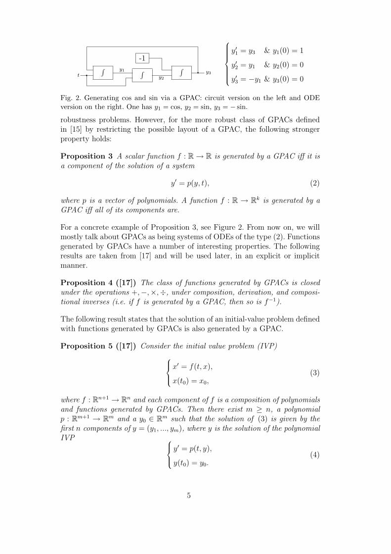
y′1 = y3 & y1(0) = 1

y′2 = y1 & y2(0) = 0

y′3 = −y1 & y3(0) = 0

Fig. 2. Generating cos and sin via a GPAC: circuit version on the left and ODEversion on the right. One has y1 = cos, y2 = sin, y3 = − sin.

robustness problems. However, for the more robust class of GPACs definedin [15] by restricting the possible layout of a GPAC, the following strongerproperty holds:

Proposition 3 A scalar function f : R → R is generated by a GPAC iff it isa component of the solution of a system

y′ = p(y, t), (2)

where p is a vector of polynomials. A function f : R → Rk is generated by aGPAC iff all of its components are.

For a concrete example of Proposition 3, see Figure 2. From now on, we willmostly talk about GPACs as being systems of ODEs of the type (2). Functionsgenerated by GPACs have a number of interesting properties. The followingresults are taken from [17] and will be used later, in an explicit or implicitmanner.

Proposition 4 ([17]) The class of functions generated by GPACs is closedunder the operations +,−,×,÷, under composition, derivation, and composi-tional inverses (i.e. if f is generated by a GPAC, then so is f−1).

The following result states that the solution of an initial-value problem definedwith functions generated by GPACs is also generated by a GPAC.

Proposition 5 ([17]) Consider the initial value problem (IVP)x′ = f(t, x),

x(t0) = x0,(3)

where f : Rn+1 → Rn and each component of f is a composition of polynomialsand functions generated by GPACs. Then there exist m ≥ n, a polynomialp : Rm+1 → Rm and a y0 ∈ Rm such that the solution of (3) is given by thefirst n components of y = (y1, ..., ym), where y is the solution of the polynomialIVP y

′ = p(t, y),

y(t0) = y0.(4)

5

We now set some useful notations.

Definition 6 In the conditions of Proposition 3, we say that t is the input ofthe GPAC and that the components y1, . . . , yn of the solution are the outputsof the GPAC.

Notice that GPAC generable functions are obviously d.a.. Another interestingconsequence is the following (recall that solutions of analytic ODEs are alwaysanalytic – cf. [18]):

Corollary 7 If f is a function generated by a GPAC, then it is real analytic.

As one can see, GPAC generation refers to a notion of “real-time” computa-tion. To follow the idea of a “converging” computation, as the one used inrecursive analysis, we now introduce the idea of GPAC computability from [1](Notice that in Shannon’s original definition of the GPAC nothing is assumedabout the constants and initial conditions of the ODE (2). In particular, therecan be non-computable reals. This kind of GPAC can trivially lead to super-Turing computations. To avoid this, the model of [1] is actually reinforcedhere):

Definition 8 A function f : [a, b] → R is GPAC-computable 2 iff there existsome computable polynomials 3 p : Rn+1 → Rn, p0 : R → R, and n − 1computable real values α1, ..., αn−1 such that:

(1) (y1, ..., yn) is the solution of the Cauchy problem y′ = p(y, t) with initialcondition (α1, ..., αn−1, p0(x)) set at time t0 = 0

(2) There are i, j ∈ {1, ..., n} such that limt→∞ yj(t) = 0 and |f(x)− yi(t)| ≤yj(t) for all x ∈ [a, b] and all t ∈ [0,+∞). 4

We remark that α1, . . . , αn−1 are auxiliary parameters needed to compute f .We will also use the following notation. If we are given the GPAC (2), withinitial condition (α1, ..., αn−1, p0(x)) set at time t0 = 0, where α1, ..., αn−1 arefixed computable values, and where x may vary for each computation, as inDefinition (8), we say that the initial condition x sets the output of the GPAC(2).

Proposition 9 ([1]) The Gamma function Γ is GPAC-computable.

2 Note that in this paper, the term GPAC-computability refers to this particularnotion. The expression “generated by a GPAC” corresponds to Shannon’s notion ofcomputability.3 The notion of computable function and computable real will be provided in thenext section.4 We suppose that y(t) is defined for all t ≥ 0. This condition is not necessar-ily satisfied for all polynomial ODEs, and we restrict our attention only to ODEssatisfying this condition.

6

In this paper, we show that for compact domains, GPAC-computable functionsare precisely the computable functions in the sense of computable analysis.

2.2 Computable Analysis

Recursive analysis, or computable analysis, was introduced by Turing [19],Grzegorczyk [20], and Lacombe [21].

The idea underlying computable analysis is to extend the classical computabil-ity theory so that it can deal with real quantities. See [7] for an up-to-datemonograph of computable analysis from the computability point of view, or[6] for a presentation from a complexity point of view.

In this approach, informally, a function f : R → R is computable if thereis a computer program that does the following. Let x ∈ R be an arbitraryelement in the domain of f . Given an output precision 2−n, the program hasto compute a rational approximation of f(x) with precision 2−n.

To formalize this notion, we need oracle TMs. We say that M is an oracle TMif, at any step of the computation of M using oracle φ : N → Nk, M is allowedto query the value φ(n) for any n written on its tape.

Definition 10 (1) A sequence {rn} of rational numbers is called a ρ-nameof a real number x if there are three functions a, b and c from N to N suchthat for all n ∈ N, rn = (−1)a(n) b(n)

c(n)+1and

|rn − x| ≤ 1

2n. (5)

(2) A real number x is called computable if it has a computable ρ-name, i.e.,if a, b and c in (5) are computable (recursive) functions.

(3) A sequence {xk}k∈N of real numbers is computable if there are three com-putable functions a, b, c from N2 to N such that, for all k, n ∈ N,∣∣∣∣∣(−1)a(k,n) b(k, n)

c(k, n) + 1− xk

∣∣∣∣∣ ≤ 1

2n.

The notion of the ρ-name can be extended to points in Rl as follows: a se-quence {(r1n, r2n, . . . , rln)}n∈N of rational vectors is called a ρ-name of x =(x1, x2, . . . , xl) ∈ Rl if {rjn}n∈N is a ρ-name of xj, 1 ≤ j ≤ l. Similarly, onecan define computable points and sequences over Rl, l > 1, by assuming thateach component is computable. Next we present a notion of computability foropen and closed subsets of Rl (cf. [7], Definition 5.1.15).

7

Definition 11 (1) An open set E ⊆ Rl is called recursively enumerable (r.e.for short) open if there are computable sequences {an} and {rn}, an ∈E ∩Ql and rn ∈ Q such that

E = ∪∞n=0B(an, rn).

Without loss of generality one can also suppose that for any n ∈ N,the closure of B(an, rn), denoted as B(an, rn), is contained in E, whereB(an, rn) = {x ∈ Rl : |x− an| < rn}.

(2) A closed subset K ⊆ Rl is called r.e. closed if there exist computablesequences {bn} and {sn}, bn ∈ Ql and sn ∈ Q, such that {B(bn, sn)}n∈Nenumerates all rational open balls intersecting K.

(3) An open set E ⊆ Rl is called computable (or recursive) if E is r.e. openand its complement Ec is r.e. closed. Similarly, a closed set K ⊆ Rl iscalled computable (or recursive) if K is r.e. closed and its complementKc is r.e. open.

It is well known [7, Example 5.1.17] that an open interval (α, β) ⊆ R or aclosed interval [α, β] is computable if and only if α and β are computablereal numbers. Having defined the notion of recursive and r.e. sets, we are nowready to introduce the notion of computable functions defined on those sets[5–7].

Definition 12 Let A ⊆ Rl be either a r.e. open set or a r.e. closed set. Afunction f : A→ Rm is computable if there is an oracle Turing machine suchthat for any input n ∈ N (accuracy) and any ρ-name of x ∈ A given as anoracle, the machine outputs a rational vector r satisfying |r − f(x)| ≤ 2−n.

The following result is a straightforward adaptation of Corollary 2.14 from [6].

Proposition 13 A real function f : [a, b] → R is computable iff there existthree computable functions m : N → N, sgn, abs : N4 → N such that:

(1) m is a modulus of continuity for f , i.e. for all n ∈ N and all x, y ∈ [a, b],one has

|x− y| ≤ 2−m(n) =⇒ |f(x)− f(y)| ≤ 2−n

(2) For all (i, j, k) ∈ N3 such that (−1)ij/2k ∈ [a, b], and all n ∈ N,∣∣∣∣∣(−1)sgn(i,j,k,n)abs(i, j, k, n)

2n− f

((−1)i j

2k

)∣∣∣∣∣ ≤ 2−n.

2.3 Simulating TMs with ODEs

8

To prove the main result of this paper, we need to simulate a TM with dif-ferential equations. To this end, we recall in this section some results from[12].

For simplicity, and without loss of generality, we only consider Turing machinesusing 10 symbols and set the following coding. Let M be some one tape Turingmachine, with m states and 10 symbols. Then to each state we associate anumber in {1, ...,m} and to each symbol we associate a number in {0, ..., 9},assuming that the blank symbol corresponds to the 0. If

...B B B a−k a−k+1... a−1 a0 a1... anBBB...

is the tape content of M, where a0 is the currently scanned symbol, then itcan be coded in the following two integers:

y1 = a0 + a110 + ...+ an10n y2 = a−1 + a−210 + ...+ a−k10k−1. (6)

The configuration of M is then given by its state s, and two integers y1 and y2.The transition function of M corresponds therefore to a function ψM : N3 → N3

(we consider that if x0 ∈ N3 is an halting configuration, then ψ(x0) = x0, i.e.x0 is a fixed point). In [12] it is shown that ψM admits a robust extension to R3

and that this extension can be written as the composition of polynomials, theexponential, the trigonometric functions, and their inverses (such a functionwill be termed closed-form). In what follows, ‖ · ‖∞ stands for the sup-norm:‖x‖∞ = max1≤i≤n |xi| and ψ[j](x0) stands for jth iteration of function ψ onx0: ψ

[0](x0) = x0, and ψ[j+1](x0) = ψ(ψ[j](x0)).

Proposition 14 ([12]) Let ψM : N3 → N3 be the transition function of aTuring machine M, under the encoding described above and let 0 < ε < 1/2.Then ψM admits a computable closed-form extension ΨM : R3 → R3, robustto perturbations in the following sense: for all j ∈ N, and for all x0 ∈ R3

satisfying ‖x0 − x0‖∞ ≤ ε, where x0 ∈ N3 represents an initial configuration,∥∥∥Ψ[j](x0)− ψ[j](x0)∥∥∥∞≤ ε.

More generally, if M has l tapes, then its transition function is defined overN2l+1 and also admits a closed-form robust extension to R2l+1.

The following result is an adaptation of Theorem 4 from [12] and shows thatGPACs can iterate the transition function of a given Turing machine.

Proposition 15 ([12]) Suppose that ψM : N2l+1 → N2l+1 is the transitionfunction of a Turing machine M, under the encoding presented in Equation(6), x0 ∈ N2l+1 represents an initial configuration and ε, δ > 0 are constants

9

satisfying ε + δ < 1/2. Then there is a computable polynomial p and somecomputable value α ∈ Rn

z′ = p(z, t), z(0) = (x0, α)

such that for all x0 ∈ R2l+1 satisfying ‖x0 − x0‖∞ ≤ ε, one has 5

∥∥∥z1(t)− ψ[j]M (x0)

∥∥∥∞≤ δ.

for all j ∈ N and for all t ∈ [j, j + 1/2].

If there exists some computable value α ∈ Rn such that z′ = p(z, t) has theproperties described in Proposition 15, we say that the GPAC z′ = p(z, t)simulates the Turing machine M on input x.

Later we will use this result and, for that reason, it is convenient to surveysome ideas underlying its proof. In particular, let ψ : N → N be a functionover the integers that admits a closed-form extension Ψ : R → R to the reals.We would like to iterate ψ with a system of analytic ODEs. In [12] it is shownthat this can be done (a more detailed analysis can be found in [17]) with asystem of the type

y′1 = f1(Ψ(z1), y1, t) (7)

z′1 = g1(y1, z1, t)

where f1, g1 : R3 → R are computable closed-form functions and Ψ is supposedto be robust in the following manner: for all n ∈ N

|x− n| < δ ⇒ |Ψ(x)−Ψ(n)| < δ.

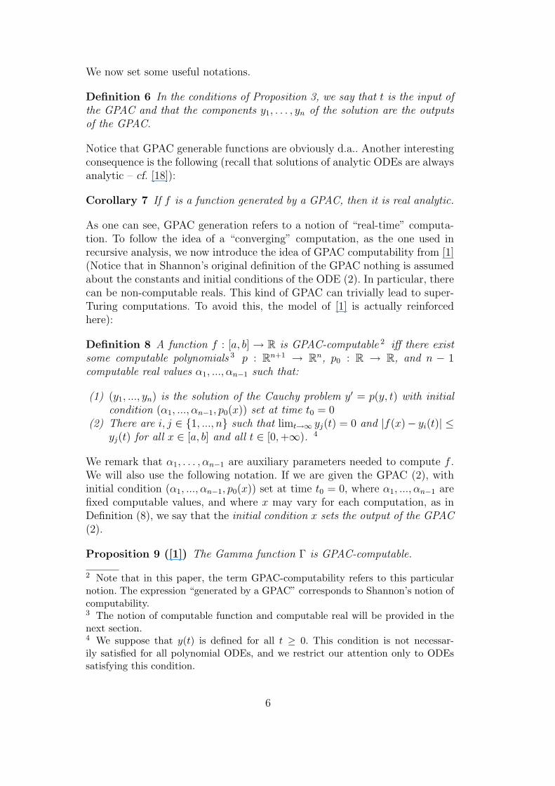
The ODE (7) can be shown to be equivalent to a (larger) polynomial ODE(cf. Proposition 5). Ideally, the variables y1, z1 have the following behavioron an interval [n, n + 1], where n ∈ N (cf. Fig. 3). On [n, n + 1/2], variablez1 is kept constant to the value ψ[n](x0). This kind of “memory” is then usedby the first equation of (7) to update the variable y1 to the value ψ[n+1](x0).In the following next half-interval [n + 1/2, n + 1], the roles of y1 and z1 areswitched: y1 is kept constant to the value ψ[n+1](x0) and z1 is updated to thisvalue.

However, this is only an ideal behavior since real analytic functions cannot beconstant in an interval without be constant everywhere. Instead, the functionsf1, g1 are defined so that the derivatives of y1 and z1 are kept sufficiently closeto zero when their respective values should be kept constant. These functionscan be defined to be computable and closed-form [12], [17]. A similar result

5 For simplicity, we denote the solution z of the initial-value problem by (z1, z2),where z1 ∈ R2l+1 and z2 ∈ Rn.

10

0.5 1 1.5 2 2.5 3

Fig. 3. Simulation of the iteration of a map ψ via ODEs. The solid line representsthe variable y1 and the dashed line represents z1.

can be obtained for the case of an 2l+1-dimensional map ψ and, in particular,to the case of Turing machines (use the map Ψ given by Proposition 14).

Finally, we want to read the value ψ[n](x0) from (7) with precision bounded byδ. As we mentioned earlier, in the time interval [n, n+1/2], z1 is kept close tothe value ψ[n](x0). In particular, it can be shown in the constructions from [12]that there is some η < 1/2 such that, for t ∈ [n, n+1/2], ‖z1(t)−ψ[n](x0)‖ ≤ η.Using the error-contracting function σ defined in the following result of [12]

Proposition 16 Let σ : R → R be defined by

σ(x) = x− 0.2 sin(2πx). (8)

Let ε ∈ [0, 1/2). Then there is some contracting factor λε ∈ (0, 1) such that,∀δ ∈ [−ε, ε], and for all n ∈ Z, one has |σ(n+ δ)− n| < λεδ.

We see that it is enough to apply σ a fixed number of times k to the variablez1 to get the desired accuracy in the interval [n, n+1/2] (just pick some k sat-isfying σ[k](η) ≤ δ). This still can be obtained as the solution of a polynomialODE.

Refer to [12] for full details.

3 The result

The main result of this paper relates computable analysis with the GPAC,showing their equivalence in the framework described in the previous section.

Theorem 17 (Main result) Let a and b be computable reals. A functionf : [a, b] → R is computable iff it is GPAC-computable.

11

We postpone the proof of this result to Sections 5 and 6.

4 Simulating Type-2 machines with GPACs

We present in this section a result that shows that GPACs can simulate oracleTuring machines, under a suitable encoding. This will be necessary to proveTheorem 17.

From Proposition 15, we know how to simulate a Turing machine. However,the error of the output is bounded by some fixed quantity ε > 0, whereas inType-2 machines we would like that the output is given with error boundedby 2−n, where n is one of the inputs of the machine. The next theorem showshow this can be done with a GPAC.

Theorem 18 Let f : [a, b] → R be a computable function. Then there existsa GPAC and some index i such that if we set the initial conditions (x, n) ∈[a, b]×R, where |n− n| ≤ ε < 1/2, with n ∈ N, there exists some T ≥ 0 suchthat the output yi of the GPAC satisfies |yi(t)− f(x)| ≤ 2−n for all t ≥ T .

Before giving the proof of the theorem, we provide some preliminary lemmas.To compute f(x) with a GPAC, we want to use the hypothesis that f iscomputable. Hence, it would be useful to get a GPAC that, when we set theinitial condition x ∈ [a, b], outputs a succession of rationals converging to x.This succession could then be used to compute approximations of f(x), asin condition 2 of Proposition 13. The problem is, given x, to get integers i,j, and 2k such that (−1)ij/2k approximates x enough to compute f(x) withprecision 2−n, and to compute the values sgn(i, j, k, n) and abs(i, j, k, n).

We assume first in what follows that [a, b] ⊆ R+, so that x is always positive.It follows that i can be considered as constant 0. Now, from Proposition 13,this is sufficient to take k = m(n) (where m is a modulus of continuity), andj ' x2m(n).

In the following lemma, the function g(j, n) is intended to represent functionabs(0, j,m(n), n).

By a barycenter of x, y ∈ R we mean a value of the form tx + (1 − t)y, fort ∈ [0, 1]. By other words, a barycenter is a point in the segment of line joiningx to y.

Lemma 19 Let g : N2 → N be a recursive function, [a, b] ⊆ R+ be a boundedinterval, m : N → N be a recursive function, and ε be a real number satisfying0 < ε < 1/4. Then there is a GPAC with the following property: for allx ∈ [a, b] and all j, n ∈ N satisfying j ≤ x2m(n) < j + 1, there exists some

12

0.2 0.4 0.6 0.8 1

Fig. 4. Functions ω1 and ω2. The solid line represents ω1, while the dashed linerepresents ω2.

T > 0 and some index i such that, when we set initial conditions n, x2m(n),where |n− n| < ε and

∣∣∣x2m(n) − x2m(n)∣∣∣ < ε, the output yi of the GPAC

satisfies |yi(t) − c| ≤ ε for all t ≥ T , where c is a barycenter of g(j, n) andg(j + 1, n).

Proof. By Proposition 15 there is a GPAC G that when set on initial conditionk, n, where

∣∣∣k − k∣∣∣, |n− n| < 1/3 (the reason why we use 1/3 will be clear

later) and k, n ∈ N, ultimately (i.e. at any time t ≥ T for some T > 0) outputsg(k, n) with an error less than or equal to ε/2 (k is intended to be j or j+ 1).Define k1 = x2m(n). We would like to use k = k1 as an initial condition toGPAC G. However, k1 is not guaranteed to be close to an integer (i.e. withindistance 1/3). We show now how to overcome this. Let us consider two cases:

(1) If k1 ∈ [l − 1/4, l + 1/4], for some l ∈ {j, j + 1}, then we can set k = k1.With this initial condition, the output of GPAC G (let us call it y1) willbe g(j, n) or g(j + 1, n), plus an error not exceeding ε/2. Therefore, theoutput satisfies the conditions imposed by the lemma. Notice that thisreasoning extends for the case k1 ∈ [l − 1/3, l + 1/3], because (integer)initial conditions of the GPAC can be perturbed by an amount boundedby 1/3;

(2) If k1 ∈ [j+1/4, j+3/4], then we can set the initial condition k = k1−1/2.With this initial condition, the output of GPAC G (let us call it y2) willbe g(j, n) plus an error not exceeding ε/2. Therefore, the output satisfiesthe conditions imposed by the lemma. Notice that this reasoning extendsfor the case k1 ∈ [l + 1/6, l + 5/6].

The real problem here is to implement both cases in a single GPAC. SinceGPACs do not allow the existence of discontinuous functions that might worklike a “case checker,” we have to resort to a different approach.

From the study of the previous cases, we know the following: there is a GPACG such that on initial conditions k1 or k1− 1/2, outputs y1 or y2, respectively.We now consider a new GPAC, obtained with two copies of G, but where onecopy has initial condition set to k1, and the other has initial condition set to

13

0.2 0.4 0.6 0.8 1

-1

1

2

3

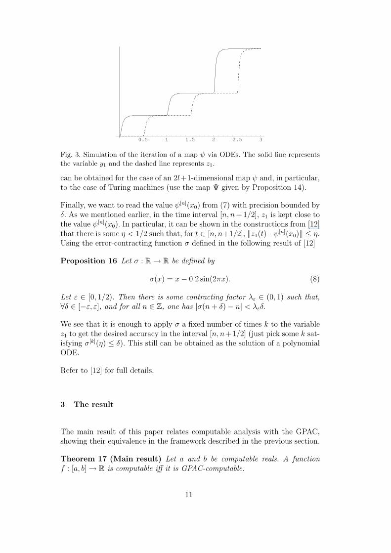
Fig. 5. Function Υ.

k1−1/2 (from the comments following Definition 8, both cases are covered bythe expression “each copy has initial condition set to k1”). Hence, this GPACoutputs both y1 and y2. We now combine these outputs to get the desiredresult.

Assume we had two periodic functions ω1 and ω2, with period 1 and graphssimilar to the ones depicted in Fig. 4. We do not explicitly define ω1 and ω2,but rather state their most important properties: (i) for every t ∈ R, ω1(t) ≥ 0,ω2(t) ≥ 0, and ω1(t)+ω2(t) > 0, (ii) ω1(t) > 0 implies that t ∈ (a−1/3, a+1/3)for some a ∈ N, and (iii) ω2(t) > 0 implies that t ∈ (a + 1/6, a + 5/6)for some a ∈ N. Remark that, for all a ∈ N, (ii) implies ω1(t) = 0 for allt ∈ (a+ 1/3, a+ 2/3), and (iii) implies ω2(t) = 0 for all t ∈ (a− 1/6, a+ 1/6).Then, taking into account the previous two cases described above, one seesthat we could output the value

y =ω1(k1)y1 + ω2(k1)y2

ω1(k1) + ω2(k1). (9)

that would be correct in any of the two cases above. Indeed, the only casewhere both ω1(k1) and ω2(k1) are non-null is whenever k1 ∈ [l+ 2/3, l+ 5/6],where both outputs y1 and y2 are valid, and the result is a barycenter of y1

and y2, i.e. a barycenter of g(j, n) and g(j + 1, n) plus an error not exceedingε/2.

However, ω1 and ω2 are not GPAC-generable since they are not analytic.Alternatively, we will use closed-form functions that approximate ω1 and ω2.In particular, we use the function l2 defined in [12] as below, with the followingproperty.

Proposition 20 ([12]) Let l2 : R2 → R be given by l2(x, y) = 1π

arctan(4y(x−1/2)) + 1

2. For y > 0 one has:

(1) If x ≤ 1/4, then 0 < l2(x, y) < 1/y;(2) If x ≥ 3/4, then 1− 1/y < l2(a, y) < 1.

14

We also use the periodic function Υ : R → R defined by

Υ(x) = 1 + 2 sin 2π(x+ 1/4)

with period 1 and whose graph is depicted in Fig. 5. Notice that for x ∈[1/3, 2/3], Υ(x) ≤ 0, and for x ∈ [−1/4, 1/4], Υ(x) ≥ 1. Therefore, we cantake

ω1(x) = l2(Υ(x), 1/δ) ' ω1(x), ω2(x) = l2(Υ(x− 1/2), 1/δ) ' ω2(x)

since |ω1(x)−ω1(x)| ≤ δ, for x ∈ [a+1/3, a+2/3], where a ∈ Z, and similarlyfor ω2. Moreover, |ω1(x)− 1| ≤ δ for x ∈ [a− 1/4, a + 1/4], and similarly forω2, which implies that

ω1(t) + ω2(t) > 1− 2δ � 0,

for all t ∈ R (i.e. the magnitude of ω1(t) + ω2(t) is not comparable to that ofδ, to avoid problems). Now, we just have to substitute (9) by

y ' ω1(k1)y1 + ω2(k1)y2

ω1(k1) + ω2(k1). (10)

If we pick 1/δ = γ(y1 + y2 + 1), for some γ > 0 (the value 1 is to avoid asingularity for y1 = y2 = 0), we conclude that l2(Υ(k1), 1/δ)y1 approachesω1(k1)y1 with error bounded by γ, and similarly for the other term. Moreover,Υ(k1) + Υ(k1 − 1/2) > 1 − 2γ. This implies that y in (10) is computed witherror bounded by 2γ/(1− 2γ) < ε/2 for γ sufficiently small. By other words,this yields a GPAC with an output yi such that for some T > 0, |yi(t)− c| ≤ εfor all t ≥ T , where c is a barycenter of g(j, n) and g(j + 1, n).

In many occasions it will be useful to switch the behavior of a GPAC uponsome “control function” y : R → R which is also the output of some GPAC.Ideally, we would like to have the situation pictured in Fig. 6, which illustratesa coupled system that behaves like a “switch”. There one can see on theabove graph two functions f1 and f2, generated by GPACs. The graph belowrepresents the control function and a value α ∈ R called the threshold value.Then we would like to have a GPAC with output z such that, if y(t) < α,then z(t) = f1(t), and z(t) = f2(t) otherwise.

Of course, the previous idea cannot be implemented with a GPAC, since we al-low immediate transitions between two distinct functions, which would yield adiscontinuous function. To remedy that, we allow some transition zone aroundthe threshold value (in gray in the second graph of Fig. 6).

The construction of switching functions has to be further relaxed to cope withthe fact that only analytic functions can be used. Therefore, function z in thefollowing lemma will just be an approximation of f1 and f2.

15

t

t

y(t)

ff1

f2

α

Fig. 6. Switching functions. Functions f1 and f2 are represented in the first graphby the dashed and dotted line, respectively. The resulting function is represented ingray. The second graph displays the control function y, where α is the threshold.

Lemma 21 (Switching functions) Let y, f1, f2 : R → R be three functionsgenerated by GPACs (y is called the control function) and ε > 0. Then thereis a function f : R → R generated by a GPAC with the following property: forall t ∈ R, |f(t)− f1(t)| ≤ ε if y(t) ≤ α− 1/4

|f(t)− f2(t)| ≤ ε if y(t) ≥ α+ 1/4.

Proof. This can be done in a quite straightforward way using the function l2introduced in the proof of Lemma 19. It suffices to take

f = f1.l2

(α+ 1/2− y(t),

f1 + f2

ε/2

)+ f2.l2

(y(t)− α+ 1/2,

f1 + f2

ε/2

)

It is easy to see that f satisfies the given conditions.

We will mainly use this lemma to switch between dynamics simulating differentTuring machines. Suppose that the GPACs z′1 = p1(t, z1) and z′2 = p2(t, z2)simulate two Turing machines TM1 and TM2 as in Proposition 15, respectively.Then if we have a control function yi(t), provided by the output of a thirdGPAC y′ = p(t, y), we can build a function f that switches between f1 = p1

and f2 = p2, yielding a new system y′(t) = p(t, y(t)), z′(t) = f(t, z(t), yi(t)),simulating the transition function of TM1 and TM2, according to the value ofyi(t). From Proposition 5, this corresponds to a GPAC.

An useful application will be to simulate two Turing machines TM1 and TM2

working in series, i.e. where the output of TM1 is be used as the input of TM2.

16

Indeed, when simulating TM1 with a GPAC as in Proposition 15 we cansuppose that the states are coded by the integers 1, . . . ,m, where state mcorresponds to the halting state, and that there is a variable yi of the GPACgiving the current state of TM1 in the simulation with error bounded by 1/4 forevery t ∈ [n, n+1/2]. Therefore, if we set α = m−1/2 and y = yi in Lemma 21,we have a way of switching between dynamic of a GPACs simulating TM1 andanother one simulating TM2 upon the value of yi, i.e. depending on whetherTM1 is still running, or already halted.

We can obtain a GPAC having the desired property in the following manner.The initial condition sets the input of TM1 and this GPAC simulates TM1

until it halts. When this happens, the variables coding the tape contents havethe input of TM2. Then we switch the evolution law of this GPAC so thatnow it simulates TM2, thus giving the desired output (to avoid interferenceproblems, the control function should be given by a separated GPAC that justsimulates TM1 and that stays in an halting configuration after this Turingmachine halts).

From the robustness conditions of Proposition 15, by choosing ε sufficientlysmall in the lemma above, one can ensure that errors will stay controlled ateach step, so that a correct simulation of TM1 and then TM2 will happen.

In some cases, we will need to switch to a dynamic that sets one variable tosome value. This can be done with the following lemma, taken from [17].

Lemma 22 ([17] Resetting configurations) Let ε ∈ R satisfy 1/4 ≥ ε >0. Let y be some GPAC generated function and t0 < t1 be some reals.

There is a polynomial p such that the solution of z′ = p(t, z, y) with some fixedinitial condition at t0 satisfies ‖z(t1) − k‖∞ < ε, whenever ‖y(t) − k‖∞ ≤ εfor all t ∈ [t0, t1] for some vector k ∈ Nm.

Proof of Theorem 18. For simplicity, let us suppose that a > 0 so thatwe don’t have to care about sign of x ∈ [a, b]. This is never problematicsince, if a < 0, we can always shift [a, b] by an amount k ∈ N such thata+k > 0, to define a new computable function h : [a+k, b+k] → R satisfyingh(x) = f(x− k).

Suppose also that f(x) always takes the same sign for all x ∈ [a, b]. The casewhere the sign of f(x) switches can be reduced to this one. Indeed, since [a, b]is compact, there is some l ∈ Z such that g(x) = l+f(x) > 0, for all x ∈ [a, b].Once we have a GPAC computing g(x), we just have to subtract l to theoutput to obtain a GPAC computing f(x). So, to fix ideas, let us supposethat f(x) always takes positive values.

Let us now proceed with the proof. Since f is computable, according to Propo-

17

sition 13, and previous discussions, there are recursive functions m : N → N,abs (the function sgn is no longer needed since f(x) takes positive values)such that given x ∈ [a, b] and non-negative integers j, n satisfying∣∣∣j/2m(n) − x

∣∣∣ < 2−m(n), (11)

one has ∣∣∣∣∣abs(0, j,m(n), n)

2n− f(x)

∣∣∣∣∣ < 2

2n.

We will design a GPAC with an output yi such that, for some T > 0, for allt ≥ T , yi(t) is always close to

abs(0, j,m(n), n)

2n, (12)

the error between two values being bounded by 2−n. This will be sufficient toprove the theorem.

Let us show how we can compute (12) with a GPAC. Let TM0 and TM1 beTuring machines computing 2n and 2m(n) on input n. From Proposition 15,there are GPACs simulating these Turing machines. This yields two GPACswith outputs y1 and y2, so that on initial condition n close to n, one has|y1(t) − 2n| ≤ ε and |y2(t) − 2m(n)| ≤ ε for all t ≥ T2 for some T2. Moreover,since [a, b] is bounded, we can suppose that |xy2(t)−x2m(n)| ≤ ε (if necessary,apply σ a fixed number of times, independent of n, to y2). The values nand xy2 can then be used to feed the GPAC described in Lemma 19, withg(j, n) = abs(0, j,m(n), n). This GPAC U3 has an output y3, which, after sometime T3, yields a barycenter of abs(0, j,m(n), n) and abs(0, j+1,m(n), n) plusan error bounded by ε. Since m is a modulus of continuity,

|abs(0, j,m(n), n)− abs(0, j + 1,m(n), n)| ≤ 1.

This implies that the output of U3, let it call abs(j, n), satisfies

|y3(t)− abs(0, j,m(n), n)| ≤ 1 + ε

for all t ≥ T3. Since [a, b] is bounded, there is some η ∈ N such that onehas abs(0, j,m(n), n) ≤ 2nη for all n ∈ N and all j satisfying (11) for everyx ∈ [a, b]. Therefore∣∣∣∣∣y3(t)

y1(t)− abs(0, j,m(n), n)

2n

∣∣∣∣∣ ≤ ε.abs(0, j,m(n), n) + 2n(1 + ε)

2n(2n − ε)≤

≤ εη + 1 + ε

2n2−1≤ λ2−n (13)

18

with λ = 2(εη + 1 + ε) independent of j, n, for all t ≥ T3, thus giving an ap-propriate approximation of abs(0, j,m(n), n)/2n, with error bounded by λ2−n,with λ independent of j, n. This proves the theorem.

Remark 23 Notice that after the time T referred to in Theorem 18, the cor-responding GPAC continues to output forever an approximation of f(x) witherror bounded by 2−n. This is because, as assumed in Section 2.3, the haltingconfiguration of the Turing machine simulated by the GPAC is a fixed point(modulo some error bounded by ε).

5 Proof of the “only if” direction of Theorem 17

Our idea is the following. From Theorem 18, we already know how to generatef(x) with precision 2−n with a GPAC G fed with approximations of n andx2m(n) as initial conditions, say in components y1 and y2, respectively. Hence,to get a GPAC with an output converging to f(x) in the limit, it suffices toimplement the previous theorem in a cyclic way: start the computation withn = 0. When the computation finishes, increment n, repeat the computation,and so on.

To do so, we need to address several problems. The first one is to know whenthe computation with the current n is over. Indeed, Theorem 18 tells us thatthis happens after some time T , but does not give us any procedure to computethis instant T .

This can be solved by building another GPAC that provides a correspondingcontrol function. Indeed, consider a clocking Turing machine TM0 that basi-cally simulates all involved Turing machines in the constructions of Theorem18 on all possible arguments x ∈ [a, b] of type k2n (that are finitely many).This guarantees that whenever TM0 terminates on input n, we are sure thatall involved Turing machines in the constructions of Theorem 18 have hadenough time to do their computations in GPAC G, and so that the output iscorrect. The description of TM0, on input n ∈ N, is as follows:

(1) Compute the first k1 ∈ Z such that k1/n ≥ a, and the last k2 ∈ Z suchthat k2/n ≤ b

(2) For i = k1 to k2 simulate Turing machines involved in the proof of The-orem 18 on input (i, n).

Observe that Step 1 can be implemented because, by hypothesis, a and b arecomputable constants. The Turing machine TM0 can be simulated by a GPAC(independent from GPAC G). The output yi of this GPAC that encodes thestate of TM0 can be used as a control function. Indeed, whenever it becomes

19

greater than m0 − 1/2, where m0 is the number of states of TM0, this meansthat TM0 halted, and hence the output of G is correct. This solves our firstproblem.

Actually, we need to simulate G on increasing n. So, more precisely, we considera Turing machine TM1 that does the following:

(1) Start with n = 0(2) Simulate TM0 with input n(3) Increment n and go to Step 2.

Suppose, without loss of generality, that this Turing machine has m1 states,where m1 is the halting state (that is never reached), and m1 − 1 is a specialstate, only reached in the transition of Step 3 to Step 1. Value m1 − 3/2 canthen be used a threshold. Whenever the output encoding the state of TM1,call it yi, is higher than m1 − 3/2, we know that the computation of G is overfor corresponding n.

We can then use Lemmas 21 and 22 so that control function yi resets the valueof y1 and y2 to approximations of n+1 and x2m(n+1), respectively, and beginsa new cycle by allowing again the simulation of G on these new values for y1

and y2.

So far we have seen that while y1 and y2 are respectively approximations of nand x2m(n), one of the components of the system, say yj, approaches f(x) witherror 2−n. However, during the following time period, when n is incremented,yj fluctuates before converging to f(x) with error 2−(n+1). Therefore, yj doesn’tmatch condition 2 of Definition 8 for all times.

To define a component of the system that converges to f(x) with time, we usethe components of the system that encode the values of abs(0, j,m(n), n) and2n in each time period. We create a pair of components, say z1, z2, that are resetto the values of abs(0, j,m(n), n) and 2n respectively, at the end of each timeperiod. This can be done with Lemma 22 using the control function yi. Moreprecisely, when yi is above the threshold, z1, z2 approach abs(0, j,m(n), n)and 2n. During the following time period, i.e. while yi is below the threshold,z1, z2 are kept approximately constant. This can be done with Lemma 21 byswitching the dynamics from our current system to a GPAC that simulatesa Turing machine in a fixed configuration. Again, we use yi as the controlfunction.

Hence, a sufficient approximation of f(x) is then given by z1/z2, and a boundon current error on f(x), as required in Definition 8, is given by 1/z2 bothvalues being valid at any time.

20

6 Proof of the “if” direction of Theorem 17

We now proceed with the proof of the “if” direction of Theorem 17. Letf : [a, b] → R be a GPAC-computable function. We want to show that f iscomputable in the sense of computable analysis. By definition, we know thatthere is a computable polynomial ODE y

′ = p(t, y)

y(0) = (α, x)(14)

whose solution has two components yi : R2 → R and yj : R2 → R such that

|f(x)− yi(x, t)| ≤ yj(x, t) and limt→∞

yj(x, t) = 0 (15)

Since we have to study the computability of functions defined by ODEs, weresort to the following result, taken from [22].

Theorem 24 Let E ⊆ Rm+1 be a r.e. open set and f : E → Rm be a com-putable analytic function. Let (α, β) be the maximal interval of existence ofthe solution x(t) of the initial-value problem x = f(t, x),

x(t0) = x0,(16)

where (t0, x0) is a computable point in E. Then (α, β) is a r.e. open intervaland x is a computable function on (α, β). In particular, there is an oracle TMthat on inputs (t0, x0) outputs the solution x.

Since for (14) E = Rm+1 is r.e. and p is computable, we conclude that the so-lution is computable over the maximal interval, which is assumed in Definition8 to include (0,+∞). It follows that yi and yj are computable in (0,∞).

Suppose that we want to compute f(x) with precision 2−n. Then proceed withthe following algorithm.

(1) Set t = 1(2) Compute an approximation yj of yj(x, t) with precision 2−(n+2)

(3) If yj > 2−(n+2) then set t := t+ 1 and go to Step 2(4) Compute yi(x, t) with precision 2−(n+1) and output the result

Steps 1, 2 and 3 are used to determine an integer value of t for which |yj(x, t)| ≤2−(n+1). Once this value is obtained, an approximation of yi(x, t) with precision

21

2−(n+1) will provide an approximation of f(x) with error 2−n, due to (15), thusproviding the desired output. This proves the result.

7 Conclusion

In this paper we established some links between computable analysis andShannon’s General Purpose Analog Computer. In particular, we showed thatcontrarily to what was previously suggested, the GPAC and computable anal-ysis can be made equivalent from a computability point of view, as long as wetake an adequate notion of computation for the GPAC. In addition to thoseresults it would be interesting to answer the following questions. Is it possi-ble to have similar results, but at a complexity level? For instance, using theframework of [6], is it possible to relate polynomially-time computable func-tions to a class of GPAC-computable functions where the error ε is given as afunction of a polynomial of t? And if this is true, can this result be generalizedto other classes of complexity? From the computability perspective, our resultssuggest that polynomial ODEs and GPACs are very natural continuous-timecounterparts to Turing machines.

Acknowledgments. This work was partially supported by Fundacao paraa Ciencia e a Tecnologia and EU FEDER POCTI/POCI via CLC, projectConTComp POCTI/MAT/45978 /2002, grant SFRH/BD/17436/2004 (DG),and within the initiative RealNComp of SQIG - IT. Additional support wasalso provided by the Fundacao Calouste Gulbenkian through the ProgramaGulbenkian de Estımulo a Investigacao, and by EGIDE and GRICES under theProgram Pessoa through the project Calculabilite et complexite des modelesde calculs a temps continu.

References

[1] D. S. Graca, Some recent developments on Shannon’s General Purpose AnalogComputer, Math. Log. Quart. 50 (4-5) (2004) 473–485.

[2] L. Blum, M. Shub, S. Smale, On a theory of computation and complexity overthe real numbers: NP-completeness, recursive functions and universal machines,Bull. Amer. Math. Soc. 21 (1) (1989) 1–46.

[3] C. Moore, Recursion theory on the reals and continuous-time computation,Theoret. Comput. Sci. 162 (1996) 23–44.

[4] H. T. Siegelmann, Neural Networks and Analog Computation: Beyond theTuring Limit, Birkhauser, 1999.

22

[5] M. B. Pour-El, J. I. Richards, Computability in Analysis and Physics, Springer,1989.

[6] K.-I. Ko, Computational Complexity of Real Functions, Birkhauser, 1991.

[7] K. Weihrauch, Computable Analysis: an Introduction, Springer, 2000.

[8] C. E. Shannon, Mathematical theory of the differential analyzer, J. Math. Phys.MIT 20 (1941) 337–354.

[9] V. Bush, The differential analyzer. A new machine for solving differentialequations, J. Franklin Inst. 212 (1931) 447–488.

[10] J. Mycka, J. F. Costa, Real recursive functions and their hierarchy, J.Complexity 20 (6) (2004) 835–857.

[11] O. Bournez, E. Hainry, Recursive analysis characterized as a class of realrecursive functions, to appear in Fund. Inform.

[12] D. S. Graca, M. L. Campagnolo, J. Buescu, Robust simulations of Turingmachines with analytic maps and flows, in: S. B. Cooper, B. Lowe, L. Torenvliet(Eds.), CiE 2005: New Computational Paradigms, LNCS 3526, Springer, 2005,pp. 169–179.

[13] M. B. Pour-El, Abstract computability and its relations to the general purposeanalog computer, Trans. Amer. Math. Soc. 199 (1974) 1–28.

[14] L. Lipshitz, L. A. Rubel, A differentially algebraic replacement theorem, andanalog computability, Proc. Amer. Math. Soc. 99 (2) (1987) 367–372.

[15] D. S. Graca, J. F. Costa, Analog computers and recursive functions over thereals, J. Complexity 19 (5) (2003) 644–664.

[16] L. A. Rubel, A survey of transcendentally transcendental functions, Amer.Math. Monthly 96 (9) (1989) 777–788.

[17] D. S. Graca, M. L. Campagnolo, J. Buescu, Computability with polynomialdifferential equations, submitted for publication.

[18] V. I. Arnold, Ordinary Differential Equations, MIT Press, 1978.

[19] A. M. Turing, On computable numbers, with an application to theEntscheidungsproblem, Proc. London Math. Soc. 2 (42) (1936) 230–265.

[20] A. Grzegorczyk, On the definitions of computable real continuous functions,Fund. Math. 44 (1957) 61–71.

[21] D. Lacombe, Extension de la notion de fonction recursive aux fonctions d’uneou plusieurs variables reelles III, Comptes Rendus de l’Academie des SciencesParis 241 (1955) 151–153.

[22] D. Graca, N. Zhong, J. Buescu, Maximal intervals of computable IVPs are notnecessarily computable, trans. Amer. Math. Soc., to appear.

23