Using boundary methods to compute the Casimir energy

arX

iv:1

003.

2011

v1 [

quan

t-ph

] 1

0 M

ar 2

010

March 11, 2010 1:9 WSPC - Proceedings Trim Size: 9in x 6in lombardo-mazzitelli-2

1

Using boundary methods to compute the Casimir energy

F.C. Lombardo1, F.D. Mazzitelli1, and P.I. Villar1,2

1 Departamento de Fısica Juan Jose Giambiagi, FCEyN UBA, Facultad de CienciasExactas y Naturales, Ciudad Universitaria, Pabellon I, 1428 Buenos Aires, Argentina

2 Computer Applications on Science and Engineering Department, BarcelonaSupercomputing Center (BSC), 29, Jordi Girona 08034 Barcelona, Spain

We discuss new approaches to compute numerically the Casimir interactionenergy for waveguides of arbitrary section, based on the boundary methodstraditionally used to compute eigenvalues of the 2D Helmholtz equation. Thesemethods are combined with the Cauchy’s theorem in order to perform thesum over modes. As an illustration, we describe a point-matching techniqueto compute the vacuum energy for waveguides containing media with differentpermittivities. We present explicit numerical evaluations for perfect conductingsurfaces in the case of concentric corrugated cylinders and a circular cylinderinside an elliptic one.

Keywords: Style file; LATEX; Proceedings; World Scientific Publishing.

1. Introduction

In this paper we will be concerned with the numerical calculation of the

Casimir interaction energy in geometries with translational invariance along

one direction, i.e. very long cylinders of arbitrary section. For the sake of

simplicity, we will first discuss the case of a massless quantum scalar field

that satisfies Dirichlet or Neumann boundary conditions on the surfaces of

the cylinders. As we will see, in some particular situations the generalization

to the electromagnetic field and/or more general boundary conditions will

be straightforward.

The Casimir energy is formally given by

E12(σ) = limσ→0

1

2

∑

p

(e−σwpwp − e−σwpwp) , (1)

where wp are the eigenfrequencies of the scalar field satisfying the appro-

priate boundary conditions on the surfaces of the shells, and wp are those

corresponding to a situation in which the distances between the shells is

http://arxiv.org/abs/1003.2011v1


2

very large. The subindex p denotes the set of quantum numbers associated

to each eigenfrequency. We have introduced an exponential cutoff for high

frequency modes.

For the particular geometry considered here, p = (n, kz) and the eigen-

frequencies are of the form ωn,kz=

√

k2 + λ2n, where kz is a continuous

variable associated to the translational invariance along the z-direction and

λ2 are the eigenvalues of the Laplacian on the two-dimensional transversal

section Σ contained in the plane (x,y):

∆2u = −λ2u . (2)

The eigenfunctions u(x) satisfy Dirichlet or Neumann boundary conditions

on Γ, the boundary of Σ.

The Helmholtz equation (2) arises in many branches of physics, from

the vibration of membranes to quantum billiards, and there are a plethora

of methods to compute numerically its eigenfunctions and eigenvalues.1

Among them, the ”boundary methods” are based on the following strategy:

the solution u is written as a (finite) linear combination of basis functions

that satisfy Helmholtz equation inside Σ. The coefficients of the linear com-

bination are chosen in such a way that the boundary conditions are satisfied

at a finite number of points on Γ. The linear system of equations that de-

termine the coefficients has a non trivial solution only for some particular

values of λ, the eigenvalues of the system.

For example, in the Point Matching Method (PMM),2 one expands the

eigenfunction u in terms of a basis of solutions of the Helmholtz equation

in free space ϕ(λ)j (x)

u(x) =

∞∑

j=1

ajϕ(λ)j (x) . (3)

In the numerical calculation this expansion is truncated at given j = N , and

the boundary conditions are imposed on N points on Γ. These boundary

conditions become a set of homogeneous, linear equations for the unknown

coefficients aj (Ma = 0, with M a λ-dependent N ×N matrix) which has

nontrivial solutions only when detM = 0. The last equation can be used to

determine numerically the eigenvalues λn.

In a similar approach, known as the Method of Fundamental Solu-

tions (MFS),3 the eigenfunction u is expanded in terms of solutions of the

Helmholtz equation with a point source at an arbitrary location sj , that we


3

denote by uλ(x, sj)

u(x) =

∞∑

j=1

bjuλ(x, sj) . (4)

If the sources are located outside Σ, this is a solution of the homogeneous

Helmholtz equation inside Σ. Once again, the sum is truncated at j = N ,

and the coefficients bj are determined by solving the linear system that re-

sults when imposing the boundary conditions on a finite number of points

on Γ. The roots of the determinant of the associated matrix are the eigenfre-

quencies of the problem. This is the simplest version of the MFS, in which

the locations of the sources are fixed.

One can find in the literature discussions about spurious solutions, im-

provements and alternative methods to find the eigenvalues. We refer the

reader to Refs.1,4 for more details.

A crucial point is that, at a practical level, the knowledge of the spec-

trum of the Helmholtz equation is not enough to compute the Casimir

energy. The reason is that the numerical evaluation of the sum over modes

in Eq.(1) is extremely unstable,5 and one has to subtract very large num-

bers to compute the finite interaction energy. The calculation is complicated

even for the simplest case of Casimir effect in 1 + 1 dimensions.

Instead of performing explicitly the summation, it is far more efficient

to combine the methods mentioned previously with the Cauchy’s theorem

1

2πi

∫

C

dz z e−σz d

dzln f(z) =

∑

i

zi e−σzi , (5)

where f(z) is an analytic function in the complex z plane within the closed

contour C, with simple zeros at z1, z2, . . . within C. We use this result

to replace the sum over the eigenvalues of the Helmholtz equation in the

Casimir energy Eq.(1) by a contour integral. In this way, it is not necessary

to solve numerically the equation detM = 0 for the eigenvalues, but to take

f = detM in the Cauchy’s theorem. In other words, if in the numerical

method to solve the Helmholtz equation the eigenvalues are the roots of

a given function, one can integrate this function in the complex plane in

order to get the Casimir energy. The combination of the use of numerical

methods to compute the eigenvalues with the Cauchy’s theorem is the main

idea we want to put forward in this paper.

In the next Section we will describe the simplest version of the PMM to

a situation in which the surfaces separate regions of different permittivities,

generalizing our previous results6 for perfect conductors. In Sections 3 and 4


4

we will review some numerical evaluations of the Casimir interaction energy

for perfect conductors. In Section 5 we include our final remarks.

2. Point-Matching Numerical Approach

A media-separated waveguide presents an interesting setup for the applica-

tion of the PMM. This technique has been widely used to solve eigenvalue

problems in many areas of engineering science.2 The boundary conditions

are imposed at a finite number of points around the periphery of both

media.

Fig. 1. A two-separated media waveguide in which one conductor encloses two differentdielectric media. Each has arbitrary cross section.

For the sake of concreteness, we will bear in mind the situation in which

one perfect conductor encloses two dielectric media, as shown in Fig.1,

although the method could be applied to more general cases.

The general solution of the Helmholtz equation in region I (inside the

inner cylinder) is

u =∑

m

AmJm(λ(I)r)eimθ , (6)

while in region II (annular region)

u =∑

m

[BmJm(λ(II)r) + CmH(1)m (λ(II)r)]eimθ , (7)

where (r, θ) are polar coordinates, and Jm and H(1)m are the m-th order

Bessel functions. The constants Am, Bm and Cm are determined by the

boundary conditions. In both equations we have defined λ(a) =√

ǫaω2 − k2z .


5

We assume the outer surface to be a ”perfect conductor”, and impose

Dirichlet boundary conditions on a finite number of points (rq, θq) of C2:

0 =

S∑

m=−S

[BmJm(λ(II)rq) + CmH(1)m (λ(II)rq)]e

imθq , (8)

(alternatively, for the TE modes of the electromagnetic field, one should

impose Neumann boundary conditions). The surface C1 as a dielectric in-

terphase separating media ǫ1 and ǫ2, and therefore we impose continuity of

the field and its derivative:S∑

m=−S

AmJm(λ(I)rp)eimθp =

S∑

m=−S

[BmJm(λ(II)rp) + CmH(1)m (λ(II)rp)]e

imθp (9)

S∑

m=−S

AmJ ′

m(λ(I)rp)eimθp =

λ(II)

λ(I)

S∑

m=−S

[BmJ ′

m(λ(II)rp) + CmH ′(1)m (λ(II)rp)]e

imθp ,

where (rp, θp) are points on the curve C1.

The boundary conditions can be written, in matrix form, as

0 = N1B +N2C,

R1A = M1B +M2C,

R2A = M ′

1B +M ′

2C. (10)

Eliminating the coefficients Am we end with

N1B +N2C = 0, P1B + P2C = 0, (11)

where P1 and P2 can be written as

P1 = M1 −R1R−12 M ′

1, P2 = M2 −R1R−12 M ′

2 . (12)

It is worthy to note that as R1R−12 is proportional to λ2/λ1, then

R1R−12 → 0 when ǫ1 → ∞. Thus, the matrices P1 → M1 and P2 → M2, re-

obtaining in this way, the usual perfect conductor wave-guide case studied

in.6

For the system of Eq.(11) to have non trivial solutions, the determinant

must be zero, i.e.

det

[

N1 N2

P1 P2

]

= detP2 · detN1 · det(1−N2P−12 P1N

−11 ) = 0 . (13)

This equation determines the eigenfrequencies associated to the geometry.

However, as already mentioned, in order to compute the Casimir energy it

is not necessary to find each eigenvalue but to integrate the determinant

Q = det(1−N2P−12 P1N

−11 ) in the complex plane.


6

We have developed a numerical Fortran routine in order to evaluate the

Casimir interaction energy in the case in which the field satisfies Dirichlet

or Neumann boundary conditions on both curves C1 and C2. In this case

one should consider the fields only in region II with ǫ2 = 1. After some

straightforward steps one can re-write the Casimir energy as a single in-

tegral in the imaginary axis iy = λ(II). For Dirichlet boundary conditions

the result is

E12 =L

4π

∫

∞

0

dy y lnQ(iy) , (14)

while for Neumann boundary conditions one can derive a similar expression

with a different function Q. It is worth to stress that these Casimir energies

correspond to those of TM and TE modes of the electromagnetic field in

the presence of perfect conductors.

3. Cylindrical rack and pinion

When two concentric cylinders have corrugations, the vacuum energy pro-

duces a torque that could, in principle, make one cylinder rotate with re-

spect to the other. This “cylindrical rack and pinion” has been proposed in

Ref.,7 where the torque has been computed using the proximity force ap-

proximation. It was further analyzed in,8 where the authors obtained per-

turbative results for Dirichlet boundary conditions in the limit of small am-

plitude corrugations. In this Section, we numerically evaluate the Casimir

interaction energy for two concentric corrugated, perfect conductor cylin-

ders. The cylinders have radii a and b, and we will denote by r− = b − a

the mean distance between them and by r+ = a + b the sum of the radii.

We will use the notation α = b/a. The points in the mesh, that give us the

corrugated cylinder boundaries, are described by the following functions:

ha(θ) = h sin(νθ) ; hb(θ) = h sin(νθ + φ0), (15)

where h is the corrugation amplitude and ν is the frequency associated

with these corrugations. The Casimir torque can be calculated by taking

the derivative of the interaction energy with respect to the shifted angle

T = −∂E12/∂φ0.

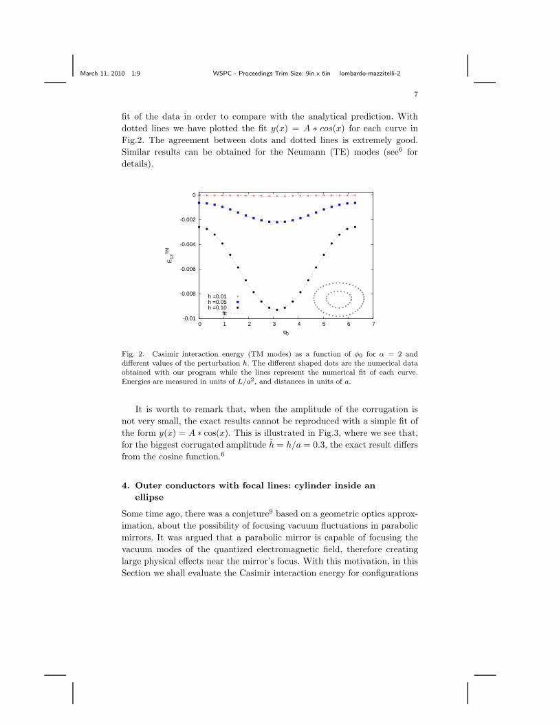
In Fig.2 we show the numerical evaluation of the TM Casimir interaction

energy for this geometry. The plot shows the results obtained using the

PMM with α = 2 and corrugation frequency ν = 3, for different values

of the amplitude of the corrugation h. As expected the amplitude of the

oscillations grows with h. For each value of h we have performed a numerical


7

fit of the data in order to compare with the analytical prediction. With

dotted lines we have plotted the fit y(x) = A ∗ cos(x) for each curve in

Fig.2. The agreement between dots and dotted lines is extremely good.

Similar results can be obtained for the Neumann (TE) modes (see6 for

details).

-0.01

-0.008

-0.006

-0.004

-0.002

0

0 1 2 3 4 5 6 7

E12

TM

φ0

h =0.01h =0.05h =0.10

fit

Fig. 2. Casimir interaction energy (TM modes) as a function of φ0 for α = 2 anddifferent values of the perturbation h. The different shaped dots are the numerical dataobtained with our program while the lines represent the numerical fit of each curve.Energies are measured in units of L/a2, and distances in units of a.

It is worth to remark that, when the amplitude of the corrugation is

not very small, the exact results cannot be reproduced with a simple fit of

the form y(x) = A ∗ cos(x). This is illustrated in Fig.3, where we see that,

for the biggest corrugated amplitude h = h/a = 0.3, the exact result differs

from the cosine function.6

4. Outer conductors with focal lines: cylinder inside an

ellipse

Some time ago, there was a conjeture9 based on a geometric optics approx-

imation, about the possibility of focusing vacuum fluctuations in parabolic

mirrors. It was argued that a parabolic mirror is capable of focusing the

vacuum modes of the quantized electromagnetic field, therefore creating

large physical effects near the mirror’s focus. With this motivation, in this

Section we shall evaluate the Casimir interaction energy for configurations


8

-0.2

-0.18

-0.16

-0.14

-0.12

-0.1

-0.08

-0.06

-0.04

-0.02

0

0 1 2 3 4 5 6 7

E12

φ0

TMTE

Fig. 3. Casimir interaction energy (TE and TM modes) as a function of φ0 for α = 2,ν = 3 and h = 0.3. The different shaped dots are the numerical data obtained by ourprogram while the line represents the numerical fit of each curve. In this case, the plotshows that the exact result cannot be fitted by a function y(x) = A ∗ cos(x). Energiesare measured in units of L/a2.

in which the outer conducting shell has a cross section that contains focal

points.

We will consider one small inner cylinder and an outer ellipse. We will

denote by a the radius of the inner cylinder, by b1 and b2 the minor and

major semiaxes of the ellipse, respectively, and by f the distance between

the foci and the center of the ellipse. The coordinates of the center of the

cylinder with respect to the center of the ellipse will be (ǫx, ǫy). We will use

an additional tilde to denote adimensional quantities, i.e distances in units

of a: bi = bi/a , f = f/a, etc.

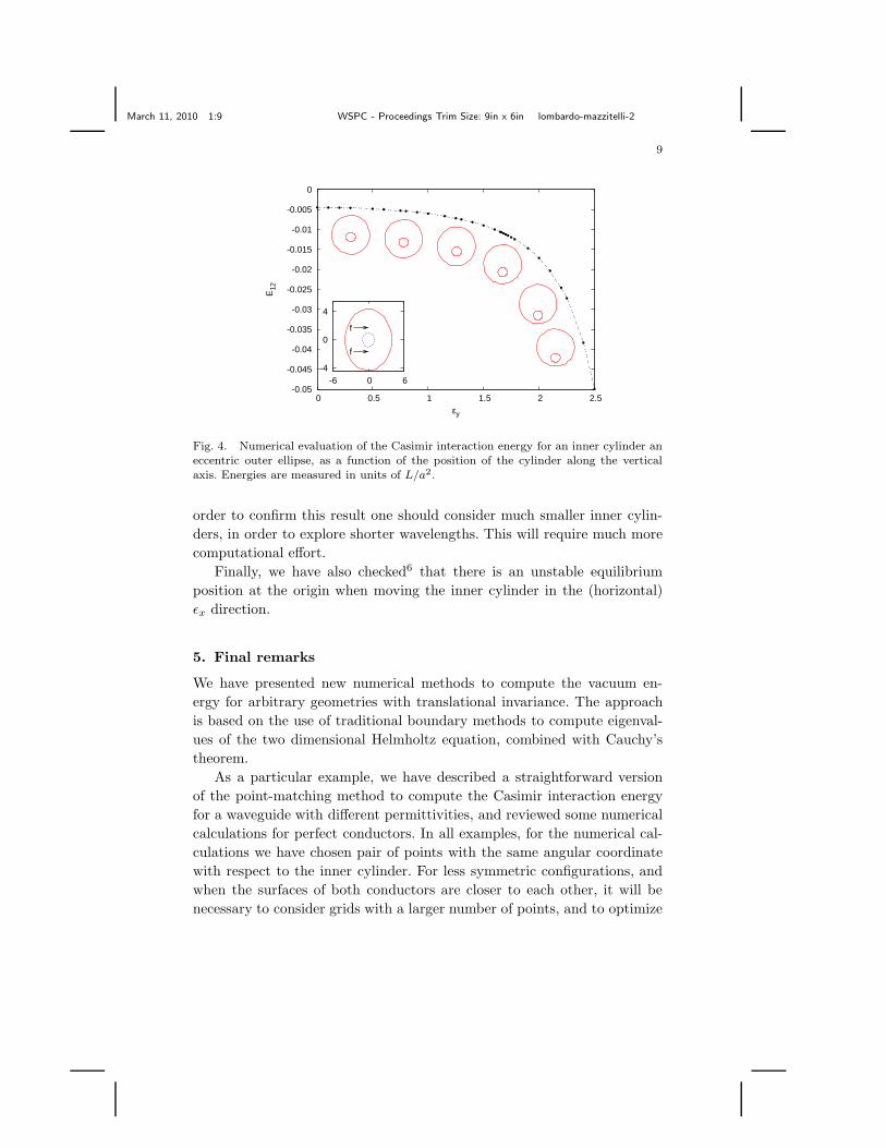
For this configuration, we use a mesh where with an inner cylinder, and

an outer ellipse with semiaxes b1 = 4 and b2 = 4.33. The ellipse has two

focal points at f = 1.66. We present the results for the Casimir energy in

Fig.4.

From Fig.4 it is possible to see that there is an unstable equilibrium

position at the origin under displacements of the inner cylinder along the

(vertical) ǫy direction. As expected, it is also possible to check that the

energy grows as well as the cylinder gets closer to the surface of the outer

ellipse. Fig.4 also shows a monotonic behaviour of the energy as a function

of the position, even when passing through the focus. So we do not see a

focusing of vacuum fluctuations near the focus of the ellipse. However, in


9

-0.05

-0.045

-0.04

-0.035

-0.03

-0.025

-0.02

-0.015

-0.01

-0.005

0

0 0.5 1 1.5 2 2.5

E12

εy

-4

0

4

-6 0 6

f

f

Fig. 4. Numerical evaluation of the Casimir interaction energy for an inner cylinder aneccentric outer ellipse, as a function of the position of the cylinder along the verticalaxis. Energies are measured in units of L/a2.

order to confirm this result one should consider much smaller inner cylin-

ders, in order to explore shorter wavelengths. This will require much more

computational effort.

Finally, we have also checked6 that there is an unstable equilibrium

position at the origin when moving the inner cylinder in the (horizontal)

ǫx direction.

5. Final remarks

We have presented new numerical methods to compute the vacuum en-

ergy for arbitrary geometries with translational invariance. The approach

is based on the use of traditional boundary methods to compute eigenval-

ues of the two dimensional Helmholtz equation, combined with Cauchy’s

theorem.

As a particular example, we have described a straightforward version

of the point-matching method to compute the Casimir interaction energy

for a waveguide with different permittivities, and reviewed some numerical

calculations for perfect conductors. In all examples, for the numerical cal-

culations we have chosen pair of points with the same angular coordinate

with respect to the inner cylinder. For less symmetric configurations, and

when the surfaces of both conductors are closer to each other, it will be

necessary to consider grids with a larger number of points, and to optimize


10

their positions. As in the applications to acoustic or classical electromag-

netism, special care must be taken for surfaces with pronounced edges,

clefts or ”handles”, where the point-matching technique may not be accu-

rate to determine the eigenfrequencies. In these cases, more sophisticated

approaches4 could be necessary to optimize the numerical evaluation and

to avoid spurious solutions.

We would like to thank Kim Milton for the organization and his kind

hospitality during QFEXT09. This work has been supported by CONICET,

UBA and ANPCyT, Argentina.

References

1. J.R. Kuttler and V.G. Sigillito, SIAM Review 26, 163 (1984).2. R Bates, IEEE Trans. on Microwave Theory and Techniques, Vol. MTT-17,

297 (1969); H. Y. Yee and N.F.Audeh, IEEE Trans. on Microwave Theoryand Techniques, Vol. MTT-13, 847 (1965); ibidem Vol. MTT-14, 487 (1966);J.R. Kuttler and V.G. Sigillito, SIAM Review bf 26, 163 (1984) and refer-ences therein. For a generalization and applications to scattering problemssee F.M. Kahnert, J. Quant. Spectrosc. Radiat. Transfer 79-80, 775 (2003)and references therein.

3. A. Karageorghis, Appl. Math. Lett. 14, 837 (2001); C.C. Tsai et al, Proc.R. Soc. A462, 1442 (2006).

4. J.V. Villadsen and E. Stewart, Chem. Engng. Sci. 22, 1483 (1967); T. Betckeand L.N. Trefethen, SIAM Review 47, 469 (2005)C.J.S. Alves and P.R.S.Antunes, CMC 2, 251 (2005); D. Cohen, N. Lepore and E.J. Heller, J. Phys.A: Math. Gen. 37, 2139 (2004); P. Amore, arXiv 0910.4798v1 [quant-ph].

5. A. Rodriguez, M. Ibanescu, D. Iannuzzi, F. Capasso, J. D. Joannopoulos,and S.G. Johnson, Phys. Rev. Lett. 99, 080401 (2007).

6. F.C. Lombardo, F.D. Mazzitelli, P.I. Villar, and M. Vazquez, Phys. Rev.D80, 0605018 (2009).

7. F. D. Mazzitelli, F. C. Lombardo and P. I. Villar, J. Phys.: Conf. Ser. 161,012015 (2009).

8. I. Cavero-Pelaez, K.A. Milton, P. Parashar and K.V. Shajesh, Phys. Rev.D 78, 065019 (2008).

9. L.H. Ford and N.F. Svaiter, Phys. Rev. A 62, 062105 (2000).

Using boundary methods to compute the Casimir energy

Documents

Transcript of Using boundary methods to compute the Casimir energy