QUANTITATIVE ANALYSIS OF TOMOGRAPHIC VOLUMES

Structure TensorComputation,Visualization,

and Application

Vedrana Andersen Dahl

June 8, 2019

1 Computation

In the context of volumetric (3D) image analysis, a structure tensor is a 3-by-3 matrixwhich summarizes orientation in a certain neighborhood around a certain point.

For example, consider volumetric data showing a bundle of roughly parallel fibers.If we extract two cubes from this volume, mutually displaced along the predominantfiber orientation, the two cubes will have very similar intensities. For two cubesdisplaced along other orientations the cube intensities would be more different. Forthis reason, measuring the change of intensities between slightly displaced cubesmay be used for determining predominant orientation of imaged structures.

It turns out that, given an initial point and a size of the cube, squared change ofintensities may be expressed as uT S u, where u is the direction of the displacementand S is 3-by-3 symmetric positive semi-definite matrix – a structure tensor. Findingpredominant orientation now amounts to finding u which minimizes uT S u.

For a more formal derivation, consider a volumetric data V defined on the do-main Ω ⊂ R3, where V (p) denotes voxel intensity at the point p = [px py pz ]T .

1

Consider an arbitrary but fixed neighborhood N around a point p, such that N (p) ⊂Ω. Computing

D = ∑p′∈N (p)

(V (p′+u)−V (p′)

)2 .

gives us a measure of how intensities change when we displace this neighborhoodalong u, and we will be looking for u which yields smallest D .

Note that u = 0 trivially minimizes D , and to eliminate the length of displacementfrom the minimization we will be looking for a solution where u is a unit vector.

Assuming a small displacement we may use first order Taylor expansion

V (p′+u) =V (p′)+ [Vx (p′) Vy (p′) Vz (p′)

]u

where we use notation Vx = ∂V∂x , and correspondingly for partial derivatives in y and

z direction. We now have

D = ∑p′∈N (p)

([Vx (p′) Vy (p′) Vz (p′)

]u)2

Finally, exploiting commutativity of the inner product leads to

D = uT∑

p′∈N (p)

Vx (p′)Vy (p′)Vz (p′)

[Vx (p′) Vy (p′) Vz (p′)

]u .

So, as earlier claimed, we arrived to expression D = uT S u, where S is a 3-by-3 matrix– a structure tensor computed in a point p and using a neighborhood N . That Sis symmetric and positive semi-definite follows directly from the construction of S(note that D ≥ 0).

If this requires demystifying, it helps to understand that D is a quadratic functionof coordinates of u. The expression D = uT S u is a compact notation for

D = sxx x2 + sy y y2 + szz z2 + sx y x y + sxz xz + sy z y z ,

where u = [x y z]T and

S = sxx sx y sxz

sx y sy y sy z

sxz sy z szz

.

Due to the construction of S, that values of D along any line through origin arequadratic with zero in origin.

While it is difficult to illustrate D in 3D, its 2D counterpart is elliptic paraboloid, seeFig. 1. Finding unit vector u that minimizes D in 2D case corresponds to consideringvalues of paraboloid above the unit circle, and finding the direction where values ofD are smallest.

2

Figure 1: The illustration of minimization problem in 2D, with paraboloid surfacedefined by values of D for any displacement (x, y). In orange-red we show the val-ues of D above the unit circle, and orange-red dot indicates minimal value whichcorresponds to predominant orientation. In magenta-red we show the values of Dabove the line where y = 1, and magenta-red dot indicates minimal value whichcorresponds to optical flow.

Using a compact notation for gradient ∇V = [Vx Vy Vz

]T , structure tensor is

S =∑∇V (∇V )T .

Her we imply that structure tensor is computed for every voxel of the volume, i.e.structure tensor is a matrix-valued function over Ω. The summation is conductedover a neighborhood of each voxel, and result will be the same (up to the multiplica-tive factor) if summation is replaced by an averaging filter.

Two Gaussian filters are usually involved in computing structure tensor, see [1]for detailed description of 2D case. The one Gaussian filter has to do with averagingorientation information in the neighborhood. This can be achieved using a convo-lution with a Gaussian Kρ , where parameter ρ, called integration scale, reflects thesize of the neighborhood. Now we have

S = Kρ ∗(∇V (∇V )T )

.

The second Gaussian has to do with computing partial derivatives in gradient ∇V .To make differentiation less sensitive to noise we may convolve the volume with aGaussian prior to computing derivatives. More efficiently, utilizing derivative theo-rem of convolution, partial derivatives can be computed by convolving with deriva-tives of Gaussian. We denote such gradient ∇σV . The parameter σ is called noise

3

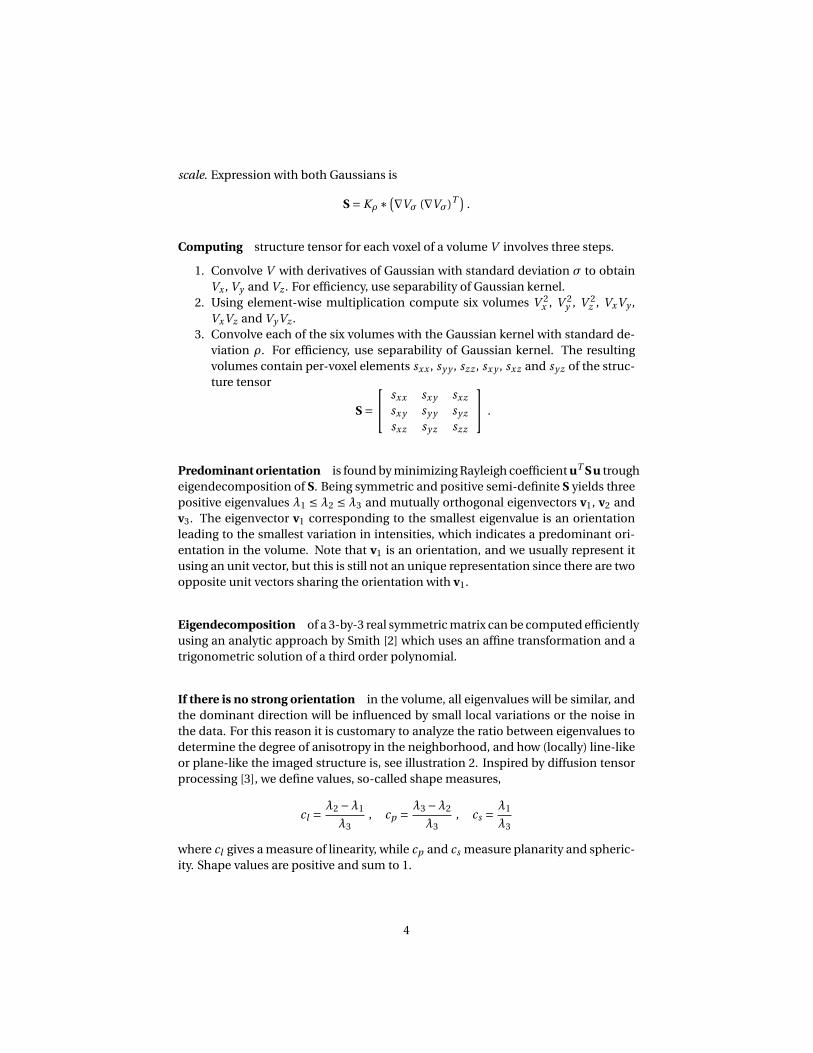
scale. Expression with both Gaussians is

S = Kρ ∗(∇Vσ (∇Vσ)T )

.

Computing structure tensor for each voxel of a volume V involves three steps.

1. Convolve V with derivatives of Gaussian with standard deviation σ to obtainVx , Vy and Vz . For efficiency, use separability of Gaussian kernel.

2. Using element-wise multiplication compute six volumes V 2x , V 2

y , V 2z , VxVy ,

VxVz and Vy Vz .3. Convolve each of the six volumes with the Gaussian kernel with standard de-

viation ρ. For efficiency, use separability of Gaussian kernel. The resultingvolumes contain per-voxel elements sxx , sy y , szz , sx y , sxz and sy z of the struc-ture tensor

S = sxx sx y sxz

sx y sy y sy z

sxz sy z szz

.

Predominant orientation is found by minimizing Rayleigh coefficient uT S u trougheigendecomposition of S. Being symmetric and positive semi-definite S yields threepositive eigenvalues λ1 ≤ λ2 ≤ λ3 and mutually orthogonal eigenvectors v1, v2 andv3. The eigenvector v1 corresponding to the smallest eigenvalue is an orientationleading to the smallest variation in intensities, which indicates a predominant ori-entation in the volume. Note that v1 is an orientation, and we usually represent itusing an unit vector, but this is still not an unique representation since there are twoopposite unit vectors sharing the orientation with v1.

Eigendecomposition of a 3-by-3 real symmetric matrix can be computed efficientlyusing an analytic approach by Smith [2] which uses an affine transformation and atrigonometric solution of a third order polynomial.

If there is no strong orientation in the volume, all eigenvalues will be similar, andthe dominant direction will be influenced by small local variations or the noise inthe data. For this reason it is customary to analyze the ratio between eigenvalues todetermine the degree of anisotropy in the neighborhood, and how (locally) line-likeor plane-like the imaged structure is, see illustration 2. Inspired by diffusion tensorprocessing [3], we define values, so-called shape measures,

cl =λ2 −λ1

λ3, cp = λ3 −λ2

λ3, cs = λ1

λ3

where cl gives a measure of linearity, while cp and cs measure planarity and spheric-ity. Shape values are positive and sum to 1.

4

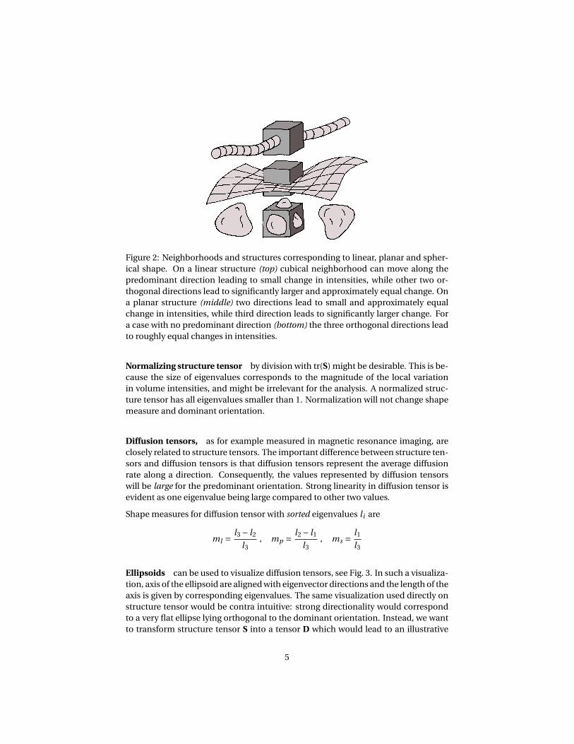
Figure 2: Neighborhoods and structures corresponding to linear, planar and spher-ical shape. On a linear structure (top) cubical neighborhood can move along thepredominant direction leading to small change in intensities, while other two or-thogonal directions lead to significantly larger and approximately equal change. Ona planar structure (middle) two directions lead to small and approximately equalchange in intensities, while third direction leads to significantly larger change. Fora case with no predominant direction (bottom) the three orthogonal directions leadto roughly equal changes in intensities.

Normalizing structure tensor by division with tr(S) might be desirable. This is be-cause the size of eigenvalues corresponds to the magnitude of the local variationin volume intensities, and might be irrelevant for the analysis. A normalized struc-ture tensor has all eigenvalues smaller than 1. Normalization will not change shapemeasure and dominant orientation.

Diffusion tensors, as for example measured in magnetic resonance imaging, areclosely related to structure tensors. The important difference between structure ten-sors and diffusion tensors is that diffusion tensors represent the average diffusionrate along a direction. Consequently, the values represented by diffusion tensorswill be large for the predominant orientation. Strong linearity in diffusion tensor isevident as one eigenvalue being large compared to other two values.

Shape measures for diffusion tensor with sorted eigenvalues li are

ml =l3 − l2

l3, mp = l2 − l1

l3, ms = l1

l3

Ellipsoids can be used to visualize diffusion tensors, see Fig. 3. In such a visualiza-tion, axis of the ellipsoid are aligned with eigenvector directions and the length of theaxis is given by corresponding eigenvalues. The same visualization used directly onstructure tensor would be contra intuitive: strong directionality would correspondto a very flat ellipse lying orthogonal to the dominant orientation. Instead, we wantto transform structure tensor S into a tensor D which would lead to an illustrative

5

Figure 3: Ellipsoids corresponding to tensors of different anisotropy and direction.

visualization using ellipsoids. Transformation should be such that S and D shareeigenvectors, and that eigenvalues of D are computed from eigenvalues of S.

Inspired by Weickert’s model for 2D (see [1] Sec. 5.2.1) we define a transformation

D = exp

(−S

s

)or equivalently, utilizing the properties of matrix exponential,

D = Vexp

(−Λσ

)V−1 ,

where matrices V and Λ are given by eigendecomposition S = VΛV−1. Parameter scontrols the anisotropy of D. Large values of s lead to high anisotropy. TODO: can agood s be computed by requiring that shape measures are unchanged? Seems thatvalues around 0.4 are good.

This expression is continent since the matrix exponential of diagonal matrix can beobtained by computing exponentials of elements on the diagonal.

Optical flow, typically used for determining apparent motion of objects in videoframes, is closely related to orientation estimation. A sequence of video frames isalso represented as 3D structure, but the third (temporal) dimension is treated dif-ferently when analyzing object motion. Since time always moves forward, the mo-tion of objects between frames is [x y 1]T . Similar situation occurs when an-alyzing volumetric 3D data where imaged objects have a predominant direction,e.g. along z axis, and we are concerned with finding a local deviation from this pre-defined direction. See Fig. 4.

To compute optical flow, we need to minimize uT S u,constrained by u = [x y 1]T .Note the difference from the problem of finding dominant orientation – here, thedisplacement in z direction is set to 1. For optical flow, choosing x = 0 and y = 0 is

6

not trivially solving the equation so we need no additional constrain on the lengthof the displacement, and the optimal displacement may be of arbitrary length. Fur-thermore, because of fixed z the solution (x, y) is oriented – the opposite direction(−x,−y) would be a solution for z =−1. It is again useful to consider Fig. 1.

For minimization, recall that uT S u is quadratic in respect to x and y , so the pointwhere partial derivatives vanish can be found by solving a linear system. The systemto solve is [

sxx sx y

sx y sy y

][xy

]=−

[sxz

sy z

]. (1)

So elements of the structure tensor S may be used for computing optical flow in eachvoxel of the volume.

We have now covered optical flow and its connection to structure tensor. However,an explanation of how optical flow is computed usually starts with considering onepoint p, and a problem of finding x and y such that

V (p+ [x y 1]T )−V (p) = 0.

As earlier, we can use first order Taylor expansion yielding

Vx (p)x +Vy (p)y +Vz (p) = 0,

which is an equation with two unknowns, and solution can not be dertermined.

Lucas-Kanade solution for optical flow involves considering a neighborhood, suchthat every pixel pi ∈ N contributes with one equation. This gives an overdeterminedsystem

......

Vx (pi ) Vy (pi )...

...

[

xy

]=−

...

Vz (pi )...

Finding linear least squares solution to an overdetermined system Ax = b is equiva-lent to solving a system AT Ax = AT b, and for our case this is exactly (1)

In summary, structure tensor is a 3-by-3 matrix that can be computed in eachvolume voxel. The computation of structure tensor requires two parameters: noisescale σ and integration scale ρ. Being symmetric, structure tensor can be repre-sented with 6 scalar values. The most important information extracted from struc-ture tensor is a dominant orientation. Dominant orientation is a unit vector withequivalence relation −v ≡ v. Shape measures, also extracted from structure tensor,may also be of interest. Shape measures are three scalar, cl , cp and cs , which sumto 1.

7

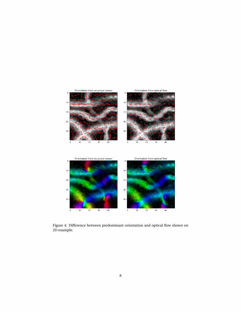
Figure 4: Difference between predominant orientation and optical flow shown on2D example.

8

2 Visualization

Having extracted structure tensor and performed its eigendecomposition, followingvalues are available for every volume voxel.

• Voxel intensity V , a scalar value in a certain range.• Shape measures cl , cp and cs , three scalar values summing to 1.• Dominant orientation v1, an orientation vector (unit vector with equivalence

relation −v ≡ v).• Other information, such as v2, v3, and the valuesλ1,λ2 andλ3 is also available,

but usually of no special interest.

Visualizing this information often requires some care.

Shape measures, being three scalar values can be conveniently represented usingthree RGB color channels. Voxels with large cl will appear red, large cp will be green,and large cs blue. This is the approach used in Fig. 5.

Predominant orientation, is a 3D unit vector with equivalence relation −v ≡ v.A common way of visualizing orientation is to use absolute values of vector coor-dinates, i.e. |vx |, |vy |, and |vz |, as three RGB color channels. This satisfies the re-quired property that−v and v map to the same color. In this mapping, here denotedRGB color mapping, orientations roughly aligned with x direction will be red, thosealigned with y green, and z blue. RGB mapping is favorable for interpretation of theorientations when the imaged object is aligned with the coordinate system (for ex-ample, object elongated in z direction). Another example of is medical image anal-ysis which uses anatomical planes (sagittal, coronal and transverse).

Undesirable property of the RBG color scheme is that different orientations map tothe same color, for example four orientations corresponding to main diagonals inunit cube all map to gray. In Fig. 5 RGB color mapping gives a useful informationon orientation of the structures aligned with coordinate axses. However, a rotationof the object results in a situation with two different (orthogonal) orientations beingvisualized in similar colors.

A similar situation occurs when analyzing composite material as shown in Fig. 6. Inthis case, orientation distribution is largely planar, so a fan-like color scheme hasbeen devised for visualizing orientations. In more general cases, icosahedron-basedscheme might be favorable.

TODO: Explain fan-line color scheme

(r, g ,b) = (1− z2)hsv2rgb(arctan

(y/x

),1,1

)+0.5z2

where hsv2rgb is a piecewise linear function describing conversion from HSV colorspace to RGB color space.

9

Shape measure and predominant orientation are computed for every voxel in thevolume – regardless of whether the voxel is within the object or material which weinvestigate. When using volume rendering to visualize the extracted measures, if thevalue is shown in every voxel, the valuable information might be occluded. For thisreason it might be beneficiary to combine visualization of extracted measures withthe intensity values, which carry information on voxels containing, or not contain-ing, material. A visually pleasing result is obtained if voxels containing no materialare shown transparent. Furthermore, predominant orientation is only relevant forvoxels exhibiting high linearity, so shape measure may be combined with visualiza-tion of predominant orientation,

TODO: Refer to the book [4] for visualization.

3 Applications

Some uses of orientation information obtained from the structure tensor are:

• Volumetric visualization of the shape measures and/or the predominant ori-entation. See Sec. 3.1.

• Producing distributions fo orientations by collecting orientation vectors in thevolume. These distributions live on a half sphere, which can complicate thevisualization, comparison, and fitting of distributions.

• Orientation information extracted form volumetric data may be used for mod-eling, or compared against results from simulation.

• Using local orientation to segment the volume into regions of constant orien-tation,

• Using local orientation to tune smoothness constraint in MRF segmentation.• Using local orientation to guide fibre tracking.• Orientation-aware smoothing.

.

TODO: Expand application.

3.1 Visualizing cotton fibres

Visualizing dominant orientation using may be used for complex fiber systems. InFig. 7 we colorize tomographic data of plain-weave cotton fabric. The yarns of thefabric are single (one-ply), where cotton fibres are held together by a small amountof twist. Orientation of the cotton fibres is therefore given by the weave pattern andthe twist of the yarn. Since fibres mostly lye in the plane of the fabric, fan-basedcolors are well suited for visualizing fibre orientation.

10

Figure 5: Orientation analysis on a synthetic objects. Top row: a configuration con-taining linear structures aligned with the coordinate axis, a sphere and a disc. Sec-ond row: the same configuration as above, but rotated. Third row: linear structureswith random orientations and spherical structures. Forth row: RGB color mappingused for visualizing orientations. Left column: Input data. Second column: shapemeasures shown using colors (red - linearity, green - planarity, blue - sphericity).Third colum: dominant orientation shown using RGB color mapping. Fourth col-umn: dominant orientation weighted by linearity.

11

Figure 6: Orientation analysis of composite material visualized using three differentcolor mappings. Top row: a volume with layered fibre structure. Middle row showscut trough the volume to reveal the orientations of the different layers. Bottom rowshows different color mapping for visualizing orientations. First column shows in-put data. Second column uses RGB color mapping. Third column uses fan-basedcolors. Forth column uses icosahedron-based colors.

12

Figure 7: Using colors to visualize dominant orientation of the cotton fibres in thewoven fabric. Color reveals the direction of the twist holding the cotton fibres to-gether in a yarn.

13

References

[1] J. Weickert, Anisotropic diffusion in image processing. Teubner Stuttgart, 1998,vol. 1. [Online]. Available: https://www.mia.uni-saarland.de/weickert/Papers/book.pdf

[2] O. K. Smith, “Eigenvalues of a symmetric 3× 3 matrix,” Communications of theACM, vol. 4, no. 4, p. 168, 1961. [Online]. Available: https://dl.acm.org/citation.cfm?id=366316

[3] C.-F. Westin, S. E. Maier, H. Mamata, A. Nabavi, F. A. Jolesz, and R. Kikinis,“Processing and visualization for diffusion tensor MRI,” Medical image analy-sis, vol. 6, no. 2, pp. 93–108, 2002.

[4] J. Weickert and H. Hagen, Visualization and processing of tensor fields. SpringerScience & Business Media, 2005.

14