
The Internal Combustion Engine Modelling Modelling ... - DTU
309
General rights Copyright and moral rights for the publications made accessible in the public portal are retained by the authors and/or other copyright owners and it is a condition of accessing publications that users recognise and abide by the legal requirements associated with these rights. Users may download and print one copy of any publication from the public portal for the purpose of private study or research. You may not further distribute the material or use it for any profit-making activity or commercial gain You may freely distribute the URL identifying the publication in the public portal If you believe that this document breaches copyright please contact us providing details, and we will remove access to the work immediately and investigate your claim. Downloaded from orbit.dtu.dk on: Feb 03, 2022 The Internal Combustion Engine Modelling Modelling, Estimation and Control Issues Vigild, Christian Winge Publication date: 2002 Document Version Publisher's PDF, also known as Version of record Link back to DTU Orbit Citation (APA): Vigild, C. W. (2002). The Internal Combustion Engine Modelling: Modelling, Estimation and Control Issues.
-
Upload
khangminh22 -
Category
Documents
-
view
0 -
download
0
Transcript of The Internal Combustion Engine Modelling Modelling ... - DTU

General rights Copyright and moral rights for the publications made accessible in the public portal are retained by the authors and/or other copyright owners and it is a condition of accessing publications that users recognise and abide by the legal requirements associated with these rights.
Users may download and print one copy of any publication from the public portal for the purpose of private study or research.
You may not further distribute the material or use it for any profit-making activity or commercial gain
You may freely distribute the URL identifying the publication in the public portal If you believe that this document breaches copyright please contact us providing details, and we will remove access to the work immediately and investigate your claim.
Downloaded from orbit.dtu.dk on: Feb 03, 2022
The Internal Combustion Engine ModellingModelling, Estimation and Control Issues
Vigild, Christian Winge
Publication date:2002
Document VersionPublisher's PDF, also known as Version of record
Link back to DTU Orbit
Citation (APA):Vigild, C. W. (2002). The Internal Combustion Engine Modelling: Modelling, Estimation and Control Issues.

The Internal Combustion EngineModelling, Estimation and Control Issues
Christian Winge Vigild
SUBMITTED IN PARTIAL FULFILLMENT OF THEREQUIREMENTS FOR THE DEGREE OF
DOCTOR OF PHILOSOPHYAT
TECHNICAL UNIVERSITY OF DENMARKLYNGBY, DENMARK
DECEMBER 2001
Copyright c�
by Christian Winge Vigild, 2001

ØRSTED �DTU, AutomationDTU, Bld. 326DK-2800 Kgs. LyngbyDenmarkPhone +45 4525 3550
Copyright c�
ØRSTED �DTU, Automation 2001
Printed in Denmark at DTU, Kgs. Lyngby01-A-918ISBN 87-87950-90-1

TECHNICAL UNIVERSITY OF DENMARK
INSTITUTE OF AUTOMATION
The following persons, signing here, hereby certify that they have read and recom-mend to the Konsistorium the acceptance of a dissertation entitled ”The InternalCombustion Engine – Modelling, Estimation and Control Issues” by ChristianWinge Vigild in partial fulfillment of the requirements for the degree of Doctor ofPhilosophy.
Dated: December 2001
External Examiner:Lars Eriksson
Research Supervisors:Elbert L. Hendricks
Spencer C. Sorenson
Examining Committee:
iii

iv

TECHNICAL UNIVERSITY OF DENMARK
December, 2001
Author: Christian Winge VigildTitle: The Internal Combustion Engine –
Modelling, Estimation and Control IssuesDepartment: Department of AutomationDegree: Ph.D. Convocation: - Year: 2002
Permission is hereby granted to The Technical University of Denmark to circulateand to copy for non-commercial purposes, at its discretion, the above title upon therequest of individuals or institutions.
Signature of Author
THE AUTHOR RESERVES ALL OTHER PUBLICATION RIGHTS AND NEI-THER THE THESIS NOR EXTENSIVE EXTRACTS FROM IT MAY BE PRINTEDOR OTHERWISE REPRODUCED WITHOUT THE AUTHOR’S WRITTEN PER-MISSION.
THE AUTHOR ATTESTS THAT PERMISSION HAS BEEN OBTAINED FORTHE USE OF ANY COPYRIGHTED MATERIAL APPEARING IN THIS THE-SIS (OTHER THAN BRIEF EXCERPTS REQUIRING ONLY PROPER ACKNOWL-EDGEMENT IN SCHOLARLY WRITING) AND THAT ALL SUCH USE ISCLEARLY ACKNOWLEDGED.
v

vi

To my grandparents:
Tove & Herluf Vigildand
Else & Kaj Nielsen
vii

viii
Contents
List of Figures xiii
List of Tables xxi
List of Articles Included xxiv
Abstract xxvi
Dansk resume xxviii
Acknowledgements xxix
Introduction 1
1 Recent MVEM based control developments 71.1 Introduction . . . . . . . . . . . . . . . . . . . . . . . . . . . . . 71.2 ��� air-to-fuel ratio control . . . . . . . . . . . . . . . . . . . . . 9SAE Paper No. 1999-01-0854 . . . . . . . . . . . . . . . . . . . . . . 111.3 Predictive air-to-fuel ratio control . . . . . . . . . . . . . . . . . 27SAE Paper No. 2000-01-0260 . . . . . . . . . . . . . . . . . . . . . . 311.4 A basic validation of the MVEM framework . . . . . . . . . . . . 57
2 Engine Modelling 592.1 Introduction . . . . . . . . . . . . . . . . . . . . . . . . . . . . . 592.2 Explanatory remarks . . . . . . . . . . . . . . . . . . . . . . . . 622.3 Turbocharger modelling . . . . . . . . . . . . . . . . . . . . . . . 63
2.3.1 Introduction . . . . . . . . . . . . . . . . . . . . . . . . . 632.3.2 Turbocharger parameters . . . . . . . . . . . . . . . . . . 652.3.3 Centrifugal compressor model . . . . . . . . . . . . . . . 65
2.3.3.1 Compressor elementary . . . . . . . . . . . . . 652.3.3.2 Slip . . . . . . . . . . . . . . . . . . . . . . . . 722.3.3.3 Total energy transfer or ����� modelling . . . . 742.3.3.4 Compressor data . . . . . . . . . . . . . . . . . 752.3.3.5 ��� �� model deduction from data . . . . . . . . 79
ix
CONTENTS
2.3.3.6 Speedline shapes . . . . . . . . . . . . . . . . . 842.3.3.7 Energy losses or ����� ����� modelling . . . . . . . 862.3.3.8 Incidence loss . . . . . . . . . . . . . . . . . . 882.3.3.9 Frictional loss . . . . . . . . . . . . . . . . . . 922.3.3.10 ��� � ����� model deduction from data . . . . . . . 942.3.3.11 Mass flow model . . . . . . . . . . . . . . . . . 962.3.3.12 Mass flow model validation . . . . . . . . . . . 1002.3.3.13 Summary . . . . . . . . . . . . . . . . . . . . . 105
2.3.4 Radial variable geometry turbine model . . . . . . . . . . 1062.3.4.1 Modus operandi . . . . . . . . . . . . . . . . . 1062.3.4.2 VGT (Variable Geometry Turbine) elementary . 1072.3.4.3 Literature . . . . . . . . . . . . . . . . . . . . 1122.3.4.4 VGT data set . . . . . . . . . . . . . . . . . . . 1132.3.4.5 LWLS (Locally Weighted Least Square) regression1142.3.4.6 Physical based VGT modelling . . . . . . . . . 1242.3.4.7 Summary . . . . . . . . . . . . . . . . . . . . . 142
2.3.5 Turbocharger speed modelling . . . . . . . . . . . . . . . 1432.4 Filling and Emptying models . . . . . . . . . . . . . . . . . . . . 1442.5 Pipe flow model . . . . . . . . . . . . . . . . . . . . . . . . . . . 1462.6 Throttle model . . . . . . . . . . . . . . . . . . . . . . . . . . . 1492.7 Intake ports . . . . . . . . . . . . . . . . . . . . . . . . . . . . . 1532.8 Heat exchangers . . . . . . . . . . . . . . . . . . . . . . . . . . . 154
2.8.1 EGR cooler . . . . . . . . . . . . . . . . . . . . . . . . . 1552.8.2 Intercooler . . . . . . . . . . . . . . . . . . . . . . . . . 1592.8.3 MVEM approach to intake system modelling . . . . . . . 1612.8.4 Sectioned dynamic heat exchanger modelling . . . . . . . 1682.8.5 Unsteady flow conditions . . . . . . . . . . . . . . . . . . 1682.8.6 EGR cooler simulation study and engine measurements. . 1702.8.7 Summary . . . . . . . . . . . . . . . . . . . . . . . . . . 180
2.9 Phenomenological combustion modelling . . . . . . . . . . . . . 1802.9.1 DI Diesel engines . . . . . . . . . . . . . . . . . . . . . . 1802.9.2 Gasoline engines with port fuel injection . . . . . . . . . 1882.9.3 Combustion chamber heat transfer. . . . . . . . . . . . . . 188
2.10 Crank shaft . . . . . . . . . . . . . . . . . . . . . . . . . . . . . 1892.11 VES and a simulation example . . . . . . . . . . . . . . . . . . . 190
2.11.1 A simulation example . . . . . . . . . . . . . . . . . . . 1912.12 Summary, remarks and conclusions . . . . . . . . . . . . . . . . 1972.13 Appendix . . . . . . . . . . . . . . . . . . . . . . . . . . . . . . 200SAE Paper No. 1999-01-0909 . . . . . . . . . . . . . . . . . . . . . . 201
3 Estimation & Identification 2093.1 EGR Rate estimation . . . . . . . . . . . . . . . . . . . . . . . . 209
3.1.1 MAF sensor performance . . . . . . . . . . . . . . . . . 2103.1.2 Exhaust Sensor Performance . . . . . . . . . . . . . . . . 212
x
CONTENTS
3.1.2.1 Differential Equations for the relevant dynamics 2123.1.2.2 Steady State Operation . . . . . . . . . . . . . 2143.1.2.3 Relative Error Bounds for the Exhaust Sensors . 216
3.1.3 Thermal ratio EGR estimation . . . . . . . . . . . . . . . 2193.1.4 Summary . . . . . . . . . . . . . . . . . . . . . . . . . . 220
3.2 Interfacing strategy and reality . . . . . . . . . . . . . . . . . . . 221SAE Paper No. 2000-01-0268 . . . . . . . . . . . . . . . . . . . . . . 223
4 Control of sign-reversal systems 2294.1 Sign-reversal control . . . . . . . . . . . . . . . . . . . . . . . . 229
4.1.1 VGT-MAF sign reversal control . . . . . . . . . . . . . . 2344.1.1.1 MAF Balancing . . . . . . . . . . . . . . . . . 236
4.1.2 Summary . . . . . . . . . . . . . . . . . . . . . . . . . . 246
5 Conclusions and recommendations 2475.1 Conclusions . . . . . . . . . . . . . . . . . . . . . . . . . . . . . 2475.2 Recommendations . . . . . . . . . . . . . . . . . . . . . . . . . . 249
A Reduction of ����� ��� � 251
B Impeller incidence loss 253
C Burnt mass fraction dynamics 255
D TDMVEM pressure and temperature ODEs 257
Glossary 259
Bibliography 269
xi

CONTENTS
xii
List of Figures
1 Estimated environmentally pollution load in 1998, [18] . . . . . . 1
2 Typical efficiency of a Three Way Catalyst [54]. . . . . . . . . . . 2
2.1 Layout schematic of a modern Diesel engine equipped with EGR(Exhaust Gas Recirculation) and a waste-gate controlled turbocharger(courtesy of Ford Motor Company). . . . . . . . . . . . . . . . . 61
2.2 Compressor map of a Allied Signal centrifugal compressor withbacksweep impeller, splitter blades, and vaneless diffuser. The twodashed lines are the surge line and maximum efficiency line, re-spectively, left to right. . . . . . . . . . . . . . . . . . . . . . . . 66
2.3 Centrifugal compressor components. . . . . . . . . . . . . . . . . 67
2.4 Centrifugal compressor entropy–enthalpy diagram . . . . . . . . . 68
2.5 Inducer velocity triangles. The blue triangle and the black trianglesshow the velocity distribution with and without pre-whirl, respec-tively . . . . . . . . . . . . . . . . . . . . . . . . . . . . . . . . 69
2.6 Velocity triangle at the impeller tip. . . . . . . . . . . . . . . . . 71
2.7 Relative flow conditions for a radial impeller without splitter bladesand an impeller of the backsweep type with splitter blades, alongwith an illustration of the flow separation at the impeller outlet . . 72
2.8 Compressor A efficiency and flow characteristics together with surgeline and maximum efficiency line. The data points are marked with’+’ . . . . . . . . . . . . . . . . . . . . . . . . . . . . . . . . . . 77
2.9 Efficiency and flow characteristics for compressor B . . . . . . . . 77
2.10 Efficiency and flow characteristics for compressor C . . . . . . . . 78
2.11 Interpolated efficiency surface and contour for compressor A. . . . 78
2.12 The left plot, on basis of the interpolated efficiency surface com-puted, shows the specific enthalpy speedlines. Speedline pointsnecessitating efficiency extrapolation are omitted. The dashed en-thalpy speedlines are derived using the efficiency mean value. Thenormalized enthalpy speedlines are plotted in the right figure. . . . 79
xiii

LIST OF FIGURES
2.13 The left plot shows the iteratively computed impeller tip tempera-ture, ��� , speedlines together with the outlet temperature, � � . Usingthese temperatures the gas densities !"� and !#� may be found. Thecomputed densities are illustrated in the plot to the right togetherwith a linear fit of the impeller density, $!"� . Computations utilizingsurge data are marked with % . . . . . . . . . . . . . . . . . . . . . 81
2.14 Non- (black solid) and !&� (red solid) normalized energy curves.The dashed green line is the best general fit forced through the !��normalized energy speed curves. . . . . . . . . . . . . . . . . . . 82
2.15 '�(")�� speedlines for compressor A. The dashed black speedlinesare measurement data and the blue lines are derived using equa-tion 2.48. . . . . . . . . . . . . . . . . . . . . . . . . . . . . . . 83
2.16 The left plot depicts the computed angle, *+� , of the relative outletvelocity ,-� . The corresponding computed slip factors are illus-trated in the plot to the right. Computations utilizing surge data aremarked with % . . . . . . . . . . . . . . . . . . . . . . . . . . . . 84
2.17 Radial compressor map illustration. . . . . . . . . . . . . . . . . 852.18 Backsweep compressor map illustration. . . . . . . . . . . . . . . 862.19 Illustration of the flow separation at the inducer . . . . . . . . . . 892.20 Inducer velocity triangles in the no inlet pre-whirl case. . . . . . . 902.21 A sketch of the inducer flow conditions is seen to the left. A frontal
view of the impeller together with dimensions are depicted to theright. . . . . . . . . . . . . . . . . . . . . . . . . . . . . . . . . 90
2.22 Illustrative sketches of the rotational energy components in the im-peller flow. . . . . . . . . . . . . . . . . . . . . . . . . . . . . . 94
2.23 The energy losses according to the data for compressor A is in theplot to the left drawn together with the model based deduced losses( '�(". /�0�0213'�(")��546'�(")�7 8 ). The right plot shows the '�(�)�� model(red solid curves) together with the corresponding data points. Theblue curves illustrate the energy required by isentropic compres-sion, '�(")�7 8 . . . . . . . . . . . . . . . . . . . . . . . . . . . . . . 95
2.24 The incidence and friction energy losses computed for compres-sor A. The total enthalpy loss (sum of collision and friction loss)speedlines are compared with measurements in the lower plot. Themeasurement speedlines are seen as solid red curves with the indi-vidual data point marked as ’ 9 ’. . . . . . . . . . . . . . . . . . . 97
2.25 Plot of the data point derived loss speedlines, normalized togetherwith the data fitted loss model (Blue solid curve). Data points aremarked with 9 . . . . . . . . . . . . . . . . . . . . . . . . . . . . 98
2.26 Comparison between base model and parameter adjusted compres-sor mass flow model. The solid black lines illustrates the measuredspeedlines for the three compressors, blue and red 9 are positiveand negative solutions to equation 2.77, respectively, and the greendashed curves are the compressor surge lines. . . . . . . . . . . . 101
xiv

LIST OF FIGURES
2.27 Relative mass flow error together with the estimated normal errordistribution, N :<;+=?>A@�B=DC . . . . . . . . . . . . . . . . . . . . . . . 102
2.28 Comparison of the estimated cumulative density to that of the the-oretical N(0,1) distribution. . . . . . . . . . . . . . . . . . . . . . 104
2.29 Pneumatically actuated VGT turbo from Allied Signal (courtesy ofFord Motor Company). . . . . . . . . . . . . . . . . . . . . . . . 106
2.30 Variable geometry turbine diagram. . . . . . . . . . . . . . . . . 1082.31 VGT Entropy–Enthalpy diagram. . . . . . . . . . . . . . . . . . . 1082.32 Rotor entry and exit velocity triangles. . . . . . . . . . . . . . . . 1102.33 Mass flow characteristics for the GT15V NS111(39). . . . . . . . 1152.34 Efficiency characteristics for for GT15V NS111(39). . . . . . . . 1152.35 Illustration of the E#F noise penetration. Note, the realized noise
time G is same for the two plots on right. . . . . . . . . . . . . . . 1192.36 Comparison between HIKJ<L M , N J<L OP (red curves) and the belonging
LWLS estimates (blue curves), respectively. . . . . . . . . . . . . 1222.37 Relative LWLS estimation error. . . . . . . . . . . . . . . . . . . 1222.38 LWLS estimated surfaces for HIQJ<L M respectively N J<L OP with RTSAU J fixed
to 1. The HIVJ<L M surface is limited to WYX W[Z kgs according to specifica-
tion in table 2.8, and the minimum efficiency is here set to 1 %. . . 1232.39 Equivalence area, \^]�_ , and fraction coefficient, ` , as function of
the normalized VGT position. The dashed lines illustrate the 95%confidence intervals around the lines identified. . . . . . . . . . . 127
2.40 Comparison between the physical deducted VGT model and mea-surements. The measurements are marked with a . . . . . . . . . . 128
2.41 The relative error of the mass flow model predictions and mea-surements. The mean and variance of the relative error in % arecomputed to -0.002% and 0.305% B , respectively. The plot to theright shows the distribution of the different important pressures asthe nozzle opens. . . . . . . . . . . . . . . . . . . . . . . . . . . 128
2.42 Fluctuation scenario in exhaust manifold and its influence on theeffective Turbine mass flow. The figure also illustrates how theb c – HIdJ<L M characteristic alters with turbine speed due to the pressuregradient field created around the rotor. . . . . . . . . . . . . . . . 129
2.43 Diagrammatic illustration of the nozzle inlet conditions. . . . . . . 1302.44 The nozzle flow . . . . . . . . . . . . . . . . . . . . . . . . . . . 1322.45 Computed discharge coefficient and nozzle flow model validation. 1342.46 N J<L OP model performance. The first three plot show the perfor-
mance of the turbine efficiency model before multiplicative correc-tion, and the last two plots depict the turbine model performanceafter the correction. . . . . . . . . . . . . . . . . . . . . . . . . . 139
2.47 Enthalpy loss distribution. . . . . . . . . . . . . . . . . . . . . . 140
xv
LIST OF FIGURES
2.48 Extrapolated turbine efficiency surfaces for e[fAgAh�i 0, 0.5 and 1.Remark: in the region with compressor like behavior of the turbine,the efficiency has been fixed at 1%. . . . . . . . . . . . . . . . . . 141
2.49 Filling and Emptying modelling approach illustration. The pro-peller illustrates the auxiliary power input, j , and k is the heattransfer. . . . . . . . . . . . . . . . . . . . . . . . . . . . . . . . 145
2.50 Pipe mass flow and Reynolds number surfaces for a 1m long pipeevaluated with normal atmospheric dry air properties, i.e. lminDo pDqYn2r[nts#u v
Pars, wxixy{z q K, and |di 101.3207kPa . . . . . . . . 149
2.51 The upper part of the figure shows an illustration of the throttleflow conditions. The lower part of the figure illustrate the simpli-fications, presented in [47], made from geometrically considera-tions. The throttle mass flow model derived from this simplifiedflow scenario is known as the two flow path throttle model. . . . . 151
2.52 1-pass water jacket EGR cooler with exhaust side mount EGR valve.1552.53 Illustration of EGR mass packet on its way through one of the }�~
EGR cooler pipes. . . . . . . . . . . . . . . . . . . . . . . . . . . 1572.54 Relative error made when using the assumption w������ ��i���"� w�����w�����h�� . The plot to the left shows the relative temperature error for
different levels of cooler effectiveness. The plot to the right showsthe accompanying mass assessment error. . . . . . . . . . . . . . 161
2.55 Illustration of a typical intake system for a modern 2.0 liter tur-bocharged Diesel engine. The figure also depicts the approximatevalues of the volume and states for the individual sections. . . . . 163
2.56 Typical distribution picture of the intake system mass for a 2.0 literturbocharged Diesel engine generated from experimental data. Thedashed black line shows the ratio between the estimated mass bythe one volume model, �� , and the total intake mass obtained usinga sectioned volume approach. The subscripts indicate the geomet-ric location of the different masses (see figure 2.55). Remark: Themass contained in the heat exchangers is computer by equation 2.210.163
2.57 Relative comparison between �D~ from the TDMVEM and ����t� fromthe AMVEM. . . . . . . . . . . . . . . . . . . . . . . . . . . . . 167
2.58 Relative longitudinal position of the mean cooler temperature to-gether with the mean temperature gradient for different cooler ef-fectiveness levels. In the computations the ambient temperature isassumed to be 298 K. . . . . . . . . . . . . . . . . . . . . . . . . 169
2.59 Selected EGR cooler node location. . . . . . . . . . . . . . . . . 1702.60 Isolated EGR cooler system simulation study. The individual plot
portray the raw and cycle-averaged normalized EGR position, tem-perature distribution and pressure distribution, respectively. Thecurve color notation utilized is given in table 2.16 . . . . . . . . . 174
xvi

LIST OF FIGURES
2.61 Isolated EGR cooler system simulation study. The individual plotsportray the raw and cycle-averaged burnt mass fraction distribu-tion, control volume flows and burnt mass boundary flows, respec-tively. The curve color notation used is given in table 2.17 . . . . 176
2.62 Temperature distribution in the EGR system with/without pump-ing fluctuation presence. The distribution from the unsteady flowsimulation (see figure 2.61) is plotted to the left for the sake of con-venience. The plot to the right depicts the temperature distributionobtained in the steady flow scenario. . . . . . . . . . . . . . . . . 177
2.63 Water jacket cooled EGR heat exchanger performance derived froma steady state mapping data set of a 2.0 liter turbocharged DI (Di-rect Injection) Diesel engine. . . . . . . . . . . . . . . . . . . . . 179
2.64 �{� LWLS identification. The green surface to the left shows the�{� surface identified by a second order LWLS polynomial in � �¢¡A£and ¤ with 25 grid points. The map data points are marked with o,and as an addition the 25% (green line), 50% (black line) and 75%(blue line) steady state EGR rate lines are imposed on the surface.The plots to the right depicts the LWLS estimated �Y� (solid redcurve) together measurement data points and the belonging relativeerror. The individual ”bows” in this upper righthand plot indicatedata points belonging to the same engine speed set point. . . . . . 184
2.65 LWLS identified FMEP for the experimental 2.0l Diesel engine.The FMEP surface identified (green mesh surface) together withmeasurements is seen to the left. The identification routine (solidred line) compared to measurements as a function of operatingpoint is illustrated to the right. The relative modelling error canwith the LWLS algorithm selected be kept within ¥ 10%. . . . . 185
2.66 Graphical evaluation of the ¦T§�¨�© identification. . . . . . . . . . . . 186
2.67 Exhaust port temperature estimation. The measurements as func-tion of operating point are seen as a solid blue curve in the upperplot. The green dashed line is the implicit estimation of ª §¬« , andred dash-dot line illustrates the explicit solution to ª §¬« utilizing §�¨�©« . The relative error of the implicit estimation and explicit es-timation algorithm are marked by ’o’ and ’x’, respectively, in thelowest plot. . . . . . . . . . . . . . . . . . . . . . . . . . . . . . 187
2.68 Speed reference and load torque trajectories utilized in the simula-tion study. . . . . . . . . . . . . . . . . . . . . . . . . . . . . . . 193
xvii

LIST OF FIGURES
2.69 Simulation study of a twin turbocharged V6 Diesel engine. Theupper left plot shows the relative fast accelerator tip-ins and tip-outs during the first 60 seconds of simulation. The correspondingfast responses of the intake- and exhaust temperatures and pres-sures are clear in the three surrounding plots. The displacementof the simulated V6 engine is larger than the original specificationfor the prototype. The compressors will therefore operate closer tothe choke limit, the so called the stonewall, and the pressure dropacross turbines increases due to the possible larger mass flow. Thepressure difference between the exhaust- and the intake system isdue to this turbocharger–engine mismatch thus larger than the pres-sure difference normally experienced with modern turbochargedDiesel engines. The ® level depicted in the lower right plot is inthe high load part of the simulation (250 sec. to 340 sec.) lowerthan normally required due to the high amount of EGR applied.Normally, EGR is only utilized up to approximately 2500 rpm on anormal Diesel engine for light duty applications. The ¯±°�²A³ controltrajectory used (see figure 2.71) would most likely lead to immensesoot emissions in reality. . . . . . . . . . . . . . . . . . . . . . . 194
2.70 Simulation study of a twin turbocharged V6 Diesel engine – con-tinued. Remark: The flows ´µQ¶ , ´µ °�²A³ , ´µV·�¸ and ´µd¹ are the flowsthrough the individual components and not the total mass flows.The upper left plot shows that the compressor mass flow (blue line)responds very promptly to changes in the accelerator, the VGT andthe EGR position. The mass flow through the individual turbines( ´µd¹�º ´µV·�¸�» ´µK¼¾½ ´µ °�²A³ ) is even more sensitive to fast EGRvalve VGT vane position actuation due to the much smaller ex-haust manifold volume. This is especially noticed between 270 to300 seconds of simulation where the VGT- and the EGR positionare changed fast one and two times, respectively. This fast excita-tion of the actuators leads to relatively large excursions in ´µ-¹ . Fur-thermore, the turbocharger speed responds faster to changes thanthe engine speed. This is clear from the steps in the ¿ÁÀ curve fol-lowed a slope nearly matching the engine speed slope. Finally, theproduced engine brake torque is depicted in the lowest left plot. . . 195
2.71 Simulation study of a twin turbocharged V6 Diesel engine – con-tinued 2. The upper left plot shows the fuel command generated bythe fuel controller. The modification of the original EGR and VGTcontrol trajectories is noticed between 280 and 350 seconds of sim-ulation. Here, the VGTs were required to be opened fully and theminimum EGR valve position was set to 0.3 to avoid turbochargersfrom over-speeding. . . . . . . . . . . . . . . . . . . . . . . . . . 196
3.1 Relative EGR rate error boundaries with  3% MAF sensor. . . . . 211
xviii

LIST OF FIGURES
3.2 Schematic diagram of the combustion process in a diesel engine. . 2133.3 Steady state burnt mass fraction in the intake manifold, ÃÅÄ¢ÆAÇ , as a
function of O È�É Ê�Ë�Ì , Í and EGRrate . . . . . . . . . . . . . . . . . 2163.4 Fuel–port mass flow, Î , surface as a function of O È , Í in the ex-
haust pipe and EGRrate during steady state engine operation . . . 2173.5 Requirements to the exhaust sensors’ performance if a relative er-
ror of Ï 5% on the EGRrate is desired. The plots show the errorsurfaces on which the performance requirements are just met. . . . 218
3.6 Contour plot of the upper error surfaces shown in figure 3.5. . . . 2183.7 Relative EGRrate error contours achieved with a Ï 3% O È / Í sensor. 2183.8 Evaluation of the steady state ÐÑ Ê�ÒAÓ and Ô Ê�ÒAÓ estimation algorithms
on engine map data for a 2.0 liter turbocharged Diesel engine withengine speeds ranging from 1000 rpm to 2500rpm. Note: ÐÑ Ê�ÒAÓerrors larger than 200% are neglected for the sake of graphical clarity.220
4.1 Sign reversal illustration. . . . . . . . . . . . . . . . . . . . . . . 2304.2 Amplitude Modulation illustration. . . . . . . . . . . . . . . . . . 2314.3 Sign reversal regions found by 1D WAVE Õ simulation. In the
green regions the VGT equipped turbochargers behave as expectedi.e. VGT closure leads to a higher mass flow through the com-pressor. The red dashed border line indicates regions where tur-bine/compressor map data density is low or where map extrapola-tion is required. . . . . . . . . . . . . . . . . . . . . . . . . . . . 235
4.4 Schematically illustration of the V6 Diesel engine together withthe location specification of selected sensors and actuators. . . . . 237
4.5 Block diagram of the VGT balancing controller setup. . . . . . . . 2394.6 Illustration of the VGT-MAF (Mass Air Flow) sign reversal detec-
tion scheme for the small signal amplitude and phase. . . . . . . . 2394.7 MAF balancing controller. . . . . . . . . . . . . . . . . . . . . . 2404.8 Simulation results obtained with the MAF balancing strategy and
the SR (Sign Reversal) estimation strategy enabled. The red andblue curves depict the right and left engine bank results, respec-tively. The actual sign control is depicted in the lowest left plotin the figure. Every time one of phase estimates crosses the -180 Ölimit (dashed line) the corresponding sign is toggled. . . . . . . . 243
4.9 MAF balancing scenarios with no control, control and excitationbut no SR detection, and control, excitation and SR detection en-abled. The red and blue curves represent the right and left com-pressor mass flow, respectively. . . . . . . . . . . . . . . . . . . . 245
D.1 Illustration of a typical intake system for a modern turbochargedDiesel engine. The figure also depicts the approximate volumefraction and the states for the individual intake system sections.The constant ×"Ø is the total volume of the intake system. . . . . . . 257
xix

LIST OF FIGURES
xx

List of Tables
2.1 Experimental compressors. . . . . . . . . . . . . . . . . . . . . . 762.2 Identified parameter for ÙÚ&ÛÝÜ f Þ ß àtá . . . . . . . . . . . . . . . . . 812.3 Identified â and ã parameters for the three compressors. . . . . . . 832.4 The by equation 2.74 identified compressor parameters. . . . . . . 952.5 Identified compressor loss parameter. . . . . . . . . . . . . . . . . 962.6 Readjusted gains belonging to the individual elements in the com-
pressor parameter vector ä . . . . . . . . . . . . . . . . . . . . . . 992.7 Anderson–Darling test values. . . . . . . . . . . . . . . . . . . . 1032.8 Dimensional specifications for GT15V NS111(39) VGT (see also
figure 2.30). The data marked with ’*’ is found by mechanicaldisassembling of the VGT and should thus be treated as more de-scriptive than accurate. . . . . . . . . . . . . . . . . . . . . . . . 114
2.9 Identified parameters for P with different noise settings. . . . . . . 1192.10 Identified mass flow model parameters with variable å . . . . . . . 1262.11 Identified mass flow model parameters with å Ü3æDç è{éYætê . . . . . . 1262.12 Turbine friction coefficients identified. . . . . . . . . . . . . . . . 1372.13 General values for effectiveness and maximum pressure drop for
1-, 2- and 3-pass EGR coolers after completed soot fouling [26]. . 1562.14 EGR cooler system specifications. NOTE: Specifications marked
with ’*’ are found by local dismantling of the EGR system. . . . . 1712.15 Physical constants and engine parameters used in the VES (Virtual
Engine Simulator) EGR cooler simulation study. . . . . . . . . . . 1712.16 Notation support to figure 2.60 . . . . . . . . . . . . . . . . . . . 1752.17 Notation support to figure 2.61 . . . . . . . . . . . . . . . . . . . 1772.18 Specifications for the V6 engine. Remark: Some of the design
parameters have been changed compared to the original model forpropriety reasons. . . . . . . . . . . . . . . . . . . . . . . . . . . 192
4.1 Setting of SR estimation parameters. . . . . . . . . . . . . . . . . 241
xxi

LIST OF TABLES
xxii

List of Articles Included
C. W. Vigild, M. Struwe, E. Hendricks and K. P. H. Andersen, ”To-wards Robust ëdì Control of an SI engine’s Air/Fuel Ratio“,SAE Technical Paper No. 2000-01-0268 . . . . . . . . . . . 11
A. Chevalier, C. W. Vigild ,E. Hendricks, ”Predicting the Port AirMass Flow of SI Engines in A/F Ratio Control Applications“,SAE Technical Paper No. 2000-01-0260 . . . . . . . . . . . 31
M. Føns, M. Muller, A. Chevalier, C. W. Vigild, E. Hendricks and S.C. Sorenson, ”Mean Value Engine Modelling of an SI Enginewith EGR“, SAE Technical Paper No. 1999-01-0909 . . . . 201
C. W. Vigild, A. Chevalier, E. Hendricks, ”Avoiding Signal Aliasing inEvent-Based Control“, SAE Technical Paper No. 2000-01-0268 . . . . . . . . . . . . . . . . . . . . . . . . . . . . . . 223
xxiii

ARTICLES INCLUDED
xxiv

Abstract
Alternative power-trains have become buzz words in the automotive industry inthe recent past. New technologies like Lithium-Ion batteries or fuel cells combinedwith high efficient electrical motors show promising results. However both tech-nologies are extremely expensive and important questions like ”How are we goingto supply fuel-cells with hydrogen in an environmentally friendly way?”, ”Howare we going to improve the range - and recharging speed - of electrical vehicles?”and ”How will our existing infrastructure cope with such changes?” are still leftunanswered. Hence, the internal combustion engine with all its shortcomings is tostay with us for the next many years. What the future will really bring in this areais uncertain, but one thing can be said for sure; the time of the pipe in – pipe outengine concept is over.
Modern engines, Diesel or gasoline, have in the recent past been provided withmany new technologies to improve both performance and handling and to copewith the tightening emission legislations. However, as new devices are included,the number of control inputs is also gradually increased. Hence, the control matrixdimension has grown to a considerably size, and the typical table and regressionbased engine calibration procedures currently in use today contain both challengingand time-consuming tasks. One way to improve understanding of engines andprovide a more comprehensive picture of the control problem is by use of simplifiedphysical modelling – one of the main thrusts of this dissertation.
The application of simplified physical modelling as a foundation for engineestimation and control design is first motivated by two control applications. Thecontrol problem concerns Air/Fuel ratio control of Spark Ignition engines. Twodifferent ways of control are presented; one based on a model based ExtendedKalman Filter updated predictor, and one based on robust íQî techniques. Bothcontrollers are validated on an engine dynamometer and engine data traces arepresented. The successful application of the model based controllers is then themotivation behind the research in simplified engine modelling to be presented inthis dissertation.
One of the objectives of this dissertation is to propose a framework for simpli-fied modelling of internal combustion engines and selected subcomponents. Thishas lead to the development of a new modelling concept for Variable Geometry tur-bochargers, and a simplified Exhaust Gas Recirculation (EGR) model which canpredict the temperature distribution along the exhaust gas recirculation system with
xxv

ABSTRACT
unsteady flows. Furthermore, since engine combustion modelling often is carriedout on a phenomenological level due to its complex nature, a new regression toolis developed which eases this modelling task.
In the chapter concerning estimation, one of the most important findings is thatEGR cannot be robustly controlled despite measurement of the air to fuel ratio inexhaust gas.
The work closes with a presentation of a new estimation methodology whichmay supply a control strategy with an estimate of the actual control direction. Theestimator is utilized in a control strategy which balances the intake mass flow ofa twin-turbocharged V-engine. Since there exists a point of sign reversal in theVGT position–air mass flow characteristic, whose exact location is unknown, thecontrol problem is posed with serious stability issues. These problems have beensolved with the new non-linear estimation methodology developed – a sign-reversalestimator.
xxvi

Dansk resume
Forbrændingsmotoren–
Modellering, estimering og regulerings-problematik
Alternative køretøjer er p.t. meget omdiskuteret i medierne. Nye teknologier somLithium-Ion batterier eller brændstofceller kombineret med høj effektive elektriskemotorer har vist lovende resultater. Disse teknologier er dog begge ekstremt dyreog vigtige spørgsmal som: ”Hvordan vil vi forsyne brændstofceller med hydrogenpa en miljøvenlig made?“, ”Hvordan vil vi forbedre elektriske køretøjers rækkev-ide og opladningstid?“, og ”Hvordan vil vores eksisterende infrastruktur reagererpa sadane forandringer?“ er stadig ubesvarede. Forbrændingsmotoren vil derfor,skønt alle dens ulemper, være det fortrukne fremdriftsmiddel i den næste arrække.Hvad fremtiden vil bringe indenfor automobil udvikling er dog usikker, men enting kan blive sagt med sikkerhed; den simple rør ind–rør ud forbrændingsmotorsdage er talte.
Moderne Diesel- og benzin-motorer er i de seneste ar blevet udstyret med enrække nye teknologier for at forbedre performance og køreegenskaber, og for atimødekomme de til stadighed hardere emissionskrav. Men, lige sa hurtigt somde nye teknologier blive monteret stiger antallet af reguleringsmuligheder. Derforer kontrolproblemets dimension i dag vokset til en formidabel størrelse , og dentypiske regressionsbaserede motorkalibreringsprocedure er blevet en vanskelig ogtidskrævende opgave. En made at forbedre motor- og kontrolproblem forstaelsenpa er ved at benytte simplificerede fysiske modeller – dette er et af hovedomraderenei denne afhandling.
Anvendelse af simplificerede fysisk baserede modeller som grundlag for esti-mations- og kontrol-design er konsolideret af to kontroleksempler. Reguleringsprob-lemet er i begge tilfælde luft/brændstof-forhold kontrol af benzinmotorer. To vidtforskellige metoder bliver præsenteret: en baseret pa et robust ïñð kontroldesign,mens den anden metode er baseret pa en Extended Kalman Filter opdateret predik-tor. Begge regulatorer er blevet afprøvet pa en motor-prøvestand med gode resul-tater til følge. Et udpluk af maleresultaterne er præsenteret i dette arbejde. Dennesuccessfulde anvendelse af fysisk modelbaserede regulatorer er motivationen bagdet arbejdet som vil blive præsenteret i denne afhandling.
xxvii

DANSK RESUME
Et af formalene er udarbejdelsen af en standardiseret metode til simpel mod-ellering af forbrændingsmotore og udvalgte motorkomponenter. Dette arbejde harledt til udvikling af et Variable Geometry turbo modelleringskoncept, og en sim-plificeret Exhaust Gas Recirculation (EGR) model, som kan predikterer temper-aturdistribution trends under varierende strømningsforhold. Da selve forbrænd-ingsprocessen i motoren er sa kompliceret er modelleringsarbejdet ofte udført udfra fænomensbetragtninger. For at lette dette modelleringsarbejde er der i dettearbejde udviklet et simpelt regressionsbaseret værktøj til at kortlægge visse mo-toregenskaber.
I estimationskapitlet er en alarmerende iagttagelse gjort; Ekstern udstødnings-recirkulering (EGR) kan kun kontrolleres i abensløjfe selvom om udstødningsgas-forholdene er kendt!
Afhandlingen afslutter med en præsentation af balanceringskontrol af indsug-ningsluftmassestrømningerne pa en bi-turbo monteret V motor. Dette kontrol-problem er umadelig vanskeligt, idet der eksisterer et punkt i VGT position–kom-pressormassestrømnings-karakteristikken, hvis nøjagtige placering er ukendt, hvorfortegnet skifter. Dette kan naturligvis lede til alvorlige stabilitetsproblemer. Prob-lemet er løst med en nyudviklet estimationsmetode – sign-reversal estimatoren.
xxviii

Acknowledgements
During a work of this length one is inevitable bound to meet people who are ableto inspire through their passion and knowledge of engine and control technologiesin general.... and this work is no exception.
I joined the Engine Control Group at the Technical University of Denmark leadby Professor Elbert Hendricks and Professor Spencer C. Sorenson together withmy fellow student Michael Struwe in an early period of our Master study – andfrom this group we also graduated as Masters. Here we found the man who manyinternally in the group refer to as the old dude, Professor Elbert Hendricks. Elbert’svery unorthodox way of interacting with his students was at first very surprising andscaring, but after some time I came to appreciate this – we were not his studentsbut rather his boys. Thank you...
Furthermore, I would like to thank my supervisors Elbert Hendricks and SpencerC.Sorenson for giving me the opportunity to carry out this project.
This project probably would not have been finished if had not been for twopersons in particular. First, I wish to thank Dipl. Ing. Thomas Nitsche who isa dear colleague of mine here in the Diesel combustion research group at FordForschungszentrum, Aachen. Thomas was an invaluable sparring partner duringthe modelling work presented in this dissertation. His great experience with jetpropulsion systems gathered through his years at Roll’s Royce helped greatly inthe quest of what is and what is not important in turbocharger modelling. Fur-thermore, in addition to just being a good friend Thomas sacrificed many hours inproof reading the manuscript and on moral support.Thomas – thank you.
Secondly, I wish to thank Ph.D. Evangelos Karvounis, my team leader at FordForschungszentrum, Aachen. Evangelos is at best comparable with an astronom-ically phenomenon – the black hole. Everything that is worth knowing about en-gines regardless of gasoline or diesel, simulation and modelling is sucked in andembodied in him, hence he was and is an invaluable source of information. Evan-gelos was always available if a problem came up and despite being on vacation hetook the time needed to resolve troubling matters. And... and ... and.Evangelos – thank you.
xxix

ACKNOWLEDGEMENTS
Dr. Urs Christen and Ph.D.-student M.Sc. Jim Benjamin Luther are gratefullyacknowledged for always being available for technical discussions and for helpingout with the English language.
Ford Forschungszentrum Aachen GmbH and its people are gratefully acknowl-edged for all the support during the project.
On the private side I would like to thank my wife Andrea for all her supportand patience during miserable times. Hopefully, we now get the time to do moretogether.
Last but not least I would like to thank my family for all the support they haveprovided from the time my vocabulary was limited to ”øf” until Andrea found myfirst grey hairs.
Christian Winge Vigild
Aachen, GermanyDecember, 2001
xxx
Introduction
Motivation
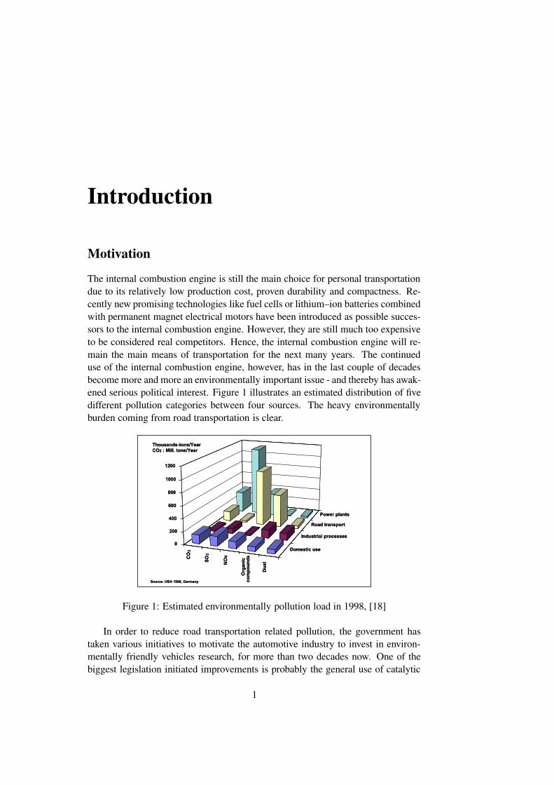
The internal combustion engine is still the main choice for personal transportationdue to its relatively low production cost, proven durability and compactness. Re-cently new promising technologies like fuel cells or lithium–ion batteries combinedwith permanent magnet electrical motors have been introduced as possible succes-sors to the internal combustion engine. However, they are still much too expensiveto be considered real competitors. Hence, the internal combustion engine will re-main the main means of transportation for the next many years. The continueduse of the internal combustion engine, however, has in the last couple of decadesbecome more and more an environmentally important issue - and thereby has awak-ened serious political interest. Figure 1 illustrates an estimated distribution of fivedifferent pollution categories between four sources. The heavy environmentallyburden coming from road transportation is clear.
CO2
SO2
NOx
Orga
nicco
mpou
nds
Dust
D o m e s t i c u s eI n d u s t r i a l p r o c e s s e s
R o a d t r a n s p o r tP o w e r p l a n t s
02 0 04 0 06 0 08 0 01 0 0 01 2 0 0
T h o u s a n d s - t o n s / Y e a rC O 2 : M i l l . t o n s / Y e a r
S o u r c e : U B A 1 9 9 8 , G e r m a n y
CO2
SO2
NOx
Orga
nicco
mpou
nds
Dust
D o m e s t i c u s eI n d u s t r i a l p r o c e s s e s
R o a d t r a n s p o r tP o w e r p l a n t s
02 0 04 0 06 0 08 0 01 0 0 01 2 0 0
T h o u s a n d s - t o n s / Y e a rC O 2 : M i l l . t o n s / Y e a r
S o u r c e : U B A 1 9 9 8 , G e r m a n y
Figure 1: Estimated environmentally pollution load in 1998, [18]
In order to reduce road transportation related pollution, the government hastaken various initiatives to motivate the automotive industry to invest in environ-mentally friendly vehicles research, for more than two decades now. One of thebiggest legislation initiated improvements is probably the general use of catalytic
1

INTRODUCTION
converters. The first family of catalysts introduced in series production was of theoxidation type, which were able to lower CO (Carbon Oxide) pollution by approx-imately 80%. Shortly after followed the TWC (Three Way Catalyst) (1981) andtoxic exhaust gas components CO, HC (Hydrocarbon) and NOX could now simul-taneously be converted into environmentally harmless emissions. However, theTWC could only be used with gasoline engines and furthermore called for a veryprecise control of the AFR (Air/Fuel Ratio) around the stoichiometric level duringboth transient and steady state engine operation. Even small excursions outside thewindow of ò 1% around the stoichiometric level lowers the TWCs efficiency dras-tically. A typical picture of the TWC’s efficiency level is graphically illustrated infigure 2.
14.3 14.4 14.5 14.6 14.7 14.8 14.9 150
10
20
30
40
50
60
70
80
90
100
PSfrag replacements
80% efficiency windowó ô<õ ö
Con
vers
ion
effic
ienc
y,[%
]
÷
NOXCOHC
Stoichiometry
Figure 2: Typical efficiency of a Three Way Catalyst [54].
The development of environmentally friendly gasoline engines has continued,and since the application of catalytic converters, several new technologies like e.g.EGR and GDI (Gasoline Direct Injection), have been introduced to reduce toxicexhaust products. However, augmenting the basic engine design with new tech-nologies often leads to additional degrees of control freedom, and hence controlhandles that need to be adjusted simultaneously; the control task has thus experi-enced an almost exponential growth.
In the later years global warming has become an environmentally issue tooand has received a lot of public attention, and hence initiated political interest.The general accepted opinion is that CO ø (Carbon Dioxide), which formerly hasbeen recognized as a harmless combustion bi-product, promotes global warming.Hence, the outlet of CO ø has to be controlled. Since road transportation relatedCO ø constitutes a large fraction of the total global humanly generated CO ø pro-
2
duction, public focus will in the future probably increase in this area. However,since CO ù is a natural bi-product when burning a fossil fuel, the only really log-ical way to reduce the CO ù outlet is to improve transport vehicle fuel economy.Another reason to improve mileage is of course the increasing fuel prices. Here,the modern Diesel engine has proven itself as a worthy competitor to the gasolineengine both in terms of drivability, performance and of course its better fuel effi-ciency. What used to be recognized as a smelly, heavy, and everything else thansporty engine has developed into a high torque–high performance engine withoutsacrificing exhaust emissions. This is due to technological improvements in areaslike air boosting systems, fuel injection systems, exhaust gas recirculation systemsand combustion chamber design improvements. However, just like the case withthe gasoline engine this has also increased the order of the state space that needs tobe controlled.
The actual handling of the the additional degrees of control freedom is oftenin the automotive industry encompassed by augmenting existing engine controlstrategies by new sub-level strategies. The sub-level strategies are, however, mostoften basic table look-up strategies simply imposed on an existing control structurewithout changing the main control structures. Hence, conventional control strate-gies have now evolved into control structures with often more than ten thousandcalibration coefficients (see e.g. [10]), and the corresponding calibration task nor-mally proves to be both a challenging and time consuming assignment. The workload is actually so intense that it has spawned a new kind of work force in theautomotive industry – the calibrators.
Dynamic physical modelling and simulation have in the later years proven toaid tremendously in the engine design phase due to the often much more compre-hensive picture provided by such models and the engine controller design is noexception. With the introduction of the electronically embedded MVEM (MeanValue Engine Model) to estimate essential engine states, several look-up tablescould be eliminated. Hence, research in such models and physically based controldesigns are important key elements if the ever increasing engine control task is tobe mastered.
Objectives and contributions
The title of the Ph.D. study was ”Robust Control of Nonlinear Systems“. However,due to the vast variety of different control issues covered by such a title, since whatcontrol objects are not included by the nonlinear definition? and who does not wanta robust control design?, this dissertation is devoted to investigation, modelling,estimation and control of the internal combustion engine; Hence, the title ”TheInternal Combustion Engine – Modelling, Estimation and Control Issues“. This ismerely a specialization of the original project.
To motivate the research in the MVEM (Mean Value Engine Model) frameworkfor estimation and control design the first chapter presents two AFR controllers
3
INTRODUCTION
designed by utilizing the MVEM framework.In the first application the AFR of an SI (Spark Ignition) engine is controlled
around stoichiometry by a time based úKû designed controller without using pre-dictive measures to overcome time delay limitations. Since the controller is timebased, the engine time delay will vary with engine speed. However, the restrictionsimposed by this dynamic variation are included in the control design, making asubsequent system inspection by ü analysis possible. Furthermore, the volumetricengine efficiency variation is thrown into the control design, making volumetricefficiency table implementation for AFR control purposes obsolete.
The next controller is based on a zero dimensional model of the intake man-ifold system together with an empirical model of the engine pumping fluctuationdynamics as a model background for an SI AFR event based predictor design. Themodel based predictor uses an EKF (Extended Kalman Filter) to initialize its states.Due to the predictive nature of the AFR control, and by postponing the intake throt-tle command a fixed number of event based samples, the AFR control performancemay be boosted considerably compared to conventional control algorithms.
Although both controllers utilize a completely different control strategy theyhave both been successfully tested on an engine test bed at DTU (Technical Uni-versity of Denmark). Thus, the good modelling framework of the MVEM is con-firmed initiating a further research in extensions to the MVEM framework andapplications; the topic set for the rest of the dissertation.
As already mentioned in the beginning of this dissertation the internal com-bustion engine has been augmented with several new technologies to meet futureemission- and performance targets. However, due to the often very ad-hoc fashionin which the control possibilities offered by the new technologies are utilized, theoverall engine control picture becomes lost in the control strategy design phase.To improve focus on engine control essentials compact simplified engine modelshas gained great interest recently. Such models provided a way to test and debugcontrol structures before actual implementation. However, the models are quite of-ten based on look-up table interpolation or polynomial regression equations alone;The flexibility and scalability of such models are obviously poor. Hence, one of theobjectives of this dissertation is to develop a unified way to model modern com-bustion engines. This has lead to the development of VES; an objective C codeintended for use in the SIMULINK ý /MATLAB ý environment. The goal of this en-gine library is to offer an open and improved way to set up physically based zerodimensional engine models, since key engine components are basically treated justas LEGO bricks; key engine components can be added, removed and edited asrequired.
The development of VES has spawned several new contributions in the mod-elling field . First, the radial turbocharger has been carefully analyzed and brokendown into three key elements: thermodynamic compressor and turbine behavior,and dynamic turbocharger wheel behavior. The compressor mass flow model hasbeen statistically tested on three compressor maps and found optimal in all threecases i.e. the modelling error is normally distributed with mean value zero and is
4

relatively small. The turbine model is able to describe the mass flow through aturbine equipped with adjustable inlet nozzles, a so called VGT, within high ac-curacy. Furthermore, the model is able to provide a prediction of where the massflow through the turbine reverses i.e. the turbine acts as a compressor.
Secondly, the introduction of EGR systems as a means to lower engine NOXproduction renders the application of isothermal MVEMs for observer designsproblematic due to the large temperature gradient between exhaust and intake airsystems. This problem was first addressed in [75] and lead to model augmenta-tion by a temperature state equation. This allowed for a dynamic description ofthe intake manifold temperature and thus more precise AFR control. However, anunavoidable mixing between the throttle body air and EGR will always exist whenback flow conditions are present, making it impossible to assess the right meanvalue of the energy flow out the EGR system, E þ ÿ����������� ������� , in a MVEM frame-work. This statement was first predicted by a simplified EGR system model andlater proven by measurements.
Third, precise EGR control is mandatory for optimal emissions control. How-ever, after initial detailed system analysis it is here concluded that the EGR rateor rather the burnt mass fraction in the intake manifold can not be directly noraccurately estimated from either intake air flow, exhaust gas composition or tem-perature measurements. Hence, EGR control can only be controlled in an openloop fashion.
Fourth, engine control and estimation algorithms are run in an either time basedor event based fashion. One of the arguments for doing the data sampling timebased is the better utilization of sensor information since the anti-aliasing filters donot have to be designed for the lowest sampling frequency, while event based sam-pling may simplify certain engine observer designs. A new family of anti-aliasingfilters is presented here which can provide optimal measurement bandwidth inde-pendently of the engine speed, and is thus optimal for event based engine controland estimation strategies.
Fifth, a new estimation methodology based on AM (Amplitude Modulation)techniques to locate sign reversal points in a systems input-output characteristicswithout the need for dynamic observer information is developed. This estimationmethod is later successfully applied in a simulation study to toggle the output signof a MAF balancing controller on a bi-turbo equipped V6 engine model.
Dissertation organization
The dissertation is divided in five main chapters.
The first chapter introduces briefly some of the control problems encounteredwith the internal combustion engine. The advent of the MVEM (Mean Value En-gine Model) framework in the late 1980’s has been shown to ease and simplifythe design of both estimation and control strategies. The good modelling qualities
5
INTRODUCTION
offered by this framework are confirmed by two applications included in this dis-sertation concerning AFR control of SI engines. The first controller is based on a���
control design, while the second AFR controller utilizes an event based pre-dictive control design. The large difference in the control philosophy behind theAFR controllers and the successful experimental application in both cases supportsthe vast number of possibilities offered by the MVEM framework. This chapter isthe introduction to and the motivation behind the rest of dissertation.
Chapter 2 discusses the engine modelling concepts which have been eitherdeveloped or utilized in this text. Attention has especially been put on the tur-bocharger, EGR system and phenomenological combustion modelling.
In chapter 3 different EGR rate estimation schemes are analyzed. First thenecessary dynamic state equations are found and combined to prepare the basicsfor a later steady state analysis of relative sensor measurement errors’ influence onEGR estimation performance. Furthermore, a new family of anti-aliasing filtersis presented, which can provide event based estimation schemes with the optimalamount of sensor information independent of engine speed.
Chapter 4 presents and discusses the results obtained with a newly developedsign-reversal detection algorithm. The algorithm can locate points of sign rever-sal in a dynamic system’s characteristics, and thereby toggle the controller outputsign. In this way it is possible to maintain the control direction desired. The sign-reversal estimation algorithm is later validated and confirmed by simulations.
Chapter 5 closes the dissertation with final conclusions and recommendationsfor future work.
6
Chapter 1
Recent MVEM based controldevelopments
The purpose of this chapter is to provide the motivation for theresearch in simplified modelling of the internal combustion enginepresented in this dissertation. The motivation is established by apresentation of two air-fuel ratio controllers for spark ignition en-gines. The controllers are both designed by utilizing the MVEM(Mean Value Engine Model) framework. However, the controllersdesigned originate from two very different control philosophies.The successful experimentally evaluation of both controllers andthe significant diversity in the underlying control philosophy mo-tivate the research in extensions to the MVEM framework.
1.1 Introduction
Control of IC (Internal Combustion) engines has become a more and more chal-lenging task. In the early days of IC engines up to the time where the automobilehad become almost universal possession in the West, engine control was merelylimited to compensate for the SI engine’s hesitation to accelerator pedal tip-insand engine knocking. The first control problem was accomplished by the carbure-tor with the latter being achieved by a pneumatically controlled servomechanismmounted on the spark distributor; Both mechanisms are of the pure feed-forwardcontrol type. The Diesel engine was in theory even easier to control from a dy-namic point of view since there was generally speaking only one control problem,the air-to-fuel ratio control problem. This control problem was in principle limitedto an adjustment of the fuel control screw on the Diesel pump such that excessiveexhaust smoke and extensive engine wear at full load were avoided. The actualspeed control of the engine was done directly by the driver (and is for many com-mercial passenger cars available today still left to the driver) or the speed-governor(mostly used in heavy-duty applications), with the latter being adjustable through
7

CHAPTER 1. RECENT MVEM BASED CONTROL DEVELOPMENTS
one or more calibration screws. Hence, the only really closed engine control loopwas until the recent past the driver–engine speed control loop.
The invention of a number of new technologies to reduce emissions and in-crease engine performance has rendered the simplified engine control picture pre-sented above obsolete. Key elements from this list of new automotive technologiesand the corresponding advantages/disadvantages associated are presented in moredetail in chapter 2. A more elaborate list and discussion will therefore not be givenhere. The general rule is that the state space needing control actions grows in sizeas various technologies are moved from the list of possible engine components tothe list of standard engine components. An example is the adoption of electronicfuel injection systems and three-way catalysts to reduce the emissions of SI en-gines. Gasoline fuel injection systems were already in the middle 1950’s availableas a power option (see [31]), but were later reintroduced as a mandatory equipmentnecessary to meet the strict fuelling requirements required by the TWC; a require-ment not achievable with the standard fitted carburetor at that time. The fuellingstrategy was in parallel to this transformed from a pure mechanically implementedsystem into software code and implemented with the wonder of the century; themicroprocessor. However, the fuelling strategy implemented was normally just anumber of different lookup tables in engine speed and intake manifold pressure;thus it was merely a static picture of the engine’s behavior. These tables definedthe steady state fuelling strategy for the engine. Engine hesitation due to throttletip-ins was compensated for with a differentiating network controlled by the size ofthe throttle angle derivative, and possible stationary AFR errors were removed by afeedback loop around the EGO (Exhaust Gas Oxygen) sensor fitted to the exhaustmanifold. Although it was possible to control the engine fuelling more precisely,more time and money were now needed for the calibration process of the individualtables to achieve acceptable drivability and engine emissions. Furthermore, as newtables were added to existing strategies to improve performance in an incrementalway, the control picture became in general only more blurred and fuzzy (see e.g.[30]).
A strong attack on the problems and the complications with conventional AFRcontrol strategies for SI engines briefly presented above was in 1990 given in thearticle ”Mean Value Modeling of Spark Ignition Engines” by E. Hendricks and S.C. Sorenson, see [49]. The research in [49] defined a framework for simplifiedSI engine modelling; an extension to the MVEM terminology introduced earlierin the article ”The Analysis of Mean Value Engine Models” by E. Hendricks, see[43]1. It can be argued that the modelling framework behind the MVEM conceptwas outline as early as 1980 by D. Dobner, see [28]. This research presents a dis-crete engine model with an isothermal description of the intake manifold pressure.However, investigation of the simulation results presented in [28] obtained witha mathematical mean value model of an 5.7 liter carbureted SI engine indicates
1The research presented in [43] was motivated by the good modelling accuracy of a large, two-stroke Diesel engine obtained earlier in [42]
8
1.2. ��� AIR-TO-FUEL RATIO CONTROL
that the mass exchange computation is erroneous; the air mass flow basically staysconstant after a throttle tip-out although the intake manifold pressure level has notstabilized. This is not physically realistic and would thus make a model based ob-server design difficult. Hence, it was at first with the presentation of the SI MVEMin [49] that observer based control of e.g. the AFR has been tractable.
Since the introduction of the MVEM framework, numerous investigations andapplications using this framework have been reported to the engineering commu-nity, and the list of articles is today of an impressive length2. Two recent articleswritten by the author and co-authors attacking the AFR control problem of SI en-gines and belonging to the list mentioned are included in this dissertation. Thefirst article is entitled ”Towards robust H-infinity control of an SI engine’s air/fuelratio” and the second is entitled ”Predicting the port air mass flow of SI enginesin air/fuel ratio control applications”. Both articles were presented at the annualSAE (Society of Automotive Engineers) conference in Detroit in 1999 and 2000,respectively.
Although the control concepts behind the final AFR controllers developed inthe two articles are very different they both utilize an observer derived from theMVEM framework to achieve the AFR control targets set. Hence, both articlesutilize the vast number of possibilities offered by the MVEM framework, and thestrategies developed are later confirmed by experimental results.
1.2 ��� air-to-fuel ratio control
The SAE paper ”Towards robust H-infinity control of an SI engine’s air/fuel ratio”,based on some of the research carried out earlier in [103], attacks the AFR controlproblem of SI engines in a rather untraditional way. Here, the intake air flow is re-garded as a perturbation of the engine’s AFR and the ��� controller developed thusattempts to attenuated (reject) the effects of the intake port mass flow changes asmuch as possible. The intake port mass flow is well described in transients as wellas in steady state by the engine speed, the cycle averaged intake pressure, the en-gine’s volumetric efficiency (see section 2.7), and the intake manifold temperature.Thus, neglecting the intake temperature dynamics, the final control design shouldbe made robust against changes in the three variables remaining. Such an AFRcontroller design is very interesting and is worth pursuing since it would eliminatethe need for an intake manifold pressure sensor and the implementation and cali-bration of a lookup table of the engine’s volumetric efficiency in the AFR controlalgorithm.
The observer behind the final control design is derived by at first establishinga dynamic description of the AFR signal path from the fuel injection to the mea-surement point. This nonlinear model is then later utilized to create the � -object; alinear state space model of the AFR signal path. The development of the nonlinear
2A list of articles authored by the ECG (Engine Control Group) at Technical University of Den-mark may be found online at http://www.iau.dtu.dk/� eh/elb pub.html
9

CHAPTER 1. RECENT MVEM BASED CONTROL DEVELOPMENTS
AFR model is based on the isothermal MVEM described in [50] and [47], and thefuel film model presented in [52].
The final AFR feedback controller utilizes two measurement signals: The �exhaust sensor signal and the MAF measurement obtained upstream of the throttlebody. The � measurement is required to insure that the overall system is detectable(see e.g. [41]). The MAF measurement is optional. However, if it is included in thefinal control design the transient performance of ��� AFR control strategy may beimproved considerably. This is quite logical since if this measurement is omitted,then the ��� controller can only counteract AFR perturbations after they have beenregistered by the � sensor in the exhaust pipe. The bandwidth of this loop is signif-icantly limited by the time delays introduced between the fuel injection and the �measurement. However, if the observer incorporated in the controller is augmentedwith a MAF input, possible AFR perturbations may registered earlier and therebyimprove transient control performance. Unfortunately, series production MAF sen-sors based on hot-film or hot-wire technology are after some service time knownto be troubled by significant stationary measurement errors (see [94]). Hence, thefinal controller uses only a bandwidth filtered version of the MAF signal to avoidsteady state AFR control problems.
The final controller was designed, digitally implemented, and experimentallytested by the author and one of the co-authors, M. Struwe, on one of the enginetest-beds available to the ECG (Engine Control Group) at DTU. Some of the ex-perimental results obtained are included in the paper.
10

1.2. �� AIR-TO-FUEL RATIO CONTROL
!#"$"$"&%(' !)%('+*+,.-/1032547698;:=<>0@?;AB:#CEDGF�[email protected][Z5\ IB]UHMI;^U_`:baGH6dcfe[AB^gTh<>43C.HM0
ifj&k�lnmpo�l qsrVtElurwvsx[yKlnv�luzn{| q}k�m�ox�rh~��#�L�.�Sr&{wx�k�mMx�r� zn�.x�ko��[x�r&{wk�ln���wm�����u����� �`�p���w��� ���`���n� �n�d�p�s�&�`�����p�u�� ln��jwq}x�zd )o�k�¡�¢fx£ �p��¤�`�u¥ ¦&�p���n�`�
§ ¨d©�ª9« §�¬$ª�����®.�u���u�¯� �u��� �u��� ���+�°���u� �w±w� �°²p³�´��`�(µ&�¶�u� � · ±&³sµ&¸s�`�����u�u�����p��p� £M¹ �`��®�� ���9� �#�¶�O�����9º��u���n�����w�d�p� ��� � ���p� �M���p� ����¤ »�d�°�p»�� ����pº�º�� ��®7�p�O�u�����`��®�� ����¼ �.� �u�¶�n�U�p� �$� �M���p��� ���$�g� ´������u� ���@�p������O����®�� ���O��º������¶�u� ��®#º(��� �M��½ ¹ �d����¤�`���u�9�u��¤´��°�w�.� �°�¶�u� �����p����`���u���)� � �u���$±&³}µ[�u�d¾`�`�u�$�u���#���p»�� �.»����n��¤ �`�����u�����������u���p� � �¿ ������+� �[�°���¶Àn´�������� ��� ¿ � ���S�fÁ ¹ � �`��¤»������f� �u�����@¦&Â)Ã9Ä�n�����n����½7�O�����°Å(���°�u� ����»��p��¤ ¿ � ¤M���U�p�w�u��� �9� �`��¤»������f� �M��ºU� �Æ ´�� ��� �n�d�p� �)�p��¤@�n�`� ¤���X�`Ç��°�`�¶¤��+È�¦w¾�½3�O��� �$� �$�p� �u��®��°�����`����M���n�d�p� �(� ���&���`�`´����¶�u�&�u�°�p���n� �`�M�&±&³}µB�°�������u��� ½�O��� �ɺ��pº(�`��º��u���n�`�M�����w��� ¿@Ê · �����u���p� � ¾`��¤.±w� �°²p³´����Mµw�¶�u� �¸�°���M�u�u���}�d�°�����¤��� ��®��U· Ë�Ìd�°���M�u�u��� ¸ ¿ ��� �u�@�����.���u���+� ¿ ���¶�� �p�u®��`�+»��p��¤ ¿ � ¤M�u�S�p��¤U�`�p��®�´��p���p�M�u�`������»�´�� �u�����u� ¿ � �u�Í�u�°¥�nº(�������u�$�n�`� �����u��¤d�`��®�� ���w�p�p�u� �p»�� �w�p��¤+º��p���p�d�°�u�`�s�p�p�u� �¶�u� ������½!ÏΰРª9«dÑ�Ò�Ó�¬+ª Î Ñ Ð±;�+��¤�`�u�g�`��®�� ���$�°���M�u�u�����n��n�u�`�Ô�°�����n� � ���Oº������n�`�M�u� � �p�}� ¿ ����p� � º��p�n�°�`Õs�$Öp»����n��Ö.� ´��`���`�p� �°´�� ����� ��� �p��¤ � Ê ���w×S�`�����u������ �M��º�Øs�n�`��Ù�®�´��u�3Ú�½7�O��� �¶�p�u� �p»�� �¶� Ê �p��¤Uׯ�p�u� ¤�°Ù�����¤@� �� Æ ´��¶�u� ���f·nÚ¶¸�½
Ê ÛÝÜÞgßuàásâ ã ÜÞgä× Û á â ã ÜÞ äÜÞ ßuà
· Ú¶¸
åg�M� � �p� �u�`�Í�u���3»����n��� ´����#�`�p� �`´�� �¶��� ���Í� ��¤��°�u�`�u�d� ���¶¤�»��������p� �.�����u�&æ�� ¿ �u�g�p�f�`��®�� ���$� �u���X���°�p»�� �d� ����M´�º�½��)���� ��¤�°Ç7� ���9�u���d���p»�� ��� ����M´�º@� �$�`�p� �°´�� �¶����¤3� �u���X�`��®�� ��� �n�`�¥�n���#�d�����n´��u�`�d�`�M���`½.±L�+���u�+��¤�p�p���°��¤g�d�°�u����¤g�u� ���n�u� ���¶�u��������p� �9�d�����wæ�� ¿ � �9»M�3´��n�d�p�w�p�7��»��n�`�u�����&�����u����� Æ ´���Ø�� � ��������Så�ç.Â�åè· åg���p�éç��p� ´��ÍÂ���®�� ���Så���¤�`� ¸3��»��u�`�u���`�7º��u�°¥�n�����u�¶¤d� �7ê Ú°ëÉ�p��¤3ê È`ë ½s�O���&»����n�w� ´��`�(� �M��º������u���p� � �$��º������¶�u����p�u��´���¤f�u���3� �u��� �u��� ���+�`�u�u� ���p� �°²�� ´��`�)��º(�`���¶�u� ��®7º���� ���d� �Í���n¥¤�`�)���d�p����� �`���&���¶Ç� �$´��V�O���u�`�&ìf�¶� íO�¶���p� �� �9· �)ì[íO¸��°îd¥�°� �`���°��½ £ � ���`�)�u���)»����n��� ´��`���`�p� �°´�� �¶��� ���9�d�M� �}�p� �u�`�+� �}¤�����)� �ï�ð�ñ ò�ó¶ô�ópõnö�ñ òÉ÷ ø¶ópõ ò õ ÷sñ ù&ú ûuï¶ü¶ý.þ�ÿ
��º(�`��� ���º�Øp�����#±&³}µL· ±w� �°²p³�´��`�ɵw�¶�u� �¸ ¿ � � �(�������&�.�u�`��¤�����°����+¤�u� � �)� �u���L�u���#¤���n� �u��¤d��º��`���¶��� ��®9º���� ���w¤´��w�u�9�`Å(���°����� � ���� ´��`��Ù�� �L� ���u�d�¶��� ����Øp� ´��`��� �¶Àn�¶���u���������¶�u� ��®�ê �¶ë(�p��¤+�����p��®����s� ������.����� ´��+�°���u� �&�°î �°� �`���°������� �Oê �¶ë ½ ¹ ������¤�`�)�u�d�d�p� ���°�p� ���u���¤���u� �u��¤ Ê ����×7��º(�`���¶�u� ��®wº���� ���}� ��� �������°�����u�p�u�O���w� ���°���uº������¶����p�����°�u� ��� Ê ¥ � �`��¤»������+� ���º+� �u���¯�p�d�°Ç����p´�� �)�p� �°²�� ´��`���n�����n������$�u���&� ´������p� ®����u� �u���g½}�O���.������� ��� Ê ¥ � ����¤»����u��� ���º��$´��n�O»���`�pº��p»�� ���p�.���`�`º�� ��® ÊÍ¿ � �u��� �S��� �� ¿ � ��¤� ¿ �p�u��´���¤@�u����u�`� �`�u�`���°�dº(��� �M� · Ê@Û Ú¶¸.� �7�������+���p�f� �f����¤�`�.�u�3���u�u´��u�d�®���¤7�)ì[íK�°î �°� �`���`��½9�O��� Ê ¥ � ����¤»����u�g� ���º3� �#�n�`�`�f���w�u���� � ¿ �`�&� ���ºg� ��Ù�®�´��u��Ú�½w�)���9�u�p���p��� ´��`�}�`���+���p��¤f· »����n�9� ´��`��`�p� �°´�� �¶�u� ���S�p��¤U�°���u�u�¶���u� ���@�u�`����� �u��������� Ê ¥ � ���º(¸9� �d�n�`�M������u��´�®��7���&�w³�íKÙ�� ���`�dê ��ës� �7����¤�`�&�����°���dº������u�¶�u�$� ���&�u����°ÅÉ�����°�)�p�É�u���&� ´��`��Ù�� �V¤����p�+� �`��� �d�u���#� �����p���&�d�p��� � ��� ¤�»(�°¥� ���u��� �$� �$�°������`�n�u��¤7� �M�u�7��º�´�� �n� ¿ � ¤M�u�U�n� ®����p���pº�º�����º��u� �¶���� ���O�u���.� ´��`��� �¶Àn���������w¤��� ���`��½�O���#�°���M�u�u�����n�u�u´�����´��u�w¤�¶�u�°�u� »(��¤d�p»(�¶���w�����s�����&�d�p� ��¤� � ¥��¤�p�p���°�p®���Õ����$�d�����n´��u�w�p��� �°�)� ���p»�� � � �n�d�p��¤�²¶�p��º(�`�n� ���u���p���°�� ���¶�¶�p� � �p»�� ��Ø&���nº(���°� �p� � � ¿ � �u�K�u���nº(�������u���p�p�u� �¶�u� ������� �S�u����`��®�� ����¼ �&º��p���p�d�°�u�����9· ¤´��$�u� �`� �u���`�9�����p��®����w� �g�����$��º(�`���¶�u¥� ��®3º(��� �M�+���+�p®��`� ��®g�°Å(���°����¸�½@Ä&��� ¿ ���3���3�¶���`���`���+�+�������n�º��u��»�� �`���$� �9�u�7� ���u�$´�� �������f�°���+º�� �°��� �d�¤�`�O�p�&����� �����u� �u��n��� �u�`� ¿ ��� ���Í� ���u� Æ ´�� �u��¤U� ���d�u���g� ´��`� � � ��®U���¶� �°´�� �¶�u� �p��½ ¹ ������ �9� �u�`ºf� �9�n´��`�°���u� � ´�� ØÉ�����d�`�p�g�����`�7º�����°�`�¶¤ ¿ � ���@¤���n� ®��¥� ��®d� Ê ¥ �`�����u�u��� � ���s� ���)�u���#�p���`���p� ���d�¤�`� ¿ ��� ���d���p�������`��®p� �����º(�`���¶�u� ��®+º(��� �M�#�p��¤�º��p���p�d�°�u�`�O�p�p�u� �¶�u� ������� ���������`�°��´��M��½Ä#���°�������g�d�¤���w� �����p�p� � �p»�� ��ØO�f� � �����p��� �n��¤����`���n� ���Í�p�.� ��`�p�;»��ͤ�`�u� ����¤ ¿ ��� �u�L� �7�n´�� �°�p»�� �@� ���f�pº�º�� � �`�¶�u� ���K�p�d�u���ËgÌd�°�������u���$�+�°�����¤��� ��®���½ £ ��� �u�`�=������� � �����p�u� �u� ���3�`�p�L»�����p��¤� ��¤����s�d�¤����º��p���p�d�°�u�`��´����°�`�u���p� �M�u� ���`½}���.�u���#�p´������������� ¿ � �¶¤®���Ø��u��� �$� �9�u����Ù(��� �+�pº�º�� � �`�¶��� ���U�p�w�d�¤���u�@�u��»�´�� �ËgÌd�°�������u���M�u��������� Æ ´����}�u�9º��������u� �`�p��� ���u���u���p���°���$»�´�� ��� ���d�`�¥®�� ���9�°���M�u�u��� ½�O���$�u�`���p� ��¤���w�p�}�u��� �&º��pº(�`�&� �#�nº�� � �#´�º3� �M�u�d�����u�`�9���p� �º��p�n�°�`Õ� Âs��®�� ���#�d�¤�`� � ��®� ±K��� ¿;Ê Ë Ì �`�����u����� � �`�O¤���n� ®��� £ ���p»�� � � �n���p��¤ º(�`�n� ���u���p���°�.�p���p� ��n� ���� ü������ ö�� � ò ÷�ö õ�� õnù°÷ � ø.ô! ü���� ò õ ù¶ò � ö�ñ ò#"¶ò õ�$&%
11

CHAPTER 1. RECENT MVEM BASED CONTROL DEVELOPMENTS
Engine Throttle
Fuel Film Compensator
< m ax >
L th
( Φ ref - δΦ )
Air Mass Flow Estimator/Table
λ exh Controller
XEGO
TWC Air
< m ax >
m ap
X: H or U
Φ ref
δΦ
x: t or p
m at
m fi m fu
λ exh
Engine emissions
')( *�+-,/.10�2�354 6�798;:�( <=*�,9<=>?6=@A<=B�.�B-*�( B-.C76�B�D9,/6�4FE/G�E D9.�>�H�I!J-.K+-L-LM.N,54 6&6�LO( BOD/J-.QPM*�+-,/.Q( ERD/J-.CSM<�E�.T@ +-.�4�7�<=4 7+-4 <UD/( 6�B�H�I5J-.KSM<�E�.Q@ +-.�47�<=4 7+-4 <UD/( 6�B�7�<=BV.�( D/J-.�,QSF.1SM<�E�.N:�6�B�<=B�<=( ,K7/JM<=,/*�.CD9<=S-4 .W4 6�6�8&+-LYX 76�B�Z�.�B�D9( 6�BM<=4�76�B&D/,/6�4)E D9,9<UD/.�*�GM[R6�,K<=BV.NE D/( >;<UD9.W6=@�D/J-.\<U( ,Q>�<�E/E] 6=^_X 6�SME�.�,/Z�.�,176�B�D9,/6�4RE�D/,9<UD/.N*�G-[9Ha`TD/J-.N,WB-.N7.NE/E9<=,/G�4 6&6�LMEW( BbD/J-.O.�B-*�( B-.O76�B�D9,/6�4RE D9,9<UD/.�*�GcX @ 6�,1.�d-<=>;L-4 .;D9J-.�( :�4 .OE/LM.�.N:e76�B&D/,/6�44 6&6�LF[RJM<UZ�.KSF.�.�BV6�>\( D�D/.N:O@ 6�,5D9J-.WE/<=8�.K6=@R74 <=,/( D�G�Hf gKh�i�j�hVg?k?l;m�gKnI!J-( E!E�.N79D/( 6�B�:�.NE/7,/( SM.UE5<1oVpKqRor@ 6�,!<=BVs&tR.�B-*�( B-.K.Nu�+-( L-LM.N:^T( D9Jv<Yo�w�t\@ +-.�4K( BUx�.N79D9( 6�ByE/G�E D9.�>�H?I!J-.�L-+-,9LM6&E�.�6=@CD9J-( E.�B-*�( B-.;>\6-:�.�4�( EQD96V:�.NE/7�,/( SF.1D9J-.�E�( *=BF<U4�LM<UD/Ja@ ,/6�>_D/J-.;@ +-.�4( BUx�.N79D9( 6�B�D/6�D/J-.\zV>\.N<�E/+-,/.�>\.NB�DQ( BVD/J-.1.d�JM<=+ME�DTL-( LM.�HTI!J-( E>;6�:�.�4�( EQD9J-.�B�D96�SF.\4 ( B-.N<=,/( E�.N:�( Bb6�,9:�.�,KD/JM<UDCD/J-.�E D9<=BM:-<=,9:{V|W@ ,9<=>;.�^56�,/8V7�<=B�SM.;<=L-L-4 ( .N:#HCI5J-( EK.�B-*�( B-.1>;6�:�.N4)^T( 4 4ASM.,/.�@ .�,/,/.N:;D/6�J-.�,/.W<�ERD9J-.1z�6�S�x�.N79DUHI!J-.R>\6-:�.�4=D/6QSM.RL-,/.NE�.NB�D/.U:Q( E#SM<�E/.N:K6�BKD/J-.!o�pCqRo?.NB-*�( B-..Nu&+M<UD/( 6�BME5LM,/.NE�.�B&D/.N:O( B�} 09~ �)} ��~A<=BM:b} �N~ H�T�������A�&�Q�y�F�N�O�K� ����� �c�U�A����F�=�F�M�b���M�A� ���F� �!�� >\6-:�.�4!6=@QD/J-.�@ +-.�4T>;<�E/E ] 6U^�D96�D/J-.�7G&4 ( BM:�.N,9E1( E1B-.N7�.NE �E/<=,9GeE�( BM7.OB-6=D�<=4 456=@QD/J-.�( BUx�.U79D/.N:e@ +-.N4!>�<�E/E1( E\( BY*&<�E�.�6�+ME@ 6�,/>�^TJ-.�BaD9J-.;( B&D9<=8�.;Z=<U4 Z�.NEK6�LM.NBME�H � @ ,9<�79D9( 6�Bb6=@RD/J-.�( B��x�.N7D/.N:�@ +-.�4A>;<�E/ET,9.�>;<=( BMETZ=<=LM6�,/( ��.N:�<=BM:V( ET>;( d-.N:V^!( D/JVD/J-.<=( ,KSM.@ 6�,9.1( DC( EKE�+M798�.N:V( B�D/6�D9J-.\7�6�>1S-+ME D/( 6�B�79JM<=>1SF.�,NHCI5J-.,/.N>;<=( B-( B-*a@ +-.�4T>�<�E/E1( E;:�.�LF6&E�( D9.N:�6�B�D9J-.�( B�D9<=8�.�>;<=B-( @ 6�4 :^!<=4 4Q<�E�<�@ +-.�4TPM4 >�HyI!J-.�@ +-.�4Q>�<�E/E ] 6=^�( E�E/79J-.�>�<ND9( 7N<=4 4 GE�J-6=^TBV( BVPM*�+-,/.\ \@ 6�,K<=B�.�B-*�( B-.W.Nu&+-( L-LF.N:V^T( D/Jbo�w�tHbI5J-..�Z=<=LF6�,9<UD/( 6�BV6=@5D/J-.\@ +M.�4APM4 >�( B&D/,/6-:�+M7.NEC:�G&BM<=>;( 7NEQ( B�D96OD/J-.@ +-.N4A( BUx�.N7D/( 6�BbE�G-E D/.�>VHCI!J-.1.�Z=<=LM6�,9<UD9( 6�B ] 6=^y@ ,/6�>rD/J-.1@ +-.�4PM4 >���¡¢�£N£ ��( ER:�.NE/7�,/( SF.N:1S�G\<QPM,E DR6=,:�.�,A6�,9:�( BM<=,/G1:�( ¤#.�,/.�B&D/( <=4.Nu&+M<UD/( 6�B�H)I!J-.!D/( >;.Q76�BME D9<=B&D�( B1D9J-.Q`C¥KqcX `K,9:�( BM<=,/G1¥Q( ¤#.�,��.�B&D/( <=4RqRu&+M<UD/( 6�BF[Q( EQD/JM.;.�Z=<=LM6�,9<UD9( 6�B�D/( >\.�7�6�BME D9<=B�DK@ 6�,CD/J-.@ +-.N4�PM4 >��&¦ £ H�I!J-.!( B-L-+�DRD96KD/J-( ERE/+-SME�G�E D9.�>§( E�D/J-.T@ ,9<�79D/( 6�[email protected]@ +-.�4A>�<�E/E ] 6U^W�M¨��MD/JM<UDC( EK:�.�LM6&E�( D/.N:�6�B�D/J-.\^!<=4 4 HKI5J-.Z=<=LM6�,9( ��.N:�LM6�,�D9( 6�[email protected]@ +-.�4A>;<�E/E ] 6U^W�V¡¢ £N© �F( EQ:�.UE/7,/( SM.N:S�GV<=B�<=4 *�.�S-,9<=( 7C.Nu&+M<UD/( 6�B�HKI!J-.WD96UD<=4#@ +-.N4A>;<�E/E ] 6U^yD/6�D/J-..�B-*�( B-.���¡¢ £ �&( E�D/J-.QE/+->§6=@b¡¢ £N© <=BM:ª¡¢ £U£ H�I!J-.TD/6=D9<=4MoVpKq5o>;6�:�.�45} ��~�@ 6�,!D/J-.K@ +-.N4#>�<�E/E ] 6U^v( ETE�J-6U^TBO( B�.Nu&+M<UD/( 6�BbX �[9�
«¢ £U£W¬ 0¦ £ X y¡¢ £U£T® ¨¯¡¢ £�° [¡¢ £�©C¬ X 0Ta¨b[5¡¢ £�°¡¢ £1¬ ¡¢ £N©!® ¡¢ £N£ >;<�E/Ev7�6�BME�.�,/Z=<UD/( 6�B X �[I!J-.CZU<=,/( <=S-4 .NE5¨±<=BM:O¦ £ <=,/.KB-6�,/>�<=4 4 G;>�<=L-LM.N:O@ 6�,5D9J-.WE�LF.�7( PF7�.NB-*�( B-.b<�EV<e@ +-BM79D9( 6�By6=@1.�B-*�( B-.bE�LF.�.N:v²?<=BM:³( B&D9<=8�.
m fi
m fv
m ff
m f
m ff
')( *�+-,/.1 �2�'-+-.�4�>�<�E/E ] 6=^y<UD!D/J-.W( B&D9<=8�.CLM6�,�DUH>�<=B-( @ 6�4 :OL-,/.NE9E�+-,/.5´ ° H�T� �¶µO�F·N¸Y�F� � ¹&�&�cº��C»�� �³�U�A���9�#�=�F�M�b�y�F�A� ���F� �!�I!J-.�B-6�,/>�<=4 ( ��.N: � 'A¼r<UD\D/J-.�( B�D<=8�.�LF6�,�D;( E�7�<=4 7+-4 <UD/.N:�<�EE�J-6=^!B�( Be.Nu&+M<UD/( 6�BvX 0U[9H½¡¢V¾/¿ <=BM:À¡¢ £ ( Be.Nu&+M<UD/( 6�BvX�0U[W<=,/.B-6=^y,9.�L-4 <�7.U:OS&G�D9J-.�( ,K7�6�,/,/.NE�LF6�BM:�( B-*�oVpKqRo±.Nu&+M<UD/( 6�BMET<�E( B�.Nu&+M<UD/( 6�BbX Á&[�z�X�¡¢ £N°/ ²  ´ ° [ ¬ à Ä�Å ©�Æ Ç0U =È�É�Ê Ë=ÌQÍ ° X�¡¢ £N£Q® X 0Ta¨b[!¡¢ £N° [ ²�´ ° X Á&[I!J-.�E D<UD/.;.Nu�+M<UD9( 6�B�@ 6�,1ze7�<=BaSF.\@ 6�+-BM:aS&Ga:�( ¤#.�,/.�B&D/( <UD/( 6�B��.Nu&+M<UD/( 6�BbX Î�[9� ¡z ¬ 0É�Ê Ë;¡¢ £ «¢V¾/¿ ¡¢V¾/¿É�Ê Ë\¡¢VÏ£ «¢ £¬ 0¡¢ £ Ð «¢�¾�¿É�Ê Ë ez «¢ £UÑ
X �[
12
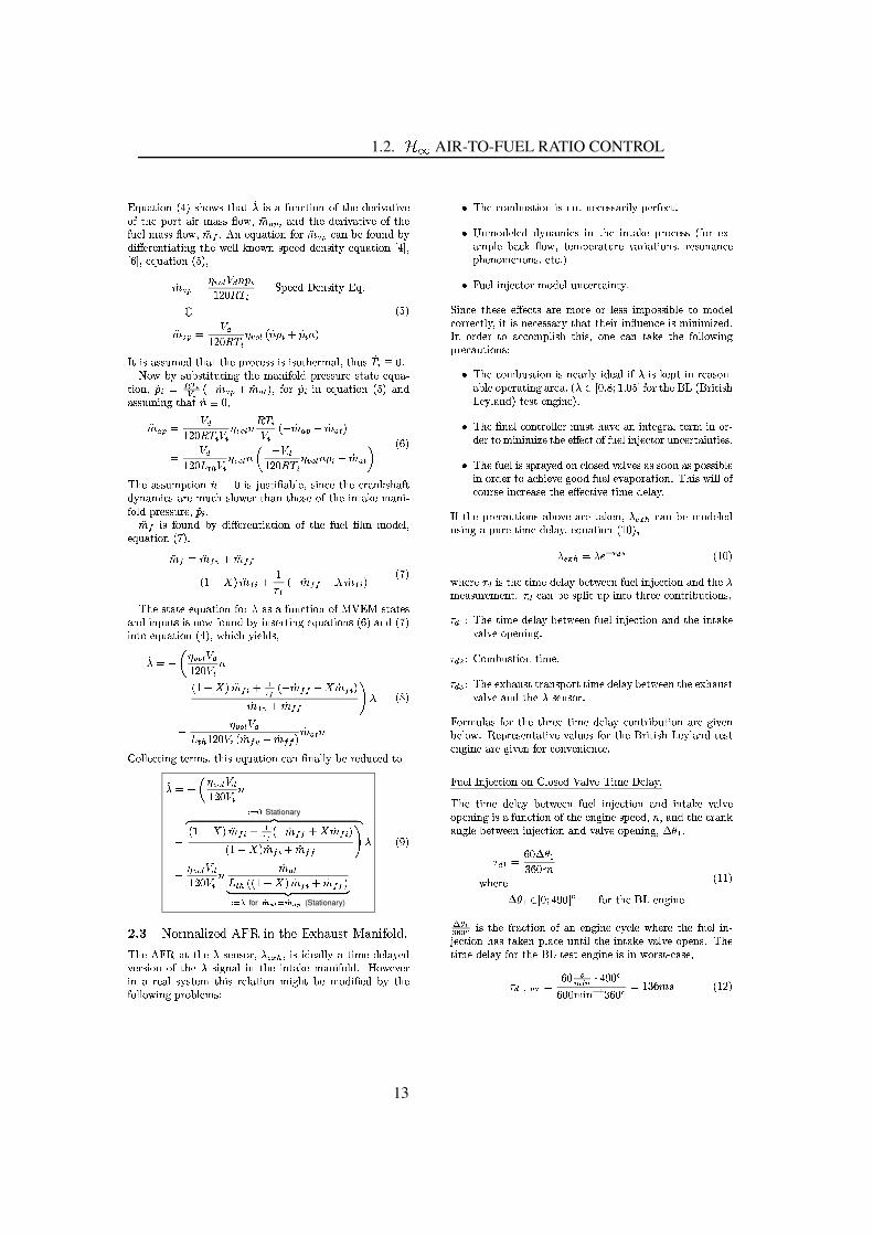
1.2. Ò±Ó AIR-TO-FUEL RATIO CONTROL
Ô5Õ�ÖM×UØ9Ù Ú�ÛcÜ Ý�ÞKß/à-ÚUáQßTØ9àM×UØ�âãaÙ ßC×Oä Ö-ÛMå9Ø/Ù Ú�ÛbÚ=ä5Ø/à-æ�ç�æ�è/Ù éU×UØ9Ù é�æÚ=ä5Ø9à-æ�êMÚ�è�Ø\×=Ù èWë;×�ß9ßKìMÚUáWí�îï�ð�ñ íA×=ÛMçaØ/à-æ�ç�æ�è9Ù é=×UØ/Ù é�æ;Ú=ä5Ø/à-æä Ö-æNò#ë�×�ß/ß5ìMÚ=áWí1îïVó-ôRõ Û�æNÕ&ÖM×UØ/Ù Ú�Û�ä Ú�èYîï�ð�ñ å�×=Û�öFæKä Ú�Ö-ÛMç�ö�÷ç�Ù øFæNè/æ�Û�Ø9Ù ×UØ9Ù Û-ùOØ/à-æ;á5æ�ò òAú�Û-ÚUáTÛbß�êMæNæNçaç�æ�ÛMß�Ù Ø�÷�æNÕ�ÖM×UØ9Ù Ú�Ûcû ÝUü íû ýNü í�æUÕ�ÖM×UØ/Ù Ú�ÛbÜ þ�Þ9íâï ð/ñCÿ�������� ���� ���������� � � êMæNæNç��Qæ�ÛMß�Ù Ø�÷�ÔRÕ ô�îïVð/ñ ÿ ���������� � ����� � Ü â�� ��� â � �)Þ
Ü þ�Þ� ØQÙ ßT×�ß/ß�Ö-ë;æNç;Ø9àM×UØTØ/à-æCê-è9Ú�åæNß/ß!Ù ß5Ù ß�Ú=Ø/à-æ�è9ë;×=ò í&Ø/à�ÖMßyâ� �! � ô"QÚUá?ö&÷bß�Ö-öMß Ø9Ù Ø9Ö�Ø/Ù Û-ù�Ø/à-æOë;×=Û-Ù ä Ú�ò çaê-è/æUß/ß�Ö-è/æ�ß Ø×UØ/æ;æNÕ&ÖM×�#Ø9Ù Ú�Û�í â � ÿ%$'&�() ( Ü * âïVð/ñ � âï�ð,+ ÞíAä Ú�è â �TÙ Û�æNÕ&ÖM×UØ/Ù Ú=ÛyÜ þ=Þ1×=ÛMç×�ß/ß/Ö-ë\Ù Û-ù1Ø/àM×UØ â�- � íîï�ð�ñ ÿ � ���������'� � � �.��� � � ���'�� � Ü * âïVð/ñ � âïVð/+ Þ
ÿ ��������0 + 1 �2� ����� � �43 *����������5� � �.��� � �� ��� âï�ð,+ 6 Ü ý&Þ7!à-æ�×=ß9ß�Ö-ë\ê�Ø9Ù Ú�Û â�8 � Ù ß:9�ÖMß Ø/Ù ;F×=ö-ò æ�íAß�Ù ÛMå�æ1Ø/à-æ�åè9×=Û-ú-ß�àM×Uä Øç�÷�ÛM×=ë\Ù å�ßK×=è/æWë1ÖMå9àaß�ò Ú=á5æ�èTØ/àM×=ÛVØ/à-Ú&ß�æ1Ú=ä�Ø9à-æ1Ù Û&Ø9×=ú�æ1ë;×=Û-Ù #ä Ú�ò çOê-è/æNß9ß�Ö-è/æ�í â � ôîï�ó Ù ß;ä Ú�Ö-ÛMçcö�÷Yç�Ù øFæ�è9æ�Û�Ø9Ù ×UØ/Ù Ú�Û³Ú=äKØ9à-æVä Ö-æNò5;Mò ë ë;Ú�ç�æ�ò íæNÕ&ÖM×UØ/Ù Ú�ÛbÜ <�Þ ôîïVó ÿ îïVó � ��îï�óNóÿ Ü � *>=bÞCîïVó ��� �? ó Ü�* âï�óNó �4= âïVó � Þ Ü <�Þ7!à-æ1ß Ø9×UØ/æWæNÕ&ÖM×UØ/Ù Ú�Û�ä Ú�èQã�×�ßT×1ä Ö-ÛMå9Ø9Ù Ú�ÛVÚ=äA@�BCÔA@±ß Ø×UØ/æNß×=ÛMç;Ù Û-ê-Ö�Ø9ß5Ù ßRÛ-ÚUáYä Ú�Ö-ÛMç\ö�÷\Ù ÛMß�æ�è/Ø/Ù Û-ù1æNÕ�ÖM×UØ9Ù Ú�ÛMßKÜ ý&Þ�×UÛFçVÜ <�ÞÙ Û�Ø9Ú\æNÕ&ÖM×UØ/Ù Ú�ÛbÜ Ý�Þ9í-á!à-Ù å9à�÷&Ù æ�ò ç-ß�íâã ÿ * 3 ����� � ������� ��� �� Ü � *C=aÞ1îïVó ���EDF�G Ü * âï�óUó �4= âï�ó � Þâï�ó � � âïVóUó H ã� �.��� � �0 + 1 ����� �2�-Ü âï�ó � � âïVóUó Þ âïVð/+ �
Ü I&ÞJ Ú�ò ò æNå9Ø9Ù Û-ù\Ø/æ�è/ë�ß�í&Ø/à-Ù ß!æUÕ�ÖM×UØ/Ù Ú�Û�åN×=ÛK;MÛM×=ò ò ÷OöFæCè/æNç�ÖMå�æNç;Ø9Ú
âã ÿ *L3 ����� � ������� ��� �� M N'O StationaryP Q/R SÜ � *>=bÞWîï�ó ���EDF,G Ü�* âï�óUó �4= âï�ó � ÞÜ � *>=bÞ âï�ó �2� âïVóUó H ã� �.��� � ������ �2� � âï�ð,+0 + 1 Ü/Ü � *C=bÞ âïVó ��� âï�óNó ÞR S�P Q
M NUT for VWYX�Z N VWYX [ (Stationary)
Ü \&Þ
]Y^ _a`cbd�egf�h i j�k.lnm�oqpri sgt�uvk>w5xvuyf�zv{�t}|Lf�svi ~�bh l:�7!à-æ õ5�v� ×UØKØ/à-æ�ãbß�æNÛMß�Ú�èNí�ã� � 1 í#Ù ßKÙ ç�æN×=ò ò ÷�×�Ø/Ù ë\æ�ç�æ�ò ×N÷�æNçé�æ�èß�Ù Ú�Û�Ú=äQØ/à-æaãcß�Ù ù�ÛM×=ò5Ù ÛYØ9à-æ�Ù Û�Ø9×=ú�æ�ë�×UÛMÙ ä Ú�ò ç ô8� ÚUá!æ�é�æ�èÙ Ûv×aè9æN×=òQß�÷-ß Ø/æ�ë Ø/à-Ù ß�è/æNò ×UØ/Ù Ú�Ûcë\Ù ù�à�ØOöFæ�ë\Ú-ç�Ù ;MæUçYö�÷�Ø/à-æä Ú�ò ò Ú=á!Ù Û-ù\ê-è/Ú�ö-ò æNë;ß��
� 75à-æ1åÚ�ë1ö-ÖMß Ø/Ù Ú�ÛOÙ ß!Û-Ú=ØTÛ-æUåæNß/ß/×=è/Ù ò ÷�êMæ�è�ä æUå9Ø ô�8� Û-ë\Ú-ç�æ�ò æNçvç�÷&ÛM×=ë;Ù åNß�Ù ÛcØ9à-æ�Ù Û�Ø×=ú�æ�ê-è/Ú-åæNß/ßaÜ ä Ú�èOæ���#×=ë\ê-ò æaöM×�å9úYìMÚUáWíTØ/æ�ë;êMæNè9×UØ/Ö-è/æaé=×=è/Ù ×UØ/Ù Ú�ÛMß�í!è/æUß�Ú�ÛM×=ÛMåæê-à-æ�Û-Ú�ë\æ�ÛMÚ=ÛMßNí�æ�Ø9å ô Þ�8� Ö-æNò#Ù Û�9�æNå9Ø9Ú�èTë;Ú�ç�æ�ò�Ö-ÛMåæ�è/Ø9×=Ù Û&Ø�÷ ô� Ù ÛMåæVØ/à-æNß�æ�æøFæNåØ9ß�×=è/æ�ë;Ú�è/æVÚ�è;ò æNß/ß;Ù ë\êFÚ&ß/ß�Ù ö-ò æ�Ø9Úbë;Ú�ç-æ�òåÚ�è/è9æNå9Ø/ò ÷�í�Ù ØQÙ ß!Û-æNå�æNß/ß/×=è/÷;Ø/àM×UØTØ/à-æNÙ èQÙ Û�ìMÖ-æ�ÛMå�æCÙ ß!ë\Ù Û-Ù ë\Ù ��æNç ô� ÛvÚ�è9ç�æNè;Ø9Úc×�å�åÚ�ë;ê-ò Ù ß�àcØ9à-Ù ß�íQÚ�Û-æbå�×=Û³Ø9×=ú�æ�Ø/à-æ�ä Ú�ò ò Ú=á!Ù Û-ùê-è/æUå�×=Ö�Ø/Ù Ú�ÛMß��� 75à-æ\åÚ�ë1ö-ÖMß�Ø/Ù Ú�ÛVÙ ßTÛMæN×=è/ò ÷OÙ ç�æN×=ò�Ù ä!ã�Ù ßTú�æ�ê�ØKÙ Û�è/æN×�ß�Ú�Û�#×=ö-ò æRÚ�êFæ�è9×UØ9Ù Û-ùK×=è/æU×-í&Ü ã��eû �2� I2� ��� � þNü�ä Ú�è�Ø/à-æY���aÜ �5è/Ù Ø9Ù ß�à�#æ�÷�ò ×=ÛMçMÞRØ/æUß ØTæNÛ-ù�Ù Û-æUÞ ô� 75à-æq;MÛM×=ò�åÚ�Û�Ø9è/Ú�ò ò æ�è5ë1ÖMß ØQàM×Ué�æC×UÛ�Ù Û�Ø/æNù�è9×=òMØ/æ�è9ëªÙ ÛVÚ�è�#ç�æ�è#Ø9ÚTë;Ù Û-Ù ë\Ù ��æ�Ø/à-æRæ�øFæNå9Ø)Ú=ä�ä Ö-æ�ò&Ù Û�9�æNåØ/Ú�è�Ö-ÛMåæ�è�Ø×=Ù Û&Ø/Ù æUß ô� 75à-æ5ä Ö-æ�ò-Ù ßAß�ê-è×N÷�æNçCÚ�Û\åò Ú&ß�æUçWéU×=ò é�æNß)×�ßAß�Ú�Ú�Û\×�ß�êFÚ&ß/ß�Ù öMò æÙ Û�Ú�è9ç�æ�è�Ø/Ú\×�å/à-Ù æ�é�æTù�Ú&Ú-ç1ä Ö-æ�òFæ�é=×UêFÚ�è9×UØ/Ù Ú�Û ô 7!à-Ù ß�áTÙ ò òMÚ=äåÚ�Ö-è9ß�æCÙ ÛMåè9æN×�ß�æQØ/à-æWæøFæNåØ/Ù é�æKØ/Ù ë\æ1ç�æ�ò ×N÷ ô� ä!Ø/à-æ�ê-è9æNå�×=Ö�Ø/Ù Ú�ÛMßC×=öFÚUé�æ�×=è9æ1Ø9×=ú�æNÛ�íAã� � 1 åN×=ÛböMæ�ë;Ú�ç�æ�ò æNçÖMß�Ù Û-ù�×\ê-Ö-è/æKØ/Ù ë;æWç�æNò ×U÷�í�æNÕ&ÖM×NØ9Ù Ú�ÛeÜ ��� Þíã� � 1 ÿ ã2��� F,��� Ü ��� Þ
áTà-æ�è/æ ? TÙ ßAØ9à-æ5Ø9Ù ë;æKç�æ�ò ×U÷WöFæØ�á5æ�æ�Û;ä Ö-æ�òMÙ Û�9�æNå9Ø9Ù Ú�ÛO×=ÛMçWØ/à-æCãë;æN×�ß�Ö-è/æ�ë;æ�Û&Ø ôv? Wå�×=Û�öMæ1ß�ê-ò Ù ØQÖ-ê�Ù Û�Ø/Ú;Ø/à-è/æ�æWåÚ�Û&Ø/è/Ù ö-Ö�Ø/Ù Ú�ÛMß�í? D �Y75à-æWØ9Ù ë;æ\ç�æNò ×U÷OöFæØ�á5æ�æ�Û�ä Ö-æNòAÙ Û�9�æNåØ/Ù Ú�Ûa×=ÛMçOØ9à-æ1Ù Û�Ø×=ú�æéU×=ò é�æKÚ�êFæ�Û-Ù Û-ù ô? /��� J Ú�ë1ö-ÖMß Ø9Ù Ú�ÛOØ/Ù ë\æ ô? /���Y75à-æ5æ���àM×=ÖMß Ø�Ø9è9×=ÛMß�êMÚ�è/Ø#Ø/Ù ë;æ5ç�æNò ×U÷QöMæØ�á5æNæ�ÛCØ/à-æRæ��-àM×=ÖMß ØéU×=ò é�æC×=ÛMçOØ/à-æ\ãVß�æ�ÛMß�Ú�è ô� Ú�è/ë1Ö-ò ×�ßKä Ú�èWØ/à-æ�Ø/à-è9æ�æ;Ø/Ù ë\æ�ç�æ�ò ×N÷eåÚ�Û�Ø9è/Ù ö-Ö�Ø9Ù Ú�Ûe×=è/æ�ù�Ù é�æ�ÛöFæ�ò Ú=á ôq� æ�ê-è/æNß�æ�Û&Ø9×UØ/Ù é�æWé=×=ò Ö-æUßTä Ú�èQØ9à-æ��5è/Ù Ø/Ù ß�à>�#æN÷&ò ×=ÛMç�Ø9æNß Øæ�Û-ù�Ù Û-æW×=è/æKù�Ù é�æ�ÛOä Ú�èTåÚ�Û�é�æ�Û-Ù æ�ÛMåæ ô� Ö-æ�ò!� Û�9�æNå9Ø9Ù Ú�Û�Ú�Û J ò Ú&ß�æNçcBR×=ò é�æ�75Ù ë;æq�Qæ�ò ×N÷ ô7!à-æbØ/Ù ë\æeç�æNò ×N÷vöFæØ�á5æ�æ�Ûvä Ö-æ�òWÙ Û�9�æNå9Ø9Ù Ú�Û�×=ÛMçvÙ Û�Ø×=ú=æeéU×=ò é�æÚ�êFæ�Û-Ù Û-ù1Ù ß5×Qä Ö-ÛMå9Ø9Ù Ú�Û;Ú=ä#Ø/à-æQæ�Û-ù�Ù Û-æKß�êMæ�æUç#í���í&×=ÛMç1Ø9à-æQåè9×=Û-ú×=Û-ù�ò æKöFæØ�á5æ�æ�ÛVÙ Û�9�æUå9Ø/Ù Ú�ÛV×=ÛMç�é=×=ò é�æKÚ�êFæ�Û-Ù Û-ù-í��� D ô? D ÿ ý � ��� D� ý �.� �áTà-æ�è/æ ��� D �Fü � ��Ý.\ � ü � ä Ú�è!Ø/à-æ��:�bæ�Û-ù�Ù Û-æ Ü ��� Þ�A����,�O� Ù ßCØ/à-æ�ä è9×�å9Ø/Ù Ú�ÛeÚ=äQ×=Ûeæ�Û-ù�Ù Û-æOå�÷�åò æ�á!à-æNè/æ;Ø/à-æ�ä Ö-æ�ò5Ù Û�#9�æNåØ/Ù Ú�ÛbàM×�ßQØ9×=ú�æ�Ûaê-ò ×�åæ\Ö-Û&Ø/Ù òAØ9à-æ1Ù Û�Ø×=ú�æ\éU×=ò é�æ1Ú�êFæ�ÛMß ô 7!à-æØ9Ù ë;æWç�æ�ò ×N÷;ä Ú�è!Ø/à-æ¡�:�aØ/æNß ØQæ�Û-ù�Ù Û-æKÙ ß!Ù Û�á!Ú�è9ß Ø�# åN×�ß�æ�í
? D/¢�£!¤ ÿ ý �¥�W � ¦}§ Ý�\ � �ý ��� ë\Ù Û� D � ý �.� ÿ ��� ý ï-¨ Ü ��� Þ
13

CHAPTER 1. RECENT MVEM BASED CONTROL DEVELOPMENTS
©�ª�«¡¬2�® ¯,° ª�±}²�° «�³¡´5³�µ ¶�·�¸²:¹2³Y¯/° «º³q»�³�µ ¶�·�° ±�¯/¼,ª�»��½�³�»º¬.·�¯,¹2³q½�ª�«¡¬2�® ¯/° ª�±K° ®�³�¾�¿2¼,³�®,®�³�»¶�®v¶5À 2±�½/¯/° ª�±ºª�À2¯/¹2³Y½�¼/¶�±2Á¡¶�±2Â�µ ³�¬�³�¯ Ã:³�³�±�° ±.¯/¶�Á�³�Ä�¶�µ Ä�³:ª�¿³�±�Å° ±2ÂK¶�±�»�³�¾2¹�¶��® ¯5Ä�¶�µ Ä�³qª�¿³�±2° ±2Â2Æ'Ç¡È�É�ƶ�±�»�³�±2Â�° ±2³�®�¿³�³�»'Æ�Êy¸²:¹2³�½�ª�«¡¬2�® ¯,° ª�±K¯/° «º³�»�³�µ ¶�·K³�¾�¿2¼,³�®/®�° ª�±�° ®�ÆË�Ì ÉYÍÏÎ�Ð Ç¡È�ÉÊ!Ñ Î�Ð.ÒÃ:¹2³�¼/³ Ç�È É�ÍgÓ.Ô.Õ Ò Ö:× ³�±2Â�° ±2³ Ø Ù Ñ.Ú¶�±�»cÃY° µ µ'¬³q° ±c¯/¹2³�®�³�¯Ë Ì É�ÛÝÜ Î�Ð¥Þß:à á}â Ó.Ô.Õ ÒÎ�Ð�Ð�Ð�ãcä Êvå!æ â Ñ Î�Ð.Òç Î�Ð¥Þß:à á�â Ó.Ô.Õ ÒÎ�Ð�Ð�ãcä Êvå'æ â Ñ Î�Ð.Ò.èÍÝé Ù Ó ç Ù Ñ Î�ê ã-ë Ø Ù Ó ÚÀ ª�¼Y±2ª�¼,«K¶�µ'³�±2Â�° ±2³qª�¿³�¼/¶�¯,° ±2¡¿ª�° ±�¯/®�¸²U¼/¶�±�®�¿�ª�¼,¯/¶�¯,° ª�±c²:° «�³¡´5³�µ ¶�·�¸²:¹2³}¯,° «�³>»�³�µ ¶�·8° ±.¯,¼,ª2»��½�³�»g¬.·ì¯,¹2³-¯,¼/¶�±�®�¿ª�¼�¯/¶�¯/° ª�±8ª�Àq¯,¹2³³�¾2¹�¶��® ¯q«K¶�¯�¯,³�¼�À ¼,ª�«í¯/¹2³�³�¾2¹�¶��® ¯qÄ�¶�µ Ä�³¡¯,ªc¯,¹2³cî>®,³�±�®�ª�¼�° ®«ºª�»�³�µ ³�»}¶�®5¶º¿�µ 2ÂK¿2¼,ª�¿�¶�Â.¶�¯/° ±2Â�¯,¹2¼,ª�2Â�¹�¯,¹�³¡³�¾�¹�¶��® ¯�¿2° ¿³�¸²:¹2³º¿2µ 2Â�«ºª�»�³�µUÀ ª�¼�¯/¹2³�¯,¼/¶�±�®�¿ª�¼�¯/¶�¯/° ª�±}¯/° «º³K»�³�µ ¶�·�Æ Ë�Ì/ï Æ!° ®¶�±>¶�µ Â�³�¬2¼/¶�° ½�À 2±�½/¯,° ª�±>ª�Ày¯/¹2³¡¿2¼,³�®,®�2¼,³�° ±-¯,¹2³�³�¾�¹�¶��®�¯�¿2° ¿³�Æð'ñ ò�ó Æ�¯,¹2³�»�° ®�¯/¶�±�½�³Y¬³�¯�Ã�³�³�±ºÄ�¶�µ Ä�³5¶�±�»º®�³�±�®�ª�¼�Æ�ô ñ ò�ó Æ�¯/¹2³:¯,³�«¡Å¿³�¼/¶�¯,2¼/³:° ±¡¯,¹2³Y³�¾2¹�¶�® ¯y¿2° ¿³�Æ�õ ñ ò�ó Æ�¯/¹2³:³�ö³�½/¯/° Ä�³5¶�¼,³�¶5ª�À�¯,¹2³³�¾2¹�¶��® ¯A¿2° ¿³�Æ�÷ ñ ò�ó Æ.¶�±�»¡¯/¹2³:«K¶�®,®vø�ª�Ã8° ±¡¯/¹2³Y³�¾2¹�¶��® ¯A¿2° ¿³�Æùã ñ ò�ó ¸ Ö ·-«K¶�®,®q½�ª�±�®,³�¼,Ä�¶�¯,° ª�±}¯/¹2³º«º¶�®/®5ø�ª�ÃqÆ ùã ñ ò�ó Æ'° ±>¯,¹2³¿2° ¿�³�° ®A¶�¬ª��¯A¯/¹2³�®,¶�«º³5¶�®v¯,¹2³Yø�ª�Ãn¶�¯y¯/¹2³5° ±.¯/¶�Á�³5¿�ª�¼�¯�Æ ùã-ú�û Æ° ±C¯,¹2³cü}ý�þ�üC¸v²:¹2³ºÿ�±�¶�µyÀ ª�¼,«¡2µ ¶�³¡À ª�¼�¯/¹2³º¯,¼/¶�±�®�¿ª�¼�¯/¶�¯/° ª�±¯/° «º³�»�³�µ ¶�·K° ®�¯,¹2³�±Ë�Ì,ï Í�� ñ ò�ó ô ñ ò�ó ÷ ñ ò�óùã ú,û Í û�� ����� � �� ô ñ ò�ó ÷ ñ ò�óùã ú,û Ø Ù � Ú²:¹2³:¯,¼/¶�±�®�¿ª�¼�¯/¶�¯/° ª�±�¯,° «�³5»�³�µ ¶�·�Æ Ë�Ì/ï Æ�Ã:° µ µ2¬³Y° ±�¯,¹2³5®�³�¯A¬�³�µ ª�ÃÀ ª�¼Y±2ª�¼,«K¶�µ'ª�¿�³�¼/¶�¯/° ±2Â�¿ª�° ±.¯/®:ª�ÀU¯,¹2³ Ö:× ¯,³�® ¯Y³�±2Â�° ±2³�ÆË Ì,ï Û é Õ ç Õ � ê ã}ë Ø Ù Î Ú²:¹2³q¯/ª�¯/¶�µ'¯,° «�³�»�³�µ ¶�·c° ®:¯,¹2³�®�2«Ïª�Àv¯/¹2³q¯,¹2¼/³�³q¯,° «�³�»�³�µ ¶�·½�ª�±.¯,¼,° ¬2�¯,° ª�±�®�¸�²:¹2³q¯,° «�³�»2³�µ ¶�·�Æ Ë�Ì Æ2ÃY° µ µU¬�³�° ±�¯,¹2³�À ª�µ µ ª�ÃY° ±2®�³�¯:À ª�¼:¯,¹2³ Ö:× ¯,³�®�¯Y³�±2Â�° ±2³q³���2° ¿2¿�³�»cÃY° ¯,¹� �þ�����Æ �þ������ Ë�Ì Û é Ù Î ç Õ�Ô�� ê ã}ë Ø Ù � Ú��� �������� "!�#%$'&(#�)"�+*²:¹2³c¯/³�® ¯K³�±2Â�° ±2³�° ®�³��.2° ¿2¿³�»8ÃY° ¯,¹n¶�±-,.�"/Y³�½�ª�¼/»�³�¼ Õ�Ó Ð�Ð þ0 þ2143íîì®�³�±�®�ª�¼�À ¼,ª�« þ�©:ü é � ê ¸-²�¹�° ®�®�³�±�®�ª�¼�° ®�µ ° ±2³�¶�¼�À ª�¼î Û é Ð65 � ç Ù 5 � ê ¶�±�»n½�¶�±g¬�³-«ºª�»�³�µ ³�»n¶�®K¶>ÿ�¼�® ¯Kª�¼/»�³�¼c® ¯�¶�¯,³³��.�¶�¯,° ª�±cÃY° ¯,¹�Â�ª�ª�»�¶�¿2¿2¼,ª�¾2° «K¶�¯,° ª�±!Æ.³��.�¶�¯,° ª�± Ø Ù 7 Ú�¸î ß Ø ë Úî ñ ò�ó Ø ë Ú Í ÙË98 ë�: Ù Ø Ù 7 Ú²:¹2³¡î.Å�®�³�±�®�ª�¼�; ®A¯,° «º³�½�ª�±�® ¯/¶�±.¯:° ®Y»�³�¿�³�±�»�³�±�¯5ª�±c¯/¹2³5¯/³�«�¿³�¼�Ŷ�¯/2¼,³5° ±K¯/¹2³�³�¾�¹�¶��® ¯Y¿2° ¿³ é 7 ê ¸���ª�¼�±2ª�¼/«º¶�µª�¿�³�¼/¶�¯/° ±2Â�¿ª�° ±�¯/®ª�À'¯/¹2³ Ö:× ¯/³�® ¯:³�±2Â�° ±2³�Æ�¯/¹2³5¯,° «º³q½�ª�±�® ¯�¶�±.¯�ÃY° µ µ¬�³�° ±K° ±�¯/³�¼,Ä�¶�µ®�³�¯�Æ Ë�8 Û é � Ð+<=?>A@�B ç Ô�Ó+C >>A@B�êUã}ë Ø Ù Ô Ú
��� DFE4 "GH "�JIK#% L9$�#%*.&M#�)"��*²:¹2³q«�ª2»�³�µ'À ª�¼�¯,¹2³q¿2¼,ª�¿�¶�Â.¶�¯,° ª�±Kª�Àyîc¯,¹2¼/ª�2Â�¹º¯/¹2³�³�±2Â�° ±2³�¯,ª¯/¹2³º®�³�±�®,ª�¼�±2ª�à ¹�¶�®5¯,ª�¬�³ºµ ° ±2³�¶�¼,° ®�³�»}° ±>ª�¼/»�³�¼5¯,ª}¶�¿2¿2µ ·�¯,¹2³® ¯�¶�±�»2¶�¼/»KNPO�Å À ¼/¶�«º³�Ã�ª�¼,Á'¸QSR TSR U × ° ±2³�¶�¼,° ®/¶�¯/° ª�±cª�ÀU¯/¹2³¡îJ �¯�¶�¯,³�þ��.�¶�¯,° ª�±!¸²:¹2³º® ¯/¶�¯,³¡³����¶�¯/° ª�±}À ª�¼qî-° ®5µ ° ±2³�¶�¼,° ®�³�»�° ±>¶�¿2¿³�±�»�° ¾�, ÃY° ¯,¹¼,³�®�¿�³�½�¯5¯/ªc¯/¹2³�® ¯�¶�¯,³�® ùãJV�V Ævî'Æ ùãJV à ¶�±�»}¯,¹2³º° ±2¿2�¯�®�ÊyÆ'WãJV à Æùã úX ¸QSR TSR Q ,Y¿2¿2¼,ª�¾2° «K¶�¯,° ª�±cª�ÀU¯,¹2³¡þy±2Â�° ±2³q²:° «º³¡´Y³�µ ¶�·�¸²:¹2³c³�±2Â�° ±2³+; ®�¯,° «º³}»�³�µ ¶�·C° ®¡À ª�¼�¿2¹.·2®�° ½�¶�µ:¼,³�¶�®�ª�±�®qµ ° ±2Á�³�»4¯,ª¯/¹2³�½�¼/¶�±2Á�®,¹�¶�À ¯5®�¿³�³�»'Æ�ÊyÆ�¶�®5½�¶�±}¬³¡®�³�³�±}° ±}³��.�¶�¯,° ª�±�® Ø Ù�Ù Ú�ÆØ�Ù Ñ.ÚA¶�±�» Ø�Ù � Ú/¸y²:¹2³5¯,ª�¯/¶�µ³�±2Â�° ±2³5¯,° «º³q»�³�µ ¶�·�À ª�¼�¯,¹2³ Ö:× ¯/³�® ¯³�±2Â�° ±2³�½�¶�±cÃY° ¯/¹�Â�ª.ª2»�¶�¿�¿2¼,ª�¾2° «K¶�¯,° ª�±c¬³q«ºª�»�³�µ ³�»�¶�®�Æ
Ë�Ì ÍZYÊ Í�Ð65 Ù 7 �+[�\ ð ã â ëÊ Ø Õ Ð Ú²:¹2° ®:¯,° «�³¡»�³�µ ¶�·c¶�¿2¿2¼,ª�¾�° «º¶�¯,° ª�±cÃ:¶�®AÀ ª�2±�»c¬�·K¼,³�Â�¼,³�®,®�° ª�±!¸²:¹2³-¯,° «�³C»�³�µ ¶�·g¶�¬ª�Ä�³-¹�¶�®º¯,ªì¬³C¶�¿2¿2¼,ª�¾2° «K¶�¯,³�»8¬³�À ª�¼,³¶�¿2¿2µ ° ½�¶�¯/° ª�± ª�À�¯,¹2³4®�¯/¶�±�»2¶�¼/»]NPO�Å À ¼�¶�«�³�Ã�ª�¼,Á'¸ ²�¹�³>¿2¹�¶�®�³®�¹2° À ¯�ª�Àv¯/¹2³q¯,° «�³�»�³�µ ¶�·c° ®Yª�À ¯,³�±>¶�¿2¿�¼,ª�¾2° «K¶�¯,³�»c¬�·c³�° ¯/¹2³�¼�¶�±ª�¼/»�° ±�¶�¼,·�µ ª�Ã4¿�¶�®,®'ÿ�µ ¯,³�¼vª�¼y¶.^y¶�»�_³Uÿ�µ ¯,³�¼�¸v²�¹2³Y½,¹2ª�° ½�³Aª�À�ª�¼/»�³�¼¶�±�»a`�ª�¼A¯ ·�¿�³�ª�À!¯/¹2³5¯,° «º³q»�³�µ ¶�·K¶�¿2¿2¼,ª�¾2° «K¶�¯,° ª�±º° ®�»�³�¿�³�±�»�³�±�¯ª�±c¯,¹2³q¶�¿2¿2µ ° ½�¶�¯/° ª�±!Æ�®,³�³q¶�¿2¿³�±�»�° ¾�©�¸"� ¯Y° ®:®�¹2ª�ÃY±c° ± é Ñ ê ¯/¹�¶�¯¶º®�³�½�ª�±�»cª�¼/»�³�¼�^y¶�»�_³Yÿ�µ ¯/³�¼Y° ®:®,cbK½�° ³�±�¯�Æ2Ã:¹2³�±c«ºª�»�³�µ ° ±2Â�¯,¹2³¯/° «º³�»�³�µ ¶�·�¸v²:¹2³5®�¯,¼,�½/¯/2¼,³Yª�À¯/¹2³Y¯,° «�³�»�³�µ ¶�·º¶�¿2¿2¼,ª�¾2° «K¶�¯,° ±2Â^y¶�»�_³5ÿ�µ ¯/³�¼Y° ®Y®,¹2ª�ÃY±c° ±cÿ�Â�2¼,³qÑ2Æ�®�³�³�¶�¿2¿³�±�»�° ¾-©�¸
-2n0ξ
12n0ξ
Σ-
Σ-
λ
λexh
6n0ξ�U° Â�2¼,³�Ñ6�d^v¶�»�_³q¶�¿2¿2¼,ª�¾�° «º¶�¯/° ª�±Kª�ÀU¯/¹2³q³�±2Â�° ±2³+; ®A¯/° «º³�»�³�µ ¶�·²:¹2³-¯,³�¼,«%Ê > ° ±nÿ�Â�2¼,³>Ñ4° ®º¯/¹2³-±2ª�«º° ±�¶�µ�Ä�¶�µ 2³-À ª�¼K¯,¹2³½�¼�¶�±2Á2®�¹�¶�À ¯5®�¿³�³�»c° ±c¯/¹2³e,f`g�ì½�ª�±.¯,¼,ª�µ'»�³�®�° Â�±!¸
QSR TSR h î.Å?3�¬ci�³�½/¯q©Aª�±.¯,¼,ª�µ!ü�ª2»�³�µ ¸²:¹2³�ª�Ä�³�¼/¶�µ µvî.Å ª�¬�i�³�½/¯�ÃY¹2° ½/¹-Ã:¶�®Y�®�³�»}° ±�¯/¹2³jNkO�Å�»�³�®�° Â�±-ª�À¯/¹2³l,.�"/r½�ª�±.¯,¼,ª�µ µ ³�¼K° ®c¶8®�° ¾�¯,¹ ª�¼/»�³�¼c«�ª2»�³�µ ¸Ý²:¹2³>«ºª�»2³�µ½�ª�±�®�° ® ¯vª�À?�'¯�Ã�ª�® ¯�¶�¯,³�®U«�ª2»�³�µ ° ±2Â5¯,¹2³AÀ 2³�µ.° ±9i�³�½/¯,° ª�±�»�·.±�¶�«º° ½�®�ƪ�±2³�® ¯/¶�¯,³Y«ºª�»�³�µ ° ±2ºî'Æ�¯�Ã�ª�® ¯�¶�¯,³�®A¶�¿2¿2¼,ª�¾2° «K¶�¯,° ±2Â�¯,¹2³Y³�±�Â�° ±2³¯/° «º³q»�³�µ ¶�·�Æ.¶�±�»�ÿ�±¶�µ µ ·¡ª�±2³�®�¯/¶�¯,³5«ºª2»�³�µ ° ±2Â�¯,¹2³�»�·�±�¶�«�° ½�®Aª�À¯/¹2³ 0 þ�1e3g®�³�±�®�ª�¼�¸!²:¹2³:¬2µ ª2½,Á�»�° ¶�Â�¼/¶�«Lª�À2¯,¹2³Y½�ª�±�¯/¼,ª�µ.ª�¬�i�³�½/¯° ®y®�¹2ª�ÃY±¡° ±¡ÿ�Â�2¼/³ Ó ¸y²�¹2³5½�ª�¼,¼,³�®�¿�ª�±�»�° ±2Âq® ¯/¶�¯/³Y®�¿�¶�½�³Y®,·�® ¯,³�«³��.�¶�¯,° ª�±�®:½�¶�±c¬³�À ª�2±�»�° ±}¶�¿2¿³�±�»�° ¾ Ö ¸
14

1.2. mon AIR-TO-FUEL RATIO CONTROL
-
m ff
-120 RT i L th λ 0 2
1000 τ f V d
- RT i L th λ 0 2
1000 V i
- RT i L th ( 1 - X ) λ 0 2
1000 V i
-120 RT i L th ( 1 + X ) X λ 0 2
1000 τ f V d
-120 RT i L th (1 - X ) λ 0 2
1000 V d
Σ
Σ
Σ
n 2 Σ δ 2
n 1
1 n 0
Σ
η 2 Σ δ 3
η 1
1 η vol 0
Σ
RT i λ 0 1000 V i
Σ
W p
1 p i 0
δ 1
Σ
W n
n 0
δ 2
Σ V d
120 V i
W η
η vol 0
δ 3
Σ
W n
n 0
δ 2
Σ 12 ξ
W n
n 0
δ 2
Σ -2 ξ
W n
n 0
δ 2
Σ 6 ξ
Σ
Σ
1 τ λ
Σ Σ
ε 21 δ 21 ε 31
δ 31
ε 11 δ 11
δ 22 ε 22 δ 32 ε 32
-
ε 23 δ 23
-
-
-
ε 24 δ 24 ε 25 δ 25
λ m
λ 2 λ 1
λ
m at
m fi
m fi
K
Σ
λ ref
W e z 1
-
p pW mat
W u z 2
W AF Σ
L th
- z 3
Σ
1 τ f
X τ f
8
Control object modeling
Pertubation modeling
Performance weights
Signal Weights
p p
q�r s+t6uv�wax"y�z {6|}�~cr �gs+u��g��� {+u���6v�z r �6v9�gur �?v9~K��{+���?v9|����2r ����%v�u?�tau�a�9�r {+�K�K{c~cv�z r �6sa���av�u� {+u�K�g�a|Avg�g�?r s+�a�gzc��v�r s+�������g�a~��'|A{+�+��u{+z z v�u���'�k�-��J��� r �����6v4� t6v�z�az ��� �A�9�v+�%�kr �2��6ve�6{+u���gz r ��v�~k�.q"���9�2���6v4r �+�A�g}+vf�%{+u?���%�%�4�g�a~P�a�e�guvf��6vj� ���9��v��2r �'��6v��"�+~��v.�az �v�u��a�g�a~�a�a�gz z k�a¡�r ����ave¢.£2¤4¥��?v��a�{+u�¦ �2� �A�9�v+�
15

CHAPTER 1. RECENT MVEM BASED CONTROL DEVELOPMENTS
§ ¨K©KªJ«e¬K©�(®k¯4°S±�²kª³2´6µ�¶6·6¸�¶a¹�º?µ.¹g»%¼´6½ º�º?µ�¾�¼�½ ¹+¿�½ º"¼�¹jÀcµ�º¾�¸½ Á%µ2¼�´6µfº?Âcº ¼�µ�Ãĺ?µA¼·6¶Å ¿aÀj¼´6µ.¾A¹+¿�¼¸¹+Æ Æ µ�¸�Àcµ�º?½ Ç+¿SÈ"³2´6µ�º?Â6º ¼µ�Ãɺ?µA¼·6¶�º?´6¹9Ê.º Å ¿�µ Å º?ÂÅ ¿aÀ'¾A¹+ÃK¶6¸µ�´6µ�¿aº?½ Ë+µ�Ê Å Âj¼�¹jÃ�¹6Àcµ�Æa¼�´6µfÃK¹�º ¼�½ Ã�¶%¹+¸?¼ Å ¿�¼2¶%µ�¸?̼�·6¸Á Å ¼½ ¹+¿aº�½ ¿Í¼´6µÏÎÍÃK¹cÀ6µ�Æ È�³�´6µÐº?µ�¾�¼½ ¹+¿-¼�´6µ�¿ Å À6Àc¸µ�º�º?µ�º¾A¹+¿�¼¸¹+Æ�Àcµ�º½ Ç+¿J» ¹+¸�Ñ.Ò"Óɵ�¿6Ç+½ ¿6µ�¾A¹+¿�¼¸¹+Æ È�³2´6µK¸µ Å Àcµ�¸e½ ºe¸µAÌ» µ�¸�¸µ�ÀP¼¹ Å ¶6¶%µ�¿aÀc½ Ô�Õɽ ¿J¹+¸�Àcµ�¸�¼�¹'¹+Ác¼ Å ½ ¿ Å'Ö ·6½ ¾�×k¹gË+µ�¸Ëc½ µ�ʹg»4¼´6µP» ¹+¸Ã Å Æ ½ º?ÃØ·aºµ�À]½ ¿-¼´6µ�Àcµ�º?½ Ç+¿ Å ¿aÀ Å ¿ Å Æ Âcº?½ º�¹g»4¼´6µÙPÚ�¾A¹+¿�¼¸¹+Æ Æ µ�¸�È"Û » Å Ã�¹+¸µf¼´6¹+¸¹+·6Ç+´k¹9Ë+µ�¸Ë�½ µ�Ê͹g»�¼´6µ4» ¹+¸Ã Å Æ Ì½ º?Ãܽ º2¿6µ�µ�Àcµ�ÀSÝ�¼�´6µ4¸µ Å Àcµ�¸2½ º2¸µA» µ�¸¸µ9ÀK¼�¹PÞ ß9à Èá�â?ãåä.æ�ç�è9é"ç�êdë6è9ì í%î(ï(í�ð"æ+ñ�òÛ ¿e¹+¸�Àcµ�¸%¼�¹ Å Ë+¹+½ Àfà Š×c½ ¿6Ç�¼´6µdóa¿ Å ÆgÙPÚjÌ ¾A¹+¿�¼¸¹+Æ Æ µ�¸SÀcµ9º?½ Ç+¿4¼�¹�¹¾A¹+¿aºµ�¸Ë Å ¼½ Ë+µ�ÝS¿6µ�Ç+Æ ½ Ç+½ Á6Æ µK·6¿a¾�µ�¸?¼ Å ½ ¿+¼�½ µ�ºjº?´6¹+·6Æ À�¿6¹g¼�Áaµ�ÃK¹cÀ�̵�Æ µ�ÀÈÍÛ ¿Ï¼�´6½ ºK¶ Å ¶%µ�¸K½ ¼�´ Å ºKÁ%µ�µ�¿ÍÀcµ�¾A½ Àcµ�Àϼ¹ Å À6Àc¸µ�ºº�¹+¿6Æ Â¼�´6µ�·6¿a¾Aµ�¸¼ Å ½ ¿�¼½ µ�º"½ ¿K¼´6µ�µ�¿6Ç+½ ¿6µ+ô º"Ë+¹+Æ ·6Ã�µ�¼¸½ ¾�µAõ�¾A½ µ�¿a¾AÂ+Ý+ö+÷�ø ù?ÝÅ ¿aÀ�¼´6µe¹+¶aµ�¸ Å ¼�½ ¿6ÇK¶a¹+½ ¿+¼fÀcµ�¶%µ�¿aÀcµ�¿a¾A½ µ�º�¹9»%ú%û Å ¿aÀ'üdÈýSþ ÿ%þ ÿ�� ¹6Àcµ�Æ ½ ¿6Ç�¼´6µ�ú%û��.¿a¾Aµ�¸?¼ Å ½ ¿+¼?Â+ÈÒ�½ Ç+·6¸µ��kº?´6¹gÊ�º�¼´ Å ¼.¼´6µ�à Š¿6½ » ¹+Æ ÀP¶6¸µ�ºº?·6¸µ�ú%û�´ Å º Å ¸µ�¾A½ ¶c̸¹6¾ Å Æ"Àcµ�¶aµ�¿aÀcµ�¿%¾AÂJ½ ¿J¼´6µ'ÎJ¹+Á��?µ�¾A¼�Èj³2´6½ º4Àcµ�¶%µ�¿aÀcµ�¿a¾AÂJ¹+¸½ Çg̽ ¿ Å ¼µ�ºj» ¸¹+Ão¼´6µP¸µ�¶6Æ Å ¾�µ�Ã�µ�¿�¼�¹g»��� û kÊ�½ ¼´]½ ¼�ô º�µ Ö ·6½ Ë Å Æ µ�¿�¼º?¶%µ�µ�À(Àcµ�¿aº?½ ¼?Â͵ Ö · Å ¼½ ¹+¿SÝfºµ�µ Å ¶6¶%µ�¿aÀc½ Ô��fÈ�³2´6µ�à Š¿6½ » ¹+Æ À¶6¸µ9ºº?·6¸µ�à ŠÂKË Å ¸Â�Á%µA¼?Ê�µ�µ�¿��6È �eÁ Å ¸ Å ¿aÀ��fÁ Å ¸�È����� Ê2½ Æ Æ%¼´�·aºË Å ¸ÂlÁ%µA¼?Ê�µ�µ�¿���Á Å ¸�� � Å ¿aÀ��6È ���PÁ Å ¸�� � Èϳ2´6½ º�Ë Å ¸½ Å ¼½ ¹+¿Ð½ ºÃK¹cÀcµ�Æ µ�À Å º Å ¿ Å À6Àc½ ¼½ ËgµK·6¿a¾Aµ�¸¼ Å ½ ¿�¼?ÂP½ ¿�¼�´6µ'Îl¹+Á��?µ�¾�¼�È�³�´6µ·6¿a¾Aµ�¸?¼ Å ½ ¿+¼?ÂϽ º Å Æ ½ ¿6µ Å ¸K» ·6¿a¾A¼½ ¹+¿M¹g»4¼�´6µJ¸µ Å Æ.¶%µ�¸?¼·6¸Á Å ¼�½ ¹+¿� ��� Þ ���!��Aà È�³2´6µe·6¿a¾Aµ�¸¼ Å ½ ¿�¼?Â'Ê2µ�½ Ç+´�¼#" � Å ¿aÀk¿6¹+ÃK½ ¿ Å Æ�¹+¶c̵�¸ Å ¼½ ¿6Ç�¶%¹+½ ¿�¼$���� % Å ¸µ.» ¹+·6¿aÀ Å º2½ ¿Pµ Ö · Å ¼�½ ¹+¿'& (��*)�È
" �,+ ���� - ./� 0 1���� - .3254(�ú%û + �� � - ./� 076 �� � - .3254(
& (��*)
ýSþ ÿ%þ 89� ¹6Àcµ�Æ ½ ¿6Ç�¼´6µeü���¿a¾Aµ�¸¼ Å ½ ¿�¼?Â+ȳ2´6µ2¾A¸ Å ¿6×6º?´ Å » ¼dº¶aµ�µ�ÀÝgüdÝg½ ºS» ¹+·6¿aÀjÁ%¹g¼´j¼¹f´ Å Ë+µ Å Æ ½ ¿6µ Å ¸ Å ¿aÀ¸µ9¾A½ ¶6¸¹6¾ Å Æ�Àcµ�¶aµ�¿aÀcµ�¿a¾AÂн ¿Ï¼´6µkº?¼ Å ¼µ'µ Ö · Å ¼½ ¹+¿l» ¹+¸�ÎϽ ¿Ð¼´6µ½ ¿+¼ Å ×+µfà Š¿6½ » ¹+Æ ÀÈ2Ò6·6¸?¼´6µ�¸ÃK¹+¸µf¼´6µe¶ Å ¸ Å ÃKµA¼�µ�¸�º�½ ¿k¼�´6µ;: Å À=<µóaÆ ¼µ�¸e¼�½ ÃKµ'Àcµ�Æ Å Â Å ¶6¶6¸¹�Ô6½ à Š¼½ ¹g¿ Å ¸µKÃK¹cÀcµ�Æ µ�À Å ºf» ·6¿a¾A¼½ ¹+¿aº¹g»Sü'» ¹+¸d¼�´6µ.¸µ Å º?¹+¿aº"ÃKµ�¿+¼�½ ¹+¿6µ�ÀK½ ¿'º?µ�¾A¼½ ¹g¿�(cÈ >cÈ (cÈSÛ ¿�¹+¸�Àcµ�¸"¼�¹Å Ë+¹+½ ÀP¾A¹+¿aºµ�¸Ë Å ¼½ ºÃܽ ¿P¼�´6µ�Àcµ9º?½ Ç+¿�¹g»d¼´6µ�Ë Å ¸�½ Å ¼½ ¹+¿aº Å ¸¹+·6¿aÀ¼�´6µ4¿6¹+ÃK½ ¿ Å ÆË Å Æ ·6µ9º2ü? Å ¿aÀ@�AB% Å ¸µfÃK¹cÀcµ�Æ µ�À Å º�» ·6¿a¾�¼�½ ¹+¿aº2¹g»¼�´6µ�º Å ÃKµ2¶aµ�¸?¼·6¸Á Å ¼�½ ¹+¿SÝ ��C È=D�½ ¿a¾Aµ2½ ¼�½ ºS¼�´6µ.º Å Ã�µ2¸µ Å Æ6¶aµ�¸?¼�·6¸?ÌÁ Å ¼�½ ¹+¿ ��C ¼´ Å ¼j½ º4½ ¿�Ë+¹+Æ Ë+µ�ÀJ½ ¿�¼´6µ�·6¿a¾Aµ�¸?¼ Å ½ ¿+¼?Â�Ã�¹6Àcµ�Æ ½ ¿6Çk¹g»¼�´6µjË Å ¸½ Å ¼½ ¹+¿aº�Ýa¹+¿6µj¹9»�¼´6µ�·6¿a¾Aµ�¸?¼ Å ½ ¿+¼?ÂkÃ�¹6Àcµ�Æ º.Ê�½ Æ Æ"´ Å Ë+µf¼�¹Á%µ Å ¿6¹+¿6Æ ½ ¿6µ Å ¸�» ·6¿a¾�¼½ ¹+¿k¹g» ��C ÈdÛ ¼�Ê Å º�Àcµ�¾A½ Àcµ�À�¼¹�Ã�¹6Àcµ�Æ%¼´6µ·6¿a¾Aµ�¸?¼ Å ½ ¿+¼?ÂP½ ¿�¼´6µ Ö · Å ¿�¼½ ¼? �AB% Å º Å ¿6¹+¿6Æ ½ ¿6µ Å ¸f» ·6¿a¾�¼�½ ¹+¿�¹g»��C È�³2´6½ º�Ê Å º Å ¾�¾A¹+Ã�¶6Æ ½ º?´aµ�ÀfÁc ÅFE ½ ¿6µ Å ¸"Ò6¸ Å ¾�¼½ ¹+¿ Å Æ+³S¸ Å ¿aº?» ¹+¸?Ìà Š¼½ ¹+¿G& E Ò"³H).¹g»�¼´6µK·6¿a¾Aµ�¸?¼ Å ½ ¿�¼?Â%ô º.¸µ�¾A½ ¶6¸¹c¾ Å ÆdÀcµ�¶aµ�¿aÀcµ�¿a¾AÂ
½ ¿ � C È�³2´6µ E Ò"³M½ º�º?´6¹gÊ2¿k½ ¿Pµ Ö · Å ¼�½ ¹+¿'& (�(�) Å ¿aÀ�& (B�I)�Èü + ü? 6 ��C " A+ ü/JFKML 6 ü/J2û A( 6 ��C ü/JFKNLO �ü/J2û A(+ � 6 ��CPAB.32Q4 � A�.?� 0AB.32Q4MR/AB./� 0CAB.3254�R?A�.?� 0S �ü + CAB.3254�R?A�.?� 0� 6 ��CPAB.32Q4 � A�.?� 0AB.32Q4MR/AB./� 0
& (�(�)
³2´6µ4¸�µ�º?·6Æ ¼2» ¸¹+Ãܵ Ö · Å ¼½ ¹+¿�& (�(�)�½ º�¼¸ Å ¿aº » ¹+¸ÃKµ�À'½ ¿�¼¹ ÅTE Ò"³fÝ�ü + ü CQC 6 ü � C���C ü C ��F �ü �Q� �UC+ ü CQC ��C & ü � C ü C � �ü �Q� ü CQC )�F �ü �Q� ��CÊ2´6½ ¾�´kÆ µ Å À6º�¼�¹ ü �Q� + ü/JFKNLO �ü/J2û Aü/JFKNL 6 ü/J2û A + ü �*Vü CQC + (ü/JFKML 6 ü3J�û A + ü? Vü � C ü C � + ü/JWKMLO �ü/J2û A& ü/JFKNL 6 ü/J2û A ) C + ü C
& (B�I)
³2´6µ E Ò"³M½ º�¸µ Å Æ ½ º?µ�À�ÁcÂK¼´6µeÁ6Æ ¹6¾×kÀc½ Å Ç+¸ Å ÃĽ ¿'óaÇ+·6¸µ;>cÈn 12 n 21 Σ
n 11
δ 2
Σ n 22 Ò�½ Ç+·6¸µ�>�X���Æ ¹6¾×]Àc½ Å Ç+¸ Å Ã ¸µ�¶6¸µ�º?µ�¿�¼½ ¿6ÇJ¼�´6µ E Ò"³�½ ¿-µ Ö · Š̼�½ ¹+¿'& (�(�) Å ¿aÀY& (B�I)�ȳ2´6µeË Å ¸½ Å ¼½ ¹+¿ Å ¸¹+·6¿aÀ�ü? e½ º2Ã�¹6Àcµ�Æ µ�À'½ ¿'¼´6µjº Å Ã�µ4Ê Å Â Å º���� % Å º Å ¿ Å À6Àc½ ¼½ Ë+µ�·6¿a¾Aµ�¸?¼ Å ½ ¿+¼?Â+Èl³2´6½ ºjÂ�½ µ�Æ À6º4¼�´6µ�» ¹+Æ Æ ¹gÊ2½ ¿6ÇË Å Æ ·6µ9º�» ¹+¸#" A Å ¿aÀ�ü? +Ý" AZ+ ü/JFKNLO �ü/J2û A(ü? + ü/JFKNL 6 ü/J2û A(
& (*��)
ýSþ ÿ%þ ý9� ¹6Àcµ�Æ ½ ¿6Ç�¼´6µO[d¹+Æ ·6Ã�µ�¼¸½ ¾O\"õ'¾A½ µ�¿a¾AÂ+Ýcö ÷�ø ù Ý��¿a¾Aµ�¸?¼ Å ½ ¿�¼ Â�ȳ2´6µ�º ¼ Å ¼�µPµ Ö · Å ¼�½ ¹+¿]» ¹+¸'ÎÍ´ Å ºKÁa¹g¼�´-Æ ½ ¿6µ Å ¸ Å ¿aÀ]¸µ�¾A½ ¶6¸¹c¾ Å ÆÀcµ�¶%µ�¿aÀcµ�¿a¾�Â�Ê2½ ¼´k¸µ�º?¶%µ�¾�¼�¼¹j¼�´6µfË+¹+Æ ·6ÃKµA¼¸½ ¾�µAõ'¾A½ µ�¿%¾AÂ+Ýcö ÷�ø ù ÝÅ ºfÊ Å º�¼´6µ�¾ Å º?µjÊ�½ ¼�´�üdÈj³2´6µ�ÃK¹cÀcµ�Æ ½ ¿6Ç'¹g»�¼´6µK·6¿a¾Aµ�¸?¼ Å ½ ¿�¼ ½ ¿(ö ÷�ø ù ½ º'¼�´6µ�¸µA» ¹+¸µlº ¼¸ Å ½ Ç+´+¼'» ¹+¸Ê Å ¸�Àͺ?½ ¿a¾Aµ�½ ¼k» ¹+Æ Æ ¹gÊ�º�¼´6µ
16
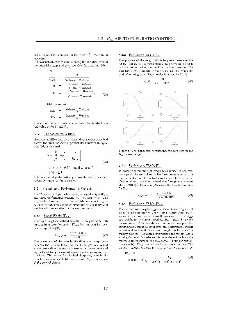
1.2. ]@^ AIR-TO-FUEL RATIO CONTROL
_7`MaQbdcde�c�f c�g�h�aNbPi*a;jWi�kOlPk5`Ue�m n�aQbd`poqiBnPesrtvu `�w5aQldwQxPi*aNm c�n_7c�e�`�f m ndgPyz bd`W{Mc�nPk5aNiBn�aMk3m n�|�c�f |�`*eOm n;_7c�e�`�f m nPgFaNbd`W|*iBwNm i*aQm c�n;iBwQc�ldnPeaNbd`�}IlPiBn�aQm aQm `UkW~���� � �;iBnPe9r�N�Q� � � iBwQ`Og�m |�`�n�m n�`U}IlPi*aQm c�n�� �����My�3��z �~���� � ��� �~���� � � �F�M�H�'~I�M� � � ��� t~ r ��� ~���� � � �F�N� � ~���� � � �W� t~���� � � �F�N�H�'~���� � � �W� t~I� ��� ~��M� � � �F�N� � ~���� � � �W� t� ~���� � � �F�M�F�'~I�M� � � �W� t � �� ede�m aQm |�`�ldnP{M`�w5aMiBm nIa5h~���� � � � ~���� � � �F�M�H�'~I�M� � � ��� t�� � � ~ ��� � � �F�M� � ~ �M� � � ��� t�
� �����
z bd`�kQm ��`OcB�3aNbd` u `�w5aQldwNxPiUaNm c�n�m kH{Mc�n�aNwQc�f f `UepxIh� �¡OjFbdm {Nb�m kFiwQ`*iBf?|*iBf ld`�i�k=� c�wH r i*n¢e� ��By£/¤ ¥¢¤ ¦ z bd`;§�aQwQl¢{NaQldwQ`Ue�¨O©5ª=f c�{N«?y� wQc�_¬aQbd`Ti�ede�m aNm |�`;iBnPe �/��z ldnP{M`�wQaNiBm nIa5h�_Tcde�`�f kHe�`*kQ{MwQm xP`UeiBx¢c*|�`��aQbd`�®PnPiBfFk5aQwQlP{NaNldwQ`Ue u `�w5aNldwQxPi*aQm c�n�_7i*aNwQm ¯�m n�`U}IlPi*©aNm c�n'� �B°I�=m kWc�x�aNiBm nd`Ue?y¨ �
±² r ³ ³³ U��´Mµ*¶dµ ³³ ³ �¡�´��*¶��·¸
r*¹ �� ¹ U¡#º�»=¼I½T¾ �'¿qÀ �IÁd ¾ � ÀN¿ ÁPà ¹Ä ¨ ÄUÅÇÆ �� �B°I�
z bdm k;k aQwQlP{MaQldwQ`Ue u `�w5aNldwQxPi*aQm c�n�g�c*|�`�wNnPkFaQbd`pk5m ��`7cB��aNbd` u `�w5©aNldwQxPi*aQm c�n�m n u l�aNkWaQcTaNbd`;È�c�x�É5`U{NaUyÊFË ÌÎÍ�Ï Ð¢ÑÓÒ¢Ô Õ;ÒPÑ�Ö�×HØIÙ�Ú5Û¢ÙUÜvÒPÑ�ÝIØ�ÞsØ�Ï Ð¢ß?à*áIâz bd`Óã Å © k5`�aQl u m nO®Pg�ldwQ`=äFbPi�k/c�nd`=m n u l�aÓk5m g�nPiBf�j�`�m g�bIa � �F�QåiBnPe'aNbdwQ`�` u `�wQ� c�wQ_7iBnP{M`�j�`�m g�b�aMk ��æ ��ç iBnPe �éè?ê y z bd`iB_ u f m aQlPe�`�{NbPiBwNi�{NaN`�wQm k aNm {;cB�WaQbd`pjW`�m g�bIaNk�iBwQ`pk5`�`�n'm n�®Pg�ldwQ`°dy z bd`ée�`Uk5m g�nqiBnPev{Qbdc�m {M`�cB�;k aNwQlP{NaQldwQ`�cB�#aNbd`�m nPe�m |Im e�lPiBfj�`Um g�bIaNkWjWm f f?x¢`�e�`*kQ{MwQm xP`Ue�m n�aNbd`Ond`M¯�aHk5`U{NaNm c�nPk�y£/¤ ë/¤ ¥ §Im g�nPiBf?ì�`�m g�bIa � �F�QåMyz bd`Hm n u l�a�j�`�m g�b�a�m kÓwQ`UiBf m k5`*e7i�k=i�í ³;î �Hf c*j u i�kQkÓ®Pf aN`�w�jFm aQbldndm a5h�gIiBm n�i*aF�U`�wQcT� wQ`*}�ld`�nP{MhIy � �F�QåWbPi�kWaQbd`�aQwNiBnPk � `UwW� ldnP{N©aNm c�n�m n�`U}�lPi*aNm c�n'� ��ï��
� �F�QåM� ðU� � � ³�ñPò ð=��° ³Bóð���° ³Bó � ��ï��z bd` u f i�{M`�_T`Un�apcB�#aQbd` u c�f `�m nGaQbd`�®Pf aQ`�wpm k7i'{Mc�_ u wQc�_Tm k5`x¢`Ma5j�`�`�n�aNbd`pjWm k5béaQc�� c�f f cBjôaQwNiBnPk5m `�n�aT{Qb¢i*nPgB`*kOm nöõ÷��QåOiBnPei*a#aNbd`7kQiB_7`;aQm _7`T_piBm nIaNiBm néi�_7`UiBn�|BiBf ld`7_7`Ui�k5ldwQ`�_7`�n�a#cB�õ÷��Qå�jWm aQbdc�l�a=aQc�c�g�wQ`Ui*a�iBn7m n�øPld`�nP{M`F� wQc�_ôaQbd` u ld_ u m ndgOøPlP{N©aNlPi*aQm cBn¢k�y z bd`�wQ`Ui�kQcBn'� c�wTaQbd`�bdm g�b�� wQ`U}Ild`�nP{Mh'��`UwQc�m n�aQbd`aNwNiBnPk � `�wÓ� ldnP{NaQm c�n7m k�aQcO� ldf ®Pf fdaNbd`Hk aMiBnPediBwNe�ã Å wQ`U}Ildm wQ`�_7`�nIaNkcB�3aQbd`;{Mc�n�aNwQc�f?c�x�É5`U{NaUy
£/¤ ë/¤ ë9ù `Uw5� c�wQ_7iBnP{M`#j�`�m gBbIa � æ yz bd` u ldw u cIkQ`pcB��aNbd`�j�`�m g�bIa ��æ m kOaNc u ldndm k5b�`�wQwQc�wNkOm n�aQbd`� �Óú y z bPi*aWm k�diBn�ldnPe�`Uk5m wN`Ue�k aQ`Ui�e�hpk aNi*aN`H`UwQwQc�w=m npaNbd` � ��úm kFaNc�xP`;_7m ndm _Tm ��`Ueéi�k#k5cIc�néiBnPe�i�kF_;lP{Nbéi�k u cIkQk5m xdf `Iy z bd`k aNwQlP{NaQldwN`=cB� ��æUû k�iB_ u f m aNlPe�`�{NbPiBwNi�{NaQ`UwQm k aNm {�m k?aQb�lPk/_;lP{Nb�f m «�`aNbPi*aFcB�=iBn�m n�aQ`Ug�wNi*aQc�wUy z bd`OaQwNiBnPk � `�w�� ldnP{NaNm c�n�� c�w �éæ m k��æ � ð*� � � ³�³ð�� �Fü�� ³ ñ¢ý � �BþI�
100 105 101010−4
10−3
10−2
10−1
100
ω [rad/sec]
Mag
nitu
de
Wmat
10−10 10−5 100 10510−5
100
105
1010
ω [rad/sec]
Mag
nitu
de
We
100 105 101010−2
100
102
104
ω [rad/sec]
Mag
nitu
de
Wu
10−5 100 10510−4
10−2
100
102
ω [rad/sec]
Mag
nitu
de
WAF
� m g�ldwQ`�°dÿ z bd`;k5m g�nPiBf/iBnPe u `�w5� c�wQ_7iBnP{�`#j�`�m g�bIaNk�lPk5`Ue�m n�aQbd`ã Å {Mc�n�aNwQc�f?e�`Uk5m g�n/y£/¤ ë/¤ £9ù `Uw5� c�wQ_7iBnP{M`#ìé`�m g�b�a ��ç y� n'c�wNe�`�wOaQc�_7m ndm _Tm ��`7bdm g�b�� wQ`U}�ld`UnP{Mm `*k7� ndc�m k5`*�#m n�aQbd`�{�c�n�©aNwQc�f=k5m g�nPiBf ¢aNbd`p{Mc�nIaQwQc�fÓk5`MaNl u bPi�k#x¢`�`�n'iBldg�_7`�nIaQ`UeéjWm aQb'ibdm g�b u i�kQkÓ®Pf aN`�w�� c�w=aQbd`O{Mc�nIaQwQc�f?k5m g�nPiBf��÷����5y z bd`H®Pf aQ`�wWm k�m _T©u f `�_T`Un�aQ`*eék5c�m a u ldndm k5bd`UkO{Mc�nIaQwQc�f�k5m g�nPiBf3� wQ`U}�ld`UnP{Mh�{Mc�nIaQ`�nIaiBx¢c*|�` � �*ä ³�� ��� y��}�lPi*aNm c�n�� � �I��k5bdcBjFk�aQbd`FaQwNiBnPk � `�w�� ldnP{MaQm c�n� c�w ��ç y
�éç � ð*� � ��� � üB� ³ ¡ ð=��° ³Bóð=�G° ³ üB� ³ ò ó � � �I�£/¤ ë/¤ ¦ ù `Uw5� c�wQ_7iBnP{M`#ìé`�m g�b�a � è?ê yz bd` u `Uw5� c�wQ_7iBnP{M`Wj�`�m g�bIa �éè?ê m k3m nPkQ`�w5aQ`Ue;m n�aNbd`�ã Å {�cBnIaQwQc�fk5`�aQl u m nTc�wNe�`�w�aNcOm _ u wQcB|�`=aQbd`#{Mc�n�aNwQc�fdk aNwNi*aQ`�g�hOaQwNiBnPk5m `�n�a=wQ`�©k u c�nPk5`�� aQm u © m n'iBnPe�aQm u © c�l�aOaQbdwNcBa5aQf `TwQ`*k u c�nPk5`*�My z b�lPk ��è/êm k;i�j�`�m g�b�aTc�n'aQbd`�`�wNwQc�w;k5m gBn¢i*f��Óå �Tõ÷���� � õ÷��QåNy'§Im nP{M`paQbd`_7`Ui�k5ldwQ`�_7`�nIapcB�#aQbd`ék aQ`*i�e�hGk aMiUaN`�iBm wp_pi�kQk;øPcBj u i�k5a7aQbd`aNbdwQcBa5aQf ` u f i*aN`#_Tm g�b�aWx¢`#`�wQwQc�nd`�c�lPkU*aNbd` u `�w5� c�wQ_piBnP{M`Hj�`�m g�bIam k�e�`Uk5m g�nd`Ue�k5c�aQbPi*a�m a�bPi�k;i�k5_piBf fÓj�`�m g�b�a;c�n�aQbd`p��`�wQc�� wQ`M©}Ild`�nP{Mhv{Mc�n�aN`�n�a*y � apbdm g�bd`�wT� wQ`*}�ld`�nP{Mm `Uk;aNbd`�j�`�m g�b�apbPi�k7ik5_piBf f?gIiBm n/�iBgIiBm n7m npc�wMe�`�w=aQcT_7m ndm _Tm ��`HaQbd`O`��?`U{NaNk=� wQc�_saQbd`u ld_ u m ndg�øPlP{NaNlPi*aQm c�n'm n�aQbd`$õ÷��NåOk5m g�nPiBf y z bIlPk#aNbd` u `�wQ� c�w5©_piBnP{M`�j�`�m g�b�a �éè?ê bPi�k�aNcpbPiU|�`OxPiBnPe u i�kQkHk aQwQlP{NaNldwQ`�y z bd`aNwNiBnPk � `�wW� ldnP{NaQm c�n�k5`�f `U{NaN`Uep� c�w ��è?ê m n�aNbd`�{Mc�nIaQwQc�f/k5`MaQl u m k� è?ê � ð*�
� � � ä�þIï ü�� ³ µ ð���° ü�� ³�ñ µ ó� ðW� ³ � ° ó ��� ð=�G° ³Bó �M� ð���° ³Bó � � í ³ �
17

CHAPTER 1. RECENT MVEM BASED CONTROL DEVELOPMENTS
��� ��������� �"!$#%� &('�)+*�, - �/.0/132�465 7�8:9$;=<>2�5 7�1�?@9 8:AB?C132/D:2�EGF H�EGI�9 8:J�2></2�5 7�1+?C4K9 EG2/83H$<L5 8=MJ�; N:A=2%A�5 8O?C132P46Q34 ?G2�IR462�?GN3D�F H�E�S�T�U3H�E/?G135 4�46Q34 ?G2�IR462�?GN3D�9V�W 46N3X:H�D=?C5 IY9 ;�Z�[�J�H�8+?GEGH�; ; 2�E\5 4KA=2$465 7�832%ABF H�EK2�837�5 832>H�D:2�E�9$?6M5 837�D:H�5 8�?C4/5 8Y?C132]EC9 837�2]^`_ba c�d V=eCf d V%g"h EGD3Ii9 8:APj kK_ba l3d m e c gX:9 E%T�0/132]Z [ J�H�8+?GEGH�; ; 2�E/5 4>F H�N38:A�X+QO9 8�5 ?G2�E�9$?G5 n�2BD3EGH3J�2%4G4/46H?C1:9$?/?C132BEG2%o+N35 EC2�I�2�8+?/5 8�2%o+N:9$?G5 H�8bp q3c$r>5 4@F N3; s:; ; 2%A"Tt�uwv p S/xGy`r t [{z c�xGl V%|=} k ~<�132�EG2|3} k ~���I�5 8� p t�uwv p S/xGy�r t [ r
p q3c$r� 8+?GEGH3A=N:JC?G5 H�8OH F@9 V�W 7+9 XOX 2�?6<>2�2�8 | } k ~ 9 8:AO?G132 | N:462$AO5 8?C132/Z [ J�H�8�?CEGH�;:A=2%465 7�8�5 8:46N3EG2%4�2��=5 4 ?G2%8:J�2/H F\9B46IY9 ; ;37+9 5 8�7+9 XX 2�?6<>2�2�8�?C132�I�9$�35 I�N3I�?CEC9 8:4 F 2�EY7+9 5 8�X 2�?6<>2�2�8�?C132�5 83D3N=?C49 8:ABH�N=?GD3N=?�4wH F+?C132@J�; H+462%AB; H=H�DP46Q34 ?G2�I�9 8:A]?G132>EG2%o+N35 EG2�I�2�8+?C446D 2%J�5 s:2%A�X+QO?G132�D 2�E6F H�EGIY9 8:J�2P<>2%5 7�1�?�4�T�0/1=N:4]9�4G46N3EG5 837�?G1:9$?83H�832PH FK?G132�J�; H+462%A�; H=H�D�D:H�; 2%4�H FK?G132�46Q34 ?G2�I�?G2%8:A34/?GH </9 ECA345 8=s:835 ?6Q�T��\H�; 2%4w?C2�8:A=5 837]?GH </9 ECA34w5 8=s:835 ?6Q�I�5 7�1�?@J�9 N:462/8+N3I�2�E6M5 J�9 ;+D3EGH�X3; 2�IY4�TKU=N3; s:; ; I�2%8�?�H F3?C132>D:2�EGF H�EGI�9 8:J�2>EG2%o+N35 EG2�I�2�8+?C4J�9 8�X 2(JG132%J h 2%APX=QPJ�H�I�D:9 EG5 837(?G132�9 I�D3; 5 ?CN:A=2�JC1:9 EC9�JC?C2�EG5 46?G5 J%4H F=?G132@5 8:A=5 n+5 A=N:9 ;�5 83D3N=?�4"?GH�?G132@H�N=?GD3N=?�4"H F=?G132>4GQ=4 ?C2�I�?GH�?G1:9$?H F�?G1:2�5 8+n�2�EG?G2%A�D 2�E6F H�EGIY9 8:J�2P<>2�5 7�1�?�4(I�N3; ?C5 D3; 5 2%A�<�5 ?G1 | T]� F?C132]J�H�8+?GEGH�; ; 2�E�F N3; s:; ; 4@?G132(EG2%o+N35 EC2�I�2�8+?C4@5 8Y2%o+N:9$?G5 H�8�p q3c$r\?G132JC1:9 EC9�JC?C2�EG5 4 ?C5 J%4]F EGH�I�5 83D3N=?C4�?GH�?C132�46D:2$J�5 s JOH�N=?GD3N=?�<�5 ; ;/X:2X 2�; H$< |w���"�� T � � 5 4B?G132YD 2�E6F H�EGIY9 8:J�2�<>2%5 7�1+?P9$?G?C9�JC132%A�?CH?C132BH�N=?CD3N=?�<�135 JC1�5 4�9 8:9 ; Q3462%A"T� 8�?G132�Z [ J�H�8�?CEGH�; ; 2�E�<�135 JC1�5 4YEG2�n=5 2%<>2%A�132�EG2���9bEGH�X3N:4 ?H�X:462%EGn�2�EK5 4>9 N=?GH�IY9$?G5 J�9 ; ; QP5 8:J�; N:A=2%A"T�0/132/F 2%2%A=X:9�J h 7+9 5 8�IY9$M?CEG5 ��F H�EB?G135 4]H�X:462�EGn�2%E]5 4P� [��O[ T�0/132Y4 ?C9$?G2�F 2�2%A=X:9�J h 7+9 5 8IY9$?GEG5 ��F EGH�I�?G132�H�X:462�EGn�2%E�46?C9$?G2%4K?GHB?G132(J�H�8+?GEGH�;35 83D3N=?@n�2%J�?GH�E5 4 u [OT��{X3; H3J h A=5 9 7�E�9 I�H F/?C132YH$n�2�EC9 ; ;@46Q=46?G2�I�9�4B<>2�; ;>9�4F N3E6?C132�E�2��=D3; 9 8:9$?G5 H�8O5 4/7�5 n�2�8O5 8�9 D3D 2�8:A=5 ����T��� �����O��� & �\*%, *0/132�7�H+9 ;>H FB� 9 8:9 ; Q3465 4�5 4�?GH`?C2%4 ?�F H�EYJ�2�E6?�9 5 8�A=2%465 EC2%AL46Q34 M?C2�I¡D3ECH D 2�E6?C5 2%4�T�0>132]46Q=46?G2�I¡D3EGH�D:2%E6?G5 2%4�<�135 JC1Y9 EG2�83H�EGIY9 ; ; Q?C2%4 ?G2%A�9 EG2/¢�H�I�5 8:9 ;:�K2�E6F H�EGIY9$8 J�2��$£�H�X3N:4 ?>¤�?C9 X35 ; 5 ?6Q�9 8:A�£/H MX3N:4 ?]�K2�E6F H�EGIY9 8:J�2�T0/132O46Q34 ?G2�I�5 4BF H�EGI�N3; 9$?C2%Ab9�4P9 8�N3D3D 2�E�¥wU�0�X 2�F H�EG2�?G1329 8:9 ; Q=465 4>5 4(J�9 EGEG5 2%AYH�N=?%T@0>132P¥\UK0�5 4�7�5 n�2�8OX=QuK¦ p §�xC¨�r@��§�©G©>ªL§�© � ¨�p «�¬�§ �G� r �w� § � © p q f r�]4�I�2�8+?G5 H�832%A�9 X:H n�2�?C132bD3EGH�D:2�EG?G5 2$4OH FYJ�H�8�?CEGH�;B4GQ=4 ?C2�I<�135 JC1�83H�EGI�9 ; ; QO9 EG2P9 8:9 ; Q=462%AO9 EG2+c�T�¢�H�I�5 8:9 ;�¤�?�9 X35 ; 5 ?6Qbp ¢]¤3rCT"0/132�83H�I�5 8:9 ;/p ¨i��l+r�J�; H+462%A; H=H�D�46Q34 ?G2�Ii5 4�4 ?C9 X3; 2+Tf T�¢�H�I�5 8:9 ;w�K2�E6F H�EGIY9 8:J�2�p ¢]�>rCT:0/132B83H�I�5 8:9 ;wJ�; H+4G2%AY; H+H�D46Q=4 ?C2�IiJ�9 8YF N3; s:; ;"?G132PA=2�IY9 8:A34>5 83132�EG2�8+?�5 8O?G132BD 2�E6F H�E6MI�9 8:J�2B<>2�5 7�1�?�4�Tq3T�£/H�X3N:4 ?]¤�?�9$X:5 ; 5 ?6Q�p £(¤:rCT:0>132�J�; H+462%AY; H+H�D�46Q34 ?G2�I�5 4/46?C9$MX3; 2�2�n�2�8�<�132�8`<>H�EC4 ?]J%9�462�D:2�EG?GN3EGX:9$?G5 H�8�H F�?C132�4GQ=4 ?C2�I5 4/D3EG2%462�8+?%T
m:T�£/H�X3N:4 ?K�K2�E6F H�EGIY9 8:J�2�p £(�>r�T%0>132>J�; H+462%A]; H=H�DP46Q34 ?G2�I�F N3; Ms:; ; 4"?G132@D 2�E6F H�EGI�9 8:J�2@46D:2%J�5 s J�9$?C5 H�8:4w2�n�2�8]?C132�8]?C132@<>H�EC46?J�9�462BD:2�E6?CN3EGX:9$?G5 H�8OH FK?G132�46Q=4 ?C2�I�5 4�D3EG2%462�8+?%T0/132`9 X:H n�2�EG2%o+N35 EG2%I�2�8+?C4�J%9 8�X:2�?G2$4 ?G2%A�X+Q�9 8�4 ?GEGN:JC?CN3EG2%A465 837�N3; 9 E�n 9 ; N32�9 8:9 ; Q=465 4�T`0/132�4 ?GEGN:JC?CN3EG2%AL465 837�N3; 9 E�n$9 ; N32�5 47�5 n�2�8OX=Q�?G132BF H�; ; H$<�5 8:7�A=2�s:835 ?G5 H�8ba ® g¯�°3±+² ³w² ´"² µK³�¶`·G¸B¹w°`º�´w»:¼w½:´w¼w»"°3¾�º%² ³w¿\¼wÀ Á\»�Â=Á\À+¼w°���ÃÄ\Å�ÆBÇÉÈCÅ�Ê`Ë Ì Í$Å�Î�ÏCÐ Ñ(Ò Ó ÅGÔ�Ñ�Ê Æ Õ�Ì Ô ÖYÊ$Î Ó Å�ÆB¨×ÈCÅ�ÊbØ�Å�Æ�Ð6ÙÏCÐ Ñ(Ò Ó ÅCÔPÑ�Ê Æ ÕCÌ ÏCÅ�Ø/Ú�Ì Æ ÛOÜÝ p ¨�r/Þ�c�Ê Î ßPÊ]Ë Ì Í$Å�Î�È�Ó Ð%ÏCàPß Ì Ê%Ë�Ð Î Ê ÓØ�Æ Õ�á3Ï�Æ á=Õ6ÅYâ Ú\Û3Å�ÕGÅ�Ø�Ð Ñ�Å�Ð6ÙPÆ Û3ÅP¨�k(Ñ�Ì Ë%Û=Æ(ÈGÅ�ÕGÅ Ò3ÅCÊ Æ ÅCßOÊ Î ßCã"Ð ÕÕGÅCÊ Ó ä�å�æ Û3Å�Õ6ÅCÊ ÓwÎ Ð Î3ç Î Å Ë�Ê Æ Ì Í$Å>ÙCá=Î Ï�Æ Ì Ð ÎO�@p Ç�rBÌ Ø�ß�Å è�Î ÅCßOÈ�é%Ö
�@p Ç�r�ê cI�5 8�ë ìCí�î ï�ð ñ ò ó � ìGí�ô/õ�ö ÷"ø�ùÙ�Ð Õ õ ØCÆ ÕCá:Ï�Æ á=ÕGÅCß�Ê Î ßOúû ò õKö ü �wýÚ\Û3Å�ÕGŨ���þ õ@ÿ�� � �{øååå å å å åååø�� � �Bõ��
� p q�q+r0/132�D:2�EGF H�EGI�9 8:J�2/<>2%5 7�1+?C4 ��� � � ¦ � ��� 9 EG2�JC1:9 837�2%A�9�J�MJ�H�ECA=5 837�?CHY2%o�N:9$?C5 H�8Lp q m=r>X 2�F H�EG2B?C132�¢�H�I�5 8:9 ;K�\2%E6F H�EGI�9 8:J�29 8:AP£�H�X3N:4 ?��K2�EGF H�EGI�9 8:J�2@9 8:9 ; Q=465 4"H F3?G132 ��J�H�8+?GEGH�;�5 4\J�9 EGEG5 2%AH�N=?$T
� � ù � � cc�xGl V%| � � p q m=r0/135 4/2%o+N:9$?G5 H�8O4C9%Q=4@?C1:9$?(¢(��9 8:AO9�D3EGH3J�2�2%A=5 837�£���9 8:9 ; Q=465 45 4wF N3; s:; ; 2$AP5 F3?G1:2@5 8:A=5 n+5 A=N:9 ;=9 I�D3; 5 ?GN:A=2�JG1:9 EC9�JC?C2�EG5 4 ?G5 J�4wA=H(83H ?2��:J�2�2%AB?C132>I�9$�35 IY9 ;=46D:2%J�5 s:2%A�9 I�D3; 5 ?GN:A=2%4KX+QBI�H�EG2@?G1:9 8 V�W T��� ��� � £/H�X3N:4 ?B¤�?C9 X35 ; 5 ? Q���8:9 ; Q3465 4�TU\5 7�N3EG2��P4613H$<(4K?C1:9$?@?G132BJ�H�8�?CEGH�;:46Q=4 ?C2�I�F N3; s:; ; 4/£�H�X3N:4 ?�¤�?C9$MX35 ; 5 ?6QYF H�E�H�D:2%EC9$?G5 837�D H�5 8+?C4/5 8O?C132PEC9 837�2]H F6� j k�_ba l3d m e c g������9 8:A�^`_�a c�d c V=e m:d V%g���� j���T
10−3 10−2 10−1 100 101 102 1030
0.2
0.4
0.6
0.8
1
1.2
1.4
1.6
−. : Robust Stability
−− : Nominal Performance
− : Robust Performance
µ−analysis of the λ−control (Robust Stability fulfilled)
ω [rad/s]
µ
U\5 7�N3EG2��=B£�H�X3N:4 ?�¤�?C9 X35 ; 5 ?6Q�F N3; s:; ; 2%A"T�0/132�H�D 2�EC9$?C5 837�EC9 837�2H F�?G132�¤+�L2�837�5 832�5 4�132�EG2��Yj k�_ a l3d m e c g������ 9 8:AR^ _a c�d c V=e m:d V%g���� j��`T
18

1.2. � � AIR-TO-FUEL RATIO CONTROL
!�" #�" $&% ')(+*�, -/.103254 ')276�8:9�;<0>=?9�8:@ AB,5C ,3DE C F)*+270HGI,7J+'LK/,M-7J�8L-N-7J+0O;<')9�-727')@P,5A+, -7036Q4 *+@ R�@ @ ,S% ')(+*�, -.103254 ')2�6P8:9�;<0M4 ')2M')TU032�8L-7C 9+FHTU')C 9�-�,VC 9I-7J+0N2�8:9+F)0�':45WYXUZN[\ ]+^ _�`7]+^ G�acb�d<e)fg8:9�hji�[ \ k)^ l a `�mB^ m acb�n�f7X�oND
10−3 10−2 10−1 100 101 102 1030
0.1
0.2
0.3
0.4
0.5
0.6
0.7
0.8
0.9
1
−. : Robust Stability
−− : Nominal Performance
− : Robust Performance
µ−analysis of the λ−control (Robust Performance fulfilled)
ω [rad/s]
µ
E C F)*+270NG+pq% ')(+*�, -�.�0c254 ')276P8:9�;<0M4 *+@ R�@ @ 0chrDtsYJ+0N')T�032�8L-�C 9+F2�8:9+F)0�':4u-�J+0wv�xV039+F)C 9+0NC ,VJ+0c270)WYXUZ[ \ ]+^ _�`7]+^ G�a3byd�e�fw8:9�hiN[ \ k)^ l a `�mB^ m acb�n�f�X�oNDz {/|r}Y~)�:� �w~B�U�c�+���V~B�c��� �L�s J+0q�j�P;<')9�-727')@ @ 032ShB0L,5C F)9+0ch�K 8),ShBC ,7;<270<-7C �30ch�8:9�h�C 6gT�@ 0<�6P039)-�0chSC 9w-7J+0M�Y� �>vq� ��9+F)C 9+0j�Y')9)-�27')@Y�/03�)0c@ ')T+6P039)-�v�A+, �-�036��u,5':4 -5K 8:2�0 \ kc] b DMs J+0V� �Y�>v�C ,y8j6y*�@ -7C -�8),5�BC 9+F,7':4 K 8:270T�8);��:8:F)0 hB03�)03@ ')T�0chP8L-1-7J+0�s�0c;�J+9+C ;c8:@+�?9+C �)0c2�,5C -5Au':4��/039+6�8:27�4 ')2/039+F)C 9+0g;<')9)-�27')@ D E C F)*+270y��,5J+'LK/,?8�,78:6gT+@ 0u':41-�J+0u270c,5*+@ -�,')(B-<8:C 9+0chrDs J+0MR�2�, -�-7J+27030T+@ ':-�,PC 9H-�J+0jR�F)*+2�0,5J+'LK�-7J+06P0c8),5*+270ch� WUiw8:9�hgX Z 270c,5TU')9�,50c,/8), 4 *+9�;�-�C ')9�,/':4�-7C 6g0)D�s J+0g039+F)C 9+0uC ,(U03C 9+FghB27C �)039V'L�)032?8u@ 8:27F)0/T�8:25- ':4�C -�, ')T�032<8L-7C ')9�8:@�2�8:9+F)0>8:9�h-�J+27')*+F)JV6P'�, -?':4�-�J+0uhB0c,5C F)9V2<8:9+F)0/':41-7J+0g�M;<')9)-�27')@ @ 032cDs J+0�4 ')*+25-7Jy,5*+(+T+@ ':-�,5J+':K?,U-7J�0�9+')276�8:@ C ,50ch>8:C 2�6�8),7,U��':KN8L--�J+01-�J+27':-5-7@ 0)W��� 5¡¢ ¡ £ Wc8:9�h/-�J+014 *+03@)6�8),7,U��'LKS;<')6g6�8:9�h/4 27')6O-7J+0;<')9�-727')@ @ 0c2cWg¤o¥ Z D1s J+0?hBC ¦U0c27039�;<0 (�03- K 03039y-�J+0 - K '/6�8),7,���'LK/,C 9y-�J+0?,5-70c8)hBAy, -<8L-70 J�8),1(�0c039P,5J+':K?9u-�'�(U0?6P8:C 9+@ AghB*+0 -7'�-7J+0C 9�8);3;<*+2�8L-�0�')T�032�8L-�C ')9V':4�-�J+0�4 *+03@rC 9L§50c;�-�')2�,3D�=�- -�J+0�-7C 6g0>-7J+00<¨+T�0c27C 6P039)-<, 270c��C 03KY0ch�J+03270uK J+0c270>;3')9�hB*�;�-70chrW+-7J+0uC 9L§50c;<-7C ')9,7;�J+036P0>8L�:8:C @ 8:(+@ 0�C 9�-�J+0u�Y� �>v�J�8:2�hBK 8:270�K 8),Y')9+0>C 9L§50c;<-7C ':9TU032y;<AB@ C 9�hB032uT�032y03�)039)-LDVsYJ+C ,>6P0c8:9)-u-7J�8L-u-7J+0�T+*+@ ,70PK?C h�-7J;<')6P6P8:9�h�F)C �)039P-�'u-7J+0�C 9L§50L;�-7')2 hB27C �)032�K?8),��)0327AP,56P8:@ @1� -5A�TB�C ;38:@�(�0c@ 'LK�©j6P,��<Wr-7JB*�,�-7J�0PC 9L§50L;�-7')2�,>KY03270P')T�032�8L-�0chC 9�-7J+09+')9+@ C 9+0L8L2yTU')25-7C ')9w':4?-7J+0cC 2P;�J�8L2<8);�-70327C , -7C ;3, \ ©Lb DSsYJ+C ,uC 9)-�27':�hB*�;<0LhN,5')6g0V,5C F)9+C RU;38:9�-u*+9+6P'BhB03@ @ 0chN9+')9+@ C 9+0c8:27C -�C 0c,uC 9�-�J+03C 2')TU032�8L-7C ')9�D1���)0c9g-7J+')*+F)JP-�J+0�C 9L§50c;<-7')2�,�KY032�0?')TU032�8L-70chPC 9�-7J+09+')9+@ C 9+0L8L2�TU')25-7C ')9u':4B-7J+0cC 2�;�J�8:2�8);�-70c27C , -�C ;3,cW<-7J+0��j�P;<')9)-�27')@ @ 032K 8),19+0c8:2�@ Ag;38:T�8:(+@ 0 ':4r�)0303T+C 9+Fy�PK?C -�J+C 9g-�J+0?K?C 9�hB':K krª¬«¢ ¡ £� ª�k = E %/�?hB*+27C 9+FP-7J+0u-7J+2�':-5-7@ 0u8:9+F)@ 0�-�2�8:9�,5C 039�-�,/8),?,5030c9jC 9-�J+0jR�9�8:@ T+@ ':-�C 9HR�F)*+270M�+Dqx 9O, -70c8)hBAH, -�8L-�0V-7J�0;<')9)-�27')@ @ 032�)03TB-y��K C -7J+C 9M-�J+0yK?C 9�hB'LK k ª « ¢ ¡ £ � ª « = E %/�<D�sYJ+0L,50y270<�,5*+@ -�, J�8c�)0�(U03039j')(B-�8:C 9+0ch�C 9M,5T+C -70>':4�-7J+0�4 8);�-?-7J+0u;<')9)-�27')@ @ 032J�8),>(�030c9ShB0c,5C F)9+0chM4 ')2u')T�032�8L-�C ')9NC 9S8j@ 8:27F)0gT�')27-7C ')9N':4Y-7J+0039+F)C 9+0)® , ')TU032�8L-7C 9+FP2�8:9+F)0uC 9�, -�0c8)hj':4�(�0cC 9+FP-�*+9+0chM8L-�;<@ '�,503@ A
0 2 4 6 8 10 12 14 1610
20
30
40
50Throttle angle, α
Time [s]
α [°
]
0 2 4 6 8 10 12 14 161
1.5
2
2.5Crankshaft speed, n
Time [s]
n [k
rpm
]
0 2 4 6 8 10 12 14 160.4
0.6
0.8
1
Manifold pressure pi
Time [s]
p i [bar
]
0 2 4 6 8 10 12 14 160.2
0.4
0.6
0.8
1
1.2
1.4
1.6
Fuel command mfi and normalised air mass flow L
th−1m
at
Time [s]
Mas
s flo
w [g
/s]
0 5 10 15
0.9
0.92
0.94
0.96
0.98
1
1.02
1.04
1.06
1.08
1.1
λ measured in the exhaust pipe
Time [s]E C F)*+270��+p1s J+0/R�2�, -Y-7J+27030/T+@ ':-�,Y,7J+'LK/,1-7J�0?-�J+27':-5-�@ 0�8:9+F)@ 0)W � W-�J+0�0c9+F)C 9+0)® ,u27T+6jW1iO8:9�hN-7J+0�T+2�0c,7,5*+270PC 9S-7J+0VC 9�-�8:�)0P6�8:9B�C 4 ')@ hMXUZ/8),>4 *+9�;�-�C ')9�,y':4?-7C 6P0)DNsYJ+0V, -�03T�,yC 9 � C ,y@ 'LK�T�8),7,R�@ -703270LhwK C -7JO8 kc])] 6P,y-7C 6P0M;<')9�,5-�8:9)-LDqsYJ+0j4 ')*+25-7JqT+@ ':-�C ,-�J+0y4 *+03@1��':K¯;<')6P6P8:9�h°¤o ¥ Z�-�')F:03-7J+032>K?C -7J-7J+0P9+')276�8:@ C ,50ch8:C 2P6�8:,�,y��'LK±��? ¡¢ ¡ £ D²sYJ+0MR�9�8:@ T+@ ':-VhB03T+C ;�-�,g-�J+0M6g0L8:,7*+270ch9+')276�8:@ C ,50chw8:C 2<³c4 *+0c@�2�8L-7C 'C 9w-7J+0j0<¨BJ�8:*�,5-gT+C TU0)DSsYJ+0V@ 8:27F)0K?C 9�hB':K�,7J+'LK/,�-7J+0 ª = E %�K C 9�hB'LK´8:9�h-7J+0j,56�8:@ @�K?C 9�hB':K,5J+':K?,Y-�J+0 ª « = E %µK?C 9�hB':K>D
19

CHAPTER 1. RECENT MVEM BASED CONTROL DEVELOPMENTS
¶5·�¸)¹3ºc»g¸L¼�»g¹3¸:½�º<¾ ¿+À À Á>Â�¸:·+·�ºc»gÃ)·Uº3½�¸LÄ7Å ¼+Æ�·�Ã)Å ¼)Ä<¶3Ç1ÈYÉ+Å ¶�¶5É+ÃLÊ/¶Ä�É+ºYË�¸)¶5Å ¹�½7Ã)Ë+¿�¶ Ä7¼+ºL¶7¶rÃ:¾+Ä�É+º�ÌjÍyÂPº<Ä�É+ÃB»y¸:¼�»uÅ Ä�¶�Â�¸:Å ¼y¸)»BÎ:¸:¼BÏÄ<¸:Æ)º/Å ¼j¹<Ã)ÂP·�¸:½7Å ¶7Ã)¼PÄ7ÃyÂgÃ)½�º�¹<Ã)¼�Î)ºc¼)Ä7Å Ã)¼�¸:ÀU¹<Ã)¼)Ä�½7Ã)À�ÂPº<Ä7É+Ã+»+¶3ÇÐ Ã)½7º3Ã:Î)º3½ Ä�É+ºg¶ Ä7ºc¸)»BÁ¶ Ä�¸LÄ�ºg¸:¼�»jÄ�½�¸:¼�¶5Å ºc¼)Ä/Ã)·Uº3½�¸LÄ�Å ¼+ÆVÂgÃ+»Bºc¶É�¸LÎ)º�Ë�º3ºc¼jÃ)·BÄ7Å ÂgÅ Ñ3ºc»VÅ ¼M¹<Ã)¼�¹3º3½5Ä?½�¸LÄ7É+º3½YÄ�É�¸:¼M¶5º3·�¸:½�¸LÄ�º3À Á)ÇÒ Ó?Ô�Õ�Ó Ö�×�Ø�Ù7Ô�Õ�ØÚ ¼�ÌjÍP¹<Ã)¼�Ä7½7Ã)À�Âgº<Ä�É+ÃB»BÃ)À Ã)Æ)ÁgÉ�¸)¶�Ë�ºcº3¼j¸:·+·+À Å ºc»gÄ7ÃuÄ�É+º/·+½7Ã)ËBÏÀ º3ÂÛÃ:¾ Ø�Ù º3¼+Æ)Å ¼+ºy¸:Å ½<Üc¾ ¿+º3À�½<¸LÄ7Å ÃV¹<Ã)¼)Ä�½7Ã)À Ç?È É+Å ¶/É�¸)¶?ËUº3º3¼Ã)¼+ºÃ:¾�Ä7É+º>Ý�½�¶ Ä/·+½�¸)¹�Ä7Å ¹3¸:Àr¸:·+·+À Å ¹3¸LÄ�Å Ã)¼�¶ Ã:¾�Ä7É+Å ¶?Âgº3Ä7É+ÃB»VÄ7Ã�¸g¼+Ã)¼BÏÀ Å ¼+ºc¸:½g¶7ÁB¶ Ä�º3°¸:¼�»NÄ7Ã�Å ¼�Ä7º3½7¼�¸:À ¹<Ã)ÂyË+¿�¶ Ä7Å Ã)¼Sºc¼+Æ)Å ¼+ºj¹<Ã)¼�Ä7½7Ã)À ÇÕ Ã)¼+À Å ¼�ºc¸:½7Å Ä5ÁNÃ:¾/Ä�É+ºjº3¼+Æ)Å ¼+ºVÉ�¸)¶gË�ºcº3¼wÄ7½7ºL¸LÄ7ºc»H¸)¶g¸�¶7ÁB¶ Ä�º3¿+¼�¹<ºc½5Ä�¸:Å ¼)Ä5Á�Å ¼NÄ7É+ºV¶�¸:ÂgºPÊ ¸LÁN¸)¶>·�¸:½�¸:Âgº3Ä7º3½u¿+¼�¹3º3½5Ä�¸:Å ¼)Ä5ÁÅ ¶É�¸:¼�»BÀ ºc»SÅ ¼H¹3Ã:¼BÎ)º3¼�Ä7Å Ã)¼�¸:ÀYÀ Å ¼+ºc¸:½yÌjÍg¸:·+·+À Å ¹c¸LÄ7Å Ã)¼�¶cÇNÈ É+ºjº3¼BÏÄ�Å ½7º�¸:Å ½<Üc¾ ¿+ºcÀ+½�¸LÄ�Å Ãy¹<Ã)¼)Ä�½7Ã)À�¶5ÁB¶5Ä7º3ÂMÞ:¾ ½7Ã)Â�¾ ¿+º3ÀUÅ ¼Lß5ºL¹�Ä7Å Ã)¼PÄ7Ãuº<àBÏÉ�¸:¿�¶ ÄLÞBÉ�¸)¶YË�º3ºc¼�Ä�½7ºc¸LÄ7ºc»j¸)¶YÃ)¼+ºu¹<Ã)¼)Ä�½7Ã)À�Ã)ËBß5ºc¹�ÄLÇ�È É+Å ¶�Â�¸:á)ºc¶Å Äj·�Ã�¶7¶5Å Ë+À ºÄ7ÃHÃ)ËBÄ�¸:Å ¼²¸:¼OÃLÎ)º3½�Î�Å º3Ê�Ã:¾uÄ7É+ºS¹<Ã)¼)Ä�½7Ã)À/·+½7ÃB¹3ºc¶7¶Ê?É+Å ¹�ÉjÅ ¶ ¿+¼�¿�¶5¿�¸:ÀrÅ ¼jÅ Ä�¶/¶7¹<Ã)·�ºu¸:¼�»Vº3âUºc¹�Ä�Å Î)º3¼+ºL¶7¶3Ç Ú ¼�¸:À Á�Ä7Å ¹3¸:ÀÂPº<Ä7É+Ã+»+¶>¹c¸:¼MËUºP¸:·+·+À Å ºL»MÄ7ÃM¸:¼�¸:À Á+¶5ºu¾ ¿+À Ý�À À Âgº3¼�ÄuÃ:¾ ¶ Ä�¸:Ë+Å À Å Ä5Á¸:¼�»V·�ºc½5¾ Ã)½7ÂP¸:¼�¹<º�Æ)¿�¸:½�¸:¼)Ä�º3ºc¶3Ç Ù Ä?Å ¶ ¸:À ¶5Ãg·�Ã�¶7¶7Å Ë+À º/Ä�ÃyË�¸:À ¸:¼�¹<º»BÅ âUºc½7º3¼)ÄLÞ+Ã:¾ Ä�º3¼¹<Ã)¼Bã�Å ¹�Ä7Å ¼+Æ�Þ�¹<Ã)¼�Ä7½7Ã)ÀrÃ)ËBß5ºc¹<Ä7Å Î)ºL¶?¸:Æ�¸:Å ¼�¶5Ä ºL¸)¹7ÉÃ:Ä�É+º3½ Ê?Å Ä7É+Ã)¿BÄ�¹<¿BÄ�¸:¼�»PÄ�½7Á�ÂPº<Ä7É�ÃB»+¶3ÇÙ Ä?É�¸)¶�ËUº3º3¼j·�Ã�¶7¶7Å Ë+À º/Ä7ÃgÃ)ËBÄ�¸:Å ¼�½7ºL¸)¶5Ã)¼�¸:Ë+À Á�¸)¹3¹<¿+½�¸LÄ�º Ú/ä1å¹<Ã)¼�Ä7½7Ã)À�º3Î)º3¼�Ä7É+Ã)¿+Æ)ÉV¸>Î)º3½7ÁP¸)¹3¹<¿�½�¸LÄ7º/¶7ÁB¶ Ä�º3Â�ÂPÃB»Bº3ÀrÉ�¸)¶�¼+Ã:ÄËUº3º3¼S»Bº3½7Å Î)ºL»VÝ�½�¶5ÄcÇyÈ É+Å ¶>¶5¿+Æ)Æ)ºc¶ Ä<¶?Ä7É�¸LÄuÊ Å Ä7É�¾ ¿+½5Ä7É+º3½u»Bº3Î)º3À ÏÃ)·+ÂPº3¼)ÄLÞ)Ä7É�º�¿�¶5º�Ã:¾�ÌjÍP¹<Ã)¼)Ä�½7Ã)ÀU¹c¸L¼V½7ºL»B¿�¹<º>¶5Å Æ)¼+Å ÝU¹3¸:¼�Ä7À ÁgÄ7É+º¹3¸:À Å Ë+½<¸LÄ7Å Ã)¼NÄ7Å ÂPºV¼+ºc¹<ºc¶7¶�¸L½�ÁjÄ�÷+¿BÄP¸MÆ)À Ã)Ë�¸:À�º3¼+Æ)Å ¼+ºV¹3Ã)¼)Ä7½�Ã)ÀÅ ¼)Ä�Ãg·+À ¸)¹<º>Ã)¼M¸yÆ)Å Î)º3¼jº3¼+Æ)Å ¼+º)Çä ¿+½5Ä�É+º3½g¾ ¿BÄ�¿+½7º»Bº3Î)º3À Ã)·+Âgº3¼�Ä�¶PÅ ¼�¹<À ¿�»BºjÄ7É+ºM¿�¶7ºMÃ:¾�Ây¿+À Ä�Å Ï·+À ºV¼+Ã)¼+À Å ¼+ºc¸:½7Å Ä5ÁN¿+¼�¹<º3½5Ä<¸LÅ ¼�Ä Á�Ñ3Ã)¼+ºc¶y¶5·�¸)¹3ºc»NÃ:Î)º3½>Ä�É+º�ºc¼)Ä7Å ½7ºÃ)·Uº3½�¸LÄ7Å ¼+Æ�½�¸:¼+Æ)º�Ã:¾�Ä7É+ºjºc¼+Æ)Å ¼+º)ÇwæqÉ+ºc¼q¹<Ã)¿+·+À ºL»SÊ?Å Ä�ÉHÆ�¸:Å ¼¶7¹�É+ºc»B¿+À Å ¼+Æ�Þ�Å Ä�Å ¶gÄ7É+Ã)¿+Æ)É�ÄgÄ�É�¸LÄPÄ7É+Å ¶�¸:·+·+½7Ã�¸)¹�ÉSÊ?Å À À?À ºc¸)»SÄ�ÃÀ ºc¶7¶Y¹<Ã)¼�¶7º3½7Î:¸cÄ�Å Î)º?Ñ3Ã)¼+º�¹3Ã:¼�Ä7½7Ã)À ¶�Ê É+Å À º�ÂP¸:Å ¼)Ä�¸:Å ¼+Å ¼+ÆuÄ�É+º/ÃLÎ)ºc½5ϸ:À Àr½7Ã)Ë+¿�¶ Ä7¼+ºL¶7¶YÃ:¾�Ä7É+ºu¿+¼�»Bº3½7À Á�Å ¼+ÆP¹<Ã)¼�Ä7½7Ã)ÀrÂPº<Ä7É+Ã+»BÃ)À Ã)Æ)Á�Çç èé�ê¯ë�èìgí�î>ïuðjñVëòjó�ôcõUör÷�øHù�úîVû?ñü Ú Å ½ ä ¿+º3À å ¸LÄ7Å Ã�Çý í?ü>þ ½7Å Ä7Å ¶5É Ö º3Á�À ¸:¼�»rÇë>ìgÿ���ü�� ¼+Æ)Å ¼+º Ó Ã)¼)Ä�½7Ã)À��/º3Î)º3À Ã)·+Âgº3¼�Ä Ø ÁB¶5Ä7º3ÂMÇë�û��Lü�� À ºc¹�Ä�½7Ã)¼+Å ¹ ä ¿+º3À Ù ¼Lß5ºc¹�Ä�Å Ã)¼�Ç ë�MéMü�� ºL¸LÄ7ºc» � àBÉ�¸:¿�¶ Ä �>¸)¶ Ô àBÁBÆ)º3¼H¶5º3¼�¶7Ã)½�� ¶7Ê Å Ä�¹�É+Å ¼+ÆÄ ÁB·Uº���ÇíYû ï�ü>Ö Å ¼+ºc¸:½ ä ½�¸)¹�Ä7Å Ã)¼�¸:ÀrÈ�½�¸:¼�¶ ¾ Ã)½7ÂP¸LÄ�Å Ã)¼�Çê��Vë�ê´ü Ð ºL¸:¼ ��¸:À ¿+º � ¼+Æ)Å ¼+º Ð ÃB»Bº3À Çê����Lü Ð ¿+À Ä7Å��1Ã)Å ¼�Ä Ù ¼Lß5ºL¹�Ä7Å Ã)¼�ÇèMïyûYìVü�Õ Ã:¼�À Å ¼+ºc¸:½?È�½�¸:¼�¶5Å ºc¼)Ä ä ¿+º3ÀrÝ�À Â Ó Ã)Âg·Uº3¼�¶7¸LÄ�Å Ã)¼�Çé�ÿjëyü>Ô ½�»BÅ ¼�¸:½7Á��/Å ârº3½7º3¼�Ä7Å ¸:À ��� ¿�¸LÄ7Å Ã)¼�Çñ �Pü å Å Æ)É�Ä � ¸:À ¾���À ¸:¼+º)Ç��ë�û��:ü>Ø º � ¿+º3¼�Ä7Å ¸:À � À ºc¹�Ä7½7Ã)¼+Å ¹ ä ¿+ºcÀ Ù ¼Lß5ºL¹�Ä7Å Ã)¼�Ç
���LüuØ ·�¸:½7á Ù Æ)¼+Å Ä�Å Ã)¼�Çï��tì�ü ÈYÉ+½7ºcº�æS¸cÁ Ó ¸LÄ�¸:À ÁB¶ ÄLÇðjë�MéMü�× ¼+Å Î)º3½�¶�¸:À � à+É�¸:¿�¶ Ä���¸)¶ Ô àBÁBÆ)º3¼�¶5º3¼�¶5Ã)½�� À Å ¼+ºc¸:½Ä ÁB·�º ��Ç! ö#"%$ ö'&)(�÷�ø+*Yõ%, ù -�ö'./(10 -203&�ù�ú46587 9 ü ��Ã)À ¿+ÂPº<Ä7½7Å ¹�º;:V¹<Å º3¼�¹<Á)Ç< ü>Õ Ã)½7ÂP¸:À Å Ñcºc»P¾ ¿+ºcÀ Ü:¸:Å ½ ½�¸LÄ�Å ÃP¸LÄ/Å ¼�Ä�¸:á)º>·�Ã)½5ÄLÇ= ü>Õ Ã)½�ÂP¸:À Å Ñ3ºc»j¸:Å ½3Üc¾ ¿+º3ÀU½�¸LÄ�Å Ã�¸LÄ Å ¼)Ä<¸:á)º>·�Ã)½5ÄLÇ=%> ?�@ ü>Õ Ã)½7ÂP¸:À Å Ñcºc»V¸:Å ½<Üc¾ ¿+º3ÀU½�¸LÄ�Å ÃPÅ ¼Mº<àBÉ�¸:¿�¶5Ä Â�¸:¼+Å ¾ Ã)À »rÇ=2A ü Ð ºc¸)¶5¿+½�ºc»P¼�Ã:½�ÂP¸:À Å Ñ3ºc»j¸:Å ½<Üc¾ ¿+º3Àr½�¸LÄ7Å ÃP¸LÄ?Å ¼)Ä<¸:á)º�·UÃ)½5ÄcÇBCEDGF ü ä ½�ºc¶5Éj¸:Å ½?ÂP¸)¶7¶Yã�ÃLʵ¸LÄ Å ¼)Ä<¸:á)º>·�Ã)½5ÄLÞ1H IKJL�M ÇBC DKN ü ä ½7ºc¶5ÉM¸:Å ½?ÂP¸)¶7¶�ã�Ã:ÊI¸LÄ?Ä7É+½7Ã:Ä5Ä�À º>·+À ¸LÄ7º)Þ�H IKJLOM ÇBC > ?�@ ü Ð ¸)¶7¶�ã�Ã:ʲŠ¼VÄ7É+ºuº<à+É�¸:¿�¶ Ä?·+Å ·Uº)Þ�H IKJLOM ÇBCEP ü ��¸:·UÃ)½7Å Ñ3ºL»P¾ ¿+º3À�Â�¸)¶7¶Yã�ÃLÊI¸LÄ/Å ¼�Ä�¸:á)º�·UÃ)½5ÄcÞ�H IQJLOM ÇBCEP3P ü ��¸:·�Ã)½7Å Ñ3ºc»�¾ ¿+º3À�ÂP¸)¶�¶�ã�Ã:ÊO¾ ½7Ã)Â�¾ ¿+º3À�Ý�À ÂMÞ�H IKJL M ÇBC P8R ü�Ù ¼Lß5ºL¹�Ä7ºc»V¾ ¿+º3À�ÂP¸)¶7¶Yã�ÃLÊuÞ1H IQJL�M ÇBCEP 5 ü ��¸:·�Ã)½7Å Ñ3ºc»�¾ ¿+º3À�ÂP¸)¶7¶Yã�ÃLʲ¾ ½7Ã)´Š¼Lß5ºL¹�Ä7Ã)½�¶3Þ1H IKJL�M ÇS üuÓ ½�¸:¼+áB¶5É�¸L¾ Ä?½�º3Î)Ã)À ¿BÄ�Å Ã)¼�¶Y·�ºc½ ÂPÅ ¼B¿BÄ7º)Þ'H TKU C M ÇU R ü/Ù ¼�Ä�¸:á)º�ÂP¸:¼+Å ¾ Ã)À »j·+½7ºc¶7¶5¿+½7º�Þ�H V;W6T M ÇU > ?�@ ü�� àBÉ�¸:¿�¶ Ä?Â�¸:¼+Å ¾ Ã)À »V·+½7ºc¶7¶7¿+½7º)Þ�H VQWXT M ÇY > ?3@ ü Ú Å ½/»Bº3¼�¶5Å Ä5Á�Å ¼jÄ7É+ºuº<àBÉ�¸:¿�¶ Ä?Â�¸:¼+Å ¾ Ã)À »rÞ�H3IQJA�Z M Ç[ üuÓ Ã)ÂP·+À º3àVÎ:¸:½7Å ¸:Ë+À º)Þ6\K]^�P ü�� Î:¸:·�Ã)½<¸LÄ7Å Ã)¼�Ä�Å ÂPºu¹<Ã)¼�¶ Ä<¸:¼)Ä ¾ Ã)½ Ä7É+º>¾ ¿+º3ÀrÝ�À ÂMÞ�H [ M=%_ ü È É+º = ¶5º3¼�¶5Ã)½�` ¶�Ä7Å Âgºy¹<Ã)¼�¶ Ä<¸:¼)ÄcÞ1H [ M Ça R ü�Ù ¼�Ä�¸:á)º�Â�¸:¼+Å ¾ Ã)À »VÆ�¸)¶�Ä7º3ÂP·Uº3½�¸LÄ7¿+½7º)Þ�H b M Ça�> ?�@ ü�� àBÉ�¸:¿�¶5Ä Â�¸:¼+Å ¾ Ã)À »VÆ�¸)¶�Ä�º3Âg·Uº3½�¸LÄ7¿+½�º)Þ1H b M Çc ü ä ½�¸)¹�Ä7Å Ã)¼VÃ:¾ BC P3R5ÞBÄ7É�¸LÄ/É+Å Ä�¶ Ä7É+ºuÅ ¼�Ä�¸:á)º>ÂP¸:¼+Å ¾ Ã)À »VÊ ¸:À À Çd õUö1ù80 -�ö�0Lù�úe > ?�@ üuÓ ½7Ã�¶7¶�¶7ºc¹�Ä7Å Ã)¼�¸:ÀB¸:½7ºL¸?Ã:¾�º<àBÉ�¸:¿�¶ Ä�·+Å ·Uº)ÞXfhg i�j'k l3mon2p;q C�r Çs > ?�@ ü �/Å ¶ Ä�¸:¼�¹<ºjËUº<Ä5ÊYº3º3¼wº3àBÉ�¸:¿�¶ ÄPÎ:¸:À Î)ºj¸:¼�» = ¶5ºc¼�¶5Ã)½cÞ�mBÇ fXiÂjÇt N @ üuØ Ä�Ã:Å ¹�É+Å Ã)ÂPº<Ä7½7Å ¹>¸:Å ½<Üc¾ ¿+º3Àr½<¸LÄ7Å Ã�Þ�l8j�Ç uXvBÇw ü ��¸)¶?¹<Ã)¼�¶ Ä�¸:¼�Ä ¾ Ã)½/»B½7ÁV¸:Å ½cÞ2i xXvog m6yzk6l3mon%{%| DQ};~ A ZIKJ ~ ��%� ü �/Å ¶7·+À ¸)¹<º3ÂPº3¼�Ä?Î:Ã)À ¿+ÂPº)Þ�l6g i6v6�zk l3mon�� C �� R ü�Ù ¼)Ä<¸:á:º>Â�¸:¼+Å ¾ Ã)À »VÎ)Ã)À ¿+Âgº)Þ�l6g v m6mzk6l3m n%� C �
20

1.2. ��� AIR-TO-FUEL RATIO CONTROL
���z� �z�'�z�������� �;���z�8�2�o�K� �K�h�8���z�1� �2�¡ X¢6�K�3�2�G¢6�1�' %�'£z� ��¤Q X¥��#�h¦6� �h� £O¢6�o§¨ �K¢6© ��� �2��ª��3� � «�� © ¬h��#�2¦ � �h�ª�¢o�o�8© © � �h¦2� ®
SAE Tech-nical Paper
�h�h¢2�2¯h�3°X±6² ³h�h�3¯6¯h�6�� ±3���z�8�2�o�K� �K�h�8�#��� �'«#�3� ¨ �8�K´h¢6© µ���¶�� ��� �2�· X¢6�K�3�2�G¢6�1�� %�#£z� �¤K¸z¢6�h© � �h�3� �3�)£O© ¢X�G�3�º¹�¢o¢6»1�+ X¥¼�#�h¦6� �h��£�¢6� ¨ �K¢6©E½�¾o§�K�8�K¿6�8�Q�8� ®
SAE Technical Paper�h�h¢2�2¯X± °X± ÀXÁo�2�3¯6¯X±o�
� À�� ¨ �K¬XÃ��6��ª¡��� �2��«z� ¦6� © ���6£��8Ä�� ��¤KÅ�¢6¾h¬2� ¨1Æ�Ç £�¢6� ¨ �K¢6© ¢ È�� X¥����h¦6� �h�6É ��Ê�Ë Ì1§ �;� ¨ � ¢2��� �+�h� �h� �G´1� ®�ª��6� ¨ �8�3É � ¨ ´h�3�G� �8�¶�´h�)¶1���K´h�h� �8� ©�Í��h� ¿6�8�Q�G� ¨GÎ ¢ ÈÏz�3�hµÐ� �K����¥ �2� ¨ � ¨ ¬ ¨ �EÈ ¢6�Êz¬ ¨ ¢6µ�� ¨ � ¢6�1�hÊz¬h¦2���3¯6¯XÁo�� Ñ ��Ò2�1Ó������ Î Ã�¢X¢h��� Internal Combustion Engine Funda-
mentals��ªE�3Ôz�Q��Ã�§ ��� © © �o¥ �%� � �1���3��� �1�3¯6³6¯h�
� ²3���z�8�2�o�K� �K�h�8� ��� � Ò6�8�2�G�8�1�6ª¡� �6Õ� � �h� � ¨KÖ � �8� ×'� �6Å��6�Gµ�¬2�K�K�8�1�×#� ��� �2�Ø«#��� ¨ �8�K´h¢6© µ���¶�� �¼¤K¸�¢6�h© � �h�3� � ¨ �Q� �2�G� �8� ¨ È ¬h�8©Ù © µÚ�8¢6µÂ»%�8�2�K� ¨ � ¢6�ÜÛ ¸�¶�Ì'£�Ý;� ®SAE Technical Paper
��h¢2�2¯ À6°XÁ ÞXÁo�%�3¯6¯6Àh�� Þ����z�8�2�o�K� �K�h�8�O��� ��Ò �8�%�G�8�1��ª¡� �z£O´h�8¿�� © � �3�3��Ê� �z X¢6�K�8�2�K¢ ��� %�'£�� �'¶��K¬hµÂ»h´ Î �'Ï�� �'� �2�+Ê��G� ����Ò2� ��¤Kª�¢h�o�8© © � �h¦�¢ È ¨ ´h�� � ¨ � �6�zµ����h� È ¢6© � Ù © © � �h¦Ð� Î �2� µÂ� �8�8� ®
SAE Technical Pa-per
�o�h¢2�2¯6Þ6°6°6ÀXÁo�h�3¯6¯6Þh�� Á3����£�ª+�
Engine Control and Monitoring�ß�3°h��Ì�� �Q� ¨ ¨ �K�8� ¨ �2 X¬h� ¨ �À6ÞX²o�h¹1¢X��Êz© ¨ ¢X�3�2£OÊ�¯ ÑX°X±6±o�XÍ� %� Ê��
� ³���×'¢6¬h© �G�8�1�XÒ2�X %� �'¤G¥G�o�8� ¨ � Ù �8� ¨ � ¢6�Т È' X¥#�8�h¦6� �h�z�G¬h¾hµÐ¢o�o�8© �8�� ���h� �h� �G´1� ®�ªE�6� ¨ �8�3É � ¨ ´h�3�G� �8�2¶�´h��¶��3�Q´h�h� �8� ©1Í��2� ¿6�8�Q�G� ¨G΢ È#Ïz�8�hµ�� �K�%�o¥ �2� ¨ � ¨ ¬ ¨ ��È ¢6�zÊ�¬ ¨ ¢6µ�� ¨ � ¢6�1�hªE� �3���3¯6¯XÁo�� ¯�� X� ¦6¬h�Q�� X�6¢6¦6�3� ¨ �6��� �2��¥G� �×'¢X� ¨ © � ¨ ´XÃ�� � ¨ ´1� Multivariable
feedback control��Ò ¢6´h��ļ� © � Î à o¢ �2�3���3¯6¯6Þh�
� �3°��ÒX� ��¹1� © © �8© ¬h�2���#¤KÏz�3�G� ¦6��¢ È�� � ���h¦6� �h��£�¢6� ¨ �K¢6©%Ïz�8¿6�8© ¢6»o§µÐ�8� ¨ Î � ¨ �8µ���� �)�h� �h� �G´1� ®�ªE�6� ¨ �3�3É � ¨ ´2�3�G� �8�1¶�´h�ж1�3�Q´o§�h� �8� ©hÍ��h� ¿6�8�;�G� ¨GÎ ¢ È%Ïz�8�hµ�� �K����¥ �2� ¨ � ¨ ¬ ¨ È ¢6�#Ê�¬ ¨ ¢6µÐ� ¨ � ¢6�1��3¯6¯h�6�
21
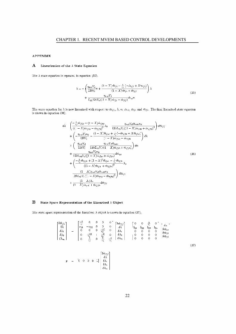
CHAPTER 1. RECENT MVEM BASED CONTROL DEVELOPMENTS
á ââ�ã�ä�å�æ;çè é�ê ë�ìoíoî�ê ï3íoð3ê ñ2ë¼ñ%ò�ð3ó'ì)ô+õ1ð3íoð3ì ã�ö�÷ íoð�ê ñ%ë
ø�ùhú ô�û ü;ý�ü ú�ú3þXÿ ý�ü�� ����� û�� ú�%ú ý�ü ú� � � ú3þ6ÿ ý�ü�� ���� ��������ô����������� !#"$&%(' !#)+*-, $ �/./�10243 ) ,657�8 9� �243�3 , . �2:3 ) � $ �;./� �2:3 ) , �243&3 < ô
, ����� !=">@? A $&%(' !#) 9 $ �;./� �243 ) , �2:3&3 � �2:B ? * �����
ø�ùhú û ü;ý�ü úú3þXÿ ý�ü�� ����C ����ô:� ûD�E�&FHG � � ú ý(��� û ú� FI� ü ù � ú û �2ú�J üzü�� �243&3+K ô K * K �24B ? K �243 ) ý(� 02:3 ) � ø�ùhú1L �2ý(GMG � � ú ý(��� û ú� û ü;ý�ü úú3þ6ÿ ý�ü�� ���� û�û ù �&F���� � ú3þXÿ ý�ü�� ���/ ��N����O �ô��P� � 5798 �243 ) Q �R $ �;./�S0243 ) Q � $ �;./� �2 3 ) Q , �2 3&3 Q � T ô Q � ����� !=" �24B ? Q * Q$&%(' > ? A ! ) 9 $ �;./� �2 3 ) Q , �2 3�3 Q �9T < O �243�3, �M� � �� ! " * Q$&%(' ! ) � $ �/.;�U02:3 ) Q ,657�8 9� �243&3 Q , . �243 ) Q � $ �;./� �2 3 ) Q , �2 3&3 Q < O ô,WV � ���� !="$&%(' !E) � ���� !=" �24B ? Q$&%(' >�? A !E) � $ �;./� �243 ) Q , �2:3&3 Q �&X O *, ���� !#" * Q$&%(' >�? A !E) � $ �;./� �243 ) Q , �2:3&3 Q � O �2:B ?, � �:Y798 �243&3 Q , $ �;./� T 02:3 ) Q � 5798 �243�3 Q � $ �/.;� �2:3 ) Q , �243&3 Q � T ô Q� $ �;./� ����� !=" �24B ? Q * Q$&%(' >�? A !#) � $ �;./� �243 ) Q , �2:3&3 Q � T < O �2:3 ), $ �/.;�Kô Q $ �/.;� �2:3 ) Q , �243&3 Q O 02:3 )
��N��
Z õ1ð3íoð3ì)õS[#íE\6ì4] ì�[�î ìXï3ìoë%ð3íoð3ê ñ%ë¼ñ%ò�ð3ó�ìEé�ê ë�ìXíoî ê ï3ì�^�ô�_a`Ub3ì�\ ðø�ùhú ûGüQý�ü ú û � ý J;ú � ú� � ú û ú �6ü;ý�ü�� ���-�(C�ü ùhú G � � ú ý(��� û ú� ô���c+d ú�J ü�� û�û ù �&F���� � ú3þXÿ ý�ü�� ���/ ��e�� Kfggggh�i 0243&3i �ôi �ô 5i �ô Ti �ô#j
k llllm � fggggghSn 57�8 'o'p' 'q T 5 � q T�T 'p' '' 'o' n 5 T7�rs '' n 5 T7 s $ n=t7 s '' 57�u ' 579u n 57�uk lllllmfggggh i �2:3&3i ôi ô 5i ô Ti ô j
k llllm ,fggggh 'v' Y7�8 'w T 5 w T�T w T�x w T9y'v'v'v''v'v'v''v'v'v'
k llllm fggh i *i �24B ?i �243 )i 0243 )k llm
z �|{ '}'}'}'~$�� fggggh i �243�3i ôi ô 5i ô Ti ô jk llllm
��e��
22
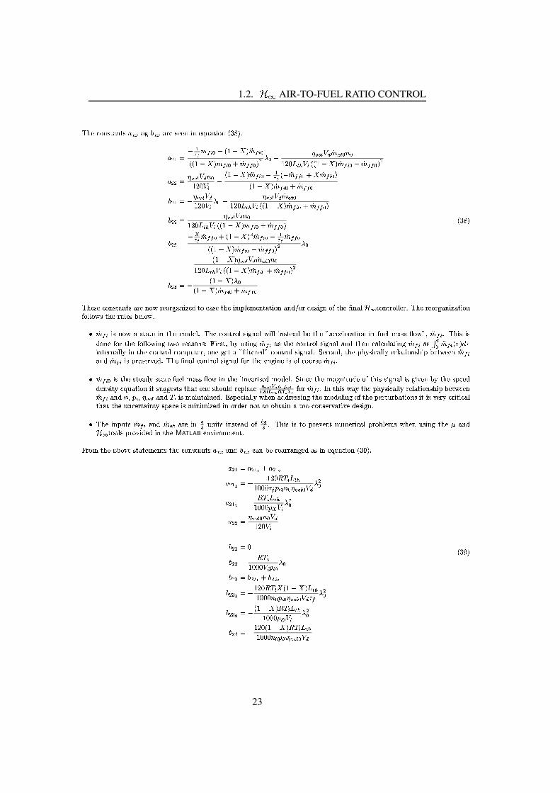
1.2. ��� AIR-TO-FUEL RATIO CONTROL
�I�E������#� ���(�����I�����a���-�����a�(���1�9������ �������#�&��� ���/� ���������������� ��9 �¡¢:£�¤ ¥ � �9¦ �;§ �S¨¢4£¤ ¥�9�9¦ �;§ � ¡¢4£¤ ¥ª© ¡¢:£&£�¥ � ��« ¥ � ¬�® ¯ °=± ¡¢4²�³ ¥´S¥¦&µ(¶�· ³ ¸ ° ¤ �9� ¦ �;§ � ¡¢4£¤ ¥ª© ¡¢4£�£¥ � ������D� ¬ �® ¯ ° ± ´ ¥¦&µ&¶ ° ¤ © � ¦ �;§ �S¨¢4£¤ ¥ª©��� � � ¡¢:£&£¥�© § ¡¢:£�¤ ¥ �� ¦ �;§ � ¡¢ £�¤ ¥ © ¡¢ £&£�¥������� �¹¬�® ¯ °#±¦�µ(¶ ° ¤ « ¥�© ¬��® ¯ °=± ¡¢:²�³ ¥¦&µ(¶�· ³ ¸ ° ¤ �9� ¦ �;§ � ¡¢4£�¤ ¥I© ¡¢4£�£¥ ������D� ¬�® ¯ °=± ´S¥¦&µ(¶�· ³ ¸ ° ¤ �9� ¦ �;§ � ¡¢4£¤ ¥ª© ¡¢:£&£¥ �����ºD���4»�9 �¡¢:£&£¥ª© � ¦ �;§ � � ¨¢:£�¤ ¥ � ��9 �¡¢4£�£¥�9�9¦ �;§ � ¡¢:£�¤ ¥I© ¡¢4£�£¥ � � « ¥� �9¦ �/§ � ¬�® ¯ °#± ¡¢:²�³ ¥´S¥¦&µ(¶�· ³ ¸ ° ¤ �9�9¦ �;§ � ¡¢:£�¤ ¥I© ¡¢4£�£¥ � �� �9¼ � � � ¦ �;§ � « ¥� ¦ �;§ � ¡¢4£�¤ ¥ª© ¡¢4£�£¥
� �����
�I�E���9�½�����#� ���(�������(�����E�(¾¿����������(�E� À��Á������&�(���ª���E�D� ¹ÃEÄ ��Âa������&��� �����(�#Á#Å&����Á+���9� ���¹�(ÆS���E�DÇ#�#�(Ä+È:Éa������������Ä Ä ����Ê�ª�E�½����������(�E� À&�&��� ���Æ ��Ä Ä �(¾��ª���E�1���EÄ ���IË=�Ä �&¾��Ì ¡¢ £�¤ � �1�E�&¾Í��� ���&���a� �;���E�¹Âa�EÁ+�Ä �a�I�E�¹������������Ä@�9� ���#�(Äʾ�� Ä Ä@� �#� ������Á4Ë#�a���E�-Î�������Ä ����&��� ���:� �;Æ �E�Ä@¹������Ï#�(¾�ÎEÐ�¨¢ £�¤ �a�I�E� �1� �Á+���E��Æ ���1���E�aÆ ��Ä Ä �&¾�� �#�-�9¾ª���������9���#�ÑDÒÊ� ��� �&ÐSË+Ó:�#�9� �#�P¨¢:£�¤ ���D���E�-������������Ä@�9� ���#�(Ä��(�#Á����E��/��(Ä ���EÄ �&��� �E� ¡¢:£�¤ ����Ô ³¥ ¨¢4£¤ � Õ#�9Ö(Õ� ��������#�(Ä Ä Ó�� �:���E�a�����������ÄU����¹ÃE�+������Ð#���E�×�����1�-Î&Ç#Ä �������ÁEÎ-������������ÄM��� ���#�(Ä �½Ø��������#ÁSÐ#���E�×ÃE��ÓE�9� ��(Ä Ä Ó�����Ä �&��� ���#�9�E� Ã:Ë#���9¾ª����Ù¨¢:£�¤�(�#Á ¡¢4£¤ � �IÃE���&�9���Ú���ÁS�Ê�I�E�1Ç#�#�(ÄU������������ÄU�9� ���#�(Ä=Æ ���ª���E�1��E��� �E�1� �I�(Æ@�����E���9� ¡¢4£�¤ �Ì ¡¢:£�¤ ¥ � �I���E�×�9������Á+Ó�� ���&���½Æ �E�ÄU¹�����ªÏ#�&¾H� �����#�1Ä � �E���(��� �9��Á�Âa�EÁ+�Ä �IØ�� �#��½���E�×¹�(���E� ���#Á+���(ÆU���E� �D�9� ���#�(ÄS� ����� Ú����Ë�Ó-���E�×�9Ã=���ÁÁ+��#�9� �9Ó¹�����#�&��� ���-� ���9�E�����&� ���Ê���#�&�ª���E�½���E�(�#Ä Á¹���ÃEÄ ������Û�Ü�Ý Þ ß&à�á�â ãä â�9� ¥�åEæ ç�èSé ä ê�â Æ ��� ¡¢:£�¤ �Êë �-���E� ��¾I�&Ó×���E�½ÃE�+Ó+�9� ��(Ä Ä Óa���Ä �&��� ���#�9�E� ùË=���9¾ª���¡¢:£�¤ �&�=Á ´ Ðì ¤ Ð ¬�® ¯ �(�#Á¹í ¤ � ��Â-�(� �����(� �E��ÁS�Êî���Ã#����� �(Ä Ä Óa¾I�E������ÁEÁ+�������9� �E�1���E�½Âa�EÁ+�Ä � �E�×�(Æ=���E�½Ã=��9���E��Ë#�&��� ���#�@� �ª� �ªÚ����Óa����� ��� ��(Ä���#�&�����E���E�#����9���(� ���9Ó��9Ã#����½� �I¹� �E� ¹� À��Á�� �:����Á+��I�E�(�I���a��Ë+���(� �4�����+�¹����#�9���Ú(�&��� Ú(�1Á+�&�9� ���U�Ì �ª�E��� �EÃE�+��� ¡¢:£�¤ �(�#Á ¡¢4²�³ �(���-� ��ï ð:�E�E� ����� �#� ���&��Á/�(Æ�ñ�ïð½�/�I�E� �×� �1���4ÃE����Ú�����×�+�E¹���� ���&ĪÃE����ËEÄ �¹��¾��E��ò�#�9� �E�:���E�-óô�(�#ÁÈ�É�������Ä �IÃE���(Ú�� Á+��Á-� �����E�MATLAB
��+Ú�� �����EÂa������ÒE����ÂP���E���(Ë=�&Ú��1� ���&���¹������ª���E�×�����#� ���(�����I� ��� �(�#Á4� ��� ��(��Ë=�1�����(�����(�E����Á¹���I� �:�����#�&��� ����� ��õ�����+�����ô������ö © �+���9÷������öI� � ¦&µ(¶�øDí ¤ · ³ ¸¦�¶�¶�¶(Õ £ ì ¤ ¥´S¥ ¬�® ¯ ¥ °#± « �¥� ��� ÷�� � ø½í ¤ · ³ ¸¦�¶�¶�¶�ì ¤ ¥ ° ¤ « �¥�+���D� ¬ ® ¯ ¥ ´ ¥ ° ±¦&µ(¶ ° ¤�������ô¶�����D� ø½í ¤¦�¶�¶�¶ ° ¤ ì ¤ ¥ « ¥����ºD�H����º ö © ����º ÷����º ö � � ¦&µ(¶�øDí ¤ § �9¦ © § � · ³ ¸¦�¶�¶�¶ ´S¥ ì ¤ ¥ ¬�® ¯ ¥ °=± Õ £ « �¥����º�÷�� � � ¦ �;§ � ø½í ¤ · ³ ¸¦¶�¶�¶�ì ¤ ¥ ° ¤ « �¥���9¼½� � ¦&µ(¶#� ¦ �;§ � ø½í ¤ · ³ ¸¦�¶�¶�¶ ´S¥ ì ¤ ¥ ¬��® ¯ ¥ °#±
� ��õ��
23
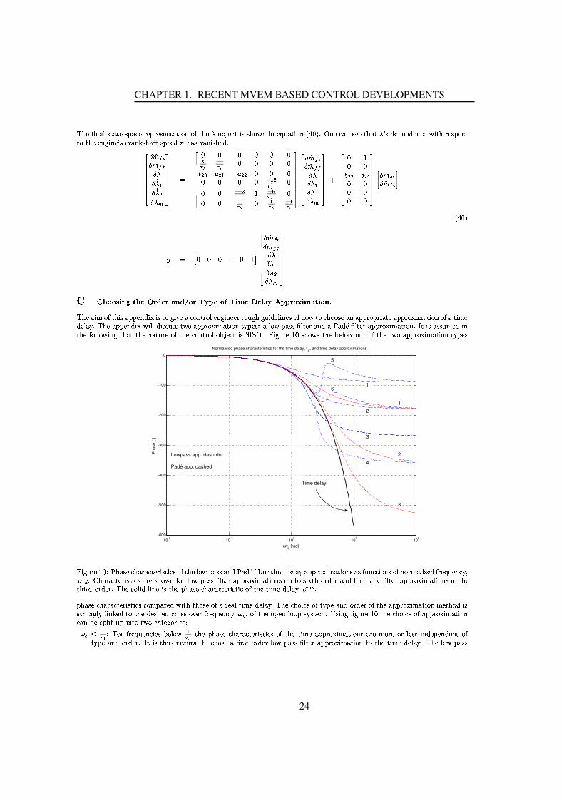
CHAPTER 1. RECENT MVEM BASED CONTROL DEVELOPMENTS
ùIúEû½ü#ý#þ(ÿ�� ��þ���û����#þ���û�û����û �9ûý���þ ��� ��ý�������úEû��������9û������ ���9ú����Iý�� ý�û����#þ ��� ��ý! "�#�$&%('DýEû)��þ(ý*�9ûû��ú#þ �+��, ��-+û��#ûý.-+ûý/��û+�0� ��ú*�û����#û �&��&�1��úEû1ûý�2�� ýEû�, �0���þ(ý�3��9ú#þ � ����=ûû�-�4;ú#þ���5&þ(ý�� �9úEû�-�%677777789:;=<�>90:;=<�<9@?�9 ?�/A9 ?�.B9 ?�.C
D EEEEEEFHG677777778#I# #I#J# #KL�MON AL�M #I#J# #P&B�QSR�B&AUT0R�B�BV#J# ##I# #I# N A�BL�WX ##I# N A�BL XZY N�[L X ##I# AL�\ # AL�\HN AL�\
D EEEEEEEF677777789 ?;=<�>9 ?; < <9 �9 �/A9 �.B9 �.C
D EEEEEEF^]67777778# Y#_#P&B�B`P&B�a#_##_##_#
D EEEEEEFb 9 ?;=c�d9:;e<�> f
g Gih #j#U#k#U# Y&l677777789 ?; <�>9 ?;=<�<9 �9 �.A9 ��B9 ��C
D EEEEEEF
"�#�$
m n1oqp�p.r�s tvu=w�ovx!y{z |qx�z�}�tq|q~.p�z������x=p/�0��s ��xe�*x�� }������v�qz p���s ��}�w�s p.t(�ùIúEûªþ�� ��������ú�� �Êþ����#û�ý.-�� �1� ���&�2�� 5�ûªþ����ý������ÿ�û�ý�2�� ýEûû�v�����2�ú�2��.� -+ûÿ � ýEû��v���#ú�� �!�&�+��ú������9ûªþ(ý×þ������������ þ ��ûªþ����������� �-þ ��� ��ý+���=þ���� �aû-+ûÿ þ���%ÊùªúEû1þ����#ûý.-�� �{�0� ÿ ÿ/-�� �&���.���@������þ����.������ �-þ ��� ��ý������=û����@þ1ÿ � ���#þ����@ü#ÿ ��û�ªþ(ý.--þ��@þ�-��ûªü#ÿ ��û�Iþ������� ��� �¹þ �&� ��ý�%v� ��� �ªþ��������aû -{� ý��úEû�� ��ÿ ÿ � �0� ý�2{��ú#þ �0��úEû×ý#þ �����û1���q��úEû�����ý������ÿ������9û��&�+� �+������'�%!�v� 2����û Y #{�9ú��������úEû1�=ûú#þ 5�� ����0���q��úEû�������þ����������� �-þ ��� ��ý������=û��
10-2
10-1
100
101
102
-600
-500
-400
-300
-200
-100
0
ωτd [rad]
Pha
se [°
]
Normalised phase characteristics for the time delay, τd, and time delay approximations
Lowpass app: dash dot
Padé app: dashed
2
1
3
4
5
6
1
2
3
Time delay
�v� 2����û Y #�����ú#þ��9û(��ú=þ �þ��&��û��� � ��� ���/������úEû�ÿ � ���#þ����Uþ(ý.-��@þ�-(�ûMü#ÿ ��û����� �aû�-+ûÿ þ��½þ������� ��� �¹þ �&� ��ý.�Sþ���� �Eý.�&��� ��ý.�����Eý�����¹þ(ÿ � �9û -0� �û ���Eûý.������(� � %��ªú#þ��þ��&��û�&� � �&� ���Iþ��û)�9ú����Iý�� ���ÿ �����#þ�����ü#ÿ ��û�Dþ������� ��� �¹þ �&� ��ý.�������&�{��� ����ú*��&-+û��þ(ý.-�� ��0�@þ�-��ûDü#ÿ ��û�Dþ����������� �-þ ��� ��ý.�(�.�������ú�� &-*��&-+û��%ÊùIúEû�����ÿ � -�ÿ � ýEû�� ����úEû��Eú#þ��9û)��ú#þ��þ��&��û��� � ��� �0���q��úEû)��� �aû1-+ûÿ þ ���� L X&¡ %�Eú#þ��9û)��ú#þ��þ�����û��� � ��� ���(�����{�#þ��û�-{�0� ��ú���ú����9û���Êþ1�û�þ(ÿ��&� �¹û)-+ûÿ þ ��%@ùIúEû)��ú���� ��û���������=û1þ(ý.-���&-+û��������úEû1þ������� ��� �¹þ �&� ��ý{�¹û���ú���-�� �� �&���ý�2�ÿ �-ÿ � ý�3�û�-{�&�1��úEû�-+û���� �û�-*�����������5�û��� �û����Eû�ý.����� �(¢ ��������úEû)���=ûý�ÿ �����e��������û��e%@£+��� ý�2aü.2����û Y #)��úEû���ú���� ��û+����þ����������� �-þ ��� ��ý�þ(ý*�=û����Eÿ � ����*� ý��&�1�������þ ��û�2����� û�����(¢�¤ AL X �{����1� �û����Eû�ý.��� û����#ûÿ � � AL X ��úEû��Eú#þ��9û���ú#þ��þ��&��û�&� � �&� ���)������úEû���� �aû�þ������� ��� �¹þ �&� ��ý.��þ��û{�{���û{���ÿ û������ ý.-+û��#ûý.-Eûý������� ���=ûaþ(ý.-=��&-+û��%)� �)� ���ú��.�Dý#þ �&���þ(ÿv���e��ú����9ûaþ¹ü.&� �)��&-+û�½ÿ � �¥�#þ��&��ü#ÿ ��û�1þ������� ��� �¹þ �&� ��ýe�&����úEû1�&� �¹û{-+ûÿ þ���%�ùIúEû×ÿ � �¦�#þ����
24

1.2. §©¨ AIR-TO-FUEL RATIO CONTROL
ª.« ¬&�®0¯�°�°�®�±�²�³ ´�¯ ¬�³ ±�µ�¶�±� ·(µ�±�¬0³ µ�¬�®�±�¶�¸.¹�+¯�µ�º�»��®�±��·@³/¬&¼�+®�³ ½�¼�¬�¼.¯�« ¾�°.« ¯�µ�{¿ ÀÁÂ�Ã(« ³ Ä�+¯�Â@¯�¶�ů�°�°�®�± ²�³ ´{¯ ¬&³ ±�µ�¯ µ/¶�¯1¹�±�µ�¬�®�±�«· ¬�®&¯ ¬&�½�º{Æ.¯�·��¶�±�µ*°�« ¯�µ�¬0³ µ�Ç��®&·�³ ±�µ�´{¯ º�· ¬�³ « «�Æ/)¸.·��¶�ÈÉ(Ê+ËÍÌÎ�Ï/Ð�Ñ ¾(¯�¹�®�±�·�·�±�Ç��®�¾ ®��Ò�¸��µ.¹�º�« ¯�®�½��® ÌÎ�Ï ³ ·¶��·�³ ®��¶�¬�¼��ª.®&· ¬±�®&¶��®0« ± Ó�°.¯�·�·¯�°�°�®�± ²�³ ´{¯ ¬�³ ±�µe·�¼�±�¸�« ¶*Æ/�¶�³ ·�¹�¯�®&¶��¶�È Ñ µ.· ¬��¯�¶¯*« ±�Ó¦°.¯�·�·�¯�°�°�®�± ²�³ ´{¯ ¬&³ ±�µ!±�¾¯*¼�³ ½�¼��®�±�®&¶��®�±�®1¯*Â@¯�¶(Å{¯�°�°�®�± ²�³ ´{¯ ¬&³ ±�µ�·�¼�±�¸�« ¶�Æ.�¸.·� ¶�È Ñ ¾0³ ¬1³ ·1¶� ·�³ ®� ¶e¬�±e´�¯�³ µ�¬&¯�³ µ!¬�¼�¹�±�µ�¬&®�±�«�±�Æ�Ô��¹�¬+´�³ µ�³ ´1¸�´Õ°�¼.¯�·��Ö/« ±�Ó�°.¯�·�·+¯�°�°�®�±�²�³ ´�¯ ¬�³ ±�µ.·�¸�°=¬�±�¾ ±�¸�®�¬�¼!±�®&¶��®+¯�®&�¸.·�¯�Æ�« �¾ ±�®)¹�®�±�·�·0± Ç��®�¾ ®��Ò�¸��µ.¹�³ �·Æ.�« ± Ó×Î�Ï È�Ø·�³ µ�½*« ±�Ó¥°.¯�·�·)¯�°�°�®�±�²�³ ´�¯ ¬�³ ±�µ.·0±�¾�¼�³ ½�¼��®)±�®&¶��®¬�¼.¯�µ�Ù�º�³ �« ¶�·+¸�µ.· ¬&¯�Æ�« �¯�°�°�®&±�²�³ ´{¯ ¬&³ ±�µ.·�È1Ø·�³ µ�½*¯�µ!¸�µ.· ¬&¯�Æ�« 1ª.« ¬��®�¯�·¯�¬&³ ´{�¶��« ¯�ºe¯�°�°�®�±�²�³ ´�¯ ¬�³ ±�µ*³ ·µ�±�¬)³ µ�¬�¸�³ ¬&³ Ç��« ºe¹�±�®&®��¹&¬+·�³ µ.¹��¯�¬&³ ´{�¶��« ¯ º�³ µ=³ ¬&·+·��« ¾�¶�±��·µ�±�¬+´{¯�Ä��¬�¼�1±�°/�µ=« ±�±�°=·�º�· ¬��´¸�µ.· ¬&¯�Æ�« �È Ñ µ.· ¬��¯�¶�¯)Â@¯�¶(Å0¯�°�°�®�±�²�³ ´�¯ ¬�³ ±�µ{¹�¯�µ�Æ.¸.·��¶�³ ¾�»��®�±��·@³ µ{¬&¼�À0Á+Â�¯�®�¯�¹�¹��°�¬&¯�Æ�« �È Ñ µ�¬�®&±�¶�¸.¹�³ µ�½�»��®�±��·@³ µ{¬�¼�+ÀÁ´{¯ º�¼.¯ Ç�1¯�µ=�Ú/ ¹&¬+¬�¼.¯ ¬)³ ·+¶��·�³ ®&¯�Æ�« �ÈÀÁÂÛ»��®�±��·¹�¯�µ=µ�±�¬)Æ.�¹�¯�µ.¹��« �¶e±�¸�¬+Æ�º*°/±�« �·+¯�µ.¶eÓ0³ « «v¬�¼�¸.·¼.¯�Ç�1¯�« ³ ´{³ ¬&³ µ�½��Ú��¹&¬±�µ!¬�¼��¯�¹&¼�³ �Ç ¯�Æ�« {¹�±�µ�¬�®�±�«@°/�®�¾ ±�®�´�¯�µ.¹��È*Ü0µ�±�¬�¼��®1½�±�±�¶!°�®�±�°.�®�¬�ºe±�¾�¬&¼��Â@¯�¶(Å�¯�°�°�®�± ²�³ ´{¯ ¬&³ ±�µ�³ ·+¬&¼.¯ ¬1³ ¬{¶�±��·�µ�±�¬1¹&¼.¯�µ�½�¬�¼��¯�´�°�« ³ ¬&¸.¶�)¹�¼.¯�®&¯�¹�¬��®�³ · ¬�³ ¹�·(±�¾�¬�¼��¹�±�µ�¬�®�±�«/±�Æ�Ô� ¹&¬0·�³ µ.¹�+³ ¬0³ ·�¯1¯�« «/°.¯�·�·@ª.« ¬��® È(Ý�±1¾ ±�®0¶��·�³ ®��¶�¹�®�±�·�·�± Ç��®(¾ ®� Ò�¸��µ.¹�³ �·(¼�³ ½�¼��®¬�¼.¯�µßÞÎ�Ï ¯{Â@¯�¶(Å0ª.« ¬&�®0±�¾@·��¹�±�µ.¶�±�®&¶��®0±�®�¼�³ ½�¼��®0´�¯�º�Æ/)¸.·��¶�Èà á�â�ã�ä�å�æçá�å�ä�è�éÛê�ëvì�í*î�ï1ð/ë/ä�ñ�ð.ò ò å�ñ*á�ä�ñ�èvó�ä è�ñ�åÑ µ!¬�¼�{¶� ·�³ ½�µ!±�¾�¯�µ í*î{ô�í Þ&õ ®��½�¸�« ¯ ¬�±�®+¯�µ.¶!®�±�Æ�¸.· ¬�¯�µ.¯�« º�·�³ ·³ ¬�³ ·)±�¾ ¬��µ�¯�¶�Ç�¯�µ�¬&¯�½��±�¸.·0¬�±�¸.·�{¯�½��µ��®&¯�« ³ ·��¶=·�º�· ¬��´ß¶��·�¹�®�³ °�¬�³ ±�µ�Èö ¼�1½��µ��®&¯�« ³ ·��¶�´{�¬�¼�±�¶e¸.·� ¶*¼��®�1³ ·+¶��°�³ ¹&¬&�¶e³ µeª.½�¸�®��÷�÷�Èùø^³ ·0¬&¼��¹�±�µ�¬�®&±�« « �®�Ö.Âú³ ·0¬�¼��°�« ¯�µ�¬Ó0³ ¬&¼=¸�µ.¹��®�¬&¯�³ µ�¬�º*´�±�¶��«q¯�µ.¶
z
K
w
∆
u v
εδ
P
û ³ ½�¸�®&�÷�÷ Ð(ü �µ��®&¯�« ³ ·��¶*·�º�· ¬��´ý·��¬�¸�°°/�®�¾ ±�®�´�¯�µ.¹� õ ¯�µ.¶{·�³ ½�µ.¯�«�Ó��³ ½�¼�¬�·�Ö�¯�µ.¶{þ¥³ ·�¯)· ¬&®�¸.¹&¬�¸.®��¶�°/�®�¬�¸�®�Æ.¯ ¬&³ ±�µ{´{¯ ¬&®�³ ²�È ö ¼�0³ µ.¶�³ Ç�³ ¶�¸.¯�«/·�³ ½�µ.¯�« ·@³ µ�¬&¼�·��¬�¸�°{³ · Ðvÿ Ö�¹�±�µ�¬�®�±�«·�³ ½�µ.¯�« ·�Ö��/Ö.´{�¯�·�¸�®��´��µ�¬·�³ ½�µ.¯�« ·�Ö��1Ö.�²�±�½��µ�±�¸.·�³ µ�°�¸�¬&·�Ö���Ö/¹�±�µ�¬�®�±�« « �¶e·�³ ½�µ.¯�« ·�Ö���Ö.°/�®�¬�¸�®�Æ.¯ ¬&³ ±�µe±�¸�¬&°�¸�¬+Ç��¹&¬&±�®�¬&±*þý¯�µ.¶�ª.µ.¯�« « º�³ ·0¬�¼�1°/�®�¬�¸�®�Æ.¯ ¬&³ ±�µe³ µ�°�¸�¬)Ç��¹&¬&±�®�¬�±�¬&¼�1°�« ¯�µ�¬�È ö ¼��·�³ ½�µ/¯ «vÇ��¹&¬&±�®��¹�±�µ�¬�¯�³ µ.·�¬&¼�±�·�1·�³ ½�µ.¯�« ·�Ö.Ó0¼�³ ¹&¼!¯�®�)¬�±�Æ/�¹�±�µ�¬&®�±�« « �¶�È��ú¼��µ¶��·�³ ½�µ�³ µ�½{¯{¹�±�µ�¬&®�±�« « �®�¬�¼�1·�º�· ¬&�´ ³ ·0¶��·�¹�®�³ Æ/�¶�Æ�º�Ö � ��� �������� Ì�Ì ¿ � à � Ì Þ ¿ � Ã� Þ Ì ¿ � à � Þ&Þ ¿ � Ã�� � �� ÿ��
ÿ � ø�¿ ��à � ¿ Ù.÷ Ã� ¼.¯�·�¬�¼�)¾ ±�« « ± Ó0³ µ�½{· ¬�¯ ¬� õ ·�°/¯�¹�+®��¯�« ³ ·�¯ ¬�³ ±�µ�Ö � � ��� � Ì � Þ� Ì ��Ì�Ì���Ì Þ� Þ � Þ Ì�� Þ�Þ
�� ¿ Ù� �Ã�ú¼��µ=¶� ·�³ ½�µ�³ µ�½ í*î�ô�í Þ ¹�±�µ�¬�®�±�« « �®�·(¬&¼�1¹�« ±�·��¶�« ±�±�°�¬&®&¯�µ.· ¾ �®0¾ ¸�µ.¹&¬�³ ±�µ*¾ ®�±�´�!#"$&% ¬�±'!)(* % ³ ·�´{³ µ�³ ´�³ »��¶�È ö ¼�)¬�®&¯�µ.· ¾ �®�¾ ¸�µ.¹�¬�³ ±�µ¾ ®�±�´+! "$,% ¬&±-!.(* % ³ ·�¬�º�°�³ ¹�¯�« « º�Ó0®�³ ¬�¬��µe¯�·0¯�µ/ ûqö È ö ¼.³ ·,/ ûqö ³ ·0·���µ*³ µ*�Ò�¸.¯ ¬�³ ±�µ�¿ Ù10�Ã&È� �� � �3254 ¿ �76 ø!à � �� �Ó0¼��®��8 �3254 ¿ �76 ø!à � � Ì&Ì:9 � Ì Þ ø ¿ ;=< � Þ&Þ ø!Ã?> Ì � Þ Ì
¿ Ù10�Ã
25

CHAPTER 1. RECENT MVEM BASED CONTROL DEVELOPMENTS
@�A�BDCFEHG)IKJ1LNMNIKO O BPMRQ S�O T�O O U J�V-W.XZY [�\N]_^)WPEa`cb'A�dKe7LNA�B=efLNMNS�G?L?S�MNBKg]ih�jHk�lnmo#p#q m q�rmts E l qu.v E lxw EHy�E�z u { w E�y�Ev E | }~ A�B.MNBv E h { Y � rm u � u m ^N� m Y q ru s E l � rm u z m ^y7E h { Y � E�z ru l q m � ru m ^.Y � u m � ru m ^N� mw E h�Y � {��b u � E s E ^?� m
Y �K��^
s Ead#J��F��E�U JFBP�1S�d�LNU I#JcY �K��^7d#MNBLNA�B�efIKO S�LNU IKJ�e7LNIHL ~ I���d�LNM?U ��MNU G.d�LfL?U�B��KS�d�LNU IKJ�e.�:@�A�BPefBDBP�KS�d�L?U IKJ�e,d#MNBKg| h k&r s E l s E kcl z rm z m l �b u s E q m q rmts E{ Y s E q u l z rm � m u ^.Y � rm u � m u ^N� m Y q ru s E l � rm u z m ^| h k ��E l ��E k&r�l q m q rm l �b u ��E z rm z m ��E{ Y � E�z ru l q m � ru m ^.Y � u m � ru m ^N� m Y z ru � E l � u m q rm ^~ A�B.M?B�� Y s E � E `cb u ^Y ���K^
��U VKS�MNB ��� efA�I ~ e,LNA�BH��O I�GN�-��U d#VKM?d#��Q IKM&LNA�B=C E G)IKJKL?MNIKO O B.MP�&@�A�BHO I�G.d�LNU IKJI#Q:L?A�B=Q B.BP����dKG?�FV1d#U J��d�LNMNU �FQ IKM,L?A�BHMNIK��S�e LIK��efB.MN�KBPMQ B.B�����dKGN���KB�G?LNIKM,d#J��FG)IKJ1LNMNIKO5efU VKJ�d#O��KBPG)LNIKM,d#MNB=efA�I ~ J�U JFLNA�BT�VKS�M?BK�
Σ
-Σ
Observer
Regulator
∞∞ XZ
2B 2C
∞+ XBBA T112
1γ
∞F
u v
��U VKS�MNB �����:� O I�GN����U d#VKM?d#��Q IKM�C E G)IKJKL?MNIKO�e LNM?S�G?LNS�MNBK�� J����fd�J�d#O �eNU etL?A�B=G)O I1efB���O I�IK¡�ef �e L?B.�aXiU eRL?BPe LNBP��Q IKM�efL?d#��U O U Lf �¢�¡�B.MNQ IKMN��d#J�G)B ~ U LNAFMNBPef¡�BPG?L7LNI�dHe LNMNS�G?L?S�MNBP��¡�B.MfLNS�MN��d�L?U IKJ5�:@�A�d�LU e.g1LNA�B=J�IKMN�aI#Q vt£ Y X\?¤H^7U e�U J��KBPe L?U V1d�LNB���� v�£ Y X\?¤�^7U e7VKU �KB.JF�1 �LNA�B=S�¡�¡�BPM&¥��t@3U JBP�KS�d�L?U IKJcY �1¦1^?�v�£ Y X\?¤�^Rh§X uNu l X u m ¤FY � { X m?m ¤H^?� m X m u Y �1¦1^
26
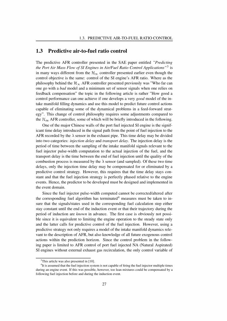
1.3. PREDICTIVE AIR-TO-FUEL RATIO CONTROL
1.3 Predictive air-to-fuel ratio control
The predictive AFR controller presented in the SAE paper entitled ”Predictingthe Port Air Mass Flow of SI Engines in Air/Fuel Ratio Control Applications”3 isin many ways different from the ¨ª© controller presented earlier even though thecontrol objective is the same: control of the SI engine’s AFR ratio. Where as thephilosophy behind the ¨ª© AFR controller presented previously was ”Who far canone go with a bad model and a minimum set of sensor signals when one relies onfeedback compensation” the topic in the following article is rather ”How good acontrol performance can one achieve if one develops a very good model of the in-take manifold filling dynamics and use this model to predict future control actionscapable of eliminating some of the dynamical problems in a feed-forward strat-egy”. This change of control philosophy requires some adjustments compared tothe ¨�© AFR controller, some of which will be briefly introduced in the following.
One of the major Chinese walls of the port fuel injected SI engine is the signif-icant time delay introduced in the signal path from the point of fuel injection to theAFR recorded by the « sensor in the exhaust pipe. This time delay may be dividedinto two categories: injection delay and transport delay. The injection delay is theperiod of time between the sampling of the intake manifold signals relevant to thefuel injector pulse-width computation to the actual injection of the fuel, and thetransport delay is the time between the end of fuel injection until the quality of thecombustion process is measured by the « sensor (and sampled). Of these two timedelays, only the injection time delay may be compensated for or eliminated by apredictive control strategy. However, this requires that the time delay stays con-stant and that the fuel injection strategy is perfectly phased relative to the engineevents. Hence, the predictor to be developed must be designed and implemented inthe event domain.
Since the fuel injector pulse-width computed cannot be corrected/altered afterthe corresponding fuel algorithm has terminated4 measures must be taken to in-sure that the signals/states used in the corresponding fuel calculation step eitherstay constant until the end of the induction event or that their trajectory during theperiod of induction are known in advance. The first case is obviously not possi-ble since it is equivalent to limiting the engine operation to the steady state onlyand the latter calls for predictive control of the fuel injection. However, using apredictive strategy not only requires a model of the intake manifold dynamics rele-vant to the description of AFR, but also knowledge of all future exogenous controlactions within the prediction horizon. Since the control problem in the follow-ing paper is limited to AFR control of port fuel injected NA (Natural Aspirated)SI engines without external exhaust gas recirculation, the only control variable of
3This article was also presented in [10].4It is assumed that the fuel injection system is not capable of firing the fuel injector multiple times
during an engine event. If this was possible, however, too lean mixtures could be compensated by afollowing fuel injection before and during the induction event.
27

CHAPTER 1. RECENT MVEM BASED CONTROL DEVELOPMENTS
interest is the throttle angle5. The throttle command was therefore postponed afixed number of event samples and made possible a prediction of the air mass flowthrough the throttle system. Although this action necessitates a drive-by-wire con-trol system, the throttle command was as mentioned before only time delayed andnot controlled; Hence, the air-lead classification of the AFR control system wasmaintained.
When a predictive control strategy is designed, the underlying dynamic modelmust as previously mentioned be of high accuracy if the feed-forward compensa-tion should be effective. This called for some adjustments of the IMVEM (Isother-mal Mean Value Engine Model) proposed earlier in [47] to improve the level ofmodel accuracy within the normal engine operation limits. First, the isothermalassumption for the intake filling dynamics was discarded and the model was ex-changed for a polytrophic description of the intake pressure and the intake tem-perature dynamics. Second, a simple second order model of the DBW (Drive ByWire) system’s dynamics was constructed. Using this model in parallel with themodels of the intake pressure and the intake temperature, the response of the throt-tle plate position within the prediction horizon could be predicted. This offersvaluable information for the throttle air mass flow model. Lastly, the air filter up-stream of the throttle body introduces a small however noticeable pressure drop,i.e. the stagnated throttle body pressure level is offset from the ambient pressurelevel. Bearing this in mind and that the throttle mass flow model proposed in thefollowing article is very sensitive not only to model errors in the intake manifoldpressure model, but also to errors in the description of the stagnated pressure up-stream of the throttle plate, measures must be taken such that the throttle bodypressure level is corrected. However, since the air filter pressure loss is mainly afunction of volumetric flow it will together with the algebraic description of thethrottle model form an algebraic loop. To overcome this problem a simple iterativealgorithm with a fixed number of steps was implemented in the final strategy.
Using a pure predictive feed-forward strategy the danger of model divergence isimmense as various model errors are accumulated. In order to minimize the dangerof such scenarios, the states of the predictive model are updated every event sam-ple by an extended Kalman filter utilizing measurement innovation from the intakemanifold pressure sensor and from the thermocouple mounted in the middle of theintake plenum. However, before the Kalman filter could be designed the predictivemodel just described needed several important augmentations. First, although thetemperature sensor6 used was fast, its time constant was still significant comparedto the time constant of the intake temperature state equation. Hence, the temper-
5The throttle type used on the experimental engine was of an older type that did not feature anyexternal air injection capabilities. Hence, the intake air mass flow was controlled completely by thethrottle position.
6The temperature sensor used during the experimental work was a conventional K-type thermo-couple. However, due to the small size of the sensing element this sensor type is 35 to 200 timesfaster than the thermistors and thermocouples normally used in mass production applications or con-ventional test cells.
28

1.3. PREDICTIVE AIR-TO-FUEL RATIO CONTROL
ature sensor required modelling to insure a correct picture of the overall dynamicsystem. Thus, a simple linear first order model was designed and later found suf-ficiently descriptive from experimental results. Second, the pressure fluctuationsin the intake manifold are deterministic and do not fulfill the requirement of beingthat of Gaussian white noise nature as required by the Kalman filter framework. In-stead, the model was augmented further by a linear network of second order tunedto the frequency of the first harmonic of the pumping fluctuations. The output ofthis filter was thereafter added to the averaged intake pressure estimate providedby the pressure state equation. This signal along with the pressure measurementformed the signal innovation to the observer. In this way the distribution of theerror between the pressure model and measurement was brought closer to a Gaus-sian noise distribution. Finally, to account for a possible steady state error betweenthe throttle mass flow model and the port mass flow a constant (deviation) variablewas added to the output of the throttle model in the temperature and pressure stateequation.
The actual computation of the corresponding Kalman gains required of coursenot only a linearized version of the model briefly described above but also a prioriknowledge of the individual state noise and measurement noise intensities. Thesewere derived from experimental data using either conventional FFT (Fast FourierTransform) techniques or soft assumptions on the process and measurement co-variances along with an inverted version of the classical Lyapunov equation.
Needless to say, however,model errors will always exist and thus to preventsteady state AFR errors, a simple, but good PI control loop around the ¬ sensorfitted to exhaust manifold was designed. The control output of this compensatorwas later added to the AFR predictor output, and hence formed the final port fuelflow command.
Finally, the port fuel flow command was sent through a fuel film compensatorto eliminate the dynamics of the fuel film. The fuel film compensator was designedaccording to the classic Aquino fuel film model with its two adjustment parametersstored in a speed–pressure map. The output of this filter is the final fuel injectioncommand sent to the fuel injection unit. However, this filter or rather its calibrationproved to be limited by great difficulties; the filter parameters maps could not besatisfactorily realized from experimental engine data using a off-line identificationalgorithm, hence the final parameters maps used in the experimental work werefound in a trial-and-error manner.
The strategy presented in detail here was finally implemented in a version ofthe ECDS (Engine Control Development System) environment (see [58]) whichhad been updated earlier in a collaboration between A. Chevalier and the author.The functionality of the strategy developed was confirmed by several different tran-sient experiments in one of the test cells available to the ECG, some of which areincluded in the article presented here.
29

CHAPTER 1. RECENT MVEM BASED CONTROL DEVELOPMENTS
30

1.3. PREDICTIVE AIR-TO-FUEL RATIO CONTROL
Copyright c
2000 Society of Automotive Engineers, Inc.
2000-01-0260
Predicting the Port Air Mass Flow of SI Enginesin Air/Fuel Ratio Control Applications
Alain ChevalierFord Motor Co.
Christian Winge VigildFord Motor Co.
ABSTRACT
With the tightening of exhaust emission standards, widebandwidth control of the air/fuel ratio (AFR) of spark ignitionengines has attracted increased interest recently. Unfortunately,time delays associated with engine operation (mainly injectiondelays and transport delays from intake to exhaust) impose se-rious limitations to the achievable control bandwidth. With aproper choice of sensors and actuators, these limitations can beminimized provided the port air mass flow can be accuratelypredicted ahead in time.
While the main objective of this work is to propose a completeAFR controller, the main focus is on the problems associatedwith port air mass flow prediction.
1 INTRODUCTION
In order to achieve maximum conversion efficiency of the three-way catalyst (TWC), the engine management system needs to beable to keep the mass of fresh air, ®'¯ and the mass of fuel, ®-° ,which are trapped in each cylinder, in a stoichiometric propor-tion ( ±:² ³ , the ratio for complete combustion). If one defines thenormalized AFR, ´ , as ´�µ ®¯®-°:±:² ³ (1)
then the requirement of the controller is to maintain ´ as closeto 1 as possible, both during steady-state and transient opera-tion. In the literature, this is known as the air/fuel ratio (AFR)control problem.
Conventional AFR strategies are based on look-up tables (non-dynamic map modeling). Associated with a feedback loop(from the ´ oxygen sensor placed in the exhaust pipe), theycan ensure that the AFR will remain in the vicinity of the sto-ichiometric point during steady-state operation (constant load
This paper is typeset in LATEX 2 ¶
and constant engine speed). However, the dynamic nature of airand fuel flows, the low pass characteristic of sensors, the de-lays required by the control system to respond to measurementsand the driver’s command (on tip-in or tip-out), and finally thetransport time required by the air-fuel mixture to cross the en-gine and reach the oxygen sensor, make conventional feedbackloop control strategies slow (with a small control bandwidth).They are thus unable to avoid large AFR excursions during tran-sient operation (acceleration, deceleration, varying engine load,wind gusts etc.). This is a key problem when trying to addressthe problem of automobile induced pollution in cities: duringrush-hour traffic, the engine is often operated in transient condi-tions, thus leading to large AFR excursions from stoichiometryand consequently poor TWC efficiency.
The purpose of this paper is to consider in detail not only thephysical characteristics of the engine, but those of the sensorsas well. In addition to these physical constraints, the details ofthe timing of the engine control microprocessor and the associ-ated actuators are taken into account. The overall goal is thus todemonstrate experimentally the effectiveness of a nearly idealtheoretical solution to the AFR control problem on a practicalsystem.
Before attempting to address the control problem, it is conve-nient to review the actual physical problems which engine con-trollers have to overcome if they are to be successful in control-ling an engine.
2 AFR CONTROL PROBLEMS
The wall-wetting phenomenon1 and the manifold filling phe-nomenon2 have been known as the source of transient AFRproblems for many years and will therefore not be discussedhere. Readers who are not familiar with these phenomena,should refer to [1], [2], [3], [4], [5] and [6] for a thorough dis-cussion. Here, the authors will discuss three problems whichthey consider to be just as important, but which have surpris-
1Some of the injected fuel is deposited on the manifold wall instead of en-tering the cylinders immediately.
2During transients, port air mass flow and throttle air mass flow differ be-cause of the filling/emptying of the intake manifold volume.
·¸ ¹Dº5»�¼Z½3º�¾&¿,»�ÀfÁ�Â,ÃÄ5ÅPÆNÇ�È�É Æ.Ê#Ë5Ì,È�É ÍKÅ.Î?ÏfÉ Ð Ñ�Ò#Ó:Ô&Å.È�Õ�Ê#ÎNÖ
31

CHAPTER 1. RECENT MVEM BASED CONTROL DEVELOPMENTS
ingly enough not enjoyed much attention in the existing litera-ture. These are the limitations imposed on the controller by thepresence of engine pumping fluctuations, poor sensor responsecharacteristics and time delays.
2.1 Pumping Fluctuations
In the intake duct, pressures and flows oscillate because of theperiodic motion of piston and valves. During the induction pro-cess, the engine operates as a pump, and the resulting periodicvariations are often referred to as pumping fluctuations [7],[8].The modulation depth of the fluctuations can be of the orderof 15% of the average signal level for the pressure and morethan 100%3 of the average signal level for the air mass flow.The source of pumping noise is periodic and so are the pump-ing fluctuations which are frequency locked to the engine eventfrequency. This is illustrated in Figure 1 where a steady statemanifold absolute pressure (MAP) signal (measured on an en-gine dynamometer) is shown both in the time domain and in thefrequency domain. The fundamental frequency (marked ×#Ø ) isclearly locked to the event frequency (marked ×1Ù ), and power isalso present in the first and second harmonics (marked ×1Ú and×�Û ). As shown in Equation 1, the mass of air that enters one
0 0.0438 0.0876 0.1314 0.1752 0.2190.94
0.96
0.98
1
1.02
1.04
1.06PSfrag replacements
ÜHÝ Þ ßà áâãä å âæç one event
one cycle
è?é�ê ë�ì ì ì�í î-ïHð ñ ò ó ô è�õ
(a) Time domain
0 91.3304 182.6607 273.9911 365.32150
0.5
1
1.5
2
2.5
3x 10⁻⁴
PSfrag replacements
one event
one cycle
öK÷ ø ù ú)ø ëPû ü Ý ý�þ ßPow
erSp
ectr
um
ä å âæÿ ç � ó ï � ø� � � ïHð � ø� � ð ï � � ø� ò � ø�� ø ï î� ó ï �
� � � � ý�þ
(b) Frequency domain
Figure 1: Intake pressure pumping fluctuations duringsteady-state operations
cylinder, �� , and consequently the mean over one event of theair mass flow related (AMFR) signals, are the only variables ofinterest in multi-point injection (MPI) AFR control. What is ac-tually desired in the conditioning of the signals from the AMFRsensors is to remove the large fluctuating component of the sig-nals without damping out their mean value during transients andwithout introducing time lags and time delays which would im-pose limitations on the system bandwidth. In conventional fu-eling strategies, this is a problem which has often been ignored.Because of the discrete nature of microprocessor-based con-trollers and given the level of pumping noise, serious aliasingproblems should be expected if no special measures are taken
3indicating backflow.
during the sampling/processing of the measurements. This is es-pecially true in event-based sampling strategies where the noisespectrum and the sampling frequency are locked.
In Figure 2, the transient performance of a 4-step moving av-erage filter (EABS4)4 averaging algorithm is simulated during afast (50 ms) tip-in and tip-out at constant idle-speed conditions(worst case). In order to emphasize the delay associated withthe filter, the pressure is also filtered with a zero-phase EABS4digital filter (i.e. the input data are processed off-line in boththe forward and reverse directions, so that the time lag intro-duced in the forward filtering is canceled by the time advanceintroduced in the backward filtering). The expected resultingtransient
trace is shown in Figure 2(b) where tip-in results in
a lean and tip-out in a rich excursion. Note that because the fil-tering delay is inversely proportional to the engine speed, theseexcursions decrease with increasing engine speed down to 5%at 6000 RPM. However, it should be clear that this
trace is in
many ways ideal (and therefore optimistic) since the effects ofmanifold filling, fuel film dynamics and injection delays werenot included in the simulation.
0.4 0.6 0.8 1 1.2 1.40.4
0.5
0.6
0.7
0.8
0.9
1
PSfrag replacements
Ü�Ý Þ ßà áâãä å âæç � � ø � êfü ï � � ø��Idle-speed
( î-ï � ó ó ô è1õ )
No filterZero-phase filter
EABS4 filter
(a) Transient event-based averaging of the intake plenum pressure
0.4 0.6 0.8 1 1.2 1.40.8
0.9
1
1.1
1.2
PSfrag replacements
Ü�Ý Þ ß
Idle-speed( )
No filter
Zero-phase filter
EABS4 filter
� Transient lean spike�Transient rich spike
�(b) � excursions (speed-density strategy)
Figure 2: The impact of filtering delays/time-lags on tran-sient AFR control. ��� is the event duration.
One way to circumvent this problem is to use model-based fil-ters (extended Kalman filter (EKF)) which have built into theman a priori dynamic picture of the mean of the AMFR signals aswell as a statistical description of the noise [9]. However, be-cause pumping noise can in no way be approximated by whitenoise, special care should be taken in the design of these fil-ters (choice of the observer structure, choice of the samplingfrequency, and calculation of the Kalman gains) if they are toperform properly. This topic is treated in more detail in a latersection.
4 ��� � Order Event Averaged Based Sampling. The signal is sampled 4 timesper event and averaged over the last 4 measurements ([7], [8]).
32

1.3. PREDICTIVE AIR-TO-FUEL RATIO CONTROL
2.2 Sensor Characteristics
The characteristics of the AMFR sensors must be taken into ac-count in the design of an engine controller. In particular, thenonlinearity and the response time of the sensor can have asignificant impact on the performance of the controller. Also,when possible, the structure of the controller should be adaptedto take full advantage of a combination of sensors. To make thediscussion more concrete, the typical characteristics of the mostcommon sensors used in AFR control are listed in Table 1.
Despite its popularity in the automotive industry, the hot wiremass air flow (MAF) sensor is clearly a bad candidate for AFRcontrol applications. It is also inadequate for direct port air massflow measurements which might be corrupted by flow reversaland large pulsations. This is discussed in further detail in [7]and [8]. A MAP sensor (possibly combined with a potentiome-ter mounted on the throttle plate axle) is clearly the best choiceamong the AMFR sensors. Despite their accuracy, the commontemperature sensors (usually thermistors) are usually too slowto catch any fast thermal effects which may occur during tran-sient operation. The � (or exhaust-gas-oxygen (EGO)) sensorsare the only sensors which give a direct measure of the AFR sig-nal and consequently are the only sensors which can guaranteethe robust performance of AFR controllers. While the switchingtype EGO sensors are clearly nonlinear and bring only limitedinformation to the ECU, production type universal exhaust-gas-oxygen (UEGO) (linear) sensors (which are slowly replacingEGO sensors) still suffer from drift problems and are quite slowcompared to MAP sensors.
But the main drawback with � sensors comes from the factthat they are placed in the exhaust manifold; as a consequence,the AFR signal is made available to the ECU only after a largetransport delay which, in turn, limits the response time of thecontroller. This is the subject of the next section.
2.3 Bandwidth Limitations Imposed by TimeDelays
From [4] it is known that the AMFR signals, during transients,respond at a speed very close to the throttle angle rise time andthus they can be assumed to have basically the same spectrumas the driver’s input spectrum. In [8] measurements made on avehicle driven on the road over various realistic road operatingconditions show that the throttle angle is commonly changedon a minimum time scale of 50 to 100 ms. This suggests thatthe link between the driver’s wishes and the throttle plate canbe roughly characterized as a low pass filter with a cut-off fre-quency of 20 rad/s. In the limit, the driver’s wishes tend to-ward white noise (series of rapid tip-in and tip-out with ran-dom amplitudes). The worst case operator input spectrum, andconsequently the spectrum of the (mean) AMFR signals, canthus be approximated as a low pass filtered white noise with abandwidth of 20 rad/s at -3 dB [8]. This value is very impor-tant because it indicates the requirements of the AFR controller
in terms of bandwidth5; approximately, the controlled systemshould perform properly (the control should be tight) to fre-quencies up to a decade above the bandwidth of the operatorspectrum (i.e. 100 to 200 rad/s) if � errors are to be avoidedduring transients.
Whatever controller is used (even if designed with no penaltyon the input), there are always limits to the performance thecontrolled system can achieve. These limits are imposed by thesystem to be controlled and by the structure of the controlleritself. Again, it should be very clear that there is no point intrying to tune the controller to perform above these limits, sincethis is impossible. For engines, the bandwidth of the AFR sys-tem is strongly limited by delays. As illustrated in Figure 3,two delays need to be considered: the injection delay and thetransport delay.
(feedback control only)
Injector
Injection delay Transport delay
ECU
Other Sensors
�sensor
� = 50 - 100 msThrottle Body
Figure 3: Injection and transport delays
2.3.1 Injection Delay and � Feedback Transport Delay
The injection delay is the time between the sampling of theAMFR sensor signals by the ECU and the time at which the in-cylinder AFR builds up to its final value, i.e. during the induc-tion of the fuel-air mixture at intake valve opening. This delayis important because any disturbance which may alter the flowduring this period can not be compensated for by the controllerand will immediately result in AFR excursions. The injectiondelay depends on three parameters:
1. Computation duration
This is the time it takes for the ECU to compute one stepof the control strategy. In a time-based strategy, this delayis usually about 15 ms long [13] (90 crankshaft degrees(cdeg) at 1000 RPM, 450 cdeg at 5000 RPM). In a crank
5It is common practice to characterize the performance of a controller interm of its frequency bandwidth. Intuitively, a large bandwidth corresponds to afaster rise time (high frequency signals are easily passed to the output). Strictlyspeaking, the concept of bandwidth only applies to linear systems for whichFourier transformation is defined. However, for nonlinear system, it is conve-nient to continue characterizing the system in terms of its bandwidth, though inthis case, it should only be interpreted as the inverse of some settling time (inAFR control, the inverse of the time it takes for the � signal to settle down to 1�
some tolerance).
33
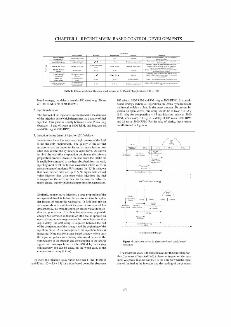
CHAPTER 1. RECENT MVEM BASED CONTROL DEVELOPMENTS
SpecificationsSensing method Accuracy Response time Linearity Comments
manifold absolutepressure (MAP) Piezoresistive silicon �! " 1 ms Excellent Dynamic response deteriorates with long pneumatic
transmission linesmanifold air
temperature (MAT)Metal film or thermistor
or thermocouple �!# " 1 - 10 sec. Nonlinear, compensated Time constant down to 200 ms with a very smallthermocouple
mass air flow (MAF) Hot wire or hot film�%$ " in stationary
flows 50 ms - 0.5 sec. Nonlinear, compensatedDynamics depends on engine operating conditions,
unidirectional, very inaccurate during transients(tip-in/out, pumping fluctuations) [10]
Throttle PositionSensor Potentiometer �%$ " 0.1 ms Excellent Several potentiometers may be used in series/parallel to
increase locally the accuracy
Crank/Cam-shafttiming/speed
Hall effect or variablereluctance & " 30 ' s - 300 ' s Excellent
The primary goal of the sensors is to provide triggerssignals to the timing processor unit of the electronic
control unit (ECU)exhaust-gas-
oxygen (EGO)Zirconium dioxide
ceramic 1 - 6% 50 ms Highly nonlinear Used as a switch between lean & reach air/fuel ratios
Sens
orty
pe
universal exhaust-gas-oxygen (UEGO)
Zirconium dioxideceramic with oxygen
pumping device1 - 6% & 50 ms Nonlinear, compensated
Subject to drift, available as production type sensor since1999
Table 1: Characteristics of the most used sensors in AFR control applications ([11], [12])
based strategy, the delay is usually 180 cdeg long (30 msat 1000 RPM, 6 ms at 5000 RPM).
2. Injection duration
The flow out of the injector is constant and it is the durationof the injection pulse which determines the quantity of fuelinjected. This pulse is usually between 2 and 15 ms long(between 12 and 90 cdeg at 1000 RPM, and between 60and 450 cdeg at 5000 RPM).
3. Injection timing (start of injection (SOI) delay)
In order to achieve low emissions, tight control of the AFRis not the only requirement. The quality of the air-fuelmixture is also an important factor: as much fuel as pos-sible should enter the cylinders in vapor form. As shownin [14], the wall-film evaporation dominates the mixturepreparation process; because the heat from the intake airis negligible compared to the heat absorbed from the wall,injecting most or all the fuel on closed hot intake valves isa requirement of modern MPI systems. In [15] it is shownthat heat-transfer rates are up to 50% higher with closedvalve injection than with open valve injection; the fuelis trapped on the valve surface for the time the valve re-mains closed, thereby giving a longer time for evaporation.
Similarly, in open valve injection, a large proportion of theunvaporized droplets follow the air stream into the cylin-der instead of hitting the wall/valve. In [16] tests run onan engine show a significant increase in emission of hy-drocarbons ( (*) ) from injection on closed valves to injec-tion on open valves. It is therefore necessary to provideenough SOI advance so that no or little fuel is sprayed onopen valves; in order to guarantee the proper injection tim-ing, a delay (the SOI delay) is required between the endof the computation of the strategy and the beginning of theinjection pulse. As a consequence, the injection delay isincreased. Note that for a time-based strategy where onlythe injection pulses are crank-synchronized (whereas thecomputation of the strategy and the sampling of the AMFRsignals are time-synchronized) the SOI delay is varyingcontinuously and can be equal, in the worst case, to thecomputational delay (15 ms).
In short, the injection delay varies between 17 ms (15+0+2)and 45 ms (15 + 15 + 15) for a time-based controller (between
102 cdeg at 1000 RPM and 900 cdeg at 5000 RPM). In a crank-based strategy (where all operations are crank-synchronized),the injection delay is fixed in the crank domain. To prevent in-jection on open valves, this delay should be at least 630 cdeg(180 cdeg for computation + 15 ms injection pulse at 5000RPM, worst case). This gives a delay of 105 ms at 1000 RPMand 21 ms at 5000 RPM. For the sake of clarity, these resultsare illustrated in Figure 4.
IntakeValve
Opening
ComputationDuration
Override ofControl Variable
Sampling of
180 deg
180 deg 180 deg 180 deg 180 deg
PulseInjection
2 - 15 ms90 - 450 deg
450 deg
Injection Delay: 630 deg21 - 105 ms
Sensor Signals
t
SOI Delay
IntakeValve
Opening
2 - 15 ms
15 ms
ComputationDuration
InjectionPulse
Override ofSampling ofSensor Signals
0 - 15 ms
15 ms15 ms 15 ms 15 ms
Override of Control Variable for Next Event
Injection Delay: 17 - 45 ms
t
SOI Delay
Control Variable
(b) Crank-based strategy
(a) Time-based strategy
Figure 4: Injection delay in time-based and crank-basedstrategies
The transport delay is the time it takes for the controlled vari-able (the mass of injected fuel) to have an impact on the mea-sured + signals; in other words, it is the time between the injec-tion of the fuel at the injectors and the reading of the + sensor
34

1.3. PREDICTIVE AIR-TO-FUEL RATIO CONTROL
signals by the ECU. Of course, the transport delay exists onlyin the case of , -feedback AFR control. If fuel is injected onclosed valves, it will take about 3 -. strokes (105 ms at 1000RPM, 21ms at 5000 RPM) before it reaches (in burned form)the exhaust manifold. It will take another 2 to 20 ms before itreaches the , sensor (transport time through the exhaust mani-fold). Clearly, no control reaction can occur before this trans-port delay and the injection delay have elapsed.
In [17], it is proved that for a stable plant with a time de-lay (Loop-delay), and whatever the integral square error (ISE)-optimal controller6 which is used, the maximum achievablebandwidth of the controlled system is equal to:/
Loop-Delay
This is the upper limit (right half plane zeros decrease this limitfurther) which can be achieved with an ideal unrealizable (nopenalty on the input) controller; note that this applies to anytype of controller, including pure feedforward.
In the case of exhaust , -feedback, the loop-delay is equal tothe sum of the injection delay and the transport delay:
Loop-Delay =Injection
Delay +Transport
Delay(best case,
time-based) = 17 ms + 23 ms
(worst case,time-based) = 45 ms + 125 ms
(best case,crank-based) = 21 ms + 23 ms
(worst case,crank-based) = 105 ms + 125 ms
In the case where the controller is based only on measurementsmade in the intake manifold, the loop-delay equals the injectiondelay only:
Loop-Delay =Injection
Delay(best case,
time-based) = 17 ms
(worst case,time-based) = 45 ms
(best case,crank-based) = 21 ms
(worst case,crank-based) = 105 ms
The consequences in terms of bandwidth limitation of thecontrolled system are summarized in Table 2. It is seen thatthe optimal bandwidth of an ideal , -feedback strategy never ex-ceeds 25 rad/s. This is much too low compared to the 200 rad/srequired for tight transient AFR control. Even for strategiesbased on intake manifold measurements only, the bandwidth is
6a controller which minimizes the integral square error ( 021354 687 9 :<;= 7 9 : 4 >@?�9 ) between the output 6 and the command = , [18].
sometimes as low as 22.5 rad/s for an ideal time-based strat-egy and 9.5 rad/s for an ideal crank-based strategy. This lattervalue corresponds to low engine speed (1000 RPM) where mostof the tip-ins happen, and is therefore the source of large tran-sient errors during acceleration. However, even if none of theabove strategies can satisfy the bandwidth requirements, strate-gies based on intake manifold measurements are clearly to bepreferred to those based on exhaust measurements, as far asoverall system bandwidth is concerned.
2.3.2 Disturbances and Injection Delay
In the previous section it was shown that even strategies basedonly on ideal intake measurements are unable to meet the band-width requirements of a tight AFR controller; this is due to thelarge injection delay imposed on the controller by the hardware.Concretely, any disturbance which may occur between the mea-surement of the AMFR signals and the actual injection of thefuel may lead to a large mismatch between the amount of in-duced fuel and the amount of induced air.
Two types of disturbances, mainly, are possible: a change ofexternal load (torque) on the crankshaft (and consequently achange of engine speed) and a change of throttle position (andconsequently a change in air mass flow). The inertia of the ve-hicle/engine prevents the engine speed from changing on timescales smaller than a few seconds (much larger than the injec-tion delay) and the disturbances associated with the varying ex-ternal load can safely be discarded on the same basis. However,because of the fast dynamics associated with the intake mani-fold, any change in the throttle position after the AMFR mea-surements are made will immediately move the port air massflow away from the value estimated (anticipated) in the ECU[19].
The resulting AFR excursions can be very large as illustrated inFigure 5. Note that in this simulation, the crank-based strategyis ideal in the sense that perfect knowledge of the port air massflow at the sampling instants, no fuel-film and no pumping fluc-tuations are assumed; the transient , excursions are solely dueto the injection delay which is set to 630 crank degrees. Theengine speed is kept constant and the only disturbance comesfrom the movement of the throttle.
3 MODELING THE INTAKE AIRDYNAMICS
In this section the Mean Value Engine Model (MVEM)7, whichforms the basis of the model-based controller described in Sec-tion 4, is presented. The validity of the model during transientoperation is discussed in a companion paper by some of the au-thors [20]. The focus is on the validity of the dynamic air flowmodel which is normally used in control applications. Threepoints critical to accurate transient modeling are emphasized:
7A compact, but accurate, description of the mean values (no pumping fluc-tuations) of some engine variables, both during steady-state and transient oper-ation
35

CHAPTER 1. RECENT MVEM BASED CONTROL DEVELOPMENTS
Controller based on exhaustmeasurements
Controller based on intakemeasurements
Best Case Worst Case Best Case Worst CaseTime-Based 25.0 rad/s 5.9 rad/s 58.8 rad/s 22.2 rad/s
Crank-Based 22.7 rad/s 4.3 rad/s 47.6 rad/s 9.5 rad/s
Table 2: Comparison of the approximate maximum bandwidth of different types of air/fuel ratio controllers. Note thatthese figures are largely over estimated since they apply to ideal unrealizable controllers with infinitely fast sensors.These figures should be compared to the required bandwidth of 200 rad/s.
0 0.5 1 1.5 2 2.5 3 3.5 4 4.5 520
25
30
35
40
45
50
PSfrag replacements
ACB D EFG H IJ KL
MONQP R R R S%T!UVXW Y D Z N\[ ] P ^ _ `V@acb dcNCef] g g P `4 cylindersh R N\[ _f] i jlk m ]
(a) Throttle position
0 0.5 1 1.5 2 2.5 3 3.5 4 4.5 58
10
12
14
16
18
20
PSfrag replacements
ACB D E
4 cylinders
n oG J pqrs L t Injection Delayu va b Zw A x vacy
(b) Air and fuel mass flow rates
0 0.5 1 1.5 2 2.5 3 3.5 4 4.5 50.8
1
1.2
1.4
1.6
PSfrag replacements
ACB D E
4 cylinders
Injection Delayz(c) { excursions (Speed-Density strategy)
Figure 5: The impact of injection delay on transient AFRcontrol.| Despite the complex nature of acoustic phenomena dur-ing transients (rapid throttle opening/closing, varying loadon the crank), conventional steady-state volumetric effi-ciency maps are capable of describing the engine breath-ing performance with a remarkable accuracy also duringfast transient operation; consequently, the so-called speeddensity equation (2) provides a very accurate descriptionof the port air mass flow, provided the mean air density isknown with equivalent accuracy in the intake manifold.
}~��@����2� b ac� � � acb d��� � ���� ��� �X�O�%� � �X�� � ���l� �����X� ���¡ 8¢ � � ���£ ��� �X� (2)
where �2� b ac� � � acb d��� � is the volumetric efficiency based onbarometric pressure, � � ��� and intake manifold tempera-ture,
�¤� �X� . For the sake of accuracy and speed, it is stored
in a map table. Unlike � � ������ � , � � b ac� � � a¤bfd��� � depends almostlinearly on the pressure ratio �¦¥ � � a¤bfd� bfac� and errors asso-ciated with linear interpolation between the points of thegrid are minimized - this is the justification for using thelatter of the two.| The isentropic converging nozzle/sudden enlargementmodel, which is normally used to describe the throttle airmass flow, is too inaccurate for actual use. Because theflow splits along two paths across the plate (one large dom-inant flow, and one small residual flow), a more accuratetwo-channel model is proposed in [20]. This model ismade up of two isentropic converging nozzle/sudden en-largement models in parallel. In the dominant channel, thepressure loss at the throat amounts to the total pressure lossacross the throttle ( �¨§%©«ª¬� ~�¯® ), whereas, in the resid-ual channel, the pressure loss only amounts to a part, °( °²±´³ ¢ � ��µ ) of the total pressure loss ( °O¶ ��§%©«ª·� ~�¯®c¸ ).Finally, the contribution of the residual flow is ¹ times thatof the dominant flow. The model is summarized below:}~��Xº ¶ » � � � �X� � �¦¼ � � � � ��� ¸½� �c¼ �� � � ���¦¾�¿ ¶ » ¸� �¹ÁÀ � ¾l ¶ �c¥ ¸ À ¹¹�À � ¾�Â2à � ª °O¶ � ªÄ�¦¥ ¸fÅ � (3)
where
�¦¥ � � � ����c¼ �¾� ¶ Æ ¸½�ÈÇ ÉËÊ¡Ì ¶ Æ � �c¥XÍ ¸ [Î ª ÉËÊ¡Ì ¶ Æ � �c¥XÍ ¸ Î�Ï [ÎÇ �c¥XÍ [Î ªÄ�c¥�Í Î�Ï [Î�¦¥XÍ �ÈÐ Ñ À �lÒ ÎÎÔÓ [�Õ ¢2Ö ×¯ 8دÙ(4)
and¾�¿ ¶ » ¸Ú�ÜÛ ¿fÝ À Û ¿@¿�Þ�ß%à ¶ » ¸ ÀÛ ¿f¤Þ�ß%à  ¶ » ¸ À Û ¿fá¤Þ�ß%à á ¶ » ¸ (5)
�c¥ is the pressure ratio across the throttle plate. �¦¥XÍ is thepressure ratio threshold below which the flow is sonic at athroat. ¾� and ¾�¿ are functions which account for com-pressibility and effective throat area changes. ° , ¹ andÛ ¿ Ý Ö�Ö�Ö Û ¿fá are fitting constants.
For pressure ratios above 0.9, the flow becomes extremelysensitive to pressure ratio variations:â ã É�¯äXå ¿½æ }~ �@ºæ �c¥ � ª<ç (6)
36

1.3. PREDICTIVE AIR-TO-FUEL RATIO CONTROL
and it is therefore important to know accurately not onlythe pressure downstream the throttle, è½éOê�ë , but also thepressure upstream, è¦ì�í . Usually, no pressure sensors areavailable upstream the throttle plate and this pressure is as-sumed to be equal to the barometric pressure, è êXé�î . How-ever, because of the presence of an air filter, neglectingthe air filter pressure loss can lead to very large throttleair mass flow modeling errors close to wide open throt-tle (WOT). It is therefore necessary to compensate for thispressure loss and the following model is proposed:
è¦ì�íCïðè¦ê�éOîÚñÄò«óÔô õ ö«÷ø�ù¯úê@ö«ûÚü ê�é�îè¦êXé�î8ý ù¯þ (7)
where ò²ó�ô õ ö , ÿ�� and ÿ�� are fitting constants (in the presentwork, the air filter was replaced with a laminar flow meterand ÿ��Qï ÿ��Qï � ). Note that Equations (3) and (7) needto be solved simultaneously for ÷ø êXö and ècì�í (implicitsolution). An iterative solution is proposed in Appendix A.
This model was tested on a steady flow bench and wasshown to describe the throttle air mass flow with an excel-lent accuracy (error � 3% of actual flow) over the entireoperating region. On an engine where the flow is typicallyunsteady, the model describes the instantaneous flow withthe same accuracy, since the throttle body is much smallerthan the wave length of the pumping fluctuations. How-ever, because of the strong nonlinearity of the flow for �close to 1 (see Equation (6)), the mean of the ��� functionapplied to (instantaneous) � differs from the �� functionapplied to the mean of � (in short: ��� �� ����� �� )so that the model of Equation (3) is not very appropriatefor Mean Value Engine Modeling ( for � close to 1 only).This is illustrated in Figure 6 where errors up to 50% areunavoidable close to WOT.
0.3 0.4 0.5 0.6 0.7 0.8 0.9 10
0.01
0.02
0.03
0.04
PSfrag replacements
���� � ��� � � ��� !
19.0 deg
77.0 deg "model
measurements
(a) Comparison between the model and the measurements for different throttleopenings (19.00, 20.00, 21.00, 22.50, 25.00, 27.50, 30.00, 35.00, 40.00, 50.00,60.00, 77.00 deg.)
0.3 0.4 0.5 0.6 0.7 0.8 0.9 1
−60
−40
−20
0
PSfrag replacements
�#�
19.0 deg
77.0 deg
model
measurements
erro
r[
$ ]
(b) Relative air mass flow error
Figure 6: Two-channel throttle air mass flow model. Notethe large error due to pumping fluctuations for pressure ra-tios close to 1.
% The isothermal assumption ( ÷ü é�êXë ï'& ) which is normallyused in the one-state manifold model8 [21] leads to a some-what inaccurate description of the intake air density duringtip-ins and tip-outs. Mass conservation and energy con-servation in the intake manifold should both be consideredto properly describe the air dynamics. The difference be-tween the isothermal model (single state) and the adiabaticmodel (two states) can be of up to 15% in port air massflow, and it is therefore important that the right model isused in order to achieve tight AFR control.
The following equations are for the two-state MVEM:÷è¦é�êXëËï ècé�êXë)(+* ü ê�é�î, éOê�ëOècé�êXë- ÷ø êXö ñ ü � ÷ø ê@í/. ( ñ �(0*÷132 4 öü êXé�î�5÷ü éOê�ë\ï ü é�êXë (+* ü êXé�î, é�êXëOècé�ê�ë- ÷ø êXö76 � ñ �( ü �98�ñ ü �*÷ø êfí�6 � ñ
�( 8.:( ñ �(0*
÷132 4 öü êXé�î 5(8)
where
ü ��ï ü é�ê�ëü êXé�î÷132 4 ö¦ï<;= ü ê�é�î¦ñ ü é�êXë> (9)
Heat transfer, ÷132 4 ö , is also included in the model since itmay play an important role during fast throttle openingsand closings where compression/expansion effects resultin large intake temperature spikes ([22], [20]). ; is theheat transfer coefficient in ?A@B7CED . ÷ø êXö and ÷ø ê@í are givenin Equations (3) and (2).
Note that in [20], it is also suggested that the pressure lossesat the junctions between the intake plenum and the intake run-ners might not be negligible, and might therefore influence thetime development of the pressure and the temperature in therunners. The solution which is proposed is to model the intakemanifold as two control volumes (one for the plenum and onefor the runners instead of one for the whole system) separatedby an orifice. Each volume is described by two state equations(mass and energy conservation), one for pressure and one fortemperature. Unfortunately, the orifice flow resistance variessignificantly with the flow velocity; at low flows, the resistanceis almost zero and the associated eigenfrequencies become infi-nite. The resulting stiffness of the 4-state model requires verysmall simulation steps which are impractical for real time ap-plications and only one control volume (2-state model) will beused in this work. This simplification results in temperature dif-ferences in the order of 10 K during fast transients.
Finally, it should be clear that because the inertia of the ve-hicle/engine prevents the engine speed from changing on time
8A differential equation which describes the time development of the airpressure in the intake manifold of a naturally aspirated spark ignition (SI) en-gine.
37

CHAPTER 1. RECENT MVEM BASED CONTROL DEVELOPMENTS
scales smaller than a few seconds, and because the engine speedcan be measured very accurately, F is treated in this work as aknown, slowly varying parameter.
4 WIDE BANDWIDTH AIR/FUEL RATIO CONTROL
In Section 2, an attempt was made to make a list of all the limita-tions, physical and practical, which make wide bandwidth AFRcontrol a challenging task. It should now be clear that thereare not many methods available to overcome these limitations.The one proposed in this research is quite similar to the onesfound in conventional transient strategies9, except that the portair mass flow is predicted ahead in time instead of being simplyestimated at the current instant. In this way, the limitation im-posed by injection time delays can be removed. The structureof this model-based wide-bandwidth predictive controller is de-picted in Figure 7. The derivation of this controller is discussedin details in the following sections.
4.1 Choice of Sensors
Because of the bandwidth limitations imposed by the transportdelay associated with G -feedback control and because of thelarge time constant of oxygen sensors, the new strategy is pri-marily based on intake manifold measurements. Among all thesensors which can be mounted on an intake manifold, a MAPsensor (time constant H 1 ms) was preferred to the popularMAF sensor which is too slow, too inaccurate, too nonlinearand more costly. Also mounted on the intake manifold are athrottle position sensor and a fast 0.4 mm Nickel/Chromium-Nickel/Aluminium type K thermocouple with a time constant of200 ms. The engine is also instrumented with an engine speed(and position) sensor and barometric pressure and temperaturesensors. Finally, a UEGO sensor is mounted in the exhaust pipeto guarantee some robustness of the controller (this is explainedlater). The engine setup is illustrated in Figure 8.
4.2 Choice of Actuators
Because it is impossible to predict what the driver intends to dowith the accelerator pedal, the bandwidth limitations imposedby the injection delay associated with conventional AFR con-trollers is a critical issue. One solution to this problem was sug-gested more than 20 years ago by Stivender [23] where the ideaof controlling not only the fuel path but also the air path wasfirst introduced as an alternative solution to AFR managementcontrol. The solution followed in this work complements theconventional fuel injectors with an electrically controlled throt-tle actuator (also known as drive by wire (DBW)). In this way,the injection delay can be compensated for.
9Fuel flow is treated as a dependant variable; intake air flow is first measuredor estimated, then fuel injectors are operated to meter the proper amount of fuelinto the engine.
0.15 0.2 0.25 0.3 0.35 0.4 0.4515
20
25
30
35
40
45
50
PSfrag replacements
IKJ L M
NO P QR ST U Prediction HorizonVAccelerator pedal position( W X )Sampled Accelerator pedalposition ( W X Y )Predicted throttle plate posi-tion ( W X Z )Drive-by-Wire command( W X [ \ )Actual throttle plate position( W )
Figure 9: Delaying the driver’s throttle command. Thedriver’s command ]^ is sampled, held and delayed (storedin a buffer) in the ECU ( ] ^#_ ). After a time equivalent tothe prediction horizon, this sampled signal is sent to theDBW actuator ( ] ^a` b ). Note that, because of the time re-sponse of the DBW, the actual throttle plate position ] dif-fers from ] ^#` b . In particular, the resulting time lag canbe large enough so that the DBW dynamics cannot be ig-nored in the prediction algorithm. With a good model ofthe DBW dynamics, the throttle position can be predictedaccurately ( ] ^ c ). As explained later, the prediction horizonis set to 495 crank degrees ( 0.0825 sec. at 1000 RPM and0.0165 sec. at 5000 RPM). This delay introduced betweenthe driver’s pedal command and the throttle plate is shortenough to be imperceptive to the driver, although this is stillto be evaluated in a vehicle under real driving conditions.
By buffering the sampled driver command into the memoryof the ECU, the throttle motion can be delayed for a time equalto the injection delay, see Figure 9. Consequently, the throttleposition is known sufficiently in advance so that the controllercan safely predict the amount of air to be sucked in during thenext induction event. For this reason, the injection delay willalso be referred to as the prediction horizon in the remainder ofthis paper.
However, because the DBW actuator is not infinitely fast, thecommanded throttle position and the actual throttle position candiffer greatly. For example, the DBW used in this work behavesas a well damped second order system with an undamped nat-ural frequency, dfe�g h , of 76.9 rad/s and a damping factor, i9e�g h ,of 0.675. As can be seen in Figure 9, the resulting time lag istoo large to be ignored during transients. In order to predict ac-curately enough the actual throttle position, the dynamics of theactuator must thus be taken into account in the predictor as well.To this end, a second-order low-pass filter is used to model theDBW dynamics:
jlk monj e#g h k m�n3p dKqe#g hm qKrts i�e�g hud�e�g h m r d qe�g h (10)
where m is the Laplace operator. j e#g h is the command signalto the DBW actuator and j is the actual throttle position (seeFigure 9). Because the controller is implemented in discrete
38
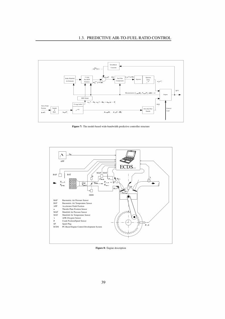
1.3. PREDICTIVE AIR-TO-FUEL RATIO CONTROL
Air Estimator Predictor
Port MAF
11-step
Hold&
Sample
Controller
Position
Intake Manifold
Driver Pedal
Engine
External
Load
Injection
Delay
12-stage buffer
DBW Model
Injectors+
+
Compensator
Fuel Film
Drive-By-Wire
Throttlevaw x y zvax y z
{ |a} }
~-feedback
{ |�} }vaw � x y z v w � � x y z��Ev w � x y���� � z
Measurements ( ���o� x y z � � ��� x y z � vax y z�� � � z ~ x y z��� � x y z�>�a�� x y���� � z
� �a�� x y �u� � z� � � x y �u� � z�>� w x y �u� � z
v w � x ya�� z � v w � x y��� z �a� � � v w � x ya�� � z
Figure 7: The model-based wide-bandwidth predictive controller structure
��������������������������������������������������������
SP
MAT� ���f�a������ ����� ¡o��� � �a�
�� ��¢MAP
¡7£ ¤
¥#¦�§
¨��©¨�ª «DBW
� ��¡ �� ¡ ����¬0¯® °� ����¬
�o±
�MAPMAT�¥
Barometric Air Pressure SensorBarometric Air Temperature Sensor
Throttle Plate Position SensorManifold Air Pressure SensorManifold Air Temperature SensorAFR (Oxygen) SensorCrank Position/Speed Sensor
SP Spark PlugECDS PC-Based Engine Control Development System
APP Accelerator Pedal Position
BAP BAT
ECDSV2.0
APP
BAPBAT
Figure 8: Engine description
39
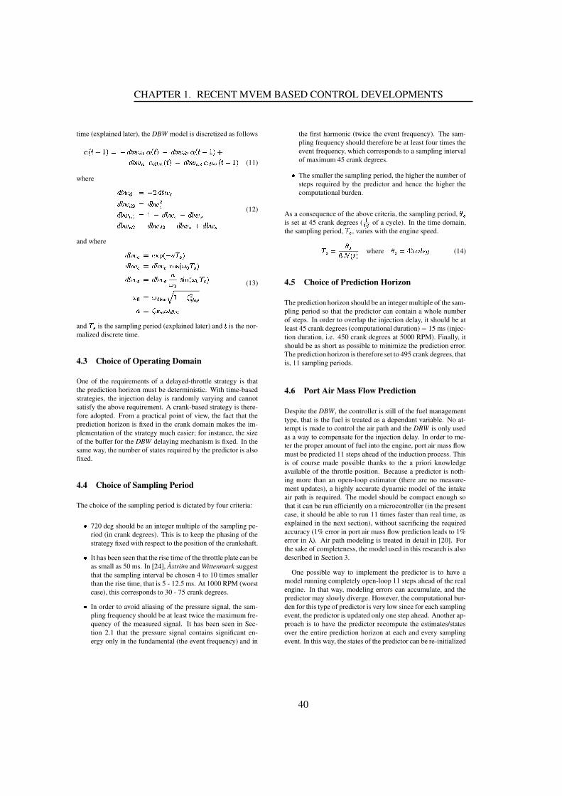
CHAPTER 1. RECENT MVEM BASED CONTROL DEVELOPMENTS
time (explained later), the DBW model is discretized as follows
²l³ ´uµ<¶o·�¸º¹¼»�½#¾/¿�À�²K³ ´�·¯¹Á»�½#¾+¿aÂu²l³ ´�¹t¶o·uµ»�½a¾/Ã�Àu²�¿�Ä ÅK³ ´a·ÆµÇ»�½a¾/Ã7Â�²�¿�Ä ÅK³ ´�¹t¶o· (11)
where »�½#¾/¿�À¯¸È¹0É�»�½#¾/Ê»�½#¾/¿#Â˸ǻ�½a¾ ÂÌ»�½a¾/Ã�À¯¸È¶Ë¹Í»�½#¾+ÊE¹Î»�½#¾+Ï»�½a¾ Ã7 ¸Ç»�½a¾ ¿# ¹Î»�½a¾ Ê µÐ»�½a¾ Ï (12)
and where »�½a¾ Ì ¸ÁÑ9Ò�Ó�³ ¹+Ô�Õ�Ï#·»�½#¾/Êָ׻�½#¾ Ì0Ø�Ù�Ú ³ Û�Ü9ÕuÏ�·»�½a¾+ϯ¸×»�½#¾ Ì ÔÛ�Ü Ú�Ý Þ ³ Û�Ü�ÕuÏ�·Û�Ü߸ÐÛf¿�Ä Ålà ¶/¹�á ¿�Ä ÅÔt¸Çá9¿#Ä ÅuÛ�¿�Ä Å(13)
and Õ�Ï is the sampling period (explained later) and ´ is the nor-malized discrete time.
4.3 Choice of Operating Domain
One of the requirements of a delayed-throttle strategy is thatthe prediction horizon must be deterministic. With time-basedstrategies, the injection delay is randomly varying and cannotsatisfy the above requirement. A crank-based strategy is there-fore adopted. From a practical point of view, the fact that theprediction horizon is fixed in the crank domain makes the im-plementation of the strategy much easier; for instance, the sizeof the buffer for the DBW delaying mechanism is fixed. In thesame way, the number of states required by the predictor is alsofixed.
4.4 Choice of Sampling Period
The choice of the sampling period is dictated by four criteria:
â 720 deg should be an integer multiple of the sampling pe-riod (in crank degrees). This is to keep the phasing of thestrategy fixed with respect to the position of the crankshaft.â It has been seen that the rise time of the throttle plate can beas small as 50 ms. In [24], Åström and Wittenmark suggestthat the sampling interval be chosen 4 to 10 times smallerthan the rise time, that is 5 - 12.5 ms. At 1000 RPM (worstcase), this corresponds to 30 - 75 crank degrees.â In order to avoid aliasing of the pressure signal, the sam-pling frequency should be at least twice the maximum fre-quency of the measured signal. It has been seen in Sec-tion 2.1 that the pressure signal contains significant en-ergy only in the fundamental (the event frequency) and in
the first harmonic (twice the event frequency). The sam-pling frequency should therefore be at least four times theevent frequency, which corresponds to a sampling intervalof maximum 45 crank degrees.â The smaller the sampling period, the higher the number ofsteps required by the predictor and hence the higher thecomputational burden.
As a consequence of the above criteria, the sampling period, ã Ïis set at 45 crank degrees (
ÀÀ�ä of a cycle). In the time domain,the sampling period, Õ�Ï , varies with the engine speed.
ÕuÏK¸ ã Ïå�æ ³ ´a· where ã ÏK¸'ç�è�é�»�ê9ë (14)
4.5 Choice of Prediction Horizon
The prediction horizon should be an integer multiple of the sam-pling period so that the predictor can contain a whole numberof steps. In order to overlap the injection delay, it should be atleast 45 crank degrees (computational duration) µ 15 ms (injec-tion duration, i.e. 450 crank degrees at 5000 RPM). Finally, itshould be as short as possible to minimize the prediction error.The prediction horizon is therefore set to 495 crank degrees, thatis, 11 sampling periods.
4.6 Port Air Mass Flow Prediction
Despite the DBW, the controller is still of the fuel managementtype, that is the fuel is treated as a dependant variable. No at-tempt is made to control the air path and the DBW is only usedas a way to compensate for the injection delay. In order to me-ter the proper amount of fuel into the engine, port air mass flowmust be predicted 11 steps ahead of the induction process. Thisis of course made possible thanks to the a priori knowledgeavailable of the throttle position. Because a predictor is noth-ing more than an open-loop estimator (there are no measure-ment updates), a highly accurate dynamic model of the intakeair path is required. The model should be compact enough sothat it can be run efficiently on a microcontroller (in the presentcase, it should be able to run 11 times faster than real time, asexplained in the next section), without sacrificing the requiredaccuracy (1% error in port air mass flow prediction leads to 1%error in ì ). Air path modeling is treated in detail in [20]. Forthe sake of completeness, the model used in this research is alsodescribed in Section 3.
One possible way to implement the predictor is to have amodel running completely open-loop 11 steps ahead of the realengine. In that way, modeling errors can accumulate, and thepredictor may slowly diverge. However, the computational bur-den for this type of predictor is very low since for each samplingevent, the predictor is updated only one step ahead. Another ap-proach is to have the predictor recompute the estimates/statesover the entire prediction horizon at each and every samplingevent. In this way, the states of the predictor can be re-initialized
40

1.3. PREDICTIVE AIR-TO-FUEL RATIO CONTROL
every sampling event according to the latest available measure-ments (i.e. the latest available information is extrapolated intothe future for the purpose of prediction). Clearly, this measure-ment update should minimize the prediction error. The draw-back of this approach is that the calculation burden is greatlyincreased since, within each sampling event, the model’s re-sponse needs to be computed over 11 time steps (in terms ofthe computer burden, one 11-step predictor is equivalent to 11one-step-ahead predictors running in parallel!). For the sake ofclarity, the modus operandi of the predictor is illustrated in Fig-ure 10.
Because accuracy is the primary requirement of modern AFRcontrollers, the 11-step predictor with measurement update isused in this research. This also establishes a limit for the bestpossible performance.
If it is assumed that, at the current instant í , estimates ofthe mean of the intake pressure and temperature ( îï�ð/ñ�ò�ó íaô ,îõ ð/ñ#ò ó í�ô ) are available (see next section), as well as measure-ments of
ï�ñ#ð/ö�ó íaô , õuñ#ð/ö9ó íaô , ÷ ó íaô , ø ó íAùÍúoô , ø ó íaô , û ø�ü�ý ó íAùúoþ�ôÿ9ÿ�ÿ�ø�ü�ý ó ílù'þ�ô � (eventually buffered in the ECU), then the11-step port air mass flow predictor can be derived as in Equa-tions (15) and (16).�ï�ð/ñ#òuó í��'úoô�� îï�ð/ñ#òuó íaô�� î �ï�ð/ñ�ò�ó íaô�ÿ õ ý�õuð/ñ#ò�ó í��'úoô�� îõ�ð/ñ#ò�ó íaô�� î �õuðlñ�ò�ó íaô�ÿ õ ý�ø ó í��'úoô�� ù�� �+ü �ø ó íaôEù�����+ü �uø ó í�ùtúoô������ ò � ø ü#ý ó í�ùtú�úoô����� � ò � ø ü�ý ó í�ùtúoþ�ô�ï�ð/ñ#òuó í��tþ�ô�� �ï�ð/ñ#òuó í��'úoô�� � �ï�ð/ñ�ò�ó í��<úoô�ÿ õ ý�õuð/ñ#ò�ó í��tþ�ô�� �õ�ð/ñ#ò�ó íaô�� � �õuðlñ�ò�ó í��'úoô�ÿ õ ý�ø ó í��tþ�ô�� ù�� �+ü � �ø ó í��'úoô3ù�����+ü �uø ó íaô������ ò �ø�ü#ý ó í�ùtú���ô����� � ò ��ø�ü�ý ó í�ùtú�úoô (15)
...�ø ó í��'ú���ô�� ù�� �+ü � �ø ó í�����ô3ù�����+ü �uø ó í�����ô������ ò � ø ü#ý ó í�ù�þ�ô����� � ò � ø ü�ý ó í�ù���ô�ï�ð/ñ#ò�ó í��'ú�úoô�� �ï�ð/ñ#òuó í��'ú���ô � � �ï�ð/ñ�òuó í��'ú���ô�ÿ õ ý�õuðlñ�òó í��'ú�úoô�� �õ�ð/ñ#ò�ó í��<ú���ô � � �õuð/ñ#ò�ó í��'ú���ô�ÿ õ ýThe hats (î ) denote estimated states and the inverted hats (
�) de-
note predicted states. The speed-density equation (Equation (2))gives the predicted port air mass flow (11 steps ahead) as a func-tion of the predicted intake manifold conditions.
�! ñ#">ó í��'ú�úoô$�%�! ñ#">ó �ï�ð/ñ#òuó í��'ú�úoô'& �õ�ð/ñ�òó í��'ú�úoô'&÷ ó íaô'& ï�ñ�ðlö�ó íaô�ô (16)
The (desired) amount of fuel which should be injected at anygiven instant and enter the cylinders 11 steps later ( !)(�(* , in unit
mass per sampling period) is given in Equation (17).
! (�(* ó í��'ú�úoô�� úoþ+� � �! ñ�"�ó í��'ú�úoô,.- / ú�0f÷ ó íaô ú132 4 * (17)
where the reference1
,132 4 * is in principle set to 1 for current
TWC’s.
In Equation (15), the state derivatives are calculated accord-ing to Equations (2), (3), (7) and(8) in which the dependant vari-ables are determined as follows:î �ï�ðlñ�òuó íaô.� �ï�ð/ñ�ò�ó îï�ðlñ�òuó íaô &¼îõ�ð/ñ�ò�ó íaôõuñ#ð/ö9ó íaô & ï�ñ#ð/ö�ó íaô5&�÷ ó í�ô5&fø ó íaô�ôî �õ�ð/ñ�ò�ó íaô.� �õ�ð/ñ�òó îï�ð/ñ#òuó íaô5&ßîõ�ð/ñ�òó í�ôõuñ#ð/ö9ó íaô & ï�ñ#ð/ö�ó íaô5&�÷ ó í�ô5&fø ó íaô�ô� �ï�ð/ñ#òuó í��'úoô.� �ï�ð/ñ�ò�ó �ï�ðlñ�òuó í��'úoô & �õ�ð/ñ�ò�ó í��'úoôõuñ#ð/ö9ó íaô & ï�ñ#ð/ö�ó íaô5&�÷ ó í�ô5& �ø ó í��'úoôaô� �õ�ð/ñ�ò�ó í��'úoô.� �õ�ð/ñ�òó �ï�ð/ñ#òuó í��'úoô & �õ�ð/ñ�òó í��'úoôõuñ#ð/ö9ó íaô & ï�ñ#ð/ö�ó íaô5&�÷ ó í�ô5& �ø ó í��'úoôaô
... (18)� �ï�ð/ñ�ò�ó í��'ú���ô$� �ï�ð/ñ�ò�ó �ï�ðlñ�òuó í��'ú���ô & �õ�ð/ñ�ò�ó í��'ú���ôõuñ#ð/ö9ó íaô & ï�ñ#ð/ö�ó íaô5&�÷ ó í�ô5& �ø ó í��'ú���ôaô� �õ�ð/ñ�ò�ó í��'ú���ô$� �õ�ð/ñ�òó �ï�ð/ñ#òuó í��'ú���ô & �õ�ð/ñ�ò�ó í��'ú���ôõuñ#ð/ö9ó íaô & ï�ñ#ð/ö�ó íaô5&�÷ ó í�ô5& �ø ó í��'ú���ôaôNote that ø ó íaô , ø ó ílù<úoô , îï�ð/ñ�ò�ó íaô and îõuð/ñ#òó íaô are used to
initialize the predictor. For the pressure and temperature stateequations, simple Euler integration is used. This is to keep thecomputer burden to an acceptable level (compared to the solu-tion which consists in linearizing then discretizing - on line -the model, and which involves the computation of many ma-trix exponential functions). Given the relatively small size ofthe sampling period, no significant accuracy penalty could beobserved for this (tested off-line).
The throttle position predictor is based on Equation (11)where ø�ü ö 6Kó íaô has been replaced by ø�ü�ý ó íKù:ú�úoô (buffered inthe ECU). ø�ü ö 6ló íaô��Çø�ü�ý ó í�ù ú�úoô (19)
4.7 Intake Air Observer
As mentioned previously, the states of the predictor (õ�ð/ñ�ò
,ï ðlñ�ò) need to be re-initialized for every sampling event (mea-
surement update). However, because not all the states of thepredictor can be measured directly (mean intake manifold pres-sure) or with the required bandwidth (intake manifold temper-ature) and because the measurements are corrupted with largenoise contributions (mainly pumping noise), an intake air ob-server is required to estimate/filter the variables of interest. Be-cause of the nonlinear nature of the intake air dynamics, an ex-tended Kalman filter (EKF) [25] is used in this research. It uses
41

CHAPTER 1. RECENT MVEM BASED CONTROL DEVELOPMENTS
777777777777777777777777777777777777777777777777
888888888888888888888888888888888888888888888888
9:9:9:9:9:9:9:9:9:9:9:9:9:9:9:9:9:9:9:9:9:9:9:9:9:9:9:9:9:9;;;;;;;;;;;;;;;;;;;;;;;;;;;;;;;;;;;;;;;;;;;;;;;;
<<<<<<<<<<<<<<<<<<<<<<<<<<<<<<<<<<<<<<<<<<<<<<<<
180
0
540 0 180 360
180 360 540 0 180
11-step predictor =?>$@ A B CEDGF F H
EV2
SOI
t t+2 t+4 t+6 t+8 t+10 t+12 t+14 t+16 t+18
I'J K L M�N$O P Q3NRI'J K L M N�O S QEN
I3J K$TI J K L M�N�O U Q'NRI J K L M N�O V QENI J K L M�N�O W Q'NRI J K L M N�O X QEN
Prediction Horizon: 11 x 45 cdeg = 495 cdeg
Y Y YIV1
EV1
IV2
SOI
Injection Pulse
IV Intake Valve lift
EV Exhaust Valve lift
TDC Cyl Z 1 TDC Cyl Z 2 TDC Cyl Z 3[
(cdeg)
[(cdeg)
Cyl \ 2
Cyl \ 1
SOI
TDC
Start of Injection (270 cdeg before TDC)
Top Dead Center
t+1 t+3 t+5 t+7 t+9 t+11 t+13 t+15 t+17
Calculation (45 cdeg)
360
60 cdeg
I J K TI J K L M�N$O O Q3NRI J K L M N�O ] QEN
11-step predictor =?> @ A B C5D^F _ H11-step predictor =?>$@ A B CED^F ` H
11-step predictor =?>$@ A B CEDGF a#H11-step predictor =b>$@ A B CEDGF c H
11-step predictor =?>$@ A B C5D^F d H11-step predictor =?>$@ A B CED^F e H
11-step predictor =b>$@ A B CEDGF f H
Figure 10: Modus operandi of the 11-step model-based predictor with measurement update. Note how the quantity offuel to be injected, gih5j , is updated on the basis of the last 4 outputs ( k 1 stroke) of the predictor/controller.
the measured intake pressure and temperature as the innovationterms.
The challenges of using EKF’s for engine applications are:
1. the presence of deterministic pumping fluctuations (whichin no way can be considered as stochastic white noise) nor-mally prevents the use of the Kalman-Bucy’s method [26]to calculate the observer gains (Riccati equations can onlybe used to determine how Gaussian white noise propagatesthrough the model).
2. finding the intensity of the process noise. The intensity ofthis noise determines the uncertainty in the different partsof the model. It is the comparison between the model un-certainties and the confidence level of the measurements(measurement noise intensities) which determines the sizeof the observer gains, and it is therefore important to useappropriate noise intensities.
The design procedure for the observer can be split in fourphases: modeling, a priori selection or calculation of noise in-tensities, determination of the gains and finally implementationof the observer. These four phases are discussed below (al-though in a different order).
Modeling The model behind the observer is given in the con-tinuous domain in Equation (20).
lm�nGo5p�qrm�nGo5pts^u$v o nGwx3nGo pym�nGo5p�z l{ o�|�}�~EnGo�|� v�� l{ o#�^}�s ���s u
l��� � |v o5nGw+� }�������� � (20a)lv nGo p�q v nGo5p�s u�v o nGwx nGo p m nGo5p z�� l{ o�|�}�~EnGo |#� � �G� �s v�� �
� v�� l{ o�� � �y� �s ��}�s ���s^ul�R� � |v o5nGw � }�������� � (20b)lv nG� q � �� |'� v nG� � v nGo5p�� }�� ����� (20c)l~EnGo |$q � ���� ~EnGo�|�}�� � ��� � (20d)l��� q � �. E¡�¢ � ��� �)¢¤£� � £ }�� ¡ ¥ (20e)l� £ q � � (20f)
and m�nyn¦q¦m$nGo pR} � £ }�������� (20g)v nyn§q v nG��}���� ��� (20h)
wherem$nyn
and v nyn are the measured intake manifold pres-sure and temperature respectively.
�������#�,�������#�
,�������
,� � ���#�
42
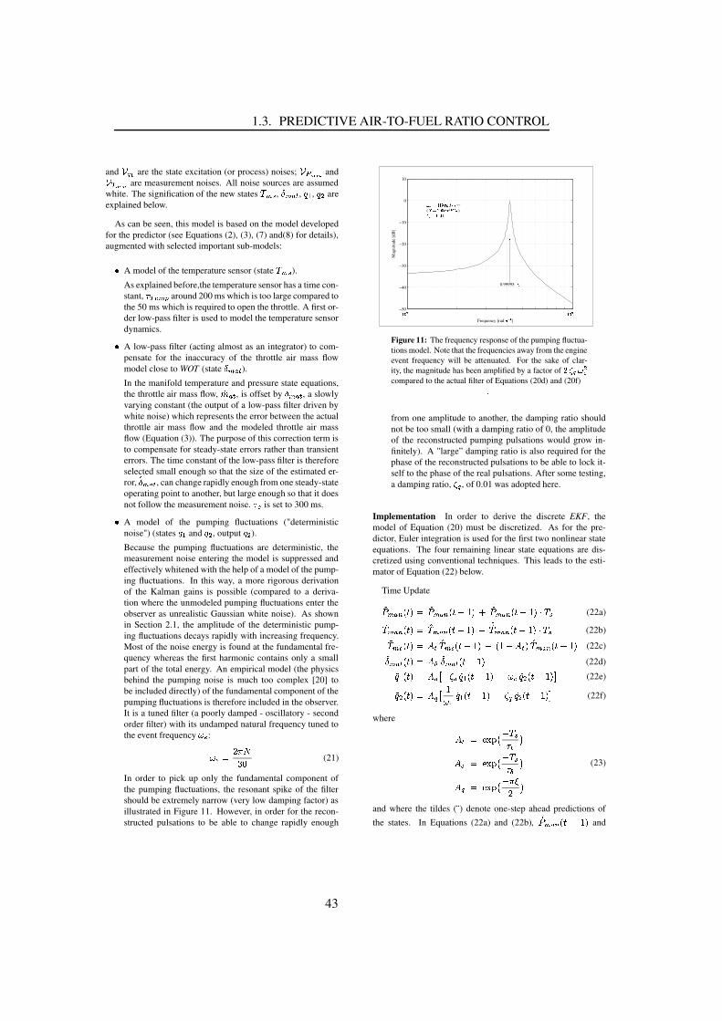
1.3. PREDICTIVE AIR-TO-FUEL RATIO CONTROL
and ¨�© ª are the state excitation (or process) noises; ¨�«�¬�¬ and¨� ¬�¬ are measurement noises. All noise sources are assumedwhite. The signification of the new states ®�¯G° , ±�¯y² ³ , ´�µ , ´�¶ areexplained below.
As can be seen, this model is based on the model developedfor the predictor (see Equations (2), (3), (7) and(8) for details),augmented with selected important sub-models:
· A model of the temperature sensor (state ®�¯G° ).As explained before,the temperature sensor has a time con-stant, ¸�'¹ ¯�º around 200 ms which is too large compared tothe 50 ms which is required to open the throttle. A first or-der low-pass filter is used to model the temperature sensordynamics.· A low-pass filter (acting almost as an integrator) to com-pensate for the inaccuracy of the throttle air mass flowmodel close to WOT (state ±�¯G² ³ ).In the manifold temperature and pressure state equations,the throttle air mass flow, »¼ ²�³ , is offset by ±E¯G² ³ , a slowlyvarying constant (the output of a low-pass filter driven bywhite noise) which represents the error between the actualthrottle air mass flow and the modeled throttle air massflow (Equation (3)). The purpose of this correction term isto compensate for steady-state errors rather than transienterrors. The time constant of the low-pass filter is thereforeselected small enough so that the size of the estimated er-ror, ½±E¯G² ³ , can change rapidly enough from one steady-stateoperating point to another, but large enough so that it doesnot follow the measurement noise. ¸�¾ is set to 300 ms.· A model of the pumping fluctuations ("deterministicnoise") (states ´�µ and ´�¶ , output ´E¶ ).Because the pumping fluctuations are deterministic, themeasurement noise entering the model is suppressed andeffectively whitened with the help of a model of the pump-ing fluctuations. In this way, a more rigorous derivationof the Kalman gains is possible (compared to a deriva-tion where the unmodeled pumping fluctuations enter theobserver as unrealistic Gaussian white noise). As shownin Section 2.1, the amplitude of the deterministic pump-ing fluctuations decays rapidly with increasing frequency.Most of the noise energy is found at the fundamental fre-quency whereas the first harmonic contains only a smallpart of the total energy. An empirical model (the physicsbehind the pumping noise is much too complex [20] tobe included directly) of the fundamental component of thepumping fluctuations is therefore included in the observer.It is a tuned filter (a poorly damped - oscillatory - secondorder filter) with its undamped natural frequency tuned tothe event frequency ¿�¹ :
¿.¹yÀ�Á�Â�ÃÄ�Å (21)
In order to pick up only the fundamental component ofthe pumping fluctuations, the resonant spike of the filtershould be extremely narrow (very low damping factor) asillustrated in Figure 11. However, in order for the recon-structed pulsations to be able to change rapidly enough
−50
−40
−30
−20
−10
0
10
PSfrag replacements
Frequency [rad Æ Ç È É ]
Mag
nitu
de[d
B]
0.99995 Ê Ë
ÌÊ Ë Í�Î Ï Ð Ñ Ò Ó Æ Ç È É( Ô Í+Õ Ö Ö Ö × Ø#Ù )Ú Û Í3Ö Ü Ö Ï
Ï Ö Ý Ï Ö ÞFigure 11: The frequency response of the pumping fluctua-tions model. Note that the frequencies away from the engineevent frequency will be attenuated. For the sake of clar-ity, the magnitude has been amplified by a factor of ß�à�á�â.ãäcompared to the actual filter of Equations (20d) and (20f)
.
from one amplitude to another, the damping ratio shouldnot be too small (with a damping ratio of 0, the amplitudeof the reconstructed pumping pulsations would grow in-finitely). A "large” damping ratio is also required for thephase of the reconstructed pulsations to be able to lock it-self to the phase of the real pulsations. After some testing,a damping ratio, åE© , of 0.01 was adopted here.
Implementation In order to derive the discrete EKF, themodel of Equation (20) must be discretized. As for the pre-dictor, Euler integration is used for the first two nonlinear stateequations. The four remaining linear state equations are dis-cretized using conventional techniques. This leads to the esti-mator of Equation (22) below.
Time Updateæç ¯G²5è�é ê�ë�À ½ç ¯G² è�é ê�ì�í�ë�î ½ »ç ¯G²5è�é ê�ìïí�ë�ðE®�° (22a)æ®�¯G²5è�é ê�ë�À ½®�¯G² è�é ê$ì�í�ë�î ½ »®�¯G² è�é ê.ì�í�ë�ðE®�° (22b)æ®�¯G°�é ê�ë�ÀòñG³ ½®�¯y°�é ê$ì�í�ë�îré íGì�ñG³�ë ½®�¯G²5è�é ê$ì�í�ë (22c)æ±E¯G² ³5é ê�ë�Àòñ^¾�½±�¯y² ³5é ê.ì�í�ë (22d)æ´�µ+é ê�ë�Àòñ ©'ó ì å5© ½´�µ+é ê$ìïí�ëRìô¿�¹ ½´E¶�é ê�ì�í�ë õ (22e)æ´�¶�é ê�ë�Àòñ ©'ó í¿�¹ ½´�µ+é ê.ì�í�ë�î åE© ½´E¶�é ê.ì�í�ë õ (22f)
where
ñG³�À:ö5÷�ø�ù ìG® °¸ ³ïúñ ¾ À:ö5÷�ø�ù ìG®�°¸E¾¦úñ © À:ö5÷�ø�ù ì Â�ûÁ ú
(23)
and where the tildes (æ) denote one-step ahead predictions of
the states. In Equations (22a) and (22b), ½ »ç ¯G² è�é êRìbí�ë and
43
CHAPTER 1. RECENT MVEM BASED CONTROL DEVELOPMENTS
ü ýþ�ÿ�� � � ����� are calculated as in Equations (20a) and (20b)(but now as functions of the previous estimates). The compactEquations (22e) and (22f) are obtained using the approximation� ��� �������� ������� ��� � � ��� ������������� .
The measurement update now becomes:ü �ÿ�� � � �! �#" �ÿ�� � � �$&%('�)!)&* �ÿyÿ %('�) � * þ�ÿyÿüþ�ÿ�� � � �! �+"þ�ÿ�� � � �!,%-' � )&* �ÿyÿ %-' �.� * þ�ÿyÿüþ�ÿ�/ � �! �+"þ�ÿ�/ � �!,%-'�0.)1* �ÿyÿ %('�0 � * þ�ÿyÿü2 ÿ��.3 � �! � "2 ÿ��!3 � �!&%('�45)1* $ÿyÿ %('�4 � * þ�ÿyÿü6 )�� �! � "6 )�� �!&%('�7.),* �ÿyÿ %('�7 � * þ�ÿyÿü6 � � �! � "6 � � �!&%('�8.),* �ÿyÿ %('�8 � * þ�ÿyÿ(24)
where* $ÿyÿ
and* þ�ÿyÿ
are the two innovation terms:* �ÿyÿ � �ÿyÿ � �!9�;: " �ÿ�� � � �!<% "6 � � �! = (25)* þ�ÿyÿ � þ�ÿyÿ � �$9� "þ�ÿ�/ � �! (26)
and where
> � >@? " �ÿ�� � � �!.ACBD� �!$E �FGGGGGGH'�)!)+'�) �' � )+' �!�'�0.)+'�0 �'�45)+'�4 �'�7.)+'�7 �'�8.)+'�8 �
IKJJJJJJL (27)
is the gain matrix of the observer. Each element is stored in theECU in table form (as a function of
Band ÿ�� � ).
Kalman gains For the sake of clarity, the continuous, nonlin-ear, state space model of Equation (20) is rewritten in the moregeneral form of Equation (28).ýM �ON � M A.P<&%(QR �OS � M &%(T (28)
whereM � : �ÿ�� � þ�ÿU� � þ�ÿ�/ 2 ÿ��!3 6 ) 6 � = V is the state vec-
tor,P �#W is the input variable,
R � : $ÿyÿ A þ�ÿyÿ = Vis
the output vector, N is a nonlinear vector function (derivedfrom the state equations), S is a linear vector function,
Q �: X&Y�Z&[$\UX V Z1[ \UX V Z1]^X&_ Z1[$`�X � a = V andT � : X&Y�Z,ZbX V Z&Zc= V are
the vector state excitation noise and measurement noise respec-tively, with matrix intensities dKe and d5f . It is assumed that
QandT
are uncorrelated white noise processes. dge and d5f areusually dependant on the engine operating conditions. In theremainder of this paragraph, it is assumed that dge is a knownfunction of
Band $ÿ�� � (as will be explained in next para-
graph).
The Kalman gains (see Equation (27)) are calculated off-linefor different stationary engine conditions (
Mih,P h
) and thenstored in table form in the ECU as a function of
Band .ÿ�� � .
The procedure to calculate the gain is outlined below. Themodel of Equation (28) is first linearized about
MihandP h
and
then discretized.M93 j ) �@k�l M93 %Dm l P 3 %(Q l � �$R�3 �OnUl M93 %(T l � �! (29)
where
k�l��Oo V ]!p q.r�s t^u v�wq!tyxxxxxx xxx t&z�t�{v�z�vg{m l��}|~ V ]h o� p q.r�s t^u v�wq!tyxxxxxx xxx t&z�t�{v�z�vg{������b�C� N � M A.P<� P xxxx xxxx xxxx �U�&� {� � � {nUl�� � S � M � M xxx xxx xxx �U�,� {(30)
and whereQ l � �! and
T l � �! , � � ��A,��AC��A �K�K� A are two uncor-related sequences of mutually uncorrelated zero-mean, vector-valued stochastic variables with variance matrices � e and � f .
Note that the system of Equation (29) was found to be ob-servable (the observability matrix formed from k�l and nUl hasfull rank) over the entire operating range. This would not bethe case if, for instance, the temperature measurement was notavailable.
The measurement noise variance, �<f , is a (2x2) matrix withthe off-diagonal elements set to zero. The first diagonal el-ement is set to the variance of the measured intake pressuresignal when the engine is not running plus the variance of the(residual) first harmonic of the pumping fluctuations (measuredfor different engine operating conditions using a Fast FourierTransform (FFT) technique). The fundamental component ofthe pumping fluctuation does not contribute to the measurementnoise since it is now a state of the observer. The second diag-onal element is set to the variance of the measured intake tem-perature signal (again, measured for different engine operatingconditions). Quite clearly, �<f is operating point dependant.
The process noise variance, �<e is deduced from dKe [27]
��e ��~ V ]h og� p q.r�s t^u v�wq!t xxxxxx xxx t,z�t�{v�z�vK{ d5e o� p ? q.r�s t^u v�wq!t xxx xxx xxx t,z�t�{v�z�vg{ Eg� ���(31)
For each operating point, the stationary Kalman gain matrixis given by > � � ln Vl : nUl � ln Vl % ��f = � ) (32)
where � l is the covariance matrix of the predictive (one stepahead) estimation error and is the solution of the Riccati Equa-tion:k�l � lKk V l � � l �k�l � lgn Vl : nUl � lgn Vl % ��f = � ) nUl � lKk V l % ��e � � (33)
where d is the identity matrix. As mentioned previously, theelements of
>are stored in the ECU in table form as a function
ofB
and $ÿU� � (the mapping grid variables).
Process noise intensity In order to calculate the gain matrix,it has been seen that the process noise intensity matrix, dge is
44
1.3. PREDICTIVE AIR-TO-FUEL RATIO CONTROL
required. Usually, finding this intensity is a difficult task. How-ever, the performance of the observer depends directly on thechoice of �5� , and it is therefore important to choose it appro-priately (it indicates the accuracy of the model compared to themeasurements). In this work, the intensity is assessed on thebasis of steady-state considerations only. First of all, �g� is as-sumed to have the following structure
�5����������� �K���&�$���g�$����� ���� �$� �5 �1� � ��� ���� � ��� ���� � �¡�5¢ �1� £ ���� � ���¤�K¥ ¦+�� � ��� ���
§K¨¨¨¨¨¨© (34)
The model can be decomposed in 4 parts: the intake plenummodel (2 states, ª1«�¬5 and ®&«U¬5 ), the temperature sensor model(1 state, ®&«�¯ ), the flow error model (1 state, °g«�¬.± ) and thepumping fluctuations model (2 states, ² � and ² � ). Becausethe phenomena behind each part are physically independent, itmakes sense to assume that the process noise sources (of eachpart) are uncorrelated. The "off-diagonal" elements of �g� aretherefore set to zero. However, the physical coupling betweenthe elements ( ª³«�¬. and ®&«�¬. ) of the intake plenum model sug-gest that cross-coupling ( �g�$� ) between ´&���1� � and ´ �1� � is pos-sible. The second order model of the pumping fluctuations onlyrequires one process noise source with intensity �¥ ¦ (see Equa-tion (20)). Finally, the temperature sensor model is assumed tobe ideal (compared to the intake plenum model) and the inten-sity of ´ �&µ ( ¶�·5¸ diagonal element) is set to zero.
Not only should the modeled fundamental pumping fluctu-ations have the right frequency, but they should also have theright amplitude. The intensity �¥ ¦ of ´1¥ ¦ is therefore selectedso that the power of the signal out of the tuned filter (Equa-tions (20d) and (20f)) equals the power in the fundamental ofthe pumping fluctuations. This leads to�K¥ ¦U��¹�º »U¼g½K¾1¿K¥CÀ �Á� � (35)
where »U¼g½K¾ is the amplitude of the fundamental component ofthe pumping fluctuations, measured using FFT techniques.
In steady-state, the process noise intensities propagatethrough the model into the states according to the Lyapunovequation »ÄÃ;Å;Ã�» ÅÆ�KÇÈ�O� (36)
where » »��ÆÉ^Ê º ËÍÌ.Î ÂÉ Ë ÏÏÏ ÏÏÏ ÏÏÏ Ð,Ñ�Ð�ÒÓ Ñ Ó Ò (37)
is the Jacobian of Ê (see Equation (28)) and à is the covariancematrix (symmetric) of the state vector ËÃÔ�
�������� ² ���1�$� ² �!� ² �$Õ ² � Ö ² �$× ² �$ز �!� ²K �&�$� ² �!Õ ² �$Ö ² �!× ² �!ز �!Õ ² �.Õ ²K �1µ ² Õ$Ö ² Õ!× ² Õ!زg�$Ö ²K�!Ö ²KÕ$ÖÙ² ¢ �1�$£Ú²5Ö.×Û²5Ö.ز �!× ² �.× ² Õ!× ² Ö.× ² ×!× ² ×!ز �!Ø ² �.Ø ² Õ!Ø ² Ö.Ø ² ×!Ø ² Ø!اK¨¨¨¨¨¨© (38)
If it is now assumed that ² ���1�$� , ²K �1� � , ²K �&µ and ²K¢ �1� £ areknown (see below), then it is possible to find the four remain-ing intensities by solving the Lyapunov Equation (36) (a linear
system of 21 equations with 21 unknowns, the 4 intensities plusthe 17 ²KÜ Ý ’s). The equation is solved for each operating point ofthe ( Þ , ª³«�¬. ) mapping grid.² ���&�$� is set to the covariance of the measured intake pres-sure, minus the first diagonal element, Ã�ß�º à�ÌKà  of the measure-ment noise variance, minus the covariance of the fundamentalpart of the pumping fluctuations (measured using FFT tech-niques) ² ���1�$� � Cov º ª1«�¬. Â1á Ã�ß�º à�ÌKà Â1á » �¼g½K¾¹ (39)
In other words, ² ���1� � comes from the variance of the manifoldpressure (including sensor noise and pumping fluctuations), mi-nus the variance of the pressure measurement noise, minus thevariance of the pumping fluctuations (which instead contributesto the intensity of ´³¥ ¦ , see Equation (35)).²g �1� � and ²K �&µ are set equal to the second diagonal element,Ã�ß�º ¹�Ì5¹  of the measurement noise variance²g �1�$� ��Ã< �1µ ��Ã�ß�º ¹�Ì.¹  (40)
In other words, it is assumed that the uncertainty in the tem-perature (a-priori) estimates and the uncertainty in the tempera-ture measurements are of the same order of magnitude. In thisway, the temperature related gains are forced to be tuned so thatmodel and measurements contribute equally to the final tem-perature estimates (this is the best solution given that no exactstatistical information about the process and the measurementnoises is available).
It is assumed that °g«�¬!± is a zero-mean gaussian stochasticprocess, with 99% probability that any value is less than thesteady-state error between the throttle MAF model and the portMAF model then ²K¢ �1� £ �;âÍãä ¬!¼ á ãä ¬!±¹�å æ�ç�æ�èêé � (41)
where ãä ¬$¼ and ãä ¬.± are given in Equations (2) and (3) respec-tively. This is of course a crude approximation since °«�¬!± is adeterministic, not a stochastic process. The fact that the steady-state solution of Equations (20a) and (20b) (without the processnoise) leads to °K«�¬!±U� ãä ¬$¼ á ãä ¬!± may help the reader under-standing Equation (41).
The result of the Kalman gain calculation procedure is illus-trated in Figure 12 where the gains are shown as a functionof ª³«�¬. or Þ (depending on which has the greatest influenceon the corresponding gain). For the ease of comparison, thegains in Figure 12 are non-dimensional (the dimensional scal-ing factors are àg� × Pa for pressures, 400 K for temperatures andàg��ë Õ kg ì í�ë � for mass flows)10.
4.8 Fuel-Film Compensator
In an MPI system, some of the fuel which is injected at theintake port does not enter the cylinders immediately and is de-
10Actually the entire derivation and implementation of the observer/controllerwas conducted non-dimensional, since this is recommended for numerical rea-sons.
45

CHAPTER 1. RECENT MVEM BASED CONTROL DEVELOPMENTS
1 2 3 40
0.2
0.4
0.6
0.8
N
k 11
0.2 0.4 0.6 0.8 1−0.03
−0.02
−0.01
0
Pman
k 12
0.2 0.4 0.6 0.8 1−0.2
−0.15
−0.1
−0.05
0
Pman
k 21
0.2 0.4 0.6 0.8 10
0.5
1
Pman
k 22
0.2 0.4 0.6 0.8 1−8
−6
−4
−2
0x 10−3
Pman
k 31
0.2 0.4 0.6 0.8 10
0.05
0.1
0.15
0.2
Pman
k 32
0.2 0.4 0.6 0.8 10
200
400
600
Pman
k 41
0.2 0.4 0.6 0.8 1−1500
−1000
−500
0
500
Pman
k 42
1 2 3 40
50
100
N
k 51
0.2 0.4 0.6 0.8 1−6
−4
−2
0
Pman
k 52
1 2 3 40.2
0.4
0.6
0.8
N
k 61
0.2 0.4 0.6 0.8 1−5
0
5
10x 10−3
Pman
k 62
Figure 12: Kalman gains (non-dimensional) as a function of î,ï1ð5ñ and ò . Note that if î^ï1ð5ñ is used as the abscissa,each line of the plot correspond to a constant ò (and viceversa). The gains have been scaled so that they can becompared within a pair (i.e. ó�ô õ and ó�ô ö for ÷9øúù&û.û.û!ü can be compared). As could be expected, the estimatesof î ï1ð5ñ , ý ö and ý õ depend more on the pressure measurement, î ï³ï , than on the temperature measurement, þ ï³ï .On the other hand, the estimate of þ^ï³ÿ , depends more on the temperature measurement, þ^ï³ï , than on the pressuremeasurement, î^ï³ï . It is also interesting to see how some of the gains become large for î,ï1ð5ñ close to 1. This ispartially due to Equation (6) and partially due to the inaccuracy of the throttle plate model in this region (see Figure 6).
posited instead in liquid form on the manifold wall. In AFRcontrol, this is known as the fuel-film problem, and leads tolarge � excursion if it is not properly compensated for. In thisresearch, a technique known as Nonlinear Fuel-Film Compen-sation ([28],[29]) is used to address this fueling dynamics prob-lem.
The compensator used here is based on a model due toAquino [1], which is widely accepted in the literature. The in-put to the model is the (mean) injected fuel mass flow, ������ ,and the output is the (mean) fuel mass flow at the intake port,���� . A fraction, � � , of the injected fuel creates a fuel puddle(or film) in the intake port, the remaining fraction, ��� � , stayssuspended in the air stream as fuel vapor, ����� . Simultaneously,the fuel puddle evaporates at a rate which is proportional to pud-dle mass, ����� . The factor � � has the dimension of time and isoften referred to as the fuel puddle (film) evaporation time con-stant. The evaporated fuel then combines with the fuel vaporflow to give the total fuel flow which actually enters the cylin-ders, ���� . Note that this model satisfies mass conservation andtherefore makes no contribution during steady-state operation.In equation form the Aquino model is:
�������� ����� � � ������� ����� � � �������� �������� �� ������� ��� ��� �������� ��������� ����� ����� �� ����� � � ������� � � (42)
� � is of the order of 0.1 - 0.5 and � � of the order of 0.25 -0.75 sec, depending on engine operating conditions.
This model can easily be discretized assuming linearity:������� ��� �!�#" $&% ��� ��� '�������� ����(" ��) ��� ��� '�������� �������� ���!� % ��� ����������� ���*� ) ��� ����������� ��� (43)
where % � � ���!� ��+-,�.$/ �0�1 � ���� �32) �4� ���!� ��� � � �0�1 � ��� % � (44)
where 0�1 is the sampling time given in Equation(14). It is im-portant to note that ����� and ��� are the quantity of fuel injectedin the manifold and the quantity of fuel inducted in a cylinderduring one sampling period (45 cdeg) respectively. An identifi-cation technique such as Maximum Likelihood Estimation [30]is used to identify the fueling parameters % � and ) � .
By inverting the fueling dynamics model of Equation (43), anonlinear discrete feed-forward compensator can be derived:������� �5� 6 �7� ����86� �5� 6 � 9% ��� ���;:������� ���) � ��� (45a):������� �5� �7�#" �<% ��� � ��'=:������� ����(" ��) ��� ����'4������� ��� 6 � (45b)
where Equation (45b) is a simple open-loop estimator of themass of fuel which is stored in the fuel film. ����8�� �4� 6 � is thequantity of fuel which should enter the cylinders 11 steps aheadin time, and ����� � ��� 6 � the corresponding quantity of fuelwhich needs to be injected immediately (during one samplingperiod). Note that����8�� �5� 6 �>�?�A@�@� � ��� 6 �B�<��@�C� � ��� 6 � (46)
46

1.3. PREDICTIVE AIR-TO-FUEL RATIO CONTROL
where DAE�EF is the output of the feedforward controller (predic-tor, see Equation (17)) and D�E�GF is the output of the feedbackcontroller (see the next section).
Placed between the air predictor and the injector, this com-pensator modifies the injected fuel quantity so as to compensatefor the amount of fuel stored in and released by the fuel film.The fueling parameters H F and I F are stored in table form inthe ECU as functions of the engine speed and intake manifoldpressure.
4.9 Bandwidth Versus Robustness: J -feedback
In theory, provided a very accurate model of the air and fuel dy-namics exists, the bandwidth of the above proposed controlleris infinite (or more rigorously, equals the sampling frequency).The fueling dynamics is assumed to be canceled and the delayof the plant has been compensated for, so that no K error shouldbe observed neither during steady-state nor during transient op-eration.
In practice, of course, modeling errors are unavoidable and Kexcursions are to be expected. Although the transient excursionsshould be much smaller than those observed with conventionalcontrollers, the steady-state errors may be larger because of thelack of direct AFR feedback. In order to make the proposedcontroller more robust against modeling errors, a UEGO sensoris mounted in the exhaust and a simple L 11-feedback controlleris introduced.
The output of this controller, M�L4N O�P , which is proportional tothe L -error ( M6L4Q R�S�TVUW�X Y Z\[ UW�Y ]�^ ) and to the integral of M�LBQ R�S(for 0 static error), is used to offset the output of the model-based predictive controller (see Figure 7) with a fuel quantityD E�GF .
D E�GF`_ a�b?c6c�d T c�e�f�g hD�i j _ aBb?c6c�dk P S c�l�m&_ a�don M6L�N O�P _ a�d (47)
where M6L�N O�P is the correction term from the feedback controller.For the sake of completeness, the L -feedback controller used inthis research is detailed in Appendix B.
Note that the presence of the transport delay associated withL -feedback does not decrease the overall bandwidth of the con-troller. One should instead consider two bandwidths: one for themodel-based predictive controller (ideally infinite), and one forthe L -feedback controller. The latter characterizes how fast thefeedback controller can compensate for the errors of the predic-tive feedforward controller. This bandwidth is of course limitedby the transport delay, but only applies to small deviations ( Lexcursions) which occur when the feedforward part is inaccu-rate.
Ideally, if the model-based predictive controller is perfect, thelambda error remains zero and the K -feedback controller doesnot influence the quantity of injected fuel. In practice, the larger
11The normalized excess of fuel. It is convenient to derive the controlleraround p instead of q since p = rs is proportional to the controlled variable (thefuel quantity) whereas q is inversely proportional to it.
the K excursions (poor predictor), the longer it takes for the L -feedback controller to bring K back to K4t�Q F (small bandwidth).On the other hand, the smaller the K excursions (good predic-tor), the shorter time it takes for the L -feedback controller tobring K back to K t�Q F (large bandwidth). Quite clearly, the im-pact of the L -feedback loop on the overall bandwidth increaseswith increasing AFR errors. This should again stress that mod-eling is a fundamental aspect of the work presented here.
For the sake of completeness, the input to the fuel film com-pensator is repeated in Equation (48).D F�u _ a�b?c6c�d TvD E�EFw_ a�b?c6c�dBb D E�GFw_ a5b?c6c�dT c�e�f g hD�i j _ a5b?c6c�dk P S c�lxm&_ a�d nBy cK�t�Q F b M6L�N O�P _ a�d z
(48)
Note however that, in principle, L -feedback only applies toresidual deviations; therefore, it does not need to be switchedoff during transient. This is unusual and represents a great sim-plification compared to conventional fueling strategies.
5 EXPERIMENTAL RESULTS
5.1 Experimental setup
In order to test the above controller, a series of experiments wasperformed on a engine dynamometer at the Technical Universityof Denmark (DTU). The engine is a 1275 cc British Leyland en-gine, with the original cylinder head (2 siamesed intake ports)replaced with a custom made head (4 independent intake ports)more suitable for MPI operation. A new intake manifold wasbuilt for this project. It consists of 4 straight runners (approx.10 cm long and 350 cc each) with a plenum (approx 3000 cc).Four injectors sprayed directly onto each intake valve. The ex-act manifold volume (from valves to throttle plate) is 4332 cc.The engine is throttled upstream of the plenum with an elec-tronically controlled actuator (DBW, whose characteristics aredescribed in Section 4).
The engine is instrumented with the sensors necessary for thecontroller (intake pressure and temperature sensors, barometricpressure and temperature sensors, throttle position sensor, en-gine position and engine speed sensor, K sensor) as described inSection 4. The K sensor is a UEGO type sensor from NTK, witha time constant of 50 ms approximately. A laminar air flow me-ter is also mounted on the engine, upstream of the throttle plate,in place of the conventional air filter. Note that this laminar flowelement is mounted only for the purpose of calibration and val-idation of the controller; it is not a part of the controller itself.
Before logging any data, all sensors and actuators were care-fully calibrated. The predictor/controller was implemented us-ing a PC-based Engine Control Development System built atDTU [31]. This system is built around a multi-tasking schedulerwhich allows the use of a normal PC as a real-time computer.All calculations are handled by the microprocessor of the PCitself. Interface with the sensors and actuators is via A/D and
47

CHAPTER 1. RECENT MVEM BASED CONTROL DEVELOPMENTS
1 1.5 2 2.5 3 3.5 4 4.5 5 5.5 620
25
30
35
40
45
50
PSfrag replacements
{}| ~ �� [� �� ] ��� � ��
(a)
1 1.5 2 2.5 3 3.5 4 4.5 5 5.5 62
2.5
3
3.5
4
PSfrag replacements
{7| ~ �[ ] � [
��� ]
(b)
1 1.5 2 2.5 3 3.5 4 4.5 5 5.5 6
0.5
0.6
0.7
0.8
0.9
1
PSfrag replacements
{7| ~ �
[ ]
[ ] � [
� �� ] �-����� �5� �x� �� �����5� �(c)
1 1.5 2 2.5 3 3.5 4 4.5 5 5.5 615
20
25
30
35
40
45
PSfrag replacements
{}| ~ �
[ ]
[ ]
[ ]
� � [� ���� ] �� � { , MAF sensor� �� � {� �� � �(d)
1 1.5 2 2.5 3 3.5 4 4.5 5 5.5 6−0.03
−0.02
−0.01
0
0.01
0.02
0.03
PSfrag replacements
{7| ~ �
[ ]
[ ]
[ ]
[ ]
, MAF sensor � ¡ [� �� ]
(e)
1 1.5 2 2.5 3 3.5 4 4.5 5 5.5 6280
290
300
310
320
PSfrag replacements
{}| ~ �
[ ]
[ ]
[ ]
[ ]
, MAF sensor
[ ] ¢[
£ ]
¤ �B��¤ � ~�¤ �5� �
(f)
0 500 1000 1500 2000 2500−0.02
−0.01
0
0.01
0.02
PSfrag replacements
[ ]
[ ]
[ ]
[ ]
, MAF sensor
[ ]
[ ]
¥[cdeg]
¡ [� �� ] �-���\¦ ��-��� ��� �(g)
1 1.5 2 2.5 3 3.5 4 4.5 5 5.5 6−10
−5
0
5
10
PSfrag replacements
[ ]
[ ]
[ ]
[ ]
, MAF sensor
[ ]
[ ]
[cdeg]
[ ]
{}| ~ �§ ��¨ [� ���� ]
�� � { ¦ � �� � {�© �5� {
(h)
0 1000 2000 3000 4000 5000 6000 7000 8000 90000.5
0.6
0.7
0.8
0.9
1
PSfrag replacements
[ ]
[ ]
[ ]
[ ]
, MAF sensor
[ ]
[ ]
[cdeg]
[ ]
[ ]
¥[cdeg]
� [
� �� ]
������� �5� ��� �� �
(i)
1 1.5 2 2.5 3 3.5 4 4.5 5 5.5 6−6
−4
−2
0
2
4
6
PSfrag replacements
[ ]
[ ]
[ ]
[ ]
, MAF sensor
[ ]
[ ]
[cdeg]
[ ]
[ ]
[cdeg]
[ ]
{}| ~ �� � �ª error[%]
(j)
Figure 13: Testing the 6-state observer. Notice the time lag between the DBW command and the actual throttle positionin Figure 13(a).
D/A cards (from ComputerBoards) in the expansion slots of thePC. Because of the special requirements of this project, both thehardware and software part of the Engine Control DevelopmentSystem (ECDS) had to be modified.
In order to meet the increased computer power demand, thewhole system was migrated to a 200MHz Pentium PC. Becauseof the high sampling frequency required during calibration (es-pecially for the FFT’s), a timing board was added in the expan-sion slot of the PC so that the scheduler can now be interruptedup to 30000 times per second.
Possibility for preemption from an external interrupt line wasalso added. In this way, the pulse signal from a 72-teeth wheelmounted on the crankshaft could be used to interrupt the sched-uler every 45 cdeg, as required by the AFR controller (or anyother value). On-line data-processing capability was added, andmonitoring features were improved as well as user friendliness(the entire system is configurable in one "config" file written inPascal and assembly code programming is no longer necessary).
The AFR controller was implemented in Pascal as one taskof the ECDS. The outputs of the controller, the DBW command( «>¬- ® ) and the fuel quantity ( ¯�°�± ) are sent, via the A/D board
48

1.3. PREDICTIVE AIR-TO-FUEL RATIO CONTROL
to the DBW unit and to the injection unit respectively.
Because the timing of the injection (control of injection de-lay) is a critical issue in this project, a special PC-based sequen-tial electronic fuel injection (SEFI) injection unit was devel-oped. A second PC, with an A/D board (to communicate withthe ECDS and interface with the additional required sensors)and a timing board (10 16-bit counters) from ComputerBoardswere installed in the expansion slots. It was programmed todrive sequentially the four injectors (the beginning of each in-jection pulse is phased 270 cdeg before top-dead-center of thecorresponding cylinder).
5.2 Testing the observer
Figure 13 shows the performance of the estimator both duringsteady-state and fast transient operation. The throttle plate isopened 20 deg with a rise time of 50 ms and the engine speedvaries between 2500 RPM and 3500 RPM. Despite the largelevel of pumping fluctuation, the observer is capable of recon-structing all the states with a remarkable accuracy. It is inter-esting to note that the observer is capable of picking up thefundamental component of the pumping fluctuations, ²�³ (seeFigures 13(c) and 13(e)), while rejecting the higher harmon-ics components (see Figure 13(g)), both during steady-state andtransient operation (see Figure 13(i)).
In Figure 13(d) the estimated throttle air mass is comparedwith measured throttle air mass flow. Again, the accuracy isexcellent, also during the initial filling spike. Note that the levelof noise on the estimated throttle air mass flow has nothing todo with the pumping fluctuations (at least directly). It is purenoise which comes from the amplification (see Equation (6)) ofthe noise on the estimated manifold pressure, ´µ5¶�·�¸
. This noiseis however a good indicator that the Kalman gains are properlytuned. (Too little noise would indicate that the gains are too low,and that the estimator is running almost open loop). Note alsohow ¹ ¶�·�º
(see Figure 13(h)) is capable of picking up the throttleair mass flow estimation error. Again, it should be clear that thethrottle air mass flow measurement is not part of the observer,and that it is shown here for the purpose of validation only.
The temperature estimates are shown on Figure 13(f). It isinteresting to see that despite a measured temperature excursionduring tip-in of only 5 K, the estimated actual temperature ex-cursion is up to 18 K. To the authors’ knowledge, this is the firsttime that such transient temperature excursions are measured(estimated) and the measurements reported in the literature.
Figure 13(j) illustrates the implication of these temperatureexcursions on the error of the port air mass flow estimate, com-pared to an estimate based on a speed density equation wherethe transient temperature variation is ignored (isothermal as-sumption). As can be seen in this case, the error is up to 6%; thisis unacceptably large for efficient TWC operation. For largerthrottle openings, the error can be up to 10% (temperature vari-ation of 30 K).
In Figure 14, the experiment of Figure 13 is repeated with theKalman gains »6¼-½ and »�¼ ³ set to zero. In this way, ´¹ ¶�·�º
is forced
to zero. As can be shown, the throttle air mass flow estimationerror at small throttle openings remains uncompensated, whichleads to a static error on the temperature estimate (physically,the throttle flow, and consequently the inflowing enthalpy, isover estimated).
1 1.5 2 2.5 3 3.5 4 4.5 5 5.5 6280
290
300
310
320PSfrag replacements
¾}¿ À ÁÂ [
à ]
Ä�Å�ÅÆÄ�Å ÀÆÄ Å�Ç È
Figure 14: Temperature estimates for the observer with-out any compensation for the throttle air mass flow error( ÉÊ-Ë5Ì�Í�ÎÐÏ
).
5.3 Testing the model-based predictive AFR con-troller
In Figure 15 the performance of the AFR controller is demon-strated over a large operating range. For each step, the throttle isoperated with a 100 ms rise time. Most of the important enginevariables are plotted so that the operating range of the engineduring the test can be judged. The parallel lines on the lambdaplot represent the Ñ*Ò�Ó normalized AFR limits. The Ô achievedclearly lies within these bounds. The correction term, ¹6ÕBÖ ¸�º ,from the Õ -feedback controller is also shown in Figure 15(e). Itshould be pointed out that, due to a bad combustion chamber,the background level of noise (measured at 3 standard devia-tions) on the Ô -signal is around 1% (as can be seen in the lastthree seconds of Figure 15(d)).
A typical conventional AFR control system will show Ô peakson the order of +/- 6-20% for a control input like that used inthis work. A sliding mode control system presented recently inthe literature shows peaks on the order of or +/-3.5% with throt-tle angle inputs about the size of those demonstrated here [32].An adaptive AFR control system published in 1995 with a sim-ilar amplitude control input but around one input level and con-stant engine speed has residual Ô noise like that in Figure 15(e)[19]. Neural network AFR control was investigated in [33] witha control input like that used here. The AFR control accuracypossible was of +/- 6%. Earlier work at DTU using special portair mass flow sensors and observer technologies gave a perfor-mance close to that found in this work [34].
In order to demonstrate the effectiveness of the model-basedpredictive AFR controller, a series of severe transient tests wasconducted on the engine, and the results are compared with anon-predictive AFR controller (the controller is exactly the sameas the model-based predictive controller except that fueling isbased on the estimated port air mass flow rather than on thepredicted port air mass flow , i.e. × ØÙ · Ú�Û ÜxÝßÞ6Þ�à
is replaced by´ ØÙ · Ú Û Ü�àin Equation (48)).
49

CHAPTER 1. RECENT MVEM BASED CONTROL DEVELOPMENTS
In Figure 16, the throttle is repeatedly opened and closed be-tween 25 deg and 35 deg, with a rise time of 100 ms and aperiod of 0.5 s. The engine is operated at a constant speed of2430 RPM. In spite of the severity of the test, the model-basedpredictive controller is still capable of maintaining á within theâ*ã�ä
limits. On the other hand, the non predictive controllerexhibits excursions up to 15%.
In Figure 17, the test is even more severe. The throttle is nowrepeatedly opened end closed between 25 deg and 45 deg, witha rise time of 50 ms and a period of 0.5 s. The model-based pre-dictive controller still gives acceptable performance whereas the
0 5 10 15 20 25 30 35 40 45 5020
30
40
50
60
PSfrag replacements å}æ ç èé [ê ëì ]
(a)
0 5 10 15 20 25 30 35 40 45 502000
2200
2400
2600
2800
PSfrag replacements å}æ ç è[ ]
í [
îïð ]
(b)
0 5 10 15 20 25 30 35 40 45 500.6
0.7
0.8
0.9
1
1.1
PSfrag replacements å}æ ç è[ ]
[ ]
ï ññ [ò óô
]
(c)
0 5 10 15 20 25 30 35 40 45 500.9
0.95
1
1.05
1.1
PSfrag replacements
å}æ ç è[ ]
[ ]
[ ]
õ(d)
0 5 10 15 20 25 30 35 40 45 50−0.1
−0.05
0
0.05
0.1PSfrag replacements
å7æ ç è[ ]
[ ]
[ ] ö÷ ø ùú
(e)
Figure 15: Test of the model-based predictive AFR con-troller over a large operating region.
0 2 4 6 8 10 12
25
30
35
40
45
PSfrag replacements å;æ ç èé
(a)
0 2 4 6 8 10 120.8
0.9
1
1.1
1.2
1.3
PSfrag replacements å}æ ç èõ
(b)
Figure 16: Comparison between model-based predictive(solid trace) and non-predictive (dashed trace) AFR con-trollers under severe transient operation.
non-predictive controller drives the engine into regions wherecombustion becomes unstable.
0 2 4 6 8 10 12
25
30
35
40
45
PSfrag replacements å}æ ç èé
(a)
0 2 4 6 8 10 120.8
0.9
1
1.1
1.2
1.3
PSfrag replacements å}æ ç èõ
(b)
Figure 17: Comparison between model-based predictive(solid trace) and non-predictive (dashed trace) AFR con-trollers under even more severe transient operation.
6 CONCLUSIONS
Some of the limitations imposed on AFR controllers have beencarefully reviewed. In particular, it is shown how determinis-tic pumping fluctuations (periodic noise due to the reciprocat-ing nature of the engine) and time delays (injection and trans-port delays) can strongly penalize the achievable performance(bandwidth) of AFR controllers during transients (no matterhow complex and how expensive the engine management sys-tem is). The only way to circumvent these limitations is througha proper choice of sensors and actuators, combined with the use
50
1.3. PREDICTIVE AIR-TO-FUEL RATIO CONTROL
of a model-based strategy. Careful control of the timing of thestrategy within the engine cycle was also found important.
The controller proposed in this paper is made up of threeparts:
1. A non-causal feedforward controller which uses infor-mation about the future accelerator pedal position to pre-dict the port air mass flow. In order to minimize the pre-diction error, an Extended Kalman Filter based on the lat-est intake manifold and temperature measurements servesas a means to initialize the states of the predictor and toextrapolate (the most recent) past information into the fu-ture. This estimator is new, not only because of the modelon which it is based, but also because of the way the ob-server gains are calculated. Since a large proportion of themeasurement noise is deterministic, a model of the pump-ing fluctuations is also included in the estimator. In thisway, all the noise entering the observer can satisfactorilybe approximated as white noise. By inverting a Lyapunovequation, the process noise intensities are calculated so asto match the noise level observed on the measured vari-ables. The controller also includes integral action to min-imize steady-state estimation errors due to modeling inac-curacy.
2. While the predictive feedforward controller provides thenecessary bandwidth during transient operation, a slowerû
-feedback controller is used to compensate for unavoid-able long term steady-state AFR deviations.
3. Before injecting the fuel, the fueling dynamics is canceledusing an inverted model of the fuel puddling process.
The controller derived was tested on an engine dynamometerand transient AFR traces were presented. The performance ofthe estimator was successfully demonstrated over the entire op-erating region with the calculated Kalman gains (fine tuning thegains during dynamometer testing was not required). The ben-efits of the predictive controller over non-predictive strategieswere also demonstrated.
However, it is felt that the fuel film compensator did not al-ways work properly and that the predictor should therefore betested in more detail. It would be interesting to test the con-troller on engines where the fuel film problem is absent, i.e. indirect injection or gaseous fuel engines.
While the observer/controller which has been developed iscomplex, it has been derived nearly without compromise as alimiting example of what can practically be accomplished. Itis also true that if a proper fuel film compensator is available,it will nearly always work as shown here. In contrast to manyother AFR control systems in the literature, proper account istaken for the effects of compression, expansion and heat trans-fer in the intake manifold. This ordinarily can lead to somewhaterratic behavior during large rapid throttle inputs, especially ifthe intake manifold is large compared to the engine displace-ment volume.
Clearly, for production applications, some simplifications and
compromises will be necessary in the algorithm presented. Nev-ertheless it is thought that the work which has been presentedsets a lower limit for what can be accomplished given the vari-ability of combustion, common production tolerances and un-avoidable engine noise.
References
[1] C. F. Aquino, “Transient A/F Control Characteristics ofthe 5 Liter Central Fuel Injection Engine,” SAE TechnicalPaper, no. 810494, 1981.
[2] E. Hendricks and S. C. Sorenson, “Mean Value Mod-eling of Spark Ignition Engines,” SAE Technical Paper,no. 900616, 1990.
[3] E. Hendricks and S. C. Sorenson, “SI Engine Controlsand Mean Value Engine Modeling,” SAE Technical Paper,no. 910258, 1991.
[4] E. Hendricks and T. Vesterholm, “The Analysis ofMean Value SI Engine Models,” SAE Technical Paper,no. 920682, 1992.
[5] P. Maloney and P. Olin, “Pneumatic and Thermal State Es-timations for Production Engine Control and Diagnostics,”SAE Technical Paper, no. 980517, 1998.
[6] P. Maloney, “An Event-Based Transient Fuel Compen-sator with Physically Based Parameters,” SAE TechnicalPaper, no. 1999-01-0553, 1999.
[7] E. Hendricks, M. Jensen, A. Chevalier, and T. Vesterholm,“Conventional Event Based Engine Control,” SAE Techni-cal Paper, no. 940377, 1994.
[8] E. Hendricks, A. Chevalier, and M. Jensen, “Event BasedEngine Control: Practical Problems and Solutions,” SAETechnical Paper, no. 950008, 1995.
[9] E. Hendricks and A. Chevalier, “Emerging Engine Con-trol Technologies,” 29th ISATA Conference on AutomotiveElectronics, June 1996. Florence, Italy.
[10] E. Hendricks, “Errors in Hot Wire MAF MeasurementSystems.” Revised Interim Report, the Technical Univer-sity of Denmark, 1992.
[11] H.-M. Wiedenmann, G. Hötzel, H. Neumann, J. Riegel,and H. Weyl, “Exhaust Gas Sensors,” in Automotive Elec-tronics Handbook (R. K. Jurgen, ed.), chapter 6, McGraw-Hill, Inc., 1995.
[12] M. H. Westbrook and J. D. Turner, Automotive Sensors.Institute of Physics Publishing, Bristol and Philadelphia,1994.
[13] L. Trajkovski, “Computer Controlled Engine ManagementSystem,” Master’s thesis, the Technical University of Den-mark, Institute of Automation, 1997. In danish.
51

CHAPTER 1. RECENT MVEM BASED CONTROL DEVELOPMENTS
[14] G. Chen, Study of Fuel-Air Mixture Formation in a Port-Injected Gasoline Engine. Ph.D. dissertation, Universityof Illinois at Chicago, 1995.
[15] J. J. G. Martins and I. C. Finlay, “Fuel Preparation inPort-Injected Engines,” SAE Technical Paper, no. 920518,1992.
[16] T. Nogi, Y. Ohyama, T. Yamauchi, and H. Kuroiwa, “Mix-ture Formation of Fuel Injection Systems in Gasoline En-gines,” SAE Technical Paper, no. 880558, 1988.
[17] S. Skogestad and I. Postlethwaith, Multivariable FeedbackControl, Analysis and Design. John Wiley & Sons, 1996.
[18] M. Morari and E. Zafiriou, Robust Process Control.Prentice-Hall, Inc., 1989. Englewood Cliffs, N.J.
[19] N. Fekete, J. Powell, U. Nester, and I. Gruden, “ModelBased Air-Fuel Ratio Control of a Lean Multi-CylinderEngine,” SAE Technical Paper, no. 950846, 1995.
[20] A. Chevalier and M. Müller, “On the Validity of MeanValue Engine Models During Transient Operation,” SAETechnical Paper, no. 2000-01-1261, 2000.
[21] E. Hendricks, M. Jensen, A. Chevalier, S. C. Sorenson,D. Trumphy, and J. Asik, “Modelling of the Intake Mani-fold Filling Dynamics,” SAE Technical Paper, no. 960037,1996.
[22] M. Müller, “Mean Value Modelling of TurbochargedSpark Ignition Engines,” Master’s thesis, The TechnicalUniversity of Denmark, Institute of Automation and De-partment of Energy, 1997.
[23] D. L. Stivender, “Engine Air Control - Basis of a Vehic-ular Systems Control Hierarchy,” SAE Technical Paper,no. 780346, 1978.
[24] K. J. Åström and B. Wittenmark, Computer-ControlledSystems: Theory and Design. Prentice-Hall International,Inc., 2nd ed., 1990.
[25] A. Gelb, ed., Applied Optimal Estimation. The M.I.T.Press, 12th printing, 1992.
[26] R. E. Kalman and R. S. Bucy, “New Results in Linear Fil-tering and Prediction Theory,” Journal of Basic Engineer-ing, Trans. ASME, vol. 83D, pp. 95–108, 1961.
[27] H. Kwakernaak and R. Sivan, Linear Optimal Control Sys-tems. Wiley-Interscience, first ed., 1972.
[28] United States Patent No. 4,939,658, July 3, 1990. As-signee: Hitachi Ltd., Tokyo, Japan.
[29] E. Hendricks, T. Vesterholm, P. Kaidantzis, P. Rasmussen,and M. C. Jensen, “Nonlinear Transient Fuel Film Com-pensation,” SAE Technical Paper, no. 930767, 1993.
[30] H. Melgaard, E. Hendricks, and H. Madsen, “ContinuousIdentification of a Four-Stroke SI Engine,” American Con-trol Conference (ACC), no. TP10, 5:30, 1990. San Diego,CA.
[31] J. Lillelund, “Design of an Engine Control DevelopmentSystem,” Master’s thesis, The Technical University ofDenmark, Institute of Automation, 1991.
[32] S. Choi, M. Won, and J. Hedrick, “Fuel Injection Controlof SI Engines,” Proceedings of the 33rd IEEE Conferenceon Des. and Control (CDC), dec 1994. Lake Buena Vista,Florida.
[33] P. Shayler and M. Goodman, “Mixture Control with Air-Flow Anticipation Using Neural Networks,” 29th ISATAConference on Automotive Electronics, June 1996. Flo-rence, Italy.
[34] P. Jensen, M. Olsen, J. Poulsen, E. Hendricks, M. Føns,and C. Jepsen, “A New Family of Nonlinear Observers forSI-Engine Air-Fuel Ratio Controls,” SAE Technical Paper,no. 970615, 1997.
[35] J. Lillelund and E. Hendricks, “A PC Engine Control De-velopment System,” SAE Technical Paper, no. 910259,1991.
ACRONYMS
AFR . . . . Air/Fuel Ratio
AMFR . . . Air Mass Flow Related
cdeg . . . . Crankshaft Degrees
DBW . . . . Drive by Wire
DTU . . . . Technical University of Denmark
EABS4 . . ü6ý þ Order Event Average Based Sampling ([7], [8])
ECDS . . . Engine Control Development System, [35]
ECU . . . . Electronic Control Unit
EGO . . . . Exhaust-Gas-Oxygen
EKF . . . . Extended Kalman Filter
FFT . . . . Fast Fourier Transformÿ��. . . . . Hydrocarbons
ISE . . . . . Integral Square Error
MAF . . . . Mass Air Flow
MAP . . . . Manifold Absolute Pressure
MAT . . . . Manifold Air Temperature
MPI . . . . Multi-Point Injection
MVEM . . Mean Value Engine Model
PI . . . . . . Proportional Integral
RPM . . . Revolutions Per Minute
SEFI . . . . Sequential Electronic Fuel Injection
52

1.3. PREDICTIVE AIR-TO-FUEL RATIO CONTROL
SI . . . . . . . Spark Ignition
SOI . . . . . Start Of Injection
TWC . . . . Three-Way Catalyst
UEGO . . Universal Exhaust-Gas-Oxygen
WOT . . . . Wide Open Throttle
VARIABLES�. . . . . . . Jacobian of � with respect to ����. . . . . . State matrix of the discretized linearized model� . . . . . . . Throttle plate angle (position), [ ���� ]� � . . . . . . Accelerator pedal position (desired throttle posi-
tion), [ ���� ]� ��� � . . . . DBW command ( � ��� delayed), [ ����� ]� � � . . . . . Predicted throttle plate position, [ ���� ]� ��� . . . . . Sampled accelerator pedal position, [ ���� ]�������. . . . Amplitude of the fundamental of the pumping fluc-
tuations [ ��� ]� �. . . . . . Input matrix of the discretized linearized model�� . . . . . . Discharge coefficient at the throttle plate��!. . . . . . Compressibility coefficient at the throttle plate" �. . . . . . Output matrix of the discretized linearized model�$#&% � . . . Coefficient of the discrete DBW model�$#&% � ! . . . Coefficient of the discrete DBW model�$#&%(' . . . Coefficient of the discrete DBW model�$#&%(' ! . . . Coefficient of the discrete DBW model)�*(+�,
. . . . Throttle air mass flow model error, [ -��/.�0�1 ]23 +4� . . . . . Port air mass flow rate, [ -��5.�0�1 ]23 +&, . . . . . Throttle air mass flow rate, [ -��5.6071 ]23 � . . . . . Cylinder port fuel mass flow, [ -��5.60 1 ]23 ��8 . . . . . Injected fuel mass flow, [ -��5.6071 ]23 ��9 . . . . Fuel vapor mass flow, [ -��5.�0�1 ])�:�; <6=. . .
:-feedback control input ( > ?�@ A BDC ?6A E&F ))�: 8 ' , . . . .:
-feedback control output (fueling correction term)G � *�* . . Intake pressure reconstruction error, [ ��� ]2H ; <�,. . . . Rate of heat transfer [IJ.�071 ]G5K�*�*
. . Intake temperature reconstruction error, [ L ]
MONP QSR T U QVP4W9�X Y Volumetric efficiency based on barometric pres-sure, � +�*(� and intake manifold temperature,
KS*(+ 'M *(+ '9�X Y . . . . Volumetric efficiency based on intake manifold con-
ditions� . . . . . . . Differential system functionZ �. . . . . . Fundamental frequency, [ []\ ]Z7 . . . . . . First harmonic frequency, [ []\ ]Z6!. . . . . . Second harmonic frequency, [ []\ ]Z ;. . . . . . . Engine event frequency, [ []\ ]^. . . . . . . Output function_ 9. . . . . . . Measurement noise intensity matrix_ �. . . . . . State excitation (process) noise intensity matrixL . . . . . . Kalman gain matrix` � . . . . . . Fuel film parameter (discrete model)Lba . . . . . A gain in the
:-PI controller (depends of c )d
. . . . . . . Normalized air/fuel ratiod ; <6=. . . . Measured
din the exhaust manifoldd 8 ' , . . . . .
dat the intake port (non measurable)3 + . . . . . Mass of fresh air trapped in a cylinder, [ -�� ]3 � . . . . . Mass of fuel trapped in a cylinder, [ -�� ]3 ��� . . . . Desired mass of fuel at the intake port [ -�� ]3 ��� . . . . Fuel puddle mass, [ -�� ]3feVg� . . . . Fuel mass quantity (output of the feedback con-
troller), [ -�� ]3 eVe� . . . . Fuel mass quantity (output of the feedforward con-troller), [ -�� ]3 ��8 . . . . . Mass of injected fuel [ -�� ]h � . . . . . . Fuel film parameter (discrete model)c . . . . . . . Engine speed, [RPM]� +�*(� . . . . Atmospheric manifold pressure, [ �J� ]:
. . . . . . . Normalized excess of fuel ( ? )� *�+ ' . . . Mean intake manifold pressure, [ �J� ]� *i* . . . . Measured intake manifold pressure, [ ��� ]�kj . . . . . . Pressure ratio�kl � . . . . . Pressure upstream the throttle plate, [ �J� ]H
. . . . . . . Variance matrix of the state vector �m . . . . . . . State of the pumping fluctuation model
53
CHAPTER 1. RECENT MVEM BASED CONTROL DEVELOPMENTS
n�o . . . . . . . Output (and state) of the pumping fluctuation modelp5q. . . . . . Variance matrix of the estimation errorn�r sSt u . . . . Covariance of the v�w(x�y -state, [ z�{ oi|6}7~�� ]n���sSt4� . . . Covariance of the �kw(x�� -state, [ �J� o ]n�� sSt � . . . Covariance of the �Vw(x�� -state, [ � o ]n�� sS� . . . . Covariance of the �Vw(� -state, [ � o ]pJ�. . . . . . Measurement noise variance matrixpJ�. . . . . Process noise variance matrix�
. . . . . . . . Time [}] or normalized time [sampling period]� x�w(� . . . . Atmospheric manifold temperature, [ � ]� q . . . . . . . Loop delay (injection + transport delay) (depends of�
) [}]�6� . . . . . . Fuel film evaporation time constant, [
}]�S� . . . . . . Engine event duration, [
}]�
. . . . . . . Crankshaft position, [ �����{ ]�Vw(x�� . . . Mean intake manifold temperature, [ � ]�Vw�w . . . . Measured intake manifold temperature, [ � ]�Vw(� . . . . . Intake temperature sensor state variable, [ � ]�V� . . . . . . � �6sSt ��7t sS� Normalized intake manifold temperature
� � . . . . . . Sampling period [}]�
. . . . . . . Input vector (state space model)�
. . . . . . . Continuous measurement noise� q. . . . . . Discrete measurement noise� r sSt u . . . Process noise of the v�w(x�y -state equation� � sSt � . . . Process noise of the � w�x�� -state equation� � sVs . . . Measurement noise of the � w�w�S� �. . . . . Process noise of the n � -state equation� � sSt � . . . Process noise of the �Sw�x�� -state equation� � sVs . . . Measurement noise of the �Vw�w� � sS� . . . . Process noise of the �Sw�� -state equation�
. . . . . . Continuous state excitation (process) noise� q. . . . . Discrete state excitation (process) noise� � . . . . . . Engine event frequency, [ 7�$� |6} ~�� ]¡
. . . . . . . State vector (state space model)¡ � . . . . . . Fraction of the injected fuel which is deposited onmanifold as fuel film¢
. . . . . . . Output vector (state space model)£��
. . . . . . . Damping ratio (pumping fluctuations model)
CONSTANTS¤S¥ . . . . . . Throttle plate angle at closed throttle position, [ ���{�¦ ]§ � ¥ ¦�¦�¦ § �&¨ Fitting constant for the throttle air mass flow model
© � . . . . . . Fitting constant for the air filter flow model© o . . . . . . Fitting constant for the air filter flow modelv . . . . . . . Fitting constant for the throttle air mass flow model
ª . . . . . . . �¬« « ® Ratio of specific heats, 1.40 for air¯. . . . . . . Heat transfer coefficient [° |�} ~�� | � ~�� ]� ��± ² y . . . . Air filter flow resistance coefficient³ ��� � . . . . Reference
³(1 for TWC optimal conversion effi-
ciency)´ y µ . . . . . Stoichiometric mass air/fuel ratio, 14.67¶ . . . . . . . Fitting constant for the throttle air mass flow model
�k� « . . . . . Critical pressure ratio (at which a throat becomessonic) . . . . . . . . Specific gas constant, 287.0 ° | z�{ ~V� | � ~V� for air
� r . . . . . . . Time constant of the v w(x�y -model��� � w¸· . . . Time constant of the intake temperature sensor [}]
��¹ � º�» . . . . Time constant of the UEGO sensor [}]� � . . . . . . . Sampling period in the crank domain, ¼$½7�����{� q ± � · . . . . Engine displacement, [ ¾ ¨ ]� w(x�� . . . Intake manifold volume, [ ¾ ¨ ]� q � � . . . . DBW undamped natural frequency [ 7�� |�} ~�� ]£ q � � . . . . DBW damping ratio
OPERATORS}. . . . . . . . Laplace operator¿À . . . . . . . Estimate of ÀÀ . . . . . . . Mean of ÀÁÀ . . . . . . . Prediction of ÀÂÀ . . . . . . . One-step ahead prediction of ÀÀ � . . . . . . Transpose of À
54

1.3. PREDICTIVE AIR-TO-FUEL RATIO CONTROL
APPENDIX
A Numerical solution to the implicit ( ÃÄ]Å�Æ , ÇSÈ�É ) problem
In order to calculate ÃÄ�Å&Æ and ÇkÈ�É , a system of 2 algebraic nonlinear equations must be solved. These two equations are repeated inEquations (49) and (50).ÃÄfÅ�Æ�Ê Ë¸Ì ÇSÍ Å�Î�Ì ÇSÈ�É Ì4ÏSÅ Í(Ð&ÑÓÒ ÇSÈ�ÉÔ Ï Å Í(Ð Õ�Ö Ê Ë Ñ�×ÙØÚ�Û Ø Õ�Ü Ê ÇkÝ�Ñ Û ÚÚ�Û Ø Õ�ÜOÞ Ø(ßáà Ê Ø(ß ÇSÝ6Ñ&â�ã (49)
Ç È�É ÒäÇ Å Í(Ð ßáåçæ�è é Æ ÃÄfê�ëÅ&Æíì ÏSÅ Í(ÐÇ Å Í(Ð7î ê7ï (50)
A simple iterative solution, suitable for real-time control applications, is given below:
1. ÇSÈ�ÉJÒðÇ Å Í(Ð (initial guess)
2. Calculate ÃÄ Å&Æ with Equation (49) ( Ø st approximation)
3. Calculate ÇSÈ�É with Equation (50) ( Ø st approximation)
4. Calculate ÃÄ]Å&Æ with Equation (49) ( ñ nd approximation)
5. Calculate ÇSÈ�É with Equation (50) ( ñ nd approximation)
6. Calculate ÃÄ]Å&Æ with Equation (49) ( ò rd approximation)
7. Calculate ÇSÈ�É with Equation (50) (Estimated ÇÓÈ�É )8. Calculate ÃÄ]Å&Æ with Equation (49) (Estimated ÃÄ]Å&Æ )
Further iterations do not give any significant improvement of the estimates.
B ó -feedback controller
The ó -feedback controller used in the work presented is a simple proportional integral (PI) controller, designed using loop-shapingtechniques. No attempt has been made to achieve a very sophisticated controller and the objective of this Appendix is simply to documenthow the PI controller used was tuned.
In order to be able to apply loop-shaping techniques, a simple linear model of the engine was used. If it is assumed that the fuellingdynamics are almost compensated for by the transient fuel film compensator and that the air dynamics are almost compensated for bythe port air mass flow predictor, the plant can be modelled as the combination of a low-pass filter (with a time constant ô�È6õ ö�÷SÒ Ø�ø�ø Äfù )representing the UEGO sensor dynamics, and a delay ( ô7úkû Ø ò ø�ø(ü�ýþ�ÿ ) representing the injection and transport delay. This is illustratedin Figure 18 where the uncompensated fuel and air dynamics (due to errors in the predictor and in the fuel film compensator) enter thesystem as a disturbance ý . The transfer function for the model is given in Equation (51).
ó�õ ���ó è Î6Æ Ê ù Ñ¸Ò ����� Ê ß ô ú Ï� ÑØ Û ô�È7õ ö�÷ ù (51)
where ó�õ ��� Ò Ø õ ���ó è Î6Æ Ò Ø è Î6Æ (52)
and where õ ��� is the measured
in the exhaust, and
è Î6Æ is the (unmeasurable)
at the intake port.
The transfer function of the PI controller is shown in Equation (53).à ó è Î6Æà ó�õ ��� Ê ù ÑíÒ å � Ø Û� ô�È6õ ö�÷ ùù¸Ê Ø Û ô�È7õ ö�÷ ù Ñ (53)
55

CHAPTER 1. RECENT MVEM BASED CONTROL DEVELOPMENTS
ControllerFeedback
FeedforwardController � � � � �� � � � �
++
+
� � � �= 1 �� ��� ��� ! " # $&% ' ( )-
*,+ - .0/ �1 2 3 4 *,- 5 67/ �1 3 8 9
ControllerFeedback
FeedforwardController
TransientFuel Film
CompensatorFuel FilmDynamics
� : ;=< >?A@ BCED 9 � F�G� � � � �� � � � �+
+
+
H � �11-stepPredictor� � � �= 1 � � � � �� ��� � � ! " # $&% ' ( )
-
*,- 5 67/ �1 3 8 9
� � � �d
++
*,+ - .0/ �1 2 3 4 CED 9 � F�G� : ;I?A@ B
Figure 18: A model of the engine suitable for tuning the PI J -feedback controller. The diagonal lines show whichparts of the system approximately compensate for each other. Note that the fuel and air dynamics are cancelled out bythe fuel-film compensator and the port air mass flow predictor respectively.
where KML�N O�P is the output of the controller and KMLRQ S�TVUXWY�Z [ \^] WY�[ _E` is the input. acb is chosen to give a 60 degree phase margin andis a function of the engine speed (since the loop delay, dfe , is a function of g ).
The discrete realization of this controller is given in Equation (54).KML�N OfP�h i&jkU ]ml e W KML�N OfPnh i ]^o j ]pl eEqKfLrN O�P�h i ]Vs jut�acbvh i&jxw l O W KMLrQ S�Trh i ]^o jyt l OMqKfLrQ S�T�h i ]Vs j z (54)
where l e&q{U}|n~��x� ]��7�d�� Q �n���l e W U ] h o t l eEq�jl O W U �7� t�h om]pl eEq�j,�0d � Q �n�l Ofq U ]�� � � l e&q t�h o�]pl eEq j,�0d�� Q �n���a b h i&jcU�a b � g�h i&j �(55)
This is the form of the controller actually used in the work presented.
56

1.4. A BASIC VALIDATION OF THE MVEM FRAMEWORK
1.4 A basic validation of the MVEM framework
The MVEM framework is based on a simplified physical picture of IC engine uti-lizing as few regression based equations as possible. However, since physics un-like mathematics cannot be proven, but only experimentally validated such a thingas a proof for the MVEM framework does not exist. Hence, an effort to provethe MVEM conception will not be conducted here, instead it will argued that theMVEM framework provides a favorable and suitable way of engine modelling forcontrol applications.
The two articles previously presented probably represent the limits imaginablefor MVEM based AFR control of a port fuel injected SI engine for the followingreasons:� The ��� controller is realized by applying a lumped version of the isother-
mal MVEM presented in [50, 47] and the fuel film model presented in [52].This model was linearized and augmented with fictional inputs representingthe model variation introduced by variations in the volumetric efficiency, theintake pressure and the engine speed. The AFR controller was finally veri-fied by experiments and exhibited an acceptable AFR control performance.Hence, this low-fidelity model manifests the possibilities available with sim-plified MVEMs, a minimum need for engine mapping, and feedback controlstrategies.� The predictive AFR controller presented in the SAE-paper number 2000-01-0260 utilizes a high-accuracy model to predict the time response of the intakemanifold dynamics. Comparing this AFR control strategy to the ��� strat-egy, it is clear that the predictive control algorithm with the extended Kalmanfilter initialization procedure is superior in terms of AFR performance. Thedownside of the strategy is the extensive calibration (mapping) of the enginerequired by the control design. Furthermore, due to the relatively long pre-dictive horizon required (11 steps!) by the control design, causes danger ofa significant degradation in the control performance due to engine ageing ef-fects and tolerances exists. One obvious example is the possible presence ofmodel and/or map interpolation errors, or unforseen external perturbations.The effect of such scenarios will become more pronounced as the horizonof prediction is extended due to error accumulation. The predictive feed-forward control design is therefore more fragile than ��� feedback controldesign. The predictive controller thus represents the other extreme madepossible with a high-fidelity MVEM and feed-forward control.
Following the arguments presented above it is clear that the MVEM frame-work offers good modelling capabilities and scalability for a variety for differentcontrol designs. Hence, it is of great interest to encourage the research in modelextensions to the MVEM framework and thereby making it easier to include manyof the recently introduced or emerging engine technologies. The extension of the
57

CHAPTER 1. RECENT MVEM BASED CONTROL DEVELOPMENTS
MVEM framework with models of some of these new technologies is the topic ofthe following chapter.
58

Chapter 2
Engine Modelling
This chapter will present the most important modelling work car-ried out during this project. First, a new variable geometryturbocharger model is presented and compared to manufacturermaps, followed by the EGR and combustion modelling contribu-tions. The EGR model is a simplified dynamic model just ad-vanced enough that the influence of engine pumping may be in-vestigated. The combustion modelling contribution is based on alocally weighted regression methodology. Together with severalother automotive sub-models this forms the basis for the develop-ment of an objective based C library intended for the SIMULINK �environment.
2.1 Introduction
The last twenty years have enjoyed a dramatic interest increase in engine mod-elling for control purposes and with good reason. The automotive industry standstoday, and in the recent past, faced with the problems of providing the market withIC engines meeting the government emission legislation while still being able toprovide the customer with acceptable engine performance. In order to meet thesedemands both the SI and CI (Compression Ignition) engines have undergone somesignificant changes. Of these changes the most noticeable ones have probably beenmade in the engine’s air path some of which are summarized below.
Modern standard SI engines are now equipped with EGR, electronic fuel injec-tion of the GDI or MPI (Multi Point Injection) types, exhaust gas after treatmentcomponents like the TWC, and DBW control of the engine throttle. The list ofcomponents for more exotic engines is further augmented by auxiliaries like com-pressors, turbochargers, and throttle-less mass flow control through VVT (VariableValve Timing) or VVL (Variable Valve Lift) technologies among others.
The development of and research in Diesel engines have not standing still ei-ther. Some would even claim that the basic Diesel engine design has been changedmore radically than the SI engine. What used to be a noisy, smoking but robust
59

CHAPTER 2. ENGINE MODELLING
engine mostly used in heavy duty vehicles has now attacked the SI engine’s mainterrain – namely the passenger car market. This has mainly been achieved throughnew diesel injection technologies like the TDI (Turbo Direct Injection) system fromVolkswagen and the common–rail system, VGT/VNT (Variable Nozzle Turbine)turbocharger technology, and HSDI (High Speed Direct Injection) engine designs.The future diesel engine is thus approaching 70 �7�� ���E�M� , almost a factor 3 larger thanengines 20 years ago, while still providing an unbeatable fuel economy comparedto the SI engine. But trees do not grow into heaven; the diesel engine is generallyspeaking still more polluting than the MPI SI engine with comparable displacementvolume in terms of NOX and soot emissions, and disregarding CO � emissions.These problems the engine manufactures are trying to counteract by increasinglytighter control of the EGR, the boost pressure and the fuel injection timing andstructure. Recycling a portion of the exhaust gas back to the intake manifold isknown to lower the combustion temperature mainly due to a higher thermal heatcapacity of the intake gas. However as EGR is also known to increase PM (Particu-late Matter) production, which lately has received much public attention, since sootparticles apparently are cancer provocative. Thus in order to meet both the tighterNOX and PM legislation some new diesel cars are being provided with exhaustfilters, known as DPF (Diesel Particle Filter). The long term efficiency and envi-ronmental impact of such filters, however, still remains unverified. A schematiclayout of a modern diesel engine showing of the engine technologies mentioned isshown in figure 2.1.
With this short overview of engine technologies already introduced or beingintroduced in future passenger cars it is clear that the control burden has also ex-perienced an almost exponentially growth. So far most automotive control algo-rithms are developed using ad-hoc methodologies and often disregarding controlloops which are already implemented. This way natural interactions between en-gine states might be disrespected and thereby lead to unfortunate control actions(internal competing controllers). Hence, engine control source codes have growninto a tremendously size which is both hard to understand and overview.
In the author’s opinion the only safe way to solve or ease the future controlburden is by using simple comprehensible engine modelling structures. Only suchstructures can provide the control engineer with the necessary level of model com-plexity such that natural physical couplings are respected, and still be abstractenough to provide an overall picture of the dynamic engine behavior.
60

2.1. INTRODUCTION
1. Fuel injection pump 17. Cylinder head temperature sensor2. Pump Control unit (PCU) 18. Vacuum pump3. Fuel filter 19. Engine coolant temperature sensor4. Electric fuel lift pump 20. Manifold absolute pressure sensor5. Crankshaft position sensor 21. Air charge temperature sensor6. Port deactivation position sensor 22. EGR cooler7. Port deactivation vacuum actuator 23. Intercooler8. Port deactivation vacuum regulator 24. Mass air flow sensor9. EGR throttle position sensor 25. Air filter10. EGR throttle vacuum actuator 26. Turbocharger compressor11. EGR throttle vacuum regulator 27. Turbocharger turbine12. EGR valve position sensor 28. Turbocharger wastegate13. EGR valve vacuum actuator 29. Catalytic converter14. EGR valve vacuum regulator 30. Instrument cluster15. Glow plug 31. Accelerator pedal16. Fuel injector 32. Ignition key
Figure 2.1: Layout schematic of a modern Diesel engine equipped with EGR anda waste-gate controlled turbocharger (courtesy of Ford Motor Company).
61

CHAPTER 2. ENGINE MODELLING
2.2 Explanatory remarks
The specific stagnation or total enthalpy of a gas, �¡ , will here be defined as thesum of the static enthalpy, � , kinetic energy and potential energy,
�¢ ¤£¥��¦¨§ª©« ¦¬7® (2.1)
where § is the gas velocity, ¬ is the height, and ® is the gravitational accelera-tion. The potential energy contribution is often of minor importance in most enginemodelling aspects and can thus safely be neglected. Hence equation 2.1 reducesto, �¢ ¤£¥��¦ §ª©« (2.2)
Furthermore it will be assumed that the gas properties pressure ¯ , temperature °and volume ± relation can be described by the ideal gas law:¯¡±²£´³¶µ·° (2.3)
where ³ is the mass of the gas, and µ is the gas constant. This assumption isreasonable for moderate pressures and temperatures [87].
The specific heat capacities at constant volume, ¸0¹ , and constant pressure, ¸�º ,are derived from the the internal gas energy » and the enthalpy, � , in the followingmanner,
¸R¹¼£¾½¼¿ »¿ °ÁÀ ¹ £Ã »Â ° £´¸R¹uÄ�°ªÅ¸�ºÆ£¾½ ¿ �¿ ° À º £  � ° £Ç¸�º¢Ä�°ªÅ (2.4)
since the specific internal energy and the specific enthalpy are functions of temper-ature only.
The difference in the specific heats equals the gas constant, µµÈ£Ç¸�º¼ÉʸR¹ (2.5)
while heat capacity ratio is defined as,
Ë £ ¸�º¢Ä�°ªÅ¸R¹yÄ�°ªÅ £ Ë Ä�°ªÅ (2.6)
The specific heats will in this text be assumed constant, if this is not explicitlystated, since most of the temperature changes experienced in the engine air path1
1The combustion processes excepted
62

2.3. TURBOCHARGER MODELLING
are moderate. Hence, descriptive values of Ì , ÍÏÎ and Í�Ð will be used.ÍRμÑÇÒÇÓÍRÎyÓ�ÔªÕ7ÖMÔªÕÍ�ÐÆÑÇÒÇÓÍ�ТÓ�ÔªÕ7ÖMÔªÕ̶ÑÇÒÇÓrÌpÓ�ÔªÕ7ÖMÔªÕwith Ô¥ÑÈ×0Ø^ÙÛÚ�ÜÝÖ Ô�Þ�ß�à�áâØ^áÔ�Þ^ã�äæå
(2.7)
The mean value notation will be in the following be omitted for the sake of conve-nience.
The gas temperature and pressure are for an isentropic2 process related asçéèAêìëí Ô ëí Ñ çéèAêìëè Ô ëè (2.8)
The stagnation pressure and temperature can now be found from the definitionsand functions given above,
Ô í ÑîÔïñðªòó Í�Ðç í Ñ ç�ôéõ ïöðªòó Í�ÐxÔÁ÷ùøøúyû(2.9)
if the gas is isentropically brought to rest.
2.3 Turbocharger modelling
2.3.1 Introduction
A buzz word in the automotive industry today is engine downsizing. This isnot so much derived from an economic point of view but rather from a packag-ing/performance point of view. The list of auxiliary components in a standard car’sengine compartment has clearly increased over the last decade. Components likethe air conditioning coolant pump, closed coupled TWC, hydraulic steering as-sistance, air/pollen filters for the cabin air, not to mention all the added sensorsand actuators, are all parts of a standard middle class car today. Meanwhile, theengine compartment size has decreased to meet the increased customer require-ments for cabin and trunk space while keeping the overall size of the car the same.Thus designing an engine compartment containing all the necessary components isnowadays often a very challenging task for the designers. Lastly, engine downsiz-ing is also a way to reduce the weight of the car, whence improving car handlingand mileage.
Downsizing a NA engine while maintaining the same engine performance interms of torque and power over the entire operating range of the engine though is
2Adiabatic and reversible process
63

CHAPTER 2. ENGINE MODELLING
not an easy task. The maximum power a given engine can deliver is limited byhow much fuel it can burn efficiently. This is of course dependent upon how muchfresh air the engine can induct per cycle.
A way to maintain engine torque and power as the engine displacement vol-ume decreases, at least in a steady state sense, is by intake air supercharging, i.eincreasing the intake manifold air density. The basic methods of supercharging aremechanical supercharging, turbocharging and pressure wave supercharging.
Mechanical supercharging is most often done by a separate air compressor di-rectly driven by the engine through a belt/chain drive or gear3.
Turbocharging implies the use of an exhaust manifold mounted turbine to ex-tract energy from the exhaust gas. The turbine is directly coupled to the compressorthrough a shaft, thus a part of the exhaust energy extracted is returned to the intakemanifold in terms of an air density increase.
The last method mentioned, which is highly uncommon today, is pressure wavesupercharging. This method is probably best known as Comprex supercharging.The Comprex devices make use of the fact that the pressure equalisation happensa lot faster than the temperature equalisation if two fluids with different pressuresand temperatures are brought together in a long narrow pipe. The schematics ofsuch a device together with a brief introduction of the elementary theory behindthe Comprex compressor can be found in [54].
The idea of supercharging the intake air on IC engines is not new, but has in thepast mostly been used on stationary CI engines operating at constant speed or inrace cars. Fitting a turbocharger to a normal SI car is quite clearly not an easy taskfor the following reasons. First, one major problem when fitting to a turbochargeron a SI engine is engine knocking (fuel mixture detonation). This problem can byminimized by increasing the quality of the fuel e.g. increasing the gasoline octanenumber and/or by fuel additives like lead. Increasing the octane number is costlyand lead additives are now prohibited for environmental reasons. Hence, the onlyreally effective method to avoiding engine knocking is by engine compression ratioreduction. However, the engine’s fuel efficiency is thereby also reduced. Secondly,it is only recently that the turbocharging technology has reached such level of matu-rity that the wide flow range experienced in CI/SI engines for private transportationcan be attained, while at the same time maintaining a reasonable compressor ef-ficiency. Third, the automotive industry is very cost sensitive. Overall earningsper car in the range of 1% of the sales price in this industry is rather the rule thanthe exception. Thus, a costly component like a turbocharger or compressor is onlyintroduced in middle class cars if it is really necessary from the competitive pointof view.
Thus, it is only in recent years that downsized supercharged SI/CI engines inlarger numbers are starting to emerge in the automotive market. The growth in thediesel market has been so dramatic, though, that turbocharged diesel engines are
3A clutch is sometimes included in the compressor transmission for noise and/or fuel consump-tion reasons.
64

2.3. TURBOCHARGER MODELLING
ruling the CI engine market today.For the reasons presented above turbocharger modelling is becoming more and
more necessary in off-line simulations and for engine control system design. It hashere been decided to investigate turbomachinery with variable nozzle geometrysince this seems to be the turbocharger technology for the present and near future.
2.3.2 Turbocharger parameters
The characteristics of a turbine or compressor are often provided in maps. Thesemaps relate turbomachinery quantities like isentropic efficiency, mass flow rate,pressure ratio and rotational speed together. An example of a compressor map isshown in figure 2.2. The actual mapping process itself is normally carried out atconstant rotational speeds as implied by figure 2.2. These lines of constant speedwill in this text, adopted from [83], be referred to as ’speedlines’.
Turbocharger flow rate ( üý�þ or üýÛÿ ) and rotational speed ( � þ or � ÿ ) are in themaps normally corrected with respect to upstream conditions. This is done in orderthat the characteristics of the turbocharger can be represented by just one map (losstemperature dependencies are however neglected).
It is customary to correct the parameters in one of the following two ways,
� þ��,ÿ�� þ�� � þ��,ÿ� ��� üý þ��,ÿ�� þ�� üý þ��,ÿ � ��� �� (2.10)
or
� þ��,ÿ�� þ � � þ��,ÿ� ������ ����� ����� üý þ��,ÿ�� þ � üý þ��,ÿ � ������ ����� ������ ���� ����� ����� (2.11)
where the subscript 01 refers to upstream stagnation conditions. The latter correc-tion method, used by Garrett4 (see e.g. [14]), will be adopted here.
2.3.3 Centrifugal compressor model
2.3.3.1 Compressor elementary
The centrifugal (radial) compressor consists of four basic components or sections:� A stationary inlet casing (vaned or vaneless).� A rotating impeller.� A stationary diffuser (vaned or vaneless)� Collector/Volute
Figure 2.3 shows a sketch of a centrifugal compressor with a vaneless inlet anddiffuser. These components have the following functions:
4Now part of Allied Signal
65

CHAPTER 2. ENGINE MODELLING
0 0.05 0.1 0.151
1.5
2
2.5
3
3.5
4Compressor map for data set No. 98030401
Pre
ssur
e ra
tio p
1/p2
Corrected mass flow (W*sqrt(T1c
/298K)/(p1c
/750mmHg)) [kg/s]
100000
120000
140000
160000
180000
200000
220000
240000
60
65
68
70
72
74
7677
Figure 2.2: Compressor map of a Allied Signal centrifugal compressor with back-sweep impeller, splitter blades, and vaneless diffuser. The two dashed lines are thesurge line and maximum efficiency line, respectively, left to right.
66
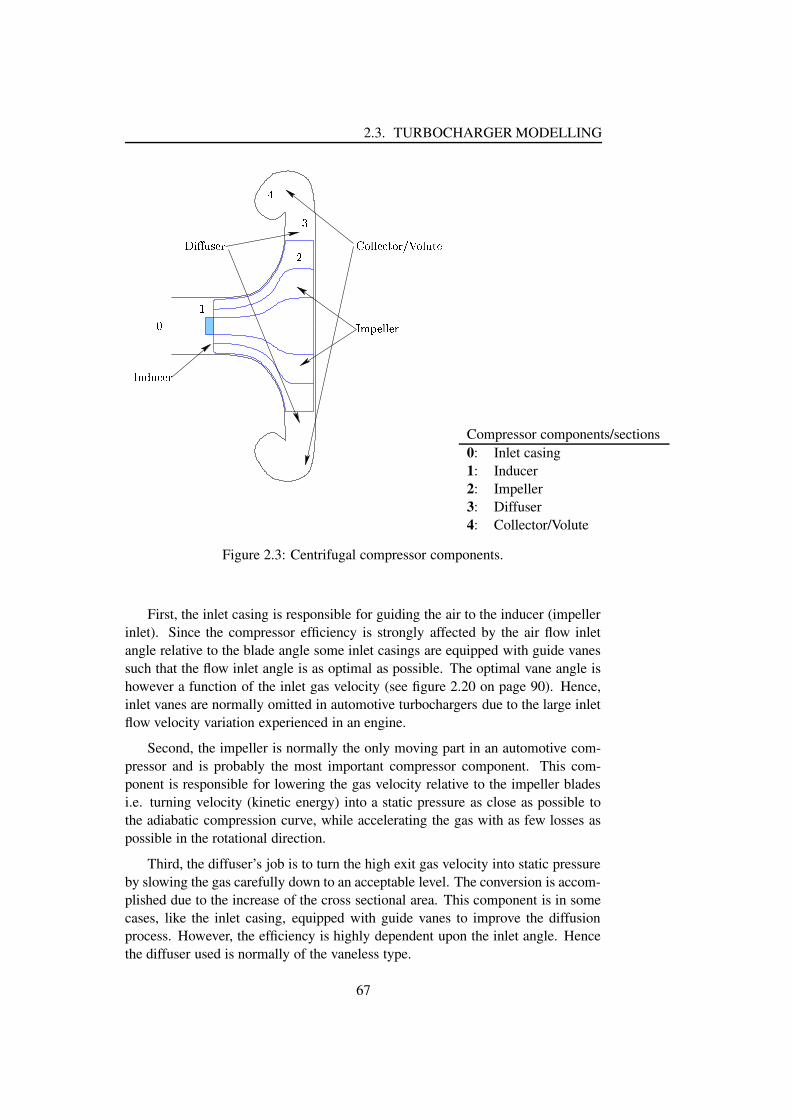
2.3. TURBOCHARGER MODELLING
��� � � !�"�#�� $�%'&(� � )*#�!
+-,�. !�� � !�$+0/21 )2"�!�$
354 6 )27�!�$
8 9:;
<
Compressor components/sections0: Inlet casing1: Inducer2: Impeller3: Diffuser4: Collector/Volute
Figure 2.3: Centrifugal compressor components.
First, the inlet casing is responsible for guiding the air to the inducer (impellerinlet). Since the compressor efficiency is strongly affected by the air flow inletangle relative to the blade angle some inlet casings are equipped with guide vanessuch that the flow inlet angle is as optimal as possible. The optimal vane angle ishowever a function of the inlet gas velocity (see figure 2.20 on page 90). Hence,inlet vanes are normally omitted in automotive turbochargers due to the large inletflow velocity variation experienced in an engine.
Second, the impeller is normally the only moving part in an automotive com-pressor and is probably the most important compressor component. This com-ponent is responsible for lowering the gas velocity relative to the impeller bladesi.e. turning velocity (kinetic energy) into a static pressure as close as possible tothe adiabatic compression curve, while accelerating the gas with as few losses aspossible in the rotational direction.
Third, the diffuser’s job is to turn the high exit gas velocity into static pressureby slowing the gas carefully down to an acceptable level. The conversion is accom-plished due to the increase of the cross sectional area. This component is in somecases, like the inlet casing, equipped with guide vanes to improve the diffusionprocess. However, the efficiency is highly dependent upon the inlet angle. Hencethe diffuser used is normally of the vaneless type.
67
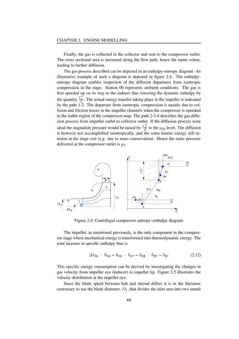
CHAPTER 2. ENGINE MODELLING
Finally, the gas is collected in the collector and sent to the compressor outlet.The cross sectional area is increased along the flow path, hence the name volute,leading to further diffusion.
The gas process described can be depicted in an enthalpy-entropy diagram. Anillustrative example of such a diagram is depicted in figure 2.4. The enthalpy-entropy diagram enables inspection of the different departures from isentropiccompression in the stage. Station 00 represents ambient conditions. The gas isfirst speeded up on its way to the inducer thus lowering the dynamic enthalpy bythe quantity =>?@ . The actual energy transfer taking place in the impeller is indicatedby the path 1-2. The departure from isentropic compression is mainly due to col-lision and friction losses in the impeller channels when the compressor is operatedin the stable region of the compressor map. The path 2-3-4 describes the gas diffu-sion process from impeller outlet to collector outlet. If the diffusion process wereideal the stagnation pressure would be raised by = >>@ to the ACB @ level. The diffusionis however not accomplished isentropically, and the some kinetic energy still re-mains at the stage exit (e.g. due to mass conservation). Hence the static pressuredelivered at the compressor outlet is AD .
EF
G
HIJ K L I J K MI5N
FG
O
P
QSRQUT-RQ*VQUW
Q�XQUTYXQ TYV
E
Z�[\V
ZU[]V
Z [[V
H^H H EQUT_T
``a
Figure 2.4: Centrifugal compressor entropy–enthalpy diagram
The impeller, as mentioned previously, is the only component in the compres-sor stage where mechanical energy is transformed into thermodynamic energy. Thetotal increase in specific enthalpy thus isbdc B'e�f c B^Dhg c B'Bif c B @ g c B'Bjf c B @ g c B�k (2.12)
This specific energy consumption can be derived by investigating the changes ingas velocity from impeller eye (inducer) to impeller tip. Figure 2.5 illustrates thevelocity distribution at the impeller eye.
Since the blade speed between hub and shroud differs it is in the literaturecustomary to use the blade diameter, lmk ,that divides the inlet area into two annuli
68
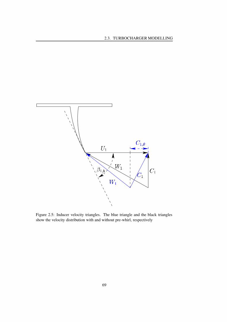
2.3. TURBOCHARGER MODELLING
nporq s t ou ou o
t o
v o t orq w
Figure 2.5: Inducer velocity triangles. The blue triangle and the black trianglesshow the velocity distribution with and without pre-whirl, respectively
69

CHAPTER 2. ENGINE MODELLING
of equal area for speed calculations, thusxzy{j|~}��� xzy��� �j� xzy��� ��� (2.13)
wherex ��� � and
x ��� � are the hub and shroud diameter of the inducer, respectively.Whence, the tangential speed of the impeller eye, � {
, at this diameter is
� { | x {������� |�� x { ������ (2.14)
The air is entering the inducer at this diameter with the absolute velocity � {. Given
the blade and gas velocities the gas velocity relative to the impellers blades, � {,
can found from the following vectorial relationship5 ,
� | ����� (2.15)
The torque exerted on the impeller on the inlet side can thus be found to be,
� { | �¡ � x { � { � ¢� (2.16)
since the angular momentum of the gas is the moment of linear momentum. Hence,the torque exerted is the product of the mass flow �¡ �
, radius and the tangentialvelocity component, � { � ¢ .
The energy transfer to the impeller on the inducer side is found as the productof the torque and angular speed, � �
,£ { | � { � � | �¡ � � { � { � ¢ (2.17)
The velocity triangle at the impeller tip is shown in figure 2.6.The figure shows the ideal velocity triangle (no slip) together with the actual
velocity triangle. The term slip factor expresses the ratio between the tangentialcomponent of the absolute velocity and either one of the tangential velocities; underideal conditions or the impeller tip speed. Thus, slip, ¤ , is defined as
¤¦¥ � y � ¢� y � ¢'§ or ¤¨¥ � y � ¢� y (2.18)
The slip phenomenon is discussed in more detail in section 2.3.3.2.The torque exerted on the air by the impeller, � y , is again found from angular
momentum considerations to be � y | �¡ � x y � y � ¢� (2.19)
and the power consumed is £ y | � y � � | �¡ � � y � y � ¢ (2.20)
5The subscripts are omitted, since velocity triangles are in general constructed according to equa-tion 2.15.
70

2.3. TURBOCHARGER MODELLING
PSfrag replacements
No slip
Actual ©
ª¬« «® «
® «�¯ °
® «�¯ ±² « ² «�³´j«
Figure 2.6: Velocity triangle at the impeller tip.
The impeller power consumption, µ·¶ , can now derived from equation 2.17 onthe facing page and 2.20 on the preceding page to be
µ¸¶�¹»º¼ ¶�½d¾À¿�Á ¶�¹Âµ¸ÃÅÄƵ·ÇŹȺ¼ ¶É�ÊËÃ2Ì Ã�Á Í ÄÎÊ�ÇUÌ Ç'Á Í2Ï (2.21)
This formula is also known as the Euler equation. In order to shed more light onthe energy transfer, one must revert to the velocity triangles drawn in figure 2.5 andin figure 2.6. The relative velocity, Ð , at impeller exit or inlet is given by
Ð Ã ¹ÑÊ Ã·Ò Ì Ã ÄÔÓ¬ÊÕÌ Í (2.22)
Using this expression the Euler equation can be rewritten as
µ¸¶�¹Èº¼ ¶×ÖÓØÙÚ Û Ì Ãà Ä�Ì ÃÇ�ÜÝ ÞUß à
Absolute kinetic energy change
Ò Û Ê Ãà ÄÎÊ ÃÇáÜÝ ÞUß àCentrifugal energy change
Ò Û Ð ÃÇ ÄÔÐ ÃÃCÜÝ ÞUß àRelative kinetic energy change
âYãä (2.23)
The first term in this alternative form of the Euler equation represents the absolutekinetic energy change in the impeller. The second term represents the change incentrifugal energy as the gas is moved from one radius of rotation to another. Thisrotational energy raises the static pressure in the impeller. Finally, the static im-peller pressure is also changed as the velocity relative to the impeller changes. Thiscontribution is represented by the third term in equation 2.23
Most of the compressors, if not all, in automotive turbochargers are constructedwithout stationary pre-whirl vanes in front of the inducer. Pre-whirl vanes enhance
71

CHAPTER 2. ENGINE MODELLING
the compressor efficiency around some mass flow design point. The efficiencyoutside the design region, however, will be tempered dramatically. This hampersthe employment of pre-whirl vanes in compressors experiencing large mass flowvariations e.g. automotive compressors. The theory presented in the literature(see [83], [87] and [40]) states that the tangential component (whirl) of the airapproaching the inducer is negligible. Thus, the enthalpy transfer described by theEuler formula in equation 2.21 on the page before reduces to
ådæÀç�è é�êìë éíî é êÑïËð2ñóò è ð(2.24)
Using the slip definition ô¨õ÷ö(ø�ù úû ø this equation may be rewritten as
ådæÀç�è é�ê ô ï ðð(2.25)
Thus, the specific energy transfer is dependent on the impeller speed alone if theslip factor is assumed constant.
2.3.3.2 Slip
The slip phenomenon is experienced under all normal flow conditions, since theinertia (mass) of the gas prevents the tangential gas velocity from matching thetangential blade velocity. The gas will thus rotate relative to the impeller channel,but in the opposite direction. Whence the tangential velocity of the gas,
ñ ð�è ò,
leaving the impeller will be smaller than the ideal tangential velocity (ïhð
for aradial designed impeller) due to this relative rotation. The phenomenon is soughtillustrated by the impeller tip schematics in figure 2.7.ü_ý þ ÿ ���� � ��� � � � � � �� � ����� � ��� � �� � ��� � ü_ý þ ÿ �
�� ��� ����� � � � � �� ��� ��� � ���� � � � �
! �� � � �#"�� ���
Figure 2.7: Relative flow conditions for a radial impeller without splitter blades andan impeller of the backsweep type with splitter blades, along with an illustration ofthe flow separation at the impeller outlet
72

2.3. TURBOCHARGER MODELLING
The figure shows the schematics of an impeller with radial design and a back-sweep impeller with splitter blades, respectively, together with the relative gas ve-locity along the blades. The problem of using radial impellers vs. backsweepimpellers in automotive applications is clear from the figure. Due to the harderradial acceleration of the gas in the radial case the pressure difference betweenthe pressure side (blade front side) and the suction side (blade backside) is larger.Hence, the chance of flow separation and thus compressor surge is greater. Thebacksweep impeller, however, accelerates the gas more gently6 , and together withthe use of splitter blades the pressure difference between the pressure- and suctionside of the impeller blade is smaller. Thus, the surge region of backsweep impellercompressors is smaller providing the backsweep impeller with a larger stable op-erating range compared to that of the radial type. The maximum energy transferfor a backsweep impeller, however, will be lower due to the lower tangential gasvelocity at the impeller tip.
The existence of this pressure difference between the pressure- and suction sideof the impeller leads to an obvious velocity difference between the gas exiting theimpeller at the suction side and pressure side, respectively. The existing flow is soto say split in a ”main jet stream” and a ”wake jet stream”. It is stated in [87] thatthe ”wake jet flow” comprises approximately 15% of the mass flow but occupies35% of the impeller exit area for a radially vaned impeller close to the surge region.This, of course, complicates the mean velocity computation of the gas leaving theimpeller.
An empirical attempt to describe the speed conditions at the impeller tip withinthe confines of one-dimensional modelling is by the use of the slip factor definition.This factor is explained below.
It is customary in the literature (see [83], [87] and [40]) to express the idealnessof the compressor as the ratio between the actual tangential gas velocity,
$&%(' ), and
the ideal absolute exit velocity,$*)(' %,+
, or the impeller tip speed, - ) . This ratio isknown as the slip factor and is, as mentioned, defined by.0/ $1)(' %$1)(' %,+ (2.26)
or .0/ $1)(' %- ) (2.27)
The slip factor, . , can be increased by increasing the number of impeller blades.The added viscous drag from the blades will hamper the relative gas rotation atthe cost of larger frictional losses and added manufacturing complexities. Numer-ous models for the slip factor exist in the literature, [117] and [36]. Most of thesemodels are based solely on design parameters. One such fixed slip factor formula,
6The effective channel path of a backsweep impeller is longer compared to a radial impeller forthe same impeller diameter
73

CHAPTER 2. ENGINE MODELLING
which can be applied to both backsweep type and radial vaned impellers, is pre-sented in [87] and is repeated here,243 5516 78(9�:,;=<�>�?A@,:,;1BDC�E FBDGIHKJ#L,M�NPO E Q (2.28)
with R = 0.3 for a radial vaned impeller and 0.2 for a backsweep impeller.However, the slip factor is known to vary with mass flow, [87], [115] and [15].
A mass flow dependent slip factor formulation is presented in [15] (see also [83]).The formula, known as the Reffstrup slip factor, is repeated in equation 2.29.243TS1U(V 8W 8 3 516YX[Z�\^]*_ 8 V `ba 5ced 5 agfKh OjiDk�l�mon O E Qp q (2.29)
where X is the ratio between radial gas velocity, S 8 V r , and impeller tip speed,X 3 S roV 8W 8 3 stvuw 8�xzy|{�} W 8 (2.30)~is the number of impeller blades, y�{ impeller outlet diameter, } impeller outlet
width, and w 8 is the static outlet gas density.The Reffstrup slip formula will be used throughout the rest of the compres-
sor modelling work in this text, since it includes a dependency on the mass flowrate. The eminent importance of this mass flow dependency will become clear insection 2.3.3.5 on page 79.
Remark: The slip angle, _ 8 , and impeller blade angle, _ 8 V ` , are defined counter-clockwise. Hence, both angles are negative for backsweep type impellers.
2.3.3.3 Total energy transfer or ���K� u modelling
The total energy transfer to the compressor can be found by combining equa-tion 2.25 on page 72 and the Reffstrup slip factor. Thus, the following structureof the Euler equation is obtained� u 3 stvu ����� u 3 stvu W 88 d 516YX[Z�\^]�_ 8 V `ba 5c�d 5 agfKh Oji�k�l�mon O E Qp q[q (2.31)
The factor multiplying the squared impeller tip speed may be split in a constantand mass flow dependent part, thus the specific energy transfer takes the followingform ����� u 3 W 88 d�� 6 } st4�W 8 q (2.32)
where � 3 5 a 5c d 5 agfKh Oji�k�l�mon O E Qp q and } 3 Z�\^]*_ 8 V `w 8�xzy|{P} (2.33)
74
2.3. TURBOCHARGER MODELLING
Since it is assumed that all gases can treated as perfect gases the enthalpy riseacross the compressor stage may formulated as�����,�1�����,�I�g���(�I���o�*���z�,�I�e�z�(�(�
(2.34)
The ”total to total” isentropic efficiency7, � �o� ��� , is defined as the ratio betweenthe total specific energy transfer and the specific energy transfer required for anisentropic compression, thus� �o� ���0� �����,�o� �����,� � �z�,�(� ¡¢�e�z�(��z�,�I�e�z�(� (2.35)
The relation between pressure and temperature for an isentropic process is re-peated in equation 2.36 £=¤ � £ �,�£ �(� �¦¥ �z�,�(� ¡�z�(�¨§ª©©�«�¬ (2.36)
The expression for the total specific energy transfer as function of ambientconditions, stage efficiency and pressure ratio may now be found by combiningequations 2.34, 2.35 and 2.36.�����,�1� �o���z�(�� �o� ��� ¥ £ ©�«�¬©
¤ �® § (2.37)
Utilizing the equations 2.32 and 2.37, the impeller speed, stage efficiency, massflow and pressure ratio may be related.�����,�A� �o���z�(�� �o� ��� ¥ £ ©�«�¬©
¤ �¯ § �±° �� ¥�²´³Yµ·¶¸ �°b� § (2.38)
2.3.3.4 Compressor data
Having developed the background for one dimensional compressor modelling inthe preceding sections the one dimensional compressor model’s accuracy with realdata will now be examined. It has been decided to evaluate the final physicalcompressor model, to be finalized in the coming sections, based on data for threedifferent compressors to prove the model’s generality. The intermediate resultsobtained for compressor A, however, will only be presented for the sake of clarityand convenience. The data for the compressors, all manufactured by Allied SignalLtd., are listed in table 2.1.
All the compressors have the same design except for the trim size ( ¹ �� ¡ – ¹|ºratio, see [14] and figure 2.4). Although the difference on the outer diameter ofthe inducer, ¹ �� ¡ , seems negligible, the effect on the compressor characteristic is
7The difference between ”total to total” and ”total to static” efficiency is often negligible for mostcompressors calculations, since the volute exit velocity is small
75

CHAPTER 2. ENGINE MODELLING
Compressor A Compressor B Compressor CManufacture Allied Signal Ltd. Allied Signal Ltd. Allied Signal Ltd.
Compressor Type No. C101 E(44) C101 E(44) C101 E(44)Impeller diameter [mm] 44 44 44
Trim 55 50 45A/R 0.33 0.33 0.33
Main blade No. 6 6 6Splitter blade No. 6 6 6
Impeller tip width » [mm] 4 4 4Inducer dia. (hub) » [mm] 12 12 12
Inducer dia. (shroud) [mm] 32.6 31.1 29.5Impeller tip angle » [ ¼ ] -45 -45 -45
Inducer blade angle » [ ¼ ] -40 -40 -40
Table 2.1: Experimental compressor specifications. Remark: Measures markedwith ½ are found by local dismantling of the turbocharger and should such be treatedof more descriptive than accurate.
tremendous. The importance of trim setting is evident when comparing the char-acteristics of the compressors in figure 2.8, 2.9 and 2.10. A trim decrease looselyspeaking moves the whole of the compressor map closer to the abscissa. An inter-esting effect of a trim decrease is the movement of the so called stonewall (max-imum mass flow for a given impeller speed). However, the effect is as expectedsince the inducer by design is the flow limiting component of the compressor, andhence a natural consequence of the radial gas velocity deceleration/radial stage areaenlargement. Whence, the radial area must increase along the impeller channel toconvert the radial kinetic energy into pressure.
Another interesting observation, confirming a typical problem, is the notoriouslack of data points at low pressure ratios8.
The use of the compressor data presented in the figures 2.8, 2.9 and 2.10 iscomplicated by the fact that the efficiency data point and speedline data point in-dices do not coincide. To overcome this problem interpolated efficiency valuesare computed for each speedline point. Speedline data points necessitating an effi-ciency extrapolation are omitted.
The computation of the interpolated efficiency surface is outline in the follow-ing. First a data grid is constructed by Delaunay data triangulation, see [32] and[80], such that each data point is connected to its natural neighbors. This set oftriangles based on the scattered compressor data are then used to define what datapoints are appropriate in a subsequent identification procedure. This way of defin-ing properness for an interpolation point is fortunate, since interpolation indicesthat are not contained within a triangle may be discarded i.e. data extrapolationcan be avoided; a property clear from figure 2.11. Having defined interpolationpoint properness and identification data a cubic interpolation is carried out forcingthe efficiency surface through each data point.
8Compressor map points at lower impeller speed are often not provided by the manufacturer.The reason is rather obvious; the small temperature increase across the stage at such operating pointmakes it difficult to assess the compressor accurately.
76

2.3. TURBOCHARGER MODELLING
0 0.05 0.1 0.151
1.5
2
2.5
3
3.5
100000120000
140000
160000
180000
200000
220000
240000
60
65
6870
72
74
7677
PSfrag replacements
Corrected mass flow ¾¿AÀ�Á ÀK ¾¿AÀ�à ÄoÅ�ÆÇ�È�ÉjÊË Å�ÆÌ�Í Å�Î�Î=ÏDÐ , [kg/s]
Pres
sure
Rat
io
Ñ ÒÓÔ Õ Ô ÖCorrected compressor map.
A
Figure 2.8: Compressor A efficiency and flow characteristics together with surgeline and maximum efficiency line. The data points are marked with ’+’
0 0.05 0.1 0.151
1.5
2
2.5
3
3.5
100000120000
140000
160000
180000
200000
220000
60
6568
7072
74
7675
PSfrag replacements
Corrected mass flow ¾¿AÀ�Á ÀK ¾¿AÀ�à ÄoÅ�ÆÇ�È�ÉjÊË Å�ÆÌ�Í Å�Î�Î=ÏDÐ , [kg/s]
Pres
sure
Rat
io
Ñ ÒÓÔ Õ Ô ÖCorrected compressor map.
B
Figure 2.9: Efficiency and flow characteristics for compressor B
77

CHAPTER 2. ENGINE MODELLING
0 0.05 0.1 0.151
1.5
2
2.5
3
3.5
100000120000
140000
160000
180000
200000
220000
60
6568
7072
74
76PSfrag replacements
Corrected mass flow ×ØAÙ�Ú ÙKÛ ×ØAÙ�Ü ÝoÞ�ßà�á�âjãä Þ�ßå�æ Þ�ç�ç=èDé , [kg/s]
Pres
sure
Rat
io
ê ëìí î í ïCorrected compressor map.
C
Figure 2.10: Efficiency and flow characteristics for compressor C
0
0.05
0.1
0.15
0.2
11.5
22.5
33.5
455
60
65
70
75
80
PSfrag replacements
Mass flow ðñAò�ó ò , [kg/s]Pressure Ratio ô�õ
Compressor A efficiency surface.
Effi
cien
cy
ö ÷ [%]
60
62
64
66
68
70
72
74
76
0.04 0.06 0.08 0.1 0.12 0.14
1.5
2
2.5
3
3.5
PSfrag replacementsMass flow , [kg/s]
Pressure Ratio
Compressor A efficiency surface.
Efficiency [%]
Mass flow ðñ1ò�ó ò , [kg/s]
Pres
sure
Rat
io
ø ùCompressor A efficiency contour.
Figure 2.11: Interpolated efficiency surface and contour for compressor A.
78

2.3. TURBOCHARGER MODELLING
2.3.3.5 ú�û=ü,ý model deduction from data
The specific enthalpy speedlines may be derived by using equation 2.37 on page 75.The computed enthalpy speedlines are plotted in figure 2.12. Looking at the speed-lines in the left plot the importance of a correct efficiency estimation is evident.The difference between the speedlines based on interpolated efficiency data andthe speedlines derived using the mean value of the efficiency data is not negligible.
0.02 0.04 0.06 0.08 0.1 0.12 0.14 0.160
0.2
0.4
0.6
0.8
1
1.2
1.4
1.6
1.8
2x 10⁵
100000 rpm
120000 rpm140000 rpm
160000 rpm
180000 rpm
200000 rpm
220000 rpm
240000 rpm
PSfrag replacements
þÿ�� � kgs �
� � � �� J kg
Specific energy transfer.
rpm0.5 1 1.5 2 2.5 3
x 10−4
0.45
0.5
0.55
0.6
0.65
0.7
0.75
0.8
PSfrag replacementskgs
Jkg
Specific energy transfer.
rpm
� ���� � kgm �
� � � � �� �Specific energy transfer, normalized.
Figure 2.12: The left plot, on basis of the interpolated efficiency surface computed,shows the specific enthalpy speedlines. Speedline points necessitating efficiencyextrapolation are omitted. The dashed enthalpy speedlines are derived using theefficiency mean value. The normalized enthalpy speedlines are plotted in the rightfigure.
It was found in section 2.3.3.3 on page 74, equation 2.32, that the total specificenergy transfer can also be deduced from the impeller speed and mass flow. Thisequation is repeated below for the sake of convenience.ú�û�ü,ý������� ��� �"!$#% ý� � & (2.39)
According to [83] the coefficients�
and!
may be regarded as constants for a givenspeed under the assumption that the gas density stays constant throughout the im-peller channel. The validity of this statement is to some extent confirmed by thestructure of the speedlines in the right plot in figure 2.12, since the the individ-ual speedlines are almost linear functions of
þÿ��')( . The statement may, however,be tested since
�is given by geometric data alone and the varying parameter in!
is static density at the impeller tip, * � . Hence, the only assumption which hasto be tested is the validity of the * �,+ *�- assumption. This will be tested in thefollowing.
79

CHAPTER 2. ENGINE MODELLING
The enthalpy at the impeller tip and volute exit are related in the followingmanner .0/21 35476 839;: .0/21=<>476 8<9;: .0/21 8 476 889 (2.40)
The density at the impeller tip, ? 8 , may be derived as? 8 : ? 3A@ 1 31 8CBEDDGFIH (2.41)
under the assumption that the diffuser and volute are lossless i.e. the kinetic energyavailable at the impeller tip is transformed into pressure isentropically. This as-sumption is justifiable for the whole operating range of a compressor with vanelessdiffuser, since the diffuser and volute losses together only comprise a maximum of5% of the total enthalpy losses according to [87] and [40].
The specific kinetic energy at the impeller tip, JLK , may be found by using thevelocity triangle in figure 2.6 and the slip factor definitionJMK :ON9QP 6 88SR T 4 6 88SR UWV: N9YX @ Z[ 3? 8W\ ]_^a`bB 8 4dc 82e�88gf (2.42)
The kinetic energy remaining at stage exit is often of minor importance i.e. theexit velocity is negligible. Hence, the enthalpy equation in equation 2.40, may bereduced without any loss of generality to.0/21 3 : .0/21 hSi : .0/21 8 4 6 889 (2.43)
The temperature
1 8 may now implicitly be computed from equation 2.41, 2.42and 2.43 by computing the minimum quadratic criterionjlk�mon :qpsrutvIw @ 1 8>x 1 354 JMK.0/ B 8 (2.44)
Figure 2.13 depicts the iteratively computed impeller temperature,
1 8 , and im-peller density, ? 8 . The stage outlet temperature
153is derived from compressor data
as 1 3 : 1 hSyLz N 4 N{ 3 R v�v @I| H�FbDHT x N B~} (2.45)
and the density as ? 3 : | T | hSy� 1 3 (2.46)
and are include in the figure as boundary conditions. The figure clearly shows thatthe assumption ? 8 : ? y used in [83] is not valid. The static impeller tip density
80

2.3. TURBOCHARGER MODELLING
1 1.5 2 2.5 3 3.5 4300
320
340
360
380
400
420
440
460
480
PSfrag replacements
�a�� � ���� [K]
Outlet temp. ��� and tip temp �I�����I�
1 1.5 2 2.5 3 3.5 41
1.5
2
2.5
PSfrag replacements
[K]
Outlet temp. and tip temp
�a�� � ,� � ,� � � ,� �� kg m
��Gas density � �
� � , �� ��W���������
Figure 2.13: The left plot shows the iteratively computed impeller tip temperature,� �, speedlines together with the outlet temperature,
���. Using these temperatures
the gas densities � � and � � may be found. The computed densities are illustrated inthe plot to the right together with a linear fit of the impeller density, �� � . Computa-tions utilizing surge data are marked with .is approximately 50% larger than �=¡ in the high pressure region of the compressormap.
The question is how this knowledge can be include in a model for the totalspecific energy transfer, ¢�£ � . The kinetic energy available at the impeller tip canfrom the above discussion be derived based on the impeller velocity triangle. Hav-ing computed this energy, the temperature
�¤�may be found analogous to equa-
tion 2.43. But since the triangle itself is temperature dependent, the solution to� �/ � � will be of implicit nature if this method of calculation is chosen. To over-
come this hurdle it is decided here to utilize the apparently linear relationship infigure 2.13 between the pressure ratio ¥ ¦ and the impeller tip density � � . Whence,a descriptive value for � � is found as� �M§q¨ � � ¥©¦«ªY¬ � � (2.47)
The identified parameters for all three compressors are listed in table 2.2.C®°¯A± kgm ²W³ ´ ®°¯A± kg
m ²W³ µ C®°¯ ¶ ´ ®°¯�·0¸ ¹»º0¼ � ± kgm ²W³ ½ ��� ± kg
m ²W³ ¾ ��¿�À»ÁaÂÄÃMÅ kg¯
m ÆÄÇCompressor A 0.2924 0.8359 1.1283 1.1680 1.348Compressor B 0.2971 0.8680 1.1651 1.1680 0.652Compressor C 0,3181 0,8359 1.1540 1.1680 0.990
Table 2.2: Identified parameter for �� �A§ f È ¥©¦aÉ .The generality of the functional dependency found between ¥5¦ and � � is con-
firmed by the small variance around the identified line, and by the fact that the � �81

CHAPTER 2. ENGINE MODELLING
estimate for the boundary condition Ê ËAÌÎÍ is very close to the ambient gas density,Ï�Ð Ì ÏbÑSÐ .The ordinate in figure 2.12’s right plot is normalized by the identified ÒÏ�Ó func-
tion. The result is illustrated in figure 2.14. The normalization leads to a furtherregularization of the normalized enthalpy speedlines.
The green dashed line in Figure 2.12 shows the best linear fit for the ÔÖÕ×�ØÙÚSÛÝÜ)Û)Þlß�àaá ØÜ ÛÛãâdata set. The identified slope, Òä , and constant, Òå , of the line are estimates of ä andå
in a rewritten form of equation 2.32 on page 74æsç Ñ»è Ì�é ÓÓëê äLì åîíïëèÏbÓ é ÓCð (2.48)
with ä ÌÎÍ~ñ Íò ê Í~ñôó=õ Û÷ögøúùGû0ü Û°ý þÿ ð andå Ì�� ����� Ó�� ��� å (2.49)
0.5 1 1.5 2 2.5
x 10−4
0.45
0.5
0.55
0.6
0.65
0.7
0.75
0.8
PSfrag replacements
������������� m ��
�� � � � ,! � � � � �
Specific energy transfer and identification.
"$#&% �� ��(' f ) �����+*,���.-
"$#&% �� ��(' f ) ����/���&���.-
0 "$#&% �� ��
Figure 2.14: Non- (black solid) and Ï�Ó (red solid) normalized energy curves. Thedashed green line is the best general fit forced through the Ï©Ó normalized energyspeed curves.
In contrast to equation 2.32, the ä andå
parameters in equation 2.48 are onlydependent upon geometrical compressor specifications. This is thus a identificationprocedure which is no longer operating point dependent.
82
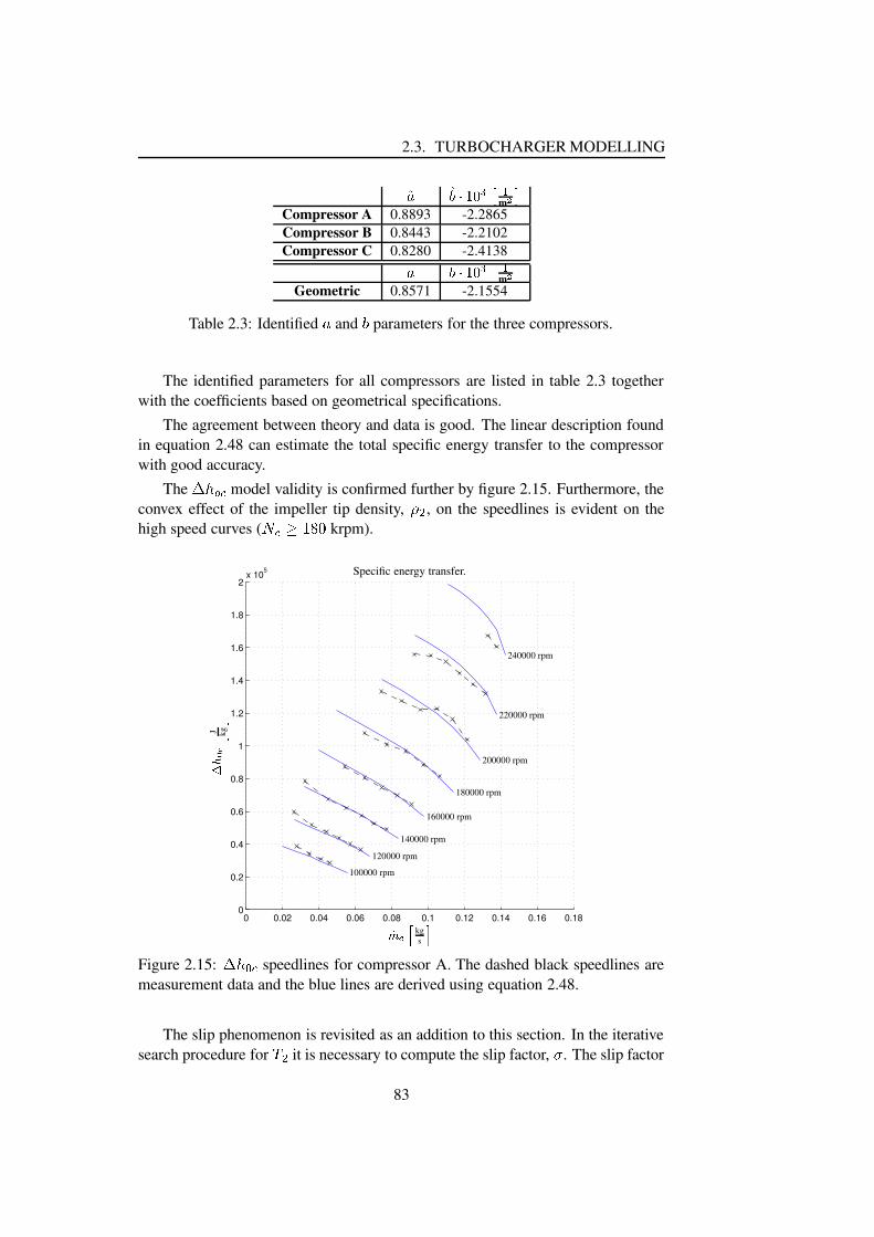
2.3. TURBOCHARGER MODELLING12 1354.6�798;:=<m >@?
Compressor A 0.8893 -2.2865Compressor B 0.8443 -2.2102Compressor C 0.8280 -2.41382 354.6�798;: <
m >@?Geometric 0.8571 -2.1554
Table 2.3: Identified A and B parameters for the three compressors.
The identified parameters for all compressors are listed in table 2.3 togetherwith the coefficients based on geometrical specifications.
The agreement between theory and data is good. The linear description foundin equation 2.48 can estimate the total specific energy transfer to the compressorwith good accuracy.
The CEDGF+H model validity is confirmed further by figure 2.15. Furthermore, theconvex effect of the impeller tip density, IGJ , on the speedlines is evident on thehigh speed curves ( KLHNMPO.QSR krpm).
0 0.02 0.04 0.06 0.08 0.1 0.12 0.14 0.16 0.180
0.2
0.4
0.6
0.8
1
1.2
1.4
1.6
1.8
2x 10⁵
100000 rpm
120000 rpm
140000 rpm
160000 rpm
180000 rpm
200000 rpm
220000 rpm
240000 rpm
PSfrag replacements
TUWVWX kgs Y
Z [ \ ]^ J kg
_
Specific energy transfer.
rpm
Figure 2.15: CEDa`&H speedlines for compressor A. The dashed black speedlines aremeasurement data and the blue lines are derived using equation 2.48.
The slip phenomenon is revisited as an addition to this section. In the iterativesearch procedure for b5J it is necessary to compute the slip factor, c . The slip factor
83

CHAPTER 2. ENGINE MODELLING
is derived from the measurements asdfehgEiGj&kl�mm (2.50)
The tangential gas velocity, n m�o p , can be found by trigonometry as9,n m�o p e l mWq n m�o rts�u�vNwam (2.51)
Inserting equation 2.50 in 2.51 and using the mass conservation law w5m is foundto be wam e uSxzy�s�u�vf{}|}~ d����9� l m@��m����.��� k � (2.52)
Equation 2.52 makes it possible to study compressor slip as the mass flowthrough the compressor is varied. This is seen in the plot to the left in figure 2.16.The general tendency independent of impeller speed is a w�m increase as the com-pressor mass flow is increased. The plot right in the figure depicts the calculatedslip factor. The slip factor decreases here in agreement with the theory developedas the mass flow increases.
0.5 1 1.5 2 2.5 3
x 10−4
−65
−64
−63
−62
−61
−60
−59
−58
−57
−56
PSfrag replacements
�������E� kgm �
� �� ��Relative flow angle �9� .
0.5 1 1.5 2 2.5 3
x 10−4
0.45
0.5
0.55
0.6
0.65
0.7
0.75
0.8
PSfrag replacementskgm
Relative flow angle .
�������E� kgm �
Slip
fact
or
�Computed slip factor for compressor A.
Figure 2.16: The left plot depicts the computed angle, w�m , of the relative outletvelocity � m . The corresponding computed slip factors are illustrated in the plot tothe right. Computations utilizing surge data are marked with � .2.3.3.6 Speedline shapes
The previous section provides an important paradigm in understanding the shapeof the speedlines based on geometry alone. It was found that the specific energyconsumed by the compressor, gEitj&k , may be described by two parameters, a slip
9Remark: � � is negative for a backsweep impeller.
84

2.3. TURBOCHARGER MODELLING
factor, � , and the squared impeller tip velocity, ¢¡¡ . The level of slip is very im-portant in predicting the specific energy consumed, £E¤�¥&¦ , by the compressor, andis fundamentally speaking a measure of the ratio between the tangential velocityof the gas leaving the impeller and the impeller tip speed. Whence, the slip shouldnot be mistaken for a loss, but rather the compressor’s ability to transfer energy.The slip level is found to be dependent upon two geometrically given constants §and ¨ , and one operating point dependent parameter ©ªW«¬��®¯ .
The pressure ratio °t± across the the stage can be found from equations 2.37and 2.48 to be°a±�²´³¶µ ¦+· ¸G¸=£E¤G¥&¦¹+º¼» ¥�½ ¾À¿@ÁÃÂÂ�Ä�Å ²ÇÆÈ µ ¦+· ¸G¸É �¡¡ËÊ § ¾ ¨(©ªW«¬��®¯¼Ì¹+º¼» ¥�½ ¾À¿@ÍÎ ÂÂ�Ä�Å (2.53)
where the parameter § is a positive constant. The sign of ¨ is impeller blade angledependent ¨ÐÏÒÑÔÓ forward sweep impeller, Õ ¡ · Ö ÏÒѨ�²ÀÑÔÓ radial impeller, Õ ¡ · Ö ²ÀѨÐ×ÒÑÔÓ backsweep impeller, Õ ¡ · Ö ×ÒÑ (2.54)
Note that the solution to °Ø± is implicit due to the functional dependence betweenÙ ¡ and °a± .The transformation of enthalpy into pressure for a radial and backsweep im-
peller, respectively, are illustrated in figure 2.17 and figure 2.18. According toequation 2.48 the enthalpy rise across a radial stage during stable compressor oper-ation (no choke and surge operation) is only rotational speed dependent. These con-stant enthalpy speedlines are transformed into constant °�± speedlines if the stageefficiency is assumed constant. However, the actual structure is convex since theenthalpy losses grow rapidly as the surge region or stonewall is approached.
PSfrag replacements
Ú «Ú «Ú «©ªW«©ªW« ©ªW«
ÛÜ Ý Þ ß àß à1 2 3
Figure 2.17: Energy transfer illustration for compressor with radial impeller.1 The enthalpy speedlines are constant since ¨�²´Ñ . 2 Assuming fixed com-
pressor efficiency the enthalpy speedlines are mapped into constant °5± speedlines.3 Typical characteristics of a compressor with a radial impeller.
The enthalpy speedlines for a backsweep impeller, neglecting the convex effectof Ù ¡ , are linearly decreasing with the mass flow, áâ ¦ . Hence, °t± will be concave in
85

CHAPTER 2. ENGINE MODELLING
the idealized case due to the exponent ãã�ä�å . The actual shape is convex though dueto the characteristics of the enthalpy losses.
PSfrag replacements
æØçæØç æØç èé çèé ç èé çê ë ì í î ïî ï1 2 3
Figure 2.18: Illustration of energy transfer for a compressor with backsweep im-peller. 1 The enthalpy speedlines are approximately linear decreasing functionsof the compressor mass flow ðñfò . 2 Assuming fixed compressor efficiency the en-thalpy speedlines are mapped into concave ó�ô speedlines due to the exponent ãã�ä�å .3 Typical characteristics of a compressor with backsweep impeller design.
The qualitative effect of the compressor efficiency can be seen from the dia-grams i.e. the energy losses increase rapidly as the mass flow moves higher (ap-proaching the stonewall) or lower (approaching the surge region) away from thepoint of maximum efficiency with the latter being the most aggressive of the two.Thus, the missing link in a quantitative understanding of the compressor behavioris a loss model.
2.3.3.7 Energy losses or õEöt÷ ø&ù,ù modelling
The compressor pressure- and efficiency characteristics are often modelled sepa-rately (see [63], [91], [108] and [61]). However, applying this methodology, theconnection between the two models is lost i.e. the total error level when combiningthe models may be unacceptable due to an unfortunate mathematical interfacing ofthe models. Hence, it is decided here to develop an efficiency model as close tothe level of physics allowed by one-dimensional modelling such that the compres-sor may be understood from a comprehensive picture instead of just a collectionof arbitrary equations. A positive side effect to this approach is the simultaneouscreation of a rough design tool compressor.
The stage efficiency definition in equation 2.35 on page 75 can be expressed interms of specific energies úûò+ü ýGýÿþ õEö�� ò+ü �õEö�� ò+ü ��� õEöG÷ ø&ù,ù (2.55)
86

2.3. TURBOCHARGER MODELLING
where ��������������� ��������� ����������� ������������ �"!�#%$'&#( ��)+* (2.56)
The total compressor loss given by the specific energy����� ����
originates fromseveral sources. Some of the sources are listed below:
Clearance: A small clearance, , � � , between impeller wheel and the shroud sideof the housing exist due to manufacturing tolerances and temperature varia-tions. Due to this clearance some mixing between the channels will occur.An approximative value of the mixing loss in terms of efficiency degradationis given below (see [40] and [92]).- � �.�/10 2 , � �3where
3is the impeller tip width. However, the clearance is normally so
small that clearance losses can safely be neglected.
Back flow: Due to the acceleration of the fluid across the stage a pressure gradientbetween the suction side and pressure side of the impeller blade exist (see thediscussion in section 2.3.3.2 on page 72). Hence, some of the fluid leavingthe impeller will be re-injected if the local kinetic energy level is too low toovercome this suction force. One-dimensional modelling of the losses dueto this reprocessing process of some of the fluid are sparse in the literature.However, [87] suggests a typical efficiency degradation on the order of 3%points during stable compressor operation.
Volute: A inevitable loss exists due to the volute’s inability to convert all the radialkinetic energy out of the diffuser. The approximative value of this loss iswithin 2–5% points of efficiency [40].
Collision/Incidence: Collision losses are unavoidable in compressors due to off-design angles between the velocity vectors of the impeller respectively fluid.Hence, a fraction of the fluid’s kinetic energy will be dissipated.
Friction: Frictional losses are unavoidable with viscous fluids when a speed dif-ferences between boundary (surface) and fluid exists.
Heat transfer: An energy leakage to the ambient can not be avoided when a tem-perature difference between turbocharger housing and the surroundings ex-ists. However, this loss is of minor importance.
According to [87], [83] and [40] the shape of the efficiency characteristic ismainly controlled by
87

CHAPTER 2. ENGINE MODELLING4 Incidence losses in the impeller.104 Fluid friction losses in impeller and diffuser.
Therefore, it is decided here to only address the origin and modelling of these twosources.
2.3.3.8 Incidence loss
The biggest collision loss without doubt occurs in the inducer and is most widelymodelled by one of the following two approaches [87]:4 The total tangential velocity component of the inlet air is assumed destroyed.
This model is referred as the ”NASA shock loss theory”. It should be notedhere that the term ”shock” is misleading since that nothing akin to shockwaves occurs (supersonic velocities). Instead the expression should be un-derstood as a simple notion used to describe the shape of the compressorcharacteristic.4 The fluid is deviated from its original direction to the impeller channel inletnormal, just inside the impeller eye following a constant pressure process.
However, the difference between these widely used loss models is negligiblewhen applied to centrifugal compressor modelling according to [87]. The differ-ence mainly lies in the zero loss angle prediction i.e. the angle between the fluidvelocity relative to the impeller blades and the inducer velocity at which the lossvanishes. This angle is assumed equal to the inlet blade angle in the ”NASA shockloss theory” model.
Based on the simplicity of the ”NASA shock loss theory” model and the re-ported the loss estimation accuracy indifference between the two models, the NASAmodel will be adopted here.
However, a few words of caution should be said before the inducer losses aremodelled as incidence loss alone. Depending on the inducer flow conditions andimpeller speed another loss may develop and coexist together with the incidenceloss - namely stall11 [87]. Stall, or flow separation, occurs when the magnitude ofthe kinetic inlet energy falls below a specific point such that the adverse pressurebetween the pressure- and suction side of the impeller channel cannot be overcome.In the event of this separation, vortices along the suction side develop i.e boundarylayer separation occurs. This flow separation is illustrated in figure 2.19. Theseparated fluid is then re-injected into the main jet (see the discussion of back flowat the impeller tip on page 87). This reprocessing of the fluid naturally introducesa loss. This loss may in some cases actually be audible; the re-injection of the
10If a vaned instead of an annular diffuser is used the collision losses here may be of a considerablesize during off-design compressor operation and hence call for separate modelling.
11Stall may also be experienced in the vaneless diffuser when the adverse pressure gradient cannotbe overcome by the kinetic energy of the fluid leaving the impeller.
88

2.3. TURBOCHARGER MODELLING
5768.9+:<;1=�>%?�?�@'=�>A?�BDC'>E >�;1F�=FHGBD9"IKJ"9"=LGBDM�>%?
NPORQ 6TS ULVWXBDY"Z�;'=�>%?�?�@'=�>[?�BDC'>
Figure 2.19: Illustration of the flow separation at the inducer
fluid introduces aerodynamically induced vibration in the stage, thus leading to anincrease in the noise level.
Inducer stall may contribute to a complete stage stall - surge, but may also oc-cur, depending on the inducer design, in nominally stable operating modes. Furtheranalysis of inducer stall, than presented above, is complicated by the fact that nogeneric model of this loss exists in the literature [40]. However, stall losses areminimal within the compressor map (see [83]) and will be encompassed by thefollowing incidence modelling work.
Figure 2.20 illustrates velocity triangles at the inducer.According to the ”NASA shock loss theory” the incidence loss, \�]�^ _`�`a bdc"e , may
be described by \�]�^ _`�`a bdc"egfihjlknmo a p (2.58)
The tangential velocity component, k o a p�a q , is in [83] found to bek o a p�a qrf hs%tvu�w oyx{z | moA}�~ mo�} s%tvul��w o�� w o a _��+�L�u����Xw o a _��+� ~ o�� (2.59)
The subscript � indicates the tangential velocity’s radial dependence.Equation 2.59 may after some mathematical manipulation (see appendix A on
page 251) be rewritten as k o a p�a q�f | o }�~ o s%t���w o a _��+� (2.60)
The tangential velocity, k o a p , and thus the incidence loss \�].^ _`�`a bdc"e , is mostoften in the literature derived at the diameter that splits the inducer (impeller eye)
89

CHAPTER 2. ENGINE MODELLING
PSfrag replacements �1�� �R� ����R� �
���+�R��� � � ���
� �R� �R��� �Figure 2.20: Inducer velocity triangles in the no inlet pre-whirl case.
in two circles of equal area, ¡£¢¤ ¥ ¤¢§¦ ¡y¢¨ª© «{¬ ¡y¢¨ª© �® , (see e.g. [83], [87] and [40]).In this work a more generic approach, which will outlined in the following, will beintroduced.
The inflow conditions are shown diagrammatically in figure 2.21 together witha frontal view of the impeller eye. The green dashed line in front illustrates theassumed turbulent velocity profile of the fluid approaching the impeller blades.
PSfrag replacements ¯ °¯
±�²D³ ´ ±�²D³ ´± ²D³ µ ± ²D³ µFigure 2.21: A sketch of the inducer flow conditions is seen to the left. A frontalview of the impeller together with dimensions are depicted to the right.
Instead of applying the area averaging diameter an area averaging function issought. This function may be found based on the impeller eye diagram to the rightin figure 2.21.
90

2.3. TURBOCHARGER MODELLING
The area of the ring with thickness ¶v· is given by¶¹¸»º�¼¾½'¿ª·ÁÀ¶v·¹Ã�ÄÆÅÇ· Ä%Ⱥ�¼�ÉLÊ�·�¶v·ÁÀ¶v· Ä+Ë (2.61)
and constitutes the following fraction of the effective inducer inlet area
f ¿ª·¹Ãgº ¶¹¸¼ ½HÌ ÄÍªÎ Ï Å Ì ÄÍªÎ Ð È º Ê�·�¶v·ÁÀÑÉT¶v· Ä ËÓÒÁÔ ÕvÖT×Ì ÄÍªÎ Ï Å Ì ÄͪΠР(2.62)
The total enthalpy loss due to incidence may now be found by averaging thelocal incidence loss over the impeller eye inlet area. Hence, equation 2.58, 2.60and 2.62 are combined to find thatØ�Ù�Ú Û Ï�ÏÎ ÍdÜ"Ý º ÞÌ ÄÍªÎ Ï Å Ì ÄͪΠÐàß�áDâ ãäå�æ ß áDâ ç
·r¿Lè�é�¿ª·¹Ã�À�êréÓ¿ª·¹Ã'ë%ì�í�î�é Î Û�ï+𠿪·¹ÃÃ�Ä�¶v· (2.63)
Assuming that the velocity profile of the inflow is turbulent, the spatial radialvelocity variation of ê é may be neglected. This assumption is reasonable in lightof the turbulence created by the impeller blades. Thus, a solution to the integral inequation 2.63 is found asØ�Ù�Ú Û Ï�ÏÎ ÍdÜ"Ý º ÞÌ ÄÍªÎ Ï Å Ì ÄͪΠÐ<ñò ¼ Ä+ó¾ÄÝ ½ ÌAôÍªÎ Ï Å ÌAôͪΠРÈõ"ö Ä À ¼ ó Ý êré�ë%ì�í�î�é Î Û�ï+ð ½ Ì[÷ÍªÎ Ï Å Ì[÷ͪΠРÈø¹ù
À ê Äé ë%ì�í Ä î�é Î Û�ï+ð ½ Ì ÄÍªÎ Ï Å Ì ÄͪΠРÈÊ úû(2.64)
by substituting the tangential inducer velocity, èré , withè�éÓ¿ª·¹Ã�º Ê"¼ü· ó Ýõ"ö (2.65)
In the solution to equation 2.63 the blade angle, flow angle, îgé , and hence opti-mal inlet angle, î�é Î Û�ï+ð are assumed constant. An interesting consequence of thisassumption is that an incidence loss independent of the operating mode will al-ways be present (see appendix B on page 253). Hence the conclusion given in [83]stating that incidence and friction losses can be treated separately is not valid.
91
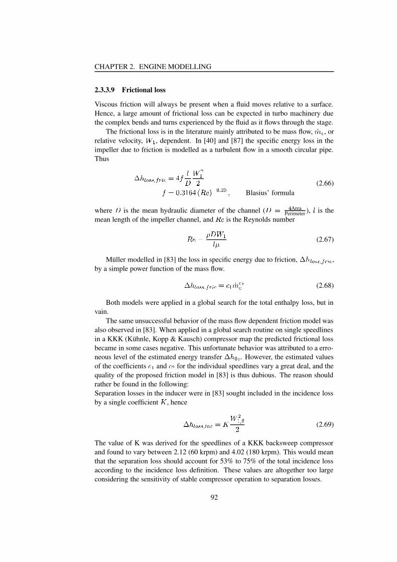
CHAPTER 2. ENGINE MODELLING
2.3.3.9 Frictional loss
Viscous friction will always be present when a fluid moves relative to a surface.Hence, a large amount of frictional loss can be expected in turbo machinery duethe complex bends and turns experienced by the fluid as it flows through the stage.
The frictional loss is in the literature mainly attributed to be mass flow, ýþ ÿ , orrelative velocity,
���, dependent. In [40] and [87] the specific energy loss in the
impeller due to friction is modelled as a turbulent flow in a smooth circular pipe.Thus ����� ��� ����� ÿ��������� ��������! #" $#%'&(�*),+.-(/103254 ��687 Blasius’ formula
(2.66)
where�
is the mean hydraulic diameter of the channel (� � 9 Area
Perimeter ), � is themean length of the impeller channel, and +.- is the Reynolds number+.-:�<; ���=��?> (2.67)
Muller modelled in [83] the loss in specific energy due to friction,���@� ��� ����� ÿ ,
by a simple power function of the mass flow.����� ��� ����� ÿ��!A � ýþ ÿ,Bÿ (2.68)
Both models were applied in a global search for the total enthalpy loss, but invain.
The same unsuccessful behavior of the mass flow dependent friction model wasalso observed in [83]. When applied in a global search routine on single speedlinesin a KKK (Kuhnle, Kopp & Kausch) compressor map the predicted frictional lossbecame in some cases negative. This unfortunate behavior was attributed to a erro-neous level of the estimated energy transfer
��� 2 ÿ . However, the estimated valuesof the coefficients A � and A � for the individual speedlines vary a great deal, and thequality of the proposed friction model in [83] is thus dubious. The reason shouldrather be found in the following:Separation losses in the inducer were in [83] sought included in the incidence lossby a single coefficient C , hence����� ��� �ED ÿ�� C ���� F� (2.69)
The value of K was derived for the speedlines of a KKK backsweep compressorand found to vary between 2.12 (60 krpm) and 4.02 (180 krpm). This would meanthat the separation loss should account for 53% to 75% of the total incidence lossaccording to the incidence loss definition. These values are altogether too largeconsidering the sensitivity of stable compressor operation to separation losses.
92
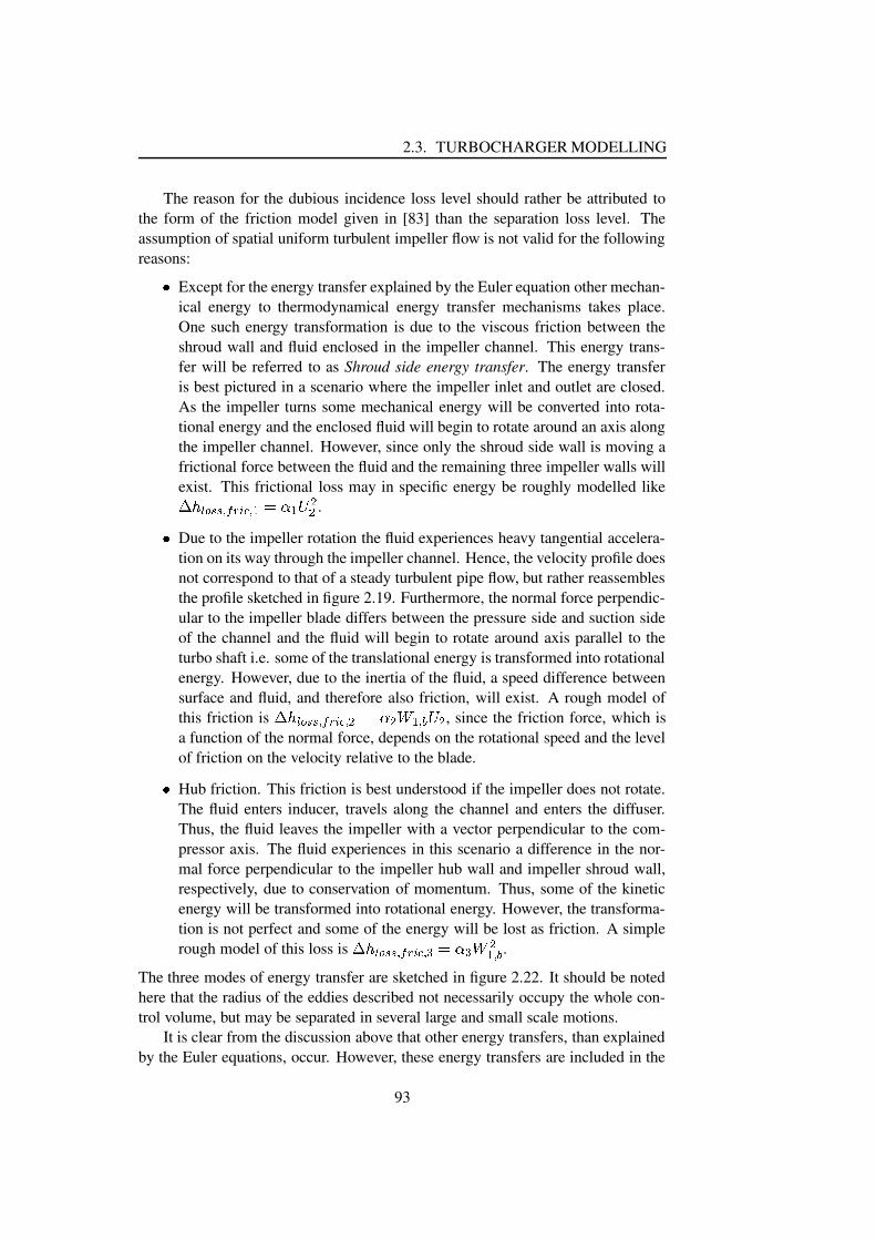
2.3. TURBOCHARGER MODELLING
The reason for the dubious incidence loss level should rather be attributed tothe form of the friction model given in [83] than the separation loss level. Theassumption of spatial uniform turbulent impeller flow is not valid for the followingreasons:G Except for the energy transfer explained by the Euler equation other mechan-
ical energy to thermodynamical energy transfer mechanisms takes place.One such energy transformation is due to the viscous friction between theshroud wall and fluid enclosed in the impeller channel. This energy trans-fer will be referred to as Shroud side energy transfer. The energy transferis best pictured in a scenario where the impeller inlet and outlet are closed.As the impeller turns some mechanical energy will be converted into rota-tional energy and the enclosed fluid will begin to rotate around an axis alongthe impeller channel. However, since only the shroud side wall is moving africtional force between the fluid and the remaining three impeller walls willexist. This frictional loss may in specific energy be roughly modelled likeH�I�J K�L�L�M N�O�PRQ�M SUT!V S�WYXX .G Due to the impeller rotation the fluid experiences heavy tangential accelera-tion on its way through the impeller channel. Hence, the velocity profile doesnot correspond to that of a steady turbulent pipe flow, but rather reassemblesthe profile sketched in figure 2.19. Furthermore, the normal force perpendic-ular to the impeller blade differs between the pressure side and suction sideof the channel and the fluid will begin to rotate around axis parallel to theturbo shaft i.e. some of the translational energy is transformed into rotationalenergy. However, due to the inertia of the fluid, a speed difference betweensurface and fluid, and therefore also friction, will exist. A rough model ofthis friction is
H�I3J K�L�L�M N�O�PRQ�M X T<V X[Z S�M \ W X , since the friction force, which isa function of the normal force, depends on the rotational speed and the levelof friction on the velocity relative to the blade.G Hub friction. This friction is best understood if the impeller does not rotate.The fluid enters inducer, travels along the channel and enters the diffuser.Thus, the fluid leaves the impeller with a vector perpendicular to the com-pressor axis. The fluid experiences in this scenario a difference in the nor-mal force perpendicular to the impeller hub wall and impeller shroud wall,respectively, due to conservation of momentum. Thus, some of the kineticenergy will be transformed into rotational energy. However, the transforma-tion is not perfect and some of the energy will be lost as friction. A simplerough model of this loss is
H�I]J K�L�L�M N�O�PRQ�M ^_T!V ^ Z XS�M \ .The three modes of energy transfer are sketched in figure 2.22. It should be notedhere that the radius of the eddies described not necessarily occupy the whole con-trol volume, but may be separated in several large and small scale motions.
It is clear from the discussion above that other energy transfers, than explainedby the Euler equations, occur. However, these energy transfers are included in the
93

CHAPTER 2. ENGINE MODELLING
PSfrag replacements
Impeller blade ` f acbedd'f ` f aRgYhji k�b d f ` f l�gmdhji kjn
Figure 2.22: Illustrative sketches of the rotational energy components in the im-peller flow.
slip factor. Hence, a global acceptable model of the friction loss iso�p�q r�s�s�t u�v�wRx�yzo�p�q r�s�s�t u�v�wRx�t {}|~o�p�q r�s�s�t u�v�wRx�t ��|~o�p�q r�s�s�t u�v�wRx�t �y!� {�� �� |�� �[� {�t � ��� |�� �'� �{�t � (2.70)
2.3.3.10o�p3q r�s�s
model deduction from data
The specific energy loss,o�p]q r�s�s
, may be derived from the data in the followingmanner o�p�q r�s�s�y������ x� x����(��� {:���U��� h�v ����� (2.71)
It should be noted again that the compressor efficiency is found by map interpola-tion (see section 2.3.3.4 on page 75)
The according to equation 2.71 computed energy losses are illustrated in fig-ure 2.23.
The total specific energy loss may be modelled according to the last two sec-tions as o�p�q r�s�s�yzo�p�q r�s�s�t u�v�wRx@|~o�p�q r�s�s�t wE��x
(2.72)
The incidence and friction loss models are repeated below for the sake of conve-nience.���'� ,¡¢¡ i £ ¤1¥]¦ {§ d£Ri ¡3¨ § d£Ri ©«ª¬] d�®�d¥ l §3¯£Ri
¡ ¨ §3¯£Ri ©5n° � d ± ® ¥�² h(³µ´�¶'·�hji ¢¸�¹ l §3º£Ri ¡ ¨ §3º£Ri ©�n»½¼
± ² dh ³µ´�¶ d ·�hji ¢¸�¹ l § d£Ri ¡ ¨ § d£Ri © n� ¾¿���'� ,¡¢¡ i À�Áµ£ ¥3¦e h b dd ±  d gYhji k�b d ±  º g dhji k(2.73)
94
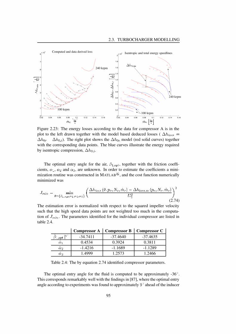
2.3. TURBOCHARGER MODELLING
0.02 0.04 0.06 0.08 0.1 0.12 0.14 0.160
1
2
3
4
5
6
7
8x 10⁴
PSfrag replacements
ÃÄUÅUÆ kgs Ç
È É Ê ËÌÌÍ J kg
ÎComputed and data derived loss
100 krpm
240 krpm
0.02 0.04 0.06 0.08 0.1 0.12 0.14 0.160
0.2
0.4
0.6
0.8
1
1.2
1.4
1.6
1.8
2x 10⁵
PSfrag replacementskgsJ
kg
Computed and data derived loss
100 krpm
240 krpm
ÃÄUÅUÆ kgs Ç
È É Ï Ð ÑÈ É ÏÓÒÔÍ J kg
ÎIsentropic and total energy speedlines
100 krpm
240 krpm
Õ�Ö'× Ø,Ù¢Ù
Figure 2.23: The energy losses according to the data for compressor A is in theplot to the left drawn together with the model based deduced losses ( Ú�Û@Ü Ý�Þ�ÞàßÚ�Û�á�âUãäÚ�Û�á5å æ ). The right plot shows the Ú�Û]á�â model (red solid curves) togetherwith the corresponding data points. The blue curves illustrate the energy requiredby isentropic compression, Ú�Û]á5å æ .
The optimal entry angle for the air, ç8è�å Ý¢é�ê , together with the friction coeffi-cients, ëUè , ë8ì and ë8í , are unknown. In order to estimate the coefficients a mini-mization routine was constructed in MATLAB î , and the cost function numericallyminimized wasï Ä æEð�ß ñ�òcóô½õ@ö,÷�øjù Ø¢ú�û å ü ø å üþý½å ü ÿ � � Ú�Û�Ü Ý�Þ�Þ����������� â����� â��8ã�Ú�Û�Ü Ý�Þ�Þ å Ä � ���� â����� â��� ìì � ì
(2.74)The estimation error is normalized with respect to the squared impeller velocitysuch that the high speed data points are not weighted too much in the computa-tion of
ï Ä æEð . The parameters identified for the individual compressor are listed intable 2.4.
Compressor A Compressor B Compressor C�ç�è�å Ý¢é�ê�� ��� -34.7411 -37.4640 -37.4635�ë�è 0.4534 0.3924 0.3811�ë8ì -1.4216 -1.1689 -1.1289�ë8í 1.4999 1.2573 1.2466
Table 2.4: The by equation 2.74 identified compressor parameters.
The optimal entry angle for the fluid is computed to be approximately -36 � .This corresponds remarkably well with the findings in [87], where the optimal entryangle according to experiments was found to approximately � � ahead of the inducer
95

CHAPTER 2. ENGINE MODELLING
blade angle. Thus, the computed blade angle is approximately -45 � compared tothe measured angle of -40 � .
Figure 2.24 depicts the incidence- and friction loss curves obtained for com-pressor A. The two losses are collected in the lower plot and compared to the totalenthalpy loss derived from data. The agreement between model and data is reason-able.
Having demonstrated the loss model’s ability to describe the incidence- andfriction losses, the loss model may be simplified since the friction component andincidence component share the same structure. Therefore, without loss of general-ity the total loss model may be transformed into "!$# %'&(&*),+.--0/2143�5768:9+ -2; -=< 1 - 68:9+ - < 1$>@? (2.75)
However, using the equation above the ability to attribute the loss to differentsources is naturally lost.
Table 2.5 shows the parameters, 1A3 , 1 - and 1$> , identified by forcing the en-thalpy loss function in equation 2.75 through the loss data set. It is noticed that the
Compressor A Compressor B Compressor CB143DCFE@GIHKJ m Lkg L�M 9.8313 9.3874 11.9660B1 - CFE@G > J mkg M -4.2866 -3.8306 -4.1834B1$> 0.6095 0.5360 0.5122
Table 2.5: Identified compressor loss parameter.
loss function apparently gets more mass flow and less rotational speed dependentas the compressor trim setting decreases. The enthalpy loss curve identified forcompressor A is shown in figure 2.25. The agreement between data and model isreasonable.
2.3.3.11 Mass flow model
Filling and emptying model structures necessitate description of the incoming andoutgoing mass flows in a control volume. Since these models for engine controlpurposes have proven their versatility in simple engine modelling for control and/orestimation purposes (see e.g. [69, 63, 45, 49, 51, 19, 50], [53], [107], [13], [103],[112] or [22]), it is of course natural to investigate the possibilities in establishinga general model of the compressor mass flow. This way the mandatory descriptionof the inlet mass is provided, and the existing engine model structures based on thefilling and emptying model approach may be reused.
A formula for the mass flow through the compressor may be found by com-bining equation 2.48 on page 82, 2.56 on page 87, 2.47 on page 81,and 2.75 on
96

2.3. TURBOCHARGER MODELLING
0.02 0.04 0.06 0.08 0.1 0.12 0.14 0.160
2000
4000
6000
8000
10000
12000
PSfrag replacements
NO=P=Q kgs R
S T U VWW XY Z[\ J kg
]Computed incidence loss
100 krpm
240 krpm
0.02 0.04 0.06 0.08 0.1 0.12 0.14 0.160.5
1
1.5
2
2.5
3
3.5
4
4.5x 10⁴
PSfrag replacementskgsJ
kg
Computed incidence loss
100 krpm
240 krpm
NO=P=Q kgs R
S T U VWW X^ _Y [\ J kg
]Computed friction loss
100 krpm
240 krpm
` a
0.02 0.04 0.06 0.08 0.1 0.12 0.14 0.160.5
1
1.5
2
2.5
3
3.5
4
4.5
5
5.5x 10⁴
PSfrag replacementskgsJ
kg
Computed incidence loss
100 krpm
240 krpmkgsJ
kg
Computed friction loss
100 krpm
240 krpm
NO=P=Q kgs R
S T U VWW\ J kg
]Total enthalpy loss bdcfe gih�h
j P4k 100 krpm
j P4k 240 krpm
Figure 2.24: The incidence and friction energy losses computed for compressor A.The total enthalpy loss (sum of collision and friction loss) speedlines are comparedwith measurements in the lower plot. The measurement speedlines are seen assolid red curves with the individual data point marked as ’ l ’.
97
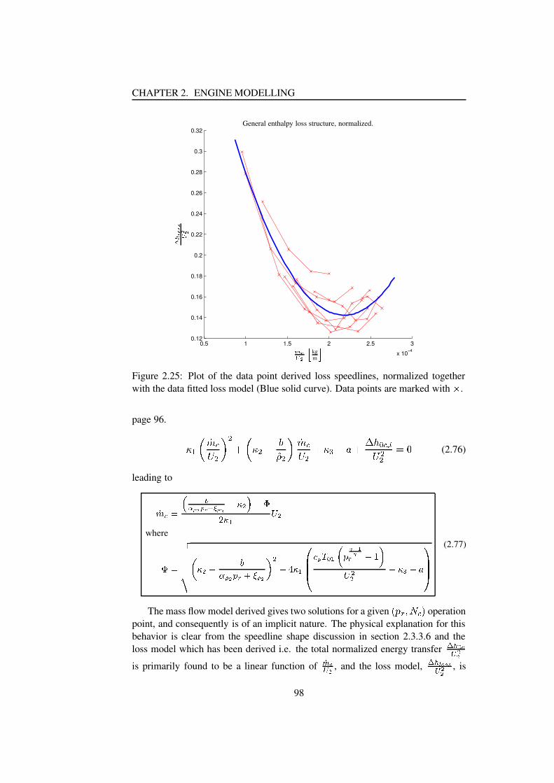
CHAPTER 2. ENGINE MODELLING
0.5 1 1.5 2 2.5 3
x 10−4
0.12
0.14
0.16
0.18
0.2
0.22
0.24
0.26
0.28
0.3
0.32
PSfrag replacements mn2op�q"r kgm s
t u v wxx yz zGeneral enthalpy loss structure, normalized.
Figure 2.25: Plot of the data point derived loss speedlines, normalized togetherwith the data fitted loss model (Blue solid curve). Data points are marked with { .
page 96. |4}�~���:��d�A� ��� ~�| �D����� ��� ��:��d� � |$� ��� ���"�$� ��� �� �� ��� (2.76)
leading to������¡ ¢£�¤ q�¥�¦(§�¨ ¤ qª©¬«®�¯ª°0±² «´³ µ where± �·¶¸¸¸¸¸¹ º «®�© »¼¾½ qÀ¿ÂÁ�Ã¬Ä ½ qÆÅ ©ÈÇÉ«´³.ÊËËÌ=Í ¥@Î´Ï ³ º ¿�ÐÒÑÉÓÐÁ ©0Ô Åµ à «®Õ�©×Ö�Ø�ÙÙÚ (2.77)
The mass flow model derived gives two solutions for a given Û ÜAÝ�Þ�ß ��à operationpoint, and consequently is of an implicit nature. The physical explanation for thisbehavior is clear from the speedline shape discussion in section 2.3.3.6 and theloss model which has been derived i.e. the total normalized energy transfer ádâfã�äå4ææis primarily found to be a linear function of çè äå æ , and the loss model, ádâfé êië�ëå4ææ , is
98

2.3. TURBOCHARGER MODELLING
quadratic in ìí=îï®ð . Furthermore, the implicit characteristic is clear from the highspeed speedlines in the compressor characteristics presented in section 2.3.3.4 onpage 75.
However, the compressor is a follower i.e. the steady state compressor massflow is determined by the pipe system downstream of compressor12 . Hence thequasi-steady state mass flow may be found using an auxiliary mass flow function.Examples of such auxiliary mass flow functions areñ Throttle mass flow in the SI engine scenario (see eg. [83]).ñ Intake port mass flow (minus possible EGR mass low) in a DI/IDI Diesel
engine scenario.ñ Connecting pipe mass flow in a Bi-Turbo – connected throttle body scenario.
Hence the unique solution to the compressor mass flow isòó:ô=õ ö"÷Føìíúù®û ìíúüîAý ìíDþî2ÿ�� òó�� òó����� � (2.78)
The three models constituting the mass flow model have been identified sep-arately, and a possible model deterioration due to accumulated estimation errorsin the individual models may exist. Hence, a identification routine readjusting the9 model coefficients such that the criterion below is minimized is implemented inMATLAB. ìí=î��� �� õ � òó:ô � ������� ô � ��� òó:ô � ������� ô������ ���� � (2.79)
The parameter vector is a gain vector, which readjusts the compressor param-eter vector � in the following manner!�Kõ"�$# õ&% ')(* �+ -,�.0/ ð 21434/ ð -567'8 -946 � �:�6;,=<?> (2.80)
The gain vector identified, , is listed in table 2.6. The table confirms that the
Compressor A Compressor B Compressor C ' 1.0341 0.9961 0.9354 � 0.7869 0.7912 0.6656 -, 0.9708 0.9105 0.9450 21 1.0972 1.3032 1.3908 -5 1.1009 1.1142 1.1933 -9 0.9050 0.9116 0.9736 �: 0.9757 1.0024 1.0378
Table 2.6: Readjusted gains belonging to the individual elements in the compressorparameter vector � .
12Stable compressor operation is assumed.
99

CHAPTER 2. ENGINE MODELLING
error on the different parameters generally is small since the gains identified de-viate modestly from the expected value of 1. However, interestingly enough, theslope, @ACB D EF�GIH�B D , of the total normalized energy transfer, J�KL2MN DD , is the parameter un-dergoing the biggest relative change of the compressor parameters and should beattributed to the base mass flow model’s overestimation for the high speed speed-lines. This tendency is general for all three compressors and is graphically visiblein the maps to the left in figure 2.26. The three maps to the right depict the pre-dicted compressor mass flow and measurements. It is evident that a relatively smallreadjustment of the individual elements in O can improve the model prediction per-formance significantly.
It should be noted that the prediction to the left of the surge line should only beseen as a best guess of the compressor mass flow mean value since they belong toan uncharted part of the compressor characteristics. However, the predictions showa high degree of resemblance with surge area speedlines presented in [40], and itis believed that the model derived together with a simple restriction model for thenegative mass flow region may also be used in basic surge area simulation studies.
2.3.3.12 Mass flow model validation
The mass flow model derived in the last section shows a high degree of estimationaccuracy. However, can it be concluded or somehow tested that the derived modelgrasps the essentials of the compressor mass flow behavior? Hence, the purpose ofthis section is the investigation of the hypothesis belowPRQTS UV�WYX Z�[�\�]^W=_a`cb UV�WedfZ�[�\�]^W�gihOkjRlnmolnpPrqsS UV�WYX Z�[�\�]^W=_$t`cb UV�WedfZ�[�\�]^W�gihOkjRlnmolnp (2.81)
where m is a steady stochastic error on the mass flow prediction b UV�W with the fol-lowing distribution m�u N X2vw\�xYyz _ (2.82)
The variable p is the measurement noise. However, all the measurements are car-ried out with state of the art equipment in the compressor manufacture’s laborato-ries, and the assumption p|{ v is viable.
The relative error in the mass flow predictions is computed for all three com-pressors and graphically illustrated in Figure 2.27. The relative errors are generallykept within an acceptable }�~ v % interval. A couple of outliers are encountered inthe low mass flow region due to the increased relative error sensitivity in this re-gion. The plots to the right in figure 2.27 are the corresponding estimated errordistribution shown together with the normal error distributions, N �-� z \�x yz�� . Thecorresponding identified mean value, � z ` E X m _ , is clearly of a negligible signifi-cance. Hence the mean value assumption presented in equation 2.82 seems valid.
100
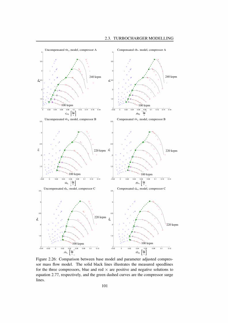
2.3. TURBOCHARGER MODELLING
0 0.02 0.04 0.06 0.08 0.1 0.12 0.14 0.16 0.181
1.5
2
2.5
3
3.5
4
PSfrag replacements
��8�8� kgs �
� �
Uncompensated��e� model, compressor A
100 krpm
240 krpm
−0.02 0 0.02 0.04 0.06 0.08 0.1 0.12 0.14 0.161
1.5
2
2.5
3
3.5
4
PSfrag replacementskgs
Uncompensated model, compressor A
100 krpm
240 krpm
��8�8� kgs �
� �
Compensated��e� model, compressor A
100 krpm
240 krpm
−0.02 0 0.02 0.04 0.06 0.08 0.1 0.12 0.141
1.5
2
2.5
3
3.5
PSfrag replacementskgs
Uncompensated model, compressor A
100 krpm
240 krpmkgs
Compensated model, compressor A
100 krpm
240 krpm
��8�8� kgs �
� �
Uncompensated��e� model, compressor B
100 krpm
220 krpm
−0.02 0 0.02 0.04 0.06 0.08 0.1 0.12 0.141
1.5
2
2.5
3
3.5
PSfrag replacementskgs
Uncompensated model, compressor A
100 krpm
240 krpmkgs
Compensated model, compressor A
100 krpm
240 krpmkgs
Uncompensated model, compressor B
100 krpm
220 krpm
��8�8� kgs �
� �
Compensated��e� model, compressor B
100 krpm
220 krpm
−0.04 −0.02 0 0.02 0.04 0.06 0.08 0.1 0.121
1.5
2
2.5
3
3.5
PSfrag replacementskgs
Uncompensated model, compressor A
100 krpm
240 krpmkgs
Compensated model, compressor A
100 krpm
240 krpmkgs
Uncompensated model, compressor B
100 krpm
220 krpmkgs
Compensated model, compressor B
100 krpm
220 krpm
��8�8� kgs �
� �
Uncompensated��e� model, compressor C
100 krpm
220 krpm
−0.02 0 0.02 0.04 0.06 0.08 0.1 0.121
1.5
2
2.5
3
3.5
PSfrag replacementskgs
Uncompensated model, compressor A
100 krpm
240 krpmkgs
Compensated model, compressor A
100 krpm
240 krpmkgs
Uncompensated model, compressor B
100 krpm
220 krpmkgs
Compensated model, compressor B
100 krpm
220 krpmkgs
Uncompensated model, compressor C
100 krpm
220 krpm
��8�8� kgs �
� �
Compensated��e� model, compressor C
100 krpm
220 krpm
Figure 2.26: Comparison between base model and parameter adjusted compres-sor mass flow model. The solid black lines illustrates the measured speedlinesfor the three compressors, blue and red � are positive and negative solutions toequation 2.77, respectively, and the green dashed curves are the compressor surgelines.
101
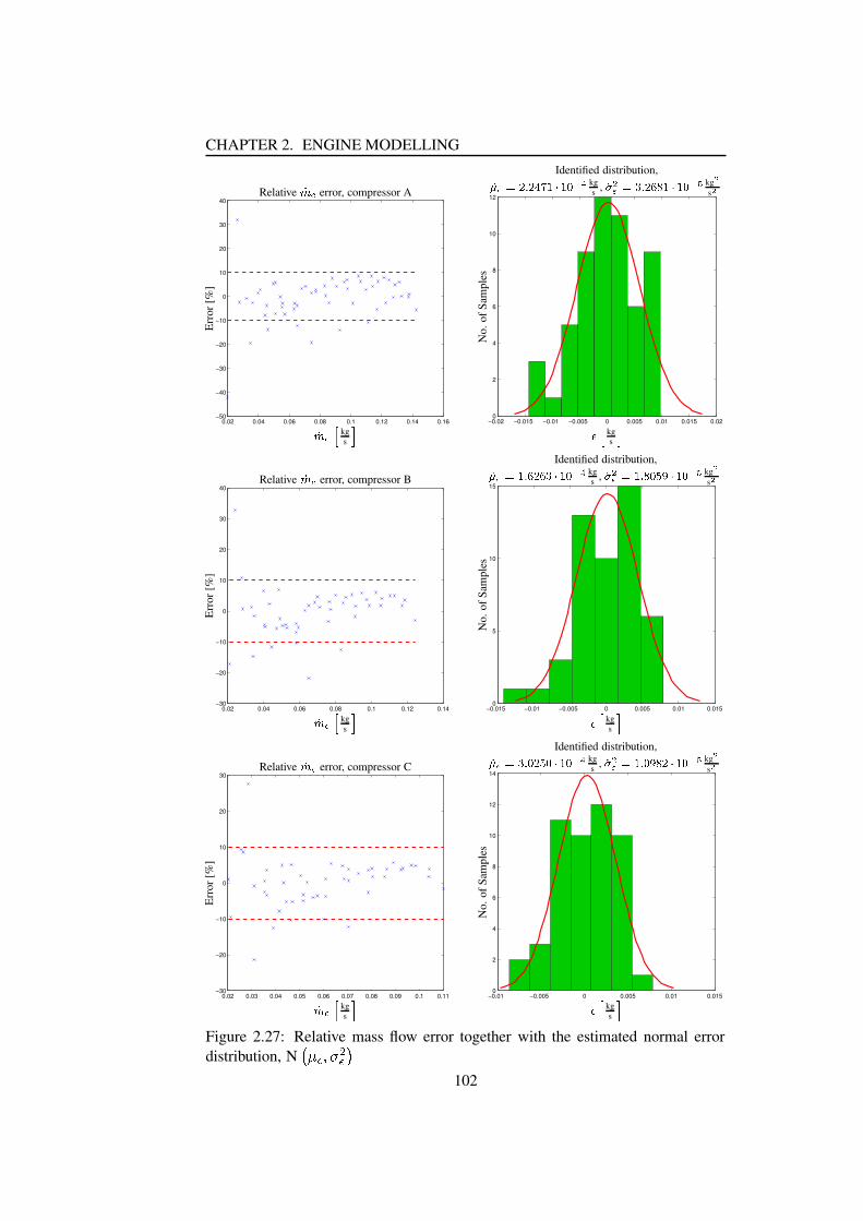
CHAPTER 2. ENGINE MODELLING
0.02 0.04 0.06 0.08 0.1 0.12 0.14 0.16−50
−40
−30
−20
−10
0
10
20
30
40
PSfrag replacements
��8�8� kgs �
Err
or[%
]Relative
��8� error, compressor A
−0.02 −0.015 −0.01 −0.005 0 0.005 0.01 0.015 0.020
2
4
6
8
10
12
PSfrag replacementskgs
Error [%]
Relative error, compressor A
�0� kgs �
No.
ofSa
mpl
es
Identified distribution,����;���=� �f�)�)�i�����=�C kgs ,
�¡�¢� ��£=� ��¤�¥=�i�����=�k¦ kg §s §
0.02 0.04 0.06 0.08 0.1 0.12 0.14−30
−20
−10
0
10
20
30
40
PSfrag replacementskgs
Error [%]
Relative error, compressor Akgs
No. of SamplesIdentified distribution,
kgs , kg
s
��8�8� kgs �
Err
or[%
]
Relative��8� error, compressor B
−0.015 −0.01 −0.005 0 0.005 0.01 0.0150
5
10
15
PSfrag replacementskgs
Error [%]
Relative error, compressor Akgs
No. of SamplesIdentified distribution,
kgs , kg
s
kgs
Error [%]
Relative error, compressor B
¨ � kgs �
No.
ofSa
mpl
es
Identified distribution,©ª�«;¬|�® ¯�°�¯�±;²��³=´Cµ kgs ,
©¶�·« ¬|�® ¸�³�¹�º;²��³=´k» kg ¼s ¼
0.02 0.03 0.04 0.05 0.06 0.07 0.08 0.09 0.1 0.11−30
−20
−10
0
10
20
30
PSfrag replacementskgs
Error [%]
Relative error, compressor Akgs
No. of SamplesIdentified distribution,
kgs , kg
s
kgs
Error [%]
Relative error, compressor Bkgs
No. of SamplesIdentified distribution,
kgs , kg
s
��8�8� kgs �
Err
or[%
]
Relative��8� error, compressor C
−0.01 −0.005 0 0.005 0.01 0.0150
2
4
6
8
10
12
14
PSfrag replacementskgs
Error [%]
Relative error, compressor Akgs
No. of SamplesIdentified distribution,
kgs , kg
s
kgs
Error [%]
Relative error, compressor Bkgs
No. of SamplesIdentified distribution,
kgs , kg
s
kgs
Error [%]
Relative error, compressor C
¨ � kgs �
No.
ofSa
mpl
es
Identified distribution,©ª�«;¬�±=® ³�°�¹�³;²��³ ´Cµ kgs ,
©¶ ·« ¬|�® ³�º�¸�°;²��³ ´k» kg ¼s ¼
Figure 2.27: Relative mass flow error together with the estimated normal errordistribution, N ½-¾ ¨�¿�À °¨�Á
102

2.3. TURBOCHARGER MODELLING
This conclusion naturally leads to the question – ”does the variable ÂÃ4Ä followa N(0,1) distribution?”. In order to answer the question an Anderson–Darling testis conducted.
The Anderson-Darling test is designed to test goodness-of-fit in the tails of aprobability density function based on a weighted-average of the squared differencebetween the observed and expected cumulative densities. Because of its relativehigh emphasis on fit quality in the tails, the Anderson–Darling statistic may beparticularly useful in statistically goodness-of-fit tests. The reader is directed to[88] or [101] for a more elaborate treatment of the Anderson–Darling test.
The Anderson–Darling test size is defined byÅÇÆ$ÈÊÉ$ËÌÉÎÍwhereÍÏÈÑÐÒ ÓÕÔ0Ö$×�Ø ÉÚÙË Û2ÜÕÝÞÛ F Û2ß Ó�à�àYá ÜÕÝÞÛ ÙâÉ
F Ûãß Ð�äÓÕå0Ö=à�à�à (2.83)
where N is the number of samples, ß Ó is the ordered variable i.e. ß Ö$æ ß Æ æÊç4ç4çIæß Ð , and F Ûãß à
is the cumulative distribution function to be tested, here the normalcumulative distribution function.
Table 2.7 shows the computedÅ Æ
values together with the critical value forthe test, [88]. The test value,
Å Æ, is for all compressors below the critical value
of 1.321, and the è|é hypothesis presented in equation 2.81 can with a confidencelevel of 95% not be overruled – the distribution of ê may be described by a normaldistribution. Å Æ
p-value ë Ô é=ì é�í ÂÃ4Äïî N Û2ðwñ Ù àóò Å ÆTôöõCompressor A 0.4433 1.3210 ÷Compressor B 0.6634 1.3210 ÷Compressor C 0.7948 1.3210 ÷
Table 2.7: Anderson–Darling test values.
It should be noted that the ê data set was not detrended prior to the Anderson–Darling, but only scaled with the estimated standard deviation øù Â , to strengthen thetest confidence. Whence, the assumption ú Â È ð is viable since all tests terminatedsuccessfully.
Finally as a final stage of model validation, the estimated cumulative distribu-tion function for ê is compared to the theoretical cumulative normal distributionF Û ê à . The results for the three compressors are shown graphically in figure 2.28.The figure shows that the general variance of the EDF (Empirical DistributionFunction) around the theoretical CDF (Cumulative Distribution Function) is of ac-ceptable level, however with an increasing degradation when moving from com-pressor A to compressor C; a conclusion supported by the Anderson–Darling test.However, the general curve tendency is linear, hence it can not from the plots be
103

CHAPTER 2. ENGINE MODELLING
0 0.1 0.2 0.3 0.4 0.5 0.6 0.7 0.8 0.9 10
0.1
0.2
0.3
0.4
0.5
0.6
0.7
0.8
0.9
1
PSfrag replacements
F ûýü-þ
ÿ F
� ��Cumulative density function comparison
A
0 0.1 0.2 0.3 0.4 0.5 0.6 0.7 0.8 0.9 10
0.1
0.2
0.3
0.4
0.5
0.6
0.7
0.8
0.9
1
PSfrag replacementsF
F
Cumulative density function comparison
A
F ûýü-þ
ÿ F
� ��Cumulative density function comparison
B
0 0.1 0.2 0.3 0.4 0.5 0.6 0.7 0.8 0.9 10
0.1
0.2
0.3
0.4
0.5
0.6
0.7
0.8
0.9
1
PSfrag replacementsF
F
Cumulative density function comparison
AF
F
Cumulative density function comparison
B
F ûýü-þ
ÿ F
� ��Cumulative density function comparison
CF������ ü� ��� ������� ��������
F�������� !#"%$ � !'& �(
Figure 2.28: Comparison of the estimated cumulative density to that of the theo-retical N(0,1) distribution.
104
2.3. TURBOCHARGER MODELLING
concluded that the normal distribution hypothesis may be overruled. Hence, thegraphical comparison of the cumulative distribution functions supports the conclu-sion of the EDF test.
On basis of the graphic test results given along with the positive conclusionof the Anderson–Darling EDF test it is here stated that the derived compressormodel, within the limits of the manufacturer compressor map, is able to capturethe essentials in compressor flow modelling.
2.3.3.13 Summary
The section describes the development of a one-dimensional compressor mass flowmodel based on physical considerations. The derived mass flow model is repeatedbelow for the sake of convenience.)*,+'-/. 0132�4658769;:<2�4>=@?BA8C�DFEG ?IH J A
whereE -LKMMMMMN O ?BAP= QR S 4<TVU%W@X S 4�Y A =[Z�?IH�\]]^`_ 5baIc H O T%d�e�fdU =Fg YJ AA W ?BhP=jilk8mmn (2.84)
The implicit equation structure is turned into an explicit solution byoprqts uwv#xyz|{B} yz|~��� yz������� op�� opr���b� � (2.85)
whereopr���b� is an auxiliary mass flow describing the general flow out of a selected
control volume.The mass flow model consists of 7 operating point independent parameters:� , � , �%��� , ����� describing the total energy transfer in the model, and �'� , ��� , ���
describing the compressor energy loss. The number of coefficients may be reducedto 6 since the parameters � and � � may be collected as one variable in the totalmodel. However, the ability to split the energy transfer in total specific energy andspecific loss energy is lost.
The mass flow model was on a statistical basis found descriptive throughout themap supplied for three different compressors, all manufactured by Allied Signal.Hence, the model derived is a good candidate in the selection of compressor modelsfor robust modelling in the sense that the model also scales well outside of thecompressor map.
105
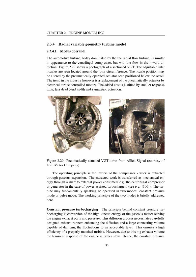
CHAPTER 2. ENGINE MODELLING
2.3.4 Radial variable geometry turbine model
2.3.4.1 Modus operandi
The automotive turbine, today dominated by the the radial flow turbine, is similarin appearance to the centrifugal compressor, but with the flow in the inward di-rection. Figure 2.29 shows a photograph of a sectioned VGT. The adjustable inletnozzles are seen located around the rotor circumference. The nozzle position maybe altered by the pneumatically operated actuator seen positioned below the scroll.The trend in the industry however is a replacement of the pneumatically actuator byelectrical torque controlled motors. The added cost is justified by smaller responsetime, less dead band width and symmetric actuation.
Figure 2.29: Pneumatically actuated VGT turbo from Allied Signal (courtesy ofFord Motor Company).
The operating principle is the inverse of the compressor - work is extractedthrough gaseous expansion. The extracted work is transferred as mechanical en-ergy through a shaft to external power consumers e.g. the centrifugal compressoror generator in the case of power assisted turbochargers (see e.g. [106]). The tur-bine may fundamentally speaking be operated in two modes: constant pressuremode or pulse mode. The working principle of the two modes is briefly addressedhere.
Constant pressure turbocharging The principle behind constant pressure tur-bocharging is conversion of the high kinetic energy of the gaseous matter leavingthe engine exhaust ports into pressure. This diffusion process necessitates carefullydesigned exhaust runners enhancing the diffusion and a large connecting volumecapable of damping the fluctuations to an acceptable level. This ensures a highefficiency of a properly matched turbine. However, due to this big exhaust volumethe transient response of the engine is rather slow. Hence, the constant pressure
106

2.3. TURBOCHARGER MODELLING
turbocharging principle is mainly use on stand alone engines operating at a fixedspeed e.g. power generators. Furthermore, the back pressure will be relativelyhigh, and an increased pumping loss may be expected, especially in the case of athrottled engine.
Pulse mode turbocharging The other extreme of turbine operation is the pulsemode operation. Here the exhaust flow is sought stagnated as little as possiblebefore turbine entry i.e. kinetic energy preservation. The pulse mode exhaust man-ifold is thus characterized by separate relatively thin short runners. The pressureratio across the turbine is characterized by a high narrow pressure burst followed bya long period with a stage pressure ratio close to unity until the next pressure burstarrives, [87, 54]. The penalty is evidently a degradation of the turbine efficiency.It is actually fortunate that the turbine is able to function at all under these condi-tions. However, if the exhaust runners are grouped carefully, an acceptable levelof turbine operating efficiency can be achieved. Furthermore, the small exhaustvolume gives the pulse mode strategy a much faster transient response comparedto the constant pressure strategy.
The pulse mode strategy is quite clearly the relevant choice for automotiveapplications due to the better transient response and ease of packaging.
2.3.4.2 VGT elementary
The VGT consists of the four base components listed below.� Inlet casing or scroll� Variable inlet nozzles.� Rotor� Exducer (Rotor eye) and outlet pipe.
A sketch of a VGT depicting the key elements mentioned is shown in fig-ure 2.30.
The job of the scroll is purely to deliver a uniform flow to the nozzle entry.The flow is then accelerated through the nozzles due to the radial area decreasei.e. pressure is converted into kinetic energy. The actual energy transfer occursin the rotor. The rotor should be designed so that the kinetic exit energy is mini-mized as much as possible. This process description is pictured schematically inthe enthalpy-entropy diagram such that the loss sources may be understood indi-vidually. Station 01 refers here to scroll inlet stagnation conditions. However, theflow enters the nozzle with absolute velocity �>� , and the static enthalpy is thereby aquantity ����� smaller than the stagnation enthalpy. Between station 1 and 2 the flowis accelerated due to the area decrease mentioned above and the flow will leave thenozzles with absolute velocity � � . However, some of the thermodynamic energy
107

CHAPTER 2. ENGINE MODELLING
PSfrag replacements
Scroll
Adjustablenozzles
Rotor
Exducerand outlet ¡ ¡b¢ £¥¤ ¦¨§ © ª« ¬� ®¯�°²±´³µ
¶¸·¹ · º
£Figure 2.30: Variable geometry turbine diagram.
PSfrag replacements
1
23
4
»
¼½�¾¿À ½�¾¾À
½�¾ÁÀ01
1
2
3
4
04
Â�à ÂbÄ À À ÂbÅ ÂbÆÂbÄ�Æ
Figure 2.31: VGT Entropy–Enthalpy diagram.
108

2.3. TURBOCHARGER MODELLING
is lost mainly due to the collision between nozzles and fluid during flow entry andthe inevitable nozzle passage friction. This leads to a significant entropy increase.The line connecting station 2 to 3 describes the process between nozzle exit androtor entry. Since this space is relatively small the distance between station 2 and3 normally negligible. The path 3 to 4 describes the actual energy extraction. Thispath is not ideal either mainly due to collision and friction losses. Finally, since afair amount of the kinetic energy can not be extracted fully the stagnation pressure,Ç È6É , will be higher than the static pressure Ç�É . Since no work takes place in thescroll and nozzles the total work extraction may be found to beÊ%Ë'ÌÎÍÏ Ë¸Ð�ÑwÒ È�Ó`Ô ÑwÒ È6ÉlÕ ÌÖÍÏ Ë¸Ð�ÑwÒ ÈØ×�Ô ÑwÒ È6ÉlÕ (2.86)
Similar to the compressor case this energy transfer may also be derived froman investigation of the inlet and outlet fluid velocities. Figure 2.32 shows the fluidvelocity conditions at the rotor entry and exducer, respectively.
The torque extracted may be derived dual to the compressor description. Thus,the rate of change of angular momentum equals the sum of external torques. Sincethe change of angular momentum corresponds to the change of the moment oflinear momentum, the effective torque, Ù Ë , is found toÙ Ë'ÌÎÍÏ Ë�ÐÛÚÝÜbÞ ×�ß à Ô Ú É Þ Éáß à Õ (2.87)
The radius,Ú É , is normally selected as the radius of the circle splitting the ex-
ducer area in two annuli of equal area i.e.Ú É Ì ÓÉ â ã[äÉáß åçæ ã[äÉáß è . Multiplying
equation 2.87 with the rotor angular speed the extracted power is found toÊ%ËPÌÎÍÏ ËÛé'Ë�Ð�ÚÝÜbÞ ×�ß à Ô Ú É Þ Éáß à Õ ÌÎÍÏ Ë�Ðëê × Þ ×�ß à Ô ê É Þ Éáß à Õ (2.88)
Combining equations 2.88 and 2.86 the effective work extracted in terms of specificenergy may be expressed asÑwÒ È�ß Ë'ÌìÐíê × Þ ×�ß à Ô ê É Þ Éáß à Õ (2.89)
However, since the absolute exit velocityÞ É is desired to be small for efficiency
reasons, the rotor design is optimized so that swirl is minimized i.e.Þ Éáß àçîðï , and
the previous equation may be reduced even further toÑwÒ È�ß Ë'Ìñê × Þ ×�ß à (2.90)
The enthalpy released due to the expansion on a total-to-total basis is given bythe isentropic relation belowÑwÒ È Ë ß ò Ìðó6ôlõ È�Ó�öP÷�Ôùø Ç È�ÓÇ È6É;ú@û�ü�ýýÿþ (2.91)
109
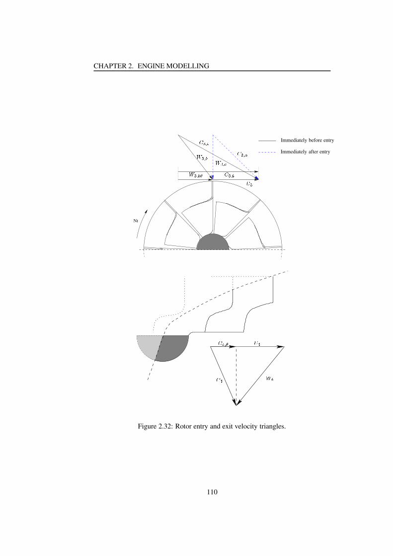
CHAPTER 2. ENGINE MODELLING
Nt
PSfrag replacements
Immediately before entry
Immediately after entry
���� ��� �� ��� � � ��� �� ��� �� ���� � � ��� �
PSfrag replacements
Immediately before entry
Immediately after entry
�� � �� �� �
Figure 2.32: Rotor entry and exit velocity triangles.
110

2.3. TURBOCHARGER MODELLING
Hence the total-to-total turbine efficiency is found to����� ����� ����� � ������ ��� �! "$#%� �'&�($) �+*-, "$#%� �'&/.0) �$1"$#%� �'&�($) �+*32546,87 #9&�(#9&/.%: (/;%<<>= ) �+*-, ) �$1) �+*3254?,A@ (/;%<<B � ��� = (2.92)
However, the kinetic energy of the fluid leaving the exducer will always be lost.Therefore, a more natural choice of stage efficiency description is to relate inletstagnation conditions to static outlet conditions, i.e.����� �DCE� ����� � ������ ��� �! "$#%� �'&�($) �+*-, "$#%� �'&/.F) �$1"$#%� �'&�(�) �+*32546, 7 #9&�(#9. : (/;%<<>= ) �+*-, ) �$1) �+*32546,A@ (/;%<<B = (2.93)
and ����� ��� �G�H"$#') �+*JIK4?,L2 @M�+*@N1 = (/;%<<>O (2.94)
Finally, the total-to-static enthalpy loss is defined by,��� ��� P QSR�R � ����� ��� � ,T����� �K�8U 4?, ����� �DCNV ����� ��� � (2.95)
In an effort to generalize specifications of turbines, manufactures also often useterms like aspect ratio, trim, and U/C characteristics.
The aspect ratio or abbreviated A/R (Area/Radius Ratio) of a turbine is definedas the ratio between volute inlet area and effective volute inlet radius (see e.g. [87]).This ratio gives a rough measure of the fluid’s entry angle into the rotor in the caseof a vaneless nozzle or into the vaned nozzle ring, respectively,and is thus a tool inthe engine-turbine matching procedure. The setting of A/R is however most criticalin the case with a vaneless nozzle ring.
The trim setting specifies the ratio between rotor inlet diameter and exducer di-ameter, and is already described in the compressor section (see 2.3.3.4 on page 75).
It is customary in the classification of turbine efficiency to plot the efficiencyagainst the so called U/C (Turbocharger wheel velocity/maximum fluid velocityRatio) number. The U/C term is a dimensionless number relating rotor tip veloc-ity, WKX , to the gas velocity, Y R , achieved if the fluid had followed an isentropicexpansion from inlet stagnation conditions to static outlet conditions, i.e.WY � WKXY R � W BZ [ "$#') �+* 2 46,A@ (/;%<<B = (2.96)
Although the use of U/C ratio analogy is only valid for pure impulse turbine de-signs13, it provides a non-dimensional form of the turbine speed, thus providingvaluable information when matching turbines and compressors.
13The static rotor inlet enthalpy \^]�_ equals the outlet stagnation enthalpy \^] &/. following anisentropic expansion line.
111

CHAPTER 2. ENGINE MODELLING
2.3.4.3 Literature
The literature on VGT modelling for MVEM or control purposes is sparse. Mostmodels rely on table interpolation when computing the mass flow, `a�b and the tur-bine efficiency c b . However, as stated in the previous section, the turbines are oftenmapped very sparsely, and most often the map only covers the mid to high rev-olution areas of the turbine operating range. This of course hampers successfulcalculation of `adb and c b .
In [91] two fitting techniques for VGT mass flow modelling purposes are pre-sented: one based on the isentropic nozzle flow equation and one based on neuralnetworks. However, the first fitting technique cannot capture the effect of the cen-trifugal field around the rotor, and large mass flow errors can be expected in thelow pressure region of the turbine map. The neural network does not improve theprediction quality noticeably, and is further hampered by the need for artificial datapoints for realistic predictions in the low pressure range of the turbine map.
The turbine efficiency was modelled in [91] by a second order polynomial inef�gwith the coefficients linearly dependent on turbine speed. Due to the rela-
tively high amount of ”fiddling” required getting the models proposed in [91] towork these models will not be considered further here.
Reverting to modelling of automotive turbines with a fixed geometry nozzlering in the quest for a general VGT model, the three sources [63, 61, 83] are ofinterest. Addressing mass flow modelling the initial step in all three sources isan investigation of the possibilities in applying the isentropic nozzle flow equationrepeated below
`aAh%i$j!kmlnno nnpg?q^r h%i$jts9u�vw xzy u�vS{| v}~�� ����������5�6� { v | }}~�� � { ~3��� �'�G���� }} | v (subsonic)g?q^r h%i$jts9u�vw xzy u�v�� � � ��'�G��� }F� v��� } | v�� � { ~3� � �'�G���� }} | v (sonic)
(2.97)where { ~ k�s9u�vs9� ,
g?qis the discharge coefficient, and
r h%i$j the minimum effectiveopen area of the nozzle.
The application of the isentropic nozzle equation is justifiable since the turbine,fundamentally speaking, may be viewed as two nozzles in series; the nozzle ringand the rotor, respectively.
Converting equation 2.97 into corrected mass flow, and collecting the upstreamconditions together with
gqand
r h%i$j an equivalence ”area” factor,rJ��
, may befound as r3�� k g?q^r h%i$j {M¡ �� ¢3£ ¡ �^¤
y u�vy u�v/¥ ¦¨§/©s9u�vs u�v/¥ ¦¨§/© k g?q^r h%i$j { ¡ �Sª ~ �$«¬ ¢3£ ¡ �Sª ~ �$« (2.98)
This factor was in [61, 83] found to decrease with turbine speed increase andpressure ratio decrease, respectively. This is however to be expected due to thevariation in the centrifugal field around the rotor wheel as it turns.
112

2.3. TURBOCHARGER MODELLING
The variable ¯®�° ’s variation was in [63, 61] found to be mainly a linear functionfor either fixed pressure ratio, ±D² , or turbine speed, ³�´ . Hence, the equivalence areawas approximated by 3®�°6µ·¶�´�¸/±N²-¹>¶�´º
with ¶�´¼»G½·¶¾¸S¿ » ³À´Á Â�à ¸ ¹>¶�º+¿ »�Ä for Åƽ8Ç%ÄFÈ (2.99)
where the constants, ¶É´�¿ » , are determined subsequently by regression.The turbine efficiency ÊÉ´ was in [63, 61] modelled using a third order polyno-
mial in U/C and speed dependent coefficients, i.e.Ê�´Ë½ÌÊ�´�¿ ÍDÎE½·Ï+Ð�Ñ Ð ¹>Ï+º9Ñ º ¹>Ï9¸+ÑÒ¹>Ï Ãwith ÏF»G½tÓÕÔ/Ö ×ÙØDÓ+Ú�Ö ×�Û�ÜÓFÝFÞMÛ�Ü for ÅK½Hß?àÕàÕàâáãÄäÑå½çæ Ýè¾é (2.100)
However, this model was in [83] found being to inaccurate when applied tothe map data for the KKK turbine investigated. Hence, the model structure waschanged and a more suitable efficiency description was found to beÊ�´K½�ê$º-ë¨ÑÌìíÑ ²S®$î�ï º ¹TêF¸Gë¨ÑÌìíÑ ²S®$î�ï ¹Òð
where ð ½ ê$Ð^ìñÊ ÍN¿ ²S®$îÑ ²S®$î ½ ê�òâÊ�´M¹Tê$óÊ ´�¿ ²S®$î ½ ê$ôⳠд ¹õêSöâ³ º´ ¹Tê$÷â³À´M¹Tê$ø (2.101)
necessitating a subsequent identification of the coefficients ê�¸ÕÄÕàÕàÕà�ÄSê$ø .The turbine models presented above are split in two parts: a mass flow model
and an efficiency model. The mass flow models are based on soft semi-physicalconsiderations whereas the efficiency models are all pure fitting functions. Use ofthe models proposed in [63, 61, 83] to model VGT mass flow and efficiency wouldnecessitate an augmentation of the models. An obvious augmentation would beto first identify the individual coefficients for a given fixed position of the nozzlesvanes (fixed VGT position) and later model the coefficient’s variation by polyno-mials of the VGT position, ù%ú0û0´ . However, this would clearly require identificationof a relatively large number of coefficients. Moreover, the models only providea quite ambiguous picture of the VGT behavior. This, together with the expectedpoor extrapolation accuracy, calls for a reinvestigation of turbine modelling, and isthe task for the rest of this section.
2.3.4.4 VGT data set
The validation of the turbine identification procedures and theories established inthe following section is based on a data set for an Allied Signal VGT. The data set
113

CHAPTER 2. ENGINE MODELLING
was selected because of its exceptionally large size (252 points). A normal data setmay consist of as few as 35 point to cover the whole operating range of a VGT.
The dimensional specifications for the VGT are listed table 2.8, and the designbasically speaking reassembles that of the VGT shown in figure 2.29.
Type definition GT15V NS111(39)Trim 76A/R, ü in ý 0.42No. of nozzles, þ�ÿ���� 9Rotor diameter,
���, ümm ý 39
Rotor inlet width, ��� , ümm ý 6.2Inner nozzle ring diameter,
� ��� � , ümm ý 41.3Outer nozzle ring diameter,
� ��� � , ümm ý 77.5Nozzle ring axel diameter,
� ��� � , ümm ý 60.0Nozzle blade length, ��ÿ , ümm ý 17.0Nozzle blade tip length, ��ÿ ��� � , ümm ý 7.0
Maximum corrected mass flow, �� �� �� ����� , � kgs � 0.08
Table 2.8: Dimensional specifications for GT15V NS111(39) VGT (see also fig-ure 2.30). The data marked with ’*’ is found by mechanical disassembling of theVGT and should thus be treated as more descriptive than accurate.
Figure 2.33 shows the flow characteristics of the turbine. The effect of thenozzle position variation on the mass flow characteristic is evident; an increase ofthe VGT position for a given pressure ratio, � � , leads to higher a mass flow.
Creation of a comprehensive picture of the turbine efficiency is complicateddue to the added degree of freedom. However, a general design rule, within theboundaries of the supplier map, is to peak the efficiency around a normalized VGTposition of 0.5. This is also the case for the VGT investigated here and is unmis-takably clear in figure 2.34. The figure also shows, that despite the uncommonlylarge amount of data, only the descending part of the ���! characteristic has beencharted. This is of course unfortunate considering a subsequent efficiency identifi-cation investigation.
However, due to the large amount of data available for different "$#�% � settings,generalized conclusions concerning turbine modelling may nevertheless be ex-tracted from the data.
2.3.4.5 LWLS (Locally Weighted Least Square) regression
Modelling of turbines, especially when employed in highly fluctuating flows, is asoften stated a cumbersome affair. However, a model of the mass flow through theturbine is mandatory in the creation of an exhaust filling–emptying model whichcan predict the dynamic behavior of the exhaust temperature and pressure. This
114
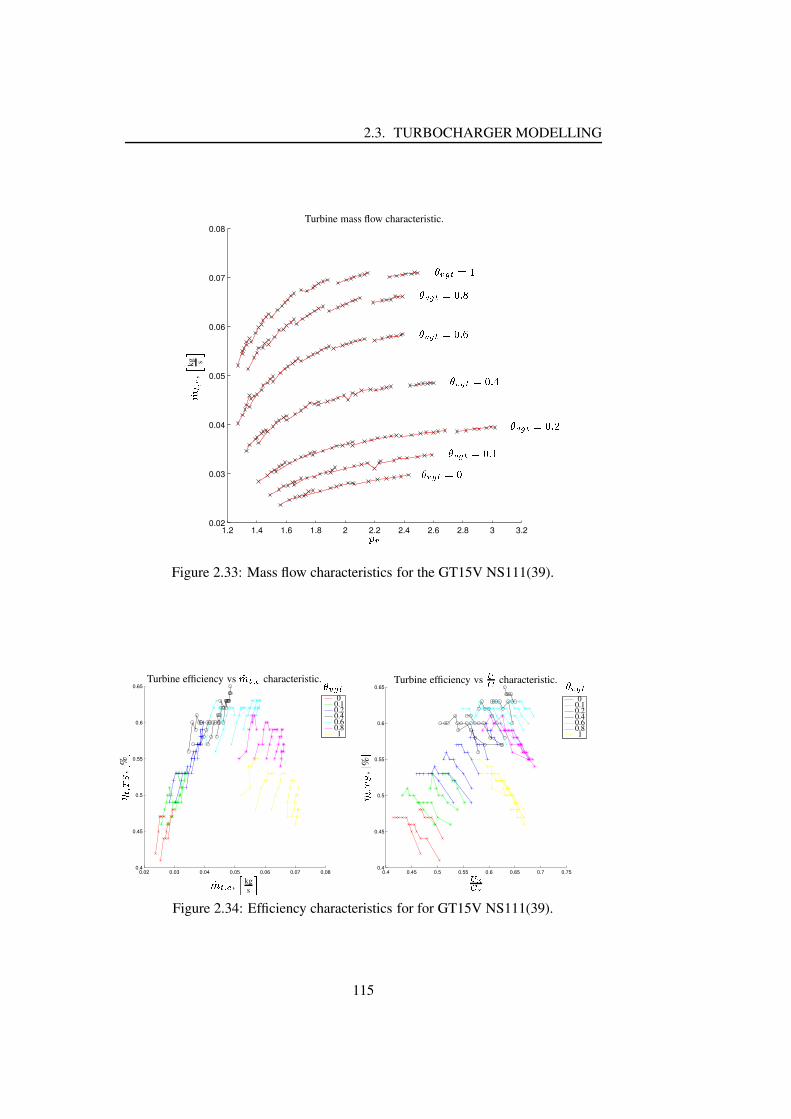
2.3. TURBOCHARGER MODELLING
1.2 1.4 1.6 1.8 2 2.2 2.4 2.6 2.8 3 3.20.02
0.03
0.04
0.05
0.06
0.07
0.08
PSfrag replacements& ' (*)+ ,, kg s
-
.0/
Turbine mass flow characteristic.
132�4357698132�4357698;: <132�4357698;: =
132�4357698;: >132�4357698;: ?132�4357698;: @132�43576A<
Figure 2.33: Mass flow characteristics for the GT15V NS111(39).
0.02 0.03 0.04 0.05 0.06 0.07 0.080.4
0.45
0.5
0.55
0.6
0.65
PSfrag replacements
B (*)CD ,E %
F
GH 5JI K , L kgs M
Turbine efficiency vsGH 5JI K characteristic.
00.10.20.40.60.81
132�435
0.4 0.45 0.5 0.55 0.6 0.65 0.7 0.750.4
0.45
0.5
0.55
0.6
0.65
PSfrag replacements, %
, kgs
Turbine efficiency vs characteristic.
0
0.1
0.2
0.4
0.6
0.8
1
B (*)CD ,E %
F
NPOQ�R
Turbine efficiency vsNQ characteristic.
00.10.20.40.60.81
132�435
Figure 2.34: Efficiency characteristics for for GT15V NS111(39).
115

CHAPTER 2. ENGINE MODELLING
would commonly necessitate models of the exhaust port mass flow and tempera-ture, EGR mass flow and turbine mass flow.
The insertion of variable vanes in the turbine nozzle evidently does not easethe modelling task. Therefore, the most customary used control oriented VGT’smass flow models found in the literature rely on table interpolation, regressionanalysis, or linear model approximation (see e.g. [16, 39, 104, 87, 91, 108, 84, 63]),where the two first methods of modelling are the most commonly found. Thatanalysis and modelling based on map interpolation or regression are natural choiceswhen modelling complex structures like the VGT is evident due to their reasonablysimple employment in dynamical models. However, regression analysis shouldnot be done without a initial analysis (physical investigation) for these obviousstatements:S
The model quality is proportional to data quality.SThe data set must cover as the complete region of interest for simulation -and as dense as possible.SExtrapolation accuracy is often very questionable.
The words of caution or prerequisites above are however quite often neglected, andthe regression models derived are employed without question (see e.g. [83, 91,108]).
However, since regression analysis has proven to be a very versatile tool inthe analysis of complex phenomenons, e.g. combustion processes, internal enginefriction forces etc. [49, 62], it is worth investigating the possibility of constructinga generalized regression tool for automotive analysis. This is the topic for rest ofthis section.
The most often encountered generalized modelling concepts in the literatureare neural network or polynomial structures. Neural networks are certainly use-ful tools when addressing automotive modelling. However, successful applicationof neural networks requires a great deal of insight and use of sophisticated opti-mization algorithms. Hence, the emphasis here is on the application of polynomialstructures in the search for a descriptive correlation between inputs and outputs.
The most often encountered multi variable polynomial structure for regressionin the literature is based on the application of one high order multi variable poly-nomial to model the behavior of a given phenomenon e.g. VGT mass flow andefficiency (see e.g. [83, 108]). However, this method has several disadvantages:S
Undesirable extraneous curvature between data points.SA large number of polynomial coefficients needs to be identified.SSteep gradients outside the identification region due to high order polyno-mial terms.SThe cost function might not be convex.
116

2.3. TURBOCHARGER MODELLINGT Large identification regions often necessitate high order polynomial struc-tures to achieve an acceptable level of modelling accuracy.T Sophisticated minimization algorithms are often needed.
Clearly, one of the biggest problems stated above is the need of higher orderpolynomials to achieve the desire level of modelling accuracy. This spawns ofanother requirement also listed above – identification of a large number of poly-nomial coefficients is mandatory. However, if the space spanned by the selectedcorrelation function inputs is split into numerous subspaces, when a local multivariable polynomial structure, often of a much lower order, may be found. Thisparadigm is here referred to as local regression, and the details of establishingsuch a regression analysis are outlined below.
The signal of interest is assumed in the algebraic case described byUWV f XZY�[]\_^ (2.102)
or in the dynamic case by the difference functionUa`bV f XZY ` [c\_^ `with Y `dV XZe `gfchi e `gfkjlimmmgi e `gfonkiqpr`$iqpr`gfchimmmgiqpr`gfos [ (2.103)
where ^ is independent normally distributed noise, i.e. ^ut N X�v i�w j [ .In order for a viable solution to exist the following is required,T The solution to the function f X mmm [ is unique with respect to Y .T The function f is continuously differentiable.
Proof: Follows directly from the definition of Taylor series.The conditions above can most often not be checked prior to the regression
analysis, however, a subsequent application of a statistical tool like the Anderson–Darling test may tell whether or not the functional description found can capturethe essential features of U ’s behavior within the boundaries of the data set (see e.g.section 2.3.3.12).
Assuming that the function f fulfills the necessary requirements, f may be de-scribed by,
f X�x7[ Vzy{ |*}�~��Y�� X����g�A[|f X�x7[;� � } �3� (2.104)
The equation above uses a parallel space of x i.e. x V x ~ \��9� f X�x7[ V f X�x ~ i ��[ .Introducing the error � this function is rewritten as
f X�x7[ V P X���\�x ~ [c\ O �$X��u\�x ~ [ n!��h�� (2.105)
where P is a multi variable polynomial of order � and O is an error function.
117

CHAPTER 2. ENGINE MODELLING
Assuming that the error function is small in some neighborhood of �7� such thatit can be represented by the noise process � , then an estimate of � in the neighbor-hood of ��� is given by, ��W� E �Z�]� �7��� f ���7���¡ A���£¢�¤u�¤_�¦¥ §;¨k©�§;¨$ªc«0©¬¬¬0©�§g«g©�§P�; (2.106)
where ¤ is the coefficient vector of the polynomial .Having established a feasible regression structure the next thing missing is the
definition of local data – the data belonging to the local subspace defined earlier.Local data is here defined as a predetermined fraction, ® , of the total data set layingwithin a hypersphere with Euclidian radius ¯ and center �$� . The radius ¯ of thesphere may be found by a NN (Nearest Neighbor) criterion. The NN criterionfollows: given ° data points, a fraction factor ® , and grid point �7� , then NN datapoints are the ±²� round ��®a°³� data points in the closest Euclidian proximity of thegrid point ��� .
A suitable cost function in the computation of ¤�´ belonging to grid point µ isthe quadratic function given below¶ ´·�¹¸º »*¼ «�½_¾£¿
»¯dÀ �Z� »rÁ A�� »kà � �;Ä ´a¢�¤�´a�q�3Å (2.107)
Hence the coefficient vector, ¤u´ , belonging to the polynomial �´Æ�3ÇÈ¢�¤�´!� is derivedby computing ¤�´d�¡É�Ê�Ë�ÌWÍ*ÎÏoÐ � ¶ ´!� (2.108)
The solution to the LS (Least Square) criterion in equation 2.108 is linear in thecoefficients space. Hence the solution to ¤�´ is found in a straightforward mannerby applying the pseudo inverse,¤�´d�ÒÑ�Ó T Ô Ó�Õ ªc« Ó T Ô�Ö (2.109)
where Ó is the regressor matrix containing the ± inputs to the system, Ô is a diag-onal ±Ò×ر weight matrix with the diagonal Ù ½ ´« ©¬¬¬0© ½ ´¸ Ú 14, and Ö is the mea-surement vector containing the ± measurements of � . Thus, the solution to ¤Û´ isglobal and optimal for a given polynomial structure.
Before proceeding to application of the theory outlined above on turbine esti-mation, a few words of caution should be mentioned about the influence of noise.It is thought that this is best illustrated with an example.
First equation 2.103 is generalized toÜ ´d� f ��Ýg´!� à ��Þ ´�a´d� Ü ´ à �qß´ (2.110)
14Another often applied data weighting structure is the Epanechnikov structure (see e.g. [72]).
118

2.3. TURBOCHARGER MODELLING
where à�á is white process noise, and àÈâ is white measurement noise. An exampleof such a process given below ãrädåçæ�èÆé êlë$ì!ì!ìlãríägîcï�ð à á äñ ädåòãrä ð à â ä
where óô õãrö�å�ë
à á äø÷ N ù èÆú�û íáoüàqâä ÷N ù èÆú�û íâ ü
(2.111)
This function was simulated in the MATLAB ý environment and 100 data pointswere generated with different noise settings. The simulation results are given infigure 2.35.
0 10 20 30 40 50 60 70 80 90 1000
0.5
1
1.5
2
2.5
3
3.5
4
PSfrag replacements
þ , ÿ���� ÿ � � ö
ä� �
0 10 20 30 40 50 60 70 80 90 100−1
−0.5
0
0.5
1
1.5
2
2.5
3
3.5
4
PSfrag replacements
,
� , ����� , �� �� N ��������� ���
�� �
0 10 20 30 40 50 60 70 80 90 100−1
0
1
2
3
4
5
PSfrag replacements
,
, , N
þ , ÿ ��� N � ö � ö ï ! , ÿ � � ö
ä� �
Figure 2.35: Illustration of the ñ ä noise penetration. Note, the realized noise timeà is same for the two plots on right.
The parameters identified listed in table 2.9 clearly show the noise effect on theestimation quality. " í " ï " öû íá å¡û íâ å¡è
0.24999 0 0û íá å¡èÆé #
,
û íâ å¡è0.2316 0.0565 -0.0502
û íá å¡è,
û íâ å¡èÆé #0.1744 0.2796 -0.0625
Table 2.9: Identified parameters for P with different noise settings.
The table states a general problem in nonlinear system identification, noisespectrum wrapping (see e.g. [72]). In the case of process noise the noise spectrumis unchanged i.e.
E$&%ñ(''' %) å )&* å f ù�+ ü-,/.0 � 0
V$&%ñ(''' %) å )&* å¡ûcíá (2.112)
However, in the case of measurement noise the chances of successful parameterestimation is ill conditioned for the following reason. The stationary white noise
119

CHAPTER 2. ENGINE MODELLING
to step 1 , 2435 , will enter the regressor 6 5 in entry 1 of the identification data i.e. awrapping of the noise spectrum will occur( see e.g. [17]). Thus the non-recursiveestimates, 78 , will be biased. The above explanation is sought illustrated by a smallexample:
Let 9 be stationary white noise such that 9;: N <�=?>4@BADC , and let EGFIHJA . Thequestion is now what is the distribution of K . The distribution may be found byinvestigating the cumulative distribution of HL <MHNCOFQPR<S9;TUHNCVF WX Y[Z @ \]^`_badcfe4ggMh gjilk (2.113)
L <MEmC�Fon =?> Eqpr=PR<�s X EqTQ9;T X EmCt> Equr= (2.114)
Hence,L <MEmC may be written as,L <MEmCVF;vwx wy
z{ A}|f~ { ��^ { � adcfe4ggMh g ilk > Equr==?> Eqpr= (2.115)
A change of the noise mean value is clear from the equations above, hence the datavector, � , will be biased. In the simple case above the bias is found to be� <MEmCVF _] � E���<MEmC i E
where ��<MEmC�F WX E a cf�gMh g(2.116)
The conclusion is, although the function order of the system to be identifiedis correct the estimation quality15 might deteriorate when measurement noise ispresent.���� and � � LWLS estimation Despite the warnings given above LWLS may beutilized to estimate the hypersphere of
������ � and � ��� �d� , since the turbine maps pro-vide are made using state-of-the-art measurement equipment. Hence, the measure-ment noise level is assumed negligible.
The
������ � and � ��� �d� hyperspheres are assumed affine in � ��� � , ��� and8��4� � , i.e. a
unique description is������ � F ������ � <�� ��� � >����D> 8��4� � C� ��� �d� FI� ��� �d� <�� ��� � >����D> 8��4� � C (2.117)
15Identification structure dependent.
120

2.3. TURBOCHARGER MODELLING
The input variables are scaled prior to the identification procedure������ ���I �¡G¢D£¤ M�¦¥B�§¡G¨ª©& M�¦¥«¥¡G¢D£j M�¦¥B�§¡G¨ª©j M�¦¥ (2.118)
where�
is either one of ¬(�® ¯ , °�± and ²�³4´4 , and��¶µr· �¹¸[º»¸�¼
. This step is taken toprevent numerical problems.
The second order Taylor series belonging to equation 2.117 with scaled dimen-sionless inputs has the structure½R �¬¹�® ¯¿¾ �°�±D¾ �²�³4´4 ¥V� ²DÀOÁ²ÄÃÆÅ �¬¹�® ¯ � �¬¹�® ¯}® À¿ÇGÁ²DÈ �°�± � �°�±}® À ¥ Á²DÉÊÅ �²�³4´4 � �²�³4´4�® À¿ÇÁ²ÄëÃÆÅ �¬¹�® ¯ � �¬¹�® ¯}® À�Ç È Á²DÈ«È �°�± � �°�±}® À ¥ È Á˲DÉ«ÉÌÅ �²�³4´4 � �²�³4´4�® À-Ç ÈÁ²ÄÃÍÈÊÅ �¬¹�® ¯ � �¬¹�® ¯}® À�Ç �°�± � �°�±}® À ¥Á²ÄÃÍÉÊÅ �¬¹�® ¯ � �¬¹�® ¯}® À�Ç�Å �²�³4´4 � �²�³4´4�® À-ÇÁ²DÈ«É �°�± � �°�±}® À ¥ Å �²�³4´4 � �²�³4´4�® À-Ç
(2.119)
The cubic space with the constraints Î �°&±ÄÎt¾ÄÏÏÏ �²�³4´4»ÏÏÏ ¾ÄÏÏÏ �¬¹�® ¯fÏÏÏJÐ ¸is divided into
1000 subspaces of equal size i.e. the side length of each individual subspace is0.2. The origin of each Taylor expansion is now chosen as one of the
¸f¸ É �o¸»ÑfÑ?¸individual node points in the scaled input space, i.e.�� À µÓÒl�¹¸ ¾ �ÊÔ?Õ Ö ¾ �ÊÔ?Õ × ¾ �ÊÔ?Õ Ø ¾ �ÊÔ?Õ � ¾ Ô ¾ Ô�Õ � ¾ Ô?Õ Ø ¾ Ô�Õ × ¾ Ô?Õ Ö ¾ ¸DÙ (2.120)
A reasonable data fraction, Ú , is here 0.3. This data fraction insures that inverseof ÛmÜBÝÞÛ is well posed i.e. its eigenvalues are significantly different from 0. How-ever, choosing Ú too high might limit the ability to capture local curvature. Hence,the local neighbor data fraction number is
Ô?Õ ÑNß �fàf� �âá[×.
A cubic weighting function is selected here to shape the data kernel number ã ,ä ´å �;æç èbé ¸ê� Å�ë�ì±Íí Ç É¿î É ¾ forÔ Ð ë�ì±Íí Ð ¸Ô ¾ else
(2.121)
where the bandwidth ïD´ is set to be the euclidian distance between grid point ²lÀ�® ´and the closest measurement point outside the data kernel hypersphere i.e ïl´ �ð4ñlòjó à � ²DÀ�® ´ ð È .
The setup is complete and the only thing missing is the computation of thecoefficient vector ô for of each the 1331 individual polynomials. This is doneaccording to equation 2.109.
The LWLS estimates of õö �® ¯ and ÷f�® Üdø , respectively, are compared to measure-ments in figure 2.36. The LWLS estimation technique are clearly able to resolvethe curvature of the turbine mass flow and efficiency with reasonable smoothing.
121

CHAPTER 2. ENGINE MODELLING
0 50 100 150 200 250
0.025
0.03
0.035
0.04
0.045
0.05
0.055
0.06
0.065
0.07
PSfrag replacements
Data No.
ù ú ûªüý ,þ kg s
ÿLWLS mass flow validation.
0 50 100 150 200 250
45
50
55
60
65
PSfrag replacements
Data No., kg
s
LWLS mass flow validation.
Data No.
� ûªü�� ,� %
�LWLS efficiency validation.
Figure 2.36: Comparison between���� � , � � �� (red curves) and the belonging
LWLS estimates (blue curves), respectively.
The good quality of the fit within regression data boundaries is further con-firmed by the small relative errors obtained. The relative estimation errors areplotted in figure 2.37.
0.02 0.03 0.04 0.05 0.06 0.07 0.08−5
−4
−3
−2
−1
0
1
2
3
PSfrag replacements
������ � , � kgs �
Rel
ativ
eer
ror,
� %
�Relative LWLS mass flow error.
40 45 50 55 60 65−4
−3
−2
−1
0
1
2
3
4
PSfrag replacements, kg
s
Relative error, %
Relative LWLS mass flow error.
� ��� ��� , �% �
Rel
ativ
eer
ror,
� %
�Relative LWLS efficiency error.
Figure 2.37: Relative LWLS estimation error.
However, despite the good estimation quality within kernel boundary the ex-trapolation accuracy deteriorates rapidly with increased kernel sphere distance.This is illustrated in figure 2.38.
The plot to the right shows the estimated���� � surface with �! #" � fixed to 1. The
surface shows the expected good performance within the kernel but a completelyunrealistic curvature outside, especially for small U/C ratios. It should be notedthat
��$� � has been limited to 0.08 kgs according to the specification in table 2.8.
122
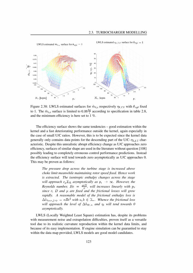
2.3. TURBOCHARGER MODELLING
11.5
22.5
33.5
6070
8090
100110
1200.045
0.05
0.055
0.06
0.065
0.07
0.075
0.08
PSfrag replacements
%'&(*), + krpm ,
- . /102 ,3 kg s
4LWLS estimated 56 )�7 8 surface for 9;:=< )?>A@
11.5
22.5
33.5
6070
8090
100110
1200
10
20
30
40
50
60
PSfrag replacements
, krpm
, kgs
LWLS estimated surface for
%'&(*), + krpm ,
B /10CD ,E %
FLWLS estimated G )�7 H�I surface for 9;:=< )J>K@
Figure 2.38: LWLS estimated surfaces for LM�NO P respectively Q NO R�S with TVU#W N fixedto 1. The LMXNO P surface is limited to YJZ Y\[ kg
s according to specification in table 2.8,and the minimum efficiency is here set to 1 %.
The efficiency surface shows the same tendencies – good estimation within thekernel and a fast deteriorating performance outside the kernel, again especially inthe case of small U/C ratios. However, this is to be expected since the kernel datagenerally only contains data points for the descending part of the U/C– Q NO R�S char-acteristic. Despite this unrealistic abrupt efficiency change as U/C approaches zeroefficiency, surfaces of similar shape are used in the literature without question [108]possibly leading to completely erroneous control performance predictions. Insteadthe efficiency surface will tend towards zero asymptotically as U/C approaches 0.This may be proven as follows:
The pressure drop across the turbine stage is increased abovechoke limit meanwhile maintaining rotor speed fixed. Hence workis extracted. The isentropic enthalpy changes across the stagewill approach ] %!^*_ @ asymptotically as `badcfe . However, theReynolds number, gihkjml P=no , will increases linearly with `�asince ] , p and q are fixed and the frictional losses will growrapidly. A reasonable model of the frictional enthalpy loss isrKsut vxw;w O y a{z P j}|?gih'~ with |����$����� . Whence the frictional losswill approach the level of
rKs _ NO w , and Q N will tend towards 0asymptotically.
LWLS (Locally Weighted Least Square) estimation has, despite its problemswith measurement noise and extrapolation difficulties, proven itself as a versatiletool due to its realistic curvature reproduction within the kernel data limits, andbecause of its easy implementation. If engine simulation can be guarantied to staywithin the data map provided, LWLS models are good model candidates.
123

CHAPTER 2. ENGINE MODELLING
2.3.4.6 Physical based VGT modelling
The modelling approach taken to model VGT characteristics is of a more pragmaticnature than the one taken in the compressor modelling section. This has been donemainly because of the reported relatively good accuracy within the data boundariesachieved utilizing the isentropic nozzle equation (see equation 2.97 on page 112).Whence, the mass flow, ���� , and efficiency, � � , aspects are here separated.
VGT mass flow modelling The theory to developed here is based on using theisentropic nozzle equation repeated below.
��$���{�������� ���������� ���{��� � �'¡{¢£ ¤¦¥ ¡{¢!§©¨?ª«¬ � �® ¯;°°�±*²´³¶µ¸· § ª¹¨ ««¬ � �»º ¼ § ¬ � �´½¿¾ °!ÀÁ²¯Ã «« ¨?ª (subsonic)
����� ���{��� � �'¡{¢£ ¤¦¥ ¡{¢ £ Ä ¾ ¯°!ÀÁ²  «�Å ªÆ=Ç « ¨?ªÉÈ ¼ § ¬ � �´Ê¿¾ °!ÀÁ²¯  «« ¨?ª (sonic)
(2.122)where §�Ë � and Ì Ë � are the upstream pressure and temperature, respectively.
Due to the rotor rotation accompanied by a centrifugal pressure field builduparound the rotor a certain pressure ratio must exist for the mass flow to be positive.If the pressure ratio is smaller than this minimum pressure ratio, § ¬ � Í�ÎÏ� , the char-acteristic will be inverted and the turbine will function as a bad compressor. Thus,it is assumed here that § ¬ � Í�ÎÏ�Ð� § ¬ � Í�ÎÏ�ÒÑÓÔ� ¼ § ¬'Õ (2.123)
The flow through first the nozzle ring and later the rotor is considered equiva-lent to a flow through two nozzles in series. The flow through each nozzle is thusmodelled as in equation 2.122. Whence the flow is,�� ���{��Ö ¬ �;� � �� ���{��Ö ¬ �;�Á× � ���{��Ö ¬ �;� ¼ � � � ���{��Ö ¬ �;� ¼ § Ë � � ���{��Ö ¬ �;� ¼ Ì Ë � � ���{��Ö ¬ �;� ¼ § ¬ � ���{��Ö ¬ �;�ÙØ(2.124)Since the volume of the turbine stage is expected to be of negligible size the gasdynamics may be neglected, i.e. ��$���{�©� �� ¬ �;�Ú� ��$� (2.125)
The effective pressure ratio across the stage can naturally be split in two parts:the effective pressure ratio across the nozzle ring and the effective pressure ratioacross the rotor, i.e § ¬ � Û{Ü'Ü � § ¬ � ���{� § ¬ � ¬ �;� .
Based on the statement above the theory to be tested here is:
A certain pressure ratio across the turbine stage is required for a pos-itive flow to exist. Therefore, the effective pressure ratio across thestage may be found as,
§ ¬ � Û{Ü'Ü � § ¬§ ¬ � Í�ÎÏ�124

2.3. TURBOCHARGER MODELLING
This pressure ratio may subsequently be divided in two parts: a nozzlepressure ratio, ÝbÞ{ß à�á{â and a rotor pressure ratio, Ý�Þ{ß Þxá;ã , i.e.Ý�Þ©äåÝ�Þ{ß æ�çÏàèÝ�Þ{ß à�á{â=Ý�Þ{ß Þxá;ãThe pressure ratios, Ý�Þ{ß à�á{â and Ý�Þ{ß Þxá;ã , derived may be found asÝ�Þ{ß Þxá;ãÁä�éëê Ý Þ{ß ì{í'íïî#ðVñ#ò ã{ó'Ý Þ{ß ì{í'íÝ�Þ{ß à�á{â�ä ôéëê Ý Þ{ß ì{í'íïî#ðVñ#ò ã{óUtilizing the pressure ratios found (provided õ÷ö and ø have been de-termined) the flow through the nozzle ring and rotor can be computed,respectively. However, neglecting the dynamics of the connecting vol-ume only one of the pressure ratios is needed. Therefore, one turbinemass flow model candidate isùú ãÁä ùú ã�êÙõ�ö î ø�Þxá;ã î Ý�û�ü î{ý û�ü î Ý�Þ{ß Þxá;ã=ó
In order to validate the theorem above the model given in the following threeequations are implemented in the MATLAB þ environment.ÿ����õ�� ����æ� � ����� ä���
Ý�Þ{ß æ�çÏà ä�� ô������� ���! Þ#"Ôãß $&%(')+* ü ý,�-xß Þxì{í/.10243 0 (2.126)
Ý Þ{ß ì{í'í ä Ý�ÞÝ�Þ{ß æ�çÏàÝ�Þ{ß Þxá;ãÁä ô�576 Ý Þ{ß ì{í'íô�586ø÷ì:9¸ä õ�ö�ø�Þxá;ã (2.127)
ùú ãß $�ä<;===> ===?ø÷ì:9 ü(@ 2 � ACB4DE FHG @ 2 � ACB4D Ý 3I20Þ{ß Þxá;ã&J ':KKML - ÿ ô�� Ý 243 00Þ{ß Þxá;ã � î Ý�Þ{ß Þxá;ã�NPO KRQ -'TS 00 3I2 (subsonic)ø÷ì:9 ü(@ 2 � ACB4DE FHG @ 2 � ACB4D E U O 'KRQ - S 0WV 2XZY 0 3I2\[ î Ý�Þ{ß Þxá;ã�]PO KRQ -' S 00 3I2 (sonic)
(2.128)The three parameters ø ì:9 , � and 6 are found as the arguments that minimize
the LS criterion for each of the seven different settings of the VGT position, ð?ñ#ò ã ,i.e. ^ äT_+`&a bdcfeg �ih jkB\l ß �xß mRn�opàM�q- O ùú ãß ${ß à �sr ùú ãß ${ß à S ' (2.129)
125

CHAPTER 2. ENGINE MODELLINGtvu:wyx(z:{4| }C~4�� �H� z:{4| }C~4��� kgs � � ��!�&�&�i�
0 0.0459 1.2019 0.73280.1 0.0513 1.2892 0.75570.2 0.0587 1.2131 0.92190.4 0.0722 1.3232 1.45360.6 0.0867 1.4976 1.95480.8 0.0976 1.4483 3.7628
1 0.1048 1.4839 4.4928
Table 2.10: Identified mass flow model parameters with variable � .The identified parameters are listed in table 2.10. As expected
t�u:wand ����� ��� �
( � ) increase with�R�&�&�
, whereas � exhibits only a slight tendency to increase with�!�&�&�opening.
Inspired by [87] � is fixed to the mean value of the column data in table 2.10,and a rerun of the identification procedure is made. Table 2.11 lists the identifiedvalues for
t�u:wand � with � fixed to 1.351. This value is reasonably close to the
value of 1.2 given in [87].tvu:wsx(z:{4| }C~4�� �H� z:{4| }C~4��� kg
s � ��!�&�&�i�0 0.0457 0.6999
0.1 0.0512 0.74200.2 0.0584 0.86690.4 0.0722 1.42650.6 0.0870 2.23770.8 0.0976 4.6719
1 0.1049 5.9881
Table 2.11: Identified mass flow model parameters with � ���+� �M�����.
Another interesting phenomenon found by comparing table 2.10 and 2.11 ishow fixing � affects the two other parameters:
t�u:wis completely unaffected on
any significance level, and only � is noticeably altered. Comparing the
t�u:wand �
level against�R�&�&�
graphically the following very interesting plots in figure 2.39 areobtained.
The figure clearly shows that the first and second order approximation of
t�u:wand � , respectively, are reasonable. The representative polynomials are identifiedas
tvu:w�� �!�&�&�:� � � �+� ¡+�M¢R£¤�!�&�&�¦¥��+� ���!¡!£I�¨§¤���I©«ªm ¬� � �!�&�&�:� ��I� ®M�M¯M¯+� ¬�&�&�q° ��� £±���(�+�!�&�&�¦¥���� ¯M®M�+� (2.130)
These two functions provide the missing link between the position of the VGTvanes and the mass flow through the turbine.
126
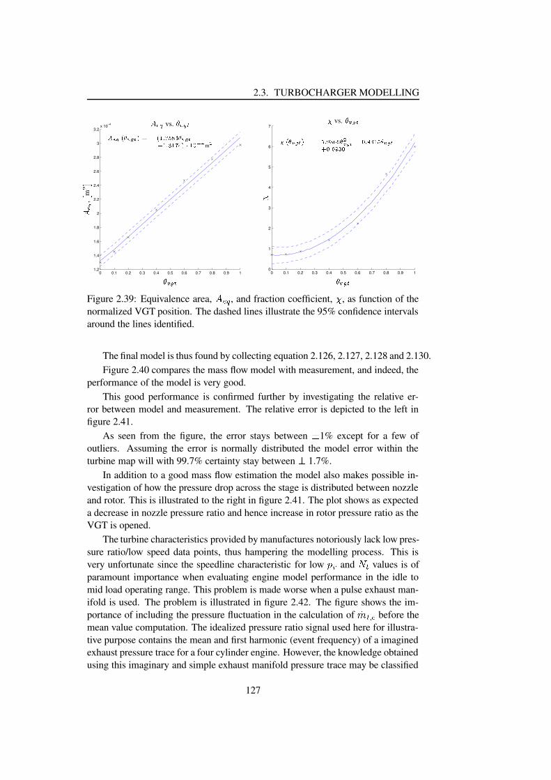
2.3. TURBOCHARGER MODELLING
0 0.1 0.2 0.3 0.4 0.5 0.6 0.7 0.8 0.9 11.2
1.4
1.6
1.8
2
2.2
2.4
2.6
2.8
3
3.2x 10⁻⁴
PSfrag replacements
²:³Z´:µ¶:·¸ ,¹ m
º»¼k½\¾
vs.²:³Z´:µ¿±À\ÁH Ã4ÄZÅÇÆÇÈMÉÊ Ë4Ì Í4ÎÇÏ4ÐÇÃ4ÄZÅÇÆÑ Ë4Ì Ò:Ë\ÍÇÐCÓ!Ô:Ë Õ:Ö(×
m Ø
0 0.1 0.2 0.3 0.4 0.5 0.6 0.7 0.8 0.9 10
1
2
3
4
5
6
7
PSfrag replacements
, m
vs.
m
²:³Z´:µÙ
Ú vs.²:³Z´:µÛ  Ã4ÄZÅÇÆÇȤÉÜÎZÌ Ý4Ò4Þ4ÞÇà ØÄZÅÇÆIß Õ:Ì Ð4Ò:Ë\Î\Ã4ÄZÅÇÆÑ Õ:Ì Þ4Ý4Ò4Õ
Figure 2.39: Equivalence area, àá:â , and fraction coefficient, ã , as function of thenormalized VGT position. The dashed lines illustrate the 95% confidence intervalsaround the lines identified.
The final model is thus found by collecting equation 2.126, 2.127, 2.128 and 2.130.Figure 2.40 compares the mass flow model with measurement, and indeed, the
performance of the model is very good.This good performance is confirmed further by investigating the relative er-
ror between model and measurement. The relative error is depicted to the left infigure 2.41.
As seen from the figure, the error stays between ä 1% except for a few ofoutliers. Assuming the error is normally distributed the model error within theturbine map will with 99.7% certainty stay between ä 1.7%.
In addition to a good mass flow estimation the model also makes possible in-vestigation of how the pressure drop across the stage is distributed between nozzleand rotor. This is illustrated to the right in figure 2.41. The plot shows as expecteda decrease in nozzle pressure ratio and hence increase in rotor pressure ratio as theVGT is opened.
The turbine characteristics provided by manufactures notoriously lack low pres-sure ratio/low speed data points, thus hampering the modelling process. This isvery unfortunate since the speedline characteristic for low åqæ and ç�è values is ofparamount importance when evaluating engine model performance in the idle tomid load operating range. This problem is made worse when a pulse exhaust man-ifold is used. The problem is illustrated in figure 2.42. The figure shows the im-portance of including the pressure fluctuation in the calculation of éê èÇë ì before themean value computation. The idealized pressure ratio signal used here for illustra-tive purpose contains the mean and first harmonic (event frequency) of a imaginedexhaust pressure trace for a four cylinder engine. However, the knowledge obtainedusing this imaginary and simple exhaust manifold pressure trace may be classified
127

CHAPTER 2. ENGINE MODELLING
1.2 1.4 1.6 1.8 2 2.2 2.4 2.6 2.8 3 3.20.02
0.03
0.04
0.05
0.06
0.07
0.08
PSfrag replacements
í(î
ï ð ñfòó ,ô kg s
õPhysical ö÷�ø model vs. ö÷�ø ù ú data.
û:üZý øIþ ÿû:üZý øIþ ÿ � � û:üZý øIþ ÿ � �û:üZý øIþ ÿ � �û:üZý øIþ ÿ � �û:üZý øIþ ÿ � �û:üZý øIþ �
60.471.4
��� ����� � krpm
60.671.6
82.593.6
60.6
71.4
82.693.5
104.8115.8
60.5
71.4
82.6
93.5104.6
115.6
60.8
71.6
82.6
93.5
104.5115.5
71.4
82.5
93.4
104.4115.5
60.7
71.3
82.4
93.4104.3 115.3
Figure 2.40: Comparison between the physical deducted VGT model and measure-ments. The measurements are marked with � .
0.02 0.03 0.04 0.05 0.06 0.07 0.08−3
−2
−1
0
1
2
3
4
5
PSfrag replacements
ö÷�ø ù ú , � kgs �
Rel
ativ
eer
ror,
� %
�Relative error of physical model.
0 50 100 150 200 250 3001
1.5
2
2.5
3
3.5
PSfrag replacements, kg
s
Relative error, %
Relative error of physical model.
Data No.
� � �� � ò��� �� � ò��� �� � ò��ñí(î! í î4ù "�#�# í(î4ù $!%'& and í(î4ù î�%Zø as the nozzle opens.
0
0.1
0.2
0.4
0.6 0.8 (�)'*,+.-0/ í(îí î4ù "�#�#í(î4ù î�%Zøí(î4ù $!%'&Figure 2.41: The relative error of the mass flow model predictions and measure-ments. The mean and variance of the relative error in % are computed to -0.002%and 0.305% � , respectively. The plot to the right shows the distribution of the dif-ferent important pressures as the nozzle opens.
128

2.3. TURBOCHARGER MODELLING
as general for the for following reason. The pressure ratio across the turbine stagemay stay close to zero flow conditions much of the time16 i.e. (the pressure ratioacross the turbine stage is close to 1 , see e.g. [60] ). This close to non-flow con-dition is followed by a hot, narrow and high pressure burst ( see e.g [60] ) whichutilizes a great extend of the turbine 243 – 5687,9 : characteristic. Hence, the real turbinemass flow trace will be similar in appearance to the mass flow traces presented inpresented in figure 2.42 .
0 100 200 300 400 500 600 7001
1.2
1.4
1.6
1.8
2
2.2
2.4
2.6
2.8
3
0 0.01 0.02 0.03 0.04 0.05 0.06 0.07 0.081
1.2
1.4
1.6
1.8
2
2.2
2.4
2.6
2.8
3
0 0.01 0.02 0.03 0.04 0.05 0.06 0.07 0.08
0
100
200
300
400
500
600
700
800
PSfrag replacements
;=<?>A@CB DFE'G HJILKNMNOPNQ @SRUTWV B D QXWYFZ[]\,^ _a` XbY ;=<dcfe Mhgji \F>A@ack> Q @CB K V gsXWYFZ[]\,^ _a` ;=<Ne Mhgji \4>A@lcF> V K B m P g
sError = VnV B oqpXWYFZ[]\,^ _a` XbY ;=<dcfe Mhgji \F> V ck>Wm Q B @nm g
sXWYFZ[]\,^ _a` ;=<Ne Mhgji \4> V cF>rohs.B P K gs
Error = V DCB Dtp
uvxwzy { , | kgs }
~ �VGT pressure–mass flow characteristic
uvxwzy { , | kgs }
��� ,� ��Turbine flow
���, � ���
� �Turbine pressure ratio ���'�,�=�x�����'�,�=���
10krpm
10krpm
120krpm
120krpm
Figure 2.42: Fluctuation scenario in exhaust manifold and its influence on the ef-fective Turbine mass flow. The figure also illustrates how the 2k3 – 5687,9 : characteristicalters with turbine speed due to the pressure gradient field created around the rotor.
This conclusion is analogous to the research presented in [10] where the intakemanifold pressure fluctuation’s influence on correct throttle mass flow estimationwas investigated.
16Exhaust manifold design dependent.
129

CHAPTER 2. ENGINE MODELLING
VGT efficiency modelling The loss model to be present here is analogous tothe compressor loss model and is primarily based on fluid velocity investigations.However, the availability of a mass flow model makes some of the turbine lossestimation steps easier when compared to their dual in the compressor loss model,since some of the important fluid velocities can be readily computer prior to theloss calculation.
The nozzle inlet conditions are sketched in figure 2.43, where the notation willbe defined in which follows.
PSfrag replacements
��� � ��C��=� � � �
�C�� � � �N� � � �N� �
¡ �¡ � ¡ �
Figure 2.43: Diagrammatic illustration of the nozzle inlet conditions.
The first task is establish the size and direction of the absolute nozzle inletvelocity, ¢0£ . Assuming the scroll inlet process is ideal the angular momentum ofthe gas is conserved, i.e. ¤¦¥ ¢ ¥f§ ¨�© ¤«ª.§ ¬ ¢ £ § ¨ (2.131)
where¤¦¥
is the distance from turbine center to the centroid of the scroll inlet wheremass distribution is initiated.
¤bª.§ ¬is the radius of the circle connecting the nozzle
inlet tips, and is of course t®�¯�° dependent.The scroll volume of an automotive turbine is small, hence neglecting filling–
emptying dynamics of the turbine stage is justifiable. Thus, due to mass conserva-tion the mass flow in and out of the scroll are equal, i.e.±² ° ©´³ ¥�µ¶¥ ¢ ¥f§ ¨·©¹¸tº ¤«ª.§ ¬¼»!½ ³ £¼¢�£ § ½ (2.132)
whereµ¶¥
is the area of scroll inlet centroid mentioned above.The inlet angle, ¾?£ , is defined as¿¼À�Áà¾L£¼Ä Å ¢�£ § ½¢ £ § ¨ (2.133)
Collecting equation 2.131, 2.132 and 2.133 the cotangent of the inlet angle, ¾0£ ,can be rewritten as ¿¼À�ÁÆ ¾L£¼Ä © µ¶¥ ³ ¥¸tº »!½¼¤¦¥ ³ £ (2.134)
130

2.3. TURBOCHARGER MODELLING
The acceleration of the flow from turbine inlet to nozzle is small. Hence, thestatic gas density change is small, i.e. ÇÉÈËÊÌÇÍ , allowing a further reduction ofequation 2.134 to μÏ�ÐÃÑ,Ò È¼Ó Ô Õ ÍÖt×FØ!ÙhÚ Í (2.135)
Thus, the gas inlet angle,
Ò È is only a function of the A/R setting of the turbine.Using the equation above, the inlet angle of the experimental turbine is found to be75 Û .
The relation above is of course very idealized especially in the case of pulseturbocharging. However, the problem is most pronounced in the case with vanelessnozzle ring turbines due to the harsher accelerations (higher local friction) andthe larger control volume, and less important in inlet nozzles with guide vanes.Due to its simplicity the inlet angle of the gas will thus be computed according toequation 2.135.
The inlet angle for turbine with vaneless nozzle ring has been studied in greaterdetail in [34] (see also [87]).
The next step in turbine loss modelling is the construction of a model of thenozzle friction and incidence losses, along with a discussion of the assumptionsmade in the pursuit of this goal.
Applying the theory above for the direction of the inlet flow velocity togetherwith the law of continuity, Ü«È may be written asÜ�ÈÝÔ Ü�ÈfÞ ÙμÏCßÆÑ,Ò È¼Ó Ô àá8âÖt×4Ú«ã Þ ä Ø!Ù ÇåÈ Î¼ÏCßÆÑ,Ò È¼Ó (2.136)
Due to the collision between gas and the vaned nozzle ring a loss will bepresent. Analog to the NASA incidence loss model presented in the compressorsection this energy loss is modelled byæèçSé ãtê Þ ã äjë�Ôíìïîã Þ ðÖ (2.137)
Whence, the change in the tangential velocity is dissipated as heat. However, thesize and direction of the nozzle outlet velocity is not readily available.
According to [38] the outlet angle of the gas,
Òî , may from common steam
turbine practice be found as μÏCßÆÑ,Òî ÓLÔòñ ãó ã (2.138)
whereó ã
is the radial distance between the nozzle tips, and ñ ã is the minimum dis-tance between neighboring nozzle blades. Although the relation above is a roughapproximation the error introduced is small according to [87]. However, it shouldnot be forgotten how sensitive rotor operation is with respect to the incoming flowangle; an issue dual to the compressor impeller incidence losses discussed in thecompressor section. It is therefore likely that a certain level of modelling error
131

CHAPTER 2. ENGINE MODELLING
may be expected when using this expression. However, it is decided here to pro-ceed with the turbine loss modelling using this relation due to its simplicity
The radial distance, ôhõ , is found as (see evt. figure 2.32)
ôdõ÷öòøtùûú,ü«ýjþ ÿ�� � õ þ ��� ����� ú õ����� õ (2.139)
The minimum distance between blades, �Nõ , may from geometrical considerationsbe found as the vector going through the nozzle outlet tip perpendicular to thedirection vector of the neighboring nozzle blade.
Figure 2.44 shows ô¼õ , �dõ and �� as a function of the nozzle blade angle õ forthe experimental VGT. It is noticed that �� is close being a linear function of theblade angle.
30 35 40 45 50 55 60 65 706
8
10
12
14
16
18
PSfrag replacements
��� , � ������ ! � ," m
m
#$ � , % � v.s nozzle blade angle
% �$ �
30 35 40 45 50 55 60 65 7020
25
30
35
40
45
50
55
60
65
PSfrag replacements,
, mm
, v.s nozzle blade angle
��� , � ���
& ' ," (#Nozzle flow outlet angle vs. ���
Figure 2.44: The nozzle flow
The size of the absolute outlet velocity ) � is more difficult to characterize evenbefore the strong influence of the frictional forces along nozzle passage, since ititself is a function of the energy loss *,+ � õ.- þ õ./10 i.e the relation is implicit. Insteadit is assumed that the gas attains an angle of �� after nozzle entry, and the point ofno loss is achieved when 32 ö �� . A energy loss model fulfilling these conditionsis
*,+ � õ.- þ õ./10�ö 45 �õ þ 6øwith 45 õ þ 6 ö7) 2 �98;: ú �2 � �� � ö7) 2 �98;: ú � õ<� (2.140)
The nozzle incidence loss will be modelled according to the definition above in thefollowing.
132

2.3. TURBOCHARGER MODELLING
The static pressure and temperature at the nozzle inlet after the nozzle collisionprocess is found as =�>�? @BAC= >�? DFEHG,I�JLK.M ? K.N1OP1QR >�? @BA R >�? D (2.141)
assuming an isobaric loss profile is followed. The subscripts S and T denote afterincidence and before incidence conditions, respectively.
The stagnation inlet conditions are from considerations of continuity derivedas =VUW>�? @XAY=�>�? @ E[ZX\>�? @] P1QR UW>�? @BA R >�? @_^ =�>�? @=VUW>�? @a`cbdfe b
where Z >�? @BA ghji].kVl K ? N TnmWo >�? @Fpq�ras \(2.142)
The inlet conditions and geometry, respectively, are now known and may to-gether with the mass flow model form the basis for computation of the nozzledischarge coefficient.
ghji Autvvvw vvvxZzy3{ K.N1O Q}| df~ �� ��� | df~ � R e�dbm ? K.N1O�� \����� > ^F��� R dfe bbm ? K.N1O ` � R m ? K.N1O���� ��� >\�� bb e�dZzy3{ K.N1O Q}| df~ �� ��� | df~ � � � � \��� > � bn� d��� b e�d�� � R m ? K.N1O���� ��� >\ � bb e�d
where { K.N1O A Tnm�� K���KR m ? K.N1O A R mR m ? � JLK R m ? m N i(2.143)
The discharge coefficient for each of the seven �� 9¡ i positions is found as theargument minimizing the cumulative quadratic error between gh¢i and £ ghji , i.e.
Zzy A¥¤.¦9§©¨,ª;«¬�¯®±° UW² > °´³µ¶�· > � gh i ? ¶ � £ gh i ? ¶ � \ (2.144)
where £ ghji is computed according to equation 2.143.The results of the Z�y computations are graphically illustrated in figure 2.45.
133

CHAPTER 2. ENGINE MODELLING
0 0.1 0.2 0.3 0.4 0.5 0.6 0.7 0.8 0.9 10.2
0.3
0.4
0.5
0.6
0.7
0.8
0.9
1
PSfrag replacements
¸�¹�º�»
¼ ½
Nozzle ring discharge coefficient ¾<¿À.ÁXÂzÃ�Ä ÅÇÆfÆÈÃÈÉ�ÊË�ÌÈÍ�Î Ã�Ä ÏÈÐfÑ�Ò;É Ë�ÌÈÍ Î Ã�Ä ÏÈÐfÓfÔ
0 10 20 30 40 50 60 70 80 90 1000.02
0.04
0.06
0.08
0.1
0.12
0.14
0.16
0.18
PSfrag replacements
Nozzle ring discharge coefficient
¸�¹�º�»�Õ×Ö0.1
0.20.4
0.6
0.8
¸�¹�º�»�ÕÙØ
ÚÜÛ}ÝnÞ�ß, à kPa á
â ã ä åæ â ã ä ,ç
kg s
èNozzle flow model validation
Figure 2.45: Computed discharge coefficient and nozzle flow model validation.
The plot to the left shows the computed discharge coefficients for the sevenVGT positions. The discharge coefficient may be approximated with good accu-racy by a second order polynomial in é�ê9ë9ì . The polynomial together with it’s 95%confidence interval are seen as a solid and dashed blue lines, respectively.
The discharge coefficient, as expected, is found to increase as the VGT opens.Hence, frictional forces become more and more dominant with VGT closure.
The plot to the right in figure 2.45 shows a comparison between flow measure-ments and estimates obtained utilizing equation 2.143 with the discharge descrip-tion just mentioned. The agreement is good and adds to the confidence in the pres-sure distribution model developed as a part of the turbine mass flow model. Onlyat large VGT positions and relatively large pressure drops is a small disagreementnoticed. This disagreement can possibly be traced back to the nozzle incidenceloss approximation made earlier in this section. However, since the disagreementis so small this has not been investigated.
The next problem is the development of suitable models for the nozzle pas-sage friction loss, rotor incidence loss and rotor friction loss. This is, however, anextremely difficult task since the individual loss process are hard to separate. Anidentification procedure must thus estimate the individual loss process parameterssimultaneously in order to be successful.
The friction loss in the nozzle passages is Reynolds number dependent, and iscommonly approximated as a power function of this number, i.eí,îaïð1ñ�òôó¥õ�öø÷}ùWú
forõaúnû�üþý�ÿ
(2.145)
A loss model with the structure given above was implemented however in vain.The structure was found to give unrealistic low friction losses at small VGT open-ings and at high inlet temperatures, respectively. Instead, the Reynolds number
134

2.3. TURBOCHARGER MODELLING
definition was changed from � ��� ������� ���� to�� �� � ������ ����� ������� ��� �� !��� �#"�$�&%')( (2.146)
and the nozzle enthalpy loss due friction computed as*,+ �-��.0/�� $21�3 �54 � ������ ����� ����� �� 76 (2.147)
Using this analogy the Reynolds number loss correlation is made almost indepen-dent of the nozzle position and the upstream temperature conditions i.e geometricand thermodynamic conditions are lumped into the correlation.
Before the rotor inlet conditions can be computed the nozzle outlet conditionsmust be determined.
The pressure ratio across the nozzle ring, 8 ��� $21�3 , is readily available from themass flow model, and the nozzle outlet temperature following an isentropic expan-sion process may be found as � % � . � ������� � 8 ��92::��� $21�3 (2.148)
However, due to the friction loss the real static outlet temperature is� % � � % � .�; *,+ �-��.0/�� $21�3<�= (2.149)
The static outlet pressure is readily found to be8 % �>8 ����� �8 ��� $21�3 (2.150)
Hence, the absolute velocity of the gas leaving the nozzles is
� % � ?@BA � � %C $EDF��"�$ 8 % (2.151)
After nozzle exit the flow is accelerated further due to area decrease. Thisflow acceleration may with good approximation be assumed lossless since the flowdistance from nozzle exit to rotor inlet is small. Furthermore, it is assumed that theflow retains the flow angle G % . Thus, the tangential velocity increase is derived to
�IH � J�� 6 � � $K� �� � � %�LNMPO G % (2.152)
and the radial velocity component of � H before rotor entry to
�IH � ��� 6 � � $K� �� � � %RQ-STL G % (2.153)
135

CHAPTER 2. ENGINE MODELLING
The rotor inlet conditions are shown schematically in figure 2.32 on page 110.The collision loss is found analogous to the compressor impeller incidence loss
assuming that the complete tangential component of the relative kinetic energy isdestroyed. This model is in the literature referred to as the NACA model (see e.g.[98, 87]). The loss in specific energy is thus found asU,VXWZY2[�\ ]�^`_badcfeg \ h�\ ij alkm g \ h�\ nporq g7s ej (2.154)
The pressure and temperature before rotor entry aret g \ n a t e o m eg \ n o m eeju g \ n a u e�v t et g \ n2wyxz�{ x (2.155)
Assuming an isobaric loss profile the inlet conditions immediately after rotor entryare (see evt. figure 2.32 on page 110)t g \ i�a t g \ nb| U,VXWZY2[�\ ]�^`_}�~u g \ i�a u g \ nc g \ i�a m g \ ]�\ i�a �� _� t g \ ij2� ��]7�F] u g \ i k radial rotor design s (2.156)
In the computation of the relative velocity it is assumed, that the flow follows therotor blade angle immediately after the collision.
The friction model structure developed in the compressor section is here reusedto model the rotor friction loss, i.e.U,V�� ]�W0[�\ ]�^`_ a t g \ it���� \ ]�� �B��� � q eg | � e c g \ i q g | � g c eg \ i#� (2.157)
The scaling coefficient �#�`� ��#� z � ���� is introduced since the rotor friction loss was foundto scale badly with temperature increase.
The total specific enthalpy loss is found as the sum of the four contribution justmodelledU,V _�\ � ^��`� a5U,VXWZY2[�\ ]�^`_ | U,V�� ]�W0[�\ ]�^`_�| U,VXWZY2[�\ Y2^�� | U,V�� ]�W0[�\ Y2^��
(2.158)
The coefficients of the frictional loss model are found by minimizing the crite-rion in equation 2.159, and are listed in table 2.12.� � ^��`� a������ ��� U,V _�\ � ^��`��\ � o U¡ V _�\ � ^��`��\ �£¢ e (2.159)
136
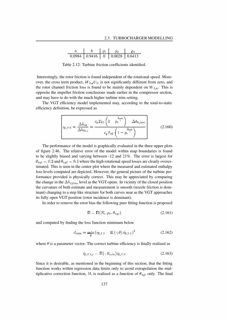
2.3. TURBOCHARGER MODELLING¤ ¥ ¦K§ ¦2¨ ¦2©0.0984 0.9416 0 0.0028 0.6413
Table 2.12: Turbine friction coefficients identified.
Interestingly, the rotor friction is found independent of the rotational speed. More-over, the cross term product, ª ©�« ¬2®© , is not significantly different from zero, andthe rotor channel friction loss is found to be mainly dependent on ª ©�« ¬ . This isopposite the impeller friction conclusions made earlier in the compressor section,and may have to do with the much higher turbine trim setting.
The VGT efficiency model implemented may, according to the total-to-staticefficiency definition, be expressed as
¯±°�« ²R³µ´·¶,¸!¹ °¶,¸!¹ °�« º ´¼»�½#¾ ¹ §�¿ÁÀÃÂBÄÆÅ�Ç2ÈÈÉËÊ Â ¶,¸ °�« Ì Í�Î`λ�½#¾ ¹ § ¿ ÀÃÂBÄÆÅ�Ç2ÈÈÉËÊ (2.160)
The performance of the model is graphically evaluated in the three upper plotsof figure 2.46. The relative error of the model within map boundaries is foundto be slightly biased and varying between -12 and 21%. The error is largest forÏ£ÐNÑ °p´5ÒEÓ Ô and
Ï£ÐNÑ °p´5ÒEÓ Õ where the high rotational speed losses are clearly overes-timated. This is seen in the center plot where the measured and estimated enthalpyloss levels computed are depicted. However, the general picture of the turbine per-formance provided is physically correct. This may be appreciated by comparingthe change in the ¶,¸ °�« Ì Í�Î`Î level as the VGT opens. In vicinity of the closed positionthe curvature of both estimate and measurement is smooth (nozzle friction is dom-inant) changing to a step like structure for both curves near as the VGT approachesits fully open VGT position (rotor incidence is dominant).
In order to remove the error bias the following pure fitting function is proposedÖ ´ ÖØ×�Ù °�Ú�Ä É Ú Ï£ÐNÑ °`Û (2.161)
and computed by finding the loss function minimum belowÜTÝ ºZÞ,´5ß,àPáâ × ¯±°�« ²R³Ø Öã×`ä0å Ï Û)毱°�« ²R³�Û ¨ (2.162)
whereÏ
is a parameter vector. The correct turbine efficiency is finally realized as毱°�« ²R³±« ç�´ ÖØ×`ä0å Ï Ý ºZÞ�ÛK毱°�« ²R³ (2.163)
Since it is desirable, as mentioned in the beginning of this section, that the fittingfunction works within regression data limits only to avoid extrapolation the mul-tiplicative correction function,
Ö, is realized as a function of
ÏKÐNÑ ° only. The final
137
CHAPTER 2. ENGINE MODELLING
fitting function minimizing the LS criterion is realized as a second order polyno-mial in è#éNêNë ì éNêNë®íïî�ðEñ ò2óEô7õ2èTöéNêNëÁ÷ ðEñ ò2óTò2õ2è£éNêNë ÷ ðEñ ø±ù±ú±ú (2.164)
The corrected turbine efficiency, ûü ë�ý þRÿ±ý � , is graphically evaluated in the two lower-most plots in figure 2.46. It is clearly seen here that the fitting function is able toremove the bias from the relative error, and reduces the relative error to be within awindow of
� ô�ð�� . However, since the function only works on ûü ë�ý þRÿ it does not pro-vide any information on where the enthalpy losses are falsely distributed. Hence,the correction will not be used in the evaluation of the enthalpy loss distribution ofthe turbine stage.
The efficiency model makes a better understanding possible of how the en-thalpy loss is distributed between the nozzle ring and rotor as the VGT opens. Thisloss distribution is graphically illustrated in figure 2.47. The figure clearly shows,as expected from figure 2.46, that the two most dominant loss sources are the noz-zle ring friction loss for small VGT settings and rotor incidence loss for largerVGT settings, respectively. Another interesting observation made is the rather lowmagnitude of the computed rotor friction. However, the trim size of 76 (see ta-ble 2.8 ) for the rotor is a lot larger than those for the compressors examined in thecompressor modelling section i.e. the flow path basically speaking only changesits direction but not its dimensions. Hence, the rotor loss computations presentedabove are not unrealistic.
The physical loss model is now complete making a loss surface estimationfrom è£éNêNë , � ë�ý � and ��� alone possible. Such surfaces are for è±éNêNë,í ð , 0.5 and1 depicted in figure 2.48. The surfaces show the skewed nature of the turbineefficiency. Unfortunately, as mentioned in discussion of the pressure fluctuationsand effective turbine mass flow, a great deal of the turbine operation takes place inthe vicinity of ���Øí (no flow). Hence, following a typical pressure cycle in theexhaust manifold, an efficiency trajectory may be drawn on these surfaces exactlywhere they are strongly skewed. Therefore, the effective efficiency mean valuemay be considerably smaller than in the case with constant pressure turbocharging.
Although the low-speed/high pressure efficiencies look a bit too high, theyare not unrealistic. The measurements, however, do not cover this region, but thegeneral U/C line shows a growing tendency with a U/C decrease (see figure 2.33on page 115). Thus none of the U/C- ü ë�ý þRÿ lines have reached their maximum level.
Increasing the pressure ratio (not shown graphically here) the surfaces arefound tending towards zero efficiency asymptotically. This is a property desiredfrom the theory outlined in the beginning of this section.
The following natural question to the just presented radial turbine efficiencymodel now arises: ”Is a relative error window of approximately
� ô�ð�� accept-able?”. The answer is: ”It depends on the application”. If the model should beused in an high fidelity application requiring a level of accuracy within a few per-cent the only natural step further would be to model the complete exhaust system bywave action models (see e.g [118]). These model structures generally tend to have
138

2.3. TURBOCHARGER MODELLING
0 50 100 150 200 2500.4
0.5
0.6
0.7
0.8
0 50 100 150 200 2500
5
10x 104
0 50 100 150 200 250
−10
0
10
20
PSfrag replacements
Measured and computed turbine efficiency.
� �� �� �� � �� ��
Data No.
����� ��������� ���
Enthalpy level comparison.
� � � �� � �� � �� !"" �� � �� !""
,
# J kg
$Data No.
00.1 0.2 0.4 0.6 0.8 %'&)(+*-,/.02143 *�5 6 0871 *�5 9 :+;<;021 *�5 9 :+;<;
Relative error.
Rel
.Err
,
= %
>Data No.
0 50 100 150 200 2500.4
0.5
0.6
0.7
0.8
0 50 100 150 200 250−10
−5
0
5
10
15
PSfrag replacementsMeasured and computed turbine efficiency.
Data No.
Enthalpy level comparison.
, Jkg
Data No.
0
0.1
0.2
0.4
0.6
0.8
Relative error.Rel. Err, %
Data No.
Measured turbine efficiency and computed turbine efficiency after multiplicative correction.
� �� �� �� � �� �� ?
Data No.
Relative error achieved with multiplicative correction.
Rel
.Err
,
= %
>Data No.
����� ��������� ���@� A
Figure 2.46: BDC+E FHG model performance. The first three plot show the performanceof the turbine efficiency model before multiplicative correction, and the last twoplots depict the turbine model performance after the correction.
139

CHAPTER 2. ENGINE MODELLING
0 50 100 150 200 2500
0.5
1
1.5
2
2.5
3
3.5
4
4.5
5x 10⁴
PSfrag replacements
Estimated loss distribution.
I J K LMM NI J OPQ RSLT NI J USO Q RSLT
I J O PQ RPLV NI J U SO Q RPLV
,
W J kg
X
Data No.
00.1
0.2
0.4
0.60.8 Y'Z)[+\�]_^
`�acbed�f g)h i jek l<m�neo�p+q r s t u2v4w xzy+{ xz|+}u2v�~�� w y+{ � | \
u2v \ { � |+�<�
Figure 2.47: Enthalpy loss distribution.
a higher number of tuneable parameters compared to the radial turbine model justpresented. Thus, a higher level of accuracy can more easily be achieved. However,such models are not suited as modelling background for engine control designs.If however a MVEM framework is considered, in which the exhaust fluctuationsare neglected, the accuracy level of the VGT efficiency model presented is suffi-cient for the following intuitive reasons. Efficiency degradation levels up to 30%in pulse-turbocharging application are to be expected (see [60]) if the turbine ef-ficiency estimate is computed utilizing the mean values of the exhaust pressureand the temperature. If an on-engine turbine efficiency modelling accuracy levelshould be achieved within a few percent the thermodynamic states in front of theturbine inlet must be known within high precision. It is shown in [118] that areasonable detail level of the inlet state frequency spectrum must contain at leastinformation about the third harmonic of the exhaust pulsation (this corresponds tothree times the event frequency of a four cylinder engine). This required spectrumbandwidth is much larger than the bandwidth obtainable with MVEM realized en-gine models. According to e.g. [43] the bandwidth of MVEM type models are bitbelow the engine cycle frequency. Hence, the spectrum provided by a MVEM typeengine model is at least one decade below that required by a successful physicalbased computation of the turbine efficiency. Thus, if a high fidelity MVEM typeengine model is required a substantial amount of work used on massaging modelparameters to fit the data is to be expected.
140
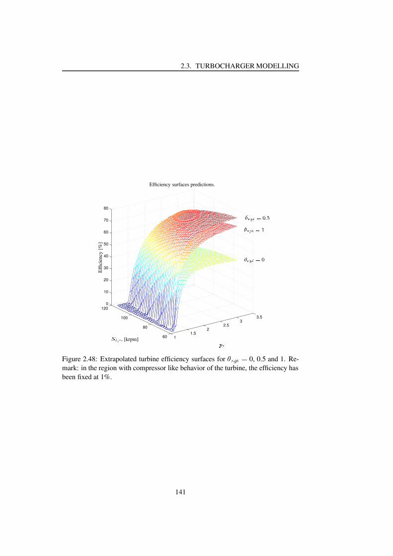
2.3. TURBOCHARGER MODELLING
11.5
22.5
33.5
60
80
100
1200
10
20
30
40
50
60
70
80
PSfrag replacements
Efficiency surfaces predictions.
�8��� �, [krpm] ���
Effi
cien
cy[%
] ���)� �-������)� �-���z� ����)� �-���
Figure 2.48: Extrapolated turbine efficiency surfaces for ��������� 0, 0.5 and 1. Re-mark: in the region with compressor like behavior of the turbine, the efficiency hasbeen fixed at 1%.
141
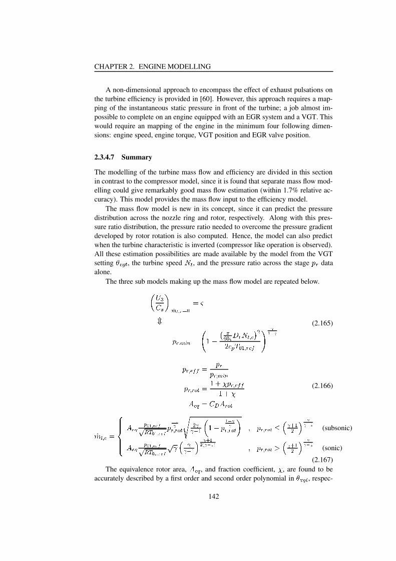
CHAPTER 2. ENGINE MODELLING
A non-dimensional approach to encompass the effect of exhaust pulsations onthe turbine efficiency is provided in [60]. However, this approach requires a map-ping of the instantaneous static pressure in front of the turbine; a job almost im-possible to complete on an engine equipped with an EGR system and a VGT. Thiswould require an mapping of the engine in the minimum four following dimen-sions: engine speed, engine torque, VGT position and EGR valve position.
2.3.4.7 Summary
The modelling of the turbine mass flow and efficiency are divided in this sectionin contrast to the compressor model, since it is found that separate mass flow mod-elling could give remarkably good mass flow estimation (within 1.7% relative ac-curacy). This model provides the mass flow input to the efficiency model.
The mass flow model is new in its concept, since it can predict the pressuredistribution across the nozzle ring and rotor, respectively. Along with this pres-sure ratio distribution, the pressure ratio needed to overcome the pressure gradientdeveloped by rotor rotation is also computed. Hence, the model can also predictwhen the turbine characteristic is inverted (compressor like operation is observed).All these estimation possibilities are made available by the model from the VGTsetting ������ , the turbine speed ¡¢ , and the pressure ratio across the stage £8¤ dataalone.
The three sub models making up the mass flow model are repeated below.¥�¦¨§©�ªD«¬z®¯±°�² ³µ´H¶�·¹¸º£�¤µ» ¯½¼e¾ ·À¿¨ÁÃÂÅÄÇÆÈ ¶µÉ�Ê ¤@¡ +» Ë�ÌÎÍÏÑеÒ�Ó ¶zÔ » ¤4ÕµÖØ×ØÙÚ'Û Ù
(2.165)
£ ¤µ» ÕµÖ�Ö · £�¤£�¤µ» ¯½¼e¾£�¤µ» ¤4Ü� · Á±ÝßÞ £ ¤µ» ÕµÖ�ÖÁ½ÝßÞà Õ�á · ©�â à ¤4Ü� (2.166)
ãä +» Ë ·æåçççè çççéà Õ�á Ò�ê Ú ² ë�ì'íî ï2ð ê Ú ² ë�ì'í £ Û-ÚÙ¤µ» ¤4Ü� �ñ Í�òò�ó Ô ¥ Á࣠Ú'Û ÙÙ¤µ» ¤4Ü� « ô £�¤µ» ¤4Ü� ¨õ÷ö ò�ø ÔÍúù ÙÙ Û-Ú (subsonic)à Õ�á Ò�ê Ú ² ë�ì'íî ï2ð ê Ú ² ë�ì'í î û ö Íò�ø Ô ù Ù�ü Úý)þ Ù Û-Ú<ÿ ô £�¤µ» ¤4Ü� ��÷ö ò�ø ÔÍ ù ÙÙ Û-Ú (sonic)
(2.167)The equivalence rotor area,
à Õ�á , and fraction coefficient, Þ , are found to beaccurately described by a first order and second order polynomial in ������ , respec-
142

2.3. TURBOCHARGER MODELLING
tively. ��������� � ������������ � �������� ��� � ����� � ��� � � � � � � �� � ��� ��� (2.168)
The turbine efficiency does not require extra auxiliary inputs other than thosedescribed above. The model accuracy within the map limits is found to be between-12% and 21% relative accuracy, and slightly biased. Introducing a pure polyno-mial fitting function of second order, � �� � ���
, with the independent variable beingthe VGT position,
�! � �, the bias on the relative turbine efficiency modelling error
can be removed. The span of relative modelling error is thereby also reduced, andtend to stay within a limit of "$#�%'& in general. This level of modelling accuracy isof a level generally acceptable for the MVEM framework.
Since the model is built up by sub-models of the collision and friction enthalpylosses appearing in the nozzle ring and rotor, respectively, it allows an inspectionof the total enthalpy loss distribution.
2.3.5 Turbocharger speed modelling
The rotational speed of the turbocharger, as is evident from the compressor andturbine model investigations, is of paramount importance in the description of thecompressor’s and the turbine’s characteristics. A good model of the turbochargershaft dynamics must thus exist if off line turbocharger simulations are to be accu-rate.
Since the impeller wheel and rotor wheel are connected through a shaft i.e.(*),+-(/.0+-( �(2.169)
only one state equation is needed to describe the shaft dynamics.The power delivered to the shaft is computed by the VGT model as1 ���324 �65 �7 )98;:=<?> � �@7 �BADCFE #HGJILK6M?NNO 7 �BADC!P (2.170)
and the power extracted by the compressor to1�. �324 .@QSR � . (2.171)
Hence a good model candidate is given by Newton’s second law,2( ���UTWVX %ZY � #[ )�(*) � 1 � G 1�. �(2.172)
where[ )
is the moment of inertia of the shaft, impeller and rotor combination.However, depending on design it might be necessary to include viscous forces
in the bearing, and/or the viscous drag force between the turbocharger housing and
143

CHAPTER 2. ENGINE MODELLING
impeller and rotor backside, respectively. An alternative form of equation 2.172 isthus \]_^�`UaWbc?dZe9f gh ij]*i�k6l ^nm l�o�p mqbc?dLr�s tDuh i (2.173)
withr�s tDu `-v;w@x y ] s�zB{ |^~}/��� x ^�� ^ b f ] figD� d d������� m ���w�� }/��� x o ��o@b f ] figD� d d��6���� m ���w�� (2.174)
where the the coefficientsv�w@x y
,v;w@x f and ��� x ^B� ��� x o need to be estimated from ex-
perimental data.v�w@x f is most likely found in the interval between 1 and 2, whereas��� x u decreases from 0.1 to 0.002 as the Reynolds number, ���;���� or �������� , is in-
creased from g d�� to g d�� (see e.g. [87, 65]).Another more pragmatic approach is to include the viscous effects on the shaft
dynamics by introducing a mechanical efficiency scalar, � i�x � in equation 2.172.Hence, the effects of the auxiliary viscous forces, r?s tDu , are included in � i�x � , andthe turbo shaft state equation is rewritten as\]_^�`Ua bc?dZe f gh ij]*i�k� i�x � l ^nm l�o�p (2.175)
2.4 Filling and Emptying models
Filling and Emptying modelling has proven its quality in engine state estimation(see e.g. [19, 50, 53, 103, 112]), as a modelling foundation for engine state predic-tors (see e.g. [10, 22]), and OBD (Onboard Diagnostics) systems (see e.g. [76]).
An illustration of a FE (Filling and Emptying) volume is depicted in figure 2.49,and such a volume may be described by the laws of energy conservation and massconservation, i.e. \��` \k J¡np ` \ J¡ } \¡` \ £¢¥¤�¦ } £¢¥¤ \¦`¨§Z©ª«�¬ y \ ® x «!¯�« }°§Z±ª«�¬ y l « } §Z²ª«�¬ y \³ «
\ `¨§Z©ª«�¬ y \ ® x «(2.176)
assuming that the volume properties are spatially constant. Since auxiliary powerinputs (e.g. actuator actions) may safely be neglected, except for the combustionprocess, l is assumed equal to zero in the following.
Differentiating the ideal gas law with respect to time, assuming constant vol-ume, the following ODE (Ordinary Differential Equation) is found\ `µ´� ¦ \¶ m ¶ ´� ¦ f \¦_· a \´¹¸ d e (2.177)
144

2.4. FILLING AND EMPTYING MODELS
PSfrag replacements
º» ¼ ½ ¾¿À¾¼�Á= ý Ã
¾¼�Á= Ľ Ä ¾¼�Á= Ž Å
Figure 2.49: Filling and Emptying modelling approach illustration. The propellerillustrates the auxiliary power input, Æ , and Ç is the heat transfer.
Utilizing the equations above the pressure in the volume may be derived to be
ÈÉJÊ°Ë9Ì�ÍÎ ÏÐSÑZÒÓÔ�ÕjÖ�×jØ ÈÙ®Ú�Û Ô*ÜÞÝ'ß Í ÔÍ ÈÙ®Ú�Û Ô�à Ø ÈÙ®Ú�Û Ô*áÞÝ'ß ÈÙ®Ú�Û Ô!âãà ÑZäÓÔ�ÕjÖ ÈÇ Ôå=æ Íèçé(2.178)
The introduction of EGR necessitates a description of the concentration of theexhaust gas content in the individual FE volumes. A way to model the dynamicbehavior of the exhaust gas concentration, is by describing the mass fraction burnt,ê
, of the total control volume mass17, Ù , i.e.êìë Ù£íîDï=ð!ñÙ (2.179)
A dynamic description ofê
in a control volume may be derived as
Èê ÊóòÙ ÑZÒÓÔ�ÕjÖnØ ÈÙ®Ú�Û Ô_ÜÞÝ'ß Ø ê Ô�ô ê ß ÈÙ®Ú�Û Ô (2.180)
Hence, the dynamic behavior of a control volume in the engine’s air path may
17The spatially variation of õ is neglected, i.e. instantaneous perfect mixing is assumed as soonas the burnt mass has entered the control volume
145
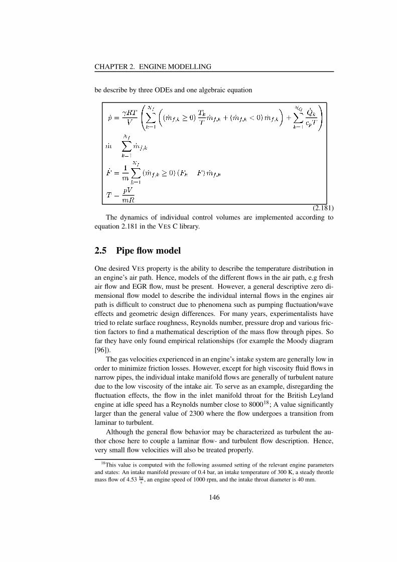
CHAPTER 2. ENGINE MODELLING
be describe by three ODEs and one algebraic equationö÷Jø°ù9ú�ûü ýþSÿ�������� �� ö��� ������� û �û ö��� ��� ö��� ������� ö��� ����� ÿ�������� ö� ���� û! "ö ø ÿ�������� ö��� �ö# ø%$ ÿ�������� ö��� �&����� # �(' # � ö��� �û ø ÷ ü ú
(2.181)The dynamics of individual control volumes are implemented according to
equation 2.181 in the VES C library.
2.5 Pipe flow model
One desired VES property is the ability to describe the temperature distribution inan engine’s air path. Hence, models of the different flows in the air path, e.g freshair flow and EGR flow, must be present. However, a general descriptive zero di-mensional flow model to describe the individual internal flows in the engines airpath is difficult to construct due to phenomena such as pumping fluctuation/waveeffects and geometric design differences. For many years, experimentalists havetried to relate surface roughness, Reynolds number, pressure drop and various fric-tion factors to find a mathematical description of the mass flow through pipes. Sofar they have only found empirical relationships (for example the Moody diagram[96]).
The gas velocities experienced in an engine’s intake system are generally low inorder to minimize friction losses. However, except for high viscosity fluid flows innarrow pipes, the individual intake manifold flows are generally of turbulent naturedue to the low viscosity of the intake air. To serve as an example, disregarding thefluctuation effects, the flow in the inlet manifold throat for the British Leylandengine at idle speed has a Reynolds number close to 800018; A value significantlylarger than the general value of 2300 where the flow undergoes a transition fromlaminar to turbulent.
Although the general flow behavior may be characterized as turbulent the au-thor chose here to couple a laminar flow- and turbulent flow description. Hence,very small flow velocities will also be treated properly.
18This value is computed with the following assumed setting of the relevant engine parametersand states: An intake manifold pressure of 0.4 bar, an intake temperature of 300 K, a steady throttlemass flow of 4.53 kg
s , an engine speed of 1000 rpm, and the intake throat diameter is 40 mm.
146
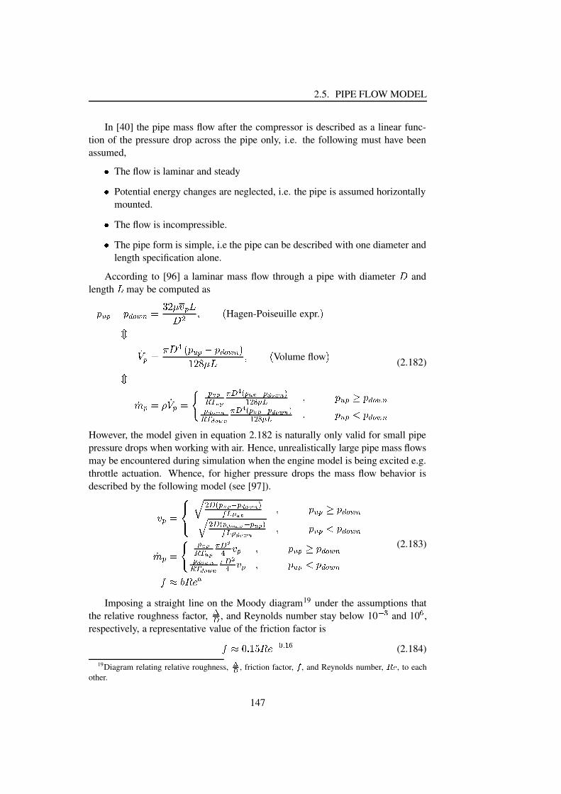
2.5. PIPE FLOW MODEL
In [40] the pipe mass flow after the compressor is described as a linear func-tion of the pressure drop across the pipe only, i.e. the following must have beenassumed,)
The flow is laminar and steady)Potential energy changes are neglected, i.e. the pipe is assumed horizontallymounted.)The flow is incompressible.)The pipe form is simple, i.e the pipe can be described with one diameter andlength specification alone.
According to [96] a laminar mass flow through a pipe with diameter * andlength + may be computed as,.-0/(12,43658749;:=<?>�@ A / +*!BDC E Hagen-Poiseuille expr. FG HI /&:KJ *ML E ,.-0/(12,43658749 FN >?O�@ + C E Volume flow FG HPQ/&:SR HI /&:KT /VU�WXZY U�W\[?]_^a` /VU�Wcb�/�dfefg?h�ij Blk�m�n C ,.-0/poq,43658749/�dfefg?hXZY dfefg?hr[?]_^a` /VU�Wcb�/�dfefg?h�ij Blk�m�n C ,.-0/psq,43658749
(2.182)
However, the model given in equation 2.182 is naturally only valid for small pipepressure drops when working with air. Hence, unrealistically large pipe mass flowsmay be encountered during simulation when the engine model is being excited e.g.throttle actuation. Whence, for higher pressure drops the mass flow behavior isdescribed by the following model (see [97]).A /&:%tu vxw B ]r` /VU�WVb�/�dfefg?hyiz n�{ U�W C ,.-0/poq,436587491 w B ]r` /�dfefg?h|b�/VU�W�iz n�{ dfefg?h C ,.-0/psq,43658749HPQ/�:KT /VU�WXZY U�W [?]~}L A / C ,.-0/poq,43658749/�dfefg?hXZY dfefg?h [?]~}L A / C ,.-0/psq,43658749�2���a���V� (2.183)
Imposing a straight line on the Moody diagram19 under the assumptions thatthe relative roughness factor, � ] , and Reynolds number stay below 10
b.�and 10 � ,
respectively, a representative value of the friction factor is������� NV� ��� b.�a� j � (2.184)19Diagram relating relative roughness, �� , friction factor, � , and Reynolds number, �_� , to each
other.
147

CHAPTER 2. ENGINE MODELLING
The roughness value for the intake manifold material is normally found to bebetween 1.62 �������.� mm (plastic) and 0.02mm (steel) (see [29]) and the hydraulicpipe diameter is normally above 10mm. The roughness value is assumed to bein the neighborhood of 0.001 (conservative estimate). Reynolds numbers in theneighborhood of 10 � would require flow velocities close to the speed of sound forall normal intake manifold designs i.e. a maximum upper limit of ��� to 10 � isvalid.
Combining the laminar and turbulent pipe flow models presented above thefinal model is derived as,�¡ £¢ �¤ �(¥;¦¨§ª©0«¡¬§¯®6°8±4²Z³´µ « K¶!· ¦ ¸.©0«º¹2¸4®6°8±4²�³»?¤�¼�½µ « %¾¿À ¿ÁÃÂ¯Ä «VÅ�Æ � «�ÇfÈfÉ?Ê�˨ÌrÍÏΠͨÐÑaÒ Ñ6Ó�Ô�Õ0Ö Î ×ÏØÅ�Æ2Ù Ö Î Í¨Ð6Ú�Û ÍÍÏÎ ×ÏØÝÜ ¸.©0«pÞq¸4®6°8±4²
Â Ä «�ÇfÈfÉ?Ê � «VÅ�Æ�Ë¨Ì ÍÏΠͨÐÑaÒ Ñ6Ó�Ô�Õ Ö Î ×ÏØÇfÈfÉ?Ê Ù Ö Î Í¨ÐlÚ Û ÍÍÏÎ ×ÏØ Ü ¸.©0«pßq¸4®6°8±4²àá ¾À Á�â6ã?äæå  ç Æè Û � Ü Õ Ì éç ÆÙ Þx����êâ6ã?äæå  éç Æè Û � Ü Õ Ì éç ÆÙ ßx����êëì « Kí «VÅ�ÆîZï Å�Æ\ð Ì~ñò à Ü ¸.©0«pÞq¸4®6°8±4²«�ÇfÈfÉ?ÊîZï ÇfÈfÉ?Ê ð Ì~ñò à Ü ¸.©0«pßq¸4®6°8±4²
(2.185)
The Reynolds number, ���cê , where the transition from laminar to turbulent flowoccurs is found as the point of intersection between the two friction lines ó � òî.ô(laminar) flow and ó ��õ��Vöy���?� ÑaÒ ÷ � in the Moody diagram. Hence the point oftransition is here selected to be����ê ùøûú�ü��õ��Vö¯ý ÍÍÏÎ ×ÏØÿþ � » öy� (2.186)
The value of ���Vê is a bit lower than the normal value of 2300. However, the generalvalue of 2300 is for steady flows and not unsteady flows. The general velocityprofile of the flow will hence reassemble a turbulent profile rather than a laminarprofile i.e. the lower ���cê value is reasonable.
The post-processing of the computed gas velocities, µ « and´µ « , with a hyper-
bolic tangent function insures that the flow velocity, à , never exceeds the speed ofsound.
Figure 2.50 shows the mass flow characteristic of 1m long pipe with a varyingdiameter between 1cm and 5cm under normal atmospheric conditions.
It should be be noted that extreme accuracy of the pipe mass flow model is notmandatory since the bandwidth limiting components are normally not the pipes but
148

2.6. THROTTLE MODEL
01000
20003000
40005000
0.01
0.02
0.03
0.04
0.050
0.05
0.1
0.15
0.2
0.25
0.3
0.35
PSfrag replacements
���, � Pa ��
, �m�� � � , kg s
Pipe mass flow vs. pipe diameter and
���.
01000
20003000
40005000
0.01
0.02
0.03
0.04
0.05102
103
104
105
106
PSfrag replacements, Pa
, m
, kgs
Pipe mass flow vs. pipe diameter and .
���, � Pa ��
, �m �� � �� �� �
Reynolds number surface
Figure 2.50: Pipe mass flow and Reynolds number surfaces for a 1m long pipeevaluated with normal atmospheric dry air properties, i.e. ������� ���������! #"%$ Pa � s,& �('*)*� K, and +,� 101.3207kPa
rather input components like throttles or compressors, and output components likethe intake port mass flow (speed-density equation). Furthermore, the pressure gra-dient between the individual volumes comprising the intake system are normallyvery small for both transient and steady state pipe flows. However, the mass flowcomputations must still be descriptive i.e. mass flows which are too small will givean unrealistically slow response of the pressure and temperature states to excitation,and mass flows which are too large will give an unrealistically fast pressure risetime and unrealistically large temperature spikes due to expansion/compression.
The pipe mass flow model implemented in VES follows the structure given inequation 2.185.
2.6 Throttle model
The mass flow to a SI engine, without VVT/VVL, is normally controlled by a throt-tle, hence the name throttle body for the intake system upstream of the throttle plateposition. However, throttles are nowadays also encountered in Diesel engines as ameans to increase the EGR rate and/or to increase pumping losses and reduce freshair flow, thereby increasing the exhaust temperature, to promote DPF regeneration.Furthermore, a throttle is also normally used to damped out engine shaking duringshut down (closing the throttle completely introduces a large vacuum in the intakemanifold and the engine comes rapidly to a standstill).
The mass flow passing the throttle is normally modelled by the isentropic flowequation for a converging–diverging nozzle. The nozzle equation is repeated below
149

CHAPTER 2. ENGINE MODELLING
for the sake of convenience.
-.,/�02143 56667 6668:9<;>= /�021@?BADCFEHG2IJ K�L G2INM�OPQSR TVUU*WYX[Z]\_^ M Pa` OPQcb d M QSegf UihjXT�k PO `�P9<;>= /�021@?BADCFEHG2IJ K�L G2I J l f TUihjXNk Pnm Ooqp Pa` Osr d M QStgf UihjXT�k PO `�PM Qvu \
(2.187)
with M Q being the ratio between upstream stagnation pressure and static throat pres-sure, and A the throttle angle. However, it is evident that a direct measurement ofthe throat pressure is impossible, since first the flow is divided around the throttleplate, and second the position of the throat varies with the throttle angle. Hence,the kinetic energy of the flow is commonly assumed lost following an isobaric line(converging–sudden expansion nozzle). Thus, it is customary to approximate thethroat pressure with the downstream pipe or plenum pressure. However, just asthere is no such thing as a perfect isentropic process, there is no such thing as aperfect loss either, i.e. some of the of kinetic energy will be recovered as pressure.
The complexity of the throttle mass flow is sought illustrated in figure 2.51. Thefigure illustrates how the flow is divided in a primary- and secondary flow aroundthe throttle plate. Immediately after the throttle plate vortices will be generated dueto local pressure differences and internal flow friction. This phenomenon is illus-trated by the two large scale vortices generated behind the throttle plate. Stream-line photographs made of an experimental setup analogous to a series coupling ofa venturi, throttle and manifold plenum is presented in [54].
The minimum geometrical area for flow passage of an elliptical throttle platecapable of complete passage closure is
= /�021@?BADC@3xw�y T Z]\_^ yy X@za{}| ?~ADC b (2.188)
where the plate- and stem thickness are assumed negligible, y is the pipe radius,and y X is maximum plate radius. The detailed calculations behind equation 2.188may be found in [103].
The idea of dividing the throttle flow in a primary mass flow,-.�� , and a sec-
ondary mass flow,-.�� , was first presented in [47] under the term two flow path
throttle model. Furthermore, the main functional effects of the throttle angle andpressure ratio on the throttle flow were here separated into two functions, � X ?BADCand � T ? M Q C , i.e. -.����%?~A d M#��� � E d M%� ��/ d2� ��� � E CD3 M#��� � E� � ��� � E � X ?BADC � T ? M Q C (2.189)
150
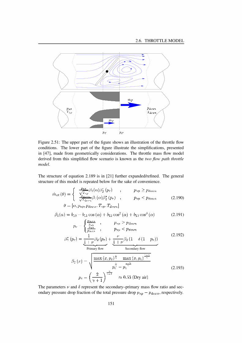
2.6. THROTTLE MODEL
PSfrag replacements
�H�2�� �2� �!�q�q�*�� �q�q�*��N� �N���<�
��<�
Figure 2.51: The upper part of the figure shows an illustration of the throttle flowconditions. The lower part of the figure illustrate the simplifications, presentedin [47], made from geometrically considerations. The throttle mass flow modelderived from this simplified flow scenario is known as the two flow path throttlemodel.
The structure of equation 2.189 is in [21] further expanded/refined. The generalstructure of this model is repeated below for the sake of convenience.������%�B ¢¡D£¥¤ �H�2�¦ � �2�¢§Y¨ �B©D¡ §«ª¬ � %®H¡ ¯ %° �²± #³�´Vµ#¶· �!�q�q�*�¸ � �q�q�*� §Y¨ �B©D¡ §«ª¬ � %®H¡¹¯ %° �²º #³�´Vµ#¶ »£½¼ ©¾¯B%° � ¯B#³�´Vµ#¶¿¯2À�° � ¯2ÀY³�´Vµ#¶}Á (2.190)
§Y¨ �B©D¡¾£( ¨qÃ¾Ä Â ¨Å¨¿ÆaÇ}È �~©D¡ Ä Â ¨ ¬ ÆaÇ}È ¬ �B©D¡ Ä Â ¨qÉYÆaÇ}È É �~©D¡ (2.191)%®4£¥¤ �HÊ#Ë ��H�2� ¯ %° �²± #³�´Vµ#¶�H�2��HÊ#Ë � ¯ %° �²º #³�´Vµ#¶§ ª¬ � %®H¡@£ ÌÌ ÄÎÍ § ¬ � %®H¡Ï ÐaÑ ÒPrimary flow
Ä ÍÌ ÄÎÍ § ¬ � Ì ·ÔÓ � Ì · %®H¡Å¡Ï ÐaÑ ÒSecondary flow
(2.192)
§ ¬ �BÕY¡D£ Ö××Ø ÙÛÚiÜ �sÕj¯B#Ýn¡�Þß · ÙÛÚiÜ �BÕj¯B#Ýn¡ Þsà ßß ÞßÝ · Þsà ßßÝ#Ý@£âáäãå Ä Ì¿æ ßßaç Þ èxé�ê ë*ì � Dry air ¡ (2.193)
The parameters Í and Ó represent the secondary–primary mass flow ratio and sec-ondary pressure drop fraction of the total pressure drop ]° � · #³�´Vµ#¶ , respectively.
151

CHAPTER 2. ENGINE MODELLING
The parameters í , î and ïiðòñ must be identified numerically from throttle flowmeasurements. It can be argued that í and î must be functions of the throttleposition, i.e. íôó(í]õBöD÷ and îøó(î¢õBöD÷ . However, through discussion with one of theco-authors of [47, 21], A. Chevalier, it was clarified that the parameters exhibitedonly very moderate ö dependency. Hence the parameters í and î are assumedconstant in [21]. The explanation behind this might be found in the concept behindthe two-channel converging–sudden expansion model. The geometrical effects isapparently not as important as stated in [47].
Despite the high level of model accuracy achieved, ùxú 10% for pressure ratiosbelow 0.95 with real engine data, the two flow path model fails to capture theeffects for pressure ratios above 0.95. In this region the relative error is close to -60% and ú 15% when mean pressure and real pressure conditions are utilized in themass flow calculation, respectively. Thus, the mass flow estimate error has clearlyincreased in this part of the throttle characteristics i.e. the throttle friction levelis estimated wrongly. This is understandable since the model exhibits an extremepressure ratio sensitivity in this region, sinceû�üý�þ�ÿû��������� for
��� �� (2.194)
Instead it is here suggested that the throttle airflow to computed according to eitherone of the throttle models presented above, and the equivalent pipe mass flow usingthe pipe mass flow model presented in section 2.5 on page 146 in parallel. Thepipe length � is set to the horizontal distance between the throttle tips, and theequivalent pipe diameter is computed such that
�� ��� ó��������@õBöD÷ . The actual pipemass flow is sequently found as� üý�þ�ÿ � ó���� � õ � üý�þ�ÿ"! � �$#%� üý�þ�ÿ"! & � ÷ (2.195)
whereüý�þ�ÿ"! � and
üý�þ�ÿ"! & are the mass flow solution to the isentropic nozzle equationand the pipe equation, respectively. This is the model implemented in VES.
As a final word of caution it should be mentioned that correct estimation ofthe throttle mass flow close to
�'� ó is extremely problematic based on pressuremeasurements alone. Even if such a thing as a perfect physical model of a butterflyvalve existed, it would be ”useless” with the current automotive pressure sensorsavailable (¿1% absolute measurement accuracy). This is here exemplified by asmall example: A throttle plate for a 2.0 liter NA SI engine normally has a diam-eter close to 50mm, [103]. The throttle geometry is here approximated by a pipewith an inner diameter of 50mm and a length of 55mm. A pressure drop of 1kPaacross such a pipe would, using the pipe model, attain a value of approximately600 ( ) under normal atmospheric upstream conditions. The pressure drop of 1kPais exactly the absolute deterministic measurement error for the commonly used 0–1atm intake manifold piezo-resistive pressure transducer [103, 22, 10]. Hence, if thissetup is to be used for online throttle flow estimation with
�*�,+.-0/ 1�2, sensor fusion
is needed. An obvious choice for automotive application would of course be to
152

2.7. INTAKE PORTS
fuse the estimation of the throttle mass flow with an eventual hotwire/hotfilm MAFmeasurement. However, when the throttle is close to WOT (Wide Open Throttle)the waves will propagate more easily through the intake system. This might courseserious problems obtaining the correct measurement if a hotwire/hotfilm sensor isused, since such sensor’s measurement quality deteriorates rapidly when exposedto pumping fluctuations. This phenomenon has been investigated thoroughly in theECG at DTU and is still under investigation (see e.g. [44])
2.7 Intake ports
A good knowledge of the intake port mass flow is of paramount importance ifacceptable performance of several control strategies is to be achieved. Two suchcontrol problems are the AFR control problem of MPI equipped SI engines andthe EGR rate control in Diesel engines. The first simply because this is the flowfor which the AFR is sought kept constant (see [112, 22]) and the latter since nodirect measurement method of the EGR mass flow is currently available, i.e. 3465�798is approximated as 34;:�<>= MAF. However, commercial sensors for series produc-tion applications, capable of measuring the port mass flow directly, are currentlynot available20 . Instead, the air mass is often estimated from other engine measure-ments. The most common open loop estimation strategy used to derive a measureof the cycle averaged port air mass flow is the well known speed-density equation.Dependent upon which engine sensor signals are available this equation may haveseveral different structures, where two most common equation forms encounteredare repeated below
34?:�<A@CB :9DFEG$H�I JLKNMOQP�RTS :9DFE34?:�<A@CB DF:9UG$H�I JLKNMOQP�R S DF:9U (2.196)
where indicates that the corresponding variable has averaged over an engine cy-cle. The non-dimensional variable B G$H�I , referred to as the volumetric engine effi-ciency, is an empiric attempt to describe the breathing performance of the engine.The parameters B :9DFEG$H�I and B DF:9UG$H�I are normally found from steady state engine mea-surements, i.e.
B :9DFEG$H�I @ OQP�R�V,W :9DFEJLKNMYX :9DFE MAF
B DF:9UG$H�I @ OQP�R�V W DF:9UJLKNM X DF:9U MAF(2.197)
20A prototype port air mass flow sensor has been developed by the ECG at DTU (see [37]). How-ever, the measurement principal is not completely non-intrusive, and might thus change the breathingperformance of the engine. Furthermore, the method is not directly applicable on DI engines withEGR
153
CHAPTER 2. ENGINE MODELLING
and sequently stored in a 2D engine map with Z and []\F^9_ as indices. For aacceptable performance it might however be necessary to readjust the level of `Na$b�cby an intake temperature correction factor. A commonly used correction factor isd egfghjie fghjiQk lnmpo , [54].
It is shown in [47, 75], referred to as the ” q asr [�t ” methodology, that ` \F^9_a$b�c [�\F^9_exhibits a strong linear [ \F^9_ dependency and only a weak engine speed depen-dency for pressure ratios, ['uwv x fghji
x hjf'y smaller than 0.95. Hence, using this method-ology when storing the volumetric efficiency, i.e. ` \F^9_a$b�c [�\F^9_ is stored instead of` \F^9_a$b�c , the interpolation accuracy may be improved.
Since no direct measurement method, as mentioned, is available the static `Na$b�cmap is also used to derived the port air mass flow during transients. It is thus likelythat this might introduce significantly errors due to ramming effect. However, themagnitude and characteristic of this likely error is investigated thoroughly in [21]by 1D modelling. It is found that the static speed density equation, for a plenumtype manifold, is able to describe the event mean value of the port mass flow witha remarkably accuracy. Hence for MVEM based modelling and control the speeddensity equation is a good choice.
In the cases where a greater model detail level is desired (e.g. wave modelling)the intake and exhaust valve’s flow restriction need separate modelling. The intakeand exhaust are customarily of the poppet valve type except for a few exotic en-gine designs. One modelling approach (as with other common valve types) is toutilize the isentropic nozzle equation together with a geometrically derived modelof the minimum flow area, and a discharge coefficient, z,{ , to account for the un-avoidable modelling errors introduced by the isentropic assumption. Models of theminimum valve area are readily available in literature, and it is in VES selectedto implemented a poppet valve model structure according to model proposed in[54]. The size and character of the discharge coefficient are also addressed in [54].Since poppet valves are utilized to control other flows than just the engine portmass flow e.g. EGR mass flow and idle speed by-pass mass flow, the model is alsoused in larger VES engine sub-models like the EGR cooling system described insection 2.8.1.
2.8 Heat exchangers
Two heat exchangers are commonly found in a modern turbocharged engine’s airpath namely the intercooler and the EGR cooler. Depending on the engine config-uration the added air path volume due to the heat exchangers may need dynamicmodelling in the description of the three main air path characteristics: pressure,gaseous mass contained and burnt mass fraction. Hence, this section is devoted tothe investigation of possible model structures for convenient 0-D heat exchangermodels.
154
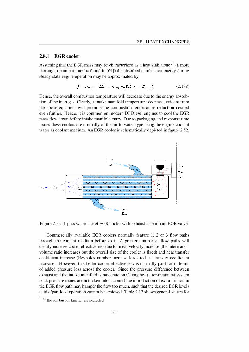
2.8. HEAT EXCHANGERS
2.8.1 EGR cooler
Assuming that the EGR mass may be characterized as a heat sink alone21 (a morethorough treatment may be found in [64]) the absorbed combustion energy duringsteady state engine operation may be approximated by|~}���?���9��������� }���?���9�����w��� ���Q�� �'�F�9�N� (2.198)
Hence, the overall combustion temperature will decrease due to the energy absorb-tion of the inert gas. Clearly, a intake manifold temperature decrease, evident fromthe above equation, will promote the combustion temperature reduction desiredeven further. Hence, it is common on modern DI Diesel engines to cool the EGRmass flow down before intake manifold entry. Due to packaging and response timeissues these coolers are normally of the air-to-water type using the engine coolantwater as coolant medium. An EGR cooler is schematically depicted in figure 2.52.
������������
����������������������������������������������������������������������������������������������������������������������������������������������������������������������������������������������������������������������������������������������������������������������������������������������������������������������������������������������������������������������������������������������������������������������������������������������������������������������������������������������������������������������������������������������������������������������������������������������������������������������������������������������������������������������������������������������������������������������������������������������������������������������������������������������������������������������������������������������������������������������������������������������������������������������������������������������������������������������������������������������������������������������������������������������������������������������������������������������������������������������������������������������������������������������������������������������������������������������������������������������������������������������������������������������������������������������������������������������������������������
������������������������������������������������������������������������������������������������������������������������������������������������������������������������������������������������������������������������������������������������������������������������������������������������������������������������������������������������������������������������������������������������������������������������������������������������������������������������������������������������������������������������������������������������������������������������������������������������������������������������������������������������������������������������������������������������������������������������������������������������������������������������������������������������������������������������������������������������������������������������������������������������������������������������������������������������������������������������������������������������������������������������������������������������������������������������������������������������������������������������������������������������������������������������������������������������������������������������������������������������������������������������������������������������������������������������������������������������������������������������������������������������������������������������������������������������������������������������������������������������������������������������������������������������������������������������������������������������������������������������������������������
�����������������������������������������������������������������������������������������������������������������������������������������������������������������������������������������������������������������������������������������������������������������������������������������������������������������������������������
�¡ ¢ £ ¤¥ ¡ ¢ £¦¤§ ¡ ¢ £ ¤ ¨ ©¥ ¨ ©§ ¨ ©
ª�« ¬¦® « ¬¦¯ « ¬¦ª�° ± ± ²
ª�° ± ± ²
³´ « µ ¶³´ ° ± ± ²
³´ ° ± ± ²
Figure 2.52: 1-pass water jacket EGR cooler with exhaust side mount EGR valve.
Commercially available EGR coolers normally feature 1, 2 or 3 flow pathsthrough the coolant medium before exit. A greater number of flow paths willclearly increase cooler effectiveness due to linear velocity increase (the intern area-volume ratio increases but the overall size of the cooler is fixed) and heat transfercoefficient increase (Reynolds number increase leads to heat transfer coefficientincrease). However, this better cooler effectiveness is normally paid for in termsof added pressure loss across the cooler. Since the pressure difference betweenexhaust and the intake manifold is moderate on CI engines (after-treatment systemback pressure issues are not taken into account) the introduction of extra friction inthe EGR flow path may hamper the flow too much, such that the desired EGR levelsat idle/part load operation cannot be achieved. Table 2.13 shows general values for
21The combustion kinetics are neglected
155
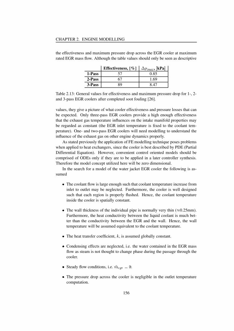
CHAPTER 2. ENGINE MODELLING
the effectiveness and maximum pressure drop across the EGR cooler at maximumrated EGR mass flow. Although the table values should only be seen as descriptive
Effectiveness, [%] ·,¸'¹Fº9» , ¼ kPa ½1-Pass 57 0.852-Pass 67 1.693-Pass 89 8.47
Table 2.13: General values for effectiveness and maximum pressure drop for 1-, 2-and 3-pass EGR coolers after completed soot fouling [26].
values, they give a picture of what cooler effectiveness and pressure losses that canbe expected. Only three-pass EGR coolers provide a high enough effectivenessthat the exhaust gas temperature influences on the intake manifold properties maybe regarded as constant (the EGR inlet temperature is fixed to the coolant tem-perature). One- and two-pass EGR coolers will need modelling to understand theinfluence of the exhaust gas on other engine dynamics properly.
As stated previously the application of FE modelling technique poses problemswhen applied to heat exchangers, since the cooler is best described by PDE (PartialDifferential Equation). However, convenient control oriented models should becomprised of ODEs only if they are to be applied in a later controller synthesis.Therefore the model concept utilized here will be zero dimensional.
In the search for a model of the water jacket EGR cooler the following is as-sumed¾
The coolant flow is large enough such that coolant temperature increase frominlet to outlet may be neglected. Furthermore, the cooler is well designedsuch that each region is properly flushed. Hence, the coolant temperatureinside the cooler is spatially constant.¾The wall thickness of the individual pipe is normally very thin ( ¿ 0.25mm).Furthermore, the heat conductivity between the liquid coolant is much bet-ter than the conductivity between the EGR and the wall. Hence, the walltemperature will be assumed equivalent to the coolant temperature.¾The heat transfer coefficient, À , is assumed globally constant.¾Condensing effects are neglected, i.e. the water contained in the EGR massflow as steam is not thought to change phase during the passage through thecooler.¾Steady flow conditions, i.e. ÁÂÄÃ�Å9ÆwÇ�È .¾The pressure drop across the cooler is negligible in the outlet temperaturecomputation.
156

2.8. HEAT EXCHANGERS
PSfrag replacements
É$Ê%Ë
É$ÊQÌ
Í Ë
Í Ì
Î Ë
Î Ì
ÏÐË
Ï*ÌÒÑ
Ó]ÔÖÕØ× ×ÙÚ�Û
Figure 2.53: Illustration of EGR mass packet on its way through one of the Ü ÍEGR cooler pipes.
Ý The mass flow through the individual pipe is position independent, i.e. Þßáà�â9ã�ä åFæÞß?à�â9ã�ä ç�èæêéëFìîíYïç�è , where Ü Í is the number of cooling pipes in the cooler.
Of the above assumptions the largest error is most likely introduced by the steadyflow assumption. EGR cooler are normally closely coupled to the exhaust manifoldwith the EGR valve mounted up or downstream of the cooler. Hence, rather largeflow fluctuations may be expected. Treatment of the fluctuations mentioned willbe addressed in section 2.8.5.
The outlet temperature model proposed here will be derived from a lagrangianpoint of view.
Figure 2.53 illustrates the passage conditions for package of constant mass onits way through one of the EGR cooler pipes.This mass package may be described by the following four equations.
The volume rate change of the package is given by
ð ð ñîò�óCôöõÞ÷]øCù;÷ ÞøúæLû ûNü ònó�ôöõÞß?ý,þÿù ß?ý Þþ�Þøúæ øþ Þþ
(2.199)
The local velocity of the package, Þ� , is found as
Þ� æ�� ý,þ����Í ÷ Þß?à�â9ãÜ Í (2.200)
157

CHAPTER 2. ENGINE MODELLING
The change in the internal energy of the package is found as� �������������� ��� ��� ��� �!��"�$#%� � �'&�()�*,+.- *� / #10 � / 2 & ( (2.201)
The heat transfer,/
, from the mass package to the pipe wall is thought to be pureconvective. The convective heat transfer is here modelled by/3�54 � *7678:9 9�2�* �;�!< �54;=�>@? � *7678:9 9A2B* �C��D �54FE (>@?� *7678:9 9A2B* � (2.202)
The package temperature,*
, as function of time, � , may now be found by combin-ing equation 2.199, 2.201 and 2.202 to obtain*5� 4 )�*& >@? + ?$� *7678:9 9A2B* �G � � & >@? + ?E )H4 IJKML ION�PRQ S* � *7678:9 9A2B* � �!TG* �U�R� � *�VXWMYO*7678:9 9[ZM\^]*�VXWMY � Z \^] 2 S �_# *7678:9 9with ` �aE )�*7678:9 9U4& >@? + ?
(2.203)
The position, D , at time � is now found by combining equation 2.200 and 2.203 toDb�U�R� � E � VXcRd )�*�VXWMYe*7678:9 9=�>@? &gf ? ]JKML7h ZM\^]*�VXWMY � Z \^] 2 S �_# *7678:9 9 �!T� E � VXcRd )�*7678:9 9=�>i? &gf ? `kj[lnm *�VXWMY@oXZM\^]_2 SMp # *7678:9 9*7678:9 9 q for �srtDurwv ? (2.204)
Finally, the solution to equation 2.204 for which Db�U�R� � v ? is found and insertedin equation 2.203, thereby deriving the following expression for the cooler outlettemperature,
*_x �y� .*�x{z ] � � VXcRde| *7678:9 9 | *�VXWMY � � *7678:9 9~}yZ��e�������^���.�M��� NU�{��� ��� 2 S�� # *�VXWMYZ��e�������^���.�M��� NU�{��� ���for� VXcRd�� � (2.205)
158

2.8. HEAT EXCHANGERS
2.8.2 Intercooler
The principal motivation behind turbocharging an IC engine is naturally to increaseits specific power and brake torque. However, since not only the pressure after thecompressor is raised but also the temperature the benefits of the turbocharger arepartly offset. To minimize the negative effects of the increased inlet temperature thecharged air is nowadays commonly sent through a heat exchanger, the intercooler,to increase the density of the boosted air charge before its entry into the intakemanifold. The insertion of an intercooler in the air path will, however, degrade thetransient response of the engine due to the added intake volume. Thus, selectingan appropriate intercooler is often a compromise between desired effectivenessat a rated mass flow, restriction concerns and transient performance expectations.Fortunately, the air-to-air coolers, customarily used nowadays, have normally avery high level of effectiveness. The cooler effectiveness is defined as�������'�$��� ����� �:��$� ���R �:�B¡£¢ �¥¤§¦ ¢�¨ �M�¢ �¥¤§¦ ¢ �R©«ª (2.206)
The effectiveness of a properly sized intercooler is in [83] found between 0.82 and0.99, i.e. the output flow temperature will be close to the ambient temperature22 .Due to the high effectiveness expected the focus here will be on adequate coolertemperature description for a later inclusion in the heat exchanger pressure dynam-ics description. In this quest the following will be assumed¬ The ambient temperature is well known.¬ The cooling flow through the air cooler is large compared to the intercooler
flow, i.e. the coolant temperature changes across the cooling element arenegligible.¬ The pressure drop across the intercooler is negligible in the computation ofthe total gaseous mass contained in the intercooler.¬ Intercooler fouling due to e.g. evaporated turbocharger oil is neglected.¬ Steady flow conditions prevail.¬ The intercooler effectiveness is constant.¬ The intercooler temperature only varies along the flow direction and is flowpath independent.¬ The convection parameter is assumed globally constant for fixed values of®¯ ��� , ¢ �¥¤ and ¢ �R©«ª .22The intercooler is often dimensioned such that the maximum difference between the intake
plenum temperature and the ambient temperature is close to 35K at maximum rated boost pressure[2].
159
CHAPTER 2. ENGINE MODELLING
The first goal is to derive the mean intercooler temperature, °b±�²´³ µ , fulfilling¶ ±�²R·A±�²¸ °7±�²´³ µ�¹»º ±�² (2.207)
Hence, first the total gaseous mass contained in the intercooler must be computed.Assuming the outlet profile along the flow path may be described by equation 2.205the heat transfer coefficient required to obtain intercooler effectiveness ¼M±�² is½H¾ ¼�±�²�¿�Àº ±�²:Á ¹ Â[ÃÅÄ ÆÆÈÇ ¼�±�²^É Àº ±�²´Ê´ËÌ�Í ËÏÎ~ËÏÐ�Ë (2.208)
Inserting this in equation 2.205 where ÎÑË has been exchanged with the relativeposition Ò , the temperature profile along the flow path is found to
° ¾ Ò�Á ¹ °�Ó µ«Ô ÄÖÕØ××�Ù Ú�Û ÜOÝßÞà.á ÇwÆ É1â °7±¥ãÕä××�Ù ÚUÛ Ü^Ý Þà.áfor å Òuæèç é;êRÎ~ËOë¼�±�²Öæ�ëìé;ê Æ ç
(2.209)
The gaseous mass contained in the intercooler is found by
º ±�² ¹îí Û Üï ðòñ ¾ ·óÁ{ô;· ¹öõ áï÷eø ð ¶ ±�²�Îù±�²´³ úMÎù±�²´³ û¸ ÕØ××�Ù Ú�Û ÜOÝ Þà.á°�Ó µ«Ô Ä Õ ××�Ù Ú�Û Ü Ý Þà.á ÇwÆ Éüâ °7±¥ã ô�Ò¹ ¶ ·A±�²¸ °�Ó µ«Ô Â[ÃÕ$ý Û þýeÿ�� � Ý Ç Â[ÃÕ,ý Û þýeÿ�� � â ÚUÛ Ü×�Ù Ú�Û ÜOÝÂ[à ¾ ÆÖÇ ¼�±�²:Á (2.210)
Finally is the mean temperature of the intercooler is found by a combination ofequation 2.207 and 2.210:°7±�²´³ µ ¹ Â[à ¾ ÆÈÇ ¼�±�²RÁÂ[ÃÕ,ý Û þýeÿ�� � Ý â Â[ÃÕ ýeÿ�� ��� ×�Ù Ú�Û Ü �ý Û þ � ×�Ù Ú�Û Ü ��� Ú ýeÿ�� � Ý °�Ó µ«Ô (2.211)
It is customary in the assessment of the gaseous mass contained in the inter-cooler to use the ideal gas law with the mean temperature set to °b±�²´³ µ ¹ ×� ¾ °7±¥ã â°�� �{Á (see e.g [83]). Hence, it is interesting to investigate the behavior of the dif-ference between this assumption and the averaged cooler temperature model de-veloped above. The mean cooler temperature model derived above is the referencemodel in the following. Figure 2.54 shows the relative computational error for themean cooler temperature and mass, respectively. As expected the error is seen to
160

2.8. HEAT EXCHANGERS
increase with temperature difference and cooler effectiveness, and might be as high19% on the temperature calculation and -16% in the contained mass computation.However, since the cooler effectiveness drops with mass flow increases the relativeerror is for all normal steady flow operating conditions23 most likely to be within8% and -7% for the temperature and mass computation, respectively.
0 20 40 60 80 100 120 140 160 180 2000
2
4
6
8
10
12
14
16
18
20
PSfrag replacements
���������������� , [K]
Rel
.Err
or,[
%]
Relative mean temperature error
��� � =40%
60%
70%
80%
90%
95%
99%
0 20 40 60 80 100 120 140 160 180 200−16
−14
−12
−10
−8
−6
−4
−2
0
PSfrag replacements, [K]
Rel. Error, [%]
Relative mean temperature error
=40%
60%
70%
80%
90%
95%
99%
����� ���������� , [K]
Rel
.Err
or,[
%]
Relative mass error � =40%
60%
70%
80%
90%
95%
99%
Figure 2.54: Relative error made when using the assumption !#"%$'& (*),+-/. !0"2143!5�6 798 . The plot to the left shows the relative temperature error for different lev-els of cooler effectiveness. The plot to the right shows the accompanying massassessment error.
2.8.3 MVEM approach to intake system modelling
Since the introduction of turbochargers, heat exchangers and exhaust recirculationequipment in the automotive engine’s air induction path the one state, :�(<;=1 , equa-tion approximation (also known as the IMVEM, see e.g [47, 49]) commonly usedfails to describe the dynamic and steady state behavior of the complete intake sys-tem adequately. The two state, :0(<;=1 and !0(<;=1 , intake system model, also known asthe AMVEM (Adiabatic Mean Value Engine Model) (see the SAE-paper number1999-01-0909 included on page 200) was therefore introduced, which should beable to estimate the impact of the high temperature EGR inlet flow on the intakemanifold conditions. This model was later experimentally tested by one of the co-authors, Professor E. Hendricks, on an engine dynamometer test bench at DTU.The experimental results obtained, of which some are included in the SAE-papernumber 1999-01-0909, clearly showed a high consistency between the simulationresults and the experiments, and the good modelling properties of the AMVEM
23For a properly fitted turbocharger the compressor outlet temperature increase is in the vicinity of0 K close to engine idling. As the engine speed increases the pressure ratio across the compressor isincreased; and thereby are also the temperature difference and the compressor mass flow increased.Hence, the temperature difference will generally increase with engine fresh air mass flow increases.
161

CHAPTER 2. ENGINE MODELLING
were confirmed. However, the intake manifold of the experimental NA SI test en-gine can with good approximation be classified as one large plenum with the EGRentry point located just downstream of the throttle plate (see e.g. the pictures in[37]). Furthermore, the EGR valve is mounted close to the EGR entry point, thus,the (small) volume of the EGR pipe24 is separated from the intake system. Hence,the layout of the intake system will, generally speaking, fulfill the assumptionsmade with a two state FE modelling approach. However, considering the normaldesign of the intake system for a modern intercooled and turbocharged DI Dieselengine equipped with an EGR system (see e.g. the engine illustration in figure 4.3on page 235), the AMVEM will most likely fail to predict the dynamic and steadystate behavior of the intake manifold states, since it does not take into account thegeometric location of the individual mass flow entry- or exit points. The reasoningfor this will be explained in the following.
Normally, the total volume of a modern turbocharged DI Diesel engine’s intakeair system is distributed in the following manner [2]:
> The intake plenum volume downstream of the EGR inlet point is approxi-mately 50% to 60% of the engine displacement.
> The intake system volume including the intercooler volume (throttle bodyvolume) is about 200% to 250% of that of the engine displacement.
> The volume of the EGR system is about 25% the engine displacement.
With this distribution of the intake air path the intake plenum volume will onlycomprise 22% to 27% of the total volume of the intake system. However, it is thetemperature of this volume which determine the accuracy of the total mass flowestimation (speed-density equation). Thus, a good estimation of this temperatureis highly desirable.
In order to be a bit more specific the intake system layout for a modern 2.0 literturbocharged Diesel engine will roughly follow the specifications in figure 2.55 [3].The distribution of the gaseous mass between the seven intake sections depicted infigure 2.55, when evaluated on the corresponding steady state engine map of a 2.0liter engine25 , is shown in figure 2.56. The total mass, ? , in the system is computedas the sum of the masses contained in the seven volumes. The mass entrapped inthe heat exchangers is computed by equation 2.210 and not by the ideal gas law asit is done for the remaining five volumes. The mass contained, when following theone volume approach, is calculated as
@?BAC/D<E=FHGIJ�K�LNM JOQP D<E=F (2.212)
24No EGR cooler was used during the experimental work.25Dipl. Ing. Daniel Rottger is gratefully acknowledged for providing the steady state engine map.
162

2.8. HEAT EXCHANGERSPSfrag replacements
RTSU<VXW�YZSU\[
]=^X_�`badc�e fhgij^X_�`hk lnm=o=^X_�`ba\o�l/prq
]�l/prq#aQs�gi=l/prqtm=o�l/prq]�u2v `hk w axc�e y�gi=l/prqtm=o�l/prqz]�u2v `hk { aQs�gi=| } k ~X� u m=o�l/prq�
]�| }Nad�hgi=| } k l m=o�| }Na\o�l/prq
]=p } aQshe y�gijp } m=o=p } a\o�l/prq
]=^X_�`hk ��axc�e sXy�gij^X_�`jm=o=^X_�`hk ��a\o�l/prq
Figure 2.55: Illustration of a typical intake system for a modern 2.0 liter tur-bocharged Diesel engine. The figure also depicts the approximate values of thevolume and states for the individual sections.
0 10 20 30 40 50 60 70 80 90 1000
0.2
0.4
0.6
0.8
1
0 10 20 30 40 50 60 70 80 90 100−15
−10
−5
0
5
10
PSfrag replacements
Relative intake system mass distribution.
Data no.
Rel
ativ
em
ass
frac
tion,
� � �. � p }� | }� u2v `hk {� u2v `hk w� l/prq� ^X_�`� ^X_�`hk ���1000 1250 1500 1750 2000 2250 2500 2750 rpm
Relative error of the one FE intake model’s mass distribution.
Data no.
� � �� �,[
%]
Figure 2.56: Typical distribution picture of the intake system mass for a 2.0 literturbocharged Diesel engine generated from experimental data. The dashed blackline shows the ratio between the estimated mass by the one volume model, �� , andthe total intake mass obtained using a sectioned volume approach. The subscriptsindicate the geometric location of the different masses (see figure 2.55). Remark:The mass contained in the heat exchangers is computer by equation 2.210.
163

CHAPTER 2. ENGINE MODELLING
The ratio between �� and � is plotted as a dashed black line in the upper plot infigure 2.56. The regions where the �� is smaller than � indicates low/part loadoperation points with the EGR system being active. In these cases the estimatecomputed by the one volume approximation is too small since the temperature ofthe intake manifold is in general higher than the rest of the intake system. Thiscan be traced back to the influence of the high temperature EGR inlet flow. When�� is too large the engine is operated in a high load with no EGR key point of theengine map. Here, the boost pressure is high and the temperature upstream of theintercooler is significantly above that of the ambient temperature but also that of theintake manifold temperature. Hence, the one volume approximation will producea too large estimate of the mass contained. However, the relative error of the onevolume approximation is reasonably small. This is confirmed by the lower plot infigure 2.56 showing that the relative error between �� and � stays between -15%and 10% within the supplied engine map. Hence, although the volume of intakemanifold only constitute about 20% of the total intake system volume, the totalsteady state mass contained in the system can be estimated fairly well from thepressure and the temperature measurements obtained in the intake plenum alone.This is fortunate since it speaks in favor for the approximation of the intake systemby one FE volume alone.
Adequate modelling accuracy of the intake system’s dynamic response will,however, most likely not be obtainable with the AMVEM model proposed in SAE-paper number 1999-01-0909 (see [75]), when this model is utilized on a intercooledturbocharged Diesel engine equipped with an EGR system. The differential equa-tions of the AMVEM are repeated below for the sake of convenience.
������������������� ����' �¡¢����£b¤ ���¥�¦�§=¡¢¥�¦�§�¨ ����9©ª¡������¬«�¡�������®� ¡������������� �����9� � ¡¢����£0¨4¡������¬« ����' ¢¤ � � ¡¢¥�¦�§#¨4¡������¬« ���¥�¦�§�¨ � � ¨°¯±«h¡������ ����9©²«
(2.213)
where ³�´ is the volume of the intake system downstream of the throttle plate. Thismodel in [75] is developed for NA SI engines which have a simpler intake systemthan those of modern Diesel engines. Furthermore, the AMVEM does not respectgeometrically how the EGR enters the intake system. Inspecting the generic intakesystem for a Diesel engine depicted in figure 2.55 a reasonable approximation ofthe volume split would more likely be
³¢µj¶ : The volume of the pipe connection between the compressor and the inter-cooler. This volume has a reasonable low area-to-volume ratio, and the rele-vant FE model is therefore adiabatic.
³�´%¶ : Intercooler volume. This volume has a very high area-to-volume ratio. Hence,a reasonable simple FE model is isothermal. The corresponding mean tem-perature of the cooler is found by equation 2.211 on page 160.
164
2.8. HEAT EXCHANGERS
·�¸�¹ªº'» ¼: This volume separates the intercooler exit and the EGR inlet point. This vol-
ume has a low area-to-volume ratio, and the relevant FE model is thereforeadiabatic.
·�¸�¹ªº'» ½¿¾À·�Á<Â=Ã: The volume comprising the intake system downstream of EGR point and
upstream of the engine’s intake ports. This volume has reasonably low area-to-volume ratio. Hence, the adequate FE model for this volume is of anadiabatic nature.
·¬ÄžÀ·¢Æ9Ç º: The total volume of the EGR system. This volume is in general small com-
pared to the volume of the complete intake system. Hence, the volume canwith a reasonable good approximation be neglected in the dynamic meanvalue description of the intake system pressure.
The system order of the complete intake system volume is thus seven, four pressureODEs and three temperature ODEs, if the temperatures and pressures of intakesystem are approximated according to the philosophy above. However, the generallevel of the flow friction between individual volumes is low (normally the pressureloss is within a few kPa). Hence, the following assumption for the general intakesystem pressure level, È0É , is reasonable.
È/É�ÊËÈ ÂjÌ ÊËÈ/É Ì ÊËÈ ¸�¹ªº'» ¼ ÊËÈ ¸�¹ªº'» ½ ÊËÈ Á<Â=à (2.214)
The total order of the intake model is thereby reduced by three state equations to atotal of four state equations.
The next challenge is to examine the relative importance of the three temper-ature state equations ÍÎ ÂjÌ , ÍÎ ¸�¹ªº'» ¼ and ÍÏÎ Á<Â=à , where the temperature
ÏÎ Á<Â=Ãis the
spatially averaged temperature of the volume downstream of the EGR inlet point,·�¸�¹ªº'» ½x¾Ð·�Á<Â=Ã. First, the relative importance of the dynamic response of
Î ÂjÌwill
be discussed. The volume·bÂjÌ
is in general smaller than the engine displacementvolume. Hence, the mass contained in this volume is exchanged at a rate betweena half and one engine cycle. Hence, the mean value response26 of the temperaturewill rapidly follow the exit temperature of the compressor during quasi-steady en-gine operation. The only expansion or compression phenomena experienced in thisvolume are due to either turbocharger excitation, EGR valve actuation, or enginespeed changes. The frequency spectrum of these excitations is in general smallcompared to the bandwidth of the
Î ÂjÌstate equation. Hence, the time response of·¢ÂjÌ
’s temperature may be approximated byÎ Ì
and thus be considered as an alge-braic equation i.e. ÍÎ ÂjÌ Ê�Ñ . In addition to this the intercooler would dampen (filter)the effects of possible neglected compression/expansion spikes in
Î ÂjÌonÎ Á<Â=Ã
. Inanalogy with this approach the time response of
·0¸�¹ªº'» ¼’s temperature will primarily
follow the exit temperature of the intercooler. The dynamic behavior ofÎ ¸�¹ªº'» ¼
mayin correspondence with the
Î ÂjÌmodel also be neglected, since the assumptions
26The individual compressions and expansions due to engine pumping is neglected in accordancewith the MVEM philosophy.
165

CHAPTER 2. ENGINE MODELLING
made previously for ÒbÓjÔ are in general also valid here. However, this volume doesdirectly interact with the intake plenum, and modelling errors in its temperaturedescription will by nature have a more severe effect than Õ#ÓjÔ model errors. Thevolume is, however, typically small and the flow restriction to the intake plenumand intercooler, respectively, is negligible. Hence, rapid compression or expan-sion spikes in the time response of Õ�Ö�תØ'Ù Ú are highly unlikely to be encounteredindependently of how the Diesel engine is excited.
The intake temperature, however, is controlled by three mass flows or betterenergy flows, namely ÛÜ Ö�תØ'Ù Ú=Ý'ÞßÕ0à%ÔâáãÛÜ Ô'Ý'ÞßÕ0à%Ô , ÛÜåä9æ Ø Ý'ÞßÕ ä9æ Ø and ÛÜ Ó9ÞtÝ'ÞèçÕ0é<Ó=ê . Thedynamic behavior of çÕ0é<Ó=ê can in contrast to Õ�ÓjÔ and Õ0Ö�תØ'Ù Ú , respectively, not beneglected due to the possible large temperature difference between Õ#à%Ô and Õ ä9æ Ø .Hence, Õé<Ó=ê cannot adequately be approximated by any of the upstream tempera-tures, and a dynamic model is needed to reproduce its time response.
The AMVEM in its current structure does not provide a means to estimatethe amount fresh air entering the intake ports during transient engine operationwhen the EGR system is activated. A convenient way to overcome this problemis to estimate the time response of the burnt mass fraction in the intake throat andplenum, çë é<Ó=ê . The fresh air mass flow at the intake ports, ÛÜ Ó9Þ Ù ì , during steadystate as well transient engine operation, may then later be obtain by the speed-density equation as
ÛÜ Ó9Þ Ù ìâíïî'ðdñ ë é<Ó=ê¢òNótôjõ'ö ÷ à�ø Ò¢ùð úüûtýÐçÕ0é<Ó=ê (2.215)
A good knowledge of this flow is of evident importance when addressing the prob-lem of transient control of a Diesel engine’s AFR. The dynamic equation for çë é<Ó=êmay directly be derived from the material in section 2.4 as
Ûçë é<Ó=êþí ÷ à�çÒ�é<Ó=êçÕ0é<Ó=ê�ýÿ î ë ä9æ Ø ñ çë é<Ó=ê/òxÛÜåä9æ Ø ñ çë é<Ó=ê ÛÜ Ö�תØ'Ù Ú � (2.216)
Collecting the assumptions and simplifications made above the dynamic behav-ior of the intake system for a modern turbocharged diesel equipped with EGR maybe described by the following equations (the equations are derived in appendix D).�Þ��������� ������ �é��������� �� � �é ����� ���� � �é!�"$#�%� &(' � �� �") � �� �* � � �� �+ �� �") � � ���� �,� * � �+ � �� � � ���� �,� *.-0/ � ) 1 � �� �") � � ���� �%� �* ��� �� � �� �") � �� ��� ���� ��� & � ���� �Þ�� �* ��� � � 2 ' ������ �3� ���� �54 �é������6��2 ' �� � �3� ���� �54 �é �6� 2 ' � Ú 4 � ���� � �é!�"$#��7 ��� ��� Þ�� �* ��� �� ���� � & � 2 7 ����� �8�7 ��� �54 �é������ �8�7 ��� � �é � #
Assumptions: �é -0/ � ) 1�9 �é � Ù �é������ Ù �é � Ù �é!�"�:<;(2.217)
This third order system will be referred to as the TDMVEM (Turbo Diesel MeanValue Engine Model). The close relationship between the TDMVEM and the
166
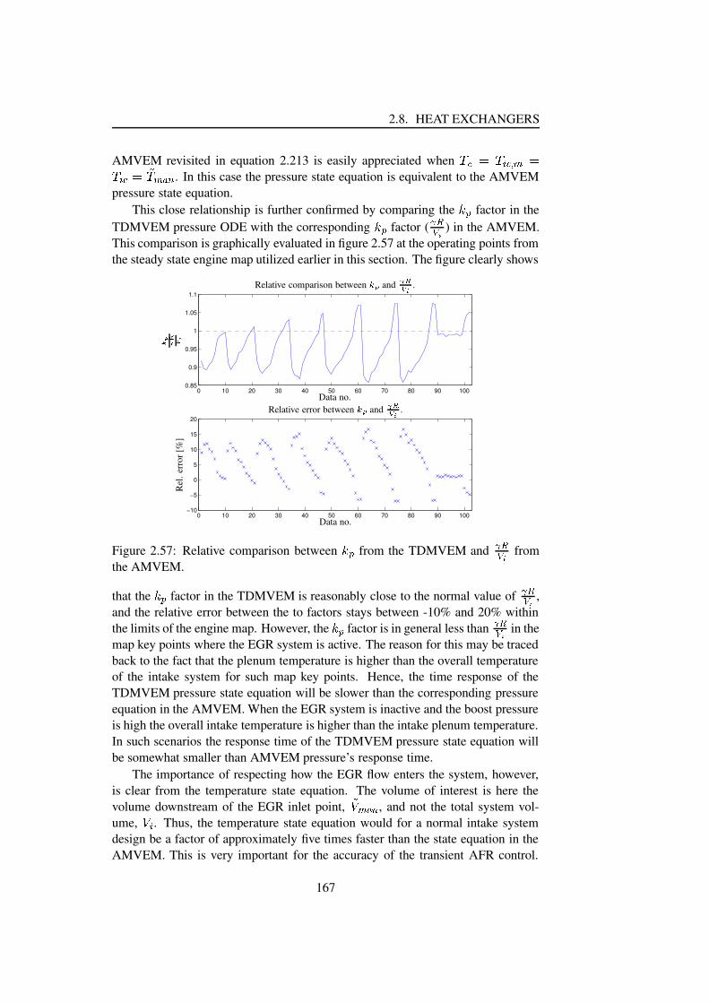
2.8. HEAT EXCHANGERS
AMVEM revisited in equation 2.213 is easily appreciated when =%>@?A=CB0>D EF?=CB0>G?IH=CE�JLK . In this case the pressure state equation is equivalent to the AMVEMpressure state equation.
This close relationship is further confirmed by comparing the M�N factor in theTDMVEM pressure ODE with the corresponding M5N factor ( O�PQ.R ) in the AMVEM.This comparison is graphically evaluated in figure 2.57 at the operating points fromthe steady state engine map utilized earlier in this section. The figure clearly shows
0 10 20 30 40 50 60 70 80 90 1000.85
0.9
0.95
1
1.05
1.1
0 10 20 30 40 50 60 70 80 90 100−10
−5
0
5
10
15
20PSfrag replacements
Relative comparison between S T and UWVX Y .
Data no.
Z0[ \] ^ _Relative error between S T and UWVX Y .
Data no.
Rel
.err
or[%
]
Figure 2.57: Relative comparison between M5N from the TDMVEM and O�PQ.R fromthe AMVEM.
that the M`N factor in the TDMVEM is reasonably close to the normal value of O�PQ.R ,and the relative error between the to factors stays between -10% and 20% withinthe limits of the engine map. However, the M5N factor is in general less than O�PQ.R in themap key points where the EGR system is active. The reason for this may be tracedback to the fact that the plenum temperature is higher than the overall temperatureof the intake system for such map key points. Hence, the time response of theTDMVEM pressure state equation will be slower than the corresponding pressureequation in the AMVEM. When the EGR system is inactive and the boost pressureis high the overall intake temperature is higher than the intake plenum temperature.In such scenarios the response time of the TDMVEM pressure state equation willbe somewhat smaller than AMVEM pressure’s response time.
The importance of respecting how the EGR flow enters the system, however,is clear from the temperature state equation. The volume of interest is here thevolume downstream of the EGR inlet point, Ha E�JLK , and not the total system vol-ume,
a B . Thus, the temperature state equation would for a normal intake systemdesign be a factor of approximately five times faster than the state equation in theAMVEM. This is very important for the accuracy of the transient AFR control.
167

CHAPTER 2. ENGINE MODELLING
In this respect the AMVEM has been augmented further by a third state equation;The burnt mass fraction state equation. This estimate of the burnt mass content inthe intake plenum may later be applied together with the commonly used speed-density equation to provide an estimate of the fresh air mass flow at the intake portsduring transient as well as steady state engine operation.
2.8.4 Sectioned dynamic heat exchanger modelling
The local temperature differences observed in the intake system may in some casesbe of vital importance in the estimation of how the individual sections of the intakesystem interact with each other. Thus, it may be convenient to divide the intakesystem up in several subsystems such that a more coherent picture of the temper-ature distribution can be established. In such a modelling concept it is natural toseparate the cooler volume from the piping- and plenum volumes since the largesttemperature changes are to be expected here.
A picture of the cooler’s temperature distribution is here established by divid-ing this component into three separate volumes: inlet volume, cooling element andoutlet volume. The dynamic description of the inlet and outlet volume follows thegeneral FE modelling concept outlined in section 2.4, whereas the dynamic behav-ior of the cooler element pressure is modelled assuming isothermal conditions; Anassumption justifiable due to the large area-volume ratio of the cooler. The separatecontrol volumes are in the following referred to as nodes.
The mass flow or rather energy flow between the individual nodes are com-puted using the pipe flow model described in section 2.5. The pipe model requiresthe geometrical distance between the individual nodes as input for the flow com-putation. This is achieved in the following manner. It is here decided to locate theinlet and outlet node in the geometrically defined center of the assumed cylindricalprofile of the these volumes. The geometric location of the cooling element node ischosen to follow the mean temperature location. The relative node location understeady flow conditions is depicted in figure 2.58. Finally, the geometric distancebetween neighboring nodes is used as input to the pipe mass flow model.
2.8.5 Unsteady flow conditions
Since the flow conditions normally experienced in automotive coolers are far frombeing steady, some special care in the cooler temperature distribution modellingmust be taken, such that the physic effects experienced during throttle tip-ins andtip-outs, or simply with the unavoidable pumping fluctuations, can be included.This is, however, a challenging task due to the limitations imposed by the 0-Dmodelling concept. Fortunately, the wavelength of the pumping fluctuations islarge in comparison with the longitudinal length of the cooling element under allnormal engine operation and engine design conditions . Hence, the phasing errorbetween the mass flow estimation provide by the pipe mass flow model and theactual mass flow conditions are negligible. Therefore, the mass flow estimation of
168

2.8. HEAT EXCHANGERS
0 20 40 60 80 100 120 140 160 180 2000.32
0.34
0.36
0.38
0.4
0.42
0.44
0.46
0.48
0.5
PSfrag replacements
bdcfe�g(h ikjlnm , [K]
op q r s tuv wyxRelative mean temp. position. z
=40%60%70%
80%
90%
95%
99%
0 20 40 60 80 100 120 140 160 180 2000
20
40
60
80
100
120
140
160
PSfrag replacements, [K]
Relative mean temp. position.
=40%
60%
70%
80%
90%
95%
99%
bdc�e g(h ikjlnm , [K]
{ | } ~��{ ��� ,[K]
Mean int. cooler temp difference.z=40%
60%
70%
80%
90%
95%
99%
Figure 2.58: Relative longitudinal position of the mean cooler temperature togetherwith the mean temperature gradient for different cooler effectiveness levels. In thecomputations the ambient temperature is assumed to be 298 K.
the inlet and outlet flow of the cooler may be used as a toggle in the estimationof the inlet and outlet temperature of the cooling element along with mean coolertemperature estimation. Furthermore, the temperature is assumed to follow theflow i.e. no energy dissipation will take place in the longitudinal direction of theelement. Hence, a suitable model for the dynamic response of the inlet coolertemperature is ������L� �y����� ��� �� �y��� ��� h �"� � �@������3�����L� �y� � � �� �y��¡ ������L� �y���������L� � � �� �y��� � (2.218)
and the dynamic response of the of outlet temperature is found to������L� ¢�£�¤d� � ��� �� ¢�£�¤%¡ ��� h �"� ¥"¦W§ ������3�����L� ¢�£�¤�� � �� ¢�£�¤%� ������L� ¢�£�¤d�������L� ¨ � �� ¢�£�¤,¡ � (2.219)
where �� is the flow direction dependent cooler inlet/outlet temperature. The flowdirection dependent temperature may be computed by equation 2.206 using a fixedsetting of the effectiveness or a effectiveness map. If the effectiveness level, © , isunknown the inlet/outlet temperature can be derived by applying equation 2.205.The individual time constants, ª , in the two first order ODEs is set to a third27 of
27The factor «¬ insures that the ODE has reached approximately 95% of its steady state valuewithin the pipe transportation time.
169

CHAPTER 2. ENGINE MODELLING
the travel time of a plug flow between the inlet node and outlet node i.e.�®A¯�°²±³µ´(¶· ´ (2.220)
The mean temperature dynamic is treated in the same manner as the inlet andoutlet temperature except for the velocity calculation, which is taken as the meanvalue of the inlet and outlet mass flow.
In the case where the mass flow through the cooling element approaches zerothe dynamics described by the above temperature distribution model will be tooslow. A situation where this happens is for instance when the EGR valve is closed,and the EGR cooler volume is acting as a resonance volume. Instead, the gaseousmatter inside the cooler is treated as a stationary gas dissipating energy to thecoolant medium, i.e. the three temperatures describing the temperature distribu-tion along the element follow ¶¸ ®º¹ ±»$¼�·¾½ ¸�¿+ÀÀÁ(Â3¸ÄÃ
(2.221)
2.8.6 EGR cooler simulation study and engine measurements.
This section presents and discusses the simulation results obtained with the heatexchanger model presented above. The purpose with this simulation study is toinvestigate the behavior of cooler’s temperature distribution and flow characteristicwhen the EGR system is exposed to upstream pressure pulsations.
The cooler type selected for simulation is a water jacket cooled EGR heat ex-changer normally fitted on a 2.0 liter 4 cylinder turbocharged DI Diesel engine.The cooler model, augmented with an extra node to described the local thermo-dynamic conditions in the pipe connection between the EGR cooler and intakeplenum, is graphically summarized in figure 2.59. The notation for the individual
ÅÆÅÅÆÅÇÆÇÇÆÇ
ÈÆÈÆÈÈÆÈÆÈÉÆÉÉÆÉÊÆÊÆÊÆÊÆÊÆÊÆÊÆÊÆÊÆÊÆÊÆÊÆÊÆÊÆÊÆÊÆÊÆÊÆÊÆÊÆÊÆÊÆÊÆÊÆÊÆÊÆÊÆÊÆÊÆÊÆÊÆÊÆÊÊÆÊÆÊÆÊÆÊÆÊÆÊÆÊÆÊÆÊÆÊÆÊÆÊÆÊÆÊÆÊÆÊÆÊÆÊÆÊÆÊÆÊÆÊÆÊÆÊÆÊÆÊÆÊÆÊÆÊÆÊÆÊÆÊÊÆÊÆÊÆÊÆÊÆÊÆÊÆÊÆÊÆÊÆÊÆÊÆÊÆÊÆÊÆÊÆÊÆÊÆÊÆÊÆÊÆÊÆÊÆÊÆÊÆÊÆÊÆÊÆÊÆÊÆÊÆÊÆÊÊÆÊÆÊÆÊÆÊÆÊÆÊÆÊÆÊÆÊÆÊÆÊÆÊÆÊÆÊÆÊÆÊÆÊÆÊÆÊÆÊÆÊÆÊÆÊÆÊÆÊÆÊÆÊÆÊÆÊÆÊÆÊÆÊÊÆÊÆÊÆÊÆÊÆÊÆÊÆÊÆÊÆÊÆÊÆÊÆÊÆÊÆÊÆÊÆÊÆÊÆÊÆÊÆÊÆÊÆÊÆÊÆÊÆÊÆÊÆÊÆÊÆÊÆÊÆÊÆÊÊÆÊÆÊÆÊÆÊÆÊÆÊÆÊÆÊÆÊÆÊÆÊÆÊÆÊÆÊÆÊÆÊÆÊÆÊÆÊÆÊÆÊÆÊÆÊÆÊÆÊÆÊÆÊÆÊÆÊÆÊÆÊÆÊÊÆÊÆÊÆÊÆÊÆÊÆÊÆÊÆÊÆÊÆÊÆÊÆÊÆÊÆÊÆÊÆÊÆÊÆÊÆÊÆÊÆÊÆÊÆÊÆÊÆÊÆÊÆÊÆÊÆÊÆÊÆÊÆÊÊÆÊÆÊÆÊÆÊÆÊÆÊÆÊÆÊÆÊÆÊÆÊÆÊÆÊÆÊÆÊÆÊÆÊÆÊÆÊÆÊÆÊÆÊÆÊÆÊÆÊÆÊÆÊÆÊÆÊÆÊÆÊÆÊÊÆÊÆÊÆÊÆÊÆÊÆÊÆÊÆÊÆÊÆÊÆÊÆÊÆÊÆÊÆÊÆÊÆÊÆÊÆÊÆÊÆÊÆÊÆÊÆÊÆÊÆÊÆÊÆÊÆÊÆÊÆÊÆÊÊÆÊÆÊÆÊÆÊÆÊÆÊÆÊÆÊÆÊÆÊÆÊÆÊÆÊÆÊÆÊÆÊÆÊÆÊÆÊÆÊÆÊÆÊÆÊÆÊÆÊÆÊÆÊÆÊÆÊÆÊÆÊÆÊÊÆÊÆÊÆÊÆÊÆÊÆÊÆÊÆÊÆÊÆÊÆÊÆÊÆÊÆÊÆÊÆÊÆÊÆÊÆÊÆÊÆÊÆÊÆÊÆÊÆÊÆÊÆÊÆÊÆÊÆÊÆÊÆÊÊÆÊÆÊÆÊÆÊÆÊÆÊÆÊÆÊÆÊÆÊÆÊÆÊÆÊÆÊÆÊÆÊÆÊÆÊÆÊÆÊÆÊÆÊÆÊÆÊÆÊÆÊÆÊÆÊÆÊÆÊÆÊÆÊÊÆÊÆÊÆÊÆÊÆÊÆÊÆÊÆÊÆÊÆÊÆÊÆÊÆÊÆÊÆÊÆÊÆÊÆÊÆÊÆÊÆÊÆÊÆÊÆÊÆÊÆÊÆÊÆÊÆÊÆÊÆÊÆÊÊÆÊÆÊÆÊÆÊÆÊÆÊÆÊÆÊÆÊÆÊÆÊÆÊÆÊÆÊÆÊÆÊÆÊÆÊÆÊÆÊÆÊÆÊÆÊÆÊÆÊÆÊÆÊÆÊÆÊÆÊÆÊÆÊÊÆÊÆÊÆÊÆÊÆÊÆÊÆÊÆÊÆÊÆÊÆÊÆÊÆÊÆÊÆÊÆÊÆÊÆÊÆÊÆÊÆÊÆÊÆÊÆÊÆÊÆÊÆÊÆÊÆÊÆÊÆÊÆÊÊÆÊÆÊÆÊÆÊÆÊÆÊÆÊÆÊÆÊÆÊÆÊÆÊÆÊÆÊÆÊÆÊÆÊÆÊÆÊÆÊÆÊÆÊÆÊÆÊÆÊÆÊÆÊÆÊÆÊÆÊÆÊÆÊÊÆÊÆÊÆÊÆÊÆÊÆÊÆÊÆÊÆÊÆÊÆÊÆÊÆÊÆÊÆÊÆÊÆÊÆÊÆÊÆÊÆÊÆÊÆÊÆÊÆÊÆÊÆÊÆÊÆÊÆÊÆÊÆÊÊÆÊÆÊÆÊÆÊÆÊÆÊÆÊÆÊÆÊÆÊÆÊÆÊÆÊÆÊÆÊÆÊÆÊÆÊÆÊÆÊÆÊÆÊÆÊÆÊÆÊÆÊÆÊÆÊÆÊÆÊÆÊÆÊÊÆÊÆÊÆÊÆÊÆÊÆÊÆÊÆÊÆÊÆÊÆÊÆÊÆÊÆÊÆÊÆÊÆÊÆÊÆÊÆÊÆÊÆÊÆÊÆÊÆÊÆÊÆÊÆÊÆÊÆÊÆÊÆÊËÆËÆËÆËÆËÆËÆËÆËÆËÆËÆËÆËÆËÆËÆËÆËÆËÆËÆËÆËÆËÆËÆËÆËÆËÆËÆËÆËÆËÆËÆËÆËËÆËÆËÆËÆËÆËÆËÆËÆËÆËÆËÆËÆËÆËÆËÆËÆËÆËÆËÆËÆËÆËÆËÆËÆËÆËÆËÆËÆËÆËÆËÆËËÆËÆËÆËÆËÆËÆËÆËÆËÆËÆËÆËÆËÆËÆËÆËÆËÆËÆËÆËÆËÆËÆËÆËÆËÆËÆËÆËÆËÆËÆËÆËËÆËÆËÆËÆËÆËÆËÆËÆËÆËÆËÆËÆËÆËÆËÆËÆËÆËÆËÆËÆËÆËÆËÆËÆËÆËÆËÆËÆËÆËÆËÆËËÆËÆËÆËÆËÆËÆËÆËÆËÆËÆËÆËÆËÆËÆËÆËÆËÆËÆËÆËÆËÆËÆËÆËÆËÆËÆËÆËÆËÆËÆËÆËËÆËÆËÆËÆËÆËÆËÆËÆËÆËÆËÆËÆËÆËÆËÆËÆËÆËÆËÆËÆËÆËÆËÆËÆËÆËÆËÆËÆËÆËÆËÆËËÆËÆËÆËÆËÆËÆËÆËÆËÆËÆËÆËÆËÆËÆËÆËÆËÆËÆËÆËÆËÆËÆËÆËÆËÆËÆËÆËÆËÆËÆËÆËËÆËÆËÆËÆËÆËÆËÆËÆËÆËÆËÆËÆËÆËÆËÆËÆËÆËÆËÆËÆËÆËÆËÆËÆËÆËÆËÆËÆËÆËÆËÆËËÆËÆËÆËÆËÆËÆËÆËÆËÆËÆËÆËÆËÆËÆËÆËÆËÆËÆËÆËÆËÆËÆËÆËÆËÆËÆËÆËÆËÆËÆËÆËËÆËÆËÆËÆËÆËÆËÆËÆËÆËÆËÆËÆËÆËÆËÆËÆËÆËÆËÆËÆËÆËÆËÆËÆËÆËÆËÆËÆËÆËÆËÆËËÆËÆËÆËÆËÆËÆËÆËÆËÆËÆËÆËÆËÆËÆËÆËÆËÆËÆËÆËÆËÆËÆËÆËÆËÆËÆËÆËÆËÆËÆËÆËËÆËÆËÆËÆËÆËÆËÆËÆËÆËÆËÆËÆËÆËÆËÆËÆËÆËÆËÆËÆËÆËÆËÆËÆËÆËÆËÆËÆËÆËÆËÆËËÆËÆËÆËÆËÆËÆËÆËÆËÆËÆËÆËÆËÆËÆËÆËÆËÆËÆËÆËÆËÆËÆËÆËÆËÆËÆËÆËÆËÆËÆËÆËËÆËÆËÆËÆËÆËÆËÆËÆËÆËÆËÆËÆËÆËÆËÆËÆËÆËÆËÆËÆËÆËÆËÆËÆËÆËÆËÆËÆËÆËÆËÆËËÆËÆËÆËÆËÆËÆËÆËÆËÆËÆËÆËÆËÆËÆËÆËÆËÆËÆËÆËÆËÆËÆËÆËÆËÆËÆËÆËÆËÆËÆËÆËËÆËÆËÆËÆËÆËÆËÆËÆËÆËÆËÆËÆËÆËÆËÆËÆËÆËÆËÆËÆËÆËÆËÆËÆËÆËÆËÆËÆËÆËÆËÆËËÆËÆËÆËÆËÆËÆËÆËÆËÆËÆËÆËÆËÆËÆËÆËÆËÆËÆËÆËÆËÆËÆËÆËÆËÆËÆËÆËÆËÆËÆËÆËËÆËÆËÆËÆËÆËÆËÆËÆËÆËÆËÆËÆËÆËÆËÆËÆËÆËÆËÆËÆËÆËÆËÆËÆËÆËÆËÆËÆËÆËÆËÆËÌÆÌÆÌÆÌÆÌÆÌÆÌÆÌÆÌÌÆÌÆÌÆÌÆÌÆÌÆÌÆÌÆÌÌÆÌÆÌÆÌÆÌÆÌÆÌÆÌÆÌÌÆÌÆÌÆÌÆÌÆÌÆÌÆÌÆÌÌÆÌÆÌÆÌÆÌÆÌÆÌÆÌÆÌÌÆÌÆÌÆÌÆÌÆÌÆÌÆÌÆÌÌÆÌÆÌÆÌÆÌÆÌÆÌÆÌÆÌÌÆÌÆÌÆÌÆÌÆÌÆÌÆÌÆÌÌÆÌÆÌÆÌÆÌÆÌÆÌÆÌÆÌÍÆÍÆÍÆÍÆÍÆÍÆÍÆÍÆÍÍÆÍÆÍÆÍÆÍÆÍÆÍÆÍÆÍÍÆÍÆÍÆÍÆÍÆÍÆÍÆÍÆÍÍÆÍÆÍÆÍÆÍÆÍÆÍÆÍÆÍÍÆÍÆÍÆÍÆÍÆÍÆÍÆÍÆÍÍÆÍÆÍÆÍÆÍÆÍÆÍÆÍÆÍÍÆÍÆÍÆÍÆÍÆÍÆÍÆÍÆÍÍÆÍÆÍÆÍÆÍÆÍÆÍÆÍÆÍ
ÎÆÎÆÎÆÎÆÎÆÎÆÎÆÎÆÎÎÆÎÆÎÆÎÆÎÆÎÆÎÆÎÆÎÎÆÎÆÎÆÎÆÎÆÎÆÎÆÎÆÎÎÆÎÆÎÆÎÆÎÆÎÆÎÆÎÆÎÎÆÎÆÎÆÎÆÎÆÎÆÎÆÎÆÎÎÆÎÆÎÆÎÆÎÆÎÆÎÆÎÆÎÎÆÎÆÎÆÎÆÎÆÎÆÎÆÎÆÎÎÆÎÆÎÆÎÆÎÆÎÆÎÆÎÆÎÎÆÎÆÎÆÎÆÎÆÎÆÎÆÎÆÎÏÆÏÆÏÆÏÆÏÆÏÆÏÆÏÆÏÏÆÏÆÏÆÏÆÏÆÏÆÏÆÏÆÏÏÆÏÆÏÆÏÆÏÆÏÆÏÆÏÆÏÏÆÏÆÏÆÏÆÏÆÏÆÏÆÏÆÏÏÆÏÆÏÆÏÆÏÆÏÆÏÆÏÆÏÏÆÏÆÏÆÏÆÏÆÏÆÏÆÏÆÏÏÆÏÆÏÆÏÆÏÆÏÆÏÆÏÆÏÏÆÏÆÏÆÏÆÏÆÏÆÏÆÏÆÏÐ�Ñ Ò ÓÔ Ñ Ò ÓÕ Ñ Ò ÓÐ�Ö ×Ô Ö ×Õ Ö ×Ð�Ø ×Ô Ø ×Õ Ø ×
Ð Ñ ÙÔ Ñ ÙÕ Ñ ÙÚÕ+Û�Ü ÝÐ Û�Ü ÝÚÔ Û�Ü Ý Ð�Ó ÑÔ Ó ÑÕ Ó Ñ
Ô Ó Ñ Þ Ö Ý
Ô Ó Ñ Þ Ø ß à
Figure 2.59: Selected EGR cooler node location.
170
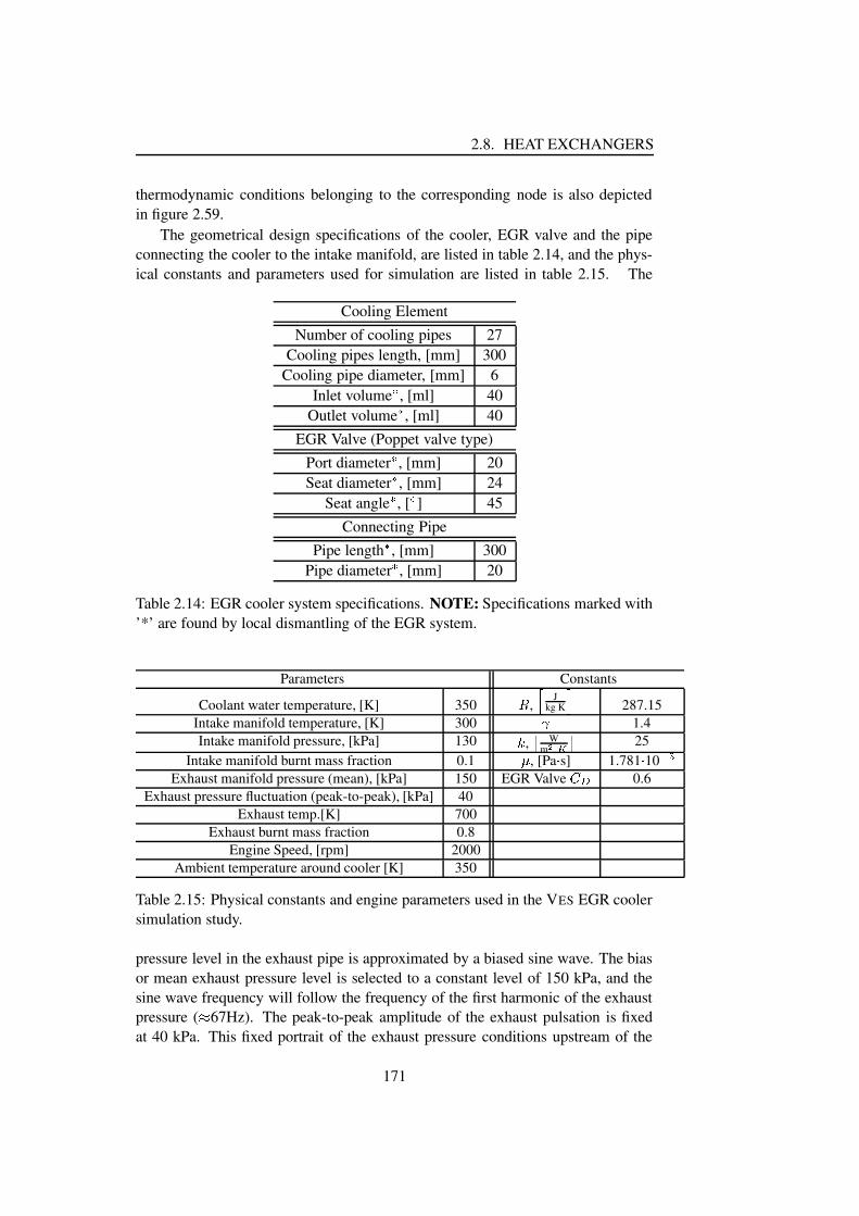
2.8. HEAT EXCHANGERS
thermodynamic conditions belonging to the corresponding node is also depictedin figure 2.59.
The geometrical design specifications of the cooler, EGR valve and the pipeconnecting the cooler to the intake manifold, are listed in table 2.14, and the phys-ical constants and parameters used for simulation are listed in table 2.15. The
Cooling ElementNumber of cooling pipes 27
Cooling pipes length, [mm] 300Cooling pipe diameter, [mm] 6
Inlet volume á , [ml] 40Outlet volume á , [ml] 40
EGR Valve (Poppet valve type)Port diameter á , [mm] 20Seat diameter á , [mm] 24
Seat angle á , [ â ] 45Connecting Pipe
Pipe length á , [mm] 300Pipe diameter á , [mm] 20
Table 2.14: EGR cooler system specifications. NOTE: Specifications marked with’*’ are found by local dismantling of the EGR system.
Parameters Constants
Coolant water temperature, [K] 350 ã , ä Jkg K å 287.15
Intake manifold temperature, [K] 300 æ 1.4Intake manifold pressure, [kPa] 130 ç , è W
m é�êìë 25Intake manifold burnt mass fraction 0.1 í , [Pa î s] 1.781 î 10 ï�ð
Exhaust manifold pressure (mean), [kPa] 150 EGR Valve ñ%ò 0.6Exhaust pressure fluctuation (peak-to-peak), [kPa] 40
Exhaust temp.[K] 700Exhaust burnt mass fraction 0.8
Engine Speed, [rpm] 2000Ambient temperature around cooler [K] 350
Table 2.15: Physical constants and engine parameters used in the VES EGR coolersimulation study.
pressure level in the exhaust pipe is approximated by a biased sine wave. The biasor mean exhaust pressure level is selected to a constant level of 150 kPa, and thesine wave frequency will follow the frequency of the first harmonic of the exhaustpressure ( ó 67Hz). The peak-to-peak amplitude of the exhaust pulsation is fixedat 40 kPa. This fixed portrait of the exhaust pressure conditions upstream of the
171

CHAPTER 2. ENGINE MODELLING
turbine is of course a very simplified. The peak-to-peak amplitude of the pulsationwill change with engine load changes and/or actuation of the VGT’s position ofthe vanes. However, despite this simple picture the pulsation model does reflectthe pressure level conditions fairly well when compared to the experimental pres-sure traces presented in [60] and [59]. The pressure pulsation level in the exhaustmanifold is in [59] experimentally found to vary as much as 65 kPa peak-to-peakdespite a moderate level of engine load ( 25% of maximum rated torque ). Further-more, due to this rather excessive level of pulsation the absolute exhaust pressureis below that of the intake system pressure for a significant fraction of the eventperiod. The EGR mass flow is therefore negative for a considerable fraction ofthe engine event period. The EGR mass flow’s behavior is also examined by awave action model based simulation study in the research presented in [59]. Usingthis model based approach it is determined that EGR backflow may exist for asmuch as 50% of the engine’s event period. Hence, the selected pulsation model isreasonable since it covers such scenarios.
The exhaust temperature is kept constant at 700 K in the following simulationstudy. This is obviously not representative for the stagnated temperature conditionsnormally experienced in a turbocharged DI engine. However, this step is made suchthat the effect of the exhaust pressure pulsations can be isolated. This is also reasonfor keeping the intake manifold’s temperature and pressure fixed at 300 K and 130kPa, respectively.
Figure 2.60 and 2.61 show the simulation results obtained with the isolatedVES implemented EGR system. The first column of plots depicts in both figuresthe raw signals whereas the the second columns show the cycle averaged signals.To aid the interpretation of the individual curve plots the tables 2.16 and 2.17 areincluded to support the notation used in mentioned figures.
The first row in figure 2.60 illustrate the slowly opening–instantaneous closingof the EGR valve. The slowly opening of the valve insures a quasi steady statebehavior of the system throughout the duration of the valve opening process.
The second row shows the individual node temperatures, which can be seenas a discrete EGR cooler temperature distribution. The different nodes, i.e. in-let volume, cooling element volume, outlet volume and pipe connection volume,are plotted with red, blue, magenta and orange, respectively. The green and blackcurves are the inlet temperature and outlet temperature of the cooling element,respectively. It is interesting to observe at low flow rates (the first 4 sec.) that al-though the mean flow through the cooling system is positive, the temperature in thepipe connection drops below the coolant and ambient surrounding’s temperature of350 Kelvin. This is due to the moderate fluctuation level in the system. Hence, ifthe cooler effectiveness is computed utilizing pipe connection temperature mea-surements, effectiveness levels larger than 100% may be expected. At higher flowrates the outlet temperature of the cooling system increases and cooler effective-ness drops. Here, it is interesting to notice how the inlet volume- and mean coolertemperatures begin to drop (after 4 and 7 sec, respectively) due to an increasinglysevereness of the pumping fluctuations in the system i.e. the back flow between
172

2.8. HEAT EXCHANGERS
the exhaust pipe and the cooler are no longer of a negligible level. After 80%of the opening period the flow through the system saturates i.e. the flow throughthe EGR valve is now restricted by the valve throat diameter and not the poppetvalve itself, and the outlet temperature reaches a final level of approximately 480K corresponding to a cooler effectiveness level of 37%.
The third row in figure 2.60 depicts the raw- and cycle averaged pressure levelsat the different node locations, respectively. The red curve is the exhaust pres-sure, green the cooler entry volume pressure, blue the cooler element pressurelevel, black the cooler outlet volume pressure, magenta the pipe connection pres-sure level, and finally the orange curve is the intake manifold pressure level whichis held constant. The pressure distribution clearly shows that inclusion of the pipefriction is important at higher flow rates for a correct estimation of the overall massflow through the EGR system. If the pipe friction is neglected, however, this couldlead to significant errors in the EGR valve mass computation. The reason is forthis is simple. The pressure in the inlet volume downstream of the EGR valve willat relative high flow rates be significantly offset from the intake pressure. This willof course offset the prediction of the pressure ratio across EGR valve if the inletvolume pressure is approximated by the intake plenum pressure. The first row infigure 2.61 depicts the distribution of burnt mass in the EGR cooler system, andthe corresponding curve color notation is given in the first row of table 2.17. Itshould here be noted that the burnt mass fraction, ô , is a volume averaged measureand not a position dependent measure. The burnt mass level in the pipe connectiondecreases in the beginning away from its initial value of 0.5, again, due to enginepumping. The effect of the fluctuations is here, however, even more pronouncedthan in the case with the EGR system temperature distribution. First the mean pipeconnection fraction reaches a peak value of approximately 0.55 after which theburnt mass level decreases and finally attains a level of approx 0.47 as the flow ratethrough the system saturates. This behavior would of course not be encounteredwith steady mass flows where all node burnt mass fraction would attain the samelevel of 0.8 as in the exhaust system. After the first initial 10 sec. the EGR valveis instantaneously closed. This is followed by a rapid decrease of the burnt massfraction especially in the pipe connection node due to the gas contraction initiatedby the heat transfer between the EGR system and the coolant water/surroundings.
The second row in figure 2.61 illustrates the raw- and cycle averaged mass flowbetween the individual nodes and the boundary systems, where orange is the EGRvalve mass flow, magenta is the inlet mass flow to the cooler, black is the flowout of the cooling element, the blue curve is the mass exchange between the outletvolume and the pipe connection, and finally the red curve depicts the mass flow outof the EGR pipe connection. As expected the flow through the system increases asthe EGR valve is opened reaching a final mean value of approximately 17 g
s .The characteristic of the individual node burnt mass fraction might of course
lead to the question: is the law of mass conservation violated? Hence, in orderto prove that the burnt mass flow into the EGR system equals the burnt mass flowout of the system during steady state operation, the instant burnt mass exchange
173
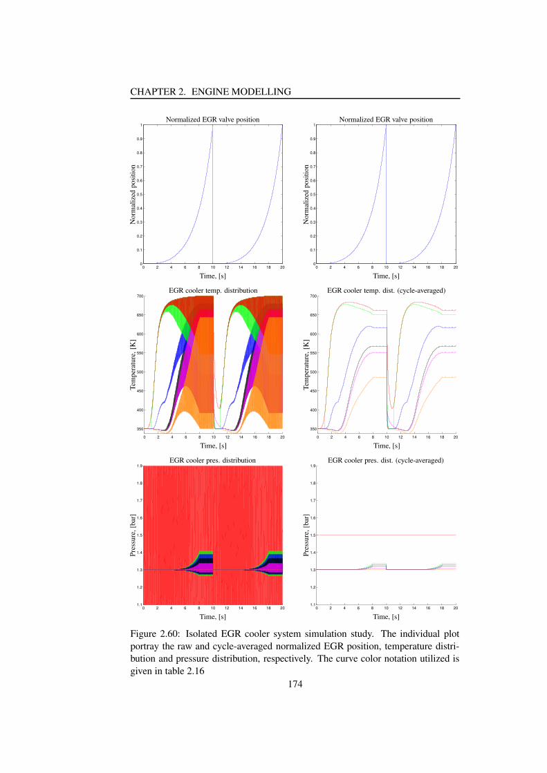
CHAPTER 2. ENGINE MODELLING
0 2 4 6 8 10 12 14 16 18 200
0.1
0.2
0.3
0.4
0.5
0.6
0.7
0.8
0.9
1
PSfrag replacements
Normalized EGR valve position
Nor
mal
ized
posi
tion
Time, [s]0 2 4 6 8 10 12 14 16 18 20
0
0.1
0.2
0.3
0.4
0.5
0.6
0.7
0.8
0.9
1
PSfrag replacements
Normalized EGR valve position
Normalized position
Time, [s]
Normalized EGR valve position
Nor
mal
ized
posi
tion
Time, [s]
0 2 4 6 8 10 12 14 16 18 20
350
400
450
500
550
600
650
700
PSfrag replacementsNormalized EGR valve position
Normalized position
Time, [s]
Normalized EGR valve position
Normalized position
Time, [s]
EGR cooler temp. distribution
Tem
pera
ture
,[K
]
Time, [s]0 2 4 6 8 10 12 14 16 18 20
350
400
450
500
550
600
650
700
PSfrag replacements
Normalized EGR valve position
Normalized position
Time, [s]
Normalized EGR valve position
Normalized position
Time, [s]
EGR cooler temp. distribution
Temperature, [K]
Time, [s]
EGR cooler temp. dist. (cycle-averaged)
Tem
pera
ture
,[K
]
Time, [s]
0 2 4 6 8 10 12 14 16 18 201.1
1.2
1.3
1.4
1.5
1.6
1.7
1.8
1.9
PSfrag replacements
Normalized EGR valve position
Normalized position
Time, [s]
Normalized EGR valve position
Normalized position
Time, [s]
EGR cooler temp. distribution
Temperature, [K]
Time, [s]
EGR cooler temp. dist. (cycle-averaged)
Temperature, [K]
Time, [s]
EGR cooler pres. distribution
Pres
sure
,[ba
r]
Time, [s]0 2 4 6 8 10 12 14 16 18 20
1.1
1.2
1.3
1.4
1.5
1.6
1.7
1.8
1.9
PSfrag replacements
Normalized EGR valve position
Normalized position
Time, [s]
Normalized EGR valve position
Normalized position
Time, [s]
EGR cooler temp. distribution
Temperature, [K]
Time, [s]
EGR cooler temp. dist. (cycle-averaged)
Temperature, [K]
Time, [s]
EGR cooler pres. distribution
Pressure, [bar]
Time, [s]
EGR cooler pres. dist. (cycle-averaged)
Pres
sure
,[ba
r]
Time, [s]
Figure 2.60: Isolated EGR cooler system simulation study. The individual plotportray the raw and cycle-averaged normalized EGR position, temperature distri-bution and pressure distribution, respectively. The curve color notation utilized isgiven in table 2.16
174
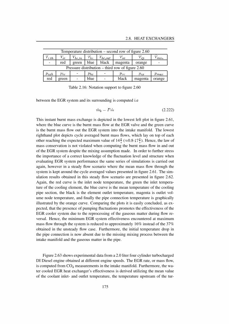
2.8. HEAT EXCHANGERS
Temperature distribution – second row of figure 2.60õ�ö"÷�ø õCùyú õ�ø�öLû ùyü õ�ø�ö õ�ø�öLû ý�þ�ÿ õ ý ú õ ö�� �õ����Lü- red green blue black magenta orange -
Pressure distribution – third row of figure 2.60� ö"÷�ø � ùyú - � ø�ö - � ý ú � ö�� � ���Lüred green - blue - black magenta orange
Table 2.16: Notation support to figure 2.60
between the EGR system and its surrounding is computed i.e�� ��� � (2.222)
This instant burnt mass exchange is depicted in the lowest left plot in figure 2.61,where the blue curve is the burnt mass flow at the EGR valve and the green curveis the burnt mass flow out the EGR system into the intake manifold. The lowestrighthand plot depicts cycle averaged burnt mass flows, which lay on top of eachother reaching the expected maximum value of 14 g
s ( � 0.8 ����� gs ). Hence, the law of
mass conservation is not violated when computing the burnt mass flow in and outof the EGR system despite the mixing assumption made. In order to further stressthe importance of a correct knowledge of the fluctuation level and structure whenevaluating EGR system performance the same series of simulations is carried outagain, however in a steady flow scenario where the mean mass flow through thesystem is kept around the cycle averaged values presented in figure 2.61. The sim-ulation results obtained in this steady flow scenario are presented in figure 2.62.Again, the red curve is the inlet node temperature, the green the inlet tempera-ture of the cooling element, the blue curve is the mean temperature of the coolingpipe section, the black is the element outlet temperature, magenta is outlet vol-ume node temperature, and finally the pipe connection temperature is graphicallyillustrated by the orange curve. Comparing the plots it is easily concluded, as ex-pected, that the presence of pumping fluctuations promotes the effectiveness of theEGR cooler system due to the reprocessing of the gaseous matter during flow re-versal. Hence, the minimum EGR system effectiveness encountered at maximummass flow through the system is reduced to approximately 16% instead of the 37%obtained in the unsteady flow case. Furthermore, the initial temperature drop inthe pipe connection is now absent due to the missing mixing process between theintake manifold and the gaseous matter in the pipe.
Figure 2.63 shows experimental data from a 2.0 liter four cylinder turbochargedDI Diesel engine obtained at different engine speeds. The EGR rate, or mass flow,is computed from CO � measurements in the intake manifold. Furthermore, the wa-ter cooled EGR heat exchanger’s effectiveness is derived utilizing the mean valueof the coolant inlet- and outlet temperature, the temperature upstream of the tur-
175

CHAPTER 2. ENGINE MODELLING
0 2 4 6 8 10 12 14 16 18 200.2
0.3
0.4
0.5
0.6
0.7
PSfrag replacements
Burnt mass frac. distribution.
Bur
ntm
ass
frac
tion
Time, [s]0 2 4 6 8 10 12 14 16 18 20
0.2
0.3
0.4
0.5
0.6
0.7
PSfrag replacements
Burnt mass frac. distribution.
Burnt mass fraction
Time, [s]
Burnt mass frac. dist. (cycle-averaged)
Bur
ntm
ass
frac
tion
Time, [s]
0 2 4 6 8 10 12 14 16 18 20
−0.04
−0.03
−0.02
−0.01
0
0.01
0.02
0.03
0.04
0.05
0.06
PSfrag replacements
Burnt mass frac. distribution.
Burnt mass fraction
Time, [s]
Burnt mass frac. dist. (cycle-averaged)
Burnt mass fraction
Time, [s]
Internal mass flows.
Mas
sflo
w,
� kg s
�
Time, [s]0 2 4 6 8 10 12 14 16 18 20
−0.04
−0.03
−0.02
−0.01
0
0.01
0.02
0.03
0.04
0.05
0.06
PSfrag replacements
Burnt mass frac. distribution.
Burnt mass fraction
Time, [s]
Burnt mass frac. dist. (cycle-averaged)
Burnt mass fraction
Time, [s]
Internal mass flows.Mass flow, kg
s
Time, [s]
Internal mass flows (cycle-averaged).M
ass
flow
,
� kg s
�
Time, [s]
0 2 4 6 8 10 12 14 16 18 20
−0.015
−0.01
−0.005
0
0.005
0.01
0.015
0.02
0.025
0.03
0.035
PSfrag replacements
Burnt mass frac. distribution.
Burnt mass fraction
Time, [s]
Burnt mass frac. dist. (cycle-averaged)
Burnt mass fraction
Time, [s]
Internal mass flows.Mass flow, kg
s
Time, [s]
Internal mass flows (cycle-averaged).Mass flow, kg
s
Time, [s]
Burnt mass flow In/Out.
Mas
sflo
w,
� kg s
�
Time, [s]0 2 4 6 8 10 12 14 16 18 20
−0.015
−0.01
−0.005
0
0.005
0.01
0.015
0.02
0.025
0.03
0.035
PSfrag replacements
Burnt mass frac. distribution.
Burnt mass fraction
Time, [s]
Burnt mass frac. dist. (cycle-averaged)
Burnt mass fraction
Time, [s]
Internal mass flows.Mass flow, kg
s
Time, [s]
Internal mass flows (cycle-averaged).Mass flow, kg
s
Time, [s]
Burnt mass flow In/Out.Mass flow, kg
s
Time, [s]
Burnt mass flow In/Out (cycle-averaged).
Mas
sflo
w,
� kg s
�
Time, [s]
Figure 2.61: Isolated EGR cooler system simulation study. The individual plotsportray the raw and cycle-averaged burnt mass fraction distribution, control volumeflows and burnt mass boundary flows, respectively. The curve color notation usedis given in table 2.17
176
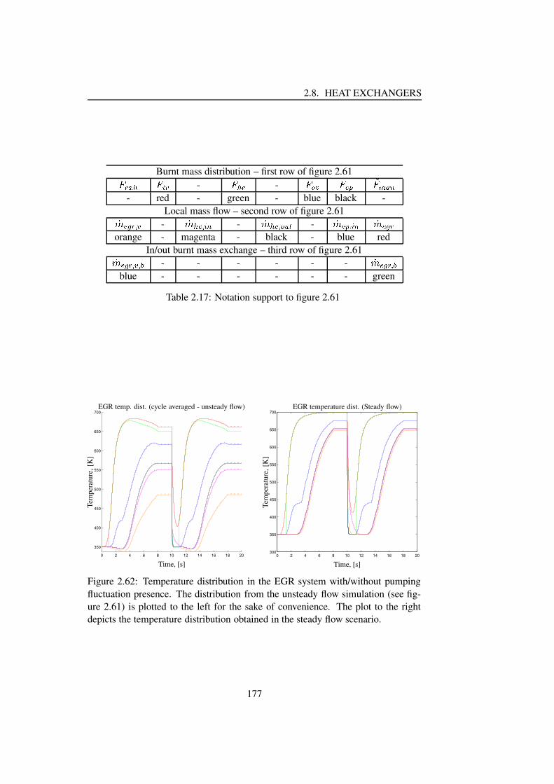
2.8. HEAT EXCHANGERS
Burnt mass distribution – first row of figure 2.61������� �! #"-
�����-
��$%" � ��& '�!(�)+*- red - green - blue black -
Local mass flow – second row of figure 2.61,- ��.+/10 " -,- ���+0 #* -
,- ���+0 $%2�3 -,- ��&40 #* ,- ��.+/
orange - magenta - black - blue redIn/out burnt mass exchange – third row of figure 2.61,- ��.+/10 " 0 5 - - - - - -
,- ��.+/10 5blue - - - - - - green
Table 2.17: Notation support to figure 2.61
0 2 4 6 8 10 12 14 16 18 20
350
400
450
500
550
600
650
700
PSfrag replacements
EGR temp. dist. (cycle averaged - unsteady flow)
Tem
pera
ture
,[K
]
Time, [s]0 2 4 6 8 10 12 14 16 18 20
300
350
400
450
500
550
600
650
700
PSfrag replacements
EGR temp. dist. (cycle averaged - unsteady flow)
Temperature, [K]
Time, [s]
EGR temperature dist. (Steady flow)
Tem
pera
ture
,[K
]
Time, [s]
Figure 2.62: Temperature distribution in the EGR system with/without pumpingfluctuation presence. The distribution from the unsteady flow simulation (see fig-ure 2.61) is plotted to the left for the sake of convenience. The plot to the rightdepicts the temperature distribution obtained in the steady flow scenario.
177
CHAPTER 2. ENGINE MODELLING
bine, and the temperature in the pipe connecting the EGR cooler to the intakemanifold i.e. 6+7�8+9;: < 7�=�>@? <�ACB A 7< 7�=�>D? <FEHG1G1I (2.223)
Since the mapping data set does not contain any complete cycle measurementtraces but only steady state measurement points the level of the pumping fluctu-ation in the EGR system is unknown. However, a kind of fluctuation level indi-cation must be provided to aid the investigation of the EGR cooler effectiveness’behavior. The following non-dimensional fluctuation level indicator is proposedhere J K L 7�=�> ? LNM�O+PL 7�=�> QCRQCR%S M�O = TT M�O = (2.224)
The first part expresses the pressure difference ratio across the complete EGR sys-tem, and hence a measure of what fluctuation amplitude may be expected acrossthe system. The second part relates the measured engine brake torque to the maxi-mum engine brake torque. Since the enthalpy level in the exhaust system generallyincreases with engine load this ratio is a good indicator of the fluctuation ampli-tude in the exhaust system. The third and final part relates the engine speed to aselected maximum speed level. Since the harmonics of the individual pulsationsare locked to the engine cycle frequency, this last part will give an indication thepulsation frequency intensity. A similar approach is utilized in [60] to characterizethe turbines’ efficiency under pulsating flow conditions.
The data evaluation is further hampered by the fact that the temperature mea-surements obtained are something in between the local static and stagnation tem-perature. This problem may especially be important for the exhaust manifold tem-perature measurement due to the high kinetic energy pulsations present, and mayas such offset the EGR cooler effectiveness computation.
The first plot in figure 2.63 illustrates the EGR effectiveness computed by equa-tion 2.223 at engine speeds ranging from 1000 rpm to 2500 rpm. The pulsationindicator, used to assist the interpretation of effectiveness characteristic, is shownto the right in figure 2.63. That the indicator indeed provides useful informationis clear from the fact that where the mass flow data points are in the vicinity ofeach other, the effectiveness speed-line curvature follows the indicator speed-linecurvature, except for a couple of low mass flow measurement points.
The effectiveness figure clearly shows the mixing phenomenon experiencedwith pulsating flows as the effectiveness level for low mass flows are found to ex-ceed 100%. This effectiveness behavior is already found and discussed in the sim-ulation study presented earlier. The low speed effectiveness speedlines (1000 rpm–1500 rpm) exhibit an interesting behavior at higher mass flows where the effec-tiveness level is seen to increase within a reasonable narrow mass flow window.The indicator
Jis for these point, however, found to be almost constant, hence
the changes in engine load and pressure gradient across the heat exchanger systemcan be assumed constant for these operating points. Furthermore, the exhaust tem-perature is found to change less than 40K, where the effectiveness level increases
178

2.8. HEAT EXCHANGERS
more than 20%. It will be argued that since the upstream and downstream con-ditions of the cooler are unchanged these upward characteristic bends are linkedto an excessively opening of the EGR valve. An excessively opening of the EGRvalve will in these operating ranges of the engine only lead to a moderate EGRmass flow increase due to the small pressure gradient across the valve, howeverthe pulsation level will noticeably increase. Hence, just as it was experienced inthe simulation study, the increase in the fluctuation level will enhance EGR coolereffectiveness. However, to draw general conclusions the effectiveness may be saidto increase with pulsation amplitude and frequency and decrease with EGR massflow, the general trends also predicted by the VES implemented EGR model.
0 0.005 0.01 0.015 0.02 0.0250.3
0.4
0.5
0.6
0.7
0.8
0.9
1
1.1
1.2
1.3
1000125015001750200022502501
PSfrag replacements
UV�W�X%Y , Z kgs [
Eff
ectiv
enes
s
\ ]^_Estimated EGR cooler effectiveness.` W�X%Ybadc due to mixing
with intake manifold mat-ter.
` W�X%Y increase due to pul-sation level increase.
0 0.005 0.01 0.015 0.02 0.025−0.01
0
0.01
0.02
0.03
0.04
0.05
0.06
0.07
0.08
0.091000125015001750200022502501
PSfrag replacements, kg
s
Effectiveness
Estimated EGR cooler effectiveness.due to mixing
with intake manifold mat-ter.
increase due to pul-sation level increase.
UV�W�X%Y , Z kgs [
Puls
atio
nIn
dica
tor
ePulsation level indication.
0 0.005 0.01 0.015 0.02 0.0250
10
20
30
40
50
60
1000125015001750200022502501
PSfrag replacements, kg
s
Effectiveness
Estimated EGR cooler effectiveness.due to mixing
with intake manifold mat-ter.
increase due to pul-sation level increase.
, kgs
Pulsation Indicator
Pulsation level indication.
UV�W�X%Y , Z kgs [
EG
Rra
te,[
%]
EGR rate as function ofUVfW�X%Y .
Figure 2.63: Water jacket cooled EGR heat exchanger performance derived from asteady state mapping data set of a 2.0 liter turbocharged DI Diesel engine.
The lower plot in figure 2.63, illustrating the EGRrate as function of ghji�k+l ,clearly shows that the engine map presented span the complete range of the EGRrate levels in normal modern Diesel engine. The findings and statements derivedfrom the simulation study and the measurement data inspection may thus be re-garded to be of general nature.
179

CHAPTER 2. ENGINE MODELLING
The simulation study, supported by steady state engine measurements, unfor-tunately shows that effectiveness level of the EGR cooler is very dependent upona good knowledge of the pulsation level and frequency in the assessment of thisproperty. This will of course make an EGR cooler model inclusion in the MVEMstructure for either observer or modelling purposes difficult.
2.8.7 Summary
This section is devoted completely to the investigation of how the two most com-monly encountered heat exchangers in the engine air path, the intercooler and EGRcooler, may be included in a non-iterative engine model design. The problem ofmodelling the pressure and temperature dynamics for zero dimensional enginemodel inclusion are essentially made difficult due to the large entropy gradientacross this control volume. However, the air-to-air cross flow intercooler normallyhas a high level of effectiveness such that this parameter can be regarded as con-stant. This way it is possible to derive a mean temperature model, which is valid forquasi-stationary modelling purposes, and makes possible a better assessment of thegaseous mass contained in the heat-exchanger volume. Furthermore, it is arguedthat the dynamic heat exchanger temperature and pressure modelling may be sep-arated i.e. the heat exchanger may be regarded as an isothermal control volume.Next, a new non-iterative EGR cooler model capable of predicting the essentialeffects encountered with pulsating flows is also presented. The trends found bysimulation are supported by steady state engine measurements and the model thusprovides a fast non-iterative heat exchanger modelling approach. However, due tothe model complexity, the model cannot readily be included in an observer designbut is rather intended to be used in off-line 0D and 1D engine simulation studies.
2.9 Phenomenological combustion modelling
The combustion process, regardless of whether it is the SI or CI case, is probablythe least understood part of the physical phenomena taking place in an engine, andhence the part providing the greatest difficulties to explain within the confines ofcurrent physical- and chemical understanding.
2.9.1 DI Diesel engines
Modern DI engines equipped with common rail technology are capable of multiplediesel fuel injections before and after TDC (Top Dead Center). Normally, twoinjections take place before TDC. These injections are classified as the pilot- andmain injections. The pilot injection is used to reduce the steep cylinder pressuregradient occurring shortly after the main injection. Post injection is used as means
180
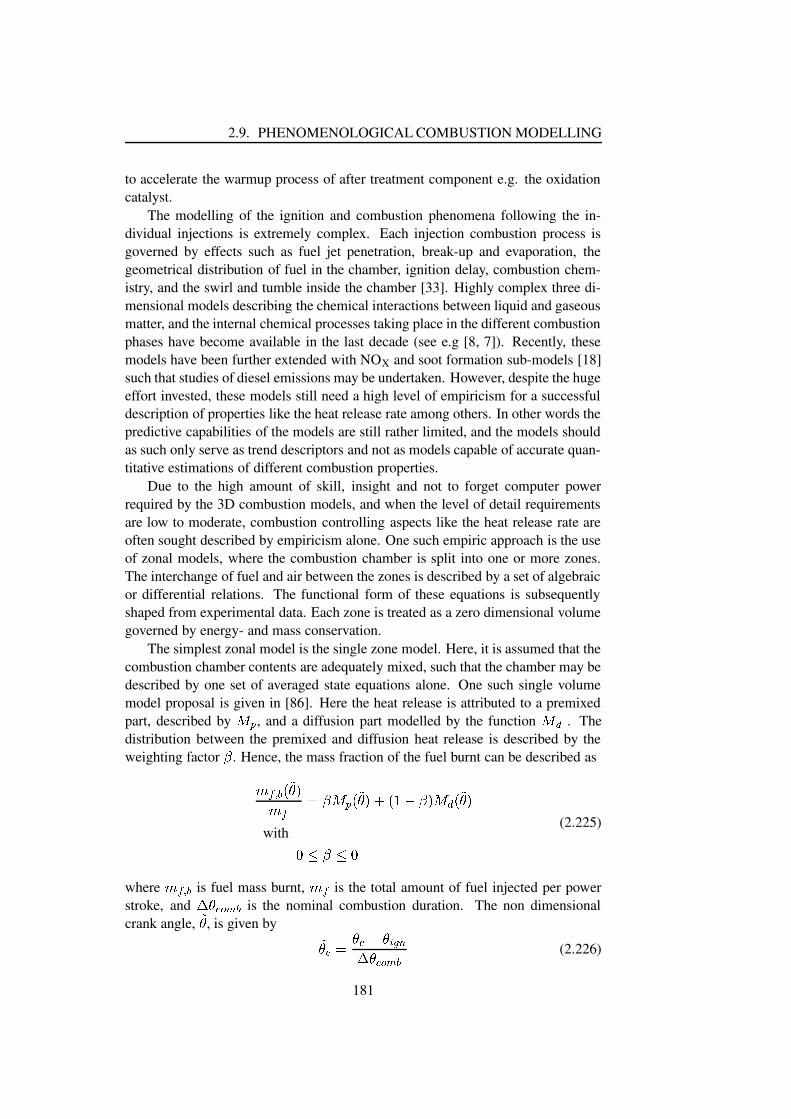
2.9. PHENOMENOLOGICAL COMBUSTION MODELLING
to accelerate the warmup process of after treatment component e.g. the oxidationcatalyst.
The modelling of the ignition and combustion phenomena following the in-dividual injections is extremely complex. Each injection combustion process isgoverned by effects such as fuel jet penetration, break-up and evaporation, thegeometrical distribution of fuel in the chamber, ignition delay, combustion chem-istry, and the swirl and tumble inside the chamber [33]. Highly complex three di-mensional models describing the chemical interactions between liquid and gaseousmatter, and the internal chemical processes taking place in the different combustionphases have become available in the last decade (see e.g [8, 7]). Recently, thesemodels have been further extended with NOX and soot formation sub-models [18]such that studies of diesel emissions may be undertaken. However, despite the hugeeffort invested, these models still need a high level of empiricism for a successfuldescription of properties like the heat release rate among others. In other words thepredictive capabilities of the models are still rather limited, and the models shouldas such only serve as trend descriptors and not as models capable of accurate quan-titative estimations of different combustion properties.
Due to the high amount of skill, insight and not to forget computer powerrequired by the 3D combustion models, and when the level of detail requirementsare low to moderate, combustion controlling aspects like the heat release rate areoften sought described by empiricism alone. One such empiric approach is the useof zonal models, where the combustion chamber is split into one or more zones.The interchange of fuel and air between the zones is described by a set of algebraicor differential relations. The functional form of these equations is subsequentlyshaped from experimental data. Each zone is treated as a zero dimensional volumegoverned by energy- and mass conservation.
The simplest zonal model is the single zone model. Here, it is assumed that thecombustion chamber contents are adequately mixed, such that the chamber may bedescribed by one set of averaged state equations alone. One such single volumemodel proposal is given in [86]. Here the heat release is attributed to a premixedpart, described by mon , and a diffusion part modelled by the function mqp . Thedistribution between the premixed and diffusion heat release is described by theweighting factor r . Hence, the mass fraction of the fuel burnt can be described assjtvu wCxCyz|{sjt } r!m~n xCyz�{�� x1��� r { mdp xCyz�{
with ��� r �q� (2.225)
where sjtvu w is fuel mass burnt, s~t is the total amount of fuel injected per powerstroke, and � z4�H�%� w is the nominal combustion duration. The non dimensionalcrank angle, yz , is given by yz�� } z�� � z��#�+�� z��H�%� w (2.226)
181

CHAPTER 2. ENGINE MODELLING
where ��� is the crank angle domain of interest, and ���#�+� is the crank angle wherethe ignition is initiated. The premixed combustion phase is described by�~���C��|� ���f ¢¡£�� ���¤£¥§¦©¨ ¤£¥+ª (2.227)
and the diffusion governed combustion is model by�d«��C��|�¬���� d4® ¤|¯ ¦�°±+² ¯ ª (2.228)
where the later is recognized as a normal Wiebe function. The empirical coeffi-cients ³ �4´ , ³ ��µ , ³ « ´ and ³ « µ are modelled by,³ �4´ �·¶F¸��4¹ ¶�ºD»��C¼ ®N½ �¿¾ �#�+��ÀÁ� µ§Â ó ��µ �·º4¼�¼�¼³ « ´ � �vÄ�¹ ¶ÅÇÆ Â È1éó « µ ��¼É¹ Ê4Ë£³ Æ Â µ©Ì« ´ (2.229)
where À is the engine speed,¾ �#�+� is the ignition delay in milliseconds, and
Åis
the fuel-air ratio of the matter trapped in the combustion chamber. The distributionbetween premixed- and combustion may be modelled asÍ ���f ÏÎ ÅÇо�Ñ�#�+� (2.230)
where suitable ranges for the three empirical constants are given as¼É¹ ÒÔÓ Î Óq¼É¹ Ë�º ¼É¹ ¶�º�ÓÖÕFÓq¼É¹ Ä�º ¼É¹ ¶�º�Óq×@Óq¼É¹ º (2.231)
Finally may the heat release rate be found fromØ ÑHÙ%Ú�Ð �ÜÛ£ÝjÞvß ÐÛ �áà@â�ã �åä Í Û �~�Û � ¸ � �� Í � Û �d«Û �Ïæ ÝjÞ à@â�ã (2.232)
where à@â�ã is the heating value of the fuel. The single zone, or Watson model,has been applied with success in global diesel engine performance studies [27],and is thus a good model candidate when only a moderately detailed model of thecombustion system is required.
In the two zone model the combustion chamber is split in two zones, whereone contains bulk air and the other the volume of combustion. The heat releasein the combustion zone may, analogous to the single zone model, be described bya phenomenological heat release model like the one presented above. Since themodel is capable of distinguishing between bulk air temperature and the combus-tion zone temperature more realistic inputs to emission models can be provided.This more realistic picture of the emission formation has triggered off the devel-opment of multi zone combustion models. The multi zone models have shown
182
2.9. PHENOMENOLOGICAL COMBUSTION MODELLING
improved emission prediction capabilities (see eg. [25]) compared to the simplersingle- and two zone models. However, the introduction of a large number of co-efficients and parameters that need to be identified prior to model application oftenmakes the problem mathematically as well as physically undefined i.e. the identi-fication problem is not affine in the parameter space. Hence, for the most part itcannot be concluded whether or not the same level of model accuracy could not beachieved with a completely different setting of the parameters.
In the case where only a MVEM modelling level is needed the actual combus-tion processes may be disregarded completely, and the crank angle dynamics maybe described from energy conservation alone. The distribution of the energy re-leased by combustion between heat losses, shaft work, friction losses among otherscan thus be described by efficiencies and/or MEP (Mean Effective Pressure) alone(see e.g. [63, 54]). The different efficiencies/MEPs are of course dependent onseveral engine design- and operating point parameters and variables. These depen-dencies are often extremely complex and not well understood. Hence, the differentefficiencies and MEPs are sought modelled from empiricism alone.
It is in this research found that the LWLS estimation scheme presented in sec-tion 2.3.4.5 on page 114, with a following appropriate validation of the correlationsobtained, provides a fast and easy tool for MVEM based combustion modelling.However, it cannot be stated strongly enough, that the input variables to the corre-lation routine must not only span the steady operating range but also the transientrange. If this evident, but hardly practically met, condition is neglected, unfor-tunate regions of the correlation sphere without data support may be entered andlead to erroneous simulation results. The LWLS method will verified on steadystate map data for a 2.0 l VGT equipped DI Diesel engine28 . The engine wasmapped at selected key points in the speed-torque map of the engine up to 2750rpm and was controlled by the standard ECU (Engine Control Unit). Hence, theengine map utilized will completely cover the region of speed-torque engine mapwhere the EGR system is active.
In the analysis of the engine data it is found convenient to describe the com-bustion behavior by the three following phenomenological properties:çdè�é : Indicated engine efficiency.ç FMEP: Friction mean effective pressure.çëêvì�í�î : Exhaust energy fraction.
The indicated engine efficiency is defined as the fraction of the released fuelenergy extracted as useful piston work during the compression–expansion part ofthe cycle, i.e. è�é!ï ðcycle ñÇò¿ó§ô�õÉö÷jøvù ò¿ó§òHô ì+ú@û�üÏýÜþ ò¿ó§ô ù ÿ���������÷jø4ú@û�ü (2.233)
28Dipl. Ing. Daniel Rottger is gratefully acknowledged for providing the steady state engine map.
183

CHAPTER 2. ENGINE MODELLING
The efficiency is dependent on the point of combustion, AFR, initial inert gas con-tent ( ��� ��� ), and entrained mass in the combustion chamber among others. How-ever, ��� is found to have a strong � dependency, and a weaker �� ��� dependency29 .These observed properties were utilized in a successful second order LWLS iden-tification of ��� as function of �� ��� and � . The successfully identified ��� surfacespanned by � and �� ��� is shown in figure 2.64. The surface covers a rather large
2
3
4
5
6 00.05
0.10.15
0.20.25
0.3
0
0.05
0.1
0.15
0.2
0.25
0.3
0.35
0.4
0.45
0.5
PSfrag replacements
� �������
� �
LWLS identified �� surface
0 10 20 30 40 50 60 70 80 90 1000.25
0.3
0.35
0.4
0.45
0 10 20 30 40 50 60 70 80 90 100
−4
−2
0
2
4
6
8
PSfrag replacements
LWLS identified surface
Evaluation of �� identification.
Data No
� �
Data No
Rel
ativ
eer
ror,
[%]
Figure 2.64: ��� LWLS identification. The green surface to the left shows the �!�surface identified by a second order LWLS polynomial in �� ��� and � with 25grid points. The map data points are marked with o, and as an addition the 25%(green line), 50% (black line) and 75% (blue line) steady state EGR rate lines areimposed on the surface. The plots to the right depicts the LWLS estimated �"� (solidred curve) together measurement data points and the belonging relative error. Theindividual ”bows” in this upper righthand plot indicate data points belonging to thesame engine speed set point.
region necessitating extrapolation. However, this region is located primarily out-side the 50% EGR rate line, and thus is only reachable during large engine speeddecelerations. During such scenarios the magnitude of the engine efficiency is ofminor importance compared to friction and load factors for a correct estimation ofthe crankshaft speed dynamics. The good identification quality of the 25 grid pointLWLS is supported by a relative low relative error, which is basically kept within#
5%.Viscous friction and pumping losses cannot be avoided and play an important
role in characterization of the crank shaft dynamics close to idle speed or part loadengine operation. However, it is difficult to divide the total loss in either pumpingwork, which is mainly a function of intake, exhaust and ambient pressure, and theinevitably viscous friction loss between cylinder liners and walls, and bearings.
29No injection point data is provided with the data set. Hence, it is assumed here that the injectiontiming is optimized for maximum engine efficiency.
184

2.9. PHENOMENOLOGICAL COMBUSTION MODELLING
Hence it is here decided only to address phenomenological modelling of the totalwork i.e. the pumping work is lumped into the frictional mean effective pressure,FMEP (Friction Mean Effective Pressure), definition. The frictional mean effectivepressure is from the data derived as
FMEP $ %'&)(+*-,/.-0 13254�16"758 $ %:9<; ,�=> (�?A@ BDCFE3G 8IH6"758 (2.234)
since the indicated efficiency is known. In the case where; ,
is unknown FMEPis often identified from the so called Willans line [54]. However, this method wastested for the sake of completeness but found very inaccurate. The size of the ex-perimental DI engine’s FMEP is found to be strongly rotational speed dependent,as expected, and to a minor degree intake manifold density dependent. This obser-vation was utilized in a successful LWLS identification with 25 grid points. Theperformance of the LWLS FMEP algorithm is graphically illustrated in figure 2.65.The FMEP level is clearly overestimated in the low speed–high intake density re-
1000
1500
2000
2500
3000
0.5
1
1.5
2
2.550
100
150
200
250
PSfrag replacements
J, [rpm]
KML�N�O , P kgm Q3R
STUV ,[
kPa]
LWLS identified FMEP surface
0 10 20 30 40 50 60 70 80 90 10060
80
100
120
140
0 10 20 30 40 50 60 70 80 90 100−10
−5
0
5
10
15
PSfrag replacements
, [rpm], kg
m
, [kPa]
LWLS identified FMEP surface
Evaluation of FMEP identification.
Data No
STUV ,[
kPa]
Data No
Rel
ativ
eer
ror,
[%]
Figure 2.65: LWLS identified FMEP for the experimental 2.0l Diesel engine. TheFMEP surface identified (green mesh surface) together with measurements is seento the left. The identification routine (solid red line) compared to measurements asa function of operating point is illustrated to the right. The relative modelling errorcan with the LWLS algorithm selected be kept within W 10%.
gion of the surface. However, since the intake dynamics is a lot faster comparedto the crankshaft dynamics this region will never be entered during either steadystate or transient operating conditions. Hence, the FMEP surface spanned by
8and X 4 Y�Z may be accepted to be globally valid.
The two quantities; ,
and FMEP are in principle together with engine speedand fuel flow the only variables needed in a MVEM modelling of the crankshaftdynamics. However, due to the AFR and X 4 Y�Z dependencies the crank shaft dy-namics will also be indirectly dependent upon the turbocharger performance. Since
185
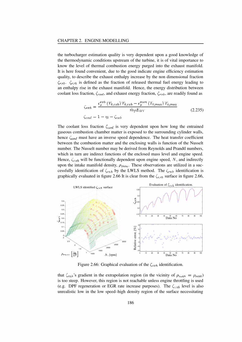
CHAPTER 2. ENGINE MODELLING
the turbocharger estimation quality is very dependent upon a good knowledge ofthe thermodynamic conditions upstream of the turbine, it is of vital importance toknow the level of thermal combustion energy purged into the exhaust manifold.It is here found convenient, due to the good indicate engine efficiency estimationquality, to describe the exhaust enthalpy increase by the non dimensional fraction[+\^]5_
.[+\^]5_
is defined as the fraction of released thermal fuel energy leading toan enthalpy rise in the exhaust manifold. Hence, the energy distribution betweencoolant loss fraction,
[5`ba-a-c, and exhaust energy fraction,
[5\^]5_, are readily found as
[+\^]5_edgf \^]5_hjilknmpo \^]5_rq knmpo \^]5_ts fpu v�wh ilk mpo u v�w q k mpo u v�wxy{z'|A} ~[+`ba-a-c�d��:s�����s�[+\^]5_ (2.235)
The coolant loss fraction[5`ba-a-c
is very dependent upon how long the entrainedgaseous combustion chamber matter is exposed to the surrounding cylinder walls,hence
[+`ba-a-cmust have an inverse speed dependence. The heat transfer coefficient
between the combustion matter and the enclosing walls is function of the Nusseltnumber. The Nusselt number may be derived from Reynolds and Prandtl numbers,which in turn are indirect functions of the enclosed mass level and engine speed.Hence,
[3\^]5_will be functionally dependent upon engine speed, � , and indirectly
upon the intake manifold density, � u v�w . These observations are utilized in a suc-cessfully identification of
[5\^]5_by the LWLS method. The
[5\^]5_identification is
graphically evaluated in figure 2.66 It is clear from the[�\^]5_
surface in figure 2.66,
1000
1500
2000
2500
3000
1
1.5
2
2.5
30
0.05
0.1
0.15
0.2
0.25
0.3
0.35
0.4
PSfrag replacements
�, [rpm]
�M����� , � kgm �3�
�����
LWLS identified �b�<��� surface
0 10 20 30 40 50 60 70 80 90 1000.15
0.2
0.25
0.3
0.35
0 10 20 30 40 50 60 70 80 90 100−15
−10
−5
0
5
10
15
PSfrag replacements
, [rpm], kg
m
LWLS identified surface
Evaluation of �b�<��� identification.
Data No
�����
Data No
Rel
ativ
eer
ror,
[%]
Figure 2.66: Graphical evaluation of the[�\^]5_
identification.
that[+\^]5_
’s gradient in the extrapolation region (in the vicinity of � u v�w d � v�u � )is too steep. However, this region is not reachable unless engine throttling is used(e.g. DPF regeneration or EGR rate increase purposes). The
['\^]5_level is also
unrealistic low in the low speed–high density region of the surface necessitating
186

2.9. PHENOMENOLOGICAL COMBUSTION MODELLING
extrapolation. These area is however not reachable independent of transient- orsteady state operation of the engine due to the low level of thermodynamic energyavailable in the exhaust manifold. Hence, the ���^�5� surface identified may be usedin both transient and steady state simulation studies of un-throttled DI Diesel en-gines. If data points are available in this region of the map, it is believed that asuccessfully identification of �5�^�5� as a function of � and �¡ ¢�£ alone will still bepossible.
Finally, the estimation quality of the exhaust port temperature after exhaustport coolant loss, ¤ �¦¥ , is evaluated for the sake of completeness. This temperaturemay readily be found found from the definition of ���^�5� to
¤ �¦¥¨§ �+�^�5� ©ª{«©ª ¢ ¥¬ ©ª{«¯®A° ±² �^�5�¥ ¬ ² ¡ ¢�£¥² �^�5�¥ ¤³¡ ¢�£ (2.236)
This equation is implicit due to ² �^�5�¥ ’s exhaust temperature dependence. Instead, adescriptive mean value of ² �^�5�¥ is used i.e.
¤ �¦¥e§ �+�^�5� ©ª{«©ª ¢ ¥A¬ ©ª{« ®A° ±² �^�5�¥ ¬ ² ¡ ¢�£¥² �^�5�¥ ¤³¡ ¢�£ (2.237)
Both equations are graphically evaluated in figure 2.67. The implicit estimation
0 10 20 30 40 50 60 70 80 90 100
400
500
600
700
800
900
0 10 20 30 40 50 60 70 80 90 100−6
−4
−2
0
2
4
6
PSfrag replacements
Data No.
´bµ¶ ·¸ ´bµ¶ ·¸ ´ µ¶ ,[K
]
Data No.
Rel
ativ
eE
rror
,[%
]
Exhaust temperature estimation evaluation.
Figure 2.67: Exhaust port temperature estimation. The measurements as functionof operating point are seen as a solid blue curve in the upper plot. The green dashedline is the implicit estimation of ¤ �¦¥ , and red dash-dot line illustrates the explicitsolution to ¤ �¦¥ utilizing ² �^�5�¥ . The relative error of the implicit estimation andexplicit estimation algorithm are marked by ’o’ and ’x’, respectively, in the lowestplot.
187
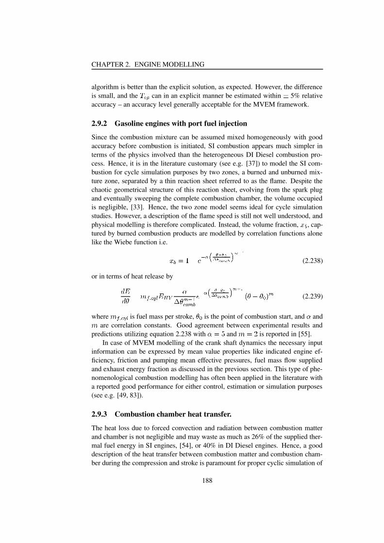
CHAPTER 2. ENGINE MODELLING
algorithm is better than the explicit solution, as expected. However, the differenceis small, and the ¹»º¦¼ can in an explicit manner be estimated within ½ 5% relativeaccuracy – an accuracy level generally acceptable for the MVEM framework.
2.9.2 Gasoline engines with port fuel injection
Since the combustion mixture can be assumed mixed homogeneously with goodaccuracy before combustion is initiated, SI combustion appears much simpler interms of the physics involved than the heterogeneous DI Diesel combustion pro-cess. Hence, it is in the literature customary (see e.g. [37]) to model the SI com-bustion for cycle simulation purposes by two zones, a burned and unburned mix-ture zone, separated by a thin reaction sheet referred to as the flame. Despite thechaotic geometrical structure of this reaction sheet, evolving from the spark plugand eventually sweeping the complete combustion chamber, the volume occupiedis negligible, [33]. Hence, the two zone model seems ideal for cycle simulationstudies. However, a description of the flame speed is still not well understood, andphysical modelling is therefore complicated. Instead, the volume fraction, ¾)¿ , cap-tured by burned combustion products are modelled by correlation functions alonelike the Wiebe function i.e.
¾�¿ÁÀ�Â:Ã�Ä'Å�ÆnÇÉÈ�Ê'ÈÌËÍ È<ΦÏ^гÑÒ ÐnÓÕÔ (2.238)
or in terms of heat release byÖr×ÖrØ ÀÚÙ{Û+Ü ÝÌÞpß ×Aà á âã Ø�ä¯å�æÝbç ä ¿ Ä'Å�ÆnÇ{È�Ê'ÈÌËÍ È<ΦÏ^гÑÒ ÐnÓÕÔ�è Ø Ã Ø�é5ê ä (2.239)
where Ù{Û+Ü ÝÌÞpß is fuel mass per stroke,Ø�é
is the point of combustion start, and â andÙ are correlation constants. Good agreement between experimental results andpredictions utilizing equation 2.238 with â Àìë and ÙíÀìî is reported in [55].
In case of MVEM modelling of the crank shaft dynamics the necessary inputinformation can be expressed by mean value properties like indicated engine ef-ficiency, friction and pumping mean effective pressures, fuel mass flow suppliedand exhaust energy fraction as discussed in the previous section. This type of phe-nomenological combustion modelling has often been applied in the literature witha reported good performance for either control, estimation or simulation purposes(see e.g. [49, 83]).
2.9.3 Combustion chamber heat transfer.
The heat loss due to forced convection and radiation between combustion matterand chamber is not negligible and may waste as much as 26% of the supplied ther-mal fuel energy in SI engines, [54], or 40% in DI Diesel engines. Hence, a gooddescription of the heat transfer between combustion matter and combustion cham-ber during the compression and stroke is paramount for proper cyclic simulation of
188
2.10. CRANK SHAFT
the combustion process. Furthermore, the exhaust enthalpy loss, primarily due tothe high turbulence level in the vicinity of the exhaust valve during cylinder purg-ing, is also important in the description of the exhaust pipe enthalpy level. Exhaustgas temperature drops exceeding more than 400 K across the exhaust port for someSI engine scenarios with bad port insulation have been reported in the literature[83, 57]
In the calculation of the cylinder wall heat transfer it is customary in 0D/1Dsimulation studies to rely on spatially averaged (the temperature of the gaseousmatter and surrounding wall of the given zone/chamber are assumed constant) em-pirical relationships. One commonly encountered model in the literature is theAnnand model [83, 33] which utilizes Newton’s law of cooling in description ofthe convective heat transfer and grey body modelling in the description of the heattransfer due to radiation. Hence, the Annand expression in its final form becomesïñðòAóbô�õ öø÷!ù{ú¯û óbô�ü'ýþ ÿ������������ ��� � �������� �������� ����� ��� ��� � (2.240)
whereòAóbô�õ ö
is the wetted surface area of the combustion chamber and thus afunction of the piston position, þ is a characteristic length normally chosen as thecylinder bore width, û óbô�ü'ý the conductivity of the combustion chamber material,and
�is the radiative emissivity. Normally the corresponding Nusselt number is
computed as, ù{ú ð������ ö ð�� ÷! ú þ" � ö(2.241)
with the characteristic velocity,ú
, often set to the mean piston velocity i.e.úÉð$# �&%(' ô*),+�ù-/. (2.242)
Although the above correlation does not take flow characteristics like swirl andtumble into consideration, good agreement with measurements using values of 0between 0.7 and 0.85 is reported in the literature [33], while the parameters
�and�
have to be identified from existing experimental data.In the computation of the enthalpy loss in the exhaust port the same analogy,
just presented, is used except for the Reynolds number computation [83]. Here oneof the following Reynolds numbers is used.���Að 1324"65�798 or
���Að 24:7<; ô '*%" ò ; ô '*% (2.243)
where 798 is the valve head diameter, 7=; ô '*% is the minimum port diameter, andò ; ô '*% is the exit cross sectional area of the port.
2.10 Crank shaft
The crank shaft or engine speedù
is an important variable in computation of thealgebraic and differential equations comprising the different engine sub-models.
189
CHAPTER 2. ENGINE MODELLING
However, the level of detail or signal spectrum needed for appropriate transientmodelling of the crank shaft’s rotational speed is very task dependent.
In cycle based simulation studies a mechanical model of the drive line is nec-essary for a dynamical description of different powertrain components e.g. the in-dividual combustion’s influence on the crank dynamics. Such models of differentdetail level ranging for pure stiff mechanical analysis [109] to models incorporat-ing the dynamical performance of the individual intake and exhaust valves [113]are readily available in the literature.
In MVEM based simulation and control studies the dynamic detailing levelrequirement is often much smaller. Hence, the crank shaft state equation is basedon conservation of rotational energy using cycle mean values of the individualenergy inputs and outputs of the system. Hence, the rate of change of the enginespeed utilizing the definition outlined in section 2.9.1 is found as>?A@ABDC/EFHG�I >J�KMLONQPSRMTVU P,W�XY I[Z FMEP U]\_^ `*a�bcedgfihj? (2.244)
wherecedgfih
is the engine’s moment of inertia. However simple, this type of modelhas shown good agreement with experimental data both during harsh transient andsteady state engine operation (see e.g. [63, 49]).
2.11 VES and a simulation example
The main motivation behind the VES (Virtual Engine Simulation) C library forSIMULINK k is the development of a package containing different IC engine sub-models for the automotive control engineer. The advantages of this over a directimplementation in SIMULINK k are the shorter simulation time and the improvedflow control offered by S-functions. The first is obvious since a direct hard codedimplementation in C generally has a lower number of required CPU operationsthan SIMULINK k only models. The latter since the structure of the model im-plementation is directly controllable within C; this is not generally the case withSIMULINK k . The downside of the coin is the lost graphical interpretation of thesystem; the model is no longer in block diagrammatic form.
The model background for VES is so far simply the C implemented version ofthe material previously presented in this chapter30 . The idea, however, is that thelibrary should be expandable with new user defined functions similar to librariesbehind the KIVA CFD environment31 .
30Remark: Some of the models exist at the point of writing only in the SIMULINK l environment.31The KIVA framework, a transient, three-dimensional, multi-phase, multi-component code for
the analysis of chemically reacting flows with sprays has been developed at the Los Alamos NationalLaboratory. This CFD code provides a way to analyze the combustion quality of e.g. Diesel. Moreinformation may be obtained online at http://gnarly.lanl.gov/Kiva/Kiva.html
190

2.11. VES AND A SIMULATION EXAMPLE
2.11.1 A simulation example
This section will give an example of the possibilities with the simplified engine sub-models offered by VES. A simulation study using VES has already been conductedearlier in section 2.8.6 where the exhaust fluctuations’ effect on the effectivenesslevel of EGR-cooler was investigated. However, the focus of the simulation to bepresented will not be on the instantaneous behavior of an isolated engine compo-nent or subsystem but the mean value behavior of a full implementation of a DIDiesel engine according to the MVEM framework.
The model utilized in the engine simulation was originally the model of a pro-totype Ford V6 Diesel engine which has been used to study different control andestimation designs and drive-cycle performance at FFA (Ford Forschungszentrum,Aachen). A more detailed list of applications cannot be included for proprietaryreasons.
The twin turbocharged V (Diesel) engine design has always been appealing forpackaging reasons, and with the advances made in the turbocharging technologyarea in the recent years, this engine design is becoming more and more common inthe engine selection for the upper middle class car to the luxury car. Examples ofthe commercially available passenger cars featuring this engine design are the 4.0liter V8 BMW engine, the Mercedes 4.0 liter Diesel V8 in the S400 CDI, and theV6 and V10 Diesel engines manufactured by Volkswagen. All these engines usetwin turbocharging to reached their individual performance targets. Hence, withthe recent boom in the Diesel market and the reasonably large market for uppermedium class and luxury cars, the turbocharged V engine will most likely becomevery popular in the near future. Modelling, estimation and control research in suchengine designs is therefore naturally of interest.
The specifications for the V6 engine simulation model are briefly outlined intable 2.18.
It has earlier been shown that the mass flow through the EGR cooler, fitted on aDI Diesel engine, and its effectiveness cannot be well described (see section 2.8.6)by the MVEM framework; a description of the pumping fluctuations is requiredsince the system is operated in an area with strong nonlinearities. However, to beable to describe the dynamic and steady state trends introduced by the EGR systema model of the EGR mass flow and the EGR temperature must be present. Thus,a fairly simple model is constructed by describing the EGR mass flow throughthe system by the isentropic nozzle equation utilizing the mean exhaust and themean intake manifold pressure, and by fixing effectiveness level of the cooler to areasonable value of 50% (see e.g. table 2.13).
The scope of the simulation study presented will be limited to a study of theV6 engine’s response to a part of the EUDC (EUropean Drive Cycle). The reasonfor this is natural when considering that the V6 has seven inputs (brake load, twoEGR valve positions, two VGT rack positions and two bank fuel injection inputs)and numerous outputs; The system space of interest is enormous. Thus, the work-load required by a complete graphical documentation of possible excitation of the
191
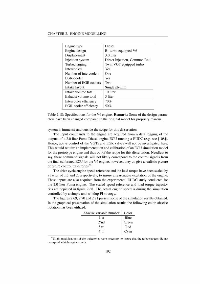
CHAPTER 2. ENGINE MODELLING
Engine type DieselEngine design Bi-turbo equipped V6Displacement 3.0 literInjection system Direct Injection, Common RailTurbocharging Twin VGT equipped turboIntercooled YesNumber of intercoolers OneEGR-cooler YesNumber of EGR coolers TwoIntake layout Single plenumIntake volume total 10 literExhaust volume total 3 literIntercooler efficiency 70%EGR-cooler efficiency 50%
Table 2.18: Specifications for the V6 engine. Remark: Some of the design param-eters have been changed compared to the original model for propriety reasons.
system is immense and outside the scope for this dissertation.The input commands to the engine are acquired from a data logging of the
outputs of a 2.0 liter Puma Diesel engine ECU running a EUDC (e.g. see [108]).Hence, active control of the VGTs and EGR valves will not be investigated here.This would require an implementation and calibration of an ECU simulation modelfor the prototype engine and thus out of the scope for this dissertation. Needless tosay, these command signals will not likely correspond to the control signals fromthe final calibrated ECU for the V6 engine, however, they do give a realistic pictureof future control trajectories32 .
The drive cycle engine speed reference and the load torque have been scaled bya factor of 1.5 and 2, respectively, to insure a reasonable excitation of the engine.These inputs are also acquired from the experimental EUDC study conducted forthe 2.0 liter Puma engine. The scaled speed reference and load torque trajecto-ries are depicted in figure 2.68. The actual engine speed is during the simulationcontrolled by a simple anti-windup PI strategy.
The figures 2.69, 2.70 and 2.71 present some of the simulation results obtained.In the graphical presentation of the simulation results the following color–abscisenotation has been utilized:
Abscise variable number Color1’st Blue2’nd Green3’rd Red4’th Cyan
32Slight modifications of the trajectories were necessary to insure that the turbochargers did notoverspeed at high engine speeds.
192

2.11. VES AND A SIMULATION EXAMPLE
0 50 100 150 200 250 300 350 4001000
1500
2000
2500
3000
3500
4000
0 50 100 150 200 250 300 350 4000
50
100
150
200
250
300PSfrag replacements
m[nop ,[rpm]Speed reference.
q r stu ,[Nm]
Time [s]
Load torque.
Figure 2.68: Speed reference and load torque trajectories utilized in the simulationstudy.
The variable notation has been defined earlier, however, an explanation of the allvariables to be presented may also be found in the glossary starting at page 259.The figures clearly show that a large portion of the engine’s speed-load map hasbeen excited with the model exhibiting a reasonable behavior i.e.:v The closing and opening of the VGTs lead to an increase and a decrease in
the intake pressure, respectively.v The closing and opening of the VGTs lead to an increase and a decrease inthe exhaust pressure, respectively.v The closing and opening of the EGR valves lead to an increase and decreasein the EGR rate, respectively.v The closing and opening of the EGR valves lead to an increase and decreasein the exhaust pressure, respectively.v The exhaust temperature goes up with load increases and w decreases. Theexhaust temperature goes down with load decreases and w increases.v The intake temperature is a weighted sum of the EGR temperature and theexit temperature of the intercooler.
193

CHAPTER 2. ENGINE MODELLING
0 100 200 300 4001500
2000
2500
3000
3500
4000
0 100 200 300 400100
200
300
400
500
0 100 200 300 400300
400
500
600
0 100 200 300 400400
600
800
1000
0 100 200 300 4000
0.2
0.4
0.6
0 100 200 300 400
2
4
6
PSfrag replacements
x�yx[z{| ,[rpm]
} ~�� y} {�� ,[k
Pa]
�&� y� {�z y� ~��y� � � ,[K] � {�� ,[K]
EG
Rra
te �Time [s] Time [s]
Figure 2.69: Simulation study of a twin turbocharged V6 Diesel engine. The upperleft plot shows the relative fast accelerator tip-ins and tip-outs during the first 60seconds of simulation. The corresponding fast responses of the intake- and exhausttemperatures and pressures are clear in the three surrounding plots. The displace-ment of the simulated V6 engine is larger than the original specification for theprototype. The compressors will therefore operate closer to the choke limit, the socalled the stonewall, and the pressure drop across turbines increases due to the pos-sible larger mass flow. The pressure difference between the exhaust- and the intakesystem is due to this turbocharger–engine mismatch thus larger than the pressuredifference normally experienced with modern turbocharged Diesel engines. The�
level depicted in the lower right plot is in the high load part of the simulation(250 sec. to 340 sec.) lower than normally required due to the high amount ofEGR applied. Normally, EGR is only utilized up to approximately 2500 rpm on anormal Diesel engine for light duty applications. The �e�g��� control trajectory used(see figure 2.71) would most likely lead to immense soot emissions in reality.
194
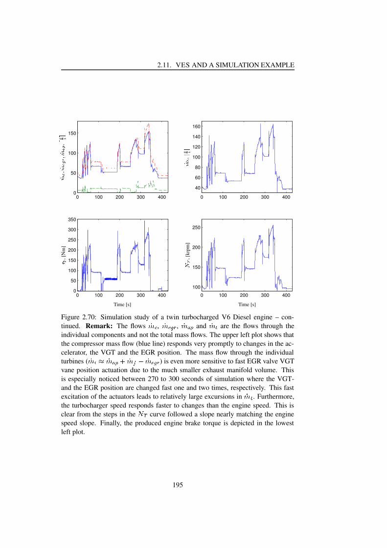
2.11. VES AND A SIMULATION EXAMPLE
0 100 200 300 4000
50
100
150
0 100 200 300 400
40
60
80
100
120
140
160
0 100 200 300 4000
50
100
150
200
250
300
350
0 100 200 300 400
100
150
200
250
PSfrag replacements
� � � �� � ��� �� � ��
,
� g s
�� � � ,� g s
�
� � ,[Nm] � � ,[krpm]
Time [s] Time [s]
Figure 2.70: Simulation study of a twin turbocharged V6 Diesel engine – con-tinued. Remark: The flows ��H , ��:¡g¢�£ , ��:¤g¥ and ��§¦ are the flows through theindividual components and not the total mass flows. The upper left plot shows thatthe compressor mass flow (blue line) responds very promptly to changes in the ac-celerator, the VGT and the EGR position. The mass flow through the individualturbines ( ��:¦_¨ ��:¤g¥ª© ���«�¬ ��:¡g¢�£ ) is even more sensitive to fast EGR valve VGTvane position actuation due to the much smaller exhaust manifold volume. Thisis especially noticed between 270 to 300 seconds of simulation where the VGT-and the EGR position are changed fast one and two times, respectively. This fastexcitation of the actuators leads to relatively large excursions in ��¦ . Furthermore,the turbocharger speed responds faster to changes than the engine speed. This isclear from the steps in the ¯® curve followed a slope nearly matching the enginespeed slope. Finally, the produced engine brake torque is depicted in the lowestleft plot.
195
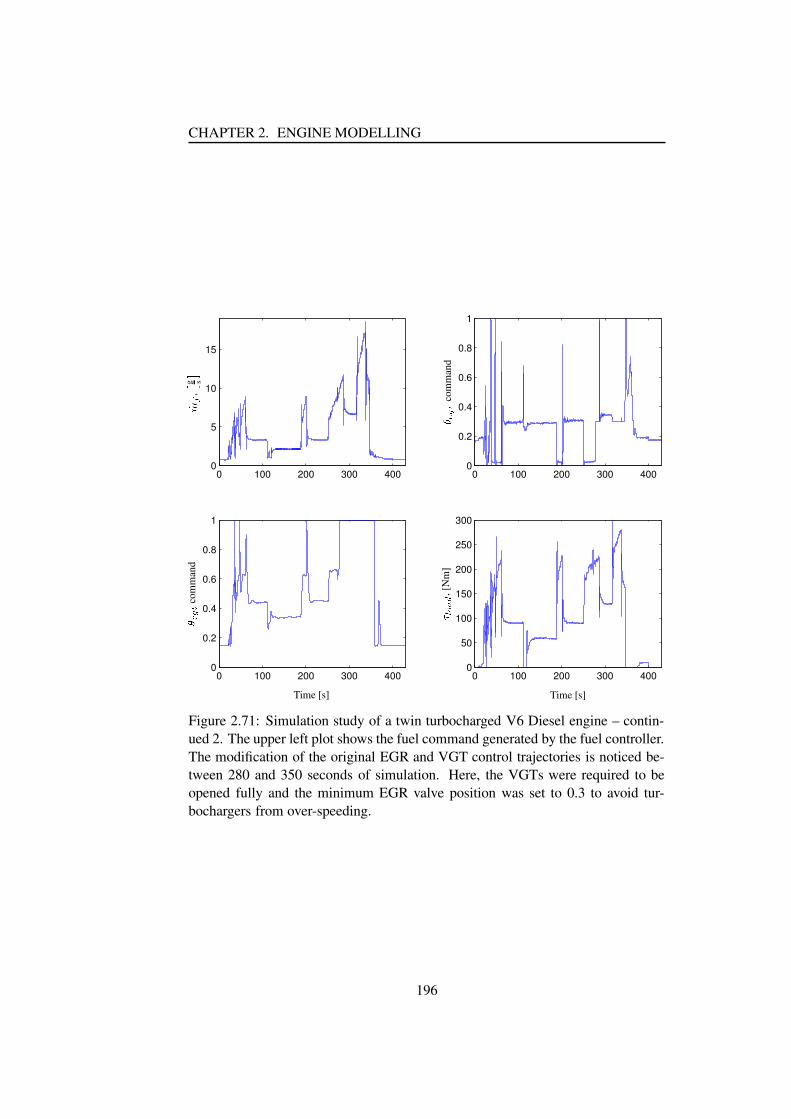
CHAPTER 2. ENGINE MODELLING
0 100 200 300 4000
5
10
15
0 100 200 300 4000
0.2
0.4
0.6
0.8
1
0 100 200 300 4000
0.2
0.4
0.6
0.8
1
0 100 200 300 4000
50
100
150
200
250
300
PSfrag replacements
° ± ² ,³ g s
´ µ·¶¸¹co
mm
and
µ·º¸» command ¼ ½ ¾¿À ,[Nm]
Time [s] Time [s]
Figure 2.71: Simulation study of a twin turbocharged V6 Diesel engine – contin-ued 2. The upper left plot shows the fuel command generated by the fuel controller.The modification of the original EGR and VGT control trajectories is noticed be-tween 280 and 350 seconds of simulation. Here, the VGTs were required to beopened fully and the minimum EGR valve position was set to 0.3 to avoid tur-bochargers from over-speeding.
196

2.12. SUMMARY, REMARKS AND CONCLUSIONS
The simulation results presented confirm the driving philosophy behind theMVEM framework: The ability to describe the response trends of IC engines byan interconnection of compact physically based engine sub-models. Although theV6 MVEM has been augmented by several new sub-models or revised sub-modelscompared to earlier work published by the ECG to capture the picture of the fun-damental dynamics governing the V6 engine, it is still in a very compact form andis thus suitable for engine estimation and control design. Hence, the simulation re-sults presented here support the statements made earlier by E. Hendricks and S. C.Sorenson in [49] and J. P. Jensen et al in [63] that MVEM modelling is a valuabletool in the development of engine control strategies.
2.12 Summary, remarks and conclusions
The chapter has dealt with the development or presentation of simple comprehen-sive engine sub-models. First, the commonly found radial turbocharger has beendivided in three separate models; an algebraic compressor model, an algebraic vari-able geometry turbine model and a first order dynamic model of the turbochargerwheel velocity. In the compressor model the mass flow and enthalpy losses aretreated simultaneously, whereas the VGT mass flow and efficiency are separatedinto two independent models. All models show a reasonably good modelling ac-curacy even in regions necessitating extrapolation from mapped data.
Next, a dynamic model of heat exchangers capable of describing the trends inunsteady flow scenarios is presented. Based on this model, it is concluded thataccurate estimation of the burnt mass flow or energy flow into the intake manifoldis badly posed when EGR back flow exists due to the mixing with intake manifoldmatter because of the pressure fluctuations.
Furthermore, the TDMVEM (Turbo Diesel Mean Value Engine Model), anextension to the MVEM framework, has also been presented in the section. Thismodel is derived by utilizing a simplified model of the gaseous mass containedin the intercooler and a soft assumption on the intake throat mass flow. Hence,the heat exchanger is included in the normal filling-emptying picture of the intakedynamics earlier utilized in other MVEM applications (e.g. see [63, 49]).
Phenomenological combustion models are presented together with the intro-duction of a new way of creating different maps for zero dimensional energy con-servation based combustion models utilizing the LWLS algorithm. Selected com-bustion process related maps have been identified for a 2.0 liter turbocharged DIDiesel engine. These maps are presented together with steady state dynamometerdata.
The three models described above are implemented in an object oriented Clibrary, VES, together with templates of FE volume models, butterfly and pop-pet valve models and crankshaft models. This makes it possible to rapidly createSIMULINK Á models of SI or CI engines independently of the engine air path de-sign.
197

CHAPTER 2. ENGINE MODELLING
The modelling framework presented is at the present time implemented in standalone engine simulation tools, which have aided in control, estimation and emissionstrategies, and power-train performance research and development studies at FFA.A more detailed presentation of such applications and the corresponding resultsobtained cannot be given in this dissertation for confidentiality reasons.
Comments to the fuel film dynamics.The careful reader has probably noticed a missing modelling section: fuel filmdynamics modelling for MPI equipped SI engines, a step deliberately taken aftermany hours of work unsuccessfully trying to describe engine measurement tracesby the simple  - à models (e.g. see [10]). Although the simplified  - à modelspresented in the literature by Hendricks (see e.g [52]) and Aquino (see e.g [12])clearly could provide some compensation of the fuel film dynamics experienced inCFI (Central Fuel Injection) equipped SI engines, due to the large manifold wallarea exposed to the fuel film, they are clearly giving problems when used withMPI systems. It will here be argued that the fuel rail pressure regulation system’sdynamics is of higher or at least just as high importance as the fuel film dynamics.
The fuel mass flow leaving the MPI injectors may within good accuracy bemodelled by a simple Bernoulli relation (this assumption is even reasonably validfor modern Diesel injectors where a pressure more than hundred times larger thanthe rail pressure in a typical MPI system is utilized; see e.g. [8]) .i.e.ÄÅ�Æ,Ç ÈÊÉÌË�Í�Î É/Ï*ÐeÑ ÒiÓ ÆÕÔOÖ§Í�Î É/Ï*Ðe× ÒiÓ ÆªØ ÖÚÙ[Û�È(ÜÞݧÖÚß Û�Éáà (2.245)
where Î É/Ï*Ð is the sectional area of the injector outlet, and Ö6Ù[Û�È(Ü is the rail pressure.Since the rail pressure in MPI systems is relative low ( â Ò�ã ä Ýæå ã ä bar, abso-lute) the injected fuel mass is greatly influenced by variations in the average intakemanifold pressure. Normally, the pressure drop across the injectors, ÔOÖ , is main-tained constant by controlling the rail pressure. This is customarily accomplishedby a mechanically controlled pressure regulator fitted to the fuel rail system. Themechanically controlled system is basically two control volumes separated by a di-aphragm. The pressure of one control volume is controlled by the intake manifoldpressure, whereas the pressure on the other side is developed by the fuel supplysystem. A small mass-spring-damper system (a combination of a control ball anda retainer) is fitted to the diaphragm controlling the pressure loss across the fuelexit valve. A schematic diagram of a sectioned pressure regulator for MPI systemsmay be found in [67].
Hence, the valve system is basically a coupling of two mass-spring-dampersystems and is of fourth order. However, since the control ball–retainer system issignificantly smaller than the diaphragm system its bandwidth is likely to be notice-able larger than the diaphragm system’s bandwidth. For this reason, a reasonableapproximation is to assume that the pressure drop across the injectors is controlledby the diaphragm system and the fuel pressure pulsations are attenuated by thecontrol valve–retainer system. Thus, the system of interest in the modelling of the
198

2.12. SUMMARY, REMARKS AND CONCLUSIONS
signal transfer between the intake manifold pressure and the fuel rail pressure isthe diaphragm system with the control ball attaining a fixed position (working likea normal needle valve). Hence, the dynamics of the control ball–retainer will beneglected and referred to as a needle in the following.
A change in the averaged intake manifold pressure leads to a movement of thediaphragm. The diaphragm is physically connected to a spring and the valve needleitself, thus the equilibrium position of the diaphragm or needle isçOèVé�êQëgêíìíî<ïñð3òóðVôjõ
(2.246)
whereî
is the spring constant of the diaphragm-spring combination,ð
the needleposition,
éOêQëgêthe diaphragm area, and
ð�ôis the needle position for
çOè§ì�ö. The
diaphragm and spring system can at best be classified as a mass-spring-dampersystem i.e. a dynamic system of second order. Now suppose the bandwidth of thissystem is comparable to the frequency of the engine pumping. In such a scenariothe needle position would basically follow a sine curve with a frequency dictatedby the engine speed, thus leading to very poor control of the fuel mass flow. If,on the other hand, the bandwidth of the pressure regulator is well below the en-gine pumping frequency a good control of the steady state fuel mass flow can beachieved. However, the response time of the intake manifold pressure, during en-gine idling or part load operation scenarios, is generally in the vicinity of the firstengine pumping harmonic’s period. Hence during harsh throttle tip-ins or tip-outslarge deviations in the desired pressure drop across the injectors may be expected,thus lead to significant deviations away from the desired fuel mass flow. This prob-lem is not present with the CFI system due to the injector’s location upstream ofthe throttle plate. Finally, it should be stated here that this scenario is only spec-ulation and not confirmed yet by experiments made by the author. However, R. P.Izydorek and G. C. Oberheide have in [93] included experimental results showingthat the settling time of the rail pressure is more than 12 times longer than the set-tling time of the intake manifold pressure after a step in the throttle plate positionleading to an increase of 50 kPa in the intake pressure. In addition to this, fuel railpressure variations up to 91 kPa still exist in the fuel rail after the intake pressurehas settled. Using the Bernoulli flow model mentioned earlier and a settled railpressure of 380 kPa this is equivalent to a relative error in the mass flow injectionbetween -7% and 9%, and an absolute error in ÷ of 7% to -8%! Furthermore, thetime response of the fuel rail pressure resembles that of a second order system to ahigh degree, thus supporting the second order (linear) system approximation of theintake pressure–fuel rail pressure signal path discussed earlier.
The use of the ø - ù model with MPI systems, in either of its two forms (see [52]and [12]), itself is heavily attacked in [31]. The fuel film fraction, ø , is accordingto [31] very close to 1, and almost all of the injected fuel enters the combustionchamber in liquid form. Hence, in accordance with the pressure rail dynamic issuespresented previously, a fuel film compensator implemented according to either [52]and [12] will most likely rather compensate for some of the fuel rail dynamics thanthe fuel film dynamics itself.
199

CHAPTER 2. ENGINE MODELLING
2.13 Appendix
The use of EGR as a means to lower the NOX production of the IC engine is to-day a well establish technology with more than 30 years of reported experimentaland theoretical results in the literature. During this time areas like promoted en-gine wear due to EGR, engine efficiency influences due to EGR, NOX emissionsreduction capabilities with EGR on CI and SI engines etc. have been and are stillinvestigated. However, dynamic model based control of the EGR is today still in itsinfancy which is interestingly enough since tight control of EGR is of paramountimportance in modern DI engines if the emissions legislation is to be met.
The problem of including EGR in the MVEM framework has been attackedearlier in section 2.8.3 leading to the formulation of the TDMVEM. However, thedevelopment of the this model is heavily inspired by the work already existing inthe literature. The first MVEM based attempt to describe the dynamic behavior of aNA SI engine equipped with an EGR system reported to the SAE community is tothe author’s knowledge presented by Weeks, R. W. et al in [95]. The pressure stateequation presented in this work does include a derivative temperature dependency.The final SIMULINK ú model presented does, however, not respect the differencein the internal energy between the EGR flow and the intake air flow, and the intaketemperature is fixed to a constant value. This temperature difference may howeverbe significantly and thereby offset the intake manifold temperature considerablycompared to the ambient temperature. Hence, in order to improve the transient andsteady state estimation capabilities of the MVEM when the EGR system is acti-vated the MVEM was first reworked in [83] and later in [37]. The research carriedout in [83] and [37] was in 1999 presented at the annual SAE conference in Detroitin the SAE-paper number 1999-01-0909. The paper was entitled Mean Value En-gine Modeling of an SI engine with EGR. This article presents the theoretical workbehind the new MVEM extension – the AMVEM. The good estimation (observer)properties of this simplified engine model were later confirmed by Professor E.Hendricks through an experimental study conducted on a NA SI engine retrofittedwith an EGR system. The experimental study was conducted at DTU and someof the experimental results made during this study are included in the SAE-papernumber 1999-01-0909, [75]. Furthermore, the article provides a good introductionto and a preliminary study of the EGR estimation and/or control problem. Hence,the paper is included here for the sake of completeness.
200

2.13. APPENDIX
1
1999-01-0909
Mean Value Engine Modelling of an SI Engine with EGR
Michael FonsMaersk Oil and Gas A/S
Martin MullerDelphi Automotive Systems
Alain ChevalierFord Motor Co.
Christian Vigild, Elbert Hendricks and Spencer C. SorensonTechnical University of Denmark
Copyright © 1999 Society of Automotive Engineers, Inc.
ABSTRACT
Mean Value Engine Models (MVEMs) are simplified,dynamic engine models which are physically based.Such models are useful for control studies, for enginecontrol system analysis and for model based engine con-trol systems. Very few published MVEMs have includedthe effects of Exhaust Gas Recirculation (EGR). Thepurpose of this paper is to present a modified MVEMwhich includes EGR in a physical way. It has been testedusing newly developed, very fast manifold pressure, man-ifold temperature, port and EGR mass flow sensors.Reasonable agreement has been obtained on an experi-emental engine, mounted on a dynamometer.
1. INTRODUCTION
It is clear that Exhaust Gas Recirculation (EGR) is a vitalcomponent of modern engine control systems. It is onlywith the use of this technology that it is possible to reducethe NOx component of SI engine exhausts to acceptablelevels given current legislation. EGR also provides amethod to reduce exhaust temperature and thus preventThree Way Catalyst (TWC) damage.
At the current time the only EGR control strategy whichhas been described in detail in the literature is based onstatic relationships depending on stationary engine map-ping [1]. It is however by now well known that in order todo accurate air/fuel ratio control, dynamic engine modelsare necessary for the design of engine control systems,for model and/or observer based control [2], [3]. Thus adynamic engine model has to be constructed whichincludes EGR and which is of the Mean Value EngineModel (MVEM) type. Currently only such models have asimplicity and accuracy which allows them to be codedinto engine control microprocessors.
This paper is a preliminary study of the possibility of con-structing such a model using conventional physical prin-ciples. Unfortunately EGR systems are somewhatmore complex than purely naturally aspirated Spark Igni-tion (SI) engines because of the heat of the exhaustgases. It is however the essence of modelling on theMVEM level to isolate the dominant physical effect oreffects in any engine subsystem, not to describe all of thedetails of engine operation. This paper is aimed at thisgoal.
2. ISOTHERMAL MVEM DEVELOPED EARLIER
In work which has been published earlier, a model for theintake manifold filling dynamics has been derived andvalidated in a number of different experiments [2] andapplications [3], including some production ones: [4], [5],[6]. This model is obtained by differentiating the ideal gaslaw applied to the mass of air in the intake manifold:
. (1)
Assuming that
(2)
this yields with the differentiation of equation (1) the mostsimple manifold pressure state equation
(3)
where the last equation on the right is obtained byassuming that the intake manifold temperature is con-stant. This is thus an isothermal MVEM. The port andthrottle air mass flows are given by the expressions
ii
iip =
R TV
m
201

CHAPTER 2. ENGINE MODELLING
2
, (4)
and
,
where
(5)
and mat0, mat1, α1, α2, p1, p2, pn, pc are constants.
3. ADIABATIC MVEM INCLUDING EGR
In an SI engine which is not equipped with EGR it hasbeen shown that the simple state equation on the right inequation (3) is sufficiently accurate to describe thedynamics of the intake manifold. This however cannotobtain in an engine which has EGR because then theintake manifold temperature cannot even approximatelybe assumed to be constant. The presence of EGR thusmakes it imperative to consider the energy balance in theintake manifold. Neglecting heat exchange, this leads tothe next higher order MVEM model of the intake manifoldfilling dynamnics: an adiabatic model.
When EGR is taken into account mass conservationrequires that
. (6)
Using energy conservation this leads to the equation
. (7)
As the enthalpy can be expressed as, equation (7) can be written as
the differential equation
(8)
where . Using the ideal gas law, equation(1) for mi and the fact that , this equa-tion can be further reduced to
. (9)
Applying mass conservation from equation (6) finallyleads to the expression:
(10)
Using equation (3) this means that the manifold pressurestate equation becomes
(11)
Together equations (10) and (11) are the adiabaticMVEM which includes EGR. An assumption which isimplicit in their use is that there is perfect mixing of thefresh air flow and the EGR flow.
In the limit when the EGR flow is zero, equations (3) and(10) and (11) give exactly the same solution as should beexpected. However during rapid transients, equation (10)gives a differentiating effect, leading to a temperaturespike in its response. This is due to adiabatic compres-sion or expansion, depending on whether the throttle isbeing opened or closed. This leads in turn to an increaseor decrease of the air density in the intake manifold,resulting in different port air mass flows than those pre-dicted by equation (3) during transitions. The errorinvolved can be significant during such transients [3], [7].
In order to use the adiabatic MVEM it is necessary tospecify the EGR mass flow and temperature. To findthese quantities without using direct measurements is notstraight forward and does require the use of some empir-ism because of the wide range of the physical effectswhich determine them. Using one of the devices cur-rently available for EGR mass flow control it is possible tosolve the EGR mass flow determination problem usingfeedforward and calibration techniques. Finding the EGRtemperature is somewhat more difficult and will not betreated here.
3.1 EGR MASS FLOW DETERMINATION – A devicewhich is currently available of EGR control is the DelphiLinear Exhaust Recirculation Valve [8]. In use, this valve
ap id
iv im (n, p ) = V
120 R T e p nû ⋅ü ý
at i ata
a1 2 r atm ( , p ) = m 1
p
T ( ) ( p ) + m
û α β α β 0
i at EGR apm = m + m - mû û û û
at a EGR EGR ap i
i v i i v i
m h + m h - m h
= d(m u)
dt = m c T + m c T
þ þ þþ þ⋅ ⋅ ⋅
⋅
x xh = T R / ( - 1)κ κ
- m T R
( - 1) m c - m
Tm
ap i
i v
i i
i
þ þκκ
κ = c / cp v
vc = R / ( - 1)κ
iat a i
i i
EGR EGR i
i i
ap2
i
i i
i2
i
i i
T = m T R Tp V
+ m T R Tp V
- m T R
p V - m
T Rp V
þ þ þþ þκ κ
κ
202
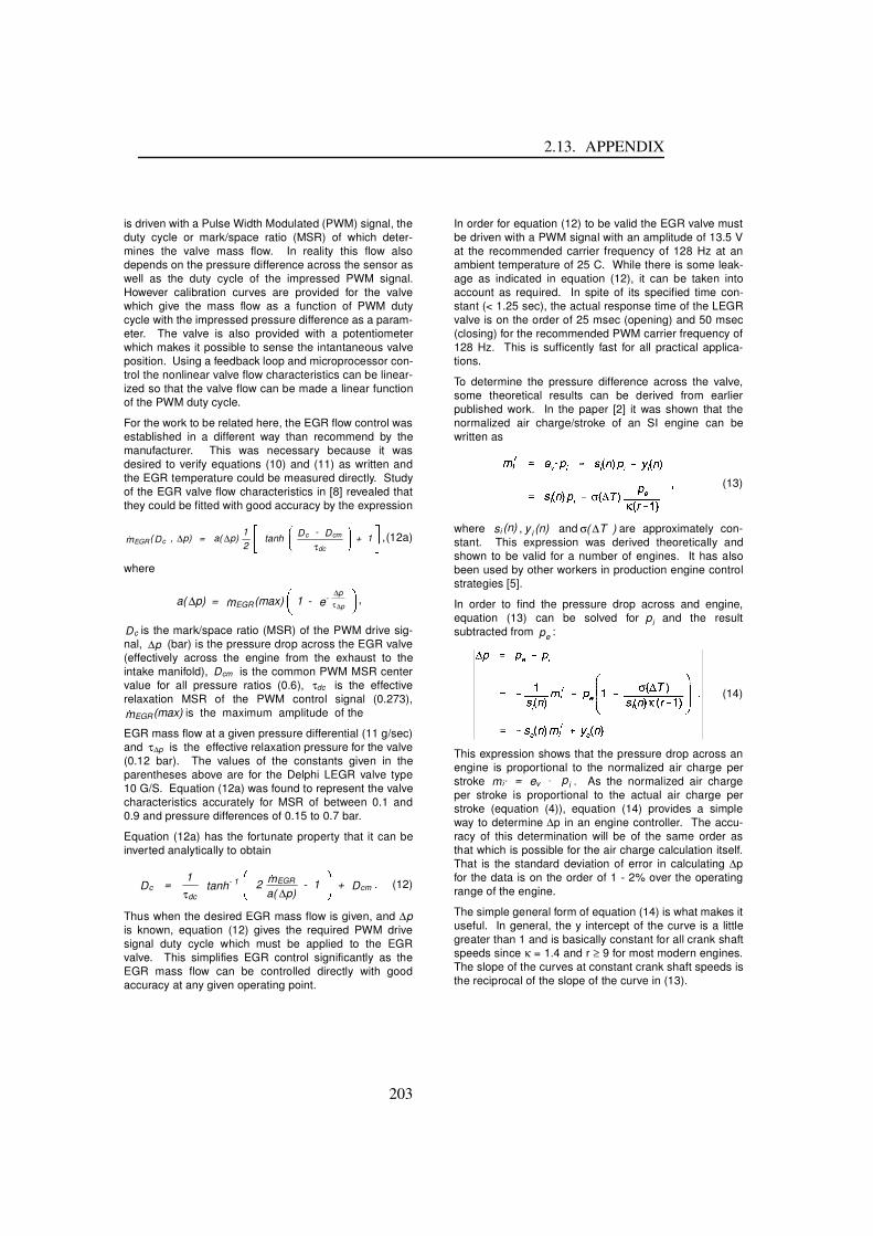
2.13. APPENDIX
3
is driven with a Pulse Width Modulated (PWM) signal, theduty cycle or mark/space ratio (MSR) of which deter-mines the valve mass flow. In reality this flow alsodepends on the pressure difference across the sensor aswell as the duty cycle of the impressed PWM signal.However calibration curves are provided for the valvewhich give the mass flow as a function of PWM dutycycle with the impressed pressure difference as a param-eter. The valve is also provided with a potentiometerwhich makes it possible to sense the intantaneous valveposition. Using a feedback loop and microprocessor con-trol the nonlinear valve flow characteristics can be linear-ized so that the valve flow can be made a linear functionof the PWM duty cycle.
For the work to be related here, the EGR flow control wasestablished in a different way than recommend by themanufacturer. This was necessary because it wasdesired to verify equations (10) and (11) as written andthe EGR temperature could be measured directly. Studyof the EGR valve flow characteristics in [8] revealed thatthey could be fitted with good accuracy by the expression
,(12a)
where
,
is the mark/space ratio (MSR) of the PWM drive sig-nal, (bar) is the pressure drop across the EGR valve(effectively across the engine from the exhaust to theintake manifold), is the common PWM MSR centervalue for all pressure ratios (0.6), is the effectiverelaxation MSR of the PWM control signal (0.273),
is the maximum amplitude of the
EGR mass flow at a given pressure differential (11 g/sec)and is the effective relaxation pressure for the valve(0.12 bar). The values of the constants given in theparentheses above are for the Delphi LEGR valve type10 G/S. Equation (12a) was found to represent the valvecharacteristics accurately for MSR of between 0.1 and0.9 and pressure differences of 0.15 to 0.7 bar.
Equation (12a) has the fortunate property that it can beinverted analytically to obtain
. (12)
Thus when the desired EGR mass flow is given, and ∆pis known, equation (12) gives the required PWM drivesignal duty cycle which must be applied to the EGRvalve. This simplifies EGR control significantly as theEGR mass flow can be controlled directly with goodaccuracy at any given operating point.
In order for equation (12) to be valid the EGR valve mustbe driven with a PWM signal with an amplitude of 13.5 Vat the recommended carrier frequency of 128 Hz at anambient temperature of 25 C. While there is some leak-age as indicated in equation (12), it can be taken intoaccount as required. In spite of its specified time con-stant (< 1.25 sec), the actual response time of the LEGRvalve is on the order of 25 msec (opening) and 50 msec(closing) for the recommended PWM carrier frequency of128 Hz. This is sufficently fast for all practical applica-tions.
To determine the pressure difference across the valve,some theoretical results can be derived from earlierpublished work. In the paper [2] it was shown that thenormalized air charge/stroke of an SI engine can bewritten as
(13)
where , and are approximately con-stant. This expression was derived theoretically andshown to be valid for a number of engines. It has alsobeen used by other workers in production engine controlstrategies [5].
In order to find the pressure drop across and engine,equation (13) can be solved for and the resultsubtracted from :
(14)
This expression shows that the pressure drop across anengine is proportional to the normalized air charge perstroke . As the normalized air chargeper stroke is proportional to the actual air charge perstroke (equation (4)), equation (14) provides a simpleway to determine ∆p in an engine controller. The accu-racy of this determination will be of the same order asthat which is possible for the air charge calculation itself.That is the standard deviation of error in calculating ∆pfor the data is on the order of 1 - 2% over the operatingrange of the engine.
The simple general form of equation (14) is what makes ituseful. In general, the y intercept of the curve is a littlegreater than 1 and is basically constant for all crank shaftspeeds since κ = 1.4 and r ≥ 9 for most modern engines.The slope of the curves at constant crank shaft speeds isthe reciprocal of the slope of the curve in (13).
EGR cc cm
dcm (D , p) = a( p)
12
D - D + 1 ÿ tanh∆ ∆τ
��� �� ���� �a( p) = m (max) 1 - e EGR
- p
p∆∆
∆�
τ
� ��cD
∆p
cmDdcτ
EGRm (max)�∆pτ
cdc
- 1 EGRcmD =
1 2 m
a( p) - 1 + D
τtanh �
∆
��� �� �
is (n) iy (n) σ( T )∆
ipep
′ ⋅i v im = e p
203

CHAPTER 2. ENGINE MODELLING
4
Using the same numbers which were used in[2], , , , , pe =1.05 bar and , it is possible to find the approxi-mate numbers se = 1.050 and ye = 0.952. Thus for this"standard" engine example one finds equation (14) to be
. (15)
That engines do display the dependence predicted byequation (14) can be shown using data from the fiveengines considered in [2]. Figures 1a - 1c are plots of thedifferential engine pressure vs the normalized air chargefor three of the engines from this paper. The basic valid-ity of the functional form of equation (14) is thus con-firmed.
Mean values for the parameters of the engines in [2] aregiven in table 1 below. This table shows that the pre-dicted slopes and y intercepts agree fairly well with thoseof the actual engines. Obviously some of the inaccu-racy in the table is due to the approximate way in whichthe parameters have been determined. Only the meanslopes are given, the crank shaft speed dependencebeing ignored, as it is weak.
It has to be remembered that equation (14) is generallyvalid for engines but because of details intake andexhaust manifold configuration, it will in most casesrequire some detailed engine mapping. Equation (14)suggests however that this mapping will not be very diffi-cult because of the simple form of the equation, except atvery low and very high air mass flows. At these extremesthe curve will bend upwards due to heating.
On the other hand that the engine output power is depen-dent on the actual fresh air charge per stroke and not onthe EGR air mass flow. This means that the actual freshair mass flow,
, (16)
(where f refers to the fresh charge) is what determinesthe fuel which is injected into the engine while isfound from
(17)
and
(18)
The port air mass flow, , has to be measured or esti-mated. If estimation is to be used then this can take sev-eral different forms, depending on the air mass flowrelated sensor type used [2], [4], [5], [6], [9].
Once the differential pressure is known, it is possible touse this information together with the documentation forthe Delphi EGR valve to determine the EGR mass flow.If other valves are to be used a similar approach can betaken.
4. EXPERIMENTAL RESULTS
In order to test the adiabatic MVEM above experimentswere conducted with a modified 1275 cc British Leylandengine. This engine was equipped with a speciallydesigned 7 port head [10] which made it into a crossflowengine. The intake and exhaust valves were of Cooper Sdimensions. It was provided with port fuel injectors andcould work either in an EFI or SEFI mode, requiring onlysoftware changes. The intake manifold volume wasabout 3 times the engine displacement volume. Very fastpressure, port air mass flow and temperature sensorswere installed in the intake manifold and the throttle airmass flow was measured with a laminar flow meter.These sensors are all significantly fast to resolve all ofthe transients which might be applied to the engine downto an event level (see Appendix).
To control the engine, log data and carry out simulationsa specially developed Engine Control Development Sys-tem (ECDS) was used together with 12 bit A/D and D/Acards in a Pentium PC. This software was also used tolinearize the Delphi 18 g/s LEGP Valve which wasinstalled for EGR control. The ECDS system is very fastand allows sampling times down to 0.25 msec. Samplingtimes used for the experiments to be reviewed were 0.25- 1 msec.
Tests were carried out over the entire operating range ofthe engine but only a few of these will be reviewedhere. The main question is if the model of equations (10)and (11) show the correct behavior for common EGRfeed levels. Figure 2 shows a sample of results obtainedat a typical operating point, both with and without EGR.
Table I. Approximate mean values of the parameters in equation (14) for the set of engines treated in [2]. Notice that the values displayed have been obtained in part graphically from figures 1a - 1c.
parameters se ye
1.1 L Ford (1.) 1.026 0.925
1.1 L Ford (2.) 1.000 0.910
1.8 L 4v/cyl (< 4000 rpm)
1.080 0.920
4.9 L Ford 0.880 0.905
1275 cc BL 1.000 0.900
∆T = 15C iT = 300C r = 10 κ = 1.4ι = 0.9
∆p = p - p = - 1.050 m + 0.952e i i⋅ ′
apf ap EGRm = m - m� � �
∆ p
apm�
204

2.13. APPENDIX
5
(a) (b)
(c)
Figure 1. Figures 1a - 1c. Above and to the right. These figures show the differential engine pressure plotted as a function of the normalized air charge per stroke for three engines treated earlier in [2]. The two Ford 1.1 L engines are different
engines ((1) and (2)) and were measured at different times by different groups. The 1275 cc BL (British Leyland) engine is the experimental engine used in this paper.
205

CHAPTER 2. ENGINE MODELLING
6
(a)
(b)
Figure 2. Figure 2a (without EGR: left and above) and figure 2b (with EGR: left and below) at approximately the same operating point. The EGR mass flow is about 10% of the fresh mixture flow and the EGR gas temperature is about 448 K. Measurements are shaded and model simulations are solid black lines.
Figures 2a and 2b show the response of the engine withand without EGR at a low part load operating point. Infigure 2a there is no EGR and in figure 2b the EGR massflow is about 10% of the fresh air mass flow: the EGRtemperature is about 448 K. Measurements are shownshaded while parallel simulations with the model of equa-tions (10) and (11) are single lines. Engine pumping fluc-tuations are apparent in the intake manifold pressure andthe fast throttle transients are somewhat smoothed bymanifold filling. The throttle air mass flow shows theexpected filling spike and the total port air mass flowshows the effect of engine pumping. The port air massflow is obtained by event averaging and summing the 4intake port air mass flow measurements. At the rapidthrottle transitions the manifold temperature increases ordecreases significantly: this is an effect of the new MVEMtemperature equation. It can be seen that the intakemanifold temperature measurements do not quite comeup to the model predictions. It is thought that this is theresult of heat transfer in the intake manifold to the sur-roundings in the engine.
Figure 2b shows what happens when the EGR is appliedto the engine at nearly the same operating point as in fig-ure 2a. The manifold pressure increases but at the sametime the crank shaft speed decreases significantly. Airmass flow to the engine via the throttle body decreasesat the same time, while the port air mass flow increases.The intake manifold temperature increases due to theeffect of the EGR gas heat and the same rapid tempera-ture spikes as before occur but this time with a somewhatlarger amplitude.
The overall accuracy displayed in figure 2 is reasonablygood but the temperature predicitons are in all cases a lit-tle too low. This suggests that there is some heat transferwhich takes place which is not in the model.
5. CONCLUSIONS
A dynamic adiabatic model has been constructed for theintake manifold with EGR using physical considerations.It has been found that this model is closely related to theisothermal MVEM investigated earlier and is a naturalextention of it. The main difference between the isother-mal and adiabatic models is the presence of a large tem-perature spike during rapid throttle plate movements.The accuracy displayed by the model is sufficient formost practical control purposes.
206

2.13. APPENDIX
7
As a secondary result, a useful expression for the pres-sure difference between the intake manifold has beenderived which is simple and relatively accurate. Thisexpression makes it possible to predict the performanceof the EGR valve without extra measurements.
Clearly the results which have been presented are pre-liminary but the overall accuracy displayed is encourag-ing and suggests that it may soon be possible to includeEGR in model based control systems in a convenient andsimple manner. This is currently a subject for continuingresearch.
6. ACKNOWLEDGEMENTS
The authors wish to acknowledge the professional assis-tance of Joe Asik, Dave Trumpy and Mike O'Sullivan ofFord Motor Co. in early stages of this work. They alsowish to thank Jim Waters of Delphi Automotive Systemsfor his help in obtaining the Delphi EGR valves used inthis paper.
7. REFERENCES
1. Azzoni, P., Minelli, G., Moro, D., and Serra, G., "A Model forEGR Mass Flow Rate Estimation", SAE Technical PaperNo. 970030, 1997.
2. Hendricks, E., Chevalier, A., Jensen, M., Sorenson, S. C.,Trumpy, D., and Asik, J., "Modelling of the Intake ManifoldFilling Dynamics", SAE Technical Paper No. 960037, 1996.
3. Müller, M., Hendricks, E., and Sorenson, S. C., "MeanValue Modelling of Turbocharged Spark Ignition Engines",SAE Technical Paper No. 980784, 1998.
4. Hendricks, E., Vesterholm, and Sorenson, S. C., "NonlinearClosed Loop, SI Engine Control Observers", SAE TechnicalPaper No. 920237, 1992.
5. Gerhardt, J., Benninger, N., and Hess, W., "Torque-BasedSystem Structure of an Electronic Engine ManagementSystem as a New Base for Drive Train Systems (BoschME7 System)", 6. Aachener Kolloqium, Fahrzeug- undMotorentechnik, Aachen, Germany, 20.-22. October, 1997.
6. Maloney, P., and Olin, P., "Pneumatic and Thermal StateEstimators for Production Engine Control and Diagnostics",SAE Technical Paper No. 980517, 1998.
7. Føns, M., Indførelse af Recirkulering af Udstødningsgas(EGR) i SI-Motorer (Implementation of EGR on an SIEngine, In Danish), Masters Thesis, Institute for Automa-tion, Laboratory for Energetics, Report No. IAU97E09,Technical University of Denmark, September, 1998.
8. Lyko, B. M., Application Manual for the Linear Exhaust GasRecirculation Valve, Delphi Energy and Engine Manage-ment Systems, Rochester, New York, 1995.
9. Jensen, P. B., Olsen, M. B., Poulsen, J., Fons, M., and Hen-dricks, E., "A New Family of Nonlinear Observers for SIEngine Air/Fuel Ratio Control", SAE Technical Paper No.970615, 1997.
10. The specially prepared 7 port head for the 1275cc BritishLeyland engine was provided by Georg Mikkelsen, ÅKMRacing, Lerpyttervej 31, 7700 Thisted, Denmark, +45 9792 01 82.
8. NOMENCLATURE
The following symbols are used in this paper:
time (sec) throttle plate angle (degrees) engine speed (rpm/1000 or krpm)
ambient pressure (bar)
ambient temperature (degrees Kelvin)
absolute manifold pressure (bar)
intake manifold temperature (degrees Kelvin)
EGR temperature (degrees Kelvin)
exhaust manifold pressure (bar)
(bar)
air mass flow past throttle plate (kg/sec)
air mass flow into intake port (kg/sec)
EGR mass flow (kg/sec)
normalized air charge per stroke
air mass in the intake manifold (kg)
measured value of the variable 3 volumetric efficiency based on manifold conditions
engine displacement (liters)
manifold + port passage volume (m3)
gas constant (here 287 X 10-5) ratio of the specfic heats = 1.4 for air
stoichiometeric air/fuel ratio (14.67)
slope of pressure difference curve, with normalized air charge, see [2] intercept of pressure difference curve, with normalized air charge, see [2] compression ratio
mean temperature rise during intake stroke
tαn
ap
aT
ip
iT
EGRT
ep
∆pe ip - p
atm�apm� EGRm�′im ( e p )v i⋅
im
mx x
ve
dV
iV
Rκ
thL
es (n)
ey (n)
r
σ( T)∆ 1 / ( 1 + T / T )i∆
∆T
207

CHAPTER 2. ENGINE MODELLING
8
APPENDIX
The basic characteristics of the prototype port air massflow and EGR flow sensors used in this paper are sum-marized below.
Port Mass Air Flow (MAFp) and EGR Flow Sensor Char-acteristics:
a. basic accuracy: +/- 1 %, error standard deviation.b. linearity (steady state): +/- 0.5 %, physical lineariza-
tion.c. linearity (dynamic): +/- 1.0 %.d. response direction: bi-directional, symmetric.e. response time: < 1 msec.f. vibration sensitivity: small.
g. temperature error: +/- 2.0 %, -5/+50°C (approx.).h. light off time: < 10 msec.i. size: 38 mm (MAFp) and 22 mm (EGR).
The basic characteristics of the prototype fast tempera-ture sensors used in this paper are summarized below.
Temperature Sensor Characteristics:
a. basic accuracy: +/- 1 %, error standard deviation.b. linearity (steady state): +/- 0.5 %, physical lineariza-
tion.c. linearity (dynamic): as above.d. response direction: bi-directional, symmetric.e. response time: < 1 msec.f. vibration sensitivity: small.
g. temperature range: 0 - 350 C.h. light off time: < 5 msec.i. size: small.j. mounting sensitivity:non-critical.
208

Chapter 3
Estimation & Identification
EGR mass flow estimation is a critical point in modern engine con-trol strategies if current emissions legislation is to be met. Sincemost estimation strategies utilize MAF, exhaust gas composition ortemperature measurements in the computation of the EGR mass itis vital to know what level of estimation accuracy can be expectedusing these inputs. Hence, the first topic of this chapter is the in-vestigation of different EGR estimation strategies and how deter-ministic measurement errors will influence estimation accuracy.Secondly, anti-aliasing filters, developed for event-based strate-gies, capable of providing optimal measurement bandwidth with-out the danger of aliasing are presented. High measurement band-width without the danger of signal aliasing is of great importancefor a correct estimation of several engine states.
3.1 EGR Rate estimation
Tight control of the exhaust gas recirculation (EGR) is of paramount importancewhen targeting the minimization of NOX and PM emissions from DI engines.Hence, in the light of the future requirement for stringent control of the EGR rate,or rather the burnt mass fraction level in the intake manifold, this section is dedi-cated to the investigation of what accuracy level can be obtained with productiontype engine sensors.
Direct measurement of the EGR volume flow is possible by measuring the pres-sure drop across a restriction. However, due to the relative high exhaust PM levelin DI engines, this method is not viable due to restriction clogging issues. Hence,the EGR mass flow must be estimated from other engine state measurements andstate estimates.
The MAF measurement, normally obtained with a hot-wire/film sensor down-stream of the intake air filter box, is without doubt the single most important mea-surements in a conventional EGR estimation strategy. However, new exhaust O � / �sensors suited for application with lean burn engines are emerging on the automo-
209

CHAPTER 3. ESTIMATION & IDENTIFICATION
tive market. Combined with the exhaust gas composition information provided bythese new exhaust sensors and with other selected engine measurement/estimates,new EGR estimation strategies are made possible.
Dependent upon operating point and AFR the EGR rate may maximally vary�5% relatively to the EGR rate set point, or otherwise excessive Diesel engine
emissions [5] can be expected. This maximum setting of�
5% for the relativetolerance on the EGR rate will be used throughout this section.
First the EGR rate estimation strategy based solely on the MAF measurementwill be evaluated and later compared to the corresponding results expected using alinear O � / exhaust sensor.
Since direct measurement of the EGR mass flow is complicated due to the highEGR particulate level, this section will also evaluate estimation strategies basedupon thermal information from temperature measurements obtained in the engineintake system, thereby avoiding the use of the speed-density equation.
3.1.1 MAF sensor performance
The EGR rate is commonly computed by subtracting the MAF signal from theintake port mass flow normally estimated by the speed-density equation. Hence, itis of natural interest to determine what level of steady state accuracy that can beachieved with production type MAF sensors.
The best MAF sensors currently available from Bosch, based on hot film tech-nology, have a relative error on the mass flow measurement in the range of
�3%
(see [6])1. Although this error seems negligible it has a major impact on the es-timation of the EGR rate even when the total mass flow to the engine is knownexactly. This significant influence on the EGR estimation will be shown below.
The ratio between the intake air mass flow and the EGR flow is by definition,!"$#&%('*) +!"-,/. '10 243EGRrate
EGRrate065 ,/. ' 0 !"-7/8 3 !"-,/. '!"-,/. ' (3.1)
and
EGRrate9 !"-,/. '!"-7/8 (3.2)
The intake throat mass flow,!":#&%('*) + , is in steady state related to the measure intake
mass flow, MAF, in the following manner!"$#&%('*) +<; MAF = 2>3@?BAC D !"-,/. ' 0 !"-,/. 'FE ?MAF
(3.3)
1The setting of G 3% is for a new sensor. However, the absolute value of the relative sensor erroris known to increase to approximately 25% (see [94]) over time depending on the local pollutionlevel.
210

3.1. EGR RATE ESTIMATION
0 0.05 0.1 0.15 0.2 0.25 0.3 0.35 0.4 0.45 0.5−60
−40
−20
0
20
40
60
PSfrag replacements
EGRrate
Rel
.EG
Rra
tees
timat
ion
erro
r,[%
]
Relative EGR rate estimation error boundaries obtain with a H 3% MAF sensor
Figure 3.1: Relative EGR rate error boundaries with I 3% MAF sensor.
since the JK:L/MON JK$P&Q(R*S TVU JK-W/X RZY MAF U\[ JK-W/X R under the assumption that the portmass flow can be estimated correctly. The parameter ] is in the last equation therelative fractional error on the MAF measurement. The relative steady state erroron the EGR rate estimation may now independently of the engine characteristicsbe derived from the last two equations as
EGRrate,estY [ JK-W/X RJK-L/M Y_^ U ]a` W/X R^ U ` W/X Rb
Error,[%] Y ^(cdc EGRrate,est e EGRrateEGRrateY ^(cdc ]a` W/X RfY ^(cdc ] ^ge EGRrate
EGRrate
(3.4)
Figure 3.1 shows the error boundaries on the EGR rate estimation expected witha I 3% MAF sensor. It is clear from the figure that even if the total mass flowinducted by the engine is known precisely, the slightest error in the MAF mea-surement will have a serious impact on the EGR rate estimation/control accuracy.Only at higher EGR rates will the error approach the acceptable level of I 5%.Inaccuracies in the fuelling rate (error between demanded and actual fuelling) arenot considered in this analysis, but will further exacerbate the EGR/AFR controlaccuracy.
211

CHAPTER 3. ESTIMATION & IDENTIFICATION
3.1.2 Exhaust Sensor Performance
The effect of the relative error on the O h measurements in the engine’s exhaust pipeon the estimation of the EGR rate is examined in this section.
3.1.2.1 Differential Equations for the relevant dynamics
The burnt mass fraction in the intake manifold, ikj<lnm , can be described by the ODE(see e.g. appendix C on page 255 where the burnt mass fraction of a arbitrary con-trol volume fulfilling the assumption made with the filling and emptying approachis derived), oipj<lnmrq sft j<lnmu j<lnmwvwj<lnm xnx izy/{n|<}~ipj<lnmV� o� y/{n|4}�ipj<lnm o�$�&� |*� � � (3.5)
wheres
is the gas constant for air,t j<lnm is the gas temperature in the intake man-
ifold. u j<lnm and vwj<lnm are the manifold pressure and the manifold volume, respec-tively. i�y/{n| is the burnt mass fraction content in the EGR mass flow,
o� y/{n| . Finally,o�$�&� |*� � is the air mass flow in the intake throat just upstream of the EGR inlet point.The change of mass in the intake manifold is given by mass conservation,o� j<lnm�q o� y/{n|k� o�$�&� |*� � } o� l/� (3.6)
whereo� l/� is the mass flow at the intake ports.
Scaled exhaust O h equations The scaled O h concentration2 in the cylinder of aDI engine can be described as,
O h�� ����� x�� �kqFresh air mass flow available for combustion� ��� �x*� }~ipj<lnm x�� }~������� o� l/� x�� }~�����p}
Fresh air mass flow requiredby stoichiometric combustion� ��� �� |�y*� o� �o� l/� x�� }~������� o� �� ��� �
Total mass flow through the system
(3.7)
where ��� is the time delay between the closing of the intake valve and fuel injection.The numerator is simply the difference between the fresh air mass flow availablebefore combustion and air mass consumed by combustion (
� |�y*� o� � ). The scaledoxygen concentration in the exhaust is just a time delayed version of the oxygenconcentration in the cylinder. Hence, the following expression for O h�� y/� � is ob-tained.
O h�� y/� � x�� �kq o� ln� |*� y/� �o� ln� |*� y/� � � o�-¡�¢ |*mBy¤£�� y/� �q x*� }~ipj<lnm x�� }~���¥}~�(�n�n� o� l/� x�� }~���¥}~�(�¦�p} � |�y*� o� � x�� }~�(�n�o� l/� x�� }~���¥}~�(�n�§� o� � x�� }��(�¦�(3.8)
2The O ¨ is here scaled such that O ¨ =1 and O ¨ =0 refer to fresh air flow and completely burnedflow respectively
212

3.1. EGR RATE ESTIMATION
where the time delay ©«ª is the time between fuel injection and the opening of theexhaust valve. The equation is schematically depicted in figure 3.2.
PSfrag replacements¬ ¥®�¯Z°± ®/²³�´Vµ ¬ ¥®�¯·¶¸°± ®/²
°±4¹¬ º�»n¼ °± º�»n¼³½´Vµ ¬ º�»n¼ ¶¸°± º�»n¼
Figure 3.2: Schematic diagram of the combustion process in a diesel engine.
Scaled ¾ equations The description of the scaled air-to-fuel ratio3, ¾ , is directlyavailable from O ¿ expressions derived previously. However, special care must betaken in the definition of the fresh air mass flow and the fuel mass flow goingto engine or else the the computed ¾ level exhaust will be biased compared tomeasurements. The total air flow intake, fresh as well as burnt, is computed asÀÁ-Ânà ÄgÅ ÀÁ-Â/Æ�ǧÈ4É È¾ Ä�Ê*ËZÌ ÈVÍ ± ÂnÎÐÏ (3.9)
Thus, the total intake air flow is the difference between the total intake flow,ÀÁ~Â/Æ
and intake flow which was formerly fuel. The total fuel flow is found analogous tothe previous equation as ÀÁ Ë�Ñ«Ê¤Ò Å ÀÁ ËZÌ ÈÈ Ì ¾ Ä�Ê*Ë Í ± ÂnÎ ÀÁ-Â/Æ (3.10)
The scaled ¾ in the cylinder can be described as,
¾ ª�Ó Ò/Ô�ÕnÖ Å ÀÁ-Ânà ľ Ä�Ê*Ë ÀÁ Ë�ѫʤÒÅ È4É ´×aØ º ¹(Ù ´ Í ± ÂnÎ Ô�Õ É © à ־ Ä�Ê*ËOÚ °±4¹°± ®/² ³ Û�µVÜ/Ý ¶ Ì ´×aØ º ¹(Ù ´ Í ± ÂnÎ Ô�Õ É © à ֤Þ(3.11)
After combustion the cylinder mass is purged into the exhaust pipe during the ex-haust stroke, hence the ¾ level in the exhaust pipe will be the total cylinder ¾ timedelayed. Therefore the ¾ level in the exhaust pipe, ¾ Ê/ßaà , is,¾ Ê/ßaàwÔ�ÕnÖ Å ¾ ª�Ó Ò�Ô�Õ É ©(ª Ö (3.12)
3 á is scaled with the stoichiometric ratio, á Ø º ¹ , between diesel and fresh air, which in this workis fixed to a value of14.7.
213

CHAPTER 3. ESTIMATION & IDENTIFICATION
where the delay âaã is the time between the fuel injection and the correspondingopening of the exhaust valves.
3.1.2.2 Steady State Operation
The burnt mass fraction in the intake manifold will in steady state be,äåpæ<çnè�éëêì åpæ<çnè�é äí-î/ïnðäí-î/ïnðkñóòõô å å î/ïnðéEGRrate ö*÷>ø O ù�ú î/ûaüþý
(3.13)
since äí$ÿ ü(ð ú � é òõô åEGRrate
é äí-î/ïnðäí-î/ïnðFñóòõô åå î/ïnð é ÷4ø O ù�ú î/ûaü (3.14)
Exhaust O ù in steady state Inserting the above equations in equation 3.8, thefollowing expression for the steady state EGR rate is obtained,
EGRrateé � ÷>ø O ù�ú î/ûaü � ÷ ñ äí��äí ç���� ø� ð�î � äí��äí ç���� ÷÷4ø O ù�ú î/ûaü (3.15)
The fresh air mass flow to the engine, MAF, is related to the EGR rate in thefollowing way,
MAFé äí ç�� ö*÷>ø EGRrate
ý (3.16)
Inserting this information into equation 3.15 the scaled O ù�ú î/ûaü can be found as,
EGRrate ö*÷>ø O ù�ú î/ûaüþý é ÷>ø O ù�ú î/ûaü � ÷ ñ ö*÷>ø EGRrateý äí��MAF
�ø� ð�î � ö*÷>ø EGRrate
ý äí��MAFì
ö*÷>ø EGRrateý ö O ù�ú î/ûaü ø ÷ ý é ø O ù�ú î/ûaü ö*÷>ø EGRrate
ý äí��MAFø� ð�î � ö*÷>ø EGRrate
ý äí��MAFì
O ù�ú î/ûaü é ÷>ø� ð�î ��æ �MAF÷ ñ æ �
MAF
(3.17)
214
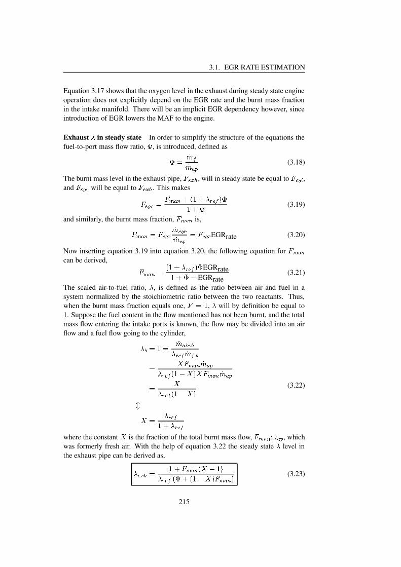
3.1. EGR RATE ESTIMATION
Equation 3.17 shows that the oxygen level in the exhaust during steady state engineoperation does not explicitly depend on the EGR rate and the burnt mass fractionin the intake manifold. There will be an implicit EGR dependency however, sinceintroduction of EGR lowers the MAF to the engine.
Exhaust � in steady state In order to simplify the structure of the equations thefuel-to-port mass flow ratio, � , is introduced, defined as��� ���������� (3.18)
The burnt mass level in the exhaust pipe, ������� , will in steady state be equal to ���! #" ,and � ��$&% will be equal to �'����� . This makes
� ��$&% � �)( �&*,+.-0/ + �1%2� �43 �/5+ � (3.19)
and similarly, the burnt mass fraction, ��( �&* is,�)( �&* �.� ��$&% �� ��$&%������ �.� ��$&% EGRrate (3.20)
Now inserting equation 3.19 into equation 3.20, the following equation for �5( �&*can be derived, �)( �&* � -0/5+ �1%2� �43 � EGRrate/6+ �87 EGRrate
(3.21)
The scaled air-to-fuel ratio, � , is defined as the ratio between air and fuel in asystem normalized by the stoichiometric ratio between the two reactants. Thus,when the burnt mass fraction equals one, �9� / , � will by definition be equal to1. Suppose the fuel content in the flow mentioned has not been burnt, and the totalmass flow entering the intake ports is known, the flow may be divided into an airflow and a fuel flow going to the cylinder,�;:�� / � �� �&< %0= :�1%2� � ���� = :� > �)( �&* �������1%2� �1-0/ 7 > 3 > �)( �&* ������� >�1%2� �1-0/ 7 > 3?
> � �1%2� �/5+ �1%2� �(3.22)
where the constant > is the fraction of the total burnt mass flow, �6( �&* ������ , whichwas formerly fresh air. With the help of equation 3.22 the steady state � level inthe exhaust pipe can be derived as,
�;�����,� /5+ �)( �&*�- > 7 /@3�1%2� �A- � +B-0/ 7 > 3 �)( �&*C3 (3.23)
215

CHAPTER 3. ESTIMATION & IDENTIFICATION
3.1.2.3 Relative Error Bounds for the Exhaust Sensors
The effect of measurement errors on the O D / E level in the exhaust will be studied inthis section. A MATLAB F program was constructed in order to analyze the sensorerror’s effect on the accurate estimation of the EGRrate. This program is capableof calculating the maximum allowed relative sensor error for various error boundson the EGRrate. The following are assumed in the simulations,G The port mass flow HI�J�K can be determined exactly from the speed-density
equation. The speed-density equation is given as,
HI�J�K,LNMPORQ0SUTWV;XZYC[ J&\]�^`_Pacb [ J&\ (3.24)
where MPORQ0S is the engine’s volumetric efficiency. T and VdX are the engine’sspeed and displacement respectively. Perfect knowledge of the intake mani-fold conditions will also be assumed.G The fuel system provides a precise measurement of the injected fuel massflow, HI�e .G The maximum allowed relative error on the EGRrate is here, to serve as anexample, set to f 5%.G The relative sensor error is assumed to be the same as for the MAF sensor( f 3%).
Figure 3.3 shows the burnt mass fraction, g [ J&\ , in steady state as a function ofthe O D concentration in the exhaust pipe, exhaust E and EGR rate. In order to
0.2
0.4
0.6
0.8
0
0.1
0.2
0.3
0.40
0.05
0.1
0.15
0.2
0.25
0.3
PSfrag replacements
O h�i jlk&mEGRrate
npoqr
Steady state s4tvu2w surface vs. O h�i jlk&m and EGRrate
12
34
56
7
0
0.1
0.2
0.3
0.40
0.05
0.1
0.15
0.2
0.25
0.3
0.35
PSfrag replacementsO
EGRrate
Steady state surface vs. O and EGRrate
x jlk&mEGRrate
npoqr
Steady state sPtvu2w surface vs.x jlk&m and EGRrate
Figure 3.3: Steady state burnt mass fraction in the intake manifold, g [ J&\ , as afunction of O D#y z�{�| , E and EGRrate
216

3.1. EGR RATE ESTIMATION
compute }�~5�&� , the program must first determine the surface of the fuel-port massflow ratio, � , at the equilibrium levels defined in section 3.1.2.2. Figure 3.4 showsthe surface computed for � . These surfaces define the fuelling strategy used in
00.2
0.40.6
0.81 0
0.1
0.2
0.3
0.40
0.01
0.02
0.03
0.04
0.05
0.06
PSfrag replacements
O ��� �l�&� EGRrate
�
Steady state � surface vs. O ��� �l�&� and EGRrate
12
34
56
7 0
0.1
0.2
0.3
0.4
0
0.01
0.02
0.03
0.04
0.05
0.06
PSfrag replacementsO
EGRrate
Steady state surface vs. O and EGRrate
� �l�&� EGRrate
�
Steady state � surface vs.� �l�&� and EGRrate
Figure 3.4: Fuel–port mass flow, � , surface as a function of O � , � in the exhaustpipe and EGRrate during steady state engine operation
the simulations. The corresponding error surfaces are shown in figure 3.5, and thecontour of the upper surfaces are plotted in figure 3.6. The figures clearly showthe difficult requirements of the O � / � sensor’s performance, if the relative erroron the EGRrate is to be kept below the specified limits everywhere in the plane.As one might expect, the sensor requirements are more relaxed as the EGRrate isincreased. Figure 3.7 shows the relative error on EGRrate for fixed relative sensorerror readings at � 3%. The figure shows, as expected, that the EGRrate error goesup as the EGRrate decreases and that a large region of the surface is outside thewindow � 5%.
This section has clearly shown the importance of the ability to obtain accuratemeasurements of the oxygen/ � level in the exhaust if the EGR rate is to be con-trolled accurately without the use of a MAF sensor. The bottom line is that anestimation of the EGR rate based solely on the O � / � sensor information will notbe able to determine the EGR rate within a � 5% relative error bound everywherein the O � / � –EGRrate plane.
217
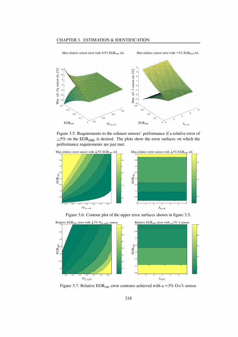
CHAPTER 3. ESTIMATION & IDENTIFICATION
0.2
0.4
0.6
0.8
0
0.1
0.2
0.3
0.4
−15
−10
−5
0
5
10
15
PSfrag replacements
O ��� �l�&�EGRrate
Max
.rel
.O
� sensorer
r,[%
]Max relative sensor error with � 5% EGRrate tol.
0
2
4
6
8
0
0.1
0.2
0.3
0.4−4
−3
−2
−1
0
1
2
3
4
PSfrag replacementsO
EGRrate
Max. rel. O sensor err, [%]
Max relative sensor error with 5% EGRrate tol.
� �l�&�EGRrate
Max
.rel
.
� sens
orer
r,[%
]
Max relative sensor error with � 5% EGRrate tol.
Figure 3.5: Requirements to the exhaust sensors’ performance if a relative error of�5% on the EGRrate is desired. The plots show the error surfaces on which the
performance requirements are just met.
0.5
1
1.5
2
2.5
3
3.5
4
0.2 0.3 0.4 0.5 0.6 0.7 0.80
0.05
0.1
0.15
0.2
0.25
0.3
0.35
0.4
0.1
0.10.1
0.5
0.5
0.5
0.5
1
1
1
1
2
2
2
3
3
3
4
4
PSfrag replacements
O ��� �l�&�
EG
Rra
te
Max relative error sensor with � 5% EGRrate tol.
0.5
1
1.5
2
2.5
3
1 2 3 4 5 6 70
0.05
0.1
0.15
0.2
0.25
0.3
0.35
0.4
0.10.10.1
0.50.50.5
111
333
PSfrag replacementsO
EGRrate
Max relative error sensor with 5% EGRrate tol.
� �l�&�
EG
Rra
te
Max relative error sensor with � 5% EGRrate tol.
Figure 3.6: Contour plot of the upper error surfaces shown in figure 3.5.
10
20
30
40
50
60
70
0.2 0.3 0.4 0.5 0.6 0.7 0.8
0.1
0.15
0.2
0.25
0.3
0.35
0.4
2
2
5
5
5
10
10
10
25
25
25
50
50
75
PSfrag replacements
O ��� �l�&�
EG
Rra
te
Relative EGRrate error with � 3% O ��� �l�&� sensor.
5
10
15
20
25
1 2 3 4 5 6 7
0.05
0.1
0.15
0.2
0.25
0.3
0.35
0.4
5 5 5
10 10 10
25 25 25
PSfrag replacementsO
EGRrate
Relative EGRrate error with 3% O sensor.
� �l�&�
EG
Rra
te
Relative EGRrate error with � 3%�
sensor.
Figure 3.7: Relative EGRrate error contours achieved with a�
3% O � / � sensor.
218
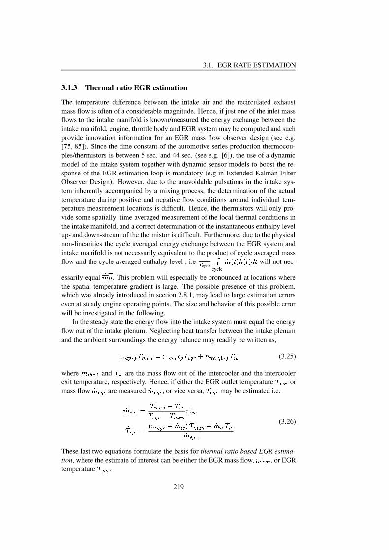
3.1. EGR RATE ESTIMATION
3.1.3 Thermal ratio EGR estimation
The temperature difference between the intake air and the recirculated exhaustmass flow is often of a considerable magnitude. Hence, if just one of the inlet massflows to the intake manifold is known/measured the energy exchange between theintake manifold, engine, throttle body and EGR system may be computed and suchprovide innovation information for an EGR mass flow observer design (see e.g.[75, 85]). Since the time constant of the automotive series production thermocou-ples/thermistors is between 5 sec. and 44 sec. (see e.g. [6]), the use of a dynamicmodel of the intake system together with dynamic sensor models to boost the re-sponse of the EGR estimation loop is mandatory (e.g in Extended Kalman FilterObserver Design). However, due to the unavoidable pulsations in the intake sys-tem inherently accompanied by a mixing process, the determination of the actualtemperature during positive and negative flow conditions around individual tem-perature measurement locations is difficult. Hence, the thermistors will only pro-vide some spatially–time averaged measurement of the local thermal conditions inthe intake manifold, and a correct determination of the instantaneous enthalpy levelup- and down-stream of the thermistor is difficult. Furthermore, due to the physicalnon-linearities the cycle averaged energy exchange between the EGR system andintake manifold is not necessarily equivalent to the product of cycle averaged massflow and the cycle averaged enthalpy level , i.e ��
cycle �cycle �� �¢¡&£0¤)�¢¡&£Z¥4¡ will not nec-
essarily equal �� ¤ . This problem will especially be pronounced at locations wherethe spatial temperature gradient is large. The possible presence of this problem,which was already introduced in section 2.8.1, may lead to large estimation errorseven at steady engine operating points. The size and behavior of this possible errorwill be investigated in the following.
In the steady state the energy flow into the intake system must equal the energyflow out of the intake plenum. Neglecting heat transfer between the intake plenumand the ambient surroundings the energy balance may readily be written as,
���¦�§P¨0§ª©d«5¦&¬® ���¯�°&±#¨0§ª©�¯�°&±�² ��´³¶µ ±0· � ¨0§ª©d¸º¹ (3.25)
where ��´³¶µ ±0· � and ©d¸º¹ are the mass flow out of the intercooler and the intercoolerexit temperature, respectively. Hence, if either the EGR outlet temperature ©�¯�°&± ormass flow ���¯�°&± are measured ���¯�°&± , or vice versa, ©»¯�°&± may be estimated i.e.¼ ���¯�°&±A ©d«5¦&¬¾½W©d¸º¹©�¯�°&±5½W©d«5¦&¬ ��´¸º¹¼©�¯�°&±A � ���¯�°&±�² ��´¸º¹R£4©d«5¦&¬¿² ��´¸º¹Z©d¸º¹���¯�°&±
(3.26)
These last two equations formulate the basis for thermal ratio based EGR estima-tion, where the estimate of interest can be either the EGR mass flow, ��À¯�°&± , or EGRtemperature ©»¯�°&± .
219
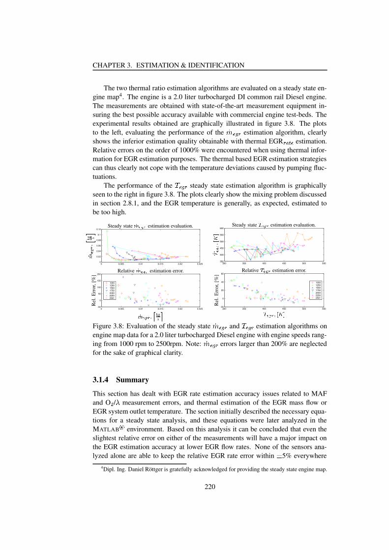
CHAPTER 3. ESTIMATION & IDENTIFICATION
The two thermal ratio estimation algorithms are evaluated on a steady state en-gine map4. The engine is a 2.0 liter turbocharged DI common rail Diesel engine.The measurements are obtained with state-of-the-art measurement equipment in-suring the best possible accuracy available with commercial engine test-beds. Theexperimental results obtained are graphically illustrated in figure 3.8. The plotsto the left, evaluating the performance of the ÁÂWÃ�Ä&Å estimation algorithm, clearlyshows the inferior estimation quality obtainable with thermal EGR Å2Æ&Ƕà estimation.Relative errors on the order of 1000% were encountered when using thermal infor-mation for EGR estimation purposes. The thermal based EGR estimation strategiescan thus clearly not cope with the temperature deviations caused by pumping fluc-tuations.
The performance of the È Ã�Ä&Å steady state estimation algorithm is graphicallyseen to the right in figure 3.8. The plots clearly show the mixing problem discussedin section 2.8.1, and the EGR temperature is generally, as expected, estimated tobe too high.
0 0.005 0.01 0.015 0.02 0.0250
0.02
0.04
0.06
0.08
0.1
0.12
0 0.005 0.01 0.015 0.02 0.025−50
0
50
100
150
200
1000125015001750200022502501
PSfrag replacements
Steady state ÉÊ Ë¢ÌZÍ estimation evaluation.
Î Ï Ð ÑÒÓ ,Ô kg s
ÕRelative ÉÊ5Ë¢ÌZÍ estimation error.
ÉÊ5Ë¢ÌZÍ , Ö kgs ×R
el.E
rror
,[%
]
300 350 400 450 500 550350
400
450
500
550
600
300 350 400 450 500 550−20
0
20
40
60
1000125015001750200022502501
PSfrag replacementsSteady state estimation evaluation.
, kgs
Relative estimation error.
, kgs
Rel. Error, [%]
Steady state Ø Ë¢ÌZÍ estimation evaluation.
Î Ù ÑÒÓ ,Ú ÛÜ
Relative Ø Ë¢ÌZÍ estimation error.
Ø Ë¢ÌZÍ , Ý Þ6ßRel
.Err
or,[
%]
Figure 3.8: Evaluation of the steady state ÁÂàÃ�Ä&Å and È Ã�Ä&Å estimation algorithms onengine map data for a 2.0 liter turbocharged Diesel engine with engine speeds rang-ing from 1000 rpm to 2500rpm. Note: ÁÂàÃ�Ä&Å errors larger than 200% are neglectedfor the sake of graphical clarity.
3.1.4 Summary
This section has dealt with EGR rate estimation accuracy issues related to MAFand O á / â measurement errors, and thermal estimation of the EGR mass flow orEGR system outlet temperature. The section initially described the necessary equa-tions for a steady state analysis, and these equations were later analyzed in theMATLAB ã environment. Based on this analysis it can be concluded that even theslightest relative error on either of the measurements will have a major impact onthe EGR estimation accuracy at lower EGR flow rates. None of the sensors ana-lyzed alone are able to keep the relative EGR rate error within ä 5% everywhere
4Dipl. Ing. Daniel Rottger is gratefully acknowledged for providing the steady state engine map.
220

3.2. INTERFACING STRATEGY AND REALITY
in the operating space. Even with sensor fusion it will be hard to improve the lowlevel EGR rate estimation accuracy, since all the estimation algorithms exhibit thesame large error sensitivity tendency at small EGR rates. When evaluating the datait can be concluded that the O å / æ based EGR control algorithm exhibits the sameerror sensitivity as the one based on the MAF sensor. However, the use of an O å / æsensor will allow for better control at small air–fuel ratios, AFR, (i.e. close to thesmoke limit) by nature of the feedback information it provides. Furthermore, itprovides for robust control of the AFR across the operating range, irrespective offuelling rate tolerances.
In the MAF/exhaust sensor analysis it is assumed that the gaseous mass flowentering the engine is known exactly, however, correct estimation of the mass flowis known to be troublesome since it depends on intake temperature and pressure,pressure difference across the engine, and the engine’s breathing behavior amongothers. Along with this it is also assumed that the fuel injection system will beable to provide an exact estimate of the fuel mass flow injected. Errors in thesetwo estimates, çè�é�ê and çè�ë , will of course have a detrimental effect on the EGRrate estimation and control schemes. Again, when using the O å / æ sensor, the AFRcontrol can be made robust with respect to the aforementioned estimation errors.
The section also concludes that EGR rate estimation based on temperature in-formation obtained by thermistors mounted in the intake air path can only be ex-pected to be of inferior quality, and are hence not applicable in high performanceEGR estimation strategies.
3.2 Interfacing strategy and reality
The automotive engine is a machine governed by a mixture of differential equa-tions in continuous time, event based equations linked to the crankshaft timing,and algebraic equations. Hence, which domain, time based or event based, shouldbe selected for off-line engine simulations is often rather a matter of taste than ac-tual science. However, the choice of domain for estimation and/or control strategydesigns is more complicated. In [111] it is concluded that the speed control of DIDiesel engines should be implemented time based for reasons of stability, whereascontrol involving flows (e.g. EGR rate control) should be implemented event basedto minimize the size of the gain scheduling maps.
A digital implementation of the individual control and estimation strategiesin the ECU is today mandatory. The reason for this is evident due to the muchbroader window of functions (some of which are unique) and flexibility, and thebetter performance/cost ratio offered by digital systems compared to analog sys-tems. The downside of the digital systems, however, is the required discretizationof the underlying control/estimation dynamics and the sampling of the continuousexogenous input signals to the different algorithms. This necessitates an analoglow pass filtering of the external signals mentioned prior to the sampling process.If this low pass filtering of the individual signals is ignored danger of data corrup-
221

CHAPTER 3. ESTIMATION & IDENTIFICATION
tion exists since some of the higher frequencies ( ìîíïªð ) of the input signal may beconvoluted into a frequencies between 0 and half the sampling frequency, íïªð . Thisphenomenon is known as signal aliasing. Thus, the signal frequencies above íïªðmust be attenuated appropriately by low pass filters, the anti-aliasing filters, beforethe input signals are quantized by the analog-to-digital converter.
One of the implementation issues arising when designing anti-aliasing filtersfor engine strategies utilizing event sampled measurements is the selection of filterbandwidth. The filter bandwidth needs to be within half the sampling frequency atengine idling if signal aliasing is to be avoided. However, such a filter bandwidthwould generally be five to nine times smaller than the bandwidth achievable atmaximum rated engine speed. Hence, the bandwidth attainable for some selectedevent-based estimation and control strategies might reduced with such a conserva-tive filter design. This problem was addressed in the SAE paper ”Avoiding SignalAliasing in Event Based Engine Control”, number 2000-01-0268 and a possible so-lution realized by a combination of time based sampling and separate digital filterdesign was provided. The paper is included in this research but was also presentedat the 2000 SAE conference held in Detroit.
222

3.2. INTERFACING STRATEGY AND REALITY
ñóò;ò;òõôRò�ö`ôRòvñ1÷;øùûú5ü6ýZþÿý������ ý������ ù�0ý�� �õý���� ý���� ú���������� ���)þ�������ý������Àü���� �1ü�! "$#&%('*)&% +-,/.�%0,21-3546%(17%08(9:�8(+-%(,<;>=�?�=@!�"23BAC+-8(%(3D#
EGFIHKJLE�FIHKMKN0O�PGQGR�M(SUTUQ�V0H0PGWYX$ZIN0OGT[Q\ 8(] 3D#�)_^53`,$92#&%(aGb2'
c`T[N0OGQ&d NUZ*eDf2QGd gITUHKM(d V(hiF*j-k$TUQGWlZ*H0m
n`o[prqIs t u[vrw xy{zU|[|[|@}*o x t ~0w q�oU�`�7�*w(o[�@oUw t �r~2�D�Iu[t ��~K~0s(�0��� � x[�
���i�D�@���l���
��Z*Q�h�W�FGJ�TUH0Q/N�FIQIVKH0FIeiM(V0HKZrV0T[R*d T[Mj FIH�TUQGRId QGT�NUFIQIV0H0FIelZ*H0T�&ZIM(TrJ5FIQ6TUgITUQIV��&ZIM(T[J6M0Z*Wi�Ge d QGR&���$��TUHKZrVKd QGR_V0O&T�NUFIQIV0HKFIeM VKHKZrV0TURIh�d QV0OGTlTUgIT[QIV�J�FIWiZ*d Q WlZrmITrM�d V��&F�M0M0d �Ge T�V0F�FI��V�Z*d QM0Z*Wi�Ge TrMlZrV�M(��T[N�d ��N�NUHKZ*QGm�M(O&Zrj V�Z*QGRIe T[Mld Q�V0OGTTUQGRId QGTN�h��N�e TI�B�2OGd NKO�d M�F*j V0TUQ J�T[M(d HKZ*�Ge T@j FIH@N�TUH(V�Z*d QN�FIQ�V0H0FIe-M V0HKZrVKTURId T[M[���QGT7F*jGVKOGT �Gd RIRIT[M V-J�d M0ZIJ�grZ*Q�VKZ*RIT[MBd Q�gIFIe gIT[J �2d VKO�TUgITUQIVC�&ZIM(T[JM VKHKZrV0TURId T[M¡d M$M0d RIQ&Z*e`Z*e d ZIM(d QGR�ZrV$e Fr�6TUQGRId QGT�M(��TUT[JGM2FIH�Z�OGd RION�FIWi�GP�VKZrVKd FIQ&Z*eB�GPGHKJ�T[QLZrV$OGd RIOGTUH2TUQGRId QGT@M(�&TUTrJGMU�c¡OGd MB�&Z*��TUH`�GH0T[M(TUQ�VKMDZ*Q T[ZIM0h�M(FIe P�VKd FIQ V0F2V0OGT Zre d Z*M0d QGR2�GH0FI���
e TUW/Z*��FrgITI�C¢ jDVKOGT JGZrVKZ��&T�V(� T[TUQiV0OGT TUgITUQ�V �&ZIM(T[JlMKZrWi�Ge T[M7d MM VKFIH0T[JlP&M(d Q&R�Z@V0d W�T �&ZIM(T[J�M VKHKZrV0TURIh���d V2d M¡M(OGFr�2Q�OGTUH0T$V0O&ZrV$ZM(PG�&M0T[£IPGTUQ�V V0HKT[ZrV0WiTUQIV¡F*jDVKOGT M0Z*W��Ge T[J�JGZrVKZ�ZIM Z@V0d W�T M(TUH0d T[MVKFIRIT�V0OGTUH �¡d V0OLZ�M(PGd VKZ*�Ge T$e F*���&ZIM0MC�&e V0TUH¡M(V0H0P&NKVKPGH0T�NUZ*Q�ZrgIF*d JZ*e d ZIM(d QGR&�
ö¥¤�¦ �@�i§l¨L©L��� ¤ § ¦
k$PGH0d QGRLV0OGT�e ZIM V�ª*«LhITrZrH�M Z*�G�Ge d NUZrVKd FIQ F*j2TUe T[NKV0HKFIQGd NiNUFIQIV0HKFIeZIM$ZiW�T[Z*Q&M¡V0F�ZINKOGd T[gIT N�T[H(VKZ*d Q�N�FIQIVKH0FIeBRIF�Z*e M¡O&ZIM2RIFIQGT j H0FIWQGFIQ�� T�¬�d M VKZ*Q�V�V0F�NUFIW��Ge T�V0TlM0FrgITUH0TUd RIQIV(hI����QGT�F*j V0OGTlH0T[ZIM(FIQ&Mj FIH2V0OGd M$N0O&Z*QGRIT j H0FIWYW�TrN0O&Z*QGd NUZ*e`N�FIQIVKH0FIe�V0FlTUe T[NKVKH0FIQGd N@N�FIQ��VKH0FIe�d M-VKF�mITUTU��PG���¡d V0O�V0OGT TUgITUH d Q&N�H0T[ZIM(d QGR�O&Z*HKJ�TUH TUWid M0M(d FIQe TURId M0e ZrV0d FIQD�$X2QFI��g�d FIP&M$T�¬GZ*Wi�Ge T�d M�X2d H�*EGPGTUeC®$ZrV0d F ¯ X$EC®$°N�FIQ�V0H0FIe�j FIH ±�¢`TUQGRId QGT[MU�`¢ Q�FIHKJ�TUHCV0F@ZINKOGd TUgIT¡WiZr¬Gd W�PGW²c¡OGH0TUT³�Z[h�´ ZrV�Z*e hGM VL¯ c¡³�´2°�T�µ�N�d TUQ&N�h�VKOGTLX$EC®¶O&ZIM�VKF���TlmITU��V�2d VKOGd Q�Z�·�¸�¹Y�2d Q&J�Fr�²Z*H0FIPGQ&J�V0OGT�M V0FId NKOGd FIW�T�VKH0d N�X$EC®²d QVKOGT2WiT[Z*QD�7±�P&N0O�ZINUN�PGHKZIN�h��¡ZIMCQGF*V �&F�MKM(d �Ge T2�2d VKOlNUZ*H0�GPGH0TUV0FIHVKT[N0OGQGFIe FIRIhI�º7e TrNKV0H0FIQGd N_W�d N�H0FI�GH0FGN�T[M0M(FIH N�FIQIVKH0FIeid M d QGOGTUH0T[QIV0e h»�&ZIM(T[J
FIQ_J�d MKN�H0T�V0T�MKZ*W��Ge d QGR�j FIH�WiZ*Q�hH0T[ZIM(FIQ&M@F*j$�2OGd NKO V(� F��2d e e��T�W�TUQ�V0d FIQGT[J_OGTUH0TI�6E`d HKM Vr� V0F�JGZrh�¼ MlN�FIQ�V0H0FIe$M V0HKZrVKTURId T[MiZ*H0TF*j2j Z*d HKe h NUFIW��Ge T�¬ Q&ZrVKPGH0T¯ VKZ*�Ge T�e F�FIm�PG�D�CQGFIQGe d QGT[Z*H�NUFIQIV0HKFIeM VKHKZrV0TURId T[M�T�VKN*� °>M(P&NKO�V0O&ZrVZ*Q5TUe T[NKV0H0FIQGd N�d W��Ge TUWiTUQIV�ZrV0d FIQ�2d VKO��GPGH0TUe h�Z*Q&Z*e FIR�J�TUg�d NUT[Mid MlQGF*Vl��F�M0M(d �Ge TI�»±�T[N�FIQ&JB� V0OGT�2d M0OVKFNKO&Z*QGRITlM(V0HKZrV0T[R*d T[M �2d V0OGFIP�ViNKO&Z*QGRId QGR�O&Z*HKJ��2ZrHKT�j FIHVKd WiT�Z*Q&JiN�F�M V H0T[ZIM(FIQ&M7M(PGRIRIT[M V�M`VKO&ZrV7VKOGT�M V0HKZrVKTURIh�M(OGFIPGe Ji�&T
½D¾[¿ ÀDÁrÂKÁ*Ã(ÄD¿ ÀBÅ ÆrÁ*Ã À Ã Å-¿ Ç$È É0½rÊrË ÌKÍ
d W��Ge TUW�T[QIVKT[J�ZIM¡NUF�J�TI�k$PGHKd QGR�V0OGT2J�TUgITUe FI�GW�T[QIVCF*jGVKF�JGZrh�¼ MDTUQGRId QGT2N�FIQIVKH0FIe�M V0HKZrV0TU�
RId T[M¡FIQGT@FIQLRIFId QGRiJ�d M0N�P&M0M(d FIQ�O&ZIM2�&TUT[QL�2OGT�V0OGTUH2VKOGT@NUF*Q�V0H0FIeM VKHKZrV0TURIh�M(OGFIPGe J��&T2d W��Ge TUW�T[QIV0TrJ�TUgITUQ�V-�&ZIM(T[JL¯ VKOGT$M0Z*W��Ge d QGRj H0Tr£IPGTUQ&N�h d M�e F�NKmIT[J�V0FTUQGRId QGT�M(�&T[T[J&° FIH V0d W�T��&ZIM(T[J�¯ N�FIQ��M V�Z*QIV�M0Z*W��Ge d QGR�j H0T[£�PGTUQ&N�h&°K� c OGT�M(PG�G�&FIH0V0TUHKM¡F*jCTUgITUQ�V2�&ZIM(T[JM VKHKZrV0TURIhI�&M(TUTlÎ Ï�Ð ��O&Z[gIT@N�e Z*d W�TrJiVKO&ZrV¡VKOGT@JGZrVKZiM0Z*Wi�Ge d QGRiZ*Q&JN�FIQ�V0H0FIe-M(OGFIPGe J��&T�d W��Ge TUW�T[QIVKT[J�TUgITUQ�V��&ZIM(T[JM(d Q&N�T�M(FIW�T�F*jVKOGT�WlZrÑ(FIH¡TUQGRId QGT�T[£�P&ZrV0d FIQ&M¡N�FIPGe Jl��T M(d Wi�Ge d �&T[JB�-c¡OGTUh�Z*e M(FN�e Z*d WÒV0O&ZrV�d V�d MLW�FIH0TQ&ZrV0PGHKZ*e$VKF�J�F�VKOGT M0Z*Wi�Ge d QGR�TUgITUQ�V�&ZIM(T[J_¯ Ó��i°$M(d Q&N�T@V0OGTiTUQGRId QGT�d VKM0TUe j¡d M�Z*QTUgITUQ�V J�H0d gIT[Q�WlZr�NKOGd QGT��Cc OGT2M(PG�G��FIH(V0T[HKM`F*jGV0d W�T¡�&ZIM(T[J�¯ �@�i°CM V0HKZrVKTURIhI�*M(T[T Î ª[Ð �Î ¸rÐ7Z*Q&J�Î ÔrÐ �BO&Z[gIT�N�e Z*d WiT[JLVKO&ZrV@M0Z*W��Ge d QGRLM(OGFIPGe J��&TUTUQ J�FIQGTP&M(d QGR@Z�N�FIQ&M VKZ*Q�V-M0Z*Wi�Ge d QGR$V0d W�TI�IM(d Q&N�T¡WlZrQ�h�VKd WiT�� NUF*Q�M VKZ*QIV�M¯ TI� R&�CM(TUQ&M(FIHBV0d W�T¡N�FIQ&M VKZ*Q�VKMK°��2d e e�M(VKZ[h N�FIQ&M VKZ*Q�V`d Q V0OGT7TUQ&R*d QGTFI��TUHKZrV0d QGRLHKZ*QGRITiZ*Q&J�VKOGTlº Õ�M0Z*W��Ge d QGRLj H0T[£�PGTUQ&N�h�W�P&M V@�&TOGd RIO�ZrV$d J�e T@M(��TUT[J�V0FiJ�TrM0N�H0d �&T V0OGT WlZ*QGd j F*e JLJ�h�Q&Z*W�d NUM2J�PGH(�d QGR V0OGH0F*V(VKe TLV0d ��� d Q�Z*Q&J�VKd ��� FIP�V��¡d V0O�M(P�µ�N�d TUQIVl�&Z*Q&J��2d J�V0O�GH0TrN�d M(d FIQD� E�PGH0V0OGTUH0WiFIH0T@d V d M�N�e Z*d WiT[JLVKO&ZrV Z*QIVKd �(Z*e d ZIM(d QGRi�&e �VKTUHKMl�¡d e e���TJGd µ�N�PGe V�V0F�J�T[M(d RIQ_j FIHlVKOGT�TUgITUQ�V��&ZIM(T[J�NUZIM(TI�M(d Q&N�T�VKOGT�M0Z*Wi�Ge d QGR�j H0T[£�PGTUQ&N�h�d M�QGF*Vi�G¬�T[J_d Q�V0d WiTI��c¡O&ZrVVKOGT e ZIM V2�GHKF*�Ge TUWYNUZ*QL��T�M(FIe gIT[Jld j`VKOGT�JGZrVKZiM0Z*W��Ge T[M2Z*H0T ZIN��£�PGd H0TrJ�VKd WiT��&ZIM(T[J�Z*Q&J�M(PG�&M0T[£IPGTUQ�V0e hlVKH0T[ZrV0TrJ�J�d RId V�Zre e hLd QZWid N�HKFI�GH0F�N�T[MKM(FIH d M2M(OGF*�¡QLd QLV0OGd M¡�&Z*��TUH[�¢ VLd Mi�¡TUe e$m�QGFr�2Q»¯ ±�O&Z*QGQGFIQD¼ MiHKPGe Tr°�V0O&ZrV�Zre e2j H0Tr£IPGTUQ&N�d T[M
Z*��FrgIT@O&Z*e j7V0OGTiM0Z*W��Ge d QGRlj H0T[£�PGTUQ&N�h���d j QGF*V M(PG�G�GH0T[MKM(T[JB���2d e e��T�j FIe J�T[J�d QIVKF_Z�j H0T[£IPGT[Q&N�h��¡d Q&J�Fr����TUe Fr��O&Z*e j VKOGT M0Z*W���Ge d QGR�j H0T[£�PGTUQ&N�hI�-c OGd MCT�Ö�T[N�V-�¡d e e&N�FIH0H0PG��V`VKOGT¡W�T[ZIM0PGH0T[J�JGZrVKZ�2OGd NKOLT[gITUQIVKP&Z*e e hld M¡V0F���T�VKHKZ*Q&M(e ZrV0T[J���hLZiN�FIQIVKH0FIe e TUH¡FIH¡O�P��WlZ*Q�FI��TUHKZrV0FIH�M(P&N0O�V0O&ZrV�Z*�G�GH0FI�GH0d ZrV0T�NUFIQIV0HKFIe$ZINKV0d FIQ&MlNUZ*Q��TiVKZ*mITUQD��E&Z*PGe V(h Z*e d ZIM(T[J JGZrVKZL�2d e e7N�T[H(VKZ*d QGe he T[ZIJV0F�TUH0H0F*�QGTUFIP&M@N�FIQ�V0H0FIe-ZINKVKd FIQ&MU�lX2e d ZIM(d QGRLd M@F*j V0TUQ�Z[gIFId J�T[J���h��&e VKTUH(�d QGR�VKOGT�M(d RIQ&Z*e M@�&TUj FIH0TiV0OGTUh�Z*H0T�M0Z*W��&e T[JB��c¡OGd M@WiT�V0OGFGJ�d M� T[e eBm�QGFr�2Qlj FIH7VKd WiT �&ZIM(TrJlMKZ*W��Ge d QGRiZ*Q&JiVKOGT@ZINKV0P&Z*eBd W��Ge T��WiTUQIV�ZrV0d FIQ�d M2TrZIM(h�M0d Q&N�T@V0OGT@�&Z*Q&J��2d J�VKO�F*jCV0OGT@�GH0TU� �&e VKTUHKM2d M�G¬GT[JB�7E�FIH$TUgITUQ�V2�&Z*M0T[J�M0Z*Wi�Ge d QGR&��OGF*� TUgITUH[��Z��GH0FI��TUH2NKOGFId N�TF*j-�GH0TU� �&e VKTUH2�&Z*Q&J��2d J�V0O�d M¡WiFIH0T@J�TUe d N[ZrV0TI�7¢ jCVKOGT@�&Z*Q&J��2d J�V0Od M@VKF�F M0WiZ*e e �CV0F�FW�P&NKO�d Q�j FIH0WlZrV0d FIQ��2d e e¡grZ*QGd M(O_ZrV�OGd RIOGTUHTUQGRId QGTLM(�&T[T[JGM�Z*Q&J VKO�P&M�e d W�d V�V0OGT�ZIN0OGd TUg*Z*�Ge Tl��TUH(j FIH0WlZ*Q&N�TF*j¡V0OGT�N�FIQIVKH0FIeCj TUT[J��&ZINKm�e F�FI�&MU��¢ j(�`FIQVKOGTlF*V0OGTUH@O&Z*Q&JB�DV0OGT�&Z*Q&J��2d J�VKOld M7NKOGF�M(TUQ�VKF�F�OGd RIOD��JGZrVKZ �2d e e&�&T�Z*e d ZIM(T[JiZrV7e F*� TUH
223

CHAPTER 3. ESTIMATION & IDENTIFICATION
×UØGÙIÚ ØG×�Û(Ü�×U×[ÝGÛUÞ�ß$×[Û(Ú ÙIØ�à*á2ÜGâ0×�ã ä&å æK×UâKÛ Ú Û�æ0çG×UâK×�á àIâ0×iØGàIâ0èlé*å å êé�ë�àIèiÜGâ0àIè�Ú Û(×�ì�×�æ(í ×U×UØ�æ0çG×iÝ�×[Û(Ú â0×�æ0à�â0×[ë�àIØ&Û æKâ0î&ëKæ$æKçG×�æ0à*æ�é*åá â0×rïIîG×UØ&ë�ê ÜGÚ ëKæ0îGâ0סéIÛ`éIëUë�îGâ�éræ0×Uå ê éIÛDÜ&à�Û0Û0Ú ìGå × éræCçGÚ ÙIçG×Uâ`×[ØGÙIÚ ØG×Û(Ü�×U×[ÝGÛ¡é*Ø&Ýlæ0çG× Ý�×[Û(Ú â0×$æ0ài×Uå Ú èiÚ Ø&éræ0× é*å Ú éIÛ0Ú ØGÙ�éræ2å à*í ×Uâ ×[ØGÙIÚ ØG×Û(Ü�×U×[ÝGÛUÞð Û(àIå î�æ0Ú àIØ�æ0à@æ0çG×$é*å Ú éIÛ(Ú ØGÙ ÜGâ0àIìGå ×[è»Ú Øi×[ñ*×[ØIæ7ì&éIÛ(×[ÝiÛ æ0âKéræK×�ã
ÙIÚ ×[Ûlí¡Ú å å�ì&×ÙIÚ ñI×UØ�Ú Ø�æKçGÚ Û�Ü&é*Ü&×[â[Þ�òGîGâ(æ0çG×UâKè�àIâ0×�Ú æ�Û(çGàIîGå Ýì�×LÛ(æKéræ0×[Ý æ0ç&éræ�æKçG×�ÙIà�é*å à*á2æ0çGÚ Û�Ü&é*Ü�×Uâ�Ú Ûió`ô&õiæKà ë�àIØ&ëUå î&Ý�×í2çG×�æKçG×Uâ2àIâ$ØGà*æ$ÝGéræ�éiÛ0é*è�Ü&å Ú ØGÙlé*Ø&ÝLë�àIØ�æ0â0àIåDÛ(çGàIîGå Ý�ì�×�Ý�àIØG××UñI×[ØIæ2àIâ¡æ0Ú è�×@ì&éIÛ(×[ÝBÞ
ö ÷�ø7ùU÷�ú`ù�û�ü
ý Ø�è�à�Û(æ�×[ØGÙIÚ ØG×�ë�àIØ�æ0â0àIå�Û(ê�Û æK×UèiÛLæKçG× èi×[é*Ø�ñré*å îG×�à*áiëU×Uâ(ãæ�é*Ú Øi×UØGÙIÚ ØG×$Ü&é*âKé*è�×Uæ0×UâKÛ`å Ú þI×2Ú ØIæKé*þI×2èlérØ&Ú á àIå Ý�ÜGâ0×[Û0Û0îGâ0×Iÿ��������é*Ø&Ý�ràIâ2é*Ú â¡èléIÛ0Û�&àrí5æ0àiæ0çG×@×UØGÙIÚ ØG×Iÿ �� ���Kÿ&é*â0× ØG×[ë�×rÛ0Û0é*â0ê�á àIâæKçG×�ë�àIè�ÜGî�æ�éræ0Ú àIØ�à*á-Ú èiÜ&àIâ(æ�é*ØIæ ë�àIØIæKâ0àIå`Û(Ú ÙIØ&é*å Û¡å Ú þI× æKçG×@á îG×UåèléIÛ0Û�&àrí@ÿ��� ��� ÿ�æKà�æKçG× ×UØGÙIÚ ØG×Iÿ�� ��� ÿ�� ���`é*Ø&Ý�� ��� Þð Ø�×��Gé*èiÜGå × àrá�çGàrí_é*å Ú éIÛ(Ú ØGÙ�ë[é*Ø�Ý�Ú Û(æ0àIâ(æ`æKçGסè�×[é*Ø�ñré*å îG× Ú Û
Û(çGà*í2Ø Ú Ø@ò`Ú ÙIîGâ0×��IÞ! çG×7ä&ÙIîGâ0×7Û0çGàrí$Û�æ í¡à$Û0é*èiÜGå × Û(×[ï�îG×UØ&ë�×[Û
0 1 2 3 4 5 6 7 8 9 100
0.5
1
1.5
2
2.5Aliasing Example
Time
Sig
nal a
nd S
ampl
es
ò`Ú Ù*î&â0×"�$#&%�×[é*Ø�ñré*å îG× Ý�Ú Û æ0àIâ0æ0Ú àIØLì�ê�é*å Ú éIÛ(Ú ØGÙ&Þá àIâ�æ0çG×�Û0é*èi×LëUàIØIæ0Ú Ø�î&à*î�Û@æ0Ú è�×�Û(Ú ÙIØ&é*å Þ' ¡çG×�ä&âKÛ æ�Û(×[ï�îG×UØ&ë�×Ú Û�Ü�×Uâ(á ×[ëKæKå ê_Ú Ø_ÜGç&éIÛ(×�í¡Ú æ0ç_æKçG×�ë�àIØ�æ0Ú Ø�îGàIî&ÛiÛ(Ú ÙIØ&é*å2é*Ø&Ý�æ0çG×èi×[é*Ø�ñ*é*å îG×LÚ Û�æ0ç�î&Û�ØGà*æ�é�(�×[ëKæK×[ÝBÞ ý Ø�æ0çG×�Û(×rë�àIØ&Ý�ëUéIÛ(×�æ0çG×ë�àIØ�æ0Ú Ø�îGàIî&Û2Û(Ú ÙIØ&é*åBÚ Û$Û(çGÚ á æK×[Ý*)+�$, ë�àIè�Ü&é*â0×rÝiæ0àiæ0çG×�Û0é*è�ÜGå Ú ØGÙ×UñI×[ØIæ[ÿGí¡çGÚ ë0ç�ë�å ×ré*â0å êiå ×[éIÝGÛ æ0àlé�è�×ré*Ø�ñ*é*å îG×@ìGÚ éIÛ[Þð èiàIâ0×�ÙI×UØG×UâKé*å`ÜGÚ ëKæKîGâ0×�à*á¡é*å Ú éIÛ(Ú ØGÙlÚ Û�ÙIÚ ñI×[Ø�Ú Øò`Ú ÙIîGâ0×.-�Þ ¡çG×�æ0àIÜ6à*á@æ0çG×ä&ÙIîGâ0×Û(çGà*í$Û�é�ÙIÚ ñI×UØ5Û0Ú ÙIØ&é*å Û(Ü�×[ëKæ0â0îGè�Þ ¡çGÚ Û-Û(Ú ÙIØ&é*å�Ú Û`ØGàrí�Û0é*èiÜGå ×[Ý@í2Ú æ0ç@æ0çG×2Û0é*èiÜGå Ú ØGÙ2á â0×rïIîG×UØ&ë�ê0/21[Þ ¡çG×�å à*í�Û0é*èiÜGå Ú ØGÙlá â0×[ï�îG×UØ&ë�ê�á àIâKëU×[Û�é*å åDá â0×[ïIîG×UØ�ë�Ú ×[Û�àIî�æKÛ0Ú Ý�×
æKçG× 3�4 ��56!7 ��56&8 í¡Ú Ø&Ý�àrí@ÿIÚ áBØGà*æ7â0×UèiàrñI×[ÝBÿ[æKà ì�×$Ý�à*í¡Ø�ã(Û0é*è�ÜGå ×[ÝÚ ØIæKà æ0çGÚ Ûlí2Ú Ø&Ý�à*í@Þ! çGÚ Ûi×�(B×[ëKæ�Ú ÛiÚ å å î&Û æKâKéræ0×[Ý_Ú Ø_æKçG×�å à*í ×UâÜ&é*â(æ�à*á$ò`Ú ÙIîGâ0×�-�Þ ý Ø&Û æK×[éIÝ à*á¡àIì�æ�é*Ú ØGÚ ØGÙ�æ0çG×�Ý�×[Û(Ú â0×[Ý�Û(Ú ÙIØ&é*åÛ(Ü�×[ëKæKâ0îGè:9 å Ú ÙIç�æ7ÙIâKé[ê�Û(Ü&×[ë�æ0â0îGè*;BæKçG×$éIëUïIîGÚ â0×[Ý�Û(Ü&×rëKæ0â0îGè»í2Ú å åì�×$Ý�Ú Û æ0àIâ(æK×[ÝiéIÛ7ÜGÚ ëKæKîGâ0×[Ý�ì�ê@æKçG×2îGÜGÜ�×Uâ Û0Ü&×[ëKæKâ0îGè<9 ÝGé*â0þ�ÙIâKérêÛ(Ü�×[ëKæKâ0îGè.; Ú Ø�æ0çG× ä&ÙIîGâ0×IÞ ¡çG×lë�àIØ&ë�å î&Û(Ú àIØ�Ú Û$æ0ç&éræ@Ú ØàIâKÝ�×Uâ$æKàLéIëKçGÚ ×UñI×rÝLæKçG×iÝ�×[Û(Ú â0×[ÝÛ(Ü�×[ëKæKâ0îGè»á àIâ7ë�àIØ�æ0â0àIåGàIâ>=@?¡ßA9 =$Ø*? à�é*âKÝ�ß$Ú é*ÙIØGà�Û æ0Ú ëUÛ�;`ÜGîGâ(ãÜ�à�Û(×[ÛUÿIæ0çG×�á â0×[ï�îG×UØ&ë�Ú ×[Û é*ì&à*ñI× �B56 ØG×U×[ÝiæKà�ì&× â0×UèiàrñI×[ÝBÞ&C�Ú Ø&ë�×Ü�×Uâ(á ×[ëKæ�ä�å æ0×[âKÛ�Ý�à�ØGà*æ�×���Ú Û æ�9 ×IÞ Ù&Þ�îGØGÚ æié*è�ÜGå Ú ä�ë[é[æKÚ àIØ�îGÜ æKà
D EF G
HI D EF
D EF G
HI D EFKJ�L MON�P Q R�S
ò`Ú ÙIîGâ0×T-+#ß$Ú Û æ0àIâ(æK×[Ý�Û0Ü&×[ëKæKâ0îGèÒérá æK×UâLÛ0é*è�ÜGå Ú ØGÙ&ÞU/21�Ú Û�æ0çG×Û0é*èiÜGå Ú ØGÙ�á âK×[ïIîG×UØ&ëUê�é*Ø&Ý�V�Ú Û æ0çG×�Û(Ü&×[ë�æ0â0îGè<é*è�ÜGå Ú æKî&Ý�×IÞ
�B56 é*Ø&ÝXWU×[â0à é*èiÜGå Ú ä�ëUéræ0Ú àIØ�àIî�æKÛ0Ú Ý�×�æKçGÚ Ûiâ0×[ÙIÚ àIØ�;Kÿ7Ú æ�Ú ÛiØGàIâ(ãèlé*å å êØG×[ë�×rÛ0Û0é*â0ê�æ0àëKçGà�à�Û(×iæ0çG×�Û0é*èiÜGå Ú ØGÙ�á â0×[ïIîG×[Ø&ë�êIÿ&/21[ÿ-éræå ×[éIÛ æY)�æ0Ú èi×[Û-çGÚ ÙIçG×UâCæKç&é*Ø�æKçGסì&é*Ø&Ý�í2Ú Ý�æ0ç�à*á�æ0çG×2å à*í�Ü&éIÛ0Û`ä&å ãæK×UâZ9 é*ØIæKÚ ã é*å Ú éIÛ0Ú ØGÙlä&å æK×Uâ�;¡æ0àLÜGâ0à*ñ�Ú Ý�×�×[ØGàIîGÙIç�çGÚ ÙIç�á â0×[ïIîG×[Ø&ë�êéræ0æ0×UØ�î&éræ0Ú àIØDÞ[ \2ù�ø�]0^@_�úO]`_Za�b"]`a�_*^ ú ¡çGâ0×U×�Ý�Ú (B×Uâ0×UØ�æ Û(àIå î�æKÚ àIØ&ÛCæ0à æKçG×$é*å Ú éIÛ(Ú ØGÙ ÜGâ0àIìGå ×Uè»â0×Uå éræ0×[Ý�æ0àæKçG×-×UñI×[ØIæDì&éIÛ(×[Ý ë�àIØ�æ0â0àIåIÛ(æ0âKéræ0×[Ù*Ú ×[ÛBé*â0×CÙIÚ ñI×UØ Ú Ø æ0çG×-á àIå å àrí2Ú ØGÙ&Þ ¡çG×»ì&éIÛ(Ú ë�Ú Ý�×[é/ì&×UçGÚ Ø&Ý<æ0çG×�ä&å æ0×Uâ�Ý�×[Û(Ú ÙIØ�Ú Û5àIî�æ0å Ú ØG×[ÝÛ0ëKçG×Uèléræ0Ú ëUé*å å ê�Ú ØLò`Ú ÙIîGâK×@cGÞU ¡çG×2ä&ÙIîGâ0×$Û0çGàrí$Û7çGàrí_æKçG× é*Ø&érãå àIÙ�Ú ØGÜGî�æ�Û�é*â0×�ä&âKÛ(æ@ÜGâ0×�ã ä&å æK×Uâ0×[Ýì�êé*ÜGÜGâ0àIÜGâKÚ éræ0×[å ê�Ý�×[Û(Ú ÙIØG×[Ýé*Ø&é*å àIÙLé*Ø�æ0Ú ã é*å Ú éIÛ(Ú Ø&Ùiä&å æ0×[âKÛZ9 ì&é*Ø&Ý�í¡Ú Ý�æ0çDÿ&/�d�e�f&g h ÿi)LàIâ èiàIâ0×æKÚ èi×[Û�Û(èié*å å ×[â2æ0ç&é*Ø�æ0çG×�Û0é*èiÜGå Ú ØGÙiá â0×[ï�îG×UØ&ë�êIÿO/�j�f�; á àIå å à*í ×[Ýì�êæ0Ú è�×lì&éIÛ(×rÝ ÛKé*è�ÜGå Ú ØGÙ&Þk ¡çG×LéIëUïIîGÚ â0×[Ý Û0é*èiÜGå ×[Û�é*âK×�æ0çG×UØá ×[Ý�æKà�Ý�Ú ÙIÚ æKé*å2ä&å æK×UâKÛUÞl çG×�ì&é*Ø&Ý�í¡Ú Ý�æ0ç�à*á$æKçG×[Û(×Lä&å æ0×UâKÛlé*â0×ëKç&é*ØGÙI×[Ý àIØGå Ú ØG×LéIÛ á îGØ&ëKæ0Ú àIØ�à*á$×UÚ æ0çG×Uâ�×UØGÙIÚ ØG×LÛ(Ü&×U×rÝBÿ&m�ÿ-àIââ0×rë�×UÚ ñI×[Ý�é*ØknY?5Ú ØIæ0×[â0â0îGÜ�æKÛUÿio�p�f � Þq ¡çG×@â0×réIÝ�×Uâ�Û(çGàIîGå ÝLØGà*æ0×æKç&éræ æ0çG×$ì&é*Ø&Ý�í2Ú Ý�æ0ç�à*áBæ0çG× Ý�Ú ÙIÚ æKé*å&ä&å æ0×UâKÛ Ý�à�×[Û7ØGà*æ¡ØG×[ë�×[Û0Û0é*â(ãÚ å ê�ç&érñI× æ0à ì�סæ0çG×$ÛKé*è�×Iÿ*ìGî�æ ëUé*Øiì&×$éIÝ�r(î&Û æK×[Ý@á àIâ7×[éIëKç�Ú ØGÜGî�æÛ(Ú ÙIØ&é*å Þq ç&Ú Û$èié*þI×rÛ¡Ú æ�Ü&à�Û0Û0Ú ìGå ×@æ0à�éIÝ�r(î&Û æ$æKçG×�ì&é*Ø&Ý�í¡Ú Ý�æ0ç�à*á×[éIëKç�ä&å æK×Uâ@Û(î&ëKç�æ0ç&éræ@àIØGå êLæKçG×iÝ�×[Û(Ú â0×[Ý�á â0×[ï�îG×UØ&ë�ê�Û(Ü�×[ëKæKâ0îGèá àIâ2×[éIëKç�Ú ØGÜGî�æ�Û(Ú ÙIØ&é*å�Ú Û2éIëUï�îGÚ â0×rÝBÞð Û�×��GÜGå é*Ú ØG×[Ý ÜGâK×Uñ�Ú àIî&Û(å ê�ÿ-Ú æiÚ Û�Ý�×[Û0Ú âKé*ìGå ×læ0ç&éræ�æKçG×LëUî�æ0à2(á â0×rïIîG×UØ&ë�ê�à*á¡æKçG×s9 Ý�Ú ÙIÚ æKé*å ;@é*ØIæ0Ú ã é*å Ú éIÛ(Ú ØGÙLä&å æ0×Uâ�ì&×�å à�ëKþI×[Ýæ0àæKçG× ×UØGÙIÚ ØG×�á â0×rïIîG×UØ&ë�ê�ÿ
/2d�e�f�t / p�fu 9B��;í2çG×Uâ0× u Ú Û7æKçG×@Ý�×[Û0Ú â0×[ÝlâKéræKÚ à�ì&×Uæ í¡×U×UØ�×[ñI×UØIæ¡ì&éIÛ0×[Ý�Û0é*è�ÜGå Ú ØGÙá â0×rïIîG×UØ&ë�ê�ÿO/ pOf ÿDé*Ø&ÝLæ0çG×�ä&å æK×Uâ ì&é*Ø&Ý�í¡Ú Ý�æ0çDÿ�/ d�e�f Þ ý æ Ú Û�â0×[ë�ãàIèiè�×UØ&Ý�×rÝ�æ0ç&éræ u Ú Ûv) àIâ-å é*â0ÙI×[â[Þ� ¡çGס×[ñI×UØIæCá â0×rïIîG×UØ&ëUêIÿw/ pOf ÿÚ Û¡ÙIÚ ñI×UØ�ì�êIÿ
/ p�f t m xOy�$z 9 -$;í2çG×Uâ0×Zm�Ú Û$æ0çG×�×UØGÙIÚ ØG×�Û0Ü&×U×[Ý�Ú Ø�â0ÜGè�ÿixOy@Ú Û$æ0çG×�Ø�îGè�ì&×Uâ à*á×UñI×[ØIæ¡ì&éIÛ(×[Ý�Û0é*è�ÜGå ×[Û7Ü�×Uâ¡×UØGÙIÚ ØG×$âK×UñIàIå î�æKÚ àIØs9 ×IÞ Ù&ÞvxOy�t|{ á àIâ)+�$, Û0é*è�ÜGå Ú ØGÙiÜ&×[â0Ú àGÝ;KÞý Ø�æ0çG× á àIå å à*í¡Ú ØGÙ$æ0çGסæ0×Uâ0è~}�� �w�.���"�0����� ���2Ú Û`î&Û0×[Ý æKà â0×Uá ×Uâ
æKà æ0çG×2á éIëKæ-æKç&éræ-æKçG×$é*å Ú éIÛ(Ú ØGÙ�ä&å æ0×[â7Ú Û7é�ç&é*â�Ý�í¡é*â0סàIâ7Û(à*á æ(í¡é*âK×
224

3.2. INTERFACING STRATEGY AND REALITY
� ����>�w��� � �B� � � � � � �B� � ����>�w��� � �
�2�B� � � �� � ¡ ¢ £� ¤ ¡k¥K¦§� � ¡� ¨ ¡ ¥ ¦§
©�ª�«
©�¬ � ® � � ¯ °± � ²³ � ´ � � µ ´ ² $� � ¯ °
¶
· ´ � ´ ® � �¸ � ¹>º � ¯ ¯2»�´ � ® � ¯
± � ²¼³ � ´ � ���� ½ �v���� �B�v�� �B� ¥ � ½ �¾2¿ � ¯
��� À Á � � ��� À Á �� à �
ª � � ® ´ � ¿ � ¿ ¯µ ´ ² ± ´ � � � �
�2� ® ´ Ä �2� ´ � ¯ ´ � � »�´ � ® � ¯
ÅvÆ Ç$ȼÉ�Ê`˼Ì&Í Î+Ï+ÈÐ@ÑqÒ�Ê�É�Ó$Ï+ÆiÎ2Ô&Õ�ÖÓ2× Î$Ç+Ø2ÙqÆ Ç$Æ Ú�Ó2×OÕ�Ö$Ú�Æ ÛBÕ�× Æ Ó$ÐBÆ Ö¼Ç*Å�Æ × Ú�Ê�É�ÜÆ Ý"Ò¼× Ê�ÝZÊ�Ö$Ú�Ê�ÏkÈ¼Ö¼Æ Ú�ÞOÆ ÖÐBÊ�É�Ú�Ê�ÏsßÊ�ÚBà�Ê�Ê�Ö Ú�á¼Ê"ÝZÊ�Ó$ÐBȼÉ�Ê�ÏsÐBÆ Ç$ÖÓ2× ÐÓ2ÖÏ.Ú�á¼Ê0â�ã>ä`Üå>á¼É�Ê�Ê@Ò¼É�Î$ÒÎwÐBÊ�Ï"æ× Ú�Ê�É>Æ Ý"Ò¼× Ê�ÝZÊ�Ö$Ú�Ó�Ú�Æ Î$ÖÐ�à�Æ × ×iß�ÊKÏ+Ê�Ð�ç�É�Æ ßÊ�ÏÆ Ö*Ú�áÊ@Ô Î$× × Î�à�Æ Ö¼ÇÜè�éBêìë`í îvïXð.ñ'ò�ówôOõ ö$ó ÷.õ ø�ùlúüû¼ýZþ�ñ�ÿvîOø� Ô+Ú�á¼ÊYÊ�Ö¼Ç$Æ Ö¼Ê�ÐBÒ�Ê�Ê�Ï��AÆ ÐOç�Î$ÖwÚ�Æ ÖwȼÎ$ÈÐB× �qÓ���Ó2Æ × Ó2ß¼× Ê�� Æ Ü Ê$ÜOÔ Î$ÉiÊ�Ó$ç�áâ��Ð�Ó2ÝZÒ¼× Ê��Þ2Ú�á¼Êqç�È+Ú�Î��.Ô É�Ê� $ȼÊ�Öç��$Þ���������Þ$Î2ÔÚ�á¼ÊqÓ2Ö$Ú�Æ Û Ó2× Æ Ó$Ð�Æ Ö¼Çæ× Ú�Ê�É*ç�Ó2ÖXß�Ê�ȼÒiϼÓ�Ú�Ê�Ï'Ó�Ú.Ê�Ó$ç�á'â��~Ê��$Ê�ÖwÚZÓ$ÐZÓ Ô È¼Öç�Ú�Æ Î$Ö'Î2ÔÊ�Ö¼Ç$Æ Ö¼Ê`ÐBÒÊ�Ê�ÏiÞ
��������� �������� ! �"��#��
! � �
å>á¼Ê�æ× Ú�Ê�ÉZßÓ2ÖÏ+à�Æ ÏwÚ�á Î$ß+Ú�Ó2Æ Ö¼Ê�ÏiÞ$��������Þ>ç�Ó2Ö ßÊ Ö¼Î$É�Ý.Ó2× Æ %�Ê�Ïà�Æ Ú�á*É�Ê�ÐBÒÊ�ç�Ú�Ú�Î0Ú�á¼Ê`ç�Î$ÖÐ Ú�Ó2Ö$Ú�å$�lÐ�Ó2Ý"Ò¼× Æ Ö¼Ç0Ô É�Ê� wȼÊ�Öç&�wÞ'��()��Þ�)*�+ �-,����� � ���������()�
� ���.���� ��()�
!
� /0
å>á¼Æ ÐKà>Ó���Î2Ô>Ï+Ê�Ð�ç�É�Æ ß¼Æ Ö¼Ç*Ú�á¼Ê0æ× Ú�Ê�É`ßÓ2ÖÏ+à�Æ ÏwÚ�áTÆ ÐKç�Î$Ö0�$Ê�Ö¼Æ Ê�ÖwÚÐBÆ Öç�ÊZÚ�á¼ÊZæ× Ú�Ê�É0ÒÓ2É�Ó�ÝZÊ�Ú�Ê�É�ÐKÐ Ú�Ó���ç�Î$ÖÐ Ú�Ó2ÖwÚKÔ Î$É"Ó�æ'1¼Ê�Ï3254 6572-8 7É�Ó�Ú�Æ ÎÜè�é 9 ë`í îvïXð.ñ'ò�ówôOõ ö$ó ÷.õ ø�ù;:=<:þ�ñ�ø�ó�>�>2îOÿ�ø*û¼ýZþ�ñ�ÿvî�ø� Ö"Ú�á¼Êqç�Ó$ÐBÊ�à�á¼Ê�É�Ê�Ú�á¼Ê�Ê�Ö¼Ç$Æ Ö¼Ê@ÐBÒÊ�Ê�ÏiÞ���ÞwÆ ÐYÖ¼Î2Ú�Ï+Æ É�Ê�ç�Ú�× ��� Ó2ÖÏç�Î$ÖwÚ�Æ ÖwȼÎ$ÈÐB× �'�Ó���Ó2Æ × Ó2ß¼× Ê$Þ¼Æ Ú@ç�Ó2Ö ßÊ0Ó2Ò¼Ò¼É�Î�1+Æ Ý.Ó�Ú�Ê�Ï*ß���ç�Î$ȼÖwÚBÛÆ Ö¼Ç�Ú�á¼Ê.ÖwȼÝ0ß�Ê�É`Î2Ô�å$�UÊ��$Ê�ÖwÚ�ÐKßÊ�ÚBà�Ê�Ê�ÖsÚBà�Î ÐBÈç�ç�Ê�Ð�ÐBÆ �$Ê.â��Ê��$Ê�Ö$Ú�Ð�Þ
�@? ����.����(A�B� C&#.� *�DFE�G C&#�� * �H.(A�
� I�à�á¼Ê�É�Ê��.()�B� C&#�� *�D.E�G C�#.� * YÆ Ð�Ú�á¼Ê`ÖwȼÝ0ß�Ê�ÉqÎ2ÔOÚ�Æ ÝZÊ0Ð�Ó2Ý"Ò¼× Ê�Ðß�Ê�ÚBà�Ê�Ê�ÖKÚ�á¼Ê�ç�ȼÉ�É�Ê�ÖwÚ�Ó2ÖÏqÚ�á¼Ê&Ò¼É�Ê��wÆ Î$ÈÐOâ��sÐ�Ó2ÝZÒ¼× Ê�Ð�Þ�Ó2ÖÏ�H.(A�Æ ÐZÚ�á¼Êsç�Î$ÖÐ Ú�Ó2ÖwÚ*Ð�Ó2ÝZÒ¼× Æ Ö¼ÇTÚ�Æ Ý"Ê$ÜAãYÎ$Ý0ß¼Æ Ö¼Æ Ö¼Ç�Ê� $ÈÓ�Ú�Æ Î$Ö3� I�à�Æ Ú�áTÊ� wÈÓ�Ú�Æ Î2ÖÐJ� @Ó2ÖÏK� L��Ç$Æ �$Ê�Ð@Ú�á¼Ê"ßÓ2Öϼà>Æ ÏwÚ�áOÞM�����-�qÞiÎ2ÔÚ�á¼Ê`Ï+Æ Ç$Æ Ú�Ó�×iæ× Ú�Ê�É�Þ¼à>á¼Æ ç�á�Æ Ö Ö¼Î$É�ÝZÓ2× Æ %�Ê�ÏZÔ Î$É�Ý ßÊ�ç�Î$ÝZÊ�Ð�Þ
�)*�+ �-,�&�-� � �.()�B� C�#.� *�D.E�G C�#.� * �HF()�
��(A�
! � �
å>á¼Ê Ï+Ê�ÐBÆ Ç$Ö'Î2Ô�Ú�á¼Ê Ï+Æ Ç$Æ Ú�Ó2×�æ× Ú�Ê�É�Ð"Æ Ð0Ú�á¼Ê�Ö ç�Î$Ý"ÒÓ2É�Ó2ß¼× Ê.Ú�ÎÚ�áÓ�Ú>Ï+Ê�Ð�ç�É�Æ ß�Ê�Ï"Æ Ö"Ú�á¼ÊqÒ¼É�Ê��wÆ Î$ÈÐ&Ð�Ê�ç�Ú�Æ Î$ÖZÊ&1ç�Ê�Ò+ÚYÔ Î$É&Ú�á¼ÊqßÓ2ÖÏwÛà�Æ ÏwÚ�á�ç�Ó�× ç�È¼× Ó�Ú�Æ Î$ÖN� Ê&1+Ò¼× Ó2Æ Ö¼Ê�Ï.Ó2ß�Î��$Ê��Ó2ÖÏ"Ú�á¼Ê@Ô Ó$ç�Ú�Ú�áÓ�Ú�Æ Ú�Æ ÐÖ¼Î2Ú0ÒÎwÐ�ÐBÆ ß¼× Ê"Ú�ΠȼÒ�ϼÓ�Ú�Ê"Ú�á¼Ê"æ× Ú�Ê�É�Ð@Ô É�Î$Ý å$�UÐ�Ó2ÝZÒ¼× Ê"Ú�ÎkåO�Ð�Ó2ÝZÒ¼× ÊP� Ê&1¼Ò¼× Ó2Æ Ö¼Ê�Ï*× Ó�Ú�Ê�É>Æ Ö*Ú�á¼Ê`ÐBÊ�ç�Ú�Æ Î$Ö)�ÜÕ Ð�ç�á¼Ê�ÝZÓ�Ú�Æ ç áÓ2É�Ï+à>Ó2É�ÊkÏ+Æ Ó2Ç$É�Ó2Ý Î2Ô`Ú�á¼Æ ÐZæ× Ú�Ê�É Æ Ð�ÐBá¼Î�à�ÖÆ ÖlÅvÆ Ç$ȼÉ�ÊQ/ÜSR�Ê�É�ÊB�.()�B� C&#�� *0DFE�G C�#.� * "Æ Ð.Ò¼É�Î��wÆ Ï+Ê�ÏXß0�
T&U V�W�X&Y Z W [0\ Y V�] ^ U _ `Y _ [a�U ` U b Y ^ c-U ^ b W d U _ `e�W Y [0f�g b�he�W Z W bi i i i j k l
m n o
m p o
qm p o
r n o
q qm p o
s
s t u
v�w&x
y u
w�z g _ b�x�]{ |}~� ��
Å�Æ Ç$ȼÉ�ÊO/ÌM�+ç�á¼Ê�Ý.Ó�Ú�Æ ç>Ï+Æ Ó2Ç$É�Ó2Ý Î2Ô)� ÖwÚ�Ê�É�É�ȼÒ+Ú�qÎ��$Ê�É�Ö¼Ê�Ï0Å�Æ × Ú�Ê�ÉBÛÆ Ö¼ÇÓ ÐBÆ Ý"Ò¼× Ê.ç�Î$ȼÖ$Ú�Ê�ÉKÖ¼Ê�ÚBà�Î$É-�iÜZå�á¼Ê.ҼȼÉ�ÒÎwÐBÊZÎ2ÔYÚ�á¼Ê.ç�Î$ȼÖwÚ�Ê�É`Æ ÐÚ�Î*ç�Î$ȼÖ$Ú�Ú�á¼Ê0ÖwȼÝ0ß�Ê�É�Î2ÔYåO�|Ð�Ó2Ý"Ò¼× Ê�Ð>ß�Ê�ÚBà�Ê�Ê�Ökâ�lÐ�Ó2ÝZÒ¼× Ê�Ð�Ü�lá¼Ê�Ö!Ó2Ö|â�� Æ Ö$Ú�Ê�É�É�ȼÒ+Ú�Æ Ð.É�Ê�ç�Ê�Æ �$Ê�ÏiÞ>Ú�á¼ÊTç�Î$ȼÖ$Ú�Ê�ÉP��Ó2× È¼ÊsÆ ÐÒ¼× Ó$ç�Ê�Ï'Æ Ö Ó2Ö Î$È+Ú�Ò¼È+Ú.É�Ê�Ç$Æ Ð Ú�Ê�É0Ô Î$× × Î2à�Ê�Ï�ß0�'Ó�ç�Î$ȼÖ$Ú�Ê�É"É�Ê�ÐBÊ�ÚÓ2ÖÏ"É�Ê�Û Ó2É�ÝZÆ Ö¼ÇÜvå�á¼ÊqÆ ÖÏ+Æ �wÆ Ï+ÈÓ2×ßÓ2ÖÏ+à�Æ ÏwÚ�áZÎ2ÔiÚ�á¼Ê�æ× Ú�Ê�É�Ð�Ó2É�ÊÚ�á¼Ê�Ö�ȼÒiϼÓ�Ú�Ê�Ï Ó$Ð>Æ Ö�Ê� wÈÓ�Ú�Æ Î$Ö�� � �Ü��Ê�ç�Ó2ÈÐBÊ&Ú�á¼ÊO������� Ô É�Ê� $ȼÊ�Öç&�Kç�Ó2ÖKÎ$Ö¼× �@ß�Ê>ç�Ó2× ç�È¼× Ó�Ú�Ê�ÏKÓ�Ú�Ú�á¼ÊÊ�ÖÏ"Î2Ô�Ê�Ó$ç�á"â�XÐB× Æ ç�Ê$Þ�Ú�á¼Ê�Ð�Ó2ÝZÒ¼× Ê�Ï0ϼÓ�Ú�ÓqÖÊ�Ê�Ï`Ú�ÎKßÊ�Ð Ú�Î$É�Ê�Ï0Æ ÖÓZß¼È0��Ê�É>Ô Î$É�ßÓ�Ú�ç�á�Ò¼É�μç�Ê�Ð�ÐBÆ Ö¼Ç"Ó�Ú>Ú�á¼ÊKÊ�ÖÏ�Î2ÔvÊ�Ó$ç�á�â��lÊ��$Ê�Ö$Ú�Ü
�lá¼Ê�Ö"Ú�á¼Ê>Ö¼Ê�1wÚ�â���Æ Ö$Ú�Ê�É�É�ȼÒ+ÚYÎ+ç�ç�ȼÉ�Ð�Þ�Ú�á¼Ê>Ô Î$× × Î�à�Æ Ö¼Ç@áÓ2Ò¼Ò�Ê�ÖÐ� Æ ÖkÓZç�Î$Ý"ÒÓ$ç�Ú�Ô Î$É�Ý��Ü� �.(A� Æ Ð�É�Ê�Ó$ÏiÜ
225
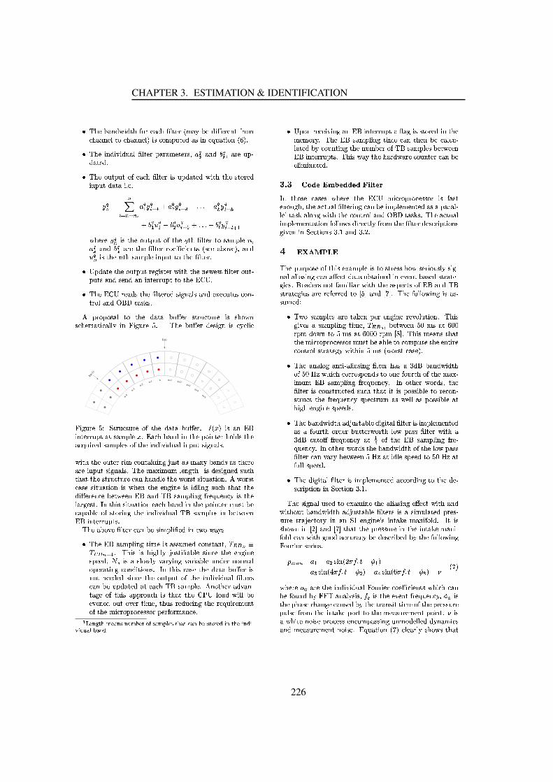
CHAPTER 3. ESTIMATION & IDENTIFICATION
�K��'���A���A�0�$� ���-�Q� �������������A� �����J� �������A���0� �)���-�����=� �-����-�A���'�'���)�-�����A���'�'��� ¡� ¢$�&����£'¤0��������¢O� �Q��¥�¤A����� ���¦� §� �¨
�K��'�P� �A�0� ©0� �0¤A�����A� �-����£A�������J�&�-����¢�ªM«0¬ ���A�K®&¬ ª����-��¤'£0¯�'���-���F¨�K��'����¤0�-£'¤0�����O�����-�N�A� �-����� ¢�¤'£F�'���-�����$� �-���-�'��¢5�-���-���� �'£'¤0�=�'������� ¨ ��¨
° ¬±J²±³
´ µ ±�¶F±�·« ¬¸ ° ¬´ ¶ ¸¡¹ « ¬º ° ¬´ ¶ º ¹;»�»�»�¹ « ¬¼ ° ¬´ ¶ ¼
¹ ® ¬¸�½F¬´ ¹ ® ¬º ½.¬´ ¶ ¸¡¹¾»�»�»�¹ ® ¬¿ ° ¬´ ¶ ¿ À ¸�O�'���-��°A¬± � ¢��-�'�J��¤0�-£'¤0���������'��Á����B�A� �-�������Q¢-���J£'� ��¡ª« ¬ ���A�K® ¬ ���-�J�-�'���A� �-���������&ÃP�&� ������¢�� ¢5���P���A��©��� �ª¡���A�½ ¬± � ¢�-�'�ÄÂ)�-�B¢-����£'� �=� �'£'¤0�$�-�����'�=�A� �-����¨
�KÅ$£)�'�������-�'����¤0��£'¤0�O�-��Æ�� ¢ �-����O� �-���-�'�=�'�����¢ ��A� �����O��¤0�5¯£'¤0��¢$���A��¢5���A�Q���P� �������-�-¤'£0�$�-���-�'�ÄÇOÈOÅĨ
�K��'��ÇÈOÅ"�������'¢����'���A� �-���-���Q¢5� Æ��A��� ¢O���A���&É0���&¤0�-��¢��&���0¯�-�-���.���A�QÊ=ËOÌ"�&��¢5Í0¢�¨
Î £'�-��£)��¢-���¦���Ï�-�'�Ð�'�����Ï�'¤0�)���Ñ¢ ���-¤A���-¤'���Ò� ¢Ó¢5�'���O�¢-���'�������-� ����� � ��� �;ÔM� Æ�¤'�-�NÕ0¨Ö�O�'�B�'¤0�)�����0��¢5� Æ��×� ¢P�&�'�&� � �
nn-1
n-3
n+1
n+4
n+5
n+2
I(n-1
)
n-4
n-2 n+3
I(n)
Ô�� Æ�¤'�-�¦Õ0Ø×Ù��-�-¤A�&�-¤'�-�N�����-�'�¦�'���&�¦�'¤0�F����¨ÛÚA� ÜF �� ¢Q���"Ç�Ë� �������-�-¤'£0�$����¢-���J£'� �=Ü�¨�Ç��������A���A��� �����'��£A��� ���-���O�'��� �'¢��-�'�����¥�¤'� �����P¢-���J£'� ��¢�����-�'�Ä� �A�0� ©�� �0¤A���.� �'£'¤0�=¢5� Æ��A��� ¢�¨�$� �����-�'�=��¤0�-�����-� �Ò�&�����&��� �'� �'ÆOÝ5¤A¢ �$��¢�J���0���A���A�'¢��¢¡���'���-����-�Ä� �'£'¤0��¢5� Æ��A��� ¢�¨O�O�'�Ä����É0� ��¤'�Ò� ���'Æ��-� ¸ � ¢$�0��¢5� Æ��'���Q¢-¤A�-����A���¡���'�=¢ �-�-¤A�&�-¤'�-�������J�A���A�0� �O���'�������¢ �¢5� �-¤A���-� ���.¨ Î ����&¢ �����¢-�P¢5� �-¤A����� ����� ¢��$�'���¦���'�P���'Æ�� �'�P� ¢�� �0� � �'Æ�¢5¤A�-���-�A�����-�'��0� �)���-���A�&�J�A�&�5������NÇË3���A�B�$Ë3¢�����£'� � �'ÆP� �-��¥�¤A���A�&�Q� ¢=�-�'�� ���-Æ���¢ ��¨�Þ �J�-�'� ¢O¢5� �-¤A����� �����������J�A���A�J� ���-�'�=£)��� ���-�����¤A¢ �O�A�����£A���'� �J����¢ �����-� �'Æ����'�P� �A�0� ©�� �0¤A����$Ëߢ�����£'� ��¢�� ���)�&�5������ÇË×� �������-�-¤'£0��¢�¨�O�'�����A��©����A� �-���$�����Q�A��¢5� �J£'� � �A����� �P�5����O���0¢�K��'��ÇË"¢-����£'� � �'ÆJ��� �J��� ¢=��¢-¢5¤'�����Q�&���A¢ ��������ªAà.á.â ±�ãàFá�â ±�¶ ¸ ¨3�O�'� ¢�� ¢��'� Æ��'� �NÝ5¤A¢ �-� �)���'� ��¢5� �A�������'�B���'Æ�� �'�¢5£A�����Fª¡ä¦ªM� ¢��Q¢-� ���O� �N©����-��� �'ÆQ©����-� ���'� ��¤'�A�0�����'���-�������£A��������� �'ÆB�����A�0� �-� ���A¢�¨QÞ �����'� ¢�����¢5�J�-�'���'�����Q�'¤0�F����� ¢�'�����'�����0���K¢5� �A�&�����'�P��¤0��£'¤0�����$�-�'��� �A�'� ©0� �0¤A����A� ������¢�����B�)��¤'£)�'�������N���=�����-���OË3¢-���J£'� ��¨ Î �'���-�'�������0©����0¯����Æ��Q���=�-�'� ¢P��£'£'�-�����-�K� ¢����A�����-�'��ÈOå�ÅÐ� �������$� � ���A���©����'���B��¤0����©������-� ����ª)����¤A¢��-���0¤A�&� �'Æ����'���-��¥�¤'� ����������������-�'���J� �&�-��£'���0�&��¢-¢-���£A���-� ���-�J���A�&��¨
æ5ç�è5é�ê-ë ì�í$è5î�é�ïFé�ð�íñ�è5ò)ó�ô0ï î�í$õ�ö è ï)ë ì�î5ë�÷5î�é�ñ�èMï ë ó&ò è5ø$ù é$ë ì�èMù é�ø�ù úû ù ø�ð�î�ö�ñ�î�é�ø
�KÅ$£A���P�-������� ©0� �'Æ����PÇËK� ���-���-�-¤'£0�$��ü)��Æ�� ¢O¢ �-���-���J� �J�-�'������J���-��¨N��'�PÇËÓ¢-����£'� � �'ÆQ��� �J�P�����N���'�����)������� ��¤0¯� ���-���J�0���&��¤'���-� �'ÆÄ�-�'�=�0¤'���A������M�$Ë;¢-����£'� ��¢��)�&�5������Ç�Ë�� �������-�-¤'£0��¢�¨¡��'� ¢��O���Ä�-�'���A�����0�O�����O����¤'���-�����������A���� � ��� �A���-���F¨
ý$þ ý ÿ ����������� ����������� � �����Þ �Û���'��¢5�3����¢5��¢K�O�'���-�"���'�3ÇOÈÅ �J� �&�-��£'�-�'�&��¢-¢-���K� ¢×� ��¢ ����'��¤'Æ��.ª����'�$���&�-¤A�����A� �-���-� �'ÆÄ�������A�O� ��£'� ���J������������¢¡��£A������� ¯� ���'�&��¢5ÍJ��� ���'ÆÄ�O� �-�J���'���&�����-�-���A���A�PÊ�ËOÌ×����¢5Í'¢�¨M�O�'��������¤A���� ��£'� ���������&����� ����� ��� � ����¢M�0� �-�����-� �=� ����� �-�'�O�A� �������0��¢-�&�-� £0�-� ���A¢Æ�� ©����P� �BÙ����&�-� ���A¢��'¨ �����A���'¨ �0¨� �� � !#"%$���O�'��£'¤'�-£A��¢5�=���.���'� ¢�&ÉA����£'� �=� ¢�-�J¢ �-����¢-¢��'���"¢5���-� ��¤A¢5� ��¢5� Æ�¯�A���F��� � ��¢5� �'Æ������P���F�����O�'���&�����0����� �'����� ����©�������A��¢5����¢ �-�����-��¯Æ�� ��¢�¨'&O�����0���&¢��'���O� ���J� � � ���$�$� ���P�-�'����¢5£A������¢O���¡ÇË;���A���OË¢ �������-��Æ�� ��¢����-���-�&� ���-�-���Q�-��( Õ*)O���A�+( ,*) ¨J�O�'��� ��� � ���O� �'Æ�� ¢Ä��¢ ¯¢5¤'�J���FØ�K����¢-����£'� ��¢�����������Í�����£)���J���'Æ�� �'���-��©���� ¤0�-� ���.¨K�O�'� ¢Æ�� ©���¢��N¢-����£'� � �AÆ���� �J��ª¡à á�â�- ªM�)�&�5������×Õ/.Q�J¢����J§�.�.�-£'�@�0���O�����QÕ��J¢=���=§�.�.�.J�-£'�0( 1�) ¨=�O�'� ¢$�������)¢O���A����-�'�O��� �&�-��£'�-�'�&��¢-¢5���.��¤A¢ �¡�A�O���'� �¡�����&����£'¤0�����-�'������-� �-��&�������-���.¢ �-��������Æ��J�$� ���'� �NÕÄ��¢Ä� �O����¢ ������¢5�� �¨
�K��'�Q���A��� ��ÆN�����-� ¯ ��� � ��¢5� �'ÆQ�A� �-���J�A��¢������'ËÓ�A���A�0�$� ���-����¡Õ/.32�4=�$�'� �����&���-�-��¢5£A���A�'¢¡�������'��� ��¤'�-�-�P���.�-�'���J��É0¯� ��¤'� Ç�ËТ-���J£'� � �'Æ�� ����¥�¤'���A����¨3Þ �×�����'���P������'¢�ª�-�'��A� �-����� ¢��&���A¢ ���-¤A���-���B¢5¤A���B�-�A���Ä� �Ä� ¢�£A��¢�¢5� �'� �Ä�����-�������0¯¢ �-�-¤A�������'��� �-��¥�¤'���A�&��¢5£)�������-¤'� ��¢Ä���� ���¢Ä£)��¢-¢5� �'� �P����'� Æ������'Æ�� �'�Ä¢5£A�����'¢�¨
�K��'���A���A�0�$� ����������Ý5¤A¢ �����'� ���0� Æ�� �������A� �-���.� ¢.� �J£'� ���������-�����¢��B� ��¤'�5�-�������0�����'¤0�5�����-����5���¦� ���Ò£A��¢-¢��A� �������$� ���K����'Ë@�&¤0�-���"� �-��¥�¤'���A�&�¾��� ¸5 ���Ä�-�'�¦Ç�ËТ�����£'� � �'Æ�� �-�&¯¥�¤'���A�&��¨MÞ �����-�'���������'¢����'���A���A�0�$� �����J���)���'��� ���×£A��¢-¢�A� �-���$�����P©����-�J�A�&�5�������Õ32�4Ä���O� �0� ��¢5£)�������-��Õ/.32�4Ä���� ¤'� �M¢5£A�����F¨
�K��'���0� Æ�� �����F�A� �����$� ¢O� ��£'� ���������-���Q�����&�����0� �'ÆÄ�����-�'���0�&¯¢-�&�-� £0�-� ����� �NÙ�������� �����'¨ ��¨
�O�'��¢5� Æ��A���.¤A¢5���P�����&É'���J� �'���-�'����� � ��¢5� �'Æ��&�F�������O� �-�B���A��$� ���'��¤0���A���A�0�$� ����������Ý5¤A¢ �&���'� �J�A� �-����¢Ä� ¢��Q¢5� ��¤'� ���-����£'�-��¢ ¯¢5¤'�-�B�-�&��Ý5�����-���-�K� �¾��� Ù�Þ����'Æ�� �'��6 ¢P� ������Í��B�����'� � ��� �F¨ßÞ �Q� ¢¢5�'���O�B� �+( ��)¡���A�7( ,�).���A�����-�'��£'�-��¢�¢5¤'�-��� �Q�-�'��� ������Í��Ä�J���'� ¯� ��� �P�����P�$� ���PÆ��0�0�������&¤'�����&�J�A�Ä�0��¢-�&�-� �A���J�0�����'��� ��� � ���O� �'ÆÔ'��¤'�-� ���$¢-���-� ��¢�ª8:9�; ± ² « ¸ ¹ « º ¢5� ��� �=<�>/?A@�B7C ¸
«�DF¢5� ��� E�<�>�?F@GB7C º ¹ « 5 ¢5� ��� §/<�>/?F@GB7CHD� ¹+I � ,�
�$�'���-��« ���-�=�-�'��� �A�0� ©�� �0¤A����Ô'��¤'�-� ���������&ÃP�&� ������¢$�$�'� ���Q������)�=� ��¤'�A�P���PÔ¡ÔM�¾���A��� �'¢5� ¢�ªJ> ? � ¢����'����©������O� �-��¥�¤'���A�&��ªHC � ¢���'�O£'�A��¢5�O�-�A���'Æ��O����¤A¢5���Ä���=���'��-�����A¢5� ����� �J����A�-�'�£'�-��¢�¢5¤'�-�£'¤'� ¢5�=� �-���Ñ�-�'��� ������Í��=£)���5��-���-�'���J����¢5¤'�-���J�����O£)��� ����¨ I � ¢�J�O�'� �-�Ä�'��� ¢5��£'�-�0�&��¢-¢���A�&����£A��¢-¢-� �'ÆJ¤'�'���'�0��� � �����0�0�A����� ��¢���A�N�J����¢5¤'�-���J�������'��� ¢5��¨�Ç¥�¤A���-� ���×� ,� =��� �����-� �N¢5�'����¢����A���
226

3.2. INTERFACING STRATEGY AND REALITY
KALJM3NPO/QSRJT M�U�UJO=KAO3V N�W:X�YJZHU[KPX[WHM�\*X�Q]M3O/T V O�NFM�U�O=K^T X/_�M*`�M*Z�ab V ZJM�NFR:M*M�U�cdNFV ZH\eM KPLJM�NPO/Q]RJT V Z bgf `PM�h YJM*ZH\ei7V NSM�h�YHO/T�KAX�KPLJMM*j�M�Z�K f `PM=h�YJM*ZH\ei kmldLJM f `PM�h YJM*ZH\eV M�NO/W:X=j�M n�o p�q3KPX�O/RJRJ`PX�r�aV QSO=KAM*T igs/o[p^q�t uHT KPM*`m\eY�KPX/v f `PM�h:k w�_dV T T�KAL YHN^W:M f X�T U�M�U�V Z KPXf `PM=h�YJM*ZH\eV M�N�WHMeKF_�M*M�Z�o[O/ZHUgn�oSp^q�k�x Z�KALJV N\*O�NFM%KPLJM3RHM*`FKAYJ`FaWHO=KAV X�Zyc:z�{ |A|/cJX f KALJM3Q]M=O/Z�j=O/T YJM�cH_dV KPLJX�Y�K%\eX�ZHNFV U�M�`PV Z b ZJX�V NFMO/ZHU[uHT KAM*`PV Z b Mev�M�\AKAN*cJ\�O/Z�WHM3U�M*`PV j�M�U O�N�c
z�{ |A|�}�~7����NFV Z�t �=���/{P�A� w�~�� �yNFV Zyt �����/{P�e��w~7� �yNFV Z�t �/���/{P�A� w}�� � NFV Z�tF~^� � wy��� � NFV Z�t ~� � w��+� � NFV Z�t ~� � w
_dLJM�`PM�A�m}��� ����
t � w
_�V KALm�A�dKALJMGKA`AO�j�M*T=KAV QSM'X f KALJM'RJ`PM=NPNFYJ`PMGRJYJT NFM f `PX�Q�KPLJM�V Z KAO/��Mj/O/T j�MGKPX�KPLJM�Q]M�O�NFYJ`AM*Q]M*Z KyR:X�V Z K�c=O/ZHU � KPLJM�U�V N KeO/ZH\eMGW:MeKF_�M*M*ZKALJM�NFMKF_�X]R:X�V Z KAN*k� V b YJ`PMd�%NFLJX/_�N�O%NFV Q3YJT O=KAM�UmV Z KAO/��MdQ[O/ZJV f X�T UmRJ`AM�NPNFYJ`PMGKA`AO=a� M�\eKPX�`Pi f X�`�M�Z b V ZJM3NFRHM*M=UJN f `PX�Q�n�o�o�o3`ARJQ�KAX ��o�o�om`ARJQ�O/ZHUWHO�\A�+O b O/V Zyk�ldLJM�RJ`PM�NPNFYJ`PM�KP`AO�\eM�LHO�NSW:M*M*Z�NFV Q]RJT V uHM�U�M�k b kKALJMQ[O/ZJV f X�T USuHT T V Z b U�i�ZHO/Q]V \*N�LHO�j�M^W:M*M*Z�ZJM b T M=\AKPM�U O/ZHUSKPLJM\eX�Me� \eV M*Z KAN�V Z M�h�Y:O�KAV X�Zgt ��w'O/`PM^O�NPNPYJQ]M�U]KAX]WHM^V ZHU�M*R:M*ZHU�M*Z�K
X f M�Z b V ZJMmX�R:M*`AO=KPV Z b R:X�V Z K�k^l�LJM�NPM3NFV QSRJT M3RJL iJNFV \*O/T�O�NPNFYJQSR�aKAV X�ZHN�O/`PM^X�ZJT i]Q[O�U�M�KPX3V T T YHN KP`AO=KAM\eT M�O/`PT imKALJMMev:M=\AK�X f NFV b ZHO/TO/T V O�NFV Z b kldLJM^u b YJ`PM\*T M�O/`PT iSNPLJX=_^NGKPLJM%O/T V O�NFV Z b RJ`PX�WJT M�Q�O=KdT X=_�M*Z�a
b V ZJMgNFRHM*M=UJN*k�l�LJV N[V N O�N[MerJRHM=\AKPM�U�NFV ZH\*M�KALJMgO/ZHO/T X b O/Z�KPV aO/T V O�NFV Z b uHT KPM*` V N�cdO�N[QSM*Z�KAV X�ZJM�U+RJ`PM�j V X�YHNFT i�c�O�U � YHN KAM�U�NPYH\PLKALHO=KSKPLJMgNFV b ZHO/T�NPRHM�\AKA`PYJQ O=K LJV b L+M�Z b V ZJM�NFR:M*M�UJN[O/`PM�RJ`PMeaNFM�`Pj�M�U O�NdO�\*\*YJ`AO=KPM*T i[O�NdRHX NPNFV WJT M k
¡ ¢S£S¤g¢3¥'¦�§y¨�£[¤ldLJV N RHO/R:M*` LHO�N�O�UJU�`PM�NPNFM=U�KALJMgO/T V O�NFV Z b RJ`PX�WJT M*Q©V Z j�X�T j�M�U_�V KAL�ª�«�NPO/QSRJT V Z b O/ZHU�LHO�N�RJ`PX�RHX NFM=USKALJ`PM*Mm¬�ZHO/T X b�/® V b V KeO/T¬�Z KPV a ¬�T V O�NFV Z b uHT KPM*`eN%KAX�NFX�T j�MSKALJV NSRJ`PX�WJT M*Q�k�¬�T TdRJ`PX�R:X NFM�UuHT KPM*`AN�NPO/QSRJT M^KALJMmUJO=KAO]O=K^O]\eX�ZHN KeO/Z�K^NPO/QSRJT V Z b KAV QSM�k'l�LJM*Z_�V KAL OmNFYJWHNFM=h�YJM*Z K�U�V b V KeO/TJuHT KPM�`PV Z b RJ`AX�\eM�NAN*c=KALJMNPO/QSRJT M�N'O/`PMRJ`PXJ\eM�NPNPM�U�t \eX�Z KPV Z YJX�YHNFT i]X�`�V Z�OmWHO=Ke\PL[QSX�U�M=w�NFYH\PLSKALHO=K�KPLJMNFR:M�\AKA`PYJQ X f M=O�\PL�NFV b ZHO/T f YJT uHT T N ¯ LHO/ZJZJX�Zy° N NPO/Q]RJT V Z b T O�_mcV k M�k c�KALHO=K[KPLJMgLJV b LJM=N K U�M�NFV `PM�U f `PM�h YJM*ZH\ei�V N[ZJX7QSX�`PM�KPL:O=ZLHO/T f KPLHM%M*j�M*Z K�WHO�NFM�U�NPO/Q]RJT V Z b]f `PM�h YJM*ZH\ei�k
± ¤�£[²#³¤�¢]¥'´%µm¦�¶ ³·�¸ ¹�º:»�¼y½+¾ ¿³À Á ªGj�M*Z K�«dO�NFM�U�k³%¢]¦�Á ª'Z b V ZJM3Â'X�Z KP`PX�TyÃ�ZJV K=k£[À]Ä�ÁmÅ Z�«�X O/`AU ® V O b ZJX NFKPV \�kµ3À[Á ldV QSMm«dO�NFM�U�kµmÆ�¢[Á ldLJ`PM*M%Ç�O�i�ÂdO=KAO/T i�N K=k
È]É ¹�Ê É:Ë�Ì Í ¾ ÎGÏ É ¹ É ½ Í�Ð=Í ¹�¾ É »�ÑÓÒ]º:»�¾ Ð/É » Ð ¾ ¿�JÔÕ Á ry° KAL�U�M*ZJX�QSV ZHO=KPX�`�\eX�Me�SM�Z�K�V Z#KALJM�hH° KPLÖU�V b V KeO/TSO/Z�KPV aO/T V O�NFV Z b uHT KAM*`�k× ÔÕ Á ry° KALmZJX�Q]V ZHO=KPX�`�\eX�Me�[M*Z�K�V Z%KPLJMdhH° KPL3U�V b V KeO=T O/Z KPV a O/T V O�NFV Z buHT KPM�`�kØ Á ¬�QSRJT V KPYHU�Mz�{ |P| Á ® Â�M*`P`PX�`�U�YJM%KPX[O/T V O�NFV Z b k�=�eÙPÚ ÁÛ UJ«Ü\eY�KAX/v f `PM�h�YJM�ZH\ei�X f KALJMSU�V b V KAO/TGO/Z�KAV aFO/T V O�NFV Z b uHT aKPM*`�c�Ý Þ�ß/à k�:á�â |Pã�eÙPÚ Á%ä X�`PQ[O/T V q*M�U Û UJ«å\eY�KAX/v f `PM�h YJM*ZH\ei�X f KPLJM�O/Z�KPV aO/T V O�NFV Z b uHT KAM*`�k�=�eÙPÚ'æ ç Á%Û UJ«�\eY�KAX/v f `PM�h YJM*ZH\ei�X f KALJMgO/ZHO/T X b O/Z KPV a O/T V O�NFV Z buHT KPM�`�=è�Ú Á ª'j�M*Z�K�WHO�NFM�U�NPO/QSRJT V Z b3f `PM=h�YJM*ZH\ei cyÝ Þ�ß/à k�/é Á ¯�O/Q]RJT V Z b]f `PM�h YJM*ZH\ei�cyÝ Þ�ß/à k�=ê Ú Á Â�X�ZHN KAO/Z K^NPO/Q]RJT V Z b]f `PM�h YJM*ZH\ei�c�Ý Þ�ß/à� Á%ë O=KPV XmW:MeKF_�M*M*Z[NFR:M�\eV u:\dLJM=O�Kd\*O/RHO�\eV KPV M�N'O=K�\eX�ZHN KeO/Z�K'RJ`PM=N a
NFYJ`PMmO/ZHU�\eX�ZHN KeO/Z�K�j�X�T YJQSM�kì èyÚ á Á ª'j�M*Z�K�WHO�NFM=U[V Z�KAM*`P`PYJR�K^O=KNPO/Q]RJT MZykì èyÚ á Á ldV Q]MmWHO�NFM�U[V Z�KAM*`P`PYJR�K^O=KNPO/Q]RJT M%Zykí Á Â�`AO/ZJ��NFLHO f K�`PM*j�X�T Y�KPV X�ZHN�RHM*`�QSV Z�Y�KPM�c�Ý îPïHð à kñ | Á%ä YJQ3W:M*`^X f NPO/QSRJT M�NdR:M*`�M*Z b V ZJM%`PM*j�X�T Y�KAV X�Zykï:ã�ò á Á x Z KAO/��M%QSO/ZJV f X�T U�RJ`PM�NPNFYJ`PM c�Ý × ��î�à kï ã�ò á�ó�ô õ Á x Z KAO/��MmQSO/ZJV f X�T U�RJ`PM�NPNFYJ`AM�cJZJX�`PQ[O/T�¬�ZHO/T X b ¬^Z�KPV a¬�T V O�NFV Z b � V T KPM�`�kï:ã�ò á�ô õ�öJõJ÷ Á x Z�KeO/��MøQSO/ZJV f X�T U©RJ`PM�NANFYJ`PM�c#¬�ZHO/T X b�/® V b V KAO/T¬�Z�KAV a O/T V O�NPV Z b � V T KPM*`�k� Ámù O�N�\eX�ZHN KAO/Z K f X�`^U�`Pi O/V `�cH�/� ��ú n=s�ûüPýeþî Á%ë O=KPV X[WHMeKF_�M�M*Z�ª�«ÓNPO/Q]RJT V Z b]f `PM�h�YJM*Z:\ei�O/ZHU uHT KPM�`^WHO/ZHU a_dV U KPLyk�e� Á ly`eO�j�M*TyKAV QSMSX f KPLJMSRJ`AM�NPNFYJ`PM3RJYJT N f `PX�QøKALJM]V Z�KAO/��M]R:X�`FKKPX]KALJM%QSM�O�NFYJ`PMR:X�V Z K�V Z KPLJMmV Z KAO/��M%QSO/ZJV f X�T U�c�Ý ÿeà k� èyÚ Á ª'j�M*Z�K�WHO�NFM�U�NPO/QSRJT MKPV Q]M cyÝ ÿeà k� ãdò á Á lyM*QSRHM�`AO=KPYJ`PM%V Z�KPLJMmV Z KAO/��M%QSO/ZJV f X�T U�cyÝ ��à k� ê Ú Á Â�X�ZHN KAO/Z K^NPO/Q]RJT MKPV Q]M�c�Ý ÿAà k� Ôá�� x ZJRJY�KdKAX3uHT KPM*`��3O=K^NPO/QSRJT M ñ k� Ôá � Å Y�KPRJY�K^X f uHT KPM�`��]O=K^NPO/Q]RJT M ñ k
227

CHAPTER 3. ESTIMATION & IDENTIFICATION
0 1 2 3 4 5 60.4
0.45
0.5
0.55
0.6
0.65
Time [s]
p man
, pm
an,E
BV
BW
, pm
an,N
EB
Comparison of normal EB sampling and EB sampling with variable BW
0 1 2 3 4 5 65
10
15
20
25
30
35
40
45
50
Time [s]
f 3dB [H
z]
Bandwidth of the digital 4. order Butterworth filter
� � ����������������� ��� ����� � ��!"���$#�!&%'!" ()��� %$�*�,+-�����,!�!"�����.���*%$/"�,0*�*� ��1' 2-������ 2 �*% 3 ��(�% 2� � � � +4% � � 2��5#6 ���4������2�� ��(�% �87:9;!�% (���� 2��< !"� � +'� 2��$=�>@?BA6C*D EGFIHJ>% 2K+L789M!�% (.��� 2���#6 �*�4% +,/"�K! ��%$NK� �.% � % !" 2���OK� �*�P�&NK% 2K+I#� +Q��� < +�% !"���,+L� 2��$=*>?BA6C*D FIHIR�HIS�T.�8���.��� �$�&� 2�*���&�� � � ���K% 2K+U!"��� #6!����$#V�*���WNK% 2K+I#6 +Q�*�5� ��*���)% +,/"�K! �*% N�� �&+I � ��% �GOK� ���,�6X % �� �$!�% !������W�,2�� 2��)!"�K�P�$+50��K% 2�� �$!:� ��� (ZY,[ [ [�����(\���� [ [ [)����(]% 2K+UNK% 0�3�% �Q% 2@T^`_�a _�bB_�c5d6_6ef Y�g)h8�� 2@> i�j"kl% 2K+�h:�Q%$��!P>Q�-7�T >Bm�7J2�� 2��6n�1I2K% (� 0P!P�B�� (.��j9�% !��,+)oJ�P�*!"�K!8h8�*% 2�3 j"p62�� � �69�% !"�$+G> q�r�s�tvu�w*x*yIzK{ x*| }�~6| �� wP��>�2��KTK� � [ �KY$�Q>KY,� � ��Tf �,g&���P2K+I�� 0�3�!P>�7�T >G� �P2K!"�P2@>G�4T >@h8���PX % � �P�,>�p)T >�Q� ���P2K!"� 2@>G��Th�T >J�@����(.���Q1 >Jn)T >J% 2K+4p�!� 3G>B�KT >Wm��U��+I�P� � 2��'� ���*���� 2Ij��% 3 ��(.% 2� � � � +.OK� � 2���+I1I2K% (� 0P!P> q�rIs�t;uKw*x*yIz�{ x*| }�~6| � wP�*>2K��TK� � [ [ �Q�I>�Y,� � ��Tf �$g&���P2K+I�� 0�3�!P>7�T >B� �P2K!"�P2@>J�-T >Jh8���PX % � �P�,>p)T >J% 2K+LoJ�,! �*�P�"j�K� � (5> ��T >Gm*h8� 2QX �P2Q�� � 2K% �Q7JX �P2Q�J9�% !"�,+&7:2�� 2��6h8� 2Q����� � > qr�s�t\uKw�x*yIzK{ x*| }G~6| � wP�*>�2��KTK� �Q[ �Q� �I>KY,� � �KTf � g&���P2K+I�� 0�3�!P>B76T >Jh8���PX % � �P�,>p&T >J% 2K+-� �P2K!"�P2@>B�4T >Wm�7JX �P2Q�9�% !��,+47J2�� 2��5h8� 2 �*��� � ���J�*% 0*�* 0P% �8�J�*� N�� �P(�!)% 2K+��Q� � �Ij�* � 2K!P> q�rIs�t\uKw�x*yIzK{ x*| }G~�| � wP��>�2��KTK�Q� [ [ [ ��>KY,� �Q�ITf �,g)h8���PX % � �P�,>�p)T��4T��WT >Io� � � +G>Kh�T��MT >�% 2K+����P2K+I�� 0�3�!PT�76T >m��:���,+I 0*�� 2��5�����U�B� �"�)p6 �.�'% !�!)�� � #�� �W�Q�7J2�� 2��,!& 2pW� ����%$�� �5h8� 2 �*��� �Bp6����� 0,%$�� � 2K!,> q'rIs�t�uKw*x*yIz�{ x*| }~6| �� wP��>�2��KT�� [ [ [$j [�Y�j [Q� � [�> � [ [ [�Tf �$gWo� � � +G>@h�T��MT >�p62K+I�,�*!"�P2@>�k.TK�BT��&T >��6�P2K+��� 0*3I!P>�76T >�% 2K+�Q�����Q#�� >K�-T >:m��@� #�% �*+�!���� N��K! ����j 2IOK2� � 15h8� 2 �*��� �G� �J% 2�I�'7:2�� 2�� � !Lp6 ��� �����P���6%$�* �K> q;r�s�t�u�w*x*yIz�{ x*| }&~6| � wP�*>2K��T@Y,� � �$j"[�Y�j [ �Q�$�K>�Y,� � ��Tf �,g)h8���PX % � �P�,>8p&T:�-TJ�&T >��U{ � w���|$z�� �J{ � � yM�J� zK� ��� }6�"��� y�ws�{ � �¡G¢KwP}�£6| � { �¤�"�Lr � | ��¥¦t8zI§ { z�w�¨�T©�:�Knª�����$!" !P>)�8�����,0*��2� 0P% ��«62� X �P��!" �"1¬� �Un��,2�(.% ��3G>.� 2K! �� ���I����� � ��p6�Ij�*� (.%$�* � 2@>�p6���KT@Y,� � ��Tf �$g&��*%$/"3 �$X�!"3Q > :T >Bm*h:� (.���I���P�6h8� 2Q����� � � �$+)7:2�� 2����'% 2K% � ��j(.�P2Q���Q1�! ���,(U>I 25+�% 2� !��@> q.�'% !"���P�,� !:�����,!" !P>������&��,0���2� j0,% �8«62� X �P�*!" � 1L� ��n��P2�(�% ��3�>� 2K! �* �*�I����� � �)p6�I�*� (.%$�� � 2@>�I�P�I�,T@Y,� �Q�IT
228
Chapter 4
Control of sign-reversal systems
This chapter is devoted to the presentation of a newly developedestimation algorithm: the sign reversal estimator. The estimatordeveloped is later applied in a control design for a V6 Dieselengine. The control problem involves the balancing of the in-take mass flow between the compressors on a twin-turbochargerequipped V6-engine. The sign-reversal point in VGT-MAF char-acteristic, who’s exact location is unknown, is found utilizing theestimation methodology developed.
4.1 Sign-reversal control
Most control strategies rely on a good a priori knowledge of the functional inter-face between the control inputs and state derivatives, or at least the sign of thetransfer function should be known. The matter of sign determination can also bereformulated as; will a change in ® lead to an increase or decrease of ¯ ? Assumingthat the system may be described by°¯²±´³-µP¯�¶�·¹¸�µP®�¶ (4.1)
this problem may be graphically illustrated as in figure 4.1.Assuming the autonomous system,
°¯º±»³-µP¯�¶ , independent of ¯ , is stable thefunctional behavior of ¸�µP®�¶ visualized in figure 4.1 is readily interpretable. First,an increase in ® will increase ¯ , which is followed by region where ¯ decreases as® increases further. Finally, passing the local minima in a left to the right mannerthe slope, ¼�½¼�¾ , is again positive. Following this trajectory the controllability ofthe dynamic system is lost twice when ¼�¿À ¾:Á¼�¾ ±Ã . Such points, where systemcontrollability is lost followed by a slope inversion in the slope characteristic, willbe referred to here as sign reversal points. If the transfer characteristics of ³-µP¯�¶and ¸�µP®�¶ are assumed known with good accuracy or more generally the system°¯²±´³-µP¯5Ä�®�¶Å ±Æ¸�µP¯5Ä�®�¶ (4.2)
229

CHAPTER 4. CONTROL OF SIGN-REVERSAL SYSTEMS
PSfrag replacements
Ç
ÈÉPÊË
Sign Reversal Problem
Local maximum,Local controllability loss point
Local minimum,Local controllability loss point
Figure 4.1: Sign reversal illustration.
is well defined, controllers based on a standard LQG (Linear Quadratic Gaussian)or ÌªÍ framework utilizing gain-scheduling techniques may readily be used, pro-vided Î-ÏPÐ5Ñ Ç�Ò ÑIÓ�ÏPÐ5Ñ Ç�Ò¤ÔÖÕ\× (4.3)
and ØÙÙÚMÛ Î-ÏPÐ5Ñ Ç�Ò
Û Ð ÜÜÜÜÜÜвÝÞÐ.ßÇ Ý Ç ß
Ñ Û Î-ÏPÐ5Ñ Ç�ÒÛ Ç ÜÜÜÜÜÜ
ÐàÝÞÐ.ßÇ Ý Ç ß
áââã are stabilizableØ
ÙÙÚlÛ Î-ÏPÐ5Ñ Ç�ÒÛ Ð ÜÜÜÜÜÜ
вÝÞÐ.ßÇ Ý Ç ß
Ñ Û Ó�ÏPÐ5Ñ Ç�ÒÛ Ð ÜÜÜÜÜÜ
ÐàÝÞÐ.ßÇ Ý Ç ß
áââã are detectable
(4.4)
Depending on the controller layout further system properties may be required (seee.g. [41, 99, 71, 24]).
In the vicinity of the sign reversal points special care must be taken to avoidchattering e.g. the controller output must be limited to Ç ß
when äJå:æ ç8è é:êäéÝìë
as longas the unlimited controller output, í ÏPî Ò , stays within a predefined signal window1.
1Controller integrator states need to be frozen when the control signal is within the predefined
230
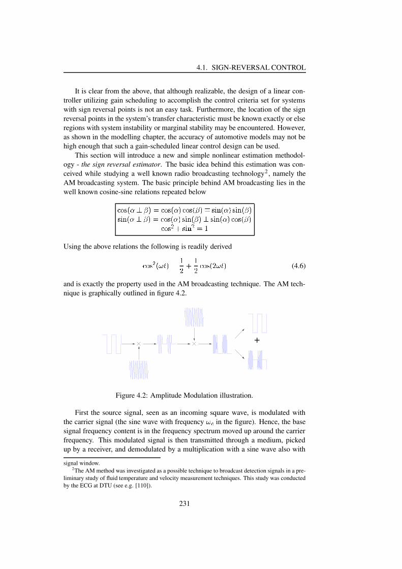
4.1. SIGN-REVERSAL CONTROL
It is clear from the above, that although realizable, the design of a linear con-troller utilizing gain scheduling to accomplish the control criteria set for systemswith sign reversal points is not an easy task. Furthermore, the location of the signreversal points in the system’s transfer characteristic must be known exactly or elseregions with system instability or marginal stability may be encountered. However,as shown in the modelling chapter, the accuracy of automotive models may not behigh enough that such a gain-scheduled linear control design can be used.
This section will introduce a new and simple nonlinear estimation methodol-ogy - the sign reversal estimator. The basic idea behind this estimation was con-ceived while studying a well known radio broadcasting technology2 , namely theAM broadcasting system. The basic principle behind AM broadcasting lies in thewell known cosine-sine relations repeated below
ï@ð6ñ:ò,óàôöõL÷4øìï@ð6ñJò,ó-÷�ï@ð6ñ8òPõL÷5ùöñKú*ûUò,ó-÷�ñKú*û5òPõL÷ñKú*ûUò,óàôöõL÷4øìï@ð6ñJò,ó-÷�ñKú*û5òPõL÷UôºñKú*ûUò,ó-÷�ï@ð6ñ8òPõL÷ï@ð6ñ�üUýþñKú*û ü ø ÿUsing the above relations the following is readily derived
ï@ð6ñ ü ò ��� ÷-ø ÿ� ý ÿ� ï@ð6ñ:ò � ��� ÷ (4.6)
and is exactly the property used in the AM broadcasting technique. The AM tech-nique is graphically outlined in figure 4.2.
PSfrag replacements
+
Figure 4.2: Amplitude Modulation illustration.
First the source signal, seen as an incoming square wave, is modulated withthe carrier signal (the sine wave with frequency ��� in the figure). Hence, the basesignal frequency content is in the frequency spectrum moved up around the carrierfrequency. This modulated signal is then transmitted through a medium, pickedup by a receiver, and demodulated by a multiplication with a sine wave also with
signal window.2The AM method was investigated as a possible technique to broadcast detection signals in a pre-
liminary study of fluid temperature and velocity measurement techniques. This study was conductedby the ECG at DTU (see e.g. [110]).
231

CHAPTER 4. CONTROL OF SIGN-REVERSAL SYSTEMS
frequency �� . The demodulated signal may now be low pass filtered, thereby re-moving the signal content around the frequency ���� , amplified, and finally thesource signal is recreated. This property may be exploited in a system identifica-tion process to acquire small signal amplitude and phase information for a dynamicsystem.
In order to apply the sign reversal estimator, only a few requirements need tobe fulfilled. When the unknown system has a sine wave on one of its inputs theoutput of interest must fulfill the following:� The system output may be represented by a Fourier series .i.e
������������������������������! "� ��� ���#�%$ �&��')(�*,+-.0/21 ' .4365 ����7 ��� ����*98 . ���! "��7 ��� �����')(&* +-.0/21;: . ���! "��7 ��� �"*9< . �(4.7)� Signal energy at the carrier frequency must exist i.e.�=' 1�>��? @ 8 1�>��?;��A : 1B>��? (4.8)� The transition function is continuous and at least one time differentiable i.e.�DCFE 1
The first two requirements insure existence of information energy at the carrierfrequency �� , and the third requirement ensures that the slope of � is well defined.
Assuming the amplitude of the sine wave imposed is small enough such thatsmall signal plant operation can be supposed, the small signal output may be ap-proximated by G �������H�IJ���! "� ��� �"*9<�� (4.9)
where the amplitude I may be interpreted as the secant of the � region excited byG �������&�LKNMO7&� ��� ��� .The next problem is the isolation of
G ������ . This problem is solved using atuned linear second order filter, referred to as a pick-up in the following, designedto attenuate frequencies around �&� . The transfer function of this filter isP
pick-up�=KQ��� RK�S�* 0TQ� . K4* � S. (4.10)
where T is the damping ratio, � . is the undamped filter frequency, and R is thefilter amplification. The filter parameters R and � . are adjusted such a way thatthe requirements in equation 4.11 are fulfilled.U P
pick-up�WV ��� � U �YX Z [ U P pick-up
�WV � � U[ �\\\\ � � ��� ��? (4.11)
232

4.1. SIGN-REVERSAL CONTROL
However, the application of this filter will shift the phase of ]N^�_�`�a somewhat, whichlater on must be considered in the b and c identification procedure. The filter willhere be referred to as a pick-up filter due to its amplitude characteristic.
The pick-up filter output is subsequently multiplied by d6egfh_ji�k#a and f�l!m"_ji�k�a ,respectively. Hence the following estimation signals are createdno^qp4r�bJf�l!m"_ji�ks`"t9cutvc)w%x)a)f�l!m"_ji�ky`�ar{z| bJd6egfh_=cut9c)w%x;a~}�z| bJd6egfh_ | i�ky`"t9cut9c)w%x;ano^g��r�bJf�l!m"_ji�ks`"t9cutvc)w%x)a)d6egfh_ji�ky`�ar z| bJf�l!m"_=cut9c)w%x;a"t z| bJf�l!m"_ | i�ky`"t9cutvc)w%x)a
(4.12)
where c)w%x is the pick-up filter phase shift mentioned at the carrier frequency i4k .These signal are subsequently low-pass filtered, thus providing the two quasi steadystate signals n^qp�r{z| bJd6egfQ_=c�t9c)w%x)an^g��r z| bJf�l!m"_=cut9c)w%x)a (4.13)
Finally, utilizing the equation above the small signal amplitude and phase shift areestimated as
nc�r����� �����Q� d6� � m�����#���6�N� }�c)w%x�} |Q��� n^qp � n^g�����
... t�� � n^qp���� � n^g�����
... } � � n^qp����nb�r �� � | ��6��O�� ¢¡ �£Q¤¥£6¦�§N¨ � nc�t9c)w%x�©«ª�¬®¯±° �Q²&³�ª�¬µ´y¯Y° ¬µ¶y¯ ²�³·²h} |Q� ° ¬¹¸s¯ ²| ��#� �º »�¡ �£Q¤¥£6¦�§N¨ � nc�t9c)w%x�© ²µ¬µ¶y¯ ° ¬®¯ ª ³ ²µ¬¹¸s¯ ° ¬µ´y¯ ª(4.14)
Due to the estimator’s construction phase shifts can only estimated within a 360 ¼window. However, most physical automotive subsystems can at best be describedas low-pass filters with a falling phase shift characteristic, and the system’s signalamplification is normally heavily attenuated after the first -180 ¼ of phase shift.Thus, it is decided to position the phase in a ½ � °#¾0¿ �q¼g½ window, since this is thephase window normally of interest for most normal control applications. However,for the sake of completeness, systems with a large time delay in the signal pathshould be mentioned. Here system amplitude characteristic may remain flat whilethe phase is undergoing large changes.
Since the sign reversal estimator does not contain any model, dynamic nornon-dynamic, providing innovation information in a broad frequency window, theestimator can only provide amplitude and phase information at one frequency only
233

CHAPTER 4. CONTROL OF SIGN-REVERSAL SYSTEMS
- the carrier frequency À�Á . However, to put it a bit philosophically; too much in-formation may equal entropy increase – it is not the amount of information thatmatters, it is the right information that matters. Increasing the number of necessaryidentification algorithmic procedure steps, prerequisites and assumptions etc. aim-ing to lower information entropy might instead unwillingly increase the entropy.
4.1.1 VGT-MAF sign reversal control
An example of a system where sign reversal may be encountered is in the trans-lation of the VGT position, ÂQÃ�Ä�Å , to engine air mass flow. Normally, closure ofthe VGT will lead to a higher fresh air mass flow, MAF, to the engine. Assumingthe EGR valve is closed, such that the EGR–VGT interaction can be neglected, aslight closure of the nozzle vanes around the turbine rotor will increase the pressuredrop across the turbine implying a potential energy increase. Assuming that tur-bine efficiency changes may be neglected, the transformation of this extra potentialenergy into kinetic energy will speed up the turbine. The faster revolution of theturbo wheel leads to an increase of the intake manifold pressure and thereby in-crease the intake port air mass flow. Furthermore, since the compressor fundamen-tally speaking is a mass flow follower the fresh air mass flow to the engine, MAF,will also be increased. The extra exhaust mass flow will increase the speed of theturbocharger further until the equilibrium ÆÇ Á�ÈuÉ®Ê�Ë Á�Ì�Í%Î�ÏNÐhÀ~Å�ÑÒÆÇ ÅOÈuÉ®Ê�Ë Å=Ó0ÅÔË Õ¥Ö isreached. However, further closure of the VGT might at some point lead to a drop inMAF although the pressure drop across the turbine is increased. This is due to thesteep slope of the nozzle ring friction. Hence, the thermodynamic power deliveredto the turbine rotor will drop, followed by decreasing turbocharger speed, intakemanifold pressure and MAF. The reader is referred to chapter 2 where the dynamicbehavior of the individual subsystems are explained.
The phenomenon just explained is graphically illustrated in figure 4.3. The fig-ure shows a × - ÂhÃ�Ä�Å 1D WAVE Ø model3 mapping of the ÂhÃ�Ä�Å –MAF characteristicsfor a V6 DI Diesel engine. The engine is equipped with two turbochargers fittedto a split intake manifold construction. The mapping was accomplished utilizing aMATLAB Ø /SIMULINK Ø –WAVE Ø maximum/minimum procedure interface devel-oped by the author.
The left upper contour plot in figure 4.3 shows the anticipated behavior of VGTclosure leading to a MAF gain can be expected independently of engine fuellingand VGT position at an engine speed of 1500rpm (revolutions per minute). Thisis as expected since the exhaust energy is relatively low at 1500rpm and lower.At an engine speed of 2000rpm the first signs of sign reversal begin to emerge.Closing the VGT below a point of approximately 0.15 will lead to a MAF decreaseinstead of the expected increase. The same behavior is also clear in the 2500rpm to3500rpm contour plots. However, a model related problem was encountered here,related to the sparse turbocharger map density in the outer operating regions of
3Dr. Arnd Sommerhoff from FFA is gratefully acknowledged for the provision of the WAVE Ùengine model, and for the discussions during the interpretation of the simulation results obtained.
234
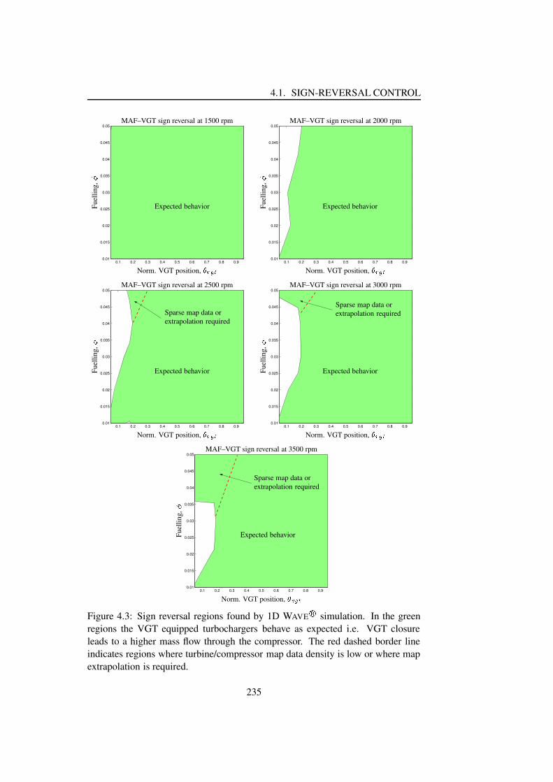
4.1. SIGN-REVERSAL CONTROL
0.1 0.2 0.3 0.4 0.5 0.6 0.7 0.8 0.90.01
0.015
0.02
0.025
0.03
0.035
0.04
0.045
0.05
PSfrag replacements
Norm. VGT position, ÚyÛ¢ÜsÝ
Fuel
ling,
Þ
MAF–VGT sign reversal at 1500 rpm
Expected behavior
0.1 0.2 0.3 0.4 0.5 0.6 0.7 0.8 0.90.01
0.015
0.02
0.025
0.03
0.035
0.04
0.045
0.05
PSfrag replacementsNorm. VGT position,
Fuelling,
MAF–VGT sign reversal at 1500 rpm
Expected behavior
Norm. VGT position, ÚyÛ¢ÜsÝFu
ellin
g,
Þ
MAF–VGT sign reversal at 2000 rpm
Expected behavior
0.1 0.2 0.3 0.4 0.5 0.6 0.7 0.8 0.90.01
0.015
0.02
0.025
0.03
0.035
0.04
0.045
0.05
PSfrag replacementsNorm. VGT position,
Fuelling,
MAF–VGT sign reversal at 1500 rpm
Expected behavior
Norm. VGT position,
Fuelling,
MAF–VGT sign reversal at 2000 rpm
Expected behavior
Norm. VGT position, ÚyÛ¢ÜsÝ
Fuel
ling,
Þ
MAF–VGT sign reversal at 2500 rpm
Expected behavior
Sparse map data orextrapolation required
0.1 0.2 0.3 0.4 0.5 0.6 0.7 0.8 0.90.01
0.015
0.02
0.025
0.03
0.035
0.04
0.045
0.05
PSfrag replacementsNorm. VGT position,
Fuelling,
MAF–VGT sign reversal at 1500 rpm
Expected behavior
Norm. VGT position,
Fuelling,
MAF–VGT sign reversal at 2000 rpm
Expected behavior
Norm. VGT position,
Fuelling,
MAF–VGT sign reversal at 2500 rpm
Expected behaviorSparse map data orextrapolation required
Norm. VGT position, ÚyÛ¢ÜsÝ
Fuel
ling,
Þ
MAF–VGT sign reversal at 3000 rpm
Expected behavior
Sparse map data orextrapolation required
0.1 0.2 0.3 0.4 0.5 0.6 0.7 0.8 0.90.01
0.015
0.02
0.025
0.03
0.035
0.04
0.045
0.05
PSfrag replacementsNorm. VGT position,
Fuelling,
MAF–VGT sign reversal at 1500 rpm
Expected behavior
Norm. VGT position,
Fuelling,
MAF–VGT sign reversal at 2000 rpm
Expected behavior
Norm. VGT position,
Fuelling,
MAF–VGT sign reversal at 2500 rpm
Expected behaviorSparse map data orextrapolation required
Norm. VGT position,
Fuelling,
MAF–VGT sign reversal at 3000 rpm
Expected behaviorSparse map data orextrapolation required
Norm. VGT position, ÚyÛ¢ÜsÝ
Fuel
ling,
Þ
MAF–VGT sign reversal at 3500 rpm
Expected behavior
Sparse map data orextrapolation required
Figure 4.3: Sign reversal regions found by 1D WAVE ß simulation. In the greenregions the VGT equipped turbochargers behave as expected i.e. VGT closureleads to a higher mass flow through the compressor. The red dashed border lineindicates regions where turbine/compressor map data density is low or where mapextrapolation is required.
235

CHAPTER 4. CONTROL OF SIGN-REVERSAL SYSTEMS
the turbocharger. This problem is already addressed in the turbocharger modellingsection. Hence turbocharger operation in this area might lead to large modelling er-rors. This is mainly noticed in the 2500rpm–3500rpm contour plots as an overratedturbine efficiency. Instead, the boundary between normal and inverted VGT oper-ation is believed to follow the red dashed line. The turbocharger maps used duringthe WAVE à simulation study could have been extended using the turbochargermodelling techniques developed in section 2.3, and thereby probably provide abetter simulation performance. However, since the simulation study is very timeconsuming4 and the existence of sign reversal has been proven, further WAVE àsimulation studies have been omitted. Furthermore, the point of sign reversal isalso dependent upon the ambient conditions, and an exact specification of whereinverted VGT operation can be expected is thus difficult to predict or map.
Simulation studies at higher engine speeds have been omitted since the maxi-mum rated turbocharger speed is reached before the point of sign reversal.
4.1.1.1 MAF Balancing
Having proven the existence of a sign reversal point in the ágâ�ã�ä –MAF characteristicthis section will illustrate how control problems arising from sign reversal pointscan be avoided when balancing the MAF between two turbochargers on a DieselV-engine.
The control problem to be presented is not only present with blue sky researchprojects but is already an issue with commercially available engines. Examples ofcommercially available passenger cars featuring a twin turbocharged engine designare the 4.0 liter V8 BMW engine, the Mercedes 4.0 liter Diesel V8 in the S400CDI, and the V6 and V105 Diesel engines manufactured by Volkswagen. All theseengines use twin turbochargers to reached their individual performance targets.The control problem to be presented is therefore of generic nature.
The V6 engine is fundamentally speaking designed like two three cylinder en-gines sharing a common crankshaft and intake manifold, and each engine bankhas its own set of sensors and actuators. The location of the engine sensors andactuators are shown in the engine illustration in figure 4.4.
The V6 Diesel engine is modelled in the MATLAB à /SIMULINK à environmentusing the zero dimensional modelling methodologies explained in chapter 2, exceptfor the turbochargers and EGR cooling system67. The turbocharger efficiency andmass flow rate of the compressor and turbine, respectively, are modelled by sin-gle polynomial regression equations. This turbocharger modelling concept caused
4The WAVE å simulation study presented used more than one week of effective simulation timeon a HP work-station
5The V10 Diesel engine is part of the engine program for the new VW Phaeton to be introduced.6The V6 Diesel MVEM was constructed from an existing model of an Diesel engine, see e.g.
[108]7Dr. Urs Christen is gratefully acknowledged for helpful discussions during the development of
the first V6 model
236

4.1. SIGN-REVERSAL CONTROL
PSfrag replacements
æNç¹è�éMAF êësì¢ísîjï ê
ë îWð ê ï êësñ�í ê ï ê
MAF òë ì¢ísîjï ò
ë îWð ê ï òë ñ�í ê ï ò
Figure 4.4: Schematically illustration of the V6 Diesel engine together with thelocation specification of selected sensors and actuators.
certain problems during the simulation study, which will be addressed later in thissection8 . Furthermore, the turbochargers used are approximately 60% too large9
and high intake manifold pressures ( ó 1.8 bar) in the mid-load engine operatingrange are inaccessible. However, despite the oversized turbochargers the sign re-versal point is present in the characteristic, and the turbocharger model is thus goodenough to prove the validity of the sign reversal control concept.
The EGR cooler’s effectiveness level and the mass flow rate through the systemare described by regression equations [108].
The V-engine design combined with the use of a bi-turbo–common manifoldstrategy might lead to certain imbalance problems between the engine banks forthe following reasons:ô If the engine is mounted in an east–west manner in the engine compartment a
difference in the ambient air temperature surrounding the two exhaust man-ifolds will inevitably exist. Furthermore, the convective heat transfer be-tween the front side exhaust manifold will be forced more strongly than theheat transfer on the engine backside. Thus, depending on vehicle speed andambient temperature the energy level in the two exhaust manifolds may bedifferent, and front side turbocharger’s speed will be lower than the backsideturbocharger’s speed. This speed difference may cause the turbocharger withthe lower speed to go into surge operation, dependent on the intake manifoldpressure.
8The problems encountered with regression based model were the motivation behind the physi-cally derived turbocharger model presented in the modelling chapter.
9The layout of the V6 was not fixed at the time the simulation study was conducted. It wastherefore decided to use the turbocharger model readily available from another Diesel engine model.
237

CHAPTER 4. CONTROL OF SIGN-REVERSAL SYSTEMS
õ Due to packaging restrictions the design of the individual throttle bodies maybe significantly different in both volume and shape posing both transient andsteady state balancing issues between the two engine banks. One issue couldbe a significant difference in the breathing behavior between the two enginebanks.õ Since the intake manifold is shared a normal speed density strategy can onlyestimate the total mass flow to the engine. This may lead to an EGR imbal-ance between the banks, since the normal speed density-MAF based EGRestimation strategy can only provide an estimate of the total EGR mass flowto the engine and not how the EGR mass flow, ö÷Fø¢ù�ú is distributed betweenthe two banks.õ In the case where a significant EGR imbalance between the banks exists,despite non-discriminating VGT control, danger of turbocharger surge ispresent due to the significant difference in the energy flow through the in-dividual VGTs.
Two of the imbalance issues above concerns the danger of surge. One way (ne-glecting the relative small pressure drop difference between the throttle bodies andthe possible difference between the compressors) to minimize the danger of oneturbocharger pushing the other turbocharger into surge operation is to insure thatthe speed of the turbochargers are kept at the same value. However, a direct mea-surement of the turbocharger speed is normally not available. A way to overcomethis problem is by controlling the air mass flow through each compressor, since, ifthe differences in the upstream conditions may be neglected and the compressors’performances are in the close vicinity of each other, controlling the mass air flowthrough each compressor would be equivalent to turbocharger speed control.
Control Problem FormulationIn the following the design of a MAF balancing controller capable of eliminatinga possible steady state MAF difference between the engine banks will be outlined.
Eliminating a possible MAF error will minimize the danger of one turbochargerpushing the other turbocharger into surge operation. However, the control problemis difficult due to a possible presence of a sign reversal point in the û;ü ù�ý –MAF char-acteristic. This control problem is further made worse by the fact that the existenceand location of the point of sign reversal is very difficult to forecast. However, withthe sign reversal estimation methodology explained earlier in section 4.1 and pro-vided the VGT actuators have a reasonably small dead-band, it will be shown thatthe sign reversal point may be estimated and used to toggle the controller outputsign. Although it would be possible to eliminate an eventual MAF error by onlydiscriminating the base VGT signal from the boost pressure control strategy on oneof the VGTs, such a control strategy would pose problems. When a fully opened orfully closed VGT position is reached, system controllability would be lost. Instead,the VGT base position from the ECU, û0ü ù�ýÔþ ÿ , will be offset on both VGTs, thereby
238

4.1. SIGN-REVERSAL CONTROL
providing a broader window of system controllability. A schematic block diagramof the VGT position offset controller is shown in figure 4.5.
PSfrag replacements
-MAF �MAF � MAF Balancing
Controller
-1
1
sign���� ���
sign���� ���
sign���� ���
sign���� ���
� �
��� ���� ���� ���� �
�� �� ���� ��� �� ���� � �� ���� � �� ���� �Figure 4.5: Block diagram of the VGT balancing controller setup.�
– � EstimationIn order to determine the direction of control the sign of the ������� –MAF DC ampli-fication must be estimated. Initially different ARX (Auto Regressive eXogenous)adaptive model structures (up to fourth order) together with an imposed squarewave ( ����� � �!�"�����$# %�&('�) ) on the VGT reference position were investigated as a meansto determine the control direction i.e.
sign *,+�.-0/sign
1 +243,5 +2(6�7�8 6 5 +249:7�8 9 �:�:�; 5 +< 6�7 8 6 5 +< 9=7 8 9 5 �:�:�">>>>> 7 / ;!? (4.15)
However, the individual coefficient estimates were found to vary significantly de-spite quasi-steady state engine operation and therefore were not suited for DC gainestimation. Hence, further investigation of linear adaptive estimation strategies wasnot carried out. Instead, the nonlinear sign reversal estimator is used for control di-rection estimation.
PSfrag replacements
��� ���� �A@B�� �� �� +
+
Excitation sine wave
MAF� � �DCFE � �� �� � � � #�G �
MAF
pick-up filter
Demodulation Signal
Demodulation Signal (-90 H )
Low pass filter
Low pass filter
�I=J�I�K L –
�est.
�� �LFigure 4.6: Illustration of the VGT-MAF sign reversal detection scheme for thesmall signal amplitude and phase.
239

CHAPTER 4. CONTROL OF SIGN-REVERSAL SYSTEMS
Figure 4.6 illustrates the implementation of the estimator used for each enginebank. The control signal for the individual VGT has an excitation sine wave offrequency M0N added to it. This excitation signal is later, after travelling through thesystem, isolated by a pick-up filter tuned to the frequency MON , followed by indi-vidual multiplications with sine and cosine waves, and sent to the P - Q estimationalgorithm. The amplification sign is finally computed as
sign RTSP�UWV sign R SQFXZY[U (4.16)
Due to a relative large intake manifold volume it was decided to locate the carrierfrequency, M0N , at the same frequency of 2 Hz for both banks, such that the esti-mation algorithms’ response times are the same. Cross talk problems between thealgorithms was anticipated but not encountered during simulation.
Base Control DesignThe basic MAF balancing controller is a simple PI (Proportional–Integral) con-troller. The block diagram of the controller is shown in figure 4.7. The controlleris seen to consist of two integrators and one proportional gain. The two integratorsmay be enabled and disabled using the \^]`_"a�b(ced switch and provide a method toavoid integrator wind-up.
When a control direction sign reversal is detected the individual integrator isreset through the f switch. During reset, special care must be taken when re-initializing the individual integrator to insure a bumpless transfer from one opera-tion mode to the other i.e.g"h"i�j�k$l m V g"h"i�j�k$l m"n[oprq:s l m VutwvyxTz{vy| m X}| m"n[o4~ X q m"n[o4~ (4.17)PSfrag replacements
��
����������� �sign ��������
��� ������� �sign � ������
��� � �
� � � �
� �
� �
� �
� �MAF � =MAF
�-MAF
�, � gs � ���
������
Figure 4.7: MAF balancing controller.
240

4.1. SIGN-REVERSAL CONTROL
Carrier frequency, �,� 2 HzDamping ratio, � 0.05
Modulation depth, ��� 0.05Low pass filter type Butterworth
Low pass filter order 4Low pass filter break freq. 1 Hz
Proportional gain, ¢¡ 1Integration gain, ¤£ 5
Table 4.1: Setting of SR estimation parameters.
Logic implementationThe level of logic needed to control the integrators is limited, and basically onlyconsists of two block, reset logic and freeze (hold) integrator logic.
The reset logic simply compares the estimated amplitude sign between neigh-boring samples i.e. ¥.¦¨§
sign ©,ª�.«�¬¤¦ sign ©,ª�.«�¬"®[¯�° (4.18)
Hence, every time the sign changes the individual integrator is reset and re-initializedwith the value ±(²4³ ¬
Furthermore, the range of control signal, ´¶µ�·�¸ ³ ²O¹Zº ´"µ�·�¸ , has been reduced by ahalf of the amplitude of the excitation sine wave in each end of the control signalwindow. This is mandatory for the excitation sine wave to prevail independently ofthe control signal.
Since the offset sign of the individual VGT discrimination signal is alreadyknown, the enable/disable logic algorithm will be same for each integrator. Thealgorithm is listed in equation 4.19.»=¼ ½�¾ ¦ ©$´"µ�·�¸,¿À�Á�=«� §
sign ©0ª�B«OÃÀĶ°.ÂÅ© MAF �{¿ÀÄ�«»=Æ £Ç· Æ ¦ ©$´"µ�·�¸,ÈÀ´"µ�·�¸ ³ ÉOÊ�ËBÌ �Á�=«Í §sign ©,ª�.«ÏÎÀĶ°.ÂÅ© MAF �{ÈÀÄ�«Ð ¦
NOT © »=¼ ½�¾ ¹ »=Æ £Ç· Æ « (4.19)
The first condition checks if the minimum ´¶µ�·�¸ has been reached and the º ´!µ�·�¸control direction. If the control algorithm requests an opening of the VGT this willbe allowed, however, further closure of the VGT will be prohibited. The oppositerules are valid when ´!µ�·�¸ has reached the upper VGT position limit.
Simulation studyIn order to verify the functionality of the sign reversal estimator together with theMAF balancing control strategy, several simulations with engine model presentedin the beginning of section 4.1.1.1 are made in SIMULINK Ñ . The value of someof the simulation parameters are given in table 4.1: The 2Hz carrier frequency isinitially selected since it is assumed the frequency is well below the bandwidth of
241

CHAPTER 4. CONTROL OF SIGN-REVERSAL SYSTEMS
the system. The MAF sensors (see e.g [6]) and VGT position actuator’s dynamicsare approximated by first order low-pass filters with a response time of 15ms and100ms, respectively.
As a test sequence 430 seconds of the EUDC was chosen. However, due to theoversized turbochargers the velocity reference input to the engine speed controlleris raised by 30% to insure a reasonable excitation of the turbochargers.
The base VGT control signal is acquired from a experimental mapping of a2.0 liter Puma engine running a EUDC. The EUDC mapping has been discussedearlier in section 2.11. This base trajectory will naturally not be the same as thesignal computed by the final calibrated V6 ECU, however it provides a realisticbase signal input to the VGTs and spans the complete control input range of theVGTs. Furthermore, the simulations are performed without EGR to avoid crosstalk between the EGR system and the turbocharger system.
The control problem is created by reducing the right engine bank’s volumet-ric efficiency by 10%, thereby lowering the thermodynamic power available to theright bank VGT. This problem is selected since it both affects the exhaust temper-ature and the mass flow through the turbine. This is equivalent to control scenariosin which large temperature gradients between the exhaust manifolds exist, or whena significant difference in the bank breathing behavior is present
Figure 4.8 shows the simulation results obtained with the MAF balancing con-trol strategy and the SR estimation algorithm enabled. The red and blue curvesillustrate the right and left bank simulation results, respectively. The engine speedis seen to vary between approximately 1000rpm and 3000rpm. Below the enginespeed trace the intake manifold pressure is seen. The curve clearly shows the ef-fect of the oversized turbochargers resulting in a rather low boost pressure. Theproblems with the regression equation based turbocharger model are also evident,since the pressure is too large close to idle speed. Hence, the compressor modelclearly overestimates the compressor mass flow here. Furthermore, the compressorefficiency is rather underestimated in the vicinity of such engine operating pointsand expresses itself as a too high intake temperature. It should here be note thatno intercooler model is used in the simulation, and the intake temperature is thusgenerally high. Just below the intake manifold temperature the port mass flow forthe individual bank is plotted, clearly showing the effect of the 10% volumetricefficiency difference between the engine banks.
The estimated amplitude and phase shift of the VGT–MAF system is graphi-cally illustrated in the lower left corner of figure 4.8. The estimated amplitude, ÒÓ ,is for both banks generally low during low load–low speed engine operation. Thisis as expected since the thermodynamic exhaust power is low during such opera-tions, and the MAF sensitivity to VGT movements is thus small. During the first 60seconds of the simulation the engine experiences a series of relatively fast tip-insand tip-outs. The effect of this on the SR estimation is especially clear in the phaseshift detection. Here, the phase shifts in a rather oscillatory manner. Between 250and 370 seconds the engine speed is raised by a factor of two, and together withsome rapid VGT tip-ins, this leads to a higher boost pressure. Due to the larger
242

4.1. SIGN-REVERSAL CONTROL
0 50 100 150 200 250 300 350 400 450500
1000
1500
2000
2500
3000
3500
0 50 100 150 200 250 300 350 400 45095
100
105
110
115
120
125
PSfrag replacements
Engine speed
N,[
rpm
]
Intake pressure
Time, [s]
Ô ÕÖ× ,[kPa]
0 50 100 150 200 250 300 350 400 4501
2
3
4
5
6
7
0 50 100 150 200 250 300 350 400 4500
1
2
3
4
PSfrag replacements
Engine speed
N, [rpm]
Intake pressure
Time, [s]
, [kPa]
Air-Fuel ratioØFuel flow
Time, [s]
Ù Ú Û ÜÝÞ ,ß g s
à
0 50 100 150 200 250 300 350 400 450200
400
600
800
1000
0 50 100 150 200 250 300 350 400 45090
100
110
120
130
140
150
PSfrag replacements
Engine speed
N, [rpm]
Intake pressure
Time, [s]
, [kPa]
Air-Fuel ratio
Fuel flow
Time, [s], g
s
Exhaust Temperatureá Ýâã ,[K]
Exhaust Pressure
Time, [s]
Ô Ýâã ,[kPa]
0 50 100 150 200 250 300 350 400 450290
300
310
320
330
340
0 50 100 150 200 250 300 350 400 4500.01
0.015
0.02
0.025
0.03
0.035
0.04
0.045
PSfrag replacements
Engine speed
N, [rpm]
Intake pressure
Time, [s]
, [kPa]
Air-Fuel ratio
Fuel flow
Time, [s], g
s
Exhaust Temperature
, [K]
Exhaust Pressure
Time, [s]
, [kPa]
Intake Temperatureá ÕÖ× ,[K]Intake port mass flow
Time, [s]
Ù Ú Öä ,[kPa]
0 50 100 150 200 250 300 350 400 450−40
−30
−20
−10
0
10
20
30
0 50 100 150 200 250 300 350 400 450−300
−250
−200
−150
−100
−50
0
PSfrag replacements
Engine speed
N, [rpm]
Intake pressure
Time, [s]
, [kPa]
Air-Fuel ratio
Fuel flow
Time, [s], g
s
Exhaust Temperature
, [K]
Exhaust Pressure
Time, [s]
, [kPa]
Intake Temperature
, [K]
Intake port mass flow
Time, [s]
, [kPa]
Estimated VGT–MAF amplitude.å æ ,
ß g s
çè éàEstimated VGT–MAF phase shift.
Time, [s]
å ê ,
ë ìí 0 50 100 150 200 250 300 350 400 4500
0.2
0.4
0.6
0.8
1
0 50 100 150 200 250 300 350 400 4500
50
100
150
200
PSfrag replacements
Engine speed
N, [rpm]
Intake pressure
Time, [s]
, [kPa]
Air-Fuel ratio
Fuel flow
Time, [s], g
s
Exhaust Temperature
, [K]
Exhaust Pressure
Time, [s]
, [kPa]
Intake Temperature
, [K]
Intake port mass flow
Time, [s]
, [kPa]
Estimated VGT–MAF amplitude.
, gs
Estimated VGT–MAF phase shift.
Time, [s]
,
VGT position.î�ïðñTorque Load
Time, [s]
ò ó ,[Nm]
Figure 4.8: Simulation results obtained with the MAF balancing strategy and theSR estimation strategy enabled. The red and blue curves depict the right and leftengine bank results, respectively. The actual sign control is depicted in the lowestleft plot in the figure. Every time one of phase estimates crosses the -180 ô limit(dashed line) the corresponding sign is toggled.
243

CHAPTER 4. CONTROL OF SIGN-REVERSAL SYSTEMS
thermodynamical power available to the turbine the VGT excitation signal propa-gation becomes pronounced. This is especially seen on the estimated amplitudes,õö
, which are raised by almost 30dB. However, the amplitudeõö
is much lower thanexpected and the phase change is the opposite of the expected. Hence, the carrierfrequency of 2 Hz is apparently above the system bandwidth. However, assumingthe structure of the system’s amplitude and phase shift characteristics are main-tained, this does not influence the sign reversal detection algorithm. Instead, thethreshold is changed to
sign ÷ õöÁø^ùuúsign ÷ õûýüZþ ø
(4.20)
and the SR algorithm thus still provides a correct estimate of the control direction.Of course the carrier frequency ÿ�� could be lowered, but this would effect theestimation speed negatively.
The discrimination between the individual VGT positions is clear on�������
tracesalso shown in figure 4.8, and as expected the right bank VGT needs to be closedmore due to the lower exhaust mass flow.
Figure 4.9 shows the simulation results obtained with no balancing control,MAF balancing control and excitation but the sign reversal algorithm disabled, andMAF balancing control, excitation and SR detection. The plots where no balancingcontrol is implemented clearly show a difference between the MAFs during mod-erate boost pressures. However, during the engine idling or low load scenarios theerror is negligible as expected due to the low exhaust energy available. Thus, theturbochargers are more or less inactive.
The mid section of figure 4.9 depicts the results obtain with the PI balancingcontroller implemented but with the SR algorithm disabled. The figures clearlyshow how the system becomes unstable in the regions where the control directionis the opposite of the expected. Between 300 and 430 seconds the control directionreturns to normal and the MAF error between the banks is minimized.
In the last part of figure 4.9 the SR algorithm provides an estimate of the controldirection. Using this estimate to toggle the control direction of the MAF balancingcontroller clearly improves the control performance. The scatter in the MAF errorbetween 70 and 170 seconds on the MAF error trace is not due to the detectionalgorithm. This is seen by comparing the estimated phase shift in figure 4.8 withthe MAF error trace, since the chatter frequency is much higher than both the signshift and excitation frequency. Instead, the chattering is believed caused by internaldiscontinuities in the turbocharger model.
Figure 4.9 clearly proves the sign reversal estimators ability to correctly assessthe control direction.
Implementation IssuesImplementation of the MAF balancing strategy may cause certain problems sum-marized below.
244

4.1. SIGN-REVERSAL CONTROL
0 50 100 150 200 250 300 350 400 45010
15
20
25
30
35
40
45
0 50 100 150 200 250 300 350 400 450−4
−2
0
2
4
6
8
PSfrag replacements
MAF without balancing control.
MA
F
� ,MAF , g s
�MAF error
Time, [s]
MA
F
� , g s
�
0 50 100 150 200 250 300 350 400 45010
15
20
25
30
35
40
0 50 100 150 200 250 300 350 400 450−10
−5
0
5
10
PSfrag replacements
MAF without balancing control.
MAF ,MAF , gs
MAF error
Time, [s]MAF , g
s
MAF with balancing control and excitation but no SR estimation.
MA
F
� ,MAF , g s
�MAF error
Time, [s]
MA
F
� , g s
�
0 50 100 150 200 250 300 350 400 45010
15
20
25
30
35
40
0 50 100 150 200 250 300 350 400 450−4
−3
−2
−1
0
1
2
3
PSfrag replacements
MAF without balancing control.
MAF ,MAF , gs
MAF error
Time, [s]MAF , g
s
MAF with balancing control and excitation but no SR estimation.
MAF ,MAF , gs
MAF error
Time, [s]MAF , g
s
MAF with balancing control, excitation, and SR estimation.
MA
F
� ,MAF , g s
�MAF error
Time, [s]
MA
F
� , g s
�Figure 4.9: MAF balancing scenarios with no control, control and excitation butno SR detection, and control, excitation and SR detection enabled. The red andblue curves represent the right and left compressor mass flow, respectively.
245
CHAPTER 4. CONTROL OF SIGN-REVERSAL SYSTEMS
MAF error: MAF sensors based on hot wire or hot film technology are known to driftwith age. In [94] relative errors in the range of -25% are reported. Further-more the relative error is found to increase with flow rate. Hence, imple-mentation of the MAF balancing strategy might unwillingly lead to MAFimbalance and force one of the turbochargers into surge operation.
Excitation: The excitation signal imposed on the VGT position might degrade drivabil-ity.
Dead band: The pneumatic actuators normally used to control the VGT positions havea relatively large actuation dead band, which may render suitable excitationimpossible. Hence, implementation of the SR algorithm may call for elec-trical actuation of the individual VGT position, and thus add to productioncost. However, electrical drives are normally faster compared to their pneu-matic equivalents and have a build-in position sensor. Therefore both OBDand the control task may benefit from this added bandwidth and feedbackinformation.
The probably biggest hinderance for a successful implementation of MAF bal-ancing strategy is the possible presence of a large MAF measurement error. Fur-thermore, the MAF measurement is together with an adaptive loop normally usedto update the volumetric efficiency table when EGR is disabled. This renders itimpossible to use the speed density strategy in a sensor fusion strategy to reducethe influence of MAF measurement errors.
A successful implementation of a MAF balancing strategy will require highprecision MAF measurements.
4.1.2 Summary
In this section a new and simple methodology to detect sign reversal points in theinput-output characteristic of a given dynamic system is presented. The method isbased on system excitation by sine waves of known frequencies to assess the gainand phase shift of the system. The method is successfully applied on a bi-turboequipped V6 engine model to balance the intake mass flow air between the twocompressors. Despite local curvature in the turbocharger’s characteristics resultingin derivative sign changes the sign reversal algorithm is able to detect points of signreversal. This is later used to toggle the sign of the implemented MAF balancingcontroller’s output thereby maintaining the desired control direction.
246

Chapter 5
Conclusions andrecommendations
The conclusions drawn from this work will in this section be pre-sented along with future horizons of work.
5.1 Conclusions
The dissertations opens with a presentation of two papers both about the samecontrol problem: Air/Fuel Ratio Control of Spark Ignition Engines. In the articleentitled ”Towards Robust �� Control of an SI Engine’s Air/Fuel Ratio” the AFRcontrol problem is addressed by developing a dynamic description of the AFRpath through the engine to the AFR measurement point in the exhaust pipe. Thefuel-film dynamics is lumped into this model. The existing transport time delaybetween fuel injection and � measurement is approximated by a Pade filter. Sinceit was decided to implement the AFR time based the time delay varies with enginespeed. The effects of this time delay variation are included in the model usingphysical considerations. Using a �� framework the controller is made robustwith respect to time delay and volumetric engine efficiency variations, respectively.Hence, the controller does not need the presence of a fuel-film compensator and avolumetric efficiency look-up table to function. The �� was tested on an enginedynamometer at DTU, and found capable of keeping the experimental SI engine’sAFR in the close vicinity of the desired AFR level despite fast throttle actuation.
The second article is based on a dynamic model of the intake manifold pressureand temperature augmented with models of the intake air thermocouple dynamics,engine pumping fluctuations (empirical), and a limited ”integrator” state to accountfor possible errors in the algebraic throttle mass flow model, ������ . This model isused in a estimator-predictor setup, where the predictor is initialized by the estima-tor to each sampling time. The estimator itself is a basic EKF. The noise intensitiesrequired for the observer gain calculation are prior to the filter design computedutilizing Lyapunov formula inversion. By delaying the throttle command a fixednumber of engine samples, the prediction scheme makes it possible to counteract
247

CHAPTER 5. CONCLUSIONS AND RECOMMENDATIONS
the injection delay. Since the base controller runs open loop, steady state AFRerrors are unavoidable. These errors are eliminated by a simple PI control lawaround the exhaust pipe � sensor. The controller was successfully tested on anengine dynamometer setup at DTU. Despite severe throttle actuation scenarios thepredictive controller was able to maintain the AFR close around the stoichiomet-ric level. However, some tuning of the implemented fuel-film compensator wasneeded to reach acceptable AFR control performance, and may have masked someof the problems with the predictive control strategy.
Both controllers briefly presented above utilize an underlying observer to de-scribe the dynamic behavior of the signal path of interest, and both observers arederived utilizing the MVEM framework. However, the control philosophies uti-lized in the two papers are completely different although the control target is thesame. This diversity provides a basic validation of the MVEM framework since itshows that the MVEM framework makes possible a generic dynamic descriptionof a NA SI engine’s intake manifold. Hence, future research in the possibilities ofthis framework is of clear interest to the engine control community. However, dueto new technologies this modelling framework must be extended with new enginesub-models. This is one of the main thrusts of this dissertation.
Controlling the internal combustion engine has become a challenging task andwith the equipment and components being introduced to boost engine performanceand lower emissions, the control burden is likely increase in the future. One way toincrease performance and improve mileage is by engine-downsizing necessitatingintake air compression, and with the advances made in turbocharger technologyin the recent years, a big fraction of the next decade’s engines are most likely tobe turbocharged. Hence, the dissertation has put a large emphasis on turbochargermodelling intended for control- and simulation purposes leading to the develop-ment of a new VGT turbocharger model. The new model provides a comprehen-sive picture of the link between the turbine nozzle position, the mass flow throughthe compressor and turbine, and of the enthalpy loss distribution between the indi-vidual stages. Furthermore, since the models are based on physical considerationsalone they scale very well with different turbochargers and offer good extrapolationproperties.
Next, the dynamic behavior of the EGR system has been investigated especiallywith the goal to estimate the EGR outlet temperature using a newly developed sim-plified model of the EGR system. The immediate importance of a good knowledgethe EGR outlet temperature is clear for an accurate dynamic description of theintake manifold temperature. Unfortunately, due to a possible unfortunate mixingprocesses between the EGR system’s and the intake manifold’s gaseous matter, cor-rect assessment of the EGR system’s outlet temperature in a MVEM framework istroublesome. This simulation finding is later confirmed by measurements obtainedfrom a 2.0 liter turbocharged DI Diesel engine equipped with a water-mantel EGRcooler. The EGR mass flow cannot be computed from the measurement informa-tion provided by the MAF sensor and the thermocouples located upstream of EGRinlet point, in the EGR pipe connection, and intake manifold information alone,
248

5.2. RECOMMENDATIONS
when the pressure ratio across the EGR systems oscillates around one.The introduction of EGR introduces additional control challenges than the tem-
perature measurement problem mentioned above. After having set up the dynamicand algebraic equations necessary for an inspection of the burnt mass fraction inthe intake manifold, it is found that the EGR rate or burnt mass fraction ������� mayonly be controlled in open loop even given exhaust gas composition informationfrom a � or O sensor. Therefore, robust control of the EGR system is impossible.
A new method of phenomenological combustion modelling based on LocallyWeighted Least Square (LWLS) estimation is introduced and evaluated on com-bustion data from a 2.0 liter Diesel engine. The method seems to be a good tool tocapture fast and efficiently the behavior of the engine efficiency, !#" , engine meaneffective friction pressure, FMEP, and the exhaust gas energy fraction, $&%('*) .
Most of the modelling framework presented is at the present time implementedin stand alone engine simulation models providing valuable dynamic input to ex-tern engine emission models and power-train models. A more detailed discussionof such model applications is not included in this dissertation for confidentialityreasons.
A new family of anti-aliasing filters intended for use with event based controlstrategies is presented which offers optimum bandwidth without violating Shanon’ssampling law. Hence, the filters will allow for a boost of event based strategies’control performance in the medium to high speed engine operating range.
The dissertation closes with a presentation of a new control methodology, thesign reversal controller. The controller is developed and discussed in this work.The estimation of the point of input–output characteristic sign reversal is computedby Amplitude Modulation methods. The sign reversal estimation is later used totoggle the output signal sign on a MAF balancing controller developed for bi-turboV-engine designs. The estimator-controller combination is subsequently verifiedon a high order V6 engine simulation model. The estimator was able to maintainsystem stability without use of any underlying model-based observer structure.
5.2 Recommendations
One thought comes in to mind when remembering the experiences during the au-thor’s time in the automotive industry: model-controller interaction. Quite oftenthe design of the engine’s air path is changed frequently in a number of fundamen-tal ways from the time the engine is still just a name on the paper until the firstone leaves the production plant. The experience is: the design often changes fasterthan a proper accompanying analysis of control and estimation properties like plantobservability and controllability can be made. Hence, future emphasis should beput on developing and enhancing simple object oriented engine models enabling afast estimation and control plant analysis.
Although this work has emphasized heavily the modelling aspect, a large task
249
CHAPTER 5. CONCLUSIONS AND RECOMMENDATIONS
is still pending: after-treatment system modelling for control and zero-dimensionalengine simulation studies. Such models would provide vital information whendesigning control systems as operating the engine in the most fuel efficient way isnot necessarily equivalent to minimizing the emissions. A few examples are:
Catalyst light-off: Modern diesel engines with their extraordinary fuel efficiencypose a serious problem with oxidation catalysts – their low exhaust temper-ature when idling. Although a good oxidation catalyst lights off between150 and 200 + C this limit might not be low enough to keep the catalyst activeduring all driving scenarios. An idle speed exhaust temperature as low as100 + is not unlikely, and the catalyst may thus go inactive. Hence, this maylead to excessive exhaust emissions when a long period of engine idling isfollowed by an engine acceleration.
DPF control: DPFs pose a number of control problems of which two will be men-tioned here. First, as the filter become more and more contaminated with par-ticles the pressure drop across the filter increases (up to 70kPa at maximumrated engine speed). This will naturally offset the EGR and VGT controlmaps. Hence, future VGT and EGR control strategies must be designed tobe robust with respect to DPF influences. Secondly, the filter must be re-generated (the particulate matter is oxidized) within regular intervals. Hencethe exhaust/filter temperature needs to be controlled, especially when no fueladditives are used.
TWC control: The emission storage capacity or regeneration of the TWC requiresmodelling so that more realistic AFR control studies of SI engines may beinitiated.
The MVEM modelling concept for AFR control itself may in the coming yearsneed augmentation with new sub-models or restructuring. Modern throttle-lessnatural aspirated engines, like the BMW VVL equipped SI engine, do not sharethe same dynamic intake manifold behavior as their throttled equivalents, i.e. thereis no filling–emptying of the intake manifold during accelerator pedal tip-ins andtip-outs. Furthermore, direct application of the speed-density equation as a meansto estimate the engine port mass flow is made difficult by the extra degrees offreedom offered by the VVL and VVT technologies.
250

Appendix A
Reduction of, -/.102.�3
In [84] the tangential velocity component of the fluid relative to the compressorimpeller is derived to be46587 917 :<; =>@?BADC 5FEHG IKJ5MLON J5<L >@?BAHPQC 5�R CTSVUXWZYA�[]\^CTSVUXW N 5`_ (A.1)
This expression may however be reduced considerably. First the expression isrewritten into46587 917 :<; =>@?BADC 5FEHG I J5MLON J5<L >@?BAHPVC 5�R CTSVUXWZYA�[]\�CTSVUXW N 5 _; N 5>@?BADC 5/a�b I J5MLON J5N J5 L >@?BADC 5 >@?BADCTSVUXW L A�[]\^C 5 A�[]\�CTSVUXWA�[]\^CTSVUXW c; =>@?BADC 5dG I J5MLON J5<LON 5 E >@?BADCTSVUXWA�[]\^CTSVUXW L A�[]\^C 5>@?BADC 5 _; =>@?BADC 5dG IKJ5MLON J5<LON 5 PV>@?&eTCTSVUXW L e�f&\gC 5 Y
(A.2)
C 5 is defined by velocities as C 5 ; fih`>@e�f&\ E R N 5I 5 _ (A.3)
Inserting equation A.3 in A.2 yields46587 917 :<; R N J5I 5 LON 5 >@?&eTCTSVUXW L =>@?BADC 5dG I J5KLON J5 (A.4)
Utilizing Euler’s laws allows fih`>@e�f&\HPQjDY to be rewritten asj ; e�f&\gk ; l`mon R lipqmonr P l mon L l pqmon Y ; r = R l J mon= L l J mons k ; fih`>@e�f&\gj ;t=u rdv \ E r L jr R j _ (A.5)
251
APPENDIX A. REDUCTION OF wyx8z {1z |and }@~B���Q��� as }@~B�D�/���`�o�����i�q�o�� (A.6)
Using the two above equations the following may be derived}@~B���V������}@~B�H�o�i�`}@���&�<�D��� �� ��� ��� (A.7)
Now by substituting ���T�� � for � equation A.4 may be rewritten asw6x8z {1z �<�¡ £¢ �x¤ x¥� ¢ x }@~&�T¦T§V¨X© �«ª ��� ¢ �x¤ �x�¬ ¤ �x � ¢ �x (A.8)
and after reduction the relative inlet gaseous velocity tangential to the compressorimpeller blades is found to bew6x8z {1z �<� ¤ x � ¢ x }@~&�T¦T§V¨X© (A.9)
q.e.d.
252

Appendix B
Impeller incidence loss
The enthalpy loss due to the collision between the fluid and the compressor im-peller during compressor entry may be derived as,¯®D° ±8²Z²8³ ´¶µi·�¸ ¹º¼»´Q³ ²�½ º¼»´Q³ ¾À¿Á� »XÃ�»·ÅÄ ºKÆ´Q³ ² ½ ºKÆ´Q³ ¾iÇÈiÉ » Ê Â Ã ·`ËgÌDÍ@Î&ÏDÐ�Ì8³ ±VÑXÒ Ä º¼Ó´Q³ ² ½ º¼Ó´Q³ ¾iÇÔ�Õ
Ê Ë »Ì Í@Î&Ï » Ð�Ì8³ ±VÑXÒ Ä º »´Q³ ² ½ º »´Q³ ¾ ÇÖ ×Ø(B.1)
Furthermore, the following geometrical constraints are givenº ´Q³ ²<Ù º ´Q³ ¾ º ´Q³ ²@Ú º ´Q³ ¾ Ù É(B.2)
along with the parameter and variable constraintsà ·@Ú1ËgÌgÛ É ½ÝÜ ÉBÞMß Ð�Ì8³ ±VÑXÒ ßÀÉBÞ (B.3)
Now, àâá à ·@Ú1ËgÌ@ã is there an inlet angle,Ð�Ì
, such that®T° ±8²Z²8³ ´¶µi·â¸ É
? Hence,Í@Î&ÏDÐ�Ì8³ ±VÑXÒmust fulfil the followingÍ@Î&ÏDÐ�Ì8³ ±VÑXÒ ¸åäDæ&çdèêéTë áíìTîïñð ò ä ìTîïñð ó ãÆ�ô õ«ö æ&÷8çdèêé ÷ë áoìTîïñð ò ä ìTîïñð ó ã ÷Æ�ô ÷ ½ Ö æ&÷8ç�÷è áoìTøïñð ò ä ìTøïñð ó ã áoì ÷ïñð ò ä ì ÷ïñð ó ã é ÷ëù8ú ÷Ö Ë »Ì Ä º »´Q³ ² ½ º »´Q³ ¾ Ǹ  à ·Ö ËgÌ Ä º »´Q³ ² ½ º »´Q³ ¾ Ç ¿Á ½ Ä º¼Ó´Q³ ² ½ º¼Ó´Q³ ¾iÇÔ�Õõ ûüüý Ä º Ó´Q³ ² ½ º Ó´Q³ ¾ Ç »Ô�Õ » ½ Ö Ä º Æ´Q³ ² ½ º Æ´Q³ ¾ Ç Ä º »´Q³ ² ½ º »´Q³ ¾ ÇÈiÉ » ×XþþØ
(B.4)
253

APPENDIX B. IMPELLER INCIDENCE LOSS
Thus, for real solutions to exist the following must be true,ÿ��������� �� ����� ������ ������� �� ����� �� ��� ��� �� � ��� �� (B.5)
Now introducing the variable ��������� � ��� ! for which "$#%�&#(' , the inequality abovemay be rewritten as ) � � '+* � � � �-,/. � , ' � �) � � '+* ��0 � ,21 �23 465 0 � ,217, 3 465 #8"9 0 � ,21 �23 465 0 � ,21:, 3 4�5 #8" (B.6)
This inequality is of course only fulfilled in the interval �<;>= � 1 � 3 4@?�� 1:, 3 4BA .HenceC+D�EGF "IHKJ7L F "IH � �� F "IH � �� F ":M NPORQ S TU� �WV E �X"ZY � �� F � �� \[ �^]
(B.7)
q.e.d.
254
Appendix C
Burnt mass fraction dynamics
The burnt mass fraction, _ , in a given volume, ` , is defined by_badc�ec (C.1)
where c�e and c is the burnt gaseous mass and mass, respectively, in the volume.The definition assumes furthermore that the distribution of the burnt mass in thesystem is constant i.e. f&g6h ijh k _blnm (C.2)
so that the burnt mass and fresh mass leaving the system can be compute byoc�e h pTqjr an_ oc pTqjrocts h pTqjr a(uwvyxz_�{ oc pTqjr (C.3)
where the subscripts | and } indicate burnt mass and fresh mass respectively. Thevariable
oc pTqjr is the total mass flow out the control volume ` . Differentiating _with respect to the time ~ the following expression is obtained.o_�a oc�ec x oc�c�ec�� (C.4)
The gaseous mass, burnt as well as fresh, is assumed to be well described by theideal gas law, hence c a�� `�Z� c�e a�� `�Z� _ (C.5)
where � and�
are the pressure and the temperature in the control volume ` . Theexpression above assumes additionally that the differences in the gas propertiesbetween the burnt gas and fresh gas are negligible. The principle of mass conser-vation gives oc a��� ���\� oc �oc�e a �� ���\� uUu oc ��� m�{T_ � oc �R� u oc ��� m�{T_ oc � { (C.6)
255
APPENDIX C. BURNT MASS FRACTION DYNAMICS
where positive mass flows, ��t� , are defined as mass flows going into the controlvolume � . The variable, � � , is the burnt mass concentration of the correspondingpositive inlet mass flow, and � is the total number of flows in and out of the controlvolume � .
The expressions in equation C.5 and equation C.6 are now inserted in equa-tion C.4 to obtain ��b���Z�� � ���� �� \¡�¢ �����£8¤�¥ ¢ � �§¦ � ¥ ����©¨ (C.7)
Hence, the burnt mass fraction � is only affected by positive inlet flows and theircorresponding level of burnt mass content.
256

Appendix D
TDMVEM pressure andtemperature ODEs
The generic layout intake of a turbocharged Diesel engine is schematically pre-sented in figure D.1PSfrag replacements
ª¬«¯®°T±²«-³´¶µ·©¸º¹y»T¼ »�½¾´U¿ÀÁµ·©¸¾Â Ã�ĶŶµ·©¸º¹ÆÅUÃ�Ç�È´UÃ�Ç�È�¹G»T¼ ÉËÊ�´U¿À¶Ã�Ç�È6ĶÅUÃ�Ç�È´UÌWÍ ¸¾Â Î ¹G»T¼ »�Ͼ´U¿À¶Ã�Ç�È6ĶÅUÃ�Ç�ÈдUÌWÍ ¸¾Â Ñ ¹G»T¼ ÉËÊ�´U¿À¶¿ ÒwĶÅUÃ�Ç�ÈÓ´U¿ ÒI¹y»T¼ Ô�´ ÌÀ¶¿ Ò Â Ã Ä¶ÅU¿ ÒI¹ÆÅUÃ�Ç�È
´¶Ç Ò ¹G»T¼ Õ¾´U¿ÀÁÇ Ò Ä¶Å¶Ç Ò ¹ÆÅUÃ�Ç�È´¶µ·©¸¾Â Ö×¹y»T¼ »�Õ¾´U¿ÀÁµ·©¸KĶŶµ·©¸¾Â Ö×¹ÆÅUÃ�Ç�È
Figure D.1: Illustration of a typical intake system for a modern turbocharged Dieselengine. The figure also depicts the approximate volume fraction and the states forthe individual intake system sections. The constant ا٠is the total volume of theintake system.
The total mass contained in this system isÚ Ù×ÛÝܺÞÁß Ø ÞÁßàZá ÞÁßãâ Ü Ù ß ØäÙ ßàZá Ù ßwå â Ü Þ¶æ Øäç�è�é å êàZá Ù ß â Ü Þ¶æ§ë Øäç�è�é å ì â Ø Þ¶æRíàZá Þ¶æ â ܺîðï é Ø îðï éàZá îðï é å â ܺîðï é å ñ Ø îðï é å ñàZá îðï é(D.1)Neglecting the small influence of the EGR cooler and the EGR pipe connection andassuming that the overall pressure loss in the intake system is small, this equationis rewritten as Ú Ù×Û Ü Ù�Ø ÞÁßàZá ÞÁß�â Ü Ù�ØäÙ ßàZá Ù ßwå â Ü Ù�Øäç�è�é å êàZá Ù ßòâ Ü Ù�óØ Þ¶æàZá Þ¶æ (D.2)
257

APPENDIX D. TDMVEM PRESSURE AND TEMPERATURE ODES
where ô�õ is the overall pressure level in the intake system and ö÷äø¯ù¶ú is the volumedownstream of the EGR inlet point. Differentiating this equation with respect totime yields the following equation.ûü õ\ý ûô�õþ ÿ ÷Rù �� ù � � ÷ õ �� õ ��� ø � ÷���� � �� õ � � ö÷äø¯ù¶ú� ø¯ù¶ú
� ô�õþ������ ö÷Rù � � �����������û� ù ����ù � � ö÷ õ � � ��� � �����û� õ ��� ø� �õ ��� ø � ö÷���� � � � ��� �������û� õ �� �õ � � ö÷äø¯ù¶ú û� ø¯ù¶ú���ø¯ù¶ú !�"""#(D.3)
The assumptionsû� ù ��$ û� õ � �%� are valid since the overall bandwidth of the inputs
excitations (turbocharger and EGR valve) is small due to the throttle-less intake de-sign. Furthermore, the temperatures
� ù � and� õ � may adequately be described by
the compressor outlet temperature and the intercooler models, respectively. Utiliz-ing the law of mass conservation the equation below is obtained.ûü'& ( � ûü � � ûü ù ) ý ûô�õþ ÿ ÷Rù �� ù � � ÷ õ �� õ ��� ø � ÷���� � �� õ � � ö÷äø¯ù¶ú� ø¯ù¶ú
� ô�õþ ö÷äø¯ù¶ú û� ø¯ù¶ú� �ø¯ù¶ú* ûô�õ×ý þ ÿ ûü'& ( � ûü � � ûü ù ) � ô�õ�ö÷äø¯ù¶ú û� ø¯ù¶úþ ���ø¯ù¶ú + ÿ ÷Rù �� ù � � ÷ õ �� õ ��� ø � ÷���� � �� õ � � ö÷äø¯ù¶ú� ø¯ù¶ú -, �
(D.4)
The intake temperature derivative can readily be obtain from the AMVEM asû� ø¯ù¶ú ý þ � ø¯ù¶úô�õ�ö÷äø¯ù¶ú ÿ �/. � & ( � � ø¯ù¶ú � ûü'& ( � �/. � õ � � � ø¯ù¶ú �10 032 ��4 ûü � �ûü ��� � � � �/. �65 � � ø¯ù¶ú�ûü ù ) (D.5)
Inserting this temperature description in the pressure state equation presented aboveyields the following TDMVEM pressure ODE.ûô�õ×ý87 ):9 � & ( ûü'& ( � � õ � ûü � � ö� ø¯ù¶ú�ûü ù )<;7 ) ý þ . � � � õ ��� ø � õ �÷Rù � � õ � � õ ��� ø ö� ø¯ù¶ú � ÷ õ � � � � õ � ö� ø¯ù¶ú � ÷���� � � � � � õ ��� ø ö� ø¯ù¶ú � ö÷äø¯ù¶ú � � � õ ��� ø � õ �
(D.6)
It is seen that the TDMVEM pressure state equation is a temperature and volumeaveraged version of the AMVEM pressure state equation.
258

Glossary
Acronyms
A/R . . . . . . . . . . . Area/Radius Ratio
AFR . . . . . . . . . . . Air/Fuel Ratio
AM . . . . . . . . . . . . Amplitude Modula-tion
AMVEM . . . . . . Adiabatic Mean ValueEngine Model
ARX . . . . . . . . . . Auto Regressive eX-ogenous
CDF . . . . . . . . . . . Cumulative Distri-bution Function
CFI . . . . . . . . . . . . Central Fuel Injec-tion.
CI . . . . . . . . . . . . . Compression Igni-tion
CO . . . . . . . . . . . . Carbon Oxide
CO = . . . . . . . . . . . Carbon Dioxide
DBW . . . . . . . . . . Drive By Wire
DI . . . . . . . . . . . . . Direct Injection
DPF . . . . . . . . . . . Diesel Particle Fil-ter
DTU . . . . . . . . . . Technical Universityof Denmark
ECDS . . . . . . . . . Engine Control De-velopment System
ECG . . . . . . . . . . . Engine Control Group
ECM . . . . . . . . . . Engine Control andMonitoring
ECU . . . . . . . . . . . Engine Control Unit
EDF . . . . . . . . . . . Empirical Distribu-tion Function
EGO . . . . . . . . . . Exhaust Gas Oxy-gen
EGR . . . . . . . . . . . Exhaust Gas Recir-culation
EKF . . . . . . . . . . . Extended Kalman Fil-ter
EUDC . . . . . . . . . EUropean Drive Cy-cle
FE . . . . . . . . . . . . . Filling and Empty-ing
FFA . . . . . . . . . . . Ford Forschungszen-trum, Aachen
FFT . . . . . . . . . . . Fast Fourier Trans-form
FMEP . . . . . . . . . Friction Mean Effec-tive Pressure
GDI . . . . . . . . . . . Gasoline Direct In-jection
HC . . . . . . . . . . . . Hydrocarbon
259
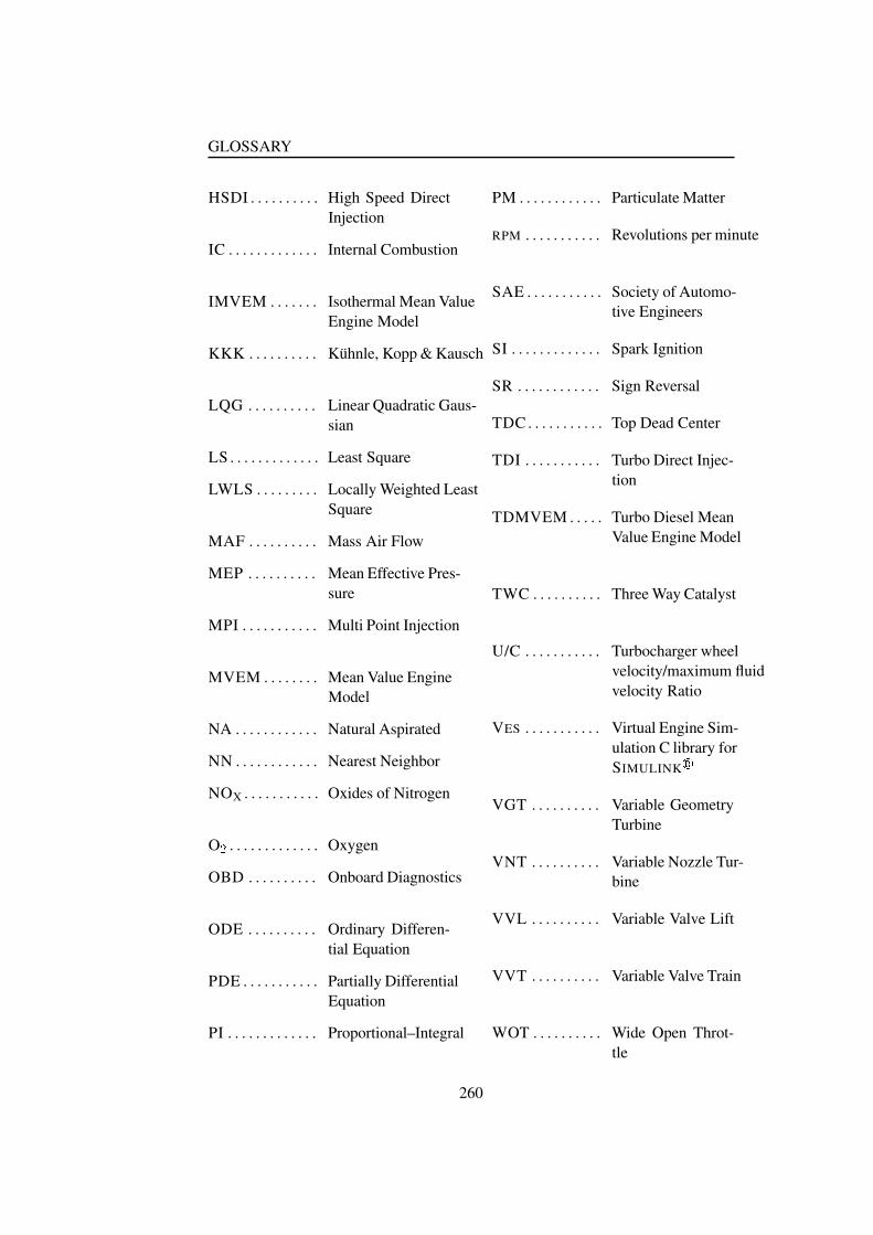
GLOSSARY
HSDI . . . . . . . . . . High Speed DirectInjection
IC . . . . . . . . . . . . . Internal Combustion
IMVEM . . . . . . . Isothermal Mean ValueEngine Model
KKK . . . . . . . . . . Kuhnle, Kopp & Kausch
LQG . . . . . . . . . . Linear Quadratic Gaus-sian
LS . . . . . . . . . . . . . Least Square
LWLS . . . . . . . . . Locally Weighted LeastSquare
MAF . . . . . . . . . . Mass Air Flow
MEP . . . . . . . . . . Mean Effective Pres-sure
MPI . . . . . . . . . . . Multi Point Injection
MVEM . . . . . . . . Mean Value EngineModel
NA . . . . . . . . . . . . Natural Aspirated
NN . . . . . . . . . . . . Nearest Neighbor
NOX . . . . . . . . . . . Oxides of Nitrogen
O > . . . . . . . . . . . . . Oxygen
OBD . . . . . . . . . . Onboard Diagnostics
ODE . . . . . . . . . . Ordinary Differen-tial Equation
PDE . . . . . . . . . . . Partially DifferentialEquation
PI . . . . . . . . . . . . . Proportional–Integral
PM . . . . . . . . . . . . Particulate Matter
RPM . . . . . . . . . . . Revolutions per minute
SAE . . . . . . . . . . . Society of Automo-tive Engineers
SI . . . . . . . . . . . . . Spark Ignition
SR . . . . . . . . . . . . Sign Reversal
TDC . . . . . . . . . . . Top Dead Center
TDI . . . . . . . . . . . Turbo Direct Injec-tion
TDMVEM . . . . . Turbo Diesel MeanValue Engine Model
TWC . . . . . . . . . . Three Way Catalyst
U/C . . . . . . . . . . . Turbocharger wheelvelocity/maximum fluidvelocity Ratio
VES . . . . . . . . . . . Virtual Engine Sim-ulation C library forSIMULINK ?
VGT . . . . . . . . . . Variable GeometryTurbine
VNT . . . . . . . . . . Variable Nozzle Tur-bine
VVL . . . . . . . . . . Variable Valve Lift
VVT . . . . . . . . . . Variable Valve Train
WOT . . . . . . . . . . Wide Open Throt-tle
260

Variables@�ACB. . . . . . . . . . . . Equivalent areaDFEHG @JILK�MONQPCRTS U�VTWX Y�Z PCRTS U�VTW .
[ . . . . . . . . . . . . . . Heat exchanger vari-able.[]\ . . . . . . . . . . . . . VGT nozzle inlet flowangle.[_^ . . . . . . . . . . . . . VGT nozzle outletflow angle.[ I
. . . . . . . . . . . . . VGT nozzle bladeangle.@JILK�M
. . . . . . . . . . . Minimum sectionalnozzle area.@a`
. . . . . . . . . . . . . Inlet area of the VGTscroll.b
. . . . . . . . . . . . . . Distribution betweenpremixed and diffu-sion combustion.b ^ . . . . . . . . . . . . . Slip angle.b ^dc e . . . . . . . . . . . . Impeller blade an-gle.EHG
. . . . . . . . . . . . Discharge Coefficient.
f . . . . . . . . . . . . . . VGT pressure ratiodistribution variable.E ^dc g . . . . . . . . . . . Radial exit velocityof the compressor fluid.E `
. . . . . . . . . . . . . Gas velocity follow-ing isentropic expan-sion or absolute VGTscroll flow velocity.
E \�c h . . . . . . . . . . . Tangential velocitycomponent of
E \ atentry diameter i \ .E ^dc h . . . . . . . . . . . Tangential velocitycomponent of
E ^ (im-peller tip).E ^dc h�e . . . . . . . . . . . Ideal fluid exit ve-locity (no slip).Ekj c h . . . . . . . . . . . Tangential velocitycomponent of
E jat
rotor inlet.Eml c h . . . . . . . . . . . Tangential velocitycomponent of
E lat
rotor outlet radius n l.
i \ . . . . . . . . . . . . . Averaged inducer di-ameter.o [ I
. . . . . . . . . . . . VGT nozzle ring flowangle change.odI
. . . . . . . . . . . . . Minimum distancebetween neighboringVGT blades.oqpsr KCt e . . . . . . . . . Nominal combustionduration.uwv3x \ . . . . . . . . . . Total enthalpy riseat station 1.uwv3x ^ . . . . . . . . . . Total enthalpy riseat station 2.uwv3x j
. . . . . . . . . . Total enthalpy riseat station 3.uwv3x l
. . . . . . . . . . Total enthalpy riseat station 4.uwv3x r
. . . . . . . . . . Total enthalpy riseacross compressor stage.
261

GLOSSARYywz3{d| }. . . . . . . . . . Isentropic enthalpy
rise across compres-sor stage.ywz3{d| ~
. . . . . . . . . . Effective enthalpy dropacross turbine stage.
ywz3{�~�| }. . . . . . . . . Isentropic enthalpy
drop across turbinestage.ywz��
. . . . . . . . . . . Static enthalpy riseat station 1.ywz3�
. . . . . . . . . . . Static enthalpy riseat station 2.ywz3�
. . . . . . . . . . . Static enthalpy riseat station 3.ywz��
. . . . . . . . . . . Static enthalpy riseat station 4.ywz3� ���C�
. . . . . . . . . Total enthalpy loss.
ywz3� ���C� | ����}��. . . . . Enthalpy loss due to
friction.ywz3� ���C� | }1�L�. . . . . . Enthalpy loss due to
collision.��'� � . . . . . . . . . . . Intake port mass flow.
�� � � | � . . . . . . . . . . Fresh intake port massflow.�� �
. . . . . . . . . . . . . Compressor mass flow.
�� ��| �. . . . . . . . . . . Compressor mass flow,
corrected.��'� � � . . . . . . . . . . . EGR mass flow.
�� � ���. . . . . . . . . . Isentropic nozzle mass
flow or mass flowthrough the VGT noz-zle ring.�� � � ~
. . . . . . . . . . . Mass flow throughthe rotor.�� ~
. . . . . . . . . . . . . Turbine mass flow.�� ~
. . . . . . . . . . . . . Turbine mass flow,corrected.�J�
. . . . . . . . . . . . . Kinetic energy.� . . . . . . . . . . . . . . Slip factor parame-ter or model–mea-surement error or noiseor heat exchanger ef-fectiveness.� }�� . . . . . . . . . . . . . EGR cooler effec-tiveness.� }�� . . . . . . . . . . . . . Intercooler effective-ness.� }�� . . . . . . . . . . . . . Descriptive intercoolereffectiveness.� ��| �3�
. . . . . . . . . . Isentropic compres-sor efficiency, totalto total.� } . . . . . . . . . . . . . . Engine fuel efficiency.
� ~�| �3�. . . . . . . . . . . Isentropic turbine ef-
ficiency, total to to-tal.�
. . . . . . . . . . . . . . Pulsation level index.��� }1�. . . . . . . . . . . Minimum cost func-
tion value.
262

�. . . . . . . . . . . . . . Coefficient vector to
the polynomial � . '¡�¢ . . . . . . . . . . . . Mass between com-pressor and intercooler.£¥¤
. . . . . . . . . . . . Normalized diffusioncombustion function. '¦ §©¨ . . . . . . . . . . . EGR cooler gas mass. '¦ §©¨�ª « . . . . . . . . . Gaseous mass in theEGR pipe connec-tion. ¬ . . . . . . . . . . . . Total entrapped fuelmass in the individ-ual cylinder. ¬ ª ® . . . . . . . . . . . Total entrapped fuelmass burnt in the in-dividual cylinder. °¯�¢ . . . . . . . . . . . . Contained mass inthe intercooler. °±k¡©² . . . . . . . . . . Intake plenum gasmass.£ « . . . . . . . . . . . . Normalized premixedcombustion function.
°³´ ¨�ª µ . . . . . . . . . . Mass between inter-cooler and EGR in-let point. °³´ ¨�ª ¶ . . . . . . . . . . Mass between EGRinlet point and plenum.·
. . . . . . . . . . . . . Engine speed.· ¢ . . . . . . . . . . . . . Compressor revolu-tions.
· « . . . . . . . . . . . . . No. of EGR coolerpipes.· ³ . . . . . . . . . . . . . Turbine revolutions.·¸
. . . . . . . . . . . . Nusselt number.¹. . . . . . . . . . . . . . LWLS weight ma-
trix.� . . . . . . . . . . . . . . LWLS polynomial orpower.º¼»dµ . . . . . . . . . . . . Stagnated pressureat station 1.º¼»�¶ . . . . . . . . . . . . Stagnated pressureat station 2.º¼»�½ . . . . . . . . . . . . Stagnated pressureat station 3.º¼»�¾ . . . . . . . . . . . . Stagnated pressureat station 4.º¿µ . . . . . . . . . . . . . Static pressure at sta-tion 1.º¼¶ . . . . . . . . . . . . . Static pressure at sta-tion 2.º¼½ . . . . . . . . . . . . . Static pressure at sta-tion 3.ºÀ¾ . . . . . . . . . . . . . Static pressure at sta-tion 4.� ¢ . . . . . . . . . . . . . Compressor powerconsumption.º ¢TÁd . . . . . . . . . . . . Cylinder pressure.� ¬ ¨�¯�¢�ª «�ÃQ±_« . . . . . . Power loss to enginepumping.Ä
. . . . . . . . . . . . . . Ratio between Å ¨�ª ¶and Æ ¶ or LWLS re-gressor vector or fuel/airratio.
263

GLOSSARYÇÀÈ . . . . . . . . . . . . . . Overall pressure levelin the intake system.
ÇÀÈ�É . . . . . . . . . . . . . Intercooler pressure.
ÇÀÊ . . . . . . . . . . . . . Pressure ratio acrosscompressor or tur-bine ( Ë�ÌËQÍCÎ or ËQÍCÎËQÏ ).ÇÀÊ . . . . . . . . . . . . . Effective pressure ra-tio the VGT ( РǼÊ�Ñ ÒLÓ�Ô�ÇÀÊ�Ñ Ê�ÓCÕ ).
ÇÀÊ�Ñ ÖmÈ1Ò . . . . . . . . . . Minimum turbine pres-sure ratio needed toovercome the cen-trifugal pressure gra-dient around the ro-tor.ÇÀÊ . . . . . . . . . . . . . Effective pressure ra-tio across the VGTnozzle ring.ÇÀÊ . . . . . . . . . . . . . Effective pressure ra-tio across the rotor.
ÇÀÊ . . . . . . . . . . . . . Pressure ratio acrossturbine, total to to-tal.× Õ . . . . . . . . . . . . . Turbine power pro-duction.Ø
. . . . . . . . . . . . . . Heat transfer.Ø É�ÓCÖkÙ . . . . . . . . . . Combustion heat re-lease rate.Ú . . . . . . . . . . . . . . RadiusÛÝÜ
. . . . . . . . . . . . . Reynolds number.ÚQÞ . . . . . . . . . . . . . Kernel bandwidth.
ß3à . . . . . . . . . . . . . Static fluid densityat impeller eye.ßâá . . . . . . . . . . . . . Static fluid densityat impeller tip.ßâÉ . . . . . . . . . . . . . Static compressor out-let density.Û ÈãÑ ä . . . . . . . . . . . Inducer radius, hubside.Û ÈãÑ å . . . . . . . . . . . . Inducer radius, shroudside.Û Ê . . . . . . . . . . . . . Rotor radius.æ . . . . . . . . . . . . . . Compressor slip fac-tor, or variance.çéè�ê
. . . . . . . . . . . . Stagnation temper-ature at station 4.çéè Ñ ë . . . . . . . . . . . . Stagnation temper-ature at station ì .ç á . . . . . . . . . . . . . Static impeller fluidexit temperature.çéí É . . . . . . . . . . . . Temperature in thecompressor-intercoolerpipe connection.ç í ÖkÙ . . . . . . . . . . . Ambient temperature.
î . . . . . . . . . . . . . . Torque or time con-stant.î á . . . . . . . . . . . . . Torque exerted on thefluid by the impeller(impeller tip condi-tions).ç É . . . . . . . . . . . . . Static compressor out-let temperature.çéï Þ©Ê . . . . . . . . . . . EGR temperature.
264
ðéñ ò©ó�ô õ. . . . . . . . . Mean EGR cooler tem-
perature.ðéñãö. . . . . . . . . . . . Exhaust port temper-
ature.ð ñ ÷Qø. . . . . . . . . . . Exhaust gas temper-
ature.ð øQñ©ô ù1ú. . . . . . . . . . Heat exchanger cool-
ing element inlet tem-perature.ð øQñ©ô ûCüQý
. . . . . . . . . Heat exchanger cool-ing element outlet tem-perature.þ
. . . . . . . . . . . . . . Input variable vec-tor.þsÿ
. . . . . . . . . . . . . Input variable vec-tor origin.þsÿ ô ò
. . . . . . . . . . . . LWLS grid point.þ ñ. . . . . . . . . . . . . Crankshaft position.þ ù1ò©ú
. . . . . . . . . . . . Crank position wherethe combustion ini-tiated.þ�� ò©ý
. . . . . . . . . . . . VGT position.ð øQñ©ô ÷. . . . . . . . . . . Heat exchanger tem-
perature at position� .ð�ù���ô õ. . . . . . . . . . . Mean intercooler tem-
perature.ð�ù���ô ûCüQý. . . . . . . . . . Intercooler exit tem-
perature.ð�õ��©ú. . . . . . . . . . Intake manifold tem-
perature.ðéûCüQý. . . . . . . . . . . Heat exchanger out-
let temperature.
ð�� � . . . . . . . . . . . Heat exchanger wall
temperature.�
. . . . . . . . . . . . . . Internal energy or tur-bocharger related ve-locities.
� . . . . . . . . . . . . . . Specific internal en-ergy.
�� . . . . . . . . . . . . . Inducer blade veloc-
ity at diameter � .
���. . . . . . . . . . . . . Impeller tip veloc-
ity.���
. . . . . . . . . . . . . Rotor tip velocity (sta-tion 3).
���. . . . . . . . . . . . . Exducer velocity at
radius � � (station 4).
�. . . . . . . . . . . . . . Volume.
� . . . . . . . . . . . . . . U/C ratio at which� ó�� � ó�ô õmù1ú.
� ö . . . . . . . . . . . . . Average laminar pipefluid velocity.
�. . . . . . . . . . . . . Relative fluid veloc-
ity.��
. . . . . . . . . . . . Relative fluid inletvelocity (inducer).
�� . . . . . . . . . . . . Relative fluid inlet
velocity (inducer).� ô �dô ó
. . . . . . . . . . Tangential compo-nent of
�� at radius .
� ú. . . . . . . . . . . . Vectorial velocity dif-
ference between ! and ! � (VGT model).
265

GLOSSARY
"$#&% '. . . . . . . . . . . Tangential velocity
component of" #
.
("$#&% '. . . . . . . . . . . Approximated tan-
gential velocity com-ponent of
" #.
)+*-,.,./. . . . . . . . . . . Coolant energy frac-
tion.)+02143
. . . . . . . . . . . Exhaust energy frac-tion.
)5#. . . . . . . . . . . . . Spherical distance be-
tween VGT blade tips.
6. . . . . . . . . . . . . . LWLS data kernel.
Constants7 . . . . . . . . . . . . . . 8:9<; * model param-
eter.
=?> . . . . . . . . . . . . . Impeller friction pa-rameter.
=�@ . . . . . . . . . . . . . Impeller friction pa-rameter.
=�A . . . . . . . . . . . . . Impeller friction pa-rameter.
=CB5D . . . . . . . . . . . . E @ model parameter.
F. . . . . . . . . . . . . . Impeller outlet width
or 8:9G; * model pa-rameter.
H > . . . . . . . . . . . . . Inducer blade angle.
H > % ,JILK . . . . . . . . . . Optimal fluid entryangle (inducer).
FM. . . . . . . . . . . . . Rotor inlet width.
N�> . . . . . . . . . . . . . Muller friction modelcoefficient.
N+@ . . . . . . . . . . . . . Muller friction modelcoefficient.
O�P > . . . . . . . . . . . . Diffusion combus-tion parameter.
O�P @ . . . . . . . . . . . . Diffusion combus-tion parameter.
N I . . . . . . . . . . . . . Specific heat capac-ity at fixed pressure.
O�I > . . . . . . . . . . . . Premixed combus-tion parameter.
O�I @ . . . . . . . . . . . . Premixed combus-tion parameter.
N5Q . . . . . . . . . . . . . Specific heat capac-ity at fixed volume.
RTS. . . . . . . . . . . . . Impeller outlet diam-
eter.RVUW% 3
. . . . . . . . . . . Inducer diameter, hubside.
R UW% X. . . . . . . . . . . . Inducer diameter, shroud
side.YZ K % * % [�\ 1
. . . . . . . Maximum correctedturbine mass flow.
R I. . . . . . . . . . . . . Diamter of the in-
dividual heat exchangerpipe.
R M. . . . . . . . . . . . . Rotor diameter.
R M.% \. . . . . . . . . . . Nozzle ring diame-
ter (blade axel cen-troid).
R M.% U. . . . . . . . . . . . Inner nozzle ring di-
ameter.
266

]V^._ `. . . . . . . . . . . Outer nozzle ring di-
ameter.acb�d
. . . . . . . . . . . Fuel heating value.
e . . . . . . . . . . . . . . fWgf-h ratioi&j2kml
. . . . . . . . . . . Moment of inertia ofthe engine.
n. . . . . . . . . . . . . . Heat transfer coef-
ficient.o k
. . . . . . . . . . . . . . VGT nozzle bladelength.
o k&_ p�q r. . . . . . . . . . . VGT nozzle blade
length from axel totip.
sCr. . . . . . . . . . . . . Length of the indi-
vidual heat exchangerpipes.
s�t p�^u`.v+j. . . . . . . . . Engine stroke length.
wxky`.z. . . . . . . . . . . No. of VGT nozzle
blades.
{ q|l}k . . . . . . . . . . . . Ignition delay.~
. . . . . . . . . . . . . . Parameter vector.�G�f . . . . . . . . . . . . Volume between com-
pressor and intercooler.
�G�. . . . . . . . . . . . . Engine displacement
volume.�Gj2l}^
. . . . . . . . . . . EGR cooler volume.
�Gj2l}^._ r. . . . . . . . . . EGR pipe connec-
tion volume.��q
. . . . . . . . . . . . . Total intake systemvolume.
��qf . . . . . . . . . . . . . Intercooler volume.
�����}k. . . . . . . . . . Intake plenum vol-
ume.� p��L^._ �
. . . . . . . . . . Volume between in-tercooler and EGRinlet point.
� p��L^._ �. . . . . . . . . . Volume between EGR
inlet point and plenum.
�L�5�. . . . . . . . . . . . . � � model parameter.
�. . . . . . . . . . . . . . Impeller/Rotor blade
number.
267

GLOSSARY
268
Bibliography
[1] United States Patent No. 4,939,658, July 3, 1990. Assignee: Hitachi Ltd.,Tokyo, Japan.
[2] Private communication with Dr. Ing. Arnd Sommerhoff, technical specialistat Ford Fordschungszentrum Aachen GmbH.
[3] Private communication with Dipl. Ing. Daniel Rottger, research engineer atFord Fordschungszentrum Aachen GmbH.
[4] The specially prepared 7 port head for the 1275cc British Leyland engineswas provided by Georg Mikkelsen, AKM Racing, Lerpyttevaj 31, 7700Thisted, Denmark, Phone: (+45) 97920182.
[5] E-mail communication between Christian Laurent, PSA, and the author onthe 5th of June, 2000.
[6] BOSCH sensor program 98/99, Bosch No. 1 987-720-535/804.
[7] A. A. Amsden, KIVA-3: A KIVA Program with Block-Structured Mesh forComplex Geometries, Los Alamos National Laboratory, 1993, Report No:LA-12503-MS.
[8] A. A. Amsden, P. J. O’Rourke, and T. D. Butler, KIVA-II: A ComputerProgram for Chemically Reactive Flows with Sprays, Los Alamos NationalLaboratory, 1989, Report No: LA-11560-MS.
[9] A. Gelb (ed.), Applied optimal estimation, The M.I.T. Press, 12th printing,1992.
[10] A. M. R. Chevalier, Wide Bandwidth Control of the Air/Fuel Ratio of SparkIgnition Engines, Ph.D. dissertation, Technical University of Denmark, In-stitute for Automation, 2000.
[11] ECM (Engine Control and Monitoring), 101 Street, Suite 365, Los Altos,CA 94022,USA.
[12] C. F. Aquino, Transient A/F Control Characteristics of the 5 Liter CentralFuel Injection Engine, SAE Technical Paper (1981), no. 810494.
269

BIBLIOGRAPHY
[13] B. Ault, V. K. Jones, J. D. Powell, and G. F. Franklin, Adaptive Air-FuelRatio Control of a Spark Ignition Engine, SAE Technical Paper (1994),no. 940373.
[14] B. Horner, Garrett Turbocharger Specifications and Calculations, AlliedSignals, 1980, Garrett is now part of Allied Signals.
[15] B. Qvale and V. Bothmann, Notes in turbomachinery, Laboratory for Ener-getics, Technical University of Denmark, 1994, Part 1–3.
[16] C. Hong and N. Watson, Turbocharged S.’I. Engine Simulation under Steadyand Transient Conditions, SAE Technical Paper (1988), no. 880122.
[17] C. W. Vigild, A. Chevalier, and E. Hendricks, Avoiding Signal Aliasing inEvent-Based Engine Control, SAE Technical Paper (2000), no. 2000-01-0268.
[18] Carl-Anders Hergart, Modeling Combustion and Soot Emissions in aSmall-Bore Direct-Injection Diesel Engine, Ph.D. dissertation, Rheinisch-Westalische Technische Hochschule Aachen, 2001.
[19] C.-F. Chang, N.P. Fekete, and J. D. Powell, Engine Air-Fuel Ratio ControlUsing an Event-Based Observer, SAE Technical Paper (1993), no. 930766.
[20] G. Chen, M. T. Vincent, and T. R. Gutermuth, The Behavior of MultiphaseFuel-Flow in the Intake Port, SAE Technical Paper (1994), no. 940445.
[21] A. Chevalier and M. Muller, On the Validity of Mean Value Engine Mod-els During Transient Operation, SAE Technical Paper (2000), no. 2000-01-1261.
[22] A. Chevalier and C. W. Vigild, Predicting the Port Air Mass Flow of SIEngines in A/F Ratio Control Applications, SAE Technical Paper (2000),no. 2000-01-0260.
[23] S.B. Choi, M. Won, and J.K. Hedrick, Fuel Injection Control of SI En-gines, Proceedings of the 33rd IEEE Conference on Des. and Control (CDC)(1994), Lake Buena Vista, Florida.
[24] Urs Christen, Engineering Aspects of ��� Control, Ph.D. dissertation, SwissFederal Institute of Technology, 1996, Diss. ETH No. 11433.
[25] D. A. Kouremenos, C. D. Rakopoulos, and E. Karvounis, ThermodynamicAnalysis of Direct Injection Diesel Engines by Multi-zone Modeling, ASMEWA-Meeting, Boston, MA, USA 3.3 (1987), 67–77.
[26] DieselNet, Exhaust Gas Recirculation, URL: http://www.dieselnet.com.
270

BIBLIOGRAPHY
[27] D.N. Assanis and J.B. Heywood, Development and Use of a ComputerSimulation of the Turbocompounded Diesel System for Engine Perfor-mance and Component Heat Transfer Studies, SAE Technical Paper (1986),no. 860329.
[28] Donald J. Dobner, A Mathematical Engine Model for Development of Dy-namic Engine Control, SAE Technical Paper (1980), no. 800054.
[29] E. Trostmann, Pneumatical Control - Notes to Course 8204, Technical Uni-versity of Denmark, 1987, in danish.
[30] Inc Electromotive, TEC-I,TEC-II and HPV-3B, Total Engine Control, En-gine Management Systems by Electromotive, Inc, Installation and User’sManual, Electromotive, Inc, 14004 - J Willard Road, Chantilly, Virgina22021.
[31] D. Engler, Manifold Fuel Film, Modelling and Prevention, Master’s thesis,Technical University of Denmark, Institute of Automation, 2001.
[32] David Eppstein, Delunay triangulation – part of geometry in action, a col-lection of applications of computational geometry., Theory Group, ICS,UC Irvine., URL: http://www.ics.uci.edu/˜eppstein/gina/delaunay.html.
[33] Evangelos Karvounis, Development and use of a multi-purspose simulationframework for internal combustion engine design, Master’s thesis, Univer-sity of Illinois at Urbana-Champaign, 1991.
[34] F. S. Bhinder, Investigation of flow in a nozzleless spiral casing of a radial–inward flow gas turbine, Proc. Inst. Mech. Engers. 184 (1969/70), Pt 3G(II).
[35] N.P. Fekete, J.D. Powell, U. Nester, and I. Gruden, Model Based Air-Fuel Ratio Control of a Lean Multi-Cylinder Engine, SAE Technical Paper(1995), no. 950846.
[36] C.R. Ferguson, The Centrifugal Compressor Stage, Butterworth, 1963, Lon-don.
[37] M. Føns, Indførelse af Recirkulering af Udstødningsgas (EGR) i SI-Motorer,Master’s thesis, The Technical University of Denmark, Department of En-ergy and Institute of Automation, DTU, 1997, In danish.
[38] G. F. Hiett and I. H. Johnston, Experiments concerning the aerodynamicperformance of inward radial turbines, Proc. Inst. Mech. Engers. 178(1963/64), Pt 31(II).
[39] G. L. Gissinger, P. M. Frank, and J. Wunnennberg, Model-Based Elec-tronic Engine and Turbocharger Control, SAE Technical Paper (1990),no. 900595.
271

BIBLIOGRAPHY
[40] J. T. Gravdahl, Modeling and Control of Surge and Rotating Stall in Com-pressors, Ph.D. dissertation, Norwegian University of Science and Technol-ogy, Trondheim, Norway, 1998, Report 98-6-W.
[41] H. Kwakernaak and R. Sivan, Linear optimal control systems, first ed.,Wiley-Interscience, 1972.
[42] E. Hendricks, A Compact, Comprehensive Model of Large Turbocharged,Two-Stroke Diesel Engines, SAE Technical Paper (1986), no. 861190.
[43] , The Analysis of Mean Value Engine Models, SAE Technical Paper(1989), no. 890563.
[44] , Errors in Hot Wire MAF Measurement Systems, Revised InterimReport, Technical University of Denmark, 1992.
[45] E. Hendricks and A. Chevalier, Emerging Engine Control Technologies,29th ISATA Conference on Automotive Electronics (1996), no. 96AE029,Florence, Italy.
[46] E. Hendricks, A. Chevalier, and M. Jensen, Event Based Engine Control:Practical Problems and Solutions, SAE Technical Paper (1995), no. 950008.
[47] E. Hendricks, M. Jensen, A. Chevalier, S. C. Sorenson, D. Trumphy, andJ. Asik, Modelling of the Intake Manifold Filling Dynamics, SAE TechnicalPaper (1996), no. 960037.
[48] E. Hendricks, M. Jensen, A. Chevalier, and T. Vesterholm, ConventionalEvent Based Engine Control, SAE Technical Paper (1994), no. 940377.
[49] E. Hendricks and S. C. Sorenson, Mean Value Modeling of Spark IgnitionEngines, SAE Technical Paper (1990), no. 900616.
[50] , SI Engine Controls and Mean Value Engine Modeling, SAE Tech-nical Paper (1991), no. 910258.
[51] E. Hendricks and T. Vesterholm, The Analysis of Mean Value SI EngineModels, SAE Technical Paper (1992), no. 920682.
[52] E. Hendricks, T. Vesterholm, P. Kaidantzis, P. Rasmussen, and M. C. Jensen,Nonlinear Transient Fuel Film Compensation, SAE Technical Paper (1993),no. 930767.
[53] E. Hendricks, T. Vesterholm, and S. C. Sorenson, Nonlinear, Closed Loop,SI Engine Control Observers, SAE Technical Paper (1992), no. 920237.
[54] J. B. Heywood, Internal Combustion Engine Fundamentals, McGraw-Hill,Inc., 1988.
272

BIBLIOGRAPHY
[55] J. B. Heywood, J. M. Higgins, P. A. Watts, and R. J. Tabaczynski, Devel-opment and Use of a Cycle Simulation to Predict SI Engine Efficiency andNOx Emissions, SAE Technical Paper (1979), no. 790291.
[56] J. Gerhardt, N. Benninger, and W. Hess, Torque-Based System Structure ofan Electronic Engine Management System as a New Base for Drive TrainSystems (Bosch ME7 System), 6. Aachener Kolloqium, Fahrzeug- und Mo-tortechnik (Aachen, Germany), 20.-22. October 1997, in german.
[57] J. H. Horlock and D. E. Winterbone, The Thermodynamics and Gas Dynam-ics of Internal-Combustion Engines, vol. 2, Oxford University Press, 1986.
[58] J. Lillelund, Design of an Engine Control Development System, Master’sthesis, The Technical University of Denmark, Institute of Automation, 1991.
[59] J. M. Lujan, F. Payri, F. Vera, and C. Guardiola, Modelling, Effect and Be-haviour of the EGR Venturi in a Heavy-Duty Diesel Engine, SAE TechnicalPaper (2001), no. 2001-01-3227.
[60] J. M. Lujan, J. Galindo, and J. R. Serrano, Efficiency Characterization ofCentripetal Turbines under Pulsating Flow Conditions, SAE Technical Pa-per (2001), no. 2001-01-0272.
[61] J.-P Jensen and A. F. Kristensen, Development of Dynamic Diesel EngineModels, Modelling Principle for Turbocharged Diesel Engine, Master’s the-sis, The Technical University of Denmark, Department of Energy, DTU,1990, In danish.
[62] J.-P. Jensen, Kristensen, A.F., S.C Sorenson, N. Houbak, and E. Hendricks,Transient simulation of a small turbocharged diesel engine, Proc. I Mech ESem. on Engine Transient Perm. (1990).
[63] , Mean value modeling of a small turbocharged diesel engine, SAETechnical Paper (1991), no. 910070.
[64] J. P. Mello and A. M. Mellor, NOX Emmisions from Direct Injection DieselEngines with Water/Steam Dilution, SAE Technical Paper (1999), no. 1999-01-0836.
[65] J. W. Daily and R. E. Nece, Chamber dimension effects on induced flow andfrictional resistance of enclosed rotating discs, Trans. ASME J. Basic Engng82 (1960).
[66] P.B. Jensen, M.B. Olsen, J. Poulsen, E. Hendricks, M. Føns, and C. Jepsen, ANew Family of Nonlinear Observers for SI-Engine Air-Fuel Ratio Controls,SAE Technical Paper (1997), no. 970615.
273
BIBLIOGRAPHY
[67] Jun-Lon Chen, Mark Eubank, and Robert Wattleworth, Improving ValveRetainer Life for Fuel Pressure Regulators, SAE Technical Paper (1999),no. 1999-01-0794.
[68] K. J. Astrom and B. Wittenmark, Computer-Controlled Systems: Theoryand Design, 2nd ed., Prentice-Hall International, Inc., 1990.
[69] P. Kaidantzis, P. Rasmussen, M. Jensen, T. Vesterholm, and E. Hendricks,Robust Self-Calibrating Lambda Feedback for SI Engines, SAE TechnicalPaper (1993), no. 930860.
[70] R. E. Kalman and R. S. Bucy, New Results in Linear Filtering and PredictionTheory, Journal of Basic Engineering, Trans. ASME 83D (1961), 95–108.
[71] Kemin Zhou and John C. Doyle, Essentials of robust control, Prentice-HallInternational, Inc., 1998.
[72] Lennart Ljung, System Identification: Theory for the User, second ed., Pren-tice Hall, Inc, 1999.
[73] J. Lillelund and E. Hendricks, A PC Engine Control Development System,SAE Technical Paper (1991), no. 910259.
[74] B. M. Lyko, Application Manual for the Linear Exhaust Gas ReciculationValve, Delphi Energy and Engine Management Systems, 1995.
[75] M. Føns, M. Muller, A. Chevalier, C. W. Vigild, S. C. Sorenson, and E.Hendricks, Mean Value Engine Modeling of an SI engine with EGR, SAETechnical Paper (1999), no. 1999-01-0909.
[76] M. Nyberg and L. Nielsen, Model-based diagnosis for the air intake systemof the SI engine, SAE Technical Paper (1997), no. 970209.
[77] P.J. Maloney, An Event-Based Transient Fuel Compensator with PhysicallyBased Parameters, SAE Technical Paper (1999), no. 1999-01-0553.
[78] P.J. Maloney and P.M. Olin, Pneumatic and Thermal State Estimations forProduction Engine Control and Diagnostics, SAE Technical Paper (1998),no. 980517.
[79] J. J. G. Martins and I. C. Finlay, Fuel Preparation in Port-Injected Engines,SAE Technical Paper (1992), no. 920518.
[80] Mathworks, Matlab function reference, release 11 revision ed.
[81] H. Melgaard, E. Hendricks, and H. Madsen, Continuous Identification ofa Four-Stroke SI Engine, American Control Conference (ACC) (1990),no. TP10, 5:30, San Diego, CA.
274

BIBLIOGRAPHY
[82] M. Morari and E. Zafiriou, Robust Process Control, Prentice-Hall, Inc.,1989, Englewood Cliffs, N.J.
[83] M. Muller, Mean Value Modelling of Turbocharged Spark Ignition Engines,Master’s thesis, The Technical University of Denmark, Institute of Automa-tion and Department of Energy, 1997.
[84] M. Muller, E. Hendricks, and S. C. Sorenson, Mean Value Modelingof Turbocharged Spark Ignition Engines, SAE Technical Paper (1998),no. 980784.
[85] Muller, Martin, Olin, Peter M., and Schreurs, Bart, Dynamic EGR estima-tion for production engine control, SAE Technical Paper (2001), no. 2001-01-0553.
[86] N. Watson, A. D. Pilley, and M. Marzouk, A Combustion Correlation forDiesel Engine Simulation, SAE Technical Paper (1980), no. 800029.
[87] N. Watson and M. S. Janota, Turbocharging the internal combustion engine,first ed., MACMILLIAN EDUCATION LTD, 1982.
[88] NIST/SEMATECH, Engineering statistical handbook, NIST/SEMATECH,URL: http://www.itl.nist.gov/div898/handbook/index.htm.
[89] T. Nogi, Y. Ohyama, T. Yamauchi, and H. Kuroiwa, Mixture Formation ofFuel Injection Systems in Gasoline Engines, SAE Technical Paper (1988),no. 880558.
[90] P. Azzoni, G. Minelli, D. Moro, and G. Serra, A Model for EGR Flow RateEstimation, SAE Technical Paper (1997), no. 970030.
[91] P. E. Moraal and I. V. Kolmanovsky, Turbocharger Modeling for AutomotiveControl Applications, SAE Technical Paper (1999), no. 1999-01-0908.
[92] R. C. Pampreen, Small turbomachinery compressor and fan aerodynamics,Journal of engineering for power (1973), no. 95, 251–256.
[93] Randall P. Izydorek and G. Clarke Oberheide, Improved Pulsation Damperfor the Fuel Injector Rail, SAE Technical Paper (1997), no. 971071.
[94] Reuter, Wolfgang, Loesing, Karl-Heinrich, and Golden, John E, An im-proved anti-pulsation mass airflow sensor, SAE Technical Paper (2001),no. 2001-01-0985.
[95] Rober W. Weeks and John. J. Moskwa, Automotive Engine Modelingfor Real-Time Control Using MATLAB/SIMULINK, SAE Technical Paper(1995), no. 950417.
275

BIBLIOGRAPHY
[96] Robert A. Granger, Fluid mechanics, first ed., Dover, 1985.
[97] Robert. W. Fox and Alan T. McDonald, Introduction to Fluid Mechanics,fourth ed., John Wiley & Sons, Inc, 1994, SI version.
[98] S. M. Futral and C. A. Wasserbauer, Off-design performance predictionwith experimental verification for a radial inflow turbine, National Advi-sory Committee for Aeronautics (now NASA), 1965, NACA TN D-2621.
[99] S. Skogestad and I. Postlethwaith, Multivariable Feedback Control, Analysisand Design, John Wiley & Sons, 1996.
[100] P.J. Shayler and M.S. Goodman, Mixture Control with Air-Flow AnticipationUsing Neural Networks, 29th ISATA Conference on Automotive Electronics(1996), no. 96AE025, Florence, Italy.
[101] M. A. Stephens, EDF Statistics for Goodness of Fit and Some Comparisons,Journal of the American Statistical Association 69 (1974), 730–737.
[102] D. L. Stivender, Engine Air Control - Basis of a Vehicular Systems ControlHierarchy, SAE Technical Paper (1978), no. 780346.
[103] M. Struwe and C. W. Vigild, Robust ��� Control of an SI Engine’s Air/FuelRatio, Master’s thesis, Technical University of Denmark, Institute of Au-tomation, 1997, In danish.
[104] Thomas Morel, Rifat Keribar, and Paul N. Blumberg, A New Approach toIntegrating Engine Performance and Component Design Analysis ThroughSimulation, SAE Technical Paper (1988), no. 880131.
[105] L. Trajkovski, Computer Controlled Engine Management System, Master’sthesis, Technical University of Denmark, Institute of Automation, 1997, Indanish.
[106] Turbodyne, URL: http://www.turbodyne.com.
[107] R. C. Turin and H. P. Geering, Model-Based Adaptive Fuel Control in an SIEngine, SAE Technical Paper (1994), no. 940374.
[108] U. Christen, P.E. Moraal, and K.J. Vantine, Model identification and im-plementation in MATLAB/ SIMULINK for the 90 PS PUMA 2.4 liter DIDiesel engine, Technical Report SRR 1998-0136, Ford Motor Company,Ford Forschungszentrum, Aachen, Susterfeldstrasse 200, D-52072 Aachen,Germany, 1998.
[109] U. Kiencke and L. Nielsen, Automotive Control Systems, Springer Verlag,2000.
276
BIBLIOGRAPHY
[110] Tamon Ueda, Temperature- and flow-measurement by ultrasonics , RevisedInterim Report, Technical University of Denmark, in danish, 1999.
[111] Urs Christen, Katie J. Vantine, and Nick Collings, Event-Based Mean-ValueModeling of DI Diesel Engines for Controller Design, SAE Technical Paper(2001), no. 2001-01-1242.
[112] C. W. Vigild, K. P. H. Andersen, E. Hendricks, and M. Struwe, TowardsRobust H-infinity Control of an SI Engine’s Air/Fuel Ratio, SAE TechnicalPaper (1999), no. 1999-01-0854.
[113] Michael Wahle, Dynamic (Kinematik und Kinetik), WissenschaftsverlagMainz in Aachen, 1998, in German.
[114] M. H. Westbrook and J. D. Turner, Automotive Sensors, Institute of PhysicsPublishing, Bristol and Philadelphia, 1994.
[115] A. Whitfield, Slip factor of a centrifugal compressor and its variation flowrate, Proc. Inst. Mech, Engrs, 188 (1974), no. 32/74.
[116] H.-M. Wiedenmann, G. Hotzel, H. Neumann, J. Riegel, and H. Weyl, Ex-haust Gas Sensors, Automotive Electronics Handbook (R. K. Jurgen, ed.),McGraw-Hill, Inc., 1995.
[117] F. J. Wiesner, A review of slip factors for centrifugal impellers, ASME Pub-lication 66-WA-FE-18 (1966).
[118] Xiao Hu and Patrick B. Lawless, Prediction of On-Engine Efficiency forthe Radial Turbine of a Pulse Turbocharged Engine, SAE Technical Paper(2001), no. 2001-01-1238.
277

BIBLIOGRAPHY
278