Optimization in Modern Power Systems DTU Course 31765

Optimization inModern Power Systems

DTU Course 31765

Lecture Notes

Spyros Chatzivasileiadis

Technical University of Denmark (DTU)

September 2018

arX

iv:1

811.

0094

3v1

[cs

.SY

] 2

Nov

201

8

Preface

These lecture notes aim to supplement the study material for the course“31765: Optimization in modern power systems” at the Technical Univer-sity of Denmark (DTU). They do not substitute the lecture slides and thediscussions carried out during class. The course content is defined by thematerial taught in the class, which these notes aim to support to a certainextent.

The first edition of the present lecture notes was prepared for the aca-demic year 2018-2019. Note that the material presented in these notes is aconstant work in progress.

For any comments, errors, or omissions, you are welcome to contact meat [email protected].

Special thanks to the students of the 31765 course for their remarks andsuggestions to improve these lecture notes.

Spyros ChatzivasileiadisSeptember 2018

Copenhagen, Denmark

iii

mailto:[email protected]

Contents

Preface . . . . . . . . . . . . . . . . . . . . . . . . . . . . . . . . . iii

1 Introduction 1

1.1 Terms and Definitions . . . . . . . . . . . . . . . . . . . . . . 1

1.1.1 Marginal cost of a generator . . . . . . . . . . . . . . . 1

1.1.2 Contingency . . . . . . . . . . . . . . . . . . . . . . . 2

1.1.3 N-1 Security . . . . . . . . . . . . . . . . . . . . . . . 2

1.1.4 Congestion . . . . . . . . . . . . . . . . . . . . . . . . 3

1.1.5 Copperplate . . . . . . . . . . . . . . . . . . . . . . . . 3

1.2 Outline of the Lecture Notes . . . . . . . . . . . . . . . . . . 3

1.3 Further reading material . . . . . . . . . . . . . . . . . . . . . 3

2 Economic Dispatch 5

2.1 What is economic dispatch? . . . . . . . . . . . . . . . . . . . 5

2.2 Merit-Order Curve . . . . . . . . . . . . . . . . . . . . . . . . 6

2.3 Formulation of the optimization problem . . . . . . . . . . . . 7

2.4 System Marginal Price . . . . . . . . . . . . . . . . . . . . . . 8

2.5 Marginal Generator . . . . . . . . . . . . . . . . . . . . . . . 8

3 DC Optimal Power Flow 11

3.1 Why is it called DC OPF? . . . . . . . . . . . . . . . . . . . . 11

3.2 Economic Dispatch vs. DC OPF . . . . . . . . . . . . . . . . 11

3.3 DC Power Flow . . . . . . . . . . . . . . . . . . . . . . . . . . 12

3.4 Bus Susceptance Matrix . . . . . . . . . . . . . . . . . . . . . 13

3.4.1 Constructing the Bus Susceptance Matrix . . . . . . . 13

3.5 Formulation of the optimization problem . . . . . . . . . . . . 14

3.6 Locational Marginal Prices . . . . . . . . . . . . . . . . . . . 14

3.6.1 Extraction of the Locational Marginal Prices . . . . . 15

3.7 Key Discussion Points . . . . . . . . . . . . . . . . . . . . . . 15

3.8 Power Transfer Distribution Factors (PTDF) . . . . . . . . . 18

3.8.1 Calculation of the PTDF . . . . . . . . . . . . . . . . 19

3.8.2 Example . . . . . . . . . . . . . . . . . . . . . . . . . . 21

3.9 DC-OPF formulation based on PTDF . . . . . . . . . . . . . 22

v

vi Contents

4 AC Optimal Power Flow 234.1 What is AC Optimal Power Flow? . . . . . . . . . . . . . . . 234.2 AC Power Flow . . . . . . . . . . . . . . . . . . . . . . . . . . 24

4.2.1 Modeling transmission lines: the π-model . . . . . . . 244.2.2 Current flow along a line . . . . . . . . . . . . . . . . 244.2.3 Line Admittance Matrix . . . . . . . . . . . . . . . . . 254.2.4 Bus Admittance Matrix . . . . . . . . . . . . . . . . . 264.2.5 AC Power Flow Equations . . . . . . . . . . . . . . . . 28

4.3 Formulation of the optimization problem . . . . . . . . . . . . 294.3.1 Objective Function for the AC Optimal Power Flow . 304.3.2 Transmission Line Limit constraints: Current vs Power 324.3.3 Bus Voltage Magnitude Limits . . . . . . . . . . . . . 344.3.4 Bus Voltage Angle Limits . . . . . . . . . . . . . . . . 34

4.4 Operations with complex numbers . . . . . . . . . . . . . . . 344.5 From the AC power flow equations to the DC power flow . . 354.6 Nodal Prices (LMPs) in AC-OPF . . . . . . . . . . . . . . . . 37

4.6.1 LMPS in the AC-OPF vs DC-OPF . . . . . . . . . . . 37

A Derivation of Locational Marginal Prices 39

Bibliography 42

1Introduction

1.1 Terms and Definitions

In this section, we define a set of terms that will be recurring across severalchapters of these notes.

1.1.1 Marginal cost of a generator

Marginal cost is the cost of a generator for producing one unit of energy.The cost can be expressed in any monetary unit, e.g. Eur, USD, DKK,CHF, etc. Energy is usually expressed in MWh or kWh, depending on thesize of the generator and our system. For example in a wholesale market of atransmission system, we will usually express the marginal cost as Eur/MWh(or USD/MWh, etc.). In a microgrid, we would probably go for Eur/kWh(or DKK/kWh, etc.).

Limitations and Clarifications

– In the optimal power flow problem, the generator costs are assumedeither linear: f(PG) = cGPG, or quadratic: f(PG) = aGP

2G + bGPG.

The constant terms in both functions are usually neglected in theoptimization, as they do not change the result of the optimization (itis just a constant offset of the final result). But: if they exist, theymust be included for the calculation of the final cost.

– The marginal generator cost is the derivative of the generator cost

curve, i.e.d f(PG)

dPG. As a result, if the generator cost is linear, then the

marginal cost cG is a constant. If the generator cost is quadratic, themarginal cost aGPG + bG is linear.

– The generator cost as used in the optimal power flow problems is anapproximation of the true generator cost. The true cost curve of thegenerators f(PG) is (a) non-linear, and (b) it includes startup costsand shutdown costs, i.e. there are constant terms in f(PG) that areapplied when the generator is turned on or off.

– Before the unbundling, vertically integrated monopolies usually ap-proximated the cost of their conventional generators with a quadraticcost curve, as this was a closer approximation to the real cost of theconventional generator (e.g. coal, gas, oil).

1

2 1. Introduction

– In electricity markets, the generator costs are usually linear. In a mar-ket environment, the marginal cost represents the bid of a generatorin the market. It is much more straightforward, and more transparent(from the market operation point of view) to express this as a linearcost, i.e. every MWh you would like to buy from me will cost x USD. Ifwe were expressing this as a quadratic cost, it would mean that we bida linear marginal cost function aGPG + bG, which makes things muchmore complicated. Expressing this function with words, it would meanthat the first MWh has a cost of aG + bG, but every subsequent MWhhas a continuously higher cost by an additive term aG. Such a costfunction is difficult to be understood by traders and market operatorsduring daily trading.

– Generators bid in the market their marginal cost, which as explainedabove, is a constant term (representing a linear cost curve). In that,they neglect their fixed costs, which usually include startup/shutdownand other costs, and have to approximate their variable costs with alinear function. For their fixed costs, they are usually compensatedoutside the day-ahead or intra-day market dispatch, through a unitcommitment procedure which considers startup and shutdown gener-ator costs.

1.1.2 Contingency

By definition, contingency refers to a future event or circumstance whichis possible but cannot be predicted with certainty. In power system jargon,the term “contingency” refers to incidents that deviate from the plannedoperation and can affect the security of the power system. Contingenciesinclude for example line outages, transformer outages, bus outages, loadoutages, and deviations of the power generation due to e.g. wind forecasterrors or solar forecast errors. Contingencies are very often mentioned in thecontext of N-1 security criterion (see Section 1.1.3).

1.1.3 N-1 Security

Most of the power systems around the world operate in a N-1 secure state.The N-1 security criterion stipulates that the power system must remainsecure in the event of losing any single component of the system, i.e. assum-ing a system has N components, the system must remain secure even if itoperates with N-1 components. Such a system is said to satisfy the N-1 secu-rity criterion and is called N-1 secure. In that context, a contingency is anycomponent outage that leads to a system operation with N-1 components.

1.2. Outline of the Lecture Notes 3

1.1.4 Congestion

The term congestion usually refers to lines or transformers. A congestedline means a line that is loaded to the maximum of its transmission ca-pacity, and as a result, it cannot carry additional power. Line (or for thatpurpose transformer) congestions have a negative impact on social welfare.Because of congestions, the cheapest generation units cannot produce allnecessary power to cover the demand. Instead, more expensive units locateddownstream of a congestion must be dispatched to supply the missing power.This increases the total generation cost.

1.1.5 Copperplate

We usually refer to a “copperplate network”. By that we mean that thenetwork has infinite transmission capacity, which allows us to neglect allnetwork constraints. The network constraints include the transmission linelimit constraints, and the power flow constraints which model (a) how thepower is distributed along the lines, and (b) the line losses. Neglecting theseconstraints gives a first approximation of the solution, simplifying a lotour calculations. The term “copperplate” (probably) comes from a “cop-per plate”, i.e. assuming that on top of all our injection and load nodes weplace a copper plate, so that all nodes are connected with each other andan infinite capacity for power transfer.

1.2 Outline of the Lecture Notes

These notes are structured as follows:

Chapter 2: Economic Dispatch This chapter presents a short overview ofthe market clearing based on power pools, defines the system marginal price,and the marginal generators.

Chapter 3: DC-OPF This chapter introduces the DC Optimal Power Flow.

Chapter 4: AC-OPF This chapter introduces the AC Optimal Power Flow.

Chapter 5: Semidefinite Programming This chapter introduces Semidef-inite Programming and the SDP-based Optimal Power Flow.

1.3 Further reading material

1. S. Chatzivasileiadis (2012). Transmission investments in deregulatedelectricity markets. Technical Report, ETH Zurich, EEH Power Sys-tems Laboratory, May 2012.

4 1. Introduction

2Economic Dispatch

2.1 What is economic dispatch?

Imagine you are the operator of a power system: this can be a neighborhoodmicrogrid, a large transmission system of a whole country, or something inbetween. Your job is to supply electricity to all loads in your system withthe minimum possible cost. What do you do?

First, you need to know how much the electric demand from all yourloads will be. Second, you need information about your generators: which ofthem are available, how much electric energy can they produce, and at whatcost? When you have this information, your job is to decide which generatorswill be dispatched so that you cover all electric demand at minimum cost 1.

Generally speaking, “Economic Dispatch” describes the process of select-ing which generators to “dispatch” in order to achieve the most economicoperation for your power system. This is the process that most system op-erators traditionally carried out, before the unbundling of the power sec-tor, i.e. when utilities were vertically integrated monopolies owning boththe generation and the network infrastructure. After the unbundling, “Eco-nomic Dispatch” is the process that electricity markets operating under the“Power Exchange” or “Power Pool” use.

Over the years, industry and academia have used the term “EconomicDispatch” to describe variations of the same process, e.g. some economicdispatch algorithms might include network constraints and others might not,some algorithms may consider ramp constraints of the generators and othersmay not, etc. Most literature however converges to the following definitionof economic dispatch, which we will also use for the purpose of these lecturenotes:

Economic Dispatch: the optimization process that determines the opera-tion of the least-cost available generators, given (a) the total electric demand,and (b) the minimum and maximum operation limits of each generator.

As you can easily see, this definition excludes the consideration of anynetwork constraints (e.g. line limits), any additional generation constraints(e.g. ramp limits), and any additional security constraints.

1This of course assumes that the total energy that can produced by your generatorsexceeds the total load demand at all times. In most power systems this is true. In theopposite case, the operator will have to decide not to serve some load (this is called loadshedding or load curtailment)

5

6 2. Economic Dispatch

Having defined our problem, we must now see how we can solve it. Theeconomic dispatch problem can be solved both graphically and through anoptimization procedure. Given that you know nothing about optimizationhow would you solve it?

2.2 Merit-Order Curve

Before the unbundling of the power sector, the merit-order curve was theapproach that has been traditionally used by utility engineers to decidewhich of their generators in the system they should dispatch to achieve theminimum operation cost. It still serves as an excellent visual tool to carryout the economic dispatch. Fig. 2.1 shows an example of a merit-order curve.

0 A B C D

cG1

cG2

cG3

cG4

price

power

G1 G2 G3 G4

PD

Figure 2.1: Economic dispatch based on the merit-order curve.

Here are the steps to draw a merit-order curve and determine the eco-nomic dispatch. We assume linear generator costs, and, thus, constant marginalcosts for each generator.

1. Gather the marginal costs and the maximum generating capacity ofeach generator.

2. Rank the generators from minimum to maximum marginal cost.

3. Draw a cost curve, where the x-axis represents the power productionand the y-axis represents the marginal generator cost.

4. Start with the cheapest marginal cost and place one generator nextto each other, also considering the maximum transmission capacity of

2.3. Formulation of the optimization problem 7

each generator. Taking as example Fig. 2.1, it must hold A = PmaxG1,

B = PmaxG1+ PmaxG2

, C = B + PmaxG3, D = C + PmaxG4

, and cG1 ≤ cG2 ≤cG3 ≤ cG4 .

5. Find the intersection of the total power demand PD on the x-axis.

6. All the generators on the left of PD must be dispatched. The rest shallnot produce any power.

7. The generator used to meet the last MWh of demand is called the“marginal generator” (see also Section 2.5).

8. The marginal cost of the marginal generator is called the “systemmarginal price” (see also Section 2.4). This is the price that all con-sumers must pay, and the price that all generators which were dis-patched will receive (independent of their marginal cost, which bydefinition must lower or equal to the system marginal price).

Why is it called merit-order curve? Because we rank the generators basedon their “merit”. Here, generators with lower marginal costs will have ahigher merit, i.e. they are “better” for the economic operation of the system.

Limitations

– The economic dispatch assumes a copperplate network (see 1.1.5), i.e.a lossless and unrestricted flow of electricity from point A to point B.This means that it neglects all network constraints, including trans-mission line limits, line congestions, and transmission losses.

– In such markets, system operators receive the market outcome, i.e. thedispatch of each generator determined through the economic dispatch,and run a full AC power flow, including the N-1 security criterion. Ifthey identify violation of operating limits, e.g. line limits or voltagelimits, they carry out redispatching measures (redispatching might bepart of an ancillary services market).

2.3 Formulation of the optimization problem

Equations (2.1)–(2.3) present the formulation of the economic dispatch prob-lem as an optimization problem:

minPGi

∑i

cGiPGi (2.1)


subject to:

PminGi≤ PGi ≤ PmaxGi

(2.2)∑i

PGi = PD (2.3)

The objective function (2.1) minimizes the total power generation cost,where ci is the marginal cost of every generator and PGi is the amount ofpower it generates. Eq. 2.2 requires that all generators must not violate theirminimum or maximum limits, while 2.3 stipulates that all generated powermust be equal to the electricity demand. By the way, do you notice a dis-crepancy in the units of the objective function?

In the objective function, the marginal cost is given in monetaryunits per units of energy, e.g. Eur/MWh. The generation outputhowever is given in units of power, e.g. MW. This means that theresulting cost is cost per unit of time, e.g. Eur/h. In other words,the Economic Dispatch (and the Optimal Power Flow as we will seein next chapters), determine the power output of each generator fora specific time period. This time period can range from a coupleof minutes, e.g. 5 minutes, one hour (usual for day-ahead markets),or up to several hours, if this is a block offer. During the specifiedtime period, the generator is expected to provide a constant PG. Asyou may understand, this might not be too difficult for conventionalgenerators, which can directly control their power output, but itbecomes a challenge for renewable energy sources, where their outputis dependent on the weather conditions. What measures can we take,so that renewable generators can participate more easily in electricitymarkets?

2.4 System Marginal Price

The system marginal price defines the price that all consumers connected tothis system will pay. That price is the same, i.e. “uniform”, for all consumers,and corresponds to the marginal cost of the marginal generator. As we willsee in Section 2.5, the marginal generator is the plant used to meet the lastMWh of demand.

2.5 Marginal Generator

The “marginal generator” is the plant used to meet the last MWh of demand.If we assume:

– linear costs, that

2.5. Marginal Generator 9

– are different for each generator (even if very slightly), and

– no network constraints,

then there will be exactly one marginal generator in our system If we havelinear costs and we do consider the network constraints, then we will havemore than one marginal generators in our system, if (and only if2) thereis one or more line congestions. We will revisit the marginal generators inChapter 3, where we will discuss about the DC Optimal Power Flow.

2the “if and only if” holds for the vast majority of cases that assume different linearcosts for each generator (even if slightly different). There are isolated cases where a certaincombination of grid topology, line reactances, and generator costs can make the “and onlyif” statement not true.

3DC Optimal Power Flow

In this chapter we will introduce the DC Optimal Power Flow.

3.1 Why is it called DC OPF?

The terms “DC OPF” and “DC Power Flow” date back to the ’60s and havenothing to do with High Voltage DC lines, and Direct Current in general.

The original power flow equations for AC systems are non-linear equa-tions of complex numbers, having a quadratic relationship between powerand voltage, e.g. the apparent power flow on a line is given by Sij =V 2i y∗ij − ViV ∗j yij , where Vi, V j, yij are all complex numbers (see Chapter 4

for more details). Instead, the term “DC Power Flow” refers to a linearizedform of the power flow equations.

Attention: DC OPF has absolutely nothing to do with DC lines orDC grids. DC Power Flow denotes the linearization of the originalnon-linear AC Power Flow equations. As a term, it is a “remnant”of the 60’s, when DC transmission technology was still at its infancy.It was probably inspired from the fact that the DC power flow, as anapproximation, does not consider reactive power and does not haveany sinus terms, similar to DC network equations. Please be awarethat additional formulations are necessary to consider DC lines andDC grids in the optimal power flow formulation (both for the DC-OPF and the AC-OPF).

3.2 Economic Dispatch vs. DC OPF

The difference between the Economic Dispatch, as described in Chapter 2,and the DC Optimal Power Flow, is that DC-OPF considers the line flowsin the network and it includes constraints for the line flow limits. On thecontrary, Economic Dispatch considers a copperplate network, assuming thatthere are no constraints for power flowing between any two points in thenetwork.

Giving a glimpse into the following sections 3.3–3.5, as we will see one ofthe most common ways to consider the line flows is to introduce the voltageangles θ as additional variables in our problem. And in order to associatethem with the active power injections, we will need to include the nodalbalance equations, as shown in (3.6) in matrix form. For that, we will also

11

12 3. DC-OPF

need to form the so-called Bus Susceptance Matrix. But before going intothis, let’s start with some basics.

3.3 DC Power Flow

P12V1 δ1 V2 δ2

x12

Figure 3.1: Power flow along a line (DC Power Flow)

The DC power flow is an approximation of the non-linear AC power flowequations. To arrive at that approximation, we need to take a set of certainassumptions.

In a first step, if we assume that the ohmic resistance of the line is muchsmaller than its series reactance, then the active power flow is given by (3.1).(Note: for the moment, please accept that (3.1) holds. In Chapter 4 we willderive the full power flow equations and show how we arrive at (3.1). )

P12 = V1V2sin(δ1 − δ2)

x12(3.1)

Equation (3.1) is obviously non-linear: it contains a sinus term, and aproduct of two variables (voltages). To linearize this equation, we make thefollowing assumptions:

1) Voltage constant and at nominal value: V1 = V2 = 1 p.u.2) Angle differences are small: sin(δ1 − δ2) = δ1 − δ2

P12 =δ1 − δ2x12

= b12(δ1 − δ2) (3.2)

The assumptions of constant voltage and small angle differences are ap-propriate for lightly loaded systems, but as soon as we operate the powersystem closer to its limits, the voltage angle differences are no longer small.Furthermore, the assumption that the voltages remain constant traces backto the fact that in transmission systems, several nodes include infrastruc-ture for voltage control, especially at the generator buses. This is not truefor most of the nodes in distribution networks, while even in transmissionnetworks, there is a significant number of nodes that do not have any voltagecontrol.

Therefore, the DC power flow is a good approximation for lightly loadedsystems, and possibly good enough to give a first idea of the power flows inany system, but should not be considered accurate beyond a certain operat-ing point. Still, because of its linear characteristics (which ensures tractabil-ity for very large scale problems, guarantees convergence to global optimum,

3.4. Bus Susceptance Matrix 13

and several other favorable properties) is widely used in electricity marketclearing algorithms.

3.4 Bus Susceptance Matrix

As shown in (3.2), the active power flow is associated with the voltage anglesδ and the line susceptances bij . In this section, we explain how we form thebus susceptance matrix, which will help us build the linear system describinghow the bus voltage angles δ are associated with the bus injections Pi.

From Fig. 3.2, we can derive:

P1 = P12 + P13 (3.3)

P1 = b12(δ1 − δ2) + b13(δ1 − δ3) (3.4)

P1 = (b12 + b13)δ1 − b12δ2 − b13δ3 (3.5)

1 2

3

P1b12P12 P2

P13

b13 b23

−P3

Figure 3.2: 3-bus system

In matrix notation, we can express (3.5) for all nodes as follows:

P = Bδ, (3.6)

where P1

P2

P3

=

b12 + b13 −b12 −b13−b12 b12 + b23 −b23−b13 −b23 b13 + b23

δ1δ2δ3

3.4.1 Constructing the Bus Susceptance Matrix

Matrix B is called the Bus Susceptance Matrix and has the following form:

B =

b12 + b13 −b12 −b13−b12 b12 + b23 −b23−b13 −b23 b13 + b23

14 3. DC-OPF

To construct the Bus Susceptance Matrix, which is used for DC Power Flowand DC Optimal Power Flow calculations, we can follow the following rules:

– Diagonal elements Bii: sum of all line susceptances bik for all the linesconnected at bus i. Bii =

∑k bik

– Off-diagonal elements Bij :

– If there is a line between nodes i and j: Bij = −bij– If there is no line between nodes i and j: Bij = 0

– Diagonal elements are always positive

– Off-diagonal elements are always non-positive (zero or negative)


Having defined the power flow along a line, and the relationship betweenpower injections and voltage angles through the bus susceptance matrix, wecan now formulate the DC Optimal Power Flow problem.

min∑i

ciPGi (3.7)

subject to:B · δ = PG −PD (3.8)

−Pij,max ≤1

xij(δi − δj) ≤ Pij,max ∀i, j ∈ E (3.9)

PminGi≤ PGi ≤PmaxGi

∀i ∈ N (3.10)

Although our objective function only minimizes the total generation cost,the DC-OPF with the standard power flow equations contains both thepower generation PG and the voltage angles δ in the vector of the optimiza-tion variables. To accomodate that, in the objective function we add a zerocost for all angle variables.

3.6 Locational Marginal Prices

The DC-OPF is widely used in electricity markets as the market clearingalgorithm. In realistic implementations it contains a large number of addi-tional constraints and variables to account for different market products,e.g. block orders, and others. But fundamentally, all implementations buildon the formulation we presented in Section 3.5.

The formulation in (3.7) – (3.10) minimizes the total generation costs,when it receives the bids of each generator. But for this algorithm to be

3.7. Key Discussion Points 15

used by a market operator, it shall also define the price that each genera-tor must receive. It has been found that the lagrangian multipliers of theequality constraints (3.8) can be interpreted as locational marginal prices,representing the price for injecting 1 additional unit of energy at the specificnode. For details on the derivation please refer to Appendix A.

Locational Marginal Prices, or LMPs, are often also called “Nodal Prices”.In these lecture notes, we will use the two terms interchangeably.

3.6.1 Extraction of the Locational Marginal Prices

Note that in order to extract the LMPs, it is required that the objectivefunction minimizes solely the generation costs.

If the objective function represents the minimization of the gen-eration costs, then the lagrangrian multipliers ν1, ν2, . . . , νN of theequality constraints P = Bδ represent the nodal prices.

P1 = B11δ1 +B12δ2 + . . .+B1NδN : ν1

P2 = B21δ1 +B22δ2 + . . .+B2NδN : ν2

...

PN = BN1δ1 +BN2δ2 + . . .+BNNδN : νN

There is one lagrangian multiplier νn for each nodal equation, andas a result, there is one nodal price for each node.

The LMPs denote what is the cost for injecting one additionalMWh (“marginal”) at the specific node (“locational”):

– This is the price that a consumer should pay at that node

– This is the price that a producer should get paid at that node

Most common solvers calculate the Lagrangian multipliers along with theoptimal solution, so it is usually straightforward to extract the nodal priceswhile solving an optimal power flow problem.

3.7 Key Discussion Points

This section summarizes a set of key points, that are important to rememberwhen we formulate or implement the DC-OPF.

16 3. DC-OPF

Figure 3.3: y = sin δ (blue line) vs y = δ (red line). We see that the approx-imation sin δ = δ holds well for angles up to π/6. Beyond thatpoint, the accuracy of the approximation decreases substantially.

δ is in rad The approximation sin δ ≈ δ holds for small angles δ and aslong as δ is expressed in rad. Indeed, let’s assume an angle δ = 30◦. It issin 30◦ = 0.5 and δ = π

6 = 0.5236 rad. So, as long as δ is expressed inrad, we can say that sin π

6 ≈π6 = 0.5236. Fig. 3.3 presents graphically the

accuracy of the approximation sin δ = δ. As we can observe, beyond δ = π6

the accuracy of the approximation decreases.If you remember from (3.2), the approximation sin(δ1−δ2) = δ1−δ2 was

made for the voltage angle difference between neighboring buses. So, whatis important to remember is that if two neighboring buses have a voltageangle difference beyond π/6 this approximation is no longer accurate.

Having said that, it is important to stress that both the DC power flowand the DC Optimal Power Flow are widely used in practice for highlyloaded systems and voltage angle differences that go beyond π/6 (e.g. marketclearing). However, it is important to remember that in order to make surethat the system is secure, and no line flow constraints or voltage constraintsare violated, we need to plug the DC-OPF results in an AC power flow or anAC-OPF and check if any violations occur. If violations occur, the systemoperator needs to perform a redispatching.

If δ is in rad, then P is in per unit From (3.8) it holds that B ·δ = P . Allelements of the Bus Susceptance Matrix B are in the per unit system (p.u.).Since rad is dimensionless, if δ is in rad, all elements of vectors P must bein p.u.

Note: It is possible to use kW or MW for P (instead of p.u.), but in thatcase δ will not represent voltage angles. It is generally advised to keep P in

3.7. Key Discussion Points 17

p.u. (and as a result δ in rad). There are two main reasons for that, bothrelated to the numerical accuracy of the optimization solvers, as we explainin the following paragraph.

Scaling, numerical accuracy, and the per unit system Scaling of variablesand constraints is important for all numerical solvers, including the solversused for the solution of optimization problems. In general, we try to keepvariables and constraints to values close to [-10,. . . ,10], ideally in the range[-1,. . . ,1]. There are two main reasons for that:

– First, and most importantly, the number of floating point numbers thatcan be represented by computers within the range [−1, 1] is almost aslarge as anywhere else in R, i.e. (−∞,−1) and (1,∞). By havingfloating point values within the region [−1, 1], the accuracy of thenumerical solver increases substantially. The per unit system is helpfulfor that: it transforms large values of 100’s of MW to values around 1p.u.

– The numerical solvers converge to a solution after several iterations.In every iteration they check the new solution against the solutionof the previous iteration. If the difference is smaller than a tolerancevalue then they stop. Tolerances are used both for optimality (objectivefunction) and feasibility (constraints). Default values are around 10−6.Imagine now that you express the active power in Watts, and P1 = 100MW. Then while evaluating the constraint B11δ1+B12δ2+B13δ3 = P1

the solver will try to achieve an accuracy of 100’000’000.0000001 W.If you have expressed P1 in p.u with baseMVA = 100 MW, then thesolver will try to achieve an accuracy of 1.0000001 p.u. which is equal to100’000’010 W. When we are dealing with Megawatts, the differenceof some Watts is almost negligible. By appropriate scaling (and theper unit system is a helpful scaling trick in this case) we can developoptimization problems that solve much more efficiently.

Scaling is so important that almost all optimization solvers do some kindof internal scaling, in order to bring the problem in an appropriate form tosolve efficiently. So, essentially, even if our problem is badly scaled, state-of-the-art solvers will try to bring it to an appropriate form. Still, we knowmuch better than any generic solver the problem we want to solve. As aresult, it is usually much more effective if we try to do some scaling of theproblem ourselves than rely only on the solver.

For example, if our objective function min∑

i ciPGi evaluates to hun-dreds of thousands of dollars per hour, we can add a scaling factor, e.g.min 1

1000

∑i ciPGi . The result of the optimization, i.e. the values of each

variable will be exactly the same, as the feasible space depends on the con-straints. We only need to remember that as soon as we have obtained the

18 3. DC-OPF

solution, we need to multiply the objective function value by 1’000 to findthe actual cost.

B in DC-OPF vs Y in AC-OPF We need to be careful when we arebuilding the Bus Susceptance matrix B. The elements of B are based on the

inverse of the reactances, i.e. Bij = −bij (for i 6= j) and bij =1

xij. When

calculating bij we must not assume that it is the imaginary part of theadmittance yij = gij + jbij . The term yij comes from inverting the compleximpedance zij = rij + jxij , and in that case Im{yij} will be negative.

Example: Assume zij = rij + jxij = 0.02 + j0.4 p.u. Then:

– yij =1

zij= 10− j20

– but, for the purposes of the DC-OPF (and DC Power Flow)bij = 10.4 =

20, which is different from the Im{yij}. In Chapter 4 we will see wherethis difference comes from.

3.8 Power Transfer Distribution Factors (PTDF)

As we mentioned earlier in this chapter, the main difference between theEconomic Dispatch algorithm, and the DC-OPF is that the DC-OPF con-siders how the power is distributed along the lines, and includes all lineflow constraints (using a linear approximation of the active power flow). Todo that, we needed to intoduce additional variables, the voltage angles δ,and additional constraints on top of the line flow constraints, i.e. the nodalbalance equations P = Bδ.

But can we calculate the line flow constraints without the need to com-pute δ? Yes! By reformulating our constraints and using the Power TransferDistribution Factors (PTDF).

The PTDF is a linear sensitivity that represents the marginal change ofthe active power flow on a line if we apply a marginal increase of the powerinjection at a node. Take for example the 3-bus system of Fig. 3.2. Assumethat the slack bus is Bus 1. Then PTDF13,2 = 0.33 means that if we inject1 MW at Bus 2 (and we receive it at Bus 1 – or, in other words, Bus 1reduces its power injection by 1 MW), then the power flow along line 1-3will increase by 0.33 MW. For every tuple 〈line, node〉 we have a differentpower transfer distribution factor (PTDF).

In more formal terms, the change in the flow of line ij associated with apower injection at node m and an equivalent withdrawal at the slack bus isgiven by:

∆Pij = PTDFij,m∆Pm (3.11)

3.8. Power Transfer Distribution Factors (PTDF) 19

Imagine now that we want to calculate what is the change of the flow inline ij, if we inject 10 MW at node m (e.g. a generator node) and receiveit at a random node n (e.g. a load node), other than the slack bus. Sincewe are working within the DC-OPF context, we have linear equations andwe neglect transmission losses. As a result, ∆Pm→n = 10MW is the sameas injecting in bus m 10 MW and receiving them at slack bus k, and theninjecting at slack bus k 10 MW and receiving them at bus n. This can bewritten as: ∆Pm = 10 MW, ∆Pk = −10 + 10 = 0 MW, ∆Pn = −10 MW,where the positive sign (+) means power injection and the negative (-)withdrawal.

Following (3.11), we can write:

∆Pij = PTDFij,m∆Pm + PTDFij,n∆Pn

= PTDFij,m · 10 + PTDFij,n · (−10)

= (PTDFij,m − PTDFij,n) · 10

= PTDFij,mn · 10⇒

∆Pij = PTDFij,mn ·∆Pm→n, (3.12)

where PTDFij,mn = PTDFij,m − PTDFij,n

From (3.12), it becomes obvious that the calculation of the line flows areindependent of the choice of the slack bus. To be more specific, although thevalues of PTDFij,m, PTDFij,n will change by selecting a different slack bus,the difference PTDFij,mn = PTDFij,m − PTDFij,n will remain the sameirrespective of the choice of slack bus.

In case now we want to calculate the total flow over a line, from (3.11)it follows that:

Pij =∑m

PTDFij,mPm, (3.13)

where Pm are the injections/withdrawals at every bus of the system.

3.8.1 Calculation of the PTDF

The PTDF of line i− j for power injection at node m and power withdrawalat node n is given by:

PTDFij,mn =Xim −Xjm −Xin +Xjn

xij(3.14)

wherexij reactance of the transmission line conneting node i and node jXim is the entry in the ith row and the mth column of the bus

reactance matrix Xbus

20 3. DC-OPF

Bus Reactance Matrix To calculate (3.14), we need first to calculate thebus reactance matrix. The Bus Reactance Matrix is essentially the inverseof the Bus Susceptance Matrix, as introduced in Section 3.4. However, theBus Susceptance Matrix B is a singular matrix, and thus it is not invertible.In order to invert it and obtain the bus reactance matrix, we follow theprocedure below:

1. From the Nbus × Nbus size Bus Susceptance Matrix Bbus remove therow and column that correspond to the slack bus to form B̃bus withsize (Nbus − 1)× (Nbus − 1)

2. Invert B̃bus, which still has size (Nbus − 1)× (Nbus − 1)

3. Add a row and column of zeros at the row and column correspondingto the slack bus to form the Nbus ×Nbus size matrix Xbus = B̃−1

bus

Having obtained the bus reactance matrix, we can now calculate each signlePTDF element through (3.14).

If, however, we want to calculate the whole PTDF matrix, i.e. for alllines and nodes, there is a simpler procedure. As shown in (3.15), the PTDFmatrix is the product of the Bus Reactance Matrix and the Line SusceptanceMatrix:

PTDF = BlineB̃−1bus (3.15)

We have outlined above how to calculate the Bus Reactance Matrix. Inthe paragraph below, we will focus on the Line Susceptance Matrix.

Line Susceptance Matrix The line susceptance matrix collects all linearequations (as shown in (3.9)) that relate the voltage angles δi with the lineflows Pline,ij . In other words, the Line Susceptance Matrix helps us write ina compact form the linear equations for all line flows as follows:

Pline = Blineδ ⇔ Pline,ij =1

xij(δi − δj) ∀i, j ∈ E (3.16)

How do we form the line susceptance matrix?

– Bline has dimensions L×N , where L is the number of lines and N thenumber of nodes.

– every row has only two non-zero elements; these are at the columnscorresponding to the nodes each line connects

Example What is the Line Susceptance Matrix for the 3-bus system inFig. 3.2?

3.8. Power Transfer Distribution Factors (PTDF) 21

Solution

Bline =

b12 −b12 0b13 0 −b130 b23 −b23

Attention! The Line Susceptance Matrix in this example happens to be a 3×3matrix (i.e. square), because our example has 3 lines and 3 buses. Contraryto the Bus Susceptance Matrix which is always square, however, the LineSusceptance Matrix is most often not square. Most transmission systems aremeshed power systems and have more lines than buses. This results to thinmatrices (i.e. more rows than columns) for the Line Susceptance Matrix.

Forming the Line Flow Constraints with PTDFFrom (3.8), it is:

δ = B̃−1bus(PG −PD) (3.17)

while from (3.16), we can form the line flow constraints as follows:

Blineδ ≤ Pmaxline (3.18)

Then, replacing δ in (3.18) with (3.17), we define:

PTDF = BlineB̃−1bus (3.19)

and we get:PTDF (PG −PD) ≤ Pmax

line (3.20)

In Section 3.9, we will see how we formulate a DC-OPF program using thePTDFs and equation (3.20) as a constraint.

3.8.2 Example

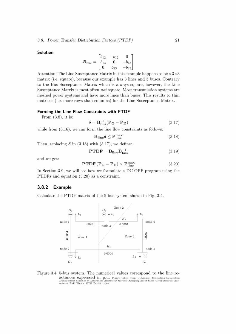
Calculate the PTDF matrix of the 5-bus system shown in Fig. 3.4.

48 Chapter 4. Mathematical Modeling CM Schemes

elasticity.

4.2.4 Modeling of the Transmission System

DC Power Flow Approximations

The above sections outlined the models used for the representation ofthe demand (loads) as well as the supply side (generators). In order toestablish a marketplace between both entities the power produced mustbe transported via the transmission grid, causing a certain power flowover the transmission lines. Figure 4.5 presents an example network asconsidered within the scope of the simulator.

~

~~

~

node 1

node 2

node 3

node 4

node 5

G1

G2

G3

G4

L1

L2

L3 L4

L5

K1

K2

0.0

064

0.0281

0.0304

0.0297

0.0

297

Zone 1

Zone 2

Zone 3

Figure 4.5: Power System Description

As shown, generators and loads are connected by transmission lines,which ‘carry’ a certain flow. For modeling the transmission lines anddetermining the flow, the so-called telegraph equations can be used.However, a simpler and more commonly used representation is the π-line model, which can be directly derived from the telegraph equations.The π-model is characterized by the series resistance, the series reac-tance as well as the shunt susceptance and the shunt conductance ofthe transmission line. Using this model in conjunction with representa-tions of generators and loads, the active and reactive power flows on thelines can be determined. Unfortunately, this approach of computing the

Figure 3.4: 5-bus system. The numerical values correspond to the line re-actances expressed in p.u. Figure taken from: T.Krause, Evaluating CongestionManagement Schemes in Liberalized Electricity Markets Applying Agent-based Computational Eco-nomics, PhD Thesis, ETH Zurich, 2007.

22 3. DC-OPF

Solution1 2 3 4 5

1-2 0 -0.9432 -0.2496 -0.5133 -0.67321-3 0 -0.0568 -0.7504 -0.4867 -0.32682-5 0 0.0568 -0.2496 -0.5133 -0.67323-4 0 -0.0568 0.2496 -0.4867 -0.32684-5 0 -0.0568 0.2496 0.5133 -0.3268

3.9 DC-OPF formulation based on PTDF

Based on the above, we can calculate all line flows with the help of (3.20),without the need of the nodal balance equations (3.8) or the additionalvariables δ. The DC-OPF based on PTDFs is formulated as follows:

min∑i

ciPGi

subject to:

PminGi≤PGi ≤ PmaxGi

(3.21)∑i

PGi−∑i

PDi = 0 (3.22)

−Pmaxline ≤ PTDF(PG −PD) ≤ Pmax

line (3.23)

Note that we still need to have a single equation which will ensure thatthe total generation equal the total demand, as shown (3.22). But we do nothave a separate equality constraint for each node; this is not necessary.

The DC-OPF based on PTDF formulation is currently used for the flow-based market coupling of the European markets. Each node corresponds toa zone (usually a country) and PTDFs are derived for the interconnectionsbetween countries.

4AC Optimal Power Flow

4.1 What is AC Optimal Power Flow?

The AC Optimal Power Flow is an optimization algorithm that considersthe full AC power flow equations. Assuming that the model parametersare correct, this is the most accurate representation of the power flows ina system. This means that the setpoints determined by the optimizationcorrespond as close as possible to reality. The US Federal Energy RegulatoryCommission (FERC) states that the ultimate goal for an electricity marketsoftware should be a security-constrained AC optimal power flow with unitcommitmnent [?]. FERC goes on further to indicate that a good optimizationsolution technique could potentially save tens of billions of dollars annually[?].

In this chapter we will introduce the basic formulation of the AC optimalpower flow. This is the foundation of any AC optimal power flow algorithm(e.g. security-constrained AC-OPF, unit commitment AC-OPF, optimal ACtransmission switching, etc.)

Compared to the DC-OPF formulation that we discussed in the pre-vious chapter, the benefits of the AC-OPF are (i) increased accuracy, (ii)considers voltage, (iii) considers reactive power, (iv) considers currents, (v)considers transmission losses (and other types of losses). However, thereare also drawbacks. The AC power flow equations are quadratic equations(since the power is dependent on the square of the voltage), and if we includethem in an optimization problem as equality constraints, they result to anon-linear non-convex problem. Non-convex problems are in general muchharder to solve, and there is no guarantee that the solver can find the globalminimum. In the past years, serious efforts have been made to “convexify”the AC-OPF. The usual procedure to do that is to relax the non-convexproblem to a convex one (i.e. by defining a convex function around thenon-convex function), then solve the convex problem, and obtain the globaloptimum. If the global optimum is feasible for the original problem, thenwe have identified the optimal solution. If the global optimum lies outsidethe feasible space, then we employ a series of different techniques to recovera feasible solution as close as possible to the global optimum. In the nextchapter, we will discuss the convex relaxations of the AC-OPF, focusing onthe Semidefinite Programming formulation.

One of the central elements for the implementation of the AC-OPF isthe modeling of the transmission lines. In the following sections we outline

23

24 4. AC-OPF

the modeling of the transmission lines, and the derivation of the AC powerflow equations. For more details, the interested reader is encouraged to referto dedicated textbooks in the field (e.g. [?]).

4.2 AC Power Flow

4.2.1 Modeling transmission lines: the π-model

The most usual representation of a transmission line in power systems isthe so-called π-model. For lines between 25 km and 250 km, the π-model isthe most prefered modeling approach. Although there are both simpler andmore complex modelling approaches for the transmission lines (see [?]), inthis chapter we will focus only on the π-model for transmission lines, as thisis the model used by the vast majority of AC-OPF software.

Vi Vj

Rij + jXij

jBij

2

jBij

2

Figure 4.1: π-model of the line

Assume a transmission line connected between the nodes i and j in anetwork, as shown in Fig. 4.1. The π-model of a transmission line consistsof a series impedance Rij + jXij connected at the nodes i and j, and twoequal shunt susceptances, one connected at node i and the other at node j.

We usually represent the π-model by the series admittance: yij =1

Rij + jXij,

and by the shunt susceptances at both ends of the line: ysh,i = ysh,j = jBij2

.

4.2.2 Current flow along a line

Assume a current entering node i in Fig. 4.1. How will it flow along the line?A large part of it will flow along the series admittance yij , but there willalso be some current flowing along the shunt susceptance ysh,i. The totalcurrent entering node i will be equal to:

Ii→j = Ish,i + Iij = ysh,iVi + yij(Vi − Vj) (4.1)

In matrix form (4.1) is written as:

Ii→j =[ysh,i + yij −yij

] [ViVj

](4.2)

4.2. AC Power Flow 25

Similar is the case for a current entering the line at node j. In that casethe total current will be equal to:

Ij→i = Ish,j + Iji = ysh,jVj + yij(Vj − Vi) (4.3)

Again, in matrix form (4.3) is written as:

Ij→i =[−yij ysh,j + yij

] [ViVj

](4.4)

Comparing (4.1) with (4.3) (or, equivalently, (4.2) with (4.4)), we seethat Ii→j 6= −Ij→i. This means that part of the current that is injected atnode i never arrives at node j, and vice versa. The difference between Ii→jand −Ij→i is part of the losses along the transmission line.

4.2.3 Line Admittance Matrix

Looking at (4.2) and (4.4), the question soon arises if it is possible to organizeall current flows in a vector, and form a set of linear equations in a matrixform. Indeed, similar to the line susceptance matrix we saw in chapter 3 wecan form the line admittance matrix.

As shown in (4.5), the line admittance matrix Yline links the bus voltagesV1, . . . , Vn to the current flows I1→2, . . . , Im→n:

Iline = YlineV (4.5)

As already mentioned, taking a look at (4.2) and (4.4), we realize thatthe current flowing in the direction i→ j is different from the current flowingin the opposite direction j → i, with the difference between the two currentsbeing related to the losses along the line. Because of this difference, we mustformulate two line admittance matrices, one for the direction i→ j and onefor the direction j → i.

I1→2

...Ii→j...

Im→n

=

ysh,1 + y12 −y12 0 . . . . . . 0...

......

......

0 . . . ysh,i + yij . . . −yij . . . 0...

......

......

0 . . . . . . ysh,m + ymn . . . −ymn

V1V2...Vi...Vj...Vn

(4.6)

26 4. AC-OPF

I2→1

...Ij→i...

In→m

=

−y12 ysh,1 + y12 0 . . . . . . 0...

......

......

0 . . . −yij . . . ysh,i + yij . . . 0...

......

......

0 . . . . . . −ymn . . . ysh,m + ymn

V1V2...Vi...Vj...Vn

(4.7)

A variety of symbols have been used to identify the two different line ad-mittance matrices in (4.6) and (4.7), e.g. Y from

line , Y toline in different textbooks,

slides, or notes. In these lecture notes, we will use the symbols Yline,i→j todenote the line admittance matrix of (4.6) and Yline,j→i for the line admit-tance matrix of (4.7).

Forming the Line Admittance Matrix

1. Yline is an L×N matrix, where L is the number of lines and N is thenumber of nodes

2. if row k corresponds to line i→ j:

– start node i: Yline,ki = ysh,i + yij

– end node j: Yline,kj = −yij– rest of the row elements are zero

3. yij =1

Rij + jXijis the admittance of line ij

4. ysh,i is the shunt capacitance jBij/2 of the π-model of the line

5. We must create two Yline matrices. One for i→ j and one for j → i.

4.2.4 Bus Admittance Matrix

In order to be able to form the AC-OPF constraints, it is necessary to beable to compute the bus power injections. The bus power injection showsthe net power that is entering or leaving a bus. By definition, in AC systemsthe net apparent power at a bus is equal to the product of the bus voltage(complex number) and the conjugate of the bus current (complex number):

Si = ViI∗i (4.8)

4.2. AC Power Flow 27

According to Kirchhoff’s law, the net current injection at a bus is equalto the sum of currents leaving the bus. The sum of currents leaving a busi is the sum of the line currents flowing along all lines connected to bus i.This is expressed by (4.9):

Ii =∑k

Iik,where k are all the buses connected to bus i (4.9)

Let us now assume that from bus i emanate two lines which connect ito buses m and n. Using also the result of (4.1), it is:

Ii = Iim + Iin

= (yi→msh,i + yim)Vi − yimVm + (yi→nsh,i + yin)Vi − yinVn= (yi→msh,i + yim + yi→nsh,i + yin)Vi − yimVm − yinVn (4.10)

In matrix form (4.10) is written as:

Ii = [ysh,im + yim + ysh,in + yin − yim − yin]

ViVmVn

(4.11)

Similar to our considerations for the Line Admittance Matrix, and givenour passion for vectors and matrices – which must have become quite obviousby now (!) – the question arises what is the algebraic relationship that canlink vectors of bus currents and bus voltages. This is the role of the BusAdmittance Matrix Ybus:

Ibus = YbusV (4.12)

Taking a close look at (4.11), we observe that the matrix element multi-plied with Vi is the sum of all line admittances plus all the shunt elementsconnected to bus i (usually these are the line shunts from the π-model, but itcan also be additional shunt capacitors or inductors often used for reactivecompensation). On the contrary, the matrix elements that are multipliedwith the voltages at the neighboring buses are just the negative of the lineadmittance connecting the neighboring bus to bus i. For an arbitrary powersystem, where bus i is connected to buses m and n, bus 1 is only connectedto bus 2, and bus n is only connected to bus i, the Bus Admittance Matrix

28 4. AC-OPF

will have the following form:

I1...Ii...In

=

ysh,1 + y12 −y12 0 . . . . . . 0...

......

......

0 . . . ysh,im + yim + ysh,in + yin . . . −yim . . .− yin...

......

......

0 . . . −yin . . . . . . ysh,n + yin

V1V2...Vi...Vn

(4.13)

Forming the Bus Admittance Matrix

1. Ybus is an N ×N matrix, where N is the number of nodes

2. diagonal elements: Ybus,ii =∑

t∈I ysh,t +∑

k yik, where k are all thebuses connected to bus i

3. off-diagonal elements:

– Ybus,ij = −yij if nodes i and j are connected by a line1

– Ybus,ij = 0 if nodes i and j are not connected

4. yij =1

Rij + jXijis the admittance of line ij

5. ysh,i are all shunt elements t connected to bus i, including the shuntcapacitance of the π-model of the line

4.2.5 AC Power Flow Equations

From (4.13), it is Ii = Ybus, row-iV, where Ybus, row-i denotes the i-th row ofthe Ybus matrix. Therefore, the apparent power at bus i is:

Si = ViI∗i

= ViY∗bus, row-iV

∗

If we now want to express the bus apparent power in vector form, theproblem is that we need to multiply from the left each row of the matrixYbus with the complex number Vi. To do that we introduce the notationdiag(V). Here, by diag(V) we denote a diagonal N ×N matrix, where theN diagonal elements are equal to the N ×1 vector V, and all the rest of thematrix elements are zero.

1If there are more than one lines connecting the same nodes, then they must all beadded to Ybus,ij , Ybus,ii, Ybus,jj .


Then, for all buses, the apparent power S = [S1 . . . SN ]T is:

S = diag(V)Y∗busV∗ (4.14)

The net apparent power injection at every bus is equal to the totalgeneration minus the total load connected at the bus. In vector form:

S = Sgen − Sload (4.15)

Combining (4.14) and (4.15), the AC power flow equations are given by:

Sgen − Sload = diag(V)Y∗busV∗ (4.16)


In Section 4.2, we have introduced two types of equations. First, the equa-tions about the line currents. Second, the equations about the bus currentand bus power injections. These two sets of equations will form a fundamen-tal part of our constraints in the AC Optimal Power Flow problem:

minPGi

cccTPPPG (4.17)

subject to:

AC flow SG − SL = diag(V)Y∗busV

∗(4.18)

Line Current |Yline,i→jV| ≤ Iline,max (4.19)

|Yline,j→iV| ≤ Iline,max (4.20)

or Apparent Flow |V iY∗line,i→j,row-iV

∗| ≤ Si→j,max (4.21)

|V jY∗line,j→i,row-jV

∗| ≤ Sj→i,max (4.22)

Gen. Active Power 0 ≤ PG ≤ PG,max (4.23)

Gen. Reactive Power −QG,max ≤ QG ≤ QG,max (4.24)

Voltage Magnituge Vmin ≤ V ≤ Vmax (4.25)

Voltage Angle δδδmin ≤ δδδ ≤ δδδmax (4.26)

All shown variables are vectors or matrices. The bar above a variabledenotes complex numbers. The operator (·)∗ denotes the complex conjugate.To simplify notation, the bar denoting a complex number is dropped in therest of this chapter. Attention! The current flow constraints are defined asvectors, i.e. for all lines. The apparent power line constraints are defined perline.

The AC-OPF formulation, as we present it in (4.27), minimizes the activepower generation costs. However, for the AC-OPF, we can set several differ-ent objectives. For a more detailed discussion, please refer to Section 4.3.1.

30 4. AC-OPF

Constraints (4.18) are the only equality constraints in the standard AC-OPF formulation, and they denote the AC power flow equations. Any oper-ating point that will be determined through the optimization must satisfythe AC power flow equations in order to be a true operating point of thepower system.

Constraints (4.19) - (4.20) represent the line current inequality con-straints. If our transmission line limits are represented by the current thermallimit, these are the inequality constraints that must be used. If, on the otherhand, the line thermal limits are set by the apparent power, then (4.21) –(4.22) must be used, which refer to the apparent power flow. In any case,only one set of these constraints must be used: either the line current limit(4.19) - (4.20) of the apparent power line flow limit (4.21) – (4.22).

Constraints (4.23) refer to the active power bounds of the generators,while constraints (4.24) refer to the generators’ reactive power bounds. Con-straints (4.25) refer the maximum and minimum allowable limits for the busvoltage magnitudes (no complex numbers here), and constraints (4.26) referto maximum and minimum allowable limits for the voltage angles.

4.3.1 Objective Function for the AC Optimal Power Flow

Despite the goal to clear all electricity markets with an algorithm based onthe AC-OPF in the future, the AC Optimal Power Flow can be used fora number of different purposes. Here we list four of those, among severalexamples.

Minimization of costs: As shown in (4.27), one of the most common usesfor the AC-OPF is the minimization of the costs for producing electricity.The objective function minimizes the total costs for generating active power:

minPGi

cccTPPPG (4.27)

This objective function can be used both for clearing electricity markets,but also in vertically integrated utilities that want to reduce their operatingcosts (in that case possibly assuming quadratic costs).

Minimization of active and reactive power losses: The minimization ofthe active and reactive power losses is probably among the most importantdaily functions of the system operator – after, of course, ensuring that thepower system is secure and not threatened by blackouts. To minimize theactive and reactive power losses, the objective function can be of the form:

min∑i,j∈L

Sij + Sji (4.28)


The total losses along a line i−j are equal to the apparent power leavingnode i minus the apparent power arriving node j. As shown in Fig. 4.2, thepower leaving node i is Si→j . The apparent power arriving at node j is equalto −Sj→i; this is because by convention the direction j → i is positive, sothe power exiting node j will have a direction opposite to j → i.

According to this:

Slosses = Si→j − (−Sj→i) (4.29)

Slosses = Si→j+Sj→i (4.30)

i j

Rij + jXij

jBij

2

jBij

2

Si→j −Sj→i

Figure 4.2: π-model of the line and apparent power flows

Maintaining a constant voltage profile: At times power system operatorsmay want to maintain a constant voltage profile across all or a part of thesystem nodes. This, for example, might help them avoid voltage instabilityproblems. An optimization in this case may help them identify what is thepreferrable set of actions, usually related to the injection or absorption ofreactive power, to achieve the desired profile. The objective function canhave for example the following form (among several possibilities):

min∑i

(Vi − Vsetpoint,i)2 (4.31)

The quadratic objective function in this case helps us minimize both thepositive and the negative deviations of the voltage from the desired setpoint.A different option would be to minimize the absolute value of the deviation,i.e. min

∑i |Vi − Vsetpoint,i|. In that case, however, for most solvers we need

to reformulate our problem in order to remove the absolute value from ourobjective function, as it is a non-smooth function.

For this problem, we may also consider different objective functions,e.g. to minimize both the voltage deviation and the required changes inreactive power – but we must be careful when it comes to multi-objectiveoptimization. We can also consider additional constraints for our problem,e.g. that the active power injection at every bus must remain constant tothe pre-decided level. In that case we have to replace (4.23) with an equalityconstraint of the form PPP = PPP setpoint.

32 4. AC-OPF

Transmission investments: This formulation usually involves mixed inte-ger programming, as the optimizer must be able to choose among differentoptions for new transmission lines. In its simplest form, however, the goalof transmission investments might be to determine what is the minimumcapacity upgrades in existing lines, in order to reduce the operating cost. Tosimplify things further, as an initial “back-of-the-envelope” calculation onemay neglect that the line upgrades are performed in blocks, i.e. either up-grading an exisiting line by e.g. 100 MVA or not; upgrading to any desirablevalue i.e. 53.5 MVA is impossible – not from a technical perspective, butrather from the availability of the options provided by manufacturers. Toavoid this discontinuity, one can assume that the line upgrade is a continuousvariable. In that case, the objective function will look like:

min∑t∈H

cTt PG, t+ cTlinesline (4.32)

where∑

t∈H cTt PG, t is the sum of the generating costs over the projectedlifetime of the transmission line, cline is the cost of line upgrade per unit ofadditional capacity, and sline is the newly added capacity, measured eitherin Amperes (current) or in MVA (power).

Besides the objective function, we also have to add variable sline eitherto line current inequalities (4.19) - (4.20) of the apparent power flow (4.21)– (4.22). For example, for the line current inequalities, this would look like:

|YlineV| ≤ Iline,max + sline (4.33)

After we solve the optimization, we can then perform a more detailed cost-benefit analysis and select one of the available capacity upgrade options,that will probably be close to our optimization result.

4.3.2 Transmission Line Limit constraints: Current vs Power

As shown in (4.19) - (4.20) and (4.21) – (4.22), we can have different typesof inequalities to express the line limits. But what are the inequalities weshould use, and when each of them is most appropriate?

Several OPF formulations are imposing the apparent power limits foroverhead lines, cables, and transformers. This should not be always the case,however.

Especially for overhead lines (OHL) and cables, it is preferrable to usethe line current limits. The OHL and cable manufacturers usually indicatethe thermal limits of their conductors in Amperes, since it is the currentthat is the limiting factor for the thermal stress of the OHL or cables. So,for overhead lines and cables it is better to use the line current inequalities(4.19) - (4.20) as limits.

For transformers, on the other hand, it is difficult to set the currentlimit as constraint, as primary side and secondary side have different line


currents (although in the per unit system they will both be the same). Themanufacturers of transformers usually give the apparent power as the limitto prevent overloads and excessive thermal stress of their equipment. So, fortransformers, it is usually preferrable to use the apparent power limit, asexpressed by (4.21) – (4.22).

Besides current and apparent power limits, literature also suggests theuse of active power limits. Indeed, active power can be the limiting factor forthe transmission along very long lines. Beyond certain lengths, and as thereactance xij of the line increases, the limiting factor for the power transferbecomes its steady-state stability limit, which is given by the relationsip:

Pij,max =1

xijViVj (4.34)

In case of very long lines (over a few hundred of kilometers) using the activepower flow limit is preferrable. In that case, the active power flow along aline will be equal to Re(Si→j) = Re(ViI

∗i→j). Following the derivations we

present in Section 4.4, the active power limit inequality constraints are givenby the equations:

[Re(Vi) − Im(Vi)

] [Re(Yline,i→j) − Im(Yline,i→j)Im(Yline,i→j) Re(Yline,i→j)

]∗ [Re(V)Im(V)

]∗≤ Pij,max

(4.35)

[Re(Vj) − Im(Vj)

] [Re(Yline,j→i) − Im(Yline,j→i)Im(Yline,j→i) Re(Yline,j→i)

]∗ [Re(V)Im(V)

]∗≤ Pji,max

(4.36)Notice that Re(Vi),− Im(Vi),Re(Vj),− Im(Vj), Pij,max and Pji,max are

scalars while the rest, shown in boldface, are vectors or matrices.

Line Limits: Absent of real models and datasheets, we often need to usepublicly available power system models. These sources may often containonly the apparent power flow limit and provide no information about theline current limit (e.g. this is the case for Matpower case files, and someIEEE systems). There is a straightforward way to transform any apparentpower limit to a good approximation of an equivalent line current limit. Hereis how to do this.

As it must be well known by now, it is: S = V I∗. Taking the absolutevalue of the left and right terms, and considering that for any complexnumber holds |z| = |z∗|, it is:

|S| = |V ||I| (4.37)

Assuming that our lines are operated at nominal voltage (this is the onlyapproximation we make), it must be V = 1p.u. So, as long as (4.37) is

34 4. AC-OPF

expressed in per unit, then |S| = |I|. This means that the line current limitis equal to the apparent power limit expressed in per unit:

Si→j,max = Ii→j,max in per unit; orSi→j,maxSbase

=Ii→j,maxIbase

(4.38)

4.3.3 Bus Voltage Magnitude Limits

To maintain safe operation, we usually bound the voltage magnitude withina small range of aceeptable limits. In the vast majority of cases we allowa maximum voltage deviation of 10% or less. This means that the voltagebounds are often Vmin = 0.9 p.u. and Vmax = 1.1 p.u. However, we can oftenimpose even tighter limits, e.g. Vmin = 0.95 p.u. and Vmax = 1.05 p.u. Ingeneral, any voltage magnitude limits that do not allow more than 10%deviation are acceptable, but depending on the system and the application,we need to be considerate of tighter voltage limits.

4.3.4 Bus Voltage Angle Limits

Voltage angle limits are important for the non-linear solver of the AC-OPF.Due to the fact that our equations use complex numbers, we can obtainseveral instances of exactly the same power flow solution in “angle intervals”of 360o. For example, V = 1.02∠15o = 1.02∠375o = 1.02∠−345o. Bybounding our bus voltage angles within the range of 0o and 360o, we guidethe solver to a unique solution and avoid possible degenerate cases, wherethe solver oscillates between two exactly equivalent solutions that are justshifted by 360o. Limiting our solutions between −180o and 180o is equivalentto 0 and 360o and is usually preferrable. Since, in our formulations we areusually computing in rad, then the most usual angle limits are:

δmin = −π ≤ δ ≤ π = δmax (4.39)

4.4 Operations with complex numbers when formu-lating the optimization problem

Non-linear solvers in Matlab accept complex numbers, so we can directlyenter the problem formulation in a complex number format. However, thereare several other solvers that cannot deal with complex numbers, and requirethe input of real numbers instead. Interfaces like YALMIP overcome thisissue for the user by directly accepting the complex number formulationand translating it to real numbers.

Being able to transform complex number operations to operations withreal numbers is a skill that is sometimes required (e.g. if we code in a differentenvironment from Matlab, or dealing with semidefinite programming, as we

4.5. From the AC power flow equations to the DC power flow 35

will see in the next chapter). In this section we describe how we can dealwith this problem.

Suppose we want to multiply complex numbers z1 = a + jb and z2 =c+ jd. Then:

z3 = z1z2 = (a+ jb)(c+ jd) = ac− bd+ j(ad+ bc) (4.40)

We can separate the real and imaginary part of a complex number by treat-ing z as a 2× 1 vector of real numbers, in the form: z = [a b]T .

Having this in mind, we can transform the multiplication of two complexnumbers to a multiplication of a matrix with a vector of real numbers, asfollows:

z3 =

[ac− bdbc+ ad

]=

[a −bb a

] [cd

](4.41)

In other words, we can express the multiplication of any complex num-bers to a multiplication of real numbers as follows:[

Re(z3)Im(z3)

]=

[Re(z1) − Im(z1)Im(z1) Re(z1)

] [Re(z2)Im(z2)

](4.42)

This property also extends to multiplication of vectors of complex num-bers. Assume I = YV, where I,V are complex vectors, and Y is a complexmatrix. From the above equation, we can generalize as follows:[

Re(I)Im(I)

]=

[Re(Y) − Im(Y)Im(Y) Re(Y)

] [Re(V)Im(V)

](4.43)

4.5 From the AC power flow equations to the DCpower flow

The time for your patience since Chapter 3 and (3.1) is now coming to anend! Starting from the full AC power flow equations, in this section we willpresent how we arrived at equation (3.1), which formed the basis of our DCpower flow equations. This creates the link between AC power flow and DCpower flow, while explicitly stating all assumptions made.

The power flow along a line is:

Si→j = ViI∗i→j = Vi(y

∗sh,iV

∗i + y∗ij(V

∗i − V ∗j )) (4.44)

Assumptions:

1. Assume a negligible shunt conductance: gsh,ij = 0 ⇒ ysh,i = jbsh,i.This is true for most power system modeling approaches, as even theπ-model of a transmission line usually neglects the shunt conductance.

36 4. AC-OPF

2. Assume a negligible series resistance: zij = rij + jxij ≈ jxij . Then

yij = −j 1

xij. In transmission systems it is usually R << X for the

series impedance in the π-model of the transmission line. Therefore,especially for lightly loaded systems, neglecting it will not have a largeimpact on the results. (Note: this assumption is not quite valid indistribution systems, where R can be comparable to X; the full ACpower flow equations must be used for optimization in distributionsystems)

According to the above two assumptions, the current I∗i→j , shown in(4.44), becomes:

I∗ij = −jbsh,iV ∗i + j1

xij(V ∗i − V ∗j )) (4.45)

3. Assume: Vi = Vi∠0 and Vj = Vj∠θ, with θ = δj − δi (no loss ofgenerality with this assumption). Then:

I∗ij =− jbsh,iVi + j1

xij(Vi − (Vj cos θ − jVj sin θ)) (4.46)

=− jbsh,iVi + j1

xijVi − j

1

xijVj cos θ − 1

xijVj sin θ (4.47)

As Vi = Vi∠0, Vi is a real number. Then the active power transfer alonga line is:

Pij = Re{Sij} = Vi Re{I∗ij} = − 1

xijViVj sin θ (4.48)

As we have set δ = θj − θi, it is:

Pij =1

xijViVj sin(δi − δj), (4.49)

which is exactly the equation (3.1)As already mentioned in Chapter 3, to arrive at the DC power flow

equations, we further make the following assumptions:

4. Vi, Vj are constant and equal to 1 p.u.

5. sin θ ≈ θ, where θ must be in rad

Then:

Pij =1

xij(δi − δj)

For a more detailed discussion of the assumptions (4) and (5), the inter-ested reader is referred to Chapter 3.

4.6. Nodal Prices (LMPs) in AC-OPF 37

4.6 Nodal Prices (LMPs) in AC-OPF

The nodal prices in the AC-OPF are the lagrangian multipliers of the equal-ity constraints for the active power flow.

To calculate them, we need to split equality constraints (4.18) to theirreal and imaginary part, as follows:

PG −PL = Re diag(V)Y∗busV

∗(4.50)

QG −QL = Im diag(V)Y∗busV

∗(4.51)

The Lagrangian multipliers associated with equality constraints (4.50)are the nodal prices for the AC-OPF problem. They show what is themarginal cost of the demand of an additional MW at each node.

4.6.1 LMPS in the AC-OPF vs DC-OPF

Attention: The nodal prices calculated through the AC-OPF will alwaysdiffer at different buses. Contrary to the DC-OPF, where the nodal pricesare exactly the same at all buses if there is no congestion, this is not thecase here. The AC-OPF explicitly considers the line losses, and these are anintegral component of the nodal prices in the AC-OPF. As a result, besidesthe generator cost and the contribution to the line congestion, in the AC-OPF there is a third cost component which has to do with the amount oflosses incurred to the system by the demand of an extra MW at a specificbus.

Considering that the consumption of an additional MW will incur adifferent amount of system losses depending on where this is consumed, thisis why the LMPs in the AC-OPF always differ from each other, even if thereis no line congestion.

38 4. AC-OPF

Appendix ADerivation of Locational Marginal Prices

min∑i

ciPGi

subject to:

PminGi≤ PGi ≤ PmaxGi

∑i

PGi −∑i

PDi = 0

PTDF(PG −PD) ≤ Pmaxline

L(PG, ν, λ, µ) =

NPG∑i=1

ciPG,i + ν ·

NPG∑i=1

PG,i −NPL∑i=1

PL,i

+

NL∑i=1

λ+i · [PTDFi · (PG −PL)− FL,i]

+

NL∑i=1

λ−i · [−PTDFi · (PG −PL)− FL,i]

+

NPG∑i=1

µ+i · (PG,i − PG,i,max) +

NPG∑i=1

µ−i · (−PG,i)

– Assume a 3-bus system with 3 generators, and 1 load on bus 3

– We assume an auxilliary variable ξ3 that represents very small changesof the load in Bus 3. We assume ξ3 = 0.

– Then it is P̂L = PL + Ξ, where Ξ = [0 0 ξ3]T .

39

40 A. Derivation of Locational Marginal Prices

1 2

3

L(PG, ν, λ, µ,Ξ) =

NPG∑i=1

ciPG,i + ν ·

NPG∑i=1

PG,i −NPL∑i=1

PL,i − ξi

+

NL∑i=1

λ+i · [PTDFi · (PG −PL − Ξ)− FL,i]

+

NL∑i=1

λ−i · [−PTDFi · (PG −PL − Ξ)− FL,i]

+

NPG∑i=1


NPG∑i=1

µ−i · (−PG,i).

– To save space in this slide: Ki ≡ PTDFi

L(PG, ν, λ, µ, ξ3) =

NPG∑i=1

ciPG,i + ν ·

NPG∑i=1

PG,i −NPL∑i=1

PL,i − ξ3

+

NL∑i=1

λ+i · [Ki,1 · PG,1 +Ki,2 · PG,2 +Ki,3 · (PG,3 − PL,3 − ξ3)− FL,i]

+

NL∑i=1

λ−i · [−Ki,1 · PG,1 −Ki,2 · PG,2 −Ki,3 · (PG,3 − PL,3 − ξ3)− FL,i]

+

NPG∑i=1


NPG∑i=1

µ−i · (−PG,i).

– No congestion ⇒ all λi = 0

– One marginal generator: only one generator has both µ+i = 0 andµ−i = 0

41

– Assume G2 is marginal; PG1 = PG1,max; PG3 = 0.

∂L∂PG,i

= 0, for all i ∈ NPG

c1 + ν + µ+1 = 0

c2 + ν = 0

c3 + ν + µ−3 = 0

Marginal change in the cost functionfor a marginal change in load:

LMP3 =∂L∂ξ3

= −ν

Attention! ξ3 does not exist in the optimization problem and is not anoptimization variable. We do not need to derive any KKT conditions w.r.t.

ξ3, e.g. ∂L∂ξ3

= 0.ξ3 is just an auxilliary variable. It helps us “represent” the marginal

change in the load of bus 3. ∂L∂ξ3

quantifies its effect on the Lagrangian.

– No congestion ⇒ all λi = 0

– One marginal generator: only one generator has both µ+i = 0 andµ−i = 0

– Assume G2 is marginal; PG1 = PG1,max; PG3 = 0.

∂L∂PG,i


c1 + ν + µ+1 = 0

c2 + ν = 0

c3 + ν + µ−3 = 0


LMP3 =∂L∂ξ3

= −ν

LMP3 = −ν = c2: nodal price on bus 3!How much is the LMP on the other buses?

– Assume that line 1-3 gets congested in the direction 1→ 3⇒ λ+13 6= 0

– Now G2 and G3 are both marginal gens; PG1 = PG1,max.

∂L∂PG,i


c1 + ν + µ+1 + λ+13PTDF13,1 = 0

c2 + ν + λ+13PTDF13,2 = 0

c3 + ν + λ+13PTDF13,3 = 0


LMP3 =∂L∂ξ3

= −ν − λ+13PTDF13,3

To find LMP3 I need ν and λ+13How do I find ν and λ+13?

42 A. Derivation of Locational Marginal Prices

– Solve the linear system with 2 equations and 2 unknowns: ν and λ+13

c2 + ν + λ+13PTDF13,2 = 0

c3 + ν + λ+13PTDF13,3 = 0

– What can we say about the LMPs on different buses?

LMPi = −ν − λ+13PTDF13,i

– If there is a congestion, the LMPs are no longer the same on everybus. They are dependent on the congestion!

Optimization in Modern Power Systems DTU Course 31765

Documents

Transcript of Optimization in Modern Power Systems DTU Course 31765