General rights Copyright and moral rights for the publications made accessible in the public portal are retained by the authors and/or other copyright owners and it is a condition of accessing publications that users recognise and abide by the legal requirements associated with these rights.

Users may download and print one copy of any publication from the public portal for the purpose of private study or research.

You may not further distribute the material or use it for any profit-making activity or commercial gain

You may freely distribute the URL identifying the publication in the public portal If you believe that this document breaches copyright please contact us providing details, and we will remove access to the work immediately and investigate your claim.

Downloaded from orbit.dtu.dk on: Feb 10, 2022

Computational Screening of Energy Materials

Pandey, Mohnish

Publication date:2015

Link back to DTU Orbit

Citation (APA):Pandey, M. (2015). Computational Screening of Energy Materials. Technical University of Denmark.

Computational Screeningof Energy Materials

PhD ThesisMohnish Pandey

Computational Screening of Energy MaterialsPhD ThesisJuly 2015

Mohnish Pandeymohpa@fysik.dtu.dk

Supervisors:Karsten Wedel JacobsenKristian Sommer Thygesen

Center for Atomic-scale Materials DesignDepartment of PhysicsTechnical University of Denmark

Preface

This thesis is submitted for the candidacy of PhD degree in Physics from theTechnical University of Denmark. The work contained in the thesis was carriedout at the Center for Atomic-scale Materials Design (CAMd), Department ofPhysics in the period from August 2012 to July 2015 under the supervision ofProf. Karsten W. Jacobsen and Prof. Kristian S. Thygesen.I cannot thank enough my supervisors Karsten and Kristian for their continu-ous support in my projects. Every bit of discussion I had with them improvedmy understanding of the subject matter. Their immense zeal in the projectsand their unparalleled guidance always kept me motivated and helped me toget over the bottlenecks I faced during my research.Also, I would like to thank Aleksandra, Ivano, Filip, Niels and Thomas forall the suggestions and discussions regarding different projects. Big thanks toChris, Kirsten, Kristian, Martin, Niels and Simon Lamowski for generouslyagreeing to proofread the thesis and for the good times at CAMd. A deepgratitude to Jens Jørgen and Marcin for helping in the code developmentsand troubleshootings and Ole for taking such a good care of Niflheim for itsseamless functioning. A huge thanks to Marianne for making my move toDenmark easy by taking care of all the rigmarole and other administrativematters.Among friends my special thanks to Kristian for his continuous support andinvitations for Indian festival dinners to make me feel home. I would also liketo thank my other colleagues at CAMd - Korina, Manuel, Morten, Per, Simoneand Ulrik for all the fun times.Last but not least my heartfelt thanks to my family members for their continu-ous support and my girlfriend Shrutija for not letting me feel the long-distancerelationship really as long-distance and supporting me in all the ways she could.

Mohnish PandeyKongens Lyngby, July 2015

Abstract

The current energy consumption of the worlds population relies heavily on fos-sil fuels. Unfortunately, the consumption of fossil fuels not only results in theemission of greenhouse gases which have deleterious effect on the envrionmentbut also the fossil fuel reserve is limited. Therefore, it is the need of the hourto search for environmentally benign renewable energy resources. The biggestsource of the renewable energy is our sun and the immense energy it providescan be used to power the whole planet. However, an efficient way to harvestthe solar energy to meet all the energy demand has not been realized yet.

A promising way to utilize the solar energy is the photon assisted watersplitting. The process involves the absorption of sunlight with a semiconduct-ing material (or a photoabsorber) and the generated electron-hole pair can beused to produce hydrogen by splitting the water. However, a single materialcannot accomplish the whole process of the hydrogen evolution. In order doso, a material should be able to absorb the sunlight and generate the electron-hole pairs and evolve hydrogen at the cathode and oxygen at anode using thegenerated electron and hole respectively.

This thesis using first-principle calculations explores materials for the lightabsorption with the bandgap, band edge positions and the stability in aqueousconditions as descriptors. This strategy results in a handful of materials whichcan act as good photoabsorbers for the water splitting reaction. Additionally,strategies to tune the bandgap for different applications is also explored. Tocarry out the cathode reaction, two-dimensional metal dichalcogenides and ox-ides are explored with a suggestion of few potential candidates for the hydrogenevolution reaction.

The thermodynamics of all the above process requires an accurate descrip-tion of the energies with the first-principle calculations. Therefore, along thisline the accuracy and predictability of the Meta-Generalized Gradient Approx-imation functional with Bayesian error estimation is also assessed.

Resumé

Jordens befolkning er i dag fuldstændig afhængig af fossile brændstoffer forat producere den nødvendige energi. Denne afhængighed er meget uforde-lagtig, idet lageret af tilgængelige fossile brændstoffer er stærkt begrænset sam-tidigt med, at afbrændingen af fossile brændstoffer producerer klimaskadeligedrivhusgasser. Det er derfor nødvendigt, at finde miljøsikre vedvarende en-ergikilder. Den største tilgængelige vedvarende energikilde er solen, hvis en-ergiudladning er stor nok til at dække hele vores planets energiforbrug. Dogmangler vi stadigvæk en måde hvorpå solenergien kan høstes effektivt.En lovende metode til at opfange solenergi er foton-assisteret vandspaltning.Denne metode indbefatter et halvleder-materiale, der absorberer en fotonhvilket genererer et elektron-hul par, som kan bruges til at producere brintvia vandspaltning. Det er dog umuligt for et enkelt materiale, at stå for heleden foton-assisterede vandspaltnings proces. For at muliggøre processen erdet nødvendigt både at have et foton-absorberende materiale, der absorberersollyset og genererer elektron-hul parret, et anodemateriale, der faciliterer il-tudvindingsdelen af vandspaltning ved hjælp af det genererede hul, samt etkatodemateriale, som anvender den genererede elektron til at udvikle brint.I denne afhandling anvendes første princip beregninger til at finde foton-absorberende materialer, hvor materialernes båndgab, placering af båndkan-ten samt materialernes stabilitet i vand bruges som deskriptorer. Ved brugaf denne strategi identificeres en håndfuld foton-absorberende materialer, somværende velegnede til brug i foton-assisteret vandspaltning. Derudover under-søges flere muligheder for at optimere et materiales båndgab til brug i forskel-lige sammenhænge. En række todimensionale metaldichalkogener og metalox-ider undersøges til brug som katodematerialer, og flere potentielt brugbarekandidater præsenteres.Det er nødvendigt at bruge metoder, der giver akkurate første princip energier,for korrekt at beskrive termodynamikken i alle de ovenfor nævnte processer.Derfor undersøges præcisionen af funktionalet med Meta-Generaliseret Gradi-ent Approksimation baseret Bayesiansk fejl-estimation.

List of papers

• Heats of Formation of Folids with Error Estimation: The mBEEF Func-tional with and without Fitted Reference Energies M. Pandey and K.W. Jacobsen, Physical Review B 91 (23), 235201 (2015)

• Two-Dimensional Metal Dichalcogenides and Oxides for Hydrogen Evo-lution: A Computational Screening Approach M. Pandey, A. Vojvodic,K. S. Thygesen and K. W. Jacobsen, The Journal of Physical ChemistryLetters 6 (9), 1577-1585 (2015)

• New Light-Harvesting Materials Using Accurate and Efficient BandgapCalculations I. E. Castelli, F. Hüser, M. Pandey, H. Li, K. S. Thygesen,B. Seger, A. Jain, K. A. Persson, G. Ceder and K. W. Jacobsen, Ad-vanced Energy Materials 5 (2) (2015)

• Band-gap Engineering of Functional Perovskites Through Quantum Con-finement and Tunneling I. E. Castelli, M. Pandey, K. S. Thygesen andK. W. Jacobsen, Physical Review B 91 (16), 165309 (2015)

Contents

1 Introduction 1

2 Theory 42.1 Schrödinger Equation . . . . . . . . . . . . . . . . . . . . . . . 4

2.1.1 Adiabatic and Born-Oppenheimer approximation . . . . 52.2 Density Functional Theory: An Introduction . . . . . . . . . . 6

2.2.1 Local (Spin) Density Approximation (L(S)DA) and Gen-eralized Gradient Approximation (GGA) . . . . . . . . 7

2.3 Calculation of Bandgaps with DFT . . . . . . . . . . . . . . . . 82.3.1 A Brief Introduction to the Hybrid Functionals . . . . . 9

2.4 Implementation of DFT in the GPAW (Grid-based ProjectorAugmented Wave) code . . . . . . . . . . . . . . . . . . . . . . 112.4.1 A Brief Introduction to the PAW Method . . . . . . . . 11

3 Heats of Formation of the Solids 133.1 Introduction . . . . . . . . . . . . . . . . . . . . . . . . . . . . . 133.2 Calculation of the heats of formation without the fitting . . . . 143.3 Calculation of the heats of formation with the fitting . . . . . . 153.4 Outliers in the different predictions . . . . . . . . . . . . . . . . 173.5 True versus predicted error in the mBEEF functional . . . . . . 203.6 Cross validation . . . . . . . . . . . . . . . . . . . . . . . . . . . 203.7 Conclusion . . . . . . . . . . . . . . . . . . . . . . . . . . . . . 22

4 Hydrogen Evolution from Two-Dimensional Materials 254.1 Introduction . . . . . . . . . . . . . . . . . . . . . . . . . . . . . 254.2 Details of the atomic structure . . . . . . . . . . . . . . . . . . 264.3 Stability with respect to the standard states . . . . . . . . . . . 294.4 Adsorption of hydrogen on the basal planes . . . . . . . . . . . 29

xi

4.5 Candidates for the HER . . . . . . . . . . . . . . . . . . . . . . 35

5 Materials for Light Absorption 425.1 Introduction . . . . . . . . . . . . . . . . . . . . . . . . . . . . . 425.2 Mechanism of photoelectrochemical water splitting . . . . . . . 435.3 Different methods for the bandgap calculation . . . . . . . . . . 445.4 Candidates for photoelectrochemical water splitting . . . . . . 465.5 Bandgap engineering of functional perovskites . . . . . . . . . . 495.6 Conclusion . . . . . . . . . . . . . . . . . . . . . . . . . . . . . 57

6 Trends in Stability and Bandgaps of Binary Compounds inDifferent Crystal Structures 586.1 Introduction . . . . . . . . . . . . . . . . . . . . . . . . . . . . . 586.2 Results and Discussions . . . . . . . . . . . . . . . . . . . . . . 596.3 Conclusion . . . . . . . . . . . . . . . . . . . . . . . . . . . . . 70

7 Final Remarks 71

Bibliography 72

Papers 82Paper I . . . . . . . . . . . . . . . . . . . . . . . . . . . . . . . . . . 82Paper II . . . . . . . . . . . . . . . . . . . . . . . . . . . . . . . . . . 94Paper III . . . . . . . . . . . . . . . . . . . . . . . . . . . . . . . . . 109Paper IV . . . . . . . . . . . . . . . . . . . . . . . . . . . . . . . . . 138

Chapter 1

Introduction

Chemical fuels are the most widely used energy resource due to their high en-ergy density and ease of availability. Additionally, storing chemical fuels andtransferring them from one place to another is easier e.g. through pipelines.Therefore, all the above factors made society heavily dependent on them for itsenergy consumption which is increasing every year. Eventually, the increasingconsumption of fossil fuels is leading to increased greenhouse gas emissions.For example, the global CO2 emission in 2001 was approximately 24.07 giga-ton/year (Gt/yr) which is projected to increase to 40.3 Gt/yr by 2050 and48.8 Gt/yr by the end of 2100 [1]. An increase in CO2 emission by almosttwo times in the next three decades will pose a serious threat to the environ-ment. Additionally, the availability of the fossil fuels will also become scarce atsome point. Therefore, it is the need of the hour to search for environmentallybenign and abundant renewable energy resources.

Renewable energy sources e.g. wind energy, hydro-electricity, solar thermalconversion, solar electricity, solar fuels etc. may serve as viable alternatives tothe fossil fuels [2]. Among all renewable energy resources, the biggest sourceof the renewable energy is our sun and the immense energy it provides can beused to power the whole planet. However, we are very far from realizing thedream of being completely dependent on the sun for our energy requirements.The challenge lies in utilizing the solar energy in an efficient and economicalway [1, 2]. However, concerted and continuous efforts by theoreticians and ex-perimentalists are being put in order to overcome these challenges. Figure 1.1shows a model of the workflow for the materials design with mutual feedbackof the experimentalists and theoreticians.

1

2

Figure 1.1: Concerted effort of experimentalists and theoreticians. The mu-tual feedback from each other leads to an efficient materials design and un-derstanding of a given physical/chemical process. Image courtesy: SUNCAT(http://suncat.stanford.edu).

Among many possible ways to utilize solar energy one of the most promis-ing ways is to harvest the solar energy for the photon assisted water splitting.The process proceeds via absorption of sunlight with a semiconducting mate-rial and the generated electron-hole pairs can be used to produce hydrogen bysplitting the water [3]. Unfortunately, the process is not as simple as it soundsand the main challenge lies in finding a material which can accomplish thewhole process of hydrogen evolution efficiently. In order to do so, a materialshould be able to absorb the sunlight to generate electron-hole pairs and evolvehydrogen at cathode and oxygen at anode using the generated electron andhole respectively. All these criteria are hard to meet by a single material. Anadditional constraint is also imposed by the abundance and toxicity of differ-ent elements going in the workflow of materials design [4]. Because of all thecomplications involved, even after decades of explorations for a suitable ma-terial for photoelectrochemical watersplitting, the best material has not been

3

found. Additionally, due to limited resources and time a large materials spacemakes it intractable to find a material experimentally which can carry out theabove process. On the other hand, the quantum mechanical calculations onlarge number of materials can be done with relatively less resources and time.Therefore, inputs are required from the quantum mechanical calculations toaccelerate the process of materials design.

This thesis, using first-principle calculations, explores materials for thelight absorption using the bandgap, band edge positions and the stability inaqueous conditions as descriptors. This strategy results in handful of mate-rials which can act as good photoabsorbers for the water splitting reaction.Additionally, strategies to tune the bandgap for different applications is alsoexplored. To carry out the cathode reaction, two-dimensional metal dichalco-genides and oxides are explored with suggestion of few potential candidatesfor the hydrogen evolution reaction.

The thermodynamics of all the above processes requires an accurate de-scription of the energies with first-principle calculations. Therefore, along thisline the accuracy and predictability of the Meta-Generalized Gradient Approx-imation functional with Bayesian error estimation is also assessed.

Chapter 2

Theory

In this chapter a brief description of the electronic structure method is pre-sented. An introduction to the Density Functional Theory (DFT) and theapproximations used for the calculations of the energies and the bandgaps isdiscussed. A condensed overview of the practicalities of the electronic structurecalculations is also presented.

2.1 Schrödinger EquationA complete quantum mechanical description of a system requires the knowl-edge of an abstract object called the wavefunction. In principle, the wave-function can be obtained by solving the time dependent Schrödinger equationwhich can be written as [5]:

i~∂|Ψ〉∂t

= H|Ψ〉, (2.1)

where |Ψ〉 and H are the wavefunction and the Hamiltonian of the systemrespectively. The Hamiltonian holds the information of the total energy ofthe system that is conserved for a time independent potential. Hence, thestationary state solution to the Schrödinger equation will be a product of thetime dependent phase and a time independent part which is nothing but theeigenfunction of the Hamiltonian. Therefore, calculating the stationary stateof the Hamiltonian is central to the time independent description of a system.

Since our interest lies in understanding the physical and chemical propertiesof materials which are governed by the electrons in time independent potential

4

5

in most of the cases, it is relevant to consider the time independent Schrödingerequation. The time independent Schrödinger equation in the position basis canbe written as [6]:

HΨ(r, R) = E(r, R)Ψ(r, R), (2.2)

where E(r, R) is the eigenvalue of the Hamiltonian of the system and r andR represent the electronic and nuclear coordinates. In an expanded form theHamiltonian can be written as:

H = −N∑I=1

~2

2MI∇2I −

n∑i=1

~2

2mi∇2i + e2

2

N∑I=1

N∑J 6=I

ZIZJ|RI −RJ |

(2.3)

+e2

2

n∑i=1

n∑j 6=i

1ri − rj

− e2N∑I=1

n∑i=1

ZI|RI − ri|

,

where first and second term on the right hand side represent the kineticenergy of the nuclei and electrons respectively, third term corresponds tothe nuclear-nuclear Coulomb interaction, fourth term represents the electron-electron Coulomb interaction and the last term is Coulomb interaction betweenthe electrons and nuclei.

Unfortunately, the eigenvalues and eigenfunctions of the full Hamiltonianwith coupled electronic and nuclear degrees of freedom can only be obtainedfor very few simple systems. Therefore, approximations are needed to makethe electronic structure problem tractable.

2.1.1 Adiabatic and Born-Oppenheimer approximationOne of the commonly used approximation to decouple the nuclear and elec-tronic degrees of freedom is the adiabatic approximation. It is based on thefact that the ratio of of the mass of the electrons and nuclei is very small,therefore, the electrons instantaneously adjust their wavefunctions if there is adynamical evolution of the nuclear wavefunctions. In other words, due to thesluggish dynamics of the nuclear wavefunction the electrons are always in astationary state of the Hamiltonian with the instantaneous nuclear potential.The wavefunction of the system within the adiabatic approximation can bewritten as [6]:

Ψ(R, r, t) = Θn(R, t)Φn(R, r), (2.4)

where n denotes the nth adiabatic state of the electrons, Θn(R, t) representsthe nuclear wavefunction and Φn(R, r) denotes the electronic wavefunction.

6

In the above ansatz, the dependence of electronic wavefunction on the nu-clear coordinates gives a correction for the electronic eigenvalues of the orderm/M(which comes from applying the kinetic energy operator of the nuclei onthe electronic wavefunctions). The small correction of the order m/M whenincluded results to the adiabatic approximation and when neglected gives theso called Born-Oppenheimer approximation. The Born-Oppenheimer approx-imation results in an electronic Schrödinger equation Hamiltonian which canbe written as [6]:

he = −n∑i=1

~2

2mi∇2i + e2

2

n∑i=1

n∑j 6=i

1ri − rj

− e2N∑I=1

n∑i=1

ZI|RI − ri|

.

The above approximation simplifies the electronic problem significantly but notsufficiently to make it tractable for complex systems. The complexity mainlyarises from the electron-electron interaction term in the electronic Hamilto-nian. Density functional theory (DFT) which is discussed in the next sectionprovides an elegant way to solve the electronic structure problem of complexelectronic systems.

2.2 Density Functional Theory: An Introduc-tion

The density functional theory came into being from the two theorems by Ho-henberg and Kohn which are [7]:Theorem 1: The electronic density uniquely determines the external poten-tial up to a trivial additive constant.Theorem 2: The ground state energy of an electron system is a universalfunctional of the ground state electronic density.

Above theorems make it possible to map an interacting system to a non-interacting electron system with the same electronic density leading to so calledKohn-Sham equations. The non-interacting electron system is much easier tosolve since the wavefunction of the system factorizes. The mapping signifi-cantly simplifies the electronic structure problem since the electronic densitywhich is dependendent only on three coordinates becomes the central object asopposed to the wavefunction in the Schrödinger equation which has 3N degreesof freedom. The potential which enters the independent particle Hamiltoniancan be derived from the total energy of the system if one knows how the en-ergy depends on the electronic density. Kohn-Sham equation for independent

7

particles can be written as:−1

2∇2 + vext(r) +

∫d3r

n(r)|r− r′| + vxc[n](r)

φi(r) = εiφi(r). (2.5)

The first term denotes the kinetic energy operator, second term is the externalpotential which typically comes from nuclei, third term is the Hartree potentialand vxc[n](r) represents the exchange-correlation potential which arises fromthe antisymmetric and many body nature of the wavefunction. The exchage-correlation potential vxc[n](r) entering the Kohn-Sham equation can be writtenas:

vxc[n](r) = δExcδn(r) . (2.6)

Up to this point no approximations in the Kohn-Sham system has been made,therefore, the formalism in principle is exact. But our ignorance about the ex-act form of Exc demands approximations to calculate the ground state proper-ties of the system hence deviating us from exactness. Fortunately, the approx-imations for the exchange-correlation energy make the quantum mechanicaltreatement of complex materials tractable with a reasonable accuracy. Few ofthe well know approximations are the local density approximation (LDA) [8],the generalized gradient approximation (GGA) [9], and hybrid functionals e.g.HSE06 [10, 11]. A brief overview of the different approximations is given inthe following subsection.

2.2.1 Local (Spin) Density Approximation (L(S)DA) andGeneralized Gradient Approximation (GGA)

The local density approximation is the first approximation employed in thedensity functional theory. It is built using the free electron gas as a modelsystem, and is therefore expected to perform well for systems with reasonablyhomogeneous charge density. Since its inception it has been widely used andhas produced remarkable results. The exchange energy density under theframework of the LDA can be written as:

εX(n(r))LDA = −34

(3π

)1/3n(r)1/3. (2.7)

The correlation part has been derived from quantum Monte Carlo calculationsand can be found in Ref. [6]. Despite being quite succesful LDA occasionallyperforms badly especially for the systems having very inhomogeneous charge

8

density. One might conclude that this behavior arises due to the local natureof the functional. Therefore, a natural way to improve over LDA is to includethe gradients of density in the energy functional. The generalized gradientapproximation provides such a framework to improve over the LDA functionalby an inclusion of the density gradients. The most commonly used functionalunder the GGA framework is known as PBE functional named after its de-velopers [9]. In the PBE functional the exchange energy density of the LDAis augmented by an enhancement factor which depends on the density and itsgradient. The PBE exchange energy can be expressed as:

EGGAX =∫d3rεX(n(r))LDAFX(s), (2.8)

where FX(s) denotes the exchange enhancement factor with s= |∇n(r)]/2kFn(r).One of the crucial property that the enhancement factor should have is thatin the limit of very small s it should behave in a way that the PBE exchangeenergy approaches the exchange energy with the LSDA. Keeping this in mindthe following expression for FX(s) has been proposed:

FX(s) = 1 + κ− κ

1 + µs2/κ. (2.9)

The inclusion of the exchange enhancement factor in the exchange energyshowed significant improvement over the LDA functionals for the systems withsignificantly varying charge density. Since then the PBE functional has beenone of the most widely used functional in electronic structure problems.

2.3 Calculation of Bandgaps with DFTDespite being quite successful in the prediction of ground state properties ofreal materials, Kohn-Sham DFT (KS-DFT) has some drawabacks [12]. Oneof the most commonly known problem with KS-DFT is the systematic un-derestimation of bandgaps [13]. Over the years, numerous studies have beenperformed in order to have an understanding of the bandgap problem and atthe same time finding its solution. A very thorough study to understand thedifferent sources of the errors in the bandgap prediction has been done in theRef. [13]. For example, depending on the convexity (concavity) of the func-tional between the integer particle number, localization (delocalization) leadsto too high (low) bandgap predictions for the periodic systems. Therefore, itwould be desirable to include an additional localization effect in the concave

9

functionals (like LDA) whereas employing a delocalization effect in the convexfunctionals would improve the bandgap predictions.

As explained in Ref. [13] the energy in LDA like functional behave linearlybetween integer points in periodic systems. Therefore one would expect it togive correct bandgaps. But, the linear behavior has wrong slopes due to whichit systematically underestimates the bandgap. To account for the incorrectslopes the correction in the derivative discontinuity can be applied leadingto improved prediction of the bandgap. One such functional is the GLLB-SCfunctional which includes an explicit calculation of the derivative discontinuity.The details of the functional can be found in Ref. [14, 15].

The other method to improve over the LDA/GGA functionals is to incor-porate a fraction of Hartree-Fock exchange (or exact exchange) which has aconvex behavior. Thus, the Hartree-Fock exchange when added in an appro-priate fraction in the LDA exchange gives a reasonable behavior between theinteger points of the particle number. Generally, the LDA/GGA functionalshaving a fraction of exact exchange are called hybrid functionals. Most com-monly used hybrid functionals in condensed matter systems are PBE0 andHSE03/HSE06 [10, 11, 16, 17]. A brief introduction to the HSE functionalwill be provided here since its implementation in GPAW was carried out as apart of this thesis.

2.3.1 A Brief Introduction to the Hybrid FunctionalsThe PBE0 or HSE functionals have 25 % of exact exchange (at least that ishow it started) mixed with 75 % of GGA exchange. The exchange correlationenergy in the PBE0 functional can be written as:

EPBE0xc = 0.25EHFx + 0.75EPBEx + EPBEc . (2.10)

The (1 /|r− r′|) dependence of HF exchange gives rise to a singularity at r =r’( or q = q’ in reciprocal space). Therefore, it is essential to get rid of thesingularity to prevent divergence. Additionally, a very high density of k-pointsis required to resolve the interaction near the singularity.

The singularity problem has been remedied in the HSE functionals by hav-ing an additional term which prevents the exchange term from diverging. TheHSE functional has many commonalities with the PBE0 functionals. How-ever, in the HSE functional the exchange is screened by a screening parameteras opposed to the PBE0 functional which has a bare (or unscreened) exactexchange. The exchange interaction in the HSE is divided into a short range

10

and a long range part using the error function and can be written as:

1r

= erfc(ωr)r

+ erf(ωr)r

. (2.11)

The above expression shows how the splitting of the exchange interaction isachieved. The first term on the right hand side denotes the short range (SR)exact exchange whereas the second terms denotes the long range (LR) ex-change interaction. The strength of the screening is decided by the valueof the parameter ω. The final expression for the exchange energy after thesplitting can be written as:

EHSEx = 0.25EHF,SRx (ω) + 0.25EHF,LRx (ω) + 0.75EPBE,SRx (ω)+EPBE,LRx (ω)− 0.25EPBE,LRx (ω). (2.12)

It turns out that for a range of ω values pertinent for real physical systems, theEHF,LRx (ω) term cancels the −EPBE,LRx (ω) term. Thus the reduced equationfor exchange-correlation energy is:

EHSExc = 0.25EHF,SRx (ω) + 0.75EPBE,SRx (ω) + EPBE,LRx (ω) + EPBEc . (2.13)

From the above equation we can see that the exchange energy has two parts,one is screened HF exchange and the other is screened GGA exchange. Theexpression for screened exact exchange in the plane-wave basis can be writtenas [18]:

Vk(G,G’) = 〈k + G|Vx|k + G’〉

= −4πe2

Ω∑mq

2wqfqm

×∑G”

C∗qm(G’ - G”)Cqm(G - G”)|k -q + G”|2

×(1− e|k -q + G”|2/4ω2). (2.14)

In the above equation we can see that the exchange term does not have asingularity at |k -q + G”| = 0. In the HSE06 functional the optimized valueof the parameter ω is 0.11 a−1

0 (where a0 is the Bohr radius). The currentimplementation of HSE in GPAW is non self-consistent in which the GGA andHF exchange interactions are calculated with PBE calculated ground statedensity and wavefunctions.

11

2.4 Implementation of DFT in the GPAW (Grid-based Projector Augmented Wave) code

The first step in a practical implementation of DFT is choosing a basis forthe expansion of the wavefunctions. There are wide variety of bases and oneis preferred over the other depending on the kind of the calculations. In thecurrent version GPAW has plane wave, grid and linear combination of atomicorbitals (LCAO) as basis sets [19, 20]. In principle, one can solve the all elec-tron problem without making any approximation for the core electrons, butthat is not usually the case. Since for most of the applications the valence elec-trons govern the behavior of materials, its desirable to make approximationsfor the core electrons in order to make the calculations computationally lessdemanding. Many codes use pseudopotential in which the core electrons actas mere spectators and provide an effective potential to the valence electrons[21]. One of the drawbacks of the pseudopotential method is that one com-pletely looses the information of the core electrons which might be required infew cases. In order to circumvent this issue with the pseudopotentials, Blöchlproposed the projector augmented wave (PAW) method [22].

2.4.1 A Brief Introduction to the PAW MethodThe oscillatory behavior of the wavefunctions in the core regions requires largenumber of basis functions for the expansion, therefore, making the calculationscomputationally demanding. In the Blöchl formalism a linear transformationis applied to an auxilliary smooth wavefunction in order to obtain the full allelectron Kohn-Sham (KS) wavefunction. The operation can be written as [23]:

|ψn〉 = T |ψn〉, (2.15)

where |ψn〉 and |ψn〉 are the true and auxilliary wavefunctions respectively.One of the properties required by the transformation operator is that it shouldnot affect the wavefunction outside a given cutoff radius. The above require-ment is due the similar nature of the true wavefunction and the auxilliarywavefunction outside the cutoff radius. Therefore T can be written as:

T = I +∑a

T a, (2.16)

a denotes the atom index and with the expression above the T a does not haveany effect outside the cutoff radius. The true wavefunction inside the augmen-tation sphere can be expanded in terms of the partial waves and the partial

12

waves can be be obtained by the application of the transformation operatoron the auxilliary smooth partial waves. The above steps along with the com-pleteness of the smooth partial waves give the expression of the transformationoperator which then can be used to get the full KS wavefunction. Thus, bythe this approach one always have the access to the full wavefunction.

Chapter 3

Heats of Formation of theSolids

3.1 IntroductionIn the last chapter a brief description about the density functional theory(DFT) was provided with a short introduction to the different functionals andtheir accuracy. In this chapter, one of the application of DFT is looked ati.e. the calculation of heats of formation of the solid compounds with differentfunctionals particularly focussing on the accuracy of their predictions.

The accuracy of the energetics of a thermodynamic process obtained withthe different functionals depends on the fortuituous cancellation of errors.However, if the nature of species on the different side of a reaction differssignificantly then the cancellation of errors may not be complete thus leadingto an inaccurate energetics. For example, one of the most basic reaction is theformation of the solids from the elements in their reference state. In this casethe chemical environment of the solid formed is very different from the chem-ical environment of the elemental phases. In cases like these the cancellationof errors may not be complete thus ending up giving inaccurate results [24].The same reason renders standard LDA/GGA to give the heat of formation ofthe solids deviating from experiments by ∼0.25 eV per atom [25]. Therefore,large errors in the prediction of the heats of formation may not be appropriatein situations like large scale screening of materials where thermodynamic sta-bility is one of the main criterion for the existence of the compounds [26, 27].Hence, in order to get greater accuracy higher level methods are required. On

13

14

the other hand, most of the higher level methods are computationally quiteexpensive and cannot be used for large scale computations.

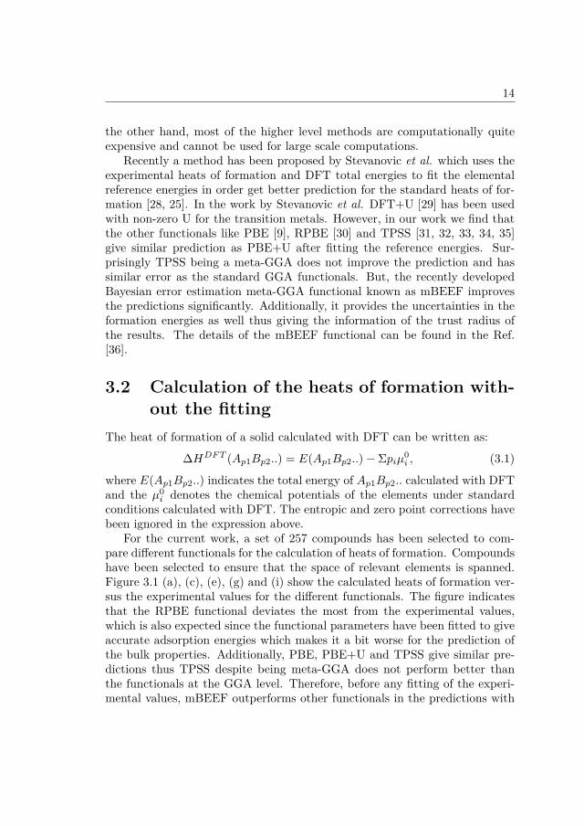
Recently a method has been proposed by Stevanovic et al. which uses theexperimental heats of formation and DFT total energies to fit the elementalreference energies in order get better prediction for the standard heats of for-mation [28, 25]. In the work by Stevanovic et al. DFT+U [29] has been usedwith non-zero U for the transition metals. However, in our work we find thatthe other functionals like PBE [9], RPBE [30] and TPSS [31, 32, 33, 34, 35]give similar prediction as PBE+U after fitting the reference energies. Sur-prisingly TPSS being a meta-GGA does not improve the prediction and hassimilar error as the standard GGA functionals. But, the recently developedBayesian error estimation meta-GGA functional known as mBEEF improvesthe predictions significantly. Additionally, it provides the uncertainties in theformation energies as well thus giving the information of the trust radius ofthe results. The details of the mBEEF functional can be found in the Ref.[36].

3.2 Calculation of the heats of formation with-out the fitting

The heat of formation of a solid calculated with DFT can be written as:

∆HDFT (Ap1Bp2..) = E(Ap1Bp2..)− Σpiµ0i , (3.1)

where E(Ap1Bp2..) indicates the total energy of Ap1Bp2.. calculated with DFTand the µ0

i denotes the chemical potentials of the elements under standardconditions calculated with DFT. The entropic and zero point corrections havebeen ignored in the expression above.

For the current work, a set of 257 compounds has been selected to com-pare different functionals for the calculation of heats of formation. Compoundshave been selected to ensure that the space of relevant elements is spanned.Figure 3.1 (a), (c), (e), (g) and (i) show the calculated heats of formation ver-sus the experimental values for the different functionals. The figure indicatesthat the RPBE functional deviates the most from the experimental values,which is also expected since the functional parameters have been fitted to giveaccurate adsorption energies which makes it a bit worse for the prediction ofthe bulk properties. Additionally, PBE, PBE+U and TPSS give similar pre-dictions thus TPSS despite being meta-GGA does not perform better thanthe functionals at the GGA level. Therefore, before any fitting of the experi-mental values, mBEEF outperforms other functionals in the predictions with

15

significantly lower mean absolute error (MAE) and standard deviation (σ).It can also be seen that the experimental values are within the uncertaintiespredicted by the mBEEF ensemble.

3.3 Calculation of the heats of formation withthe fitting

As mentioned before, the different chemical environment of the multinary com-pounds and the reference phases leads to an incomplete error cancellation incalculating the energy differences i.e. the heats of formation. This behaviorwas manifested in the predictions in the previous section which was based onthe DFT reference energies of the elemental phases. Fitted elemental refer-ence phase energy (FERE) method [25] solves this problem to some extent byadding corrections to the DFT reference energies. The value of the correctionsis calculated by minimizing the root mean square (RMS) error of the predictedand the experimental values. The FERE heats of formation can be expressedas:

∆HFERE(Ap1Bp2..) = E(Ap1Bp2..)−Σpi(µ0

i + δµ0i ), (3.2)

The only difference between the equation above and the equation (3.1) is theterm δµ0

i which denotes the correction to reference energy of the elementalphase.

As mentioned before, a dataset of 257 compounds has been chosen forexperimental heats of formation, [25, 37] on the other hand, the number ofelements relevant for this work is limited to 62. Therefore, the calculationof the corrections involves solving an overdetermined set of equations whichcan be done by minimizing the RMS error

√∑i(∆Hi

Expt. −∆HiDFT )2. Few

points have to be kept in mind while fitting the reference energies, for example,a reasonable size of the dateset should be taken to avoid over- or under-fittingand the quality of the fit should be validated on a test dataset which hascompounds not used in the fitting procedure.

The calculated heats of formation with the FERE procedure applied to thedifferent functionals is shown in the Figure 3.1 (b), (d), (f), (h) and (j). As canbe seen from the figure, different functionals clearly improve the predictionswhen augmented with the FERE procedure. After the fitting procedure isapplied all the functionals give similar predictions with almost same MAEand σ. It is worth noticing that the mBEEF predictions before the fitting

16

Figure 3.1: (a), (c), (e), (g) and (i) show the calculated heats of formationwith different functionals. The mean absolute error (MAE) and the standarddeviation (σ) of the the difference of the calculated heats of formation andthe experimental values is also shown in the plots. The black line shows theexperimental heat of formation. The figure has been taken from the Paper-1.

17

is not too off from the predictions of the other functionals after the fitting.A possible reason for the better predictions of the mBEEF functional is thefitting of the parameters of the functional to different experimental dataset [36].Additionally, the reduced uncertainties in the Figure 3.1 (j) results from fittingthe ensemble as well to the experimental heats of formation. The individualheats of formation with the mBEEF functional with and without the fitting isshown in the Table 1 of the Paper-1.

3.4 Outliers in the different predictions

The statistical quantity σ indicates that there must be some predictions whichdeviate from the actual value (in the present case, the experimental values)by more than of the order of σ [38] and these predictions are called outliers.A commonly used measure to call a prediction as an outlier is the value of 2σwhich puts 95 % confidence in the results lying within the width of 2σ. Basedon this criterion, outliers selected for different functionals without and withthe FERE are shown in the Table 3.1. and 3.2

Table 3.1 shows that the PBE and RPBE have common outliers to someextent whereas the PBE+U, TPSS and the mBEEF functional have none orvery few common outliers. The feature in the Table 3.1 worth noticing is thatin a few cases all the functionals except mBEEF deviate from the experimentssignificantly, for example, in the PBE, RPBE, PBE+U and TPSS, deviationis as high as 0.85, 0.66, 0.82 and 0.57 eV respectively whereas the maximumdeviation in the mBEEF prediction is 0.41 eV. Therefore, even without theFERE the mBEEF predictions do not significantly deviate from the experi-mental values.

Table 3.2 shows the predictions after the fitting procedure has been applied.As expected the magnitude of the deviation from the experimental heats offormation decreases after employing the fitting. On the other hand, it canalso be seen from the table that the nature of the outliers significantly changesafter the fitting has been applied which is expected in a fitting model since thedatapoints contributing to large errors get penalized more. Additionally, thecommon feature of a large variation in the nature of the outliers before andafter the fitting rules out the possibility of the experimental errors to someextent and rather puts more weight to the limitations of the functionals.

18

Table3.1:O

utliersinthe

calculationswithoutusing

theFER

Eschem

e.The

compoundsexhibiting

deviationsof

thecalculated

heatsof

formation

fromthe

experimentalvalues

bymore

than2σ

havebeen

identifiedas

outliers.The

valuesofσforthe

differentfunctionalsareshow

nin

Fig.3.1.δH

denotesthedifference

betweencalculated

andexperim

entalheatsofform

ation.Table

hasbeen

takenfrom

thePaper-1.

PB

EδHPBE

RP

BE

δHRPBE

PB

E+

UδHPBE

+U

TP

SS

δHTPSS

mB

EE

FδHmBEEF

Al2

O3

0.48A

l2O

30.69

Al2

O3

0.48A

lP0.45

Au

F3

-0.30B

aS-0.52

FeF

20.61

BaS

-0.52B

aI2-0.48

CaF

2-0.35

BaO

-0.47F

eO0.60

BaO

-0.47B

iBr3

-0.51C

dF

2-0.34

FeF

20.61

GaN

0.57C

rS-0.82

CaS

0.48C

u2

Se

0.31F

eO0.49

HfO

20.65

CrF

3-0.47

FeF

20.57

FeS

e0.35

GaS

0.45N

iF2

0.66C

r2O

3-0.75

GaP

0.43G

aN0.33

LaN

0.46-

-G

aN0.42

Ga2

S3

0.44G

a2S3

0.37M

nS

0.60-

-G

a2S3

0.44N

iF2

0.57G

aS0.41

NiF

20.85

--

GaS

0.45P

bB

r2-0.45

GeS

e0.37

--

--

Ge4

O8

0.42S

rBr2

-0.49G

e4O

80.29

--

--

Mn

S-0.48

SrI2

-0.55N

bF

5-0.38

--

--

Mn3

O4

-0.42Z

nS

0.43O

sO4

-0.30-

--

-V

2O

3-0.42

ZrS

20.47

Pb

F2

-0.31-

--

--

--

-S

nO

20.28

--

--

--

--

TiN

-0.30

19

Table3.2:

Outlie

rsin

thecalculations

usingtheFE

RE

sche

me.

The

compo

unds

exhibitin

gde

viations

ofthe

calculated

heatsof

form

ationfro

mtheexpe

rimentalv

alue

sby

morethan

2σha

vebe

enidentifi

edas

outliers.

The

values

ofσfort

hediffe

rent

func

tiona

lsares

hownin

Fig.

3.1.δH

deno

test

hediffe

renc

ebetwe

encalculated

andexpe

rimentalh

eats

ofform

ation.

Tableha

sbe

entakenfro

mthePa

per-1.

PB

EδHFERE

PBE

RP

BE

δHFERE

RPBE

PB

E+

UδHFERE

PBE

+U

TP

SS

δHFERE

TPSS

mB

EE

FδHFERE

mBEEF

Cu

F2

0.22

Cu

F2

0.23

CoS

0.20

BaC

l 20.

24C

aF2

-0.1

8F

eF2

0.33

FeF

20.

27C

o 3O

4-0

.23

CaS

0.21

Cd

F2

-0.1

8F

eSe

-0.1

9M

nO

2-0

.21

CrO

20.

17C

sF-0

.23

Co 3

O4

-0.1

9M

nO

2-0

.25

Nb

F5

-0.3

2F

e 2O

3-0

.17

FeF

20.

29F

e 2O

3-0

.17

Nb

F5

-0.2

9N

i 3S2

-0.1

8G

aF3

0.16

KC

l0.

32F

eF2

0.19

Ni 3

S2

-0.2

1N

iF2

0.38

GeO

20.

20N

bF

5-0

.26

GaP

-0.1

6N

iF2

0.65

Pb

F2

-0.1

8M

gF2

0.19

NiF

20.

37K

F-0

.17

Ru

O4

-0.1

9R

uO

4-0

.33

Nb

F5

-0.2

3R

bI

0.25

Li 3

Sb

0.18

TaF

5-0

.22

TaF

5-0

.24

Sn

O2

0.17

SrS

0.25

MgO

-0.1

5Z

rSi

-0.2

4Z

rSi

-0.2

6T

aF5

-0.1

8S

rI2

-0.2

4M

gF2

0.17

ZrS

20.

26Z

rS2

0.24

TiN

-0.1

9T

lI0.

26M

nO

2-0

.16

--

--

VN

0.26

ZrS

i-0

.24

Nb

F5

-0.2

0-

--

-V

2O

3-0

.36

ZrS

20.

35T

iN-0

.17

--

--

Zn

F2

0.19

--

Zn

F2

0.18

--

--

ZrS

20.

16-

-Z

rS2

0.16

20

3.5 True versus predicted error in the mBEEFfunctional

As previously shown in the Figure 3.1 in most of the cases the experimentalvalues lie within the predicted uncertainties by the mBEEF functional withslight overestimation (large errorbars) of the predicted errors. However, thesize of uncertainties decreased significantly with the FERE. Therefore, in orderto understand the distribution of error before and after the fitting a histogramof the true error (∆HmBEEF - ∆HExpt. and ∆HFERE

mBEEF - ∆HExpt.) dividedby the predicted error (σBEE and σFEREBEE ) is plotted in the Figure 3.2. Thehistogram is a running average calculated as [38]:

P (12 [xi + xi+J ]) ≈ J

N(xi+J − xi), (3.3)

with xi as the statistical quantity plotted in the histogram and an intermediatevalue 20 for the parameter J has been chosen.

If the predicted error matches exactly the true error then one would expectthat the distribution would be a Gaussian of unit width (shown in green inthe figure). However, in the Figure 3.2 this is not the case. As also noticedbefore, the tendency of the mBEEF to overestimate the errors in manifestedin the large peak around zero in (a) which renders the mBEEF to have mostof the experimental values lie within the uncertainties.

However, with the FERE the distribution flattens out and becomes closerto the unit Gaussian implying that the real and the predicted error are close.The tail in the histogram indicates those cases where the predicted error issmaller than the actual error. This is a fairly common feature of the ensembleapproach [39].

3.6 Cross validationAs pointed out before, the fitting model should be such that the data is neitheroverfitted nor underfitted. Therefore, it is of utmost importance that thequality of the fit is tested on a dataset (also called as test set) which is notincluded in the fitting dataset (also called as training set). A good qualityfit should provide a reasonable prediction on a new dataset. A point worthnoticing in the current fitting scheme is that only binary compounds havebeen used in fitting dataset, therefore good predictions are expected for thenew binary compounds. Additionally, reasonable predictions can be expected

21

Figure 3.2: (a) shows the histogram of the true error divided by the predictederror before the fitting (b) shows the histogram of the true error divided by thepredicted error after the fitting. The figure has been taken from the Paper-1.

22

for ternary/tertiary compounds only if their chemical environment does notdiffer significantly from the compounds used in the fitting procedure. Hence,a test set containing a mix of binary and ternary compounds has been selectedfor the validation of the fitting.

Table 3.3 and 3.4 show the heats of formation of the test set without andwith the fitting respectively. The clear decrease in the MAE and σ shows theabsence of overfitting. As expected in any regression scheme, the improvementwith the fitted model is not as much as the improvement seen in the trainingdataset.

In the test set also, the mBEEF predictions without the fitting has thesame quality as the other functionals with the fitting and the improvementwith the fitting is only moderate in the case of the mBEEF. Therefore, areasonable prediction with the mBEEF can be obtained even without usingthe fitting with only negligibly increased computational cost as compared toother GGAs.

3.7 ConclusionThe rapidly growing area of the computational screening of the energy materi-als requiring reasonable predictions of the stability has led forward this work.The synergetic use of the DFT total energies and the experimental heats offormation provides a framework to improve the predictions. Originally, thescheme was developed for the PBE+U functionals but in this work similarimprovements has been seen for the other functionals like PBE, RPBE, TPSSand mBEEF as well.

We see that the recently developed mBEEF functional which has beenoptimized using variety of experimental dataset gives better predictions ascompared to the other functionals. Additionally, the mBEEF functional alsoprovides reasonable estimate of the uncertainties in the predictions, the fea-ture which other functionals used in this work lack. However, the uncertaintiesestimated by the mBEEF ensemble is in general overestimated which can fur-ther be reduced by using the FERE scheme along with the reduction of thetrue error as well.

Despite giving improved results FERE scheme has some drawbacks as well.The corrections are primarily based on nature of the bonding environment inthe training set, therefore, it may not significantly improve the predictions forthe systems differing from the systems used in the training set, for example, inmetal alloys which have significantly different chemical environment than thesemiconductors used in the training set. Therefore, higher level functionals

23

Table 3.3: Heats of formation of test dataset with different functionals withoutthe fitting. All the energies are in eV/atom. Table has been taken from thePaper-1.

Compound ∆HExpt. ∆HPBE ∆HRPBE ∆HPBE+U ∆HTPSS ∆HmBEEF

AgNO3 -0.26 -0.40 -0.31 -0.53 -0.47 -0.60 ± 0.22AlPO4 -2.99 -2.71 -2.58 -2.71 -2.86 -2.97 ± 0.19BeSO4 -2.16 -1.99 -1.83 -1.99 -2.09 -2.19 ± 0.16BiOCl -1.27 -1.26 -1.11 -1.26 -1.62 -1.26 ± 0.16CdSO4 -1.61 -1.42 -1.27 -1.42 -1.53 -1.59 ± 0.17CuCl2 -0.76 -0.51 -0.32 -0.70 -0.80 -0.74 ± 0.21TiBr3 -1.42 -1.24 -1.23 -1.52 -1.71 -1.37 ± 0.08NaClO4 -0.66 -0.54 -0.41 -0.54 -0.67 -0.63 ± 0.15CaSO4 -2.48 -2.24 -2.06 -2.24 -2.37 -2.40 ± 0.17Cs2S -1.24 -1.01 -0.92 -1.01 -1.47 -1.16 ± 0.18CuWO4 -1.91 -1.59 -1.41 -1.76 -1.72 -1.68 ± 0.21PbF4 -1.95 -2.13 -2.05 -2.13 -2.26 -2.32 ± 0.23MgSO4 -2.22 -1.97 -1.79 -1.97 -2.09 -2.16 ± 0.16SrSe -2.00 -2.04 -1.98 -2.04 -2.76 -2.29 ± 0.16NiSO4 -1.51 -1.11 -0.96 -1.35 -1.23 -1.42 ± 0.23FeWO4 -1.99 -1.73 -1.58 -2.01 -1.87 -1.84 ± 0.21GeP -0.11 +0.04 +0.09 +0.04 -0.19 +0.14 ± 0.08VOCl -2.10 -1.79 -1.68 -2.45 -2.07 -2.11 ± 0.24LiBO2 -2.67 -2.42 -2.30 -2.42 -2.57 -2.58 ± 0.17NaBrO3 -0.69 -0.52 -0.41 -0.52 -0.71 -0.60 ± 0.13CoSO4 -1.53 -1.09 -0.95 -1.43 -1.24 -1.40 ± 0.23PbSeO4 -1.05 -0.94 -0.81 -0.94 -1.13 -1.04 ± 0.16Mn2SiO4 -2.56 -1.83 -1.77 -2.58 -2.01 -2.29 ± 0.23ZnSO4 -1.70 -1.37 -1.20 -1.37 -1.47 -1.53 ± 0.16

MAE 0.24 0.35 0.16 0.20 0.12σ 0.28 0.39 0.19 0.26 0.16

are required to improve the description at the electronic structure level andthereby making the FERE scheme unnecessary and the mBEEF functionalseems to be promising in that direction.

24

Table 3.4: Heats of formation of test dataset with different functionals withthe fitting. All the energies are in eV/atom. Table has been taken from thePaper-1.

Compound ∆HExpt. ∆HFEREPBE

∆HFERERPBE

∆HFEREPBE+U ∆HFERE

TPSS∆HFERE

mBEEF

AgNO3 -0.26 -0.58 -0.67 -0.68 -0.45 -0.63 ± 0.16AlPO4 -2.99 -2.95 -2.97 -2.94 -3.02 -3.03 ± 0.07BeSO4 -2.16 -2.22 -2.23 -2.21 -2.19 -2.25 ± 0.11BiOCl -1.27 -1.25 -1.20 -1.23 -1.32 -1.23 ± 0.09CdSO4 -1.61 -1.61 -1.62 -1.60 -1.60 -1.63 ± 0.12CuCl2 -0.76 -0.75 -0.60 -0.84 -0.79 -0.81 ± 0.07TiBr3 -1.42 -1.38 -1.39 -1.61 -1.38 -1.43 ± 0.05NaClO4 -0.66 -0.76 -0.77 -0.73 -0.68 -0.65 ± 0.16CaSO4 -2.48 -2.41 -2.41 -2.41 -2.46 -2.43 ± 0.12Cs2S -1.24 -1.27 -1.24 -1.33 -1.97 -1.23 ± 0.06CuWO4 -1.91 -1.62 -1.60 -1.75 -1.65 -1.71 ± 0.07PbF4 -1.95 -2.19 -2.19 -2.11 -2.24 -2.13 ± 0.08MgSO4 -2.22 -2.22 -2.21 -2.21 -2.20 -2.24 ± 0.10SrSe -2.00 -2.25 -2.26 -2.29 -2.66 -2.29 ± 0.05NiSO4 -1.51 -1.35 -1.36 -1.54 -1.33 -1.50 ± 0.11FeWO4 -1.99 -1.81 -1.81 -1.94 -1.86 -1.89 ± 0.06GeP -0.11 -0.01 +0.03 -0.05 -0.28 -0.02 ± 0.07VOCl -2.10 -1.97 -1.98 -2.41 -2.05 -2.12 ± 0.07LiBO2 -2.67 -2.61 -2.61 -2.58 -2.64 -2.61 ± 0.05NaBrO3 -0.69 -0.74 -0.76 -0.72 -0.69 -0.66 ± 0.11CoSO4 -1.53 -1.30 -1.34 -1.56 -1.31 -1.43 ± 0.11PbSeO4 -1.05 -1.07 -1.09 -1.06 -1.07 -1.08 ± 0.09Mn2SiO4 -2.56 -2.17 -2.19 -2.38 -2.10 -2.25 ± 0.08ZnSO4 -1.70 -1.61 -1.61 -1.61 -1.60 -1.62 ± 0.11

MAE 0.12 0.13 0.11 0.15 0.09σ 0.16 0.17 0.15 0.25 0.14

Chapter 4

Hydrogen Evolution fromTwo-Dimensional Materials

4.1 IntroductionStorage of energy in the form of chemical bonds is one of the most used andefficient way of storing the energy. Transferring energy from one place to otherin form of chemical bonds is easier as compared to the other means such aselectricity. On the other hand, the deteriorating environmental conditions dueto the excess burning of the petroleum fuels needs our attention to look forthe alternative forms of chemical energy not having deleterious effect on theenvironment. One such fuel is hydrogen which can be used in the fuel cells thusinvolving no emission of greenhouse gas whatsoever [40, 41]. However, a cheapand efficient way of producing hydrogen has not been realized yet [42, 43, 44].One of the bottleneck to reduce the cost of hydrogen production is the use ofexpensive catalysts like Platinum a cheaper and efficient alternative of whichhas not been found yet. Recent theoretical and experimental investigations ofthe bulk Ni2P for hydrogen evolution reaction (HER) show promising resultsand hopefully in the future will serve as a viable alternative to Platinum forthe HER [45, 46, 47].

Additionally, over the last few years, two-dimensional (2D) MoS2 has beenexplored for its activity towards the HER with some promising results [48,49, 50, 51, 52]. The initial effort of the MoS2 research was focussed on theedges of the 2H structure of the MoS2 nanoparticle having metallic characteras opposed to the semiconducting states on the basal plane [53, 54]. Unfor-

25

26

tunately, relatively limited number of active sites on the edges gives very lowexchange current density for the HER. However, recent experiments on theother polymorph of the MoS2 and WS2 known as 1T structure demonstratedthe activity of the basal plane for the HER thus giving access to relativelylarger number of active sites [49, 48, 50]. Additionally, the difference in en-ergy of the 1T and 2H phase MoS2 or WS2 decreases as the dimensionalityof the system is reduced from three (bulk) to two (monolayer) thus making itfeasible to synthesize the HER active metastable phase in the 2D form [55].The different activity of the 2H and 1T phase broadens the materials spacefor HER which is the basis of this work. In this work, the basal planes of 100different metal dichalcogenides and oxides have been explored in both the 2Hand 1T structure for the HER. Primarily, criterion of stability of the materialwith respect to the standard reference phases and other competing phases andthe free energy of the hydrogen adsorption on the basal plane has been usedas descriptors for the screening of materials for the HER.

4.2 Details of the atomic structureThe 2H and 1T structures differ by the arrangement of the chalcogen/oxygenatom around the metal atoms. The 2H structure has prismatic arrangement ofthe chalcogen/oxygen atoms around the metal atom whereas in the 1T struc-ture they are octahedrally arranged. The 2H and 1T structures are shownin the Figure 4.1 (a) and (f) respectively. The black square represents theunit cell of the structures. Other structures shown in the 2H and 1T class arethe distorted derivatives of the 2H and 1T structures. The distorted struc-tures have been broadly classified based on their symmetry group which havebeen identified using certain cutoff for the rotations/translations to accountfor the residual forces in the structures. In order to identify the the distortedstructures, atoms are slightly displaced from their symmetric position in abigger unit cell in order to break the symmetry of the structure and then therelaxation is performed.

The above procedure captures all the distortions if any in the 2×2 unit cell.There might be other distortions in the larger unit cell but those cases have notbeen considered here. Fortunately, the charge density wave (CDW) structuresin compounds like TiS2 [56, 57] distorted structure of MoS2, WS2 etc. [58, 59],exhibiting quantum spin Hall effect (QSH) and the distortions in ReS2 [60] arecaptured by the above procedure thus supporting our results. However, thechoice of 0.01 eV/atom for the threshold of energy to differentiate betweenthe symmetrical and the distorted structure categorize TiS2 as symmetrical

27

Figure 4.1: (a), (f) show the 1T undistorted 1T and 2H structures respectively.Yellow spheres represent the chalcogen atoms and the cyan spheres representthe metal atoms. (b) - (e) show the distortions in the 1T structure. The unitcell of the distorted structure is shown with black solid lines and the distortionof the atoms from their ideal symmetric position is shown with black dottedlines. (g) represents the distorted 2H structure with a similar description asabove. The figure has been taken from the Paper-2.

28

structure. But, it turns out that the CDW structure of the TiS2 and thesymmetrical structure are very close in energy having the difference of the orderof 0.005 eV/atom and surprisingly these differences are captured with the aboveprocedure. On the other hand, the adsorption energy of the hydrogen is similaron the symmetrical and the distorted structure in the case of CDW structures,therefore, they have been categorized as symmetrical for consistency due to thethreshold of 0.01 eV/atom. Table 4.1 summarizes the results for the distortedstructures which are classified based on the space group (based on Herman-Maugin notation) of the distorted structure and the size of the reduced unitcell capturing the distortion. Symmetry analysis for the classification hasbeen performed using the tool given in Ref. [61]. The cutoff of of 0.05 Å onthe rotations/translations has been used in order to allow for inaccuracies orresidual forces.

Table 4.1: Classification of different compounds exhibiting distortions based onthe space group (based on Herman-Maugin notation) of the distorted structureand the size of the reduced unit cell capturing the distortions.

Class MX2 Group Unit cell Class MX2 Group Unit cell

2H CoS2 P1 2×2 2H CoSe2 P1 2×22H IrS2 P1 2×2 2H OsS2 P1 2×22H OsSe2 P1 2×2 2H PdS2 P1 2×22H PdSe2 P1 2×2 2H PdTe2 P1 2×22H ReO2 P1 2×2 2H ReS2 P1 2×22H ReSe2 P1 2×2 2H RhS2 P1 2×22H RhSe2 P1 2×2 2H RhTe2 P1 2×22H RuO2 P1 2×2 2H RuS2 P1 2×22H RuSe2 P1 2×2 2H ScS2 P1 2×22H ScSe2 P1 2×21T CoS2 P1 2×2 1T CrS2 P1 2×21T CrSe2 P1 2×2 1T FeS2 P1 2×21T IrS2 P1 2×2 1T IrSe2 P1 2×21T ReO2 P1 2×2 1T ReTe2 P1 2×21T RhS2 P1 2×2 1T RuS2 P1 2×21T RuTe2 P1 2×2 1T MoO2 P1 2×11T MoS2 P1 2×1 1T MoSe2 P1 2×11T MoTe2 P1 2×1 1T OsS2 P1 2×11T OsSe2 P1 2×1 1T OsTe2 P1 2×11T WS2 P1 2×1 1T WSe2 P1 2×11T WTe2 P1 2×1 1T ReS2 P1 2×21T ReSe2 P1 2×2 1T RuSe2 P1 2×21T TaO2 P1 2×2 1T CoSe2 P3m1 2×21T IrTe2 P3m1 2×2 1T NbO2 P3m1 2×21T OsO2 P3m1 2×2 1T RhSe2 P3m1 2×21T RuO2 P3m1 2×2 1T WO2 P3m1 2×2

29

4.3 Stability with respect to the standard statesIn the last chapter, the standard heat of formation of the compounds was dis-cussed. It has to be negative for a compound if the compound has to be stablewith respect to the standard states of the constituent elements. Therefore, asa first step the calculation of the heat of formation of the compounds has beenperformed for all the 2D materials explored here. The heatmap in the Figure4.2 shows the heats of formation of the compounds in the 2H and 1T structureand the difference in energy of the two structures. The figure shows that asignificant fraction of the compounds have positive heats of formation thusunstable [62]. Figure 4.2 (c) shows the difference in energies of the 2H and 1Tstructure. The figure clearly shows that in most of the cases the 2H and 1Tstructures are energetically very close. One of the important implication of thetwo structures having similar energy is that the HER active phase can be syn-thesized and stabilized under normal condition with suitable synthetic routesand the same fact has been realized in the case of MoS2 and WS2 [50, 48].However, an ideal situation would be that the HER active phase is the moststable phase. But, if that is not the case then a small degree of metastabilitywould make it feasible to synthesize the HER active phase. As a side note,since the standard heat of formation by definition is the stability with respectto standard states, the stability with respect to other competing phases mightalso be important, however, stability with respect to the other phases has onlybeen considered for the compounds meeting the criteria for the HER activity.

However, Figure 4.2 only shows the heats of formation of the perfectlysymmetrical 2H and 1T structures. But, as discussed in the last section thepossible distortions have also been explored for all the compounds hence itis crucial to assess the energy difference of the perfectly symmetrical and thedistorted phase of the compounds. Figure 4.3 shows the relative energy ofthe distorted phase with respect to the symmetric phase. The white squarescorresponds to the compounds manifesting massive distortions leading to thestructures not belonging to either of the 2H or 1T class, therefore, they areignored. As can be seen from the figure, a large fraction of compounds do notshow any distortions.

4.4 Adsorption of hydrogen on the basal planesOne of the widely accepted mechanism for the HER is the Volmer-Heyrovskymechanism which is a two step process; the first step is the adsorption of Hon the active site and the second step is the bond formation between the two

30

Figure 4.2: (a), (b) show the standard heats of formation of the compounds inthe 2H and 1T structure respectively. (c) shows the difference of the heats ofthe compounds in the 2H and 1T structure. All the energies are in eV/atom.The figure has been taken from the Paper-2.

31

Figure 4.3: (a) and (b) show the energy of the distorted structures (eV/atom)with respect to the perfectly symmetrical 2H and 1T structures, respectively.The white squares denote massive reconstructions upon relaxation thus leadingto structures not belonging to the 2H and 1T class of structures. All theenergies are in eV/atom. The figure has been taken from the Paper-2.

32

adsorbed hydrogen to evolve the gaseous hydrogen [63, 64]. Schematically, theenergetics of the process is shown in the Figure 4.4.

Figure 4.4: Schematic of the Volmer-Heyrovsky route for the HER.

The product and the reactant are at the same level of energy in the Figure4.4 due to the assumption that the process is at equlibrium under standardconditions thus have zero free energy. Active site in the figure is denoted bythe *. It can be seen from the figure that the intermediate H∗ may lie higheror lower in energy than the product and the reactant. If the intermediate lieshigher in energy than the reactant then the first step will be uphill and if it lieslower in the energy than the reactant then the second process will be uphill.Therefore, based on the thermodynamic argument if the process has a zerobarrier, then the free energy for the adsorption of hydrogen has to be zero[48, 65, 42]. Although the free energy for the hydrogen adsorption provides adescriptor for the HER activity, it does not provide any information about thekinetic barrier for the process but we do not explore the kinetic pathways inthis work.

In order to assess the reactivity of the basal plane the hydrogen adsorptionenergy has been calculated for different active sites on the surface. We find thatthe hydrogen prefers to adsorb on chalcogen/oxygen atoms in tilted positionsin most of the cases and does not prefers to adsorb on the metal site. Ina perfectly symmetric structure all the chalcogen atoms are equivalent thusconsidering just one of them suffices. However, in the distorted structures,the broken symmetry leads to inequivalent chalcogen sites, therefore, all theinequivalent sites have been explored for the hydrogen adsorption and thesite with the lowest adsorption energy has been chosen for further analysis.The coverage of 0.25 monolayer (ML) has been chosen initially and the highercoverage (0.5 ML) is only considered for those structures which bind hydrogentoo strongly (∆Hads

H ≥ −0.8) for 0.25 ML. However, it has been found that athigher coverages the structures massively distort leading to the structures notbelonging to either of the 2H or 1T class, therefore, higher coverages have notbeen considered any further.

33

The compounds have been grouped based on the nature of the metal atom‘M’ in MX2 i.e. the compounds have been put in the same group if the metalatoms belong to the same group in the periodic table; based on this catego-rization the plots for hydrogen adsorption energies are shown in the Figure4.5.

Figure 4.5: Hydrogen adsorption energies of the individual groups. The com-pounds have been grouped based on the nature of the metal atom ‘M’ in MX2i.e. the compounds have been put in the same group if the metal atoms belongto the same group in the periodic table. The missing data points representmassive reconstruction upon the hydrogen adsorption thus omitted from theplot. All the energies are in eV. The figure has been taken from the Paper-2.

The plot clearly shows that adsorption energies on the 2H and 1T structuresdo not follow any systematic trend in most of the cases, therefore, a simplesystematic analysis cannot be performed to rationalize the different activitiesof the different structures. However, the group containing Cr, Mo and W(group-6) shows an opposite trend as the group containing Ti, Zr and Hf(group-4). In the group-6 the 1T structure binds hydrogen strongly whereasin the group-4 the 2H structure has higher binding energy. Therefore, only thegroup-4 and group-6 have been selected to understand the origin of different

34

reactivity in different structures.Since the strength of the bonding depends on how the adsorbate states

hybridize with the adsorbent states, the position of the center of the p levelof the chalcogen atoms might give a clue about the strength of the bonding[65, 66]. The center of the p band with respect to the Fermi level can becalculated as

εp =∫∞−∞ ρ(ε)εdε∫∞−∞ ρ(ε)dε

(4.1)

The results for the sulphides and selenides of Mo, W, Ti and Zr in both the2H and 1T structures are summarized in the Table 4.2. The table indicatesthat in the case of Mo and W, the 1T structure has higher binding energy(∆HH

ads) for the hydrogen whereas in the case of Ti and Zr hydrogen bindsstrongly in the 2H structure. It can also be seen that the compounds whichhave higher binding energy have the center of the p-level closer to the Fermilevel. For example, in the case of group-6, the center of the p-level in the2H structure lies deeper with respect to the Fermi level as compared to the1T structure whereas in the group-4 the trend is opposite. Thus, it can beconcluded that the position of the p band center is somewhat correlated to thebinding energy.

Table 4.2: Heat of adsorption of hydrogen ∆HHads and the center of the p-band

εp for sulphides and selenides of Mo, W (group-6) and Ti, Zr (group-4) in the2H and 1T structures.

2H εp ∆HHads

1T εp ∆HHads

MoS2 -2.00 1.68 ± 0.07 MoS2 -1.23 0.10 ± 0.13MoSe2 -1.74 1.82 ± 0.13 MoSe2 -1.46 0.64 ± 0.11WS2 -2.32 1.95 ± 0.08 WS2 -1.37 0.23 ± 0.14WSe2 -2.03 2.03 ± 0.14 WSe2 -1.29 0.78 ± 0.15TiS2 -1.02 -0.05 ± 0.13 TiS2 -1.45 0.40 ± 0.09TiSe2 -0.89 0.44 ± 0.12 TiSe2 -1.38 0.90 ± 0.10ZrS2 -0.96 0.11 ± 0.10 ZrS2 -1.42 0.94 ± 0.07ZrSe2 -0.80 0.51 ± 0.10 ZrSe2 -1.34 1.19 ± 0.09

However, as shown in the Figure 4.6 there is hardly any trend when thedifference of the adsorption energies is plotted against the difference of thecenter of the p level for large number of compounds. The absence of any trendcan be attributed to the large variation in the nature of the metal atoms whichmakes it harder to generalize the analysis above for all the groups.

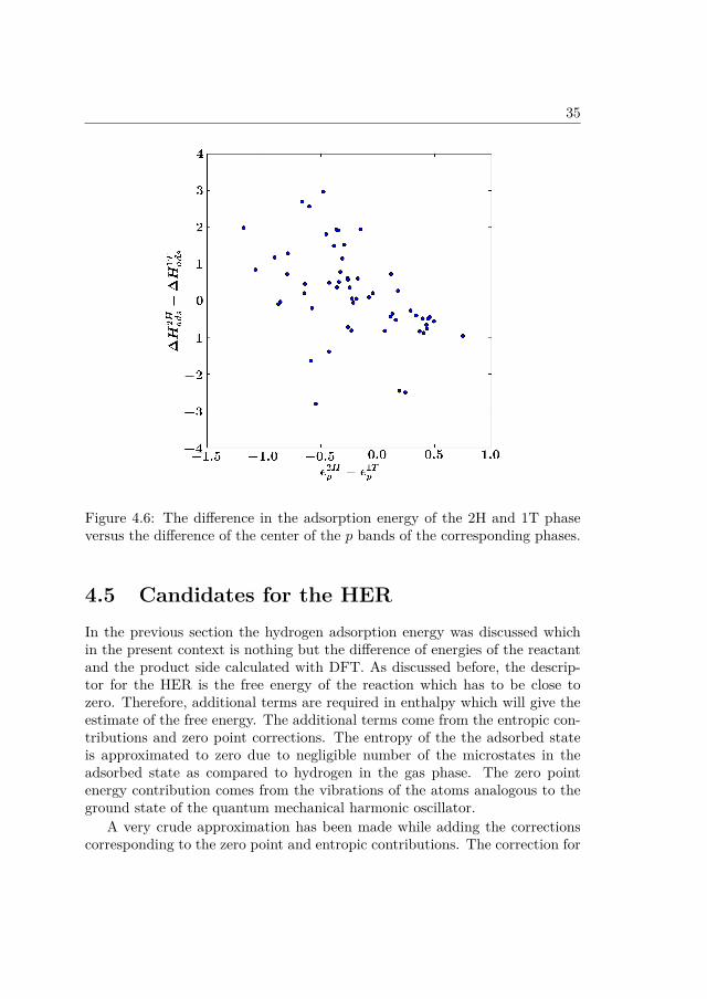
35

Figure 4.6: The difference in the adsorption energy of the 2H and 1T phaseversus the difference of the center of the p bands of the corresponding phases.

4.5 Candidates for the HERIn the previous section the hydrogen adsorption energy was discussed whichin the present context is nothing but the difference of energies of the reactantand the product side calculated with DFT. As discussed before, the descrip-tor for the HER is the free energy of the reaction which has to be close tozero. Therefore, additional terms are required in enthalpy which will give theestimate of the free energy. The additional terms come from the entropic con-tributions and zero point corrections. The entropy of the the adsorbed stateis approximated to zero due to negligible number of the microstates in theadsorbed state as compared to hydrogen in the gas phase. The zero pointenergy contribution comes from the vibrations of the atoms analogous to theground state of the quantum mechanical harmonic oscillator.

A very crude approximation has been made while adding the correctionscorresponding to the zero point and entropic contributions. The correction for

36

the same has been calculated for the 1T-MoS2 and then the same correctionhas been used for the all the other materials. This is not a perfectly validassumption, however, a tolerance of 0.5 eV for the free energy to accountfor the errors introduced due to different approximations at different levelswill likely capture the variability in the zero point and entropic corrections.In the case of 1T-MoS2 as mentioned before the entropic corrections for theadsorbed state has been ignored [54]. The calculated zero point correctionsfor the adsorbed hydrogen comes out as 0.39 eV. The zero point energy of thehydrogen in the gas phase has been taken from the Ref. [67] and is foundto be 0.27 eV and entropy of the gaseous hydrogen has been takes as 0.40 asmentioned in the Ref. [68]. By taking the difference of the corrections in thegas phase and the adsorbed state ∆ZPE comes out as 0.12 eV and -T∆S comesout as 0.40 eV, therefore, ∆ZPE -T∆S comes out to be 0.26 eV (per hydrogenatom). Therefore, the correction of 0.26 eV is added to the adsorption energiesfor all the compounds to have an estimate of the free energy.

As mentioned before, the optimum value of the free energy for the HER is0.0 eV, however, an energy window of 0.5 eV is taken to account for differenteffects like strain, coverage and solvation [48, 69]. Additionally, the estimateof the uncertainties is obtained in the calculation with the BEEF-vdW usingthe ensemble in Ref. [70]. Having the uncertainties along with the energywindow of 0.5 eV helps to calculate the probability for a material to have thefree energy of the hydrogen adsorption to lie within 0.5 eV around zero. Thecalculated probability helps to rank the material in order of their suitabilityfor the HER [71]. The probabilities are calculated as:

P (|∆G| ≤ 0.5) = 1√2πσ2

∫ 0.5+E

−0.5−Eexp

(− E

2

2σ2

)dE. (4.2)

Using the above equation, the ranking of the material meeting the criteria ofhaving the free energy for the HER (including the uncertainties) to lie in therange (-0.5, 0.5) eV is shown in the Figure 4.7. The number of compoundsfulfilling these criterion in the 2H structure in the plot is 23 whereas in the 1Tstructure there are 30 compounds meeting the required criterion.

The plot clearly shows that there are very few compounds which are presentin both the 2H and 1T structure indicating that the chemical properties mightdiffer significantly in different structures of the same compound. Addition-ally, the occurence of the compounds like MoS2 and WS2 in the 1T structurewhich have already been found experimentally as possible HER materials givescredibility to our approach [50, 48].

Up to this point the stability of the compounds have been considered only

37

Figure 4.7: (a) Calculated free energy for the hydrogen adsorption (∆GHads)along with the uncertainties and the probabilities (P(|∆G| ≤ 0.5)) that thecompounds have for the free energy to lie in the range (-0.5, 0.5) eV in the 2Hstructure. Red error bar indicate instability of the compound with respect tothe standard state. (b) Similar plot as (a) for the 1T structure.

38

with respect to the standard states of the elements whereas there might beother potentially competing phases hampering the growth of the 2D materialsfor the HER. Therefore, it is crucial to have a deeper look on the stability ofmaterials potentially suitable for the HER. If the metastability of the candidatematerial comes out to be too large as compared to the competing phase then itsunlikely that the candidate material can be synthesized and stabilized undernormal conditions. Therefore, the stability check for the candidate materialhas been performed with respect to the other competing phases with samestochiometry. Additionally, in the present work we do not explore the stabilityof the compounds in aqueous medium because in some recent works a goodcontrol over the stability of the compounds in water has been achieved bythe use of stabilizing agents [72]. All the competing bulk structures are takenfrom the The Open Quantum Materials Database (OQMD) [73] and then theenergy of candidate material is compared to the energy of the convex hull inorder to have an estimate of the degree of metastability. The data is shown inthe Table 4.3 and 4.4.

∆H in the tables denotes standard heats of formation calculated with theFERE method and ∆Hhull denotes the convex hull [73]. The symbol * insuperscript denotes the cases where the convex hull has been calculated as thelinear combination of the energies of two compounds because no compoundswere present with 1:2 stoichiometry in the database. δHhull denotes the energyof the monolayer with respect to the convex hull. ∆HExpt is the experimentalheat of formation of the compound (if available) lying on the convex hull. Theinitial list of the candidates for the HER is also compared to the predicted2D materials by Lebègue et. al [74]. In order to have an estimate of themetastability of the 2H structure with respect to the 1T structure or vice-versa the difference of the two is also shown as ∆H2H/1T (∆H1T/2H). Finally,the previously discussed probability P(|∆G| ≤ 0.5) is also listed in the table.All the energies mentioned in the table are in eV/atom.

Few important points worth noticing in the table are:• In all the cases the 2H and 1T structure do not differ by more than ∼0.4eV which is similar to the degree of metastability in MoS2 and WS2 inthe 2H and 1T structure and both the compounds can be synthesized inthe stable 2H phase and metastable 1T phase under normal conditions.Similar degree of metastability in other compounds suggest that if theycan be synthesized in one structure then it is likely that they can besynthesized in the other structure as well.

• Few of the HER materials like PdS2, PdTe2 proposed in this work havealso been predicted by Lebègue et. al [74] to exist in the monolayer form.

39

The fact that they lie above the hull by only ∼0.4 eV led us to made achoice of the threshold energy of 0.4 eV for the stability (or the feasibilityof existence) of the monolayer with the respect to the hull. The choiceof the threshold energy helps to narrow down the candidates even more,for example compounds like OsS2, ReO2, OsSe2, ScO2, RuO2 in the 2Hclass of candidates and OsO2 in the 1T class of candidates lying abovethe hull by more than 0.4 eV can be safely discarded. The names of thediscarded compounds are italicized in Table 4.3 and 4.4.

• On comparing the list of the candidates with the list of the predicted 2Dmaterials by Lebègue et. al [74], the compounds common in both thelists are selected. Given the fact that the heurestic approach of Lebègueet. al which is based on the feasibility of cleaving a bulk structure alonga certain direction due to the weak interlayer interaction gives a clue thatthe compounds common in both the list are potentially synthesizable,therefore, potential candidates for the HER. The potential candidatesare marked in bold in the Table 4.3 and 4.4.

In conclusion, this work systematically explores the materials space in thetwo-dimensional 2H and 1T structure for the hydrogen evolution reaction usingthe free energy of hydrogen adsorption as a computational descriptor. Therequirement of the activity on the basal plane ensures the presence of largenumber of active sites as compared to previously explored 2H structure ofthe MoS2 which only has the activity on the edges. A fairly large windowchosen for value of the descriptor provides a flexibility to tune the adsorptionenergy of the hydrogen by different means, for example, strain, environment,doping etc. Additionally, the robust stability analysis of the candidates foundsuitable for the HER provides a list of candidates which do not have very highdegree of metastability with respect to the bulk compounds thus potentiallysynthesizable. The adopted approach also predicts already known MoS2 andWS2 in 1T structure as candidates for HER thus supporting our approach.Finally, the most probable list of candidates is proposed based on work byLebègue et. al. The calculations therefore invite for further investigation ofsome of the best candidates suggested here like PdS2, NbS2, TiS2, TaS2, ZrS2,PdSe2, HfS2 in the 2H structure and CrS2, TaTe2, VTe2, NbS2, CrSe2 in the1T structure in addition to MoS2 and WS2 which are already known.

40

Table 4.3: Relevant energies for analysis of the stabilities of the obtained HERcandidates in the 2H-derived structures. ∆H denotes the calculated standardheat of formation. ∆Hhull denotes the heat of formation of the most stablecompound (i.e. at the convex hull) in the OQMD database[73]. The symbol *in superscript corresponds to the situation where no bulk structure with thecompound composition lies on the convex hull according to the database. Inthat case ∆Hhull is calculated as a linear combination of several structures.δHhull denotes the difference between the two previous columns, i.e. it showshow much the 2D compound lies above or below the convex hull. ∆HExpt

indicates the experimental standard heats of formation as listed in the OQMDdatabase. Lebègue et. al. [74] have analyzed the possibilities for forming 2Dcompounds based on the layered character of the bulk structures and their re-sult is also listed in the Table. ∆H2H/1T is the difference between the energiesin the two (possibly distorted) 2H and 1T structures. Finally P(|∆G| ≤ 0.5 isthe probability that the free energy of hydrogen adsorption lies within 0.5 eVfrom zero

2H-MX2 ∆H ∆Hhull δHhull ∆HExpt. Ref. [74] ∆H2H/1T P(|∆G| ≤ 0.5

RuS2 -0.31 -0.70 0.39 -0.71 No -0.01 1.00NiSe2 -0.21 -0.34 0.13 -0.38 No 0.17 1.00OsS2 0.34 -0.60 0.94 NA No -0.01 1.00ReO2 -0.91 -1.42 0.51 -1.52 No 0.05 1.00TaO2 -2.58 -3.00 0.42 NA No -0.07 1.00PdS2 0.01 -0.31 0.32 -0.28 Yes 0.17 1.00NbS2 -1.21 -1.20 -0.01 NA Yes -0.04 1.00RhS2 -0.11 -0.48 0.37 NA No 0.07 0.99ScS2 -1.46 -1.46 0.00 NA No -0.06 0.99TiS2 -1.23 -1.37 0.14 -1.41 Yes 0.15 0.98TaTe2 -0.32 -0.45 0.13 NA Yes 0.00 0.96TaS2 -1.24 -1.22 -0.02 -1.22 Yes -0.02 0.93IrS2 -0.11 -0.48 0.37 -0.46 No 0.22 0.92RhSe2 -0.17 -0.45 0.28 NA No 0.07 0.92ZrS2 -1.55 -1.73 0.18 -1.99 Yes 0.19 0.91CoS2 -0.33 -0.48 0.15 -0.51 No 0.01 0.90ScSe2 -1.30 -1.25∗ -0.05 NA No -0.01 0.60PdSe2 -0.02 -0.33 0.31 NA Yes 0.22 0.57VS2 -1.16 -1.14 -0.02 NA No -0.02 0.52CrO2 -1.99 -2.15 0.16 -2.01 No 0.03 0.47ScO2 -2.74 -3.17∗ 0.43 NA No 0.05 0.40HfS2 -1.62 -1.80 0.18 NA Yes 0.22 0.26FeS2 -0.54 -0.73 0.19 -0.59 No 0.05 0.06

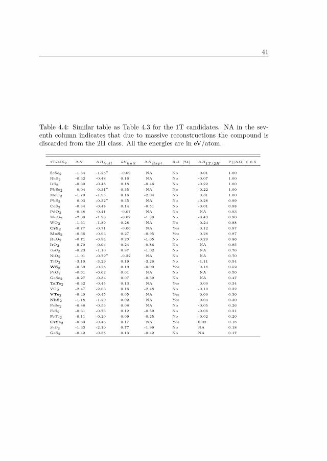
41

Table 4.4: Similar table as Table 4.3 for the 1T candidates. NA in the sev-enth column indicates that due to massive reconstructions the compound isdiscarded from the 2H class. All the energies are in eV/atom.

1T-MX2 ∆H ∆Hhull δHhull ∆HExpt. Ref. [74] ∆H1T/2H P(|∆G| ≤ 0.5

ScSe2 -1.34 -1.25∗ -0.09 NA No 0.01 1.00RhS2 -0.32 -0.48 0.16 NA No -0.07 1.00IrS2 -0.30 -0.48 0.18 -0.46 No -0.22 1.00PbSe2 0.04 -0.31∗ 0.35 NA No -0.22 1.00MoO2 -1.79 -1.95 0.16 -2.04 No 0.31 1.00PbS2 0.03 -0.32∗ 0.35 NA No -0.28 0.99CoS2 -0.34 -0.48 0.14 -0.51 No -0.01 0.98PdO2 -0.48 -0.41 -0.07 NA No NA 0.93MnO2 -2.00 -1.98 -0.02 -1.80 No -0.43 0.90WO2 -1.61 -1.89 0.28 NA No 0.24 0.88CrS2 -0.77 -0.71 -0.06 NA Yes 0.12 0.87MoS2 -0.66 -0.93 0.27 -0.95 Yes 0.28 0.87RuO2 -0.71 -0.94 0.23 -1.05 No -0.20 0.86IrO2 -0.70 -0.94 0.24 -0.86 No NA 0.85OsO2 -0.23 -1.10 0.87 -1.02 No NA 0.76NiO2 -1.01 -0.79∗ -0.22 NA No NA 0.70TiO2 -3.10 -3.29 0.19 -3.26 No -1.11 0.54WS2 -0.59 -0.78 0.19 -0.90 Yes 0.18 0.52PtO2 -0.61 -0.62 0.01 NA No NA 0.50GeSe2 -0.27 -0.34 0.07 -0.39 No NA 0.47TaTe2 -0.32 -0.45 0.13 NA Yes 0.00 0.34VO2 -2.47 -2.63 0.16 -2.48 No -0.10 0.32VTe2 -0.40 -0.45 0.05 NA Yes 0.00 0.30NbS2 -1.18 -1.20 0.02 NA Yes 0.04 0.30FeSe2 -0.48 -0.56 0.08 NA No -0.05 0.26FeS2 -0.61 -0.73 0.12 -0.59 No -0.06 0.21FeTe2 -0.11 -0.20 0.09 -0.25 No -0.02 0.20CrSe2 -0.63 -0.46 0.17 NA Yes 0.02 0.18SnO2 -1.33 -2.10 0.77 -1.99 No NA 0.18GeS2 -0.42 -0.55 0.13 -0.42 No NA 0.17

Chapter 5

Materials for LightAbsorption

5.1 IntroductionIn the last chapter the need to find alternative energy resources has beendiscussed. It was primarily based on the catalytic aspect of the hydrogenproduction. This chapter is mainly focussed on the absorption of sunlightwith semiconducting materials and the absorbed light can be used to producehydrogen by splitting the water. Harvesting the sunlight is crucial becausesolar energy is the most promising alternative resource which can meet thegrowing energy requirement on top of being environmentally benign as com-pared to the fossil fuels. Some of the routes to harness the solar energy aresolar cells, thermoelectrics, photoelectrochemical inter-conversion of chemicalsetc [75, 76, 77, 78, 79, 80, 81, 82, 83]. Photo-electrochemical routes to producechemicals have an added advantage of producing chemicals not just to be usedas fuels but also for other purposes [84].

One of the simplest photoelectrochemical reactions is the splitting of waterinto oxygen and hydrogen. The advent of TiO2 as a material to split thewater into hydrogen and oxygen revolutionized the research in the area ofphotoelectrochemical energy conversion [83]. But the wide bandgap of TiO2limits its performance only to the ultraviolet (UV) region of solar spectrum.Despite continuous effort for more than three decades no abundant and efficientbinary compound has been found to accomplish the task of visible light drivenwater splitting. The limited search space of binary compounds shifted the focus

42

43

to the compounds having more than two elements, especially ternary oxideswhich are quite stable under aqueous condition and irradiation [85, 86, 87].One of the biggest advantages of the ternary/quaternary compounds is thatthere exist lots of possibilities of tuning the bandstructure by choosing differentcombination of elements. A few of the widely studied ternary compounds areoxide perovskites, vanadates, tantalates etc. [26, 88, 85, 86, 87, 89]. Therefore,in order to find multicomponent compounds for efficient light absorption, inthis study a large number of compounds in the Materials Project Database[90, 91] have been explored. Additionally, the possibility of tuning the bandgapby layering of different semiconducting perovskites has also been explored usingBaSnO3 and BaTaO2N as model systems.

5.2 Mechanism of photoelectrochemical watersplitting

The splitting of water using the sunlight is based on the fact that the ab-sorption of sunlight generates electron-hole pairs in the semiconductor. Thegenerated electron-hole pair if have the right energy splits the water to theoxygen and hydrogen. The overall water splitting reaction can be written as[3]:

2H2O→ 2H2 + O2. (5.1)

The oxidation and reduction reactions separately are

2H2O + 4h+ → O2 + 4H+, (5.2)

2H+ + 2e− → H2. (5.3)

By definition of the normal hydrogen electrode (NHE) the free energy of theequation 5.3 is zero. The equation 5.2 however is uphill with a thermody-namic barrier of 1.23 eV [3]. If we ignore the overpotentials involved in thereaction for a moment then the maximum chemical potential of generated elec-tron (equivalently the conduction band minimum (CBM)) should be zero withrespect to the NHE whereas the minimum chemical potential of the generatedhole (equivalently the valence band maximum (VBM)) should be greater than1.23 V. However, due to various overpotentials involved the energy requiredby the electrons and holes to carry out the reaction is higher than the thermo-dynamic voltages mentioned above. A schematic of the photon induced watersplitting reaction described above is shown in the Figure 5.1.

44

As mentioned above the voltage of 1.23 V does not account for any over-potentials or non-equilibrium phenomena. The minimum overpotential asso-ciated with the oxygen evolution reaction (OER ) is ∼0.4 V and with thehydrogen evolution reaction (HER) is 0.1 V [88]. Additionally, the irradia-tion condition disrupts the equlibrium population of the electrons i.e separatequasi-Fermi levels have to be introduced for the conduction and valence bandfor the electron population. This lowers the effective driving force for the re-dox reactions. Typically, the correction due the effect of quasi-Fermi level istaken as ∼0.3 eV [88]. If all the above mentioned effects are added, it turnsout that the semiconductor should have the bandgap of at least 2 eV. In thefollowing sections the results and discussions about the screening of materialsfor the photoelectrochemical water splitting is based on the above mentioneddetails.

Figure 5.1: Schematic of the photon induced water splitting reaction.

5.3 Different methods for the bandgap calcula-tion

As mentioned before, the screening has been performed for the materials avail-able in the Materials Project Database. The Materials Project Database con-tains the subset of compounds present in the experimental database called asThe Inorganic Crystallographic Structures Database (ICSD).[92] The ICSDcontains the compounds which have been synthesized experimentally, there-fore, one can expect that the screened materials from the ICSD will be syn-thesizable under certain experimental conditions. However, the ICSD does

45

not have information about the stability of the materials in aqueous condi-tions which is also explored in this work for the stability of the photocatalystsunder in-situ conditions.

In chapter 1 a few different methods to calculate the bandgap of the semi-conductors were discussed along with their pros and cons. It has also beenpointed out that the calculation of the bandgap in a screening study should bereasonably accurate and at the same time efficient. The previously discussedGLLB-SC functional meets both the criteria in most of the cases. Therefore, inthe present study the bandgap of ∼2400 compounds has been calculated withthe GLLB-SC functional. Additionally, to test the validity of the calculatedbandgap with the GLLB-SC functional the previously discussed hybrid func-tional HSE06 and the many body perturbation theory in different flavors likeG0W0, GW0 and GW have also been used for a few selected materials. Thecomparison is shown in the Figure 5.2. The plot is divided into the high andlow bandgap materials. The figure shows that HSE06 tends to underestimatethe bandgap a bit with respect to GLLB-SC. On the other hand, GW whichis an eigenvalue self-consistent flavor of the GW approximation dovetails verywell with the GLLB-SC bandgaps in the low bandgap region. Additionally,GLLB-SC has a mean absolute error (MAE) of 0.38 eV with respect to GWthus closer to the GW predictions as compared to HSE06 and G0W0 whichhave the MAE of 0.46 and 0.51 eV respectively. GW0, being closest to the GWprediction with a MAE of only 0.29 eV, is highly computationally expensive ascompared to GLLB-SC. Therefore, GLLB-SC being reasonably accurate andan order of magnitude computationally cheaper than the GW approximationserves the purpose of bandgap prediction in a screening study. Table 5.1 sum-marizes the above mentioned mean absolute (signed) error in the bandgap ofthe compounds lying in the low region calculated with different methods withrespect to the other methods.

Table 5.1: Mean absolute (signed) error in eV for the materials in the smallbandgap region in Figure 5.2 using LDA, GLLB-SC, HSE06, G0W0 and GW0and GW

xcref LDA GLLB-SC HSE06 G0W0 GW0 GW

xc

LDA - 1.64 (-1.64) 1.21 (-1.21) 1.08 (-1.08) 1.30 (-1.30) 1.59 (-1.59)GLLB-SC 1.64 (1.64) - 0.61 (0.43) 0.59 (0.56) 0.52 (0.34) 0.38 (0.05)HSE06 1.21 (1.21) 0.61 (-0.43) - 0.25 (0.13) 0.29 (-0.09) 0.46 (-0.38)G0W0 1.08 (1.08) 0.59 (-0.56) 0.25 (-0.13) - 0.22 (-0.22) 0.51 (-0.51)GW0 1.30 (1.30) 0.52 (-0.32) 0.29 (0.09) 0.22 (0.22) - 0.29 (-0.29)GW 1.59 (1.59) 0.38 (-0.05) 0.46 (0.38) 0.51 (0.51) 0.29 (0.29) -

46

Figure 5.2: Bandgaps of few selected materials calculated with different meth-ods versus the GLLB-SC calculated bandgaps. The figure is taken from thePaper-3.

5.4 Candidates for photoelectrochemical watersplitting

A few crucial properties a material should have for an efficient absorption oflight for photoelectrochemical water splitting are:

• Bandgap in the range of visible spectrum because the solar spectrum isdominated by the visible light.

• Proper band edge positions in order to straddle the redox levels of waterin order to have the generated electron and hole at the right chemicalpotential to carry out the reaction.

• Stability of the compound in water because the reaction takes place inan aqueous medium.

Apart from the above mentioned properties, good electron-hole mobility, lowrecombination rates etc. are also required for greater efficiency. However, mod-eling of transport processes, recombination, defect centers etc. is much morecomplicated therefore not considered here for an initial stage of the screening.

47

In order to capture light in the visible range, the bandgap should lie be-tween ∼1.5-3.0 eV. Therefore the calculated bandgap with GLLB-SC shouldlie in this range for efficient absorption of the solar light by the material. Theposition of the band edges in general depend on the surface termination,[93]therefore, in order to calculate the band edges slab calculations have to beperformed. However, the position of the band edges can also be calculatedwith the empirical formula [94]:

EVBM,CBM = (χxAχyBχ

zC)1/(x+y+z) ± Egap/2 + E0, (5.4)

EVBM,CBM is the position of the valence and conduction band edge respectivelyof the compound AxByCz, χ’s are the electronegativity, Egap is the bandgapand E0=-4.5 V is the potential of the NHE with respect to the vacuum leveland the ‘+’, ‘-’ signs correspond to the VBM and CBM respectively. Theabove empirical formula provides band edges which dovetail with the slabmethod and experiments in most of the cases [94] with few exceptions.[95]Finally, the stability in aqueous conditions can be calculated by the Pourbaixdiagram.[96, 97] However, having a very tight threshold of the energy ∆Efor the stability may result in stability diagrams which do not’ agree withexperiments.[96] The reason behind this disagreement is that the stability isnot only the result of thermodynamics but the kinetics as well. On the otherhand, the Pourbaix diagrams do not contain any information about the kineticstherefore a larger energy threshold has to be employed in order to accountfor the phases which are kinetically protected. The sensitivity towards thethreshold can be seen in the Figure 5.3 which is the histogram of the GLLB-SCcalculated bandgap of all the 2400 materials considered in this work. The figureclearly shows that when a very tight threshold of 0 eV is chosen the for stability,most of the compounds turn out to be unstable in water even though many ofthem have been observed to be stable in experimental conditions. However,when a threshold of 1 eV is chosen, a reasonable number of compounds arestable in aqueous conditions. Therefore, a threshold of 1 eV is used to checkfor the stability of the compounds having suitable absorption properties forthe photoelectrochemical water splitting.

The final criteria used for the screening can be summarized as:

• 1.7 ≤ Egap ≤ 3.0 eV (to account the errors in the GLLB-SC calculatedbandgap and overpotentials).

• VBM ≥ 1.6 V and CBM ≤ -0.1 V with respect to the NHE (to accountfor the overpotentials).

48

Figure 5.3: Histogram of the GLLB-SC calculated bandgap of all 2400 mate-rials. Different color denote the stable compounds for different threshold ofenergy chosen for the stability in aqueous condition with pH = 7 and U = 0V with respect to the NHE. The figure is taken from the Paper-3.

49

• ∆E ≤ 1 eV (to account for the metastability and kinetic stabilization)at pH = 7 and -0.4 ≤ V ≤ 2.2 V which is the typical operating voltageof the device.

The materials meeting all the above criteria are selected from the pool of2400 are selected from the pool of ∼2400 and shown in the Figure 5.4. Inthe figure ∆E denotes the degree of stability of the material, the positionof the direct and indirect band edge positions are shown in red and blackrespectively. It is suprising that out of ∼2400 materials only a handful ofmaterials follow all the specified criteria. However, in recent experiments [72]a good control over the stability of semiconductors in water has ben achievedby using protective polymeric layers. Therefore, the size of the materials spacemight be expanded by relaxing the criteria of the stability in aqueous medium.The compounds written in green and underlined in the Figure 5.4 have beenrealized previously for different photoelectrochemical applications, [98, 99, 100,101, 102, 103, 104, 105] and are therefore expected to serve as viable candidatesfor photoelectrochemical water splitting.

5.5 Bandgap engineering of functional perovskitesThe previous section dealt with a specific application of solar light absorptioni.e photoelectrochemical water splitting. However, the other applications likephotovoltaics, transparent conducting oxides etc. require different size of thebandgap.[75, 76] We also saw that different factors limit the suitability ofa material for a given application e.g stability in water, toxicity, cost etc.Therefore, a systematic strategy is required to tune the bandgap of an alreadyexisting material which meets the requirement of toxicity, stability etc.

In this section the possibility of tuning the bandgap by the layering of twoperovskites, namely BaSnO3 and BaTaO2N is explored. The bandgap tuningespecially in perovskites has also been explored in previous works in systemslike SrVO3, SrTiO3 etc.[106, 107, 108, 109, 110, 111] The choice of BaSnO3 andBaTaO2N as a model system here stems from the fact that both the compoundshave been explored recently as light absorbers for the photoelectrochemicalwater splitting applications and have similar lattice constants thus the layeredsystem will not be subjected to a high stress. The protypical structure ofthe layered compound is shown in the Figure 5.5. The α (BaSnO3) and β(BaTaO2N) are stacked along the z-direction while x and y direction have theperiodicity of the cubic perovskite structure and the tuning of the bandgap isexplored by varying the number of layers of α (nα) and the number of layersof β (nβ).

50

Figure 5.4: Materials fulfilling the criteria of the bandgap, band edge positionsand stability in water in neutral pH condition and in the voltage range of -0.4to 2.2 V. ∆E denotes the degree of stability of the material. The positionof the direct and indirect band edge positions are shown in red and blackrespectively. The figure is taken from the Paper-3.

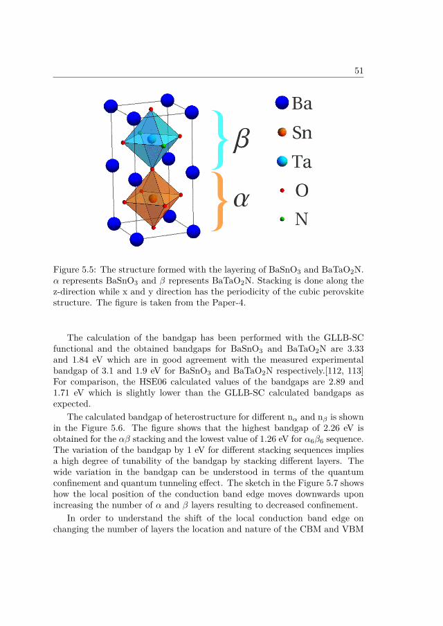
51

Figure 5.5: The structure formed with the layering of BaSnO3 and BaTaO2N.α represents BaSnO3 and β represents BaTaO2N. Stacking is done along thez-direction while x and y direction has the periodicity of the cubic perovskitestructure. The figure is taken from the Paper-4.

The calculation of the bandgap has been performed with the GLLB-SCfunctional and the obtained bandgaps for BaSnO3 and BaTaO2N are 3.33and 1.84 eV which are in good agreement with the measured experimentalbandgap of 3.1 and 1.9 eV for BaSnO3 and BaTaO2N respectively.[112, 113]For comparison, the HSE06 calculated values of the bandgaps are 2.89 and1.71 eV which is slightly lower than the GLLB-SC calculated bandgaps asexpected.

The calculated bandgap of heterostructure for different nα and nβ is shownin the Figure 5.6. The figure shows that the highest bandgap of 2.26 eV isobtained for the αβ stacking and the lowest value of 1.26 eV for α6β6 sequence.The variation of the bandgap by 1 eV for different stacking sequences impliesa high degree of tunability of the bandgap by stacking different layers. Thewide variation in the bandgap can be understood in terms of the quantumconfinement and quantum tunneling effect. The sketch in the Figure 5.7 showshow the local position of the conduction band edge moves downwards uponincreasing the number of α and β layers resulting to decreased confinement.

In order to understand the shift of the local conduction band edge onchanging the number of layers the location and nature of the CBM and VBM

52

Figure 5.6: The bandgap of the heterostructure as a function of nα and nβ .Each rectangle in the plot represents a compound with the stacking sequenceαnβm. The figure is taken from the Paper-4.

states are analyzed. In Figure 5.8 the wavefunctions of the VBM and CBMstates are plotted for αβ and α2β. The figure shows that the VBM mainlyconsists of the N2p orbitals in both αβ and α2β and is located in the β regionof the heterostructure. Additionally, calculations also suggest that the alongwith the character the position of the VBM state also does not change rela-tive to low-lying level for the different structures, therefore, it can be safelyassumed that it is only the nature and position of the conduction band whichis responsible for the bandgap variation in αβn. It can also be seen that in αβthe CBM states are located in the TaON plane and mainly consists of the Tad orbitals. Therefore, in order to see if the same trend is followed in αβn asthe number of β layers is increased the weights of the CBM state is analyzed.The Figure 5.9 shows the planar average (xy plane) of the weights of the CBMstate in the real space. The area of the circle represents the magnitude ofthe weight for the different planes stacked along the z-direction. The boxesrepresent the unit cell and the dotted lines the interface between the α and βlayers. As expected the CBM state is mainly comprised of the Ta d orbitalsand located on the TaON plane. The figure also shows that as the number ofβ layers is increased the CBM states become less confined therefore resulting

53

Figure 5.7: Sketch of the electronic level positions at an interface between αand β for different number of layers. The decreased number of layers resultingto increased confinement moves the local position of the conduction band edgeupwards. The figure is taken from the Paper-4.

Figure 5.8: Wavefunctions of the VBM and CBM states for selected hetere-ostructures. The figure is taken from the Paper-4.

54

to the downshift of the state eventually leading to decrease in the bandgap.

Figure 5.9: Planar average of the weights of the CBM state in the real spaceand the area of the circle represents the magnitude of the average. The unitcell is sketched as rectangles and the dotted lines show the interface betweenthe α and β layers. As expected the CBM state is mainly composed of theTa d orbitals. The bandgaps for different structures is also shown on the top.The figure is taken from the Paper-4.

Until now, the behavior of the heterostructure has only been analyzedwith only one α layer. However, the scenario significantly changes when thenumber of α layers is increased as shown in the Figure 5.10. The figure showsthe similar plot as in Figure 5.9 with the only difference that it has two αlayers as opposed to the Figure 5.9 which has one. As can be seen from thefigure that the CBM is now located mainly in the α part of the heterostructureand primarily consists of the Sn s states. A small weight in the β part of thestructure represents the tunneling effect. However, as expected the tunnelingeffect decreases as the number of β layers is increased and almost diminishesin going from α2β2 to α2β3. Additionally, the weights look similar in allthe structures. Therefore, the weights being similar and the diminishing ofthe tunneling effect results to almost no bandgap change as the number of βlayers ≥ 3.

In the last two kind of heterostructures it is found that keeping the numberof α layers to one has only confinement effect on increasing the number of β

55

Figure 5.10: Similar plot as in 5.9 with the only difference that it has twoα layers as opposed to the Figure 5.9 which has one. The CBM states nowmainly comprise of the Sn s states. The very small weight in the β regionindicates tunneling effect which almost diminished as the number of layers ofβ is increased beyond 2. The figure is taken from the Paper-4.

56

layers and for two α layers it is mainly the tunneling effect responsible for thebandgap variation. Therefore, it can be expected that if the number of α layersis increased while keeping the number of β layers constant the variation of thebandgap would be an interplay between the confinement and the tunnelingeffect. In order to see this effect the Figure 5.11 shows similar plot as Figure5.9 & 5.10 with the difference that the number of β layers is fixed to one whilethe number of α layers is increased. The behavior for αβ and α2β is alreadyshown in the Figure 5.9 & 5.10. In going from α2β to α6β the tunneling as wellas confinement decreses. However, the decreased tunneling has the oppositeeffect as the decreased confinement i.e as the tunneling decreases the bandgapincreases as in Figure 5.10 whereas the decreasing confinement decreases thebandgap as in Figure 5.9. These two competing effects results to a minimain the bandgap for the for a particular number of α layers. The Figure 5.11shows that up to 4 α layers the confinement effect dominates thus leading tothe bandgap reduction in moving from α2β to α4β, however, in going from α4βto α5β the diminishing tunneling dominates over the decreased confinementthus result in an increase in the bandgap. The above analysis for different

Figure 5.11: Similar plot as in 5.9 with the difference that the number of βlayer is fixed to one and the number of α layer is varied. As the number of αlayer is increased beyond α2β the tunneling and confinement effect competewith each other result in decreasing of the bandgap up to α4β and then theincrease of the bandgap. The figure is taken from the Paper-4.

57

heterostructures shows how different effects can be tuned to tailor the bandgapand the variation can be understood with simple physical arguments. Since theanalysis is quite general, therefore, it can be applied to other heterostructuresas well.

5.6 ConclusionIn this chapter a pool of ∼2400 materials is explored which can absorb solarlight for photoelectrochemical water splitting. The criteria imposed for thebandgap, band edge positions and the stability in aqueous solution in neutralpH for a certain potential range gives a handful of candidates which can serveas good photoabsorber for the water splitting reaction. The careful comparisonof the bandgap with different methods involving hybrid functionals and manybody perturbation theory methods assures credibility to the method that isused for the bandgap calculation of a large number of materials. A literaturesurvey for the materials in the list of candidates found which can act as goodphotoabsorbers suggests Ca2PbO4, Cu2PbO2 AgGaO2, AgIn2 and NaBiO3 aspotential candidates.

Additionally, a strategy to engineer the bandgap is also explored via lay-ering of different lattice matched structures. For the model systems exploredi.e BaSnO3 and BaTaO2N the calculations suggest that the variations in thebandgap of the structure can be understood with the simple arguments of con-finement and tunneling effects. This strategy can be applied to other latticematched systems for bandgap engineering.

Chapter 6

Trends in Stability andBandgaps of BinaryCompounds in DifferentCrystal Structures

6.1 IntroductionOne of the simplest class of compounds are binary compounds which onlyhave two constituent elements and different crystal structures e.g wurtzite,zinblende, rocksalt, NiAs and rutile. Often times, same compound exists indifferent crystal structures under different conditions and different structuresmay have significantly different properties. For example, the anatase phase ofTiO2 is found to be photo-catalytically active [83] where as the rutile phaseis not [114] even though both the structures are energetically very close withrutile phase being slightly more stable than anatase phase [115]. Additionally,rocksalt structure of ZnO which is significantly lower in stability as comparedto the native wurtzite structure has been stabilized in MgO matrix [116, 117].Thus, above studies suggest that compounds with different degree of metasta-bility can be synthesized and stabilized at normal conditions which motivatedus to explore different crystal structures of the same compound. In the currentwork we explore four different crystal structures of the binary compounds inAB stoichiometry where A and B are chosen from a set of 44 and 16 elements

58

59

respectively. In the set A, metals which may lead to magnetic compoundshave been ignored due to large degree of uncertainty in their bandgap calcu-lations whereas set B contains non-metals. First principle calculations werecarried out to determine the stability and bandgap of all the compounds. Wesystematically arrange the compounds in tabular form using Pettifor mapswhich involves the ordering of elements based on the their chemical scale fac-tor [118]. We also explore alloys of 32 binary compounds having the band gapin the range of 1.0-3.5 eV inspired by recent experiments on solid solutions forphoto-electrochemical water splitting applications [119, 3]. Clustering analysis[120] of the alloy compounds divides 32 compounds into different groups withcompound belonging to the same group behaving similarly for bandgaps uponalloying, thus giving the freedom too choose one compound over the other fromthe same class if required.

6.2 Results and Discussions

Figure 6.1: Crystal structures explored in the current work. (a) Rocksalt struc-ture (Space Group - Fm3m) (b) Wurtzite structure (Space Group - P63mc)(c) NiAs structure (Space Group - P63/mmc) (d) Zincblende structure (SpaceGroup - F 43m)

60

Table 6.1: Grouping of compounds in Figure 6.3 based on the range of geo-metric mean of chemical scale factor χ

Group Range(√χAχB)

1 0.00 - 1.452 1.45 - 1.753 1.75 - 1.954 1.95 - 2.105 2.10 - 2.306 2.30 - 3.10

Table 6.2: Standard enthalpy ∆H of formation of binary compounds inwurtzite structure having the bandgap in the range of 1.0 - 3.5 eV chosento form ternary wurtzite structures for bandgap engineering of binary com-pounds. ∆HOQMD shows the enthalpy of formation of the with same sto-ichiometry in the minimum energy structure and ∆Hhull represents the en-thalpy above the convex hull calculated from OQMD database. [73] All theenergies are mentioned in eV/atom.

Compound ∆H ∆HOQMD ∆Hhull Compound ∆H ∆HOQMD ∆Hhull

GaN -0.72 -0.59 -0.13 ZnO -1.77 -1.68 -0.09ScN -2.05 -2.04 -0.01 GeO -1.03 -1.94 0.45AgF -0.94 -1.21 0.27 SnO -1.18 -1.58 0.40PbO -0.97 -1.36 0.39 AgI -0.32 -0.38 0.06LaN -1.50 -1.44 -0.06 YN -1.97 -1.81 -0.16InP -0.33 -0.37 0.04 GaP -0.59 -0.55 -0.04AlAs -0.62 -0.49 -0.14 AlP -0.86 -0.76 -0.10AgCl -0.56 -0.67 0.11 AgBr -0.46 -0.55 0.09CdTe -0.37 -0.47 -0.10 AlSb -0.32 -0.17 -0.15CdSe -0.69 -0.64 -0.05 ZnTe -0.56 -0.47 -0.09ZnSe -0.90 -0.72 -0.18 CdS -0.75 -0.81 0.06GeS -0.42 -0.42 0.00 AlI -0.27 -0.05 0.27AlBr -0.58 -0.31 0.34 GeSe -0.33 -0.22 -0.11SnS -0.48 -0.66 0.18 SnSe -0.44 -0.48 0.04PbS -0.41 -0.71 0.30 PbSe -0.38 -0.57 0.19GeTe -0.05 -0.09 0.04 PbTe -0.05 -0.41 0.36

Figure 6.2 shows the ball and stick model of the crystal structures exploredin the present work. Binary compounds crystallizing in NiAs and wurtzitestructures have four atoms in the unit cell with the coordination number ofsix and four respectively, whereas the primitive unit cell of the rocksalt andzincblende structures contains two atoms with a coordination number of sixand four respectively. In the light of recent experiments on the synthesis ofcompounds violating chemical/octet rules under extreme conditions we do notimpose any chemical rules to narrow down the search space in our calculations

61

Figure 6.2: Heatmap of standard enthalpy of formation of compounds in dif-ferent crystal structures. Each square in the heat map represents a compoundswith constituent elements represented by ordinate and abscissa of that square.

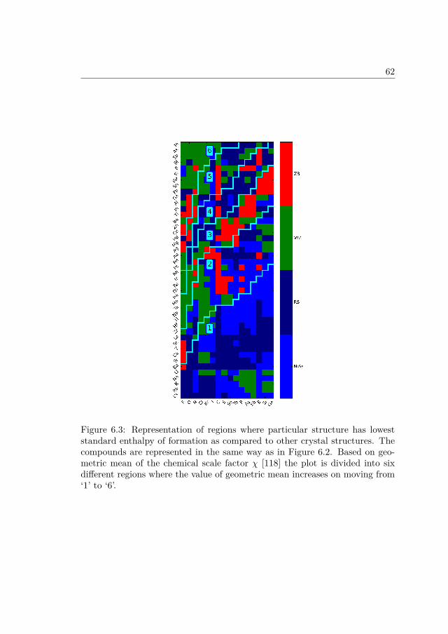
62

Figure 6.3: Representation of regions where particular structure has loweststandard enthalpy of formation as compared to other crystal structures. Thecompounds are represented in the same way as in Figure 6.2. Based on geo-metric mean of the chemical scale factor χ [118] the plot is divided into sixdifferent regions where the value of geometric mean increases on moving from‘1’ to ‘6’.

63

Figure 6.4: Band gap of compounds in different crystal structures. The whiteregion in the plots shows the metallic compound i.e. with zero bandgap

64

Figure 6.5: Dendrogram based on difference of average bandgap of the con-stituent compounds in the alloy and calculated bandgap of the alloy. Theconstituent compounds have been selected from the pool of compounds withwurtzite structure and having the bandgap in the range of 1.0-3.5 eV.

65

Figure 6.6: (a) Calculated bandgap of the alloys. The constituent compoundshave wurtzite structures with the bandgap lying in the range of 1.0-3.5 eV.White spaces show alloys with zero bandgap. (b) Shows enthalpy of mixing ofthe alloy compounds with respect to constituent compounds.

66

[121]. In our work we calculate the stability of compounds with respect to thestandard reference states only. Since our interest lies in comparing the trendsin thermodynamic and electronic properties of the compounds in differentcrystal structures with 1:1 stoichimetry, we do not consider the compoundswith the stoichiometry different from 1:1. In the calculations we ignore fewmetals leading to magnetic structures since a reliable approach to calculatethe bandgap of magnetic semiconductors with the GLLB-SC functional hasnot been developed yet.

Figure 6.2 shows the heatmaps of the standard heat of formation of all thecompounds in which the elements are arranged as per the chemical scale χproposed by Pettifor [118]. As can be seen from the figure that the heat of for-mation in all four crystal structures follow the similar pattern which indicatesthat if the compound is stable with respect to the standard states in one crystalstructure it will be stable in the other crystal structure as well. But negativeformation energy does not guarantees that the structure can be stabilized inthat phase which is inhibited by the existence of other competing phases inthe ambient environment. But the control over the ambient condition for thegrowth can be achieved by for example temperature, pressure, surfactants anddoping [122, 123, 124]. Pressure as one of the control mechanism in the growthprocess gives a tool to stabilize structure with different volumes. For example,if the most stable structure has a lower volume (e.g. rocksalt or NiAs) thenapplying tensile stress may favor the higher volume phase (e.g. wurtzite orzincblende) whereas a lower volume phase will be favored under compressivestress if the most stable structure has a higher volume. The above process canbe realized in experiments [116, 125] with the growth on a substrate with differ-ent lattice mismatch thus providing a way to apply the compressive and tensilestress. Thus, above strategies to manipulate crystal structures suggest thatthe compounds can possibily be synthesized and stabilized in different crystalstructures with different volumes. Therefore, in the current work we choosecrystal structures spanning a wide range of volumes with the zincblende andwurzite having higher volumes due to low coordination number as opposed tothe rocksalt and NiAs structures which have larger coordination number thuslower volumes.

In addition to the standard heat of formation as shown in Figure 6.2 onemight also be interested in region where a particular crystal structure has thelowest enthalpy of formation as compared to other crystal structures. Fig-ure 6.3 shows the minimum energy crystal structure for different compounds.As can be inferred from the figure, there are very few isolated regions for agiven crystal structure. Hence, compounds when arranged in Pettifor mapsform clusters having the same most stable crystal structure. Therefore, we

67

group the compounds in Figure 6.3 in six different groups based on the geo-metric mean of the chemical scale factor χ [118]. The range of geometric meanof groups is shown in Table 6.1.

The grouping in Figure 6.3 shows an apparent correlation between thecrystal structure and the geometic mean of the chemical scale factor of thecompounds. For very small values of geometric mean (Group 1) the compoundprefers to have the low volume structure i.e. rocksalt or NiAs whereas at largervalues(Group 6) the compound prefer to have more open structure i.e. wurtziteor zincblende. Few green parts in the Group 1 for compounds like LiF, LiClis the artifact of the calculation since these compounds are known to have therocksalt structure. On the other hand,the difference in energies of the wurtziteand rocksalt structure of these compounds as per our calculations is of theorder of 0.05 eV which is small and can be safely ignored. The region of extremevalues of the geometric mean in Figure 6.3 i.e. Group 1 and 6 are the regionof extreme ionicity of the compounds with very small values indicating largeionicity (more closed structures) whereas very large values showing greatercovalent character (more open structures) [118]. On the other hand, the regionof moderate ionicity i.e. Group 2-5 is not dominated by one crystal structure.Group 2 has large fraction of WZ and NiAs structures, Group 3 ZB structure,Group 4 RS structure and Group 5 WZ and RS structures.

In Figure 6.4 we show the bandgap of all the compounds. The white regionsin the heatmap show the zero bandgap materials by which we can see that outof 704 materials in each group very few turn out be semiconducting with thesmallest number of semiconductors in the NiAs structure and the largest num-ber in the ZB structure. The plot also shows that despite having the similarheat of formation, the wurtzite and zincblende have quite dissimilar trend inbandgaps(especially indirect gap) which is a well known phenomenon [126].Hence, in cases where the WZ and ZB have significantly different bandgaps,stabilizing the structure with the required bandgap can be achieved efficientlydue to the similar heats of formation.

In addition to modifying the structures to tune the bandgap, bandgapengineering can also be achieved by making solid solutions of different semi-conductors. The same has been realized in the experiments in recent workscarried out in Domen’s group [119, 3] in which the mixture of GaN and ZnOhas the bandgap of ∼2.5 eV as opposed to the bandgap of ∼3.4 eV of the con-stituent compounds GaN and ZnO. Thus, these experimental results suggestthat the alloying can be used as a method for the bandgap tailoring. Hence,guided by the above experiments we also explore the alloys of binary com-pounds in the wurtzite structures having the bandgap in the range of 1.0 -3.5 eV. The stability of the alloy with respect to the constituent compounds

68

mixed in an equimolar ratio is described by the enthalpy of mixing as

∆HABCDmix = EABCDtot − EABtot − ECDtot (6.1)

where Eitot is the total energy of the compound ‘i’. Table 6.2 shows the heat offormation of the compounds in the wurtzite structure having the bandgap inthe range of 1.0-3.5 eV, ∆H is the heat of formation calculated in the presentwork, ∆HOQMD is the heat of formation as given in the OQMD (The OpenQuantum Materials Database) database [73] for the structure which has theminimum energy at 1:1 stochiometry and ∆Hhull is the relative energy of thecompound in the current work with respect to the convex hull as given in theOQMD database. Since the enthalpies in OQMD database are based on DFTreference energies whereas we use corrected reference energies as proposed byStevanovic et al. [25], therefore the difference 0.15 eV/atom or less in oursand OQMD calculations will lie within in the error bar due to the differentmethods used for the calculation of the reference energies. Compounds likeAlI, AlBr which are significantly above the convex hull and have no structurewhich is stable at 1:1 stochiometry and also expected to be unstable basedon the valence rule can be ruled out as they may not be possibly synthesizedunder normal/moderate conditions. On the other hand, compounds like GeO,AgF and PbO have different structures other than the wurtzite which arestable and lie below the convex hull. Even though energy of the wurtzitestructure of these compounds lies above the convex hull by ∼0.35 eV/atom(Table 6.1), its likely that they can be stabilized in the wurtzite form sincethey exist in structures which are stable at the same stoichiometry. So, theirsynthesis/stabilization might be possible under moderate conditions.

In order to study the trends we made a crude approximation of the solidsolution with a unit cell of four atoms due large computational time requiredfor a larger unit cell. Based on the previous works, we believe the that theapproximations made will not change the results drastically [127].

The similarity between the compounds forming the mixture in terms of thedeviation of the bandgap of the mixture from the average of the bandgaps ofconstituent compounds has been assessed by the so-called dendrogram plot.Dendrogram is a tree diagram used in the generating hierarchical structuresamong the elements representing the data [120]. In Figure 6.5, we show thedendrogram plot with euclidean metric of the difference of the average bandgapof the constituent compounds and the calculated bandgap of the alloy. Theclustering in a dendrogram is based on the distance measure (dAB) of two

69

components given as

dAB =∑CD

(EgapAB + EgapCD

2 − EgapABCD

)2(6.2)

In the equation above AB corresponds to the compound for which the dis-tance measure has to be calculated and the summation index CD correspondsto other compounds in the set of binary compounds which are combined withAB to form alloys. Based on the distance measure the compounds with cutoffdistance measures will be clustered together. The clustering of compoundslike ZnO and GaN, CdS and CdSe, ZnTe and CdTe, for which the thermo-dynamic/light absorption properties of the solid solutions have already beenexplored experimentally complements our study [119, 128, 129]. As one wouldexpect on the chemical grounds, clustering naturally leads to the grouping ofthe chalcogenides of the Group 12 elements, chalcogenides of Group 14 ele-ments, silver halides and the compounds of the trivalent ions with the Group15 elements. As can be seen from the values close to zero along the blockdiagonal in the dendrogram plot that in most of the cases when the mixturesare formed from compounds in the same group, the resultant bandgaps differonly by ∼0.5 eV from the average of the bandgaps. On the other hand, mix-ing of the compounds from different groups leads to a significant reduction ofthe bandgap with respect to the average of the bandgaps in most of the casesas shown with the red blocks. The detailed description of the above trendwould require electronic structure analysis of every mixture which is beyondthe scope of the current work.

Figure 6.6(a) and (b) show the bandgap and enthalpy of mixing ∆Hmix ofthe mixture as given by equation (6.1). Since, The positive correlation betweenthe bandgap and the stability [130] renders some of the mixtures metallic dueto the large positive heat of mixing. As one would anticipate that the mixingof compounds with very different lattice constants will be energetically un-favorable, the red regions in Figure 6.6(b) manifest the expected trend. Forexample, ZnO, GaN, ScN have similar volumes, so their mixture with the tel-lurides, selenides or compounds of lead which have much larger volumes resultto significantly positive heat of mixing which in turn leads to zero bandgapof those mixtures. Thus, exploring mixtures of compounds with similar lat-tice constant will have a higher probability of giving compounds with a finitebandgap.

Combiningly, Figure 6.5 and 6.6 show that the bandgap of most of thestable mixtures along the block diagonal 1 (bottom left to top right) havebandgap of ∼2.5 eV except the block containing the chalcogenides of zinc and

70

cadmium which has lower bandgap due to low bandgaps of the constituentcompounds. On the other hand, stable compounds along the block diagonal2 (top left to bottom right) are low bandgap mixtures with the bandgap ∼1.5eV. Thus, the dichotomy in the bandgaps allows us to look in a definite regionof the materials space for the required range of bandgaps suitable for theapplication in hand.

6.3 ConclusionIn the current work we have carried out a systematic analysis of the com-pounds in different crystal structures spanning a wide range of volumes andhaving the AB stoichiometry. The correlation between the crystal structureand the chemical scale factor χ gives a rationale to understand the effect ofelectronegativity on the crystal structure of the compounds. In addition tothe binary compounds, detailed analysis of their alloys gives a rationale forthe bandgap engineering via solid solutions of the semiconductors. The anal-ysis carried out in the current work for the binary semiconductors can also begeneralized to the systems containing more than two elements thus providingan elegant route to tailor the bandgap as required by the application in handlike photo-electrochemical water splitting, solar cells.

Chapter 7

Final Remarks

In the previous chapters, challenges involved in the process of materials designhave been looked at. The challenges are not only faced by experimentalists butby theoreticians as well. The bottlenecks in experiments come from the lim-ited resources and time whereas the computational scientists having access topowerful computers are limited by the accuracy of the computational methodsand approximations made to mimic the experiments. But, these limitationsin no way stop us to move forward. Experimental tools are becoming increas-ingly advanced whereas day to day developments in theory and algorithms aremaking computations more and more reliable.

In this work, an attempt to solve some of the materials design problemwith computations and some strategies to face future challenges for the sameare looked at. The assessment of recently developed mBEEF functional for theprediction of the heats of formation is an example for theoretical developmentswhereas the screening of materials for light absorption and hydrogen evolutionreaction is an attempt to solve materials design problem regarding energy.Finally, exploring one of the many methods for the bandgap engineering showshow we can expand the materials space by using the already existing materialsfor different applications.

In all the above problems, we got help from the available experimentaldata whether it was heats of formation, activity for hydrogen evolution orthe photoelectrochemical water splitting. This implies that no matter howfast, cheap and efficient computer simulations become, at the end of the daythe calculated numbers have to agree with experiments. As Feynman oncesaid: “It doesn’t matter how beautiful your theory is, it doesn’t matter howsmart you are. If it doesn’t agree with experiment, it’s wrong.” Therefore,

71

72

the experiments and theory have to go hand in hand to solve materials designproblem in a reliable and efficient way.

One of recent examples of the synergistic effort of the experiments andtheory is machine learning. People are trying to solve materials design prob-lems using machine learning. However, the reliability of machine learning fordifferent fields is different. For example, machine learning in astronomy is rea-sonably reliable because the experimental data is provided only by a very fewtelescopes which are very well tested. On the other hand, machine learningin materials design suffers with a lot of ambiguity, for example, variations inpseudopotentials, different electronic structure codes, plethora of unreliableexperimental data etc. Therefore, I personally feel that the dream of solvingmaterials design problem with machine learning is very far from realizable inthe near future and we still have to resort to more fundamental science thanblindly using computers.

Bibliography

[1] N. S. Lewis and D. G. Nocera. PNAS, 103:15729–15735, 2006.

[2] N. Armaroli and V. Balzani. Angew. Chem. Int. Ed., 46:52–66, 2007.

[3] K. Maeda and K. Domen. Chem. Mater., 22:612–623, 2010.

[4] P. C. K. Vesborg and T. F. Jaramillo. RSC Adv., 2:7933–7947, 2012.

[5] E. Schrödinger. Annalen der Physik, 384:361–376, 1926.

[6] J. Kohanoff. Electronic Structure Calculations for Solids and Molecules.Cambridge University Press, 2006. Cambridge Books Online.

[7] P. Hohenberg and W. Kohn. Phys. Rev., 136:B864, 1964.

[8] W. Kohn and L. J. Sham. Phys. Rev., 140:A1133, 1965.

[9] J. P. Perdew, K. Burke, and M. Ernzerhof. Phys. Rev. Lett., 77:3865,1996.

[10] J. Heyd, G. E. Scuseria, and M. Ernzerhof. J. Chem. Phys., 118:8207,2003.

[11] A. V. Krukau, O. A. Vydrov, A. F. Izmaylov, and G. E. Scuseria. J.Chem. Phys., 125:224106, 2006.

[12] A. J. Cohen, P. Mori-Sánchez, andW. Yang. Science, 321(5890):792–794,2008.

[13] P. Mori-Sánchez, A. J. Cohen, and W. Yang. Phys. Rev. Lett.,100(14):146401, 2008.

[14] O. Gritsenko, R. van Leeuwen, E. van Lenthe, and E. J. Baerends. Phys.Rev. A, 51:1944, 1995.

73

74

[15] M. Kuisma, J. Ojanen, J. Enkovaara, and T. T. Rantala. Phys. Rev. B,82:115106, 2010.

[16] J. P. Perdew, M. Ernzerhof, and K. Burke. J. Chem. Phys., 105:9982,1996.

[17] C. Adamo and V. Barone. J. Chem. Phys., 110:6158, 1999.

[18] J. Paer, M. Marsman, K. Hummer, G. Kresse, and I. C. Gerber. J.Chem. Phys., 124:154709, 2006.

[19] J. Enkovaara, C. Rostgaard, J. J. Mortensen, J. Chen, M. Dułak,L. Ferrighi, J. Gavnholt, C. Glinsvad, V. Haikola, H. A. Hansen, H. H.Kristoffersen, M. Kuisma, A. H. Larsen, L. Lehtovaara, M. Ljungberg,O. Lopez-Acevedo, P. G. Moses, J. Ojanen, T. Olsen, V. Petzold, N. A.Romero, J. Stausholm-Møller, M. Strange, G. A. Tritsaris, M. Vanin,M. Walter, B. Hammer, H. Häkkinen, G. K. H. Madsen, R. M. Nieminen,J. K. Nørskov, M. Puska, T. T. Rantala, J. Schiøtz, K. S. Thygesen, andK. W. Jacobsen. Journal of Physics: Condensed Matter, 22(25):253202,2010.

[20] J. J. Mortensen, L. B. Hansen, and K. W. Jacobsen. Phys. Rev. B,71:035109, 2005.

[21] D. Vanderbilt. Phys. Rev. B, 41:7892–7895, 1990.

[22] P. E. Blöchl. Phys. Rev. B, 50:17953–17979, 1994.

[23] C. Rostgaard. arXiv preprint arXiv:0910.1921v2 , 2009.

[24] M. Fuchs, J. L. F. Da Silva, C. Stampfl, J. Neugebauer, and M. Scheffler.Phys. Rev. B, 65:245212, 2002.

[25] V. Stevanović, S. Lany, X. Zhang, and A. Zunger. Phys. Rev. B,85:115104, 2012.

[26] I. E. Castelli, T. Olsen, S. Datta, D. D. Landis, S. Dahl, K. S. Thygesen,and K. W. Jacobsen. Energy Environ. Sci., 5:5814–5819, 2012.

[27] X. Zhang, V. Stevanović, M. d’Avezac, S. Lany, and A. Zunger. Phys.Rev. B, 86:014109, 2012.

[28] S. Lany. Phys. Rev. B, 78:245207, 2008.

75

[29] S. L. Dudarev, G. A. Botton, S. Y. Savrasov, C. J. Humphreys, andA. P. Sutton. Phys. Rev. B, 57:1505, 1998.

[30] B. Hammer, L. B. Hansen, and J. K. Nørskov. Phys. Rev. B, 59:7413,1999.

[31] J. M. Tao, J. P. Perdew, V. N. Staroverov, and G. E. Scuseria. Phys.Rev. Lett., 91(14):146401, 2003.

[32] R. Peverati and D. G. Truhlar. Phil. Trans. R. Soc. A, 372:2011, 2014.

[33] L. A. Constantin, E. Fabiano, and F. Della Sala. . Chem. TheoryComput., 9(5):2256–2263, 2013.

[34] J. Sun, J. P. Perdew, and A. Ruzsinszky. Proceedings of the NationalAcademy of Sciences, 112(3):685–689, 2015.

[35] F. Della Sala, E. Fabiano, and L. A. Constantin. Phys. Rev. B,91:035126, 2015.

[36] J. Wellendorff, K. T. Lundgaard, K. W. Jacobsen, and T. Bligaard. J.Chem. Phys., 140:144107, 2014.

[37] Standard thermodynamic properties of chemical substances, 2000. http://www.update.uu.se/~jolkkonen/pdf/CRC_TD.pdf.

[38] W. H. Press, B. P. Flannery, S. A. Teukolsky, and W. T. Vetterling.Numerical Recipes in C. Cambridge University Press, 1988.

[39] K. S. Brown S. L. Frederiksen, K. W. Jacobsen and J. P. Sethna. Phys.Rev. Lett., 93(16):165501, 2004.

[40] M. S. Dressselhaus and I. L. Thomas. Nature, 414:332–337, 2001.

[41] G. W. Crabtree, M. S. Dresselhaus, and M. V. Buchanan. Phys. Today,57:39–44, 2004.

[42] J. Greeley, T. F. Jaramillo, J. L. Bonde, I. Chorkendorff, and J. K.Nørskov. Nat. Mater., 5:909–913, 2006.

[43] Y. Okamoto, S. Ida, J. Hyodo, H. Hagiwara, and T. J. Ishihara. J. Am.Chem. Soc., 133:18034–18037, 2011.

[44] S. Cobo, J. Heidkamp, P.-A. Jacques, J. Fize, V. Fourmond, L-Guetaz,B. Jousselme, V. Ivanova, H. Dau, S. Palacin, M. Fontecave, andV. Artero. Nat. Mater., 11:802–807, 2012.

76

[45] P. Liu and J. A. Rodriguez. J. Am. Chem. Soc., 127:14871–14878, 2005.

[46] E. J. Popczun, J. R. McKone, C. G. Read, A. J. Biacchi, A. M. Wiltrout,N. S. Lewis, and R. E. Schaak. J. Am. Chem. Soc., 135:9267–9270, 2013.

[47] L. Feng J. Rossmeisl M. H. Hansen, L. A. Stern and X. Hu. Phys. Chem.Chem. Phys., 17:10823–10829, 2015.

[48] D. Voiry, H. Yamaguchi, J. Li, R. Silva, D. C. B. Alves, T. Fujita,M. Chen, T. Asefa, V. B. Shenoy, G. Eda, and M. Chhowalla . Nat.Mater., 12:850–855, 2013.

[49] M. A. Lukowski, A. S. Daniel, F. Meng, A. Forticaux, L. Li, and S. Jin.J. Am. Chem. Soc., 135:10274–10277, 2013.

[50] D. Voiry, M. Salehi, R. Silva, T. Fujita, M. Chen, T. Asefa, V. B. Shenoy,G. Eda, and M. Chhowalla. Nano Letters, 13:6222–6227, 2013.

[51] H. Wang, Z. Lu, D. Kong, J. Sun, T. M. Hymel, and Y. Cui. ACS Nano,8:4940–4947, 2014.

[52] T. F. Jaramillo, K. P. Jørgensen, J. Bonde, J. H. Nielsen, S. Horch, andI. Chorkendorff. Science, 317:100–102, 2007.

[53] M. V. Bollinger, K. W. Jacobsen, and J. K. Nørskov. Phys. Rev. B,67:085410, 2003.

[54] B. Hinnemann, P. G. Moses, J. Bonde, K. P. Jørgensen, J. H. Nielsen,S. Horsch, I. Chorkendorff, and J. K. Nørskov. J. Am. Chem. Soc.,127:5308–5309, 2005.

[55] A. N. Enyashin, L. Yadgarov, L. Houben, I. Popov, M. Weidenbach,R. Tenne, M. Bar-Sadan, and G. Seifert. J. Phys. Chem. C, 115:24586–24591, 2011.

[56] K. Rossnage. J. Phys.: Condens. Matter, 23:213001, 2011.

[57] K. Dolui and S. Sanvito. arXiv preprint arXiv:1310.1866 , 2013.

[58] L. Fu X. Qian, J. Liu and J. Li. Science, 346:1344–1347, 2014.

[59] M. Kan, J. Y. Wang, X. W. Li, S. H. Zhang, Y. W. Li, Y. Kawazoe,Q. Sun, and P. Jena. J. Phys. Chem. C, 118:1515–1522, 2014.

77

[60] S. Tongay, H. Sahin, C. Ko, A. Luce, W. Fan, K. Liu, J. Zhou, Y.-S.Huang, C.-H. Ho, J. Yan, D. F. Ogletree, S. Aloni, J. Ji, S. Li, J. Li,F. M. Peeters, and J. Wu. Nat. Commun., 5:3252, 2014.

[61] H. T. Stokes and D. M. Hatch. J. Appl. Cryst., 38:237–238, 2005.

[62] C. Ataca, H. Şahin, and S. Ciraci. J. Phys. Chem. C, 116:8983–8999,2012.

[63] S. Trasatti. J. Electroanal. Chem., 39:163, 1972.

[64] J. O’M. Bockris, A. K. N. Reddy, and M. Gamboa-Aldeco. ModernElectrochemistry 2A 2nd ed. Kluwer Academic/Plenum Publishers: NewYork, 1998.

[65] C. Tsai, F. A.-Pedersen, and J. K. Nørskov. Nano Letters, 14:1381–1387,2014.

[66] C. Tsai, J. K. Nørskov K. Chan, and F. A.-Pedersen. J. Phys. Chem.Lett., 5:3884–3889, 2014.

[67] K. K. Irikura. J. Phys. Chem. Ref. Data, 36:389, 2007.

[68]

[69] L. C. Seitz, Z. Chen, A. J. Forman, B. A. Pinaud, J. D. Benck, and T. F.Jaramillo. ChemSusChem, 7:1372, 2014.

[70] J. Wellendorff, K. T. Lundgaard, A. Møgelhøj, V. Petzold, D. D. Lan-dis, J. K. Nørskov, T. Bligaard, and K. W. Jacobsen. Phys. Rev. B,85:235149, 2012.

[71] A. J. Medford, J. Wellendorff, A. Vojvodic, F. Studt, F. A.-Pedersen,K. W. Jacobsen, T. Bligaard, and J. K. Nørkov. Science, 345:197, 2014.

[72] S. Mubeen, J. Lee, N. Singh, M. Moskovitsb, and E. W. McFarland.Energy Environ. Sci., 6:1633, 2013.

[73] J. E. Saal, S. Kirklin, M. Aykol, B. Meredig, and C. Wolverton. JOM,65:1501–1509, 2013.

[74] S. Lebègue, T. Björkman, M. Klintenberg, R. M. Nieminen, andO. Eriksson. Phys. Rev. X, 3:031002, 2013.

78

[75] L. Vayssierres. On Solar Hydrogen and Nanotechnology. John Wileyand Sons (Asia) Pvt. Ltd, 2009.

[76] G.A. Chamberlain. Solar Cells, 8(1):47 – 83, 1983.

[77] M. Grätzel. J. Photochemistry and Photobiology C: PhotochemistryReviews, 4(2):145 – 153, 2003.

[78] M. Ni, M. K.H. Leung, D. Y.C. Leung, and K. Sumathy. Renewable andSustainable Energy Reviews, 11(3):401 – 425, 2007.

[79] A. Kudo and Y. Miseki. Chem. Soc. Rev., 38:253–278, 2009.

[80] K. Sayama Z. Zou, J. Ye and H. Arakawa. Nature, 414:625–627, 2001.

[81] L. Schmidt-Mende, A. Fechtenkötter, K. Müllen, E. Moons, R. H. Friend,and J. D. MacKenzie. Science, 293(5532):1119–1122, 2001.

[82] A. Hagfeldt and M. Grätzel. Accounts of Chemical Research, 33(5):269–277, 2000.

[83] A. Fujishima and K. Honda. Nature, 238:37–38, 1972.

[84] B. Kumar, M. Llorente, J. Froehlich, T. Dang, A. Sathrum, and C. P.Kubiak. Annual Review of Physical Chemistry, 63(1):541–569, 2012.

[85] C. S. Enache, D. Lloyd, M. R. Damen, J. Schoonman, and R. van deKrol. The Journal of Physical Chemistry C, 113(44):19351–19360, 2009.

[86] Y. Liang, T. Tsubota, L. P. A. Mooij, and R. van de Krol. The Journalof Physical Chemistry C, 115(35):17594–17598, 2011.

[87] F. F. Abdi and R. van de Krol. The Journal of Physical Chemistry C,116(17):9398–9404, 2012.

[88] K. S. Thygesen S. Dahl I. Chorkendorff T. F. Jaramillo I. E. Castelli,D. D. Landis and K. W. Jacobsen. Energy Environ. Sci., 5:9034–9043,2012.

[89] M. Oshikiri, M. Boero, J. Ye, Z. Zou, and G. Kido. J. Chem. Phys.,117(15):7313–7318, 2002.

[90] G. Hautier W. Chen W. D. Richards S. Dacek S. Cholia D. Gunter D.Skinner G. Ceder A. Jain, S. P. Ong and K. A. Persson. APL Materials,1:011002, 2013.

79

[91] M. Pandey H. Li K. S. Thygesen B. Seger A. Jain K. A. Persson G.Ceder K. W. Jacobsen I. E. Castelli, F. Hüser. Adv. Energy Mater.,5:1400915, 2015.

[92] A. Belsky, M. Hellenbrandt, V. L. Karen, and P. Luksch. Acta Cryst.,B58:364–369, 2002.

[93] D. S. Ginley W. Tumas V. Stevanovic, S. Lany and A. Zunger. Phys.Chem. Chem. Phys., 16:3706, 2014.

[94] M. A. Butler and D. S. Ginley. J. Electrochem. Soc., 125:228–232, 1978.

[95] Filip A. Rasmussen and Kristian S. Thygesen. J. Phys. Chem. C,119(23):13169–13183, 2015.

[96] K. S. Thygesen I. E. Castelli and K. W. Jacobsen. Top. Catal., 57(1–4):265–272, 2014.

[97] P. Lazic K. A. Persson, B. Waldwick and G. Ceder. Phys. Rev. B,85:235438, 2012.

[98] A. E. Lavat R. P. Diez, E. J. Baran and M. C. Grasselli. J. Phys. Chem.Solids, 56:135, 1995.

[99] K. Rubesova and D. Sykorova. J. Sol-Gel Sci. Technol., 49:228, 2009.

[100] C. L. Teske H. Szillat. Z. Anorg. Allge. Chem., 620:1307, 1994.

[101] R. Nagarajan H. Yanagi, J. Tate and A. W. Sleight. Solid StateCommun., 122:295, 2002.

[102] H. Irie Y. Maruyama and K. Hashimoto. J. Phys. Chem. B, 110:23274,2006.

[103] D. Chen Z. G. Zou S. X. Ouyang, N. Kikugawa and J. H. Ye. J. Phys.Chem. C, 113:1560, 2009.

[104] M. Katagiri T. Kako, Z. G. Zou and J. H. Ye. Chem. Mater., 19:198,2007.

[105] Q. Z. Liu Y. F. Zhu J. J. Liu, S. F. Chen and J. F. Zhang. Chem. Phys.Lett., 572:101, 2013.

[106] H. Kumigashira S. Okamoto S. Aizaki A. Fujimori K. Yoshimatsu,T. Okabe and M. Oshima. Phys. Rev. Lett., 104:147601, 2010.

80

[107] M. Kobayashi K. Horiba T. Yoshida A. Fujimori M. Oshima K. Yoshi-matsu, E. Sakai and H. Kumigashira. Phys. Rev. B, 88:115308, 2013.

[108] H. Kumigashira T. Yoshida A. Fujimori K. Yoshimatsu, K. Horiba andM. Oshima. Science, 333:319, 2011.

[109] S. Kumar S. J. May J. A. Borchers B. B. Maranwille J. Zarestky S. G.E. te Velthuis J. van den Brink T. S. Santos, B. J. Kirby and A. Bhat-tacharya. Phys. Rev. Lett., 107:167202, 2011.

[110] C. R. Freeze C. A. Jackson, J. Y. Zhang and S. Stemmer. Nat. Commun.,5:1, 2014.

[111] B. Ehrlich C. Grote and R. F. Berger. Phys. Rev. B, 90:205202, 2014.

[112] H. W. Eng H. Mizoguchi and P. M. Woodward. Inorg. Chem., 43:1667,2004.

[113] H. Hara J. N. Kondo D. Yamasita, T. Takata and K. Domen. Solid StateIonics, 172:591, 2004.

[114] T. Luttrell, S. Halpegamage, J. Tao, A. Kramer, S. Sutter, andM. Batzill. Scientific Reports, 4:4043, 2014.

[115] M. Lazzeri, A. Vittadini, and A. Selloni. Phys. Rev. B, 63:155409, 2001.

[116] S. W. H. Eijt, J. de Roode, H. Schut, B. J. Kooi, and J. Th. M. DeHosson. App. Phys. Lett., 91:201906, 2007.

[117] A. N. Baranov, O. O. Kurakevych, V. A. Tafeenko, P. S. Sokolov, G. N.Panin, and V. L. Solozhenko. Jour. App. Phys., 107:073519, 2010.

[118] D. G. Pettifor. Jour. Phys. C:Solid State Phys., 19:285–313, 1986.

[119] K. Maeda, T. Takata, M. Hara, N. Saito, Y. Inoue, H. Kobayashi, andK. Domen. Jour. Am. Chem. Soc., 127:8286–8287, 2005.

[120] I. E. Castelli and K. W. Jacobsen. Modelling Simul. Mater. Sci. Eng.,22:055007, 2014.

[121] W. Zhang, A. R. Oganov, A. F. Goncharov, Q. Zhu, S. E. Boulfelfel,A. O. Lyakhov, E. Stavrou, M. Somayazulu, V. B. Prakapenka, andZ. Konopkova. Science, 342:1502–1505, 2013.

[122] M. Pandey and R. G. S. Pala. Jour. Chem. Phys., 136:044703, 2012.

81

[123] M. Pandey and R. G. S. Pala. Jour. Phys. Chem. C, 117:7643–7647,2013.

[124] P. Gangwar, M. Pandey S. Sivakumar, R. G. S. Pala, andG. Parthasarathy. Cryst. Growth Des., 13:2344–2349, 2013.

[125] H. L. Meyerheim, C. Tusche, A. Ernst, S. Ostanin, I. V. Maznichenko,K. Mohseni, N. Jedrecy, J. Zegenhagen, J. Roy, I. Mertig, andJ. Kirschner. Phys. Rev. Lett., 102:156102, 2009.

[126] C-Y. Yeh, S.-H. Wei, and A. Zunger. Phys. Rev. B, 50(8):2715(R), 1994.

[127] J. N. Hart and N. L. Allan. Adv. Mater., 25:2989–2993, 2013.

[128] V.R. Sidorko and L.V. Goncharuk. J. Alloys Compd., 228:13–15, 1995.

[129] M. A. Hossain, J. R. Jennings, N. Mathews, and Q. Wang. Phys. Chem.Chem. Phys., 14:7154–7161, 2012.

[130] J. Portier, H. S. Hilal, I. Saadeddin, S. J. Hwang, M. A. Subramanian,and G. Campet. Prog. Solid State Ch., 32:207–217, 2004.

Papers

Paper IHeats of formation of solids with error estimation: The mBEEFfunctional with and without fitted reference energiesM. Pandey and K. W. Jacobsen Physical Review B 91 (23), 235201 (2015)

82

PHYSICAL REVIEW B 91, 235201 (2015)

Heats of formation of solids with error estimation: The mBEEF functional with andwithout fitted reference energies

Mohnish Pandey and Karsten W. Jacobsen*

Center for Atomic-scale Materials Design, Department of Physics, Technical University of Denmark, DK-2800 Kongens Lyngby, Denmark(Received 30 January 2015; revised manuscript received 12 May 2015; published 3 June 2015)

The need for prediction of accurate electronic binding energies has led to the development of different schemesfor combining density functional calculations, typically at the level of the generalized gradient approximation(GGA), with experimental information. We analyze one such scheme by Stevanovic et al. [Phys. Rev. B85, 115104 (2012)] for predictions of compound enthalpies of formation using fitted elemental-phase referenceenergies. We show that different versions of GGA with or without +U and a meta-GGA (TPSS) lead to comparableaccuracy after fitting the reference energies. Our results also show that the recently developed mBEEF, a Bayesianerror estimation functional, gives comparable accuracy with the other functionals even without the fitting. ThemBEEF functional furthermore supplies an ensemble estimate of the prediction errors in reasonable agreementwith the actual errors. We also show that using the fitting scheme on the mBEEF ensemble leads to improvedaccuracy including realistic error estimation.

DOI: 10.1103/PhysRevB.91.235201 PACS number(s): 71.15.Mb, 31.15.eg, 71.15.Nc

I. INTRODUCTION

In the past two decades, Kohn-Sham density functionaltheory (KS-DFT) based electronic structure calculations [1,2]have greatly enhanced our understanding of the properties ofmaterials. The drastic reduction in the number of degrees offreedom in the electronic structure problem within the KS-DFTframework makes it an efficient tool for quantum mechanicaldescription of materials. The key ingredient in the KS-DFTis an energy functional which depends on the ground-stateelectronic density and the accuracy of calculations dependson the quality of the approximations applied to the functional.Efficient and realistic description of materials requires cal-culations which are not too computationally expensive andreasonably accurate. In the generalized gradient approximationframework (GGA) the PBE functional [3] has been widelyused and has a reasonable trade-off between accuracy andefficiency. Despite being remarkably successful in the past, ithas its limitations as well. For example, the heats of formationpredicted by the PBE functional deviate from experiments by∼0.25 eV/atom [4] which makes it difficult to predict thestabilities of compounds in many cases. It severely plaguesthe process of searching for new materials for differentapplications where stability of the compounds is one of themain criteria [5–7].

Recently, Stevanovic et al. proposed a scheme known as fit-ted elemental reference phase energies (FERE) to improve theprediction of the heats of formation of semiconductors [4,8].Their scheme is based on the idea of using the reference phaseenergies as parameters and calculating these parameters byminimizing the root mean square (rms) error between thecalculated and experimental heats of formation. The schemeuses a mixture of the PBE and PBE with Hubbard-U correction(PBE+U) for the calculation of the heats of formation. Theproposed scheme shows clear improvement when comparingwith the experimental heats of formation of solids. In thepresent work, we carry out similar analysis with a class of GGA

*kwj@fysik.dtu.dk

functionals, namely, the PBE without Hubbard-U corrections,PBE with U corrections, and RPBE [9]. We furthermoreexploit the possibilities at the meta-GGA level by includingthe TPSS functional [10–14] as a representative together witha recently developed meta-GGA functional mBEEF [15], aBayesian error estimation functional. One of the advantagesof the mBEEF functional over the other functionals is that itsupplies an error estimate which tells how reliable a particularcalculated energy difference is. The details of the mBEEFfunctional and its comparison to other GGAs and meta-GGAfunctionals in terms of exchange enhancement factors can befound in Ref. [15]. Calculating the heats of formation on atest set of 24 compounds which have not been used in thethe data set for fitting, we show that the mBEEF functionalwithout any fitting is nearly as accurate as the fitted GGAfunctionals and the fitted TPSS functional and includes arealistic error prediction with a small overestimation. Applyingthe FERE scheme to the mBEEF ensemble leads to animproved prediction quality and a corresponding reductionof the predicted error bars. Quantitatively, the rms errors inthe training data set with the PBE, RPBE, PBE+U, TPSS, andmBEEF functionals reduce from 0.22, 0.28, 0.21, 0.21, and0.14 eV per atom to 0.09, 0.09, 0.08, 0.10, and 0.07 eV peratom.

II. COMPUTATIONAL METHODOLOGY

All the calculations in the current work use the GPAWcode [16] with the projector augmented wave (PAW) [17]description of the atoms. We consider the PBE [3], RPBE [9],PBE+U [18], TPSS [10], and mBEEF [15] exchange-correlation functionals. For the PBE+U calculations, as sug-gested by Stevanovic et al., we use the value of U = 3.0 eV forall the transition elements except Ag and Cu for which we usea U value of 5.0 eV. In the calculations involving magnetism,the spin configurations have been taken from the lowest energystructure reported in the experiments. For example, the Fereference state which has the bcc structure has been treatedferromagnetically whereas the iron oxide has been treated

1098-0121/2015/91(23)/235201(9) 235201-1 ©2015 American Physical Society

MOHNISH PANDEY AND KARSTEN W. JACOBSEN PHYSICAL REVIEW B 91, 235201 (2015)

antiferromagnetically as reported in the experiments. We use areal-space description of the wave functions with a grid spacingof 0.18 A. A Fermi temperature of 0.05 eV for the solid phasesis used to enhance convergence. Brillouin zone sampling isdone with a k-point mesh of 33a−1

x × 33a−1y × 33a−1

z with theMonkhorst-Pack [19] sampling scheme. Forces are minimizeddown to 0.05 eV/A for all the relaxations. Uncertainties in theheats of formations with the mBEEF functionals are explicitlycalculated using the ensemble of functionals proposed inRef. [20]. All the experimental heats of formation have beentaken from Refs. [4,21].

III. RESULTS AND DISCUSSIONS

A. Heats of formation with the DFT

The standard heat of formation of a solid calculated withDFT is

H DFT(Ap1Bp2 . . . ) = E(Ap1Bp2 . . . ) − piμ0i , (1)

where E(Ap1Bp2 . . . ) indicates the total energy of Ap1Bp2 . . .

calculated with DFT and the μ0i denotes the chemical potentials

of the elements under standard conditions calculated withDFT. The entropic and zero-point energy corrections have beenignored in the above expression. The calculation of the heatsof formation using the above expression with the PBE, RPBE,TPSS, and PBE+U functionals provide a single number asthe best estimate of the heat of formation. In comparison,the mBEEF functional provides both a best estimate but alsovia the ensemble of functionals an estimation of the error baron the calculated heat of formation. The functionals in themBEEF ensemble differ from each other by the values of theparameters defining the functional [15].

The calculated heats of formation versus the experimentalheats of formation (eV/per atom) of a set of 257 binarycompounds with the PBE, RPBE, PBE+U, TPSS, and mBEEFfunctionals are shown in Fig. 1, panels (a), (c), (e), (g), and (i).The set of compounds we use has about 80% overlap with theset of 252 compounds used by Stevanovic et al. [4] and thefull list of compounds is given in Table I along with the heatsof formation calculated with the mBEEF and the mBEEF withfitting of reference energies. The difference between our dataset and the one of Stevanovic et al. gives rise to somewhatdifferent results in detail but the trends remain the same. In thefigure MAE and σ denote the mean absolute error and standarddeviation with respect to the experimental heats of formation.The observed trend in Figs. 1(a) and 1(c) is a similar behaviorfor the PBE and RPBE functionals with underbinding in mostof the cases with a very few overbinding cases. This behaviorin the GGA functionals arises due to the overbinding of thereference phases and the underbinding in the multinary com-pounds leading to an incomplete cancellation of the errors [22].In Fig. 1(e) the direction of the deviation in the PBE+U heatsof formation is not very systematic, i.e., underbinding in somecases and overbinding in others. This behavior has also beenobserved in Ref. [23]. The predictions do not significantlyimprove with the TPSS functional as shown in Fig. 1(g). TheMAE and rms in the TPSS predictions turn out to be similarto the GGA functionals. An important factor in the calculatederrors is the dissimilar nature of the reactants and the products.Reactions in which both sides have similar compounds are

FIG. 1. (Color online) (a), (c), (e), (g), and (i) show the heatsof formation calculated with the PBE, RPBE, PBE+U, TPSS, andmBEEF functionals, respectively, versus the experimental heats offormation. (b), (d), (f), (h), and (j) show the heats of formationcalculated with PBE, RPBE, PBE+U, TPSS, and mBEEF function-als, respectively, versus the experimental heats of formation aftercorrecting the reference phase energies using the experimental heatsof formation as the training set. MAE and σ in (a)–(j) indicate themean absolute error and standard deviation of the calculated heats offormation with respect to the experimental heats of formation.

235201-2

HEATS OF FORMATION OF SOLIDS WITH ERROR . . . PHYSICAL REVIEW B 91, 235201 (2015)

TABLE I. The heats of formation of the solids used in the training set calculated with the mBEEF (HmBEEF) and mBEEF with the FERE(H FERE

mBEEF). The experimental values (HExpt) are also given for comparison. All the energies are in eV/atom.

Compound HExpt HmBEEF H FEREmBEEF Compound HExpt HmBEEF H FERE

mBEEF

Ag2Se − 0.15 0.02 ± 0.12 − 0.07 ± 0.09 AgCl − 0.66 − 0.56 ± 0.24 − 0.58 ± 0.09AgI − 0.32 − 0.32 ± 0.13 − 0.39 ± 0.08 Ag2O − 0.11 − 0.07 ± 0.20 − 0.14 ± 0.03Ag2O2 − 0.06 − 0.07 ± 0.19 − 0.13 ± 0.04 AlCl3 − 1.82 − 1.74 ± 0.19 − 1.80 ± 0.05AlF3 − 3.90 − 3.93 ± 0.27 − 3.85 ± 0.06 Al2O3 − 3.47 − 3.24 ± 0.24 − 3.41 ± 0.07AlN − 1.65 − 1.55 ± 0.23 − 1.72 ± 0.04 AlAs − 0.61 − 0.66 ± 0.14 − 0.64 ± 0.05AlP − 0.85 − 0.76 ± 0.15 − 0.87 ± 0.06 Al2Se3 − 1.18 − 0.93 ± 0.12 − 1.13 ± 0.04AsI3 − 0.15 − 0.18 ± 0.03 − 0.12 ± 0.04 AuBr − 0.07 − 0.11 ± 0.11 − 0.06 ± 0.03AuCl − 0.18 − 0.27 ± 0.17 − 0.12 ± 0.04 AuI − 0.00 − 0.08 ± 0.11 0.03 ± 0.04Au2O3 − 0.01 − 0.11 ± 0.19 − 0.02 ± 0.05 AuCl3 − 0.17 − 0.39 ± 0.20 − 0.29 ± 0.05AuF3 − 0.94 − 1.24 ± 0.23 − 1.01 ± 0.09 BN − 1.32 − 1.38 ± 0.14 − 1.34 ± 0.04B2O3 − 2.64 − 2.60 ± 0.16 − 2.61 ± 0.05 BaF2 − 4.17 − 4.40 ± 0.28 − 4.25 ± 0.04BaO2 − 2.19 − 2.19 ± 0.23 − 2.22 ± 0.05 BaS − 2.38 − 2.39 ± 0.17 − 2.44 ± 0.04BaCl2 − 2.95 − 2.96 ± 0.23 − 2.94 ± 0.04 BaO − 2.86 − 2.75 ± 0.22 − 2.77 ± 0.04BaBr2 − 2.62 − 2.48 ± 0.13 − 2.59 ± 0.03 BaI2 − 2.10 − 2.02 ± 0.11 − 2.07 ± 0.04BeO − 3.14 − 2.95 ± 0.23 − 3.03 ± 0.05 BeS − 1.21 − 1.18 ± 0.16 − 1.28 ± 0.04BeI2 − 0.67 − 0.64 ± 0.06 − 0.72 ± 0.06 BiBr3 − 0.72 − 0.71 ± 0.08 − 0.81 ± 0.05Bi2O3 − 1.19 − 1.17 ± 0.15 − 1.16 ± 0.07 Bi2S3 − 0.30 − 0.29 ± 0.09 − 0.31 ± 0.07CaF2 − 4.21 − 4.56 ± 0.29 − 4.39 ± 0.07 CaI2 − 1.84 − 1.82 ± 0.10 − 1.84 ± 0.05CaO − 3.29 − 3.25 ± 0.25 − 3.23 ± 0.04 CaS − 2.45 − 2.43 ± 0.19 − 2.43 ± 0.04CaBr2 − 2.36 − 2.26 ± 0.10 − 2.34 ± 0.03 CaCl2 − 2.75 − 2.78 ± 0.22 − 2.72 ± 0.05CaC2 − 0.21 − 0.13 ± 0.12 − 0.21 ± 0.04 CdS − 0.78 − 0.77 ± 0.13 − 0.80 ± 0.05CdF2 − 2.42 − 2.76 ± 0.29 − 2.60 ± 0.08 CdO − 1.34 − 1.20 ± 0.20 − 1.20 ± 0.10CdSe − 0.75 − 0.71 ± 0.10 − 0.74 ± 0.05 CdTe − 0.48 − 0.61 ± 0.10 − 0.51 ± 0.04CdI2 − 0.70 − 0.63 ± 0.07 − 0.66 ± 0.05 CoS − 0.43 − 0.28 ± 0.17 − 0.31 ± 0.08CoSe − 0.32 − 0.27 ± 0.19 − 0.31 ± 0.03 Co3O4 − 1.32 − 1.50 ± 0.38 − 1.51 ± 0.14Co3S4 − 0.53 − 0.45 ± 0.16 − 0.49 ± 0.07 CrS − 0.81 − 0.83 ± 0.16 − 0.77 ± 0.12CrF3 − 3.00 − 3.26 ± 0.34 − 3.04 ± 0.09 CrO2 − 2.07 − 2.06 ± 0.28 − 2.02 ± 0.06Cr2O3 − 2.36 − 2.52 ± 0.33 − 2.46 ± 0.07 CrF4 − 2.58 − 2.72 ± 0.25 − 2.50 ± 0.11CsBr − 2.10 − 1.99 ± 0.10 − 2.10 ± 0.03 CsCl − 2.30 − 2.25 ± 0.18 − 2.27 ± 0.01CsF − 2.87 − 2.98 ± 0.22 − 2.90 ± 0.04 Cu3N 0.18 0.34 ± 0.14 0.12 ± 0.03CuO − 0.82 − 0.58 ± 0.21 − 0.76 ± 0.04 Cu2O − 0.58 − 0.36 ± 0.20 − 0.58 ± 0.05CuF2 − 1.88 − 1.85 ± 0.29 − 1.80 ± 0.13 Cu2Sb − 0.04 0.02 ± 0.05 − 0.07 ± 0.04CuI − 0.35 − 0.15 ± 0.10 − 0.33 ± 0.04 Cu2Se − 0.21 0.10 ± 0.10 − 0.13 ± 0.03Cu3P − 0.17 0.01 ± 0.05 − 0.18 ± 0.09 CuS − 0.28 − 0.17 ± 0.16 − 0.37 ± 0.05Fe2O3 − 1.71 − 1.69 ± 0.26 − 1.89 ± 0.11 FeS − 0.52 − 0.35 ± 0.12 − 0.61 ± 0.04FeF2 − 2.46 − 2.27 ± 0.31 − 2.27 ± 0.10 FeO − 1.41 − 1.15 ± 0.19 − 1.39 ± 0.08FeSe − 0.39 − 0.04 ± 0.11 − 0.30 ± 0.13 GaN − 0.81 − 0.48 ± 0.17 − 0.72 ± 0.06GaP − 0.47 − 0.44 ± 0.08 − 0.63 ± 0.05 GaAs − 0.39 − 0.42 ± 0.08 − 0.47 ± 0.02GaSb − 0.22 − 0.20 ± 0.06 − 0.29 ± 0.03 GaCl3 − 1.36 − 1.25 ± 0.20 − 1.34 ± 0.09GaF3 − 3.01 − 2.96 ± 0.24 − 2.92 ± 0.03 Ga2O3 − 2.26 − 1.99 ± 0.19 − 2.21 ± 0.03Ga2S3 − 1.07 − 0.70 ± 0.11 − 0.95 ± 0.04 Ga2Se3 − 0.85 − 0.59 ± 0.08 − 0.85 ± 0.03GaSe − 0.83 − 0.61 ± 0.06 − 0.91 ± 0.03 GaS − 1.09 − 0.68 ± 0.08 − 0.98 ± 0.04GeTe − 0.10 − 0.04 ± 0.06 − 0.17 ± 0.04 GeS − 0.39 − 0.20 ± 0.08 − 0.46 ± 0.03Ge3O6 − 1.90 − 1.78 ± 0.16 − 1.95 ± 0.07 GeSe − 0.48 − 0.11 ± 0.07 − 0.38 ± 0.04Ge4O8 − 2.00 − 1.71 ± 0.15 − 1.88 ± 0.08 HfN − 1.91 − 1.74 ± 0.14 − 1.94 ± 0.06HfCl4 − 2.05 − 2.07 ± 0.22 − 2.11 ± 0.06 HfO2 − 3.95 − 3.71 ± 0.23 − 3.88 ± 0.05HfF4 − 4.00 − 4.07 ± 0.26 − 3.98 ± 0.04 HgSe − 0.24 − 0.26 ± 0.11 − 0.31 ± 0.02HgTe − 0.22 − 0.32 ± 0.13 − 0.23 ± 0.02 HgS − 0.30 − 0.21 ± 0.13 − 0.26 ± 0.03HgO − 0.47 − 0.36 ± 0.14 − 0.38 ± 0.05 HgI2 − 0.36 − 0.37 ± 0.07 − 0.41 ± 0.02HgCl2 − 0.77 − 0.82 ± 0.21 − 0.79 ± 0.07 InN − 0.10 0.00 ± 0.15 − 0.12 ± 0.03InP − 0.46 − 0.34 ± 0.08 − 0.41 ± 0.04 InTe − 0.50 − 0.32 ± 0.04 − 0.37 ± 0.06InAs − 0.31 − 0.39 ± 0.08 − 0.31 ± 0.03 InS − 0.70 − 0.61 ± 0.13 − 0.78 ± 0.02InSb − 0.16 − 0.27 ± 0.07 − 0.24 ± 0.03 IrO2 − 0.95 − 0.79 ± 0.18 − 0.92 ± 0.03IrCl3 − 0.64 − 0.59 ± 0.17 − 0.64 ± 0.03 IrS2 − 0.48 − 0.36 ± 0.14 − 0.52 ± 0.03K2O − 1.25 − 1.22 ± 0.21 − 1.28 ± 0.05 K2S − 1.31 − 1.24 ± 0.16 − 1.31 ± 0.04K2Se − 1.36 − 1.24 ± 0.14 − 1.31 ± 0.05 KF − 2.94 − 3.19 ± 0.24 − 3.11 ± 0.06KCl − 2.26 − 2.25 ± 0.17 − 2.26 ± 0.02 K2O2 − 1.28 − 1.23 ± 0.22 − 1.28 ± 0.06

235201-3

MOHNISH PANDEY AND KARSTEN W. JACOBSEN PHYSICAL REVIEW B 91, 235201 (2015)

TABLE I. (Continued.)

Compound HExpt HmBEEF H FEREmBEEF Compound HExpt HmBEEF H FERE

mBEEF

K3As − 0.48 − 0.40 ± 0.11 − 0.35 ± 0.06 K2S2 − 1.12 − 1.11 ± 0.14 − 1.18 ± 0.03LaS − 2.36 − 2.14 ± 0.16 − 2.40 ± 0.07 LaN − 1.57 − 1.32 ± 0.18 − 1.53 ± 0.07LaI3 − 1.73 − 1.61 ± 0.09 − 1.76 ± 0.03 LaCl3 − 2.78 − 2.67 ± 0.23 − 2.75 ± 0.06Li2O − 2.07 − 2.00 ± 0.26 − 2.07 ± 0.10 Li2S − 1.52 − 1.51 ± 0.15 − 1.59 ± 0.03Li2Se − 1.45 − 1.37 ± 0.11 − 1.46 ± 0.04 Li3N − 0.43 − 0.45 ± 0.24 − 0.50 ± 0.10Li3Sb − 0.83 − 0.67 ± 0.07 − 0.65 ± 0.09 LiF − 3.19 − 3.37 ± 0.23 − 3.30 ± 0.07Li3Bi − 0.60 − 0.57 ± 0.05 − 0.61 ± 0.09 LiCl − 2.12 − 2.03 ± 0.17 − 2.05 ± 0.11Li2O2 − 1.64 − 1.58 ± 0.21 − 1.64 ± 0.06 MgTe − 1.08 − 1.05 ± 0.09 − 1.06 ± 0.04MgS − 1.79 − 1.60 ± 0.15 − 1.74 ± 0.06 MgSe − 1.52 − 1.41 ± 0.12 − 1.56 ± 0.05MgO − 3.11 − 3.14 ± 0.20 − 3.26 ± 0.06 Mg3Bi2 − 0.32 − 0.23 ± 0.07 − 0.32 ± 0.05MgF2 − 3.88 − 3.79 ± 0.25 − 3.71 ± 0.05 MnS − 1.11 − 1.08 ± 0.23 − 1.03 ± 0.06MnO2 − 1.80 − 1.99 ± 0.28 − 1.96 ± 0.09 Mn3O4 − 2.05 − 2.13 ± 0.28 − 2.07 ± 0.01Mn2O3 − 1.99 − 1.99 ± 0.27 − 1.94 ± 0.02 MoS2 − 0.81 − 0.83 ± 0.08 − 0.86 ± 0.03MoO2 − 2.03 − 1.95 ± 0.18 − 1.96 ± 0.04 MoO3 − 1.93 − 1.93 ± 0.18 − 1.95 ± 0.05NaF − 2.97 − 3.04 ± 0.21 − 2.93 ± 0.05 Na2O − 1.43 − 1.49 ± 0.18 − 1.51 ± 0.10Na2S − 1.26 − 1.24 ± 0.12 − 1.28 ± 0.03 Na2Se − 1.18 − 1.19 ± 0.12 − 1.23 ± 0.04Na2C2 0.06 0.12 ± 0.09 0.04 ± 0.03 NaCl − 2.13 − 2.09 ± 0.17 − 2.07 ± 0.06Na2S2 − 1.03 − 0.97 ± 0.12 − 1.02 ± 0.04 Na2Se2 − 0.97 − 0.95 ± 0.13 − 1.00 ± 0.06Na3Bi − 0.46 − 0.40 ± 0.07 − 0.39 ± 0.06 Na2O2 − 1.32 − 1.26 ± 0.18 − 1.29 ± 0.08NbN − 1.22 − 1.15 ± 0.13 − 1.13 ± 0.04 NbO − 2.10 − 2.06 ± 0.14 − 2.07 ± 0.03Nb2O5 − 2.81 − 2.85 ± 0.21 − 2.87 ± 0.04 NbF5 − 3.13 − 3.52 ± 0.23 − 3.33 ± 0.13NbO2 − 2.75 − 2.76 ± 0.23 − 2.77 ± 0.05 NbCl5 − 1.38 − 1.46 ± 0.22 − 1.42 ± 0.05NiS − 0.43 − 0.17 ± 0.12 − 0.35 ± 0.04 NiSb − 0.34 − 0.36 ± 0.07 − 0.33 ± 0.06NiTe − 0.28 − 0.23 ± 0.06 − 0.28 ± 0.03 NiSe − 0.31 − 0.14 ± 0.09 − 0.32 ± 0.03Ni3S2 − 0.42 − 0.28 ± 0.13 − 0.48 ± 0.03 OsO4 − 0.82 − 1.12 ± 0.19 − 0.83 ± 0.01PI3 − 0.16 − 0.05 ± 0.06 − 0.06 ± 0.05 PCl3 − 0.83 − 0.83 ± 0.21 − 0.76 ± 0.09PBr5 − 0.47 − 0.31 ± 0.04 − 0.42 ± 0.05 PCl5 − 0.77 − 0.74 ± 0.19 − 0.68 ± 0.06PbO − 1.13 − 1.08 ± 0.16 − 1.08 ± 0.04 PbS − 0.52 − 0.52 ± 0.14 − 0.53 ± 0.06PbF2 − 2.29 − 2.60 ± 0.25 − 2.43 ± 0.04 PbO2 − 0.96 − 0.87 ± 0.18 − 0.88 ± 0.05PbCl2 − 1.24 − 1.29 ± 0.19 − 1.24 ± 0.06 PbBr2 − 0.96 − 0.88 ± 0.09 − 0.97 ± 0.03PdO − 0.44 − 0.56 ± 0.27 − 0.52 ± 0.09 Pd4S − 0.14 − 0.14 ± 0.09 − 0.07 ± 0.09PdS − 0.39 − 0.41 ± 0.19 − 0.40 ± 0.07 PdS2 − 0.28 − 0.31 ± 0.14 − 0.33 ± 0.05PtS − 0.42 − 0.43 ± 0.18 − 0.51 ± 0.03 PtS2 − 0.38 − 0.36 ± 0.12 − 0.44 ± 0.06Pt2O2 − 0.37 − 0.19 ± 0.22 − 0.24 ± 0.06 PtO2 − 0.57 − 0.53 ± 0.20 − 0.58 ± 0.04RbF − 2.89 − 2.95 ± 0.22 − 2.87 ± 0.04 RbI − 1.73 − 1.71 ± 0.09 − 1.77 ± 0.05Rb2O − 1.17 − 1.04 ± 0.21 − 1.10 ± 0.05 Rb2S − 1.25 − 1.16 ± 0.15 − 1.23 ± 0.04Rb2O2 − 1.22 − 1.28 ± 0.20 − 1.33 ± 0.05 RbCl − 2.26 − 2.23 ± 0.17 − 2.24 ± 0.02ReO3 − 1.58 − 1.63 ± 0.17 − 1.69 ± 0.06 ReO2 − 1.54 − 1.40 ± 0.17 − 1.46 ± 0.05RhO2 − 0.85 − 0.87 ± 0.23 − 0.87 ± 0.04 RhCl3 − 0.77 − 0.87 ± 0.21 − 0.81 ± 0.03Rh2S3 − 0.54 − 0.53 ± 0.18 − 0.55 ± 0.04 Rh2O3 − 0.84 − 0.80 ± 0.28 − 0.79 ± 0.05RuO2 − 1.05 − 1.11 ± 0.22 − 0.99 ± 0.06 RuBr3 − 0.36 − 0.34 ± 0.08 − 0.35 ± 0.04RuCl3 − 0.53 − 0.74 ± 0.20 − 0.60 ± 0.04 RuO4 − 0.50 − 0.58 ± 0.19 − 0.53 ± 0.19SbF3 − 2.37 − 2.49 ± 0.23 − 2.24 ± 0.07 Sb2O5 − 1.44 − 1.50 ± 0.19 − 1.43 ± 0.06ScAs − 1.39 − 1.53 ± 0.06 − 1.45 ± 0.03 ScF3 − 4.22 − 4.22 ± 0.25 − 4.11 ± 0.06ScCl3 − 2.40 − 2.37 ± 0.21 − 2.39 ± 0.05 SiC − 0.34 − 0.25 ± 0.09 − 0.32 ± 0.07SiO2 − 3.13 − 3.06 ± 0.17 − 3.09 ± 0.06 SiS2 − 0.88 − 0.78 ± 0.06 − 0.83 ± 0.06SiSe2 − 0.61 − 0.50 ± 0.06 − 0.55 ± 0.06 Si3N4 − 1.10 − 1.17 ± 0.14 − 1.15 ± 0.09SnO − 1.48 − 1.20 ± 0.14 − 1.42 ± 0.04 SnS2 − 0.53 − 0.37 ± 0.09 − 0.56 ± 0.03SnSe2 − 0.43 − 0.28 ± 0.06 − 0.48 ± 0.03 SnO2 − 1.97 − 1.73 ± 0.21 − 1.89 ± 0.05SnS − 0.57 − 0.34 ± 0.11 − 0.58 ± 0.03 SnSe − 0.47 − 0.27 ± 0.10 − 0.52 ± 0.04SrO2 − 2.19 − 2.32 ± 0.23 − 2.31 ± 0.06 SrO − 3.07 − 3.08 ± 0.24 − 3.05 ± 0.04SrS − 2.45 − 2.44 ± 0.19 − 2.44 ± 0.04 SrCl2 − 2.86 − 2.88 ± 0.23 − 2.81 ± 0.05SrBr2 − 2.48 − 2.38 ± 0.11 − 2.45 ± 0.03 SrI2 − 1.93 − 1.92 ± 0.10 − 1.93 ± 0.02TaN − 1.30 − 1.14 ± 0.13 − 1.25 ± 0.05 TaSi2 − 0.47 − 0.36 ± 0.17 − 0.43 ± 0.07Ta2O5 − 3.03 − 2.99 ± 0.23 − 3.09 ± 0.06 TaF5 − 3.29 − 3.56 ± 0.23 − 3.41 ± 0.10TaCl5 − 1.48 − 1.51 ± 0.21 − 1.51 ± 0.06 TiS − 1.41 − 1.44 ± 0.10 − 1.37 ± 0.06TiS2 − 1.41 − 1.41 ± 0.12 − 1.38 ± 0.04 TiN − 1.58 − 1.88 ± 0.12 − 1.75 ± 0.03Ti2O3 − 3.15 − 3.14 ± 0.19 − 3.07 ± 0.03 TiAs − 0.78 − 1.02 ± 0.05 − 0.69 ± 0.03

235201-4

HEATS OF FORMATION OF SOLIDS WITH ERROR . . . PHYSICAL REVIEW B 91, 235201 (2015)

TABLE I. (Continued.)

Compound HExpt HmBEEF H FEREmBEEF Compound HExpt HmBEEF H FERE

mBEEF

TiO2 − 3.26 − 3.37 ± 0.21 − 3.32 ± 0.05 TlI − 0.64 − 0.70 ± 0.10 − 0.67 ± 0.04TlBr − 0.90 − 0.95 ± 0.11 − 0.97 ± 0.05 TlCl − 1.06 − 1.16 ± 0.20 − 1.08 ± 0.07Tl2O − 0.62 − 0.68 ± 0.15 − 0.61 ± 0.08 TlF − 1.68 − 1.80 ± 0.21 − 1.62 ± 0.03Tl2S − 0.34 − 0.37 ± 0.12 − 0.32 ± 0.05 VN − 1.13 − 0.99 ± 0.13 − 1.00 ± 0.08V2O3 − 2.53 − 2.58 ± 0.29 − 2.62 ± 0.11 V2O5 − 2.29 − 2.31 ± 0.20 − 2.35 ± 0.06VO2 − 2.47 − 2.48 ± 0.23 − 2.52 ± 0.04 WBr6 − 0.52 − 0.41 ± 0.07 − 0.51 ± 0.03WO3 − 2.04 − 2.08 ± 0.19 − 2.05 ± 0.02 YAs − 1.68 − 1.75 ± 0.08 − 1.68 ± 0.02YCl3 − 2.59 − 2.63 ± 0.22 − 2.67 ± 0.05 YF3 − 4.45 − 4.45 ± 0.27 − 4.36 ± 0.04ZnO − 1.81 − 1.57 ± 0.21 − 1.75 ± 0.04 ZnSe − 0.85 − 0.76 ± 0.12 − 0.97 ± 0.02ZnTe − 0.61 − 0.56 ± 0.08 − 0.64 ± 0.01 ZnS − 1.07 − 0.89 ± 0.14 − 1.10 ± 0.03ZnCl2 − 1.43 − 1.36 ± 0.19 − 1.44 ± 0.05 ZnF2 − 2.64 − 2.50 ± 0.25 − 2.46 ± 0.05ZrO2 − 3.80 − 3.75 ± 0.23 − 3.79 ± 0.05 ZrCl4 − 2.03 − 2.11 ± 0.22 − 2.08 ± 0.03ZrSi − 0.80 − 0.93 ± 0.11 − 0.94 ± 0.05 ZrN − 1.89 − 1.84 ± 0.13 − 1.85 ± 0.06ZrS2 − 1.96 − 1.73 ± 0.14 − 1.79 ± 0.06

shown to give smaller errors when compared to experi-ments [22]. Figure 1(i) shows the calculated heats of formationwith the mBEEF functional with calculated error bars indicatedwith green bars. The calculated values are significantly closerto the experimental values compared to the values obtainedfrom the PBE, RPBE, PBE+U, and TPSS functionals. As canbe seen from the figure the experimental values are within theerror bars predicted by the mBEEF functional.

The mBEEF functional thus seems to be more accuratethan both the GGA functionals and the TPSS which is alsoa meta-GGA functional. However, it should also be notedthat in the construction of the mBEEF functional considerableoptimization to experimental databases was performed. Inthe following we investigate how the scheme suggested byStevanovic et al. [4] helps in improving the predictions for thedifferent functionals.

B. Heats of formation with the FERE

In the previous section we noticed that the limited pre-dictability of the TPSS and the GGA functionals mainly arisesfrom the different nature of the bonding in the multinary phasesand the reference phases. The FERE scheme [4] circumventsthis problem by adding corrections to the reference phaseenergies. The heats of formation calculated with the FEREcan be written as

H FERE(Ap1Bp2 . . . )

= E(Ap1Bp2 . . . ) − pi

(μ0

i + δμ0i

), (2)

where the δμ0i ’s are the corrections added to the reference

phase energies to improve the heats of formation. The valuesof the δμ0

i ’s can be calculated by a linear regression fit byminimizing the root mean square (rms) error between thecalculated (H DFT) and the experimental (H Expt) heats offormation. The size of the training set has to be sufficientlylarge to avoid any overfitting and the quality of the fit must bevalidated on a test set. The linear regression requires that thenumber of parameters in the linear model which need to befitted to the observations be smaller than the number of datapoints; i.e., the system of the equations has to be overdeter-mined. We calculate 62 parameters which correspond to the

corrections to the reference phase energies of 62 elements byusing a training set of 257 compounds with the experimentalheats of formation available. The parameters can be calculatedusing singular value decomposition (SVD) [24] by minimizingthe rms error |HExpt − HDFT|2. The calculated referenceenergies are tabulated in the Supplemental Material [25].

Figure 1, panels (b), (d), (f), (h), and (j), shows the heatsof formation calculated after adding the corrections to thereference phase energies. The comparison with panels (a),(c), (e), (g), and (i) of the figure clearly shows that the MAEand σ are significantly reduced after applying the correctionsto the reference phase energies. Interestingly, all the GGAfunctionals give similar heats of formation after employingthe corrections even though they differ before applying thecorrections. The TPSS functional does not perform any betterthan the GGA functionals after applying the corrections.

As noted the performance of mBEEF before fitting issomewhat better than the GGAs and the TPSS functional andin fact, as we shall see later, it is comparable to the fitted GGAsand the TPSS on a test set. However, for comparison we alsoapply the FERE fitting procedure to the mBEEF functionaland this does naturally lead to an improvement on the trainingset. As mentioned before, we furthermore employ the fittingprocedure on all the functionals in the mBEEF ensembleanticipating a reduction of the error and the fluctuations withinthe ensemble. This is indeed the case. In Fig. 1(j) we can seethat the uncertainties are significantly reduced as compared toFig. 1(i). The reduction in the size of the uncertainties is inagreement with the fact that the fitted mBEEF predictions aremore accurate.

C. Analysis of outliers

The appearance of outliers with and without the fittingfor the PBE, RPBE, and PBE+U functionals may occurfor two reasons: (1) error in the experimental data, and (2)some systems are poorly described with the given functional.The compounds having the deviation of the calculated heatof formation (δH ) from the experimental value by twice ofthe standard deviation (2σ ) are shown in Table II. The tableclearly shows that all the functionals except for PBE and RPBE

235201-5

MOHNISH PANDEY AND KARSTEN W. JACOBSEN PHYSICAL REVIEW B 91, 235201 (2015)

TABLE II. Outliers in the calculations without using the FERE scheme. The compounds exhibiting deviations of the calculated heats offormation from the experimental values by more than 2σ have been identified as outliers. The values of σ for the different functionals areshown in Fig. 1. δH denotes the difference between calculated and experimental heats of formation.

PBE δHPBE RPBE δHRPBE PBE+U δHPBE+U TPSS δHTPSS mBEEF δHmBEEF

Al2O3 0.48 Al2O3 0.69 Al2O3 0.48 AlP 0.45 AuF3 − 0.30BaS − 0.52 FeF2 0.61 BaS − 0.52 BaI2 − 0.48 CaF2 − 0.35BaO − 0.47 FeO 0.60 BaO − 0.47 BiBr3 − 0.51 CdF2 − 0.34FeF2 0.61 GaN 0.57 CrS − 0.82 CaS 0.48 Cu2Se 0.31FeO 0.49 HfO2 0.65 CrF3 − 0.47 FeF2 0.57 FeSe 0.35GaS 0.451 NiF2 0.66 Cr2O3 − 0.75 GaP 0.43 GaN 0.33LaN 0.46 GaN 0.42 Ga2S3 0.44 Ga2S3 0.37MnS 0.60 Ga2S3 0.44 NiF2 0.57 GaS 0.41NiF2 0.85 GaS 0.45 PbBr2 − 0.45 GeSe 0.37

Ge4O8 0.42 SrBr2 − 0.49 Ge4O8 0.29MnS − 0.48 SrI2 − 0.55 NbF5 − 0.38

Mn3O4 − 0.42 ZnS 0.43 OsO4 − 0.30V2O3 − 0.42 ZrS2 0.47 PbF2 − 0.31

SnO2 0.28TiN − 0.30

have none or very few common outliers. For example, thepredictions for barium-containing compounds is a little worseonly in the PBE, PBE+U, and the TPSS whereas the outlierscontaining chromium are present in the PBE+U functionalonly. On the other hand, even if the gallium is present in all thefunctionals it is not the same compound which is an outlier.

Additionally, the outliers present in the mBEEF calcula-tions do not deviate from the experimental value by more than0.41 eV per atom whereas the outliers present in the GGAfunctionals and the TPSS have deviations as high as 0.85and 0.57 eV per atom, respectively. The deviations shownfor the mBEEF functional are relative to a common rms errorσ = 0.14 eV and not based on the ensemble estimated errors.The large variation in outliers with functional seems to indicatethat the appearance of outliers is as might be expected notdue to experimental errors but rather due to limitations of thedifferent functionals.

Table III shows the outliers after the fitting has been applied.We see that the outliers are to a large extent different from theones before the fitting and again they also vary considerably forthe different functionals. This means that we cannot identifyparticular issues with specific systems. The PBE and RPBEfunctionals continue to have significant overlap of outliers afterthe fitting.

D. Statistical analysis of the mBEEF predictions

The error bars predicted by the mBEEF ensemble are inreasonable agreement with the actual errors as can be seenfrom Fig. 1(i). In order to study the quality of the error barprediction in more detail we show in Fig. 2(a) a histogramof the actual error, i.e., the deviation between the mBEEFprediction and the experimental value (HmBEEF − HExpt)divided by the predicted error bar (σBEE). The histogram is a

TABLE III. Outliers in the calculations using the FERE scheme. The compounds exhibiting deviations of the calculated heats of formationfrom the experimental values by more than 2σ have been identified as outliers. The values of σ for the different functionals are shown in Fig. 1.δH denotes the difference between calculated and experimental heats of formation.

PBE δH FEREPBE RPBE δH FERE

RPBE PBE+U δH FEREPBE+U TPSS δH FERE

TPSS mBEEF δH FEREmBEEF

CuF2 0.22 CuF2 0.23 CoS 0.20 BaCl2 0.24 CaF2 − 0.18FeF2 0.33 FeF2 0.27 Co3O4 − 0.23 CaS 0.21 CdF2 − 0.18FeSe − 0.19 MnO2 − 0.21 CrO2 0.17 CsF − 0.23 Co3O4 − 0.19MnO2 − 0.25 NbF5 − 0.32 Fe2O3 − 0.17 FeF2 0.29 Fe2O3 − 0.17NbF5 − 0.29 Ni3S2 − 0.18 GaF3 0.16 KCl 0.32 FeF2 0.19Ni3S2 − 0.21 NiF2 0.38 GeO2 0.20 NbF5 − 0.26 GaP − 0.16NiF2 0.65 PbF2 − 0.18 MgF2 0.19 NiF2 0.37 KF − 0.17RuO4 − 0.19 RuO4 − 0.33 NbF5 − 0.23 RbI 0.25 Li3Sb 0.18TaF5 − 0.22 TaF5 − 0.24 SnO2 0.17 SrS 0.25 MgO − 0.15ZrSi − 0.24 ZrSi − 0.26 TaF5 − 0.18 SrI2 − 0.24 MgF2 0.17ZrS2 0.26 ZrS2 0.24 TiN − 0.19 TlI 0.26 MnO2 − 0.16

VN 0.26 ZrSi − 0.24 NbF5 − 0.20V2O3 − 0.36 ZrS2 0.35 TiN − 0.17ZnF2 0.19 ZnF2 0.18ZrS2 0.16 ZrS2 0.16

235201-6

HEATS OF FORMATION OF SOLIDS WITH ERROR . . . PHYSICAL REVIEW B 91, 235201 (2015)

FIG. 2. (Color online) (a) Shows the probability distribution ofthe calculated error (HmBEEF − HExpt) in the heat of formationdivided by the estimated error (σBEE) from the ensemble of func-tionals. (b) Shows the probability distribution of the calculatederror (H FERE

mBEEF − HExpt) in the heat of formation divided bythe estimated error (σ FERE

BEE ) from the ensemble of functionals aftercorrecting the reference phase energies. The ensemble energies havealso been recalculated employing the fitting eventually giving thenew error estimates σ FERE

BEE . The green plots in (a) and (b) show theGaussian distributions with zero mean and unit standard deviation.

running average calculated as [24]

P

(1

2[xi + xi+J ]

)≈ J

N (xi+J − xi), (3)

with xi being the ratio between actual error and predictederror, and the parameter J = 20. For a perfect statistical errorprediction one could expect that the distribution would beGaussian with a width of 1, which is also shown in the figurefor comparison. The large peak in the histogram around zeroshows that there is some tendency for the error prediction tobe on the large side, but the overall agreement is quite good.

If the FERE fitting procedure is applied to the mBEEFensemble the ratios of real to predicted errors result in thehistogram shown in Fig. 2(b). Both the real (H FERE

mBEEF −HExpt) and the predicted errors (σ FERE

BEE ) are now smaller butthe relative distribution remains fairly close to a Gaussianof unit width. However, now a tail in the histogram appears

indicating that for some systems the predicted error can be 3 or4 times smaller than the actual error. This is a fairly commonfeature of the ensemble approach [26].

E. Cross validation

In any regression process it is necessary to validate thequality of the regression over a set of test data which isnot the part of the training data set. Overfitting, i.e., moreparameters in the model than required to model the data, willlead to poor prediction of the test data set. One of the mostimportant features that a fitting scheme should possess is thepredictability on a completely new data set. One might expectgood predictions on a data set which is similar in nature tothe training data set. For example, in our case, we expect agood predictability for the binary compounds since we useonly binary compounds in the training data set. The fittingprocedure provides corrections for the reference energies of theelements which are independent of the chemical environmentsof the atoms. Therefore, we can expect that if the environmentschange considerably, which can for example be the case forternary or quarternary compounds, the improvement will beless pronounced.

Hence, in the test we not only include the binary compoundsbut the ternary compounds as well. We compose a set of 24binary and ternary compounds where the experimental heatsof formation are available and which are not present in thetraining data. We summarize the results in Table IV. As forthe training set the MAE and σ in general show a significantdecrease with the fitted reference energies indicating that wedo not overfit. However, the improvement is somewhat lessthan for the training set which is also what could be expected.Also for the test set we see that the three functionals PBE,RPBE, and PBE+U reach the same level of accuray afterfitting although PBE+U is considerably better before fitting.The performance of the TPSS functional does not seem to beany better than any of the GGA functionals. In fact the rmserror for TPSS is only slightly reduced after fitting, while theMAE is reduced more. This behavior can be traced to a singlesystem (Cs2S), which is clearly poorly corrected by the fittingscheme. We have not been able to identify why this is thecase. It can be noted that Cs was not included in the databaseconsidered by Stevanovic et al. [4].

The most interesting feature is that the mBEEF functionalalready before fitting is of the same quality as the otherfunctionals after fitting. Furthermore, the improvement of themBEEF results using the fitting is only moderate. This meansthat moving to mBEEF the fitting procedure can be completelyavoided at only a moderate cost in computational time (lessthan a factor to 2) compared to the GGAs.

In compounds such as SrSe and Mn2SiO4 the predictionswith mBEEF remain the same after the fitting procedure;however, the estimated error is significantly reduced leading tolarge real error relative to the predicted uncertainty. It shouldbe noted that it is an inherent limitation in the ensembleerror estimation that fluctuations in the predictions can onlyresult from fluctuations within the defined model space (i.e.,meta-GGA in this case). If errors appear which cannot bedescribed by such fluctuations an underestimation of the errormay result.

235201-7

MOHNISH PANDEY AND KARSTEN W. JACOBSEN PHYSICAL REVIEW B 91, 235201 (2015)

TABLE IV. Heats of formation of the solid compounds calculated with the different functionals with and without employing the fittingprocedure. The set below was not used in the training set for fitting the reference phase energies. All the energies are in eV/atom.

Compound HExpt HPBE HRPBE HPBE+U HTPSS HmBEEF H FEREPBE H FERE

RPBE H FEREPBE+U H FERE

TPSS H FEREmBEEF

AgNO3 − 0.26 − 0.40 − 0.31 − 0.53 − 0.47 −0.60 ± 0.22 − 0.58 − 0.67 − 0.68 − 0.45 −0.63 ± 0.16AlPO4 − 2.99 − 2.71 − 2.58 − 2.71 − 2.86 −2.97 ± 0.19 − 2.95 − 2.97 − 2.94 − 3.02 −3.03 ± 0.07BeSO4 − 2.16 − 1.99 − 1.83 − 1.99 − 2.09 −2.19 ± 0.16 − 2.22 − 2.23 − 2.21 − 2.19 −2.25 ± 0.11BiOCl − 1.27 − 1.26 − 1.11 − 1.26 − 1.62 −1.26 ± 0.16 − 1.25 − 1.20 − 1.23 − 1.32 −1.23 ± 0.09CdSO4 − 1.61 − 1.42 − 1.27 − 1.42 − 1.53 −1.59 ± 0.17 − 1.61 − 1.62 − 1.60 − 1.60 −1.63 ± 0.12CuCl2 − 0.76 − 0.51 − 0.32 − 0.70 − 0.80 −0.74 ± 0.21 − 0.75 − 0.60 − 0.84 − 0.79 −0.81 ± 0.07TiBr3 − 1.42 − 1.24 − 1.23 − 1.52 − 1.71 −1.37 ± 0.08 − 1.38 − 1.39 − 1.61 − 1.38 −1.43 ± 0.05NaClO4 − 0.66 − 0.54 − 0.41 − 0.54 − 0.67 −0.63 ± 0.15 − 0.76 − 0.77 − 0.73 − 0.68 −0.65 ± 0.16CaSO4 − 2.48 − 2.24 − 2.06 − 2.24 − 2.37 −2.40 ± 0.17 − 2.41 − 2.41 − 2.41 − 2.46 −2.43 ± 0.12Cs2S − 1.24 − 1.01 − 0.92 − 1.01 − 1.47 −1.16 ± 0.18 − 1.27 − 1.24 − 1.33 − 1.97 −1.23 ± 0.06CuWO4 − 1.91 − 1.59 − 1.41 − 1.76 − 1.72 −1.68 ± 0.21 − 1.62 − 1.60 − 1.75 − 1.65 −1.71 ± 0.07PbF4 − 1.95 − 2.13 − 2.05 − 2.13 − 2.26 −2.32 ± 0.23 − 2.19 − 2.19 − 2.11 − 2.24 −2.13 ± 0.08MgSO4 − 2.22 − 1.97 − 1.79 − 1.97 − 2.09 −2.16 ± 0.16 − 2.22 − 2.21 − 2.21 − 2.20 −2.24 ± 0.10SrSe − 2.00 − 2.04 − 1.98 − 2.04 − 2.76 −2.29 ± 0.16 − 2.25 − 2.26 − 2.29 − 2.66 −2.29 ± 0.05NiSO4 − 1.51 − 1.11 − 0.96 − 1.35 − 1.23 −1.42 ± 0.23 − 1.35 − 1.36 − 1.54 − 1.33 −1.50 ± 0.11FeWO4 − 1.99 − 1.73 − 1.58 − 2.01 − 1.87 −1.84 ± 0.21 − 1.81 − 1.81 − 1.94 − 1.86 −1.89 ± 0.06GeP − 0.11 +0.04 +0.09 +0.04 − 0.19 +0.14 ± 0.08 − 0.01 +0.03 − 0.05 − 0.28 −0.02 ± 0.07VOCl − 2.10 − 1.79 − 1.68 − 2.45 − 2.07 −2.11 ± 0.24 − 1.97 − 1.98 − 2.41 − 2.05 −2.12 ± 0.07LiBO2 − 2.67 − 2.42 − 2.30 − 2.42 − 2.57 −2.58 ± 0.17 − 2.61 − 2.61 − 2.58 − 2.64 −2.61 ± 0.05NaBrO3 − 0.69 − 0.52 − 0.41 − 0.52 − 0.71 −0.60 ± 0.13 − 0.74 − 0.76 − 0.72 − 0.69 −0.66 ± 0.11CoSO4 − 1.53 − 1.09 − 0.95 − 1.43 − 1.24 −1.40 ± 0.23 − 1.30 − 1.34 − 1.56 − 1.31 −1.43 ± 0.11PbSeO4 − 1.05 − 0.94 − 0.81 − 0.94 − 1.13 −1.04 ± 0.16 − 1.07 − 1.09 − 1.06 − 1.07 −1.08 ± 0.09Mn2SiO4 − 2.56 − 1.83 − 1.77 − 2.58 − 2.01 −2.29 ± 0.23 − 2.17 − 2.19 − 2.38 − 2.10 −2.25 ± 0.08ZnSO4 − 1.70 − 1.37 − 1.20 − 1.37 − 1.47 −1.53 ± 0.16 − 1.61 − 1.61 − 1.61 − 1.60 −1.62 ± 0.11MAE 0.24 0.35 0.16 0.20 0.12 0.12 0.13 0.11 0.15 0.09σ 0.28 0.39 0.19 0.26 0.16 0.16 0.17 0.15 0.25 0.14

IV. CONCLUSION

The need for accurate predictions of material stabilitieshas led to the development of schemes combining DFT totalenergy calculations with experimental information. We haveanalyzed one such scheme for calculation of heats of formationwhich fit the reference energies for elemental systems. Thescheme was developed with the PBE+U functional, but weshow that comparable predictive power is obtained using otherGGAs such as PBE or RPBE or the meta-GGA TPSS. We havefurthermore seen that the mBEEF functional, which is a meta-GGA and which has been extensively optimized to a variety ofexperimental data, leads to much improved estimation of heatsof formation even without applying the fitting procedure. ThemBEEF functional furthermore includes realistic ensembleestimates of the calculated formation energies. Applyingthe fitting scheme to mBEEF leads to a further reductionof the error and narrows the ensemble error estimationaccordingly.

The FERE scheme clearly has its limitations. The correctionof only the binding energies of the reference systems makesmost sense if the character of the bonding differs significantlybetween the material at hand and the reference systems. Thisis for example the case for a metal oxide, in which the bondingmay be quite different from the one in an oxygen moleculeand in the pure metal. However, oxygen can enter in manydifferent ways in different materials and only improving onthe molecular energy cannot be a solution to improved heats offormation in the long run. Moving to more accurate functionalsis therefore a must, and the current work shows that applyinga meta-GGA such as mBEEF already provides a significantimprovement in the prediction of solid heats of formation.

ACKNOWLEDGMENTS

The authors acknowledge CASE (Catalysis for SustainableEnergy) initiative. CASE is funded by the Danish Ministry ofScience, Technology and Innovation.

[1] P. Hohenberg and W. Kohn, Phys. Rev. 136, B864 (1964).[2] W. Kohn and L. J. Sham, Phys. Rev. 140, A1133 (1965).[3] J. P. Perdew, K. Burke, and M. Ernzerhof, Phys. Rev. Lett. 77,

3865 (1996).[4] V. Stevanovic, S. Lany, X. Zhang, and A. Zunger, Phys. Rev. B

85, 115104 (2012).

[5] I. E. Castelli, T. Olsen, S. Datta, D. D. Landis, S. Dahl, K. S.Thygesen, and K. W. Jacobsen, Energy Environ. Sci. 5, 5814(2012).

[6] A. Jain, G. Hautier, C. J. Moore, S. P. Ong, C. C. Fischer, T.Mueller, K. A. Persson, and G. Ceder, Comput. Mater. Sci. 50,2295 (2011).

235201-8

HEATS OF FORMATION OF SOLIDS WITH ERROR . . . PHYSICAL REVIEW B 91, 235201 (2015)

[7] X. Zhang, V. Stevanovic, M. d’Avezac, S. Lany, and A. Zunger,Phys. Rev. B 86, 014109 (2012).

[8] S. Lany, Phys. Rev. B 78, 245207 (2008).[9] B. Hammer, L. B. Hansen, and J. K. Nørskov, Phys. Rev. B 59,

7413 (1999).[10] J. M. Tao, J. P. Perdew, V. N. Staroverov, and G. E. Scuseria,

Phys. Rev. Lett. 91, 146401 (2003).[11] R. Peverati and D. G. Truhlar, Philos. Trans. R. Soc. A 372,

2011 (2014).[12] L. A. Constantin, E. Fabiano, and F. Della Sala, Chem. Theory

Comput. 9, 2256 (2013).[13] J. Sun, J. P. Perdew, and A. Ruzsinszky, Proc. Natl. Acad. Sci.

USA 112, 685 (2015).[14] F. Della Sala, E. Fabiano, and L. A. Constantin, Phys. Rev. B

91, 035126 (2015).[15] J. Wellendorff, K. T. Lundgaard, K. W. Jacobsen, and T.

Bligaard, J. Chem. Phys. 140, 144107 (2014).[16] J. Enkovaara, C. Rostgaard, J. J. Mortensen, J. Chen, M. Dułak,

L. Ferrighi, J. Gavnholt, C. Glinsvad, V. Haikola, H. A. Hansen,H. H. Kristoffersen, M. Kuisma, A. H. Larsen, L. Lehtovaara, M.Ljungberg, O. Lopez-Acevedo, P. G. Moses, J. Ojanen, T. Olsen,V. Petzold, N. A. Romero, J. Stausholm-Møller, M. Strange,G. A. Tritsaris, M. Vanin, M. Walter, B. Hammer, H. Hakkinen,G. K. H. Madsen, R. M. Nieminen, J. K. Nørskov, M. Puska,

T. T. Rantala, J. Schiøtz, K. S. Thygesen, and K. W. Jacobsen,J. Phys.: Condens. Matter 22, 253202 (2010).

[17] G. Kresse and D. Joubert, Phys. Rev. B 59, 1758 (1999).[18] S. L. Dudarev, G. A. Botton, S. Y. Savrasov, C. J. Humphreys,

and A. P. Sutton, Phys. Rev. B 57, 1505 (1998).[19] H. J. Monkhorst and J. D. Pack, Phys. Rev. B 13, 5188

(1976).[20] J. Wellendorff, K. T. Lundgaard, A. Møgelhøj, V. Petzold, D. D.

Landis, J. K. Nørskov, T. Bligaard, and K. W. Jacobsen, Phys.Rev. B 85, 235149 (2012).

[21] Standard thermodynamic properties of chemical substances,http://www.update.uu.se/∼jolkkonen/pdf/CRC_TD.pdf.

[22] M. Fuchs, J. L. F. Da Silva, C. Stampfl, J. Neugebauer, andM. Scheffler, Phys. Rev. B 65, 245212 (2002).

[23] G. Hautier, S. P. Ong, A. Jain, C. J. Moore, and G. Ceder, Phys.Rev. B 85, 155208 (2012).

[24] W. H. Press, B. P. Flannery, S. A. Teukolsky, and W. T.Vetterling, Numerical Recipes in C (Cambridge UniversityPress, Cambridge, 1988).

[25] See Supplemental Material at http://link.aps.org/supplemental/10.1103/PhysRevB.91.235201 for the reference energies calcu-lated with different functionals with and without the fitting.

[26] S. L. Frederiksen, K. W. Jacobsen, K. S. Brown, and J. P. Sethna,Phys. Rev. Lett. 93, 165501 (2004).

235201-9

Supplementary Information: Heats of formation of solids with error estimation: themBEEF functional with and without fitted reference energies.

Mohnish Pandey1 and Karsten W. Jacobsen,11Center for Atomic-scale Materials Design, Department of Physics,

Technical University of Denmark, DK - 2800 Kongens Lyngby, Denmark(Dated: April 14, 2015)

TABLE I: Energies (in eV/atom) of the reference states of elementsbefore and after the fitting

Element µP BE µF EREP BE µRP BE µF ERE

RP BE µP BE+U µF EREP BE+U µT P SS µF ERE

T P SS µmBEEF µF EREmBEEF

Li -1.904 -1.68 -1.796 -1.521 -1.904 -1.685 -2.481 -2.391 -4.62 -4.536Be -3.699 -3.413 -3.412 -3.056 -3.699 -3.406 -4.668 -4.24 -7.528 -7.406B -6.691 -6.612 -6.296 -6.244 -6.691 -6.682 -7.84 -7.646 -11.726 -11.773Na -1.322 -1.116 -1.201 -0.974 -1.322 -1.112 -4.701 -4.492 -15.925 -15.915Mg -1.614 -1.152 -1.422 -0.902 -1.614 -1.154 -5.343 -4.949 -18.121 -17.919Al -3.745 -3.058 -3.489 -2.714 -3.745 -3.103 -7.765 -7.049 -22.134 -21.773Si -5.393 -5.351 -5.094 -5.052 -5.393 -5.299 -9.543 -9.68 -25.89 -25.908K -1.232 -0.977 -1.133 -0.818 -1.232 -0.975 -7.092 -6.937 -32.652 -32.589Ca -1.663 -1.702 -1.473 -1.397 -1.663 -1.65 -8.06 -7.708 -35.485 -35.57Zn -1.201 -0.805 -0.818 -0.405 -1.201 -0.798 -8.592 -8.056 -61.628 -61.3Ga -2.899 -2.324 -2.544 -1.954 -2.899 -2.382 -10.126 -9.52 -66.906 -66.399Ge -4.499 -4.206 -4.161 -3.833 -4.499 -4.229 -11.448 -11.441 -72.126 -71.683As -4.648 -5.026 -4.278 -4.731 -4.648 -4.945 -11.764 -12.12 -75.744 -76.153Rb -0.926 -0.646 -0.814 -0.469 -0.926 -0.618 -8.185 -7.772 -87.101 -87.036Sr -1.677 -1.309 -1.488 -1.003 -1.677 -1.277 -8.095 -8.374 -91.307 -91.402Cd -0.958 -0.858 -0.563 -0.479 -0.958 -0.853 -6.97 -6.766 -130.798 -130.821In -2.793 -2.42 -2.426 -2.043 -2.793 -2.511 -8.594 -8.168 -137.051 -136.79Sn -4.149 -3.924 -3.815 -3.519 -4.149 -3.953 -9.468 -9.515 -142.951 -142.552Sb -4.463 -4.799 -4.093 -4.46 -4.463 -4.66 -9.599 -10.057 -147.587 -147.917Te -3.188 -3.314 -2.834 -3.016 -3.188 -3.268 -8.042 -8.177 -150.633 -150.804Cs -0.813 -0.504 -0.699 -0.333 -0.813 -0.437 -4.551 -3.886 -161.584 -161.519Ba -0.208 -1.365 0.024 -1.049 -0.208 -1.312 -4.588 -4.762 -166.612 -166.602Hg -0.917 -0.902 -0.543 -0.505 -0.917 -0.909 12.263 12.372 -308.363 -308.362Tl -2.569 -2.72 -2.17 -2.399 -2.569 -2.69 11.337 11.435 -316.931 -317.061Pb -3.875 -4.086 -3.49 -3.678 -3.875 -4.037 11.282 10.815 -325.376 -325.429Bi -4.717 -5.16 -4.334 -4.786 -4.717 -5.154 11.223 10.45 -333.537 -333.615Sc -4.667 -4.183 -4.366 -3.763 -3.29 -2.878 -11.312 -11.112 -40.093 -39.857Ti -6.701 -6.818 -6.296 -6.27 -4.303 -4.529 -13.529 -13.779 -44.225 -44.465Y -4.696 -4.104 -4.384 -3.668 -3.289 -2.844 -12.161 -11.813 -97.841 -97.554Zr -7.409 -7.269 -7.007 -6.778 -4.934 -4.981 -14.826 -14.851 -104.147 -104.108Nb -10.387 -10.523 -9.867 -9.918 -6.985 -7.41 -17.614 -17.889 -110.943 -110.977Mo -11.265 -11.707 -10.693 -11.062 -7.716 -8.104 -18.546 -18.813 -115.777 -115.834Ru -9.498 -10.24 -8.839 -9.597 -6.297 -7.733 -16.396 -16.939 -121.956 -122.391Continued on next page

2

Element µP BE µF EREP BE µRP BE µF ERE

RP BE µP BE+U µF EREP BE+U µT P SS µF ERE

T P SS µmBEEF µF EREmBEEF

Rh -7.321 -7.309 -6.677 -6.506 -4.927 -5.661 -14.047 -13.963 -123.897 -123.991Pd -3.924 -4.008 -3.295 -3.329 -3.061 -3.411 -10.189 -10.504 -124.77 -124.889Ag -3.0 -2.887 -2.478 -2.396 -2.708 -2.781 -9.091 -9.053 -128.335 -128.251La -4.631 -3.922 -4.265 -3.488 -3.024 -2.722 -8.023 -7.424 -173.66 -173.225Hf -7.515 -7.06 -7.109 -6.481 -5.042 -4.645 -0.351 -0.011 -260.384 -259.967Ta -9.891 -9.938 -9.399 -9.355 -6.598 -6.798 -2.094 -2.232 -269.497 -269.265Re -11.673 -12.234 -11.081 -11.474 -7.951 -8.59 -2.586 -2.987 -284.828 -284.711Os -11.221 -13.821 -10.593 -13.804 -7.776 -10.239 -1.414 -3.323 -291.189 -292.814Ir -9.401 -9.509 -8.77 -8.704 -6.671 -7.443 0.959 1.13 -296.091 -295.784Pt -6.487 -6.575 -5.834 -5.854 -5.086 -5.641 4.667 4.937 -299.885 -299.82Au -3.251 -3.608 -2.665 -3.115 -2.951 -3.324 8.892 8.668 -303.481 -303.752C -9.224 -9.041 -8.808 -8.669 -9.224 -9.069 -10.548 -10.54 -15.405 -15.242N -8.482 -8.396 -8.301 -7.956 -8.482 -8.257 -10.078 -10.218 -15.89 -15.906O -5.296 -5.071 -5.164 -4.716 -5.296 -5.097 -7.237 -7.227 -14.146 -14.106F -1.982 -1.85 -1.879 -1.656 -1.982 -1.964 -4.51 -4.409 -12.572 -12.793P -5.362 -5.547 -5.054 -5.272 -5.362 -5.45 -10.024 -9.84 -27.769 -27.902S -4.058 -3.904 -3.841 -3.621 -4.058 -3.859 -9.091 -8.903 -28.577 -28.491Cl -1.73 -1.531 -1.635 -1.371 -1.73 -1.581 -6.86 -6.999 -28.461 -28.506Se -3.476 -3.419 -3.236 -3.145 -3.476 -3.373 -10.962 -10.879 -78.331 -78.242Br -1.604 -1.373 -1.395 -1.189 -1.604 -1.413 -8.654 -9.018 -80.263 -80.1I -1.483 -1.382 -1.26 -1.199 -1.483 -1.422 -5.923 -6.25 -153.497 -153.435V -8.538 -8.414 -8.048 -7.84 -5.245 -5.705 -15.485 -15.407 -48.275 -48.239Cr -9.447 -9.001 -8.887 -8.428 -5.931 -7.736 -16.616 -16.204 -51.629 -51.838Mn -9.811 -9.101 -9.271 -8.738 -7.11 -8.23 -17.157 -16.631 -54.674 -54.865Fe -9.077 -8.501 -8.596 -8.011 -7.039 -7.314 -16.46 -15.848 -56.897 -56.463Co -8.376 -8.188 -7.876 -7.533 -6.122 -6.337 -15.79 -15.601 -58.893 -58.915Ni -7.278 -6.915 -6.757 -6.363 -5.539 -5.416 -14.815 -14.428 -60.806 -60.529Cu -3.81 -3.506 -3.307 -2.99 -3.373 -3.243 -11.163 -10.928 -60.624 -60.321W -11.589 -12.593 -11.051 -12.076 -8.108 -9.06 -3.176 -3.858 -278.013 -278.279

94

Paper IITwo-Dimensional Metal Dichalcogenides and Oxides for HydrogenEvolution: A Computational Screening ApproachM. Pandey, A. Vojvodic, K. S. Thygesen and K. W. Jacobsen The Journal ofPhysical Chemistry Letters 6 (9), 1577-1585 (2015)

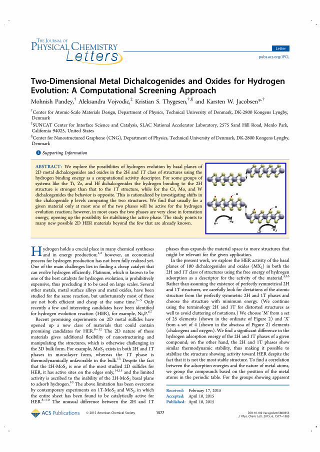
Two-Dimensional Metal Dichalcogenides and Oxides for HydrogenEvolution: A Computational Screening ApproachMohnish Pandey,† Aleksandra Vojvodic,‡ Kristian S. Thygesen,†,§ and Karsten W. Jacobsen*,†

†Center for Atomic-Scale Materials Design, Department of Physics, Technical University of Denmark, DK-2800 Kongens Lyngby,Denmark‡SUNCAT Center for Interface Science and Catalysis, SLAC National Accelerator Laboratory, 2575 Sand Hill Road, Menlo Park,California 94025, United States§Center for Nanostructured Graphene (CNG), Department of Physics, Technical University of Denmark, DK-2800 Kongens Lyngby,Denmark

*S Supporting Information

ABSTRACT: We explore the possibilities of hydrogen evolution by basal planes of2D metal dichalcogenides and oxides in the 2H and 1T class of structures using thehydrogen binding energy as a computational activity descriptor. For some groups ofsystems like the Ti, Zr, and Hf dichalcogenides the hydrogen bonding to the 2Hstructure is stronger than that to the 1T structure, while for the Cr, Mo, and Wdichalcogenides the behavior is opposite. This is rationalized by investigating shifts inthe chalcogenide p levels comparing the two structures. We find that usually for agiven material only at most one of the two phases will be active for the hydrogenevolution reaction; however, in most cases the two phases are very close in formationenergy, opening up the possibility for stabilizing the active phase. The study points tomany new possible 2D HER materials beyond the few that are already known.

Hydrogen holds a crucial place in many chemical synthesesand in energy production;1,2 however, an economical

process for hydrogen production has not been fully realized yet.One of the main challenges lies in finding a cheap catalyst thatcan evolve hydrogen efficiently. Platinum, which is known to beone of the best catalysts for hydrogen evolution, is prohibitivelyexpensive, thus precluding it to be used on large scales. Severalother metals, metal surface alloys and metal oxides, have beenstudied for the same reaction, but unfortunately most of theseare not both efficient and cheap at the same time.3−5 Onlyrecently a few and interesting candidates have been identifiedfor hydrogen evolution reaction (HER), for example, Ni2P.

6,7

Recent promising experiments on 2D metal sulfides haveopened up a new class of materials that could containpromising candidates for HER.8−12 The 2D nature of thesematerials gives additional flexibility of nanostructuring andmanipulating the structures, which is otherwise challenging inthe 3D bulk form. For example, MoS2 exists in both 2H and 1Tphases in monolayer form, whereas the 1T phase isthermodynamically unfavorable in the bulk.13 Despite the factthat the 2H-MoS2 is one of the most studied 2D sulfides forHER, it has active sites on the edges only,14,15 and the limitedactivity is ascribed to the inability of the 2H-MoS2 basal planeto adsorb hydrogen.10 The above limitation has been overcomeby contemporary experiments on 1T-MoS2 and WS2, in whichthe entire sheet has been found to be catalytically active forHER.8−10 The unusual difference between the 2H and 1T

phases thus expands the material space to more structures thatmight be relevant for the given application.In the present work, we explore the HER activity of the basal

planes of 100 dichalcogenides and oxides (MX2) in both the2H and 1T class of structures using the free energy of hydrogenadsorption as a descriptor for the activity of the material.3,16

Rather than assuming the existence of perfectly symmetrical 2Hand 1T structures, we carefully look for deviations of the atomicstructure from the perfectly symmetric 2H and 1T phases andchoose the structure with minimum energy. (We continueusing the terminology 2H and 1T for distorted structures aswell to avoid cluttering of notations.) We choose ‘M’ from a setof 25 elements (shown in the ordinate of Figure 2) and ‘X’from a set of 4 (shown in the abscissa of Figure 2) elements(chalcogens and oxygen). We find a significant difference in thehydrogen adsorption energy of the 2H and 1T phases of a givencompound; on the other hand, the 2H and 1T phases showsimilar thermodynamic stability, thus making it possible tostabilize the structure showing activity toward HER despite thefact that it is not the most stable structure. To find a correlationbetween the adsorption energies and the nature of metal atoms,we group the compounds based on the position of the metalatoms in the periodic table. For the groups showing apparent

Received: February 17, 2015Accepted: April 10, 2015Published: April 10, 2015

Letter

pubs.acs.org/JPCL

© 2015 American Chemical Society 1577 DOI: 10.1021/acs.jpclett.5b00353J. Phys. Chem. Lett. 2015, 6, 1577−1585

difference of the 2H and 1T phases for hydrogen adsorption,we show that the relative position of the p level of ‘X’ withrespect to the Fermi level plays a decisive role for hydrogenadsorption. On the basis of the descriptor employed to screenthe materials for HER, we point to many new possible 2D HERmaterials beyond the few that are already known.In the present work, we use GPAW,17 an electronic structure

code based on the projector-augmented wave (PAW)18

formalism. The PBE19 functional is used for the calculationof lattice constants, and the calculated lattice constants havebeen used throughout the work. Structures showing distortionshave been reoptimized, and the recalculated lattice constantsare used. We calculate the heat of formation using the fittedelemental reference phase energies (FERE) scheme employedover the PBE calculated energies, as proposed by Stevanovic etal.20 A grid spacing of 0.18 Å is used to expand the wavefunctions in real space, and a Fermi−Dirac smearing of 0.05 eVis employed to accelerate the convergence. The Brillouin zonefor the smallest unit cell (1 × 1) is sampled using aMonkhorst−Pack21 scheme with a k-point mesh of 18 × 18× 1, and for 2 × 2 unit cells, we use a 9 × 9 × 1 k-point grid. Alloptimizations are carried out using a Quasi-Newton algorithm,and the forces are converged down to 0.05 eV/Å for allrelaxations. Spin-polarized calculations are performed for thecalculation of lattice constants as well as for the adsorptionenergies. Adsorption energies are calculated using the BEEF-vdW functional.22 Uncertainties in adsorption energies areexplicitly calculated using the ensemble of functionals proposedin ref 22. The calculated uncertainties are used to estimate theprobability that a given material will have the free-energydescriptor for HER lying within a given range. The calculatedprobabilities help to rank the different materials based on theirsuitability23 for HER. We add several corrections to thecalculated total energy differences to estimate the adsorption

free energy. The zero point energy corrections to the energiesof all systems are to a first order approximation taken to be thesame as the ones calculated for the 1T-MoS2 monolayerstructure. We get the zero-point correction of the adsorbedhydrogen as 0.39 eV at the standard state. We ignore theentropic corrections for the adsorbed state while calculating thetotal correction as in ref 15. The zero-point energy of the H2molecule has been taken from the ref 24 and is found to be 0.54eV. The entropic correction of 0.40 eV from the gas-phase H2 istaken from ref 25. By taking the difference of the corrections inthe gas phase and the adsorbed state, ΔZPE comes out as 0.12eV and −TΔS comes out as 0.20 eV; therefore, ΔZPE − TΔScomes out to be 0.32 eV.The current work focuses on the 2H and 1T structures and

their distorted derivatives of 2D metal dichalcogenides andoxides some of which have been realized in recent experi-ments.10−12 The structural difference between the 1T and 2Hphases originates from the difference in coordination environ-ment around the metal atom. The 2H phase of MX2 has atrigonal prismatic structure with ‘M’ at the center of the prismand ‘X’ at the vertices, where the 1T phase has an octahedralcoordinated structure with ‘M’ at the center of the octahedronand ‘X’ at the vertices. Figure 1a,f shows the top view of the 2Hand 1T structure, respectively. Figure 1b−e,g representsdistorted derivatives of the 2H and 1T structures, which willbe discussed later. The significant difference in atomic structureof the two phases might lead to differences in theirthermodynamic and electronic properties. The difference inthermodynamic properties will directly influence the relativestability of the two phases, whereas different electronicproperties will have an effect on the chemical reactivity. Todetect the distortions, if any, in the 2H and 1T structures, wefollow the steps: (1) Adsorb the hydrogen in the 2 × 2 unit cellto break the symmetry of the structure and allow the structure

Figure 1. (a) Top view of a 1T monolayer (P32/m1 space group). (b) Monolayer with distortions belonging to the 1T class and P1 spacegroup withunit cell size 2 × 2. (c) Monolayer with distortions belonging to the 1T class and P1 spacegroup with unit cell size 2 × 2. (d) Monolayer withdistortions belonging to the 1T class and P1 spacegroup with unit cell size 2 × 1. (e) Monolayer with distortions belonging to the 1T class and P3m1spacegroup with unit cell size 2 × 2. (f) Top-view of a 2H monolayer (P6 m2 space group). (g) Monolayer with distortions belonging to the 2H classand P1 spacegroup with unicell size 2 × 2. Unit cells have been drawn (black solid lines) to show the size of the unit cell, and a few selected bonds(black broken lines) between metal atoms have been shown to highlight the difference between different structures.

The Journal of Physical Chemistry Letters Letter

DOI: 10.1021/acs.jpclett.5b00353J. Phys. Chem. Lett. 2015, 6, 1577−1585

1578

to relax. (2) Remove the hydrogen from the structure obtainedfrom step 1 and relax the structure. (3) If the structure obtainedafter step 2 is the same as the perfectly symmetric structure,then there are no distortions present or else the structure isdistorted. (4) Cases may exist in which step 2 leads to localminima in new structures; therefore, one has to compare theenergy obtained after step 2 and the energy of the perfectlysymmetric structure and choose the one with lower energy.Following the steps previously outlined, the distortions

present under HER conditions can most likely be obtained.Similar distortions in MoS2 have been explored by Kan et al.,26

but we see a wider range of distortions. Therefore, instead ofusing their terminology, we categorize the distortions in a moregeneral way based on the space group and the size of the unitcell.Figure 2a,b shows the calculated standard heats of formation

of the 2D MX2 compounds in the 2H and 1T phases. In

calculating the standard heat of formation, we neglect any zero-point or entropic correction. As can be seen from the Figurethe region of stable compounds is very similar in the twostructures. With very few exceptions, the compound that isstable (unstable) in one structure exhibits stability (instability)in the other structure as well. Figure 2c shows the difference inenthalpies of the different compounds by which we canestimate the extent to which the two phases differthermodynamically. The obtained trend in the relative stabilityof the 2H and 1T phases agrees well with the calculations ofAtaca et al.27 We see that for most of the compounds theenergy difference between the 2H and the 1T phase is smallerthan ∼0.4 eV/atom. Recent experiments on MoS2

10 and WS28

show that the distorted 1T phase despite being energeticallyhigher than the 2H phase by ∼0.3 eV/atom can be stabilized.These experiments thus suggest that the metastable phase of a

2D MX2 compound with a positive heat of formation as high as∼0.3 eV/atom relative to the stable phase can be synthesizedand stabilized under normal conditions using suitable syntheticroutes.28 Thus, the generally small energy differences shown inFigure 2c indicate that the atomic structure of 2D MX2 can betuned, if required, for the application in hand. Therefore, weexplore both the 2H and 1T class of structures of MX2 to findsuitable materials for HER.Figure 3a,b shows the energy of distorted structures with

respect to perfectly symmetric 2H and 1T structures,

respectively. The white squares denote massive reconstructionupon relaxation, thus leading to structures neither belonging tothe 2H or 1T class of structures. We do not investigate thesesystems any further. Upon analyzing the nature of reconstruc-tions in the more moderately distorted structures, it turns outthat the distortions occurring in the 1T structure can becategorized in four different symmetry groups, whereas thedistortions in the 2H structure can be captured by only onegroup. Starting with the structures with slightly displaced atomsfrom their ideal positions in the perfect 2H and 1T structures,that is, without symmetries in a 2 × 2 unit cell, upon relaxation,some compounds in 1T structure gain symmetry in such a waythat all of the symmetry operations can be captured in a 2 × 1unit cell, thus leading to reduction in the size of unit cell. This isnot the case for any of the 2H structures. Therefore, wecategorize the distorted structures based on the space groupsand the unit cell size using the tool described in ref 29. Table 1shows the categorization of the distortions based on the spacegroup and the size of the reduced unit cell. The forces cannotbe brought down to exactly zero during the optimization

Figure 2. (a,b) Heatmap of standard heat of formation (in eV/atom)of compounds in undistorted 2H and 1T structures, respectively. (c)Difference in enthalpies between the 2H and 1T structures (in eV/atom) of different compounds. Each compound is represented by asquare, and the constituent elements are represented by thecorresponding ordinate and abscissa of the square. The difference inenergies is in eV/atom.

Figure 3. (a,b) Energy of the distorted structures (eV/atom) withrespect to the perfectly symmetrical 2H and 1T structures,respectively. The white squares denote massive reconstruction uponrelaxation, thus leading to structures not belonging to the 2H and 1Tclass of structures.

The Journal of Physical Chemistry Letters Letter

DOI: 10.1021/acs.jpclett.5b00353J. Phys. Chem. Lett. 2015, 6, 1577−1585

1579

process; therefore, to overcome inaccuracies in the forces, weemploy a cutoff of 0.05 Å on the rotations/translations toidentify the symmetry operations. For six structures where thedifference in energy of the distorted structure and the perfectlysymmetrical structure is <0.01 eV per atom, we categorize theminto the symmetrical structure for the previously mentionedreason. We find that for all of the distorted structures in the 2Hclass, the type of distortion is similar to the one shown inFigure 1g. Therefore, we categorize them in the same class asthose that have the unit cell size of 2 × 2 and the space groupP1. Figure 1b−e shows the four different types of distortionsobserved in the 1T structure. There are subtle differences in allof these four groups. Panel b does not have any symmetry andthus belongs to the P1 group, panel c shows the distortionssimilar to panel b but has an inversion symmetry and thusbelongs to P1 as also observed by Tongay et al. for ReS2.

30 Thedistortions in panel d are such that the structure forms stripeswith periodicity of one unit cell, resulting in a unit cell size of 2× 1. Panel e has the least distortion and inherits most of thesymmetry operations from the symmetric 1T structure andbelongs to the P3m1 space group.Additionally, as previously mentioned, discarding distorted

phases that differ in energy from the perfectly symmetricstructures by <0.01 eV per atom might result in missing someof the charge density wave (CDW) phases, for example, inTiS2.

31,32 In the case of TiS2 we found that for a 12 atom unitcell (2 × 2 unit cell) the distorted and the perfectly symmetricstructure differ by only ∼0.04 eV (∼0.004 eV per atom). Itturns out that due to similar energy differences the CDWphases of other compounds, for example, TaS2, are all discardeddue to the previously mentioned reason. Discarding the CDWphases does not affect our results for the HER, which isdependent only on the energy differences, which are very smallin the previously mentioned cases.In previous works the strength of hydrogen binding on a

catalyst surface has been used as a descriptor for the ability to

Table 1. Categorization of Different Compounds Based onthe Deviation of Their Structures from Perfect 2H or 1TStructures and the Size of the Unit Cella

class MX2 group unit cell class MX2 group unit cell

2H CoS2 P1 2 × 2 2H CoSe2 P1 2 × 22H IrS2 P1 2 × 2 2H OsS2 P1 2 × 22H OsSe2 P1 2 × 2 2H PdS2 P1 2 × 22H PdSe2 P1 2 × 2 2H PdTe2 P1 2 × 22H ReO2 P1 2 × 2 2H ReS2 P1 2 × 22H ReSe2 P1 2 × 2 2H RhS2 P1 2 × 22H RhSe2 P1 2 × 2 2H RhTe2 P1 2 × 22H RuO2 P1 2 × 2 2H RuS2 P1 2 × 22H RuSe2 P1 2 × 2 2H ScS2 P1 2 × 22H ScSe2 P1 2 × 21T CoS2 P1 2 × 2 1T CrS2 P1 2 × 21T CrSe2 P1 2 × 2 1T FeS2 P1 2 × 21T IrS2 P1 2 × 2 1T IrSe2 P1 2 × 21T ReO2 P1 2 × 2 1T ReTe2 P1 2 × 21T RhS2 P1 2 × 2 1T RuS2 P1 2 × 21T RuTe2 P1 2 × 2 1T MoO2 P1 2 × 11T MoS2 P1 2 × 1 1T MoSe2 P1 2 × 11T MoTe2 P1 2 × 1 1T OsS2 P1 2 × 11T OsSe2 P1 2 × 1 1T OsTe2 P1 2 × 11T WS2 P1 2 × 1 1T WSe2 P1 2 × 11T WTe2 P1 2 × 1 1T ReS2 P1 2 × 21T ReSe2 P1 2 × 2 1T RuSe2 P1 2 × 21T TaO2 P1 2 × 2 1T CoSe2 P3m1 2 × 21T IrTe2 P3m1 2 × 2 1T NbO2 P3m1 2 × 21T OsO2 P3m1 2 × 2 1T RhSe2 P3m1 2 × 21T RuO2 P3m1 2 × 2 1T WO2 P3m1 2 × 2

aThe class represents the type of undistorted structure to which thecompound belongs, the group represents the space group of thedistorted structure as per Herman−Maugin notation, and the unit cellrepresents the size of the reduced unit cell with respect to the 1 × 1unit cell of the perfect 2H or 1T structures.

Figure 4. Adsorption energies of the individual groups of compounds. The grouping of the compounds is based on the position of the metal atom ofMX2 in the periodic table. The missing data points in the plots show the instability of those compounds toward hydrogen adsorption; that is, in thesecases hydrogen pulls out the ‘X’ atom from the monolayer and moves far from the surface. All energies shown in the ordinates are in electronvolts.

The Journal of Physical Chemistry Letters Letter

DOI: 10.1021/acs.jpclett.5b00353J. Phys. Chem. Lett. 2015, 6, 1577−1585

1580

evolve hydrogen, and it has been found that the optimum valueof the free energy of hydrogen adsorption (ΔGH) on thesurface of the material should be close to zero.3,8,16 The freeenergy of hydrogen adsorption comes out as a descriptor basedon the Volmer−Heyrovsky route for the HER. The stepsinvolved in the Volmer−Heyrovsky process can be writtenas33,34

+ + * → *+ −H e H (1)

* → + *2H H 22 (2)

where * denotes the active site. At zero potential the free-energy difference between H+ + e− and H2 is (by definition)zero, and the intermediate state of adsorbed hydrogen providesan effective barrier for the process, which should be as close tozero as possible. Therefore, to determine the reactivity of thebasal plane, we first calculate the hydrogen adsorption energyon different sites. The adsorption energy is calculated relative tothe hydrogen molecule and the most stable clean substratewithin the given class (1T or 2H). In all of the 1T and 2Hclasses of the MX2 structures, we find that the most favorablehydrogen adsorption site on the basal plane is on top of thechalcogen/oxygen atoms. For distorted structures, dependingon the symmetry, H will bind differently to the differentchalcogen/oxygen atoms. For further analysis we select theadsorption site with the strongest binding. We start with one-fourth (0.25 ML) of a monolayer of coverage (one hydrogenper four chalcogen/metal atom) and select only thecompounds binding hydrogen too strongly (ΔHH

ads ≥ −0.8)for higher coverages. Calculations for higher H adsorptioncoverages reveal massive reconstructions, and the finalstructures do not belong to any of the structure in the 2Hand 1T class; therefore, we choose not to explore the cases ofhigher coverage any further and focus only on one-fourth of amonolayer of coverage in the current work. To establish thetrends in the strength of hydrogen binding, we use the heat ofadsorption (total energy differences) and incorporate zero-point energies and entropic effects only in the stage ofevaluating the suitability of materials for HER.Figure 4 shows the calculated heats of hydrogen adsorption

(ΔHadsH ) on the 2H and 1T basal planes with 0.25 ML coverage

of hydrogen. Upon hydrogen adsorption, not all of the surfacesare stable; therefore, we discard the compounds (missing datapoints) in the plots that are unstable toward hydrogenadsorption, that is, in these cases hydrogen pulls out the ‘X’atom from the monolayer and moves far from the surface or thestructure massively reconstructs and transforms to a structurenot belonging to the 2H or 1T class. As can be seen, the heat ofadsorption varies widely by several electronvolts. An overalltrend is that the bonding strength is increased as theelectronegativity of the chalcogenide is increased. There isclearly no simple relation between the hydrogen bonding to the2H and 1T structures. Depending on the metal andchalcogenide in question the bonding to the 1T class may bestronger or weaker than the bonding to the 2H class.To shed some light on the chemistry behind the different

adsorption energies, we shall focus on only two of the metalgroups that stand out in Figure 4. For the metals Ti, Zr, and Hfthe bonding to the 2H structure is clearly stronger than that forthe 1T, while for the metals Cr, Mo, and W we have anopposite trend. To understand these opposite behaviors weanalyze the density of states (DOS) projected onto the ‘X’ porbital in MX2.

16 Figure 5a−d shows the DOS of pristine

monolayers. The calculated position of the p-band center (ϵp)(obtained as the first moment of the projected density ofstates) with respect to the Fermi level of the pristinemonolayers explains the difference in reactivity of the twogroups. A higher-lying p level indicates possible stronger effectsof hybridization with the hydrogen s state.16 The calculated ϵpfor MoS2 in the 1T structure lies closer to the Fermi level ascompared with the 2H structure, whereas for TiS2, the ϵp forthe 2H structure lies closer to the Fermi level as compared withthe 1T structure. Table 2 shows the adsorption energy (ΔHads

H )and center of p band for compounds selected from the groupsto which MoS2 and TiS2 belong. As can be seen from the Table,other compounds also show the same correlation between ϵpand ΔHads

H . These results show that the nature of the metalatom35 along with the symmetry of the structure has asignificant effect on the reactivity.We calculate for 0.25 ML coverage the heats of adsorption

(ΔHadsH ) including error bars (σ) with the BEEF-vdW functional

to assess the confidence interval of heats of adsorption.22 Asmentioned earlier, we add zero point and entropic correctionsof 0.32 eV in all the heats of adsorption to get the free energy ofadsorption. Here we assume that the corrections will not vary

Figure 5. (a) Density of states (DOS) plot of MoS2 and TiS2 in the2H and 1T structures. MoS2 and TiS2 belong to two different groupsas shown in Figure 4). ϵp denotes the position of the center of the pband with respect to the Fermi level. The shaded region correspondsto occupied states.

The Journal of Physical Chemistry Letters Letter

DOI: 10.1021/acs.jpclett.5b00353J. Phys. Chem. Lett. 2015, 6, 1577−1585

1581

much for different compounds, hence we choose the samecorrection as we have calculated for 1T-MoS2 monolayerstructure. Since the optimum value of free energy (ΔGopt) forHER is ∼0.0 eV, we consider the range of free energy from−0.5 to 0.5 eV to take into account the effect of coverage,strain, and so on.8,36 Having an allowable range of free energy,mean adsorption energies along with uncertainties allows us tocalculate the probability (P(|ΔG| ≤ 0.5)) of a material havingfree energy for HER in the given interval. Assuming a Gaussiandistribution of uncertainties around the mean value, E, of theadsorption, probabilities can be calculated as

∫πσ σ

|Δ | ≤ = −− −

+ ⎛⎝⎜

⎞⎠⎟P G

EE( 0.5)

1

2exp

2d

E

E

2 0.5

0.5 2

2(3)

The calculated probabilities will help in narrowing down thematerial space for potential experimental investigation bydiscarding the materials with very small probabilities. In Figure6, we show the compounds in the 2H and 1T class of structuresranked according to the calculated probability measure. TheFigure includes compounds with a probability as low as 0.15.This leads to 21 compounds in the 2H class of structures and26 compounds in the 1T class of structures. For eachcompound, the calculated free energy is shown together withthe error bar from the BEEF−vdW ensemble. We see that

MoS2 and WS2 appear on the list of candidates for the 1Tstructure (although not with the highest probability) in supportof the recent experiments indicating possible hydrogenevolution for these systems.8,10 The only compounds thatappear on both the 2H and 1T lists are NbS2, RhS2, RuS2, IrS2,CoS2, ScSe2, RuO2, and TaTe2, illustrating the fact that thechemical activity is very sensitive to the crystal structure.Having identified possible 2D materials with promising

binding properties for hydrogen, it is appropriate to investigatethe stability of these materials further. There are twopossibilities that may hamper the growth and stability of the2H or 1T phases of the 2D materials found to be active forHER: (1) much higher stability of the competing bulkstructures or the standard states, thus leading to thedissociation of the 2D phase into these compounds, and (2)relative stability of the 2H and 1T phases also matters. Forexample, if the 2H phase of a material is HER-active but ismuch higher in energy than the 1T structure, it is unlikely thatthe material can be synthesized and stabilized in the 2Hstructure. Therefore, the HER-active 2D materials must not lieabove a certain degree of metastability with respect to thecompeting bulk structures or the standard states, and also itshould not be energetically too high with respect to the other2D phase of the material. In the present work, we do notexplore the stability of compounds in water because a recentstudy has shown that with stabilizing agents compounds can bestabilized in water, making this criterion less important.37 Thepresence of water might also have an effect on the adsorptionenergies, but in the current work having a fairly wide window ofthe free energy of adsorption for the candidate materials, weexpect to have allowed for the effect of water.Calculated data to address the previously described issues are

collected in Table 3a,b. The second column of the Table showsthe calculated standard heats of formation, ΔH, for themonolayers (as shown for all the compounds in Figure 2) inthe 2H and 1T classes of structure, respectively. The thirdcolumn ΔHhull is calculated using structural information fromthe OQMD database.38 The OQMD database containsstandard DFT energy calculations for a large selection ofknown compounds from the ICSD database39 plus a number ofstandard structures. In the case of binary systems, this results in

Table 2. Heat of Adsorption of Hydrogen, ΔHadsH , and the

Center of the p Band, ϵp, for Compounds Belonging toDifferent Groups in the 2H and 1T Structuresa

2H ϵp ΔHadsH 1T ϵp ΔHads

H

MoS2 −2.00 1.68 ± 0.07 MoS2 −1.23 0.10 ± 0.13MoSe2 −1.74 1.82 ± 0.13 MoSe2 −1.46 0.64 ± 0.11WS2 −2.32 1.95 ± 0.08 WS2 −1.37 0.23 ± 0.14WSe2 −2.03 2.03 ± 0.14 WSe2 −1.29 0.78 ± 0.15TiS2 −1.02 −0.05 ± 0.13 TiS2 −1.45 0.40 ± 0.09TiSe2 −0.89 0.44 ± 0.12 TiSe2 −1.38 0.90 ± 0.10ZrS2 −0.96 0.11 ± 0.10 ZrS2 −1.42 0.94 ± 0.07ZrSe2 −0.80 0.51 ± 0.10 ZrSe2 −1.34 1.19 ± 0.09

aGrouping of the compounds is performed based on the group of theperiodic table to which the metal atom in MX2 belongs.

Figure 6. (a) 2H compounds having a free energy of hydrogen adsorption (ΔGadsH ) in the range of (−0.5, 0.5) eV along with uncertainties for 0.25

ML coverage and probabilities (P(|ΔG| ≤ 0.5)) as calculated from eq 3. Red error bars indicate that the structure is unstable with respect to thestandard states.

The Journal of Physical Chemistry Letters Letter

DOI: 10.1021/acs.jpclett.5b00353J. Phys. Chem. Lett. 2015, 6, 1577−1585

1582

Table 3. (a) Relevant Energies for Analysis of the Stabilities of the Obtained HER Candidates in the 2H-Derived Structuresa

and (b) Similar Table for the 1T Candidatesb

(a)

2H-MX2 ΔH ΔHhull ΔHhull ΔHexpt. ref 40 ΔH2H/1T P(|ΔG| ≤ 0.5)

RuS2 −0.31 −0.70 0.39 −0.71 no −0.01 1.00NiSe2 −0.21 −0.34 0.13 −0.38 no 0.17 1.00OsS2 0.34 −0.60 0.94 NA no −0.01 1.00TaO2 −2.58 −3.00 0.42 NA no −0.07 1.00ReO2 −0.91 −1.42 0.51 −1.52 no 0.05 1.00RhS2 −0.11 −0.48 0.37 NA no 0.07 1.00PdS2 0.01 −0.31 0.32 −0.28 yes 0.17 1.00NbS2 −1.21 −1.20 −0.01 NA yes −0.04 0.98ScS2 −1.46 −1.46 0.00 NA no −0.06 0.96TiS2 −1.23 −1.37 0.14 −1.41 yes 0.15 0.96TaTe2 −0.32 −0.45 0.13 NA yes 0.00 0.89CoS2 −0.33 −0.48 0.15 −0.51 no 0.01 0.86IrS2 −0.11 −0.48 0.37 −0.46 no 0.22 0.84RhSe2 −0.17 −0.45 0.28 NA no 0.07 0.81TaS2 −1.24 −1.22 −0.02 −1.22 yes −0.02 0.78ZrS2 −1.55 −1.73 0.18 −1.99 yes 0.19 0.77ScO2 −2.74 −3.17* 0.43 NA no 0.05 0.49VS2 −1.16 −1.14 −0.02 NA no −0.02 0.46ScSe2 −1.30 −1.25* −0.05 NA no −0.01 0.43CrO2 −1.99 −2.15 0.16 −2.01 no 0.03 0.37PdSe2 −0.02 −0.33 0.31 NA yes 0.22 0.37

(b)

1T-MX2 ΔH ΔHhull ΔHhull ΔHexpt. ref 40 ΔH1T/2H P(|ΔG| ≤ 0.5)

ScSe2 −1.34 −1.25* −0.09 NA no 0.01 1.00MoO2 −1.79 −1.95 0.16 −2.04 no 0.31 1.00RhS2 −0.32 −0.48 0.16 NA no −0.07 1.00IrS2 −0.30 −0.48 0.18 −0.46 no −0.22 0.99PbSe2 0.04 −0.31* 0.35 NA no −0.22 0.99PbS2 0.03 −0.32* 0.35 NA no −0.28 0.98PdO2 −0.48 −0.41 −0.07 NA no NA 0.97WO2 −1.61 −1.89 0.28 NA no 0.24 0.94CoS2 −0.34 −0.48 0.14 −0.51 no −0.01 0.94RuO2 −0.71 −0.94 0.23 −1.05 no −0.20 0.92IrO2 −0.70 −0.94 0.24 −0.86 no NA 0.92MnO2 −2.00 −1.98 −0.02 −1.80 no −0.43 0.87NiO2 −1.01 −0.79* −0.22 NA no NA 0.83CrS2 −0.77 −0.71 −0.06 NA yes 0.12 0.83MoS2 −0.66 −0.93 0.27 −0.95 yes 0.28 0.74OsO2 −0.23 −1.10 0.87 −1.02 no NA 0.65VO2 −2.47 −2.63 0.16 −2.48 no −0.10 0.43TiO2 −3.10 −3.29 0.19 −3.26 no −1.11 0.43GeSe2 −0.27 −0.34 0.07 −0.39 no NA 0.38PtO2 −0.61 −0.62 0.01 NA no NA 0.36WS2 −0.59 −0.78 0.19 −0.90 yes 0.18 0.35VTe2 −0.40 −0.45 0.05 NA yes 0.00 0.27TaTe2 −0.32 −0.45 0.13 NA yes 0.00 0.24FeSe2 −0.48 −0.56 0.08 NA no −0.05 0.23NbS2 −1.18 −1.20 0.02 NA yes 0.04 0.22FeTe2 −0.11 −0.20 0.09 −0.25 no −0.02 0.16

aΔH denotes the calculated standard heat of formation. ΔHhull denotes the heat of formation of the most stable compound (i.e., at the convex hull)in the OQMD database.38 The symbol * in superscript corresponds to the situation, where no bulk structure with the compound composition lies onthe convex hull according to the database. In that case, ΔHhull is calculated as a linear combination of several structures. ΔHhull denotes the differencebetween the two previous columns; that is, it shows how much the 2D compound lies above or below the convex hull. ΔHexpt. indicates theexperimental standard heats of formation as listed in the OQMD database. Lebegue al.40 have analyzed the possibilities for forming 2D compoundsbased on the layered character of the bulk structures and their result is also listed in the Table. ΔH2H/1T is the difference between the energies in thetwo (possibly distorted) 2H and 1T structures. Finally, P(|ΔG| ≤ 0.5) is the probability that the free energy of hydrogen adsorption lies within 0.5 eVfrom zero, as described in Figure 6. All the energies are in eV/atom. bNA in the seventh column indicates that due to massive reconstructions thecompound is discarded from the 2H class. All energies are in eV/atom.

The Journal of Physical Chemistry Letters Letter

DOI: 10.1021/acs.jpclett.5b00353J. Phys. Chem. Lett. 2015, 6, 1577−1585

1583

calculations of the most stable structures as a function ofrelative concentration of the two constituents identifying theso-called convex hull of lowest energy structures. For a givenMX2 compound, we extract the structure with the lowestenergy at this 1:2 composition of the M-X phase diagram fromthe database. In most cases a compound with the 1:2composition exists as the most stable one. If that is not thecase we extract the two structures that linearly combine to givethe lowest energy of the convex energy hull at the 1:2composition. We note that all structures are reoptimized andenergies are calculated with the approach we use here. Thefourth column, ΔHhull, shows our calculated heat of formationwith respect to the convex hull. If two structures are used toobtain the energy of the hull, ΔHhull, then it is indicated with anasterisk on the number. For comparison, the experimental heatsof formation for the most stable compounds are shown in thethird column when available in the OQMD database. As can beseen, the calculated heats of formation are in good agreementwith the experimental data with a RMS deviation of only 0.09eV. The fourth column shows the difference between columns1 and 2, that is, how much the energy of the 2D material isabove (or below) the energy at the convex hull. The seventhcolumn in Table 3 shows the heat of formation of the 2H (1T)class of structure with respect to the 1T (2H) class of structuresΔH2H/1T (ΔH1T/2H). We find that the energy differencebetween the catalytically active candidate and its analogue inthe other structure is usually not very large. As previouslymentioned HER-active materials like MoS2 and WS2 in the 1Tphase have a degree of metastability as high as 0.3 eV/atomwith respect to the 2H phase and lie above the hull by ∼0.3 eV/atom; nevertheless, they have been synthesized and stabilizedunder ambient conditions.10 Surprisingly, none of the otherHER-active materials differ from their corresponding 2Danalogue in energy by >0.3 eV/atom. Therefore, in the list ofproposed HER materials, if the material can be synthesized andstabilized in one of the two phases, then it is highly likely that itcan be synthesized and stabilized in the other phase as well.Some of the compounds like PdS2 and PdTe2, which have

been found to be HER-active in the current work, have alsobeen suggested to exist in monolayer form by Lebegue al.40 Ascan be seen from Table 3a,b, PdS2 and PdTe2 lie above the hullby ∼0.35 eV. Therefore, we choose a threshold of 0.4 eV forΔHhull for stability of compounds. The given criteria narrowsthe list of the candidates, specifically OsS2, ReO2, OsSe2, ScO2,and RuO2 in the 2H class of candidates and OsO2 in the 1Tclass of candidates do not fulfill this criteria. The names of thesecompounds are italicized in Table 3a,b. A few monolayers inTable 3a,b have lower energy than the energy of the convexhull. One of the reasons for this behavior might be the existenceof other more stable bulk structures than the ones consideredin the OQMD database, for example, structures obtained bystacking the 2D layers.Additionally, we also compare our findings of 2D materials

for HER with the recent study by Lebegue et al.40 that is basedon predicting the existence of 2D materials from experimentalbulk structures. The exiguous overlap between our results andthe ones by Lebegue al. arises from the fact that ourconclusions are based on thermodynamic arguments obtainedwith ab initio calculations, whereas the work of Lebegue al.relies more on heuristic arguments of the ability of cleaving abulk along a direction of weak bonding. The compounds of theMX2 class proposed in their work are all present in our work,thus supporting our approach. A few compounds in Table 3a,b

are written in bold. We select them based on the work byLebegue et al.40 by looking for “yes” in the column VI in Table3a,b because it is highly likely that they can be synthesized andstabilized with minimal effort.In the current study, we suggest several 2D materials in the

2H and 1T structures as potential candidates for the hydrogenevolution reaction. The activity of the basal plane in all of thediscovered candidates will provide a much larger number ofactive sites as compared with 2D materials like 2H MoS2, whereonly edges are active. Our analysis is using the calculatedadsorption free energy as a well-established descriptor forhydrogen evolution. We furthermore investigate the stability ofthe compounds in some detail by comparing heats of formationof both competing layered phases and bulk structures. Recentexperimental stabilization of different layered phases seem toindicate that fairly large metastability of several tenths of an eV/atom can be overcome by appropriate synthesis routes, makingit likely that many of the suggested compounds could beexperimentally synthesized. It has recently been demonstratedthat the MoS2 and WS2 in the 1T phase can evolve hydrogen,and these systems also appear in our screening, but otheridentified systems should according to the calculations providehigher activity. The calculations therefore invite furtherinvestigation of some of the best candidates suggested here.

ASSOCIATED CONTENT*S Supporting InformationLattice constants and adsorption energy of hydrogen areprovided in the tables. This material is available free of chargevia the Internet at http://pubs.acs.org.

AUTHOR INFORMATIONCorresponding Author*E-mail: kwj@fysik.dtu.dk.NotesThe authors declare no competing financial interest.

ACKNOWLEDGMENTSWe acknowledge CASE (Catalysis for Sustainable Energy)initiative of the Danish Ministry of Science for funding theproject. The Center for Nanostructured Graphene is sponsoredby the Danish National Research Foundation, ProjectDNRF58. We thank Jens K. Nørskov and Charlie Tsai fromSUNCAT (Stanford University) for helpful discussions.

REFERENCES(1) Dressselhaus, M. S.; Thomas, I. L. Alternative EnergyTechnologies. Nature 2001, 414, 332−337.(2) Crabtree, G. W.; Dresselhaus, M. S.; Buchanan, M. V. TheHydrogen Economy. Phys. Today 2004, 57, 39−44.(3) Greeley, J.; Jaramillo, T. F.; Bonde, J. L.; Chorkendorff, I.;Nørskov, J. K. Computational High-Throughput Screening ofElectrocatalytic Materials for Hydrogen Evolution. Nat. Mater. 2006,5, 909−913.(4) Okamoto, Y.; Ida, S.; Hyodo, J.; Hagiwara, H.; Ishihara, T. J.Synthesis and Photocatalytic Activity of Rhodium-doped CalciumNiobate Nanosheets for Hydrogen Production from a Water/Methanol System without Cocatalyst Loading. J. Am. Chem. Soc.2011, 133, 18034−18037.(5) Cobo, S.; Heidkamp, J.; Jacques, P.-A.; Fize, J.; Fourmond, V.;Guetaz, L.; Jousselme, B.; Ivanova, V.; Dau, H.; Palacin, S.; et al. AJanus Cobalt-Based Catalytic Material for Electro-Splitting of Water.Nat. Mater. 2012, 11, 802−807.

The Journal of Physical Chemistry Letters Letter

DOI: 10.1021/acs.jpclett.5b00353J. Phys. Chem. Lett. 2015, 6, 1577−1585

1584

(6) Liu, P.; Rodriguez, J. A. Catalysts for Hydrogen Evolution fromthe [NiFe] Hydrogenase to the Ni2P (001) Surface: The Importanceof Ensemble Effect. J. Am. Chem. Soc. 2005, 127, 14871−14878.(7) Popczun, E. J.; McKone, J. R.; Read, C. G.; Biacchi, A. J.;Wiltrout, A. M.; Lewis, N. S.; Schaak, R. E. Nanostructured NickelPhosphide as an Electrocatalyst for the Hydrogen Evolution Reaction.J. Am. Chem. Soc. 2013, 135, 9267−9270.(8) Voiry, D.; Yamaguchi, H.; Li, J.; Silva, R.; Alves, D. C. B.; Fujita,T.; Chen, M.; Asefa, T.; Shenoy, V. B.; Eda, G.; et al. EnhancedCatalytic Activity in Strained Chemically Exfoliated WS2 Nanosheetsfor Hydrogen Evolution. Nat. Mater. 2013, 12, 850−855.(9) Lukowski, M. A.; Daniel, A. S.; Meng, F.; Forticaux, A.; Li, L.; Jin,S. Enhanced Hydrogen Evolution Catalysis from ChemicallyExfoliated Metallic MoS2 Nanosheets. J. Am. Chem. Soc. 2013, 135,10274−10277.(10) Voiry, D.; Salehi, M.; Silva, R.; Fujita, T.; Chen, M.; Asefa, T.;Shenoy, V. B.; Eda, G.; Chhowalla, M. Conducting MoS2 Nanosheetsas Catalysts for Hydrogen Evolution Reaction. Nano Lett. 2013, 13,6222−6227.(11) Wang, H.; Lu, Z.; Kong, D.; Sun, J.; Hymel, T. M.; Cui, Y.Electrochemical Tuning of MoS2 Nanoparticles on Three-dimensionalSubstrate for Efficient Hydrogen Evolution. ACS Nano 2014, 8, 4940−4947.(12) Jaramillo, T. F.; Jørgensen, K. P.; Bonde, J.; Nielsen, J. H.;Horch, S.; Chorkendorff, I. Identification of Active Edge Sites forElectrochemical H2 Evolution from MoS2 Nanocatalysts. Science 2007,317, 100−102.(13) Enyashin, A. N.; Yadgarov, L.; Houben, L.; Popov, I.;Weidenbach, M.; Tenne, R.; Bar-Sadan, M.; Seifert, G. New Routefor Stabilization of 1T-WS2 and MoS2 Phases. J. Phys. Chem. C 2011,115, 24586−24591.(14) Bollinger, M. V.; Jacobsen, K. W.; Nørskov, J. K. Atomic andElectronic Structure of MoS2 Nanoparticles. Phys. Rev. B 2003, 67,085410.(15) Hinnemann, B.; Moses, P. G.; Bonde, J.; Jørgensen, K. P.;Nielsen, J. H.; Horsch, S.; Chorkendorff, I.; Nørskov, J. K. BiomemeticHydrogen Evolution: MoS2 Nanoparticles as Catalyst for HydrogenEvolution. J. Am. Chem. Soc. 2005, 127, 5308−5309.(16) Tsai, C.; A.-Pedersen, F.; Nørskov, J. K. Tuning the MoS2 Edge-Site Activity for Hydrogen Evolution via Support Interactions. NanoLett. 2014, 14, 1381−1387.(17) Enkovaara, J.; Rostgaard, C.; Mortensen, J. J.; Chen, J.; Dulak,M.; Ferrighi, L.; Gavnholt, J.; Glinsvad, C.; Haikola, V.; Hansen, H. A.;et al. Electronic Structure Calculations with GPAW: A real-spaceImplementation of the Projector Augmented-wave Method. J. Phys.:Condens. Matter 2010, 22, 253202.(18) Kresse, G.; Joubert, D. From Ultrasoft Pseudopotentials to theProjector Augmented-Wave Method. Phys. Rev. B 1999, 59, 1758−1775.(19) Perdew, J. P.; Burke, K.; Ernzerhof, M. Generalized GradientApproximation Made Simple. Phys. Rev. Lett. 1996, 77, 3865.(20) Stevanovic, V.; Lany, S.; Zhang, X.; Zunger, A. CorrectingDensity Functional Ttheory for Accurate Predictions of CompoundEnthalpies of Formation: Fitted Elemental-phase Reference Energies.Phys. Rev. B 2012, 85, 115104.(21) Monkhorst, H. J.; Pack, J. D. Special Points for Brillouin-zoneIntegrations. Phys. Rev. B 1976, 13, 12.(22) Wellendorff, J.; Lundgaard, K. T.; Møgelhøj, A.; Petzold, V.;Landis, D. D.; Nørskov, J. K.; Bligaard, T.; Jacobsen, K. W. DensityFunctionals for Surface Science: Exchange-correlation Model Develop-ment with Bayesian Error Estimation. Phys. Rev. B 2012, 85, 235149.(23) Medford, A. J.; Wellendorff, J.; Vojvodic, A.; Studt, F.; A.-Pedersen, F.; Jacobsen, K. W.; Bligaard, T.; Nørkov, J. K. Assessing theReliability of Calculated Catalytic Ammonia Synthesis Rates. Science2014, 345, 197.(24) Irikura, K. K. Experimental Vibrational Zero-Point Energies:Diatomic Molecules. J. Phys. Chem. Ref. Data 2007, 36, 389.

(25) Linstrom, P. J., Mallard, W. NIST Chemistry WebBook; NISTStandard Reference Database 69; National Institute of Standards andTechnology: Gaithersburg, MD, 1998.(26) Kan, M.; Wang, J. Y.; Li, X. W.; Zhang, S. H.; Li, Y. W.;Kawazoe, Y.; Sun, Q.; Jena, P. Structures and Phase Transition of aMoS2 Monolayer. J. Phys. Chem. C 2014, 118, 1515−1522.(27) Ataca, C.; ahin, H.; Ciraci, S. Stable, Single-Layer MX2Transition-Metal Oxides and Dichalcogenides in a Honeycomb-LikeStructure. J. Phys. Chem. C 2012, 116, 8983−8999.(28) Lin, Y.-C.; Dumcenco, D. O.; Huang, Y.-S.; Suenaga, K. AtomicMechanism of the Semiconducting-to-Metallic Phase Transition inSingle-Layered MoS2. Nat. Nanotechnol. 2014, 9, 391−396.(29) Stokes, H. T.; Hatch, D. M. FINDSYM: Program for Identifyingthe Space Group Symmetry of a Crystal. J. Appl. Crystallogr. 2005, 38,237−238.(30) Tongay, S.; Fan, W.; Kang, J.; Park, J.; Koldemir, U.; Suh, J.;Narang, D. S.; Liu, K.; Ji, J.; Li, J.; et al. Monolayer Behaviour in BulkReS2 Due to Electronic and Vibrational Decoupling. Nat. Commun.2014, 5, 3252.(31) Rossnage, K. On the Origin of Charge-Density Waves in SelectLayered Transition-Metal Dichalcogenides. J. Phys.: Condens. Matter2011, 23, 213001.(32) Dolui, K.; Sanvito, S. Dimensionality Driven Charge DensityWave Instability in TiS2. arXiv 2013, arXiv:1310.1866v1 [cond-mat.mes-hall].(33) Trasatti, S. Work Function, Electronegativity, and Electro-chemical Behaviour of Metals: III. Electrolytic Hydrogen Evolution inAcid Solutions. J. Electroanal. Chem. 1972, 39, 163.(34) Bockris, J. O.; Reddy, A. K. N.; Gamboa-Aldeco, M. ModernElectrochemistry 2A, 2nd ed.; Kluwer Academic/Plenum Publishers:New York, 1998.(35) (a) Tsai, C.; Chan, K.; Nørskov, J. K.; Abild-Pedersen, F.Understanding the Reactivity of Layered Transition-Metal Sulfides: ASingle Electronic Descriptor for Structure and Adsorption. J. Phys.Chem. Lett. 2014, 5, 3884−3889. (b) Tsai, C.; Chan, K.; Nørskov, J.K.; Abild-Pedersen, F. Theoretical Insights into the HydrogenEvolution Activity of Layered Transition Metal Dichalcogenides.Surf. Sci. 2015, 10.1016/j.susc.2015.01.019.(36) Seitz, L. C.; Chen, Z.; Forman, A. J.; Pinaud, B. A.; Benck, J. D.;Jaramillo, T. F. Modeling Practical Performance Limits of Photo-electrochemical Water Splitting Based on the Current State ofMaterials Research. ChemSusChem 2014, 7, 1372.(37) Mubeen, S.; Lee, J.; Singh, N.; Moskovitsb, M.; McFarland, E.W. Stabilizing Inorganic Photoelectrodes for Efficient Solar-to-Chemical Energy Conversion. Energy Environ. Sci. 2013, 6, 1633.(38) Saal, J. E.; Kirklin, S.; Aykol, M.; Meredig, B.; Wolverton, C.Materials Design and Discovery with High-Throughput DensityFunctional Theory: The Open Quantum Materials Database(OQMD). JOM 2013, 65, 1501−1509.(39) Belsky, A.; Hellenbrandt, M.; Karen, V. L.; Luksch, P. Newdevelopments in the Inorganic Crystal Structure Database (ICSD):Accessibility in Support of Materials Research and Design. ActaCrystallogr. 2002, B58, 364−369.(40) Lebegue, S.; Bjorkman, T.; Klintenberg, M.; Nieminen, R. M.;Eriksson, O. Two-Dimensional Materials from Data Filtering and AbInitio Calculations. Phys. Rev. X 2013, 3, 031002.

The Journal of Physical Chemistry Letters Letter

DOI: 10.1021/acs.jpclett.5b00353J. Phys. Chem. Lett. 2015, 6, 1577−1585

1585

Correction to “Two-Dimensional Metal Dichalcogenides and Oxidesfor Hydrogen Evolution: A Computational Screening Approach”Mohnish Pandey, Aleksandra Vojvodic, Kristian S. Thygesen, and Karsten W. Jacobsen*J. Phys. Chem. Lett. 2015, 6(9), 1577−1585. DOI: 10.1021/acs.jpclett.5b00353

The estimation of the correction to the calculated hydrogenadsorption energy to obtain the free energy of adsorption

is wrong. We state in the present version of the manuscript(pg 1578 column 2) that the zero-point correction for theadsorbed hydrogen is 0.39 eV and that for the H2 moleculeis 0.54 eV. The correct values should be 0.20 and 0.27 eV.This means that the correction to the energy becomes 0.26 eVinstead of the quoted 0.32 eV. The conclusions of the Letter areessentially unchanged because the error is smaller than thecalculated error bars on the individual calculated heats offormation and much smaller than the energy window of 0.5 eV

used for identifying good HER candidates. Furthermore, theestimated correction is just an estimate based on a single system(MoS2) and can be expected to have some variation from systemto system that is not taken into account. However, because of thechange in the correction term Figure 6 and the last column ofTable 3 change in detail. The changes are fairly small, but becausethe probability factor P is used for ordering, some of the systemsare swapped in Figure 6 and Table 3. We have included thefigure and table the way they would look if a correction value of0.26 eV is used instead.

Figure 6.

Table 3

2 H-MX2 ΔH ΔHhulla δHhull ΔHexpt. ref 1 ΔH2H/1T P(|Δ G| ≤ 0.5)

RuS2 −0.31 −0.70 0.39 −0.71 no −0.01 1.00NiSe2 −0.21 −0.34 0.13 −0.38 no 0.17 1.00OsS2 0.34 −0.60 0.94 NA no −0.01 1.00ReO2 −0.91 −1.42 0.51 −1.52 no 0.05 1.00TaO2 −2.58 −3.00 0.42 NA no −0.07 1.00PdS2 0.01 −0.31 0.32 −0.28 yes 0.17 1.00NbS2 −1.21 −1.20 −0.01 NA yes −0.04 1.00RhS2 −0.11 −0.48 0.37 NA no 0.07 0.99ScS2 −1.46 −1.46 0.00 NA no −0.06 0.99TiS2 −1.23 −1.37 0.14 −1.41 yes 0.15 0.98TaTe2 −0.32 −0.45 0.13 NA yes 0.00 0.96TaS2 −1.24 −1.22 −0.02 −1.22 yes −0.02 0.93IrS2 −0.11 −0.48 0.37 −0.46 no 0.22 0.92RhSe2 −0.17 −0.45 0.28 NA no 0.07 0.92ZrS2 −1.55 −1.73 0.18 −1.99 yes 0.19 0.91

Addition/Correction

pubs.acs.org/JPCL

© 2015 American Chemical Society 2669 DOI: 10.1021/acs.jpclett.5b01299J. Phys. Chem. Lett. 2015, 6, 2669−2670

REFERENCES(1) Lebegue, S.; Bjorkman, T.; Klintenberg, M.; Nieminen, R. M.;Eriksson, O. Two-Dimensional Materials from Data Filtering andAb Initio Calculations. Phys. Rev. X 2013, 3, 031002.

2 H-MX2 ΔH ΔHhulla δHhull ΔHexpt. ref 1 ΔH2H/1T P(|Δ G| ≤ 0.5)

CoS2 −0.33 −0.48 0.15 −0.51 no 0.01 0.90ScSe2 −1.30 −1.25* −0.05 NA no −0.01 0.60PdSe2 −0.02 −0.33 0.31 NA yes 0.22 0.57VS2 −1.16 −1.14 −0.02 NA no −0.02 0.52CrO2 −1.99 −2.15 0.16 −2.01 no 0.03 0.47ScO2 −2.74 −3.17* 0.43 NA no 0.05 0.40HfS2 −1.62 −1.80 0.18 NA yes 0.22 0.26FeS2 −0.54 −0.73 0.19 −0.59 no 0.05 0.06

1 T-MX2 ΔH ΔHhulla δHhull ΔHexpt. ref 1 ΔH1T/2H P(|ΔG| ≤ 0.5)

ScSe2 −1.34 −1.25* −0.09 NA no 0.01 1.00RhS2 −0.32 −0.48 0.16 NA no −0.07 1.00IrS2 −0.30 −0.48 0.18 −0.46 no −0.22 1.00PbSe2 0.04 −0.31* 0.35 NA no −0.22 1.00MoO2 −1.79 −1.95 0.16 −2.04 no 0.31 1.00PbS2 0.03 −0.32* 0.35 NA no −0.28 0.99CoS2 −0.34 −0.48 0.14 −0.51 no −0.01 0.98PdO2 −0.48 −0.41 −0.07 NA no NA 0.93MnO2 −2.00 −1.98 −0.02 −1.80 no −0.43 0.90WO2 −1.61 −1.89 0.28 NA no 0.24 0.88CrS2 −0.77 −0.71 −0.06 NA yes 0.12 0.87MoS2 −0.66 −0.93 0.27 −0.95 yes 0.28 0.87RuO2 −0.71 −0.94 0.23 −1.05 no −0.20 0.86IrO2 −0.70 −0.94 0.24 −0.86 no NA 0.85OsO2 −0.23 −1.10 0.87 −1.02 no NA 0.76NiO2 −1.01 −0.79* −0.22 NA no NA 0.70TiO2 −3.10 −3.29 0.19 −3.26 no −1.11 0.54WS2 −0.59 −0.78 0.19 −0.90 yes 0.18 0.52PtO2 −0.61 −0.62 0.01 NA no NA 0.50GeSe2 −0.27 −0.34 0.07 −0.39 no NA 0.47TaTe2 −0.32 −0.45 0.13 NA yes 0.00 0.34VO2 −2.47 −2.63 0.16 −2.48 no −0.10 0.32VTe2 −0.40 −0.45 0.05 NA yes 0.00 0.30NbS2 −1.18 −1.20 0.02 NA yes 0.04 0.30FeSe2 −0.48 −0.56 0.08 NA no −0.05 0.26FeS2 −0.61 −0.73 0.12 −0.59 no −0.06 0.21FeTe2 −0.11 −0.20 0.09 −0.25 no −0.02 0.20CrSe2 −0.63 −0.46 0.17 NA yes 0.02 0.18SnO2 −1.33 −2.10 0.77 −1.99 no NA 0.18GeS2 −0.42 −0.55 0.13 −0.42 no NA 0.17

aThe symbol * in superscript corresponds to the situation where no bulk structure with the compound composition lies on the convex hullaccording to the database. In that case, ΔHhull is calculated as a linear combination of several structures.

Table 3 Continued

The Journal of Physical Chemistry Letters Addition/Correction

DOI: 10.1021/acs.jpclett.5b01299J. Phys. Chem. Lett. 2015, 6, 2669−2670

2670

Supplementary Information: Two-dimensional

Metal Dichalcogenides and Oxides for Hydrogen

Evolution: A Computational Screening Approach

Mohnish Pandey,† Aleksandra Vojvodic,‡ Kristian S. Thygesen,†,¶ and Karsten

W. Jacobsen∗,†

Center for Atomic-scale Materials Design, Department of Physics, Technical University of

Denmark, DK - 2800 Kongens Lyngby, Denmark, SUNCAT Center for Interface Science

and Catalysis, SLAC National Accelerator Laboratory 2575 Sand Hill Road, California

94025, United States, and Center for Nanostructured Graphene (CNG), Department of

Physics, Technical University of Denmark, DK - 2800 Kongens Lyngby, Denmark

E-mail: kwj@fysik.dtu.dk

∗To whom correspondence should be addressed†Center for Atomic-scale Materials Design, Department of Physics, Technical University of Denmark, DK

- 2800 Kongens Lyngby, Denmark‡SUNCAT Center for Interface Science and Catalysis, SLAC National Accelerator Laboratory 2575 Sand

Hill Road, California 94025, United States¶Center for Nanostructured Graphene (CNG), Department of Physics, Technical University of Denmark,

DK - 2800 Kongens Lyngby, Denmark

Table 1: Adsorption energies ∆HHads (in eV) and lattice constants a (in angstrom)

of the compounds with 2H structure and 2×2 unitcell as shown in Figure 4.

2H-MX2 ∆HHads a 2H-MX2 ∆HH

ads a 2H-MX2 ∆HHads a

ScS2 -0.072 7.56 ScSe2 0.205 7.88 CoS2 -0.114 6.45CoSe2 0.425 6.72 RuO2 -0.986 5.83 RuS2 -0.231 6.71RuSe2 0.389 6.94 RuTe2 0.406 7.4 RhS2 -0.425 6.83RhSe2 0.075 7.12 RhTe2 0.727 7.57 PdS2 -0.255 7.81PdSe2 0.22 8.04 ReO2 -0.295 5.6 ReS2 0.897 6.31ReSe2 1.279 6.9 ReTe2 1.653 7.42 OsS2 -0.35 6.77OsSe2 0.409 7.03 OsTe2 1.058 7.5 IrS2 -0.384 6.85IrSe2 0.04 7.11 PtTe2 0.573 7.84 PbO2 -1.778 6.47ScTe2 0.934 7.26 TiS2 -0.05 6.72 TiSe2 0.436 6.98TiTe2 0.683 7.49 VO2 -1.173 5.53 VS2 0.216 6.35VSe2 0.806 6.71 VTe2 1.043 7.2 CrO2 0.259 5.19CrS2 1.228 6.09 CrSe2 1.564 6.41 CrTe2 1.447 6.95MnSe2 1.926 6.72 MnTe2 3.009 7.35 FeO2 -1.436 5.44FeS2 0.347 6.32 FeTe2 1.684 7.15 CoO2 -1.788 5.52CoTe2 0.77 7.25 NiSe2 -0.348 7.03 NiTe2 0.693 7.44ZrS2 0.108 7.14 ZrSe2 0.511 7.4 ZrTe2 0.698 7.84NbS2 -0.038 6.73 NbSe2 0.361 6.94 NbTe2 0.51 7.37MoO2 1.263 5.65 MoS2 1.681 6.35 MoSe2 1.824 6.66MoTe2 1.742 7.09 PdTe2 0.421 8.05 HfS2 0.302 7.08HfSe2 0.643 7.35 HfTe2 0.755 7.82 TaO2 -0.467 5.96TaS2 0.113 6.72 TaSe2 0.498 6.94 TaTe2 0.487 7.39IrTe2 0.022 7.6 WO2 1.842 5.68 WS2 1.95 6.36WSe2 2.033 6.66 WTe2 1.874 7.1 ScO2 -0.829 6.48

Table 2: Adsorption energies ∆HHads (in eV) and lattice constants a (in angstrom)

of the compounds with 1T structure and 2×2 unitcell as shown in Figure 4.

1T-MX2 ∆HHads a 1T-MX2 ∆HH

ads a 1T-MX2 ∆HHads a

CoS2 -0.008 6.41 CoSe2 0.486 6.71 CoTe2 0.647 7.26CrO2 -1.462 5.85 FeO2 -1.196 5.65 FeS2 0.354 6.39FeSe2 0.54 6.76 FeTe2 0.601 7.28 GeO2 1.561 5.82GeS2 0.487 6.87 GeSe2 0.26 7.26 HfO2 2.104 6.46HfS2 1.179 7.3 HfSe2 1.41 7.53 HfTe2 1.318 7.97IrO2 -0.59 6.33 IrS2 -0.137 7.12 IrSe2 0.714 7.43IrTe2 0.662 7.78 MnO2 -0.173 5.81 MnSe2 1.042 6.97MnTe2 2.882 7.48 MoO2 -0.424 5.83 MoS2 0.096 6.34MoSe2 0.643 6.58 MoTe2 0.909 6.98 NbS2 0.376 6.79NbSe2 0.714 6.96 NbTe2 0.47 7.29 NiO2 -0.686 5.71NiS2 0.447 6.74 NiSe2 0.756 7.09 NiTe2 0.994 7.56OsO2 0.115 6.23 OsS2 0.999 6.97 OsTe2 1.223 7.72PbO2 -1.017 6.84 PbSe2 -0.127 8.02 PdO2 -0.515 6.23PdS2 0.37 7.1 PdSe2 0.813 7.46 PdTe2 0.659 8.05PtO2 0.242 6.35 PtS2 0.839 7.14 PtSe2 1.009 7.49PtTe2 0.966 8.03 ReO2 0.997 5.63 ReS2 1.485 6.16ReSe2 1.593 6.33 ReTe2 1.531 6.81 RhO2 -1.285 6.23RhS2 -0.151 7.01 RhSe2 0.406 7.18 RhTe2 0.607 7.59RuO2 -0.563 6.17 RuS2 0.509 6.78 RuSe2 0.862 6.92RuTe2 0.731 7.54 ScO2 -2.259 6.49 ScS2 -0.926 7.48ScSe2 -0.338 7.71 ScTe2 0.57 7.64 SnO2 0.437 6.51SnS2 0.877 7.39 SnSe2 0.778 7.72 SnTe2 0.44 8.24TaO2 0.893 6.14 TaS2 1.041 6.8 TaSe2 0.794 6.99TaTe2 0.327 7.36 TiO2 0.218 6.02 TiS2 0.402 6.89TiSe2 0.901 7.08 TiTe2 1.083 7.51 VO2 -0.857 5.82VS2 0.522 6.35 VSe2 0.69 6.74 VTe2 0.52 7.21WO2 -0.58 5.83 WS2 0.233 6.39 WSe2 0.789 6.62WTe2 0.79 7.0 ZrO2 1.706 6.49 ZrS2 0.941 7.35ZrSe2 1.19 7.58 ZrTe2 1.187 7.96 CoO2 -1.55 5.68PbS2 -0.111 7.68 CrTe2 0.639 7.36 MnS2 0.469 6.75CrS2 -0.089 6.67 CrSe2 0.41 6.87 OsSe2 1.149 7.19

109

Paper IIINew Light-Harvesting Materials Using Accurate and Efficient BandgapCalculationsI. E. Castelli, F. Hüser, M. Pandey, H. Li, K. S. Thygesen, B. Seger, A. Jain,K. A. Persson, G. Ceder and K. W. Jacobsen Advanced Energy Materials 5(2) (2015)

FULL P

APER

© 2014 WILEY-VCH Verlag GmbH & Co. KGaA, Weinheim (1 of 7) 1400915wileyonlinelibrary.com

New Light-Harvesting Materials Using Accurate and Effi cient Bandgap Calculations

Ivano E. Castelli ,* Falco Hüser , Mohnish Pandey , Hong Li , Kristian S. Thygesen , Brian Seger , Anubhav Jain , Kristin A. Persson , Gerbrand Ceder , and Karsten W. Jacobsen

the search for stable binary and ternary alloys, [ 1 ] batteries, [ 2 ] carbon capture and storage, [ 3 ] photovoltaics, [ 4,5 ] dye sensitized solar cells, [ 6 ] and water splitting mate-rials [ 7,8 ] has been guided by computational studies. The huge amount of data pro-duced during these studies has been col-lected in several databases, for example, the Materials Project database, [ 9 ] the AFLOWLIB consortium [ 1 ] and the Compu-tational Materials Repository. [ 10 , 11 ]

Experimental data are also collected into databases such as the Inorganic Crystal Structure Database (ICSD) [ 12 ] and the Landolt-Börnstein database [ 13 ] : the former contains around 160 000 crystal structures, the latter collects the electronic, magnetic, thermodynamic properties of 250 000 compounds. The ICSD database is one of the most complete repositories for crystal information. Despite this, the electronic properties are not always available and so

they are not included. One of the tasks for computational condensed matter sci-

entists is to fi ll in the missing information in experimental databases. In this paper, we present the calculations of around 2400 bandgaps of known materials using the GLLB-SC poten-tial by Gritsenko, van Leeuwen, van Lenthe, and Baerends, [ 14 ] (GLLB) adapted by Kuisma et al. [ 15 ] to include the correlation for solids (-SC). The GLLB-SC potential is implemented in the framework of density functional theory (DFT) in the electronic structure code GPAW. [ 16,17 ] The structures under investigation are obtained from the Materials Project database. [ 9 ] As of March 2014, it contains around 50 000 structures optimized with DFT from the ICSD entries. We then compare the bandgaps of 20 compounds calculated with different methods, namely local density approximation (LDA), GLLB-SC, GW approximations (G 0 W 0 , GW 0 , and GW) and the range-separated hybrid func-tional by Heyd, Scuseria, and Ernzerhof (HSE06). At the end, we apply a screening procedure, discussed in detail and used in previous works, [ 7,8 ] to fi nd new light harvesting materials suit-able for water splitting devices.

2. The Calculation of Bandgaps

Experimental databases mostly contain information about the crystal structure of materials. It is more complicated to

Dr. I. E. Castelli, Dr. F. Hüser, M. Pandey, Dr. H. Li, Prof. K. S. Thygesen, Prof. K. W. Jacobsen Center for Atomic-scale Materials Design Department of Physics Technical University of Denmark Kongens Lyngby , DK 2800 , Denmark E-mail: ivca@fysik.dtu.dk Dr. B. Seger Center for Individual Nanoparticle Functionality Department of Physics Technical University of Denmark Kongens Lyngby , DK 2800 , Denmark Dr. A. Jain, Dr. K. A. Persson Computational Research Division Lawrence Berkeley National Laboratory Berkeley , CA 94720 , USA Prof. G. Ceder Massachusetts Institute of Technology Cambridge , MA 02139 , USA

DOI: 10.1002/aenm.201400915

Electronic bandgap calculations are presented for 2400 experimentally known materials from the Materials Project database and the bandgaps, obtained with different types of functionals within density functional theory and (partial) self-consistent GW approximation, are compared for 20 randomly chosen compounds forming an unconventional set of ternary and quaternary materials. It is shown that the computationally cheap GLLB-SC potential gives results in good agreement (around 15%) with the more advanced and demanding eigenvalue-self-consistent GW. This allows for a high-throughput screening of materials for different applications where the bandgaps are used as descriptors for the effi ciency of a photoelectrochemical device. Here, new light harvesting materials are proposed to be used in a one-photon photo-electrochemical device for water splitting by combining the estimation of the bandgaps with the stability analysis using Pourbaix diagrams and with the evaluation of the position of the band edges. Using this methodology, 25 candidate materials are obtained and 5 of them appear to have a realistic pos-sibility of being used as photocatalyst in a one-photon water splitting device.

1. Introduction

High-throughput materials design is becoming more and more important in materials science thanks to theory develop-ments that make computer simulations more reliable, and to an increase in computational resources. During the last decade,

Adv. Energy Mater. 2015, 5, 1400915

www.MaterialsViews.comwww.advenergymat.de

FULL

PAPER

© 2014 WILEY-VCH Verlag GmbH & Co. KGaA, Weinheim1400915 (2 of 7) wileyonlinelibrary.com

obtain access to information about the electronic structure of compounds. The bandgap is a key discriminating property for a large number of applications, including solar absorbers, thermoelectrics, transparent conductors, contact and buffer layers, etc. In recent works, [ 7,8 ] the bandgap has been used as a descriptor for the effi ciency of a light absorber. In this part, we calculate the electronic bandgaps of experimentally known compounds. All the structures investigated here are available in the Materials Project database [ 9 ] and have been previously optimized using the generalized gradient approximation (GGA) functional by Perdew, Burke, and Ernzerhof (PBE), and GGA PBE+U for some of the structures. [ 18 ] While standard DFT usu-ally gives good result for the optimization of the crystal struc-ture, it fails in the calculation of bandgaps. [ 19 ] The Kohn-Sham bandgaps of semiconductors, given by the minimum energy difference between the bottom of the conduction band and the top of the valence band, are seriously underestimated because of the approximate description of the exchange-correlation functionals, the self-interaction error, [ 20 ] and the missing deriva-tive discontinuity. [ 21 ] Many-body methods, such as the GW approximation, give more reliable results with an increase (at least one order of magnitude) of the computational cost. Hybrid functionals, e.g., PBE0 or HSE06, that incorporate a portion of Hartree-Fock exact exchange, usually give reasonable results for semiconductors, [ 22 ] but fail for metals and wide bandgap insulators. [ 23,24 ] All these methods are expensive to be used in a screening project of several thousands of materials and, in particular the GW approximation, can only be effi ciently used to refi ne the results obtained with computationally cheaper approximations. [ 25 ]

Here, the bandgaps are calculated using the GLLB-SC func-tional, [ 16 ] that is an improved description of the original GLLB functional [ 14 ] adapted for solids. The GLLB functional contains by construction the evaluation of the derivative discontinuity. It is a further approximation to the KLI approximation to the exact exchange optimized effective potential (EXX-OEP). [ 26 ] The fun-damental, or quasi-particle (QP), bandgap is given as the dif-ference in the ionization potential (IP) and the electron affi nity (EA) and thus directly linked to photo-emission and inverse photo-emission measurements. The Kohn-Sham (KS) bandgap differs from the QP gap by the derivative discontinuity, Δ xc :

IP EA .gapQP

gapKSE E xc= − = + Δ (1)

GW, on the other hand, gives directly QP energies. It is impor-tant to keep in mind that the bandgaps obtained from optical measurements can be signifi cantly lower than the QP gaps due to excitonic effects, and one thus speaks of an optical bandgap instead. [ 27 ]

The GLLB-SC functional has been recently tested against other computational methods (mainly non-self-consistent G 0 W 0 ) and experiments for single metal oxides, [ 8 ] for semicon-ductors, [ 28 ] and for perovskite materials for light harvesting. [ 25 ] The GLLB-SC results are expected to be within an error of 0.5 eV. We thus expect that this accuracy is good enough for projects involving thousands of calculations required in a screening study. In addition, with the GLLB-SC is possible to calculate larger crystal structures. For example, recently, the GLLB-SC has been widely used to calculate the bandgaps of 240 organometal halide perovskites [ 29 ] which show very interesting

optical properties for light harvesting and energy conversion. [ 30 ] We note that the GLLB-SC has also given good results for the position of the d -states in noble metals such as silver. [ 31 ]

The Materials Project database is constantly updated and so far we have calculated the bandgaps of around 2400 mate-rials. Those materials have been selected because of their rela-tive simple structure, their stability and because they show a bandgap at the GGA level. Despite its low computational cost, the GLLB-SC functional is at least twice as expensive as a standard GGA calculation [ 32 ] and it is demanding to calculate the bandgaps of large crystal structures of more than 40/50 atoms. Around 6 months has been the computational time required for the bandgap calculations for the 2400 materials using Nifl heim, the supercomputer facility installed at DTU Physics. On a single core machine, the time required would have been around 16.5 years. All the calculated quasi-particle gaps, together with the corresponding ids from the Materials Project and ICSD databases and the chemical formula, are listed in the Supporting Information. In addition, this informa-tion is included and freely available in both the Materials Pro-ject database and the Computational Materials Repository.

The distribution of the bandgaps, calculated with GLLB-SC, of the 2400 materials is shown in Figure 1 (in blue). Even though very large bandgap insulators have been found, the region with a large number of materials correspond to the vis-ible light range, between 1.5 and 3.0 eV. When the stability in water at pH = 7 and at potential 0 V versus normal hydrogen electrode (NHE) is considered by means of Pourbaix dia-grams, [ 33 ] the number of materials that might be stable is signif-icantly reduced. The Pourbaix diagrams give information about the thermodynamics of the reactions, while other factors, such as kinetics and surfaces passivation, are not included. For these and other reasons, here we have considered two energy thresh-olds to defi ne if a material is stable (Δ E = 1 and 0 eV/atom, shown in red and green bars in the fi gure, where Δ E is the total energy difference between the material and the most stable phases in which it can separate). Within the energy threshold of 1 eV/atom, more than 50% of the small bandgap semiconduc-tors are unstable in water, while it seems that all the materials

Adv. Energy Mater. 2015, 5, 1400915

www.MaterialsViews.comwww.advenergymat.de

Figure 1. Histogram of the GLLB-SC bandgaps for all the 2400 calculated materials (in blue). We consider the two energy thresholds 1 eV/atom (in red) and 0 eV/atom (in green) for the stability in water, which is calculated at zero potential ( U = 0 V vs NHE) and neutral pH.

FULL P

APER

© 2014 WILEY-VCH Verlag GmbH & Co. KGaA, Weinheim (3 of 7) 1400915wileyonlinelibrary.com

with a gap larger that 10 eV are stable in water. Only around 4% of the materials are stable, when the more strict threshold of 0 eV/atom is used. This may indicate that considering a Δ E larger than zero can help to identify the materials that are experimentally observed to be stable in water.

The electronic structures of 20 materials, randomly picked from the calculated set to cover the full bandgap range and with a reasonable unit cell size, were also calculated using the non-self-consistent G 0 W 0 and the eigenvalue-self-consistent GW 0 and GW as well as the HSE06 hybrid scheme ( Figure 2 ). This unconventional set of structures contains ternary and quater-nary materials including oxides, nitrides, sulfi des, phosphates and chlorides and thus it is a broader set compared to the ones used elsewhere in the literature. [ 34 ]

QP gaps were obtained in the G 0 W 0 approximation in a plane wave representation using LDA wavefunctions and eigen-values as starting point. A detailed description of the imple-mentation of this method in GPAW can be found in ref. [ 28 ] . The initial Kohn-Sham states and energies were calculated in a plane wave basis with kinetic energies up to 600 eV. The same value is used for determining the exact exchange contributions. The G 0 W 0 self-energy was carefully converged with respect to k points, number of bands and plane wave cutoff energy for each material individually. Typically, a (7 × 7 × 7) k -point sam-pling, 100–200 eV energy cutoff and unoccupied bands up to the same energy (a few hundred bands in total) were found to be suffi cient in order to converge band gaps within less than 0.1 eV. Both, the plasmon pole approximation (PPA) by Godby and Needs [ 35 ] and the explicit frequency dependence of the die-lectric function, ε ( ω ), have been used, yielding almost identical results.

It is well known that G 0 W 0 underestimates bandgaps com-pared to experiments and better results can be obtained using (partial) self-consistent GW [ 34 ] where the LDA wavefunctions are kept fi xed while the eigenvalues are updated self-consist-ently. Recently, [ 28 ] it was shown for a set of well known semi-conductors and insulators, that the MAEs for GLLB-SC and

G 0 W 0 with respect to experiments are 0.4 and 0.3 eV, respec-tively, with a tendency of the former to overestimate the gaps, while the latter underestimates them.

Two levels of (partial) self-consistency have been investi-gated: i) in the case of GW 0 , the self-consistency in the eigen-values is performed for the Green’s functions (G) only, whereas ii) in the case of GW, the eigenvalues are updated both in G and in the dielectric matrix of the screened potential ( W ). In general, for the 20 materials described in this section, three or four iterations are necessary to converge band gaps within less than 30 meV and 50 meV for GW 0 and GW, respectively. Due to the high computational costs, the k-point mesh and energy cutoff used for GW 0 and GW are coarser than the ones used for G 0 W 0 . Typically the low convergence criteria of (3 × 3 × 3) k -point sampling and 100 eV energy cutoff are used for GW 0 and GW. The band gaps are then extrapolated to the dense k-point grids and high plane wave cut off, using the difference between the low and high convergence parameters in the G 0 W 0 calculations. For more details about GW 0 and GW, see ref. [ 34 ] and references therein.

Hybrid functional based calculations were performed with the range-separated screened-exchange HSE06 functional. [ 36,37 ] The wavefunctions were expanded in a plane-wave basis with a 700 eV cutoff. We use a Monkhorst-Pack [ 38 ] grid of 33 × ( a x −1 , a y −1 , a z −1 ) k -points, where a x , a y and a z are the lattice constants in x , y and z direction, respectively, and the Γ-point is always included. In the current work, all HSE06 calculations were per-formed non-self-consistently from the PBE ground state density and wavefunctions. Generally, there is good agreement between the non-self-consistent calculations and the self-consistently obtained results [ 24 ] which indicates that self-consistency will not be important in the current work.

For all materials in this study, comparison between the dif-ferent methods is shown by means of the direct Γ point gap, in order to avoid the need for interpolation of the band structure in the case that the minimum of the conduction band is not located at a high symmetry point in the Brillouin zone.

Figure 2 shows the bandgaps for the 20 selected materials calculated with LDA, different levels of the GW approximation, HSE06, and GLLB-SC. Only a few experimental data points are available, and mainly optical measurements which are there-fore not directly comparable with our values. Ideally photoemis-sion and inverse photoemission measurements could be used to compare to our calculated bandgaps, but these are not avail-able for this set of structures.

It is natural to divide the 20 materials into small and wide bandgap semiconductors to give a better evaluation of the signed and mean absolute and relative errors [ 39 ] for the different methods studied here ( Table 1 for the small gap set). Similar data for the wide gaps is reported in the Supporting Informa-tion together with the comparison of band structures calculated with different methods for two compounds.

As expected, for both the groups, LDA seriously underesti-mates the bandgaps. The mean absolute error (MAE) of GLLB-SC with respect to G 0 W 0 and to HSE06 is larger than 0.5 eV for the small bandgaps with a clear tendency for GLLB-SC to over-estimate the bandgaps with respect to HSE06 and to G 0 W 0 as shown by the signed error and Figure 3 a,b. G 0 W 0 and HSE06 are very close, with a MAE of approximately 0.25 eV (G 0 W 0

Adv. Energy Mater. 2015, 5, 1400915

www.MaterialsViews.comwww.advenergymat.de

Figure 2. Bandgaps at Γ-point of 20 structure calculated with LDA (in black), GW approximations with PPA (G 0 W 0 in red, GW 0 in purple and GW in orange), GLLB-SC (in blue), and HSE06 (in green). Both the KS bandgap and the derivative discontinuity are indicated for the GLLB-SC gaps. The materials for which the Γ-point gap corresponds to the bandgap, are indicated with *.

FULL

PAPER

© 2014 WILEY-VCH Verlag GmbH & Co. KGaA, Weinheim1400915 (4 of 7) wileyonlinelibrary.com

underestimates with respect to HSE06). The GW 0 approxima-tion gives a MAE of around 0.5 eV for the GLLB-SC and slightly less than 0.3 eV for HSE06 and the other two GW levels. The GLLB-SC is the closest to the self-consistent GW with a MAE of 0.38 eV when compared with HSE06 and G 0 W 0 which have a MAE close to 0.5 eV.

GLLB-SC has a mean relative errors (MRE) with respect to GW equal to 15% better that the MRE for HSE06 and G 0 W 0 (16 and 18%, respectively), while GW 0 performs better with an error of 10%. The HSE06 error increases to 23% for the wide bandgap set, as shown in the Supporting Information.

The computational costs required for the methods are very different. G 0 W 0 is one or two orders of magnitude more expen-sive that GLLB-SC which is slightly more expensive than a standard GGA calculation. HSE06 is slightly more expensive than GLLB-SC but still cheaper than G 0 W 0 . The computational cost increases even further for the (partial) self-consistent GW where more iterations are needed.

The bandgaps calculated with GLLB-SC can now be used as a descriptor in a screening study. In the following section, we propose a handful of materials that can be used in a water split-ting device using a high-throughput screening approach.

3. Screening for Water Splitting Materials

The starting point of a screening study is to defi ne the descrip-tors that correlate the microscopic quantities calculated using ab-initio quantum mechanics simulations with the macroscopic properties of a material. [ 40 ] For example, the formation enthalpy of a compound can describe its stability, the bandgap its absorp-tion properties, and so on.

The set of data calculated here can provide the search space for the computational screening of materials for different applications, such as light absorbers (photovoltaics and photo-catalysis), transparent conductors, and thermoelectrics. Here, we illustrate this approach by proposing a handful of mate-rials that can be used to produce energy through photoelec-trochemical splitting of water into oxygen and hydrogen using solar light. In a water splitting device, solar energy is used to divide water into hydrogen and oxygen: the solar light is har-vested by a semiconductor and electron-hole pairs are created. The electrons and holes then reach the surface of the semicon-ductor where, if they are at the right potentials with respect to the redox levels of water, the electrons reduce the protons and the holes oxidize the water. The properties required by a semiconductor to be used in this device are: i) stability, ii) high light absorption, iii) photogenerated charges with appropriate energies. In addition iv) good electron-hole mobility, v) high catalytic activity, vi) non-toxicity, and vii) cost-effectiveness are desirable properties. The screening is based on three criteria: stability, bandgap in the visible light range, and band edges of the semiconductor well positioned versus the redox levels of water. These represent the descriptors for the properties (i–iii), i.e., a stable material with a well positioned bandgap in the vis-ible light range. A more detailed explanation of the water split-ting device can be found in previous works. [ 7,8 ]

Previous studies have described the search for new com-pounds to be used in a water splitting cell both in the perovskite crystal symmetry (cubic, [ 7,8 ] double, [ 41 ] and layered in the Rud-dlesden Popper phase [ 25 ] ) and in the oxynitride and nitride class of materials using a data mining approach. [ 42 ] Here, instead of searching for completely new materials, we consider structures

Adv. Energy Mater. 2015, 5, 1400915

www.MaterialsViews.comwww.advenergymat.de

Table 1. Mean absolute (signed) error, in eV, for the small bandgaps of the materials in Figure 2 calculated using LDA, GLLB-SC, HSE06, G 0 W 0 , GW 0 and GW.

xc ref LDA GLLB-SC HSE06 G 0 W 0 GW 0 GW

xc

LDA – 1.64 (−1.64) 1.21 (−1.21) 1.08 (−1.08) 1.30 (−1.30) 1.59 (−1.59)

GLLB-SC 1.64 (1.64) – 0.61 (0.43) 0.59 (0.56) 0.52 (0.34) 0.38 (0.05)

HSE06 1.21 (1.21) 0.61 (−0.43) – 0.25 (0.13) 0.29 (−0.09) 0.46 (−0.38)

G 0 W 0 1.08 (1.08) 0.59 (−0.56) 0.25 (−0.13) – 0.22 (−0.22) 0.51 (−0.51)

GW 0 1.30 (1.30) 0.52 (−0.34) 0.29 (0.09) 0.22 (0.22) – 0.29 (−0.29)

GW 1.59 (1.59) 0.38 (−0.05) 0.46 (0.38) 0.51 (0.51) 0.29 (0.29) –

Figure 3. a) HSE06, b) G 0 W 0 , c) GW 0 , and d) GW bandgaps as a func-tion of the GLLB-SC gaps. All the methods except GW underestimate the gaps with respect to the GLLB-SC. The signed error of GLLB-SC and GW is 0.05 eV.

FULL P

APER

© 2014 WILEY-VCH Verlag GmbH & Co. KGaA, Weinheim (5 of 7) 1400915wileyonlinelibrary.com

already optimized by nature, i.e., known to exist. While no new compounds will be proposed, this scheme has the advantage of the known synthesis procedure so that testing and validation can be prioritized.

Although all the materials studied here are experimen-tally known, i.e., they are stable, or at least metastable, little is known about their stability in contact with water. The corro-sion problem can be investigated using the so-called Pourbaix diagrams, where solid and dissolved substances are combined in a single phase diagram so that the stable species (solid and/or aqueous ion) can be determined, as a function of pH and potential. The total energies of the solid phases, taken from the ICSD and the Materials Project databases, [ 9,12 ] are obtained with DFT (using the RPBE xc-functional [ 43 ] ). Data for the dissolved ions, instead, come from experiments. [ 44,45 ] This method for evaluating stability in water has been already investigated and validated elsewhere. [ 33,46 ]

It is diffi cult to defi ne a single energy threshold under which a material is considered stable because of metastability, reac-tion kinetics, effect and passivation of the surfaces as well as inaccuracy in the calculations and experiments. Here, we con-sider a generous energy threshold of 1 eV/atom. We propose 25 compounds ( Figure 4 ), that also fulfi ll the criteria relating to the bandgap and band edges positions, stable in a potential window corresponding to the working potential of the device (bare redox levels of water plus reaction overpotentials and quasi-Fermi levels, i.e., between −0.4 and 2.2 V) and in neutral pH (pH = 7). Neutral pH is desirable because it is not harmful to environment and not corrosive however the effi ciency of the

device can be improved by operating at very acid or alkaline conditions.

The bandgaps have been calculated with the GLLB-SC func-tional. The bare energy required to split water is 1.23 eV. This energy is not enough to run the water splitting reactions and some overpotentials are needed (0.1 eV for hydrogen evolution and 0.4 eV for oxygen production [ 47 ] ). When the semiconductor is under illumination and electron-hole pairs are created, the electron and hole densities are above their equilibrium values and a single Fermi level cannot describe their populations. The quasi-Fermi levels describe these non-equilibrium popula-tions, located ≈0.25 eV below (above) the conduction (valence) bands for an undoped semiconductor and they correspond to the effective energy of the photogenerated electrons and holes. The minimum bandgap to run the water splitting reaction is at least 2 eV. The maximum realistic effi ciency of a water splitting device is around 7%. [ 48 ] This effi ciency is quite low, especially when compared with the standard technologies for photovol-taics. A higher effi ciency can be obtained using a multiphoton device [ 7,49 ] albeit increasing the technological diffi culties and thus the price of the device. In this work, we focus on the one-photon device emphasizing the simplicity of the device rather than effi ciency. [ 50 ]

There are several methods to obtain the positions of the band edges, [ 51,52 ] all computationally rather demanding and not suited to be used in a screening study. Here, the positions of the band edges have been calculated using an empirical equa-tion based on the geometrical average of the electronegativi-ties in the Mulliken scale of the individual atoms that form the

Adv. Energy Mater. 2015, 5, 1400915

www.MaterialsViews.comwww.advenergymat.de

Figure 4. The most stable materials with potential for one-photon water splitting. The stability in water of each material is calculated as the energy difference between the material and the most stable phases (solid and aqueous) in which it can separate in a potential range between −0.4 and 2.2 V and at pH = 7. The color scale runs from green (i.e., stable) to red (unstable compounds). In the plot, the indirect and direct positions of the valence and conduction band edges (BE) are indicated in black and red as well as the indirect and direct bandgap (BG).

FULL

PAPER

© 2014 WILEY-VCH Verlag GmbH & Co. KGaA, Weinheim1400915 (6 of 7) wileyonlinelibrary.com

structure. [ 53 ] For example, the valence (conduction) band edges of ZrS 2 is:

( ) /2 ,VB,CB Zr S2

gap 0E E Eχ χ= ± + (2) where χ Zr and χ S are the electronegativities of Zr and S, E gap the calculated bandgap, and E 0 = −4.5 V the difference between the normal hydrogen electrode (NHE) and vacuum level.

The screening criteria can be summarized as: stability in water: Δ E ≤ 1.0 eV/atom; bandgap: 1.7 ≤ E gap ≤ 3.0 eV; and band edges position: CB edge < −0.1 V vs NHE and VB edge > 1.6 V vs NHE.

Figure 4 shows the 25 stable semiconductors fulfi lling the screening requirements out of the 2400 calculated materials. The fi gure combines the evaluation of the stability using Pour-baix diagrams, calculated at pH = 7 and in a potential range between −0.4 and 2.2 eV, where stable and unstable compounds are indicated in green and red, and the indirect and direct posi-tions of the valence and conduction band edges are drawn with black and red lines, respectively. In particular, oxides tend to be more stable at the oxidative potential, as the O 2p orbitals, that usually form the valence band of oxides, are low in energy and thermodynamically favorable. In general, the problem of sta-bility in water is important but not crucial to the design a new light harvester material. Necessarily, the photoharvester can be protected by transparent protective shields that remove the problem of corrosion due to water and oxygen and hydrogen ions in solution. [ 54 ] On the other hand, the use of a transparent shield increases the manufacturing diffi culties and the total cost of the photodevice.

We performed a literature search for available information of the candidate materials of Figure 4 . In particular, we are inter-ested in data regarding stability in water, light absorption, and industrial applications. Five materials of Figure 4 (green under-lined formula) have a realistic possibility of success as a one-photon photocatalytic water splitting material. Ca 2 PbO 4 has an optical bandgap of approximately 1.8 eV [ 55 ] and it is used as a primer for stainless steel due to its lower toxicity compared to lead oxide. [ 56 ] Cu 2 PbO 2 was originally synthesized by Szillat et al. and they showed the material was insoluble in basic solu-tions. [ 57 ] This compound has an optical bandgap of 1.7 eV and is naturally p-type semiconductor. [ 58 ] α -AgGaO 2 has been shown to have a bandgap of 2.4 eV whereas a bandgap of 2.1–2.2 eV has been found for β-AgGaO 2 . [ 59,60 ] AgInO 2 has a bandgap of 1.9 eV. [ 60 ] AgGaO 2 and AgInO 2 have been successfully tested for photocatalytic degradation of alcohols. [ 59,60 ] NaBiO 3 has a bandgap of 2.6 eV, and has already been used for photocatalytic degradation of pollutants. [ 61 ] Using computational modeling, Liu et al. found a bandgap of 2.2 eV and a valence and conduc-tion band that straddles the water splitting redox reactions. [ 62 ]

Some materials show an experimental bandgap above 3.0 eV and thus are unsuited for an effective water splitting catalyst. For example, BaSnO 3 , which has already been proposed as a light harvester material in previous work [ 7,8 ] in which the cubic perovskites have been investigated, has a bandgap of 3.1–3.3 eV and luminesces at 1.4 eV. [ 63 ] It has been tested for photochem-ical H 2 and O 2 evolution using sacrifi cial donors, however its water splitting activity is inhibited due to defect-assisted recom-bination. [ 64 ] In 2 O 3 has a bandgap near 3.4 eV (however some papers report a bandgap of 2.8 eV [ 65 ] ) and a conduction band

near 0.00 V vs RHE. [ 66 ] It has been used as a photocatalyst [ 67 ] or to enhance the catalytic performances of photocatalysts, such as LaTiO 2 N. [ 68 ] A detailed analysis of all the candidate materials is reported in the Supporting Information.

4. Conclusions

In this work, we have calculated the bandgaps of approximately 2400 known materials, available in the Materials Project data-base, using a recently implemented functional that includes the evaluation of the derivative discontinuity.

As a fi rst step, we compared the bandgaps calculated with the GLLB-SC potential with several levels of the GW approxi-mation and hybrid HSE06 scheme for 20 materials. We showed that the agreement between GLLB-SC and GW is rather good, with a MRE of around 15% better than the agreement between G 0 W 0 (or HSE06) and GW and with a signifi cant savings in the computational cost.

Secondly, we have applied a screening procedure to the set of calculated materials with the goal of fi nding new materials to be used in a one-photon water splitting device. We combined the calculation of the bandgaps with the evaluation of Pourbaix diagrams to estimate the materials’ stability in water with the evaluation of the band edge positions to determine whether the photogenerated charges carry the energy necessary to initiate a water splitting reaction. An a posteriori literature search shows that at least fi ve of them (Ca 2 PbO 4 , Cu 2 PbO 2 , AgGaO 2 , AgInO 2 , and NaBiO 3 ) might be suitable to be used in a water splitting device and require further experimental investigation.

The calculated data may be of relevance for other applica-tions within sustainable energy materials and all the data are made available to the public in the Materials Project database and in the Computational Materials Repository.

Supporting Information Supporting Information is available from the Wiley Online Library or from the author.

Acknowledgments The authors acknowledge support from the Catalysis for Sustainable Energy (CASE) initiative funded by the Danish Ministry of Science, Technology and Innovation, from the Danish National Research Foundation for funding The Center for Individual Nanoparticle Functionality (CINF) (DNRF54) and from the Center on Nanostructuring for the Effi cient Energy Conversion (CNEEC) at Stanford University, an Energy Frontier Research Center founded by the US Department of Energy, Offi ce of Science, Offi ce of Basic Energy Sciences under award number DE-SC0001060. Work at the Lawrence Berkeley National Laboratory was supported by the Assistant Secretary for Energy Effi ciency and Renewable Energy, under Contract No. DE-AC02-05CH11231. The Materials Project work is supported by Department of Energy’s Basic Energy Sciences program under Grant No. EDCBEE.

Received: June 3, 2014 Revised: July 29, 2014

Published online: August 21, 2014

Adv. Energy Mater. 2015, 5, 1400915

www.MaterialsViews.comwww.advenergymat.de

FULL P

APER

© 2014 WILEY-VCH Verlag GmbH & Co. KGaA, Weinheim (7 of 7) 1400915wileyonlinelibrary.com

[1] S. Curtarolo , W. Setyawan , G. L. Hart , M. Jahnatek , R. V. Chepulskii , R. H. Taylor , S. Wang , J. Xue , K. Yang , O. Levy , M. J. Mehl , H. T. Stokes , D. O. Demchenko , D. Morgan , Comput. Mater. Sci. 2012 , 58 , 218 .

[2] G. Ceder , Y.-M. Chiang , D. R. Sadoway , M. K. Aydinol , Y.-I. Jang , B. Huang , Nature 1998 , 392 , 694 .

[3] L.-C. Lin , A. H. Berger , R. L. Martin , J. Kim , J. A. Swisher , K. Jariwala , C. H. Rycroft , A. S. Bhown , M. W. Deem , M. Haranczyk , B. Smit , Nat. Mater. 2012 , 11 , 633 .

[4] J. Hachmann , R. Olivares-Amaya , S. Atahan-Evrenk , C. Amador-Bedolla , R. S. Sanchez-Carrera , A. Gold-Parker , L. Vogt , A. M. Brockway , A. Aspuru-Guzik , J. Phys. Chem. Lett. 2011 , 2 , 2241 .

[5] M. d’Avezac , J.-W. Luo , T. Chanier , A. Zunger , Phys. Rev. Lett. 2012 , 108 , 027401 .

[6] K. B. Ørnsø , J. M. Garcia-Lastra , K. S. Thygesen , Phys. Chem. Chem. Phys. 2013 , 15 , 19478 .

[7] I. E. Castelli , D. D. Landis , K. S. Thygesen , S. Dahl , I. Chorkendorff , T. F. Jaramillo , K. W. Jacobsen , Energy Environ. Sci. 2012 , 5 , 9034 .

[8] I. E. Castelli , T. Olsen , S. Datta , D. D. Landis , S. Dahl , K. S. Thygesen , K. W. Jacobsen , Energy Environ. Sci. 2012 , 5 , 5814 .

[9] Materials Project - A Materials Genome Approach, http://material-sproject.org/ (accessed August 2014) .

[10] D. D. Landis , J. S. Hummelshoj , S. Nestorov , J. Greeley , M. Dulak , T. Bligaard , J. K. Norskov , K. W. Jacobsen , J. Comput. Sci. Eng. 2012 , 14 , 51 .

[11] Computational Materials Repository, https://cmr.fysik.dtu.dk/ (accessed August 2014) .

[12] ICSDWeb, http://www.fi z-karlsruhe.de/icsd_web.html (accessed July 2014) .

[13] The Landolt-Börnstein Database, http://www.springermaterials.com/docs/index.html (accessed May 2014) .

[14] O. Gritsenko , R. van Leeuwen , E. van Lenthe , E. J. Baerends , Phys. Rev. A 1995 , 51 , 1944 .

[15] M. Kuisma , J. Ojanen , J. Enkovaara , T. T. Rantala , Phys. Rev. B 2010 , 82 , 115106 .

[16] J. J. Mortensen , L. B. Hansen , K. W. Jacobsen , Phys. Rev. B 2005 , 71 , 35109 .

[17] J. Enkovaara , C. Rostgaard , J. J. Mortensen , J. Chen , M. Dulak , L. Ferrighi , J. Gavnholt , C. Glinsvad , V. Haikola , H. A. Hansen , H. H. Kristoffersen , M. Kuisma , A. H. Larsen , L. Lehtovaara , M. Ljungberg , O. Lopez-Acevedo , P. G. Moses , J. Ojanen , T. Olsen , V. Petzold , N. A. Romero , J. Stausholm-Møller , M. Strange , G. A. Tritsaris , M. Vanin , M. Walter , B. Hammer , H. Häkkinen , G. K. H. Madsen , R. M. Nieminen , J. K. Nørskov , M. Puska , T. T. Rantala , J. Schiøtz , K. S. Thygesen , K. W. Jacobsen , J. Phys. Con-dens. Matter 2010 , 22 , 253202 .

[18] A. Jain , S. P. Ong , G. Hautier , W. Chen , W. D. Richards , S. Dacek , S. Cholia , D. Gunter , D. Skinner , G. Ceder , K. A. Persson , APL Mater. 2013 , 1 , 011002 .

[19] J. P. Perdew , Int. J. Quantum Chem. 1985 , 28 , 497 . [20] J. P. Perdew , A. Zunger , Phys. Rev. B 1981 , 23 , 5048 . [21] R. W. Godby , M. Schlüter , L. J. Sham , Phys. Rev. Lett. 1986 , 56 , 2415 . [22] J. Heyd , J. E. Peralta , G. E. Scuseria , R. L. Martin , J. Chem. Phys.

2005 , 123 , 174101 . [23] J. E. Moussa , P. A. Schultz , J. R. Chelikowsky , J. Chem. Phys. 2012 ,

136 , 204117 . [24] J. Paier , M. Marsman , K. Hummer , G. Kresse , I. C. Gerber ,

J. G. Ángyán , J. Chem. Phys. 2006 , 124 , 154709 . [25] I. E. Castelli , J. M. García-Lastra , F. Hüser , K. S. Thygesen ,

K. W. Jacobsen , New J. Phys. 2013 , 15 , 105026 . [26] J. D. Talman , W. F. Shadwick , Phys. Rev. A 1976 , 14 , 36 . [27] G. Onida , L. Reining , A. Rubio , Rev. Mod. Phys. 2002 , 74 , 601 . [28] F. Hüser , T. Olsen , K. S. Thygesen , Phys. Rev. B 2013 , 87 , 235132 . [29] I. E. Castelli , J. M. García-Lastra , K. S. Thygesen , K. W. Jacobsen ,

APL Mater . DOI: 10.1063/1.4893495.

[30] I. Borriello , G. Cantele , D. Ninno , Phys. Rev. B 2008 , 77 , 235214 . [31] J. Yan , K. W. Jacobsen , K. S. Thygesen , Phys. Rev. B 2011 , 84 , 235430 . [32] Typically a k-point mesh fi ner than a GGA calculation is required. For

the calculations presented here, we have used a k-point sampling equal to 35 × a i −1 in each direction, where a i is the lattice constant, with Γ-point are included.

[33] I. E. Castelli , K. S. Thygesen , K. W. Jacobsen , Top. Catal. 2013 , 57 , 1 . [34] M. Shishkin , G. Kresse , Phys. Rev. B 2007 , 75 , 235102 . [35] R. W. Godby , R. J. Needs , Phys. Rev. Lett. 1989 , 62 , 1169 . [36] J. Heyd , G. E. Scuseria , M. Ernzerhof , J. Chem. Phys. 2003 , 118 , 8207 . [37] A. V. Krukau , O. A. Vydrov , A. F. Izmaylov , G. E. Scuseria , J. Chem.

Phys. 2006 , 125 , 224106 . [38] H. J. Monkhorst , J. D. Pack , Phys. Rev. B 1976 , 13 , 5188 . [39] The signed error (SE), is calculated as E En n

SE 1gapxc

gapxcref∑= − , and

the mean absolute error (MAE) as E En nMAE 1

gapxc

gapxcref∑= − , where

Egapxc indicates the bandgaps calculated with the test exchange-cor-

relation (xc) functional, Egapxcref and the bandgaps obtained with the

reference functional. The mean relative error (MRE) is given by

nE E

EnMRE 1 gap

xcgapxcref

gapxcref∑= −

. [40] S. Curtarolo , G. L. W. Hart , M. B. Nardelli , N. Mingo , S. Sanvito ,

O. Levy , Nat. Mater. 2013 , 12 , 191 . [41] I. E. Castelli , K. S. Thygesen , K. W. Jacobsen , MRS Online Proc. Lib.

2013 , 1523 . [42] Y. Wu , P. Lazic , G. Hautier , K. Persson , G. Ceder , Energy Environ. Sci.

2013 , 6 , 157 . [43] B. Hammer , L. B. Hansen , J. K. Nørskov , Phys. Rev. B 1999 , 59 , 7413 . [44] J. W. Johnson , E. H. Oelkers , H. C. Helgeson , Computers Geosci.

1992 , 18 , 899 . [45] M. Pourbaix , Atlas of Electrochemical Equilibria in Aqueous Solutions,

v. 1, Pergamon Press, London 1966 . [46] K. A. Persson , B. Waldwick , P. Lazic , G. Ceder , Phys. Rev. B 2012 , 85 ,

235438 . [47] S. Trasatti , Croat. Chem. Acta , 1990 , 63 , 313 . [48] M. R. Weber , M. J. Dignam , Int. J. Hydrogen Energy 1986 , 11 , 225 . [49] M. Gratzel , Nature 2001 , 414 , 338 . [50] B. A. Pinaud , J. D. Benck , L. C. Seitz , A. J. Forman , Z. Chen ,

T. G. Deutsch , B. D. James , K. N. Baum , G. N. Baum , S. Ardo , H. Wang , E. Millere , T. F. Jaramillo , Energy Environ. Sci. 2013 , 6 , 1983 .

[51] Y. Wu , M. K. Y. Chan , G. Ceder , Phys. Rev. B 2011 , 83 , 235301 . [52] P. G. Moses , C. G. V. de Walle , Appl. Phys. Lett. 2010 , 96 , 021908 . [53] M. A. Butler , D. S. Ginley , J. Electrochem. Soc. 1978 , 125 , 228 . [54] B. Seger , A. B. Laursen , P. C. K. Vesborg , T. Pedersen , O. Hansen ,

S. Dahl , I. Chorkendorff , Angew. Chem. Int. Ed. 2012 , 51 , 9128 . [55] R. P. Diez , E. J. Baran , A. E. Lavat , M. C. Grasselli , J. Phys. Chem.

Solids 1995 , 56 , 135 . [56] K. Rubesova , D. Sykorova , J. Sol-Gel Sci. Technol. 2009 , 49 , 228 . [57] H. Szillat , C. L. Teske , Z. Anorg. Allge. Chem. 1994 , 620 , 1307 . [58] H. Yanagi , J. Tate , R. Nagarajan , A. W. Sleight , Solid State Commun.

2002 , 122 , 295 . [59] Y. Maruyama , H. Irie , K. Hashimoto , J. Phys. Chem. B 2006 , 110 ,

23274 . [60] S. X. Ouyang , N. Kikugawa , D. Chen , Z. G. Zou , J. H. Ye , J. Phys.

Chem. C 2009 , 113 , 1560 . [61] T. Kako , Z. G. Zou , M. Katagiri , J. H. Ye , Chem. Mater. 2007 , 19 , 198 . [62] J. J. Liu , S. F. Chen , Q. Z. Liu , Y. F. Zhu , J. F. Zhang , Chem. Phys.

Lett. 2013 , 572 , 101 . [63] H. Mizoguchi , P. M. Woodward , C. H. Park , D. A. Keszler , J. Am.

Chem. Soc. 2004 , 126 , 9796 . [64] W. Zhang , J. Tang , J. Ye , J. Mater. Res. 2007 , 22 , 1859 . [65] J. Lv , T. Kako , Z. Li , Z. Zou , J. Ye , J. Phys. Chem.C 2010 , 114 , 6157 . [66] E. Y. Wang , L. Hsu , J. Electrochem. Soc. 1978 , 125 , 1328 . [67] A. Kudo , I. Mikami , J. Chem. Soc., Faraday Trans. 1998 , 94 , 2929 . [68] C. M. Leroy , A. E. Maegli , K. Sivula , T. Hisatomi , N. Xanthopoulos ,

E. H. Otal , S. Yoon , A. Weidenkaff , R. Sanjines , M. Gratzel , Chem. Commun. 2012 , 48 , 820 .

Adv. Energy Mater. 2015, 5, 1400915

www.MaterialsViews.comwww.advenergymat.de

Copyright WILEY-VCH Verlag GmbH & Co. KGaA, 69469 Weinheim, Germany, 2014.

Supporting Information

for Adv. Energy Mater., DOI: 10.1002/aenm.201400915

New Light-Harvesting Materials Using Accurate and EfficientBandgap Calculations

Ivano E. Castelli,* Falco Hüser, Mohnish Pandey, Hong Li,Kristian S. Thygesen, Brian Seger, Anubhav Jain, Kristin A.Persson, Gerbrand Ceder, and Karsten W. Jacobsen

New Light Harvesting Materials Using Accurate and EfficientBandgap Calculations - Supplementary Materials InformationIvano E. Castelli,a Falco Huser,a Mohnish Pandey,a Hong Li,a Kristian S. Thygesen,a BrianSeger,b Anubhav Jain,c Kristin Persson,c Gerbrand Ceder,d and Karsten W. Jacobsena

This Supplementary Information is divided in three sec-tions. (i) First, we expand the comparison between the differ-ent methods to calculate the bandgaps, looking at the signed,mean absolute and relative errors for the investigated set of20 materials. In addition, the band structures calculated withGLLB-SC are compared with the eigenvalues obtained fromHSE06 and from the different levels of GW, for the two mate-rials ZrS2 and BaHfN2. (ii) Second, a feasibility study of allthe candidate materials for one-photon water splitting shownin Figure 4, is reported by looking at the literature availableabout these materials. In the manuscript, only the five more re-alistic materials and the materials known to the community aredescribed. (iii) Third, the complete list of calculated bandgapswith their id are reported. These data are also freely availableon the Materials Project database [1] and on the ComputationalMaterials Repository. [2]

Comparison of Different Methods to Calculatethe Bandgaps

Figure 2 in the manuscript, shows the bandgaps for a set ofmaterials calculated with LDA, different levels of the GW ap-proximation, HSE06, and GLLB-SC. The set of materials hasbeen divided into small and wide bandgap semiconductors andonly the analysis of the errors of the small bandgap set hasbeen reported. Here, we expand the analysis also to the widebandgap materials.

Table 1 shows the mean absolute (signed) errors for thewide bandgaps. GLLB-SC is the exchange-correlation func-tional that approximates better the eigenvalue-self-consistentGW with an MAE of 1.54 eV, slightly better than G0W0 (MAEof 1.62 eV). The performance of HSE06 versus GW is con-siderably worst for the wide bandgap set compared with thesmall gap ensemble. In fact, for the small bandgaps, the MAEis 0.46 eV, worse than GLLB-SC and better than G0W0, whilefor the wide gaps, the MAE is 2.38 eV. This is even moreclear from the MRE (Table 2), where the mean relative error

a Center for Atomic-scale Materials Design, Department of Physics, Techni-cal University of Denmark, DK 2800 Kongens Lyngby, Denmark.b Center for Individual Nanoparticle Functionality, Department of Physics,Technical University of Denmark, DK 2800 Kongens Lyngby, Denmark.c Computational Research Division, Lawrence Berkeley National Laboratory,1 Cyclotron Rd, Berkeley, CA 94720, USA.d Massachusetts Institute of Technology, Cambridge, MA 02139, USA.

Fig. 1 Band structure, aligned to the valence band, of ZrS2 (id1186) calculated with GLLB-SC (blue lines), HSE06 (greensquares), G0W0 (red dots), GW0 (purple diamonds), and GW(orange triangles).

Fig. 2 Band structure, aligned to the valence band, of BaHfN2 (id10322) calculated with GLLB-SC, HSE06, and different GW levels.

for GLLB-SC and G0W0 with respect to GW is slightly bet-ter for wide gap sets compared to the small set (14.7% and15.1% for the GLLB-SC and 16.1% and 18.0% for the G0W0,respectively), while it is much worst for the wide gaps set withrespect to the small gaps set for HSE06 (22.7% and 16.4%,respectively). As expected for construction, GW0 gives animprovement of the results of G0W0, and gives the best ap-proximation to the GW gaps. Despite this, the computationalcost required by any level of GW is at this stage to high tobe used in a high-throughput screening and cheaper methodsshould be preferred. The materials thus identified can be thenstudied with more accurate methods.

For both HSE06 and GW levels, the computational costs

1

aaaaaaaaaxc

xcrefLDA GLLB-SC HSE06 G0W0 GW0 GW

LDA — 3.75 (−3.75) 2.23 (−2.23) 3.30 (−3.00) 3.57 (−3.57) 4.62 (−4.62)GLLB-SC 3.75 (3.75) — 1.62 (1.51) 1.37 (0.75) 1.39 (0.17) 1.54 (−0.87)HSE06 2.23 (2.23) 1.62 (−1.51) — 0.76 (−0.76) 1.34 (−1.34) 2.38 (−2.38)G0W0 3.00 (3.00) 1.37 (−0.75) 0.76 (0.76) — 0.58 (−0.58) 1.62 (−1.62)GW0 3.57 (3.57) 1.39 (−0.17) 1.34 (1.34) 0.58 (0.58) — 1.04 (−1.04)GW 4.62 (4.62) 1.54 (0.87) 2.38 (2.38) 1.62 (1.62) 1.04 (1.04) —

Table 1 Mean absolute (signed) error, in eV, for the wide bandgaps of the materials in Figure 2 calculated using LDA, GLLB-SC, HSE06,G0W0, GW0 and GW as exchange-correlation functionals.

aaaaaaaaaxc

xcrefLDA GLLB-SC HSE06 G0W0 GW0 GW

LDA — 56.8 (42.3) 50.3 (30.2) 47.9 (35.7) 52.4 (39.4) 56.7(45.7)GLLB-SC 156.9 (73.3) — 27.2 (22.5) 28.0 (18.5) 22.0 (17.0) 15.1 (14.7)HSE06 121.4 (44.6) 20.3 (17.9) — 13.0 (8.1) 12.8 (13.6) 16.4 (22.7)G0W0 103.1 (58.9) 19.5 (16.3) 10.0 (9.5) — 9.0 (6.2) 18.0 (16.1)GW0 124.9 (70.5) 17.9 (17.1) 12.6 (17.0) 10.1 (6.7) — 9.9 (10.6)GW 153.3 (91.0) 15.4 (18.6) 19.7 (31.0) 22.7 (19.4) 11.4 (11.9) —

Table 2 Mean relative error, in %, for the small (wide) bandgaps of the materials in Figure 2 calculated using LDA, GLLB-SC, HSE06,G0W0, GW0 and GW as exchange-correlation functionals.

2

only allow for calculations on rather coarse k-point grids. Anaccurate interpolation of the band structure from these pointsis not possible, since both methods are non-selfconsistent.Nevertheless, we can compare the band structures obtainedwith GLLB-SC with the two last occupied and two first unoc-cupied eigenvalues of some k-points (mainly high-symmetrypoints). For ZrS2 (Figure 1), the band structure and thebandgap calculated with GLLB-SC is very similar to the onesobtained from HSE06 and GW levels. Different levels of GWdiffer from each other only by a constant shift correspond-ing to the difference in the bandgaps. The situation is differ-ent for BaHfN2 (Figure 2). Whereas the valence bands arealmost identical, there are significant changes in the conduc-tion bands. Around the Γ-point, the order of the two lowestconduction bands changes from GLLB-SC through HSE06 toG0W0. For both the cases, an increase of the level of self-consistency, from G0W0 to GW, has only the effect of a con-stant shift of the unoccupied bands equal to the bandgap dif-ference. These two examples shows two cases of excellentmatching and differences between the methods, respectively.

Literature Review of the Candidate Materials

In this section, we list the information found in the literaturefor the candidate materials of Figure 4. In the manuscript,the materials with a realistic possibility of success have beendescribed together with BaSnO3 and In2O3 that are the candi-dates of the list already known to the water splitting commu-nity. We describe now the remaining materials.

• AlAgO2: Sheets et al. have shown that AlAgO2 has anoptical bandgap of 3.6 eV. [3] In an unrelated study pub-lished at almost the same time, Ouyang et al. found abandgap of 2.95 eV. [4] While there is a significant differ-ence in bandgaps, both are too large for optimal absorp-tion from the solar spectrum.

• BaCdO2: this was originally synthesized by von Schner-ing. [5] Very little is known about this material.∗

• Ba3In2O6: initially synthesized by Mader et al. [6], istoxic and harmful [7]. Very little is known about this ma-terial.

• Ba4LiCuO4(CO3)2: originally synthesized by Tams etal.. [8] Very little is known about this material.

• Ba4NaCuO4(CO3)2: this material was initially synthe-sized by Vernooy et al. [9] Very little is known about thismaterial.

• Ba2NaOsO6: this is a Mott-insulator and a ferromag-netic material, [10] which was originally synthesized by

∗Very little is known normally means it has only been synthesized once.

Stitzer et al. [11] The material is black, thus indicating itsbandgap is probably below 1.7 eV, and it is toxic. [7]

• CdIn2O4: originally synthesized by Shannon et al. [12]

This material is typically n-type and can be highly doped.Can be found in either a spinel, inverted spinel, or an or-thorhombic structure. This material has been shown tohave a bandgap of 2.67−3.24 eV. [13]

• Cs2PtBr6: this material was produced only one time, thusthere is little information on it. [14]

• Li2PbO3: there are two forms of this material, [15,16] nei-ther have been investigated thoroughly. It is toxic andharmful. [7]

• LiRhO2: Scheer et al. synthesized a α-LiRhO2. [17] Hob-bie et al. synthesized a black β -LiRhO2. [18] Little in-formation is known on the photochemical properties ofeither of these phases.

• NaBiO2: it was originally synthesized by Schwedes etal. [19] Very little information is known on this material.

• Na2PdCl4: this material is reddish brown, but slightlysoluble in water. [20]

• Na3BiO4: it was originally synthesized by Schwedes etal. [21] Little is known about this material.

• NaCoO2: Takahashi et al. showed that theoretically thebandgap should be 1.3 eV. [22] NaCoO2 can be oxidizedby iodine (redox potential 0.54 V vs NHE), thus it ishighly unlikely that this material will be stable enoughto do water oxidation. [23]

• NaRhO2: originally synthesized by Hobbie et al. [24] Itcan be oxidized by Na2S2O8, thus it is unlikely that itwill be stable during O2 evolution conditions. [25]

• KAg2AsO4: this material has only been synthesized byCurda et al. [26] There is very little information on thismaterial.

• K2PdBr4: this material has a bandgap of around 2 eV, butit is water soluble. [27]

• Sr2FeWO6: this material is black, with a bandgap of0.1 eV. [28]

Calculated Bandgaps

In this section, we report the chemical formulas, the ids, andthe bandgaps of the calculated 2400 materials. The informa-tion reported here are also available electronically in the Ma-terials Project database [1] and in the Computational MaterialsRepository. [2]

3

Form

ula

MP

IdIC

SDId

Gap

Form

ula

MP

IdIC

SDId

Gap

Form

ula

MP

IdIC

SDId

Gap

CoA

s 227

1542

613

0.1

(0.3

)Sr

2Pb

3082

810

5624

0.1

(0.1

)C

aAgP

1227

710

016

0.1

(0.3

)Sr

MgS

i15

642

4245

70.

1(0

.1)

Rh 2

S 317

173

1534

40.

1(0

.1)

SrM

gGe

1564

342

458

0.1

(0.1

)Ta

AgS

358

2184

910

0.1

(0.4

)K

2MnS

e 287

1665

456

0.1

(0.2

)N

aCuS

e74

3312

155

0.1

(0.1

)V

4As 2

O13

3244

760

781

0.1

(0.1

)L

i 2M

nO3

1898

820

2639

0.1

(0.2

)C

r 4In

CuS

e 820

809

2502

460.

1(0

.1)

YN

iSb

1152

010

5331

0.2

(1.3

)T

l 4Te

3Pb

2074

064

8621

0.2

(0.2

)In

AgT

e 222

386

1044

760.

2(0

.2)

CsM

nBr 3

2304

897

030.

2(0

.3)

ScN

iSb

3432

7669

50.

2(1

.3)

Na 4

CoO

431

593

4196

0.2

(0.2

)Y

SbPt

4964

6495

780.

2(0

.2)

RbM

nBr 3

5055

9697

040.

2(0

.3)

CsM

nI3

5406

0910

042

0.2

(0.3

)C

s 2K

4Fe 2

O5

5412

3465

942

0.2

(0.2

)C

aAgA

s56

1560

4730

0.2

(0.3

)L

i 3L

aSb 2

8405

4962

50.

2(1

.0)

Li 2

AgS

b16

238

5258

90.

2(0

.2)

Cu 2

GeS

315

252

8513

80.

2(0

.2)

Sr2S

n97

865

2722

0.2

(0.2

)C

dSb

1321

5283

10.

2(0

.5)

CuA

gO2

7237

9388

00.

2(0

.2)

CaA

sAu

3927

1079

150.

2(0

.3)

Sb10

455

402

0.2

(0.5

)Z

rSnT

e92

8980

190

0.2

(0.3

)Pb

Au 2

1987

156

261

0.2

(0.4

)L

i 2Z

nGe

1241

117

1498

0.2

(0.4

)C

aSbA

u16

245

5266

20.

2(0

.3)

VPO

418

835

8228

60.

2(0

.2)

CsI

n 354

2339

1028

670.

2(0

.4)

Nb 3

I 827

772

2576

70.

2(0

.3)

MoB

r 323

312

9422

0.2

(0.2

)C

uSe 2

O5

3199

2450

590.

2(0

.3)

MoC

l 322

853

8387

80.

3(0

.3)

YIr

3074

610

4600

0.3

(1.1

)A

s 2R

h15

954

4261

60.

3(0

.4)

Cs 6

Fe2O

554

1385

7313

40.

3(0

.3)

Ba 3

CrN

312

905

1548

020.

3(0

.5)

Sr(A

s 3Pt

2)2

1450

062

518

0.3

(0.4

)B

a(Z

nP) 2

7426

1214

50.

3(0

.8)

SiR

u18

985

209

0.3

(0.5

)H

fSnP

d11

869

1067

730.

3(1

.3)

Sb2R

u20

928

4260

80.

3(0

.6)

BaS

nHg

1181

910

6311

0.3

(0.5

)C

aPA

u10

677

5266

10.

3(0

.3)

Cs 2

CoS

e 287

7067

392

0.3

(0.3

)C

a(C

dSb)

274

3012

151

0.3

(0.4

)L

aP5

1864

9654

50.

3(1

.0)

Na 2

In51

0678

1068

570.

3(0

.4)

CaA

gSb

1121

456

982

0.4

(0.6

)C

4861

7290

0.4

(0.4

)K

3FeO

350

4570

1653

40.

4(0

.4)

LiA

lGe

5920

1520

870.

4(1

.7)

ReT

eS52

2282

721

0.4

(0.8

)T

lTe 3

Pt2

9251

7878

70.

4(0

.6)

HfC

u 2Te

336

5065

5974

0.4

(0.6

)Fe

Si87

163

3541

0.4

(0.4

)Fe

Te2

2065

342

727

0.4

(0.8

)L

iSi

795

1605

380.

4(0

.9)

GeP

tSe

2081

782

20.

5(1

.1)

Te2R

u26

710

6001

0.5

(1.3

)L

iAlS

i31

6115

2086

0.5

(2.2

)P 2

Rh

1595

342

615

0.5

(0.9

)C

dAs 2

471

2051

80.

5(1

.0)

Sr(Z

nAs)

277

7023

248

0.5

(0.5

)L

a 3M

nGaS

750

4891

3841

30.

5(0

.6)

MgB

436

565

3968

0.5

(1.0

)Sb

2Ir

1247

4262

00.

5(0

.8)

TiS 2

2156

6512

170.

5(1

.0)

SrC

uSb

1074

953

339

0.5

(0.9

)A

lVFe

257

7810

7814

0.5

(0.8

)L

iScI

328

835

7333

90.

5(0

.7)

BaB

iO3

2294

215

1894

0.5

(1.1

)A

l 2(F

eSi)

329

110

8366

40.

5(0

.6)

OsS

220

905

6477

500.

6(1

.0)

GaA

s25

3410

7946

0.6

(0.6

)Sb

2Os

2695

6477

570.

6(1

.0)

AuS

e27

9373

700

0.6

(1.5

)R

bGa 3

3149

310

3943

0.6

(0.8

)P

157

1508

730.

6(0

.6)

CoP

214

285

3831

60.

6(0

.7)

Mg 2

Ge

408

1513

890.

6(1

.6)

Cd(

PtO

2)3

8212

3540

70.

6(0

.6)

YB

4Mo

7691

2008

10.

6(0

.7)

LaT

eAs

1038

328

0231

0.6

(0.6

)Sr

(PIr

) 215

074

7353

10.

6(0

.6)

Si3A

g 3(S

nP3)

218

310

5259

50.

6(0

.8)

Si3R

u 222

192

9558

60.

6(0

.6)

BaP

3Pt 2

2837

362

520

0.6

(0.8

)Z

r 3N

i 3Sb

417

926

8799

50.

6(0

.9)

CsC

uBr 3

2733

610

184

0.6

(0.7

)B

a(C

dAs)

282

8130

917

0.6

(0.7

)M

g 2Sn

2343

1581

810.

6(1

.9)

GaA

gTe 2

4899

1561

280.

6(0

.6)

K2C

dPb

5044

9810

041

0.6

(0.7

)In

AuO

219

723

9567

20.

6(1

.5)

Ba(

GeA

s)2

2781

026

417

0.7

(0.9

)M

g 2Si

1367

1637

080.

7(2

.5)

As 2

Ru

766

4257

80.

7(1

.2)

Ca(

ZnA

s)2

9571

1000

640.

7(0

.7)

Al 2

Os

7188

5810

80.

7(1

.5)

ScSb

Pt71

7377

948

0.7

(0.7

)G

aCuT

e 238

3960

0219

0.7

(0.7

)L

iZnS

b99

1942

064

0.7

(0.7

)Y

P 598

5440

9188

0.7

(1.2

)Fe

As 2

2008

4180

50.

7(1

.0)

KA

g 3Se

297

8240

2643

0.7

(0.8

)Sr

(CdA

s)2

7771

2324

90.

7(0

.7)

SrC

uP16

321

5332

30.

7(1

.2)

CaC

uP84

3249

740

0.7

(1.6

)P 3

Au 2

2725

880

580.

7(1

.2)

Ca(

PIr)

211

168

9575

60.

7(0

.7)

CaC

rP2O

719

134

4117

430.

7(0

.7)

SiSb

Pt11

152

4131

940.

7(0

.8)

Ba(

As 3

Pt2)

214

501

6251

90.

7(0

.7)

P 2Ir

1015

544

661

0.8

(1.8

)T

lBiS

e 229

662

4331

40.

8(0

.8)

Si3N

iP4

8311

3945

20.

8(0

.9)

TiS 3

9920

4207

20.

8(0

.8)

KSn

Sb34

8640

816

0.8

(0.8

)K

Sb2

2905

580

945

0.8

(1.1

)C

a(C

dAs)

270

6710

0065

0.8

(0.8

)K

Ga 3

181

1036

490.

8(0

.9)

K2A

g 4S 3

7494

863

0.8

(0.8

)Sr

CaP

b21

166

1720

080.

8(0

.8)

TaTe

4I28

691

6753

30.

8(0

.9)

Te19

1616

900.

8(0

.8)

CaC

uAs

4120

6594

350.

8(0

.9)

CsS

cCl 3

2735

910

474

0.8

(1.1

)T

lPd 2

Se3

7038

7878

60.

8(0

.9)

Sc(A

lC) 3

4798

6604

020.

8(2

.2)

Tl(

TeM

o)3

1609

690

811

0.8

(1.0

)Sn

Te18

8365

2763

0.8

(0.8

)A

gF3

1853

680

477

0.8

(1.0

)A

g 3Te

2Au

5710

6047

880.

8(0

.9)

PtSe

211

1564

9594

0.9

(1.2

)Sr

CaS

n20

726

1720

070.

9(0

.9)

FeSe

276

063

3489

0.9

(1.5

)N

a 2Pd

3O4

2756

261

570.

9(0

.9)

P 2Pd

2826

648

163

0.9

(1.1

)Si

3P2P

t29

157

8494

40.

9(1

.5)

Rb 2

Te5

3100

230

734

0.9

(1.1

)T

l(M

oSe)

334

1153

119

0.9

(1.0

)B

aCaG

e16

252

5268

10.

9(0

.9)

BaC

aSi

1625

352

682

0.9

(0.9

)G

aAgS

e 255

1852

570

0.9

(0.9

)

4

AuS

eBr

2719

928

970.

9(1

.3)

CoP

Se10

368

5306

00.

9(1

.1)

Y3S

b 4A

u 313

654

957

0.9

(1.0

)K

ZnS

b74

3812

161

0.9

(0.9

)B

a 2C

uClO

255

1456

1038

0.9

(1.1

)K

ZnA

s74

2110

459

0.9

(0.9

)B

aCaS

n11

265

5864

10.

9(0

.9)

Na 4

FeO

319

026

2363

50.

9(0

.9)

Ta2C

rO6

3162

951

175

0.9

(0.9

)C

a 2Sb

9925

4213

50.

9(1

.0)

ZrI

323

282

3270

40.

9(1

.0)

La 2

CoI

rO6

1886

279

496

0.9

(0.9

)R

bAg 3

Te2

1048

190

872

1.0

(1.0

)A

g 2B

iO3

2355

841

5958

1.0

(1.0

)Pd

Se2

2418

1703

271.

0(1

.5)

Ca 2

Si25

1715

8275

1.0

(1.0

)T

lBiT

e 227

438

1541

21.

0(1

.0)

CdS

iAs 2

3078

6099

801.

0(1

.0)

Hg 2

GeS

e 431

6759

911

1.0

(1.0

)C

sAg 3

Se2

1623

452

558

1.0

(1.0

)T

lPt 2

Se3

5414

8778

785

1.0

(1.1

)B

i 4R

uI2

5417

7140

6949

1.0

(1.0

)C

a 3G

eO17

193

4133

831.

0(1

.0)

Ag 3

Ge 5

P 617

862

7005

51.

0(1

.2)

Ta2P

d 3Se

818

010

7331

81.

0(1

.2)

Cs 2

SnI 6

2763

622

105

1.0

(1.0

)Pt

I 328

268

4712

01.

0(1

.0)

BaA

s 231

243

4141

391.

0(1

.0)

MnP

448

710

0786

1.0

(1.1

)C

u 2O

361

1721

741.

0(1

.0)

HfS

e 315

622

4207

51.

0(1

.3)

KSn

As

3481

4081

51.

0(1

.0)

Te3A

s 248

454

097

1.0

(1.0

)C

a 2G

e30

444

854

1.0

(1.0

)Sr

(GaT

e 2) 2

6987

4116

61.

0(1

.2)

FeP 2

2002

763

3072

1.0

(1.3

)Ta

CuS

331

0266

0123

1.0

(1.0

)N

bTeI

354

0924

3537

71.

0(1

.1)

SrH

fN2

9383

8253

81.

0(1

.8)

Tl 2

(CdS

b)3

2974

176

500

1.0

(1.0

)Z

rSe 2

2076

1092

911.

1(1

.9)

Mg 3

Sb2

2646

2456

921.

1(1

.9)

PtS

288

6543

791.

1(1

.2)

TlS

e18

3665

2068

1.1

(1.4

)C

a 3Si

O11

649

4133

821.

1(1

.1)

PtO

212

8564

7320

1.1

(1.4

)R

bSc 5

Te8

1333

624

5998

1.1

(1.3

)Si

149

1505

301.

1(3

.1)

As 2

Ir15

649

4257

31.

1(1

.2)

LiA

uI4

5054

6240

6967

1.1

(1.2

)B

i 4R

uBr 2

5417

7240

6951

1.1

(1.1

)C

dP4

7904

2560

51.

1(1

.3)

LiA

s79

4326

472

1.1

(1.3

)B

a 2G

eAs 2

8195

3515

11.

1(1

.3)

Li 3

LaP

284

0749

627

1.1

(1.5

)G

eTe

938

1599

071.

1(1

.2)

GeA

s95

4886

361

1.1

(1.2

)Sc

4C3

1566

142

760

1.1

(1.1

)Si

3Os 2

1660

895

590

1.1

(1.1

)L

aAs 2

5056

4028

0294

1.1

(1.4

)N

a 3In

As 2

2162

230

0139

1.1

(1.1

)N

aNbS

e 279

3926

287

1.1

(1.5

)In

2HgT

e 419

765

2565

21.

1(1

.1)

LaZ

nAsO

5495

8916

3779

1.1

(1.1

)N

bSbR

u50

5297

8392

91.

1(2

.0)

KZ

rCuS

e 393

1880

625

1.1

(1.1

)Sb

2WO

654

1435

7559

51.

1(1

.1)

SiC

u 2Se

315

896

8823

61.

1(1

.1)

ZrT

lCuS

e 370

5082

561

1.1

(1.1

)Ti

Nb 3

O6

2969

928

0002

1.1

(1.3

)Ta

TlS

310

795

4123

851.

1(1

.1)

FeSb

S27

904

2416

11.

1(1

.2)

NaT

iCuS

350

5171

7388

61.

1(1

.1)

SiTe

Pt29

397

4004

871.

1(1

.2)

Li 3

Bi

2322

258

797

1.2

(1.8

)A

s 2O

s24

5542

610

1.2

(1.4

)Sr

2Ge

2576

5392

31.

2(1

.2)

Ca(

MgB

i)2

2920

810

0048

1.2

(1.2

)B

aLaI

430

111

4122

761.

2(1

.2)

ZrS

e 316

8365

2241

1.2

(1.4

)B

a 3P 4

1428

938

322

1.2

(1.2

)C

dTe

406

1616

931.

2(1

.2)

CoA

sS46

2743

221

1.2

(1.4

)A

gF75

9218

008

1.2

(2.6

)L

iNbS

279

3626

284

1.2

(1.9

)B

a 2G

eP2

8194

3515

01.

2(1

.4)

LaR

hO3

5163

1723

531.

2(1

.2)

PdS 2

1368

216

694

1.2

(1.9

)R

b 2N

i 3Se

418

691

7897

61.

2(1

.4)

LiB

iO3

2907

782

277

1.2

(1.3

)Sr

3GeO

3095

041

3385

1.2

(1.2

)Ti

SnPt

3084

710

5799

1.2

(1.9

)L

aZnP

O70

6085

777

1.2

(1.2

)G

a 2H

gTe 4

1633

753

575

1.2

(1.2

)L

aCuT

eS10

288

8801

21.

2(1

.2)

CsZ

rCuS

e 371

5228

0701

1.2

(1.2

)T

l 5Se

2Br

2892

175

960

1.2

(1.2

)N

a 4Fe

O4

1902

259

585

1.2

(1.2

)R

uSe 2

1922

6506

111.

2(1

.4)

InP

2035

164

0192

1.2

(1.2

)Sr

As

1049

8335

31.

2(1

.8)

SrL

aI4

5057

9341

2275

1.2

(1.2

)K

2SnB

i31

486

1076

161.

2(1

.3)

CdS

e26

9162

0439

1.3

(1.3

)Sc

N28

5715

7501

1.3

(2.2

)K

2SnT

e 528

080

3621

51.

3(1

.4)

Ba(

MgB

i)2

2920

910

0049

1.3

(1.3

)T

l 2Te

329

711

4108

951.

3(1

.5)

SrC

aGe

1241

817

2006

1.3

(1.3

)G

eAs 2

1752

423

872

1.3

(1.4

)R

b 2A

s 315

556

4093

811.

3(1

.4)

CdG

eP2

3668

4289

51.

3(1

.3)

MgP

438

442

030

1.3

(1.4

)N

aZnP

4824

1609

551.

3(1

.3)

NbS

eI3

5418

1741

0743

1.3

(1.3

)K

NbS

279

3826

286

1.3

(1.6

)N

aSb

7944

2647

31.

3(1

.4)

Ba(

CdP

) 282

7930

915

1.3

(1.4

)T

l 2Pt

2O7

1380

122

215

1.3

(1.3

)T

l 3G

eTe 3

1721

749

658

1.3

(1.5

)B

a 2T

l 2O

518

327

6322

1.3

(1.3

)Te

2I27

655

107

1.3

(1.3

)N

bTeB

r 328

038

3537

61.

3(1

.4)

P 10A

u 7I

2737

012

162

1.3

(1.4

)B

a(Sc

Te2)

217

501

4163

261.

3(1

.3)

Ta3I

723

238

1421

11.

3(1

.4)

NaN

bS2

7937

2628

51.

3(1

.9)

SnSe

691

1082

931.

3(1

.4)

CsA

uI3

2845

359

269

1.3

(1.3

)L

iCuO

291

5874

978

1.3

(1.6

)N

bFeS

b94

3783

928

1.3

(2.0

)H

fBrN

3030

251

773

1.3

(1.3

)A

g 2C

O3

4691

2810

401.

3(2

.1)

In2H

gS4

2235

656

081

1.3

(1.5

)Sb

(IF 3

) 250

4965

6330

11.

3(1

.3)

SrC

aSi

7084

1720

051.

3(1

.3)

VS 4

5411

5564

770

1.3

(1.4

)C

uTe 2

Cl

3097

164

11.

3(1

.7)

Sr2S

i11

0616

0102

1.3

(1.3

)H

fTlC

uSe 3

9397

8256

31.

3(1

.3)

KC

uSe

7435

1215

71.

3(1

.3)

ZrB

r 323

247

3270

31.

3(1

.4)

Ca 3

(CoO

3)2

1879

224

6282

1.3

(1.3

)Pb

Se20

667

6575

611.

4(1

.4)

TlI

nTe 2

2279

164

0633

1.4

(1.5

)P 2

Os

2319

4260

91.

4(1

.7)

Bi 2

Pt2O

723

341

1611

041.

4(1

.4)

BeP

227

148

2262

1.4

(1.5

)L

i 4N

Cl

2914

984

649

1.4

(2.0

)T

lAgS

e29

238

1007

101.

4(1

.4)

BaN

aBi

3123

541

3810

1.4

(1.4

)Z

rCoB

i31

451

1071

201.

4(2

.1)

Cs 2

Ni 3

Se4

1433

633

891

1.4

(1.6

)Sr

3As 4

1533

910

0110

1.4

(1.6

)C

s 2Pd

I 650

5635

2801

891.

4(1

.5)

Te2M

o60

224

155

1.4

(1.4

)P 2

Pt73

064

7971

1.4

(1.9

)L

iZnN

7575

1679

01.

4(1

.4)

Na 2

SbA

u77

7423

255

1.4

(1.5

)

5

Sr(Z

nP) 2

8276

3091

11.

4(1

.4)

K(M

oS) 3

8116

3075

21.

4(1

.5)

Rb(

MoS

) 381

1730

753

1.4

(1.5

)C

a 3(G

eAs 2

) 218

504

1645

51.

4(1

.5)

Ba(

AgT

e)2

1850

124

6048

1.4

(1.4

)C

s 2Pt

I 623

060

3719

31.

4(1

.4)

RbP

b21

525

4094

361.

4(1

.4)

KPb

2152

640

1436

1.4

(1.4

)C

d 2A

s 3I

2757

782

161.

4(1

.7)

Te2B

r27

648

106

1.4

(1.5

)Z

nCu 2

GeS

464

0815

2752

1.4

(1.4

)In

2HgS

e 420

731

2564

91.

4(1

.4)

TiC

oSb

5967

6249

201.

4(2

.2)

SnSe

266

543

857

1.4

(1.8

)N

bI3O

5462

8541

8088

1.4

(1.4

)K

2Pd 3

Se4

1433

933

894

1.4

(1.5

)C

oAgO

219

178

2461

571.

4(1

.7)

InA

gS2

1983

315

6129

1.4

(1.4

)A

g 2G

eS3

9900

4171

11.

4(1

.5)

RbS

b74

4414

030

1.4

(1.4

)Z

rCl 3

2287

132

702

1.4

(1.6

)R

eCl 3

2317

462

222

1.4

(1.4

)C

a(B

C) 2

1028

988

019

1.5

(1.9

)G

aAgO

211

020

9566

51.

5(2

.5)

Zn(

InTe

2)2

2083

225

650

1.5

(1.5

)Pb

S21

276

6575

601.

5(1

.5)

Rb 2

(NbC

l 3) 3

2297

640

4165

1.5

(1.6

)Z

rCl 2

2316

230

052

1.5

(1.6

)C

lO2

2320

767

663

1.5

(1.5

)R

b 3B

i23

304

5884

91.

5(1

.6)

LiA

g 3O

227

227

4204

1.5

(1.5

)R

bAuB

r 327

300

9577

1.5

(1.6

)N

aAg 3

O2

2730

396

271.

5(1

.5)

Sr3(

InP 2

) 228

324

6133

51.

5(1

.5)

Te4M

oBr

2919

082

245

1.5

(1.5

)Sr

LiB

i51

0112

5880

01.

5(1

.5)

SrP

7931

2626

21.

5(2

.1)

K2T

e 2Pt

8623

4043

21.

5(2

.1)

K2S

e 376

7012

641.

5(1

.7)

CdH

gO2

9146

7484

81.

5(1

.5)

Ba 3

(Si 2

P 3) 2

2788

729

261

1.5

(1.5

)N

a 10C

aSn 1

230

252

2400

061.

5(1

.5)

Nb 2

Se9

5411

0662

538

1.5

(1.5

)L

aS2

1508

4184

051.

5(2

.0)

CuB

iSeO

2311

674

475

1.5

(1.6

)B

i 2Se

O2

5520

9841

1143

1.5

(2.3

)N

aSnP

2952

940

9010

1.5

(2.0

)K

2NiA

s 296

7330

0120

1.5

(1.5

)Ta

SbR

u31

454

1071

231.

5(2

.5)

VC

u 3Se

421

855

6291

481.

5(1

.8)

CdC

u 2G

eS4

1398

226

150

1.5

(1.5

)Y

4OsB

r 428

744

7151

31.

5(1

.5)

Hg 2

As 3

Br

2889

975

169

1.5

(1.7

)T

lInS

220

042

4241

91.

5(2

.0)

CuP

292

765

3601

1.5

(1.6

)C

uSbS

e 220

331

3035

81.

5(1

.6)

CuB

iS2

2298

234

936

1.5

(1.7

)B

aCu 2

SnSe

412

364

1708

571.

5(1

.5)

Ba 2

FeM

oO6

5106

7524

6544

1.5

(1.6

)M

g(B

iO3)

228

447

5000

51.

5(1

.5)

NaZ

rCuS

e 350

5172

7388

81.

5(1

.5)

FeSi

217

1423

408

1.5

(1.5

)N

bI5

3148

725

503

1.5

(1.6

)Te

RhC

l22

945

5685

31.

6(1

.7)

CsA

uCl 3

2348

441

7363

1.6

(1.6

)Y

2Cl 3

2767

823

337

1.6

(1.7

)N

aAuS

e 229

139

8400

41.

6(1

.7)

Ca 3

BiN

3114

910

6320

1.6

(1.6

)Z

nSiA

s 235

9561

1411

1.6

(1.6

)K

Ag 2

AsO

412

015

4097

931.

6(2

.5)

NaS

e15

668

4340

81.

6(1

.6)

TeA

uI50

4668

1661

1.6

(1.7

)N

aTaN

254

7576

382

1.6

(2.0

)M

gAs 4

7623

1079

1.6

(1.6

)Sr

3SbN

7752

1520

521.

6(1

.6)

BaP

378

0823

618

1.6

(1.6

)R

b 2Te

320

9577

994

1.6

(1.7

)Sr

(CdP

) 282

7730

912

1.6

(1.6

)C

a(Z

nP) 2

9569

1000

621.

6(1

.6)

RbA

s10

802

4125

941.

6(1

.6)

K2N

i 3S 4

1722

881

731

1.6

(1.8

)R

b 3Sn

4Au

1740

110

7445

1.6

(1.7

)Pd

I 227

747

2512

01.

6(1

.6)

Na 1

0SrS

n 12

3025

324

0007

1.6

(1.6

)K

CuT

e74

3612

158

1.6

(1.6

)B

aAg 2

GeS

473

9410

040

1.6

(2.4

)Sn

S22

3115

6130

1.6

(1.8

)R

b 2Pd

3Se 4

1434

033

895

1.6

(1.7

)C

uTe 2

Br

3103

667

252

1.6

(1.9

)Sb

2Se 3

2160

1715

691.

6(1

.6)

BaC

uN50

5338

8606

41.

6(1

.6)

KTe

2072

9674

11.

7(1

.7)

Li 3

Sb20

7464

2341

1.7

(3.3

)Y

N21

1416

1075

1.7

(2.0

)N

aInT

e 222

483

2534

61.

7(2

.0)

Ga 2

Te5

2371

3203

41.

7(1

.7)

GeS

e70

063

7866

1.7

(1.7

)A

uClO

2726

581

901.

7(1

.9)

TiB

rN27

849

2739

51.

7(1

.7)

TiN

Cl

2785

027

396

1.7

(1.7

)YA

gTe 2

1290

315

4792

1.7

(1.7

)R

bPt 2

Se3

1479

769

439

1.7

(1.7

)Fe

S 215

2210

9374

1.7

(2.1

)Z

n(G

aTe 2

) 215

777

4488

81.

7(1

.7)

Ga 2

HgS

e 447

3083

712

1.7

(1.7

)B

a(Pd

S 2) 2

5052

3079

930

1.7

(1.9

)Te

AuB

r 854

1134

6312

91.

7(1

.8)

Cs 2

Pd(I

Br 2

) 254

3024

2404

801.

7(1

.8)

SrL

iSb

7756

1722

161.

7(1

.7)

Na 2

AsA

u77

7323

254

1.7

(1.8

)C

a(C

dP) 2

9570

1000

631.

7(1

.7)

Na 5

GeA

s 316

861

3001

871.

7(1

.8)

KN

a 4G

eAs 3

1692

130

0204

1.7

(1.8

)Si

2Os

1712

342

730

1.7

(1.8

)Sr

3(G

eAs 2

) 217

504

1645

41.

7(1

.7)

Ca(

RhO

2)2

1799

817

0597

1.7

(1.7

)Ta

I 2O

2902

780

109

1.7

(1.8

)B

i 4O

730

303

5177

81.

7(1

.9)

CdA

g 4G

e 2S 7

5422

0095

121

1.7

(1.7

)Pt

Br 3

2316

523

127

1.7

(1.7

)T

l 2O

5514

7077

699

1.7

(1.7

)N

aCuO

245

4120

3080

1.7

(2.0

)R

bCu 3

S 210

985

4096

461.

7(1

.8)

LiC

aSb

1626

452

775

1.7

(1.7

)R

eSe 2

5415

8281

813

1.7

(1.7

)K

2Sn 2

Se5

8966

7237

91.

7(2

.0)

TePb

1971

715

3711

1.7

(1.7

)R

uS2

2030

5601

91.

7(2

.1)

KZ

rCuS

393

1780

624

1.7

(1.7

)K

2VC

uSe 4

1522

084

303

1.7

(1.9

)N

aHfC

uSe 3

5054

4840

2578

1.7

(1.7

)B

aLiS

b10

485

2805

741.

8(1

.9)

BaL

iAs

1061

656

445

1.8

(1.8

)B

a(In

Te2)

221

183

4116

81.

8(2

.0)

ZnT

e21

7616

2756

1.8

(1.8

)T

l 2Sn

2S3

2801

133

531

1.8

(1.9

)K

AuS

e 229

138

8400

31.

8(2

.0)

Zr 2

SN2

1158

396

971

1.8

(2.8

)C

d(G

aTe 2

) 213

949

2564

61.

8(1

.8)

KA

gSe

1623

652

586

1.8

(1.8

)C

s 2Pd

3Se 4

5048

5533

892

1.8

(1.9

)W

Br 6

5049

9362

048

1.8

(1.8

)N

aSbS

254

1443

909

1.8

(1.9

)A

uCl 2

5416

5620

1436

1.8

(1.9

)K

YO

284

0949

650

1.8

(1.8

)R

bTe

9064

7317

91.

8(2

.2)

Ca 3

AlA

s 317

186

3272

71.

8(1

.8)

Ga 7

Te10

1838

840

0668

1.8

(1.8

)N

aGe

2965

743

275

1.8

(1.8

)K

2LiI

nAs 2

5054

3140

2147

1.8

(1.9

)B

a 3G

aP3

5417

1540

2177

1.8

(1.8

)B

aCuT

eF13

287

2456

241.

8(1

.8)

VC

u 3S 4

3762

6289

571.

8(2

.1)

Cd 2

SnO

459

6669

297

1.8

(1.8

)T

lPt 2

S 392

7278

784

1.8

(1.8

)K

V(C

uS2)

263

7640

2924

1.8

(1.9

)L

iP95

8810

0465

1.8

(2.0

)R

bCuP

dSe 5

1111

528

1424

1.8

(1.8

)R

b 2VA

gSe 4

1463

550

462

1.8

(2.0

)

6

Sr(I

nTe 2

) 220

397

4116

71.

8(2

.0)

LaC

uSe 2

1179

099

675

1.8

(1.8

)C

uTe 2

I31

037

6725

31.

8(1

.9)

Rb 3

Sb16

319

7799

11.

8(1

.9)

CuR

hO2

1411

629

214

1.8

(1.9

)K

Sb15

3656

529

1.8

(1.8

)N

aPt 2

Se3

2898

778

788

1.8

(1.8

)B

aYA

gTe 3

1033

788

717

1.9

(2.1

)B

P14

7961

5154

1.9

(4.1

)C

d(In

Se2)

222

304

1519

541.

9(1

.9)

Zn(

InSe

2)2

2260

725

647

1.9

(1.9

)In

Se22

691

4147

71.

9(1

.9)

AgB

r23

231

6506

11.

9(3

.2)

Au 2

O3

2725

380

141.

9(2

.1)

Bi(

TeB

r 2) 2

2912

783

806

1.9

(2.0

)C

a 3B

N3

3031

595

814

1.9

(1.9

)N

bCl 4

3104

010

101.

9(1

.9)

Sr3P

414

288

3832

11.

9(2

.0)

Na 2

PtSe

214

588

4042

91.

9(2

.3)

MoS

e 216

3464

4334

1.9

(1.9

)Sc

AgS

e 212

908

1551

151.

9(2

.4)

ScT

lSe 2

1331

341

8475

1.9

(2.1

)Pd

F 413

868

1555

1.9

(1.9

)B

160

1080

261.

9(2

.4)

Rb 3

Ge 4

Au

1783

041

3724

1.9

(2.1

)P 4

Ru

5044

4324

921.

9(2

.1)

TiI 4

5410

1339

820

1.9

(2.0

)L

i 3A

s75

743

987

1.9

(2.9

)B

aSe 2

7547

1635

81.

9(2

.0)

Al 2

HgT

e 479

1025

641

1.9

(1.9

)N

a 3Sb

7956

2688

21.

9(1

.9)

K2A

s 2Pd

8147

3200

91.

9(2

.0)

K2P

382

6233

259

1.9

(1.9

)K

5As 2

Au

8683

4069

81.

9(2

.0)

Cs 2

As 2

Pd88

5769

647

1.9

(2.1

)T

lPd 3

O4

5478

2276

1.9

(2.1

)C

a(M

gSb)

295

6510

0045

1.9

(2.5

)B

a 4Sb

2O97

7440

2284

1.9

(1.9

)B

a(M

gSb)

295

6710

0047

1.9

(2.6

)Z

rSnS

317

324

7371

11.

9(1

.9)

K2S

e 518

609

7238

01.

9(1

.9)

I23

153

6770

41.

9(2

.0)

TeI

2327

366

641

1.9

(1.9

)R

b 5Si

As 3

1749

030

0191

1.9

(2.0

)N

b 2H

g 2O

713

803

2222

61.

9(2

.3)

AlT

lSe 2

9579

1001

301.

9(2

.1)

YZ

nAsO

5460

1116

3780

1.9

(1.9

)L

aTaN

2O55

0514

4111

381.

9(1

.9)

Cs 2

Se3

7449

1409

51.

9(1

.9)

Na 2

AgS

b73

9210

010

1.9

(2.1

)C

uSe 2

Br

2956

741

0004

1.9

(1.9

)H

g 2P 3

Cl

2887

574

771

1.9

(2.4

)C

uSe 2

Cl

3103

868

292

1.9

(2.0

)VA

g 3O

418

889

4174

691.

9(2

.3)

HfT

lCuS

393

9682

562

1.9

(1.9

)C

uSbS

244

6841

8753

1.9

(2.1

)N

aNbN

270

1772

557

1.9

(2.1

)K

3As

1401

826

887

1.9

(2.0

)Fe

MoO

454

1843

4301

31.

9(1

.9)

Cs 2

Ni 3

S 428

486

6301

01.

9(2

.1)

PPdS

e31

2377

772

1.9

(1.9

)N

a 2Pd

S 210

223

7653

32.

0(2

.4)

Rb 2

P 320

7965

4296

2.0

(2.1

)Pd

PbF 4

2080

510

8992

2.0

(2.2

)T

lInS

e 222

232

6405

262.

0(2

.1)

InA

gO2

2266

020

2429

2.0

(2.5

)K

2AgB

i27

549

1156

2.0

(2.2

)T

l 2Pd

Cl 4

2988

989

601

2.0

(2.5

)Sc

TlS

213

312

4184

742.

0(3

.0)

Rb 2

As 2

Pt13

445

1075

292.

0(2

.0)

Cs 2

P 314

652

6518

52.

0(2

.2)

Cd(

RhO

2)2

1410

028

954

2.0

(2.0

)Z

nGeP

245

2463

7511

2.0

(2.1

)G

aTe

5428

1215

3456

2.0

(2.1

)L

i 3P

736

2408

612.

0(3

.3)

KT

lO2

8175

3355

32.

0(2

.2)

K2P

tSe 2

8621

4043

02.

0(2

.5)

Ca 2

Pt3O

887

1065

412

2.0

(2.0

)B

a 2Z

nN2

9307

8037

72.

0(2

.0)

Fe(S

iP) 4

9198

7900

52.

0(2

.1)

K3N

a 2Sn

As 3

1844

740

560

2.0

(2.0

)G

e 19(

PI) 4

2342

063

194

2.0

(2.0

)K

2Te 2

As

2938

030

0184

2.0

(2.1

)K

2SnT

e 329

835

4094

832.

0(2

.0)

Cs 3

Ge 4

Au

5103

4141

3725

2.0

(2.1

)K

2WSe

418

138

5924

22.

0(2

.0)

Ba(

YTe

2)2

1787

290

335

2.0

(2.0

)Ta

(IC

l)2

2868

369

688

2.0

(2.0

)Sc

2CC

l 228

479

5912

42.

0(2

.3)

GaC

uS2

5238

1567

862.

0(2

.0)

BaG

e 221

3915

7612

2.0

(2.0

)C

a 3V

N3

9029

7211

82.

0(2

.0)

Ba 4

LiC

u(C

O5)

215

472

4011

222.

0(2

.5)

WSe

218

2140

752

2.0

(2.0

)R

b(Sb

Se2)

297

9840

2887

2.0

(2.3

)C

o(R

eO4)

231

516

5101

52.

0(2

.0)

SbIr

S86

3041

400

2.0

(2.3

)Z

n(R

hO2)

251

4610

9298

2.0

(2.0

)Sr

2FeW

O6

1926

615

3430

2.0

(2.0

)K

AuB

r 429

694

2800

332.

0(2

.0)

ZnS

e11

9016

2755

2.1

(2.1

)Sr

3(Si

As 2

) 211

677

1645

32.

1(2

.1)

K2N

aInA

s 221

510

3001

372.

1(2

.1)

GeS

2242

6538

962.

1(2

.1)

AlS

b26

2415

1218

2.1

(2.4

)B

i 2SO

227

891

2945

12.

1(2

.4)

Co(

ClO

4)2

3162

133

288

2.1

(2.1

)C

s(Sb

Se2)

233

1241

5580

2.1

(2.4

)O

212

957

1564

812.

1(2

.2)

AlA

gTe 2

1409

228

746

2.1

(2.1

)T

l 2G

eSe 3

1424

235

043

2.1

(2.3

)B

e 2C

1569

6161

852.

1(5

.5)

NaN

bO2

3744

3002

442.

1(2

.1)

Ag 3

SbS 3

4515

6498

62.

1(2

.6)

K2G

eAs 2

8930

7122

22.

1(2

.1)

Al 2

Te5

9254

7894

12.

1(2

.4)

LiB

eAs

9562

1000

042.

1(2

.3)

Ti(S

nO2)

218

288

1632

302.

1(2

.1)

Sr3(

GeP

2)2

1835

141

182

2.1

(2.1

)N

a 4G

e 2Te

528

107

3718

32.

1(2

.1)

PtI 2

2831

960

760

2.1

(2.2

)B

a(Te

P 2) 2

3127

541

2643

2.1

(2.2

)B

e 2Te

7Cl 6

5057

8839

1156

2.1

(2.2

)B

iAuB

r 654

1774

4072

202.

1(2

.1)

Pb3O

454

2494

3625

32.

1(2

.1)

LiB

C92

4478

731

2.1

(2.5

)Sr

TiN

295

1785

770

2.1

(2.1

)In

2S3

2221

615

1645

2.1

(2.1

)C

a 4B

i 2O

5518

7341

6137

2.1

(2.3

)C

s 2C

uF6

2869

265

259

2.1

(2.2

)Pd

SeO

354

5482

2495

042.

1(2

.4)

TaC

u 3Te

492

9580

282

2.1

(2.4

)N

a 2C

uAs

1568

543

937

2.1

(2.3

)C

uBr

2291

330

090

2.1

(2.1

)R

bCuO

274

6715

096

2.1

(2.4

)K

ZnP

7437

1216

02.

1(2

.1)

Na 2

CuP

7639

1153

2.1

(2.4

)K

2VC

uS4

1514

781

414

2.1

(2.4

)R

b 2V

CuS

415

219

8430

22.

1(2

.4)

HfS

nS3

8725

6566

72.

1(2

.1)

Ag 2

PdC

l 428

557

6523

92.

1(2

.2)

Tl 2

Sn(A

sS3)

260

2330

0252

2.1

(2.2

)K

2Pd 3

S 499

1041

885

2.1

(2.2

)K

InTe

219

851

7341

02.

1(2

.3)

AgH

gAsS

362

1565

3762

2.1

(2.3

)N

aP74

4014

009

2.1

(2.1

)Fe

Br 2

2288

040

9571

2.1

(2.1

)B

aCu 2

SnS 4

1795

452

685

2.1

(2.1

)C

r 2A

g 2O

750

4441

2433

2.1

(2.1

)B

aPt 2

S 329

289

2011

462.

1(2

.3)

FeSO

419

254

2409

472.

1(2

.1)

Sc2C

dS4

1095

394

994

2.2

(2.2

)In

6Ge 2

PtO

922

186

1708

972.

2(2

.4)

RbI

nTe 2

2225

575

346

2.2

(2.5

)C

a 2N

Cl

2293

615

3101

2.2

(2.3

)Te

3Cl 2

2762

810

52.

2(2

.3)

K2P

tBr 6

2769

123

771

2.2

(2.2

)K

4CdA

s 229

585

3001

902.

2(2

.3)

NaT

lO2

3056

6449

192.

2(2

.3)

7

Ca 4

Sb2O

1366

016

353

2.2

(2.5

)B

a 2Si

Te4

1444

849

751

2.2

(2.2

)N

aSe 2

1551

440

2584

2.2

(2.3

)A

gAuF

416

060

9007

12.

2(2

.2)

Hg 2

GeO

413

995

2634

02.

2(2

.2)

Na 3

P15

9817

1012

2.2

(2.2

)R

hBr 3

5047

1928

245

2.2

(2.3

)K

Pt2S

351

0130

4006

22.

2(2

.2)

PtS 2

762

6599

632.

2(2

.3)

CsT

e83

6183

351

2.2

(2.2

)N

a 2A

gAs

8411

4900

72.

2(2

.2)

Ba(

AgS

) 285

7950

183

2.2

(2.2

)N

a 3Sb

Se4

8703

6514

12.

2(2

.2)

Ca 2

ZnN

288

1869

049

2.2

(2.3

)Sr

2ZnN

293

0680

376

2.2

(2.2

)B

a 2H

fS4

9321

8065

22.

2(2

.2)

ZrS

399

2142

073

2.2

(2.3

)H

fS3

9922

4207

42.

2(2

.2)

NaL

i 2Sb

5077

5424

42.

2(3

.0)

GaA

gS2

5343

1567

852.

2(2

.2)

Sr5M

o 2N

731

231

4139

322.

2(2

.2)

BaP

1050

4809

3529

52.

2(2

.4)

Rb 5

GeP

317

978

3001

862.

2(2

.2)

Ag 3

PS4

1245

941

6585

2.2

(2.2

)K

Li 2

As

2899

478

938

2.2

(2.2

)H

gAsO

330

284

4112

302.

2(2

.6)

WS 2

224

5601

42.

2(2

.3)

VN

Cl 4

2786

828

128

2.2

(2.2

)B

aHgS

228

007

3264

82.

2(2

.2)

Sr3G

aN3

7191

2812

592.

2(2

.3)

GaS

e19

4343

540

2.2

(2.2

)H

f(Te

2Cl 3

) 229

419

4015

892.

2(2

.2)

HgP

Se3

7293

2565

2.2

(2.2

)B

a 4N

aCu(

CO

5)2

6841

8060

62.

2(2

.7)

K2V

AgS

489

0066

840

2.2

(2.3

)K

(SnS

e 2) 2

2876

972

386

2.2

(2.4

)L

a 2S 3

7475

1515

12.

2(2

.2)

SrTa

NO

255

2454

4111

372.

2(2

.2)

RbC

uSe 4

1836

540

4225

2.2

(2.2

)H

g 2P 3

Br

2887

474

770

2.2

(2.2

)A

gHg 3

SbO

612

362

1707

642.

2(2

.3)

ZrS

211

8656

012

2.3

(3.0

)L

i 2Pb

O3

2245

035

182

2.3

(2.4

)N

aInS

e 222

473

2555

82.

3(2

.5)

K2P

dCl 6

2306

733

709

2.3

(2.3

)C

sSnB

r 327

214

4071

2.3

(2.3

)C

sGeI

328

377

6255

92.

3(2

.3)

PAuS

430

938

4130

092.

3(2

.5)

Hf 3

N4

1166

097

997

2.3

(2.3

)A

g 3A

sS3

4431

6180

62.

3(2

.7)

ZnS

iP2

4763

6481

452.

3(2

.3)

AsS

eI50

5373

2007

992.

3(2

.3)

K2C

d 2O

375

3416

223

2.3

(2.3

)C

aPdF

481

6132

674

2.3

(2.3

)K

3Sb 2

Au 3

9273

7897

72.

3(2

.5)

K5P

2Au

1462

440

700

2.3

(2.4

)N

aAg 3

S 216

992

7319

82.

3(2

.3)

Tl 2

TeS 3

1717

239

1285

2.3

(2.5

)B

iTeI

2296

574

501

2.3

(2.4

)B

a 5P 4

1756

641

3273

2.3

(2.5

)K

GaT

e 217

965

4111

702.

3(2

.3)

Cs 2

VAgS

486

8450

460

2.3

(2.4

)K

Se92

6873

172

2.3

(2.7

)L

iBeP

9915

4203

72.

3(2

.6)

Ag 2

HgI

423

485

1503

432.

3(2

.3)

NbC

u 3Se

440

4362

8479

2.3

(2.7

)R

b 2Sn

As 2

8931

7122

32.

3(2

.4)

K2P

Au

9687

3002

012.

3(2

.3)

AlC

uTe 2

8017

2873

52.

3(2

.3)

Cs 2

SnA

s 289

3471

226

2.3

(2.5

)Sb

I 3C

l 823

536

3266

22.

3(2

.3)

K2T

iS3

2876

672

377

2.3

(2.3

)K

P74

4114

010

2.3

(2.3

)Pd

SO4

2895

279

559

2.3

(2.3

)R

b 2VA

gS4

8901

6684

12.

3(2

.4)

Cd 2

GaA

gS4

6356

1701

082.

3(2

.3)

BaZ

rS3

5407

7123

288

2.3

(2.3

)N

a 2Pt

S 210

246

8721

92.

4(2

.8)

Cs 3

Sb10

378

5324

32.

4(2

.7)

LiI

nTe 2

2078

216

2674

2.4

(2.4

)Z

nO21

3316

3380

2.4

(2.4

)In

Br

2287

055

189

2.4

(2.6

)A

gCl

2292

264

734

2.4

(4.1

)G

a 2Pd

I 830

946

4132

302.

4(2

.5)

Cs 2

TiS 3

3247

6601

772.

4(2

.5)

BaL

iP13

277

4168

902.

4(2

.4)

AlA

gSe 2

1409

128

745

2.4

(2.4

)C

d(G

aSe 2

) 237

7216

3949

2.4

(2.4

)C

s 2Pd

3S4

5102

6826

250

2.4

(2.5

)C

dS67

215

4188

2.4

(2.4

)L

i 2Pd

O2

7608

6119

92.

4(2

.7)

Cs 2

O79

8827

919

2.4

(3.1

)B

a(M

gAs)

282

8030

916

2.4

(2.8

)Si

P 299

9643

098

2.4

(2.4

)K

2NaG

aAs 2

9676

3001

292.

4(2

.4)

Cs 2

Pt3S

e 414

338

3389

32.

4(2

.5)

Tl 2

B2S

e 716

183

4114

682.

4(2

.4)

Na 5

SiA

s 318

139

3001

882.

4(2

.4)

CsG

aTe 2

1768

840

2613

2.4

(2.4

)K

2In 3

AgS

e 621

705

5485

92.

4(2

.4)

Tl 2

Au 4

S 329

898

5123

52.

4(2

.4)

MoS

2Cl 3

5047

1628

062

2.4

(2.4

)In

GaS

e 350

4952

6293

02.

4(2

.4)

AlC

uSe 2

8016

2873

42.

4(2

.4)

BaS

nO3

3163

4313

82.

4(2

.6)

K4H

gAs 2

2948

440

2573

2.4

(2.4

)L

i 2Pd

O2

5457

5019

007

2.4

(2.8

)H

gO12

2440

316

2.4

(2.8

)H

gI2

2319

215

0345

2.4

(2.4

)N

b 2Sn

O6

3324

1638

152.

4(2

.5)

NaA

sS2

5942

6552

192.

4(2

.4)

KN

b(C

uSe 2

) 265

9965

5976

2.4

(2.4

)L

aCuS

248

4141

5078

2.4

(2.4

)T

l 3B

Se3

2849

040

375

2.4

(2.6

)C

rHgO

419

380

4161

472.

4(2

.4)

Cu 3

PS4

3934

4122

402.

4(2

.4)

CsL

a 2C

uSe 4

5058

1593

680

2.4

(2.5

)Sb

2S3

2809

1718

532.

4(2

.5)

NaC

oO2

1892

196

428

2.4

(2.5

)N

a 6P 4

W90

0771

647

2.4

(2.4

)B

aLaC

uTe 3

1706

388

715

2.4

(2.4

)Ta

2FeO

631

755

4012

642.

4(2

.4)

Ca 3

PN11

824

1063

502.

5(2

.5)

GaP

2490

6350

412.

5(2

.7)

K2P

dBr 4

2713

819

822.

5(2

.6)

Ta3N

527

488

1625

32.

5(2

.6)

MgS

iP2

2961

6427

342.

5(2

.5)

Al 2

HgS

e 430

3833

827

2.5

(2.5

)B

aZrN

231

0474

905

2.5

(2.5

)K

Ag 2

PS4

1253

242

0033

2.5

(3.3

)Si

4P4R

u14

983

7900

62.

5(2

.6)

SrL

i 4N

215

845

8741

32.

5(2

.7)

CdP

291

362

336

2.5

(2.6

)C

dSiP

246

6644

260

2.5

(2.5

)R

bAuB

r 451

0267

2602

22.

5(2

.6)

K2P

dO2

5405

8461

582.

5(2

.6)

BaC

dO2

7899

2555

52.

5(2

.6)

K2P

tS2

7928

2625

82.

5(3

.0)

Rb 2

PtS 2

7929

2625

92.

5(2

.9)

Ba(

MgP

) 282

7830

914

2.5

(3.1

)Pt

F 489

4371

579

2.5

(2.5

)R

bTeA

u90

0871

652

2.5

(2.5

)R

b 3Sb

2Au 3

9274

7897

82.

5(2

.7)

AlA

gO2

9631

9566

22.

5(3

.4)

Ti(P

S 3) 2

1366

616

403

2.5

(2.5

)C

a 6G

aN5

1787

533

795

2.5

(2.6

)Sr

3TaA

s 3O

1819

940

9567

2.5

(2.5

)A

gI22

925

1615

792.

5(2

.5)

P 2Pt

O7

2928

220

0871

2.5

(2.5

)N

a 2W

4O13

3253

361

412.

5(3

.0)

RbI

n 3S 5

5426

5459

667

2.5

(2.5

)L

iAlB

1482

0435

336

2.5

(2.9

)R

b 2Si

As 2

6960

6061

72.

5(2

.8)

CuC

l22

914

2398

82.

5(2

.5)

K2S

iAs 2

6984

4042

62.

5(2

.8)

Na 4

HgP

228

591

6726

02.

5(2

.6)

Ba(

AuO

2)2

9297

8032

72.

5(2

.5)

As 2

Se3

909

4405

82.

5(2

.7)

Ba 2

GeS

e 411

902

4141

662.

5(2

.5)

8

Si2H

g 6O

728

712

6912

32.

5(2

.8)

SiA

s18

6315

3457

2.5

(2.6

)In

S20

094

6601

052.

5(2

.7)

Ba 2

PbO

420

098

6654

42.

5(3

.0)

SbSe

I22

996

3129

22.

5(2

.6)

Sc2S

340

165

4308

2.5

(2.5

)C

s 6G

aSb 3

9697

3002

162.

5(2

.5)

TlV

3O8

1899

665

773

2.5

(2.5

)T

lP5

2741

115

021

2.5

(2.6

)W

O3

5104

1765

3651

2.5

(2.5

)C

sYH

gSe 3

1112

328

1440

2.6

(2.6

)C

dIn 2

O4

2104

715

9740

2.6

(2.7

)C

sIn 5

S 822

007

4087

82.

6(2

.7)

Li 3

N22

5115

6902

2.6

(2.7

)N

b(SC

l)2

2736

210

484

2.6

(2.6

)Ir

Br 3

2739

714

212

2.6

(2.7

)A

g 2S

3105

398

454

2.6

(2.8

)Sr

PdF 4

1262

210

8990

2.6

(2.6

)R

b 2Pt

3S4

4030

6495

182.

6(2

.7)

Cs 2

TeI 6

5409

5738

105

2.6

(2.9

)Z

rBrN

5419

1287

797

2.6

(2.6

)N

aRhO

288

3066

280

2.6

(2.7

)T

l 3A

sS3

9791

1002

922.

6(2

.8)

RbS

e90

6373

177

2.6

(2.8

)R

b 3A

sSe 4

1830

540

4080

2.6

(2.6

)N

a 5Sn

P 318

317

3001

892.

6(2

.6)

Sc2P

bSe 4

5428

2615

4528

2.6

(2.7

)Sn

O2

856

1574

492.

6(2

.6)

Cu 2

PbO

229

396

4006

572.

6(2

.8)

Rb 2

Sn2O

378

6324

816

2.6

(2.6

)Sr

5(A

uO4)

228

796

7196

52.

6(2

.6)

CdS

i(C

uS2)

264

4916

924

2.6

(2.6

)Sr

(AuO

2)2

9298

8032

82.

6(2

.7)

NaA

gF4

7386

9903

2.6

(2.7

)A

gSbS

239

2294

647

2.6

(2.7

)A

uCl 3

2764

722

146

2.6

(2.7

)C

a 3A

sN41

9265

7356

2.6

(2.6

)N

aAuO

220

343

4095

472.

6(2

.9)

Ba 3

In2O

620

352

6525

82.

6(3

.1)

KH

gF3

7483

1517

02.

6(2

.6)

SnG

eS3

5045

6377

962.

6(2

.7)

LiR

hO2

1411

529

213

2.6

(2.6

)R

bHgS

bSe 3

6300

9006

72.

6(2

.8)

RbI

n 5S 8

2093

840

877

2.7

(2.8

)A

lAs

2172

6591

402.

7(3

.2)

In2O

322

323

2432

52.

7(2

.7)

Bi 2

S 322

856

2010

662.

7(2

.7)

Br

2315

420

1692

2.7

(2.7

)N

aSi

2402

4099

532.

7(2

.9)

RhC

l 327

770

2576

42.

7(2

.8)

Pd(S

eCl 3

) 228

175

3943

52.

7(2

.8)

PdC

l 229

487

4046

242.

7(2

.8)

Cs 2

PtB

r 630

062

7738

12.

7(2

.7)

P 2Pd

3S8

3006

3536

12.

7(2

.8)

LiM

gAs

1255

810

7954

2.7

(3.2

)K

YTe

216

763

4199

952.

7(3

.6)

K2A

gSb

7643

1155

2.7

(2.8

)A

l 2Z

nTe 4

7908

2563

92.

7(2

.7)

Al 2

CdT

e 479

0925

640

2.7

(2.7

)N

aBeA

s95

7310

0091

2.7

(2.9

)N

a 2B

2Se 7

5004

6586

922.

7(2

.8)

Ca(

MgA

s)2

9564

1000

412.

7(3

.0)

KB

aPSe

418

156

4146

372.

7(2

.7)

IBr

2763

922

120

2.7

(2.8

)K

AuC

l 427

181

2607

2.7

(2.7

)R

b 4Z

r 3Se

1454

2013

2806

362.

7(2

.8)

Na 3

MoN

354

1291

6756

52.

7(2

.7)

NaM

gAs

5962

4179

82.

7(2

.7)

BiT

eCl

2894

479

362

2.7

(2.8

)V

HgO

354

1588

8224

22.

7(2

.8)

InSb

S 321

365

3002

072.

7(2

.8)

CsC

uF4

5409

2135

264

2.7

(2.8

)R

b 2N

bCuS

e 415

222

8430

52.

7(3

.0)

Na 2

ZrS

e 372

1941

2158

2.7

(2.9

)K

2NbC

uSe 4

9003

7332

42.

7(2

.8)

Ca(

AuO

2)2

2898

8338

62.

7(2

.7)

Cs 2

ZrS

e 398

5640

9294

2.7

(2.7

)H

fPbS

322

147

6566

82.

7(2

.7)

AgH

gSI

2314

054

796

2.7

(2.7

)H

g 2W

O4

3254

290

085

2.7

(3.0

)Sr

Cu 2

GeS

418

685

1000

52.

7(2

.8)

K2L

iGaA

s 297

0340

1208

2.7

(2.7

)Z

rFeC

l 628

208

3966

62.

7(2

.7)

BaH

fN2

1032

250

994

2.8

(2.8

)N

aBiO

222

984

1736

242.

8(2

.8)

Ca 3

C3C

l 228

160

3381

82.

8(2

.9)

K4C

dP2

2830

261

084

2.8

(2.9

)T

lAuC

l 428

368

6210

72.

8(2

.8)

Ga 2

TeSe

228

423

6461

72.

8(2

.8)

Cs 2

Au 2

Se3

2919

485

708

2.8

(2.8

)K

3Ag 3

As 2

1420

632

016

2.8

(2.8

)Z

nPdF

613

983

2616

52.

8(2

.8)

RbY

Te2

1676

441

9996

2.8

(3.6

)L

a 4Se

3O4

4412

4191

282.

8(2

.8)

Tl 3

BO

345

8410

196

2.8

(2.8

)G

a 2H

gS4

4809

6722

02.

8(2

.8)

Tl 3

BS 3

5053

9920

2528

2.8

(3.0

)C

l 2O

5054

6640

7768

2.8

(2.8

)R

bBiS

250

5761

5273

52.

8(3

.2)

CsN

bN2

8978

7254

62.

8(2

.8)

Sr3(

AlP

2)2

9843

4091

342.

8(2

.8)

AgA

sS2

1374

018

101

2.8

(2.9

)C

sLaC

dTe 3

1249

117

3316

2.8

(2.8

)K

7TaA

s 418

073

3801

102.

8(2

.9)

InI

2320

255

179

2.8

(2.9

)N

a 2Pd

Cl 4

2935

920

2971

2.8

(2.8

)R

b 2Te

I 628

070

3600

92.

8(3

.0)

Cs 3

Na 2

SnP 3

1770

750

533

2.8

(2.8

)Sr

(InS

e 2) 2

2173

341

555

2.8

(2.8

)N

bCu 3

S 456

2110

8392

2.8

(3.2

)H

gI22

859

1579

812.

8(2

.9)

SnS 2

1170

6509

922.

8(3

.1)

LaB

i 2IO

454

6672

9242

42.

8(3

.2)

Cs(

SbS 2

) 288

9067

976

2.8

(3.0

)T

lSbS

228

230

3549

82.

8(2

.8)

Tl 2

PAuS

495

1085

680

2.8

(2.9

)K

2Sn 2

O3

8624

4046

32.

8(2

.8)

NaA

gO69

8349

752

2.8

(2.9

)L

aSO

2862

668

498

2.8

(3.4

)L

iCuO

5127

4975

52.

8(3

.1)

K3I

nP2

2025

630

0141

2.8

(2.8

)K

Ta(C

uSe 2

) 260

1365

9203

2.8

(2.8

)R

bTa(

CuS

e 2) 2

1192

541

4274

2.8

(2.9

)C

s 2Ti

(CuS

e 2) 2

1048

928

0646

2.8

(3.0

)C

s 2N

bCuS

e 415

223

8430

62.

8(3

.1)

Ba 2

VN

317

696

8017

72.

8(2

.8)

Sr2V

N3

1701

280

176

2.8

(2.8

)C

a 2V

N3

1789

240

9644

2.8

(2.9

)N

aAlT

e 210

163

4470

12.

9(3

.0)

Rb 2

PtC

210

919

9439

52.

9(2

.9)

Sr2P

bO4

2094

416

806

2.9

(3.1

)K

2NaI

nP2

2151

130

0132

2.9

(2.9

)N

a 2Pt

O2

2231

325

018

2.9

(3.2

)C

dO2

2310

1093

392.

9(3

.0)

Na 3

BiO

427

345

1031

92.

9(3

.0)

K2T

eI6

2768

823

649

2.9

(3.1

)K

4BeA

s 229

584

3001

112.

9(2

.9)

ZnG

eN2

2979

1554

632.

9(2

.9)

MgB

9N30

091

2809

382.

9(2

.9)

RbA

u30

373

5842

82.

9(4

.0)

Ga 2

PdB

r 830

945

4132

292.

9(2

.9)

BaP

dF4

1262

310

8991

2.9

(2.9

)Sr

LiP

1327

641

6889

2.9

(3.0

)B

6O13

4665

6231

2.9

(2.9

)A

lP15

5060

9021

2.9

(4.6

)B

aAgT

eF16

742

4193

822.

9(2

.9)

InTe

I50

5356

1007

032.

9(2

.9)

Ag 2

SO4

5625

5235

62.

9(3

.1)

HgF

706

7235

42.

9(3

.7)

AuF

394

280

478

2.9

(3.0

)K

2SiP

282

3536

367

2.9

(3.3

)Sr

4As 2

O82

9933

904

2.9

(2.9

)K

4HgP

287

5367

263

2.9

(3.0

)C

a 4A

s 2O

8789

6820

32.

9(3

.1)

Cs 2

SiP 2

8932

7122

42.

9(3

.4)

NbN

O75

9610

312.

9(3

.0)

Hg 2

NO

458

2461

437

2.9

(2.9

)K

2NaA

lAs 2

9069

7328

02.

9(3

.0)

Cs 2

Pt3S

413

992

2626

62.

9(2

.9)

9

K4T

a 2S 1

118

664

4106

722.

9(2

.9)

TlI

328

329

6134

92.

9(3

.0)

K3S

nSe 3

5418

7541

0863

2.9

(3.0

)R

b 2S 3

7446

1409

22.

9(3

.0)

K2C

uP84

4661

082

2.9

(2.9

)K

2CuA

s15

684

4393

62.

9(2

.9)

K2A

gP97

7840

2572

2.9

(2.9

)Sr

CuS

eF21

228

1727

982.

9(2

.9)

BaS

nS2

1218

125

872.

9(3

.0)

SbSI

2304

128

305

2.9

(3.0

)R

eNC

lF5

2309

833

542

2.9

(2.9

)B

aYA

gSe 3

6647

1042

372.

9(3

.1)

LiI

nSe 2

2018

756

532

2.9

(2.9

)B

a(A

lTe 2

) 228

505

4116

52.

9(2

.9)

GeA

sSe

5053

6010

0828

2.9

(2.9

)Sr

4PdO

650

5606

8813

52.

9(2

.9)

Na 2

LiG

aAs 2

9722

4021

112.

9(2

.9)

YSF

1008

687

130

3.0

(3.0

)K

SbS 2

1170

360

138

3.0

(3.1

)C

a 2Pb

O4

2113

736

629

3.0

(3.2

)A

s(B

rF2)

328

159

3381

13.

0(3

.1)

Pd(S

Cl 3

) 228

174

3943

43.

0(3

.1)

Sn2O

F 529

590

4093

933.

0(3

.6)

Na 3

AgO

235

2724

817

3.0

(3.1

)N

aSrP

1327

541

6887

3.0

(3.0

)T

l 3V

S 455

1365

5086

3.0

(3.0

)T

l 2Pt

Cl 6

5046

9526

710

3.0

(3.0

)A

uBr

5053

6620

0287

3.0

(3.0

)C

a 4P 2

O53

8040

2952

3.0

(3.2

)L

aSF

5394

9335

03.

0(3

.0)

CsB

iS2

5413

7872

975

3.0

(3.1

)K

2B2S

e 754

2637

6586

933.

0(3

.1)

SiP

2798

8714

93.

0(3

.0)

GaN

805

1538

903.

0(3

.0)

Zr(

PS3)

282

0335

298

3.0

(3.2

)Sr

4P2O

8298

3390

33.

0(3

.1)

Cs 2

NbA

gSe 4

1463

750

464

3.0

(3.1

)B

aLa 2

ZnS

516

452

9371

13.

0(3

.1)

NaB

iO3

2305

491

776

3.0

(3.0

)B

iIO

2298

724

610

3.0

(3.3

)A

l 2Pd

Cl 8

5045

4715

595

3.0

(3.0

)K

3Cu 3

As 2

1420

532

015

3.0

(3.1

)C

sCu 3

O2

5533

0341

3342

3.0

(3.1

)H

g 3(T

eBr)

227

853

2740

23.

0(3

.0)

PPbS

e 320

316

6555

653.

0(3

.1)

NaN

b(C

uS2)

261

8184

301

3.0

(3.0

)K

4ZnP

211

719

6726

13.

1(3

.1)

PBr 5

2287

415

559

3.1

(3.2

)K

2PdC

l 422

956

2752

23.

1(3

.1)

PtC

l 223

290

9866

83.

1(3

.1)

IrC

l 327

666

2317

13.

1(3

.2)

KT

lO27

716

1570

3.1

(3.5

)K

3Al 2

As 3

2834

760

950

3.1

(3.1

)C

dPdF

613

984

2616

63.

1(3

.1)

Tl 2

SiSe

314

241

3504

23.

1(3

.3)

Y2M

gSe 4

1580

376

052

3.1

(3.1

)M

g 3P 2

2514

6427

253.

1(3

.1)

Rb 2

GeS

e 397

9440

2719

3.1

(3.1

)Sn

I 227

194

2831

3.1

(3.2

)Z

rP2S

731

014

5070

13.

1(3

.2)

K3C

u 3P 2

7439

1216

33.

1(3

.2)

YB

i 2B

rO4

5532

4392

418

3.1

(3.4

)Y

Bi 2

IO4

5518

1692

432

3.1

(3.5

)H

gPS 3

2717

825

643.

1(3

.2)

V2O

551

0583

1579

883.

1(3

.3)

SbSB

r22

971

6180

23.

1(3

.2)

Sr2G

eSe 4

3029

341

3023

3.1

(3.1

)K

2NaG

aP2

9666

3001

123.

1(3

.2)

Rb 2

Ti(C

uS2)

271

2928

0644

3.1

(3.3

)Se

Br

5409

4337

017

3.1

(3.2

)K

AgF

473

8772

715

3.1

(3.2

)N

bAgO

312

725

5564

93.

1(3

.6)

HgS

O4

3228

1003

163.

1(3

.4)

Tl 3

SbS 4

1536

010

0849

3.1

(3.1

)H

g(A

uF4)

229

170

8541

43.

2(3

.2)

PtPb

F 620

458

4057

3.2

(3.5

)Pb

F 320

652

2346

73.

2(3

.2)

Rb 2

PbO

321

489

1413

3.2

(3.2

)In

GaO

322

606

3033

93.

2(3

.4)

K2S

eBr 6

2303

636

228

3.2

(3.5

)B

eTe

252

6164

393.

2(4

.9)

InO

F27

175

2521

3.2

(3.2

)C

a(A

uF6)

228

153

3931

53.

2(3

.2)

Cd(

AuF

4)2

2916

985

413

3.2

(3.2

)P 2

PdO

629

274

2006

773.

2(3

.3)

AsC

l 530

106

4121

033.

2(3

.2)

K3G

eSe 3

1443

547

112

3.2

(3.2

)B

a(B

eN) 2

1292

741

5304

3.2

(3.2

)C

aTe

1519

6196

183.

2(4

.2)

Ba 2

PdF 6

5056

2188

802

3.2

(3.2

)C

s 2Pt

C2

5058

2594

397

3.2

(3.2

)A

sS54

2810

1532

813.

2(3

.2)

BaS

268

442

134

3.2

(3.2

)M

gPdF

679

2126

163

3.2

(3.2

)H

gF2

8177

3361

43.

2(3

.2)

Rb 2

B2S

e 716

184

4114

693.

2(3

.3)

Zn(

AuF

4)2

1751

265

286

3.2

(3.3

)B

a 2Sn

Se3F

217

805

1713

443.

2(3

.2)

RbP

Se6

1794

517

0334

3.2

(3.2

)N

a 3G

eSe 3

1841

161

400

3.2

(3.2

)R

bI3

2832

861

348

3.2

(3.3

)C

s 7A

u 5O

251

0075

9582

13.

2(3

.3)

KB

i(W

O4)

251

0667

4191

143.

2(3

.3)

Rb 2

WS 4

1704

828

1586

3.2

(3.2

)A

sSe 3

(ClF

2)3

2357

575

450

3.2

(3.3

)C

uBS 2

1295

415

6413

3.2

(3.2

)N

aV(O

F)2

1895

375

418

3.2

(3.6

)L

aCuS

eO55

2488

9675

83.

2(3

.2)

YB

i 2C

lO4

5526

0492

405

3.2

(3.4

)B

a 2B

iSbO

623

127

1429

3.2

(4.0

)V

2CdO

655

0436

1592

63.

2(3

.2)

Rb 2

TaC

uSe 4

1192

441

4272

3.2

(3.4

)N

aCuO

1458

049

756

3.2

(3.3

)H

g 2P 2

S 727

171

2490

3.2

(3.5

)H

g 3(T

eCl)

250

4706

2740

13.

2(3

.2)

K2T

aCuS

e 489

7272

427

3.2

(3.3

)K

Sb(P

Se3)

271

2390

152

3.2

(3.3

)K

PSe 6

1862

517

0333

3.2

(3.2

)N

a 4Sn

Se4

2876

872

384

3.2

(3.2

)C

s 2A

gSbS

451

0710

5536

73.

2(3

.2)

TaT

l(C

uS2)

298

1540

2636

3.2

(3.2

)Sb

Br 5

F 654

1259

6905

63.

2(3

.2)

Ca 4

PdO

610

299

8813

43.

2(3

.2)

Mg(

InS 2

) 220

493

5309

63.

3(3

.3)

Li 4

PbO

422

170

3835

03.

3(3

.3)

KL

i 6B

iO6

2358

272

840

3.3

(3.3

)IC

l 327

729

2471

43.

3(3

.3)

LiC

aN31

468

1073

043.

3(3

.3)

Li 2

ZrN

232

1678

790

3.3

(4.0

)Sr

2LiR

eO6

1252

541

8991

3.3

(3.3

)C

d 2Si

O4

4530

5053

13.

3(3

.4)

GeI

250

4756

2317

63.

3(3

.6)

Ga 2

S 353

934

647

3.3

(3.3

)R

b 2C

d(PS

e 3) 2

5418

9750

959

3.3

(3.4

)A

u 2S

947

6122

823.

3(3

.3)

CdP

S 353

2879

556

3.3

(3.7

)A

g 2Se

O3

1691

378

388

3.3

(3.4

)C

sI3

2287

627

252

3.3

(3.3

)C

a 2PI

2304

060

683.

3(3

.6)

TaTe

Br9

2971

641

0949

3.3

(3.4

)C

s 2Pd

Cl 4

3031

495

812

3.3

(3.3

)K

2GeS

e 396

9230

0233

3.3

(3.4

)Sr

(CuO

) 213

900

2500

23.

3(3

.3)

GaC

uI4

2940

340

0817

3.3

(3.3

)C

sCuO

5410

3737

079

3.3

(3.3

)Ta

Cu 3

S 410

748

5333

53.

3(3

.7)

Ba(

GaS

e 2) 2

7841

2438

63.

3(3

.4)

Hg 3

(SeC

l)2

2785

127

400

3.3

(3.3

)K

2SnS

e 396

9330

0234

3.3

(3.3

)M

gCrO

419

120

1811

73.

3(3

.4)

PbO

2044

264

7260

3.3

(3.7

)K

2PA

uS4

9509

8567

93.

3(3

.3)

YC

uS2

1053

392

458

3.3

(3.3

)Y

CuP

bS3

5428

0215

2555

3.3

(3.5

)In

I 250

5387

2016

073.

3(3

.3)

TlB

r 250

4527

1421

63.

3(3

.3)

Pt(S

Cl 4

) 228

721

6601

23.

3(3

.3)

Zn(

SbO

3)2

3188

3040

93.

3(3

.3)

K3V

5O14

5407

8724

068

3.3

(3.4

)

10

BaT

e10

0061

6165

3.4

(3.7

)C

sAuO

1054

840

9553

3.4

(3.4

)K

2Mg(

PSe 3

) 211

643

4131

683.

4(3

.4)

Rb 2

PtC

l 623

350

2902

83.

4(3

.4)

Rb 2

TeB

r 623

383

4952

13.

4(3

.6)

GaT

eCl

2744

915

582

3.4

(3.4

)B

e 4Te

O7

2760

813

223.

4(3

.4)

PI2

2944

320

3216

3.4

(3.5

)R

uS3C

l 829

568

4101

123.

4(3

.4)

Cd(

GaO

2)2

3443

1597

393.

4(3

.4)

GaS

2507

6546

853.

4(3

.5)

KS

1287

4340

63.

4(3

.7)

SiC

7631

1561

903.

4(4

.5)

K3S

iTe 3

7657

1238

3.4

(3.6

)K

PS3

8267

3327

83.

4(3

.4)

RbC

aAs

9845

4091

773.

4(3

.5)

Na 3

AlP

251

2240

2081

3.4

(3.5

)M

g(Sc

S 2) 2

1430

737

423

3.4

(3.4

)L

i 2Pd

F 613

985

2616

73.

4(3

.4)

Sr2L

iReN

410

556

4114

543.

4(3

.4)

Cs 2

WS 4

1736

124

9347

3.4

(3.4

)R

bSnI

329

405

4009

343.

4(3

.4)

CsS

nI3

2738

114

070

3.4

(3.5

)T

l 6Si

2O7

2722

842

303.

4(3

.4)

Ca 4

GeN

429

808

2802

513.

4(3

.4)

CsI

2Br

5046

4123

120

3.4

(3.4

)G

e 3N

413

852

2367

23.

4(3

.4)

SbPb

ClO

223

138

3615

93.

4(3

.4)

Rb 2

SnSe

391

4574

844

3.4

(3.4

)B

a 3B

PO3

9712

4020

173.

4(3

.6)

Cs 2

HgI

428

421

6311

03.

4(3

.4)

RbC

uO86

6540

159

3.4

(3.4

)H

gMoO

419

363

2533

3.4

(3.6

)K

2W2O

719

037

6728

43.

4(3

.9)

CaC

rO4

1921

583

387

3.4

(3.4

)B

a 3B

AsO

397

9340

2682

3.4

(3.5

)L

i 10B

rN3

2898

978

819

3.4

(3.7

)H

g 2P 2

O7

5049

8159

280

3.4

(3.8

)K

2TeS

e 350

4959

6301

23.

4(3

.5)

Al 2

Se3

1167

414

373

3.5

(3.5

)K

2Pb 2

O3

2069

414

123.

5(3

.5)

BiS

Cl

2331

810

0173

3.5

(3.5

)C

s 2Te

Br 6

2340

527

695

3.5

(3.7

)A

uI27

725

2461

93.

5(3

.6)

Tl 2

TeB

r 631

076

9912

73.

5(3

.6)

Al 2

CdS

e 431

5951

422

3.5

(3.5

)L

iAuF

412

263

9908

3.5

(3.5

)N

aTl 2

RhF

614

037

2734

03.

5(3

.5)

CsA

gO14

579

4975

43.

5(3

.5)

Sr2S

b 2O

741

0377

062

3.5

(3.8

)Z

nPtF

682

5637

444

3.5

(3.5

)R

bAgO

8603

4975

33.

5(3

.5)

Na 3

AsS

e 386

8650

491

3.5

(3.5

)R

b 3B

As 2

9718

4020

823.

5(3

.6)

RbC

aSb

9846

4091

783.

5(3

.6)

K4B

eP2

9872

3001

103.

5(3

.5)

Hg 3

(SF)

275

8016

927

3.5

(3.6

)R

bAuS

e97

3140

2190

3.5

(3.6

)T

lBS 2

8946

7159

33.

5(3

.6)

RbA

uO10

547

4095

523.

5(3

.5)

K2N

bAgS

415

214

8429

23.

5(3

.6)

RbS

bS2

1536

620

0263

3.5

(3.5

)Sr

3(G

aN2)

216

945

1704

413.

5(3

.5)

K2S

517

146

4467

53.

5(3

.5)

Tl 3

B3S

1017

823

7308

63.

5(3

.5)

AsI

323

218

5656

73.

5(3

.6)

KT

lBr 4

2804

835

418

3.5

(3.5

)L

a 3A

gSnS

754

2888

4173

163.

5(3

.5)

SrC

uSF

1244

415

7433

3.5

(3.5

)B

a(C

uO) 2

7374

9456

3.5

(3.5

)Sb

I 323

281

5656

93.

5(3

.5)

NaA

uF4

7388

9905

3.5

(3.5

)K

CuO

1429

637

325

3.5

(3.6

)Sr

Te19

5865

2879

3.5

(4.2

)Pb

CN

219

727

4109

153.

5(3

.8)

NaI

nS2

2028

964

0036

3.5

(3.7

)Sc

PS4

6999

6755

93.

5(3

.6)

BiV

O4

6131

7265

3651

3.5

(3.5

)C

aPSe

311

007

4127

653.

6(3

.7)

ZnS

1069

516

2754

3.6

(3.6

)Sc

AgO

211

022

9566

83.

6(4

.0)

CsB

r 2F

2865

069

124

3.6

(3.7

)K

2PtC

l 422

934

3701

43.

6(3

.6)

BiS

Br

2332

431

389

3.6

(3.6

)C

sAu

2667

1509

713.

6(4

.1)

TlF

326

3218

029

3.6

(3.6

)G

a 2Te

S 227

255

8028

3.6

(3.6

)M

gPSe

330

943

4131

653.

6(3

.6)

KA

uF6

1244

241

5874

3.6

(3.6

)K

2ZnT

e 212

535

4200

883.

6(3

.7)

La 2

TeO

245

4789

557

3.6

(3.9

)K

2PdF

450

4853

3388

83.

6(3

.7)

Rb 2

Zn 3

O4

5055

0140

754

3.6

(3.6

)L

iInO

254

8863

9886

3.6

(4.2

)A

l 2H

gS4

7906

2563

53.

6(3

.6)

Tl 4

SiS 4

8479

5917

03.

6(3

.8)

KA

gO86

6040

154

3.6

(3.6

)L

aSeF

7738

2101

03.

6(3

.6)

RbA

u 3Se

293

8582

541

3.6

(3.8

)K

AuS

e98

8140

759

3.6

(3.7

)N

aS2

1218

025

863.

6(3

.6)

Ba 2

LiR

eN4

1055

541

1453

3.6

(3.6

)R

b 2S 5

1691

110

0321

3.6

(3.6

)B

a 3(A

lN2)

217

133

4105

783.

6(3

.7)

Na 3

SiTe

317

291

1557

93.

6(3

.6)

Mg(

AuF

4)2

1755

565

287

3.6

(3.6

)K

4SnS

e 418

132

7238

53.

6(3

.6)

LiG

aI3

2934

520

2642

3.6

(3.6

)Z

rI4

5411

1262

243

3.6

(3.6

)H

gBr

2317

715

7980

3.6

(3.9

)N

ClO

5057

2741

1511

3.6

(3.7

)Sr

SnO

328

7916

1783

3.6

(3.7

)B

a 2C

aMoO

619

403

4531

73.

6(3

.7)

As 2

PbO

620

015

8106

33.

6(4

.0)

V2C

d 2O

718

740

6208

13.

6(3

.8)

NbA

gO3

5537

5564

63.

6(3

.6)

Na 3

SbS 4

1016

744

707

3.7

(3.7

)B

aPSe

311

008

4127

683.

7(3

.8)

CsY

CdS

e 311

116

2814

333.

7(3

.7)

SrM

g 2N

210

550

4108

263.

7(3

.7)

KIn

P 2S 7

2258

391

755

3.7

(3.7

)PC

l 523

228

2666

13.

7(3

.7)

NC

lO6

2777

425

817

3.7

(3.7

)R

b 2N

aRhF

614

038

2734

13.

7(3

.7)

K2N

aRhF

614

039

2734

23.

7(3

.7)

Cd(

GaS

2)2

4452

6198

723.

7(3

.7)

InB

rO50

4656

2405

93.

7(3

.8)

CsP

S 350

4838

3327

73.

7(3

.7)

AlA

gS2

5782

6046

983.

7(3

.7)

Al 2

ZnS

e 479

0725

636

3.7

(3.7

)B

a 4L

i(Sb

O4)

379

7120

2200

3.7

(3.8

)C

dPtF

658

5878

906

3.7

(3.7

)Sr

3ScR

hO6

1824

751

137

3.7

(3.7

)K

AlT

e 218

347

4111

713.

7(3

.7)

LaI

327

979

3159

63.

7(3

.8)

NbA

lCl 8

2835

862

029

3.7

(3.7

)R

b 2C

dO2

2836

462

054

3.7

(3.7

)N

a 4Se

O5

2987

141

1401

3.7

(3.8

)K

2Zn 3

O4

5049

3662

146

3.7

(3.7

)B

a 2Sn

S 454

1832

4203

63.

7(3

.7)

AgN

O3

5521

8537

43.

7(4

.0)

Cs 2

HfI

629

398

2013

083.

7(3

.8)

SrPS

e 371

9841

2766

3.7

(3.7

)H

g 2SO

474

6115

005

3.7

(4.3

)V

2Zn 2

O7

1970

728

863.

7(3

.8)

PbW

O4

5407

1981

13.

7(3

.7)

OsO

3F2

2884

573

732

3.7

(3.7

)K

2TeB

r 622

963

6511

53.

8(3

.9)

BiP

bClO

223

084

3186

03.

8(3

.8)

Ba 2

YB

iO6

2313

765

555

3.8

(3.8

)T

lCl 2

2720

540

313.

8(3

.8)

SBr

2809

937

020

3.8

(3.9

)B

iClF

828

194

3955

53.

8(3

.8)

B6P

2839

562

748

3.8

(4.0

)K

BiO

230

988

1623

93.

8(3

.8)

Ba 2

ZnG

e 2S 6

O17

244

1417

43.

8(3

.8)

CsB

r 350

4635

2213

03.

8(3

.8)

KA

gCO

354

1966

4094

843.

8(3

.8)

SrC

rO4

5428

8516

0793

3.8

(3.8

)

11

B6A

s62

410

7916

3.8

(3.8

)C

sRb 2

PdF 5

8202

3528

63.

8(3

.8)

RbS

9062

7317

63.

8(3

.9)

K3B

P 296

6430

0104

3.8

(3.9

)K

3Nb 3

(BO

6)2

1524

885

091

3.8

(3.8

)K

3AsS

e 318

594

5049

23.

8(3

.8)

TlI

2285

855

193

3.8

(3.9

)PI

Cl 6

2782

426

594

3.8

(3.8

)K

2CdO

227

742

2500

43.

8(3

.8)

CdI

228

248

3811

63.

8(3

.9)

LiI

nI4

5410

0136

599

3.8

(3.8

)A

lCuS

249

7942

124

3.8

(3.8

)K

2NaA

lP2

9068

7327

93.

8(3

.9)

Sb2O

321

3664

7390

3.8

(3.8

)C

dMoO

419

039

8445

53.

8(3

.9)

Rb 2

TaC

uS4

1192

341

4271

3.8

(4.0

)B

a 2B

i 2O

528

670

6986

43.

8(3

.8)

AlC

uO2

3748

6084

43.

8(4

.5)

Sr3C

dPtO

610

392

2805

183.

8(3

.9)

KSb

O2

1041

741

1214

3.9

(3.9

)C

sGeC

l 322

988

6255

73.

9(3

.9)

MoP

bO4

2505

456

111

3.9

(4.0

)A

lIC

l 627

935

2651

03.

9(3

.9)

Cs 2

PtC

l 429

216

1001

553.

9(3

.9)

BrN

O3

2952

640

7765

3.9

(3.9

)Sr

TiO

346

5117

0091

3.9

(3.9

)L

iBiO

250

4893

4602

23.

9(3

.9)

KA

uF4

5309

1032

73.

9(3

.9)

TaT

l 3Se

410

644

5243

13.

9(3

.9)

Sr2S

nS3F

217

676

1713

463.

9(3

.9)

Ba 2

CdS

318

309

6665

43.

9(3

.9)

PI3

2752

931

13.

9(3

.9)

Na 3

TlO

229

454

2020

283.

9(4

.1)

Sr(I

nS2)

221

781

3001

763.

9(3

.9)

HgP

b 2(C

lO) 2

5468

6274

973

3.9

(4.3

)C

d(A

sO3)

271

2828

0576

3.9

(4.2

)M

gV2O

650

4510

1039

13.

9(3

.9)

Rb 2

TiC

l 627

827

2668

93.

9(3

.9)

SbC

l 523

176

2503

633.

9(3

.9)

Rb 2

Cr 2

O7

1965

815

034

3.9

(3.9

)H

f(PS

3)2

1444

447

228

3.9

(4.0

)M

g 2V

2O7

3250

023

213.

9(3

.9)

Sr(B

eN) 2

1191

941

3356

4.0

(4.1

)C

sAgB

r 223

454

1503

014.

0(4

.3)

CsS

2926

620

0474

4.0

(4.2

)G

aI3

3095

441

3457

4.0

(4.0

)R

bAuF

434

1933

952

4.0

(4.0

)A

l 2Z

nS4

4842

7627

84.

0(4

.0)

Rb 2

PbO

250

4598

2267

4.0

(4.0

)G

eS2

5426

1365

4304

4.0

(4.1

)C

aMg 2

N2

5795

4111

754.

0(4

.0)

Ba 2

ZnS

355

8765

3999

4.0

(4.0

)R

b 3B

P 297

2040

2084

4.0

(4.1

)L

i 2Pt

F 613

986

2616

84.

0(4

.0)

SrT

lPS 4

1709

024

9346

4.0

(4.0

)M

g 2G

eS4

1744

123

525

4.0

(4.1

)Sr

2NbN

317

701

5102

84.

0(4

.1)

RbL

iZn 2

O3

1842

267

145

4.0

(4.0

)C

sIC

l 222

990

1426

04.

0(4

.1)

SCl 2

2812

838

351

4.0

(4.0

)K

3Nb 3

Si2O

1317

059

1593

84.

0(4

.0)

RbA

uS90

1071

654

4.0

(4.2

)A

sPO

514

367

3664

94.

0(4

.1)

Ba(

InS 2

) 221

943

4602

04.

0(4

.0)

RbL

aSe 2

7176

2810

674.

0(4

.4)

Sc2S

O2

7288

2450

4.0

(4.4

)C

sCu 3

S 277

8623

326

4.0

(4.1

)C

aV2O

632

526

2106

44.

0(4

.1)

Tl 3

VO

432

479

8066

74.

0(4

.0)

K2L

iAlP

264

5077

275

4.0

(4.2

)Sc

VO

419

247

7807

34.

0(4

.0)

RbL

iCrO

418

741

7254

84.

0(4

.1)

BaC

rO4

1966

262

560

4.0

(4.0

)L

i 2G

ePbS

419

896

2810

114.

0(4

.1)

CsC

u 2B

r 323

017

4961

34.

0(4

.0)

Sr2G

eS4

4578

2538

14.

0(4

.1)

VC

l 3O

5048

2036

214

4.0

(4.0

)B

a(A

uF4)

228

719

6528

94.

0(4

.0)

InPS

420

790

1699

4.1

(4.2

)Si

Se2

2214

265

1863

4.1

(4.1

)T

lBr

2287

561

532

4.1

(4.1

)B

rF3

2329

731

689

4.1

(4.3

)K

Sn2B

r 523

541

1519

834.

1(4

.3)

Tl 2

TeC

l 627

833

2670

54.

1(4

.3)

Bi 3

ClO

429

558

4093

304.

1(4

.3)

KTa

O3

3614

5644

04.

1(4

.6)

NaG

e 2N

314

433

4710

04.

1(4

.2)

Nb 2

O5

1595

6537

374.

1(4

.6)

K3G

eS3

1443

463

6776

4.1

(4.1

)B

a 2Si

Se4

1444

749

750

4.1

(4.1

)K

2PtF

638

2187

360

4.1

(4.1

)L

iAlT

e 245

8616

2672

4.1

(4.1

)T

l 2Si

S 381

9035

041

4.1

(4.2

)N

a 5R

eO6

8253

3838

24.

1(4

.1)

Ca 2

Ta2O

714

026

2712

14.

1(4

.1)

Rb 2

TaA

gS4

1521

784

295

4.1

(4.1

)Sr

3(A

lN2)

217

129

7482

44.

1(4

.1)

Ba 2

Nb 6

Te2O

2116

998

4051

074.

1(4

.1)

Ba 2

TaN

317

400

7450

34.

1(4

.1)

TiT

l 2O

317

986

6105

4.1

(4.1

)B

i 3B

rO4

2944

720

1691

4.1

(4.2

)G

aPS 4

3097

926

134.

1(4

.1)

Li 6

MoN

488

0466

095

4.1

(4.2

)B

aZnS

O54

8469

1712

394.

1(4

.1)

KA

uS70

7720

2178

4.1

(4.2

)L

i 4M

oO5

1911

740

270

4.1

(4.1

)B

a 2In

O3F

1995

681

876

4.1

(4.6

)Sr

4Ti 3

O10

3121

334

630

4.1

(4.3

)N

b 2C

d 2O

754

7216

1921

4.1

(4.3

)R

bSbO

210

418

4112

164.

2(4

.3)

CaI

n 2O

422

766

5239

04.

2(4

.2)

Rb 2

TeC

l 622

975

2902

74.

2(4

.3)

BiB

rO23

072

2914

44.

2(4

.5)

KA

s 4IO

623

126

6520

74.

2(4

.6)

BPS

427

724

2461

84.

2(4

.6)

Rb 2

SeC

l 627

829

2669

24.

2(4

.4)

Ga 4

GeO

829

455

2020

444.

2(4

.2)

RbB

iO2

2952

140

7208

4.2

(4.2

)Sn

Br 2

2986

241

1177

4.2

(4.3

)Sr

3(B

S 3) 2

3023

941

2879

4.2

(4.3

)Sb

S 2N

F 612

368

1708

714.

2(4

.2)

ZnP

bF6

1361

015

107

4.2

(4.2

)B

aSe

1253

6161

244.

2(4

.4)

TiO

239

016

1908

4.2

(4.5

)YA

gO2

5100

3495

674

4.2

(4.4

)Ta

TeC

l954

1877

4109

474.

2(4

.3)

Rb 2

PtF 6

8192

3510

84.

2(4

.2)

CaP

tF6

8255

3744

34.

2(4

.2)

Li 2

O2

841

1521

834.

2(4

.2)

ZnO

284

8460

763

4.2

(4.3

)B

aLa 2

PtO

588

0968

794

4.2

(4.2

)G

a 2O

388

683

645

4.2

(4.2

)C

sAu 3

Se2

9386

8254

24.

2(4

.4)

NbB

O4

8615

6320

24.

2(4

.2)

K3S

bS4

9781

4026

424.

2(4

.2)

Cs 2

TaA

gS4

1521

884

296

4.2

(4.2

)B

a 2Sn

S 3F 2

1791

817

1343

4.2

(4.2

)K

3AlT

e 318

378

3001

684.

2(4

.4)

PbI 2

2288

377

325

4.2

(4.3

)R

bPbI

323

517

6067

4.2

(4.2

)K

BiP

2S7

2357

274

019

4.2

(4.2

)B

iI3

2284

936

182

4.2

(4.2

)Te

6Br 2

O11

2925

120

0007

4.2

(4.2

)C

a 3PI

327

272

9026

4.2

(4.2

)C

d 4O

F 650

5174

7403

14.

2(4

.2)

K2T

eS3

5055

5628

0023

4.2

(4.2

)L

aBN

250

5493

4105

984.

2(4

.3)

Li 4

GeS

451

0033

9564

94.

2(4

.3)

CdC

N2

1096

995

264

4.2

(4.2

)Sr

3BPO

397

0240

1207

4.2

(4.4

)Y

2NC

l 328

580

6582

94.

2(4

.7)

Na 3

PS4

2878

272

860

4.2

(4.2

)K

2SrT

a 2O

771

4893

492

4.2

(4.5

)C

aSe

1415

6195

724.

2(5

.1)

ReA

gO4

7094

2800

864.

2(4

.2)

LiV

O3

1944

023

477

4.2

(4.2

)Te

O2

2125

1593

264.

2(4

.2)

WO

F 454

0636

1039

34.

2(4

.2)

NaY

S 210

226

7654

34.

3(5

.1)

12

Na 4

ReN

310

419

4112

434.

3(4

.4)

NaS

r 4(B

N2)

310

811

9257

74.

3(5

.0)

TlC

l23

167

2910

74.

3(4

.3)

ClF

2950

440

6442

4.3

(4.3

)C

a 3A

sBr 3

5044

8842

64.

3(4

.4)

K3B

rO50

4857

3392

04.

3(4

.3)

SrZ

nO2

5637

2555

64.

3(4

.3)

K3I

O28

171

3651

24.

3(4

.3)

K4I

2O9

2776

425

694

4.3

(4.3

)N

a 3A

uO2

2836

562

066

4.3

(4.3

)K

GaI

429

402

4008

164.

3(4

.3)

CsP

bI3

5408

3927

979

4.3

(4.3

)B

aHgO

239

1583

411

4.3

(4.9

)Sc

CuO

236

4215

1929

4.3

(4.7

)Z

nWO

418

918

1626

834.

3(4

.3)

CdW

O4

1938

787

937

4.3

(4.4

)N

aGeS

bO5

6526

3968

94.

3(4

.3)

K3A

uSe 2

1557

140

2000

4.3

(4.3

)M

gTe

1039

6428

834.

4(4

.4)

CsB

rF22

935

8402

04.

4(4

.4)

CsP

bCl 3

2303

729

072

4.4

(4.4

)L

i 2Te

2530

6423

994.

4(5

.2)

KT

lCl 4

2738

514

105

4.4

(4.4

)B

iF5

2774

325

023

4.4

(4.6

)C

s 2Se

Cl 6

2783

026

693

4.4

(4.5

)N

a 4Sn

S 429

628

4203

54.

4(4

.4)

CsN

O2

3288

5032

84.

4(4

.5)

ZrS

O35

1931

721

4.4

(5.0

)L

i 3A

uS2

1599

928

0535

4.4

(4.4

)B

eSe

1541

6164

194.

4(5

.9)

K2B

2S7

4351

6578

094.

4(4

.5)

Na 5

InS 4

5054

1430

0175

4.4

(4.4

)N

aInO

251

7534

600

4.4

(4.6

)Z

rNC

l54

2791

1514

684.

4(4

.4)

Zn(

GaO

2)2

5794

8111

34.

4(4

.5)

Na 3

AsS

358

3010

364.

4(4

.4)

Cs 2

PtF 6

9262

7895

54.

4(4

.4)

Na 3

GaS

e 317

148

3001

644.

4(4

.4)

Sr2T

aN3

1751

896

126

4.4

(4.5

)N

a 5A

sO5

1781

641

1721

4.4

(4.5

)K

3TaS

418

148

5935

54.

4(4

.4)

RbI

nI4

2819

836

601

4.4

(4.4

)T

lCdB

r 328

219

3980

84.

4(4

.4)

Ge 2

S 3B

r 254

0792

2437

04.

4(4

.5)

InG

aBr 4

5412

8369

652

4.4

(4.5

)C

aHgO

270

4180

717

4.4

(5.0

)K

4Br 2

O28

627

6850

54.

4(4

.4)

HgC

l22

897

1579

794.

4(4

.6)

Sr4L

i(B

N2)

397

2340

2173

4.4

(5.1

)V

InO

425

113

1551

624.

4(4

.4)

LiS

bO3

4995

2030

324.

4(4

.4)

KV

O3

1881

544

528

4.4

(4.4

)Y

6WO

1219

005

9203

74.

4(4

.5)

KC

uS28

270

4900

84.

4(4

.4)

Li 5

ReN

438

3892

468

4.4

(4.4

)R

b 2Sn

O2

2793

124

805

4.5

(4.5

)Sn

2OF 2

2748

094

84.

5(4

.6)

InC

lO27

702

2405

84.

5(4

.7)

NO

227

8920

1142

4.5

(4.5

)C

a 3A

sCl 3

2806

936

002

4.5

(4.7

)Ti

(SeO

3)2

2926

020

0203

4.5

(4.5

)C

sBiO

229

506

4065

644.

5(4

.5)

Sr2S

nS4

3029

441

3024

4.5

(4.5

)Pb

F 434

178

895

4.5

(4.7

)Sr

Se27

5853

949

4.5

(5.0

)G

e 2N

2O41

8720

0849

4.5

(4.6

)R

b 2H

gO2

5072

6627

64.

5(4

.5)

P 2S 5

5417

8840

9061

4.5

(4.6

)T

l 6Se

I 428

517

4052

04.

5(4

.5)

MgG

eN2

7798

2350

24.

5(4

.5)

KN

aTe

8755

6727

64.

5(4

.5)

KB

aPS 4

1708

841

4639

4.5

(4.5

)I 2

O5

2326

127

516

4.5

(4.5

)R

b 4In

2S5

2767

023

253

4.5

(4.5

)B

aNb 2

O6

2815

039

272

4.5

(4.8

)L

i 4Ta

N3

5057

9541

2585

4.5

(4.7

)L

a 2Se

O2

7233

2580

44.

5(4

.9)

SnF 3

8289

3378

64.

5(4

.8)

CsS

bO2

5102

7359

329

4.5

(4.5

)H

gBr 2

2329

230

290

4.5

(4.5

)R

b 2H

gF4

8962

7235

24.

5(5

.6)

TiB

r 427

634

2210

34.

5(4

.5)

LiC

a 4(B

N2)

367

9940

0339

4.5

(5.1

)N

aVC

dO4

1944

915

1411

4.5

(4.5

)G

aCuC

l 450

5410

3001

034.

5(4

.5)

LaV

O4

1916

241

1083

4.5

(4.5

)K

2HgS

228

859

7450

04.

5(4

.5)

Hg 3

(BO

3)2

4710

4096

884.

5(4

.6)

BaT

i(B

O3)

211

659

9797

24.

6(4

.6)

BiC

lO22

939

2914

34.

6(5

.2)

Na 2

O2

2340

1092

764.

6(4

.9)

K2S

nCl 6

2349

960

584.

6(4

.6)

Tl 2

SnC

l 627

832

2670

04.

6(4

.7)

Na 2

Te27

8465

6377

4.6

(4.6

)L

iGaB

r 328

327

6133

84.

6(4

.6)

KL

aSiS

412

924

4145

444.

6(4

.6)

BaS

1500

6160

594.

6(4

.7)

CsN

aTe

5339

1075

694.

6(4

.6)

CsA

gCl 2

5427

7215

0299

4.6

(4.9

)K

2HgO

258

6066

275

4.6

(4.6

)C

aGeN

278

0123

523

4.6

(4.6

)N

aLiT

e87

5467

274

4.6

(4.6

)B

aTeO

354

3110

106

4.6

(4.6

)N

aAlS

e 217

060

3001

734.

6(4

.6)

Rb 3

TaS 4

1722

051

115

4.6

(4.6

)T

lSnF

717

649

7889

94.

6(4

.6)

LiI

nGeO

417

854

6222

94.

6(4

.6)

Na 2

Si2S

e 518

562

4900

14.

6(4

.7)

KIO

323

487

2019

84.

6(4

.6)

SBr 2

O28

407

6297

24.

6(4

.7)

Cs 2

AgI

354

0881

3065

84.

6(4

.6)

Cs 2

HgF

489

6372

353

4.6

(5.6

)Ta

Tl 3

S 475

6216

571

4.6

(4.6

)K

NaV

2O6

1943

215

3450

4.6

(4.6

)C

sCu 2

Cl 3

2306

549

612

4.6

(4.6

)N

aVO

319

083

2103

4.6

(4.6

)Sr

2ZnW

O6

1928

272

811

4.6

(4.7

)N

a 3A

gS2

9634

2018

004.

6(4

.8)

Tl 6

SI4

2793

829

265

4.6

(4.6

)L

iZnP

S 411

175

9578

54.

7(5

.0)

Cl 2

2284

820

1696

4.7

(4.8

)G

aBr 2

2838

462

665

4.7

(4.7

)K

LaS

215

781

4494

24.

7(4

.9)

BaZ

nO2

4236

2581

24.

7(4

.7)

NaN

bO3

4514

2815

24.

7(4

.7)

CsO

7896

2552

94.

7(4

.8)

BaT

iO3

5020

1004

644.

7(5

.0)

Sr(B

S 2) 2

8947

7159

44.

7(4

.7)

RbL

aS2

9361

8139

44.

7(5

.0)

BI 3

2318

928

328

4.7

(4.9

)T

lIO

322

981

6210

64.

7(4

.7)

Ba 3

(GaS

3)2

2930

220

1421

4.7

(4.7

)K

Ag(

NO

3)2

1842

910

0711

4.7

(4.7

)R

bGeI

O6

5496

9773

613

4.7

(4.8

)H

fNC

l54

1911

8779

54.

7(4

.7)

Sr2C

aWO

618

742

3646

04.

7(4

.7)

Ba 2

CaW

O6

1918

224

6117

4.7

(4.8

)Sr

2MgW

O6

1942

015

5310

4.7

(4.7

)B

a 3N

b 2Z

nO9

7249

1570

444.

7(4

.9)

TaPC

l 10

5046

8426

097

4.7

(4.7

)R

b 2Sn

Cl 6

2305

929

026

4.8

(4.8

)SO

227

726

2464

54.

8(5

.2)

Li 5

Br 2

N29

025

7883

64.

8(4

.9)

Sr(B

iO2)

229

048

8066

84.

8(4

.8)

TeSe

O4

2929

920

1413

4.8

(4.9

)B

a(B

S 2) 2

3012

641

2516

4.8

(4.9

)T

l 2Z

nI4

3053

237

099

4.8

(4.9

)A

lBiB

r 631

268

4142

624.

8(4

.8)

KB

S 215

012

7961

44.

8(4

.8)

CaS

1672

6195

404.

8(5

.5)

KL

iTe

4495

6788

74.

8(4

.8)

SCl

5048

2437

016

4.8

(4.9

)A

l 2C

dS4

5928

2563

44.

8(4

.8)

InPO

475

6616

618

4.8

(5.0

)H

fSO

7787

2332

74.

8(5

.5)

CsA

u 3S 2

9384

8254

04.

8(5

.0)

Sr2T

a 2O

712

286

601

4.8

(4.8

)M

gSe 2

O5

1677

140

2917

4.8

(4.8

)B

a 3Te

2O9

1700

910

0797

4.8

(4.8

)

13

NbB

iO4

2341

374

338

4.8

(4.9

)Ta

Cl 4

F27

854

2741

34.

8(4

.8)

KT

lF4

2720

940

464.

8(4

.8)

TiSO

550

5270

8062

74.

8(4

.8)

RbC

dBr 3

5045

2980

84.

8(4

.9)

K3T

a 3(B

O6)

298

7020

1143

4.8

(4.9

)B

a 2Sn

O4

3359

8185

04.

8(5

.1)

Cd 2

B2O

572

1028

1357

4.8

(4.8

)M

gWO

418

875

6790

54.

8(4

.9)

Tl 2

MoO

418

938

2806

084.

8(4

.8)

Sr2C

dWO

619

014

2456

834.

8(4

.9)

Ca 3

V2O

854

2076

4122

734.

8(4

.9)

SrTe

O4

4274

6050

74.

8(4

.8)

Ca(

BeN

) 211

918

4133

574.

9(5

.0)

PbB

rF23

008

1550

114.

9(4

.9)

KA

s 4B

rO6

2308

365

206

4.9

(5.1

)N

a 3B

S 329

976

4116

084.

9(5

.0)

Na 2

Se12

6654

281

4.9

(4.9

)T

l 3A

sO4

1557

340

7561

4.9

(5.1

)M

gSe

1303

115

9398

4.9

(4.9

)B

aO13

4261

6005

4.9

(4.9

)R

b 2O

1394

7790

64.

9(5

.3)

LiG

aS2

3647

9691

44.

9(4

.9)

CdC

O3

4385

1567

554.

9(5

.7)

OsO

454

0783

2380

34.

9(4

.9)

K2Z

nO2

8187

3460

34.

9(4

.9)

CsN

aSe

8658

4132

24.

9(5

.0)

ZnS

e 2O

518

373

2355

4.9

(4.9

)M

gTi 2

O5

2823

237

232

4.9

(4.9

)R

bIO

327

193

2825

4.9

(4.9

)B

aSbC

lO2

5455

0020

0962

4.9

(4.9

)In

BO

370

2775

254

4.9

(5.3

)L

aCuO

220

072

1810

24.

9(5

.0)

KG

eNO

6955

6000

24.

9(4

.9)

KN

aSe

2859

567

278

4.9

(4.9

)C

aMoO

419

330

4097

854.

9(4

.9)

P 3N

519

5495

782

4.9

(5.6

)Sr

S10

8724

9177

5.0

(5.4

)R

b 2Se

1132

736

584

5.0

(5.2

)K

Sn2C

l 523

539

1519

825.

0(5

.0)

RbB

S 215

013

7961

55.

0(5

.0)

Tl 3

PO4

5709

6078

05.

0(5

.2)

SrG

a 4O

718

253

1031

65.

0(5

.0)

Ba 2

Ga 2

S 518

421

3825

65.

0(5

.0)

Sr2I

nI5

2350

415

2021

5.0

(5.0

)C

sIO

328

295

6100

95.

0(5

.0)

CsS

nCl 3

2739

414

199

5.0

(5.0

)C

s 2Z

n 3S 4

5056

3353

242

5.0

(5.0

)R

bLiS

e92

5078

878

5.0

(5.0

)N

a 3Sb

O4

7404

1032

05.

0(5

.0)

NaL

iSe

2860

367

359

5.0

(5.0

)L

i 2W

O4

1926

010

445.

0(5

.1)

CdS

e 2O

591

7875

230

5.0

(5.2

)L

i 6W

N4

3503

1536

205.

0(5

.0)

La 2

Sn2O

740

8615

3813

5.0

(5.0

)A

l 6C

d 4Te

O12

9535

8615

55.

0(5

.0)

Ta2O

510

390

2803

965.

1(5

.3)

PbSe

O3

2071

698

376

5.1

(5.1

)R

b 3In

S 322

303

2325

25.

1(5

.1)

AsB

r 323

317

2457

95.

1(5

.3)

CdB

r 227

934

2578

25.

1(5

.1)

BiB

O3

3125

041

3621

5.1

(5.1

)Ti

CdO

313

641

1598

95.

1(5

.1)

BeS

422

6164

135.

1(7

.5)

MgG

eO3

4819

2016

645.

1(5

.2)

Rb 2

ZnI

450

5748

5642

55.

1(5

.1)

Cs 2

Sn(G

eO3)

354

0707

1903

15.

1(5

.2)

CsC

dBr 3

5418

9987

261

5.1

(5.1

)T

lNO

359

1575

253

5.1

(5.2

)C

d 4P 6

SN12

8921

7101

95.

1(5

.1)

Sr2B

N2F

1023

450

843

5.1

(5.1

)K

3Ta 3

Si2O

1316

855

1593

75.

1(5

.1)

K3B

S 329

975

4116

075.

1(5

.2)

Pb2O

F 227

355

1041

65.

1(5

.3)

Ba 3

Zn 6

Si4T

eO20

5430

3441

6231

5.1

(5.1

)Sn

3BrF

523

452

2000

315.

1(5

.1)

BaB

iIO

255

1243

9751

15.

1(5

.3)

NbI

nO4

9595

1006

955.

1(5

.3)

Sr3V

2O8

1938

673

258

5.1

(5.2

)Y

2Sn 2

O7

3370

1601

155.

1(5

.1)

KIn

Br 4

2293

247

141

5.2

(5.2

)R

bPb 2

Br 5

2304

326

663

5.2

(5.4

)A

l 2S 3

2654

3002

135.

2(5

.2)

K2T

e17

4764

1376

5.2

(5.2

)C

aInB

r 350

5024

5413

85.

2(5

.4)

RbO

7895

2552

85.

2(5

.3)

KL

iSe

8756

6727

75.

2(5

.3)

CaT

iGeO

517

784

1717

955.

2(5

.2)

K3P

S 417

989

2459

95.

2(5

.2)

Cd 2

P 2O

727

686

2354

25.

2(5

.5)

Sr3T

e 4O

1130

026

5679

85.

2(5

.3)

Ta2Z

nO6

1776

536

289

5.2

(5.2

)B

a 2Y

NbO

672

5117

2407

5.2

(5.2

)N

aCaV

O4

1930

232

573

5.2

(5.2

)H

gCl 2

2285

576

648

5.2

(5.2

)L

iAlS

e 271

1728

0225

5.2

(5.2

)C

aPS 3

9789

4051

925.

2(5

.2)

MgM

oO4

1904

720

418

5.2

(5.3

)L

iAl(

MoO

4)2

1920

916

175

5.2

(5.2

)N

a 4W

O5

1933

485

063

5.2

(5.2

)R

bLa(

WO

4)2

1968

027

737

5.2

(5.2

)Sr

(AlS

e 2) 2

8422

4973

25.

2(5

.2)

Li 4

TeO

548

0420

2326

5.2

(5.3

)R

bTlF

427

210

4047

5.2

(5.3

)C

dSeO

391

8675

273

5.2

(5.2

)B

aPS 3

1100

641

2764

5.3

(5.3

)A

gClO

422

993

9629

5.3

(6.1

)N

a 3B

iO3

2791

423

347

5.3

(5.3

)Pb

Br 2

2807

736

170

5.3

(5.4

)L

iBeN

2946

340

2341

5.3

(5.4

)L

iNO

381

8067

981

5.3

(5.6

)N

a 3Sb

O3

8076

2334

65.

3(5

.3)

Rb 3

PS4

1686

340

9818

5.3

(5.3

)Z

n(IO

3)2

2336

054

086

5.3

(5.3

)T

lCdC

l 328

218

3980

75.

3(5

.3)

Ga 1

0GeP

b 3O

2050

4827

3717

85.

3(5

.4)

La 3

TaO

751

0513

5565

55.

3(5

.3)

Ca(

SbO

3)2

9125

7453

95.

3(5

.6)

Na 4

Br 2

O28

599

6728

35.

3(5

.3)

KSb

O3

5477

9233

546

5.3

(5.4

)B

a 3V

2O8

1936

541

8460

5.3

(5.4

)Sr

PS3

9788

4051

915.

3(5

.3)

P 4N

3Cl 1

128

792

7191

35.

3(5

.3)

ScT

l(M

oO4)

219

450

2503

405.

3(5

.3)

SnF 2

7457

1419

55.

3(6

.0)

SnC

l 229

179

8197

95.

3(5

.3)

Sr2B

N2C

l23

131

4063

925.

4(5

.6)

Li 2

Se22

8664

2355

5.4

(5.8

)L

iBiF

627

419

1511

95.

4(5

.4)

Na 3

PS3O

1173

898

651

5.4

(5.4

)L

iNbO

337

3141

5526

5.4

(5.4

)N

aNO

345

3142

0041

5.4

(5.5

)C

sAl(

MoO

4)2

5421

1628

0947

5.4

(5.4

)Sb

OF

7609

1901

95.

4(5

.6)

Li 3

BS 3

5614

3801

045.

4(5

.4)

K2S

e84

2660

440

5.4

(5.5

)C

dSO

484

5960

571

5.4

(5.7

)B

a(Sb

O3)

291

2774

541

5.4

(5.5

)B

a 2Z

nO3

1791

136

659

5.4

(5.4

)C

d(IO

3)2

2764

013

975.

4(5

.5)

TlB

O2

2824

436

404

5.4

(5.4

)Sr

Ta2O

617

715

3970

65.

4(5

.4)

PBr 2

N23

457

2727

15.

4(5

.4)

K3V

O4

1905

241

385.

4(5

.4)

Ca 2

SnO

447

4717

3626

5.4

(5.4

)A

lTl(

MoO

4)2

1873

325

0339

5.4

(5.4

)Sr

MoO

418

834

2458

025.

4(5

.4)

KA

l(M

oO4)

219

352

2801

85.

4(5

.4)

Na 4

SnO

496

5520

2818

5.4

(5.4

)R

bNbO

332

8320

0854

5.4

(5.4

)Pb

SeO

422

342

4092

15.

5(5

.6)

AsC

l 2F 3

2344

433

884

5.5

(5.5

)Sr

O2

2697

6474

745.

5(5

.7)

PBr 3

2725

780

525.

5(5

.5)

CsB

iF6

2742

215

122

5.5

(5.6

)Te

2O3F

229

185

8216

25.

5(5

.5)

Cs 3

As 5

O9

3030

041

3151

5.5

(5.6

)M

gS13

1565

9124

5.5

(6.3

)Si

S 216

0227

205

5.5

(5.8

)

14

BaS

iN2

3777

1702

695.

5(5

.6)

La 2

SO2

4511

2601

455.

5(6

.0)

SrSi

N2

4549

1702

705.

5(5

.6)

TaB

O4

4624

4024

045.

5(5

.5)

Rb 2

CdC

l 450

5668

5116

85.

5(5

.9)

Tl 2

CO

354

3045

2412

455.

5(5

.6)

SeO

272

659

712

5.5

(5.9

)M

g 3Te

O6

3118

2361

15.

5(5

.7)

Rb 2

S80

4129

208

5.5

(5.8

)K

2O97

164

1282

5.5

(5.9

)K

NO

351

5828

077

5.5

(5.5

)L

iTa 3

O8

7638

493

5.5

(5.6

)N

a 4I 2

O22

937

6711

25.

5(5

.5)

K3B

iO3

2952

440

7293

5.5

(5.5

)Ta

BiO

430

900

9742

35.

5(5

.6)

NO

F50

5726

4115

105.

5(5

.6)

BaS

n(G

eO3)

354

0635

1038

45.

5(5

.6)

BaB

iClO

255

2806

7953

25.

5(5

.5)

SrB

iBrO

255

2234

9750

95.

5(5

.6)

Na 3

ClO

2860

267

319

5.5

(5.5

)C

s 2L

iVO

454

1190

4021

95.

5(5

.5)

Cs 2

NaV

O4

1944

765

963

5.5

(5.6

)Sr

2YN

bO6

6019

1636

645.

5(5

.5)

Rb 2

LiV

O4

1912

340

218

5.5

(5.5

)R

bLa(

MoO

4)2

1968

742

700

5.5

(5.6

)Sb

Br 3

2739

914

217

5.5

(5.7

)N

aInB

r 428

569

6546

25.

5(5

.5)

BaO

211

0580

750

5.6

(5.6

)B

iOF

2307

424

096

5.6

(5.6

)N

a 2O

2352

6449

175.

6(5

.6)

BrF

527

987

3169

05.

6(5

.6)

BaA

l 2Sb

2O7

1288

515

4362

5.6

(5.8

)Y

2SO

212

894

1545

825.

6(5

.7)

CsG

aS2

5038

4188

85.

6(5

.7)

YN

bO4

5387

2033

55.

6(5

.8)

CaN

667

641

2259

5.6

(5.6

)R

bNaS

8799

6848

95.

6(5

.7)

Li 3

SbO

457

6927

9592

5.6

(5.6

)K

SeO

2F92

0578

398

5.6

(5.6

)In

2P2O

717

100

4128

555.

6(5

.6)

LiG

aCl 3

2934

420

2641

5.6

(5.7

)Sr

2CuB

rO2

5525

3765

470

5.6

(5.7

)N

a 2Z

nGeO

464

0276

314

5.6

(5.7

)N

aSr 3

NbO

663

6141

8494

5.6

(5.7

)G

a 2Pb

O4

2049

680

129

5.7

(5.8

)B

iCl 3

2290

841

179

5.7

(5.9

)G

e 3(B

iO3)

423

560

2013

565.

7(5

.8)

MgS

eO4

1263

010

9070

5.7

(5.8

)Sn

ClF

5045

1964

75.

7(5

.7)

CaW

O4

5105

6315

5792

5.7

(5.7

)N

aReO

455

5852

337

5.7

(5.7

)M

g 2A

s 2O

756

1823

548

5.7

(5.7

)B

aAl 4

S 782

5833

237

5.7

(5.8

)B

aTiO

F 416

915

7274

05.

7(5

.7)

LiZ

nAsO

418

048

8618

45.

7(5

.7)

Be 3

N2

1833

741

2667

5.7

(5.7

)R

b 4C

dBr 6

2831

560

625

5.7

(5.7

)L

iGaB

r 428

326

6133

75.

7(5

.7)

CaN

b 2O

617

101

1520

85.

7(5

.7)

Bi 3

B5O

1223

549

4128

315.

7(5

.9)

CsN

aS69

7341

323

5.7

(5.7

)Sr

BiC

lO2

5472

4484

636

5.7

(5.7

)C

sTa(

BO

3)2

9309

8042

35.

7(5

.9)

SbA

sO3

2810

937

187

5.7

(5.8

)N

a 3M

o(O

F)3

1875

397

453

5.7

(5.8

)A

lCuC

l 428

020

3505

05.

7(5

.8)

SbC

lF8

2731

498

995.

7(5

.7)

TiT

l 2F 6

1040

241

0802

5.8

(5.9

)Pb

BrC

l22

997

4588

15.

8(5

.9)

CaH

223

713

1559

875.

8(6

.6)

BaH

223

715

1559

895.

8(6

.3)

K2N

aAlH

624

412

1528

915.

8(5

.8)

LiN

326

5915

5166

5.8

(6.2

)Z

nCN

229

826

2805

235.

8(6

.1)

AlI

330

930

3912

475.

8(5

.8)

Ba(

IO3)

230

991

2327

65.

8(5

.9)

Ca(

AsO

3)2

4555

7737

95.

8(6

.1)

RbI

n(M

oO4)

250

4506

1018

65.

8(5

.8)

Na 2

S64

865

6376

5.8

(5.8

)T

lF72

090

996

5.8

(5.9

)L

i 2Z

nGeO

481

8434

362

5.8

(5.8

)Sn

B4O

713

252

2492

065.

8(6

.3)

Pb2C

O4

5057

0291

714

5.8

(5.9

)K

NaS

5049

3862

658

5.8

(5.8

)B

aPbF

619

799

2552

15.

8(5

.8)

ScB

rO54

6279

1707

745.

8(5

.8)

BaM

oO4

1927

616

1851

5.8

(5.8

)R

bTaO

330

3323

015.

8(5

.8)

AsC

lF8

2792

623

775

5.9

(5.9

)N

aGaO

233

3836

652

5.9

(5.9

)K

2TiO

313

133

1622

165.

9(5

.9)

Mg 2

PN3

3933

5022

45.

9(6

.6)

CsM

gI3

5055

8687

262

5.9

(6.0

)C

aBiC

lO2

5530

2584

635

5.9

(6.0

)A

s 2O

315

8165

5563

5.9

(6.0

)R

bLiS

8751

6725

45.

9(5

.9)

TaIn

O4

8979

7256

95.

9(6

.0)

LiG

aO2

5854

9308

75.

9(5

.9)

Li 3

BN

250

0115

5129

5.9

(6.2

)R

b 3G

aO3

1374

422

705.

9(5

.9)

Na 3

ScB

r 629

417

4013

355.

9(5

.9)

K4Z

r 5O

1227

377

1402

45.

9(5

.9)

Sr3G

a 4O

930

158

5154

65.

9(5

.9)

NaG

aBr 4

5050

8469

650

5.9

(5.9

)G

aAsO

439

9641

949

5.9

(5.9

)K

2S10

2264

1321

6.0

(6.1

)K

NaL

aNbO

510

942

9474

36.

0(6

.0)

SrN

621

3141

2255

6.0

(6.0

)C

dCl 2

2288

130

255

6.0

(6.0

)SC

l 2O

2840

662

971

6.0

(6.0

)Z

n 3S 2

O9

3098

615

280

6.0

(6.0

)Sr

SeO

333

9524

0888

6.0

(6.0

)Sr

2ZnG

e 2O

717

392

3915

96.

0(6

.0)

GeO

273

359

639

6.0

(6.1

)K

2TeO

387

2465

640

6.0

(6.2

)L

i 16T

a 2N

8O14

871

7169

66.

0(6

.0)

NaI

O3

2298

929

098

6.0

(6.1

)L

i 2Te

O3

2723

143

176.

0(6

.2)

Na 3

In2(

PO4)

317

349

8477

66.

0(6

.1)

SbC

l 322

872

8258

6.0

(6.1

)C

sPbF

320

282

9343

86.

0(6

.0)

KA

lAs 2

O7

9230

7971

16.

0(6

.1)

CsS

bClF

323

576

2002

966.

0(6

.0)

Li 2

SnO

335

4021

053

6.0

(6.1

)Z

n(R

eO4)

210

326

5101

76.

1(6

.1)

Li 2

S11

5354

396

6.1

(7.0

)L

aBr 3

2326

331

581

6.1

(6.1

)K

CdC

l 323

442

3135

76.

1(6

.2)

CdF

224

125

0165

6.1

(6.6

)B

a 2Y

TaO

612

385

1711

766.

1(6

.1)

Ba 2

LaT

aO6

1305

516

0169

6.1

(6.3

)L

i 2Ti

GeO

513

182

2502

976.

1(6

.2)

BaZ

rO3

3834

9746

26.

1(6

.2)

KSO

476

2254

024

6.1

(6.2

)B

aI2

2326

015

707

6.1

(6.1

)Ta

2Zn 3

O8

2825

146

001

6.1

(6.1

)N

a 3N

bO4

2724

761

166.

1(6

.1)

LiA

lGeO

416

947

6723

86.

1(6

.1)

HfT

e 3O

818

352

9078

6.1

(6.1

)R

bMgH

323

738

1591

766.

1(6

.3)

Sr2I

2O55

1203

4098

966.

1(6

.1)

K2M

oO4

1891

415

0842

6.1

(6.2

)Pb

CO

319

893

5610

16.

1(6

.2)

BaC

N2

2889

875

041

6.1

(6.1

)K

BrO

322

958

3366

36.

2(6

.2)

PbC

lF22

964

3028

76.

2(6

.2)

SrH

223

714

1559

886.

2(6

.9)

BeA

lH5

2371

915

6311

6.2

(6.2

)R

b 2Z

rCl 6

2783

126

694

6.2

(6.2

)Sr

4I6O

2991

028

0585

6.2

(6.2

)K

ReO

447

5772

503

6.2

(6.2

)L

aNbO

452

9581

618

6.2

(6.3

)N

a 2C

N2

5419

8941

1341

6.2

(6.3

)N

aLiS

8452

6109

16.

2(6

.2)

Na 5

TaO

589

5772

297

6.2

(6.2

)K

MgH

323

737

1591

756.

2(7

.9)

SrW

O4

1916

315

5793

6.2

(6.2

)M

gPbF

619

734

1510

66.

2(6

.2)

La 3

Ga 5

SnO

1467

8855

416

6.2

(6.2

)

15

AsC

l 323

280

3513

36.

3(6

.6)

PbC

l 223

291

2773

66.

3(6

.5)

CsS

rN9

2922

810

0461

6.3

(6.4

)K

AsO

230

298

4131

496.

3(6

.4)

MgS

eO3

1227

149

46.

3(6

.5)

CaT

aAlO

515

733

5071

86.

3(6

.3)

BaN

617

0765

3607

6.3

(6.3

)R

bReO

440

3552

339

6.3

(6.3

)K

LiS

8430

4722

96.

3(6

.3)

TaA

lO4

1433

333

885

6.3

(6.5

)C

a 4A

l 6Te

O12

1531

286

156

6.3

(6.3

)M

gI2

2320

552

279

6.3

(6.4

)C

sMgH

323

751

1622

606.

3(6

.6)

MgS

n(B

O3)

211

715

2826

66.

3(6

.4)

ScA

sO4

5461

2515

5920

6.3

(6.3

)R

b 2M

oO4

1921

224

904

6.3

(6.3

)Z

n 4B

6O13

4812

1002

906.

3(6

.4)

NaA

lI4

2939

540

0521

6.3

(6.3

)C

a 2B

N2F

1023

350

842

6.3

(6.3

)Si

3(B

iO3)

423

331

2678

76.

4(6

.5)

SrC

N2

1231

759

860

6.4

(7.1

)R

b 3A

lO3

1495

174

969

6.4

(6.4

)N

aGe 2

(PO

4)3

5429

1916

4019

6.4

(6.5

)A

lN66

116

3953

6.4

(6.4

)G

eF2

7595

1803

06.

4(6

.8)

Na 2

GeO

357

8416

226.

4(6

.6)

CsC

dF3

8399

4958

26.

4(7

.3)

Ba 3

NaT

aO6

8961

7233

16.

4(6

.4)

YTa

O4

5377

3842

06.

4(6

.7)

Rb 6

Ge 2

O7

1822

473

551

6.4

(6.4

)B

aSeO

369

8954

156

6.4

(6.5

)Sr

Sn(B

O3)

280

0028

267

6.4

(6.8

)K

2CN

210

408

4110

946.

5(6

.5)

PCl 3

2323

027

798

6.5

(6.6

)K

2ZnB

r 423

535

7293

16.

5(6

.5)

ZrO

228

5815

7403

6.5

(6.5

)A

l 2Z

nO4

2908

1632

686.

5(6

.5)

RbA

sO2

3029

941

3150

6.5

(6.5

)Sb

PO4

3439

6297

76.

5(6

.8)

MgS

iN2

3677

9073

16.

5(6

.8)

ZrG

eO4

8042

2926

26.

5(6

.6)

NaS

c(G

eO3)

280

5422

503

6.5

(6.5

)Z

n 4P 6

SN12

1583

376

440

6.5

(6.7

)Sr

GeO

317

464

5930

36.

5(6

.6)

CaG

eO3

1776

140

3086

6.5

(6.6

)Sr

CdP

2O7

1769

372

672

6.5

(6.5

)C

a 3Sc

2(G

eO4)

321

989

2021

56.

5(6

.5)

Na 3

AlH

623

705

1546

736.

5(6

.5)

RbB

rO3

2887

274

768

6.5

(6.5

)N

a 2Z

nSiO

463

9134

565

6.5

(6.6

)G

eP2O

728

883

7487

66.

5(6

.5)

Rb 2

TiO

354

0378

842

6.5

(6.5

)N

aN3

2200

377

323

6.6

(7.0

)B

Br 3

2322

517

3374

6.6

(6.8

)M

gO2

2589

4173

26.

6(6

.7)

SeO

F 227

367

1211

06.

6(6

.6)

SeF 4

2917

285

451

6.6

(6.6

)Sr

2YSb

O6

1287

815

4033

6.6

(6.7

)C

aCN

241

2441

8451

6.6

(7.3

)YA

sO4

8058

2451

36.

6(6

.6)

Na 2

SeO

451

4115

0706

6.6

(6.7

)T

lZnP

O4

1816

874

811

6.6

(6.7

)N

aScC

l 429

432

4022

736.

6(6

.7)

Zr 4

Cd(

PO4)

654

1299

6682

06.

6(6

.6)

Na 4

GeO

429

7062

595

6.6

(6.6

)K

SO2F

6560

9306

06.

6(6

.6)

SnF 4

2706

7889

46.

6(6

.8)

KC

dF3

9628

2013

296.

6(6

.6)

BaW

O4

1904

815

5512

6.6

(6.6

)B

aBA

sO5

9784

4044

396.

6(6

.6)

Mg(

BeN

) 211

917

4133

586.

7(7

.3)

ScC

l 323

309

3823

56.

7(6

.7)

K2N

aTlF

613

798

2211

46.

7(6

.7)

RbS

cO2

7650

1270

6.7

(7.1

)T

lSbF

683

4836

264

6.7

(6.9

)K

Na 2

BO

382

6333

261

6.7

(6.9

)R

bNa 2

BO

388

7267

525

6.7

(6.9

)B

aSeO

412

010

4098

106.

7(6

.8)

BaG

eO3

1386

323

925

6.7

(6.7

)L

i 2Z

nSiO

417

288

8237

6.7

(6.7

)N

aMgH

323

730

1582

516.

7(6

.7)

Sc2(

SeO

3)3

3106

598

624

6.7

(6.8

)N

a 2L

i 3G

aO4

5409

4537

071

6.7

(6.7

)S(

ClO

) 228

405

6297

06.

7(6

.7)

HfC

l 429

422

4020

546.

7(6

.7)

RbS

O2F

6384

9306

86.

7(6

.7)

KC

SN65

1167

582

6.7

(6.7

)Sr

ZrO

343

8715

9454

6.7

(6.8

)H

fGeO

497

5520

2080

6.7

(6.7

)C

aPbF

620

463

2552

26.

8(6

.8)

KH

SeO

324

433

2086

26.

8(6

.9)

CaI

230

031

5228

06.

8(7

.2)

Mg 3

NF 3

7604

1832

06.

8(6

.8)

RbL

aO2

7972

2733

16.

8(6

.8)

KN

382

715

5168

6.8

(6.8

)N

a 2Se

O3

5416

2809

416.

8(6

.8)

Mg 4

Ta2O

917

481

6530

16.

8(6

.8)

KA

sOF 4

1753

990

276.

8(6

.8)

K2L

i 3G

aO4

1777

435

290

6.8

(6.8

)C

aZn 2

(PO

4)2

1830

820

2571

6.8

(6.9

)N

aI23

268

6150

26.

8(6

.8)

K2B

eO2

2791

523

633

6.8

(6.9

)B

a 4I 6

O29

909

2805

846.

8(6

.8)

Na 3

BO

351

0256

1351

6.8

(6.9

)C

sBrO

328

873

7476

96.

8(6

.8)

NaC

SN66

3395

46.

8(6

.8)

KL

i 6Ta

O6

9059

7315

96.

8(6

.9)

TlS

bF4

2928

620

1084

6.8

(6.8

)Z

nCl 2

2290

915

916

6.9

(6.9

)K

4CdC

l 623

392

6075

36.

9(7

.0)

SrO

2472

2491

786.

9(7

.0)

As 2

SO6

2723

042

976.

9(7

.0)

NaC

dF3

4360

1638

676.

9(6

.9)

KL

aO2

7958

2700

16.

9(6

.9)

Rb 2

Li 2

GeO

484

5061

087

6.9

(7.0

)N

aSi 2

N3

8973

7246

66.

9(6

.9)

K2S

eO4

5226

2018

826.

9(6

.9)

Ba 1

0P6S

O24

1699

041

0785

6.9

(6.9

)R

b 2Si

3SnO

917

382

1902

86.

9(7

.2)

K3N

a(Se

O4)

217

839

7346

36.

9(6

.9)

BaS

i 3Sn

O9

1850

210

385

6.9

(7.1

)Z

nF2

1873

5398

16.

9(7

.0)

K2W

O4

1878

015

0840

6.9

(7.0

)Sb

F 318

8030

411

6.9

(7.2

)K

3AlO

391

5774

968

6.9

(6.9

)Sr

3GaO

4F65

0950

735

6.9

(7.0

)Z

nSO

451

2671

018

6.9

(7.0

)Pb

SO4

2229

815

4273

7.0

(7.2

)B

a(B

rO3)

250

5008

4028

77.

0(7

.1)

RbN

374

315

5169

7.0

(7.0

)N

aScO

279

1425

729

7.0

(7.7

)C

s 2L

i 2G

eO4

8313

3653

27.

0(7

.0)

NaY

GeO

417

543

8549

77.

0(7

.1)

Cs 6

Si2O

718

315

4116

657.

0(7

.0)

Na 3

Ca 2

TaO

618

480

2802

847.

0(7

.0)

BaL

a 2B

eO5

1841

465

292

7.0

(7.0

)R

b 4C

dCl 6

2293

015

1893

7.0

(7.0

)L

iI22

899

4142

447.

0(7

.0)

PNC

l 223

375

1092

727.

0(7

.0)

Tl 2

SnF 6

1040

141

0801

7.0

(7.0

)L

aGeB

O5

1995

739

262

7.0

(7.0

)H

fO2

352

1731

587.

0(7

.0)

AlG

aCl 4

5411

1162

232

7.0

(7.0

)L

aAlO

329

2015

3830

7.1

(7.1

)K

2ZrG

e 2O

716

871

8884

37.

1(7

.1)

RbA

lO2

1407

028

373

7.1

(7.1

)R

b 2L

iAsO

414

363

3664

47.

1(7

.2)

KSc

O2

8188

3495

87.

1(7

.5)

CsN

a 2B

O3

8871

6752

47.

1(7

.1)

Li 2

CN

296

1020

0369

7.1

(7.2

)N

a 4H

f 2(G

eO4)

314

526

6580

77.

1(7

.1)

Zr 3

Tl 2

OF 1

217

315

4800

37.

1(7

.1)

RbZ

nPO

418

463

7177

87.

1(7

.1)

Rb 3

PbC

l 529

883

8957

07.

1(7

.1)

LiI

nP2O

784

9160

935

7.1

(7.1

)C

dS2O

717

586

6306

77.

1(7

.1)

Y2C

(NO

) 254

6864

2453

327.

1(7

.1)

CsS

O2F

6368

9307

87.

1(7

.2)

CaM

gAsO

4F70

3556

862

7.1

(7.1

)

16

La 2

MgG

eO6

1158

597

016

7.2

(7.3

)N

aBrO

323

339

2883

17.

2(7

.2)

TaA

gF6

2999

341

1796

7.2

(7.2

)Si

2CN

430

161

9354

47.

2(7

.2)

BA

sO4

3277

4134

387.

2(7

.6)

ZnS

nF6

1390

325

012

7.2

(7.2

)L

i 4G

eO4

4558

6517

77.

2(7

.2)

LiS

cO2

5840

3612

47.

2(7

.2)

Na 4

SiO

475

0062

594

7.2

(7.3

)C

s 2N

aAsO

483

1436

533

7.2

(7.2

)C

s 2Z

rO3

8759

6734

57.

2(7

.2)

Cs 2

Li 2

TiO

482

9433

810

7.2

(7.3

)Si

3N4

988

1700

067.

2(7

.4)

Ba 3

(AsO

4)2

9783

4044

387.

2(7

.2)

CsZ

nPO

418

673

8545

77.

2(7

.2)

Sr10

P 6SO

2417

447

4107

837.

2(7

.2)

IF5

2325

760

217.

2(7

.2)

TlT

eF5

2990

390

619

7.2

(7.4

)C

a 2H

f 7O

1 627

221

4136

7.2

(7.2

)C

sNa 3

Li 1

2(G

eO4)

417

125

7909

87.

2(7

.3)

NaS

bF4

2926

920

0573

7.2

(7.2

)C

aO26

0516

3628

7.3

(7.6

)L

i 2C

aGeO

476

1119

024

7.3

(7.3

)Sr

Zn 2

(PO

4)2

8810

6888

17.

3(7

.3)

SrG

a 2(S

iO4)

214

235

3441

47.

3(7

.3)

KL

i 3G

eO4

1800

238

324

7.3

(7.3

)K

I22

898

5224

47.

3(7

.3)

RbI

2290

361

536

7.3

(7.3

)B

aIF

2295

111

287.

3(7

.3)

K4B

e 3O

528

158

3380

87.

3(7

.3)

LiG

aSiO

418

147

6512

57.

3(7

.3)

Na 4

TiO

414

726

6962

17.

3(7

.3)

NaL

i 2A

sO4

9066

7320

07.

3(7

.4)

LaA

sO4

4917

1559

177.

3(7

.3)

LaB

rO23

023

8433

67.

4(7

.4)

PbF 2

315

5398

47.

4(7

.5)

CdS

nF6

1390

725

017

7.4

(7.4

)A

lTlF

437

5120

2458

7.4

(7.5

)B

a 3N

b 2O

854

2201

9519

37.

4(7

.4)

K2Z

rO3

1844

916

264

7.4

(7.4

)K

ZnP

O4

1859

188

955

7.4

(7.4

)N

bF5

1868

726

647

7.4

(7.4

)Sr

IF23

046

1592

807.

4(7

.4)

Zr 2

P 2O

927

132

1922

7.4

(7.5

)L

i 3A

sO4

9197

7592

77.

4(7

.5)

SrH

fO3

3378

1629

067.

4(7

.4)

BiF

323

237

9015

7.5

(7.6

)A

lBr 3

2328

839

768

7.5

(7.5

)C

sMgB

r 329

750

8726

07.

5(7

.5)

Li 2

TiF 6

7603

1831

37.

5(7

.5)

BaT

iF6

8291

3378

97.

5(7

.5)

InB

F 485

8650

218

7.5

(7.5

)R

b 2L

iGaF

614

638

5046

87.

5(7

.5)

RbG

aCl 4

3023

140

9650

7.5

(7.5

)N

aZnF

337

9572

320

7.5

(7.5

)K

2Pb(

SO4)

221

099

7689

17.

6(7

.8)

LaC

l 322

896

3157

47.

6(7

.6)

CsL

iBr 2

2305

724

5979

7.6

(7.9

)C

sAsF

457

0754

852

7.6

(7.6

)A

sPO

481

4031

879

7.6

(7.6

)C

sK2S

c(PO

4)2

8564

6178

77.

6(7

.7)

ScB

O3

8697

6501

07.

6(7

.6)

LiG

eBO

488

7367

535

7.6

(7.8

)B

N98

435

538

7.6

(7.9

)N

aAlO

292

1279

404

7.6

(7.6

)L

iYO

270

2045

511

7.6

(7.6

)N

a 3Y

Br 6

2908

082

355

7.6

(7.7

)Sc

OF

4661

1005

647.

7(7

.7)

Ba 2

Zn 7

F 18

5418

2740

925

7.7

(7.7

)A

lAsO

478

4924

512

7.7

(7.7

)K

6Si 2

O7

3099

017

064

7.7

(7.7

)In

F 369

4938

306

7.7

(7.7

)N

a 2M

gSiO

464

0615

619

7.7

(7.7

)C

aAl 4

O7

4867

4451

97.

7(7

.7)

La 2

Hf 2

O7

1253

315

3815

7.7

(7.7

)N

aPN

210

572

4118

187.

8(7

.8)

BaZ

nCl 4

2337

341

0193

7.8

(7.8

)B

aBr 2

2745

615

706

7.8

(7.8

)N

a 4B

2O5

2756

410

061

7.8

(7.8

)Sr

Be 3

O4

2779

126

179

7.8

(7.8

)G

aPO

435

1815

5446

7.8

(7.8

)L

iBiF

450

5032

6540

47.

8(8

.1)

Sc2S

i 2O

755

9416

214

7.8

(7.9

)Z

n(PO

3)2

8230

3604

07.

8(7

.8)

K3S

c(PO

4)2

1703

561

786

7.8

(7.8

)N

a 3Ta

F 817

245

2661

17.

8(7

.8)

LaC

lO23

025

8433

07.

9(7

.9)

MgB

r 230

034

5236

67.

9(7

.9)

CsA

lO2

1406

928

372

7.9

(7.9

)Si

2N2O

4497

4155

757.

9(7

.9)

Na 2

SiO

345

3374

640

7.9

(8.1

)Z

rSiO

448

2015

8108

7.9

(8.1

)L

iInF

488

9266

693

7.9

(7.9

)Sc

2(SO

4)3

1680

041

1221

7.9

(7.9

)K

2Li 1

4Zr 3

O14

1720

865

445

7.9

(7.9

)Sr

CO

338

2256

099

7.9

(7.9

)L

i 2N

bF6

9752

2017

557.

9(7

.9)

Y2B

e 2G

eO7

5410

4039

122

7.9

(7.9

)C

sNbF

611

980

4124

448.

0(8

.1)

NaB

r22

916

6167

28.

0(8

.0)

BC

l 323

184

2786

98.

0(8

.1)

Li 6

MgB

r 829

008

7327

58.

0(8

.0)

ScPO

442

0020

1132

8.0

(8.2

)N

aBO

238

8915

967

8.0

(8.0

)K

NbF

675

7116

729

8.0

(8.0

)B

a 2L

aC3O

9F18

111

2500

598.

0(8

.2)

Ca 4

LaB

3O10

6076

2500

128.

0(8

.0)

CaB

r 222

888

1422

08.

1(8

.1)

CsB

r22

906

4429

08.

1(8

.1)

RbL

iBr 2

2823

730

719

8.1

(8.1

)C

sCaB

r 330

056

7724

28.

1(8

.2)

SrL

iBO

310

814

9284

28.

1(8

.3)

Sr3S

c(B

O3)

317

562

7533

98.

1(8

.2)

NaT

eF5

2935

520

2879

8.1

(8.1

)N

a 2M

g(C

O3)

260

2610

0482

8.1

(8.1

)M

gO12

6516

1607

8.1

(8.1

)N

a 2C

O3

2238

181

003

8.2

(8.2

)L

iAlO

234

2730

249

8.2

(8.2

)Sr

(ClO

3)2

5049

9161

157

8.2

(8.3

)B

eSiN

279

1325

704

8.2

(8.4

)Z

nP4O

1115

438

3002

298.

2(8

.2)

Sr2S

iO4

1851

036

041

8.2

(8.2

)L

aOF

7100

7642

78.

2(8

.4)

Ba 2

Mg(

BO

3)2

9259

7598

68.

2(8

.2)

LiB

r23

259

2798

28.

3(8

.3)

NaC

NO

5465

0027

138

8.3

(8.5

)M

g 2B

O3F

7995

2809

68.

3(8

.3)

Na 3

Sc2(

PO4)

316

956

6540

68.

3(8

.3)

Ge(

SF6)

228

291

6007

98.

3(8

.3)

ZrP

bF6

7310

4051

8.3

(8.3

)R

bBr

2286

718

017

8.4

(8.4

)K

Br

2325

118

015

8.4

(8.4

)A

sF3

2802

735

132

8.4

(8.5

)Y

ClO

5047

8631

667

8.4

(8.4

)M

gCO

353

4915

6763

8.4

(8.9

)A

sF5

8723

6547

78.

4(8

.4)

Ba 2

SiO

417

612

2847

68.

4(8

.4)

BaH

f(PO

4)2

5455

4824

5690

8.4

(8.5

)B

aSiO

373

3962

458.

4(8

.5)

BaL

iBO

364

9992

843

8.4

(8.5

)Y

OF

3637

3062

38.

5(8

.5)

BaZ

nF4

3881

4029

268.

5(8

.5)

CaC

O3

3953

1584

728.

5(8

.5)

Tl 2

SiF 6

5033

5229

28.

5(8

.5)

KA

sF6

7569

1666

38.

5(8

.5)

K2Z

nF4

9583

1002

988.

5(9

.4)

KA

lSiO

494

8083

449

8.5

(8.5

)C

sMgP

O4

1832

926

0423

8.5

(8.5

)B

aBeS

iO4

5507

5186

792

8.5

(8.6

)K

2CO

339

6366

943

8.5

(8.5

)Sr

BrF

2302

415

5008

8.6

(8.6

)Y

Cl 3

2745

515

684

8.6

(8.6

)L

i 4Si

O4

1173

798

615

8.6

(8.8

)G

aF3

588

4095

078.

6(8

.6)

RbN

a 3L

i 12(

SiO

4)4

1724

074

865

8.6

(8.6

)C

sKN

a 2L

i 12(

SiO

4)4

1771

874

864

8.6

(8.7

)B

a 3In

2F12

2827

448

182

8.6

(8.6

)C

aMg(

CO

3)2

6459

1715

088.

6(8

.8)

Sr2M

gSi 2

O7

6564

1553

008.

6(8

.8)

17

Ba 2

MgS

i 2O

793

3881

117

8.6

(8.7

)T

lClO

430

530

3356

48.

7(8

.7)

HfS

iO4

4609

5911

18.

7(8

.8)

Y2S

i 2O

756

5228

1313

8.7

(8.7

)K

CaC

O3F

6867

1546

858.

7(8

.7)

BaB

rF23

070

3539

38.

8(8

.8)

Cs 2

NaY

Cl 6

2312

024

5353

8.8

(8.8

)L

i 2O

5530

9010

8886

8.8

(8.8

)L

i 2Si

O3

5012

1004

028.

8(9

.0)

RbM

gCl 3

5044

5940

368.

8(8

.8)

La 2

SO6

4078

6682

48.

8(9

.0)

BaA

l 2B

2O7

9844

4091

718.

8(8

.8)

Li 2

CaS

iO4

7610

1902

38.

9(9

.3)

Mg 3

(BO

3)2

5005

3138

58.

9(9

.2)

Rb 2

SrP 2

O7

1435

439

506

8.9

(8.9

)M

gP4O

1115

437

3002

148.

9(8

.9)

LiA

lSiO

418

220

9270

88.

9(9

.0)

BaC

l 223

199

1570

59.

0(9

.0)

BeB

r 230

139

9258

49.

0(9

.2)

Na 2

BeB

2O5

1673

724

9341

9.0

(9.0

)P 2

O5

2452

7737

79.

0(9

.0)

RbS

bF6

9821

4080

719.

0(9

.0)

Cs 2

SrP 2

O7

1435

539

507

9.0

(9.0

)M

g 2B

2O5

1825

681

229

9.0

(9.1

)B

aSnF

682

9033

788

9.0

(9.0

)C

sLiC

l 223

364

2459

729.

1(9

.3)

Na 2

S 2O

731

269

4130

499.

1(9

.2)

SrA

l 2B

2O7

1593

989

423

9.1

(9.1

)C

sSbF

696

3620

1886

9.1

(9.1

)R

b 2Z

r 3O

F 12

1708

595

848

9.1

(9.2

)K

SrPO

417

975

8359

89.

1(9

.1)

RbB

aPO

417

832

7200

19.

1(9

.1)

KH

CO

323

724

1571

669.

1(9

.1)

SrC

l 223

209

2896

49.

2(9

.5)

K2M

gCl 4

2720

740

359.

2(9

.4)

LiB

O2

3635

2008

919.

2(9

.2)

Mg 3

(PO

4)2

1439

631

005

9.2

(9.2

)R

b 2B

4O7

1698

085

093

9.2

(9.2

)A

lH12

(ClO

2)3

2374

322

071

9.2

(9.2

)N

a 2C

a(PO

3)4

5415

2281

393

9.2

(9.2

)N

aAlP

2O7

1677

740

0462

9.2

(9.2

)C

a 4C

l 6O

2332

641

8946

9.2

(9.2

)K

2Be 2

PbF 8

7385

9902

9.2

(9.3

)A

l 2O

311

4316

1060

9.3

(9.3

)C

sCl

2286

544

289

9.3

(9.3

)C

sMgC

l 323

004

5416

79.

3(9

.3)

AlC

lO27

863

2781

29.

3(9

.3)

Ba 3

(PO

4)2

3857

1508

669.

3(9

.4)

NaA

lPO

4F86

7840

522

9.3

(9.3

)C

sBeP

O4

1539

520

2604

9.3

(9.3

)K

Na 2

(PO

3)3

1788

923

469.

3(9

.3)

K2Z

r 3O

F 12

1788

828

1350

9.3

(9.3

)N

a 2B

4O7

1794

120

409.

3(9

.3)

Al 2

O3

5525

5843

732

9.3

(9.3

)L

aSiB

O5

7051

8339

89.

3(9

.3)

Sr3(

PO4)

246

3215

0869

9.4

(9.5

)R

bLiC

l 250

4888

3621

69.

4(9

.4)

SrZ

nF4

5078

3136

79.

4(9

.4)

BaB

e 2Si

2O7

1279

715

1563

9.4

(9.6

)M

g(PO

3)2

1862

042

809.

4(9

.5)

BaM

gP2O

718

343

3939

89.

4(9

.4)

SrM

gP2O

718

469

2807

829.

4(9

.4)

YAl 3

(BO

3)4

6062

9196

29.

4(9

.5)

RbP

O3

4135

7473

69.

4(9

.4)

Na 6

S 2C

lO8F

2365

726

914

9.5

(9.5

)M

gSO

475

7216

759

9.5

(9.5

)N

aAlC

l 423

363

3527

89.

5(9

.5)

SiC

l 428

391

6227

99.

5(9

.5)

Ba(

AlC

l 4) 2

5057

5556

735

9.5

(9.5

)N

a 2Sn

F 688

1168

980

9.5

(9.5

)Sr

BPO

564

8677

519

9.5

(9.5

)N

aCl

2286

224

0598

9.6

(9.6

)R

bCl

2329

516

2798

9.6

(9.6

)B

aGeF

614

006

2661

49.

6(9

.6)

Na 2

SO4

4770

8150

69.

6(9

.6)

KA

l(SO

4)2

7645

6017

09.

6(9

.6)

LiC

lO4

3030

141

3238

9.6

(9.7

)C

s 2Sn

F 672

9728

19.

6(9

.6)

CaC

l 222

904

2464

179.

7(9

.7)

NaC

lO4

2296

820

0405

9.7

(9.9

)L

i 2G

eF6

7791

2340

69.

7(9

.7)

Li 2

BeS

iO4

8070

2830

79.

7(9

.9)

LiA

lCl 4

2298

335

275

9.7

(9.7

)C

sAlC

l 427

260

8118

9.7

(9.7

)Si

O2

6945

1626

159.

7(9

.7)

K3N

a(SO

4)2

2245

727

658

9.8

(9.9

)K

Cl

2319

322

156

9.8

(9.8

)B

aClF

2343

235

487

9.8

(9.9

)K

ClO

423

526

3511

19.

8(9

.8)

Al 4

(B2O

5)3

5105

0954

854

9.8

(10.

0)Y

PO4

5132

5611

39.

8(9

.8)

RbC

lO4

2843

363

363

9.8

(9.8

)H

fF4

3103

366

008

9.8

(9.9

)T

lBF 4

5101

3630

0222

9.8

(9.8

)M

gCl 2

2321

026

157

9.9

(9.9

)L

i 3PO

413

725

1025

79.

9(9

.9)

K2Z

rF6

5450

2503

719.

9(9

.9)

CaS

nF6

8224

3571

39.

9(9

.9)

NaZ

r 2Z

nF11

1514

181

223

10.0

(10.

1)G

eF4

9816

2025

5810

.0(1

0.2)

SrSO

452

8592

608

10.0

(10.

1)R

b 2H

f 3O

F 12

1725

695

847

10.0

(10.

0)B

aZr 2

F 10

5054

0020

2530

10.0

(10.

0)L

i 3B

7O12

1682

868

475

10.0

(10.

0)K

LiS

O4

6800

8882

910

.0(1

0.0)

LaP

O4

3962

2106

610

.0(1

0.0)

CaS

O4

4406

5610

710

.1(1

0.5)

SF6

8560

6336

210

.1(1

0.1)

SiO

254

7211

1622

4610

.1(1

0.1)

AlP

O4

7848

2451

110

.2(1

0.2)

LiC

l22

905

2798

110

.3(1

0.3)

K2G

eF6

1416

830

310

10.3

(10.

3)L

iSiB

O4

8874

6753

610

.4(1

0.8)

CsF

1784

5383

210

.5(1

0.8)

Rb 2

GeF

688

1268

982

10.5

(10.

5)C

s 2G

eF6

8217

3554

710

.6(1

0.6)

RbH

2OF

2370

041

5010

10.7

(10.

7)C

sBe 2

BO

3F2

5533

4220

000

10.7

(10.

7)K

2HfF

614

128

2951

410

.8(1

0.9)

B2O

330

636

066

10.8

(10.

9)C

s 2N

aAlF

665

2893

459

10.8

(10.

8)B

eCl 2

2326

731

696

10.9

(11.

0)Sc

F 310

694

7707

111

.0(1

1.4)

KR

b 2G

aF6

1319

041

6605

11.0

(11.

0)L

i 2Z

rF6

4002

1679

311

.0(1

1.1)

KB

e 2B

O3F

268

7015

5156

11.0

(11.

0)B

eO25

4216

3819

11.1

(11.

1)L

iCaG

aF6

1282

915

2300

11.1

(11.

2)Si

H4

2373

915

9307

11.1

(11.

1)K

Be 3

ZnF

918

509

1802

211

.2(1

1.2)

Cs 2

ZrF

679

0325

598

11.2

(11.

2)R

bF11

718

5382

811

.3(1

1.4)

BeS

O4

5055

6844

801

11.4

(11.

5)Sr

B4O

755

4095

300

11.4

(11.

7)C

sCO

F 314

734

6997

111

.4(1

1.4)

Li 2

CaH

fF8

1657

795

248

11.4

(11.

4)C

O2

2006

622

398

11.5

(11.

5)B

PO4

3589

1503

8011

.6(1

1.6)

Cs 2

CaF

415

157

8261

611

.7(1

1.8)

Rb 2

MgF

488

6169

681

12.1

(12.

2)C

s 2H

fF6

1394

825

600

12.2

(12.

2)K

F46

353

824

12.2

(12.

2)R

bCaF

336

5420

1253

12.3

(12.

4)K

PF6

4608

5625

812

.4(1

2.4)

NaF

682

5384

012

.4(1

2.4)

BaF

210

2953

980

12.5

(12.

6)K

2MgF

431

212

3351

912

.5(1

2.6)

CsC

aF3

7104

4530

912

.5(1

2.5)

MgF

218

1015

9315

12.5

(12.

5)PF

585

1162

554

12.6

(12.

6)K

MgF

334

4894

089

12.7

(12.

9)R

b 3N

aBe 2

F 813

630

1576

412

.7(1

2.8)

SrF 2

981

4140

212

.7(1

2.7)

Cs 2

NaA

l 3F 1

212

309

1578

412

.7(1

2.7)

CaF

227

4165

6448

12.8

(13.

0)K

AlF

429

1020

1949

12.8

(12.

8)L

iPF 6

9143

7483

012

.8(1

2.8)

K2N

aAlF

665

8660

2712

.8(1

2.8)

NaP

F 610

474

9061

512

.9(1

2.9)

18

BaS

iF6

5588

2015

1012

.9(1

2.9)

K2A

lF5

9486

8186

412

.9(1

2.9)

CaA

lF5

8836

6956

313

.0(1

3.0)

SrA

lF5

1655

741

1509

13.0

(13.

0)Y

F 324

1626

595

13.1

(13.

1)L

aF3

905

2397

213

.1(1

3.1)

NaC

aAlF

617

944

8054

213

.2(1

3.2)

Rb 2

SiF 6

1049

238

547

13.3

(13.

3)A

lF3

468

3830

513

.3(1

3.3)

K2S

iF6

3042

3854

613

.4(1

3.4)

LiY

F 437

0096

727

13.4

(13.

4)C

s 2Si

F 640

4738

548

13.4

(13.

4)N

a 2L

iBe 2

F 712

240

9430

13.5

(13.

6)L

iCaA

lF6

6134

1503

3313

.6(1

3.6)

SrB

eF4

9726

4043

9613

.7(1

3.7)

SiF 4

1818

4814

714

.0(1

4.4)

LiF

1138

5383

914

.6(1

4.6)

BeF

215

951

4149

214

.6(1

4.8)

CF 4

1167

6578

616

.0(1

6.1)

Tabl

e3

Lis

toft

hein

dire

ct(d

irec

t)ba

ndga

psso

rted

fori

ncre

asin

gga

p,in

eV,o

fthe

calc

ulat

ed24

50st

ruct

ures

.The

chem

ical

form

ulas

,the

Mat

eria

lsPr

ojec

tand

ICSD

Ids

are

also

incl

uded

.

19

REFERENCES REFERENCES

References

[1] Materials Project - A Materials Genome Approach,http://materialsproject.org/.

[2] Computational Materials Repository, https://wiki.fysik.dtu.dk/cmr/ (Documentation) ,and https://cmr.fysik.dtu.dk/ (Database).

[3] W. C. Sheets, E. S. Stampler, M. I. Bertoni, M. Sasaki,T. J. Marks, T. O. Mason, K. R. Poeppelmeier, InorganicChemistry 47, 2696 (2008).

[4] S. Ouyang, Z. Li, Z. Ouyang, T. Yu, J. Ye, Z. Zou, Jour-nal of Physical Chemistry C 112, 3134 (2008).

[5] H. G. Schnering, Zeitschrift Fur Anorganische Und All-gemeine Chemie 314, 144 (1962).

[6] K. Mader, H. Mullerbuschbaum, Zeitschrift Fur Anor-ganische Und Allgemeine Chemie 559, 89 (1988).

[7] The Landolt-Bornstein Database, http://www.springermaterials.com/docs/index.html.

[8] G. Tams, H. Mullerbuschbaum, Zeitschrift Fur Natur-forschung Section B-a Journal of Chemical Sciences 50,56 (1995).

[9] P. D. Vernooy, A. M. Stacy, Journal of Solid State Chem-istry 95, 270 (1991).

[10] A. S. Erickson, S. Misra, G. J. Miller, R. R. Gupta,Z. Schlesinger, W. A. Harrison, J. M. Kim, I. R. Fisher,Physical Review Letters 99 (2007).

[11] K. E. Stitzer, M. D. Smith, H. C. zur Loye, Solid StateSciences 4, 311 (2002).

[12] R. D. Shannon, J. L. Gillson, R. J. Bouchard, Journal ofPhysics and Chemistry of Solids 38, 877 (1977).

[13] T. Pisarkiewicz, K. Zakrzewska, E. Leja, Thin SolidFilms 153, 479 (1987).

[14] G. Ferrari, L. Coghi, Gazzetta Chimica Italiana 71, 440(1941).

[15] B. Brazel, R. Hoppe, Zeitschrift Fur NaturforschungSection B-a Journal of Chemical Sciences 37, 1369(1982).

[16] B. Brazel, R. Hoppe, Zeitschrift Fur NaturforschungSection B-a Journal of Chemical Sciences 38, 661(1983).

[17] J. J. Scheer, A. E. Vanarkel, R. D. Heyding, CanadianJournal of Chemistry-Revue Canadienne De Chimie 33,683 (1955).

[18] K. Hobbie, R. Hoppe, Zeitschrift Fur Anorganische UndAllgemeine Chemie 535, 20 (1986).

[19] B. Schwedes, R. Hoppe, Zeitschrift Fur AnorganischeUnd Allgemeine Chemie 391, 313 (1972).

[20] D. Choueiry, E.-i. Negishi, Handbook of Organopalla-dium Chemistry for Organic Synthesis (2002), ISBN 0-471-31506-0.

[21] B. Schwedes, R. Hoppe, Zeitschrift Fur AnorganischeUnd Allgemeine Chemie 393, 136 (1972).

[22] Y. Takahashi, Y. Gotoh, J. Akimoto, Journal of SolidState Chemistry 172, 22 (2003).

[23] S. Miyazaki, S. Kikkawa, M. Koizumi, Synthetic Metals6, 211 (1983).

[24] K. Hobbie, R. Hoppe, Zeitschrift Fur Anorganische UndAllgemeine Chemie 565, 106 (1988).

[25] S. Park, K. Kang, W. Si, W. S. Yoon, Y. Lee, A. R. Mood-enbaugh, L. H. Lewis, T. Vogt, Solid State Communica-tions 135, 51 (2005).

[26] J. Curda, E. M. Peters, W. Klein, M. Jansen, ZeitschriftFur Kristallographie-New Crystal Structures 219, 345(2004).

[27] Y. Pelletier, C. Reber, Inorganic Chemistry 36, 721(1997).

[28] N. E. Massa, J. A. Alonso, M. J. Martinez-Lope, M. T.Casais, Physical Review B 72 (2005).

20

138

Paper IVBand-gap engineering of functional perovskites through quantumconfinement and tunnelingI. E. Castelli, M. Pandey, K. S. Thygesen and K. W. Jacobsen Physical ReviewB 91 (16), 165309 (2015)

PHYSICAL REVIEW B 91, 165309 (2015)

Band-gap engineering of functional perovskites through quantum confinement and tunneling

Ivano E. Castelli,* Mohnish Pandey, Kristian S. Thygesen, and Karsten W. JacobsenCenter for Atomic-scale Materials Design, Department of Physics, Technical University of Denmark, DK-2800 Kongens Lyngby, Denmark

(Received 30 December 2014; revised manuscript received 25 March 2015; published 24 April 2015)

An optimal band gap that allows for a high solar-to-fuel energy conversion efficiency is one of the key factors toachieve sustainability. We investigate computationally the band gaps and optical spectra of functional perovskitescomposed of layers of the two cubic perovskite semiconductors BaSnO3 and BaTaO2N. Starting from an indirectgap of around 3.3 eV for BaSnO3 and a direct gap of 1.8 eV for BaTaO2N, different layerings can be used todesign a direct gap of the functional perovskite between 2.3 and 1.2 eV. The variations of the band gap can beunderstood in terms of quantum confinement and tunneling. We also calculate the light absorption of the differentheterostructures and demonstrate a large sensitivity to the detailed layering.

DOI: 10.1103/PhysRevB.91.165309 PACS number(s): 68.35.bg, 73.21.Ac, 73.20.−r, 78.20.−e

I. INTRODUCTION

Functional oxides form a fascinating class of materialsexhibiting a large range of phenomena and with great potentialfor technological applications. Some of their properties includehigh-temperature superconductivity, multiferroic and half-metallic behavior, thermoelectric, magnetocaloric, and photo-conductivity effects, transport phenomena, and catalytic prop-erties [1]. The oxides in the perovskite structure constitute aninteresting subclass with high stability and new underexploredpossibilities for producing layered heterostructures with atom-ically well-defined interfaces. Effects of quantum confinementin atomically layered perovskites have been discussed inseveral different heterosystems [2]. Yoshimatsu et al. [3–5]have studied quantum wells of the metal SrVO3 embeddedin an insulator, SrTiO3, with photoemission, demonstratingthat modifications of the electronic structure develop belowsix layers of SrVO3 and that for a single layer a substantialgap appears. Other studies include confinement effects onthe magnetic structure of LaMnO3/SrMnO3 superlattices [6]and recent investigations of how non-Fermi-liquid behaviorappears when a SrTiO3 quantum well embedded in SmTiO3

is sufficiently thin [7]. More recently, Grote et al. [8] haveinvestigated how to tune the band gap of tin- and lead-halideperovskites through effects of atomic layering and quantumconfinement.

In the present work, we investigate the band gaps and thelight-absorption properties of functional perovskites obtainedby stacking cubic perovskite planes, with general formulaABO3, in one direction (say, the z axis) while the other twodirections preserve the cubic symmetry, as shown in Fig. 1. Thepossibilities for producing such structures are numerous, butlittle is known about the potential for systematic, quantitativecontrol of their properties. We show that a large variation of theband gap can be obtained and that the size of the band gap fora particular stacking sequence can be understood in terms ofconfinement and tunneling behavior. Using these ingredients,an engineering of the band gap can be pursued to tune the gap

*ivca@fysik.dtu.dk. Present address: Theory and Simulation ofMaterials (THEOS) and National Center for Computational Designand Discovery of Novel Materials (MARVEL), Ecole PolytechniqueFederale de Lausanne, CH-1015 Lausanne, Switzerland.

to a desired window. This approach could potentially be usedto achieve high efficiencies in light-harvesting devices.

More specifically, we consider combinations of the twocubic perovskite semiconductors BaSnO3 and BaTaO2N,indicated with α and β in Fig. 1, respectively [9]. The choiceof these two materials as building blocks is based on the factthat both BaSnO3 and BaTaO2N have been previously selectedas good materials for light harvesting and photocatalytic watersplitting [10,11] and their crystal lattices are rather similar,with the consequence that the obtained layered structure [12]will not be subjected to high stress.

All of the calculations presented in this work are performedin the framework of density functional theory (DFT) usingthe electronic structure code GPAW [13,14]. Due to the well-known problem of standard DFT with the underestimationof the band gaps, the gaps have been calculated using theGLLB-SC potential by Gritsenko, van Leeuwen, van Lenthe,and Baerends (GLLB) [15], modified by Kuisma et al. [16]to include the correlation for solids (-SC). This potentialhas been shown to provide realistic estimates of band gapswhen compared with other more advanced computationalmethods and experiments for a range of semiconductors andinsulators including oxides without too strong correlationeffects [10,17–19]. One reason for the favorable comparisonis the addition to the DFT Kohn-Sham gap of the so-calledderivative discontinuity, which is explicitly calculated in theGLLB-SC approach. We have furthermore performed hybridcalculations using the functional proposed by Heyd, Scuseria,and Ernzerhof (HSE06) [20,21] as a comparison for a subsetof the layered materials investigated in this work.

II. BAND GAPS

The compounds that we study here are all obtained bystacking nα layers of α with nβ layers of β, where 1 nα(β) 6, and then repeating this unit periodically. The latticeparameter is taken equal to the average value of the latticesof α and β (4.1 A [22]). BaSnO3 and BaTaO2N have beenfrozen in their perfect cubic perovskite symmetry, i.e., withoutany distortion. Even though distortions usually have largeeffects on the band gaps, BaSnO3 and BaTaO2N have a highcubicity so that the changes in the band gaps are expected tobe small. Keeping the structures frozen in the cubic symmetryfurthermore allows us to analyze the changes in the electronic

1098-0121/2015/91(16)/165309(6) 165309-1 ©2015 American Physical Society

CASTELLI, PANDEY, THYGESEN, AND JACOBSEN PHYSICAL REVIEW B 91, 165309 (2015)

FIG. 1. (Color online) Unit cell of the αβ structure. The cubicperovskite planes are stacked in the z direction, while the x and y

directions maintain the usual periodicity of a cubic perovskite. α

indicates the BaSnO3 perovskite, and β the BaTaO2N.

properties of the materials due only to the different stackings,regardless of any changes caused by structure relaxation.

Using GLLB-SC, BaSnO3 shows an indirect band gapbetween the and R points of 3.33 eV, while BaTaO2Nis found to have a direct band gap at of 1.84 eV. Thiscompares favorably with experiments where the optical gapshave been measured, through diffuse reflectance spectra, to 3.1and 1.9 eV for BaSnO3 [23] and BaTaO2N [24], respectively.HSE calculations slightly underestimate the gaps (2.89 eV forBaSnO3 and 1.71 eV for BaTaO2N).

Figure 2 reports the band gaps for the 36 αnαβnβ

structuresas a function of the number of α and β planes. The gaps varyconsiderably spanning a region of 1 eV, illustrating the highdegree of tunability of the band gap. The simplest combinationwith only one layer of α and β in the heterostructure gives thewidest gap with a value of 2.26 eV, not too far from the averageof the band gaps of the two constituent cubic perovskites. (Forcomparison, the HSE method gives again a slightly lower valueof 2.04 eV.) More complex combinations exhibit reduced band

FIG. 2. (Color online) Calculated band gaps as a function of thenumber of α (BaSnO3) and β (BaTaO2N) layers. Each rectangle inthe plot represents a layered periodic structure with sequence αnβm.

FIG. 3. (Color online) Sketch of the electronic level positions atan interface between layers of BaSnO3 and BaTaO2N. When the layerthickness is reduced, the local position of the conduction-band edgemoves up due to confinement.

gaps depending on their composition. As we shall show in thefollowing, the significant complicated variation of the bandgap shown in Fig. 2 can essentially be understood in terms ofelectronic confinement and tunneling effects.

In Fig. 3, we sketch how the local band edges are positionedrelative to each other for different layer thicknesses. For thethickest layer structure, α6β6, we have the smallest band gapof 1.26 eV. The state at the valence-band maximum (VBM)is composed mainly of N2p orbitals with a minor contributionfrom the O2p orbitals and is located in the β part of the material.In fact, all of the mixed compositions have a direct band gapat the point, with the VBM state of this character locatedin the β part of the material. The character of the VBM statecan, for example, be seen in Figs. 4(a) and 4(c) for the αβ

and α2β structures, respectively. Not only is the character ofthe VBM state the same for all structures, but the calculationsalso indicate that it does not move much relative to a low-lyingatomic state in BaTaO2N, and we shall therefore regard thislevel as fixed in the following and ascribe the variations tochanges in the conduction band.

FIG. 4. (Color online) Wave functions of states at the valence-band maximum (VBM) and the conduction-band minimum (CBM)for some combinations of α and β layers.

165309-2

BAND-GAP ENGINEERING OF FUNCTIONAL . . . PHYSICAL REVIEW B 91, 165309 (2015)

FIG. 5. (Color online) The figure illustrates the weights of theCBM state in real space. The vertical axes are along the stackingdirection of the material and the areas of the circles indicate theweights of the CBM state for a particular atomic xy plane. The boxesshow the extent of the supercell in the direction of the stacking (z),and the dashed lines mark the interfaces between the α and β layers.Above the figure, the calculated band gaps for the different stackingsequences are denoted. The CBM state is mainly composed of Ta d

orbitals, as shown in Fig. 4(b).

To understand the variation of the conduction-band min-imum in Fig. 3, we first consider the compounds with theformula αβ

nβ, where the band gap decreases as a function of

the number of β layers. The CBM states for these systemsare located only on the TaON plane, as shown in Fig. 5, andgenerated by the Ta5d orbitals, as plotted in Fig. 4(b) for theαβ case. The variation of the band gap as a function of nβ

is a result of quantum confinement. The empty states in thesingle α layer are shifted up out of reach, and the CBM statein β becomes less confined with the increase of the numberof β layers in the αβ

nβstructures, as can be seen in Fig. 5.

The reduction of the confinement results in a down-shift of theCBM level and thus a reduced band gap, as also sketched inFig. 3.

The situation is radically different for all the combinationsα

nαβ

nβ, with nα 2. Now the CBM state is not located in β,

but in α. It is located mainly on the Sn5s orbitals, as shown inFig. 4(d). If, for example, we consider the compounds α2βn,the CBM state is localized in the α2 layers and essentiallylooks the same, as seen in Fig. 6. The band gap is thereforealso largely unchanged for n 3. For n = 2, a small reductionrelative to the situation with n 3 is seen and this reductionbecomes even larger for n = 1 (see Fig. 2). We ascribe thisreduction to quantum tunneling through the thin β layers. Ascan be seen in Fig. 6, the CBM states decay into the β layersand the tunneling coupling, for small thicknesses, will resultin a lowering of the CBM level and thus a decrease of the bandgap.

The interplay between quantum confinement and tunnelingis seen most clearly for the nβ = 1 systems (Fig. 7). Ignoringthe αβ structure that has a different nature for the CBM levelwith respect to the other systems, the CBM state becomes

FIG. 6. (Color online) Weight of the CBM state in each xy planeof the nα = 2 structure. The CBM state is now composed of Sn s

states, with some tunneling through the TaON plane [Fig. 4(d)]. Thetunneling progressively reduces with the increase of β layers.

less confined with the increase of the number of α layers,with the consequence of a decrease in the band gap. Andas we have seen, the band gap is further reduced becauseof tunneling through the single β TaON layer. However,for larger thicknesses of the α layer, the tunneling effect isreduced because the now less-confined CBM state has loweramplitude at the interface. This interplay between confinementand tunneling leads to the increase of the band gap betweennα = 4 and nα = 5.

As we have seen, the variation of the band gaps for thedifferent periodic αnβm compounds can be understood fromthe confinement effects shown in the level diagram in Fig. 3together with additional tunneling effects if β1 or β2 layers arepresent. Does this lesson apply to more complicated sequences

FIG. 7. (Color online) Weight of the CBM state in each xy planeof the nβ = 1 structure. The character of the CBM state changesdrastically with nα: TaON is responsible for the CBM state for thenα = 1 structure, while for nα > 1, it is SnO2 [Figs. 4(b) and 4(d)].The tunneling across the TaON plane has an effect until nα = 4.

165309-3

CASTELLI, PANDEY, THYGESEN, AND JACOBSEN PHYSICAL REVIEW B 91, 165309 (2015)

of layers? Some test calculations seem to indicate so. Acompound with the periodic repetition of αβαβnβ

reproducesexactly the same gaps as the αβnβ

. This is to be expected sincefrom the level diagram in Fig. 3 we should expect the CBMstate to be located in the βnβ

layer with little tunneling throughthe α layers. Another example is the systems with sequenceαβαnα

β, which exhibit a small increase (up to about 0.2 eV) ofthe band gap for nα 2 as compared to the αnα

β compounds.This can be understood in terms of reduced tunneling becausethe αnα

layers are now separated by βαβ instead of a single β

layer reducing the tunneling effect.

III. OPTICAL PROPERTIES

A number of technological applications such as photo-voltaics or photocatalysis depend on the availability of efficientabsorbers of light in the visible spectrum. This requires anappropriate band gap of the material, and band-gap tuning istherefore a key issue. However, the band gap does not by itselfprovide any information about the magnitude of the matrixelements responsible for light absorption. For symmetryreasons, the light absorption can be dipole allowed or forbiddenand—in particular for heterostructures—the transitions maytake place between states with different degree of spatialoverlap, giving rise to large variations of the absorptionstrengths.

To address this issue, we perform linear response cal-culations [25], using the adiabatic local density approxima-tion (ALDA), and determine the optical absorption of theinvestigated systems focusing for simplicity on the systemswith nα = 1 or nβ = 1 [26]. The optical absorption spec-trum is calculated using time-dependent density functionaltheory (TDDFT) from the density response function χ .The response function evaluated at point r to first orderin a time-dependent perturbation of frequency ω applied atpoint r′ is χ (r,r′,ω) = δn(r,ω)/δVext(r′,ω), where δn is theinduced density under the perturbation caused by the externalpotential Vext.

The microscopic dielectric matrix is defined as

ε−1GG′(q,ω) = δGG′ + 4π

|q + G|2 χGG′(q,ω), (1)

where G and G′ are reciprocal lattice vectors, and q is awave vector of the first Brillouin zone. The optical absorptionspectrum is given by Imε(q → 0,ω), where ε(q → 0,ω) =

1ε−1

00 (q→0,ω).

Figure 8 shows the optical absorption for the nα = 1systems. In the plot, we distinguish between the case wherethe light is polarized along the xy and the z directions. Thexy plane, in fact, maintains the cubic symmetry, while thestacking of the layers takes place in the z direction. For thesecompounds, the CBM and VBM states are located in the sameregion of space, namely, in the TaON layers, and thus theabsorption starts at the direct band gap and is quite intense,especially for polarizations in the xy direction. The situationis different for the nβ = 1 systems (Fig. 9), where the VBMstate is located in the TaON layer, while the CBM state hasmost weight on the BaO2 layers. The absorption here startsat much higher energies than the band gap (except for the αβ

compound, in black in the figure, which has the VBM and

FIG. 8. (Color online) Calculated optical absorption for the nα =1 systems. The direct band gaps are indicated with verticalarrows.

CBM states located in the same region). The first transitionwith appreciable weight is between two TaON states in the β

layer, and the absorption curves are therefore fairly similar,independent of the band gap.

Table I reports the efficiencies of the two sequences. Theefficiency is calculated as the percentage of the collectedphotons of the global solar spectrum at AM1.5 [27]. As alsoshown in Figs. 8 and 9, the efficiency is higher for lightpolarized in the xy direction than along z. αβ2 and α2β arealmost comparable because the higher absorption properties ofthe former are balanced by the lower band gap of the latter, andthe two systems collect almost the same amount of photons.The efficiency of the αβnβ

sequence always increases with thenumber of layers, while the one of αnαβ decreases even thoughthe gap closes.

The calculations thus indicate that the absorption crosssection at the α − β interface is quite limited and that the

FIG. 9. (Color online) Calculated optical absorption for the nβ =1 systems. The direct band gaps are indicated with vertical arrows.

165309-4

BAND-GAP ENGINEERING OF FUNCTIONAL . . . PHYSICAL REVIEW B 91, 165309 (2015)

TABLE I. Gap (in eV) and photon-absorption efficiency η (in%, for light polarized in the xy and z directions) of the sequencesαβnβ

and αnαβ , calculated for a thickness of 10−7 m. The efficiencycalculated for the pure α and β cubic perovskites is included forcomparison.

Gap ηxy ηz Gap ηxy ηz

α 3.33 0.1 0.1 β 1.84 14.9 6.4αβ 2.26 4.3 0.9 αβ 2.26 4.3 0.9αβ2 2.10 7.0 1.5 α2β 1.57 5.3 2.1αβ3 2.04 8.9 2.4 α3β 1.41 4.3 2.0αβ4 2.00 10.0 3.0 α4β 1.27 4.1 2.0αβ5 1.98 10.7 3.5 α5β 1.40 2.8 1.5αβ6 1.97 11.3 3.8 α6β 1.35 2.6 1.5

band-edge states have to be localized in the same layers toobtain efficient absorption.

IV. CONCLUSIONS

In this work, we have investigated the electronic propertiesof perovskite heterostructures obtained by stacking BaSnO3

and BaTaO2N layers. The band gap is seen to be tunableover the wide range of around 1 eV and the variationcan be understood in terms of quantum confinement andtunneling. Confinement leads to up-shifts of the conduction-band minimum and thus to increase of the band gap, whiletunneling effects reduce the confinement and lead to lowerband gap. The tunneling effects are seen to decay over a fewperovskite unit cells. The systems studied here are close tocubic and with similar lattice constants, but in general band-gap formation in layered perovskites can be expected to dependsensitively also on strain and lattice distortions/reconstructions[28].

The calculated optical absorption spectra for the het-erostructures indicate that high absorption is only obtained

if the VBM and CBM states are localized in the same spatialregion. The design of heterostructures for efficient visible-lightabsorption therefore requires not only appropriate bandgaps, but also tailored band-edge states with proper spatialoverlap.

The stacking of BaSnO3 and BaTaO2N layers that we havedescribed here is a type-II heterojunction with the conductionband of BaSnO3 above the valence band of BaTaO2N. A type-Iheterojunction can be designed using different perovskites.One example is LaAlO3 (as α) and LaTiO2N (as β), with acalculated indirect band gap between and R points of 6.11and a direct gap at the point of 1.49 eV, respectively, andwhere the band edges of LaTiO2N are placed in between theedges of LaAlO3. Preliminary results show that due to the largeband gap of α, there is no tunneling through the α layer andthere is already a full confinement of the β layers with a singleα [29]. In addition, the band gaps of the layered combinationsare direct, with the VBM formed by N2p orbitals and the CBMcomposed of Ti3d . Also in this case, the stacking has the effectof placing the VBM and CBM closer together spatially. Thisfact might increase the absorption properties of the materialsand, together with the possibility of tuning the band gap usingquantum confinement and tunneling, can be used to designnovel light-harvesting heterojunctions.

ACKNOWLEDGMENTS

The authors acknowledge support from the Catalysis forSustainable Energy (CASE) initiative funded by the DanishMinistry of Science, Technology and Innovation, and fromthe Center on Nanostructuring for the Efficient Energy Con-version (CNEEC) at Stanford University, an Energy FrontierResearch Center founded by the U.S. Department of Energy,Office of Science, Office of Basic Energy Sciences underAward No. DE-SC0001060. K.S.T. acknowledges supportfrom the Danish Council for Independent Research SapereAude Program through Grant No. 11-1051390. The Center forNanostructured Graphene is sponsored by the Danish NationalResearch Foundation, Project No. DNRF58.

[1] F. M. Granozio, G. Koster, and G. Rijnders, Mater. Res. Bull.38, 1017 (2013).

[2] S. Stemmer and A. J. Millis, Mater. Res. Bull. 38, 1032(2013).

[3] K. Yoshimatsu, T. Okabe, H. Kumigashira, S. Okamoto,S. Aizaki, A. Fujimori, and M. Oshima, Phys. Rev. Lett. 104,147601 (2010).

[4] K. Yoshimatsu, E. Sakai, M. Kobayashi, K. Horiba, T. Yoshida,A. Fujimori, M. Oshima, and H. Kumigashira, Phys. Rev. B 88,115308 (2013).

[5] K. Yoshimatsu, K. Horiba, H. Kumigashira, T. Yoshida,A. Fujimori, and M. Oshima, Science 333, 319 (2011).

[6] T. S. Santos, B. J. Kirby, S. Kumar, S. J. May, J. A. Borchers,B. B. Maranville, J. Zarestky, S. G. E. te Velthuis, J. vanden Brink, and A. Bhattacharya, Phys. Rev. Lett. 107, 167202(2011).

[7] C. A. Jackson, J. Y. Zhang, C. R. Freeze, and S. Stemmer, Nat.Commun. 5, 1 (2014).

[8] C. Grote, B. Ehrlich, and R. F. Berger, Phys. Rev. B 90, 205202(2014).

[9] We consider, for simplicity, only the simplest ordered structureof the nitrogen atoms. Some check calculations within the unitcells we use indicate that exchanging O and N atoms so thatthe number of O and N neighbors of the Ta atoms stays fixedonly gives minor changes to both the stability and the band gap(changes less than 0.1 eV). If the O and N coordination of theTa atoms is changed, the stability is significantly decreased.

[10] I. E. Castelli, T. Olsen, S. Datta, D. D. Landis, S. Dahl, K. S.Thygesen, and K. W. Jacobsen, Energy Environ. Sci. 5, 5814(2012).

[11] I. E. Castelli, D. D. Landis, K. S. Thygesen, S. Dahl,I. Chorkendorff, T. F. Jaramillo, and K. W. Jacobsen, EnergyEnviron. Sci. 5, 9034 (2012).

[12] Layered perovskite usually is the name given to ABO3 per-ovskites separated by some motifs. Some examples are theRuddlesden-Popper and the Dion-Jacobson phases. In this work,

165309-5

CASTELLI, PANDEY, THYGESEN, AND JACOBSEN PHYSICAL REVIEW B 91, 165309 (2015)

with layered perovskite, we indicate layers of cubic perovskitesstacked in the z direction.

[13] J. J. Mortensen, L. B. Hansen, and K. W. Jacobsen, Phys. Rev.B 71, 035109 (2005).

[14] J. Enkovaara, C. Rostgaard, J. J. Mortensen, J. Chen, M. Dulak,L. Ferrighi, J. Gavnholt, C. Glinsvad, V. Haikola, H. A. Hansen,H. H. Kristoffersen, M. Kuisma, A. H. Larsen, L. Lehtovaara,M. Ljungberg, O. Lopez-Acevedo, P. G. Moses, J. Ojanen,T. Olsen, V. Petzold, N. A. Romero, J. Stausholm-Møller,M. Strange, G. A. Tritsaris, M. Vanin, M. Walter, B. Hammer,H. Hakkinen, G. K. H. Madsen, R. M. Nieminen, J. K. Nørskov,M. Puska, T. T. Rantala, J. Schiøtz, K. S. Thygesen, and K. W.Jacobsen, J. Phys. Condens. Matter 22, 253202 (2010).

[15] O. Gritsenko, R. van Leeuwen, E. van Lenthe, and E. J.Baerends, Phys. Rev. A 51, 1944 (1995).

[16] M. Kuisma, J. Ojanen, J. Enkovaara, and T. T. Rantala, Phys.Rev. B 82, 115106 (2010).

[17] F. Huser, T. Olsen, and K. S. Thygesen, Phys. Rev. B 87, 235132(2013).

[18] I. E. Castelli, J. M. Garcıa-Lastra, F. Huser, K. S. Thygesen, andK. W. Jacobsen, New J. Phys. 15, 105026 (2013).

[19] I. E. Castelli, F. Huser, M. Pandey, H. Li, K. S. Thygesen,B. Seger, A. Jain, K. A. Persson, G. Ceder, and K. W. Jacobsen,Adv. Energy Mater. 5, 1400915 (2015).

[20] J. Heyd, G. E. Scuseria, and M. Ernzerhof, J. Chem. Phys. 118,8207 (2003).

[21] A. V. Krukau, O. A. Vydrov, A. F. Izmaylov, and G. E. Scuseria,J. Chem. Phys. 125, 224106 (2006).

[22] The lattice parameters of α and β calculated with the PBEsolfunctional [30] are 4.12 and 4.08 A, respectively, in very goodagreement with the experimental values (4.11 A for both α [31]and β [32]).

[23] H. Mizoguchi, H. W. Eng, and P. M. Woodward, Inorg. Chem.43, 1667 (2004).

[24] D. Yamasita, T. Takata, M. Hara, J. N. Kondo, and K. Domen,Solid State Ionics 172, 591 (2004).

[25] J. Yan, J. J. Mortensen, K. W. Jacobsen, and K. S. Thygesen,Phys. Rev. B 83, 245122 (2011).

[26] TDDFT-ALDA does not include excitonic effects. However, theexciton binding energy Eexc can be estimated using the Wannier-Mott model,

Eexc = Rμ

m

1

ε2M

,

where R = 13.606 eV, 1μ

= 1μ∗

c+ 1

μ∗v, with μ∗

c and μ∗v the

hole and electron effective masses at the CBM and VBM,respectively, and εM is the macroscopic dielectric constant.Based on this, we estimate the exciton binding energies forBaSnO3 and BaTaO2N to be of the order of 0.3 and 0.1 eV,respectively, and about 0.2 eV for the αβ sequence.

[27] The efficiency η is given by

η = 1

ntot

∫ ∞

gapphabs(E)nph(E)dE,

where ntot is the total number of photons from the sun measuredat AM1.5, phabs(E) is the photon absorptivity of the material,and nph(E) is the number of sun photons as a function ofenergy E, in eV. The photon absorptivity depends on the theabsorption coefficient α(E) and on the depth of the materialalong the absorption direction L: phabs(E) = 1 − e−α(E)L. Theabsorption coefficient is α(E) = 2Ek(E)

c, where and c are the

Planck constant and the speed of light, respectively, and k

is obtained from the absorption spectrum as k2 = 12 (−Reε +√

Re2ε + Im2ε).[28] H. Li, I. E. Castelli, K. S. Thygesen, and K. W. Jacobsen, Phys.

Rev. B 91, 045204 (2015).[29] The calculated gaps for this combination, as well as for the

BaSnO3-BaTaO2N, are available in the Computational MaterialsRepository at https://cmr.fysik.dtu.dk/.

[30] J. P. Perdew, A. Ruzsinszky, G. I. Csonka, O. A. Vydrov, G. E.Scuseria, L. A. Constantin, X. Zhou, and K. Burke, Phys. Rev.Lett. 100, 136406 (2008).

[31] H. Mizoguchi, P. M. Woodward, C.-H. Park, and D. A. Keszler,J. Am. Chem. Soc. 126, 9796 (2004).

[32] F. Pors, R. Marchand, Y. Laurent, P. Bacher, and G. Roult, Mater.Res. Bull. 23, 1447 (1988).

165309-6