Horseshoe chaos and subharmonic orbits in the nanoelectromechanical Casimir nonlinear oscillator

INTERNATIONAL JOURNAL OF CIRCUIT THEORY AND APPLICATIONSInt. J. Circ. Theor. Appl. (2012)Published online in Wiley Online Library (wileyonlinelibrary.com). DOI: 10.1002/cta.1810

Horseshoe chaos and subharmonic orbits in thenanoelectromechanical Casimir nonlinear oscillator

Michele Bonnin*,†

Department of Electronics and Telecommunications, Politecnico di Torino, Turin, Italy

SUMMARY

The progressive miniaturization of electronic components today makes feasible to exploit the nanoscalelevel. At this scale, phenomena peculiar of the quantum world arise, which can be exploited to realizeinnovative and potential breakthrough devices. In this paper, the dynamic behavior of one such device,the Casimir nonlinear oscillator is analyzed. Using the Melnikov’s method, we prove that under the effectof a weak damping and a weak periodic forcing, complex behaviors in the form of Smale’s horseshoes arise,and the mechanism leading to their birth is revealed. Copyright © 2012 John Wiley & Sons, Ltd.

Received 19 December 2010; Accepted 12 February 2012

KEY WORDS: nano devices; Casimir effect; nonlinear oscillators; homoclinic orbits; Melnikov method;horseshoes; subharmonic orbits; limit cycles

1. INTRODUCTION

The progressive reduction in size of electronic components, which in about 50 years has covered theinterval from centimeters to microns, is now undergoing a further dramatic descent from the micoto the nanoscale. At this scale, the laws of physics are quantum mechanical in nature, and newamazing phenomena, which are unexpected from a classical perspective, emerge [1–5].

An important prediction of quantum electrodynamics (QED) is the existence of irreduciblefluctuations of the electromagnetic field even in vacuum. These fluctuations are responsible of vander Waals forces between atoms, and of Casimir forces, that is, interactions between electricallyneutral and highly conductive metals [6]. The key difference between the two cases is that in theCasimir case, the retardation effects caused by the finite speed of light cannot be neglected, as in thevan der Waals limit, and are actually dominant [7].

The boundary conditions imposed on the electromagnetic field by the presence of metallic surfaceslead to a spatial redistribution of the mode density with respect to the free space, creating a spatialgradient of the zero-point energy density and hence a net force between the metals [7]. Apart fromits intrinsic relevance from the point of view of theoretical physics, the Casimir effect has recentlyattracted considerable attention for its possible engineer applications. Boundary conditions can betailored, thus raising the interesting possibility of designing QED forces for specific applications,exploiting the fascinating idea to use the vacuum1 as a device itself. In this optic, nano electrometers[8], actuators [9], resonators, and nonlinear oscillators have been realized [10–12]. Theseapplications are driven by the idea that purely electrical components can be advantageously replacedby electromechanical analogs. The benefits include smaller size, lower damping, and improved

1Actually the zero-point energy.

*Correspondence to: Michele Bonnin, Department of Electronics and Telecommunications, Politecnico di Torino, Turin, Italy.†E-mail:[email protected]

Copyright © 2012 John Wiley & Sons, Ltd.

M. BONNIN

performances. These devices also offer the desirable feature of being easily integrated with solid-statecircuits, enabling the development of interconnected chips with integrated mechanical and electricalfunctionality.

The Casimir force rapidly increases as the surface separation decreases, becoming the dominantinteraction mechanism between neutral objects when the separation between the metallic surfaces isreduced to less than 100 nm. On the one hand, because of this mesoscopic nature, the dynamic behaviorof such devices can be described in terms of classical dynamics. On the other hand, because of thenonlinear dependence of Casimir force on distance, one is forced to fully resort to the machinery ofnonlinear dynamics.

Whereas there is a vast experimental literature about hysteretic response and bistability of nonlinearoscillators in quantum optics, solid-state physics, mechanics, and electronics, it was only in [12] that theexperimental observation of such phenomena caused by QED effects was given. As pointed out by theauthors, the strong nonlinear dependence on the distance limits the accuracy in the determination of theforce. However, from a nonlinear dynamics point of view, nanoelectromechanical systems offer greaterflexibility in terms of designing for specific nonlinearity, excitation, and parameter coefficients and thusprovide fertile ground for designs that achieve complex, yet tailored, dynamic behaviors.

In this paper, we study the dynamic behavior of the Casimir nonlinear oscillator in the stronglynonlinear, weakly damped, weakly forced regime. We believe that a deep understanding of thedevice’s dynamics is compulsory for design purpose. On the one hand, to take full advantage of itsunique dynamic features, and on the other hand, to avoid undesired behaviors.

The manuscript is organized as follows: In Section 2, we describe the Casimir nonlinear oscillator,and we derive the equations describing its dynamic behavior in the conservative limit. We obtain itsphase portrait and we show that its time–domain behavior, that is, waveforms, cannot be obtainedexplicitly. In Section 3, we consider a Taylor expansion of the dynamic equations. We show that inthe region surrounding the working point, the approximate equations accurately reproduce thequalitative dynamics of the exact equations. We show the existence of a homoclinic loop and ofperiodic orbits, and we derive the evolution of these trajectories in the time–domain. In Section 4,we introduce the Melnikov’s method, which will be instrumental to investigate the effect of frictionand periodic forcing on the structures identified earlier. We show the emergence of subharmonicorbits and the formation of homoclinic tangencies, which imply the existence of Smale horseshoes,and we discuss their implication on the oscillator dynamics. Section 5 is devoted to conclusions.

2. THE CASIMIR NONLINEAR OSCILLATOR

The Casimir nonlinear oscillator was first proposed and theoretically analyzed in [10], and laterrealized and experimentally tested in [11,12]. A cross view of a simple model is shown in Figure 1.It is composed of a metallic plate (upper thick grey line), free to rotate about two torsional rods(black dot). The plate is subject to the restoring elastic force and to the Casimir force, which arisesfrom the interaction with a fixed metallic sphere of radius R placed at a distance z. The choice of thespherical shape for one of the interacting surfaces is justified to avoid alignment problems. Thetorsional mode of the oscillator is excited by applying a driving voltage to an electrode fixed underthe plate (left lower grey line). The top plate is grounded, and the amplitude of oscillation isevaluated by measuring the time-varying capacitance between the plate and a detection electrode(right lower grey line). To give an idea of the sizes involved in the experimental setup of [12], theoscillating plate is 3.5-mm thick, with a surface of 500 mm2 and an inertia momentumI = 7.1� 10� 17 kgm2, the torsional constant of the rod is a = 2.1� 10� 8 nm, the sphere has radiusR= 100mm, the distance z is varied between some tens and some hundreds of nm, b=131.0mm andthe amplitude of the oscillations is about 5.6 nm.

For this arrangement, the Casimir force takes the value [7]

FC ¼ p3ℏcR360z3

; (1)

Copyright © 2012 John Wiley & Sons, Ltd. Int. J. Circ. Theor. Appl. (2012)DOI: 10.1002/cta

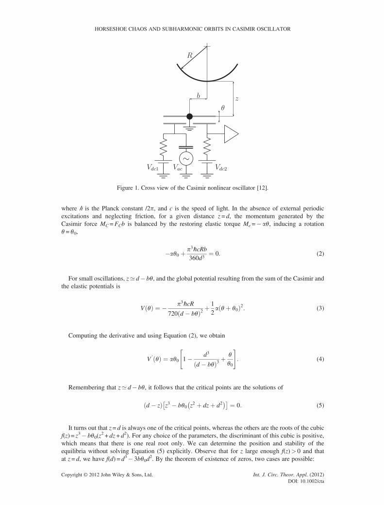
Figure 1. Cross view of the Casimir nonlinear oscillator [12].

HORSESHOE CHAOS AND SUBHARMONIC ORBITS IN CASIMIR OSCILLATOR

where ℏ is the Planck constant /2p, and c is the speed of light. In the absence of external periodicexcitations and neglecting friction, for a given distance z = d, the momentum generated by theCasimir force MC =FCb is balanced by the restoring elastic torque Me=� aθ, inducing a rotationθ= θ0,

�aθ0 þ p3ℏcRb360d3

¼ 0: (2)

For small oscillations, z’ d� bθ, and the global potential resulting from the sum of the Casimir andthe elastic potentials is

V θð Þ ¼ � p3ℏcR720 d � bθð Þ2 þ

12a θþ θ0ð Þ2: (3)

Computing the derivative and using Equation (2), we obtain

V ′ θð Þ ¼ aθ0 1� d3

d � bθð Þ3 þθθ0

" #: (4)

Remembering that z’ d� bθ, it follows that the critical points are the solutions of

d � zð Þ z3 � bθ0 z2 þ dzþ d2� �� ¼ 0: (5)

It turns out that z= d is always one of the critical points, whereas the others are the roots of the cubicf(z) = z3� bθ0(z

2 + dz + d2). For any choice of the parameters, the discriminant of this cubic is positive,which means that there is one real root only. We can determine the position and stability of theequilibria without solving Equation (5) explicitly. Observe that for z large enough f(z)> 0 and thatat z= d, we have f(d) = d3� 3bθ0d

2. By the theorem of existence of zeros, two cases are possible:


M. BONNIN

• For d> 3bθ0, and f(d)> 0, the root is located at z*< d, which implies that θ*> 0. Thus, atθ = 0 there is a local minimum of V(θ), which corresponds to a neutrally stable equilibrium(a center). At θ*> 0, the potential has a local maximum, which corresponds to an unstableequilibrium (a saddle).

• For d< 3bθ0, and f(d)< 0, the situation is reversed. The root is located at z*> d, that is, at θ*< 0,which is an equilibrium of center type, and θ= 0 is a saddle.

Without loss of generality, hereinafter we shall restrict our attention to the first case.From Equation (3), the Lagrange equation of motion is

€θ þ aIθþ θ0ð Þ � p3ℏcRb

360I d � bθð Þ3 ¼ 0; (6)

where I is the inertia momentum of the oscillating plate. Equation (6) can be rewritten as the system offirst order ODEs

_θ ¼ J

_J ¼ o20θ0

d3

d � bθð Þ3 �θθ0

� 1

" #;

8><>: (7)

where Equation (2) has been used and the oscillator’s natural frequencyo20 ¼ a=I has been introduced.

On dividing one equation by the other, we obtain

dθdJ

¼ J

o20θ0

d3

d�bθð Þ3 � θθ0� 1

h i : (8)

Separating the variables and integrating both sides, we find

J2

2þ o2

0

2θþ θ0ð Þ2 � o2

0θ0d3

2b d � bθð Þ2 ¼ E; (9)

where E is the integration constant. Thus, system (6) is conservative with Hamiltonian,

H θ; Jð Þ ¼ J2

2þ o2

0

2θþ θ0ð Þ2 � o2

0θ0d3

2b d � bθð Þ2 : (10)

The level sets H(θ, J) =E define the solution curves. The corresponding phase portrait is shownin Figure 2.

It is important to stress that the Casimir potential (3) and the subsequent analysis have beenderived under the hypothesis of small amplitude oscillations. Therefore, the phase portrait ofFigure 2 reliably describes the behavior of the Casimir oscillator only as long as this conditionis not violated. This imposes some constrains on the oscillator’s constructive parameters. In thisoptic, Figure 2 can be viewed as a design toolkit: The choice of the parameter values is good aslong as θ remains within a reasonable range, whose width is prescribed by the desired accuracyof the model.


Figure 2. Phase portrait of the Hamiltonian system (6). The system has a neutrally stable equilibrium ofcenter type at the origin, and an unstable equilibrium of saddle type at θ*.


Equation (9) implies that

J ¼ �ffiffiffiffiffiffiffiffiffiffiffiffiffiffiffiffiffiffiffiffiffiffiffiffiffiffiffiffiffiffiffiffiffiffiffiffiffiffiffiffiffiffiffiffiffiffiffiffiffiffiffiffiffiffiffiffiffiffiffiffiffiffiffiffiffi2E � o2

0 θþ θ0ð Þ2 � o20θ0d3

b d � bθ0ð Þ2s

: (11)

Introducing the positive determination in the first of Equation (7), we arrive to

_θ ¼ffiffiffiffiffiffiffiffiffiffiffiffiffiffiffiffiffiffiffiffiffiffiffiffiffiffiffiffiffiffiffiffiffiffiffiffiffiffiffiffiffiffiffiffiffiffiffiffiffiffiffiffiffiffiffiffiffiffiffiffiffiffiffiffiffi2E � o2

0 θþ θ0ð Þ2 � o20θ0d3

b d � bθ0ð Þ2s

: (12)

Separating and integrating the variables, it is possible to obtain, at least in an implicit form, the timeevolution of trajectories (θ(t), J(t)) solution to Equation (7). These solutions are obtained by solving anintegral of type

ZR θð Þw θð Þ dθ ¼ t (13)

where R(θ) is a rational function and w2 is a quartic function of θ [13]. It turns out that, for the problemunder investigation, Equation (13) involves the sum of elementary and elliptic functions, and thuscannot be inverted to give the explicit time dependence for θ(t) and J(t).

Therefore, if one is interested in the time domain evolution, that is, the waveforms of the statevariables, the exact equation of motion provides little useful information. In the next section, weshall see that such information can be obtained by considering the Taylor approximation of theCasimir force, which accurately reproduces the qualitative behavior of the exact equation, at least inthe neighborhood of the working point.

3. TAYLOR EXPANSION OF CASIMIR FORCE, HOMOCLINIC LOOP, ANDPERIODIC ORBITS

The analysis of the previous section has been carried out under the hypothesis of small amplitudeoscillations, using the approximation z’ d� bθ. Under this hypothesis, the Casimir force can beTaylor-expanded around the stable equilibrium position z= d. Following [12], the Taylor series istruncated at θ3, and the resulting potential is


M. BONNIN

V θð Þ ¼ 12a θþ θ0ð Þ2 � FC dð Þbθþ F′

C dð Þb22

θ2 � F00C dð Þb36

θ3 þ F000C dð Þb424

θ4; (14)

where FC dð Þ;F′C dð Þ;F00

C dð Þ;F 000C dð Þ are the Casimir force, and its first, second, and third derivatives

evaluated at a distance d, respectively. To simplify the equations, it is convenient to introduce theparameters

l ¼ � o20 þ

F′C dð Þb2I

� �; m ¼ F

00C dð Þb32I

; n ¼ �F000C dð Þb46I

: (15)

The potential V(θ) has a local minimum in the origin, two local maxima at

θ� ¼ 12

�mn�

ffiffiffiffiffiffiffiffiffiffiffiffiffiffiffiffiffim2

n2� 4

ln

r !; (16)

and decreases unbounded for both θ< θ� and θ> θ+. Therefore, the system has a neutrally stableequilibrium in the origin (a center), and two unstable equilibria at θ�, which are of saddle type. Thisphase portrait is known as the saddle–loop case [14].

RemarkWith respect to the original system, one of the two saddles does not correspond to an actual equilibriumpoint, but rather it is an artifact caused by the Taylor expansion of the Casimir force. This artifact, how-ever, will not invalidate our analysis. In fact, we shall study the dynamic behavior of the oscillatoraround the center and one saddle equilibrium point, where the Taylor expanded-equation accuratelyreproduces the exact qualitative dynamics.

The Lagrange equation of motion is

€θ ¼ lθþ mθ2 þ nθ3 (17)

or, rewritten as a system of first-order ODEs

_θ ¼ J_J ¼ nθ θ� θþð Þ θ� θ�ð Þ:

(18)

To further simplify the system, we introduce a new variable f= θ� θ+, new parameters

r ¼ n 2θþ � θ�ð Þ; s ¼ nθþ θþ � θ�ð Þ (19)

and we perform a linear change of coordinates

f; J; tð Þ !ffiffiffisn

rf;

sffiffiffin

p J;1ffiffiffis

p t

�; (20)

reducing Equation (18) to

_f ¼ J_J ¼ f3 þ xf2 þ f;

(21)

where x ¼ r=ffiffiffiffiffins

p. In Equation (21), one saddle has been shifted in the origin, one in f� and the center

to f+, where



f� ¼ 12

�x�ffiffiffiffiffiffiffiffiffiffiffiffiffix2 � 4

q �: (22)

RemarkThe linear scaling (20) presents both pros and cons. On the one hand, a direct interpretation of theequation’s parameters in terms of the oscillator’s constructive features is lost. This makes difficult adirect comparison between the dynamic behavior predicted by the model and that of the originaloscillator. This comparison is postponed to a future work. On the other hand, Equation (21) ismuch simpler than the original one (Equation (7)), as it depends on the parameter x only, whichadsorbs all the others. The linear scaling presents another advantage. The small scales involvedin the experimental setup result in convergence problem, which makes troublesome the numericalintegration of original state equations. The scaling introduces a normalization, which removes both,extremely large or extremely small, parameters and solves this problem. For instance, for the set ofvalues described at the beginning of Section 2 and with an equilibrium distance d= 50 nm, theparameter x takes the value x= 2.2055.

With the same procedure described in the previous section, we derive the Hamiltonian

H f; Jð Þ ¼ J2

2� f4

4� xf3

3� f2

2: (23)

The trajectories determined by the level sets H(f, J) =E are shown in Figure 3, where the points

f� and ~f�, which will be fundamental in the forthcoming analysis, are also reported. Obviously,the presence of the second saddle point f�, which does not correspond to an actual equilibrium ofthe device, gives rise to not physical behaviors. However, in what follows, we shall investigate theregion surrounding the homoclinic orbit and its interior, where Figures 2 and 3 show the samequalitative dynamics.

3.1. Homoclinic loop

We shall now prove that, for certain values of the parameter x, system (21) possesses a homoclinicorbit through the origin, which corresponds to a trajectory with zero energy delimiting a regionfilled with periodic orbits.

Figure 3. Phase portrait of the Hamiltonian system (17). The system has a neutrally stable equilibrium ofcenter type at f+, and two unstable equilibria of saddle type at the origin and at f�. The curves corresponding

to trajectories with zero energy intersect the f-axis at ~f� (open orbit) and ~fþ (homoclinic loop).


M. BONNIN

For the orbit through the origin, we have H(0, 0) = 0, which implies that

J ¼ �ffiffiffiffiffiffiffiffiffiffiffiffiffiffiffiffiffiffiffiffiffiffiffiffiffiffiffiffiffiffiffiffiffiffiffiffiffiffiffiffif2 f2

2þ 2xf

3þ 1

�s: (24)

In the phase plane, this curve intersects the f-axis in three points: ~f ¼ 0, and

~f� ¼ � 2x3�

ffiffiffiffiffiffiffiffiffiffiffiffiffiffiffi4x2

9� 2

s; (25)

provided that x > 3ffiffiffi2

p=2 . Introducing the positive determination of Equation (24) in the first of

Equation (21), we obtain

_f ¼ffiffiffiffiffiffiffiffiffiffiffiffiffiffiffiffiffiffiffiffiffiffiffiffiffiffiffiffiffiffiffiffiffiffiffiffiffiffiffiffif2 f2

2þ 2xf

3þ 1

�s: (26)

By separation of variables, Equation (26) can be integrated from zero to t in terms of elementary

functions, because it has repeated roots. Choosing as initial conditions f 0ð Þ; J 0ð Þð Þ ¼ ~fþ; 0�

, the

integration yields

f tð Þ ¼ fh tð Þ ¼ 3tanh2 t�K

2 � 1

2x� 3ffiffiffi2

ptanh t�K

2

(27)

where

K ¼ 2atanh

ffiffiffi2

p

2~fþ

�: (28)

Computing the derivative and making use of the properties of hyperbolic functions, we derive

Jh tð Þ ¼ 12xsinh t � Kð Þ � 18ffiffiffi2

pcosh t � Kð Þ

2xþ 2xcosh t � Kð Þ � 3ffiffiffi2

psinh t � Kð Þ� �2 : (29)

It is readily seen that

limt!�1

fh tð Þ; Jh tð Þð Þ ¼ 0; 0ð Þ (30)

as required in order (fh(t), Jh(t)) to be a homoclinic loop through the origin.To show that the region inside the homoclinic loop is filled with periodic orbits, we take into

account that, for x > 3ffiffiffi2

p=2, Equations (22) and (25) imply ~fþ < fþ < 0, that is, the center lies

inside the region delimited by the homoclinic orbit. Because outside the interval between the twosaddles the potential decreases unbounded, it follows that the homoclinic orbit is the separatrixbetween a region filled with periodic orbits and a region characterized by unbounded trajectories.



3.2. Periodic trajectories

For any initial condition (f(0), J(0)) = (f0, 0), with ~fþ < f0 < 0, the solution curves of Equation (21)are the level sets H(f, J) =E, that is,

J2

2� f4

4� xf3

3� f2

2¼ E (31)

where the exact value of the energy is found imposing the passage trough (f0, 0)

E ¼ �f40

4� xf3

0

3� f2

0

2: (32)

Equation (31) implies that

J ¼ �ffiffiffiffiffiffiffiffiffiffiffiffiffiffiffiffiffiffiffiffiffiffiffiffiffiffiffiffiffiffiffiffiffiffiffiffiffiffiffiffiffiffiffiffi2E þ f4

2þ 2xf3

3þ f2

s: (33)

Taking the positive determination, and introducing in the first of Equation (21) yields

_f ¼ffiffiffiffiffiffiffiffiffiffiffiffiffiffiffiffiffiffiffiffiffiffiffiffiffiffiffiffiffiffiffiffiffiffiffiffiffiffiffiffiffiffiffiffi2E þ f4

2þ 2xf3

3þ f2

s: (34)

Separating the variables, and integrating from zero to t, we are lead to the integral

Z f tð Þ

f0

f xð Þ½ ��12dx ¼ t (35)

where f xð Þ ¼ 2E þ 12 x4 þ 2x

3 x3 þ x2. It can be shown (see [13]) that this integral has the solution

f tð Þ ¼ fm tð Þ ¼ f0 þ14f ′ f0ð Þ P ffiffiffiffiffiffiffiffiffiffiffiffiffiffi

e1 � e3p

t; g2; g3ð Þ � 124

f00f0ð Þ

� ��1

(36)

where P ffiffiffiffiffiffiffiffiffiffiffiffiffiffie1 � e3

pt; g2; g3

� �is the Weierstrass elliptic function with invariants

g2 ¼ E þ 112

; g3 ¼ E

6� 1216

� x2E18

; (37)

and e1≥ e2≥ e3 are the roots of

4t3 � g2t � g3 ¼ 0: (38)

Introducing the Jacobi elliptic functions2 sn(u|m), cn(u|m), and dn(u|m), where u is the argumentand m is the elliptic modulus, we have

2A fair complete overview of Jacobi and Weierstrass elliptic functions, elliptic integrals and their properties can be foundin [15,16].


M. BONNIN

P ffiffiffiffiffiffiffiffiffiffiffiffiffiffie1 � e3

pt; g2; g3ð Þ ¼ e3 þ e1 � e3

sn2ffiffiffiffiffiffiffiffiffiffiffiffiffiffie1 � e3

pt e2�e3e1�e3

�� :

� (39)

To simplify notation in what follows, the modulus m ¼ e2�e3e1�e3

of the elliptic functions will be

omitted. Introducing w ¼ ffiffiffiffiffiffiffiffiffiffiffiffiffiffie1 � e3

pand making use of the properties of elliptic functions, we can

rewrite fm(t) as

fm tð Þ ¼ f0 þf ′ f0ð Þsn2 wtð Þ

4 w2 þ e3 � 124 f

00 f0ð Þ� �sn2 wtð Þ� � : (40)

Computing the derivative, we obtain

Jm tð Þ ¼ f ′ f0ð Þsn wtð Þcn wtð Þdn wtð Þ2w 1� n sn2 wtð Þ½ �2 ; (41)

where the parameter

n ¼ f00f0ð Þ � 24e324w

(42)

has been introduced.Equations (40) and (41) imply that the period of the periodic trajectory (fm(t), Jm(t)) is determined

by the period of the Jacobi functions, which is Tm ¼ 2K mð Þw , where K(m) is the complete elliptic integral

of the first kind.The relationships between initial condition, energy, elliptic modulus and period deserve some

comments. From Equation (32), it follows that for J(0) = 0 and f0 in the interval ~fþ; 0�

, the

energy is negative, it has a minimum at the center f0 =f+, and increases as f0 approaches either the

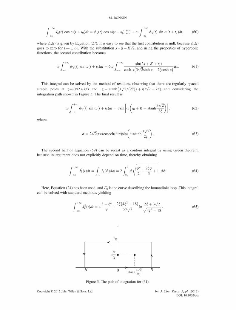
origin or ~fþ . In other words, the energy of the periodic orbits increases as the orbits approach thehomoclinic loop. The relation between initial condition and elliptic modulus is much morecomplicated, as it involves e1, e2, and e3. By computing these roots analytically, one finds that at thecenter, e2 = e3, which implies that m= 0. Conversely at the saddle, where E= 0, one has e1 = e2,which means that m= 1. Trajectories associated to any intermediate value of the energy have0<m< 1. Numerical analysis reveals that the modulus is a strictly increasing function of theenergy, the example for x = 9 is shown in the left-hand part of Figure 4. Therefore, because of theproperties of K(m), the period Tm is a strictly increasing function of the energy as well, and goes toinfinity as E! 0, as shown in the right-hand part of Figure 4.

−2.5 −2 −1.5 −1 −0.5 00

0.2

0.4

0.6

0.8

1

−2.5 −2 −1.5 −1 −0.5 0x 10−3x 10−3

5

10

15

20

25

30

35

40

45

Figure 4. The dependence of the elliptic modulus m (left) and the period Tm (right) on the energy E, for x= 9.



Before leaving this section, we show that the periodic orbits converge to the homoclinic loop as

f0 ! ~fþ , as it is suggested by the vertical asymptote of the Tm(E) curve in Figure 4. In this limit,E= 0 and the roots ei of Equation (38) are easily computed giving e1 = e2 = 1/12, and e3 =� 1/6,which yields w= 1/2 and m= 1. Taking into account that sn(u|1) = tanh(u) and with some algebra,Equation (40) reduces to

fm tð Þ m¼1 ¼ 22x3þ 2

~fþ

!cosh t� 2x

3

" #�1

:

�� (43)

On the other hand, by using the subtraction formula for hyperbolic function, Equation (27) can berecast as

fh tð Þ ¼ 22x3sinh K þ

ffiffiffi2

pcosh K

�sinh t � 2x

3cosh K þ

ffiffiffi2

psinh K

�cosh t � 2x

3

� ��1

: (44)

By comparison, it turns out that the two expressions coincide if and only if the followingidentities hold

2x3sinh K þ

ffiffiffi2

pcosh K ¼ 0

2x3cosh K þ

ffiffiffi2

psinh K ¼ � 2x

3þ 2

~fþ

!:

8>>><>>>:

(45)

The first identity can be rewritten as

2x3sinh K þ

ffiffiffi2

pcosh K ¼ 4x

3sinh

K

2cosh

K

2þ

ffiffiffi2

pcosh2

K

2þ sinh2

K

2

�¼ 0: (46)

Dividing by cosh2K/2 yields

ffiffiffi2

ptanh2

K

2þ 4x

3tanh

K

2þ

ffiffiffi2

p¼ 0: (47)

Using the definition of K given by Equation (28), we obtain

~f2þ þ 4x

3~fþ þ 1

2¼ 0 (48)

which is readily verified by Equation (25).On the other hand, summing both sides of Equation (45), collecting common terms and using the

definition of hyperbolic functions, we find


M. BONNIN

K ¼ ln �2x3 þ 2

~fþ2x3 þ ffiffiffi

2p

0@

1A: (49)

Using again Equations (25) and (28), and the property

2atanh x ¼ ln1þ x

1� x(50)

the second identity follows.

4. THE MELNIKOV METHOD

We now turn our attention to study the influence that a weak damping and a weak periodic forcingexert on the trajectories described in the previous section. We shall show that by properly choosingthe damping coefficient, the forcing strength and its frequency, highly degenerate structures, namelySmale horseshoes, birth.

First introduced by Smale [17], horseshoes are invariant Cantor sets on which the associated map ishyperbolic and has positive topological entropy. Because they are not attracting, these sets represent,from the observational point of view, transient chaos. Horseshoes are robust, in the sense that theypersist under perturbations of the vector field. The main tool to investigate the presence of horseshoesin a class of periodically perturbed systems, is the Melnikov method [18]. In the simplest form, theMelnikov method applies to second-order, Hamiltonian systems, subject to a periodic perturbation

_x ¼ f1 x; yð Þ þ e g1 x; y; tð Þ_y ¼ f2 x; yð Þ þ e g2 x; y; tð Þ;

(51)

where e≪ 1 measures the strength of the perturbation, and gi(x, y, t) = gi(x, y, t+ T), i= 1, 2. To applyMelnikov method, the following assumptions must hold [19]:

• For e= 0, the system exhibits a homoclinic orbit through a hyperbolic saddle point.• The interior of the homoclinic orbit is filled with a continuous family of periodic orbits.

It is convenient to rewrite system (51) as an autonomous third-order system

_x ¼ f1 x; yð Þ þ e g1 x; y; θð Þ_y ¼ f2 x; yð Þ þ e g2 x; y; θð Þ_θ ¼ 1;

8<: (52)

With θ2 S1. For e= 0, system (52) possesses a limit cycle. Taking a cross section Σt0 ¼x; y; tð Þ : t ¼ t0 2 0; T½ �f g transversal to this cycle, the corresponding Poincaré map Pt0

0 : Σt0 ! Σt0

has a hyperbolic saddle point. For e sufficiently small, by the implicit function theorem, the saddlepoint survives, but the homoclinic manifold splits, leading to the stable and unstable manifolds ofthe new saddle point of the Poincaré map. The separation between these new manifolds is measuredon Σt0 by the Melnikov integral. If the manifolds intersect transversely once, then they intersect eachother transversely infinitely many times, because they are invariants of the Poincaré map. Denotingas q0(t) the homoclinic loop of the unperturbed system, the Melnikov integral is given by

M t0ð Þ ¼Z þ1

�1f q0 tð Þð Þ∧g q0 tð Þ; t þ t0ð Þdt (53)

where f∧g ¼ f1g2 � f2g1. If the Melnikov function has simple zeros, that is, if there exist some t0such that



M t0ð Þ ¼ 0; M′ t0ð Þ ¼ dM t0ð Þdt0

6¼ 0; (54)

then it follows that the Poincaré map has a transverse homoclinic point to the saddle point. Theexistence of such orbits implies, via the Smale–Birkhoff theorem, the presence of Smalehorseshoes. Because the dynamics of the horseshoe is “chaotic”, one can conclude that thePoincaré map and hence the time-periodically perturbed system (51) possess “chaotic” behavior.

The Melnikov method also represents an effective tool to investigate the effect of periodicperturbations on the orbits inside the homoclinic loop. This method has been successfully applied tothe analysis and design of oscillating nonlinear circuits and systems [20–22]. Assume that qm(t) is aperiodic orbit of the unperturbed system, with period Tm= pT/q, where p, q are relative primeintegers, and define the subharmonic Melnikov function

Mp=q t0ð Þ ¼Z qT

0f qm tð Þð Þ∧g qm tð Þ; t þ t0ð Þdt: (55)

If Mp/q(t0) has simple zeros and dTm/dE 6¼ 0, that is, if the center is regular (non-isochronous), thenfor e small enough, the Poincaré map has a fixed point, and the time-periodically perturbed system hasa subharmonic periodic orbit of period pT. This orbit represents a limit cycle, which survives to theperturbation, “emerging” from the center.

4.1. Horseshoes in the Casimir nonlinear oscillator

When a small friction and a small periodic forcing are taken into account, Equation (17) should bemodified to

€θ ¼ lθþ mθ2 þ nθ3 þ e Acosot � g _θ� �

(56)

where e≪ 1, A is the amplitude of the forcing and g is the damping constant. Consequently, Equation(18) becomes

_f ¼ J_J ¼ f3 þ xf2 þ fþ e A cos ot � gJð Þ

(57)

where, to simplify the equations, new scaled parameters

g;A;oð Þ ! gffiffiffis

p ;A

ffiffiffiffiffins3

r;offiffiffis

p �

(58)

have been introduced.It has been shown in the previous section that, in the absence of friction and forcing, the Casimir

oscillator possesses a homoclinic loop delimiting a region filled with periodic orbits. Thus,Melnikov method can be applied to system (57). The resulting Melnikov function is

M t0ð Þ ¼Z þ1

�1Jh tð Þ A cos o t þ t0ð Þ � gJh tð Þ½ �dt (59)

where Jh(t) is given by Equation (29). To solve this integral, we split it into two halves. For the firsthalf, using integration by parts, we obtain


M. BONNIN

Z þ1

�1Jh tð Þ cos o t þ t0ð Þdt ¼ fh tð Þ cos o t þ t0ð Þjþ1

�1 þ oZ þ1

�1fh tð Þ sin o t þ t0ð Þdt; (60)

where fh(t) is given by Equation (27). It is easy to see that the first contribution is null, because fh(t)goes to zero for t!�1. With the substitution x= (t�K)/2, and using the properties of hyperbolicfunctions, the second contribution becomes

oZ þ1

�1fh tð Þ sin o t þ t0ð Þdt ¼ 6o

Z þ1

�1

sin 2xþ K þ t0ð Þcosh x 3

ffiffiffi2

psinh x� 2xcosh x

� � dx: (61)

This integral can be solved by the method of residues, observing that there are regularly spacedsimple poles at z= i(p/2 + kp) and z ¼ atanh 3

ffiffiffi2

p= 2xð Þ� �þ i p=2þ kpð Þ; and considering the

integration path shown in Figure 5. The final result is

oZ þ1

�1fh tð Þ sin o t þ t0ð Þdt ¼ ssin o t0 þ K þ atanh

3ffiffiffi2

p

2x

�� ; (62)

where

s ¼ 2ffiffiffi2

ppocosech opð Þsin oatanh

3ffiffiffi2

p

2x

�: (63)

The second half of Equation (59) can be recast as a contour integral by using Green theorem,because its argument does not explicitly depend on time, thereby obtaining

Z þ1

�1J2h tð Þdt ¼

ZΓ0Jh fð Þdf ¼ 2

Z 0

~fþf

ffiffiffiffiffiffiffiffiffiffiffiffiffiffiffiffiffiffiffiffiffiffiffiffiffiffiffiffif2

2þ 2xf

3þ 1

sdf: (64)

Here, Equation (24) has been used, and Γ0 is the curve describing the homoclinic loop. This integralcan be solved with standard methods, yielding

Z þ1

�1J2h tð Þdt ¼ 4

3� x2

9þ 2x 4x2 � 18

� �27

ffiffiffi2

p ln2xþ 3

ffiffiffi2

pffiffiffiffiffiffiffiffiffiffiffiffiffiffiffiffiffiffi4x2 � 18

p : (65)

Figure 5. The path of integration for (61).



Putting everything together, the Melnikov function results to be

M t0ð Þ ¼ �grþ Assin o t0 þ K þ atanh3ffiffiffi2

p

2x

�� (66)

where

r ¼ 43� x2

9þ 2x 4x2 � 18

� �27

ffiffiffi2

p ln2xþ 3

ffiffiffi2

pffiffiffiffiffiffiffiffiffiffiffiffiffiffiffiffiffiffi4x2 � 18

p : (67)

The Melnikov function has infinitely many zeros provided

sin o t0 þ K þ atanh3ffiffiffi2

p

2x

�� ¼ r

sgA: (68)

These zeros are simple if dM t0ð Þdt0

6¼ 0, where the derivative is

dM t0ð Þdt0

¼ oAscos o t0 þ K þ atanh3ffiffiffi2

p

2x

�� : (69)

Therefore, a sufficient condition to have dM t0ð Þdt0

6¼ 0 when M(t0) = 0 is

�1 < sin o t0 þ K þ atanh3ffiffiffi2

p

2x

�� < 1 (70)

from which we finally derive the condition to have homoclinic tangencies

A

g>

rs

�� : (71)

In Figure 6 are shown the stable (black dots) and unstable (red dots) manifolds of the unstable nodeon the Poincaré mapΣt0, obtained through numerical simulations for x = 4, e g = 0.1, o= 1, and differentvalues of eA. For eA less than the critical value, the manifolds are separated. For eA= 0.020, in perfectagreement with the critical value eAc = 0.02 obtained from Equation (71), the first homoclinic tangencyoccurs. For higher values of eA, the manifolds intersect transversally. Despite only a first-orderMelnikov function has been used, the theoretical analysis is surprisingly accurate.

At this point, it seems appropriate to make some comments on the results just obtained. TheMelnikov method allows us to prove the existence of transversal homoclinic points, and hence todeduce the existence of hyperbolic invariant sets. We do not know however if trajectories tend tothe hyperbolic invariant sets located analytically. Indeed, a horseshoe and the set of pointsasymptotic to it usually have zero Lebesgue measure, and it is entirely possible for a map to have ahorseshoe and at the same time to have the orbit of Lebesgue–almost every point tend to anequilibrium. In fact, we may observe transient periods of chaos followed by asymptotically periodicmotions. The attracting invariant set remains to be determined. This will be the goal of the next section.

4.2. Subharmonic orbits

We now turn the attention to the family of periodic orbits within the homoclinic loop Γ0, aiming todetermine whether some of these orbits survive to the perturbation. If their number is finite, theybecome isolated periodic orbits, that is, limit cycles of the perturbed system.


−0.5 −0.4 −0.3 −0.2 −0.1 0−0.15

−0.1

−0.05

0

0.05

0.1

0.15

0.2

φ

J

−0.4 −0.3 −0.2 −0.1 0

−0.1

−0.05

0

0.05

0.1

0.15

0.2

φ

J

−0.4 −0.3 −0.2 −0.1 0

−0.1

−0.05

0

0.05

0.1

0.15

0.2

φ

J

Figure 6. Stable (black dots) and unstable (red dots) manifolds of the unstable node on the Poincaré map Σt0,obtained through numerical simulations for different forcing amplitudes. Upper left: eA = 0.015. Upper right:

eA= 0.020. Lower: eA = 0.025.

M. BONNIN

Let T= 2p/o be the period of the forcing. The resonance condition for the periodic orbits isqTm = pT, with q, p2 IN, or in other terms

pom ¼ qo (72)

where om is the frequency of the unperturbed periodic orbit. For the sake of simplicity, we shall restrictour attention to the case q = 1. The subharmonic Melnikov function is

Mp t0ð Þ ¼Z pT

0Jm tð Þ Acos t þ t0ð Þ � gJm tð Þ½ �dt (73)

where Jm(t) is given by Equation (41). Using addition formula, this integral becomes

Mp t0ð Þ ¼ A cos ot0R pT0 Jm tð Þ cos ot dt � A sin ot0

R pT0 Jm tð Þ sin ot dt

�gR pT0 J2m tð Þdt: (74)

The first two integrals can be solved with the help of Fourier series. For the first one, we have

R pT0 Jm tð Þ cos ot dt ¼ R Tm0 J0 þ

Xþ1

k¼1

JAk cos komt þ JBk sin komt� �" #

cos pomtdt

¼ pom

JAp

(75)

where JAp is the p-th Fourier cosine coefficients of Jm(t)

JAp ¼ 2Tm

Z Tm

0Jm tð Þcos pomtdt ¼ f ′ f0ð Þ

wTm

Z Tm

0

sn wtð Þcn wtð Þdn wtð Þ1� n sn2 wtð Þ½ �2 cos pomtdt: (76)

With an integration by parts



JAp ¼ pomf ′ f0ð Þ8nw2

FBp þ GB

p

� (77)

whereFBp andG

Bp are the p-th sine coefficients of 1þ

ffiffiffin

psn wtð Þ½ ��1 and 1� ffiffiffi

np

sn wtð Þ½ ��1, respectively.These coefficients can be computed with the help of the results of [23], from which results

FBp ¼ 1

K mð ÞZ 2K mð Þ

0

sinppu

K mð Þ1þ ffiffiffi

np

sn udu

¼ �ffiffiffin

pp

K mð Þ ffiffiffiffiffiffiffiffiffiffiffiffiffiffiffiffiffiffiffiffiffiffiffiffiffiffiffiffiffiffi1� nð Þ 1� mð Þp sin

ppu02K mð Þ sin

pp2cosech

ppK ′ mð Þ2K mð Þ

(78)

GBp ¼ �FB

p (79)

where u0 is such that

dn u0ð Þ ¼ffiffiffiffiffiffiffiffiffiffiffiffi1� m

1� n

r; (80)

and K′(m) =K(1�m). Because of Equations (77) and (79), it turns out that JAp ¼ 0.The same procedure applied to the second integral yields

R pT0 Jm tð Þsinot dt ¼ R Tm0 J0 þ

Xþ1

k¼1

JAk coskomt þ JBk sinkomt� �" #

sinpomt dt

¼ pom

JBp

(81)

where JBp is the p-th sine coefficients of Jm(t)

JBp ¼ � pomf ′ f0ð Þ8nw2

FAp þ GA

p

� ; (82)

and FAp ;G

Ap are the p-th cosine coefficients of 1þ ffiffiffi

np

sn wtð Þ½ ��1 and 1� ffiffiffin

psn wtð Þ½ ��1, respectively.

Using the results of [23], once more we have

FAp ¼ 1

K mð ÞZ 2K mð Þ

0

cosppuK mð Þ

1þ ffiffiffin

psn u

du

¼ffiffiffin

pp

K mð Þ ffiffiffiffiffiffiffiffiffiffiffiffiffiffiffiffiffiffiffiffiffiffiffiffiffiffiffiffiffiffi1� nð Þ 1� mð Þp sin

ppu02K mð Þ cos

pp2cosech

ppK ′ mð Þ2K mð Þ

(83)

GAp ¼ FA

p : (84)

Therefore, FAp is identically null for odd values of p, and Equation (82) becomes

JBp ¼ � pomf ′ f0ð Þ4nw2

FAp : (85)

It remains to solve the last integral of Equation (74), that is,R pT0 J2 tð Þdt. Using Equation (41), the

resonance condition, and taking into account that sn u is an odd function, whereas cn u and dn u areeven, we obtain


M. BONNIN

Z pT

0J2m tð Þdt ¼ f ′ f0ð Þ2

2w3

Z K mð Þ

0

sn2zcn2zdn2z

1� n sn2zð Þ4 dz (86)

where z=wt. This last integral can be solved using the results of [16],

Z K mð Þ

0

sn2zcn2zdn2z

1� n sn2zð Þ4 dz ¼ AK mð Þ þ BE mð Þ þ CΠ n;mð Þ (87)

where A, B, and C are rational functions of m and n, given by

A ¼ m2 3� 6nð Þ þ 2mn2 2þ nð Þ þ n2 �4þ 4� 3nð Þn½ �48n3 n� 1ð Þ2 n� mð Þ (88)

B ¼ 3m2 � 4m mþ 1ð Þnþ 2 2þ mþ 2;m2ð Þn2 � 4 1þ mð Þn3 þ 3n4

48n2 n� 1ð Þ2 n� mð Þ2 (89)

C ¼ � mþ n� 2ð Þn½ � m� n2ð Þ m 2n� 1ð Þ � n2½ �16n3 n� 1ð Þ2 n� mð Þ2 (90)

and K(m), E(m), and Π(n,m) are the complete elliptic integrals of the first, second, and third kind,respectively.

Putting everything together, the subharmonic Melnikov integral (74) results to be

Mp t0ð Þ ¼ Appf ′ f0ð Þ4nw2

FAp sinot0 � g

f ′ f0ð Þ22w3

AK mð Þ þ BE mð Þ þ CΠ n;mð Þ½ �: (91)

As a first comment, it is easy to observe that as a consequence of Equation (84), for odd values of p,the Melnikov integral is independent of t0, that is, M

p(t0) is either identically null or always differentfrom zero. Therefore, we do not expect odd resonances to occur. For p even, Mp(t0) = 0 implies

sino t0 ¼ gA

2nf ′ f0ð ÞppwFA

p

AK mð Þ þ BE mð Þ þ CΠ n;mð Þ½ �: (92)

For the derivative, we have

dMp t0ð Þdt0

¼ Appf ′ f0ð Þo4nw2

cosot0: (93)

Thus, Mp(t0) has a simple zero provided

�1 <gA

2nf ′ f0ð ÞppwFA

p

AK mð Þ þ BE mð Þ þ CΠ n;mð Þ½ � < 1: (94)

These inequalities lead to the condition for the existence of subharmonic orbits

A

g>

2nppw

f ′ f0ð ÞFAp

AK mð Þ þ BE mð Þ þ CΠ n;mð Þ½ ��

��: (95)

In Figure 7, two limit cycles, which coexist for x = 4, o= 1, eg= 0.1, and eA= 0.02 are shown. Thesmall cycle on the right, which corresponds to the hyperbolic saddle point of the Poincaré map


−0.4 −0.3 −0.2 −0.1 0−0.1

−0.05

0

0.05

0.1

φ

J

Figure 7. Two coexisting limit cycles for x= 4, o= 1, eg = 0.1, and eA = 0.02. Floquet’s multipliers are: forthe left limit cycle l1 = 1, l2, 3 = 0.4580� i0.5690; for the right cycle m1 = 1, m2 = 0.0014, and m3 = 391.6301.


discussed at the beginning of Section 4, is of saddle type. The cycle on the left is asymptotically stable,it appears significantly before the transversal homoclinic trajectory, and persists as the ratio A/g isincreased. Eventually, this limit cycle coexists with the Smale’s horseshoes, representing theinvariant attracting set to which trajectories converge after the period of “transient chaos”. The limitcycles have been obtained using harmonic balance, which makes easy to detect unstable cycles ofsaddle type. The Floquet’s multipliers, which determine the stability of the cycles, have beencomputed by using the numerical algorithm described in [24], pp. 58–59.

5. CONCLUSIONS

When the size of electronic components shrinks down to the nanoscale level, quantum phenomena canno longer be neglected. This paper analyzes the dynamic behavior of a nanoelectromechanicalnonlinear oscillator, where the nonlinearity stems from a QED effect, that is, the Casimir force.

The dynamic behavior of the oscillator in the conservative limit is determined. It is shown that, inthe neighborhood of the working point, the dynamics can be accurately reproduced by considering aTaylor expansion of the Casimir force. By introducing a linear scaling of the state variables, notonly the state equations are simplified but also convergence problems and numerical inaccuracies inthe numerical integration of the state equations due to the nanoscale of the oscillator are avoided.

The existence of a homoclinic loop through a saddle point delimiting a region filled with periodicorbits is proved, and the analytical time domain formulas for such trajectories are given. Theseorbits are very sensitive to external perturbations, which may represent dissipative effects or periodicforcing signals. For some values of the damping constant and of the forcing amplitude, highlydegenerate structures, in the form of Smale’s horseshoes, may occur.

Using the method of Melnikov, the existence of these exotic structures in the Casimir nonlinearoscillator is proved, and the critical values of the perturbation’s parameters at which the horseshoesemerge are given. To the best of the author’s knowledge, the occurrence of such dynamic behaviorcaused by a QED effect is reported here for the first time.

It is also shown that horseshoes, which are not attracting, may coexist with periodic attractors, towhich trajectories converge after periods of “transient chaos”. A deep understanding of thesephenomena in the oscillator dynamics is believed to be crucial for both designers interested tospecific applications of nanoscale devices, or in order to avoid undesired behaviors.

ACKNOWLEDGEMENTS

This work was partially supported by the CRT Foundation. The author gratefully thanks the Istituto Super-iore Mario Boella and the regional government of Piedmont for financial support.


M. BONNIN

REFERENCES

1. Csurgay ÁI, Porod W, Goodnick SM. Special issues on nanoelectronic circuits. International Journal of CircuitTheory and Applications 2000; 28(6):521–599.

2. Csurgay ÁI, Porod W, Goodnick SM. Special issues on nanoelectronic circuits. International Journal of CircuitTheory and Applications 2001; 29(1):1–150.

3. Csurgay ÁI, Porod W. Special issues on nanoelectronic circuits. International Journal of Circuit Theory andApplications 2003; 31(1):1–117.



6. Casimir HBG. On the attraction between two perfectly conducting plates. Proceedings of the KoninklijkeNederlandse Akademie Van Wetenschappen 1948; 60:793–795.

7. Milonni PW. The Quantum Vacuum: An Introduction to Quantum Electrodynamics. Academic Press: San Diego(USA), 1994.

8. Cleland AN, Roukes ML. A nanometer-scale mechanical electrometer. Nature 1998; 392:160–162.9. Camarota B, LaHaye MD, Buu O, Schwab KC. Approaching the quantum limit of a nanomechanical resonator.

Science 2004; 304:74–77.10. Serry FM, Walliser D, Maclay GJ. The anharmonic Casimir oscillator (ACO)–the Casimir effect in a model

microelectromechanical system. Journal of Microelectromechanical Systems 1995; 4(4):193–205.11. Chan HB, Aksyuk VA, Kleinman RN, Bishop DJ, Capasso F. Quantum mechanical actuation of microelectromecha-

nical systems by the Casimir force. Science 2001; 291:1941–1944.12. Chan HB, Aksyuk VA, Kleinman RN, Bishop DJ, Capasso F. Nonlinear micromechanical Casimir oscillator.

Physical Review Letters 2001; 87:211801–1–211801–4.13. Whittaker ET, Watson GN. A Course in Modern Analysis. Cambridge University Press: Cambridge (UK), 1902.14. Dumortier F, Li C. Perturbation from an elliptic Hamiltonian of degree four, I. Saddle loop and two saddle cycle.

Journal of Differential Equations 2001; 176:114–157.15. Abramowitz M, Stegun IA. Handbook of Mathematical Functions. National Bureau of Standards: Washington, DC,

1964.16. Byrd PF, Friedman MD. Handbook of Elliptic Integrals for Engineers and Scientists (2nd edn). Springer–Verlag:

New York (USA), 1971.17. Smale S. Differentiable dynamical systems. Bulletin of the American Mathematical Society 1967; 73:717–817.18. Melnikov VK. On the stability of the center for time periodic perturbation. Transaction of the Moscow Mathematical

Society 1963; 12:1–56.19. Guckenheimer J, Holmes P. Nonlinear Oscillations, Dynamical Systems and Bifurcations of Vector Fields (5th edn).

Springer–Verlag: New York, 1997.20. Savov VN, Georgiev ZD, Todorov TG. Analysis and synthesis of perturbed Duffing oscillators. International

Journal of Circuit Theory and Applications 2006; 34(3):281–306.21. Bonnin M. Harmonic balance, Melnikov method and nonlinear oscillators under resonant perturbation. International

Journal of Circuit Theory and Applications 2008; 36:247–274.22. Georgiev ZD, Karagineva IL. Analysis and synthesis of oscillator systems described by perturbed double hump

Duffing equations. International Journal of Circuit Theory and Applications 2010 in press.23. Shi-dong W, Ji-bin L. Fourier series of rational fractions of Jacobian elliptic functions. Applied Mathematics and

Mechanics 1988; 9(6):541–556.24. Farkas M. Periodic Motions. Springer–Verlag: New York (USA), 1994.


Horseshoe chaos and subharmonic orbits in the nanoelectromechanical Casimir nonlinear oscillator

Documents

Transcript of Horseshoe chaos and subharmonic orbits in the nanoelectromechanical Casimir nonlinear oscillator