Subharmonic resonance of Venice gates in waves. Part 2. Sinusoidally modulated incident waves

J. Fluid Mech. (1997), vol. 349, pp. 327–359. Printed in the United Kingdom

c© 1997 Cambridge University Press

327

Subharmonic resonance of Venice gates in waves.Part 2. Sinusoidally modulated incident waves

By P A O L O S A M M A R C O† , H O A N G H. T R A N,O D E D G O T T L I E B‡ AND C H I A N G C. M E I

Department of Civil and Environmental Engineering,Massachusetts Institute of Technology, Cambridge, MA, 02139, USA

(Received 11 March 1997 and in revised form 17 June 1997)

In order to examine the effects of finite bandwidth of the incident sea spectrum onthe resonance of the articulated storm gates for Venice Lagoon, we consider a narrowband consisting of the carrier frequency and two sidebands. The evolution equationfor the gate oscillations now has a time-periodic coefficient, and is equivalent to a non-autonomous dynamical system. For small damping and weak forcing, approximateanalysis for local and global bifurcations are carried out, and extended by directnumerical simulation. Typical bifurcation scenarios are also examined by laboratoryexperiments.

1. IntroductionIn Part 1 (Sammarco et al. 1997) we have derived the nonlinear evolution equation

describing the out-of-phase rotation of Venice gates resonated subharmonically bynormally incident waves. The case of uniform amplitude was investigated in detail.Since the frequency band of sea waves in nature is usually finite, we wish to examinein this Part the effects of an idealized narrow band consisting of a slightly detunedcentral (carrier) frequency 2ω = 2 (ω0 + ∆ω) and two sidebands 2ω+Ω and 2ω−Ω,with Ω = ε2Ω2ω0 1. The envelope of the incident waves is therefore modulatedsinusoidally in time with the period 2π/Ω

A2 = A2 + A2 cosΩ2t2, (1.1)

where t2 = ε2ω0t′ denotes the dimensionless slow time with t′ being the physical time.

Since the time derivative of A2 introduces terms of O(ε2) smaller than those present,the evolution equation must be

−iθt2 = ω2θ + (cN + icR) θ2θ∗ + cFA2θ∗ + (1 + i) δ2cLθ + icQ|θ|θ. (1.2)

with A2 depending on time through (1.1). In terms of physical quantities the extendedevolution equation is

− i

ω0

θ′t′ =∆ω

ω0

θ′ + (cN + icR) θ′2θ′∗

+ cF

(A′

b′+A′

b′cosΩt′

)θ′∗

+ (1 + i) δcLθ′ + icQ|θ′|θ′. (1.3)

Owing to the time dependence of a coefficient, the above dynamical system is

† Present address: DITS, University of Rome ‘La Sapienza’, Italy.‡ Present address: Department of Mechanical Engineering, Technion, Haifa, Israel.

328 P. Sammarco, H. H. Tran, O. Gottlieb and C. C. Mei

non–autonomous: complicated bifurcations such as period-doubling and chaos areexpected as the properties of the incident waves are varied. In this Part we wish toexamine such bifurcations and describe comprehensive experiments in a wave basinfor a battery of gates, with the dual objectives of illustrating the nonlinear dynamicsof a novel project in coastal engineering, and revealing the rich physics embodied bythe Landau–Stuart equation.

To simplify subsequent analysis of (1.3) we retain the normalization used in Part1, except that the amplitude A′ of the steady part of the incident wave is used as ascale below:

α =cR

cN, β =

cL

cF A′/b′, γ =

cQ(cN cF A′/b′

)1/2,

W =∆ω/ω0

cF A′/b′, ϑ =

(cN

cF

)1/2θ′(

A′/b′)1/2

, T = cFA′

b′ω0t

′.

(1.4)

The evolution equation becomes

−iϑT = Wϑ+ (1 + iα) ϑ2ϑ∗ + (1 + a cos σT ) ϑ∗ + (1 + i) βϑ+ iγ|ϑ|ϑ. (1.5)

As before α represents the normalized damping due to radiation, β and γ thenormalized linear and quadratic viscous damping respectively, and W representsthe normalized detuning, while the normalized angular displacement ϑ is essentiallythe ratio between the angular displacement θ′ and the square root of the incident

wave amplitude divided by the modal half-period,(A′/b′

)1/2. As new bifurcation

parameters, a and σ are respectively the normalized amplitude and frequency ofmodulation of the incident wave

a =A′

A′, σ =

Ω

ω0cFA′/b′. (1.6)

They will also be referred to as the forcing amplitude and frequency, respectively, ofthe dynamical system (1.5).

2. The non-autonomous dynamical systemWith the introduction of action-angle coordinates R and ψ via ϑ = iR1/2eiψ , the

complex equation (1.5) can be expressed as a real, non-autonomous dynamical system

RT = −2R[αR + (1 + a cos σT ) sin 2ψ + β + γR1/2

]= −Hψ − GR,

ψT = W + β + R − (1 + a cos σT ) cos 2ψ = HR − Gψ.

(2.1)

Here H denotes the Hamiltonian function

H(R, ψ, T ) = 12R2 + R (W + β)− R (1 + a cos σT ) cos 2ψ, (2.2)

while G denotes the gradient function

G(R, ψ) = 23αR3 + βR2 + 4

5γR5/2. (2.3)

Later, the numerical results for ϑ can be more conveniently displayed in Cartesian

Subharmonic resonance of Venice gates in waves. Part 2 329

coordinates, ϑ = X + iY , in terms of which (1.5) takes the following form:

XT = (1 + a cos σT −W − β)Y − βX − (Y + αX)(X2 + Y 2

)−X

(X2 + Y 2

)1/2

=−HY − GX,YT = (1 + a cos σT +W + β)X − βY + (X − αY )

(X2 + Y 2

)− γY

(X2 + Y 2

)1/2

=HX − GY .

(2.4)

The Hamiltonian function H is now

H(X,Y , T ) = 12

(X2 − Y 2

)(1 + a cos σT ) + 1

2(W + β)

(X2 + Y 2

)+ 1

4

(X2 + Y 2

)2,

(2.5)

while the gradient function G(X,Y ) is

G(X,Y ) = 12α(X2 + Y 2

)2+ 1

2β(X2 + Y 2

)+ 1

3γ(X2 + Y 2

)3/2. (2.6)

Note that the viscous boundary layer effects enter the conservative part as a frequencyshift through the combination W + β.

Both for gaining analytical insight on the complex behaviour of the above system(2.1) or (2.4), and for comparison with the laboratory experiments where dampingof all varieties is small, we first give approximate local and global analyses for smallcoefficients α, β, γ and low modulational amplitude a. The results will be used tocheck and to guide the more general numerical integration as well as laboratoryexperiments.

3. The mathematical limit of zero damping and forcingSetting to zero the forcing amplitude a and all the damping coefficients (radiation,

linear and quadratic) in (2.1), the reduced dynamical system in action-angle form is

RT = −2R sin 2ψ, ψT = W + R − cos 2ψ. (3.1)

There are at most three fixed points: one at the origin and two elsewhere,

O =

0, 12

cos−1 W, s = 1−W, 0 , u =

−1−W, π

2

. (3.2)

The Jacobian of the linearized system is

J(R, ψ) =

[−2 sin 2ψ −4R cos 2ψ

1 2 sin 2ψ

]. (3.3)

It follows easily that the origin is an unstable saddle if |W | < 1, and a centre with

oscillation frequency λ = 2(W 2 − 1

)1/2if |W | > 1. The fixed point s exists only if

W < 1 and is a centre with oscillation frequency λ = 2 (1−W )1/2. The fixed pointu exists if W < −1 and is an unstable saddle. Sample phase trajectories obtainedby plotting the contours of constant Hamiltonian are shown in figure 1(a, b, c) forW = 1.5, W = 0 and W = −1.5 respectively.

As an alternative, the linearized system in Cartesian form is

XT = (1−W )Y − Y(X2 + Y 2

), YT = (1 +W )X +X

(X2 + Y 2

). (3.4)

There are at most five, instead of three, fixed points located at

O = 0, 0 ,

s1

s2

=

0,± (1−W )1/2,

u1

u2

=± (−1−W )1/2 , 0

. (3.5)


Denoting

Rs = 1−W, ψs = 0, (3.6)

the fixed point s is related to s1,2 of (3.5) byXs1

Xs2

= ∓Rs1/2 sinψs,

Ys1Ys2

= ±Rs1/2 cosψs. (3.7)

Similarly, by denoting

Ru = −1−W, ψu = π/2 (3.8)

u is related to u1,2 byXu1

Xu2

= ∓Ru1/2 sinψu,

Yu1

Yu2

= ±Ru1/2 cosψu. (3.9)

Phase portraits equivalent to figure 1(a, b, c) are shown in figure 1(d, e, f).For weak oscillations around s or s1,2 the effects of weak dissipation and forcing

can be easily analysed for the simplest case where the modulational frequency of theincident waves σ is not equal to any rational multiples of λ = 2 (1−W )1/2 ≡ 2Rs

1/2.The gate envelope θ then responds linearly without resonance and oscillates atthe same modulational frequency. The synchronous modulational response has beenrecently brought to the attention both theoretically and experimentally by Jiang et al.(1996) in the context of Faraday waves. By straightforward perturbation analysis (fora 1 and α, β, γ = O

(a2)) it can be shown that the natural oscillation must damp

out in time, and, in action-angle form, the forced oscillation is given to the leadingorder by

R = Rs −aλ2

σ2 − λ2cos σT + O(a2), ψ =

aσ

σ2 − λ2sin σT + O(a2). (3.10)

Thus the envelope of the gates responds without resonance and synchronously tothe incident wave modulation. Equation (3.10) of course becomes singular as σ → λ,corresponding to synchronous modulational resonance. The perturbation analysis alsoreveals other possibilities of subharmonic and superharmonic resonances. In the nextsection these resonances will be analysed asymptotically by the method of multiplescales, as in Trulsen & Mei (1995).

4. Local bifurcations of the gate envelopeBecause of the myriad frequencies involved, it is important to stress that σ is

the normalized frequency of the wave envelope and λ is the normalized naturalfrequency of the gate envelope. Recall that the incident wave has the carrier frequency2 (ω0 + ∆ω)), and the gate oscillates at the central frequency ω0 + ∆ω. In this sectionwe shall focus on the effects of a slight detuning of the wave envelope modulationfrom the gate envelope oscillation, i.e. the difference between mσ and nλ, with m, nbeing integers. This modulational detuning should be distinguished from W , whichis the normalized detuning ∆ω of the carrier wave from the natural frequency ω0 ofthe trapped mode (cf. (1.4)).

4.1. Subharmonic modulational resonance

Let µ be a small ordering parameter; the frequency detuning of the incident waveenvelope as well as the modulation amplitude and damping also are small, i.e.

σ = 2(λ+ µ2d2

), a = µ2a2, α = µ2α2, β = µ2β2, γ = µ2γ2. (4.1)


2

1

0

–1

–2

Y

(d)

–2 0 2

X

2

1

0

–1

–2

(e)

–2 0 2

X

2

1

0

–1

–2

( f )

–2 0 2

X

–3

3

6

5

4

1

0

R

(a)

–π/2 0 π/2

ψ

(b) (c)

s1

s1

s2

u2 u1

s2

3

2

6

5

4

1

0–π/2 0 π/2

ψ

3

2

s

s

u

6

5

4

1

0–π/2 0 π/2

ψ

3

2

Figure 1. Sample phase planes for limiting Hamiltonian system. (a, b, c) Phase planes in action-anglecoordinates. Trajectories flow from left to right. (a) W = 1.5; (b) W = 0; (c) W = −1.5. (d, e, f)Phase planes in Cartesian coordinates. Trajectories flow counterclockwise. (d) W = 1.5; (e) W = 0;(f) W = −1.5.

We Taylor expand system (2.1) about the non-trivial fixed point s, R = Rs ≡1 − W, ψ = ψs ≡ 0, and introduce the new slow time scale T2 = µ2T and themultiple-scale expansions

R = Rs +

3∑p=1

µpRp + O(µ4), ψ =

3∑p=1

µpψp + O(µ4). (4.2)

The O(µ) system is homogeneous and corresponds to an undamped oscillator ofnatural frequency λ = 2Rs

1/2 and without forcing (a = 0)

R1T + λ2ψ1 = 0, ψ1T − R1 = 0. (4.3)

The response is a limit cycle and can be expressed in the form

R1 = R11e−i(λ+µ2d2)T + ∗, ψ1 = ψ11e

−i(λ+µ2d2)T + ∗, (4.4)

where R11 = R11(T2), ψ11 = ψ11(T2) are undetermined at this order.


At O(µ2), we have

R2T + λ2ψ2 = −4R1ψ1 − λ2(λ2α2 + 4β2 + 2λγ2

)/8,

ψ2T − R2 = 2ψ21 + β2 − a2 cos

[2(λ+ µ2d2

)T].

(4.5)

Thus only the zeroth and second harmonics are forced through the quadratic terms.The second harmonic is also forced by the modulation amplitude a2. The solution isof the form

R2 = R20 + R22e−i2(λ+µ2d2)T + ∗, ψ2 = ψ20 + ψ22e

−i2(λ+µ2d2)T + ∗. (4.6)

The amplitudes of the forced harmonics (2,0) and (2,2) are easily found.At O(µ3), the system is

R3T + λ2ψ3 =−R1T2− 4R2ψ1 − 4R1ψ2 − R1

(λ2α2 + 2β2 + 3

2λγ2

)−λ2ψ1a2 cos

[2(λ+ µ2d2

)T],

ψ3T − R3 =−ψ1T2+ 4ψ1ψ2 − a3 cos

[(λ+ µ2d2

)T].

(4.7)

Since the problem for the first harmonic (3,1) is inhomogeneous, secular terms mustbe removed, yielding an evolution equation for R11

−iR11T2=

(1

λ+

12

λ3

)R2

11R∗11 + i

(λ2

2α2 + β2 +

3

4λγ2

)R11

+

(d2 +

2β2

λ

)R11 +

(λ

4+

1

λ

)a2R

∗11, (4.8)

ψ11 =i

λR11. (4.9)

Equation (4.9) can be normalized to:

−ir11τ = r211r∗11 + iBr11 + Dr11 + r∗11, (4.10)

where

r11 =R11

a1/22

2

λ

(λ2 + 12

λ2 + 4

)1/2

. (4.11)

The normalized effective damping coefficient is

B =

(λ2

2α2 + β2 +

3

4λγ2

)[a2

(λ

4+

1

λ

)]−1

. (4.12)

The normalized detuning is

D =1

a2

(d2 +

2β2

λ

)(λ

4+

1

λ

)−1

, (4.13)

and the normalized slow time is

τ = T2a2

(λ

4+

1

λ

). (4.14)

Equation (4.10 ) which is also of the Landau–Stuart form governs the envelopeof the limit cycle, itself the envelope of the gate oscillations. Using action-angle


variables, r11 = ρ1/2eiφ, and separating real and imaginary part of (4.10), we obtainthe dynamical system

ρτ = −2ρ (B − sin 2φ) , φτ = ρ+ D + cos 2φ. (4.15)

Let us begin with the trivial fixed point at the origin ρ = 0, cos 2φ = −D. Linearizingthe first of (4.15) for ρ = 0 + ρ′, with ρ′ 1,

ρ′τ = −2Bρ′ ∓(1− D2

)1/2, (4.16)

we get

ρ′ ∝ e2[∓(1−D2)

1/2−B]τ. (4.17)

This fixed point is unstable if

B < 1 and |D| <(1− B2

)1/2, (4.18)

and stable otherwise. Using the definition (4.12) for B, the first condition above forinstability becomes

a2 >

(λ2

2α2 + β2 +

3

4λγ2

)(λ

4+

1

λ

)−1

, (4.19)

or in physical variables

A′

A′>

[λ2

2

cR

cN+

cL

cFA′/b′+

3

4λ

cQ(cNcFA′/b

)1/2

](λ

4+

1

λ

)−1

. (4.20)

Recall by definition (1.4), λ = 2 (1−W )1/2 is related to detuning ∆ω via W =

∆ωb′/ω0cFA′.

Since λ → 0 as W → 1, the threshold for a2 decreases to zero. In view of (1.4)for W , it follows that this subharmonic modulational resonance is easily excited byweak modulation of incident waves, when the detuning ∆ω is positive and close tothe right-hand branch TP of the region of instability shown in figure 7 of Part 1.

Using (4.12) and (4.13), the threshold of instability |D| =(1− B2

)1/2corresponds

to a hyperbola in the (d2, a2)-plane,

d2 = ±[a2

2

(λ

4+

1

λ

)2

−(λ2

2α2 + β2 +

3

4λγ2

)2]1/2

− 2β2

λ. (4.21)

The region of instability lies above the hyperbola, whose vertex is located at

d2 = −2β2

λ, a2 =

(λ2

2α2 + β2 +

3

4λγ2

)(λ

4+

1

λ

)−1

(4.22)

at which D = 0 and B = 1, marking the lowest a2 that can destabilize the envelope.Returning to (4.15), two other fixed points with finite amplitudes can be found as

the roots of the quadratic equation

ρ2 + 2Dρ+ D2 + B2 = 1. (4.23)

To distinguish these fixed points from s, u of the unmodulated dynamical system inPart 1, the solutions of 4.23) are denoted by

sm = ρs, φs , um = ρu, φu , (4.24)


4

3

2

1

0

a2

–2 –1 0

d2 = (σ/2–λ)/µ2

1 2

TP

II

SP

III

Figure 2. Region of instability for the subharmonic modulational resonance; W = 0,α2 = β2 = γ2 = 0.1, for which B = 0.45. Region I: stable trivial fixed point s. Region II: un-stable trivial fixed point um coexisting with sm (region of instability). Region III: stable trivial fixedfixed point coexisting with sm and um.

where ρsρu

= −D ±

(1− B2

)1/2, (4.25)

and φsφu

=

0π/2

± 1

2sin−1 B. (4.26)

The roots (4.25) are real if B < 1. Since ρ > 0 it is necessary that D <(1− B2

)1/2for

sm to exist, and D < −(1− B2

)1/2for um to exist.

The Jacobian of the system evaluated at the fixed points (sm, um) is

J =

[0 −4ρ (ρ+ D)1 −2B

], (4.27)

where ρ indicates either ρs or ρu. The eigenvalues are

−B ±[B2 − 4ρ (D + ρ)

]1/2. (4.28)

and the larger eigenvalue is positive when

ρ > −D. (4.29)

Therefore, comparing (4.29) with (4.25), it is immediately clear that sm is always stableand um is always unstable.

In figure 2 a sample region of modulational instability is shown for α2 = β2 = γ2 =0.1 and λ = 2 (W = 0). Along the + branch of (4.21), denoted by TP in figure 2,the origin loses stability in a transcritical pitchfork bifurcation; along the − branch,denoted by SP, the origin loses stability in a subcritical pitchfork bifurcation and thenon-trivial response jumps to a finite value. Whenever the detuning d2 and amplitudea2 of the modulation fall above the hyperbola (region II in figure 2), the subharmoniclimit cycle envelope sm occurs. To the left of SP and above the vertex of the hyperbola


1.0

0.8

0.4

0.2

0

2µ|R

11|

3λ/4

σ/2

0.6

7λ/8 λ 9λ/8 5λ/4

(b)

1.0

0.8

0.4

0.2

0

2µ|R

11| 0.6

(a)

Figure 3. Bifurcation diagrams for α = β = γ = 0.01 and W = 0. Solid and dashed lines denotethe stable and the unstable analytical solutions respectively; open circles the numerical solution. (a)a = 0.05; (b) a = 0.10.

(region III in figure 2) the stable non-trivial solution sm coexists with the unstable umand the stable trivial fixed point.

Now let us examine the effects of detuning W of the carrier wave. It followsfrom (4.21) that as λ → 0 (i.e. as W → 1) the region of instability becomes thewhole half–plane a2 > 0. At the same time the response decreases to zero, as canbe deduced from (4.12), (4.13) and the explicit expression for the non-trivial root

ρs = −D +(1− B2

)1/2. From (1.4), the condition W → 1 implies that the carrier

wave amplitude A′ and detuning ∆ω fall near the right branch TP of the thresholdof instability in figure 7 of Part 1. Thus, although this modulational resonance canbe excited more easily, the excited response must be very small in magnitude.

Sample bifurcation diagrams of modulational instability are shown for W = 0 andα = β = γ = 0.01 in figure 3(a, b). The approximate predictions of the amplitudeof the first harmonic 2µ|R11| (solid lines) are confirmed by the result of numericalintegration of (1.5) (circles) for a = 0.05 (figure 3a) and a = 0.10 (figure 3b), theresonance threshold being a = 0.045.


4.2. Synchronous modulational resonance

To excite this resonance, let the modulation detuning and damping terms be O(µ2)and the modulation amplitude even smaller:

σ = λ+ µ2d2, α = µ2α2, β = µ2β2, γ = µ2γ2, a = µ3a3. (4.30)

Expanding as in (4.2) we find the O(µ) system is again the free oscillator, so theresponse is of the form (4.4). Pursuing the perturbation analysis to O(µ3) as in thelast section, we find by removing the secularity for (3,1) an evolution equation for R11

of the Landau–Stuart type

−iR11T2=

(1

λ+

12

λ3

)R2

11R∗11 + i

(λ2

2α2 + β2 +

3

4λγ2

)R11 +

(d2 +

2β2

λ

)R11 +

λ

4a3,

(4.31)

ψ11 =i

λR11. (4.32)

Equation (4.32) differs from (4.9) only in the forcing term. Fixed points of the aboveequation are the amplitudes of the limit cycle around s. Straightforward analysissimilar to that for subharmonic resonance shows that there can be one (stable) orthree fixed points (two stable and one unstable), depending on the detuning d2.Because of the triple-valued region, hysteresis and jump phenomena are possible. Thebifurcation diagram is typical of other synchronous resonance of nonlinear systems,similar to the Duffing problem with a soft spring (see for example Jordan & Smith1987). Details are omitted here (see Sammarco 1996).

We have also carried out a similar asymptotic analysis for the superharmonic modu-lational resonance where the modulational frequency is σ =

(λ+ µ2d2

)/2 (Sammarco

1996).As is well known for dissipative systems, period-doubling by subharmonic resonance

can be a prelude to chaos and strange attractors. This will be examined numericallyin a later section.

5. Global bifurcationsRecall in figure 1 that in the Hamiltonian limit there is a saddle point for |W | < 1

and two saddle points for W < −1. With additional higher-order terms the homoclinicor heteroclinic orbits through the saddles may be disturbed to yield horseshoe tanglesand to provide the lower bound for global chaos. For the onset of these globalbifurcations we employ the Melnikov method (Guckenheimer & Holmes 1983) whichapplies to a slightly perturbed system of the form

RT = f1(R, ψ) + µg1(R, ψ, T ), ψT = f2(R, ψ) + µg2(R, ψ, T ), (5.1)

with f1, f2 being Hamiltonian, g1, g2 periodic in T , and µ 1. Let the homo-clinic orbit of the associated Poincare map of the Hamiltonian part be denoted byRh(T ), ψh(T )

. Then the zero of the Melnikov function

M =

∫ ∞−∞

dT[f1(R

h, ψh)g2(Rh, ψh, T )− f2(R

h, ψh)g1(Rh, ψh, T )

](5.2)

gives approximately the threshold for Smale’s horseshoe which is a prelude to globalchaos. We now assume that all dampings and modulational forcing are O(µ) which is


a small ordering parameter unrelated to µ in the last section:

α = µα1, β = µβ1, γ = µγ1, a = µa1. (5.3)

Then system (2.1) can be recast in the form (5.1) with

f1 = −2R sin 2ψ,g1 = −2R

(α1R + β1 + γ1R

1/2 + a1 cos σT sin 2ψ)

f2 = W + R − cos 2ψ,g2 = − (β1 + a1 cos σT cos 2ψ) .

(5.4)

First we analyse the homoclinic connection for |W | < 1, then the heteroclinic con-nections for W < −1.

5.1. Homoclinic orbit, |W | < 1

Referring to figure 1(b) (for W = 0), the homoclinic orbitRh, ψh

is the phase curve

that goes from R, ψ = 0,−π/4 to 0, π/4. Since the orbit passes through theorigin of the phase plane, the Hamiltonian (2.2) with a = β = γ = 0 vanishes:

H(R, ψ) = H(0, 1

2cos−1 W

)= 0, i.e. 1

2R +W − cos 2ψ = 0. (5.5)

It follows from f2 of (5.4) that

ψhT = cos 2ψ −W, (5.6)

which can be integrated with the initial condition that ψh(0;W ) = 0. AfterwardsRh can be obtained from (5.5), with the initial condition Rh(0;W ) = 2 (1−W ). Theresults are

Rh(T − T0;W ) =2(1−W 2

)W + cosh [2κ (T − T0)]

, (5.7)

ψh(T − T0;W ) = arctan

(1−W1 +W

)1/2

tanh [κ (T − T0)]

. (5.8)

For brevity we have defined κ =(1−W 2

)1/2.

The Melnikov function is given by

M(σ, T0;W, α1, β1, γ1, a1) =

∫ ∞−∞

dT [f1g2 − f2g1]R=Rh,ψ=ψh

=

∫ ∞−∞

dT 2Rh[a1

(W + Rh

)sin 2ψh cos σT − β1 sin 2ψh

+(W + Rh − cos 2ψh

) (α1R

h + β1 + γ1Rh1/2)]. (5.9)

Substituting expressions (5.7) and (5.8) into the integrands of (5.9), we get

M = Πα(W )α1 +Πβ(W )β1 +Πγ(W )γ1 −Πa(σ,W )a1 sin σT0 (5.10)

where all but Πγ(W ) can be explicitly evaluated by contour integration†

Πα(W ) =

∫ ∞−∞

dT 2Rh2 (W + Rh − cos 2ψh

)= 4

[(1 + 2W 2

)(π2− arctan

W

κ

)− 3Wκ

], (5.11)

† O. Gottlieb, 1995, in an unpublished study on edge waves.


Πβ(W ) =

∫ ∞−∞

dT 2Rh(W + Rh − cos 2ψh − sin 2ψh

)= 4

[W

(−π

2+ arctan

W

κ

)+ κ

], (5.12)

Πγ(W ) =

∫ ∞−∞

dT 2Rh3/2 (

W + Rh − cos 2ψh)

=(21/2κ

)5∫ ∞−∞

dT W + cosh [2κ (T − T0)]−5/2, (5.13)

−Πa(σ,W ) sin σT0 =

∫ ∞−∞

dT 2Rh(W + Rh

)sin 2ψh cos σT

= −πσ2 sin σT0 cosh

(σ arccosW

2κ

)/sinh

(πσ2κ

). (5.14)

Πγ can only be evaluated numerically. Details can be found in Sammarco (1996).For fixed α1, β1, γ1,W , σ, the Melinkov function (5.10) oscillates sinusoidally with

T0. Therefore the necessary condition M = 0 is met when

a1 =Πα(W ) α1 +Πβ(W ) β1 +Πγ(W ) γ1

Πa(σ,W ). (5.15)

For fixed damping constants, homoclinic tangle occurs when the forcing amplitudea1 exceeds the above value. Equation (5.15) is linear in α1, β1, γ1. Therefore, for fixedW and σ, the smaller the dissipation coefficients, the lower the threshold for forcinga1 to give rise to horseshoe tangles.

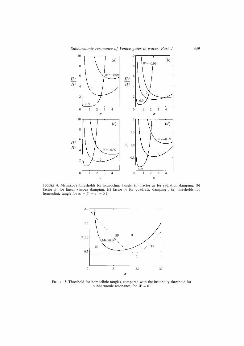
On the other hand, for given values of the dissipation coefficients, (5.15) has anonlinear dependence on both the detuning of the carrier wave W and on thefrequency of modulation σ. Figure 4 shows the dependence of the threshold on σ forW = −0.99, 0, 0.9. First, the coefficients of the three damping coefficients α1, β1, γ1,

Πα(W )

Πa(σ,W ),

Πβ(W )

Πa(σ,W ),

Πγ(W )

Πa(σ,W ), (5.16)

are shown in figure 4(a, b, c). Then in figure 4(d) the threshold (5.15) is displayed forα1 = β1 = γ1 = 0.1. For different W the three ratios in (5.16) depend similarly onσ. They all have a minimum which decreases in magnitude and shifts towards lowerfrequency for larger W . Hence positively detuned carrier waves with low frequencyof modulation can lead to homoclinic tangles even with very small a.

It can also be shown that for a given σ and varying W , the threshold a1 has aminimum which decreases with σ, and moves towards positive W .

Let us compare the period-doubling threshold with the threshold for homoclinictangles. Multiplying (4.21) by µ2 we get the threshold for period doubling in terms ofσ = 2

(λ+ µ2d2

)and a:

σ = 2

λ±[a2

(λ

4+

1

λ

)2

−(λ2

2α+ β +

3

4λγ

)2]1/2

− 2β

λ

, (5.17)

where λ = 2 (1−W )1/2. Similarly multiplication of (5.15) by µ yields

a =Πα(W ) α+Πβ(W ) β +Πγ(W ) γ

Πa(σ,W ). (5.18)


10

4

2

0

(c)

1 2

σ3 4

8

6Π γ

ΠaW = –0.99

0

2

1.0

0.5

0

(d )

1 2

σ3 4

1.5

a1

W = –0.99

0

10

4

2

0

(a)

1 2

σ3 4

8

6Π α

Πa

W = –0.99

0

10

4

2

0

(b)

1 2

σ3 4

8

6Π β

Πa

W = –0.99

0

0.90.9

0.9

Figure 4. Melnikov’s thresholds for homoclinic tangle. (a) Factor α1 for radiation damping; (b)factor β1 for linear viscous damping; (c) factor γ1 for quadratic damping ; (d) thresholds forhomoclinic tangle for α1 = β1 = γ1 = 0.1

2.0

1.5

1.0

0.5

0

a

λ 2λ

σ

TP

IISP

III

Melnikov

I

3λ

Figure 5. Threshold for homoclinic tangles, compared with the instability threshold forsubharmonic resonance, for W = 0.


10

4

2

0

(c)

1 2

σ3 4

8

6Π γ

Πa

W = –1.5

–1.01

2

1.0

0.5

0

(d )

1 2

σ3 4

1.5

a1

W = –1.5

–1.01

10

4

2

0

(a)

1 2

σ3 4

8

6Π α

Πa

W = –1.5

–1.01

10

4

2

0

(b)

1 2

σ3 4

8

6Π β

Πa

W = –1.5

–1.01

–1.01

–1.01

–1.5

–1.5

–1.01

–1.5

–1.01

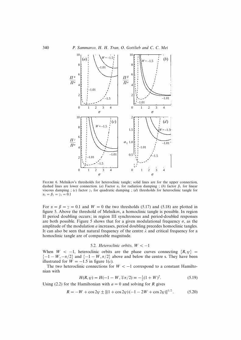
Figure 6. Melnikov’s thresholds for heteroclinic tangle; solid lines are for the upper connection,dashed lines are lower connection. (a) Factor α1 for radiation damping ; (b) factor β1 for linearviscous damping ; (c) factor γ1 for quadratic damping ; (d) thresholds for heteroclinic tangle forα1 = β1 = γ1 = 0.1

For α = β = γ = 0.1 and W = 0 the two thresholds (5.17) and (5.18) are plotted infigure 5. Above the threshold of Melnikov, a homoclinic tangle is possible. In regionII period doubling occurs; in region III synchronous and period-doubled responsesare both possible. Figure 5 shows that for a given modulational frequency σ, as theamplitude of the modulation a increases, period doubling precedes homoclinic tangles.It can also be seen that natural frequency of the centre λ and critical frequency for ahomoclinic tangle are of comparable magnitude.

5.2. Heteroclinic orbits, W < −1

When W < −1, heteroclinic orbits are the phase curves connecting R, ψ =−1−W,−π/2 and −1−W,π/2 above and below the centre s. They have beenillustrated for W = −1.5 in figure 1(c).

The two heteroclinic connections for W < −1 correspond to a constant Hamilto-nian with

H(R, ψ) = H(−1−W,∓π/2) ≡ − 12(1 +W )2. (5.19)

Using (2.2) for the Hamiltonian with a = 0 and solving for R gives

R = −W + cos 2ψ ± [(1 + cos 2ψ) (−1− 2W + cos 2ψ)]1/2 . (5.20)


Substitution in f2 of (5.4) gives a first-order equation in ψ only:

ψT = ± 1

2 cosψ(−W − 1 + cos2 ψ

)1/2, (5.21)

which can be integrated subject to the initial conditions at T = T0, ψh±(0;W ) = 0.

Rh± can then be obtained from (5.20). Finally, the heteroclinic orbits Rh±, ψh± are

Rh±(T − T0;W ) = −(1 +W )(−W )1/2 cosh [2κ (T − T0)]± 1

(−W )1/2 cosh [2κ (T − T0)]∓ 1, (5.22)

ψh±(T − T0;W ) = arctan

(W

1 +W

)1/2

sinh [2κ (T − T0)]

, (5.23)

where the ± superscript refers to the upper and lower orbits and κ is the shorthand for

(−1−W )1/2; note that Rh± satisfies the initial condition Rh±(0;W ) =[(−W )1/2 ± 1

]2

.

Upon substitution of (5.22) (5.23) into (5.9) we obtain for each of the two orbits aMelnikov function which has the same form as (5.10), but with

Πα±(W ) = ∓4W

[(W − 2)

(arctan κ−

π0

)+ 3κ

], (5.24)

Πβ±(W ) = ±4

[W

(arctan κ−

π0

)+ κ

], (5.25)

Πγ±(W ) = ±4 (1 +W )2 [W (1 +W )]1/2

∫ ∞−∞

dT cosh [2κ (T − T0)]

×

(−W )1/2 cosh [2κ (T − T0)]± 11/2

×

(−W )1/2 cosh [2κ (T − T0)]∓ 1−5/2

, (5.26)

Πa±(σ,W ) = πσ2

cosh

σ

[arccos

(1/ (−W )1/2

)−π0

]/2κ

sinh

(πσ /2κ

) . (5.27)

Πα±, Πβ± and Πa± are found analytically. Πγ± can be evaluated only numerically.Details are given in Sammarco (1996).

In figure 6(a, b, c) the three ratios of (5.16) are plotted for the lower and upperorbits respectively by dashed and solid lines. With the same line styles, figure 6(d)shows the thresholds for α1 = β1 = γ1 of the two orbits.

For each orbit the contributions from the three dissipation sources (radiation, linearand quadratic viscous) behave similarly. As the detuning frequency W decreases from−1, the thresholds increase for both the upper orbits (solid lines) and the the lowerorbit (dashed line). Note that for detuning increasingly closer to −1, horseshoe tanglesof the lower orbit occur practically at a1 = 0 and for increasingly smaller frequency.

On the other hand the threshold for the upper orbit is very high (a1 > 1). Bytaking the limit W → −1 of expressions (5.11) to (5.14) and of (5.24)+ to (5.27)+ (orby simply comparing figures 4 and 6) it can be seen that as W → −1 the thresholdfor the upper heteroclinic orbit approaches the threshold for the homoclinic orbit,in agreement with the fact that the heteroclinc orbits reduce to homoclinic orbitswhen W = −1. In the same limit, the threshold for the lower heteroclinic orbit has


(a)

2.44

2.98

1.82

Continuation of sidewalls

Al beam for potentiometers

Al ramp

Gates

Sidewalls

Wave paddles

4.81

3.08

0.83

0.46Al base plate

0.623.

650.

63

2.63

Bea

ch

(b)

9.0

19.9

Base

Styrofoam

3.5

1.3

12.4Adapter for arm

71.9

Styrofoam

Hinge

SS screw

Base Nylon bearing

Front Side

66.0

1.9

Top

24.9

12.7

5.1

Figure 7. (a) Wave basin setup. Dimensions in m. (b) Model gate in the basin experiment.Dimensions in cm.

a minimum that tends to zero; however the area above the threshold curve alsodimnishes to zero, i.e. both the left- and right-branches of the threshold curve tendsto the line σ = 0. Thus it is the threshold of the upper heteroclinic orbit that matters.

We have performed many numerical simulations based on direct integration of (2.1)or, equivalently, (2.4). For brevity we shall only discuss results corresponding to the


laboratory experiments with a view to uncovering the various bifurcations includingchaos. The experiments are therefore discussed first.

6. Laboratory observation of envelope bifurcations6.1. The experimental setup

Preliminary tests for the two-gates setup in a narrow flume, as described in Part 1,failed to yield interesting results predicted by the theory, owing to the relatively largedamping contributed by the sidewalls of the flume. We have therefore installed amulti-gate barrier in a wide wave basin. The gate dimensions are slightly differentfrom those in Part 1. The general layout of the experiments is displayed in figure 7(a).

Thirteen hollow gates made of Plexiglas are hinged on a common horizontal axisspanning the entire width at mid-length of a wide channel, as sketched in figure 7(b).Two end gates next to the sidewalls are only half as wide as the other gates, in orderthat the sidewalls serve as two planes of mirror symmetry. The hinges are made ofnylon bearings to reduce friction. Styrofoam is taped on the front and back of thegates to boost buoyancy; its edges are rounded to reduce separation losses. The waterdepth is maintained at 0.83 m.

Free-surface displacements are measured by four conductivity probes on the in-cidence side and three on the transmission side. Gate rotations are recorded byconnecting potentiometers to each of the full-width gates. For this model, the eigen-frequency is ω0/2π = 0.70 Hz. The following coefficients of the evolution equationsare computed theoretically by ignoring the rounded corners

cN = 27.330, cR = 2.271, cF = 1.630. (6.1)

As a preliminary step we find the frictional damping coefficients by giving neigh-bouring gates an equal and opposite rotation from the vertical position, and releasingthem simultaneously. The time series of the free oscillations are used to determinethe best damping coefficients to fit the theoretical curve, as discussed in Part 1. Theresults are

cL = 0.01, cQ = 0.48, (6.2)

which are considerably less than those found in the flume with just two gates. Thesecoefficients are used in all numerical experiments with incident waves.

6.2. Choice of experimental parameters

As noted in the local analysis of §4 and the global analysis of §5, period doublingand homoclinc tangles are easily excited even with low modulational amplitude a,when the carrier wave detuning is such that W → 1. However in this limit theamplitude of the period-doubled limit cycle decreases to zero and becomes hardto detect experimentally. Moreover, in the same limit, λ = 2 (1−W )1/2 → 0. Theforcing frequency σ, which must be around 2λ for a period-doubled (and eventuallychaotic) response to occur, must also be small. Since small modulational frequenciescorrespond to long modulational periods, the neighbourhood of W → 1 woulddemand prohibitively large data storage in experiments.

The global analysis showed that as W decreases from 1 to −1 the amplitudethresholds for the homoclinic (|W | < 1), and upper heteroclinic tangles(W < −1), become increasingly high (see figure 6); chaos is more difficult to gener-ate experimentally. For horseshoe tangles arising from the lower heteroclinic orbit,(W < −1), the threshold also increases as W decreases towards −1 (cf. figure 6).


3

2

1

0

–1

–2

–3–3 –2 –1 0 1 2 3

X (deg.)

(c)

Y (

deg.

)

10–2

0 0.02 0.04 0.06 0.08

Frequency (Hz)

(d )

100

102

104

106

6

4

2

0

–2

–4

–60 50 100 150

t (s)

(a)

Θ (

deg.

)

0.4 0.6 0.8

Frequency (Hz)

(b)

Pow

er s

pect

rum

(de

g2 .

s)

100

102

104

106

108

1.0

Pow

er s

pect

rum

(de

g2 .

s)

Figure 8. Measured gate response for Ω/2π = 0.04 Hz, a = 0.47; Synchronous envelope response.(a) Time series of gate rotation; (b) spectrum of gate rotation; (c) envelope phase portrait andPoincare section ; (d) spectrum of gate envelope.

However, in this limit, interesting dynamics occurs only for small σ, so that the needfor large data storage renders the neighbourhood of W → −1 also impractical forexperiments.

In addition to the considerations above, cross-waves were observed on the incidentside of the finite wave basin, and limit the range of frequencies that can be usedto explore the bifurcation phenomenon for an infinitely long gate system. We havetherefore forcused our measurements around W = 0. Using the values in (6.2), wefind

α = 0.0831, β =0.0061

A′/b′, γ =

0.0719(A′/b′

)1/2. (6.3)

For an incident wave amplitude A′ = 0.015 m and half modal period b′ = 0.250 m,(6.3) gives β = 0.102, γ = 0.293, i.e. α, β, γ = O(0.1). Thus dissipation by waveradiation and in viscous boundary layers is indeed small, while damping by vortexshedding is also not large; therefore the analytical approximations in previous sectionsshould be relevant.

The incident wave is defined by four physical parameters: the carrier wave am-


3

2

1

0

–1

–2

–3–3 –2 –1 0 1 2 3

X (deg.)

(c)

Y (

deg.

)

10–2

0 0.02 0.04 0.06 0.08

Frequency (Hz)

(d )

100

102

104

106

6

4

2

0

–2

–4

–60 50 100 150

t (s)

(a)

Θ (

deg.

)

0.4 0.6 0.8

Frequency (Hz)

(b)

Pow

er s

pect

rum

(de

g.2

s)

100

102

104

106

108

1.0

Pow

er s

pect

rum

(de

g.2

s)

Figure 9. As figure 8 but for a = 0.57; period-two envelope response.

plitude A′, the carrier wave detuning ∆ω, the modulation amplitude A′ and the

modulational frequency Ω. For each carrier wave amplitude A′ and detuning ∆ω, weshall seek a region in the parameter plane (Ω, A′) for which a large variety of modu-lational responses (synchronous, period-doubled, chaotic) occurs within the physicalconstraint of the experiments.

From §4.1, the condition for subharmonic envelope bifurcation σ = 2λ = 4 (1−W )1/2

can be recast as

Ω/ω0

cFA′/b′

= 4

(1− ∆ω/ω0

cFA′/b′

)1/2

or∆ω

ω0

= cFA′

b′− Ω2

16ω20

b′

cFA′, (6.4)

which relates the modulational frequency Ω, the amplitude A′

and detuning ∆ω ofthe carrier wave.

A second condition for subharmonic modulational resonance is that the amplitudeof modulation a = A′/A′ should be larger than the threshold given by the right-handside of (4.20). These two criteria define the regions of interest and provide guidancefor the experiments.


3

2

1

0

–1

–2

–3–3 –2 –1 0 1 2 3

X (deg.)

(c)

Y (

deg.

)

10–2

0 0.02 0.04 0.06 0.08

Frequency (Hz)

(d )

100

102

104

106

6

4

2

0

–2

–4

–60 50 100 150

t (s)

(a)

Θ (

deg.

)

0.4 0.6 0.8

Frequency (Hz)

(b)

Pow

er s

pect

rum

(de

g.2

s)

100

102

104

106

108

1.0

108

Pow

er s

pect

rum

(de

g.2

s)

Figure 10. As figure 8 but for a = 0.87; chaotic envelope oscillations.

6.3. Procedure of observation

With the help of an automated system for wave generation and data acquisition,records are taken for a wide range of incident waves. As in Part 1, the amplitudesof the incident and reflected carrier waves, and the corresponding sidebands aredetermined from their peaks in the Fourier spectra of the free-surface displacementsmeasured at two points x and x+ d on the incidence side.

The time series of the gate rotation contains information regarding the fast oscilla-tions of the trapped mode and the slow oscillations of the envelope modulation. Bythe technique of Hilbert transform (Melville 1983), the time series of the envelope isextracted.

For W = 0, we collected data by scanning over a significant range of both Ωand a. The variety of observed bifurcation scenarios crudely resembles the numericalsimulations. Here we focus attention on the details of observed data for one modula-tional frequency only, Ω/2π = 0.04 Hz; this choice was made because the thresholdof bifurcation is the lowest, as will be shown later. The steady component of theincident wave amplitude is fixed at A = 0.015 m.


3

2

1

0

–1

–2

–3–3 –2 –1 0 1 2 3

X (deg.)

(c)

Y (

deg.

)

10–2

0 0.02 0.04 0.06 0.08

Frequency (Hz)

(d )

100

102

104

106

6

4

2

0

–2

–4

–60 50 100 150

t (s)

(a)

Θ (

deg.

)

0.4 0.6 0.8

Frequency (Hz)

(b)

100

102

104

106

1.0

108

Pow

er s

pect

rum

(de

g.2

s)Po

wer

spe

ctru

m (

deg.

2 s)

Figure 11. As figure 8 but for a = 1.02; chaotic envelope oscillations.

6.4. Observed bifurcation scenarios

Figure 8 shows the measured results for a = 0.47. Note that the left sideband is largerthan the right sideband. We also remark that the inclination of the line joining theorigin and the centre of the limit cycle (and the point Poincare map of the phasecurve) with respect to the X-axis depends on the choice of the initial point in themeasured time series. It can be shown (Tran 1996) that as the initial point is changedalong a measured time series, this line rotates around the origin of the phase plane.The size of the attractors and their distance from the origin and the envelope spectraare however unaffected, hence the rotation is inconsequential dynamically. Physicallythe distance between the centre of the limit cycle and the origin is the mean oscillationamplitude of the time series and measures the energy peak at half the carrier wavefrequency, i.e. at ω0/2π = 0.7 rad s−1. The size of the limit cycle is a measure of themodulation from the mean. We have also found that the phase portraits are affectedstrongly by the precise value of the spectral peak. The resolution of the Fourierspectrum however depends on the sampling rates. A minute shift of the peak value(by, say, 10−7 Hz) can make a single line appear as a thick band We therefore choose


3

2

1

0

–1

–2

–3–3 –2 –1 0 1 2 3

X (deg.)

(c)

Y (

deg.

)

10–2

0 0.02 0.04 0.06 0.08

Frequency (Hz)

(d )

100

102

104

106

6

4

2

0

–2

–4

–60 50 100 150

t (s)

(a)

Θ (

deg.

)

0.4 0.6 0.8

Frequency (Hz)

(b)

100

102

104

106

1.0

108

108

Pow

er s

pect

rum

(de

g.2

s)Po

wer

spe

ctru

m (

deg.

2 s)

Figure 12. As figure 8 but for a = 1.03; frequency down-shift.

the peak frequency by minimizing the size of the Poincare map which should be apoint in principle.

Next, for a larger amplitude, a = 0.57 (figure 9), a period-two modulational responseappears. The asymmetry of the sidebands is again evident.

Around a = 0.77 transition to chaotic oscillations is observed. Figures 10 and 11show the observed results for a = 0.87 and 1.02 which are representative of the regimeof the strange attractor. A period-four bifurcation from the period-doubled orbit hasbeen identified in two cases, a = 0.68 and a = 0.81, only by a small peak at Ω/4.Poincare sections constructed from the measurements are however not sufficientlyclear and are omitted.

Finally for a large amplitude of modulation, a = 1.03, a frequency downshift isevident, as in figure 12. The spectrum of the envelope in figure 12(d) has a dominantpeak at Ω/2 and no energy at Ω. The spectra of the time series in figure 12(b) hasthe peak at ω0 − Ω/2 with two sidebands shifted by ±Ω. Similar data are recordedfor a = 1.13 and a = 1.30 (Tran 1996).


2.0

1.5

1.0

0.5

0 0.02

Ω/2π

a

0.04 0.06 0.08 0.10

Period 1

Period 2

Period 4

Period 8

Period 16

Chaos

Figure 13. Predicted bifurcation scenarios for basin model, W = 0. Shaded areas: numericalsimulation; dashed curves: approximate thresholds for period doubling; solid curve: Melnikovthreshold.

7. Numerical bifurcation scenarios7.1. Homoclinic tangles W = 0

Comprehensive numerical simulations have been performed for −1 < W < 1 to coverthe important part of the parameter plane of a vs. σ (∝ Ω). To see the overall picture,the various scenarios for W = 0 are typical and are summarized in figure 13. Tofacilitate comparison with experiments, numerical integration is first carried out innon-dimensional coordinates; the results are then transformed to physical coordinatesvia

A′

A′= a ≡ A2

A2

, Ω = σω0cFA′

b′. (7.1)

The lowest threshold for period-doubling bifurcation is seen to be at Ω/2π =0.040 Hz. The region of chaotic motion appears in a band bounded from both


4

3

2

1

–1

–2

–3

–4 –2 0 2 4

X (deg.)

(c)

Y (

deg.

)

10–2

0 0.02 0.04 0.06 0.08

Frequency (Hz)

(d )

100

102

104

106

6

4

2

0

–2

–4

–60 50 100 150

t (s)

(a)

Θ (

deg.

)

0.4 0.6 0.8

Frequency (Hz)

(b)

100

102

104

106

1.0

108

0

–4

Pow

er s

pect

rum

(de

g.2

s)Po

wer

spe

ctru

m (

deg.

2 s)

Figure 14. Computed gate response for Ω/2π = 0.04 Hz, a = 0.47. Synchronous response. (a) Timeseries of gate rotation; (b) spectrum of gate rotation; (c) Phase trajectory and Poincare map of gateenvelope; (d) spectrum of envelope.

above and below by subharmonic responses. There is a thin strip of period-fourresponse, embedded in a wider band of chaos, for modulational frequencies rangingapproximately from 0.032 to 0.06 Hz. The numerical thresholds for period-doublingand for global chaos are in qualitative agreement with the approximate analyticalthresholds given by multiple-scales and Melnikov’s method respectively. Similar chartshave been obtained by Sammarco (1996) for different values of α, β, γ and W .

We next present the details of numerical integration of the dynamical system (2.4)by fixing the modulational frequency at Ω/2π = 0.040 Hz for which measurementshave been described in the previous section. The computed time series of the envelopeX(T ), Y (T ) is first transformed to a time series of the gate rotation Θ ′(t′) by usingthe definition (1.4) of ϑ = X + iY :

Θ ′(t′) =

(cFA

′

cNb′

)1/2

(X + iY ) e−iωt′ + ∗ =

(cFA

′

cNb′

)1/2

2[X(t′) cosωt′ + Y (t′) sinωt′

].

(7.2)


4

2

–2

–4 –2 0 2 4

X (deg.)

(c)

Y (

deg.

)

10–2

0 0.02 0.04 0.06 0.08

Frequency (Hz)

(d )

100

102

104

106

6

4

2

0

–2

–4

–60 50 100 150

t (s)

(a)

Θ (

deg.

)

0.4 0.6 0.8

Frequency (Hz)

(b)

100

102

104

106

1.0

108

0

–4

Pow

er s

pect

rum

(de

g.2

s)Po

wer

spe

ctru

m (

deg.

2 s)

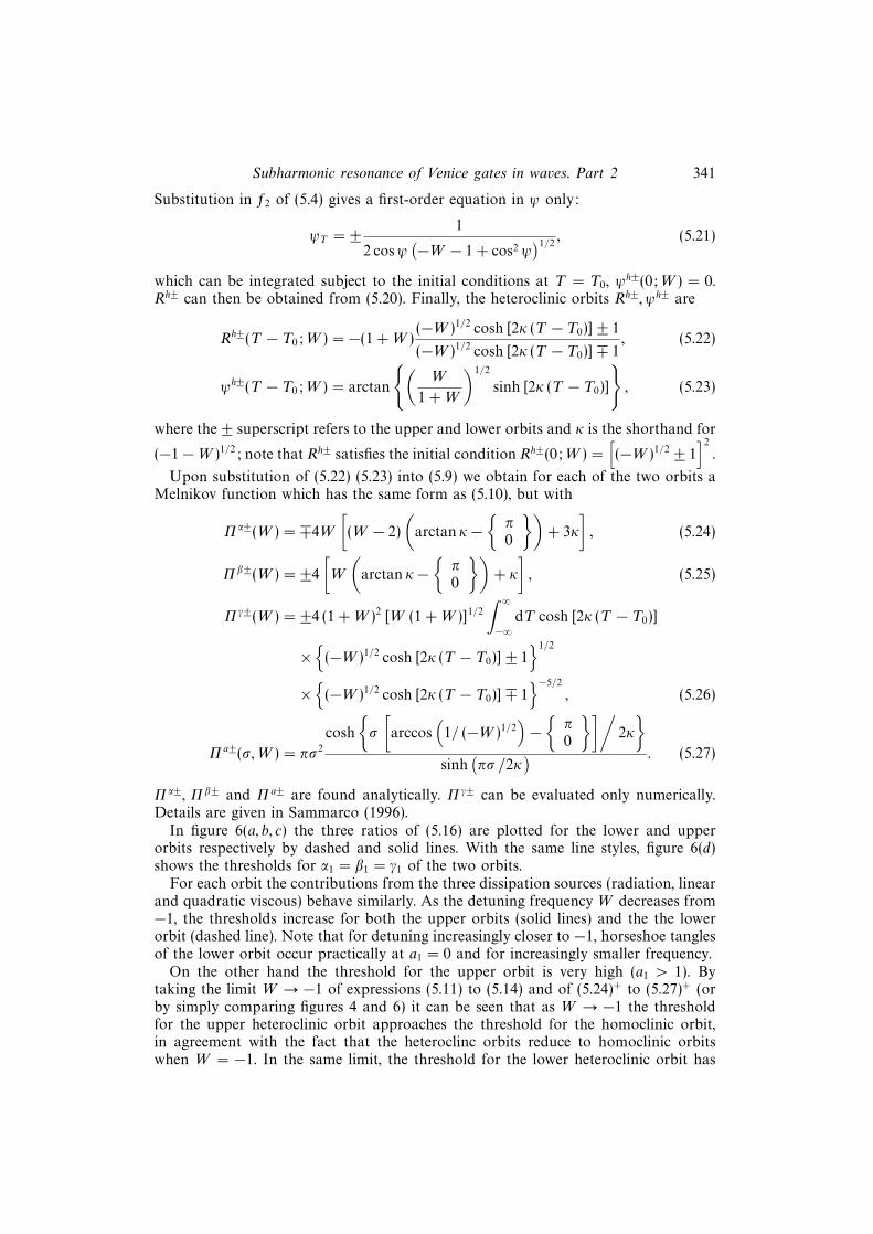
Figure 15. As figure 14 but for a = 0.67; subharmonic response.

Since the detuning of the carrier wave is chosen to be zero, W = 0, in (7.2) ω = ω0.Computed results for increasing a are plotted in groups of figures. In each group(a) gives time series (7.2) of gate displacement, (b) the spectrum of (7.2), (c) thephase-plane trajectories of the envelope in X,Y , and the Poincare map marked bya cross, and (d) the spectrum of the envelope X. The Poincare map is obtained bysampling the time series of the envelope after every interval of 2π/Ω.

For a = 0.47 the response is synchronous, as can be seen in figure 14. The resultsare similar to the observed ones shown in figure 8. Note, in this and following graphs,there is a common feature of all the spectra shown in (b): the left sidebands areconsistently larger than the right sidebands. This agrees with the observed data andappears to be an inherent feature of the Landau–Stuart equation.

Theoretically, for small amplitude a, there are two coexisting limit cycles in theCartesian phase plane X,Y . They lie symmetrically with respect to the origin of thephase plane and represent oscillations of period 2π/Ω around the fixed points s1,2 offigure 1(e). A trajectory tends to one or the other depending on the initial conditions.The corresponding two time series of the angular displacement are identical but fora phase shift equal to π.

The threshold of period doubling is found numerically to be at a = 0.57. When


4

2

–2

–4 –2 0 2 4

X (deg.)

(c)

Y (

deg.

)

10–2

0 0.02 0.04 0.06 0.08

Frequency (Hz)

(d )

100

102

104

106

6

4

2

0

–2

–4

–60 50 100 150

t (s)

(a)

Θ (

deg.

)

0.4 0.6 0.8

Frequency (Hz)

(b)

100

102

104

106

1.0

108

0

–4

108

Pow

er s

pect

rum

(de

g.2

s)Po

wer

spe

ctru

m (

deg.

2 s)

Figure 16. As figure 14 but for a = 0.77. Period-four response.

the modulational amplitude is increased to a = 0.64, subharmonic resonance is fullydeveloped. We show in figure 15 the results for a = 0.67. In (b) the sidebands at(ω0 ± Ω/2)/2π = 0.7 ± 0.02 Hz are strong, as in (d) at (Ω/2)/2π = 0.02 Hz. Thesefeatures are the same as those seen in the experiments for a = 0.57, as shown in figure9. The period-doubled envelope bifurcates to a period-four orbit when a = 0.77. Infigure 16b) a small peak is born at ω0 ± Ω/4 and in (c) four fixed points appear inthe Poincare map. In (d), the subharmonic at

(Ω/4

)/2π = 0.01 Hz is evident.

Chaos is fully developed when a = 0.81, as can be seen in figure 17. The spectrumin (b) maintains its peak at ω0 but is broad-banded. In (c) the strange attractorspreads across the origin, which is a saddle point, to all four quadrants of the phaseplane. Note that the S-shaped skeleton of the strange attractor resembles strongly thehomoclinc orbit in figure 1(e), indicating the effect of homoclinic tangle, i.e. infinitetransverse intersections of the stable and unstable manifolds near the homoclinicconnection of figure 1(e).

For a = 0.87, figure 18 shows that chaos is replaced by period quadrupling with adownshift of the central spectral peak by Ω/4, as is clearly shown in (b), (c) and (d).

When a is increased to a = 0.97, chaotic motion reappears, as shown in figures


5

–5 0 5

X (deg.)

(c)

Y (

deg.

)

10–2

0 0.02 0.04 0.06 0.08

Frequency (Hz)

(d )

100

102

104

106

6

4

2

0

–2

–4

–60 50 100 150

t (s)

(a)

Θ (

deg.

)

0.4 0.6 0.8

Frequency (Hz)

(b)

100

102

104

106

1.0

108

0

–5

Pow

er s

pect

rum

(de

g.2

s)Po

wer

spe

ctru

m (

deg.

2 s)

Figure 17. As figure 14 but for a = 0.81. Chaotic motion.

19(b) and 19(d) . The maximum energy is still around ω0−Ω/4. With further increaseof a, the spectral peak shifts down to

(ω0 − Ω/2

)/2π = 0.68 Hz.

For a = 1.07, chaos disappears again while frequency downshift is complete. Figure20(a) shows that the modulation is strictly periodic while (b) shows the frequencypeak at ω0 − Ω/2, corresponding to the complete depletion of energy at ω0 in (d).The closed trajectory in (c) is symmetrical with respect to the origin. For largermodulational amplitudes a, the response remains subharmonic in the envelope, withthe peak shifted by Ω/2 and increasingly larger phase trajectory in the (X,Y )-plane.The shape and size of the phase portraits are close to those observed experimentally(cf. figure 12 for a = 1.03).

The scenario depicted in figures 14 to 20 is typical of numerical simulations atother frequencies for different ranges of a (Sammarco 1996).

In summary, the theory largely confirms the laboratory observations, althoughnot always at precisely the same modulational amplitudes. In particular the observedsequence of bifurcations leading to aperiodic motion is found in the numerical simula-tions, and the phase-plane geometries of period-doubled orbits and strange attractorsessentially reproduced. In all the experimental spectra the left sideband is alwayslarger than the right sideband; this is confirmed by the theoretical computations.


5

–5 0 5

X (deg.)

(c)

Y (

deg.

)

10–2

0 0.02 0.04 0.06 0.08

Frequency (Hz)

(d )

100

102

104

106

6

4

2

0

–2

–4

–60 50 100 150

t (s)

(a)

Θ (

deg.

)

0.4 0.6 0.8

Frequency (Hz)

(b)

100

102

104

106

1.0

108

0

–5

Pow

er s

pect

rum

(de

g.2

s)Po

wer

spe

ctru

m (

deg.

2 s)

Figure 18. As figure 14 but for a = 0.87. Period-four and downshift by(Ω/4

)/2π = 0.01 Hz.

Moreover, when the modulational wave amplitude a is sufficiently large, the observeddownshift of the central peak of the response is again predicted.

Better agreement would require experiments in a much larger wave basin, sincespurious standing waves have been observed along the wavemakers and on the inci-dence side far from the gates. Such cross-waves result from reasonably large incidentwaves (hence nonlinearity) at certain frequencies within the range of our interest.In addition, rounding of gate corners to reduce damping implies a certain discrep-ancy between the theoretical and experimental geometries, which may also contributeto the discrepancies that remain between numerical predictions and observed data.Needless to say, the realm of the Landau–Stewart equation is limited in its range oftime and amplitude; a more fully nonlinear theory would also reduce the remainingdiscrepancies.

7.2. Heteroclinic tangles, W = −1.5

The dynamics for W < −1 involves heteroclinc tangles and is more complex, anddifficult to study in our laboratory. Figure 21 summarizes the numerical bifurcationscenarios for W = −1.5. The Melnikov threshold for the upper (lower) heteroclinicorbit is shown by the solid (dashed) curve. For low frequencies (< 0.06 Hz), period


5

–5 0 5

X (deg.)

(c)

Y (

deg.

)

10–2

0 0.02 0.04 0.06 0.08

Frequency (Hz)

(d )

100

102

104

106

6

4

2

0

–2

–4

–60 50 100 150

t (s)

(a)

Θ (

deg.

)

0.4 0.6 0.8

Frequency (Hz)

(b)

100

102

104

106

1.0

108

0

–5

Pow

er s

pect

rum

(de

g.2

s)Po

wer

spe

ctru

m (

deg.

2 s)

Figure 19. As figure 14 but for a = 0.97, chaotic motion.

doubling and chaos occur for a considerably above the predicted threshold forheteroclinic tangles (solid line). The region of chaos is limited in size and chaoticmotion does not occur at all for very low frequency. This is consistent with the knownfact that the Melnikov threshold for horshoe tangles is a necessary but not always asufficient condition for global chaos (Moon, Cusumano & Holmes 1987). For higherfrequency (> 0.06 Hz) chaotic behaviour occurs only for relatively large a, and iscloser to the Melnikov threshold for the upper orbit (solid line).

In these numerical simulations, both trivial and non-trivial limit cycles are possible;the solution settles in several cases on the trivial state. Indeed in figure 21 the entireperiod-1 region above the band of chaotic response is the trivial solution.

Sample phase trajectories and resulting Poincare sections are shown for W = −1.5in figures 22(a, b, c) and 22(d, e, f) respectively. Figures 22(a) and 22(d) correspond tothe point in the parameter plane of figure 21 Ω/2π, a = 0.023, 1.29, for whichglobal analysis suggest that only the lower heteroclinc orbit tangles. Figures 22(b)and 22(e) are for Ω/2π, a = 0.045, 2.67, where global analysis admits horseshoetangles for both lower and upper heteroclinic orbits. Finally figures 22(c) and 22(f)are for Ω/2π, a = 0.12, 2.67 where instead tangles occur only for the upper orbit.In this last case the phase trajectory never crosses the X-axis, a feature common to


5

–5 0 5

X (deg.)

(c)

Y (

deg.

)

10–2

0 0.02 0.04 0.06 0.08

Frequency (Hz)

(d )

100

102

104

106

6

4

2

0

–2

–4

–60 50 100 150

t (s)

(a)

Θ (

deg.

)

0.4 0.6 0.8

Frequency (Hz)

(b)

100

102

104

106

1.0

108

0

–5

108

Pow

er s

pect

rum

(de

g.2

s)Po

wer

spe

ctru

m (

deg.

2 s)

Figure 20. Computed gate response for Ω/2π = 0.04 Hz, a = 1.07. Downshift is complete. (a) Timeseries of gate rotation; (b) spectrum of gate rotation; (c) phase trajectory and Poincare map of gateenvelope; (d) spectrum of envelope

all the strange attractors belonging to the band of chaos for Ω/2π > 0.07 of figure21.

8. ConclusionsTo see the effects of finite bandwidth of the incident sea waves on the subharmonic

resonance of the proposed Venice gates, we have considered the simplest modelof a narrow-banded spectrum. The amplitude of the incident wave is periodicallymodulated in time. As a consequence the evolution equation for the envelope ofgate oscillations becomes a second-order non-autonomous dynamical system. Forsmall damping and wave modulation, local bifurcations are analysed by multiple-scale approximations to investigate modulational resonances. The prelude to chaos isanalysed by the Melnikov method for Smale’s horseshoe tangles of either homoclinicor heteroclinic orbits in the phase plane. The approximate criteria for local and globalbifurcations give preliminary guidance for experiments.

Extensive numerical investigation of the above parameter plane corroborates with


1.0

0.04

a

0.12 0.16

Ω/2π

0.5

0

1.5

2.0

2.5

3.0

0.08

Figure 21. Predicted bifurcation scenarios for basin model, W = −1.5. Shaded areas: numericalsimulation; solid curve: Melnikov threshold for upper heteroclinic orbit; dashed curve: Melnikovthreshold for lower heteroclinic orbit.

the analytical predictions, and further delineated the regions of period quadruplingand chaos.

For a fixed modulational frequency in the incident sea, hence sideband widthfrom the carrier wave, the general picture of the gate envelope can be summarizedas follows. For a wavetrain with small periodic modulation a, the gate envelope issynchronous with the wave modulation. Increase of a induces bifurcations through asequence of period doublings until modulational chaos is attained. For higher a abovea band of chaos, the gate envelope returns to the state of subharmonic resonance,which is distinguished from the period doubling at lower a by a phase orbit symmetricabout the origin. In the spectrum of the gate rotation, this state corresponds to adownshift of the central frequency from half the incident carrier wave of a quantityequal to half the modulational frequency. The response here is much larger thanthe non-resonant response to the same modulational wave amplitude but at a largermodulational frequency.

Numerical findings indicate that for sufficiently high frequency of modulation,no temporal resonances of any kind are possible. This means that large sidebandsdo not alter the resonance phenomenon induced by the carrier wave frequency.Specifically the period-doubling bifurcation route to chaos occurs only in suffi-ciently narrow wave sidebands, i.e. when the normalized separation σ of the side-bands from the central peak is around twice the natural frequency of the envelopeλ = 2 (1−W )1/2. For increasingly positive detuning of the carrier wave, i.e. as W → 1,


–4

–5

Y (

deg.

)

–8

0

8

0 5

4

X (deg.)

(d )

–5

–10–10

0

10

0 10

5

X (deg.)

(e)

–4

–5–6

0

6

0 5

4

X (deg.)

( f )

2

–2

–4

–5

Y (

deg.

)

–8

0

8

0 5

4

(a)

–5

–10–10

0

10

0 10

5

(b)

–4

–5–6

0

6

0 5

4

(c)

2

–2

Figure 22. Sample strange attractors forW = −1.5. (a, b, c) Phase-plane trajectories. (d, e, f) Poincaresections. (a, d) Ω/2π = 0.023 Hz, a = 1.29. (b, e) Ω/2π = 0.045 Hz, a = 2.67. (c, f) Ω/2π = 0.12 Hz,a = 2.47.

modulational instability occurs for sidebands increasingly close to the central peak,and over a much longer time scale. On the other hand, as W decreases (negative de-tuning ∆ω), the thresholds for homoclinic or heteroclinic tangles and period doublingincrease significantly. These findings should be helpful in the gate to avoid unwantedresonances.

In the present study, attention has been limited to a single mode. It is known inother physical contexts that chaotic motion can occur as a consequence of nonlinearinteraction between adjacent modes (Ciliberto & Gollub 1984 for Faraday waves, orMei & Zhou 1991 for bubble resonance by sound). Since adjacent gate modes can beclose according to the linearized theory of Mei et al. (1994), modal interaction is anaspect worth investigating both theoretically and experimentally.

In the proposed design, the Venice gates are inclined at 50 from the horizon. Itis likely that gate evolution equation will remain of Landau–Stuart type. However,both the first-order theory for the trapped modes, and the higher-order theory for


computing the coefficients of the Landau–Stuart equation must require the numericalsolution of a number of wave–body interaction problems.

Finally, the effects of long-scale modulation along the barrier may require the studyof a nonlinear Schrodinger equation with a time-dependent coefficient; the likelihoodof spatial-temporal chaos should be interesting. Neglected in the present study, thedifference in mean sea levels on two sides of the barrier in a storm also warrantadditional efforts in the future.

We thank Professor Alberto Noli, University of Rome, and Professor Attilio Adami,University of Padua, for their encouragement which initiated the authors’ interests inthis problem. Funding has been provided by grants from US Office of Naval Research(Accelerated Research Initiative on Nonlinear Ocean Waves directed by Dr T. Swean(Grants Nos. N00014-92-J-1754, and N00014-95-1-8040 (AASERT)), US NationalScience Foundation (Grants Nos. CTS-9115689 and CTS 9634120 ) directed by DrsS. Traugott and R. Arndt, and Consorzio Venzia Nuova for laboratory equipments.

REFERENCES

Agnon, Y. & Mei, C. C. 1985 Slow-drift motion of a two-dimensional block in beam seas. J. FluidMech. 151, 279–294.

Ciliberto, S. & Gollub, J. P. 1985 Chaotic mode competition in parametrically forced surfacewaves. J. Fluid Mech. 158, 381–398.

Guckenheimer, J. & Holmes, P. 1983 Nonlinear Oscillations, Dynamical Systems, and Bifurcationsof Vector Fields. Springer.

Jiang, L., Ting, C., Perlin, M. & Schultz, W. W. 1996 Moderate and steep Faraday wavesinstabilities, modulation and temporal asymmetries. J. Fluid Mech. 329, 275–307.

Jordan, D. W. & Smith, P. 1986 Nonlinear Ordinary Differential Equations. Clarendon.

Lo, E. & Mei, C. C. 1985 A numerical study of water-wave modulation based on a higher-ordernonlinear Schrodinger equation. J. Fluid Mech. 150, 395–416.

Mei, C. C., Sammarco, P. Chan, E. S. & Procaccini, C. 1994 Subharmonic resonance of proposedstorm gates for Venice Lagoon. Proc. R. Soc. Lond. A 444, 463–479.

Mei, C. C. & Zhou, X. 1991 Parametric resonance of a spherical bubble J. Fluid Mech. 229, 29–50.

Melville, W. K. 1983 Wave modulation and breakdown. J. Fluid Mech. 128, 489–506.

Moon, F. C., Cusumano, J. & Holmes, P. J. 1987 Evidence for homoclinic orbits as a precursor tochaos in a magnetic pendulum. Physica 24D, 383–390.

Sammarco, P. 1996 Theory of subharmonic resonance of storm gates for Venice Lagoon. PhD thesis,MIT, Dept. of Civil & Environmetal Engineering.

Sammarco, P., Tran, H. H. & Mei, C. C. 1997 Subharmonic resonance of Venice gates in waves.Part 1. Evolution equation and uniform incident waves. J. Fluid Mech. 349, 295–325.

Tran, H. 1996 Experiments on subharmonic resonance of storm gates for Venice Lagoon. MS thesis,MIT, Dept. of Civil & Environmetal Engineering.

Trulsen, K. & Mei, C. C. 1995 Modulation of three resonanting gravity–capillary waves by a longgravity wave. J. Fluid Mech. 290, 345–376.

Subharmonic resonance of Venice gates in waves. Part 2. Sinusoidally modulated incident waves

Documents

Transcript of Subharmonic resonance of Venice gates in waves. Part 2. Sinusoidally modulated incident waves