arX

iv:0

709.

2075

v1 [

hep-

ph]

13

Sep

2007

Detecting Chameleons through Casimir Force Measurements

Philippe Brax,1 Carsten van de Bruck,2 Anne-Christine Davis,3 David F. Mota,4 and Douglas Shaw3

1 Service de Physique Theorique CEA/DSM/SPhT,Unite de recherche associee au CNRS, CEA-Saclay F-91191 Gif/Yvette cedex, France.

2 Department of Applied Mathematics, The University of Sheffield,Hounsfield Road, Sheffield S3 7RH, United Kingdom

3Department of Applied Mathematics and Theoretical Physics,Centre for Mathematical Sciences, Cambridge CB2 0WA, United Kingdom

4Institut fur Theoretische Physik, Universitat Heidelberg,Philosophenweg 16/19, D-69120 Heidelberg, Germany

The best laboratory constraints on strongly coupled chameleon fields come not from tests of gravityper se but from precision measurements of the Casimir force. The chameleonic force between twonearby bodies is more akin to a Casimir-like force than a gravitational one: The chameleon forcebehaves as an inverse power of the distance of separation between the surfaces of two bodies, justas the Casimir force does. Additionally, experimental tests of gravity often employ a thin metallicsheet to shield electrostatic forces, however this sheet mask any detectable signal due to the presenceof a strongly coupled chameleon field. As a result of this shielding, experiments that are designed tospecifically test the behaviour of gravity are often unable to place any constraint on chameleon fieldswith a strong coupling to matter. Casimir force measurements do not employ a physical electrostaticshield and as such are able to put tighter constraints on the properties of chameleons fields witha strong matter coupling than tests of gravity. Motivated by this, we perform a full investigationon the possibility of testing chameleon model with both present and future Casimir experiments.We find that present days measurements are not able to detect the chameleon. However, futureexperiments have a strong possibility of detecting or rule out a whole class of chameleon models.

PACS numbers: 14.80.-j, 12.20.Fv

I. INTRODUCTION

One of the most common predictions made by modern theories for physics beyond the standard model is theexistence of light scalar fields. It is usually the case that these fields couple to matter and hence mediate a new (or‘fifth’) force between bodies. To date, however, no such new force has been detected, despite numerous experimentalattempts to do so [1]. Any force associated with light scalar fields must therefore be considerably weaker than gravityover these scales, and under the conditions, that have so far been probed experimentally. This imposes a strongconstraint on the properties of any new scalar fields; they must either interact with matter much more weakly thangravity does, or they must be sufficiently massive in the laboratory so as to have remained undetected. If the mass,mφ, of the scalar field is a constant then one must require that ~c/mφ . 0.1 mm if the field is to couple to matter witha strength equal to that of gravity. The bounds on fields whose interactions with matter have a super-gravitationalstrength are even tighter [1].

It has recently be shown, however, that the most stringent experimental limits on the properties of light scalarfields can be exponentially relaxed if the scalar field theory in question possesses a chameleon mechanism [2, 3]. Thechameleon mechanism provides a way to suppress the forces mediated by the scalar fields via non-linear field self-interactions. A direct result of these self-interactions is that the mass of the field is no longer fixed but depends on,amongst other things, the ambient density of matter. The properties of these scalar fields therefore change dependingon the environment; it is for this reason that such fields have been dubbed chameleon fields. Importantly, Chameleonfields could potentially also be responsible for the observed late-time acceleration of the Universe [4, 5]. If this doesindeed turn out to be the case, it raises the exciting prospect of being able to directly detect, probe and potentiallyeven manipulate dark energy under controlled laboratory conditions. The properties of chameleon field theories areconstrained by experimental tests of gravity, however, as a result of their chameleonic behaviour, theories in which thefields and matter interact with at least gravitational strength are not currently ruled out [2, 3]. Indeed, laboratory-based gravitational tests alone cannot even place an upper bound strength of chameleonic interactions with matter [3].It was recently shown that some strongly-coupled (i.e. compared to gravity) chameleon theories predict alterationsto the way in which light propagates through the vacuum in the presence of a magnetic field [6, 7]; the resultantbirefringence and dichroism could be detected by laboratory searches for axion-like-particles e.g PVLAS, Q&A andBMV [9].

In Ref. [3] it was shown that the best laboratory constraints on strongly coupled chameleon fields come not fromtests of gravity per se but from precision measurements of the Casimir force. In some ways this is not surprising. As

2

we shall see, the chameleonic force between two nearby bodies is, in many ways, more akin to a Casimir-like forcethan a gravitational one. Much like the Casimir force, the chameleonic force generally depends only very weakly onthe composition and density of the test masses and in one class of theories, the chameleon force behaves as an inversepower of the distance of separation between the surfaces of two bodies. Additionally, unlike gravitational forces, thechameleonic force can be shielded [3].

Experimental tests of gravity often employ a thin metallic sheet to shield electrostatic forces, however this sheetwas also shown in Ref. [3] to mask any detectable signal due to the presence of strongly coupled chameleon fields.This is because, in such theories, the shield develops what is known as a thin-shell. This means that the range of thechameleon field, λφ = ~c/mφ, inside the metallic sheet is much smaller than the thickness of the sheet, dshield. Inexperimental tests of gravity, one measures the force or torque on one test mass (‘the detector’) due to the movementor rotation of another (’the attractor’). The electrostatic shield sits between the two. The shield is held fixed relativeto the the detector and is uniform. As a result, residual forces due to the shield itself do not result in any detectableeffect. In chameleon theories, the electrostatic shield attenuates the chameleonic force (or torque) due to the attractorby a factor of exp(−mφdshield). If mφdshield ≫ 1, the electrostatic shield therefore acts as a near perfect shield ofthe chameleonic force due to the attractor. Since mφ is larger for strongly coupled fields than it is in more weaklyinteracting ones, experiments that are designed to specifically test the behaviour of gravity are often unable to placeany constraint on chameleon fields with a strong coupling to matter. Casimir force measurements, on the other hand,do not employ a physical electrostatic shield and as such are able to put tighter constraints on the properties ofchameleons fields with a strong matter coupling than tests of gravity.

A preliminary analysis of the constraints on chameleon fields provided by Casimir force measurements was madein Ref. [3]. In this paper we refine, extend and generalize this earlier study. Our primary aim is to extract thebounds that measurements of the Casimir force currently place on chameleon theories and to make predictions forwhat near future Casimir experiments will be able to detect. We shall see that there is a very real prospect thatthe next generation of Casimir force experiments will be able to detect or rule out most chameleonic models of darkenergy.

This paper is organized as follows: In Section II we introduce the chameleon model in greater detail as well as theconcept of a thin-shell. When dealing with gravitational tests, it is generally the case that if the test masses have thin-shells, then all detectable effects due to chameleon fields are exponentially attenuated. In Casimir force experiments,however, the opposite is true. This is because when very small separations are used, the gradient of chameleon forceis largest for thin-shelled test bodies, and Casimir tests are generally most sensitive not to the magnitude of anynew forces but to their gradients. In Section III we present the conditions that must be satisfied for a test bodyto have a thin-shell. In Section IV we derive the form of the chameleonic force between two nearby bodies suchas those used to measure the Casimir force. These results are applied in Section V to predict the extra force thatshould be detected by Casimir force measurements if chameleon fields exist. We also consider to what extent currentexperiments constrain two of the simplest and most widely studied classes of chameleon theories. In the penultimatesection, we then consider the extent to which planned future experiments will be able to extend the constraints onchameleon theories, and identify two proposed tests that have the sensitivity to detect or rule out most chameleontheories in which the chameleon potential is associated with dark energy. We conclude in VII with a discussion of ourresults.

II. CHAMELEON THEORIES

A. The Action

As was mentioned above, chameleon theories are essentially scalar field theories with a self-interaction potentialand a coupling to matter; they are specified by the action

S =

∫

d4x√−g

(

1

2κ24

R − gµν∂µφ∂νφ− V (φ)

)

(1)

+ Sm(eφ/Migµν , ψm), (2)

where φ is the chameleon field, Sm is the matter action and ψm are the matter fields; V (φ) is the self-interactionpotential.

The strength of the interaction between φ and the matter fields is determined by the one or more mass scales Mi.In general, we expect different particle species to couple with different strengths to the chameleon field i.e. a differentMi for each ψm. Such a differential coupling generally leads to violations of the weak equivalence principle (WEPhereafter). Constraints on any WEP violation are very tight [1]. Importantly though, it has been shown that V (φ)

3

can be chosen so that any violations of WEP are too small to be have been detected thus far [2, 3]. Even though theMi are generally different for different species, if Mi 6= 0, we expect Mi ∼ O(M) where M being some mass scaleassociated with the theory. In this paper we are concerned with those signatures of chameleon theories that could bedetected through measurements of the Casimir force. Since these measurements place bounds on the magnitude (orgradient) of close range forces rather than on any violation of WEP, and since also all that matters in this context isthe coupling of the chameleon field to atoms rather than any more exotic form of matter, allowing for different Mi isan usually an unnecessary complication. Henceforth, we assume a universal coupling Mi = M for all i and take thematter fields to be non-relativistic. The scalar field, φ, then obeys:

�φ = V ′(φ) +eφ/Mρ

M, (3)

where ρ is the background density of matter. The coupling to matter implies that particle masses in the Einsteinframe depend on the value of φ

m(φ) = eφ/Mm0 (4)

where m0 = const is the bare mass. We parametrize the strength of the chameleon to matter coupling by β where

β =MPl

M, (5)

and MPl = 1/√

8πG ≈ 2.4 × 1018 GeV. On microscopic scales (and over sufficiently short distances), the chameleonforce between two particles is then 2β2 times the strength of their mutual gravitational attraction.

If the mass, mφ ≡√

V ′′(φ), of φ is a constant then one must either require that mφ & 1 meV or β ≪ 1 for sucha theory not to have been already ruled out by experimental tests of gravity [1]. If, however, the mass of the scalarfield grows with the background density of matter, then a much wider range of scenarios is possible [2–4]. In highdensity regions mφ can then be large enough so as to satisfy the constraints coming from tests of gravity. At thesame time, the mass of the field can be small enough in low density regions to produce detectable and potentiallyimportant alterations to standard physical laws. Scalar fields that have this property are said to be Chameleon fields.Assuming d lnm(φ)/dφ ≥ 0 as it is above, a scalar field theory possesses a chameleon mechanism if, for some rangeof φ, the self-interaction potential, V (φ), has the following properties:

V ′(φ) < 0, V ′′ > 0, V ′′′(φ) < 0, (6)

where V ′ = dV/dφ. Whether or not the chameleon mechanism is both active and strong enough to evade currentexperimental constraints depends partially on the details of the theory, i.e. V (φ) and M , and partially on the initialconditions (see Refs. [2–4] for a more detailed discussion). For exponential matter couplings and a potential of theform:

V (φ) = Λ40 exp(Λn/φn) ≈ Λ4

0

(

1 +Λn

φn

)

(7)

the chameleon mechanism can in principle hide the field such that there is no conflict with current laboratory, solarsystem or cosmological experiments and observations [2, 4]. Importantly, for a large range of values of Λ, the chameleonmechanism is strong enough in such theories to allow even strongly coupled theories with M ≪MPl to have remainedundetected [3]. The first term in V (φ) corresponds to an effective cosmological constant whilst the second term is aRatra-Peebles inverse power law potential. If one assumes that φ is additionally responsible for late-time accelerationof the universe then one must require Λ0 ≈ (2.4 ± 0.1) × 10−12 GeV. In the simplest theories, Λ ∼ O(Λ0) so thatthere is only energy scale in the potential; it is arguable that this represents the most natural scenario. The smallnessof Λ0, means that, as a dark energy candidate, Chameleon theory do not solve either the naturalless problem orthe coincidence problem. However, although it would certainly be desirable to have a model which solved both ofthese problems, one cannot exclude the possibility that the acceleration of the Universe is the first sign of some newphysics associated with an O(Λ0) energy scale. If this is truly the case then one must look for new ways in which toprobe physics at this low energy scale. As we show in this paper, the use of Casimir force experiments to search forchameleon fields is once such probe.

Throughout the rest of this paper, it is our aim to remain as general as possible and assume as little about theprecise form of V (φ) as is necessary. However, when we come to more detailed discussions and make specific numericalpredictions, it will be necessary to chose a particular form for V (φ). In these situations we assume that V (φ) haseither has the following form:

V (φ) = Λ40

(

1 +Λn

φn

)

.

4

or

V (φ) = Λ40 exp(Λn/φn).

We do this not because these forms of V are in any way preferred or to be expected, but merely as they have been themost widely studied in the literature and, in the case of the power-law potential, because is the simplest with whichto perform analytical calculations. The power-law form is also useful as an example as it displays, for different valuesof the n, many the features that we expect to see in more general chameleon theories.

The evolution of the chameleon field in the presence of ambient matter with density ρmatter is determined by theeffective potential:

Veff(φ) = V (φ) + ρmattereφ/M (8)

Limits on any variation of the fundamental constants of Nature mean that, under the conditions that are accessiblein the laboratory, we must have φ/M ≪ 1 [3]. Henceforth we therefore take exp(φ/M) ≈ 1 + φ/M . Even in theorieswhere V (φ) has no minimum of its own (e.g. where it has a runaway form), the conditions given by Eq. (6) on V (φ)ensure that the effective potential has minimum at φ = φmin(ρmatter) where

V ′

eff(φmin) = 0 = V ′(φmin) +ρmatter

M. (9)

B. Thin-shells

In chameleon field theories, macroscopic bodies may develop what has been called a ‘thin-shell’. Generally speaking,a body of density ρc is said to have a thin-shell if, deep inside that body, φ is at, or lies very close to, the minimumof its effective potential (where φ = φc ≡ φmin(ρc) say). We take the density of matter outside the body to be ρb; faroutside the body φ ≈ φb ≡ φmin(ρb).

Thin-shelled bodies are so-called because, for such bodies, almost all of the change in φ (from φb to φc) occurs ina thin region near the surface of the body. The thickness of the part of this thin region that lies inside the body isgenerally ≈ O(1/mc) where mc ≡ mφ(φc). If the body has thickness R then, a necessary (but not sufficient) conditionfor a body to have a thin-shell is mcR ≫ 1.

As a rule of thumb, larger bodies tend to have thin-shells whereas smaller bodies do not. Precisely what is meantby ‘larger’ and ‘smaller’, however, depends on the details of the theory. We discuss this further in Section III below. Ifmb = mφ(φb) is the mass of the chameleon in the background then the chameleon force between two non-thin-shelledbodies, separated by a distance r, is 2β2e−mbr times as strong as their mutual gravitational attraction. Importantly,the force between two thin-shelled bodies is much weaker [2]. Moreover, it has been shown that the chameleonic forcebetween two thin-shelled bodies is, to leading order, independent of the strength, β, with which the chameleon fieldcouples to either body [3]. In a body with a thin-shell, it is as if the chameleon field and the resultant force onlyinteract with and act on the matter that is in the thin-shell region near the body’s surface.

III. THIN-SHELL IN CASIMIR FORCE EXPERIMENTS

Before we can consider the form or magnitude of chameleonic force we need to know whether or not the testmasses used to measure the Casimir force are predicted to have thin-shells. In subsection III A we state the thin-shellconditions for an isolated spherical body in the context of general chameleon theory, which are themselves derivedin Appendix A. We then consider whether these conditions hold for the test masses used in those Casimir forcemeasurements that have been conducted thus far in subsection III B.

A. Thin-Shell Conditions

In general, ‘larger’ bodies have thin-shells whereas ‘smaller’ ones do not. How small is ‘small’, however, generallydepends on the details of the theory. The test-masses used in Casimir force experiments come in a number of differentshapes and sizes. Some experiments used relatively small test masses, with typical length scales of O(102 µm), whilstothers, perhaps most notably that performed by Lamoreaux in 1997 [10], used relatively large test masses with lengthscales of 1 − 10 cm.

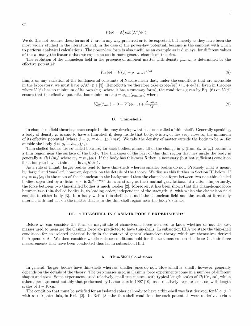
The condition that must be satisfied for an isolated spherical body to have a thin-shell was first derived, for V ∝ φ−n

with n > 0 potentials, in Ref. [2]. In Ref. [3], the thin-shell conditions for such potentials were re-derived (via a

5

different method) and extended to theories with n ≤ −4. The thin-shell conditions for theories with n < −4, n = −4and n > 0 were found to be qualitatively different.

In Appendix A, we derive the thin-shell condition for general V (φ). We consider an isolated spherical body withdensity ρc, radius R in a background with density ρb. We define φb by V ′(φb) = −ρb/M and φc by V ′(φc) = −ρc/M .We also define mb = mφ(φb) and mc = mφ(φc). If mbR ≫ 1 then the body will always have a thin-shell of somedescription as almost all variation in φ will take place in a thin region (of thickness at most ∼ 1/mb) near the surfaceof the body. However, if mc ≈ mb then this thin-shell would be linear, i.e. we would see almost the same behaviourif we considered a Yukawa theory with mass mb (for which the field equations would be linear). In the cases weconsider, however, ρc ≫ ρb and so necessarily mc ≫ mb. If mcR is large enough then, whatever the value of mbR, abody may have a non-linear thin-shell. Non-linear thin-shells are associated with the dominance, near the surface ofthe body, of non-linear terms in the field equations. Such behaviour would not occur in theories where φ has only aYukawa coupling to matter. This non-linear behaviour is key in allowing chameleon theories to evade the stringentexperimental constraints on the coupling of a scalar field to matter that exist for Yukawa theories. In Appendix Awe find that a necessary and sufficient condition for a non-linear thin-shell, in a general chameleon theory, is:

C =(ρc − ρb)f(mbR)R2

2M [m2bR

2 +mbR+ 1]& φb − φc −

(ρc − ρb)(1 − f(mbR))

Mm2c

, (10)

where this defines C. An equivalent statement of this condition is:

m2cR

2

m2bR

2 +mbR+ 1&

2Mm2c (φb − φc)

(ρc − ρb)f(mbR)− 2(1 − f(mbR))

f(mbR)≥ 2. (11)

We have defined:

f(mbR) = 2e−mbR cosh(mbR)

[

1 +1

mbR+

1

m2bR

2

](

1 − tanhmbR

mbR

)

.

As mbR → 0, f(mbR) → 2/3 and as mbR → ∞, f(mbR) → 1.Far from a spherical body with a non-linear thin-shell φ has the form:

φ ≈ φb −CthinRe

mb(R−r)

r,

where

Cthin(1 +mbR+m2bR

2)

V ′(φb) − V ′(φb − Cthin)=R2

2.

We note that Cthin = Cthin(R, φb) and is therefore independent of ρc/M . It follows that, in all chameleon theories, farfrom a body with a non-linear thin-shell φ is independent of ρc/M i.e. it is independent of the strength with whichthe chameleon field couples to the matter in the body. This, more than anything else, is what makes it so difficult forexperimental tests of gravity to place a lower bound on M .

In many cases, it is only necessary to consider the following sufficient condition for a thin-shell:

C & φb − φc,

where C is given by Eq. (10).

B. Applying the Thin-Shell Conditions

We now consider whether or not the test masses used in experimental measurements of the Casimir force aregenerally predicted to have non-linear thin-shells. The above thin-shell conditions are valid for isolated, sphericalbodies. Generally, however, at least one of the test masses used in Casimir force measurements is neither isolated norspherical. Isolated in this case means that there is enough space between the body in consideration and any otherbodies for, in all directions, mφ(φ) to have decreased to be about mb before any other body is encountered.

Generally speaking, mφ → mb over a distance of about 1/mb. We therefore take an isolated body to be one outsidewhich there is a region of thickness at least & 1/mb in which ρ ≈ ρb.

For isolated non-spherical bodies, such as rectangular plates with volume V and longest dimension 2D, the abovethin-shell conditions still apply (to a good approximation) provided one replaces R by

√

3V/4πD (i.e. one should

6

replace R2 by the volume divided by the longest distance from the centre of mass of the body and its surface). Iftwo plates with volumes V1 and V2 and longest dimensions 2D1 and 2D2 respectively are placed a distance d apart,with d & 1/mb, Eq. (10) gives the thin-condition for each plate with R replaced by

√

3Vi/4πDi for i = 1, 2. If,however, d≪ 1/mb, then plates are not isolated and they effectively count as one mass for the purposes of applyingthe thin-shell conditions. Provided 1/mc is small compared to the smallest dimension of each plate, the thin-shell

condition for both plates is then given by Eq. (10) but with R =√

3Vtot/4πDtot where Vtot is the total volume of theplates (excluding the space in between them) and Dtot is the half longest dimension of the two plates when consideredas a single object.

The overall geometry of the set-ups used for Casimir force measurement is generally quite complicated . Even inexperiments where the test masses are themselves relatively small and thin, the apparatus that surrounds them is not.Furthermore, the test masses are generally not isolated in the sense defined above. This complicates the applicationof the thin-shell conditions, and generally it can only be done thoroughly within the context of a specific chameleontheory or class.

For definiteness and as an example we consider theories where V (φ) has a Ratra-Pebbles form V (φ) = Λ40(1 +

(Λ/φ)n), where n > 0. We take Λ40 = 2.4 × 10−3 eV so that the constant term in the potential is responsible for the

late time acceleration of the Universe and specifically consider theories where Λ ≈ Λ0. In Casimir force experimentsthe test masses are much denser than the laboratory vacuum in which they sit and so we take ρc ≫ ρb; this impliesthat φc ≪ φb since n > 0. Given these considerations, the thin-shell condition, Eq. (10), simplifies to:

C ≡ ρcR2f(mbR)

2M(1 +mbR +m2bR

2)& φb.

Since ρc ≫ ρb if mbR & 1 then this condition is automatically satisfied. We therefore restrict our attention to thosecases where mbR ≪ 1. For ρc ≫ ρb and mbR≪ 1, the thin-shell condition is:

GMbody

R&

φb

2β2M,

where Mbody is the mass of the body and β = MPl/M . Note that such a simplification of the thin-shell condition willgenerally occur for all theories where (φ can be shifted so that) φ(ρ) → 0 as ρ ≡ −MV ′(φ(ρ)) → ∞.

We take the pressure of the laboratory vacuum to be p × 10−4 torr, p ∼ O(1) or greater for all Casimir forcemeasurements made to date. We then find that:

φb

2β2M= β−

n+2n+1 p−

1n+1Bn,

where

Bn = 4.9 × 10−31(

5.1n× 1010)

1n+1 .

The largest value of Bn occurs for n ≈ 0.048 at which Bn ≈ 4.5× 10−22 and Bn decreases very quickly to 4.9× 10−31

as n→ ∞. Additionally, as is discussed more fully in Refs. [2, 3], one must be aware that the smallest value that mb

can take in laboratory vacuum which has a smallest length scale Lvac is O(1/Lvac). If a typical value of Lvac = 1 m,we therefore have

φb/2β2M . β−1

[

4.9 × 10−31(

1.5n(n+ 1) × 108)

1n+2

]

< 1.5 × 10−27.

For bodies with ρc ≥ ρglass ≈ 3 g cm−3, we have:

GMbody

R≥ 6.7 × 10−27

(

V

R cm2

)

,

where V is the volume of the body. If we take V to be the volume of the smallest isolated system associated witheither of the test masses, and R = Dlong the longest distance from the surface of this system to its centre of mass,then the test bodies will certainly have thin-shells if:

Reff ≡√

V

Dlong&

1

2√β

cm.

For this choice of potential and |n| ∼ O(1), the Eot-Wash experiment [14] requires that if β ≥ 10−2 and Λ =2.3× 10−3 eV then β must be larger than 102 [3]. For V = Λ4

0(1 + Λn/φn) with Λ = Λ0 = 2.4× 10−3 eV, ‖n‖ ∼ O(1),we have checked that the thin-shell condition certainly holds for the test masses used in the Casimir force experimentsreported in Refs. [10, 15–19] provided β & 103. In other words, it holds for most strongly coupled chameleon theoriesthat are not already ruled out by tests of gravity such as the Eot-Wash experiment.

7

C. Discussion

We found above for V = Λ40(1 + Λn/φ), |n| ∼ O(1) and Λ = Λ0 = 2.4 × 103 eV , the test masses used in all

Casimir force experiments conducted to date are predicted to have thin-shells in all theories with β & 103. In someexperiments, where particularly large test masses are used, the test masses are also predicted to have thin-shells forO(1) values of β.

If V = Λ40f((Λ/φ)n), n > 0, Λ ≈ Λ0 = 2.4 × 10−3 eV where f ′′ > 0 and f is normalized so that f ′ = 1 (e.g.

V = Λ40 exp(Λn/φn), then the potential is always steeper than the Ratra-Peebles form considered above and as such

the thin-shell conditions are less stringent.In the next section we calculate the chameleonic force between two nearby bodies under the assumption that they

have thin-shells. In the absence of thin-shells, the chameleon field behaves in the same way as a Yukawa field, and theconstraints on any Yukawa coupling to matter derived from Casimir force measurements can be directly applied tochameleon theories. There is, therefore, nothing new to say about the non thin-shelled case, and we do not considerit further.

We find below that the gradient in the chameleonic force between two nearby thin-shelled bodies is generally muchsteeper than it would be if there were no thin-shells present. Casimir force experiments generally measure gradientsin forces (changes in forces between two separations). So they are generally more sensitive to relatively small quicklyvarying forces with a steep gradient than they are to large but nearly constant ones. The presence of thin-shelled testmasses is therefore an aide rather than a hindrance to the detection of chameleon fields via Casimir force measurements.The opposite is generally true of gravitational tests [2, 3]. The stronger the matter coupling, the more likely it is thata given body has a thin-shell. Experiments designed along the lines of Casimir force measurements are therefore farbetter suited to the search for strongly coupled chameleon fields than tests that are specifically designed to search forforces with gravitational (or sub-gravitational) strength.

IV. THE CHAMELEONIC ‘CASIMIR’ FORCE

In this section we calculate the Casimir-like force between two nearby bodies due to their interaction with achameleon field. The form of both the Casimir force and the chameleonic force are highly dependent on the geometryof the experiment [3, 11, 12]. The form of these forces is most easily calculated when the geometry is that of twoparallel plates. Making accurate measurements of forces using this set-up is, however, notoriously difficult as itrequires that the plates be both very smooth and held parallel to a high precision. For this reason, most experimentsconducted to date have measured the Casimir force between a plate and a sphere rather than between two plates.Presently the highest precision measurements have been made using the sphere-plate geometry. By measuring thegradient of such a force between a sphere and a plate it is possible to determine the force between two parallel plates.In Section IVA we calculate the chameleon force between two parallel plates, and in Section IVB we calculate thechameleon force for the sphere-plate geometry.

A. Parallel Plates Geometry

The parallel plate geometry is the easiest to study analytically. For simplicity we take both plates to have the samecomposition. We shall see that, provided the plates both have thin shells and are much denser than their environment,the chameleon force is in largely independent of composition of either plate. We take the plates to have thin-shellsand to be separated by a distance d.

We define x = 0 to be the point midway between the two plates; the surfaces of the plates are then at x = ±d/2.In −d/2 < x < d/2 we have:

d2φ

dx2= V ′(φ) − V ′(φb),

where we have defined V ′(φb) = −ρb/M with ρb the ambient density of matter outside the plates. Inside the plateswe have:

d2φ

dx2= V ′(φ) − V ′(φc),

where V ′(φc) = −ρc/M and ρc is the density of the plates. Deep inside either plate φ → const ≈ φc and dφ/dx = 0

8

at x = 0 by symmetry. We use the shorthand φ0 ≡ φ(x = 0). Integrating both of these equations once gives:

(

dφdx

)2

= 2 (V (φ) − V (φ0) − V ′(φb)(φ− φ0)) −d/2 < x < d/2, (12)

(

dφdx

)2

= 2 (V (φ) − V (φc) − V ′(φc)(φ− φc)) x2 > d/4. (13)

We define φs = φ(x = ±d/2), so that φs is the value of φ on the surface of the plates. By matching the aboveequations are x = ±d/2, we arrive at:

φs =V (φc) − V ′(φc)φc − V (φ0) + V ′(φb)φ0

V ′(φb) − V ′(φc). (14)

If one of the plates were to be removed then φs on the surface of the remaining plate (= φs0 say) would be given byEq. (14) but with φ0 → φb. The perturbation, δφs = φs − φs0, in φs due to presence of the second plate is therefore:

δφs =V (φb) − V (φ0) − V ′(φb)(φb − φ0)

V ′(φb) − V ′(φc).

Deep inside either plate the perturbation, δφ, in φ due to the presence of the second plate is exponentially attenuated.This is because the chameleon mass inside either plate mc ≡ mφ(φc) is, by the thin-shell conditions, large comparedto the thickness of the plate.

The attractive force per unit area, Fφ/A, on one plate due to the other is given by:

Fφ

A=

∫ d/2+D

d/2

dxρc

M

dδφ

dx≈ V ′(φc)δφs, (15)

where D is the plate thickness and we have used ρc/M = −V ′(φc). Taking ρc ≫ ρb we then find:

Fφ

A= V (φ0) − V (φb) + V ′(φb)(φb − φ0) ≤ V (φ0) − V (φb). (16)

To leading order in ρb/ρc, Fφ/A depends only on φ0 and φb.To a first approximation, we calculate φ0 by linearizing the equation for φ in −d/2 < x < d/2 about φ0. In

−d/2 < x < d/2 we find:

φ− φ0 =2 (V ′

0 − V ′

b )

m20

sinh2(m0x

2

)

. (17)

where V ′

0 = V ′(φ0) and V ′

b = V ′(φb). If, as is the case in theories with V = Λ40f((Λ/φ)n), n > 0 and f ′ > 0, we

expect that φ on the surface of the plates is very small compared to φ0, then m0 is given approximately by:

sinh2

(

m0d

4

)

≈ m20φ0

2 (V ′

b − V ′

0). (18)

If V = Λ40(1 + Λn/φn) (and n > 0) when mbd≫ 1 this gives:

m0d ≈ 4 sinh−1

√

(n+ 1)

2.

This is a good approximation for n ∼ O(1), but it breaks down for larger values of n. More generally, we mustcalculate m0d by a more complicated method that takes proper account of the non-linear nature of the potential. Wedefine y =

√

V − V0 − V ′

b (φ− φ0) and 1/W (y) = (V ′

b −V ′(φ)) ≥ 0. From the chameleon field equation we then have:

√2

∫ ys

0

W (y)dy =d

2, (19)

where ys = y(φ = φs). The above integral can then either be calculated numerically for a given V (φ) or, as is oftenmore helpful, via an analytical approximation. We show below that for mbd ≫ 1, m0d ∼ O(1). When mc ≫ m0,which therefore corresponds to mcd≫ 1, we have m0ysW0 ≫ 1. It can be checked that, W (y) always decreases faster

9

than 1/y as y increases for y ≫ 1/m0W0. We can therefore approximate Eq. (19) by replacing ys with ∞ as theupper limit of the integral:

√2

∫

∞

0

W (y)dy =d

2,

Since m0 ≤ mc, if mcd . 1 then we must have m0 ≈ mc. In the mcd≫ 1 case, we proceed by defining

k2 =V ′′′

0 (V ′

0 − V ′

b )

m40

, (20)

where a subscript 0 indicates that the quantity is evaluated for φ = φ0, and a subscript b means that it is evaluatedfor φ = φb. When m0 ≫ mb, which we shall see corresponds to mbd≪ 1, k2 is, for many choices of potentials, almostindependent of φ0. The value of k2 dictates the dynamics of the theory, and determines how φ0 depends on d. Weevaluate Eq. (19) approximately in Appendix B. We find that if, as is often the case, 1/3 . k2 ≤ 2, then we candefine

neff = (2 − k2)/(k2 − 1) (21)

leading to

m0d ≈√

2neff + 2

neffB

(

1

2,1

2+

1

neff

)

, (22)

where B(·, ·) is the Beta function. 1/3 . k2 ≤ 2 implies that neff ≥ 0 or neff . −5/2. This approximation becomesexact when V = Λ4 + Λ4(Λ/φ)n and m0 ≫ mb. For such a potential neff = n, and the requirement that m0 ≫ mb

implies mbd≪ 2 (or all n). For very steep potentials, e.g. V = Λ4 exp((Λ/φ)n) when φ0 ≪ Λ, k2 ≈ 1 when m0 ≫ mb.This corresponds to n2

eff → ∞. It is clear that m0d ∼ O(1).

If k2 ≥ 2 then we find in Appendix B that:

m0d ≈ π3/2

2√

2(k2 − 2)(1/2)

[

J2−1/4

(

1

2√k2 − 2

)

+ Y 2−1/4

(

1

2√k2 − 2

)]

, (23)

where J−1/4(·) and Y−1/4(·) are Bessel functions. For small 4(k2 − 2) this gives:

m0d ≈√

2π(

1 − 3(k2 − 2)/8)

,

and if k2 ≫ 2 we have:

m0d ≈ B(

14 ,

14

)

√2k

≈ 5.24√k.

The 1/3 < k2 ≤ 2 and k2 ≥ 2 approximations for m0d are continuous at k2 = 2.In Appendix B, we show that when k2 . 1/3 the analytical approximation used to evaluate φ0(d) for k2 & 1/3

breaks down. When k2 is small it is either because at least one of k20 = V

(3)0 V ′

0/m40 or 1 − V ′

b /V′

0 is small. Theorieswith small k2

0 only exhibit very weak non-linear behaviour near φ0 and so we do not consider them further.It is important to know how Fφ/A behaves as k2 → 0 because as d→ ∞ we have φ0 → φb. In Appendix B we find

that for mbd≫ 5 we have:

mbd

2≈ ln(12) − ln(k2), (24)

and so

Fφ

A∼ 72m6

be−mbd

V ′′′ 2b

. (25)

We have now derived the expressions for Fφ(d)/A for different classes of theory and for different ranges of d. Theseexpression generally consist of an exact expression for Fφ/A as a non-linear function of φ0 and an approximate implicitequation for φ0 as a non-linear function of d. In these cases an explicit equation for Fφ/A as a function of d canonly be found once V (φ) is specified. In the limit d → ∞, it was possible to find an explicit expression for Fφ/A

10

10−2

100

102

104

106

108

10−10

10−8

10−6

10−4

10−2

100

Cha

mel

eoni

c P

ress

ure:

(V

(φc)−

Λ4 0)−

1 Fφ/A

Separation of plates: mc d

Behaviour of Chameleonic Pressure for V = Λ40(1+Λn/φn); n = 1

d = mc−1

d = mb−1

Power−law behaviourExponential

behaviour

Constantforce

behaviour

10−2

100

102

104

106

108

10−15

10−10

10−5

100

Cha

mel

eoni

c P

ress

ure:

(V

(φc)−

Λ4 0)−

1 Fφ/A

Separation of plates: mc d

Behaviour of Chameleonic Pressure for V = Λ40(1+Λn/φn); n = 4

d = mc−1

d = mb−1

Power−law behaviour

Exponential behaviour

Constantforce

behaviour

10−2

100

102

104

106

108

10−25

10−20

10−15

10−10

10−5

100

Cha

mel

eoni

c P

ress

ure:

(V

(φc)−

Λ4 0)−

1 Fφ/A

Separation of plates: mc d

Behaviour of Chameleonic Pressure for V = Λ40(1+Λn/φn); n = −8

d = mc−1

d = mb−1

Power−law behaviour

Exponential behaviour

Constantforce

behaviour

FIG. 1: The dependence of the chameleonic pressure, Fφ/A, between two parallel plates on separation, d. We have takenV (φ) = Λ4

0(1+Λn/φn) and fixed mc/mb = 106. The three plots show the behaviour of Fφ/A for a theory with n = 1, n = 4 andn = −8. Each of these are respectively representative of theories with 0 < n ≤ 2, n > 2 and n ≤ −4. Three types of behaviourare clearly visible in these plots. For d . m−1

c , Fφ/A ≈ Vc −Vb which is independent of d: this is the ‘constant force behaviour’.For m−1

c ≪ d ≪ m−1b , Fφ/A ∝ 1/dp for some p. Theories with 0 < n ≤ 2 have 0 < p ≤ 1. If n > 2 then 1 < p < 2 and if

n ≤ −4 we have 2 < p ≤ −4. This is the ‘power-law behaviour’. Finally when d ≪ m−1b , Fφ/A ∝ exp(−mbd), i.e. we have

‘exponential behaviour’. Note that in a standard Yukawa scalar field theory (where mφ = const) one would have Fφ/A ≈ constfor d ≪ m−1

φ and an exponential drop-off for d & m−1φ ; however there would be no region of power-law behaviour.

as a function of d. We note that when d ≫ m−1c , the leading chameleonic force is independent of mc, and hence

also of the strength with which the chameleon field couples to the body. In general, the approximate expressionsfor φ0(d) derived above should be seen as providing a good order of magnitude estimate for Fφ/A rather than anaccurate numerical prediction. This said, in some cases the expressions found above are actually exact. Specifically,if V (φ) = Λ4

0(1 + Λn/φn) then Eq. (22) is exact (and neff = n) in the limit m−1b ≪ d ≪ m−1

c . Additionally, ifV (φ) = Λ4

0 exp(g(φ/Λ)) and φ0 is such that g′′(φ0Λ)/g′ 2(φ0Λ) ≪ 1 then Eq. (22) with k2 = 1 provides an excellentapproximation when m−1

b ≪ d ≪ m−1c . When one only wishes to consider a specific form of V (φ), numerically

accurate predictions for Fφ/A can be made by performing the integral in Eq. (19) numerically.

We now consider two specific examples. Firstly, if V (φ) = Λ40(1 + Λn/φn) and m−1

c ≪ d≪ m−1b then:

Fφ(d)

A= Λ4

0Kn (Λdd)−

2n

n+2 , (26)

11

where Λd = Λ20/Λ and

Kn =

(

√

2

n2B

(

1

2,1

2+

1

n

)

)2n

n+2

. (27)

In all chameleon theories with power-law potentials, Fφ/A drops off as 1/dp for some p in this regime. In theorieswith 0 < n ≤ 2, 0 < p ≤ 1; if n > 2 1 < p < 2 and if n ≤ −4 we have 2 < p ≤ 4.

If d . m−1c then m0 ≈ mc and so:

Fφ(d)

A≈ Vc − Vb − V ′

b (φc − φb) ≈ Vc − Vb.

where the last approximation holds if ρc ≫ ρb. In this regime, the chameleonic force is independent of d at leadingorder. Finally if d≫ m−1

b we have from Eq. (25):

Fφ

A∼ 72n(n+ 1)Vbe

−mbd

(n+ 2)2.

In FIG. 1 we show the behaviour of the chameleonic pressure, Fφ/A, in all three regimes (d . m−1c , m−1

c ≪ d≪ m−1b

and d ≫ m−1b ) for chameleon theories with n = −8, n = 1 and n = 4. In all cases we have fixed mc/mb = 106. The

n = −8 plot is representative of theories with n ≤ −4 and the n = 4 is representative of theories with n > 2. Then = 1 graph show an example for a theory with 0 < n ≤ 2. The three types of behaviour: constant force for d . m−1

c ,power-law for m−1

c ≪ d ≪ m−1b and exponential drop-off for d ≪ m−1

b are clearly visible in these plots. The maindifference in the behaviour of the force for the different values of n is the slope of Fφ/A in the power-law drop-offregion.

If V (φ) = Λ40 exp(Λn/φn) and again m−1

b ≪ d≪ m−1c , then:

neff =n2/(n+ 1) + 2(φ0/Λ)n + n(φ0/Λ)2n

(φ0/Λ)2n.

For small (Λ/φ)n, we have neff = n and hence Fφ/A is given by Eq. (26); this limit corresponds to m0 ≪ Λd so

d≫ Λd−1. In the opposite limit when m0 ≫ Λd i.e. d≪ Λ−1d , we have instead neff ≈ n2(Λ/φ)2n/(n+ 1) and so:

m20d

2 ≈ 2π2

[

1 +1 − 4 ln(2)

neff

]

.

It follows that:

Fφ(d)

A≈ Λ22π2

n2h(Λdd)2n+2

n d2

[

1 − n+ 1

nh(Λdd)

]

− Λ40, (28)

where h(Λdd) is a slowly varying function of Λdd defined by:

h2+2/neh =2π2

n2(Λ20d/Λ)2

. (29)

The above expression for Fφ/A is valid provided that (n+1)/nh(Λdd) ≪ 1. Note that, in all cases, Fφ(d)/A ∼ O(Λ40)

when d ≈ Λ/Λ20. When d . m−1

c , we have in all cases that:

Fφ

A≈ Vc − Vb + V ′

b (φb − φc).

When d≪ m−1b , Eq. (25) gives the behaviour of Fφ/A.

Note, for comparison,that the Casimir force per unit area between two parallel plates with separation d at zerotemperature is:

Fcas(d)

A=

π2

240d4. (30)

12

B. Sphere-Plate Geometry

Calculating the chameleonic and Casimir forces is simplest for the parallel plate geometry. However, the mostaccurate measurements of the Casimir force have been made using a sphere and a plate. In this geometry, the Casimirforce depends only on the radius of curvature, R, of the curved body, and the distance, d≪ R, between the surfacesof the two bodies at the point of least separation.

We now calculate the chameleonic force between a sphere with radius R and a circular plate with total surface areaA. d is defined to be smallest separation between these bodies. The z direction is defined to be perpendicular to theplate, and we take r to be a radial coordinate which measures the distance from the point of least separation in theplane of the plate. Both the plate and the sphere are assumed to have thin-shells.

In the region between the two bodies the chameleon field satisfies:

dφ2

dz2+

d2φ

dr2+

1

r

dφ

dr= V ′(φ) − V ′(φb). (31)

At r, the separation between the sphere and the plate in the z-direction is

s(r) ≡ d+R

(

1 −(

1 − r2

R2

)

12

)

.

We define φPP(z, s) to be the value of the chameleon field in the parallel plate set-up for plates with separation s.When s ≪ R, we can approximate φ(z, r) in the sphere-plate geometry by φPP(z, s(r)). This approximation is validso long as:

∣

∣

∣

∣

∣

d2φdr2 + 1

rdφdr

d2φdz2

∣

∣

∣

∣

∣

≪ 1.

Now in the parallel plate set-up we found that:

√2

∫ y(φ(z);φ0)

0

W (y′;φ0)dy′ =

s

2− z

2,

where z = 0 is the surface of the plate. We then have:

dφ

ds=

[

W (y)

W (0)− y

W (0)

∫ y

0

1

y′∂W

∂y′dy′]

dφ0

ds− y√

2.

Therefore if V ′(φs)/V′

0 ≫ 1:

dφ0

ds≈ −W (0)

[√2

∫

∞

0

∂W

∂y′1

y′dy′]

−1

. (32)

Inserting the equation for s(r) we arrive at:

d2φ

dz2= −1/W (y),

dφ

dr=

√

R2 − (R + d− s)2

R + d− s(r)

dφ

ds.

It is clear then that the approximation φ ≈ φPP(r, s(r)) is good provided that d ≤ s ≪ R i.e. r, d ≪ R. Allsphere-plate Casimir measurements have d≪ R.

Whenever φ(z, r) ≈ φPP(z, s(r)) we have:

dFφ

dA≈ V (φ0(s(r))) − V (φb) − V ′(φb)(φ0(s(r)) − φb),

and for r ≪ R, dA = 2πr dr ≈ 2πR ds. The contribution to total force between the plate and the sphere from thepoints with r ≪ R is:

Fφ(r) ≈ 2πR

∫ s(r)

0

ds′ [V (φ0(s(r′))) − V (φb) − V ′(φb)(φ0(s(r

′)) − φb)] .

13

We define rmax = min(√

A/π,R) i.e. rmax is the smaller of R and the radius of the circular plate. We also definesmax = s(rmax); smax is then the largest separation between the surfaces of the plate and the sphere. If dFφ/dA dropsoff faster than 1/s for all s & s∗ for some s∗ ≪ R, then the dominant contribution to the total force between thesphere and the plate comes from the region where s≪ R. To a very good approximation we therefore have:

F totφ ≈ 2πR

∫ smax

d

ds′ [V (φ0(s(r′))) − V (φb) − V ′(φb)(φ0(s(r

′)) − φb)] . (33)

In some chameleon theories, however, dFφ/dA drops off more slowly than 1/s for all s . O(R) ≪ m−1b . In these

cases, Eq. (33) is no longer accurate.In all theories dF tot

φ (d)/dd ≈ 2πRdFφ(d)/dA provided d≪ R. By measuring the gradient of F totφ (d), it is therefore

possible to extract the form of dFφ(d)/dA. dFφ(d)/dA is equal to the force per unit area between two parallel plateswith distance of separation d.

It is clear that the dependence of dFφ/dA on s plays an important role. In particular, theories where it drops offmore slower than 1/s behave differently from those where the drop off is faster. When m0 ≫ mb we have:

dFφ

dA≈ V (φ0) − V (φb).

We define Q(φ0;V ) = d ln(V (φ0) − V (φb))/d ln(1/s). If Q(φ0(s);V ) > 1 for all s > s∗ (and < 1 otherwise), wheres∗ ≪ min(smax, 1/mb), then the dominant contribution to the total force comes from points with separations ≈ s∗. Inthese cases Eq. (33) provides a good approximation to F tot

φ . If no such s∗ exists but mbsmax ≫ 1 then the dominant

contribution to F totφ comes from points with separations ≈ 1/mb; in these cases we may also use Eq. (33) to calculate

F totφ . If neither of these conditions hold, then dominant contribution to F tot

φ comes from separations ∼ O(smax). The

assumption that φ ≈ φPP(z, s(r)) fails for s ∼ O(smax) and it is particularly bad if smax ∼ O(R). In these cases thechameleon field equations are too complicated to solve analytically. However, Eq. (33) is still expected to providean order of magnitude estimate for F tot

φ . This is because the assumption that φ ≈ φPP(z, s(r)) only breaks down for

s ∼ O(smax) but holds for all smaller values of s. We therefore, do not expect φ(z, smax) to be very different fromφPP(z, smax) or F tot

φ to be very different from the form given by Eq. (33).

If V = Λ40(1 + Λn/φn) then dFφ(s)/dA drops off more slowly than 1/s when mbs ≪ 1 for −2 < n < 2. Theories

with −2 ≤ n ≤ 0 are not valid chameleon theories. Theories where 0 < n < 2 therefore make qualitatively differentpredictions for F tot

φ than do those where n > 2 or n ≤ −4.

In the sphere-plate geometry (with m−1c ≪ d ≪ R, m−1

b and mbd ≪ 1), the total chameleonic force for theorieswith n > 2 or n ≤ −4 is given to a very good approximation by:

F totφ (d) ≈ 2πΛ2

0ΛR

(

n+ 2

n− 2

)

Kn (Λdd)−

n−2n+2 , (34)

where Kn is given by Eq. (27) and, as above, Λd = Λ20/Λ.

In theories with 0 < n ≤ 2, however, we have:

F totφ (d) ≈ F0(smax,mb) − 2πΛ2

0ΛR

(

n+ 2

2 − n

)

(Λdd)2−n

n+2 . (35)

where F0 is independent of d and is calculated in Appendix C. If mbsmax ≪ 1 then we are only able to find the orderof magnitude of F0:

F0 ∼ 2πΛ20ΛR

(

n+ 2

2 − n

)

Kn (Λdsmax)2−n

n+2 , mbsmax ≪ 1. (36)

If mbsmax ≫ 1, however, we are able to calculate F0:

F0 = 2πΛ20ΛR

(

n+ 2

2 − n

)

KnDn

(

anΛd

mb

)2−n

n+2

, mbsmax ≫ 1. (37)

where

an =

√

2(n+ 1)

nB

(

1

2,1

2+

1

n

)

, (38)

Dn =4n(n+ 1)

(n+ 4)(n+ 2)

(

1 +2 − n

3(n+ 2)βn

)

, (39)

14

and

βn =n+ 2

2n2

[

2(n+ 1)

(

Ψ

(

1

n

)

− Ψ

(

1

2+

1

n

)

+ n

)

− n

]

.

Ψ ( · ) is the Digamma function.If V = Λ4

0 exp(Λn/φn) then for Λdd≪ 1 so that (n+ 1)h(Λdd)/n≪ 1 where h is given by Eq. (29), we found that:

dFφ(d)

dA=

Λ22π2

n2h(Λdd)2n+2

n d2

[

1 − n+ 1

nh(Λdd)+ O(1/f2)

]

,

Since 2(n+1)/(nh) < 1, dFφ/dA drops off faster than 1/d for all n. For (n+1)/(nh(Λdd)) ≪ 1and m−1c ≪ d≪ m−1

b ,the total force between a sphere and a plate is:

F totφ = F1(smax,mb) +

4π3Λ2R

n2h(Λdd)2n+2

n d

[

1 + 3n+ 1

nh(Λdd)+ O(1/h2)

]

. (40)

If Λdsmax ≪ 1 or mb/Λd ≫ 1 then the F1 term is negligible relative to the d-dependant term. If however Λdsmax ≫ 1and mb/Λd ≪ 1, F1 = F0(smax,mb) as given by Eqs. (36 and 37).

For comparison, note that, the total Casimir force between a sphere and a plate is

Ftot =π3R

360d3. (41)

V. PREDICTIONS AND CONSTRAINTS

We now use the results derived above to make specific predictions and derive constraints on theories with eitherV (φ) = Λ4

0(1 + Λn/φn) or V (φ) = Λ40 exp(Λn/φn); Λ0 = 2.4 × 10−3 eV. The simplest and most natural scenario

is Λ ≈ Λ0. With these potentials, the energy density of the chameleon field can be identified with dark energycosmologically. If Λ = 2.4 × 10−3 eV then

Λd = d/ (82.2µm) , Λ4 = 6.92 × 10−3 µdyne cm−2 = 6.92 × 10−7 mPa.

For either of the potentials given above one must require n > 0 or n ≤ −4 for a valid chameleon theory to emerge[3]. When m−1

c ≪ d ≪ m−1b , Eq. (22) is actually exact for theories with power-law potentials. In these power-law

theories, the force per unit area between two parallel plates when m−1c ≪ d ≪ m−1

b is given by Eq. (26). Whenmbd & 5, dFφ/dA is given by Eq. (24). The total chameleon force in the sphere-plate geometry is (when mbd ≪ 1)given by Eq. (34) if n > 2 or n ≤ −4 or by Eq. (35) if 0 < n ≤ 2.

We begin by considering how Casimir force measurements presently constrain chameleon theories, and then discussthe prospects for the detection of chameleon fields by the next generation of such tests in the next section.

The first attempt to measure the Casimir force between two parallel plates was made in 1958 by Sparnaay [15].The data he found contained large systematic errors, due mostly to the determination of d, and so was only said to”not contradict Casimir’s theoretical prediction”. At the largest separations probed (∼ 2µm) this experiment wassensitive to pressures between the two plates of 0.1 mPa (=1 mdyne cm−2), however the inaccuracy in determining dwas generally ±0.12µm. This measurement was conducted in a vacuum with pressure 10−2 torr.

The Casimir force between two parallel plates was successfully measured by Bressi et. al. [16]. They measured theCasimir force between 0.5−3.0µm to an average precision of 15%. This corresponds to a sensitivity of approximately1 mPa. A vacuum pressure with 10−3 torr was used in this experiment.

The most accurate measurements of the Casimir force between two parallel plates have, however, been made bymeasuring the gradient of the force between a sphere and a plate. Dynamical measurements of the force between asphere and a plate would detect not F tot

φ (d) but dF totφ /dd and hence, by Eq. (33), dFφ/dA.

We define Pφ = dFφ/dA to be the chameleonic pressure between two parallel plates. The Casimir pressure betweentwo such plates is similarly defined to be Pc = π2/240d4. Thermal corrections to the Casimir force [21] are sub-leadingorder at the separations that have been probed thus far, and so we do not consider them at this point. To date, themost accurate measurements of Pc over separations d ∼ 0.16µm− 1.2µm have been made by Decca et al. in a seriesof three experiments taking place between 2003 and 2007 [17–19]. We define P to be the total measured pressurebetween two parallel plates. Using their most recent experiment, described in Ref. [19], Decca et al. found thefollowing 95% confidence intervals on ∆P = P −Pc: at d = 162nm, |∆P | < 21.2mPa, at d = 400nm, |∆P | < 0.69mPa

15

102

103

104

10−6

10−5

10−4

10−3

10−2

10−1

100

101

102

Parallel Plate Constraints on n > 0 theories

Separation (nm)

Cha

mel

eoni

c P

ress

ure

(mP

a)

V(φ) = Λ04 (1+Λ

0n/φn)

Λ0 = 2.4 × 10−3eV

n = 10

n = 4

n = 1

n = 1/2

Indiana07 Padova

Sparnaay

Indiana03

(a)

Slope of Potential (n)

log(

M/G

eV)

Applicability of Predictions shown in (a)

1 2 3 4 5 6 7 8 9 102

4

6

8

10

12

14

16

18

no thin shells and / or mc d < 1

mb d > 1

Applicable region

(b)

FIG. 2: The solid lines in Figure (a) show the predicted chameleonic pressure between two parallel plates for V =Λ4

0 (1 + Λn/φn), n > 0 and Λ = Λ0 = 2.4 × 10−3 eV. The dotted lines show the current experimental constraints on anysuch pressure. Sparnaay, Padova, Indiana03 and Indiana07 refer to Refs. [15], [16], [17] and [19] respectively. The predictionsshown in Figure (a) only apply when the test masses have thin-shells and for m−1

c ≪ d ≪ m−1b ; mc is the chameleon mass

inside the test masses and mb is the chameleon mass in the background. The white region in Figure (b) shows the values of thechameleon to matter coupling, M , for which the predictions shown in Figure (a) are applicable to the most recent experimentconducted by Decca et al., labeled Indiana07 in Figure (a).

and at d = 746nm, |∆P | < 0.35mPa. In the first experiment [17], measurements were also made for larger separations.For 450nm ≤ z < 1200nm, they found |∆P | < 0.54mPa. At d = 162nm, 400nm and 746nm the results of Decca et al.represent a detection of the Casimir force to an accuracy of 0.19%, 0.9% and 9.0% respectively. A vacuum pressureof 10−4 torr was used in making all of these measurements.

In FIGs 2a and 3a we plot Pφ vs. d for m−1c ≪ d≪ m−1

b as solid lines for representative values of n: n = 1/2, 1, 4, 10in the former plot, and n = −4,−6,−8,−10 in the latter for V (φ) = Λ4

0(1 + Λn/φn). In all these plots we have takenΛ = Λ0 = 2.4× 10−3 eV. The dotted lines show the experimental limits on |∆P (z)| and the labels Sparnaay, Padova,Indiana03 and Indiana07 refer to Refs. [15], [16], [17] and [19] respectively. For Padova we have taken the upperbound on |∆P | to be 1 mPa.

It is very clear from FIG. 2a that the magnitude of the chameleonic pressure, Pφ, predicted by theories with n > 0and Λ = Λ0 = 2.4 × 10−3 eV currently lies well below the experimental limits. The predicted Pc(d) is everywhereat least 2 orders of magnitude smaller than the current experiment bounds. The story is very different for n ≤ −4theories with the same value of Λ. FIG. 3a clearly shows that the n = −4 and −6 theories are strongly ruled outby the latest 95% confidence limits found by Decca et al. [19] (labeled Indiana07 on the plot). Indeed the n = −4theories is even ruled out by the 1958 measurements made by Sparnaay [15]. The value of Pφ predicted by the n = −8theory is close to edge of what is currently allowed. For n > 0, the larger n is, the steeper the drop-off in Pφ(d) withd and, as a result, the larger Pφ(d) is at separations < Λ−1 ≈ 82µm. Very shallow potentials (0 < n < 2) predictthe smallest Pφ(d). This is disappointing, as the shallower the potential is, the larger the difference (∆φ) betweenthe value of φ here on Earth and in the cosmological background. Both variations in the traditional ‘constants’ ofNature and the magnitude of the chameleon force between distant thin-shelled bodies grow with ∆φ [3]. The larger∆φ is, then, the more scope there is for the presence of a chameleon field to produce non-negligible and potentiallydetectable alterations to the standard cosmological model.

The values of Pφ plotted in FIGs. 2a and 3a are accurate provided m−1c ≪ d≪ m−1

b and the test masses have thin-shells. It is clear that the strongest constraint comes from the 2007 experiment of Decca et al.. For these constraintsto actually be comparable with the plotted values of Pc, it must therefore be the case that m−1

c ≪ d ≪ m−1b for

d ∼ 0.2 − 0.8µm. We must also require that the test bodies used in this experiment have thin-shells. If M is toosmall (β too large) then mbd≫ 1 for the above range of separations. The chameleonic force between the plates wouldthen be exponentially suppressed (by a factor ≈ exp(−mbd)) and as such would be negligible. If M is too large (βtoo small) then the test bodies will either lose their thin-shells or mcd & O(1). In the absence of a thin-shell, thechameleon force has a Yukawa form with mass mb and we would certainly have mbd≪ 1. Casimir force experimentssuch as those conducted by Decca et al. are, however, only sensitive to Yukawa forces for which mbd ∼ O(1). If the

16

102

103

104

10−4

10−2

100

102

104

Separation (nm)

Cha

mel

eoni

c P

ress

ure

(mP

a)

Parallel Plate Constraints on n ≤ −4 theories

V(φ) = Λ04 (1+Λ

0n/φn)

Λ0 = 2.4 × 10−3eV

n =−4

n = −6n = −8

n = −10

Indiana07

Padova

Sparnaay

Indiana03

(a)

Slope of Potential (n)

log(

M/G

eV)

Applicability of Predictions shown in (a)

−10 −9 −8 −7 −6 −5 −42

4

6

8

10

12

14

16

18

no thin shells and / or mc d < 1

mb d > 1

Applicable region

(b)

FIG. 3: The solid lines in Figure (a) show the predicted chameleonic pressure between two parallel plates for V = Λ4+Λ4+n/φn,n ≤ −4 and Λ = Λ0 = 2.4×10−3 eV. The dotted lines show the current experimental constraints on any such pressure. Sparnaay,Padova, Indiana03 and Indiana07 refer to Refs. [15], [16], [17] and [19] respectively. The predictions shown in Figure (a) onlyapply when the test masses have thin-shells and for m−1

c ≪ d ≪ m−1b ; mc is the chameleon mass inside the test masses and

mb is the chameleon mass in the background. The white region in Figure (b) shows the values of the chameleon to mattercoupling, M , for which the predictions shown in Figure (a) are applicable to the most recent experiment conducted by Deccaet al., labeled Indiana07 in Figure (a).

test-masses do not have thin-shells then, Casimir force experiments cannot be used to constrain chameleon theories.If mcd & O(1), then Pφ ≈ const and so, once again, Casimir force experiments would be unable to constrain it. FIGs.2b and 3b shows the values of M = MPl/β for which the values of Pφ shown in FIGs. 2a and 3a can be comparedwith the Indiana07 constraints.

102

103

104

10−6

10−5

10−4

10−3

10−2

10−1

100

101

102

Separation (nm)

Cha

mel

eoni

c P

ress

ure

(mP

a)

Parallel Plate Constraints on V = Λ4 exp(Λn/φn) theories; Λ = 2.4 × 10−3eV

n =−4

n = 10

n =1/2

n = −10

Indiana07

Padova

Sparnaay

Indiana03

FIG. 4: The solid lines show the predicted chameleonic pressure between two parallel plates for V = Λ40 expΛn/φn and

Λ = Λ0 = 2.4 × 10−3 eV. The dotted lines show the current experimental constraints on any such pressure. Sparnaay, Padova,Indiana03 and Indiana07 refer to Refs. [15], [16], [17] and [19] respectively. The predictions shown above only apply when thetest masses have thin-shells, m−1

c ≪ d ≪ m−1b ; mc is the chameleon mass inside the test masses and mb is the chameleon mass

in the background.

The predictions and constraints found above apply to theories with V (φ) ≈ Λ40(1 + Λn/φn). If V = Λ4

0g(Λn/φn),

where g(y) has a Taylor expansion about y = 0 and g′(0) = 1, then the above predictions would apply for (Λ/φ)n ≪ 1i.e. mφ ≪ Λ. We expect Λ = Λ0 ≈ 2.4 × 10−3 eV so that the chameleon field is responsible for the late time

17

acceleration of the universe. The above predictions would then only apply if d ≫ Λ−1 ≈ 82µm, which is not thecase. Generally speaking, if the potential is very steep, Pφ = Fφ/A ∝ 1/d2 which is a stronger d dependence thanthat exhibited by theories with V = Λ4

0(1 + Λn/φn) and n > 0, but a weaker d-dependence than that predicted bypower-law theories with n ≤ −4.

For concreteness, we consider the parallel plate predictions and constraints for a theory with V = Λ40 exp Λn/φn

and again Λ = Λ0 = 2.4 × 10−3 eV. For d ≪ 82µm we find if n > 0 the chameleonic pressure, Pφ(d), predicted bysuch theories is larger than that predicted by theories with V = Λ4

0(1 + Λn/φn); if n ≤ −4, the opposite is true. FIG.4 shows the predictions for Pφ made by a theory with V = Λ4

0 expΛn/φn. It is clear from these plots that currently nosuch models are ruled out, although the predicted chameleonic pressure for n = 1/2 is an order of magnitude largerthan it would if V (φ) were exactly Λ4

0(1 + Λn/φn).The experiments performed by Decca et al. employed the sphere-plate geometry but measured the Casimir force

dynamically. Dynamical experiments such as these directly measure not forces but the rate of change of forces withseparation i.e. dF/dd. Since dF/dd ∝ dF/dA, what is actually measured is equivalent to the force per unit areabetween two parallel plates. Other experiments that use the sphere-plate geometry have made static, rather thandynamical, measurements of the force between the two bodies. Static measurements allow one to place limits on theforce itself rather than its gradient. It should be noted that when such measurements are performed, it is necessary tocalibrate the experiment so as to eliminate any electro-static forces. This has the effect that at some large separation,dcal say, the force between the sphere and the plate is defined to be zero. If one has an expression for the force F (d)then, what would actually be measured by these experiments is ∆F (d) = F (d) − F (dcal). These experiments aretherefore insensitive to forces that are virtually constant for d < dcal.

In 1997, Lamoreaux measured the force between a spherical lens with radius (12.5±0.3) cm and a 2.54 cm diameter,0.5 cm thick optical flat [10]. Measurements of the Casimir force where made for separations in the 0.6 to 6µm rangeand the Casimir force was measured to an overall accuracy of 15%. The calibration of the system was performed ata separation of about 10µm. At the largest separations (d & 1µm), the results of this experiment place an upperbound on the magnitude of any residual force, which includes any thermal corrections to the Casimir force, of about30 pN. The experiment was conducted in a vacuum with pressure 10−4 torr.

102

103

104

10−5

10−4

10−3

10−2

10−1

100

101

Separation (nm)

(Cha

mel

eoni

c F

orce

)/ R

(pN

cm

−1 )

Sphere−Plate Constraints on n >0 theories

V(φ) = Λ04 (1+Λ

0n/φn)

Λ0 = 2.4 × 10−3eV

Lamoreaux(a)

n = 10

n = 4

n = 1

n = 1/2

Slope of Potential (n)

log(

M/G

eV)

Applicability of Predictions shown in (a)

1 2 3 4 5 6 7 8 9 102

4

6

8

10

12

14

16

18

no thin shells and / or mc d < 1

mb d

cal > 1

Applicable region

(b)

FIG. 5: The solid lines in Figure (a) shows (F totφ (d) − F tot

φ (dcal))/R where F totφ is the predicted chameleonic force between a

sphere and a plate, for V = Λ40(1+Λn/φn), n > 0 and Λ = Λ0 = 2.4×10−3 eV. R is the radius of the sphere and we have taken

dcal = 10 µm. The dotted line shows the current best experimental constraint on any such force pressure, which comes fromRef. [10]. The predictions shown in Figure (a) only apply when the test masses have thin-shells, mcd ≫ 1 and mbdcal ≪ 1; mc

is the chameleon mass inside the test masses and mb is the chameleon mass in the background. The white region in Figure (b)shows the values of the chameleon to matter coupling, M , for which the predictions shown in Figure (a) are applicable to the1997 Casimir force measurement performed by Lamoreaux [10].

A similar measurement was made in 1998 by Mohideen & Roy [13]. In this experiment a relatively small polystyrenesphere was used with diameter 196µm, and the system was calibrated at a separation of about 900 nm. Mohideen& Roy were able to measure the Casimir force to precision of 1% at the smallest separation of about 100 nm. Theyfound an RMS derivation between experiment and theory of 1.4 pN [13]. The error bars on the measurements atindividual separations were however larger, being about ±7 pN. This experiment was performed in a vacuum withpressure 50mTorr.

18

In additional to dynamical force measurements, in their 2003 experiment Decca et al. also made a static measure-ment of the Casimir force [17]. The experiment was calibrated at a separation of 3µm. The direct force measurementslimit |∆F | . 0.5 pN for 400 nm . d . 1200 nm. In this experiment the sphere had radius (296±2)µm and the vacuumpressure was 10−4 torr.

We found in Section IVB that when the sphere and the plate have thin-shells and m−1c d≪ m−1

b then if dcal ≪ m−1b :

∆F totφ ≈ 2πRΛ2

0ΛKn

(

n+ 2

n− 2

)

[

(Λdd)−

n−2n+2 − (Λddcal)

−n−2n+2

]

,

where Λd = Λ20/Λ. If, however, dcal & m−1

b then

∆F totφ ≈ 2πRΛ2

0ΛKn

(

n+ 2

n− 2

)

[

(Λdd)−

n−2n+2 −Dn

(

anΛd

mb

)

−n−2n+2

]

.

It should be noted the terms that for m−1b , dcal ≫ d, the terms that depend on mb and dcal are only important for

0 < n < 2 theories. For all n, the larger R is (for fixed d), the larger ∆F totφ (d). R is largest (by several orders of

magnitude) in the 1997 Lamoreaux experiment [10]. The relatively large dimensions (∼ O(cm)) of the test massesused in this experiment (see Ref. [10]) ensure that they have thin-shells for a larger range of M than do the test massesused in Refs. [13] and [17]. Currently then, the best constraints on chameleon theories from static measurements ofthe Casimir force using the sphere-plate geometry are provided by the Lamoreaux experiment.

102

103

104

10−4

10−2

100

102

104

106

108

Separation (nm)

(Cha

mel

eoni

c F

orce

)/ R

(pN

cm

−1 )

Sphere−Plate Constraints on n >0 theories

V(φ) = Λ04 (1+Λ

0n/φn)

Λ0 = 2.4 × 10−3eV

Lamoreaux

(a)

n = −4

n = −6n = −8

n = −10

Slope of Potential (n)

log(

M/G

eV)

Applicability of Predictions shown in (a)

−10 −9 −8 −7 −6 −5 −42

4

6

8

10

12

14

16

18

no thin shells and / or mc d < 1

mb d

cal > 1

Applicable region

(b)

FIG. 6: The solid lines in Figure (a) shows (F totφ (d) − F tot

φ (dcal))/R where F totφ is the predicted chameleonic force between

a sphere and a plate, for V = Λ40(1 + Λn/φn), n ≤ −4 and Λ = Λ0 = 2.4 × 10−3 eV. R is the radius of the sphere and we

have taken dcal = 10 µm. The dotted line shows the current best experimental constraint on any such force pressure, whichcomes from Ref. [10]. The predictions shown in Figure (a) only apply when the test masses have thin-shells, mcd ≫ 1 andmbdcal ≪ 1; mc is the chameleon mass inside the test masses and mb is the chameleon mass in the background. The whiteregion in Figure (b) shows the values of the chameleon to matter coupling, M , for which the predictions shown in Figure (a)are applicable to the 1997 Casimir force measurement performed by Lamoreaux [10].

In FIGs. 5a and 6a we plot, as solid lines, the predicted values of ∆F totφ (d)/R with dcal = 10µm, such as it is

in Lamoreaux experiment [10]. In making these predictions, we have taken V (φ) = Λ40(1 + Λn/φn) and Λ = Λ0 =

2.4 × 10−3 eV. These predictions are accurate provided m−1c < d < dcal ≪ m−1

b and the test masses have thin-shells.If either of these conditions did not hold, then ∆F tot

φ would be much smaller. The dotted line in each plot is the upper

bound placed on ∆F totφ /R by the 1997 experiment of Lamoreaux [10]. FIG. 5a shows the predictions for n > 0. We

see that if n > 0, the predicted values of ∆F totφ /R are several orders of magnitude smaller than the current experiment

upper bound. Predictions for n ≤ −4 are shown in FIG. 6a. It is clear to see that theories with this potential andΛ = 2.4×10−3 eV and n = −4 and −6 are strongly ruled out by the Casimir force measurements made by Lamoreaux[10]. This picture is remarkably similar to that found by comparing measurements of the force between two parallelplates with the predictions of chameleon theories; there too theories with n = −4 and −6 were ruled out.

19

102

103

104

10−5

10−4

10−3

10−2

10−1

100

101

Separation (nm)

(Cha

mel

eoni

c F

orce

)/ R

(pN

cm

−1 )

Sphere−Plate Constraints on V =Λ4 exp(Λn/φ) theories; Λ = 2.4 × 10−3 eV

Lamoreaux

n = −4

n = −10

n = −1/2

n = −10

FIG. 7: The solid lines show (F totφ (d) − F tot

φ (dcal))/R where F totφ is the predicted chameleonic force between a sphere and a

plate, for V = Λ40 expΛn/φn and Λ = Λ0 = 2.4 × 10−3 eV. R is the radius of the sphere and we have taken dcal = 10 µm.

The dotted line shows the current best experimental constraint on any such force pressure, which comes from Ref. [10]. Thepredictions are valid for m−1

c ≪ d < dcal ≪ m−1b ; mc is the chameleon mass inside the test masses and mb is the chameleon

mass in the background.

For the predictions shown in FIGs. 5a and 6a to apply to the 1997 experiment performed by Lamoreaux, we mustrequire that the test masses have thin-shells, mcd ≫ 1 and that mbdcal ≪ 1. If either of these conditions fail thenthe magnitude of the force due to the presence of the chameleon field would be much smaller than the predictionsshown. The white region in FIGs. 5b and 6b indicates the values of the chameleon to matter coupling, M , wherethese conditions are predicted to hold for an experiment such as Lamoreaux’s [10]. FIG. 7 shows how the predictionsfor ∆F tot

φ = (F totφ (d)−F tot

φ (dcal)) with V = Λ40 exp Λn/φn and Λ = Λ0 = 2.4×10−3 eV compared to the experimental

data. It is clear that currently no such theories are ruled out.We conclude this section by presenting the current combined constraints from Casimir force experiments on

Chameleon theories with V (φ) = Λ40(1 + Λn/φn) and matter coupling M ; Λ0 = 2.4× 10−3 eV. The current combined

constraints on M and Λ for theories with n = −8, n = −4, n = 1 and n = 4 are show in FIG. (8). As we notedabove chameleon theories with n = −4, Λ ≈ Λ0 and M . 5 × 1013 GeV are currently ruled out. The n = −4corresponds to a theory where V (φ) = Λ4

0 + λφ4 where λ = (Λ0/Λ)4. This potential first considered in the context ofchameleon theories in Ref. [20]. The strongest constraint on λ from Casimir force measurements is Λ < 2 × 10−4 eVi.e. λ > 104 for 104 GeV . M . 1012 GeV. In the n = −8, n = 1 and n = 4 plots we can see that Λ ≈ Λ0 is notcurrently excluded (indeed this the case for all theories with n ≤ −8 or n > 0). In general, the steeper the drop-offof Fφ/A with d is, the stronger the constraints on Λ are. For n > 0, the steepness of Fφ/A increases as n → ∞; forn ≤ −4 the steepness decreases as n → −∞. Currently the strongest constraints on Λ are: for n = 1, Λ < 40 eV for2 × 105 GeV < M < 3 × 1013 GeV; for n = 4, Λ < 0.1 eV for 2 × 105 GeV < M < 2 × 1013 GeV and for n = −8,Λ < 3× 10−3 eV for 2× 105 GeV < M < 7× 1012 GeV. For potentials like V = Λ4

0 exp(Λ/φ)n, which are steeper thanany power-law, we generally have Λ . 10 − 100Λ0 for 105 . M . 1013 GeV. Although Casimir force measurementsare generally unable to see chameleon theories with Λ ≈ Λ0 at present, they do generally require Λ be no more thana few orders of magnitude larger than Λ0. Unless we are prepared to allow for two small but unrelated energy scalesin the theory, it therefore, if chameleon fields do exist, seems natural that we should expect Λ ≈ Λ0.

VI. PROSPECTS FOR FUTURE EXPERIMENTS

Measurements of the Casimir force have so far been unable to rule out or detect chameleon theories where the energyscale of the potential is approximately the dark energy scale of 2.4 × 10−3 eV . The exception are the n = −4 andn = −6 chameleon theories with Ratra-Peebles potentials. In this section we consider the prospects for future Casimirmeasurements detecting chameleon field theories, in particular those with Λ = 2.4 × 10−3 eV . We shall identify two

20

Energy scale of potential: Λ (eV)

Cha

mel

eon

to m

atte

r co

uplin

g: M

(G

eV)

Current Constraints from Casimir Measurements on Chameleon Theories

10−4

10−2

100

105

1010

1015

V(φ) = Λ04(1+Λn/φn); n = −8

Λ0 = 2.4 × 10−3 eV

Λ = Λ0

M = MPl

Excluded Region95% confidence

Energy scale of potential: Λ (eV)

Cha

mel

eon

to m

atte

r co

uplin

g: M

(G

eV)

Current Constraints from Casimir Measurements on Chameleon Theories

10−4

10−2

100

105

1010

1015

V(φ) = Λ04(1+Λn/φn); n = −4

Λ0 = 2.4 × 10−3 eV

Λ = Λ0

M = MPl

Excluded Region95% confidence

Energy scale of potential: Λ (eV)

Cha

mel

eon

to m

atte

r co

uplin

g: M

(G

eV)

Current Constraints from Casimir Measurements on Chameleon Theories

10−2

100

102

104

106

105

1010

1015

V(φ) = Λ04(1+Λn/φn); n = 1

Λ0 = 2.4 × 10−3 eV

Λ = Λ0

M = MPl

Excluded Region95% confidence

Energy scale of potential: Λ (eV)

Cha

mel

eon

to m

atte

r co

uplin

g: M

(G

eV)

Current Constraints from Casimir Measurements on Chameleon Theories

10−2

100

102

104

106

105

1010

1015

V(φ) = Λ04(1+Λn/φn); n = 4

Λ0 = 2.4 × 10−3 eV

Λ = Λ0

M = MPl

Excluded Region95% confidence

FIG. 8: Current constraints from Casimir force measurements on chameleon theories with V (φ) = Λ40(1 + Λn/φn); Λ0 =

2.4 × 10−3 eV. The cases n = −8, n = −4, n = 1 and n = 4 are shown above. Presently Λ ≈ Λ0 is only ruled out for theorieswith n = −4 and n = −6 (for which a plot is not shown). See text for further discussion.

proposed experiments that could potentially make such a detection.We define ε(d) to be the ratio of the chameleonic, Fφ, and Casimir, Fcas forces between two parallel plates:

ε(d) =Fφ

Fcas,

If the chameleonic force is to be detected or ruled out, one would have to measure the Casimir force at a separationd to an accuracy of 100ε(d)%. If V (φ) = Λ4

0G((Λ/φ)n), for some G such that G(1) = 1 and G′(1), G′′(1)/2 ∼ O(1),then we would find Fφ/A ≈ AφΛ4

0H(Λdd) where Λd = Λ20/Λ and H is some function related to G; H(1) = 1 and

Aφ ∼ O(1). It follows that

ε(d) ≈ 240AφΛ4

π2Λ40

(Λdd)4H(Λdd).

For Aφ ∼ O(1), 240Aφ/π2 ∼ O(20). Thus in the simplest and most natural situation where there is only one energy

scale associated with the potential i.e. Λ ≈ Λ0, we expect ε(Λ−10 ) ∼ O(20). If G(Λdd) ∝ d−2 and Λ ≈ Λ0, then

ε(d) ∼ O(1) when d ∼ O(Λ−10 /3). If we take Λ ≈ Λ0 = 2.4 × 10−3 eV then Λ−1

0 ≈ 82µm. We would then expectε(d) ∼ O(1) when d ≈ 30µm. At d ≈ 10µm, the ratio of the chameleon to the Casimir force would then be afew percent. This provides us with a rough estimate for the sensitivity required to detect chameleon theories withΛ ≈ Λ0 ≈ 2.4 × 10−3 eV. A more precise requirement can, of course, be given when V (φ) is specified.

21

100

101

102

10−4

10−3

10−2

10−1

100

101

102

Plate seperation: d (µ m)

For

ce R

atio

: Fφ/F

cas =

ε(d

)Relative Strengths of Forces between two Parallel Plates

n = 1/2

n = 10

n = −8

n = −10

V(φ) = Λ4 + Λ4+n/φn

Λ = 2.4 × 10−3eVTemperature = 0 K

1%

100%

(a)

100

101

102

10−4

10−3

10−2

10−1

100

101

102

Plate seperation: d (µ m)

For

ce R

atio

: Fφ/F

cas=

ε(d

)

Relative Strengths of Forces between two Parallel Plates

n = 1/2

n = 10

n = −4

n = −10

V(φ) = Λ4 exp(Λn/φn)Λ = 2.4 × 10−3eV

Temperature = 0 K

1%

100%

(b)

FIG. 9: Relative strengths of the chameleonic and Casimir forces between two parallel plates at zero temperature. We havetaken Λ = 2.4 × 10−3 eV. Figure (a) is for V = Λ4 + Λ4+n/φn and figure (b) for V = Λ4 exp(Λn/φn) with Λ = 2.4 × 10−3 eV.For most values of n we see that ε(d) = 1 for d ≈ 30 − 40µm. At d ≈ 10 µm, ε ≈ 0.01 − 0.1 in most cases.

If V = Λ40 (1 + Λn/φn) then for mbd≪ 1:

ε(d) = εpow(d;n) ≡ 240KnΛ4

π2Λ40

(Λdd)2(n+4)

n+2 . (42)

If V = Λ40 exp Λn/φn then for mbd≪ 1 and Λ0d≪ 1 so that (n+ 1)/nh(Λd) ≪ 1:

ε(d) ≈ εexp(d;n) =480Λ4

n2Λ40h(Λdd)

2n+22

(Λdd)2(n+4)

n+2

[

1 − n+ 1

nh(Λdd)

]

. (43)

If V = Λ40 exp Λn/φn and d ≫ Λ−1

d we have ε = εpow. For both of these examples Fφ/A grows more slowly than theCasimir force as d→ 0. We plot ε(d) against d for both of these potentials in FIG. 9. In both figures we have takenΛ = Λ0 = 2.4×10−3 eV. For most values of n we see that ε(d) = 100% for d ≈ 30−40µm, and ε(d) ≈ 1%−10% whend ≈ 10µ. In principle at least, all of these chameleon theories could be detected if one were able to unambiguouslymeasures forces that were 1% the size of zero-point Casimir force at d ≈ 10µm. This corresponds to a sensitivity topressure, P = F/A, between the two plates of 0.13pNcm−2 = 1.3nPa. As we discuss further below, such a precisionis well within the reach of the next generation of experiments. However, in order to actually detect the chameleonicforce one must not only be able to reach this sensitivity, but also be able to calculate and control all backgroundnon-chameleonic forces to the same precision. Whilst it is possible to do this for the zero-point (i.e. zero temperature)Casimir force and any electrostatic forces, it becomes a problem at room temperature and at separations of about10µm. Under these conditions the thermal contribution to the Casimir force is expected to dominate over the zero-point force. If one were able to calculate the thermal contribution to the Casimir force accurately then this would notbe a major problem. However, there are currently two main approaches to calculating the thermal Casimir force andthere is a great amount of debate and disagreement as to which is correct [21]. The two models are often refereed toas the Drude model [22] and the plasma model [23]. For an excellent review of the current status of this controversysee Ref. [21].

For separations larger than 5µm, the thermal Casimir force between two perfectly reflecting mirrors is:

Fthermal

A≡ ζ(3)kBT

4πd3,

where kB is Boltzmann’s constant. The competing more realistic models predict Fthermal/2 . Fthermal . Fthermal. AtT = 300K and at d = 10µm we then have 1.5 . Fthermal/Fcas . 3.0. At 10µm , the magnitude of the chameleonicforce for Λ = Λ0 ≈ 2.4 × 10−3 eV is generally about 1% of the total Casimir force (including thermal correction).

In FIGs. 10 and 11 we indicate how Fφ/(Fcas + Fthermal) and Fφ/Fthermal depend on T and d.To detect, or rule out, the presence of chameleon fields with Λ ≈ Λ0 ≈ 2.4 × 10−3 eV at a separation of O(10)µm,

one first has to calculate both the zero-point Casimir force to an accuracy of better than 1% and then either to be

22

0 50 100 150 200 250 300

10−3

10−2

10−1

100

Temperature: T (K)

For

ce R

atio

: Fφ/(

Fca

s+F

ther

mal

)Dependence of Force Ratio for two Parallel Plates on Temperature

n = 1/2n = 10n = −8n = −10

1%

100%

V(φ) = Λ4 + Λ4+n/φn

Λ = 2.4 × 10−3 eVd = 10 µ m

(a)

100

101

102

10−3

10−2

10−1

100

101

Temperature: T (K)

For

ce R

atio

: Fφ/F

ther

mal

Ratio of Fφ and F

thermal at d = 10µ m

n = 1/2n = 10n = −8n = −10

1%

100%

V(φ) = Λ4 + Λ4+n/φn

Λ = 2.4 × 10−3 eVd = 10 µ m

(b)

100

101

102

10−4

10−3

10−2

10−1

100

101

102

Plate seperation: d (µ m)

For

ce R

atio

: Fφ/(

Fca

s+F

ther

mal

)

Relative strength of Forces between two Parallel Plates at 300 K

n = 1/2n = 10n = −8n = −10

1%

100%

V(φ) = Λ4 + Λ4+n/φn

Λ = 2.4 × 10−3 eVT = 300 K

(c)

FIG. 10: Relative strengths of the chameleonic and the Casimir forces between two parallel plates at different temperatures.We have taken V = Λ4

0(1 + Λn)/φn and Λ = Λ0 = 2.4 × 10−3 eV. Figure (a) shows how Fφ/(Fcas + Fthermal) at d = 10 µmdepends on T , and figure (b) shows the temperature dependence of Fφ/Fthermal. If n = 1/2 then we see that the chameleonicforce only dominates over the thermal contribution to the Casimir force for T . 2K. Figure (c) shows how Fφ/(Fcas +Fthermal)at 300 K depends on separation, d. We see that at 300 K and with d ≈ 10 µm, ε ≈ 0.005 − 0.1.

able to do the same for the thermal Casimir force. Otherwise perform the experiment at sufficiently low temperatureso that Fthermal ≪ Fφ. From FIGs. 10 and 11 we see that to realize this latter option for most theories consideredhere, the experiment would have to be run at T ∼ O(1)K or cooler.

The Gravitation group at the University of Birmingham [24] have constructed a super-conducting torsion balancethat they intend to use to measure, amongst other things, the Casimir force at 4.2 K [24]. Precise details of theseparations they will probe and the precision which they expect to achieve have not yet been announced. However,even at d ≈ 10µm, it is clear from Figures 10b and 11b that even with T = 4.2 K the chameleonic force between twoparallel plates is still generally only 0.3 − 3 times the size of the thermal contribution to the Casimir force. Even atthis low temperature, one would still have to be able to calculate the thermal Casimir force to greater accuracy thanis currently possible due to the controversy over the different models.

The thermal Casimir force drops off as 1/d3 as d → ∞. Of the chameleon theories considered here only thosewith n = −4 and n = −6 exhibit a faster drop off for d ≪ m−1

b and with a Ratra-Peebles power-law potential,these theories are already ruled out for Λ ≈ Λ0 = 2.4 × 10−3 eV. If one wished to avoid having accurately model thethermal Casimir force, one could take advantage of the slow drop-off of the chameleonic force, and run a Casimir forceexperiment at separations where the chameleonic force is predicted to dominate over the total Casimir force. ForΛ ≈ Λ0 ≈ 2.4× 10−3 eV, this would generally involve running the experiment at separations larger than 30− 100µm.Although this range of separations has already been probed by tests of gravity such as the Eot-Wash experiment

23

0 50 100 150 200 250 30010

−3

10−2

10−1

100

Temperature: T (K)

For

ce R

atio

: Fφ/(

Fca

s+F

ther

mal

)Dependence of Force Ratio for two Parallel Plates on Temperature

n = 1/2n = 10n = −4n = −10

V(φ) = Λ4 exp(Λn/φn)Λ = 2.4 × 10−3 eV

d = 10 µ m

100%

1%

(a)

100

101

102

10−3

10−2

10−1

100

101

102

Temperature: T (K)

For

ce R

atio

: Fφ/F

ther

mal

Ratio of Fφ and F

thermal at d = 10µ m

n = 1/2n = 10n = −4n = −10

V(φ) = Λ4 exp(Λn/φn)Λ = 2.4 × 10−3 eV

d = 10 µ m

100%

1%

(b)

100

101

102

10−4

10−3

10−2

10−1

100

101

102

Plate seperation: d (µ m)

For

ce R

atio

: Fφ/(

Fca

s+F

ther

mal

)

Relative Strength of Forces between two Parallel Plates at 300K

n = 1/2

n =10

n = −4

n = −10

V(φ) = Λ4 exp(Λn/φn)Λ = 2.4 × 10−3 eV

T = 300K

100%

1%

(c)

FIG. 11: Relative strengths of the chameleonic and the Casimir forces between two parallel plates at different temperatures.We have taken V = Λ4

0 exp(Λn/φ) and Λ = Λ0 = 2.4 × 10−3 eV. Figure (a) shows how Fφ/(Fcas + Fthermal) at d = 10 µmdepends on T , and figure (b) shows the temperature dependence of Fφ/Fthermal. If n = 1/2, the chameleonic force dominatesover the thermal contribution to the Casimir force for T . 5K. Figure (c) shows how Fφ/(Fcas + Fthermal) at 300 K dependson separation, d. At 300 K and with d ≈ 10 µm, ε ≈ 0.002 − 0.02.

[14], the physical electrostatic shield that is employed in such tests would block any signal due to strongly coupledchameleon fields [3].

Importantly, the way in which electrostatic forces are controlled in Casimir force measurements, i.e. without aphysical shield, does not shield the chameleonic force [3]. Hence any such experiment could probe relatively largeseparations and could use large test masses (i.e. with lengths scales of a few centimeters or more) so as to magnifyany new forces. Given the size of the test masses, and the very high accuracy force measurements that would berequired, it would seem sensible for any such experiment to make use of a torsion balance as was used by Lamoreauxin Ref. [10]. Lamoreaux has discussed a number of improvements to his 1997 experiment [25] which would allow it todetect chameleon fields with Λ ≈ Λ0 ≈ 2.4 × 10−3 eV. We discuss this further below in section VI B.

In the longer term, there are a number of planned experiments (not least the new one proposed by Lamoreaux) thataim to detect the thermal Casimir force to high accuracy. If experiments can decide which is the best model, thenone of these new experiments, proposed in Ref. [26] and already under construction at the Institute Laue-Langevin(ILL) in Grenoble, would ultimately be able to detect or rule out the presence of chameleonic forces at d ≈ 10µm.We discuss this experiment further below.

24

A. Proposed Grenoble Experiment

In Ref. [26], Lambrecht et al. proposed a new experiment to measure the Casimir force between two parallelplates and search for thermal corrections in the 1 − 10µm separation range using a high sensitivity torsion balance.Previous attempts to make such measurements [15, 16] using this geometry have been limited by the extent to whichthe plates can be kept parallel. The solution that Lambrecht et al. proposed in Ref. [26] was to take advantageof the inclinometer developed for a neutron experiment performed at the Institute Laue-Langevin (ILL) in Grenoble[28]. This would allow them to limit deviations from parallelism at the 10−6radians level. For comparison the Padovaexperiment of Bressi et al. [16] had estimated deviations from parallelism of 3 × 10−5radians. The surface area ofthe plates that will be used in the new experiment would be of the order of 120 cm2. The force measurements madeusing the torsion balance would have a resolution of about 1pN for 5µm . d . 10µm [26]. The aim of this proposedexperiment is two-fold. Firstly, it should contribute to the settling of the controversy that surrounds the correctapproach to calculating the thermal Casimir force. Secondly, with a theoretical model for the thermal Casimir forceestablished, it would be able to probe for the presence of new forces.

Ene

rgy

Sca

le o

f Pot

entia

l: Λ

(eV

)

Slope of potential: n

Potential Constraints from new Grenoble experiment

0 2 4 6 8 10 12

10−5

10−4

10−3

10−2

Natural for ChameleonicDark Energyi.e. Λ = Λ

0

Detectable Region(>95% confidence)

V(φ)=Λ40(1+Λn/φn)

(a)

Ene

rgy

Sca

le o

f Pot

entia

l: Λ

(eV

)

Slope of potential: n

Potential Constraints from new Grenoble experiment

0 2 4 6 8 10 12

10−5

10−4

10−3

10−2

Natural for ChameleonicDark Energyi.e. Λ = Λ

0

Detectable Region(>95% confidence)

V(φ)=Λ40 exp(Λn/φn)

(b)

FIG. 12: Shaded area is the region of Λ-n parameter space that could potentially be detected or ruled out with 95% confidenceby the new Grenoble experiment proposed by Lambrecht et al. in Ref. [26]. Figure (a) is for V = Λ4

0(1+Λn)/φn and figure (b)for V = Λ4

0 exp(Λn/φn) with Λ0 = (2.4±0.1)×10−3 eV. If Λ = Λ0, which would be natural is the chameleon field is responsiblefor the late time acceleration of the universe, then Λ must lie between the two dotted lines i.e. Λ = (2.4 ± 0.1) × 10−3 eV. Itshould be noted that for these constraints to apply the chameleon to matter coupling β = MPl/M must be large enough fortest masses to have thin-shells and small enough for the inverse chameleon mass in the background to be large compared withthe separations probed i.e. m−1

b ≫ 10µm. Both of these requirements will depend to varying degrees on the quality of thelaboratory vacuum in which the experiment is performed.

In order for there to be a detectable chameleonic force one must ensure that the laboratory vacuum is goodenough so that the chameleon mass in the background, mb, is ≪ ~c/10µm. Provided that this is the case and the1pN sensitivity can be reached with background and systematic effects controlled at the same level, the Grenobleexperiment proposed in Ref. [26] would, by making measurements for distances 5µm < d < 10µm be able to detect,or rule out, a large number of chameleon theories. Specifically if V = Λ4

0 exp(Λn/φn) and Λ = Λ0 = 2.4 × 10−3 eV,then this new experiment could detect or rule out all theories with 1/8 . |n| . 80 with at least 99.5% confidence.Additionally, it would be able to rule or detect all theories with V (φ) = Λ4

0(1 + Λn)/φn, Λ = Λ0 = 2.4× 10−3 eV andn ≤ −4 or n > 1/3 with the same confidence. Figure 12 shows 95% confidence limits on the values of n and Λ thatthis new test should ultimately be able to place on chameleon theories.

The region of M space that will be accessible to this new experiment will depend on, amongst other things, Λ, nand the quality of the laboratory vacuum and the thickness and composition of the test masses. Firstly, it is requiredthat the test-masses have thin-shells. In this experiment the test masses are 15 mm thick glass plates. The thin-shellconditions generally hold for all β = MPl/M & O(1).

Constant forces are not detected by this experiment. We define mc to be the chameleon mass inside the testmasses. If mcd ≪ 1 for 5µm ≤ d ≤ 10µm then the force between the plates will be virtually constant, and thereforeundetectable. Additionally if mbd≫ 1, the chameleonic force will be undetectably small.

25

Energy scale of potential: Λ (eV)

Cha

mel

eon

to m

atte

r co

uplin

g: M

(G

eV)

Potential Constraints from new Grenoble Experiment with Pvac

=10−3 torr

10−4

10−3

10−2

10−1

105

1010

1015

V(φ) = Λ04(1+Λn/φn); n =1

Λ0 = 2.4 × 10−3 eV

Λ = Λ0

M = MPl

Detectable region> 95% confidence

Energy scale of potential: Λ (eV)

Cha

mel

eon

to m

atte

r co

uplin

g: M

(G

eV)

Potential Constraints from new Grenoble Experiment with Pvac

=10−7 torr

10−4

10−3

10−2

10−1

105

1010

1015

V(φ) = Λ04 (1+Λn/φn); n =1

Λ0 = 2.4 × 10−3 eV

Λ = Λ0

M = MPl

Detectable region> 95% confidence

Energy scale of potential: Λ (eV)

Cha

mel

eon

to m

atte

r co

uplin

g: M

(G

eV)

Potential Constraints from new Grenoble Experiment with Pvac

=10−3 torr

10−4

10−3

10−2

10−1

105

1010

1015

V(φ) = Λ04 exp(Λn/φn); n =1

Λ0 = 2.4 × 10−3 eV

Λ = Λ0

M = MPl

Detectable region> 95% confidence

Energy scale of potential: Λ (eV)

Cha

mel

eon

to m

atte

r co

uplin

g: M

(G

eV)

Potential Constraints from new Grenoble Experiment with Pvac

=10−7 torr

10−4

10−3

10−2

10−1

105

1010

1015

V(φ) = Λ04 exp(Λn/φn); n =1

Λ0 = 2.4 × 10−3 eV

Λ = Λ0

M = MPl

Detectable region> 95% confidence

FIG. 13: Shaded area is the region of Λ-M parameter space that could potentially be detected or ruled out with 95% confidenceby the new Grenoble experiment proposed by Lambrecht et al. in Ref. [26] for two choice of the vacuum pressure. The plotsshown are for n = 1 with either V = Λ4

0(1+Λn)/φn or V = Λ40 exp(Λn/φn). The situation for other O(1) values of n is similar.

Λ0 = (2.4 ± 0.1) × 10−3 eV. If Pvac = 10−3torr then for both choices of potential, the Grenoble experiment could detect alln = 1 theories with Λ = 2.4 × 108 and 107GeV . M . 1016GeV. If Pvac is lowered to 107torr, then values of M smaller than104GeV could be detected.

Figure 13 shows the region of M -Λ parameter space that the new Grenoble experiment could potentially detect forn = 1 and two choices for the vacuum pressure, Pvac. We have taken V = Λ0(1 + Λn/φn) and n = 1. The picture isvery similar for other O(1) values of n and for V = Λ4

0 exp(Λn/φn). It is clear that the better the vacuum pressure,the smaller the values of M that can be detected. If Pvac = 10−3torr then for both choices of potential, the Grenobleexperiment could detect all n = 1 theories with Λ = 2.4 × 108 and 107GeV . M . 1016GeV. If Pvac is lowered to107torr, then values of M smaller than 104GeV could be detected.

Since values of M smaller than 104 GeV are not generally consistent with particle physics [6], a 107torr vacuumwould be sufficient to detect or rule out all chameleon theories with V = Λ4

0(1 + Λn/φ) or V = Λ40 exp(Λn/φn) and

Λ = Λ0 = (2.4 ± 0.1) × 10−3eV and M . 1016 GeV.Provided the laboratory vacuum is of sufficient quality, the Grenoble experiment proposed by Lambrecht et al.

[26] has the potential to detect or rule out almost all of the strongly coupled chameleon theories with Λ = Λ0 =(2.4 ± 0.1) × 10−3eV consider here. Before this could be done however, the controversy that surrounds the correctmethod for calculating the thermal Casimir force would have to be settled, and the total Casimir force modeledtheoretically to an accuracy of better than 1% at d ≈ 5 − 10µm.

26

B. New Lamoreaux Experiment

From Figures 10c and 11c it is clear that the chameleonic force predicted by n > 0 theories with either V =Λ4

0(1 + Λn/φn) or V = Λ40 exp(Λn/φn) and Λ ≈ Λ0 = 2.4 × 10−3 eV dominates over the expected thermal correction

when d ≈ 70µm− 300µm. At such large separations the chameleonic force between two parallel plates is more than100 times the size of the zero-point Casimir force. If one wished to detect or rule out chameleonic forces but to avoidthe controversy that surrounds the thermal Casimir force, one could therefore search for new forces at separationswhere the chameleonic force dominates over the total Casimir force.

Energy scale of Potential: Λ (eV)

Cha

mel

eon

to m

atte

r co

uplin

g: M

(G

eV)

Potential Constraints from New Lamoreaux Experiment

10−4

10−3

10−2

10−1

105

1010

1015

M = MPl

Λ = Λ0

V(φ) = Λ04(1+Λn/φn); n =1

Λ0 = 2.4 × 10−3 eV

Energy scale of potential: Λ (eV)

Cha

mel

eon

to m

atte

r co

uplin

g: M

(G

eV)

Predictions for New Experiment Proposed by Lamoreaux

10−4

10−3

10−2

10−1

105

1010

1015

Λ = Λ0

M = MPl

V(φ) = Λ04exp(Λn/φn)

Λ0 = 2.4 × 10−3 eV

FIG. 14: Shaded area is the region of M -Λ parameter space that could potentially be detected or ruled out the new experimentproposed by Lamoreaux [25, 27] i.e. ∆F tot

φ (33 µm) = F totφ (33 µm) − F tot

φ (dcal = 1 cm) > 0.1 pN. The plot on the left is for

V = Λ40(1 + Λn)/φn, Λ0 = 2.4 × 10−3 eV and n = 1, and the one on the right is for V = Λ4

0 exp(Λn/φn), Λ0 = 2.4 × 10−3 eVand n = 1. The graphs for other values of n close to 1 are similar.

Lamoreaux has proposed a number of improvements to his 1997 torsion balance experiment [25, 27]. The newexperiment would be stable for separations as large as 1 cm [25]. The improved experiment would make use of oneflat plate and a curved one with radius of curvature 3 − 4 cm[25]. The pressure of the vacuum is intended to be5×10−7 torr [25]. Ultimately, this new experiment should be able to detect changes in forces that are as small as about0.1pN [25]. We assume that the experiment is electrostatically calibrated at dcal ≈ 1 cm, and that the chameleonicforce can be distinguished from any residual electrostatic forces (which would behave as 1/d and 1/d2).

We define ∆F totφ (d) = F tot

φ (d) − F totφ (1 cm). The total Casimir force is less than 0.05 pN for d & 33µm. Therefore,

even without a precise knowledge of the thermal corrections to the Casimir force, the new test proposed by Lamoreauxshould be able to detect the chameleonic force provided ∆F tot

φ (d = 33µm) > 0.1 pN.Figure 14 shows the region of the M − Λ parameter space of n = 1 chameleon theories that the new Lamoreaux

experiment will be able to detect or rule out i.e. ∆Fφ i.e. the values of M and Λ for which ∆Fφ(d = 33µm) > 0.1 pN.We have plotted for both V = Λ4

0(1 + Λn/φn) and V = Λ40 exp(Λn/φn). We note that for n = 1, this new test would

be able to detect 107 GeV < M < 1018 GeV for Λ = Λ0. Furthermore, it would be sensitive to values of Λ as small as7 × 10−4 eV. With either potential, for n > 0, the chameleonic force between a sphere and a plate drops more slowlythan 1/d.

For n = 1 and Λ ≈ Λ0 = 2.4 × 10−3 eV, larger values of M (i.e. smaller chameleon to matter couplings) should bedetectable by the new Lamoreaux experiment but not the new Grenoble test [26]. However the new Grenoble testis sensitive to smaller values of Λ. For the Grenoble test to detect n = 1 chameleon fields, we found that one wouldfirst have to be able to model the thermal Casimir force to an accuracy of better than 1%. In the new Lamoreauxexperiment, however, the chameleonic force dominates over the total Casimir force when d = 33µm and n = 1, andso useful constraints could be derived without a detailed knowledge of the thermal contributions to the Casimir force.

In the Grenoble experiment, a relatively large range of n could ultimately be detected. If one wishes to avoid havingto deal with thermal corrections, however, this is not the case for the Lamoreaux experiment. In Figure 15 we showthe predicted contours, in n −M parameter space, of ∆Fφ(Λ−1

0 ≈ 82µm) with Λ = Λ0. We have only plotted ∆Fφ

contours for values of n−M for which the test masses have thin-shells. In the absence of a thin-shell, the chameleonfield behaves simply as a Yukawa field with mass mb. The 0.1 pN contour represents the limit of detectability for

27

Slope of Potential (n)

Cha

mel

eon

to m

atte

r co

uplin

g: M

(G

eV)

Predictions for New Experiment Proposed by Lamoreaux

0 0.5 1 1.5 2

105

1010

1015

1020

∆ Fφ > 0.01 pN

∆ Fφ > 0.1 pN

∆ Fφ > 1pN

∆ Fφ >0.05pN

M = MPl

∆ Fφ < 0.01pN(a)

Slope of Potential (n)

Cha

mel

eon

to m

atte

r co

uplin

g: M

(G

eV)

Predictions for New Experiment Proposed by Lamoreaux

0 1 2 3 4 5 6 7 8

105

1010

1015

1020

∆ Fφ > 0.01 pN

∆ Fφ > 0.1pN

∆ Fφ >0.05pN

M = MPl

(b)

FIG. 15: Shaded areas show the contours of the predicted values ∆F totφ (82µm) = F tot

φ (82 µm) − F totφ (dcal = 1 cm) in the

new experiment proposed by Lamoreaux [25, 27]. We have taken V (φ) = Λ40(1 + Λn/φn) and Λ = Λ0 = 2.4 × 10−3 eV. The

experiment should be sensitive to ∆F totφ > 0.1 pN. At this separation the total Casimir force is < 7.6 × 10−3 pN, and so, with

improved sensitivity, it should ultimately be able to distinguish chameleonic forces as 0.01 pN from the Casimir backgroundwithout an incontravertible model for the thermal contribution to the Casimir force.

the new experiment proposed by Lamoreaux. At a separation d = Λ−10 ≈ 82µm, the total Casimir force (including

thermal correction) between the sphere and the plate is less than 7.6 × 10−3 pN. With the sensitivity of 0.1 pN, theLamoreaux test would be unable, without an undisputed model for the thermal Casimir force, to detect n . 1.6. Ifthe sensitivity of the torsion balance could be improved by an order of magnitude, the Lamoreaux would be capableof detecting or ruling out chameleon theories with n . 6. Note that, at this separation ∆F tot

φ , for n ≤ −8 theories

would still be too small to detect. The Lamoreaux experiment is most sensitive to chameleon theories with n ∼ O(1);this is because dF tot

φ /d d has a slow (but not too slow) drop-off as d→ ∞ in these theories.

VII. CONCLUSIONS

We have investigated the possibility of using experiments which measure the Casimir force to constrain theorieswhere a scalar field is coupled to matter and where there is a chameleon mechanism. Our primary aim was to extractthe bounds that Casimir force tests currently place on chameleon theories and to make predictions for what nearfuture Casimir experiments will be able to detect.

Chameleon theories are particular interesting because, for certain choices of potential, they can be agent responsiblefor the late-time acceleration. For chameleonic dark energy, one must generally require a potential of the formV = Λ4

0F (φ/Λ) where Λ0 = (2.4 ± 0.1) × 10−3 eV, F = 1 cosmologically today and F ′(1), F ′′(1) ∼ O(1) sets thescale of Λ. To the best of our knowledge, chameleon models of dark energy almost always feature at least one scaleenergy scale, Λ0, and so do not in themselves alleviate the fine-tuning problems associated with dark energy. If thesemodels are to be seen as in some sense ‘natural’ then one would probably have to postulate the existence of newphysics at energy scales of the order of Λ0. It is clear from this and previous works that chameleon theories withΛ ≈ Λ0 = (2.4± 0.1)× 10−3 eV could have remained undetected thus far are not generally ruled out. This, combinedwith the lack of a generally accepted solution to the naturalness problem of the dark energy scale, means that weshould not discount the possibility that there really is some new physics associated with the meV scale. Albeit withoutany obvious connection to chameleon fields, this possibility has also be raised in the context of the super-symmetriclarge energy dimensions (SLED) proposal [8]. What makes the SLED proposal and chameleonic dark energy modelso interesting is that, unlike so many other explanations of dark energy, they make predictions that are eminentlytestable and falsifiable by near future laboratory experiments. If all we ever learn about dark energy comes fromastronomical observations then cosmic variance alone means it may be difficult to ever fully understand its behaviourand its origins. If dark energy can be detected under the controlled conditions of laboratory experiments, however,then the prospects for understanding it could potentially be much better.

In this work, we have aimed to remain as general as possible in our treatment of chameleon theories although when

28

specific predictions have been required we have taken the potential to be of the form of either V (φ) = V1 = Λ40

(

1 + Λn

φn

)

or V (φ) = V2 = Λ40 exp(Λn/φn). For different values of n and Λ these potentials were shown to result in a wide range

of different predictions for Casimir force experiments. Additionally, one can generally think of a more general potentialas behaving locally as one of these two potentials for some n, Λ and Λ0. These choices for the form of V are thereforevery handy for understanding the extent to which Casimir force experiments constrain general chameleon theories.

We found that the magnitude of the chameleonic force that would be detectable by Casimir force measurement,generally constrains Λ . O(100)Λ0 = (2.4±0.1)×10−3 eV. Although for very shallow potential larger values of Λ arestill allowed, we still found that generally both Λ and Λ0 must be small in experimentally viable chameleonic darkenergy models. If one small energy scale in the Universe seems undesirable then two unrelated small energy scales isat least doubly so. It therefore seems natural that Λ and Λ0 be related i.e. Λ ≈ Λ0. We found that the chameleonicforce predicted by theories with Λ = Λ0 = 2.4 × 10−3 eV and V = V1 and n > 0, or n < −10 or V = V2 with any n,lies well below the present days experimental limits set by measurements of the Casimir force. However, this is notthe case for theories with V = V1 and n = −4 or n = −6 (and Λ = Λ0) which are strongly ruled out by the latest95% confidence limits found by Decca et al. [19]. Additionally, the prediction for V = V1, n = −8 theory lies close tothe edge of what is currently allowed. In all allowed theories, the chameleonic force between two parallel plates withseparation d increases more slowly than 1/d3 as d→ 0.

Casimir force experiments are generally more sensitive to large gradients in forces than they are to large butslowly varying forces. As a result, there are only able to place constraints on Yukawa fields with mass, mφ, if theyprobe separations,d, such that mφd ∼ O(1). If the test masses used in these tests do not have thin-shells, then thechameleon field behaves as a Yukawa field with mass mb, where mb is the chameleon mass in the background. If wetake mc ≫ mb to be the chameleon mass deep inside the thin-shelled test masses, then for a large range of separationsm−1

c . d . m−1b we found that the chameleon force increased as d → 0 like some inverse power of d; crucially

this is a much steeper variation of the force with d than is predicted for a Yukawa field. For mcd . 1, however,the chameleonic force between thin-shelled bodies depends only very weakly on d which makes it difficult to detect.If mbd ≫ 1 then the chameleonic force is exponentially attenuated. Casimir force measurements therefore providethe strongest constraints on chameleon theories for which m−1

c . d . m−1b which limits the range of chameleon to

matter couplings that they can detect. Specifically, if Λ = Λ0 and the matter coupling has gravitational strengthi.e. M ∼ O(MPl) then it is generally the case that mcd . 1 and / or the test masses do not have thin-shells. As aresult, we saw that Casimir force tests are best suited to searching for and limiting the properties of strongly coupledchameleon fields i.e. MPl/M ≫ 1. This is useful, as it is precisely these strongly coupled theories that are the mostdifficult to constrain [3]. If M & O(MPl) then excellent constrains on chameleon fields come from laboratory tests ofthe inverse square law (ISL) such as the Eot-Wash experiment [14]. Since the bounds on chameleon theories comingfrom the Eot-Wash experiment have been discussed in great detail elsewhere [2, 3, 14] we have not focussed on themhere, although it should be noted that many of the formulae derived in this work are also useful for estimating thesize of any chameleonic signal that could be detected by that test. It should be noted, however, that the electrostaticshielding used by such tests, however, also acts as a chameleon force shield if the matter is coupled to the chameleonmuch more strongly than it is to gravity. Casimir force measurements and ISL tests therefore probe different valuesof the chameleon to matter coupling and taken together place the strongest constrains on chameleon fields with agravitational or super-gravitational strength matter coupling.

For m−1c . d . m−1

b and V = V1 or V = V2 and Λ ≈ Λ0 we found the chameleon force between two parallel plateswas generally about O(1)% of the size of the total Casimir force at separations of d ≈ 10µm. At larger separations,the dominant contribution to the Casimir force is expected to come from thermal effects the precise form of whichis a matter of some controversy. Even still, in the parallel plate geometry, the chameleonic and total Casimir forceswere found to be generally equal in magnitude for Λdd ∼ O(1) where Λd = Λ2

0/Λ ≈ 82µm for Λ ≈ Λ0. In the sphereplate geometry the situation is slightly more complicated but generally the chameleonic force dominates for smallervalues of d.

For Λ ≈ Λ0, the predicted chameleonic force per unit surface area is very small. It is therefore desirable to uselarger rather than smaller test masses so as to increase the surface area and amplify any chameleonic force. It is nosurprise then that the some of the best current constraints on it are provided by the 1997 Lamoreaux experiment [10],in which test masses with relatively large dimensions were used. The relativity large dimensions of the test massesalso means that they have thin-shells for a larger range of couplings and so this experiment was sensitive to a largerrange of coupling than were the tests reported in Refs. [13] and [17] where smaller test masses were used.

We identified two future experiments with experiment with excellent prospects for detecting or ruling out chameleonfields associated with the energy scale of dark energy. Both experiments share some common features: they both makeuse of relatively large, 1 − 10cm, test masses, and both probe larger separations than previous tests. Additionallyboth experiments make us of torsion balances to measure the forces. The experiments in question the new testsproposed by Lambrecht et al. [26] and under construction in Grenoble and the new Lamoreaux experiment [25, 27].We found that these tests are complementary to each other. Provided the laboratory vacuum is of sufficient quality,

29

the Grenoble experiment [26] has the sensitivity to detect or rule out almost all of the strongly coupled chameleontheories which are at the same time dark energy candidates (Λ = Λ0 = (2.4 ± 0.1) × 10−3eV. However, before thiscould be done, the controversy that surrounds the correct method for calculating the thermal Casimir force wouldhave to be settled, and the total Casimir force modelled theoretically to an accuracy of better than 1% at distancesof ≈ 5 − 10µm. The Grenoble experiment has, in fact, be designed to help settle this controversy and so it is highlyfeasible that in the longer term they will be able to detect or rule out chameleon fields.

The new experiment proposed by Lamoreaux [25, 27] could be used to probe even larger separations than theGrenoble test. For n ∼ O(1), Λ ≈ Λ0 and V = V1 or V = V2, we predicted that the chameleonic force woulddominate over the total Casimir force when d & 33µm. By probing separations slightly larger than this, the new testis predicted to have the sensitivity to detect chameleon fields with 0 . n . 1.6 for a larger range of M than could theGrenoble experiment; although the Grenoble experiment sees a much larger range of M . Crucially though, since thechameleonic force would dominate over the Casimir force at these separations, the new test proposed by Lamoreauxcould make such a detection without a detailed knowledge of the thermal contributions to the Casimir force.

For m−1c . d . m−1

b the chameleonic force that is detectable by Casimir force experiments depends is virtuallyindependent of the strength with which the chameleon couples to matter, M , as well as the density and compositionof the test masses. This, of course, means that whilst Casimir force experiments are excellent probes of the propertiesof the chameleon potential e.g. n, Λ and Λ0, they are unable to provide much information about M . By a happycoincidence, however, the converse is true of experiments that search for the conversion of photons into chameleons,e.g. BRFT, PVLAS, BMV [9]. In the region of peak sensitivity the effects detectable by those tests depend onlyindirectly and as a result fairly weakly on V (φ) but have a very strong dependence on M [6, 7]. Casimir forcemeasurements and light propagation experiments therefore provide complementary constraints on the properties ofchameleons.

In summary: Tests of gravity generally assume that any new forces behave a lot like gravity: exhibiting a similardependence on the density of test masses and being difficult to shield. The force mediated by chameleon fields obeysneither of these assumptions, and it is partly for this reason that chameleon fields are so difficult to detect or ruleout using traditional tests of gravity. We have found that Casimir force measurements already provide the strongestconstraints on chameleons fields with strong matter couplings. However, most chameleons theories where the potentialis associated with the energy scale of dark energy, 2.4 × 10−3 eV, remain hidden from these tests. This underlinesjust how little we know about potential new physics associated with this small energy scale. The next generation ofCasimir force tests however will offer greatly increased sensitive and will probe larger separations where the effect ofchameleonic force relative to the Casimir force is more pronounced. Provided the controversy surrounding the thermalCasimir force can be settle, these experiments will have the sensitivity to detect or rule out almost all strongly coupledchameleon fields which are dark energy candidates. The prospect of detecting new physics, such as chameleon fieldsassociated with the meV scale of dark energy, in the laboratory is an exciting one. If no such detection is made thenthe potentials of viable chameleon theories would have to feature an energy scale ≪ Λ0 which would seem highlyunnatural. Whatever the outcome, by probing separations between 10µm and 100µm the new generation of Casimirforce measurements have the potential to increase what is currently known about the nature and origins of darkenergy.

Acknowledgments

We are grateful to P. Antonini, G. Hammond, D. Krause, S. Lamoreaux, R. Onofrio and for sharing informationabout the experiments, and we also thank H. Gies for helpful comments. CvdB and ACD are supported partlyby PPARC. DFM is supported by the Alexander von Humboldt Foundation. DJS is supported by PPARC. PhBacknowledges support from RTN European programme MRN-CT-2004-503369.

APPENDIX A: GENERALIZED THIN-SHELL CONDITIONS

In this appendix, we derive the condition for a body to have a thin-shell in a chameleon theory with general V (φ).Consider an isolated spherical body with density ρc, radius R in a background with density ρb. We take r be thedistance from the centre of the body. The chameleon field evolves in the effective potential:

Veff(φ; ρ) = V (φ) +φ

Mρ.

30

We have taken the body to be isolated. By this we mean that the length scale, Lb, of the region where ρ = ρb is largeenough for φ ≈ φb far from the body. φb is defined to be the minimum of Veff when ρ = ρb:

V ′(φb) = − ρb

M. (A1)

We also define mb = mφ(φb) =√

V ′′(φb) to be the mass of the chameleon near φ = φb. In the region where ρ = ρb,

perturbations in the chameleon field about φb decay exponentially over a length scale ∼ m−1b . The isolated condition

therefore translates to requiring mbLb ≫ 1.The statement that a body of density ρc has a thin-shell is equivalent to requiring that φ ≈ φc deep inside the

body, where V ′

eff(φc; ρc) = 0 defines ρc i.e.:

V ′(φc) = − ρc

M. (A2)

We define mc = mφ(φc).In this set-up, the chameleon field equation, Eq. (3), reduces to:

d2φ

dr2+

2

r

dφ

dr= V ′(φ) − V ′(φb) r > R, (A3)

d2φ

dr2+

2

r

dφ

dr= V ′(φ) − V ′(φc) r < R, (A4)

We define φ0 in r > R by the equation:

d2φ0

dr2+

2

r

dφ0

dr= m2

b(φ0 − φb), (A5)

If φ ≈ φ0 in r > R then the φ field produced by body behaves as if it were a linear perturbation about φ = φb inr > R.

We now prove that if φ ∼ φ0 as r → ∞ and φ0 < φb then φ < φ0 in r > R. We take φ = φ0 + φ1, and|φ1/(φ0 − φb)| → 0 as r → ∞. We wish to prove that φ1 < 0. We write φ1 = χe−mbr/r and then:

(

e−mbrχ′)

′

= r{

(V ′(φ0 + φ1) − V ′(φb) −m2b(φ0 + φ1 − φb)

}

. (A6)

As r → ∞ we certainly have φ < φb. We have required V ′′′(φ) < 0 which implies that if φ < φb then:

V ′(φ) − V ′(φb) −m2b(φ− φb) < 0.

It follows that as r → ∞ we must have:(

e−mbrχ′)

′

< 0,

and so since e−mbrχ′ → 0 by as r → ∞ by the requirement that φ ∼ φ0 as r → ∞, we must have for large r that:

χ′(r) > 0 ⇒ χ(r) < 0 ⇒ φ1(r) < 0

Thus φ1(r) < 0 provided that:

V ′(φ0 + φ1(r)) − V ′(φb) −m2b(φ0 + φ1(r) − φb) < 0

but since required φ0 < φb this certainly holds as r → ∞ and continues to do so provided thatφ1(r) < 0. It followsφ1(r) < 0 and thus φ < φ0 for all r > R. We will need this shortly.

A full solution of the field equations requires φ(r = R) ≥ φc, since V ′(φ) < 0. For a body to have a thin-shell, itmust fulfil φ ≈ φc inside the body which requires that all perturbations in φ about φc decay over a length scale thatis smaller than R. A necessary condition for this is mcR & 1. It is enough, however, to have m(φ(r = R))R ≫ 1 onthe surface of the body. Since m(φ(R)) > m(φ0(R)) (as φ(R) < φ0 by continuity) then its enough to predict thatm(φ0(R))R ≫ 1. If we assume that there is no thin-shell, then we would have to have m(φ0(R))R . 1, but if theassumption of no thin-shell leads us to predicting φ0(R) < φc then because of mcR ≫ 1 this cannot be the case.

We now find a sufficient condition for the existence of a thin-shell, by assuming that the body does not have athin-shell and seeing when this leads to a contradiction. If a body does not have a thin-shell then in r > R:

φ ≈ φ0(r) ≡ φb −CRe−mb(r−R)

r, (A7)

31

for some constant C. And in r < R Eq. (A4) can be linearised to,

d2φ

dr2+

2

r

dφ

dr= m2

b(φ− φb) +ρc − ρb

M:

and so in r < R we would have:

φ ≈ φb −δρc

Mm2b

+

(

δρc

Mm2b

− C)

R sinh(mbr)

r sinh(mbR), (A8)

where

C =δρce

−mbR cosh(mbR)

Mm2b

[

1 − tanh(mbR)

mbR

]

(A9)

= (V ′(φb) − V ′(φc))e−mbR cosh(mbR)

m2b

[

1 − tanh(mbR)

mbR

]

,

and δρc = ρc − ρb. However, if φ0(r = R) = φb − C ≤ φc then we found that there certainly is a thin-shell, whichleads to a contradiction. A sufficient condition for the existence of a thin-shell is therefore:

C ≥ φb − φc. (A10)

1. Linear Thin-Shells

Consider Eq. (A8) which gives the form of φ in r < R in those cases where it is acceptable to linearize the fieldequation about φ = φb. If mbR ≫ 1 then all variation of φ inside dies off in a thin region near the surface of thebody (over thickness ∼ 1/mb). Furthermore if this linearisation is correct then φc ≈ φb − δρc/Mm2

c , and so φ ≈ φc

deep inside the body. It follows from the definition of a thin-shell that such a body would have one. However, thistype of thin-shell behaviour also exists in Yukawa scalar field theories where mφ = const; it has nothing to do withthe non-linear nature of the field equation which give the theory its chameleonic properties. We therefore deem thisto be a linear thin-shell.

If mbR ≫ 1 then a body will have a linear-thin shell provided φc ≈ φc which implies mc ≈ mb. Outside of a bodywith a linear thin-shell, φ has the form:

φ ≈ φb −CRe−mb(r−R)

r,

where C is given by Eq. (A9). Since C depends on δρc/M it is clear that the chameleonic field far from the bodydepends on both the density of the body and the strength with which the chameleon couples to it. This is preciselywhat one naıvely expects to see in scalar field theories with a coupling to matter. This behaviour is, however, verymuch associated with linear field equations and it is not, as we shall see, what one finds when the non-linear natureof the chameleon field equation dominates the behaviour of the field.

2. Non-Linear Thin-Shells

In addition to linear thin-shells, which exist even in theories with a simple Yukawa scalar field theories, chameleontheories also exhibit non-linear thin-shell behaviour. If a body has a thin-shell of any description then all variationin φ is exponentially small outside a thin region near the surface of the body. As was shown in ref. [3] for V ∝ φ−n

theories, when a body has a non-linear thin-shell, the chameleon field far from the body is independent of δρc/M .This is one of the key features of chameleon theories that allows models with M ≪ MPl to evade the constraintscoming from experimental tests of gravity and searches for WEP violation [3].

Outside the body, φ obeys Eq. (A3) and by integrating this once we find:

1

2

(

dφ

dr

)2

= V (φ) − V (φb) − V ′(φb)(φ − φb) +

∫

∞

r

2

x

(

dφ

dx

)2

dx, (A11)

In r > R, we have dφ/dr > 0 and so defining d = r −R,

y2 =1

2

(

dφ

dr

)2

32

and ys = y(r = R) we have:

x =

∫ ys

y(x)

W (z)dz, (A12)

where

W (y) = (V ′

b − V ′ + 2√

2y/r)−1.

Defining

χ2 =

∫

∞

r

2

x

(

dφ

dx

)2

dx,

it is useful to write:

W (y)−1 =[

V ′

b − V ′ −mb

√

2(y2 − χ2)]

+

[

mb

√

2(y2 − χ2) +2√

2y

r

]

. (A13)

If V = Vb + V ′

b (φ − φb) + 12m

2b(φ − φb)

2 then the terms in the first set of square brackets would vanish (note thatφb > φ); these terms are therefore associated with the non-linear nature of the field equations. Whatever the potentialis, the terms in the second set of square brackets are manifestly increasing more slowly than y as y → ∞. From thedefinition of y, it is clear that if near the surface of the body:

V ′

b − V ′ ≫ 2√

2y

r=

2

r

dφ

dr,

then φ is varying over scales that are small compared with r, and so we have thin-shell behaviour of some description.If additionally:

[

V ′

b − V ′ −mb

√

2(y2 − χ2)]

≫[

mb

√

2(y2 − χ2) +2√

2y

r

]

, (A14)

near the surface of the body then the non-linear terms in the field equations dominate the behaviour of φ. This istherefore the condition for a non-linear thin-shell.

If the non-linear thin-shell condition holds then φ is a quickly varying function near r = R. Let us define δR ≪ Rto be the scale over which dφ/dr varies near r = R. We then have χ2 ∼ O(∆r/R)y2 and so χ2 ≪ y2 near the surfaceof a body for which Eq. (A14) holds. For r ≪ R we then have:

V ′

b − V ′ −mb

√

2(y2 − χ2) ≈ Q(y) = V ′

b − V ′ −mb

√2y, (A15)

y2 ≈ y2 = V (φ) − V (φb) − V ′(φb)(φ− φb), (A16)

which equality as y → ∞. It can then be checked that V ′′′ < 0 implies that:

d lnQ

d ln y> 1,

and so Q increases always increases faster than y. Thus when Eq. (A14) holds, W (y) → 0 faster than 1/y as yincreases. Thus not only does the integral in Eq. (A12) converges as ys → ∞, but this should additionally providea very good approximation to y(x) whenever y(x) ≪ ys and Eq. (A14) holds for y = ys. The far chameleon fieldperturbation produces by bodies for which Eq. (A14) holds near their surface is therefore almost independent of ys. Itis for this reason that the perturbation in the chameleon field far from a body with a non-linear thin-shell is virtuallyindependent of the value of φ on the surface of the body and, as a result, of ρc/M .

We now return to the non-linear thin shell condition, Eq. (A14), and rephrase it in a more useful form. We beginby assuming that a body does not have a thin-shell and hence that φ ∼ φ0(r) in r > R. We then look to see when thisassumption leads to a contradiction. The assumption that there is no thin-shell and φ ∼ φ0 implies, by Eq. (A14),that at r = R:

V ′(φb) − V ′(φb − C) .2CR2

(

1 +mbR+m2bR

2)

. (A17)

33

Using Eq. (A9) to give C for a non-thin shelled body, we find that Eq. (A17) is violated, implying that there mustbe a non-linear thin-shell, when:

V ′(φb − C) − V ′(φb)

V ′(φc) − V ′(φb)& f(mbR),

where

f(mbR) = 2e−mbR cosh(mbR)

[

1 +1

mbR+

1

m2bR

2

](

1 − tanhmbR

mbR

)

.

If mbR ≪ 1, f(mbR) ∼ 23 and if mbR ≫ 1 then f(mbR) ∼ 1; f(mb) is monotonic in mbR. The non-linear thin-shell

condition (or the thin-shell condition for short) is therefore approximately equivalent to:

C =(ρc − ρb)f(mbR)R2

2M [m2bR

2 +mbR+ 1]& φb − φc −

(ρc − ρb)(1 − f(mbR))

Mm2c

. (A18)

or

m2cR

2

m2bR

2 +mbR+ 1&

2Mm2c (φb − φc)

(ρc − ρb)f(mbR)− 2(1 − f(mbR))

f(mbR)≥ 2. (A19)

These conditions could, alternatively, be written as C > Cthin where

Cthin(1 +mbR+m2bR

2)

V ′(φb) − V ′(φb − Cthin)=R2

2.

It is clear from its definition that the Cthin depends only on R, mb and the form of V (φ). It is independent of ρc/M .Since, in a thin-shelled body, almost all variation in φ takes places in a thin region near the surface of the body, thenon-linear terms in the field equation should only be important over scales ≪ R. Far from a thin-shelled body, φshould therefore behave if the field equations were linear i.e.:

φ ∼ φb −C∗Remb(R−r)

r,

for some C∗. If C∗ ≪ Cthin, then the thin-shell conditions would not be satisfied near the surface of the body, andif C∗ ≫ Cthin then by Eq. (A14) the non-linear terms in the field equation would begin to dominate far at r ≫ R.It must therefore be the case that C∗ ≈ Cthin for thin-shelled bodies. As r/R → ∞ then we have, for a thin-shelledbody, that:

φ ≈ φb −CthinRe

mb(R−r)

r. (A20)

As should be the case, the large r behaviour of R is, to leading order, independent of ρc/M and depends only on mb,R and, through Cthin on the form of V (φ).

APPENDIX B: FORCE BETWEEN TWO PARALLEL PLATES

It was shown in section IVA that the chameleonic force between two parallel plates with thin-shells and separationd is given by:

Fφ

A= V (φ0) − V (φb) + V ′(φb)(φb − φ0) ≤ V (φ0) − V (φb), (B1)

where (provided d≫ 1/mc, where mc is the chameleon mass inside the plates) φ0(d) is given by:

√2

∫

∞

0

W (y;φ0)dy =d

2, (B2)

where we have defined y =√

V − V0 − V ′

b (φ− φ0) and 1/W (y;φ0) = (V ′

b − V ′(φ)) ≥ 0. We define P (y) by:

d lnW

d ln y= −2V ′′(V − V (φ0) − V ′

b (φ− φ0))

(V ′(φ) − V ′

b )2≡ −P (y),

34

As y → ∞, the condition that V ′′′ < 0, implies that P (y) > 1 as y → ∞. We define y−1 by P (y−1) = 1; the dominantcontribution to the integral in Eq. (B2) then comes from O(y−1) values of y. Defining φ−1 by y(φ−1) = y−1, we finda good estimate of φ−1 by expanding P (y) about y to order (φ− φ0)

2:

V ′′′

0 (φ−1 − φ0)2 ≈ V ′

0 − V ′

b . (B3)

Now, linearization of the field equations about φ0 is a good approximation provided that:

V ′′′

0 (φ− φ0)2

2(V ′

0 − V ′

b )≪ 1.

The point φ = φ−1 therefore lies close to the edge of the region where the linear approximation is valid. Since this isthe case, we approximate the integral in Eq. (B2) by expanding W (y) out about y = 0 (φ = φ0):

(V ′

b − V ′)2 = 1/W 2(y) ∼ (V ′

b − V ′

0)2(1 + 2a2y2 + k2a4y4 +O(y6)). (B4)

where we have defined

a2 =m2

0

(V ′

b − V ′

0)2, k2 =

V ′′′

0 (V ′

0 − V ′

b )

m40

.

If k2 ≤ 2 then to O(y4) we can rewrite 1/W 2(y) as:

1

W (y)2≈ (V ′

b − V ′

0 )2[

(1 + c2y2)2p +O(y6)]

, (B5)

where c2 = a2/p and (2p− 1)/p = k2, and 0 ≤ k2 ≤ 2 implies p ≥ 1/2.We define neff = (2 − k2)/(k2 − 1) so that p = 1 + 1/neff. W (y) drops off faster than 1/y for y4 > 1/k2.The approximation of W (y) given by Eq. (B5) is therefore approximately the same as that given by Eq. (B4) for

y4 . 1/k2, as long as the new O(y6) terms introduced in Eq.(B5) are smaller than the O(y4) terms at y4 = 1/k2.This requires: p > 4/7 i.e. k2 > 1/4. To ensure that we are likely to be justified in ignoring the O(y6) terms, wetherefore require k2 ≥ 1/3. Therefore for 1/3 ≤ k2 ≤ 2 we find that:

d

2≈

√2

V ′

b − V ′

0

∫

∞

0

dy

(1 + c2y2)1+1/neff.

Performing this integral, we arrive at:

m0d ≈√

2(neff + 1)

neffB

(

1

2,1

2+

1

neff

)

, (B6)

where B(·, ·) is the Beta function, neff = (2 − k2)/(k2 − 1) and 1/4 ≤ k2 < 2 i.e. neff > 0 or neff ≤ −7/3. WhenV = Λ4 + Λ4(Λ/φ)n and m0 ≫ mb this approximation for m0d is actually exact and neff = n; note that for such apotential we require n ≤ −4 or n > 0 for a valid chameleon theory to emerge. Note that the condition m0 ≫ mb

implies:

mbd≪√

2(neff + 1)

neffB

(

1

2,1

2+

1

neff

)

.

We now consider the small k2 case. If k2 is small it is either because k20 ≡ V ′′′

0 V ′

0/m40 is small, or because 1−V ′

b/V′

0

is small. In the former case, the approximation:

1

W (y)2≈ (V ′

0 − V ′

b )2(1 + 2a2y2 + k2a4y4 +O(y6)),

is generally no longer valid to O(y4) at the point y = y−1, where W (y) ∼ C/y, for some C. When this approximationdoes hold at y = y−1, we have a2y2

−1 ≈ 1/k2. The O(y6) terms are of the order −gk2a6y6/3 where,

g =

(

1 − V(4)0 (V ′

0 − V ′

b )

m20V

(3)0

)

.

35

For the O(y6) term to be smaller than the O(y4) at y = y−1 we need |gk2a2y2−1| = |g| < 3k2. If V

(4)0 V ′

0/V(3)0 V

(2)0 ∼

O(1), then this condition generally holds provided that 3k2 & 1. It is for this reason that we took k2 ≥ 1/3 in theprevious case. If k2 is smaller than a 1/3, however, then it is generally the case that |g| < 3k2 does not hold. If k2

is small because k20 is, then the behaviour of W (y) near the point where it drops off like 1/y is determined by higher

derivatives in V than V(3)0 . However, chameleon potentials with k2

0 ≪ 1 are not generally very natural, and so we donot consider them here. What is important to understand is behaviour of φ0 as φ0 → φb.

As d→ ∞, φ0 converges to φb and so k2 → 0. It is important to understand how φ0 and hence Fφ/A behave whend & O(1/mb). For large separations, φ0 → φb. For φ close to φ0 then we have:

y2 + y20 ≈ m2

b

2(φ− φb)

2 +V ′′′

b

6(φ − φb)

3,

where

y20 = V0 − Vb − V ′

b (φ0 − φb) =Fφ

A.

Expanding W 2(y) we find:

1

W 2(y)= (Vb − V )2 ≈ m4

b(φ− φb)2 +m2

bV′′′

b (φ − φb)3 +O((φ − φb)

4).

We therefore have:

1

W 2(y)∼ 2m2

b(y2 + y2

0) −2V ′′′

b

3mb(2(y2 + y2

0))3/2. (B7)

We then have:

mbd

2≈∫

∞

0

dt√t2 + 1

√

1 + l2(t2 + 1)1/2,

where

l2 = −2√

2V ′′′

b y03m3

b

≈ 2k2

3.

For mbd≫ 1 we then have:

mbd

2≈∫

∞

0

dt√1 + l2 cosh t

≈ 2 sinh−1

√2

l− l2

4+O(l4) ≈ ln(8) − 2 ln(l) +O(l4).

Thus as d→ ∞ we have:

mbd

2≈ ln(12) − ln(k2). (B8)

This approximation therefore certainly requires l2 . 1 to be valid i.e. k2 . 3/2. Furthermore we must also havemb ≈ m0. If this holds then: m2

0 ≈ m2b(1 + k2) and so m2

0/m2b ≈ 1 requires: k2 ≪ 1, which in turn requires

mbd≫ 2 ln(12) ≈ 5. Thus for mbd≫ 5 we have

Fφ

A∼ 72m6

be−mbd

V ′′′ 2b

. (B9)

Finally, we consider the behaviour of m0d and hence Fφ/A for k2 > 2. In this case we write:

1

W 2(y)≈ (V ′

0 − V ′

b )2(1 + 2a2y2 + 2a4y4 + (k2 − 2)a4y4 +O(y6)),

36

and so to O(y4) we have:

1

W 2(y)≈ (V ′

0 − V ′

b )2e2a2y2

(1 + (k2 − 2)a4y4).

We therefore find that:

m0d ≈ π3/2

2√

2(k2 − 2)(1/2)

[

J2−1/4

(

1

2√k2 − 2

)

+ Y 2−1/4

(

1

2√k2 − 2

)]

, (B10)

where J−1/4 and Y−1/4 are Bessel functions. For small 4(k2 − 2) this gives:

m0d ≈√

2π(

1 − 3(k2 − 2)/8)

,

and if k2 ≫ 2 we have:

m0d ≈ B(

14 ,

14

)

√2k

≈ 5.24√k,

where, as above, B(·, ·) is the Beta function. Note that the 1/3 < k2 < 2 and k2 > 2 approximations for m0d(k2) are

continuous at k2 = 2.

APPENDIX C: FORCE BETWEEN A SPHERE AND A PLATE FOR POWER-LAW POTENTIALS

WITH 0 < n ≤ 2

In this appendix we derive the force between a sphere and a plate for a power-law potential with 0 < n ≤ 2. Thepotential is taken to have the form: V = Λ4 + Λ4(Λ/φ)n. When m0 ≫ mb, Eq. (22) is exact and we have:

m0d =

√

2n+ 1

nB

(

1

2,1

2+

1

n

)

≡√

n(n+ 1)Kn+22n

n .

This result is valid so long as:

mbd≪√

2n+ 2

nB

(

1

2,1

2+

1

n

)

.

For 0 < n ≤ 2 the RHS of the above expression takes values between about 2.5 and 3.2. Provided mbd≪ 3, the forcedFφ between two parallel surfaces with separation s and area dA is:

dFφ

dA≈ KnΛ4 (Λs)

−2n

n+2 . (C1)

Let us now take one of the surfaces to be a sphere of radius R. The minimum separation of the sphere and plateis taken to to be d. Provided mbR ≪ 1, d ≪ R, we showed in section IVB that the total force, F tot

φ , is, to a goodapproximation, given by:

F totφ ≈ 2πR

∫

∞

d

dFφ(s)

dAds. (C2)

When n > 2 and m0 ≫ mb, dFφ(s)/dA drops off faster than 1/s. No matter what n is, we found in appendix Bthat when m0 ≈ mb, dFφ(s)/dA ∝ e−mbd. Therefore when n > 2, the dominant contribution to the F tot

φ comes from

values of s ≈ d. If, as is often the case, mbd ≪ 1, we can therefore calculate F totφ to leading order knowing only the

form of dFφ(s)/dA for mbs ≪ 1. This is given by Eq. (C1). This calculation is performed in section IVB and so isnot repeated here.

In this appendix we consider the behaviour of Fφ when 0 < n ≤ 2. In these theories, when mbs ≪ 1, dFφ(s)/dAdrops off more slowly than 1/s. When mbs & 5, dFφ(s)/dA ∝ e−mbd. We therefore expect that Fφ(s)/A first dropsoff faster than 1/s when s = s−1 ∼ O(1/mb) < 5/mb. The dominant contribution to the integral in Eq. (C2) thencomes from values of s that are O(s−1) i.e. O(1/mb).

37

We found in Appendix B that the assumption, m0 ≈ mb required mbd & 5. It is therefore safe to assume thatm0(s−1) is large compared to mb. The 1/3 ≤ k2 ≤ 2 approximation for m0s, Eq. (B6) can therefore be applied. Wedefine x = V ′

b /V′

0 ; x→ 1 as s→ ∞ and x→ 0 as s→ 0. We then have:

neff =n+ (n+ 2)x

1 − (n+ 2)x,

and so by Eq. (B6) we have:

mbs = xn+2

2(n+1)m0s ≈ L(x) ≡ xn+2

2(n+1)

√

2(n+ 1)

n+ (n+ 2)xB

(

1

2,−1

2+

n+ 1

n+ (n+ 2)x

)

. (C3)

Now

dFφ

dA= V0 − Vb − V ′

b (φ0 − φb) = Vb

(

x−n

n+1 − 1 + n(x1

n+1 − 1))

. (C4)

By Eq. (C2)

F totφ = 2πR

∫

∞

0

dFφ(s)

dAds− 2πR

∫ d

0

dFφ(s)

dAds

For 0 < n < 2, and provided mbd≪ 1, the second term on the right hand side of the above expression evaluates to:

2πR

∫ d

0

dFφ(s)

dAds ≈ 2πKnΛ3R(n+ 2)

2 − n(Λd)(

2−n

n+2 ) .

We define:

F0 = 2πR

∫

∞

0

dFφ(s)

dAds.

Using Eq. (C4) we have:

F0 = 2πRVb

mb

∫ 1

0

(

x−n

n+1 − 1 + n(x1

n+1 − 1))

d(mbs),

= 2πRVb

mb

∫ 1

0

(

x−n

n+1 − 1 + n(x1

n+1 − 1))

L′(x)dx, (C5)

where the last equality follows from Eq. (C3) and L′(x) = dL/dx; L(x) is given by Eq. (C3).We now wish to evaluate F0 approximately. The dominant contribution to F0 comes from values of x near the point

where:(

x−n

n+1 − 1 + n(x1

n+1 − 1))

L(x) (C6)

takes its maximum value. For all 0 < n < 2, this maximum occurs for values of x < 0.5. Our assumption thatmb/ms = x(n+2)/(2(n+1)) ≪ 1 is therefore justified.

We define xmax to be the value of x at the maximum of Eq. (C6); the smaller n is, the larger xmax becomes. For0 < x . O(xmax) we find that:

√

2(n+ 1)

n+ (n+ 2)xB

(

1

2,−1

2+

n+ 1

n+ (n+ 2)x

)

≈√

2(n+ 1)

nB

(

1

2,1

2+

1

n

)

(1 + (βn − 1)x)

1 − x. (C7)

where

βn =n+ 2

2n2

[

2(n+ 1)

(

Ψ

(

1

n

)

− Ψ

(

1

2+

1

n

)

+ n

)

− n

]

and where Ψ is the Digamma function i.e. Ψ(x) = Γ′(x)/Γ(x). We use Eq. (C7) to approximate the right hand sideof Eq. (C3), and thus to approximate L(x) as:

L(x) ≈ xn+2

2(n+1)

√

2(n+ 1)

nB

(

1

2,1

2+

1

n

)

(1 + (βn − 1)x)

(1 − x).

38

Putting this approximation for L(x) into Eq. (C5) we find

F0 ≈ 2πRDn

(

n+ 2

2 − n

)

√

2

n2B

(

1

2,1

2+

1

n

)

(

√

n(n+ 1)Vb

mb

)

,

where:

Dn =4n(n+ 1)

(n+ 4)(n+ 2)

(

1 +2 − n

3(n+ 2)βn

)

.

We note that D2 = 1. F0 may therefore be written as:

F0 ≈ 2π

(

n+ 2

2 − n

)

Λ3RKnDn

(

anΛ

mb

)2−n

n+2

(C8)

where we have defined

an =

√

2(n+ 1)

nB

(

1

2,1

2+

1

n

)

.

Thus for 0 < n < 2 the total force between a sphere and a plate with separation d≪ m−1b ≪ R is:

F totφ (0 < n < 2) = 2πΛ3RKn

(

n+ 2

2 − n

)

[

Dn

(

anΛ

mb

)2−n

n+2

− (Λd)2−n

n+2

]

. (C9)

By taking the limit of this equation as n→ 2 we find if n = 2:

F totφ (n = 2) = 2πΛ3RK2

[

log

(

a2

mbd

)

− 4D′

2

]

,

where D′

2 = dDn/dn|n=2. We find that 4D′

2 = 2 + 2 log 2, a2 = 2√

3 and K2 =√

2. Thus:

F totφ (n = 2) = 2

√2πΛ3R log

( √3

2e2mbd

)

. (C10)

[1] For a review of experimental tests of the Equivalence Principle and General Relativity , see C.M. Will, Theory andExperiment in Gravitational Physics, 2nd Ed., (Basic Books/Perseus Group, New York, 1993); C.M. Will, Living Rev. Rel.9, 3 (2006).

[2] J. Khoury and A. Weltman, Phys. Rev. Lett. 93, 171104 (2004); Phys. Rev. D 69, 044026 (2004).[3] D. F. Mota and D. J. Shaw, Phys. Rev. D.75, 063501 (2007); Phys. Rev. Lett. 97 (2006) 151102.[4] Ph. Brax, C. van de Bruck, A.-C. Davis, J. Khoury and A. Weltman, Phys. Rev. D 70, 123518 (2004).[5] Ph. Brax, C. van de Bruck, A. C. Davis and A. M. Green, Phys. Lett. B 633, 441 (2006).[6] Ph. Brax, C. van de Bruck, A. C. Davis, arXiv:hep-ph/0703243[7] P. Brax, C. van de Bruck, A. C. Davis, D. F. Mota and D. J. Shaw, arXiv:0707.2801 [hep-ph].[8] C.P. Burgess, arXiv:hep-th/0411140v1; P. Callin and C.P. Burgess, Nucl.Phys. B 752 60-79 (2006); C.P. Burgess,

arXiv:0708.0911v1 [hep-ph].[9] E. Zavattini et al. [PVLAS Coll.], Phys. Rev. Lett. 96, 110406 (2006); W. T. Ni in Frontier Tests of QED and Physics of

the Vacuum, editted by E. Zavatinni et al. (Sofia: Heron Press, 1998), pp. 83; S. J. Chen et al., arXiv:hep-ex/0308071;R. Cameron et al. [BRFT Coll.], Phys. Rev. D 47, 3707 (1993).

[10] S. K. Lamoreaux, Phys. Rev. Lett. 78, 5 (1997).[11] H. Gies and K. Klingmuller, Phys. Rev. Lett. 97, 220405 (2006); Phys. Rev. D 74, 045002 (2006); Phys. Rev. Lett. 96,

220401 (2006);[12] H. Gies, K. Langfeld and L. Moyaerts, JHEP 0306, 018 (2003).[13] U. Mohideen and A. Roy, Phys. Rev. Lett. 81, 4549 (1998); G. L. Klimchitskaya et al., Phys. Rev. A. 60, 3487 (1999).[14] C. D. Hoyle et al., Phys. Rev. Lett. 86, 1418 (2001).[15] M. J. Sparnaay, Physica 24, 751 (1958).[16] G. Bressi et al., Phys. Rev. Lett. 88, 041804 (2002).

39

[17] R. S. Decca et al., Phys. Rev. Lett. 91, 050402 (2003).[18] R. S. Decca et al., Ann. Phys. 318, 37 (2005).[19] R. S. Decca et al., Phys. Rev. D 75, 077101 (2007).[20] B. Feldman and A. Nelson, JHEP 08 002 (2006).[21] V. M. Mostepanenko et al., J. Phys. A: Math. Gen. 39, 6589-6600 (2006).[22] J. S. Hoye et al., Phys. Rev. E 67, 056116 (2003); K. A. Milton, J. Phys. A: Math. Gen. 37, R209 (2004); M. Bostrom

and B. E. Sernelius, Physica A 339 53 (2004); I. Brevik et al., Phys. Rev. E 71, 056101 (2005).[23] C. Genet, A. Lambrecht and S. Reynaud, Phys. Rev. A. 62 012110 (2000); M. Bordag et al., Phys. Rev. Lett. 85 503

(2000).[24] C.C. Speake, G.D. Hammond, C. Trenkel, G.K. Rochester and T.J. Sumner, Meas. Sci. Technol. 10, 435 (1999); G.D.

Hammond, A. Pulido-Paton, C.C. Speake and C. Trenkel, Rev. Sci. Instr. 75, 955 (2004); C. Trenkel, G.D. Hammondand C.C. Speake, Precis. Eng. 24, 139 (2000). See also: http://www.sr.bham.ac.uk/gravity/rh,c,1.html and for theproposed Casimir force experiment: http://www.sr.bham.ac.uk/gravity/rh,c,3.html.

[25] S. K. Lamoreaux, [Private Communication].[26] A. Lambrecht et al., Class. Quant. Grav. 22, 5397 (2005).[27] S. K. Lamoreaux and T. W. Buttler, Phys. Rev. E 71, 036109 (2005).[28] V. V. Nesvizhevsky et al., Nucl. Instr. Meth. A 440, 754 (2000); V. V. Nesvizhevsky et al., Nature 415, 297 (2002);

V. V. Nesvizhevsky et al., Phys. Rev. D 67, 102002 (2003); V. V. Nesvizhevsky et al. and K. V. Protasov Class. QuantumGrav. 21, 4557 (2004); V. V. Nesvizhevsky et al. Eur. Phys. J. C 40, 479 (2005).