arX

iv:c

ond-

mat

/041

2482

v2

23

Mar

200

5

A Local Method for Detecting Communities

James P. Bagrow1 and Erik M. Bollt2,1

1 Department of Physics, Clarkson University, Potsdam, NY 13699-5820, USA.2 Department of Math and Computer Science, Clarkson University, Potsdam, NY 13699-5815, USA.

March 23, 2005

Abstract

We propose a novel method of community detection that is computationally inexpensive and pos-

sesses physical significance to a member of a social network. This method is unlike many divisive and

agglomerative techniques and is local in the sense that a community can be detected within a network

without requiring knowledge of the entire network. A global application of this method is also introduced.

Several artificial and real-world networks, including the famous Zachary Karate club, are analyzed.

1 Introduction

It has been shown in the past that many interesting systems can be represented as networks composed ofvertices and edges [1, 2, 3, 4]. Such systems include the Internet [5], social and friendship networks [6], foodwebs [7], and citation networks [8, 9]. For example, a social network may represent people as vertices andedges linking vertices when those people are on a first-name basis.

A topic of current interest in the area of networks has been the idea of communities and their detection. ACommunity could be loosely described as a collection of vertices within a graph that are densely connectedamongst themselves while being loosely connected to the rest of the graph [10, 11, 12]. Many networksexhibit such a community structure and this motivates our work. This description, however, is somewhatvague and open to interpretation. This leads to the possibility that different techniques for detecting thesecommunities may lead to slightly different yet equally valid results. We emphasize this variation in Section2.4.

Several techniques have been proposed to detect community structure inside of a network. The recentand highly successful betweenness centrality algorithm due to Newman and Girvan [13, 14, 15] performswell within a variety of networks but it is costly to compute (O(n2m) on a graph with n vertices and m

edges) [15]. More importantly, while betweenness centrality has been shown to be a useful quantity fordetecting community structure, it is knowledge not usually attainable to a vertex within the graph.

In this paper we ask, if a person were to move to a new town, what actions would he or she take tosee what community or communities they belong to? Most community detection methods using hierarchicalclustering fall within two categories: divisive and agglomerative [6, 15]. Both forms, including those usingbetweenness and other methods, are global algorithms and don’t represent feasible actions that a member ofa network could undertake to identify the network’s community structure. The method proposed here maybetter represent actions that members of a network would undertake to identify their own communities.

2 The Algorithm

The proposed algorithm consists of an l-shell spreading outward from a starting vertex. As the startingvertex’s nearest neighbors and next nearest neighbors, etc. are visited by the l-shell, two quantities arecomputed: the emerging degree and total emerging degree. The emerging degree of a vertex is defined as the

1

number of edges that connect that vertex to vertices the l-shell has not already visited as it expanded fromthe previous l−1, l−2, ... -shells. Note that edges between vertices within the same l-shell do not contributeto the emerging degree.

Let us define the following notation for the emerging degree and total emerging degree:

kei (j) = emerging degree of vertex i from a

shell started at vertex j.

K lj = total emerging degree of a shell of

depth l starting from vertex j. (1)

The total emerging degree of an l-shell is then the sum of the emerging degrees of all vertices on theleading edge of the l-shell. This can also be thought of as the total number of emerging edges from thatl-shell [16]. We see that the total emerging degree at depth l is not necessarily the number of vertices atdepth l + 1. At depth 0, the total emerging degree is just the degree of the starting vertex. At depth l, it isthe total number of edges from vertices at depth l connected to vertices at depth > l.

It follows from Eqn. 1 that:

K0

j = kj

K lj =

∑

i∈Slj

kei (j) (2)

where Slj is the leading edge of the l-shell, that is, the set of all vertices exactly l steps away from vertex j.

In addition, let us define the change in total emerging degree:

∆K lj =

K lj

K l−1

j

(3)

for a shell at depth l starting from vertex j.The algorithm works by expanding an l-shell outward from some starting vertex j and comparing the

change in total emerging degree to some threshold α. When:

∆K lj < α (4)

the l-shell ceases to grow and all vertices covered by shells of a depth ≤ l are listed as members of vertex j’scommunity.

We describe our algorithm roughly as follows. For a starting vertex j:

1. Start an l-shell, l = 0, at vertex j (add j to the list of community members) and compute K0

j .

2. Spread the l-shell, l = 1, add the neighbors of j to the list, and compute K1

j

3. Compute ∆K1

j . If ∆K1

j < α, then a community has been found. Stop the algorithm.

4. Else repeat from step 2 for the next l-shell, until α is crossed or the entire connected component isadded to the community list.

See Algorithm 1 for more exact pseudocode.

Since there tend to be many interconnections within a community, so definied, as an l-shell grows outwardfrom some starting vertex within a community, the total emerging degree will tend to increase. See Section3 for more discussion of an idealized graph model with community structure. When the l-shell reaches the“border” of the community, the number of emerging edges will decrease sharply. This is because, at thispoint, the only emerging edges are those connecting the community to the rest of the graph which are, bydefinition, less in number than those within the community.

2

By introducing a single parameter, α, and monitoring ∆K lj , the l-shell’s growth can be stopped when it

has covered the community. It is this fact that allows for the starting vertex to detect its community locally:at the last depth before α is crossed, it does not matter where the emerging edges lead. See Section 2.1 forresults using our purely local method.

Our method is not perfect, however, and it is possible for the l-shell to “spill over” the community itis detecting. This is dependent on how the starting vertex is situated within the graph: if it is closer (orequally close) to some non-community vertex or vertices than to some community vertices, the l-shell mayspread along two or more communities at the same time. To alleviate this effect, one can run the algorithmN times, using each vertex as a starting vertex, and then achieve a group consensus as to which verticesbelong to which communities. This idea is discussed in Section 2.2.

Algorithm 1: Local algorithm to determine a starting vertex’s community 1. Note that emerging isa function of the l-shell and the graph that returns the total emerging degree.

s ∈ V ; // s is the starting vertexKd−1

s ←− 1;Q←− empty queue; // search queueC ←− empty queue; // community queueenqueue s −→ Q;Kd

s ←− emerging (Q, C, G(V, E));

∆Kds ←−

Kds

Kd−1

s

;

while ∆Kds > α do

Kd−1

s ←− Kds ;

foreach q ∈ Q dodequeue q ←− Q;enqueue q −→ C;enqueue neighbors(q) −→ Q;

end

Kds ←− emerging (Q, C, G(V, E));

∆Kds ←−

Kds

Kd−1

s

;

end

The idea of having an expanding l-shell encompass a community is not in itself new here. The hub-basedalgorithm in [16] expands multiple l-shells simultaneously from the n vertices of highest degree (the hubs)until all vertices are within an l-shell. While computationally inexpensive, this method has the followingdrawback: the number of communities detected is arbitrarily pre-assigned and the algorithm neglects thepossibility of having two hubs within the same community. In addition, it requires knowledge of the entiregraph; it is a global algorithm, not local.

2.1 Select Local Results

We have applied Algorithm 1 to the Zachary Karate club as shown in Figure 1. Figure 2 shows the actualsplit the club underwent. We complete two runs, one starting from vertex 17 and another from vertex 24.

1Note that this algorithm differs slightly from the one outlined in the text of Section 2. In the pseudocode we have essentiallychosen a K−1

j= 1 to seed the algorithm. This has an impact on α: if α is larger than the degree of the starting vertex, then the

l-shell’s growth will terminate immediately and the result will be a singleton community. Throughout the paper, we have usedthe algorithm described in the text: ∆K1

jis the first value compared to α and requires gathering both K0

j(which is just the

degree of vertex j) and K1

j. When starting the algorithm in this way, the l-shell will always spread to the immediate neighbors

of the starting vertex before the change in total emerging degree is compared to α. This results in all runs listing the neighborsof the starting vertex as member’s of that starting vertex’s community, regardless of α. This only impacts the results for largeα (which usually lead to a final result of N singleton communities anyway) and has no effect on the results presented here.

3

17

2426

2830

3334

10

1516

19

21

23

25

3227

29

311 2

45

6

78

11

12

13

18

223

914

20

Figure 1: Two local results on the Zachary KarateClub with α = 1.9. Boxes and diamonds representthe output of Algorithm 1 when starting from vertex24, while circles and diamonds represent the outputwhen starting from vertex 17.

Figure 2: Actual breakdown of the KarateClub. [18]

Five vertices (3, 9, 14, 20, and 32) were claimed by both runs as members of that starting vertex’s community.Please note that this graph and all subsequent graphs and dendrograms were drawn using [17].

We interpret our results as follows. The five vertices that are listed as members of both starting vertex’scommunities tend to fall on the “border” between the two groups. This makes sense to us since each vertexis linked roughly equally to both communities. One can imagine these five members had the most difficultchoice to make when the club split. Far from being an unwanted result, this overlap could be used to predictvertices that may be more likely to switch communities in the future (in an evolving network) or whichvertices are least isolated within a single community.

2.2 Obtaining Global Information

Algorithm 1 is a method for a single vertex to determine something about its community membership.It seems reasonable that, by surveying all the locally-determined membership listings, one should be ableto generate an idea of the global structure of the network. Here we propose a simple method using amembership matrix to obtain such a picture and to overcome membership overlap (discussed in Section 2.1)when determining a “consensus” partitioning of the network.

For any given starting vertex j, Algorithm 1 can return a vector, vj of size N , where the ith component is1 if vertex i is a member of the starting vertex’s community and 0 otherwise. These vectors can be assembledto form a N x N membership matrix,

M = (v1|v2|...|vN )t (5)

where the jth row contains the results from using vertex j as the algorithm’s starting point. This allows fora good way to visualize the resultant data when starting the algorithm from multiple vertices.

We define a Distance between rows i and j of the membership matrix as the total number of differencesbetween their components:

Distance(i, j) = n−

n∑

k=1

δ (Mik, Mjk) (6)

where δ (Mik, Mjk) = 1 if Mik = Mjk and 0 otherwise.Now we perform a simple sorting algorithm on M . For the ith row:

4

5 10 15 20 25 30

5

10

15

20

25

30

Figure 3: Membership matrix M for the ZacharyKarate Club before sorting, with α = 1.2. Redboxes indicate a value of 1, blue 0.

5 10 15 20 25 30

5

10

15

20

25

30

Figure 4: Sorted membership matrix M for theKarate Club , with α = 1.2.

1. Find Distance(i, j) for all rows j > i.

2. Pick the row that is the smallest Distance to row i (call it row k) and interchange it with rowi + 1. This requires swapping rows i + 1 and k and swapping columns i + 1 and k. Columns areswapped because a row interchange is equivalent to a renumbering of the involved vertices, so that newnumbering must be kept consistent throughout M .

3. Repeat for row i + 1.

Unfortunately, the sorting step can be computationally expensive. Finding Distance(i, j) costs O(N).When the sorting algorithm begins at the first row, there are N − 1 Distances to find, so the cost of the firstsort is O(N(N − 1)) ∼ O(N2). This is then repeated for the next row, costing O(N(N − 2)) ∼ O(N2), andso on for each additional row. Since there are N rows, the total cost is:

N∑

i=1

N (N − i) = N

(

N2 −1

2N (N + 1)

)

= O(N3) (7)

The result of this sorting/renumbering is a membership matrix that is much more indicative of structure.Specifically, we have a sorted membership matrix,

M = P tMP (8)

where P is a permutation matrix effectively resulting from the above. Well-separated communities appearas blocks along the diagonal, and imperfections within the blocks can indicate substructure (See Figures 3and 4).

2.3 Finding a hierarchy of sub-communities

Sorting the membership matrix already provides a useful means of visualizing the results of all the differentruns of the local algorithm, but this is not enough to determine how any present sub-communities relate tolarger communities. Therefore, here we introduce a further operation to apply to M to generate a dendrogramof the community structure.

5

For row i, we compute a cumulative row distance, CDi:

CD1 = 0

CDi = Distance(i, i− 1) + CDi−1

=

i∑

j=2

Distance(j − 1, j) (9)

Plotting the row number i versus the cumulative distance CDi will yield a collection of points of increasingvalue falling into discrete bands that indicate the members of each community. Note that the row number i

is the new sorted number i for that vertex: one needs to keep track of all the individual sorting operationsto maintain the original number of that vertex, that is, through the permutations P . This step of findingthese cumulative distances costs ∼ O(N2) operations. See Figures 9, 13, 17, and 20, for plots of examplesof these cumulative row distances for various networks. These plots are useful for visualization but are notstrictly necessary to get the sub-community hierarchy.

Finally, to yield a dendrogram of the community structure, the following operation is performed:

1. d←− 1.

2. Compute Distance(i− 1, i) for all i = 2..n.

3. Choose the smallest Distance (often zero for identical rows) and call it Dmin.

4. Cd ←− empty queue. // clustering queue

5. enqueue 1st vertex −→ Cd.

6. FOR i = 2..n :

6.1. IF Distance(i− 1, i) > Dmin:

6.1.1. d←− d + 1.

6.1.2. Cd ←− empty queue.

6.2. enqueue ith vertex −→ Cd.

7. Repeat from 3 for next smallest Distance until all Distances have been used.

Essentially, we are moving down the rows of M and grouping together all the vertices whose correspondingrows are closer together than Dmin until we arrive at a row that is farther away than Dmin. Then we starta new group and begin grouping the subsequent vertices together until we again find a row that is fartheraway than Dmin, and so forth. This is then repeated using the next smallest Distance as Dmin. This has acourse-graining effect: as we use larger Distances for Dmin, farther vertices will start grouping together.

Grouping the rows of M in this way is equivalent to grouping the vertices of the graph together intoa sub-community hierarchy. This is also similar in form to many agglomerative techniques, with the rowdistances of M used as a similarity measure. These groupings can then be used to generate a dendrogramof the sub-community structure if we assume that each vertex is a singleton before we started grouping andthat after the largest Distance is used, all vertices are grouped together. See Figures 10, 14, 18, 21, 24, and27 for such dendrograms.

2.4 The impact of α

The algorithm is based on a single parameter, α, which controls when to stop the spread of the l-shell. Whenα = 0, the l-shell will never stop until the entire connected component has been visited. As α increases insize, l-shells will tend to stop growing sooner, until eventually they do not spread beyond the starting vertexand the final result will be N singleton communities. This is guaranteed to happen when α > kmax, wherekmax is the largest degree in the network.

6

10 20 30 40 50 60 70 80

10

20

30

40

50

60

70

80

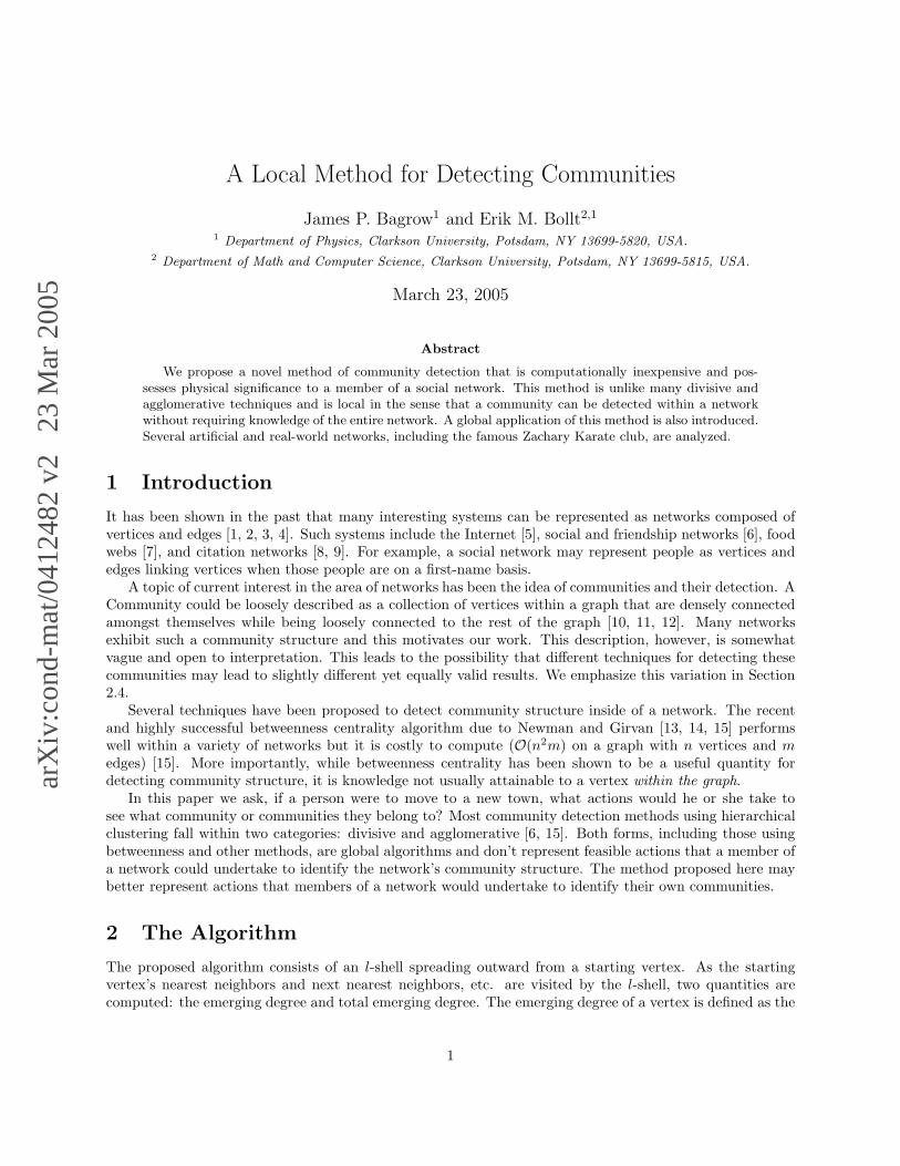
Figure 5: Membership matrix for Ideal graph 3 aftersorting, with α = 0.25. Note the increased numberof ”spilled” vertices in the the middle rows, as com-pared with Figure 16.

10 20 30 40 50 60 70 80

10

20

30

40

50

60

70

80

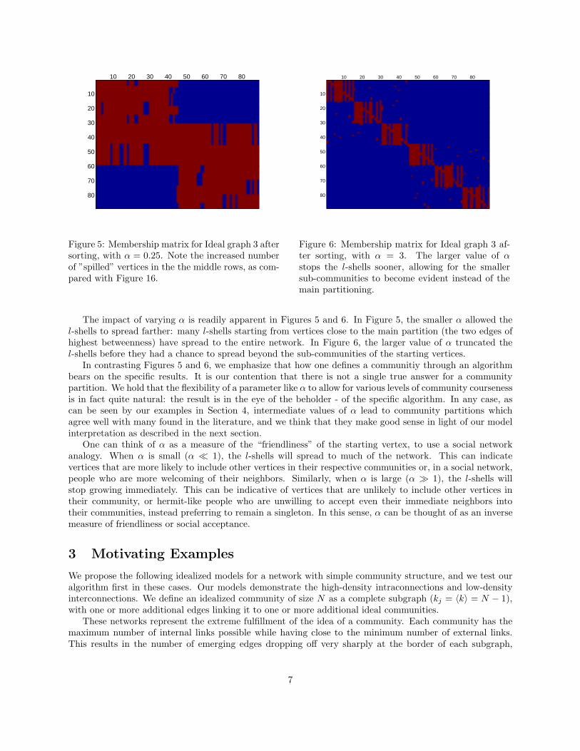
Figure 6: Membership matrix for Ideal graph 3 af-ter sorting, with α = 3. The larger value of α

stops the l-shells sooner, allowing for the smallersub-communities to become evident instead of themain partitioning.

The impact of varying α is readily apparent in Figures 5 and 6. In Figure 5, the smaller α allowed thel-shells to spread farther: many l-shells starting from vertices close to the main partition (the two edges ofhighest betweenness) have spread to the entire network. In Figure 6, the larger value of α truncated thel-shells before they had a chance to spread beyond the sub-communities of the starting vertices.

In contrasting Figures 5 and 6, we emphasize that how one defines a communitiy through an algorithmbears on the specific results. It is our contention that there is not a single true answer for a communitypartition. We hold that the flexibility of a parameter like α to allow for various levels of community coursenessis in fact quite natural: the result is in the eye of the beholder - of the specific algorithm. In any case, ascan be seen by our examples in Section 4, intermediate values of α lead to community partitions whichagree well with many found in the literature, and we think that they make good sense in light of our modelinterpretation as described in the next section.

One can think of α as a measure of the “friendliness” of the starting vertex, to use a social networkanalogy. When α is small (α ≪ 1), the l-shells will spread to much of the network. This can indicatevertices that are more likely to include other vertices in their respective communities or, in a social network,people who are more welcoming of their neighbors. Similarly, when α is large (α ≫ 1), the l-shells willstop growing immediately. This can be indicative of vertices that are unlikely to include other vertices intheir community, or hermit-like people who are unwilling to accept even their immediate neighbors intotheir communities, instead preferring to remain a singleton. In this sense, α can be thought of as an inversemeasure of friendliness or social acceptance.

3 Motivating Examples

We propose the following idealized models for a network with simple community structure, and we test ouralgorithm first in these cases. Our models demonstrate the high-density intraconnections and low-densityinterconnections. We define an idealized community of size N as a complete subgraph (kj = 〈k〉 = N − 1),with one or more additional edges linking it to one or more additional ideal communities.

These networks represent the extreme fulfillment of the idea of a community. Each community has themaximum number of internal links possible while having close to the minimum number of external links.This results in the number of emerging edges dropping off very sharply at the border of each subgraph,

7

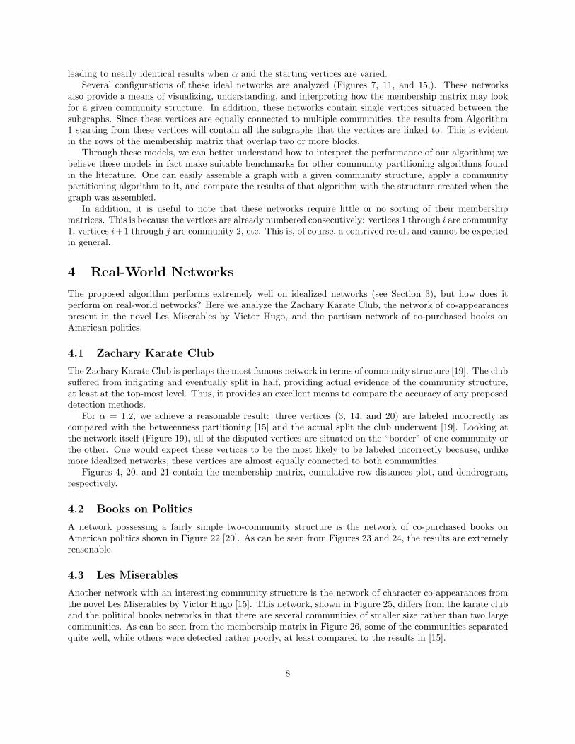
leading to nearly identical results when α and the starting vertices are varied.Several configurations of these ideal networks are analyzed (Figures 7, 11, and 15,). These networks

also provide a means of visualizing, understanding, and interpreting how the membership matrix may lookfor a given community structure. In addition, these networks contain single vertices situated between thesubgraphs. Since these vertices are equally connected to multiple communities, the results from Algorithm1 starting from these vertices will contain all the subgraphs that the vertices are linked to. This is evidentin the rows of the membership matrix that overlap two or more blocks.

Through these models, we can better understand how to interpret the performance of our algorithm; webelieve these models in fact make suitable benchmarks for other community partitioning algorithms foundin the literature. One can easily assemble a graph with a given community structure, apply a communitypartitioning algorithm to it, and compare the results of that algorithm with the structure created when thegraph was assembled.

In addition, it is useful to note that these networks require little or no sorting of their membershipmatrices. This is because the vertices are already numbered consecutively: vertices 1 through i are community1, vertices i+1 through j are community 2, etc. This is, of course, a contrived result and cannot be expectedin general.

4 Real-World Networks

The proposed algorithm performs extremely well on idealized networks (see Section 3), but how does itperform on real-world networks? Here we analyze the Zachary Karate Club, the network of co-appearancespresent in the novel Les Miserables by Victor Hugo, and the partisan network of co-purchased books onAmerican politics.

4.1 Zachary Karate Club

The Zachary Karate Club is perhaps the most famous network in terms of community structure [19]. The clubsuffered from infighting and eventually split in half, providing actual evidence of the community structure,at least at the top-most level. Thus, it provides an excellent means to compare the accuracy of any proposeddetection methods.

For α = 1.2, we achieve a reasonable result: three vertices (3, 14, and 20) are labeled incorrectly ascompared with the betweenness partitioning [15] and the actual split the club underwent [19]. Looking atthe network itself (Figure 19), all of the disputed vertices are situated on the “border” of one community orthe other. One would expect these vertices to be the most likely to be labeled incorrectly because, unlikemore idealized networks, these vertices are almost equally connected to both communities.

Figures 4, 20, and 21 contain the membership matrix, cumulative row distances plot, and dendrogram,respectively.

4.2 Books on Politics

A network possessing a fairly simple two-community structure is the network of co-purchased books onAmerican politics shown in Figure 22 [20]. As can be seen from Figures 23 and 24, the results are extremelyreasonable.

4.3 Les Miserables

Another network with an interesting community structure is the network of character co-appearances fromthe novel Les Miserables by Victor Hugo [15]. This network, shown in Figure 25, differs from the karate cluband the political books networks in that there are several communities of smaller size rather than two largecommunities. As can be seen from the membership matrix in Figure 26, some of the communities separatedquite well, while others were detected rather poorly, at least compared to the results in [15].

8

1 2

3

456

7 8910

11

1213

1415

16

17

18

1920

2122

232425

26

2728

29 30

31

Figure 7: Ideal graph 1: Two complete subgraphsof size 15 bridged by a common vertex.

5 10 15 20 25 30

5

10

15

20

25

30

Figure 8: Membership matrix for Ideal graph 1.Note that no sorting was required. α = 1, but forthese idealized model graphs, the results are identi-cal for a wide range of α values.

0 10 20 300

10

20

30

40

Node Number (After Sorting)

Cum

ulat

ive

Dis

tanc

e

Figure 9: Cumulative row distances for Ideal graph1. Generated using the membership matrix shownin Figure 8.

1 2 3 4 5 6 7 8 9 10 11 12 13 14 15 16 17 18 19 20 21 22 23 24 25 26 27 28 29 30 31

Figure 10: Dendrogram for Ideal graph 1. Noticethat central member vertex 16 is idealized here asa community unto itself, which in light of the formof the graph in Figure 7, simply means that 16 iscentral between two communities. Notice also thespecial placement of members 15 and 17.

9

1

2

3

45

67 8

910

11

12 13

1415

1617

1819 20

21

22

23

2425

26

27

28

2930

31

32

33

3435

36

37

38

3940

41

42 43

44

45464748

4950

5152

535455

5657

585960 62

63

64

65

6667

68

69

70

71

61

72

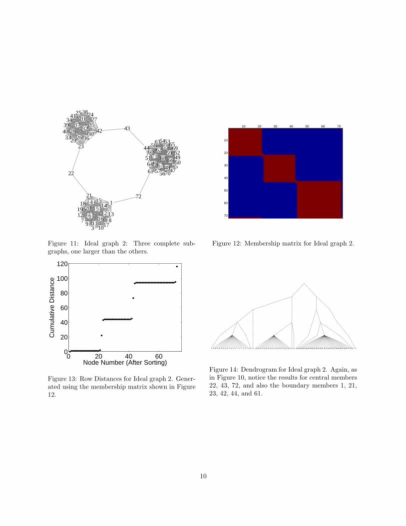
Figure 11: Ideal graph 2: Three complete sub-graphs, one larger than the others.

10 20 30 40 50 60 70

10

20

30

40

50

60

70

Figure 12: Membership matrix for Ideal graph 2.

0 20 40 600

20

40

60

80

100

120

Node Number (After Sorting)

Cum

ulat

ive

Dis

tanc

e

Figure 13: Row Distances for Ideal graph 2. Gener-ated using the membership matrix shown in Figure12.

1 2 3 4 5 6 7 8 9 10 11 12 13 14 15 16 17 18 19 20 21 22 23 24 25 26 27 28 29 30 31 32 33 34 35 36 37 38 39 40 41 42 43 44 45 46 47 48 49 50 51 52 53 54 55 56 57 58 59 60 62 63 64 65 66 67 68 69 70 71 61 72

Figure 14: Dendrogram for Ideal graph 2. Again, asin Figure 10, notice the results for central members22, 43, 72, and also the boundary members 1, 21,23, 42, 44, and 61.

10

12

345

67

89

10

1617

1819

202122

2324

25

3132

33

34

35

3637 38

3940

11

12

1314

1530 2928

2726

4142 43

44

45

54

464748

49505152

53

55

6061

62 6364 65

66

6768

69 7576

77

78

79

80

81

82

83

84

565759

58

7071

7273

74

85

86

87

8889

Figure 15: Ideal graph 3: Three complete subgraphsjoined together by multiple edges with singletonsattached bridged by a single vertex to another groupof similar (but not identical) structure.

10 20 30 40 50 60 70 80

10

20

30

40

50

60

70

80

Figure 16: Membership matrix for Ideal graph 3,α = 0.87.

0 20 40 60 800

20

40

60

80

100

120

140

Node Number (After Sorting)

Cum

ulat

ive

Dis

tanc

e

Figure 17: Row Distances for Ideal graph 3, α =0.87. Generated using the membership matrixshown in Figure 16

1 7 10 11 2 3 4 12 13 14 6 8 9 5 15 16 17 20 21 29 30 22 25 28 23 26 27 24 18 19 32 36 37 42 35 31 41 44 40 34 43 38 39 33 54 53 58 49 52 55 48 59 60 61 67 68 70 71 62 64 72 74 65 66 69 73 63 75 76 80 84 88 78 82 86 89 79 81 83 85 87 77 46 57 50 51 56 47 45

Figure 18: Dendrogram for Ideal graph 2, α = 0.87.Now with central members, for different scale com-munities, the dendrogram becomes more compli-cated in contrast to those in Figures 10 and 14.

11

112

13

56

711

1822

842

314 20

932

17

3128 29

33

1034

25

26

19

211516 23

27

30

24

Figure 19: The Zachary Karate club. The coloringindicates the membership of the two clusters of thetopmost branch of the dendrogram (Figure 21)

0 10 20 300

10

20

30

40

50

Node Number (After Sorting)

Cum

ulat

ive

Dis

tanc

e

Figure 20: Cumulative row distances for theKarate club, computed using the membership ma-trix shown in Figure 4 (α = 1.2).

1 12 13 5 6 7 11 18 22 8 4 2 17 3 14 20 9 25 26 32 28 29 33 10 31 19 21 15 16 23 27 34 30 24

Figure 21: Dendrogram for the Karate club, using the membership matrix shown in Figure 4 (α = 1.2).

12

14

10 736

5211

8

15

13 1625 3023

1420 9

18

19

22

1733

2924 283126

3236

27

21

12

3537

48606467

5556

50 51

425446

4953

5259

58

576361

62

41

45

476539

4438

4043

66

34

Figure 22: The network of co-purchased books onAmerican politics [20]. Here a link is drawn betweentwo vertices if those books were purchased togetherfrom a major online retailer.

10 20 30 40 50 60

10

20

30

40

50

60

Figure 23: Membership matrix for the Books onPolitics network. α = 1.2.

1 2 4 8 10 11 15 9 13 16 20 25 30 23 18 17 24 12 28 31 26 32 36 19 22 29 33 27 21 7 3 6 5 14 35 37 67 48 46 55 56 50 51 45 49 53 47 39 44 42 38 52 40 54 58 57 63 59 66 61 62 41 60 34 43 65 64

Figure 24: Dendrogram for the Books on Politics network. Generated using the membership matrix shownin Figure 23. Note that vertices 35 and 37 are rows 34 and 35, respectively, of the membership matrix.

5 Conclusions

In this paper, we have introduced Algorithm 1, a new method for detecting community structure. Thismethod is local and may be applied in situations where other methods are too inefficient; for example, whenone is concerned with a single community and not the complete community structure of a graph. A single

13

Myriel

Napoleon

CountessDeLo

Geborand

Champtercier

Cravatte

Count OldMan

Gribier

Jondrette

MlleVaubois

MmePontmercy

Judge

Champmathieu

Brevet

Chenildieu

Cochepaille

Bamatabois

Fameuil

Blacheville

Favourite

Dahlia

Zephine

Listolier

Tholomyes

Fantine

Perpetue

Gueulemer

Babet

Brujon

Eponine

AnzelmaBoulatruelle

Thenardier

MagnonPontmercy

Marius

BaronessT

LtGillenormand

Mabeuf

MotherPlutarch

CombeferreFeuilly

Bahorel

Joly

Courfeyrac

BossuetEnjolras

Grantaire

Prouvaire

MmeHucheloup

Gavroche

Child1

Child2

MmeBurgonJavert

Gervais

MmeDeR

Scaufflaire

Isabeau

Valjean

LabarreWoman1 Woman2

Toussaint

MotherInnocent

Fauchelevent

MmeMagloireMlleBaptistine

Simplice

Marguerite

MmeThenardier

Cosette

Gillenormand

MlleGillenormandClaquesous

Montparnasse

Figure 25: The network of character co-appearancesfrom the novel Les Miserables by Victor Hugo. SeeFigure 27 for partitioning.

10 20 30 40 50 60 70

10

20

30

40

50

60

70

Figure 26: Membership matrix (after sorting) forthe Les Mis network. α = 6.9.

1 2 5 6 7 8 9 10 46 47 54 53 35 36 37 38 39 30 19 20 21 22 23 18 17 24 31 69 70 76 42 43 41 26 51 40 56 57 55 58 68 60 62 64 66 63 65 59 67 61 77 49 74 75 48 28 16 14 33 15 12 11 34 44 73 45 29 4 3 32 13 25 27 50 52 71 72

Figure 27: Dendrogram for the Les Mis social network. Generated using the membership matrix shown inFigure 26.

14

parameter, α, is used, making it very easy to tune the output of the algorithm, as was shown in Section 2.4.We have also proposed one possible method of applying Algorithm 1 globally (see Sections 2.2 and

2.3). Sorting the membership matrix is expensive and limits this global application to smaller networks. Inaddition, the membership matrix is, unlike an adjacency matrix, not necessarily sparse for a sparse graph:it will only be sparse when the sizes of the individual communities are all much smaller than the size of thenetwork as a whole. This limits the possibility of replacing the membership matrix with a more efficientdata structure.

We feel that Algorithm 1 is a useful result, due to both its simplicity and flexibility. For example, ourglobal application could be easily altered to become more efficient: one imagines the cost of the sortingalgorithm can be offset a great deal by only starting Algorithm 1 from a fraction of the vertices, f , insteadof all vertices in the graph. This reduces the cost of the sorting algorithm by a factor of f3, a real savingsfor small f , with the presumed tradeoff being a reduction in accuracy as f decreases. Other applications ofAlgorithm 1 besides the expensive use of the membership matrix may also be discovered.

The Zachary Karate club has become an almost canonical representative of a community structure. Thepossibility remains, however, that outside factors may not be represented in the dataset. If this is true, thenthe club’s fissure should not be used as the sole means of justification for a community detection method.For example, some of the border nodes, represented as diamonds in Figure 1, could well have joined eithercommunity, based solely on the network at hand. This can lead to ambiguity in the final partition. Thepoint is that the algorithm defines the community; the community should not define the algorithm.

Another concept, often neglected in determining communities, is the idea of a relative result. Who isto say that someone in a town agrees with what community the rest of the town feels he or she belongsto? It seems feasible that a vertex that is equally linked to two communities in a graph is just as likely tocorrespond to a person who thinks he or she is a member of both communities as it is to correspond to aperson who feels they are independent of both larger communities. If one considers the output of Algorithm1 to be what the starting vertex “believes” to be his or her community, then this method may prove to be auseful tool when analyzing relative results. This is not useful for many applications of community detectionwhere a final structure is necessary, such as minimizing crosstalk between parallel processors in a computer,but it may prove very useful in areas such as social networks.

Acknowledgements

The authors are grateful to Hernan Rozenfeld and Daniel ben-Avraham for useful discussions and to MarkNewman for useful data. This work was supported by the NSF under grants DMS0404778.

References

[1] S. H. Strogatz, Exploring complex networks. Nature 410, 268-276 (2001).

[2] R. Albert and A.-L. Barabasi, Statistical mechanics of complex networks. Rev. Mod. Phys. 74, 47–97(2002).

[3] M. E. J. Newman, The structure and function of complex networks. SIAM Review 45, 167–256 (2003).

[4] S. N. Dorogovtsev and J. F. F. Mendes, Evolution of Networks: From Biological Nets to the Internet andWWW. Oxford University Press, Oxford (2003).

[5] M. Faloutsos, P. Faloutsos, and C. Faloutsos, On power-law relationships of the internet topology. Com-puter Communications Review 29, 251–262 (1999).

[6] J. Scott, Social Network Analysis: A Handbook. Sage Publications, London, 2nd edition (2000).

[7] J. A. Dunne, R. J. Williams, and N. D. Martinez, Food-web structure and network theory: The role ofconnectance and size. Proc. Natl. Acad. Sci. USA 99, 12917–12922 (2002).

15

[8] S. Redner, How popular is your paper? An empirical study of the citation distribution. Eur. Phys. J. B4, 131–134 (1998).

[9] M. E. J. Newman, The structure of scientific collaboration networks. Proc. Natl. Acad. Sci. USA 98,404–409 (2001).

[10] S. Wasserman and K. Faust, Social Network Analysis. Cambridge University Press, Cambridge (1994).

[11] G. W. Flake, S. R. Lawrence, C. L Giles, and F .M. Coetzee, Self-organization and indentification ofWeb communities. IEEE Computer 35, 66-71 (2002).

[12] F. Radicchi, C. Castellano, F. Cecconi, V. Loreto, and D. Parisi, Defining and identifying communitiesin networks. Proc. Natl. Acad. Sci. USA 101, 2658-2663 (2004)

[13] M. E. J. Newman, Mixing patterns in networks. Phys. Rev. E 67 , 026126 (2003).

[14] M. Girvan and M. E. J. Newman, Community structure in social and biological networks. Proc. Natl.Acad. Sci. USA 99, 7821-7826 (2002).

[15] M. E. J. Newman and M. Girvan, Finding and evaluating community structure in networks, Phys. Rev.E 69, 026113 (2004).

[16] L. da F. Costa, Hub-based community finding. Preprint cond-mat/0405022 (2004).

[17] Graphviz - Graph Visualization Software Home page: http://www.graphviz.org/

[18] Image courtesy Mark Newman’s site at http://www-personal.umich.edu/∼mejn/networks/

[19] W. W. Zachary, An information flow model for conflict and fission in small groups. Journal of Anthro-pological Research 33, 452–473 (1977).

[20] V. Krebs, Political Patterns on the WWW – Divided We Stand. Home page:http://www.orgnet.com/divided2.html

16