SVSLOPE - Bentley Communities
180
SVSLOPE 2D/3D LIMIT EQUILIBRIUM SLOPE STABILITY ANALYSIS Verification Manual Written by: The Bentley Systems Team Last Updated: Friday, December 13, 2019 Bentley Systems Incorporated
-
Upload
khangminh22 -
Category
Documents
-
view
2 -
download
0
Transcript of SVSLOPE - Bentley Communities

SVSLOPE 2D/3D LIMIT EQUILIBRIUM
SLOPE STABILITY ANALYSIS
Verification Manual
Written by: The Bentley Systems Team
Last Updated: Friday, December 13, 2019
Bentley Systems Incorporated

COPYRIGHT NOTICE Copyright © 2019, Bentley Systems, Incorporated. All Rights Reserved. Including software, file formats, and audiovisual displays; may only be used pursuant to applicable software license
agreement; contains confidential and proprietary information of Bentley Systems, Incorporated and/or third parties which is
protected by copyright and trade secret law and may not be provided or otherwise made available without proper
authorization.
TRADEMARK NOTICE
Bentley, "B" Bentley logo, SoilVision.com, SoilVision logo, and SOILVISION, SVSLOPE, SVOFFICE, SVOFFICE 5/GE, SVOFFICE
5/GT, SVOFFICE 5/WR, SVSOILS, SVFLUX, SVSOLID, SVCHEM, SVAIR, SVHEAT, SVSEISMIC and SVDESIGNER are either
registered or unregistered trademarks or service marks of Bentley Systems, Incorporated. All other marks are the property of
their respective owners.

BENTLEY SYSTEMS Table of Contents 3 of 180
1 INTRODUCTION ....................................................................................................................................................... 6
2 ACADS MODELS ....................................................................................................................................................... 7
2.1 1(A) SIMPLE SLOPE ...................................................................................................................................................... 7 2.2 1(B) TENSION CRACK .................................................................................................................................................. 9 2.3 1(C) NON-HOMOGENEOUS ....................................................................................................................................... 11 2.4 1(D) NON-HOMOGENOUS WITH SEISMIC LOAD .................................................................................................. 12 2.5 NON-HOMOGENOUS CRITICAL SEISMIC COEFFICIENT ANALYSIS ............................................................... 14 2.6 NON-HOMOGENOUS NEWMARK DISPLACEMENT ANALYSIS ........................................................................ 15 2.7 2(A) TALBINGO DAM, DRY ....................................................................................................................................... 16 2.8 2(B) TALBINGO DAM, DRY PREDEFINED SLIP SURFACE ................................................................................... 18 2.9 3(A) WATER TABLE MODELED WITH WEAK SEAM ............................................................................................ 20 2.10 3(B) WATER TABLE MODELED WITH WEAK SEAM WITH PREDEFINED SLIP SURFACE ........................ 21 2.11 4 EXTERNAL LOADING, PORE-PRESSURE DEFINED BY WATER TABLE .................................................. 22
3 SVSLOPE GROUP 1 ................................................................................................................................................. 25
3.1 LANESTER EMBANKMENT VERIFICATION ......................................................................................................... 25 3.2 CUBZAC-LES-PONTS EMBANKMENT .................................................................................................................... 26 3.3 ARAI AND TAGYO HOMOGENEOUS SLOPE ......................................................................................................... 28 3.4 ARAI AND TAGYO LAYERED SLOPE ..................................................................................................................... 29 3.5 ARAI AND TAGYO PORE-WATER PRESSURE SLOPE .......................................................................................... 31 3.6 YAMAGAMI AND UETA SIMPLE SLOPE ................................................................................................................ 33 3.7 BAKER SIMPLE SLOPE .............................................................................................................................................. 34 3.8 GRECO LAYERED SLOPE .......................................................................................................................................... 35 3.9 GRECO WEAK LAYER SLOPE .................................................................................................................................. 37 3.10 FREDLUND AND KRAHN HOMOGENEOUS SLOPE ......................................................................................... 39 3.11 FREDLUND AND KRAHN WEAK LAYER SLOPE ............................................................................................. 41 3.12 LOW TWO LAYER SLOPE ..................................................................................................................................... 43 3.13 LOW THREE LAYER SLOPE ................................................................................................................................. 44 3.14 CHEN AND SHAO FRICTIONLESS SLOPE ......................................................................................................... 45 3.15 PRANDTL BEARING CAPACITY ......................................................................................................................... 46 3.16 PRANDTL BEARING CAPACITY – NON-VERTICAL SLICES .......................................................................... 47 3.17 CHOWDHURY AND XU (1995) ............................................................................................................................. 48 3.18 DUNCAN – LASH TERMINAL .............................................................................................................................. 51 3.19 BORGES AND CARDOSO – GEOSYNTHETIC EMBANKMENT ....................................................................... 52 3.20 BORGES AND CARDOSO – GEOSYNTHETIC EMBANKMENT #2 .................................................................. 53 3.21 BORGES AND CARDOSO – GEOSYNTHETIC EMBANKMENT #3 .................................................................. 55 3.22 SYNCRUDE PROBABILISTIC TAILINGS DYKE ................................................................................................ 57 3.23 CANNON DAM ....................................................................................................................................................... 58 3.24 CANNON DAM #2 ................................................................................................................................................... 59 3.25 LI AND LUMB – RELIABILITY INDEX ................................................................................................................ 62 3.26 REINFORCEMENT BACK ANALYSIS ................................................................................................................. 63 3.27 TANDJIRIA – GEOSYNTHETIC REINFORCED EMBANKMENT ..................................................................... 65 3.28 BAKER AND LESCHINSKY – EARTH DAM ....................................................................................................... 67 3.29 BAKER – PLANAR HOMOGENEOUS .................................................................................................................. 69 3.30 SHEAHAN – AMHEARST SOIL NAILS ................................................................................................................ 70 3.31 SHEAHAN – CLOUTERRE TEST WALL .............................................................................................................. 71 3.32 SNAILZ – REINFORCED SLOPE ........................................................................................................................... 72 3.33 SNAILZ – GEOTEXTILE LAYERS ........................................................................................................................ 74 3.34 ZHU – FOUR LAYER SLOPE ................................................................................................................................. 75 3.35 ZHU AND LEE – HETEROGENEOUS SLOPE ...................................................................................................... 76 3.36 PRIEST – RIGID BLOCKS ...................................................................................................................................... 78 3.37 YAMAGAMI – STABILIZING PILES .................................................................................................................... 79 3.38 POCKOSKI AND DUNCAN – SIMPLE SLOPE ..................................................................................................... 80 3.39 POCKOSKI AND DUNCAN – TENSION CRACKS .............................................................................................. 81 3.40 POCKOSKI AND DUNCAN – REINFORCED SLOPE .......................................................................................... 81 3.41 POCKOSKI AND DUNCAN – TIE-BACK WALL ................................................................................................. 83

BENTLEY SYSTEMS Table of Contents 4 of 180
3.42 POCKOSKI AND DUNCAN - REINFORCEMENT ............................................................................................... 84 3.43 POCKOSKI AND DUNCAN – SOIL NAILS ........................................................................................................... 85 3.44 LOUKIDIS – SEISMIC COEFFICIENT .................................................................................................................. 87 3.45 LOUKIDIS – SEISMIC COEFFICIENT #2 .............................................................................................................. 88
4 SVSLOPE GROUP 2 ................................................................................................................................................. 90
4.1 SIMPLE MULTI – LAYER SLOPE .............................................................................................................................. 90 4.2 BLOCK SEARCH MODEL .......................................................................................................................................... 91 4.3 COMPOSITE SLIP SURFACES ................................................................................................................................... 92 4.4 RETAINING WALL ..................................................................................................................................................... 93 4.5 FABRIC MODEL .......................................................................................................................................................... 94 4.6 BISHOP AND MORGENSTERN - HOMOGENEOUS ................................................................................................ 96 4.7 FREDLUND AND KRAHN (1977) .............................................................................................................................. 97 4.8 SIMPLE TWO MATERIAL MODEL ........................................................................................................................... 98 4.9 INFINITE SLOPE MODEL ........................................................................................................................................... 99 4.10 LAMBE AND WHITMAN – DRAINED SLOPE .................................................................................................. 101 4.11 PORE-WATER PRESSURES AT DISCRETE POINTS ........................................................................................ 102
5 SVSLOPE GROUP 3 ............................................................................................................................................... 104
5.1 RAPID DRAWDOWN – 3 STEP METHOD ............................................................................................................... 104 5.2 RAPID DRAWDOWN - WALTER BOULDIN DAM ....................................................................................................... 107 5.3 RAPID DRAWDOWN - USACE BENCHMARK ........................................................................................................... 108 5.4 RAPID DRAWDOWN - PUMPED STORAGE PROJECT DAM ......................................................................................... 108 5.5 RAPID DRAWDOWN - PILARCITOS DAM .................................................................................................................. 110 5.6 SHEAR NORMAL FUNCTION ................................................................................................................................. 111 5.7 FILL SLOPE USING A RETAINING WALL ............................................................................................................. 113 5.8 PROBABILITY – JAMES BAY CASE HISTORY ..................................................................................................... 114 5.9 EUROCODE 7 – CUTTING IN STILL CLAY ............................................................................................................ 116 5.10 EUROCODE 7 – EARTH DAM ............................................................................................................................. 117 5.11 ANISOTROPIC LINEAR MODEL (ALM1) .......................................................................................................... 118 5.12 SPECTRAL PSEUDO-STATIC ANALYSIS ......................................................................................................... 120 5.13 OPEN PIT COAL MINE – NON-VERTICAL SLICES .......................................................................................... 121
6 DYNAMIC PROGRAMMING (SAFE) MODELS ................................................................................................ 123
6.1 PHAM CHAPTER 4 FIGURE 4.1 ............................................................................................................................... 123 6.2 PHAM CHAPTER 5 FIGURES 5.7 TO 5.12 ............................................................................................................... 124 6.3 PHAM CHAPTER 5 FIGURES 5.28 TO 5.33 ............................................................................................................. 126 6.4 PHAM CHAPTER 5 FIGURE 5.44 (2002) .................................................................................................................. 127 6.5 3-LAYER SLOPE RESTING ON A HARD SURFACE ............................................................................................. 129 6.6 THIN AND WEAK LAYERS RESTING ON BEDROCK .......................................................................................... 130 6.7 LODALEN CASE HISTORY ...................................................................................................................................... 131
7 3D BENCHMARKS ................................................................................................................................................ 133
7.1 A SIMPLE 3D SLOPE IN CLAY ................................................................................................................................ 133 7.2 A MODEL COMPARED TO VARIATIONAL APPROACH .................................................................................... 134 7.3 ELLIPSOIDAL SLIDING SURFACE WITH TOE SUBMERGENCE ....................................................................... 135 7.4 COMPOSITE ELLIPSOID/WEDGE SURFACE ........................................................................................................ 137 7.5 EMBANKMENT CORNER ........................................................................................................................................ 139 7.6 WASTE PILE FAILURE WEDGES............................................................................................................................ 140 7.7 A GENERAL SLIDING SURFACE ............................................................................................................................ 143 7.8 KETTLEMAN WASTE LANDFILL FAILURE ......................................................................................................... 145 7.9 BEDROCK LAYER CONSIDERATION ................................................................................................................... 147 7.10 MULTIPLE PIEZOMETRIC SURFACES ............................................................................................................. 148 7.11 ARBITRARY SLIDING DIRECTION ................................................................................................................... 150
8 FEATURE EXAMPLES FOR 3D MODELS ......................................................................................................... 152
8.1 FREDLUND AND KRAHN (1977) 2D TO 3D ........................................................................................................... 152 8.2 EARTHQUAKE LOAD .............................................................................................................................................. 153

BENTLEY SYSTEMS Table of Contents 5 of 180
8.3 POINT LOAD .............................................................................................................................................................. 155 8.4 TENSION CRACK ...................................................................................................................................................... 156 8.5 PORE WATER PRESSURES AT DISCRETE POINTS ............................................................................................. 157 8.6 SUPPORTS – END ANCHORED ............................................................................................................................... 159 8.7 3-STAGE RAPID DRAWDOWN ............................................................................................................................... 160
9 SVSLOPE (SEISMIC) EXAMPLES ....................................................................................................................... 162
9.1 S-WAVE PROPAGATION IN AN ELASTIC COLUMN .......................................................................................... 162 9.2 P-WAVE PROPAGATION IN AN ELASTIC SOIL COLUMN ................................................................................. 166 9.3 REFRACTION SEISMOLOGY .................................................................................................................................. 170
10 REFERENCES ........................................................................................................................................................ 178

BENTLEY SYSTEMS Introduction 6 of 180
1 INTRODUCTION The word “Verification”, when used in connection with computer software can be defined as “the ability of the computer code to provide a solution consistent with the physics of the problem. There are also other factors such as initial conditions, boundary conditions, and control variables that may affect the accuracy of the code to perform as stated. “Verification” is generally achieved by solving a series of so-called “benchmark” problems. “Benchmark” problems are problems for which there is a closed-form solution or for which the solution has become “reasonably certain” as a result of longhand calculations that have been performed. Publication of the “benchmark” solutions in research journals or textbooks also lends credibility to the solution. There are also example problems that have been solved and published in User Manual documentation associated with other comparable software packages. While these are valuables checks to perform, it must be realized that it is possible that errors can be transferred from one’s software solution to another. Consequently, care must be taken in performing the “verification” process on a particular software package. It must also be
remembered there is never such a thing as complete software verification for “all” possible problems. Rather, it is an ongoing process that establishes credibility with time. Bentley Systems takes the process of “verification” most seriously and has undertaken a wide range of steps to ensure that the SVSLOPE software will perform as intended by the theory of limit equilibrium slope stability. The following models represent comparisons made to textbook solutions, hand calculations, and other software packages. We at Bentley Systems Ltd., are dedicated to providing our clients with reliable and tested software. While the following list of example models is comprehensive, it does not reflect the entirety of models, which may be posed to the SVSLOPE software. It is our recommendation that checks be performed on all model runs prior to presentation of results. It is also our recommendation that the modeling process move from simple to complex models with simpler models being verified through the use of hand calculations or simple spreadsheet calculations.

BENTLEY SYSTEMS ACADS Models 7 of 180
2 ACADS MODELS The following group of models represents a series of models originally presented in the Australian ACADS study (Giam & Donald, 1989). The study presented a series of benchmark examples and allowed a variety of consultants using differing software packages to solve the models. The results were then reviewed by an expert review panel and an answer was established. The SVSLOPE software package was compared to these models in the following sections.
2.1 1(A) SIMPLE SLOPE Project: Slopes_Group_1 Model: VS_1 This model contains a simple case of a total stress analysis without considering pore-water pressures. It is a simple analysis that represents a homogenous slope with given soil properties. This model is originally published by the ACADS study (Giam & Donald, 1989).
2.1.1 Geometry and Material Properties
The slope properties that are in use for this model are presented in Table 1. The requirements for this problem are the factor
of safety and its corresponding critical circular failure surface.
Figure 1 Geometry of the Simple Slope model
Table 1 Material Properties of the Simple Slope model
c (kN/m2) (degrees) (kN/m3)
3.0 19.6 20.0
2.1.2 Results and Discussions
The grid and radius method was used to identify a critical slip surface location. A grid of centers of 20 x 20 was used along with 11 tangent points.
This period of a total of 4851 circular slip surfaces. The results of the analysis for each different analysis method are presented in Table 2. The Factor of Safety published by the ACADS study was 1.00.

BENTLEY SYSTEMS ACADS Models 8 of 180
Table 2 Results of the Simple Slope model
Method
Factor of Safety Difference
(%) Slide SVSLOPE
Ordinary 0.947 0.945 -0.211
Bishop Simplified 0.987 0.989 0.203
Janbu Simplified 0.939 0.939 0.000
Spencer 0.986 0.988 0.203
GLE 0.986 0.988 0.203
Figure 2 Solution of the Simple Slope model using the Spencer method
Figure 3 Solution of the Simple Slope model using the GLE method

BENTLEY SYSTEMS ACADS Models 9 of 180
Figure 4 Solution of the Simple Slope model using the Janbu Simplified method
2.2 1(B) TENSION CRACK Project: Slopes_Group_1 Model: VS_2 This model has the same slope geometry as verification problem #1, with the exception that a tension crack zone has been added as shown in Figure 5. For this problem, a suitable tension crack depth is required. Water is assumed to fill the tension crack. The calculations the equation used to calculate the tension crack depth is shown below (Craig, 1997).
sin1
sin1,
2
+
−== a
a
kky
cDepth
2.2.1 Geometry and Material Properties
Figure 5 Geometry of the Tension Crack model
Table 3 Material Properties of the Tension Crack model
c (kN/m2) (degrees) (kN/m3)
32.0 10.0 20.0
2.2.2 Results and Discussions
The grid and radius search technique was used to locate the most critical slip surface. A grid 20 x 20 grid of centers was used along with 11 tangents points. A total of 4851 slip surface was generated. The values of the critical factor of safety are shown in Table 4. The Bishop, Spencer, GLE and Janbu’s corrected, solutions are shown along with the location of the critical slip surface. The Factor of Safety published by the ACADS study is 1.65 to 1.70.

BENTLEY SYSTEMS ACADS Models 10 of 180
Table 4 Results of the Tension Crack model
Method
Factor of Safety Difference
(with Slide)
(%)
Difference
(with
SLOPE/W)
(%)
Slide
Slope/W SVSLOPE
Moment Force Moment Force
Ordinary 1.521 1.52 1.521 0.00 0.07
Bishop Simplified 1.596 1.592 1.593 -0.19 0.06
Janbu Simplified 1.382 1.38 1.38 -0.15 0.29
Spencer 1.592 1.594 1.599 1.589 1.589 -0.19 0.31
M-P 1.592 1.588 1.594 1.59 1.59 -0.13 0.13
GLE 1.592 1.588 1.588 1.59 1.59 -0.13 0.13
Figure 6 Solution of the Tension Crack model using the Bishop Simplified method
Figure 7 Solution of the Tension Crack model using the Spencer method

BENTLEY SYSTEMS ACADS Models 11 of 180
Figure 8 Solution of the Tension Crack model using the GLE Method
Figure 9 Solution of the Tension Crack model using the Janbu Simplified method
2.3 1(C) NON-HOMOGENEOUS Project: Slopes_Group_1 Model: VS_3 This model is a non-homogenous three-layer slope with material properties shown in Table 5. The calculation of the factor of safety and its corresponding critical slip surface is shown.
2.3.1 Geometry and Material Properties
Figure 10 Geometry of the Non-Homogenous model
Table 5 Material Properties of the Non-Homogenous model
c (kN/m2) (degrees) (kN/m3)
Soil #1 0.0 38.0 19.5
Soil #2 5.3 23.0 19.5
Soil #3 7.2 20.0 19.5

BENTLEY SYSTEMS ACADS Models 12 of 180
2.3.2 Results and Discussions
The grid and radius technique was used to determine the location of the critical slip surface. A slip surface centers search grid of 20 x 20 was used for the grid of centers and 11 tangents points were used at each grid center. This resulted in total of 4851 trial slip surfaces. The results of the factor of safety calculations are shown in Table 6. The Factor of Safety published by the ACADS study was 1.39.
Table 6 Results of the Non-Homogenous model
Method
Factor of Safety Difference
(%)
Slide
SVSLOPE
Moment Force
Ordinary 1.232 1.231 -0.08
Bishop Simplified 1.405 1.405 0.00
Spencer 1.375 1.374 1.374 0.15
GLE 1.374 1.376 1.375 0.07
Figure 11 Solution of the non-homogenous model using the Bishop Simplified method
2.4 1(D) NON-HOMOGENOUS WITH SEISMIC LOAD Project: Slopes_Group_1 Model: VS_4 This model is identical to the previous model with the exception that a horizontal seismically induced acceleration of 0.15g was included in the analysis. The intent of this model is to test the ability of the software to analyze seismic conditions.
2.4.1 Geometry and Material Properties
The model requires the calculations of the factor of safety and the corresponding location of the critical slip surface. No pore-water pressures are designated and therefore a total stress analysis is performed.
Figure 12 Geometry of the Non-Homogeneous with Seismic Load model

BENTLEY SYSTEMS ACADS Models 13 of 180
Table 7 Material Properties of the Non-Homogenous with Seismic Load
c kN/m2) (degrees) (kN/m3)
Soil #1 0.0 38.0 19.5
Soil #2 5.3 23.0 19.5
Soil #3 7.2 20.00 19.5
2.4.2 Results and Discussions
The results of the analysis produce the following table of factors of safety for the Bishop, Spencer. GLE, Janbu Simplified methods. The Factor of Safety published by the ACADS study was 1.00.
Table 8 Results of the Non-Homogenous with Seismic Load model
Method
Factor of Safety Difference
(%)
Slide
SVSLOPE
Moment Force
Ordinary 0.884 0.884 0.00
Bishop Simplified 1.015 1.014 3 0.00
Janbu Simplified 0.897 0.897 0.00
Spencer 0.991 0.991 0.99 0.00
GLE 0.989 0.991 0.99 0.20
Figure 13 Results using the GLE method on VS_4 model

BENTLEY SYSTEMS ACADS Models 14 of 180
2.5 NON-HOMOGENOUS CRITICAL SEISMIC COEFFICIENT ANALYSIS Project: Slopes_Group_3 Model: VS4_Critical_Ky This model is identical to the previous model with the exception that an advanced seismic analysis was conducted to
determine the critical seismic coefficient that results in a destabilized slope with FOS of 1.0. The intent of this model is to test the ability of the software to analyze seismic conditions.
2.5.1 Geometry and Material Properties
The model requires the calculations of the factor of safety and the corresponding location of the critical slip surface. No pore-water pressures are designated and therefore a total stress analysis is performed.
Figure 14 Geometry of the Non-Homogeneous Critical Seismic Coefficient Analysis model
Table 9 Material Properties of the Non-Homogenous Critical Seismic Coefficient Analysis
c kN/m2) (degrees) (kN/m3)
Soil #1 0.0 38.0 19.5
Soil #2 5.3 23.0 19.5
Soil #3 7.2 20.00 19.5
2.5.2 Results and Discussions
The results of the analysis produce the following table of factors of safety for the Spencer, M-P and GLE.
Table 10 Results of the Non-Homogenous Critical Seismic Coefficient Analysis model
Method
Factor of Safety Difference
(%)
Slide
SVSLOPE
Moment Force
Spencer 0.146 0.145 0.145 0.00
M-P 0.146 0.145 0.146 0.00
GLE 0.146 0.145 0.145 0.00

BENTLEY SYSTEMS ACADS Models 15 of 180
Figure 15 Results using the GLE method Critical Seismic Coefficient Analysis model
2.6 NON-HOMOGENOUS NEWMARK DISPLACEMENT ANALYSIS Project: Slopes_Group_3 Model: VS4_Newmark_Disp This model is identical to the previous model with the exception that a Newmark Displacement analysis was carried out on the slope. The intent of this model is to test the ability of the software to analyze seismic conditions.
2.6.1 Geometry and Material Properties
The model requires the calculations of the factor of safety and the corresponding location of the critical slip surface. No pore-water pressures are designated and therefore a total stress analysis is performed.
Figure 16 Geometry of the Non-Homogeneous Newmark Displacement Analysis model
Table 11 Material Properties of the Non-Homogenous Newmark Displacement Analysis
c kN/m2) (degrees) (kN/m3)
Soil #1 0.0 38.0 19.5
Soil #2 5.3 23.0 19.5
Soil #3 7.2 20.00 19.5
2.6.2 Results and Discussions
The results of the analysis produce the following table of permanent displacements.

BENTLEY SYSTEMS ACADS Models 16 of 180
Table 12 Results of the Non-Homogenous Newmark Displacement Analysis
Method
Permanent Displacement
Difference
(%)
Slide
(m)
SVSLOPE
Moment
(m)
Force
(m)
Bishop Simplified 0.02232 0.022 0.00
Janbu Simplified 0.10819 0.108 0.00
Corps #1 0.04233 0.042 0.00
Corps #2 0.03998 0.039 2.45
Lowe-Karafiath 0.05282 0.049 7.23
Spencer 0.0329 0.033 0.034 0.00
GLE 0.0349 0.033 0.034 5.44
M-P 0.0349 0.033 0.033 5.44
Sarma 0.0373 0.036 0.036 3.49
Figure 17 Results using the GLE method Newmark Displacement Analysis model
2.7 2(A) TALBINGO DAM, DRY Project: Slopes_Group_1 Model: VS_5 This model is the Talbingo Dam (Giam & Donald, 1989) for the end-of-construction stage. Soil properties are given in Table 13 and the geometrical data is given in Table 14.
2.7.1 Geometry and Material Properties
The model requirements are that a factor of safety and a corresponding location of the critical failure surface must be calculated.
Figure 18 Geometry of the Talbingo Dam model

BENTLEY SYSTEMS ACADS Models 17 of 180
Table 13 Material Properties of the Talbingo Dam model
c (kN/m2) (degrees) (kN/m3)
Rock fill 0 45 20.4
Transitions 0 45 20.4
Filter 0 45 20.4
Core 85 23 18.1
Table 14 Geometry Data of Talbingo Dam, with weak layer
Pt. # Xc (m) Yc (m) Pt. # Xc (m) Yc (m) Pt. # Xc (m) Yc (m)
1 0 0 10 515 65.3 19 307.1 0
2 315.5 162 11 521.1 65.3 20 331.3 130.6
3 319.5 162 12 577.9 31.4 21 328.8 146.1
4 321.6 162 13 585.1 31.4 22 310.7 0
5 327.6 162 14 648 0 23 333.7 130.6
6 386.9 130.6 15 168.1 0 24 331.3 146.1
7 394.1 130.6 16 302.2 130.6 25 372.4 0
8 453.4 97.9 17 200.7 0 26 347 130.6
9 460.6 97.9 18 311.9 130.6 - - -
2.7.2 Results and Discussions
Resulting Factor of Safety are calculated that are shown in Table 15. The Factor of Safety published by the ACADS study is (1.95)/1.90.
Table 15 Results of the Talbingo Dam model
Method
Factor of Safety
(Neglect PWP, with no
cracks)
Difference
(%)
Slide
SVSLOPE
Moment Force
Ordinary 1.948 1.949 0.05
Bishop Simplified 1.948 1.95 0.10
Janbu Simplified 1.919 1.92 0.05
Spencer 1.948 1.95 1.95 0.10
GLE 1.948 1.95 1.949 0.10
Figure 19 Solution of the Talbingo Dam model using the Bishop Simplified method

BENTLEY SYSTEMS ACADS Models 18 of 180
Figure 20 Solution of the Talbingo Dam model using the Spencer method
Figure 21 Solution of the Talbingo Dam model using the GLE Method
2.8 2(B) TALBINGO DAM, DRY PREDEFINED SLIP SURFACE Project: Slopes_Group_1 Model: VS_6 The model #6 is identical to model #5 with the exception is that a singular slip surface of known center and radius is analyzed in this particular problem.
2.8.1 Geometry and Material Properties
Figure 22 Geometry of the Talbingo Dam, Dry Predefined Slip Surface model
Table 16 - Data for slip circle
Xc Yc (m) Radium (m)
100.3 291 278.8
Table 17 - Material Properties of the Talbingo Dam
c (kN/m2) (degrees) (kN/m3)
Rock fill 0 45 20.4
Transitions 0 45 20.4

BENTLEY SYSTEMS ACADS Models 19 of 180
Filter 0 45 20.4
Core 85 23 18.1
2.8.2 Results and Discussions
The following table illustrates the factor of safety and the methodology used for analyzing these conditions. The results are presented in Table 18. The Factor of Safety published by the ACADS study was 2.29.
Table 18 Results of the Talbingo Dam
Method
Factor of Safety
(Neglect PWP, with no cracks)
Difference
(%)
Slide SVSLOPE
Moment Force Moment Force
Bishop Simplified 2.208 2.207 -0.05
Spencer 2.292 2.291 2.291 -0.04
GLE 2.301 2.298 2.298 -0.13
Figure 23 Solution using the Bishop Simplified method
Figure 24 Solution using the Spencer method

BENTLEY SYSTEMS ACADS Models 20 of 180
Figure 25 Solution using the GLE method
2.9 3(A) WATER TABLE MODELED WITH WEAK SEAM Project: Slopes_Group_1 Model: VS_7 This particular model illustrates the analysis of a slope containing a both a water table and a weak layer. The water table is assumed to coincide with the base of the weak layer. In this case, the effects of negative pore-water pressure above the water tables were ignored.
2.9.1 Geometry and Material Properties
The tension crack zone is also ignored in this model. The requirement is to calculation of the Factor of Safety and the corresponding noncircular failure surface.
Figure 26 Geometry of the Water Table Modeled with the Weak Seam model
Table 19 - Material Properties of the Water Table
c (kN/m2) (degrees) (kN/m3)
Soil #1 28.5 20.0 18.84
Soil #2 0 10.0 18.84
2.9.2 Results and Discussions
The results of the analysis can be seen in Table 20. The Factor of Safety published by the ACADS study was 1.26.
Table 20 – Results of the Water Table
Method
Factor of Safety Difference
(%) Slide SVSLOPE
Spencer 1.258 1.269 1.268 0.87
GLE 1.246 1.264 1.264 1.45

BENTLEY SYSTEMS ACADS Models 21 of 180
Figure 27 Solution using the GLE Method
2.10 3(B) WATER TABLE MODELED WITH WEAK SEAM WITH PREDEFINED SLIP SURFACE
Project: Slopes_Group_1 Model: VS_8 This problem #8 is identical to problem #7, except when a non-circular slip surface of known coordinates is analyzed. NOTE:
The values for each model can be viewed in the ACADS document publication and presented alongside the SVSLOPE solutions.
2.10.1 Geometry and Material Properties
Figure 28 Geometry of the Water Table Modeled with Weak Seam with Predefined Slip Surface model
Table 21 Failure Surface Coordinates
X (m) Y (m)
41.85 27.75
44.00 26.50
63.50 27.00
73.31 40.00
Table 22 Material Properties of the Water Table Modeled with Weak Seam
c (kN/m2) (degrees) (kN/m3)
Soil #1 28.5 20.0 18.84
Soil #2 0 10.0 18.84

BENTLEY SYSTEMS ACADS Models 22 of 180
2.10.2 Results and Discussions
The Factor of Safety published by the ACADS study was 1.34.
Table 23 Results of pre-defined slip surface model
Method
Factor of Safety Difference
(%)
Slide
SVSLOPE
Moment Force
Spencer 1.277 1.277 1.277 0.00
GLE 1.262 1.258 1.258 -0.32
Figure 29 Solution using the Spencer method
Figure 30 Solution using the GLE method
2.11 4 EXTERNAL LOADING, PORE-PRESSURE DEFINED BY WATER TABLE
Project: Slopes_Group_1 Model: VS_9, VS_9_Optimization, VS_9_Optimization_Greco This is a more complex example involving a weak layer, pore-water pressures and surcharges. The ACADS verification program received a wide range of answers for this model and fully expected this during the program. The soil parameters, external loadings and piezometric surface are shown in the following diagram. The tension cracks are ignored in this example. The model requirement is that the noncircular slip surface and the corresponding factor of safety are required.
2.11.1 Geometry and Material Properties
A block search for the critical noncircular failure surface is carried out by defining two line searches to block search squares within the weak layer. A number of different random surfaces were generated by the search and the results compared well with the actual results.

BENTLEY SYSTEMS ACADS Models 23 of 180
Table 24 External Loadings
X (m) Y (m) Normal Stress
(kN/m2)
23.00 27.75 20.00
43.00 27.75 20.00
70.00 40.00 20.00
80.00 40.00 40.00
Table 25 Data for Piezometric Surface
Pt. # Xc (m) Yc (m)
1 20.0 27.75
2 43.0 27.75
3 49.0 29.8
4 60.0 34.0
5 66.0 35.8
6 74.0 37.6
7 80.0 38.4
8 84.0 38.4
Pt#: Refer to Figure 31
Figure 31 Geometry of the External Loading, Pore-Pressure defined by Water Table model
Table 26 Material Properties of the External Loading
c (kN/m2) (degrees) (kN/m3)
Soil #1 28.5 20.0 18.84
Soil #2 0 10.0 18.84
2.11.2 Results and Discussions
The results of this model illustrate the difference between a model with no optimization and a model where optimization methods are used. What is interesting in this case is that the optimized methods yield a lower Factory of Safety than the non-optimization techniques.
Table 27 – Optimization (Greco in SVSlope)
Method
Factor of Safety
Difference
(%)
(Optimization-Greco)
Slide
SVSLOPE
Moment Force
Spencer 0.715 0.69 0.69 -2.82
GLE 0.685 0.676 0.675 -1.31
Table 28 – Optimization (Optimize Surfaces option in SVSlope)
Method
Factor of Safety
Difference
(%)
(Optimization-Greco)
Slide
SVSLOPE
Moment Force
Spencer 0.715 0.697 0.696 -2.52
GLE 0.685 0.671 0.671 -2.19

BENTLEY SYSTEMS ACADS Models 24 of 180
Table 29 - No optimization
Method
Factor of Safety Difference
(%)
Slide
SVSLOPE
Moment Force
Spencer 0.760 0.722 0.722 -5.00
GLE 0.721 0.695 0.695 -3.61
Figure 32 Solution using the Spencer Method
Figure 33 Solution using the GLE Method

BENTLEY SYSTEMS SVSLOPE Group 1 25 of 180
3 SVSLOPE GROUP 1 The following examples compare the results of SVSLOPE against published solutions presented in textbooks or journal papers.
3.1 LANESTER EMBANKMENT VERIFICATION Project: Slopes_Group_1 Model: VS_12 This problem is the Lanester embankment (in France) which was built with an induced failure for testing and research purposes in 1969 (Pilot et al, 1982). A dry tension crack zone is assumed to spread over the entire embankment for this model.
3.1.1 Geometry and Material Properties
The pore-water pressures are derived from Table data, from raw data presented for this model, and interpolated data across the model domain using the bilinear interpolation method. The location of the critical slip surface and the corresponding factor of safety are required for this model.
Figure 34 Geometry of the Lanester Embankment model
Table 30 Material Properties of the Lanester Embankment
c (kN/m2) (degrees) γ (kN/m3)
Embankment 30 31.0 18.2
Soft Clay 4 37.0 14.0
Silty Clay 7.5 33.0 13.2
Sandy Clay 8.5 35.0 13.7
Table 31 Water Pressure Points
Pt. # Xc (m) Yc (m) U kPa) Pt.# Xc (m) Yc (m) u (kPa) Pt.# Xc (m) Yc (m) u (kPa)
1 26.5 9 20 9 16 8.5 60 17 31.5 3 80
2 31.5 8.5 20 10 21 8.2 60 18 10.5 6 100
3 10.58 9.3 40 11 26.5 6 60 19 16 5 100
4 16 9.3 40 12 31.5 5 60 20 21 4.5 100
5 21 9.3 40 13 10.5 7.5 80 21 26 2.5 100
6 26.5 7.5 40 14 16 7.5 80 22 31.5 1.3 100
7 31.5 6.8 40 15 21 5.6 80 23 - - -
8 10.5 8.5 60 16 26 4.2 80 24 - - -
3.1.2 Results and Discussions
The results of the analysis are presented in Table 32.

BENTLEY SYSTEMS SVSLOPE Group 1 26 of 180
Table 32 Results of the Lanester Embankment model
Method
Factor of Safety
Difference
(%)
Slide
SVSLOPE
Moment Force
Spencer 1.079 1.072 1.071 -0.65
M-P 1.077 1.068 1.068 -0.84
GLE 1.077 1.068 1.068 -0.84
Note:No solution in Slide for the critical slip surface(SVSlope)
in Bishop
Table 33 Results of the Lanester Embankment model
Method
Factor of Safety
(Water Table) Difference
(%)
Slide
SVSLOPE
Moment Force
Spencer 2.645 2.647 2.647 0.08
M-P 2.644 2.647 2.647 0.11
GLE 2.644 2.647 2.647 0.11
3.2 CUBZAC-LES-PONTS EMBANKMENT Project: Slopes_Group_1 Model: VS_13 In 1974, the Cubzac-les-Ponts embankment (in France) was built and a failure induced for testing and research purposes. This model represents an analysis of that particular problem.
3.2.1 Geometry and Material Properties
Figure 35 Geometry of the Cubzac-les-Ponts embankment model

BENTLEY SYSTEMS SVSLOPE Group 1 27 of 180
Table 34 Water Pressure Points, u
Pt. # Xc (m) Yc (m) u (kPa) Pt.# Xc (m) Yc (m) u (kPa) Pt.# Xc (m) Yc (m) u (kPa)
1 11.5 4.5 125 16 16 7.2 25 31 24.5 7.2 25
2 11.5 5.3 100 17 18 2.3 125 32 27 3.1 100
3 11.5 6.8 50 18 18 5.3 100 33 27 6.1 50
4 11.5 7.2 25 19 18 6.8 50 34 27 7.2 25
5 12.75 3.35 125 20 18 7.2 25 35 29.75 1.55 100
6 12.75 5.2 100 21 20 1.15 125 36 29.75 5.55 50
7 12.75 6.8 50 22 20 4.85 100 37 29.75 7.2 25
8 12.75 7.2 25 23 20 6.8 50 38 32.5 0 100
9 14 2.3 125 24 20 7.2 25 39 32.5 5 50
10 14 5.1 100 25 22 0 125 40 32.5 7.2 25
11 14 6.8 50 26 22 4.4 100 41 37.25 4.7 50
12 14 7.2 25 27 22 6.8 50 42 37.25 6.85 25
13 16 2.3 125 28 22 7.2 25 43 42 4.4 50
14 16 5.2 100 29 24.5 3.75 100 44 42 6.5 25
15 16 6.8 50 30 24.5 6.45 50 45 - - -
In Table 35 it presents the pore-water pressures at designated points. The pore-water pressures at the case of the slice were interpolation from the given data using a bio interpolation method. The location of the critical slip surface and the corresponding factor of safety are to be determined.
Table 35 Material Properties of the Cubzac-les-Ponts Embankment model
c (kN/m2) (degrees) γ (kN/m3)
Embankment 0 35.0 21.2
Upper Clay 10 24.0 15.5
Lower Clay 10 28.4 15.5
3.2.2 Results and Discussions
The resulting factors of safety from the SVSLOPE software are shown in Table 36.
Table 36 Results of the Cubzac-les-Ponts Embankment model
Method
Factor of Safety
Difference
(%)
Slide
SVSLOPE
Moment Force
Bishop Simplified 1.314 1.317 0.23
Spencer 1.334 1.339 1.339 0.38
GLE 1.336 1.34 1.34 0.30
Figure 36 Results of the Cubzac-les-Ponts model using the Bishop Simplified method

BENTLEY SYSTEMS SVSLOPE Group 1 28 of 180
3.3 ARAI AND TAGYO HOMOGENEOUS SLOPE Project: Slopes_Group_1 Model: VS_14_Circular Arai and Tagyo (1985) presented simple homogeneous soil slope with zero pore-water pressure. This model represents
analysis of this particular problem and the results are provided in Table 38.
3.3.1 Geometry and Material Properties
There are no pore-water pressures input for this problem. The position of the critical slip surface, as well the calculated factor of safety is required in this analysis.
Figure 37 Geometry of the Arai and Tagyo Homogenous Slope Circular model
Table 37 Material Properties of the Arai and Tagyo Homogenous Slope Circular model
c (kN/m2) (degrees) γ (kN/m3)
Soil 41.65 15.0 18.82
3.3.2 Results and Discussions
3.3.2.1 Part 1 Circular Slip Surface Results: using grid and radius method.
The following results were obtained using the grid and radius search technique.
Table 38 Circular Results – using auto refine search
Method
Factor of Safety Difference
(%) Slide SVSLOPE
Bishop Simplified 1.409 1.406 -0.21
Janbu Simplified 1.319 1.323 0.30
GLE 1.406 1.404 -0.14
Figure 38 Circular Failure Surface using Bishop Simplified method

BENTLEY SYSTEMS SVSLOPE Group 1 29 of 180
3.4 ARAI AND TAGYO LAYERED SLOPE Project: Slopes_Group_1 Model: VS_15_Circular, VS_15_NonCircular Arai and Tagyo (1985) present an example, which consists of a layered slope, where a layer of low shear strength is located
between two high strength layers. The results of this analysis have also been presented by Kim, et al. (2002), Malkawi et al. (2001) and Greco (1996).
3.4.1 Geometry and Material Properties
There are no pore-water pressures in this example. The corresponding model and set up data are presented in the following section. The position of the most critical slip surface as well as the calculated factor of safety is required for this analysis.
Figure 39 Geometry of the Arai and Tagyo Layered Slope model
Table 39 Material Properties of the Arai and Tagyo Layered Slope
c (kN/m2) (degrees) γ (kN/m3)
Upper Layer 29.4 12.0 18.82
Middle Layer 9.8 5.0 18.82
Lower Layer 294 40.0 18.82
3.4.2 Results and Discussions
3.4.2.1 Circular results
The entry and exist point search method are used to determine the location of the critical slip surface. The results are shown in Table 40.
Table 40 Circular Results – using auto refine search
Method
Factor of Safety Difference
(%) Slide SVSLOPE
Bishop Simplified 0.421 0.423 0.48
Janbu Simplified 0.410 0.415 1.22
Spencer 0.424 0.426 0.47
Figure 40 Circular Failure Surface using Bishop Simplified Method

BENTLEY SYSTEMS SVSLOPE Group 1 30 of 180
3.4.2.2 Noncircular results
The noncircular slip surface analyses were performed using the Spencer method, and the Greco searching technique. The results of the Greco technique are presented in Table 41.
Table 41 Noncircular Results using Random search with Optimization (1000 surfaces)
Method
Factor of Safety Difference
(%)
Slide SVSLOPE
Moment Force Moment Force
Janbu Simplified 0.394 0.397 0.76
Spencer 0.412 0.412 0.424 0.424 0.49
Figure 41 Noncircular Failure Surface using Spencer method and Random Search

BENTLEY SYSTEMS SVSLOPE Group 1 31 of 180
3.5 ARAI AND TAGYO PORE-WATER PRESSURE SLOPE Project: Slopes_Group_1 Model: VS_16_Circular, VS_16_NonCircular This example 3 is from Arai and Tagyo, (1985). The model is a simple homogeneous soil slope with pore-water pressures.
3.5.1 Geometry and Material Properties
The model contains a high water table with a daylight facing water table existing along the slope. The location of the water table is shown in the below Figure 42.
Figure 42 Geometry of the Arai and Tagyo Pore-Water Pressure Slope model
The pore-water pressures are calculated assuming hydrostatic conditions. Specific the pore-water pressures at point below the water table are calculated from the vertical distance to the water table and multiplying by the unit weight of water. It is assumed that there is no effect of suction above the water table. The location of the vertical slip surface and the value of the factor of safety were required for this analysis.
Table 42 Material Properties of the Arai and Tagyo Pore-Water Pressure Slope model
c (kN/m2) (degrees) γ (kN/m3)
Soil 41.65 15.0 18.82
3.5.2 Results and Discussions
3.5.2.1 Circular results
The grid and radius search technique was used to determine the location of the critical slip surface. The results are shown in Table 43.
Table 43 Circular Results using Auto Refine Search
Method Factor of Safety
Difference
(%) Slide SVSLOPE
Bishop Simplified 1.117 1.124 0.63
Janbu Simplified 1.046 1.046 0.00
GLE 1.118 1.124 0.57

BENTLEY SYSTEMS SVSLOPE Group 1 32 of 180
Figure 43 Failure Surface using Bishop Simplified method
3.5.2.2 Noncircular results
A noncircular analysis was also performed using the Greco search technique. The Greco search technique was applied with the Spencer and Janbu Simplified methods to yield the following Factor of Safety.
Table 44 Noncircular Results using Random Search with Monte Carlo Optimization
Method
Factor of Safety
Difference
(%)
Arai &
Tagyo 1985
Slide SVSLOPE
Moment Force Moment Force
Janbu Simplified 0.995 0.968 0.967 -0.10
Spencer 1.094 1.094 1.097 1.096 -0.27
Figure 44 Noncircular Failure using Janbu Simplified Method

BENTLEY SYSTEMS SVSLOPE Group 1 33 of 180
3.6 YAMAGAMI AND UETA SIMPLE SLOPE Project: Slopes_Group_1 Model: VS_17_Circular, VS_17_NonCircular This model was originally presented by Yamagami and Ueta (1988). The model consists of a simple homogeneous soil slope
and zero pore-water pressures. The model was also analyzed by Greco in 1996.
3.6.1 Geometry and Material Properties
The location of the critical slip surface and the corresponding factor of safety are to be calculated.
Figure 45 Geometry of the Yamagami and Ueta Simple Slope model
Table 45 Material Properties of the Yamagami and Ueta Simple Slope model
c (kN/m2) (degrees) γ (kN/m3)
Soil 9.8 10.0 17.64
3.6.2 Results and Discussions
3.6.2.1 Circular results
The analysis was performed using a specified range of entry and exit points. The calculated factors of safety for the Bishop’s Simplified and Ordinary method are tabulated in Table 46.
Table 46 Circular Results using auto refine search
Method
Factor of Safety Difference
(%) Slide SVSLOPE
Ordinary 1.278 1.28 0.16
Bishop Simplified 1.344 1.346 0.15
Figure 46 Failure surface using Bishop Simplified method
3.6.2.2 Noncircular results
The critical noncircular slip surface was obtained using the Greco search method. The Greco search method results as well as the SVSLOPE results are presented in Table 47. In this particular case, the results of SVSLOPE are believed to be more optimal.

BENTLEY SYSTEMS SVSLOPE Group 1 34 of 180
Table 47 Noncircular Results using Random search with Monte Carlo optimization in SLIDE and using the GRECO search in SVSlope
Method
Factor of Safety Difference
(%)
Slide SVSLOPE
Moment Force Moment Force
Janbu Simplified 1.178 1.178 0.00
Spencer 1.324 1.324 1.324 1.319 0.00
Figure 47 Noncircular failure using Spencer Method
3.7 BAKER SIMPLE SLOPE Project: Slopes_Group_1 Model: VS_18_NonCircular Baker (1980) published the results of this model, which was originally published by Spencer, (1969).
3.7.1 Geometry and Material Properties
It consists of a simple homogeneous soil slope with a pore-water pressure distribution defined by a pore pressure coefficient, ru of 0.5.
Figure 48 Geometry of the Baker Simple Slope model
Table 48 Material Properties of the Baker Simple Slope model
c (kN/m2) (degrees) γ (kN/m3) ru
Soil 10.8 40.0 17.64 0.5

BENTLEY SYSTEMS SVSLOPE Group 1 35 of 180
3.7.2 Results and Discussions
3.7.2.1 Noncircular results
This model is solved using the Greco search technique along with Spencer’s method of calculating the factor of safety. The results may for the critical slip surfaces are shown in Figure 49.
Table 49 Noncircular Results using Random Search with Monte Carlo optimization
Method
Factor of Safety
Difference
(%)
Baker
(1980)
Spencer
(1969)
Slide SVSLOPE
Moment Force Moment Force
Spencer 1.02 1.08 1.01 1.01 1.01 1.009 0.00
Figure 49 Noncircular Failure Surface using Spencer method along with the Greco search technique
3.8 GRECO LAYERED SLOPE Project: Slopes_Group_1 Model: VS_19_NonCircular This model was taken from Greco, 1996, Example # 4. It consists of a layered slope without pore-water pressures. It was originally published by Yamagami and Ueta (1988).
3.8.1 Geometry and Material Properties
The model consists of an earth dam type structure with three underlying soil layers.
Figure 50 Geometry of the Greco Layered Structure model

BENTLEY SYSTEMS SVSLOPE Group 1 36 of 180
Table 50 Material Properties of the Greco Layered Structure model
c (kN/m2) (degrees) γ (kN/m3)
Upper Layer 49 29.0 20.38
Layer 2 0 30.0 17.64
Layer 3 7.84 20.0 20.38
Bottom Layer 0 30.0 17.64
3.8.2 Results and Discussions
3.8.2.1 Noncircular results
Using the Greco method, the following factors of safety were calculated for the Spencer method. The results are displayed in the Table 51 for the critical slip surface.
Table 51 Noncircular Results using random search with Monte Carlo technique with convex surfaces
Method
Factor of Safety
Difference
(%)
Greco
1996
Spencer
1969
Slide SVSLOPE
Moment Force Moment Force
Spencer 1.40-1.42 1.40-1.42 1.398 1.398 1.4 1.4 0.14
GLE 1.398 1.398 1.39 1.39 0.57
Figure 51 NonCircular failure surface using the Spencer method

BENTLEY SYSTEMS SVSLOPE Group 1 37 of 180
3.9 GRECO WEAK LAYER SLOPE Project: Slopes_Group_1 Model: VS_20_Circular, VS_20_NonCircular_Greco This model is taken from Greco’s paper (1986) (Example #5). The model was originally published by Chen and Shao (1988).
It consists of a layered slope with pore-water pressures and designated by a phreatic line.
3.9.1 Geometry and Material Properties
The geometry also has a weak seam, and it is modeled as a 0.5m thick material layer at the base of the model. The critical slip surface and the corresponding factor of safety are to be calculated for a circular and noncircular slip surface.
Figure 52 Geometry of the Greco Weak Layer Slope model
Table 52 Material Properties of the Greco Weak Layer Slope model
c (kN/m2) (degrees) γ (kN/m3)
Layer 1 9.8 35.0 20.0
Layer 2 58.8 25.0 19.0
Layer 3 19.8 30.0 21.5
Layer 4 9.8 16.0 21.5
3.9.2 Results and Discussions
3.9.2.1 Circular Results
The results of the circular analysis are shown in Table 53.
Table 53 Circular Results using a grid search and a focus object at the toe (40x40 grid)
Method
Factor of Safety
Difference
(%)
Greco
(1996) Slide SVSLOPE
Bishop Simplfied 1.087 1.074 -1.12
Janbu Simplified 0.995 0.984 -1.11
Spencer 1.08 1.093 1.081 -1.10

BENTLEY SYSTEMS SVSLOPE Group 1 38 of 180
Figure 53 Circular Failure Surface using Bishop Simplified method
Figure 54 Circular Failure Surface using Spencer method
3.9.2.2 Noncircular results
The results were obtained using the block search method. The block search method produced the following Factor of Safety.
Table 54 Noncircular Results using block search polyline in the weak seam and Monte Carlo optimization
Method
Factor of Safety
(Greco) Difference
(%) Slide SVSLOPE
Spencer 1.007 0.987 -1.99
Figure 55 Noncircular Failure Surface using Spencer method and Block Search

BENTLEY SYSTEMS SVSLOPE Group 1 39 of 180
3.10 FREDLUND AND KRAHN HOMOGENEOUS SLOPE Project: Slopes_Group_1 Model: VS_21_Dry, VS_21_Ru, VS_21_WT Fredlund and Krahn (1977) originally published this model. The intent of this model was to study the effect of various pore-
water pressures and the resulting factor of safety.
3.10.1 Geometry and Material Properties
The model consists of a homogeneous slope consisting of three separate water conditions; namely:
1. Dry soil, 2. ru defined pore-water pressures, and 3. Pore pressures defined using a water table, WT.
The calculations for this mode are performed in imperial units to be consistent with the original paper. Other authors such as Baker, (1980), Greco (1986) and Malkawi (2001) have also analyzed this slope.
Figure 56 Geometry of the Fredlund and Krahn Homogenous Slope model
Table 55 Material Properties of the Fredlund and Krahn Homogenous Slope model
c (psf) (degrees) γ (pcf) ru (case2)
Soil 10.8 40.0 17.64 0.5
3.10.2 Results and Discussions
The results of the defined circular analysis are presented in Table 56.
Table 56 Results of the Circular slip surface analysis
Case Ordinary
(F & K)
Ordinary
Bishop
(F & K)
Bishop
Simplified
Spencer
(F & K)
Spencer
M-P
(F & K)
M-P
1-Dry 1.928 1.930 2.080 2.079 2.073 2.075 2.076 2.075
2-Ru 1.607 1.609 1.766 1.762 1.761 1.760 1.764 1.760
3-WT 1.693 1.696 1.834 1.832 1.830 1.831 1.832 1.831
Table 57 Results–Dry
Method
Factor of Safety
Difference
(%)
Fredlund
& Krahn
(1977)
Slide
SVSLOPE
Moment Force
Ordinary 1.928 1.931 1.931 0.00
Bishop Simplified 2.08 2.079 2.079 0.00
Spencer 2.073 2.075 2.075 2.075 0.00
M-P 2.076 2.075 2.075 2.075 0.00

BENTLEY SYSTEMS SVSLOPE Group 1 40 of 180
Figure 57 Location of the Circular slip surface for the Fredlund & Krahn (1977),
Dry slope analysis with the Spencer method.
Table 58 Results of the analysis with ru pore-water pressures
Method
Factor of Safety
Difference
(%)
Fredlund
& Krahn
(1977)
Slide
SVSLOPE
Moment Force
Ordinary 1.607 1.609 1.612 0.20
Bishop
Simplified 1.766 1.763 1.762 -0.06
Spencer 1.761 1.76 1.76 1.76 0.00
M-P 1.764 1.76 1.76 1.76 0.00
Table 59 Results of the analysis with a designated water table, WT
Method
Factor of Safety
Difference
(%)
Fredlund
& Krahn
(1977)
Slide
SVSLOPE
Moment Force
Ordinary 1.693 1.697 1.696 -0.06
Bishop Simplified 1.834 1.833 1.832 -0.06
Spencer 1.83 1.831 1.831 1.831 0.00
M-P 1.832 1.831 1.83 1.83 -0.06

BENTLEY SYSTEMS SVSLOPE Group 1 41 of 180
3.11 FREDLUND AND KRAHN WEAK LAYER SLOPE Project: Slopes_Group_1 Model: VS_22_Dry, VS_22_Ru, VS_22_WT In 1977, Fredlund and Krahn published a paper, which contained a verification model consisting of a slope with a weak layer
and three different designations of water pressure conditions. A number of different authors, such as Kim and Salgado (2002), Baker (1980), and Zhu, Lee and Jiang (2003), have also analyzed this slope.
3.11.1 Geometry and Material Properties
The model consists of a slope with a weak layer, which is sandwiched between soil strata. The water conditions are defined as follows:
1. Dry soil, 2. ru defined pore-water pressures, and 3. Pore pressures defined using a water table, WT.
The model is set up in imperial units to be consistent with the original paper. The location of the weak layer appears to be slightly different in some of the mentioned references above. The results for this example model are sensitive to the location of the weak layer. Therefore, the results may vary in the second decimal place. The geometry is shown in Figure 58. The location of the composite slip surface provided in the original paper was shown as having coordinates, xc = 120, yc = 90 and radius = 80. The GLE method was run with a half sign interslice force function for calculating the factor of safety.
Figure 58 Geometry of the Fredlund and Krahn (1977) Weak Layer Slope model
Table 60 Material Properties of the Fredlund and Krahn (1977) Weak Layer Slope model
c (psf) (degrees) γ (pcf) Ru (case2)
Upper Soil 600 120 0.25
Weak Layer 0 10.0 120 0.25
3.11.2 Results and Discussions
The computer results for three cases are presented in Tables 56, 57 and 58 for SVSLOPE, Fredlund and Krahn and Zhu et al, respectively.
Table 61 Composite Circular Results SVSLOPE
Method Case 1:
Dry
Case 2:
Ru
Case 3:
WT
Ordinary 1.299 1.039 1.174
Bishop Simplified 1.382 1.123 1.242
Spencer 1.382 1.124 1.244
GLE/M-P 1.382 1.124 1.244
Table 62 Composite Circular Slip Surface Results Fredlund & Krahn (1977)
Method Case 1:
Dry
Case 2:
Ru
Case 3:
WT
Ordinary 1.288 1.029 1.171
Bishop Simplified 1.377 1.124 1.248
Spencer 1.373 1.118 1.245
GLE/M-P 1.370 1.118 1.245

BENTLEY SYSTEMS SVSLOPE Group 1 42 of 180
Table 63 Composite Circular Slip Surface Results Zhu, Lee, and Jiang (2003)
Method Case 1:
Dry
Case 2:
Ru
Case 3:
WT
Ordinary 1.300 1.038 1.192
Bishop Simplified 1.380 1.118 1.260
Spencer 1.381 1.119 1.261
GLE/M-P 1.371 1.109 1.254
The computer results are also presented for each of the pore-water pressure conditions in Table 59 to 61. In this case, a comparison of 4 computer software package results is compared.
Table 64 Comparison of computed factors of safety for the Case of a Dry slope
Method
Factor of Safety
Difference
(%)
Fredlund
& Krahn
Zhu, Lee
& Jiang
Slide
SVSLOPE
Moment Force
Ordinary 1.288 1.300 1.300 1.299 -0.08
Bishop Simplified 1.377 1.380 1.382 1.382 0.00
Spencer 1.373 1.381 1.382 1.382 1.382 0.00
M-P 1.370 1.371 1.372 1.372 1.372 0.00
Table 65 Comparison of computed factors of safety for the Case of a designated Ru value
Method
Factor of Safety
Difference
(%)
Fredlund
& Krahn
Zhu, Lee
& Jiang
Slide
SVSLOPE
Moment Force
Ordinary 1.029 1.038 1.039 1.043 0.39
Bishop Simplified 1.124 1.118 1.124 1.123 -0.09
Spencer 1.118 1.119 1.118 1.124 1.124 0.54
M-P 1.118 1.109 1.118 1.114 1.114 -0.36
Table 66 Comparison of computed factors of safety for the Case of a designated water table, WT
Method
Factor of Safety
Difference
(%)
Fredlund
& Krahn
Zhu, Lee
& Jiang
Slide
SVSLOPE
Moment Force
Ordinary 1.171 1.192 1.174 1.173 -0.09
Bishop Simplified 1.248 1.260 1.243 1.242 -0.08
Spencer 1.245 1.261 1.244 1.244 1.244 0.00
M-P 1.245 1.254 1.237 1.237 1.237 0.00
Figure 59 Solution when using SVSLOPE and Ru value for the M-P method

BENTLEY SYSTEMS SVSLOPE Group 1 43 of 180
3.12 LOW TWO LAYER SLOPE Project: Slopes_Group_1 Model: VS_23 This model was originally published by Low (1989). The model consisted of a slope overlaying two soil layers. The soil
properties defined are shown in Table 67. The middle and lower soils have constant and linear by varying undrained shear strengths.
3.12.1 Geometry and Material Properties
The position of the critical slip surface and the corresponding factor of safety were calculated for a critical slip surface using both the Bishop Simplified and Ordinary/Fellenius methods.
Figure 60 Geometry of the Low Two Layer Slope model
Table 67 - Material Properties of the Low Two Layer Slope model
Cutop
(kN/m2)
Cubottom
(kN/m2)
(degrees) γ (kN/m3)
Upper Soil 95 95 15 20
Middle Soil 15 15 0 20
Lower Soil 15 30 0 20
3.12.2 Results and Discussions
The results of a circular slip surface analysis are presented in Table 63, showing a comparison with published results.
3.12.2.1 Circular Results
Table 68 Circular Results of the Low Two Layer Slope model
Method
Factor of Safety Difference
(%)
Kim (2002)
Low (1989)
Slide
SVSLOPE
Moment Force
Ordinary 1.36 1.37 1.365 -0.37
Bishop Simplified 1.17 1.14 1.192 1.175 -1.43

BENTLEY SYSTEMS SVSLOPE Group 1 44 of 180
3.12.2.2 Grid and radius search method
The results of the grid and radius search method can be seen in the following figures.
Figure 61 Circular Slip Surfaces using Ordinary/Fellenius Method
Figure 62 Circular Slip Surfaces using Bishop Simplified method
3.13 LOW THREE LAYER SLOPE Project: Slopes_Group_1 Model: VS_24
This model is also taken from Low (1989) and it consists of a slope with three layers with three different undrained shear strength values.
3.13.1 Geometry and Material Properties
The geometry for a verification problem #24 is shown in Figure 63. The position of the critical slip surface and the corresponding factor of safety are calculated for a circular slip surface using both the Bishop Simplified and Ordinary/Fellenius methods. The material properties are shown in Table 69.
Figure 63 Geometry of the Low Three Layer Slope model

BENTLEY SYSTEMS SVSLOPE Group 1 45 of 180
Table 69 Material Properties of the Low Three Layer Slope model
Cu (kN/m2) (kN/m3)
Upper Layer 30 18
Middle Layer 20 18
Bottom Layer 150 18
3.13.2 Results and Discussions
3.13.2.1 Circular Results
The following results were calculated using the auto refine search technique in SVSLOPE.
Table 70 Circular Results–auto refine search technique
Method
Factor of Safety
Difference
(%)
Low
(1989) Slide SVSLOPE
Ordinary 1.44 1.439 1.439 0.00
Bishop Simplified 1.44 1.439 1.439 0.00
Figure 64 Circular Failure Surfaces using Bishop’s Simplified method
3.14 CHEN AND SHAO FRICTIONLESS SLOPE Project: Slopes_Group_1 Model: VS_25 Chen and Shao (1988) presented the problem to illustrate a plasticity solution for a weightless frictionless slope subjected to a vertical load. This problem was first solved by Prandtl (1921).
3.14.1 Geometry and Material Properties
The critical load position for the critical slip surface was defined by Prandtl and is shown in Figure 65. The critical failure surface has a theoretical factor of safety of 1.0. The critical uniformly distributed load for failure is presented in the paper as 149.31 kN/m, with a length equal to the slope height of 10m. NOTE:
A “custom” interslice shear force function was used with GLE and Morgenstern-Price methods as shown in Chen and Shao (1988).
x F(x)
0 1
0.3 1
0.6 0
1 0

BENTLEY SYSTEMS SVSLOPE Group 1 46 of 180
Figure 65 Geometry of the Chen and Shao Frictionless Slope model
Table 71 Material Properties of the Chen and Shao Frictionless Slope model
c (kN/m2) ' (degrees) γ (kN/m3)
Soil 49 0.0 1e-06
3.14.2 Results and Discussions
Table 72 Results of the Chen and Shao Frictionless Slope
Method
Factor of Safety
Difference
(%)
Theoretical
Fs
Slide
SVSLOPE
Moment Force
Spencer 1 1.051 1.049 1.049 -0.19
M-P 1 1.009 0.996 0.996 -1.29
GLE 1 1.009 1.000 1.000 -0.89
3.15 PRANDTL BEARING CAPACITY Project: Slopes_Group_1 Model: VS_26 This verification test models the well-known Prandtl solution for bearing capacity; namely,
( )2/12 += Cqc
3.15.1 Geometry and Material Properties
The material properties are given in Table 68. For an cohesion of 20kN/m2, qc is calculated to be 102.83 kN/m. A uniformly distributed load of 102.83kN/m was applied over a width of 10m as shown in Figure 68. The theoretical critical failure surface was used for the analysis.
Figure 66 Geometry of the Bearing Failure model

BENTLEY SYSTEMS SVSLOPE Group 1 47 of 180
Table 73 Material Properties of the Bearing Failure model
c (kN/m2) ' (degrees) γ (kN/m3)
Soil 20 0 1e-06
3.15.2 Results and Discussions
Figure 67 Presentation of the resulting factor of safety for the Prandtl bearing capacity problem
Table 74 Results of the Prandtl Bearing Capacity
Method
Factor of Safety
Difference
(%)
Theoretical
Fs Slide
SVSLOPE
Moment Force
Spencer 1.000 0.941 0.940 0.939 -0.11
3.16 PRANDTL BEARING CAPACITY – NON-VERTICAL SLICES Project: Slopes_ SarmaNonVerticalSlices Model: VS_26_SarmaNonVerticalSlices
This verification test models the well-known Prandtl solution for bearing capacity; namely,
( )2/12 += Cqc
3.16.1 Geometry and Material Properties
The material properties are given in Table 68. For an cohesion of 20kN/m2, qc is calculated to be 102.83 kN/m. A uniformly distributed load of 102.83kN/m was applied over a width of 10m as shown in Figure 68. The theoretical critical failure surface was used for the analysis.
Figure 68 Geometry of the Bearing Failure model

BENTLEY SYSTEMS SVSLOPE Group 1 48 of 180
Table 75 Material Properties of the Bearing Failure model
c (kN/m2) ' (degrees) γ (kN/m3)
Soil 20 0 1e-06
3.16.2 Results and Discussions
For this model, the vertical slices method gives a FOS of about 0.94, and the Sarma Non-Vertical Slices analysis can give the exact FOS from the theoretical solution.
Figure 69 Resulting factor of safety for the Prandtl bearing capacity problem using Sarma Non-Vertical Slices analysis
Table 76 Results of the Prandtl Bearing Capacity
Method
Factor of Safety
Difference
(%)
Theoretical
Fs Slide
SVSLOPE
Moment Force
Sarma Non-Vertical Slices 1.000 1.002 1.002 0.0
3.17 CHOWDHURY AND XU (1995) Project: Slopes_Group_1 Model: VS_28 This set of verification problems were originally published by Chowdhury and Xu (1995). The Congress St. Cut model, which was first analyzed by Ireland (1954), contained the geometry for the first four examples.
3.17.1 Purpose
The purpose of these models is to perform a statistic analysis in which the probability of failure is calculated when the input parameters are represented in terms of means and standard deviations.
3.17.2 Geometry and Material Properties
In each of these examples 1 to 4, two sets of circular slip surfaces are considered. One set places the failure surface tangential to the lower boundary of Clay 2 layer and the second considers the slip surface tangential to the lower boundary of Clay 3. The soil models used for both clays are constant undrained shear strength.
NOTE:
Chowdhury and Xu do not consider the strength of the upper sand layer in the examples 1 to 4. As well, they use the Bishop Simplified method for all their analysis.

BENTLEY SYSTEMS SVSLOPE Group 1 49 of 180
The unit weights for soil materials are not provided in the original paper by Chowdhury and Xu. Information also is not provided regarding the geometry of the critical slip surface. In this particular example, material unit weights that enable SVSLOPE to obtain factor of safety values, similar to those in addicted in the paper are used.
Figure 70 Geometry of the VS_28 Example 1
3.17.3 Example #1
Table 77 Example 1 Input Data
Soil Layer
Clay 1 Clay 2 Clay 3
c1 c2 c3
Mean (kPa) 55 43 56
Stdv. (kPa) 20.4 8.2 13.2
(kN/m3) 21 22 22
Table 78 Results of Example 1 with Layer 2
Method
Factor of Safety
Difference
(%)
Chowdhury
and Xu Slide
SVSLOPE
Moment Force
PF(%) FS PF(%) FS PF(%) FS
Bishop Simplified 1.128 26.592 1.128 24.61 1.128 24.35 0.00
Table 79 Results Example 1 with Layer 3
Method
Factor of Safety
Difference
(%)
Chowdhury
and Xu
Slide
SVSLOPE
Moment Force
PF(%) FS PF(%) FS PF(%) FS
Bishop Simplified 1.109 27.389 1.109 27.89 1.111 26.35 0.18
3.17.4 Example #2
Table 80 Example 2 Input Data
Soil Layer
Clay 1 Clay 2 Clay 3
c1 c2 c3
Mean (kPa) 68.1 39.3 50.8
Standard Deviation (kPa) 6.6 1.4 1.5
(kN/m3) 21 22 22
BENTLEY SYSTEMS SVSLOPE Group 1 50 of 180
Table 81 Results of Example 2 with Layer 2
Method
Factor of Safety
Difference
(%)
Chowdhury
and Xu
Slide
SVSLOPE
Moment Force
PF(%) FS PF(%) FS PF(%) FS
Bishop Simplified 1.1096 0.48 1.108 0.37 1.108 0.39 0.00
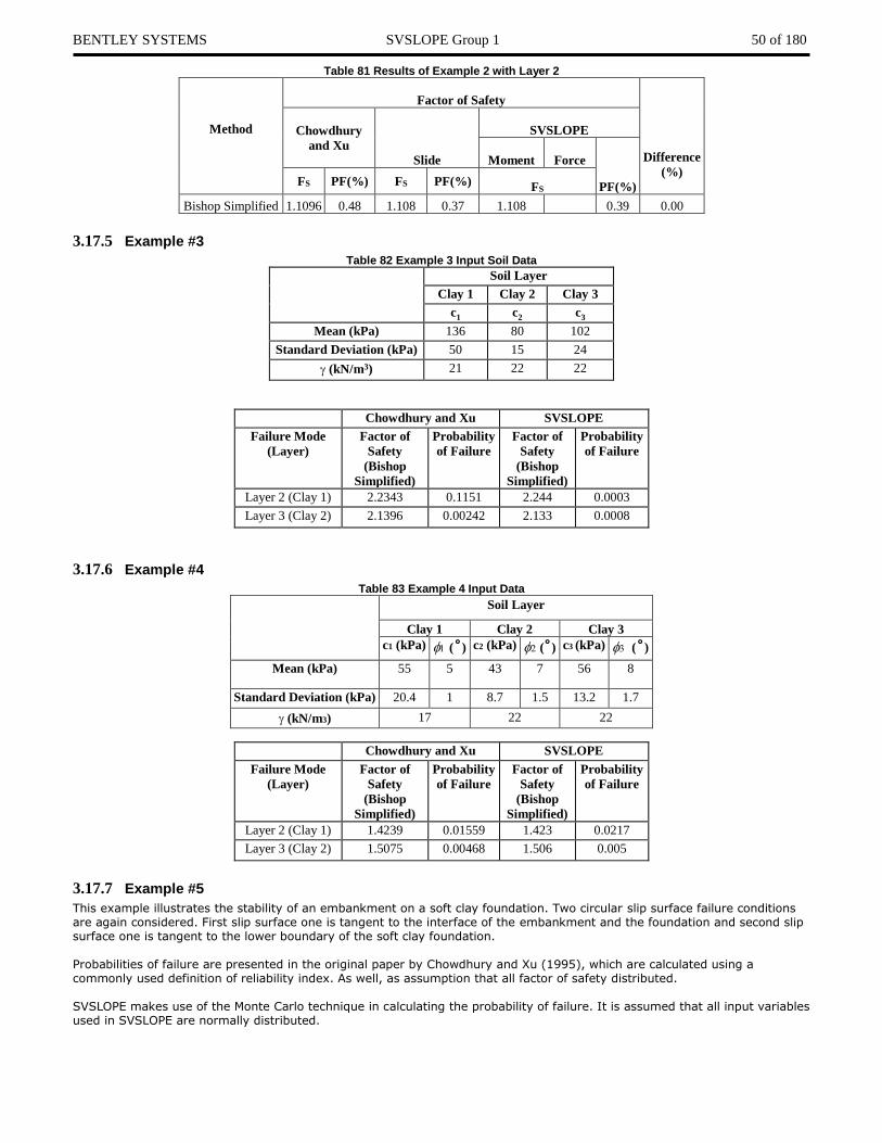
3.17.5 Example #3
Table 82 Example 3 Input Soil Data
Soil Layer
Clay 1 Clay 2 Clay 3
c1 c2 c3
Mean (kPa) 136 80 102
Standard Deviation (kPa) 50 15 24
(kN/m3) 21 22 22
Chowdhury and Xu SVSLOPE
Failure Mode
(Layer)
Factor of
Safety
(Bishop
Simplified)
Probability
of Failure
Factor of
Safety
(Bishop
Simplified)
Probability
of Failure
Layer 2 (Clay 1) 2.2343 0.1151 2.244 0.0003
Layer 3 (Clay 2) 2.1396 0.00242 2.133 0.0008
3.17.6 Example #4
Table 83 Example 4 Input Data
Soil Layer
Clay 1 Clay 2 Clay 3
c1 (kPa) ( ̊ ) c2 (kPa) ( ̊ ) c3 (kPa) ( ̊ )
Mean (kPa) 55 5 43 7 56 8
Standard Deviation (kPa) 20.4 1 8.7 1.5 13.2 1.7
(kN/m3) 17 22 22
Chowdhury and Xu SVSLOPE
Failure Mode
(Layer)
Factor of
Safety
(Bishop
Simplified)
Probability
of Failure
Factor of
Safety
(Bishop
Simplified)
Probability
of Failure
Layer 2 (Clay 1) 1.4239 0.01559 1.423 0.0217
Layer 3 (Clay 2) 1.5075 0.00468 1.506 0.005
3.17.7 Example #5
This example illustrates the stability of an embankment on a soft clay foundation. Two circular slip surface failure conditions are again considered. First slip surface one is tangent to the interface of the embankment and the foundation and second slip surface one is tangent to the lower boundary of the soft clay foundation. Probabilities of failure are presented in the original paper by Chowdhury and Xu (1995), which are calculated using a commonly used definition of reliability index. As well, as assumption that all factor of safety distributed. SVSLOPE makes use of the Monte Carlo technique in calculating the probability of failure. It is assumed that all input variables used in SVSLOPE are normally distributed.

BENTLEY SYSTEMS SVSLOPE Group 1 51 of 180
Table 84 Example 5 Input Data
Soil Layer
Layer 1 Layer 2
c1 (kPa) ( ̊ ) c2 (kPa) ( ̊ )
Mean (kPa) 10 12 40 0
Standard Deviation
(kPa)
2 3 8 0
(kN/m3) 20 18
Chowdhury and Xu SVSLOPE
Failure Mode
(Layer)
Factor of
Safety
(Bishop
Simplified)
Probability
of Failure
Factor of
Safety
(Bishop
Simplified)
Probability
of Failure
Layer 1 1.1625 0.20225 1.159 0.1966
Layer 2 1.1479 0.19733
Table 85 Material Properties
c (kN/m2) (degrees) (kN/m3)
Sand 0 0 21
3.18 DUNCAN – LASH TERMINAL Project: Slopes_Group_1 Model: VS_29 Duncan (2000) published a model that examines the failure of the 100ft high underwater slope at the lighter Abroad Ship (LASH) terminal at the Port of San Francisco, U.S.A. The values that are used in this analysis were published by Duncan (2000). It was assumed that the cohesion was 100 psf an deviation of –20ft and increases linearly with depth at the rate of 9.8psf per ft. The Latin-HyperCube simulation technique was performed using 10000 samples to compute both the probability of failure and the reliability index of the estimated failure surface, as defined with Duncan, (2000). Janbu, Spencer, and GLE methods were used to computer the factors of safety.
3.18.1 Geometry and Material Properties
The model geometry is illustrated in Figure 71.
Figure 71 Geometry of the Duncan (2000) model

BENTLEY SYSTEMS SVSLOPE Group 1 52 of 180
3.18.2 Results and Discussions
Table 86 Results of the Duncan (2000) model
Method
Factor of Safety Difference
(%) Slide SVSLOPE
Janbu Simplified 1.127 1.138 0.98
Spencer 1.150 1.159 0.78
GLE 1.161 1.163 0.17
Note: Probability analysis cannot be performed at this time, because
the cohesion change with depth is not included in SVSLOPE.
3.19 BORGES AND CARDOSO – GEOSYNTHETIC EMBANKMENT Project: Slopes_Group_1 Model: VS_30_case1, VS_30_case2 This example considers the stability of a geosynthetic-reinforced embankment on soft soil. The problem was originally published by Borges and Cardoso (2002). The sand embankment region is represented by Mohr-Coulomb strength model and the foundation material is soft clay in which it contains varied undrained shear strength. The geosynthetic has a tensile strength of 200 KN/m, is not anchored, and has no adhesion.
3.19.1 Geometry and Material Properties
It also has a frictional resistance against slip of 33.7 degrees. The reinforcement force for this example is assumed to be parallel to the reinforcement. This model is analyzed using the Bishop Simplified method. Since the original authors used the moment based limit equilibrium method for this model, the reinforcement is modeled as a passive force. This procedure is consistent with how the authors implemented reinforcement forces in the limit equilibrium methods in SVSLOPE.
Figure 72 Geometry of the Borges and Cardoso Geosynthetic Embankment Case 1
Table 87 Material Properties of Borges and Cardoso-Embankment
c (kN/m2) (degrees) γ (kN/m3)
Embankment 0 35 20
cu top
(kN/m2)
cu bottom
(kN/m2)
γ
(kN/m3)
Upper Clay 8.490 8.490 17
Middle Clay 8.490 4.725 17
Lower Clay 4.725 13.125 17
3.19.2 Results and Discussion
Table 88 Results for Case 1
Method
Factor of Safety
(Case 1-single circular)
Difference
(%)
Borges
& Cardoso
Slide
SVSLOPE
Moment Force
Bishop Simplified 1.74 1.659 1.664 0.30

BENTLEY SYSTEMS SVSLOPE Group 1 53 of 180
Table 89 Results for Case 2
Method
Factor of Safety
(Case 2-single circular) Difference
(%)
Borges
& Cardoso
Slide
SVSLOPE
Moment Force
Bishop Simplified 1.77 1.692 1.696 0.24
3.20 BORGES AND CARDOSO – GEOSYNTHETIC EMBANKMENT #2 Project: Slopes_Group_1 Model: VS_31_Case1, VS_31_Case2 This model looks at the stability of a geosynthetic-reinforced embankment placed over a soft soil. This model was original published by Borges and Cardoso (2002). This is their Case 2 example. The model is set up as a more compotent material overlaying soft clay with varying undrained shear strength. The geosynthetic has a tensile strength of 200 KN/m and a frictional resistance of 33.7 degrees. The geosynthetic is not anchored and has no adhesion. In this case, the reinforcement force is parallel to the reinforcement. The Bishop Simplified method was used to analyze this model. The reinforcement is modeled as a passive force. This corresponds to the manner in which the authors implemented
the reinforcement force in their original papers.
3.20.1 Geometry and Material Properties
Figure 73 Geometry of the VS_31 Case 1 Example by Borges and Cardoso (2002)
Table 90 Material Properties of Borges and Cardoso – Embankment #2
c (kN/m2) (degrees) γ (kN/m3)
Embankment 0 35 20
cu top
(kN/m2)
cu bottom
(kN/m2)
γ (kN/m3)
Clay 1 33 33 17
Clay 2 16 16 17
Clay 3 16 18.4 17
Clay 4 18.4 55.1 17
3.20.2 Results and Discussions
Table 91 Results for the VS_31 Case 1 example by Borges and Cardoso (2002)
Method
Factor of Safety
(Case 1 - single circular slip surface)
Difference
(%)
Borges
& Cardoso
Slide
SVSLOPE
(Slice = 30)
Slices = 25
(on Manual) Slices = 30 Slices = 40 Moment Force
Ordinary 1.346 1.346 1.323 1.346 0
Bishop Simplified 1.19 1.176 1.176 1.166 1.176 0.00
Janbu Simplified 1.208 1.208 1.205 1.207 -0.08

BENTLEY SYSTEMS SVSLOPE Group 1 54 of 180
Figure 74 Results of the VS_31 Case 1 using the Ordinary method
Table 92 Results of Case 2 example by Borges and Cardoso (2002)
Method
Factor of Safety
(Case 2 - single circular slip surface)
Difference
(%)
Borges
& Cardoso
Slide SVSLOPE
Slices = 25
(on Manual) Slices = 30 Slices = 40 Moment Force
Ordinary 1.282 1.282 1.277 1.282 0.00
Bishop Simplified 1.15 1.163 1.162 1.16 1.163 -0.06
Janbu Simplified 1.17 1.17 1.169 1.171 -0.09

BENTLEY SYSTEMS SVSLOPE Group 1 55 of 180
3.21 BORGES AND CARDOSO – GEOSYNTHETIC EMBANKMENT #3 Project: Slopes_Group_1 Model: VS_32Case1, VS_32Case2, VS_32Case3 This is the case 3 example taken from Borges and Cardoso (2002). This particular model looks at the stability of a
geosynthetic-reinforced embankment on soft soil.
3.21.1 Geometry and Material Properties
The material properties are the same as the previous two examples. The geosynthetic in this case has the tensile strength of 200 KN/m as well as a frictional resistance of 39.6 degrees. The Bishop Simplified analysis method is used for consistency with the method used by the authors. The two embankment materials are implemented in the model. The lower embankment material is 0 to 1 m and the upper embankment material is from 1 to 7 m (Case 1) or 1 to 8.75m (Case 2). The geosynthetic is placed at the elevation 0.9 m, just inside on the lower embankment material.
Figure 75 Geometry of the VS_32_Case 1 model
Figure 76 Geometry of the VS_32_Case 2 model
Table 93 Material Properties
c (kN/m2) (degrees) γ (kN/m3)
Upper Embankment 0 35 21.9
Lower Embankment 0 33 17.2

BENTLEY SYSTEMS SVSLOPE Group 1 56 of 180
cu (kN/m2) γ (kN/m3)
Clay 1 43 18
Clay 2 31 16.6
Clay 3 30 13.5
Clay 4 32 17
Clay 5 32 17.5
3.21.2 Results and Discussions
Table 94 Results Case 1-Embankment Height = 7m
SVSLOPE
Factor of
Safety
Overturning
Moment
(kN/m/m)
Resisting
Moment
(kN/m/m)
Circle A (SVSLOPE)
Circle A (Borges & Cardoso) 34166 42695
Circle B (SVSLOPE)
Circle (Borges & Cardoso) 63870 75754
Table 95 Results Case 2-Embankment Height = 8.75m
SVSLOPE
Factor of
Safety
Overturning
Moment
(kN/m/m)
Resisting
Moment
(kN/m/m)
Circle C (SVSLOPE) 64873 63846
Circle C (Borges & Cardoso) 65116 64784
Table 96 Results for Case 1
Method
Factor of Safety
(Case 1)
Difference
(%)
Borges
& Cardoso
Slide
SVSLOPE
Moment Force
Bishop Simplified 1.25 1.225 1.227 0.16
Table 97 Results for Case 2
Method
Factor of Safety
(Case 2) Difference
(%)
Borges
& Cardoso
Slide
SVSLOPE
Moment Force
Bishop Simplified 1.19 1.219 1.220 0.08
Table 98 Results for Case 3
Method
Factor of Safety
(Case 3) Difference
(%)
Borges
& Cardoso
Slide
SVSLOPE
Moment Force
Bishop Simplified 0.99 0.984 0.984 0.00

BENTLEY SYSTEMS SVSLOPE Group 1 57 of 180
Figure 77 Results of the VS_32_Case 3 model using the Bishop Simplified method
3.22 SYNCRUDE PROBABILISTIC TAILINGS DYKE Project: Slopes_Group_1 Model: VS_33 This example model was published by El-Ramly et al (2003). This model is designed for the calculation of the factor of safety for a Syncrude tailings dyke in Alberta, Canada. In this case, a probabilistic analysis is performed. This paper does not consider spaciously variation of soil properties, and is therefore described as a simplified probabilistic analysis. The original geometry from the El-Ramly et al (2003) paper is shown in Figure 78. The material parameters are input into SVSLOPE as shown in Table 99. The soil parameters were considered probabilistic by El-Ramly et al. They varied the friction angle of the Kca clay-shale, the pore pressure ratio in the same layer, the friction angle of the Pgs sandy till layer and the pore pressure ratios in this layer in the middle and the toe of the dyke. In the SVSLOPE model we consider the variation of the friction angles of the Kca clay-shale and Pgs sandy till. The phreatic surface indicated in Figure 79 was used in place of the pore pressure ratios. In order in to be consistent the El-Ramly paper the Bishop Simplified analysis method was used. A Monte Carlo analysis was used to calculate the probability of failure. It is worth noting that it is assumed that all probabilistic input parameters are normally distributed.
3.22.1 Geometry and Material Properties
Figure 78 Original Geometry of the Syncrude Tailings Dyke model
Figure 79 Phreatic Surface

BENTLEY SYSTEMS SVSLOPE Group 1 58 of 180
Figure 80 Geometry of the Syncrude Tailing Dyke model
Table 99 Material Properties of the Syncrude Tailing Dyke model
c (kN/m2) (degrees) Standard
Deviation of
(degrees)
γ (kN/m3)
Tailings sand 0 34 - 20
Glacio-fluvial sand 0 34 - 17
Sandy till 0 34 - 17
Clayey Till 0 7.5 - 17
Distributed clay-shale 0 7.5 - 17
3.22.2 Results and Discussions
Table 100 Results of the Syncrude Tailing Dyke model
Method
Factor of Safety
Difference
(%)
El-Ramly Slide SVSLOPE
Determ PF(%) Determ
Probabilitistic
Determ
Probabilitistic
Mean PF(%) Mean PF(%)
Bishop
Simplified 1.31 0.16 1.305 1.327 0.154 1.303 1.304 3.65 -0.15
3.23 CANNON DAM Project: Slopes_Group_1 Model: VS_34_Monte The Cannon Dam model was published from Wolff and Harr (1987). The probabilistic analysis results from SVSLOPE are compared to the results published in the paper by Wolff and Harr for a noncircular slip surfaces. Wolff and Harr (1987) used the point-estimate method for their probability analysis failure for the Cannon Dam. The location of critical slip surface was taken from their paper. The input parameters; namely, friction angle for the Phase I and Phase II fills was calculated. The unit weights of the fills were back-calculated in order to match the factor of safety computed by Wolff and Harr. Wolff and Harr (1987) based on the stochastic properties provided in the paper originally published results that only satisfied force equilibrium.
3.23.1 Geometry and Material Properties
Figure 81 Geometry of the Cannon Dam model – VS_34
Table 101 Material Properties of the Cannon Dam
Material c (lb/ft2) Standard
Deviation of
c (lb/ft2)
(degrees) Standard
deviation of
(degrees)
Correlation
coefficient for
c and
γ (lb/ft3)

BENTLEY SYSTEMS SVSLOPE Group 1 59 of 180
Phase I fill 2,230 6.33 150
Phase II fill 2,901.6 14.8 150
Material 3 1 50 150
Material 4 1 35 150
Spoil Fill 3,000 60 150
Filter - 35 120
3.23.2 Results and Discussions
The results were compared to those obtained by GLE and the Spencer methods. It is assumed in the SVSLOPE model that all the probabilistic input variables are normally distributed.
Table 102 Results of the Cannon Dam
Method
Factor of Safety
Difference
(%)
Wolff and Harr Slide SVSLOPE
Deterministic PF(%)
Deterministic
Probabilitistic
Deterministic
Probabilitistic
Mean PF(%) Mean PF(%)
Spencer 2.36 4.55 2.383 2.401 0.355 2.386 2.386 0.13
GLE 2.333 2.358 0.355 2.343 2.343 0.43
3.24 CANNON DAM #2 Project: Slopes_Group_1 Model: VS_35_1_Fig.7_SurfaceA, VS_35_1_Fig.7_SurfaceB, VS_35_1_Fig.7_SurfaceC, VS_35_1_Fig.7_SurfaceD, VS_35_1_Fig.7_SurfaceE, VS_35_1_Fig.8_SurfaceB, VS_35_1_Fig.8_SurfaceF, VS_35_1_Fig.8_SurfaceG, VS_35_1_Fig.8_SurfaceH This model of the Cannon Dam in Missouri was presented by Hassan and Wolff (1999). The purpose of this verification model is to look at duplicating reliability index results for several circular failure surfaces as specified in the original paper. Hassan and Wolff (1999) presented a new reliability based approach in their paper. The cross-section of the Cannon Dam is shown below. The Bishop Simplified method of slices was used to analyze this verification problem. The present set of slip circles are those shown in Figure 82 of the Hassan and Wolff paper and Figure 83 shows the model input parameters. The Hassan and Wolff (1999) paper does not provided all the required input parameters. Therefore we selected values for the missing parameters that allowed to us to match the factors of safety for some of the circles slip surfaces shown in Figure 82. The assumption is made in this analysis that all the probabilistic input variables are normally distributed for performing the Monte Carlo simulations. The reliability indices calculated in SVSLOPE are based on the mean and standard deviations of the factor of safety values
calculated in the simulations. The reliability indices shown in the results section are calculated using the assumption that the factors of safety values are log-normally (Hassan and Wolff, 1999). The results obtained from SVSLOPE and the results from Hassan and Wolff are shown in Table 104.
3.24.1 Geometry and Material Properties
Figure 82 Hassan and
Wolff’s Geometry

BENTLEY SYSTEMS SVSLOPE Group 1 60 of 180
Figure 83 Hassan and Wolff (1999) paper
Figure 84 Geometry of VS_35_1_Fig7_Surface A - Cannon Dam #2
Table 103 Material Properties of the Cannon Dam #2
Material c (lb/ft2) Standard
Deviation of
c (lb/ft2)
(degrees) Standard
deviation of
(degrees)
Correlation
coefficient for
c and
γ (lb/ft3)
Phase I clay fill 117.79 58.89 8.5 8.5 0.1 22
Phase II clay fill 143.64 79 15 9 -0.55 22
Sand Filter 0 - 35 - - 22
Foundation sand 5 - 18 - - 22
Spoil fill 5 - 35 - - 25

BENTLEY SYSTEMS SVSLOPE Group 1 61 of 180
3.24.2 Results and Discussions
Table 104 Results of the Cannon Dam #2
Surfaces Method
Factor of Safety
Difference
(%)
Hanssan and
Wolff Slide SVSLOPE
Determ
Reliability
Index-
lognormal Determ
Probabilitistic
Determ
Probabilitistic
Mean
RI-
Lognormal PF(%) Mean RI PF(%)
Figure 7
Bishop 2.8 4.55
2.551 2.6 10.95 0 2.55 2.664 9.00 0 -0.04 Surface A
Figure 7
Bishop 2.4 3.987
2.82 3.1 4.351 0.1 2.818 3.166 4.25 0.3 -0.071 Surface B
Figure 7
Bishop 2.5 4.606
2.777 3.1 4.263 1.2 2.782 3.117 4.21 0.3 0.18 Surface C
Figure 7
Bishop 2.5 8.468
2.583 2.6 11.09 0 2.582 2.697 9.07 0 -0.04 Surface D
Figure 7
Bishop 2.6 10.04
2.692 2.8 10.28 0 2.691 2.824 8.42 0 -0.04 Surface E
Figure 8
Bishop 3 3.987
2.676 2.9 4.858 0 2.676 3.141 4.21 0 0.00 Surface B
Figure 8
Bishop 3.9 4.95
3.598 3.8 5.485 0 3.596 3.984 5.03 0 -0.06 Surface F
Figure 8
Bishop 11 5.544
6.074 6.1 5.563 0 6.071 6.670 4.84 0.3 -0.05 Surface G
Figure 8
Bishop 6.3 4.838
11.23 11 6.394 0 11.224 12.26 5.95 0 -0.05

BENTLEY SYSTEMS SVSLOPE Group 1 62 of 180
3.25 LI AND LUMB – RELIABILITY INDEX Project: Slopes_Group_1 Model: VS_36 This model is original presented in Li and Lumb (1987) and Hassan and Wolff (1999). The purpose of this model is to analyze
the reliability indices of a simple homogenous slope. The verification compares of the reliability index of the deterministic global circular surface and the minimum reliability index value obtained from an analysis of multiple slip surfaces.
3.25.1 Geometry and Material Properties
The geometry is presented in Figure 85 and the material properties are presented in Table 105. In this analysis the Bishop Simplified method of analysis was used. A Monte Carlo analysis was used which assumes that all input probability variables are normally distributed. The reliability indices are calculated on the assumption that the factors of safety values are distributed log normal. This interpretation is consisted with the original analysis presented by Hassan and Wolff (1999). Separate reliability indices are calculated for the minimum deterministic critical slip surface, as well as the critical probabilistic slip surface.
Figure 85 Geometry of the Li and Lumb – Reliability Index model
Table 105 Material Properties of the Li and Lumb (1987) reliability index
Property Mean Value Standard
deviation
c (kN/m2) 18 3.6
(degrees) 30 3
γ (kN/m3) 18 0.9
Ru 0.2 0.02
3.25.2 Results and Discussions
The overall reliability indices of the slope are compared with reliability calculated by Hassan and Wolff (1999). The results are shown in the Table 106:
Table 106 Results of the Li and Lumb (1987) reliability index
Method
Factor of Safety
Difference
(%)
Hassan and
Wolf (1999) Slide SVSLOPE
Reliability
Index
Log normal
FS
Reliability
Index
Log normal
Probability
of Failure
(%)
FS
Reliability
Index
Log normal
Probability
of Failure
(%)
Bishop
Simplified 1.339 1.338 -0.08
Janbu
Simplified 1.261 1.257 -0.32

BENTLEY SYSTEMS SVSLOPE Group 1 63 of 180
3.26 REINFORCEMENT BACK ANALYSIS Project: Slopes_Group_1 Model: VS_37_NoReinforcement, VS_37_ReinZone This model is originally presented in the reference manual of slope stability program XSTABL (1999). A back analysis is used
to determine the amount of reinforcement required to stabilize a slope. Relatively simple geometry and slope conditions are used along with one non-cohesive soil material. The analysis proceeds in two steps:
• Determining the reinforcement needed to stabilize a slope to predetermine a factor of safety value of 1.5, and • Establishing the minimum required length of reinforcement.
In Figure 86 it describes the slope model and the solution. In XSTABL the slip surfaces past only through the toe of the slope. This type of restriction has been duplicated in SVSLOPE by placing an exist point near the toe of the slope.
3.26.1 Geometry and Material Properties
Figure 86 Geometry of the NoReinforcement Back Analysis model
It should also be noted that when there is no cohesive, the slip surface would tend to rise to the ground surface. Therefore, a minimum depth was imposed on considered slip surfaces. The next step involved changing the slope and including a reinforced zone with a higher friction angle calculated from the formula presented in the XSTABL Reference Manual, (1999).
( )
crit
r
rre
F
FwhereF
F
min
1
inf tantan
=
= −
The length of the reinforced zone was varied manually until the factor of safety value very close to 1.5 was obtained. The results can be seen in Table 107.
3.26.2 Results and Discussions
Table 107 Results Back Analysis – Reinforcement
Method
Factor of Safety Difference
(%) Slide SVSLOPE
Ordinary 0.756
Bishop Simplified 0.765 0.76 0.71
Janbu Simplified 0.739 0.756 2.30
Table 108 NoReinforcement
Method
Factor of Safety Difference
(%) Slide SVSLOPE
Bishop Simplified 0.765 0.771 0.78
Janbu Simplified 0.739 0.743 0.54

BENTLEY SYSTEMS SVSLOPE Group 1 64 of 180
Figure 87 Results of the NoReinforcement Back Analysis model
Table 109 Reinforced Zone, neglect pore-water pressures and no cracks
Method
Factor of Safety Difference
(%)
Slope/W SVSLOPE
Moment Force Moment Force
Ordinary
Bishop Simplified 1.504 1.533 1.93
Janbu Simplified 1.247 1.279 2.57

BENTLEY SYSTEMS SVSLOPE Group 1 65 of 180
3.27 TANDJIRIA – GEOSYNTHETIC REINFORCED EMBANKMENT Project: Slopes_Group_1 Model: VS_39_Clay_NoRein_Circular, VS_39_Clay_NoRein_NonCircular, VS_39_Clay_Rein_Circular, VS_39_Clay_Rein_NonCircular, VS_39_Sand_NoRein_Circular, VS_39_Sand_NoRein_NonCircular,
VS_39_Sand_Rein_Circular, VS_39_Sand_Rein_NonCircular This model was originally presented by Tandjiria (2002) as their example #1 problem. The stability of a geosynthetic-reinforced embankment on soft soil was examined. This problem examines the stability of the embankment when it consists of sand or an undrained clay fill. The objective of this example is to compute the required reinforcement force to yield a factor of safety of 1.35. Circular and noncircular critical slip surfaces were examined. In each case presented, the embankment was first modeled without reinforcement and the critical slip surfaces determined. Then the determined critical slip surface was used in the reinforcement model to determine the reinforcement force to achieve a factor of safety of 1.35. The above approach was used for both the clay embankment with a circular and noncircular slip surface. All cases incorporate a tension crack in the embankment. Water is allowed to fill the tension cracks in the case of the clay embankment. In this case the reinforcement was located at the base of the embankment. Both Spencer and GLE methods were used to analyze the slope. The GLE method used a half sine interslice function.
NOTE:
The reinforcement is modeled as an active force since Tandjiria (2002) modeled the force in this manner.
3.27.1 Geometry and Material Properties
Figure 88 Clay Fill Embankment (circular) Reinforcement
Table 110 Material Properties of the clay fill embankment
cu/c (kN/m2) (degrees) γ (kN/m3)
Clay Fill Embankment 20 0 19.4
Sand Fill Embankment 0 37 17.0
Soft Clay Foundation 20 0 19.4
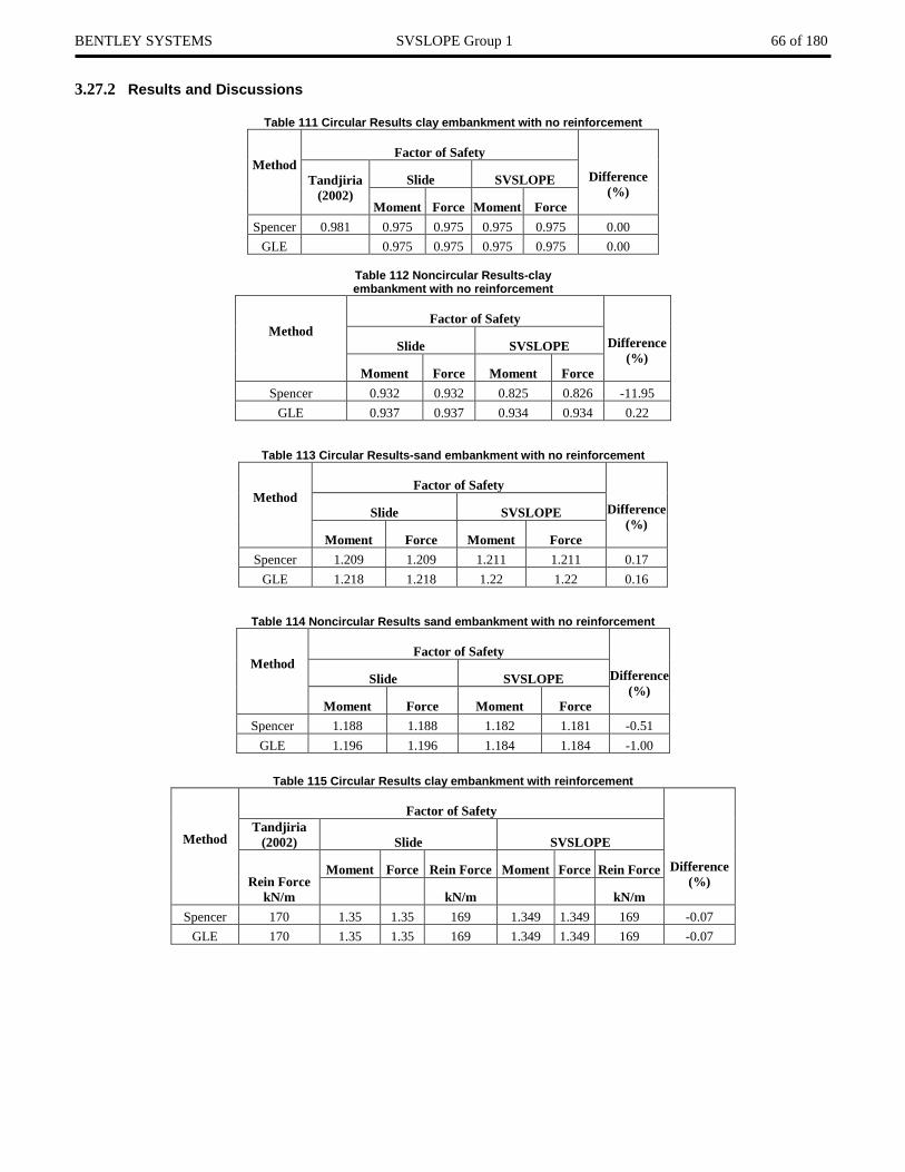
BENTLEY SYSTEMS SVSLOPE Group 1 66 of 180
3.27.2 Results and Discussions
Table 111 Circular Results clay embankment with no reinforcement
Method
Factor of Safety
Difference
(%)
Tandjiria
(2002)
Slide SVSLOPE
Moment Force Moment Force
Spencer 0.981 0.975 0.975 0.975 0.975 0.00
GLE 0.975 0.975 0.975 0.975 0.00
Table 112 Noncircular Results-clay embankment with no reinforcement
Method
Factor of Safety
Difference
(%)
Slide SVSLOPE
Moment Force Moment Force
Spencer 0.932 0.932 0.825 0.826 -11.95
GLE 0.937 0.937 0.934 0.934 0.22
Table 113 Circular Results-sand embankment with no reinforcement
Method
Factor of Safety
Difference
(%)
Slide SVSLOPE
Moment Force Moment Force
Spencer 1.209 1.209 1.211 1.211 0.17
GLE 1.218 1.218 1.22 1.22 0.16
Table 114 Noncircular Results sand embankment with no reinforcement
Method
Factor of Safety
Difference
(%)
Slide SVSLOPE
Moment Force Moment Force
Spencer 1.188 1.188 1.182 1.181 -0.51
GLE 1.196 1.196 1.184 1.184 -1.00
Table 115 Circular Results clay embankment with reinforcement
Method
Factor of Safety
Difference
(%)
Tandjiria
(2002) Slide SVSLOPE
Rein Force
kN/m
Moment Force Rein Force Moment Force Rein Force
kN/m kN/m
Spencer 170 1.35 1.35 169 1.349 1.349 169 -0.07
GLE 170 1.35 1.35 169 1.349 1.349 169 -0.07

BENTLEY SYSTEMS SVSLOPE Group 1 67 of 180
Figure 89 Results of the Clay embankment reinforcement circular
Table 116 Noncircular Results clay embankment with reinforcement
Method
Factor of Safety
Difference
(%)
Tandjiria
(2002) Slide SVSLOPE
Rein Force
kN/m
Moment Force Rein Force Moment Force Rein Force
kN/m kN/m
Spencer 190 1.351 1.351 184 1.353 1.352 184 0.15
GLE 190 1.366 1.366 184 1.367 1.367 184 0.07
Table 117 Circular Results sand embankment with reinforcement
Method
Factor of Safety
Difference
(%)
Tandjiria
(2002) Slide SVSLOPE
Rein Force
kN/m
Moment Force Rein Force
kN/m
Moment Force Rein Force
kN/m
Spencer 45 1.35 1.35 44 1.347 1.347 44 -0.22
GLE 45 1.357 1.357 44 1.354 1.354 44 -0.29
Table 118 Noncircular Results sand embankment with reinforcement
Method
Factor of Safety
Difference
(%)
Tandjiria
(2002) Slide SVSLOPE
Rein Force
kN/m
Moment Force
Rein Force
kN/m
Moment Force
Rein Force
kN/m
Spencer 56 1.35 1.35 56 1.358 1.357 53 0.59
GLE 56 1.359 1.359 56 1.362 1.362 53 0.22
3.28 BAKER AND LESCHINSKY – EARTH DAM Project: Slopes_Group_1 Model: VS_42_circular, VS_42_noncircular This model was original published by Baker and Leshchinsky (2001). It was presented to illustrate the use of safety maps as practical tools for slope stability analysis.
3.28.1 Geometry and Material Properties
The geometry of the model can be seen in Figure 90. The model consists of a clay core with granular fill surrounding the core. The model has a solid base. A dry tension crack is placed at the top of the model to stimulate a 5m thick crack layer. All trial slip surfaces must be plotted on the dam to obtain a safety map of regional safety factors of safety. Noncircular slip surfaces and corresponding factor of

BENTLEY SYSTEMS SVSLOPE Group 1 68 of 180
safety are also required in this analysis.
Figure 90 Geometry of the Baker and Leshchinsky Earth Dam Circular model
Table 119 Material Properties of the Earth Dam Circular model
c (kN/m2) (degrees) γ (kN/m3)
Clay core 0 20 20
Granular Fill 0 40 21.5
Hard Base 200 45 24
Figure 91 Geometry of the VS_42_noncircular model
3.28.2 Results and Discussions
Table 120 Results - Circular failure surface, 80 x 80 grid
Method
Factor of Safety
(VS_42_Circular Slip Surfaces) Difference
(%)
Baker &
Leshchinsky
Slide
SVSLOPE
Moment Force
Spencer 1.91 1.923 1.923 1.923 0.00
Table 121 Results Noncircular using Random Search with Optimization (zero faces)
Method
Factor of Safety
(VS_42_Non-Circular Slip Surfaces) Difference
(%)
Baker &
Leshchinsky
Slide
SVSLOPE
Moment Force
Spencer 1.91 1.857 1.857 1.856 0.00

BENTLEY SYSTEMS SVSLOPE Group 1 69 of 180
3.29 BAKER – PLANAR HOMOGENEOUS Project: Slopes_Group_1 Model: VS_43_BlockSearch, VS_43_Circular This model is original published by Baker (2001), and looks at the factor of safety of planar slip surfaces. The results are
compared at various failure plane angles. The slope presented is homogenous and dry.
3.29.1 Geometry and Material Properties
The geometry can be seen in Figure 92. In this case, there are two tests that must be run on this slope. The first test is that the plot of factors of safety versus x-coordinate are required for all critical failure planes passing through the toe of the slope. Subsequently, the critical circular slip surfaces in Zone A must determined at which point the safety factors versus x-coordinate for Zone A must be plotted. A method of locating the factor of safety as a function of the failure plane angle is presented.
Figure 92 Geometry of the Baker (2001) - Planar Homogeneous Slope
Table 122 Material Properties of the Baker (2001) - Planar Homogenous Slope
c (kN/m2) (degrees) γ (kN/m3)
Material 30 30 20
Figure 93 Baker's (2001) Distribution
3.29.2 Results and Discussions
Table 123 Results non-circular Baker (2001)
Method
Factory of Safety
Difference
(%)
Baker
(2001)
RocPlane 2.0 Slide SVSLOPE
FS Angle FS Angle FS Angle
Janbu Simplified 1.35 1.351 49.5 1.352 49.5 1.352 49.5 0

BENTLEY SYSTEMS SVSLOPE Group 1 70 of 180
3.30 SHEAHAN – AMHEARST SOIL NAILS Project: Slopes_Group_1 Model: VS_47 This problem was published by Sheahan (2003). It examines the Amhearst test wall, which was a soil nailed wall in clay that
failed due to over excavation.
3.30.1 Purpose
The purpose of the analysis is to determine the location of the critical planar slip surface and associated factor of safety.
3.30.2 Geometry and Material Properties
This particular analysis involves a planar failure through a soil nailed wall. The factor of safety is calculated for the undrained, homogeneous slope. In this case the slope is reinforced by two rows of nails. The shotcrete plate on the soil nails has a weight of 14.6 kN/m. This weight is modeled as a point load at the top of the wall face.
Figure 94 Geometry of the Sheahan Amhearst Soil Nails Model
Table 124 Material Properties of the Sheaham Amhearst Soil Nails model
Material c (kN/m2) γ (kN/m3)
Amherst Clay 25 18.9
Table 125 Soil Nail Properties
Type Out-of-plane
Spacing (m)
Tensile Strength
(kN)
Plate Strength
(kN)
Bond Strength
(kN)
Length
(m)
Number
of rows
Passive 1.5 118 86 15 4.9 2
3.30.3 Results and Discussions
Table 126 Results – Sheahan-Amhearst Soil Nails
Method
Factor of Safety
Difference
(%)
Sheahan
(2003)
Slide
SVSLOPE
Moment Force
Janbu Simplified 0.887 0.888 0.89 0.23

BENTLEY SYSTEMS SVSLOPE Group 1 71 of 180
3.31 SHEAHAN – CLOUTERRE TEST WALL Project: Slopes_Group_1 Model: VS_48, VS_48_45Deg, VS_48_50Deg, VS_48_55Deg, VS_48_60Deg, VS_48_65Deg, VS_48_70Deg
This problem was presented by Sheahan (2003) and it examines the Clouterre Test Wall. The test wall was constructed using Fontainebleu sand and failed by backfill saturation. The test was carried out as part of the French national project on soil nailing.
3.31.1 Purpose
The purpose of this analysis is to determine the factor of safety for six different plane angles ranging from 45 to 70 degrees.
3.31.2 Geometry and Material Properties
The relationship between the failure slope angle and the factor of safety of a homogeneous slope is examined in this case. The primary resistance against failure is friction generated by the soil weight. The test wall was reinforced using seven rows of soil nails and a shotcrete plate weighting 13.2 kN/m. The shotcrete plate weighting was modeled as point load acting on the wall face.
Figure 95 Geometry of the Sheahan Clouterre Test Wall model
Table 127 Material Properties of the Sheahan Clouterre Test Wall model
Material c (kN/m2) (degrees) γ (kN/m3)
Fontainebleau Sand 3 38 20
Table 128 Soil Nail Properties
Type Out-of-plane
Spacing (m)
Tensile Strength
(kN)
Plate Strength
(kN)
Bond Strength
(kN)
Passive 1.5 15 59 7.5
3.31.3 Results and Discussions
Table 129 Results Janbu Simplified (Sheahan, 2003)
Method
Factory of Safety Difference
(%)
Slide
SVSLOPE
Moment Force
Janbu Simplified 0.921 0.922 0.11

BENTLEY SYSTEMS SVSLOPE Group 1 72 of 180
Figure 96 Results of theVS_48 model using the Janbu Simplied method
Table 130 Results for different slope angles of the failure surface
Slope Angle
Factor of Safety
Difference
(%) Sheahan
Slide
Janbu
Simplified
SVSLOPE
Janbu
Simplified
45 1.176 1.124 1.123 -0.09
50 1.070 1.043 1.043 0.00
55 0.989 0.989 0.989 0.00
60 0.929 0.946 0.945 -0.11
65 0.893 0.921 0.922 0.11
70 0.887 0.922 0.924 0.22
3.32 SNAILZ – REINFORCED SLOPE Project: Slopes_Group_1 Model: VS_49 This model was taken from the SNAILZ reference manual (http://www.dot.ca.gov/hq/esc/geotech). The model has two materials and is a slope reinforced with a soldier pile tieback wall. Imperial units are used for this particular model.
3.32.1 Purpose
The purpose of this model is to determine the factor of safety for a given slip surface.
3.32.2 Geometry and Material Properties
There are two different types of reinforcements in this model. Each of the two rows of soil nails has different bar diameters, which results in different tension capabilities. The soldier piles are modeled using a micro-pile in SVSLOPE.
Figure 97 Geometry of the Snailz Reinforced Slope model

BENTLEY SYSTEMS SVSLOPE Group 1 73 of 180
Table 131 Material Properties of the Snailz Reinforced Slope
Material c (psf) (degrees) γ (pcf)
Layer 1 600 24 120
Layer 2 300 34 130
Table 132 Soil Nail Properties (Active)
Out-of-plane
Spacing (m)
Tensile
Strength (lb)
Plate Strength
(kN)
Bond Strength
(kN)
Soil Nail: top now 8 120344.9 120344.9 13571.68
Soil Nail: bottom row 8 164217.3 164217.3 13571.68
Micro-pile (active) 1 Pile shear strength: 5900 lb.
3.32.3 Results and Discussions
Table 133 Results of the Snailz Reinforced Slope
Method
Factor of Safety Difference
(%)
SNAILZ
Slide
SVSLOPE
Moment Force
Janbu Simplified 1.52 1.446 1.446 0.00
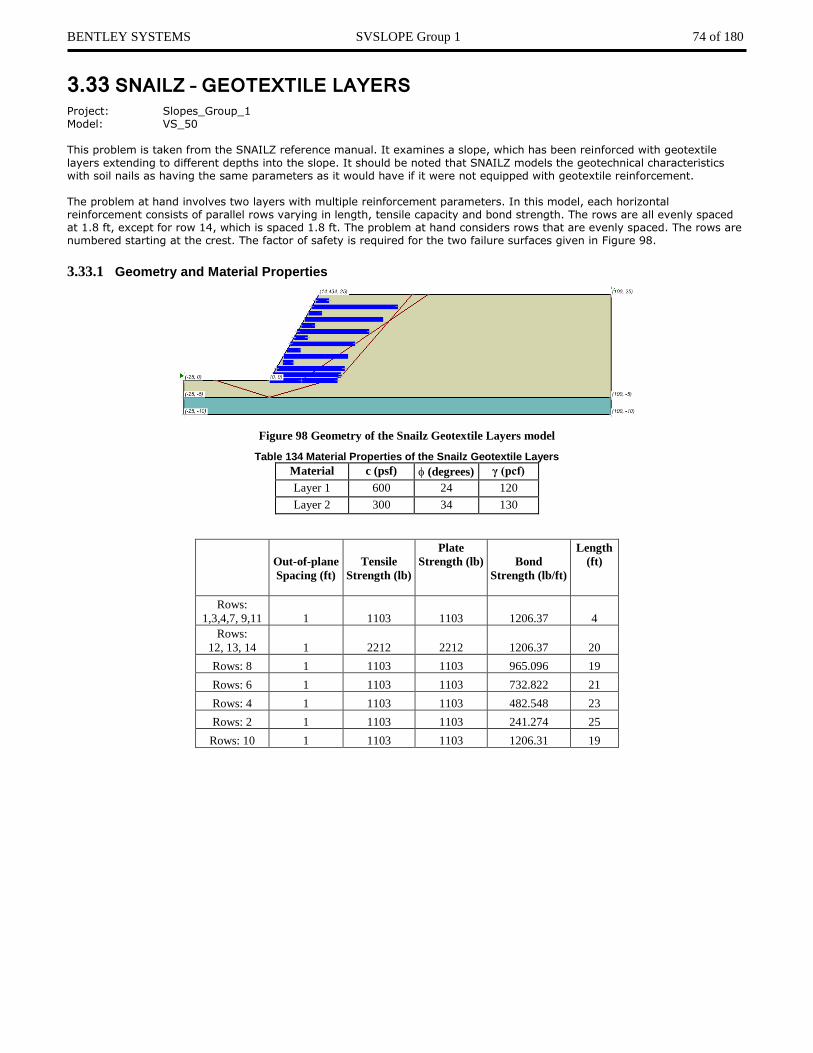
BENTLEY SYSTEMS SVSLOPE Group 1 74 of 180
3.33 SNAILZ – GEOTEXTILE LAYERS Project: Slopes_Group_1 Model: VS_50 This problem is taken from the SNAILZ reference manual. It examines a slope, which has been reinforced with geotextile
layers extending to different depths into the slope. It should be noted that SNAILZ models the geotechnical characteristics with soil nails as having the same parameters as it would have if it were not equipped with geotextile reinforcement. The problem at hand involves two layers with multiple reinforcement parameters. In this model, each horizontal reinforcement consists of parallel rows varying in length, tensile capacity and bond strength. The rows are all evenly spaced at 1.8 ft, except for row 14, which is spaced 1.8 ft. The problem at hand considers rows that are evenly spaced. The rows are numbered starting at the crest. The factor of safety is required for the two failure surfaces given in Figure 98.
3.33.1 Geometry and Material Properties
Figure 98 Geometry of the Snailz Geotextile Layers model
Table 134 Material Properties of the Snailz Geotextile Layers
Material c (psf) (degrees) γ (pcf)
Layer 1 600 24 120
Layer 2 300 34 130
Out-of-plane
Spacing (ft)
Tensile
Strength (lb)
Plate
Strength (lb)
Bond
Strength (lb/ft)
Length
(ft)
Rows:
1,3,4,7, 9,11 1 1103 1103 1206.37 4
Rows:
12, 13, 14 1 2212 2212 1206.37 20
Rows: 8 1 1103 1103 965.096 19
Rows: 6 1 1103 1103 732.822 21
Rows: 4 1 1103 1103 482.548 23
Rows: 2 1 1103 1103 241.274 25
Rows: 10 1 1103 1103 1206.31 19

BENTLEY SYSTEMS SVSLOPE Group 1 75 of 180
3.33.2 Results and Discussions
Table 135 Results for Case 1
Method
Factor of Safety Difference
(%)
Slide
SVSLOPE
Moment Force
Janbu Simplified 1.354 1.354 0.00
Spencer 1.618 1.617 1.617 -0.06
GLE 1.621 1.617 1.616 -0.25
Note: “Corrected” Janbu method is not available in SVSlope, so the results were
compared to the Janbu Simplified method
3.34 ZHU – FOUR LAYER SLOPE Project: Slopes_Group_1 Model: VS_51 This model was presented by Zhu (2003). The problem consists of four soil layers with a designated slip surface, using a number of different methods. The multiple layers slope is analyzed using circular slip surfaces. Tension cracks are placed through the top layer and the slope is assumed to be subjected to earthquake conditions with a seismic coefficient of 0.1. In this case, the factor of safety for the surface with 100 slices is required using all methods of analysis. The tolerance level is set at 0.001.
3.34.1 Geometry and Material Properties
Figure 99 Geometry of the Zhu Four Layer Slope model
Table 136 Material Properties of the Zhu Four Layer Slope
Material c (kN/m2) (degrees) γ (kN/m3)
Layer 1 (top) 20 32 18.2
Layer 2 25 30 18.0
Layer 3 40 18 18.5
Layer 4 (bottom) 40 28 18.8
3.34.2 Results and Discussions
Table 137 Results for Case 1
Method
Factor of Safety Difference
(%)
Zhu
Slide
SVSLOPE
Moment Force
Ordinary 1.066 1.075 1.072 -0.28
Bishop Simplified 1.278 1.288 1.285 -0.23
Janbu Simplified 1.112 1.121 1.115 -0.54
Corps of Engineers #2 1.377 1.420 1.41 -0.70
Lowe-Karafiath 1.290 1.288 1.295 0.54

BENTLEY SYSTEMS SVSLOPE Group 1 76 of 180
Spencer 1.293 1.302 1.300 1.299 -0.15
M-P 1.313 1.313 1.309 1.309 -0.31
GLE 1.313 1.313 1.309 1.309 -0.31
Figure 100 Results of using the GLE method VS_51
3.35 ZHU AND LEE – HETEROGENEOUS SLOPE Project: Slopes_Group_1 Model: VS_52 Zhu and Lee (2002) presented this model to analyze a heterogeneous slope under wet and dry conditions. Four different slip surfaces were analyzed for each of these conditions. A dry tension crack was placed at the top of the slope and the factor of safety was required for eight separate cases, four distinct slip surfaces under dry conditions, and four distinct slip surfaces when a water table was included (Table 2).
In this case surfaces 1 and 3 were circular, while surfaces 2 and 4 are noncircular. Critical slip surfaces 1 and 2 are shallow, and critical slip surfaces 3 and 4 are deep.
3.35.1 Geometry and Material Properties
Figure 101 Geometry of the Zhu and Lee Heterogenous Slope model (VS_52_1_dry)
Table 138 Material Properties of the Zhu and Lee Heterogenous Slope model
Material c (kN/m2) (degrees) γ (kN/m3)
Layer 1 (top) 20 18 18.8
Layer 2 40 22 18.5
Layer 3 25 26 18.4
Layer 4 (bottom) 10 12 18.0

BENTLEY SYSTEMS SVSLOPE Group 1 77 of 180
Table 139 Water Table Geometry wet condition
Coordinates Arc
(0, -20)
(0,0)
(6,3)
(100568, 5.284)
(25.314, 9.002)
(39.149, 10.269)
(50,10.269)
3.35.2 Results and Discussions
Table 140 Surface 1 Circular, shallow
Method
Factor of Safety
(1-dry-single circular)
Difference
(%)
Zhu
& Lee Slide
SVSLOPE
Moment Force
Ordinary 1.935 1.934 1.934 0.00
Bishop Simplified 2.011 2.010 2.010 0.00
Spencer 2.035 2.017 2.017 2.017 0.00
M-P 2.035 2.017 2.017 2.017 0.00
Figure 102 Results using the M-P method VS_52_1_dry
Table 141 Results - Surface 2 Circular, deep Grid search
Method
Factor of Safety
(1-wet single circular) Difference
(%)
Zhu
& Lee Slide
SVSLOPE
Moment Force
Ordinary 1.496 1.460 1.460 0.00
Bishop Simplified 1.534 1.526 1.526 0.00
Spencer 1.559 1.533 1.533 1.533 0.00
M-P 1.559 1.533 1.533 1.533 0.00
Table 142 Results Surface 3 Circular, deep Grid search
Method
Factor of Safety
(3-dry Grid tangent) Difference
(%)
Zhu
& Lee Slide
SVSLOPE
Moment Force
Ordinary 1.229 1.495 1.490 -0.33
Bishop Simplified 1.429 1.804 1.799 -0.28
Spencer 1.836 1.804 1.801 1.801 -0.17
M-P 1.823 1.790 1.790 1.790 0.00

BENTLEY SYSTEMS SVSLOPE Group 1 78 of 180
Table 143 Results Surface 3 Wet Grid Tangent
Method
Factor of Safety
(3-wet Grid Tangent) Difference
(%)
Zhu
& Lee Slide
SVSLOPE
Moment Force
Ordinary 0.922 0.812 0.854 5.17
Bishop Simplified 1.079 1.176 1.162 -1.19
Spencer 1.211 1.189 1.175 1.174 -1.18
M-P 1.197 1.174 1.167 1.167 -0.60
Table 144 Results Surface 4 Noncircular, deep dry Path search
Method
Factor of Safety
(4-dry Path Search) Difference
(%)
Zhu
& Lee Slide
SVSLOPE
Moment Force
Spencer 1.772 1.797 1.743 1.743 -3.01
M-P 1.765 1.776 1.746 1.746 -1.69
Table 145 Results Surface 5 Non-circular wet path search
Method
Factor of Safety
(4-wet-Path Search) Difference
(%)
Zhu
& Lee Slide
SVSLOPE
Moment Force
Spencer 1.150 1.176 1.146 1.145 -2.55
M-P 1.141 1.162 1.139 1.139 -1.98
3.36 PRIEST – RIGID BLOCKS Project: Slopes_Group_1 Model: VS_53, VS_53_Dry This model was presented by Priest (1993) for the analysis of rigid blocks. It also contains a sensitivity analysis on various
parameters. The model presents a homogeneous slope undergoing failure along a specified noncircular surface. In this case the slope has a tension crack, which is 15m deep at the crest.
3.36.1 Purpose
The purpose of this analysis is to determine a factor of safety for the block.
3.36.2 Geometry and Material Properties
A water table is also present in this analysis. Water fills the tension crack 25% at the line of failure. The water table is also assumed to be horizontal until it passes the intersection between the tension crack and the failure plane. The water table then dips steeply and linearly approaches the toe.

BENTLEY SYSTEMS SVSLOPE Group 1 79 of 180
Figure 103 Geometry of the Priest Rigid Block Model (VS_53)
Table 146 Material Properties of the Priest Rigid Block model
Material c (kN/m2) (degrees) γ (kN/m3)
Material 1 20 30 25
3.36.3 Results and Discussions
Table 147 Results of the Priest Rigid Block model
Method
Factor of Safety Difference
(%)
Priest
Rocplane
Slide
SVSLOPE
Moment Force
Janbu Simplified 1.049 1.049 1.049 1.049 0
3.37 YAMAGAMI – STABILIZING PILES Project: Slopes_Group_1 Model: VS_54_nopile, VS_54_withpile This model was taken from Yamagami (2000) and it examines the reinforcement of an unstable slope. The slope is reinforced using stabilizing piles. The homogeneous slope can be seen in Figure 104. The model is analyzed using a circular slip surface. The single row of micro-piles, act as passive reinforcement. The piles are spaced 1m apart horizontally and have shear strength of 10.7 kN.
3.37.1 Purpose
The purpose of this analysis is to determine factor of safety for the slope with or without reinforcement.
3.37.2 Geometry and Material Properties
Figure 104 Geometry of the Yamagami example with Pile (VS_54)

BENTLEY SYSTEMS SVSLOPE Group 1 80 of 180
Table 148 Material Properties of the Yamagami example
Material c (kN/m2) (degrees) γ (kN/m3)
Material 1 4.9 10 15.68
3.37.3 Results and Discussions
Table 149 No Pile Results
Method
Factor of Safety
(no pile)
Difference
(%)
Yamagami
(2000)
Slide
SVSLOPE
Moment Force
Bishop Simplified 1.1 1.102 1.102 0.00
Table 150 With Pile Results
Method
Factor of Safety
(with pile) Difference
(%)
Yamagami
(2000)
Slide
SVSLOPE
Moment Force
Bishop Simplified 1.2 1.193 1.194 0.08
3.38 POCKOSKI AND DUNCAN – SIMPLE SLOPE Project: Slopes_Group_1 Model: VS_55 Pockoski and Duncan (2000) presented this model. The analysis of a homogeneous, un-reinforced slope is first presented. A water table is present and the slip surfaces are circular.
3.38.1 Purpose
The purpose of this model is to confirm the ability of SVSLOPE to analyze a simple slope using seven different software packages. Also it is to calculate critical slip surface and the factor of safety.
3.38.2 Geometry and Material Properties
Figure 105 Geometry of the Pockoski and Duncan Simple Slope model
Table 151 Material Properties of the Pockoski and Duncan Simple Slope
Material c (psf) (degrees) γ (pcf)
Sandy Clay 300 30 120
3.38.3 Results and Discussions
Table 152 Results of the Pockoski and Duncan Simple Slope model
Method
Factor of Safety Difference
(%)
UTEXAS4
Slope/W
WINSTABL
XSTABL
RSS
Slide
SVSLOPE
Moment Force
Ordinary - 1.04 - - - 1.052 1.076 2.28
Bishop Simplified 1.29 1.29 1.29 1.29 1.29 1.293 1.292 -0.08
Janbu Simplified 1.15 1.15 1.2 1.24 1.15 1.151 1.151 0.00

BENTLEY SYSTEMS SVSLOPE Group 1 81 of 180
Lowe-Karafiath 1.32 - - - - 1.318 1.324 0.46
Spencer 1.3 1.3 1.34 - - 1.3 1.298 1.298 -0.15
3.39 POCKOSKI AND DUNCAN – TENSION CRACKS Project: Slopes_Group_1 Model: VS_56 This is second test slope presented by Pockoski and Duncan (2000). This model is similar to the previous model with the exception that a dry tension crack is included.
3.39.1 Geometry and Material Properties
Figure 106 Geometry of the Pockoski and Duncan model
Table 153 Material Properties of the Pockoski and Duncan model
Material c (psf) (degrees) γ (pcf)
Sandy Clay 300 30 120
3.39.2 Results and Discussions
Table 154 Results of the Pockoski and Duncan model
Method
Factor of Safety Difference
(%)
UTEXAS4
Slope/W
WINSTABL
XSTABL
RSS
Slide
SVSLOPE
Moment Force
Ordinary - 1.02 - - - 1.03 1.058 2.72
Bishop Simplified 1.28 1.28 1.31 1.28 1.28 1.285 1.284 -0.08
Janbu Simplified 1.14 1.14 1.18 1.23 1.13 1.142 1.139 -0.26
Lowe-Karafiath 1.31 - - - - 1.305 1.314 0.69
Spencer 1.29 1.29 1.32 - - 1.289 1.29 1.29 0.08
SNAIL Fs = 1.18 (Wedge method)
GOLD-NAIL Fs = 1.30 (Circular method)
3.40 POCKOSKI AND DUNCAN – REINFORCED SLOPE Project: Slopes_Group_1 Model: VS_57_composite, VS_57_No composite This is a continuation of the Pockoski and Duncan (2000), comparison of eight different computer programs for the analysis of reinforced slopes. This is the third test slope. In this case, a water table is also included. The slope is analyzed with and without composite slip surfaces in order to compare results with programs that have this option as well as those that do not have this option.

BENTLEY SYSTEMS SVSLOPE Group 1 82 of 180
3.40.1 Geometry and Material Properties
Figure 107 Geometry of the VS_57_composite/non circular
Table 155 Material Properties
Material c (psf) (degrees) γ (pcf)
Sandy Clay 300 130
Highly Plastic Clay 0 25 130
3.40.2 Results and Discussions
Table 156 Composite Surface Non Circular
Method
Factor of Safety Composite surfaces/NonCircular Difference
(%)
Slope/W
XSTABL
Slide
SVSLOPE
Moment Force
Ordinary 0.85 0.944 1.014 7.42
Bishop Simplified 1.39 1.41 1.392 1.391 -0.07
Janbu Simplified 1.21 1.34 1.222 1.22 -0.16
Lowe-Karafiath 1.385 1.41 1.81
Spencer 1.4 1.4 1.399 1.398 -0.07
SNAIL Fs = 1.39 (Wedge method)
Figure 108 Results VS_57 composite using Spencer method
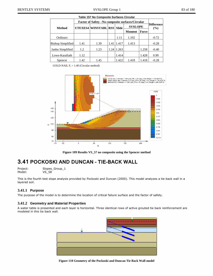
BENTLEY SYSTEMS SVSLOPE Group 1 83 of 180
Table 157 No Composite Surfaces Circular
Method
Factor of Safety –No composite surfaces/Circular Difference
(%)
UTEXES4
WINSTABL
RSS
Slide
SVSLOPE
Moment Force
Ordinary 1.11 1.102 -0.72
Bishop Simplified 1.41 1.39 1.41 1.417 1.413 -0.28
Janbu Simplified 1.2 1.23 1.24 1.263 1.258 -0.40
Lowe-Karafiath 1.12 1.414 1.428 0.99
Spencer 1.42 1.45 1.422 1.418 1.418 -0.28
GOLD-NAIL Fs = 1.40 (Circular method)
Figure 109 Results VS_57 no composite using the Spencer method
3.41 POCKOSKI AND DUNCAN – TIE-BACK WALL Project: Slopes_Group_1 Model: VS_58 This is the fourth test slope analysis provided by Pockoski and Duncan (2000). This model analyzes a tie-back wall in a layered soil.
3.41.1 Purpose
The purpose of the model is to determine the location of critical failure surface and the factor of safety.
3.41.2 Geometry and Material Properties
A water table is presented and each layer is horizontal. Three identical rows of active grouted tie back reinforcement are modeled in this tie back wall.
Figure 110 Geometry of the Pockoski and Duncan Tie Back Wall model

BENTLEY SYSTEMS SVSLOPE Group 1 84 of 180
Table 158 Material Properties of the Pockoski and Duncan Tie Back Wall model
Layer c (psf) (degrees) γ (pcf)
Granular Fill (GF) 0 30 120.4
Cohesive Fill (CF) 0 30 114.7
Organic Silt (OS) 900 0 110.2
OC Crust (OC) 2485 0 117.8
Upper Marine Clay (UM) 1670 0 117.8
Middle Marine Clay (MM) 960 0 117.8
Lower Marine Clay (LM) 1085 0 117.8
Glaciomarine Deposits (GD) 1500 0 147.1
Table 159 Grouted Tieback Properties all rows
Tensile Cap.
(lbs)
Plate Cap.
(lbs)
Bond Strength
(lb/ft)
Bond Length
(ft)
Out-of-Plane
Spacing (ft)
247343 247343 4000 40 4
3.41.3 Results and Discussions
Table 160 Results
Method
Factor of Safety
Difference
(%)
UTEXAS4
Slope/W
WINSTABL
Slide
SVSLOPE
Moment Force
Ordinary 1.12 1.125 1.125 0.00
Bishop Simplified 1.14 1.14 1.16 1.147 1.149 0.17
Janbu Simplified 1.13 1.05 1.12 1.061 1.061 0.00
Lowe-Karafiath 1.20 1.175 1.311 11.57
Spencer 1.14 1.14 1.20 1.145 1.146 1.146 0.09 GOLD-NAIL Fs = 1.19 (Circular)
SNAIL Fs = 1.03 (Wedge method-noncircular)
3.42 POCKOSKI AND DUNCAN - REINFORCEMENT Project: Slopes_Group_1
Model: VS_59 This is the fifth test slope provided by Pockoski and Duncan, (2000). This scenario varies the effect of the reinforcement. The analysis represents a tie back wall and homogeneous sand.
3.42.1 Geometry and Material Properties
A single row of active grouted tieback support is installed for this problem. A water table is present, circular critical slip surfaces are considered and the resulting factor of safety is required.

BENTLEY SYSTEMS SVSLOPE Group 1 85 of 180
Figure 111 Geometry of the Reinforcement model VS_59
Table 161 Material Properties of the Pockoski and Duncan Reinforcement model
Material c (psf) (degrees) γ (pcf)
Sand 0 30 120
Table 162 Soil Nail Properties
Tensile Cap.
(lbs)
Plate Cap.
(lbs)
Bond Strength
(lb/ft)
Bond Length
(ft)
Out-of-Plane
Spacing (ft)
184077 184077 5000 22 8
3.42.2 Results and Discussions
Table 163 Results Circular
Method
Factor of Safety Difference
(%)
UTEXAS4
Slope/W
WINSTABL
Slide
SVSLOPE
Moment Force
Ordinary - 0.62 - 0.626 0.702 - 12.14
Bishop Simplified 0.56 0.60 0.74 0.583 0.583 - 0.00
Janbu Simplified 0.64 0.61 0.76 0.583 - 0.584 0.17
Lowe-Karafiath 0.76 0.588 - 0.59 0.34
Spencer 0.65 0.60 0.59 0.594 0.592 0.592 -0.33
GOLD-NAIL Fs = 0.62 Circular
SNAIL Fs = 0.62 Wedge method noncircular
3.43 POCKOSKI AND DUNCAN – SOIL NAILS Project: Slopes_Group_1 Model: VS_60 This is the seventh test slope providing by Pockoski and Duncan (2000). This model analyzes a soil nailed wall in homogenous clay. There is a dry tension crack down to the first nail. Two uniformly distributed loads of 500 lb/ft and 250 lb/ft are applied
on the high bench.
3.43.1 Purpose
The purpose of the model is to calculate the critical slip surface (through the toe) as well as the factor of the safety.
3.43.2 Geometry and Material Properties
There are also five parallel rows passive soil nails that reinforce the wall. In this case, each row has identical strength characteristics.
Figure 112 Geometry of the Pockoski and Duncan Soil Nails model (VS_60)
Table 164 Material Properties of the Pockoski and Duncan Soil Nails model
Material c (psf) (degrees) γ (pcf)
Sand 800 0 120

BENTLEY SYSTEMS SVSLOPE Group 1 86 of 180
Table 165 Soil Nail Properties
Tensile Cap.
(lbs)
Plate Cap.
(lbs)
Bond Strength
(lb/ft)
Out-of-Plane
Spacing (ft)
25918 25918 1508 5
3.43.3 Results and Discussions
Table 166 Results Dry Circular
Method
Factor of Safety
(Dry Circular) Difference
(%)
UTEXAS4
SLOPE/W
WINSTABL
Slide
SVSLOPE
Moment Force
Ordinary - 1.00 - 0.99 0.994 0.40
Bishop Simplified 1.00 1.01 1.06 0.997 0.994 -0.30
Janbu Simplified 1.08 1.07 1.10 1.041 1.041 0.00
Lowe-Karafiath 1.00 1.021 1.02 -0.10
GLE 1.02 1.02 0.99 1.01 1.026 1.027 1.58 GOLD-NAIL Fs = 0.91 Circular Method
SNAIL Fs = 0.84 Wedge Method
Figure 113 Results using the GLE method VS_60

BENTLEY SYSTEMS SVSLOPE Group 1 87 of 180
3.44 LOUKIDIS – SEISMIC COEFFICIENT Project: Slopes_Group_1 Model: VS_62 This model was published by Loukidis et al. (2003) and provides a method for determining the critical seismic coefficient kc.
The seismic coefficient determined corresponds a factor of safety of 1.0. This is their first example.
3.44.1 Purpose
The purpose of this verification problem is to reproduce a safety factor of 1 using Spencer's method and the seismic coefficients presented in the Loukidis et al. paper (2003).
3.44.2 Geometry and Material Properties
A simple homogenous earth slope is subjected to seismic loading. Both circular and noncircular slip surfaces are considered in
the analysis and all slip surfaces must pass through the toe of the slope. Two independent pore-water pressures conditions are given consideration:
• Dry slope, and • Ru of 0.05.
Figure 114 Geometry of the Loukidis Seismic Coefficient model (VS_62_Dry)
Table 167 Seismic Coefficients
Dry Slope 0.432
Ru = 0.5 0.132
3.44.3 Results and Discussions
Table 168 Results Dry Slope (kc = 0.432)
Type Spencer Bishop Simplified
Circular (Grid Search) 1.001 0.991
Noncircular (Path search with optimization) 0.999 0.989
Table 169 Results Ru = 0.5 (kc = 0.132)
Type Spencer Bishop Simplified
Circular (Grid Search) 1.001 0.987
Noncircular (Path search with optimization) 0.998 0.966

BENTLEY SYSTEMS SVSLOPE Group 1 88 of 180
Table 170 Results Wet Circular
Method
Factor of Safety (Wet Circular)
Difference
(%) Slide
SVSLOPE
Moment Force
Bishop Simplified 0.987 0.991 0.41
Janbu Simplified 0.899 0.901 0.22
Corp Engineers#1 0.984 0.988 0.41
Corp Engineers#2 0.994 1.002 0.81
Lowe-Karafiath 0.976 0.982 0.61
Spencer 1.001 1.009 1.008 0.80
M-P 1.00 1.008 1.008 0.80
GLE 1.00 1.008 1.008 0.80
Loukidis Fs = 1.00 (Spencer)
Table 171 Results Wet No-Circular
Method
Factor of Safety
(Wet Non-Circular) Difference
(%)
Slide
SVSLOPE
Moment Force
Bishop Simplified 0.966 0.967 -0.41
GLE 1.012 1.006 1.006 0.60
Loukidis Fs = 1.00 (Spencer)
3.45 LOUKIDIS – SEISMIC COEFFICIENT #2 Project: Slopes_Group_1 Model: VS_63
This is the second example problem presented by Loukidis et al., 2003. The effect of the critical seismic coefficient is examined in this example. This model analyzes a layered dry slope under seismic loading conditions.
3.45.1 Purpose
The purpose of the model is to bring the Spencer's factor of safety to 1.0 using the author's presented seismic coefficient of 0.115. The Loukidis analysis was for the case of a log-spiral surface.
3.45.2 Geometry and Material Properties
This problem is analyzed in SVSLOPE by using a Greco search technique with a Monte Carlo optimization. The critical slip surface in this case passes through the material boundary on the slope between the middle and lower layers.
Figure 115 Geometry of the Loukidis Seismic Coefficient model

BENTLEY SYSTEMS SVSLOPE Group 1 89 of 180
Table 172 - Material Properties of the Loukidis Seismic Coefficient model
Layer c (kN/m2) (degrees) γ (kN/m3)
Top 4 30 17
Middle 25 15 19
Bottom 15 45 19
3.45.3 Results and Discussions
Table 173 Results of the Dry Circular
Method
Factor of Safety
(Dry Circular) Difference
(%)
Loukidis
et al (2003)
Slide
SVSLOPE
Moment Force
Spencer 1.00 0.991 0.992 0.992 0.10

BENTLEY SYSTEMS SVSLOPE Group 2 90 of 180
4 SVSLOPE GROUP 2 This chapter represents the second set of examples problems used to verify the SVSLOPE software. It also represents a collection of classic examples, which verify the calculation of the factor of safety in various cases. Including variations in material properties, water table locations, circular and non-circular slip surfaces and anchors.
4.1 SIMPLE MULTI – LAYER SLOPE Project: Slopes_Group_2 Model: VW_1 This example creates a simple multi-layer slope in which the potential slip surfaces crosses three or four different material and there is a water table in the example.
4.1.1 Purpose
The primary purpose of this model is to analyze a typical case with circular slip surfaces. The Bishop Simplified method was used to calculate the factor of safety.
4.1.2 Geometry and Material Properties
In this model approximately 20 points were used in the grid and radius search method. The pore-water pressures were specified using a piezometric line. The model consists of silty clay over layering sandy clay tills.
Figure 116 Geometry of the Simple Multi-Layer Slope Model
4.1.3 Results and Discussions
In Table 174, it illustrates the location of the critical slip surface. The analysis resulted in a factor of safety of approximately 1.2.
Table 174 Results of the Simple Multi-Layer Slope model
Method
Factor of Safety Difference
(%)
Slope/W SVSLOPE
Moment Force Moment Force
Ordinary 1.101 1.104 0.27
Bishop Simplified 1.211 1.214 0.25
Janbu Simplied 1.090 1.113 0.36
Corps. of Engineers #1 1.255 1.257 0.16
Corps. of Engineers #2 1.290 1.294 0.31
Lowe-Karafiath 1.249 1.248 -0.08
Spencer 1.210 1.210 1.213 1.213 0.25
M-P 1.211 1.214 1.213 1.213 0.17
GLE 1.211 1.211 1.213 1.213 0.17

BENTLEY SYSTEMS SVSLOPE Group 2 91 of 180
Figure 117 Results using the GLE method VW_1
4.2 BLOCK SEARCH MODEL Project: Slopes_Group_2 Model: VW_3 The Morgenstern-Price method of calculations is used in this case. Tension cracks are also applied in the upper zone as well as downstream water bonded.
4.2.1 Purpose
The purpose of this example is to illustrate the use of the block search technique to generate a series of potential slip surfaces.
4.2.2 Geometry and Material Properties
The minimum block slip surface is selected given the contribution of a number of trial slip surfaces and the influence of the associated tension crack zone.
Figure 118 Geometry of the Block Search Model
4.2.3 Results and Discussions
In the following table it illustrates the identification of the most critical slip surfaces with the calculated Factor of Safety approximately equal to 1.0.
Table 175 Results of the Block Search model
Method
Factor of Safety Difference
(%)
Slope/W SVSLOPE
Moment Force Moment Force
Ordinary 0.974 0.974 0.00
Bishop Simplified 1.065 1.065 0.00
Janbu Simplified 1.035 1.033 0.19
Corps of Engineers #1 1.218 1.223 0.41
Corps of Engineers #2 1.268 1.267 -0.08
Lowe-Karafiath 1.303 1.276 -2.07
Spencer 1.078 1.071 1.079 1.079 0.09
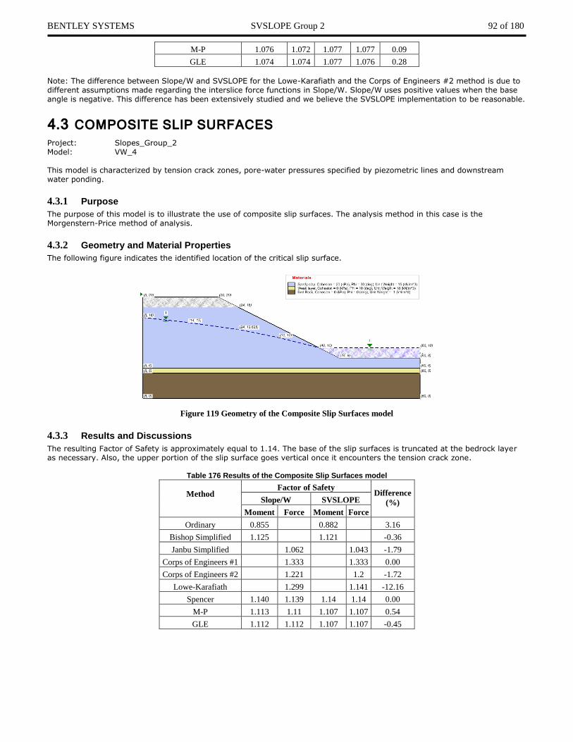
BENTLEY SYSTEMS SVSLOPE Group 2 92 of 180
M-P 1.076 1.072 1.077 1.077 0.09
GLE 1.074 1.074 1.077 1.076 0.28
Note: The difference between Slope/W and SVSLOPE for the Lowe-Karafiath and the Corps of Engineers #2 method is due to different assumptions made regarding the interslice force functions in Slope/W. Slope/W uses positive values when the base angle is negative. This difference has been extensively studied and we believe the SVSLOPE implementation to be reasonable.
4.3 COMPOSITE SLIP SURFACES Project: Slopes_Group_2 Model: VW_4 This model is characterized by tension crack zones, pore-water pressures specified by piezometric lines and downstream water ponding.
4.3.1 Purpose
The purpose of this model is to illustrate the use of composite slip surfaces. The analysis method in this case is the Morgenstern-Price method of analysis.
4.3.2 Geometry and Material Properties
The following figure indicates the identified location of the critical slip surface.
Figure 119 Geometry of the Composite Slip Surfaces model
4.3.3 Results and Discussions
The resulting Factor of Safety is approximately equal to 1.14. The base of the slip surfaces is truncated at the bedrock layer as necessary. Also, the upper portion of the slip surface goes vertical once it encounters the tension crack zone.
Table 176 Results of the Composite Slip Surfaces model
Method
Factor of Safety Difference
(%)
Slope/W SVSLOPE
Moment Force Moment Force
Ordinary 0.855 0.882 3.16
Bishop Simplified 1.125 1.121 -0.36
Janbu Simplified 1.062 1.043 -1.79
Corps of Engineers #1 1.333 1.333 0.00
Corps of Engineers #2 1.221 1.2 -1.72
Lowe-Karafiath 1.299 1.141 -12.16
Spencer 1.140 1.139 1.14 1.14 0.00
M-P 1.113 1.11 1.107 1.107 0.54
GLE 1.112 1.112 1.107 1.107 -0.45

BENTLEY SYSTEMS SVSLOPE Group 2 93 of 180
4.4 RETAINING WALL Project: Slopes_Group_2 Model: VW_5 This model illustrates the use of fully specified slip surfaces, a single search center and a retaining wall in order to calculate the location of the critical slip surface.
4.4.1 Purpose
The primary purpose of this model is to illustrate the analysis of the stability of a gravity retaining wall using a fully specified slip surface.
4.4.2 Geometry and Material Properties
The Spencer Method is used to calculate the factor of safety. In the following figure it shows the calculations for the Factor of Safety on specified slip surfaces.
Figure 120 Geometry of the Retaining Wall model

BENTLEY SYSTEMS SVSLOPE Group 2 94 of 180
4.4.3 Results and Discussions
A final factor of safety of 1.677 was calculated.
Table 177 Results of the Retaining Wall model
Method
Factor of Safety Difference
(%)
Slope/W SVSLOPE
Moment Force Moment Force
Ordinary 1.368 1.369 0.07
Bishop Simplified 1.479 1.481 0.14
Janbu Simplified 1.320 1.323 0.23
Corps of Engineers #1 1.697 1.700 0.18
Spencer 1.677 1.669 1.685 1.685 0.48
M-P 1.678 1.672 1.682 1.681 0.24
GLE 1.680 1.680 1.682 1.682 0.12
4.5 FABRIC MODEL Project: Slopes_Group_2 Model: VW_6_Fabric This model has contained no pore-water pressures and represents a single specified circular slip surface. A single applied line load is applied to the crest of the slope. The geo-fabric reinforcements are entered as anchor loads with full bond length and variable applied loads.
4.5.1 Purpose
The purpose of this example is to show how geo-fabric reinforcement can be represented in a slope stability analysis. In this case, the GLE method is used to calculate the factor of safety.
4.5.2 Geometry and Material Properties
The calculation of the Factor of Safety is shown in the following figure. A factor of safety of 1.502 was calculated using SVSLOPE. Of particular interest is the free bond diagram for slices 5 and 10, which are shown in the Figure 121.
Figure 121 Geometry of the Fabric Model (VW_6)
4.5.3 Results and Discussions
In this case, the line load applied at crest of the slope is specified as 10KN/m and is shown in the free body diagram of Slice no. 5. A force mobilize load of 21.165 KN/m was calculated as the force in the anchor. The calculation of this force can be seen in free body diagram for Slice 10.

BENTLEY SYSTEMS SVSLOPE Group 2 95 of 180
4.5.4 Table 178 Fabric model Results
Method
Factor of Safety Difference
(%)
Slope/W SVSLOPE
Moment Force Moment Force
Ordinary 1.518 1.525 0.46
Bishop Simplified 1.663 1.668 0.30
Janbu Simplified 1.496 1.508 0.80
Corps of Engineers #1 1.703 1.705 0.12
Corps of Engineers #2 1.783 1.808 1.40
Spencer 1.643 1.646 1.650 1.634 0.73
M-P 1.641 1.637 1.646 1.646 0.31
GLE 1.640 1.640 1.646 1.646 0.37
Note: Reinforcement constant = 50 KN
Table 179 Fabric No rein/no line load
Method
Factor of Safety
(No reinforcement / no line load) Difference
(%)
Slope/W SVSLOPE
Moment Force Moment Force
Ordinary 1.291 1.297 0.46
Bishop Simplified 1.444 1.447 0.21
Janbu Simplified 1.292 1.300 0.62
Corps of Engineers #1 1.484
Corps of Engineers #2 1.572
Lowe-Karafiath NA
Spencer 1.426 1.429 1.43 1.430 0.07
M-P 1.427 1.427
GLE 1.423 1.423 1.427 1.427 0.28
Table 180 Fabric no reinforcement/with line load
Method
Factor of Safety
(No reinforcement with line load) Difference
(%)
Slope/W SVSLOPE
Moment Force Moment Force
Ordinary 1.281 1.287 0.47
Bishop Simplified 1.434 1.436 0.14
Janbu Simplified 1.283 1.291 0.62
Spencer 1.416 1.418 1.421 1.407 0.78
GLE 1.413 1.413 1.417 1.417 0.28
Table 181 Fabric with rein and no line load
Method
Factor of Safety
(with rein but no line load) Difference
(%)
Slope/W SVSLOPE
Moment Force Moment Force
Ordinary 1.386 1.392 0.43
Bishop Simplified 1.535 1.538 0.20
Janbu Simplified 1.397 1.387 0.72
Spencer 1.517 1.512 1.523 1.508 0.26
GLE 1.514 1.514 1.518 1.518 0.26

BENTLEY SYSTEMS SVSLOPE Group 2 96 of 180
4.6 BISHOP AND MORGENSTERN - HOMOGENEOUS Project: Slopes_Group_2 Model: VW_7 This example problem is based on an example problem original published by Bishop and Morgenstern, (1960). The solutions
presented in the original work developed a series of stability charts that could then be used to estimate the factor of safety for simple, homogenous earth slopes.
4.6.1 Purpose
The purpose of this model is to illustrate agreement between the SVSLOPE software and the original slope stability charts.
4.6.2 Geometry and Material Properties
The slope of this particular model is at a ratio to 4 horizontal to 1 vertical. The grid and radius search technique was used to identify the location of the critical slip surface.
Figure 122 Geometry of the Bishop and Morgenstern Homogenous Model
4.6.3 Results and Discussions
The location of the critical slip surface and the calculation of the factor of safety can be seen in the following table. A factor of safety of 1.35 was calculated which agrees well with stability chart calculations. In this case, the Bishop Simplified method and the Morgenstern-Price method yields similar results.
Table 182 Chart results Bishop and Morgenstern Homogenous model
Method
Factor of Safety Difference
(%)
Slope/W SVSLOPE
Moment Force Moment Force
Ordinary 1.231 1.232 0.08
Bishop Simplified 1.337 1.338 0.08
Janbu Simplified 1.261 1.262 0.08
Corps of Engineers #1 1.344 1.345 0.07
Corps of Engineers #2 1.351 1.352 0.07
Lowe-Karafiath 1.347 1.346 -0.08
Spencer 1.338 1.339 1.339 1.339 0.08
M-P 1.338 1.34 1.339 1.338 0.08
GLE 1.338 1.338 1.339 1.338 0.08

BENTLEY SYSTEMS SVSLOPE Group 2 97 of 180
4.7 FREDLUND AND KRAHN (1977) Project: Slopes_Group_2 Model: VW_8 This example model was originally presented by Fredlund and Krahn (1977). It represented a comparison study of various
slope stability methods.
4.7.1 Purpose
In this example, the slope is comprised of three layers. The upper layer contains a weak layer at its base. The weak layer subsequently overlays a bedrock layer.
4.7.2 Geometry and Material Properties
The critical slip surface will potentially come down and follow along the weak layer, but will not extend into the strong bedrock.
Figure 123 Geometry of the Fredlund and Krahn (1977) Model
4.7.3 Results and Discussions
The following table shows the results of the calculations for this model. The results compare reasonably to the results calculated by Fredlund and Krahn (1977).
Table 183 Results of the Fredlund and Krahn (1977)
Method
Factor of Safety Difference
(%)
Slope/W SVSLOPE
Moment Force Moment Force
Ordinary 1.147 1.151 0.35
Bishop Simplified 1.210 1.213 0.25
Janbu Simplified 1.186 1.191 0.42
Corps of Engineers #1 1.272 1.273 0.08
Corps of Engineers #2 1.259 1.263 0.32
Spencer 1.212 1.212 1.215 1.214 0.25
M-P 1.205 1.205 1.209 1.208 0.33
GLE 1.205 1.205 1.209 1.208 0.33

BENTLEY SYSTEMS SVSLOPE Group 2 98 of 180
Figure 124 Critical slip surface calculated for the Fredlund and Krahn model (Ordinary method)
4.8 SIMPLE TWO MATERIAL MODEL Project: Slopes_Group_2 Model: VW_9 This example consists of a simple two layers slope with a water table. The problem is analyzed using the Bishop Simplified method as well as the Morgenstern Price method.
4.8.1 Purpose
The purpose of this example is to illustrate the calculation of the Factor of Safety for a simple slope example.
4.8.2 Geometry and Material Properties
Figure 125 Geometry of the Simple Two Material slope model
c (kN/m2) (degrees) (kN/m3)
Upper Soil 5.0 20.0 15.00
Lower Soil 10.0 25.0 18.00
4.8.3 Results and Discussions
The factors of safety calculated for this example are shown in Table 184. The results agree well with those calculated using the Slope/W software.
Table 184 Results of the Simple Two Material model
Method
Factor of Safety Difference
(%)
Slope/W SVSLOPE
Moment Force Moment Force
Ordinary 1.279 1.283
Bishop Simplified 1.464 1.466 0.14
Janbu Simplified 1.286 1.290
Corps of Engineers #1 1.502 1.505 0.20
Corps of Engineers #2 1.534 1.536 0.13
Lowe-Karafiath 1.498 1.505 0.47

BENTLEY SYSTEMS SVSLOPE Group 2 99 of 180
Spencer 1.467 1.469 1.469 1.469 0.14
M-P 1.466 1.471 1.468 1.467 0.14
GLE 1.466 1.466 1.468 1.468 0.14
4.9 INFINITE SLOPE MODEL Project: Slopes_Group_2 Model: VW_11 This example illustrates the use of the software to calculate the stability of a semi-infinite slope. In this case the Morgenstern-price method was used to calculate the Factor of Safety.
4.9.1 Geometry and Material Properties
Figure 126 Geometry of Infinite Slope model
4.9.2 Results and Discussions
The results of the analysis are shown in Table 185 comparing SVSLOPE to Slope/W and Slide. The results can be compared to the calculated closed-form solutions as presented in Table 186 from the Slope/W documentation. Note that Slope/W uses a different method than SVSLOPE such that different slices are used in the calculation of FOS when tension cracks are considered, refer to Figure 127 and Figure 128.
Table 185 Infinite Slope model
Method
Factor of Safety SVSLOPE
Difference
Slope/W Slide SVSLOPE Slope/W Slide
Moment Force Moment Force Moment Force (%) (%)
Ordinary 1.400 1.461 1.479 5.61 1.20
Bishop Simplified 1.402 1.477 1.495 6.66 1.25
Janbu Simplified 1.400 1.462 1.462 4.46 0.03
Corps of Engineers #1 1.400 1.481 1.480 5.74 0.04
Corps of Engineers #2 1.400 1.481 1.482 5.86 0.07
Lowe-Karafiath 1.400 1.476 1.482 5.86 0.41
Spencer 1.400 1.400 1.478 1.478 1.481 1.481 5.79 0.21
M-P 1.400 1.400 1.466 1.466 1.466 1.467 4.74 0.03
GLE 1.400 1.400 1.466 1.466 1.467 1.467 4.79 0.08
Table 186 Slope/W infinite slope results closed form solution comparison

BENTLEY SYSTEMS SVSLOPE Group 2 100 of 180
Figure 127 Infinite Slope model Slope/W results slices
Figure 128 Infinite Slope model SVSLOPE results slices

BENTLEY SYSTEMS SVSLOPE Group 2 101 of 180
4.10 LAMBE AND WHITMAN – DRAINED SLOPE Project: Slopes_Group_2 Model: VW_12 This model was originally presented by Lambe and Whitman (1969). In the original solution Lambe and Whitman presented a
hand-calculated Factor of Safety for a simple slope with under drain.
4.10.1 Geometry and Material Properties
The slope is 20 feet high and has a slope of 1 horizontal to 1.5 vertical. The slope consists of a single homogenous material. The slip surface is assumed to be circular with the radius of 30 feet. In the original calculations, the pore-water pressures conditions in the slope were characterized by a flow net.
Figure 129 Geometry of the Lambe and Whitman – Drained Slope model
4.10.2 Results and Discussions
The results of the SVSLOPE software package are compared to the original Lambe and Whitman calculations.
Table 187 Lambe and Whitman – Drained Slope model
Method
Factor of Safety
Difference
(%)
Slope/W
(30 slices)
SVSLOPE
(30 slices)
Moment Force Moment Force
Ordinary 1.198 1.200 0.18
Bishop Simplified 1.332 1.333 0.08
Janbu Simplified 1.207 1.210 0.25
Corps of Engineers #1 1.376 1.381 0.36
Corps of Engineers #2 1.397 1.401 0.29
Lowe-Karafiath 1.346 NS
Spencer 1.332 1.338 1.334 1.333 0.15
M-P 1.332 1.339 1.335 1.334 0.23
GLE 1.332 1.332 1.335 1.334 0.23

BENTLEY SYSTEMS SVSLOPE Group 2 102 of 180
4.11 PORE-WATER PRESSURES AT DISCRETE POINTS Project: Slopes_Group_2 Model: VW_13, VW_13_NoTensionCrack_NoPWP, VW_13_NoPWP, VW_13_NoTensionCrack A single circular slip surface was used in this case and a tension crack zone was specified through the use of a limiting angle
designation.
4.11.1 Purpose
The purpose of this model is to illustrate the use of specified pore-water pressures at discrete points in the model. The GLE method is used to analyze this case.
4.11.2 Geometry and Material Properties
A spline interpolation was used between the pore-water pressures points in order to determine the pore-water pressures at the base of each slice.
Figure 130 Geometry of the Pore-Water Pressures a Discrete Points model
4.11.3 Results and Discussions
The results of the analysis are shown in Table 188 comparing SVSLOPE to Slope/W and Slide. A comparision of the SVSLOPE models with different combinations pore-water pressure discrete points and tension cracks is presented in Table 189. Note that Slope/W uses a different method than SVSLOPE such that different slices are used in the calculation of FOS when tension cracks are considered, refer to Figure 131 and Figure 132.
Table 188 Discrete points model results
Method
Factor of Safety Difference
(%)
Slope/W SVSLOPE
Moment Force Moment Force
GLE 1.382 1.299 1.298 6.03
Table 189 Comparison of SVSLOPE models with and without pore-water pressures and tension cracks
Method
Factor of Safety
Neglect pore-
water pressures
and no cracks
With pore-water
pressure, no tension
cracks
Neglect pore-water
pressures with
tension cracks
Moment Force Moment Force Moment Force
Ordinary 1.544 1.222 1.544
Bishop Simplified 1.624 1.285 1.624
Janbu Simplified 1.531 1.238 1.531
Corps of Engineers #1 1.671
Corps of Engineers #2 1.710
Lowe-Karafiath 1.664
Spencer 1.622 1.623
M-P 1.622 1.621
GLE 1.622 1.621 1.286 1.286 1.622 1.621

BENTLEY SYSTEMS SVSLOPE Group 2 103 of 180
Figure 131 Spatial Pore Water Pressure Head model Slope/W results slices
Figure 132 Spatial Pore Water Pressure Head model SVSLOPE results slices

BENTLEY SYSTEMS SVSLOPE Group 3 104 of 180
5 SVSLOPE GROUP 3 The following section represents the third group of benchmark examples used to verify the correctness of the SVSlope software. These examples are generally related to some of the more recent and advanced features of the software.
5.1 RAPID DRAWDOWN – 3 STEP METHOD This example documents the implementation of the 3-stage rapid drawdown procedure originally proposed by the USACE and later updated by Duncan et al. (1990). This rapid drawdown procedure represents a total stress approximation of effective stress conditions. The three-stage procedure incorporates aspects of both the U.S. Army Corps of Engineers (1970) method as well as the Lowe and Karafiath’s (1959) method. The procedure is designed to account for the effect of drainage and the fact that the drained strength may be less than the undrained strength. It is important to note that it differs from the Corps of Engineers’ procedure in the way that undrained strength is evaluated and the way that drained strength is taken into account. In a manner similar to Lowe and Karafiath the procedure accounts for the effects of anisotropic consolidation, which can result in significantly higher undrained shear strength (Duncan, 2005). Project: SVSlope_Group_3 Model: RDD01, RDD_WT, RDD_NoWT, RDD_WT35
5.1.1 Purpose
The purpose of this set of examples is to demonstrate the correct implementation of the three-stage analysis for total stress rapid drawdown calculation in SVSlope.
5.1.2 Geometry and Material Properties
In this example a simple slope is set up as shown in Figure 133. Several scenarios were created with both the water table at the top of the slope and at the bottom. The final scenario (RDD01) then evaluates the movement of the water table from the top of the slope to the bottom using the three-stage analysis.
Figure 133 Geometry of the simple slope used for rapid drawdown calculations

BENTLEY SYSTEMS SVSLOPE Group 3 105 of 180
5.1.3 Results and Discussions
The various scenarios were evaluated using the SVSLOPE, Slide, and Slope/w software packages. The results can be seen in Table 190, Table 191,
Table 192, and Table 193. It can be seen from the analysis results that there is very reasonable agreement between the three software packages. It should be noted, however, that at the writing of this document the Slide software does not specifically implement the three-stage method of rapid drawdown as proposed by Duncan (1990). Therefore the Slide software was not compared in the total stress rapid draw-down method comparison. The small differences in calculations between software packages are generally less than 4% and are reasonable when all potential influences of this set of calculations are considered.
Figure 134 Example of results of three-stage rapid drawdown calculation
Table 190 Comparison of software package answers for the three-stage analysis
Method
Rapid Draw-Down
SVSLOPE Slope/W
Moment Force Moment Force
Ordinary 0.317 0.450
Bishop 0.397 0.560
Janbu 0.335 0.500
Engineer#1 0.499 1.584 0.530
Engineer#2 0.337 0.530
L-K 0.308
Spencer 0.522 0.522 0.480 0.480
M-P 0.521 0.521 0.490 0.490
GLE 0.510 0.510 0.490 0.490
Model:RDD01
Table 191 Comparison when water table follows ground surface
Method
WT Along Ground Surface
SVSLOPE Slope/W Slide
Moment Force Moment Force Moment Force
Ordinary 0.504 0.583 0.443
Bishop 0.568 0.574 0.571
Janbu 0.496 0.498 0.497
Engineer#1 0.599 0.604 0.622
Engineer#2 0.634 0.621 0.584
L-K 0.595 0.589 0.585
Spencer 0.582 0.582 0.894 0.594 0.602 0.602
M-P 0.583 0.583 0.593 0.593 0.586 0.586
GLE 0.583 0.583 0.586 0.586
Model: RDD_WT

BENTLEY SYSTEMS SVSLOPE Group 3 106 of 180
Table 192 Comparison when there is no water table
Method
No WT
SVSLOPE Slope/W Slide
Moment Force Moment Force Moment Force
Ordinary 0.999 1.002 0.999
Bishop 1.108 1.113 1.108
Janbu 0.991 0.994 0.991
Engineer#1 1.119 1.121 1.119
Engineer#2 1.147 1.150 1.146
L-K 1.114 1.122 N/A
Spencer 1.106 1.106 0.894 1.110 1.106 1.106
M-P 1.108 1.111 0.593 1.113 1.108 1.111
GLE 1.105 1.105 1.108 1.108
Model: RDD_NoWT
Table 193 Comparison when the water table is at an elevation of 35m
Method
No WT
SVSLOPE Slope/W Slide
Moment Force Moment Force Moment Force
Ordinary 0.918 1.146 0.699
Bishop 1.252 1.258 1.252
Janbu 1.126 1.128 1.126
Engineer#1 N/A 7.357 7.767
Engineer#2 N/A 1.128 1.126
L-K N/A 1.438 N/A
Spencer 1.257 1.256 1.262 1.254 1.254
M-P 1.256 1.255 1.261 1.254 1.254
GLE 1.256 1.256 1.255 1.255
Model:RDD_WT35

BENTLEY SYSTEMS SVSLOPE Group 3 107 of 180
5.2 RAPID DRAWDOWN - WALTER BOULDIN DAM Walter Bouldin Dam is a rolled earthfill embankment. The dam is about 60 feet high, sitting on 80 feet of clayey sand and gravel. Overlying the gravel are a layer of cretaceous clay, a zone of micaceous silt, and a clayey silty sand layer that covers the slope. During a rapid drawdown of 32 feet in 5.5 hours the Walter Bouldin Dam failed on February 10, 1975. Project: Slopes_Group_3 Model: RDD_WalterBouldinDam
5.2.1 Purpose
The purpose of this model is to document the correct solution of the rapid drawdown methodology as presented by Duncan et al. (1990).
5.2.2 Geometry and Material Properties
Figure 135 Geometry of the Walter Bouldin Dam
5.2.3 Results and Discussions
The results of the analysis are found to compare well with the implementation of the Duncan method in the Slope/W software. The noted differences are reasonable and acceptable. Duncan reported a factor of safety of 1.04 and it is believed that Spencer’s method is utilized.
Figure 136 Slip surface location for the Walter Bouldin dam

BENTLEY SYSTEMS SVSLOPE Group 3 108 of 180
Table 194 Comparison of FOS with Slope/W for Walter Bouldin Dam
Method
Factor of Safety Difference
(%) SVSlope Slope/W
Moment Force Moment Force
Bishop 1.002 1.016 -1.397
Spencer 0.999 0.998 1.02 -2.352
Table 195 Comparison of FOS between SVSLOPE and Duncan et al. (1990)
Corps #2 Lowe-Karafiath
Duncan et al. (1990) 0.93 1.09
SVSLOPE 1.016 1.034
Difference 9.2% -5.1%
5.3 RAPID DRAWDOWN - USACE BENCHMARK This benchmark example is created by the US Army Corps of Engineers in the Appendix G of the Engineering Manual – EM 1110-2-1902. It’s published FOS = 1.44. The rapid drawdown water level is from 103 feet to 24 feet. Project: SVSlope_Group_3 Model: RDD_USACE
5.3.1 Purpose
The purpose of this model is to document the correct solution of the rapid drawdown methodology as presented by Duncan et al. (1990).
5.3.2 Geometry and Material Properties
Figure 137 Geometry of the USACE Benchmark Example
5.3.3 Results and Discussions
The results of the analysis are found to compare well with the implementation of the Duncan method in the Slope/W software. The noted differences are reasonable and acceptable.
Table 196 Comparison of FOS with Slope/W for USACE benchmark
Method
Factor of Safety Difference
(%) SVSlope Slope/W
Moment Force Moment Force
Bishop 1.435 1.428 0.508
Janbu 1.269 1.279 0.777
Spencer 1.427 1.427 1.433 0.58
5.4 RAPID DRAWDOWN - PUMPED STORAGE PROJECT DAM The Pumped Storage Project Dam has a densely compacted, silty clay core. The lower portion of the upstream slope is a zone of random materials with the equivalent of same strength properties as the core. The upper portion of the upstream slope and the entire downstream slope is a free draining rock fill. For the rapid drawdown analysis the water level is lowered from 545 feet to 380 feet. The Duncan 3-Stage Rapid Drawdown Analysis method is used in SVSlope to solve this model. The implementation of the

BENTLEY SYSTEMS SVSLOPE Group 3 109 of 180
method is based on the theory presented by Duncan, Wright, and Wong (1990). Project: SVSlope_Group_3 Model: RDD_Pumped_Storage_Project_Dam, RDD_Pumped_Storage_Project_Dam_3D
5.4.1 Purpose
The purpose of this model is to document the correct solution of the rapid drawdown methodology as presented by Duncan et al. (1990).
5.4.2 Geometry and Material Properties
Figure 138 Geometry of the Pumped Storage Project Dam
5.4.3 Results and Discussions
The results of the analysis are found to compare well with the implementation of the Duncan method in the Slope/W software.
The noted differences are reasonable and acceptable.
Table 197 Comparison of FOS with Slope/W for Pumped Storage Project Dam
Method
Factor of Safety Difference
(%) SVSlope Slope/W
Moment Force Moment Force
Bishop 1.538 1.534 0.23
Janbu 1.423 1.420 0.24
Spencer 1.527 1.528 1.537 0.641

BENTLEY SYSTEMS SVSLOPE Group 3 110 of 180
5.5 RAPID DRAWDOWN - PILARCITOS DAM The Pilarcitos Dam is a homogeneous rolled earth-fill embankment. The slope failure occurred after the water level was lowered from elevation of 692 to elevation of 657 between Oct. 07 and Nov. 19, 1969. Project: SVSlope_Group_3
Model: RDD_PilarcitosDam
5.5.1 Purpose
The purpose of this model is to document the correct solution of the rapid drawdown methodology as presented by Duncan et al. (1990).
5.5.2 Geometry and Material Properties
Figure 139 Geometry of the Pilarcitos Dam
5.5.3 Results and Discussions
The results of the analysis are found to compare well with the implementation of the Duncan method in the Slope/W software. The noted differences are reasonable and acceptable. The FOS published by Duncan is 1.05 for the Lowe and Karafiath method.
Figure 140 Location of the critical slip surface for the Pilarcitos Dam
Table 198 Comparison of FOS with Slope/W for Pilarcitos Dam
Method
Factor of Safety Difference
(%) SVSlope Slope/W
Moment Force Moment Force

BENTLEY SYSTEMS SVSLOPE Group 3 111 of 180
Bishop 1.077 1.047 2.901
Janbu 1.043 1.006 3.684
Spencer 1.063 1.063 1.051 1.166
Table 199 Comparison of FOS with Duncan et al. (1990)
Corps #2 Lowe-Karafiath
Duncan et al. (1990) 0.82 1.05
SVSLOPE 0.844 0.967
Difference 2.9% -7.9%
5.6 SHEAR NORMAL FUNCTION This example documents the implementation of the shear normal function material model. Project: SVSlope_Group_3 Model: VS_1_SNF
5.6.1 Purpose
The purpose of this example is to demonstrate the correct implementation of the shear normal function material model calculation in SVSlope.
5.6.2 Geometry and Material Properties
In this example a simple slope is set up as shown in Figure 141. A fully specified circular slip surface is used.
Figure 141 Geometry of the simple slope used for shear normal force calculations

BENTLEY SYSTEMS SVSLOPE Group 3 112 of 180
5.6.3 Results and Discussions
The model was evaluated using the SVSLOPE and Slide software packages. The results can be seen in Table 190. It can be seen from the analysis results that there is very reasonable agreement between the two software packages.
Figure 142 Example of results of shear normal function calculation
Table 200 Comparison of software package answers for analysis
Method
Factor of Safety Difference
(%) Slide SVSlope
Moment Force
Ordinary 1.283 1.283 0.000
Bishop 1.34 1.34 0.000
Janbu Simplified 1.274 1.274 0.000
Corps of Engineer#1 1.345 1.345 0.000
Corps of Engineer#2 1.35 1.35 0.000
Lowe-Karafiath 1.343 1.344 0.074
Spencer 1.338 1.338 1.338 0.000
M-P 1.338 1.338 1.338 0.000
GLE 1.338 1.338 1.338 0.000

BENTLEY SYSTEMS SVSLOPE Group 3 113 of 180
5.7 FILL SLOPE USING A RETAINING WALL Project: Slope_Group_3 Model: RainfallInducedFillSlopeFailure The FillSlope model is constructed using retaining walls with three kinds of material shown in the following table. This model
demonstrates the use of SVSlope in analyzing the safety situation of a slope using a retaining wall.
5.7.1 Geometry and Material Properties
The model is set up with the geometry shown below and the material regions are entered. The material properties that are in use for this model are presented in the following table. A water surface is assigned through the back of the slope. A slip surface is defined by line segments and cuts through the region filled with the Backfill material.
Figure 143 Geometry of the FillSlope model
Table 201 Material Properties of the FillSlope model
Material Names Sat. Unit Wt. (kN/m3) Cohesion (kPa) Friction Angle (deg)
Original 20.6 34 29
Backfill 19.7 19.7 31.6
Concrete 23.6 600.0 0.0

BENTLEY SYSTEMS SVSLOPE Group 3 114 of 180
5.7.2 Results and Discussions
The model uses the Janbu simplified method to calculate a factor of safety (FOS) of 1.58. Compared to the FOS value 1.62 produced by STABL, the difference is -2.53 %. This difference is reasonable giving the slight variation in the geometry of the critical slip surface in SVSlope compared to STABL.
Figure 144 Solution of the FillSlope model using Janbu Simplified method
5.8 PROBABILITY – JAMES BAY CASE HISTORY Project: Slope_Group_3 Model: James_Bay_sampling_everyslice, James_Bay_sampling_nospatial, James_Bay_sampling30m,
James_Bay_sampling40m, James_Bay_sampling50m, James_Bay_sampling80m, James_Bay_sampling100m
The James Bay project required the construction of dykes and sensitive clay. These model show the construction of the dykes using 5 materials shown in the following table. The models demonstrate the use of SVSlope in performing probabilistic stability analysis.
5.8.1 Geometry and Material Properties
The models are set up with the geometry shown below and the material regions are entered. The material properties that are in use for these models are presented in the following table. Also, the probability parameters used due to uncertainties in the
soil properties are presented in Table 198. All variables are assumed to have normal distribution. A grid and point search method is used to search for the slip surface.
Figure 145 Geometry of the James Bay Probability model
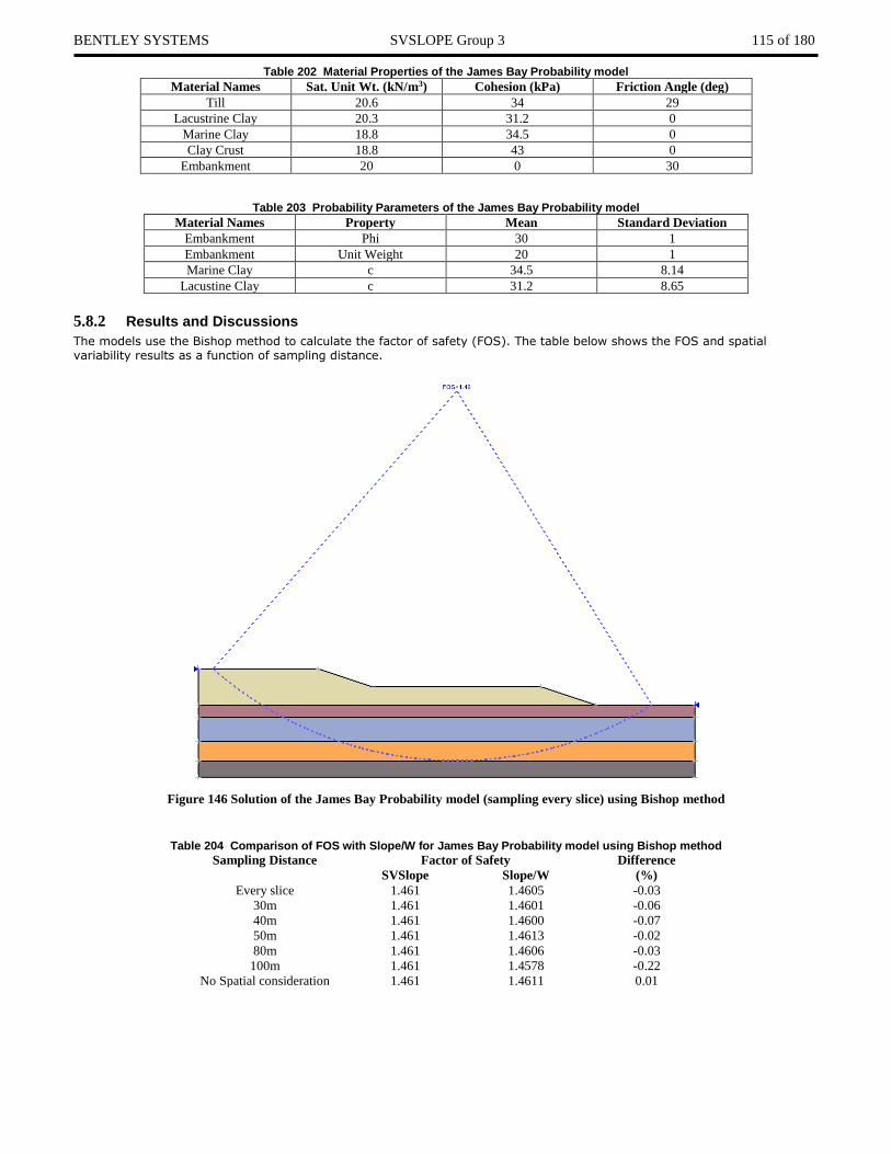
BENTLEY SYSTEMS SVSLOPE Group 3 115 of 180
Table 202 Material Properties of the James Bay Probability model
Material Names Sat. Unit Wt. (kN/m3) Cohesion (kPa) Friction Angle (deg)
Till 20.6 34 29
Lacustrine Clay 20.3 31.2 0
Marine Clay 18.8 34.5 0
Clay Crust 18.8 43 0
Embankment 20 0 30
Table 203 Probability Parameters of the James Bay Probability model
Material Names Property Mean Standard Deviation
Embankment Phi 30 1
Embankment Unit Weight 20 1
Marine Clay c 34.5 8.14
Lacustine Clay c 31.2 8.65
5.8.2 Results and Discussions
The models use the Bishop method to calculate the factor of safety (FOS). The table below shows the FOS and spatial variability results as a function of sampling distance.
Figure 146 Solution of the James Bay Probability model (sampling every slice) using Bishop method
Table 204 Comparison of FOS with Slope/W for James Bay Probability model using Bishop method
Sampling Distance Factor of Safety Difference
(%) SVSlope Slope/W
Every slice 1.461 1.4605 -0.03
30m 1.461 1.4601 -0.06
40m 1.461 1.4600 -0.07
50m 1.461 1.4613 -0.02
80m 1.461 1.4606 -0.03
100m 1.461 1.4578 -0.22
No Spatial consideration 1.461 1.4611 0.01

BENTLEY SYSTEMS SVSLOPE Group 3 116 of 180
Table 205 Spatial variability results for the James Bay Probability model
Sampling
Distance
Standard Deviation Probability of failure
(%)
Reliability Index
SVSlope Slope/W SVSlope Slope/W SVSlope Slope/W
Every slice 0.06477 0.05537 0.000 0.000 7.406 7.109
30m 0.1336 0.12795 0.017 0.003 3.435 3.596
40m 0.1494 0.14518 0.053 0.050 3.103 3.168
50m 0.1494 0.15446 0.053 0.100 3.103 2.986
80m 0.213 0.19617 1.467 0.937 2.149 2.348
100m 0.213 0.19842 1.467 0.990 2.149 2.308
No spatial
consideration
0.215 0.21295 1.363 1.340 2.154 2.165
5.9 EUROCODE 7 – CUTTING IN STILL CLAY Project: Slope_Group_3 Model: Eurocode_CuttingInClay This example model is based on the book titled "Designers' Guide to EN 1997-1" on page 202. The water table line may not
be exactly the same as that on the book since it does not provide the coordinates.
5.9.1 Geometry and Material Properties
The model is set up with the geometry shown below. The material properties that are in use for this model are presented in the following table. A permanent distributed load with magnitude = 35KPa is applied as shown in the Figure.
Figure 147 Geometry of the model
Table 206 Material Properties of the model
Material Names Sat. Unit Wt. (kN/m3) Cohesion (kPa) Friction Angle (deg)
Soil1 20 10 28
5.9.2 Results and Discussions
Eurocode 7 Design Approach 3 is selected to do the analysis. Grid and Tangent search method is used. The FOS is equal to 1.193 for Simplified Bishop method published in the book. The following table lists the comparison result with Slide.
Table 207 Comparison of FOS with Slide
Method
Factor of Safety Difference
(%) SVSlope Slide
Moment Force Moment Force
Bishop 1.172 1.177 -0.425
Janbu 1.043 1.052 -0.856
Spencer 1.174 1.174 1.179 -0.424

BENTLEY SYSTEMS SVSLOPE Group 3 117 of 180
Figure 148 Solution of the model using Simplified Bishop method
5.10 EUROCODE 7 – EARTH DAM Project: Slope_Group_3
Model: Eurocode_Dam This example model is based on the book titled "Smith’s Elements of Soil Mechanics" 8th edition, example 5.12.
5.10.1 Geometry and Material Properties
The model is set up with the geometry shown below. The material properties that are in use for this model are presented in the following table. It is a coupled SVSlope and SVFlux model, in which the water table line is obtained from the SVFlux.
Figure 149 Geometry of the model
Table 208 Material Properties of the model
Material Names Sat. Unit Wt. (kN/m3) Cohesion (kPa) Friction Angle (deg)
Original 19.2 12 20
5.10.2 Results and Discussions
Eurocode 7 Design Approach 1, Combination 2 is selected to do the analysis. The model uses the Enxtry and Exit search method to calculate a factor of safety (FOS). The FOS is equal to 1.07 for Simplified Bishop method published in the book (page 198). The following table lists the comparison result with Slide.
Table 209 Comparison of FOS with Slide
Method
Factor of Safety Difference
(%) SVSlope Slide
Moment Force Moment Force
Bishop 1.093 1.096 -0.274

BENTLEY SYSTEMS SVSLOPE Group 3 118 of 180
Janbu 1.031 1.027 0.389
Spencer 1.093 1.093 1.100 -0.636
Figure 150 Solution of the model using Simplified Bishop method
5.11 ANISOTROPIC LINEAR MODEL (ALM1) Project: Slopes_Group_3 Model: Section_B_ALM1, Section_B_ALM1_Cuckoo This verification model was developed to examine a slope with complex faulting and stratigraphy and was solved using the Anisotropic Linear Model (ALM1). The model was analyzed in SVSLOPE with both the Path Search and Cuckoo Search methods.
5.11.1 Geometry and Material Properties
The material properties are given in Table 210 and Table 211. The geometry is defined as shown in Figure 151.
Figure 151 Geometry of the Section_B_ALM1 model
Table 210 Mohr-Coulomb Material Properties of the Section_B_ALM1 model
c (kN/m2) ' (degrees) γ (kN/m3)
MCS 139 32 22
FWZ 184 43 30
DG1 163 39 35
DG2 124 32 35
DG3 150 37 35
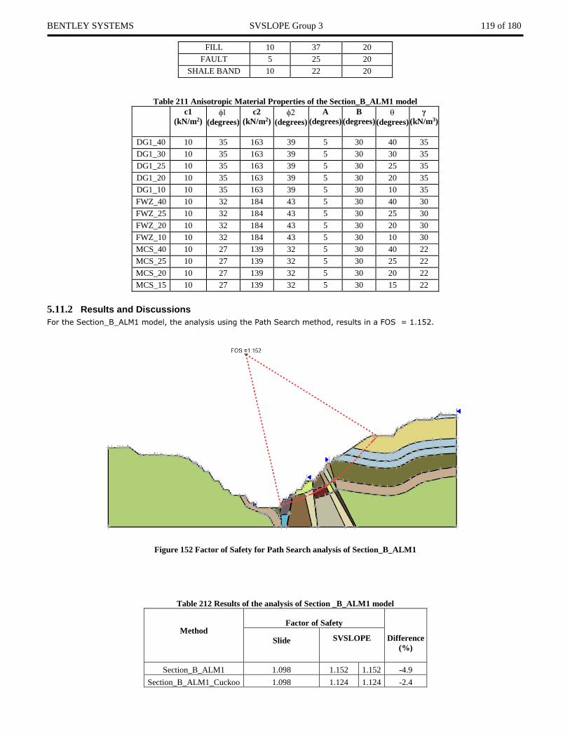
BENTLEY SYSTEMS SVSLOPE Group 3 119 of 180
FILL 10 37 20
FAULT 5 25 20
SHALE BAND 10 22 20
Table 211 Anisotropic Material Properties of the Section_B_ALM1 model
c1
(kN/m2)
(degrees)
c2
(kN/m2)
(degrees)
A
(degrees)
B
(degrees)
(degrees)
γ
(kN/m3)
DG1_40 10 35 163 39 5 30 40 35
DG1_30 10 35 163 39 5 30 30 35
DG1_25 10 35 163 39 5 30 25 35
DG1_20 10 35 163 39 5 30 20 35
DG1_10 10 35 163 39 5 30 10 35
FWZ_40 10 32 184 43 5 30 40 30
FWZ_25 10 32 184 43 5 30 25 30
FWZ_20 10 32 184 43 5 30 20 30
FWZ_10 10 32 184 43 5 30 10 30
MCS_40 10 27 139 32 5 30 40 22
MCS_25 10 27 139 32 5 30 25 22
MCS_20 10 27 139 32 5 30 20 22
MCS_15 10 27 139 32 5 30 15 22
5.11.2 Results and Discussions
For the Section_B_ALM1 model, the analysis using the Path Search method, results in a FOS = 1.152.
Figure 152 Factor of Safety for Path Search analysis of Section_B_ALM1
Table 212 Results of the analysis of Section _B_ALM1 model
Method
Factor of Safety
Difference
(%)
Slide
SVSLOPE
Section_B_ALM1 1.098 1.152 1.152 -4.9
Section_B_ALM1_Cuckoo 1.098 1.124 1.124 -2.4

BENTLEY SYSTEMS SVSLOPE Group 3 120 of 180
5.12 SPECTRAL PSEUDO-STATIC ANALYSIS Project: Slopes_Group_3 Model: Spectral_Seismic
This verification model represents a clay slope divided into 5m thick sub-layers with the cohesion increasing with depth. The slope is subjected to a spectral pseudo-static load. The model is developed from Ghobrial et al. (2015). Ghobrial results were a FOS = 1.08 using the Spectral Pseudo-Static Seismic analysis method.
5.12.1 Geometry and Material Properties
The material properties are given in Table 215. The geometry is defined as shown Figure 153. The Seismic Coefficient is 0.035 and the value of coefficients a and b are both set to 2.
Table 213 Material Properties of the model
Material Names Sat. Unit Wt. (kN/m3) Cohesion (kPa) Friction Angle (deg)
Clay1 16.051 25 0
Clay2 16.275 30 0
Clay3 16.466 35 0
Clay4 16.634 40 0
Clay5 16.784 45 0
Clay6 16.919 50 0
Clay7 17.042 55 0
Clay8 17.155 60 0
Figure 153 Geometry of Spectral Seismic model
5.12.2 Results and Discussions
For this model, the analysis using the Path Search method with a Spectral Pseudo-Static load results in a FOS = 1.093 for the GLE calculation. The results published by Ghobrial et. al. were a FOS = 1.08 using the Spectral Pseudo-Static Seismic analysis method.
Table 214 Results of the analysis of the Spectral Seismic model
Method
Factor of Safety Difference
(%)
Ghobrial et. al. SVSLOPE (GLE)
Spectral Pseudo-Static 1.08 1.093 -1.2

BENTLEY SYSTEMS SVSLOPE Group 3 121 of 180
Figure 154 Factor of Safety for Spectral Seismic model
5.13 OPEN PIT COAL MINE – NON-VERTICAL SLICES Project: Slopes_SarmaNonVerticalSlices Model: OpenPit_SarmaNonVerticalSlices This verification model represents the slope in a large open pit coal mine. A thin coal seam is overlain by soft tuff. An existing failure in the slope shows that sliding occurs along the coal seam. There is a reservoir near the crest and the water table line is high due to seepage.
5.13.1 Geometry and Material Properties
The material properties are given in Table 215. The geometry is defined as shown in Figure 155. There
are 8 user specified slice boundaries, their coordinates and strength parameters are shown in .
Figure 155 Geometry of the Open Pit Coal Mine Sarma Non-Vertical Slices model
Table 215 Material Properties of the Open Pit Coal Mine Sarma Non-Vertical Slices model
c (kN/m2) ' (degrees) γ (kN/m3)
Soil 2 30 27.37

BENTLEY SYSTEMS SVSLOPE Group 3 122 of 180
Table 216 User defined slice boundary properties for the Open Pit Coal Mine Sarma Non-Vertical Slices model
Slice
Boundary
Lower X
(m)
Lower Y
(m)
Upper X
(m)
Upper Y
(m)
c (kN/m2) ' (degrees)
1 17 12 17 26 2 30
2 29 10 29 26 2 30
3 30 10 30 24 2 30
4 50 8 50 25 2 30
5 80 11 68 37 0 18
6 155 65 140 88 0 18
7 173 80 165 90 0 18
8 186 89 178 99 0 18
5.13.2 Results and Discussions
For this model, the Sarma Non-Vertical Slices analysis results in a FOS = 1.094.
Figure 156 Factor of Safety for Fully Specified Surface using Sarma Non-Vertical Slices analysis
Table 217 Results of the Open Pit Coal Mine model
Method
Factor of Safety
Difference
(%)
Slide
SVSLOPE
Sarma Non-Vertical Slices 1.091 1.094 0.275

BENTLEY SYSTEMS Dynamic Programming (SAFE) Models 123 of 180
6 DYNAMIC PROGRAMMING (SAFE) MODELS This section documents the numerical models used to verify that the implementation of the dynamic programming algorithm is consistent with the implementation of Pham (2002) and that the dynamic programming search method compares reasonably to traditional method of slices limit equilibrium methods. The following examples are taken from the thesis by Pham (2002).
6.1 PHAM CHAPTER 4 FIGURE 4.1 Project: SVSlope_SAFE Models: Pham_Ch4_Figure4_1_SAFE, Pham_Ch4_Figure4_1_SAFE_Stress, Pham_Ch4_Figure4_1 The first example used to verify the SVSLOPE-SAFE calculation method is a simple homogenous slope at 2:1 with a groundwater table passing through the toe of the slope.
6.1.1 Geometry and Material Properties
The geometry of the slope is shown in Figure 157 and the material properties are as given in Figure 158. The soil is assumed to behave as a linear elastic material.
Figure 157 Geometry of the Pham_Ch4_Figure4_1 models
6.1.2 Results and Discussions
The most commonly used methods of slices yield the same location of the critical slip surface. These methods include the M-P (1965) method, the GLE (Fredlund et al., 1981) method, the Bishop’s Simplified (1955) method and the Spencer (1967) method. The corresponding factors of safety calculated by these methods are very similar. The published solution presented by Pham (2002) is shown in Figure 158.
Figure 158 Results of the Chapter 4 Figure 4 _1 (Pham, 2002)
Table 218 Results Figure 4.1 (Pham)
Method
Factor of Safety Difference
(%) Pham SVSLOPE

BENTLEY SYSTEMS Dynamic Programming (SAFE) Models 124 of 180
Moment Force Moment Force
Bishop 1.167 1.165 -0.17
GLE 1.167 1.165 -0.17
Janbu Simplified 1.068 1.068 0.00
M-P 1.167 1.165 1.164 -0.17
Ordinary 1.030 1.037 0.68
Spencer 1.168 1.166 1.165 -0.17
SAFE 1.017 1.077 5.90
Figure 159 Calculated Factor of Safety by the SVSLOPE-SAFE method
6.2 PHAM CHAPTER 5 FIGURES 5.7 TO 5.12 Project: SVSlope_SAFE Models: Pham_Ch5_Figure5_7_SAFE to Pham_Ch5_Figure5_12_SAFE and
Pham_Ch5_Figure5_7_SAFE_Stress to Pham_Ch5_Figure5_12_SAFE_Stress and Pham_Ch5_Figure5_7 to Pham_Ch5_Figure5_12
The models corresponding to Figures 5.7 to 5.12 in Pham (2002) illustrate the critical slip surfaces obtained by various methods for a homogeneous slope with a water table that passes through the toe of the slope i.e., a wet slope. The results from the SVSLOPE-SAFE calculation method as well as the Morgenstern-Price (1965) method and the Bishop Simplified (1955) method are shown below.
6.2.1 Geometry and Material Properties
The wet slope is 10 metres high with a slope ratio of 2:1 horizontal to vertical distance. The soil
cohesion, Poisson’s ratio and the internal friction angles were varied as shown in .
Figure 160 Geometry used for Pham Ch5 Figure 5_7 to 5_12 models

BENTLEY SYSTEMS Dynamic Programming (SAFE) Models 125 of 180
Table 219 Soil Properties
Model Poisson’s
Ratio
Cohesion
(kPa)
(degrees)
b
(degrees)
Pham_Ch5_Figure5_7 0.33 20 10 5
Pham_Ch5_Figure5_8 0.33 30 10 5
Pham_Ch5_Figure5_9 0.33 10 30 20
Pham_Ch5_Figure5_10 0.48 10 10 5
Pham_Ch5_Figure5_11 0.48 20 10 5
Pham_Ch5_Figure5_12 0.48 40 30 20
6.2.2 Results and Discussions
The results of the analyses for each different analysis methods are presented in the tables below.
Table 220 Results Figure 5.7 (Pham)
Method
Factor of Safety Difference
(%)
Pham SVSLOPE
Moment Force Moment Force
Bishop Simplified 1.167 1.165 -0.17
M-P 1.168 1.165 1.164 -0.26
SAFE 1.017 1.077 -5.90
Table 221 Results Figure 5.8 SAFE (Pham)
Method
Factor of Safety Difference
(%)
Pham SVSLOPE
Moment Force Moment Force
Bishop Simplified 1.520 1.514 -0.40
M-P 1.519 1.513 1.513 -0.40
SAFE 1.325 1.410 6.42
Table 222 Results Figure 5.9 (Pham)
Method
Factor of Safety Difference
(%)
Pham SVSLOPE
Moment Force Moment Force
Bishop Simplified 1.686 1.684 -0.12
M-P 1.691 1.687 -0.24
SAFE 1.554 1.610 3.60
Table 223 Results Figure 5.10 (Pham)
Method
Factor of Safety Difference
(%)
Pham SVSLOPE
Moment Force Moment Force
Bishop Simplified 0.786 0.792 -0.51
M-P 0.797 0.791 0.791 -0.76
SAFE 0.805 0.793 -1.49
Table 224 Results Figure 5.11 (Pham)
Method
Factor of Safety Difference
(%)
Pham SVSLOPE
Moment Force Moment Force
Bishop Simplified 1.167 1.165 -0.17
M-P 1.168 1.165 1.164 -0.26
SAFE 1.162 1.149 -1.12

BENTLEY SYSTEMS Dynamic Programming (SAFE) Models 126 of 180
Table 225 Results Figure 5.12 (Pham)
Method
Factor of Safety Difference
(%)
Pham SVSLOPE
Moment Force Moment Force
Bishop Simplified 2.896 2.879 -0.59
M-P 2.896 2.879 2.879 -0.59
SAFE 2.916 2.871 -1.54
6.3 PHAM CHAPTER 5 FIGURES 5.28 TO 5.33 Project: SVSlope_SAFE Models: Pham_Ch5_Figure5_28_SAFE to Pham_Ch5_Figure5_33_SAFE and Pham_Ch5_Figure5_28_SAFE_Stress to
Pham_Ch5_Figure5_33_SAFE_Stress and Pham_Ch5_Figure5_28 to Pham_Ch5_Figure5_33 The models corresponding to Figures 5.28 to 5.33 in Pham (2002) show the locations of the critical slip surfaces obtained both by Pham (2002) as well as by other methods of slices, such as the Morgenstern-Price (1965) method, and the Bishop Simplified (1955) method.
6.3.1 Geometry and Material Properties
The geometry for these models is the same as in previous section but now the toe of the slope is partially submerged. The soil properties are shown in Table 226.
Figure 161 Geometry used in Chapter 5 Figures 5_28 to 5_33 from Pham (2002)
Table 226 Soil Properties
Model Poisson’s
Ratio
Cohesion
(kPa)
(degrees)
b
(degrees)
Pham_Ch5_Figure5_28 0.33 20 10 5
Pham_Ch5_Figure5_29 0.33 30 10 5
Pham_Ch5_Figure5_30 0.33 10 30 20
Pham_Ch5_Figure5_31 0.48 20 10 5
Pham_Ch5_Figure5_32 0.48 20 20 10
Pham_Ch5_Figure5_33 0.48 10 30 20
6.3.2 Results and Discussions
The results of the analyses for each different analysis methods are presented in the tables below.
Table 227 Results Ch5 Figure 5.28 (Pham)
Method
Factor of Safety Difference
(%)
Pham SVSLOPE
Moment Force Moment Force
Bishop Simplified 1.248 1.226 -1.79
M-P 1.247 1.225 1.225 -1.80
SAFE 1.150 1.095 -4.78

BENTLEY SYSTEMS Dynamic Programming (SAFE) Models 127 of 180
Table 228 Results Ch5 Figure 5.29 (Pham)
Method
Factor of Safety Difference
(%)
Pham SVSLOPE
Moment Force Moment Force
Bishop Simplified 1.638 1.614 -1.49
M-P 1.637 1.613 1.613 -1.49
SAFE 1.492 1.431 -4.09
Table 229 Results Ch5 Figure 5.30 (Pham)
Method
Factor of Safety Difference
(%)
Pham SVSLOPE
Moment Force Moment Force
Bishop Simplified 1.800 1.732 -3.93
M-P 1.801 1.736 -3.74
SAFE 1.678 1.702 1.43
Table 230 Results Ch5 Figure 5.31 (Pham)
Method
Factor of Safety Difference
(%)
Pham SVSLOPE
Moment Force Moment Force
Bishop Simplified 1.248 1.226 -1.76
M-P 1.247 1.225 1.225 -1.80
SAFE 1.244 1.151 -7.48
Table 231 Results Ch5 Figure 5.32
Method
Factor of Safety Difference
(%)
Pham SVSLOPE
Moment Force Moment Force
Bishop Simplified 1.725 1.698 -1.59
M-P 1.723 1.697 1.697 -1.53
SAFE 1.736 1.645 -5.24
Table 232 Results Ch5 Figure 5.33
Method
Factor of Safety Difference
(%)
Pham SVSLOPE
Moment Force Moment Force
Bishop Simplified 1.800 1.732 -3.78
M-P 1.801 1.801 1.736 1.736 -3.74
SAFE 1.832 1.823 -0.49
6.4 PHAM CHAPTER 5 FIGURE 5.44 (2002) Project: SVSlope_SAFE Models: Pham_Ch5_Figure5_44_SAFE, Pham_Ch5_Figure5_44_SAFE_Stress, Pham_Ch5_Figure5_44 This example problem contains two soil layers with shear strength parameters as shown in the following figures. The Poisson’s Ratio was selected assuming the soil was normally consolidated. A reasonable value of Young’s modulus was also assumed.
6.4.1 Geometry and Material Properties
The geometry of the slope is shown in Figure 162 and the soil properties are as given in Figure 163.

BENTLEY SYSTEMS Dynamic Programming (SAFE) Models 128 of 180
Figure 162 Geometry of the Pham_Ch5_Figure5_44 models
6.4.2 Results and Discussions
The published solution presented by Pham (2002) is shown in Figure 163.
Figure 163 Locations of the critical slip surfaces in the 2-layer slope (Pham, 2002)
Table 233 Results Ch5 figure 5.44 (Pham)
Method
Factor of Safety Difference
(%)
Pham SVSLOPE
Moment Force Moment Force
Bishop Simplified 1.483 1.482 -0.07
Janbu Simplified 1.293 1.299 0.46
M-P 1.485 1.485 1.485 1.485 0
SAFE 1.413 1.443 2.12
Figure 164 Results of the SVSLOPE-SAFE analysis for the two-layer slope

BENTLEY SYSTEMS Dynamic Programming (SAFE) Models 129 of 180
6.5 3-LAYER SLOPE RESTING ON A HARD SURFACE Project: SVSlope_SAFE Models: Pham_Ch5_Figure5_48_SAFE, Pham_Ch5_Figure5_48_SAFE_Stress, Pham_Ch5_Figure5_48 This model from Pham (2002) contains three layers of soil with the base layer being considerably harder than the above
layers. The soil is assumed to be linear elastic and normally consolidated. The Poisson’s ratio was approximated using the procedure suggested by Pham (2002).
6.5.1 Geometry and Material Properties
The geometry of the problem is shown in Figure 165 and the soil properties are as published in Pham (2002) and given in Figure 166.
Figure 165 Geometry of the 3-Layer Slope Resting on a Hard Surface model
6.5.2 Results and Discussions
The published solution by Pham (2002) for the 3-soil layer system is shown in Figure 166.
Figure 166 Locations of the critical slip surface in 3-layer slope resting on a hard foundation Pham, (2002)
Figure 167 Calculated Factor of Safety by the SVSLOPE-SAFE method

BENTLEY SYSTEMS Dynamic Programming (SAFE) Models 130 of 180
Table 234 Comparison between Pham (2002) and SVSLOPE
Method
Factor of Safety Difference
(%)
Pham SVSLOPE
Moment Force Moment Force
Bishop Simplfied 1.014 1.025 1.07
M-P 1.013 1.025 1.025 1.17
SAFE 1.010 1.072 6.14
6.6 THIN AND WEAK LAYERS RESTING ON BEDROCK Project: SVSlope_SAFE Models: Pham_Ch5_Figure5_52_SAFE, Pham_Ch5_Figure5_52_SAFE_Stress, Pham_Ch5_Figure5_52 This model is comprised of three layers; a weak and a thin layer over top of bedrock. The toe of the slope is partially submerged. This example is considered a typical case in which block movement is believed to be the most likely mode of failure.
6.6.1 Geometry and Material Properties
The geometry of the slope is given in Figure 168 and the soil properties are Pham (2002) as shown in Figure 169.
Figure 168 Geometry of the Thin and Weak Layer Resting on Bedrock model
6.6.2 Results and Discussions
The published solution by Pham (2002) for the 3-soil layer with bedrock is shown in Figure 169.
Figure 169 Results of Chapter5 Figure5_52 (Pham, 2002)

BENTLEY SYSTEMS Dynamic Programming (SAFE) Models 131 of 180
Figure 170 Results of Pham_Ch 5 Figure 5_52 model calculated by SVSLOPE-SAFE method
Table 235 Results for the example with a bedrock layer
Method
Factor of Safety Difference
(%)
Pham SVSLOPE
Moment Force Moment Force
Bishop 1.125 1.084 -3.78
M-P 1.14 1.076 1.075 -5.95
SAFE 0.955 0.878 -8.06
6.7 LODALEN CASE HISTORY Project: SVSlope_SAFE Models: Pham_Ch5_Figure5_56_SAFE, Pham_Ch5_Figure5_56_SAFE_Stress, Pham_Ch5_Figure5_56 The Lodalen slide (Oslo, Norway) is a classical case history in the published research on slope stability. The case is modelled as a homogenous slope with shear strength parameters equal to the average published values as presented in Pham (2002).
6.7.1 Geometry and Material Properties
The geometry of the problem was published by Sevaldson (1956). According to data reported by Sevaldson (1956), the groundwater table passed through the toe of the slope. The geometry and the groundwater conditions of the Slide No. 2 at Lodalen are presented in Figure 171 and Figure 172.
Figure 171 Geometry of the Lodalen Case History model

BENTLEY SYSTEMS Dynamic Programming (SAFE) Models 132 of 180
6.7.2 Results and Discussions
The published solution by Pham (2002) for the Lodalen Slide No. 2 is shown in Figure 172.
Figure 172 Pham (2002) thesis Chapter 5, Figure 5.56
Table 236 Results of calculations
Method
Factor of Safety Difference
(%)
Pham SVSLOPE
Moment Force Moment Force
Bishop Simplified 1.000 0.951 -5.15
SAFE 0.998 0.975 -2.30

BENTLEY SYSTEMS 3D Benchmarks 133 of 180
7 3D BENCHMARKS The following group of models represents a series of models previously published in literature. They are selected as common benchmark models. It should be noted that in the cases where SVSLOPE-3D is compared to other software it is difficult to determine which software package is correct. Therefore, differences between software packages should not be interpreted as an “error” in one of the particular packages.
7.1 A SIMPLE 3D SLOPE IN CLAY Project: Slopes_3D Model: 3D_Slope_in_Clay This model represents a three-dimensional slope stability problem in clay. The model involves a spherical failure surface in clay and is often used in the literature as a benchmark example against which numerical models are validated (Hungr 1989, Silverstri 2006).
7.1.1 Geometry and Material Properties
The slope geometry and material properties utilized for this model are presented in Figure 173 and Table 237. The requirements for this problem are the factor of safety and its comparison to its closed-form solution.
Table 237 Material Properties of the Simple Slope model
c (kN/m2) (degrees) (kN/m3)
0.1 0 1
7.1.2 Results and Discussions
The fully specified ellipsoid (spherical) slip surface is utilized in the analysis to make an exact comparison with published results. The sphere radius is 1.0 and its center is located at (4.780, 5, 7.960).
There are 42 rows x 42 columns used in the analysis which results in a total of 872 active columns. The factor of safety for Bishops method is 1.398. A summary of the factors of safety for this benchmark example is presented in Table 238.
Table 238 A summary of factors of safety for the simple 3D slope in clay
Method Factor of Safety
Difference
(%)
Closed-Form Solution (Hungr et al. 1989) 1.402 1.816
Closed-Form Solution (Silverstri 2005) 1.377 -
CLARA-W Solution 42x42 (Hungr et al. 1989) 1.400 1.643
3D-SLOPE solution (Lam, et al. 1993) 1.402 1.816
SVSLOPE 3D 1.398 1.525

BENTLEY SYSTEMS 3D Benchmarks 134 of 180
Figure 173 Geometry and results of the Simple 3D Slope model in Clay
7.2 A MODEL COMPARED TO VARIATIONAL APPROACH Project: Slopes_3D Model: Hungr_Leshchinski_3D
Leshchinski et al. (1985) proposed an analytical solution for sliding surfaces with logarithmic spirals. It satisfies all equilibrium conditions. Lateral equilibrium is met by symmetry.
7.2.1 Geometry and Material Properties
The slope geometry and material properties that are in use for this model are presented in Figure 174. Hungr et al. (1989) presented the geometry in detail.

BENTLEY SYSTEMS 3D Benchmarks 135 of 180
Figure 174 Ellipsoidal Sliding Surface
X-Coordinate -0.670
Y-Coordinate 0.000
Z-Coordinate 1.737
Tangent Plane -0.124
Aspect Ratio 0.660
7.2.2 Results and Discussions
The fully specified ellipsoid slip surface with aspect ratio = 0.66 is used in the analysis to make a comparison with published results. The center of the ellipsoid is located at (-0.67, 0, 1.737). The result is shown in Figure 175. A summary of the factors of safety for this benchmark example is presented in Table 239. The results match CLARA-W with a difference of less than 1.6%.
Table 239 A summary of factors of safety for the Hungr_Leshchinski_3D model
Method Factor of Safety
Difference
(%)
Analytical Solution (Leshchinski et al. 1985) 1.25 -
CLARA-W Solution (Hungr et al. 1989) 1.23 1.6
SVSLOPE 3D 1.245 0.4
Figure 175 Result of the Hungr Leshchinski 3D model
7.3 ELLIPSOIDAL SLIDING SURFACE WITH TOE SUBMERGENCE Project: Slopes_3D Model: Ellipsoidal_Toe_Submergence, Grid_Tangent_Toe_Submergence This problem models the upstream portion of an earth dam which was built with a sloping clay core surrounded by granular material. The water surface is higher than the ground surface in the front of the toe, so toe submergence will be considered.

BENTLEY SYSTEMS 3D Benchmarks 136 of 180
This model was originally presented in the CLARA-W verification manual. It should be noted that the unit weights in this example are close to buoyant values but are reproduced in the current example for the sake of consistency with the original model as presented in the CLARA-W documentation.
7.3.1 Geometry and Material Properties
The pore-water pressure is defined with the water surface (grid data). In the Ellipsoidal_Toe_Submergence model, a fully specified ellipsoidal sliding surface is used. In the Grid_Tangent_Toe_Submergence model, the grid and tangent search method is utilized. For the Ellipsoidal_Toe_Submergence model, the center of the ellipsoid is located at (149.170, 0, 356.090), the tangent plane is located at 108.40. Since the model is symmetrical, only half of the slope is analyzed. The geometry and material properties are shown in Figure 176 and Table 240.
Table 240 Material Properties of the Ellipsoidal_Toe_Submergence
c (psf) (degrees) γ (lb/ft^3)
RockFill 0 35.0 70.6
Core 100 29 70.6
Fill 0 28 70.6
R1 10000 35.0 100
Figure 176 Geometry of the Ellipsoidal_Toe_Submergence model with the water surface
7.3.2 Results and Discussions
The results of the analysis are presented in Table 241 and Figure 177. It can be seen that the results of the software match
reasonably well with CLARA-W. Differences of less than 5% are considered reasonable.
Table 241 Results of the Ellipsoidal_Toe_Submergence model analysis
Method
Factor of Safety
Difference
(%)
CLARA-W SVSLOPE 3D
Moment Force
Bishop 1.300 1.311 0.846
Janbu Simplified 1.230 1.242 0.976
Spencer 1.260 1.316 1.315 4.365

BENTLEY SYSTEMS 3D Benchmarks 137 of 180
Figure 177 Result of analysis of Ellipsoidal_Toe_Submergence model with display of 3D sliding mass
7.4 COMPOSITE ELLIPSOID/WEDGE SURFACE Project: Slopes_3D Model: Composite_Ellipsoid_Wedge This model is created based on the 2D example model by Fredlund and Krahn (1977). It is a 2:1 clay slope with a horizontal weak layer and single water surface. The weak layer is modeled with a wedge plane with the “weak layer” material as the discontinuity material. The sliding surface is an ellipsoid surface combined with the wedge plane.
7.4.1 Geometry and Material Properties
The pore-water pressure is defined with the water surface (grid data). The sliding surface is a composite ellipsoid and wedge plane. The center point of the ellipsoid is located at (60, 50, 90). The corresponding tangent plane location is at 6.890 and its aspect ratio is 0.750. The wedge is a horizontal plane used to simulate the horizontal weak layer with elevation at 17 (ft). The model’s geometry and material properties are presented in Figure 178 and Table 242.

BENTLEY SYSTEMS 3D Benchmarks 138 of 180
Figure 178 Geometry of the Composite_Ellipsoid_Wedge model
Table 242 Material Properties of Composite_Ellipsoid_Wedge
c (psf) (degrees) γ (lb/ft^3)
clay 600 20 120
Weak layer 0 10 20
7.4.2 Results and Discussions
The resulting factors of safety from the SVSLOPE 3D software are shown in Table 243 and Figure 179. The results of SVSLOPE match CLARA-W with a difference of less than 2.5%.
Table 243 Results of the Composite_Ellipsoid_Wedge model
Method
Factor of Safety
Difference
(%)
CLARA-W
SVSLOPE 3D
Moment Force
Bishop 1.710 1.679 -1.813
Spencer 1.710 1.683 1.682 -1.579
M-P 1.720 1.681 1.682 -2.267
Janbu Simplified 1.670 1.648 -1.317

BENTLEY SYSTEMS 3D Benchmarks 139 of 180
Figure 179 Results of the Composite_Ellipsoid_Wedge model using the Bishop Simplified method
7.5 EMBANKMENT CORNER Project: Slopes_3D Model: Embankment_Corner This model represents an embankment corner. The grid and tangent search method is utilized to identify the critical slip surface.
7.5.1 Geometry and Material Properties
There is no pore-water pressure input for this problem. The geometry and material properties are shown in Figure 180 and Table 244.
Figure 180 Geometry of Embankment_Corner model
Table 244 Material Properties of the Embankment_Corner model
c (kN/m2) (degrees) γ (kN/m3)
Mat1 10 22 20

BENTLEY SYSTEMS 3D Benchmarks 140 of 180
7.5.2 Results and Discussions
The following results are obtained using the grid and tangent search technique and are shown in Table 245 and Figure 181. A maximum difference of 2.715% was noted which is reasonable.
Table 245 Results of the Embankment_Corner
Method
Factor of Safety Difference
(%) CLARA-W SVSLOPE3D
Bishop 1.824 1.838 0.768
Janbu Simplified 1.560 1.571 0.705
Spencer 1.784 1.841 3.195
M-P 1.830 1.828 -0.109
Figure 181 Result of Embankment_Corner model with Bishop Simplified method
7.6 WASTE PILE FAILURE WEDGES Project: Slopes_3D Model: WastePileFailure_Wedges This model uses multiple planar wedges as sliding surfaces. It represents a waste pile failure controlled by a weak interface between the waste material and its foundation. The weak surface is defined by discontinuity material “disc”. All other three wedge planes forming the sliding surface have the properties of the waste material.
7.6.1 Geometry and Material Properties
Pore-water pressure is present in this example and is defined by a water surface. The corresponding model and wedges data are presented in Figure 182. The material properties are presented in Table 246.
Table 246 Material Properties of CLARA-W example 5
c (kN/m2) (degrees) γ (kN/m3)
Fill 0 35 18
Clay Foundation 50 20 20
disc 0 12 0

BENTLEY SYSTEMS 3D Benchmarks 141 of 180
Figure 182 Geometry of WastePileFailure_Wedges model with the wedges data
Wedge Sliding Surfaces
X (m) Y (m) Z (m) Dip (deg.) Dip Dir. (Deg)
Wedge #1 0 90 10 7 0
Wedge #2 60 90 12 32 0
Wedge #3 0 90 -35 45 87
Wedge #4 0 90 -35 45 -87
7.6.2 Results and Discussions
The results are shown in Table 247 and Figure 183. CLARA-W does not have converged solution for Spencer method and
there is a significant difference between CLARA-W and SVSLOPE 3D with the M-P method. The calculations of the M-P method in the CLARA-W software seems questionable given the significant difference between the Bishop and M-P result in the CLARA-W software.
Table 247 Results of WastePileFailure_Wedges
Method
Factor of Safety Difference
(%) CLARA-W SVSLOPE3D
Bishop 1.150 1.153 0.261
Janbu Simplified 1.150 1.154 0.348
Spencer - 1.132 -
M-P 1.380 1.133 -17.899

BENTLEY SYSTEMS 3D Benchmarks 142 of 180
Figure 183 Results of WastePileFailure_Wedges model

BENTLEY SYSTEMS 3D Benchmarks 143 of 180
7.7 A GENERAL SLIDING SURFACE Project: Slopes_3D Model: General_sliding_surface This example demonstrates the use of general sliding surface. In the original “Example 6” in CLARA-W the model used a
Hoek-Brown strength model for the shale bedrock layer material, since there is a different implementation of the Hoek-Brown model in CLARA-W and SVSLOPE, the bedrock material strength model is changed to a Mohr-Coulomb in both the CLARA-W and SVSLOPE 3D software packages for the convenience of comparison.
7.7.1 Geometry and Material Properties
The pore-water pressures are specified with a water surface (grid data). The geometry and material properties are shown in Figure 184 and Table 248.
Figure 184 Geometry of the General_sliding_surface model
Table 248 Material Properties of General_sliding_surface model
c (kN/m2) (degrees) γ (kN/m3)
Glacial Till 0 35 22
wasRock 100 45 26
7.7.2 Results and Discussions
The results are shown in Table 249 and Figure 185. The slight differences between the software packages are considered reasonable.
Table 249 Results of General_sliding_surface example
Method Factor of Safety
Difference
(%) CLARA-W SVSLOPE3D
Bishop 2.22 2.242 0.991
Janbu Simplified 2.170 2.193 1.06
Spencer 2.230 2.211 -0.852
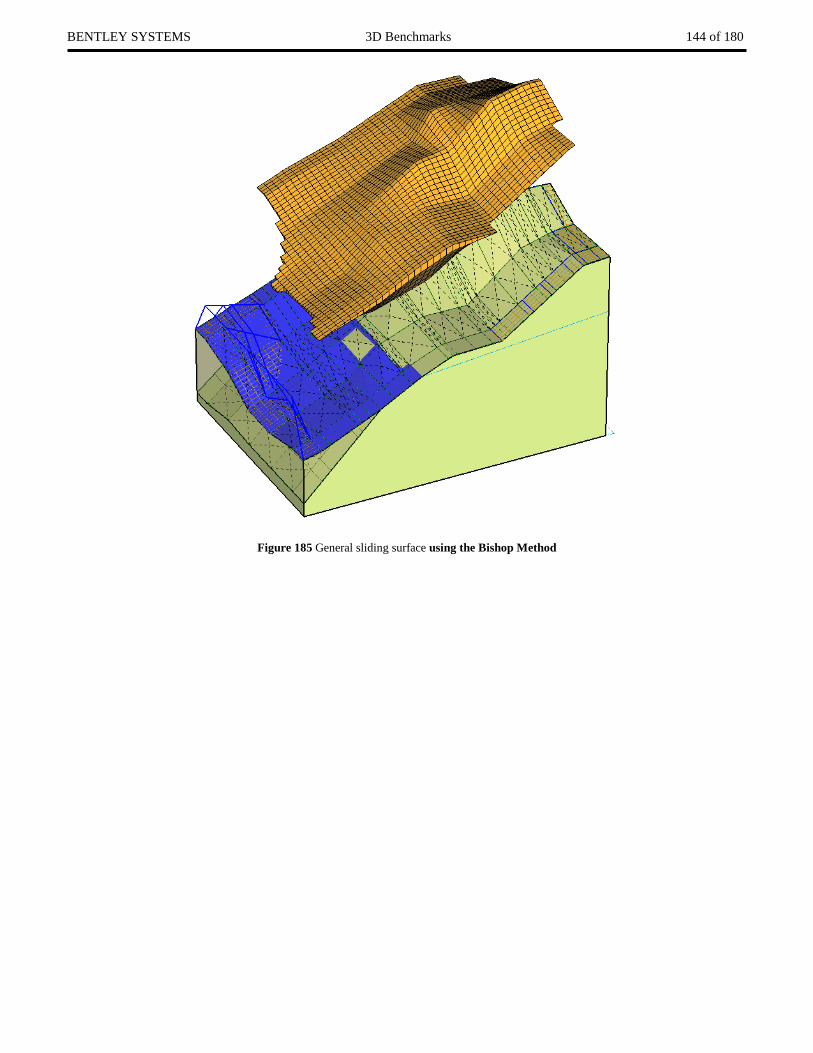
BENTLEY SYSTEMS 3D Benchmarks 144 of 180
Figure 185 General sliding surface using the Bishop Method
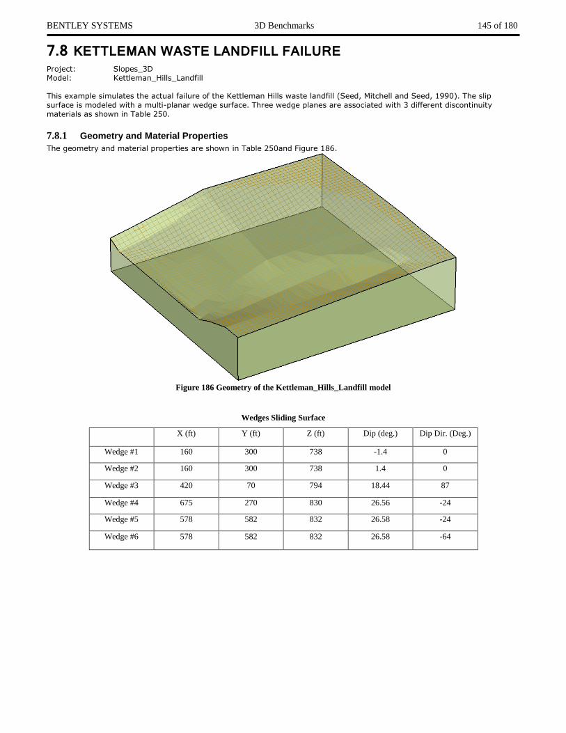
BENTLEY SYSTEMS 3D Benchmarks 145 of 180
7.8 KETTLEMAN WASTE LANDFILL FAILURE Project: Slopes_3D Model: Kettleman_Hills_Landfill This example simulates the actual failure of the Kettleman Hills waste landfill (Seed, Mitchell and Seed, 1990). The slip
surface is modeled with a multi-planar wedge surface. Three wedge planes are associated with 3 different discontinuity materials as shown in Table 250.
7.8.1 Geometry and Material Properties
The geometry and material properties are shown in Table 250and Figure 186.
Figure 186 Geometry of the Kettleman_Hills_Landfill model
Wedges Sliding Surface
X (ft) Y (ft) Z (ft) Dip (deg.) Dip Dir. (Deg.)
Wedge #1 160 300 738 -1.4 0
Wedge #2 160 300 738 1.4 0
Wedge #3 420 70 794 18.44 87
Wedge #4 675 270 830 26.56 -24
Wedge #5 578 582 832 26.58 -24
Wedge #6 578 582 832 26.58 -64

BENTLEY SYSTEMS 3D Benchmarks 146 of 180
Table 250 Material Properties of the Kettleman_Hills_Landfill model
c (psf) (degrees) γ (lb/ft^3)
Mat1 0 20 110
Dis1 0 8 127
Disc2 0 8.5 127
Dis3 900 0 127
7.8.2 Results and Discussions
The results are presented in Table 251 and Figure 187. The differences between the software packages is deemed negligible.
Table 251 Results of the Kettleman_Hills_Landfill model
Method
Factor of Safety Difference
(%) CLARA-W SVSLOPE3D
Bishop 1.160 1.164 0.345
Janbu Simplified 1.140 1.149 0.789
Spencer 1.160 1.172 1.034
M-P 1.170 1.168 -0.171
Figure 187 Failure Sliding Surface of Kettleman_Hills_Landfill model

BENTLEY SYSTEMS 3D Benchmarks 147 of 180
7.9 BEDROCK LAYER CONSIDERATION Project: Slopes_3D Model: Bedrock This is a simple symmetrical slope problem therefore only half is analyzed. An ellipsoidal sliding surface is utilized. The lower material layer is bedrock. The ellipsoidal sliding surface will be cut off when passing through the bedrock layer. CLARA-W’s Spencer method does not converge in this model.
7.9.1 Geometry and Material Properties
The geometry and material properties are presented in Figure 188 and Table 252.
Figure 188 Ellipsoidal Sliding Surface
X-Coordinate Y-Coordinate Z-Coordinate Tangent Plane Aspect Ratio
30.000 60.000 60.000 0.000 0.700
Table 252 Material Properties of Bedrock model
c (kN/m2) (degrees) γ (kN/m3)
Material2 15 25 20
7.9.2 Results and Discussions
The results are shown in Figure 189 and Table 253. The differences between the software packages are considered negligible.

BENTLEY SYSTEMS 3D Benchmarks 148 of 180
Figure 189 Failure sliding surface of the Bedrock model
Table 253 Results of the Bedrock model
Method
Factor of Safety Difference
(%) CLARA-W SVSLOPE3D
Bishop 1.20 1.175 -2.083
Janbu Simplified 1.17 1.150 -1.709
M-P 1.19 1.145 -3.782
7.10 MULTIPLE PIEZOMETRIC SURFACES Project: Slopes_3D Model: multi_piezo_surfaces There are six layers in this model. Each layer is associated with a different piezometric surface in order to simulate the condition of upward seepage.
7.10.1 Geometry and Material Properties
A fully specified Ellipsoidal sliding surface is used in this analysis, the geometry and material properties are shown in Table 254 and Figure 190.
Table 254 Material Properties of the multi_piezo_surfaces model
c (kN/m2) (degrees) γ (kN/m3)
Clayer1 20 18 19

BENTLEY SYSTEMS 3D Benchmarks 149 of 180
Figure 190 Geometry of the multi_piezo_surfaces model
7.10.2 Results and Discussions
The results are shown in Figure 191 and Table 255. Negligible differences between the software packages are noted.
Table 255 Results of the multi_piezo_surfaces model comparison
Method
Factor of Safety Difference
(%) CLARA-W SVSLOPE3D
Bishop 2.15 2.164 0.651
Janbu Simplified 1.93 1.939 0.466
Spencer 2.15 2.145 -0.233
M-P 2.16 2.138 -1.019

BENTLEY SYSTEMS 3D Benchmarks 150 of 180
Figure 191 Failure sliding mass of the multi_piezo_surfaces model
7.11 ARBITRARY SLIDING DIRECTION Project: Slopes_3D Model: Arbitrary_Sliding_Direction This benchmark is used to illustrate the analysis of a three-dimensional slope stability model using the Orientation Analysis feature of SVSLOPE, i.e., a slip surface direction that does not follow the x-axis. The model is analyzed using the Bishop Simplified, Janbu Simplified and the GLE methods. A range of slip surface directions is analyzed and the effect on the factor of safety for the slope is noted. The purpose of this benchmark is to analyze the stability of a simple slope along several different slip surface directions and present the resultant factors of safety.
This model was developed because the sliding direction becomes an additional searching parameter. The correct sliding direction is unknown at the start of the analysis and must be determined by the user.
The model is developed from: Jiang et al. 2003. Jiang results were a FOS = 1.33 using the Dynamic Programming search method and the Janbu analysis method.
7.11.1 Geometry and Material Properties
This example consists of a simple one layer slope. The geometry and material properties are shown in Table 256 and Figure 192.
Table 256 Material Properties of the Arbitrary Sliding Direction model
c (kPa) (degrees) γ (kN/m^3)
soil 11.7 24.7 17.66

BENTLEY SYSTEMS 3D Benchmarks 151 of 180
Figure 192 Geometry of the Arbitrary Sliding Direction model
7.11.2 Results and Discussions
The results of the analysis are presented in Table 257 and Figure 193 Result of analysis of Arbitrary Sliding Direction model with display of 3D sliding mass. The model illustrates in the table results from Jiang et. Al. (2003) compared to SVSLOPE 3D. The differences of less than 5% are considered reasonable. The sliding direction was determined with a preliminary guess and then searched through a range of possible sliding directions on either side of the preliminary guess.
Table 257 Results of the Arbitrary Sliding Direction model analysis
Method
Factor of Safety
Difference (%) Jiang et. al. 2003 SVSLOPE 3D
Janbu Simplified 1.33 1.285 3.38
Bishop Simplified - 1.404 -
GLE - 1.408 -
Figure 193 Result of analysis of Arbitrary Sliding Direction model with display of 3D sliding mass

BENTLEY SYSTEMS FEATURE EXAMPLES FOR 3D MODELS 152 of 180
8 FEATURE EXAMPLES FOR 3D MODELS This chapter presents some examples published in Journals to verify the SVSLOPE 3D software and some benchmark models to test some individual features by comparing the results with CLARA-W or with corresponding 2D models. The models in this chapter also represent a collection of classic examples. The examples are chosen to verify the calculation of the factor of safety in various cases, including variations in material properties, water table locations, etc.
8.1 FREDLUND AND KRAHN (1977) 2D TO 3D Project: Slopes_3D Model: FredlundAndKrahn_1977_3D This model was created based on the 2D example model by Fredlund and Krahn (1977) by extending the 2D model into 3D. It is similar to the 3D benchmark model – CLARA-W example2 (Composite Ellipsoid Wedge), but this model is a more “exact” match with the original 2D model without using the wedge plane and a discontinuity material. In this example an ellipsoidal sliding surface is utilized and the weak layer is kept as a separate layer.
8.1.1 Geometry and Material Properties
The geometry and material properties are shown in Table 258 and Figure 194.
Table 258 Material Properties of Fredlund and Krahn (1977) 3D model
c (psf) (degrees) γ (lb/ft^3)
clay 600 20 120
Weak layer 0 10 120
Bed rock
Figure 194 Geometry of 3D Example Model – Fredlund and Krahn (1977)
Ellipsoidal Sliding Surface
X-Coordinate 120.000
Y-Coordinate 0.000
Z-Coordinate 90.000
Tangent Plane 10.000
Aspect Ratio 1.000
8.1.2 Results and Discussions
This model illustrates in the 2D results from Fredlund and Krahn (1977) compared to the SVSLOPE 3D results and CLARA-W results. The 3D FOS is about 30% larger than 2D FOS on average.

BENTLEY SYSTEMS FEATURE EXAMPLES FOR 3D MODELS 153 of 180
Table 259 Results of the Fredlund and Krahn (1977) 3D model
Method
Factor of Safety
Difference
(%)
Fredlund and Krahn
(1977) 2D CLARA-W SVSLOPE 3D
Ordinary 1.171 1.514 -
Bishop Simplified 1.248 1.62 1.67 -3.09
Janbu Simplified 1.333 1.648 -
Corps. of Engineers #1 - 1.805 -
Corps. of Engineers #2 - 1.800 -
Spencer 1.245 1.713 -
M-P 1.250 1.675 -
GLE - 1.675 -
Sarma - 1.706 -
Figure 195 Results of the Fredlund and Krahn (1977) 3D model
8.2 EARTHQUAKE LOAD Project: Slopes_3D Model: earthquake_load This model is used to benchmark the horizontal earthquake load calculations in the SVSLOPE 3D software.
8.2.1 Geometry and Material Properties
The model geometry and material properties are the same as the Ellipsoidal_Toe_Submergence with the addition of the horizontal earth quake load as shown in Figure 196.

BENTLEY SYSTEMS FEATURE EXAMPLES FOR 3D MODELS 154 of 180
Figure 196 Geometry of earthquake_load Model with earth quake load
8.2.2 Results and Discussions
The Results are shown in Table 260. The result of the comparison is a reasonable comparison to the CLARA-W software.
Table 260 Results of the earthquake_load model
Method
Factor of Safety
Difference
(%)
CLARA-W
SVSLOPE 3D
Moment Force
Bishop 1.040 1.066 2.500
Janbu Simplified 0.99 1.010 2.020
Spencer 1.00 1.070 1.070 7.000
Figure 197 Results of earthquake_load Model with earth quake load

BENTLEY SYSTEMS FEATURE EXAMPLES FOR 3D MODELS 155 of 180
8.3 POINT LOAD Project: Slopes_3D Model: point_load This model is used to benchmark the point load.
8.3.1 Geometry and Material Properties
The model geometry and material properties are the same as the Ellipsoidal_Toe_Submergence with the exception of an addition of the point load as shown in Figure 198.
Figure 198 Geometry of the point_load model with a point load
8.3.2 Results and Discussions
The Results are shown in Table 261. The differences between calculations in each software package are considered negligible.
Table 261 Results of the point_load model
Method
Factor of Safety
Difference
(%)
CLARA-W
SVSLOPE 3D
Moment Force
Bishop 1.340 1.365 1.866
Janbu Simplified 1.340 1.353 0.970
Spencer - 1.360 1.360 -

BENTLEY SYSTEMS FEATURE EXAMPLES FOR 3D MODELS 156 of 180
Figure 199 Results of the point_load model with a point load
8.4 TENSION CRACK Project: Slopes_3D Model: Tension_Crack This model is used to benchmark the tension crack.
8.4.1 Geometry and Material Properties
The model geometry and material properties are the same as the Ellipsoidal_Toe_Submergence with the addition of the tension crack information. The tension crack is specified by X-coordinate = 300. It is specified that 80% of the tension crack is filled with water.
Figure 200 Geometry of the the Tension_crack model

BENTLEY SYSTEMS FEATURE EXAMPLES FOR 3D MODELS 157 of 180
8.4.2 Results and Discussions
The Results are shown in Table 262 and Figure 201.
Table 262 Results of the Tension_Crack model
Method
Factor of Safety
Difference
(%)
CLARA-W
SVSLOPE 3D
Moment Force
Bishop 1.26 1.284 1.905
Janbu Simplified 1.19 1.212 1.849
Spencer - 1.348 1.348 -
Figure 201 Result of the Tension_crack model
8.5 PORE WATER PRESSURES AT DISCRETE POINTS Project: Slopes_3D Model: PWP_discrete_points This model is used to benchmark the discrete points method to specify the pore water pressures in SVSLOPE 3D. The discrete points (specified in terms of pressure head) in this model are used to simulate the water table surface in the original Ellipsoidal_Toe_Submergence model.
8.5.1 Geometry and Material Properties
The model geometry and material properties are the same as the Ellipsoidal_Toe_Submergence model with a change of the initial condition – from water surface to discrete points (pressure head). The model geometry is shown in Figure 202 including contouring of the discrete points (in terms of pressure head).

BENTLEY SYSTEMS FEATURE EXAMPLES FOR 3D MODELS 158 of 180
Figure 202 Geometry PWP_discrete_points model with discrete points contoured
8.5.2 Results and Discussions
The Results are shown in Table 263. The results from CLARA-W are based on the pore-water pressure dataset with a water table surface. The differences are deemed to be negligible.
Table 263 Results of the PWP_discrete_points model
Method
Factor of Safety
Difference
(%)
CLARA-W
SVSLOPE 3D
Moment Force
Bishop 1.30 1.306 0.462
Janbu Simplified 1.23 1.237 0.569
Spencer 1.26 1.310 1.310 3.968
Figure 203 Results of PWP_discrete_points model with discrete points contoured

BENTLEY SYSTEMS FEATURE EXAMPLES FOR 3D MODELS 159 of 180
8.6 SUPPORTS – END ANCHORED Project: Slopes_3D Model: Support_End_Anchored This model is utilized to benchmark the discrete End Anchored support type in SVSLOPE 3D. CLARA-W does not implement Supports, so in order to benchmark the supports the same magnitude of external point load was specified in CLARA-W as the magnitude of end anchor tensile capacity in SVSLOPE 3D. The location of the external point load in CLARA-W is the same location of the entry point of the support on the ground surface in SVSLOPE 3D.
8.6.1 Geometry and Material Properties
The model geometry and material properties are the same as the Ellipsoidal_Toe_Submergence model with the addition of one End Anchored support. The tensile capacity of the end anchored support is 5x10⁶ lb. The surface point coordinate of the support on the ground surface is (250, 2, 179.898), the internal point of the support in the sliding mass is (400, 2, 179.898). The location of the support is shown in Figure 204.
Figure 204 Geometry of Support_End_Anchored Model
8.6.2 Results and Discussions
The Results are shown in Table 264. The results from CLARA-W are based on corresponding external point load settings.
Table 264 Results of the Support_End_Anchored model
Method
Factor of Safety
Difference
(%)
CLARA-W
SVSLOPE 3D
Moment Force
Bishop 1.760 1.754 -0.341
Janbu Simplified 1.730 1.729 -0.058
Spencer 1.940 1.753 1.752 -9.639

BENTLEY SYSTEMS FEATURE EXAMPLES FOR 3D MODELS 160 of 180
Figure 205 Results of Support_End_Anchored Model
8.7 3-STAGE RAPID DRAWDOWN Project: Slopes_3D Model: RDD_USACE_3D This example model was originally presented in Corps of Engineers, Engineering Manual (2003) as a demo of Duncan’s 3-stage rapid drawdown analysis in 2D. Hand calculation of the FOS of Bishop method is 1.44 for 2D. Here it is extended to 3D.
8.7.1 Geometry and Material Properties
The geometry is a direct extension from the 2D model section. The material properties are the same as in the 2D case. There are two water table surfaces in this model. The initial water table surface is located at an elevation of 103ft. The final water table surface is located at an elevation of 24ft as shown in Figure 206.
Figure 206 Geometry of the RDD_USACE_3D Model

BENTLEY SYSTEMS FEATURE EXAMPLES FOR 3D MODELS 161 of 180
8.7.2 Results and Discussions
The following table shows the results of the calculations for this model. The SVSLOPE 2D results are also shown. The difference between 2D and 3D calculations is about 7% in this particular model. The hand calculation 2D result with Bishops Method is 1.44.
Table 265 Results of the RDD_USACE_3D model
Method
Factor of Safety
Difference
(%)
SVSLOPE 2D
SVSLOPE 3D
Moment Force
Bishop 1.436 1.551 8.00
Spencer 1.426 1.578 1.578 10.66
Figure 207 Results of the RDD_USACE_3D Model

BENTLEY SYSTEMS SVSLOPE (SEISMIC) EXAMPLES 162 of 180
9 SVSLOPE (SEISMIC) EXAMPLES SVSLOPE (Seismic) is a Technical Preview. In this section, SVSLOPE (Seismic) is used to simulate various dynamic stress-strain problems using 2D plane strain analysis. SVSLOPE (Seismic) uses a time-domain finite element method for solving dynamic problems.
9.1 S-WAVE PROPAGATION IN AN ELASTIC COLUMN Reference: Brinkgreve (2002) Project: Seismic_2D Model: 2D_SoilColumn_SWave, 2D_SoilColumn_SWave_1
Main Factors Considered:
• The displacement field due to the propagation of an S-wave along the y-axis in an elastic soil column under plane strain condition and comparison with PLAXIS 2D results
9.1.1 Model Description
A linear elastic soil column was considered and the propagation of an S-waves along the column was modeled. The propagation of the S-Wave generates displacements dominantly in the x-direction in the soil column. Due to the finite velocity of the S-wave, the response of each material point within the domain depends on the time required for the S-wave to travel from its source to that point. The soil column can be modeled as a 2D plane strain problem. The results of analysis using
SVSLOPE (Seismic) was compared against PLAXIS 2D results for this problem. The total time of dynamic analysis was set to 2 seconds with time increments, ∆𝑡 = 0.001 𝑠. Newmark parameters were set to 𝛿 = 0.53 and 𝛼 = 0.2652. These values will
introduce a small artificial damping to the system which damps out spurious oscillations in the solution. No material damping was considered in this problem.
Figure 208. Geometry and boundary conditions (different x and y scales):
(a) Fixed bottom boundary and (b) Nonreflecting bottom boundary
Point A
Point B
Point C Point C
Point B
Point A
(a) (b)

BENTLEY SYSTEMS SVSLOPE (SEISMIC) EXAMPLES 163 of 180
9.1.2 Geometry and Boundary Conditions
Figure 208 shows the geometry and boundary conditions of the model. A column of soil with the depth of 10 m and width of 0.25 m was modeled. The side and bottom boundaries of the model were fixed in their tangential directions. The top boundary of the domain is subject to a constant displacement in the x-direction, 𝑢𝑥 = 0.001 𝑚, which generates an S-wave
propagating from the surface of the soil column to the bottom. To verify the effect of the non-reflecting boundary conditions, a second simulation was carried out in which the fixed boundary condition at the bottom boundary was replaced with nonreflecting boundary conditions.
9.1.3 Material Properties
A summary of the elastic material properties is provided in Table 266.
Table 266. Input material properties
Parameter Value
Young’s modulus (E) 18,000 kPa
Poisson’s ratio () 0.2
Total unit weight () 19.620 kN/m3

BENTLEY SYSTEMS SVSLOPE (SEISMIC) EXAMPLES 164 of 180
9.1.4 Results
Three observation points, points A, B, and C, were considered respectively at the bottom, middle, and top of the soil column. The velocity of the S-wave in the soil column can be calculated from the material properties as 𝑉𝑆 = 61.24 𝑚/𝑠. Therefore, it will take 𝑡1 = 0.082 𝑠 for the S-wave to reach point B for the first time. The bottom boundary of the domain is fixed. Hence, the
wave reflects back into the domain when reaches the bottom boundary. The time required for the wave to reach point B for the second and third time during the analysis were calculated to be, respectively, 𝑡2 = 3𝑡1 = 0.245 𝑠 and 𝑡3 = 5𝑡1 = 0.408 𝑠. Figure 209 illustrates the horizontal deformation of points A, B, and C over time computed by SVSLOPE (Seismic) and PLAXIS. The figure shows that SVSLOPE (Seismic) results for this problem match very well with PLAXIS results. The estimated arrival times of the S-wave at point B were also marked in this figure. The arrival times estimated by SVSLOPE (Seismic) for the first, second and third incidences of the S-wave with point B are, respectively, 𝑡1 = 0.083 𝑠, 𝑡2 = 0.247 𝑠, and 𝑡3 = 0.410 𝑠, which
are in agreement with the analytical values. When a nonreflecting boundary condition is applied at the bottom boundary (see Figure 208), the energy of the waves reaching the bottom boundary is absorbed by the enforced boundary condition. Therefore, no reflection should be detected at the observation points within the domain. This behavior is shown in Figure 210. As illustrated in the figure, the arrival time of the S-wave at point B is the same as the time calculated in the previous case, i.e., 𝑡 = 𝑡1 = 0.083 𝑠. However, the second and
third arrivals do not occur in this case as the wave does not reflect into the domain. It should be noted that the bottom boundary is not fixed in this case; hence, the arrival time of the S-wave at the bottom boundary can also be estimated from the numerical results. Using Figure 210, the estimated time for the arrival of the wave at Point A is 𝑡 = 0.165 𝑠, which is in
agreement with the theoretical time, 𝑡 = 2𝑡1 = 0.166 𝑠. Figure 210 also provides a comparison between SVSLOPE (Seismic) results and the solution of the same problem using PLAXIS software.
Figure 209. Time-history of horizontal displacement at Points A, B, and C with fixed boundary condition at the bottom boundary

BENTLEY SYSTEMS SVSLOPE (SEISMIC) EXAMPLES 165 of 180
Figure 210. Time-history of horizontal displacement at Points A, B, and C with nonreflecting boundary condition at the bottom
boundary

BENTLEY SYSTEMS SVSLOPE (SEISMIC) EXAMPLES 166 of 180
9.2 P-WAVE PROPAGATION IN AN ELASTIC SOIL COLUMN Reference: Brinkgreve (2002) Project: Seismic_2D Model: 2D_SoilColumn_PWave, 2D_SoilColumn_PWave_1
Main Factors Considered:
• The displacement field due to the propagation of a P-wave along the y-axis in an elastic soil column under plane strain condition and comparison with PLAXIS 2D results
9.2.1 Model Description
A linear elastic soil column was considered, and the propagation of P-waves within the column was modeled. The propagation of the P-Wave generats displacements dominantly in the y-direction in the soil column. Due to the finite velocity of the P-wave, the response of each material point within the domain depends on the time required for the P-wave to travel to that point from its source. The soil column can be modeled as a 2D plane strain problem. The results of analysis using SVSLOPE (Seismic) were compared against the numerical results of PLAXIS 2D for this problem. The total time of dynamic analysis was set to 1 second with time increments, ∆𝑡 = 0.001 𝑠. Newmark parameters were set to 𝛿 = 0.53 and 𝛼 = 0.2652. These values will
introduce a small artificial damping to the system which damps out spurious oscillations in the solution. The damping ratio is set to zero for this problem.

BENTLEY SYSTEMS SVSLOPE (SEISMIC) EXAMPLES 167 of 180
Figure 211. Geometry and boundary conditions (different x and y scales):
(a) Fixed bottom boundary and (b) Nonreflecting bottom boundary
9.2.2 Geometry and Boundary Conditions
Figure 211 shows the geometry and boundary conditions of the model. A column of soil with the depth of 10 m and the width of 0.25 m was modeled. The side and bottom boundaries of the model were fixed in the direction normal to the boundary. The top boundary of the domain is subject to a constant displacement in the y-direction, 𝑢𝑦 = 0.001 𝑚, which generates a P-wave
propagating from the surface of the soil column to the bottom. To verify the effect of the non-reflecting boundary conditions, a second simulation was carried out in which the fixed boundary condition at the bottom boundary was replaced with nonreflecting boundary conditions.
9.2.3 Material Properties
A summary of the elastic material properties is provided in Table 267.
Table 267. Input material properties
Parameter Value
Young’s modulus (E) 18,000 kPa
Poisson’s ratio () 0.2
Total unit weight () 19.62 kN/m3
9.2.4 Results
Three observation points, points A, B, and C, were considered respectively at the bottom, middle, and top of the soil column. The velocity of the P-wave in the soil column can be calculated from the material properties as 𝑉𝑃 = 100 𝑚/𝑠. Therefore, it will
take 𝑡1 = 0.050 𝑠 for the P-wave to reach point B for the first time. When the bottom boundary of the domain is fixed, the wave
reflects into the domain upon reaching the bottom boundary. Hence, the time required for the wave to reach point B for the second time during the analysis is calculated as 𝑡2 = 3𝑡1 = 0.150 𝑠. Figure 212 shows the horizontal deformation of points A, B, and C over time for both SVSLOPE (Seismic) and PLAXIS. The figure shows that SVSLOPE (Seismic) results match very well with PLAXIS results. The estimated arrival times of the P-wave at point B were also shown in this figure. The arrival times estimated by SVSLOPE (Seismic) for the first and second incidences of the P-wave with point B are respectively 𝑡1 = 0.051 𝑠 and 𝑡2 = 0.152 𝑠, which are in agreement with the analytical
values. When a nonreflecting boundary condition is applied at the bottom boundary, the energy of the waves reaching the bottom boundary is absorbed by the enforced boundary condition. Therefore, no reflection should be detected at the observation
Point A
Point B
Point C Point C
Point B
Point A
(a) (b)

BENTLEY SYSTEMS SVSLOPE (SEISMIC) EXAMPLES 168 of 180
points within the domain. This behavior is clearly shown in Figure 213. As illustrated in the figure, the arrival time of the P-wave at point B is the same as the time calculated in the previous case, i.e., 𝑡 = 𝑡1 = 0.051 𝑠. However, the second and third
arrivals do not occur in this case as the wave does not reflect into the domain. It should be noted that the bottom boundary is not fixed in this case; hence, the arrival time of the P-wave at the bottom boundary can also be estimated from the numerical results. Using Figure 213, the estimated time for the arrival of the wave at Point A is 𝑡 = 0.102 𝑠 which is in agreement with
the theoretical arrival time, 𝑡 = 2𝑡1 = 0.100 𝑠. Figure 213 also provides a comparison between SVSLOPE (Seismic) results and the solution of the same problem using PLAXIS software.
Figure 212. Time-history of vertical displacement at Points A, B, and C with fixed boundary condition at the bottom boundary

BENTLEY SYSTEMS SVSLOPE (SEISMIC) EXAMPLES 169 of 180
Figure 213. Time-history of vertical displacement at Points A, B, and C with nonreflecting boundary condition at the bottom
boundary

BENTLEY SYSTEMS SVSLOPE (SEISMIC) EXAMPLES 170 of 180
9.3 REFRACTION SEISMOLOGY Reference: Fowler (1990) Project: Seismic_2D Model: 2D_Refraction
Main Factors Considered:
• Determine the velocity of the P-wave and estimate the thickness of the soil layer in a two-layer elastic medium using refraction seismology
9.3.1 Model Description
The behavior of body waves in an elastic medium depends on the physical properties of the medium. When body waves propagate in a heterogenious medium, such as a layered soil, their propagation speed and direction of propagation change according to the relative rigidity of the layers encountered. This phenomenon can be used to extract important information about soil layers. For example, one can estimate material properties (such as wave speeds) of different soil layers and the thickness of each layer using the motion recorded at the surface.
Figure 214. Wave behavior in a two-layer medium
Consider the two-layer soil model shown in Figure 214. Let us choose the matrial properties of the two layers such that the product of the mass density, 𝜌, and wave velocity, 𝑉, of the bottom layer, 𝜌2𝑉2, is greater that that of the top layer, 𝜌1𝑉1. The
product of the mass density and wave velocity of a matrial is known as its acoustic impedance (see for example Kinsler et al. (1999) for more information). An acoustic transmitter, located at the surface, transmits a compressional wave signal (p-wave) towards the interface of the two layers. An array of geophones, set along the surface of the top layer, records the response of the layer at the surface. The compressional wave travels within the top layer with 𝑉1 until it reaches the interface.
Due to the difference between the acoustic impedance of the two layers, a part of the wave energy reflects back into the top layer (reflected wave). The remaining part of the wave propagates through the bottom layer; however, its strike angle and propagation speed change according to Snell’s law:
𝑉1
𝑉2
=sin 𝛼1
sin 𝛼2
[ 1 ]
BENTLEY SYSTEMS SVSLOPE (SEISMIC) EXAMPLES 171 of 180
in which 𝛼1 and 𝛼2 are the direction angles of the wave ray in the first and second layers respectively (see Figure 214).
The wave ray that reaches the second layer travels faster than the initial wave as it propagates in the bottom layer with a higher wave speed. The wave front traveling along the interface acts as a new wave source and transmits new waves within the top layer towards the surface. These waves are known as Refracted waves. The geophones located on the surface of the
top layer will record the wave ray that has travelled directly through the top layer (direct wave) as well as the refracted wave ray (see Figure 214). Geophones that are closer to the wave source record the arrival of the direct wave prior to the refracted wave arrival as it takes longer for the wave to travel to the interface and return to the surface. Contrarily, geophones located far from the wave source record the refracted wave prior to the direct ray as the wave has had enough time to travel through the second layer (with a higher wave speed) to catch up the direct wave. Knowing the arrival time of the wave at each geophone and its distance form the wave source, one is able calculate the speed of the wave in each layer and the thickness of the top layer (Fowler 1990). In this verification, we simulate the phenomenon explained above and use the information recorded at the surface to estimate the speed of the P-wave in each layer and the thickness of the top layer. A 2D plane strain model of a two layer soil was considered. A time increment of ∆𝑡 = 2.5 m𝑠 was used for dynamic analysis. Newmark parameters were set to 𝛿 = 0.50 and 𝛼 =0.25; therefore, no numerical damping was engaged in the computations. An overall damping ratio of 𝜉 = 0.50% was assumed
for this problem (at response frequencies 0.5 Hz and 1.0 Hz). Material properties of the layers are presented in Table 268.
Table 268. Input material properties
Parameter Top Layer Bottom Layer
Young’s modulus (E) 18,000 kPa 180,000 kPa
Poisson’s ratio () 0.25 0.3
Total unit weight () 19.6 kN/m3 21 kN/m3

BENTLEY SYSTEMS SVSLOPE (SEISMIC) EXAMPLES 172 of 180
Figure 215. Geometry and boundary conditions of the model
9.3.2 Geometry and Boundary Conditions
The geometry and boundary conditions of the model are illustrated in Figure 215. Each layer has a thickness of 20 m and width of 150 m. An array of geophones (history points), at every 15 m, was set along the surface (named S1 through S11 from left to right). The wave source was modeled by means of a vertical dynamic line load with an amplitude of 100 kN/m applied at the upper left corner of the domain. The variation of the line load over time is shown in Figure 216. The left boundary of the model was fixed in the x-direction. Non-reflecting boundary conditions were set at the right and bottom boundaries and the top boundary was left free.
Figure 216. Variation of dynamic force over time
9.3.3 Results
To calculate the velocity of the P-wave in each layer, we first need to estimate the wave arrival time at each geophone. The arrival times can be captured using the seismograph recorded by the geophone. For this problem, we use the recorded displacement in the x-direction to capture the arrival time of the P-wave. Figure 217 illustrates the recorded displacement at
each geophone for the two-layer soil model (blue). To provide a reference for comparison, the displacement in the x-direction for an equivalent model with only one soil layer (with a thickness of 40.0 m) is also provided at each station (red). This will allow the reader to compare the response of the model with the response of a case in which no refraction occurs. For each recording, the arrival time can be estimated by capturing the time at which the first significant displacement is recorded. Determining the exact arrival time from the recorded seismograph is a nontrivial task as the graphs do not clearly show an abrupt initial jump in the displacement to be taken as the arrival of the P-wave. As an estimate of the wave arrival time, in this verification example, we take the mean value of the time points corresponding to the first local minimum and maximum of each graph (This assumption is consistent with the numerical results presented in sections Error! Reference source not found. and Error! Reference source not found. for P- and S-wave arrivals). The arrival time was calculated for each graph and is marked with vertical dashed lines in Figure 217. The estimated arrival time of the wave at each geophone is presented in Table 269. The theoretical time of arrival of the direct and refracted rays at a geophone, located at distance, x, from the source, can be calculated as linear functions of the speed of the P-wave in the top and bottom layers (Fowler 1990):
𝑡𝐷𝑖𝑟𝑒𝑐𝑡 =𝑥
𝑉1
[ 2 ]

BENTLEY SYSTEMS SVSLOPE (SEISMIC) EXAMPLES 173 of 180
𝑡𝑅𝑒𝑓𝑟𝑎𝑐𝑡𝑒𝑑 =
𝑥
𝑉2
+ 2𝐻1
√𝑉22 − 𝑉1
2
𝑉1𝑉2
[ 3 ]
where 𝐻1 is the thichkness of the top layer.
Table 269 also provides the theoretical arrival time of the direct and refracted ray at each geophone. The values corresponding to the first arrival time are presented in bold fonts. From the theoretical values, it can be seen that the first wave arriving at geophones, S1 through S4, is expected to be the direct wave whereas the rest of the geophones are expected to record the refracted wave first. To calculate the speed of the P-wave in each layer, one can plot the estimated values of the first arrival time at each geophone versus the distance of the geophone from the source, as presented in Figure 218. The estimated values from SVSLOPE (Seismic) numerical results are ploted in red dots. It can be seen that SVSLOPE (Seismic) results are in agreement with the theoretical values. The relations, [2] and [3], are linear. Hence, the speed of the P-wave in the first and second layers can be estimated by fitting two lines to the numerical results. The slopes of these lines represent the reciprocals of the wave speeds (see Figure 218). The linear functions fitted to the SVSLOPE (Seismic) numerical results are shown in Figure 218. It should be noted that the estimated value for S5 (located at x=60.0 m) has been excluded from the data used for fitting linear functions. The reason of this exclusion is that S5 is located only slightly away from the cross-over point at which the direct and refracted rays are expected to arrive simultaneously. As a result, the interaction of the two waves could increase the error in estimating the arrival time at this point, compared to the other points.
Table 269. Estimated and theoretical time of arrival of waves at different geophones (theoretical first arrival times are bolded)
Station Distance from source (m) Estimated first arrival time
(s) (SVSLOPE (Seismic))
Theoretical arrival time
(s) (Direct ray)
Theoretical arrival time
(s) (Refracted ray)
S1 0.0 0.0 0.0 0.366
S2 0.136 0.144 0.411
S3 30.0 0.284 0.289 0.455
S4 45.0 0.431 0.433 0.499
S5 60.0 0.565 0.577 0.544
S6 75.0 0.593 0.722 0.589
S7 90.0 0.636 0.866 0.633
S8 105.0 0.680 1.010 0.678
S9 120.0 0.724 1.154 0.723
S10 135.0 0.773 1.299 0.767
S11 150.0 0.821 1.443 0.812
Using the estimated slope values from the fitted lines, the speed of the P-wave within the first and second layers can be
estimated as �̅�1 = 104.16 𝑚/𝑠 (compare to the theoretical value 𝑉1 = 103.95 𝑚
𝑠 (0.2% error)), and �̅�2 = 333.33 𝑚/𝑠 (compare to
the theoretical value 𝑉2 = 336.49 𝑚
𝑠 (0.9% error)).
The thickness of the top layer, 𝐻1, can be estimated from the estimated values of wave velocity as (Fowler 1990):
𝐻1 = 𝑡𝑥=0
𝑉1𝑉2
2√𝑉22 − 𝑉1
2 [ 4 ]

BENTLEY SYSTEMS SVSLOPE (SEISMIC) EXAMPLES 174 of 180
where 𝑡𝑥=0 denotes the intercept of the refraction line. From Figure 218, the estimated value of the intercept is 𝑡�̅�=0 = 0.3623 𝑠.
Substituting the estimated values of 𝑡�̅�=0, �̅�1, and �̅�2 into [4], the thickness of the top layer can be evaluated as �̅�1 = 19.87 𝑚
which has an error of 0.65% compared to the actual thickness of the layer, 𝐻1 = 20.0 𝑚.
Figure 217. Recorded displacement in x-direction at each geophone for two-layer soil model (blue) and single layer reference model
(red)

BENTLEY SYSTEMS SVSLOPE (SEISMIC) EXAMPLES 175 of 180
Figure 218. P-wave arrival time at each geophone vs geophone distance from the wave source. SVSLOPE (Seismic) results have been
presented in red dots. Black Solid lines represent the estimated arrival lines (direct and refracted waves) using SVSLOPE (Seismic)
results. The slopes of the estimated lines were used for calculating P-wave velocities in the first and second layers and for estimating
the thickness of the top layer. Figure 219 illustrates the contours of horizontal displacement, generated by SVSLOPE (Seismic), at three different time steps. Locations of the direct wave front, wave front in the bottom layer, and refracted wave front are marked in each graqph. The phenomenon explained in section Error! Reference source not found. can be clearly recognized in this figure. At early time, the wave propagates only within the top soil layer. Hence, geophones located close to the wave source record the arrival of the direct wave ray (Figure 219a). The wave propagates with a higher speed once it enters the bottom layer. As a result, the wave front in the bottom layer is always ahead of the wave front in the top layer (Figure 219b). The propagation of the wave front along the interface transmits the refracted waves toward the surface. The refracted wave front within the top layer can be seen in Figure 219c.

BENTLEY SYSTEMS SVSLOPE (SEISMIC) EXAMPLES 176 of 180
Figure 219. Contours of horizontal displacement and location of wave front at different time steps
(a)
(b)
(c)

BENTLEY SYSTEMS SVSLOPE (SEISMIC) EXAMPLES 177 of 180

BENTLEY SYSTEMS References 178 of 180
10 REFERENCES Arai, K. and Tagyo, K. (1985), "Determination of Noncircular Slip Surface giving the minimum factor of safety in slope stability analysis", Soils and Foundations. Vol. 25, No.1 pp. 43-51. Baker, R. (1980), "Determination of the critical slip surface in slope stability computations", International Journal for Numerical and Analytical Methods in Geomechanics, Vol.4, pp. 333-359. Baker, R. and Leshchinsky, D. (2001), "Spatial Distribution of Safety Factors", Journal of Geotechnical and Geoenvironmental Engineering, February 2001, pp. 135-144. Baker, R. (2003), "Inter-relations between experimental and computational aspects of slope stability analysis", International Journal for Numerical and Analytical Methods in Geomechanics, No. 27, pp. 379-401. Baker, R. (1993), "Slope stability analysis for undrained loading conditions", International Journal for Numerical and Analytical Methods in Geomechanics, Vol. 17, pp. 15-43.
Borges, J. L. and Cardoso, A.S. (2002), "Overall stability of geosynthetic-reinforced embankments on soft soils", Geotextiles and Geomembranes, Vol. 20, pp. 395-421. Brinkgreve, R.B. (2002), Plaxis Version 8 Dynamic Manual, Lisse, Balkema. Chen, Z. and Shao, C. (1988). "Evaluation of minimum factor of safety in slope stability analysis", Canadian Geotechnical Journal, Vol. 25, pp. 735-748. Chowdhury, R.N. and Xu, D.W. (1995), "Geotechnical system reliability of slopes", Reliability Engineering and System Safety. Vol. 47, pp. 141-151. Craig, R. F., (1997), Soil Mechanics, 6th Edition. Routledge, UK June, 1997 Duncan, M.J., (2000), "Factors of Safety and Reliability in Geotechnical Engineering", Journal of Geotechnical of Geoenvironmental Engineering. April pp. 307-316. Duncan, J.M., and Wright, S.G., 2005, "Soil Strength and Slope Stability", John Wiley & Sons, Inc. Duncan, J.M., Wright, S.G., and Wong, K.S., 1990, "Slope stability during rapid drawdown", Proceedings of the H. Bolton Seed Memorial Symposium, May, Vol. 2, pp. 253-272. El-Ramly, H., Morgenstern, N.R. and Cruden, D.M. (2003), "Probabilistic stability analysis of a tailings dyke on presheared clay-shale", Canadian Geotechnical Journal, Vol. 40, pp. 192-208. FlexPDE 6 (2007). Reference Manual, PDE Solutions Inc., Spokane Valley, WA 99206. FlexPDE 7 (2017). Reference Manual, PDE Solutions Inc., Spokane Valley, WA 99206. Fowler, C.M.R. (1990), An Introduction to Global Geophysics (2nd ed.). Cambridge University Press. Fredlund, D.G. and Krahn, J. (1977), "Comparison of slope stability methods of analysis", Canadian Geotechnical Journal Vol. 14, No. 3, pp. 429-439. Ghobrial, F., Karray, M., Delisle, M-C. and Ledoux, C. (2015), Development of spectral pseudo-static method for dynamic clayey slope stability analysis. 68th Canadian Geotechnical Conference, Quebec City, Quebec, Canada. Giam, P.S.K. and I.B. Donald (1989), "Example problems for testing soil slope stability programs", Civil Engineering Research Report No. 8/1989, Monash University, ISBN 0867469218, ISSN 01556282. Giam, P.S.K. (1989). "Improved methods and computational approaches to geotechnical stability analysis", Ph.D., Thesis, Department. of Civil Engineering, Monash University, Melbourne, Australia. Greco, V.R. (1996), "Efficient Monte Carlo technique for locating critical slip surface", Journal of Geotechnical Engineering. Vol. 122, No. 7, July, pp. 517-525.
Hassan, A.M. and Wolff, T.E. (1999), "Search algorithm for minimum reliability index of earth slopes", Journal of Geotechnical and Geoenvironmental Engineering, Vol. 125, No. 4, April 1999, pp. 301-308. Hungr O., Salgado F.M. and Byrne P.M. (1989), "Evaluation of a three-dimensional method of slope stability analysis", Canadian Geotechnical Journal, Vol. 26, pp. 697-686. Ireland, H.O. (1954), "Stability analysis of the Congress Street open cut in Chicago", Geotechnique, Vol. 4, pp. 163-168. Jiang, J-C., Baker, R., and Yamagami, T. (2003), "The effect of strength envelope non linearity on slope stability

BENTLEY SYSTEMS References 179 of 180
computations", Canadian Geotechnical Journal, No. 40, pp. 308-325. Kim, J., Salgado, R., Lee, J. (2002), "Stability analysis of complex soil slopes using limit analysis", Journal and Geotechnical and Geoenvironmental Engineering. Vol. 128, No. 7, July, pp. 546-557. Kinsler, L.E., Frey A.R., Coppens, A.B., & Sanders J.V. (1999). Fundamentals of Acoustics (4th ed.), Wiley. Lambe, T., and Whitman, R. (1969). “Soil Mechanics”, John Wiley & Sons, New York, N.Y. Leshchinski D., Baker, R., and Silver, M.L. (1985). "Three dimensional analysis of slope stability", International Journal for Numerical and Analytical Methods in Geomechanics, vol. 9, pp. 199-223. Li, S.K. and Lumb, P. (1987). "Probabilistic design of slopes", Canadian Geotechnical Journal, Vol. 24, No. 4, pp. 520-535. Loukidis, D., Bandini, P., and Salgado, R. (2003), "Stability of seismically loaded slopes using limit analysis", Geotechnique, No. 5, pp. 463-479. Low, B. (1989), "Stability analysis of embankment on soft ground." Journal of Geotechnical Engineering, Vol. 115, No. 2, pp. 221-227. Malkawi, A.I.H, Hassan, W.F., and Sarma, S.K. (2001), "Global search method for locating general slip surface using Monte Carlo techniques." Journal of Geotechnical and Geoenvironmental Engineering. Vol. 127, No. 8 August, 99. 688-698. Pham, Ha, (2002), "Slope Stability Analysis using Dynamic Programming Method Combined with a Finite Element Stress Analysis", University of Saskatchewan, Saskatoon, Canada Pilot, G., Trake, B. and La Rochelle, P. (1982). "Effective stress analysis of the stability of embankments on soft soils", Canadian Geotechnical Journal, Vol. 19, pp. 433-450. Pockoski, M., and Duncan, J.M., (2002). "Comparison of Computer Programs for Analysis of Reinforced Slopes", Virginia Polytechnic Institute and State University, December 2000. Prandtl, L. (1921), "Uber die Eindringungsfestigkeit (Harte) plastischer Baustoffe und die Festigkeit von Schneiben (On the penetrating strength (hardness) of plastic construction materials and strength of curring edges)", Zeitschrift fur Agnewandte Mathematik und Mechanik, Vol. 1, pp. 15-20. Priest, S. (1993), "Discontinuity analysis for rock engineering", Chapman & Hall, London, pp. 219-226. Sarma, S.K. (1979). "Stability Analysis of Embankments and Slopes". J. Geotech. Eng. Div. ASCE 105, No. 12, pp. 1511-
1524. Seed, R.B., Mitchell, J.K. and Seed, H.B.. (1990). "Kettlemen Hills Waste Landfill Slope Failure", ASCE Journal of Geotechnical Engineering, 116:669-690. Sevaldson, R.A., (1956). "The slide in Lodalen, October 6th, 1954". Geotechnique, No. 6, pp. 167-182. Sheahan, T., and Ho. L., (2003), "Simplified trail wedge method for soil nailed wall analysis", Journal of Geotechnical of Geoenvironmental Engineering, Vol. 17, pp. 117-124. Silvertri V. (2006), "A three-dimensional slope stability problem in clay", Canadian Geotechnical Journal, Vol. 43, pp. 224-228. Spencer, E. (1969), "A method of analysis of the stability of embankments assuming parallel inter-slice forces", Geotechnique, Vol. 17, pp. 11-26. Tandjiria, V., Low. B.K., and Teh, C.I. (2002), "Effect of reinforcement force distribution on stability of embankment", Geotextiles and Geomembranes, No. 20 pp. 423- 443. Wolff, T.F. and Harr, M.E. (1987), "Slope design for earth dams", Reliability and Risk Analysis in civil Engineering 2, Proceedings of the Fifth International Conference on Applications of Statistics and Probability in Soil and Structural Engineering, Vancouver, BC, Canada, May, 1987, pp. 725-732. XSTABL, (1999), Slope Stability Reference Manual, Version 5.2, pp 11-26. Yamagami, T., Jiang, J.C., and Ueno, K. (2000), "A limit equilibrium stability analysis of slope with stabilizing piles", Slope Stability 2000, pp. 343-354. Yamagami, T. and Ueta, Y. (1988), "Search for noncircular slip surfaces by the Morgenstern-Price method", Proc. 6th Int. Conf. Numerical Methods in Geomechanics, pp. 1335-1340 Zhu, D., Lee, C.F., and Jiang, H.D, (2003), "Generalized framework of limit equilibrium methods for slope stability analysis." Geotechnique, No. 4, pp. 337-395.

BENTLEY SYSTEMS References 180 of 180
Zhu, D., and Lee, C. (2002), "Explicit limit equilibrium solution for slope stability", International Journal for Numerical and Analytical Methods in Geomechanics, No. 26, pp. 1573-1590.