Casimir forces in the time domain: Applications

Alexander P. McCauley,1 Alejandro W. Rodriguez,1 John D. Joannopoulos,1 and Steven G. Johnson2

1Department of Physics, Massachusetts Institute of Technology, Cambridge, MA 021392Department of Mathematics, Massachusetts Institute of Technology, Cambridge, MA 02139

Our preceding paper, Ref. 1, introduced a method to compute Casimir forces in arbitrary ge-ometries and for arbitrary materials that was based on a finite-difference time-domain (FDTD)scheme. In this manuscript, we focus on the efficient implementation of our method for geometriesof practical interest and extend our previous proof-of-concept algorithm in one dimension to prob-lems in two and three dimensions, introducing a number of new optimizations. We consider Casimirpiston-like problems with nonmonotonic and monotonic force dependence on sidewall separation,both for previously solved geometries to validate our method and also for new geometries involvingmagnetic sidewalls and/or cylindrical pistons. We include realistic dielectric materials to calculatethe force between suspended silicon waveguides or on a suspended membrane with periodic grooves,also demonstrating the application of PML absorbing boundaries and/or periodic boundaries. Inaddition we apply this method to a realizable three-dimensional system in which a silica sphere isstably suspended in a fluid above an indented metallic substrate. More generally, the method allowsoff-the-shelf FDTD software, already supporting a wide variety of materials (including dielectric,magnetic, and even anisotropic materials) and boundary conditions, to be exploited for the Casimirproblem.

I. INTRODUCTION

The Casimir force, arising due to quantum fluctua-tions of the electromagnetic field [2], has been widelystudied over the past few decades [3, 4, 5, 6] and ver-ified by many experiments. Until recently, most workson the subject had been restricted to simple geometries,such as parallel plates or similar approximations thereof.However, new theoretical methods capable of comput-ing the force in arbitrary geometries have already be-gun to explore the strong geometry dependence of theforce and have demonstrated a number of interesting ef-fects [7, 8, 9, 10, 11, 12, 13, 14, 15, 16]. A substan-tial motivation for the study of this effect is due to re-cent progress in the field of nano-technology, especiallyin the fabrication of micro-electro-mechanical systems(MEMS), where Casimir forces have been observed [17]and may play a significant role in “stiction” and otherphenomena involving small surface separations. Cur-rently, most work on Casimir forces is carried out byspecialists in the field. In order to help open this field toother scientists and engineers, such as the MEMS com-munity, we believe it fruitful to frame the calculation ofthe force in a fashion that may be more accessible tobroader audiences.

In Ref. 1, with that goal in mind, we introduceda theoretical framework for computing Casimir forcesvia the standard finite-difference time-domain (FDTD)method of classical computational electromagnetism [18](for which software is already widely available). The pur-pose of this manuscript is to describe how these compu-tations may be implemented in higher dimensions andto demonstrate the flexibility and strengths of this ap-proach. In particular, we demonstrate calculations ofCasimir forces in two- and three-dimensional geometries,including three-dimensional geometries without any ro-tational or translational symmetry. Furthermore, we de-

scribe a harmonic expansion technique that substantiallyincreases the speed of the computation for many systems,allowing Casimir forces to be efficiently computed evenon single computers, although parallel FDTD software isalso common and greatly expands the range of accessibleproblems.

Our manuscript is organized as follows: First, inSec. II, we briefly describe the algorithm presentedin Ref. 1 to compute Casimir forces in the time do-main. This is followed by an important modificationinvolving a harmonic expansion technique that greatlyreduces the computational cost of the method. Second,Sec. III presents a number of calculations in two- andthree-dimensional geometries. In particular, Sec. III Apresents calculations of the force in the piston-like struc-ture of Ref. 8, and these are checked against previousresults. These calculations demonstrate both the va-lidity of our approach and the desirable properties ofthe harmonic expansion. In subsequent sections, wedemonstrate computations exploiting various symmetriesin three dimensions: translation-invariance, cylindricalsymmetry, and periodic boundaries. These symmetriestransform the calculation into the solution of a set of two-dimensional problems. Finally in Sec. III E we demon-strate a fully three-dimensional computation involvingthe stable levitation of a sphere in a high-dielectricfluid above an indented metal surface. We exploit afreely available FDTD code [19], which handles sym-metries and cylindrical coordinates and also is script-able/programmable in order to automatically run the se-quence of FDTD simulations required to determine theCasimir force [20]. Finally, in the Appendix, we presentdetails of the derivations of the harmonic expansion andan optimization of the computation of g(t).

arX

iv:0

906.

5170

v2 [

quan

t-ph

] 2

7 O

ct 2

009

2

vacuum

h

metal aS

R

FIG. 1: Schematic showing the two-dimensional piston-likeconfiguration of [22]: Two perfectly conducting circular cylin-ders of radius R, separated by a distance a, are sandwichedbetween two perfectly conducting plates (the materials areeither perfect metallic or perfect magnetic conductors). Theseparation between the blocks and the cylinder surface is de-noted as h.

II. HARMONIC EXPANSION

In this section we briefly summarize the methodof Ref. 1, and introduce an additional step which greatlyreduces the computational cost of running simulations inhigher dimensions.

In Ref. 1, we described a method to calculate Casimirforces in the time domain. Our approach involves a mod-ification of the well-known stress-tensor method [21], inwhich the force on an object can be found by integrat-ing the Minkowski stress tensor around a surface S sur-rounding the object ( Fig. 1), and over all frequencies.Our recent approach [1] abandons the frequency domainaltogether in favor of a purely time-domain scheme inwhich the force on an object is computed via a seriesof independent FDTD calculations in which sources areplaced at each point on S. The electromagnetic responseto these sources is then integrated in time against a pre-determined function g(−t).

The main purpose of this approach is to compute theeffect of the entire frequency spectrum in a single simula-tion for each source, rather than a separate set of calcu-lations for each frequency as in most previous work [12].

We exactly transform the problem into a mathemati-cally equivalent system in which an arbitrary dissipationis introduced. This dissipation will cause the electromag-netic response to converge rapidly, greatly reducing thesimulation time. In particular, a frequency-independent,spatially uniform conductivity σ is chosen so that theforce will converge very rapidly as a function of simula-tion time. For all values of σ, the force will converge tothe same value, but the optimal σ results in the short-est simulation time and will depend on the system underconsideration. Unless otherwise stated, for the simula-tions in this paper, we use σ = 1 (in units of 2πc/a, abeing a typical length scale in the problem).

In particular, the Casimir force is given by:

Fi = Im~π

∫ ∞0

dt g(−t)(ΓEi (t) + ΓHi (t)

), (1)

where g(t) is a geometry-independent function discussedfurther in the Appendix, and the Γ(t) are functions of

the electromagnetic fields on the surface S defined in ourprevious work [1].

Written in terms of the electric field response in direc-tion i at (t,x) to a source current J(t,x) = δ(t)δ(x−x′)in direction j, Eij(t; x,x′), the quantity ΓEi (t) is definedas:

ΓEi (t) ≡∫S

dSj (x)

(Eij(t; x,x)− 1

2δij∑k

Ekk(t; x,x)

)

≡∫dSj(x) ΓEij(t; x,x)

where dSj(x) ≡ dS(x)nj(x), dS(x) the differential areaelement and n(x) is the unit normal vector to S at x. Asimilar definition holds for ΓHi (t) involving the magneticfield Green’s function Hij .

As described in Ref. 1, computation of the Casimirforce entails finding both ΓE(t; x,x) and the ΓH(t; x,x)field response with a separate time-domain simulation forevery point x ∈ S.

While each individual simulation can be performedvery efficiently on modern computers, the surface S will,in general, consist of hundreds or thousands of pixels orvoxels. This requires a large number of time-domain sim-ulations, this number being highly dependent upon theresolution and shape of S, making the computation po-tentially very costly in practice.

We can dramatically reduce the number of requiredsimulations by reformulating the force in terms of a har-monic expansion in ΓE(t; x,x), involving the distributedfield responses to distributed currents. This is done asfollows [an analogous derivation holds for ΓH(t; x,x)]:

As S is assumed to be a compact surface, we canrewrite Γij(t; x,x) as an integral over S:

ΓEij(t; x,x) =∫S

dS(x′) ΓEij(t; x,x′)δS(x− x′) (2)

where in this integral dS is a scalar unit of area, and δSdenotes a δ-function with respect to integrals over thesurface S. Given a set of orthonormal basis functions{fn(x)} defined on and complete over S, we can makethe following expansion of the δ function, valid for allpoints x,x′ ∈ S:

δS(x− x′) =∑n

fn(x)fn(x′) (3)

The fn(x) can be an arbitrary set of functions, assumingthat they are complete and orthonormal on S [31].

Inserting this expansion of the δ-function into Equa-tion (2) and rearranging terms yields:

ΓEij(t; x,x) =∑n

fn(x)(∫

S

dS(x′) ΓEij(t; x,x′)fn(x′)

)(4)

The term in parentheses can be understood in a physicalcontext: it is the electric-field response at position x and

3

++

= ++

+ +

S

FIG. 2: Differing harmonic expansions of the source currents(red) on the surface S. The left part shows an expansion us-ing point sources, where each dot represents a different sim-ulation. The right part corresponds to using fn(x) ∼ cos(x)for each side of S. Either basis forms a complete basis for allfunctions in S.

time t to a current source on the surface S of the formJ(x, t) = δ(t)fn(x). We denote this quantity by ΓEij;n:

ΓEij;n(t,x) ≡∫S

dS(x′) ΓEij(t; x,x′)fn(x′) (5)

where the n subscript indicates that this is a fieldin response to a current source determined by fn(x).ΓEij;n(t,x) is exactly what can be measured in an FDTDsimulation using a current J(x, t) = δ(t)fn(x) for each n.This equivalence is illustrated in Fig. 2.

The procedure is now only slightly modified from theone outlined in Ref. 1: after defining a geometry anda surface S of integration, one will additionally need tospecify a set of harmonic basis functions {fn(x)} on S.For each harmonic moment n, one inserts a current func-tion J(x, t) = δ(t)fn(x) on S and measures the field re-sponse Γij;n(x, t). Summing over all harmonic momentswill yield the total force.

In the following section, we take as our harmonicsource basis the Fourier cosine series for each side of Sconsidered separately, which provides a convenient andefficient basis for computation. We then illustrate its ap-plication to systems of perfect conductors and dielectricsin two and three dimensions. Three-dimensional sys-tems with cylindrical symmetry are treated separately,as the harmonic expansion (as derived in the Appendix)becomes considerably simpler in this case.

III. NUMERICAL IMPLEMENTATION

In principle, any surface S and any harmonic sourcebasis can be used. Point sources, as discussed in Ref. 1,are a simple, although highly inefficient, example. How-ever, many common FDTD algorithms (including the onewe employ in this paper) involve simulation on a dis-cretized grid. For these applications, a rectangular sur-face S with an expansion basis separately defined on eachface of S is the simplest. In this case, the field integrationalong each face can be performed to high accuracy and

converges rapidly. The Fourier cosine series on a discretegrid is essentially a discrete cosine transform (DCT), awell known discrete orthogonal basis with rapid conver-gence properties [23]. This in contrast to discretizingsome basis such as spherical harmonics that are only ap-proximately orthogonal when discretized on a rectangu-lar grid.

A. Two-dimensional systems

In this section we consider a variant of the piston-likeconfiguration of Ref. 8, shown as the inset to Fig. 3. Thissystem consists of two cylindrical rods sandwiched be-tween two sidewalls, and is of interest due to the nonmonotonic dependence of the Casimir force between thetwo blocks as the vertical wall separation h/a is varied.The case of perfect metallic sidewalls (ε(x) = −∞) hasbeen solved previously [22]; here we also treat the case ofperfect magnetic conductor sidewalls (µ(x) = −∞) as asimple demonstration of method using magnetic materi-als.

While three-dimensional in nature, the system istranslation-invariant in the z-direction and involves onlyperfect metallic or magnetic conductors. As discussedin Ref. 12 this situation can actually be treated asthe two-dimensional problem depicted in Fig. 2 usinga slightly different form for g(−t) in Eq. (1) (givenin the Appendix). The reason we consider the three-dimensional case is that we can directly compare theresults for the case of metallic sidewalls to the high-precision scattering calculations of Ref. 22 (which usesa specialized exponentially convergent basis for cylin-der/plane geometries).

For this system, the surface S consists of four faces,each of which is a line segment of some length Lparametrized by a single variable x. We employ a co-sine basis for our harmonic expansion on each face of S.The basis functions for each side are then:

fn(x) =

√2L

cos(nπxL

), n = 0, 1, . . . (6)

where L is the length of the edge, and fn(x) = 0 for allpoints x not on that edge of S. These functions, and theirequivalence to a computation using δ-function sources asbasis functions, are shown in Fig. 2.

In the case of our FDTD algorithm, space is discretizedon a Yee grid [18], and in most cases x will turn out tolie in between two grid points. One can run separatesimulations in which each edge of S is displaced in theappropriate direction so that all of its sources lie on agrid point. However, we find that it is sufficient to placesuitably averaged currents on neighboring grid points, asseveral available FDTD implementations provide featuresto accurately interpolate currents from any location ontothe grid.

4

0 0.5 1 1.5 2 2.5 3 3.5 40

0.2

0.4

0.6

0.8

1

h/R

F/F

PFA

1.2Magnetic Sidewall

Sidewall

Metal

Metallic Sidewall

TE (Neumann)

TM (Dirichlet)

total

FIG. 3: Force for the double cylinders of [22] as a func-tion of sidewall separation h/a, normalized by the PFA forceFPFA = ~cζ(3)d/8πa3. Red/blue/black squares show theTE/TM/total force in the presence of metallic sidewalls, ascomputed by the FDTD method (squares). The solid linesindicate the results from the scattering calculations of [22],showing excellent agreement. Dashed lines indicate the sameforce components, but in the presence of perfect magnetic-conductor sidewalls (computed via FDTD). Note that the to-tal force is nonmonotonic for electric sidewalls and monotonicfor magnetic sidewalls.

The force, as a function of the vertical sidewall sepa-ration h/a, and for both TE and TM field components,is shown in Fig. 3 and checked against previously knownresults for the case of perfect metallic sidewalls [22]. Wealso show the force (dashed lines) for the case of perfectmagnetic conductor sidewalls.

In the case of metallic sidewalls, the force is nonmono-tonic in h/a. As explained in Ref. 22, this is due to thecompetition between the TM force, which dominates forlarge h/a but is suppressed for small h/a, and the TEforce, which has the opposite behavior, explained via themethod of images for the conducting walls. Switchingto perfect magnetic conductor sidewalls causes the TMforce to be enhanced for small h/a and the TE force to besuppressed, because the image currents flip sign for mag-netic conductors compared to electric conductors. Asshown in Fig. 3, this results in a monotonic force for thiscase.

The result of the above calculation is a time-dependentfield similar to that of Fig. 4, which when manipulated asprescribed in the previous section, will yield the Casimirforce. As in Ref. 1, our ability to express the force for adissipationless system (perfect-metal blocks in vacuum)in terms of the response of an artificial dissipative sys-tem (σ 6= 0) means that the fields, such as those shownin Fig. 4, rapidly decay away, and hence only a shortsimulation is required for each source term.

In addition, Fig. 5 shows the convergence of the har-monic expansion as a function of n. Asymptotically for

`

t=0 t=0.2

t=0.7 t=1.7

FIG. 4: ΓEyy;n=2(t,x) snapshots (blue/white/red = posi-

tive/zero/negative) for the n = 2 term in the harmonic cosineexpansion on the leftmost face of S for the double blocks con-figuration of [8] at selected times (in units of a/c).

0 10 20 30 40 50

10

10

10

10

10

-5

-3

-1

1

3

n

F n (a

rbitr

ary

units

)

n-4

FIG. 5: Relative contribution of harmonic moment n in thecosine basis to the total Casimir force for the double blocksconfiguration (shown in the inset)

large n, an n−1/4 power law is clearly discernible. Theexplanation for this convergence follows readily from thegeometry of S: the electric field E(x), when viewed asa function along S, will have nonzero first derivativesat the corners. However, the cosine series used here al-ways has a vanishing derivative. This implies that itscosine transform components will decay asymptoticallyas n−2 [24]. As ΓE is related to the correlation function〈E(x)E(x)〉, their contributions will decay as n−4. Onecould instead consider a Fourier series defined around thewhole perimeter of S, but the convergence rate will bethe same because the derivatives of the fields will be dis-continuous around the corners of S. A circular surfacewould have no corners in the continuous case, but on adiscretized grid would effectively have many corners andhence poor convergence with resolution.

B. Dispersive Materials

Dispersion in FDTD in general requires fitting anactual dispersion to a simple model (eg. a series ofLorentzians or Drude peaks). Assuming this has beendone, these models can then be analytically continuedonto the complex conductivity contour.

5

10 103101 2

10-2

100

102

104

Forc

e (p

N/1

0 µm

)

d (nm)

Perfect Metal (PFA)

Si (PFA)

Exactd

Silicon220nm

300nm

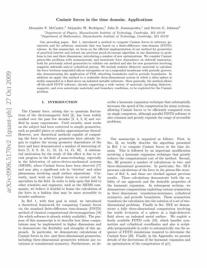
FIG. 6: Force per unit length between long silicon waveg-uides suspended in air [25], determined by the FDTD method(red triangles). Also shown is the analogous one-dimensionalcomputation assuming silicon plates of finite thickness (bluedashes), and the result F = π2/240d4A for perfect metals(assuming plate area A equal to the interaction area of thewaveguides).

As an example of a calculation involving dispersive ma-terials, we consider in this section a geometry recentlyused to measure the classical optical force between twosuspended waveguides [25], confirming a prediction [26]that the sign of the classical force depends on the rel-ative phase of modes excited in the two waveguides.We now compute the Casimir force in the same geom-etry, which consists of two identical silicon waveguidesin empty space. We model silicon as a dielectric withdispersion given by:

ε(ω) = εf +εf − ε0

1−(ωω0

)2 (7)

where ω0 = 6.6 × 1015 rad/sec, and ε0 = 1.035, εf =11.87. This dispersion can be implemented in FDTDby the standard technique of auxiliary differential equa-tions [18] mapped into the complex-ω plane as explainedin Ref. 1.

The system is translation-invariant in the z direction.If it consisted only of perfect conductors, we could usethe trick of the previous section and compute the forcein only one 2d simulation. However, dielectrics hybridizethe two polarizations and require an explicit kz integral,as discussed in Ref. 12. Each value of kz corresponds to aseparate two-dimensional simulation with Bloch-periodicboundary conditions. The value of the force for each kzis smooth and rapidly decaying, so in general only a fewkz points are needed.

To simulate the infinite open space around the waveg-uides, it is ideal to have “absorbing boundaries” so thatwaves from sources on S do no reflect back from theboundaries. We employ the standard technique of per-fectly matched layers (PML), which are a thin layer of ar-tificial absorbing material placed adjacent to the bound-

ary and designed to have nearly zero reflections [18].The results are shown in red in Fig. 6. We also show(in blue) the force obtained using the proximity forceapproximation (PFA) calculations based on the Lifshitzformula [27, 28]. For the PFA, we assume two paral-lel silicon plates, infinite in both directions perpendic-ular to the force and having the same thickness as thewaveguides in the direction parallel to the force, com-puting the PFA contribution from the surface area of thewaveguide. As expected, at distances smaller than thewaveguide width, the actual and PFA results are in goodagreement, while as the waveguide separation increases,the PFA becomes more inaccurate. For example, by aseparation of 300nm, the PFA result is off by 50%. Wealso show for comparison the force for the same surfacebetween two perfectly metallic plates, also assuming in-finite extent in both transverse directions.

C. Three dimensions with cylindrical symmetry

In the case of cylindrical symmetry, we can employa cylindrical surface S and a complex exponential basiseimφ in the φ direction. For a geometry with cylindricalsymmetry and a separable source with eimφ dependence,the resulting fields are also separable with the same φ de-pendence, and the unknowns reduce to a two-dimensional(r, z) problem for each m. This results in a substan-tial reduction in computational costs compared to a fullthree-dimensional computation.

Treating the reduced system as a two-dimensionalspace with coordinates (r, z), the expression for the force(as derived in the Appendix) is now:

Fi =∑n

∫ ∞0

dt Im[g(−t)]∫S

dsj(x) Γij;n(x, t) (8)

where the m-dependence has been absorbed into the def-inition of Γ above:

Γij;n(x, t) ≡ Γij;n,m=0(x, t)+2∑m>0

Re[Γij;n,m(x, t)], (9)

and dsj = ds nj(x), ds being a one-dimensional Carte-sian line element. As derived in the Appendix, the Ja-cobian factor r obtained from converting to cylindricalcoordinates cancels out, so that the one-dimensional (r-independent) measure ds is the appropriate one to use inthe surface integration. Also, the 2 Re[· · · ] comes fromthe fact that the +m and −m terms are complex conju-gates. Although the exponentials eimφ are complex, onlythe real part of the field response appears in Eq. (9),allowing us to use Im[g(−t)] alone in Eq. (8).

Given an eimφ dependence in the fields, one can writeMaxwell’s equations in cylindrical coordinates to obtain atwo-dimensional equation involving only the fields in the(r, z) plane. This simplification is incorporated into manyFDTD solvers, as in the one we currently employ [19],with the computational cell being restricted to the (r, z)

6

0 0.2 0.4 0.6 0.8 1 1.2 1.4 1.6 1.8 20

0.2

0.4

0.6

0.8

1

1.2

h/a

F (

Arb

itrar

y U

nits

)

h

a

Sidewall

Magnetic Sidewall

Metallic Sidewall

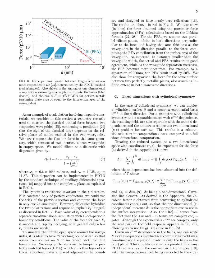
FIG. 7: Force as a function of outer sidewall spacing h/a forthe cylindrically-symmetric piston configuration shown in thefigure. Both plates are perfect metals, and the forces for bothperfect metallic and perfect magnetic conductor sidewalls areshown. Note that in contrast to Fig. 3, here the force ismonotonic in h/a for the metallic case and non monotonic forthe magnetic case.

plane and m appearing as a parameter. When this isthe case, the implementation of cylindrical symmetry isalmost identical to the two-dimensional situation. Theonly difference is that now there is an additional indexm over which the force must be summed.

To illustrate the use of this algorithm with cylindricalsymmetry, we examine the 3d system shown in the insetof Fig. 7. This configuration is similar to the configura-tion of cylindrical rods of Fig. 3, except that instead oftranslational (z) invariance we instead impose rotational(φ) invariance. In this case, the two sidewalls are joinedto form a cylindrical tube. We examine the force betweenthe two blocks as a function of h/a (the h = 0 case hasbeen solved analytically [29]).

Due to the two-dimensional nature of this problem,computation time is comparable to that of the two-dimensional double block geometry of the previous sec-tion. Rough results (at resolution 40, accurate to withina few percentage points) can be obtained rapidly on asingle computer (about 5 minutes running on 8 proces-sors) are shown in Fig. 7 for each value of h/a. Onlyindices n,m ∈ {0, 1, 2} are needed for the result to haveconverged to within 1%, after which the error is domi-nated by the spatial discretization. PML is used alongthe top and bottom walls of the tube.

In contrast to the case of two pistons with transla-tional symmetry, the force for metallic sidewalls is mono-tonic in h/a. Somewhat surprisingly, when the side-walls are switched to perfect magnetic conductors theforce becomes non monotonic again. Although the useof perfectly magnetic conductor sidewalls in this exam-ple is unphysical, it demonstrates the use of a general-purpose algorithm to examine the material-dependenceof the Casimir force. If we wished to use dispersive

10010

10

10

10

0

1

2

3

SiliconSilica

zx

y

Plate Separation (nm)

Forc

e (p

N /

100

m2

µ

200 30050

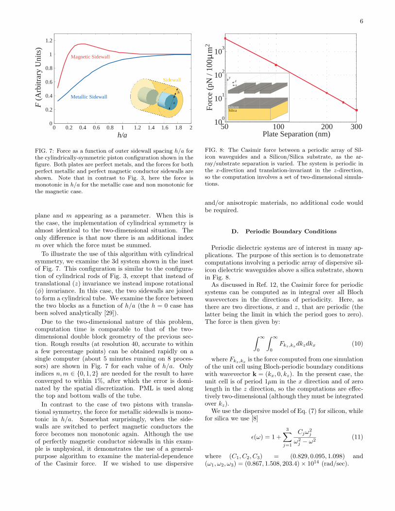
FIG. 8: The Casimir force between a periodic array of Sil-icon waveguides and a Silicon/Silica substrate, as the ar-ray/substrate separation is varied. The system is periodic inthe x-direction and translation-invariant in the z-direction,so the computation involves a set of two-dimensional simula-tions.

and/or anisotropic materials, no additional code wouldbe required.

D. Periodic Boundary Conditions

Periodic dielectric systems are of interest in many ap-plications. The purpose of this section is to demonstratecomputations involving a periodic array of dispersive sil-icon dielectric waveguides above a silica substrate, shownin Fig. 8.

As discussed in Ref. 12, the Casimir force for periodicsystems can be computed as in integral over all Blochwavevectors in the directions of periodicity. Here, asthere are two directions, x and z, that are periodic (thelatter being the limit in which the period goes to zero).The force is then given by:

∫ ∞0

∫ ∞0

Fkz,kxdkzdkx (10)

where Fkz,kx is the force computed from one simulationof the unit cell using Bloch-periodic boundary conditionswith wavevector k = (kx, 0, kz). In the present case, theunit cell is of period 1µm in the x direction and of zerolength in the z direction, so the computations are effec-tively two-dimensional (although they must be integratedover kz).

We use the dispersive model of Eq. (7) for silicon, whilefor silica we use [8]

ε(ω) = 1 +3∑j=1

Cjω2j

ω2j − ω2

(11)

where (C1, C2, C3) = (0.829, 0.095, 1.098) and(ω1, ω2, ω3) = (0.867, 1.508, 203.4)× 1014 (rad/sec).

7

x

y

z

Bromobenzene

Metal

Silica

GravityCasimir1µm

FIG. 9: Three-dimensional configuration showing stable levi-tation. At the equilibrium point, the force of gravity countersthe Casimir force, while the Casimir force from the walls ofthe spherical indentation confine the sphere laterally

E. Full 3d computations

As a final demonstration, we compute the Casimirforce for a fully three-dimensional system, without theuse of special symmetries. The system used is depictedin Fig. 9.

This setup demonstrates stable levitation with the aidof a fluid medium, which has been explored previouslyin Ref. 9. With this example, we present a setup simi-lar to that used previously to measure repulsive Casimirforces [6], with the hope that this system may be exper-imentally feasible.

A silica sphere sits atop a perfect metal plane which hasa spherical indentation in it. The sphere is immersed inbromobenzene. As the system satisfies εsphere < εfluid <εplane, the sphere feels a repulsive Casimir force up-wards [6]. This is balanced by the downward force ofgravity, which confines the sphere vertically. In addition,the Casimir repulsion from the sides of the spherical in-dentation confine the sphere in the lateral direction. Theradius of the sphere is 1µm, and the circular indenta-tion in the metal is formed from a circle of radius 2µm,with a center 1µm above the plane. For computationalsimplicity, in this model we neglect dispersion and usethe zero-frequency values for the dielectrics, as the basiceffect does not depend upon the dispersion (the precisevalues for the equilibrium separations will be changedwith dispersive materials). These are ε = 2.02 for silicaand ε = 4.30.

An efficient strategy to determine the stable point isto first calculate the force on the glass sphere when itsaxis is aligned with the symmetry axis of the indenta-tion. This configuration is cylindrically-symmetric andcan be efficiently computed as in the previous section.Results for a specific configuration, with a sphere radiusof 500 nm and an indentation radius of 1 µm, are shownin Fig. 10.

0.3 0.4 0.5 0.6-1

0

1

2

Vertical Displacement h ( m)µ

F Tot

al /

F Gra

vity

Repulsive Attractive

a

h

FIG. 10: Total (Casimir + gravity) vertical (z) force on thesilica sphere (depicted in the inset) as the height h of thesphere’s surface above the indentation surface is varied. Thepoint of vertical equilibrium occurs at h ∼ 450 nm.

-150 -100 -50 0 50 100 150-3

-2

-1

0

1

2

Exact ForceLinear Fit

F /

F Gra

vity

x

Horizontal-Displacement ∆x (nm)

∆x

h = 450 nm

FIG. 11: Casimir restoring force on the sphere as a function oflateral displacement dx, when the vertical position is fixed ath = 450 nm, the height at which gravity balances the Casimirforce

.

The force of gravity is balanced against the Casimirforce at a height of h = 450 nm. To determine thestrength of lateral confinement, we perform a fully three-dimensional computation in which the center of thesphere is displaced laterally from equilibrium by a dis-tance dx (the vertical position is held fixed at the equilib-rium value h = 450nm). The results are shown in Fig. 11.It is seen that over a fairly wide range (|∆x| < 100 nm)the linear term is a good approximation to the force,whereas for larger displacements the Casimir force be-gins to increase more rapidly. Of course, at these largerseparations the vertical force is no longer zero, due to thecurvature of the indentation, and so must be re-computedas well.

The fully three-dimensional computations are rather

8

large, and require roughly a hundred CPU hours perforce point. However, these Casimir calculations paral-lelize very easily – every source term, polarization, and k-point can be computed in parallel, and individual FDTDcalculations can be parallelized in our existing software –so we can compute each force point in under an hour ona supercomputer (with 1000+ processors). In contrast,the 2d and cylindrical calculations require tens of minutesper force point. We believe that this method is usablein situations involving complex three-dimensional mate-rials (e.g, periodic systems or systems with anisotropicmaterials).

IV. CONCLUDING REMARKS

We have demonstrated a practical implementation ofa general FDTD method for computing Casimir forcesvia a harmonic expansion in source currents. The utilityof such a method is that many different systems (disper-sive, anisotropic, periodic boundary conditions) can allbe simulated with the same algorithm.

In practice, the harmonic expansion converges rapidlywith higher harmonic moments, making the overall com-putation complexity of the FDTD method O(N1+1/d)for N grid points and d spatial dimensions. This arisesfrom the O(N) number of computations needed for oneFDTD time step, while the time increment used willvary inversely with the spatial resolution [18], leadingto O(N1/d) time steps per simulation. In addition, thereis a constant factor proportional to the number of termsretained in the harmonic expansion, as an independentsimulation is required for each term. For comparison,without a harmonic expansion one would have to run aseparate simulation for each point on S. In that case,there would be O(N (d−1)/d) points, leading to an overallcomputational cost of O(N2) [1].

We do not claim that this is the most efficient tech-nique for computing Casimir forces, as there are otherworks that have also demonstrated very efficient meth-ods capable of handling arbitrary three-dimensional ge-ometries, such as a recently-developed boundary-elementmethod [13]. However, these integral-equation methodsand their implementations must be substantially revisedwhen new types of materials or boundary conditions aredesired that change the underlying Green’s function (e.g.,going from metals to dielectrics, periodic boundary con-ditions, or isotropic to anisotropic materials), whereasvery general FDTD codes, requiring no modifications,are available off-the-shelf.

V. ACKNOWLEDGMENTS

We are grateful to S. Jamal Rahi for sharing his scat-tering algorithm with us. We are also grateful to PeterBermel and Ardavan Oskooi for helpful discussions.

VI. APPENDIX

A. Simplified computation of g(t)

In Ref. 1 we introduced a geometry-independent func-tion g(t), which resulted from the Fourier transform of acertain function of frequency, termed g(ξ), which is givenby [1]:

g(ξ) = −iξ(

1 +iσ

ξ

)1 + iσ/2ξ√

1 + iσ/ξΘ(ξ) (12)

Once g(t) is known, it can be integrated against the fieldsin time, allowing one to compute a decaying time-serieswhich will, when integrated over time, yield the correctCasimir force.g(ξ) has the behavior that it diverges in the high-

frequency limit. For large ξ, g(ξ) has the form:

g(ξ)→ g1(ξ) ≡ ξ

iΘ(ξ) + σΘ(ξ) as ξ →∞ (13)

Viewing g1(ξ) as a function, we could only compute itsFourier transform g1(t) by introducing a cutoff in thefrequency integral at the Nyquist frequency, since thetime signal is only defined up to a finite sampling rateand the integral of a divergent function may appear tobe undefined in the limit of no cutoff.

Applying this procedure to compute g(−t) yields atime series that has strong oscillations at the Nyquistfrequency. The amplitude of these oscillations can bequite high, increasing the time needed to obtain conver-gence and also making any physical interpretation of thetime series more difficult.

These oscillations are entirely due to the high-frequency behavior of g(ξ), where g(ξ) ∼ g1(ξ). However,g(t) and g(ξ) only appear when when they are being in-tegrated against smooth, rapidly decaying field functionsΓ(x, t) or Γ(x, ξ). In this case, g can be viewed as atempered distribution (such as the δ-function) [30]. Al-though g(ξ) diverges for large ξ, this divergence is only apower law, so it is a tempered distribution and its Fouriertransform is well-defined without any truncation. In par-ticular, the Fourier transform of g1(ξ) is given by:

g1(−t) =i

2π

(1t2

+σ

t

)(14)

Adding and subtracting the term g1(ξ) from g(ξ), theremaining term decays to zero for large ξ and can beFourier transformed numerically without the use of ahigh-frequency cutoff, allowing g(−t) to be computed asthe sum of g1(t) plus the Fourier transform of a well-behaved function. This results in a much smoother g(−t)which will give the same final force as the g(−t) usedin Ref. 1, but will also have a much more well-behavedtime dependence.

In Fig. 12 we plot the convergence of the force as afunction of time for the same system using the g(−t)

9

0 2 4 6 8 10 12 14 16 18

10

10

10

10

10

10

-4

-3

-2

-1

0

1

g(t) High-ξ cutoff g(t) No cutoff

i

i

10 10 10 10 10 10-2 -1 0 1 2 4

10-2

10-1

100

101

10-3

t

t (a/c)

Forc

e E

rror

(ar

bitr

ary

units

)

Im[g

(-t)

]

FIG. 12: Plot of the force error (force after a finite time in-tegration vs. the force after a very long run time) for g(t)determined from a numerical transform as in Ref. 1 and fromthe analytic transform of the high-frequency components. In-set: Im[g(−t)] obtained without a cutoff, in which the high-frequency divergence is integrated analytically. Compare withFig. 1 of Ref. 1

obtained by use of a high-frequency cutoff and for onein which g1(ξ) is transformed analytically and the re-mainder is transformed without a cutoff. The inset plotsIm g(−t) obtained without using a cutoff (since the realpart is not used in this paper) for σ = 10. If a complexharmonic basis is used, one must take care to use the fullg(t) and not only its imaginary part.

1. Further simplification

In addition to the treatment of the high-frequency di-vergence in the previous section, we find it convenientto also Fourier transform the low-frequency singularityof g(ξ) analytically. As discussed in Ref. 1, the low-frequency limit of g(ξ) is given by:

g(ξ)→ g2(ξ) ≡√i

2σ3/2

ξ1/2Θ(ξ) as ξ → 0 (15)

The Fourier transform of g2(ξ), viewed as a distribu-tion, is:

g2(−t) =i

4√π

σ3/2

t1/2(16)

After removing both the high- and low-frequency di-vergences of g(ξ), we perform a numerical Fourier trans-form on the function δg(ξ) ≡ g(ξ)−g1(ξ)−g2(ξ), which iswell-behaved in both the high- and low-frequency limits.

In the present text we are only concerned with realsources, in which case all fields Γ(x, t) are real and onlythe imaginary part of g(−t) contributes to the forcein Equation (1). The imaginary part of g(−t) is then:

Im[g(−t)] = Im(δg(−t)) +1

2π

(1t2

+σ

t

)+

14√π

σ3/2

t1/2

(17)

2. Perfect conductors and z-invariance

As discussed in Ref. 12, the stress-tensor frequencyintegral for a three-dimensional z-invariant system in-volving only vacuum and perfect metallic conductors isidentical in value to the integral of the stress tensor forthe associated two-dimensional system (corresponding totaking a z = 0 crossection), with an extra factor of iω/2in the frequency integrand. In the time domain, this cor-responds to solving the two-dimensional system with anew g(−t).

In this case the Fourier transform can be performedanalytically. The result is:

Im[g(−t)] =1

2π

(2t3

+3σ2t2

+σ2

2t

)(18)

B. Harmonic expansion in cylindrical coordinates

The extension of the above derivation to three dimen-sions and non-Cartesian coordinate systems is straight-forward, as the only difference is in the representation ofthe δ-function. Because the case of rotational invariancepresents some simplification, we will explicitly presentthe result for this case below.

For cylindrical symmetry, we work in cylindrical coor-dinates (r, φ, z) and choose a surface S that is also rota-tionally invariant about the z-axis. S is then a surface ofrevolution, consisting of the rotation of a parametrizedcurve (r(s), φ = 0, z(s)) about the z axis. The most prac-tical harmonic expansion basis consists of functions of theform fn(x)eimφ. Given a φ dependence, many FDTDsolvers will solve a modified set of Maxwell’s Equationsinvolving only the (r, z) coordinates. In this case, for eachm the problem is reduced to a two-dimensional problemwhere both sources and fields are specified only in the(r, z)-plane.

Once the fields are determined in the (r, z)-plane, theforce contribution for each m is given by:

∫ 2π

0

dφ

∫S

dsj(x) r(x)e−imφ∫ 2π

0

dφ′∫S

ds(x′) r(x′)eimφ′δS(x− x′)ΓEij;m(t; x,x′)

(19)

where the values of x range over the full three-dimensional (r, φ, z) system. Here we introduce the

10

Cartesian line element ds along the one-dimensional sur-face S in anticipation of the cancellation of the Jacobianfactor r(x) from the integration over S. We have explic-itly written only the contribution for ΓE , the contributionfor ΓH being identical in form.

In cylindrical coordinates, the representation of the δ-function is:

δ(x− x′) =1

2πr(x)δ(φ− φ′)δ(r − r′)δ(z − z′) (20)

For simplicity, assume that S consists entirely of z =constant and r = constant surfaces (the more generalcase follows by an analogous derivation). In these cases,the surface δ-function δS is given by:

δS(x− x′) =1

2πr(x)δ(φ− φ′)δ(r − r′), z = constant

δS(x− x′) =1

2πr(x)δ(φ− φ′)δ(z − z′), r = constant

In either case, we see that upon substitution of eitherform of δS into Eq. (19), we obtain a cancellation withthe first r(x) factor. Now, one picks an appropriate de-composition of δS into functions fn (a choice of r = constor z = const merely implies that the fn will either befunctions of z, or r, respectively). We denote either caseas fn(x), with the r and z dependence implicit.

We now consider the contribution for each value of n.The integral over x′ is:

ΓEij;nm(t,x) =∫ 2π

0

dφ′∫S

ds(x′)r(x′)ΓEij;nm(t,x,x′)fn(x′)eimφ′

As noted in the text, ΓEij;nm(t,x) is simply the fieldmeasured in the FDTD simulation due to a three-dimensional current source of the form fn(x)eimφ. In

the case of cylindrical symmetry, this field must have aφ dependence of the form eimφ:

ΓEij;nm(t, r, z, φ) = ΓEij;nm(t, r, z)eimφ (21)

This factor of eimφ cancels with the remaining e−imφ.The integral over φ then produces a factor of 2π thatcancels the one introduced by δS . After removing thesefactors, the problem is reduced to one of integrating thefield responses entirely in the (r, z) plane. The contribu-tion for each n and m is then:∫

S

dsj(x) fn(x)ΓEij;nm(t, r, z) (22)

If one chooses the fn(x) to be real-valued, the contri-butions for +m and −m are related by complex conjuga-tion. The sum over m can then be rewritten as the realpart of a sum over only non negative values of m. Thefinal result for the force from the electric field terms isthen:

Fi =∫ ∞

0

dt Im[g(−t)]∑n

∫S

dsj(r, z) fn(r, z)ΓEij;n(t, r, z)

(23)where the m-dependence has been absorbed into the def-inition of Γij;n as follows:

ΓEij;n(t, r, z) ≡ ΓEij;n,m=0(t, r, z) + 2∑m>0

Re[ΓEij;nm(t, r, z)]

(24)We have also explicitly included the dependence on r

and z to emphasize that the integrals are confined tothe two-dimensional (r, z) plane. The force receives ananalogous contribution from the magnetic-field terms.

[1] A. W. Rodriguez, A. P. McCauley, J. D. Joannopoulos,and S. G. Johnson, Phys. Rev. A 80, 012115 (2009).

[2] H. B. G. Casimir, Proc. K. Ned. Akad. Wet. 51, 793(1948).

[3] T. H. Boyer, Phys. Rev. A 9, 2078 (1974).[4] S. K. Lamoreaux, Phys. Rev. Lett. 78, 5 (1997).[5] H. B. Chan, V. A. Aksyuk, R. N. Kleinman, D. J. Bishop,

and F. Capasso, Science 291, 1941 (2001).[6] J. Munday, F. Capasso, and V. A. Parsegia, Nature 457,

170 (2009).[7] M. Antezza, L. P. Pitaevskiı, S. Stringari, and V. B. Sve-

tovoy, Phys. Rev. Lett. 97, 223203 (2006).[8] A. Rodriguez, M. Ibannescu, D. Iannuzzi, F. Capasso,

J. D. Joannopoulos, and S. G. Johnson, Phys. Rev. Lett.99, 080401 (2007).

[9] A. W. Rodriguez, J. Munday, D. Davlit, F. Capasso, J. D.Joannopoulos, and S. G. Johnson, Phys. Rev. Lett. 101,190404 (2008).

[10] T. Emig, N. Graham, R. L. Jaffe, and M. Kardar, Phys.Rev. Lett. 99, 170403 (2007).

[11] T. Emig, Phys. Rev. Lett. 98, 160801 (2007).[12] A. Rodriguez, M. Ibannescu, D. Iannuzzi, J. D.

Joannopoulos, and S. G. Johnson, Phys. Rev. A 76,032106 (2007).

[13] H. T. M. Reid, A. W. Rodriguez, J. White, and S. G.Johnson, Phys. Rev. Lett. 103, 040401 (2008).

[14] S. Pasquali and A. C. Maggs, J. Chem. Phys. 129, 014703(2008).

[15] S. Pasquali and A. C. Maggs, Phys. Rev. A. (R) 79,020102 (2009).

[16] H. Gies and K. Klingmuller, Phys. Rev. Lett. 97, 220405(2006).

[17] F. M. Serry, D. Walliser, and M. G. Jordan, J. Appl.Phys. 84, 2501 (1998).

[18] A. Taflove and S. C. Hagness, Computational Electro-dynamics: The Finite-Difference Time-Domain Method

11

(Artech, Norwood, MA, 2000).[19] A. Farjadpour, D. Roundy, A. Rodriguez, M. Ibanescu,

P. Bermel, J. Burr, J. D. Joannopoulos, and S. G. John-son, Opt. Lett. 31, 2972 (2006).

[20] A. P. McCauley, A. W. Rodriguez, and S. J. Johnson,Casimir meep wiki, http://ab-initio.mit.edu/wiki/

index.php/Casimir_calculations_in_Meep.[21] L. D. Landau, E. M. Lifshitz, and L. P. Pitaevskiı, Sta-

tistical Physics Part 2, vol. 9 (Pergamon Press, Oxford,1960).

[22] S. J. Rahi, A. W. Rodriguez, T. Emig, R. L. Jaffe,S. G. Johnson, and M. Kardar, Phys. Rev. A 77, 030101(2008).

[23] R. K. Rao and P. Yip, Discrete Cosine Transform:Algorithms, Advantages, Applications (Academic Press,Boston, 1990).

[24] J. P. Boyd, Chebychev and Fourier Spectral Methods(Dover, New York, 2001), 2nd ed.

[25] M. Li, W. H. P. Pernice, and H. X. Tang, arXiv:atom-ph/0903.5117 (2009).

[26] M. L. Povinelli, M. Loncar, M. Ibanescu, E. J. Smythe,S. G. Johnson, F. Capasso, and J. D. Joannopoulos, Opt.Lett. 30, 3042 (2005).

[27] E. M. Lifshitz, Dokl. Akad. Nauk. SSSR 100, 879 (1955).[28] I. E. Dzyaloshinskiı, E. M. Lifshitz, and L. P. Pitaevskiı,

Adv. Phys. 10, 165 (1961).[29] V. M. Marachevsky, Phys. Rev. D 75, 085019 (2007).[30] W. Rudin, Real and Complex Analysis (McGraw-Hill,

New York, 1966).[31] Non-orthogonal functions may be used, but this case

greatly complicates the analysis and will not be treatedhere.