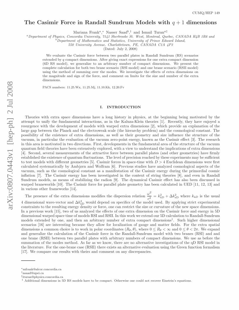
arX

iv:0

807.

0443

v1 [

hep-

ph]

2 J

ul 2

008

CUMQ/HEP 149

The Casimir Force in Randall Sundrum Models with q + 1 dimensions

Mariana Franka,∗ Nasser Saadb,† and Ismail Turana‡

aDepartment of Physics, Concordia University, 7141 Sherbrooke St. West, Montreal, Quebec, CANADA H4B 1R6 andbDepartment of Mathematics and Statistics, University of Prince Edward Island,

550 University Avenue, Charlottetown, PE, CANADA C1A 4P3

(Dated: July 2, 2008)

We evaluate the Casimir force between two parallel plates in Randall Sundrum (RS) scenariosextended by q compact dimensions. After giving exact expressions for one extra compact dimension(6D RS model), we generalize to an arbitrary number of compact dimensions. We present thecomplete calculation for both two brane scenario (RSI model) and one brane scenario (RSII model)using the method of summing over the modes. We investigate the effects of extra dimensions onthe magnitude and sign of the force, and comment on limits for the size and number of the extradimensions.

PACS numbers: 11.25.Wx, 11.25.Mj, 11.10.Kk, 12.20.Fv

I. INTRODUCTION

Theories with extra space dimensions have a long history in physics, at the beginning being motivated by theattempt to unify the fundamental interactions, as in the Kaluza-Klein theories [1]. Recently, they have enjoyed aresurgence with the development of models with warped extra dimensions [2], which provide an explanation of thelarge gap between the Planck and the electroweak scale (the hierarchy problem) and the cosmological constant. Thepossibility of the existence of extra dimensions, as well as their geometry and size influence the structure of thevacuum, in particular the evaluation of the vacuum zero-point energy, known as the Casimir effect [3]. The researchin this area is motivated in two directions. First, developments in the fundamental area of the structure of the vacuumquantum field theories have been extensively explored, with a view to understand the implications of extra dimensions[4]. Second, several measurements of the attractive force between parallel plates (and other geometries) have firmlyestablished the existence of quantum fluctuations. The level of precision reached by these experiments may be sufficientto test models with different geometries [5]. Casimir forces in space-time with D > 4 Euclidean dimensions were firstcalculated systematically by Ambjørn and Wolfram [6]. Previous studies have analyzed cosmological aspects of thevacuum, such as the cosmological constant as a manifestation of the Casimir energy during the primordial cosmicinflation [7]. The Casimir energy has been investigated in the context of string theories [8], and even in RandallSundrum models, as means of stabilizing the radion [9]. The dynamical Casimir effect has also been discussed inwarped braneworlds [10]. The Casimir force for parallel plate geometry has been calculated in UED [11, 12, 13] andin various other frameworks [14].

The presence of the extra dimensions modifies the dispersion relationω2

c2= k2

4D + ∆k2xD where k4D is the usual

4 dimensional wave-vector and ∆k2xD would depend on specifics of the model used. By applying strict experimental

constraints to the resulting energy density or force, one can restrict the size or curvature of the new space dimensions.In a previous work [15], two of us analyzed the effects of one extra dimension on the Casimir force and energy in 5Ddimensional warped space time of models RSI and RSII. In this work we extend our 5D calculation to Randall-Sundrummodels extended by one, and then an arbitrary number of extra compact dimensions1. Such higher dimensionalscenarios [16] are interesting because they allow for localization of gauge and matter fields. For the extra spatialdimensions a common choice is to work in polar coordinates (Rθ, θ), where 0 ≤ Rθ < ∞ and 0 ≤ θ < 2π. We expandand generalize the calculation of the Casimir force in the Randall-Sundrum model with two branes (RSI) and andone brane (RSII) between two parallel plates with arbitrary numbers of compact dimensions. We use as before thesummation of the modes method. As far as we know, there are no alternative investigations of the qD RSI model inthe literature. For the one-brane case (RSII) there exists an alternative evaluation using the Green function formalism[17]. We compare our results with theirs and comment on any discrepancies.

∗mfrank@alcor.concordia.ca†nsaad@upei.ca‡ituran@physics.concordia.ca1 Additional dimensions in 5D RS models have to be compact. Otherwise one could not recover Einstein’s equations.

2

Our paper is organized as follows. In the next section, we introduce some general features of the model in 6dimensions and derive the dispersion relation. In section III we present our analysis of the Casimir force in RSImodels. We start with the 6 dimensional model (one extra compact dimension) and then generalize to an arbitrarynumber. We do the same for the RSII model in section IV. The numerical and graphical analysis of our results isincluded in section V, where we try to restrict the size and number of extra dimensions. We compare our results withothers, summarize and conclude in section VI.

II. RANDALL SUNDRUM MODEL WITH EXTRA COMPACT DIMENSIONS

The metric of 5D space-time Randall-Sundrum (RS) model with 4D Poincare invariance is

ds25D = e−2k|y|ηµνdxµdxν − dy2 , (1)

where k−1 is the radius of 5D Anti-de Sitter AdS5 space, y is the spatial orbifolded extra dimension and ηµν is the

usual 4D metric with the convention diag (+,−,−,−).The generalization to more than one extra spatial dimension can also be done, and as mentioned earlier, these

dimensions must be compact. Localization of graviton on the brane motivates us to consider additional dimensionsboth compact and warped [18]. The metric in generalized (3+ q +2) dimensions (where 3+1 are the usual space-timedimensions, there is one extra y spatial dimension, and the extra q are compact and warped dimensions) is [16]

ds25D+n = e−2k|y|

ηµνdxµdxν −q∑

j=1

R2jdθ2

j

− dy2 , (2)

where y is non-compact and θj ’s are compact extra coordinates running from 0 to 2πRj. This metric can be a solutionto Einstein equations in (5 + q) dimensions with negative bulk cosmological constant [6, 16]. In the 6D case, (2) forn = 1 becomes

ds26D = e−2k|y|

(ηµνdxµdxν − R2dθ2

)− dy2 , (3)

where we simply use R and θ for the extra compact warped dimension. Here the 6D metric gMN is

ds26D = gMNdxMdxN , (4)

such that gMN = e−2k|y| diag(ηµν ,−1,−e2k|y|)2. The Greek indices µ, ν run over 0 to 3 while Roman indices M, Nrun over 0 to 5.

As in our 5D calculation [15] , we use the scalar field analogy to represent the photon in 6D. The field equation fora scalar field φ in 6D with mass m6 can be obtained from the Lagrange density L(φ, ∂Mφ),

L(φ, ∂Mφ) =√−g

(1

2gMN∂Mφ∂Nφ − 1

2m6φ

2

)

, (5)

where g is the determinant of the metric gMN which is y-dependent. (This has discussed previously in [19] and weinclude it here for completeness.) The field equation for φ becomes

(

e2k|y|ηµν∂µ∂ν − R−2e2k|y|∂2θ −√−g

−1∂y

(√−g∂y

)+ m2

6

)

φ = 0. (6)

By using the separation of variables for φ(xµ, θ, y) = X(xµ)Y (y)Θ(θ), one gets for y > 0

d2Y (y)

dy2− 5k

dY (y)

dy+ m2e2kyY (y) − m2

6Y (y) = 0 , (7)

ηµν d2X(x)

dxµdxν+ m2

effX(x) = 0 , (8)

Θn(θ) =1√2πR

einθ, n = 0, 1, 2... (9)

2 Note that gMN = e2k|y| diag(ηµν ,−1,−e−2k|y|).

3

where m2eff ≡ m2 + n2/R2 is the effective mass in 4D. Since we use the scalar field-photon analogy, we consider the

massless scalar field3.Equation (2.7) can be solved directly using the master formula for the equation of the form [20]:

y′′ + ay′ + (beλx + c)y = 0. (10)

The solution for (2.7) with m6 6= 0, with an appropriate choice of parameters, becomes:

Y = e5ky/2[C1Jν(1

kmeky) + C2Yν(

1

kmeky)] (11)

where Jν(z) and Yν(z) are the Bessel functions of the first and second kind and ν = 12k

√

25k2 + 4m26. For the massless

case ν = 5/2.We apply the Neumann boundary conditions ∂yY (0) = 0 = ∂yY (πR0), to obtain the masses m as solutions to the

transcendental equation

J 32(m

k)Y 3

2(m

keπkR0) − Y 3

2(m

k)J 3

2(m

keπkR0) = 0 (12)

Expressing the Bessel functions Jn+ 12(x) in terms of elementary functions we get, in the limit κ, m > 0 and πkR0 ≫ 1

tan

((eπkR0 − 1)m

k

)

=(eπkR0 − 1)km

(k2 + m2eπkR0)(13)

This is the exact solution. Following the same technique as in the 5D case, for πkR0 ≫ 1 we can neglect Y3/2 forlarge arguments and reduce equation (12) to

J 32(m

keπkR0) = 0 . (14)

The asymptotic form of Jν(x) =

√

2

nx2cos(x− νπ

2− π

4) is valid for any ν as long as x ≫ |ν2 −1/4| is satisfied. Then,

the basic idea is to set the argument of cosine function (2N − 1)π/2, N = 1, 2, 3..., so that cosine vanishes. Thus, forarbitrary ν we have

x − νπ

2− π

4= (2N − 1)

π

2(15)

and get x as

x =

(

N +2ν − 1

4

)

π . (16)

This reduces to x = (N + 1/4)π for ν = 1 in 5D case. In 6D (or any higher dimensions), we obtain ν = 3/2 whichinstead gives x = (N +1/2)π for the zeros of (2.14). (See the Numerical Analysis section for further details.) Puttingthe argument of J3/2 from above and using index N for m, which is now discrete, we get

mN = (N +1

2)πke−πkR0 , N = 1, 2, 3... (17)

This is the form of m which should enter the energy density equation. Note that mN = 0 for N = 0 , which will be

important later. Also, for the 5D case mN = (N +1

4)πke−πkR0 , N = 1, 2, 3... [15].

III. THE CASIMIR FORCE IN THE RSI MODEL

In RSI, there are two branes, localized at y = 0 and y = L, with Z2 symmetry y ↔ −y, L+y ↔ L−y. The 3-braneshave equal opposite tensions. The positive tension brane has a fundamental scale MRS and is hidden; SM fields are

3 There are some issues with the massive case in 6D for RSII since there are no zero modes. See [19] for details.

4

located on the negative tension brane, which is visible. The exponential warping factor gives rise to an effective scaleon the visible brane located at y = L

M2Pl =

M3RS

k

[1 − e−2kL

]. (18)

A mechanism is needed to recover 4-dimensional General Relativity at low-energy, and this corresponds to introducingan extra degree of freedom known as the radion. A suitable choice of L (often taken to be related to the compactifiedradius, L = πR0) and k allows the Kaluza-Klein (KK) spectrum to be discrete, and the lowest masses to be of O(TeV),which predicts different collider signatures at low energies from those of large extra dimensions. As consistency withthe low energy theory requires MPl ∼ MRS ∼ k, there are no additional hierarchies in this model. The scale ofthe 4-dimensional physical phenomena space transverse to the 5th dimension is then specified by the warp factor :Λ = MPl e

−kπR0 , and if we take Λ ∼ 1 TeV, then we expect kR0 ∼ 12.

A. The 6D RSI Case

The effective dispersion relation in 4D can be obtained from (8) in k-space. It becomes

((ikµ)(ikµ) + m2

eff

)X(k) = 0 , (19)

where kµ = (w/c,k). Hence, the following dispersion relation is obtained

w(k) = c∞∑

n=0

√

k2 +n2

R2+ m2

eff , (20)

If we further assume two-plates configuration separated by a distance a and apply Dirichlet boundary conditions alongz-axis, we obtain the Casimir energy density per unit plate

EI6D = Vorb

~

2

∫d2

k⊥

(2π)2

p c

∞∑

n,l=0

√

k2

⊥ +π2l2

a2+

n2

R2+ m2

, (21)

where Vorb is the volume of the orbifold and p is the polarization factor in 6D. This is our starting point in calculatingthe Casimir force.After finding the discrete m values corresponding to the RSI model with the above approximation, we can write thetotal frequency as

w = p∞′∑

l,n,N=0

c

√

k2⊥ +

π2l2

a2+

n2

R2+ m2

N (22)

where prime indicates that l = n = N = 0 is excluded and mN is given as

mN =

{0 if N = 0κ(N + 1

2 ) if N = 1, 2, . . .

with κ ≡ πke−πkR0. Note that the radius R of the sixth dimension is in general different than R0 of the fifth dimension.Rewriting the triple sum and rearranging the single and double sums to start with 0, we obtain

wlnN = pc

∞′∑

ℓ,n,N=0

√

k2⊥ +

π2ℓ2

a2+

n2

R2+ m2

N

= pc

∞′∑

ℓ,n=0

√

k2⊥ +

π2ℓ2

a2+

n2

R2+ pc

∞∑

ℓ,n,N=0

√

k2⊥ +

π2ℓ2

a2+

n2

R2+ m2

N

− pc∞∑

ℓ,n=0

√

k2⊥ +

π2ℓ2

a2+

n2

R2+

κ2

4. (23)

5

The Casimir energy density per unit plate is given by

EI6D = Vorbf

~

2

∫d2

k⊥

(2π)2

p c∞∑

n,l=0

√

k2

⊥ +π2l2

a2+

n2

R2+ m2

N

. (24)

We obtain

EI6D = Vorbf

pc~Γ(− 32 )

8πΓ(− 12 )

( ∞′∑

ℓ,n=0

(π2ℓ2

a2+

n2

R2

) 32

+

∞∑

ℓ,n,N=0

(π2ℓ2

a2+

n2

R2+ κ2(N +

1

2)2) 3

2

−∞∑

ℓ,n=0

(π2ℓ2

a2+

n2

R2+

κ2

4

) 32)

.

In order to evaluate this expression we introduce the Epstein Zeta Function ZN(a1, . . . , aN ; s) [21]:

ZN (a1 . . . , aN ; s) =∞′∑

n1,...,nN=−∞

(a1n

21 + . . . aNn2

N

)− s2 (25)

and the inhomogeneous Epstein Hurwitz Function EcN [21]:

EcN (s; a1, . . . , aN ; c1, . . . , cN ) =

∞∑

n1,...,nN=0

N∑

j=1

aj (nj + cj)2+ c

−s

. (26)

We can write the energy density between the plates in a compact form as

EI6D = Vorb

pc~Γ(− 32 )

8πΓ(− 12 )

{∞′∑

ℓ,n=0

(π2ℓ2

a2+

n2

R2

) 32

+ E3(−3

2;π2

a2,

1

R2, κ2; 0, 0,

1

2) − E

κ2

42 (−3

2;π2

a2,

1

R2; 0, 0)

}

= Vorb

pc~Γ(− 32 )

8πΓ(− 12 )

(1

4Z2(

1

R,π

a;−3) +

1

4Z1(

π

a;−3) +

1

4Z1(

1

R;−3) + E3(−

3

2;π2

a2,

1

R2, κ2; 0, 0,

1

2)

− Eκ2

42 (−3

2;π2

a2,

1

R2; 0, 0)

)

(27)

where the last form is obtained computing the explicit analytic expansion for the sums. Using the reflection formulafor the Epstein Zeta function [6]

Zp(a1, . . . , ap; s) = a−11 . . . a−1

p

πs

πp/2

Γ(p−s2 )

Γ( s2 )

Zp(1

a1, . . . ,

1

ap; p − s), (28)

we may write the first double sum on the right side

1

4

[

Z2(1

R,π

a;−3) + Z1(

1

R;−3) + Z1(

π

a;−3)

]

=1

2Γ(− 32 )π7/2

[3 Ra

8πZ2

(

R,a

π; 5)

+1

R3ζ(4) +

π3

a3ζ(4)

]

where in the last term we introduced the Riemann Zeta Function [21]: ζ(s) =∑∞

n=1 n−s.

The triple sum E3(− 32 ; π2

a2 , 1R2 , κ2; 0, 0, 1

2 ) is evaluated using [21]

E3(s; a1, a2, a3; c1, c2, c3) =1

Γ(s)

∞∑

m=0

(−1)m

m!am1 ζH(−2m, c1)Γ(s + m)E2(s + m; a2, a3; c2, c3)

+1

2

√π

a1

Γ(s − 12 )

Γ(s)E2(s −

1

2; a2, a3; c2, c3)

+

√π

a1

cos(2πc1)

Γ(s)

∞∑

n1=1

∞∑

n2,n3=0

∫ ∞

0

dt ts−32 exp[−π2n2

1

a1t− t

3∑

j=2

aj(nj + cj)2]

6

to obtain

E3(−3

2;π2

a2,

1

R2, κ2 ; 0, 0,

1

2) = ζH(0, 0)E2(−

3

2;

1

R2, κ2; 0,

1

2) +

1

2

a√π

Γ(−2)

Γ(− 32 )

E2(−2;1

R2, κ2; 0,

1

2)

+2

a√

πΓ(− 32 )

∞∑

ℓ=1

∞∑

n,N=0

ℓ−2

(n2

R2+ κ2(N +

1

2)2)

K2

(

2aℓ

√

n2

R2+ κ2(N +

1

2)2

)

.

The double sum Eκ2/42

(

−3

2;π2

a2,

1

R2; 0, 0

)

can be regarded as a special case of the inhomogeneous Epstein-Hurwitz

Zeta function and its expansion [21]

Ec2(s; a1, a2; c1, c2) =

a−s2

Γ(s)

∞∑

m=0

(−1)mΓ(s + m)

m!

(a1

a2

)m

ζH(−2m, c1)Ec/a2

1 (s + m; 1; c2)

+a1/2−s2

2

√π

a1

Γ(s − 12 )

Γ(s)E

c/a2

1 (s − 1/2; 1; c2)

+2πs

Γ(s)cos(2πc1)a

−s/2−1/41

∞∑

n1=1

∞∑

n2=0

ns−1/21 [a2(n2 + c2)

2 + c]−s/2+1/4

× Ks−1/2

(2πn1√

a1

√

a2(n2 + c2)2 + c

)

, (29)

where Kν(x) is the modified Bessel function Kν(x) =π

2

(I−ν − Iν)

sin νπ, with Iν(x) =

∞∑

s=0

1

s!(s + ν)!

(x

2

)2s+ν

. The sum is

finally obtained as

Eκ2/42

(

−3

2;π2

a2,

1

R2; 0, 0

)

= ζH(0, 0)Eκ2

41 (−3

2;

1

R2, 0) +

1

2

a√π

Γ(−2)

Γ(− 32 )

Eκ2

41 (−2;

1

R2; 0)

+2

a√

πΓ(− 32 )

∞∑

ℓ=1

∞∑

n=0

ℓ−2

(n2

R2+

κ2

4

)

K2

(

2ℓa

√

n2

R2+

κ2

4

)

. (30)

Combining the three terms given above, we obtain, for the Casimir energy between the plates:

EI6D = Vorb

pc~Γ(− 32 )

8πΓ(− 12 )

{

1

2Γ(− 32 )π

72

[3

8

Ra

πZ2(R,

a

π; 5) +

1

R3ζ(4) +

π3

a3ζ(4)

]

+ ζH(0, 0)E2(−3

2;

1

R2, κ2; 0,

1

2) +

1

2

a√π

Γ(−2)

Γ(− 32 )

E2(−2;1

R2, κ2; 0,

1

2)

+2

a√

πΓ(− 32 )

∞∑

ℓ=1

∞∑

n,N=0

ℓ−2

(n2

R2+ κ2(N +

1

2)2)

K2

(

2aℓ

√

n2

R2+ κ2(N +

1

2)2

)

− ζH(0, 0)Eκ2

41 (−3

2;

1

R2, 0) − 1

2

a√π

Γ(−2)

Γ(− 32 )

Eκ2

41 (−2;

1

R2; 0)

− 2

a√

πΓ(− 32 )

∞∑

ℓ=1

∞∑

n=0

ℓ−2

(n2

R2+

κ2

4

)

K2

(

2ℓa

√

n2

R2+

κ2

4

)}

. (31)

Before proceeding further the energy without plates must be subtracted. Let’s call the energy density without theplates ǫ6D

np . The renormalized total energy shift can be given as

EI (ren)6D = E

I6DA − ǫ6D

np A a, (32)

where A is the area of one plate. The energy density without plates ǫ6Dnp is given by

ǫ6Dnp = Vorb

~

2

∫d3

k

(2π)3

pc

∞′∑

n,N=0n=N 6=0

√

k2 +

n2

R2+ m2

N

7

= Vorb~

2pc

∫d3

k

(2π)3

(∞∑

n=1

√

k2 +

n2

R2+

∞∑

n=0

∞∑

N=0

√

k2 +

n2

R2+ m2

N −∞∑

n=0

√

k2 +

n2

R2+

κ2

4

)

. (33)

This yields, in terms of the previously defined functions

ǫ6Dnp = −Vorb~pc

16

[

3

4π6

1

R4ζ(5) +

Γ(−2)

π32 Γ(− 1

2 )E2(−2;

1

R2, κ2; 0,

1

2) − Γ(−2)

π32 Γ(− 1

2 )E

κ2

41 (−2;

1

R2, 0)

]

.

Then the total energy in the 6D RSI is

EI (ren)6D = AVorb

pc~Γ(− 32 )

8πΓ(− 12 )

{

1

2Γ(− 32 )π

72

[3

8

Ra

πZ2(R,

a

π; 5) +

1

R3ζ(4) +

π3

a3ζ(4)

]

+2

a√

πΓ(− 32 )

∞∑

ℓ=1

∞∑

n,N=0

ℓ−2

(n2

R2+ κ2(N +

1

2)2)

K2

(

2aℓ

√

n2

R2+ κ2(N +

1

2)2

)

− 2

a√

πΓ(− 32 )

∞∑

ℓ=1

∞∑

n=0

ℓ−2

(n2

R2+

κ2

4

)

K2

(

2ℓa

√

n2

R2+

κ2

4

)}

+AaVorb

2

~pc

16π5

3

4π

1

R4ζ(5) + (terms independent of a). (34)

We note that this expression contains no divergent terms and is finite, as expected, because the divergent terms in

ǫ6Dnp cancel exactly the ones in E

I6D. The Casimir force is given by the derivative of the Casimir energy E

I (ren)6D with

respect to the plate separation a:

F I6D = −∂E

I (ren)6D

∂a. (35)

We use the the definition of Z2 to calculate derivatives. The force becomes, using (34),

FI6D

A= Vorb

pc~

16π2

{

1

2π3

[

3

8

R

πZ2(R,

a

π; 5) − 15

8

Ra2

π3

∞′∑

n,N=−∞

N2

(

n2R2 +a2N2

π2

)− 72

− 3π3

a4ζ(4)

− 3

4π

1

R4ζ(5)

]

− 6

a2

∞∑

ℓ,N=1

∞∑

n=0

ℓ−2

(n2

R2+ κ2(N +

1

2)2)

K2

(

2aℓ

√

n2

R2+ κ2(N +

1

2)2

)

− 4

a

∞∑

ℓ,N=1

∞∑

n=0

ℓ−1

(n2

R2+ κ2(N +

1

2)2) 3

2

K1

(

2aℓ

√

n2

R2+ κ2(N +

1

2)2

)}

(36)

where we use the identity ∂zKν(z) = −Kν−1(z)− ν

zKν(z). This expression is our final formula for the Casimir force

density (force per unit area) for the 6 dimensional RSI model. Comparison with the expression for the force in 5Dmodels [15] shows that the terms in the square bracket arise as contributions from the extra compact dimension andare called UED-like terms, as in [11]; while the last two terms given as Bessel functions are the contribution of the5D warped coordinates and will be called Bessel terms. In the limit R → ∞:

FI5D

A= −Vorb

pc~

16π2

{

3

2a4ζ(4) +

[

6κ2

a2

∞∑

N=0

∞∑

ℓ=1

ℓ−2(N +1

2)2K2

(

2aℓκ(N +1

2)

)

+ 4aκ

∞∑

N=0

∞∑

ℓ=1

ℓ−1(N +1

2)3K1

(

2aℓκ(N +1

2)

)]}

. (37)

The first term is the Casimir force without the extra dimensions, and the two Bessel terms coincide with those in the5D consideration [15], except for the argument of the Bessel function. The difference in arguments arises from thelocation of the zeros of the Bessel functions in 5 and 6 dimensions, as shown in the previous section, and N + 1/2has to be replaced with N + 1/4 as well, since the solution for mN in 5D is different from the one in 6D. Note that

−Vorb3pc~

15π2a4ζ(4) = −pπ2c~

480a4=

p

2FnoRS. Thus the expressions (2.18) from [15] and (37) are consistent with each

other.

8

B. The qD RSI case

We continue by generalizing this expression to q extra compact dimensions. We proceed as before. We calculatefirst the energy density between the plates, then the energy density without the plates. We use this to evaluate theenergy shift and then compute the force.

The energy density between the plates for q compact dimensions (qD) is

wqD = pc

∞∑

ℓ=0

q∏

i=1

∞′∑

ni,N=0

√√√√k

2⊥ +

π2ℓ2

a2+

q∑

j=1

n2j

R2j

+ m2N

= pc∞∑

ℓ=0

q∏

i=1

∞′∑

ni=0

√√√√k

2⊥ +

π2ℓ2

a2+

q∑

j=1

n2j

R2j

+ pc∞∑

ℓ=0

q∏

i=1

∞∑

ni,N=0

√√√√k

2⊥ +

π2ℓ2

a2+

q∑

j=1

n2j

R2j

+ m2N

− pc

∞∑

ℓ=0

q∏

i=1

∞∑

ni=0

√√√√k

2⊥ +

π2ℓ2

a2+

q∑

j=1

n2j

R2j

+κ2

4(38)

which give the energy density as

EIqD = Vorb

~

2

∫d2

k⊥

(2π)2

pc

∞∑

ℓ=0

q∏

i=1

∞′∑

ni,N=0

√√√√k

2⊥ +

π2ℓ2

a2+

q∑

j=1

n2j

R2j

+ m2N

= Vorbpc~

8π

Γ(− 32 )

Γ(− 12 )

(∞∑

ℓ=0

q∏

i=1

∞′∑

ni=0

(π2ℓ2

a2+

q∑

j=1

n2j

R2j

)32 +

∞∑

ℓ=0

q∏

i=1

∞∑

ni,N=0

(π2ℓ2

a2+

q∑

j=1

n2j

R2j

+ κ2(N +1

2)2)

32

−∞∑

ℓ=0

q∏

i=1

∞∑

ni=0

(π2ℓ2

a2+

q∑

j=1

n2j

R2j

+κ2

4)

32

)

. (39)

We obtain, after expressing everything in terms of Epstein Zeta and Epstein Hurwitz functions:

EIqD = Vorb

pc~

8π

Γ(− 32 )

Γ(− 12 )

(

1

2q+1

[

Zq+1(π

a,

1

R1, . . . ,

1

Rq;−3) +

∑

q

Zq({π

a,

1

R1, . . . ,

1

Rq};−3)

+∑

q−1

Zq−1({π

a,

1

R1, . . . ,

1

Rq};−3) +

∑

q−2

Zq−2({π

a,

1

R1, . . . ,

1

Rq};−3)

+ . . . +∑

1

Z1({π

a,

1

R1, . . . ,

1

Rq};−3)

]

− 1

2Eq+1(−

3

2;

1

R21

, . . . ,1

R2q

, κ2

︸ ︷︷ ︸

q + 1 terms

; 0, 0, . . . ,1

2︸ ︷︷ ︸

q + 1 terms

)

+1

2

a√π

Γ(−2)

Γ(− 32 )

Eq+1(−2;1

R21

, . . . ,1

R2q

, κ2

︸ ︷︷ ︸

q + 1 terms

; 0, 0, . . . ,1

2︸ ︷︷ ︸

q + 1 terms

)

+2

a√

πΓ(− 32 )

∞∑

ℓ=1

∞∑

n1,n2,...,nq,N=0

ℓ−2

(q∑

i=1

n2i

R2i

+ κ2(N +1

2)2

)

K2

2aℓ

√√√√

q∑

i=1

n2i

R2i

+ κ2(N +1

2)2

+1

2E

κ2

4q (−3

2;

1

R21

, . . . ,1

R2q

︸ ︷︷ ︸

q terms

; 0, 0, . . . , 0︸ ︷︷ ︸

q terms

) − 1

2

a√π

Γ(−2)

Γ(− 32 )

Eκ2

4q (−2;

1

R21

, . . . ,1

R2q

︸ ︷︷ ︸

q terms

; 0, 0, . . . , 0︸ ︷︷ ︸

q terms

)

− 2

a√

πΓ(− 32 )

∞∑

ℓ=1

∞∑

n1,n2,...,nq

ℓ−2

(q∑

i=1

n2i

R2i

+κ2

4

)

K2

2aℓ

√√√√

q∑

i=1

n2i

R2i

+κ2

4

)

(40)

where∑

q indicates the sum over a permutation of the set q-terms of {πa , 1

R1, . . . , 1

Rq}, ∑q−1 indicates the sum over

9

a permutation of (q − 1)-terms of {πa , 1

R1, . . . , 1

Rq}, and so on. Note that

∑

1 Z1 is the sum over a permutation of one

term of {πa , 1

R1, . . . , 1

Rq}.

The energy density without the plate ǫqDnp is given by

ǫqDnp = Vorb

~

2

∫d3

k

(2π)3pc

q∏

i=1

∞′∑

ni=0

√√√√k

2 +

q∑

j=1

n2j

R2j

+ Vorb~

2

∫d3

k

(2π)3pc

q∏

i=1

∞∑

ni=0,N=0

√√√√k

2 +

q∑

j=1

n2j

R2j

+ m2N

− Vorb~

2

∫d3

k

(2π)3pc

q∏

i=1

∞∑

ni=0

√√√√k

2 +

q∑

j=1

n2j

R2j

+κ2

4(41)

which gives:

ǫqDnp = Vorb

pc~Γ(−2)

2q+3π32 Γ(− 1

2 )

[

Zq({1

R1, . . . ,

1

Rq};−4) +

∑

q−1

Zq−1({1

R1, . . . ,

1

Rq};−4)

+∑

q−2

Zq−2({1

R1, . . . ,

1

Rq};−4) + . . . +

∑

1

Z1({1

R1, . . . ,

1

Rq};−4)

]

+ Vorbpc~Γ(−2)

16π32 Γ(− 1

2 )Eq+1(−2;

1

R21

, . . . ,1

R2q

, κ2; 0, . . . ,1

2)

− Vorbpc~Γ(−2)

16π32 Γ(− 1

2 )E

κ2

4q (−2;

1

R21

, . . . ,1

R2q

; 0, . . . , 0). (42)

The renormalized energy shift is then given by

EI (ren)qD = E

IqDA − ǫqD

np Aa. (43)

As before, the divergent terms in the vacuum energy without plates exactly cancel the divergent terms in the energydensity between the plates. This yields, for the energy density, in a compact form

EI (ren)qD

A=

Vorb pc~

Γ(− 12 )

{

1

2q+3π4

q+1∑

k=1

Γ(k+32 )

πk2

[∑

〈k〉

{ a

π, R1, ..., Rq}〈k〉Zk({ a

π, R1, ..., Rq}〈k〉; k + 3)

− a

π

∑

〈k−1〉

{ a

π, R1, ..., Rq}〈k−1〉Zk−1({

a

π, R1, ..., Rq}〈k−1〉; k + 3)

]

+1

4aπ32

∞∑

ℓ=1

ℓ−2

[ ∞∑

n1,n2,...,nq=0

∞∑

N=1

(q∑

i=1

n2i

R2i

+ κ2(N +1

2)2

)

K2

2aℓ

√√√√

q∑

i=1

n2i

R2i

+ κ2(N +1

2)2

]}

+ (terms independent of a) (44)

where { aπ , R1, ..., Rq}〈k〉 represents all possible sets with the k element chosen in each case. So, { a

π , R1, ..., Rq}〈0〉 is anempty set. In the formula above we highlighted the finiteness of the energy density by using the reflection formula,see [6] and (28), allowing us to write:

Zq(1

R1, . . . ,

1

Rq;−4) =

1

πq2 +4

Γ( q+42 )

Γ(−2)

(q∏

i=1

Ri

)

Zq(R1, . . . , Rq; q + 4)

∑

q−1

Zq−1({1

R1, . . . ,

1

Rq};−4) =

1

πq−12 +4

Γ( q+32 )

Γ(−2)

∑

q−1

{R1, . . . , Rq}Zq−1({R1, . . . , Rq}; q + 3).

For calculating the force,F

IqD

A= −∂(

EI (ren)qD

A )

∂a, note that using

Zq+1(a

π, R1, . . . , Rq; q + 4) =

∞′∑

ℓ,n1,n2,...,nq=−∞

(a2ℓ2

π2+ R2

1n21 + . . . + R2

qn2q

)− q+42

10

we obtain

∂

∂aZq+1(

a

π, R1, . . . , Rq; q + 4) = − (q + 4)a

π2

∞′∑

ℓ,n1,n2,...,nq=−∞

ℓ2

(a2ℓ2

π2+ R2

1n21 + . . . + R2

qn2q

)− q+62

.

Further, for∂

∂a

∑

q

{ aπ , R1, . . . , Rq}

πq

2 +3Zq({

a

π, R1, . . . , Rq}; q + 3), we note that only one term that will be independent

of a. Thus, we may write it as

∂

∂a

∑

q

{ aπ , R1, . . . , Rq}

πq

2

Zq({a

π, R1, . . . , Rq}; q + 3) =

∑

q−1

{R1, . . . , Rq}π

q

2+1Zq({

a

π, R1, . . . , Rq}; q + 3)

− (q + 3)a2

π2

∑

q−1

{R1, . . . , Rq}π

q

2 +1

∞′∑

l,{n1,...,nq}=−∞

l2(

a2l2

π2+ {R2

1n21 + . . . + R2

qn2q})− q+5

2

.

Then we obtain the general expression for the force in qD RSI, in compact form

FIqD

A=

Vorb pc~

2√

π

{

1

2q+3π5

[q+1∑

k=1

Γ(k+32 )

πk2

∑

〈k−1〉

{R1, ..., Rq}〈k−1〉

(

Zk(a

π, {R1, ..., Rq}〈k−1〉; k + 3)

− Zk−1({R1, ..., Rq}〈k−1〉; k + 3) − (k + 3)a2

π2

∞′∑

ℓ,{ni}〈k−1〉=−∞

ℓ2

(a2ℓ2

π2+ {Rini}2

〈k−1〉

)−k+52

)]

− 1

π32

∞∑

ℓ=1

∞∑

n1,n2,...,nq=0

∞∑

N=1

[3

4a2ℓ2

(q∑

i=1

n2i

R2i

+ κ2(N +1

2)2

)

K2

2aℓ

√√√√

q∑

i=1

n2i

R2i

+ κ2(N +1

2)2

+1

2aℓ

(q∑

i=1

n2i

R2i

+ κ2(N +1

2)2

) 32

K1

2aℓ

√√√√

q∑

i=1

n2i

R2i

+ κ2(N +1

2)2

]}

. (45)

In differentiation we always assume that, other than aπ term, there is always at least one term chosen from the rest,

{R1, R2, ..., Rq}. We include the term with k = 1 in the sum with the convention that {R1, R2, ..., Rq}〈0〉 = 1 andZ0 = 0.

As a check on our result, we verify for the case q = 1 it reproduces the 6D force found in the previous section. Wehave, for q = 1

FI6D

A=

Vorb pc~

2√

π

{

1

24π5

[

Γ(52 )

πR

(

Z2(a

π, R; 5) − Z1(R; 5) − 5a2

π2

∞′∑

ℓ,n=−∞

ℓ2

(a2ℓ2

π2+ n2R2

)− 52

)

+1

π12

(

Z1(a

π; 4) − 4a2

π2

∞′∑

ℓ=−∞

ℓ2

(a2ℓ2

π2

)−3)]

− 1

π32

∞∑

ℓ,N=1

∞∑

n=0

[3

4a2ℓ2

(n2

R2+ κ2(N +

1

2)2)

K2

(

2aℓ

√

n2

R2+ κ2(N +

1

2)2

)

+1

2aℓ

(n2

R2+ κ2(N +

1

2)2) 3

2

K1

(

2aℓ

√

n2

R2+ κ2(N +

1

2)2

)]}

. (46)

Observing that Z1(a

π; 4) = −6π3

a4ζ(4), the expression (46) is identical to (36). Thus the qD result coincides with the

6D in the appropriate limit.

IV. THE CASIMIR FORCE IN RSII MODELS

In the Randall Sundrum model II (RSII), there is only one positive tension brane. It may be thought of as a limitingcase of the previous model, where one brane is located at infinity (R0 → ∞). If there is a warped extra dimension,

11

large scales at the Planck brane are shifted at the TeV brane and the relationship between energy scales is given by

M2Pl =

M3RS

k. (47)

Limits on Newton’s law set lower bounds on the brane tension and the fundamental scale of RSII [22]. It hasbeen shown also [23] that massless bulk scalars in the Randall Sundrum background (2.1) have similar propertiesas gravitons: there exists a localized zero mode and a Kaluza-Klein continuum of arbitrarily light states weaklyinteracting with matter residing on the brane. The spectrum of RSII is a continuous spectrum of m > 0 KK modes,and there are no O(TeV) signatures for this model at the colliders. The infinite dimension makes a finite contributionto the 5-dimensional volume because of the warp factor, and the effective size of the extra dimension probed is 1/k.

A. The 6D RSII case

We use the same procedure to evaluate the force in the RSII model as in the 5D case. The difference here is thatthe spectrum is continuous in m and consists of all m ≥ 0. The extra dimensional summation in N becomes anintegral with measure dm/k. We note that in RSII in addition to the continuous mode, there is the zero (discrete)mode which needs to be handled separately. The total energy density is the sum of zero and continuous modes:

EII6D,tot = E

II6D(0) + E

II6D. (48)

where

EII6D(0) =

cp~

2

∫d2

k⊥

(2π)2

∞′∑

l,n=0

√

k2⊥ +

π2l2

a2+

n2

R2

EII6D =

cp~

2

∫dm

k

∫d2

k⊥

(2π)2

∞′∑

l,n=0

√

k2⊥ +

π2l2

a2+

n2

R2+ m2

(49)

where the first expression is the discrete zero-mode and the second is the continuous m > 0 mode. We deal with thezero-mode first. E

II6D(0) is already calculated in RSI. It can be written as

EII6D(0) =

pc~Γ(− 32 )

8πΓ(− 12 )

(1

4Z2(

1

R,π

a;−3) +

1

4Z1(

π

a;−3) +

1

4Z1(

1

R;−3)

)

. (50)

We re-write the zero mode energy density by using the reflection formula (28) to give

EII6D(0) = − pc~

64π5

(3

4

Ra

πZ2(R,

a

π; 5) +

2

R3(1 +

π3R3

a3)ζ(4)

)

. (51)

We calculate the no-plate form of the zero-mode energy as well. The expression is the same as the zero-mass term inthe no-plate energy density in the 6D RSI model:

ǫ6D(0)np = −1

4

pc~

16π5

3

4π

2

R4ζ(5). (52)

The energy shift for the zero mode becomes (including the area A and volume (aA) factors for the energy)

EII (ren)6D(0)

A= − pc~

64π5

(3

4

Ra

πZ2(R,

a

π; 5) +

2

R3(1 +

π3R3

a3)ζ(4) − 3

4π

2a

R4ζ(5)

)

(53)

yielding the force for the zero mode component

FII6D(0)

A=

pc~

64π5

{3

4

R

πZ2(R,

a

π; 5) − 15

4

Ra2

π3

∞′∑

n1,n2=−∞

n21

(a2n2

1

π2+ R2n2

2

)−7/2

− 6π3

a4ζ(4) − 3

4π

2

R4ζ(5)

}

. (54)

12

The continuos mode energy density (4.3) can further be written as

EII6D =

cp~

2

∫dm

k

∫d2

k⊥

(2π)2

( ∞∑

l,n=1

√

k2⊥ +

π2l2

a2+

n2

R2+ m2 +

∞∑

n=1

√

k2⊥ +

n2

R2+ m2 +

∞∑

l=1

√

k2⊥ +

π2l2

a2+ m2

)

yielding, for the energy between the plates,

EII6D =

cp~

64

Γ(−2)

k√

πΓ(− 12 )

[2aR

π6Γ(−2)Z2(

a

π, R; 6) +

(1

R4+

π4

a4

)3

2π4Γ(−2)ζ(5)

]

=cp~

32

1

k√

πΓ(− 12 )

[aR

π6Z2(

a

π, R; 6) +

3

4π4

(1

R4+

π4

a4

)

ζ(5)

]

. (55)

The energy without the plate in RSII models is simply, for continuous modes,

ǫ6Dnp =

cp~

2

∫dm

k

∫d3

k

(2π)3

(∞∑

n=1

√

k2 +

n2

R2+ m2

)

= − cp~

64πR5k(2√

π)

2

π112

2ζ(6) − cp~

32π7R5kζ(6). (56)

We now compute the force in Casimir 6D including the zero mode contribution as

FII6D

A=

FII6D(0)

A− ∂E

II (ren)6D

∂a=

FII6D(0)

A−

∂(EII6D − Aaǫ6D

np )

∂a

=F

II6D(0)

A+

cp~

64

1

kπ

R

π6Z2(

a

π, R; 6) − 6a2R

π8

∞′∑

n1,n2=−∞

n21

(a2n2

1

π2+ R2n2

2

)−4

− 3

a5ζ(5) − 2

π6R5ζ(6)

. (57)

This is our final expression for the 6D force in RSII models, where

F II6D(0)

A=

pc~

64π5

{3

4

R

πZ2(

a

π, R; 5)− 15

4

Ra2

π3

∞∑

n1,n2=−∞

n21

(a2n2

1

π2+ R2n2

2

)−7/2

− 6π3

a4ζ(4) − 3

4π

2

R4ζ(5)

}

.

Comparing this expression with the corresponding one in 5D, we have, for R → ∞

FII5D

A= − cp~

64π5

[6π3

a4ζ(4)

]

− cp~

64

1

kπ

[3

a5ζ(5)

]

= FnoRS

(p

2+

45p

2π3akζ(5)

)

(58)

where in the last expression we used FnoRS = − 6c~

32π2a4ζ(4) = − π2c~

240a4which is exactly what we obtained in (2.20) of

[15].

B. The qD RSII case

As we did in 6D, we quote the zero mode renormalized energy and the corresponding force from qD RSI results.We can get them from (44) and (45), respectively. It is sufficient to switch off the term with Hurwitz Zeta functions.We have

EII (ren)qD(0)

A=

pc~

Γ(− 12 )

1

2q+4π4

q+1∑

k=1

Γ(k+32 )

πk2

[∑

〈k〉

{ a

π, R1, ..., Rq}〈k〉Zk({ a

π, R1, ..., Rq}〈k〉; k + 3)

− a

π

∑

〈k−1〉

{ a

π, R1, ..., Rq}〈k−1〉Zk−1({

a

π, R1, ..., Rq}〈k−1〉; k + 3)

]

+ (terms independent of a). (59)

13

and

FIIqD(0)

A=

pc~

2√

π

1

2q+4π5

q+1∑

k=1

Γ(k+32 )

πk2

∑

〈k−1〉

{R1, ..., Rq}〈k−1〉

(

Zk(a

π, {R1, ..., Rq}〈k−1〉; k + 3)

− Zk−1({R1, ..., Rq}〈k−1〉; k + 3) − (k + 3)a2

π2

∞′∑

ℓ,{ni}〈k−1〉=−∞

ℓ2

(a2ℓ2

π2+ {Rini}2

〈k−1〉

)−k+52

)

. (60)

Calculation of the energy and the force for the continuous mode gives

EIIqD =

cp~

2

∫dm

k

∫d2

k⊥

(2π)2

∞∑

ℓ=0

q∏

i=1

∞′∑

ni=0

√√√√k

2⊥ +

π2l2

a2+

q∑

j=1

n2j

R2j

+ m2

=pc~

2q+5k√

ππ4

1

Γ(− 12 )

q+1∑

k=1

Γ(k+42 )

πk2

∑

〈k〉

{ a

π, R1, ..., Rq}〈k〉Zk({ a

π, R1, ..., Rq}〈k〉; k + 4). (61)

For the energy without the plate in qD for RSII models, we have

ǫqDnp =

cp~

2

∫dm

k

∫d3

k

(2π)3

q∏

i=1

∞′∑

ni=0

√√√√k

2 +

q∑

j=1

n2j

R2j

+ m2

(62)

which yields

ǫqDnp =

cp~

2q+4πkΓ(− 12 )

[

(q∏

i=1

Ri

)

πq

2 +5Γ(

q + 5

2)Zq(R1, . . . , Rq; q + 5)

+∑

q−1

{R1, . . . , Rq}π

q−12 +5

Γ(q + 4

2)Zq−1({R1, . . . , Rq}; q + 4) (63)

+∑

q−2

{R1, . . . , Rq}π

q−22 +5

Γ(q + 3

2)Zq−2({R1, . . . , Rq}; q + 3) + . . . + 2

∑

1

{R1, . . . , Rq}π

112

Z1({R1, . . . , Rq}; 6)

]

.

Following the same method as used for the force in qD RSI model, we obtain the force

FIIqD

A=

FIIqD(0)

A−

∂EII (ren)qD

∂a=

FIIqD(0)

A−

∂(EIIqD − AaǫqD

np )

∂a.

Then the general expression for the force in qD RSII models is, in compact form

FIIqD

A=

FIIqD(0)

A+

pc~

2q+6π6k

{q+1∑

k=1

Γ(k+42 )

πk2

∑

〈k−1〉

{R1, ..., Rq}〈k−1〉

(

Zk(a

π, {R1, ..., Rq}〈k−1〉; k + 4)

− Zk−1({R1, ..., Rq}〈k−1〉; k + 4) − (k + 4)a2

π2

∞′∑

ℓ,{ni}〈k−1〉=−∞

ℓ2

(a2ℓ2

π2+ {Rini}2

〈k−1〉

)− k+62

)}

(64)

where k in the factor is the curvature of the space and the force corresponding to zero mode is (by reproducing theexpression from (60) )

FIIqD(0)

A=

pc~

2√

π

1

2q+4π5

q+1∑

k=1

Γ(k+32 )

πk2

∑

〈k−1〉

{R1, ..., Rq}〈k−1〉

[

Zk(a

π, {R1, ..., Rq}〈k−1〉; k + 3)

− Zk−1({R1, ..., Rq}〈k−1〉; k + 3) − (k + 3)a2

π2

∞′∑

ℓ,{ni}〈k−1〉=−∞

ℓ2

(a2ℓ2

π2+ {Rini}2

〈k−1〉

)− k+52

]

. (65)

14

As a check on our result, we verify that in the case q = 1 it reproduces the RSII 6D force found in the previoussection. We have, for q = 1

FII6D

A=

pc~

27π6k

{

Γ(3)

π1R

(

Z2(a

π, R; 6)− Z1(R; 6) − 6a2

π2

∞′∑

ℓ,n=−∞

ℓ2

(a2ℓ2

π2+ n2R2

)−4]

+Γ(5/2)

π12

[

Z1(a

π; 5) − 5a2

π2

∞′∑

ℓ=−∞

ℓ2

(a2ℓ2

π2

)− 72]}

+pc~

2√

π

1

24π5

{

Γ(52 )

π1R

[

Z2(a

π, R; 5) − Z1(R; 5) − 5a2

π2

∞′∑

ℓ,n=−∞

ℓ2

(a2ℓ2

π2+ n2R2

)− 72

]

+1

π12

[

Z1(a

π; 4) − 4a2

π2

∞′∑

ℓ=−∞

ℓ2

(a2ℓ2

π2

)−3 ]}

. (66)

Observing again that Z1(a

π; 4) = −6π3

a4ζ(4), −Γ(5/2)

π12

(

Z1(a

π; 5) +

5a2

π2

∞′∑

ℓ=−∞

ℓ2

(a2ℓ2

π2

)− 72)

= −3

4

8π5

a5ζ(5), as well as

RZ1(R; 6) =2

R5ζ(6), the expression (66) is identical to (57). We have thus shown that the qD expression for the

Casimir force reduces, with the appropriate substitutions, to the previously obtained expression in 6D.

V. NUMERICAL ANALYSIS AND DISCUSSION

In the previous two sections we presented complete compact expressions for the Casimir force between two parallelplanes in Randall Sundrum Models extended by q compact dimensions. The models thus contain one non-compactextra dimension y, associated with a curvature parameter κ which is determined by the 5D mass, as well as q compactones. In the simplest case, the model will contain one compact (θ) and one non-compact dimension (the 6D case).We analyze the 6D model first, then comment on an arbitrary number of compact dimensions by comparing 7D with6D.

Additionally we distinguish between the two Randall Sundrum scenarios. In the (phenomenologically) more popularversion of the model there are two branes, localized at y = 0 and y = πR0, with opposite tensions, called RSI. In thenumerical analysis we concentrate on the RSI model, as RSII does not set any limits on the number or size of extradimensions. The only approximation we have used in the derivation of the force is the form of mN . We obtained mN

as (N +1/2)κ in 6D by taking (N +1/2)π as the zeros of Bessel function J3/2(x0). In 5D the relevant Bessel functionwas J1(x0) and mN was approximated as (N + 1/4)κ in our previous study [15]. In Fig. 1 we show the differencebetween the exact zeros of J1,3/2 and our approximation as a functions of N . As seen, the approximation works betteras N increases, but is already good for small N values as well.

The contribution of the compact dimensions (θ1, θ2, ...) to the force resemble the one in universal extra dimensions(UED), not surprisingly, as they enter into the dispersion relation in the same way. Whereas a full expression for theCasimir force for an arbitrary number of universal extra dimensions does not exist in the literature, our 6D result isthe same as in [11] in the limit κ → 0. We note that our force expression for qD naturally recovers the q-dimensionalgeneralization of 5D UED as κ → 0.

The difference between the Casimir force in RSI and RSII models rests in the appearance of the Bessel functionterms, which are the contribution from the discrete KK spectrum, absent in RSII due to the lack of the secondboundary condition. The Casimir force was calculated for RSII model in both 6D and qD case in [19] and in [17],respectively, using the Green’s function method. We find it rather difficult to compare our results to theirs, as theydo not present an expression for the force in terms of analytic functions. In the 6D analysis, they obtain the same

effective 4D Casimir force as we do (p

2FnoRS) under appropriate limits. Comparing their results in qD to ours, we

both have FIIqD = FnoRS (1 + ∆RS), but while in our case ∆RS is a dimensionless term, as it should be, their term is

of the form [(const)/Length], which is clearly problematic.We now proceed to analyze the implications of the expressions obtained on the size and number of the extra

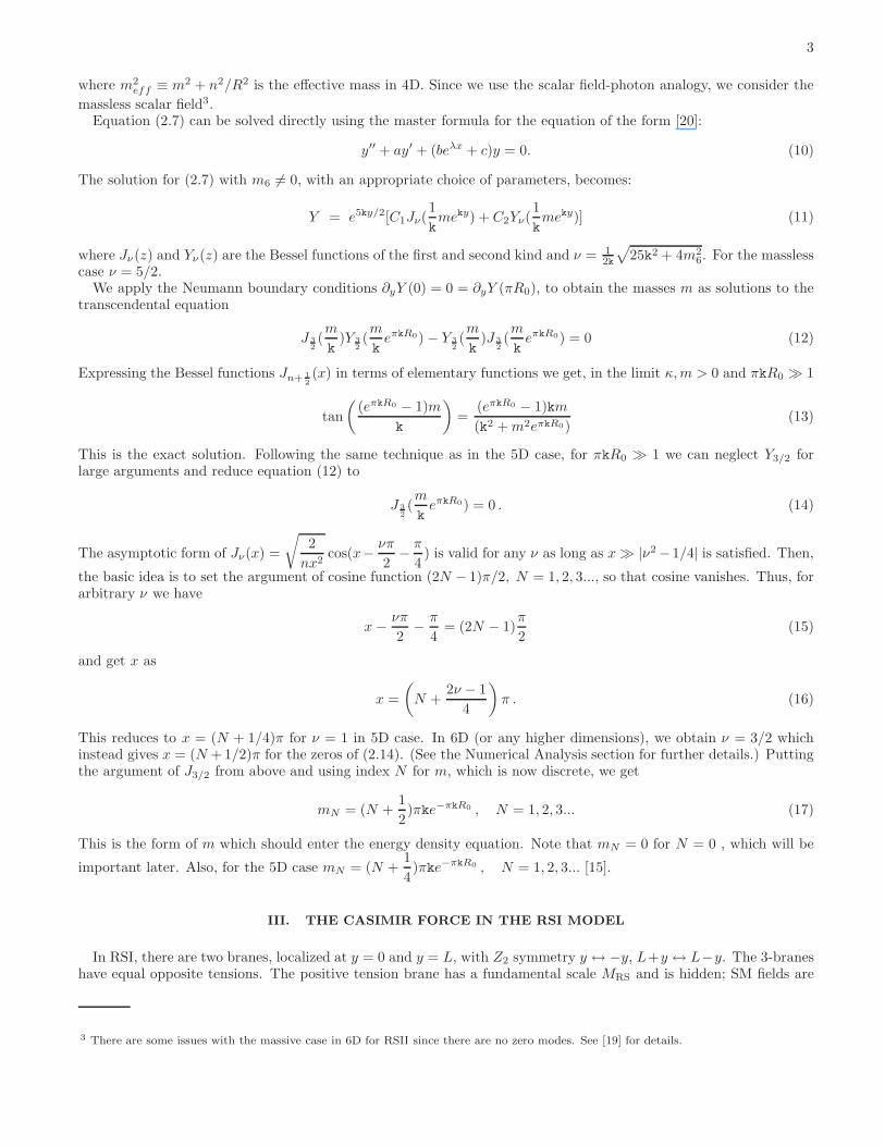
dimensions in RSI model. We first analyze the effect of one extra compact dimension in Fig. 2 as a function of plateseparation a. We fix k = 1019 GeV and the radius of θ as Rθ = 0.001 µm in the left panel and Rθ = 0.5 µm in theright panel. In each case, there are curves for various kRy values. As we can see, all curves with kRy values less than21 coincide and are represented as one curve. In this case there is no contribution coming from RS (Bessel terms)

15

and our results reduce to those in to 5D UED. This feature can also be seen from our analytical expression given in(36). The RS effects are included only in the Bessel function terms and the rest is the same as for 5D UED for the6D case and for (q − 1)D for the qD RS case. We analyzed (36) more systematically using an analytical approach.This method is also helpful when estimating what one would expect numerically by adding more extra dimensions.

We first tried to understand why effects appear from RS at around kRy = 21. We concentrate on the term withthe modified Bessel function K2 (a similar analysis will hold for the K1 term as well):

∞∑

ℓ,N=1

∞∑

n=0

ℓ−2

(n2

R2+ κ2(N +

1

2)2)

K2

(

2aℓ

√

n2

R2+ κ2(N +

1

2)2

)

. (67)

The dominant contributions come when the argument of K2 is small, thus the first few terms of series are dominant.In addition, as Rθ gets smaller and smaller, it increases the argument of K2 (for non-zero n of course,) and no matterhow small κ is, there is no contribution from terms with Bessel functions. Thus, the n = 0 term in the series isdominant. For simplicity, take ℓ = N = 1 and call the argument of K2 as xn,ℓ,N . Then, the dominant term is

x0,1,1 = aκ. The limiting form of Kα(x) is, for 0 ≪ x ≪√

α + 1

Kα(x) −→ Γ(α)

2

(2

x

)α

. (68)

The condition on x0,1,1 gives a critical value where the Bessel terms start being sizable. For example, for a = 0.5 µmand k = 1019 GeV, the critical value of kRy becomes (kRy)C = 21.0034. At any value greater than this critical value,κ becomes exponentially smaller and the Bessel terms completely dominate contributions from the other terms. Thisis exactly the effect seen in Fig. 2. The same analysis for the K1 term gives 21.068 for the critical value of kRy. Thelimiting form of the K1 and K2 terms, including the factors in front (but not the sign) becomes (κ/a)2 and 3/a4,respectively.

We need to emphasize another feature. Like the Casimir force in 4D, the force in 6D vanishes as the plate separationincreases. The ζ(5) term in (36) is independent of a and blows up as Rθ decreases. To see that the force in 6D behaves

(N + 1/2)π − J3/2(x0)(N + 1/4)π − J1(x0)

5D

6D

N

Zero

sof

J3/2(x

0)

and

J1(x

0)

10009008007006005004003002001000

10−1

10−2

10−3

10−4

FIG. 1: The approximations used for the zeros of the Bessel functions of first kind J1(x) and J3/2(x) for 5D and 6D, respectively.

16

kRy = 22.0

kRy = 21.5

kRy ≤ 21.0no RS (4D)

a ± 0.1µm

Rθ = 0.001 µm

k = 1019 GeV

a (µm)

F/A

(N/cm

2)

32.521.510.5

0.0 · 100

−5.0 · 10−7

−1.0 · 10−6

−1.5 · 10−6

−2.0 · 10−6kRy = 22.0

kRy = 21.5

kRy ≤ 21.0no RS (4D)

a ± 0.1µm

Rθ = 0.5µm

k = 1019 GeV

a (µm)

F/A

(N/cm

2)

32.521.510.5

0.0 · 100

−5.0 · 10−7

−1.0 · 10−6

−1.5 · 10−6

−2.0 · 10−6

FIG. 2: The Casimir force in 6D as a function of plate separation a for various kRy values with k = 1019 GeV and Rθ = 0.001 µm

in the left panel and Rθ = 0.5 µm in the right panel. The shaded region represents ±0.1 µm error for the measurement of plateseparation a.

like 1/a4 for very small Rθ values, consider the Epstein Zeta function Z2(R, a/π; 5) term in (36). One can expandZ2(R, a/π; 5) as, defining µ = a/Rθ,

Z2(1,√

d; s) = 2ζ(s) +2√

π

d(s−1)/2

Γ( s−12 )

Γ(s/2)ζ(s − 1) + Q(s, d) (69)

where

Q(s, d) =8πs/2

d(s−1)/4Γ(s/2)

∞∑

n=1

n(s−1)/2n∑

m=1

m−sm∑

ℓ=1

cos

(2πℓn

m

)

K s−12

(2π√

dn). (70)

In our case, d = (µ/π)2 and s = 5. Thus, we have

Z2(1, µ/π; 5) = 2ζ(5) +8π4

3ζ(4)

1

µ4+ Q(5, µ2/π2). (71)

If Rθ is small for a fixed a, we have µ ≫ 1 and Z2(1, µ/π; 5) goes to 2ζ(5) which exactly cancels the other ζ(5) termin (36). We are left with the ζ(4) term which is very close to the 4D force term. Note that Q(s, d) also vanishes as µincreases. For example, the force in 6D becomes, as µ ≫ 1

FI6D

A−→ −~cpπ2

240

1

µ4R4θ

+3~cp

128π6

1

R4θ

[

(1 + 2µ2 ∂

∂µ2)Q(5, µ2/π2)

]

(72)

where the second term vanishes in this limit. This analysis can be generalized to the qD case and it can be showedthat the same type of cancellations hold. Numerically, for small Rθ values, we need the precise cancellation of verylarge numbers which require high numerical precision in the calculation.

As can be seen from the above discussion, adding more compact dimensions would not affect much the kRy

dependence of the force. Extra dimensions bring an extra suppression factor for the Bessel terms (when 1/Rθiand

κ are comparable) but these effects will be minor for most cases. The force will feel the effect of extra Rθ’s in qDcoming from the terms other than the Bessel functions. As kRy is not affeted, in this limit the force is identical tothat in UED in q dimensions. There exist some studies in the literature [11] as well as some debate on whether the

17

Rθ = 0.5µm,7D RS

Rθ = 0.5µm,6D RS

Rθ = 0.001µm,7D RS

Rθ = 0.001µm,6D RSno RS (4D)

a ± 0.1µm

kRy = 15

k = 1019 GeV

a (µm)

F/A

(N/cm

2)

32.521.510.5

0.0 · 100

−5.0 · 10−7

−1.0 · 10−6

−1.5 · 10−6

−2.0 · 10−6

FIG. 3: The Casimir force in 6D and 7D as a function of plate separation a for Rθ = 0.001µm and 0.5µm with k = 1019 GeVand kRy = 15. Here Rθ1 = Rθ2 = Rθ is assumed. The shaded region represents ±0.1 µm error for the measurement of plateseparation a.

force is attractive or repulsive in extra universal dimensions [13]. As shown in previous sections, the 5D form of ourforce in κ → 0 limit is identical to the 5D result of [11] in UED and the force is always attractive. In Fig. 3 wedisplay the force in both 6D and 7D as a function of a for two values of Rθ, 0.001 µm and 0.5 µm. Here we assumeRθ1 = Rθ2 = Rθ. We chose kRy = 15, where there is practically no RS contribution from the Bessel terms so we canmaximize the effects from extra compact dimensions. This can be considered like 6D UED in this limit. As in 5DUED, the force remains negative in 6D as well, thanks to the precise cancellation of a-independent 1/R4

θ terms (or Z1

terms in general) with the ones from the Z2 term (similarly between Z3 and Z2 terms as well), as discussed above in6D RSI. In 5D UED, the bound from Casimir force on Rθ is very weak (about 0.01µm) [11] but adding more compactdimensions, as seen from Fig. 3, will strengthen the bound. Conversely, if the limit on the size of extra dimensions isheld constant, their number will be restricted. However, unless one introduces a large number of compact dimensions,it would be unrealistic from Casimir force considerations to get bounds on the size or number of extra dimensions asstrong as the ones from b → sγ, for example [24], which requires Rθ to be less than 10−12µm in 5D UED.

VI. SUMMARY AND CONCLUSION

We calculate, using dimensional regularization, the Casimir force between two parallel plates in Randall Sundrummodels with extra compact dimensions. We include both the one brane scenario (referred to as RSII) and the twobrane scenario (RSI). We present explicit analytic expressions for the energy between the plates, the renormalizedenergy, and finally for the Casimir force for the cases of one extra compact dimension (6D), and finally q extra compactdimensions (qD) in each model.

We show consistency of the expressions both from qD to 6D and 5D models (RS models with no compact dimensions).We also show that in the limit in which the non-compact dimension of Randall Sundrum models becomes irrelevant,

18

our expressions reproduce exactly the known UED expression in one extra dimension. In that limit, our results presentthe generalization of the Casimir energy in q universal extra dimensions, and we settle the controversy regarding thesign of the force. We also compare our results with a calculation in RSII models in 6D and qD and briefly discuss thediscrepancies.

For the RSII model, comparison with the known Casimir force in 4D yields (as in 5D) negligible corrections, makingthis model not as interesting phenomenologically as RSI. In RSI, we perform an analytical and numerical analysis ofour results and discuss the effects of extra compact dimensions on the size of kRy, the relevant parameter for RSImodels, as well as the consequences of the RS models on the size of the compact (UED like) dimensions. Finally,we analyze the effects of having additional compact dimensions. Although the bounds on the size of the compactdimensions obtained are not as strong as those coming from other low energy experimental restrictions, our resultsinclude a comprehensive range of numerical and analytical explorations of the Casimir force in extra dimensions, andwe are consistent with previous calculations in both RS and UED models in the relevant limits.

VII. ACKNOWLEDGMENT

M.F., I.T. and N.S. are supported in part by NSERC of Canada under the Grants No. SAP01105354 and GP249507.

[1] T. Kaluza, Sitzungsber. Preuss. Akad. Wiss. Berlin (Math. Phys. ) 1921, 966 (1921); O. Klein, Z. Phys. 37 (1926) 895[Surveys High Energ. Phys. 5 (1986) 241].

[2] L. Randall and R. Sundrum, Phys. Rev. Lett. 83, 4690 (1999); L. Randall and R. Sundrum, Phys. Rev. Lett. 83, 3370(1999); L. Randall and R. Sundrum, Nucl. Phys. B 557, 79 (1999).

[3] H. B. Casimir, Kon. Ned. Akad. Wetensch. Proc. 51, 793 (1948).[4] E. Ponton and E. Poppitz, JHEP 0106 (2001) 019; R. Hofmann, P. Kanti and M. Pospelov, Phys. Rev. D 63, 124020

(2001); W. H. Huang, Phys. Lett. B 497, 317 (2001); N. Graham, R. L. Jaffe, V. Khemani, M. Quandt, M. Scandurra andH. Weigel, Nucl. Phys. B 645, 49 (2002); A. A. Saharian and M. R. Setare, Phys. Lett. B 552, 119 (2003); E. Elizalde,S. Nojiri, S. D. Odintsov and S. Ogushi, Phys. Rev. D 67 (2003) 063515.

[5] M. Bordag, U. Mohideen, and V. M. Mostepanenko, Phys. Rep. 353, 1 (2001); S. K. Lamoreaux, Phys. Rev. Lett. 78, 5(1997); G. Bressi, G. Carugno, R. Onofrio, and G. Ruoso, Phys. Rev. Lett. 88, 041804 (2002).

[6] J. Ambjørn and S. Wolfram, Annals Phys. 147, 33 (1983).[7] M. Peloso and E. Poppitz, Phys. Rev. D 68, 125009 (2003); E. Elizalde, Phys. Lett. B 516 (2001) 143; M. Pietroni, Phys.

Rev. D 67, 103523 (2003); M. R. Setare, hep-th/0308109; A. C. Melissinos, hep-ph/0112266; C. L. Gardner, Phys. Lett.B 524, 21 (2002); K. A. Milton, R. Kantowski, C. Kao and Y. Wang, Mod. Phys. Lett. A 16, 2281 (2001); E. Carugno,M. Litterio, F. Occhionero and G. Pollifrone, Phys. Rev. D 53, 6863 (1996); W. Naylor and M. Sasaki, Phys. Lett. B 542

(2002) 289.[8] M. Fabinger and P. Horava, Nucl. Phys. B 580, 243 (2000); H. Gies, K. Langfeld and L. Moyaerts, JHEP 0306, 018 (2003);

I. Brevik and A. A. Bytsenko, hep-th/0002064; L. Hadasz, G. Lambiase and V. V. Nesterenko, Phys. Rev. D 62, 025011(2000).

[9] J. Garriga and A. Pomarol, Phys. Lett. B 560, 91 (2003); O. Pujolas, Int. J. Theor. Phys. 40, 2131 (2001); J. Garriga,O. Pujolas and T. Tanaka, Nucl. Phys. B 605, 192 (2001); A. Flachi, I. G. Moss and D. J. Toms, Phys. Rev. D 64, 105029(2001); A. Flachi and D. J. Toms, Nucl. Phys. B 610, 144 (2001); W. D. Goldberger and I. Z. Rothstein, Phys. Lett. B491 (2000) 339; E. Elizalde, S. Nojiri, S. D. Odintsov and S. Ogushi, Phys. Rev. D 67, 063515 (2003).

[10] R. Durrer and M. Ruser, Phys. Rev. Lett. 99, 071601 (2007); M. Ruser and R. Durrer, Phys. Rev. D 76, 104014 (2007).[11] K. Poppenhaeger, S. Hossenfelder, S. Hofmann and M. Bleicher, Phys. Lett. B 582, 1 (2004).[12] F. Pascoal, L. F. A. Oliveira, F. S. S. da Rosa and C. Farina, hep-th/0701181.[13] H. Cheng, Phys. Lett. B 643, 311 (2006); H. Cheng, Mod. Phys. Lett. A 21, 1957 (2006).[14] S. k. Nam, JHEP 0010, 044 (2000); W. H. Huang, Phys. Lett. B 497, 317 (2001); R. Casadio, A. Gruppuso, B. Harms and

O. Micu, arXiv:0704.2251 [hep-th]; M. Frank and I. Turan, Phys. Rev. D 74, 033016 (2006); R. Linares, H. A. Morales-Tecotl and O. Pedraza, Phys. Lett. B 633, 362 (2006); M. Minamitsuji, arXiv:0704.3623 [gr-qc].

[15] M. Frank, I. Turan and L. Ziegler, Phys. Rev. D 76, 015008 (2007).[16] T. Gherghetta and M. E. Shaposhnikov, Phys. Rev. Lett. 85, 240 (2000).[17] R. Linares, H. A. Morales-Tecotl and O. Pedraza, arXiv:0804.2042 [hep-ph].[18] V. A. Rubakov, Phys. Usp. 44, 871 (2001) [Usp. Fiz. Nauk 171, 913 (2001)].[19] R. Linares, H. A. Morales-Tecotl and O. Pedraza, Phys. Rev. D 77, 066012 (2008).[20] A. Polyanin and V. Zaitsev, Handbook of exact solutions for ordinary differential equations, Chapman and Hall/CRC, Boca

Raton, Florida, 2003.[21] E. Elizalde, S. D. Odintsov, A. Romeo, A. A. Bytsenko and S. Zerbini, Zeta Regularization Techniques With Applications,

Singapore, Singapore: World Scientific (1994); E. Elizalde, Grav. Cosmol. 8, 43 (2002) E. Elizalde, PoS IC2006, 008(2006); E. Elizalde, J. Math. Phys. 35, 6100 (1994); E. Elizalde, J. Phys. A 22, 931 (1989).

19

[22] R. Maartens, Living Rev. Rel. 7, 7 (2004).[23] S. B. Giddings, E. Katz and L. Randall, JHEP 0003, 023 (2000).[24] U. Haisch and A. Weiler, Phys. Rev. D 76, 034014 (2007).