Work supported in part by Department of Energy contract DE-AC02-76SF00515

MADPH-05-1432

SLAC-PUB-11357

Off-the-Wall Higgs in the Universal Randall-Sundrum Model

Hooman Davoudiasl,1, ∗ Ben Lillie,2, † and Thomas G. Rizzo2, ‡

1Department of Physics, University of Wisconsin, Madison, WI 53706

2Stanford Linear Accelerator Center,

2575 Sand Hill Rd., Menlo Park, CA 94025

Abstract

We outline a consistent Randall-Sundrum (RS) framework in which a fundamental 5-dimensional

Higgs doublet induces electroweak symmetry breaking (EWSB). In this framework of a warped

Universal Extra Dimension, the lightest Kaluza-Klein (KK) mode of the bulk Higgs is tachyonic

leading to a vacuum expectation value (vev) at the TeV scale. The consistency of this picture

imposes a set of constraints on the parameters in the Higgs sector. A novel feature of our scenario

is the emergence of an adjustable bulk profile for the Higgs vev. We also find a tower of non-

tachyonic Higgs KK modes at the weak scale. We consider an interesting implementation of this

“Off-the-Wall Higgs” mechanism where the 5-dimensional curvature-scalar coupling alone generates

the tachyonic mode responsible for EWSB. In this case, additional relations among the parameters

of the Higgs and gravitational sectors are established. We discuss the experimental signatures of

the bulk Higgs in general, and those of the “Gravity-Induced” EWSB in particular.

∗Electronic address: hooman@physics.wisc.edu†Electronic address: lillieb@slac.stanford.edu‡Electronic address: rizzo@slac.stanford.edu

Submitted to Journal of High Energy Physics (JHEP)

August 2005

I. INTRODUCTION

The Higgs mechanism in the Standard Model (SM) provides a simple and economical

explanation for electroweak symmetry breaking (EWSB). In the SM, it is assumed that the

Higgs potential contains a tachyonic negative mass-squared term that causes the Higgs to

develop a vacuum expectation value (vev), resulting in EWSB. However, the source of this

tachyonic mass, which must be of order 100 GeV, is not explained in the SM.

Another mystery regarding the Higgs sector, pointing to physics beyond the SM, is the size

of the typical Higgs mass compared to the cutoff scale; this is the usual hierarchy problem.

For example, if we take the 4-dimensional (4-d) reduced Planck mass MP l ∼ 2 × 1018 GeV

to be the cutoff scale, we would naively expect quantum corrections to raise the Higgs mass

to be near MP l, which is O(1016) too large.

An interesting explanation of the hierarchy is provided by the Randall-Sundrum (RS)

model [1]. In this model, a curved 5-d (bulk) spacetime called AdS5 is bounded by 4-

d Minkowski boundaries, corresponding to the geometry of the observed universe. The

curvature of the 5-d spacetime induces a sliding scale along the warped extra dimension,

geometrically generating the weak scale from a large Planckian scale, at one of the 4-d

boundaries. This boundary is referred to as the TeV-brane, hereafter. The geometrical red-

shifting in the RS model is exponential and hence capable of explaining large hierarchies,

using parameters that are typical in the model. In the original RS model, the only 5-d

field is the graviton[1, 2]. Numerous works have since extended the RS setup to include

bulk fermions and gauge fields[3]. However, even though the SM can be promoted to a 5-d

theory, the fundamental Higgs field responsible for EWSB has been typically kept on the

TeV-brane in the RS model. The reason for this has been to avoid problems associated

with extreme fine-tuning[4] which the RS model is constructed to resolve, and conflict with

known experimental data[5]. Thus, the Higgs is treated as a 4-d field in the RS geometry.

(There have also been attempts to build RS models without fundamental Higgs bosons[6]

where the role of the Higgs doublet as a source of Goldstone bosons is played by the fifth

components of the gauge fields themselves.)

In this work, we study the requirements for successful EWSB, using a fundamental 5-

d Higgs doublet in the RS background. We show that by appropriate choices of the Higgs

sector parameters in the bulk and on the branes, one can generate a single tachyonic Kaluza-

2

Klein (KK) mode of the Higgs field in the low energy 4-d theory. This tachyonic mode is

identified as the SM Higgs field. Given a quartic bulk term for the Higgs, the tachyonic mode

will lead to the usual 4-d Higgs mechanism and endow the electroweak gauge bosons with

mass. A novel feature of this mechanism is that the Higgs vev now has a profile that extends

into the bulk and is no longer a constant. This provides for new model-building possibilities

that we will briefly discuss in our presentation. A typical signature of our scenario is the

emergence of a tower of Higgs KK modes whose detection at future colliders we will consider

in this work. Since all of the SM fields are now in the bulk, this scenario is an example of a

warped Universal Extra Dimension[7].

The “Off-the-Wall Higgs” mechanism outlined above, like its 4-d SM counterpart, does

not explain the origin of the mass parameters of the Higgs potential. It would be interesting

if the RS geometry itself could provide the necessary mass scales of the 5-d Higgs sector,

leading to novel connections between the gravity and the Higgs sector parameters. We show

that a modified version of the RS gravity sector does indeed provide such a mass scale that

can result in a successful realization of the Off-the-Wall Higgs mechanism. The central

observation is that the most general bulk action in the RS model should include a term

ξRΦ†Φ, coupling the Ricci curvature scalar and the Higgs[8, 9]. Because there is a constant

curvature in AdS5 as well as δ-function terms on both branes, this coupling acts as a mass

term for the Higgs and, with the appropriate choice of parameters, can lead to EWSB. This

picture provides a link between the seemingly unrelated Higgs and gravitational parameters

and eliminates the need for ad hoc masses in the Higgs potential.

To realize this idea, we consider the most general 5-d action for a scalar coupled to gravity,

including all terms with dimension 6 and lower that are consistent with gauge symmetry and

general coordinate invariance. (We choose to include dimension 6 because we need quartic

terms in the scalar potential for stability; it turns out these are the only terms of dimension

6 allowed.) In addition to the standard kinetic and coupling terms, this action then includes

the curvature-scalar coupling, along with a string motivated[10] higher curvature Gauss-

Bonnet term (GBT)[11] and brane localized kinetic terms (BKT’s)[12] for the graviton[13].

In principle one could directly include ad hoc tachyonic mass terms for the Higgs. However,

we find that, under the assumption that these terms are small, there are phenomenologically

acceptable regions of parameter space where EWSB is solely driven by the gravity sector. It

is interesting to note that in the favored region typical values of ξ are close to the conformal

3

value ξ = −3/16.

This connection between gravity and the Higgs sectors leads to experimentally observable

signals that could point to this picture as the correct mechanism of EWSB. For example, it is

well-known that curvature-Higgs coupling on the TeV-brane leads to radion-Higgs mixing[8].

The same effect exists with our bulk Higgs. We discuss how measuring the Higgs-radion

mixing in conjunction with other collider measurements in the Higgs and gravity sectors can

test the gravity-induced EWSB scenario and establish its parameters.

In the next section, we will describe the ingredients for achieving consistent bulk Higgs

mediated EWSB in the RS geometry while section III discusses the details of the generation

of masses for the SM electroweak gauge bosons. Section IV focuses on the gravity-induced

realization of EWSB with a bulk Higgs and the new constraints on the Higgs and gravity

parameters that need to be satisfied in a successful scenario. Section V is devoted to a

discussion of experimental tests and the novel phenomenological aspects of our scenario,

such as the KK Higgs physics at colliders. Here, we also outline the measurements that will

result in the establishment of gravity-induced EWSB in the RS model. In section VI, we

present our conclusions.

II. BULK HIGGS EWSB IN RS: THE GENERAL FRAMEWORK

In this section we will describe the overall framework for our model and the general

mechanism of bulk Higgs EWSB in the RS scenario. In particular we will demonstrate how

the SM gauge boson masses are generated and the appearance of the Higgs KK spectrum.

We perform our analysis using the standard RS geometry[1]: two branes are located at the

fixed points of an S1/Z2 orbifold; between the branes, which are separated by a distance

πrc, is a slice of AdS5 and the metric is given by

ds2 = e−2σηµνdxµdxν − dy2 . (1)

Here, σ = k|y| with k being the so-called curvature parameter whose value is of order the

5-d Planck/fundamental scale, M , and y is the co-ordinate of the fifth dimension. In order

to be as straightforward as possible and to present the essential features of the model we

will delay any discussion of the localization of the SM fermions until a later section and for

now only assume that the SM gauge and Higgs fields are in the bulk. With this caveat our

4

action is given by

S = SHiggs + Sgauge , (2)

where

SHiggs =

∫d5x

√−g

[(DAΦ)†(DAΦ) − λ5Φ(Φ†Φ)2 −

(m2 +

µ2H

kδ(y − πrc) − µ2

P

kδ(y)

)Φ†Φ

],

(3)

and Sgauge is the usual action for the 5-d SM gauge fields. Note that in addition to the bulk

mass m2 for the Higgs field Φ we have allowed for mass terms on both the TeV and Planck

branes: µ2H,P . We have written a quartic interaction for the Higgs field only in the bulk.

One can in principle also add quartic terms for the Higgs on both branes but this does not

alter any of the physics that we now discuss and so we will drop such terms for simplicity

from the very beginning. Since we will be interested in first generating a tachyonic Higgs

mass and then shifting the field as in the SM, the role of the quartic term is just to stabilize

the potential allowing for a positive mass-squared physical Higgs. A simple bulk quartic is

sufficient for these purposes.

Let us focus on the free Higgs case (i.e., ignoring gauge and self-couplings as well as other

particles such as the Goldstone bosons so that we take Φ → φ) and truncate SHiggs to those

parts of the action involving only the various mass terms. Studying this truncated action

for the free Higgs field allows us to perform the KK decomposition. We then have

Strunc =

∫d5x

√−g

[(∂Aφ)†(∂Aφ) − m2φ†φ +

1

kφ†φ [µ2

P δ(y) − µ2Hδ(y − πrc)]

]. (4)

To scale out dimensional factors and to make contact with our later development we define

m2 = 20k2ξ and µ2P,H = 16k2ξβP,H since k is the canonical scale for RS masses. Note that

the parameters ξ, βP,H are dimensionless and are expected to be O(1) but may, in principle,

be of arbitrary sign. The choice of these unusual looking factors will be made clear below.

What are we looking for in the (ξ, βP,H) parameter space? To obtain EWSB in a manner

consistent with the SM our basic criterion is to find regions where there exists one, and only

one, TeV scale tachyonic mode that we can identify with the SM Higgs. The remaining

Higgs KK tower fields must also be normal, i.e., non-tachyonic. Clearly, if none of the

three mass terms in the action above are tachyonic no light tachyon will occur in the free

Higgs spectrum. To go further, we must obtain the relevant expressions for the Higgs KK

masses and wavefunctions so we let φ → ∑n φn(x)χn(y). Substituting this expression into

5

the action above and following the usual KK decomposition procedure leads to the equation

of motion for the Higgs KK wavefunctions, χn:

∂y

(e−4σ∂yχn

)− m2e−4σχn +

1

ke−4σ[µ2

P δ(y) − µ2Hδ(y − πrc)]χn + m2

ne−2σχn = 0 , (5)

with mn being the Higgs KK mass eigenvalues. The solutions are of the familiar form[14]

χn =e2σ

Nn

ζν

(xnεeσ

), (6)

with Nn a normalization factor, mn = xnkε, ε = e−πkrc 10−16, ν2 = 4 + m2/k2 = 4 + 20ξ,

and ζν = Jν + κnYν , being the usual Bessel functions. While the κn are determined by the

boundary conditions on the Planck brane and are generally very small, of order ε2ν , the

values of the xn are determined from the boundary condition on the TeV brane. Explicitly

one finds

−κn =

[2(1 +

µ2P

4k2

)− ν]Jν(xnε) + xnεJν−1(xnε)[

2(1 +

µ2P

4k2

)− ν]Yν(xnε) + xnεYν−1(xnε)

, (7)

while the xn roots can be obtained from[2(1 +

µ2H

4k2

)− ν

]ζν(xn) + xnζν−1(xn) = 0 . (8)

Since the κn are quite small the values of the parameters βP and, correspondingly, µ2P , are

generally numerically irrelevant to the analysis that we will perform below (even for the case

of ν = 0 provided βP is O(1)). Given the remaining two parameters, there are four possible

sign choices to consider and we need to explore the solutions of the equations above in all

these cases. However, we find that if the combination ξβH > 0 (µ2H > 0) then either no

tachyon exists or that the resulting Higgs vev is Planck scale, independent of the sign of m2.

This corresponds to an xn root of the equation above whose value is of order ε−1; recall that

we are seeking a single tachyonic root of order unity since mn = xnkε and we expect that

kε to be at most of order a few hundred GeV in order to solve the hierarchy. Clearly, we

must instead choose the parameters such that µ2H , ξβH < 0. In this case the two remaining

regions,

(I) ξ > 0, βH < 0

(II) ξ < 0, βH > 0

6

are found to be quite distinct since in the former case ν2 > 0 is guaranteed and thus ν is

always real.

What conditions are necessary in these two regions in order to find only one, single O(1)

tachyonic root, xT ? Our first goal is to find at least one such root which is O(1). Let us

assume that ν is real (and positive without loss of generality). Analytically, the best way to

find a tachyonic root which is O(1) is to look for the conditions on the parameters necessary

to obtain a zero-mode and then to perturb around these. The root equation, Eq.(8), above

already tells us that if the term in the square brackets is zero then xnζν−1(xn) = 0, implying

a root xn = 0; thus if ν = 2 + 8ξβH = 0 we obtain a zero mode. Similarly, if we set the

term in the square bracket equal to −2ν and use the Bessel function identity, 2νζν(z) =

z[ζν+1(z) − ζν−1(z)], we obtain xnζν+1(xn) = 0, which again has a zero root, and implies

−ν = 2 + 8ξβH = 0. Since ν ≥ 0, by hypothesis, these two equations lead directly to

a pair of bounds on ξ which are necessary to satisfy in order to obtain O(1) tachyonic

roots: we first obtain the bound ξ ≥ (≤)ξ1 in region I(II). Recalling, in addition, that

ν2 = 4 + 20ξ = (2 + 8ξβH)2 ≥ 0, yields a second constraint ξ ≥ (≤)ξ2 in region I(II). The

ξ1,2 are given by the expressions

ξ1 = − 1

4βH

ξ2 =5 − 8βH

16β2H

. (9)

Observe that in region I, ν is always real since ξ ≥ 0 there. Furthermore, if these constraints

are satisfied we find there exists only a single O(1) tachyonic root, provided that ν is real.

Interestingly, if these two constraints are not satisfied one finds no tachyons whatsoever so

that EWSB cannot occur in those parameter space regions.

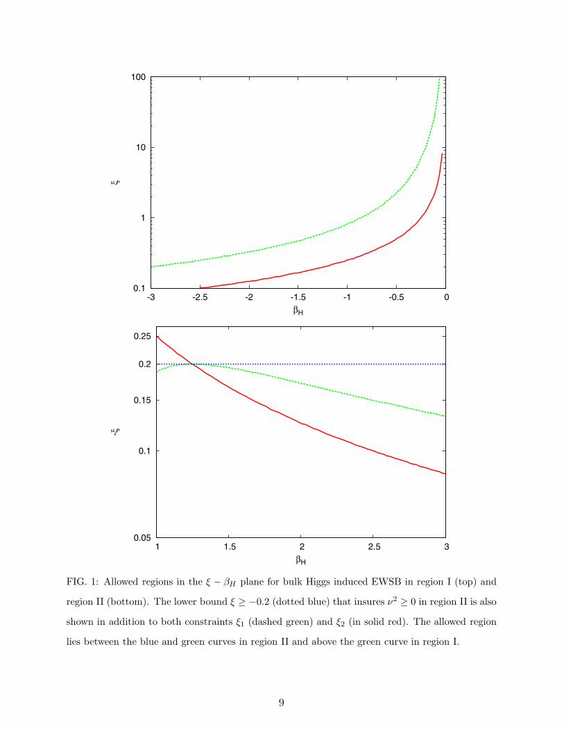
What do these constraints look like in regions I and II? Fig.1 shows all of the constraints

in the ξ−βH plane for both regions I and II. Note that in region II, since ξ < 0, to maintain

our assumption that ν is real requires that ξ ≥ −0.2 as is also shown in the figure. In

region I, since it is always true that ξ2 > ξ1, only the requirement that ξ > ξ2 as a function

of βH is relevant and the allowed region is rather simple. This is not the case in region II

where ξ1 = ξ2 when βH = 5/4. In fact with the assumption that ν is real we are forced to

have βH ≥ 5/4 in region II since there are now three simultaneous constraints to satisfy.

What if we give up this ν2 > 0 assumption which populates the dominant part of region II?

When ξ < −0.2 then ν is purely imaginary and one finds a multitude of O(1) and larger

7

tachyonic roots, thus violating our requirements that only one such root should exist. In

addition, because ν is imaginary the factor ε2ν in κn becomes a rapidly varying phase leading

to extreme parameter sensitivity. This is apparently a pathological regime where it is not

obvious that any consistent EWSB scenario can be constructed. Thus from now on we will

ignore the possibility that ν may be imaginary.

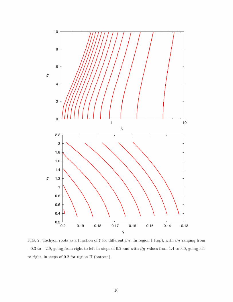
Fig.2 shows the possible values of the tachyonic root, xT , as a function of ξ for a wide

range of βH values in both allowed regions. We see that for a significant range of the ξ and

βH parameters that indeed xT is of order unity. It is important to observe that the value

βH = 1 is outside of the region II allowed range. Further restrictions on the parameter space

will occur when we consider the gauge boson masses in more detail in the next section.

Noting the mass of the Higgs tachyonic field and inserting the Higgs KK decomposition

φ =∑

n φn(x)χn(y) = φT χT + ..., back into the action, integrating over y and extracting

only the resulting potential for the 4-d part of the tachyonic field, φT , yields the familiar

expression

V = −m2T φ†

T φT + λ4(φ†T φT )2 , (10)

where

λ4 = λ5Φ

∫dy

√−g χ4T (y) , (11)

so that we can shift the field φT → (v + H)/√

2 as usual. There are several things to note

about this: (i) the physical ‘SM’ Higgs mass is given by mH =√

2mT =√

2xT kε and is fixed

relative to the masses of all the other KK states and (ii) although the tachyonic φ mass

is on the TeV brane, and possibly in the bulk as well, the Higgs vev now has a non-trivial

profile in the 5-d bulk given by χT /√

2. As we can easily see this function is very highly

peaked near the TeV brane since χT ∼ e(2+ν)σ. This is why we ‘see’ a TeV scale vev and

Higgs boson mass and also why we avoid some of the previous problems with placing the

Higgs field in the RS bulk[4]. Note that the overall shape of the Higgs profile is adjustable

by varying the parameters ξ and βH . (iii) It is important to observe that the vev, v, in

the expression above is of the same scale as that of the SM Higgs, ∼ 246 GeV, and is not

Planckian.

8

0.1

1

10

100

-3 -2.5 -2 -1.5 -1 -0.5 0

ξ

βH

0.25

0.2

0.15

0.1

0.05 1 1.5 2 2.5 3

-ξ

βH

FIG. 1: Allowed regions in the ξ − βH plane for bulk Higgs induced EWSB in region I (top) and

region II (bottom). The lower bound ξ ≥ −0.2 (dotted blue) that insures ν2 ≥ 0 in region II is also

shown in addition to both constraints ξ1 (dashed green) and ξ2 (in solid red). The allowed region

lies between the blue and green curves in region II and above the green curve in region I.

9

0

2

4

6

8

10

1 10

x T

ξ

0.2

0.4

0.6

0.8

1

1.2

1.4

1.6

1.8

2

2.2

-0.2 -0.19 -0.18 -0.17 -0.16 -0.15 -0.14 -0.13

x T

ξ

FIG. 2: Tachyon roots as a function of ξ for different βH . In region I (top), with βH ranging from

−0.3 to −2.9, going from right to left in steps of 0.2 and with βH values from 1.4 to 3.0, going left

to right, in steps of 0.2 for region II (bottom).

10

III. GAUGE BOSON MASSES

The masses of the SM gauge bosons are, as usual, generated via the kinetic terms in

SHiggs. Unlike the usual RS-type scenario, the Higgs vev is no longer restricted to the TeV

brane but has a profile, χT , in the extra dimension. To extract the gauge boson mass terms

from SHiggs we can perform the standard KK decomposition and combine these terms with

those obtained from the relevant pieces of Sgauge obtaining the gauge boson wavefunctions

and KK mass spectra. To be specific, let us consider the case of the W boson. Suppressing

Lorentz indices, we employ the KK decomposition W =∑

n Wn(x)fn(y) and obtain the

following equation for the gauge KK states:

∂y

(e−2σ∂yfn

)− 1

4g2

5v2χ2

T e−2σfn + m2nfn = 0 , (12)

where g5 is the 5-d SU(2)L gauge coupling. It is important to notice that (i) the 4-d Higgs

TeV-scale vev, v appears here, not a 5-d vev and (ii) the tachyonic Higgs profile is present

in the mass generating term. Now we would like to solve this equation to obtain the W KK

spectrum and wavefunctions; however, due to the presence of χ2T (y), which is a combination

of Bessel functions of imaginary argument, an analytic solution is not obtainable. We may,

however, obtain a fairly good approximate solution by remembering that χT is strongly

peaked at the TeV brane in which case χ2T → ε−2δ(y − πrc). One can thus solve the

resulting equation exactly, but then we would have no idea how good our approximation is.

We will refer to this as the ‘δ-function limit’. The overall validity of this approximation will

certainly improve for larger ξ since then χ2T ∼ e2(ν+2)σ becomes even more sharply peaked

near the TeV brane in this case.

To obtain a better approximation, we performed the following calculation: we let χ2T →

λε−2δ(y − πrc), where λ here is a free parameter, and solved this equation analytically for

the usual KK spectrum and eigenfunctions. We then treat the difference

Vpt =1

4g2

5v2[χ2

T e−2σ − λδ(y − πrc)], (13)

as a first order ‘perturbing potential’ and calculate the elements of the W mass squared

matrix for the KK states. Lastly, we vary the parameter λ until this mass-squared matrix

is as diagonal as possible. In particular, we are specifically interested in making the off-

diagonal elements in the first row and column be as small as possible as these influence

11

the W mass via mixing. Our expectation is that λ will be near unity if our approximation

is valid. Performing this analysis for several choices of the input parameters tells us that

indeed λ 1.1 − 1.2 in region I where ν is large and, in region II, λ 1.1 − 1.3 where ν

is smaller. Thus the δ-function limit is a reasonable approximation in both regions and can

be improved upon by choosing a λ in the above range. We now have gotten the W KK

masses and eigenfunctions to a very good approximation. Obtaining the KK masses etc for

the other SM gauge fields can be done in a parallel manner. To connect with the 4-d SM we

must also relate the 5-d coupling, g5, to the usual SM g. If the SM fermions are localized

near either brane this can be done by defining the weak coupling as that between the brane

fermions and the would-be W zero mode, i.e., g2 = g25f0(y = 0, πrc)

2. If BKT’s for the

gauge fields are present, this definition is easily modified to include such effects[12].

From this analysis we can extract the ‘roots’ corresponding to the mass of, e.g., the W

boson in the usual manner, i.e., MW = xW kε. We typically find that xW 0.20 − 0.25

from which we may infer that kε ∼ 350 GeV. Using this result we would conclude that

xT = 1 corresponds to a Higgs mass of ∼ 500 GeV so that this suggests that somewhat

smaller values of xT ∼ 0.5 might be considered more favorable. From Fig. 3 we see that

it is easy to obtain such values in both regions I and II as long as we live near the ξ1,2

boundaries. How are the W and Z masses correlated in this model? Without extending

the gauge group in the bulk to SU(2)L × SU(2)R × U(1)B−L, as would be done in a more

realistic model[6, 17], there is no custodial symmetry present to insure the validity of the SM

MW = MZ cos θw relationship, i.e., ρ = 1. As discussed in Ref.[15], if v/(kε) <∼ 1 then the

gauge KK mass scales approximately linearly in v and we can obtain ρ 1. This relation

will become more exact as v/(kε) becomes smaller. However, when v/(kε) becomes very

large then the generated gauge boson mass becomes independent of v and we would thus

obtain MW = MZ , a gross violation of custodial symmetry. Since we sit between the two

extremes, v ∼ kε, we certainly would expect such violations to be of some significance in

the present case. Sampling the model parameter space we do indeed find sizeable deviations

of ρ from unity due to custodial symmetry violation. Here we make use of the approximate

gauge boson mass matrix calculations described above, and obtain deviations which are of

order 5−10%, some of which may arise from the approximations we have made in obtaining

the roots and wavefunctions. These deviations can be cured through an extension of the SM

gauge group which enforces custodial symmetry as discussed above.

12

FIG. 3: The curves correspond to fixed tachyon root values, xT = 0 (black) to 2.5 (cyan), in steps

of 0.5, as functions of ξ and βH in regions I (top) and II (bottom).

IV. GRAVITY-INDUCED ELECTROWEAK SYMMETRY BREAKING

As an example of EWSB with a bulk Higgs we now turn to the special case where EWSB

is triggered by gravity.

13

A. Gravity Action

In this case we need to consider a generalized version of the usual RS gravitational action

which augments the above action:

S = Sbulk + Sbranes + SHiggs + Sgauge , (14)

where now the various terms are given by

Sbulk =

∫d5x

√−g

[M3

2R − Λb +

αM

2

(R2 − 4RABRAB + RABCDRABCD

)]

Sbranes =∑

branes

∫d5x

√−g

[M3

kγiR4 − Λi

]δ(y − yi)

SHiggs =

∫d5x

√−g

[(DAΦ)†(DAΦ) − λ5Φ(Φ†Φ)2 + ξRΦ†Φ

], (15)

and Sgauge is as above. In these expressions M is the 5-d Planck or fundamental scale, R is

the usual 5-d Ricci curvature with Λb being the bulk cosmological constant, all of which are

familiar from the usual RS model. Generally, k and M are expected not to be very different

in magnitude in order to avoid introducing another hierarchy problem. The piece of Sbulk

which is quadratic in the curvature is the GBT with α being a dimensionless parameter

which we take to be of indefinite sign and roughly of O(1). The γi are graviton BKT’s for

the TeV (i = π) and Planck (i = 0) branes and R4 are the 4-d Ricci scalars derived from the

corresponding induced metrics on both branes. The Λi are the usual RS brane tensions. The

term ξRΦ†Φ in SHiggs is the bulk Higgs-curvature mixing term with ξ soon to be identified

with the parameter introduced in Section II. This is the most general form allowed for the

gravitational action in the RS model framework.

There are no bare Higgs mass terms of any kind in this action as they are assumed to be

generated from the Ricci scalar R. In order to generate the Higgs mass terms let us briefly

recall that in the usual RS scenario, the 5-d Ricci scalar obtains a ‘vev’, i.e., the RS metric

itself produces a background value for R. Employing the conventional RS relationships

between the bulk and brane tensions, Einstein’s equations lead to 〈R〉 = −20k2 +16k[δ(y)−δ(y − πrc)] so that with, e.g., ξ > 0, 〈R〉 induces a positive mass squared for the Higgs in

the bulk and on the TeV brane and a negative mass squared on the Planck brane. (Note

that the original RS model requires that βH = βP = 1.) This would lead to a 4-d theory

14

where the Higgs vev is of Planck scale as we found previously so that we must instead choose

ξ < 0. However, in that case we saw that βH ≥ 5/4 is required to obtain EWSB. Thus,

unless we alter the RS model in some way we cannot achieve gravity-induced EWSB.

The important role played by the GBT in this action is to maintain the general properties

of the RS model while allowing an extension of the parameter space, i.e., to βH = 1, for this

scenario to be phenomenologically successful. As was recognized long ago by Kim, Kyae

and Lee and subsequently discussed by other authors[11], the GBT allows us to modify the

relationship between the tensions of the TeV and Planck branes and the other RS parameters

which adds additional flexibility in the model. In particular one now finds that

ΛP lanck = −ΛTeV = 6kM3(1 − 4αk2

3M2

)≡ 6kM3βH , (16)

so that the gravity induced effective free Higgs action is just

Seff =

∫d5x

√−g

[(∂AΦ)†(∂AΦ) − m2(Φ†Φ) +

µ2

kΦ†Φ[δ(y) − δ(y − πrc)]

], (17)

and we identify m2 = 20k2ξ and µ2 = 16k2ξβH as above in Section II. Given our previous

general analysis, the allowed parameter space for gravity-induced EWSB is already known.

B. Classical Stability

With the addition of gravity to our original action, the ξ term leads to a number of new

effects, in particular mixing among the whole Higgs tower and radion fields. To address these

issues requires several steps: First, we must extract from the action the kinetic term for the

radion and see that it is properly normalized. Although this is straightforward it is non-

trivial for the case at hand. Here we follow the work of Csaki, Graesser and Kribs(CGK)[8]

and expand the metric as in their Eq.(3.2):

ds2 = e−2σ−2F ηµνdxµdxν − [1 + 2F ]2dy2 . (18)

We write their quantity F as e2σr0(x). Next we insert this metric into the Sbulk, Sbranes and

SHiggs terms in the action, perform a series expansion keeping terms only through second

order in the derivatives of r0, and integrate over y dropping terms which are subleading in

ε. This results in a kinetic term for r0 of the form

6M3

k(∂r0)

2N2r , (19)

15

where N2r sums over several distinct contributions:

N2r =

(1 − 4α

k2

M2

)(1 − 2Ωπ) , (20)

with

Ω0,π ≡ 4αk2/M2 ± γ0,π

1 − 4αk2/M2. (21)

Note that N2r contains the usual contributions from the Ricci scalar as well as those from

both the GBT and BKT’s. This quantity must be positive definite to avoid ghosts in the

radion sector and this can be much more easily accomplished in region II where βH is positive

and α is negative.

As has been discussed by several authors[11], the presence of the BKT’s and GBT in the

RS model can result in the graviton and/or radion field becoming a ghost and the possible

presence of a physical tachyon in the graviton spectrum; avoiding these problems constrains

the model parameters as we saw in the case of N2r above. Furthermore, eliminating the

possibility of tachyons in the gravity sector requires[11] that the parameter Ωπ < 0. Given

this condition N2r > 0 is automatically satisfied in region II while seemingly very difficult to

satisfy in region I.

To make contact with TeV scale physics we must relate M3/k to M2

P l; recall that in the

simple RS scenario M3/k = M2

P l neglecting terms of order ε2. In turns out that in the case

of the graviton, the requirement that the norm of this field also be positive definite, i.e., be

ghost-free, is the same as requiring that M2

P l be positive definite when expressed in terms

of the parameters in the action. Writing

M2

P l =M3

kN2

g , (22)

a straightforward calculation[16] leads to the relation

N2g =

(1 − 4α

k2

M2

)(1 + 2Ω0) +

ξkv2

M3ε2> 0 , (23)

where again O(ε2) terms have been neglected and we have taken the δ-function approxima-

tion for simplicity in the last term since it is ∼ 0.01 or less. It is difficult for us to obtain

N2r,g > 0 in region I simultaneously. In region II, to obtain N2

g > 0 we only require that

Ω0 > −1/2 which is a rather mild constraint. Note that if both N2r,g > 0 then the graviton

KK’s also have positive definite norms. A curious observation is that there exists a small but

16

finite region of the parameter space where no graviton brane terms are required to obtain

both N2r,g > 0; in such a case Ω0 = Ωπ

>∼ − 1/2. Finally, putting all these pieces together

we can write the normalized radion field, r, as

r0 = rε2

√6Λπ

Ng

Nr

, (24)

where Λπ = MP lε. Observe that in the original RS model both Nr,g = 1; the ratio N =

Ng/Nr will occur frequently in the expressions below.

Thus we conclude that we can obtain a working model of gravity-induced EWSB provided

we live in region II. As shown in Figs. 1 and 3, typical values of ξ in region II are close to

the conformal value ξ = −3/16.

C. Higgs-Radion Mixing

Since the normalized form of the radion field is now known, we can return to the action

and extract out pieces which are quadratic in the scalars, perform the associated KK decom-

positions (ignoring for now the KK expansions of the Goldstone bosons which do not mix

with the radion as we will see below) and integrate over y leaving us with the 4-d effective

Lagrangian (a sum over n is implied)

L = −1

2HnHn − 1

2m2

HnH2

n − 1

2m2

rr2

+ ξγAnHnr − 1

2

[1 + Bξγ2

]rr , (25)

which is analogous to that obtained by CGK[8] in their Eq.(10.12); here γ = v√6Λπ

0.01 − 0.05. Defining n = T, i with ‘T ’ labeling the mode that gets a vev, the coefficients

are given by

AT = 2ε2N

∫dy χ2

T 2N

Ai = 2ε2N

∫dy χT χi 0

B = −6ε4N2

∫dy e2k|y|χ2

T −6N2 . (26)

where the approximate results hold in the δ-function limit. Employing a scan of the parame-

ter space we find that these approximations hold to better than 50%; the true values tend

to be somewhat below those given by the δ-function approximation, e.g., AT 1.3(1.7) and

17

−B 3.4−4.1(4.8−5.5) in region II(I). Here we make some note of the factor ‘2’ appearing

in the definition of An above; this value is a result of the mixing terms being bulk operators

with the full 5-d Ricci scalar. In the standard case of wall Higgs fields, R → Rind and ‘2’ →‘6’ and the results of CGK are recovered. The kinetic mixing can be removed as usual by

suitable field redefinitions:

Hn → H ′n + ξγβAnr

′

r → βr′ , (27)

with

β−2 = 1 + Bξγ2 − ξ2γ2A2n , (28)

where a sum on the index n = (T, i) is now understood. Demanding that β−2 be positive

places another constraint on our model parameters, in particular, we obtain a bound on the

parameter ξ:

B

2A2n

[1 +

(1 +

4A2n

γ2B2

)1/2]≤ ξ ≤ B

2A2n

[1 −

(1 +

4A2n

γ2B2

)1/2]. (29)

Given our parameter space this bound is easily satisfied. Mass mixing remains but this can

be easily read off from L above and follows the usual course[8].

V. EXPERIMENTAL SIGNATURES

In this section we will discuss some of the phenomenological features of our model as well

as how our framework may be experimentally tested.

In a fully realistic model, all SM fields should live in the bulk. The 5-d fermion masses

will be chosen so that the overlap of the would-be zero mode with χT produces the correct

Yukawa couplings. Some mechanism also needs to be introduced to protect the ρ parameter,

such as enlarging the gauge group to SU(2)L × SU(2)R ×U(1)B−L[6, 17]. It is known that,

in this type of model with a Higgs on the IR brane, there is a tension between producing the

correct top mass and not causing too large a shift in the Zbb coupling. With the non-trivial

profile χT this problem should be softened, since the left-handed top (and hence the left

handed bottom) field can be moved closer to the Planck brane.

18

A. Higgs KK Excitations

Our framework describes a wide class of potential models with a new feature: the funda-

mental SM Higgs field is in the RS bulk and thus has a scalar KK excitation spectrum[18].

This is a completely new feature previously not considered within the RS model structure.

Once the values of βH and ξ are specified in our model so are the ratios of the masses of the

Higgs KK’s to that of the usual Higgs. (We will ignore radion mixing in this discussion for

simplicity since it is likely to have little influence on the Higgs KK excitations.) Exploring

this parameter space one generically finds that the first Higgs KK excitation has a mass

∼ 30−100(15−30) times larger than the W in region I(II), with the largest ratios obtained

for ξ near its boundary value. This suggests a mass range for the lightest Higgs KK state

of >∼ 1 − 1.5 TeV and is generally found to be more massive than the first graviton KK

excitation. To address this point, Fig. 4 shows the root values for the first Higgs KK as a

function of βH for different values of ξ in both regions. Here we see that almost all of the

time the Higgs KK is more massive than the first graviton KK. It is important to remember

that the masses of all the Higgs KK excitations are fixed once the values of ξ and βH are

known.

Can such a KK state be observed at planned colliders? Unless the couplings are very

large the Higgs KK states seem to be beyond the range of the LHC but may be produced

by Z bremsstrahlung at multi-TeV linear colliders such as CLIC. To address this issue we

must ask how a Higgs KK couples to SM fields. To obtain the HnWW -type couplings we

return to the Higgs kinetic term in SHiggs and extract out the term which is bilinear in the

W field yet linear in the Higgs. Then we perform the usual KK decomposition for each field

and extract the relevant coupling which we can express as an integral over y:

Seff =

∫d4x

∑n

HnW †µW µ 1

2g2

5v

∫dy e−2σχT χnf 2

0 . (30)

Interestingly we see that if the W wave-function were flat the integral would vanish by

orthogonality suggesting a small coupling. However, we also know that that the most sig-

nificant deviation in flatness for this gauge boson wavefunction occurs near the TeV brane

where χT is largest. To set the scale for this coupling and to make the connection with

the conventional SM WWH coupling strength, gSMWWH = g2v/2, we note that if we take the

light fermions to be localized near the Planck brane, we can define g2 = 2πrcg25. We can

19

FIG. 4: Roots for the first Higgs KK excitation as a function of βH for different values of ξ in

regions I (top) and II (bottom). In region I, ξ = 0.2 is the lowest curve with ξ increasing by 0.2

for each subsequent curve. The curves are cut off on the right hand side by the ξ constraints. In

region II, from top to bottom ξ runs from −0.120 to −0.195 in steps of 0.005. The largest possible

value for the first graviton KK root consistent with the constraint Ωπ ≤ 0 found in the case of

gravity induced breaking is shown as the dashed line.

20

then perform the integral above and scale the resulting WWH1 effective coupling to the SM

value. A scan of the parameter space in both regions I and II indicates that the coupling of

H1 to WW is substantially suppressed in comparison to the SM WWH value. We find that

gWWH1/gSMWWH 0.02−0.13 with the larger values appearing in region II. With these rather

small couplings it is clear that a large integrated luminosity will be necessary to detect the

H1 KK state if it is produced by gauge boson fusion or radiated off a gauge boson leg.

It is interesting to note that a similar expression to the above with χn → χT allows us

to calculate the usual Higgs coupling to the W . Ordinarily one would imagine that this is

purely proportional to M2W as in the SM. Here, due to the backreaction of the gauge boson

wavefunction this is no longer the case. This can be see from Eq.(12) by setting n = 0,

multiplying by f0, integrating over y and solving for m20 = M2

W . Using orthonormality,

integrating by-parts and employing the usual ∂yf0 = 0 boundary conditions on both branes

gives

M2W =

1

4g2

5v2

∫dy e−2σf 2

0 χ2T +

∫dy e−2σ(∂yf0)

2 , (31)

where the first term on the right is directly due to the Higgs boson vev while the second

corresponds to backreaction. Here we can see explicitly that these two components are of

the same sign; from this we can conclude that the HWW coupling in this model is less than

in the SM. This shift in the coupling of the Higgs to gauge bosons can be significant and can

be measured at the LHC/ILC. As in the case of H1 above, we can scale the WWH effective

coupling by the corresponding SM value. A numerical scan of the parameter space in regions

I and II indicates that gWWH/gSMWWH 0.45−0.70, with the larger values obtained in region

II. This large shift in coupling strength will be easily observable at the ILC and likely also

to be seen at the LHC. Of course the appearance of a suppression of the WWH coupling

in the RS model framework is not limited to the present scenario and is thus not a unique

feature of the present scheme[17].

The Higgs self-interactions as well as the Higgs KK’s coupling to SM Higgs can be ob-

tained through the quartic self-couplings appearing in SHiggs. To this end, we remind our-

selves that Φ†Φ can be written as

Φ†Φ =1

2(v + H)2χ2

T + (v + H)χT

∑n

χnHn +1

2

∑n,m

χnχmHnHm + G+G− +1

2G0G0 , (32)

where here the G’s are the non-KK expanded 5-d Goldstone particles. We first observe

that there are no trilinear or quartic couplings between a single Goldstone KK and the SM

21

Higgs; however, such terms for the couplings of two Higgs to a single Higgs KK excitation

do exist. To evaluate these terms we first observe that we can immediately relate λ5Φ to the

SM quartic coupling, λSM = m2H/(2v2), via the integral

λSM = λ5Φ

∫dy

√−gχ4T . (33)

Thus the HnHH and HnHHH couplings can be obtained from the action

S ′eff =

∑n

λeffn

∫d4x (3vH2 + H3)Hn , (34)

where

λeffn = λSM

∫dy

√−g χ3T χn∫

dy√−gχ4

T

. (35)

In a similar manner, one can calculate the equivalent of the SM Higgs trilinear coupling; one

finds that one recovers the SM expression when the definition of λ5Φ in terms of λSM given

above is employed. A sampling of the model parameter space indicates that λeff1/λSM 0.4 − 0.6 so that the H1 → HH decay mode branching fraction will be sizeable.

Given the properties of the H1 KK state it is likely that this particle can be most easily

produced in gg-fusion or in γγ collisions which can proceed through top quark loops. The

reason for this is that with the top in the RS bulk it is likely that the H1tt coupling will

remain reasonably strong. Another possibility would thus be the associated production of

an H1 together with tt.

B. Direct Tests

In the case of gravity-induced EWSB there are strong correlations between the Higgs

and gravity sectors. Although there are many parameters in the model, they are already

constrained by the analysis above and they are all likely to be accessible through future

collider experiment. This implies that the scenario becomes overconstrained and the model

structure can be directly tested. As we will see, such measurements will require LHC/ILC

and likely a multi-TeV e+e− collider for detailed studies of both the scalar and graviton

sector. The reason for this is clear: we need precision measurements and the masses of some

of the important states can be in excess of 1 TeV.

Let us begin with the gravity sector: We assume that the first three graviton KK ex-

citations, Gi=1,2,3, are accessible and that their properties can be determined in detail

22

at e+e− colliders. A measurement of the relative KK masses gives us Ωπ as this mass

ratio depends only on this single parameter and any individual mass then provides the

quantity kε. A measurement of the ratio of partial widths for the same final sate, e.g.,

Γ(G2 → µ+µ−)/Γ(G1 → µ+µ−), yields a determination of a combination of the parameters

Ω0,π while an overall width measurement yields us Λπ. The graviton KK spectrum is such

that G3 → 2G1 is kinematically allowed[19] and the possibility of studying such decays in

detail at e+e− colliders has already been discussed in the literature[20]. The rate and an-

gular distribution for this processes is sensitive to both the existence of BKT’s as well as

the GBT[10] allowing us to separate these two contributions once Λπ is known. However,

such precision measurements of G3 are likely to require a multi-TeV linear collider. When

Ωπ<∼ −0.28, the decay G2 → 2G1 is also allowed with different contributing weights arising

from the BKT’s and GBT contributions. In either case, it is likely that the graviton sector

alone will tell us α, γ0,π, Λπ, k/M and hence βH . As one can see, a combination of just these

measurements is already rather restrictive and may be sufficient to confirm or exclude the

present model.

Now for the scalar sector: We assume that the two lightest states, which are mixtures

of radion with the Higgs, can both be observed so that their masses and couplings can

be well determined. From these data it will be possible to reconstruct the mixing matrix

which provides for us the ‘weak’ eigenstate mass parameters as well as a determinations of

ξ. Given ξ, the Higgs and first KK Higgs masses, the value of βH can again be extracted

and compared with that obtained from the gravity sector. A confirmation of the model is

obtained if the two values agree.

VI. CONCLUSIONS

The consistency of having a fundamental 5-d Higgs doublet in the RS geometry was

studied in this work. We showed that by assigning appropriate bulk and brane masses for

the 5-d “Off-the-Wall” Higgs, one can achieve a realistic 4-d picture of EWSB, without

finetuning. In our construct, the SM Higgs is the lightest KK mode of the bulk doublet

which in the 4-d reduction has a tachyonic mass, leading to EWSB. Since all of the SM

fields are now in the RS bulk, this scenario represents an example of a warped Universal

Extra Dimension.

23

Previous attempts at EWSB with a bulk Higgs field in the RS geometry were plagued

by extreme fine-tuning and phenomenological problems[4]. Nearly all such models had con-

sidered endowing the bulk Higgs with a 5-d constant vev which yielded massive SM gauge

bosons in 5 dimensions. However, in our framework, EWSB involves only one KK mode

of the bulk Higgs and is hence localized. The resulting Higgs vev has a bulk-profile that

is identical to that of the physical SM Higgs. Although the consistency of the bulk Higgs

scenario imposes non-trivial constraints on our framework, we observe that a realistic 4-d

phenomenology can be achieved for a range of parameters.

A particularly interesting realization of the Off-the-Wall Higgs EWSB employs the gravi-

tational sector of the RS model to provide the necessary bulk and brane mass scales. These

scales are then related to the 5-d curvature of the RS geometry. Consequently, new relations

and constraints among the parameters of the Higgs and gravitational sectors are obtained.

In this “gravity-induced” EWSB scenario, the higher curvature Gauss-Bonnet terms play

an important role. The coupling of the gravity and Higgs sectors as well as the introduction

of the higher derivative terms affect the classical stability of the RS geometry. We find that

one of the two regions of parameter space is favored by these stability considerations. As

we have shown, typical values of ξ in region II are close to the conformal value ξ = −3/16.

We outlined the experimental tests and phenomenological features of the Off-the-Wall

Higgs and gravity-induced EWSB in our work. A novel feature of our general bulk scenario

is the existence of an adjustable 5-d profile of the Higgs vev which can provide a new tool for

model building. Generically, we also expect the appearance of TeV scale Higgs KK modes.

In the case of gravity-induced EWSB, observation of radion-Higgs mixing, together with

measurements of the Higgs and graviton KK modes can provide tests of this mechanism at

future colliders; TeV-scale e+e− colliders are well-suited for this purpose.

In summary, we have presented a consistent framework for placing the Higgs doublet in

the RS geometry bulk and achieving EWSB at low energies. The possibility that 5-d gravity

drives 4-d EWSB is considered and shown to be a viable option. With the Higgs residing in

the RS bulk, the entire SM can be thought of as a 5-d theory and it also becomes feasible

to think of bulk gravity as the cause of EWSB. This provides a cohesive 5-d picture of all

the known forces of nature that is both predictive and free of large hierarchies.

Note added: After this paper was essentially completed, Ref.[21] was brought to our

attention where the possibility of using the bulk curvature in the RS model to generate

24

the Higgs vev was also considered. As discussed in this work, the parameter space point

employed by these authors leads to multiple tachyons in the scalar spectrum and is plagued

by extreme parameter sensitivity.

Acknowledgments

H. Davoudiasl would like to thank K. Agashe, D. Chung and F. Petriello for discussions

related to this paper. This work was supported in part by the U.S. Department of Energy

under grant DE-FG02-95ER40896 and contract DE-AC02-76SF0051. The research of H.D.

is also supported in part by the P.A.M. Dirac Fellowship, awarded by the Department of

Physics at the University of Wisconsin-Madison. The authors would also like to thank the

Aspen Center of Physics for their hospitality while this work was being completed.

[1] L. Randall and R. Sundrum, Phys. Rev. Lett. 83, 3370 (1999) [arXiv:hep-ph/9905221].

[2] H. Davoudiasl, J. L. Hewett and T. G. Rizzo, Phys. Rev. Lett. 84, 2080 (2000) [arXiv:hep-

ph/9909255].

[3] H. Davoudiasl, J. L. Hewett and T. G. Rizzo, Phys. Lett. B 473, 43 (2000) [arXiv:hep-

ph/9911262] and Phys. Rev. D 63, 075004 (2001) [arXiv:hep-ph/0006041]; A. Pomarol, Phys.

Lett. B 486, 153 (2000) [arXiv:hep-ph/9911294]; Y. Grossman and M. Neubert, Phys. Lett. B

474, 361 (2000) [arXiv:hep-ph/9912408]; T. Gherghetta and A. Pomarol, Nucl. Phys. B 586,

141 (2000) [arXiv:hep-ph/0003129].

[4] S. Chang, J. Hisano, H. Nakano, N. Okada and M. Yamaguchi, Phys. Rev. D 62, 084025

(2000) [arXiv:hep-ph/9912498]; S. J. Huber and Q. Shafi, Phys. Rev. D 63, 045010 (2001)

[arXiv:hep-ph/0005286]; see also the second paper in Ref.[3].

[5] [LEP Collaborations], arXiv:hep-ex/0412015.

[6] C. Csaki, C. Grojean, H. Murayama, L. Pilo and J. Terning, Phys. Rev. D 69, 055006 (2004)

[arXiv:hep-ph/0305237]; C. Csaki, C. Grojean, L. Pilo and J. Terning, Phys. Rev. Lett. 92,

101802 (2004) [arXiv:hep-ph/0308038]. G. Cacciapaglia, C. Csaki, C. Grojean and J. Tern-

ing, Phys. Rev. D 70, 075014 (2004) [arXiv:hep-ph/0401160] and Phys. Rev. D 71, 035015

(2005) [arXiv:hep-ph/0409126]; G. Cacciapaglia, C. Csaki, C. Grojean, M. Reece and J. Tern-

25

ing, arXiv:hep-ph/0505001. C. Csaki, C. Grojean, J. Hubisz, Y. Shirman and J. Terning,

Phys. Rev. D 70, 015012 (2004) [arXiv:hep-ph/0310355]; Y. Nomura, JHEP 0311, 050 (2003)

[arXiv:hep-ph/0309189]; R. Barbieri, A. Pomarol and R. Rattazzi, Phys. Lett. B 591, 141

(2004) [arXiv:hep-ph/0310285]. H. Davoudiasl, J. L. Hewett, B. Lillie and T. G. Rizzo, Phys.

Rev. D 70, 015006 (2004) [arXiv:hep-ph/0312193] and JHEP 0405, 015 (2004) [arXiv:hep-

ph/0403300]; J. L. Hewett, B. Lillie and T. G. Rizzo, JHEP 0410, 014 (2004) [arXiv:hep-

ph/0407059]; R. S. Chivukula, E. H. Simmons, H. J. He, M. Kurachi and M. Tanabashi,

Phys. Rev. D 70, 075008 (2004) [arXiv:hep-ph/0406077] and Phys. Lett. B 603, 210 (2004)

[arXiv:hep-ph/0408262].

[7] T. Appelquist, H. C. Cheng and B. A. Dobrescu, Phys. Rev. D 64, 035002 (2001) [arXiv:hep-

ph/0012100]; H. C. Cheng, K. T. Matchev and M. Schmaltz, Phys. Rev. D 66, 056006

(2002) [arXiv:hep-ph/0205314] and Phys. Rev. D 66, 036005 (2002) [arXiv:hep-ph/0204342];

T. G. Rizzo, Phys. Rev. D 64, 095010 (2001) [arXiv:hep-ph/0106336].

[8] G. F. Giudice, R. Rattazzi and J. D. Wells, Nucl. Phys. B 595, 250 (2001) [arXiv:hep-

ph/0002178]; C. Csaki, M. L. Graesser and G. D. Kribs, Phys. Rev. D 63, 065002 (2001)

[arXiv:hep-th/0008151]; D. Dominici, B. Grzadkowski, J. F. Gunion and M. Toharia, Acta

Phys. Polon. B 33, 2507 (2002) [arXiv:hep-ph/0206197] and Nucl. Phys. B 671, 243 (2003)

[arXiv:hep-ph/0206192]; J. L. Hewett and T. G. Rizzo, JHEP 0308, 028 (2003) [arXiv:hep-

ph/0202155].

[9] See, however, K. Farakos and P. Pasipoularides, arXiv:hep-th/0504014;

[10] B. Zwiebach, Phys. Lett. B 156, 315 (1985); B. Zumino, Phys. Rept. 137, 109 (1986).

[11] J. E. Kim, B. Kyae and H. M. Lee, Nucl. Phys. B 582, 296 (2000) [Erratum-ibid. B 591, 587

(2000)] [arXiv:hep-th/0004005] and Phys. Rev. D 62, 045013 (2000) [arXiv:hep-ph/9912344];

K. A. Meissner and M. Olechowski, Phys. Rev. D 65, 064017 (2002) [arXiv:hep-th/0106203]

and Phys. Rev. Lett. 86, 3708 (2001) [arXiv:hep-th/0009122]; Y. M. Cho, I. P. Neupane and

P. S. Wesson, Nucl. Phys. B 621, 388 (2002) [arXiv:hep-th/0104227]; I. P. Neupane, Class.

Quant. Grav. 19, 5507 (2002) [arXiv:hep-th/0106100]; C. Charmousis and J. F. Dufaux,

Phys. Rev. D 70, 106002 (2004) [arXiv:hep-th/0311267]; Y. Shtanov and A. Viznyuk, Class.

Quant. Grav. 22, 987 (2005) [arXiv:hep-th/0312261]; P. Brax, N. Chatillon and D. A. Steer,

Phys. Lett. B 608, 130 (2005) [arXiv:hep-th/0411058]; T. G. Rizzo, JHEP 0501, 028 (2005)

[arXiv:hep-ph/0412087].

26

[12] H. Davoudiasl, J. L. Hewett and T. G. Rizzo, Phys. Rev. D 68, 045002 (2003) [arXiv:hep-

ph/0212279]; M. Carena, E. Ponton, T. M. P. Tait and C. E. M. Wagner, Phys. Rev. D

67, 096006 (2003) [arXiv:hep-ph/0212307]; F. del Aguila, M. Perez-Victoria and J. San-

tiago, Acta Phys. Polon. B 34, 5511 (2003) [arXiv:hep-ph/0310353], Eur. Phys. J. C 33,

S773 (2004) [arXiv:hep-ph/0310352], arXiv:hep-ph/0305119 and JHEP 0302, 051 (2003)

[arXiv:hep-th/0302023].

[13] H. Davoudiasl, J. L. Hewett and T. G. Rizzo, JHEP 0308, 034 (2003) [arXiv:hep-ph/0305086];

S. L. Dubovsky and M. V. Libanov, JHEP 0311, 038 (2003) [arXiv:hep-th/0309131]; G. Ko-

finas, R. Maartens and E. Papantonopoulos, JHEP 0310, 066 (2003) [arXiv:hep-th/0307138].

[14] W. D. Goldberger and M. B. Wise, Phys. Rev. Lett. 83, 4922 (1999) [arXiv:hep-ph/9907447].

[15] For a discussion, see the second paper in Ref.[12].

[16] For an outline of the calculation and original references, see the last paper in Ref[11].

[17] K. Agashe, A. Delgado, M. J. May and R. Sundrum, JHEP 0308, 050 (2003) [arXiv:hep-

ph/0308036]; B. Lillie, arXiv:hep-ph/0505074.

[18] See, however, A. Kehagias and K. Tamvakis, arXiv:hep-th/0507130; C. H. Chang and J. N. Ng,

Phys. Lett. B 488, 390 (2000) [arXiv:hep-ph/0006164]; K. Agashe, R. Contino and A. Pomarol,

Nucl. Phys. B 719, 165 (2005) [arXiv:hep-ph/0412089]; G. Denardo and E. Spallucci, Class.

Quant. Grav. 6, 1915 (1989); R. Contino, Y. Nomura and A. Pomarol, Nucl. Phys. B 671,

148 (2003) [arXiv:hep-ph/0306259].

[19] H. Davoudiasl and T. G. Rizzo, Phys. Lett. B 512, 100 (2001) [arXiv:hep-ph/0104199].

[20] M. Battaglia, A. De Roeck and T. Rizzo, in Proc. of the APS/DPF/DPB Summer Study on

the Future of Particle Physics (Snowmass 2001) ed. N. Graf, eConf C010630, E3022 (2001)

[arXiv:hep-ph/0112169].

[21] A. Flachi and D. J. Toms, Phys. Lett. B 491, 157 (2000) [arXiv:hep-th/0007025].

27