Statistical analysis tools for the Higgs discovery and beyond
66
Wouter Verkerke (Nikhef) Statistical analysis tools for the Higgs discovery and beyond
-
Upload
khangminh22 -
Category
Documents
-
view
1 -
download
0
Transcript of Statistical analysis tools for the Higgs discovery and beyond
Wouter Verkerke (Nikhef)
Statistical analysis tools for the Higgs discovery and beyond
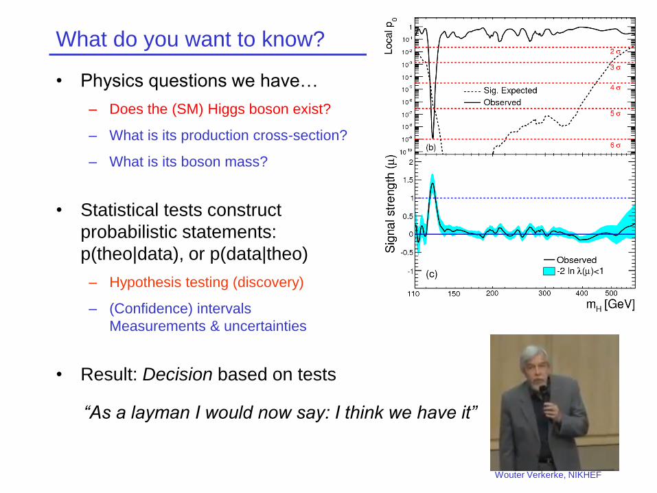
What do you want to know?
• Physics questions we have…
– Does the (SM) Higgs boson exist?
– What is its production cross-section?
– What is its boson mass?
• Statistical tests construct
probabilistic statements:
p(theo|data), or p(data|theo)
– Hypothesis testing (discovery)
– (Confidence) intervals
Measurements & uncertainties
• Result: Decision based on tests
Wouter Verkerke, NIKHEF
“As a layman I would now say: I think we have it”
All experimental results start with the formulation of a
model
• Examples of HEP physics models being tested
– SM with m(top)=172,173,174 GeV Measurement top quark mass
– SM with/without Higgs boson Discovery of Higgs boson
– SM with composite fermions/Higgs Measurement of Higgs coupling properties
• Via chain of physics simulation, showering MC, detector simulation
and analysis software, a physics model is reduced to a statistical
model
Wouter Verkerke, NIKHEF
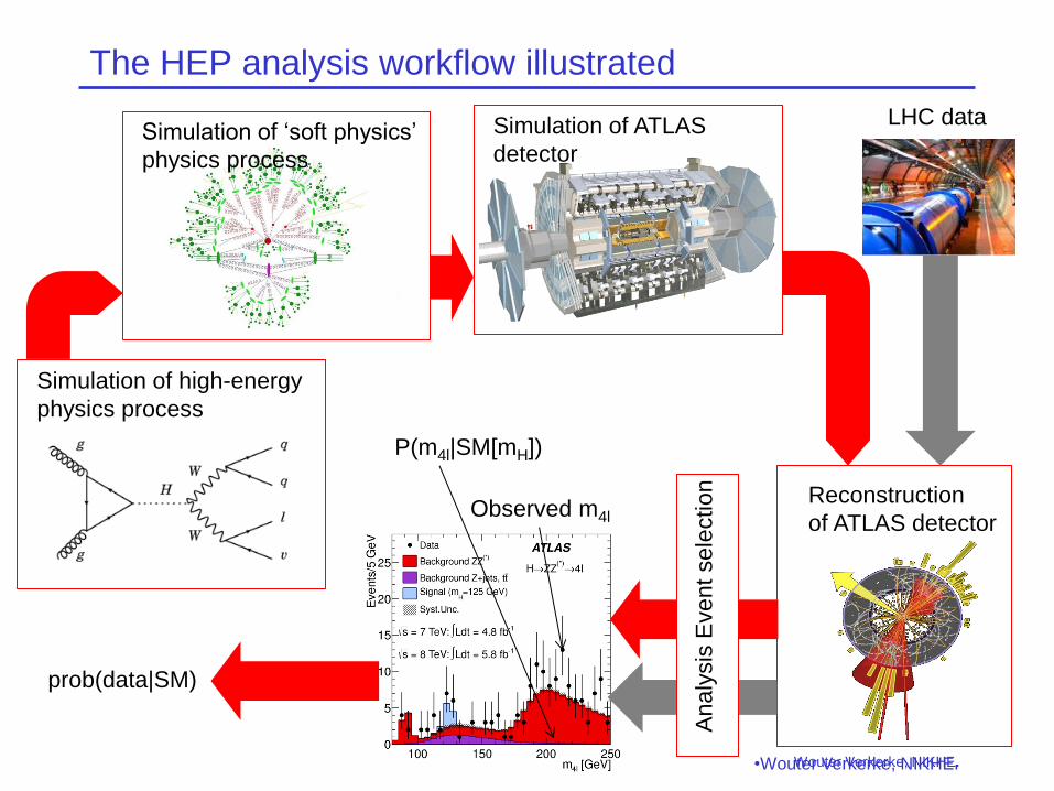
The HEP analysis workflow illustrated
Wouter Verkerke, NIKHEF •Wouter Verkerke, NIKHEF
Simulation of high-energy
physics process
Simulation of ‘soft physics’
physics process
Simulation of ATLAS
detector
Reconstruction
of ATLAS detector
LHC data
An
aly
sis
Eve
nt
se
lectio
n
prob(data|SM)
P(m4l|SM[mH])
Observed m4l
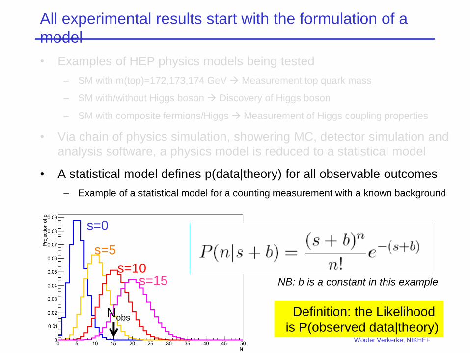
All experimental results start with the formulation of a
model
• Examples of HEP physics models being tested
– SM with m(top)=172,173,174 GeV Measurement top quark mass
– SM with/without Higgs boson Discovery of Higgs boson
– SM with composite fermions/Higgs Measurement of Higgs coupling properties
• Via chain of physics simulation, showering MC, detector simulation and
analysis software, a physics model is reduced to a statistical model
• A statistical model defines p(data|theory) for all observable outcomes
– Example of a statistical model for a counting measurement with a known background
Wouter Verkerke, NIKHEF
s=0
s=5
s=10 s=15 NB: b is a constant in this example
Definition: the Likelihood
is P(observed data|theory) Nobs
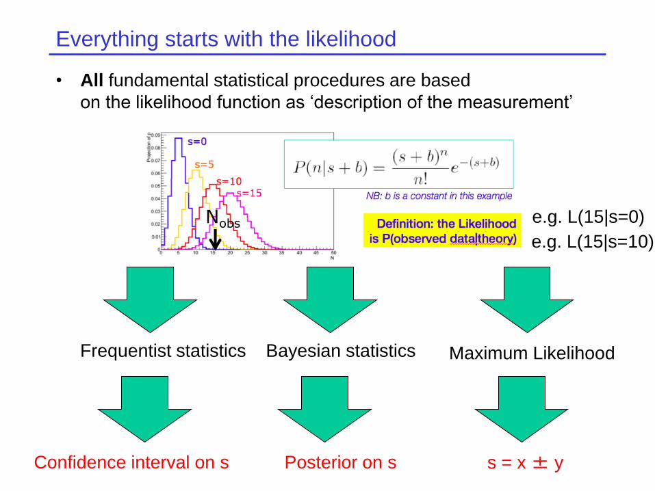
Everything starts with the likelihood
• All fundamental statistical procedures are based
on the likelihood function as ‘description of the measurement’
Frequentist statistics
Confidence interval on s Posterior on s s = x ± y
Bayesian statistics Maximum Likelihood
Nobs e.g. L(15|s=0)
e.g. L(15|s=10)
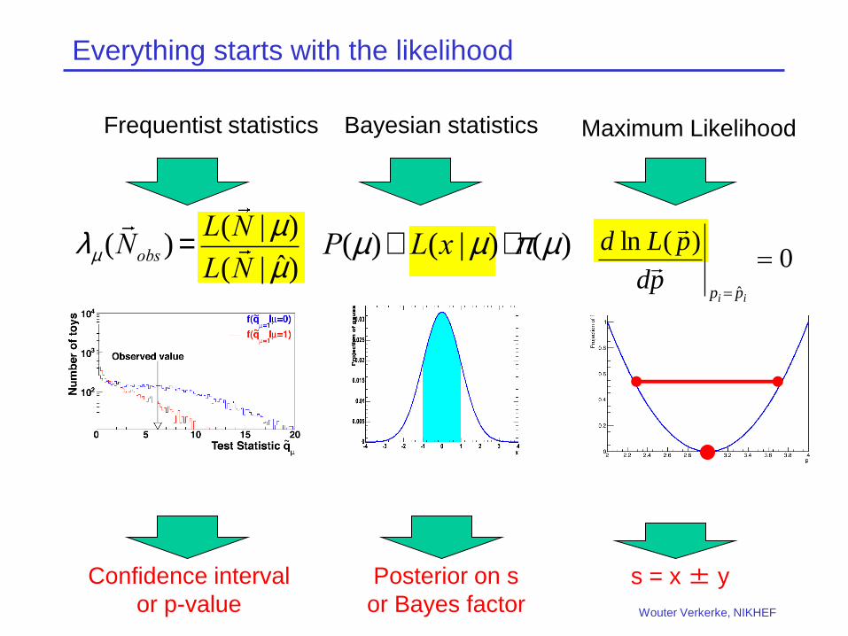
Everything starts with the likelihood
Wouter Verkerke, NIKHEF
Frequentist statistics
Confidence interval
or p-value
Posterior on s
or Bayes factor
s = x ± y
Bayesian statistics Maximum Likelihood
lm (Nobs ) =L(N | m)
L(N | m̂)P(m)µL(x |m) ×p(m)
0)(ln
ˆ
ii pp
pd
pLd
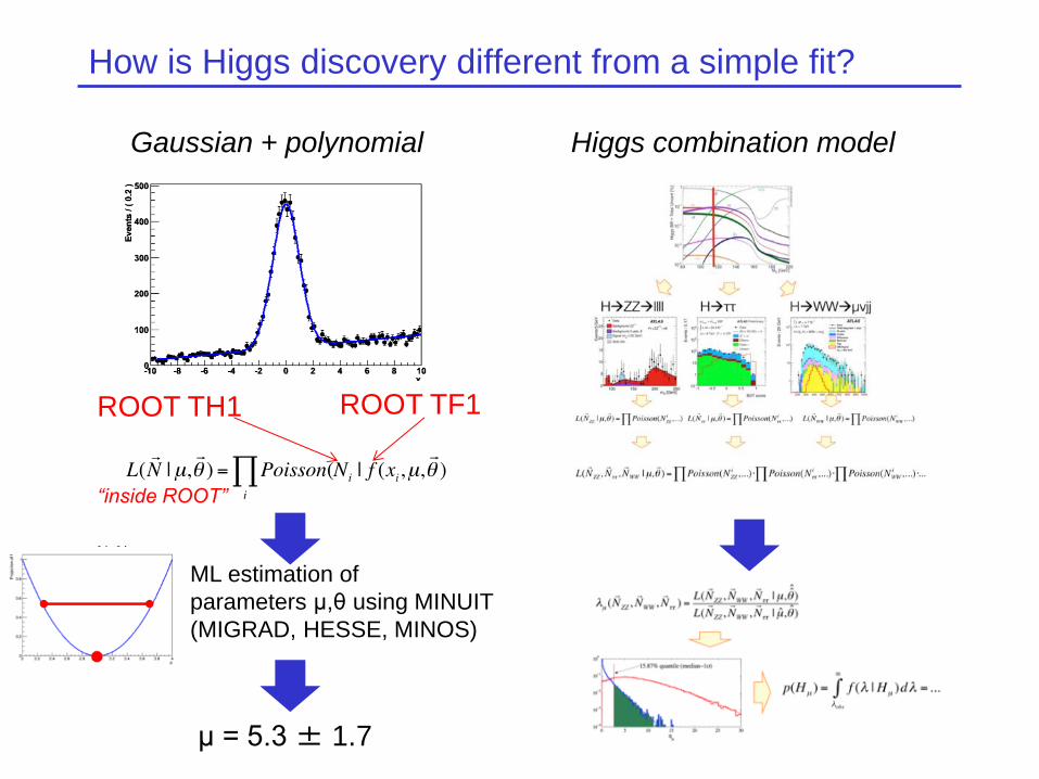
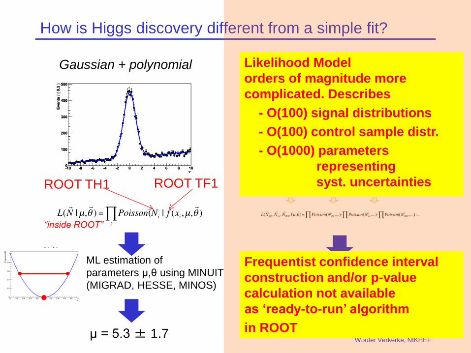
How is Higgs discovery different from a simple fit?
Wouter Verkerke, NIKHEF
Higgs combination model Gaussian + polynomial
ROOT TH1 ROOT TF1
μ = 5.3 ± 1.7
“inside ROOT”
ML estimation of
parameters μ,θ using MINUIT
(MIGRAD, HESSE, MINOS)
ML estimation of
parameters μ,θ using MINUIT
(MIGRAD, HESSE, MINOS)
How is Higgs discovery different from a simple fit?
Wouter Verkerke, NIKHEF
Higgs combination model Gaussian + polynomial
ROOT TH1 ROOT TF1
μ = 5.3 ± 1.7
“inside ROOT”
Likelihood Model
orders of magnitude more
complicated. Describes
- O(100) signal distributions
- O(100) control sample distr.
- O(1000) parameters
representing
syst. uncertainties
Frequentist confidence interval
construction and/or p-value
calculation not available
as ‘ready-to-run’ algorithm
in ROOT
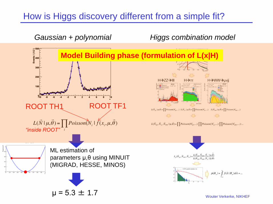
How is Higgs discovery different from a simple fit?
Wouter Verkerke, NIKHEF
Higgs combination model Gaussian + polynomial
ROOT TH1 ROOT TF1
μ = 5.3 ± 1.7
“inside ROOT”
Model Building phase (formulation of L(x|H)
ML estimation of
parameters μ,θ using MINUIT
(MIGRAD, HESSE, MINOS)
ML estimation of
parameters μ,θ using MINUIT
(MIGRAD, HESSE, MINOS)
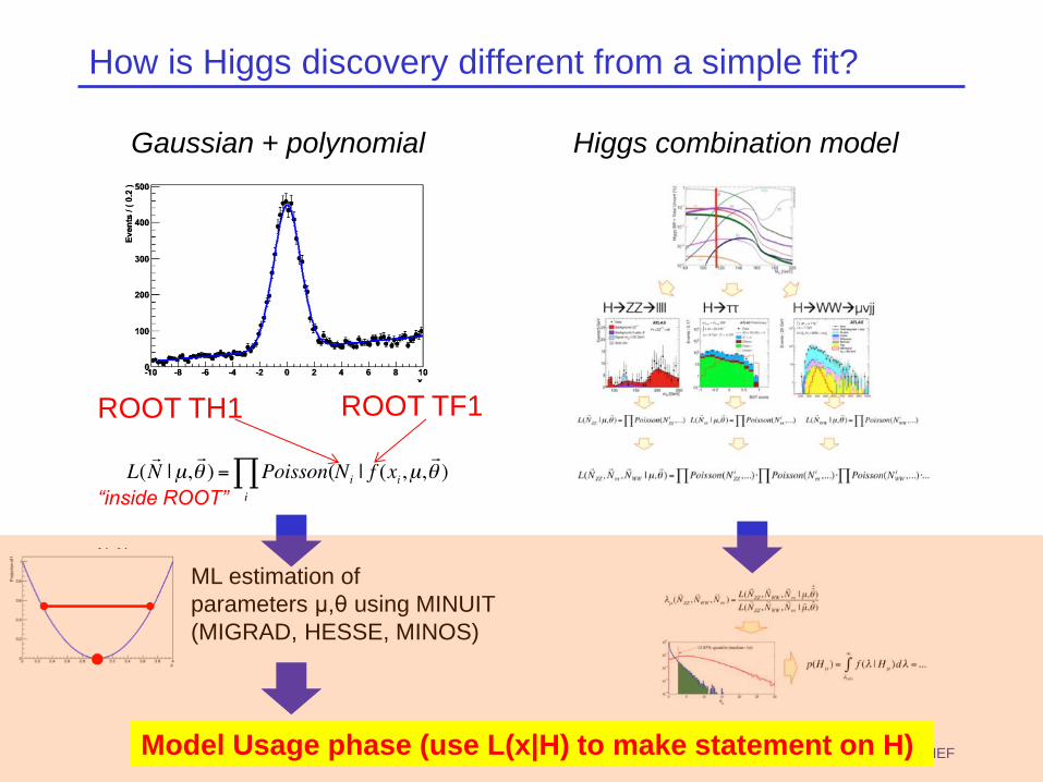
How is Higgs discovery different from a simple fit?
Wouter Verkerke, NIKHEF
Higgs combination model Gaussian + polynomial
ROOT TH1 ROOT TF1
μ = 5.3 ± 1.7
“inside ROOT”
Model Usage phase (use L(x|H) to make statement on H)
ML estimation of
parameters μ,θ using MINUIT
(MIGRAD, HESSE, MINOS)
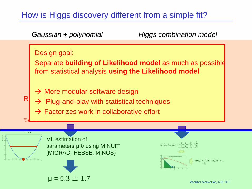
How is Higgs discovery different from a simple fit?
Wouter Verkerke, NIKHEF
Higgs combination model Gaussian + polynomial
ROOT TH1 ROOT TF1
μ = 5.3 ± 1.7
“inside ROOT”
Design goal:
Separate building of Likelihood model as much as possible
from statistical analysis using the Likelihood model
More modular software design
‘Plug-and-play with statistical techniques
Factorizes work in collaborative effort
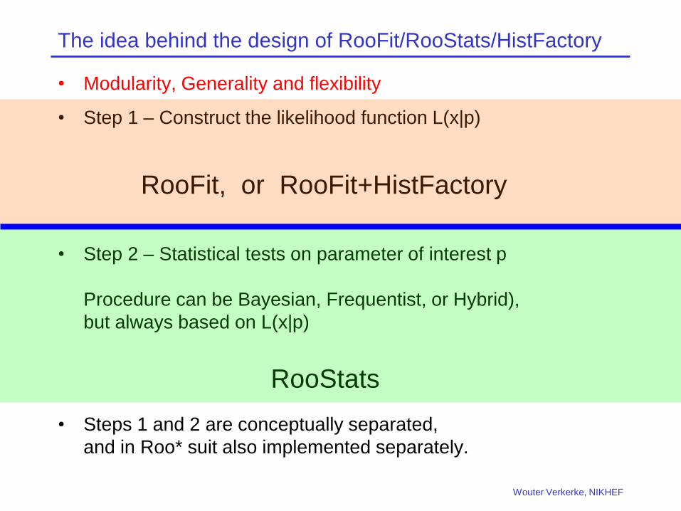
The idea behind the design of RooFit/RooStats/HistFactory
• Modularity, Generality and flexibility
• Step 1 – Construct the likelihood function L(x|p)
• Step 2 – Statistical tests on parameter of interest p
Procedure can be Bayesian, Frequentist, or Hybrid),
but always based on L(x|p)
• Steps 1 and 2 are conceptually separated,
and in Roo* suit also implemented separately.
Wouter Verkerke, NIKHEF
RooFit, or RooFit+HistFactory
RooStats
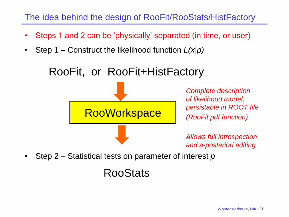
The idea behind the design of RooFit/RooStats/HistFactory
• Steps 1 and 2 can be ‘physically’ separated (in time, or user)
• Step 1 – Construct the likelihood function L(x|p)
• Step 2 – Statistical tests on parameter of interest p
Wouter Verkerke, NIKHEF
RooFit, or RooFit+HistFactory
RooStats
RooWorkspace
Complete description
of likelihood model,
persistable in ROOT file
(RooFit pdf function)
Allows full introspection
and a-posteriori editing
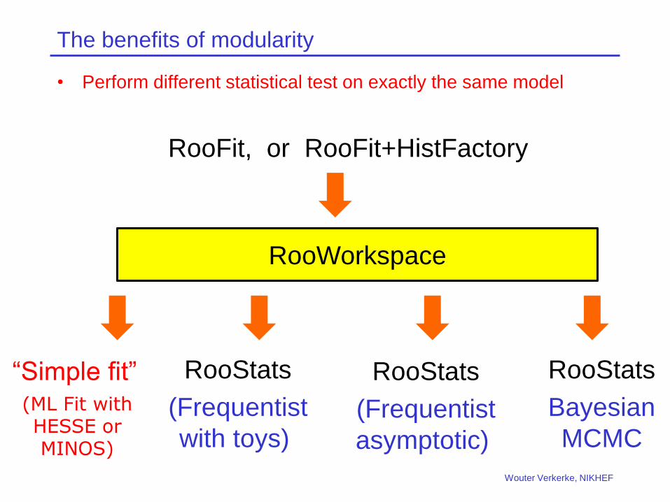
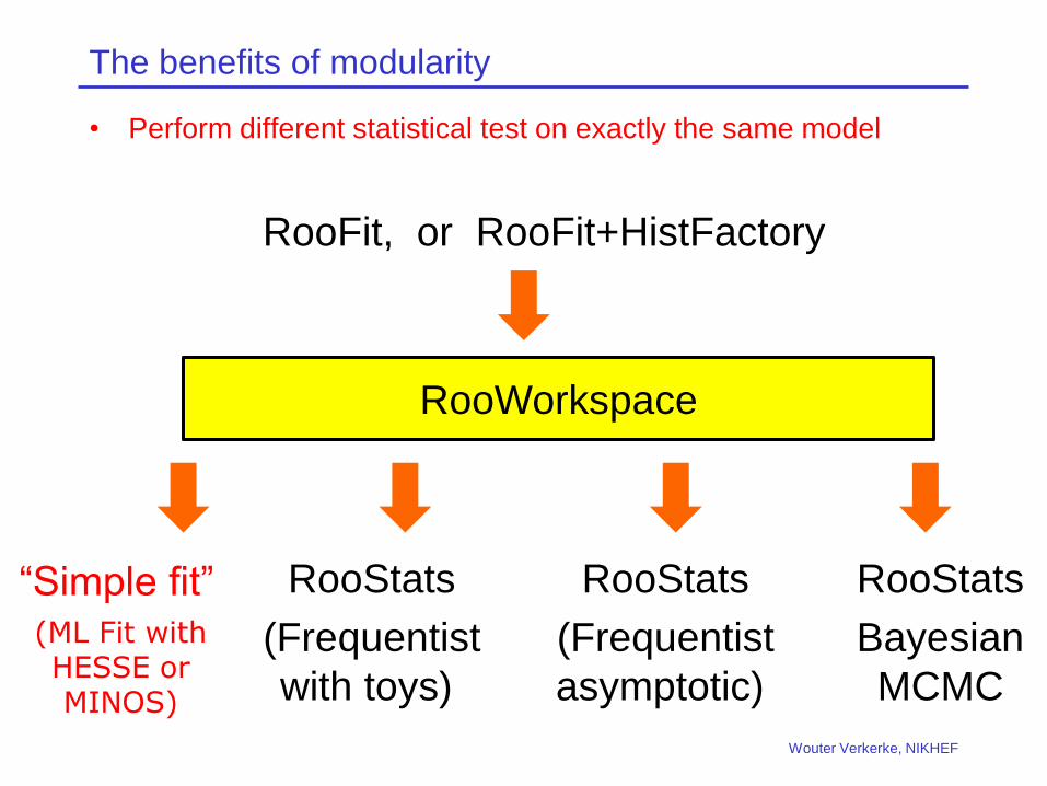
The benefits of modularity
• Perform different statistical test on exactly the same model
Wouter Verkerke, NIKHEF
RooFit, or RooFit+HistFactory
RooStats
(Frequentist
with toys)
RooWorkspace
RooStats
(Frequentist
asymptotic)
RooStats
Bayesian
MCMC
“Simple fit”
(ML Fit with HESSE or MINOS)

RooFit
WV + D. Kirkby - 1999
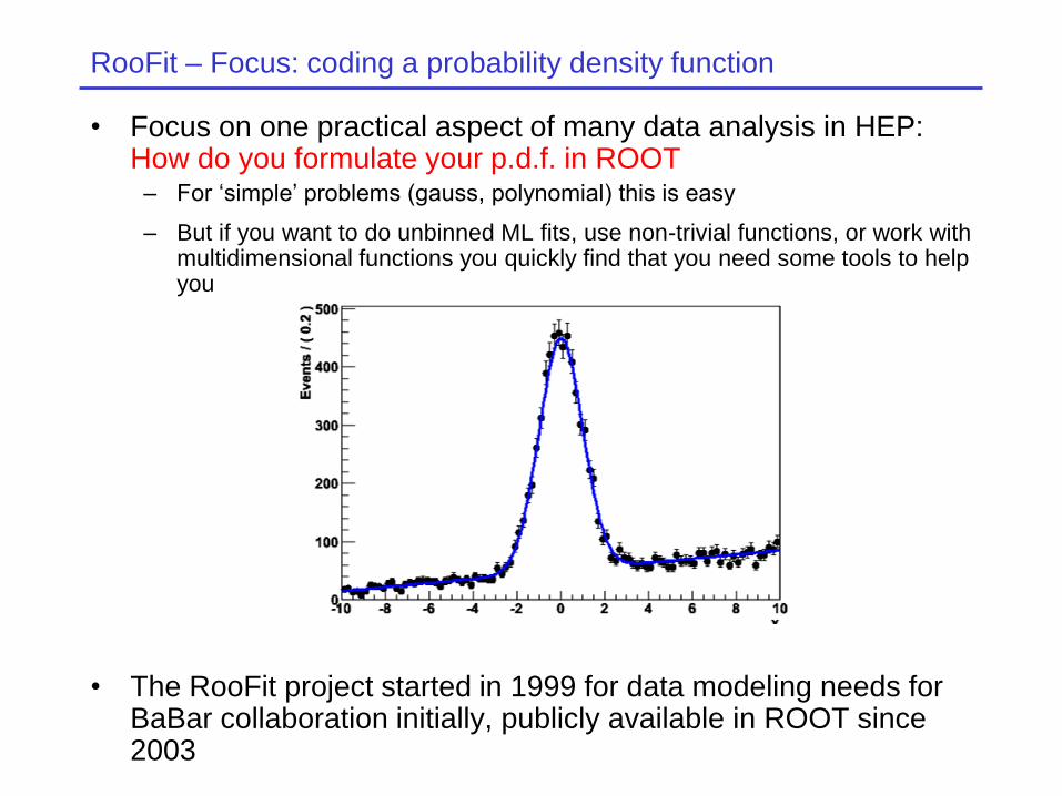
RooFit – Focus: coding a probability density function
• Focus on one practical aspect of many data analysis in HEP: How do you formulate your p.d.f. in ROOT
– For ‘simple’ problems (gauss, polynomial) this is easy
– But if you want to do unbinned ML fits, use non-trivial functions, or work with multidimensional functions you quickly find that you need some tools to help you
• The RooFit project started in 1999 for data modeling needs for BaBar collaboration initially, publicly available in ROOT since 2003
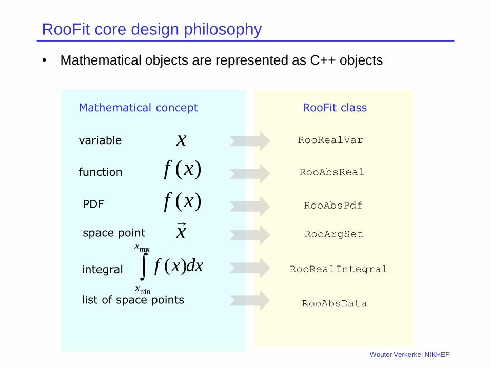
RooFit core design philosophy
• Mathematical objects are represented as C++ objects
variable RooRealVar
function RooAbsReal
PDF RooAbsPdf
space point RooArgSet
list of space points RooAbsData
integral RooRealIntegral
RooFit class Mathematical concept
)(xf
x
x
dxxf
x
x
max
min
)(
)(xf
Wouter Verkerke, NIKHEF
Wouter Verkerke, NIKHEF
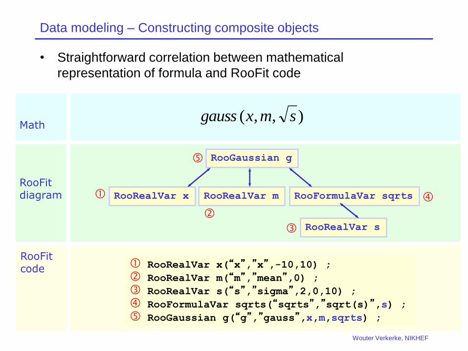
Data modeling – Constructing composite objects
• Straightforward correlation between mathematical
representation of formula and RooFit code
RooRealVar x
RooRealVar s
RooFormulaVar sqrts
RooGaussian g
RooRealVar x(“x”,”x”,-10,10) ;
RooRealVar m(“m”,”mean”,0) ;
RooRealVar s(“s”,”sigma”,2,0,10) ;
RooFormulaVar sqrts(“sqrts”,”sqrt(s)”,s) ;
RooGaussian g(“g”,”gauss”,x,m,sqrts) ;
Math
RooFit diagram
RooFit code
RooRealVar m
),,( smxgauss
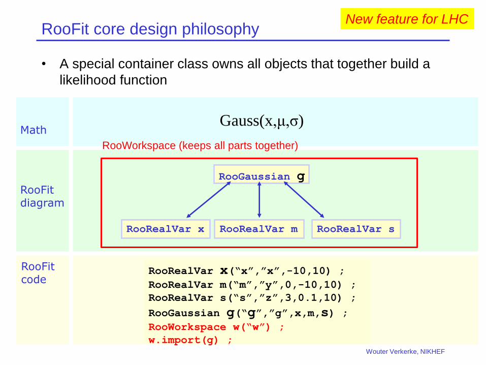
RooFit core design philosophy
• A special container class owns all objects that together build a
likelihood function
RooRealVar x RooRealVar m RooRealVar s
RooGaussian g
RooRealVar x(“x”,”x”,-10,10) ; RooRealVar m(“m”,”y”,0,-10,10) ;
RooRealVar s(“s”,”z”,3,0.1,10) ;
RooGaussian g(“g”,”g”,x,m,s) ; RooWorkspace w(“w”) ;
w.import(g) ;
Math
RooFit diagram
RooFit code
RooWorkspace (keeps all parts together)
Gauss(x,μ,σ)
Wouter Verkerke, NIKHEF
New feature for LHC
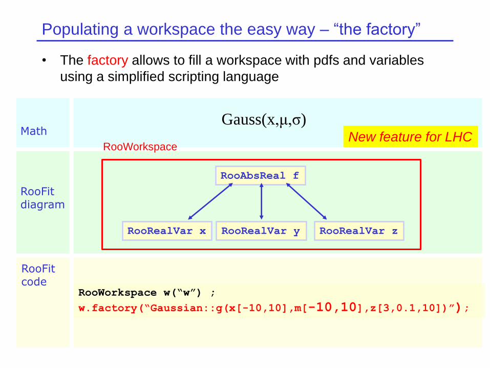
Populating a workspace the easy way – “the factory”
• The factory allows to fill a workspace with pdfs and variables
using a simplified scripting language
RooRealVar x RooRealVar y RooRealVar z
RooAbsReal f
RooWorkspace w(“w”) ;
w.factory(“Gaussian::g(x[-10,10],m[-10,10],z[3,0.1,10])”);
Math
RooFit diagram
RooFit code
RooWorkspace
Gauss(x,μ,σ) New feature for LHC
Wouter Verkerke, NIKHEF
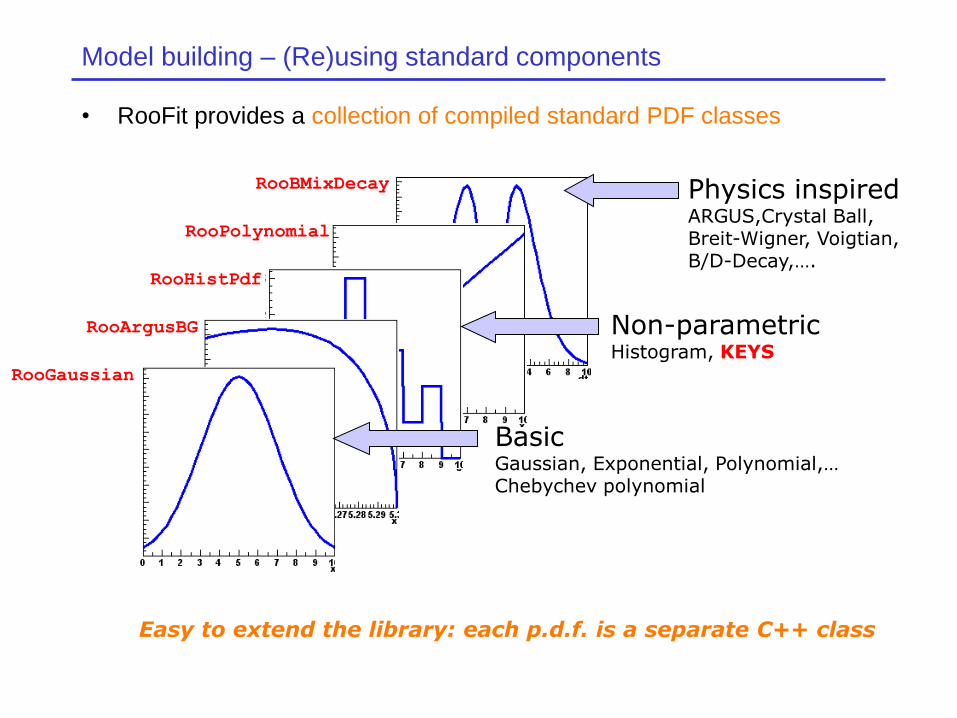
Model building – (Re)using standard components
• RooFit provides a collection of compiled standard PDF classes
RooArgusBG
RooPolynomial
RooBMixDecay
RooHistPdf
RooGaussian
Basic Gaussian, Exponential, Polynomial,… Chebychev polynomial
Physics inspired ARGUS,Crystal Ball, Breit-Wigner, Voigtian, B/D-Decay,….
Non-parametric Histogram, KEYS
Easy to extend the library: each p.d.f. is a separate C++ class
Wouter Verkerke, NIKHEF
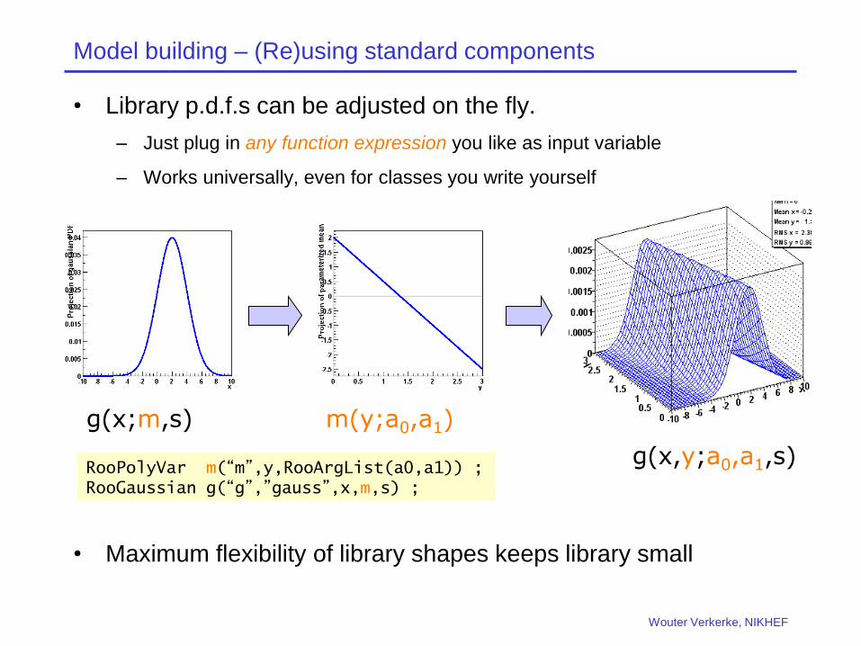
Model building – (Re)using standard components
• Library p.d.f.s can be adjusted on the fly.
– Just plug in any function expression you like as input variable
– Works universally, even for classes you write yourself
• Maximum flexibility of library shapes keeps library small
g(x,y;a0,a1,s)
g(x;m,s) m(y;a0,a1)
RooPolyVar m(“m”,y,RooArgList(a0,a1)) ; RooGaussian g(“g”,”gauss”,x,m,s) ;
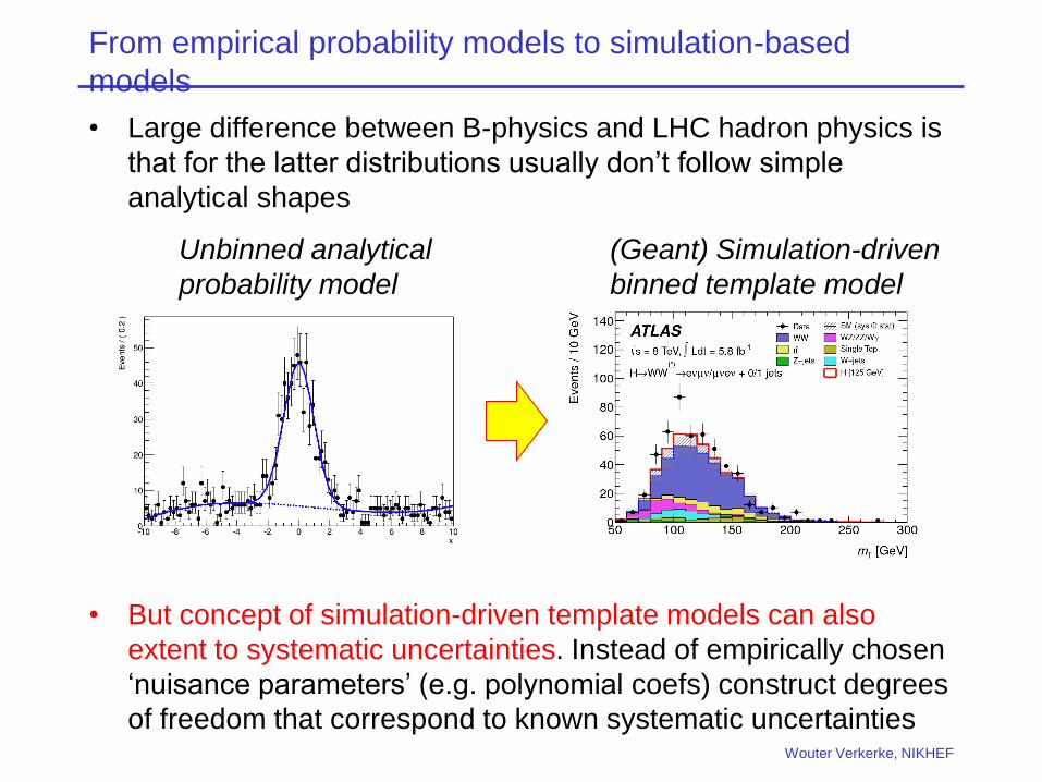
From empirical probability models to simulation-based
models
• Large difference between B-physics and LHC hadron physics is
that for the latter distributions usually don’t follow simple
analytical shapes
• But concept of simulation-driven template models can also
extent to systematic uncertainties. Instead of empirically chosen
‘nuisance parameters’ (e.g. polynomial coefs) construct degrees
of freedom that correspond to known systematic uncertainties Wouter Verkerke, NIKHEF
Unbinned analytical
probability model
(Geant) Simulation-driven
binned template model
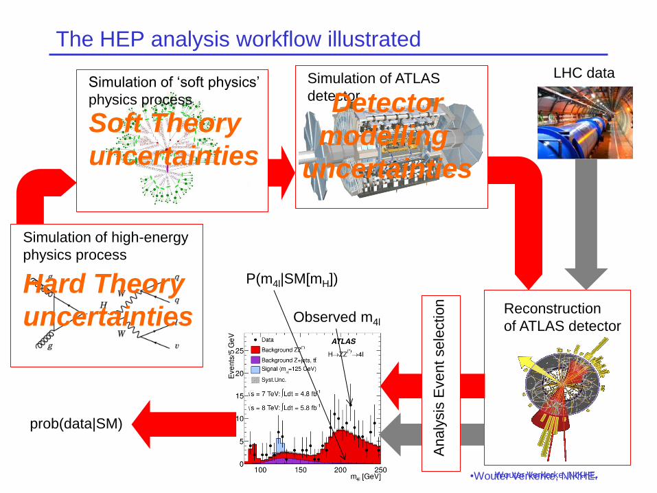
The HEP analysis workflow illustrated
Wouter Verkerke, NIKHEF •Wouter Verkerke, NIKHEF
Simulation of high-energy
physics process
Simulation of ‘soft physics’
physics process
Simulation of ATLAS
detector
Reconstruction
of ATLAS detector
LHC data
An
aly
sis
Eve
nt
se
lectio
n
prob(data|SM)
P(m4l|SM[mH])
Observed m4l
Hard Theory
uncertainties
Soft Theory
uncertainties
Detector
modelling
uncertainties
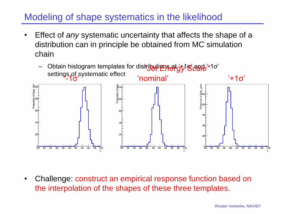
Modeling of shape systematics in the likelihood
• Effect of any systematic uncertainty that affects the shape of a
distribution can in principle be obtained from MC simulation
chain
– Obtain histogram templates for distributions at ‘+1σ’ and ‘-1σ’
settings of systematic effect
• Challenge: construct an empirical response function based on
the interpolation of the shapes of these three templates.
Wouter Verkerke, NIKHEF
‘-1σ’ ‘nominal’ ‘+1σ’
“Jet Energy Scale”
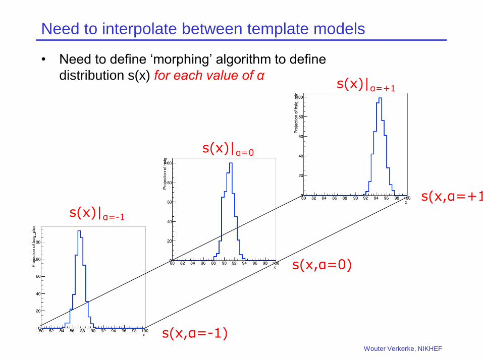
Need to interpolate between template models
• Need to define ‘morphing’ algorithm to define
distribution s(x) for each value of α
Wouter Verkerke, NIKHEF
s(x,α=-1)
s(x,α=0)
s(x,α=+1) s(x)|α=-1
s(x)|α=0
s(x)|α=+1
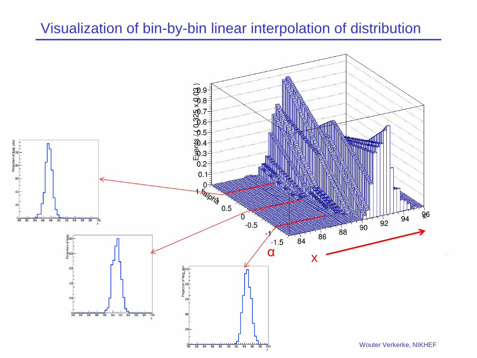
Visualization of bin-by-bin linear interpolation of distribution
Wouter Verkerke, NIKHEF
x α
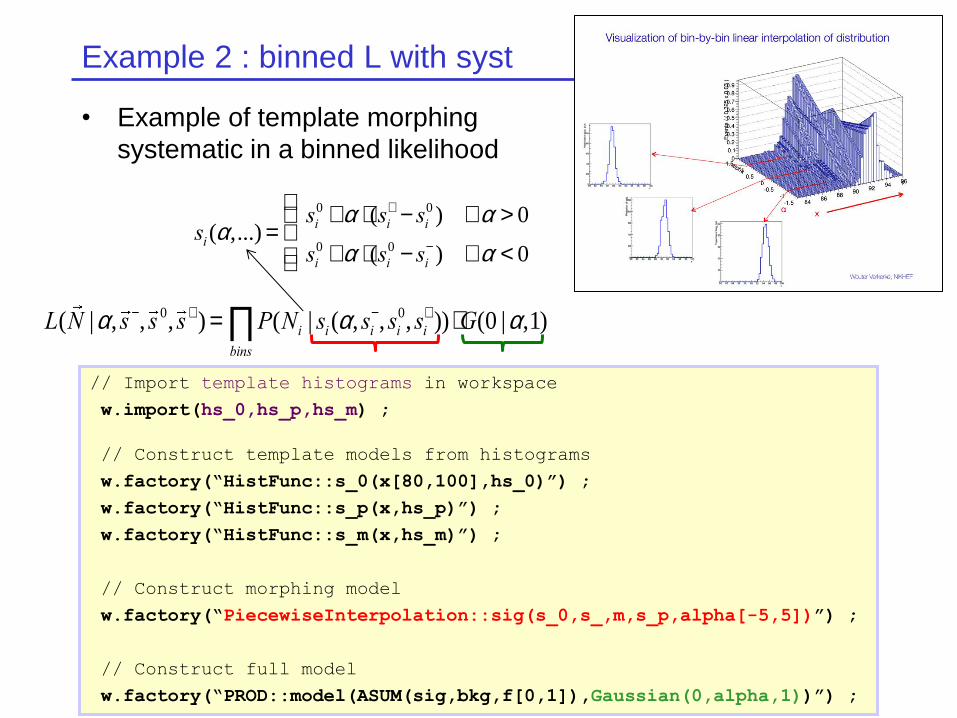
Example 2 : binned L with syst
• Example of template morphing
systematic in a binned likelihood
Wouter Verkerke, NIKHEF
L(N |a, s -, s 0, s+) = P(Ni | si(a, si-, si
0, si+)
bins
Õ ) ×G(0 |a,1)
si(a,...) =si
0 +a × (si+ - si
0 ) "a > 0
si0 +a × (si
0 - si-) "a < 0
ì
íï
îï
// Import template histograms in workspace
w.import(hs_0,hs_p,hs_m) ;
// Construct template models from histograms
w.factory(“HistFunc::s_0(x[80,100],hs_0)”) ;
w.factory(“HistFunc::s_p(x,hs_p)”) ;
w.factory(“HistFunc::s_m(x,hs_m)”) ;
// Construct morphing model
w.factory(“PiecewiseInterpolation::sig(s_0,s_,m,s_p,alpha[-5,5])”) ;
// Construct full model
w.factory(“PROD::model(ASUM(sig,bkg,f[0,1]),Gaussian(0,alpha,1))”) ;
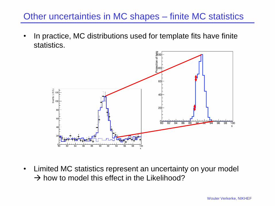
Other uncertainties in MC shapes – finite MC statistics
• In practice, MC distributions used for template fits have finite
statistics.
• Limited MC statistics represent an uncertainty on your model
how to model this effect in the Likelihood?
Wouter Verkerke, NIKHEF
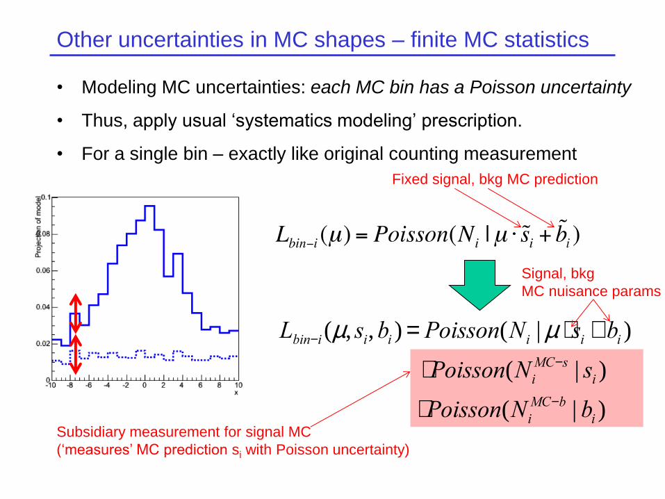
Other uncertainties in MC shapes – finite MC statistics
• Modeling MC uncertainties: each MC bin has a Poisson uncertainty
• Thus, apply usual ‘systematics modeling’ prescription.
• For a single bin – exactly like original counting measurement
Lbin-i(m, si,bi ) = Poisson(Ni | m × si +bi )
×Poisson(NiMC-s | si )
×Poisson(NiMC-b | bi )
Fixed signal, bkg MC prediction
Signal, bkg
MC nuisance params
Subsidiary measurement for signal MC
(‘measures’ MC prediction si with Poisson uncertainty)
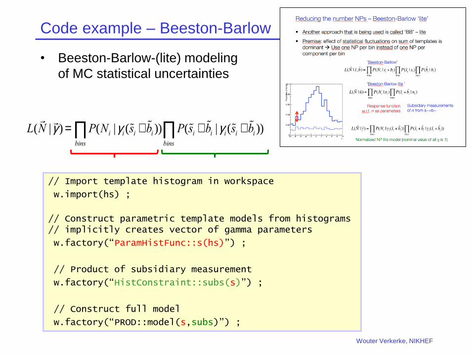
Code example – Beeston-Barlow
• Beeston-Barlow-(lite) modeling
of MC statistical uncertainties
Wouter Verkerke, NIKHEF
L(N |g ) = P(Ni |gi(si +bi ))bins
Õ P(si +bi |g i(si +bibins
Õ ))
// Import template histogram in workspace
w.import(hs) ;
// Construct parametric template models from histograms // implicitly creates vector of gamma parameters
w.factory(“ParamHistFunc::s(hs)”) ;
// Product of subsidiary measurement
w.factory(“HistConstraint::subs(s)”) ;
// Construct full model
w.factory(“PROD::model(s,subs)”) ;
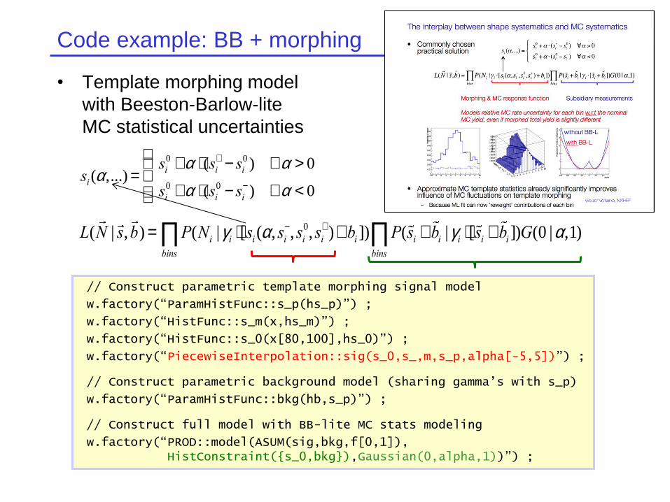
Code example: BB + morphing
• Template morphing model
with Beeston-Barlow-lite
MC statistical uncertainties
L(N | s,b) = P(Ni |g i ×[si(a, si-, si
0, si+)+bi ])
bins
Õ P(si +bi |gi ×[si +bi ]bins
Õ )G(0 |a,1)
si(a,...) =si
0 +a × (si+ - si
0 ) "a > 0
si0 +a × (si
0 - si-) "a < 0
ì
íï
îï
// Construct parametric template morphing signal model
w.factory(“ParamHistFunc::s_p(hs_p)”) ;
w.factory(“HistFunc::s_m(x,hs_m)”) ;
w.factory(“HistFunc::s_0(x[80,100],hs_0)”) ;
w.factory(“PiecewiseInterpolation::sig(s_0,s_,m,s_p,alpha[-5,5])”) ;
// Construct parametric background model (sharing gamma’s with s_p)
w.factory(“ParamHistFunc::bkg(hb,s_p)”) ;
// Construct full model with BB-lite MC stats modeling
w.factory(“PROD::model(ASUM(sig,bkg,f[0,1]), HistConstraint({s_0,bkg}),Gaussian(0,alpha,1))”) ;
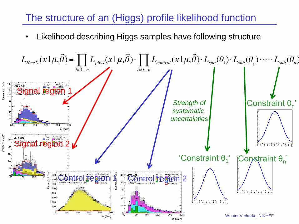
The structure of an (Higgs) profile likelihood function
• Likelihood describing Higgs samples have following structure
Wouter Verkerke, NIKHEF
Signal region 1
Signal region 2
Control region 1 Control region 2
‘Constraint θ1’ ‘Constraint θn’
‘Constraint θn’ Strength of
systematic
uncertainties
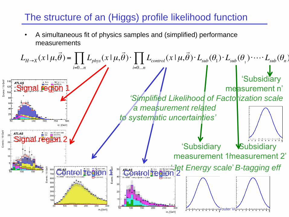
The structure of an (Higgs) profile likelihood function
• A simultaneous fit of physics samples and (simplified) performance
measurements
Wouter Verkerke, NIKHEF
Signal region 1
Signal region 2
Control region 1 Control region 2
‘Simplified Likelihood of
a measurement related
to systematic uncertainties’
‘Subsidiary
measurement 1’
‘Jet Energy scale’
‘Subsidiary
measurement 2’
B-tagging eff
‘Subsidiary
measurement n’
Factorization scale

The Workspace
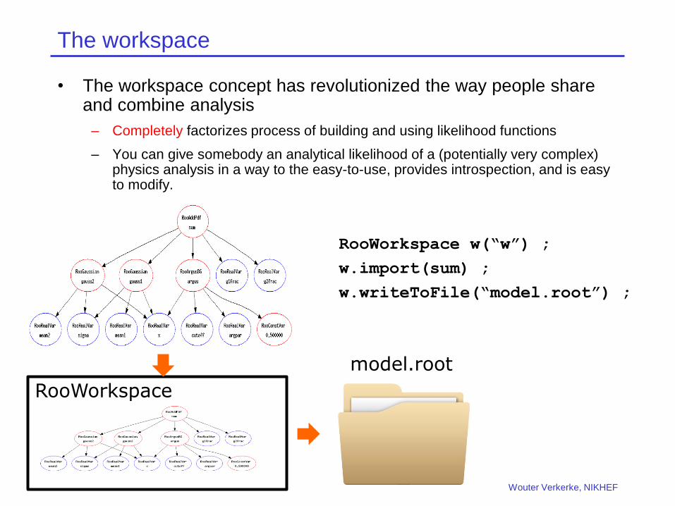
The workspace
• The workspace concept has revolutionized the way people share and combine analysis
– Completely factorizes process of building and using likelihood functions
– You can give somebody an analytical likelihood of a (potentially very complex) physics analysis in a way to the easy-to-use, provides introspection, and is easy to modify.
Wouter Verkerke, NIKHEF
RooWorkspace
RooWorkspace w(“w”) ;
w.import(sum) ;
w.writeToFile(“model.root”) ;
model.root
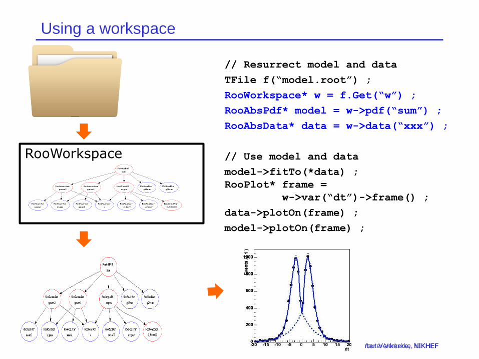
Using a workspace
Wouter Verkerke, NIKHEF Wouter Verkerke, NIKHEF
RooWorkspace
// Resurrect model and data
TFile f(“model.root”) ;
RooWorkspace* w = f.Get(“w”) ;
RooAbsPdf* model = w->pdf(“sum”) ;
RooAbsData* data = w->data(“xxx”) ;
// Use model and data
model->fitTo(*data) ;
RooPlot* frame =
w->var(“dt”)->frame() ;
data->plotOn(frame) ;
model->plotOn(frame) ;
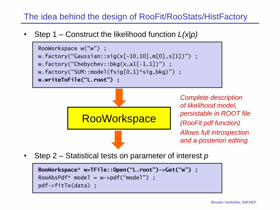
The idea behind the design of RooFit/RooStats/HistFactory
• Step 1 – Construct the likelihood function L(x|p)
• Step 2 – Statistical tests on parameter of interest p
Wouter Verkerke, NIKHEF
RooFit, or RooFit+HistFactory
RooStats
RooWorkspace
Complete description
of likelihood model,
persistable in ROOT file
(RooFit pdf function)
Allows full introspection
and a-posteriori editing
RooWorkspace w(“w”) ;
w.factory(“Gaussian::sig(x[-10,10],m[0],s[1])”) ;
w.factory(“Chebychev::bkg(x,a1[-1,1])”) ;
w.factory(“SUM::model(fsig[0,1]*sig,bkg)”) ;
w.writeToFile(“L.root”) ;
RooWorkspace* w=TFile::Open(“L.root”)->Get(“w”) ;
RooAbsPdf* model = w->pdf(“model”) ;
pdf->fitTo(data) ;
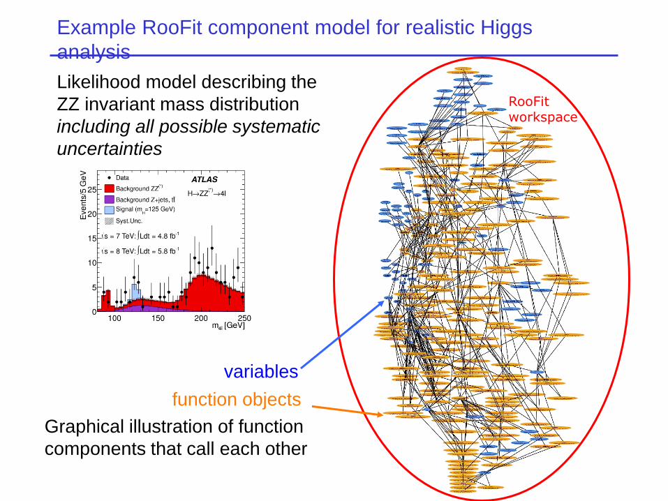
Example RooFit component model for realistic Higgs
analysis
variables
function objects
Graphical illustration of function
components that call each other
Likelihood model describing the
ZZ invariant mass distribution
including all possible systematic
uncertainties
RooFit workspace
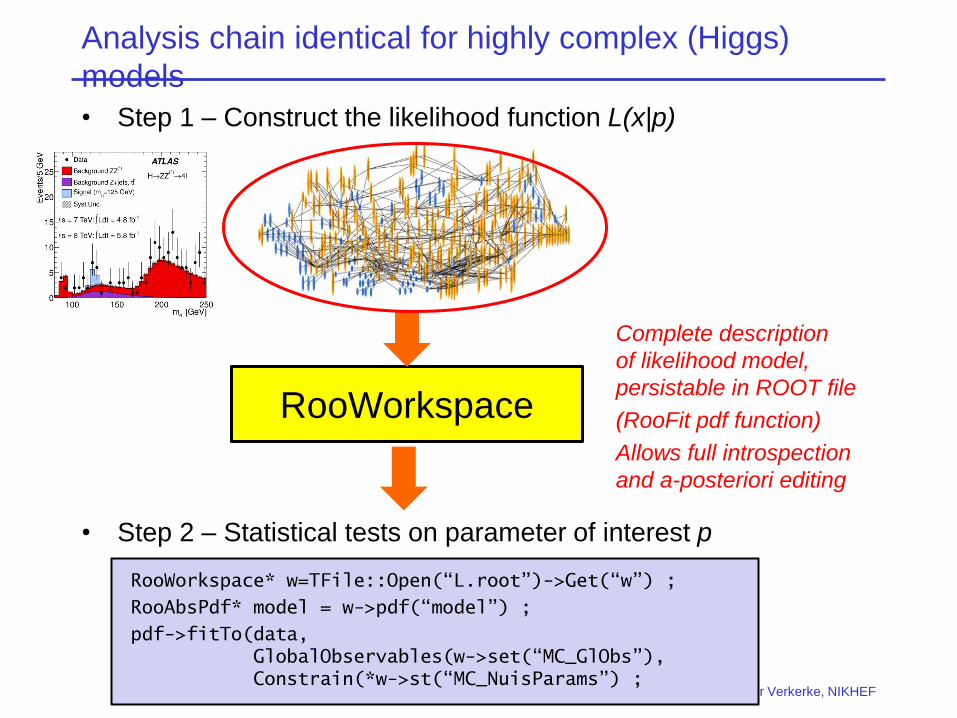
Analysis chain identical for highly complex (Higgs)
models
• Step 1 – Construct the likelihood function L(x|p)
• Step 2 – Statistical tests on parameter of interest p
Wouter Verkerke, NIKHEF
RooStats
RooWorkspace
Complete description
of likelihood model,
persistable in ROOT file
(RooFit pdf function)
Allows full introspection
and a-posteriori editing
RooWorkspace* w=TFile::Open(“L.root”)->Get(“w”) ;
RooAbsPdf* model = w->pdf(“model”) ;
pdf->fitTo(data,
GlobalObservables(w->set(“MC_GlObs”),
Constrain(*w->st(“MC_NuisParams”) ;
Workspaces power collaborative statistical modelling
• Ability to persist complete(*) Likelihood models
has profound implications for HEP analysis workflow
– (*) Describing signal regions, control regions, and including nuisance
parameters for all systematic uncertainties)
• Anyone with ROOT (and one ROOT file with a workspace)
can re-run any entire statistical analysis out-of-the-box
– About 5 lines of code are needed
– Including estimate of systematic uncertainties
• Unprecedented new possibilities for cross-checking results,
in-depth checks of structure of analysis
– Trivial to run variants of analysis (what if ‘Jet Energy Scale uncertainty’ is
7% instead of 4%). Just change number and rerun.
– But can also make structural changes a posteri. For example, rerun with
assumption that JES uncertainty in forward and barrel region of detector are
100% correlated instead of being uncorrelated.
Wouter Verkerke, NIKHEF
Collaborative statistical modelling
• As an experiment, you can effectively build a library of
measurements, of which the full likelihood model is
preserved for later use
– Already done now, experiments have such libraries of workspace files,
– Archived in AFS directories, or even in SVN….
– Version control of SVN, or numbering scheme in directories allows for easy
validation and debugging as new features are added
• Building of combined likelihood models greatly simplified.
– Start from persisted components. No need to (re)build input components.
– No need to know how individual components were built, or are internally
structured. Just need to know meaning of parameters.
– Combinations can be produced (much) later than original analyses.
– Even analyses that were never originally intended to be combined with
anything else can be included in joint likelihoods at a later time
Wouter Verkerke, NIKHEF
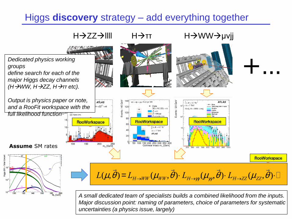
Higgs discovery strategy – add everything together
HZZllll Hττ HWWμνjj
+…
Assume SM rates
L(m,q ) = LH®WW (mWW ,q ) ×LH®gg (mgg ,q ) ×LH®ZZ (mZZ,q ) ×…
Dedicated physics working
groups
define search for each of the
major Higgs decay channels
(HWW, HZZ, Hττ etc).
Output is physics paper or note,
and a RooFit workspace with the
full likelihood function
A small dedicated team of specialists builds a combined likelihood from the inputs.
Major discussion point: naming of parameters, choice of parameters for systematic
uncertainties (a physics issue, largely)
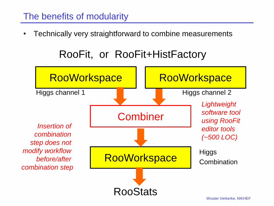
The benefits of modularity
• Technically very straightforward to combine measurements
Wouter Verkerke, NIKHEF
RooFit, or RooFit+HistFactory
RooStats
RooWorkspace RooWorkspace
RooWorkspace
Higgs channel 1 Higgs channel 2
Combiner
RooStats
Higgs
Combination
Lightweight
software tool
using RooFit
editor tools
(~500 LOC)
Insertion of
combination
step does not
modify workflow
before/after
combination step
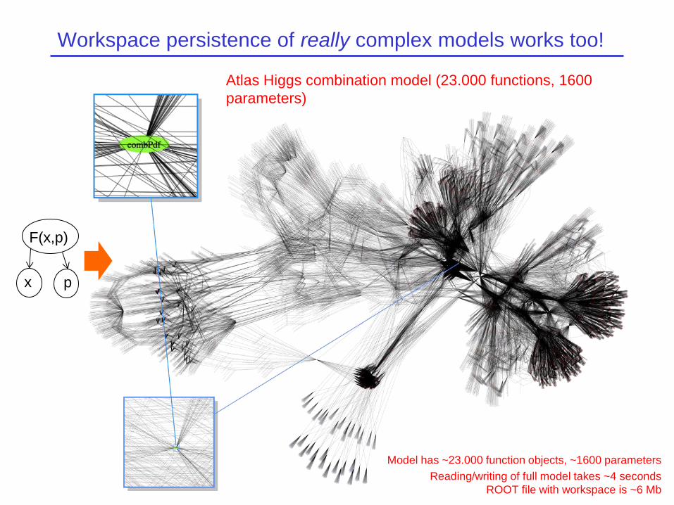
Workspace persistence of really complex models works too!
F(x,p)
x p
Atlas Higgs combination model (23.000 functions, 1600
parameters)
Model has ~23.000 function objects, ~1600 parameters
Reading/writing of full model takes ~4 seconds
ROOT file with workspace is ~6 Mb
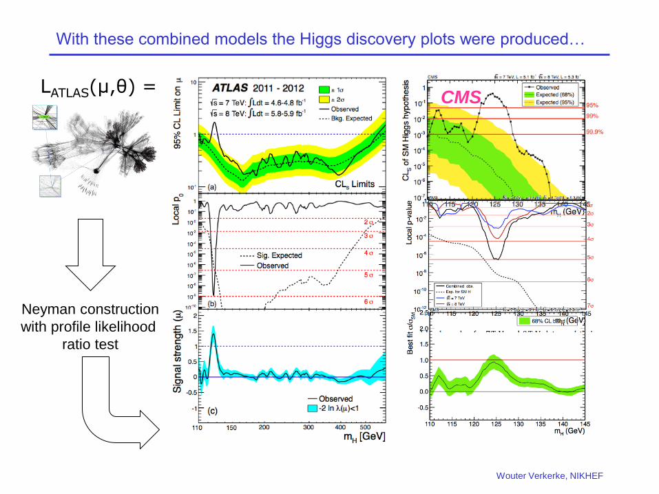
With these combined models the Higgs discovery plots were produced…
Wouter Verkerke, NIKHEF
LATLAS(μ,θ) =
Neyman construction
with profile likelihood
ratio test
CMS
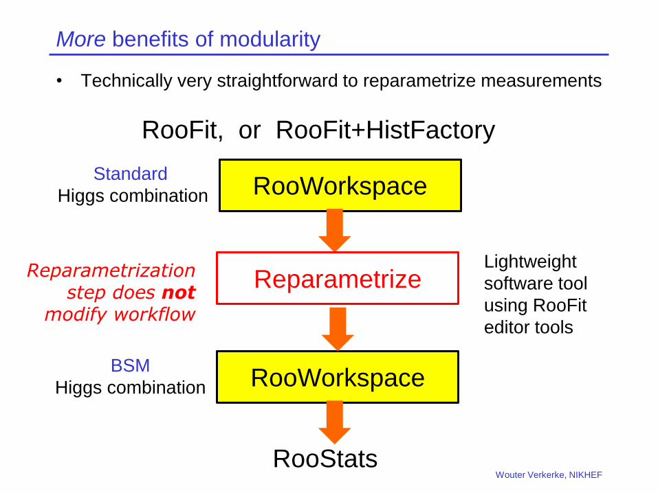
More benefits of modularity
• Technically very straightforward to reparametrize measurements
Wouter Verkerke, NIKHEF
RooFit, or RooFit+HistFactory
RooStats
RooWorkspace
RooWorkspace
Standard
Higgs combination
Reparametrize
RooStats
Lightweight
software tool
using RooFit
editor tools
Reparametrization step does not
modify workflow
BSM
Higgs combination
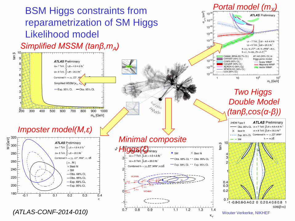
BSM Higgs constraints from
reparametrization of SM Higgs
Likelihood model
Wouter Verkerke, NIKHEF
Simplified MSSM (tanβ,mA)
Imposter model(M,ε)
Minimal composite
Higgs(ξ)
Two Higgs
Double Model
(tanβ,cos(α-β))
Portal model (mX)
(ATLAS-CONF-2014-010)
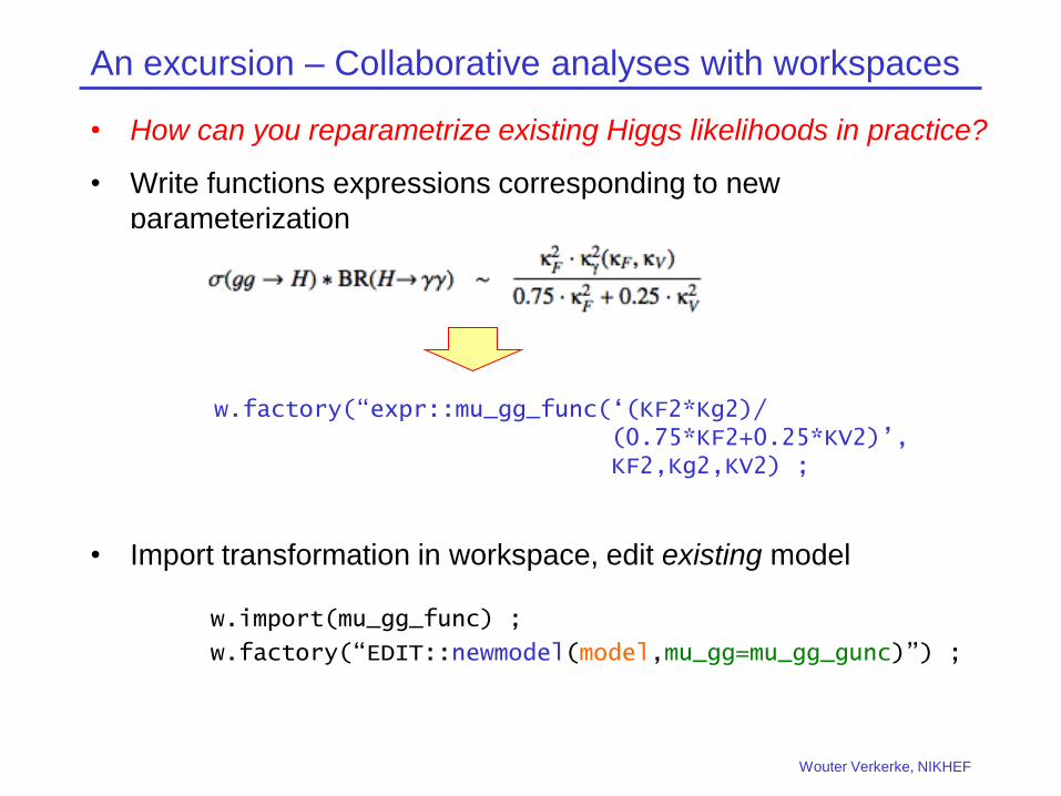
An excursion – Collaborative analyses with workspaces
• How can you reparametrize existing Higgs likelihoods in practice?
• Write functions expressions corresponding to new
parameterization
• Import transformation in workspace, edit existing model
Wouter Verkerke, NIKHEF
w.factory(“expr::mu_gg_func(‘(KF2*Kg2)/ (0.75*KF2+0.25*KV2)’, KF2,Kg2,KV2) ;
w.import(mu_gg_func) ;
w.factory(“EDIT::newmodel(model,mu_gg=mu_gg_gunc)”) ;

HistFactory
K. Cranmer, A. Shibata, G. Lewis, L. Moneta, W. Verkerke (2010)
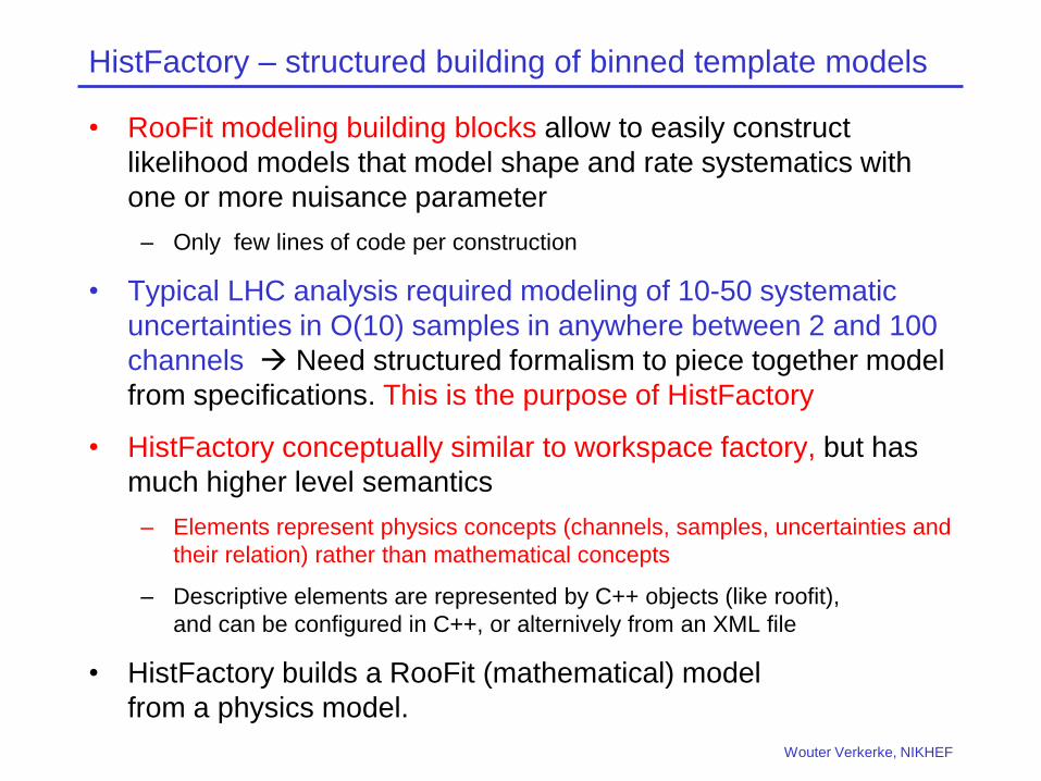
HistFactory – structured building of binned template models
• RooFit modeling building blocks allow to easily construct
likelihood models that model shape and rate systematics with
one or more nuisance parameter
– Only few lines of code per construction
• Typical LHC analysis required modeling of 10-50 systematic
uncertainties in O(10) samples in anywhere between 2 and 100
channels Need structured formalism to piece together model
from specifications. This is the purpose of HistFactory
• HistFactory conceptually similar to workspace factory, but has
much higher level semantics
– Elements represent physics concepts (channels, samples, uncertainties and
their relation) rather than mathematical concepts
– Descriptive elements are represented by C++ objects (like roofit),
and can be configured in C++, or alternively from an XML file
• HistFactory builds a RooFit (mathematical) model
from a physics model.
Wouter Verkerke, NIKHEF
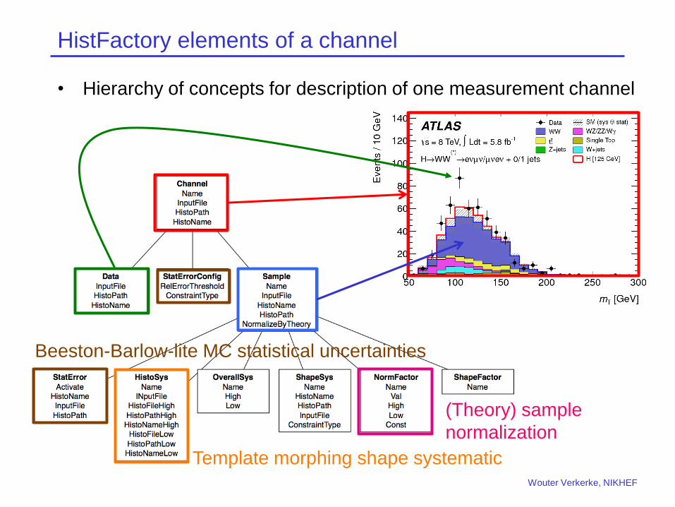
HistFactory elements of a channel
• Hierarchy of concepts for description of one measurement channel
Wouter Verkerke, NIKHEF
(Theory) sample
normalization
Template morphing shape systematic
Beeston-Barlow-lite MC statistical uncertainties
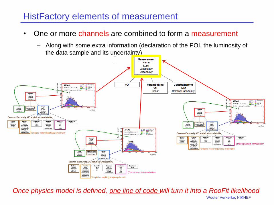
HistFactory elements of measurement
• One or more channels are combined to form a measurement
– Along with some extra information (declaration of the POI, the luminosity of
the data sample and its uncertainty)
Wouter Verkerke, NIKHEF
Once physics model is defined, one line of code will turn it into a RooFit likelihood
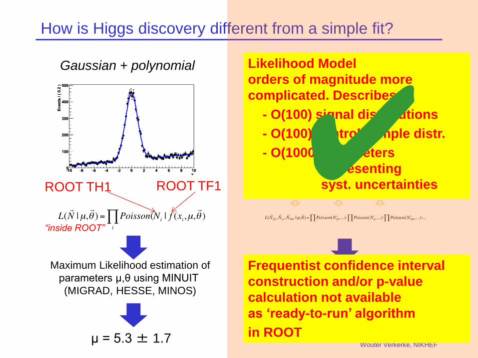
How is Higgs discovery different from a simple fit?
Wouter Verkerke, NIKHEF
Higgs combination model Gaussian + polynomial
ROOT TH1 ROOT TF1
Maximum Likelihood estimation of
parameters μ,θ using MINUIT
(MIGRAD, HESSE, MINOS)
μ = 5.3 ± 1.7
“inside ROOT”
Likelihood Model
orders of magnitude more
complicated. Describes
- O(100) signal distributions
- O(100) control sample distr.
- O(1000) parameters
representing
syst. uncertainties
Frequentist confidence interval
construction and/or p-value
calculation not available
as ‘ready-to-run’ algorithm
in ROOT
✔
RooStats
K. Cranmer, L. Moneta, S. Kreiss, G. Kukartsev, G. Schott, G. Petrucciani, WV - 2008
The benefits of modularity
• Perform different statistical test on exactly the same model
Wouter Verkerke, NIKHEF
RooFit, or RooFit+HistFactory
RooStats
(Frequentist
with toys)
RooWorkspace
RooStats
(Frequentist
asymptotic)
RooStats
Bayesian
MCMC
“Simple fit”
(ML Fit with HESSE or MINOS)
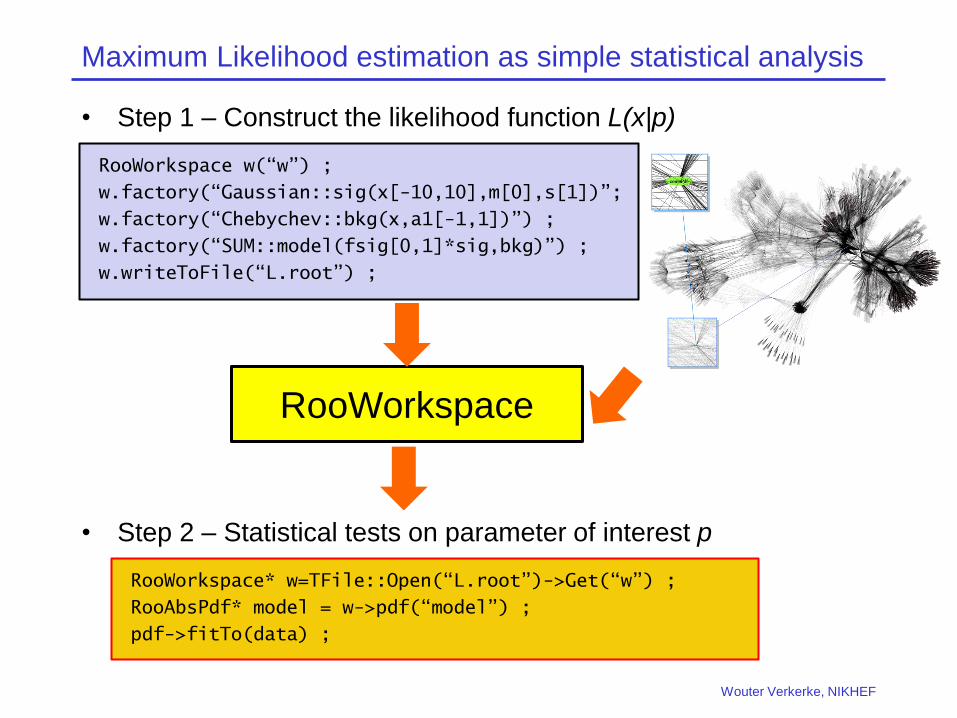
Maximum Likelihood estimation as simple statistical analysis
• Step 1 – Construct the likelihood function L(x|p)
• Step 2 – Statistical tests on parameter of interest p
Wouter Verkerke, NIKHEF
RooStats
RooWorkspace
RooWorkspace w(“w”) ;
w.factory(“Gaussian::sig(x[-10,10],m[0],s[1])”;
w.factory(“Chebychev::bkg(x,a1[-1,1])”) ;
w.factory(“SUM::model(fsig[0,1]*sig,bkg)”) ;
w.writeToFile(“L.root”) ;
RooWorkspace* w=TFile::Open(“L.root”)->Get(“w”) ;
RooAbsPdf* model = w->pdf(“model”) ;
pdf->fitTo(data) ;
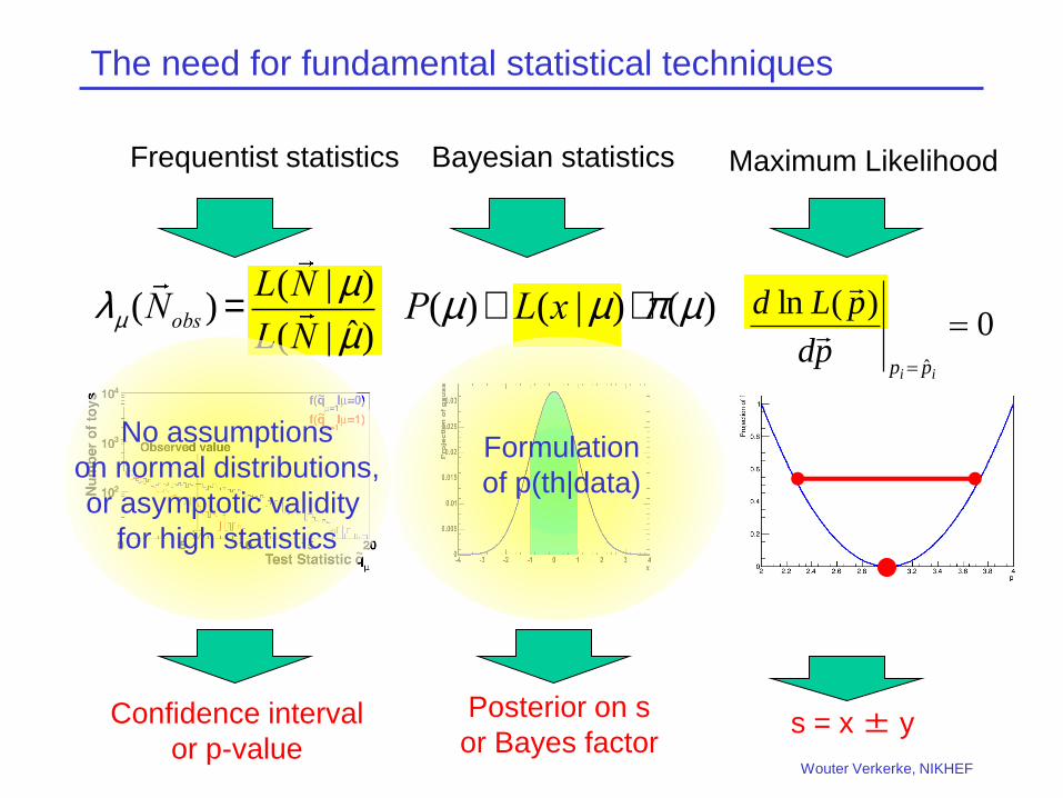
The need for fundamental statistical techniques
Wouter Verkerke, NIKHEF
Frequentist statistics
Confidence interval
or p-value
Posterior on s
or Bayes factor s = x ± y
Bayesian statistics Maximum Likelihood
lm (Nobs ) =L(N | m)
L(N | m̂)P(m)µL(x |m) ×p(m)
0)(ln
ˆ
ii pp
pd
pLd
No assumptions
on normal distributions,
or asymptotic validity
for high statistics
Formulation
of p(th|data)
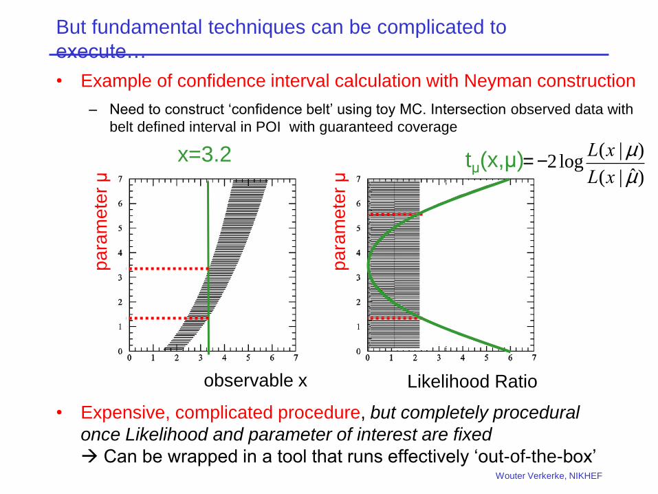
But fundamental techniques can be complicated to
execute…
• Example of confidence interval calculation with Neyman construction
– Need to construct ‘confidence belt’ using toy MC. Intersection observed data with
belt defined interval in POI with guaranteed coverage
• Expensive, complicated procedure, but completely procedural
once Likelihood and parameter of interest are fixed
Can be wrapped in a tool that runs effectively ‘out-of-the-box’
Wouter Verkerke, NIKHEF
x=3.2
observable x
pa
ram
ete
r μ
tμ(x,μ)
Likelihood Ratio
pa
ram
ete
r μ
= -2 logL(x | m)
L(x | m̂)
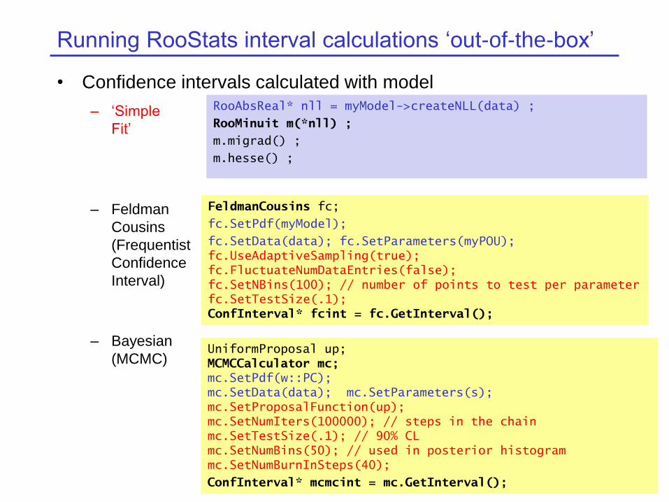
Running RooStats interval calculations ‘out-of-the-box’
• Confidence intervals calculated with model
– ‘Simple
Fit’
– Feldman
Cousins
(Frequentist
Confidence
Interval)
– Bayesian
(MCMC)
Wouter Verkerke, NIKHEF
FeldmanCousins fc;
fc.SetPdf(myModel);
fc.SetData(data); fc.SetParameters(myPOU);
fc.UseAdaptiveSampling(true);
fc.FluctuateNumDataEntries(false);
fc.SetNBins(100); // number of points to test per parameter
fc.SetTestSize(.1);
ConfInterval* fcint = fc.GetInterval();
UniformProposal up;
MCMCCalculator mc;
mc.SetPdf(w::PC);
mc.SetData(data); mc.SetParameters(s);
mc.SetProposalFunction(up);
mc.SetNumIters(100000); // steps in the chain
mc.SetTestSize(.1); // 90% CL
mc.SetNumBins(50); // used in posterior histogram
mc.SetNumBurnInSteps(40);
ConfInterval* mcmcint = mc.GetInterval();
RooAbsReal* nll = myModel->createNLL(data) ;
RooMinuit m(*nll) ;
m.migrad() ;
m.hesse() ;
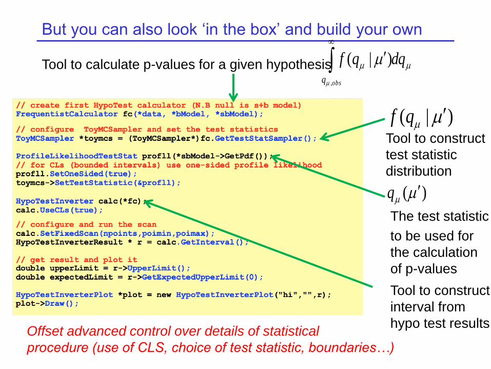
But you can also look ‘in the box’ and build your own
Tool to calculate p-values for a given hypothesis
Tool to construct
interval from
hypo test results
The test statistic
to be used for
the calculation
of p-values
)(q
dqqf
obsq
,
)|(
)|( qf
Tool to construct
test statistic
distribution
Offset advanced control over details of statistical
procedure (use of CLS, choice of test statistic, boundaries…)
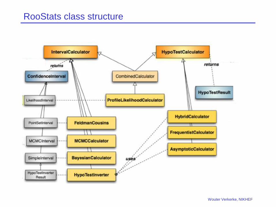
RooStats class structure
Wouter Verkerke, NIKHEF
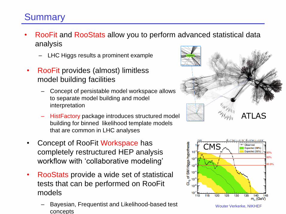
Summary
• RooFit and RooStats allow you to perform advanced statistical data
analysis
– LHC Higgs results a prominent example
Wouter Verkerke, NIKHEF
• RooFit provides (almost) limitless
model building facilities
– Concept of persistable model workspace allows
to separate model building and model
interpretation
– HistFactory package introduces structured model
building for binned likelihood template models
that are common in LHC analyses
• Concept of RooFit Workspace has
completely restructured HEP analysis
workflow with ‘collaborative modeling’
• RooStats provide a wide set of statistical
tests that can be performed on RooFit
models
– Bayesian, Frequentist and Likelihood-based test
concepts
CMS
ATLAS
The future - physics
• Many more high-profile RooFit/RooStats full likelihood
combinations in the works
– Combination of ATLAS and CMS Higgs results
– CMS/LHC combination of rare B-decays
• But many more combinations are easily imaginable & feasible
– Combination across physics domains (e.g. SUSY and Higgs, or Exotics and
Higgs) reparametrization allows to constrain parameters of BSM physics
models that have features in both domains (e.g. 2 Higgs Doublet Models)
– Incorporation of more sophisticated models for detector performance
measurements (now often simple Gaussians).
Many ideas ongoing (e.g eigenvector diagonalization of calibration
uncertainties across pT bins less parameters with correlated subsidiary
measurement), modeling of correlated effects between systematic
uncertainties (e.g. Jet energy scales and flavor tagging)
Wouter Verkerke, NIKHEF
The future - computing
• Technical scaling and performance generally unproblematic
– MINUIT has been shown to still work with 10.000 parameters, but do you really need so much detail?
– Persistence works miraculously well, given complexity of serialization problem
– Algorithmic optimization of likelihood calculations works well
– Likelihood calculations trivially parallelizable. But more work can be done here (e.g. portability of calculations to GPUs, taking advantage of modern processor architectures for vectorization)
– Bayesian algorithms still need more development and tuning
• But physicists are very good and pushing performance and scalability to the limits
– Generally, one keep adding features and details until model becomes ‘too slow’
– But if every Higgs channel reaches this point on its own, a channel combination is already ‘way too slow’ from the onset
– Need to learn how to limit complexity Prune irrelevant details from physics models, possibly a posteriori. Work in progress, some good ideas around
• Looking forward to LHC Run-2
Wouter Verkerke, NIKHEF