THESIS_H_CLILVERD.pdf - UCL Discovery
388
1 HYDROECOLOGICAL MONITORING AND MODELLING OF RIVER-FLOODPLAIN RESTORATION IN A UK LOWLAND RIVER MEADOW By Hannah Marie Clilverd UCL A thesis submitted for the degree of Doctor of Philosophy
-
Upload
khangminh22 -
Category
Documents
-
view
2 -
download
0
Transcript of THESIS_H_CLILVERD.pdf - UCL Discovery

1
HYDROECOLOGICAL MONITORING AND MODELLING OF RIVER-FLOODPLAIN RESTORATION IN A UK LOWLAND
RIVER MEADOW
By
Hannah Marie Clilverd
UCL
A thesis submitted for the degree of Doctor of Philosophy

2
SIGNED DECLARATION
I, Hannah Marie Clilverd confirm that the work presented in
this thesis is my own. Where information has been derived
from other sources, I confirm that this has been indicated in
the thesis.

3
ABSTRACT
Channelization and embankment of rivers has led to major ecological
degradation of aquatic habitats worldwide. River restoration can be used to
restore favourable hydrological conditions for target processes or species.
This study is based on rarely available, detailed pre- and post-restoration
hydrological data collected from 2007–2010 from a wet grassland meadow in
Norfolk, UK. Based on these data, coupled hydrological/hydraulic models
were developed of pre-embankment and post-embankment conditions using
the MIKE-SHE/MIKE-11 system. Fine-scale plant and chemical sampling
was conducted on the floodplain meadow to assess the spatial pattern of
plant communities in relation to soil physicochemical conditions. Simulated
groundwater levels for a 10-year period were then used to predict changes in
plant community composition following embankment-removal. Hydrology was
identified as the primary driver of plant community composition, while soil
fertility was also important. Embankment removal resulted in widespread
floodplain inundation at high river flows and frequent localised flooding at the
river edge at lower flows. Subsequently, groundwater levels were higher and
subsurface storage was greater. The restoration had a moderate effect on
flood-peak attenuation and improved free drainage to the river.
Reinstatement of overbank flows did not substantially affect the degree of
aeration stress on the meadow, except along the river embankments where
sum exceedance values for aeration stress increased from 0 m weeks (dry-
grassland) to 7 m weeks (fen). The restored groundwater regime may be
suitable for more diverse plant assemblages. However the benefits of
flooding (e.g. propagule dispersal, reduced competition) may be over-ridden
without management to reduce waterlogging during the growing season, or
balance additional nutrient supply from river water. The results from this
study suggest that removal of river embankments can increase river-
floodplain hydrological connectivity to form a more natural flood-pulsed
wetland ecotone, which favours conditions for enhanced flood storage, plant
species composition and nutrient retention.

4
ACKNOWLEDGEMENTS
I would like to thank my adviser Julian Thompson, for his input, insight and
support throughout my graduate career at UCL. In addition, I would like to
thank the other members of my committee, Carl Sayer, Kate Heppell, and
Jan Axmacher, whose ideas and guidance were invaluable. I would like to
thank my family particularly my partner, Dayton Dove, who provided endless
love and encouragement, and my children, Rowan and Annabel, who
provided laughter and diversion, and my parents Karen and Anthony who
inspired in me a love of the natural environment.
Funding and other support for this study was provided by the Environment
Agency, UCL Department of Geography, University of London Central
Research Fund Grant, and the UCL Graduate School. I thank Ross Haddow
and Adel MacNicol of the Stody Estate for their practical support and
encouragement, Richard Hey for designing the river restoration, the River
Glaven Conservation Group, Environment Agency, Wild Trout Trust, and
Natural England for their technical support during the embankment removal.
Special thanks are extended to Tony Leach, Derek Sayer, Chabungbam
Rajagopal Singh, Victoria Sheppard and Helene Burningham for their
assistance in the field, and Simon Dobinson, Laura Shotbolt, Charlie
Stratford, and Ian Patmore for assistance in the laboratory.

5
TABLE OF CONTENTS
TITLE PAGE .................................................................................... 1
SIGNED DECLARATION ................................................................. 2
ABSTRACT ...................................................................................... 3
ACKNOWLEDGEMENTS ................................................................. 4
TABLE OF CONTENTS ................................................................... 5
LIST OF TABLES ........................................................................... 10
LIST OF FIGURES ......................................................................... 12
Chapter 1: River-floodplain habitats and functions ......................... 20
1.1 Introduction .............................................................................................. 20
1.2 Research rationale, aims and objectives ................................................. 23
1.3. Thesis structure ...................................................................................... 26
Chapter 2: Hydrological, chemical, and ecological characteristics
of floodplain environments .............................................................. 29
2.1 Introduction .............................................................................................. 29
2.2 Floodplain and riparian zone hydrology ................................................... 29
2.2.1 Conceptual models of floodplain and riparian zone hydrology .......... 29
2.2.2 The hyporheic zone .......................................................................... 35
2.2.3 Hydrological connectivity and its importance .................................... 36
2.3 Riparian zone biogeochemistry ............................................................... 45
2.3.1 Biogeochemical transformations in riparian sediments ..................... 45
2.3.2 Nitrogen and phosphorus biogeochemistry....................................... 47
2.3.3 Water quality functions and management of floodplains ................... 50
2.4 Riparian zone community composition .................................................... 54
2.4.1 The effects of waterlogging on plant community-composition ........... 54
2.4.2 Fertilisation of riparian zones ............................................................ 60
2.4.3 Grazing impacts on plant diversity .................................................... 64
2.4.4 Flooding disturbance and propagule dispersal ................................. 66
2.4.5 Human pressures on lowland wet grasslands ................................... 68
2.4.6 Management of lowland hay meadows ............................................. 70

6
2.5 River regulation, and restoration ............................................................. 71
2.5.1 Channel modification ........................................................................ 71
2.5.2. Restoration techniques .................................................................... 74
2.6 Hydrological modelling ............................................................................ 79
2.6.1 Model classification and representation of hydrological processes ... 79
2.6.2 Surface water-groundwater modelling and river restoration .............. 88
2.7 Conclusions ............................................................................................. 94
Chapter 3: The River Glaven and Hunworth Meadow ..................... 95
3.1 Introduction .............................................................................................. 95
3.2 Location and climatology ......................................................................... 95
3.3 Geology of the River Glaven catchment ................................................ 100
3.4 Surface water quality ............................................................................. 105
3.5 Flora, fauna, and conservation value of the River Glaven ..................... 106
3.6 Modification of the River Glaven and land management at Hunworth
Meadow ....................................................................................................... 110
3.7 The River Glaven restoration project ..................................................... 114
Chapter 4: Methods Part I – hydrological and chemical monitoring117
4.1 Introduction ............................................................................................ 117
4.2 Study design .......................................................................................... 117
4.3. Hydrological monitoring ........................................................................ 123
4.3.1 Groundwater and surface water levels ........................................... 123
4.3.2 Base flow index and flow exceedance values ................................. 124
4.3.3 Evapotranspiration .......................................................................... 124
4.3.4 Hydraulic conductivity ..................................................................... 128
4.4 River-floodplain biogeochemical monitoring .......................................... 132
4.4.1 Soil structural and physical properties ............................................ 132
4.4.2 Water chemistry sampling and analysis .......................................... 133
4.4.3 Oxygen concentration in soil pores ................................................. 134
4.4.4 River and floodplain topography ..................................................... 137
4.5 Flood prediction ..................................................................................... 139
4.5.1 Bankfull capacity ............................................................................. 139
4.4.2 Recurrence intervals ....................................................................... 147

7
4.6 Statistical analyses ................................................................................ 148
4.6.1 Linear regression models and diagnostics tests ............................. 148
Chapter 5: The hydrology and biogeochemistry of the embanked
and restored floodplain meadow ................................................... 149
5.1. Introduction ........................................................................................... 149
5.2. Results ................................................................................................. 149
5.2.1 River embankments ........................................................................ 149
5.2.2 Climate and hydrology .................................................................... 152
5.2.3 Soil physical and chemical properties ............................................. 159
5.2.4 Bankfull capacity ............................................................................. 162
5.2.5 Groundwater response to embankment removal ............................ 166
5.2.6 Hydrological controls on chemistry ................................................. 168
5.3 Discussion ............................................................................................. 175
5.3.1 River-floodplain hydrological linkages ............................................. 175
5.3.2 Floodplain ecohydrology ................................................................. 178
Chapter 6: Methods – Part II: Hydrological/hydraulic modelling .... 180
6.1 Introduction ............................................................................................ 180
6.2 MIKE SHE model development ............................................................. 180
6.2.1 Model domain and topography ....................................................... 180
6.2.2 Hydrological and climate data ......................................................... 186
6.2.3 Overland flow .................................................................................. 193
6.2.4 Unsaturated zone ........................................................................... 194
6.2.5 Saturated zone ............................................................................... 198
6.2.6 Boundary conditions ....................................................................... 201
6.2.7 Simulation specification .................................................................. 203
6.3 MIKE 11 model development ................................................................ 204
6.3.1 River channel and ditch network ..................................................... 204
6.3.2 Specification of hydrodynamic parameters ..................................... 209
6.4 Model calibration and parameter optimisation ....................................... 212
6.4.1 Sensitivity analysis .......................................................................... 212
6.4.2 Model calibration and validation ...................................................... 216
6.5 Impact assessment of embankment removal ........................................ 220

8
Chapter 7: Coupled hydrological/hydraulic modelling of river
restoration and floodplain hydrodynamics .................................... 229
7.1 Introduction ............................................................................................ 229
7.2 Results .................................................................................................. 229
7.2.1 Model calibration and validation ...................................................... 229
7.2.2 Impacts of embankment removal on overbank flows and floodplain
inundation ................................................................................................ 236
7.2.3 Impacts of embankment removal on groundwater .......................... 243
7.2.4 Impacts of embankment removal on groundwater flowpaths .......... 247
7.2.5 Impacts of embankment removal on floodplain storage and flood-
peak attenuation ...................................................................................... 252
7.3 Discussion ............................................................................................. 256
7.3.1 Channel modification ...................................................................... 256
7.3.2 Simulation of floodplain hydrological processes ............................. 257
7.3.3 River-floodplain connectivity ........................................................... 258
7.3.4 Floodplain storage and flood-peak attenuation ............................... 260
7.3.5 Climate ............................................................................................ 261
Chapter 8: Methods – Part III: botanical and soil chemistry data
collection and analysis ................................................................. 263
8.1 Introduction ............................................................................................ 263
8.2 Floodplain plant community composition ............................................... 263
8.2.1 Vegetation composition................................................................... 263
8.2.2 Floodplain topography .................................................................... 265
8.3 Soil physicochemistry ............................................................................ 265
8.3.1 Soil extractable ions ........................................................................ 265
8.3.2 Soil pore water chemistry ................................................................ 267
8.3.3 Analysis of total carbon and nitrogen content in soil ....................... 267
8.3.4 Air-filled porosity ............................................................................. 268
8.3.5 Aeration stress index ...................................................................... 272
8.3.6 Oxygen concentration in soil pores ................................................. 273
8.4 Statistical analyses ................................................................................ 275
8.4.1 Linear regression models and diagnostics tests ............................. 275

9
8.4.2 Multivariate analysis........................................................................ 275
Chapter 9: Simulation of the effects of river restoration on plant
community composition ................................................................ 277
9.1. Results ................................................................................................. 277
9.1.1 Groundwater hydrology and soil moisture gradients ....................... 277
9.1.2 Soil Nutrient Status ......................................................................... 283
9.1.3 Community composition.................................................................. 286
9.1.4 Hydrological modelling outputs ....................................................... 297
9.1.5 Habitat suitability ............................................................................. 301
9.2 Discussion ............................................................................................. 308
9.2.1 Hydrological controls on floodplain processes and plant diversity .. 308
9.2.2 Water regime of the restored floodplain meadow ........................... 311
9.2.3 Predicting plant community composition change ............................ 312
9.2.4 Management implications ............................................................... 315
Chapter 10: Conclusions and recommendations for future
research ....................................................................................... 317
10.1 Conclusions ......................................................................................... 317
10.2 Further research directions .................................................................. 322
10.2.1 Limitations of the study ................................................................. 322
10.2.2 Climate impact studies .................................................................. 328
REFERENCES ............................................................................. 331

10
LIST OF TABLES
Table 2.1: Sequence of microbial redox reactions ............................................ 46
Table 2.2: Characteristics of sheep grazing, cattle grazing and hay cutting in
agriculturally unimproved grasslands ................................................................ 66
Table 3.1: Water chemistry (pH, nitrate, phosphate and dissolved oxygen) of the
River Glaven ................................................................................................... 106
Table 3.2: Water Framework Directive Classifications for the River Glaven ... 109
Table 4.1. Corresponding Environment Agency river discharge and stage .... 141
Table 4.2: Stream morphology of the River Glaven ........................................ 144
Table 4.3: General descriptions and physical criteria for Rosgen’s stream
classification system ....................................................................................... 145
Table 5.1: Mean annual river flow (range), Q10, Q95, and Q95 ..................... 153
Table 5.2: Summer (June − September) mean (± 95% confidence interval) air
temperature, total precipitation, total potential evapotranspiration, and mean
annual river discharge (±95% confidence interval) ......................................... 155
Table 5.3: Hydraulic gradient, hydraulic conductivity and groundwater flow rate
(mean ± 95 % confidence interval) for the well transects ................................ 157
Table 5.4: Soil chemistry of Hunworth Meadow .............................................. 160
Table 5.5. Hydraulic conductivity values for various sediment ........................ 161
Table 5.6: Bankfull height above ODN, bankfull river discharge from the river
stage–discharge relationship, and calculated using Manning’s equation, and
bankfull recurrence interval ............................................................................. 163
Table 5.7: Chemistry of the River Glaven and Hunworth Meadow groundwater
wells ................................................................................................................ 170
Table 6.1 Soil properties of Hunworth Meadow topsoil ................................... 195
Table 6.2: Range of height of capillary rise for Hunworth Meadow ................. 197
Table 6.3: Representative hydraulic conductivity values for various geological
materials ......................................................................................................... 199
Table 6.4: Specific yield for various geological materials ................................ 200

11
Table 6.5: Representative specific storage values for various geological
materials ......................................................................................................... 200
Table 6.6: List of model parameters and their initial, lower and upper limit values
used in the AUTOCAL sensitivity analysis ...................................................... 213
Table 6.7: Scaled sensitivity coefficients for parameter used in the AUTOCAL
sensitivity analysis .......................................................................................... 215
Table 6.8: MIKE SHE and MIKE 11 parameter values for the automatically
calibrated 15 x 15 m grid model ...................................................................... 218
Table 6.9: Final calibrated MIKE SHE and MIKE 11 parameter values .......... 220
Table 6.10: Total annual precipitation at Mannington Hall (<10 km from the
study site) and river discharge at Hunworth from 2001 – 2010 ....................... 221
Table 7.1: Mean error (ME - m), correlation coefficient (R), and Nash-Sutcliffe
model efficiency coefficient (NSE) .................................................................. 235
Table 8.1: Soil chemical extractants ............................................................... 266
Table 9.1: ANOVA and parameter estimates for predicting soil moisture content
........................................................................................................................ 281
Table 9.2: ANOVA and parameter estimates for the reduced soil moisture model
........................................................................................................................ 281
Table 9.3: Soil (n = 113) and pore water (n = 53) chemistry ........................... 284
Table 9.4: Frequency of presence and mean relative percent cover of plant
species on Hunworth Meadow ........................................................................ 287
Table 9.5: Eigenvalues and cumulative percentage variance for each CA axis of
the vegetation data ......................................................................................... 293
Table 9.6: British National Vegetation Classification (NVC) communities ....... 294
Table 9.7: Eigenvalues and cumulative percentage variance for each CCA axis
of the vegetation and environmental data ....................................................... 296
Table 9.8: Temperature and dissolved oxygen concentration measured in soil
pores ............................................................................................................... 302
Table 9.9: Cumulative aeration stress index for plants ................................... 305
Table 10.1: Comparison of river length and sinuosity ..................................... 326

12
LIST OF FIGURES
Figure 2.1: Conceptual model of the basin hydrological cycle .......................... 30
Figure 2.2: The principal kinds of wetlands related to duration and depth of
flooding ............................................................................................................. 33
Figure 2.3: Conceptual hydrogeologic model illustrating varying groundwater
flow systems in riparian zones .......................................................................... 34
Figure 2.4: Conceptual model of the groundwater-surface water interface ....... 36
Figure 2.5: Examples of longitudinal, vertical, and horizontal linkages important
for sustaining healthy river ecosystems ............................................................ 37
Figure 2.6: Variation in bank storage ................................................................ 40
Figure 2.7: Riparian hydraulic gradient and stream‐groundwater exchange
dynamics in a steep headwater valley .............................................................. 42
Figure 2.8: Comparison of flood peak inflow/outflow values for incised and
restored conditions ............................................................................................ 43
Figure 2.9: Upstream and downstream hydrographs for different precipitation
events ............................................................................................................... 45
Figure 2.10: Conceptual model of metabolic processes along subsurface
flowpaths ........................................................................................................... 47
Figure 2.11: Forms and interactions of phosphorus .......................................... 50
Figure 2.12: The percentage of wetlands studied which exhibited reduction and
an increase in N and P loading in riparian zones .............................................. 53
Figure 2.13: Niche space at (a) Tadham and (b) Cricklade .............................. 56
Figure 2.14: Water-regime of each community type ......................................... 59
Figure 2.15: The relationship between redox potential and water table depth .. 60
Figure 2.16: Relationship between nutrient supply ratio (S1/S2) and equilibrium
species richness (SR), evenness (E) and Shannon index (H) .......................... 64
Figure 2.17: Conceptual model showing pathways for water-dispersed
propagules in rivers ........................................................................................... 67
Figure 2.18: The distribution of species-rich lowland wet grasslands (MG4 under
the UK National Vegetation Communities system) in England ......................... 70

13
Figure 2.19: Examples of modifications to river channels ................................. 73
Figure 2.20: Model classification ....................................................................... 80
Figure 2.21: Schematic of MIKE SHE model .................................................... 86
Figure 2.22: Simulated groundwater depth (top two panels) and ditch water level
(bottom two pannels) at four locations within the Elmley Marshes .................... 89
Figure 2.23: Impact of changing weir height upon simulated surface flooding
(top panel), ditch levels (middle panel), and groundwater depth (bottom panel)
within the Elmley Marshes ................................................................................ 90
Figure 2.24: Comparison of simulated and observed groundwater depth at two
piezometer locations within a wet meadow ....................................................... 91
Figure 2.25: Seasonal water table elevation (WTE) differences ....................... 92
Figure 2.26: (a) Precipitation, (b) surface water outflow, (c) downward
groundwater flow between geological layers and (d) upward groundwater flow
between geological layers ................................................................................. 93
Figure 3.1: The River Glaven restoration site at Hunworth, North Norfolk ........ 96
Figure 3.2: Monthly minimum, mean and maximum air temperature for East
Anglia ................................................................................................................ 97
Figure 3.3: Mean total monthly precipitation and potential evapotranspiration
(1985 – 2015) for East Anglia ........................................................................... 97
Figure 3.4: Topography of the River Glaven catchment .................................... 98
Figure 3.5: Chalk outcrops and groundwater divides for regions around South-
East England..................................................................................................... 99
Figure 3.6: Major rivers in North Norfolk ......................................................... 100
Figure 3.7: The glacial structures of the Cromer Ridge ................................... 101
Figure 3.8: Superficial geology of the River Glaven catchment ...................... 103
Figure 3.9: The River Glaven at Hunworth Meadow ....................................... 111
Figure 3.10: Pond at the downstream end of Hunworth Meadow ................... 112
Figure 3.11: Historical maps of the study site at Hunworth Meadow ............... 113
Figure 3.12: Embankment removal work in progress ...................................... 115
Figure 3.13: Photographs of the River Glaven at Hunworth Meadow ............. 116
Figure 4.1: Cross-sections of the embanked river and floodplain ................... 118
14
Figure 4.2: Sampling design at Hunworth Meadow ......................................... 119
Figure 4.3: Photograph of the concrete slab covering Well 2.1 ....................... 120
Figure 4.4: Sampling design at Hunworth Meadow ......................................... 121
Figure 4.5: Photographs of (a) the automatic MiniMet weather station and (b)
the Environment Agency gauging station ........................................................ 122
Figure 4.6: Time series of (a) mean daily air temperature and net solar radiation,
(b) mean daily wind speed, and (c) maximum and minimum relative humidity 127
Figure 4.7: Photograph of the piezometer intakes used in the slug tests ........ 128
Figure 4.8: Diagram of the sand-filled slug ..................................................... 128
Figure 4.9: Typical response in water table height during slug tests at Hunworth
Meadow .......................................................................................................... 129
Figure 4.10: Typical example of the log-linear change in normalized head (h0/h)
following slug removal ..................................................................................... 131
Figure 4.11: Photographs of rhizon soil moisture samplers ............................ 133
Figure 4.12: Clockwise from top of the photograph, dataloggers, position of the
oxygen optodes (protected in plastic containers), and varying depths of the
tensiometers ................................................................................................... 136
Figure 4.13: Photographs of the differential Global Positioning ...................... 138
Figure 4.14: Location of dGPS sample points for the embanked (a) and restored
(b) topographic surveys .................................................................................. 138
Figure 4.15: Relationship between river stage and mean daily river discharge
used to determine bankfull capacity ................................................................ 140
Figure 4.16: Photographs reflecting the different in-river macrophyte abundance
during the winter (a) and summer (b) months ................................................. 141
Figure 4.17: Photographs reflecting the different in-river macrophyte abundance
during a wet (a) and dry (b) summer ............................................................... 142
Figure 4.18: Water surface elevation of the River Glaven at Hunworth .......... 144
Figure 4.19: River bed substrate composition ................................................. 146
Figure 4.20: Bankfull roughness coefficients by stream type .......................... 147
Figure 5.1: Comparison of floodplain elevation adjacent to the river channel and
thalweg (lowest point along the river bed) ....................................................... 150

15
Figure 5.2: Elevation of Hunworth Meadow study site .................................... 151
Figure 5.3: Mean daily total river flow and base flow from 2002 to 2010 ........ 153
Figure 5.4. Flow duration curve (a), and mean daily river discharge (b) ......... 154
Figure 5.5: Temporal variation in (a) mean daily river discharge and total daily
precipitation, and (b) representative mean daily groundwater depth ............... 156
Figure 5.6: Cross-sections of the meadow and river channel ......................... 158
Figure 5.7: Textural triangle of soils ................................................................ 159
Figure 5.8: A portrayal of the soil horizons on Hunworth meadow .................. 161
Figure 5.9: Decline in normalised head (head ratio) for all hydraulic conductivity
tests ................................................................................................................ 162
Figure 5.10: Time series of (a) total precipitation, and (b) mean daily river
discharge ........................................................................................................ 164
Figure 5.11: Recurrence interval (return period in years) of various river
discharges on the River Glaven ...................................................................... 165
Figure 5.12: Photographs of the same location on the River Glaven during
differing river flows (a) before and (b)after embankment removal ................... 166
Figure 5.13: Temporal variation in mean daily groundwater height above
Ordnance Datum Newlyn ................................................................................ 167
Figure 5.14: Ternary plot of base cation chemistry ......................................... 169
Figure 5.15: Spatial variation of selected ions (mean ± 95% confidence interval;
log scale) along subsurface flowpaths ............................................................ 171
Figure 5.16: Nitrate and DO concentrations .................................................... 173
Figure 5.17: Temporal variation in (a) temperature and (b) DO concentration in
well water and soil in relation to (c) changes in groundwater height ............... 174
Figure 6.1: Cross-sections and photographs of the river and floodplain
topography ...................................................................................................... 181
Figure 6.2: Digital elevation models used in MIKE SHE ................................. 182
Figure 6.3: Digital elevation models of the (a) embanked and (b) restored
sections of the study meadow ......................................................................... 183
Figure 6.4: Comparison of absolute error for different interpolation methods . 184

16
Figure 6.5: Loss of topographic resolution with increased interpolation grid size
........................................................................................................................ 186
Figure 6.6: Comparison of level logger and hand measurements of groundwater
elevation at the Upstream Well Transect ........................................................ 188
Figure 6.7: Comparison of level logger and hand measurements of groundwater
elevation at the Midstream Well Transect ....................................................... 189
Figure 6.8: Comparison of level logger and hand measurements of groundwater
elevation at the Downstream Well Transect .................................................... 190
Figure 6.9: Spatial classification of land use ................................................... 191
Figure 6.10: Leaf area index and rooting depth values ................................... 192
Figure 6.11: Spatial extent of water bodies in MIKE SHE domain .................. 194
Figure 6.12: Relationship between hydraulic conductivity and D10 of granular
soils ................................................................................................................. 197
Figure 6.13: Boundary conditions of the MIKE SHE model ............................. 202
Figure 6.14: Spatial distribution of drainage codes used in the MIKE SHE
models ............................................................................................................ 203
Figure 6.15: An example of MIKE 11 river branches with H points and the
corresponding river links in a MIKE SHE model.............................................. 205
Figure 6.16: Delineation of the MIKE 11 River Glaven channel and location of
cross-sections ................................................................................................. 206
Figure 6.17: MIKE 11 cross-sections for the (a) embanked and (b) restored
river-banks ...................................................................................................... 207
Figure 6.18: MIKE 11 ditch cross-sections ...................................................... 208
Figure 6.19: Water levels in (a) Well 1.4 and (b) the adjacent ditch ................ 209
Figure 6.20: Time series of variable Manning’s n values used in the MIKE 11
model .............................................................................................................. 211
Figure 6.21: Spatial distribution of floodcodes in the pre-restoration MIKE SHE
model .............................................................................................................. 212
Figure 6.22: Increase in elevation absolute error with grid size ...................... 217

17
Figure 6.23 (a) Time series of mean daily air temperature at Hunworth Meadow
and Mannington Hall, and (b) relationship between air temperature at
Mannington Hall and Hunworth. ...................................................................... 222
Figure 6.24: (a) Time series of total daily precipitation at Hunworth Meadow and
Mannington Hall, and (b) relationship between precipitation at Mannington Hall
and Hunworth. ................................................................................................. 223
Figure 6.25: Simple linear regression between river discharge at Bayfield and
Hunworth gauging stations ............................................................................. 224
Figure 6.26: Time series of mean daily discharge on the River Glaven .......... 226
Figure 6.27: Time series of mean annual rainfall (a) and air temperature (b) for
East Anglia ...................................................................................................... 227
Figure 6.28: Time series of mean seasonal rainfall for the region of East Anglia,
England ........................................................................................................... 228
Figure 7.1: Comparison of observed and modelled groundwater depths for the
calibration and validation periods at the upstream well transect ..................... 231
Figure 7.2: Comparison of observed and modelled groundwater depths for the
calibration and validation periods at the midstream well transect ................... 232
Figure 7.3: Comparison of observed and modelled groundwater depths for the
calibration and validation periods at the midstream well transect ................... 233
Figure 7.4: Comparison of observed ditch water levels and MIKE SHE-simulated
groundwater levels in the ditch........................................................................ 236
Figure 7.5: River stage-discharge relationships from MIKE 11 outputs for the
embanked scenario ......................................................................................... 237
Figure 7.6: River stage-discharge relationships from MIKE 11 outputs for the
restored scenario ............................................................................................ 238
Figure 7.7: Mean daily river discharge from 2001 – 2010 ............................... 241
Figure 7.8: Comparison of simulated surface water extent and depth for the
embanked and restored scenarios .................................................................. 242
Figure 7.9: Simulated time series of water table elevation (WTE) differences
between the restored and embanked scenarios ............................................. 244

18
Figure 7.10: Comparison of simulated groundwater elevation (ODN) at well 1.1
and river stage (ODN) for the (a) embanked and (b) restored scenarios from
2001 – 2010. ................................................................................................... 246
Figure 7.11: Boxplots of simulated groundwater elevation in relation to surface
topography ...................................................................................................... 248
Figure 7.12: Simulated groundwater elevation and flow direction ................... 249
Figure 7.13: Time series of simulated post-restoration groundwater levels .... 250
Figure 7.14: Simulated exchange flow between the saturated zone and river 251
Figure 7.15: Times series of change in (a) overland and (b) subsurface storage
for the embanked and restored scenarios ....................................................... 253
Figure 7.16: Annual evapotranspiration (ET) rates ......................................... 254
Figure 7.17: Comparison of modelled mean daily river inflow and outflow ..... 255
Figure 7.18: Comparison of modelled hourly river inflow versus outflow ........ 256
Figure 8.1: Photograph of Hunworth Meadow showing the multiple layers of
vegetation ....................................................................................................... 264
Figure 8.2: Soil water release characteristic ................................................... 269
Figure 8.3: Relative shrinkage of the soil versus soil water content ................ 271
Figure 8.4: Relationship between water table depth below the soil surface
(tension) and air-filled porosity ........................................................................ 272
Figure 9.1: Water table duration curves derived from mean daily water table
depth ............................................................................................................... 279
Figure 9.2: Correlations between (a) surface elevation on the meadow and
water content of the soil (y = -23.301x + 523.45); (b) organic matter content (log
transformed) and soil water content (y = 72.8504x + -34.79), and (c) surface
elevation and organic matter content (log transformed) (y = -0.217 + 5.533). 280
Figure 9.3: Spatial variation in (a) elevation and (b) soil water content ........... 282
Figure 9.4: Spatial differences in plant available Olson P, ammonium and nitrate
across Hunworth Meadow .............................................................................. 285
Figure 9.5: Spatial differences in plant available potassium, and TOC and TON
across Hunworth Meadow .............................................................................. 285
Figure 9.6: Species richness and Shannon Diversity Index ............................ 289

19
Figure 9.7: Spatial patterns of species richness and Shannon Diversity Index289
Figure 9.8: (a) Correspondence Analysis (CA) of the vegetation data showing
(a) the embankment, middle meadow and ditch sample points (n=195) and (b)
the associated species (n=80) ........................................................................ 291
Figure 9.9: Correspondence Analysis (CA) of the vegetation data ................. 292
Figure 9.10: Constrained Canonical Correspondence Analysis (CCA) of species
composition on environmental variables ......................................................... 295
Figure 9.11: Spatial variation in Ellenberg’s indicator values for plant species
tolerance of moisture (a) and nitrogen (b) ....................................................... 297
Figure 9.12: Comparison of average water table depth for the embanked and
restored scenarios .......................................................................................... 299
Figure 9.13: Comparison of simulated water table depth relative to the soil
surface for the restored and embanked scenarios .......................................... 300
Figure 9.14: Relationship between mean daily dissolved oxygen (DO)
concentration in soil and mean daily water table (WT) depth .......................... 303
Figure 9.15: Comparison of sum exceedance values for aeration stress (SEVas)
for the embanked and restored scenarios ....................................................... 306
Figure 9.16: Post-restoration mean groundwater height for three representative
locations across the meadow .......................................................................... 307
Figure 10.1: A schematic representation of the hydrological regime of Hunworth
Meadow in the (a) embanked and (b) restored scenarios during three river flow
conditions. ....................................................................................................... 319
Figure 10.2: Photographs of the River Glaven at Hunworth Meadow ............. 325
Figure 10.3: Re-meandered river channel at Hunworth Meadow .................... 326
Figure 10.4: Comparison of river depth before and after the two stages of
restoration ....................................................................................................... 327

Chapter 1: River-floodplain habitats and functions
20
Chapter 1: River-floodplain habitats and functions
1.1 Introduction
Natural riparian river-floodplain ecosystems are strongly influenced by
disturbances due to regular flooding events (Poff et al. 1997; Naiman and
Décamps 1997; Stanford 2002). They form highly dynamic ecotones (i.e.
transitional zones) between terrestrial and aquatic environments that are
characterized by high habitat heterogeneity, primary productivity and
biodiversity (Grevilliot et al. 1998; Ward 1998; Gowing et al. 2002a, Woodcock
et al. 2005). These conditions are driven by the strong hydrological connections
between rivers and their floodplains. These in turn facilitate the exchange of
water, sediments, organic matter and nutrients that are fundamental in shaping
floodplain structure (e.g. plant community assemblages) and function (e.g.
riparian production and nutrient retention) (Triska et al. 1989; Ward and
Stanford 1995; Poff et al. 1997; Grevilliot et al. 1998; Pringle 2003). In floodplain
habitats, fluctuations in the soil water regime, associated with strong exchanges
of water with the adjacent river, are important for the creation of a dynamic and
varying physical environment (Poff et al. 1997; Robertson et al. 2001). This
variety exerts a strong influence upon species composition, and the creation
and maintenance of high biodiversity in floodplain habitats (Ward 1998;
Freeman et al. 2007).
Lowland wet grassland, the habitat type that characterises the site investigated
in this thesis, is defined as grassland growing at sites below 200 m that is
subject to periodic freshwater flooding or waterlogging (Jefferson and Grice
1998). A wet grassland’s hydrological regime is one of the most important
factors determining the plant communities that are present (Gowing et al. 1998;
Silvertown et al. 1999; Castelli et al. 2000; Kennedy et al. 2003; Dwire et al.
2006; Araya et al. 2011). Most commonly, the vegetation structure of floodplain

Chapter 1: River-floodplain habitats and functions
21
grasslands is influenced by variations in water table depth and by the
magnitude-frequency characteristics of flood events (Poff et al. 1997). These in
turn control the oxygen status in the root zone (Wheeler et al. 2004; Barber et
al. 2004). Soil nutrient availability, local and regional plant species pools and the
resultant seed availability also have important effects on wet grassland plant
community composition and are indirectly linked to river-floodplain hydrology
(Bedford et al. 1999; Kalusová et al. 2009).
Rivers and their connected riparian zones are widely recognised for the
ecosystem services they provide, which are of ecological, commercial and
societal value. They include the provision of habitat, flood water storage,
nutrient attenuation, the creation of aesthetically pleasing open spaces, and the
maintenance of biodiversity (Hill 1996a; Forshay and Stanley 2005; Ward et al.
2002; Naiman et al. 2010). These services are, however, dependent on strong
hydrological links via overbank and subsurface flow that have, in many cases,
been disrupted by anthropogenic modifications to rivers and floodplains over the
past few centuries (Ward et al. 1999; Zedler and Kercher 2005; Kondolf et al.
2006).
An estimated 50 – 60% of wetlands have been lost worldwide (Davidson 2014).
This is largely attributed to the drainage of floodplains and riparian areas for
agricultural and urban development, to water abstraction, and to pollution (Russi
et al. 2013). In England and Wales, over 40% of the total river length is
classified as severely modified (Environment Agency 2010), where, due to
alteration of the natural flow regime, the overbank flow that historically was a
regular occurrence is now regularly prevented, therefore severely limiting the
hydrological connectivity between rivers and their floodplains. As a
consequence, the transfer of water, sediment, and nutrients to floodplains has
been strongly impeded (Tockner et al. 1999; Wyżga 2001; Antheunisse et al.
2006). This has led to major ecological degradation of numerous aquatic

Chapter 1: River-floodplain habitats and functions
22
ecosystems (Erskine 1992; Petts and Calow 1996; Nilsson and Svedmark 2002;
Pedroli et al. 2002).
River embankments are engineered to limit overbank flows onto the floodplain in
order to protect adjacent land from flooding. However, river embankment can
severely impact flood defence downstream. Embankments lead to increased
channel volume and flow depth and reduced resistance to flow, which in turn
results in higher flow velocities, decreased contact time of water with sediments
that is important for the nutrient filtering capacity of aquatic environments, and
increased downstream transport of water (Darby and Simon 1999; Gilvear
1999). The importance of providing ‘room for rivers’ has become apparent given
the recent extreme weather patterns and severe flooding in the UK and
elsewhere (Hooijer et al. 2004; DEFRA 2004; Wilby et al. 2008; Met Office
2015a; Met Office 2015b). The projected higher magnitude and increased
frequency of extreme hydrological events due to climate change (Wilby et al.
2008; Thompson 2012; IPCC 2014) contributes to mounting concerns over the
future management of the nation’s rivers and floodplains (Wade et al. 2013;
Royan et al. 2015; NRFA 2016).
River restoration involving the removal of river embankments is an increasingly
popular management technique being used to re-establish river-floodplain
connections and restore a more natural, dynamic, flood-pulsed hydrological
regime (Acreman et al. 2003; Blackwell and Maltby 2006; Pescott and
Wentworth 2011). The aims of these restoration works are often multifaceted
and include enhanced floodplain biodiversity, improved nutrient-attenuation
capacity, and the provision of temporary storage of flood water (Muhar et al.
1995; Bernhardt et al. 2005). Hydrology, in terms of water quantity (duration,
depth/extent and frequency of floods) and quality (supply of nutrients and
dissolved oxygen), is an important driver of floodplain biodiversity and nutrient-
attenuation capacity (Silvertown et al., 1999; Baker and Vervier 2004; Forshay
and Stanley 2005; Dwire et al. 2006). Hence, river restoration that aims to

Chapter 1: River-floodplain habitats and functions
23
create favourable hydrological conditions for floodplain biota and the
biogeochemical cycling of nutrients is also central to the legislative plans of
governing bodies which aim to achieve good ecological and chemical status of
European waters (Water Framework Directive 2000/60/EC).
1.2 Research rationale, aims and objectives
The study was carried out at Hunworth Meadow on the River Glaven, UK. It
focusses on the removal of river embankments along a 400 m reach of the River
Glaven in the framework of a restoration scheme. A thorough understanding of
hydrological processes and their consequences (e.g. frequency, extent, and
duration of waterlogging and overbank flows) is essential for predicting changes
in wetland function and subsequent response patterns of floodplain biota, and a
variety of ecosystem services, following restoration activities. There is a need,
therefore, for integrated, process-based wetland restoration research, in order to
inform and improve the success of future restoration efforts. The effects of river
restoration on ecohydrological processes are complex, and are often difficult to
determine if there is insufficient monitoring conducted before and after the
restoration works (Kondolf 1995; Darby and Sear 2008). Consequently, an
important objective of this thesis was to establish a rigorous hydrological
monitoring programme before and after the restoration that is commonly lacking
in river restoration projects, in order to document important baseline pre-
restoration conditions against which the major effects of the restoration works
could be determined. These data were used in conjunction with hydrological
modelling to better understand the long-term effects of river restoration activities
under a variety of hydrological conditions.
The principal aim of this thesis is to advance our general understanding of river-
floodplain hydrological processes and the impact of river restoration on
floodplain soil water regimes, soil chemistry, the floodplain plant community

Chapter 1: River-floodplain habitats and functions
24
composition, and flood-peak attenuation by conducting a detailed
hydroecological analysis of a floodplain restoration (river embankment removal)
scheme.
The significance of enhancing river-floodplain interactions, i.e. hydrological
connectivity (via embankment removal), on floodplain functioning was
addressed with data from an extensive field sampling campaign. This included
two years of pre-restoration hydrological and chemical data, and 1.5 years of
post-restoration hydrological data. These data are used to address the following
research questions.
(i) What is the hydrological and biogeochemical regime of an embanked-
river floodplain?
(ii) What is the measured hydrological response to embankment removal?
To better understand the long-term impacts of restoration projects on river
processes and associated floodplain ecosystem services (e.g. flood water
storage, biodiversity, and water quality), hydrological/hydraulic modelling is
undertaken using the MIKE SHE/MIKE 11 system (Thompson et al. 2004; DHI
2007a) to simulate the effects of river restoration activities under a variety of
hydrological conditions. Coupled surface-groundwater MIKE SHE/MIKE 11
models of pre-embankment and post-embankment conditions at Hunworth
Meadow are constructed to simulate the hydrological impacts of embankment
removal. Over three years of river discharge and meteorological data, and
observed groundwater elevations, are used to, respectively, parameterise and
calibrate/validate the models.
Following model calibration, pre- and post-restoration hydrological conditions
are simulated for the same period to enable the effects of embankment removal
alone to be assessed. The simulation period for this assessment is the decade

Chapter 1: River-floodplain habitats and functions
25
2001 – 2010. The MIKE SHE/MIKE 11 simulations are used to address the
following research questions:
(iii) What are the effects of embankment removal on key components of
river-floodplain hydrology (water table elevation, frequency and extent of
floodplain inundation, flood-peak attenuation)?
(iv) How will embankment removal impact river-floodplain hydrology under a
range of expected river flow conditions?
Plant species have individual tolerance ranges to aeration stress in the root
zone that results in niche-segregation along fine-scale hydrological gradients
(Silvertown et al. 1999, Araya et al. 2011). Fine scale botanical, chemical, and
topography data were used to assess the relationships between spatial plant
distributions, soil fertility, and soil moisture and oxygen status of the root
environment in response to river flow alterations. Using a novel oxygen optode
technique, direct measurements of oxygen status in response to changing
hydrological conditions are conducted to better understand the use of water-
table position as a proxy for aeration stress in plants. A cumulative stress index
described by Gowing et al. (1998), based on the position of the water table, is
employed to predict the aeration stress in the rooting zone of plants and account
for spatial patterns in wet meadow plant community composition. Furthermore,
niche and habitat-suitability models of plant sensitivity to soil moisture regime
and simulations of water table elevation from the coupled MIKE SHE-MIKE 11
hydrological-hydraulic models are used to predict aeration stresses in the
rooting zone of plants and the effects of river restoration on plant community
composition. The work is undertaken to address the following research
questions:
(v) What are the importance of soil moisture and nutrient status in predicting
the composition of plant communities on a disconnected floodplain
meadow?

Chapter 1: River-floodplain habitats and functions
26
(vi) What is the relationship between water table depth and oxygen content
in the root zone?
(vii) What are the likely long-term impacts of floodplain restoration on the
vegetation?
In summary, this thesis seeks to investigate whether the removal of physical
barriers along rivers (i.e. embankments) can re-establish hydrological linkages
between the river channel and floodplain that promote a more dynamic, flood-
pulsed hydrological regime, a major aim of river restoration schemes globally.
With the questions stated above, this thesis addresses the implications of river
embankment removal on river processes and associated ecosystem services
(e.g. flood water storage, biodiversity, water quality), information that can be
used to direct and inform future planning and management of river restoration
schemes in the UK and further afield.
1.3. Thesis structure
This thesis is structured into nine further chapters. Chapter 2 provides a
multidisciplinary review of concepts and research in floodplain hydrology and
biogeochemistry, and details the importance and recognised qualities of
floodplains in terms of ecosystem services, the principles and application of river
restoration, and the modelling tools that can be used to quantify the hydrological
impacts of river restoration. Chapter 3 provides a site description of Hunworth
Meadow and the River Glaven catchment, and sets out the aims of the river
restoration and the techniques used to implement them. Following this, there
are three main sections that present the original research undertaken, each
addressing the different topics and questions introduced above. The first section
comprises Chapters 4 – 5, and focuses on field survey and monitoring and the
use of the resulting data to investigate the hydroecological characteristics of

Chapter 1: River-floodplain habitats and functions
27
Hunworth Meadow. Chapter 4 details the physical (topographical and
hydrological) and chemical monitoring conducted at the site. Chapter 5
describes the hydrological and biogeochemical regimes of the original
embanked river floodplain and the initial responses to embankment removal.
The second main section focuses on modelling. The MIKE SHE-MIKE 11
hydrological-hydraulic model setups are detailed in Chapter 6. This includes
specifics of the model parameterisation, development, and calibration (manual
and automatic procedures) of the MIKE SHE groundwater and the MIKE 11
surface water models. A sensitivity analysis is also included as an initial step in
the calibration process to select the most sensitive model parameters for
inclusion in the model calibration. Furthermore, details are provided of an impact
assessment method used to simulate pre- and post-restoration conditions for
the same extended period and directly assess the impact of the restoration. The
modelling results for the pre- and post-restoration models are presented in
Chapter 7, which includes analysis of the performance of the models, and
simulations of hydrological consequences of the embankment removal for a
variety of river-flow conditions (i.e. high and low flows).
The final main section focuses on floodplain vegetation. The vegetation survey
methods are outlined in Chapter 8. Fine scale chemical sampling and
comprehensive laboratory analyses for determination of plant-available nutrients
are described, which includes information of a new method of oxygen analysis
in soil air using oxygen optodes (based on fluorescence quenching) (Bittig and
Körtzinger 2015). In addition, data inputs used to calculate an aeration stress
index (presented by Gowing et al. 1998) for predicting plant sensitivity to
waterlogging is described. Chapter 9 presents the results from spatial analyses
of plant communities in relation to soil physicochemical conditions. This chapter
couples the water table simulation results from Chapter 7 with the soil aeration
index to predict plant community change associated with the floodplain
restoration.
Chapter 1: River-floodplain habitats and functions
28
The final chapter summarises the key hydroecological conclusions of the study,
and the implications for river restoration practices. It also proposes areas of
further research.
The work detailed in this thesis has already been published in / prepared for
submission to peer reviewed journals. An account of the field hydrological
monitoring and the hydrological responses to the restoration scheme that is
derived from the work presented in Chapters 4 and 5 has been published in
Hydrological Sciences Journal:
Clilverd, H.M., J.R. Thompson, C.M. Heppell, C.D. Sayer, and J.C. Axmacher,
2013. River-floodplain hydrology of an embanked lowland Chalk river and
initial response to embankment removal. Hydrological Sciences Journal
58(3): 1-24.
A paper detailing the development and application of the MIKE SHE / MIKE 11
models and their use to assess the impacts of the restoration scheme (Chapters
6 – 7) has been published in River Restoration and Applications:
http://onlinelibrary.wiley.com/doi/10.1002/rra.3036/abstract.
Clilverd, H.M., J.R. Thompson, C.M. Heppell, C.D. Sayer, and J.C. Axmacher, in
press. Coupled hydrological/hydraulic modelling of river restoration and
floodplain hydrodynamics. River Restoration and Applications.
A third paper which focuses on the vegetation and soil oxygen status research
which is presented in chapters 8-9 has been prepared for submission to Journal
of Vegetation Science.

Chapter 2: Hydrological, chemical, and ecological characteristics of floodplain environments
29
Chapter 2: Hydrological, chemical, and ecological
characteristics of floodplain environments
2.1 Introduction
This chapter details the hydrological, biogeochemical, and biological
characteristics of floodplains and the ecosystem services that they can provide.
It considers the history of river channel modification and the associated impacts
on floodplain structure and function. The restoration methods employed to
enhance and rehabilitate degraded riverine habitats are described, as well as
the monitoring techniques and modelling tools used to assess the success of
restoration works.
2.2 Floodplain and riparian zone hydrology
2.2.1 Conceptual models of floodplain and riparian zone hydrology
A floodplain can be defined as an area of land composed of alluvium that is
periodically inundated by stream or river water (Bren 1993). A riparian zone is
the area of land adjacent to streams and rivers, and can range in extent from a
narrow band of land between a headwater stream and hillslope to an expansive
floodplain that borders a large river (Naiman and Décamps 1997). Traditionally
the riparian zone only included the vegetation immediately next to the river
channel, but more recently the definition has widened to include a larger area of
land alongside the river channel, which often includes the floodplain (Burt et al.
2010). In this thesis, the terms floodplain and riparian zone are used
interchangeably to describe the area of land adjacent to rivers and stream that
periodically floods.

Chapter 2: Hydrological, chemical, and ecological characteristics of floodplain environments
30
Riparian zones are often described as being at the interface between terrestrial
and aquatic environments (Gregory et al. 1991; Triska et al. 1993a; Vázquez et
al. 2007; Mayer et al. 2010). Many floodplains and riparian zones can be
classified as wetlands where the land surface is saturated with water long
enough during the year to have a dominant influence on soil biogeochemistry
and vegetation (Hill 2000). High water table levels can result from: (1) an excess
of water in response to precipitation, which can reach floodplains via surficial
and deep groundwater pathways (Figure 2.1); (2) catchment controls on
infiltration and runoff, such as topography, geology, soil permeability, and land
cover; and (3) possible inputs from overbank inundation (Brinson 1993; Haycock
et al. 1997; Hill 2000; Jencso et al. 2010).
Figure 2.1: Conceptual model of the basin hydrological cycle amended from
Lohse et al. (2009) indicating the storage and movement of water from upslope
to a stream channel.

Chapter 2: Hydrological, chemical, and ecological characteristics of floodplain environments
31
A water balance for a riparian zone (assuming it is a distinct storage unit) can be
defined as follows:
0ΔStoragePercETGW
OverOverStreamGWPrecipSubOver
Discharge
RZStreamSeepInflowHillHill
(2.1)
These components are expressed as:
INPUTS
A) Overland flow from hillslope to the riparian zone (OverHill)
B) Subsurface flow from hillslope to the riparian zone (SubHill)
C) Precipitation (Precip)
D) Groundwater inflow (GWInflow)
E) Seepage from the stream channel through the bank (StreamSeep)
F) Overbank flow from the stream to the floodplain surface (OverStream)
OUTPUTS
A) Overland flow from the riparian zone to the stream (OverRZ)
B) Subsurface discharge from the riparian zone to the stream (GWDischarge)
C) Evapotranspiration from the Riparian Zone (ET)
D) Percolation from riparian zone into aquifers below (Perc)
Temporal and spatial changes in the importance of these processes influence
the inputs, outputs and storage in the riparian zone. High water table levels are
likely for much of year in riparian zones due to their topography (low flat
gradients) and location in the landscape (between hillslopes and streams),
which results in inputs from the adjacent slopes and stream channel (Hill 2000;
Mitsch and Gosselink 2007) (Figure 2.1). Fine-grained alluvial sediments and
accumulated organic matter on the floodplain help to sustain waterlogged
conditions (Richardson et al. 2001). Even above the water table, the soil is likely
to remain close to saturation due to capillary action (Richardson et al. 2001).

Chapter 2: Hydrological, chemical, and ecological characteristics of floodplain environments
32
Given their prominent position in the landscape between hillslopes and streams
and rivers, riparian zones can moderate and buffer the delivery of water from
the surrounding land to river channels. Consequently, riparian zones sustain
stream baseflows in interstorm periods, and attenuate downstream flood peak
discharges during storm events (Gregory et al. 1991; DeLaney 1995; Hill 2000).
Riparian zones differ in the capacity to buffer stream flows based on a number
of physical and biological characteristics, such as landscape position, soil
porosity, saturation, and organic matter content, and density and type of
vegetation (Gregory et al. 1991; Tabacchi et al. 2000; Jencso et al. 2010).
Fluctuation of the water table (hydroperiod) above the soil surface is unique to
each wetland type. The frequency (recurrence interval), and intensity (duration
and area) of flooding can be used to classify wetland type (Figure 2.2). Wet
woodlands, wet meadows, marshes, and fens are a sequence of vegetation
types that are influenced by an increasing duration of flooding. Riparian wet
meadow grasslands, the focus of this thesis, are defined by episodic flooding
that can vary in area and depth of inundation (Keddy 2010). These grasslands
occupy a relatively narrow space between swamp (lower boundary) and marsh
(upper boundary) wetland types along the water level continuum (see Figure
2.2).
Riparian zones have also been classified using hydrogeological models, which
can be used to explain the mechanisms that control spatial and temporal
variation in surface soil saturation and biogeochemistry (Gilvear 1989; Devito
and Hill 1997; Hill 2000). Some upland areas and riparian zones are underlain
with impermeable superficial geology, such as clay and dense till, which restricts
the downward flow of water and results in shallow aquifers (Figure 2.3b-d) (e.g.
Allen et al. 2010; MacDonald et al. 2014). In this hydrogeologic setting, the
water table is likely to fluctuate seasonally and interact considerably with
surface soils, which can provide suitable soil water conditions for wet meadow
grasslands, and can promote favourable redox conditions for rapid removal of

Chapter 2: Hydrological, chemical, and ecological characteristics of floodplain environments
33
nitrate as groundwater flows through it (Figure 2.3b-d) (Hill 2000; Wheeler et al.
2004).
Figure 2.2: The principal kinds of wetlands related to duration and depth of
flooding (after Brinson 1993, cited in Keddy 2010).
At one end of the hydrogeologic gradient riparian zones are located in
landscapes where groundwater fluctuation is very limited, because of shallow
soils overlying impermeable materials (Figure 2.3a). The model suggests these
wetlands only discharge water during large floods, and thus have limited effect
on stream baseflow chemistry, but can produce large flushes of elements during
storm flows. In landscapes where groundwater flows through more extensive,
but shallow flowpaths, groundwater fluctuations are more varied (Figure 2.3b-d).
At the other end of the hydrogeologic gradient, riparian zones with deep
permeable sediments connected to thick aquifers have much more stable water
tables and redox patterns. Groundwater can bypass surface soils and
vegetation at depth to the channel, and thus have a limited effect on stream
chemistry (Figure 2.3e).

Chapter 2: Hydrological, chemical, and ecological characteristics of floodplain environments
34
Figure 2.3: Conceptual hydrogeologic model illustrating varying groundwater
flow systems in riparian zones. (A) Perched aquifer riparian zone. (B) Thin
aquifer riparian zone. (C) Thin aquifer-rain dependent riparian zone. (D)
Intermediate aquifer riparian zone. (E) Thick aquifer riparian zone (from Hill
2000).

Chapter 2: Hydrological, chemical, and ecological characteristics of floodplain environments
35
2.2.2 The hyporheic zone
The hyporheic zone is the region beneath and adjacent to rivers and streams,
which contains both groundwater and surface water (Triska et al. 1993a; White
1993; Boulton et al. 1998). While river banks separate rivers from their
floodplains by limiting surface interactions, at depth the mixing of surface water
and groundwater in the hyporheic zone can connect biological and chemical
processes that are occurring in the river with the surrounding sediments, and
vice versa (Jones and Holmes 1996; Crenshaw et al. 2010; Williams et al.
2010). These interactions result in a dynamic near-river environment that is
characterised by enhanced productivity and biogeochemical activity (Findlay
1995; Hedin et al. 1998; Morrice et al. 2000), and is described as an ecotone
between the aquatic and terrestrial environments (Valett et al. 1997; Boulton et
al. 2010; Williams et al. 2010). It is important, therefore, to consider the
hyporheic zone when studying the hydrological and chemical regimes of near-
river environments.
The degree of mixing between surface and subsurface water, and the residence
time of surface water in the hyporheic zone has been investigated using
conservative tracers. Using such techniques, Triska et al. (1989) define the
hyporheic zone as the saturated sediment containing 10 – 98 % advected
surface water (Figure 2.4). This study was conducted on gravel bars of a
pristine third-order stream in California; they found that in porous soils the
hyporheic zone extended more than 10 m from the channel, with stream water
comprising 44% of flow at their sample wells. In contrast, Stanford and Ward
(1993) delineate the hyporheic zone in a biological context, as a saturated zone
hydrologically connected with the channel, and accessed by lotic-dwelling
macro-invertebrates. This definition can extend the hyporheic zone hundreds of
meters from the channel (Stanford and Gaufin 1974). In less porous soils (e.g.
organic, sandy loams), however, the hyporheic zone is more likely to extend in
the order of tens of centimetres, rather than tens of metres from the river (see
Hedin et al. 1998). The spatial and temporal variability of the hyporheic zone

Chapter 2: Hydrological, chemical, and ecological characteristics of floodplain environments
36
means that definitions are often based on specific research questions. In this
study, therefore, the hyporheic zone is defined as the saturated sediments
hydrologically connected to the river channel, characterized by chemical
gradients (e.g. in dissolved oxygen, ammonium, nitrate, and dissolved organic
carbon) (see Figure 2.4).
Figure 2.4: Conceptual model of the groundwater-surface water interface (from
Triska et al. 1989). Three zones are delineated: a channel zone containing
surface water, a hyporheic zone, and a groundwater zone. The hyporheic zone
is characterized by chemical gradients in NH4+, DOC, NO3
-, and O2.
2.2.3 Hydrological connectivity and its importance
Riparian zones lie at the terrestrial-aquatic interface, and as such are highly
connected to rivers and streams at a range of spatial and temporal scales
through the exchange of water and matter (Tockner and Stanford 2002). In a
natural state riparian ecosystems form highly dynamic regions that support a
range of diverse microhabitats and species, which are maintained by an active
balance due to regular floods that continuously reshape the river channels and
their banks, and deliver water, sediment and nutrients onto the floodplain (Junk
et al. 1989). Hydrological connectivity refers to three different vectors of
transport: (1) longitudinal, upstream-downstream connectivity, which links

Chapter 2: Hydrological, chemical, and ecological characteristics of floodplain environments
37
reaches along the river; (2) vertical, hyporheic-surface water exchanges
between sediments beneath the river and the overlying water column; and (3)
lateral overbank connections between the river and its floodplain (Figure 2.5)
(Stanford and Ward 1993; Ward and Stanford 1995; Fisher et al. 1998; Stanford
2002).
Figure 2.5: Examples of longitudinal, vertical, and horizontal linkages important
for sustaining healthy river ecosystems. Red arrows denote nutrients, green
arrows signify woody material, and blue arrows denote sediment fluxes. From
Perfect et al. (2013).

Chapter 2: Hydrological, chemical, and ecological characteristics of floodplain environments
38
Studies into the importance of longitudinal linkages in rivers and the observable
changes in physical conditions from headwaters to mouth resulted in the
development of the River Continuum Concept (Vannote et al. 1980). This model
describes rivers as longitudinally integrated systems and demonstrates how
factors in the upper catchment (temperature, organic matter inputs, transport,
utilisation, and storage) should vary in a predictable way, and are closely
connected to biological processes (respiration, nutrient cycling, biotic
assemblages) in the lower catchment. For instance, leaves that enter wooded
upland streams provide organic matter (energy) for microbes and
macroinvertebrates further downstream. As organic matter is broken down and
transported downstream, there is a shift in structural and functional
components of streams, i.e. from macroinvertebrates that live on coarse organic
particulate matter upstream to plankton that filter fine organic particulate matter
downstream. Thus, to understand what is happening at a point along a river, an
appreciation of upstream processes and linkages is important
(Vannote et al. 1980; Minshall et al. 1985; Ward 1989; Stanford 1998).
Streams and rivers are also connected by vertical linkages, which result in the
exchange of sediment, organic matter, nutrients and oxygen between the river
bed and water column. Another organising concept of flowing water, directly
linked to vertical connectivity, is the Nutrient Spiralling Concept, which describes
the average uptake length and spiralling (release) length travelled by a plant
nutrient (usually either N and P) as water travels downstream (Newbold et
al.1983). This measure is used to determine nutrient retention within a stream,
i.e. the shorter the spiral, the higher the efficiency of nutrient retention of a
stream. Spiral length is strongly correlated with stream discharge, with short
uptake lengths in small streams due to shallow depths and high sediment-
surface to water-volume ratios (Peterson et al. 2001). Short spiral lengths also
indicate nutrient limitation and high biochemical demand of the benthos (Ensign
and Doyle 2006). This is typical of healthy streams, which are generally

Chapter 2: Hydrological, chemical, and ecological characteristics of floodplain environments
39
associated with high channel complexity, available organic matter, low nutrient
concentrations, and unaltered hydrology (Grimm et al. 2005; Meyer et al. 2005).
Lateral, subsurface exchanges of water between a river and floodplain
sediments is a relatively slow, but constant water-transfer mechanism (generally
in the order of cm day-1). In permeable floodplain sediments, subsurface flow of
water from the river towards the floodplain is an important mechanism that can
facilitate removal of river nutrients via plant assimilation and denitrification,
typically 1−2 m from the river in the hyporheic zone where a strong redox
gradient exists and nitrate-rich river water or groundwater intersects with
alluvium that is rich in organic matter (Triska et al. 1989; Jones and Holmes
1996; Hedin et al. 1998; Burt et al. 1999). Likewise, floodplain interception of
shallow subsurface flow from hillslopes can be important for the removal of
agricultural fertilisers in groundwater and protection of water quality in water
courses (Vidon and Hill 2004a; Billy et al. 2010). The degree of hydrological
exchange between rivers and their floodplains varies widely and is a function of
river-floodplain geomorphology, the magnitude-frequency characteristics of river
discharge, and sediment porosity (Triska et al. 1993a; Boulton et al. 1998;
Dahm et al. 1998).
Precipitation and rising groundwater and river levels influence the exchange
between groundwater and surface water on floodplains, either through up-
welling of groundwater or down-welling of the surface water into the aquifer,
which serves to extend the hyporheic zone vertically and laterally. Burt et al.
(2002) present the basic pattern of cross-valley flow direction in floodplain
sediments (Figure 2.6), which indicate that during baseflow conditions, water
levels are maintained by groundwater discharges from floodplain sediments into
the river. During within-bank flood pulses, water levels in the channel are above
those in the floodplain, which acts to reverse the hydraulic gradient and direct
subsurface flow from the channel into the floodplain. Following flood peaks, as
river levels decline, interaction between the surface-water and groundwater

Chapter 2: Hydrological, chemical, and ecological characteristics of floodplain environments
40
interface is maintained in both directions until a hydraulic gradient towards the
stream is reinstated (Figure 2.6). Although these controls are fairly well
understood, subsurface exchange is thought to be more complex in some
settings due to morphology of the channel, valley floor, and hillslopes, as well as
during periods of hydrological change (Larkin and Sharp 1992; Woessner 2000;
Sophocleous 2002). Indeed, Burt et al. (2002) acknowledge that antecedent
conditions, local rainfall and runoff, and flood stage collectively complicate the
basic pattern presented in Figure 2.6.
Figure 2.6: Variation in bank storage. At time (a) flow is directed from the
floodplain to the river (baseflow), at time (b) a flood peak is passing and flow is
directed into the banks; at time (c) the peak has passed and the bank-storage
ridge is draining. Cited in Burt et al. (2002) based on Dingman (1994).
Voltz et al. (2013) present results from salt-tracer injections in streams, which
indicate that in steep valley floors surface-subsurface exchange is extensive.

Chapter 2: Hydrological, chemical, and ecological characteristics of floodplain environments
41
In their study, intrusion of salt-labelled stream water into the riparian aquifer
occurred throughout the baseflow recession period (Figure 2.7), and very little
change in the water table gradients during high-magnitude stream discharge
was observed. This was attributed to a dominant down-valley gradient, and river
stage in the channel acting as a boundary condition to the riparian water table.
In addition slight fluctuations in hydraulic gradients were observed due to diurnal
cycles of evapotranspiration. Patterns of riparian hydraulic gradients and
surface-groundwater exchange drive important hydrological and biogeochemical
processes in riparian sediments, such as bank storage (Burt et al. 2002) and
nutrient removal (Dahm et al. 1998; Hedin et al. 1998) that can result in flood-
peak attenuation and improved water quality downstream (Burt and Pinay 2005;
Chen and Chen (2003); Harvey and Gooseff 2015). For example, Hedin et al.
(1998) and McClain et al. (2003) demonstrate that near-river environments are
hotspots of biogeochemical activity and nutrient transformation, e.g. nutrient
removal via denitrification, where hydrological flowpaths converge with
substrates or missing reactants (discussed further in Section 2.3.1).
Overbank flow forms a second, more episodic mechanism which can often
inundate large parts of a floodplain (Malard et al. 2006). Bankfull discharges,
which typically occur every 1-2 years in natural systems, are often assumed to
control the form of the channel (Darby and Simon 1999), whereas more regular
discharges maintain the channel form and smaller scale features such as gravel
bars and bedforms (Gordon et al. 2004). Overbank flow substantially enhances
the intrusion of river water and accompanying particles into floodplain sediments
and the underlying groundwater, such that overbank flow may represent a major
source of nutrients to floodplain plants and microbes (Triska et al. 1989; Jones
et al. 1995, Pinay et al. 1995; Schade et al. 2002; Baker and Vervier 2004). In
addition overbank flow and the storage of water and sediments on the floodplain
can reduce flooding pressures downstream (e.g. Acreman et al. 2007). For
instance, in a modelling study of a small lowland stream in California conducted
by Hammersmark et al. (2008), overbank flows in a connected river-floodplain

Chapter 2: Hydrological, chemical, and ecological characteristics of floodplain environments
42
reduced river discharge downstream by up to 25%, whereas no differences in
inflow and outflow occurred in the incised river channel scenario (Figure 2.8).
Figure 2.7: Riparian hydraulic gradient and stream‐groundwater exchange
dynamics in a steep headwater valley. Change in fluid electrical conductivity
(EC) of four 48 h constant‐rate salt tracer injections is shown. Gradients at each
time step are displayed as arrows The salt tracer was injected about 40 m
above the upstream‐most well transect. Flow is from bottom right to top left.
Hydrograph (Q) in red and hyetograph (P) in black are presented in the bottom
panel. From Voltz et al. (2013).

Chapter 2: Hydrological, chemical, and ecological characteristics of floodplain environments
43
Figure 2.8: Comparison of flood peak inflow/outflow values for incised and
restored conditions (from Hammersmark et al. 2008).
Rivers and their connected riparian zones are increasingly recognised for the
flood defence services they can provide. Recent severe flooding in England,
(December 2015 was the wettest and mildest December and 2013/2014 was
the wettest winter on record in the UK) and continental Europe (2013 was one of
the wettest summers on record in central Europe) (Met Office 2015ab), are
forcing priorities in floodplains to change from a focus on development and
agricultural production towards the allocation of space along rivers for natural
flood water storage and management of flood risk (Hooijer et al. 2004; DEFRA
2004; Wilby et al. 2008). This is also, in part, being driven because of the
likelihood of more frequent and intense rainfall events associated with a warmer
climate (Jenkins et al. 2010; Murphy et al. 2010).
Floodplain storage of water can significantly attenuate many flood peaks (e.g.
Ludden et al. 1983; Beechie et al. 2013; Acreman and Holden 2013). Where
river-floodplain connectivity is intact, overbank water is slowed by vegetation on
the floodplain (e.g. Dixon et al. 2016), which leads to storage of water in ditches
and ponds, groundwater recharge, and evaporation, and consequently a
reduction in flood flows in the main channel (Anderson et al. 2006). Wide

Chapter 2: Hydrological, chemical, and ecological characteristics of floodplain environments
44
floodplains and meandering river channels, in particular, increase flow
resistance and have a strong effect on flood water retention and propogation of
the flood-wave (Zevenbergen et al. 2010).
Woltemade and Potter (1994) examined flood-peak attenuation in major
streams of the Grant River watershed, Wisconsin, using the MIKE 11 hydraulic
modelling system (see Section 2.6). Overbank flows stored water on the
floodplain and attenuated downstream flood peaks (Figure 2.9a-d). Flood events
with high peak discharge were most attenuated by overbank storage, for
example the events shown in Figure 2.9b and c, were attenuated by 34.1% and
17.4%, respectively. Flood peaks were also reduced during small overbanks
events, which resulted in 12.4% flood-peak attenuation (Figure 2.9a). However,
a larger, prolonged event was only attenuated 2.9% (Figure 2.9d), which was
attributed to limited floodplain capacity for large volumes of water in long-
duration events.
Similar reductions in flood peaks were reported in the River Cherwell, Oxford
(Acreman et al. 2003), and in Bear Creek, Northern California (Hammersmark et
al. 2008) following river-floodplain reconnections (i.e. embankment
removal).Thus natural management strategies that can maintain the self-
regulating properties of floodplains such as flood water and sediment storage,
may help to protect downstream areas from flooding. Sustainable flood risk
management and measures that work with nature are being encouraged
through legislative requirements of the Water Framework (Directive
2000/60/EC) and Floods Directives (Directive 2007/60/EC). These policies entail
sustainable flood risk measures that work with nature, and allow floodplains to
provide flood water storage as well as deliver multiple ecosystem services such
as preserving biodiversity, improving water quality, and providing recreational
areas.

Chapter 2: Hydrological, chemical, and ecological characteristics of floodplain environments
45
Figure 2.9: Upstream and downstream hydrographs for different precipitation
events (amended from Woltemade and Potter 1994).
2.3 Riparian zone biogeochemistry
2.3.1 Biogeochemical transformations in riparian sediments
Surface-subsurface hydrological exchange in riparian zones is important for the
supply of dissolved oxygen, nutrients and dissolved organic carbon to hyporheic
flowpaths, and microbially active sediments (Jones et al. 1995; Pinay et al.
1995). Microbial metabolism in hyporheic and groundwater sediments is
dependent on the supply of electron acceptors (O2, NO3-, Mn4+, Fe3+, SO4
2-,
CO2) and donors (DOC, CH4, HS-, Fe2+, Mn2+, NH4+, H2), which are used
according to the yield of free energy (Champ et al. 1979; Rysgaard et al. 1994;
Findlay 1995; Hedin et al. 1998; Morrice et al. 2000). In oxic environments (e.g.
at the river water-sediment interface), oxygen is the dominant electron acceptor
used in respiration (Table 2.1). As the residence time of water increases along
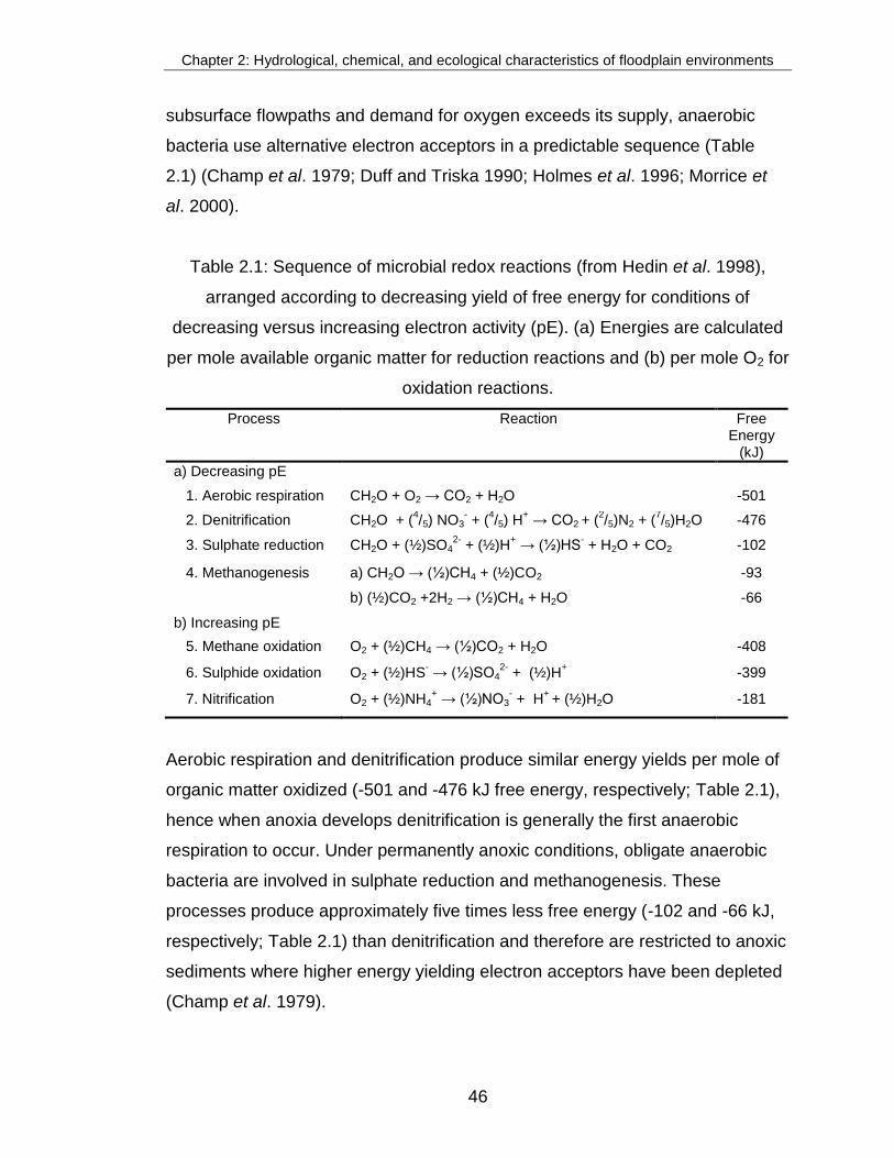
Chapter 2: Hydrological, chemical, and ecological characteristics of floodplain environments
46
subsurface flowpaths and demand for oxygen exceeds its supply, anaerobic
bacteria use alternative electron acceptors in a predictable sequence (Table
2.1) (Champ et al. 1979; Duff and Triska 1990; Holmes et al. 1996; Morrice et
al. 2000).
Table 2.1: Sequence of microbial redox reactions (from Hedin et al. 1998),
arranged according to decreasing yield of free energy for conditions of
decreasing versus increasing electron activity (pE). (a) Energies are calculated
per mole available organic matter for reduction reactions and (b) per mole O2 for
oxidation reactions.
Process Reaction Free Energy
(kJ)
a) Decreasing pE
1. Aerobic respiration CH2O + O2 → CO2 + H2O -501
2. Denitrification CH2O + (4/5) NO3
- + (
4/5) H
+ → CO2 + (
2/5)N2 + (
7/5)H2O -476
3. Sulphate reduction CH2O + (½)SO42-
+ (½)H+ → (½)HS
- + H2O + CO2 -102
4. Methanogenesis a) CH2O → (½)CH4 + (½)CO2 -93
b) (½)CO2 +2H2 → (½)CH4 + H2O -66
b) Increasing pE
5. Methane oxidation O2 + (½)CH4 → (½)CO2 + H2O -408
6. Sulphide oxidation O2 + (½)HS- → (½)SO4
2- + (½)H
+ -399
7. Nitrification O2 + (½)NH4+ → (½)NO3
- + H
+ + (½)H2O -181
Aerobic respiration and denitrification produce similar energy yields per mole of
organic matter oxidized (-501 and -476 kJ free energy, respectively; Table 2.1),
hence when anoxia develops denitrification is generally the first anaerobic
respiration to occur. Under permanently anoxic conditions, obligate anaerobic
bacteria are involved in sulphate reduction and methanogenesis. These
processes produce approximately five times less free energy (-102 and -66 kJ,
respectively; Table 2.1) than denitrification and therefore are restricted to anoxic
sediments where higher energy yielding electron acceptors have been depleted
(Champ et al. 1979).

Chapter 2: Hydrological, chemical, and ecological characteristics of floodplain environments
47
2.3.2 Nitrogen and phosphorus biogeochemistry
In near-stream and river environments where sediments are well oxygenated,
nitrification, the oxidation of ammonium to nitrite and nitrate by nitrifying
bacteria, can result in low ammonium concentration relative to nitrate (Figure
2.10) (Jones and Holmes 1996; Hedin et al. 1998; Morrice et al. 2000). As
hydrological exchange decreases and oxygen is consumed along hyporheic
flowpaths, ammonium concentration increases in the absence of nitrifying
bacteria (Figure 2.10) (Triska et al. 1993b). Denitrification can then cause nitrate
concentration to decrease along subsurface flowpaths as it is reduced to nitrous
oxide and dinitrogen gases by facultative anaerobes, which can switch between
aerobic and anaerobic respiration as environmental conditions change (Figure
2.10) (Hedin et al. 1998; Hill 2000). This can result in high rates of nitrate
removal in anoxic regions at the river-sediment interface, where supply of nitrate
and dissolved organic carbon (DOC) is great (Triska et al. 1989; Dahm et al.
1998; Hedin et al. 1998; Pinay et al. 1998; Krause et al. 2008).
Figure 2.10: Conceptual model of metabolic processes along subsurface
flowpaths (from Jones 1994).
Plant uptake, microbial immobilisation, and denitrification are the primary
mechanisms accounting for the removal of nitrate from groundwater.
Assimilation of nitrogen by plants and microbes stores nitrogen temporarily in
biomass. These stores of nitrogen are returned to the available soil nitrogen
pool when plants and/or bacteria die and are mineralised. Dissimilatory
O2
Aerobic respiration
DenitrificationNO3
Distance along groundwater flowpath
Conce
ntr
ation/R
ate
NH4O2
Aerobic respiration
DenitrificationNO3
Distance along groundwater flowpath
Conce
ntr
ation/R
ate
NH4

Chapter 2: Hydrological, chemical, and ecological characteristics of floodplain environments
48
pathways include nitrification (the conversion of ammonium to nitrate),
dissimilatory nitrate reduction to ammonium, and denitrification. Denitrification is
of particular interest in eutrophic environments as it results in the permanent
loss of nitrogen from ecosystems to the atmosphere in the form of nitrous oxide
and dinitrogen gases (Duff and Triska 2000).
The efficiency at which nitrate is removed from riparian zones is known to differ
temporally as well as spatially, in relation to variations in soil temperature
(Haycock and Pinay 1993) and hydrological pathways (residence time and
contact between soil with groundwater) (Hill 1996a; Ocampo et al. 2006). During
periods of high river flow, denitrification and plant uptake of nitrogen by
vegetation can be a substantial sink for nitrogen (Lowrance et al. 1997; Schade
et al. 2002; Banach et al. 2009). However, the relative importance of these
processes is likely to shift with periods of flooding that can increase
denitrification and limit plant activity (Baker and Vervier 2004; Shabala 2011), or
during the summer when plant growth and uptake of nutrients is high (Hefting et
al. 2005), and denitrification may be less important due to lower groundwater
levels and increased soil aeration.
Landscape features such as topography, geology, soil and vegetation types in
addition to human inputs influence the amounts of phosphorus reaching riparian
zones and streams (Gburek and Sharpley 1998; Mengistu et al. 2014).
Phosphorus is often the limiting nutrient for plant growth (Schulze et al. 2005).
There are four main reasons for this: (1) the major source of phosphorus is in
rocks, hence the release of phosphorus into ecosystems is controlled by the
slow process of weathering; (2) unlike nitrogen, there is no atmospheric form of
phosphorus and inputs via precipitation are negligible; (3) terrestrial vegetation
intercepts most phosphorus; and (4) adsorption to sediments make phosphorus
unavailable to plants (Hendricks and White 2000; Kalff 2001).

Chapter 2: Hydrological, chemical, and ecological characteristics of floodplain environments
49
Dissolved inorganic P is considered bioavailable, whereas organic P must
undergo transformation (Figure 2.11). Unlike nitrogen, there is no ‘permanent’
gaseous route for P to be removed from floodplain soils, hence P retention
refers to the storage of P in forms that will not easily be released under normal
environmental conditions i.e. either in organic forms in plant or microbial
biomass, or in inorganic forms occluded in minerals (Dunne and Reddy 2005).
The literature largely focuses on the retention of inorganic P, which is controlled
by abiotic adsorption onto soil surfaces, and precipitation reactions between P
ions and cations such as aluminium, iron, calcium, or magnesium, and biotic
microbial immobilisation, and plant uptake (Figure 2.11) (Vought et al. 1994;
Dunne et al. 2005; Reddy and DeLaune 2008). However wetland, including
floodplain, soils is often associated with low mineral and high organic matter
soils. Thus in many wetlands, where anaerobic conditions persist and
decomposition is slow, organic soils provide a long-term storage for P (Roberts
et al. 2012).

Chapter 2: Hydrological, chemical, and ecological characteristics of floodplain environments
50
Figure 2.11: Forms and interactions of phosphorus (from Hyland et al. 2005).
2.3.3 Water quality functions and management of floodplains
Many studies of riparian zones from a number of locations around the world
(e.g. USA, Canada, England, France, Denmark, and New Zealand) have
reported that riparian areas and floodplains are natural effective nutrient sinks
that can substantially reduce nutrient concentrations of water that flows through
them. In this way that can act to mitigate the effects of artificial fertilizer runoff on
surface water bodies (Lowrance et al. 1984; Dosskey 2000; Brusch
and Nilsson 1993; Vidon and Hill 2004b; Schade et al. 2002; Sabater et al.
2003; Billy et al. 2010). As such, floodplains are often described as having
kidney-like functions within the catchment (Fisher and Acreman 2004; Mitsch

Chapter 2: Hydrological, chemical, and ecological characteristics of floodplain environments
51
and Gosselink 2007; McJannet et al. 2010). The functional role of the riparian
zone as a nutrient filter is due to several important features. For instance, and
as described above, despite occupying a small area of the landscape, riparian
zones are prominently located to intercept water and nutrients as they move
between terrestrial and aquatic environments (Gregory et al. 1991). Positioned
at the land-water interface, riparian zone soils are often saturated, which leads
to anoxic conditions. As described above, these conditions are conducive to
denitrification, the microbially mediated reduction of nitrate to nitrous oxide and
dinitrogen gas. Furthermore, riparian soils are usually rich in organic carbon,
which is the dominant electron donor in many environments for heterotrophic
processes such as denitrification, and can be more important than oxygen
status in determining the rate of denitrification (Vervier et al. 1993; Holmes et al.
1996; Hedin et al. 1998; Hill et al. 2000).
A study in southern Ontario, Canada, of stream riparian sites on glacial till,
found that >90% of nitrate was removed from groundwater flowing from
agricultural land into the riparian zone. This was most rapid (i.e. within the first
15 m of riparian zone) at sites with sandy loam soils overlying a shallow 1-2 m
confining layer. A greater width of riparian buffer zone for nitrate removal was
required in sites with sand and cobble sediments (Vidon and Hill 2004a). In
contrast, Burt et al. (1999) found that despite significant potential for
denitrification (e.g. anoxia and DOC supply) at a floodplain site along the River
Thames, UK, the hydrology of the site was inappropriate as water bypassed the
riparian zone through gravel lenses beneath the floodplain. Thus, hot spots of
denitrification within riparian zones are attributed to key landscape variables
such as slope, sediment texture and depth of confining layers on hydrological
pathways that link supplies of nitrate and dissolved organic carbon (Vidon and
Hill 2004b).
Changes in land use management that optimise the nutrient filtering capacity of
riparian zones to reduce diffuse pollution are of great ecological and commercial

Chapter 2: Hydrological, chemical, and ecological characteristics of floodplain environments
52
interest. Using the USGS modular 3-dimensional finite difference groundwater
flow model MODFLOW (e.g. Chiang and Kinzelbach 1993), coupled with the
MT3D nitrate transport model (Zheng and Wang 1999), Krause et al. (2008)
found that substantial improvements to the ecological status and water quality of
a lowland stream could be achieved through changes in land management. The
simulations involved the optimisation of natural buffer zones as well as changes
to crop types, such as the extensive use of grasslands on hydromorphic soils,
increased set-aside, and an increase in the proportion of deciduous to
coniferous forest plantations; and changes in farming methods, such as crop
rotation, and a reduction in intense farming.
Fisher and Acreman (2004) conducted a review of 57 studies from around the
world that sought to determine the nutrient filtering capacity of wetlands that
included many floodplains. They found that the majority of wetlands reduced
nitrogen and phosphorus loading (Figure 2.12). Oxygen content and
waterlogging of the sediment were the main factors that were attributed to the
retention of nitrogen. These factors are often associated with periods of flooding
that alter the oxidation state of groundwater in the floodplain (e.g. Clilverd et al.
2008). Oxygen concentration was noted as the most important factor controlling
the retention of inorganic P, attributed to the binding capacity of iron and
aluminium. In contrast to nitrogen, inorganic P retention in soils requires oxic
conditions. The onset of anoxia results in lower redox potential which is coupled
with pH, and causes phosphorus to desorb from iron and aluminium solids and
return to solution (Hedricks and White 2000). However, in alkaline soils, the
availability of phosphorus is controlled by the solubility of calcium compounds.
Calcium-bound phosphorus is relatively stable and typically unavailable to
plants (Dunne and Reddy 2005). Hence, the management of floodplains for
nutrient retention is different for phosphorus and nitrogen, and different soil-
types.

Chapter 2: Hydrological, chemical, and ecological characteristics of floodplain environments
53
Figure 2.12: The percentage of wetlands studied which exhibited reduction and
an increase in N and P loading in riparian zones from Fisher and Acreman
(2004). TN/TKN = total nitrogen/Kjeldahl nitrogen; NO3 = nitrate; NH4 =
ammonium; TP = total phosphorus; Sol P = soluble phosphorus.
Seasonal variation in the extent and duration of soil saturation affects the
demand for oxygen and consequently the redox potential, which controls
nitrogen loss via denitrification (Duff and Trska 2000), and P mobility (Dunne
and Reddy 2005). As described above, high river stage and flooding can
substantially enhance river-water intrusion into the hyporheic zone, supplying
DOC, N and P to plant roots and subsurface microbes, which regulate the loss
of nutrients (Schade et al. 2002; Baker and Vervier 2004; Forshay and Stanley,
2005). However, while floodplains may act as a sink for nutrients during periods
of high river stage (Findlay 1995; Bartley and Croome 1999; Adair et al. 2004),
in contrast at low river stages when groundwater flow may be directed away
from the floodplain and towards the river, riparian zones can be a source of
nutrients to the river. If, for example, low river stage occurs in the autumn
and/or winter, N and P released from plant senescence and root turnover may
be a source of nutrients to the river (Kröger et al. 2007).

Chapter 2: Hydrological, chemical, and ecological characteristics of floodplain environments
54
Water table fluctuations, and associated cycles of drying and re-wetting in
floodplain soils, can significantly affect soil fertility by causing bursts of microbial
activity and soil organic matter turnover (Chepkwony et al. 2001). Nitrogen-
retention is maximised by varying water table heights. Where there is a close
juxtaposition of aerobic and anaerobic zones in sediments, coupled nitrification
–denitrification, i.e. diffusion of nitrate from oxidized surface layers to denitrifying
bacteria in adjacent anaerobic zones, can result in a strong potential for nitrogen
removal (Hedin et al. 1998; Strauss et al. 2006). In contrast, Pant and Reddy
(2000) and Aldous et al. (2005) suggest that frequent wetting and drying cycles
that alternate between anoxic and oxic conditions maximise the release of
mineral-bound and organic P (via mineralisation under drying conditions),
whereas stable, moist soil conditions minimise phosphorus release from
floodplain soils. A stable hydrological management regime that maximises
phosphorus retention is not appropriate however for supporting diverse riparian
floral and faunal communities, which typically flourish in environments with
naturally fluctuating hydrological conditions (Grevilliot et al. 1998; Ward 1998;
Gowing et al. 2002a; Woodcock et al. 2005). This highlights the importance of
identifying the goals of riparian management projects and the plans for
implementation.
2.4 Riparian zone community composition
2.4.1 The effects of waterlogging on plant community-composition
A wetland’s hydrological regime is a fundamental environmental factor that
determines the plant community-composition (Gowing et al. 1998; Grevilliot et
al. 1998). The Flood-Pulse Concept (FPC) (Junk et al.1989) and its more recent
extensions (Tockner et al. 2000, Junk and Wantzen 2004) concerns the key role
of pulsing river discharge on supply of flood water, sediments and nutrients onto
the floodplain. The FPC predicts that recurring overbank inundation is important
for the formation of a dynamic physical environment, which drives plant species
composition, and high biodiversity in floodplain ecosystems (Ward 1998;

Chapter 2: Hydrological, chemical, and ecological characteristics of floodplain environments
55
Opperman et al. 2010). The FPC has also drawn attention to the importance of
the intensity, frequency and timing of flood pulse events for floodplain biota to
benefit optimally from flood-deposited resources (Tockner et al. 2010). For
example, in floodplain meadows the vegetation composition of grassland
communities is sensitive to water table fluctuations, fertility, and management
(Wheeler et al. 2004). While flood disturbances of an intermediate level, in terms
of frequency and duration, is expected to enhance environmental heterogeneity
on the floodplain and increase species richness (Ward et al. 1999), excessive
flooding that results in prolonged soil saturation in the rooting zone during the
growing season can limit plant growth and cause mortality in plants (Michalcová
et al. 2011). This can lead to the development of one of a few dominant species
that are adapted to these conditions (e.g. Holcus lanatus, Juncus spp.)
(Grevilliot et al. 1998). On the other hand, prolonged flooding that occurs during
the winter when plants are dormant is less likely to negatively impact floodplain
plant communities (e.g. Beltman et al. 2007). Wantzen and Junk (2000)
highlight that disturbance sensitivities vary among species and developmental
stages of species, and point out that flood pulses should not be considered as
disturbance alone, but also a resource of riverine nutrients and organic matter.
Many studies worldwide have reported the zonation of vegetation in response to
water table depth below the ground surface (Sánchez et al. 1998; Castelli et al.
2000; Dwire et al. 2006; Toogood et al. 2008; Jung et al. 2009). Silvertown et al.
(1999) showed that plant species in European wet meadows have individual
tolerance ranges to aeration stress in the root zone that results in niche-
segregation along fine-scale hydrological gradients (Figure 2.13). The generality
of this mechanism was tested by Araya et al. (2011) by quantifying the
hydrological niches of plants in fynbos communities in the Cape Floristic
Region, South Africa. Despite the vast floristic, functional and phylogenetic
differences between fynbos and wet meadow communities, they found that the
same trade-offs occurred in response to aeration/or drying stress resulting
specialisation of species into distinct hydrological niches.

Chapter 2: Hydrological, chemical, and ecological characteristics of floodplain environments
56
Figure 2.13: Niche space at (a) Tadham and (b) Cricklade. High aeration SEVs
indicate waterlogged conditions; high soil-dryness SEVs indicate droughted
conditions. Each point is a sampling location for plant community composition.
From Silvertown et al. (1999).

Chapter 2: Hydrological, chemical, and ecological characteristics of floodplain environments
57
In wet and waterlogged conditions, root respiration and thus plant growth is
limited in the majority of vascular plants. Wetland species that tolerate such
conditions are adapted to retain high root-oxygen levels or to provide adequate
oxygen supply to their roots (Jackson and Colmer 2005). Where low oxygen
concentrations persist plants may also need to cope with the accumulation of
metal cations (e.g. Fe2+, Mn2+) and organic phytotoxins (e.g. ethanol and
acetaldehyde) released under reducing conditions due to redox-sensitive
reactions (Jackson and Colmer 2005; Shabala 2011). Furthermore, nutrient
availability changes with soil moisture content, with a maximum availability in
mesic soils and minimum availability occurring in waterlogged and very dry
conditions (Araya 2005). As discussed by Peñuelas et al. (2011), plants are
forced to specialise in order to successfully compete for varying demands on
resources, and thus hydrological gradients are strongly linked to the
biogeochemical niche.
The soil-water regime tolerances of wet meadow vegetation to aeration stress
have been investigated using both qualitative (e.g. Ellenberg 1974) and
quantitative (e.g. Gowing et al. 1998) methods. The above-mentioned studies
(i.e. Gowing et al. 1998; Silvertown et al. 1999; Araya et al. 2011) quantified
hydrological niche segregation using a cumulative stress index, ‘sum of
exceedance value’, based on the position of the water table. Water table depth
is used as a proxy of soil water content and air-filled porosity, which in turn is
used to determine aeration stress in the rooting zone of plants (Gowing et al.
1998; Silvertown et al. 1999). This is discussed further in Section 8.3.5. This
model was also used by Gowing et al. (1997) to predict the aeration and drought
stress in the rooting zone of plants and to account for spatial patterns in wet
meadow plant community composition in over 2,000 species-rich sites
throughout England. The different water regimes were used to provide a
quantitative description of favoured water regimes of particular wetland species.
This study suggested that stable water table conditions during the growing
season are linked with low levels of aeration and drought stress, that can result

Chapter 2: Hydrological, chemical, and ecological characteristics of floodplain environments
58
in high diversity swards (>22 species per m2). Conversely, extreme fluctuations
in soil water conditions result in high levels of combined aeration and drought
stresses and thus the lowest species richness (<18 species per m2). High levels
of aeration stress or drought stress typically resulted in low species richness,
which is probably due to fewer available species adapted to these conditions
(e.g. Silvertown et al. 1999).
Further work on the water regime requirements of wet grasslands was
conducted by Gowing et al. (2002). This research encompassed the analysis of
extensive botanical data from 18 wet grassland sites across England. Using
sum exceedence values, the preferred water regime of different community
types were quantified based on their tolerance to aeration and drying stress
(Figure 2.14). The water regime tolerances of wetland communities in Figure
2.14 range from high aeration stress/low drying stress in fens (S25, S24), to low
aeration stress/high drying stress in hay meadows (MG5a, MG3). In general,
Gowing et al. (2002) show that species-rich grassland communities (MG3, MG4,
MG5, MG8) are intolerant of waterlogging and were predominantly located on
the drier end of the hydrological spectrum, whereas more species-poor
communities (MG13, OV28, Agrostis-Carex) can tolerate waterlogging. The
relationship between water level (and thus aeration and drying stress) and
vegetation type presented in this study, provide a quantitative method that can
be applied to other UK wet meadow sites to predict the possible botanical
outcomes of changing water regime.
However, predictions of botanical responses to modified hydrological conditions
that allow an optimization of wet grassland management for biodiversity require
an understanding of the relationship between the soil moisture and oxygen
status of the root environment. As stated above, the cumulative stress index for
aeration stress uses water table depth, which is relatively easy to monitor (e.g.
Gilman 1994) and represents a useful descriptor of soil water content and air-
filled porosity that in turn influence the rate of oxygen diffusion in soil (Hillel
1998). However, air-filled porosity and soil oxygen status are not always

Chapter 2: Hydrological, chemical, and ecological characteristics of floodplain environments
59
strongly correlated. The oxygen concentration in soil is a function of oxygen
supply (i.e. diffusion from the soil surface) and consumption (i.e. respiration)
rates in the soil profile. Thus, in soils where respiration exceeds diffusion from
the surface, soil pores may be filled primarily with respiratory products (e.g.
CO2, CH4, H2S) rather than oxygen (e.g. Lloyd 2006). Barber et al. (2004) used
water content and redox potential measurements to characterize the aeration
status of peat soil. Although redox potential was related to water table depth at
shallow depths, no significant relationship was found for data from 0.4 m depth
(Figure 2.15). This was attributed to rates of oxygen diffusion being less than
aerobic respiration. The relationship between aeration status and water table
depth needs further study, and more direct measures of oxygen status in
response to changing hydrological conditions could help to establish the degree
to which the water table position can be used as a proxy for aeration stress in
plants.
Figure 2.14: Water-regime of each community type (mean and 95% confidence
interval) from Gowing et al. (2002).

Chapter 2: Hydrological, chemical, and ecological characteristics of floodplain environments
60
Figure 2.15: The relationship between redox potential and water table depth (a)
at 0.1 m depth and (b) at 0.4 m depth. From Barber et al. (2004).
2.4.2 Fertilisation of riparian zones
In addition to soil water regime, nutrient availability is an important factor
controlling floodplain plant assemblages at the community level (Willby et al.
2001), with nitrogen and phosphorus primarily limiting plant growth (Keddy

Chapter 2: Hydrological, chemical, and ecological characteristics of floodplain environments
61
2000). In oligotrophic environments, the supply of nutrients from aquatic to
riparian environments can be essential for floodplain primary productivity
(Shade et al. 2002). For instance, Lisuzzo et al. (2008) report that the nutrient
requirements of productive early successional plant communities that colonise
nitrogen limited Taiga floodplains cannot be accounted for by nitrogen fixation,
mineralisation, and deposition alone, which collectively only account for
approximately 26% of community nitrogen requirements. Using injections of
enriched 15NO3- into buried flowboxes (perforated pvc boxes installed in
floodplain sediments at a depth of 1.3 m), they found substantial uptake of
hyporheic nitrogen downstream in floodplain willow stands, and concluded that
during high river stage, nitrogen supply from mass flow of water through the
hyporheic zone to the roots of plants equalled or exceeded total nitrogen supply
from nitrogen mineralisation and nitrogen fixation (also see Tockner et al. 1999;
Schade et al. 2002).
As discussed above, river-derived nutrients can enter riparian areas via two
main transfer mechanisms: (1) through hyporheic flow; and (2) via overbank
inundation. Both mechanisms lead to enhanced river water intrusion in
floodplain soils; however overbank inundation also has the potential to deposit
sediment with its associated nutrients on the floodplain. The rate of nutrient
acquisition in plants is generally controlled by diffusion to the root surface
(Lambers et al. 1998). Therefore in riparian zones, infiltration of nutrient-rich
floodwater into the rooting zone can substantially accelerate the transport of
nutrients to plant roots. Such fertilisation favours the growth of competitive
species at the cost of slower growing species, which can lead to a loss of
species richness. Therefore, while floodplains may function to protect adjacent
ecosystems from nutrient loading, flood-deposited sediment and enhanced
hydrological exchange with nutrient rich river water may pose a risk to floodplain
plant communities, particularly where there is a fine balance between species-
richness and biomass (Vermeer and Berendse 1983; Waide et al. 1999). If the
river has become eutrophic, then the removal of river embankments and

Chapter 2: Hydrological, chemical, and ecological characteristics of floodplain environments
62
hydrological reconnection between rivers and historical floodplains (as
discussed in Section 2.5) may not be the most appropriate way to restore
floodplain biodiversity.
For example, a N fertilizer experiment on a species-rich flood-meadow under
hay-cutting management in the Czech Republic by Joyce (2001) showed that
species diversity was highly sensitive to nitrogen enrichment, reducing
significantly in 8 weeks, with forbs and moss most affected. The study
concluded that flood-meadows are susceptible to fertilization inputs from
intensive agricultural practice or other human activities (which could include
nutrient-rich flood water). Similarly, Beltman et al. (2007) found that on a
species-rich (average 24 species per m2) Arrhenatherion-dominated grassland
floodplain, flooding caused a general reduction in species richness and an
increase in biomass production that was similar in magnitude to the effects of
fertilisation. As flooding occurred in winter when plants were dormant,
inundation was better tolerated by sensitive species than it would have been in
summer. Hence, rather than aeration stress, the decrease in species richness
after the flood events was attributed to the germination of highly competitive
species, initially tall forbs, and later graminoids (e.g. Carex hirta - hairy sedge),
Elymus repens - couch grass). Beltman et al. (2007) concluded that increased
inundation of floodplain grasslands that already have relatively high biomass
production (above-ground production >500 g m-2 yr-1) is likely to lead to a
reduction in species richness, which is unlikely to recover without sufficient time
between flooding (>10 years).
In UK mesotrophic environments, Michalcová et al. (2011) report that species
richness is best managed for low levels of waterlogging and low soil phosphorus
concentration (<10 μg P g soil -1). As discussed in Section 2.3.3, under anoxic
conditions mineral-bound phosphorus is released into bioavailable forms. This
could in part explain the positive relationship between waterlogging and soil
available phosphorus, and the resulting negative impact on plant biodiversity in

Chapter 2: Hydrological, chemical, and ecological characteristics of floodplain environments
63
wetlands reported in this study. Similarly, Snow et al. (1997), Gowing et al.
(2002) and Critchley et al. (2002) found that species-rich wet grasslands in the
UK require low extractable P levels, within the range of 5 – 10 mg P kg-1.
The resource balance hypothesis states that multiple nutrient limitation favours
plant species richness (Braakhekke and Hooftman 1999). Multiple resource
limitation is thought to be beneficial for plant communities as it results in a
competitive balance that permits plant species to coexist. This concept is from
the competitive exclusion principle, which states that species that compete for
the same resources cannot permanently coexist (Hardin 1960). Braakhekke and
Hooftman (1999) propose that species coexistence is described by parabolic
‘humped back’ curves, with highest diversity when nutrient supply is balanced
and lowest diversity at the extremes of nutrient ratios (Figure 2.16), which they
investigated in 25 natural grasslands.
This model was also tested by Aerts et al. (2003) in a long-term (11 years) study
by adding commonly limiting nutrients, N and/or P to two mesotrophic
grasslands. They hypothesised that adding nutrients to grassland that was in
shortage of N (N:P <10) or P (N:P >14) would increase biodiversity. However
instead, nutrient addition resulted in a reduction in species diversity, which was
attributed to seed and colonisation limitation. Seemingly, although the correct
balance of N:P play a role in grassland diversity, other factors are also important
e.g. disturbance in forms of flooding (Helfield et al. 2007) and herbivory (Olff and
Ritchie 1998; Grace 1999). Furthermore, Braakhekke and Hooftman (1999)
recommend that nutrient addition as a ‘quick fix’ is not prescribed in grasslands
to attempt optimal N:P ratios, as this can disturb the balance between nutrient
and light limitation. Instead, long-term solutions are suggested, such as biomass
removal, which removes non-limiting nutrients more rapidly than limiting
nutrients, with an over-arching emphasis on management that considers as
many of the regulating factors as possible.

Chapter 2: Hydrological, chemical, and ecological characteristics of floodplain environments
64
Figure 2.16: Relationship between nutrient supply ratio (S1/S2) and equilibrium
species richness (SR), evenness (E) and Shannon index (H) in a theoretical two
plant species community competing for two essential nutrients from Braakhekke
and Hooftman (1999).
2.4.3 Grazing impacts on plant diversity
Grazing can have both positive and negative effects on species richness, but in
floodplains the effect is more likely to be positive due to the high productivity of
the vegetation (Proulx and Mazumder 1998). This can be explained by the
intermediate disturbance hypothesis (Grime 1979), which predicts that
productivity and competitive exclusion is high under conditions of low
environmental stress, whereas under high environmental stress few species are
adapted to survive. However, when in balance, i.e. following a similar ‘humped-
back’ relation to the resource balance hypothesis (see Section 2.4.2), these
stresses contribute importantly to the maintenance of biodiversity by reducing
the abundance of dominant species and increasing the number of less
competitive species.

Chapter 2: Hydrological, chemical, and ecological characteristics of floodplain environments
65
The impact of grazing pressure on plant species richness in nutrient-rich and
nutrient-poor ecosystems was evaluated by Proulx and Mazumder (1998). They
compared data from 30 published studies, and found that plant species richness
typically increases with grazing in nutrient-rich ecosystems and decreases with
grazing in nutrient-poor ecosystems. Under nutrient-poor conditions, declines in
species richness are attributed to a limitation of available resources required for
regrowth after grazing. In contrast, in nutrient-rich environments, regrowth is
less likely to be impacted by nutrient limitation.
Intensive grazing reduces botanical diversity by favouring a few species that can
either tolerate repeated defoliation (e.g. Lolium perenne (English ryegrass), and
Trifolium repens L. (white clover)), or are extremely competitive (e.g. Poa
trivialis L (rough meadow-grass)), or have strong defenses against herbivory
(e.g. Cirsium vulgare (Savi) Ten (common thistle). Intense grazing regimes also
reduce the chance for flowering and seeding (Tallowin et al. 1995). Moderate
grazing, on the other hand, can decrease competition by dominant plant
species, and encourage sward heterogeneity. However, the timing of grazing, in
terms of allowing species to set seed, and type of grazing e.g. sheep, cattle, or
hay cutting, or a combination, have varying effects on meadow plant
assemblages (Table 2.2). Long-term studies on the use of grazing during the re-
creation of a floodplain meadow in Oxfordshire, UK undertaken by Woodcock et
al. (2006; 2011), indicate that under sheep and cattle grazing, plant
assemblages are closer to the target species-rich floodplain meadows,
compared with un-grazed meadows. Hence grazing is thought to be central to
management of plant diversity of lowland grasslands.

Chapter 2: Hydrological, chemical, and ecological characteristics of floodplain environments
66
Table 2.2: Characteristics of sheep grazing, cattle grazing and hay cutting in
agriculturally unimproved grasslands (from Crofts and Jefferson 1999, cited in
Vickery et al. 2001).
Sheep Cattle Cutting
Bite the vegetation, graze close to ground level and produce very short swards of min. height 3 cm.
Bite, pull and tear the vegetation, cannot graze as close to ground level, and maintain longer swards with min. height 5-6 cm.
Able to manipulate vegetation and select items from very low in the grassland profile.
Coarse level manipulation of vegetation, and relatively unselective grazers.
Completely unselective.
Avoid tall plants in the sward, leave grass stems and often select flowers.
Take tall plants and grass stems, and occasionally select flowers (orchids).
Dead material and litter left.
Some dead material taken.
Often avoid rough, tall swards and tussocky areas.
Utilize rough, tall swards and tussocky areas.
Graze preferentially in small patches, selecting the most palatable patches available.
As sheep. Cattle swards are often particularly patchy.
Leaves swards extremely homogenous in height.
Returns some organic matter in dung and urine.
Returns organic matter in dung and urine. Large dung pats promote sward heterogeneity.
Usually returns little or no organic matter. If cuttings are left as a dense mat they cannot be utilized by decomposers.
2.4.4 Flooding disturbance and propagule dispersal
Pristine floodplains are complex, heterogeneous systems, in part down to
regular overbank inundation that increases disturbance. Flooding can create
micro-habitats that are important for the coexistence of different vegetation
types and thus maintenance of biodiversity (Pollock et al. 1998; Ward et al.
1999). As discussed in Sections 2.2 and 2.3, hydrological connectivity plays a
major part in river and floodplain health and functioning. In addition to the supply
of water and nutrients, floods open space for colonisation and aid seed
recruitment on the floodplain (Grime 1979; Silvertown et al. 1999; Helfield et al.

Chapter 2: Hydrological, chemical, and ecological characteristics of floodplain environments
67
2007; Auble and Scott 1998; Nilsson et al. 2010). The local species pool can
affect the relative distribution and richness of wetland plant species, and may
determine the effectiveness of restoration schemes (Bischoff et al. 2009).
Transport of riparian plant propagules into the river, and dispersal downstream
onto newly flood-created patches for colonization, is dependent on sufficient
hydrological exchange between the river and floodplain during flooding (Figure
2.17), and thus is likely to be impeded by river embankments (Auble and Scott
1998). Indeed, Nilsson et al. (2010) state that wetland plant communities may
often be recruitment-limited. Recent studies that have considered the role of
flood pulses for propagule dispersal suggest that flooding is important for
providing bare and wet soils, gaps in the vegetation, and the necessary
dispersal vector required for the maintenance or restoration of species-rich
floodplain vegetation (Leyer 2006; Gurnell et al. 2006; Ozinga et al. 2009;
Merritt et al. 2010).
Figure 2.17: Conceptual model showing pathways for water-dispersed
propagules in rivers. Floating propagules can be derived from (1) upstream, (2)
riparian zones, and (3) uplands. During frequent flooding, (4) some propagules
are temporarily stranded and later dispersed before germination takes place.
During large infrequent floods, (5) stranded propagules can germinate where
stranded, (5a) disperse to uplands or (5b) across the riparian zone via wind and
animals. During large floods, (6) some propagules can disperse over very long
distances. From Nilsson et al. (2010).

Chapter 2: Hydrological, chemical, and ecological characteristics of floodplain environments
68
Habitat and river restoration efforts (detailed in Section 2.5) that attempt to
optimise the water and nutrient status of grasslands in order to enhance
grassland diversity often report reduced success when there is a lack of viable
seed banks and/or dispersal opportunities for target species are limited (Donath
et al. 2003). To overcome dispersal limitation along the Upper Rhine in
Germany, Hölzel and Otte (2003) conducted a diaspore transfer experiment
using freshly mown plant material, in conjunction with topsoil removal to reduce
nutrient concentrations and create bare soil for seedling recruitment. After four
years, substantial increases in species richness were observed, and rare and
endangered plants were introduced. These findings are in agreement with other
studies that have found plant species diversity in grasslands to be strongly
governed by recruitment limitation (e.g. Tilman 1997; Pywell et al. 2002; Fraser
and Madson 2008; Hellström et al. 2009; Zeiter et al. 2013).
2.4.5 Human pressures on lowland wet grasslands
Lowland wet grasslands are mostly semi-natural habitats, subject to periodic
freshwater flooding or waterlogging (Jefferson and Grice 1998), and are often
characterised by high plant and animal biodiversity. They can support numerous
plant species and vegetation types such as grasses, broad-leaved herbs,
sedges and rushes (Wheeler et al. 2004), and provide habitat for invertebrates,
and breeding wading birds such as Vanellus vanellus (lapwing), Tringa totanus
(redshank), Gallinago gallinago (snipe), Limosa limosa (black-tailed godwit),
Philomachus pugnax (ruff), Haematopus ostralegus (oystercatcher), and
Numenius arquata (curlew) that are attracted to winter flooding (Ausden et al.
2001).
The extent and botanical nature conservation value of lowland wet grassland in
Britain declined substantially in the 20th century. Between 1930 and 1984 semi-
natural lowland grassland decreased by an estimated 97% to approximately 0.2
million ha (JNCC 1995). These losses have continued, such that it is now
estimated that the total area of species-rich wetland meadow in the UK

Chapter 2: Hydrological, chemical, and ecological characteristics of floodplain environments
69
comprises <1,500 ha (Figure 2.18) (JNCC 1995). This is primarily attributed to
agricultural intensification, including: channelization and embankment of rivers;
substantial increases in the application of inorganic fertilisers (nitrogen and
phosphorus); a switch from hay to silage, where more frequent cutting reduces
seeding opportunities for plants; and increased stocking densities on grazed
meadows, which have altered the ecohydrology of these habitats (Vickery et al.
2001; Tilman et al. 2002; Benton et al. 2003; Kleijn et al. 2009). Land
development, land drainage, and encroachment by invasive species have also
contributed to the recent declines in biodiversity of floodplain meadows (Joyce
and Wade 1998). Species-rich vegetation communities have largely been out-
competed by relatively dense, fast-growing uniform swards (Joyce 1998;
Vickery et al. 2001).
Grassland that has not been subjected to artificial fertiliser or excessive hay
cutting or grazing is a valued resource of high nature conservation value (Bignal
and McCracken 1996; Eriksson et al. 2002; Wheeler et al. 2004). The continued
decline of many lowland wet grassland has led to increased efforts to conserve
and restore many of the UK’s wetlands. This includes protection at a number of
meadows at Sites of Special Scientific Interest (SSSI) and Natural Nature
Reserves (NNRs) e.g. North Meadow Cricklade, Wiltshire, and Upwood
Meadows, Cambridgeshire (JNCC 1995). In addition, lowland hay meadows
(NVC type MG4: Alopecurus pratensis, Sanguisorba officinalis) are listed as a
priority habitat on Annex I of the EU Habitats Directive (92/43/EEC). In the UK,
this community is characterised by species-rich swards containing Festuca
rubra (red fescue), Cynosurus cristatus (crested dog's-tail), Alopecurus
pratensis (meadow foxtail), Sanguisorba officinalis (great burnet), Filipendula
ulmaria (meadow sweet) and Ranunculus acris (meadow buttercup), and
provides the main habitat for Fritillaria meleagris (snake’s head fritillary)
(Wheeler et al. 2004). Some of these sites, designated as Special Areas of
Conservation (SACs), are of European importance and are protected legally

Chapter 2: Hydrological, chemical, and ecological characteristics of floodplain environments
70
under the Habitats Directive (92/43/EEC). In the UK they form part of the
European Natura 2000 network (JNCC 2016).
Figure 2.18: The distribution of species-rich lowland wet grasslands (MG4 under
the UK National Vegetation Communities system) in England from Wheeler et
al. (2004). The size of the circle reflects the relative area of each site on an
arbitrary scale.
2.4.6 Management of lowland hay meadows
Traditional management of floodplain meadows involved a midsummer (July)
hay harvest, followed by low-density cattle and then sheep grazing of regrowth
in the autumn and winter, respectively (Jefferson and Grice 1998). This
maintained a low sward during most of the year, promoted seed dispersal and
created niches for seed germination (e.g. Linusson et al. 1998; McDonald

Chapter 2: Hydrological, chemical, and ecological characteristics of floodplain environments
71
2001), and balanced the input of river-derived nutrients to the floodplain with the
removal of nutrients in plant biomass by the use of hay cutting and grazing
(Wheeler et al. 2004). The conversion of semi-natural grassland to intensive
agriculture imposed a number of abiotic and biotic constraints on floodplain
plant diversity, largely linked to the drainage, fertilisation, and impoverishment of
seed-pools through habitat loss and fragmentation, in short, an intensification of
the low-impact farming outlined above.
Effective management strategies for improving biodiversity and favouring target
plant communities also include the removal of topsoil, which in addition to
reducing soil fertility creates bare soil and poor competition (Tallowin and Smith
2001; Verhagen et al. 2001); diaspore transfer (Kiehl and Wagner 2006;
Hedberg and Kotowski 2010), or a combination of these methods (Hölzel and
Otte 2003). Those strategies that are most effective are thought to include as
many controlling factors as possible, and avoid situations where a single factor
can dominate over the others (Braakhekke and Hooftman 1999).
2.5 River regulation, and restoration
2.5.1 Channel modification
In their natural form, rivers are heterogeneous and complex, free to change their
form and flow in relation to the natural properties of the river bed, banks, and
climate (Poff et al. 1997). Strong interactions between the river and floodplain
are characteristic of natural river systems and contribute to a state of dynamic
balance due to the regular floods that continuously reshape river channels and
their banks, and transport water, sediment and nutrients onto the floodplain
(Ward 1998). This leads to a patchwork of habitats within the river channel and
on the floodplain that can support a variety of plant and animal assemblages
(Décamps et al. 2010). Despite occupying a relatively small proportion of the

Chapter 2: Hydrological, chemical, and ecological characteristics of floodplain environments
72
total land area, riparian zones support more species than any other terrestrial
habitat (Nilsson 1992).
Aquatic ecosystems, however, have been disturbed by humans for thousands of
years through the diversion of rivers and streams for harnessing waterpower,
deforestation, and drainage and conversion of wetlands for agriculture (Tockner
and Stanford 2002). In contrast to natural rivers, modified channels are
simplified and diversity and changes to channel form are reduced, connectivity
with the floodplain is restricted, and the role of riparian vegetation is diminished
(Figure 2.19). The most severe impacts have occurred globally since the late
19th century. Intensified agriculture and industrial pressures has increased the
channelization, drainage, deforestation, and pollution of rivers, streams and the
riparian zone; in addition the construction of dams, water extraction, and flood
control, have had a lasting impact on the hydrological characteristics of river-
floodplain ecosystems (Tockner et al. 2009; Poff and Zimmerman 2010; Cheng
et al. 2012; Elosegi and Sabater 2013; Perfect et al. 2013; Roni and Beechie
2013). These disturbances have led to a rapid degradation of water quality and
habitat, which has impacted humans through impaired water supply and flood
control, and affected biota resulting in species loss (Goudie 2006). It is reported
that 50 – 60% of wetlands worldwide have been lost (Davidson 2014), and
estimates suggest that globally more than 75% of riverine habitats are degraded
(Vörösmarty et al. 2010).

Chapter 2: Hydrological, chemical, and ecological characteristics of floodplain environments
73
Figure 2.19: Examples of modifications to river channels, amended from Sear et
al. (2000).
Regulation of rivers and streams over past centuries has had a pervasive
impact on the hydrological characteristics of floodplain ecosystems. Many
floodplains, where overbank flow was historically a regular occurrence, no
longer flood frequently due to alteration of the natural flow regime (Poff and
Zimmerman 2010). River embankments limit overbank flows onto the floodplain
in order to protect adjacent land from flooding so that it can be employed for
other uses including agriculture and urban development (Darby and Simon
1999; Sear et al. 2000). However, local river embankment can severely impact
flood defence downstream. Embankments lead to increased channel volume
and flow depth and reduced resistance to flow, which in turn results in higher
Embanking
Dredging
Straightening

Chapter 2: Hydrological, chemical, and ecological characteristics of floodplain environments
74
flow velocities, decreased contact time of water with sediments (important for
the nutrient filtering capacity of aquatic environments) and increased
downstream transport of water (Darby and Simon 1999; Gilvear 1999). Other
modifications that have altered the flow-regime in riverine ecosystems include
channel straightening, simplifying, widening, damming, deepening and dredging,
culverting, bank stabilisation, and vegetation removal (Beechie et al. 2013).
These alterations have a major impact on natural patterns of longitudinal and
lateral connectivity, homogenising the river corridor (Poff et al. 1997; Tockner
and Stanford 2002), which in turn affects in-stream (e.g. Jungwirth et al. 1995)
and riparian biotic composition (Nilsson et al. 1997) and water quality (e.g.
Lefebvre et al. 2004).
2.5.2. Restoration techniques
River restoration spans a variety of activities, and can range from the creation of
new habitats, the partial restoration of lost habitats and habitat improvement, to
full restoration of ecosystem processes and function (Box 1996; Beechie et al.
2013; RRC 2014). Habitat restoration is intended to assist the recovery of a
habitat that has been degraded in order to return the system to its original or
near-natural, undisturbed state (Bond and Lake 2003; Darby and Sear 2008).
Whilst passive restoration involves the removal of human disturbance to
facilitate recovery, active restoration physically alters the habitat (e.g. via the
removal of river embankments, re-meandering previously straightened rivers
reaches, addition of spawning gravel, introduction of woody debris) and typically
focuses on the recovery of natural components and processes e.g. overbank
inundation (Hammersmark et al. 2010; Barlaup et al. 2008; Miller et al. 2010).
By addressing the root causes of habitat degradation the assumption is that if
the physical conditions and processes that control the habitat characteristics are
adequately restored then target flora and fauna will respond positively without
further intervention (Rohde et al. 2006; Katz et al. 2009). However, the link
between habitat and biotic restoration can break down and inhibit the recovery

Chapter 2: Hydrological, chemical, and ecological characteristics of floodplain environments
75
of historic conditions where there are: (1) barriers to colonisation; (2) new
species present (native or non-native); and/or (3) physical and chemical
substrate changes (Bond and Lake 2003; Katz et al. 2009). In these instances,
further intervention and management may be required to attain habitat
restoration goals.
For the reasons discussed above, restoration efforts that start from a less
disturbed point are in the end more likely to succeed due to a greater species
reservoir, and physical conditions more similar to the natural state. They are
also likely to be more cost effective (e.g. Wheeler et al. 2004). Protection of
near-pristine aquatic ecosystems that are already functioning naturally have an
important role to play in restoration ecology, in part because they provide a
baseline and control point for restoration efforts, but also because continued
human pressures such as growing population and climate change are likely to
disturb aquatic habitats at rates much greater than restoration efforts.
Several habitat restoration projects, that have physically altered the morphology
of over-regulated rivers to restore the natural flow regime, have reported
positive effects on river and floodplain plant and animal diversity (e.g. Buijse et
al. 2002; Nilsson and Svedmark 2002; Nienhuis et al. 2002; Poff and
Zimmerman 2010; Arlettaz et al. 2011). However there are few published
studies on small rivers in which the effects of river restoration have been
monitored. Small-scale river restoration works have increased in recent years,
but they are often initiated by local farmers and landowners that understand the
benefits of restoring natural flow regimes for floodplain biodiversity and water
management, and are not widely reported in the literature.
Floodplain restoration, through embankment removal (the focus of this thesis) is
now being increasingly employed to re-establish river–floodplain connections
(Bernhardt et al. 2005). The aims of these restoration works are often
multifaceted and include enhanced floodplain biodiversity, improved nutrient-
Chapter 2: Hydrological, chemical, and ecological characteristics of floodplain environments
76
attenuation capacity and the provision of temporary storage of flood water
(Muhar et al. 1995; Buijse et al. 2002; Bernhardt et al. 2005). The River
Restoration Centre (RRC 2016a) lists best-case studies of river restoration from
across the UK. Of the 72 projects listed, most were related to in-stream
restoration works to improve habitat quality for fish (e.g. weir removal, creation
of riffles, pools, and backwaters), however 15 studies involved floodplain
reconnection schemes. Four of these were located in urban environments,
where concrete channels were replaced with new natural bed profiles in order to
enhance flood protection, channel heterogeneity and aesthetic values of the
streams (i.e. River Quaggy, Chinbrook Meadows, London; River Ravensbourne,
Cornmill Gardens, London; Yardley Brook, Birmingham; Braid Burn, Edinburgh).
The remaining floodplain reconnection projects which were documented
involved breaching of flood banks (e.g Burn of Mosset, Forres, Elgin), bank
regrading (e.g. River Cam, Trumpington Meadows, South of Cambridge), the
creation of new sinuous channels (e.g. River Wensum, Bintree), floodplain
mosaics (e.g. River Thames, Farmoor reservoir, Oxford) and increased variation
in channel depth, width and flow (e.g. River Glaven, Lettteringsett).
An example of stream restoration, of a similar scale to the River Glaven (the
study site in this thesis), is reported by Baattrup-Pedersen et al. (2000). A 1.4
km section of stream channel in the headwaters of the River Gudena, Denmark
was excavated with the aim of re-establishing hydrological contact between the
stream and its valley. This included the addition of meanders, and spawning
gravel to the stream bottom, shallower banks and the raising of the streambed.
The preliminary findings after 2-years indicated that groundwater levels
increased by up to 30 cm after the restoration, and that plant communities on
the banks changed from a dominance of non-riparian species to more diverse
communities containing greater numbers of water-tolerant riparian grasses.
Similarly, a study of five lowland and 13 mountainous 200 m section river
restoration sites (also of a similar scale to the River Glaven) in western
Germany reported increased riparian habitat diversity following the removal of

Chapter 2: Hydrological, chemical, and ecological characteristics of floodplain environments
77
river embankments. Increases in habitat diversity were attributed to an increase
in mesohabitats generated by the creation of sand and gravel bars, islands and
floodplain ponds, and diversified microhabitat conditions as a result of more
frequent inundations (Januschke et al. 2011).
Restoration successes have been reported on large river systems. For example,
removal of river embankments and widening of river channels on two sections of
the Moesa River and one section of the Emme River in Switzerland designed to
restore hydrogeomorphic processes was assessed by Rohde et al. (2004).
These restoration measures led to the restoration of near-natural physical
habitat conditions, in comparison with undisturbed reference sites. This
improved patch richness and the number of riparian habitats. These changes
mainly promoted early successional plant species, however, due to the limited
size of the river widenings. Rohde et al. (2004) conclude that the success of
such restoration projects could be increased by extending the length and width
of the widenings. In another example, an ambitious project to restore inundation
regimes altered by channelization along 70 km of the Kissimmee River in
Florida, USA, is expected to improve dissolved oxygen conditions, result in the
establishment of wetland vegetation, and improve habitat for rheophilic (fast
water-loving) benthic invertebrate, fish populations, and water birds (Dahm et al.
1995). Initial results suggested that signature marshland plant communities,
Sagittaria lancifolia (bulltongue arrowhead) and Pontederia cordata (pickerel
weed), have responded positively to increased water table levels. However in
this case the elimination of an exotic species, Lygodium microphyllum (climbing
maidenhair fern), with a herbicide treatment was required to aid the hydrological
restoration trajectory of the wetland community (Toth 2009; 2010).
While there has been an exponential increase in the implementation of river
restoration projects over the past few years (Bernhardt et al. 2005), largely due
to an increased appreciation of the socioeconomic environmental services that
natural floodplains and other wetlands provide (e.g. flood defence,

Chapter 2: Hydrological, chemical, and ecological characteristics of floodplain environments
78
improvements to water quality, sediment management) (Acreman et al. 2007),
river restoration ecology is still in its infancy and hence information on the
effectiveness of different river restoration methods are still being gathered.
Many projects have been implemented without clear aims, and sufficient
monitoring before and after the restoration works to adequately determine their
success or failure (Bernhardt et al. 2005). Hence, a number of nation-wide
databases of river restoration schemes have been established to make
information about their design and success more readily available. For instance,
The River Restoration Centre provides information about more than 2,640 river
restoration schemes that have been initiated in the UK, with the aim of informing
future restoration projects (RRC 2016b).
Floodplain restoration strategies are often based on the maintenance and
recreation of wet grassland areas (e.g. via river-floodplain reconnection) related
to specific soil moisture requirements of target floodplain species (e.g Duranel et
al. 2007; Hammersmark et al. 2010). Niche and habitat-suitability models of
plant sensitivity to the soil moisture regime, such as the cumulative aeration
stress index used by Gowing et al. (1997) (discussed in Section 2.4.1), can be
used to guide adaptive management of wetland vegetation, especially when the
models are linked with predictive tools such as physically-based hydrological
models (e.g. Thompson et al. 2009; Hammersmark et al. 2010; Booth and
Loheide 2012) (discussed in Section 2.6). The ability to predict changes in soil
moisture conditions and associated impacts on the plant community
composition is promising in river restoration schemes that comprise floodplain
reconnection. Here, the length of time required to observe post-restoration
effects on plant community composition can be substantial. For instance,
Woodcock et al. (2006) report that re-creation of target (NVC MG4) plant
communities on a floodplain meadow was >18 years due to limited seed-
dispersal. Often, there is also insufficient time within monitoring programmes to
capture the full range of hydrological conditions (i.e. wet versus dry years) that
can drive community composition changes. Hydrological/hydraulic models

Chapter 2: Hydrological, chemical, and ecological characteristics of floodplain environments
79
therefore provide opportunities to investigate the expected long-term
hydroecological effects of river restoration on plant communities through the
simulation of extended periods that include this range of conditions, an
approach that is used in this thesis, and addressed in Chapters 8 and 9.
2.6 Hydrological modelling
2.6.1 Model classification and representation of hydrological processes
The maintenance and management of wetlands and their influence on biological
communities and processes is primarily dependent on the hydrological regime
(Silvertown et al. 1999; Robertson et al. 2001; Bonn et al. 2002; Baker and
Vervier 2004; Mitsch and Gosselink 2007). A thorough understanding of
hydrological processes in wetlands, and the ability to predict changes in
hydrological conditions associated with human modifications or climate is
important for improving river health and services, as stipulated by the Water
Framework (Directive 2000/60/EC) and Floods Directives (Directive
2007/60/EC).
Hydrological and hydraulic models are employed to simulate subsurface and
surface movements of water. These models can be used to quantify key
components of the hydrological regimes of wetlands, such as water table
elevation; frequency of overbank flows; depth and extent of surface flooding;
and flood-peak attenuation (e.g. Gilvear et al. 1993; Refsgaard et al. 1998;
Bradley 2002; Thompson 2004; Thompson et al. 2009; Frei et al. 2010; House
et al. 2016a). Models that adequately capture wetland hydrological processes
are therefore valuable tools for the management of water resources and the
assessment of potential ecological impacts of anthropogenic modifications (e.g.
Zhang and Mitsch 2005; Woldeamlak 2007; Thompson 2012).
There are a range of ways in which mathematical models used to represent
hydrological systems can be classified. One approach reflects a model’s

Chapter 2: Hydrological, chemical, and ecological characteristics of floodplain environments
80
representation of the inherent uncertainty within hydrological systems with two
categories being identified: 1) deterministic (mechanistic) and, 2) stochastic
(probabilistic) (Figure 2.20) (Shaw 2011). Deterministic models are process-
based, and simulate various fluxes in the hydrological system (e.g. groundwater
and channel flow) using uniquely defined physical properties. This approach is
non-random and thus deterministic models perform in a reproducible manner for
a given set of input parameters. Examples of deterministic models include HBV
(Bergström 1976, Bergström et al. 1992), TOPMODEL (Beven and Kirkby
1979), and MIKE SHE (Refsgaard and Storm 1995). Stochastic models,
conversely, simulate hydrological processes using a probabilistic approach. This
allows for random variation in one or more of the input values, which can
account for uncertainty that is inherent to measurements of earth systems.
Hence despite having set initial conditions, stochastic models produce many
possible solutions that are influenced by frequency-magnitude distribution of the
variable inputs.
Figure 2.20: Model classification modified from Abbott and Refsgaard (1996).
Deterministic models can be classified further into the following three
categories: empirical, conceptual, and physically based (Figure 2.20). Empirical
models use mathematical equations from analyses of input and output time

Chapter 2: Hydrological, chemical, and ecological characteristics of floodplain environments
81
series rather than from the physical processes in the catchment. A well-known
example of an empirical hydrological model is the Unit Hydrograph Model
(Sherman 1932), which relates rainfall excess to direct runoff assuming a linear
relationship between the two for a given catchment (Kokkonen and Jakeman
2001). Empirical models are data-dependent; hence they are specific to a given
geographical region or time-period and cannot be used accurately outside the
observed conditions. Some more process-based models may also employ
empirical approaches. For example, Thompson et al. (2015) used an empirically
established relationship between river inflows and outflows to the Inner Niger
Delta, a major floodplain wetland in West Africa, within a conceptual catchment
model used to simulate river flow and floodplain inundation. This enabled the
simulation of flood extent under a range of climate change scenarios. However it
is important to keep in mind that if conditions change, which is possible given
the dynamic nature of many environments especially when simulation periods
extend over a decade, these relationships will change and potential errors will
be introduced into model results.
In a conceptual hydrological model, physical processes are mostly represented
schematically, such as a series of interconnected stores and with the use of
simple flow equations (Davie 2008; Shaw 2011). For example, the storage of
water in soil may be estimated using a simple ‘bucket’ model, where predicted
soil water is analogous to that determined for the rise (when precipitation >
evapotranspiration) and drop (evapotranspiration > precipitation) of water in a
bucket (e.g. Robock et al. 1995; Thompson and Hollis 1995; Gasca-Tucker and
Acreman 1999). Such models can be used to capture the key processes in a
catchment, sub-catchment, or an individual wetland whilst remaining
parsimonious. However, the parameters that drive these models are not directly
measured and need to be calibrated for a given area or catchment, hence the
conceptual model may not be transferable to other catchments that were not
used in the calibration process (Thompson and Hollis 1995; Davie 2008). They
are also subject to change if the catchment characteristics that control

Chapter 2: Hydrological, chemical, and ecological characteristics of floodplain environments
82
hydrological processes are modified (e.g. due land cover change) and given
their lack of physical-basis such changes are not readily incorporated within
revised parameter values (Thompson et al. 2015).
Physically-based models, such as those used in this thesis, are based on our
understanding of the mechanisms and physics that control the hydrological
fluxes within a catchment or part thereof. In these models, the transport
processes within the hydrological cycle are represented by the governing
differential equations (Feyen et al. 2000). For example, the Richards equation
for unsaturated zone flow, the Saint Venant equations for surface flow, and the
Darcy/Boussinesq equations for groundwater flow. The physical characteristics
of a catchment/sub-catchment/wetland, such as the soil properties, topography,
land cover, are naturally spatially variable, hence physically-based models often
use a distributed approach (see further details below) (Abbott and Refsgaard
1996). Physically-based distributed models, such as MIKE-SHE (Refsgaard and
Storm 1995), IHBM (Beven et al. 1987), THALES (Grayson et al. 1992), and
MODFLOW (Harbaugh 2005) can be used to represent spatial variability within
the model domain. Since model parameters, which can be spatially distributed,
have physical meaning, distributed models have the advantage over conceptual
models in which parameters are obtained through calibration and cannot be
measured directly. They enable the simulation of changes in catchment
configuration such as land use modifications.
Hydrological models can be further classified as lumped, semi-distributed or
distributed. Lumped models are spatially homogeneous and treat the model
domain as a single unit. They do not allow for spatial variation in physical input
parameters or the hydrological outputs, and instead represent an average
response across the model domain (Sutcliffe and Parks 1989; Thompson and
Hollis 1995; Beven 2000). The advantage of using these simplified models is
that fewer parameters or data need to be defined or calibrated. However, a clear
and inherent drawback is the lack of information about spatial variability in

Chapter 2: Hydrological, chemical, and ecological characteristics of floodplain environments
83
hydrological conditions so that, for example, maps of flooding depth and water
table levels throughout a wetland area cannot be produced. Consequently, the
utility of these models to characterise spatial differences in wetland hydrology is
limited.
Conversely, distributed models account for spatial variation (potentially both
horizontally and vertically) in hydrological properties within a modelled area
including topography, soil properties, land use as well as meteorological inputs
used to drive the model (e.g. precipitation and evapotranspiration). Distributed
hydrological models may organise the catchment into a large network of grid
cells, each of which are characterized by a set of variables, and parameter
equations that are solved independently for each grid cell (Refsgaard 1997,
Beven 2000). These models are therefore data intensive and are dependent on
good quality input data, and computational power (Feyen et al. 2000). Semi-
distributed models combine the principles of both lumped and distributed
models and discretize the catchment into homogeneous zones based on factors
that may include topography, drainage area, common combinations of soil and
land use (e.g. the Hydrological Response Unit approach employed within SWAT
(Arnold and Fohrer 2005).
The classic example of a fully distributed, physically-based (although
conceptual, semi-distributed approaches are available for some processes –
e.g. Thompson et al. 2013) model is MIKE SHE (DHI 2007a) (Figure 2.21),
developed from the Système Hydrologique Européen (SHE) (Abbott et al.
1986). As a distributed model, MIKE SHE allows for spatial variations in the
physical environment (e.g. topography, geology, soil properties) through
discretisation of the study area into a regular spatial grid. For each grid cell, the
finite difference approach is used to solve the differential equations that
describe (1) saturated flow (three-dimensional Boussinesq equation), (2)
unsaturated flow (one-dimensional Richards’ equation/2 Layer UZ), and (3)
overland flow (two-dimensional Saint Venant equation). Channel flow (one-

Chapter 2: Hydrological, chemical, and ecological characteristics of floodplain environments
84
dimensional Saint Venant equation) is simulated using the one-dimensional
hydraulic modelling system, MIKE 11 (Havnø et al. 1995).
For three-dimenstional saturated flow, the general equation is:
t
hS
z
hK
y
hK
x
hK Sz
z
y
y
x
x
(2.2)
where Kx, Ky, Kz describe the hydraulic conductivity along the x, y and z axes
where material properties are different (i.e. anisotropic), h is the hydraulic head,
and Ss is the specific storage coefficient (DHI 2007b; Fitts 2013).
The unsaturated flow equation is similar to the saturated flow equation.
However, in unsaturated flow, changes in water content occur. Thus the one-
dimensional Richards’ equation can be written as:
Sz
K
zK
ztC
)()(
(2.3)
Where C is soil water capacity (which is the slope on the soil moisture retention
curve), ψ is the pressure head, t is the time, K(θ) is the unsaturated hydraulic
conductivity, z is the vertical coordinate (positive upwards), and S is the root
extraction sink (DHI 2007b; Fitts 2013).
The Saint Venant equations include the continuity equation and the dynamic/
momentum equation, and when solved yield a fully dynamic description of
shallow, two-dimensional free surface flow (DHI, 2007b). The conversion of
mass gives:
ivhy
uhxt
h
)( (2.4)

Chapter 2: Hydrological, chemical, and ecological characteristics of floodplain environments
85
and the dynamic/ momentum equation gives:
gh
qu
tg
u
xg
uu
x
hss Oxfx
1 (2.5)
gh
qv
tg
v
yg
vv
y
hss Oyfy
1 (2.6)
Where h (x, y) is the flow depth (above the ground surface), g is acceleration
due to gravity, u (x, y) and v (x, y) and the flow velocities in the x- and y-
directions, respectively, I (x, y) is the net input into overland flow (net rainfall
less infiltration), Sf is the friction slopes in the x- and y-directions, SΟ is the slope
of the ground surface. The dynamic solution of the two-dimenstional Saint
Venant equations is numerically challenging, therefore the diffusive wave
approximation implemented in MIKE SHE uses a simplification of the
momentum equation (see derivation of the equations in DHI 20007b).
The one-dimensional Saint Venant equation used to simulate river flows and
water levels is a simplification of the two-dimensional Saint Venant equation.
The derivation of the equations of continuity and momentum, employed by MIKE
11, is given in DHI (2007c). The resulting equations are:
qt
A
x
Q
(2.7)
02
2
ARC
QgQ
x
hgA
x
A
Q
t
Q
2.8)

Chapter 2: Hydrological, chemical, and ecological characteristics of floodplain environments
86
Figure 2.21: Schematic of MIKE SHE model (after Refsgaard and Knudsen,
1996, cited in Thompson et al. 2004).
Analytical solutions are used to describe evapotranspiration and interception
(Thompson 2004). DHI (2007a) and Refsgaard and Storm (1995) provide further
detail and description of the MIKE SHE equations and the parameterisation of
the MIKE SHE and MIKE 11 models. Dynamic coupling of the MIKE 11 river
model and the MIKE SHE hydrological model enables the simulation of river-
aquifer exchange, inundation from the river onto the floodplain and the return of
overland flow to the river (Thompson et al. 2004; DHI 2007a). This type of
physical model has become the main approach for assessing the response
relationship between ecosystem properties and hydroecological processes (Ma
et al. 2016).

Chapter 2: Hydrological, chemical, and ecological characteristics of floodplain environments
87
Generally, physically-based models are data-intensive; therefore when selecting
appropriate hydrological models it is important to consider the complexity of the
modelling system in relation to the availability of input data needed to
parameterise and drive these models (Shiklomanov et al. 2002; Rawlins et al.
2003). Even where field data are plentiful, a number of unknown variables are
likely to exist with regard to parameterisation of the models, necessitating
calibration and careful model validation in which model results are compared
against adequate field data is essential (Feyen et al. 2000).
The River Glaven, studied in this thesis (see Chapter 3), is a dynamic
hydrological system characterised by interaction of unsaturated and saturated
zones, and surface and subsurface flows between the river and groundwater. In
this thesis many different components, and physical properties of the
hydrological system (i.e. precipitation, potential evapotranspiration, stream flow,
groundwater elevation, topography, hydraulic conductivity, soil texture) have
been surveyed, measured and monitored. In addition, a floodplain restoration
project has modified the physical properties of the site that control the
interactions between hydrological components. MIKE SHE (DHI 2007a) was
therefore selected as a suitable model with the complexity and computational
capability to represent surface-subsurface exchange at small spatial scales, and
the flexibility to simulate hydrologic processes using a combination of distributed
and semi-distributed methods, in line with process understanding at the site. In
addition, the applicability of MIKE SHE to simulate surface-subsurface
hydrological exchange and quantify the impacts of embankment removal on
river-floodplain hydrology is documented in the literature, and as the following
section demonstrates, this model system has been successfully employed in the
simulation of wetlands with similar characteristics to the site which is central to
this thesis.

Chapter 2: Hydrological, chemical, and ecological characteristics of floodplain environments
88
2.6.2 Surface water-groundwater modelling and river restoration
Hydrological and hydraulic models are employed to simulate subsurface and
surface movements of water. These models can be used to quantify the
hydrological effects of river restoration efforts, such as water table
manipulations, embankment removal, reintroduction of meanders, and river
widening (Thompson 2004; Hammersmark et al. 2008). The effects of river
restoration on hydraulic and hydrological processes are complex, and are often
difficult to determine if there is insufficient monitoring (Kondolf 1995; Darby and
Sear 2008). Direct comparisons of measured pre- and post-restoration
hydrological conditions, while informative, are often not possible (e.g.
Hammersmark et al. 2008). Even in cases where hydrological monitoring was
initiated before a reach was restored, there is often insufficient time to capture
the range of hydrological conditions that occur in response to climate extremes
(i.e. wet versus dry years). Understanding the long-term impacts of river
restoration is important for predicting changes in wetland function and
subsequent response patterns of the floodplain biota. As a substitute for long-
term data, hydrological/hydraulic modelling is increasingly used to better
understand the effects of river restoration activities under a variety of possible
hydrometeorological conditions, such as extreme rainfall and river-flow events,
and thus form an important component of wetland restoration research
(Thompson 2004; Thompson et al. 2009; Hammersmark et al. 2010).
Coupled wetland MIKE SHE/MIKE 11 hydrologic/hydraulic models were initially
developed for floodplains on the Danube (Sørensen et al. 1996; Refsgaard and
Sørensen 1997), and have been used to study a range of wetland and other
hydrological settings at vastly different scales from major international river
basins of hundreds or thousands of km2 (Huang et al. 2010; Singh et al. 2010;
Thompson et al. 2013), to small individual wetlands (<10 km2) (Thompson 2004,
Hammersmark et al. 2008). For instance, a coupled hydrological/hydraulic
model of the Elmley Marshes, North Kent, UK, was developed by Thompson et
al. (2004) using the MIKE SHE/MIKE 11 system. The model domain comprised

Chapter 2: Hydrological, chemical, and ecological characteristics of floodplain environments
89
of 9,271 grid squares of 30 m × 30 m and covered an area of 870 ha of lowland
wet grassland. This study provides a detailed account of the modelling system
and demonstrates the successful application of coupled MIKE SHE/MIKE 11
models to simulate seasonal water table and ditch water level fluctuations (e.g.
Figure 2.22) as well as shallow flooding in a wetland. The Elmley Marshes
model also shows the utility of MIKE SHE/MIKE 11 for the simulation of water-
level management scenarios, specifically the impact of changing the height of
drop-board sluices upon groundwater and ditch water levels as well as flood
extent (Thompson 2004, Figure 2.23).
Figure 2.22: Simulated groundwater depth (top two panels) and ditch water level
(bottom two pannels) at four locations within the Elmley Marshes (amended
from Thompson et al. 2004).

Chapter 2: Hydrological, chemical, and ecological characteristics of floodplain environments
90
Figure 2.23: Impact of changing weir height upon simulated surface flooding
(top panel), ditch levels (middle panel), and groundwater depth (bottom panel)
within the Elmley Marshes. Amended from Thompson (2004).
The study conducted by Hammersmark et al. (2008) at Bear Creek, Northern
California is of particular relevance to this thesis because MIKE SHE/MIKE 11
was used to develop coupled hydrological/hydraulic models of an incised and
restored river and its floodplain. The models were comprised of 2,898 30 m × 30
m grid squares, representing a total area of 261 ha. Due to limited pre-
restoration data, the restored channel was used during the calibration and
validation processes. Channel and floodplain topography were then altered to
represent pre-restoration geomorphological conditions. Good agreement was

Chapter 2: Hydrological, chemical, and ecological characteristics of floodplain environments
91
obtained between observed groundwater depths and surface water elevations
from the calibrated post-restoration MIKE SHE/MIKE11 model (Figure 2.24).
Figure 2.24: Comparison of simulated and observed groundwater depth at two
piezometer locations within a wet meadow. The 2005 water year (left side) was
used for model calibration and the 2006 water year (right side) was used for
model validation. From Hammersmark et al. (2008).
Hydrological/hydraulic modelling of Bear Creek provided a quantitative
assessment of the effects of river restoration. Specifically, the study highlighted
three important hydrological consequences of embankment removal: (1)
increased groundwater levels and subsurface storage; (2) increased frequency
of floodplain inundation and a reduction in the magnitude of flood peaks; and (3)
decreased baseflow and annual runoff, and demonstrated the use of MIKE
SHE/MIKE 11 for the direct assessment of the effects of embankment removal
on wetland hydrology (e.g. Figure 2.25).

Chapter 2: Hydrological, chemical, and ecological characteristics of floodplain environments
92
Figure 2.25: Seasonal water table elevation (WTE) differences between the
incised and restored simulations. Positive difference indicates the restored
water table is higher than the incised water table. From Hammersmark et al.
(2008).
Coupled groundwater/surface water models of a lowland chalk wetland along
the River Lambourn, similar to the wetland studied in this thesis, were
successfully developed by House et al. (2016a) using the MIKE SHE/MIKE 11
system. A 10 ha model area was discretised using a 1 m × 1 m grid, comprising
101,689 grid cells within the model domain. Surface water and groundwater
interactions and wetland functioning were assessed (Figure 2.26) to inform
management practices at the site. The study demonstrates the complex and
significant role of groundwater-surface water interactions in wetlands, and
highlights the importance of fully considering both contributions to flooding. The
study also identified the acute impact of seasonal in-stream vegetation growth
on channel bed roughness and flow resistance, which in turn affects river stage

Chapter 2: Hydrological, chemical, and ecological characteristics of floodplain environments
93
and flow rates, and should be considered during model development and
calibration, particularly in small streams (Figure 2.26).
Figure 2.26: (a) Precipitation, (b) surface water outflow, (c) downward
groundwater flow between geological layers and (d) upward groundwater flow
between geological layers. From House et al. (2016a).

Chapter 2: Hydrological, chemical, and ecological characteristics of floodplain environments
94
2.7 Conclusions
The existing literature is in general agreement that fluctuations in water levels
(flood pulses) are an integral component of natural floodplains, necessary for
the maintenance of biodiversity, and ecosystem functioning. Whilst hydrology, in
terms of water table depth or inundation frequency/extent, is the primary factor
that determines plant community composition, other factors such as nutrient
availability, and past and current management regimes can interact to affect
different aspects of plant community composition, and thus should not be
viewed in isolation. As a consequence, there is a need for integrated, process-
driven wetland restoration research. Literature on the ecological response of
river-flow alteration is still quite fragmented, in part due to the length of time
required to study post-restoration effects. Hence, there are opportunities to
investigate the long-term ecohydrological effects of river restoration using
coupled hydrological/hydraulic models. These issues are evaluated using the
river restoration project undertaken on the River Glaven as an example of an
integrated, ecohydrological assessment of the impacts of embankment removal
on river-floodplain functioning.

Chapter 3: The River Glaven and Hunworth Meadow
95
Chapter 3: The River Glaven and Hunworth Meadow
3.1 Introduction
Hunworth Meadow, a floodplain site on the River Glaven in Norfolk, UK, was
selected as the study site due to the rare opportunity to monitor a river
restoration project before and after the works were conducted. A complete data
set was essential for assessing the measured hydrological response of
embankment removal, and for calibration and validation of the hydraulic-
hydrological models. This study also provides an opportunity to investigate the
implications of river embankment removal on river–floodplain hydrological
connectivity in a chalk setting. The River Glaven is a low altitude, calcareous
river that has been impacted by farming and land management practices.
However it still supports many important habitats of conservation value along its
length and thus contains a reservoir of species that can benefit from the
restoration of more natural hydrological conditions. Restoration studies of chalk
rivers are also limited, so Hunworth Meadow provides an opportunity to study
the effects of river restoration in a chalk setting. This chapter details the
physical, chemical and biological characteristics of the River Glaven and
Hunworth Meadow. A description of the river restoration work conducted at
Hunworth Meadow is also given.
3.2 Location and climatology
The study was conducted at Hunworth Meadow on the River Glaven, in North
Norfolk, approximately 34 km north-west of Norwich (52° 52' 55".53 N, 01° 03'
55".45 E; elevation ca. 21 m above Ordnance Datum Newlyn) (Figure 3.1). The
climate of the study region is temperate, with average annual air temperature of
9.8 °C, ranging on average from 4.7 °C in January and 17.3 °C in July (East
Anglia, UK 1985-2015 average; Met Office 2016) (Figure 3.2). Mean annual
rainfall for the East Anglia region (for the period 1985 – 2015) is approximately

Chapter 3: The River Glaven and Hunworth Meadow
96
623 mm and is characterised by higher rainfall during the autumn and winter
months (Figure 3.3). On average, the annual potential evapotranspiration,
(evaluated using the Hargreaves-Samani method (Hargreaves and Samani
1985)) reaches 600 mm, and exceeds precipitation in the summer.
Figure 3.1: The River Glaven restoration site at Hunworth, North Norfolk. The
woodland and arable border along the northeast of the meadow delineates the
base of a hillslope. The River Glaven is shown inset, with the location of the
study site at Hunworth. River flow direction is northward.

Chapter 3: The River Glaven and Hunworth Meadow
97
Figure 3.2: Monthly minimum, mean and maximum air temperature for East
Anglia for the period 1985 – 2015.
Figure 3.3: Mean total monthly precipitation and potential evapotranspiration
(1985 – 2015) for East Anglia, UK. Climatology data are from UK Met Office
regional climate summaries (Met Office 2016). Potential evapotranspiration was
estimated using the Hargreaves-Samani method (Hargreaves and Samani
1985).

Chapter 3: The River Glaven and Hunworth Meadow
98
The River Glaven is a small (17 km in length), lowland, calcareous river, has a
catchment area of 115 km2 (Figure 3.1). The river flows southwest from
headwaters in the Lower Bodham and Baconsthorpe area before taking an
acute turn at Hunworth to continue northwards to Blakeney Point, where it
discharges into the North Sea (Figures 3.1 and 3.4). Previous glaciation of this
area has resulted in the formation of glacial hill features throughout the
catchment in an otherwise flat landscape (Moorlock et al. 2002). The elevation
change from the headwaters to the mouth of the River Glaven is 50 m, which
equates to a valley slope of 2.9% (Figure 3.4). The river has two main
tributaries, the Stody Beck which meets the Glaven approximately 500 m
upstream of the study site and the Thornage Beck which joins immediately
downstream of the study site (Figure 3.1).
Figure 3.4: Topography of the River Glaven catchment, based on Ordnance
Survey 1:50k elevation data. The three-dimensional DEM was produced in
ArcScene, and was exaggerated 5×.

Chapter 3: The River Glaven and Hunworth Meadow
99
The River Glaven rises on Cromer Ridge (see Section 3.3) and flows northward
to the North Sea (Figure 3.4), with the groundwater divide generally following
the surface water divide (Figure 3.5). Similarly, other North Norfolk rivers that
drain north include the Burn, and the Stiffkey (Figure 3.6). A major groundwater
divide separates the east and west Norfolk regions and follows the surface
water divide which trends south-west for the Nar and the Wissey, and generally
east towards Great Yarmouth for the Bure, the Yare, and the Wensum (Figures
3.5 and 3.6). Chalk bedrock, which underlies the whole area, has a general
easterly dip of less than 1° (Figure 3.5). The Upper Chalk forms the main aquifer
unit. Aquifer tramissivity values vary from 1 m2 d-1 to >10 000 m2 d-1. A strong
pattern of the high transmissivity occurs in river valleys, with the lower values
typically found in interfluves, for instance high transmissivity is found at
Glandford in the Glaven valley (Allen et al. 1997). The physical hydrogeology of
the Chalk aquifer in North Norfolk is given in detail by Allen et al. (1997).
Figure 3.5: Chalk outcrops and groundwater divides for regions around South-
East England (from Allen et al. 1997)
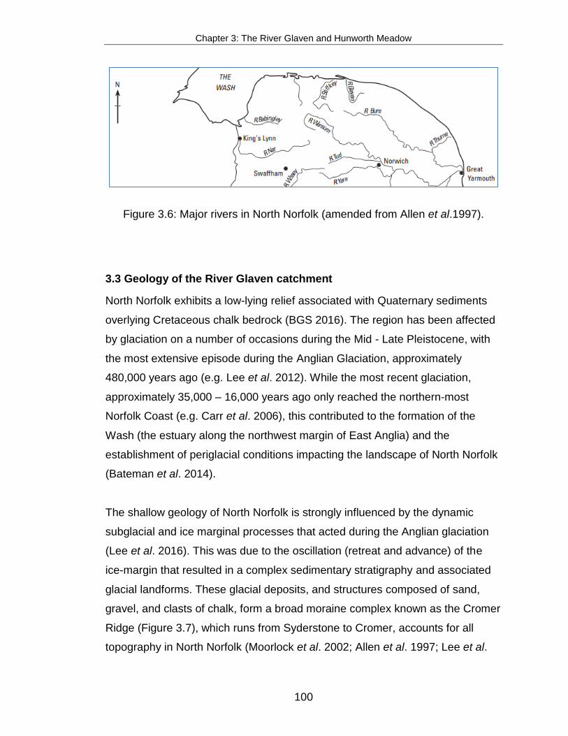
Chapter 3: The River Glaven and Hunworth Meadow
100
Figure 3.6: Major rivers in North Norfolk (amended from Allen et al.1997).
3.3 Geology of the River Glaven catchment
North Norfolk exhibits a low-lying relief associated with Quaternary sediments
overlying Cretaceous chalk bedrock (BGS 2016). The region has been affected
by glaciation on a number of occasions during the Mid - Late Pleistocene, with
the most extensive episode during the Anglian Glaciation, approximately
480,000 years ago (e.g. Lee et al. 2012). While the most recent glaciation,
approximately 35,000 – 16,000 years ago only reached the northern-most
Norfolk Coast (e.g. Carr et al. 2006), this contributed to the formation of the
Wash (the estuary along the northwest margin of East Anglia) and the
establishment of periglacial conditions impacting the landscape of North Norfolk
(Bateman et al. 2014).
The shallow geology of North Norfolk is strongly influenced by the dynamic
subglacial and ice marginal processes that acted during the Anglian glaciation
(Lee et al. 2016). This was due to the oscillation (retreat and advance) of the
ice-margin that resulted in a complex sedimentary stratigraphy and associated
glacial landforms. These glacial deposits, and structures composed of sand,
gravel, and clasts of chalk, form a broad moraine complex known as the Cromer
Ridge (Figure 3.7), which runs from Syderstone to Cromer, accounts for all
topography in North Norfolk (Moorlock et al. 2002; Allen et al. 1997; Lee et al.

Chapter 3: The River Glaven and Hunworth Meadow
101
2016), and controls the direction of river flow in the upper reaches of the River
Glaven (i.e. due to moraine ridge orientation of approximately SW-NE; Figure
3.7).
Figure 3.7: The glacial structures of the Cromer Ridge (in brown) associated
with ice marginal retreat. A summary of the processes operating during each ice
margin retreat stage is indicated in the table key (amended from Lee et al.
2016).

Chapter 3: The River Glaven and Hunworth Meadow
102
The River Glaven’s catchment is characterised by Upper Cretaceous chalk
bedrock that is overlain by chalk-rich stony, sandy, silty, boulder clay (Lowestoft
Formation) up to 40 m thick, and estimated to be less than 20 m thick at the
study site (British Geoglogical Survey borehole log Brinton Hall (TG 0378 3580)
approximately 2.5 km west of the study site; note the borehole at Brinton Hall
was drilled on the interfluve and thus the recorded till thickness of 20 m is likely
to be greater than the thickness of the till in the valley at Hunworth Meadow)
(Figure 3.8). The Lowestoft Formation outcrops extensively throughout the
Glaven catchment but is overlain by Quaternary glaciogenic sand and gravel
deposits (Briton’s Lane Sand Gravel Member) at the study site. Hillwash (also
known as Head), a poorly sorted mixture of clay, sand, silt and gravel, typically
occurs as a veneer less than one metre thick on the valley slopes, and up to
several metres thick at the base of steep slopes. Alluvium along the floodplains
of the River Glaven is estimated to be a maximum of 2 m thick, and consists
predominantly of unconsolidated layers of sand and silt, but also includes
sediments that range from clay to coarse gravel (Moorlock et al. 2002) (Figure
3.8).

Chapter 3: The River Glaven and Hunworth Meadow
103
Figure 3.8: Superficial geology of the River Glaven catchment, and regional
bedrock geology. British Geological Survey data.

Chapter 3: The River Glaven and Hunworth Meadow
104
For much of its length, the River Glaven is classified as a chalk stream (Candy
et al. 2008) (Figure 3.8). Chalk is predominantly found in the south and east of
England, which accounts for the major part of the chalk river resource of Europe
(UK BAP 2011). There are approximately 35 chalk rivers and major tributaries in
the UK that range from 20 to 90 km in length (UK BAP 2011). Chalk aquifers are
a major groundwater resource in northwestern Europe, and are the principle
aquifer in the UK (Allen et al. 2010). They form an important contribution to river
flow, maintaining stable flows of clear cool water in chalk rivers, even during
extended periods of low rainfall (Sear et al. 1999). Rain falling in a chalk
catchment mainly infiltrates into the soil and underlying bedrock, with very little
overland flow. Indeed, it is estimated that up to 90% of discharge of chalk
streams can be from groundwater (Ladle and Westlake 2006; Sear et al. 1999).
Consequently, chalk streams have a characteristic annual hydrograph due to
the slow release of water from the porous aquifer, which attenuates rainfall
events, and provides a fairly stable hydrological regime. Typically, stream flow
increases from December until March/April, when it begins to decline steadily
until the next winter (Berrie 1992).
Chalk rivers typically flow through mixed geologies for some of their length, and
although local hydraulic features are important, they often maintain some of the
characteristics of a groundwater dominated chalk system, e.g. high base flow
index, steady thermal regimes, dampened discharge fluctuations, stable
substratum dominated by gravel, high water clarity, and relatively high alkalinity
(Berrie 1992; Sear et al. 1999). For example, in some sections of the upper
reaches, the River Glaven has characteristics of a fast flowing upland gravel-
bed river, with good riffle-pool structure, whereas in parts of the lower reaches
the river flows over a chalk bed. Impermeable clay layers (see Figure 3.8) can
have some influence on flows in chalk rivers, resulting in more rapid response to
rainfall in some parts of the catchment than would otherwise be expected for a
groundwater dominated system (UK BAP 2011). In addition human acitivities
(e.g. water extractions, sewage treatment dicharges, and land use can affect the

Chapter 3: The River Glaven and Hunworth Meadow
105
groundwater dominance signature in chalk streams (Sear et al. 1999). The
element chemistry of the Chalk aquifer in North Norfolk is presented in Chapter
5 and is given in detail by Ander et al. (2006).
3.4 Surface water quality
As with flow, the chemical (e.g. pH) and physical (e.g. water temperature)
properties of surface water are relatively stable in un-impacted chalk streams
(Berrie 1992; UK BAP 2011). The River Glaven is slightly alkaline, averaging
between pH 7.7 – 8.0 (Table 3.1), which is indicative of a chalk river, mainly due
to calcium carbonate (Berrie 1992). Long-term averages of river chemistry
upstream of the study site indicate that nutrient concentrations have been fairly
constant (Table 3.1). River Glaven nutrient concentrations are moderate, with
nitrate concentrations ranging from 5.8 – 7.5 (mg N L-1) along the river,
approximately four-fold lower than the Environment Agency surface water
threshold of 30 mg NO3--N L-1 (Environment Agency 2013). Phosphate
concentrations are low and average less than 0.05 mg P L-1; these
concentrations are well below the Environment Agency threshold of 0.1 mg P L-1
(Environment Agency 2013) and meet the Water Framework Directive ‘High’
water quality standard of ≤ 0.05 mg L-1 (Table 3.2).
Dissolved oxygen concentrations are high, ranging from 95 – 98% saturation
(10.7 – 10.8 mg L-1) on average in the river. Slightly lower oxygen
concentrations occur in Selbrigg Lake, averaging 89% saturation (10.1 mg L-1),
which is to be expected due to less turbulence and mixing in the lake. Treated
sewage discharges occur into the River Glaven downstream of the study site
near Letheringsett, and downstream of Glandford. Although measurements of
river nutrients upstream of the water treatment works indicate that the water
quality in these sections is good (Table 3.1), river nutrients are likely to be
higher in the immediate vicinity of the water treatment works.

Chapter 3: The River Glaven and Hunworth Meadow
106
Table 3.1: Water chemistry (pH, nitrate, phosphate and dissolved oxygen) of the
River Glaven measured by the Environment Agency. The Selbrigg Lake and
Letheringsett Mill mean values are from samples collected from 2007 - 2010
(n=35). The Hempstead Mill and Edgefiled Bridge mean values are from
samples collected from 1983 – 2007 (n=283).
Sample Location
(upstream/ downstream of study site)
pH NO3-
(mg N L-1) PO4
3- (mg P L-1)
DO (% sat.)
DO (mg L-1)
Selbrigg Lake (upstream)
7.73 ± 0.10
ND 0.06 ± 0.01 89.34 ± 2.04
10.10 ± 0.33
Hempstead
Mill (upstream)
7.93 ± 0.03
7.49 ± 0.31
0.034 ± 0.004
98.47 ± 1.87
10.83 ± 0.53
Edgefield Bridge
(upstream)
8.03 ± 0.03
7.12 ± 0.24
0.032 ± 0.005
95.72 ± 1.17
10.73 ± 0.60
Letheringsett Mill
(downstream)
7.77 ± 0.30
5.84 ± 0.32
0.036 ± 0.004
94.50 ± 2.40
10.69 ± 0.30
3.5 Flora, fauna, and conservation value of the River Glaven
In pristine chalk rivers, stable flows of clear, cool water provide favourable
conditions for the development of diverse river macrophyte and faunal
communities, making them an important ecological resource (Berrie 1992). As
such, they have received considerable conservation attention. A number of
chalk rivers have been designated as Sites of Special Scientific Interest (SSSIs)
(Mainstone 1999), and they are a priority habitat under the EU Habitats
Directive (92/43/EEC). However, chalk rivers are under increasing
management pressures, including low-flow issues, due to enhanced
groundwater abstraction. This has led to the drying out of upper reaches, as well
as the accumulation of silt and changes in the aquatic macrophyte structure (UK

Chapter 3: The River Glaven and Hunworth Meadow
107
BAP 2011). Like most lowland rivers, chalk rivers are generally highly modified
systems. Many have been dredged, lowered and channelized for flood defence
and land drainage purposes (UK BAP 2011).
At Hunworth Meadow, a seasonal pattern of macrophyte growth and recession
occurs in the river channel, which is characteristic of chalk stream flora (Ham et
al. 1982). Dominant macrophytes are Apium nodiflorum (fool's watercress),
Phalaris arundinaceae (reed canary grass) and Rorippa nasturtium-aquaticum
(watercress); these species characteristically dominate chalk stream flora in
summer (e.g Holmes et al. 1998). The large surface area provided by
macrophytes is important for stream invertebrates, providing refugia and habitat
diversity (Berrie 1992).
Although chalk streams and rivers are an important ecological resource, they
are scarce and declining, having suffered from human pressures. The River
Glaven has been modified by agricultural and flood management practices,
such as river channelization, construction of artificial embankments, soil
drainage, and substantial increases in the application of inorganic fertilisers;
nevertheless the river flows through numerous habitat types that are of high
conservation value (e.g. wet meadows, fen meadows, riparian woodlands,
shallow lakes, and coastal marshes), which support a diversity of aquatic and
terrestrial invertebrates and several important and protected bird species such
as heron (Ardea cinerea), barn owls (Tyto alba), kingfisher (Alcedo atthis),
lapwing (Vanellus vanellus), and osprey (Pandion haliaetus) (Sayer and Lewin,
2002).
At the Hunworth Meadow river restoration site (detailed in Section 3.7), many
aquatic species of conservation interest were already present before the
restoration work commenced, including otters (Lutra lutra), the native white-
clawed crayfish (Austropotamobius pallipes), brook lampreys (Lampetra
planeri), and bullheads (Cottus gobio), which are all listed Special Area of
Conservation (SAC) species under the European Habitats Directive (92/43/EEC

Chapter 3: The River Glaven and Hunworth Meadow
108
of 21 May 1992) (JNCC 2013a) as well as wild brown trout (Salmo trutta), and
water voles (Arvicola amphibious) which are listed as a UK Biodiversity Action
Plan (UK BAP) priority species (JNCC 2013b).
The River Glaven is protected under the Freshwater Fish Directive, Natura 2000
(Habitats and/or Birds Directive), Nitrates Directive, and Shellfish Water
Directive; hence, respectively, the River Glaven is deemed a suitable water
body for sustaining fish populations, contains valuable and threatened species
and habitats, is necessary of protection against agricultural runoff, and warrants
protection of habitat (in terms of water quality) for edible shellfish (Table 3.1).
These management directives form integral components of the EU Water
Framework Directive (WFD) environmental targets for surface waters to achieve
‘good’ ecological and chemical status.
The WFD ecological status of a water body is recorded on a 5 tier scale (high,
good, moderate, poor and bad), and chemical status is recorded as good or fail
(Environment Agency 2009). The current overall WFD classification for the River
Glaven is ‘Moderate’ based on moderate fish status and good invertebrate
status, good status for surface water chemistry (e.g. ammonia, dissolved
oxygen, pH, phosphate), and poor flow dynamics (Table 3.2). A goal of “Good”
ecological status is to be achieved by 2027 for the river rather than 2015 due to
the expected high cost of achieving the WFD target.
River restoration is one method being employed to improve ecohydrological
conditions within rivers and along the riparian zone. In this study the removal of
river embankments is being evaluated as a means to improve flood storage, and
the hydrological regime on the floodplain for diversifying wet meadow
vegetation. The River Glaven is currently failing to meet the WFD goals for river
flow, and fish habitat. Hence it is important to determine the success of
restoration projects that aim to reinstate more natural river morphology, and

Chapter 3: The River Glaven and Hunworth Meadow
109
whether these methods can be used to help achieve the WFD ecological,
chemical and hydrological goals.
Table 3.2: Water Framework Directive Classifications for the River Glaven
(Environment Agency 2009).

Chapter 3: The River Glaven and Hunworth Meadow
110
3.6 Modification of the River Glaven and land management at Hunworth
Meadow
The river flows through arable land, deciduous and coniferous woodland in the
upper reaches, while grazing meadows dominate the middle reaches and
former floodplain in the lower reaches, with most of the former floodplain
environments currently disconnected from the river by embankments. Many
reaches have been subject to extensive alterations, which have involved the
deepening and straightening of the channel and the construction of
embankments. In addition, some floodplain areas have been drained and the
natural vegetation has been widely cleared and transformed for agriculture. The
natural flow of the river has also been interrupted or diverted by numerous weirs
and mills (five mills in total: Hempstead, Hunworth, Thornage, Letheringsett and
Glandford). The river Glaven flows through three manmade lakes, two upstream
of the study site at Edgefield Hall and Hempstead Mill, and one downstream at
Bayfield Hall (Oddy 2010). The mill at Thornage is located approximately 500 m
downstream of the study site and is shown in Figure 3.1.
At Hunworth, the River Glaven was constrained by embankments along the
entire length of the meadow study site (Figure 3.9). Hunworth Meadow slopes
gently in an approximate SW to NE direction, is approximately 400 m long, 40 –
80 m wide and has an area of approximately 3 ha. It is bounded to the north-
east by an arable and woodland hillslope (Figure 3.1). An agricultural drainage-
ditch on the meadow runs parallel to the river close to the base of this hillslope,
and at the time of the study was blocked towards the downstream end of the
meadow, impairing the site’s drainage and leading to near-permanent surface
water within a ponded area adjacent to the ditch.
Waterlogging at the site was evident during much of the year, particularly in the
northern, downstream region of the meadow where a pond (Figure 3.10) had
developed adjacent to a blocked drainage ditch (Figure 3.1). These waterlogged

Chapter 3: The River Glaven and Hunworth Meadow
111
soil conditions had affected the vegetation community composition on the
meadow; site walks across the meadow indicated that Holcus lanatus (Yorkshire
fog) and Juncus effusus (Common rush) were the dominant plant species.
Meadows that are dominated by these species are classified under the National
Vegetation Classification (NVC) as mesotrophic rush-pasture communities
(MG10), and are indicative of wet soils with low plant diversity (Rodwell, 1992).
In the ponded area, true aquatic plants are found such as Potamogeton natans
(broad-leaved pondweed), Typha latifolia (broadleaf cattail), Sparganium
erectum (branched bur-reed), which provided a nesting and feeding habitat for
wildfowl.
The management history of Hunworth Meadow is known from 1992 onwards.
The meadow was intensively grazed by cattle until 2000, after which a less
intense grazing regime, using mainly cattle with some sheep, has been
established. Low levels of inorganic fertiliser were used until 1997, but since
then Hunworth Meadow has not received any fertiliser application (Ross
Haddow, Stody Estate, personal communication, 9 October 2012).
Figure 3.9: The River Glaven at Hunworth Meadow, showing the river
embankments along the reach in 2007.
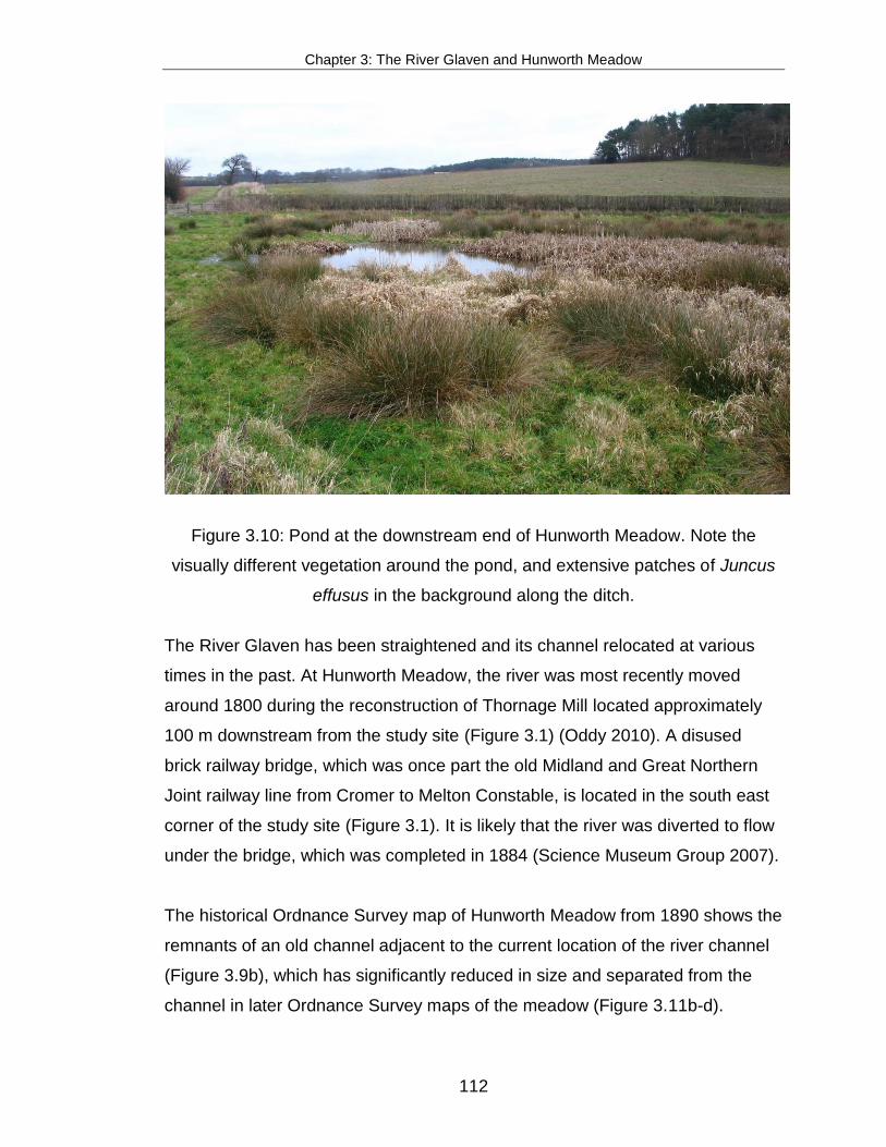
Chapter 3: The River Glaven and Hunworth Meadow
112
Figure 3.10: Pond at the downstream end of Hunworth Meadow. Note the
visually different vegetation around the pond, and extensive patches of Juncus
effusus in the background along the ditch.
The River Glaven has been straightened and its channel relocated at various
times in the past. At Hunworth Meadow, the river was most recently moved
around 1800 during the reconstruction of Thornage Mill located approximately
100 m downstream from the study site (Figure 3.1) (Oddy 2010). A disused
brick railway bridge, which was once part the old Midland and Great Northern
Joint railway line from Cromer to Melton Constable, is located in the south east
corner of the study site (Figure 3.1). It is likely that the river was diverted to flow
under the bridge, which was completed in 1884 (Science Museum Group 2007).
The historical Ordnance Survey map of Hunworth Meadow from 1890 shows the
remnants of an old channel adjacent to the current location of the river channel
(Figure 3.9b), which has significantly reduced in size and separated from the
channel in later Ordnance Survey maps of the meadow (Figure 3.11b-d).
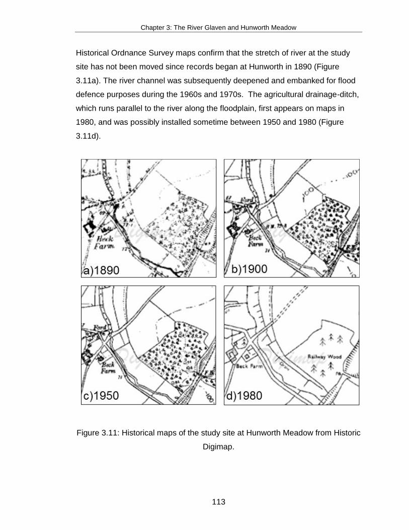
Chapter 3: The River Glaven and Hunworth Meadow
113
Historical Ordnance Survey maps confirm that the stretch of river at the study
site has not been moved since records began at Hunworth in 1890 (Figure
3.11a). The river channel was subsequently deepened and embanked for flood
defence purposes during the 1960s and 1970s. The agricultural drainage-ditch,
which runs parallel to the river along the floodplain, first appears on maps in
1980, and was possibly installed sometime between 1950 and 1980 (Figure
3.11d).
Figure 3.11: Historical maps of the study site at Hunworth Meadow from Historic
Digimap.

Chapter 3: The River Glaven and Hunworth Meadow
114
3.7 The River Glaven restoration project
Chalk rivers such as the Glaven are low energy systems poorly suited to
autonomously reinstate their natural channel structure once it has been
disturbed by engineering works (Sear et al. 2000). Hence, river restoration
through the reconfiguration of river embankments and the channel bed form an
integral part of returning the natural state and functioning of many chalk rivers.
At Hunworth, restoration of the 400 m reach of river was undertaken between 18
- 27 March 2009 by the Environment Agency in collaboration with the River
Glaven Conservation Group, the Wild Trout Trust and Natural England. The aim
of this restoration project was to increase hydrological connectivity between the
over-deepened, embanked river, and its long abandoned floodplain to improve
flood storage capacity, site drainage, and ecological diversity within the
floodplain (e.g. Leyer 2005; Acreman et al. 2007; Hammersmark et al. 2008).
Removal of the embankments and the re-profiling work extended up to 10 m
into the meadow and involved the use of heavy machinery, which resulted in the
removal of approximately 1,400 tonnes of soil from the embankments (Figure
3.12). Removal of the embankments lowered the surface elevation of the
riverbanks to the level of the adjacent meadow (Figure 3.13a and b); the river
margin was subsequently profiled so that elevation gradually increased from the
river towards the meadow, with the hope of introducing a wet to damp moisture
gradient from the river.
The restoration work was restricted to the removal of the river embankments
and did not involve modification of river channel geomorphology (Figure 3.13a
and b). However, during the excavation of the river banks, some sediment was
inadvertently deposited in the river and likely accumulated in downstream
reaches. One section along the embankment was not removed during the
restoration works in order to protect water vole burrows that were found during a
pre-restoration flora and fauna impact survey. This section was, by chance, a

Chapter 3: The River Glaven and Hunworth Meadow
115
low point along the embankments, and was located on the river bend midway
along the meadow. It is easily identified in Figure 3.13b as the undisturbed,
vegetated area surrounded by exposed soil. Relocation of a few young alder
trees that lined the river in the southern part of the meadow was required in
order for the embankment to be reprofiled in this region. The alders were
replanted at other points along the lowered embankment (Figure 3.13b).
Figure 3.12: Embankment removal work in progress (March 2009).
The spoil, which was removed from the site, was largely composed of peaty soil,
however within this there were sand and gravel horizons that likely originated
from the river. These river materials were probably placed on the meadow when
the embankments were constructed and the river was deepened in the 1960‒
70s. Approximately half of the embankment spoil was removed to an arable
field, and the remaining half was stored on the meadow for use during a second
phase in-stream restoration project. This second phase, which is discussed in
Section 10.2.2, was conducted on the same stretch of the River Glaven in
August 2010, one year after the embankment removal and after the main period
of fieldwork reported in this study. This involved the creation of a new, narrower
and more geomorphologically diverse, meandering river channel, aimed at

Chapter 3: The River Glaven and Hunworth Meadow
116
enhancing the in-stream habitat for macroinvertebrates and spawning fish. This
thesis focuses on the ecohydrological research undertaken in the monitoring
and modelling of the embankment removal at Hunworth Meadow, which is
presented in the succeeding chapters.
Figure 3.13: Photographs of the River Glaven at Hunworth Meadow showing (a)
the river embankments in January 2009 prior to the restoration and (b) the
completed restoration work with embankments removed in March 2009.

Chapter 4: Methods - hydrological and chemical monitoring
117
Chapter 4: Methods Part I – hydrological and chemical
monitoring
4.1 Introduction
In order to investigate the ecohydrological implications of river embankment
removal, a three year hydrological monitoring program was conducted at
Hunworth Meadow. It included pre- and post-restoration conditions, fine scale
analyses of floodplain topography, soil and water biogeochemistry, and
vegetation biodiversity. Results from this programme were subsequently
employed within simulations of key hydrological surface water and groundwater
processes.
This chapter describes the study design, and details the monitoring regime used
to study river-floodplain hydrological connectivity prior to and following the river
restoration. This includes information on the collection of hydrological data from
the river and floodplain, sampling and analysis of surface and groundwater
biogeochemistry, monitoring of local meteorological conditions, and topographic
surveys of the river, embankments, and floodplain.
4.2 Study design
Continuous observations of groundwater depth and river stage, measurements
of groundwater chemistry, and surveys of topography were collectively used to
determine the hydrological impacts of river restoration. Groundwater wells were
installed across the meadow in February 2007 in three transects approximately
33 – 39 m in length, each consisting of four or five wells. Transects extended
from the base of the arable and woodland hillslope to the river-embankments
and were aligned perpendicular to the river, i.e. parallel to the assumed main
groundwater flow direction (Figures 4.1 and 4.2). In addition to the Environment

Chapter 4: Methods - hydrological and chemical monitoring
118
Agency gauging station located immediately upstream of the study site (Figure
3.1), a stage board was installed in the river adjacent to the downstream well
transect (Figure 4.2).
Figure 4.1: Cross-sections of the embanked river and floodplain showing the
location of groundwater wells along the three well transects.
The wells were installed at varying depths between 1.3 and 2.0 m due to the
presence of alluvial gravels which proved difficult to penetrate with a hand-
auger. The wells were constructed from polypropylene pipe (inside diameter =
19
20
21
22
c) Upstream transect
b) Midstream transect
River
River
Ditch
Ditch
W1.6W1.4W1.3W1.2W1.1
a) Downstream transect
W2.1W2.2 W2.3 W2.4
Distance (m)
0 10 20 30 40 50 60 70 80 90
19
20
21
22
23
24
25
26
Wells
Topography
Ele
vati
on
(m
)
19
20
21
22
River
DitchW3.1
W3.2W3.3 W3.4
W3.5

Chapter 4: Methods - hydrological and chemical monitoring
119
3.0 cm), screened with 3 mm diameter holes, and wrapped in geotextile cloth to
prevent blockage by fine silts. The tops were covered with rubber caps between
sampling dates. To prevent cattle trampling and damaging the wells, the top of
the wells were approximately 1 – 2 cm below the soil surface, and covered with
a concrete slab (ca. 30 cm × 30 cm) (Figure 4.3).
An enclosure was installed at the upstream well transect in 2009 to protect in-
situ monitoring equipment from damage from grazing livestock. The enclosure
contained solar panels and dataloggers, which were wired to oxygen optodes,
tensiometers, and theta probes buried in the soil profile (Figure 4.4a and 4.4b)
to monitor soil and well oxygen concentrations, soil water potential and soil
volumetric moisture content, respectively (see Section 4.4.3). Well 3.3 was also
located within the enclosure (Figure 4.2).
Figure 4.2: Sampling design at Hunworth Meadow showing the location of the
groundwater wells.
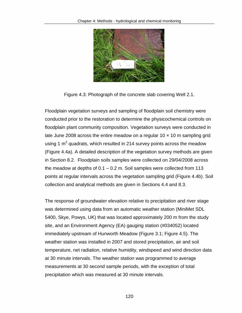
Chapter 4: Methods - hydrological and chemical monitoring
120
Figure 4.3: Photograph of the concrete slab covering Well 2.1.
Floodplain vegetation surveys and sampling of floodplain soil chemistry were
conducted prior to the restoration to determine the physicochemical controls on
floodplain plant community composition. Vegetation surveys were conducted in
late June 2008 across the entire meadow on a regular 10 × 10 m sampling grid
using 1 m2 quadrats, which resulted in 214 survey points across the meadow
(Figure 4.4a). A detailed description of the vegetation survey methods are given
in Section 8.2. Floodplain soils samples were collected on 29/04/2008 across
the meadow at depths of 0.1 – 0.2 m. Soil samples were collected from 113
points at regular intervals across the vegetation sampling grid (Figure 4.4b). Soil
collection and analytical methods are given in Sections 4.4 and 8.3.
The response of groundwater elevation relative to precipitation and river stage
was determined using data from an automatic weather station (MiniMet SDL
5400, Skye, Powys, UK) that was located approximately 200 m from the study
site, and an Environment Agency (EA) gauging station (#034052) located
immediately upstream of Hunworth Meadow (Figure 3.1; Figure 4.5). The
weather station was installed in 2007 and stored precipitation, air and soil
temperature, net radiation, relative humidity, windspeed and wind direction data
at 30 minute intervals. The weather station was programmed to average
measurements at 30 second sample periods, with the exception of total
precipitation which was measured at 30 minute intervals.

Chapter 4: Methods - hydrological and chemical monitoring
121
Figure 4.4: Sampling design at Hunworth Meadow showing the location of the
(a) botanical sampling and, (b) soil sampling points. The enclosure at the
upstream end of the meadow protected in-situ sampling equipment within from
grazing cattle.

Chapter 4: Methods - hydrological and chemical monitoring
122
Figure 4.5: Photographs of (a) the automatic MiniMet weather station and (b)
the Environment Agency gauging station located at Hunworth (#034052).
The EA gauging site at Hunworth Meadow is a relatively wide, shallow channel
with a bed width of 4 m and maximum depth of 1 m. River discharge is
measured using a v notch weir design (Figure 4.5b). Mean daily river stage and
discharge data were available for the Hunworth gauging station for the period
2001 – 2010. However, there were some gaps in the record, because seasonal
macrophyte growth in the channel downstream of the gauging station caused
water to backup over the weir that impacted on the rating curve and reduced the
accuracy of the data during these periods. This was manifested in a slow
increase in baseflow through summer, despite low or no rainfall, upon which
individual peaks associated with rainfall events were superimposed.
Subsequently, this apparent elevated baseflow would decline during the autumn
due to macrophyte dieback. The influence of the vegetation on discharge
measurements was, in some cases, removed abruptly during flood events,

Chapter 4: Methods - hydrological and chemical monitoring
123
possibly due to a devegetation of the river channel and relocation of sediment
downstream. The influence of macrophyte growth on river discharge was
easily identified in the discharge record when compared with precipitation data.
The affected data were excluded from quantitative analyses (baseflow index,
flow duration) (see Figures 5.5, 5.10, and 6.26). Another EA gauging station is
located on the River Glaven approximately 5 km downstream of the study site at
Bayfield (Station Number: 034016). Mean river discharge at Bayfield was
recorded from 1970 – present, however, unfortunately the river discharge at
Bayfield is not rated above 0.3 m (ca. 0.65 m3 s-1) due to the influence of
Letteringsett mill, located immediately upstream. Data quality and the methods
used to substitute missing data in the discharge record at Hunworth are
described in Sections 6.3 and 6.5.
4.3. Hydrological monitoring
4.3.1 Groundwater and surface water levels
To characterize fluctuations in groundwater elevation, Solinst combined
pressure transducer-dataloggers (Levelogger Gold 3.0, Ontario, Canada) were
installed in four wells at the upstream transect, one well at the midstream
transect, and in five wells at the downstream transect. Groundwater elevation
was recorded hourly from February 2007 – August 2010. A barologger was
positioned on a fence post on the boundary of Hunworth Meadow above the
water level and in air in order to compensate for barometric pressure. The
Solinst level loggers record temperature compensated water level and operate
accurately within a thermal range of -20 to +80 ˚C. The loggers are completely
autonomous, and can remain in situ recording for long periods of time (battery
life = 10yrs; max. 40,000 readings) (Solinst 2006). However, for this study the
leveloggers were downloaded and the readings checked with manual
measurements of groundwater elevation during regular field visits.

Chapter 4: Methods - hydrological and chemical monitoring
124
4.3.2 Base flow index and flow exceedance values
To assess the permeability of the surrounding geology at the study site, and the
potential for subsurface river-floodplain hydrological interactions, the river base
flow index (BFI) was calculated for each full year of EA river discharge data at
the site using a base flow separation program (BFI version 4.15) (Wahl and
Wahl 2007). The BFI program follows the Institute of Hydrology (1980) base
flow separation procedure, where the water year is divided into 5-day
increments to identify minimum flow, called a turning point. The turning points
are then connected to obtain the baseflow hydrograph. The volume of base flow
for the period is estimated by the area beneath the hydrograph. The base-flow
index is calculated as the ratio of baseflow volume to the total volume of
streamflow. High BFI values indicate groundwater dominance, which is broadly
represented by a stable flow regime (Sear et al. 1999). A detailed description of
the BFI calculation is given by Gustard et al. (1992).
The contribution of groundwater to total river flow was also analysed using flow
exceedance values for Q10 (a high flow threshold that is equalled or exceeded
for 10% of the flow record) and Q95 (a low flow threshold that is equalled or
exceeded for 95% of the flow record), which were determined from a river flow
duration curve. Q95, expressed as the percentage of mean annual river flow,
and comparisons of Q10 and Q95 provide a measure of the variability (i.e.
flashiness) of the flow regime (Gustard et al. 1992; Marsh and Hannaford 2008).
4.3.3 Evapotranspiration
Daily values of Penman-Monteith potential evapotranspiration (Monteith 1965)
were computed from meteorological data (temperature, net radiation, humidity,
wind speed) provided by the on-site weather station (Figure 4.6). These data
were supplemented by a nearby (<9 km distance) British Atmospheric Data
Centre weather station (Source ID: 24219, Mannington Hall) (Figure 3.1),
however, there were periods of time where data were not available. In instances

Chapter 4: Methods - hydrological and chemical monitoring
125
where wind speed data was unavailable an average wind speed value of 1.6 m
s-1 was used, computed from the Hunworth Meadow data.
The reference formula for grasslands described by Allen (2000) was used to
calculate potential evapotranspiration. This equation assumes a constant grass
height of 0.12 m throughout the year (see also Hough and Jones, 1997), and a
fixed surface resistance of 70 s m-1 with an albedo of 0.23 (Allen 2000), and was
calculated as:
2
2
34.01
273
900408.0
u
eeuT
GR
ETasn
o
(4.1)
where, ETo is reference evapotranspiration (mm day-1), Rn is net radiation at the
crop surface (MJ m-2 day-1), G is the soil heat flux (MJ m-2 day-1) which is small
compared to Rn, especially when the surface is covered by vegetation and
calculation time steps are >24 hours and thus was set to 0 in this instance, T is
the mean daily air temperature at 2 m height (°C), u2 is the wind speed at 2 m
height (m s-1), es is the saturation vapour pressure (kPa), ea is the actual vapour
pressure (kPa), ∆ represents the slope of the saturation vapour pressure
temperature relationship (kPa °C-1), and λ is the psychrometric constant (0.067
kPa °C-1 for 0 m altitude) (Allen 1998).
Actual vapour pressure, ea (kPa), the vapour pressure exerted by the water in
the air, was calculated using relative humidity data as:
2
100100min
maxmax
min
RHTe
RHTe
ET
oo
o
(4.2)
where e°(Tmin) is the saturation vapour pressure at daily minimum temperature
(kPa), e°(Tmax) is the saturation vapour pressure at daily maximum
temperature (kPa), RHmax is the maximum relative humidity (%), and RHmin is
the minimum relative humidity (%).There were some short periods of time where

Chapter 4: Methods - hydrological and chemical monitoring
126
the maximum humidity data was either missing or of questionable quality
(Figure 4.6). In the absence of maximum humidity data an alternative method of
calculating actual vapour pressure for the potential evapotranspiration equation
was used. The actual vapour pressure (ea) which equals the saturation vapour
pressure at the dewpoint temperature (Tdew), was estimated by assuming that
Tdew ≈ Tmin in the following equation:
3.237
27.17exp6108.0
dew
dewdew
o
aT
TTee (4.3)
The relationship Tdew ≈ Tmin holds in wet environments where the air is nearly
saturated with water vapour at sunrise when the air temperature is close to the
daily minimum temperature (Tmin) (Allen 1998).
Saturation vapour pressure, es, was calculated as:
2
minmax TeTee
oo
s
(4.4)
where, e°, is the saturation vapour pressure (kPa) at a given temperature, T:
3.237
27.17exp6108.0
T
TTeo (4.5)
The difference between the saturation and actual vapour pressure, (es – ea), is
the saturation vapour pressure deficit and indicates the actual evaporative
capacity of the air. The slope of the relationship between saturation vapour
pressure and temperature, ∆, at a given temperature was calculated as:
23.237
3.237
27.17exp6108.04098
T
T
T
(4.6)

Chapter 4: Methods - hydrological and chemical monitoring
127
Figure 4.6: Time series of (a) mean daily air temperature and net solar radiation,
(b) mean daily wind speed, and (c) maximum and minimum relative humidity.

Chapter 4: Methods - hydrological and chemical monitoring
128
4.3.4 Hydraulic conductivity
Hydraulic conductivity values of the top 2 m of soil were determined using
piezometer slug tests (n = 25) following the approach of Surridge et al. (2005).
This included six slug tests in the geotextile-screened monitoring wells (inside
diameter = 3.0 cm) already installed at the site, and 19 slug tests using
piezometers with larger intakes (Figure 4.7) specifically designed to reduce flow
resistance through the screens and more accurately measure flow through
porous organic layers. After inserting a continuous-logging Solinst 3.0 pressure
transducer into the base of the piezometer, programmed to take readings every
10 seconds, a slug, which consisted of a sand ballast-filled PVC tube (outside
diameter = 2.2 cm) sealed at both ends with rubber bungs, was lowered into the
piezometer (Figure 4.8).
Figure 4.7: Photograph of the piezometer intakes used in the slug tests.
Figure 4.8: Diagram of the sand-filled slug.
The water level (head) in the piezometer was then left to recover to pre-test
levels, at which point the slug was removed smoothly and swiftly from the
piezometer. The pressure transducer was removed and downloaded once the
water level in the piezometer had again returned to pre-test levels. A typical
response in water table height during the slug tests at Hunworth Meadow to
PVC tube
Rubber
bung
Rope

Chapter 4: Methods - hydrological and chemical monitoring
129
determine hydraulic conductivity is shown in Figure 4.9. The water level
recovery in Figure 4.9 is from a test piezometer installed adjacent to the
upstream observation well 3.1. The water level readings show the recovery of
the water table from 0 – 2,000 secs after the insertion of the pressure
transducer and the slug during the set-up of the test, and the response of water
levels during the test from 2,150 – 5,030 secs after the removal of the slug at
2140 secs.
Figure 4.9: Typical response in water table height during slug tests at Hunworth
Meadow to determine hydraulic conductivity.
Hydraulic conductivity was calculated from the recovery in hydraulic head
assuming Darcian flow as:
FT
AK (4.7)

Chapter 4: Methods - hydrological and chemical monitoring
130
where K is hydraulic conductivity (cm s-1), T is the basic hydrostatic time lag
(secs), A is the inside cross-sectional area of the piezometer (cm), and F is the
shape factor of the piezometer intake (cm) (Hvorslev 1951; Baird et al. 2004;
Surridge et al. 2005), calculated as:
2
ed
1.2l1
d
1.2llog
l 2.4πF (4.8)
where d is the outside of the intake (cm) and l is length of the intake (cm)
(Brand and Premchitt 1980; Baird et al. 2004). The hydrostatic time lag (T) was
solved by fitting equation 4.9 to the measured head recovery data using a least-
squares minimization with T as the fitted parameter:
-t/Teh
h
0
(4.9)
where h is the head difference at t (cm), h0 is the initial head difference (cm),
and t is time from the start of the test (sec) (i.e. slug withdrawal) (Hvorslev 1951;
Baird et al. 2004).
Assuming Darcian flow, head recovery during slug tests should be log-linear
(Hvorslev 1951; Baird et al. 2004). Comparisons of the decline in normalised
head (h/h0) following slug-removal (t0) and the best-fit Hvorslev equation
indicate that head recoveries were adequately log–linear (Figure 4.10). Eight
additional slug tests were undertaken at the site; however these tests were
excluded because the water level recovery was too slow to be captured
adequately during the observation period, and the early water level response
showed substantial departures from log-linearity. As only a small part of the
recovery could be used in the calculation of K, the accuracy of the test was
likely affected and these tests were removed from the analysis.

Chapter 4: Methods - hydrological and chemical monitoring
131
Figure 4.10: Typical example of the log-linear change in normalized head (h0/h)
following slug removal at time 0. Normalised heads are plotted on a linear scale
(open circles) and logarithmic scale (open squares). Line indicates best-fit
Hvorslev equation; the basic hydrostatic time lag = 753.45 secs, r2 = 0.995.
Subsurface flow rates were calculated assuming Darcian flow as:
en
Δl
ΔhΚ
υ (4.10)
where υ is flow rate (m day-1), ne is effective porosity, Δh/Δl is water table slope
obtained from hydraulic head measurements taken at each well along the
transect, and K is hydraulic conductivity in m day-1 (Domenico and Schwartz
1998). Mean values of K and Δh/Δl for each well transect were used in this
calculation.
0 500 1000 1500 2000 2500
0.0
0.2
0.4
0.6
0.8
1.0
0.01
0.1
1
No
rmalised
head
(lin
ear
scale
)
No
rmalised
head
(lo
g s
cale
)
Time (secs)
9950r2
45.753/
.
eh
h t-
0
=
=
Chapter 4: Methods - hydrological and chemical monitoring
132
4.4 River-floodplain biogeochemical monitoring
4.4.1 Soil structural and physical properties
Measurements of soil variables were confined to the upper 0.1 – 0.2 m of
floodplain soils. In April 2008, 113 soil samples were collected across the
floodplain (Figure 4.4b). Duplicate field and analytical samples were taken
randomly, were checked for sampling bias and analytical accuracy and
precision, and were averaged to give final values.
Bulk density and porosity were calculated from the difference in the volume of
saturated and dry soil (Elliot et al. 1999) collected using bulk density rings (I.D =
53 mm, height = 51 mm, volume = 100 cm3) from the top 0 – 0.2 m of soil.
Organic matter content was subsequently analysed by Loss on Ignition (Heiri et
al. 2001). Total porosity was calculated assuming a particle density of 2.65 g
cm-3 (Jarrell et al. 1999). For the analysis of soil pH, duplicate 15 g field-moist
sieved (4 mm) soil subsamples were mixed with 15 ml of dionised water. The
samples were left to equilibrate for 30 min and subsequently measured with a
HANNA HI8424 pH probe (HANNA Instruments Ltd , Bedfordshire, UK)
(Robertson et al. 1999).
Soil particle size (soil texture) was determined with optical laser diffraction using
an LS 13320 Coulter Counter particle size analyzer (Beckman Coulter Corp.,
Hialeah, Florida, USA). Prior to analysis, the soil samples were treated with
hydrogen peroxide to remove organic matter, and subsequently with sodium
hexametaphosphate (Calgon) to disaggregate the soil particles (Chappell 1998).
Soil textural class was also recorded using the “feel” method in the field during
the collection of soil samples (Brady and Weil 2002). Soil samples were also
analysed for exchangeable ions in order to determine nutrient availability for
plant and microbial uptake. The salt solutions used to extract the exchangeable

Chapter 4: Methods - hydrological and chemical monitoring
133
ions from the soil, and the analytical methods employed to measure nutrient
concentrations in the extractants are described in Chapter 8.
4.4.2 Water chemistry sampling and analysis
River water, shallow groundwater (top 1 − 2 m of soil), and rooting zone pore
water samples were taken bimonthly from 2007 − 2008 to examine the spatial
variation in subsurface and rooting zone chemistry. Groundwater samples were
collected using a point-source bailer and stored in pre-washed 250 mL
polyethylene bottles. Before acquiring samples, the wells were purged to
introduce fresh groundwater and the collection bottles were rinsed with well
water. Pore water in the rooting zone was collected using 0.1 μm rhizon
samplers, 0.1 m in length (Figure 4.11a). The rhizon samplers were attached to
evacuated test tubes with syringe needles, and inserted into the top 0.1 m soil
(Figure 4.11b). The water samples were stored in a cooler until return to the
laboratory, refrigerated, and then filtered through 0.45 μm filter paper. The
rhizon samples were not filtered in the laboratory as the water had already
passed through the 0.1 μm rhizon sampler. Any samples that could not be
analyzed within two days were frozen.
Figure 4.11: Photographs of rhizon soil moisture samplers taken in the
laboratory (a), and in the field attached to test-tubes collecting pore-water from
the rooting zone.

Chapter 4: Methods - hydrological and chemical monitoring
134
Dissolved oxygen, pH and electrical conductivity were measured in the field at
the time of water sampling using a handheld YSI-555A dissolved oxygen meter
(YSI Hydrodata Ltd, Letchworth, UK), a Mettler Toledo MP120 pH meter and a
Mettler Toledo MC126 conductivity meter (Ohio, USA), respectively. Prior to use
in the field, the pH meter was calibrated with pH 4 and pH 7 BDH Prolabo
calibration solutions (buffer tablets, VWR, Leicestershire, UK), and the
conductivity meter was calibrated using a 1413 µs calibration solution (0.01M
KCl @25°C).
In the laboratory, cations (Ca2+, Mg2+, K+, Na+, NH4+) and anions (SO4
2-, Cl-,
NO3-, NO2
-, PO43-) were analysed by ion exchange chromatography (ICS-2500,
Dionex Corp., California, USA). Dissolved organic carbon (DOC) and total
dissolved nitrogen (TDN) were determined using a HiPerTOC carbon analyser
plumbed to a HiPer5000 total nitrogen chemoluminescent detector (Thermo
Electron Corp., Delft, The Netherlands). Deep groundwater chemistry data were
obtained from an EA borehole within the Glaven catchment, located at Edgefield
(52° 52′ 49.36″ N, 01° 05′ 52.91″E), approximately 2 km from Hunworth study
site (Figure 3.6). The borehole is used to monitor water levels and chemistry in
the chalk strata, and had a response zone of 38 – 41 m below ground surface.
The chemistry data obtained from the EA borehole are assumed to be
representative of the groundwater chemistry of the chalk underlying the study
site. This is reasonable considering the close proximity of the EA borehole to the
study site, and that the chalk is laterally continuous in the region (Figure 3.6). It
is unknown whether the chalk aquifer is in hydraulic continuity with the river at
the study site; however as a point of comparison the chalk groundwater samples
were included in the chemical analyses.
4.4.3 Oxygen concentration in soil pores
Measurements of dissolved oxygen in the soil profile were obtained at 30 minute
intervals from two Aanderaa 4175 oxygen optodes (Bergen, Norway) attached

Chapter 4: Methods - hydrological and chemical monitoring
135
to Campbell Scientific CR1000 dataloggers (Loughborough, UK; Figure 4.12).
The Aanderaa Oxygen Optodes are based on the ability of certain molecules, in
this case oxygen, to influence the florescence of other molecules, in a process
called dynamic luminescence quenching (lifetime based). The Aanderaa
Oxygen Optodes were chosen for this study because, unlike electro-chemical
sensors, they do not consume oxygen and are less affected by fouling, making
them suitable for systems with limited exchange of water such as in
groundwater (Aanderaa 2006). To evaluate temporal fluctuations in oxygen
concentration within the rooting zone, the oxygen optodes were installed at the
upstream well transect (Well location 3.3) from January 2009 to August 2010
(see Figure 3.1).
The optodes, dataloggers and solar pannels were installed in an enclosure to
protect them from livestock (Figure 4.12). Initially, the optodes were installed in
wells at 0.1 and 0.3 m depths. However, in January 2010 the 0.3 m oxygen
optode was moved from the well and buried directly in the soil at 0.1 m below
the ground surface. Although the optodes can remain in-situ for more than one
year without repeated calibration (Aanderaa 2006), the calibration was checked
periodically using a zero-oxygen solution (sodium sulphite saturated in
deionised water) and 100% saturated solution (deionised water bubbled with
air).

Chapter 4: Methods - hydrological and chemical monitoring
136
Figure 4.12: Clockwise from top of the photograph, dataloggers, position of the
oxygen optodes (protected in plastic containers), and varying depths of the
tensiometers.
Soil water potential (matric potential) was measured at 30 minute intervals with
five water-filled ceramic cup Delta-T SWT4 tensiometers, three were buried in
the enclosure at depths of 0.1, 0.3, and 0.5 m, and two were buried outside of
the enclosure: one approximately 13 m from the river at a depth of 0.5 m, and
one approximately 9 m from the ditch at a depth of 0.5 m. Two Delta-T ML2X
theta probes, attached to Campbell Scientific CR1000 dataloggers
(Loughborough, UK), were installed in the enclosure at the site to measure
volumetric soil water content at 30 minute intervals (Figure 4.12). The optimal
operating range for these probes covered 0 − 0.5 m3 m-3 (accuracy within 1% for
soil specific calibration), which corresponds to a voltage output 0 − 1.0 V (Delta-
T Devices 1998). All of the readings were at or above 1.0 V, which suggests that
these probes were not suitable for soils that are so wet. Due to a narrow range

Chapter 4: Methods - hydrological and chemical monitoring
137
of soil moisture conditions measured at the site, an in-situ soil moisture release
curve (soil tension versus soil water content) could not be measured, and
laboratory analyses of soil moisture release were conducted (see Section 8.3.3).
Nevertheless, the theta probes remained in-situ for the study period in order to
measure any decrease in soil moisture that might suggest periods of soil drying
stress. A manual hand-held Delta-T ML2X theta probe was used to cross-check
the buried probe readings periodically; furthermore, the response of the buried
theta probes in drier soils (collected from the hillslope in a bucket) was checked
midway through the study period and compared with the measurements from
the hand-held meter.
4.4.4 River and floodplain topography
Surface elevation of the meadow, river channel and before their removal, the
embankments were surveyed using a differential Global Positioning System
(dGPS) (Leica Geosystems SR530 base station receiver and Series 1200 rover
receiver, Milton Keynes, UK; Figure 4.13) in April 2008 prior to the restoration,
and in July 2009 after the restoration. Each survey was conducted using the
survey pole in static mode, which according to the output data resulted in a 3D
coordinate quality of 1 – 2 cm. The meadow was surveyed at intervals of
approximately 10 m, whereas the river embankments and cross-sections were
surveyed at a higher resolution using intervals of approximately 0.25 – 0.5 m
(Figure 4.14). River channel cross-sections were surveyed at 32 transects along
the study reach prior to the restoration (Figure 4.14a) and at 23 transects after
the restoration (Figure 4.14b). Digital elevation models (DEMs) were created in
Arc-GIS using the Kriging interpolation function, which estimates values from a
statistically weighted average of nearby sample points (de Smith et al. 2007).

Chapter 4: Methods - hydrological and chemical monitoring
138
Figure 4.13: Photographs of the differential Global Positioning System base
station (a) and the rover in-use at Hunworth Meadow.
Figure 4.14: Location of dGPS sample points for the embanked (a) and restored
(b) topographic surveys.

Chapter 4: Methods - hydrological and chemical monitoring
139
4.5 Flood prediction
4.5.1 Bankfull capacity
The effects of embankment removal on the frequency of overbank inundation
were evaluated by estimating the change in bankfull capacity. A field-based
method was used to relate bankfull elevation, measured before and after
embankment removal using dGPS, to a stage board installed adjacent to the
downstream well transect (Figure 4.15). Bankfull discharge was then predicted
using a regression relationship between river stage in the Hunworth Meadow
reach and discharge at the EA gauging station upstream of the Meadow, which
was located approximately 0.3 km above the stage board (Figure 3.1). This
method assumes that groundwater exchanges and runoff inputs do not
significantly affect river discharge between the gauging station and stage board,
which is reasonable considering their close proximity.
The regression relationship between river stage and discharge for
spring/summer (April – September) follows a slightly lower trajectory than for
autumn/winter (October – March) (p<0.05, F value = 35.41) (Figure 4.15). This
can be attributed to the extensive growth of aquatic macrophytes, such as
watercress (Rorippa nasturtium-aquaticum), fool's watercress (Apium
nodiflorum), and reed canary grass (Phalaris arundinaceae), within the channel
during the growing season (Figure 4.16). Seasonal in-stream vegetation growth
can have a significant effect on the fluvial dynamics of streams by modifying
flow velocities and sedimentation rates (Champion and Tanner 2000; Clarke
2002), resulting in a reduction in channel capacity during spring and summer.
For example, river stage at the downstream well transect was higher during the
summer compared with the winter (Table 4.1). However, the higher river stage
during the summer was actually associated with lower river discharge compared
with the winter (Table 4.1). The effects are often diminished, however, at high

Chapter 4: Methods - hydrological and chemical monitoring
140
flows due to compression of the macrophyte stems, or devegetation, which can
substantially reduce flooding potential (Chambers et al. 1991; Wilcock et al.
1999; Champion and Tanner 2000). For example, Chambers et al. (1991)
reported that, in slow-flowing rivers studied in western Canada, macrophyte
biomass decreased with increasing flow velocities over a mean range of 0.2 −
0.7 m s-1, with aquatic macrophytes typically absent at velocities above 1 m s-1.
Figure 4.15: Relationship between river stage and mean daily river discharge
used to determine bankfull capacity. Lines indicate statistically significant
regression at p<0.05, yautumn/winter = 7.6795E-29e3.2285x, yspring/summer = 0.415x -
8.0379. River Glaven discharge data are from the EA gauging station (#034052)
located immediately upstream of the Hunworth Meadow.

Chapter 4: Methods - hydrological and chemical monitoring
141
Figure 4.16: Photographs reflecting the different in-river macrophyte abundance
during the winter (a) and summer (b) months at the river stage located at the DS
transect. Photograph (a) was taken on 3rd March 2009, prior to the restoration.
Photograph (b) was taken on 25th July 2010 following embankment removal.
Table 4.1. Corresponding Environment Agency river discharge and stage, and
downstream river stage for the low (a) and high (b) levels of in-river macrophyte
abundance shown in Figure 4.17.
Date
EA River Discharge
(m3 s-1)
EA river stage (m)
Downstream transect river stage (m)
3rd March 2009 (a) 0.325 0.212 0.30 25th July 2010 (b) 0.143 0.154 0.39

Chapter 4: Methods - hydrological and chemical monitoring
142
Indeed, macrophyte abundance on the River Glaven was observed to be
substantially lower during high-flow summers (mean flow: 0.38 m3 s-1) (Figure
4.17a), compared with low flow summers (mean flow: 0.19 m3 s-1) (Figure
4.17b), probably due to devegetation at higher flows. As spring/summer river
stage was only measured during periods of low river flows (0.15 – 0.24 m3 s-1)
(Figure 4.15), and the effects of macrophyte abundance is likely reduced during
high flow conditions, the spring/summer regression equation was not used to
determine bankfull capacity. Instead, bankfull capacity was calculated with the
autumn/winter regression equation (Figure 4.15), which encompasses river
stage measurements for a range of wider flows (0.25 – 1.9 m3 s-1) during low
macrophyte abundance.
Figure 4.17: Photographs reflecting the different in-river macrophyte abundance
during a wet (a) and dry (b) summer. Photograph (a) was taken on 17th July
2007, prior to the restoration. Photograph (b) was taken on 25th July 2010,
following embankment removal.

Chapter 4: Methods - hydrological and chemical monitoring
143
Bankfull discharge was also determined by a semi-empirical method using the
Manning’s equation for uniform flow as:
31321 // SARn
Q= (4.11)
where Q is discharge (m3 s-1), n is Manning’s roughness coefficient, A is bankfull
cross-sectional area (m2), R is hydraulic radius (m), and S is water surface slope
(Gordon et al. 2004). The value of Manning’s roughness coefficient (n value),
describes the channel bed resistance to flow, and was estimated using the
Rosgen (1996, 2007) stream classification method. This required the following
river morphology input parameters: bankfull width-to-depth ratio, entrenchment
ratio (flood-prone width at 2 × bankfull depth/bankfull width), water surface slope
and channel sinuosity, which were obtained from river channel cross-sections,
surveyed using dGPS, and measurements of river channel length in Arc-GIS.
The River Glaven at Hunworth has a low gradient of <0.004 (Figure 4.18), a
moderate sinuousy of 1.4 (Table 4.2), and low width to depth ratio of <9 (Table
4.2). Collectively, these characteristics most closely fit a Rosgen type C stream,
which is defined as slightly entrenched, with a riffle-pool bed form and channel
width > depth (Table 4.3). A type E stream may also be applicable, but is
typically assigned to streams with high sinuosity, which does not fit the River
Glaven. The removal of the river embankments and the associated reduction in
river incision increased entrenchment ratio and increased the width of the river
relative to depth; however these changes did not alter the classification of the
stream within the Rosgen scheme. Bed slope and sinuosity were unchanged.

Chapter 4: Methods - hydrological and chemical monitoring
144
Table 4.2: Stream morphology of the River Glaven. Entrenchment ratio, width to
depth ratio, sinuosity and bedslope parameters required for Rosgen’s stream
classification system.
Pre restoration
Post restoration
Applicable stream type
Entrenchment ratio <1.4 = entrenched 1.4-2.2 = moderate
>2.2 = slightly entrenched
2.79 15.51 C, E
Width to depth ratio <12 = low
12-40 = moderate >40 = high
7.32 8.80 E
Sinuosity <1.2 = low
1.2-1.5 = moderate >1.5 = high
1.40 1.40 C
Bed slope 0.00353 0.00353 C, E
Figure 4.18: Water surface elevation of the River Glaven at Hunworth.
Distance (m)
0 50 100 150 200 250 300
Wate
r su
rfa
ce
ele
vati
on
(m
)
19.4
19.6
19.8
20.0
20.2
20.4
20.6
Water surface slope = 0.00353
r2 = 0.983

Chapter 4: Methods - hydrological and chemical monitoring
145
Table 4.3: General descriptions and physical criteria for Rosgen’s stream
classification system. Modified from Rosgen (2007).
Stream type
Description Entrench-ment ratio
W/D ratio
Sinuosity Slope
Aa+ Very high relief. Deeply entrenched, debris transport, torrent streams. Vertical steps with deep scour pools; waterfalls
<1.4 <12 1.0 – 1.1 >0.10
A High relief. Entrenched, cascading, step-pool streams. High energy/ debris transport associated with depositional soils. Very stable if bedrock or boulder-dominated channel. Frequently spaced, deep pools in associated step-pool bed morphology
<1.5 <13 1.0 – 1.2 0.04 – 0.10
B Moderate relief. Moderately entrenched, moderate gradient, riffle dominated channel with infrequently spaced pools. Rapids predominate with scour pools. Very stable plan and profile. Stable banks.
1.4 – 2.2 >12 >1.2 0.02 – 0.039
C Broad valleys with terraces, in association with floodplains, alluvial soils. Low gradient, meandering, point bar, riffle/pool, alluvial channels with broad, well-defined floodplains.
>2.2 >12 >1.2 <0.02
D Broad valleys. Braided channel with longitudinal and transverse bars. Very wide channel with eroding banks.
n/a >40 n/a <0.04
DA Broad, low-gradient valleys with fine alluvium and/or lacustrine soils. Anastomizing (multiple channels) narrow and deep with extensive, well-vegetated floodplains and associated wetlands. Very gentle relief with highly variable sinuosities and width-to-depth ratios. Very stable streambanks.
>2.2 Highly variable
Highly variable
<.005
E Broad valley/meadows. Low gradient, meandering riffle/pool stream with low width-to-depth ratio and little deposition. Very efficient and stable. High meander width ratio.
>2.2 <12 >1.5 <0.02
F Entrenched meandering riffle/pool channel on low gradients with high width-to-depth ratio.
<1.4 >12 >1.2 <0.02
G Entrenched gully step-pool and low width-to-depth ratio on moderate gradients
<1.4 <12 >1.2 0.02 – 0.039

Chapter 4: Methods - hydrological and chemical monitoring
146
The river substrate (percentage composition of sand, gravel, cobble) was
surveyed at 53 regular points along the river on 03/03/2009. The river bed at the
site was composed of a mixed sand and gravel bed, averaging 60% sand, 35%
gravel, and 5% cobble (Figure 4.19). The substrate composition was fairly
variable along the study reach, with sandbar and gravelbar sections. The river
can be further defined within the Rosgen scheme as either a C4 (gravel bed) or
C5 (sand bed) stream. Figure 4.20 shows the typical Manning’s roughness
coefficients for different stream types. Using the values for small streams with a
vegetation influence, a C4 gravel bed stream and C5 sand bed stream
correspond with average bankfull manning’s n values of approximately 0.04 and
0.056, respectively (Figure 4.19) (Rosgen 2007). A range of bankfull discharge
estimates were calculated by holding all other terms constant and varying
Manning’s n only between the two extremes of 0.04 and 0.056. The Manning’s
bankfull estimates were subsequently compared with the bankfull stage–
discharge estimates.
Figure 4.19: River bed substrate composition of the River Glaven at Hunworth
(n=154 along 53 points).

Chapter 4: Methods - hydrological and chemical monitoring
147
Figure 4.20: Bankfull roughness coefficients by stream type for 140 streams in
the USA and New Zealand (Rosgen 2007).
4.4.2 Recurrence intervals
Recurrence interval (return period in years) of bankfull discharge was computed
using flood peaks over threshold (POT) data, which were extracted from
discharge data measured at the on-site EA gauging station from 2001 to 2010.
Flood POT was used rather than annual maximum floods because it provides
more information on flood regime and is more suitable for records of <13yrs
(Institute of Hydrology 1999). Discharge data were arranged into water years
beginning on 1 October, the threshold value was set at 0.6 m3 s-1 so that, on
average, five independent peaks per year were included in the series (Institute
of Hydrology 1999, Cunderlik and Burn 2001). Aquatic macrophytes caused
breaks in the river discharge record during some years; however, these years
were included in analysis where: (a) the gaps did not constitute a major portion
of the record, and (b) precipitation data available to confirm that large flood

Chapter 4: Methods - hydrological and chemical monitoring
148
peaks were unlikely to have been missed. The recurrence interval for bankfull
discharge was determined as:
T=qQT lnln0 (4.12)
where QT is the magnitude of flood (m3 s-1) with a return period of T years, q0 =
POT threshold discharge (=0.6 m3 s-1), β is mean discharge (=1.01 m3 s-1)
minus threshold discharge, λ is the number of peaks (=37) divided by the
number of full years of data (=8 years) (Wilson 1983).
4.6 Statistical analyses
4.6.1 Linear regression models and diagnostics tests
Simple linear regression was used to determine correlations between river stage
and mean daily river discharge for summer and winter periods. To test whether
the summer and winter regression functions differed, a full and reduced F test
comparison was used. The full model was a regression of river discharge (y) on
river stage (X1), the indicator variable for winter and summer (X2), and the
interaction term for differences in slope (X1*X2). The reduced model was a
regression of river discharge on river stage. Differences in hyporheic chemistry
along well transects were tested using one-way Analysis of Variance (ANOVA).
If a significant difference was found (p<0.05), a Tukey’s test was used to
determine which wells were significantly different (p<0.05). To meet the required
assumptions for statistical inference, plots of residuals versus X were used to
assess linearity, constant variance, and identify any outliers. The Brown-
Forsythe t-test was used to assess constancy of variance. Boxplots of residuals
and normal probability plots of residuals were used to identify nonnormality of
the error terms. Significance tests for normality using the Pearson Correlation
Coefficient were also completed to test that the normality assumption was
reasonable. Regressions and diagnostics were computed using SAS 9.2
statistical software for Windows (SAS Institute Inc., North Carolina), and Sigma
Plot 10.0 (Systat Software Inc., London).
Chapter 5: The hydrology and biogeochemistry of an embanked and restored meadow
149
Chapter 5: The hydrology and biogeochemistry of the embanked
and restored floodplain meadow
5.1. Introduction
This chapter presents the hydrological and biogeochemical data collected prior to
and after the removal of river embankments. These data are used to characterise
river-floodplain hydrology and assess the initial changes in the hydrological regime
to answer the first set of research questions outlined in Chapter 1:
(i) What is the hydrological and biogeochemical regime of an embanked-river
floodplain?
(ii) What is the measured response to embankment removal?
5.2. Results
5.2.1 River embankments
Prior to the restoration, the River Glaven was constrained by embankments that
ranged from 0.4 to 1.1 m (mean = 0.6 m) above the meadow surface (Figures 5.1
and 5.2). The embankments are evident in Figure 5.2 as a band of higher elevation
along the river compared with the adjacent floodplain. The width and depth of the
channel was fairly uniform along its length (Figures 5.1 and 5.2), indicative of a
channelized and deepened river. Prior to the restoration, channel depth (river bed
to bank top) averaged 1.4 ± 0.1 m along the study reach. After the removal of the
river embankments, channel depth was reduced by approximately 44%, averaging
0.8 ± 0.1 m along the study reach (Figure 5.1), and riverside elevation was aligned
with that of the floodplain (Figure 5.1b). Embankment removal reduced channel
cross-sectional area by approximately 51%, from a mean of 6.5 ± 0.6 m2 to 3.2 ±

Chapter 5: The hydrology and biogeochemistry of an embanked and restored meadow
150
0.7 m2 along the study reach. Surface elevation on Hunworth Meadow is below
river bankfull elevation, and decreases with distance from the river, with the
exception of a few local highs (Figure 5.2 a and b). A section along the
embankment that was not restored due to the presence of water vole burrows (see
Section 3.8) is evident in Figure 5.2c as the section of zero elevation change (in
white) on the main bend in the river channel. A slight increase (ca. 0.1 – 0.2 m) in
river bed elevation at some locations along the reach occurred after the
embankment removal (Figure 5.1). Although the restoration work did not involve
mechanical work in the channel, some sediment fell into the river during the
excavation of the river banks, which is the most probable cause of modified river
bed geomorphology observed after the restoration (see also Figure 5.6).
Figure 5.1: Comparison of floodplain elevation adjacent to the river channel and
thalweg (lowest point along the river bed) along the study reach before (embanked)
and after (restored) embankment removal. The embanked data represent the
highest point on the embankments, and the restored data represent the closest
corresponding sample point after embankment removal.
River thalweg (pre-rest.)River thalweg (post-rest.)
Distance downstream (m)
0 100 200 300 400
Ele
va
tio
n (
m)
18.5
19.0
19.5
20.0
20.5
21.0
21.5
22.0
Embanked floodplain
Restored floodplain

Chapter 5: The hydrology and biogeochemistry of an embanked and restored meadow
151
Figure 5.2: Elevation of Hunworth Meadow study site showing (a) before and (b) after embankment removal, and (c) the
difference in elevation. The DEMs were created using dGPS survey data collected in (a) June 2008 and (b) July 2009.

Chapter 5: The hydrology and biogeochemistry of an embanked and restored meadow
152
5.2.2 Climate and hydrology
The River Glaven base flow index (BFI) averaged 0.83 ± 0.04 (range = 0.75 – 0.88)
at the Hunworth gauging station, and Q95 (expressed as % of mean annual flow)
was 51%, indicating high groundwater contributions to discharge (Figure 5.3; Table
5.1). This is typical of permeable chalk aquifers, which average 0.83 BFI (range =
0.53 − 0.99) and approximately 41% Q95 (permeable catchments >30%,
impermeable <15%) (Gustard et al. 1992; Sear et al. 1999). Similarly, the flat
nature of the river flow duration curve from Q10-Q95, i.e. the small difference
between the low flow (Q95) and high flow (Q10) parameters, is indicative of a
steady flow regime (Figure 5.4a). River flow, in general, followed the characteristic
annual hydrograph of a chalk stream, with increased discharge over the winter
from early December until March, when river levels begin to decline. However,
some of the highest recorded river flows occurred during the summer (Figure 5.4b).
Precipitation had a distinct effect on river discharge, with peaks in river discharge
coinciding with precipitation events (Figure 5.5a). River response to precipitation
was rapid, typically within one day, although some events characterised by low
intensity rainfall, prolonged over a few days, resulted in a muted stream flow
response (Figure 5.5a). Shallow groundwater elevation within the Hunworth
Meadow responded rapidly (<1 day) to changing river levels, resulting in prolonged
saturation of surface soils during winter/spring (November – April), with periodic
saturation in summer/autumn (May – October) (Figure 5.5b).

Chapter 5: The hydrology and biogeochemistry of an embanked and restored meadow
153
Figure 5.3: Mean daily total river flow and base flow from 2002 to 2010. The table
inset shows base flow index (BFI) values calculated for each full year of record
using a computerised base flow separation program (Wahl and Wahl 2007).
Table 5.1: Mean annual river flow (range), Q10, Q95, and Q95 (as % of mean
annual flow) using continuous river discharge data from 2002 − 2010.
Mean annual river flow (m3 s-1) (range)
Q10 (m3 s-1)
Q95 (m3 s-1)
Q95 (as % mean annual flow)
0.26 (0.08 – 2.72) 0.37 0.13 51.39

Chapter 5: The hydrology and biogeochemistry of an embanked and restored meadow
154
Figure 5.4. Flow duration curve (a), and mean daily river discharge (b) for the River
Glaven from October 2001 – September 2010.
The period of observation prior to the restoration (2007 – 2008) was characterised
by cooler, wetter summers (Table 5.2). Summer (June − September) precipitation
in 2007 and 2008 totalled 393 and 281 mm, respectively and exceeded potential
evapotranspiration, which totalled 248 and 262 mm, respectively (Table 5.2).
Average total summer precipitation for East Anglia from 1985-2015 is169 mm (Met
Office 2016), hence summer precipitation in 2007 and 2008 was approximately

Chapter 5: The hydrology and biogeochemistry of an embanked and restored meadow
155
double the long-term average. Summer precipitation in 2007 was highest of the
four-year study period, which resulted in a shallow water table within 0.10 m of the
ground surface for much of the growing season between March and September
(Figure 5.5b). In comparison, summer water table elevations in 2008 were typically
within 0.10 m of the ground surface between March and May, due to a period of
prolonged precipitation and high river discharge, and were slightly lower during the
summer, averaging 0.33 m below the ground surface (Figure 5.5a and b) Contrary
to 2007 and 2008, the summers after the restoration were warm and dry, with total
precipitation of 178 and 261 mm in 2009 and 2010, respectively. Furthermore,
potential evapotranspiration was 10 − 19% higher, and exceeded total precipitation
(Table 5.2). Collectively, this led to average summer water table depths of 0.57 and
0.59 m below the ground surface in 2009 and 2010, respectively (Figure 5.5b).
Summer river hydrographs were very similar in 2008, 2009 and 2010, all with a
steady decline in discharge from May to August (Figure 5.5a), and mean summer
discharge of approx. 0.2 m3 s-1 (Table 5.2). However, whereas summer water table
elevation differed by less than 0.4 m on average between 2009 and 2010, water
table elevation was on average 0.13 – 0.17 m higher in 2008 compared to 2009
and 2010 (Figure 5.5b).
Table 5.2: Summer (June − September) mean (± 95% confidence interval) air
temperature, total precipitation, total potential evapotranspiration, and mean annual
river discharge (±95% confidence interval)
Year
Temperature
(°C)
Precipitation
(mm)
Evapotranspiration
(mm)
River
discharge
(m3 s-1)
2007 15.1 ± 0.3 393 248 0.38 ± 0.05
2008 15.3 ± 0.5 281 262 0.19 ± 0.01
2009 15.6 ± 0.4 178 286 0.24 ± 0.01*
2010 15.7 ± 0.5 261 295 0.19 ± 0.01
Note: ∗2009 mean river discharge is for 303 days.

Chapter 5: The hydrology and biogeochemistry of an embanked and restored meadow
156
Figure 5.5: Temporal variation in (a) mean daily river discharge and total daily precipitation, and (b) representative mean
daily groundwater depth (downstream Well 1.6) for the four study years (2007 – 2010). The river discharge data affected
by aquatic macrophyte growth (August – October 2009) are highlighted in (a).

Chapter 5: The hydrology and biogeochemistry of an embanked and restored meadow
157
Figure 5.6 shows groundwater levels on the floodplain during three different river-
flow conditions; high flow in autumn (October 2008), low flow in spring (March
2009), and low flow in summer (June 2008). The hydraulic gradient across the
floodplain is relatively flat, averaging 6.1 – 9.4 mm m-1 (Table 5.3). Groundwater
levels at the upstream transect indicate complex movements of groundwater, with
shifts in hydraulic gradient observed between periods of different river flow. In
general, groundwater levels at the upstream and midstream transect decreased
from the river towards the ditch, which was located at the lowest point of the
floodplain (Figure 5.6a and b). This was most apparent at the midstream well
transect, where the river thalweg (lowest point along the river bed) was above the
ditch thalweg (Figure 5.6b). Conversely, at the downstream transect, where the
topography flattens, groundwater levels tended to flow from the base of the
hillslope towards the river (Figure 5.6c).
Groundwater levels measured in wells next to the river (3.1 and 1.1) were not
always lower than river stage, indicating temporal changes in the hydraulic gradient
(Figure 5.3a and c). During peak discharge conditions, river stage was above the
water table in the floodplain and flow was directed away from the river and into the
floodplain, creating a bank storage ridge (Figures 5.6 (c) and 5.13). A streamward
hydraulic gradient was re-established after the flood peak had passed (see Figure
5.13c). During low river stage in winter, groundwater levels on the floodplain were
above that of the river (Figure 5.6a and b). Conversely, during dry summers, when
groundwater levels were typically low in the soil profile, river stage was often
slightly above groundwater levels (Figure 5.6).
Table 5.3: Hydraulic gradient, hydraulic conductivity and groundwater flow rate
(mean ± 95 % confidence interval) for the well transects.
Transect Hydraulic gradient (∆h/∆l)
K(cm day-1) Groundwater flow rate (cm day-1)
Upstream 0.0094 ± 0.0033 17.87 ± 28.17 0.29 ± 0.06 Midstream 0.0067 ± 0.0042 3.04 0.03 ± 0.02 Downstream 0.0061 ± 0.0057 14.23 ± 20.93 0.13 ± 0.15

Chapter 5: The hydrology and biogeochemistry of an embanked and restored meadow
158
Figure 5.6: Cross-sections of the meadow and river channel before (embanked)
and after (restored) embankment removal. Typical mean well water levels are
shown along the three well transects in relation to low and high river stage. River
stage measurements at the downstream transect are single point measurements.

Chapter 5: The hydrology and biogeochemistry of an embanked and restored meadow
159
5.2.3 Soil physical and chemical properties
Hunworth Meadow soils are predominantly composed of sand and silt, which
collectively composed 76 – 97% of the sample volume. Soil texture on the meadow
is predominantly sandy loam, and does not differ substantially from the river
embankments (p<0.05) (Figure 5.7). Soil texture in the ponded area of the meadow
however was more variable, and had higher clay content (Figure 5.7). Soils were
high in calcium concentration, with an average of 1.7 – 2.7 mg Ca2+ g-1 (Table 5.4),
and moderately fertile, with Olsen P concentrations of 6.2 – 9.5 mg P kg-1 on
average, and mean plant available potassium concentrations of 1.0 – 2.8 mg K+ g-1
(Table 5.4). Plant available ammonium concentration (average: 12.8 – 32.3 mg
NH4+-N kg-1) was 11 – 26 times greater than nitrate concentration (average: 0.5 –
3.0 mg NO3--N kg-1) (Table 5.4).
Figure 5.7: Textural triangle of soils sampled along the three well transects.

Chapter 5: The hydrology and biogeochemistry of an embanked and restored meadow
160
Table 5.4: Soil chemistry of Hunworth Meadow along the three well transects
(mean ± 95% confidence interval). Soils were sampled on 29th April 2008.
Upstream Transect
Midstream Transect
Downstream Transect
pH 6.34 ± 0.45 6.49 ± 0.74 6.51 ± 0.13 Organic matter content (%) 12.16 ± 2.62 10.98 ± 2.14 15.38 ± 10.37 Bulk density 0.71 ± 0.07 0.75 ± 0.00 0.50 ± 0.23 Ca2+ (mg g dry soil-1) 2.70 ± 0.73 1.87 ± 1.08 1.66 ± 0.93 Na+ (mg g dry soil-1) 0.12 ± 0.09 0.08 ± 0.04 0.04 ± 0.02 Mg+ (mg g dry soil-1) 0.09 ± 0.06 0.14 ± 0.09 0.10 ± 0.07 K+ (mg g dry soil-1) 0.96 ± 0.39 2.81 ± 1.36 1.25 ± 1.19 Total iron (mg kg dry soil-1) 16.50 ± 1.91 38.84 ± 54.78 66.90 ± 69.95 Al3+ (mg kg dry soil-1) 6.49 ± 2.02 9.99 ± 8.94 6.14 ± 0.85 NH4
+ (mg N kg dry soil-1) 25.31 ± 9.99 12.81 ± 16.48 32.33 ± 13.21 NO3
- (mg N kg dry soil-1) 2.96 ± 3.41 0.47 ± 0.92 2.22 ± 22.36 Olson P (mg P kg dry soil-1) 7.12 ± 4.97 6.18 ± 3.76 9.49 ± 3.58 TOC (mg kg dry soil-1) 0.57 ± 0.14 0.58 ± 0.50 0.92 ± 1.14 TN (%) 0.51 ± 0.19 0.44 ± 0.16 0.58 ± 0.44 TC (%) 5.89 ± 2.33 5.56 ± 2.38 6.94 ± 4.62
Topsoil (ca. 0-0.3m) on the meadow was slightly acidic (mean pH = 6.3 – 6.5),
moderately organic (range: 13 – 35% organic matter content; Table 3.4), with the
highest organic matter content recorded in the wetter parts of the meadow, and
had low bulk density (mean: 0.69 g cm-3) (Table 5.4). An organic-rich topsoil was
present at the site to depths of approximately 0.3 m, below which the sandy loam
topsoil was observed (Figure 5.8). Topsoil layers were underlain by alluvial gravels
at depths from approximately 0.8 m (Figure 5.8).
The majority of hydraulic conductivity measurements, obtained through well and
piezometer slug tests (see Section 4.3.4), ranged between 0.98 and 7.72 cm day-1
(Table 5.3). However, due to some higher conductivity measurements, the average
was 16.3 ± 17.2 cm day-1 (Table 5.3; Figure 5.9). Hydraulic conductivity
measurements were relatively low, with measured rates of the order expected for
silt/loess soils (see Table 5.5). Such low values suggest slow hydrological
exchange between the floodplain soils and river water, which is likely responsible
for the poor on-site drainage and ponding of water that occurred at the downstream
end of the meadow. Hydraulic conductivity (K) values tended to be higher in the

Chapter 5: The hydrology and biogeochemistry of an embanked and restored meadow
161
unscreened piezometers, which measured K at a specific depth (see Section
4.3.4), in comparison to the slug tests conducted in the geotextile-screened
monitoring wells, which gave an average soil K value for the entire length of the
piezometer. However, no clear patterns were observed across the floodplain
(Figure 5.9). The hydraulic conductivity of the underlying alluvial gravels on the
floodplain could not be measured, but are likely to be substantially higher than the
values measured in the top 2 m of sandy loam floodplain soil, for example values
of 0.2 – 844 m day-1 are reported by Miller et al. (2014) for gravel-dominated
alluvial floodplains (also see Table 5.3).
Figure 5.8: A portrayal of the soil horizons on Hunworth meadow. Note: bgs =
below ground surface.
Table 5.5. Hydraulic conductivity values for various sediment, modified from
Domenico and Schwartz (1998).
Substrate
Hydraulic conductivity (cm day-1)
Gravel 2.6 × 10³ – 2.6 × 10⁵
Coarse sand 7.8 × 100 – 5.2 × 10⁴
Medium sand 7.8 × 100 – 4.3 × 10³
Fine sand 1.7 × 100 – 1.7 × 10³
Silt loess 8.6 × 10⁻³ – 1.7 × 10²
Till 8.6 × 10⁻⁶ – 1.7 × 101
Clay 8.6 × 10⁻⁵ – 4.1 × 10⁻²
~ 0.3
~ 0.8 - 2.0
De
pth
bg
s (
m)
0
Organic rich topsoil
Sandy loam
Gravel
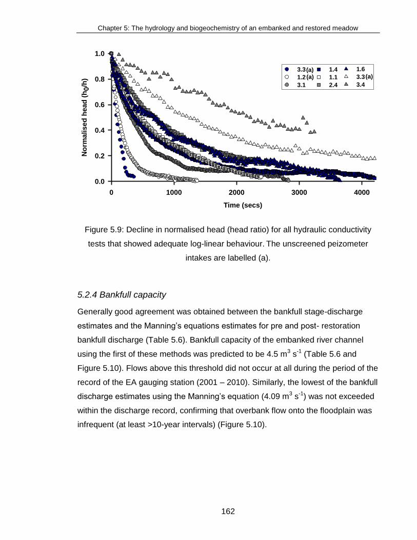
Chapter 5: The hydrology and biogeochemistry of an embanked and restored meadow
162
Figure 5.9: Decline in normalised head (head ratio) for all hydraulic conductivity
tests that showed adequate log-linear behaviour. The unscreened peizometer
intakes are labelled (a).
5.2.4 Bankfull capacity
Generally good agreement was obtained between the bankfull stage-discharge
estimates and the Manning’s equations estimates for pre and post- restoration
bankfull discharge (Table 5.6). Bankfull capacity of the embanked river channel
using the first of these methods was predicted to be 4.5 m3 s-1 (Table 5.6 and
Figure 5.10). Flows above this threshold did not occur at all during the period of the
record of the EA gauging station (2001 – 2010). Similarly, the lowest of the bankfull
discharge estimates using the Manning’s equation (4.09 m3 s-1) was not exceeded
within the discharge record, confirming that overbank flow onto the floodplain was
infrequent (at least >10-year intervals) (Figure 5.10).
Time (secs)
0 1000 2000 3000 4000
No
rma
lis
ed
he
ad
(h
0/h
)
0.0
0.2
0.4
0.6
0.8
1.0
3.3
1.2
3.1
1.4
1.1
2.4
1.6
3.3
3.4
(a)(a) (a)

Chapter 5: The hydrology and biogeochemistry of an embanked and restored meadow
163
Table 5.6: Bankfull height above ODN, bankfull river discharge from the river
stage–discharge relationship, and calculated using Manning’s equation, and
bankfull recurrence interval (not estimated for the pre-restoration bankfull
discharge due to the high uncertainty associated with extrapolating beyond the
range of data).
Transect
Bankfull elevation ODN (m)
Stage-discharge relation of bankfull
discharge (m3 s-1)
Manning’s bankfull
discharge (m3 s-1)
Pre-restoration 20.520 4.53 4.09 – 5.73 Post-restoration 20.096 1.15 1.33 – 1.87
Note: ODN: Ordnance Datum Newlyn.
Following the removal of the embankments, bankfull capacity (evaluated using the
stage–discharge method) was reduced by 75% to 1.15 m3 s-1. River discharge
exceeded this bankfull threshold during one short (1-day) high-flow event in
February 2010 that averaged 1.36 m3 s-1 (Figure 5.10). Historical river discharge
data from before the restoration indicate that flows of this magnitude are regular.
For instance, from 2001 to 2010, river discharge was above the 1.15 m3 s-1 post-
restoration bankfull capacity during a minimum of 14 high flow events, the majority
of which (11 out of the 14 recorded) occurred during the summer and autumn
(Figure 5.10). These were of short duration (1 day), with the exception of a high
river discharge period in May – June 2007, successive high flows were above
bankfull capacity within 10 – 18 days (Fig. 5.10). It is important to note that the river
discharges presented in Figure 5.10 are mean values over 24 hours. Hence during
precipitation events, peak discharge may be significantly greater than the mean
daily discharge value, particularly on a small river such as the River Glaven, where
flood events may last only a few hours.

Chapter 5: The hydrology and biogeochemistry of an embanked and restored meadow
164
Figure 5.10: Time series of (a) total precipitation, and (b) mean daily river discharge from 2001 to 2010. Pre- and post-
restoration bankfull capacity at the downstream river stage is shown in (b), above which inundation of the floodplain would
have occurred. River discharge data affected by aquatic macrophyte growth have been highlighted with dotted lines and
were not included in the analysis of bankfull discharge.

Chapter 5: The hydrology and biogeochemistry of an embanked and restored meadow
165
As bankfull flows prior to embankment removal (i.e. 4.5 m3 s-1; Table 5.6) did not
occur during the period of record (Figure 5.10), recurrence interval was not
estimated due to the high uncertainty associated with extrapolating beyond the
range of data. It can be stated, however, that the return period for these flows was
at least >14 years (Figure 5.11). Following embankment removal, the recurrence
interval for overbank flows (i.e. 1.15 m3 s-1; Table 5.6) was substantially reduced to
every 0.83 years (Figure 5.11).
Figure 5.11: Recurrence interval (return period in years) of various river discharges
on the River Glaven at Hunworth, computed using flood POT data.
A further indication that embankment removal will result in reconnection of the river
and floodplain via overbank flows is given in Figure 5.12b which shows river stage
in autumn 2008 above the restored bankfull elevation of 20.096 m (Table 5.6). This
is also apparent in photographs taken of the same location on the River Glaven
during high river flow (1.9 m3 s-1) in October 2008 before embankment removal
(Figure 5.12a) and during low river flow (0.45 m3 s-1) in January 2010 after
embankment removal (Figure 5.12b). The October 2008 stage board level is
highlighted by the white circles in Figure 5.12, and indicates that river flows of a

Chapter 5: The hydrology and biogeochemistry of an embanked and restored meadow
166
similar magnitude to October 2008 are likely to inundate the post-restoration
floodplain.
Figure 5.12: Photographs of the same location on the River Glaven during differing
river flows (a) before and (b) after embankment removal . Photograph (a) was
during a high river stage (0.87 m), and (b) was during low river stage (0.34 m).
5.2.5 Groundwater response to embankment removal
After the removal of the embankments, groundwater levels at wells 3.1 and 1.1,
which were located at the river–floodplain interface, generally remained higher than
those within wells further from the river (Figure 5.13 a and c) for much of the post-
removal period. This was particularly evident during the dry summer of 2009,
possibly due to enhanced river water intrusion at the river-floodplain interface
(Figure 5.13). In contrast to the observations close to the river, water levels in all
other wells were approximately 0.1 – 0.6 m lower in the summers following the
restoration (Figure 5.13a–c). This could be a result of the prevailing low summer
precipitation levels in these years (see Section 2.3.2). Winter water table elevations
remained unchanged following the restoration (Figure 5.13a–c), with water levels
within 0.1 m of the soil surface in all wells. Furthermore, embankment removal
lowered the soil elevation to within 0 – 0.5 m of the water table at Well 3.1. This
resulted in increased saturation of surface soils on the restored river banks for
much of the summer in 2009 and 2010 (winter 2009 data are not available) (Figure
b)a)

Chapter 5: The hydrology and biogeochemistry of an embanked and restored meadow
167
5.13a), which is likely to have important effects on soil physicochemistry in this part
of the floodplain.
Figure 5.13: Temporal variation in mean daily groundwater height above Ordnance
Datum Newlyn (ODN). Well 3.1 (a) was located on the river embankment; Wells
3.5 (a), 2.4 (b) and 1.6 (c) were located at the base of the hillslope (see Figure
4.2). Continuous measurements of groundwater height were not available for all of
the wells at the midstream transect, hence hand measurements are also plotted
(circles). River stage is plotted at the downstream transect.

Chapter 5: The hydrology and biogeochemistry of an embanked and restored meadow
168
5.2.6 Hydrological controls on chemistry
River water and regional groundwater (sampled in the chalk borehole) was slightly
alkaline (mean pH: 7.3 and 7.4, respectively) (Table 5.7). In contrast, the floodplain
well water was slightly acidic (mean pH: 6.5–6.7), potentially due to the organic-
rich soils on the meadow (see Section 5.2.3). Groundwater in the floodplain wells
and chalk borehole, and river water cation chemistry were dominated by calcium
(Table 5.7). Cation concentrations followed the pattern of Ca>Na>Mg>K, whereas
anion chemistry followed the pattern Cl->SO4->NO3
- (Table 5.7).
The relative percentage composition of base cations in the floodplain well samples
were mostly aligned in a linear fashion along the calcium and sodium axes (Figure
5.14) between the two main potential water sources: groundwater that was strongly
dominated by calcium ions and river water that was characterised by higher levels
of sodium ions (Table 5.7). The spatial variation in calcium and sodium cations in
well water indicate that the direction of groundwater flow is not strictly from upslope
through the floodplain to the stream but that floodplain well water is a mixture of
hillslope and river water. However, differences in concentration between end
members were quite small, particularly during baseflow conditions when a
groundwater signature was evident in the river water. There is also an indication of
evapotranspiration in well samples enriched in calcium. Hence, further analysis
using an end-member mixing model was not considered appropriate (e.g.
Genereux et al. 1993).
Conservative solutes such as sodium, calcium and chloride, varied spatially along
each well transect. However, there was no obvious pattern with distance from the
river (Figure 5.15a-c). One exception was the chemistry in Well 2.4 and Well 3.5,
located at the base of the woodland hillslope (Figure 5.15a and b), which was
markedly different from other wells on the meadow. Chloride and sodium
concentrations in these two wells were, respectively, on average between 1.7 − 4.2
and 1.8 − 3.8 times greater than average concentrations in the floodplain wells
(Figure 5.15a and c). This could be due to anthropogenic inputs; alternatively the

Chapter 5: The hydrology and biogeochemistry of an embanked and restored meadow
169
source may be geological, possibly due to the weathering of hillwash at the base of
the hillslope (Moorlock et al. 2002). Chloride and sodium chemistry of wells located
close to the river (within 10 m) was closer in concentration to regional groundwater
chemistry than that of the river, possibly due to limited hydrological exchange
between river water and groundwater on the floodplain.
Figure 5.14: Ternary plot of base cation chemistry in river water, wells on the
floodplain, and the EA borehole (instrumented in the chalk).
@rgb(255,0,0)
Calcium (%)
0 10 20 30 40 50 60 70 80 90 100
Sodium (%)
0
10
20
30
40
50
60
70
80
90
100
Magnesium &
Potassium (%)
0
10
20
30
40
50
60
70
80
90
100
WellRiver EA borehole

Chapter 5: The hydrology and biogeochemistry of an embanked and restored meadow
170
Table 5.7: Chemistry of the River Glaven and Hunworth Meadow groundwater wells(Mean ± 95% confidence interval).
River
Upstream Transect
Midstream Transect
Downstream Transect
EA borehole
pH in-situ 7.3 ± 0.5 6.6 ± 0.1 6.7 ± 0.2 6.5 ± 0.1 7.4 ± 0.2
Conductivity (μs cm-1) 953 ± 213 676 ± 130 775 ± 767 812 ± 111 519 ± 50 Ca2+ (mg L-1) 95.8 ±12.4 113 ± 81 71.2 ± 28.2 102.6 ± 11.5 89.7 ± 4.8 Na+ (mg L-1) 25.6 ± 5.1 13.7 ± 3.2 24.8 ± 10.5 17.6 ± 1.3 16.1 ± 0.2 Mg+ (mg L-1) 5.0 ± 0.8 3.5 ± 0.6 5.2 ± 2.2 4.3 ± 0.5 5.5 ± 0.3 K+ (mg L-1) 2.6 ± 0.4 1.0 ± 0.7 5.5 ± 3.0 1.9 ± 1.0 1.8 ± 0.1
NH4+ (mg N L-1) 0.6 ± 0.1 0.8 ± 0.3 0.6 ± 0.3 0.5 ± 0.1 0.0 ± 0.0
Cl- (mg L-1) 45.4 ± 1.0 33.9 ± 3.7 48.6 ± 23.0 27.5 ± 5.3 31.7 ± 2.5 SO4
- (mg L-1) 48.4 ± 4.1 30.7 ± 12.7 33.6 ± 17.7 14.5 ± 4.4 43.7 ± 10.1 NO3
- (mg N L-1) 6.2 ± 0.5 0.2 ± 0.1 0.4 ± 0.4 0.1 ± 0.03 0.2 ± 0.0 PO43- (mg P L-1) 0.1 ± 0.1 0.8 ± 3.3 0.1 ± 0.1 0.1 ± 0.03 No data
TDN (mg L-1) 5.5 ± 4.5 3.3 ± 0.6 4.7 ± 1.4 2.6 ± 0.6 No data DOC (mg L-1) 10.8 ± 2.3 33.8 ± 6.0 46.1 ± 7.6 32.7 ± 6.8 0.8 ± 0.2 DO (mg L-1) 10.8 ± 0.4 0.4 ± 0.2 1.0 ± 0.8 0.5 ± 0.3 1.4 ± 0.8

Chapter 5: The hydrology and biogeochemistry of an embanked and restored meadow
171
Figure 5.15: Spatial variation of selected ions (mean ± 95% confidence interval; log
scale) along subsurface flowpaths at the upstream, midstream and downstream
well transects for 2007 − 2008. Concentrations in the EA borehole (instrumented in
the chalk) are also shown. Pre-restoration topography is plotted to identify the
sample locations in relation to the river and hillslope.

Chapter 5: The hydrology and biogeochemistry of an embanked and restored meadow
172
Dissolved oxygen and nitrate concentrations in river water were, respectively,
approximately 18- and 14-fold greater than the concentrations in shallow
groundwater wells on the meadow (p<0.05) (Figure 5.16). Groundwater in these
wells was consistently depleted in DO (0.6 mg O2 L-1) and nitrate (mean = 0.21 mg
NO3--N L-1) relative to river water (mean: 10.8 mg O2 L
-1 and 6.2 mg NO3--N L-1,
respectively) (p<0.05), and exhibited little change with distance from the river.
However, nitrate concentrations at Well 3.1, which was located on the
embankment, showed greater variation than the other wells on the floodplain,
possibly indicating greater connectivity with river water (Figure 5.16a). Dissolved
organic carbon concentration, in contrast, was significantly (p<0.05) higher in the
floodplain wells (mean at different wells between 33 and 46 mg L-1) than in river
water (mean = 11 mg L-1) (Table 5.7), likely due to the presence of organic matter
on the floodplain.
Dissolved oxygen concentration in surface soils (top 0.1 – 0.3 m) was strongly
coupled with water table height (Figure 5.17b and c). As groundwater rose
vertically through the soil profile and surface soils became saturated, DO
concentration decreased rapidly within a day to 0 – 2 mg L-1, indicating reduced
conditions (Figure 17b). As the water table height fell once again, DO
concentration increased at a rate of about 0.8 – 1.4 mg L-1 day-1 to atmospheric
saturation (Figure 5.17b). Groundwater DO did not increase at any point during
periods of high river flow and elevated water table, suggesting that oxygen-rich
river water did not inundate (via overbank flow) the upstream area of the floodplain
where the DO probes were located during the study period (Figure 5.17b). This is
further supported by site observations during high-flow events. Although Figure
5.10 suggests that one overbank flow event occurred following the embankment
removal, the event was of short duration (≤1 day) and likely only inundated the
downstream, relatively lower-lying section of the floodplain.

Chapter 5: The hydrology and biogeochemistry of an embanked and restored meadow
173
Figure 5.16: Nitrate and DO concentrations (mean ± 95% confidence interval; log
scale) in river water and groundwater along subsurface flowpaths at the upstream,
midstream and downstream well transects for 2007 – 2008. Concentrations in the
EA borehole (instrumented in the chalk) are also shown. Pre-restoration
topography is plotted to identify the sample locations in relation to the river and
hillslope.

Chapter 5: The hydrology and biogeochemistry of an embanked and restored meadow
174
Figure 5.17: Temporal variation in (a) temperature and (b) DO concentration in well
water and soil in relation to (c) changes in groundwater height. DO concentrations
in well water were measured continuously at 0.1 and 0.3 m below the soil surface.
In January 2010, the 0.3 m oxygen optode was moved from the well and buried
directly in the soil at 0.1 m below the soil surface. When groundwater height is
below the respective DO optode installation height, optode data represent
atmospheric temperature and saturated DO conditions.

Chapter 5: The hydrology and biogeochemistry of an embanked and restored meadow
175
5.3 Discussion
5.3.1 River-floodplain hydrological linkages
As ecosystems strongly influenced by disturbances linked to flooding, floodplains
are widely thought to be important for mediating the flow of water, energy, matter,
and organisms between aquatic and terrestrial environments (Junk et al. 1989;
Tockner and Stanford 2002; Naiman et al. 2005; Mitsch and Gosselink 2007).
Functioning hydrological links are key for the numerous interstitial foodwebs
(Stanford and Ward 1993) and biogeochemical processes, such as aerobic
respiration, nitrification, denitrification and methanogenesis, that occur in the
saturated sediments beneath and adjacent to rivers and streams (Jones and
Holmes 1996). However, the reduction or absence of overbank inundation and the
associated flood-related natural disturbance regime have drastic effects on
biological and chemical conditions on floodplains. For example, overbank flooding
is important for the deposition of nutrients and sediments, the control of dominant
species and the transport of propagules that leads to increased species richness,
and flood water storage (Brunet et al. 1994; Ward and Stanford 1995; Silvertown et
al. 1999; Bullock and Acreman 2003; Nilsson et al. 2010).
The embankments along the River Glaven represented a substantial barrier to
river-floodplain interactions. Without overbank flow, slow horizontal subsurface flow
(<0.4 cm day-1) was the primary mechanism for the exchange of water, DO and
nutrients between the river and floodplain. With such low-flow velocities, it would
take approximately 1 year for a molecule of water to travel a distance of 1.5 m from
the river towards the floodplain. During high river flows when river stage was above
groundwater height on the floodplain, there was a greater potential for lateral
subsurface mixing of river and groundwater. However, considering the low
subsurface flow rates of these soils, groundwater movement on the floodplain is
likely to be dominated by the rapid (<1 day) vertical transfer of deeper oxygen and
nitrate-depleted groundwater through the soil profile that was observed in response

Chapter 5: The hydrology and biogeochemistry of an embanked and restored meadow
176
to precipitation. This prompt groundwater response to precipitation input, despite
low hydraulic conductivity, is a phenomenon that has been reported in many small
catchments and is not well understood (Kirchner 2003; Cloke et al. 2006).
A similar study on a chalk river in the Berkshire Downs, UK, found that the majority
of surface-subsurface hydrological exchange occurred a few tens of centimetres
from the river bed, and was limited to the gravel aquifer. The underlying chalk at
the site was found to be hydraulically separate from the river (Allen et al. 2010).
Throughout the River Glaven catchment, a chalk-rich boulder clay (Lowestoft
Formation) underlies the alluvium and gravels (Moorlock et al. 2002); this formation
is reported to be variably permeable, containing groundwater only when
weathered, fractured or interspersed with sand and gravel horizons (BGS 2007).
As the local permeability of this layer is unknown, further investigation is required.
This could involve the instrumentation of boreholes into the different geological
layers at the site. The presence of this less permeable layer at Hunworth could
restrict hydrological contact between the river and chalk bedrock. However, the
chemical similarity between the floodplain wells and chalk well samples, and the
high baseflow index and flow exceedence values for Q95, indicate interaction with
the chalk aquifer (see Sections 3.3 and 4.3.2).
The alluvial and glaciogenic gravels that overlay the Lowestoft Formation are likely
to have substantially higher hydraulic conductivity than the overlying alluvium.
While this could provide a route for more substantial mixing between river and
groundwater at depth, conservative ion chemistry in the wells has a groundwater
signature. The higher nitrate concentration measured in Well 3.1, which is located
next to the river, suggests some connectivity between the river and groundwater on
the floodplain. In general though, there was a lack of spatial and temporal variation
in the conservative ion chemistry of shallow groundwater across the floodplain,
indicating that even in a chalk setting there are regions of limited hyporheic extent.
Overbank inundation therefore, represents the only potential mechanism for
substantial surface water-groundwater connectivity.

Chapter 5: The hydrology and biogeochemistry of an embanked and restored meadow
177
Soils at Hunworth Meadow were of intermediate fertility (i.e. within the range of 5 –
15 mg kg-1 Olsen extractable phosphorus specified by Gowing et al. 2002a), likely
due to the cessation of fertilizer application at the site in 1997 and the absence of
flood water and river sediment inputs. Water flowing within the River Glaven is
substantially richer in nitrate and DO relative to floodplain groundwater, and thus
represents a potential source of nutrients to floodplain vegetation and microbes.
The large difference in nitrate and DO concentrations between river water and
groundwater <2 m away from the channel indicate that a strong redox gradient is
present at the river–floodplain interface. This part of the floodplain is likely to be an
important zone for reducing nitrate concentrations (e.g. Dahm et al. 1998; Hedin et
al. 1998; Clilverd et al. 2008).
The removal of the river embankments adjacent to Hunworth Meadow sufficiently
reduced the channel cross-sectional area, and thus bankfull capacity, to initiate
overbank inundation and reconnect the river with its floodplain. One overbank
event was observed during the period of study, and long-term river discharge data
from before the restoration indicate that river flows will regularly exceed the
restored bankfull capacity. Flood events will be of short duration, as bankfull
capacity was typically exceeded for only one day, and they will often occur during
the summer months when surface soils are dry and have a greater capacity for
water storage, which is likely to maximise floodpeak attenuation (e.g. Burt et al.
2002). Flooding may also persist for even longer periods, depending on the
infiltration and evapotranspiration rates, and the influence of in-river macrophyte
growth during the summer. Increased frequency and duration of floodplain
inundation due to embankment removal is consistent with other river restoration
studies (e.g. Acreman et al. 2003; Helfield et al. 2007; Hammersmark et al. 2008)
and is seen as one of the main aims of river restoration projects.
So far, an increase in the frequency of overbank flooding is suggested to be the
most dramatic hydrological effect following the restoration of the floodplain.
Increased groundwater levels at the river–floodplain interface have also been

Chapter 5: The hydrology and biogeochemistry of an embanked and restored meadow
178
observed, possibly due to enhanced river water intrusion. The most noticeable
change in soil saturation in this part of the floodplain, however, was due to a
lowering of the surface elevation relative to the water table height. This occurred
along a 1 – 2 m strip where the embankments were previously located, and is likely
to promote re-colonisation by wetland plant species that can tolerate periodic
waterlogging and aeration stress in the rooting zone, particularly during the
growing season (e.g. Silvertown et al. 1999; Barber et al. 2004; Wheeler et al.
2004). However, water levels in the rest of the floodplain were lower during the
summers following the restoration. This could be a result of the prevailing low
summer precipitation and high evapotranspiration rates in these years. The areal
extent of inundation on the floodplain could potentially be far-reaching due to the
low-lying elevation of the meadow in relation to the river; however, further analysis
including the application of hydrological/hydraulic modelling (e.g. Thompson et al.
2004) is required to determine flood inundation extents for a range of flows (see
Sections 6 and 7).
5.3.2 Floodplain ecohydrology
Prior to embankment removal, initial site assessments indicated that Hunworth
Meadow was comprised of a degraded Holcus lanatus – Juncus effusus rush
pasture community classified as MG10 under the UK National Vegetation
Classification system (Rodwell 1992) (see Section 3.6), which is typically
associated with waterlogged soils. This is congruent with prolonged saturation of
surface soils observed pre-restoration during winter and spring, and with the
periodic saturation occurring during summer and autumn months, all of which
occurred during within-bank river flows. Flooding, particularly during the growing
season, can cause aeration stress in plants, with prolonged waterlogging leading to
species-poor plant communities (Jackson and Colmer 2005). This stands in stark
contrast to the effects related to frequent low-intensity summer flooding of the
floodplain with oxygen-rich river water, which are predicted for the site following the
removal of the embankments along the River Glaven. Recurrent overbank

Chapter 5: The hydrology and biogeochemistry of an embanked and restored meadow
179
inundation increases environmental heterogeneity and is believed to have a
positive effect on floodplain plant diversity, firstly by limiting competition by
dominant plant species (e.g. Silvertown et al. 1999; Helfield et al. 2007), and
secondly by opening new patches for colonization by hydrochorically deposited
propagules (e.g. Auble and Scott 1998; Nilsson et al. 2010).
In contrast to brief summer inundation events, infrequent floods of lengthy duration
during the growing season can be expected to negatively affect floodplain diversity,
either by burying plants with river sediment or by exceeding tolerance limits for
anoxia in the rooting zone of sensitive species (e.g. Gowing and Youngs 1997;
Friedman and Auble 1999); however, floods of this type were not observed during
the 10 years for which river discharge data are available. Furthermore, at Hunworth
Meadow there is initial evidence to suggest that reconnection will improve drainage
and create drier conditions between flood events due to the easier drainage of the
floodplain following the removal of the embankments, which partly moderates the
effects of large floods (this is further explored in Section 7.2.2).
Re-establishment of overbank flooding may result in nutrient enrichment of
floodplain soils from flood-deposited sediment and nutrient-rich river water (Gowing
et al. 2002b). While this may function to protect adjacent ecosystems from nutrient
loading, increased nutrient supply may pose a risk to plant species richness at the
restoration site (Vermeer and Berendse 1983; Verhoeven et al. 1996; Janssens et
al. 1998; Michalcová et al. 2011) and over-ride the ecological benefits of improved
river–floodplain connections. In such instances, further management may be
required. In the case of Hunworth Meadow, which is a mesotrophic wet grassland,
the additional supply of nutrients could be managed with traditional hay cutting.
This would help balance the input of river-derived nutrients to the floodplain with
the removal of nutrients in plant biomass (Linusson et al. 1998; Wheeler et al.
2004).

Chapter 5: The hydrology and biogeochemistry of an embanked and restored meadow
180
Chapter 6: Methods – Part II: Hydrological/hydraulic modelling
6.1 Introduction
In this chapter the methods employed to simulate surface water and groundwater
elevation, groundwater recharge, surface runoff, and floodplain storage are
outlined. It describes the development (input data and parameterisation),
calibration, and validation of two coupled surface water/groundwater MIKE SHE-
MIKE 11 models used to simulate floodplain hydrology before and after the
removal of the river embankments along the River Glaven at Hunworth Meadow.
6.2 MIKE SHE model development
6.2.1 Model domain and topography
Coupled MIKE SHE/MIKE 11 hydrological/hydraulic models were developed for the
pre-restoration (embanked) and post-restoration (no embankment) scenarios,
which differed in embankment and riverbed elevation resulting from the
embankment removal. Figure 6.1 provides a representative example of the change
in river and embankment topography along the study reach. The riverbed was
slightly higher after the embankment removal works due to the accidental loss of
bank material into the river (see also Figure 5.1). This raised the riverbed in
relation to the agricultural drainage ditch, such that the river thalweg (lowest point
along the river bed) was above the ditch thalweg along the length of the meadow.
In both models, the model domain included Hunworth Meadow and extended up to
the tops of the adjacent hillsides on either side of the river. The upstream limit of
the modelled area coincided with the disused railway embankment whilst the
smaller embankment carrying an agricultural track crossing the floodplain defined
its downstream limit. The model was extended downstream of the study meadow in

Chapter 5: The hydrology and biogeochemistry of an embanked and restored meadow
181
order to prevent interference around the model boundary affecting groundwater
simulations on the meadow (Figure 6.2).
Figure 6.1: Cross-sections and photographs of the river and floodplain topography
before (embanked) and after (restored) embankment removal.
Two digital elevation models, one representing the embanked river, and the other
the restored river, were derived from dGPS surveys conducted before and after
embankment removal (see detailed description in Section 4.4.4) (Figures 6.2 and
6.3). The surface topography delineates the surface boundary of the model for
overland flow, and acts as a reference point for the depth of the saturated and
unsaturated zone layers and groundwater level observations. The DEMs were
created in Arc-GIS using the Kriging interpolation function. A comparison of three
Arc-GIS interpolation functions (Kriging, Nearest Neighbour, and IDW) indicated
that the Kriging method resulted in the least absolute error (mean error = 0.001 m)
between observed and interpolated data points, and was best able to represent
changes in topography over small spatial scales (Figure 6.4).

Chapter 5: The hydrology and biogeochemistry of an embanked and restored meadow
182
Figure 6.2: Digital elevation models used in MIKE SHEfor the (a) embanked and (b) restored river embankment models.
The extent of each the DEM delineates each respective model domain. An enlarged map of the study meadow is shown
below in Figure 6.3.

Chapter 5: The hydrology and biogeochemistry of an embanked and restored meadow
183
Figure 6.3: Digital elevation models of the (a) embanked and (b) restored sections of the study meadow. Surface
elevation of the river embankments was reduced on average by 0.8 m (see Section 5.2 for detailed results).

Chapter 5: The hydrology and biogeochemistry of an embanked and restored meadow
184
Figure 6.4: Comparison of absolute error for different interpolation methods at 1 m
grid spacing. The solid centre line and broken line within the boxplot indicate the
median and mean, respectively. The box extent and error bars denote the 25th and
75th percentiles, and 10th and 90th percentiles, respectively. The circles indicate
the presence of outliers.
Both DEMs in Figure 6.2 were re-sampled to the MIKE SHE model grid. The model
domain was divided into 5,038 grid cells of 5 m × 5 m, which represented a total
area of 12.6 hectares. As discussed below in Section 6.4.2, initial calibration steps
employed a larger grid size of 15 m × 15 m grid (610 grid cells), which resulted in
appropriate computational times for the multiple model runs during the
autocalibration process. Subsequently, the model grid size was reduced during
manual fine-tuning of the model (see section 6.4.2). Experiments during model
calibration showed little difference in simulated groundwater elevations between 1
and 5 m. In order to balance between grid resolution and computational speed,

Chapter 5: The hydrology and biogeochemistry of an embanked and restored meadow
185
common with distributed hydrological models (McMichael et al. 2006; Thompson et
al. 2013), 5 m x 5 m was selected as the optimal grid size relative to the high
resolution of topographic data available, whilst also ensuring appropriate
computational speed.
The relatively fine discretisation of the final model was needed to accurately
characterise topographic variations across the floodplain including the blocked
ditch and small-scale features such as shallow depressions and raised hummocks
that can provide microhabitats of differing soil water content that are important for
fostering high species diversity (Wheeler et al. 2004). At higher grid spacing, the
river and ditch topography were significantly dampened in the interpolation, and
were lost altogether from the 20 m grid DEMs (Figure 6.5). As the dGPS data are
discontinuous, with higher sampling densities (1 – 2 m) in key areas of topographic
change i.e. in the river, on the embankments, and in the ditch, 10 m spacing on the
meadow where the topography was relatively flat, and substantially lower sampling
densities (ca. 20 – 40 m) outside of the study meadow i.e. on the hillslopes, it is
acknowledged that the DEMs are spatially aliased across the model domain.
However, in order to capture the key study area on the floodplain in sufficient detail
and to simulate subtle differences in the water regime across the site, a 5 m grid
resolution was necessary. Ideally, the model would be organised into a network of
smaller grid sizes on the meadow (e.g. 1 m × 1 m), where it was important to
represent small changes in topography, and larger grid sizes on the hillslope (e.g.
20 m × 20 m). However spatially variable grid sizes were not an option in the
version of MIKE SHE used (Release 2009) and is also not available in the latest
software release.

Chapter 5: The hydrology and biogeochemistry of an embanked and restored meadow
186
Figure 6.5: Loss of topographic resolution with increased interpolation grid size.
Cross-sections depict the embanked river, floodplain and hillslopes from a Kriging
interpolation in ARC-GIS.
6.2.2 Hydrological and climate data
A detailed description of the well locations, instrumentation, and evapotranspiration
calculations are given in Sections 4.2 and 4.3. Over three years of river discharge
and meteorological data, and observed groundwater elevations were used to,
respectively, parameterise and calibrate/validate the models. Water level data used
in the calibration and validation process (discussed below) were available for a 24
month period from 22/02/2007 to 15/03/2009 prior to the embankment removal and
16 month period from 29/03/2009 to 25/07/2010 after the embankment removal.
Spatially uniform precipitation and potential evapotranspiration were specified, an
approach justified by the small size of the model domain (Thompson 2004). Daily
river discharge available from 2001 – 2010 from the onsite Environment Agency
gauging station (see Section 4.2) is discussed below in the MIKE 11 section).
Daily precipitation and potential evapotranspiration (see Section 4.3) inputs
required to simulate water fluxes in the unsaturated zone and recharge to the

Chapter 5: The hydrology and biogeochemistry of an embanked and restored meadow
187
saturated zone, were based on records from an automatic weather station (Skye
MiniMet SDL 5400) installed 100 m from the meadow (see Figure 3.1)
supplemented during periods of instrumental failure with data from a nearby (<10
km) UK Met Office meteorological station (source ID: 24219, Mannington Hall).
Daily Penman-Monteith potential evapotranspiration was computed from air
temperature, net radiation, relative humidity, and wind speed observations from the
on-site weather station (see Section 4.3.3).
Pressure transducers were installed in 10 wells at Hunworth Meadow in February
2007 to measure changes in groundwater height (as described in Section 4.3.1).
The level logger in Well 3.4 was removed in June 2007 due to its close proximity to
the level logger in Well 3.5 and the need for a logger in the ditch at Transect 1.
Hand measurements of water table depth recorded during site visits, which were
subsequently converted to water table elevation using dGPS measurements of the
top of the well casings, show good agreement with the level logger data, which
were generally within a few cm of each other (Figures 6.6 - 6.8). These data
underpin all of the groundwater modelling, and thus great care was taken to check
the quality of the water level data. The exception was Well 1.2, where a
disagreement of approximately 7 cm occurred between the hand measurements
and level loggers after the restoration; this potential error was taken into account
during the modelling analysis (Figure 6.8).

Chapter 5: The hydrology and biogeochemistry of an embanked and restored meadow
188
Figure 6.6: Comparison of level logger and hand measurements of groundwater
elevation at the Upstream Well Transect. The embankment removal in March 2009
is highlighted by the vertical hashed bar. The soil surface is shown by the broken
red line. Note the change in soil surface elevation at Well 3.1, which was located
on the embankment prior to the restoration.

Chapter 5: The hydrology and biogeochemistry of an embanked and restored meadow
189
Figure 6.7: Comparison of level logger and hand measurements of groundwater
elevation at the Midstream Well Transect. The embankment removal in March
2009 is highlighted by the vertical hashed bar. The soil surface is shown by the
broken red line.

Chapter 5: The hydrology and biogeochemistry of an embanked and restored meadow
190
Figure 6.8: Comparison of level logger and hand measurements of groundwater
elevation at the Downstream Well Transect. The embankment removal in March
2009 is highlighted by the vertical hashed bar. The soil surface is shown by the
broken red line.

Chapter 5: The hydrology and biogeochemistry of an embanked and restored meadow
191
Differences in land use (e.g. grassland versus woodland), which affect
evapotranspiration, runoff and thus groundwater recharge, are defined within the
MIKE SHE model domain by the allocation of different vegetation types. Each land
use category is assigned a Leaf Area Index (LAI) and rooting depth specific to the
vegetation type that it represents. Four different land use classes were defined in
the Hunworth models: roads and buildings, arable land, riparian grassland, and
mixed deciduous/coniferous woodland (Figure 6.9).
Figure 6.9: Spatial classification of land use in the model for delineating differences
in LAI and root depth.
Constant rooting depths were applied to most land use classes, with the exception
of the arable class, which was varied seasonally (range: 0 – 1.8 m) (Figure 6.10).
Root depth was set at 0.3 m on the meadow and 2.7 m was used for the mixed
deciduous/coniferous woodland (Figure 6.10c and d). Root depth values for the
woodland and arable crop (classified as winter wheat) were taken from the
literature (Canadell et al. 1996; Thorup-Kristensen et al. 2009; FAO 2013),
whereas the rooting depth for the meadow was based on investigations at the site
and measurements of water table depth, which showed that a shallow region of

Chapter 5: The hydrology and biogeochemistry of an embanked and restored meadow
192
topsoil was aerated during the growing season. Root depth was defined as 0 for
the roads and buildings land cover class (Figure 6.10).
Figure 6.10: Leaf area index and rooting depth values assigned to the four land
use classes.
Chapter 5: The hydrology and biogeochemistry of an embanked and restored meadow
193
Seasonal changes in Leaf Area Index (LAI) were applied to the arable (range: 0 –
4), meadow (range: 1 – 4) and mixed woodland (Range: 1 – 4) classes to account
for increased LAI values during the growing season (Herbst et al. 2008; Hough and
Jones, 1997). LAI was defined as 0 for the roads and buildings (Figure 6.10). LAI
values for the mixed deciduous/coniferous woodland were based on data from
Herbst et al. (2008) for two heterogeneous broad-leaved woodlands in southern
England and maximum LAI values reported by Hough and Jones (1997) for conifer
woodlands. Deciduous woodlands have a bare soil characteristic (LAI = 0) in the
winter. However, LAI values above zero were applied all year round in the model to
account for the presence of some evergreen trees and understory in the woodland
(Herbst et al. 2008).
6.2.3 Overland flow
A finite difference solution of the diffusive wave approximation was used to
simulate overland flow. The direction and amount of overland flow is controlled by
the topography, resistance to flow (described by the roughness coefficient,
Manning M for overland flow), the loss of water via evapotranspiration and the
infiltration capacity of the soil. Manning M is the inverse of the more often used
Manning’s n roughness coefficient. The higher the value of Manning’s M, the faster
the water is routed overland towards the river. Manning M was initially set at a
uniform value of 3.0 m1/3s-1 for the automatic calibration process (described in
Section 6.4), which corresponds with values given for grassland in the literature
(USDA 1986; Liu and Smedt 2004; Thompson 2004; Hammersmark et al. 2008).
Subsequently, a distributed option of Manning M was applied to the MIKE SHE
models to account for differences in overland resistance between the woodland
hillslope, patches of rushes (Juncus effusus) in the vicinity of the ditch, and the
grass meadow. The initial water depth for the overland flow calculations is usually
set as zero (DHI 2007b). An initial water depth greater than 0 mm resulted in
continuously flooded conditions across the meadow, which was not realistic; hence
the initial water depth was set at a uniform value of 0 mm and was not included as
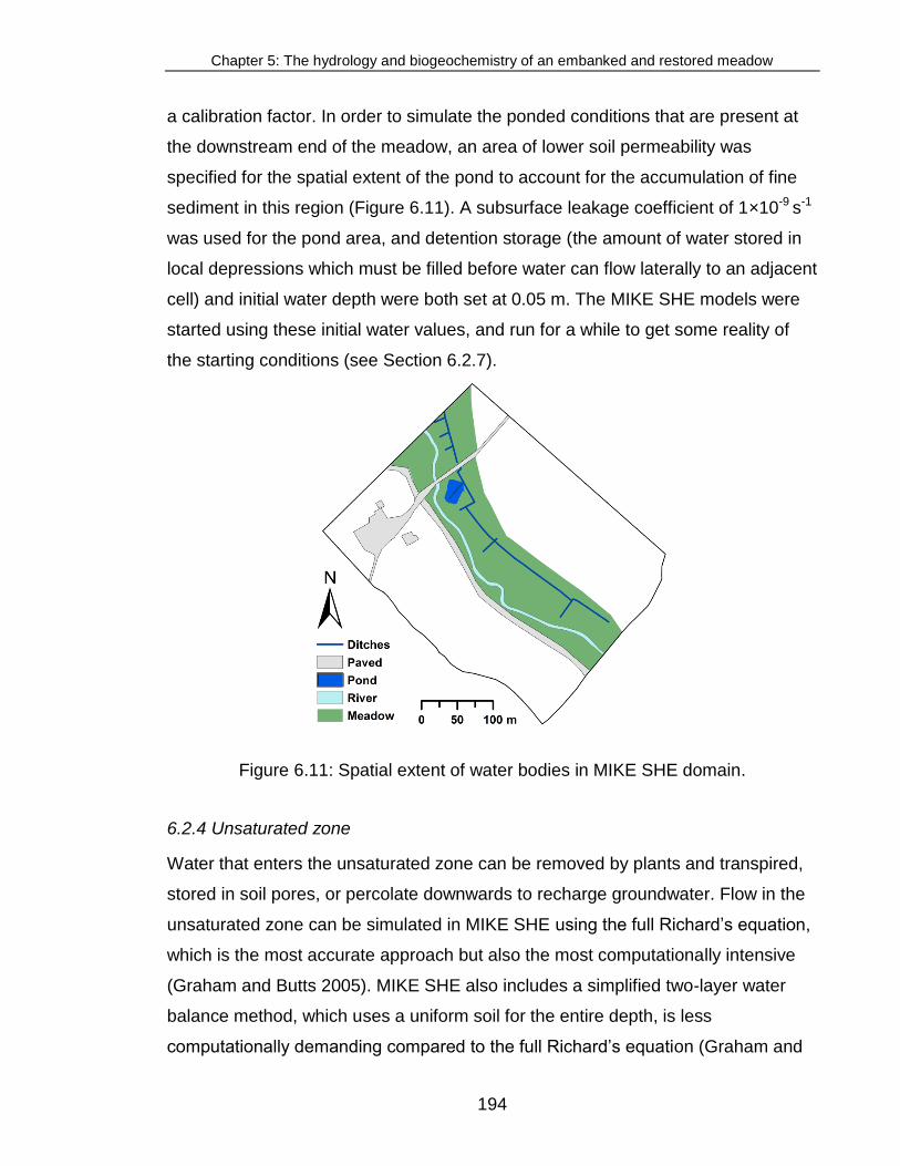
Chapter 5: The hydrology and biogeochemistry of an embanked and restored meadow
194
a calibration factor. In order to simulate the ponded conditions that are present at
the downstream end of the meadow, an area of lower soil permeability was
specified for the spatial extent of the pond to account for the accumulation of fine
sediment in this region (Figure 6.11). A subsurface leakage coefficient of 1×10⁻⁹ s-1
was used for the pond area, and detention storage (the amount of water stored in
local depressions which must be filled before water can flow laterally to an adjacent
cell) and initial water depth were both set at 0.05 m. The MIKE SHE models were
started using these initial water values, and run for a while to get some reality of
the starting conditions (see Section 6.2.7).
Figure 6.11: Spatial extent of water bodies in MIKE SHE domain.
6.2.4 Unsaturated zone
Water that enters the unsaturated zone can be removed by plants and transpired,
stored in soil pores, or percolate downwards to recharge groundwater. Flow in the
unsaturated zone can be simulated in MIKE SHE using the full Richard’s equation,
which is the most accurate approach but also the most computationally intensive
(Graham and Butts 2005). MIKE SHE also includes a simplified two-layer water
balance method, which uses a uniform soil for the entire depth, is less
computationally demanding compared to the full Richard’s equation (Graham and

Chapter 5: The hydrology and biogeochemistry of an embanked and restored meadow
195
Butts 2005; DHI 2007b), and is suitable for conditions that include the high water
tables and a rapid groundwater response to precipitation that characterize
Hunworth Meadow (e.g. Thompson 2012).
Soil properties were defined for a spatially uniform (global) unsaturated zone that
was represented using the two-layer water balance approach. The infiltration rate
of the unsaturated zone (mean: 1.88 ×10⁻⁶ m s-1) was obtained from piezometer
slug tests (n=25) conducted at the site (see Hydrological Conductivity methods in
Section 4.3.4) and was varied during calibration (see below). Soil water content at
saturation (approximately equal to the porosity) (DHI 2007b), and the water content
at field capacity were additional calibration terms. Initial values were based on
measurements of the water release characteristic (pF-curve) using a manual 08.01
sandbox (Eijkelkamp, Giesbeek, The Netherlands) (described in detail in Section
8.2.5), and averaged 0.7 (volumetric basis) and 0.2 (volumetric basis), respectively
(Table 6.1). Water content at wilting point was also varied during calibration but
could not be obtained from the water release curve as the sand box tension was
not decreased below 10 kPa (field capacity) and the wilting point in soils is typically
1,520 kPa (Brady and Weil 2002). Therefore a range of wilting point values for
sandy loam soils were obtained from the literature (mean = 0.07, volumetric basis)
to guide the initial value in the calibration (Table 6.1) (Zotarelli et al. 2010).
Table 6.1 Soil properties of Hunworth Meadow topsoil (top 10 cm)
Unsaturated zone soil properties Mean Range
Water content at saturation (volumetric): 0.7 0.6 – 0.8
Water content at field capacity (volumetric):
0.2 0.1 – 0.4
Water content at wilting point (volumetric): 0.07 0.04 – 0.1
Saturated hydraulic conductivity (m s-1): 2×10⁻⁶ 1×10⁻⁷ – 9×10⁻⁶
The two-layer water balance method divides the unsaturated zone into a root zone
that is subject to vertical draw from evapotranspiration, and lower zone that is not
(Graham and Butts 2005). The volume of water available for groundwater recharge

Chapter 5: The hydrology and biogeochemistry of an embanked and restored meadow
196
and actual evapotranspiration is calculated using the input precipitation and
evapotranspiration data (that employs the LAI and RD as described in Section
6.2.2 and physical soil properties detailed below - Table 6.1). The rate of water loss
via evapotranspiration from the unsaturated zone is dependent on the thickness of
the capillary fringe, the zone of upward capillary movement of water from the water
table. A capillary fringe can occur some distance above the water table, in
particular in fine soils (DHI 2007b; Clilverd et al. 2008). If the capillary fringe
reaches the soil surface, capillary action draws water directly from the water table,
saturating surface soils, and resulting in maximum rates of evapotranspiration.
Similarly, plant roots can draw water directly from the saturated zone if the roots
reach the capillary zone. Hence the height of the capillary zone is used as the
water table depth at which the influence of evapotranspiration starts to decrease.
Fine soils have the most influence on capillary action. The maximum height of
capillary rise for sandy loam soils at Hunworth Meadow was calculated as a
function of soil pore size using Hazen’s formula (Das 2002) of capillary rise as:
e 10
1D
Ch (6.1)
where the maximum height of capillary rise is h1 (mm), C is a constant that varies
from 10 to 50 mm2, e is the void ratio and D10 is the effective particle size, the
diameter (mm) of the smallest size fraction that accounts for less than 10% of total
soil mass. The void ratio was obtained from soil moisture measurements using 100
cm3 bulk density tins and D10 was measured with optical laser diffraction using an
LS 13320 Coulter Counter particle size analyzer (Beckman Coulter Corp., Hialeah,
Florida, USA). The low effective particle size (D10) values in Table 6.2 are
indicative of the low hydraulic conductivity values (mean: 1×10⁻⁵ m s-1) measured
at Hunworth meadow, and are in the order expected for soils that are composed of
fine sands (Murthy 2002; Figure 6.11). The capillary fringe values for Hunworth
Meadow sandy loam range from 0.4 m – 1.9 m (Table 6.2), which is consistent with
capillary rise values of >0.5 m in fine sands and silts reported by DHI (2007b), and

Chapter 5: The hydrology and biogeochemistry of an embanked and restored meadow
197
measurements in the range of 1.0 –1.5 m for weakly compacted alluvial sandy
loams and 1.5 – 2.0 m for alluvial loams (Chubarova 1972).
Table 6.2: Range of height of capillary rise for Hunworth Meadow.
Constant (mm2)
Soil void ratio e
D10 (mm)
Capillary height (m)
10 3.08 0.008 0.39 50 3.08 0.008 1.93
Figure 6.12: Relationship between hydraulic conductivity and D10 of granular soils
(Louden 1952, cited in Murthy 2002).
Preferential flow through macropores in unsaturated soil can provide an important
bypass mechanism for flow to the saturated zone in certain soil types (DHI 2007b).
Chapter 5: The hydrology and biogeochemistry of an embanked and restored meadow
198
However, the low clay content (see Section 5.2.3) and high water table conditions
(see Section 5.2.2) observed across the floodplain throughout the study period
suggest that the influence of macropores are limited and therefore macropore flow
was not included in the model.
6.2.5 Saturated zone
A finite difference solution to the three dimensional groundwater flow equation was
used to simulate flow in the saturated zone. This method allows for the vertical
discretisation of geological layers and lenses in the saturated zone, each with
specific hydraulic properties (DHI 2007b). Four geological layers are likely present
at the site based on a British Geological Survey of superficial and regional bedrock
geology in the catchment (Figure 3.6), geological strata information recorded
during the installation of a British Geological Survey groundwater borehole at
Brinton Hall (see Section 3.3), and onsite soil texture data recorded during the
installation of groundwater wells on the floodplain. These layers consist of (1)
hillwash (a poorly sorted mixture of clay, sand, silt and gravel), followed by (2)
glaciogenic sand and gravel, (3) boulder clay, and (4) chalk. In addition an alluvium
lens is present on the floodplain.
In order to minimise the computational demand, and because the physical
properties of these layers are relatively unknown at the study site, the model was
composed of a relatively simple saturated zone that represented average
geological conditions in the upper alluvial and glacial soils that were considered
separated from the chalk aquifer at the site by a layer of low permeability boulder
clay. This consisted of one geological layer with a lower elevation of 10 m above
Ordnance Datum Newlyn (ODN), and uniform hydrodynamic properties (i.e.
hydraulic conductivity and storage coefficients) which were varied during the
calibration process within a range of values determined from onsite investigations
and typical values reported in the literature (Domenico and Schwartz 1998).
Hydraulic conductivity values of the top 2 m of floodplain alluvium were determined
using piezometer slug tests (n=25), described in detail in Section 4.1. The results

Chapter 5: The hydrology and biogeochemistry of an embanked and restored meadow
199
of these tests indicate that hydraulic conductivity of the alluvium is relatively low,
ranging from 1.13×10⁻⁷ to 5.35×10⁻⁶ m s-1 in the order expected for silt soils (see
Table 5.5). The initial horizontal and vertical hydraulic conductivity values used in
the calibration process were guided by results from piezometer slug tests (mean =
1.88×10⁻⁶ m s-1) conducted on the floodplain and values reported by Domenico and
Schwartz (1998) for various geological materials (Table 6.3), both were subject to
adjustment during model calibration.
Table 6.3: Representative hydraulic conductivity values for various geological
materials (Domenico and Schwartz 1998).
Material Hydraulic Conductivity (m s-1)
Gravel 3×10⁻⁴ – 0.03
Coarse sand 9×10⁻⁷ – 0.006
Medium sand 9×10⁻⁷ – 5×10⁻⁴
Fine sand 2×10⁻⁷ – 2×10⁻⁴
Silt 1×10⁻⁹ – 2×10⁻⁵
Till 1×10-12 – 2×10⁻⁶
Clay 1×10-11 – 4.7×10⁻⁹
Limestone, dolomite 1×10⁻⁹ – 6×10⁻⁶
Specific yield, defined as the volume of water that drains per unit surface area of
aquifer per unit decline of water table, primarily represents the release of water
under gravity at the phreatic surface (Rushton 2004; DHI 2007b). Specific yield
was included in a sensitivity analysis prior to the calibration of the model. An initial
value of 0.2 was used in the sensitivity analysis based on typical ranges within the
literature for sand (Table 6.4). Specific storage, which is slightly different than
specific yield, relates to a unit volume of aquifer, and is defined as the volume of
water that drains per volume of aquifer per unit decline of water table under
saturated conditions. Thus specific storage represents the water released from
storage from the entire column of water in the aquifer, not just at the phreatic
surface (Rushton 2004; DHI 2007b). Specific storage was also used in the
sensitivity analysis; an initial value of 1.0×10⁻⁴ m-1 was used based on typical
values in the literature for sand (Table 6.5). A value of 19 m (ODN) was used for

Chapter 5: The hydrology and biogeochemistry of an embanked and restored meadow
200
the initial potential head, which was based on average water level observations
across the floodplain equivalent to between -0.2 m to -0.7 m below the ground
surface.
Table 6.4: Specific yield for various geological materials (Johnson 1967 as
reported in Domenico and Schwartz 1998).
Material Specific Yield (fraction)
Gravel, coarse 0.23
Gravel, medium 0.24
Gravel, fine 0.25
Sand, coarse 0.27
Sand, medium 0.28
Sand, medium 0.23
Silt 0.08
Clay 0.03
Limestone 0.14
Peat 0.44
Till, predominantly silt 0.06
Till, predominantly sand 0.16
Till, predominantly gravel 0.16
Table 6.5: Representative specific storage values for various geological materials
(Domenico and Mifflin 1965, as reported in Batu 1998).
Material Specific storage (m-1)
Plastic clay 2.6×10⁻³ - 2.0×10⁻²
Stiff clay 1.3×10⁻³ - 2.6×10⁻³
Medium hard clay 9.2×10⁻⁴ - 1.3×10⁻³
Loose sand 4.9×10⁻⁴ - 1.0×10⁻³
Dense sand 1.3×10⁻⁴ - 2.0×10⁻⁴
Dense sandy gravel 4.9×10⁻⁵ - 1.0×10⁻⁴
Rock, fissured 3.3×10⁻⁶ - 6.9×10⁻⁵

Chapter 5: The hydrology and biogeochemistry of an embanked and restored meadow
201
6.2.6 Boundary conditions
A combination of zero-flux (no-flow) and specified head subsurface boundary
conditions were applied around the model domain (Figure 6.13) (e.g.
Hammersmark et al. 2008). A zero-flow boundary is the default condition and is
realistic for watershed boundaries. The zero-flow boundaries are a simplification of
the system, but were justified for the summits of the hillsides on either side of the
meadows following the assumption that the groundwater divide followed the
topographic divide and provided a hydraulic boundary (e.g. Thompson 2012).
Similarly, the foundations of the railway embankment defined a physical boundary
at the upstream end of the meadows that was assumed to restrict flow into the site.
Some subsurface flow perpendicular to the river is, however, possible across the
downstream boundary of the floodplain. To facilitate this exchange a constant head
boundary of 18.8 m ODN was specified at this location using mean groundwater
height of -0.2 m ± 0.17 m from a well transect at the downstream end of the
meadow (Figure 6.13). Specified-head and constant-head boundaries can supply
an inexhaustible source of water no matter how much water is removed from a
system model (e.g. Franke et al. 1985). This is unlikely to cause a problem at the
downstream boundary of the Hunworth model as the constant head value is based
on mean groundwater elevation that fluctuated very little in this region of the
floodplain. A manual sensitivity analysis of alternative boundary options (specified
head, flux, zero-flow) was performed and demonstrated negligible effects on
simulated groundwater elevations across the floodplain beyond the immediate
location of the boundary conditions.

Chapter 5: The hydrology and biogeochemistry of an embanked and restored meadow
202
Figure 6.13: Boundary conditions of the MIKE SHE model (grid size = 5 m).
The MIKE SHE drainage option was used to represent relatively small-scale, fast
run-off along the base of the hillslope and to route drainage into topographical lows
along the agricultural ditch (e.g. Thompson et al. 2009). A drainage level and time
constant were applied along the base of the hillslope and the ditch, and were
altered in the sensitivity analysis and model calibration (Figure 6.14). A drainage
level of -1.6 m, and time constant of 6×10⁻⁸ s-1 along the base of the hillslope, with
a higher time constant of 2.6×10⁻⁷ s-1 closer to the model boundary, provided the
best overall fit.

Chapter 5: The hydrology and biogeochemistry of an embanked and restored meadow
203
Figure 6.14: Spatial distribution of drainage codes used in the MIKE SHE models
along the ditch and pond. Grid cells with code = 2 received drainage flow. Grids
cells with code = 0 did not receive drainage flows. Preference for drainage
occurred in the following order: river > boundary > depression. Grid cells not
connected to river or boundary cells drained to cells with the lowest drain level (to
create a pond).
6.2.7 Simulation specification
The MIKE SHE simulations were started using initial conditions (e.g. initial surface
water depth) stored from a point in a previous simulation run of the same model in
a ‘hot start’ file. The hot start model was run for a year and the initial conditions for
groundwater head were obtained from a representative time period, selected after
the model had stabilised. This provided more realistic initial conditions, and
prevented the need for a ‘warm-up period’ at the start of each model. The
maximum allowed time steps for the unsaturated flow (using the two-layer water

Chapter 5: The hydrology and biogeochemistry of an embanked and restored meadow
204
balance method), saturated flow (finite difference) and evapotranspiration
components were set at 24 hours. A shorter time step of 0.25 hours was specified
for the overland flow (finite difference) component to ensure model stability.
However, in flat areas with ponded water, such as on floodplains, the difference in
water depth between grid cells is close to zero, which requires very small overland
flow time steps. To allow the simulation to run with longer time steps and further
reduce numerical instability the calculated overland flows between cells were
multiplied by a damping factor to reduce flow between cells when the flow gradient
is close to zero. Rather than the default damping function in MIKE SHE, an
alternative single parabolic function was specified, which goes to zero more quickly
and is consistent with the approach used in MIKE FLOOD (DHI 2007b). This
alternative damping function was applied below a specified gradient of 0.001. All
model results were stored at 24-hour intervals to coincide with the temporal
frequency of observations.
6.3 MIKE 11 model development
6.3.1 River channel and ditch network
Channel flow was simulated with one-dimensional hydraulic MIKE 11 models
(Havnø et al. 1995). Two MIKE 11 models were developed, one for the embanked
river scenario and another for the restored scenario. Dynamic coupling of each
MIKE 11 river model and the appropriate (embanked / restored) MIKE SHE model
through the exchange of simulated water level at MIKE 11 h-points (points where
water level data are calculated along the river branch) and MIKE SHE river links
enabled the simulation of river-aquifer exchange, overland flow to channels and
inundation from the river onto the floodplain (Thompson et al. 2004; DHI 2007a).
The MIKE 11 river channels were linked to the MIKE SHE grid via river links at the
edge of each grid cell, which simplified the river geometry (e.g. Figure 6.15).
However the high resolution of the MIKE SHE grid meant that the river network
was represented well by the MIKE SHE river links.

Chapter 5: The hydrology and biogeochemistry of an embanked and restored meadow
205
Figure 6.15: An example of MIKE 11 river branches with H points and the
corresponding river links in a MIKE SHE model from DHI (2007b).
River-aquifer exchange can be calculated using different river-bed permeability
options, which account for differences in riverbed and aquifer conductance. River-
aquifer exchange of the River Glaven was simulated using the aquifer only
formulation, where the river is assumed to be in full contact with the aquifer
material. This was a suitable method given the similarity between river and
groundwater chemistry along the river-banks, and the high baseflow index (0.81)
and flow exceedance values for Q95 (51%) which indicate high groundwater
contributions to discharge at the site (see Section 5.2.2).
A 576 m section of the River Glaven beginning immediately upstream and ending
just downstream of Hunworth Meadow was digitised in MIKE 11 from 1:10,000
Ordnance Survey digital data (Land-Line.Plus) (Figure 6.16). The river was divided
into three connected sections (i.e. branches): a main river section that was within
the MIKE SHE model domain, and an upstream and downstream section that were
both outside the MIKE SHE model domain (Figure 6.16). River cross-sections for

Chapter 5: The hydrology and biogeochemistry of an embanked and restored meadow
206
the two MIKE 11 models representing pre- and post-restoration channel
configurations were specified using the results from the dGPS surveys conducted
before and after embankment removal (as discussed in Section 4.4.4). A total of 32
river transects were surveyed prior to the restoration, at intervals along the length
of the river of approximately 10 m, and 23 transects after the river restoration, at
intervals of approximately 15 m (Figure 6.16). The river channel was fairly uniform
in width along the reach, nevertheless some variation in the channel bed
topography occurred due to patchy deposits of sand and silt (Figure 6.17a).
Figure 6.16: Delineation of the MIKE 11 River Glaven channel and location of
cross-sections for the (a) embanked and (b) restored models.

Chapter 5: The hydrology and biogeochemistry of an embanked and restored meadow
207
Figure 6.17: MIKE 11 cross-sections for the (a) embanked and (b) restored river-
banks.
A discharge boundary condition was specified at the upstream end of the MIKE 11
model using daily discharge records from the Environment Agency gauging station
(#034052) located immediately upstream of Hunworth Meadow. A constant water-
level boundary condition of 18.6 m AOD was applied at the downstream end of the
MIKE 11 model. This level was just above the bed of the river at the lowest cross-
section and prevented the river drying out whilst permitting discharge of water from
the end of the model (Thompson et al. 2004). An initial water depth of 0.2 m
throughout the MIKE 11 model at the start of the simulation period was obtained
from the records of a stage board installed in river towards the downstream end of
the reach.
A blocked agricultural drainage-ditch that runs parallel to the river was also
digitised in MIKE 11, and was initially added as a separate MIKE 11 branch, which
totalled 415 m in length. The ditch channel, which was not subject to alteration

Chapter 5: The hydrology and biogeochemistry of an embanked and restored meadow
208
during the river restoration, was surveyed once resulting in 19 cross-sections. The
ditch was a uniform width of approximately 4 m, but varied in depth due to varying
amounts of organic matter and silt that had accumulated along the bottom (Figure
6.18).
Figure 6.18: MIKE 11 ditch cross-sections.
A zero flow boundary condition was set at upstream end of the ditch channel (as
the ditch did not exhibit surface inflow) and MIKE SHE provided flows into the
ditch. However, MIKE 11 does not simulate evaporation, and thus periods of
wetting and drying in the ditch could not be modelled by MIKE 11. Instead of
fluctuating in tandem with groundwater levels (Figure 6.19), the modelled ditch
water levels remained constant along the MIKE 11 branch. The MIKE 11 branch of
the ditch was therefore removed. The final grid size, as discussed above in Section
6.2.1, was sufficiently small to be able to include the ditch topography in MIKE SHE
and simulate fluctuations in the ditch surface water associated with evaporation.
A solinst pressure transducer (Levelogger Gold 3.0, Ontario, Canada) installed in
the ditch recorded hourly water levels. The ditch water level observations were

Chapter 5: The hydrology and biogeochemistry of an embanked and restored meadow
209
closely coupled with fluctuations in groundwater elevation (Figure 6.19) and were
used as an added tool in the calibration and validation process.
Figure 6.19: Water levels in (a) Well 1.4 and (b) the adjacent ditch.
6.3.2 Specification of hydrodynamic parameters
A dynamic wave approximation, which uses the full Saint Venant momentum
equation, was applied to the river to calculate channel flows. The Manning’s n
coefficient for bed resistance of the river channel usually ranges from 0.01 sec m-
1/3 for smooth channels (small flow resistance) to 0.10 sec m-1/3 for thickly
vegetated channels (large flow resistance) (DHI 2007c). A constant Manning’s n
coefficient for bed resistance of 0.08 sec m-1/3 was initially applied to the model,
however this value resulted in river levels being too high in the winter and too low
in the summer. Instead, a time varying Manning’s n coefficient was specified
throughout the MIKE 11 model for the entire discharge record from 2001 – 2010
(Figure 6.20) based on the approach used by House et al. (2016a), to account for
seasonal differences in bed resistance associated with in-stream macrophyte

Chapter 5: The hydrology and biogeochemistry of an embanked and restored meadow
210
growth. Seasonal macrophyte growth in the river was easily identified in the river
discharge record (see Section 4.5, and Figure 5.10), as it impacted the rating curve
and resulted in a slow increase in baseflow through the summer, despite low or no
rainfall. This effect declined during the autumn due to macrophyte dieback, or more
abruptly during flood events due to devegetation of the river channel (e.g.
Chambers et al. 1991). Two general summer conditions were identified for varying
Manning’s n values among years: 1) high flow summers where macrophyte growth
was restricted, and 2) low flow summers where stable conditions resulted in
substantial vegetation growth. A Manning’s n coefficient of 0.058 sec m-1/3 was
applied in the winter, and maximum values of 0.08 sec m-1/3 and 0.15 sec m-1/3
were applied in June during high flow and low flow summers, respectively (Figure
6.20). These values were guided by the fit between observed and simulated river
stage, and were within the range of 0.045 to 0.353 m1/3 s-1 reported for a UK chalk
stream by House et al. (2016a). The growth period was defined as April –
September and Manning’s n values during this period were interpolated between
the winter and summer values, which was guided by macrophyte growth
measurements in a UK chalk stream reported by Flynn et al. (2002).
It is worth noting that the modelled river levels were simulated from average daily
stage measurements recorded at the EA gauging station, whereas the observed
data were from point measurements taken at a stage board adjacent to the
downstream well transect (see Figures 3.1 and 4.2). Hence an exact fit between
observed and modelled data was not expected, particularly during high flow events
where river stage was likely to change substantially over a 24hr period. Selection
of the Manning’s n parameter was therefore based on the value that provided a
good fit between modelled and measured river levels during periods of relatively
stable river flows when point measurements were likely to be closest to mean daily
values.

Chapter 5: The hydrology and biogeochemistry of an embanked and restored meadow
211
Figure 6.20: Time series of variable Manning’s n values used in the MIKE 11 model
to account for seasonal (summer) and intrannual (wet versus dry summer)
variation in-stream macrophyte growth.
Using the approach adopted by Thompson et al. (2004) flood codes were used to
specify MIKE SHE model grid cells which could be directly inundated from the
MIKE 11 model. A delete value of 2 was given to grid squares in MIKE SHE that
would not flood, i.e. beyond the ditch, and the hillslope (Figure 6.21). Potentially
flooded cells (flood code value = 10) comprised the immediate riparian area, which
included the grid cells through which the river ran, those coincident with
embankments (if present) and the zone up to 10 m (two grid cells) onto the
meadow (Figure 6.21). These MIKE SHE grid cells were flooded by the river if
water levels simulated by MIKE 11 were higher than the corresponding MIKE SHE
grid surface level. Once a grid cell was flooded, the overland flow component of
MIKE SHE could simulate surface water movement onto adjacent model grid cells
further away from the river. Infiltration and evapotranspiration from flooded cells
would also be simulated in the same way as if flooding occurred from precipitation

Chapter 5: The hydrology and biogeochemistry of an embanked and restored meadow
212
and surface runoff or the water table reaching the ground surface (Thompson,
2004).
Figure 6.21: Spatial distribution of floodcodes in the pre-restoration MIKE SHE
model. A value of 10 indicates the area assigned a flood code value.
The MIKE 11 models were set-up to run at 1 min time steps from 22/02/2007 to
15/03/2009 prior to the embankment removal and from 29/03/2009 to 25/07/2010
after the embankment removal. Once coupled to the MIKE SHE model, the
specified MIKE SHE time-step over-rode the MIKE 11 simulation time settings to
store river flow and water levels at hourly intervals.
6.4 Model calibration and parameter optimisation
6.4.1 Sensitivity analysis
A sensitivity analysis was performed as an initial step in the calibration procedure
to identify the most important model parameters to be included in the calibration of

Chapter 5: The hydrology and biogeochemistry of an embanked and restored meadow
213
the model. This important step is necessary to reduce to the computational time
required to undertake the calibration process. The sensitivity analysis was
performed using the MIKE ZERO autocalibration program, AUTOCAL. A total of 18
parameters were included in the sensitivity analysis. Each parameter was
successively varied in AUTOCAL around an initial value within a lower and upper
range of physically possible values, which are outlined above and summarised in
Table 6.6.
Table 6.6: List of model parameters and their initial, lower and upper limit values
used in the AUTOCAL sensitivity analysis.
Parameter Initial Lower limit
Upper limit
Overland Manning M (m1/3 s-1) 3 1 4
Detention storage (mm) 5.0×10⁻³ 5.0×10⁻³ 0.3
Water content at saturation (volumetric) 0.3 0.3 0.8
Water content at field capacity (volumetric)
0.2 0.1 0.41
Water content at wilting (volumetric) 0.07 0.04 0.2
Infiltration (m s-1) 2.0×10⁻⁶ 1.0×10⁻¹¹ 0.03
Evapotranspiration surface depth (m) 0.5 0.39 1.9
Geological layer lower level (m) -10 -100 -1
Horizontal hydraulic conductivity (m s-1)
1.9×10⁻⁶ 1.0×10⁻¹¹ 0.03
Vertical hydraulic conductivity (m s-1) 3.8×10⁻⁷ 2.0×10⁻¹² 4.0×10⁻³
Specific yield (fraction) 0.2 0.03 0.3
Specific storage (m-1) 1.0×10⁻⁴ 4.9×10⁻⁵ 0.25
Initial head (m ODN) 20 15 21
Fixed head (m ODN) 19 17 21
Drainage level (m) -0.4 -2 0
Drainage time (1 s-1) 1.0×10⁻⁷ 1.0×10⁻⁷ 1.0×10⁻⁶
River water depth (m) 0.17 0.1 0.6
Riverbed resistance (m1/3 s-1) 0.08 0.01 0.1
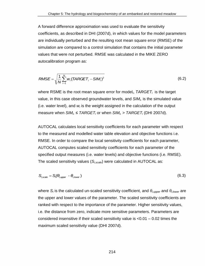
Chapter 5: The hydrology and biogeochemistry of an embanked and restored meadow
214
A forward difference approximation was used to evaluate the sensitivity
coefficients, as described in DHI (2007d), in which values for the model parameters
are individually perturbed and the resulting root mean square error (RMSE) of the
simulation are compared to a control simulation that contains the initial parameter
values that were not perturbed. RMSE was calculated in the MIKE ZERO
autocalibration program as:
2
1
)(1
ii
N
i
i SIMTARGETwN
RMSE
(6.2)
where RSME is the root mean square error for modeli, TARGETi is the target
value, in this case observed groundwater levels, and SIMi, is the simulated value
(i.e. water level), and wi is the weight assigned in the calculation of the output
measure when SIMi, ≤ TARGETi or when SIMi, > TARGETi (DHI 2007d).
AUTOCAL calculates local sensitivity coefficients for each parameter with respect
to the measured and modelled water table elevation and objective functions i.e.
RMSE. In order to compare the local sensitivity coefficients for each parameter,
AUTOCAL computes scaled sensitivity coefficients for each parameter of the
specified output measures (i.e. water levels) and objective functions (i.e. RMSE).
The scaled sensitivity values (Si,scale) were calculated in AUTOCAL as:
)i,loweri,upperii,scale - θ(θSS (6.3)
where Si is the calculated un-scaled sensitivity coefficient, and θi,upper and θi,lower are
the upper and lower values of the parameter. The scaled sensitivity coefficients are
ranked with respect to the importance of the parameter. Higher sensitivity values,
i.e. the distance from zero, indicate more sensitive parameters. Parameters are
considered insensitive if their scaled sensitivity value is <0.01 – 0.02 times the
maximum scaled sensitivity value (DHI 2007d).

Chapter 5: The hydrology and biogeochemistry of an embanked and restored meadow
215
The most sensitive parameters in descending order were horizontal hydraulic
conductivity, drainage level, drainage time, Manning M, vertical hydraulic
conductivity, and soil water content at saturation (Table 6.7). A manual
manipulation of the most sensitive parameters selected by AUTOCAL was
conducted in the MIKE SHE model in order to confirm the results of the AUTOCAL
sensitivity analysis. Subsequently, the insensitive parameters were set to constant
values using the initial values in Table 6.6, which as discussed throughout this
section were established from the field observations and the literature, whereas the
most important parameters outlined above were adjusted during the following
parameter optimisation.
Table 6.7: Scaled sensitivity coefficients for parameter used in the AUTOCAL
sensitivity analysis. Greater RMSE (absolute values), i.e. the distance from zero,
indicate more sensitive parameters. Parameters are considered insensitive if their
scaled sensitivity value is <0.01 – 0.02 times the maximum scaled sensitivity value
(absolute values).
Parameter RMSE Aggregate
Drainage level 1.14
Water content at saturation 0.11
Infiltration 0.09
Specific storage 0.02
Initial head 0.01
Fixed head 0.01
Detention storage 0.00
Specific yield 0.00
River water depth 0.00
Riverbed resistance 0.00
Water content at wilting point -0.03
Evapotranspiration surface depth -0.06
Geological layer lower level -0.10
Vertical hydraulic conductivity -0.14
Overland Manning M -0.14
Drainage time -0.96
Horizontal hydraulic conductivity -3.06

Chapter 5: The hydrology and biogeochemistry of an embanked and restored meadow
216
6.4.2 Model calibration and validation
A detailed account of the MIKE SHE model results and comparisons of the
observed and simulated groundwater elevations is provided in Section 7.
Calibration and initial model validation was undertaken using the embanked model
using a split sample approach. The 13-month period 22 February 2007 ‒ 14 March
2008 was used for calibration and the following 12 months (15/03/2008 ‒
15/03/2009) for validation. The end of this period coincided with embankment
removal so that calibrated parameter values were specified within the model
representing restored conditions with the subsequent 16 months (29/03/2009 ‒
25/07/2010) providing a second validation period. As described above, a number of
model parameters were varied during model calibration.
Initial calibration was undertaken using an automatic calibration procedure that was
based on the shuffled complex evolution method with the optimal parameter set
being selected according to the lowest aggregate RMSE (a measure of the
average magnitude of error) for the comparisons between observed and simulated
groundwater and river water levels (Duan et al. 1992; Madsen 2000 2003; DHI
2007c). This approach was undertaken for the coarser 15 m × 15 m model grid to
reduce the computational time due to the number individual model runs (n=480)
required for the automatic calibration routine to determine an optimal parameter
set.
Interpolation of surface elevation over a coarse grid size of 15 × 15 m in MIKE SHE
resulted on average in a 0.25 m over-estimate of surface elevation at the well
locations, with greater absolute error at the base of the hillslope (absolute error =
0.53 to 1.16 m) and on the river embankments (absolute error = 0.53 m), which is
represented by the outliers in Figure 6.22. At a grid spacing of 15 × 15 m multiple
wells were represented by the same grid cell, which did not allow for variation in
water levels between these wells. For this reason, three wells (one from each well
transect) located in the middle of the meadow and away from the embankments
and hillslope were used in the autocalibration process; the interpolated surface

Chapter 5: The hydrology and biogeochemistry of an embanked and restored meadow
217
elevation at these grid cells had an absolute error <1 cm. The models were run
with the selected parameter sets using the Shuffled Complex Evolution
optimization method in the MIKE ZERO AUTOCAL program (DHI 2007d). The
optimal parameter values in the autocalibration after 420 runs were selected
according to the lowest aggregate RMSE scores, which equaled 0.027. These final
MIKE SHE and MIKE 11 parameter values for the automatically calibrated model
are summarised in Table 6.8.
Figure 6.22: Increase in elevation absolute error with grid size. The solid centre line
and broken line within the boxplot indicate the median and mean, respectively. The
box extent and error bars denote the 25th and 75th percentiles, and 10th and 90th
percentiles, respectively. The circles indicate the presence of outliers.
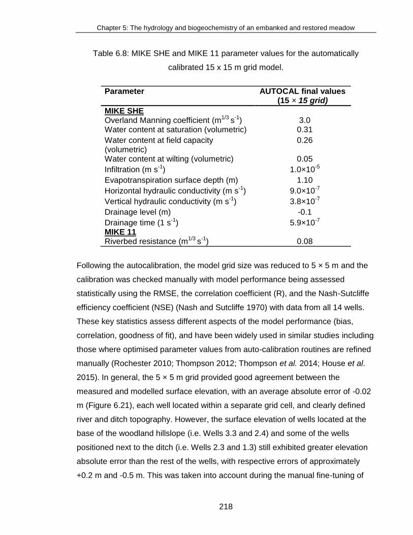
Chapter 5: The hydrology and biogeochemistry of an embanked and restored meadow
218
Table 6.8: MIKE SHE and MIKE 11 parameter values for the automatically
calibrated 15 x 15 m grid model.
Parameter AUTOCAL final values (15 × 15 grid)
MIKE SHE Overland Manning coefficient (m1/3 s-1)
3.0
Water content at saturation (volumetric) 0.31
Water content at field capacity (volumetric)
0.26
Water content at wilting (volumetric) 0.05
Infiltration (m s-1) 1.0×10⁻⁵
Evapotranspiration surface depth (m) 1.10
Horizontal hydraulic conductivity (m s-1) 9.0×10⁻⁷
Vertical hydraulic conductivity (m s-1) 3.8×10⁻⁷
Drainage level (m) -0.1
Drainage time (1 s-1) MIKE 11 Riverbed resistance (m1/3 s-1)
5.9×10⁻⁷
0.08
Following the autocalibration, the model grid size was reduced to 5 × 5 m and the
calibration was checked manually with model performance being assessed
statistically using the RMSE, the correlation coefficient (R), and the Nash-Sutcliffe
efficiency coefficient (NSE) (Nash and Sutcliffe 1970) with data from all 14 wells.
These key statistics assess different aspects of the model performance (bias,
correlation, goodness of fit), and have been widely used in similar studies including
those where optimised parameter values from auto-calibration routines are refined
manually (Rochester 2010; Thompson 2012; Thompson et al. 2014; House et al.
2015). In general, the 5 × 5 m grid provided good agreement between the
measured and modelled surface elevation, with an average absolute error of -0.02
m (Figure 6.21), each well located within a separate grid cell, and clearly defined
river and ditch topography. However, the surface elevation of wells located at the
base of the woodland hillslope (i.e. Wells 3.3 and 2.4) and some of the wells
positioned next to the ditch (i.e. Wells 2.3 and 1.3) still exhibited greater elevation
absolute error than the rest of the wells, with respective errors of approximately
+0.2 m and -0.5 m. This was taken into account during the manual fine-tuning of

Chapter 5: The hydrology and biogeochemistry of an embanked and restored meadow
219
the model, and a less accurate fit between the modelled and measured water
surface elevations was expected at these wells. The final values of the calibration
terms defined at the end of this process are summarized in Table 6.9. The final
calibrated distributed manning’s M values for overland flow are sensible for
grassland (3.0 m1/3 s-1) and light underbrush (2.5 m1/3 s-1) given in the literature
(USDA, 1986, Thompson, 2004). The volumetric soil water content for saturation,
field capacity and wilting point are within an appropriate range for a sandy loam soil
based on the laboratory results from the water release characteristic (see Section
6.2.4) and values reported for sandy loam soils (e.g. Zotarelli et al. 2010).
The calibrated evapotranspiration surface depth (i.e. the height of the capillary
zone) of 1.1 m is between the values of 0.4 m – 1.9 m calculated for Hunworth
Meadow using Hazen’s formula (Das 2002), and comparable to values of capillary
rise between 0.5 – 2.0 m for sandy loams (Chubarova 1972; Brouwer et al. 1985).
Furthermore, the final hydraulic conductivity values are in accordance with values
provided in the literature for medium sand soils (ie. 9×10⁻⁷ – 5×10⁻⁴ m s-1)
(Domenico and Schwartz 1998), and field tests at the River Glaven restoration site
(see section 6.2.5). Lastly, the time varying river bed resistance approach,
described in Section 6.3.2, was essential to account for variation in riverbed
resistance to flow associated with seasonal and interannual differences in
macrophyte abundance observed at the River Glaven. The final values of between
0.058 sec m-1/3 and 0.15 sec m-1/3 (see Figure 6.20) are sensible for a small stream
with high macrophyte growth in the summer (e.g. House et al. 2016a).The same
statistical measures were subsequently employed to assess model performance
for both of the validation periods.
Once the model parameters were selected, the performance of the model was
assessed for the two validation periods from statistical comparisons of simulated
and measured water using RMSE, the correlation coefficient (R), and the Nash-
Sutcliffe efficiency coefficient (R2) (Nash and Sutcliffe 1970). Subsequently, key
components of surface water and groundwater hydrology, such as groundwater

Chapter 5: The hydrology and biogeochemistry of an embanked and restored meadow
220
recharge, surface runoff, and floodplain storage were simulated at daily time steps
and compared between the embankment and restored floodplain scenarios. A
detailed account of the MIKE SHE/MIKE 11 model results are presented in Chapter
7.
Table 6.9: Final calibrated MIKE SHE and MIKE 11 parameter values.
Parameter Value
MIKE SHE Overland Manning M (m1/3 s-1)
3.0 (grass)
2.5 (light underbrush) Water content at saturation (volumetric) 0.40
Water content at field capacity (volumetric) 0.20
Water content at wilting (volumetric) 0.07
Saturated hydraulic conductivity (m s-1) 1×10⁻⁵
Evapotranspiration surface depth (m) 1.0
Horizontal hydraulic conductivity (m s-1) 9×10⁻⁷
Vertical hydraulic conductivity (m s-1) 1×10⁻⁷
MIKE 11 Riverbed resistance (m1/3s-1) (Time varying)
0.058 – 0.15*
*(Time varying)
6.5 Impact assessment of embankment removal
The hydrological effects of removing the embankments along the River Glaven
were investigated by running the two MIKE SHE / MIKE 11 models representing
pre- and post-restoration conditions for the same extended period with identical
climatic and river-flow conditions. This method avoids the differences in simulated
hydrological conditions that are due to interannual climate variability within the pre-
and post-restoration periods used for model calibration and validation. For
example, 2007 and 2008 (pre-restoration) were characteristically wetter than 2009
and 2010 following restoration, with total annual precipitation of 880, 784, 684, and
606 mm respectively (Table 6.10). Total annual river discharge for 2007, the period
of record used in the model calibration, was one of the highest on record (Table

Chapter 5: The hydrology and biogeochemistry of an embanked and restored meadow
221
6.10). Simulating pre- and post-restoration for the same period therefore enables
the effects of embankment removal alone to be assessed.
Table 6.10: Total annual precipitation at Mannington Hall (<10 km from the study
site) and river discharge at Hunworth from 2001 – 2010.
Hydrological year
Precipitation (mm)
Discharge (m3 s-1)
2001 614 101
2002 766 91
2003 822 87
2004 721 94
2005 703 73
2006 954 110
2007 880 103
2008 784 92
2009 684 91
2010 606 N/A*
*Discharge data not available from August 2010 onwards (see Section 4.2).
The simulation period for this assessment was the decade 2001 – 2010. As for the
calibration and validation periods, the upstream boundary condition of the MIKE 11
model was specified as mean daily discharge at the Hunworth gauging station. In
the absence of data from the local automatic weather station, daily precipitation
and Penman-Monteith potential evapotranspiration were derived from records from
the Mannington Hall meteorological station. Comparisons of the meteorological
data collected on site at the Hunworth weather station and the UK Met Office
weather station at Mannington Hall (ca. 10 km from the study site) were conducted
to validate the use of off-site weather data, which covered a longer period of
record, and were required to extend the period of simulation in the MIKE SHE/11
models. Hunworth and Mannington Hall weather stations showed excellent
agreement in temperature (r2 = 0.91) (Figure 6.23), but more variation among the
precipitation data (r2 = 0.41) (Figure 6.24). This was largely due to a slight offset in
the timing of precipitation events, which may be expected when using an off-site

Chapter 5: The hydrology and biogeochemistry of an embanked and restored meadow
222
weather station. However, the magnitude of rainfall measured at the Mannington
Hall station compared very well with the on-site station and was considered
representative of the upstream meteorological conditions affecting discharge
dynamics at Hunworth study site.
Figure 6.23 (a) Time series of mean daily air temperature at Hunworth Meadow
and Mannington Hall, and (b) relationship between air temperature at Mannington
Hall and Hunworth.

Chapter 5: The hydrology and biogeochemistry of an embanked and restored meadow
223
Figure 6.24: (a) Time series of total daily precipitation at Hunworth Meadow and
Mannington Hall, and (b) relationship between precipitation at Mannington Hall and
Hunworth.
River discharge data at Hunworth was affected by macrophyte growth for short
periods during the summer in some years (see Section 5.2.4). In order to run the
MIKE SHE/11 models continuously from 2001 to 2010, gaps in the Hunworth
discharge data resulting from macrophyte growth was plugged using a regression
established between river discharge at the EA gauging station at Bayfield (station

Chapter 5: The hydrology and biogeochemistry of an embanked and restored meadow
224
#:3034016) and the onsite EA gauging station at Hunworth (located ca. 5 km apart)
during low flow conditions (y = 0.4087x + 0.0396; r2= 0.86) (Figures 6.25 and 6.26).
As discussed in Section 3.5, river discharge at Bayfield was not rated above 0.3 m
(ca. 0.65 m3 s-1). However this did not affect the data used as the missing data for
Hunworth only occurred during low flow conditions in the summer when
macrophyste growth was at its greatest, and accordingly only baseflow data was
used in the regression (Figure 6.25).
Figure 6.25: Simple linear regression between river discharge at Bayfield and
Hunworth gauging stations (y = 0.4087x + 0.0396; r2= 0.86).
River discharge data at Hunworth was not usable from August 2010. A second-
phase in-stream restoration project conducted in August 2010, which involved
extensive geomorphological changes to the river channel (narrowing, depth
diversification, and re-meandering), inadvertently caused water to back-up over the

Chapter 5: The hydrology and biogeochemistry of an embanked and restored meadow
225
weir which affected the rating curve at the gauging station. This resulted in
inaccurate discharge calculations, which can clearly been seen in the sudden
increase in discharge after the restoration in August 2010 (Figure 6.26).
Unfortunately Bayfield is the only other gauging station on the River Glaven, and
as this section of the river was not rated above discharges of approximately 0.65
m3 s-1, the River Glaven does not currently have a fully operational gauging station.
The available meteorological and river discharge data from 2001 – 2010
represented a range of climate and river-flow conditions, including extreme high
and low river-flow years, which enabled the simulation of a spectrum of probable
flow conditions expected on the floodplain under both pre- and post-restoration
conditions. For example, during this period, some of the wettest years in the UK
occurred since records began in 1910 (Figure 6.27a). In East Anglia, the region of
the study site, total annual rainfall in 2001 averaged 780 mm, and was second
highest to the 2012 record of 810 mm. Wet years also occurred in 2004, 2007, and
2008, and were substantially above the baseline average for the region (Figure
6.28). The driest contemporary years occurred in 2003, 2005, and 2011 and were
within 3 – 18% of the driest five years on record, which averaged 346 mm (Figure
6.28a). In the UK, five of the sixth wettest years have occurred since 2000, and
eight of the warmest years have all occurred since 2002. Indeed, 2014 was the
wettest winter and warmest year in the UK for over 100 years (Figure 6.27a and b).
Seasonal rainfall in East Anglia is highly variable, but appears to have increased in
winter and summer months since 2000. Less obvious trends were evident for
spring and autumn (Figure 6.28). Contemporary river discharge and climate data
for the River Glaven provided a realistic range of expected hydrological conditions,
including extreme heavy precipitation events (e.g. summer 2007), and periods of
drought (e.g. summer/autumn 2005) that were used to predict the effects of high
and low flow scenarios on the floodplain hydrology following the removal of the
river embankments.

Chapter 5: The hydrology and biogeochemistry of an embanked and restored meadow
226
Figure 6.26: Time series of mean daily discharge on the River Glavenat Hunworth (Station #: 034052) and Bayfield
(Station #: 034016) Environment Agency gauging stations from 2001 to 2014. River discharge at Bayfield was not rated
above 0.3 m (ca. 0.65 m3 s-1). Measurements of river discharge at Hunworth were affected by a restoration project
(remeandering of the river channel) immediately downstream of the gauging station in August 2010.

Chapter 5: The hydrology and biogeochemistry of an embanked and restored meadow
227
Figure 6.27: Time series of mean annual rainfall (a) and air temperature (b) for
East Anglia, England (location of the study site) and the United Kingdom. Data are
plotted relative to the average of the 1961 – 1990 baseline period (Jones et al.
1999). Data were smoothed with a first order low pass recursive filter to highlight
trends in the data relative to the 1961 – 1990 average. Data are from the Met
Office regional climate summaries (Met office 2015).

Chapter 5: The hydrology and biogeochemistry of an embanked and restored meadow
228
Figure 6.28: Time series of mean seasonal rainfall for the region of East Anglia,
England (location of the study site), plotted relative to the average of the 1961 –
1990 baseline period (Jones et al. 1999). Data are from the Met Office regional
climate summaries (Met office, 2015).

Chapter 7: Coupled hydrological/hydraulic modelling of river restoration
229
Chapter 7: Coupled hydrological/hydraulic modelling of river
restoration and floodplain hydrodynamics
7.1 Introduction
This chapter presents a combined analysis of the monitoring and simulation results
of pre-embankment and post-embankment hydrological conditions. Simulations
from the calibrated and validated MIKE SHE / MIKE 11 models are used to predict
changes in river-floodplain hydrology due to embankment removal for an extended
10-year period, and to further enhance understanding of floodplain functioning.
This chapter therefore addresses the second set of research questions outlined in
Chapter 1:
(iii) What are the effects of embankment removal on key components of river-
floodplain hydrology (water table elevation, frequency and extent of
floodplain inundation, flood-peak attenuation)?
(iv) How will embankment removal impact river-floodplain hydrology under a
range of expected river-flow conditions?
7.2 Results
7.2.1 Model calibration and validation
For the majority of wells, there is very good agreement between the observed and
simulated groundwater levels throughout the calibration and validation periods
(Figures 7.1-7.3). The timing of simulated groundwater fluctuations fit well with the
observed data (Figure 7.1-7.3). In particular, the rapid response of groundwater
during high magnitude rainfall and river-flow events is captured well by the model
(Figures 7.1-7.3). The observed and simulated rates of groundwater decline

Chapter 7: Coupled hydrological/hydraulic modelling of river restoration
230
following periods of elevated water tables (typically March – May) also show
generally good agreement each year. During some periods of low rainfall, e.g.
August to mid-October 2009 (see Section 5.2.2), simulated groundwater levels
close to the river are higher than the observed levels, possibly due to over-
estimated instream macrophyte growth, however this difference is ≤0.2 m (Figures
7.1-7.3).
Groundwater levels on the floodplain were controlled by river stage and responses
to rainfall. The model reproduces the close connection between groundwater and
river water levels, and captures the recession of groundwater levels in response to
decreasing river levels (Figures 7.1-7.4). Seasonal changes in groundwater levels
are reproduced well by the model. Levels at each of the well locations exhibit
similar temporal patterns, with distinct seasonal fluctuation in groundwater levels in
the range of 0.4 – 0.6 m. Across the floodplain, greater fluctuations in groundwater
levels are simulated during the summer when drier conditions result in water levels
that are typically lower in the soil profile, compared with the winter when surface
soils are predominantly saturated (Figures 7.1-7.3). Consequently, greater
variability in groundwater levels occurs between summers than between winters.
The model clearly reproduces the lower groundwater levels observed during the
dry summers of 2009 and 2010 following embankment removal, compared with the
wet summers in 2007 and 2008 in which both observed and simulated groundwater
levels are higher (Figures 7.1-7.3).
The ability of the model to represent observed conditions within Hunworth Meadow
is further demonstrated in Table 7.1 that summarises the model performance
statistics for each well for the calibration period and each of the validation periods
(pre- and post-restoration). The mean error for groundwater levels was typically
less than ± 0.05 m and the correlation coefficient averaged 0.85, 0.80 and 0.85 for
the calibration and pre- and post-validation periods, respectively. Values of the
Nash-Sutcliffe efficiency coefficient were between 0.5 – 0.8 for most of the wells,
indicating fair to good model performance. In particular, excellent performance is

Chapter 7: Coupled hydrological/hydraulic modelling of river restoration
231
indicated for wells 3.1 and 3.2. The first of these was the only well located on the
embankment and as a result necessitated re-installation of monitoring equipment
after restoration (note the change in soil surface elevation in Figure 7.1a).
Figure 7.1: Comparison of observed and modelled groundwater depths for the
calibration and validation periods at the upstream well transect. Note: soil surface
elevation change at Well 3.1 (a), which was located on the embankment prior to
the restoration.

Chapter 7: Coupled hydrological/hydraulic modelling of river restoration
232
Figure 7.2: Comparison of observed and modelled groundwater depths for the
calibration and validation periods at the midstream well transect. The embankment
removal in March 2009 is highlighted by the vertical hashed bar.

Chapter 7: Coupled hydrological/hydraulic modelling of river restoration
233
Figure 7.3: Comparison of observed and modelled groundwater depths for the
calibration and validation periods at the midstream well transect. The embankment
removal in March 2009 is highlighted by the vertical hashed bar. Note: there were
problems at times with the level logger at Well 1.2, hence this well was discounted
during the calibration and validation of the model.

Chapter 7: Coupled hydrological/hydraulic modelling of river restoration
234
Water levels simulated by the model also provide a good fit at Well 1.1, which was
located next to the embankment at the downstream end of the meadow, and at
wells spanning the middle section of the meadow (Wells 2.1-2.3). The model
performs less well at the edge of the ditch, i.e. at those wells that were in many
cases within 1 m of this channel, and at the floodplain-hillslope margin. Model
performance statistics indicate a poorer fit in this narrow section of the floodplain,
with simulated groundwater levels being periodically slightly higher than observed
at Well 2.4 and lower than observed at Wells 3.4 and 3.5 (Figures 7.2 and 7.3).
These wells proved the most difficult to calibrate. In many of the calibration
simulations too much water was present at these locations.
The drainage option in MIKE SHE was employed to simulate the transfer of water
along the base of the hillslope to the drainage ditch, the topography of which was
not fully captured at the 5 m model grid resolution (see Section 6.2.6). These
effects were largely removed at smaller grid spacing (i.e. 2 m), however the
computational requirements for this model resolution was too intensive. Model
performance in some of the lower meadow wells (e.g. Wells 1.1 and 1.3) was poor
during the pre-restoration validation due to lower than observed groundwater levels
during a period of low rainfall from April-May 2008 (see Section 5.2.2).
Groundwater levels in the ditch were simulated and guided the calibration process;
however there was a slight offset in the simulated and observed water levels of
approximately +0.1 ‒ 0.2 m (Figure 7.4). This was probably due to smoothing of
the ditch topography at the 5 m grid resolution (see Figure 6.5). Ultimately,
however, the magnitude of daily groundwater changes in the ditch were captured
very well by the model (Figure 7.4).
Collectively the comparisons between observed and simulated groundwater levels
and the associated model performance statistics indicate a good ability of the
model to reproduce groundwater levels across most of the meadow for periods
both before and after the removal of river embankments. These results suggest

Chapter 7: Coupled hydrological/hydraulic modelling of river restoration
235
that the model is an appropriate tool to assess the impacts of embankment
removal upon hydrological conditions across the floodplain.
Table 7.1: Mean error (ME - m), correlation coefficient (R), and Nash-Sutcliffe
model efficiency coefficient (NSE) for the calibration (22/02/07 – 14/03/2008) and
validation (pre-restoration:15/03/2008 ‒ 15/03/2009; post-restoration: 29/03/2009
‒ 25/07/2010) periods.
Calibration (pre-restoration)
Validation (pre-restoration)
Validation (post-restoration)
Well ME R NSE ME R NSE ME R NSE
1.1 -0.02 0.79 0.60 0.02 0.71 0.14 -0.02 0.70 0.47 1.2* -0.02 0.74 -0.23 -0.05 0.42 -1.71 -0.07 0.75 0.29 1.3 0.03 0.81 0.49 0.03 0.65 0.16 0.03 0.83 0.62 1.4 0.00 0.79 0.60 0.00 0.66 0.27 -0.03 0.86 0.70 1.6 0.04 0.74 0.12 0.00 0.65 0.17 0.01 0.68 0.37 2.1 -0.13 1.00 0.62 -0.05 0.91 0.75 -0.07 0.99 0.67 2.2 -0.10 0.99 0.67 -0.01 0.85 0.58 -0.02 0.99 -6.56 2.3 0.01 0.96 0.77 0.05 0.85 0.56 0.02 0.89 0.72 2.4 -0.05 0.62 -0.80 -0.04 0.80 0.31 0.05 0.91 0.54 3.1 -0.06 0.85 0.56 0.01 0.90 0.76 -0.04 0.84 0.52 3.2 -0.04 0.89 0.73 0.03 0.89 0.75 -0.03 0.84 0.70 3.3 -0.07 0.86 0.37 0.00 0.75 0.20 0.05 0.81 0.57 3.4 0.01 0.82 0.55 0.03 0.85 0.18 n/a n/a n/a 3.5 -0.04 0.89 0.45 0.00 0.88 0.69 0.11 0.81 0.26
River stage
n/a n/a n/a 0.08 0.97 0.65 -0.03 0.65 0.18
*Note that there were problems at times with the level logger at Well 1.2 so this
well was discounted during model calibration and validation.
n/a: data not available for the period.
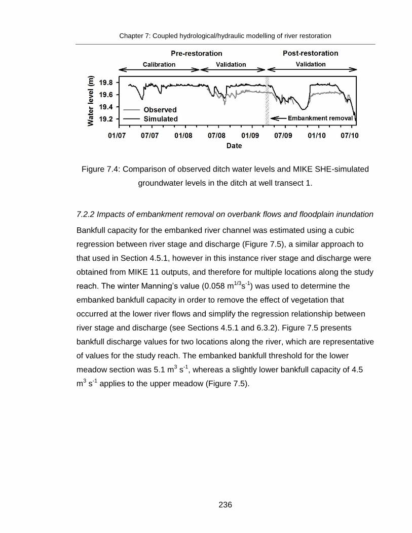
Chapter 7: Coupled hydrological/hydraulic modelling of river restoration
236
Figure 7.4: Comparison of observed ditch water levels and MIKE SHE-simulated
groundwater levels in the ditch at well transect 1.
7.2.2 Impacts of embankment removal on overbank flows and floodplain inundation
Bankfull capacity for the embanked river channel was estimated using a cubic
regression between river stage and discharge (Figure 7.5), a similar approach to
that used in Section 4.5.1, however in this instance river stage and discharge were
obtained from MIKE 11 outputs, and therefore for multiple locations along the study
reach. The winter Manning’s value (0.058 m1/3s-1) was used to determine the
embanked bankfull capacity in order to remove the effect of vegetation that
occurred at the lower river flows and simplify the regression relationship between
river stage and discharge (see Sections 4.5.1 and 6.3.2). Figure 7.5 presents
bankfull discharge values for two locations along the river, which are representative
of values for the study reach. The embanked bankfull threshold for the lower
meadow section was 5.1 m3 s-1, whereas a slightly lower bankfull capacity of 4.5
m3 s-1 applies to the upper meadow (Figure 7.5).

Chapter 7: Coupled hydrological/hydraulic modelling of river restoration
237
Figure 7.5: River stage-discharge relationships from MIKE 11 outputs for the
embanked scenario at the Lower Meadow (r2 = 0.999; y = -635.0860 + 162.9633 *
x + -11.7679 * x2 + 0.2606 * x3) and Upper Meadow (r2 = 1.000; y = -13843.7297 +
2083.8580* x + -104.5615* x2 + 1.7489* x3) areas. Bankfull discharges for the
embanked scenario were not observed during the 10-year period of the discharge
record; hence bankfull capacity was extrapolated beyond the available data and
thus should be treated with caution.
Bankfull capacity for the restored river was derived from MIKE 11 stage-discharge
relationships and bankfull measurements from the river cross-sections (Figure 7.6).
In addition, bankfull capacity was evaluated using MIKE SHE results depicting the
depth of overland water, which enabled the identification of two thresholds for
overland flow: a high discharge threshold above which widespread inundation
occurred, and a lower threshold above which localised flooding (up to one grid cell
- i.e 5 m - from the river) occurred (Figure 7.6). The high flow threshold was
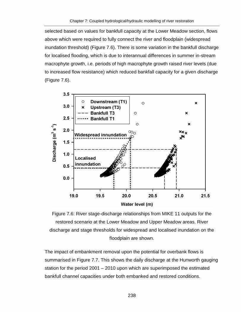
Chapter 7: Coupled hydrological/hydraulic modelling of river restoration
238
selected based on values for bankfull capacity at the Lower Meadow section, flows
above which were required to fully connect the river and floodplain (widespread
inundation threshold) (Figure 7.6). There is some variation in the bankfull discharge
for localised flooding, which is due to interannual differences in summer in-stream
macrophyte growth, i.e. periods of high macrophyte growth raised river levels (due
to increased flow resistance) which reduced bankfall capacity for a given discharge
(Figure 7.6).
Figure 7.6: River stage-discharge relationships from MIKE 11 outputs for the
restored scenario at the Lower Meadow and Upper Meadow areas. River
discharge and stage thresholds for widespread and localised inundation on the
floodplain are shown.
The impact of embankment removal upon the potential for overbank flows is
summarised in Figure 7.7. This shows the daily discharge at the Hunworth gauging
station for the period 2001 – 2010 upon which are superimposed the estimated
bankfull channel capacities under both embanked and restored conditions.

Chapter 7: Coupled hydrological/hydraulic modelling of river restoration
239
Throughout the whole 10-year period no overbank flows were simulated since the
bankfull channel capacity (5.1 m3 s-1) was greater than the maximum observed flow
of 3.1 m3 s-1. This is in agreement with the observation-based bankfull results
detailed in Section 5.2 from the river stage-discharge relationship at well transect 1
(T1) and bankfull river discharge calculated using Manning’s equation.
In contrast, river flows frequently exceeded bankfull capacity in the restored model,
where two thresholds for inundation on the floodplain were identified: the high flow
channel capacity (1.67 m3 s-1) above which widespread floodplain inundation
occurred; and the low flow channel capacity (0.59 m3 s-1) which resulted in
localised inundation at the river edge in an area corresponding to the former
location of the embankments (Figures 7.6 and 7.7). Such flooding did not occur in
pre-restoration conditions due to the steep sides of the embankments. Throughout
the 10-year period, discharge exceeded the high flow channel capacity for
widespread flooding in the restored model on nine occasions, albeit only for short
periods (1 day). Three large overbank events occurred over a month-long period
from late May – June 2007, interspersed with eight smaller localised flooding
events at the river-edge. Localised flooding was much more frequent (61
occasions) and of longer duration (2 – 3 days), and is likely to result in a more
dynamic and natural transitional zone between the river and the floodplain.
Surface flooding on the floodplain is simulated within the MIKE SHE models when
groundwater levels intercept the ground surface (in which case precipitation cannot
be infiltrated) or when the river over-tops the channel banks. In the embanked
model groundwater was the only source of flooding on the floodplain, whereas
under restored conditions inundation also occurred due to overbank flows.
Restoration of these overbank flows and the reconnection of the river and its
floodplain therefore had a marked effect on simulated floodplain hydrology. This is
clearly demonstrated in Figure 7.8, which shows the simulated extent and depth of
surface water for the pre- and post-restoration models for two high river-flow
events. The first (which occurred on 28/05/2007) is associated with a mean daily

Chapter 7: Coupled hydrological/hydraulic modelling of river restoration
240
discharge of 1.9 m3 s-1, just above the threshold channel capacity associated with
widespread inundation under restored conditions (Figure 7.8a), whilst the second
(18/07/2001) is the largest event (3.1 m3 s-1) during the 10-year simulation period
(Figure 7.8c).
Results for the embanked, pre-restoration model show that river water was
constrained within the river channel by the embankments, which were not flooded
in both events shown in Figure 7.8 and indeed throughout the 10-year simulation
period. During the smaller flood event (Figure 7.8a), flooding was limited to the
margins of the floodplain ditch and the downstream ponded area and was driven
by rising groundwater tables. During the larger river-flow event (Figure 7.8c), there
was limited groundwater flooding behind the embankments, with surface water
depth ranging between 0.0 – 0.02 m across much of the meadow, and up to 0.4 m
in topographic depressions along the ditch and ponded area in the lower meadow.
This was attributed to an extended period of low rainfall, high evapotranspiration
and low water table depths that preceded the high flow event.
Under post-restoration conditions overbank flows resulted in widespread
inundation on the floodplain that would supplement groundwater-fed surface water.
During the smaller flood event (Figure 7.8b) much of the floodplain was subject to
shallow (<0.3 m depth) inundation. Embankment removal enabled some overbank
flows at the top end of the floodplain although a relatively high section of the
riverbank and adjacent floodplain in the upper-middle part of the site was not
flooded. Further downstream the lower half of the floodplain was directly connected
with the river and the previously embanked area was inundated. During the largest
flood event (Figure 7.8d) nearly the whole floodplain was directly connected to the
river, and extensive and much deeper flooding (0.2 – 0.6 m) occurred.

Chapter 7: Coupled hydrological/hydraulic modelling of river restoration
241
Figure 7.7: Mean daily river discharge from 2001 – 2010. The embanked and restored bankfull capacity is shown, above
which widespread inundation of the floodplain would have occurred. Two bankfull thresholds, a minimum and maximum,
are shown for the restored river, which correspond to the cross-section inset; flows above these thresholds result in
localised and widespread flooding, respectively.

Chapter 7: Coupled hydrological/hydraulic modelling of river restoration
242
Figure 7.8: Comparison of simulated surface water extent and depth for the
embanked and restored scenarios during a small overbank (post-restoration) event
(28/05/07; flow = 1.9 m3 s-1) (a-b) and a larger overbank (post-restoration) event
(18/07/01; flow = 3.1 m 3 s-1) (c-d).

Chapter 7: Coupled hydrological/hydraulic modelling of river restoration
243
Simulation results show that the ditch running parallel, but to the north of the river,
played an important role in distributing flood water. Surface water resulting from
high water tables or overbanking of the river was channelled across and down the
floodplain into the ditch, which then filled and contributed to flooding along the ditch
marginal areas, ponding in topographic depressions, and subsequent groundwater
recharge leading to higher water table elevations. Surface water accumulated in
the lower section of the meadow in the region of the pond (Figure 7.8a and 7.8c).
Prior to the restoration, the ponded area that was subject to groundwater flooding
as well as being fed by the ditch, was saturated for much of the year. In this state,
the embankment acted as a barrier for water that had accumulated in this part of
the floodplain, preventing its return to the river. However, after the removal of the
embankments, drainage of surface water from the floodplain to the river was
restored. Water stored in this low-lying area of the meadow during flood events
subsequently acted as a source of return flow to the river (Figure 7.8).
7.2.3 Impacts of embankment removal on groundwater
Throughout the 10-year simulation period, groundwater levels close to the river (i.e.
within 30 m) were on average 0.01 m higher under restored conditions, whereas
groundwater levels in low lying areas of the meadow that were previously flooded
were on average 0.01 m lower in the restored scenario. This is reflected in Figure
7.9 showing the differences in groundwater levels at the 14 wells simulated by the
embanked and restored models. During periods of the highest river flows,
groundwater levels were up to 0.8 m higher under restored conditions. The largest
increases in water table elevation occurred along the river banks (e.g. wells 3.1
and 1.1), in the region of the ditch (e.g. wells 2.3 and 2.4), and on the relatively
low-lying downstream end of the floodplain. The smallest effects were seen at well
2.1 adjacent to the section of riverbank that was not restored, where increases in
water table elevation during high river-flow periods were typically less than 0.3 m
(Figure 7.9b). This location corresponds to the relatively high part of the floodplain,
where the embankments were not removed (see Section 3.8), that consequently

Chapter 7: Coupled hydrological/hydraulic modelling of river restoration
244
was not flooded under post-restoration conditions (Figure 7.8b). Some short
periods of slightly lower groundwater levels (up to -0.18 m) were simulated under
restored conditions immediately after periods of groundwater and overbank
flooding. These are most noticeable at Well 1.1 (Figure 7.9c) that was located
close to the river and the ponded area in this part of the floodplain and at Well 1.4
that was located in a low-lying area next to the ditch. These changes are most
likely due to the previously discussed improved drainage at the river-floodplain
margin.
Figure 7.9: Simulated time series of water table elevation (WTE) differences
between the restored and embanked scenarios from 2001 – 2010 (a period which
encompassed a range of wet and dry conditions). Positive differences indicate
restored WTE > embanked WTE. Differences in WTE are shown at well locations
across the floodplain at the (a) upper, (b) middle, and (c) lower well transects (see
well locations in Figure 3.1 and 7.12).
Chapter 7: Coupled hydrological/hydraulic modelling of river restoration
245
The greatest differences in water table elevation between the embanked and
restored model results occurred in spring/summer during periods of low river flows.
Simulated groundwater levels along the river (i.e. within 30 m) for the restored
model were on average 0.03 m higher (p<0.05) than those for the embanked
model in the spring/summer. No significant differences were found in the
autumn/winter (p=0.754) (Figure 7.9). This can be attributed to increased surface
flooding and floodplain storage during a number of inundation events that occurred
in the summer months. Increased floodplain storage before the beginning of the
spring/summer drawdown combined with periodic additions from summer flooding
reduces the summer groundwater head recession within the meadow (Figure
7.10). The higher simulated groundwater levels after embankment removal causes
some differences in the hydraulic gradient between the river and floodplain during
the summer. In comparison to the embanked model, results for the restored model
show that summer groundwater levels at the river margin are closer to river water
levels (Figure 7.10), resulting in more frequent reversals in the hydraulic gradient
and consequentially a more dynamic subsurface exchange.

Chapter 7: Coupled hydrological/hydraulic modelling of river restoration
246
Figure 7.10: Comparison of simulated groundwater elevation (ODN) at well 1.1 and river stage (ODN) for the (a)
embanked and (b) restored scenarios from 2001 – 2010.

Chapter 7: Coupled hydrological/hydraulic modelling of river restoration
247
7.2.4 Impacts of embankment removal on groundwater flowpaths
As discussed in Section 5.2.2, observed groundwater heads generally decreased
from the direction of the river to the floodplain at the upstream and midstream
transects groundwater (Figure 7.11a-b). In contrast, at the downstream transect,
the usual hydraulic gradient was from the hillslope towards the river (Figure 7.11c).
Hillslope water entered the floodplain in the region of the ditch (a possible remnant
river channel of the River Glaven) that is positioned at the lowest point on the
floodplain. At the upstream well transect, hillslope water intersected with
groundwater on the floodplain flowing from the direction of the river. The
confluence of these two water sources is supported by the analysis of groundwater
chemistry in Section 5.2.6. From this point on the floodplain, simulated
groundwater flow is in a down-valley direction, with the ditch providing storage.
Towards the downstream transect, where the topography flattens, groundwater
flow within the floodplain is perpendicular to the river and hillslope (Figures 7.11
and 7.12).
During the autumn and winter, simulated groundwater movements across the
floodplain are complex. A groundwater divide is simulated at the upstream and
midstream parts of the meadow with sub-surface flow simulated from both the river
and ditch to the central part of the floodplain (e.g. Figure 7.11a). At this time of
year, groundwater levels on the floodplain are close to or above river water levels.
In the lower part of the meadow, the high water table acts as a source of water to
the river, with some groundwater exchange back to the river being simulated
(Figure 7.12). During dry summer conditions, simulated river levels are above
groundwater levels in all wells (Figure 7.13). The hydraulic gradient from the
floodplain to the river is reversed and instead simulated subsurface flows are
predominantly directed from the river to the floodplain (Figure 12d). Short-term (1 –
2 day) groundwater ridging and increases in floodplain storage are simulated
during periods of peak river flows (Figure 12b and d, Figure 7.13). However,
longer-term (2 – 3 months) reversal of the hydraulic gradient, and the consequent

Chapter 7: Coupled hydrological/hydraulic modelling of river restoration
248
loss of river water to groundwater storage are simulated during dry periods in the
summer, possibly due to a dominant down-valley hydraulic gradient (Figure 7.12c
and Figure 7.13).
Figure 7.11: Boxplots of simulated groundwater elevation in relation to surface
topography along the three well transects prior to the restoration.

Chapter 7: Coupled hydrological/hydraulic modelling of river restoration
249
Figure 7.12: Simulated groundwater elevation and flow direction (arrows) during (a)
low (01/01/07) and (b) high (15/10/04) river flow winter conditions, and (c) low
(01/09/09) and (d) high (28/05/07) river flow summer conditions simulated using
the restored MIKE SHE scenario.
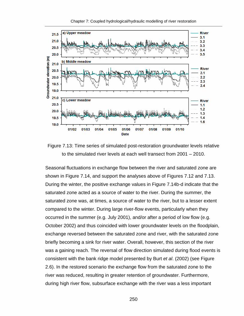
Chapter 7: Coupled hydrological/hydraulic modelling of river restoration
250
Figure 7.13: Time series of simulated post-restoration groundwater levels relative
to the simulated river levels at each well transect from 2001 – 2010.
Seasonal fluctuations in exchange flow between the river and saturated zone are
shown in Figure 7.14, and support the analyses above of Figures 7.12 and 7.13.
During the winter, the positive exchange values in Figure 7.14b-d indicate that the
saturated zone acted as a source of water to the river. During the summer, the
saturated zone was, at times, a source of water to the river, but to a lesser extent
compared to the winter. During large river-flow events, particularly when they
occurred in the summer (e.g. July 2001), and/or after a period of low flow (e.g.
October 2002) and thus coincided with lower groundwater levels on the floodplain,
exchange reversed between the saturated zone and river, with the saturated zone
briefly becoming a sink for river water. Overall, however, this section of the river
was a gaining reach. The reversal of flow direction simulated during flood events is
consistent with the bank ridge model presented by Burt et al. (2002) (see Figure
2.6). In the restored scenario the exchange flow from the saturated zone to the
river was reduced, resulting in greater retention of groundwater. Furthermore,
during high river flow, subsurface exchange with the river was a less important

Chapter 7: Coupled hydrological/hydraulic modelling of river restoration
251
exchange of water in the restored scenario, likely due to the precedence of surface
(overbank) exchange on the floodplain.
Figure 7.14: Simulated exchange flow between the saturated zone and river.
Values > zero indicate exchange from the SZ to river, whereas negative values
indicate exchange from the river to the saturated zone.

Chapter 7: Coupled hydrological/hydraulic modelling of river restoration
252
7.2.5 Impacts of embankment removal on floodplain storage and flood-peak
attenuation
The impacts of embankment removal upon both overland and subsurface water
storage within Hunworth Meadow are summarised for the 10-year simulation
period in Figure 7.15. The volume of simulated surface water stored on the
floodplain is greater in the restored model (Figure 7.15a). Particularly large
differences between the results of the two models are associated with periods
when major overbank flood events are simulated under restored conditions. For
example, the overland storage volume increases approximately six-fold during the
highest flow event (18/07/2001) after simulated restoration (maximum storage
increase of 2159 m3 compared to 373 m3 for the embanked model). As discussed
above, although surface water is stored on the floodplain in the embanked scenario
during these periods, groundwater rather than river water overtopping the
riverbanks is the source of flooding (i.e. Figure 7.8). Overbank flows substantially
enhanced surface storage, which increased 600% from an average of 144 m3 in
the embanked model to an average of 841 m3 in the restored model over the 14
peaks in overland storage shown in Figure 7.15a.
Differences in the simulated volume of subsurface storage between the embanked
and restored models are much less pronounced (Figure 7.15b). During winter
months, groundwater storage is very similar for both models as soils were typically
at or near saturation and had limited available storage capacity. However, during
the drier floodplain conditions that characterised summer months, subsurface
storage is greater under restored conditions. The largest difference in subsurface
storage occurred during a period of higher river flow at the end of the dry summer
in 2004. At this time, storage change for the original embanked model was -1099
m3 compared to -401 m3 for the restored model (Figure 7.15b), equivalent to

Chapter 7: Coupled hydrological/hydraulic modelling of river restoration
253
storage volumes in the floodplain of 38,022 m3 and 38,675 m3, respectively.
Figure 7.15: Times series of change in (a) overland and (b) subsurface storage for
the embanked and restored scenarios. Volume change is set at 0 m3 at the
beginning of the simulations (i.e. 20/02/2001).
Although the annual actual evapotranspiration (ET) totals did not differ between
embanked and restored models (Figure 7.16), the different components of total ET
were significantly different between the two models. Annual ET from the
unsaturated zone was on average 7% larger in the embanked model compared
with the restored model (p<0.05). This is the result of the higher water tables under
restored conditions that limits the depth of the unsaturated zone and the duration of
unsaturated conditions at the surface. Conversely ET from the saturated zone and
evaporation from ponded overland water were on average 10% and 12% larger for
the restored model (p<0.05), respectively.

Chapter 7: Coupled hydrological/hydraulic modelling of river restoration
254
Figure 7.16: Annual evapotranspiration (ET) rates for the embanked (E) and
restored (R) scenarios from 2002 – 2009. Four components of ET are shown:
transpiration from the unsaturated zone (UZ), ET from the saturated zone (SZ),
overland (OL) evaporation from ponded water, and canopy throughfall evaporation.
For the embanked model, river discharges were almost identical at the upstream
and downstream ends of the modelled reach demonstrating that most flows are
retained within the river channel (Figure 7.17). However, a slight reduction in
outflows (of between 1 and 3%) is evident during the highest river-flow events
(flows >1.2 m3 s-1), likely associated with loss of flow to bank storage given the
absence of simulated overbank flooding. For the restored model, differences
between river inflows and outflows began at lower flows (around 1.0 m3 s-1)
compared to the embanked model (Figure 7.18). The largest overall reductions in
river flow, however, occurred during the largest overbank events (>1.5 m3 s-1)
when inundation and recharge to the water table occurred across the floodplain
(Figure 7.18). Embankment removal and restoration of overbank flows onto the
floodplain had a moderate effect on flood-peak attenuation. The peak discharge of
the largest flood (18/07/2001) was reduced by 24% from 2.94 m3 s-1 at the top of
the restored reach to 2.31 m3 s-1 at the downstream end (Figures 7.17 and 18).
Following the highest river flows, outflow was marginally greater than inflow (max.

Chapter 7: Coupled hydrological/hydraulic modelling of river restoration
255
2% and 3% in the embanked and restored scenarios, respectively), due to some
return flow from the floodplain to the river. However, these differences are barely
noticeable in Figure 7.18.
Figure 7.17: Comparison of modelled mean daily river inflow and outflow for the (a)
embanked and (b) restored scenarios.
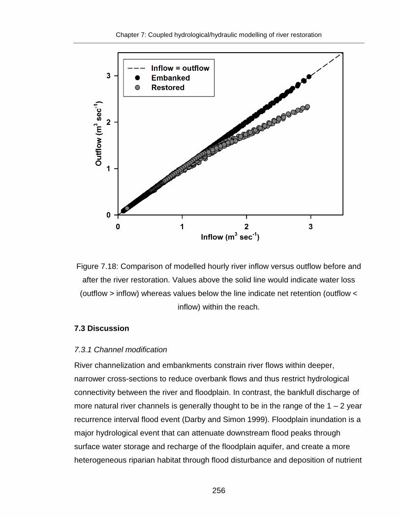
Chapter 7: Coupled hydrological/hydraulic modelling of river restoration
256
Figure 7.18: Comparison of modelled hourly river inflow versus outflow before and
after the river restoration. Values above the solid line would indicate water loss
(outflow > inflow) whereas values below the line indicate net retention (outflow <
inflow) within the reach.
7.3 Discussion
7.3.1 Channel modification
River channelization and embankments constrain river flows within deeper,
narrower cross-sections to reduce overbank flows and thus restrict hydrological
connectivity between the river and floodplain. In contrast, the bankfull discharge of
more natural river channels is generally thought to be in the range of the 1 – 2 year
recurrence interval flood event (Darby and Simon 1999). Floodplain inundation is a
major hydrological event that can attenuate downstream flood peaks through
surface water storage and recharge of the floodplain aquifer, and create a more
heterogeneous riparian habitat through flood disturbance and deposition of nutrient

Chapter 7: Coupled hydrological/hydraulic modelling of river restoration
257
rich sediments (Tockner et al. 2000; Amoros and Bornette 2002; Naiman et al.
2010; Shrestha et al. 2014). Restoration of rivers to a more natural form is an
increasingly accepted long-term solution for improving river health and functioning,
and is likely to increase in practice, encouraged through legislative requirements of
the Water Framework (Directive 2000/60/EC) and Flood Directives (Directive
2007/60/EC) and the interests of local groups (Richter et al. 2003; Perfect et al.
2013). Understanding how restoration affects river-flow dynamics and connections
with the floodplain is necessary to be able to predict and evaluate the success of
restoration schemes and guide future practices.
7.3.2 Simulation of floodplain hydrological processes
Observed groundwater levels on the floodplain of Hunworth Meadow before and
after the embankment removal were simulated well by the two coupled
hydrological/hydraulic MIKE-SHE/ MIKE 11 models. The models successfully
reproduced groundwater responses to high magnitude flood events although they
overestimated groundwater levels at the base of the hillslope (e.g. Well 2.4). This
may be because either the model grid resolution was unable to sufficiently
represent the topography of the ditch and its immediate surroundings, or the MIKE
SHE drainage function did not adequately simulate drainage towards the
topographic lows in the region of the ditch. Nonetheless, the coupled MIKE
SHE/MIKE 11 models were able to adequately predict temporal changes in
groundwater levels across the floodplain, capturing intra-annual variations in these
levels associated with climate as well as changes in hydrological fluxes related to
the restoration. Sensitivity analyses during model calibration revealed that the
models were responsive to the overland Manning’s coefficient. Greater resistance
to flow on the floodplain (e.g. applying Manning’s n values for woodland versus
grassland) reduced overbank flow depth, and after flooding, increased flood
retention on the meadow. This demonstrates the importance of vegetation type for
the management of riparian lands for reducing flood risk downstream (e.g. Piegay
1997; Tabacchi et al. 2000).

Chapter 7: Coupled hydrological/hydraulic modelling of river restoration
258
The results from the two models developed using identical hydrometeorological
conditions but with different topographical characteristics to reflect pre- and post-
restoration conditions indicate four main hydrological responses to embankment
removal on the River Glaven: (1) an increase in the frequency at which bankfull
discharges are exceeded and in turn overbank inundation of the floodplain which
was not simulated under embanked conditions, (2) increased groundwater levels
and subsurface storage within the floodplain, (3) increased overland storage on the
floodplain surface, especially during winter, and (4) moderate declines in
downstream flood peaks. These responses are consistent with those reported
following embankment removal and ‘pond and plug’ meadow restorations (where
floodplain alluvium is excavated to plug incised channels) on, for example, the
River Cherwell, Southeast England (Acreman et al. 2003), the headwaters of the
Feather River, Northern California (Loheide and Gorelick 2007), and Bear Creek,
Northern California (Hammersmark et al. 2008).
7.3.3 River-floodplain connectivity
A major aim of the river restoration was the re‐establishment of hydrological
linkages between the river channel and floodplain. Model results suggest that prior
to restoration the embankments restricted river flows to the channel, which limited
river-floodplain hydrological exchange to slow lateral subsurface flow (See Chapter
5). Removing the embankments has restored overbank water transfers onto the
floodplain, modifying the floodplain’s hydrological regime, to form a more natural
and dynamic wetland ecotone driven by flood disturbance. Widespread inundation
occurred across the floodplain during high river flows (>1.7 m3 s-1), and reached as
far as the hillslope (ca. 50 m from the river). Large overbank flows were of short
duration (around a day) and were separated by large time intervals (2.9 year return
period). Localised inundation of the immediate riparian area (within 5 m of the
channel) was a much more frequent event (0.22 year return period). Increased
river water incursions on to the floodplain is likely to improve continuity with
groundwater, and enhance the supply of river nutrients to soil microbes and plant

Chapter 7: Coupled hydrological/hydraulic modelling of river restoration
259
roots, an important influence on species composition, richness, primary
productivity, and nutrient cycling (e.g. nitrification, denitrification, methanogenesis)
within wetland environments (Hedin et al. 1998; Pinay et al. 2002; Amoros and
Bornette 2002; Clilverd et al. 2008).
The groundwater regime is one of the most important factors determining the plant
communities that are present on floodplains (Silvertown et al. 1999; Castelli et al.
2000). Hydrological models such as MIKE SHE therefore provide useful tools for
evaluating the effects of river restoration on water table depths, which can in turn
be used to predict shifts in vegetation communities and guide floodplain
management (e.g. Thompson et al. 2009). At Hunworth Meadow, groundwater
levels responded differently across the floodplain to embankment removal.
Substantial increases in groundwater levels (0.4 – 0.6 m) occurred at the river-
floodplain margin, where connectivity with the river was greatest and frequent
localised overbank flooding occurred. This resulted in increased surface soil
saturation throughout the year, which is likely to promote colonisation by wetland
plant species that can tolerate waterlogging (e.g. Wheeler et al. 2004). Restoration
also improved drainage between flood events, which could reduce flooding stress
and lessen the impact of large floods on plant communities during the growing
season. Smaller increases in water table elevation occurred as distance from the
river increased, with the exception of the ditch area which received flood waters
during large overbank events. As a result, the effects of restoration on floodplain
biota are expected to vary spatially across the floodplain. Surface flooding and
consequent surface water storage increased the volume of subsurface storage and
reduced aquifer head recession over the summer. This was due to increased
surface water inundation at the river-floodplain margin, and ponding of flood water
in topographic depressions on the floodplain. The simulated increases in
groundwater levels and subsurface storage in this study are consistent with
modelled increases in groundwater levels simulated by Hammersmark et al. (2008)
using a MIKE SHE model of floodplain restoration in Northern California.

Chapter 7: Coupled hydrological/hydraulic modelling of river restoration
260
7.3.4 Floodplain storage and flood-peak attenuation
Prior to restoration, model results suggest that bank storage contributed to a slight
(maximum 3%) decrease in downstream flood peaks. River water intrusion
increased during periods of elevated river stage, which reversed the hydraulic
gradient on the floodplain and directed some subsurface flow away from the river.
However removal of the embankments resulted in a substantially more marked
response in flood-peak attenuation. Most of the overbank water was stored
temporarily on the floodplain surface and in the ditch. Most flood water returned to
the channel downstream with improved drainage being facilitated by embankment
removal whereas prior to restoration embankments acted as a barrier for surface
water exchange from the floodplain to the river. While some overbank water was
infiltrated no noticeable changes in baseflow due to return flows occurred following
inundation events.
Before embankment removal, the floodplain at Hunworth Meadow was a
groundwater-dominated system. Rapid groundwater recharge occurred in
response to precipitation and rising river levels, likely associated with pressure
differences across the floodplain (e.g. MacDonald et al. 2014). During high winter
river flows, groundwater was typically close to the soil surface, which limited the
capacity for subsurface storage. Increased storage was available in soils in the
summer. Therefore after restoration the greatest attenuation of flood-peaks
occurred when floods followed a period of low rainfall (in particular during warm
and dry summers). Although restoration increased surface water inundation and
surface water storage, total evapotranspiration was unchanged. This was attributed
to the rapid response of groundwater to river levels and subsequent groundwater
flooding that resulted in saturated surface soils in both pre- and post restoration
conditions. This response may vary in different hydrogeological settings, where
evapotranspiration from inundated areas may act to reduce overland runoff and
further attenuate flood peaks.

Chapter 7: Coupled hydrological/hydraulic modelling of river restoration
261
Expansive inundation and storage of flood waters on Hunworth Meadow resulted in
a maximum reduction in peak river flows of 6 – 24%, along the length of restored
reach (ca. 400 m). This is a similar contribution to flood-peak attenuation reported
by other modelling studies. For instance, reductions in peak flows of 10 – 15%
were simulated along a 5 km reach of the River Cherwell, UK (Acreman et al.
2003), and 13 – 25% reductions in river discharge were reported along 3.6 km of
restored channel at Bear Creek, Northern California (Hammersmark et al. 2008).
Logically, providing increased room for flood water storage on floodplains favours
greater reductions in flood peaks, which is an appreciable benefit of river
restoration.
Many recent reviews have identified the need for larger-scale restorations that
include an environmental management plan for the catchment as a whole,
particularly where problems persist throughout the catchment, e.g. agricultural
fertiliser runoff, habitat fragmentation, urbanisation (Harper et al. 1999; Wharton
and Gilvear 2007; Bernhardt and Palmer 2011). Indeed, the restoration project at
Hunworth Meadow is part of a wider landscape approach to restoration being
implemented along the River Glaven to reconnect and buffer an array of aquatic
habitats of varying sizes (e.g. rivers, streams, ponds and ditches), with the aim of
repairing autonomous river processes and associated ecosystem services (e.g.
biodiversity, water quality) within the catchment (Sayer 2014). The removal of
embankments along other reaches of the river that is proposed as part of this
project could therefore be expected to have a cumulative impact of flood-peak
recession.
7.3.5 Climate
River restoration, and the associated improvements to river-floodplain functioning
(e.g. enhanced hydrological connectivity, groundwater retention, and flood-peak
attenuation), may provide an important tool for buffering the hydrological regime of
wetlands and other aquatic ecosystems against some of the extreme climate
Chapter 7: Coupled hydrological/hydraulic modelling of river restoration
262
variability predicted over the next century (IPCC 2014). In the UK, five of the six
wettest years have occurred since 2000, and eight of the warmest years have all
occurred since 2002 (Met Office 2015a). The wettest May to July on record since
1766 occurred in 2007 during the observational period of this restoration study
(IPCC 2014). Indeed, 2014 was the wettest winter and warmest year in the UK for
over 100 years, suggesting a trend towards warmer and wetter weather (Met Office
2015b). The majority of climate change scenarios for the UK predict that the
frequency and magnitude of floods will increase due to increased winter
precipitation (Wilby et al. 2008; Thompson 2012). Increases in air temperature will
also likely alter evapotranspiration rates and groundwater recharge, which is likely
to affect wetland species that are sensitive to changes in hydrological regime (e.g.
Gowing et al. 1998, Araya et al. 2011).
For example, a climate impacts study conducted by Thompson et al. (2009) using
MIKE SHE/MIKE 11 and UK Climate Impacts Programme (UKCIP) projections for
the 2050s simulated lower water table depths and reduced magnitude and duration
of surface water inundation within the Elmley Marshes, Southeast England. It was
suggested that these hydrological changes would lead to a loss of specialist
wetland plants adapted to the current high water tables. Similarly, House et al.
(2016a) used a MIKE SHE/MIKE 11 model of a riparian wetland on a tributary of
the River Thames to demonstrate spatially varying hydrological impacts due to
climate change that would have implications for both wetland flora and fauna.

Chapter 8: Methods – botanical and soil chemistry data collection and analysis
263
Chapter 8: Methods – Part III: botanical and soil chemistry data
collection and analysis
8.1 Introduction
This chapter describes the methods used to assess vegetation response to river
restoration and embankment removal. It includes details of the fine scale botanical
surveys, analyses of plant available nutrients, estimation of plant aeration stress
using a cumulative stress index (e.g. Gowing et al. 1998), and measurements of
dissolved oxygen concentration in the rooting zone using a novel oxygen optode
technique. In addition, a description is given of the statistical analyses that were
used to assess the importance of soil moisture and nutrient status on plant
community composition.
8.2 Floodplain plant community composition
8.2.1 Vegetation composition
Floodplain vegetation surveys prior to the restoration were conducted in late June
2008 across the entire meadow on a regular 10 × 10 m sampling grid using 1 m2
quadrats (n=206) (see Figure 4.4a). Percentage composition of all plant species
was estimated visually and typically exceeded 100% due to vegetation layering
(Figure 8.1). Soil moisture content was measured on 30/06/08 at a subset of
survey points (n = 138) aligned to the botanical grid using a ML-2X soil moisture
ThetaProbe (Delta-T Devices, Cambridge, UK) (see Figure 4.4b).
The main vegetation types for Hunworth Meadow were classified according to the
National Vegetation Classification (NVC) (Rodwell 1992) using CEH TABLEFIT
(Hill 1996b). TABLEFIT measures the degree of agreement (goodness-of-fit)
between vegetation samples and the expected species composition of each NVC
vegetation type (Hill 1996b). NVC communities were assigned for the middle

Chapter 8: Methods – botanical and soil chemistry data collection and analysis
264
meadow, ditch and river embankments using the average goodness of fit value
produced in TABLEFIT.
Figure 8.1: Photograph of Hunworth Meadow showing the multiple layers of
vegetation, taken in a NW direction, perpendicular to the River Glaven, in July
2007.
Diversity patterns of the floodplain vegetation were analysed using the Shannon
Index, which is the most commonly used measure of α-diversity (Jost 2006; Reddy
et al. 2009; Stein et al. 2010). This index describes both species richness and the
abundance distribution of a sample or site (Magurran 2004). Species richness was
calculated as the total number of species per 1 m2 quadrat. The Shannon Index
(H’) expresses heterogeneity of an assemblage, and was calculated as:
∑
ii p pΗ'=- ln (8.1)
where pi is the proportional abundance (% cover) of the ith species. The Shannon
index value is usually between 1.5 − 3.5 and rarely exceeds 4 (Magurran 2004).
Chapter 8: Methods – botanical and soil chemistry data collection and analysis
265
8.2.2 Floodplain topography
Surface elevation of the meadow and river embankments (see methods in Section
4.4.4) was surveyed at each point on the botanical survey grid at intervals of 10 m,
whereas the river embankments were surveyed at a higher resolution using
intervals of approximately 0.25 – 0.5 m (Figure 4.14.). Digital elevation models
(resolution 1 × 1 m), were created in ArcGIS using the kriging interpolation method
which (as discussed in Sections 4.4.4 and 6.2.1) estimates values from a
statistically weighted average of nearby sample points (de Smith et al. 2007). The
same approach was used to create a soil moisture map (resolution 10 × 10 m),
from the ThetaProbe data described above in Section 8.2.1.
8.3 Soil physicochemistry
8.3.1 Soil extractable ions
Soil extractable ions were measured to examine the links between plant available
nutrients and the spatial variations in plant community composition. Floodplain
soils were collected on 29/04/2008 across the meadow at shallow rooting depths of
0.1 – 0.3 m (n=113), which were observed for grasses on the meadow during soil
sampling. This method does not allow for a detailed analysis of overall plant-
available nutrients throughout the different soil horizons, however, since this would
require an even more extensive sampling and analytical approach.
Soil samples were stored in a cooler with ice until returned to the laboratory, where
they were refrigerated. Any samples that could not be analysed within two days
were frozen. In the laboratory, plant available nutrients were determined using the
following extraction methods: for analysis of nitrate, nitrite, and ammonium, 100 ml
of 1M potassium chloride was added to 10 g of soil (Robertson et al. 1999); for
determination of potassium, calcium, magnesium, sodium, aluminium, and iron,
100 ml of 1M ammonium acetate solution was added to 10 g of soil (Hendershot et

Chapter 8: Methods – botanical and soil chemistry data collection and analysis
266
al. 2008); for analysis of dissolved organic carbon, 100 ml of deionised water was
added to 10 g of soil (method amended from Robertson et al. 1999); and
phosphate was analysed using the Olsen et al. (1954) sodium bicarbonate
extraction method (Schoenau and O'Halloran 2008). Prior to extraction, roots were
removed from the field-moist soil, and the soil was mixed and passed through a 2
mm sieve. Following extraction, the samples were placed on a mixing table for 24
h, after which 50 ml subsamples were centrifuged at 3,000 rpm for 20 minutes
(method amended from Robertson et al. 1999). The supernatant was filtered using
0.45 µm Supor® hydrophilic polyethersulphone membrane filter paper and frozen
pending analysis.
Table 8.1: Soil chemical extractants
Soil
extract
Extraction chemicals
Soil weight (g)
Extraction volume (ml)
Analytical method
NO3-, NO2
-, NH4
+ 1M KCla 10 100 Skalar San++
K+, Ca2+, Mg2+, Na+, Al-, Fe3+
1M CH3COONH4
b
10
100
ICP2
TOC Dionised watera 10 100 TOC analyzer
Olsen P
0.5M NaHCO3, 0.0013M NaOH, and
Polyacrylamide solutionc
2.5
50.25
Skalar San++
aRobertson et al., (1999); bHendershot et al., 2008; cSchoenau and O'Halloran,
2008.
The percentage moisture content was determined for each soil sample by drying
triplicate 10 g subsamples of sieved field-moist soil at 105 °C overnight (Robertson
et al. 1999). This allowed the respective ion concentration for each extract to be
corrected for dilution. Inorganic nitrogen species (NO3-, NO2
- and NH4+) and
phosphorus were analysed colorimetrically using an automated continuous flow
analyser (SAN++, SKALAR, Delft, The Netherlands) following the standard San++
methods for preparation of reagents. Base cation analysis (K+, Ca2+, Mg2+, Na+, Al-,
Fe3+) was conducted using a Vista-PRO inductively coupled plasma optical
emission spectrometer (ICP-OES) with a SPS3 autosampler (Varian, The
Chapter 8: Methods – botanical and soil chemistry data collection and analysis
267
Netherlands). All soil extractable ions are reported with respect to dry weight of
soil.
Dissolved organic carbon (DOC) and total dissolved nitrogen (TDN) were
determined using a standard high temperature (1000°C) combustion method
(Thermo 2006), on a HiPerTOC carbon analyser plumbed to an HiPer5000 total
nitrogen chemoluminescent detector (Thermo Electron Corp., Delft, The
Netherlands). Prior to analysis of DOC, inorganic carbon was removed with the
addition of 1M Hydrochloric acid. For all analytes, calibration standards were
prepared fresh each week. Laboratory control samples of a known concentration,
blank samples, and duplicates (sampling and analytical), were interspersed
throughout the sample runs approximately every 10 samples.
8.3.2 Soil pore water chemistry
As discussed in Section 4.4.2, pore water in the rooting zone was collected
bimonthly from April 2007 to June 2008 using 0.1 μm rhizon samplers (see Figure
4.12b). The pore water samples were stored in a cooler until return to the
laboratory, and then refrigerated. Any samples that could not be analyzed within
two days were frozen. In the laboratory, cations (Ca2+, Mg2+, K+, Na+,NH4+) and
anions (SO42-, NO3
-, PO43-) were analysed by ion exchange chromatography (ICS-
2500, Dionex Corp., CA, USA).
8.3.3 Analysis of total carbon and nitrogen content in soil
Total carbon (TC) and total nitrogen (TN) soil contents (%) were determined by
elemental analysis (FLASH 1112 elemental analyser (EA) Thermo-Finnigan,
Bremen, Germany) using an aspartic acid standard (C: 36.09 %; H: 5.30 %; N:
10.52 %; O: 48.08 %) (Skjemstad and Baldock 2008). Prior to analysis, soil
samples were dried at 50 °C overnight, and ground and homogenised using a
agate mortar and pestle. All apparatus was cleaned thoroughly between samples
with acetone. Approximately 5 − 10 mg of soil was inserted into tin caps (8 × 5 mm,

Chapter 8: Methods – botanical and soil chemistry data collection and analysis
268
Elemental Microanalysis Ltd, Okehampton, UK) on a 6 decimal point precision
microbalance (Supermicro, Sartorius UK Ltd).
8.3.4 Air-filled porosity
To determine temporal variation in soil aeration status with changes in groundwater
elevation, the water release characteristic (pF-curve) of topsoil along Well Transect
3 (which was located near the oxygen optodes) (see Figure 4.2) were measured
(n=15). This gave the relationship between air-filled porosity and soil pore water
tension (pressure head). As pressure head and water-filled pore space decrease
air defuses into draining soil pores. Air-filled porosity can therefore be calculated
from the difference in water content of soil at a particular pressure head and the
water content at saturation (Barber et al. 2004). Soil samples were collected in bulk
density tins from the top 0 − 0.1 m of soil at three locations at Hunworth Meadow
(n=15). In the laboratory, the tins were sealed with nylon filter cloth, held tightly in
place with two rubber bands. The samples were saturated in water for five days,
after which a small amount of swelling (1 − 2 mm) was noticed in some samples
which were trimmed so that sample volume was the same as tin volume.
Using a manual 08.01 sandbox (Eijkelkamp, Giesbeek, The Netherlands) at the
Centre for Ecology and Hydrology (Wallingford), soil water content was determined
at a range of pressures from pF 0 (saturation) to pF 2.0 (-100 hPa), equivalent to a
water table elevation (i.e. pressure heads) of 0 to -1 m. Between measurements,
samples were left to equilibrate for a minimum of two weeks at each pressure.
Differences in sample volume due to shrinkage was estimated by measurement of
vertical and horizontal shrinkage space between the soil sample and the bulk
density ring, which ranged from 0 − 5 mm vertically, and 0 − 4 mm horizontally.
Some samples exhibited bubbling and swelling as the soil was dried, presumably
due to biological activity in the samples, hence these samples were excluded from
the analysis. After the final sand table measurement at pF 2.0, samples were oven
dried at 105 °C for 48 hrs to obtain the dry sample weight. Volumetric water

Chapter 8: Methods – botanical and soil chemistry data collection and analysis
269
content was calculated for each tension accounting for any change in sample
volume due to shrinkage (Elliot et al. 1999) (Figure 8.2).
Soil water content decreased fairly quickly at low tensions, indicating the presence
of large pores that readily emptied of water as the soil began to dry (Figure 8.2).
Greater tension was required to remove water from the smaller soil pores,
indicated by the flattening of the water release curve between tensions of 0.1 – 0.6
m, followed by the sharp decline in water content at higher tension (i.e. between
0.6 – 1.0 m). Saturated soil water content was estimated as 0.72 ± 0.04 (volumetric
basis). Soil shrinkage was most pronounced at tensions greater than 0.2m. In
some samples, despite the loss of water as the sample dried, the decrease in
sample volume due to shrinkage kept the soil close to saturation and limited the
aerated pore space (Figure 8.2).
Figure 8.2: Soil water release characteristic (from 0.1m depth). Errors bar depict
95% confidence interval. * denotes significant differences (p<0.05) between the
data corrected and uncorrected for shrinkage at each tension.

Chapter 8: Methods – botanical and soil chemistry data collection and analysis
270
The effect of shrinkage and swelling on air-filled porosity should be a consideration
in organic soils (Barber et al., 2004). Hence, differences in sample volume due to
shrinkage (i.e. the shrinkage space between the soil sample and the bulk density
tin), were measured and change in water content due to this shrinkage was
calculated. Air-filled porosity accounting for shrinking and swelling soil was
calculated as:
1
1
s atae (8.2)
where ea is air-filled porosity, θsat is saturated water content, θ is the water content
of the sample, and β is the relative sample volume as a function of θ (defined
below in Figure 8.3) (Barber et al. 2004). Sample shrinkage did not occur in all of
the samples and, although the relationship between relative shrinkage of the soil
and soil water content was significant (p<0.05), the correlation was fairly weak (r2 =
0.33) (Figure 8.3). Thus while it is worth noting that soils are heterogeneous, and
air-filled porosity may be slightly lower (and thus aeration stress higher) in areas on
the meadow with more organic soils, which are more likely to swell and shrink, in
order to use the cumulative aeration stress index described by Gowing et al.
(1998), and standardise the results for comparison to other studies, air-filled
porosity was calculated as the difference between the water content of the soil and
saturated water content, assuming no shrinkage or swelling of the soil (i.e. a rigid
soil).

Chapter 8: Methods – botanical and soil chemistry data collection and analysis
271
Figure 8.3: Relative shrinkage of the soil versus soil water content. A value of 1
indicates no shrinkage. β = 0.5948θ 2 - 0.3966θ + 0.9207.
Air-filled porosity increased exponentially (p<0.05) as tension increased as the
water table dropped, and increased rapidly when the water table (i.e. pressure
head) was below ~0.60 m (Figure 8.4). Assuming soil rigidity, the 0.1 (10%)
threshold porosity expected for aeration stress in plants (Wesseling and van Wijk,
1975; Gowing et al. 1998), occurred at the surface when the water table was on
average less than 0.34 m below the ground surface (Figure 8.4). This reference
water table depth is comparable to a threshold depth of 0.35 m used by Gowing et
al. (1998) to calculate sum exceedance values for aeration stress (SEVas) within a
peat-based wet grassland.
Volumetric water content
0.2 0.3 0.4 0.5 0.6 0.7 0.8 0.9
Re
lati
ve
sa
mp
le v
olu
me
0.75
0.80
0.85
0.90
0.95
1.00
r2 = 0.329
p = 0.002

Chapter 8: Methods – botanical and soil chemistry data collection and analysis
272
Figure 8.4: Relationship between water table depth below the soil surface (tension)
and air-filled porosity for Hunworth Meadow soil. The solid line represents a
statistically significant exponential model (y=0.0478exp(0.0216x)). The dotted drop
lines indicate mean water table depth at 0.1 porosity.
8.3.5 Aeration stress index
An aeration stress index for each well location (see Figure 4.2) was estimated by
determining sum exceedence values (SEVas). This index uses water table position
as a proxy for aeration stress under shallow water table conditions, i.e. where the
water table is <1 m below the soil surface (Gowing et al. 1998; Silvertown et al.
1999). Aeration stress was calculated as the integral of the difference between the
water table depth and a reference water table depth:
N
Wrefas dtDDSEV1
(8.3)
where SEVas is the sum exceedence value in metre weeks, which increases in
value with aeration stress; N is the number of weeks during the active growing
season for grasses (March – September inclusive; Gowing et al. 2002b); Dref is the

Chapter 8: Methods – botanical and soil chemistry data collection and analysis
273
reference water table depth (m) where air-filled porosity at the surface = 0.1 which,
as described above, was taken to be 0.34 m; and Dw is the average depth to the
water table (m). The integral was solved numerically for one week intervals and
only positive values were included in the integration.
As described in chapters 6 and 7, pre-restoration and post-restoration water table
elevations were simulated for a variety of possible hydrological conditions on the
meadow using coupled surface water-groundwater models from which average
water table depths during the growing season (March – September) and SEVs
were calculated for the meadow. The pre-restoration (embanked) and post-
restoration (no embankment) conditions on the meadow were simulated with two
MIKE SHE/MIKE 11 models, which differed only in embankment and riverbed
elevation as a result of the embankment removal (see Chapter 6.2.1). Fine model
discretisation (5 m grid, see Section 6.2.1) was used to accurately characterise
small-scale topographic variations in surface topography on the floodplain (e.g. the
river banks, shallow depressions, and raised hummocks), which control soil water
content, water table depth and influence habitat suitability for different plant
species (Wheeler et al. 2004). In order to predict compositional change of plant
communities on the meadow, in response to changing hydrological regimes
associated with the removal of river embankments, sum exceedence values for the
meadow were compared with known tolerances of meadow plant communities
established by Gowing et al. (1998) and Wheeler et al. (2004). SEVs were also
calculated from observed water table elevations from 2007 – 2009 to validate
simulated SEVs.
8.3.6 Oxygen concentration in soil pores
To evaluate temporal fluctuations in oxygen concentration within the rooting zone
and to test the use of water table depth as a useful proxy for aeration stress in
plants, 4175 Aanderra oxygen optodes (Bergen, Norway), described in Section
4.4.3, were used to measure DO concentrations in saturated and unsaturated soil

Chapter 8: Methods – botanical and soil chemistry data collection and analysis
274
pore spaces in the rooting zone (0 – 0.10 m below the soils surface) at the
upstream well transect from January to December 2010. Aanderra oxygen optodes
measure oxygen partial pressure of dissolved oxygen and respond equally when
measuring in air to when measuring in air-saturated fresh water (Aanderaa 2006;
ADDI 2009) Hence, in addition to the measurements of oxygen concentration in
groundwater, the optodes provided unique data on oxygen concentrations in soil
air. The amount of oxygen dissolved in water at equilibrium with air is given by
Henry's Law:
HO KairPwaterO 22 ][ (8.4)
where O2water is the concentration of DO in water (mol L-1), PO2air is oxygen
partial pressure in atmospheres (atm) and KH is Henry's constant (mol L-1 atm-1).
Henry’s law constants are dependent on temperature and salinity; in terms of the
Bunsen solubility coefficients (β) (ml gas/l water) given in Weiss (1970), KH is equal
to β/V, where V is the volume of the gas at STP (O2 = 22.4 l) (Weiss and Price
1980). The oxygen optodes were configured to record DO concentration in µmol L-
1, therefore equation 8.4 can be rearranged to give the oxygen partial pressure in
the soil pores. Oxygen saturation values in air are calculated assuming 100%
relative humidity, a pressure of 1 atmosphere, and zero salinity (Aanderaa 2006).
Dry air can result in slightly higher oxygen measurements (up to 3%) than air that
is 100% saturated with water vapour as dry air can hold more oxygen. This effect is
expected to be minimal in soil, particularly at Hunworth Meadow where the water
table was in close proximity to the buried optodes. Wetting and drying of the
sensors occurred at the study site as the water table rose above and fell below the
optodes, which can lead to a maximum error of 2% (Aanderaa 2006).

Chapter 8: Methods – botanical and soil chemistry data collection and analysis
275
8.4 Statistical analyses
8.4.1 Linear regression models and diagnostics tests
Multiple linear regression was used to determine correlations between surface
elevation, distance from the ditch and soil organic matter content on the meadow
(predictor variables) and soil moisture content (response variable). Full and
reduced models were compared in SAS 9.2 statistical software for Windows (SAS
Institute Inc., North Carolina) using the PROC REG command. Boxplots for each of
the predictor variables and the response variable provided basic range of validity,
outlier, and influence information. Residual plots identified outliers and departures
from the model assumptions. Normal probability plots of the residuals were used to
identify non-normality of the error terms. Organic matter content data were log
transformed to linearize the relationships and meet the assumptions of constant
variance and normality. A correlation matrix of all the variables using PROC CORR
computed Pearson correlation coefficients and was used to identify multicolinearity
between the predictor variables.
8.4.2 Multivariate analysis
Spatial variation of plant community composition in relation to soil environmental
conditions was analysed using ordination techniques in CANOCO 4.5 for Windows
(Informer Technologies, Inc.). Since elevation and soil moisture contents were
significantly correlated (y = -23.301x + 523.45, r2 = 0.52, p<0.05), and soil moisture
was not available for all plots (see Section 8.2.1), elevation was used in the
subsequent analysis as a strong proxy of soil moisture content. Given the
substantial turnover in the plant species data (>4 SD units), correspondance
analysis (CA) was deemed most suitable for analysis of the spatial relationship in
plant species composition. Unconstrained CA biplots of the relative position of
species and samples along the two main explanatory ordination axes were used to
visualize patterns in plant composition across the meadow (Lepš and Šmilauer
2003).

Chapter 8: Methods – botanical and soil chemistry data collection and analysis
276
Spatial patterns of plant species in relation to soil environmental parameters were
investigated using Canonical Correspondence Analysis (CCA) (Lepš and Šmilauer
2003). Prior to CCA, the data were tested for normality using normal probability
plots and the Kolmogorov-Smirnov test. Where necessary, the data were log
transformed to achieve normality. Multicollinearity among the environmental
variables was tested using Pearson and Spearman correlation coefficients. Where
independence was not found among environmental parameters, one parameter
was removed from the analysis. After conducting the CCA, constrained bi-plots
were used to investigate patterns in plant community composition in relation to soil
environmental conditions.

Chapter 9: Simulation of the effects of river restoration on plant community composition
277
Chapter 9: Simulation of the effects of river restoration on plant
community composition
In this chapter, fine scale botanical and chemical data are used to assess the
spatial pattern of plant communities in relation to soil physicochemical conditions,
and water table simulations from coupled MIKE SHE-MIKE 11 hydrological-
hydraulic models presented in Chapter 7. These data are used to predict aeration
stresses in the rooting zone of floodplain plants prior to, and following the removal
of river embankments from the River Glaven at Hunworth Meadow. The final set of
research questions are addressed:
(v) What are the importance of soil moisture and fertility on plant
communities on a disconnected floodplain?
(vi) What is the relationship between water table depth and oxygen content
in the root zone?
(vii) What are the likely long-term impacts of floodplain restoration on the
vegetation?
9.1. Results
9.1.1 Groundwater hydrology and soil moisture gradients
As demonstated in Section 5.2.2, groundwater levels within Hunworth Meadow
were typically close to the soil surface. Using 50% time exceedence as a common
reference value, mean water table depth during the wettest summer of the study
period (2007) was between 0 and 0.4 m below the ground surface (bgs) at the
upstream well transect (excluding Well 3.1 on the embankment) and between 0
and 0.2 m bgs at the downstream transect (Wells 1.1 – 1.6) for 50% of the time

Chapter 9: Simulation of the effects of river restoration on plant community composition
278
(Figure 9.1). Hence for prolonged periods during the 2007 growing season the
rooting zone (ca. 0 – 0.30 m bgs) was saturated, particularly near Well Transect 1
(Figure 9.1). Even during the driest summer (2009), the water table was frequently
above the rooting zone. Elevated regions on the meadow (see Figures 5.2 and 6.2)
such as the river embankments (Well 3.1) and areas near the hillslope (Well 3.5)
remained dry for the majority of the summer (>95% of the time) (Figure 9.1).
Soil moisture and elevation were closely linked, showing a negative linear
relationship (r2 = 0.52, p<0.05; Figure 9.2). An average 23% decrease in soil water
content resulted from an average 1 m increase in surface elevation on the meadow
(Figure 9.2a). Organic matter content was strongly correlated with soil water
content (r2 = 0.75, p<0.05; Figure 9.2b). Organic matter content was weakly,
though significantly, correlated with surface elevation (0.31; p<0.05) (Figure 9.2c)
Thus, elevation, organic matter content and distance from the ditches accounted
for 85% of the variation in soil water content (<0.05; Table 9.1). However, due to
some multicolinearity between the predictor variables, surface elevation and
organic matter content provided the most parsimonious model of soil water content
(r2 = 0.846; <0.05; Table 9.2).
Soil moisture increased in a northeasterly (downstream) direction in conjunction
with a decrease in elevation (Figure 9.3). Soil water content was lowest (11 − 30%)
along the river embankments, where surface elevation was between 21.3
(upstream) − 20.4 m ODN (downstream), and approximately 0.4 – 1.1 m above the
main meadow (Figure 9.3a). Soil moisture content was near saturation in the
region of the ditches, and at the downstream section where surface elevation was
less than 20 m above Ordnance Datum Newlyn (ODN) (Figure 9.3a), and where
surface water ponded due to the blocked drainage ditch (see Figure 7.8). Across
the remainder of the meadow, soil moisture content ranged between 20 and 80%
(Figure 9.3b).
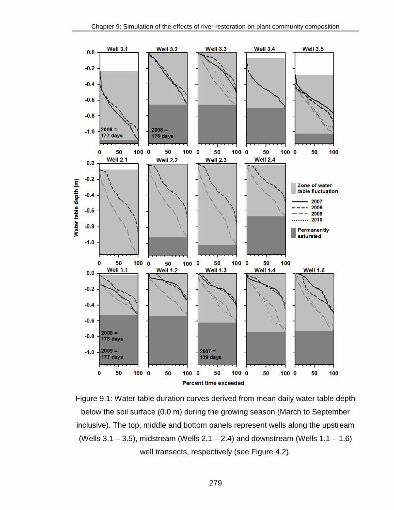
Chapter 9: Simulation of the effects of river restoration on plant community composition
279
Figure 9.1: Water table duration curves derived from mean daily water table depth
below the soil surface (0.0 m) during the growing season (March to September
inclusive). The top, middle and bottom panels represent wells along the upstream
(Wells 3.1 – 3.5), midstream (Wells 2.1 – 2.4) and downstream (Wells 1.1 – 1.6)
well transects, respectively (see Figure 4.2).

Chapter 9: Simulation of the effects of river restoration on plant community composition
280
Figure 9.2: Correlations between (a) surface elevation on the meadow and water
content of the soil (y = -23.301x + 523.45); (b) organic matter content (log
transformed) and soil water content (y = 72.8504x + -34.79), and (c) surface
elevation and organic matter content (log transformed) (y = -0.217 + 5.533).

Chapter 9: Simulation of the effects of river restoration on plant community composition
281
Table 9.1: ANOVA and parameter estimates for predicting soil moisture content
with the following parameter inputs: elevation, organic matter content, and distance
from the river.
ANOVA
R-Square Adj. R-Sq F value Pr > F 0.8518 0.8468 168.65 <.0001
Parameter Estimates
Variable DF Estimate Error t value Pr > F Intercept 1 197.84 40.53 4.88 <.0001 Elevation (m) 1 -10.60 1.87 -5.66 <.0001 Organic matter (%) 1 59.02 4.47 13.22 <.0001 Distance to ditch (m) 1 -0.11 0.055 -1.93 0.0571
Table 9.2: ANOVA and parameter estimates for the reduced soil moisture model,
using the following parameter inputs: elevation, and organic matter content.
ANOVA
R-Square Adj. R-Sq F value Pr > F 0.8456 0.8421 243.68 <.0001
Parameter Estimates
Variable DF Estimate Error t value Pr > F Intercept 1 232.51 36.88 6.31 <.0001 Elevation (m) 1 -12.41 1.65 -7.53 <.0001 Organic matter (%) 1 59.10 4.53 13.04 <.0001

Chapter 9: Simulation of the effects of river restoration on plant community composition
282
Figure 9.3: Spatial variation in (a) elevation and (b) soil water content in June 2008 on the embanked Hunworth Meadow.
The digital elevation model was created using dGPS survey data collected in June 2008.

Chapter 9: Simulation of the effects of river restoration on plant community composition
283
9.1.2 Soil Nutrient Status
Topsoils (ca. 0 – 0.3m) contained moderate levels of organic material (OM; range:
13 – 35% OM content), had low bulk density (mean: 0.69 g cm-3), and were slightly
acidic (mean in-situ-pH: 6.1) (Table 9.3). Analysis of plant available nutrients in the
topsoil revealed moderately fertile conditions, with Olsen P and plant-available
potassium concentrations in the range of 0.1 – 34 mg P kg-1 (mean: 9.2 mg P kg-1)
and 0.4 – 4.8 mg K g-1 (mean: 1.6 mg K g-1), respectively. Plant available
ammonium and nitrate concentrations ranged from 5.7 – 249.9 mg NH4+-N kg-1
(mean: 32.5 mg NH4+-N kg-1) and below detection limit (i.e. 0.1) to 25.2 mg NO3
--N
kg-1 (mean: 2.9 mg NO3--N kg-1), respectively. Soils were high in calcium, with an
average of 2.6 mg Ca2+ g-1, which far exceeded concentrations of magnesium
(mean: 0.11 mg Mg+ g-1) and sodium (mean: 0.08 mg Na+ g -1). Plant available N:P
ratios were low, averaging <5:1 (Table 9.3).
Plant available Olson P and ammonium concentrations were highest (>16 mg P kg-
1 and >75 mg N kg-1, respectively) in water-logged soils at the downstream end of
the meadow (Figure 9.4). Plant available ammonium concentrations were also
higher (>51 mg N kg-1) in wet soils along the ditch margin (Figure 9.4b). In contrast,
plant available nitrate was typically highest (>5 mg N kg-1) in the drier, upstream
soils (Figure 9.4c). Olsen P and nitrate concentrations were also raised (i.e. above
11 mg P kg-1 and 5 mg N kg-1, respectively) in soils on the river embankments, and
along the north-east boundary of the meadow (Figure 9.4) which borders the
woodland and arable hillslope (see Figure 3.1). These higher values are in contrast
to those in soils in the middle of the meadow, where concentrations of less than 5
mg P kg-1 and 1 mg N kg-1, respectively, were more typical (Figure 9.4). Plant
available potassium concentrations did not appear to show a clear spatial pattern
across the meadow (Figure 9.5a). Soil extractable TOC and TON were positively
correlated (r2 0.64; p<0.05), and occurred in the highest concentrations at the
downstream region of the meadow, and along the ditches (Figure 9.5b-c).

Chapter 9: Simulation of the effects of river restoration on plant community composition
284
Table 9.3: Soil (n = 113) and pore water (n = 53) chemistry of Hunworth Meadow
along the vegetation sample transects (mean ± 95% confidence interval).
Analyte
Mean ± 95% confidence
Soil: pH (laboratory) 6.53 ± 0.24 pH (in-situ) 6.09 ± 0.23 Organic matter content (%) 13.64 ± 1.50 Bulk density (g m-3) 0.69 ± 0.07 Ca2+ (mg g dry soil-1) 2.64 ± 0.36 Na+ (mg g dry soil-1) 0.08 ± 0.01 Mg+ (mg g dry soil-1) 0.11 ± 0.01 K+ (mg g dry soil-1) 1.64 ± 0.16 Total iron (mg kg dry soil-1) 80.96 ± 35.18 Al3+ (mg kg dry soil-1) 10.27 ± 1.54 NH4
+ (mg N kg dry soil-1) 32.46 ± 5.02 NO2
- (mg N kg dry soil-1) 0.28 ± 0.09 NO3
- (mg N kg dry soil-1) 2.86 ± 0.75 Olsen P (mg P kg dry soil-1) 9.20 ± 1.23 N:P ratio (NH4
+ + NO3- /Olsen P) 4.89 ± 0.61
TOC (mg kg dry soil-1) 0.67 ± 0.11 TON (mg kg dry soil-1) 0.10 ± 0.09 Pore water: Ca2+ (mg L-1) 119 ± 19
Na+ (mg L-1) 21.5 ± 5.7 Mg+ (mg L-1) 8.2 ± 1.5 K+ (mg L-1) 6.0 ± 2.8 NH4
+ (mg N L-1) 1.5 ± 1.2 SO4
2-(mg S L-1) 3.1 ± 2.9 NO3
- (mg N L-1) 0.5 ± 0.5 PO4
3- (mg P L-1) 0.1 ± 0.02

Chapter 9: Simulation of the effects of river restoration on plant community composition
285
Figure 9.4: Spatial differences in plant available Olson P, ammonium and nitrate
across Hunworth Meadow.
Figure 9.5: Spatial differences in plant available potassium, and TOC and TON
across Hunworth Meadow.

Chapter 9: Simulation of the effects of river restoration on plant community composition
286
The nutrient composition of root-zone pore-water was depleted in phosphate,
nitrate, and ammonium, which averaged 0.06 mg PO43--P L-1, 0.5 mg NO3
--N L-1
and 1.5 mg NH4+-N L-1, respectively (Table 9.3). Mean ammonium concentration
was approximately seven times greater than the median concentration (0.21 mg
NH4+-N L-1) due to a number of outliers. These occurred during a period of sheep
grazing and were possibly related to high concentrations of nitrogen in urine
patches. Average soil pore-water nutrient concentrations were not significantly
different to concentrations measured in groundwater wells on the meadow,
reported in Section 5.2.6 (p values: phosphate = 0.36; nitrate = 0.16, ammonium =
0.07 including outliers, and 0.78 excluding 3 outliers).
9.1.3 Community composition
The vegetation on Hunworth Meadow was dominated by Holcus lanatus,
Ranunculus repens and Agrostis stolonifera which were present in 85, 83 and 67%
of the surveyed quadrats (Table 9.4), respectively. These three species, which had
a mean relative percentage cover of 21, 23 and 7% across the meadow (Table
9.4), are indicative of damp, mesotrophic to richly fertile soils, as indicated by their
respective moisture and nitrogen Ellenberg’s values (Table 9.4). Arrhenatherum
elatius and Festuca rubra were also fairly common on the meadow, present in 27
and 43% of the samples, respectively, with a similar mean relative percentage
cover to Agrostis stolonifera. Reflecting the variable hydrological conditions
encountered on the meadow, a variety of wet- (e.g. Juncus effusus, Glyceria
fluitans, Equisetum palustre) and dry-loving (A. elatius, Urtica dioica, and Dactylis
glomerata) plants were recorded (Table 9.4).
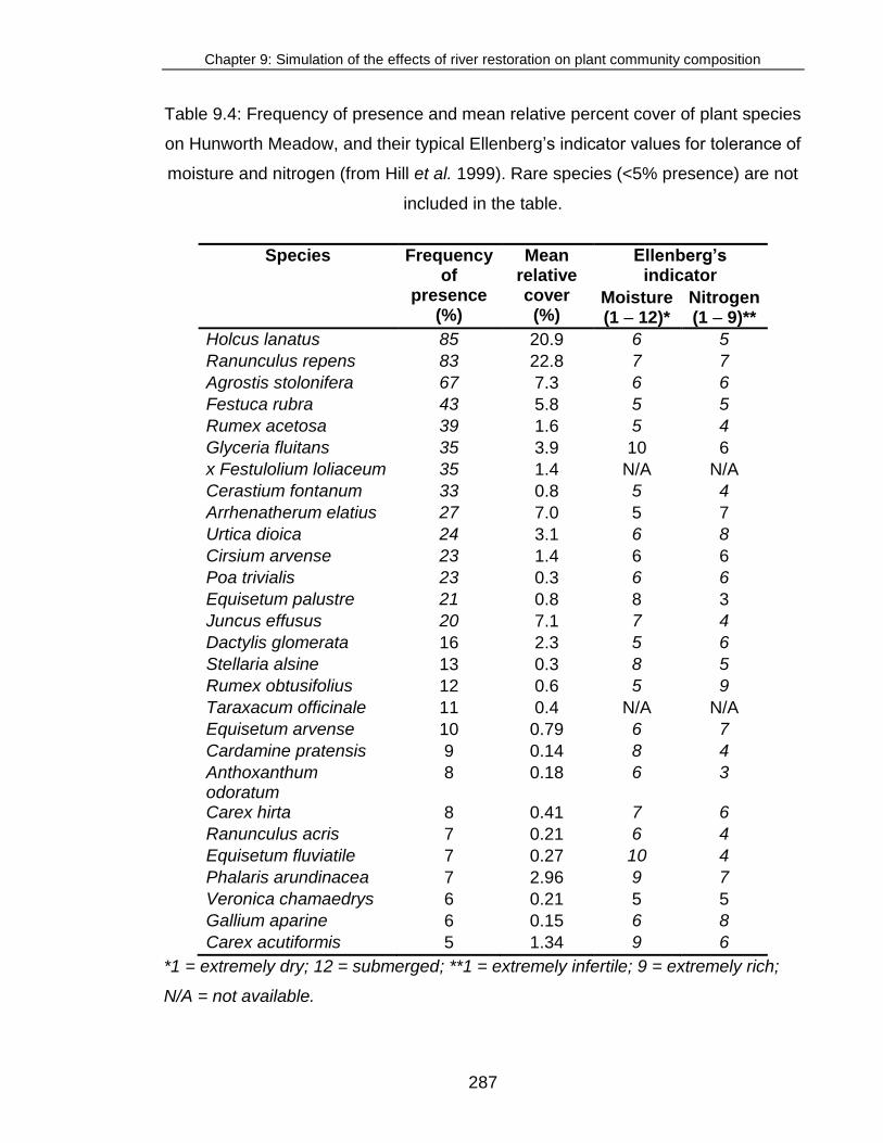
Chapter 9: Simulation of the effects of river restoration on plant community composition
287
Table 9.4: Frequency of presence and mean relative percent cover of plant species
on Hunworth Meadow, and their typical Ellenberg’s indicator values for tolerance of
moisture and nitrogen (from Hill et al. 1999). Rare species (<5% presence) are not
included in the table.
Species Frequency of
presence (%)
Mean relative cover (%)
Ellenberg’s indicator
Moisture (1 – 12)*
Nitrogen (1 – 9)**
Holcus lanatus 85 20.9 6 5
Ranunculus repens 83 22.8 7 7
Agrostis stolonifera 67 7.3 6 6
Festuca rubra 43 5.8 5 5
Rumex acetosa 39 1.6 5 4
Glyceria fluitans 35 3.9 10 6
x Festulolium loliaceum 35 1.4 N/A N/A
Cerastium fontanum 33 0.8 5 4
Arrhenatherum elatius 27 7.0 5 7
Urtica dioica 24 3.1 6 8
Cirsium arvense 23 1.4 6 6
Poa trivialis 23 0.3 6 6
Equisetum palustre 21 0.8 8 3
Juncus effusus 20 7.1 7 4
Dactylis glomerata 16 2.3 5 6
Stellaria alsine 13 0.3 8 5
Rumex obtusifolius 12 0.6 5 9
Taraxacum officinale 11 0.4 N/A N/A
Equisetum arvense 10 0.79 6 7
Cardamine pratensis 9 0.14 8 4
Anthoxanthum odoratum
8 0.18 6 3
Carex hirta 8 0.41 7 6
Ranunculus acris 7 0.21 6 4
Equisetum fluviatile 7 0.27 10 4
Phalaris arundinacea 7 2.96 9 7
Veronica chamaedrys 6 0.21 5 5
Gallium aparine 6 0.15 6 8
Carex acutiformis 5 1.34 9 6
*1 = extremely dry; 12 = submerged; **1 = extremely infertile; 9 = extremely rich;
N/A = not available.

Chapter 9: Simulation of the effects of river restoration on plant community composition
288
A total of 88 plant species were encountered within the 206 quadrats. Average
species richness was low at 8 species per m2 (Figure 9.6a), but varied substantially
between quadrats (range: 1 – 16 species per m2) (Figure 9.7). Shannon index of
diversity averaged 1.4 (Figure 9.6b), suggesting low heterogeneity of the plant
assemblages (i.e. a high degree of dominance in communities) on the meadow.
Plant diversity was generally low in the centre and in lower lying regions of the
meadow, while patches of higher species richness were encountered on the
embankments and along the ditch margins (Figure 9.7).
Correspondence Analysis (CA) identified three distinct vegetation groups or
clusters: 1) vegetation on the river embankments, 2) vegetation along the ditch
margins, and 3) the vegetation on the central sections of the meadow between the
river and ditch (Figure 9.5). In the CA plot, the first axis explained 16% of the total
species variability (Table 9.5). This main axis appears aligned to a gradient in soil
wetness, with samples from the wet ditch margins located at one end of the axis
and samples from the dry river embankments at the other. The CA plot furthermore
showed an arch-effect, indicative of the quadratic dependence of the second
ordination axis on the first ordination axis (Lepš and Šmilauer 2003). However, the
DCA’s exhibited a large amount of scattering, and as interpretation of DCAs is
restricted to the first axis only, interpretation was not improved. Initial CA analysis
identified some sample outliers that were vastly different from all other samples.
These samples were located at the downstream ponded area of the meadow and
were primarily composed of aquatic vegetation (Lemna minor, Lemna trisulca and
Potamogeton natans). As this area was an aquatic habitat (see Figure 7.8) rather
than a wet meadow these samples were excluded from further ordination analyses.

Chapter 9: Simulation of the effects of river restoration on plant community composition
289
Figure 9.6: Species richness and Shannon Diversity Index on the embanked
Hunworth Meadow. The black centre line, red centre line and box extent denote
the median, mean, and 25th and 75th percentiles, respectively. Whiskers indicate
the 10th and 90th percentiles, and the circles signify outliers outside of the 10th and
90th percentiles.
Figure 9.7: Spatial patterns of species richness and Shannon Diversity Index on
the embanked Hunworth Meadow.

Chapter 9: Simulation of the effects of river restoration on plant community composition
290
Vegetation assemblages along the river embankments were characterised by
drought-tolerant species typically thriving on mesotrophic soils, such as A. elatius,
U. dioica, D. glomerata, Plantago lanceolata and Geranium molle (Figure 9.8).
Accordingly, the community was classified as MG1 A. elatius grassland (mean
goodness of fit: 88). In contrast, the ditch margins were characterised by water-
tolerant species often found on less fertile soils, such as Carex acutiformis,
Equisetum fluviatile, J. effusus and Juncus inflexus (Figure 9.6) as represented by
MG10 H. lanatus – J. effusus rush – pasture (Table 9.6). Unlike the plants
encountered on the embankments, plants found along the ditches were also
present in some areas of the meadow. Consequently the TABLEFIT results place
the meadow community in the MG10 flood-sward, along with the OV28 A.
stolonifera – R. repens grassland community (mean goodness of fit: 60 – 68; Table
9.6).
As the embankment habitat represented dry grassland rather than wet meadow, a
second CA was performed where embankment samples were removed so that
changes in the wet meadow plant communities could be examined in detail (Figure
9.7). Axis 1 explained 15% of the total species variability (Table 9.5) and again
appeared to follow a gradient in plant moisture-tolerance, with water-loving plants
(e.g. E. fluviatile, J. effusus and J. inflexus) negatively associated with axis 1, and
less waterlogging tolerant species (e.g. A. elatius, U. dioica, Lolium perenne and
D. glomerata) found at the other end of the gradient. Many of the meadow
samples, however, were clustered together on the centre of the axis. Plant species
closely associated with these samples were H. lanatus, R. repens and Festuca
pratensis, with the dense clustering indicating little variation in community
composition amongst these samples (Figure 9.7).

Chapter 9: Simulation of the effects of river restoration on plant community composition
291
Figure 9.8: (a) Correspondence Analysis (CA) of the vegetation data showing (a) the embankment, middle meadow and
ditch sample points (n=195) and (b) the associated species (n=80). The relative distance between the species points
represents the similarity or dissimilarity of species relative abundance across the samples. To improve the visibility of
species labels, rare species (<5% presence) were removed from the plot after the CA analysis.

Chapter 9: Simulation of the effects of river restoration on plant community composition
292
Figure 9.9: Correspondence Analysis (CA) of the vegetation data showing (a) showing the middle meadow and ditch
sample points only (n=163) and (b) the associated species (n=67). The relative distance between the species points
represents the similarity or dissimilarity of species relative abundance across the samples. To improve the visibility of
species labels, rare species (<5% presence) were removed from the plot after the CA analysis.

Chapter 9: Simulation of the effects of river restoration on plant community composition
293
Table 9.5: Eigenvalues and cumulative percentage variance for each CA axis of
the vegetation data.
Axes 1 2 3 4
Embankment, meadow, and ditch:
Eigenvalues: 0.674 0.554 0.447 0.373
Cumulative percentage variance of species data:
15.7 28.7 39.1 47.8
Sum of all eigenvalues:
4.283
Meadow and ditch:
Eigenvalues: 0.572 0.542 0.391 0.321
Cumulative percentage variance of species data:
15.4 29.9 40.4 49.1
Sum of all eigenvalues:
3.721
Since elevation and soil moisture content were significantly correlated (see Figures
9.2a and 9.3), and soil moisture was not available for all plots (see Section 8.2.1),
elevation was used in the subsequent analysis as a strong proxy of soil moisture
content. Changes in the micro-topography of the meadow that represented a proxy
for variations in the soil moisture content were closely linked to vegetation changes
in the constrained Canonical Correspondence Analysis (CCA) ordination plot (r =
0.79; p<0.05; Figure 9.8; Table 9.7). Soil fertility was a significant secondary
predictor of plant species composition changes; with plant available ammonium,
phosphorus and potassium all closely correlated with CCA Axis 2 (Figure 9.8).
Similar to the first CA plot (Figure 9.6), the plant assemblage encountered on the
river embankments was clearly separated from the remaining vegetation, with this
area being characterised by low soil moisture and higher phosphorus availability
(Figure 9.8). The source of phosphate on the embankment is unclear, as these
elevated areas were not flooded with river water or sediment prior to the
restoration, although river water might provide a P source via hyporheic flowpaths
(see Chapter 5). Due to the reduced sample size of the CCA (108 samples),
environmental data was only available for four ditch samples. As a consequence,

Chapter 9: Simulation of the effects of river restoration on plant community composition
294
changes in vegetation community composition in relation to environmental data
were not discernible among the ditch and middle meadow sample groups.
Table 9.6: British National Vegetation Classification (NVC) communities for the
middle meadow, ditch and river embankments. NVC type was assigned using the
average goodness of fit value produced in TABLEFIT (Hill 1996b).
NVC Type
Mean Goodness
of fit
Community (Sub-community)
Middle Meadow
OV28a 68 Agrostis stolonifera – Ranunculus repens grassland (Pol hyd – Ror syl)
OV28 67 Agrostis stolonifera – Ranunculus repens grassland MG10b 60 Holcus lanatus – Juncus effusus rush-pasture (Junc
inflexus) MG10a 59 Holcus lanatus-Juncus effusus rush-pasture (Typical) MG10c 58 Holcus lanatus – Juncus effusus rush – pasture (Iris
pseudacor) Ditch MG10a 82 Holcus lanatus-Juncus effusus rush-pasture (Typical) M23b 75 Juncus effusus/acutiflorus – Galium palustre rush –
pasture (Juncus effuses) OV28a 71 Agrostis stolonifera – Ranunculus repens grassland (Pol
hyd – Ror syl) M23 70 Juncus effusus/acutiflorus – Galium palustre rush-
pasture MG10c 68 Holcus lanatus – Juncus effusus rush – pasture (Iris
pseudacor) Bank MG1 88 Arrhenatherum elatius coarse grassland MG1a 82 Arrhenatherum elatius coarse grassland(Festuca rubra) W24b 80 Rubus fruticosus – Holcus lanatus underscrub (Arr ela –
Her sph) MG1b 76 Arrhenatherum elatius coarse grassland (Urtica dioica) MG1c 71 Arrhenatherum elatius coarse grassland (Filip ulmaria)
*Goodness of fit: 80 – 100 = very good, 70 – 79 = good, 60 – 69 = fair, 50 – 59 =
poor, 0-49 = very poor.

Chapter 9: Simulation of the effects of river restoration on plant community composition
295
Figure 9.10: Constrained Canonical Correspondence Analysis (CCA) of species composition on environmental variables,
showing (a) embankment, middle meadow and ditch sample points, and (b) the associated species. Correlations of the
soil variables (elevation, distance from the river, organic matter content, calcium, ammonium, Olsen P, magnesium, and
potassium concentrations) with the two main axes are shown by the arrows. In total, 67 species were analysed from 108
samples that spanned 31 transects across the meadow study site.

Chapter 9: Simulation of the effects of river restoration on plant community composition
296
Table 9.7: Eigenvalues and cumulative percentage variance for each CCA axis of
the vegetation and environmental data, and summary of the Monte Carlo test.
Average Ellenberg moisture values on the meadow ranged from 5 (damp) to 11
(saturated roots) (Figure 9.11a), and highlight a wet soil-water regime experienced
by plants at the site. High values, in the range of 9 (wet) to 11 (saturated roots),
occurred at the downstream ponded area of the meadow and along the ditch
margins, whereas lower values occurred along the river embankments, typically in
the range of 5 – 6 (Figure 9.11a). Ellenberg nitrogen values indicate high soil
fertility (nitrogen values: 6 − 7) along the river embankments and at the base of the
hillslope (Figure 9.11b). Variations in Ellenberg scores across the meadow indicate
a spatial arrangement of vegetation in response to differing soil moisture and
nutrient status and support the CCA results in Figure 9.10.
Axes 1 2 3 4
Eigenvalues: 0.419 0.169 0.077 0.058 Species-environment correlations:
0.794 0.631 0.558 0.448
Cumulative percentage variance
of species data: 9.9 13.9 15.7 17 of species-environment relation: 50.3 70.5 79.8 86.8 Sum of all eigenvalues 4.241 Sum of all canonical eigenvalues
0.833
Test of significance: First axis
All axes
F-ratio 10.634 2.635 P-value 0.002 0.002

Chapter 9: Simulation of the effects of river restoration on plant community composition
297
Figure 9.11: Spatial variation in Ellenberg’s indicator values for plant species
tolerance of moisture (a) and nitrogen (b). Mean Ellenberg’s values are presented
for each sample quadrat. Moisture indicator values range from 5 (damp soils) to 11
(plant rooting under water for part of the time), and nitrogen indicator values range
from 5 (intermediate soil fertility) to 8 (between richly fertile and extremely rich soil).
9.1.4 Hydrological modelling outputs
To predict changes in soil aeration stresses and plant community composition
following embankment-removal, groundwater levels were simulated for pre-
restoration (embanked) and post-restoration (no embankment) conditions on the
meadow under identical climatic conditions for a 10-year period using coupled
MIKE SHE/MIKE 11 models, as described in Chapters 6 and 7. The simulated
MIKE SHE groundwater levels provided a good fit to water table observations from
most wells (see Figures 7.1-7.3). The mean error was typically less than ± 0.05 m,
the correlation coefficient averaged 0.85 and 0.84 for the calibration and validation
periods, respectively, and the Nash-Sutcliffe model efficiency coefficient ranged
between 0.5 and 0.8 for most of the wells (see Table 7.1). Seasonal changes in

Chapter 9: Simulation of the effects of river restoration on plant community composition
298
groundwater levels for the baseline conditions were reproduced well by the
models. In particular, they replicated timing and magnitude of groundwater
response to high rainfall and river-flow events with great accuracy (see Figures
7.1-7.3). The models also captured the groundwater recession in response to
decreasing river levels although at times simulated groundwater levels were higher
than observed levels. This difference was however typically <0.1 m.
Surface flooding on the meadow was simulated in both the embanked and restored
models. However, in the embanked model, flooding occurred due to elevated
groundwater levels following periods of high precipitation. This flooding was mainly
limited to the lower-lying areas of the meadow, while the embankments remained
dry (see Figure 7.8). Under restored conditions, flooding also occurred due to
overbank inundation (see Figure 7.8). Embankment removal increased the extent
and depth of surface water, especially close to the river, along the ditch, and in the
lower part of the meadow (see Figure 7.8).
Simulated groundwater depths below the soil surface averaged -0.31 m and -0.25
m during the growing season for the embanked and restored scenarios,
respectively (Figure 9.12a-b). Differences in water table depth after embankment
removal resulted from both topographic changes (lower surface elevation and
increased groundwater flooding e.g. Macdonald et al. (2012) and hydrological
changes (increased flood water storage and subsequent seepage) following
inundation events. The largest increases in water table elevation (i.e. declines in
depth) following restoration occurred adjacent to the river, and at the relatively low-
lying downstream end of the meadow (Figures 9.12 and 9.13a). The smallest
effects were seen adjacent to the un-restored section of riverbank (Figure 9.12).

Chapter 9: Simulation of the effects of river restoration on plant community composition
299
Figure 9.12: Comparison of average water table depth for the embanked and
restored scenarios during the active grass growing season (March – September
inclusive) (a-b) from 2001 – 2010, and during (c-d) a dry and (e-f) wet
spring/summer. Positive values indicate the meadow surface is inundated. Values
between -0.3 to 0 m (in red) indicate that water table depth is above the rooting
zone, and plants are likely to experience aeration stress.

Chapter 9: Simulation of the effects of river restoration on plant community composition
300
Figure 9.13: Comparison of simulated water table depth relative to the soil surface
for the restored and embanked scenarios from 2001 – 2010 (a period which
encompassed a range of wet and dry conditions). Water table heights are shown
for three representative well locations across the floodplain at the (a) upper, (b)
middle, and (c) lower well transects (see well locations in Figure 1).
During dry growing seasons with no overbank flows such as in 2002, groundwater
depth averaged -0.36 m and -0.31 m below ground in the embanked and restored
scenarios, respectively (Figure 9.12c-d). In the embanked scenario, groundwater
depth remained below the rooting zone (0 to 0.3 m) along the embankments and
across much of the upper meadow (Figure 9.12c). Under restored conditions,
increases in water table elevation largely occurred adjacent to the river in the

Chapter 9: Simulation of the effects of river restoration on plant community composition
301
previously embanked area (Figures 9.12d and 9.13). Surface flooding was
restricted in both scenarios to the lower meadow and to areas immediately
adjacent to the ditch. For a wet growing season, with multiple high river-flow events
and overbank flows in the restored scenario, average groundwater depths for the
embanked and restored models were -0.20 m and -0.14 m, respectively (Figure
9.12e-f). Shallow groundwater depths occurred across the meadow in both
scenarios, indicating a high degree of aeration stress, with the exception of the
near-channel areas under embanked conditions that remained much drier.
9.1.5 Habitat suitability
Oxygen status of surface soil pores (10 cm bgs) was closely linked with water table
depth (Figure 9.14). During waterlogged conditions, dissolved oxygen (DO)
concentrations responded rapidly (within one day), and soil pores in the rooting
zone were filled with anoxic groundwater (mean DO = 0.85 ± 0.26 µM). As the
water table fell, DO concentration increased close to atmospheric saturation
(mean DO = 295 ± 5 µM) typically within 3 – 6 days. Oxygen levels responded
faster, typically within 1 – 2 days, if the duration of flooding was <1 week. During
the growing season, vadose DO averaged 295 ± 5 µM (88 ± 2% air saturation),
which was close to atmospheric levels (Figure 9.14). DO concentration of
groundwater measured at 0.3 m below the ground surface followed a similar trend
(see Figure 5.17), however the optode which provided these data was installed in a
well and thus when groundwater levels were below the optode, measurements
were of DO concentration in air (rather than DO in soil shown in Figure 9.14).
Consequently, DO levels in the well responded more quickly (within 1 day) to
drying conditions compared to DO levels in the soil.
Large seasonal variations in soil oxygen concentration occurred during the study
period (Figure 9.14b). Surface soils were saturated from mid September – mid
April resulting in anoxic soil conditions (<1 µM) during autumn, winter, and early
spring (Figure 9.14b). For the majority of the active grass growing season, oxygen

Chapter 9: Simulation of the effects of river restoration on plant community composition
302
concentrations were typically close to atmospheric concentrations (Table 9.8). For
example DO in the soil pores measured 255 µM at the peak summer temperature
(19.4 °C), which is equivalent to 181,829 ppmv (Table 9.8). However five high
water table events occurred during the summer that resulted in anoxic surface soils
for 3 – 8 consecutive days.
The high oxygen concentrations measured during unsaturated soil conditions in the
summer (Figure 9.14b) indicate that diffusion of oxygen from the soil surface
exceeded the rate of consumption within the rooting zone. These results are
consistent with low sum exceedance values for aeration stress (SEVas) for the
same period (i.e. 2010) (see below). The ability to relate water table depth to soil
aeration status validates the use of water table position as a proxy of aeration
stress in wetland soils, which underpins the sum exceedance values for aeration
stress (SEVas) index (Gowing et al. (1998). However, the delayed recovery of DO
concentrations to lower water tables after saturation may lead to longer periods of
aeration stress than those predicted by water table depth alone, particularly if
prolonged flooding (>1 week) were to occur during the growing season.
Table 9.8: Temperature and dissolved oxygen concentration measured in soil
pores during 2010. Bunsen coefficients (from Weiss 1970) and Henry’s coefficients
(Bunsen/1 mole of pure gas at STP) used to determine oxygen concentration in
parts per million by volume.
Date
O2 (µM L-1)
O2 (mg L-1)
Temp (°C)
Bunsen coefficient
(ml L-1)
Henry coefficient
(moles L-1 atm-1)
O2 (ppmv)
12/26/10 0.82 0.03 1.2 0.047 0.0021 387.63
02/25/10 0.45 0.01 5.1 0.043 0.0019 232.41
04/23/10 306 9.53 10.2 0.038 0.0017 180,618
06/16/10 287 8.91 15.0 0.034 0.0015 187,567
07/02/10 255 7.93 19.4 0.031 0.0014 181,829
Oxygen concentration of dry air = 210,000 (ppmv) (Jacob 2009).

Chapter 9: Simulation of the effects of river restoration on plant community composition
303
Figure 9.14: Relationship between mean daily dissolved oxygen (DO) concentration in soil and mean daily water table
(WT) depth (a), and time series of DO concentration for 2010 (b). The DO optode was buried in soil 0.10 m below the
ground surface.

Chapter 9: Simulation of the effects of river restoration on plant community composition
304
Observed sum exceedance values for aeration stress (SEVas) averaged 2.8 ± 1.0
m weeks (range: 0 – 6.9 m weeks), suggesting that plants experienced a high
degree of aeration stress (Table 9.9). The highest parts of the meadow, i.e. on the
embankment (Well 3.1) or on the hillslope (Wells 3.4, 3.5) had the lowest values of
SEVas (<0.2 m weeks), and thus plants in these areas were expected to experience
little to no aeration stress (Table 9.9). SEVas for the embanked and restored
modelled scenarios fitted well with the observed values (Figure 9.15). The
observed data indicated that SEVas were typically high, but were lower after the
restoration (in 2009 and 2010). The modelled SEVas indicate that lower water
table heights in 2009 and 2010 were associated with prevailing low rainfall during
this period, rather than with embankment removal (Figure 9.15). Modelled SEVas
did not differ significantly, averaging 2.9 and 3.0 m weeks (p = 0.7611) before and
after the restoration, respectively. However, a large increase in aeration stress
occurred immediately next to the river, where SEVas increased from 0 m weeks
before embankment removal to 6.9 m weeks (p<0.05), on average, after
embankment removal (Figure 9.15a).
Results for the restored (no embankment) MIKE SHE model show an increase in
groundwater levels during the summer for the simulation period 2001 – 2010.
These are attributed to a number of inundation events that occurred in summer
months after embankment removal (Figure 9.16; see also Figure 7.7). The marked
increases in simulated groundwater levels along the river-margin are evident. The
modelled water table results indicate that on average, a shallow rooting zone on
the restored meadow is aerated during the growing season (Figure 9.16). A
shallow water table depth (-0.05 to -0.3 m) is simulated near the river on the
previously embanked area, whereas some deeper, but still relatively shallow water
tables (0.02 to -0.5 m) occur on the meadow. The restored water table regime in
some parts of the meadow satisfies the target hydrological conditions required for
an MG8 species-rich floodplain meadow community (Figure 9.16b), or a MG13
inundation grassland community (Figure 9.16d). During wetter than average years
(e.g. 2007), overbank inundation and surface flooding on the meadow results in

Chapter 9: Simulation of the effects of river restoration on plant community composition
305
groundwater levels which are above the limits believed to be tolerable for these
grasslands. However, since these communities can endure occasional overbank
flows (indicated by the grey areas in Figure 9.16), and wet conditions do not occur
year on year or across the entire meadow, there is the potential for the sustained
establishment of these diverse plant communities at the site. Restored conditions
on the meadow are nonetheless too wet for an MG4 species-rich hay meadow,
since the respective plant species cannot tolerate soil waterlogging at any time
during the year (Figure 9.16f).
Table 9.9: Cumulative aeration stress index for plants, also referred to as sum
exceedance values for aeration stress (SEVas), on Hunworth Meadow during the
grass growing season from March – September inclusive (31 weeks total).
Aeration stress index (SEVas) (metre weeks)
2007 2008 2009 2010
Well 1.1 2.64 4.35a 1.64b Well 1.2 6.70 6.94 3.09
Well 1.3 5.45 2.61 2.78 Well 1.4 5.86 5.78 2.51 2.32 Well 1.6 5.49 3.78 2.16 2.96
Well 2.1 2.21 0.91 Well 2.2 3.39 1.56 Well 2.3 3.23 1.45 Well 2.4 4.50 2.12
Well 3.1 0.00 0.00c
Well 3.2 2.86 2.84a 2.49b 1.60 Well 3.3 5.20 5.92 2.54 4.19 Well 3.4 0.19 Well 3.5 0.00 0.00 0.00 0.00
3 weeks of data missinga; 4 weeks of data missingb; 6 weeks of data missingc;
blank cell = too much data missing to calculate SEVas.

Chapter 9: Simulation of the effects of river restoration on plant community composition
306
Figure 9.15: Comparison of sum exceedance values for aeration stress (SEVas)
for the embanked and restored scenarios across the meadow during the active
grass growing season (March – September inclusive). Modelled SEVas is validated
with observed SEVas, where continuous water table depth data were available.
Top panel shows total rainfall (March – September). *Note that SEVas for the
embanked scenario on the embankment at (a) 3.1 was 0 m weeks from 2001 –
2010, which is not visible in the figure. The river embankment (3.1) was the only
location where mean SEVas’s were significantly different (p<0.05).

Chapter 9: Simulation of the effects of river restoration on plant community composition
307
Figure 9.16: Post-restoration mean groundwater height for three representative
locations across the meadow: the embankment/river margin (Well 3.1), middle
meadow (Well 2.1), and ditch margin (Well 2.4) superimposed upon
ecohydrological guidelines for (a-b) MG8, (c-d) MG13 and (e-f) MG4 British
National Vegetation Classification (NVC) grasslands from Wheeler et al. (2004).
The target area (white) are the conditions required for the community; conditions
that fall outside of this target area regularly result in community change (light grey);
the threshold areas (dark grey) indicate the more extreme wet or dry conditions
that if experienced in one year only will result in community change (Wheeler et al.
2004).

Chapter 9: Simulation of the effects of river restoration on plant community composition
308
9.2 Discussion
9.2.1 Hydrological controls on floodplain processes and plant diversity
River regulation and modification of the natural flow and flood regimes are major
threats to biodiversity in floodplain ecosystems (Ward et al. 1999). Plant species
richness, in particular, is reported to be sensitive to flow alteration (Poff and
Zimmerman 2010; Kuiper et al. 2014). The Flood-Pulse Concept predicts that
floodplain ecological functioning (e.g. riparian production and nutrient retention) is
flow-dependent, governed by the lateral transport of flood water, sediments and
nutrients onto the floodplain (Junk et al. 1989; Tockner and Stanford 2002).
Recurrent overbank inundation and flood-based disturbance of an intermediate
level (i.e. in terms of flooding magnitude and duration) increases environmental
heterogeneity within the riparian zone (Ward et al. 1999). This is thought to
positively affect plant community dynamics, composition, and promote maximal
diversity, firstly by opening space for colonisation by less competitive plant species
and thus allowing many species to coexist, and secondly by aiding seed
recruitment on the floodplain (Grime 1979; Silvertown et al. 1999; Helfield et al.
2007; Auble and Scott 1998; Nilsson et al. 2010).
At Hunworth Meadow, overbank flows were infrequent (>10 year recurrence
interval) under embanked conditions (see Sections 5.2.4 and 7.2.2). This severely
impeded the exchange of water and nutrients between the river and floodplain
meadow. In certain hydrogeological settings, hyporheic exchange is an important
pathway for linking biological and chemical processes (i.e. nutrient uptake and
cycling) that occur in rivers with their floodplains and vice versa (Stanford and
Ward 1993; Hedin et al. 1998). However, subsurface flow rates on the meadow
were only in the order of cm day-1 (see Section 5.2.2), and without regular
overbank events, the floodplain was essentially disconnected from the river.
Despite this, groundwater levels were generally close to the soil surface, and

Chapter 9: Simulation of the effects of river restoration on plant community composition
309
during high river flows, the rooting zone often became waterlogged due to
groundwater flooding (e.g. Macdonald et al. 2012).
The seasonal timing of flooding and accompanying aeration stresses plays an
important role in structuring wetland plant communities (Gowing and Youngs 1997;
Robertson et al. 2001), with summer flood duration being particularly important.
Joyce (1998) found that a less dynamic soil water regime tends to promote a
community characterised by stress-tolerant, competitive perennials. Indeed, at
Hunworth Meadow, the relatively wet and stable hydrological conditions of the
embanked site supported a species- poor plant community dominated by a
degraded H. lanatus – J. effusus (NVC: MG10 type) flood-sward.
Ordination of the botanical data suggested that soil moisture, predicted by surface
elevation, was the dominant environmental influence on the spatial distribution of
meadow vegetation. This is in agreement with earlier studies (e.g. Gowing et al.
1998; Silvertown et al. 1999; Castelli et al. 2000; Dwire et al. 2006). The degree of
waterlogging and resultant aeration stresses in the root environment control plant
functioning, productivity and survival (Armstrong et al. 1994; Visser et al. 2003;
Jackson and Colmer 2005). Results from Hunworth Meadow show that wet, anoxic
soil conditions persisted in the winter and intermittently in the growing season in
both the embanked and restored meadow. This is likely to be a major factor
controlling plant assemblages at the site. In addition to oxygen deprivation, wetland
plants are affected by the accompanying changes in soil chemistry (Pezeshki and
DeLaune 2012). In particular, anaerobic conditions lead to higher availability of
phosphorus related to the reduction of iron-complexes and phosphorus desorption
in low redox soils (Baldwin and Mitchell 2000; Zeitz and Velty 2002), and low
amounts of available nitrogen for plants, firstly by limiting nitrification and secondly
by promoting the removal of nitrate via denitrification (Pinay et al. 2007).
Soil fertility was found to be a secondary driver of plant species composition and
likely has a combined affect with hydrology. Topsoils were of intermediate

Chapter 9: Simulation of the effects of river restoration on plant community composition
310
phosphorus fertility, probably due to historic farming practices (fertiliser additions)
on the meadow. As is the case in many nutrient-rich habitats, Hunworth Meadow
exhibited a high dominance of a few plant species. Biodiversity of mesotrophic
plant communities is generally found to decrease in response to increased nutrient
supply (Willems et al. 1993; Grime 2001; Loreau et al. 2001; Aerts et al. 2003).
More diverse grassland communities have been found to require plant-available
phosphorus concentrations within the range of 5 – 10 mg P kg-1 (Snow et al. 1997;
Gowing et al. 2002a; Michalcová et al. 2011). Average topsoil concentration at
Hunworth was at the upper limit of this target range, and in numerous areas of the
meadow exceeded 15 mg P kg-1. In contrast, nitrate concentrations measured in
soil pore water and soil were typically low, likely associated with prolonged
waterlogging and anoxia during the winter and high demand from soil microbes
and plants. The resource balance hypothesis suggests that plant species diversity
is highest when nutrient supply ratios (N:P) are balanced, i.e. following a ‘humped-
back’ relation, which is thought to favour plant species coexistence (Braakhekke
and Hooftman, 1999; Aerts et al. 2003). In contrast, the observed low plant species
richness on Hunworth Meadow is likely due to the combined effects of high
aeration stress due to waterlogging, high available phosphorus, and nitrogen
limitation.
Flood waters and sediments are major sources of plant nutrients (P and N) to
floodplains. In turn floodplains can remove river nutrients from through-flowing
water via plant assimilation, denitrification and phosphorus adsorption, which can
reduce nutrient loading downstream. While additional nitrogen inputs could
improve diversity at the site, drier soil conditions are likely required to increase
plant availability of added nitrogen (i.e. to increase mineralisation and nitrification)
and limit phosphorus availability (i.e. increase P-adsorption) (Zeitz and Velty 2002).
For instance, Van Oorschot et al. (1997) found that in fertiliser experiments on
English floodplain meadows, added phosphorus resulted in a higher P-pool,
whereas a limited affect was noted for N-pools (likely due to losses via
denitrification). Hence, allochthonous phosphorus supplied by floods following

Chapter 9: Simulation of the effects of river restoration on plant community composition
311
reconnection of the river and floodplain may reduce species richness on the
meadow (e.g. Beltman et al. 2007; Michalcová et al. 2011). In this case, further
management of the restored site may be required; for instance via hay-cutting that
can effectively balance additional inputs of flood-derived nutrients to the floodplain
(Linusson et al. 1998; Wheeler et al. 2004).
9.2.2 Water regime of the restored floodplain meadow
Removal of the river embankments has naturalised the river form, and restored
Hunworth Meadow to an active floodplain. Hydrological/hydraulic modelling
reported in Chapter 7 indicates that under restored conditions, large floods were
fairly infrequent (flood return period of ~3 years) and typically short-lived (<1 day).
Indeed, observations of overbank flows onto the meadow confirm that flood waters
recede quickly, normally within 1 day. This is likely to minimise the negative
impacts of widespread inundation (i.e. due to prolonged waterlogging and aeration
stress) on plant diversity (e.g. Baldwin et al. 2001), particularly if inundation occurs
in the winter. In contrast, following restoration smaller-scale flooding at the river-
floodplain margin (i.e. within 5 m of the river) is simulated as occurring regularly
(return period = 0.2 years) and persisting for longer (2 – 3 days) (see Sections
7.2.2 and 7.3.3). This results in a more hydrologically connected river-floodplain
ecotone. Simulated water table elevation was higher after the embankment
removal due to lower surface elevation and increased flood water storage on the
meadow. However, results in Chapter 7 also showed periods of drier conditions on
the meadow, particularly in the ditch region and in topographic depressions, as a
result of improved drainage along the river that allows surface water to drain more
freely following floods, and so reducing the effects of large floods. These findings
may reduce the concerns of land managers who do not wish to lose productive
grazing land to flood waters, but are interested in the ecosystem benefits of river
restoration.
Low soil aeration under water-logged conditions was demonstrated using a novel
approach based on oxygen optodes, which provided direct measurements of

Chapter 9: Simulation of the effects of river restoration on plant community composition
312
vadose DO concentrations that can used to identify when plants will begin to
experience oxygen stress. High vadose DO concentrations were consistent with
low aeration stress values during the same period, confirming that air-filled porosity
and soil oxygen status were directly linked at the site. Oxygen optodes have been
successfully used in a range of environments, such as in the open ocean and in
the air above the water surface (e.g. Bittig and Körtzinger 2015), in benthic
chambers (e.g. Sommer et al. 2008; Almroth-Rosell et al. 2012), and in river
sediments (Tengberg 2004), but to our knowledge, this study is the first to use DO
optodes to measure continuous oxygen concentration in floodplain soils. Redox
potential is commonly used to characterise the oxygen status of wetland soils (e.g.
Barber et al. 2004), however the accuracy of redox measurements are constrained
by the difficulty of calibration and the time taken to obtain stable readings (Strawn
et al. 2015). Further work is needed to examine the change in soil oxygen-moisture
relationship with depth, during overbank inundation, and the relationship between
oxygen concentration and air-filled porosity in different soil types. However the
method employed in this study offers huge potential for assessing the impacts of
waterlogging and the accompanying aeration stresses on wetland plants.
9.2.3 Predicting plant community composition change
Modelled water table results for the 10-year simulation period permitted the
quantification of the hydrological effects of embankment removal for a range of
probable climate and river-flow conditions, including extreme high and low flow
years. Although both pre- and post-restoration hydrological data were monitored in
this study, and were essential for the initial site assessment as well as model
calibration and validation, these data alone were insufficient to clearly determine
water-table response to embankment removal (see Chapter 5). This was because
climate and river conditions were so different between the pre-restoration (i.e. dry)
and post-restoration (i.e. wet) observational periods that it was difficult tease apart
hydrological effects resulting from inter-annual climate variability from those due to
the restoration. As a result, hydrological/hydraulic model results from simulations of

Chapter 9: Simulation of the effects of river restoration on plant community composition
313
pre- and post-restoration conditions with identical climate inputs significantly
improved our ability to predict the potential response of plant communities to the
altered water regime.
Reinstatement of overbank flows did not substantially affect root saturation and
aeration stress on the meadow, largely because prior to embankment removal, the
meadow was already very wet and groundwater flooding was typical during high
river flows. However, an exception to this is along the river embankments, where
simulated sum exceedance values for aeration stress (SEVas) increased
dramatically from 0 m weeks (i.e. dry grassland) to approximately 7 m weeks (i.e.
fen) (p<0.05). It can be predicted, therefore, that this region is likely to undergo the
greatest plant community change, from species intolerant of flooding (e.g. A.
elatius and D. glomerata) to plants that tolerate waterlogged soils throughout most
of the growing season (e.g. Phalaris arundinacea, Ranunculus acris and
Cardamine pratensis) which were already present in wetter regions of the meadow
and could colonise along the restored river banks.
Species-rich MG4 meadows require lower levels of waterlogging than observed
across the entire meadow. Interestingly, prior to the restoration the hydrological
regime of the river embankments was suited to dry grassland communities.
Evidently, other factors (e.g. high fertility, seed dispersal) limited colonisation of
MG4 grassland in this part of the meadow. Michalcová et al. (2011) reported that
increases in plant diversity for wet mesotrophic grasslands in the UK are most
likely to occur when SEVas values are between 0 – 1 m weeks. Gowing et al.
(2002b) presented average SEVas values of ca. 2.5 m weeks (upper limit: ca. 4.5
m weeks) as the favoured water-regime of species-rich MG8 Cynosurus cristatus –
Caltha palustris grazing marsh communities, and average SEVas values of ca. 3.2
m weeks (upper limit: ca. 6 m weeks) for MG13 Agrostis stolonifera – Alopecurus
geniculatus inundation grassland communities. The restored water table regime
may be suitable for MG8 or MG13 grassland communities, both of which are of
importance for wading birds (Wheeler et al. 2004). Indeed, some particularly

Chapter 9: Simulation of the effects of river restoration on plant community composition
314
characteristic species of MG8 (e.g. C. cristatus, Cirsium palustre, Carex hirta) and
MG13 (e.g. A. stolonifera, Rumex crispus, Alopecurus geniculatus) communities
were already present on the meadow. However SEVas at Hunworth are near the
upper limits for these more diverse plant assemblages, and although there is a
gradient of hydrological change across the meadow that could support a range of
communities, results suggest that in order to achieve the greatest increases in
plant species diversity at the site, drier conditions would be required during parts of
the growing season.
Changes in the quality of flood water on the meadow may act to reduce aeration
stress during waterlogged conditions. Removal of the river embankments has
altered the flooding regime on Hunworth Meadow to include overbank flows of
oxygen-rich river water (mean: 10.8 mg O2 L-1) (see Section 5.2.6). In contrast,
prior to the restoration, the meadow was dominated by oxygen-depleted
groundwater (mean: 0.6 mg O2 L-1). Mommer et al. (2004) demonstrated that
passive diffusion of DO from the water column into submerged terrestrial plants,
i.e. Rumex palustris, is an important source of oxygen. Thus, submergence with
oxygen-rich river water may reduce shortages of oxygen and lessen stress on plant
functioning, and thus significantly affect which plant assemblages can survive the
respective conditions.
A botanical study of wet meadow sites along the River Glaven conducted by
Wotherspoon (2008) identified a number of meadows of higher botanical value in
terms of species richness (mean species richness: 15 – 20 species per m2) than
Hunworth Meadow (mean species richness: 8 species per m2). These local species
pools may provide a source of hydrochorically deposited propagules during
overbank flow events (e.g. Merritt et al. 2010), providing that river embankments
along the river upstream do not limit seed dispersal. The river embankments at
Hunworth were a substantial barrier to propagule dispersal. This was likely to be an
important factor limiting colonisation and plant diversity on the meadow, particularly

Chapter 9: Simulation of the effects of river restoration on plant community composition
315
along the river embankments, given the low levels of waterlogging prior to the
reconnection that could have supported more species-rich assemblages.
9.2.4 Management implications
Conservation efforts for UK wetland environments are particularly focused on MG4,
MG5, and MG8 species-rich wet meadows (Manchester et al. 1999). Based on
hydrological and soil physicochemical conditions of the restored floodplain
meadow, three main management options at Hunworth Meadow are proposed to
maximise the botanical value of the sward following the embankment removal: 1)
restoration and maintenance of the ditch network to lessen waterlogging during the
growing season. This would promote more favourable conditions for species-rich
MG8 communities; 2) reinstatement of traditional grazing and hay cutting regimes
to reduce nutrient loading from flood-deposited sediments, and reduce the
dominance of competitive grasses and tall species such as rushes (Juncus spp.)
(e.g. Proulx and Mazumder 1998; Crofts and Jefferson 1999; Woodcock et al.
2006); and 3) reintroduction of species (e.g. hay spreading from local meadow
sources) to supplement the local species pool, which is likely to be seed-poor due
to previous river regulation and habitat fragmentation at the site (e.g. Walker et al.
2004).
A number of other restoration and habitat improvement schemes are being
implemented in the Glaven catchment to reinstate interconnectivity among aquatic
habits, with focus on landscape-wide improvements to biodiversity (Sayer 2014).
Arable reversion in the upper reaches of the River Glaven, which includes a
management regime of cutting and baling, has successfully reinstated wet meadow
and enhanced flora from one of arable weeds (Raphanus
raphanistrum and Equisetum arvense) to grassland dominated H. lanatus, Poa
trivialis, and Potentilla anserina. In addition, the restored meadow now supports
abundant orchid populations (particularly Dactylorhiza fuchsii and also Dactylorhiza
praetermissa) (Sayer 2014). These species are of conservation interest, and are

Chapter 9: Simulation of the effects of river restoration on plant community composition
316
present locally in other meadows along the River Glaven (Wotherspoon 2009),
especially those managed with hay cut and rake regime. Reinstatement of
overbank flooding and improved connectivity with meadows along the river corridor
could result in spontaneous regeneration of these species, although more targeted
management that involves the introduction techniques discussed above could be
implemented to encourage and hasten colonisation at the site.

Chapter 10: Conclusions and recommendations for future research
317
Chapter 10: Conclusions and recommendations for future
research
10.1 Conclusions
In a natural or near-natural state river-floodplain ecosystems are characterised by
dynamic hydrological connections and complex environmental gradients (Triska et
al. 1989; Ward et al. 2001; Pringle 2003). Flood-pulsed disturbance regimes
maintain and promote spatio-temporal heterogeneity, which in turn is responsible
for high levels of biological diversity on floodplains (Poff et al. 1997; Grevilliot et al.
1998). This thesis has demonstrated that the removal of river embankments at
Hunworth Meadow has enhanced river-floodplain interactions via overbank flows
thereby restoring more natural, flood-pulse dominated hydrological conditions.
Using data from a comprehensive pre- and post-restoration hydrological monitoring
campaign, hydro-chemical monitoring, botanical surveys, hydrological/hydraulic
modelling, and the simulation of pre- and post-restoration floodplain groundwater
levels, the primary objectives of this thesis were as follows: to determine baseline
pre-restoration hydrological and chemical conditions, and botanical composition on
the floodplain and assess the measured hydrological response to river restoration;
to model the effects of embankment removal on key components of river-floodplain
hydrology (water table elevation, frequency and extent of floodplain inundation,
flood-peak attenuation) under a range of expected river-flow conditions; and to
predict plant community changes to altered soil moisture and chemistry resulting
from river-floodplain reconnection.
Results from hydrological and chemical monitoring at Hunworth Meadow presented
in Chapter 5 indicate that prior to the embankment removal the river and floodplain
were linked primarily via slow subsurface flowpaths, resulting in limited hyporheic
extent (Figure 10.1). Consequently, the soil water regime on the floodplain was

Chapter 10: Conclusions and recommendations for future research
318
controlled by anoxic, nutrient-poor groundwater. Removal of the embankments
reduced the channel capacity by an average of 60%. This re-established
opportunities for regular overbank flow allowing for bidirectional surface-subsurface
flow, and exchange of water, sediment, nutrients and matter between the river and
its floodplain. Accordingly, the floodplain is likely to shift to a more disturbance-
based environment controlled by oxygen-rich river water as well as anoxic
floodplain groundwater (Figure 10.1). Restoration of river-floodplain connectivity is
likely to cause more frequent, short duration inundation of the floodplain, resulting
in a more favourable soil water regime that may enhance floodplain plant diversity.
This will be associated with a change in the quality of flooding, i.e. from long-term,
stagnated inundation with oxygen-poor groundwater prior to the restoration, to
short-term pulses in oxygen-rich river water following restoration. These changes
should in turn reduce aeration stress during submergence, and create flood
conditions that are much more easily tolerated by a variety of wet meadow plant
species (e.g. Mommer et al. 2004). Furthermore, regular overbank flows and the
supply of nutrient-rich river water to the floodplain during the summer months when
microbial and plant activity is high will favour conditions for removal of river
nutrients by floodplain sediments, particularly at the river-floodplain interface where
a strong redox gradient is present.
Despite a fairly lengthy observational period (1.5 years) after the restoration, only
one overbank event was observed. As this flood was relatively small (resulting from
a river flood with a mean daily discharge of 1.36 m3 s-1), and was below the
bankfull threshold for widespread inundation (1.67 m3 s-1), flooding was limited to
the river-margin, and thus changes in floodplain hydrology (other than the
frequency of overbank flooding) could not be determined based on the
observational data alone (see Section 5.3.1). Interannual climate variability
complicated direct comparisons of pre- and post-restoration hydrological
conditions. For instance, the two very wet summers prior to the restoration, and the
significantly drier summers after the restoration, rendered it difficult to clearly
determine the effects of embankment removal on the floodplain soil-water regime -

Chapter 10: Conclusions and recommendations for future research
319
with the possible exception of the near-river environment. This highlights the
importance of long-term monitoring (before and after restoration works) that is
required to fully evaluate the impacts of river restoration works on floodplain hydro-
dynamics. The need for such long-term monitoring should be recongised by
regulatory bodies interested in using river restoration to meet legislative
requirements for river water quality and ecology.
Figure 10.1: A schematic representation of the hydrological regime of Hunworth
Meadow in the (a) embanked and (b) restored scenarios during three river flow
conditions.
Chapter 10: Conclusions and recommendations for future research
320
In the absence of long-term datasets, hydrological/hydraulic monitoring can be
used to assess the response to restoration under a range of hydrological
conditions (i.e. for high flow and low flow events). Coupled MIKE SHE-MIKE 11
hydrological-hydraulic models detailed in Chapters 6 and 7 were successfully
employed to simulate the significant and complex hydrological impacts of river
restoration. Model results indicate that the removal of the river embankments
provided the physical geomorphological conditions to allow regular overbank flows
that resulted in widespread floodplain inundation at high river flows (>1.7 m3 s-1),
and frequent localised flooding along the river edge during smaller events (>0.6 m3
s-1), which is seen as one of the main aims of river restoration projects (e.g.
Acreman et al. 2003, Helfield et al. 2007, Hammersmark et al. 2008).
Subsequently, groundwater levels were higher, particularly along the river-
floodplain margin where connectivity with the river was substantial resulting in
increases between 0.4 – 0.6 m (see Section 7.2.3), and subsurface storage was
greater (see Section 7.2.5). The restoration provided space for water to spill out
onto the adjacent floodplain. This had a moderate effect on flood-peak attenuation,
resulting in a maximum reduction in peak river flows of 6 – 24%, along the length of
restored reach of the River Glaven (see Section 7.2.5). In addition, removal of the
river embankments improved free drainage to the river following periods of
inundation. The restoration increased river-floodplain hydrological connectivity,
creating a more disturbance-based riparian zone that extended laterally from the
river towards the edge of the floodplain (see Figure 10.1).
The process-based methods used in this thesis to quantify the hydrological impacts
of river restoration provide powerful and practical scientific and management tools
to predict changes in habitat suitability for target biological communities, in this
instance due to changes in water table depth and duration of floodplain inundation
resulting from embankment removal. They can be used to inform policy decisions
and conservation management strategies. This study is based on rarely available
pre- and post-restoration hydrological data. However, the hydrological/hydraulic
modelling approaches employed for Hunworth Meadow can equally be used at

Chapter 10: Conclusions and recommendations for future research
321
other sites when either pre- or post-restoration data are not available (e.g.
Hammersmark et al. 2010; see also Section 10.2), or when inter-annual climate
variability and relatively short observational periods prevent direct pre- and post-
restoration comparisons. This approach may also be applied in the planning stage
of restoration projects to assess the feasibility of restoration at a site, whether
optimal water regime requirements are likely to be achieved, or to assist the design
of the restoration works.
In order to restore wet meadow biodiversity, it is important to consider the joint
effects of hydrology and soil nutrients on plant community composition. Hydrology
was identified as primary driver of plant community composition, while soil fertility
was also important (see Sections 9.1.3 and 9.2.1). Unique continuous
measurements of vadose DO concentrations using oxygen optodes indicated a
strong coupling between water table depth and DO concentrations in the rooting
zone and showed that the relationship between oxygen status and water table
fluctuations in floodplain soils can assist in the understanding of spatial and
temporal distribution patterns of lowland wet meadow vegetation. Reinstatement of
overbank flows did not substantially affect the degree of aeration stress on the
meadow because of pre-existing, very wet conditions. An exception to this was
seen along the river embankments where sum exceedance values for aeration
stress increased from 0 m weeks (dry grassland) to 7 m weeks (fen) due to a
lowering of the surface elevation relative to the water table height.
There is a gradient of hydrological conditions and post-restoration change across
the meadow that could support a range of communities. Although conservation
focus is on more species-rich meadows (MG5, MG4, MG8), there is conservation
value in restoring other British National Vegetation Classification grassland types,
particularly in terms of improving habitat for other biological species (e.g. wading
birds, dragonflies, amphibians). Embankment removal alongside the River Glaven
created a more natural flood-pulsed hydrological regime, characterised by regular,
short-duration, oxygen-rich inundation of the floodplain meadow that will likely

Chapter 10: Conclusions and recommendations for future research
322
result in improvements to river-floodplain ecosystem functioning (e.g. enhanced
habitat connectivity, patch heterogeneity) and improvements in ecosystem services
(plant biodiversity, water quality). This has important implications for the
rehabilitation, maintenance and resilience of floodplain plant communities at the
site and elsewhere.
Embankment removal as a measure for improving ecosystem functioning in
degraded wet meadows is effective. However, reduction of nutrient levels and
waterlogging are also important for restoration efforts to succeed in promoting
species-rich plant communities (Critchley et al. 2002; Michalcová et al. 2011),
particularly where floodwaters are enriched in nutrients (see Section 5.2.6). In
addition, propagule availability of target species, i.e. due to dispersal limitations
along the river or paucity in the seed-bank, is likely to be a limiting factor in the
recovery of biodiversity (Bischoff et al. 2009; Nilsson et al. 2010), and thus seed
transfer could be an effective additional restoration measure. River restoration
should focus on reinstating self-regulating, dynamic river processes important for
creating morphological heterogeneity that can benefit riparian communities. Ideally,
this would be initiated at the landscape-scale (e.g. Tockner et al. 2000, Ward et al.
2001), such that benefits in ecosystems services can be transmitted along the river
corridor.
10.2 Further research directions
10.2.1 Limitations of the study
The soil and water chemistry analyses conducted in this study for the
determination of baseline biogeochemical conditions were comprehensive.
However it would clearly have been beneficial to collect further measurements after
the restoration so that changes in soil fertility due to the restoration could be
assessed, particularly in terms of developing a management strategy for the
meadow after the restoration. This was not undertaken largely due to time and

Chapter 10: Conclusions and recommendations for future research
323
laboratory constraints associated with such an extensive chemical sampling
campaign. However, the pre-restoration data provide an essential baseline
reference against which further chemical analyses at the site can be compared,
and changes due to the restoration can be assessed. In addition, the potential
supply of phosphorus from riverine sediments, an important driver of grassland
productivity (Vitousek 2015), to the reconnected meadow was not measured, and
could be followed-up in further studies.
For the development of the MIKE SHE/MIKE 11 hydrological/hydraulic models of
Hunworth Meadow, it would have been useful to have conducted more detailed
hydrogeological surveys of the meadow using, for example, Ground Penetrating
Radar or three-dimensional electrical resistivity tomography (see House et al.
2016a). Although the geology of the region was available from British Geological
Survey maps, more detailed representation of the subsurface geology could have
assisted the model calibration process. Targeted analysis of hydraulic
conductivities of identified geological layers could then have been conducted, and
the use of distributed values for hydraulic conductivity in MIKE SHE would have
been an option.
10.2.2 Further restoration and habitat enhancement
In addition to the embankment removal, a second-phase in-stream restoration
project was conducted on the same stretch of the River Glaven in August 2010,
one year after the embankment removal and after the main period of fieldwork
reported in this thesis (Figure 10.2). This involved the creation of a new, narrower
and more geomorphically diverse, meandering river channel, with the aim of
improving in-stream habitat and further increasing hydrological connectivity
between the river and floodplain (Figures 10.2 and 10.3). Excavation of the
drainage ditch was carried out in conjunction with the re-meandering works in order
to promote drainage and a more dynamic soil water regime.

Chapter 10: Conclusions and recommendations for future research
324
Re-meandering of the river channel has had a substantial effect on in-stream
geomorphology, most notably on river sinuosity, which increased by 16% from 1.1
to 1.3. The downstream river length was also increased by 61 m (Table 10.1). A
further 58 m of channel length was added in the form of backwaters, which were
created from the remnant channel (Figure 10.3). Variation in river depth increased
slightly along the reach, with average river depths of 0.76 ± 0.15 m and 0.76 ± 0.23
m (measured as height from the bank top to river thalweg; Figure 10.4) before and
after the re-meandering, respectively. Continued monitoring of hydrological
conditions (based on the methods detailed in Chapter 4) on the floodplain
alongside regular vegetation surveys (using the methods described in Chapter 8)
will be used to evaluate changes in hydrological regime following the two differing
stages of restoration, and measure the long-term effects on floodplain
hydrodynamics and plant community composition.

Chapter 10: Conclusions and recommendations for future research
325
Figure 10.2: Photographs of the River Glaven at Hunworth Meadow showing (a)
the river embankments in January 2009 prior to embankment removal, (b) the
completed Stage I restoration work with embankments removed in March 2009,
and (c) completed Stage II restoration work with embankments removed and
remeandered river channel in December 2010.

Chapter 10: Conclusions and recommendations for future research
326
Figure 10.3: Re-meandered river channel at Hunworth Meadow.
Table 10.1: Comparison of river length and sinuosity before and after
remeandering of the river channel.
River length (m)
Sinuosity (ratio of channel to valley length)
Pre-meander 370 1.1 Post-meander 430 1.3

Chapter 10: Conclusions and recommendations for future research
327
Figure 10.4: Comparison of river depth before and after the two stages of
restoration (embankment removal and re-meandering). The black centre line,
dotted centre line and box extent denote the median, mean, and 25th and 75th
percentiles, respectively. Whiskers indicate the 10th and 90th percentiles, and the
circles signify outliers outside of the 10th and 90th percentiles.
The hydrological-hydraulic models developed in this thesis could be applied to the
second-phase restoration. This would require the creation of a further revised
digital elevation model of the meadow for the MIKE SHE model and river cross-
sections representing the new channel configurations for the MIKE 11 model.
River discharge data at Hunworth for the upstream MIKE 11 boundary condition
are not usable from August 2010 after the second-phase in-stream restoration.
Extensive geomorphological changes to the river channel (narrowing, depth

Chapter 10: Conclusions and recommendations for future research
328
diversification, and re-meandering) have inadvertently caused water to back-up
over the weir which has affected the rating curve at the gauging station, and
resulted in inaccurate discharge calculations (see Section 6.5). Thus, a model of
the re-meandered river channel could be run for the same period of analysis
presented in this thesis, i.e. 2001 – 2010, to determine the relative effects of
embankment removal and re-meandering on floodplain hydrological processes.
In addition to the restoration projects at Hunworth Meadow, a number of other
restoration activities are ongoing in the Glaven catchment involving a mosaic of
aquatic habitats of varying sizes (e.g. rivers, streams, ponds and ditches), with the
aim of repairing autonomous river processes and enhancing landscape
heterogeneity and biodiversity. Based on the hydrological changes quantified at
Hunworth Meadow due to embankment removal (i.e. increased river-floodplain
connectivity, reinstatement of flood-pulsed hydrology, increased subsurface
storage, and flood-peak attenuation) removal of embankments is suggested for
other reaches of the river in order to have a cumulative impact on river health and
associated ecosystem services (e.g. flood protection, biodiversity, water quality)
within the catchment.
10.2.2 Climate impact studies
Hydrological models are also a powerful tool when used to link hydrological impact
assessments and climate-change studies (Thompson et al. 2009; Thompson et al.
2013; House et al. 2016b). The majority of climate change scenarios for the UK
predict that the frequency and magnitude of floods will increase due to increased
winter precipitation (Wilby et al. 2008; Thompson 2012). Increases in air
temperature will also likely alter evapotranspiration rates and groundwater
recharge, which is likely to affect wetland species that are sensitive to changes in
hydrological regime (e.g. Gowing et al. 1998; Araya et al. 2011). Hydrological
models can be combined with climate scenarios by using the latter to perturb
meteorological inputs to the former. This can produce potential scenarios of

Chapter 10: Conclusions and recommendations for future research
329
climate-change effects on hydrological processes at a watershed scale (e.g. Ficklin
et al. 2009; van Roosmalen et al. 2009; Clilverd et al. 2011). Several case studies
of climate change impacts on wetland hydrology have used MIKE SHE (Thompson
et al. 2009; Singh et al. 2010; Stoll et al. 2011; Thompson 2012; Vansteenkiste et
al. 2013). A variety of carbon dioxide emissions scenarios are typically used (e.g.
low, medium, high) from relevant GCMs. The predicted changes in hydrological
regime (e.g. water table depth) under different climate scenarios can then be used
to assess the ecological responses to climate change and guide future
management for important flora and fauna conservation species accordingly (e.g.
House et al. 2016b).
For example, a climate impacts study conducted by Thompson et al. (2009) using
MIKE SHE/MIKE 11 and UK Climate Impacts Programme (UKCIP) projections for
the 2050s simulated lower water table depths and reduced magnitude and duration
of surface water inundation within the Elmley Marshes, Southeast England. It was
suggested that these hydrological changes would lead to a loss of specialist
wetland plants adapted to the current high water tables. Similarly, House et al.
(2016b) used a MIKE SHE/MIKE 11 model of a riparian wetland on a tributary of
the River Thames to demonstrate spatially varying hydrological impacts due to
climate change that would have implications for both wetland flora and fauna.
These studies point to the potential for further analysis using the
hydrological/hydraulic models of the Hunworth Meadow to assess the capacity of
river restoration to proof wetlands from the hydrological impacts of climate change.
Since hydrological conditions at the site are strongly controlled by river flow, such a
study would require the development of an additional model component that could
simulate baseline discharge at the Hunworth gauging station. This model would in
turn be forced with peturbed meteorological inputs (precipitation and PET) to
assess future river flow changes for application to the MIKE SHE/MIKE 11 models.
The latter would themselves be forced with the corresponding scenario
precipitation and PET (see House et al. 2016b). In addition, other factors that may
be impacted by climate changes and indirectly affect floodplain hydrology include

Chapter 10: Conclusions and recommendations for future research
330
vegetation (e.g. type, cover, and length of the growing season) and soil (e.g. water
holding capacity) properties (see Holman 2006), which could be altered for specific
climate scenarios
In conclusion, this thesis contributes a process-based, quantitative,
hydroecological framework to river restoration. The modelling approach described
can be used to assess the complex hydrological effects of restoration, and predict
the possible response in floodplain biota. The restoration at Hunworth Meadow
highlights the importance of dynamic hydrological linkages and interactions
between river-floodplain ecosystems, and the potential for embankment removal to
restore form and function to floodplain meadows. This study has important
implications for the planning and management of river restoration projects that aim
to enhance floodwater storage, floodplain plant biodiversity and biogeochemical
cycling of nutrients, and can serve as context for understanding and predicting the
hydroecological response to restoration in other ecosystems.

331
REFERENCES
Aanderaa, 2006. TD 218 ‘Operating manual oxygen optode 3830, 3835, 3930,
3975, 4130, 4175. 36-37’. (WWW) (http://www.aadi.no; 15th August 2010).
Abbott, M.B., J.C., Bathurst, J.A. Cunge, P.E. Oconnell, and J. Rasmussen,
1986. An Introduction to the European Hydrological System - Systeme
Hydrologique Europeen, She .1. History and Philosophy of A Physically-
Based, Distributed Modeling System. Journal of Hydrology, 87(1-2): 45-59.
Abbott, M.B. and J.C. Refsgaard (eds), 1996. Distributed Hydrological
Modelling. Dordrechy, The Netherlands: Kluwer Academic Publishers.
Acreman, M.C., R. Riddington, and D.J. Booker, 2003. Hydrological impacts of
floodplain restoration: a case study of the River Cherwell, UK. Hydrology
and Earth Systems Sciences, 7(1): 75-86.
Acreman, M.C., J. Fisher, C.J. Stratford, D.J. Mould, and J.O. Mountford, 2007.
Hydrological science and wetland restoration: some case studies from
Europe. Hydrology and Earth System Sciences, 11(1): 158-169.
Acreman, M. and J. Holden, 2013. How wetlands affect floods. Wetlands, 33(5):
773-786.
Adair, E.C., D. Binkley, and D.C. Andersen, 2004. Patterns of nitrogen
accumulation and cycling in riparian floodplain ecosystems along the
Green and Yampa rivers. Oecologia, 139: 108-116.
ADDI, 2009. ‘Oxygen optodes on Canadian Argo floats: Air measurements and
more than 4 years of sensor stability’, S&S Sensors and Systems, issue
#24, Bergen: Aanderaa Data Instruments.

332
Aerts, R., H. De Caluwe, and B. Beltman, 2003. Is the relation between nutrient
supply and biodiversity co-determined by the type of nutrient limitation?
Oikos, 101(3): 489-498.
Aldous, A., P. McCormick, C. Ferguson, S. Graham, and C. Craft, 2005.
Hydrologic Regime Controls Soil Phosphorus Fluxes in Restoration and
Undisturbed Wetlands. Restoration Ecology, 13: 341-347.
Allen, D.J., L.S. Brewerton, L.M. Coleby , B.R. Gibbs, M.A. Lewis, A.M.
Macdonald, S.J. Wagstaff, and A.T. Williams, 1997. The physical
properties of major aquifers in England and Wales. Hydrogeology Group
Technical Report WD/97/34 Environment Agency R&D Publication 8.
Keyworth, UK: British Geological Survey).
Allen, D.J., W.G. Darling, D.C. Gooddy, D.J. Lapworth, A.J. Newell, A.T.
Williams, D. Allen, and C. Abesser, 2010. Interaction between
groundwater, the hyporheic zone and a Chalk stream: a case study from
the River Lambourn, UK. Hydrogeology Journal, 18(5): 1125-1141.
Allen, R.G., 2000. Using the FAO-56 dual crop coefficient method over an
irrigated region as part of an evapotranspiration intercomparison study.
Journal of Hydrology, 229(1-2): 27-41.
Allen.R.G., L.S. Pereira, D. Raes, and M. Smith, 1998. Crop evapotranspiration
- Guidelines for computing crop water requirements. Irrigation and
drainage paper 56. (WWW) Rome: Food and Agriculture Organization of
the United Nations (http://www.fao.org/docrep/x0490e/x0490e00.htm; 25th
September 2013).
Almroth-Rosell E., A. Tengberg, S. Andersson, A. Apler, P.O.J. Hall, 2012.
Effects of simulated natural and massive resuspension on benthic oxygen,
nutrient and dissolved inorganic carbon fluxes in Loch Creran,
Scotland. Journal of sea research, 72, 38-48.

333
Amoros, C., and G. Bornette, 2002. Connectivity and biocomplexity in
waterbodies of riverine floodplains. Freshwater Biology, 474: 761-776.
Ander, E.L., P. Shand, and S. Wood, 2006. Baseline report series: 21. The
chalk and crag of the north Nofolk and the Waveney catchment. Solihull:
Environment Agency.
Anderson, B.G., I.D. Rutherfurd, and A.W. Western, 2006. An analysis of the
influence of riparian vegetation on the propagation of flood waves.
Environmental Modelling and Software, 21(9): 1290-1296.
Antheunisse, A.M., R. Loeb, L.P.M. Lamers, and J.T.A Verhoeven, 2006.
Regional differences in nutrient limitation in floodplains of selected
european rivers. River Research and Applications, 22: 1039-1055.
Araya, Y.N., 2005. Influence of soil water regime on nitrogen availability and
plant competition in wet meadows. Ph.D. dissertation, Open University.
Araya, Y.N., J. Silvertown, D.J. Gowing, K.J. McConway, H.P. Linder, and G.
Midgley, 2011. A fundamental eco-hydrological basis for niche segregation
in plant communities. New Phytologist, 189(1): 253-258.
Arlettaz, R., A. Lugon, A. Sierro, P. Werner, M. Kéry, P-A. Oggier, 2011. River
bed restoration boosts habitat mosaics and the demography of two rare
non-aquatic vertebrates. Biological Conservation, 144(8): 2126-2132.
Armstrong W., R. Brandle, M.B. Jackson, 1994. Mechanisms of flood tolerance
in plants. Acta Botanica Neerlandica; 43(4):307-358.
Arnold, J. G., and N. Fohrer, 2005. SWAT2000: current capabilities and
research opportunities in applied watershed modelling. Hydrological
processes,19(3): 563-572.

334
Auble, G.T., and M.L. Scott, 1998. Fluvial disturbance patches and cottonwood
recruitment along the upper Missouri River. Montana. Wetlands, 18(4):
546-556.
Ausden, M., W.J. Sutherland, and R. James, 2001. The effects of flooding
lowland wet grassland on soil macroinvertebrate prey of breeding wading
birds. Journal of Applied Ecology, 38(2): 320-338.
Baattrup-Pedersen, A., T. Riis, H.O. Hansen, and N. Friberg, 2000. Restoration
of a Danish headwater stream: short-term changes in plant species
abundance and composition. Aquatic Conservation: Marine and
Freshwater Ecosystem, 10(1): 13-23.
Baird, A.J., B.W.J. Surridge, and R.P. Money, 2004. An assessment of the
piezometer method for measuring the hydraulic conductivity of a Cladium
mariscus—Phragmites australis root mat in a Norfolk (UK) fen.
Hydrological Processes, 18(2): 275-291.
Baker, M.A., and P. Vervier, 2004. Hydrologic variability organic matter supply
and denitrification in the Garonne River ecosystem. Freshwater Biology,
49: 181-190.
Baldwin, A.H., M.S. Egnotovitch, E. Clarke, 2001. Hydrologic change and
vegetation of tidal freshwater marshes: field, greenhouse and seed-bank
experiments. Wetlands, 21(4): 519-531.
Baldwin, D.S. and A.M. Mitchell, 2000. The effects of drying and re-flooding on
the sediment and soil nutrient dynamics of lowland river–floodplain
systems: a synthesis. Regulated Rivers: Research and Management,
16(5): 457-467.
Banach, A.M., K. Banach, E.J.W Visser, Z. Stepniewska, A.J.M. Smits, J.G.M.
Roelofs, and L.P.M. Lamers, 2009. Effects of summer flooding on

335
floodplain biogeochemistry in Poland; implications for increased flooding
frequency. Biogeochemistry, 92: 247-262.
Barber, K.R., P.B. Leeds-Harrison, C.S. Lawson, and D.J.G. Gowing, 2004. Soil
aeration status in a lowland wet grassland. Hydrological Processes, 18(2):
329-34.
Barlaup, B.T., S.E. Gabrielsen, H. Skoglund, and T. Wiers, 2008. Addition of
spawning gravel—a means to restore spawning habitat of atlantic salmon
(Salmo salar L.), and Anadromous and resident brown trout (Salmo trutta
L.) in regulated rivers. River Research and Applications, 24(5), 543-550.
Bartley, R.G., and R. Croome, 1999. Groundwater influence on the balance and
nutrient budget of a small natural wetland in northeastern Victoria,
Australia. Ecological Engineering, 12: 133-147.
Bateman, M.D., S. Hitchens, B. Murton, J.R. Lee, and P.L.Gibbard, 2014. The
evolution of periglacial patterned ground in East Anglia, UK. Journal of
Quaternary Science, 29(4): 301-317.
Batu, V., 1998. Aquifer Hydraulics: A Comprehensive Guide to Hydrogeologic
Data Analysis. John Wiley & Sons: New York, 59.
Bedford, B.L., M.R. Walbridge and A. Aldous, 1999. Patterns in Nutrient
Availability and Plant Diversity of Temperate North American Wetlands.
Ecology, 80 (7): 2151-2169.
Beechie, T., J.S. Richardson, A.M. Gurnell, and J. Negishi, 2013. ‘Watershed
Process, Human Impacts, and Process-based Restoration’, in P. Roni and
T. Beechie (eds) Stream and Watershed Restoration: A Guide to
Restoring Riverine Processes and Habitats, Oxford: Wiley-Blackwell.

336
Beltman, B., J.H. Willems, and S. Güsewell, 2007. Flood events overrule
fertiliser effects on biomass production and species richness in riverine
grasslands. Journal of Vegetation Science, 18(5): 625-634.
Benton, T.G., J.A. Vickery, and J.D. Wilson, 2003. Farmland biodiversity: is
habitat heterogeneity the key? Trends in Ecology and Evolution,
18(4):182-188.
Bergström, S., 1976. Development and application of a conceptual runoff model
for Scandinavian catchments. Ph.D. Thesis. SMHI Reports RHO No. 7,
Norrköping.
Bergström, S., J. Harlin, and G. Lindström, 1992. Spillway design floods in
Sweden. I: New guidelines. Hydrological Sciences Journal, 37(5): 505-
519.
Bernhardt, E.S., M.A. Palmer, J.D. Allen, G. Alexander, K. Barnas, S. Brooks, J.
Carr, S. Clayton, C. Dahm, J. Follstad-Shah, D. Galat, S. Gloss, D.
Goodwin, B. Hart, R. Hassett, S. Jenkinson, S. Katz, G.M. Kondolf, P.S.
Lake, R. Lave, J.L. Meyer, T.K. O’Donnell, L. Pagano, B. Powell, and E.
Sudduth, 2005. Synthesizing U.S. river restoration efforts. Science,
308(5722): 636-637.
Bernhardt, E.S, and M.A. Palmer, 2011. River restoration: the fuzzy logic of
repairing reaches to reverse catchment scale degradation. Ecological
Applications, 21(6): 1926-1931.
Berrie, A. D., 1992. The chalk-stream environment. Hydrobiologia, 248(1): 3-9.
Beven, K.J. and M.J. Kirkby, 1979. A physically based, variable contributing
area model of basin hydrology. Hydrological Science Bulletin, 24 (1): 43-
69.

337
Beven, K., A. Calver, and E.M. Morris, 1987. The Institute of Hydrology
distributed model. Wallingford, UK: Institute of Hydrology Report No.98.
Beven, K.J., 2000. Rainfall-runoff modeling. Chichester, UK: John Wiley.
BGS, 2007. Geological assessment - detailed. Georeports GR_109305_1.
(WWW), Keyworth, Nottinghamshire: British Geological Survey
(http://www.great-yarmouth.gov.uk/appendix-11.2-2007-bgs-detailed-
report.pdf; 27th July 2011).
BGS, 2016. Regional geological accounts: East Anglia and adjoining areas.
(WWW), Keyworth, Nottinghamshire: British Geological Survey
(http://www.bgs.ac.uk/research/ukgeology/regionalGeology/home.html; 1st
March 2016).
Bignal, E.M., and D.I. McCracken, 1996. Low-intensity farming systems in the
conservation of the countryside. Journal of Applied Ecology, 33: 413-424.
Billy, C., G. Billen, M. Sebilo, F. Birgand, and J. Tournebize, 2010. Nitrogen
isotopic composition of leached nitrate and soil organic matter as an
indicator of denitrification in a sloping drained agricultural plot and
adjacent uncultivated riparian buffer strips. Soil Biology and Biochemistry,
42: 108-117.
Bischoff, A., G. Warthemann, and S. Klotz, 2009. Succession of floodplain
grasslands following reduction in land use intensity: the importance of
environmental conditions, management and dispersal. Journal of Applied
Ecology, 46: 241-249.
Bittig, H.C. and A. Körtzinger, 2015: Tackling Oxygen Optode Drift: Near-
Surface and In-Air Oxygen Optode Measurements on a Float Provide an
Accurate in Situ Reference. Journal of Atmospheric and Oceanic
Technolology, 32(8): 1536-1543.

338
Blackwell, M., and E. Maltby (eds), 2006. Ecoflood Guidelines How to use
floodplains for flood risk reduction. European Commission: Belgium.
Bond, N.R., and P.S. Lake, 2003. Local habitat restoration in streams:
Constraints on the effectiveness of restoration for stream biota. Ecological
Management & Restoration, 4(3): 193-198.
Bonn, A., Hagen, K. and Reiche, D. W.-v, 2002. The significance of flood
regimes for carabid beetle and spider communities in riparian habitats—a
comparison of three major rivers in Germany. River Research
Applications, 18(1): 43-64.
Booth, E.G. and S.P. Loheide, 2012. Hydroecological model predictions indicate
wetter and more diverse soil water regimes and vegetation types following
floodplain restoration. Journal of Geophysical Research:
Biogeosciences, 117(G2).
Boulton, A.J., S. Findlay, P. Marmonier, E.H. Stanley, and H.M. Valett, 1998.
The functional significance of the hyporheic zone in streams and rivers.
Annual Review of Ecology and Systematics, 29: 59-81.
Boulton, A.J., T. Datry, T. Kasahara, M. Mutz, and J.A. Stanford, 2010. Ecology
and management of the hyporheic zone: stream–groundwater interactions
of running waters and their floodplains. Journal of the North American
Benthological Society, 29(1): 26-40.
Box, J., 1996. Setting objectives and defining outputs for ecological restoration
and habitat creation. Restoration Ecology, 4(4): 427-432.
Braakhekke, W.G, and D.A.P. Hooftman, 1999. The resource balance
hypothesis of plant species diversity in grassland. Journal of Vegetation
Science, 10(2): 187-200.

339
Bradley, C., 2002. Simulation of the annual water table dynamics of a floodplain
wetland, Narborough Bog, UK. Journal of Hydrology, 262(1-4): 150-172.
Brady, N.C., and R.R. Weil, 2002. The nature and properties of soils, Upper
Saddle River, NJ: Prentice Hall.
Brand, E.W., and J. Premchitt, 1980. Shape factors of cylindrical piezometers.
G´eotechnique, 30(4):369-384.
Bren, L.J., 1993. Riparian zone, stream, and floodplain issues: a review. Journal
of Hydrology, 150(2-4), 277-299.
Brinson, M.M., 1993. ‘A Hydrogeomorphic Classification for Wetlands’.
Wetlands Research Program Technical Report WRP-DE-4, North
Carolina: Wetlands Research Program.
Brouwer, C., A. Goffeau, and M. Heibloem, 1985. Chapter 2 – Soil and Water,
in: Irrigation Water Management: Training Manual No. 1 - Introduction to
Irrigation. (WWW) Rome: Food and Agriculture Organization of the United
Nations (http://www.fao.org/docrep/r4082e/r4082e03.htm#chapter 2 soil
and water; 31th October 2015).
Brunet, R.C., G. Pinay, F. Gazelle, and L. Roques, 1994. Role of the floodplain
and riparian zone in suspended matter and nitrogen retention in the adour
river, south-west France. River Research and Applications, 9(1): 55-63.
Brusch, W., and B. Nilsson, 1993. Nitrate transformation and water movement
in a wetland area. Hydrobiologia, 251: 103-111.
Buijse, A.D., H. Coops, M. Staras, L.H. Jans, G.J. Van Geest, R.E. Grift, B.W.
Ibelings, W. Oosterberg, and F.C.J.M. Roozen, 2002. Restoration
strategies for river floodplains along large lowland rivers in Europe.
Freshwater Biology, 47(4): 889-907.

340
Bullock, A., and M.C. Acreman, 2003. The role of wetlands in the hydrological
cycle. Hydrology and Earth System Sciences, 7(3): 75-86.
Burt, T.P., L.S. Matchett, K.W.T. Goulding, C.P. Webster and N.E. Haycock,
1999. Denitrification in the riparian buffer zone: the role of floodplain
sediments. Hydrological Processes, 13(10): 1451-1463.
Burt, T.P., P.D. Bates, M.D. Stewart, A.J. Claxton, M.G. Anderson, D.A. Price,
2002. Water table fluctuations within the floodplain of the River Severn,
England. Journal of Hydrology, 262(1-4): 1-20.
Burt, T.P., and G. Pinay, 2005. Linking hydrology and biogeochemistry in
complex landscapes. Progress in Physical geography 29(3): 297-316.
Burt, T.P., G. Pinay, and S. Sabater. 2010. Riparian zone hydrology and
biogeochemistry. Wallingford, CT: IAHS Press.
Canadell, J., R.B. Jackson, J.R. Ehleringer, H.A. Mooney, O.E. Sala, and E.D.
Schulze, 1996. Maximum rooting depth for vegetation types at the global
scale. Oecologia, 108(4): 583-595.
Candy, I., R. Lee, and A.M. Harrison (eds), 2008. The Glaven Valley (Glandford
Quarry) (TG 055415), in Northern East Anglia Field Guide. Quaternary
Research Association, Edinburgh: City Litho Ltd, 192-203.
Carr, S.J., R. Holmes, J.J.M. van der Meer, and J. Rose, 2006. The Last Glacial
Maximum in the North Sea Basin: micromorphological evidence of
extensive glaciation. Journal of Quaternary Science, 21(2): 131-153.
Castelli, R.M., J.C. Chambers, and R.J. Tausch, 2000. Soil-plant relations along
a soil-water gradient in great basin riparian meadows. Wetlands, 20(2):
251-266.
341
Chambers, P.A., E.E. Prepas, H.R. Hamilton, and M.L. Bothwell, 1991. Current
velocity and its effect on aquatic macrophytes in flowing waters. Ecological
Applications, 1(3): 249-257.
Champ, D.R., J. Gulens, and R.E. Jackson, 1979. Oxidation–reduction
sequences in ground water flow systems. Canadian Journal of Earth
Sciences, 16:12-23.
Champion, P.D., and C.C. Tanner, 2000. Seasonality of macrophytes and
interaction with flow in a New Zealand lowland stream. Hydrobiologia
441(1): 1-12.
Chappell, A. 1998. Dispersing sandy soil for the measurement of particle size
distributions using optical laser diffraction. Catena, 31(4): 271-281.
Chen, X., and X. Chen, 2003. Stream water infiltration, bank storage, and
storage zone changes due to stream-stage fluctuations. Journal of
Hydrology, 280: 246-264.
Cheng, L., C. Kroeze, A.Y. Hoekstra, and W. Gerbens-Leenes, 2012. Past and
future trends in grey water footprints of anthropogenic nitrogen and
phosphorus inputs to major world rivers. Ecological Indicators, 18: 42-49.
Chepkwony, C.K., R.J. Haynes, R.S. Swift, and R. Harrison, 2001.
Mineralization of soil organic P induced by drying and rewetting as a
source of plant-available P in limed and unlimed samples of an acid soil.
Plant Soil, 234: 83-90.
Chiang, W.H., and W. Kinzelbach, 1993. ‘Processing Modflow (PM), pre- and
postprocessors for the simulation of flow an contaminant transport in
groundwater systems with MODFLOW, MODPATH, and MT3D’, Scientific
Software Group: Washington, DC; 346.

342
Chubarova, N.P., 1972. Computation of the height of capillary rise of water in
different genetic types of bound soils. Soil Mechanics and Foundation
Engineering, 9(1): 25-27.
Clarke, S.J., 2002. Vegetation growth in rivers: influences upon sediment and
nutrient dynamics. Progress in Physical Geography, 26(2): 159-172.
Clilverd, H.M., J.B. Jr. Jones, and K. Kielland, 2008. Nitrogen retention in the
hyporheic zone of a glacial river in interior Alaska. Biogeochemistry, 88(1):
31-46.
Clilverd, H.M., D.M. White, A.C. Tidwell, M.A. Rawlins, 2011. The sensitivity of
northern groundwater recharge to climate change: a case study in
Northwest Alaska. Journal of the American Water Resources Association
47(6): 1228-1240.
Cloke, H.L., M.G. Anderson, J.J. McDonnell, and J.P. Renaud, 2006. Using
numerical modelling to evaluate the capillary fringe groundwater ridging
hypothesis of streamflow generation. Journal of Hydrology, 316(1): 141-
162.
Crenshaw, C.L., N.B. Grimm, L.H. Zeglin, R.W. Sheibley, C.N. Dahm, and
A.D.P. Ershall, 2010. Dissolved inorganic nitrogen dynamics in the
hyporheic zone of reference and human-altered southwestern U. S.
streams. Fundamental and Applied Limnology: 176(4), 391-405.
Critchley, C.N.R., B.J. Chambers, J.A. Fowbert, R.A. Sanderson, A. Bhogal,
S.C. Rose, 2002. Association between lowland grassland plant
communities and soil properties. Biological Conservation, 105: 199-215.
Crofts, A., and R.G. Jefferson, 1999. The lowland grassland management
handbook, Peterborough: English Nature/The Wildlife Trusts.

343
Cunderlik, J.M., and DH. Burn, 2001. The use of flood regime information in
regional flood frequency analysis. Hydrological Sciences Journal, 47(1):
77-92.
Dahm, C.N., K.W. Cummins, H.M. Valett, and R.L. Coleman, 1995. An
ecosystem view of the restoration of the Kissimmee River. Restoration
Ecology, 3(3): 225-238.
Dahm, C.N., N.B. Grimm, P. Marmonier, H.M. Valett, and P. Vervier, 1998.
Nutrient dynamics at the interface between surface waters and
groundwaters. Freshwater Biology, 40(3): 427-451.
Darby, S.E., and A. Simon (eds), 1999. Incised River Channels: Processes
Forms Engineering and Management. John Wiley & Sons: Chichester.
Darby, S. and D. Sear (eds), 2008. River Restoration: Managing the Uncertainty
in Restoring Physical Habitat. John Wiley & Sons: Chichester.
Das, B.M., 2002. Principles of geotechnical engineering, 5th edn. Brooks/Cole,
Pacific Grove, California, 244.
Davidson, N.C., 2014. How much wetland has the world lost? Long-term and
recent trends in global wetland area. Marine and Freshwater
Research, 65: 934-941.
Davie, T., 2008. Fundamentals of Hydrology. Second Edition. London: Taylor
and Francis.
de Smith, M.J., M.F. Goodchild, and P.A Longley, 2007. Geospatial Analysis - a
comprehensive guide to principles techiniques and software tools,
Leicester: Troubador, 285-288.

344
Décamps, H., R.J. Naiman, and M.E. McClain, 2010. ‘Riparian Zones’, in G.E.
Likens (ed.), River Ecosystem Ecology: A Global Perspective, London:
Elsevier, 182.
DEFRA, 2004. Making space for water: taking forward a new Government
strategy for flood and coastal erosion risk management in England.
Department for Environment Food and Rural Affairs: London.
DeLaney, T.A., 1995. Benefits to downstream flood attenuation and water
quality as a result of constructed wetlands in agricultural landscapes.
Journal of Soil and Water Conservation, 50(6): 620-626.
Delta-T Devices, 1998. ThetaProbe Soil moisture sensor manual. Cambridge,
UK: Delta-T Devices Ltd.
Devito, K.J., and A.R. Hill, 1997. Sulphate dynamics in relation to groundwater–
surface water interactions in headwater wetlands of the Southern
Canadian Shield. Hydrological Processes, 11(5): 485-500.
DHI, 2007a. ‘MIKE SHE User Manual. Volume 1: Reference Guide’. Danish
Hydraulic Institute – Water and Environment, Hørsholm, Denmark.
DHI, 2007b. ‘MIKE SHE User Manual. Volume 2: Reference Guide’. Danish
Hydraulic Institute – Water and Environment, Hørsholm, Denmark.
DHI, 2007c. ‘MIKE 11 A Modelling System for Rivers and Channels. Reference
Guide’. Danish Hydraulic Institute – Water and Environment, Hørsholm,
Denmark.
DHI, 2007d. ‘MIKE ZERO Auto Calibration and Parameter Optimisation Tool.
User Guide’. Danish Hydraulic Institute – Water and Environment,
Hørsholm, Denmark.
Dingman, S.L, 1994.Physical Hydrology, Englewood Cliffs, NJ: Prentice Hall.
345
Dixon, S.J., D.A., Sear, N.A., Odoni, T., Sykes, and S.N. Lane, 2016. The
effects of river restoration on catchment scale flood risk and flood
hydrology. Earth Surf. Process. Landforms, doi: 10.1002/esp.3919.
Domenico, P.A. and M.D. Mifflin, 1965. Water from low-permeability sediments
and land subsidence, Water Resources Research, 1(4): 563-576.
Domenico, P.A, and F.W. Schwartz, 1998. Physical and chemical
hydrogeology, 2nd Edition, Chichester: John Wiley and Sons, Inc., 34-39.
Donath, T.W., N. Holzel, and A. Otte, 2003. The impact of site conditions and
seed dispersal on restoration success in alluvial meadows. Applied
vegetation science, 6(1): 13-22.
Dosskey, M.G., 2001. Toward quantifying water pollution abatement in
response to installing buffers on crop land. Environmental
Management, 28: 577-598.
Duan, Q., S. Sorooshian, and V. Gupta, 1992. Effective and efficient global
optimization for conceptual rainfall-runoff models. Water Resources
Research, 28(4): 1015-1031.
Duff, J.H., and F.J. Triska, 1990. Denitrification in sediments from the hyporheic
zone adjacent to a small forested stream. Canadian Journal of Fisheries
and Aquatic Sciences, 47(6): 1140-1147.
Duff, J.H., and F.J. Triska, 2000. ‘Nitrogen biogeochemistry and surface-
subsurface exchange in streams’, in J.B. Jones and P.J. Mulholland (eds)
Streams and ground waters, California: Academic Press, 197-235.
Dunne, E.J., and K.R. Reddy, 2005. ‘Phosphorus biogeochemistry of wetlands
in agricultural watersheds’, in: E.J. Dunne, K.R. Reddy, and O.T. Carton
(eds) Nutrient management in agricultural watersheds: a wetlands
solution. The Netherlands: Wageningen Academic Publishers, 106-108.
346
Dunne, E.J., N. Culleton, G. O’Donovan, R. Harrington, K. Daly, 2005.
Phosphorus retention and sorption by constructed wetland soils in
Southeast Ireland, Water Research, 39(18): 4355-4362.
Duranel, A.J., M.C. Acreman, C.J. Stratford, J.R. Thompson, D.J. Mould,
2007. Assessing hydrological suitability of the Thames floodplain for
species-rich meadow restoration. Hydrology and Earth System
Sciences 11(1), 170-179.
Dwire, K.A., J. Boone Kauffman, J.E. Baham, 2006. Plant species distribution
in relation to water-table depth and soil redox potential in montane
riparian meadows. Wetlands, 26(1): 131-146.
Ellenberg, H. 1974. Indicator values of vascular plants in central Europe. Scripta
Geobotanica, 9: 1-122.
Elliot, E.T., J.W. Heil, E.F. Kelly, and H.C. Monger, 1999. ‘Soil structural and
other physical properties’, in G. Robertson, D.C. Coleman, C.S. Bledsoe,
and P. Sollins (eds) Standard soil methods for long-term ecological
research, Oxford: Oxford University Press, 74-78.
Elosegi, A. and S. Sabater, 2013. Effects of hydromorphological impacts on
river ecosystem functioning: a review and suggestions for assessing
ecological impacts. Hydrobiologia, 712(1): 129-143.
Ensign, S.H., and M.W. Doyle, 2006. Nutrient spiraling in streams and river
networks. Journal of Geophysical Research: Biogeosciences, 111(G4).
Environment Agency, 2009. Annex B Anglian River Basin District. Rotherham:
Environment Agency.
Environment Agency, 2010. River Habitats in England and Wales: current state
and changes since 1995-96. Environment Agency Report: Bristol, UK.

347
Environment Agency, 2013. Water Quality. (WWW) Rotherham, UK.
(http://www.environment-agency.gov.uk/research/planning/34383.aspx;
29th April 2013.
Eriksson, O., S.A.O. Cousins, and H.H. Bruun, 2002. Land-use history and
fragmentation of traditionally managed grasslands in Scandinavia. Journal
of Vegetation Science: 13(5), 743-748.
Erskine, W.D. 1992. Channel response to large-scale river training works:
hunter river, Australia. Regulated Rivers: Research & Management, 7(3):
261-278.
FAO, 2013. Crop Water Information: Wheat (WWW) Rome, Italy: Food and
Agriculture Organization of the United Nations (FAO) Water and
Development Unit; wwwfaoorg/nr/water/cropinfo_wheathtml; 21st
September 2013.
Feyen, L., R. Vázquez, K. Christiaens, O. Sels, and J. Feyen, 2000. Application
of a distributed physically-based hydrological model to a medium size
catchment. Hydrology and Earth System Sciences Discussions, 4(1): 47-
63.
Ficklin, D.L., Y. Luo, E. Luedeling, and M. Zhang, 2009. Climate change
sensitivity assessment of a highly agricultural watershed using SWAT.
Journal of Hydrology, 374(1-2): 16-29.
Findlay, S. 1995. Importance of surface-subsurface exchange in stream
ecosystems: the hyporheic zone. Limnology and Oceanography,
40(1):150-164.
Fisher, J., and M.C. Acreman, 2004. Wetland nutrient removal: a review of the
evidence. Hydrology and Earth System Science, 8(4): 673-685.

348
Fisher, S.G., N.B., Grimm, E. Marti, R.M. Holmes, and J.B. Jr. Jones,
1998. Material spiralling in stream corridors: a telescoping ecosystem
model. Ecosystems, 1: 19-34.
Fitts, C.S., 2013. Groundwater Science. 2nd Edition, Oxford: Elsevier AP, 187-
242
Flynn, N.J., D.L. Snook, A.J. Wade, and H.P. Jarvie, 2002. Macrophyte and
periphyton dynamics in a UK Cretaceous Chalk stream: the river Kennet, a
tributary of the Thames. Science of the Total Environment, 23(282-283):
143-57.
Forshay, K.J. and E. Stanley, 2005. Rapid nitrate loss and denitrification in a
temperate river floodplain. Biogeochemistry, 75(1): 43-64.
Franke, L., T.E. Reilly, and G.D. Bennett,1987. ‘Definition of boundary and initial
conditions in the analysis of saturated ground-water flow systems – an
introduction’. Techniques of Water-Resources Investigations of the United
States Geological Survey Chapter B5. United States Government Printing
Office: Washington.
Fraser, L.H., and E.B. Madson, 2008. The interacting effects of herbivore
exclosures and seed addition in a wet meadow. Oikos, 117(7): 1057-1063.
Freeman, M.C., C.M. Pringle, and C.R. Jackson, 2007. Hydrologic connectivity
and the contribution of stream headwaters to ecological integrity at
regional scales. Journal of the American Water Resources Association,
43(1): 5-14.
Frei, S., G. Lischeid, and J. Fleckenstein, 2010. Effects of micro-topography on
surface–subsurface exchange and runoff generation in a virtual riparian
wetland – a modeling study. Advances in Water Resources 33(11): 1388-
1401.

349
Friedman, J.M., and G.T. Auble, 1999. Mortality of riparian box elder from
sediment mobilization and extended inundation. Regulated Rivers:
Research and Management, 15(5): 463-476.
Gasca-Tucker, D. and M.C. Acreman, 1999. Modelling ditch water levels on the
Pevensey Levels wetland, a lowland wet grassland in East Sussex, UK.
Physics and Chemistry of the Earth, Part B: Hydrology, Oceans and
Atmosphere, 25(7): 593-597.
Gavin, H., 2003. Impact of ditch management on the water levels of a wet
grassland in Southeast England. Agriculture, Ecosystems and
Environment, 99(1-3): 51-60.
Gburek, W.J., and A.N. Sharpley, 1998. Hydrologic controls on phosphorus loss
from upland agricultural watersheds. Journal of Environmental
Quality, 27(2): 267-277.
Genereux, D.P., H.F. Hemond, and P.J. Mulholland, 1993. Use of radon-222
and calcium as tracers in a three-end- member mixing model for
streamflow generation on the West Fork of Walker Branch Watershed.
Journal of Hydrology, 142(1-4): 167-211.
Gilman, K., 1994. Hydrology and Wetland Conservation. Chichester: Wiley.
Gilvear, D.J. 1999. Fluvial geomorphology and river engineering: future roles
utilizing a fluvial hydrosystems framework. Geomorphology 31(1–4): 229-
245.
Gilvear, D.J., J.H. Tellam,. J.W. Lloyd, and D.N. Lerner, 1989. ‘The
hydrodynamics of East Anglian fen systems’, Edgbaston: The University of
Birmingham.
Gilvear, D.J., R. Andrews, J.H. Tellam, J.W. Lloyd, and D.N. Lerner, 1993.
Quantification of the water balance and hydrogeological processes in the
350
vicinity of a small groundwater-fed wetland, East Anglia, UK. Journal of
Hydrology, 144(1-4): 311-334.
Gordon, N.D., T.A. McMahon, and B.L. Finlayson, 2004. Stream hydrology: an
introduction for ecologists, Chichester, UK: John Wiley and Sons Ltd.
Goudie, A., 2006. The human impact of the Natural Environment, sixth edition.
Blackwell Publishing Ltd, Oxford. UK.
Gowing, D.J.G., and E.G.Youngs, 1997. The effect of the hydrology of a
Thames flood meadow on its vegetation pattern. British Hydrological
Society Occasional Paper, 8: 69-80.
Gowing, D.J.G., J.C. Gilbert, E.G. Youngs, and G. Spoor, 1997. ‘Water regime
requirements of the native flora- with particular reference to ESAs’. MAFF
Commissioned Project BD0209.
Gowing, D.J.G., E.G. Youngs, J.C. Gilbert, and G. Spoor, 1998. ‘Predicting the
effect of change in water regime on plant communities’, in H. Wheater, and
C. Kirby (eds), Hydrology in a Changing Environment, vol. I, John Wiley:
Chichester; 473-483.
Gowing, D.J.G., J.R.B. Tallowin, N.B. Dise, J. Goodyear, M.E. Dodd, and R.J.
Lodge, 2002a. ‘A review of the ecology, hydrology and nutrient dynamics
of floodplain meadows in England,’ English Nature Research Reports - No.
446, Peterborough, English Nature.
Gowing, D.J.G., E.G. Youngs, K.R. Barber, J.S. Rodwell, M.V. Prosser, H.L.
Wallace, J.O. Mountford, and G. Spoor, 2002b. ‘The water regime
requirements and the response to hydrological change of grassland plant
communities’. DEFRA report, BD1310.

351
Grace, J.B., 1999. The factors controlling species density in herbaceous plant
communities: an assessment. Perspectives in Plant Ecology, Evolution
and Systematics, 2(1): 1-28.
Graham, D.N., and M.B. Butts, 2005. Flexible, integrated watershed modelling
with MIKE SHE. In Watershed Models, Eds. V.P. Singh & D.K. Frevert,
London: CRC Press, 245-272.
Grayson, R.B., I.D. Moore, and T.A. McMahon, 1992. Physically based
hydrologic modeling: 1. A terrain-based model for investigative purposes.
Water Resources Research, 28(10): 2639-2658.
Gregory, S.V., F.J. Swanson, W.A. McKee, and K.W. Cummins. 1991. An
ecosystem perspective of riparian zones. Bioscience, 41: 540-551.
Grevilliot, F., L. Krebs, and S. Muller, 1998. Comparative importance and
interference of hydrological conditions and soil nutrient gradients in floristic
biodiversity in flood meadows. Biodiversity and Conservation, 7(11): 1495-
1520.
Grime, J.P., 1979. Plant Strategies and Vegetation Processes. Wiley,
Chichester.
Grime, J.P., 2001. Plant Strategies and Vegetation Processes. 2nd Edition.
Wiley, Chichester.
Grimm, N.B., R.W. Sheibley, C.L. Crenshaw, C.N. Dahm, W.J. Roach, and L.H.
Zeglin, 2005. Journal of the North American Benthological Society, 24(3):
626-642.
Gurnell, A., K. Thompson, J. Goodson, and H. Moggridge, 2008. Propagule
deposition along river margins: linking hydrology and ecology. Journal of
Ecology, 96(3): 553-565.

352
Gustard, A., A. Bullock, and J.M. Dixon, 1992. ‘Low flow estimation in the
United Kingdom’, Institute of Hydrology Report No. 108, Wallingford:
Institute of Hydrology, 20-25.
Ham, S.F., D.A. Cooling, P.D. Hiley, P.R. McLeish, H.R.A. Scorgie and A.D.
Berrie, 1982. Growth and recession of aquatic macrophytes on a shaded
section of the River Lamboum, England, from 1971 to 1980. Freshwater
Biology, 12(1): 1-15.
Hammersmark, C.T., M. Cable Rains, and J.F. Mount, 2008. Quantifying the
hydrological effects of stream restoration in a montane meadow, Northern
California, USA. River Research and Applications, 24(6): 735-753.
Hammersmark, C.T., S.Z. Dobrowski, M.C. Rains, and J.F. Mount, 2010.
Simulated effects of stream restoration on the distribution of wet-meadow
vegetation. Restoration Ecology, 18(6): 882-893.
Harbaugh, A.W. 2005. MODFLOW-2005, the U.S. Geological Survey modular
ground-water model -- the Ground-Water Flow Process: U.S. Geological
Survey Techniques and Methods 6-A16. Reston, Virginia, USA: U.S.
Geological Survey.
Hardin, G., 1960.The Competitive Exclusion Principle, Science, 131(3409):
1292-1297.
Hargreaves, G.H., and Z.A. Samani, 1985. Reference crop evapotranspiration
from temperature. Applied Engineering in Agriculture, 1(2): 96-99.
Harper, D.M., M. Ebrahimnezhad, E. Taylor, S. Dickinson, O. Decamp, G.
Verniers, and T. Balbi, 1999. A catchment‐scale approach to the physical
restoration of lowland UK rivers. Aquatic Conservation: Marine and
Freshwater Ecosystems, 9(1): 141-157.

353
Harvey, J., and M. Gooseff, 2015. River corridor science: Hydrologic exchange
and ecological consequences from bedforms to basins. Water Recourses.
Research, 51: 6893-6922.
Havnø, K., Madsen, M.N., Dørge, J., 1995. MIKE11—a generalized river
modelling package. In: Singh, V.P., (Ed.), Computer Models of Watershed
Hydrology, Water Resources Publications, Englewood, USA, 733-782.
Haycock, N.E., and G. Pinay, 1993. Groundwater nitrate dynamics in grass and
poplar vegetated riparian buffer strips during the winter. Journal of
environmental quality, 22(2): 273-278.
Haycock, N.E., T.P. Burt, K.W.T. Goulding, G. Pinay, 1997. ‘Buffer zones: Their
processes and potential in water protection’, the proceeding of the
International Conference on Buffer Zones September 1996, Harpenden:
Quest Environmental.
Hedberg, P., and W Kotowski, New nature by sowing? The current state of
species introduction in grassland restoration, and the road ahead, Journal
for Nature Conservation, 2010, 18(4) 304-308.
Hedin, L.O., J.C. Von Fisher, N.E. Ostrom, B.P. Kennedy, M.G. Brown, and
G.P. Robertson, 1998. Thermodynamic constraints on nitrogen
transformations and other biogeochemical processes at soil-stream
interfaces. Ecology, 79(2): 684-703.
Hedricks, S.P., and D.S. White, 2000. ‘Stream and groundwater influences on
phosphorus biogeochemistry’, in J.B. Jones and P.J. Mulholland (eds)
Streams and ground waters, California: Academic Press, 221-235.
Hefting, M.M., J.C.Clement, P. Bienkowsk, Dowrick, C. Guenat, A. Butturini, S.
Topa, G. Pinay, and J.T. Verhoeven, 2005. The role of vegetation and
litter in the nitrogen dynamics of riparian buffer zones in
Europe. Ecological Engineering, 24(5): 465-482.
354
Heiri, O., A.F. Lotter, and G. Lemcke, 2001. Loss on ignition as a method for
estimating organic and carbonate content in sediments: reproducibility and
comparability of results. Journal of Paleolimnology, 25(1): 101-110.
Helfield, J.M., S.J. Capon, C. Nilsson, R. Jansson, and D. Palm, 2007.
Restoration of rivers used for timber floating: effects on riparian plant
diversity. Ecological Applications, 17(3): 840-851.
Hellström, K., A. Huhta , P. Rautio, J. Tuomi, 2009. Seed introduction and gap
creation facilitate restoration of meadow species richness. Journal for
Nature Conservation, 17(4): 236-244.
Hendershot, W.H., and H. Lalande, and M. Duquette, 2008. ‘Exchangeable
cations and total exchange capacity by the ammonium acetate method at
pH 7.0 (Lavkulich 1981)’, in M.R. Carter, and E.G. Gregorich (eds) Soil
Sampling and Methods of Analysis, Second Edition, Florida: CRC Press,
203-206.
Hendricks, S.P., and D.S. White, 2000. ‘Stream and Groundwater Influences
on Phosphorus Biogeochemistry’, in J.B. Jones and P.J. Mulholland (eds)
Streams and Groundwaters, London: Academic Press, 221-233.
Herbst M., P.T. Rosier, M.D. Morecroft, and D.J. Gowing, 2008. Comparative
measurements of transpiration and canopy conductance in two mixed
deciduous woodlands differing in structure and species composition. Tree
Physiology, 28(6): 959-970.
Hill, AR., 1996a. Nitrate removal in stream riparian zones. Journal of
Environmental Quality, 25(4): 743-755.
Hill, A.R. 2000. ‘Stream chemistry and riparian zones’, in J.B. Jones and P.J.
Mulholland (eds) Streams and Groundwaters, London: Academic Press,
83-110.

355
Hill, A.R., K.J. Devito, S. Campagnolo, and K. Sanmugadas, 2000. Subsurface
denitrification in a forest riparian zone: interactions between hydrology and
supplies of nitrate and organic carbon. Biogeochemistry, 51(2): 193-223.
Hill, M.O., 1996b. TABLEFIT version 1.0 for identification of vegetation types
(WWW), Huntingdon, Cambridgeshire: Institute of Terrestrial Ecology
(http://www.ceh.ac.uk/products/software/CEHSoftware-
TABLEFITTABLCORN.htm; 30th November, 2011).
Hill, M.O., J.O. Mountford, D.B. Roy, and R.G.H. Bunce, 1999. ‘Ellenberg's
indicator values for British plants,’ ECOFACT Volume 2 Technical Annex,
Huntingdon, Institute of Terrestrial Ecology.
Holman, I.P. 2006. Climate change impacts on groundwater recharge-
uncertainty, shortcomings, and the way forward? Hydrogeology Journal,
14(5): 637-647.
Holmes, R.B., J.B. Jones Jr., S.G. Fisher, and N.B. Grimm, 1996. Denitrification
in a nitrogen-limited stream ecosystem. Biogeochemistry, 33: 125-146.
Holmes, N.T.H., P.J. Boon, and T.A. Rowell, 1998. A revised classification
system for British rivers based on their aquatic plant communities. Aquatic
conservation marine and freshwater ecosystems, 8(4): 555-578.
Hölzel, N., and A. Otte, 2003. Restoration of a species-rich flood meadow by
topsoil removal and diaspore transfer with plant material. Applied
Vegetation Science, 6(2): 131-140.
Hooijer A., F. Klijn, G.B.M. Pedroli, and A.G. Van Os. 2004 Towards sustainable
flood risk management in the Rhine and Meuse river basins: synopsis of
the findings of IRMA-SPONGE. River Research and Applications, 20(3):
343-357.

356
Hough, M.N., and R.J.A. Jones, 1997. The United Kingdom Meteorological
Office rainfall and evaporation calculation system: MORECS version 2.0 −
an overview. Hydrology and Earth System Sciences, 1(2): 227-239.
House, A.R., J.R. Thompson, J.P.R. Sorenson, C. Roberts, M.C. Acreman,
2016a. Modelling groundwater/surface-water interaction in a managed
riparian chalk valley wetland. Hydrological Processes, 30: 447-462.
House, A.R., J.R. Thompson, and M.C. Acreman, 2016b. Projecting impacts of
climate change on hydrological conditions and biotic responses in a chalk
valley riparian wetland. Journal of Hydrology 534: 178-192.
Huang, Y., X. Chen, Y. Li, P. Willems, T. Liu, 2010. Integrated modeling system
for water resources management of Tarim River Basin. Environmental
Engineering Science, 27(3): 255-269.
Hvorslev, M.J., 1951. ‘Time lag and soil permeability in groundwater
observations. Waterways Experimental Station Bulletin 36’, United States
Army Corps of Engineers, Mississippi; 50.
Hyland C., Q. Ketterings, D. Dewing, K. Stockin, K. Czymmek, G. Albrecht, and
L. Geohring, 2005. Phosphorus Basics – The Phosphorus Cycle. (WWW)
Cornell: Nutrient Management Spear Program
(http://nmsp.css.cornell.edu; assessed 2nd March 2016).
Institute of Hydrology, 1980. ‘Low flow studies report’. Wallingford: Institute of
Hydrology.
Institute of Hydrology, 1999. ‘Flood estimation handbook, 3:Statistical
procedures for flood frequency estimation’. Wallingford: Institute of
Hydrology.
IPCC 2014: ‘Climate Change 2014: Impacts Adaptation and Vulnerability Part
B: Regional Aspects Contribution of Working Group II to the Fifth

357
Assessment Report of the Intergovernmental Panel on Climate Change’
[Barros VR, Field CB, Dokken DJ, Mastrandrea MD, Mach KJ, Bilir TE,
Chatterjee M, Ebi KL, Estrada YO, Genova RC, Girma B, Kisse ES, Levy
AN, MacCracken S, Mastrandrea PR, and White LL. (eds)] Cambridge
University Press: Cambridge.
Jackson, M.B., and T.D. Colmer, 2005. Response and adaptation by plants to
flooding stress. Annals of Botany, 96(4): 501-505.
Jacob, D.J., 2009. Introduction to atmospheric chemistry. Chichester: Princeton
University press, 3.
Janssens, F., A. Peeters, J.R.B. Tallowin, J.P. Bakker, R.M. Bekker, F. Fillat,
and M.J.M. Oomes, 1998. Relationship between soil chemical factors and
grassland diversity. Plant and Soil, 202(1): 69-78.
Januschke, K., S. Brunzel, P. Haase, and D. Hering, 2011. Effects of stream
restorations on riparian mesohabitats, vegetation and carabid beetles.
Biodiversity and Conservation, 20(13): 3147-3164.
Jarrell, W.M., D.E. Armstrong, D.F. Grigal, E.F. Kelly, H.C. Monger, and D.A.
Wedin, 1999. ‘Soil structural and other physical properties’, in G.P.
Robertson, D.C. Coleman, C.S. Bledsoe, P. Sollins (eds) Standard Soil
Methods for Long-Term Ecological Research, New York: University Press,
77.
Jefferson, R.G., and P.V. Grice, 1998. ‘The conservation of lowland wet
grassland in England’, in C.B. Joyce, and P.M. Wade (eds) European Wet
Grasslands: Biodiversity, Management and Restoration: Chichester: Wiley,
31-48.
Jencso, K.G., B.L. McGlynn, M.N. Gooseff, K.E. Bencala, S.M. Wondzell, 2010.
Hillslope hydrologic connectivity controls riparian groundwater turnover:

358
Implications of catchment structure for riparian buffering and stream water
sources. Water Resources Research, 46, W10524.
Jenkins, G., J. Murphy, D. Sexton, J. Lowe, P. Jones, and C. Kilsby, 2010. ‘UK
Climate Projections: Briefing report’. Met Office UKCP: Devon.
JNCC, 1995. Biodiversity: the UK Steering Group Report, Vol 2. (WWW)
Peterborough,UK: Joint Nature Conservation Committee
(http://jncc.defra.gov.uk/PDF/UKBAP_BiodivUKSGRep-Vol2-Tranche1-
Annfg.pdf; 7th March 2016).
JNCC, 2013a. Special Area of Conservation (SAC) species. (WWW) Joint
Nature Conservation Committee
(http://jncc.defra.gov.uk/ProtectedSites/SACselection/SAC_species.asp;
7th September 2013).
JNCC, 2013b. UK BAP priority species. (WWW) Joint Nature Conservation
Committee (http://jncc.defra.gov.uk/page-5717;7th September 2013).
JNCC, 2016. UK Protected Sites. (WWW) Peterborough,UK: Joint Nature
Conservation Committee (http://jncc.defra.gov.uk/page-4; 7th March 2016).
Johnson, A. I., 1967. ‘Specific yield - compilation of specific yields for various
materials’. U.S. Geological Survey Water Supply Paper 1662-D, 74.
Jones, J.B. Jr., 1994. Hydrologic linkage and hyporheic metabolism in a
Sonoran Desert stream. Arizona State University Dissertation.
Jones, J.B. Jr., S.G. Fisher, and N.B. Grimm, 1995. Vertical hydrologic
exchange and ecosystem metabolism in a Sonoran desert stream.
Ecology, 76:942-952.
Jones, J.B. Jr., and R.M. Holmes, 1996. Surface-subsurface interactions in
stream ecosystems. Trends in Ecology and Evolution, 11(6): 239-242.

359
Jost, L. 2006. Entropy and diversity. Oikos, 113(2): 363-375.
Joyce, C.B., and P.M. Wade, 1998. ‘Wet Grasslands: A European Perspective’,
in C.B. Joyce and P.M. Wade (eds) European Wet Grasslands:
Biodiversity, Management and Restoration, New York: Wiley, 1-12.
Joyce, C., 2001. The sensitivity of a species-rich flood-meadow plant
community to fertilizer nitrogen: the Lužnice river floodplain, Czech
Republic. Plant Ecology, 155(1): 47-60.
Jung, V., L. Hoffmann, and S. Muller, 2009. Ecophysiological responses of nine
floodplain meadow species to changing hydrological conditions. Plant
Ecology, 201(2): 589-598.
Jungwirth, M., S. Muhar, and S. Schmutz, 1995. The effects of recreated
instream and ecotone structures on the fish fauna of an epipotamal
river. Hydrobiologia, 303(1): 195-206.
Junk, W.J., P.B. Bayley, and R.E. Sparks, 1989. ‘The flood pulse concept in
river floodplain systems’, in: D.P. Doge (ed.) Proceedings of the
International Large River Symposium, Canadian Special Publication of
Fisheries and Aquatic Sciences, 106: 110-127.
Junk, W.J., and K.M. Wantzen, 2004. The flood pulse concept: new aspects,
approaches and applications - an update. In R.L. Welcomme, and T. Petr
(Eds.), Proceedings of the Second International Symposium on the
Management of Large Rivers for Fisheries (pp. 117-149). Bangkok: Food
and Agriculture Organization and Mekong River Commission, FAO
Regional Office for Asia and the Pacific.
Kalff, J., 2001. Limnology: inland water systems. New Jersery: Prentice Hall.
247.

360
Kalusová, V., MG. Le Duc, J.C. Gilbert, C.S. Lawson, D.J.G. Gowing, R.H.
Marrs, 2009. Determining the important environmental variables controlling
plant species community composition in mesotrophic grasslands in Great
Britain. Applied Vegetation Science, 12 (4): 459-471.
Katz, G.L., J.C. Stromberg, and M.W. Denslow, 2009. Streamside herbaceous
vegetation response to hydrologic restoration on the San Pedro River,
Arizona. Ecohydrology, 2(2): 213-225.
Keddy, P.A., 2000. Wetland ecology: principles and conservation. Cambridge:
Cambridge University Press, 80.
Keddy, P.A., 2010. Wetland ecology: principles and conservation. Cambridge:
Cambridge University Press, 15.
Kennedy, M.P., J.M. Milne and K.J. Murphy, 2003. Experimental growth
responses to groundwater level variation and competition in five British
wetland plant species. Wetlands Ecology and Management, 11(6): 383-
396.
Kiehl, K., and C. Wagner, 2006. Effect of hay transfer on long term
establishment of vegetation and grasshoppers on former arable fields.
Restoration Ecology, 14(1): 157-166.
Kirchner, J.W., 2003. A double paradox in catchment hydrology and
geochemistry. Hydrological Processes, 17(4), 871-874.
Kleijn, D., F. Kohler, A. Báldi, P. Batáry, E.D. Concepción, Y. Clough, M. Díaz,
D. Gabriel, A. Holzschuh, E. Knop, A. Kovács, E.J. Marshall, T.
Tscharntke, and J. Verhulst, 2009. On the relationship between farmland
biodiversity and land-use intensity in Europe. Proceedings of the Royal
Society, Series B, 276(1658): 903-909.

361
Kokkonen, T.S., and A.J. Jakeman, 2001. A comparison of metric and
conceptual approaches in rainfall-runoff modeling and its implications.
Water Resources Research, 37(9): 2345-2352.
Kondolf, G.M., 1995. Five elements for effective evaluation of stream
restoration. Restoration Ecology, 3:133-136.
Kondolf, G.M., A.J. Boulton, S. O’Daniel, G.C. Poole, F.J. Rahel, E.H. Stanley,
E. Wohl, A. Bång, J. Carlstrom, C. Cristoni, H. Huber, S. Koljonen, P.
Louhi, and K. Nakamura, 2006. Process-based ecological river restoration:
visualizing three-dimensional connectivity and dynamic vectors to recover
lost linkages. Ecology and Society, 11(2): 5.
Krause, S., J. Jacobs, A. Voss, A. Bronstert, and E. Zehe, 2008. Assessing the
impact of changes in landuse and management practices on the diffuse
pollution and retention of nitrate in a riparian floodplain. Science of The
Total Environment, 389(1): 149-164.
Kröger, R., M.M. Holland, M.T. Moore, and C.M. Cooper, 2007. Plant
senescence: A mechanism for nutrient release in temperate agricultural
wetlands. Environmental Pollution, 146: 114-119.
Kuiper J., J. H. Janse, S. Teurlincx, J.T.A. Verhoeven, and R. Alkemade, 2014.
The impact of river regulation on the biodiversity intactness of floodplain
wetlands. Wetlands Ecology and Management, 22(6): 647-658.
Ladle, M. and D.F. Westlake, 2006. ‘River and stream ecosystems of Great
Britain’, in C.E. Cushing, K.W. Cummins, and G.W. Minshall, (eds). River
and Stream Ecosystems of the World. London: University of California
Press, 344.
Lambers, H., F.S. Chapin III, and T.L. Pons, 1998. ‘Mineral nutrition’, in H.
Lambers, F.S. Chapin III, and T.L. Pons, (eds). Plant Physiological
Ecology, Heidelberg: Springer, 239-291.

362
Larkin, R.G., and J.M. Sharp, Jr., 1992. On the relationship between river-basin
geomorphology, aquifer hydraulics, and ground-water flow direction in
alluvial aquifers, Geological Society of America Bulletin, 104: 1608-1620.
Lee, J.R., F.S. Busschersand, and H.P. Sejrup, 2012. Pre-Weichselian
Quaternary glaciations of the British Isles, The Netherlands, Norway and
adjacent marine areas south of 68 N: implications for long-term ice sheet
development in northern Europe. Quaternary Science Reviews, 44: 213-
228.
Lee, J.R., E. Phillips, J. Rose, and D. Vaughan-Hirsch, 2016. The Middle
Pleistocene glacial evolution of northern East Anglia, UK: a dynamic
tectonostratigraphic–parasequence approach. Journal of Quaternary
Science. doi: 10.1002/jqs.2838.
Lefebvre, S., P. Marmonier, and G. Pinay, 2004. Stream regulation and nitrogen
dynamics in sediment interstices: comparison of natural and straightened
sectors of a third-order stream. River Research Applications, 20: 499-512.
Lepš J., and P. Šmilauer, 2003 Multivariate Analysis of Ecological Data using
CANOCO. Cambridge: Cambridge University Press.
Leyer, I., 2005. Predicting plant species’ responses to river regulation: the role
of water level fluctuations. Journal of Applied Ecology, 42(2): 239-250.
Leyer, I., 2006. Dispersal, diversity and distribution patterns in pioneer
vegetation: The role of river-floodplain connectivity. Journal of Vegetation
Science, 17(4): 407-416.
Linusson, A.-C., G.A.I. Berlin, and E.G.A. Olsson, 1998. Reduced community
diversity in semi-natural meadows in southern Sweden, 1965-1990. Plant
Ecology, 136(1): 77-94.

363
Lisuzzo, N.J., K. Kielland, and J.B. Jones Jr., 2008. Hydrologic controls of
nitrogen availability in a high-latitude, semi-arid foodplain. Ecoscience,
15(3): 366-376.
Liu, Y.B. and F. De Smedt, 2004. WetSpa Extension, A GIS-based Hydrologic
Model for Flood Prediction and Watershed Management. Documentation
and User Manual. Department of Hydrology and Hydraulic Engineering,
Vrije Universiteit Brussel: Brussel, Belgium, 51.
Lloyd, C.R. 2006. Annual carbon balance of a managed wetland meadow in the
Somerset Levels, UK. Agricultural and Forest Meteorology, 138(1): 168-
179.
Loheide, S.P., and S.M. Gorelick, 2007. Riparian hydroecology: A coupled
model of the observed interactions between groundwater flow and
meadow vegetation Patterning. Water Resources Research, 43(7).
Lohse, K.A., P.D. Brooks, J.C. McIntosh, T. Meixner, and T.E. Huxman, 2009.
Interactions between biogeochemistry and hydrologic systems. The
Annual Review of Environment and Resources, 34: 65-96.
Loreau, M., S. Naeem, P. Inchausti, J. Bengtsson, J.P Grime, A. Hector,D.U.
Hooper, M.A. Huston, D. Raffaelli, B. Schmid, D. Tilman, D.A. Wardle,
2001. Biodiversity and ecosystem functioning: current knowledge and
future challenges. Science, 294(5543): 804-808.
Louden, A.G., 1952. The computation of permeability from simple soil tests.
Geotechnique, 3(4): 165-183.
Lowrance, R.R., R.L. Todd, and L.E. Asmussen, 1984. Nutrient cycling in an
agricultural watershed: I. Phreatic movement. Journal of Environmental
Quality, 13(1): 22-27.

364
Lowrance, R.R., L.S. Altier, J.D. Newbold, R.R. Schnabel, P.M. Groffman, J.M.
Denver, D.L. Correll, J.W. Gilliam, J.L. Robinson, and R.B. Brinsfield,
1997. Water quality functions of riparian forest buffers in Chesapeake Bay
watersheds. Environmental Management, 21(5): 687-712.
Ludden, A.P., D. L. Frink, and D.H. Johnson, 1983. Water storage capacity of
natural wetland depressions in the Devils Lake Basin of North Dakota.
Journal of Soil and Water Conservation, 38(1): 45-48.
Ma, L., C.He, H. Bian, and L. Sheng, 2016. MIKE SHE modeling of
ecohydrological processes: Merits, applications, and challenges.
Ecological Engineering, In Press.
Macdonald, D., A., Dixon, A. Newell, and A. Hallaways, 2012. Groundwater
flooding within an urbanised flood plain. Journal of Flood Risk
Management, 5(1), 68-80.
MacDonald, A.M., D.J. Lapworth, A.G. Hughes, C.A. Auton, L. Maurice, A.
Finlayson, D.C. Gooddy, 2014. Groundwater flooding and hydrological
functioning in the Findhorn floodplain Scotland. Hydrology Research,
45(6): 755-773.
Madsen, H. 2000. Automatic calibration of a conceptual rainfall-runoff model
using multiple objectives. Journal of Hydrology, 235(3): 276-288.
Magurran, A.E., 2004. Measuring Biological Diversity, Oxford: Blackwell
Publishing.
Mainstone, C.P., 1999. Chalk rivers: nature conservation and management.
Water Research Centre. English Nature and the Environment Agency.
Malard, F., U. Uehlinger, R. Zah, and K. Tockner, 2006. Flood-pulse and
riverscape dynamics in a braided glacial river. Ecology, 87: 704-716.

365
Manchester, S. J., S. McNally, Joanna R. Treweek, T. H. Sparks, and J. O.
Mountford, 1999. The cost and practicality of techniques for the reversion
of arable land to lowland wet grassland—an experimental study and
review. Journal of Environmental Management, 55(2): 91-109.
Marsh, T. J., and J. Hannaford (eds), 2008. ‘UK Hydrometric Register.
Hydrological data UK series’, Centre for Ecology & Hydrology,
Oxfordshire: Alden Group Ltd, 7.
Mayer, P.M., A.H. Todd, J.A. Okay, and K.A. Dwire, 2010. Introduction to the
Featured Collection on Riparian Ecosystems and Buffers. Journal of the
American Water Resources Association, 46(2): 207-210.
McClain, M.E., E.W., Boyer, C.L. Dent, S.E. Gergel, N.B. Grimm, P.M.
Groffman,S.C. Hart, J.W. Harvey, C.A. Johnston, E. Mayorga, W.H. and
McDowell, 2003. Biogeochemical hot spots and hot moments at the
interface of terrestrial and aquatic ecosystems. Ecosystems, 6(4): 301-
312.
McDonald, A.W. 2001. Succession during re-creation of a flood-meadow 1985-
1999. Applied Vegetation Science, 4(2): 167-176.
McJannet, D., J. Wallace, R. Keen, A. Hawdon, J. Kemei, 2011. The filtering
capacity of a tropical riverine wetland: II. Sediment and nutrient balances.
Hydrological Processes, doi: 10.1002/hyp.8111.
McMichael, C.E., A.S. Hope, H.A. Loaiciga, 2006. Distributed hydrological
modelling in California semi-arid shrublands: MIKE SHE model calibration
and uncertainty estimation. Journal of Hydrology, 317: 307-324.
Mengistu, S.G., I.F. Creed, K.L., Webster, E. Enanga, and F.D. Beall, 2014.
Searching for similarity in topographic controls on carbon, nitrogen and
phosphorus export from forested headwater catchments. Hydrological
Processes, 28: 3201-3216.

366
Merritt, D.M., C. Nilsson, and R. Jansson, 2010. Consequences of propagule
dispersal and river fragmentation for riparian plant community diversity and
turnover. Ecological Monographs, 80(4): 609-626.
Met Office, 2015a. 2014 confirmed as UK's warmest year on record. (WWW)
www.metofficegovuk/news/releases/archive/2015/Record-UK-temps-2014;
3rd March 2015.
Met Office, 2015b. Records smashed during mild, wet December. (WWW)
http://www.metoffice.gov.uk/news/releases/archive/2015/early-dec-stats;
8th February 2016.
Met Office, 2016. 2015 weather summaries. (WWW)
http://www.metoffice.gov.uk/climate/uk/summaries/2015; 8th February
2016.
Meyer, J.L., M.J. Paul, W.K. Taulbee, 2005. Stream ecosystem function in
urbanizing landscapes. Journal of the North American Benthological
Society, 24(3):602-612.
Michalcová, D., J.C. Gilbert, C.S. Lawson, D.J.G. Gowing, and R.H. Marrs,
2011. The combined effect of waterlogging, extractable P and soil pH on
α-diversity: a case study on mesotrophic grasslands in the UK. Plant
Ecology, 212(5): 879-888.
Miller, S.W., P. Budy, and J.C. Schmidt, 2010. Quantifying macroinvertebrate
responses to in-stream habitat restoration: applications of meta-analysis to
river restoration. Restoration Ecology, 18(1): 8-19.
Miller, R.B., D.M. Heeren, G.A. Fox, T. Halihan, D.E. Storm, and A.R. Mittelstet,
2014. The hydraulic conductivity structure of gravel-dominated vadose
zones within alluvial floodplains. Journal of Hydrology, 513: 229-240.

367
Minshall, G.W., K.W. Cummins, R.C. Petersen, C.E. Cushing, D.A. Bruns, J.R.,
Sedell, and R.L. Vannote, 1985. Developments in stream ecosystem
theory. Canadian Journal of Fisheries and Aquatic Sciences, 42(5): 1045-
1055.
Mitsch, W.J., and J.G. Gosselink. 2007. Wetlands, 4th Edition, New York: John
Wiley and Sons, Inc., 108.
Mommer, L., O. Pedersen, and E.J.W. Visser, 2004. Acclimation of a terrestrial
plant to submergence facilitates gas exchange under water. Plant, Cell
and Environment , 27(10): 1281-1287.
Monteith, J.L. 1965. Evaporation and the environment. Proceedings of the
Society for Experimental Biology, 19: 205-234.
Moorlock, B.S.P., R.J.O. Hamblin, S.J. Booth, H. Kessler, M.A. Woods, and
P.R.N. Hobbs, 2002. Geology of the Cromer District – a brief explanation
of the geological map. Sheet Explanations of the British Geological
Survey. 1:50 000 Sheet 131 Cromer (England and Wales), Keyworth,
Nottingham, 25-26.
Morrice, J.A., C.N. Dahm, H.M. Valett, P.V. Unnikrishna, and M.E. Campana,
2000. Terminal electron accepting processes in the alluvial sediments of a
headwater stream. Journal of the North American Benthological
Society, 19(4): 593-608.
Muhar, S., S. Schmutz, and M. Jungwirth, 1995. River restoration concepts -
goals and perspectives. Hydrobiologia, 303(1-3): 183-194.
Murphy, J., D. Sexton, G. Jenkins, P Boorman, B. Booth, K. Brown, R. Clark, M.
Collins, G. Harris, and L. Kendon, 2010. UK Climate Projections science
report: Climate change projections. Met Office UKCP: Devon.

368
Murthy, V.N.S., 2002. Geotechnical Engineering: Principles and Practices of
Soil Mechanics and Foundation Engineering. New York: Marcel Dekker,
104.
Naiman, R.J., and H. Décamps, 1997. The ecology of interfaces. Annual
Review of Ecology and Systematics, 28: 621-658.
Naiman, R.J., H. Décamps, and M.E. McClain, 2005. Riparia: ecology
conservation and management of streamside communities, London:
Elsevier Academic Press, 12-14.
Naiman, R.J., H. Décamps, and M.E. McClain, 2010. Riparia: ecology
conservation and management of streamside communities. Elsevier
Academic Press: London.
Nash, I.E., and I.V. Sutcliffe, 1970. River flow forecasting through conceptual
models. Journal of Hydrology, 10(3): 282-290.
Newbold, J.D., J.W. Elwood, R.V. O'Neill, and A.L. Sheldon, 1983. Phosphorus
dynamics in a woodland stream ecosystem: a study of nutrient spiralling.
Ecology, 64(5): 1249-1265.
Nienhuis, P.H., A.D. Buijse, R.S.E.W. Leuven, A.J.M. Smits, R.J.W. de Nooij,
E.M. Samborska, 2002. Ecological rehabilitation of the lowland basin of
the river Rhine NW Europe. Hydrobiologia, 478: 53-72.
Nilsson, C. 1992. ‘Conservation management of riparian communities’. in: L.
Hansson (ed) Ecological Principles of Nature Conservation. London:
Elsevier Applied Science, 352-372.
Nilsson, C., and M. Svedmark, 2002. Basic principles and ecological
consequences of changing water regimes: riparian plant communities.
Environmental Management, 30(4): 468-480.

369
Nilsson, C., R. Jansson, and U. Zinko, 1997. Long-Term Responses of River-
Margin Vegetation to Water-Level Regulation. Science, 276(5313): 798-
800.
Nilsson, C., R.L. Brown, R. Jansson, and D.M. Merritt, 2010. The role of
hydrochory in structuring riparian and wetland vegetation. Biological
Reviews, 85(4): 837-858.
NRFA, 2016. UK River and Flow Regimes (WWW) Wallingford: Centre for
Ecology and Hydrology (http://nrfa.ceh.ac.uk/uk-river-flow-regimes; 26th
February, 2016).
Ocampo, C.J., C.E. Oldham, and M. Sivapalan, 2006. Nitrate attenuation in
agricultural catchments: Shifting balances between transport and reaction.
Water Resources Research, 42, W01408, doi:10.1029/2004WR003773.
Oddy, L., 2010. The River Glaven: state of the environment report. Norfolk
Biodiversity Information Service.
Olff, H., and M.E. Ritchie,1998. Effects of herbivores on grassland plant
diversity. Trends in Ecology and Evolution, 13(7): 261-265.
Olsen, S.R., C.V. Cole, F.S. Watanabe, and L.A. Dean, 1954. ‘Estimation of
available phosphorus in soils by extraction with sodium bicarbonate’.
United States Department of Agriculture Circular 939. Washington, D.C:
US Government Print Office.
Opperman, J. J., R Luster, B.A McKenney, M. Roberts, and A.W. Meadows,
2010. Ecologically Functional Floodplains: Connectivity, Flow Regime, and
Scale. JAWRA Journal of the American Water Resources Association,
46(2): 211-226.
Ozinga, W.A., C. Römermann, R.M. Bekker, A. Prinzing, W.L.M. Tamis, J.H.J.
Schaminée, S.M. Hennekens, K. Thompson, P. Poschlod, M. Kleyer, J.P.

370
Bakker, and J.M.Van Groenendael, 2009. Dispersal failure contributes to
plant losses in NW Europe. Ecology Letters, 12(1): 66-74.
Pant, K.H., and K.R. Reddy, 2001. Hydrologic influence on stability of organic
phosphorus in wetland detritus. Journal of Environmental Quality, 30(2):
668-74.
Pedroli, B., G. De Blust, K. Van Looy, and S. Van Rooij. 2002. Setting targets in
strategies for river restoration. Landscape Ecology, 17: 5-18.
Peñuelas, J., J. Terradas, and F. Lloret, 2011. Solving the conundrum of plant
species coexistence: water in space and time matters most. New
Phytologist, 189(1): 5-8.
Perfect, C., S. Addy, and D. Gilvear, 2013. ‘The Scottish Rivers Handbook: A
guide to the physical character of Scotland’s rivers’. Aberdeen, UK: Centre
of Expertise for Waters (CREW). CREW project number C203002.
Pescott, O., and J. Wentworth, 2011. Postnote: Natural flood management
London: Houses of Parliament Parliamentary Office of Science and
Technology.
Peterson, B.J., W.M. Wollheim, P.J. Mulholland, J.R. Webster, J.L. Meyer, J.L.
Tank, E. Marti, W.B. Bowden, H.M. Valett, A.E. Hershey, W.H. McDowell,
W.K. Dodds, S.K. Hamilton, S. Gregory and D.D. Morrall, 2001. Control of
Nitrogen Export from Watersheds by Headwater Streams. Science, 292
(5514): 86-90.
Petts, G., and P. Calow (eds) 1996. River Restoration. Selected Extracts from
"The Rivers Handbook". Blackwell Science: Oxford.
Pezeshki, S.R. and R.D. DeLaune, 2012. Soil oxidation-reduction in wetlands
and its impact on plant functioning. Biology, 1(2): 196-221.

371
Piegay, H., 1997. Interactions Between Floodplain Forests and Overbank
Flows: Data from Three Piedmont Rivers of Southeastern France. Global
Ecology and Biogeography Letters, 6(3/4): 187-196.
Pinay, G., C. Ruffinoni, and A. Fabre, 1995. Nitrogen cycling in two riparian
forest soils under different geomorphic conditions. Biogeochemistry, 4: 1-
21.
Pinay, G., B. Gumiero, E. Tabacchi, O. Gimenez, A.M. Tabacchi‐planty, M.M.
Hefting, T.P. Burt, V.A. Black, C. Nilsson, V. Iordache, F. Bureau, L.
Vought, G.E. Petts, H. Décamps, 2007. Patterns of denitrification rates in
European alluvial soils under various hydrological regimes. Freshwater
Biology, 52(2): 252-266.
Pinay, G., C. Ruffinoni, S. Wondzell, and F. Gazelle, 1998. Change in
groundwater nitrate concentration in a large river floodplain: denitrification,
uptake, or mixing? Journal of the North American Benthological Society,
17(2): 179-189.
Pinay, G, J.C. Clément, and R.J. Naiman, 2002. Basic Principles and
Ecological Consequences of Changing Water Regimes on Nitrogen
Cycling in Fluvial Systems. Environmental Management, 30(4): 481-491.
Poff, N.L., J.D. Allan, M.B. Bain, J.R. Karr, K.L. Prestegaard, B.D. Richter, R.E.
Sparks, and J.C. Stromberg, 1997. The natural flow regime: a paradigm
for river conservation and restoration. BioScience, 47(11): 769-784.
Poff, N.L., and J.K.H. Zimmerman, 2010. Ecological responses to altered flow
regimes: a literature review to inform the science and management of
environmental flows. Freshwater Biology, 55(1): 194-205.
Pollock, M.M., R.J. Naiman, and T.A. Hanley, 1998. Plant species richness in
riparian wetlands – a test of biodiversity theory. Ecology, 79(1): 94-105.

372
Pringle, C.M. 2003. What is hydrologic connectivity and why is it ecologically
important? Hydrologic Processes, 17(13): 2685-2689.
Proulx, M., and A. Mazumder, 1998. Reversal of grazing impact on plant
species richness in nutrient-poor vs. nutrient-rich ecosystems. Ecology,
79(8): 2581-2592.
Pywell, R.F., J.M. Bullock, A. Hopkins, K.J. Walker, T.H. Sparks, M.J.W., Burke,
and S. Peel, 2002. Restoration of species-rich grassland on arable land:
assessing the limiting processes using a multi-site experiment. Journal of
Applied Ecology, 39(2): 294-309.
Rawlins, M.A., R.B. Lammers, S. Frolking, B.M. Fekete, and C.J. Vörösmarty,
2003. Simulating Pan-Arctic run-off with a macro-scale terrestrial water
balance model. Hydrological Processes, 17(13): 2521-2539.
Reddy, K.R., and R.D. DeLaune, 2008. Biogeochemistry of Wetlands: Science
and Applications. Florida: Taylor and Francis Group.343-346.
Reddy, R.A., K. Balkwill, and T. McLellan, 2009. Plant species richness and
diversity of the serpentine areas on the Witwatersrand. Plant Ecology,
201:365-381.
Refsgaard, J.C., and B. Storm, 1995. ‘MIKE SHE’, in V.P. Singh (ed.),
Computer Models of Watershed Hydrology, Colorado: Water Resources
Publications, 809-846.
Refsgaard, J.C., and J. Knudsen, 1996. Operational validation and
intercomparison of different types of hydrological models. Water
Resources Research, 32(7): 2189-2202.
Refsgaard, J. C. and Sørensen, H. R. (1997) Water management of the
Gabcikovo Scheme for balancing the interest of hydropower and

373
environment. In J.C. Refsgaard and E.A. Karalis, (eds.), Operational Water
Management. Rotterdam, The Netherlands: Balkema, 365-372.
Refsgaard, J.C., 1997. Parameterisation, calibration and validation of distributed
hydrological models. Journal of Hydrology, 198: 69-97.
Refsgaard, J.C., H.R. Sorensen, I. Mucha, D. Rodak, Z. Hlavaty, L. Bansky, J.
Klucovska , J.Topolska, J. Takac, V. Kosc, H.G. Enggrob, P. Engesgaard,
J.K. Jensen, J. Fiselier, J. Griffioen, S. Hansen, 1998. An integrated model
for the Danubian lowland – methodology and applications. Water
Resources Management, 12(6): 433-465.
Richardson, J.L, J.L.Arndt, and J.A. Montgomery, 2001. ‘Hydrology of Wetland
and Related Soils’. in: J.L. Richardson and M.J. Vepraskas (eds), Wetland
Soils: Genesis, Hydrology, Landscapes, and Classification, Florida: CRC
Press LLC, 40-42.
Richter, B.D., R. Mathews, D.L. Harrison, and R. Wigington, 2003. Ecologically
sustainable water management: managing river flows for ecological
integrity. Ecological applications, 13(1): 206-224.
Roberts, W.M., M.I. Stutter, and P.M. Haygarth, 2012. Phosphorus retention
and remobilization in vegetated buffer strips: A review. Journal of
Environmental Quality, 41(2): 389-99.
Robertson, G.P., P. Sollins, B.G. Ellis, K. Lajtha, 1999. ‘Exchangeable ions, pH,
and cation exchange capacity’, in G.P. Robertson, D.C. Coleman, C.S.
Bledsoe, P. Sollins (eds) Standard Soil Methods for Long-Term Ecological
Research, New York: University Press, 106-109.
Robertson, A.I., P. Bacon, and G. Heagney, 2001. The responses of floodplain
primary production to flood frequency and timing. Journal of Applied
Ecology, 38:126-136.

374
Robock, A., K.Y. Vinnikov, and C.A. Schlosser, 1995. Use of midlatitude soil
moisture and meteorological observations to validate soil moisture
simulations with biosphere bucket models. Journal of Climate, 8:15-
35.Rochester, R.E.L., 2010. Uncertainty in hydrological modelling: a case
study in the tern catchment, Shropshire, UK. Doctoral thesis, UCL
(University College London).
Rodwell, J.S., 1992. British plant communities. Volume 3 - Grasslands and
montane communities, Cambridge: CUP.
Rohde, S., F. Kienast, and M., Bürgi, 2004. Assessing the restoration success
of river widenings: a landscape approach. Environmental Management,
34(4): 574-589.
Rohde. S., M. Hostmann, A. Peter, and K.C. Ewald, 2006. Room for rivers: An
integrative search strategy for floodplain restoration. Landscape and
Urban Planning, 78(1): 50-70.
Roni, P., and T. Beechie, 2013. ‘Introduction to restoration: key steps for
designing effective programs and projects’, in P. Roni and T. Beechie
(eds) Stream and Watershed Restoration: A Guide to Restoring Riverine
Processes and Habitats, Oxford: Wiley-Blackwell, 3-4.
Rosgen, D.L., 1996. Applied river morphology, Wildland Hydrology: Pagosa
Springs, Colorado.
Rosgen, D.L., 2007. ‘Rosgen geomorphic channel design - chapter 11’, in J.
Bernard, J.F. Fripp, and K.R. Robinson (eds.) Part 654 Stream Restoration
Design National Engineering Handbook (210-VI-NEH), Washington, D.C.:
USDA Natural Resources Conservation Service, 15.
Royan, A., C. Prudhomme, D.M. Hannah, S.J. Reynolds, D.G. Noble, and J.P.
Sadler, 2015. Climate-induced changes in river flow regimes will alter
future bird distributions. Ecosphere, 6(4):50.

375
RRC, 2014. RRC Case Study Series (WWW) Bedfordshire, UK: The River
Restoration Centre. http://www.therrc.co.uk/MOT/MOT_Introduction.pdf;
3rd April 2016.
RRC, 2016a. RRC Case Study Series (WWW) Bedfordshire, UK: The River
Restoration Centre. http://www.therrc.co.uk/case-studies; 12th March 2016.
RRC, 2016b. RRC Project Maps (WWW) Bedfordshire, UK: The River
Restoration Centre. http://www.therrc.co.uk/uk-projects-map; 5th April
2016.
Rushton, K.R., 2004. Groundwater Hydrology: Conceptual and Computational
Models John Wiley & Sons Ltd: Chichester, West Sussex. 13.
Russi, D., P. ten Brink, A. Farmer, T. Badura, D. Coates, J. Förster, R. Kumar,
and N. Davidson, 2013. The Economics of Ecosystems and Biodiversity
(TEEB) for Water and Wetlands. IEEP, Ramsar Secretariat Gland: London
and Brussels.
Rysgaard, S., N. Risgaard‐Petersen, S.N. Peter, J. Kim, and N.L. Peter, 1994.
Oxygen regulation of nitrification and denitrification in
sediments. Limnology and Oceanography, 39(7): 643-1652.
Sabater, S., A. Butturini, J.C. Clement, T. Burt, D. Dowrick, M. Hefting, V.
Matre, G. Pinay, C. Postolache, M. Rzepecki, F. and Sabater,
2003. Nitrogen removal by riparian buffers along a European climatic
gradient: Patterns and factors of variation. Ecosystems, 6(1): 20-30.
Sánchez, J.M., X.L. Otero, and J. Izco, 1998. Relationships between
vegetation and environmental characteristics in a salt-marsh system on
the coast of Northwest Spain.Plant Ecology, 136(1): 1-8.
Sayer, C., and S. Lewin, 2002. The River Glaven: State of the Environment
River Glaven Protection Group.

376
Sayer, C.D., 2014. Conservation of aquatic landscapes: ponds lakes and rivers
as integrated systems. WIREs Water 1:573–585. DOI:10.1002/wat2.1045.
Schade, J.D., E. Marti, J.R. Welter, S.G. Fisher, and N.B. Grimm, 2002.
Sources of nitrogen to the riparian zone of a desert stream: implications for
riparian vegetation and nitrogen retention. Ecosystems, 5: 68-79.
Schoenau, J.J., and I.P. O'Halloran, 2008. ‘Sodium bicarbonate-extractable
phosphorus’, in M.R. Carter, and E.G. Gregorich (eds) Soil Sampling and
Methods of Analysis, Second Edition, Florida: CRC Press, 89-94.
Schulze, E.D., E. Beck, and K. Muller-Hohenstein, 2005. Plant Ecology. Berlin:
Springer. 337.
Science Museum Group, 2007. Engineering drawings and records from the
Melton Constable Locomotive, carriage and wagon works. York: Trustees
of the National Museaum of Science and Industry.
Sear, D.A., P.D. Armitage, and F.H. Dawson, 1999. Groundwater dominated
rivers. Hydrological Processes, 13(3): 255-276.
Sear, D., D. Wilcock, M. Robinson, K. Fisher, 2000. ‘River channel modification
in the UK’, in: M. Acreman (ed) The Hydrology of the UK: A Study of
Change. Oxford: Routledge, 58.
Shabala, S., 2011. Physiological and cellular aspects of phytotoxicity tolerance
in plants: the role of membrane transporters and implications for crop
breeding for waterlogging tolerance. New Phytologist, 190: 289-298.
Shaw, E.M., Beven, K.J, Chappell, N.A. and R. Lamb, 2011. Hydrology in
Practice (Fourth Edition). London: Chapman and Hall.
Sherman, L. K., 1932. Streamflow from rainfall by the unit hydrograph method.
Eng. News Record, 108: 501-505.

377
Shiklomanov, A.I., R.B. Lammers, and C.J. Vörösmarty, 2002. Widespread
decline in hydrological monitoring threatens Pan-Arctic research. EOS
Transactions, American Geophysical Union, 832(2): 13-17.
Shrestha, J.P., A. Niklaus, N. Pasquale, B. Huber, R.L. Barnard, E. Frossard, P.
Schleppi, K. Tockner, and J. Luster, 2014. Flood pulses control soil
nitrogen cycling in a dynamic river floodplain. Geoderma, 228: 14-24.
Silvertown, J., M.E. Dodd, D.J.G. Gowing, and J.O. Mountford, 1999.
Hydrologically defined niches reveal a basis for species richness in plant
communities. Nature, 400: 61-63.
Singh, C.R., J.R. Thompson, J.R. French, D.G. Kingston, and A.W. Mackay,
2010. Modelling the impact of prescribed global warming on runoff from
headwater catchments of the Irrawaddy River and their implications for the
water level regime of Loktak Lake, northeast India. Hydrology and Earth
System Sciences, 14(9):1745-1765.
Skjemstad, J.O., and J.A. Baldock, 2008. ‘Total and organic carbon’, in M.R.
Carter, and E.G. Gregorich (eds), Soil Sampling and Methods of Analysis,
Second Edition, Florida: CRC Press (225-238).
Snow, C.S.R., R.H. Marrs, and L. Merrick, 1997. Trends in soil chemistry and
floristics associated with the establishment of a low-input meadow system
on an arable clay soil in Essex, Biological Conservation, 79(1): 35-41.
Solinst, 2006. ‘Levelogger Gold. Software Version 3 User Guide’. Ontario,
Canada.
Sommer S., M. Türk, S. Kriwanek and O. Pfannkuche, 2008. Gas exchange
system for extended in situ benthic chamber flux measurements under
controlled oxygen conditions: First application—Sea bed methane
emission measurements at Captain Arutyunov mud volcano. Limnology
and Oceanography Methods, 6: 23-33.

378
Sophocleous, M. 2002. Interactions between groundwater and surface water:
The state of the science. Hydrogeology Journal, 10(1): 52-67.
Sørenson, H.R., J. Klucovska, J. Topolska, T. Clausen, and J.C. Refsgaard,
1996. ‘An engineering case study modelling the influences of Gabcikovo
hydropower plant on the hydrology and ecology in the Slovakian part of
the river branch system of Zitny Ostrov’. In M.M. Abbott and J.C.
Refsgaard, (eds.), Distributed Hydrological Modelling. Dordrecht, The
Netherlands: Kluwer, 233-253.
Stanford, J.A., and A.R. Gaufin, 1974. Hyporheic communities of two Montana
rivers. Science, 185(4152): 700-702.
Stanford, J.A. and J.V. Ward, 1993. An ecosystem perspective of alluvial rivers:
connectivity and the hyporheic corridor. Journal of the North American
Benthological Society, 12: 48-60.
Stanford, J.A., 1998. Rivers in the landscape: introduction to the special issue
on riparian and groundwater ecology. Freshwater Biology, 40(3): 402-406.
Stanford, J.A., 2002. Rivers in the landscape: introduction to the special issue
on riparian and groundwater ecology. Freshwater Biology, 40(3): 402-406.
Stein, C., S.B. Unsicker, A. Kahmen, M. Wagner, V. Audorff, H. Auge, D. Prati,
and W. Weisser, 2010. Impact of invertebrate herbivory in grasslands
depends on plant species diversity. Ecology, 91(6): 1639-1650.
Stoll, S., H.J. Hendricks Franssen, M. Butts, and W. Kinzelbach, 2011. Analysis
of the impact of climate change on groundwater related hydrological
fluxes: a multi-model approach including different downscaling methods.
Hydrology and Earth System Science, 15(1): 21-38.
Strauss, E.A., W.B. Richardson, J.C. Cavanaugh, L.A. Bartsch, R.M. Kreiling
and A.J. Standorf, 2006. Variability and regulation of denitrification in an
379
Upper Mississippi River backwater. Journal of the North American
Benthological Society, 25(3): 596-606.
Strawn, D.G., H.L. Bohn, and G.A. O'Connor, 2015. Soil chemistry. Chichester,
UK: John Wiley & Sons.
Surridge, B.W.J., A.J. Baird, and A.L. Heathwaite, 2005. Evaluating the quality
of hydraulic conductivity estimates from piezometer slug tests in peat.
Hydrological Processes, 19(6): 1227-1244.
Sutcliffe, J.V., and Y.P. Parks, 1989. Comparative water balances of selected
African wetlands. Hydrological sciences journal, 34(1), 49-62.
Tabacchi, E., L. Lambs, H. Guilloy, A.M. Planty-Tabacchi, E. Muller, and H.
Décamps, 2000. Impacts of riparian vegetation on hydrological
processes. Hydrological processes, 14(16-17): 2959-2976.
Tallowin, J.R.B., S.K.E. Brookman, and G.L. Santos, 1995. Leaf growth and
utilization in four grass species under steady state continuous grazing.
Journal of Agricultural Science, 124(3): 403-417.
Tallowin, J.R.B., and R.E.N. Smith, 2001. Restoration of a Cirsio-Molinietum fen
meadow on an agriculturally improved pasture. Restoration Ecology, 9(2):
167-178.
Tengberg, A., 2004. Accurate oxygen monitoring made possible with optodes.
Oceans '04 MTS/IEEE Techno-Ocean '04 2004: 9(1): 110-114.
Thermo, 2006. ‘HiPerTOC SA User's Guide: Version 1.0.2.’, Delft, The
Netherlands: Thermo Electron Corporation.
Thompson, J.R., 2004. Simulation of wetland water-level manipulation using
coupled hydrological/hydraulic modeling. Physical Geography, 25(1): 39-
67.

380
Thompson, J.R., H. Refstrup Sørenson, H. Gavin, and A. Refsgaard, 2004.
Application of the coupled MIKE SHE / MIKE 11 modelling system to a
lowland wet grassland in Southeast England. Journal of Hydrology, 293(1-
4): 151-179.
Thompson, J.R., H. Gavin, A. Refsgaard, H. Refstrup Sørenson, and D.J.
Gowing, 2009. Modelling the hydrological impacts of climate change on
UK lowland wet grassland. Wetlands Ecology and Management, 17(5):
503-523.
Thompson, J.R., 2012. Modelling the impacts of climate change on upland
catchments in southwest Scotland using MIKE SHE and the UKCP09
probabilistic projections. Hydrology Research, 43(4): 507-530.
Thompson, J.R., A.J. Green, D.G. Kingston, S.N. Goslin, 2013. Assessment of
uncertainty in river flow projections for the Mekong River using multiple
GCMs and hydrological models. Journal of Hydrology, 468:1-30.
Thompson, J.R., A. Crawley, and D.G. Kingston, 2015. GCM-related uncertainty
for river flows and inundation under climate change: the Inner Niger Delta .
Hydrological Sciences Journal, DOI: 10.1080/02626667.2015.1117173.
Thorup-Kristensen K., M. Salmerón Cortasa, and R. Loges, 2009. Winter wheat
roots grow twice as deep as spring wheat roots is this important for N
uptake and N leaching losses? Plant Soil, 322(1-2): 101-114.
Tilman, D. 1997. Community invasibility, recruitment limitation, and grassland
biodiversity. Ecology, 78(1): 81-92.
Tilman, D., K.G. Cassman, P.A. Matson, R. Naylor, and S. Polasky, 2002.
Agricultural sustainability and intensive production practices. Nature,
418(6898): 671-677.

381
Tockner, K., D. Pennetzdorfer, N. Reiner, F. Schiemer, and J.V. Ward, 1999.
Hydrological connectivity, and the exchange of organic matter and
nutrients in a dynamic river–floodplain system (Danube, Austria).
Freshwater Biology, 41(3): 521-535.
Tockner, K., F. Malard, and J.V. Ward, 2000. An extension of the flood pulse
concept. Hydrological Processes, 14(16-17): 2861-2883.
Tockner, K., and J.A. Stanford, 2002. Riverine flood plains: present state and
future trends. Environmental Conservation, 29(3): 308-330.
Tockner, K., U. Uehlinger, and C.T. Robinson (eds), 2009. Rivers of Europe.
London: Academic Press.
Tockner, K., M.S. Lorang, and J.A. Stanford, 2010. River flood plains are model
ecosystems to test general hydrogeomorphic and ecological concepts.
River Research and. Applications, 26(1): 76-86.
Toogood, S.E., C.B. Joyce, and S. Waite, 2008. Response of floodplain
grassland plant communities to altered water regimes. Plant Ecology,
197(2): 285-298.
Toth, L.A., 2009. Hydrologic restoration of wetlands on the Kissimmee River
Floodplain: Complementarity of and herbicide treatment of the exotic vine
Lygodium Microphyllum. Florida Scientist, 72(2): 103.
Toth, L.A., 2010. Restoration Response of Relict Broadleaf Marshes to
Increased Water Depths. Wetlands, 30(2): 263-274.
Triska, F.J, V.C. Kennedy, R.J. Avanzino, G.W. Zellweger, and K.E. Bencala,
1989. Retention and transport of nutrients in a third order stream in
Northwestern California: hyporheic processes. Ecology, 70: 1893-1905.

382
Triska, F.J., J.H. Duff, and R.J. Avanzino, 1993a. The role of water exchange
between a stream channel and its hyporheic zone in nitrogen cycling at
the terrestrial-aquatic interface. Hydrobiologia, 251(1-3): 167-184.
Triska, F.J., J.H. Duff, and R.J. Avanzino, 1993b. Patterns of hydrological
exchange and nutrient transformation in the hyporheic zone of a gravel-
bottom stream: examining terrestrial-aquatic linkages. Freshwater
Biology, 29(1-3): 259-274.
UK BAP, 2011. ‘UK Biodiversity Action Plan: Habitat Action Plan: Chalk rivers’.
London: DEFRA.
USDA, 1986. ‘Urban hydrology for small watersheds’. United States Department
of Agriculture Technical release 55 (TR-55), Washington, DC.
Valett, H.M., C.N. Dahm, M.E. Campana, J.A. Morrice, M.A. Baker, and C.S.
Fellows, 1997. Hydrologic Influences on Groundwater-Surface Water
Ecotones: Heterogeneity in Nutrient Composition and Retention. Journal of
the North American Benthological Society, 16(1): 239-247.
Van Oorschot, M,, E. Robbemont, M. Boerstal, I van Strien, and M. van
Kerkhoven-Schmitz, 1997. Effects of Enhanced Nutrient Availability on
Plant and Soil Nutrient Dynamics in Two English Riverine
Ecosystems. Journal of Ecology, 85(2): 167-79.
van Roosmalen, L., T.O. Sonnenborg, and K.H. Jensen, 2009. Impact of climate
and land use change on the hydrology of a large-scale agricultural
catchment, Water Resources Research, 45(7): W00A15,
doi:10.1029/2007WR006760.
Vannote, R.L., G.W. Minshall, K.W. Cummins, J.R. Sedell, and C.E. Cushing.
1980. The river continuum concept. Canadian Journal of Fisheries and
Aquatic Sciences, 37: 130-137.

383
Vansteenkiste, T., M. Tavakoli, V. Ntegeka, P. Willems, F. De Smedt, and O.
Batelaan, 2013. Climate change impact on river flows and catchment
hydrology: a comparison of two spatially distributed models. Hydrological
Processes, 27(25): 3649-3662.
Vázquez, E., A.M. Romaní, F. Sabater, and A. Butturini, 2007. Effects of the
Dry–Wet Hydrological Shift on Dissolved Organic Carbon Dynamics and
Fate Across Stream–Riparian Interface in a Mediterranean Catchment.
Ecosystems, 10(2): 239-251.
Verhagen, R., J. Klooker, J.P. Bakker, and R. van Diggelen, 2001. Restoration
success of low-production plant communities on former agricultural soils
after top-soil removal. Applied Vegetation Science, 4(1): 75-82.
Verhoeven, J.T.A., W. Koerselman, and A.F.M. Meuleman, 1996. Nitrogen- or
phosphorus-limited growth in herbaceous, wet vegetation: Relations with
atmospheric inputs and management regimes. Trends in Ecology and
Evolution, 11(12): 494-497.
Vermeer, J.G., and F. Berendse, 1983. The relationship between nutrient
availability, shoot biomass and species richness in grassland and wetland
communities. Plant Ecology, 53(2): 121-126.
Vervier, P., M. Dobson, and G. Pinay, 1993. Role of interaction zones between
surface and ground waters in DOC transport and processing:
considerations for river restoration. Freshwater Biology, 29(2): 273-284.
Vickery, J., J. Tallowin, R. Feber, E. Asteraki, P. Atkinson, R. Fuller, and V.
Brown, 2001. The management of lowland neutral grasslands in Britain:
effects of agricultural practices on birds and their food resources. Journal
of Applied Ecology, 38(3): 647-664.

384
Vidon, P., and A.R. Hill, 2004a. Denitrification and patterns of electron donors
and acceptors in eight riparian zones with contrasting hydrogeology.
Biogeochemistry, 71(2): 259-283.
Vidon, P.G.F., and A.R. Hill, 2004b. Landscape controls on nitrate removal in
stream riparian zones, Water Resources. Research, 40, W03201,
doi:10.1029/2003WR002473.
Vought L.B.-M., J. Dahl, C.L. Pedersen, and J.O. Lacoursière. 1994. Nutrient
Retention in Riparian Ecotones. Ambio, 23(6): 342-48.
Wade, S.D., J. Rance, and N. Reynard, 2013. The UK climate change risk
assessment 2012: assessing the impacts on water resources to inform
policy makers. Water Resources Management, 27(4): 1085-1109.
Wahl, T.L., and K.L., Wahl, 2007. A Computer Program for Determining an
Index to Base Flow. (WWW), Lakewood: U.S. Department of the Interior
(http://www.usbr.gov/pmts/hydraulics_lab/twahl/bfi/; 9th June 2011).
Waide, R.B., M.R. Willig, C.F. Steiner, G. Mittelbach, L. Gough, S.I. Dodson,
G.P. Juday, and R. Parmenter, 1999. The relationship between
productivity and species richness. Annual Review of Ecology and
Systematics, 30: 257-300.
Walker, K.J., P.A., Stevens, D.P. Stevens, J.O. Mountford, S.J. Manchester,
and R.F. Pywell, 2004. The restoration and re-creation of species-rich
lowland grassland on land formerly managed for intensive agriculture in
the UK. Biological conservation, 119(1): 1-18.
Wantzen, K.M. and W.J. Junk, 2000. ‘The importance of stream-wetland-
systems for biodiversity: A tropical perspective’. In B. Gopal, W.J. Junk
and J.A. Davies (eds), Biodiversity in Wetlands: Assessment, function and
conservation, Leiden, The Netherlands: Backhuys Publishers (11-34).
385
Ward, J.V., 1989. The four-dimensional nature of lotic ecosystems. Journal of
the North American Benthological Society, 8(1): 2-8.
Ward, J.V., and J.A. Stanford, 1995. Ecological connectivity in alluvial river
ecosystems and its disruption by flow regulation. Regulated Rivers, 11(1):
105-119. Ward, J.V., 1998. Riverine landscapes: biodiversity patterns,
disturbance regimes, and aquatic conservation. Biological Conservation,
83(3): 269-278.
Ward, J.V., K. Tockner and F. Schiemer, 1999. Biodiversity of floodplain river
ecosystems: ecotones and connectivity. Regulated Rivers: Research and
Management, 15(1): 125-139.
Ward, J.V., K. Tockner, U. Uehlinger, and F. Malard, 2001. Understanding
natural patterns and processes in river corridors as the basis for effective
river restoration. Regulated Rivers: Research and Management, 17(4‐5):
311-323.
Ward, J.V., K. Tockner, D.B. Arscott, and C. Claret, 2002. Riverine landscape
diversity. Freshwater Biology, 47(4): 517-539.
Weiss, R.F., 1970. The solubility of nitrogen, oxygen and argon in water and
seawater. Deep-Sea Research, 17(4): 721-735.
Weiss, R.F., and B.A. Price, 1980. Nitrous oxide solubility in water and
seawater. Marine Chemistry, 8(4): 347-359.
Wesseling, J., and W.R. van Wijk, 1975. ‘Soil physical conditions in relation to
drain depth’, in: J.N. Luthin (ed.) Drainage of Agricultural Lands,
Wisconsin: American Society of Agronomy, 461-504.
Wharton, G., and D.J. Gilvear 2007. River restoration in the UK: Meeting the
dual needs of the European union water framework directive and flood
defence? International Journal of River Basin Management, 5(2):143-154.
386
Wheeler, B.D., D.J.G. Gowing, S.C. Shaw, J.O. Mountford, and R.P. Money,
2004. ‘Ecohydrological Guidelines for Lowland Wetland Plant
Communities’, Final Report, Peterborough: Environment Agency.
White, D.S. 1993. Perspectives on defining and delineating hyporheic zones.
Journal of the North American Benthological Society, 12(1): 61-69.
Wilby, R.L., K.J. Beven, and N.S. Reynard, 2008. Climate change and fluvial
flood risk in the UK: more of the same? Hydrological Processes, 22: 2511-
2523.
Wilcock, R.J., P.D. Champion, J.W. Nagels and G.F. Croker, 1999. The
influence of aquatic macrophytes on the hydraulic and physico-chemical
properties of a New Zealand lowland stream. Hydrobiologia, 416: 203-214.
Willby, N.J., I.D. Pulford, and T.H. Flowers, 2001. Tissue nutrient signatures
predict herbaceous-wetland community responses to nutrient availability.
New Phytologist, 152(3): 463-481.
Willems, J.H., R.K. Peet, and L. Bik, 1993. Changes in chalk-grassland
structure and species richness resulting from selective nutrient additions.
Journal of Vegetation Science, 4(2): 203-212.
Williams, D.D, C.M. Febria, and J.C.Y. Wong, 2010. Ecotonal and other
properties of the Hyporheic Zone. Fundamental and Applied Limnology,
176(4): 349-364.
Wilson, E.M., 1983. Engineering hydrology. London, UK: Macmillan.
Woessner, W.W., 2000. Stream and fluvial plain ground water interactions:
Rescaling hydrogeologic thought. Ground Water, 38(3): 423-429.

387
Woldeamlak , S.T., O. Batelaan, and F. De Smedt, 2007. Effects of climate
change on the groundwater system in the Grote-Nete catchment, Belgium.
Hydrogeology Journal, 15(5): 891-901.
Woltemade, C.J., and K.W. Potter, 1994. A watershed modeling analysis of
fluvial geomorphologic influences on flood peak attenuation. Water
Resources Research, 30(6): 1933-1942.
Woodcock, B.A., D.J. Mann, C. Mirieless, G.C. McGavin, and A.W. McDonald,
2005. Re-creation of a lowland flood-plain meadow: management
implications for invertebrate communities. Journal of Insect Conservation,
9(3): 207-218.
Woodcock, B.A., S. Lawson, D.J. Mann, and A.W. McDonald, 2006. Effects of
grazing management on beetle and plant assemblages during the re-
creation of a flood-plain meadow. Agriculture, Ecosystems and
Environment, 116(3-4): 225-234.
Woodcock, B.A., A.W. McDonald, and R.F. Pywell, 2011. Can long-term
floodplain meadow recreation replicate species composition and functional
characteristics of target grasslands? Journal of Applied Ecology, doi:
10.1111/j.1365-2664.2011.02029.x.
Wotherspoon, K. 2008. The influence of land management and soil properties
on the composition of lowland wet meadow vegetation, with implications
for restoration. M.Sc. thesis. Queen Mary, University of London.
Wyżga, B., 2001. Impact of the channelization-induced incision of the Skawa
and Wisłoka Rivers, southern Poland, on the conditions of overbank
deposition. Regulated Rivers: Research and Management, 17(1): 85-100.
Zedler, J.B., and S. Kercher, 2005. Wetland resources: status trends ecosystem
services and restorability. Annual Review of Environment and Resources,
30: 39-74.

388
Zeiter, M., J. Preukschas, and A. Stampfli, 2013. Seed availability in hay
meadows: Land-use intensification promotes seed rain but not the
persistent seed bank. Agriculture, Ecosystems and Environment, 171: 55-
62.
Zeitz, J., and S. Velty, 2002. Soil properties of drained and rewetted fen soils.
Journal of Plant Nutrition and Soil Science, 165(5): 618-626.
Zevenbergen, C., A Cashman, N. Evelpidou, E. Pasche, S. Garvin, and R.
Ashley. 2010. Urban Flood Management. London: CRC Press.
Zhang, L., and J.W. Mitsch, 2005. Modelling hydrological processes in created
freshwater wetlands: an integrated system approach. Environmental
Modelling and Software, 20(7): 935-946.
Zheng, C., and P.P. Wang, 1999. ‘MT3DMS: a modular three-dimensional
multispecies transport model for simulation of advection, dispersion, and
chemical reactions of contaminants in groundwater systems;
documentation and user's guide’. Contract report SERDP99-1. US Army
Corps of Engineers — Engineer Research and Development Center.
Strategic Environmental Research and Development Program, 219.
Zotarelli, L., M.D. Dukes, and K.T. Morgan, 2010. Interpretation of soil moisture
content to determine soil field capacity and avoid over-irrigating sandy
soils using soil moisture sensors. (WWW) Gainesville, Florida: University
of Florida (http://edis.ifas.ufl.edu/ae460; 26 September 2012).