THESPEED0FS0UNDINGASES

A THESIS SUBMITTED TO

THE UNIVERSITY OF LONDON

FOR THE DEGREE OF

DO C TOR OF PH ILO SOP HY

BY

J OHN PAUL MAR TIN TRUSLER

DEPAR TM EN T OF CHE MIST RY

UNIVERSITY COLLEGE LONDON

20 GORDON STREET

LONDON

MARCH 1984

WClH OAJ

ii

ACKN OWL EDGEMEN TS

This work was supervised by Dr. M. B. Ewing; I am sincerely

grateful to him for all his help, advice, and encouragement, and for

initiating my own interest in acoustic measurements. I am also most

grateful to Professor M. L. McGlashan for his close interest in this

work, and I acknowledge the co-operation and advice that I have received

from the members of the thermodynamics research group, and from many

other members of the Department of Chemistry, during my time at University

College London.

The spherical resonator was expertly machined to a fine tolerance

by Mr. D. J. Morfett, and I thank him and his colleagues in the

mechanical workshop for their co-operation throughout this work.

Valuable technical advice and assistance was also provided by Mr. D.

Knapp (instruments section) and Mr. D. Bowman (electronics section).

am grateful for the financial support of the Science and

Engineering Research Council.

Finally I acknowledge the continual support and encouragement that

I have received from my mother and step-father, and from my fiancee -

who in addition typed the majority of this thesis.

iii

ABSTRACT

The speed of sound in various gases was measured using two different

acoustic resonators. The first, a fixed-pathlength variable-frequency

cylindrical resonator, was operated between 50 and 100 kHz, while the

second, a spherical resonator of radius 60 mm, was operated between 2

and 15 kHz. The temperatures and pressures of the gases were accurately

controlled and measured.

Measurements were made on argon, xenon, helium, and 2,2-dimethyl-

propane at various temperatures between 250 and 340 K, and at pressures

below 110 kPa.

The results obtained in 2,2-dimethylpropane were used to derive

values of the perfect-gas heat capacity and the second acoustic virial

coefficient at temperatures between 250 and 340 K. The second acoustic

virial coefficients determined using the spherical resonator have a

precision of about ±0.1 per cent and have been used to calculate second

virial coefficients. Measurements of the acoustic losses in the

spherical resonator indicate that the vibrational relaxation time of 2,2-

dimethylpropane at 298.15 K and 100 kPa is 4 ns.

Detailed measurements of the speed of sound in argon indicate that

a precision approaching 1 x10-6 is possible in acoustic thermometry using

a spherical acoustic resonator. The second acoustic virial coefficients

obtained in argon are in close agreement with values calculated from the

interatomic pair-potential-energy function.

iv

TABLE0FC0NTENTS

CHAPTER 1 INTRODUCTION 1

CHAPTER 2 LINEAR ACOUSTICS 4

2.1 Introduction 4

2.2 The equation of continuity 5

2.3 The unperturbed wave equation 7

2.4 Thermal conduction and viscous drag 10

2.5 The Navier-Stokes equations 14

2.6 Simple-harmonic wave motion 17

2.7 Molecular thermal relaxation 28

References 36

CHAPTER 3 ACOUSTIC RESONANCE 38

3.1 Introduction 38

3.2 The normal modes of an acoustic cavity 38

3.3 The cylindrical cavity 52

3.4 The spherical cavity 58

3.5 Speed of sound measurements by

the resonance technique 64

Appendix A3.1 68

Appendix A3.2 78

References 85

CHAPTER 4 ELECTROACOUSTIC TRANSDUCERS 86

4.1 Introduction 86

4.2 Electrostatic transducers 91

4.3 Piezoelectric transducers 96

V

4.4 Acoustic waveguides

References

CHAPTER 5 THE EQUATIOU OF STATE AND INTERMOLECULAR FORCES

5.1 Introduction

5.2 The virial equation of state

5.3 Intermolecular forces

Appendix A5.1

References

CHAPTER 6 THE CYLINDRICAL RESONATOR

6.1 Introduction

6.2 The apparatus

6.3 Experimental procedure

6.4 Sample results

References

CHAPTER 7 THE

7.1

7.2

7.3

7.4

7.5

SPHERICAL RESONATOR

Introduction

The acoustic resonator

Instrunentation and measurement technique

The acoustic model

Sample results

Appendix A7.1

References

CHAPTER 8 EXPERIKE11TAL RESULTS

8.1 Introduction

8.2 Argon

8.3 2,2-dim. thylpropane

References

98

101

103

103

103

116

129

132

135

135

136

146

148

162

163

163

164

173

179

181

211

211

216

216

217

222

245

vi

CHAPTER 9 METROLOGICAL APPLICATIONS OF SPHERICAL RESONATORS 247

9.1 Introduction 247

9.2 Sample results 248

9.3 Conclusion 260

References 261

IST0FTABLES

6.1 Resonance frequencies (f 1

/Hz) in argon 149

6.2 (u1L) f or argon at 290.262 K 151

6.3 Resonance frequencies (f 1

/Hz) in 2,2-dimethylpropane 154

6.4 (uIL) for 2,2-dimethylpropane at 290.039 K 157

6.5 Analysis of WIL) for 2,2-dimethylpropane at 290.039 K 159

7.1 Resonance frequencies and half widths in argon at 298.15 K 182

7.2 Analysis of (ula) 2 for argon at 298-15 K 189

7.3 Analysis of (ula) 2 cor rected for the temperature jump,

argon at 298-15 K 189

7.4 Resonance frequencies and half widths in xenon at 298-15 K . 192

7.5 Analysis of (ula) 2 for xenon at 298-15 K 197

7.6 Analysis of (ula) 2 cor rected for the temperature jump,

xenon at 298.15 K 197

7.7 Resonance frequencies and half widths in helium at

298.15 K 200

7.8 Resonance frequencies and half widths in 2,2-dimethyl-

propane a t 262.61 K 203

7.9 Analysis of (ula) 2 for 2,2-dimethylpropane at 298-15 K 209

8.1 WO for argon at various temperatures and pressures 218

vii

8.2 (ula) for argon at various temperatures and pressures 219

8.3 ýa for argon and L for cylindrical resonator at

various temperatures 220

8.4 ýa for argon and a for spherical resonator at

various temperatures 220

8.5 WIL) for 2,2-dimethylpropane at various temperatures

and pressures 223

8.6 (ula) for 2,2-dimethylpropane at various temperatures

and pressures 226

8.7 Cpg IR, ý, and y for 2,2-dimethylpropane at various PýM aa

temperatures obtained from unconstrained three-term fits.

Cylindrical resonator 228

8.8 Cpg IR9 ý, and -y for 2,2-dimethylpropane at various Pqm aa

temperatures obtained from unconstrained three-term fits.

Spherical resonator 228

8.9 Cpg IR and ý for 2,2-dimethylpropane at various P3, m a

temperatures obtained from three-term fits with ya

constrained. Cylindrical resonator 232

8.10 Cpg JR and ý for 2,2-dimethylpropane at various p2m a

temperatures obtained from three-term fits with -y a

constrained. Spherical resonator 232

8.11 Second virial coefficients of 2,2-dimethylpropane 243

8.12 Ya (T) - G(T) for 2,2-dimethylpropane 243

8.13 Third virial coefficients of 2,2-dimethylpropane 243

9.1 Results in argon at 273-1600 K, Set 1 251

9.2 Results in argon at 273.16oO K, Set 2 252

9.3 Results in argon at 273-1600 K, Set 3 254

9.4 (Ula) 2 for argon at 273-1600 K 255

viii

IST0FFIGURE5

2.1 Dispersion in CO 2 at 300 K and 100 kPa 35

2.2 Absorption in CO 2 at 300 K and 100 kPa. 35

3.1 Real and imaginary components of a Lorentzian resonance 45

3.2 Amplitude and phase of a Lorentzian resonance 45

4.1a Mean displacement amplitude of a driven membrane

as a function of frequency 89

4.1b Mean displacement amplitude of a driven plate

as a function of frequency 89

4.2 An electrostatic transducer 91

4.3 Electrostatic transducers 95

4.4 A piezoelectric transducer 97

5.1 A modified Boyle's tube apparatus 107

5.2 A differential Burnett apparatus 107

5.3 A Joule-Thompson calorimeter 110

5.4 The Mayer function of argon at various temperatures . 123

5.5 Numerical inversion of second virial coefficients 126

6.1 The cylindrical resonator 137

6.2 External pipework (cylindrical resonator) 139

6.3 The electric thermostat 143

6.4 Instrumentation (cylindrical resonator) 145

6.5 <a(u/L) 2 /ap> as a function of <p> for 2,2-dimethyl-

propane at 290.039 K 159

7.1 The spherical resonator 167

ix

7.2 Containment vessel 169

7.3 External pipework (spherical resonator) 170

7.4 Instrumentation (spherical resonator) 174

7.5 In-phase and quadrature components of w as a function

of f near f 01 in xenon at 298-15 K and 40 kPa 177

7.6 Shell response at an arbitrary phase 178

7.7 Various contributions to g and Lf in argon at

298-15 K and 100 kPa 185

7.8 Excess half widths and deviations of (ula) for argon

at 298.15 K and various pressures. 186

7.9 Fractional deviations of (ula) 2 from regression lines

for argon at 298.15 K 188

7.10 Excess half widths and deviations of (ula) for xenon

at 298.15 K an. d various pressures 195

7.11 (Ula) 2 vs. p and deviations of (ula) 2 from regression

lines for xenon at 298.15 K 1ý6

7.12 (Uja) 2 vs. p and deviations of Wa) 2 from regression

lines for helium at 298-15 K 201

7.13 Half widths, deviations of (ula), and deviations of

(Ula) 2 from regression line for 2,2-dimethylpropane

at 262.61 K 208

7.14 Power amplifier (circuit diagram) 212

7.15 Preamplifier (circuit diagram) 212

7.16 Bandpass amplifier (circuit diagram) 213

8.1 a

(T) for argon 221

8.2 ýa (T) for 2,2-dimethylpropane from unconstrained

three -term fits 229

8.3 'ya (T) for 2,2-dimethylpropane 230

8.4 ýa (T) for 2,2-dimethylpropane from constrained three-

term fits 233

x

8.5 cpgm(T)/R for 2,2-dimethylpropane 235 P7

8.6 Deviations of ýa from equation (8.3.2) 239

8.7 B(T) for 2,2-dimethylpropane from various sources 242

9.1 (uJa) 2 vs. p for argon at 273-1600K 256

9.2 Deviations of (u/a) 2 from regression lines for

argon at 273.1600 K 258

Plate 1 The spherical resonator Inside back cover

1

CHAPTER1 INTR0DUCT10N

The speed of sound in a gas is closely related to the thermodynamic

properties of that gas, and its accurate measurement can therefore be

used to gain detailed information about the equation of state.

Conventionally, this information comes from measurements of the volumes

occupied by a given mass of gas at various temperatures and pressures.

Such measurements are subject to a number of significant systematic

errors; some, but not all, of which may be reduced by use of more

elaborate experimental techniques. Speed-of-sound measurements are

subject to quite different systematic errors, and these are usually more

easily identified and can be greatly reduced. Nevertheless, it is only

recently that very accurate measurements have been made in which proper

attention has been paid to the elimination of sources of uncertainty.

In view of the importance of a detailed understanding of the

performance of acoustic resonators used in speed-of-sound measurements,

two chapters of this thesis are devoted to acoustic theory. In chapter

two the relation between the speed and attenuation of sound in a fluid

and the equilibrium and transport properties of the medium is described.

The influence of the presence of a solid boundary on the equations of

acoustic wave motion is discussed in detail. Equations relating the

resonance frequencies and widths of an acoustic cavity to the speed and

attenuation of sound in the fluid it contains are derived in chapter

three. These are sufficiently general to allow a detailed description

of the performance of acoustic resonators under a wide range of

conditions, and for an assessment of their systematic errors to be made.

A detailed study of the equation of state of a gas at low pressures

over a wide range of temperatures is one nethod by which information

about pair-wise intermolecular forces may be gained. Use of the pressure

2

dependence of the sound speed in determining the equation of state is

discussed in chapter five, together iýith the question of what information

about intermolecular forces such an equation contains. In addition, the

speed of sound in the zero-pressure limit is simply related to the heat

capacity of the gas, and to the product RT of the universal gas constant

R and the thermodynamic temperature T. The principles of acoustic

thermometry and of an acoustic redetermination of the gas constant are

introduced in chapter five.

This work has employed two different pieces of apparatus. The

first was an ultrasonic cylindrical resonator operating with a fixed

pathlength and a variable excitation frequency. This is described in

chapter six and has been used to study the equation of state of 2,2-

dimethylpropane at temperatures between 250 and 340 K and at pressures

below 110 kPa. The lowest temperature studied here is about 30 K below

the normal boiling temperature, and at such low reduced temperatures

conventional volumetric measurements ýsould be subject to large systematic

errors arising from adsorption of the gas on the walls of its container.

Results at these low temperatures are essential if a direct calculation

of the intermolecular pair-potential-energy function is to be undertaken

for this substance. If similar measurements can be extended to the lower

temperatures necessary for much simpler molecules then some progress in

the field of intermolecular forces can be expected.

Although capable of high precision, a resonator operating-at high

frequencies is subject to systematic errors arising from the ill-defined

nature of the wavefield. It was therefore decided to construct a new

apparatus, based on a spherical acoustic resonator for use at audio

frequencies, in which such uncertainties were eliminated. This apparatus

is described in chapter seven and i%as capable of a precision approaching

jx 10- 6

in the speed of sound. Measurements were made of the speed of

sound in 2,2-dimethylpropane as a function of pressure at five

3

temperatures between 262.7 and 325 K, and the results indicate that

systematic errors in the earlier measurements of the pressure dependence

of the speed of sound were small in comparison with their imprecision.

The results are presented in chapter eight where second virial

coefficients of 2,2-dimethylpropane between 260 and 340 K have been

calculated. These are believed to be of substantially higher accuracy

than previous determinations. Values of the perfect-gas heat capacity

of 2,2-dimethylpropane have also been obtained with a precision of 0.1

per cent and these are in close agreement with a previous determination

at 298.15 K.

Detailed measurements of the speed of sound in argon divided by the

mean internal radius of the spherical resonator were performed at the

temperature of the triple point of water. The results are reported in

chapter nine and suggest that a redetermination of the gas constant with

a statistical imprecision of just a few parts per million should be

possible. The problem of determining the mean internal radius of the

resonator remains but, since it would be sufficient to know the volume

of the cavity, a calibration by weighing the resonator firstly in air and

secondly when filled with water of mercury should be capable of very high

precision.

4

HAPTER 2 INEARAC0USTICS

2.1 INTRODUCTION

2.2 THE EQUATION OF CONTINUITY

2.3 THE UNPERTURBED WAVE EQUATION

2.4 THERMAL CONDUCTION AND VISCOUS DRAG

2.5 THE NAVIER-STOKES EQUATIONS

2.6 SIMPLE HARMONIC ACOUSTIC WAVE MOTION

2.7 MOLECULAR THERMAL RELAXATION

2.1 INTRODUCTION

In order to investigate the relation between the speed of sound in

a fluid medium and the thermodynamics of that medium, the dynamics of

wave motion must be examined. This will necessarily introduce the link

between relevant mechanical and thermodynamic properties. It must be

recognised that, while the mechanical processes involved in the passage

of sound are intimately related to time, the equilibrium thermodynamýc

properties of the medium are not. The involvement of non-equilibrium

processes, such as thermal conduction, will be seen to be the determinant

between a simple wave equation and a much more complicated description of

the acoustic cycle. However, the effects of such processes are usually

small and can be treated as minor perturbations to the results of a

simplified analysis. This simple treatment is given in section 3, and

the remainder of this chapter deals with the various mechanisms by which

acoustic energy is dissipated. Inclusion of the corresponding terms in

the hydrodynamic equations reveals that the speed of sound differs from

that predicted in section 3, but that under a wide range of conditions

5

these effects are negligible in the bulk of the fluid; small attenuations

damp the wave motion but leave the speed of sound unperturbed. However,

in the case of molecular relaxation phenomena the perturbations can be

large and cause dispersion.

2.2 THE EQUATION OF CONTINUITY

In the discussion that follows, the Eulerian description of the

fluid will be adopted. In this notation the co-ordinate system is fixed

in space and a property of the fluid f, for example, refers to the

portion of the fluid which happens to be at the position -" of interest, r

at the time t. After a small interval dt of time, a new portion of the

fluid may have reached r; Of/90dt expresses the excess in its f over.

that in the first portion. In the alternative notation of the Lagrangian

description, the total derivative (df/dt) expresses the rate of change

in f at a point which is not fixed in space but moves with the fluid.

-* -4- The fluid velocity is denoted by the vector U =. U(r, t), and

(df/dt) = ff(r++Udtlt+dt) - f(-*, t))/dt

@X) +U Of /3y) +U Of /az)) Naflýr) +ux Of/ yz

(2.2.1)

where (x, y, z) are the Cartesian components of -r*, and (U UU) are the xyz

components of U. The relation between the total and partial derivatives

of f with respects to time is therefore

(df/dt) = Of/30 +(M)f, (2.2.2)

where the operator (U. V) is the scalar product of the fluid velocity

and the differential vector operator ý.

The equation of continuity states that if f= -c( -* I rt) is an extensive

property of the fluid then any change in the amount of f within a closed

6

surface must be caused either by fluid flow or by creation of f within

that region. The current density of f is a vector Ar, t) which

represents the flow of that property. If q is a Cartesian co-ordinate

then the component J of J is the amount of f crossing a unit area q

perpendicular to the q axis, in unit time. Thus the total current

density of f near T" is the vector j=f 'U, where f f'(rt 0 is the

density of f. The net rate at which f is lost from the volume dV

around is

ý-JdV dydz(3j /@x)dx+dxdz(9j /3y)dy+dxdy(@J /3z)dz, (2.2.3) xyz

where V,, j is the divergence of J. If in addition f is created at a

rate H(. r, t) per unit volume then the net rate of change of fl at r" is

4. -* I -* -, V-J =H-f

ý-U (M)f (2.2.4)

Equation (4) is called the equation of continuity for the density

of f. If necessary the total derivative can be found by the combination

of (2) and (4) which yields

(df'/dt) =H- f'V-U. (2.2.5)

t The symbol ý is used to represent the differential vector operator

{31(3/ýx)+ j(@19y) +ý(a/3z)), where a', j', and ý are the x, y, and z

pointing unit base vectors. The product ýf of ý and the scalar function

of position f is the gradient of the scalar field f. Similarly, the

scalar product ý-g, where a vector function of position, is the 9

4- divergence of the vector field g.

I

2.3 THE UNPERTURBED WAVE EQUATION

It is now possible to derive an equation to describe acoustic wave

motion for the limiting case in which the amplitude of the sound is small.

The simplified description of sound propagation presented in this

section is strictly applicable to an idealised fluid that has no

viscosity or thermal conductivity, that is uniform in its properties,

at rest, and that is in thermodynamic equilibrium except for the

disturbance caused by the passage of sound. In the presence of sound

the pressure exerted by the fluid will be P +Pa where p is the

equilibrium pressure and pa is the small acoustic pressure. In a

similar manner, the temperature will be T +T a and the mass density

P+ Pa The essential assumptions of linear acoustics are that the

acoustic contributions to the pressure, temperature, and density are

small compared with their equilibrium values, and that the fluid speed

is small compared with the sound speed.

The wave equation is obtained by application of Newton's second

law of motion and the equation of mass-density continuity to an element

of volume in the fluid:

-ýp a= (P + Pa) (dUldt) (p +pa )f(gu, /Dt) +(UM)U}q (2.3.1)

(2.3.2) (ýPa/ýt) = -(P +Pa (U-ý)Paý

where ýp

a is the gradient of the acoustic-pressure field.

A consequence of the assumption of linear acoustics is that the

compressibility K= (1/P) OP/3P) of the fluid is independent of pa

(although it may be dependent upon p) and therefore equation (2) may be

expressed as

KPOP a/ýt) = -(P +pa (U a

ý)p (2.3.3)

Since pa <<p, and Ua is the product of two small quantities, equation

d

(3) may be approximated by

K(3, a

/3t) = -ý-U*, (2.3.4)

correct to first order in p a9 Pa , and U, and equation (1) may be written

-ýp (2.3.5)

to the same degree of approximation. Taking the divergence of equation

(5), and applying equation (4) to eliminate U, gives the wave equation:

Kp(ý2/ýt2»p '>'

, (r, t: ) = %2.3.6)

where V2 = ý-ý is the Laplacian operator. This equation describes the

propagation of a small-amplitude acoustic disturbance in an infinite and

uniform fluid. The absence of frictional terms in equation (1) strictly

limits this form of the wave equation to a non-viscous fluid. The

problem is not yet completely specified because the compressibility K

is a function of the path of the acoustic cycle. It is assumed in this

simple treatment that the transport of heat between one region of the

fluid and another is absent, and that therefore the acoustic cycle is

adiabatic. To specify the acoustic cycle thermodynamically, the first

law is applied with the portion of fluid under consideration as the

system:

dE =Q+W, (2.3.7)

where E is the energy, Q is the heat, and W the work done on the system.

Since the composition of the system is constant, the second law states

dE = TdS - pdll, (2.3.8)

where S and V are the entropy and volume of the system. Combination of

equations (7) and (8) qives

TdS =Q+ 41 - pdV, (2.3.9)

9

and since the acoustic cycle is assumed to be adiabatic, - Q is zero.

Thus if internal friction is absent W +pdV =0 and the entropy is

constant. The isentropic compressibility KS is therefore appropriate

in the wave equation.

A particular solution of the wave equation is given by pa (r9t)

f1 (r+ ut ) and defines a wave travelling in a direction parallel to

that of the unit vector h, at a speed u.

equation yields

(@2f -ý'2) 2(@2f /@42); -)'=4+Uthg I@q PK Uqqr 1s

and the general result that u2 =(11PK S )o

Insertion of f1 into the wave

(2.3.10)

In this example the wave-

fronts are planar and perpendicular to the direction of ý; such a wave

is called a plane wave. Since equation (6) is a second-order partial-

differential equation, it must have as its solutions two independent

functions. For the plane-wave example cited here a second solution is

Pa (r, t) =f2 (r - utn), defining a plane wave travelling in the oposite

direction to the first. A general solution of the wave equation for

plane waves is therefore a linear combination of f1 and f 2"

Before proceeding to discuss the influence of viscous and thermal

conductivity perturbations in the linearized equations of motion, it

is useful to recast the description of the unperturbed wave field. In

the absence of friction the fluid flow must be irrotational and in

consequence the fluid velocity may be expresses as the gradient of a

scalar function. This scalar function is the velocity potential and

will be denoted as T(r, t) so that

± U(r, t) = (2.3.11)

Substitution in equation (5) reveals that, to first order in the

acoustic variables, the acoustic pressure is given by

pa (2.3.12)

10

This description is especially convenient because it relates both the

fluid velocity and the acoustic pressure to the single quantity, T.

In this discussion two classes of assumption have been made: those

that are common to all of linear acoustics, namely that the acoustic

variables are sufficiently small for their cross products and higher

powers to be negligible; and those adopted to obtain the simple solutionv

namely that viscous drag and thermal conduction can be neglected, and

that local thermodynamic equilibrium is established instantaneously in

the fluid. The approximations of linear acoustics are exact in the limit

Pa -*0 and in practice the small-amplitude limiting behaviour is easily

achieved. In contrast, the approximations adopted for simplicity are

not exact in the small-amplitude limit and require further discussion, I

although the result that the speed of sound is (llpKS)' is a good

approximation for a real gas.

2.4 THERMAL CONDUCTION AND VISCOUS DRAG

If there is a temperature gradient in the fluid then heat will

flow irreversibly from the regions of higher temperature to those of.

lower temperature. Similarly, if there is a velocity gradient in the

fluid then momentum will flow irreversibly from the regions of higher

velocity to those of lower velocity. Gradients of both kinds exist

in the presence of sound, and thus the acoustic cycle can never be

exactly adiabatic or frictionless. 4-

The current density of heat jH is proportional to the gradient

of the temperature:

4- iHý:

- -KýT (2.4.1)

where the constant of proportionality is the coefficient of thermal

11

conductivity. In the absence of friction, w =-pdV and equation (2.3.9)

becomes

dS = (11T)dQ, (2.4.2)

where the heat is now an infinitesimal quantity. If it is assumed that

at every instant in time there is local thermodynamic equilibrium within

any in nitesimal element of volume dV in the fluid, then equation (2)

may be differentiated with respect to timet to obtain

OS130 = UMOQ130. (2.4.3)

The quantity OQ/30 can be obtained directly from the equation of

heat-density continuity,

Vý 4, -*

OQ/30

when there are no source terms

gives

Os a

/ýO = (KV m

IT) V2T a9

(2.4.5)

where Sa is the small acoustic contribution to the molar entropy, and

Vm is the molar volume of the fluid. This equation can be used to .

calculate the transfer of energy as heat, from the sound wave, arising

t Equation (2.3.9), and therefore equation (2.4.2), is applicable

only to a closed system. The Eulerian description does not refer to a fixed amount of the fluid and cannot be applied directly. Instead the

total derivative (dS/dt) must be found, and equation (2.4.3) obtained from equation (2.2.2) by neglecting the second-order term (U4)S.

Thus the difference between the total and partial derivatives vanishes

to first order in the acoustic variables.

The neglect of frictional source terms in the equation of heat-

density continuity is justified because such terms are of the second

order in the acoustic variables.

(2.4.4)

Combination of equations (1), (3), and

12

from thermal conduction.

The effects of viscosity enter directly into the equations of

motion. Let us again consider the fluid within an element of volume 4. dxdydz around r. The force acting across the face dydz perpendicular

to Xý is P_" x

(r-*, t)dydz where Ax is a vector representing the fluid stress

on that face. In a non-viscous fluid Pi" x=IPa

G%t) and is normal to the

surface-(i"' is the x-pointing unit base vector). However, in a viscous

fluid-the interaction between any two regions which are separated by a

plane surface is no longer normal to that surface. Thus the vector

has three components:

Px= lp xx + 3p

XY + ýp

xz (2.4.7)

where 11, J', and 2 are the x, y, and z-pointing unit base vectors. The

resultant force on the element of volume dV =dxdydzl transmitted across

the faces perpendicular to the x axis, is (3p-"' /3x)dV. Similar terms X

arise for the stress and net force acting across the other faces of the

element, and thus the total resultant force acting on the element of

fluid requires nine terms, rather than three, to describe it. 4-

resultant force acting at r is therefore given by

-dV{OP 13x) + (3P 13y) + OP' xyz

Equation (8) may be given a matrix representation:

F(r, t) = -dV [313x a/Dy 3/@z] px

p

y

p

z

in which the trio of vectors Px9PY9Pz are given by

ppppp

x xx xy xz

ppp

y YX yy YZ

pppp

z L zx ZY Z Z-

The

(2.4.8)

(2.4.9)

(2.4.10)

13

where P is the scalar tensor of the fluid stress. The element P

of a is the q, component of the vector P qi'

where i, j =1,2,3, and

q, =x, q2 =yq q3 =z. For a non-viscous fluid p is very simple, having

pa on its diagonal elements and zeros elsewhere. The formulation of the

viscous-stress tensor has been discussed in detail, ' but here it will

be suf f icient to say that there are three contributions to P=P+p 11 +

P"'. The first, El, is a scalar representing the acoustic pressure and

has the elements

li -Z Pa , li (2.4.11)

P. " is a proper symmetric tensor of the second rank representing the

fluid stress resulting from shear viscosity, and has the elements

P! '. = -2Tl[(9U /aqi) - (113)ý-U), 11 i

P! I. = -TIfOU /aq3) + (9U313qi)); ii3q ij i

(2.4.12)

where U1 is the q, component of 6, and Tj is the coefficient of shear

viscosity, It should be noted that the classical shear viscosity can

contribute to the normal stress as well as to the shear stress. ' The

third contribution, Ell', is a scalar representing a friction proportional

to the rate of compression Op a

/3t). To first order in the acoustic.

variables, (ýp a

/ýt) is proportional to the divergence of the fluid

velocity and P"I is therefore defined to have the elements

Tý býOU '-- TVS(ýPal3t)'

0; iýi9 (2.4.13) ij

and Tý b is called the coefficient of bulk viscosity. The origin of this

bulk or volume viscosity will be investigated in section 7 of this chapter.

The total stress tensor P is given by the combination of equations

(11) to (13) and has the elements

14

Ppa 2TI{ OU i

/3qi) - (113)ý-U+} - qbýou

P ij

P ji -nf(3U i

1ýql) + OU i

/3qi)); iIj. (2.4.14)

This introduces viscous forces into the equations of motion.

2.5 THE NAVIER-STOKES EQUATIONS

The Navier-Stokes equations of hydrodynamics for a viscous

compressible fluid are obtained by use of the full stress tensor a

of equations (2-4.14) in the expression (2.4.9) for the force acting

on the element of volume dV around The mass of the fluid within

this region is (p +p a )dV, and application of Newton's second law of

motion results in

U/ 9 Ax a /ay a /@zl (p +p a

1- -0

in place of (2.3.1). The problem is simplified by separating a into

the sum

P= [P a-

(r1b + 4-n/3)ý-U)I + Tý (2.5.2)

where I is the nine-component tensor with elements 6 id (6

ii = 19 6 ij= 0;

ij j) and Z has the components

T 11 = -2TI{ OU 1ýqj) -

ý-U-*}

T ij = -Tl{ Ou /3qý) + OU119qj)};

Since

= Tj{V 2= -Tý x( x+ [Výx Výy Výz1 iuu 17 7 U)

(2.5.3)

(2.5.4)

15

where the vector product ýxU is the Curl of U, equation (1) beco. -iies

4p P(W/at) + (r) uvu (2.5.5) ab+

4ri / 3) ý (ý- -") - Tl-*x (ý x *)

,

correct to first order in the acoustic variables. This separation of

the stress terms is useful because any vector function of position, such

as U, can be resolved into the sum of a longitudinal component UI for

which ýxU0,

and a rotational (or transverse) component Ur for which

ýqu r=0.2-

Since the longitudinal component is irrotational, it can be

represented by the gradient of a velocity potential. In addition, the

gradient of a scalar function is entirely lonitudinal and therefore ýPa

can contribute only to the longitudinal component of (Wlat). 4,

Consequently the equation of motion (1) can be separated into a pair of

uncoupled equations:

p(a U-" 1 /at) 4p

a+ (Tlb + 4TI13)W-u, )

, and

_T, ýX (ý X -ý' )= nV 2->' POU

r /30 uru

(2.5.6)

(2.5.7)

Furthermore, equation (7) is quite unrelated to the acoustic pressure and

may be neglected in the bulk of the fluid, although it will be important

when there are boundary conditions to be satisfied.

The description now contains five unknowns: the acoustic pressu. re

Pa , temperature Ta, density pa, and molar entropy Sa, and the longitudinal

fluid velocity U1. Five equations are required to specify a solution.

The first two equations are the Navier-Stokes equation for,

irrotational fluid flow, equation (6), and equation (2.4.6), the equation

of continuity for entropy density. The third expression is the equation

of mass-density continuity

Opa /ýt) + pe, -ul = 0. (2.5.8)

The thermodynamic equation of state is the fourth expression and

interelates p. 7 pa, and Ta. For a phase of fixed composition

16

pa = (3p/@P) Tpa + OplýT)

pTa = PK TPa - paT a=P

(^ýK SPa - otTa), (2.5.9)

where KT= YK S is the isothermal compressibility, 'y =C P /C

V is the ratio

of the heat capacity of the fluid at constant pressure to-the heat

capacity at constant volume, and a =(11V)(3V1aT) P is the isobaric

expansivity of the fluid. The final equation,

Sa = (aSm/DT) pTa+

('Sm/'P)TPa

= (C pom

Ta IT) - aV mPa9 (2.5.10)

relates the acoustic entropy to Ta and p a* The modified wave equation is obtained by the elimination of U

between (6) and (8) to give

v2 Pa = (32 Pa /3t2) - ('/P) (Tlb + 4n/3) V2 (3Pa/ýt) '

followed by the elimination of pa using equation (9) to yield

v2 K Pa = YP S{ (32/ýt2) (1/p) (Tlb + 4TI/3) (9/at)V2) (Pa - ýTa) (2.5.12)

where ý =Op/3T) v= WyKS) is the thermal pressure coefficient. In the

case of isentropic flow, equation (10) shows that Ta =(TaVMIC P9m)P a=

KK -ýý) Pa and thus when S =0 and Tlb = 1ý =0 equation T- S)Pa/a='('Y-')/ a (12) reduces to the simple wave equation of section 3.

If equations (2.4.6) and (10) are combined to eliminate Sa the

equation:

(KV M

/C p9m

)V2 Ta= WaOfT a-

{(Y-1)/-Yý}PaI9 (2.5.13)

results which may be solved simultaneously with (12) for Ta and Pa* if

it is required, the longitudinal fluid velocity may be found from

POU 1 /at)

a+ (Tlb + 4TI/3)YKS(3/3t) (pa - ýT

a) (2.5.14)

the combination of (6), (8), and (9) which eliminates p a*

17

While an exact soloution of the modified wave equation is possible,

the effects of viscosity and thermal conductivity are small and it is

sufficient to consider solutions that are correct to first order in n,

Tlb , and

2.6 SIMPLE-HARMONIC WAVE MOTION

The solutions of the modified wave equation are frequency dependent

and it is convenient to adopt a harmonic analysis. The time dependent

factor for such motion is exp(-iwt) where w/27 is the frequency of the

sound. The acoustic pressure will be required to satisfy the equations:

WDOP a= -iWP a, and V2p

a= -k 2

Pa' (2.6.1)

in which k is the propagation constant. Since the acoustic temperature

is proportional to the acoustic pressure, identical relations must exist

for the spacial and time derivatives of Ta. The ratio (k1w) is to be

determined; its inverse gives the wave speed and attenuation. These are

quite general properties of damped simple-harmonic waves.

The notation is simplified if equations (2.5.12) and (2.5.13) are

recast as

2p= (Y/u 2)J(92/3t2) U (ý/@t)V2}(P - ýT ), and

a0v0aa

, 72 T= Ulk hu0

)(@/ýWT a

(Y-l)p a

/Yý},

in terms of the characteristic thermal and viscous lengths

h= (Klpu

0cp)= (KV

m /U

0C p9m ), and

V=( Tý b+

4TV 3) / Puo ,

(2.6.2)

(2.6.3)

where c is the specific heat capacity at constant pressure, and P

18

I

0= (llpKS)'. For gases, Zh and Zv are of the same order as the molecular

mean free path.

Insertion of -k 2 for V2 , and -iw for WDO, into the first of

equations (1), yields

(w 2 Y/u

2)-i (wk 2 9, -Y/u )}p + {(w 2 -y/u

2)+i (wk 2£ -y/u )} ßT = 0.

v0v0a (2.6.4)

Similarly, from the second of equations (2) the expression

{ (k 2kh UO) - iw)T

a+ {i(-Y-l)wp

a/yý) = 09 (2.6.5)

is obtained. If equations (4) and (5) are solved simultaneously for pa

then the result is

f (k / w) 41 (w2£

vZ h'y) +' (wý hu0

)} + (klw) 2 {l - '(. YL&h/uo) - '(Wýv/uo)1

- U/u 2) lp = 0. (2.6.6) 0a

This quadratic expression in (k/w) 2 is subject, again, to the

principle condition that the amplitude of the sound be small. However,

full account has now been taken of the effects of thermal conductivity

and viscosity, so that equation (6) is essentially exact in the small-

amplitude limit. It should be noted that this is a quadratic exprpssion

with two roots and that, together with the solution of the rotational

wave equation, there are now three valid solutions in place of the simple

result of section 3. Each of these solutions will yield a pair of

solutions for (k1w), but only the positive roots will be retained.

The solutions of equation (6) are given by

(k/w) = (i/2u 0Lh){

(i - iL v-

"ýL h± D) / (1 - i-yL V)

)ý (2.6.7)

where

Lh= WZ h /u

0 and Lv= WZVIU09 (2.6.8)

and D2= (1 - iL v+i -yL h2+ 4i(l--y)L h If Lv and Lh are small in

A

19

in comparison with 1 then D may be expanded in a binomial series. Thus

D iL - iyL - 2(-y-l)L 2+ 2iL + 2(-y-l)L (2.6.9) vhhh hL v

correct to first order in L and second order in Lh; since Lh occurs in

the denominator of (7), equation (9) must be second order in Lh to

provide a first-order solution for equation (7). Thus the first solution

of the longitudinal wave equation (with -D in equation 7) is

(k/w) 2= (1/u 0)2

(1 + iL +i (y-l)L h)ý

(2.6.10)

and is called the propagational mode of sound. Thus the propagation

constant k has a real part equal to (w/u 0) and a small imaginary term,

which is proportional to w2, representing energy loss from the wave.

The phase speed is identical with u0 and the attenuation is small,

provided that Lv and Lh <<l. However, if the sound frequency is

sufficiently high (or if k and k sufficiently large), then L2 and L2 hvvh

can no longer be neglected and the phase speed is found to differ from

0 by an amount that is confined to terms of the second and higher

orders in Lv and L h' For argon at 300 K and 100 kPaq Lh = 1.3 x 10- 4 and

Lv=1.1 x 10- 4 when the sound frequency is 100 kHz. 3 Thus even at quite

high frequencies the phase speed does not differ from u0 by more than. a. 8 -1

few part in 10 Since Zh and kv are approximately proportional to p,

sound attenuation will increase at lower pressures, but even at the low

pressure of 1 kPa dispersion of audio-frequency sound is slight.

The second solution of the longitudinal wave equation is given by

/w) 2= i/L u2 hho

and is called the thermal mode.

(2.6.11)

Since (k h

/W) 2 is imaginary the thermal

waves are very rapidly attenuated and can be neglected in the bulk of

the fluid. However, this mode must be included when there are boundary

conditions to be satisfied.

20

A third solution arises. from the rotational terms-in the hydro-

dynamic equations. This is called the shear mode and, since no changes

in the acoustic temperature or pressure are involved, it can be neglected

in the bulk of the fluid. Again, however, shear waves must be considered

when there are boundary conditions to be satisfied. If a harmonic

V24' 4. solution (36 /3t =-iuU , and U =-k2ý ) is imposed on equation (2.5.7)

rrrsr then the result is

w) 2=

i/L u2 s0

where

(2.6.12)

LS= Ua S /U

0 and zs= T)/PU ot (2.6.13)

and now the characteristic shear length ZS does not include the bulk

viscosity. Clearly this mode is attenuated as rapidly as the thermal

mode.

The energy withdrawn from the propagational wave is partitioned

between the thermal and shear modes which are, in effect, the diffusion

of heat and momentum from the propagating wave. Since the loss is so

small, and the attenuation of the them. al and shear waves is so high,

the amplitudes of these modes are negligible in the bulk fluid where

they have no other means of support.

Equations (5) and (2.5.14) reveal that

Tp (y- 1) Py ý) (1 - iL h )p

p, and

u 1, p (i/iwp) (i - iL

v )Vp

p9 (2.6.14)

are the propagational wave's contribution to the acoustic temperature

and longitudinal fluid velocity, where pp is the acoustic pressure of

the propagational modee.

Substitution of kh in equation (2) shows that

Ph = iyB(L h-Lv )T

h' and hence that

4- = (YýL lwp)ýT Ul, h h hl

(2.6.15)

21

are the contributions of the thermal wave to the acoustic pressure and

fluid velocity, where Th is the contribution to the acoustic temperature.

All three are small in the bulk of the fluid.

To illustrate these phenomena, the behaviour of plane simple-

harmonic waves of sound will be considered. It is first assumed that

there are no boundaries and that the sound is propagating parallel to

the z axis. For the propagational mode, the acoustic pressure will be

Pp (z 90=fW exp (-iwt) where f= w/2Tr is the real f requency. Since the

waves are plane, there will be no dependence on the other spacial co-

ordinates. Equation (1) requires that f(z) be an eigenfunction of the

2 Laplacian operator and that the corresponding eigenvalue be -k Thus

f (z) = Aexp (±ikz) are the two independent solutions and def ine positive-

and negative-going waves of amplitude A. The positive-going wave is

therefore,

Pp (zqt) =A exp(ikz - iwt) =A e- UZ expf i(wh 0

Xz -U0 0), (2.6.16)

where a is the imaginary coiiponentof k, and exp(-=) clearly describes

the attenuation of the sound. The expression

k= (w/u 0M1+

O-L v

/2) + i(y-AL h /2)q (2.6.17)

1

may be obtained from equation (10) without further approximation and thus

y= (w/2u, ){L v

+(Y-1)L hl (2.6.18)

is the coefficient of absorption. For pure monatomic, and for many

other gases, TIb = 09 Lv =L s, and a is determined by the purely classical

mechanisms of heat conduction and shear viscosity. In this case the

classical absorption coefficient a CL is about 2x 10- 11 M-

1 (f/Hz) 2 at

100 kPa, 3 and so attenuation at audio frequencies is very small.

The longitudinal component of the fluid velocity is given by

4- 1 ii (2.6.19) u1 (Z, t) = ýU + -21-i (-Y-1)L v-2v

}{p p

(Z, t) /pu 01-

22

Equation (19) illustrates the -quite general analogy between the quotients

p1U, in acoustics, and potential difference divided by electric current,

in a. c. circuit theory. The quantity pu 0 is called the characteristic

resistance of the medium.

The wavefunction of the associated thermal wave must also be an

eigenfunction of V2 and in this case the eigenvalue must be -k 2. Thus h

h (zqt) = Bexp(ik hz- iwt)

1 B expi (i-1) (w/u

0) (2L

h 2Z

_ iWt: )

describes a positive-going thermal wave.

describes a very rapid attenuation.

(2.6.20)

The real part of the exponential

For the associated shear wave Ur must be zero by definition, and

of V2 2 Ur must be a vector eigenfunction with the scalar eigenvalue -kso

Since the primary sound wave is plane and propagates parallel to the

axis, the components UX and Uy of Ur must be equal, and U must be zero.

Thus the positive-going shear wave's fluid velocity is

u+ j4) C exp (ik sz-

iwt)

+ j') c exp{ (i-1) (w/u 0)

(2L sz-

iwt)ý (2.6.21)

and again there is rapid attenuation.

When the fluid is confined to a particular region by a surface,

the soultions of the wave equation must satisfy certain boundary conditions

at that surface. If the wall is perfectly rigid then the normal component

of the fluid velocity must vanish there. For a non-rigid wall, it is

often possible to assume that the motion of any element of the surface is

determined soley by the acoustic pressure acting there. In this case the

boundary is said to

4- Z(r s

f) may be defi

4- U (r' ) where U ns n(rs)

be of local reaction, and a mechanical impedance

ned for each position rS on the surface by Z =p a

is the wall-pointing normal component of U at

If Un is zero then Z is infinite. A more convenient quantity is the

23

acoustic admittance Y =Z-1 =F- iT, %Yhose real component is the acoustic

conductance F, and whose imaginary component is the acoustic suseptance T

of the boundary surface. The general boundary condition for the total

normal fluid flow is therefore

un (r S) = Pa (r sY

G* s (2.6.22)

4 at each position rS on the surface.

In a viscous fluid the tangential component Ut of U must vanish

at the surface. A second boundary condition is therefore

t (r

5)= (2.6.23)

In a thermally conducting fluid the temperature must be a continuious

function of position. Since the heat capacity and thermal conductivity

of the boundary material are usually much greater than those of the

fluid, the third boundary condition is taken to be

Ta (r s

01 (2.6.24)

so that the temperature is constant at the wall. In the case of the

interface between a dilute gas and a metal wall this condition should be

closely obeyed. However, if the fluid is dense or has a high thermal,

conductivity then the discontinuity in the thermal impedances at the

surface will not be so large, and thermal waves may penetrate into the

wall.

The propagational mode cannot, on its own, satisfy all three of

the boundary conditions simultaneously and a combination of the three

modes is required. At the boundary surface, additional energy is

withdrawn f rom the propagating mode, and the amplitudes of the other

modes are greatly increased so that the temperature fluctuations and

tangential velocity of the propagational mode are cancelled. In the

bulk of the fluid, the amplitudes of the thermal and shear waves decay

24

exponentially, by their characteristic decay lengths 6h and 6s, from

their maxima at the surface. Equations (20) and (21) give these decay

lengths as

(u 0

/w)( . 2L h (2Z

hu0 1

/W)2 = (1+i)/k

h' and

(u 0

/W)(2L s

(2Z su0

/W) i= (1+i)/kso (2.6.25)

The regions in which the thermal and shear waves are important are

called the boundary layers; equations (25) show that the widths of

these layers are usually much less than the wavelength X= 27Tu/w of the

sound.

If the plane waves under consideration are confined to the half

space z< 0 by an infinite plane wall of local reaction then, in addition

to the positive-going wavesý there will be reflected waves which will

give rise, together with the source waves, to a composite wave field.

If the source waves are driven at an angle to the z axis such that the

motion is perpendicular to the y axis, then the pressure in the composite

wave field, due to the propagational mode, must be

pp f1 (x) f2 (y)exp(-iwt), (2. . 6.26)

where f1 and f2 are functions of their arguments. f1 describes the

tangential motion, while f2 determines the motion that is normal to the

surface. Since f1f2 must be an eigenfunction Of V2 with the eigenvalue

-k 2,

the second derivative of both functions with respect to their

arguments must be constant, and if

V2f = -k 2 f19 then 1t

v2f = (k 2_k2 )f 2t 29

where kt <k is the tangential wavenumber.

(2.6.27)

Neglecting the small thermal

and shear corrections to the propagational mode, the other acoustic

variables are given by

25

TP= {(-Y-1)/yý)f 1f2 exp(-iwt)

u PIZ = (1/iwp)(df

2 /dz)f

I exp(-iwt)

u pqx = (1/iwp)(df

1 /dx)f

2 exp(-iwt). (2.6.28)

In order to satisfy the thermal boundary condition of equation (24)

at every point on the surface, the thermal wave must have the same

dependence on x as the propagational wave. Thus

Th -': f1 Wf 3

(z)exp(-iwt), (2.6.29)

in which f3W is to be determined. Since Th is an eigenfunction Of V2

with the eigenvalue -k 2 hl

V2f -(k

2k2 )f 3ht (2.6.30)

22 where kh= (i/L

h) (W/U

0)= 2i/6 h Thus the required solution is f3

B exp (-ik_3z) where k= (k 2_ k2), but k2 <k 21k2

>>k 2, and an approximate 3htt-h

soultion is

f 3(z) = Bexp(-ik h z) = Bexpf(l-i)z/6 h) - (2.6.31)

This approximation will be valid when the wavelength of the sound is

much greater than the characteristic thermal length kh (i. e. when 1>>L h)2

and this condition is readily met. Comparison of equations (28) and (29)

reveals that the amplitude B of the thermal wave that satisfies the

boundary condition is

2 (2.6.32)

The contribution of the thermal mode to the other acoustic variables

cannot be neglected in the boundary layer, without further examination,

because of the greatly increased amplitude in this region. The

contribution to the acoustic pressure, given by the first of equations

(15), has the factor (L h -L v) and is therefore negligable, and likewise

the contribution to the tangential fluid velocity can be neglected.

26

However, the normal derivative of the thermal mode's temperature

field is very large, and the second of equations (15), shows that

U h

(i-1)(-Y-1)f f (0)(A /2pu ,z12h

2 )exp{-iwt + 0 (l-i)z/6

h (2.6.33)

is linear in 6 (rather than L hh =62 Thus h the thermal mode must be

considered when satisfying the boundary condition for normal fluid flow.

The shear mode must cancel the tangential component of the fluid

velocity arising from the propagating waves. Clearly U r, y = 0, and

-+ 4- 24- U rx = -UPIX when z =0. Thus, since ý*U

r=0 and V2U r =-k sUr

the shear

wave with velocity components

U rx = (-1/iwp) (df

1/ dx) f 2(O)exP(-iwt -ikv Z),

U= (-k 2 Ik Wp)f f (O)exp(-iwt -ik z), and r, z tv12v

Ut9y = 01 where k2 =k 2_k2 (2.6.34)

vst9

is generated at the surface. When X >> ks, as is usually the case,

k2 >> k2 and thus k can be neglected to obtain stt

u= U-1) (k 2u /W) 2U /2pu 2 )f f (O)exp{-iwt +(l-i)z/6s}. (2.6.35) tlz t0so12

The normal component of the total fluid velocity is the sum of 0

the contributions of the three modes:

U= (f /iwp) ý (df / dz) - (--ý-+i) f (0) (w 2 /2u 2){ (k u /w) 26 exp(-ik z) +

Z1220t05s (y-1)6

h exp(--ik h z)}Iexp(-iwt),

provided that ks and kh <<X . Equation (22) requires that

U (0) =(f /iwp)f(df /dz) - (i+i)f (OMW 2 /2u 2 Mk u /w) 26+

Z2 z=: o 20t0s

(y-1)6 h

llexp(-iwt)

mPa(z=o)ý

(2.6.36)

(2.6.37)

where Ym is the mechanical admittance of the wall. Since, to a very

good approximation, pa =PP =f 1f2 exp(-i,. kjt), the boundary conditions

27

reduce to a single condition which must be satisfied by the acoustic

pressure. Substitution of f1f2 MY m exp(-iwt) =U z

(0) in equation (37)

shows that this condition is

{ (1/Pa) (3Pa/ 3n)) = iwpfy m+{

(1 - ') / Pud { (-Y-l) (w6h /2u 0)+

(k tu0

/W) 2 (W6 s

12uo))l

+y +Y on r=r. 9 mhs (2.6.38)

where OP a

/3n) is the normal derivative of the acoustic pressure, and Yh

and Y are the effective acoustic admittances of the thermal and shear S boundary layers respectively, given by

yh= {(i-i)/Pu 0

}(y-1)(w/2u 0M h' and

Y M-D/Pu M2u /206, (2.6.39) s0t0

The ability to combine the boundary conditions into a simple

expression relating the acoustic pressure and its normal derivative at

the boundary, to an effective admittance of the boundary surface will

be useful when acoustic cavities are considered. Although this result

has been obtained for the simple case of the interaction between a

plane wave and a plane surface, it is not restricted to this case. In

particular, equation (38) can be applied to calculate the phase speed

and attenuation of plane sound waves propagating in ducts. The case .

of the infinite cylindrical wave-guide was first considered by

Helmholtz 4 who found that viscous drag at the walls causes the phase

speed of plane waves propagating along the tube to be less, andthe

coefficient of absorption to be higher, than in free space. The

additional effect of thermal-conduction at the boundary was included by

Kirchhoff, 5 and his results may be stated in the form

KH =k+ ('+') Cý<H (2.6.40)

where k KH is the propagation constant for plane waves propagating in a

tube of radius b, k is the free-space propagation constant given by

28

equation (17), and

'3"KH -*: (w/2u 0

b){6 s+

(-Y-l) 6 h) (2.6.41)

6 is the Kirchhoff-Helmholtz tube attenuation parameter. The derivation

of equation (41) does involve some further approximation because, in

effect, Kirchhoff and Helmholtz have assumed that the acoustic admittance

of the cylindrical boundary layer is identical with that at a plane

surface. This approximation is valid in the wide tube limit b -*- co

but direct numerical solution of the boundary-layer problem shows that

the approximation is generally accurate provided that 6s and 6h << b. 7

Equations (38) and (39) can also be applied to specify the

boundary conditions for a standing wave within a cavity, provided that

the radii of curvature of the surfaces are large compared with the

characteristic decay lengths 6h and 6s. These decay lengths are I

proportional to (wp)-z and hence the effects of the boundary layers

become increasingly important at low frequencies and low densities. In

contrast, the losses throughout the bulk of the fluid are usually only

important at high frequencies.

2.7 MOLECULAR THERMAL RELAXATION

In formulating the equations of acoustic wave motion it has so far

been assumed that the relation between the density and pressure in the

fluid is primarily a thermodynamic one. At each point in the acoustic

cycle the temperature and pressure in a small element of the fluid are

assumed to be those that would be achieved if that portion were suddenly

isolated (so that no further density fluctuations could occur) and

allowed to reach internal equilibrium. In practice there may be a delay

between the imposition of a density change and the establishment of the

29

equilibrium temperature and pressure. It will be shown that, if this

delay is short compared with 1/w, the internal friction of bulk

viscosity results. If this viscous friction is included in the problem

then the thermodynamic equations can be applied with confidence. It

has already been shown that the effects of shear viscosity, bulk

viscosity, and thermal conduction enter independently. In gases the

classical mechanisms of shear viscosity and thermal conduction are small;

thus if -n b is small its origin may be considered without the inclusion

of the classical losses. If the delay in the attainment of local

equilibrium in the fluid is of the order of 11w, then the effects will

be sufficiently large for the other perturbations to be negligable in

comparison. In either case it will not be necessary to include n or K

in the following discussion.

In the absence of thermal conduction T= (Y-1)p /-yý and

equation (2.5.9) gives

P= or p -YPa/ PKT) - a(P ""T "Y) Pa'a=( (2.7.1)

This thermodynamic equation tells us what the change in pressure would

be, following a change in density, if sufficient time had elapsed for

equilibruim to be achieved. In the presence of sound the density is

continuously fluctuatingg and it is the instantaneous acoustic pressure

p,, rather than the value pa that would be obtained from thermodynamics,

that is required in the equations of motion. In section 4 the results

of this discussion were anticipated by the inclusion of the term

in the symmetric elements of the stress tensor P It TVS(3Palý')

remains to show that the difference (Pi-Pa ) can indeed be expressed in

this form. The discussion will be limited to gases of low or moderate

density. In dense fluids empirical values of Tj b may be found but

theoretical interpretation is complicated.

The pressure exerted by a gas depends only upon its translational

30

modes of motion. If the gas density is suddenly altered then these

degrees of freedom, and thus the gas pressure, will adjust almost

immediately because few molecular collisions are required for the

equilibration of translational energy. In other words, the time

constant for the exchange of translational kinetic energy is of the

order of the time between molecular collisions. The instananeous

pressure pig just after a change in density, will not necessarily be

equal to pa because of the finite time required for the exchange of

energy between translational and internal modes of molecular motion.

In consequence, the instantaneous pressure will decay in the time

following an instantaneous compression, towards the value pa of

equation (1). This will occur at a rate which is governed by the time

constants of the relaxing degrees of freedom. The exchange of energy

between translational and internal modes can only occur, to a first

approximation, during molecular collisions and so this relaxation

phenomenon is called thermal relaxation.

Under the influence of sound the gas density is not instantaneously

altered but is fluctuating continuously at a frequency w/27T. If w is

small, equilibrium will be achieved at each instant in the acoustic

cycle. If w is large then some or all of the internal degrees of

freedom may cease to participate altogether in the acoustic cycle, and

consequently the relation between p, and ý)a will differ from that

implied by equation (1). It will first be assumed that the translational,

intermolecular, and all the internal energies are independent. The

fluctuation in the energy content of tie n th degree of freedom within

the molecules may be calculated on the assumption that equilibrium is

instantaneous. If these fluctuations have amplitudes cn, and it is

th assumed that the n degree of freedom approaches its equilibrium

state in accordance with the first-order equation:

(DE /9t) = -LE n /t

n (2.7.2)

31

where En is the energy content of the mode, and AE n

is the difference

between this and the equilibrium energý, then equation (2) defines

the relaxation time tn of the n th degree of freedom. The amplitude

of the actual energy fluctuations in the n th degree of freedom is

therefore reduced to c/ (i - iwt: ) v-, -hen the sound is harmonic and of nn

angular frequency w,. It follows that the contribution of the n th degree

of freedom to the heat capacity of the gas is also modified by the

factor (1 -iwt The relaxation times for rotational degrees of n freedom are short, usually not more than a factor of ten greater than

those of translational motion, and, assuming them to be zero, the

effective molar heat capacity at constant volume is given by

C ef f (T, p, w) = JC (Týp) -1 Cvib (T) + vib(T)/(l -iwt (2.7.3) VýM Vgm n n, m

ZnCn, m n

where C (T, p) is the equilibrum value, and C vib (T) is the contribution Vgm ným

of the n th

vibrational mode of motion. Equation (3) assumes that the

molecular degrees of freedom are independant of each other, but in

reality coupling between vibrational modes can be strong. In this case

intramolecular energy exchange occurs much more rapidly than molecular

collisions, and a single relaxation time may be employed to account for

all the vibrational modes.

If the molar heat capacity at constant pressure has the same

form as equation (3) then the ef f ective ratio of heat capacities -y(w)

will be

Ib c-c+ Cvl

09m vib, mn n9m n y (W) -- c-c+ {Cvib ))

Vým vib, m n n, m n

C+ {iwt c vib M- iwt -Y + {iwt M- iwt ))C vib / p9m nnn, M nnnnn. m Vqm 9

c iwt c vib (i - iwt i+ {iwt M- iwt ))c vib /C Vqm nnn, m nnnn n9m V, m

(2.7.4)

32

where C m=

7 Cvib is the total vibrational contribution to the vib Ln n, m equilibrium molar heat capacity. Since liwit

n Pi - iWt

n<1 and

c vib, m<CV, ml

the denominator of equation (4) may be expanded in a

binomial series to give

y(w)/y =i- i(-y-ij {wt /(, -w 2t2 ) )Cvib /c P, o nnnn, m

(y-ij {W 2t2 Mi- w2t2 »c vib /C + --oe, (2.7.5) nnnn, m p, m

Thus if wt << 1 for all n, then the effect of vibrational relaxation is

to add a small imaginary term to the effective heat-capacity ratio.

This expression can be used to evaluate the difference (Pi - Pa) in the

acoustic cycle.

For simple harmonic sound

. (ýp

a /30 = -iwp a(llpKs) = (1/PKS){-iwpoexp(-iwt)}, (2.7.6)

where p0 is the amplitude of the density fluctuations, and the true rate

of change of pressure is

(3pi/at) = (11PKS){-iW 0 exp(-iwt))-y(w)/y,

and therefore

(1/pKS)ffl--y(w)/y)iwpoexp(-iwt)dt

-P a (11PK ){l -Y(W)/Y}o

(2.7.7)

(2.7.8)

If Wt n

<<1 for all n then the terms in (wr n)2

and all higher powers may

be neglected in the expansion for -y(w). In this case J1 -y(w)/-y) is

purely imaginary and hence

(p, -pa) = -iW(p IPKS)(Y-1)1 t C, ib /C

ann n9m p9m

=KK vib /C

mo (2.7.9)

S(3Pa/3t) f (Y-')/

S'Zn'nCnjm pq

Thus (Pi- Pa) is indeed proportional to KSOPa/at) and the constant of

proportionality

33

rel KS) IT, t CV

ib /C bnn, m P, M (2.7.10)

is independent of the sound frequency provided that wt n

<< 1 for all n.

In the single-relaxation-time approximation

Y(W) = Y+ iwt

vib c

vibgm/(' -'Wtvib )c V,

1+ iwt vib

c vib, m/(' -'Wtvib )c

Vým

tw{ t vib

c vib, m

/(i -w2t2 ib )C

Pqm +w2{ (-y-1) /-y) t2 mi -w2t2 )C +0009 (2.7.11)

v

vibCvib, m vib p, m

where t vib is the vibrational relaxation time. If wt vib

is not much

less than unity then {1 - -y(w) /-y) will contain real terms and vary with

the frequency of the sound. In this case, a single coefficient of bulk

viscosity, independent of frequency, cannot account for the effects of

relaxation. Unless C vib, m

is very small, these effects will be large

and the phase speed will differ from u0. Other disipative effects will

be comparatively small and -y(w) can be used directly to find an effective

compressibilty y(w)KT which will be complex and dependent upon the

frequency. The propagation constant of simple harmonic sound will be

k(w) = Nh 0)f -Y(W) /-Y) 2 (2.7.12) 1

where Reý, w/k(w)) is the phase speed and Imfk) is the coefficient of

absorption. The phase speed increases from u0 at low frequencies, where

C eff M= CV, m 9 and approaches a somewhat higher value asymtotically at

V9m ef f high frequencies, where C V9m =C V. 11 -C vib, m ' passing through a

point of inflexion at an angular frequency that is related to 11tvib

For a perfect gas this inflexion occurs at

w= CP9 /t: (rp 9-c (2.7.13) inf jr, m vib ýV, m vib, m

34

where CP9 is the perf ect-gas. molar he; -; t capacity at cohstant volume. 119m The attenuation of the sound reaches a maximum at an angular frequency

close to w inf * For a perfect gas the angular frequency at which the

relaxation-attenuation is a maximum is

w max =W inf (uo hoo)

ý (2.7.14)

where u., is the phase speed in the lir., it w -)-oo. If necessary the total

absorption coefficient may be obtained by taking the sum of the

relaxation absorption coefficient a rel and the classical absorption

coefficient a CL * Usually at angular frequencies near w max , the

relaxation attenuation is far in excess of that due to the classical

mechanisms. For example for CO 2 gas at 300 K and 100 kPa w max /27 = 33 kHz

and, at that frequency, aCL : -- 1*5x 10-2 m- 1

an d ot rel is approximately

-1 22 16 M . 3,8 The phase speed is dramaticaly affected and U 00 exceeds U0 by

some 10 per cent. Figures 1 and 2 show the dispersion and absorption for

CO 2 at 300 K and 100 kPa. These are based on a single relaxation time

of 6.5 jis and the heat capacities given in reference 8. It should be noted

that the relaxation time is proportional to the inverse of the gas density

and so the frequencies at which dispersion is significant are even.

lower at lower pressures. Under these conditions accurate thermodynamic

results cannot be obtained even if accirate speed of sound measurements

can be made. This is because, in addition to the relaxation time, a

detailed knowledge of the equation of state is required to calculate

the dispersion and hence to obtain u0- If measurements can b6 made at

frequencies well below w inf , where the dispersion is slight, then the

extrapolation to zero frequency can be made using crude estimates of

t vib and C

vib * This would also be trie if C vib were very small as

might be the case at low temperatures. I

Relaxation is not the only possiz, le contribution to Tlb I and in

gas mixtures diffusion causes additioral sound absorption. There are

35

FIGURE 2.1. DISPERSION IN C02 AT 300 K 100 kPa.

1.10-

1.08"

1.06- Vu. ) 2

1.04-

1.02-

1.0 3.0 3.5 4.0 4.5 5.0 5.5 6.0

1 og, o(f / Hz)

FIGURE 2.2. ABSORPTION IN C02 AT300K & 100 kPa-

sound intensity attenuation per wavelength.

0.25-

relaxation 0.20- absorption

0.15-

2o<X

0.10-

0.05- cl assi Cal absorption-,

0.00-- 1 3.0 3.5 4.0 4.5 5.0 5.5 6.0

1 tog 10 (f/Hz)

36

two processes which cause a periodic separation of the components of the

mixture. These are the alternating density gradients which cause

preferential flow of the lighter molecules, and the alternating

temperature gradients which cause thermal diffusion. In the absence of

binary diffusion this separation is reversible, but in reality the

concentration gradients are damped by irreversible diffusion, and there

is a loss of energy from the acoustic cycle. In the case of the binary

gas mixture fxA + (1-x)B), this effect can be accounted for by an

additional contribution

Ti dif f= {_y2 x(1-x)pD lu 2+ {(-y-1)D YD12x('-x) 11 2 (2.7.15)

12 TI

where D 12 is the binary diffusion coefficient, DT is the thermal

diffusion coefficient, M is the mean molar mass of the mixture, and

MA and MB are the molar masses of components A and B respectively.

REFERENCES

1. Herzfeld, K. F-; Litovitz, T. A. Absorption and Dispersion of

Ultrasonic Waves. Academic press: London, 1959, p. 34-38.

2. Morse, P. M. ; Ingard, K. U. Theoretical Acoustics. McGraw-Hill:

New York, 1968, p. 278-279.

3. Cottrell, T. L. ; McCoubrey, J. C. Mol ecular Energy Transfer. in

Gases. Butterworths: London, 1961, p. 12.

4. Helmholtz, H. Verhandl. Naturhist. Med. Ver. Heidelberg 1863,3,16.

5. Kirchhoff, C. Ann. Physik 1868,1349 177. Annales de Chimie 1868,

15,491.

6. Rayleigh, J. W. S. The Theory of Sound. Dover: New York, 1945,

§ 348-350.

7. Shields, F. D.; Lee, K. P.; Wiley, W. J. J. Acoust. Soc. A. 1965,

37,724.

37

8. Reference (3), p. 88.

9. Kohler, M. Z. Phys. 1949,1279 41.

38

CHAPTER3AC0USTICRES0NANCE

3.1 INTRODUCTION

3.2 THE NORMAL MODES OF AN ACOUSTIC CAVITY

3.3 THE CYLINDRICAL CAVITY

3.4 THE SPHERICAL CAVITY

3.5 SPEED-OF-SOUND MEASUREMENTS BY THE RESONANCE TECHNIQUE

3.1 INTRODUCTION

When sound is generated continuously within a closed cavity, a

steady state is attained and the wave motion is that of a standing wave.

If the frequency of the source is coincident with a natural frequency of

the enclosure then resonance will occur. If the enclosure is of simple

geometry, and the properties of the walls are known then solutions of

the wave equation can be found that satisfy the boundary conditions.

These provide expressions which relate the resonance frequencies to the

speed and absorption of sound in the medium. I

3.2 THE NORMAL MODES OF AN ACOUSTIC CAVITY

Since the time dependence of a simple-harmonic standing wave is

spatially unif orn; , the velocity potential Y for the region R of the

cavity may be separated into the product

Y(r, t) = AI)Gr>ý) exp(-iwt)ý (3.2.1)

39

where w/27T is the frequency. -The factor (DGr") is a dimensionless %vave-

funtion which gives the spatial variation of the wave field, and A Ls a I

constant which determines its overall amplitude. The wave equation for

a damped simple-harmonic wave,

{V2 + (k/w) 2 (3 2/ýt: 2) )Y Cr>», t) = 0, (3.2.2)

will be satisfied if

V2(D(-) 2, ý ( -) I -k r (3.2.3)

where k= (w1u) + ia, and a is the coef f icient of sound absorption. The

solutions of equation (3), which are allowed within the closed region R,

are the eigenfunctions Of V2 that satisfy the boundary conditions at the

surface S of the enclosure. The corresponding eigenvalues are the

allowed values of -k 2.

and the natural frequencies of the cavity are the

complex quantities

(02TO (k-ia) - (3.2.4)

If the allowed wavenumbers k can be found then measurement of a complex

natural frequency can serve to determine both the speed and absorption

coefficient of the sound.

Since equation (3) is homogeneous, any linear combination of its

solutions is also a solution. We shall seek an infinite set of solutions

which are mutually orthogonal, finite, and continuous, within the region

R; these will define the normal modes of the cavity. All other solutions

of equation (3) which are not formed by linear combination of the normal

modes, fail to be of physical significance and are rejected. Since the

problem is three dimensional, a set of three indicies will be required

40

to distinguish between the set of normal solutions. The eigenfunctions

and their corresponding eigenvalues "ill therefore be denoted by

(D Gr", w) and -K 2W

respectively, where N stands for the necessary trio NN

of indices. If the boundary conditions vary with the frequency of the

sound then the solutions will also be frequency dependent. Each of the

normal modes obeys the orthogonality condition

r w) dV = VA (3.2.5) ", w) P Mn m )ý ff IR(DN (, M 6(n, - in 1 )6(n

2- m2 3- 3

where the integral is performed over the whole of the region R, V is the

volume of the cavity, (nl, n 2, n3) are the indices N, and (m l, m2, m3 ) are

the indices M. By definition, the Dirac delta function UX) has the

following properties:

6(Y, =0) = 1,6(Xý0) = og

f "of (X -a)dy, = f(a) ) My, m

and

for any function f(X). (3.2.6)

Thus equation (5) vanishes, unless M=N when the integral evaluates to the

product VýVM of the volume of the cavity and the N th normalization

, V. The functions Jd) (r, w)WAý'(w)} therefore form a complete constant A, NI

orthonormal set.

It will be assumed that the surface S of the enclosure is of

local reaction (this is in fact a condition for the existence of a

complete set of orthogonal solutions), and so the sole boundary condition

is

(r' )= Y( 9 W) or, nSarS rs

4. (3.2.7) (ryW)) i(w/u)(ý (r , W) y (r s ýW) N r=r sNS

where n is the component of r which points outwards from R normal to S,

41

4.

rS is a position on S, and Y(rSýW) is the effective specific

acoustic admittance of the boundary. The effect of the boundary condition

is to restrict the eigenvalues to the discrete set -K 2 (w), each member of N

which corresponds to an eigenfunction t (r, w). N These normal modes define only the form of the free oscillations

that are allowed within the cavity and, as yet, nothing about forced

oscillations which may be imposed at any frequency. However, all the

acoustic properties of the cavity, including both the transient and

steady-state response to a source of sound, can be expressed in terms of

the wavefunctions and their characteristic wavenumbers. Since a source

of finite size may alter the form of the wavefunctions, it will be

useful to consider the response to a simple-harmonic source of

inf initesimal size. The response to a source of finite size, whose

influence on the normal modes is negligible, can be simulated by summing

the effects of infinitesimal sources.

The velocity potential for the cavity in the steady state, arising

from an infinitesimal source of frequency w/27 and strength SW placed at

the source point r0 will be denoted by

-->- 4- Tw (r, ro, t) =Sw Gw(rgro)exp(-iwt), (3.2.8)

where the function GW (-r"9-r*o), defining the spatial distribution of the

driven wave field, is to be determined. YWr, ro, t) differs from the

velocity potential T of the undriven cavity because it is discontinuous

at the source point. Thus GW (r"9-rO) is not a solution of the homogeneous

wave equation; it can be shown that GL is in fact a solution of the

inhomogeneous equation

{V2 +k2)G Gr", T* 06 (r" - T" -)ý (3.2.9)

wu

42

and is therefore an eigenfunction of V2 -* I everywhere except at r 0" Gw must also satisfy the boundary condition,

f(313n)G i(wlu)G (r w r=r Sw S9rO)y(rS9w), (3.2.10)

analogous to equation (7). Whatever the form of Gw9 it may be expanded

in an infinite series of the normal modes:

G (rgro) C 4) wNNN

where the coefficients C are to be determined. N (9), and replacement of N by M, gives

22 E 1.1 Cm 4)

m (r, w) JKý (w) -kI=6 (r -r0 (3.2.12)

4 which, on multiplication by (D (r, w)dV and integration over R, reduces to N

22 CN Cro, w)/VAýj(w){KýM -k )J. (3.2.13)

) is called a Green's function, and its expansion, in The function G (r, r 0

terms of the normal modes,

22 Gw0zN ý'ýN w) (DN (r

0, w) / VAN M {Ký M-k . (3.2.14)

ensures that the boundary condition is automatically satisfied. An

important property of GW is that it is symmetric with respect to the 4-

exchange of the measurement point r and the source point - 00

The general formula for the spatial distribution of the acoustic

pressure pW in the cavity is obtained by operating on TW with p(ýJqt),

(3.2.11)

Substitution of (11) in

and then dropping the time-dependent factor, with the result

43

C+ -* 22 r9ro) = -iWPS E JO M{KýU -k )I ' wwNN Al, 2

ýD 7V(W){

2(w) -

2)j, -iwpu SE7f ý- rA Uý w (3.2.15) wA IV

(ý'W) N(

'O'W) 1 ý"

where f=w/27 is the real source frequency, and F (f)= wN(w)/27 is the N complex natural frequency of the N th

normal mode. If the N th resonance

is clearly resolved, and if f is close to the real part of F (f) , then N the N th term of equation (15) will predominate. pW (-r", -r"0) is also complex;

the real part describes the component of the acoustic pressure which is

in phase with the driving source, and the imaginary term is the component

that is in quadrature with the source. Since the frequency dependence

of the normal modes is slight, FN is effectively constant for f close to

RejFNj and is therefore the solution of the implicit equation

f- ig NN F (f fV, g NN positive-real. (3.2.16)

Clearly, if a measurement of fN - igA7 is to be made by a study of the

resonant behaviour of the cavity, then the contributions of the other

modes must be small when f is close to f This is the case at low N

frequencies (i. e. where NI are small) "here the background contribuiion

of the other terms may be expanded in a Taylor series about f=f , and N

equation (15) simplified to

2 p (r , r-" iA f/ (Fý7 -f+Bc (3.2.17)

f0NN+ N(f - fN) +"0*9

for f close to f where ABC --- are complex constants. The N' N' N' N

leading term is dominant, and A is proportional to S 4) (r-'*qw)4) (r" qw). NwNN0

If either ri" or ri" 0 coincides with a node of the standing wave then

resonance will not be observed. The complex natural frequency F N

f- Ig , and the remaining constants in equation (17), may be determined NN

from measurements of Reý and Imfp (r r' )) over a range of lp f (r9r

0f90

44

frequencies close to fA condition for precise measurements is that N

gN << fN ; this being so the denominator of the leading term in equation

may be approximated by

22 -2 f ýVl (f - N) + 'gN"

correct to first order in g and (f- f NN

negligible then the Lorentzian formula

(3.2.18)

If the background terms are

p (rq ro) If) = Jal{gV - i(f - fN) a constant, (3.2.19) f

results. For a purely Lorentzian resonance, the response of the cavity

reaches a maximum when the source frequency is coincident with the

resonance frequency f The maximum amplitude is inversely proportional N

to and, when f =f + ig , the amplitude of fp (r, r )If) is reduced to 9N N-Nf0

1//2 of its maximum value. The variation of the real and imaginary

components of equation (19) are illustrated in figure 3.1, and the

corresponding amplitude and phase are shown in figure 3.2. The width of

the in-phase-response-versus-frequency curve at half its maximum height

is 2gýV and thus g,, is referred to as the resonance half width. The much

used quantity f /2g- is a parar--eter that describes the sharpness of IV

the N th resonance peak. Although the true form of the resonance is not

quite Lorentzian, and the background terms are not usually negligible,

equation (17) has the same general behaviour as the Lorentzian formula.

It should be noted that the background terms can shift the apparent

resonance frequency and their neglect could be a source of systematic

errors in acoustic measurements.

In contrast to this situation of forced oscillations where the

frequency is real and continuously variable, free oscillations occur at

the discrete complex natural frequencies of the system. If the source

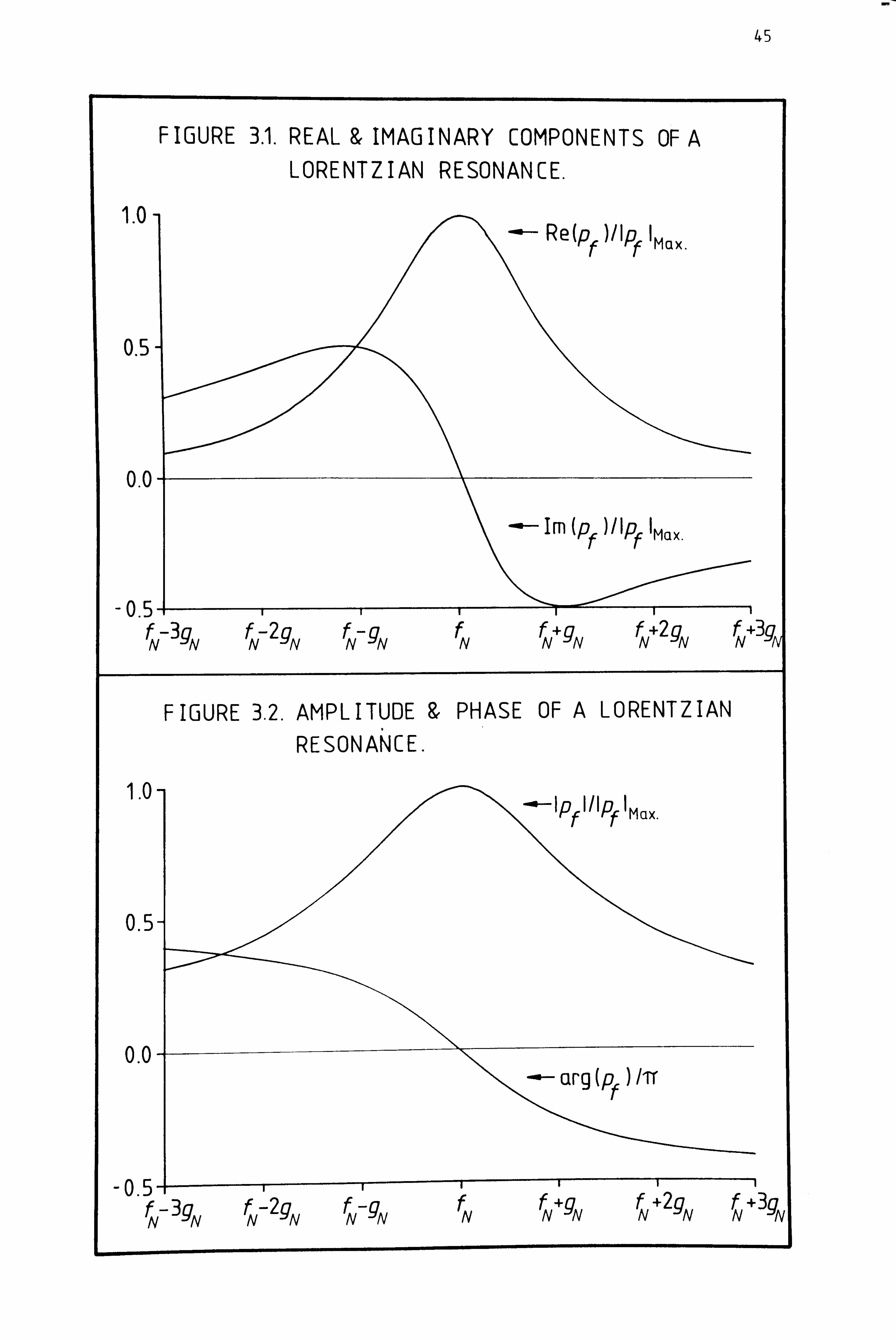
45

FIGURE 3.1. REAL & IMAGINARY COMPONENTS OF A LORENTZIAN RESONANCE.

1.0- -a-- Re(pf Vlpf lm(,..

0.5-

0.0

Im Pf )Ilpf Imcix.

-0.5- f -3G --"/v flý-2 f gN NN

fN+ 2 fN+3gN fN fN+ gN gN

FIGURE 3.2. AMPLITUDE PHASE OF A LORENTZIAN RESONANCE.

1.0- 1pf illpf lmclx.

0.5-

0.0- arg (pf ) /Tr

-0.5 f-3g NN f -2g, f-g NNNN

11i f f+g /V /V

f +2_q f+3g NNNNN

46

is suddenly shut off then the. ca-vitý ý%ill reverberate, each mode

oscillating in proportion to exp(-2-. iý v t). Thus, in the time domain,

2TrgN is the time constant with ý%hich free oscillations of the N th

standing wave decay. The amplitudes and phases of the reverberating

modes which result when a simple-harmonic source is shut off can be

obtained by the appropriate Fourier analysis. If the source had a

frequency close to one of the resonance frequencies f then the reverber- N

ation consists mainly of that mode, and a measurement of the

characteristic reverberation time can serve to determine gN.

The usefulness of these formulae clearly depends upon a detailed

knowledge of the normal modes and their corresponding wavenumbers.

However, if the geometry of the ca%ity is not particularly simple, or if

the surface admittance is irregular, then these eigenfunctions and

eigenvalues cannot be expressed in closed form, and a direct solution of

the problem is not possible. From a practical point of view a simple

geometry will always be chosen, and the mechanical compliance of the

surface can be made small and uniform by proper construction.

Nevertheless, infinitely fine tolerances cannot be achieved, and the

geometry will always deviate slightly from the ideal. Furthermorei the

effective acoustic admittance of the boundary layers is a function of the

thermophysical properties of the fluid under study and therefore varies

from one experimental situation to another. What is required is a method

by which the normal modes and the corresponding eigenvalues, of a

slightly imperfect cavity filled ýNith a real fluid, can be related to

those of an ideal enclosure containing the ideal fluid. Such a method

allows verification that a particular resonator has been fabricated to

the required tolerance and takes account of slight surface imperfections

such as might be caused by a real source or detector of sound. It also

allows the eigenvalues for the cavity to be expressed as the sum of an

idealized component ý-vhich is invariant, and a small component that varies

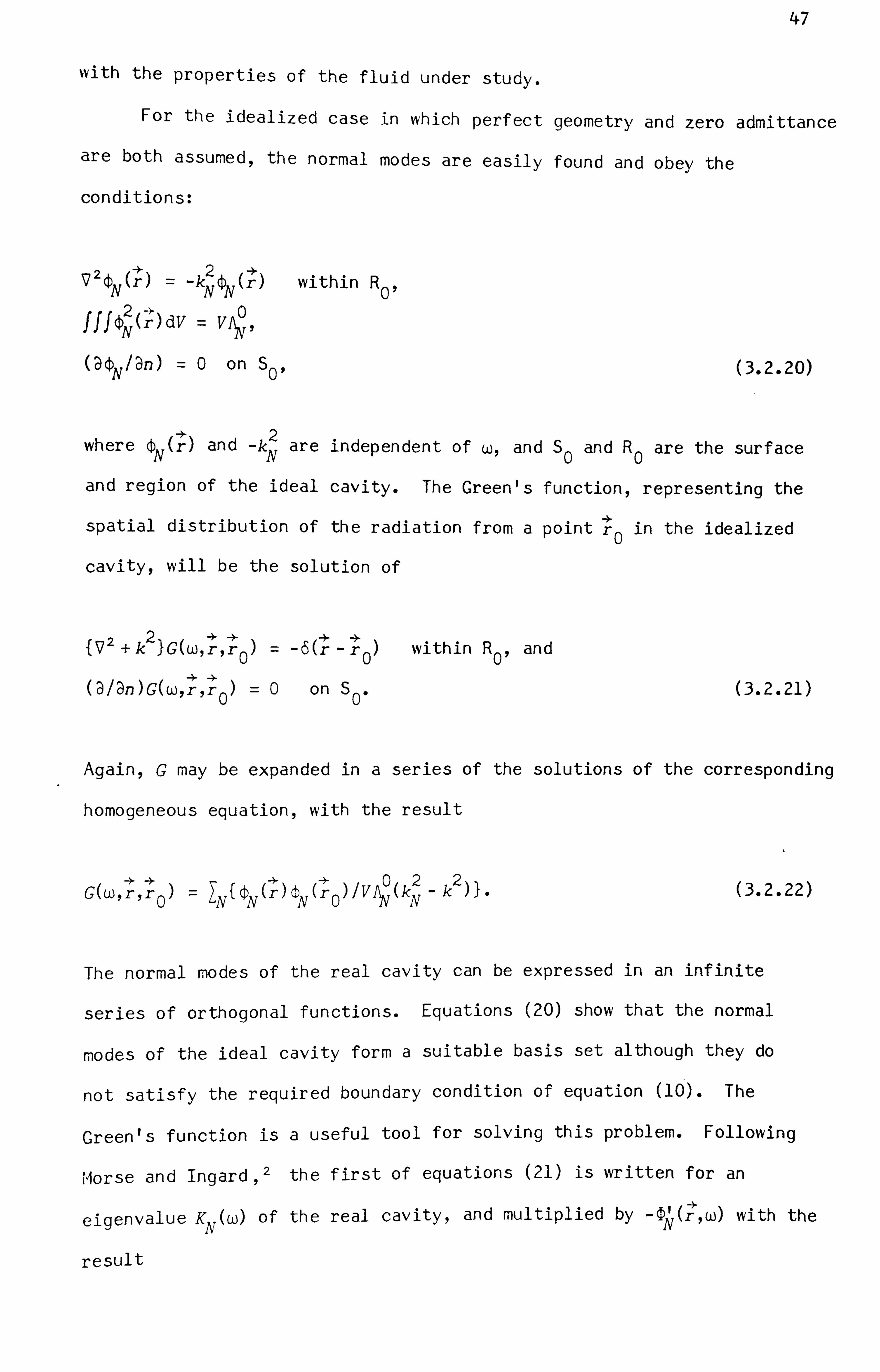
47

with the properties of the fluid under study.

For the idealized case in which perfect geometry and zero admittance

are both assumed, the normal modes are easily found and obey the

conditions:

V2ý 2 ýN(r-") within Rol r -ký N(+) fff 2 (r*) dV = VAýo ltý

0ý /9n) =0 on So, N (3.2.20)

2 where (r) and k are independent of w, and S and R are the surface ýN

N00

and region of the ideal cavity. The Green's function, representing the

spatial distribution of the radiation from a point-r"' 0 in the idealized

cavity, will be the solution of

{V2 2 -" 4- +k )G(w, r, r 0 -Mr r0

(919n)G(w, -r", r 00 on So*

within Ro, and

(3.2.21)

Again, G may be expanded in a series of the solutions of the corresponding

homogeneous equation, with the result

-* -* )022 G(wjrir 0 IN'

N( r) (tN (ro) IVAý (ký -k (3.2.22)

The normal modes of the real cavity can be expressed in an infinite

series of orthogonal functions. Equations (20) show that the normal

modes of the ideal cavity form a suitable basis set although they do

not satisfy the required boundary condition of equation (10). The

Green's function is a useful tool for solving this problem. Following

Morse and Ingard, 2 the first of equations (21) is written for an

eigenvalue KU of the real cavity, and multiplied by -V -* NN

(rýw) with the

result

48

C* )V2 W)

+ rjw r T'ý 4 GN (W' ,0 0)) rr-r0 (3.2.23)

where V is the N th eigenfunction for the real cavity, and N

2_ (2 (w) (3.2.24) )IV O{k '0NN

Equation (3) is now written for the same eigenvalue, multiplied by

G (w, rr ), and the result is combined with equation (23), the terms in N0

K (w) being eliminatedg to obtain N

)1721)1 (r+ J, 72G 4- -ý- {G rr, w) - e' ( r->., (w, V (r, w) 6 (r -r (3.2.25)

The position vectors r and r0 are now interchanged, making use of the

symmetry of the functions G (w, r, r ) and 6(r -r) with respect to such N00

an exchange, and equation (25) integrated in the co-ordinates of r0 over

the entire region R. This integration is readily performed using the

Divergence theorem t for the left-hand side and the definition (equations

6) of the Dirac delta function for the right-hand side, with the result

N (r'WN) =ffSf GN (w, ri", r-"S) n (r , w) - r-'- s, w) 0/ ýn) GN (w, r, r-"' 5 dS

(3.2.26)

The Divergence theorem relates the volume integral of the

divergence of a vector to the surface integral of the vector over the

surface S that bounds the region R

A --)- -4-

V r6r) dV =ff Sh 4, F (r) cS ff fR"'O

where n^-F(r) is the outward-pointing normal corrponent of F. A special

case of this theorem is

A. ýf(r

dS dS, fffRV2f Gr"') dV =ff Sn = ffS(3lon)f(r

where (919n)f(r) is the out"ard-pointing normal gradient of f(r).

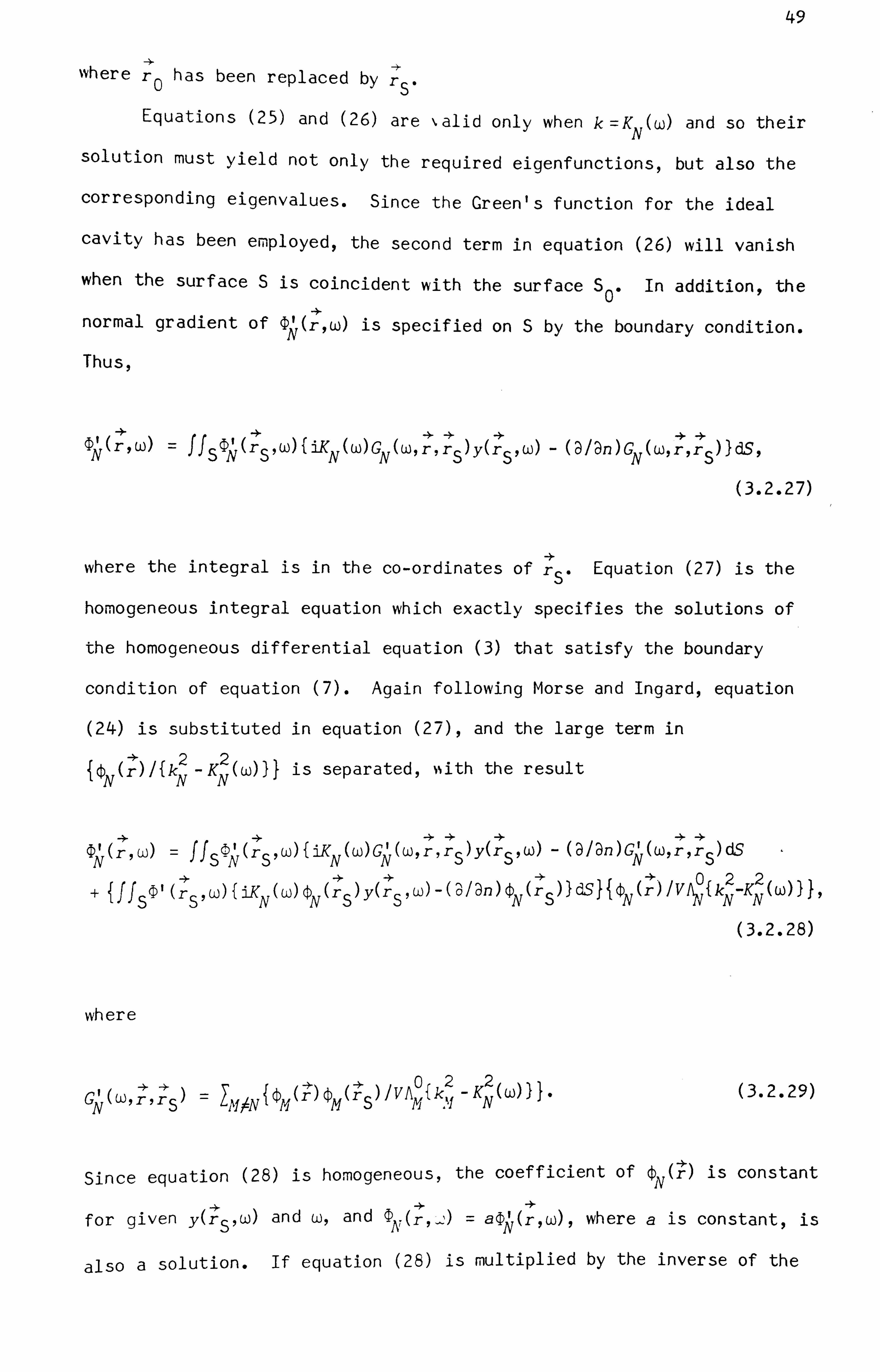
49

-4- -+ where r0 has been replaced by r S" Equations (25) and (26) are ýalid only when k =K M and so their N

solution must yield not only the required eigenfunctions, but also the

corresponding eigenvalues. Since the Green's function for the ideal

cavity has been employed, the second term in equation (26) will vanish

when the surface S is coincident with the surface S 0" In addition, the

normal gradient of 01 (r, w) is specified on S by the boundary condition. N Thus,

4- ->. -* 4. ffs(Dk(rSqw){iKN(W)GN(w, r-ý"9r )Y(r w) - (31ýn)G (w, r, r ))dS, ssNs

(3.2.27)

where the integral is in the co-ordinates of rS. Equation (27) is the

homogeneous integral equation which exactly specifies the solutions of

the homogeneous differential equation (3) that satisfy the boundary

condition of equation (7). Again following Morse and Ingard, equation

(24) is substituted in equation (27), and the large term in

2 Ký M) I is separated, Nsith the result

V(r, w) ffS(5'(rS, w)JiK MGý(Wýr, r )Y( qw) - (31@n)Gk(w, r, r WS

N -N Ns Is s 022

0'(rSgw) Yrr ol9n)ý (r )IdSjjýN(AIVIý{ký-KýM)jq + fffs 11 N (W)

N( S) Y( S'W) -(, NS

(3.2.28)

where

IV 022 r rs IG

(rS) Aý {ýýf - Kk (W) Gý(Wl-*' ")= IMýNfýA rmj (3.2.29)

Since equation (28) is homogeneous, the coefficient of ý (-") is constant Nr 4-

for given y(rS, w) and w, and a(fil(r, w), where a is constant, is A 'ýN

also a solution. If equation (28) is multiplied by the inverse of the

50

coefficient of N

IV 02'2r 1) 1 Gý. w) { iý, (w) ýN (-"" ) yS G"

, w) a/ an ) ýN G'ý )) ds I Vký -Kiý(w))/fJS N S9 rs rS rS

(3.2.30)

then the result,

('r, w) If f SID, (rS, W) {iKN M GV(W, -r"ý-r*S) yGrý",, w) - 013n)GýN, T'ý, rS)) d5, NI

(3.2.31)

defines the set of normal modes 0 which tend to as Y-*O and 5-*-S 0" The corresponding eigenvalues are obtained directly from equation (30)

by recalling that (D =aV NN

220 -Ký (W) -k + (11VA; )JfS4)N(rS, w)fiKN(w)ýN(-r"S)y('r*S, W) - 01ýn) r dS, =. N ýN ( "S)

(3.2.32)

Equations (31) and (32) may now be solved simultaneously to any desired

degree of accuracy.

These expressions for the eigenfunctions and eigenvalues of ýhe

real cavity are of considerable importance in both the design and use of

acoustic resonators. Equation (31) shows that if the surf ace admittance

or geometry is irregular, then the normal modes of the cavity are coupled

together, and the eigenfunctions of the real enclosure differ in form

from the unperturbed set. The terms arising from the failure of S to

coincide with S0 can usually be made negligibly small by careful design

and construction; detailed mechanical measurements and the appropriate

integration can verify that this is so. If the surface admittance is

uniform over the whole of S or piecewise uniform over sections of S,

and if S is close to S0 then most of the terms in the integral on the

right of equation (31) will be negligible and (D will have the same form N

51

as ýAr. A first-order solution of equation (32) is then' appropriate and

this is obtained by setting ý=ý. Thus if S =S then NN0

220 -ký +f iK (W) /VA)ff

SyCr"S 9 w) e. (-r'* ) dS N 7v It s

which is quadratic in KM and leads to N

0 4- 2 (KN(W)IkX) =1- {(il2kNVAý)ffSy(rS, w)ýý('ýr". S)dS}

correct to first order in the surface admittance. The frequency

dependence of the eigenfunctions and eigenvalues arises from the

(3.2.33)

(3.2.34)

dependence of the surface admittance on the frequency. The natural

frequencies ujN/2Tr will be predominantly determined by the speed of sound

in the fluid. However, in reality the two are not quite in proportion

because of the frequency shifts arising from the boundary-layer

admittance. It should be noted that (31) and (32) are implicit equations,

for y is a function of w and, to obtain the correct solution, the

appropriate frequency must be used in its calculation. In the case of

the free vibrations of the N th standing wave, w= wN = 2Tr(f - ig ) is

NN

appropriate but, when the motion is driven, w=27Tf, where f is the

frequency of the source.

If the surf ace admittance (or geometry) is not regular then 0 N

will differ in form from ýN , and equation (34) will only constitute a

first approximation to the required eigenvalues. A variational

calculation can yield a second approximate solution. 2 An additional

complication may arise when the state N of the system is degenerate.

In this case a number of the eigenfunctions have the same idealized

eigenvalue -k 2

and the effects of any irregularities in the surface N'

admittance or geometry are greatly amplified by the large terms

22 -1 {k - Ký (W) that remain in G,. This problem can be overcome by

52

recasting the degenerate wavefunctions in appropriate linear combinations,

and thereby forming a new basis set. These linear combinations must be

weighted so that the offending integrals in equation (31) vanish.

It is now possible to consider the wavefunctions and resonance

frequencies of the cylindrical and spherical cavities of interest, on the

assumptions that the geometry is perfect and that the surface admittance

is zero. The results of that analysis can then be combined with equation

(34) to obtain the eigenvalues of the cavities when they are filled with

a real fluid.

3.3 THE CYLINDRICAL CAVITY

The cavity is defined as a cylinder of radius b, concentric with

the z axis and extending from z=0 to z. = L; and it is assumed that the

walls are rigid, the geometry perfect, and that the thermal and shear

boundary layers are negligible. The wavefunctions ýN(T") of the cavity

will be expressed as the product

x (W)y (ý))z (Z), N IV 11 N (3.3.1)

in terms of the cylindrical co-ordinates (wqý), z) which are related to

the usual Cartesian set (-x, yz) by

x=w COS y=w sin and z=z, (3.3.2)

and for which the Laplacian operator is given by

2= (a2/aX2) + (32/DY2) + (D2/ýZ2)

= (9 2/aW2) + (11W) (DIDW) + (11W 2)(ý2/ajý2) + (ý2/ýZ2). (3.3.3)

53

The wavefunctions must satisfy the orthogonality -condition of

equations (3.2.5), which for equation (1) reduces to

fb 27T L0 bx, V (w)Xpl (w) wdwf 0Y=V j Iýr

(10 Ytj (ý)) diýf 6ZV (z)ý,. f

(z) dz Ný qlv

where 6 MN = 6(l - 11 ) Mm - mul ) Un - n') = 611'6mml6nnl*

Substitution of (1) in the time- independent wave equation (3.2.3)

(3.3.4)

separates the problem into three independent differential equations:

(11X) (d 2X/dW2) + (llwX) (dX/dw) + (k 22 (m 2/2 ýý -q)- 09

( 2y /ft2) + m2y = 09

(d 2Z/dZ2) + q2Z = 09 (3.3.5)

where -m 2 is the separation constant for Y and -q

2 is the separation 22 -21 constant for Z. The substitution w= Aký -q) -2 reveals that the first

of equations (5) is identical with Bessel's equation

(d2X/dx2) + (llx) (dXldx) + (1 -m2 /x 2 )X = 09 (3.3.6)

for which one solution is X=im (x), the cylindrical Bessel function of

order m. However, equation (6) is of the second order and there must

be two independent solutions. The second of these X=NMW, the

cylindrical Newmann function of order m, is infinite along the line

w=0 and therefore fails to be of physical significance and is rejected. 22 -'

The valid radial wavefunction i {(k -q) 2w) must satisfy the boundary mN

condition

JdJ J( k2 -q 2) 12

w)ldwj =0 mN w--b

(3.3.7)

22" and (k -q is therefore restricted to a discrete set of values.

N

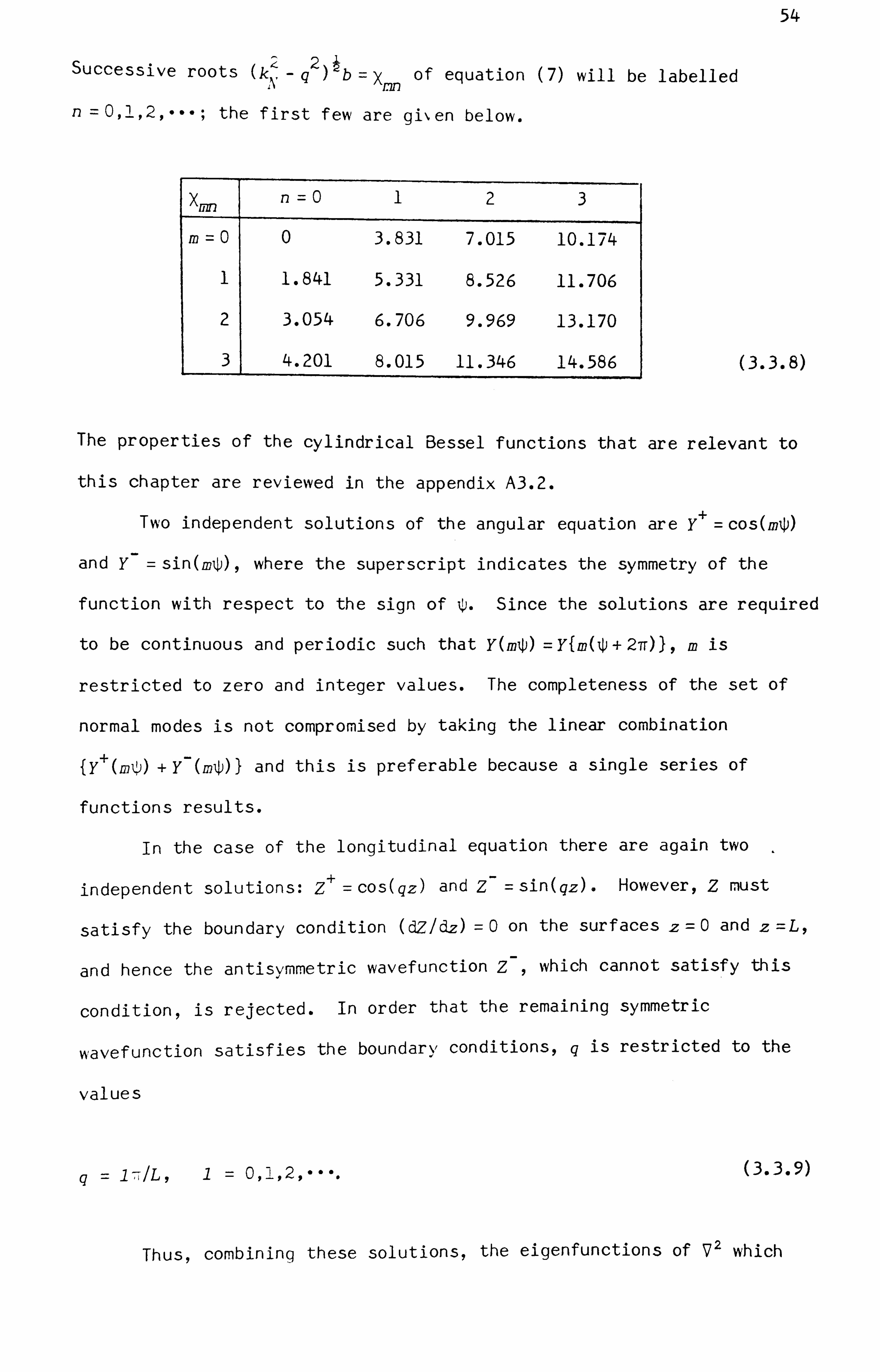
54

Successive roots q2b=X nn of equation (7) will be labelled

0,1,2, ---; the first few are gi,, en below.

Xmn n=0 1 2 3

M= 0 0 3.831 7.015 10.174

1 1.841 5.331 8.526 11.706

2 3.054 6.706 9.969 13.170

3 4.201 8.015 11.346 14.586 (3.3.8)

The properties of the cylindrical Bessel functions that are relevant to

this chapter are reviewed in the appendix A3.2.

Two independent solutions of the angular equation are Y+ = cos(mW

and Y sin(mý)), where the superscript indicates the symmetry of the

function with respect to the sign of VI. Since the solutions are required

to be continuous and periodic such that Y(mý)) =Yfm(ý)+2TO), m is

restricted to zero and integer values. The completeness of the set of

normal modes is not compromised by taking the linear combination

+ Y- and this is preferable because a single series of

functions results.

In the case of the longitudinal equation there are again two ,

independent solutions: Z+ =cos(qz) and Z- =sin(qz). However, Z must

satisfy the boundary condition (dZ/dz) =0 on the surfaces z=0 and z

and hence the antisymmetric wavefunction Z which cannot satisfy this

condition, is rejected. In order that the remaining symmetric

wavefunction satisfies the boundary conditions, q is restricted to the

values

q= 1-, i/L, 1=0,1,2, -*** (3.3.9)

Thus, combining these solutions, the eigenfunctions of V2 which

55

satisfy the boundary conditions in the idealized cylindrical cavity are

m (X

r, -)n w1b) {cos(mý)) + sin(mý)) lcos(lTrz/L) 9N=

(l, m, n) ,

(3.3.10)

where 1, m, and n may take zero and positive- integer values (negative

values are allowed but not required).

22_2 ký -(lTr/L) (Xmnlb

The corresponding eigenvalues are

and hence the natural frequencies of the cavity are

(3.3.11)

F (f NN

(fN - igN) = (u/27T) 1{(17T/L) 2+ 1 (X 1b) 22

Mn _ i0t( f1flm) (3.3.12)

where the only damping is that arising from the bulk attenuation. In

this idealized model the eigenvalues are independent of the frequency,

and the resonance frequencies f are directly proportional to the speed N

of sound. The N th mode has (1+ 1) plane longitudinal nodal surfaces

> 0), m plane radial nodes, and (n + 1) cylindrical nodes (n > 0) -'

Using the appropriate properties of the Bessel and trigonometric

functions, the orthogonality of the normal modes can be verified, and

the normalization constants shown to be

14 -2 0 Aý = (l/E: 1){' - (rnIXmn) ljm(Xmn)' E: 0 = 1, (3.3.13)

The walls of practical resonators are not perfectly rigid, nor are

the effects of thermal and viscous damping in the boundary layers

negligible. The Perturbations to the idealized eigenvalues, which are

the result of these non-ideal boundary conditions, are given to af irst

approximation by the leading term of equation (3.2.34). The surface

56

in egra. involved may be separated into the sum

ff W) 2L 27 2

Sy( rS (rS) dS fofo y(w=b, ýl,, z, -)ý)ý(w=b, ý), z)bdý)ý + I J -b 2Tr 2

of oy(wq ý)ý z (w, ý), z= 0) dý)wdw +

f bf 2'Ty(w, ý)q z2 00=L, ý; (w, ý), z= L) ftwdw (3.3.16)

of the integrals over the side and t%o ends of the cylindrical cavity.

Since the specific acoustic admittance of the viscous boundary layer is

a function of the tangential component kt of the wavenumber at the wall,

the total boundary admittance will depend upon the mode of the cavity's

excitation. For the longitudinal modes (m =n =0), kt =k at the side

walls, and kt =0 at the end walls. Thus the effective specific-acoustic-

admittances yl,, of the side and yl, e of the ends are

Yi 9s

(f )= (1 - ') (7Tf /U) f (-Y - 1) 6h +6 S} -rymgs(f), and

Yl ,e

(f (1 - D (Trf /U) (-y - h+ Ym, e (3.3.17)

in accordance with (2.6.39). The thermal and shear penetration lengths

are given by equations (2.6.25), and have the frequency dependence of 1 2 f

_vmq S and y m, e are the specific acoustic admittances of the side and

end walls that arise from their non-zero mechanical compliance. These

terms are usually very small and can be estimated from mechanical

measurements.

For the radial modes (1 =m= --) the situation is reversed; kt is

zero along the side walls, and equal to k at the end plates. Thus the

effective side-wall and end-wall specific-acoustic-admittances are

Yr, s(f) = (1-i)(7Tf/u)(Y-1)6h +y MIS

(-C) , and

(f)q Yr, e

(f i) (T, -f / U) 6h +ýsm, e

57

respectively. For both the radial and longitudinal modes y(r s f) is a

constant for each of the separated surface integrals. This would not

be so for the compound modes (mi 0 ). 0-I For the longitudinal modes A 10 2, ý)

10= cos(lTrz/L), and therefore

the corrected eigenvalues are

10 (f) =k lo-

(ilb)yl, s(f) - (2i/L )yl,

e(f) " (3.3.20)

The natural frequencies are obtained by substitution of K 10 (f) in

equation (3.2.4) and solving the resulting implicit equation for

(flo - igio):

F 10 (fl

0) = (fl 0- ig 1 0) = (u/27r){K

10 (f10) - ia(f10)1. (3.3.21)

In the case of the radial modes A0 =J2 and =JO(X w1b). On O(XOn) ýOn On

Use of the appropriate properties of the cylindrical Bessel functions

shows that

K On (f) =k On -

(ilb)y r, s

(f) - UIL)y r, e

(f) 9

and the corresponding natural frequencies are therefore

F On (f

On) = (fOn - 'g0n )= (u/27) {K On

(f On

)- ia(f On))

(30.22)

(3.3.23)

In both equations (20) and (22), the dominant frequency dependent

terms are those that arise from the viscous and thermal boundary-layer I

losses. These terms are proportional to f2 and usually make only a

small contribution to the eigenvalues which may therefore be taken as

constant over a small interval of frequencv.

58

3.4 THE SPHERICAL CAVITY

The cavity is defined as a sphere of radius a, centred at the

origin; and it is again assumed that the walls are rigid, the geometry

perfect, and that the thermal and shear boundary layers are negligible.

The wavefunctions are separated into the product

RN(r)PjV(6)QV(C), N= (l, m, n) , (3.4.1)

in terms of the spherical co-ordinates (r, e, C), where r is the magnitude

of the position vector, the co-latitude e is the angle made with the

Cartesian z axis, and the azimuth ý is the angle made with the Cartesian

axis. Thus,

r sine cosý, y=r sine siný, z=r COS6 (3.4.2)

and the Laplacian operator is given by

V2 = (32/ 3r 2) + (21r) 013r) + (l1r 2) (@ 2/ 36 2)

+(Cose/r 2 sinexa/ae)+

(l1r 2 sin

28) (a 2/aý2)

. (3.4.3)

The wavefunctions are required to obey the orthogonality condition

2f 27T (ý)Q 0 f'RN(r)RM(r)r drf'TP (e)p (e)sined6 Q (ý) dC = VAý (3.4.4)

00NM0Nm 6NM'

and substitution of (1) in the wave equation yields the three independent

differential equations

2 (1 + 1) Ir 2 (11R) (d2R/ dr2) + (2r1R) (dR/dr) + ký = 09

2) + (cose/sin' )( dP/ de) + {1 (i + 1) -m2 /sin 2 e)p = 0ý (d2 PI de ýj and

59

(d2Q/d ý2) + m2 Q= 09 (3.4.5)

in which _m2 is the separation constant for Q and -1 (1 + 1) is the

separation constant for P. The substitution r= xlk reveals that the N first of equations (5) is

(d2R/dX2) + (2/x) (dR/dx) + {i -1 (1 + 1) /x2 IR = 0. (3.4.6)

The solution of (6) is finite at the origin is X=j1 (kNr), the

spherical Bessel function of order 1. The radial boundary condition

requires that

{ dj 1 (kNr) / dr)

r=a = Oý (3.4.7)

and successive roots ka =v of this equation are labelled N 1n

the first few are given below.

v ln n0 1 2 3 4

1= 0 0.000000 4.493409 7.7255252 10.90412 14.. 06619

1 2.081576 5.940370 9.205840 12.40445 15.57924

2 3.342094 7.289932 10.61386 13.84611 17.04290

3 4.514100 8.583755 11.97273 15.24451 18.46815

4 5.646703 9.840446 13.29556 16.60935 19.86242

(3.4.8)

more extensive list of solutions, and some of the important properties

of the spherical Bessel functions, are given in the appendix A3.2.

The solutions of the angular-dependent equations are viell knovvn

and will not be discussed in detail here. The solution of the second

of equations (5) that is finite and continuous is

60

(Cose) 0+1, + 2, ---+ (3.4.9)

and the solutions of the third of equations (5), cos(mý) and sin(mC),

may be combined with (9) to define the spherical harmonics

ylm(e, 0= {COS(mý) + sin(mC) lp 1 'n I (Cose) . (3.4.10)

The function P1 ml is the ImIth associated Legendre polynomial of order

1; its important properties are reviewed in appendix A3.2.

Equation (10) may be combined with the spherical Bessel function

to define the normal modes of the cavity as

(rq e, ý) = ln rla)Y lm (e, o9N= (1 mn) .

The corresponding eigenvalues and natural frequencies are

2=_ (v /a) 2 ký ln 9 and

IV)), (3.4.12) FN (fN) = (fN - i9N) = (u /2TO j (V,,, la) - ia(f

respectively. All the states with a given 1 are (21 +1) fold degenerate,

and th eN th

mode has 1 plane longitudinal nodal surfaces, m axial nodes,

and (n + 1) spherical nodal surfaces (except for 1=0 when there are n

spherical nodes). Using the appropriate properties of the function

and Y 1M the normal modes of equation (11) can be shown to satisfy the

orthogonality condition of equation (4), with the normalization constants

022 Ak = 13/2 (21 + 1)) {1 -1 (1 + 1) /V

ln m+Im )j 1(v ln

(3.4.13)

The eigenvalues must be modified to account for the non-ideal

boundary conditions which are found in a real resonator. In the case of

61

the radially symmetric modes, - the surface corrections are particularly

simple because the motion is normal to the wall and no viscous damping

occurs. For these modes the specific acoustic admittance of the boundary

is

Yr(f) = (1 - ') (Trf/u) (y - 1) 6h +ym, r

(f) 9 (3.4.14)

where y m, r is the contribution of the mechanical compliance of the wall.

The surface integral in equation (3.2.34) is

j2 (, )012 ) dS (f)a 2i2 (v ) f2Trf 7sined6dý ffSyr(f) 0 Yr 0 On 00

4Tra 2y (f)j2(v (3.4.15) r0 On

and hence

K On (f) k On -

(i/a)y r

(f), and

F On (f

On = (f On - igo) = (u/27T)fK

On (f

On ia(f On (3.4.16)

correct to first order in the surface admittance.

I. he 1 th order (1> 0) non-radial modes of a spherical cavity are

(21 + 1) f old degenerate, and the tangential f luid f low at the surf ace is

generally a complicated function of the co-latitude and azimuth angles.

However, in the case of those non-radial modes that are of axial

symmetry (m = 0) the motion is independent of C. The tangential wave-

number kt is given by

V2 2 O(Cose) + 1) Ir 2)0 (Cose), O(cose) = -ktPý pi Pý (3.4.17)

and is constant over the surface r =a of the enclosure. The effective

specific-acoustic-admittance of the thermal and viscous boundary layers

62

of the axial modes is

Ya(f) = (i-i){(TTf/u)(Y-1)6 h+i (i + l)u6 S/ 47Ta 2

f) ý

and the required surface integral is

Ya(f)a 2i2 (v )f 27Tf Tr

p '(cose))2 sinededý 47Ta2 1 (21 + 1) }y 2 1 ln 001 a(f)jl(vl,,

)

(3.4.19)

The first-order corrected eigenvalues corresponding to the axially-

symmetric non-radial wavefunctions are therefore

Kk (i/a)[1 + 1)/'V 2 )-l y ln(f) ::::: ln - ln a (3.4.20)

The effects of boundary-shape perturbations can be estimated from

equation (3.2.32) which gives

02 (KNIk 1+ (112VAýký)ffSýN(S)(31an)ýN(r-"' )dSj

N) rs (3.4.21)

to a first-order approximation. For a near spherical surface, (3/3n)

may be replaced by 0/3r) and hence the fractional shift in the

eigenvalues of the radial modes is

(KN -k Ik =-f al3VV i2 (v v r1a) dS. (3.4.22) N) N On 0 On)lIfSjO(ý)0nr1a)jl( On

Since jl(v On )= 0, the perturbation vanishes as S-*S0, the Ideal surface

r=a- To Proceed, jO(v On r1a) and j1 (v On r1a) are both expanded in a

Taylor's series about r =a with the results

j0(v r1a) = jO(v )fl -N2 12)[(r -a)la) 2+

On On On

63

ii (v On r1a) =v OniO

(v On

) if (r -, a) la} -{ (r _ a) /a)2

2,2 + (2/ 3) 1 (r - a) la) { (20 - 1, -v On

)130) + (3.4.23)

where the derivatives have been reduced to zero-order Bessel functions

using the properties set out in appendix A3.2. Substitution of (23) in

(22) yields

(K -k Ik = -(al3V)ffSi{(r-a)la) 2

N N) N- {(r - a) la)

+ {(r_a)/a)3{(20-19v 2 )130} +---ldSp (3.4.24) On

where dS =r 2 0, C)sin6d6dC and r 0, C) is the radial co-ordinate of a SS

position on the surf ace. If c is a small parameter describing a geometric

deformation of the perfect cavity by which the volume remains unchanged,

then the leading term in the surf ace integral of { (r - a) la) will be of

2 the order of c Thus the radial modes are insensitive to geometric

imperfections. However, the non-radial wavefunctions are weighted by the

factors Y 1M (e, ý) and are sensitive in the first order to a parameter

describing a deformation. A specif ic example is the case in which the

cavity is constructed from two hollow hemispheres of unequal radii-. If

the radius of one half is a(l + ON and the radius of the other half is

a (1 - ON, where N3 = (1 + 3F- 2) -1 , then the volume is exactly independent

of F- and the first two terms in equation (24) show that the fractional

perturbation is 15c 4. Thus, in this highly symmetric case the

perturbation is vanishing to third order in c and a fine tolerance is

not required.

64

3.5 SPEED OF SOUND MEASUREMENTS BY THE RESONANCE TECHNIQUE

In principle, the speed of sound can be found from a time-of-flight

measurement, in which the time taken for a pulse of sound to travel an

accurately measured distance is determined. Methods of this type are of

practical advantage in the study of liquids and dense gases, but if the

characteristic acoustic resistance pu of the fluid is small then the

generation of a pulse with a useful amplitude becomes difficult. In

dilute gases pu is indeed small and the resonance technique, with its

continuous excitation, is clearly superior.

The purpose of this section is to briefly review the relative

merits of the various types of acoustic interferometer. Essentially,

there are two types of interferometer, classified either according to the

use of fixed geometry, and consequently variable frequency, or variable

geometry and fixed operating frequency. These are further classified

according to the use of high frequencies (N large) or low frequencies

small).

The variable geometry experiment is restricted to the use of the

longitudinal modes of a cylindrical interferometer. The cavity is driven

at a fixed frequency by a transducer which usually forms one end of the

cylinder. The remaining end is closed by a piston which is moved in the

bore of the tube in order to tune the cavity. The resonance condition

is detected either by a second transducer acting as a detector, or by

measurement of the mechanical impedance of the loaded source transducer

(this may be achieved by measurement of the corresponding electrical

impedance). In either case the measured quantity is proportional to

the Green's function of equation (3.2.14) where the excitation frequency

f is fixed and L is tuned until fl_ is coincident with The resonance

half -widths are obtained from the displacement of the reflector necessary

to reduce the amplitude of the standing wave to 1/y/2 of its maximum

65

value. This method has the. substantial advantage that the absolute

length of the cavity is not required; the speed of sound is obtained from

the travel AL of the piston necessary to shift from one order of resonance

to the next. Optical techniques can be used to measure AL with a 6 relative accuracy approaching 1x 10- In contrast, absolute knowledge

of the pathlength is required for absolute measurements by the constant-

geometry variable-frequency technique. However, in many applications

absolute measurements of sound speeds are not required, and the simpler

arrangement of af ixed-geometry resonator is advantageous.

In any cavity the range of operating frequencies is important. If

measurements are made at high frequencies, where X is much less than the

characteristic dimensions of the resonator, then the boundary layer

corrections are minimised at the expense of increased attenuation

throughout the bulk of the fluid (g S

If cc ft alf cc f) . However, as the

operating frequency is raised, the number of resonances occurring in a

given range of frequencies increases dramatically, and overlap between

adjacent modes can be a serious source of systematic error. This is

particularly severe in a cylindrical interferometer when the longitudinal

modes are driven at frequencies well above (027) (X 10

1b) because the

compound modes are often unresolved from the purely longitudinal

resonances. In addition, vibrational-relaxation absorption and

dispersion can be large at high frequencies. The systematic errors

prevalent in the various types of cylindrical interferometer have been

discussed in detail by Colclough, 3 who concludes that low-frequency

measurements in a variable pathlength interferometer are preferable

wfien high absolute accuracy is required. Nevertheless many workers have

used interferometers for sound speed measurements at high ultrasonic

frequencies to good effect and found that the problem of unresolved

modes is not generally important at the usual 1x 10-4 level of accuracy.

Low-frequency measurements are usually unaffected by dispersion,

66

and overlap between adjacent resonances can be avoided. However, the

boundary layer corrections are much larger, and accurate knowledge of the

gas transport properties is required for a calculation of these

corrections. A relative correction of lxlO- 3 is not uncommon at audio frequencies, where the precision of the measurements may be better than

1 X10 -5. Fortunately the contribution 9b of bulk absorption to the total

resonance half-widths is usually small at low frequencies, and the

contribution gS of the boundary-layer losses is easily found from the

measured half-width. The difference Af S between an idealized resonance

frequency and the measured value is equal to gS (in the absence of other

perturbations), and hence the measured half -widths can be employed to

make the corrections. These half-isidths can also be used to find the

coefficients of thermal conductivity and shear viscocity from measurements

of several resonances which have differing symmetry.

The choice of transducers, and the method by which they are coupled

to the cavity, is crucial. If a large transducer is used as the end

plate of a cylindrical resonator then the boundary condition there will

differ from that assumed in the derivation of the normal modes; the fluid

velocity at the end in motion must match that of the moving surface.

The theory of cylindrical interferometers that operate with this type of

34 transducer has been discussed in detail by Colclough and Quinn.

Measurements of the mechanical admittance (or impedance) of the loaded

transducer are essential in accurate work of this kind. It is generally

desirable to use a small transducer which approximates to a point source,

and has a negligible influence on the normal modes. Unfortunately, a

point source is very inefficient, and the amplitude of the standing wave

generated by such a device may be too small for sensitive measurements.

A spherical interferometer is necessarily of fixed geometry, and

absolute knowledge of the radius is required for absolute measurements.

Fortunately, the resonance frequencies of the radially symmetric modes of

67

a sphere are insensitive to geometric imperfections, and knowledge of the

mean radius is sufficient. Because of the absence of viscous damping,

and the f avourable surf ace area to volume ratio in a sphere, the radial

modes have Q's which are about a factor of ten greater than those of a

comparable cylinder. The boundary-layer corrections are therefore

smaller, and less severe de n-ands are placed on the quality of the gas

transport data required to calculate these corrections. Again the

measured half -width may be used to evaluate the corrections, and to

determine the coefficient of thermal conductivity for the fluid-under

study. Quite inefficient transducers may be used, and the area of the

surface perturbed by the source need only be a small fraction of the

total -

In summary, low-frequency interferometry avoids the problems of

overlapping modes and vibrational relaxation, but large boundary layer

corrections must be made. However, while the influence of the former

effects are difficult to assess, the latter are measurable. In addition,

resonance width measurements can provide accurate gas transport

quantities.

68

APPENDIX A3.1

The calculation of the boundary-layer corrections is crucial to

the accuracy of low-f requency measurements of the speed of sound in

dilute gases. The expressions derived in chapter 2 (equations 2.6-39),

for the acoustic admittance of the boundary layers, and in this chapter

(equation 3.2.34), for the corresponding perturbations to the resonance

frequencies of a cavity, form a consistent first-order approximation to

the exact solution of the problem. By this approximation the thermal and

shear corrections to the propagational wave are neglected in the boundary

layers, k22 is set equal to k2 2_ 2 is set equal to k 2. it h-kth, and kkt

has also been assumed, without proof, that the results obtained for a

plane surface may be applied to curved surfaces without modification.

In addition to these approximations there is the overall assumption that

a dilute gas may be considered as a classical continuum fluid.

Without this assumption the boundary conditions of continuous temperature

and vanishing tangential velocity do not apply. The molecular nature of

the fluid is responsible for the breakdown of these boundary conditions

at low densities, and for the resulting phenomena of molecular slip and

the temperature jump.

All these possible sources of error have been investigated by

WestoO for the case of plane waves propagating along an infinite

cylindrical waveguide. He considered the approximations made by

Kirchhoff in the derivation of the orthodox tube propagation-constant of

equation (2.6.40), and derived some more exact formulae which are

applicable to a number of limiting cases. The approximations of

Kirchhoff are the same as those made in the application of equations

(2.6.39) to the solution of the boundary-value problem at the side walls

of a cylindrical interferometer operating in the longitudinal modes.

Shields, Lee, and VyileY6 have obtained direct numerical solutions for

69

the same problem, which are valid over a wide range of frequencies and

tube radii. The relative errors introduced into sound-speed measurementsg

by the neglect of their second-oder correctionsg are of the order of the

square of the relative first-order correction itself. Unless the first-

order corrections are very large (as they would be for very narrow tubes)

the second-order corrections are negligible in all but the most precise

measurements. The effects of molecular slip were also found to be a

source of error, but the temp eratur e -jump effect, which Weston suggests

is as large, was neglected. These latter effects are of greater

importance than the approximations in the Kirchhoff -Helmholtz theory

because relatively wide tubes (b>> 6 h' 6s) are employed for speed-of-

sound measurements.

Second-order corrections have not been investigated for the

radial resonances of a spherical interferometer and will therefore be

considered here. To begin with it will be assumed that the non-classical

temperature-jump effect is neglible, and that thermal waves do not

propagate in the wall. Thus, the thermal boundary condition is the same

as was adopted in chapter 2. However, the thermal and shear corrections

to the propagational mode will not be neglected, and hence

pp (r) = AjO(K On r)exp(-iwt)

Tp (r) =A{ (y - 1) /'Yý) (1 - iLh )jO(K On r)exp(-iwt),

4- up (A = -A (e/ iu-p) (1 - iL v

)K Onjl

(K On r)exp(-iwt),

and

(A3.1.1)

are the contributions to the acoustic pressure, temperature, and f luid

velocity of the n th

radial mode, where A is a constant, and e is the

radial unit base vector. The thermal mode must satisfy the wave equation

V2 T (r) = -k 2T (A3.1.2)

hhh

" i

and the total acoustic temperature Ta =T p+Th must satisfy the boundary

condition

a (r =a) = (A 3.1.3)

at the surface r =a of the enclosure. The radially symmetric eigen-

function of V2 , which is finite at the origin and has the time dependence

of exp(-iwt), is

Th (r) = Bj 0 (k

h r)exp(-iwt),

where the amplitude

B= -A (1 - iL h) (-y - 1)jO(K

on a) /yýjo (k h a)

(A 3.1.4)

(A3.1.5)

is determined by the thermal boundary condition. The thermal wave makes

a small contribution to the acoustic pressure, given by

Ph (r) = iy ý (L h-Lv

)T h

= -iA (L h-Lv)

(-y - -7)jO(K on a) {jO(k h r)

Ijo(k h a))exp(-iwt),

and a contribution to the fluid velocity, given by

4- A

uheh /wp) (dT h/ dr)

l.. 6)

eA (1 + i) 6 (wl2cu 2)(1 -iL )(y -1)jo(K a)fjl(k r)ljo(k a)). (A3.1.7)

h0h On hh

Thus, the magnitude of the total fluid velocity at the surface r =a is

W2ý 12u 2M -iL MY -1)jl(k a)ljo(k a) L'(r = a) =A {exp (-icLt) -ýo)

{ (i - 1) (ch0hhh

- (i - iL v)i,

- Onjl (K

On a)}

71

= Ympa (r =a)

= YMAj 0 (K

On a) {1 + (L h-Lv

My --"))exp(-iwt).

Elimination of exp(-iwt) from equation (8), and some rearrangement

yields

IK jl(K a) Ijo(K a) -iwp{l + iL + (L L )(-y-l)}{Y +Yl)g (A3.1.9) On On On vh-vmh

in which

Yh' = -"(1 -')/Puo )(Y -1)(w/2u 0Hh [i - iL h+ (L

V- L h)

(y - 1))jl(k h a)ljo(k h a),

(A3.1.10)

is the effective acoustic- admittance of the thermal boundary layer. The

term 5h {1 - iL h+ (L

v-Lh )(y -1)) which is partially third order in 6h may

be-replaced by 6h, and by the same reasoning 11 +iL v+ (L

h-L V) (Y - 1) 1

may be replaced by 1 in equation (9). Since {j 1

(Z) /jO (Z) )= Z-1 - cot(z),

and kh= (1 + D/6 h' the ratio of spherical Bessel functions can be

expanded as

{jl (kha ) Ijo(k ha) } ::: 1 (1 - ') 6h /2a) - cot"' - ')'a' 6h

h /2a} +i tan (al 6h) tanh (al 6h

tan(a/6 h+i tanh (a/6h

wh er e

z- -z) / (ez + e-z)) ) 1. tanh(z) = J(e ez -)- 00 (A3.1.12)

The liniting behaviour of tanh(z) is reached very rapidly; tanh(a/6 h) =

1+ 10-6 for (a /6h )> 10, and hence

72

{jl(k h") Ij

0 (k /2, a). h8)) 6h (A3.1.13)

Thus, the specific acoustic admittance of the thermal boundary layer is

I Yh : ": {1 + (1 + D6 Yh h/2'al ý Yh 'Y /2u -(- 1) (w 0

) (6 2 la) ý h (A3.1.14)

correct to second-order in 6 h' where yh= (i - j) (-y - 1) (w/2uo) 6h is the

f irst-order approximation. The second-order term in equation (14) arises

from the curvature of the surface, and vanishes as a-ý-co- The additional

effect of this term can be demonstrated by the first-order equation

(3.4.16), which shows that the imaginary components of the eigenvalues

are perturbed by the fraction i(-y - 1) (6 h/e)

2, and that the resonance

frequencies are not shif ted. Clearly when W6 h

)> 103 the second-order

term in equation (14) is negligible. However, a direct numerical

solution of equation (9) is desirable in order to verify that the

predictions of the first-order theory are sufficiently precise. In the

present contextq the required solution is the one obtained when

w= 21Tf On' and corresponds to the situation where the cavity is driven

at its n th

radial resonance frequency. Setting K On a =, V On + 'XOn , and

yl = (ý - jo) /puO, where ý and cy are the specific acoustic -conductance and h

-susceptance of the boundary, and substituting in (9) the equations

(v On + IXOn nTr + Tan-l(c + id),

I-22 c=f V(l + va) + x(VO + va) + (Vý) and 22

+ (A3.1.15) d=f X(l + VC) - VNO /I + VC)

may be obtained. The required eigenvalues are found by iteration; if

V(m) and X (m)

are the m th

approximations to v and X then the (m+ 1) th

improved approximation is n7T + Tan-1(C (M)

+ id (m) ), where c(m) and d

(m)

are calculated f rom the im th

approximations. For example, in argon at

73

T=273K and p=10 kPa, 6h= 124.0 ýjm at 3.7 kHz, and hence Yh = (1 - DO-00312

3* The first-order theory of equation (3.4.16) predicts

that vol :::: 4.49028 6 and x0l = -0 - 00312 3' while an exact solution gives

V 01 = 4.49028 9 and X0, =-0.00312 1

(two iterations of equation 15 are

required if the first-order estimates are the starting values). Since

f 01 will occur at 3.7 kHz in a resonator of radius 60 mm filled with

argon at T= 273 K and p= 10 kPa , the second-order correction implied by

equation (14) indicates that yl =y-0.00000 If V(O) =4.5 and hh 6* 01

X (0)

0 are taken as the zeroth approximations to v and X019 then four Ol = 01 iterations of equation (15) are required using y' , with the result h

Vol :, -- 4.49028 9 and xol =-0.00311 4* Similarly close agreement, between

f irst-order theory and the prediction of equations (14) and (15), is

found for the higher-frequency modes. Clearly, even at the low pressure

of 10 kPa, the neglect of second-order terms in the boundary theory has

a negligible effect on the resonance frequencies. However, the first-

order theory does slightly overestimate the resonance half -widths (by

about 0.3 per cent in this example), and this may be marginally

significant when a measured boundary-layer correction is applied, or in

a measurement of the thermal conductivity of the medium.

Errors arising from the failure of continuum theory can be -

significant if the gas pressure is low because the mean free path Z can

become a significant fraction of the thermal and shear decay lengths.

The resulting phenomena of molecular slip and the temperature jump have

been discussed in a number of publications. 49 51 6 Since there is no

tangential motion, molecular slip will not be of importance for the

radial modes of a spherical resonator. The temperature jump is an

apparent discontinuity in the temperature, which occurs over the thin

layer of gas within a few mean free paths of a gas-to-solid interface

when there is a heat current. The temperature Te of the gas at the

boundary, as estimated from the uniform temperature gradient in the bulk

74

of the fluid, differs from the true temperature TS of the surf ace. At

sufficiently high pressures, the apparent discontinuity in the temperature

is given b Y7

(T e-Ts)=

(i H

1p) (TrMT e

/2R) i{ (2 - h) /2h)

= Hl t 1K),

(A3.1.16)

for a monatomic gas of thermal conductivity K, where iH is the component

of the heat current density which points into the surface, and the

thermal accommodation length is given by

I

t= (K p) (TrMT 12R )2f (2 - h) /2h) (A3.1.17)

The accommodation coefficient h is defined as the fraction of molecules

which are diffusely reflected from the surface, and can be measured in

the hot-wire type of thermal conductivity experiment. a

Fortunately a more fundamental boundary condition can be

imposed which does not require the temperature of the fluid at the

interface to be specified but instead simply requires the heat current

density in the gas just outside the accommodation layer to equal the

heat current density in the wall at its surface. It will be sufficient

to return to the case of the plane wall confining the gas to the half

space z <0. The heat current density in the wall is given by

4. iH=

-KWýTw (A3.1.18)

w, here Tw is the temperature, and Kw is the thermal conductivity, of the

wall material. The equation of continuity for energy density is

/2 t) + 4-, -ý-

=09 cvwpw (ýT w

17 1H (A3.1.19)

75

where C Vw is the specific heat capacity at constant volume, and pw is the

density, of the wall material. Combination of (18) and (19) results in

the thermal wave equation

fV2- (11D = 0, (A3.1.20)

where Dt= (K w/ý, Wcvw

) is the thermal diffusivity of the wall. The plane-

wave solution of equation (20), which is equal to T+T 0 exp(-iwt) at the

surface z=0, and T in the limit z -* co, is

1 T (Z, t) = T+T oexp{-iwt +(i -1)(w/2D t

)'Z), (A3.1.21)

where T is the equilibrium temperature. By analogy with the thermal

mode in the gas, a thermal decay length 6w may be defined for the wall:

11 /W) 2X (2D

t= (2

w /P

wc Vvi (A3.1.22)

and exp(-z/6 vi ) describes a rapid attenuation of the thermal oscillations

in the wall.

The magnitude of the heat current density into the wall at the

surface is

1

H :- (1 -i)K w N12D

t )2 T0 exp(-iwt)

= (1 -i)(K w 16

w )T

0 exp(-iwt), (A3.1.23)

which must equal the magnitude of the heat current density in the gas

adjacent to the wall. The gradient (913z)T a

(z =-it) of the acoustic

temperature in the gas just outside the accommodation layer gives

jH= -K(alaz)Ta(z =-lt )9 (A3.1.24)

76

and equation (16) shows that the acoustic temperature extrapolated to the

wall Te= (T - T) differs from the true acoustic temperature of the

surface by

T' - exp(-iwt) = -1 (313z)T (Z = -, ). (A3.1.25) ea

combination of equations (23) and (24) gives

T0 exp(-iwt) = -(l+i)6 w (K12K

w) (3/3z)T

a(z = -1t) 9 (A3.1.26)

and elimination of T0 exp(-iwt) in (25) results in

Te= -{l t+ (i+i)6

w (K12K

w )1(ýlýz)T

a (Z = -1 t) - (A3.1.27)

Equation (27) is the thermal boundary condition which must be satisfied

by the thermal and propagational waves in the gas. The gradient of the

acoustic temperature is evaluated in the gas just outside the

accommodation layer, where classical heat f low should occur, and the

behaviour of the acoustic temperature within the accommodation layer is

not specif ied. Te is the acoustic temperature of the fluid at z =0 that

would be calculated with the assumption that continuum theory applied

right up to the interf ace. As 1t -ý- 0 and 6w (KIK w

)-*0 the boundary

condition reverts to Ta (z=0) =0, but in the range of pressures where

1t (=Z) is a small, but significant, fraction of 6h the normal gradient of

Ta must be adjusted to satisfy (27). Since the gradient of the acoustic

temperature is very nearly linear at z =-it, the normal gradient at -1 t

may be replaced by the gradient OT e/3z)z=o

that would be found at the

interface if continuum theory applied. It then follows, using the

methods by which equations (2.6.39) %ýere derived, that the specific

acoustic admittance of the thermal boundary layer is modified by the

77

factor Ji- (1-i)(1 t

/5 h)-

(6w/6 h)

(KIK W)).

The fractional correction to

the radial eigenvalues, "bich results from this modification, is

{ (K' -K) Ik }= (y - 1) (1 la) + (1 + i) (y - 1) (6 /2a) (KIK )ý (A3.1.28) On On On t

where K' is the n th

corrected radial eigenvalue. Since the thermal On

conductivity of metals is greater than that of gases by a factor of

about 104, and 6W is of the same order as 6 h' the fractional shifts in

the resonance frequencies, arising from thermal propagation in the wall,

are negligible under all likely conditions. However, at very high gas

densities the resonance half-widths are small, and there may be a

significant effect on measurements of the coefficient of thermal

conductivity. 9

For argon at 273 K the accommodation coef f icient at a clean

metal -surface is close to unity, 4 and thus 1t =0.59 -pm at P=20 kPa (c. f.

Z=0- 51 ijm) At that pressure the fractional shift in the resonance

frequencies of a resonator of radius 60 mm is 7xlO- 6,

which is

significant by comparison with the possible precision of lxlO- 6. it

chould be noted that the resonance half -widths are not perturbed, and

that the relative effect on the resonance frequencies is independent of

the mode number n.

78

APPENDIX A3.2

This appendix lists some of the properties of the following

mathematical functions:

(a) the cylindrical Bessel functions of integer order, 10

(b) the trigonometric functions cos(a; ý)) + sin(mý)) for integer m,

(c) the spherical Bessel functions of integer order, " and

(d) the associated Legendre functions. 12

A. The Cylindrical Bessel Functions

The general solution of the second-order differential equation:

2Z/d�2) + (, /. Z) (dZ/dZ) + {, _ (r d D/z) 20 (A3.2.1)

is Z (z) = AJ (Z) + RV 0

(z), i%here A and B are arbitrary constantsý Nm (Z) is

the cylindrical Neumann function of order m, and jM (z) is the cylindrical I

Bessel f unction of order m. The Neumann functions are infinite at z=0

and are not required in the formulation of equations to describe acoustic

motion in a region containing the origin. When n, is a positive integer

or zero, JM (z) may be represented by the infinite series:

00 11/(, o +j) )(, z/2)2+ 2j

ÄT j=O

which, for large values of z, has the asymptotic forin

1 2C0S

0 (2/Tiz ',. z - (2m + 1) /41.

m CO

(A3.2.2)

(A 3.2.3)

Negative-order functions are defined by

79

j (z) =z> 09 (A 3.2.4) -M ýj

and some additional properties of the cylindrical Bessel functions are:

2(d/dz)i m

(Z) =j m-1 (Z)

m+l (Z)

im _i(z)

+ J. +l(z) = (2nýiz)i m

(Z)

fj m

(az)J m

(bz)zdz = {zl(a 2_b2 Mbi m

(az)i m-1

(bz) - aJ m (bz)J (az»

fj2(Z), zd_ ,= (Z2 /2) {j2(z) _j (z)i (A3.2.5) mm m-1 M+i

The turning points z =X mn of the m

th order function are the

solutions of (d/cLz)j MW =0, and may be obtained numerically with the

aid of the first of equations (5) and equation (2). The set of functions I

Z 2j M

(x mn z) ,n1,2, -- -oo, are mutually orthogonal in the interval

<z<1: since

i(X, )= (m/-), )i (X, )9 (A 3.2.6) ni -1 mn mn m wn

the third of equations (5) shows that

ri z)i (X Iz)zdz = 0, ný n' , (A3.2-. 7) J äjm(Xmn'

m zn

and the fourth of equations (5) that

fý z)zdz = (112)J (y, Xl - (ml)(= )2}- (A 3.2.8) m mn n. inn

The Triqonometric Functions f cos(mý) +sin(

The general solution of the second-order differential equation

(d 2y/ d'ý, 2)-n, 2Y=0 (A 3.2.9)

so

is Y(O =A cos(uiiý) +B sin(mý)) , where A and B are arbitrary constants. If

n, is an integer then the solution is periodic with a period of 27. The

set of particular solutions Jcos(mX) -; - sin(mX) )9m=0,, 1929 ... oo, are

mutually orthogonal in the interval 0< ý)/27T < 1:

f27T{Cos( Mý)) + sin(mO){cos(mlýp) + sin(m-ý)}diý = 2Tr6 to 0 mril

C. __

The Spherical Bessel Functions

The second-order differential equation:

d2 R/dr2) + (2/r)(dR/dr) + fr 2+1 (1 + 'I) lRlr 2= 09 "I

(A3.2.10)

(A3.2.11)

has the general solution R(r) =Ai1 (r) +Bn1 (r), where A and B are

arbitrary constants n (A is the spherical Neumann function of order

and j is the spherical Bessel function of order 1. The particular

solution h1 (r), obtained when A =land B =09 is called the spherical

Hankel function of order 1, and is given by the finite series:

h (i-l/i, )11=0 J(J+ s). 'Is'. (l -s)'., "(il2r)sexp(jr)g 1s

which may be resolved into real and iraginary terms to obtain

(A3.2.12)

1r)jZ 1{ (i + s) ' Is'. (1 - s) 112. ) s( _, )sl2 sin r

s=0,294 + s) Is. (1 - s) (112r)S(-l) (s+1)12

Cos rl

(A3.2.13)

where 01 ý (-l) (1 +2)/2 for even 1 and 71= (-l) (1 +1)/2 for odd 1. When

r is large j1 (r) may be approximated '-;.. the asymptotic form

81

i (r) 0 (llr)cosfr -

i(1+1)TT). 1r -)- 00 (A3.2.14)

Some important properties of the spherical Bessel functions of integer

order are:

(d/dr)j 1

(r) = fl/ (21 + 1)) lij 1-1

(r) - (1 + 1)j 1+1

ii -1

(r) +j 1+1 (r) =f (21 + 1) 1r) j1 (r)

fj 1

(ar) i1 (br) r2 dr = {r 2/ (a 2_b2 )) fbj 1

(ar) j (br) - aj 1 (br) j 1-1

(ar)

fj 2 (A r2 dr = (r 312) jj2 (r) -j (A j (r)) (A3.2.15) 11 1-1 1+1

The turning points r =vl n of the 1 th order function are the

solutions of (d/dr)j 1

(r) =0, and may be obtained numerically with the

aid of the first of equations (15) and equation (13). The following

values are accurate to ±1 in the last digit:

nV On V 1-n V 2n V 3n

0

1

2 3

4

5 6

7

8

9

10

0.000 000

4.493 409

7.725 252

10.904 122

14.066 194

17.220 755

20.371 306

23.519 453

26.666 054

29.811 599

32.956 389

2.081 576

5.940 370

9.205 840

12.404 445

15.579 236

18.742 646

21.899 696

25.052 825

28.203 361

31.352 092

3.342 094

7.289 932

10.613 855

13.846 112

17.042 902

20.221 857

23.390 490

26.552 589

29.710 280

32.864 852

4.514 100

8.583 755

11.972 730

15.244 514

18.468 148

21.666 607

24.850 085

28.023 874

31.191 016

4n

5.646 703

9.840 446

13.295 564

16.609 346

19.609 346

23.082 796

26.283 265

29.470 637

32.648 895

82

n v 5n v 6n N 7n v 8n v* 9n

0 6.756 456 7.851 078 8.934 830, 10.010 371 11.979 942 1 11.070 207 12.279 334 13.472 030 14.651 263 15.819 215 2 14.590 552 15.863 222 17.117 506 18.356 318 19.581 889 3 17.947 180 19.262 710 20.559 425 21.840 012 23.106 568 4 21.231 069 22.578 058 23.906 450 25.218 653 26.516 603 5 24.474 825 25.846 084 27.199 245 28.536 461 29.859 493

6 27.693 716 29.084 346 30.457 502 31.457 502 7 30.896 002 32.302 492

nv lOn v 11 nv 12 nv 13n v 14n

0 12.143 204 13.202 620 14.258 341 15.310 887 16.360 674

1 16.977 550 18.127 564 19.270 29'r 20.406 581 21.537 120

2 20.795 967 21.999 955 23.194 996 24.382 038 25.561 873

3 24.360 789 25.604 057 26.837 515 28.062 137 29.278 731

4 27.801 885 29.075 817 30.339 504 31.593 888 32.839 776

5 32.169 806 32.468 635

n v 15n v 16n v 17n v 18 n v 19n

0 17.408 033 18.453 241 19.496 524 20.538 073 21.578 054

1 22.662 493 23.783 192 24.899 636 26.012 188 27.121 164

2 26.735 177 27.902 527 29.064 420 30.221 292 31.373 524

3 30.488 002 31.690 558 32.886 925

nV 20n v 21 n IV 22 nV 23n v 24n

0 22.616 596 23.653 840 24.689 873 25.724 795 26.758 707

1 28.226 838 29.329 455 30.429 225 31.526 349 32.620 993

2 32.521 451

25n V26 v 27n

I- 0 27.791 60 28.823 65 29.854 8ý

28n v 29n

30.885 26 31.914 95

83

The set of functions rj 1 (v

1n r) ,n=0,1,2, -- -co, are mutually

othogonal in the interval 0 <r< 1: since

ii-l(vi,, ) = +i)/v ln)jl (v

ln ) and

jl+l (v ln

)= ln

)j 1

(v ln

)I

the third of equations (15) shows that

lj (V r) j (v tr)r 2 dr = 09 n kn'

, 01 ln 1 ln

and the fourth of equations (15) that

1ý2 (v r) r2 dr = (112)j (v + 1) /v 2 01 ln 1 ln ln

D. The Associated Leqendre Functions

The solution of the second-order differential equation

(d2P/de2) + (COse/sine) (dP/de) + ji (i + 1) -m2 /sin 2 6)p =o

(A3.2.16)

(A3.2.17)

(A3.2.18)

(A3.2.19)

that is finite and continuous in the interval 0<e< 7T is p (, ) =Plm I (cose),

the Iml th associated Legendre function of order 1, where 1 is restricted

to zero and positive integer values and m to values 0, ±l, ±2, ---±l. The

P1 n'l(x) are related to the Legendre functions P1 (A by

IM1(X) = (1

2)2 p -, x «I'm ( dm/ dxrn) P1 (x) , (A3.2.20)

and hence P0 (A P (X) The Legendre functions themselves are defined by 11

84

(x) = (l/2 11! )(d1/dx4)(x2 _1)1 9

and have the following properties:

(d/ dx) {p 1+i

(x) -p (x» (21 + 1)p 1 (x)

(i + 1)p 1+i (x) + ip (x) (2l+ 1)xP 1

(x)

fl lýi

(x) P, t (x) dx =2 611, / (21 + 1).

The first few Legendre functions of cose are:

(A3.2.21)

(A3.2.22)

PO(cost-1) = 1, pi(cose) = cose, P2 (cosO = (1/ 4) {2 cos (2e) + 1) , and

3 (cose) = (1/8) {5 cos(36) + 3cose} - (A3.2.23)

The last of equations (22) show that the set of functions P1 (A 9

1 =0,1,2, ---co, are mutually orthogonal in the interval -1<x<l. It

can also be shown 12 that the associated Legendre functions obey the

condition

I (cose)pll TI (cose) sined6 = 2(1 +1 m 1) . 16111/(21 +1)(1 -1 mI)!, (A3.2.24)

2p #00 -1

and hence that the set of functions (sine)! 7 1m1 (Cose) ,1=0,1,2.1

are mutually orthogonal in the interval o< e< Tr.

85

REFERENCES

1- Morse, P. 'I. I. ; Ingard, K. U. Theoretical Acoustics. McGraw-Hill:

New York, 1968, p. 319-320.

2. Reference 1. p. 559-561.

3. Colclough, A. R. Metrologia 1973,9,75.

4. Quinn, T. J. ; Colclough, A. R. ; Chandler, T. R. D. Phil. Trans. R.

Soc. Lond. 1976, A283,367.

5. Weston, D. E. Proc. Phys. Soc. 1953, B66,695.

6. Shields, F. D. ; Lee, K. P. ; Wiley, W. J. J. Acoust. Soc. Am. 1965,

37,724.

7. Harris, R. E. J. Chem. Phys. 1967,46,3217.

S. Thomas, L. B. ; Golike, R. C. J. Chem. Phys. 19549 229 300.

9. Carey, C. ; Bradshaw, J. ; Lin, E. ; Carnevale, E. H. Experimental

Determination of Gas Properties at High Temperatures andlor

Pressures, Arnold Engineering Development Centre, Arnold Air Force

Station, TN 37389. Report No. AEDC-TR-74-33, avialable NTIS AD-

779772.1974.

10. Reference 1. p. 210.

11. Reference 1. p. 336-338.

12. Reference 1. p. 333-335.

86

CHAPTER

4.1 INTRODUCTION

ELEC. T R0AC0USTIC

TRANSDUCERS

4.2 ELECTROSTATIC TRANSDUCERS

4.3 PIEZOELECTRIC TRANSDUCERS

4.4 ACOUSTIC WAVEGUIDES

4.1 INTRODUCTION

Electroacoustic transducers are crucial components in the design

and use of acoustic resonators. Many different schemes are possible

for the excitation and detection of acoustic resonance, but here the

emphasis will be placed upon two-transducer arrangements in which the

frequency is variable. The latter requirement places considerable

constraints on the type of transducers that may be used and, in

particular, excludes the use of resonant devices at their natural .

f requencies. In a two-transducer variable-frequency interferometer it

is assumed that the source strength S ýj t is constant as the frequency is

varied near to a resonance of the cavity, and the electrical output

from a separate detector is assumed to be proportional to the acoustic

pressure at the measurement point. This is in contrast to the

For a simple-harmonic source of arbitrary shape, Sw is defined by

S exp(-iwt) = fSn^-UdSg w

where U is the surface velocity, and n^ is the outward-pointing unit

vector normal to the surf ace element ýS.

87

arrangement in which the resonance is detected by measurement of the

variation of the mechanical impedance of the loaded source transducer as

a function of the frequency (or of displacement in a variable-path

interferometer).

The transducers may form part of the wall of the acoustic cavity,

in which case their non-zero mechanical admittance can influence the

response of the resonator. Alternatively, the transducers may be

installed outside the cavity and coupled to the interior by waveguides,

but these too can perturb the normal modes. An advantage of this

latter method is that the resonator may be operated at an extreme

temperature, while the transducers are near to the ambient temperature.

In either case, careful design is required to reduce the perturbations

to a measurable or calculable level. A compromise is usually required

between a system which offers small perturbations but low electroacoustic

efficiency, and a more efficient arrangement which has a correspondingly

large influence on the resonance frequencies and widths.

The active surface of a non-resonant transducer is usually either

a membrane or a thin plate because, when suitably mounted, the

displacement amplitude of these systems in response to a driving force

is independent of the frequency of that force, provided that this is ,

below the frequency of the fundamental resonance. Thus vibrating

plates and membranes are well suited to application in a wide range of

frequencies; the system is usually designed so that the resonance

frequency is somewhat above the maximum required operating frequency.

In the absence of damping, the mean transverse displacement

amplitude <ý)M>S over the surface of a uniform circular membrane fixed

at its rim, and driven by a uniform acoustic pressure Pexp(-iwt) on one

side only, t is given by

Since the driving force is uniform over the surface of the membrane,

only the circularly symmetric vibrations will be considered here.

88

(Plk 2T )J (k a), /J (k'a), MM2 1-1 0m

where Tm is the tension, a is the radius, and

22 OS IT

m

(4.1.1)

(4.1.2)

where P. is the mass per unit area. 1 At low frequencies, such that kMa

is less than unity, the Bessel functions may be approximated by the

leading terms in their series expansions, and equation (1) reduced to

2 <ý)M>s ý-- (pa 18T M) km (4.1.3)

At higher frequencies, the response of the membrane is punctuated by

sharp resonances which occur at the frequencies

f= (yn12-ffa) (TM/pS) 29 X- = 2.4059 (4.1.4)

where Xn are the values of Ka for which J0 (Ka) = 0. Clearly, the range

of frequencies over which the response is uniform may be extended by an

increase in the tension, but the sensitivity is thereby reduced.

Figure 4.1a shows <iý,., >S as a function of the driving frequency, for

frequencies up to twice the fundamental. Damping may be introduced to

reduce the amplitude at resonance to a finite value, and it is possible

to extend the range of fairly uniform response up to slightly above

the first resonance frequency.

The corresponding mean surf ace-cisplacement amplitude of an edge-

clamped circular plate of radius a ant thickness d is

{12P(, -C? )/yK4d--', -,. 41 (.; 7a) I (Ka)

sj (Ka)Jl'u,, -a) JO(Ka)I, (, Va)}- 0

89

FIGURE 4.1. MEAN DISPLACEMENT AMPLITUDES AS A FUNCTION OF THE FREQUENCY.

4-

3- A. driven

membrane.

co 2- CL

ýF

OA 02

f If,

4-

*10 B. dri ven 3- plate. b

2-

0-

J-)

ol 023456 f /fi

90

where y is Young's modulus, a is Poisson's ratio, 10 (X) = JO (ix) and

11 (A = -ij 1 (ix) are the zeroth- and first-order hyperbolic Bessel

functions, and

K4= {12w 2 P(1-0

2)/ Yi) , (4.1.6)

where p is the density. 293 At low frequencies, such that Ka is less

than unity, the term in square brackets in equation (5) may be

approximated by {(Ka)4 /192), and hence <ý) p>S

is approximately

a 4P (1- a

2) 116Yd3 ), Ka < 1.

The resonance frequencies of the plate are

f1= (Xnd/27Ta 2 v/12) (Y/O(j- a

2))j 9 X' = 10.2, (4.1.8)

n1

where (n7T) 2 for large values of n. Increasing the radius, or

decreasing the thickness, will improve the sensitivity at low frequencies,

but lower the frequency of the fundamental resonance. Figure 4.1b

shows <ý) p>S as a function of the driving frequency, for frequencies

up to six times the fundamental.

In the following two sections the use of plates and membranes in

electrostatic and piezoelectric transducers will be described, and

in the final section of this chapter the effects of waveguides on

the performance of a resonator will be investigated.

91

4.2 ELECTROSTATIC TRANSDUCERS

The electrostatic transducer is essentially a parallel plate

capacitor in which one plate, the backplate, is held stationary while

the other is an edge-clamped plate or membrane and moves in response to

a mechanical or electrostatic force. Figure 4.2 shows a typical

arrangement and an appropriate electrical circuit, in which E0 is a d. c.

polarization potential difference, CB is a capacitance preventing

direct current from flowing in the external circuitq and RB is a large

resistance preventing alternating current from flowing in the

polarization source. Since CB >> C, the capacitance of the transducer,

and RB >> 1/w C, the blocking capacitor and resistor have a negligible

influence on the behaviour of the network.

FIGURE 4.2. AN ELECTROSTATIC TRANSDUCER.

ba ckp late

vent

/

insulciti on /

di aphrcigm L-

transducer

The capacitance of the transducer is

C= cSIx = QIE (L.. 2.1)

where F- is the dielectric constant of the gas between the plates, S is

92

the surface area of the diaphragm, x is the separation'of the platesq

Q is the charge, and E is the total potential difference between the

plates. If the diaphragm is set in motion by an incident sound wave

then the capacitance of the transducer will fluctuate in proportion to

the displacement, and if no current flows in the circuit Q remains

constant ) then an alternating potential difference

E0= (Qlcs)<ý)> s exp(-iwt)

= (E 0

Ix 0) <ý) >, exp (-iwt) (4.2.2)

is generated across the external circuit, where <, ý >5 is the mean

surface-displacement amplitude, and x0 is the static separation.

Constant charge operation of the transducer is achieved by connection to

an amplifier having a very high input impedance, using leads with a

minimum of stray capacity. The displacement amplitude may be calculated

for low-frequency operation from equation (4.1.3) or (4.1.7), and when

operating in a dilute gas the true response will be fairly close to the

calculated value. Membranes are usually prefered to plates because

they can offer much higher sensitivity, and the fundamental resonance can

be easily damped.

The transducer is reversible; if an alternating potential

difference E, 1 exp(-iwt) is applied to the network then the static

charge is modulated, and the total electrostatic force between the

diaphragm and the backplate is

e= -Q 2/

cS = {E 0+E1 exp(-iwt))

2 (ES1x2) (4.2.3)

Since the force depends upon the square of the potential difference,

sound will be produced both at the applied angular frequency w and

the first overtone 2w . Usually Eo>> E1 and the driving frequency

93

w/2-, predominates, but if Ef-, = 0' ther sound is produced at twice the "I

driving frequency. The latter case nc-s sometimes been used to avoid

direct electromagnetic 'crosstalk' be-i-meen the source and detector; the

electrical drive signal is provided at half the required acoustic

frequency, and the crosstalk can be f-L-tered from the output of the

detector.

Equations (2) and (3) show that the sensitivity of the transducer

is increased by reducing the static separation of the plates, or by

increasing the d. c. bias. No direct account has been taken of damping

arising from internal friction, or fro-, the fluid around the diaphragm.

At low frequencies, such that the iýavelength is greater than the diameter

of the transducer, the loading of the : ransducer is slight. However,

the static gap x0 is usually -very small (20 -Wm for example) and the

volume of fluid trapped between the plates is therefore also very small.

Unless precautions are taken to increase the available volume, the

motion of the diaphragm ýNill be strongly damped by the fluctuations in

the pressure between the plates. The transducer shown in figure 4.2

is provided with a vent hole so that -Lýie pressure behind the diaphragm

remains nearly constant (unless the vent hole is also exposed to the

sound field).

The tranducer's diaphragm does not have to be all metal, and

metallized plastic membranes are freqL--ntly used. In the electret

capacitance transducer, a plastic mem-1-rane is used in which permanent

dielectric polarization has been induc. ed by heat treatment in a strong

The external polarizý=tion supply is not required for electric field. t

these transducers, but the polarizatic-ý is lost if the membrane is

exposed to a high temperature. Stretched membranes cannot be expected

to operate over a wide range of tempe-ratures without drastic alterations

This type of transducer is real. '-,., a piezoelectric device.

94

occuring in the tension, but diaphragms machined in solid metals (in

the ýsalls of the resonator, for example)should exhibit good mechanical

stability over a wide range of temperatures.

An alternative to stretched membranes or plates is the use of an

un ensioned membrane which lies freelY over the surface of the

backplate. 4 The small volume of gas trapped in the surface irregularities

of the backplate exerts critical damping of the resonances of the

membrane, and the response is uniform (though rather small) up to high

ultrasonic frequencies. The efficiency of the system can be greatly

increased by roughening of the surface of the backplate, or by the

provision of grooves or holes. Critical damping still occurs at low

frequencies (the membrane simply moves until the increase in the

pressure in the trapped volume balances the incident acoustic pressure),

. but at high frequencies, such that the dimensions of the trapped space

are no longer small compared to the wavelength, the system is again

resonant. Figure 4.3 shows two transducers of that type which have

been used in this work. The membrane material is 12 -pm thick Melinex

that has been metallized with a layer of aluminium approximately 50 nm

thick. The small transducer has been used in the spherical resonaýor

with a 200 V d. c. bias and up to 60 V r. m. s. driving signal. Both

devices operate over the entire audio-frequency range. Because of their

simple construction, high sensitivity, and wide frequency range, this

type of electrostatic transducer "ith solid dielectric has been widely

used in acoustic measurements. At high temperatures mica and quartz

dielectrics have been used, although it is difficult to obtain a 5

metallic coating that does not flake off. An alternative would be to

use a separate metal foil membrane.

Polyester film (polyethylene terephthalate), Imperial Chemical

Industries p. l. c.

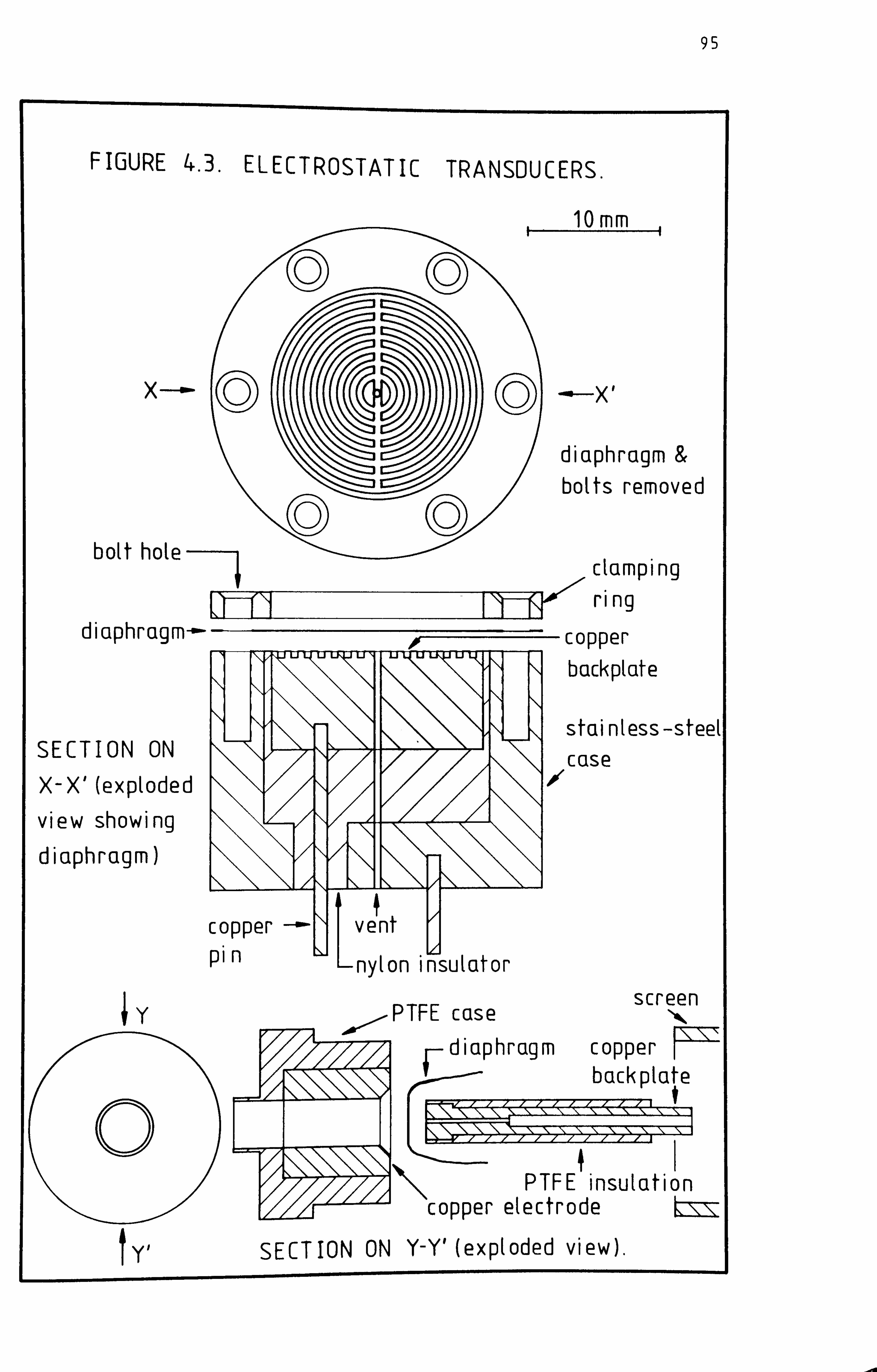
95

FIGURE 4.3. ELECTROSTATIC TRANSDUCERS.

f- 10

X---@-

,

DO

bolt hole

(D --O-X I

di ciphragm-m- ff

diaphragm & bolts removed

clamping ri ng

copper backplate

stain I ess-steell SECTION ON X-X' (exploded

view showing di ciphrcigm)

iy

c as e 01

PTFE case screen

di aph rag m copper backpla e

PTFE insulation copper electrode

f Y1 SECTION ON Y-Y' (exploded view),

Hi if L-nylon insulator

96

4.3 PIEZOELECTRIC TRANSDUCERS

The piezoelectric effect, by which a dipole moment is induced in

a solid when it is subjected to a mechanical stress, is exhibited by

certain crystals that lack inversion symmetry. At low temperatures,

ferroelectric materials can exist in two phases, one of which lacks

inversion symmetry and is piezoelectric. Above the f erroelectric

critical temperature (the Curie point) only the symmetric phase occurs,

and below that temperature the symmetric phase is usually of lower

energy, but the piezoelectric state may be metastable. Thus ferroelectric

materials may be rendered piezoelectric by cooling from a temperature

above the Curie point, in the presence of a strong electric field which

stabilizes the piezoelectric structure. At sufficiently low temperatures

the crystal structure will not revert to the symmetric form when the

electric field is switched off, and the material is permanently

polarized. However, if exposed to a temperature above the Curie the

material will depolarize. Quartz is one of the few crystals in which

the piezoelectric phase is truly stable below its Curie temperature, and

it does not therefore require polarization.

If a piezoelectric crystal is subjected to a mechanical force then

the resulting deformation causes a change in the dipole moment, and

hence alters the internal electric field. Conversely, if the crystal is

subjected to an external field then a force is generated within. it, and

a deformation occurs. Both these effects are linear and reversible (at

least for small changes). For practical purposes, metal electrodes are

deposited on opposite faces of the crystal; application of an alternating

force produces an alternating potential difference between the electrodes,

and vice versa. Unfortunately, unless the frequency is near to a natural

frequency of the crystal the effect is very small, and hence single

crystals, acting directly on the fluid, are usually only operated at

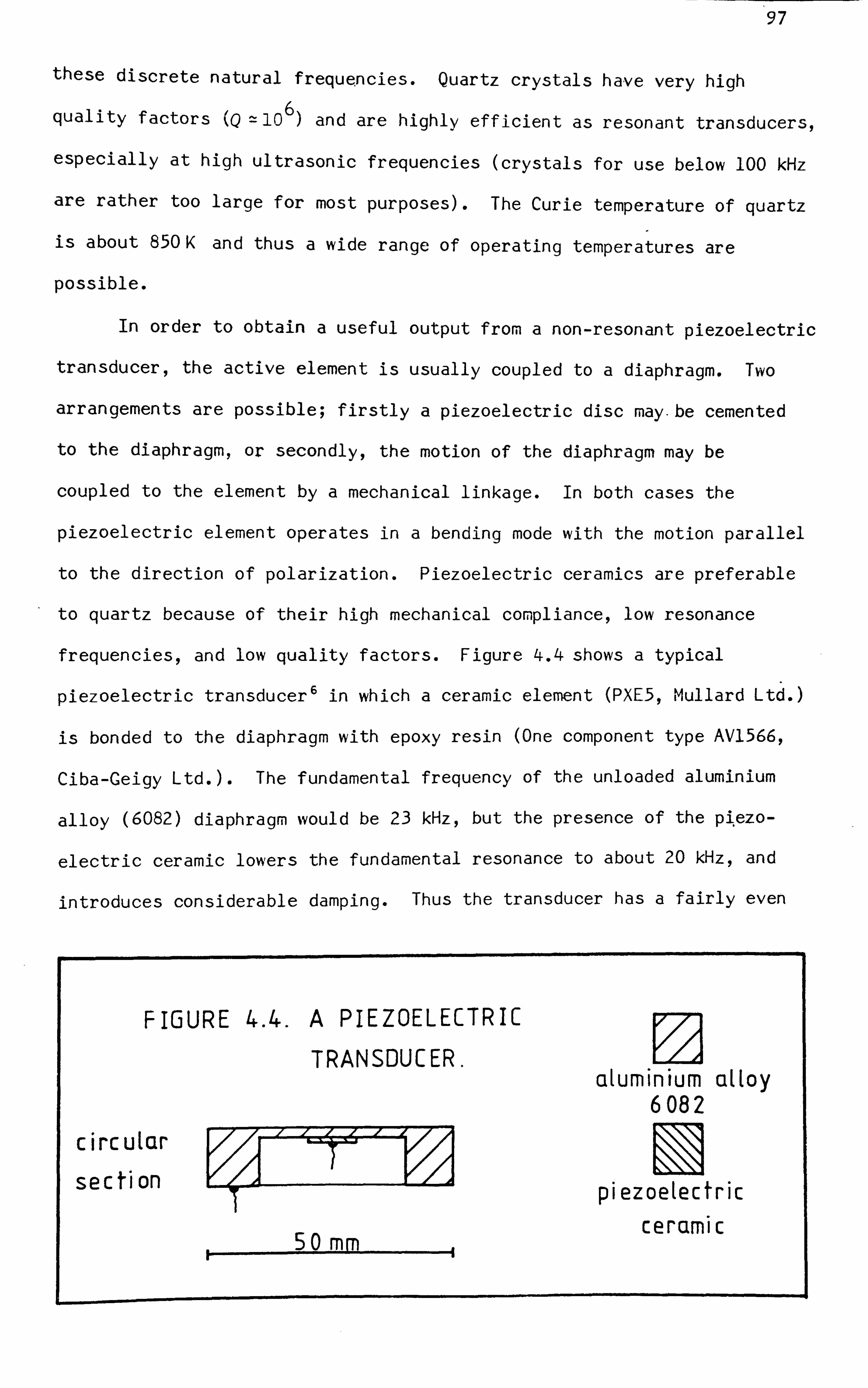
97

these discrete natural frequencies. Quartz crystals have very high

quality factors (Q =10 6)

and are highly efficient as resonant transducers,

especially at high ultrasonic frequencies (crystals for use below 100 kHz

are rather too large for most purposes). The Curie temperature of quartz

is about 850 K and thus a wide range of operating temperatures are

possible.

In order to obtain a useful output from a non-resonant piezoelectric

transducer, the active element is usually coupled to a diaphragm. Two

arrangements are possible; firstly a piezoelectric disc may. be cemented

to the diaphragm, or secondly, the motion of the diaphragm may be

coupled to the element by a mechanical linkage. In both cases the

piezoelectric element operates in a bending mode with the motion parallel

to the direction of polarization. Piezoelec-L-Iric ceramics are preferable

to quartz because of their high mechanical compliance, low resonance

frequencies, and low quality factors. Figure 4.4 shows a typical

piezoelectric transducer 6 in which a ceramic element (PXE5, Mullard Ltd. )

is bonded to the diaphragm with epoxy resin (One component type AV1566,

Ciba-Geigy Ltd. ). The fundamental frequency of the unloaded aluminium

alloy (6082) diaphragm would be 23 kHz, but the presence of the pýezo-

electric ceramic lowers the fundamental resonance to about 20 kHz, and

introduces considerable damping. Thus the transducer has a fairly even

FIGURE 4.4. A PIEZOELECTRIC

TRANSDUCER.

circular section

50 mm »

13

aluminium alloy 6082 E]

piezoelectric ceramic

98

response between resonances as well as in the low-frequency limit

(f <10 kHz). This device is used in the cylindrical interferometer at

frequencies somewhat above and below the first overtone (71 kHz), with a

sufficiently high efficiency being obtained between about 50 and 95 kHz.

The quality factor of the transducer at its first overtone is about 50,

and the static capacitance is 1.8 nF (thus stray capacitance in the

connecting leads does not lead to a great loss of signal). The maximum

operating temperature is about 370 K, and this is determined by both the

stability of the epoxy cement and the risk of thermal depoling of the

piezoelectric.

4.4 ACOUSTIC WAVEGUIDES

For a number of reasons, it may be desirable to install the

transducers outside the resonator, and to transmit and recieve the soun d

through hollow tubes. These waveguides may have a small cross-sectional

area, and therefore behave as approximately a point source and a point

detector. The tubes may terminate either in small chambers containing

the transducers, or at the more or less rigid surfaces of the transducers

themselves. The former arrangement allows the use of quite large

transducers, and if the "aveguides extend to a region of ambient

temperature then there are many commercial transducers that can be used.

In order to calculate the effects of an opening in the cavity wall

on its resonance frequencies and widths, the effective acoustic

impedance Z0 of its opening must be found. Narrow tubes (radius b<

length 1) are used, and the frequency must be below X ,. Iu/2Trb, the f irst

cut-off frequency, so that only plane waves propagate. This being the

case and letting z be the distance from the tube's opening into the

cavity, the impedance Z0 can be expressed in terms of the tube

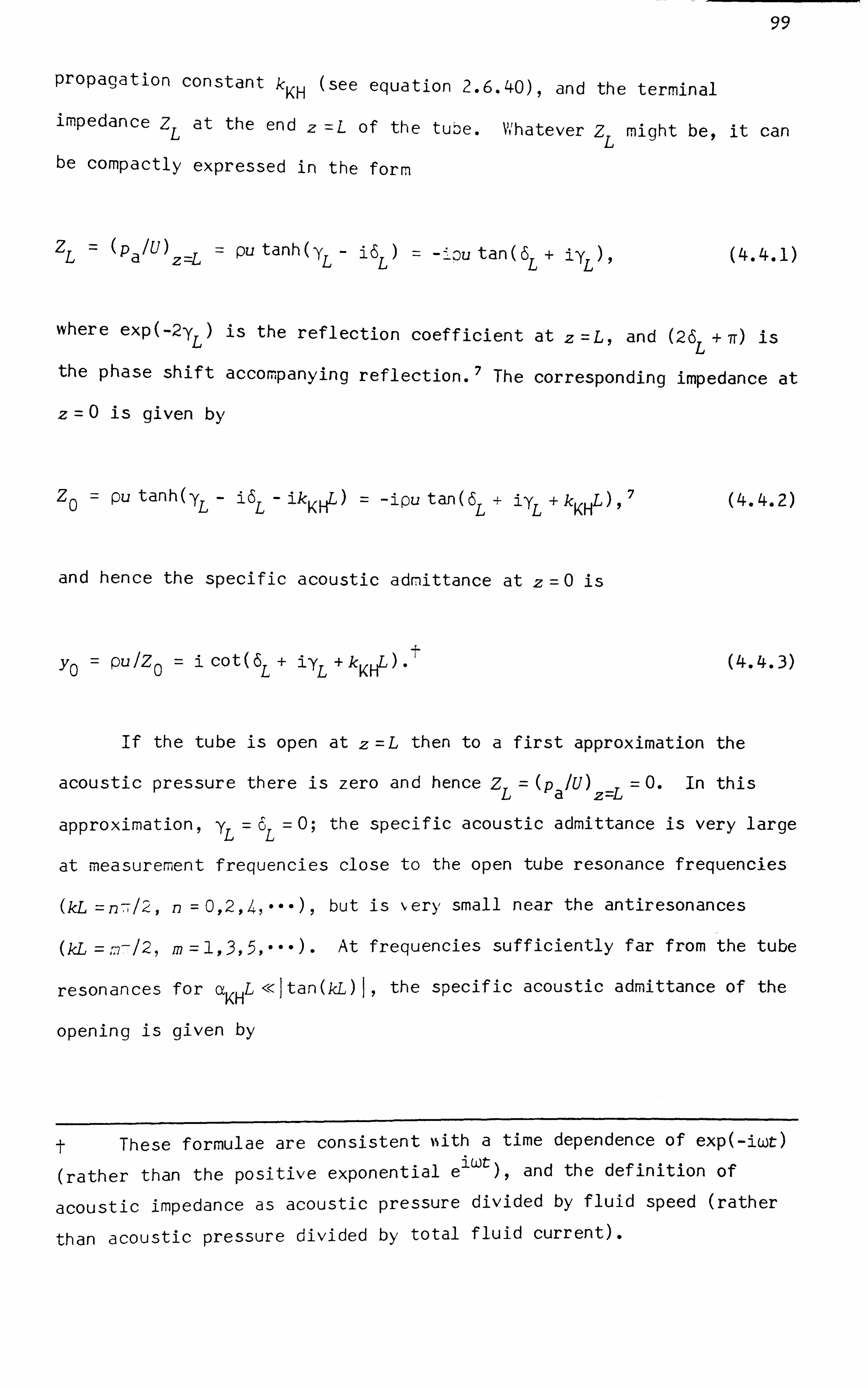
99

propagation constant k KH (see equation 2.6.40), and the terminal

impedance ZL at the end z =L of the tube. V, 'hatever ZL might be, it can be compactly expressed in the form

zL (p aIU)z=L = pu tanh(y - i6 -f-pu tan(6 + iy LLLL (L. 4.1)

where exp(-2-yL) is the reflection coefficient at z =L, and (26 L+ 7T) is

the phase shift accompanying reflection. 7 The corresponding impedance at

z= 0 is given by

Zo = pu tanh(-y L- j6 L- ik KHL) = -ipu tan (6L + iyL +k KH L), 7

and hence the specific acoustic admittance at z=0 is

-f- yo = pu /Z

0=i cot(6 L+ i-y L +k KH") *i

(4.4.2)

(4.4.3)

If the tube is open at z=L then to a first approximation the

acoustic pressure there is zero and hence ZL= (P a

/U) Z=L = 0. In this

approximation, YL = ri L=0; the specific acoustic admittance is very large

at measurement frequencies close to the open tube resonance frequencies

(kL =n-, I-, -,, n=0,2,4ý ... )

, but is \very small near the antiresonances

(kL =m-/2, m=1,3,5, ---)* At f requencies suf f iciently f ar f rom the tube

resonances for a KH L << I tan (kL) I, the specif ic acoustic admittance of the

opening is given by

t These formulae are consistent ý%ith a time dependence of exp(-iwt)

(rather than the positive exponential e'wt), and the definition of

acoustic impedance as acoustic pressure divided by fluid speed (rather

than acoustic pressure divided by total fluid current).

100

02 Yo =i cot(kL) + (aK,

-ý) cosec UL). (4.4.4)

The true terminal impedance of a tube open to free space differs from

zero because of the effects of radiation. In the case of a flanged

opening to free space the terminal impedance is given by

ZL = PU { -21(kb)

2- i8(kb)/37-i} ,' and hence

'YL = -21 (kb) 2, and

6L= 8(kb)/37, (4.4.5)

12 provided that f (kb) << 8(kb)/37 << 1 (consistent with the low frequency

conditions) , and hence equation (4) may be replaced by

02 yo =i cot (kL' )+ (oýHL ") cosec (kL where

L' =L+ 8b/3Tr, and

L+ (kb) 2 /2 (4.4.6)

are effective tube lengths. If, instead of opening to free space, the

tube ends in a chamber of volume V, whose internal dimensions are much

less than the wavelength, then the terminal impedance may be estimated

from a Helmholtz-resonator model. 9 Provided that there are no losses

within the chamber,

ZL= ipu7b 2 IkV, and hence

YL = 0, and

6L= Tan-'(Trb 2 IkV) ,

where 6L is an additional phase shift.

(4.4.7)

At frequencies such that (7Tb 2 IkV)

L=( Trb 2 IkV), and equation (4) may be replaced by

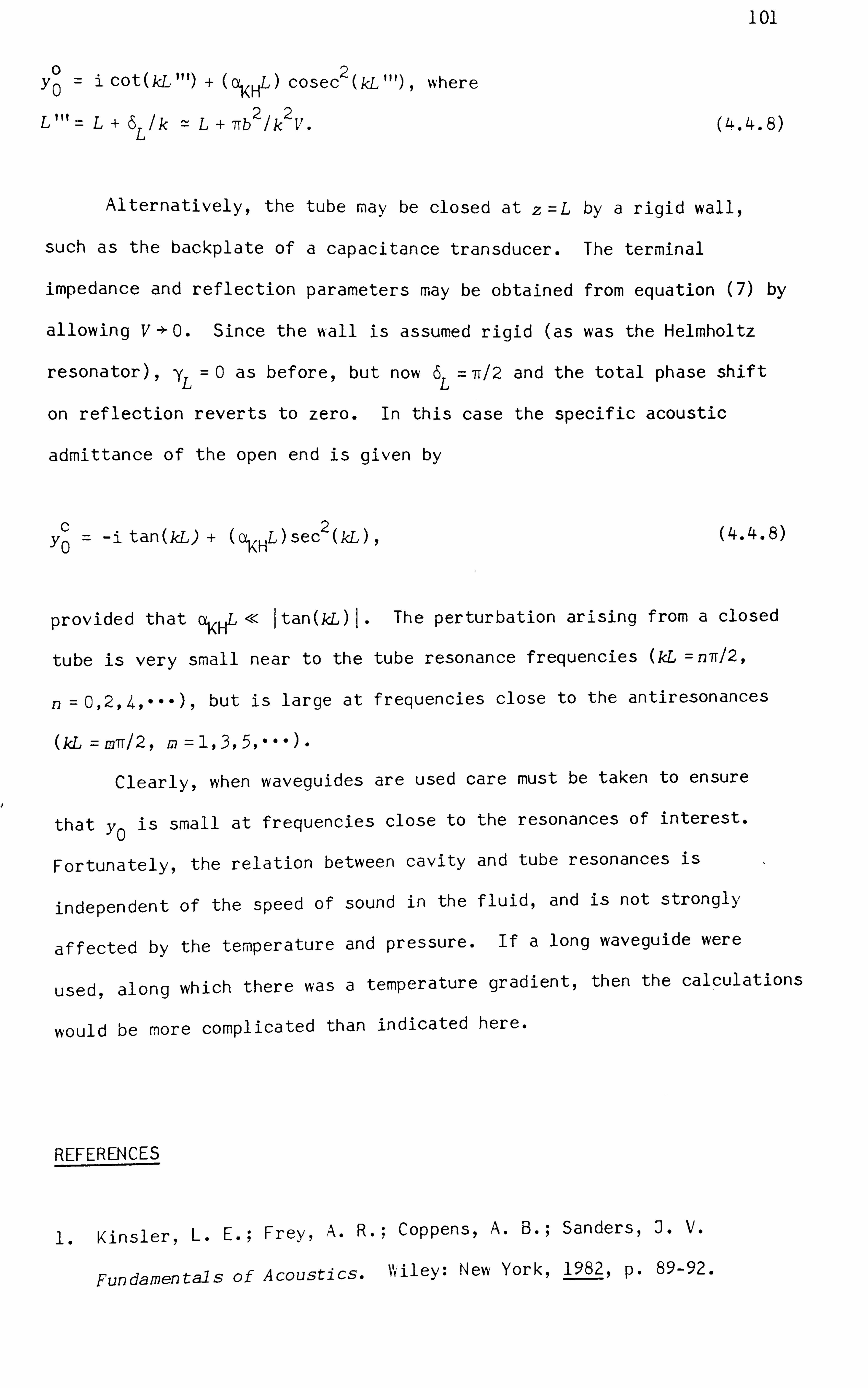
101

0 L) cosec 2 (kL ... ), where YO cot (kL + (OýH

L ... L+6LIkL+ 7Tb 2 Ik 2

V. (4.4.8)

Alternatively, the tube may be closed at z =L by a rigid wall,

such as the backplate of a capacitance transducer. The terminal

impedance and reflection parameters may be obtained from equation (7) by

allowing V -* 0. Since the wall is assumed rigid (as was the Helmholtz

resonator), yL =0 as before, but now 6L= 7T/2 and the total phase shift

on reflection reverts to zero. In this case the specific acoustic

admittance of the open end is given by

c= -i tan L) sec

2 UL) YO ( kL +H (4.4.8)

provided that Cý<H L << I tan (kL) I. The perturbation arising from a closed

tube is very small near to the tube resonance frequencies UL =n7T/2,

n=0,2,4P ---), but is large at f requencies close to the antiresonances

(kL = mTr/2, nj=1,3,5, ---).

Clearly, when waveguides are used care must be taken to ensure

that yo is small at frequencies close to the resonances of interest.

Fortunately, the relation between cavity and tube resonances is

independent of the speed of sound in the fluid, and is not strongly

affected by the temperature and pressure. If a long waveguide were

used, along which there was a temperature gradient, then the calculations

would be more complicated than indicated here.

REFERENCES

1. Kin5ler, L. E.; Frey, A. R.; Coppen5, A. B.; Sanders, J. V.

Fundamentals of Acoustics. VVýiley: New York, 1982, p. 89-92.

102

2. Reference (1), p. 92-95.

3. Morse, P. M. ; Ingard, K. U. Theoretical Acoustics. McGraw-Hill:

New York, 1968, p. 213-218.

4. Kuhl, W.; Schodder, G. R.; Schr*o*der, F. K. Acoustica. 1954,4,519.

5. Carey, C. ; Bradshaw, J. ; Lin, E. ; Carnevale, E. H. Experimental

Determination of Gas Properties at High Temperatures andlor Pressures.

Arnold Engineering Development Centre, Arnold Air Force Station,

TN37389, Report No. AEDC-TR-74-33, Available NTIS AD-779772.1974.

6. Piezoelectric Ceramics. Editors: Randeraat, J. Van; Setterington, R.

E. Mullard: London, 197 , p. 81-86.

7. Reference (3), p. 469.

8. Reference (1), p. 202.

9. Reference (1), p. 232.

103

CHAPTER

5.1 INTRODUCTION

HEEQUAT10N0FSTATEAND

IHERH0LECULARF0RCES

5.2 THE VIRIAL EQUATION OF STATE

5.3 INTERMOLECULAR FORCES

5.1 INTRODUCTION

This chapter deals with the equation of state for dilute gases.

The virial equation of state is introduced in section two and some

experimental techniques by which it can be studied are reviewed. The

role of the second virial coefficient as a determinant of intermolecular

potential energies is discussed in section three. Acoustic measurements

are seen to provide accurate information about the equation of state

which may be related directly, or indirectly through the second virial

coefficient, to intermolecular potential energies.

5.2 THE VIRIAL EQUATION OF STATE

For a single gas phase of f ixed composition there are two degrees

of freedom, and hence if any two intensive properties are held constant

then the thermodynamic state of the gas is invariant. However, in order

to specify that state, an equation of state is required to relate the

values of tý, -vo independent variables to the other equilibrium properties

of the gas. Explicitly, the equation of state:

104

Qy(yqx VX2 )=0

relates a third intensive quantity Y to the quantities X1 and X2

(5.2.1)

which are chosen as the independent variables. Specification of any

other intensive thermodynamic property requires a different mathematical

f orm of the equation of state in which the required property is the

dependent variable but, at least in principle, transformation from one

f orm to another simply requires the application of the appropriate

thermodynamic identities. Since equation (1) relates only intensive

variables, it contains no information about the extent of the phase.

The exact mathematical form of the function Q vm (vm T, p) in the

equation of state

QV (V m

T, p) =0 m

is known to be

Q= (pV IRT) - {1 + B(T)1V + C(T)1V2 + D(T) IV3 vmmmmm

(5.2.2)

(5.2.3)

where p is the pressure, VM is the molar volume, and T is the temperature,

and where R is the gas constant. Equation (3) is the virial equation of

state and B, Cq Dq ... are the second, third, fourth, --- virial

coef f icients and, f or a gas of f ixed composition, are f unctions of the

temperature only. In a sufficiently dilute gas, the series on the right

of equation (3) is found to converge rapidly. The importance of the

virial equation of state lies in its theoretical basis; the virial

coefficients B, C, D,. --- are related to the intermolecular potential

energies of clusters of two, three, four, --- molecules at a time. For

this reason precise measurements of the second virial coefficient can

be used to infer information about the intermolecular pair-potential-

105

energy functions of the interacting molecules. In a gas mixture B will

depend upon interactions between both like and unlike molecules, and

hence on more than one intermolecular pair -potential -energy function.

In particular, the second virial coefficient B(T, x) of the binary gas

mixture { (-- - x)A + A) is given by

(T, x) = (--, - x) 2B

AA + 2(1 - x)xB AB +x2B BB' (5.2.4)

where B AA and B BB are the second virial coefficients of pure A and of

pure B, and B AB is the second virial coefficient that arises from the

unlike interactions between molecules of A and of B.

From an experimental point of view the best choices for the

independent variables are often the temperature and the pressure of the

gas because both can be measured and controlled with high precision.

Thus a pressure-explicit expansion of the molar volume may be preferable

in the equation of state:

(pv m

IRT) =1+ NpIRT) + Np 2 IRT) + D(P3 IRT) + (5.2.5)

in which the coefficients P, ý!, D, ee* are related to the virial I

coefficients by

ý=B, ý= (C -B2) IRT, D= (D - 3BC -Z 2B 3)/ (RT) 2ý000* (5.2.6)

Both equation (3) and equation (5) contain infinite series which

must be truncated for practical purposes. It is not usually difficult

to find the finite series i--, bich best represents a given set of (p, V m9

T)

measurements, but the problem of f inding the values of the virial

coefficients %Nfilch are closest to the true values in the infinite series

is more subtle. It is not always possible to obtain accurate results

1 06

at sufficiently low pressures for all of the coefficients above the

second to be neglected, and incorrect truncation of the series can introduce large systematic errors into the determination of the second

virial coef f icient. This problem is eased if precise measurements can be extended to as low a fraction of the maximum pressure as is possible.

The difficulties that are inherent in any direct study of the

equation of state in the form of (3) or (5) stem mainly from the

measurement of molar volume. A direct measurement of that quantity

is not possible and it is necessary to know both volume and amount of

substance n separately, although n may be inferred from the value of

Limp _* O(pVIRT). The simplest apparatus used in the study of the

equation of state is Boyle's tube in which the pressures exerted by a

f ixed amount of substance are measured at known volumes while the

temperature is held constant. A variant on this apparatus is shown in

figure 5.1. In this apparatus a fixed amount of substance is confined

above mercury and allowed to expand into several previously calibrated

volumes under isothermal conditions, the pressure being measured after

each expansion. A null-reading pressure transducer is used to isolate

the sample f rom the external pressure gauge, but the accessible

temperatures are still limited to those at which mercury is a liquid and

has an acceptable vapour pressure. Although the amount of substance in

the apparatus is constant throughout the experiment, the amount in the

gas phase will depend upon the extent to which the material adsorbs on

the walls, and that is a function of the pressure. At low reduced

temperatures t

gas adsorption can be severe under experimental conditions

and large systematic errors in the second virial coefficient can result.

In order to separate the effects of the second virial coefficient

from those of the higher-order terms in the virial equation of state,

t In this context the reduced temperature Tr= TIT c, where Tc is the

critical temperature of the fluid.

107

thermostat

---4- to manometer

pressure transducer

FIGURE 5.1. A MODIFIED BOYLE'S TUBE APPARATUS

sample gas

mercury

L_____I to mercury suppty

FIGURE 5.2. A DIFFERENTIAL BURNETT APPARATUS

thermostat_

3 BAcD

145

i to vcicuum

I

to manometer i

to Vacuum

108

it is desirable to pursue measurements at low pressures. However, at

low pressures the gas imperfections are slight (usually contributing

less than 5 per cent of vm at a pressure of 100 kPa) and very precise

measurements of the dependent variable are required in order to resolve

B with useful precision.

Many of the difficulties outlined above may be overcome or reduced

in more sophisticated experiments, such as the one devised by Burnett. '

In this method two vessels A of volume VA and B of volume VB are

connected via valve 1 as shown in figure 5.2. The smaller vessel B is

connected via valve 2 to a vacuum pump, and vessel A is connected to a

null-reading pressure transducer 3 ýNhich isolates the sample gas from

an external manometer or pressure balance. Initially, vessel A contains

the sample gas at the highest pressure to be studied, valve 1, is closed,

and vessel B is evacuated. The pressure po =po(no, V A) corresponding to

the amount of substance n occupying the volume V is measured. Valve 2 0A

is then closed and the gas allowed to expand through valve 1 so that the

same amount of substance occupies the volume VA+VB. Once thermal

equilibrium has been achieved, valve 1 is closed and the new pressure

p, =: pl(no, VA+VBp, (nj, VA) is measured. Valve 2 is then opened to

evacuate vessel B and an amount of substance n1 remains in the appara. tus.

This procedure is repeated until a low pressure is achieved. Since the

pressure p q-1 before the q

th expansion is

pq-1 = in q-1

RTI VA )fl + B(p q-1

IRT) + ---) (5.2.7)

and the pressure pq following the q th

expansion is

Pq = {n q-1

RTI (VA + VB)){' + B(p q

IRT) +-- -} 9 (5.2.8)

the ratio (p q-1

/P q)

is given by

1 09

(p q-1

/P qNa+Na

(N a-

1)B(p q

IRT)

where the apparatus constant N- (V V )IV aABA

(5.2.9)

Thus a plot of (p q- J/P q)

against pq has the slope Na (N a-

1)BIRT and the value Na in the limit

Pq 4- 0, and hence such measurements can determine the second virial

coefficient without the need to measure either amount of substance or

volume. Unfortunately, very accurate measurements of the pressure are

required and it is not easy to meet this requirement over a wide range

of pressures. A differential method 2 can be employed to reduce the

influence of random errors in the measurement of pressure. Again

referring to figure 5.2, a second Burnett apparatus consisting of vessels

C and D, and valves 4 and 5, is connected in parallel with the manometer,

and the null-reading pressure transducer 3 is replaced by a differential

manometer. The reference apparatus is filled with a gas whose equation

of state is accurately known, and the experiment proceeds as before on

each side of the differential manometer. However, it is now only

necessary to measure one of the pressures accurately with the external

manometer; the other pressures are calculated from the small measured

pressure differences Lp q

across the differential manometer and the.

equation of state of the reference gas. This technique is one of the

best methods of studying the molar -volume -explicit equation of state

and may be used over a wide range of temperatures and pressures. A

precision of 1 cm 3

-mol- 1 in B is possible from measurements conducted at

pressures below 100 kPa. However, adsorption may still cause systematic

errors in the measurements. In the Burnett method, the effects of

adsorption can be reduced by design of vessels having equal surface-

area-to-volume ratios; the increase in available surface for adsorption

following an expansion is than approximately balanced by the reduction

in the total pressure. In any (p, Vm T) experiment the microscopic

surface area available for adsorption may be reduced by careful polishing

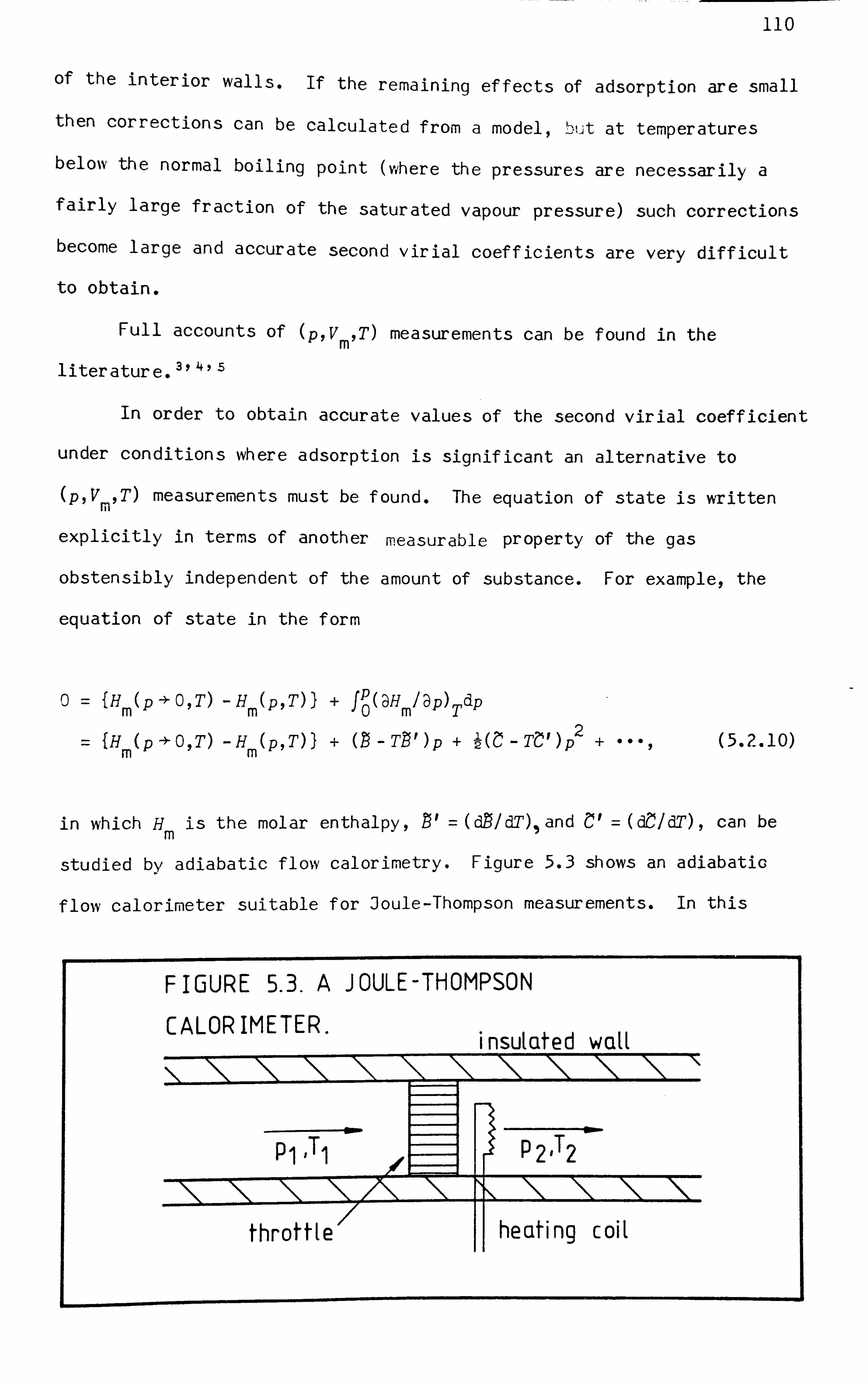
110

of the interior walls. If the remaining effects of adsorption are small

then corrections can be calculated from a model, !, D-ut at temperatures

below the normal boiling point (where the pressures are necessarily a

fairly large fraction of the saturated vapour pressure) such corrections

become large and accurate second virial coefficients are very difficult

to obtain.

Full accounts of (p, V m

T) measurements can be found in the

literature. 3y4ý

In order to obtain accurate values of the second virial coefficient

under conditions where adsorption is significant an alternative to

vm T) measurements must be found. The equation of state is written

explicitly in terms of another measurable property of the gas

obstensibly independent of the amount of substance. For example, the

equation of state in the form

0= fH (p->-0, T) -H (p, T)) + fp(aH 1ýp) dp mm0mT

2 = IH

m (p -*- 0, T) -Hm (p, T)) + (P -TP')p + -21- Tý' )p (5.2.10)

in which Hm is the molar enthalpy, P' = (dP/dT),, and Zý' = Wlff), can be

studied by adiabatic flow calorimetry. Figure 5.3 shows an adiabatic

flow calorimeter suitable for Joule-Thompson measurements. In this

FIGURE 5.3. A JOULE-THOMPSON

CALORIMETER. i nsulated wait

pj, Tj

throttle

P2, T2

heating coil

ill

apparatus, the gas under study flows at a constant rate '(dn/dt) through

a thermally insulated tube fitted with a throttle and an electric

heater. The temperatures T1 and T2, and the pressures p, and P2' on

each side of the throttle are measured, together with the molar f low

rate. In the isothermal Joule-Thompson experiment, an electrical power

P is dissipated in the heater so as to maintain T2 =T 1- The isothermal

Joule-Thompson coefficient is defined by

ýJT -': OH/3p) -' Limp I {H (T, -H (T, pl) (5.2.11) T ':

1+ P2 P2) '/(P2 -Pl)j'

and measurements of pl, P21 P, and (dn/dt) under steady-state conditions

can serve to determine

{H m

(T, P2) -HM(T, pl)) = P/(dn/dt)

Teý 22 TP 2 (P2 - pl) + (P2 - pl) +

(5.2.12)

and hence to obtain (ý - TPI ) from such measurements over a range of

pressures. Once the steady state is established, these measurements

should be independent of adsorption but are nevertheless very difficult

in practice. The main experimental difficulties arise from the presence

of temperature gradients near the throttle and the need to maintain

very steady gas flow. However, despite the considerable experimental

difficulties, reliable measurements of (P - TP) have been made under

conditions where adsorption would have been a serious problem in a

conventional (p, V m

T) apparatus. '

The speed of sound in a gas is also formally independent of the

amount of substance and can be measured with high accuracy. The

equation:

2 (11PKS)

112

provides a link between a directly measurable mechanical property of

the gas and the thermodynamic property o, K S of that gas. In order to

specify the state of a gas from (u 2 J, p) measurements, an equation of 0

state is required that is explicit in u This may be achieved by 0

expanding both q and KS : -- 'ff T in terms of equation (5) with the result:

A (T) +A T) p+A (T) 02

where

(5.2.14)

A0 (T) = (RT-Ypg1M),

A1 (T) = (-ypg /. V) f; -P + (-ypg - 1) TP' + (-Ypg - 1) 2T2 pit/yPg), and

A2 (T) = (-yPg/, ',, ) (ypg + 2)ý! + 2(-ypg - DTýl + (-yPg - 1)2 T2 ý"/2-yPg) + G(T)

(5.2.15)

In equations (15) P" = (d 2p/dT2 ) and ý11 = (d 21ý/ ClT 2), G(T) is given by

-Ypg - -Y pg _ 1)2)? (p )2 +{(, Ypg _ 1)31, yPg)T

4(ý ff) 2 G(T) = (11RT) Jý4 --; - {( 1)+4(

4(-,. -Pg - 1) TM' + 2{ (ypg - 1) 2 /-ypg)T 2 pp it +

2{ (-ypg _ 1)2 (2ypg - 1) /-ypg)T 3pipt, 1, and (5.2.16)

-yP9 = Limp_*C(C P? m

/C Vým

) (5.2.17)

is the perfect-gas value Of Y' t In a sufficiently dilute gas, equation

(14) is found to converge rapidly. The coefficients A,, A2, A3, --- are

functions of the temperature only (for a gas of fixed composition) and

the related quantities

The algebraic complexity of this transformation increases

dramatically with the inclusion of higher powers of the pressure. A

treatment of the problem, correct to second order in p, is given in

appendix A5.1.

1 13

%= (iV/-ypg)A 11 'Ya = (M/ypg)A

2'000 (5.2.18)

will be referred to here as the second, third, --- acoustic virial

coefficients. The second acoustic virial coefficient may be related to

the intermolecular pair -potential -energy functions of the gas molecules

in a similar manner to B, but a single measurement is insufficient to

determine B which instead may be obtained from measurements of ýa over

a range of temperatures. Numerical techniques have been devised for

this purpose, 7 and for the purpose of computing a wide range of

thermodynamic properties of gases from their u 2_

explicit equations of 0 state. 8' 9 Thus equation (14) retains both the experimental and the

theoretical advantages of the virial equation of state while allowing

speed-of -sound measurements to be substituted for the difficult

measurements of the molar volume.

With the notable exception of a few simple fluids such as CO 21

which can exhibit marked dispersion at audio frequencies, u0 may easily

be obtained from low frequency (below 20 kHz) measurements of u because

u -* u as w 0 the speed of

dropped. An

measurements

0. In

sound

impor

of U2

the remainder of this work it will be assumed that

is identical with u0 and the subscript will be

tant advantage of the acoustic technique is that

with a precision of 1 x1O- 5

or better may be extended

to pressures well below 100 kPa and, in favourable circumstances, to

below 10 kPa. As a result a precision of ±0.1 cm 3.

mol- 1 in ýa can be

attained and measurements over a wide range of temperatures should

provide a severe and reliable test for any proposed intermolecular

potential-energy function.

Although formally independent of the amount of substance, it has

become apparent recently that in some circumstances speed-of -sound

measurements are affected by gas adsorption or precondensation. Both

experimental 10 ' 11 and theoretical 11 evidence shows that substantial

114

errors occur in low-frequency measurements when the pressure is close to

the saturated vapour pressure. The theoretical work also suggests that

a smaller effect may occur at much loý-, er pressures, but as yet there

appears to be no supporting experimental evidence. These effects arise

from condensation and evaporation from the adsorbed film during the

acoustic cycle and make a contribution to the effective acoustic

admittance of the resonator's walls. At pressures approaching saturation,

this excess wall admittance becomes very large, particularly at low

frequencies, and the resonance half "idths increase greatly. Such

discrepant results can easily be identified and rejected but, in order

to verify that low-pressure results are truly unaffected by adsorption,

it is necessary to study the same gas in resonators having different

surface-area-to-volume ratios. This possible source of error in low-

pressure acoustic measurements should be investigated with caution, but

it must be noted that the magnitude of the predicted effects at low

pressures are very much smaller than either the proven systematic errors

in conventional (p, V m

J) measurements, or the errors in low-pressure

Joule-Thompson measurements.

Acoustic interferometry in gases is also of importance in metrology.

Measurement of A0 at the temperature of the triple point of water, whiý, re

T=273. --6 K by exact definitiong in a gas for which N and -ypg are

accurately known, can serve to deter-mine the universal gas constant R.

The currently accepted value of the gas constant has a fractional random

uncertainty of some 93 x 10 -6 ,

12 but recent measurements of A0 in argon

have provided a new value which is numerically close to the accepted

-6 value but with a fractional random uncertainty of only 18 x 10 and a

similar level of systematic uncertainty). t 13 These measurements were

perforimed in a variable-pathlength cylindrical interferometer operating

These uncertainties are based on three standard deviations.

1 15

at 5.6 kHz. New meaurements in a spherical resonator should be capable

of defining R with even higher precision. The most probable source of

error on such measurements, namely the determination of the mean radius

of the resonator, is quite different to the sources of error in the

variable-path interferometer, and hence new measurements would provide

independent verification of the earlier work.

Measurement of the ratio A0 (e)/A 0

(T = 273-16 K) , where 6 is an

empirical temperature, can be used to evaluate the true thermodynamic

temperature T(e) without exact knowledge of R and M. Alternatively if

both R and M are treated as known constants then a single measurement of

A0 (e) is sufficient to determine T(e). At temperatures below about 20 K

the uncertainty in R is unimportant and measurements of the speed of

sound in helium have been used to the obtain the true thermodynamic

temperatures of a number of If ixed-points' between J+. 2 and 20 K. 14

It seems likely that future measurements will be extended into a wider

range of temperatures, and that spherical resonators will be preferred

to the conventional variable-pathlength cylindrical instruments. At

temperatures below the critical (5-4 K for helium, 151 K for argon)

precondensation may lead to systematic errors that are significant -in

comparison with the random uncertainties, but these are expected to be

much smaller than the corresponding effects in a conventional gas

thermometer. At any temperature desorption of impurities from the walls

of the resonator can change the mean molar mass and give rise to a

systematic error.

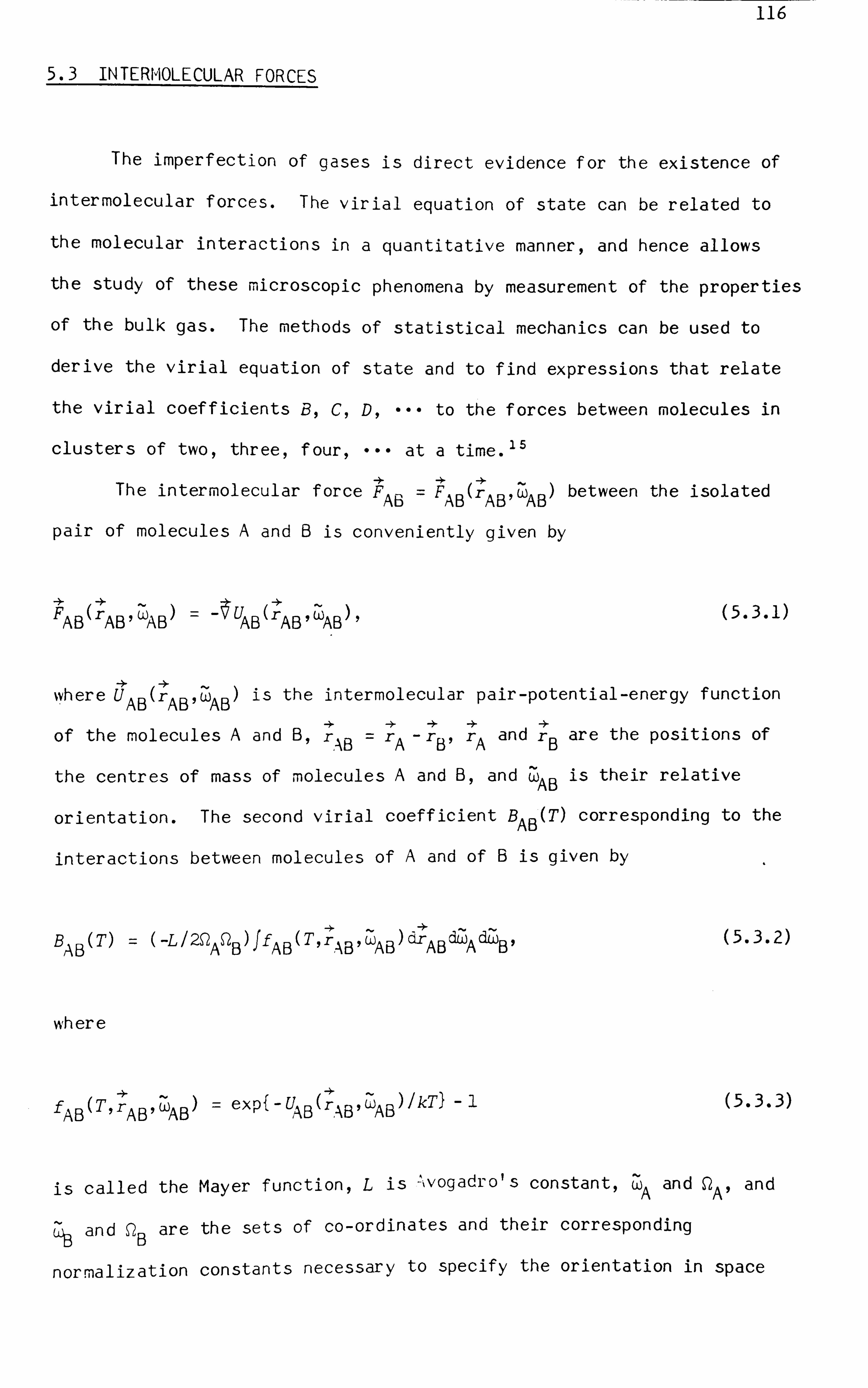
116

5.3 INTERMOLECULAR FORCES

The imperfection of gases is direct evidence for the existence of

intermolecular forces. The virial equation of state can be related to

the molecular interactions in a quantitative manner, and hence allows

the study of these microscopic phenomena by measurement of the properties

of the bulk gas. The methods of statistical mechanics can be used to

derive the virial equation of state and to f ind expressions that relate

the virial coefficients B, Cq Dq ... to the forces between molecules in

clusters of two, three, four, --- at a time. 15

4- The intermolecular force T" F Cr ý) between the isolated W AB AB ABI AB

pair of molecules A and B is conveniently given by

rwUrw FAB( AB' AB AB('AB' AB)' (5.3.1)

wh ere U AB (r

AB'w is the intermolecular pair-potential-energy function AB

of the molecules A and B, rrr,,, r and r are the positions of , AB AAB

the centres of mass of molecules A and B, and ý is their relative WA B

orientation. The second virial coefficient B AB (T) corresponding to the

interactions between molecules of A and of B is given by

BAB (T) = (-L/2Q AQ B)ff -) dý dý) A d'B' (5.3.2)

AB( T, r AB'WAB AB

where

fAB (T, rw exp{ (r. I IkT) (5.3.3) AB' AB -% AB'WAB

is called the Mayer function, L is -, vOgadro's constant, and and wA A'

and Q are the sets of co-ordinates and their corresponding 'ý3 B

normalization constants neces5ary to 5pecify the orientation in space

117

of molecules A and B, and the, integration is performed over all possible

positions and orientations. 16 The Eulerian angles e, ý, and ý) may be

used to specify the orientation of a molecule. For a monatomic molecule

no orientational angles are required and Q=1 and dw = 1. Two angles are

required for a linear molecule (dw = sin6dedC, Q =47), and for a non-

linear molecule three are required (dw = sined6dýdiý, Q= 47 2)-

In describing intermolecular f orces with a pair -potential -energy function, it is assumed that the intermolecular degrees of freedom are

distinct and independent from the remaining degrees of freedom of the

particles in the system A+B. However, in a formal sense a dif f erent

intermolecular pair -potential -energy function is required to correspond

to each of the allowed internal states of the molecules. This is certainly

the case with the electronic degrees of freedom, but electronic excitation

from the molecular ground state is slight at all accessible temperatures

f or most simple molecules and can the. ref ore be neglected. Since inter-

molecular forces are electrostatic in origin, they are coupled to the

vibrational and rotational states of the interacting molecules by the

effects of anharmonicity and centrifugal distortion, but these phenomena

usually have only a slight influence on the geometry and electron .

distribution of the molecules. In consequence, it is a reasonable

approximation to separate the internal and intermolecular degrees of

freedom and to seek a single potential-energy function. The dimension-

ality of that function, and hence the number of co-ordinates over which

it must be integrated in order to obtain B ABI depends upon the nature

of the interacting species:

atom+ atom :1 degree of freedom, QAQB=1

atom+ linear molecule :2 degrees of freedom, QAQB= 4Tr

atom+ non-linear molecule :3 degrees of freedom, QAQB= 87T 2

linear molecule +linear molecule :4 degrees of freedom, Q AQB = 167T 2

118

linear molecule +non-linear molecule : 5 degrees of freedom, Q AQB = 327T 3

non-linear molecule +non-linear molecule :6 degrees of freedom,

4 QAQB = 64Tr

In the case of the interaction between like atoms, equation (2)

is greatly simplified because fAA = jexpj -U (A IkT) - 11 9 2drsinededý

C'rAA =r

and thus

B(T) = -iLf7Tsin6def2ndýf"Dýexp{-U(r)/k7) -llr 2 dr 000

CO 2- -27TL f0f exp { -V (r) lkT) - 11 r dr, (5.3.4)

where r is the interatomic separation. Since U(r) -* 0 as r+ oo, the

Mayer function falls off to zero at large separation and the integration

in equation (4) presents no difficulty.

The derivation of the virial. equation of state is based entirely on

classical mechanics, and it is kno"n that for light molecules. at low

temperatures the wave-like properties of the particles cannot be

neglected. For H2 and He the classical theory fails completely at low

temperatures and a full quantum mechanical treatment is required. 17

However, for all other substances this is unnecessary and a semi-cl, ýssical

approach is successful. The second virial coefficient may be expanded

in a series of powers of (-h 2 /m):

B=B qO +B ql

(-h 2 hn) +B q2 (-h 2 /M) 2+B

q3 (-h 2 /M) 3+000ý (5.3.5)

where m is the mass of one molecule, -h =h/2Tr, and h is Planck's constant.

The leading term in equation (5), B qO

is the result of the classical

t Here (r, e, ý) are the spherical co-ordinates introduced in chapter

2. The origin is located at the centre of mass of one of the interacting

molecules and the angles are measured relative to laboratory fixed axes.

119

treatment, and expressions for the next three coefficients are all

known for spherically syr-mmetric potential -energy functions, ""' This

series is found to converge within three terms for all substances other

than hydrogen and helium at low te. -iiperatures.

Equation (3) is readil,. differentiated with respect to the

temperature ant it is therefore a simple matter to relate the acoustic

virial coefficient to the intermolecular pair -potential -energy function

of the molecules making up the gas. Thus f or a pure monatomic gas (for

which Ypg = 5/3 exactly) at the temperature T

ý (T) = -4TE fýf {1+ 6/ 15) k-T) + (2 / 15) (U / kT) 2 )exp(4JIkT) -ljr 2 dr, (5.3.6)

a0

where U =U(r). It has been suggested by Blatt that the methods of

statistical mechanics may be unreliable in a system subject to

displacements from equilibrium that occur at frequencies above the

ternary molecular collision Irequency. 'O Blatt predicts that ýa is a

function of the frequency and that the value of equation (6) is attained

in the limit w->-O. Substantially above the ternary collision frequency,

% is predicted to be zero. This effect should be quite obvious in

accurate measurements of u in the heavier monatomic gases but there is

no experimental evidence to suggest that it does in f act occur.

Expressions may also be derived to relate the higher virial

coefficients to intermolecular energies, but these are complicated by

the need to evaluate the energy of clusters containing more than two

molecules. In such clusters the pair-wise interaction energies are

perturbed by the presence of other molecules, and the total energy of

a system of N molecules is given by

TN (2) U(3) (r rr W) + UTotal "-- Li<ju ij W) 'i<j<k ij jk ki'

+IN ýN)

(r. r., 0009 1) (5.3.7) i<j< _k9

120

where U(4), U(---) , --- are the pair-, triplet-, --- potential-energy

functions, r ij . is the distance betNseen molecules i and j, and w stands

for the relative orientation of the molecules in the cluster. Thus the

third virial coefficient is determined not only by the three pair-wise

interaction energies of a triplet of molecules, but also by a fourth

term uniquely associated with the presence of three molecules. Although

equation (7) converges rapidly in dilute systems, many-body interactions

are important in determining the properties of solids and dense fluids,

and are a limitation on the information about pair -interaction energies

that can be gained from a study of such properties.

The wide range of experimental and theoretical methods by which

pair-wise intermolecular forces are studied have been reviewed in detail

by Maitland, Rigby, Smith, and Vi'akeham in their recent monograph; 21 here

it will be sufficient to concentrate on the role of the second virial

coefficient.

The traditional approach to the determination of intermolecular

potential energies f rom measurements of B(T) was to assume some simple

functional form for the intermolecular energy, usually of spherical

symmetry, containing two or more disposable parameters which are then

varied in order to achieve the best f it to the experimental results. ,

This usually tells one little about intermolecular forces because

different assumed functional forms can show widely different shapes for

U(r) i%bile retaining a good fit to the second virial coefficient. For

example the crude 'square-%vell potential':

co

= -E: cj<r<g0

= r> (5.3.8)

which on substitution in (4) gives

121

B(T) = (2TrLO3/3)tg 3_ (g 3_ 1)exp(E/kT)I, (5.3.9)

shojvS good agreement with the second virial coefficients of argon between

150 and 1000 K with a=0.3021 nm, g=1.641, and ( Elk) = 105.6 K. 22 While

equation (9) is useful for the correlation of second virial coefficients

it is of only limited value in the determination of intermolecular

potential energies. The function

U(r) = E: j f ml (n - m) ) (relr)r' -f n1 (n - m)) (r e

1r)R'j, (5.3.10)

attributed to Lennard-Jones, 23 but first proposed by Mie, 24 contains

f our adjustable parameters: c and re, the depth of the potential-energy

well and the intermolecular separation at which U(r) = -F-, are scaling

parameters, while m and n are shape parameters and determine the steepness

of the attractive and repulsive branches respectively. Of ten m is

taken as 6, in accordance with the known long-range dependence of the

intermolecular energy, and n as 12. Although clearly more realistic than

equation (8), and useful in model calculations and for modest

extrapolations of experimental results, the Lennard-Jones function is

a poor representation of those intermolecular potential-energy functions

that are known in detail. However, the modified form suggested by

Maitland and Smith, 25 in which m=6 and n is a linear function of r,

does give a good account of the known intermolecular potential-energy

functions of the nobel gases. 26

The problem is one of uniqueness: U as a function of r uniquely

defines B as a function of T (for a spherically symmetric system ), but

the reverse is not true. This becomes apparent when equation (4) is

recast in the f orm

co B(T) = (27TLa/3T)foMý)exp(-ýW)dý

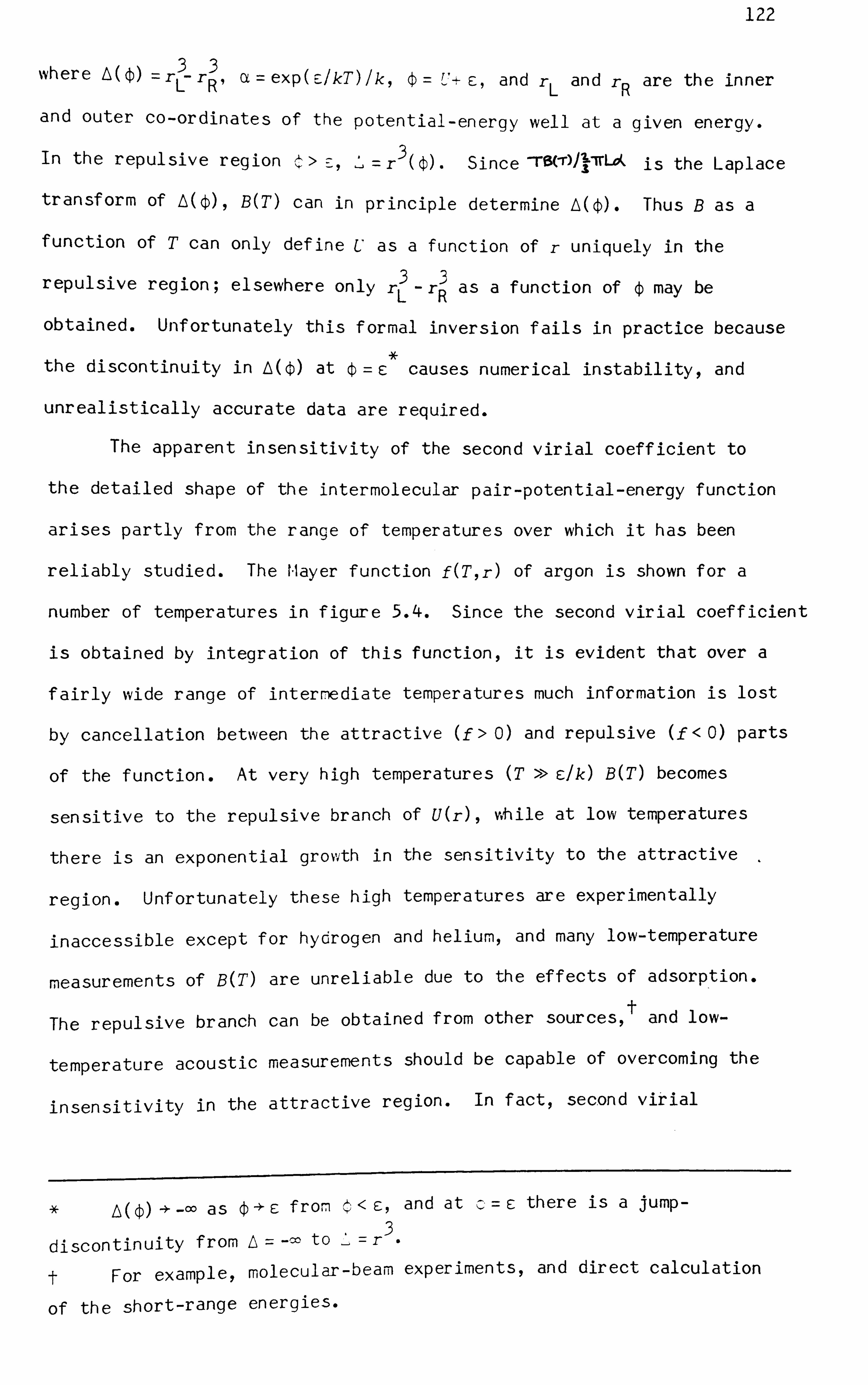
122

where AW =rý-r , a=exp( IkT)lk, ý= 7'-- F-, and rL R and r are the inner LR

and outer co-ordinates of the potential -energy well at a given energy.

In the repulsive region > r3 W. Since -TS(-r)J'61TLd .&,

is the Laplace

transform of Mý), B(T) can in principle determine Mý). Thus B as a

function of T can only define U as a function Of r uniquely in the

repulsive region; elsewhere only r3_ r3 as a function of ý may be LR

obtained. Unfortunately this formal inversion fails in practice because

the discontinuity in Mý) at ý= c* causes numerical instability, and

unrealistically accurate data are required.

The apparent insensitivity of the second virial coefficient to

the detailed shape of the intermolecular pair -potential -energy function

arises partly from the range of temperatures over which it has been

reliably studied. The I-layer function f(T, r) of argon is shown for a

number of temperatures in figure 5.4. Since the second virial coefficient

is obtained by integration of this function, it is evident that over a

fairly wide range of intermediate temperatures much information is lost

by cancellation between the attractive (f > 0) and repulsive (f < 0) parts

of the function. At very high temperatures (T >> elk) B(T) becomes

sensitive to the repulsive branch of U(r) , vfiile at low temperatures

there is an exponential growth in the sensitivity to the attractive

region. Unfortunately these high temperatures are experimentally

inaccessible except for hydrogen and helium, and many low-temperature

measurements of B(T) are unreliable due to the effects of adsorption.

t The repulsive branch can be obtained from other sources, and low-

temperature acoustic measurements should be capable of overcoming the

insensitivity in the attractive region. In fact, second virial

-co as cf rom <c, and at E: there is a jump- 3

discontinuity from -co to r For example, molecular-beam experiments, and direct calculation

of the short-range energies.

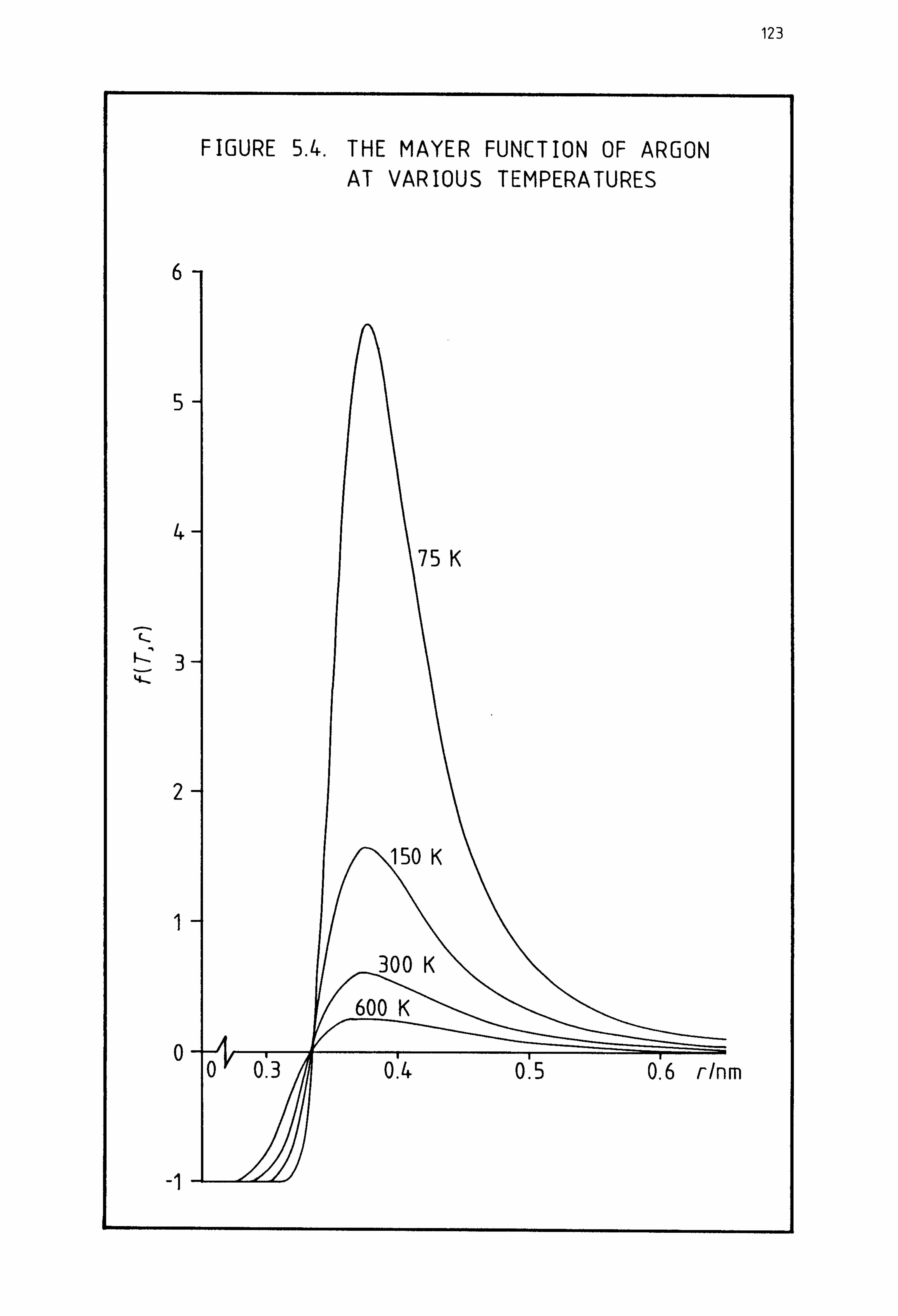
123

FIGURE 5.4. THE MAYER FUNCTION OF ARGON AT VARIOUS TEMPERATURES

6-

5-

4- 75 K

3-

2-

150 K

1

300 K

600 K

0- 0 0.3 0.4 0.5 0.6 r/nm

124

coefficients can be a much more sensitive probe of intermolecular energies

than either the results obtained with simple functional forms or the

formal inversion suggest. In recent years a number of inversion methods V have been devised by which the intermolecular pair-poten tial -energy

functions of spherically sy -metric molecules may be extracted from second

virial. coefficients which span an accessible range of temperatures with 27928929 a realistic accuracy. The most sophisticated of these methods

can yield the complete function U(r) between upper and lower limits of

r that are determined by the temperature range of the experimental

results, although the function obtained is not formally unique. It has

been established that the method works but the reasons for its success

are less clear.

The basis of the succe. ssf ul inversion technique is to relate the

intermolecular potential energy U r) at the characteristic intermolecular

distance

-%, 113 r= f3(B+TB')/27TL)

determined by the experimental B(T) results, - to kT by

UG') = F(T)kT,

where the inversion function F(T) is to be determined. A first

(5.3.12)

(5.3.13)

approximate value F0 (T) of the inversion function is calculated from an

initial approximate potential -energy function U0 (A for each of the

experimental temperatures b,,,, setting I

0 (T) =U0 (rP

0) IkT, (5.3.14)

wh er er0 is calculated from equation (12) using B +TB' calculated from

125

U 0" The inversion function is not highly sensitive to the details of

the initial approximate potential -energy function. New estimates U1( r")

of the intermolecular potential energy at rý are given by

U0(F0 (T) kT, (5.3.15)

where r' is determined by the experimental results and r' 0 by UO, and these

are found to be closer to the true potential -energy at r' than UO(D.

The first improved function U1 (r) is then used to calculate values of

B+ TBY, and hence of r' 1 and of F1 (T) at each of the experimental

temperatures. A second improved function

u2 (rD =U1G1)=F1 (T)kT, (5.3.16)

is then obtained from U1 by interpolation. This procedure is repeated

until convergence; three iterations usually suffice. Although the

procedure is insensitive to the details of U0 (r) and will converge for

any reasonable approximation, the depth of the potential -energy well is

not modified and remains as an adjustable parameter. However, comparision

of the second virial coefficients calculated from the potential -energy

function and the experimental results serves to determine c, and thus

U(r) is completely determined from 3(T) alone.

Figure 5.5 compares the HFD-C function for argon 30 with the results

of a numerical inversion of 45 values of (B + TB') in the range 84 < TIK <

700 calculated with high accuracy from that function. The initial

-i

approximation was an 11-6-8 function ' with (elk) =143 K, the true value,

and the results are shown after the third iteration. Also shown are the

deviations of the second ,,, irial coefficients generated by the

recovered function from the 45 pseudo-experimental values for different

assumed well depths. Clearly, the ýsell depth is defined to within

126

I

100

50

11.1

5

-50

-100

FIGURE 5.5. NUMERICAL 10 0 INVERSION OF SECOND VIRIAL E

m E COEFFICIENTS. 6

HFD-C function 4

oinversion results U3( r Insert: rms deviations of calc- ulated B's for different E

A^^^

50 4- 0.3

3

1 ?01 30 140 150 160 170

(EWIK

0.4 r/nm 0.5 0.6

127

per cent of the true value, and both the attractive and -repulsive

branches are recovered with high accuracy. Since each measurement of

(B+TBt) is related to an individual point on U(r), the range of

separa ions over which that function is obtained is determined by the

range of temperatures that can be studied. At each step in the inversion

procedure (B + TB) must be calculated by integration between r=0 and

r-+oo, and U(r) must be extrapolated outside the range of the experimental

results for this purpose. Fortunately the long-range form of the

intermolecular potential -energy function is known but, nevertheless, it

is desirable to obtain results at reduced temperatures T*= kTIE: down to

0.6 or below. The extrapolation at short ranges will present few

problems if the measurements can be extended to reduced temperatures of

or above. The inversion procedure is not highly sensitive to random

experimental errors, and tests with pseudo -experimental data containing

errors of a realistic magnitude drawn at random from a Gaussian

distribution indicate that the precision of the best experimental

techniques (1 cm3. mol-1 or 1 per cent of B, which ever is greater) is

32 adaquate, . Smoothing of the results is conveniently performed by

fitting B(T) with

B(T) =B0 (T) + P(T) (5.3.17)

where B0 (T) is calculated from an approximate potential -energy function

constrained to give the best fit to B(T), and P(T) is a suitable

polynomial to describe the deviation of B(T) from BOM. Equation (17)

can be differentiated to obtain B'(T) as required, and the approximate

potential -energy function can serve as the initial function UO(r) for

the inversion. Experimental values of ýa (T) obtained from acoustic

measurements could be analysed in a similar manner to obtain (B+TB')

and U00

128

Using the inversion procedure as outlined above, the second virial

coef f icients of argon in the range : ý-- < Tlk < 1000 have been inverted to

obtain U(r). 32 The results lie close to the HFD-C function, although the

well depth (c/k = 150 ±5 K) is some 5 per cent greater than expected. It

seems likely that the low-temperature second virial coefficients of argon

suffer from slight systematic errors, possibly arising from adsorption. To date our detailed knowledge of intermolecular f orces is limited

to a number of monatomic species. For these systems second virial

coefficients, gas transport properties, atomic-beam scattering results,

and spectroscopic studies can all provide definitive information about

parts of U(r). In practice, the best functions have been obtained from

a wide range of differing properties a7(d, when such results are available,

a functional form of sufficient flexibility to accommodate all the data

may be assumed and unrealistic constraints are not imposed on the form

of U(A. For polyatomic molecules inversion techniques cannot define

U(r, w^') for all relative orientations 1, but B(T) may be used to obtain

the angle averaged function by the met-tod described above. This will

exhaust all the information about intermolecular energies that is

contained in the B(T) results, and the angle-averaged function can only

be related to the true angular dependent function by use of additional

information. Considerable information about the long-range energies

can be gained by calculation of the di5persion energies, and by inclusion

of terms describing the interactions or- permanent electric moments.

Calculation of the repulsive branch may also provide useful information,

but interpretation of gas transport properties of polyatomic molecules

still presents theoretical and computa-ýional difficulties. In addition,

spectroscopic studies of the bound-state dimers can provide detailed

information about the well region* Neasurements of B(T) and ýa (T)

have an important role to play in futý----e isork and, in combination with

spectroscopic and theoretical studies, it does not seem unreasonable to

129

expect some progress for diatomic and simple polyatomic -molecules.

Hov, ever, the usefulness of the second virial coefficient does depend upon

the availability of accurate results over a wide range of temperatures.

The required range is accessible for simple molecules, and it must be

recognised that any serious investigation of intermolecular f orces

cannot be based upon studies that are restricted in this respect.

APPENDIX A5.1

The purpose of this appendix is to relate the equation of state in

the form

10, =A0+ Alp +A 2p 2+000 (A5.1.1)

to the pressure explicit expansion of the molar volume:

Vm= (RTIp){l + XpIRT) - Np 2 IRT) + -00). (A5.1.2)

The fundamental relation derived in chapter two is

-2 PK s

= (9p/3p) s= (3P'3P)T + (9p/DT)

p OTJýp)Sj (A 5.1.3)

and use of the relation

(DTI@p) s= -Os/3p) T 1(3S13T)

p, in %Nfi ich

= -(3V19T) , and (; Sl P) Tp

=C IT9 (A5.1.4)

pp

130

gives

-2 = Op/ýP) T+

(ýP/9T) p

(WaT) (TIC

= -Mv- 2 10V /4) + OV /DT )2 (TIC (A5.1.5) mmTmp pim

V2 and the required derivatives can be obtained from equation (2): M

v2= (RT1p) 2 fl+ C(pIRT) + (2C +ý 2 IRT)(p 2 IRT) + -ao m

(w m -RT1p

2+C+

Mm lýT) p

Rlp +P+ C'p + (A5.1.6)

Equations (5) and (6) may be combined to obtain

-2 = -All-(RTIp 2)

+eý+ --- + (TIC Pým

) {(Rlp) 2+ (2RP'/p) + 2Rýl + Ol )2+a0 S)l

X(pIRT) 2 {1 + 2P(pIRT) + (2ý +ý2 IRT) (p 2 IRT) + **93 -1

= fm(c Pqm -

R) IRTC Pqm

)ýl -{C1pI(C Pqm - R) )- {CC

Pqm + 2RTC' + VP) 21

X{p 2 IRT(C

pym - R) }+---1 ýl + 2P(pIRT) + (2C + ý2 IRT) (p 2 IRT) + -*ei- 19

(A 5.1.7)

and u2 may be found using a binomial expansion, with the result: 2

u JRTC Pqm

/M (C Pým -

R)

+fRTC Pým

P-1 (C Pým -

R)IJ(2PIRT) +{2P'/(C Pqm -

R))Ip

+fRTC PqM

/Al (C Pým -

R) If (2ý! +P2 IRT) (1 IRT) +{ 4PP 1 IRT (C Pým -

R)) +

INC PqM

IRT) + 2ý 1+ (P f)2 1R)f11(Cp, n, -

R)) + 140') 2 Ac PYM -

R) 2 )jP 2

+ e"". (A5.1.8)

However, the task is not yet complete because C Pqm

is also a function of

the pressure:

P9 1-\p) dp = cpg + fp{3(aH 1ýp) /DT) dp, (A 5.1.9) cC+ Mac a Pým pim 0 p9m T pim 0mTp

131

where OH m

/3P) T 7- IV

m- T(9V

m /3T)

P) and may be expanded as

OH m/

4) T :: (ý - Tp')

and the superscript "pg" denotes the perfect-gas value. Thus

(A5.1.10)

cpým = CP9 Mll - (Tp"PlCpg )- 12(Týý"P 2 /Cpg )+

pq p9m p9m

= Cpg 11 - JTV'(yP9 - 1)p/R-ypg) - ifTE! "(y P9 - 1)p 2 /Rypg) and Pým

(A5 . 1.11)

(C p9m -

R) = Cpg 11 - (TP"p/CP9 J(Teýjf p 2/Cpg )+ Vým vqm vqm

= cp9mll - iTplt(, (Pg P9 p2 9(A5.1.12) - 1) p1R) - -L{Tý! "(y IR)

vý2

and hence Jl1(C p9m -

R)) and {C p9m

/ (C Pým -

R)) are given by

-1 =I (Ypg P9 - 1) p1R) + -HTý! "(yP9 - 1) p2 IR) (C

Pým - R) - 1) IR) f1+ {TP 11(y 2

f TB "(ypg - 1) p1R) 2+

---j, and (A5.1.13)

12 pg) + IiTC,, (. Ypg _ 1)2 2 pg) cpm (c pm-

R)- = ypg f1+ {TB"(ypg - 1) p/Ry 2p 1Ry

2(, Ypg _ 1)3 p2 IR 2

'Y pg) 000 1-

Finally combining equations (8), (13), and (14) we obtain

2 pg/ill) 11 +f Tpjj(_ýpg _ 1)2 pg) + If Tlý,, (_ýpg _ 1)2 2 pg) (RTY p/Ry 2p /Ry

T2 (p j) 2 (Y P9 - 1)

3P2 IR 2 'Y pg) 0*0 1

(A5.1.14)

(RTypg/, vj)il+{TP"(y pg _ 1) 2p /Rypg) + --- I j2P(p/RT) + 2Pl(? g

-1)(plR)

2TP'P'(-Ypg _ 1)2 (p1R) 2+ ---I

(RT-ypg1M) 11 +--- 11 (2ý +ý2 IRT)(11RT)+ {4PP'(ypg -WR 2 T)

eýypg IRT} +f 2e7' ('YP9 - 1) 1R*' +{ (P ('Ypg - 1) IR2

+f 40' )2 (Ypg _ 1) 2 IR 2)

+ ... IP2

+ """� 5.1.15)

and collecting powers of p find

132

A0= (RTypg Im)

A1= ('Ypg Pj) {2P +2 (yP9 TP + (. Ypg 1) 2T 2p I/, Ypg

_ 1) Tý + (, Ypg _ 1) 2 2C A2= ('Ypg/M)j(-ypg+2)ý+2(-yp9 /2ypg)T "+G(T)jq

(A5.1.16)

where

G(T) = (11RT)IP 2+f (Ypg - 1) + 4(Ypg _ 1)2 )T 2 (PI) 2+f (Ypg - 1) 3 lypg)T4( pll)2

4(-Ypg -1)Týý' +2{(-ypg _ 1)21. y Pg) T 2pp ly +

2{ (-ypg _ 1)2 (2ypg - 1) /ypg}T 3pipt, 19 (A5.1.17)

and where the higher-order terms are even more complicated.

REFERD4CES

1. Burnett, E. S. J. Appl. Alech. 1936, A3,136.

2. Evving, M. B. ; Marsh, K. N. J. Chem. Thermodyn. 1979,11,793.

Cox, J. D. ; Lawrenson, I. J. Specialist Periodical Reports, Chemical

Thermodynamics, Volume 1. McGlashan, M. Senior reporter.

Chemical Society: London 1973, chapter 5.

Saville, G. Experimental Thermodynamics, Volume 2, Experimental

Thermodynamics of Non-Reacting Fluids. LeNeindre, B. ; Voldar, B.:

Editors. For IUPAC. Butterworths: London. 1975, chapter 6.

5. Knobler, C. M. Pure and Appl. Chem. 1983,55,455.

6. Al-Bizreh, N. ; Wormald, C. J. J. Chem. Thermodyn. 1977,9,749.

-7. Mehl, J. B. ; Holdover, 1,11. R. Proc. jl-'ighth. Symp. on Therimophysical

Properties. Sengers, J. V.: Editor. Amer. Soc. Mech. Eng.: New

York. 1982, P. 134-141.

8. Younglove, B. A. ; IcCarty, R. D. Thermodynamic Properties of

Nitrogen Gas Derived From Measuracents of Sound Speed. NASA ref.

publication 1051 and 14BSIR 79-1611.1979.

133

9. Gammon, B. E. J. Chem. Phys. 1976,049 2556.

10. Younqlove, B. A. ; McCarty, R. D. J. Chem. Thermodyn. 1980,12,1121.

11. Mehl, J. B. ; Hloldover, H. R. J. Chem. Phys. 1982,77,455.

12. Cohen, E. R. ; Taylor, B. N. J. Phys. Chem. Ref. Data 1973,2,633.

13. Colclough, A. R. ; Quinn, T. J. ; Chandler, T. R. D. Proc. R. Soc.

Lond. 1979, A368,125.

14. Colclough, A. R. Proc. R. Soc. Lond. 1979, A365,349.

15. Mayer, J. E. ; Mayer, M. G. Statistical hechanics. Wiley: New York,

1977.

16. Ref erence 21, p. 144.

17. Hirschf elder, J. 0. ; Curtiss, C. F. ; Bird, R. B. Molecular Theory of

Gases and Liquids. Wiley: New York, 1954, chapter 6.

18. Reference 21, p. 115.

19. Boyd, M. E. ; Larsen, S. Y. ; Kilpatrick, J. E. J. Chem. Phys. 19699

50,4034.

20. Blatt, J. M. J. Phys. 1976, A9, L99.

21. Maitland, G. C. ; Rigby, M. ; Smith, E. B. ; Wakeham, W. A.

Intermolecular Forces Their Origin and Determination. Clarendon

Press: Oxford, 1981.

22. rlicGlashan, IM.. L. Chemical Thermodynamics. Academic Press: London,

19791 p. 203.

23. Lennard-Jones, J. E. Proc. R. Soc. Lond. 1924, A106,441. ; and

19249 A106,463.

24. Mie, G. Ann. Phys. , Leipzig 1903,11,657.

25. Maitland, G. C. ; Smith, E. B. Chem. Phys. Lett. 1973,22ý 443.

26. Ref erence 21, p. 582.

27. Reference 21, p. 139.

25. Maitland, C. C. ; Smith, E. B. Hol. Phys. 1972,249 1185.

29. Cox, H. E. ; Crawford, F. W. ; Smith, E. B. ; Tindell, A. R. Plol. Phys.

19809 40,705.

134

30. Aziz, R. A. ; Chen, H. H. J. Chem. Phys. 1977,67,5719.

31. Klein, M. ; Hanley, H. J. M. J. Chez. Phys. 1970,53,4722.

32. Smith, E. B. ; Tindell, A. R. ; Wells, B. H. ; Crawford, B. W.

Alol. Phys. 1981,42,937.

135

CHAP 6 THECYL1 11 DRICAL RE50NAT0R

6.1 INTRODUCTION

6.2 THE APPARATUS

6.3 EXPERIMENTAL PROCEDURE

6.4 SAMPLE RESULTS: argon and 2,2-dimethylpropane

6.1 INTRODUCTION

The apparatus described in this chapter is a constant-pathlength,

variable-frequency cylindrical resonator, that had been constructed

previously in this laboratory-' Its design was based on the following

criteria:

The main requirement is f or precise measurements of the second

acoustic virial coefficient ýa and therefore for relative speeds of

sound as a function of pressure along a series of isotherms, rather than

f or absolute measurements of the sound speed. -ypg is also required, and

can be obtained from the ratio of A0 for the gas under study to that

for a monatomic gas. Thus a constant-pathlength interferometer is

preferable, and independent measurement of the pathlength is unnecessary.

(B) A wide cavity and ultrasonic frequencies can be used to reduce

boundary-layer corrections to a negligible level.

A wide range of operating frequencies can be used to check that

dispersion arising from residual boundary-layer effects, or from thermal

relaxation in the gas, is absent.

136

(D) Resonance frequencies can be ob--ained from observations of the

received amplitude as a function of t: ), e excitation frequency. Phase-

sensitive detection and measurement of, resonance widths are unnecessary

for relative accuracy of 1 x10-4.

(E) Although the resonances in the %ide cavity at ultrasonic

frequencies are not purely longitudinal (there will be unresolved

higher modes), the relation between the group speed obtained with the

assumption that the waves are plane and the speed of sound in the

unbounded gas should be approximately independent of the state of the

gas. Thus the small errors arising from the ill-defined nature of the

wavef ield tend to cancel in a ratio of speeds of sound.

In this chapter the detailed design of the cylindrical resonator,

and the experimental procedures used, will be described. Sample

measurements in argon and 2,2-dimethýlpropane will be presented here,

and the bulk of the results are reported in chapter eight.

6.2 THE APPARATUS

Figure 6.1 shows a cross-section through the acoustic cavity of

the cylindrical resonator. The transducers are as described in chapter

four, except that the electrical connection to the rear electrode of

each wasmade by means of a small spring-located screw head exerting

light pressure on the piezoelectric element. The remaining connection

to each transducer wasmade to the brass mounting frame, and the three

leads N%ere connected to tungsten rods that %Nere sealed through glass-to-

metal seals in the lid of the vessel. Prior to the final assembly, the

transducers were carefully aligned o, - their mounting frame, and the

137

FIGURE 6.1. THE CYLINDRICAL RESONATOR

ransducer iounting rame brass)

copper wall

1- 50 mm

138

pathlength adjusted to about 100 mm.

The lid of the containment vessel ýNas sealed with a viton rubber '0' -ring, while the remaining joints %ýere silver soldered. The resonator

ýNas mounted on blocks inside a concentric -shield electric furnace.

single 3.2 mm internal diameter stainless-steel pipe connected the

vessel to the external pipework and

measurement. The external pipework

The vacuum pumps consisted of a 75 mm

operating in conjunction with a rot

low pressure that could be achieved

a Penning gauge in the \ acuum line,

was used both for filling and pressure

is shown schematically in figure 6.2.

diameter oil-vapour diffusion pump

ary mechanical pump, and the ultimate

in the whole system, as measured by

"as 0.1 mPa. Gas samples could be

introduced either directly from a cylinder or by distillation from a

detachable glass ampoule.

The pressure of the sample gas was measured indirectly using a

quartz-spiral gauge (Ruska model DDR 6000) with a resolution of 1 Pa and

a full-scale reading of 115 kPa. The gauge was isolated from the sample

gas by a differential capacitance manometer (Baratron model 90M) which

was used as a null-reading instrument. Argon was used to pressurise the

Ruska gauge and a separate mechanical vacuum pump was used to lower the

pressure. Both gauges could be connected through to the main vacuu in

pumps in order to achie,. e a high vacuum and set their zero-pressure

readings. The Ruska gauge was calibrated by the manufacturers to an

accuracy of 1 Pa.

The temperature Nýas measured using a capsule-type platinum

resistance thermometer (Tinsley type 5187 SA, serial number 223 708)

located in the re-entrant well in the lid of the vessel. This

thermometer had been calibrated on the International Practical Temperature

Scale of 1968 (IPTS-65) f or use above 273-15 K prior to installation.

Measurements of the ratio R(T 68)IfR(T 08) +R5) where R(T 68) is the

resistance of the therr-ometer at the IPTS-68 temperature T 68 and Rs is a

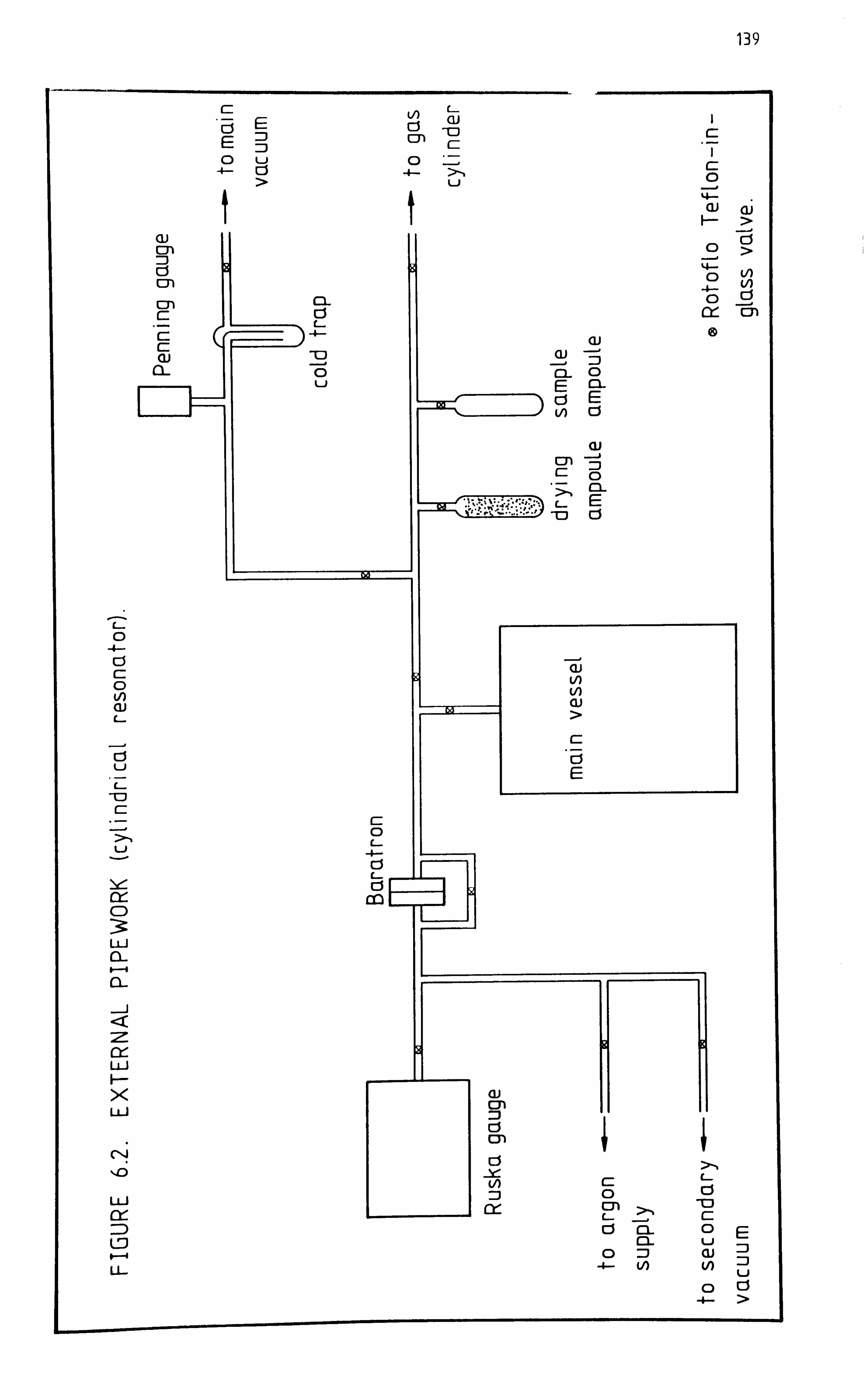
139

0 -4- Ö 0 if)

cu

-J

ci L)

> Li

CD : 3: LLJ CL

:Z er LU

k- x U-i

"0

LLJ

U3 P--4 Ll-

r- E V)

ci CY)

u ci 0 4- 0

a) F ci

V)

cj ca- 0E C3- u

0W 4-- Ln u

0 CJ 4- >

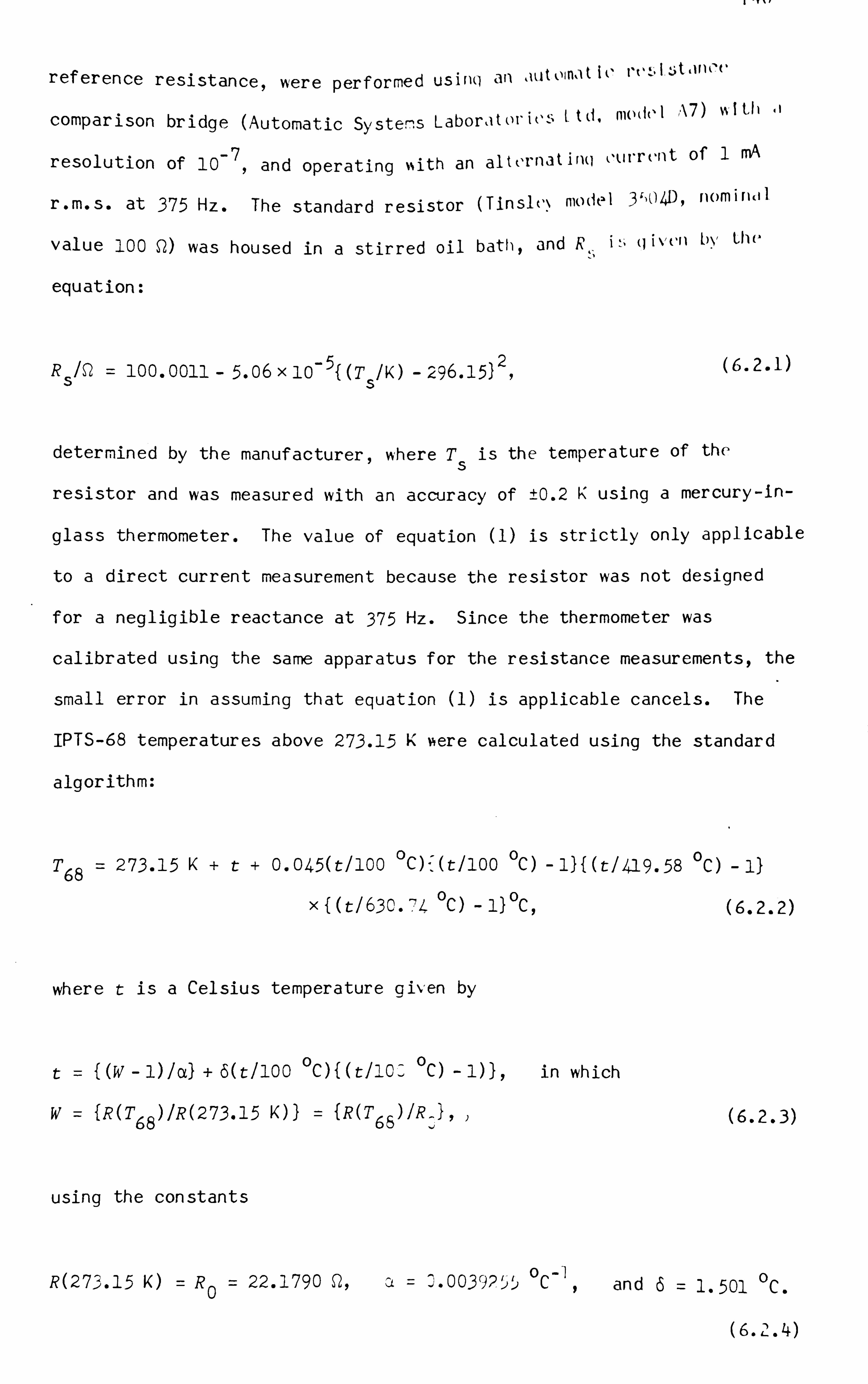
I-T%,

ref erence resistance, were perf ormed us i nq an 'Ut I tit . 1110c

comparison bridge (Automatic Systems Labor, it (W il" 1 A7) wl th

resolution of 10-7 , and operating %%ith an alternatirm OLH-rent of 1 rrIA

r. m. s. at 375 Hz. The standard resistor (Tinsl(,. \ model 3, ()4DY nomirwl

I)v value 100 0) was housed in a stirred oil bath, and R, i- (I I""' -

equation:

RSIQ = loo. ooll - 5. o6 x lo- 5{ (T s

/K) - /-96.15)2, (6.2.1)

determined by the manufacturer, where T5 is the temperature of the

resistor and was measured with an accuracy of ±0.2 K using a mercury-In-

glass thermometer. The value of equation (1) is strictly only applicable

to a direct current measurement because the resistor was not designed

for a negligible reactance at 375 Hz. Since the thermometer was

calibrated using the same apparatus for the resistance measurements, the

small error in assuming that equation (1) is applicable cancels. The

IPTS-68 temperatures above 273-15 K Aere calculated using the standard

algorithm:

T 68 = 273-15 K+t+0.045(t/100 0 C), l (t/100 OC)

- 1) { (t/419-58 OC) - 1)

(t/63C. 774 0 C)

- 1) Oc 9

where t: is a Celsius temperature given by

t={ (w - Wot) + 6(t/100 oc)f(t/-'O-- 0c) - 1)),

W= fR(T 68

)/R(273-15 K)) = {R(T 68

using the constants

in w ich

0 R(27--. 15 K) =R0= 22.1790 Q, ý-00392ýý C

(6.2.2)

(6.2.3)

and 6=1.501 OC.

( 6.2' . 4)

141

Equation (3) ý*,, as solved by iterations using G' - 1) /a as the initial

estimate of t. Between 13-81 and 27-33-15 K the IPTS-68 temperature is

given by

T_ 720 af Unk' 68 Lj=o j CCT-68 +3.28)/3.28}jKg (6.2.5)

where

w CCT-68 : -- w- AW (6.2.6)

and AW is a deviation function representing the deviations of a given

thermometer from the reference resistance ratio W CCT-681 and where

aj (j = 09 20) are a set of 21 defined constants. 2 Between 90.188 K and

273-15 K AW is given by

LW =b4 (T 68 - 273-15 K) -1 e4 (T

68- 273-15 K)3 (T 68- 373-15 K), (6.2.7)

where b4 and e4 are calibration constants. Unfortunately, the thermometer

used in this apparatus had not been calibrated f or use at temperatures

below 273-15 K. Rather than assume W= 0 or guess b4 and e 4' th e

simpler equation (2) was employed with

t={ (W - 1) /0, ) + 5{ (t: /loo OC) - 11 (t/100 0c) + $t: (t/loo OC)3{(t/, Qo OC) _1)9 (6.2.8)

where ýt=0.11 0C was assumed, in accordance with the 1948 International

Practical Temperature Scale f or the range 90.18 to 273-15 K. 3 At 250 K

(the lowest temperature studied in this work) the third term in equation

(8) contributes just 3 mK, and hence the assumption of a typical value

for ýt (rather than one determined by calibration) should not lead to

142

signif icant error. Small corrections were applied to convert the

temperatures determined in this way to the 1968 scale. The total

uncertainty in the measured T 68 's is estimated to be ± 20 mK in the

range 250 < TIK < 340.

The electric thermostat is illustrated in figure 6.3, with the

shields cut away to reveal the location of the acoustic cavity. The

inner shield, the control shield, was wound uniformly over its length with

a 600 Q (at 300 K) enamelled copper-wire resistance thermometer. Six

sets of 380 SI enamelled Manganin wire heating coils were non-inductively

wound directly over the copper thermometer. This thermometer f ormed one

arm of a d. c. Wheatstone bridge which provided the error signal for the

integrating proportional temperature controller that switched the

alternating current in the six heaters. The control temperature was set

by adjustment of the f ixed resistors in the Wheatstone bridge. The

excellent thermal contact between the shield, thermometer, and heating

coils resulted in a fast response by the control system to a change in

power demand. This, combined with the fairly long time constant for heat

exchange between the shield and the resonator (several hours in air)

provided excellent temperature stability. When left unperturbed, -the

temperature as measured by the platinum resistance thermometer could be

stable to ± 0.5 mK for 1h at 320 K. A set of thermocouples on the

control shield enabled the vertical temperature gradient to be measured,

and this could be reduced to ± 0.1 K by altering the division of power

between the heaters. The temperature gradients on the outside of the

resonator could not be measured, but should have been much smaller than

on the control shield.

The outer shield, the radiation shield, was also provided ýsith six

sets of 380 Q Manganin heating coils non-inductively wound over its

length, and there were additional 2-- -, heaters , --, ýound, one over each end. zo

These were all used to provide additional power and were operated with a

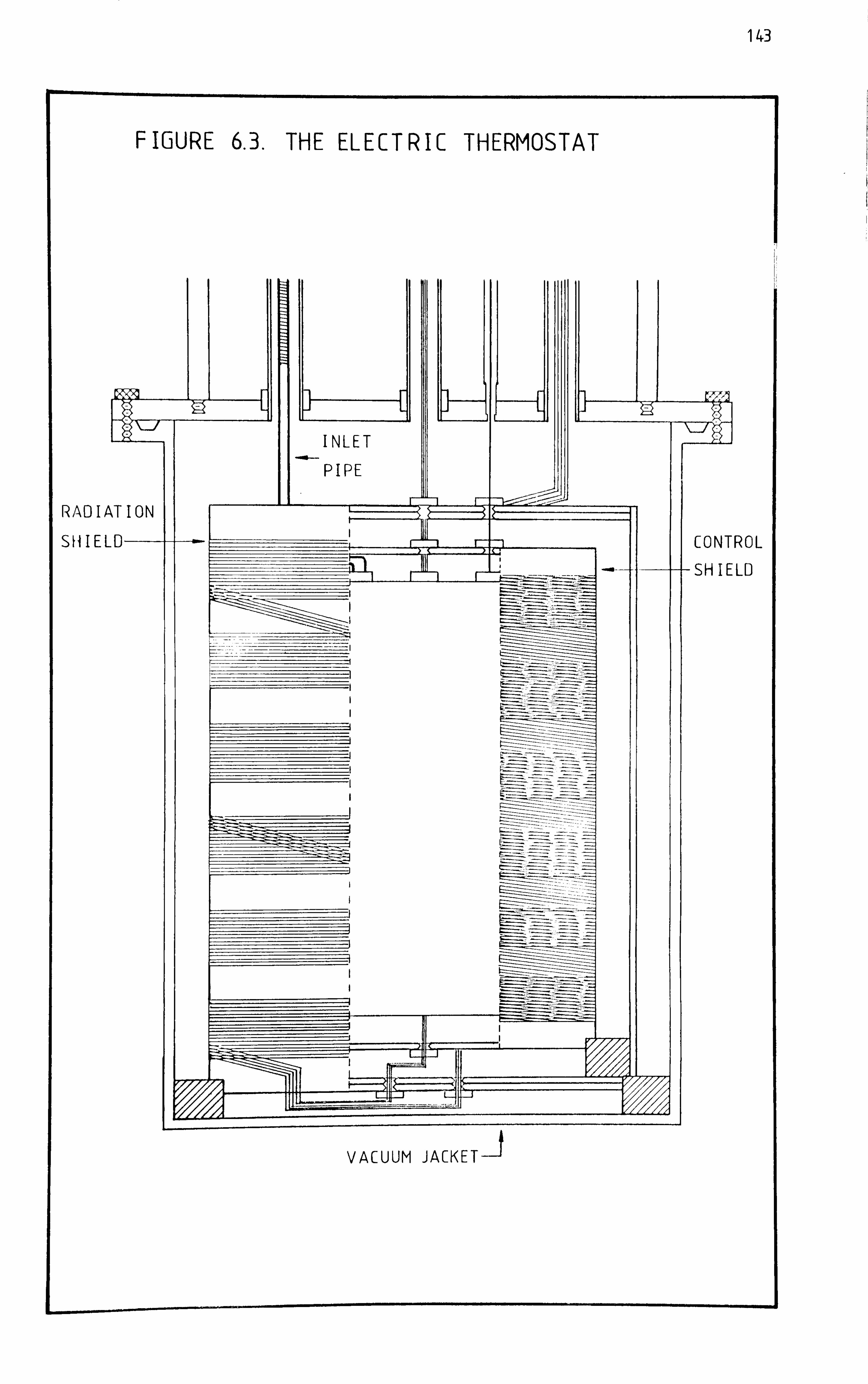
143

FIGURE 6.3. THE ELECTRIC THERMOSTAT

RADIA

SHIEL ROL LD

VACUUM JACKET-J

144

constant alternating current. Thermocouples were used to measure the

vertical temperature gradients (ýNhich could also be reduced to +- 0.1 K by

variation of the power distribution between the heaters) , and also to

measure the difference in the temperatures of the control and radiation

shields. The control shield was usually operated between 0.5 and 5K

above the radiation shield.

The whole assembly was mounted inside a brass vessel which was sealed

with a PTFE '0' -ring and could be evacuated in order to reduce the heat

loss from the apparatus. This was not found to be necessary and the

thermostat was operated in air. For operation below room temperature,

the apparatus was immersed in a refrigerated fluid bath and temperatures

down to 250 K vvere possible.

A number of glass tubes%vere sealed through the lid of the outer

vessel with glass-to-metal seals. The wires to the transducers, heaters,

and thermometers passed up these tubes to emerge through fine holes sealed

with vacuum wax. The stainless-steel inlet pipe passed up a 10 mm

internal -diameter stainless-steel tube sealed through the lid of the

outer vessel, and an 101-ring seal between the two wasprovided about

100 mm above the lid. A heater %-vaswound over the inlet pipe so that heat

loss to the refrigerated bath could be compensated, and a thermocouple was

provided to measure the vertical temperature gradient in this region.

The instrumentation used to detect the resonances is shown

schematically in figure 6.4. The signal supplied to-the. source transducer

was derived from a sine-wave signal synthesizer (Hewlett-Packard model

3320 A) that has a continuously variable frequency. The frequency was

measured using a frequency counter (Hewlett-Packard model 5381 A)

incorporating a quartz-crystal oscillator as its time base. Although the

crystal i, ý! as not housed in a thermostat, variations in the ambient

temperature altered the frequency by an insignificant amount (fractionally w

x 10- 7 K- 1). The source signal ýsas amplified to about 10 V r. m. s. so as

145

FIGURE 6.4. INSTRUMENTATION (cylindrical resonator).

146

to obtain adequate output from the transducer. The receiving transducer

ýsas connected to an amplifier having a forward potential-difference gain

of 10, C). The input resistance of this amplifier was deliberately reduced

to 1 kQ in order to reduce the sensitivity to audio-frequency noise. The amplified signal was displayed on an oscilloscope for observation of

its amplitude. Under typical conditions, the signal at the input to the

oscilloscope was about 50 mV r. m. s. at frequencies close to a resonance

frequency. Much larger signals were observed when the frequency was also

close to the resonance frequency of the transducers themselves.

6.3 EXPERIMENTAL PROCEDURE

Before beginning each set of measurements, the quartz-spiral gauge

was evacuated and its zero-pressure reading adjusted in accordance with

the manufacturers instructions. The zero-pressure reading of the

Baratron was also set under vacuum.

Samples of 2,2-dimethylpropane held in the sample ampoule were

degassed by repeatedly freezing the liquid (by immersion in liqui. d

nitrogen) , evacuating the remaining vapour, and then remelting the sample.

V, 'ater was removed by transfer of the material to a second ampoule

containing grade 4A molecular sieves, previously dried by baking at 550 K

and 1 mPa for 12 h, where it was left for 24 h before transfer to the

resonator. Samples could also be introduced directly from a gas cylinder.

The connecting pipe and gas-cylinder pressure regulator were f lushed with

the gas to avoid contamination with air. The pressure regulators used

(British Oxygen Company Ltd, type 80B) were not vacuum tight and hence

flushing was the only method by ý-, hich contamination could be reduced.

Prior to filling, the main vessel was evacuated until the pressure

in the vacuum line as indicated by the Penning gauge fell below 1 mPa.

147

During filling, the reference side of the Baratron was slowly pressurised

with argon so that the pressure difference was close to zero and the

Ruska gauge indicated the approximate sample pressure. The vessel was

initially pressurised to about 100 kPa or 80 per cent of the saturation

pressure, which ever was the smaller. The apparatus was then usually

left overnight for thermal equilibrium to be re-established before the

measurements were begun.

Each set of measurements was performed under near isothermal

conditions and at, typically, ten pressures above 10 to 20 kPa. The

observed resonance frequencies f1 of the cavity between 50 and 100 kHz

were assumed to be given by

-21- WIL) (1 + 6), (6.3.1)

where 1 is a positive integer, and 6 is the phase shift that arises from

the non-zero fluid velocity at the faces of the transducers (and also

from the effects of direct electromagnetic coupling between the source

and detector circuits) . By locating and measuring two adjacent resonance

frequencies, WO and the (1 + 6) 1s could be estimated and used to locate

the remaining resonances. The temperature and pressure were then

recorded, and all of the resonance frequencies between about 50 and 90 to

100 kHz measured with a resolution of 1 Hz. Random noise limited the

precision of an individual determination to about ±5 Hz. At each

resonance, the driving frequency was adjusted until the amplitude of the

received signal, as observed on the oscilloscope was at a maximum (f or

even values of 1), or at a minimum (for odd values of 1), and the

frequencies at which this occurred %vere taken as the resonance frequencies.

Alternate resonances result in an observed minimum in the received

amplitude because of the strong direct electromagnetic coupling

(crosstalk) between the source and detector circuits. This usually

148

contributed more than half of the received signal, and- was in phase with

the signal of acoustic origin for even values of 1 (hence the observed

maxima) but approximately iT out of phase for odd values of 1 (hence the

observed minima). About 20 to 30 min were required to record each set

of resonance frequencies, and the temperature was measured for a second

time on completion of the measurements; where there was significant drift

the mean of the two measurements was taken as the true temperature.

Usually the temperature drift was less than 5 mK. Typical results are

discussed in section 4.

After each set of frequency measurements, the gas pressure was

reduced f or the next point on the isotherm. Condensable samples were

transferred back to the sample ampoule under vacuum, while others were

simply pumped away. Such an expansion of gas f rom the vessel is nearly

adiabatic and resulted in the cavity cooling by, typically, 3 mK. About

1h would have been required for the temperature to return to the set

point but, because the drift was slo", it was not usual practice to wait

for more than about 10 min before the next set of measurements were begun.

The lowest pressure at which measurements of useful precision could be

performed was between -0 and 20 kPa because the signal of acoustic origin

became obscured by the crosstalk and random noise at lower pressures.

6.4 SAMPLE RESULTS

The following sample results iNere obtained at temperatures close

to 290 K in argon and 2,2-dimethylpropane.

The isotherm in argon covers ten pressures between 21.3 and 102.5

kPa at a mean temperature of 290.262 K. The resonance frequencies,

temperatures, and pressures are given in table 6.1. The frequency range

of the measurements iýas determined by the range over which the transducers

149

TABLE 6.1. Resonance frequencies (f 1

/Hz) in argon. I Cylindrical

resonator, mean temperature Tm= 290.262 K.

I p/P a ilO2469 93483 84743 74SS2 6657S 57449 48116 39322 29934 21292

T)/, nK 1 13 23 17 13 40 -13 -18 -22 -19 mI

34 53901 53914 53910

35 55508 55501

36 57069 57064 57060 57058 57055 57053 57050 57050

37 58669 58660

38 60211 60211 60211 60209 00206 60205 60205 60202 60204 60204

39 1 61789 61790 61788 61756 61754 61782 61778 61775 61772 61775

40 1 63366 63367 63368 63367 63364 63363 63362 63359 63356 63351

41 64937 64936 64938 64934 64930 64936 64932 64929 64927 64922

42 66522 66521 66520 66517 66515 66515 66510 66508 66507 66502

43

44

45

46

47

48

49

50

51

52

53

54

55

56

57

68103 68102 68102 66104 65106

69683 69683 69681 69679 69079 69676 69674 69671 69665 69661

71263 71261 71260 71257 71256 71254 71255 71255 71255 71255

72850 72847 72846 72S43 72542 72845 72843

74417 74416 74410 74404

76002 76000 75996 75995 75994 75992 75989 75985 75981 75980

77583 77582 77579 77575 77572 77572 77570 77568 77566 77562

79154 79152 79149 70,146 79142 79142 79141 79137 79139 79132

80729 80724 80722 8071" S0717 80716 80711 80707 80704 80700

82304 82302 82300 82295 52294 82290 82287 82284 82284 82282

83885 83885 83881 83550 53579 83879 83874 83872 83869 83863

85470 85466 85467 85463 554,61 85457 85454

87038 87040 87037 87033 57029 87025 87020 87016 87015

88622 88612 88611 SS606 55601 88598 88598

90206 90199 90199 901911 110188

150

operated with a useful efficiency. At the lower pressures, where acoustic

losses are greatest and coupling betiseen the source transducer and the

gas is least efficient, some of the resonances that were observed at

higher pressures became obscured by the crosstalk and random noise. In

addition, some of the recorded resonance frequencies are clearly

inconsistent with the bulk of the measurements and have been rejected

from the analysis. The frequencies that have been rejected (underlined

in table 6.1) yield values of WO that differ by more than two standard

deviations from the mean value of the remaining results at the same

pressure. Some of the worst affected resonances were not recorded at the

lower pressures.

In order to calculate WIL) , the 6 parameter must be f ound. Both

WL) and 6 can be f ound by a linear least-squares regression analysis in

which the equation:

f1= -21-(u/L)6+-21-(u/L)l (6.4.1)

is fitted to f1. For example, the results at 93-483 kPa yield 6= (0-158

+ 0.005) and WIL) = (3156.05 ± 0.36) s-1, and the standard deviation of the

fit is 5 Hz. t Values of 6 obtained from the results at other pressures

do not dif f er signif icantly and 5= C-158 is the optimum value f or the

isotherm. Mean values of WL) and WIL) 2 at each pressure, obtained

22 with 6=0.158 and adjusted to 290.262 K (assuming u (T

1) lu (T

2) =T 1 IT

2)2

are given in table 6.2.

Unless otherwise stated, all quoted uncertainties in this work are

+one standard deviation only. In the case of the coefficient a. of the

. th

3 independent variable, estimated in a multiple linear regression

analysis with v degrees of freedom, the confidence interval at the

probability level a is {a t (a) c., 'ý, where a. is the standard deviation V J, -7

of a and tV (a) is given by the t distribution for v degrees of freedom

in a Itwo-sided' test.

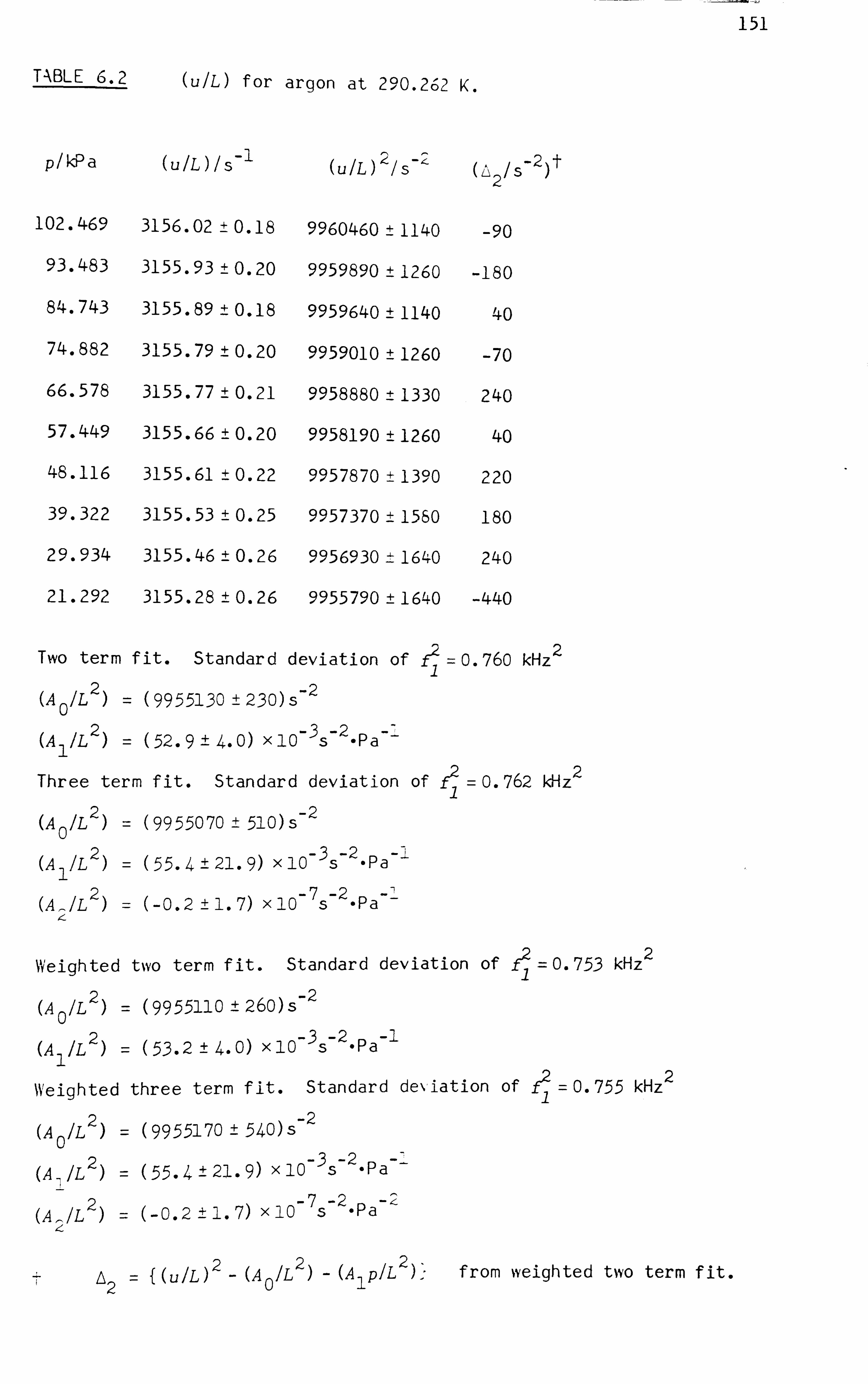
151

TABLE 6.2 (u/L) for argon at 290.262 K.

p/kPa (u/L)/S- 1 (u/L) /s- 2 /S- 2 (Lý 2

102.469 3156.02 ±0 . 18 9960460 ±1140 -90 93.483 3155.93 ±0 . 20 9959890 ±1260 -180 84.743 3155.89 ±0 . 18 9959640 ±1140 40

74.882 3155.79 ±0 . 20 9959010 ±1260 -70 66.578 3155.77 ±0 . 21 9958880 ±1330 240

57.449 3155.66 ±0 . 20 9958190 ±1260 40

48.116 3155.61 ±0 . 22 9957870 ±13190 220

39.322 3155.53 ±0 . 25 9957370 ±1560 180

29.934 3155.46 ±0 . 26 9956930 ±1640 240

21.292 3155.28 ±0 . 26 9955790 ±1640 -440

Two term fit. Standard deviation of t-2. = 0.760 kHz 2

(A 0

/L 2 (9955130 ± 230) 5- 2

2) 3 2. (A 1

/L = (52.9 ± 4.0) x 10- s- Pa- ý

Three term fit. Standard deviation of f2- =0.762 kHZ2 1

(A 0

/L 2)=( 99 550 70 ± 510) s- 2

(A 1

/L 2)= (55.4 ± 21.9) x 10- 35-2. Pa-'

(A -

/L 2)= (-0.2 ± 1.7) x 10- 7 s-

2. pa-

Weighted two term fit. Standard deviation of f2. =0.753 kHz 2

(A 0

/L 2 (9955110± 260)s- 2

(A 1

IL 2) = (53.2 ± 4.0) x 10- 3

5- 2. pa- 1

Weighted three term f it. Standard deviation of f -2 = 0.755 kHz 2

(A 0

/L 2)= (9955170 ± 540) 5- 2

(A IL 2)= (55.4 ± 21.9) x 10- 35-2. Pa--

(A /L 2)= (-0.2 ± 1.7) x 10- 7 s-

2. Pa- 2

222 from weighted two term fit. TA2 {(ulL) (A 0

/L (AlplL

152

The 173 selected resonance frequencies were analysed by fitting

the leading two and three terms of the equation:

(A /L 2+2+ (A A2 )J(l +2p+ (A A2f (1 + 6) 2P2+ (6.4.2) 012

f2 2) to using the method of least squares. The coef f icients (A A 0

(A A2), and (A 2

/L 2 ), and their standard deviations, as estimated from

two- and three-term f its to equation (2), are given in table 6.2. In the

initial regression analysis each pressure on the isotherm was given equal

weighting; the frequencies f at each pressure were weighted by

N(n1n P

where n is the total number of frequencies in the analysis, nP

In is the number at that pressure, and N =nl 1 =1 W1 is a normalisation

constant. In the weighted regression analysis the frequencies at each

pressure were weighted by N(n1n M/0 2 ), where a2 is the variance of PPP

2f 1 /(l + 5) at that pressure. This takes account of the random scatter

among the measurements. Clearly the results are well represented by a

two-term f it; inclusion of the third term actually increases the standard

deviation of the fits. The results of the weighted and unweighted

analyses are in excellent agreement. The weighted two-term fit has been

used to generate the fourth column of the table "bich gives the deviations

of the experimental results from the line of best fit. The best estimate

of the second acoustic virial coefficient, ýa= 12 .9 cm3. mol-1 , compares

reasonably well with the value 9.1 cm 3.

mol-1 obtained by differentiation

of equation (5-3-9), the square-well formula for B(T)., and with the value

9.7 cm3. mol-1 obtained by numerical integration of the HFD-C pair-

potential -energy function for argon in accordance with equation (5.3.6).

2 The weighted two-term f it estimate of A0A has been combined with

the calculated value of A0 to find the pathlength of the interferometer

at 290.26 K. The sample gas was Hatherson grade argon (Cambrian gases

Ltd) and the manufacturers claimed that the total mole fraction of

153

impurities ýýas less than 5x 10-6. Thus -yPg may be taken' as exactly 513,

and the only significant uncertainty in the molar mass M=0.039948 kg-

mol 1

should be that arising from the uncertainty in the isotopic

composition: &I =3x 10- 6

kg- mol- 1.4 If the uncertainty 6T in the measured

IPTS-68 temperature is taken to be ± 20 mK, and the uncertainty 6R in the

gas constant R =8.31441 J-K- 1. mol-

1 is taken to be ±0.00026 J-K-1-mol-l (± onee standard deviation ), then the relative uncertainty in

A0 (290.262 K) = 100 687 m 2.

s- 2 is

( 6A 0 IAO) = {(6RIR) 2+( 6TI T) 2+ (6m/m) 2 )1 = 1.1 X10-4. (6.4.3)

The relative uncertainty in the estimation of (A 0 /L 2) that arises from

the random scatter in the measurements is 0.7x, 0-4 (99 per cent

confidence interval with 171 degrees of freedom), and hence

L= (loo. 569±0.007) mm. (6.4.4)

This result is sensitive to the value chosen for 6; a change of 0.005

would correspond to about 0.01 mm in L.

The isotherm in 2,2-dimethylpropane covers ten pressures between

17.5 and 99.2 kPa at a mean temperature of 290.039 K (about 7.4 K above

the normal boiling temperature). The measured resonance frequencies,

temperatures, and pressures are given in table 6.3. The underlined

entries have been rejected from the final analysis by the same criterion

as was applied to the measurements in argon. There is no evidence in the

measurements to suggest that there was any significant dispersion at the

experimental frequencies. The mean value of 6 obtained by fitting

equation (1) to the results at each pressure is (0.158 ± 0.008). If the

results at the two lower pressures are neglected then the optimum value

(0-155±0.005)- Since the values obtained for WIL) are sensitive to

154

TABLE 6.3. Resonance frequencies Oc 1

/Hz) in 2,2-dimethylpropane.

Cylindrical resonator, mean temperature Tm= 290.039 K.

p/Pa

(T -Tm )/mK

99214

31

90781

-16

82230

2

73693

-1

63386

4

54052

9

44899

4

35361

-12

26390

-13

17519

-11

55 50230 50402 50562 50730 50920

56 51167 51316 51478 51640 51839

57 52078 52232 52397 52557 52759

58 52-090 53143 53309 53477 53678 53858 54026 54205 54375 54545

59 53903 54060 54221 54397 54597 54782 54959 55140 55315 55488

60 54808 54968 55140 55315 55521 55703 55890 56075 56231 56419

61 55719 55886 56063 56239 56448 56640 56830 57012 57186 57367

62 56638 56807 56981 57161 57380 57568 57746 57943 58120 58299

63 57546 57721 57897 58082 58295 58488 58679 58878 59057 59227

64 58451 58626 58807 58996 59214 59413 59601 59800 59979 60165

65 59366 59539 59722 59912 60141 60343 60529 60730 60916 61095

66 60283 60460 60652 60838 61070 61271 61464 61669 61856 62037

67 61194 61369 61562 61762 61995 62194 62397 62599 62792 62990

68 62098 62282 62478 62677 62911 63120 63318 63530 63728 63915

69 63010 63194 63394 63592 63832 64041 64250 64461 64658 64849

70 63920 64108 64306 64510 64753 64969 65180 65394 65593 65790

71 64839 65027 65232 65440 65686 65904 66120 66334 66529 66724

72 65740 65932 66142 66347 66599 66818 67030 67251 67457 67647

73 66659 66852 67065 67270 67525 67747 67959 68184 68391 68595

74 67552 67750 67966 68177 68435 68662 68881 69106 69315 69520

75

76 69381 69581 69797 69995 70239 70494

155

TABLE 6.3. continued.

P/kPa 99214 90781 82230 73693 63386 54052 44899 3536 1 26390 17519

(T -Tm )/mK 31 -16 2 -1 4 94 -12 -13 -11

1= 77 70267 70477 70747 70927 71197 71433

78 71196 71404 71630 71849 72124 72362

79

80 73017 73230 73467 73696 73983 74229 74479 74725 74954 75190

81 73975 74184 74419 74651 74930 75173

82 74850 75066 75300 75539 75826 76080 76325 76574 76809 77041

83 75795 76010 f. 762, S 76485 76772 77025

84 76675 76898 77141 77381 77673 77939 78182 78443 78675 78916

85 77614 77837 78050 78326 78618 78874 79128 79389 79614 79873

86 78505 78733 73951 79230 79530 79791 80042 80310 80555 80804-

87 1 79420 79649 79899 80150 80453 80719 80974 81236 81489 81731

88 1 80329 80561 80819 81069 81379 81648 81902 82182 82428

89 1 81244 81475 81731 81988 82297 82565 82827 83098 83366

90 1 82153 82387 5264-4 82910 83213 83488 83764 84036 84283

91 1 83067 83305 5356)S 83830 8414-4 54419 84694 84963 85217

92 1 83964 84208 54474 84744 85058 55344 85617 85899 86162

93 1 84888 85130 85402 85669 85994 86273 86547 86833 87090

94 1 85791 86037 86312 86582 86912 67196 87470 87772 88020

95 1 86709 86960 57233 87507 87845 55120 88412 88695

96 1 87620 87872 551'r5 88427 88755 59050 89337 89632

97 1 88521 88779 59066 89341 89680 89970 90260 90554

98 89444 89693 599; 3 90271 90601

99 1 90341 90605 90592 91170 91521

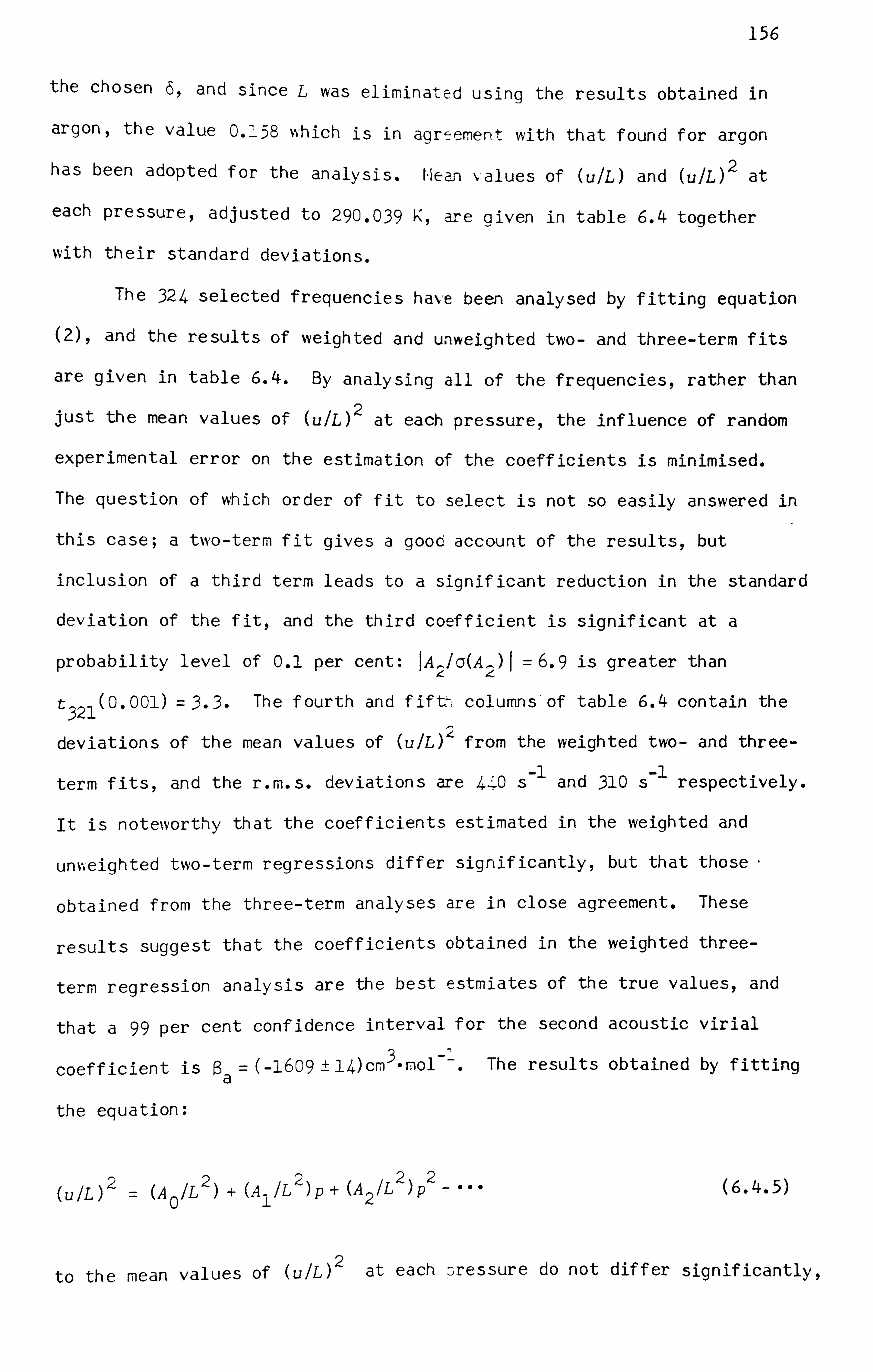
156

the chosen 5, and since L was elimina+k-; -r-d using the results obtained in

argon, the value 0.. 58 which is in agr, ý-ement with that found for argon

has been adopted for the analysis. hean , alues of (u1L) and (u1L) 2 at

each pressure, adjusted to 290-039 K, are aiven in table 6.4 together

with their standard deviations.

The 324 selected frequencies have been analysed by fitting equation

(2), and the results of weighted and unweighted two- and three-term fits

are given in table 6.4. By analysing all of the frequencies, rather than

just the mean values of WL) 2 at each pressure, the influence of random

experimental error on the estimation of the coefficients is minimised.

The question of which order of f it to select is not so easily answered in

this case; a two-term fit gives a good account of the results, but

inclusion of a third term leads to a significant reduction in the standard

deviation of the fit, and the third coefficient is significant at a

probability level of 0.1 per cent: JA-IG(A )I = 6.9 is greater than 42

t 321 (0

- 001) = 3.3. The fourth and fift. -i columns'of table 6.4 contain the

deviations of the mean values of WIL) 2 from the weighted two- and three-

ýO s and 310 s respectively. term fits, and the r. m. s. deviations are

It is noteworthy that the coefficients estimated in the weighted and

unvveighted two-term regressions differ significantly, but that those-

obtained from the three-term analyses are in close agreement. These

results suggest that the coefficients obtained in the weighted three-

term regression analysis are the best estmiates of the true values, and

that a 99 per cent conf idence interval for the second acoustic virial 3-I

coefficient is ýa =(-1609±14)cm -nol The results obtained by f itting

the equation:

2222 2_ ... (u1L) = (A

0 IL )+ (A

1 /L )p+ (A

2 /L )p (6.4.5)

to the mean values of WL) 2 at each pressure do not differ significantly,

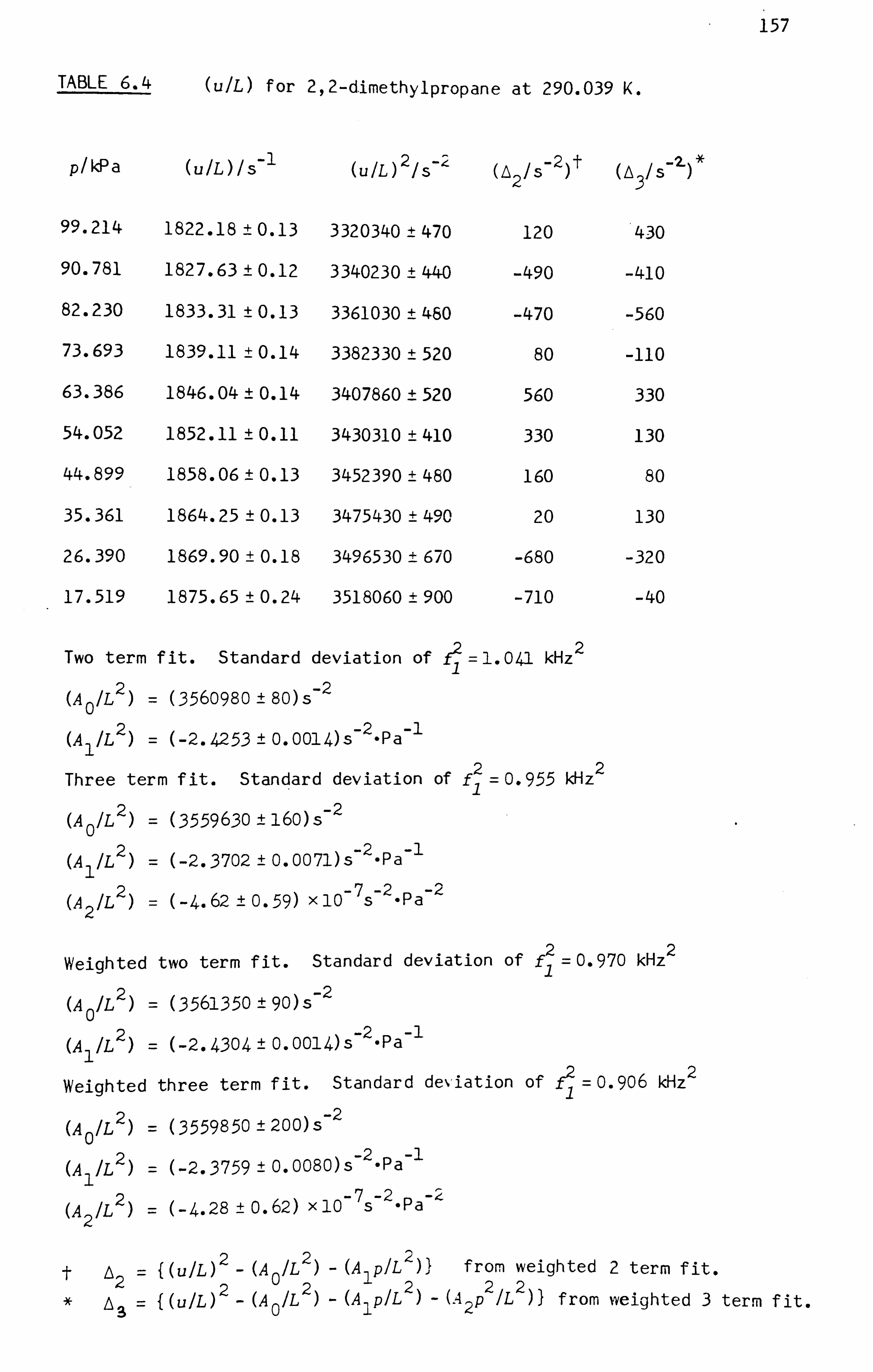
157

TABLE 6.4 WIL) for 2,2-d. imethylpropane at 290.039 K.

p/kPa (u/L)/s- 1 (u/L) 2 /S- 2 2

/S- 2t 3

/S-2-

99.214 1822.18 ±0.13 3320340 ±470 120 430

90.781 1827.63 ±0.12 3340230 ±440 -490 -410

82.230 1833.31 ±0.13 3361030 ±480 -470 -560

73.693 1839.11 ±0.14 3382330 ±520 80 -110

63.386 1846.04 ±0.14 3407860 ±520 560 330

54.052 1852.11 ±0.11 3430310 ±410 330 130

44.899 1858.06 ±0.13 3452390 ±480 160 80

35.361 1864.25 ±0.13 3475430 ±490 20 130

26.390 1869.90 ±0.18 3496530 ±670 -680 -320

17.519 1875.65 ±0.24 3518060 ±900 -710 -40

Two term f it. Standard deviation of f2. = 1.041 kHz 2

(A 0 /L 2 (356o98O ±80)s- 2

(A 1

/L 2) (-2-4253±0.0014)s- 2. Pa-1

Three term fit. Standard deviation of 2 kHz 2 fý =0-955

(A 0

/L 2 (3559630±160)s- 2

(A 1

/L 2 (-2-3702 ±0.0071)s- 2. Pa- 1

272 (A 2

/L )= (-4.62 ± 0.59) x 10- s- pa

Weighted two term fit. Standard deviation of 2 kHz 2 fý = 0.970

(A 0

/L 2) (3561350 90) S-2 2 -2 1

(A 1A

(-2-4304 0.0014) s Pa

Weighted three term fit. Standard deviation of fý =0.906 kHz 2

(A 0

/L 2) = (3559850 ±200) s-2

(A 1

/L 2)= (-2-3759 ±0.0080) s-2. Pa-1

(A 2

IL 2) = (-4.28 ± 0.62) x 10- 7

s- 2. Pa-

2_ 2) (A 2)1 from weighted 2 term fit. A2= {(u1L) (A 0

IL 2 lpIL 2j22

A3 = f(ulL) - (A 0

/L (AlplL )- (A 2P

/L from weighted 3 term fit.

158

but the influence of random errors is more pronounced in such an analysis. For example, the results of unweighted two- and three-term fits are given

in table 6.5, and the three-term fit gives ýa= (-1607 ± 55) cm 3_mol-1 (99

per cent confidence interval with seven degrees of freedom). Clearly,

the effects of random errors on the estimated coefficients are much

smaller in the two-term regression analyses, but the results are subject

to a systematic error arising from the neglect of A2. Conversely, if the

third term is included then random errors give rise to a much larger

statistical uncertainty in the estimation of ýa, and this is particularly

severe when only the mean values of WIL) 2 are analysed. An alternative

method of analysing the results is to employ a number of two-term

regressions in which the measurements at the highest pressures are

progressively neglected. Such an analysis yields the mean value of

{9 WL) 2 /9p} over the experimental range of pressures, but the required

quantity is Limp_*of9(u/L 2 )/9p}. The results obtained from unweighted

analyses at different mean pressures are given in table 6.5, and also

plotted in figure 6.5. Clearly, OWL) 2 /3P) is a linear function of the

mean pressure <p> to within the resolution of the measurements, and a

linear extrapolation gives Lim P _* of @(u/L) 2 1ýp} = (A

1A2)= (-2-354±

0.005) s- 2. Pa-1, and -21-1 32 WL) 2/3P2)

= (A 2

/L 2)= (6-5 ± 0-5) x 10- 7

s- 2

-Pa- 2.

This result implies that ýa= (-1595 ± 13) cm 3.

mol-1 (99 per cent conf idence

interval with six degrees of freedom), and this differs from the result

of three-term regression analysis by 0.9 per cent.

The perfect-gas heat capacity ratio -yPg(C 5H 12 , 290.04 K) of 2,2-

dimethylpropane at 290.04 K has been obtained by combining the best

estimate of A0A2, namely (3559850 ±200) s- 2,

with that obtained in

argon. The value of (A 0

/L ) obtained in argon at 290.26 K was adjusted

to 290.04 K with the assumption that the temperature dependence of the

pathlenqth is determined by the thermal expansion of the brass transducer

mounting f rame (using dL/dT =2x 10- 5L K- 1 )ý with the result

159

TABLE 6.5 Analysis of WL) for 2,2-dimethylpropane at 290.039 K.

Two terms. Standard deviation of WL) 2= 460 s- 2

(A o

/L 2) = (356looo± 360) S-2

A221

AIIL )= (-2.426±0.006) s- -Pa-

Three terms. Standard deviation of (u/L) 2= 370 S-2 (A 0

/L 2) = (3559740± 610) s-2

(A 1

/L 2) = (-2-372 ± 0.023) S-2. Pa-1

27 -2 -2 (A 2A)= (-4.62±1.97)xlO- s. Pa

<p>/kPa <A 0A 2>/5-2

<9 WL) 2/ýP>/s-2. Pa-1

58.753 3561000 ±360 -2.426 ±0.006

54.257 3561020 ±400 -2.427 ±0.007

49.691 3560800 ±410 -2.421 ±0.008

45.043 3560430 ±300 -2.411 ±0.006

40.268 3560100 ±180 -2.401± 0.004

35.644 3560040 ±230 -2.399 ±0.006

31.042 3559920 ±300 -2.394 ±0.009

26.423 3559810 ±550 -2.389 ±0.020

-2.36- F IGURE 6.5.

ci 0- -2.38-

/0

2.40-

2.42-

<p > /kPci 0 20 40

160

22 {A (Ar , 290.04 K) /L (290.04 K) 9947550 ± 260) s- Thus o

A0 (C P12' 290.04 K) 1A 0

(Ar, 290.04 K) =(3/5)(j!, j(Ar)/M(C 5H 12 ))

xy pg (c 5H12 , 290.04

- K)

=(0.35786 ±0.00002)9 (6.4.6)

where both the pathlength and the gas constant are eliminated, as are

systematic uncertainties in the measured IPTS-68 temperatures. In order

to calculate 9 the molar mass of the sample is required. The chemical

purity will be discussed in chapter eight, but if purity is assumed then

the molar mass is (0.072150±0.000006) kg-mol- 194 and hence -ýPg (C P 121

290.04 K) = (1.07722 ±0.00021). The corresponding value for the perfect-

gas molar heat capacity at constant pressure is

Cpg (C H, 290,04 K) IR = 13-95 ± 0.049 p, m 5 12

where the uncertainties in the molar masses have been combined in

(6.4.7)

quadrature with a 99 per cent conf idence interval for the value of

equation (6) to obtain the quoted uncertainty.

These results may be compared with the recent work of Hossenlopp

and Scott who measured the vapour heat capacity and enthalpy of

vapourisation AgH of 2,2-dimethylpropane by vapour-flow calorimetry. 5 1m

The heat-capacity measurements were used to obtain values of CP9 IR at Pqm

ten temperatures between 298-15 and 523.15 K, and these may be

represented by the empirical equation:

CP9 (T) IR = 1.296 + 4.2808 x 10- 2 (TIK) + 1.4274 x 10- 5 (TIK) 2

p7m - 3.0308 x 10 -8 (-T/ K)3 (6.4.8)

with a standard deviation of 0.009 ("ell within the experimental

161

uncertainties of ± 0.2 per cent). The short extrapolation to 290.04 K

yields CP9 IR = 14-18, and that value exceeds the value of equation (7) PIM

by 1.6 per cent. This discrepancy could arise from a systematic error of

0.13 per cent in the measured ratio A0 (C 5H 12 ý 290.04 K)/AO(Arg 290.04 K).

The enthalpies of vapourisation, obtained at eight temperatures between

264.81 and 303-50 K, were combined with values of the derivative

(dp 1+g dT) of the vapour pressure (derived f rom the literature) to obtain

the differences ATV between the molar volumes of the liquid and vapour 1m

at each temperature using Clapeyron's equation:

(CIP 1+g /dT) = AgH ITAgV . 1m1m (6.4.9)

These were then combined with esti n-ates of the molar volume of the

liquid to obtain the molar volume of the coexisting vapour, and hence to

find the second virial coefficients by neglecting the higher-order terms

in the equation of state. The results were represented by

B(T) I cm3. mol-1 = 494 - (373260 KIT) + 552f 1+ (1622.5 KIT) - exp(1622.5 KIT))

(6.4.10)

I at 264-81 K, decreasing with an estimated uncertainty of 30 cm 3.

mol-1

to ± 10 cm3. mol-1 at 303-50 K. The second acoustic virial coefficient at

290.04 K obtained by dif f erentiation of equation (10) using 'Ypg - 1* 076,

namely (-1600 ±20) cm 3.

mol- 19 is in good agreement with the acoustic

result. However, the closeness of this agreement may be fortuitous in

view of the neglect of the third virial coefficient in the determination

of equation

162

REFERENCES

1. Ewing, M. B. To be published.

2. The International Practical Temperature Scale of 1968 Amended

Edition of 1975. Metrologia 1976,12,7.

3. Quinn, T. J. Temperature. Academic press: London, 1983, p. 184.

4. Atomic Weights of the Elements 1977. Pure and Appl. Chem. 1979,

51,409.

5. Hossenlopp, 1. A.; Scott, A. D. J. Chem. Thermodyn. 1981,13,415.

163

CHA 7 THESPHERICALRES0NAT0

7.1 INTRODUCTION

7.2 THE ACOUSTIC RESONATOR

7.3 INSTRUMENTATION AND MEASUREMENT TECHNIQUE

7.4 THE ACOUSTIC MODEL

7.5 SAMPLE RESULTS: argon, xenon, helium, and 2,2-dimethylpropane

7.1 INTRODUCTION

The advantages of spherical resonators in comparison with the

conventional cylindrical designs for low-frequency (2 to 20 kHz)

measurements of sound speeds have been discussed in chapter three.

Briefly, the absence of shear boundary-layer damping for the radial

modes, and the favourable surface area to volume ratio in a sphere, lead

to very high quality factors (as high as 25 000 in this work), and to

boundary-layer corrections that are about a factor of 10 smaller than for

a comparable cylinder. In addition, the radial resonance frequencies are

insensitive to geometric imperfections in the resonator, and hence for

practical purpo5es only the volume of the cavity need be known. In recent

years M. R. Moldover and J. B. Mehl have demonstrated that speeds of

sound can be measured to a relative precision approaching 1 xio- 6

using

a spherical resonator with phase-sensitive detection. 1ý213ý4 It was

therefore decided to construct a similar apparatus in this laboratory,

initially for use in a limited range of temperatures. The apparatus has

been used to obtain highly precise speeds of sound in argon at the

temperature of the triple of water (such as would be required in a

redetermination of the gas constant), and to supplement the results

164

obtained in 2ý2--dimethylpropane using the cylindrical resonator.

7.2 THE ACOUSTIC RESONATOR

In the design of the resonator, three important factors were

considered: the radius of the sphere, the %all material and thickness,

and the location of the transducers.

The size of the resonator determines the range of operating

frequencies and the magnitude of the thermal -boundary -layer corrections.

The fractional correction (gS/fOn ) to the frequency of the n th

radial

resonance that arises from damping in the thermal boundary layer is

related to the radius a by

(gs1f On

(11a) (y - 1) (D t

/2v On U) (7.2.1)

where Dt =(Klpc p) is the thermal diffusivity of the gas, and hence a

large cavity is favoured. Use of higher-order resonances would also

reduce the magnitude of the correction, but at the expense of increased

bulk losses and overlap between modes. The choice a= 60 mm was felt to

be a suitable compromise between the conflicting requirements for small

boundary-layer perturbations and a uniform temperature in the cavity.

With u= 300 m-s-1 the first five radial resonances occur at frequencies

between 3.6 and 13.7 kHz, sufficiently low to avoid vibrational -relaxation

dispersion in most polyatomic gases.

The walls of the resonator, having a finite mechanical compliance,

vibrate in response to an acoustic pressure. In the approximation that

the fundamental 'breathing model resonance of the spherical shell is

isolated, Greenspan derived the folloýiing expression for the specific

acoustic admittance of the wall when excited by radial waves:

165

3' = i27TfapuA 1- (flf (7.2.2) m, r res

where

A= (1 + 2t3 )/2(t3 _ 1)c. u2 (7.2.3) 5s

and the breathing-mode resonance frequency is given by

fres =i (t 3_ 1)/2TT 2 (t - 1) (1+2 t3 )) -i (us/a), (7.2.4)

and where t =b1a, b is the outer radius, pS is the density of the %vall,

and us is the speed of longitudinal sound vvaves in the wall. 'ý5 The effect

of this motion is to reduce the ideal resonance frequencies by the

fraction

(Af el

If On

)= Apu 2 Ili - (f On

If res)

2)- (7.2.5)

Equation (5) is applicable at frequencies below f res provided that the

motion is purely radial. Brass and aluminium alloys were considered as

possible materials for construction, but "ith brass f res would be rather

low (about 15 kHz with e- =60 mm and t =1.2), and so aluminium was chosen.

The resonance frequency f res

is not very sensitive to the thickness of

the wall, which primarily determines the magnitude of A. The choice of

aluminium alloy 6082 6 with a= 60 mri and b= 72 mm gives A=2.7 x 10-11 Pa-1

and f =21.2 kHz. Thicker walls could have been used to reduce the res

elastic response, but with the chosen dimensions (Af el/f)

is typically

less than 1x 10-5 f or the f irst f ive radial modes at a gas pressure of

100 kPa and vanishes as p-*O. Thus equation (4) constitutes a very small

The sign of equation (4) is consistent vith the time dependence

exp(-ic, )t) used here.

166

correction to A1 and does not affect measurements of A06

The most efficient means of exciting the radial resonances of a

spherical resonator is to place the source at the centre. Moldover et

al 1 found that high order radial resonances could then be detected by

another transducer at the surface with very high signal-to-noise ratios.

However the presence of the transducer and its wires perturbs the

resonance frequencies in a manner which is difficult to calculate.

Following Moldover, it was decided to install both the transducers in the

wall of the resonator, and to place them 7/2 apart in order to avoid

overlap between the first radial mode (0,1) and the adjacent non-radial

mode (3,0) (%)30 /v Ol 0005).

The resonator is shown in cross-sections in figure 7.1. Its design

was based on the one described by Moldover and Mehl .2 The two hemi-

spheres were turned from aluminium alloy 6082 using a simple pivoting

tool for the inner surface, and a special spherical turning tool for the

outer surface. Prior to the final cutting, the two halves were

annealed to relieve stress, and then retempered by precipatation

treatment. Use of a tool of constant radius to turn each hemisphere

insured that a very close match in the radii'", as achieved (better than

Mechanical measurements on the finished resonator indicated that

the true radius of curvature was (60.16 ±0.01) mm at 293 K. The depths

of the two hemispheres differed by 0.09 mm, but their mean was (60.17±

0.02) mm at 293 K. The two halves met at an interlocking step which

insured that they were concentric when bolted together, and they touched

only on the inner edge. The internal surface was polished by hand using

an abrasive paste. Although some tooling marks remained (especially

near to the opening of each half where chatter in the lathe caused more

serious scoring) the surface had a near-mirror finish, as can be seen in

plate 1. Unfortunately the polishing erroded the sharp corners between

the inner surfaces and the rims; the radius of curvature appeared to be

167

FIGURE 7.1 THE SPHERICAL RESONATOR.

vent

fran por f

boli hot i

two perp cross-sections.

ipting - be adaptor

50mm

168

about C. 5 mm and that "ould lead to a fractional increase in the volume

- --5 of the resonator of

The transducer mounting holes shoNýn in figure 7.1 allowed for

various týpes of transducer to be installed. In this work, a small

electrostatic capacitance transducer (see f igure 4.3) was used as the

source. The active surface of this device came flush with the interior

of the cavity and, because the backplate was rigid, there should have

been no perturbation to the normal modes. The detector was a small

commercially -available electret capacitance microphone with its own built-

in preamplif ier. This device was mounted in the wall of the resonator

and coupled to the interior using aI mm diameter waveguide of length

mm machined in a close fitting adaptor. A small space between the end

of the waveguide and the active surface of the microphone was sufficiently

large f or the tube to be treated as open in the calculation of the

coupling tube corrections. This transducer arrangement is non-selective;

all modes of the cavity are excited, but because all have high quality

f actors the lo%%er order resonances are clearly resolved and no serious

overlap occurs. The measurement technique used does not rely on single-

mode excitation.

The cavity was not sealed, but instead the gas was allowed to flow

freely into and out of the resonator t; 'irougl'i a single 1 mm diameter hole

drilled in the wall. The resonator was suspended on fine wires inside a

brass vessel sealed with viton rubber '0' -rings, as shown in figure 7.2.

Two access ports in the side of the vessel are provided so that the

transducers may be changed without disassembly of the vessel . The

electrical connections to the detector are made across vacuum leadthroughs

in the cover of one of these access ports, "hile those to the source pass

through similar leadthroughs in the lid of 'the vessel.

The temperature of the cavity ýýa5 measured using a long-stem

standard platinum resistance thermometer (Leads and Northrup, serial

169

FIGURE 7.2. CONTAINMENT VESSEL.

50 mm

170

number 780308) recently calibrated on IPTS-68. The thermometer was

inserted into the well shown in f igure 7.2. The upper part of this well

was a thin walled (1 mm wall, 8 mm inside diameter) stainless-steel tube

silver soldered to the lower part, ý%fiich consisted of a large copper

block with a spherical surface bolted to the resonator. With the

exception of the measurements described in chapter 9, all resistance

measurements were performed using the A. S. L. A7 resistance comparison

bridge with the Tinsley 100 Q standard resistor (see chapter 6). The

constants in equation (6.4.3) for the Leads and Northrup thermometer were

R0= 25-56002 Q, a=0.00392578 0 C- 11 and 6=1.49578 0C at 1 mA,

(7.2.6)

and the constants in the IPTS-68 deviation function for use between

90.188 K and 273.15 K7 wer e

b42.3 x10-5 K-1 and e4=5.0 x10-5 K-4. (7.2.7)

The pressure of the sample gas "as measured indirectly using a

differential capacitance manometer (Baratron, model 221AH-A-10) to

isolate the system from the pressure gauge. Pressures up to 115 kPa were

measured with a precision of 1 Pa using the Ruska quartz-spiral gauge

(see chapter 6), while those between 11-5 and 260 kPa were measured with

a bronze-spiral gauge (Budenberg Ltd. ) to an accuracy of 0.5 kPa and a

precision of 0.1 kPa, using a Fortin barometer to measure the ambient

pressure.

The vessel was connected via a stainless-steel bellows valve

(sealed to the vessel using a Cajon VCR coupling and a nickel compression

gasket) to the vacuum system, gas cylinders, and a sample ampoule. The

pipework is shown schematically in figure 7.3. The 50 mm diameter oil-

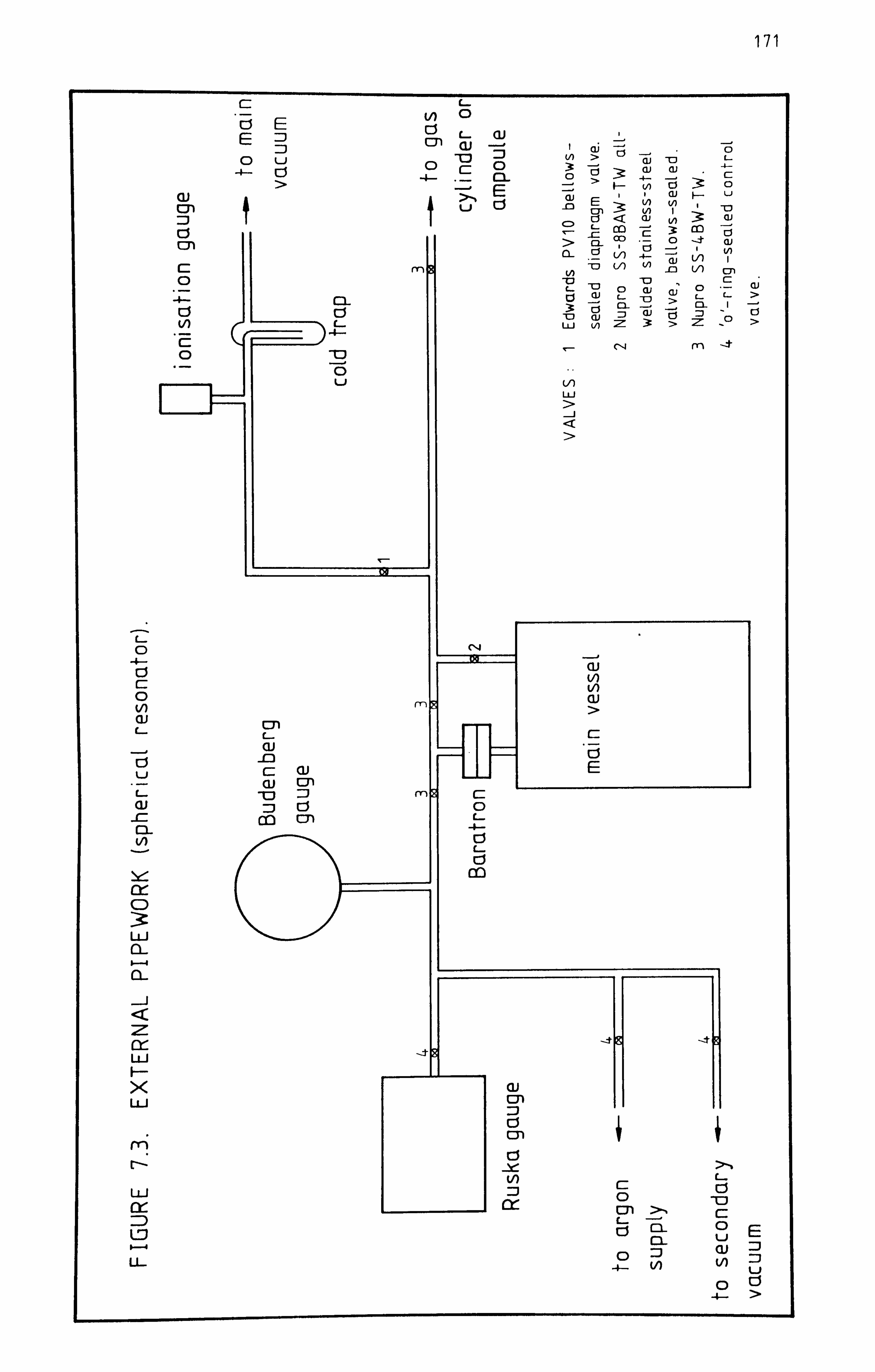
171

C5 E 0

E D C5 CD C- ai

0 D u

CU _0 :3 > 0 0

-4- C5 0 C: 0 0 0 -6 ai ai

-1. - - C: > - E V) C) 0

ai 01 u d (Ij -0

E : 3: ý) ai

(n U

-0 81 < V) 1 :6 L 00 3: CIO

C31 > C2- co .-0 -k (1) V) 4- V)

1 C: m8 W

-0 (A _0 V) On

0 -D C- 1: 3 0

-0 1 CU (1) 0 - C:

0- U 't

ai L- CL

-C) >

- C3-

L- 1

> -

A ci (Ij Z) au -E5 = -0 ci V) LLJ (A 2!: 3: > = - >

C14 m

0 U LA

w >

0 C14

4- ci ai r- (A

V) 0 (ii V) ME > Gi CM

ci -0 E u C: ai (Ij IM

-0 71 ms C: W El 0 r- C. 10 0) L- C3- -I-- V)

co Of CD : 3: LLJ r) r)

z

cy-

LLJ

F- x LLJ

m

cl LLJ cr 0 -0 cc - C: ZD

LD ci o E u LL 0

(A u C) CJ

-4- >

172

vapour diffusion pump had an ultimate lo%v pressure of 0.1 mPa, and the

main vessel could be pumped down to an ultimate low pressure of about 0.3 r-, Pa as indicated by an ionisation gauge in the connecting pipe.

The main vessel was immersed in a well-stirred water bath in which

the temperature ý%as controlled to ±1W by a commercial temperature

controller driving a 500 W heater. The stirring efficiency was very high

and as a result temperature gradients in the water bath were negligible.

Unfortunately, the stirrer motor caused so much vibration that it was

usually necessary to turn it of f while the acoustic measurements were

performed but, with a time constant between the bath and the resonator of

several h, a fe%N min (usually less than 2) without stirring generally

caused no detectable change in the temperature of the resonator. When

lef t unperturbed the temperature of the sphere would be constant to

within a few tenths of a mK for 1h or longer. A small 1W heater was

attached to the outer surf ace of the resonator and used to compensate for

the fall in its temperature following a reduction in the gas pressure.

If this had not been installed many hours would have been required for

thermal equilibrium to be re-established following an expansion. With

temperature differences between one part of the water bath and another

of , at most, 10 mK and with a long time constant for heat exchange I

between the sphere and its container (about 4h in argon and 30 min in

helium) significant temperature gradients of the resonator can be

discounted. Every indication implied that the measured temperature was

indeed the true (IPTS-68) temperature of the gas.

173

7.3 INSTRUMENTATION AND MEASUREMENT TECHNIQUE

The instrumentation used to measure resonance frequencies and

widths is shown schematically in figure 7.4. The system was based in the

Hewlett-Packard HP4192A impedance anal. %ser, which consists of a digital

frequency synthesiser and an amplitude and phase comparator. This

instrument was operated under the remote control of a small computer

(Hewlett-Packard HP87A with HP-IB interface). The internal time base of

the HP4192A was phase locked to a calibrated 10 MHz quartz-crystal

oscillator (this was housed in a thermostat built-in to a Hewlett-

Packard HP5315B opt. 004 frequency counter). Since all synthesised

frequencies had the relative accuracy of the 10 MHz reference signal, and

since this was stated to be better than 1x 10- 7, it was not necessary to

employ a separate frequency counter.

The output signal of the HP4192-A, which was variable between 0.005

and 1.100 V r. m. s., was amplified to a maximum 70 V r. m. s. and used to

drive the source transducer. A resistive potential-difference divider in

parallel with the output of the power amplifier was used to supply a

reference signal of 1Vr. m. s. to the amplitude and phase comparator.

The detector had a sensitivity of about 10 mV-Pa -1 at audio

frequencies, and was connected by a screened cable to a low-noise

amplifier having a forward potential -dif f erence gain of 1000. The

signal was then further amplified, and filtered to remove low- and high-

frequency noise, by a bandpass amplifier (potential difference gain 10;

passband 1 to 100 kHz) and fed to the measurement channel of the amplitude

and phase comparator. Under typical conditions near resonance, the

signal at the input to the HP4192A was between 0.1 and 1Vr. m. s., and

its amplitude and phase could be meas, -ýred with a resolution of 0.01 per

cent and 0.0002 rad, with a time cons--ant of

Circuit diagrams of the amplifiers constructed in this work are

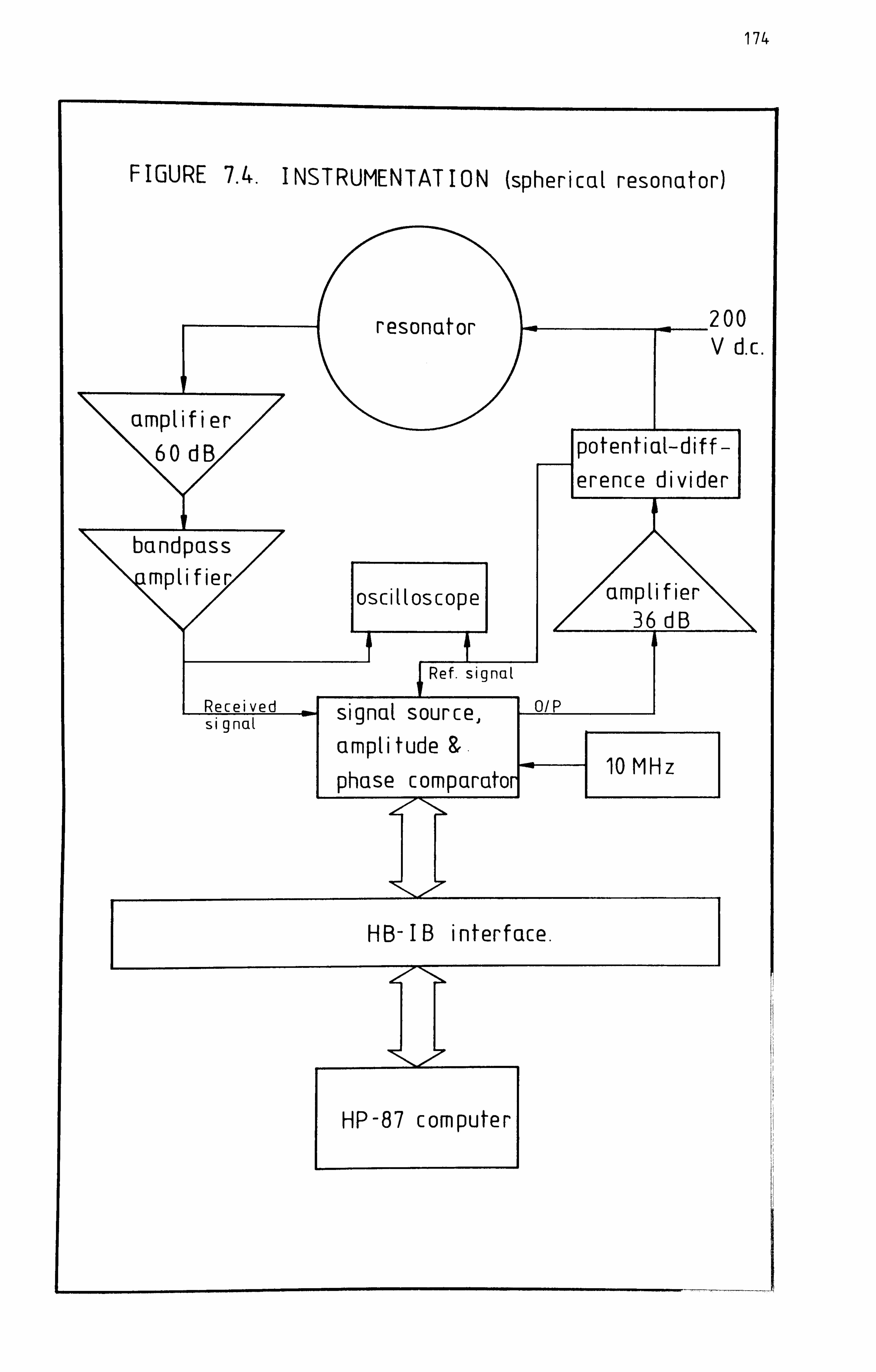
174

FIGURE 7.4. INSTRUMENTATION (spherical resonator)

175

are given in appendix A7.1. Since the reference signal for the amplitude

and phase measurements %Nas derived `-ro7i the output of the drive amplifier,

the frequency response of the source electronics was not critical to the

accuracy of the measurements. The amplitude-and-phase response of the

bandpass amplifier used in the detector circuit was measured, but only

the phase shift varied in the passband and this variation was too small

to introduce significant systematic error into the measurements reported

here.

The measurement procedure, which was similar to that adopted by

Moldover and Mehl, ' was as follows. The centre frequencies fOn and half

widths g of each of the lowest fiýe radial modes were first estimated - On

by sweeping the source frequency and observing the received signal on the

oscilloscope. Then, under the control of the computer, the relative

amplitude a and phase ý of the received signal were measured at a number

of discrete frequencies in the vicinity of each resonance. Starting at

a frequency near f On - gOn' the frequency was increased to one near

f+ in ten even increments of o 15, and then the sign of the On g On -On

increment was reversed and the frequency stepped back down to its initial

value. At each frequency, the system paused for a time 1-4/ gOn during

which the amplitude at the detector settled to within 0.02 per cent of its

final value, before recording the amplitude and phase. The measured

values of a and ý were converted into the real and imaginary parts of the

complex potential-difference ratio of the received and reference- signals,

a Cos W- ja sin (7.3.1)

and used to evaluate the constants F,, 9AqB, and C in the theoretical

form of the resonance:

lAflkF 2f2 )) +B Cf (7.3.2) On

1 76

The non-linear fitting procedure used in this analysis has been described

in detail by Mehl. 8 The twenty-two measurements of the complex variable

are used to evaluate four complex constants in equation (2). In that

equa don ,F On -f On - 'gOn in the coi-iiplex resonance frequency, A is a

complex amplitude, and B+ Cf are the leading terms of a Taylor Is series

that accounts for the background signal from other modes and from direct

coupling between source and detector. Use of careful screening reduced

the electromagnetic crosstalk to a low level, and for the lowest three

modes IB+ Cf I usually accounted f or only af ew per cent of the received

signal. The background level was higher for the other modes (as much as

50 per cent at the lowest pressures in argon) and if resonances above the

f if th had been employed then more terms in the Taylor's expansion may

have been required. Figure 7.5 shows a typical set of results and their

deviations from equation (2). With a precision of about 0.1 per cent

in w, and with Q's of several thousand, a resolution of about 10- 7f On

was acheived. The values of f On and g On obtained in this way were not

sensitive to the range of frequencies studied: measurements between

f On +2 gOn and f on+ 2gon yielded virtually identical values. No evidence

was found that suggested that f On or gon were dependent on the amplitude

of the standing wave.

No detailed investigation of the elastic response of the resonator's

shell was undertaken in this work. However, the spectrum shown in

figure 7.6 was obtained with the resonator evacuated, and it shows that

the expected resonance in the vicinity of 20 kHz is very complex.

Perhaps this was due to the presence of the thermometer well bolted to

the resonator. There is some evidence of resonances at lower frequencies,

particularly near 8.6 and 15 kHz.

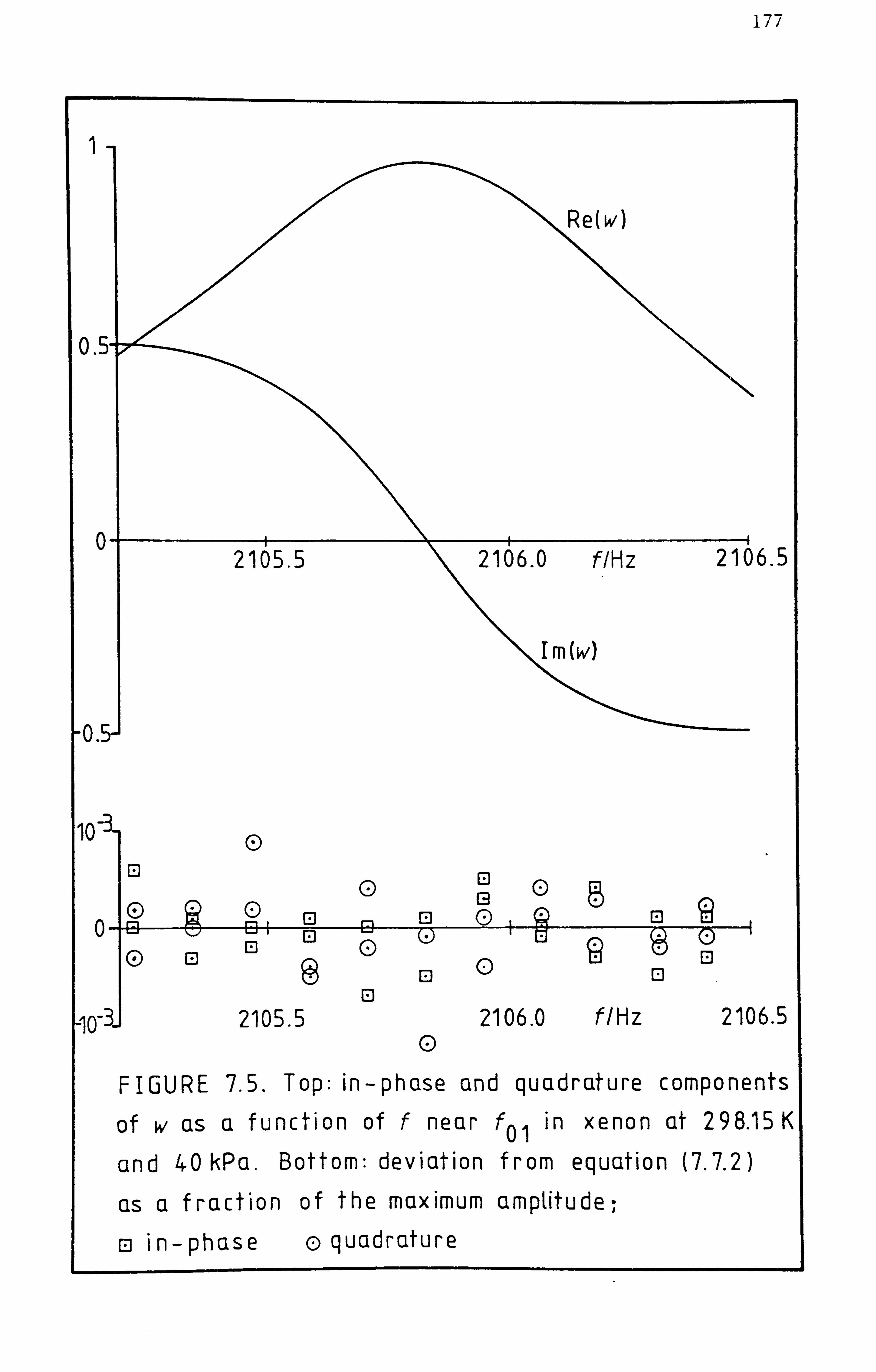
177

Re(w)

0.5-

- i ii 0

2105.5 2106.0 f/H z 2106.5

Im (W)

0.15. 1

10

El S

43 r-l ED r-l El (D I !@0 -9 1 0- - -- V-j 6.. 1 1

0 El U.

0 El 0 ID

El 13

-10-3 J 2105.5 2106.0 f/Hz 2106.5 0

FI GURE 7.5. Top: in-phase and quadrature components

of w as afu ncti on of f near f 01 in xenon at 298.15K

an d 4OkPa. Bottom: cleviati on from equation (7.7.2)

cis a fraction of the maximum ampLitucle-,

I -- Ei in-phase o quadrature

--ý j

178

179

7.4 THE ACOUSTIC MODEL

The various corrections that must be applied to the measured

resonance frequencies in order to obtain accurate speeds of sound have

been discussed in the previous chapters and in reference 2; they are

simply collected here in a convenient form for ease of reference.

The observed complex resonance frequency F On of the n th

radial

mode is given by

Ff (v u/27Ta) (, ýf + ig) On = On - igOn = On i5 (7. L.. j)

where (v On u/27a) is the unperturbed resonance frequency, and (, ýf + ig) i

is the j th

perturbation. Four mechanisms that lead to perturbation of the

resonance frequencies are included in this model. The first, and for

many gases the most important, is damping in the thermal boundary layer.

This surface effect gives rise to a perturbation,

i

Zýf + jgS = (1 + i) f (-y - 1) /2a) (D 21 s t-L On

that has equal real and imaginary components.

(7.4.2)

The classical mechanisms

of thermal conductivity and shear viscosity combine with vibrational-

relaxation absorption to give rise to an attenuation throughout the bulk

of the fluid. In the absence of significant dispersion, only the

resonance vvidths are perturbed and the contribution is

-, Tf 2 /U 2 (4D 13) + (y - 1)D + (n, k)), (7.4.3) On vtb

where Dv= (Tý/p) is the viscous diffusiN,, ity, and the vibrational-

relaxation contribution to the bulk viscosity Týb is given by equation

(2.7.10). At sufficiently high frequencies the real part of F On would

180

also be perturbed, but such effects contribute less than 10- 6f

On in this

work and have been neglected. The third perturbation arises from the

presence of the filling and coupling tubes, which are both of diameter

1 mm. The detector's coupling tube is 6 mm long, while the filling tube

is 12 mm long. Combination of equations (4.4.4), (3.4.12), and (3.2.24)

shows that f or one open tube of length L and cross-sectional area S

, Lf t- igt = -(u/27a) (S/47a 2 )Icot(v OnLla) - iotKHL cosec

2 (v On Lla)), (7.4.4)

provided that the tube resonance is well separated from the resonances of

the cavity. The fundamental resonance of the filling tube is approxi-

mately midway between the f ourth and f if th modes, and f or the detector 1s

coupling tube the fundamental resonance is well above the range of

operating frequencies. Under the conditions of the measurements reported

here gt1f On was always less than 10- 6

and has been neglected. The total

relative shifts in the resonance frequencies are -11.1 x10- 6

for the

first mode, -2.3xlO- 6f

or the second, + 0.3 x 10- 6

for the third,

+3-3 x1O -6 for the fourth, and -3.1 x 10- 6 for the fifth mode. The final

perturbation arises from the elastic response of the resonator's walls

and is given by equation (7.2.5), which for the chosen dimensions and

material reduces to

Af el = 2.7xlO-llf On

(pu 2 'pa)/{' - (fOn /21.2 kHz) 2 ). (7.4.5)

Greenspan has found the contributions to g arising from losses in the

wall and radiation from its outer surface to be negligible. '

A fifth perturbation, in effect a second-order correction to

equation (2), arising from the temperature -jump effect may be significant

at low gas pressures. A simple theory for monatomic gases is suggested

in appendix A3.1, and will be compared with the experimental results in

the following section.

181

7.5 SAMPLE RESULTS

The results presented in detail in this section were obtained in

argon, xenon, and helium at temperatures close to 298.15 K, and in 2,2-

dimethylpropane at temperatures close to 262.61 K (20 K below the normal

boiling temperature).

The gas-handling procedures used were similar to those described in

chapter six and will not be repeated here. No special precautions were

taken in these experiments to insure rigorously high chemical purity, but

the system was evacuated to 1 mPa (as indicated by an ionisation gauge in

the vacuum line) and flushed with the gas prior to filling, except for

the measurements in xenon where there ýsas insufficient gas to flush the

apparatus. Random errors in the measured temperatures are less than

±0-5 mK in these experiments, and were later reduced to ±0.1 mK by

replacing the ageing A. S. L resistance bridge with a new instrument (see -

chapter nine). The rather limited precision of the pressure measurements

above 1-15 kPa was just adequate for argon and helium, but was a def inite

limitation with xenon. All the measurements on 2,2-dimethylpropane were

performed at lower pressures using the precise quartz-spiral gauge.

The argon was supplied by Cambrian gases Ltd. who estimated tha. t 6

the total mole fraction of impurities i%as less than 5xlO- Measurements

were performed at 13 pressures betý%een 20 and 241 kPa, at a mean

temperature of 298.149 5 K. The measured values of T, p, f On , and gOn

are given in table 7.1. The uncertainties in f On and gOn , as estimated

by the non-linear regression analysis, were always less than 0.2 per cent

Of gOn' and the quality factors range from Q01 =920 at the'lowest

pressure to Q05'::: 5500 at the highest pressure studied.

The measured half -widths in argon may be compared with the directly-

measured values of the transport coefficients Tý(298.15 K, p-*O) =22.6 iiPa-

and K(23,88-15 Ký p->. O) =17.7 mVV-m -1 -k -1 taken from a recent revie%v. 9

182

TABLE 7.1 Resonance frequencies and half widths in argo-n at 298.15 K.

p/kPa TIK n f On /Hz gOn /Hz gS/Hz 9b /Hz 10 6 AgIf (ula)110 3

5-

240.8 298.1648 1 3823.351 0.593 0.572 0.006 4.0 5.346 898 2 6573.459 0.753 0.749 0.018 2.3- 5.346 919 3 9278.513 0.94-4, 0.890 0.036 1.9 5.346 921 4 11969.205 1.124 1.011 0.059 4.4 5.346 899 5 14653.660 1.338 1.119 0.089 8.9 5.346 904

200.9 298.1480 1 3822.826 0.647 0.626 0.007 3.5 5.346 380 2 6572.588 0.554 0.820 0.021 1.8 5.346 409

3 9277.284 1.040 0.975 0.043 2.5 5.346 401

4 11967.655 1.221 1.107 0.071 3.6 5.346 387

5 14651.803 1.435 1.225 0.106 7.3 5.346 399

161.0 298.1484 1 3822.402 0.723 0.699 0.009 3.9 5.345 876

2 6571.883 0.955 0.916 0.027 2.3 5.345 900

3 9276.328 1.159 1.089 0.053 1.8 5.345 901

4 11966.453 1.390 1.237 0.089 5.4 5.345 891

5 14650.309 1.578 1.368 0.133 5.2 5.345 887

121.0 298.1473 1 3821.930 0.535 0.806 0.012 4.3 5.345 367

2 6571.111 1.105 1.057 0.036 1.9 5.345 385

3 9275.276 1.346 1.256 0.071 2.1 5.345 389

4 11965.120 1.605 1.426 0.118 5.4 5.345 377

5 14648.745 1.536 1.578 0.177 5.5 5.345 386

100.020 298.1463 1 3821.658 0.915 0.887 0.015 4.4 5.345 103

2 6570.684 1.213 1.163 0.043 1.1 5.345 127

3 9274.701 1.454 1.381 0.086 1.9 5.345 133

4 11964.400 1.785 1.569 0.143 6.4 5.345 121

5 14647.870 2.017 1.736 0.214 4.6 5.345 125

79.080 298.1452 1 3821.355 1.032 0.997 0.018 4.3 5.344 838

2 6570.222 1.370 1.307 0.054 1.2 5.344 874

3 9274.066 1.667 1.553 0.108 0.6 5.34-4 870

4 11963.643 2.021 1.764 0.180 6.4 5.344 873

5 14646.933 2.277 1.952 0.270 3.7 5.344 863

60.020 298.1507 1 3821.096 1.157 1.145 0.024 4.8 5.344 628

2 6569.822 1.556 1.501 0.072 2.0 5.344 652

3 9273.559 1.941 1.783 0.143 1.6 5.344 655

183

p/kPa TIK n f On /Hz gon/Hz gS/Hz 9b /Hz 10 6

AgIf (ula)110 3 s-

1

60.020 298.1507 4 11963.002 2.338 2.025 0.237 6.3 5.344 648 5 14646.203 2.650 2.241 0.356 3.7 5.344 645

50.020 298.1527 1 3820.905 1.302 1.254 0.029 5.1 5.344 492 2 6569.552 1.745 1.644 0.086 2.3 5.344 528

3 9273.183 2.141 1.953 0.171 1.8 5.344 516 4 11962.556 2.565 2.218 0.285 5.2 5.344 514 5 14645.710 2.913 2.455 0.427 2.2 5.344 521

40.023 298.1525 1 3820.667 1.455 1.402 0.036 4.6 5.344 366 2 6569.207 1.962 1.838 0.107 2.6 5.344 404

3 9272.760 2.405 2.183 0.214 0.9 5.344 404'

4 11962.060 2.929 2.480 0.356 7.8 5.344 408

5 14645.082 3.291 2.744 0.534 0.9 5.344 395

35.016 298.1501 1 3820.525 1.555 1.498 0.042 4.0 5.344 323

2 6568.976 2.110 1.965 0.123 3.4 5.344 339

3 9272.455 2.580 2.334 0.245 0.1 5.344 335

4 11961.731 3.136 2.651 0.407 6.5 5.344 357

5 14644.671 3.562 2.933 0.610 1.3 5.344 334

30.028 298.1475 1 3820.334 1.682 1.618 0.048 4.1 5.344 245

2 6568.726 2.265 2.122 0.143 0.1 5.344 286

3 9272.120 2.826 2.521 0.285 2.2 5.344 272

4 11961.327 3.413 2.863 0.474 6.4 5.344 293

5 14644.239 3.880 3.168 0.711 0.1 5.344 283

24.995 298.1472 1 3820.158 1.842 1.773 0.058 2.8 5.344 218

2 6568.444 2.507 2.325 0.172 1.5 5.344 223

3 9271.772 3.095 2.763 0.342 -1.1 5.344 212

4 11960.960 3.796 3.138 0.570 7.4 5.3 44 253

5 14643.774 4.294 3.472 0.854 -2.2 5.344 225

20.000 298.1464 1 3819.900 2.076 1.982 0.073 5.4 5.344 155

2 6568.065 2.793 2.599 0.215 -3.2 5.344 144

3 9271.398 3.511 3.088 0.428 -0.6 5.344 190

4 11960.418 4.226 3.508 0.712 0.5 5.344 181

5 14643.160 4.935 3.881 1.068 -0.9 5.344 156

Values of (ula) are adjusted to the mean temperature of 298.1495 K.

184

These are believed to be accurate to ± -D. 2 per cent. ' The effects of

pressure on both quantities are quite negligible under the conditions of

these measurements, and perfect-gas values of u, p, and cP are sufficient

for the calculation of gS and 9b; the results of such calculations are

given in table 7.1. Typical contributions to the resonance half widths

are shown as a continuous function of frequency in figure 7.7. The

dominance of the surface term is evident. The measured half widths exceed

those calculated by just a few per cent, but this additional loss remains

unexplained. The 'excess' half widths 'ýg 7:: (9 - 9S - 9b) are listed as

fractions of the resonance frequencies in table 7.1, and selected values

are plotted on figure 7. S. For the second and third modes, AgIf is less

than 3x 10- 6

and decreases with the pressure while, for the first and

fourth modes, AgIf is systematically higher and tends to increase at low

pressures. The larger excess half widths observed for the fifth mode are

not typical; the usual behaviour was closer to that of the second and

third modes. The rapid increase in 'ýg' If with the pressure may be the IJ5 05

result of a minor shell resonance near that frequency. There is some

evidence for this in figure 7.6.

The resonance frequencies were corrected according to equation

(7.4.1), adjusted to the mean temperature, and used to generate the

values of (ula) listed in table 7.1. Typical contributions to the

relative frequency shifts L-flf are shown as a continuous function of

frequency in figure 7.7. Uncertainties in the thermal conductivity of

dilute argon at 298.15 K should not lead to errors of more than 1 x10-6 f

in the corrected frequencies. Relative deviations of (ula) from the mean

value for the first five modes at selected pressures are plotted on

f igure 7.8, and are at worst -6 x 10- 6,

and typically ±2 x 10- 6.

For the

second, third, and fifth modes the deviations are consistently small and

do not depend systematically on the pressure, while those of the f irst and

fourth modes show greater scatter. It is significant that the excess

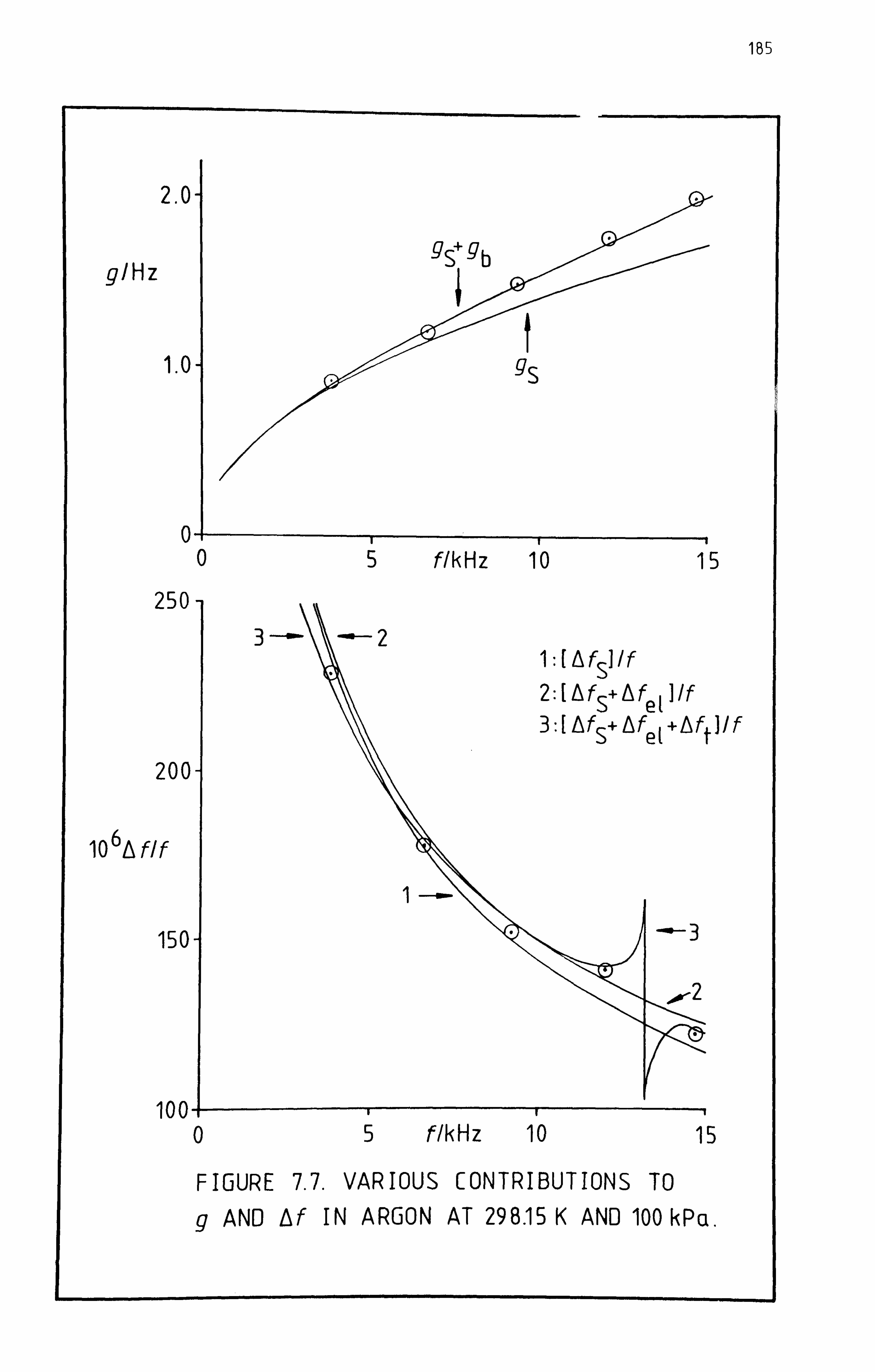
1B5

2.0-

-q! ý 9b glHz .................

1.0- gs

0 05 f/kHz 10 15

250- 3---aw- -mme- 2

1A fsl If 2: A fS+ A fe 11 If 3: AfS+ A ý( +Aft I/ f

200-

10 6A f1f

150- 3

2

100 05 f/kHz 10 15

FIGURE 7.7. VARIOUS CONTRIBUTIONS TO

g AND Af IN ARGON AT 29815 K AND 100 kPa.

186

9- 0

17

6- Zý

10 6 Ag On 0

f On 3- 0 Zý

z 17

2n345

OAr, 24lkPcL. <>Ar, 20lkPcL. ok, 161k%. X Ar, 121 kPa. Zý Ar, 79 kPa. VAr, 40 kPa 298.15 K.

4-

2-

6X 10 AU 0- 13 Vu in UX0

-2- 0

-4-

17 -61 1

12n345

FIGURE 7.8. TOP: excess hal f widths as a fraction of the resonance frequencies. BOTTOM : fractional deviations of (ula) from the mean vatue for the first five radiat modes. Au =u- u(mean) -

K __a

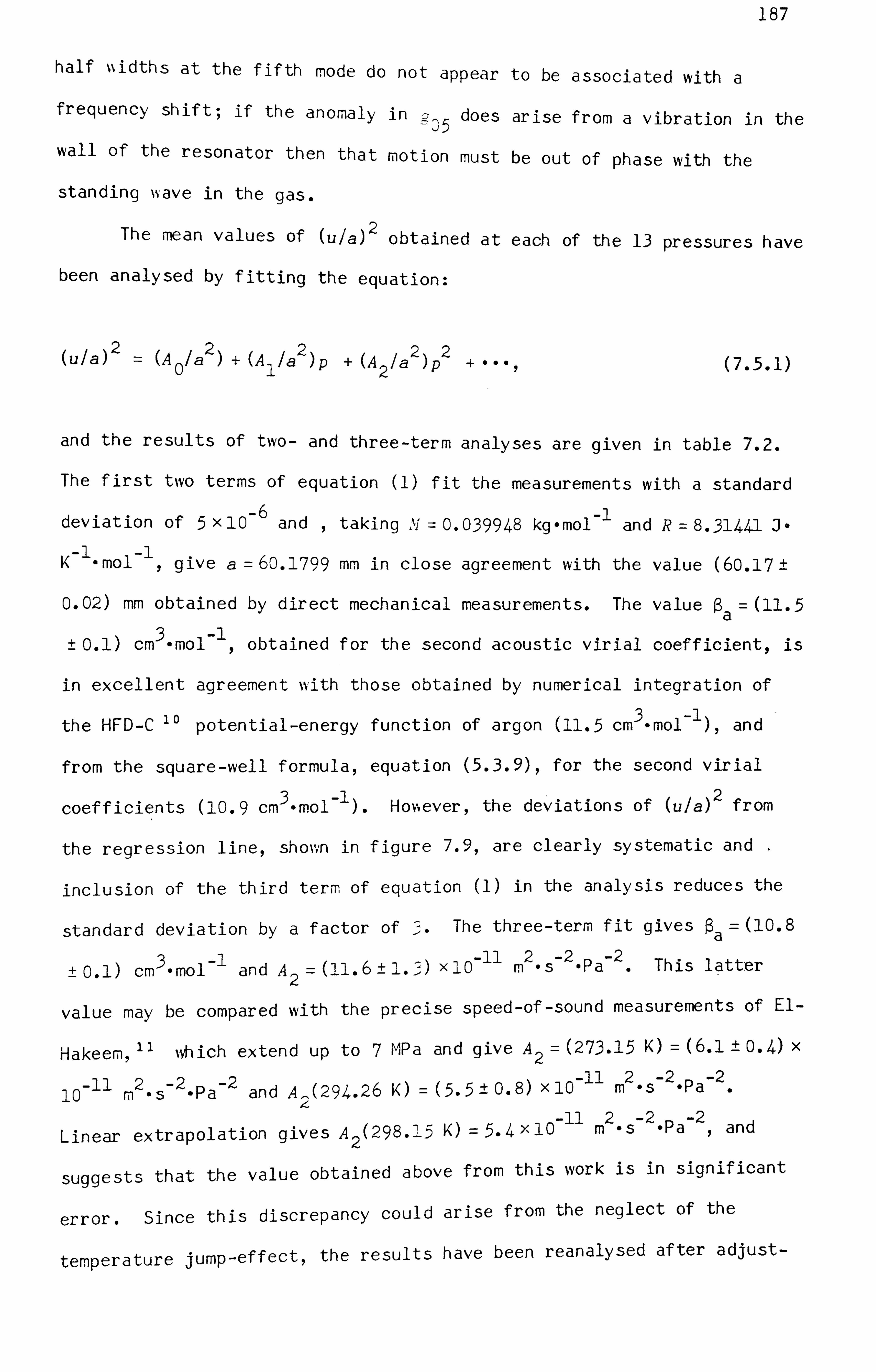
187

half %%idths at the f if th mode do not appear to be associated with a frequency shift; if the anomaly in g, does arise from a vibration in the ýýJ5 wall of the resonator then that motion must be out of phase with the

standing wave in the gas.

The mean values of (u/a) 2 obtained at each of the 13 pressures have

been analysed by fitting the equation:

(ula) 2= (A 0

la 2)+ (A 1

la 2)p+ (A 2

la 2)p2 (7.5.1)

and the results of two- and three-term analyses are given in table 7.2.

The first two terms of equation (1) fit the measurements with a standard

deviation of 5x 10- 6

and , taking N' = 0.039948 kg-mol- 1 and R=8.31443- J-

K -1 - mol -1 , give a= 60.1799 mm in close agreement with the value (60.17 ±

0.02) mm obtained by direct mechanical measurements. The value ýa= (11.5

0.1) cm3. mol-1, obtained for the second acoustic virial coef f icient, is

in excellent agreement with those obtained by numerical integration of

the HFD-C 10 potential -energy function of argon (11.5 cm3. mol-i ), and

from the square-well formula, equation (5.3.9), for the second virial

coefficients (10.9 cm3. mol-1 ). Hoýýever, the deviations of (ula) 2 from

the regression line, shov,, n in f igure 7.9, are clearly systematic and .

inclusion of the third term of equation (1) in the analysis reduces the

standard deviation by a factor of The three-term fit gives ý =(10.8 a 22 -2 0.1) cm3. mol-1 and A2= (11.6 x 10-11 m. 5 Pa This latter

value may be compared with the precise speed-of -sound measurements of El-

Hakeem, " which extend up to 7 MPa and give A2 7-- (273-15 K) = (6.1 ± 0-4)

-11 2-2 -2 -11 2 -2 -2 10 M es . Pa and A- (294.26 K) = (5-5 ± 0.8) x 10 m. s. Pa

4

Linear extrapolation gives A2 (298.15 K) = 5.4 x 10 -11 m2 -s -2 -Pa -2 , and

suggests that the value obtained above from this work is in significant

error. Since this discrepancy could arise from the neglect of the

-rature jump-effect, the results have been reanalysed after adjust- tempe

188

C)

V)

C: ) 0

0

C)

CD CN

Li Li L- CO

. r- (2-, C-Ii -6-- (N

E) 4- CD

ir u-) .. a

Z 0

CM Ir-

11 E

C--

(N4 L- ci zi a)

- Li C)

V) c: 0

-0

. 4-

>

Lri LL-

crý GEI

r- G) E)

L. Li

LD e--4

L. L CD

c**-j

c**-j

, 10

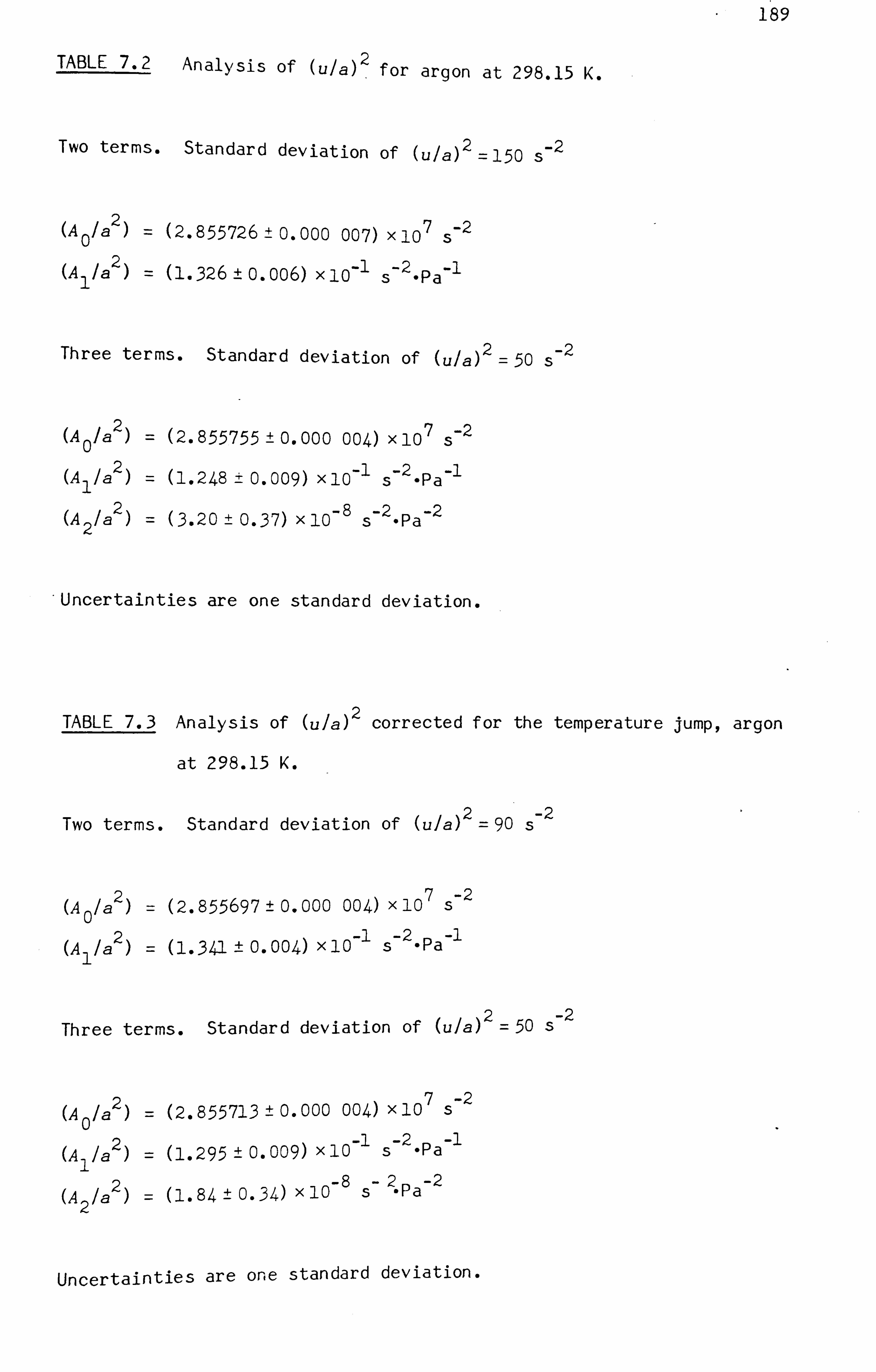
1 89

TABLE 7.2 Analysis of (u/a)2 for argon at 298.15 K.

Two terms. Standard deviation of (ula) 2= 150 s- 2

(A 0

/a 2 (2.855726 ± 0.000 007) x 10 7s -2

(A 1

/a 2 (1.326 ±0 . 006) x 10-1 s- 2. Pa-1

Three terms. Standard deviation of (ula) 2= 50 s-2

27 -2 (A 0

la )= (2.855755 ± 0.000 004) x 10 s

(A 1

la 2)= (l. 248 ± 0.009) x 10-1 s- 2. pa-i

(A 2

la 2)= (3.20 ± 0.37) x 10- 8 s-

2. Pa -2

Uncertainties are one standard deviation.

TABLE 7.3 Analysis of (ula) 2 corrected for the temperature jump, argon

at 298.15 K.

Two terms. Standard deviation of (ula) 2= 90 s -2

(A 0 la 2)= (2.855697 ± 0.000 004) x 10 7

S-2

(A 1

la 2)= (1- 341 ± 0.004) x 10-1 s- 2. Pa-1

2 -2 Three terms. Standard deviation of (ula) = 50 s

(A 0

la 2)= (2.855713 ± 0.000 004) x 10 7 S-2

(A 1

la 2)= (l. 295 ± 0.009) x 10-1 s-2. pa-i

2-8-2-2 (A 2

la )= (1 - 84 ± 0.34) x 10 5 Opa

Uncertainties are one standard deviation.

190

ment according to equation (A3.1.25) using an accommodation coefficient

1. This lowers (ula) 2 b\, 15 x 10- 6

at the lowest pressure studied.

The results of two- and three-term fits of equation (1) are given in

table 7.3. Again, the three-term fit appears to be justified and the

remaining differences between the measurements and the regression curve

shown in figure 7.9 are clearly random. The value A2= (6.7 ± 1.2) x 10-11

m2 OS -2 ePa- 2

obtained from this analysis does not differ significantly

from the one estimated from El-Hakeem's results, and the second acoustic

virial coefficient ýa= (11.2 ± 0.1) cm3. mol -1 is still in excellent

agreement with independent estimations of the highest quality.

The research grade xenon was supplied by the British Oxygen

Company who estimated that the total mole fraction of impurities was less

th an 5x 10- 5. The actual purity of the gas must have been much worse than

this because the gas mixed with air in the cylinder-head pressure

regulator several times Men samples were withdrawn for other purposes.

Measurements were performed at 14 pressures between 15 and 237 kPa, at a

mean temperature of 298.149, K. 1"Jost of the results were taken at

pressures below 100 kPa to facilitate a comparison with the predictions

of the temperature-jump theory. In addition, if the failure of kinetic

theory predicted by Blatt actually occurred then the higher frequency,

modes should yield speeds of sound that approached the ideal-gas value

much more rapidly than those obtained at lower frequencies. Unfortunately,

the measurements were much less precise at the lower pressures where the

above effects might be observed. The decline in precision was caused by

instability in the source transducer Aich became quite pronounced at low

pressures where the damping was slight and the excursions of the diaphragm

large. In later work the i.: elinex membrane was replaced and the problem

did not reOCCUr.

Neverthelessý at pressures above 50 kPa. the random errors in f On

and g On arising from this instability are estimated to be less than

191

1 X10- 6f

On (except for the first mode at the two highest pressures where

fractional errors of about 5 x1O- 6

were estimated). At lower pressures the uncertainties increase to about 23 x1O-

6 fOn in the worst case. The

measured values of T, pq f On , and gOn are given in table 7.4, together

with calculated values of g. and 9b based on the published low-pressure

gas transport properties of xenon. ' The quality factors range from

01 = 1100 at the lowest pressure to Q 05 = 7800 at the highest pressure

studied.

The excess half widths Ag are listed as fractions of the resonance

frequencies in table 7.4, and selected values are plotted on figure 7.10.

The general pattern is similar to that found in argon; the second, third,

and f if th modes tend to exhibit smaller nýgl s than the f irst and f ourth.

Relative deviations of (ula) f rom the mean value f or the f irst f ive radial

modes at selected pressures are also plotted on figure 7.10. The first

mode is systematically low by a fraction of about 3xlO- 6,

while the

remaining resonances are in very close agreement. The increased role of

random errors in both the resonance frequencies and widths is evident at

the lower pressure, but there is no evidence of dispersion to support

Blatt's theory.

The mean values of (ula) 2 are plotted as a function of the pressure

f or p< 100 kPa in f igure 7.11, and the results of two- and three-term

fits of these values to equation (1) are given in table 7.5. Derivatives

of the measured values of (ula) 2f rom the regression lines are also

shown on figure 7.11. Although the deviations Of (ula) 2 from the two-

term fit are not excessive in vie%v of the rather large random uncertainties

in the resonance frequencies, they are clearly systematic and vary

rapidly at low pressures. The three-term fit is able to accommodate 6

much of this curvature and reduce the standard deviation to 4.5 xlO-

(from 8.5 x1O -6 )- The estimated values of the second acoustic virial

mol-1 from the two-term fit, and coefficient are $a= (-10L. 3 ± 0-3) cm

192

TABLE 7.4 Resonance frequencies and half widths in xenon at 298.15 K.

p/kPa TIK n f On /Hz gOn /Hz gS/Hz 9b /Hz 10 6 Lgjf (ula)110 3

S- 1

236.2 298.1484 1 2097.695 0.251 0.238 0.002 5.1 2.933 570 2 3606.521 0.330 0.312 0.006 3.3 2.933 580 3 5090.631 0.400 0.371 0.011 3.5 2.933 584 4 6566.881 0.470 0.422 0.019 4.5 2.933 579 5 8039.699 0.517 0.466 0.028 2.8 2.933 577

200.2 298.1491 1 2099.233 0.280 0.259 0.002 9.1 2.935 741

2 3609.179 0.359 0.339 0.007 3.6 2.935 756

3 5094.382 0.431 0.403 0.013 2.9 2.935 755

4 6571.726 0.510 0.458 0.022 4.5 2.935 751

5 8045.646 0.565 0.507 0.033 3.1 2.935 753

160.0 298.1512 1 2100.941 0.303 0.290 0.003 5.2 2.938 156

2 3612.125 0.400 0.380 0.008 3.4 2.938 169

3 5098.555 0.481 0.451 0.017 2.6 2.938 171

4 6577.119 0.560, 0.512 0.027 4.5 2.938 168

5 8052.252 0.628 0.567 0.041 2.5 2.938 169

119.8 298.1487 1 2102.637 0.350 0.335 0.004 5.2 2.940 598

2 3615.058 0.461 0.439 0.011 2.9 2.940 610

3 5102.708 0.559 0.522 0.022 3.0 2.940 612

4 6582.493 0.665 0.593 0.037 5.4 2.940 6il

5 8058.835 0.734 0.656 0.055 2.9 2.940 610

100.090 298.1705 1 2103.537 0.381 0.367 0.004 4.6 2.941 791

2 3616.617 0.502 0.481 0.013 2.3 2.941 802

3 5104.915 0.605 0.571 0.026 2.0 2.941 801

4 6585.340 0.722 0.649 0.044 4.5 2.941 797

5 8062.339 0.806 0.718 0.066 2.7 2.941 800

79.930 298.1480 1 2104.276 0.426 0.410 0.006 4.9 2.942 994

2 3617.909 0.562 0.538 0.017 2.1 2.943 007

3 5106.756 0.682 0.639 0.033 1.9 2.943 010

4 6587.728 0.512 0.726 0.055 4.7 2.943 006

5 8065.267 0.904 0.803 0.083 2.2 2.943 008

193

p/ kP a TIK n f On /Hz

. gOn /Hz gS/Hz 9b /Hz 106Aglf (ula)110 3 S-1

60.020 298.1482 1 2105.068 0.490 0.474 0.008 4.5 2.944 186 2 3619.296 0.648 0.621 0.022 1.3 2.944 199 3 5108.728 0.790 0.738 0.044 1.5 2.944 199 4 6590.299 0.945 0.838 0.074 5.0 2.944 201

5 8068.420 1.054 0.927 0.110 2.1 2.944 199

50.017 298.1487 1 2105.455 0.537 0.519 0.009 4.5 2.944 787

2 3619.983 0.713 0.680 0.027 1.6 2.944 802

3 5109.709 0.868 0.808 0.053 1.3 2.944 801

4 6591.568 1.049 0.918 0.088 6.5 2.944 800

5 8069.993 1.158 1.016 0.132 1.2 2.944 802

40.020 298.1484 1 2105.828 0.602 0.580 0.011 5.1 2.945 394

2 3620.646 0.801 0.761 0.033 2.1 2.945 407

3 5110.656 0.971 0.904 0.066 0.3 2.945 402

4 6592.813 1.183 1.026 0.110 7.1 2.945 404

5 8071.508 1.351 1.135 0.165 6.2 2.945 398

35.009 298.1477 1 2105.998 0.644 0.620 0.013 5.2 2.945 690

2 3620.958 0.859 0.813 0.038 2.0 2.945 706

3 5111.122 1.072 0.966 0.076 5.8 2.945 709

4 6593.358 1.269 1.097 0.126 6.9 2.945 682

5 8072.244 1.412 1.214 0.189 1.0 2.945.698

30.021 298.1496 1 2106.174 0.696 0.670 0.015 5.5 2.945 996

2 3621.278 0.926 0.878 0.044 1.0 2.946 010

3 5111.597 1.137 1.043 0.088 1.0 2.946 017

4 6594.024 1.360 1.185 0.147 4.2 2.946 009

5 8073.021 1.549 1.311 0.221 2.1 2.946 007

25.008 298-1478 1 2106.324 0.764 0.734 0.018 5.6 2.946 304

2 3621.554 1.023 0.962 0.053 2.2 2.946 310

3 5112.012 1.244 1.143 0.106 -1.0 2.946 322

4 6594.597 1.502 1.298 0.177 4.0 2.946 324

5 8073.723 1.704 1.437 0.265 0.3 2.946 317

194

P/kPa TIK nf On /Hz /Hz 10 6

AgIf (uJa)JIO 31 g Cn ýiz gSJHz 9b

20.011 298.1464 1 2106.452

2 3621.820

3 5112.391

4 6595.161

5 8074.361

14.999 298.1481 1 2106.560

2 3622.072

3 5112.755

4 6595.615

5 8075.023

0.503 0.820 0.023 9.4 2.946 609

1.1417-5 1.076 0.067 1.6 2.946 625

1.3'eO 1.278 0.133 -4.1 2.946 624

1.711 1.452 0.221 5.8 2.946 650

1.927 1.606 0.331 -1.2 2.946 618

0.992 0.948 0.030 6.8 2.946 929

1.344 1.242 0.089 3.5 2.946 957

1.639 1.476 0.177 -2.8 2.946 939

2.055 1.677 0.295 17.2 2.946 944

2.319 1.855 0.442 2.7 2.946 941

Values of (ula) are adjusted to the man temperature of 298.1498 K.

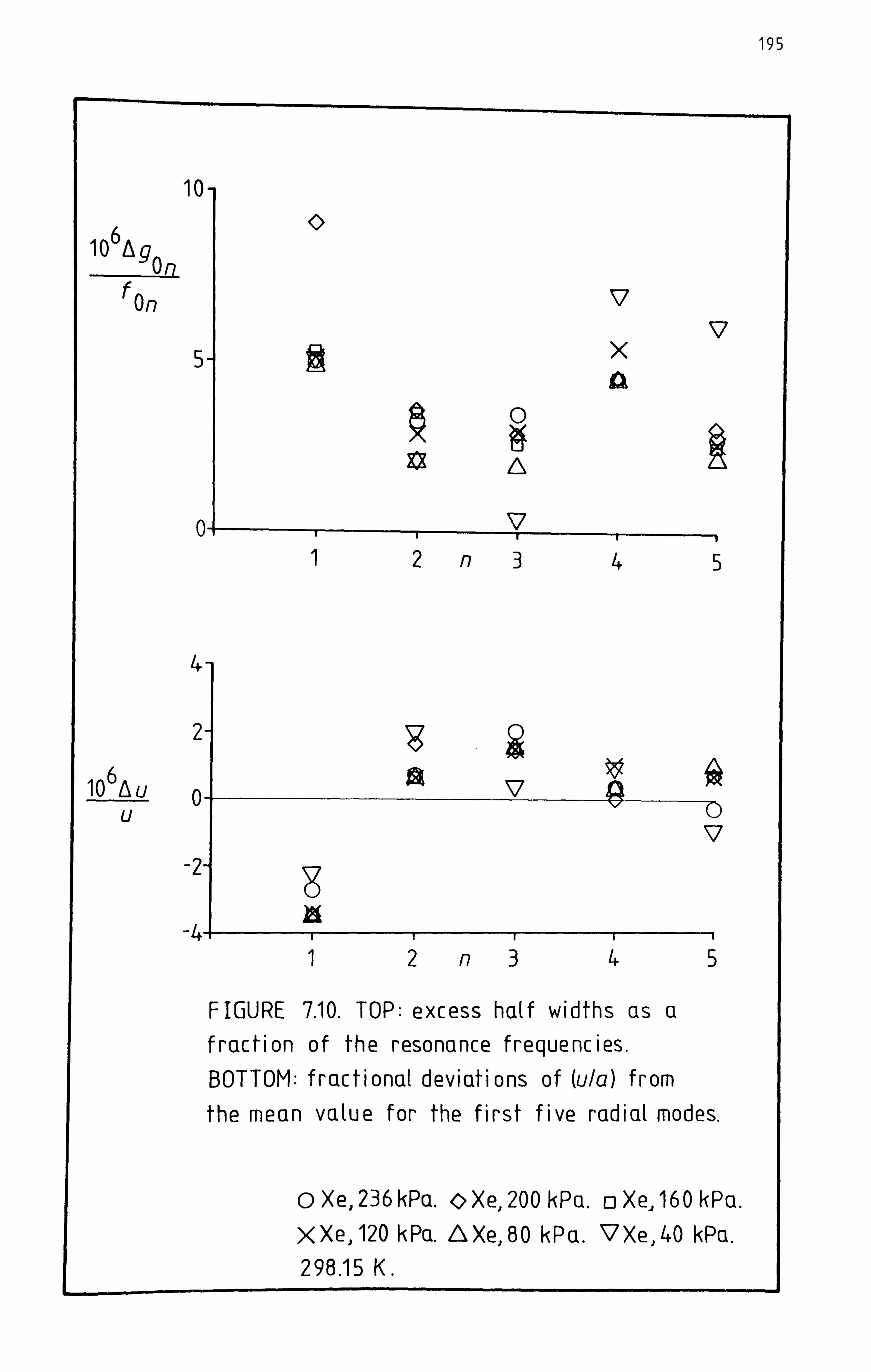
195

10-

10 6 Ag

f On 17 17

5- X

0

0- 2n345

4

2-

10 6AU is 17 U

0- 17

-2-

-4 12n345

FIGURE 7.10. TOP: excess half widths as a fraction of the resonance frequencies. BOTTOM: fractional deviations of (ula) from the mean value for the first five radial modes.

oXe. 236kPa. 0Xe, 200kPa. oXe,, 160kPa. XXe. 120 kPa. AXe., 80 kPa. 17Xe., 40 kPa. 298.15 K.

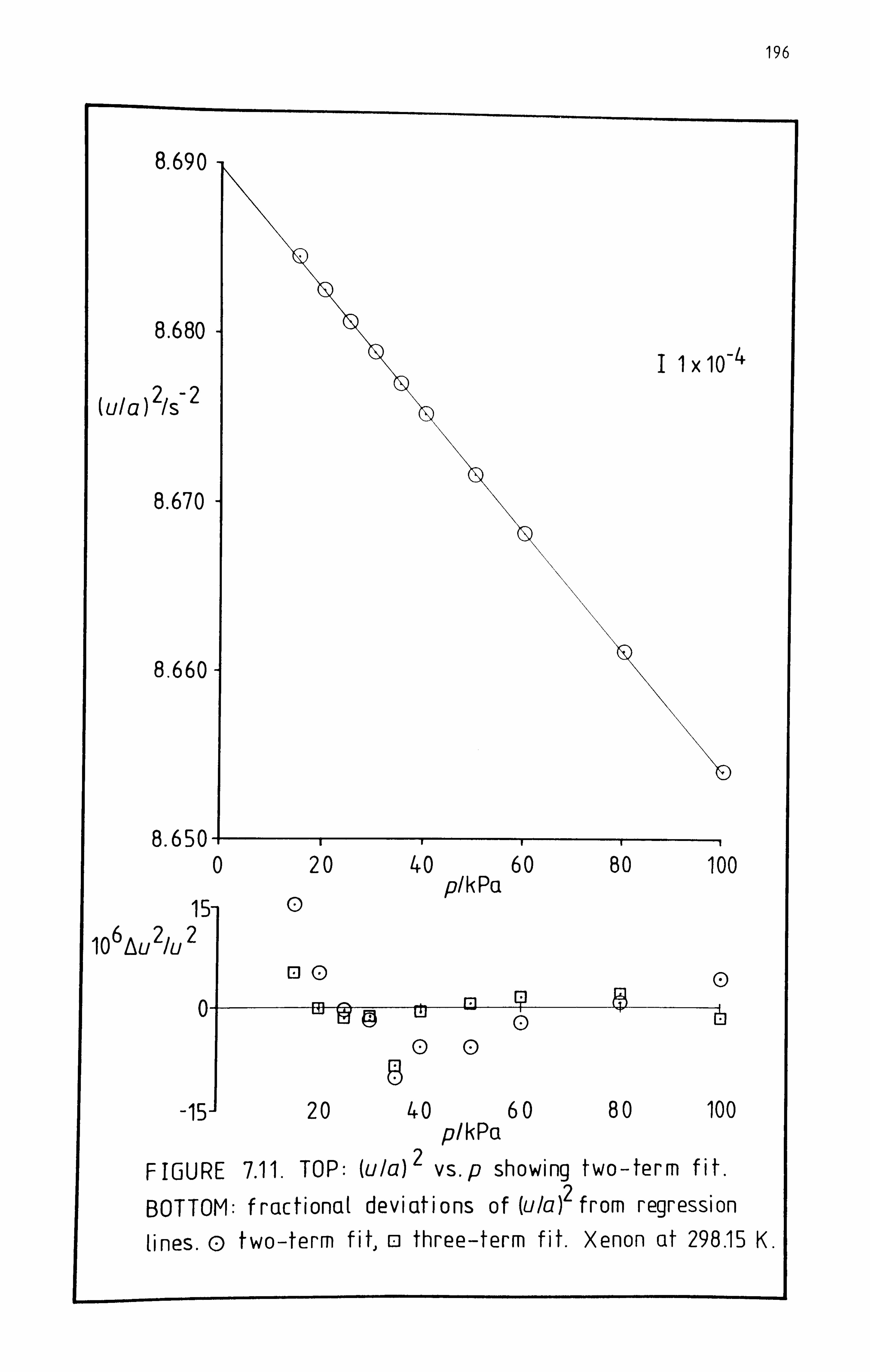
196

8.690 -

8.680 - 1 x 10-4

(ula) 2/s-2

8.670 -

8.660-

8.650 1 1 0 20 40 60 80 100

15 0 p/kPa

10 6 Au 21u 21

0- Ljj ty 0M- _r 00

6

-15- 20 40 60 80 100 p/kPa

FIGURE 7.11. TOP: (ula)2 vs-p showing two-term fit.

BOTTOM: fractional deviations of (u/a)2 from regre ssion tines. (D fwo-term fit, o three-term fit. Xenon at 298.15 K.

197

TABLE 7.5 Analysis of (ula) 2, f or \eno- at 298.15 K.

Two terms. Standard deviation of (ule) 2= 74 s- 2

(A 0 la 2 ) = (8.689659 ± '-). oc-- 047) 2

x 1C , 5-

(A 1

la 2) = (-3.553 ± 0.009) x 10-1 s- - -Pa-1

Three terms. Standard deviation of (ula)2 = 39 s- 2

(A 0

/a 2)= (8.689874 ± 0.00 3 052) x 10 6s -2

(A 1

la 2)= (-3.654±0.022) xlO-l 5- 4 -pa-1 282 (A 9.02 ± 1.93, ) xIs Pa- 2

Uncertainties are one standard deviation.

TABLE 7.6

Two terms.

Analysis of (ula) 2 corrected for the temperature jump, xenon

at 298.15 K.

Standard deviation of (ula) 2= 63 S-2

(A 0 la 2 (8.689578 ± 3.0 -- 3 038) x1 C-

65 -2

(A 1

la 2 (-3.544±0.007) x10-1 s- 2. pa-i

Three terms. Standard deviation of (ula) 2= 32 s- 2

(A 0

la 2)= (8.689752 ± 0.0 -- 0 044) x1 -- ä 5-

2

(A 1

la 2)= (-3.627 ± 0.019) x 10-1 s- 2. pa-i

(A 2

la 2)= (7.28 ± 1.62) x --D- 8

s- 2. pa-z

Uncertainties are one standard deý. iat. 4, -on.

198

ý -:: (-104.2 ± 0.6) cm3. mol-19 from the three-term fit. Inclusion of the a temperature -jump correction with an accommodation coefficient of unity

does lead to a marginal improvement, but does not account for all the

observed curvature at low pressures. The results of two- and three-term

analyses are given in table 7.6. Unfortunately, the marginal improvement

does not provide much evidence to support the temperature -jump theory.

The higher pressure results have not been included so far because of the

relatively large uncertainties in the measured pressures. However, all

the results obtained with p> 25 kPa may be represented by a linear

isotherm with a standard deviation of 4xlO- 6,

and inclusion of the third

term does not improve the f it. This analysis gives a =60.176 mm (using

11= 0.13130 kg-mol -1 ), fractionally 6x Jo- 5 below that obtained using

argon, and ýa::: (-101-10 ± 0.04) cm 3.

mol-1. The values obtained for the

second acoustic virial coefficient may be compared with that calculated

from the interatomic potential -energy function of xenon. The value

obtained from the simple form advocated by Maitland and Smith 12 is

-101.6 cm 3.

mol-1 at 298.15 K, while the square-well formula with

1.641ý CY = 0.3534 nm, and F-lk= 202.9 K, giving the best fit to the second 1

virial coefficientsi predicts ýa (298-15 K) =-101.8 cm3. mol- . These

values favour the results of two-term fits and suggest that the measure-

ments at the lovver pressures are in error.

Technical grade helium was supplied by the British Oxygen Company

without specification of its purity. While high chemical purity was not

felt to be important in these trial measurements, slow outgassing into

the sample during the course of the experiment would alter the apparent

shape of the isotherm. Since the speed of sound in helium is so high

(about 1000 m-S at 300 K) even small amounts of heavier gases would

have a serious consequence. In order to reduce this risk, the system

%%as pressurised with helium to 250 kPa and evacuated several times before

filling. A high-purity gas-cylinder pressure regulator was used to avoid

177

contamination by air. The measurements were performed at seven

pressures between 50 and 253 kPa using the first two radial modes only.

The measured values of T, p, f On' and 'g3n are given in table 7.7,

together with the calculated contributions to the half widths (again

based on published dilute-gas transport properties9) and the corrected

values of Wa) at the mean temperature of 298-147 6 K.

These results are particularly interesting because the second

radial resonance occured at frequencies very close to a major resonance

of the shell. While the (Ag/f)'s for the first mode are very similar to

those found in argon and xenon, the excess half width of the second mode

increases rapidly with the pressure. Even more marked are the differences

between the values of (ula) 2 obtained from the two modes, as can be seen

in figure 7.12. At 252.3 kPa (ula) 2 calculated from f 02 exceeds that

calculated from the first mode by 310 x1O -6 , but the two modes differ by

just 14 xlO -6 as p-->-O (on the basis of linear extrapolations). That the

second mode yielded speeds of sound greater than those of the first

(rather than less) is not surprising in view of the complexity of the

shell's vibrations near 20 kHz. In fact, figure 7.6 shows that f 02 was

just above a shell resonance (rather than just below as predicted ýy

simple theory). The very large perturbation to f 02 and the comparatively

small change in 902 is charateristic of wall motion that is in phase with

the standing wave in the gas.

These results are also interesting because, in contrast to the

heavy monatomic gases, the thermal accommodation coefficient at a

perfectly smooth metal surface is much less than unity. There is good

experimental evidence that h =0.17 for helium at a bright platinum

surface near 300 K. 13 If that value mere applicable to the wall of the

resonator then an accommodation length of 7.9 jim at 50 kPa would result,

and the resonance frequencies would be shifted by about 88 x1O- 6.

Surface imperfections increase the accommodation coefficient, but one

200

TABLE 7.7 Resonance frequencies and half ýsidths in helium at 298.15 K.

P/ k-P a TIK nf /Hz On g, -

/Hz Ln

gS/Hz /Hz 9b 10 6 AgIf (ula)110 3s -1

252.3 298.1466 1 12083.163 3.04" 2.936 0.051 5.2 16.900 24

2 20777.113 4.320 3.850 0.149 15.4 16.902 85

210.8 298.1474 1 12080.711 3.335 3.212 0.060 5.2 16.897 13

2 20772.599 4.635 4.212 0.179 11.9 16.899 27

171.0 298.1481 1 12078.271 3.726 3.566 0.074 7.1 16.894 18

2 20768.259 5.113 4.676 0.220 10.4 16.895 96

140.8 298.1492 1 12076.350 4.087 3.929 0.090 5.6 16.891 91

2 20764.573 5.599 5.153 0.267 8.9 16.893 41

110.0 298.1462 1 12074.132 4.036 4.445 0.116 6.2 16.889 58

2 20760.979 6.285 5.829 0.342 5.6 16.890 74

ý-0.00 298.1479 1 12071.813 5.466 5.212 0.159 7.9 16.887

1

33

2 20757.100 7.404 6.834 0.470 4.8 16.888 23

50.00 298.1486 1 12068.974 6.594 6.592 0.254 3.9 16.885 24

2 20752.556 9.453 8.644 0.752 2.7 16.885 86

\ alues of (ula) are adjusted to the mean temperature of 298.1476 K.

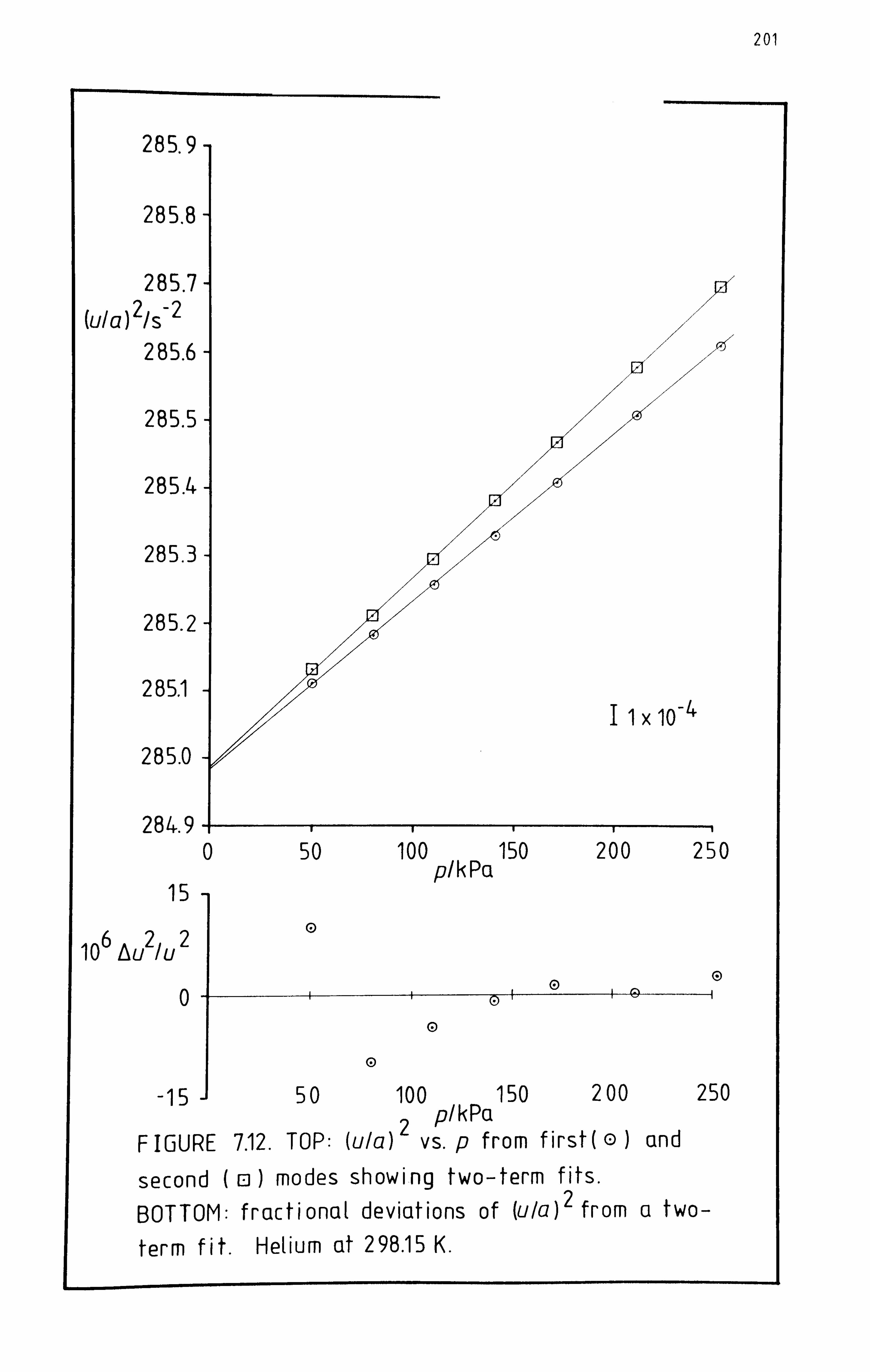
201

285.9

28S. 8

285.7 (U/a)2/S-2

285.6

285.5

285.4

285.3

285.2

285.1

285.0

284.9

15

10 6 Au 2 /u 2

0

-11;

2 p/kPa FIGURE 7.12. TOP: (ula) vs. p from first( 0 and

second (o) modes showing two-term fits.

BOTTOM: fractional deviations of (ula)2 from a two_

term fit. Helium at 298.15 K.

E)

DO

0 50 100 150 200 250 p/kPa

202

cannot predict by hoýN much. On this basis the deviations of (uja) 2 from

a two-term f it of equation (1) are simply accepted as experimental error

and no correction has been attempted. These deviations are shown for the

first mode, which should be reliable in every other respect, in figure

7.12. The regression analysis gives ýa= (21.9 ± 0.1) cm3. mol -1 and a=

60.183 mm or, if the lowest pressure in neglected, ýa= (22.01 ± o. 03) cm 3

mol -1 and a= 60.184 mm. Thus the second acoustic virial coefficient is

in excellent agreement "Ith the value (21.93 ± 0.01) cm 3.

mol-1 obtained by

Gammon using pressures of up to 15 I-Pa. 14 The contribution of A2 is

quite negligible under the conditions reported here. 15 The values of a 5

obtained using argon and helium dif f er by af raction of about 6x 10-

While this difference is rather more than expected on the basis of the

uncertainties in the molar masses, it could easily arise from impurities

in the helium. For example, a mole fraction 3 x10-5 of neon or 1.2 x10-5

of argon would increase the molar mass of the gas by a fraction 12 x 10-5

and therebý, account for the differing values of a.

The 2,2-dimethylpropane was supplied by Cambrian gases Ltd. The

liquid was degassed by vacuum sublimation and dried over molecular seives.

Measurements Nýere performed at 10 pressures between 4.9 and 31.7 kPa, at

mean temperature of 262. '09 0 K. The maximum pressure is about 69 per

cent of the saturated vapour pressure, and was therefore sufficiently

low to avoid the systematic errors, arising from the presence of adsorbed

vapour on the walls of the resonator, that were observed by Moldover and

Mehl. 3 The measured values of T, p, f On , and gOn are given in table 7.8,

and the quality factors vary from Q 05 =2900 at 4.9 kPa to Q 02 = 12900 at

31.7 kP a.

In order to analyse the various contributions to the resonance half

widths, the shear viscosity and thermal conductivity of 2,2-dimethyl-

propane %-, ere required. The viscositv was taken from the measurements by

Diaz Pena et al 16 which cover the range 263-35 < TIK < 393-15 and f it

203

TABLE 7.8 Resonance frequencies and half widths in 2,2"dimethylpropane

at 262.61 K.

p/kPa TIK n f On lHz gCn /Hz gS/Hz 9b /Hz Ag/Hz (uJa)110 3

5-1

31.717 262.6087 1 2122.309 0.100 0.054 0.004 0.042 2.967 696

2 3648.746 0.142 0.071 0.011 0.060 2.967 692

3 5150.179 0.206 0.084 0.022 0.099 2.967 696

4 6643.666 0.311 0.096 0.037 0.179 2.967 696

5 8133.689 0.372 0.106 0.055 0.211 2.967 702

29.005 262.6091 1 2125.050 0.101 0.056 0.004 0.040 2.971 530

2 3653.454 0.141 0.074 0.012 0.055 2.971 522

3 5156.824 0.205 0.088 0.024 0.094 2.971 524

4 6652.230 0.306 0.100 0.040 0.166 2.971 521

5 8144.178 0.375 0.110 0.060 0.204 2.971 528

25.974 262.6091 1 2128.071 0.103 0.059 0.005 0.039 2.975 758

2 3658.650 0.143 0.078 0.014 0.052 2.975 751

3 5164.150 0.212 0.092 0.027 0.092 2.975 748

4 6661.681 0.315 0.105 0.045 0.165 2.975 745

5 8155.746 0.389 0.116 0.067 0.205 2.975 750

22.954 262.6089 1 2131.072 0.109 0.063 0.005 0.041 2.979.959

2 3663.798 0.150 0.082 0.015 0.052 2.979 942

3 5171.422 0.220 0.098 0.031 0.092 2.979 942

4 6671.067 0.333 0.111 0.051 0.171 2.979 941

5 8167.237 0.415 0.123 0.077 0.215 2.979 946

20.037 262.6087 1 2133.949 0.115 0.067 0.006 0.043 2.983 990

2 3668.751 0.159 0.088 0.018 0.053 2.983 976

3 5178.412 0.239 0.104 0.035 0.100 2.983 974

4 6680.076 0.358 0.119 0.059 0.181 2.983 969

5 8178.268 0.453 0.131 0.088 0.234 2.983 975

204

p/kPa TIK n f On /Hz g On

/Hz gS/Hz 9b /Hz Ag/Hz (ula)110 3 s-

1

17.013 262.6087 1 2136.904 0.126 0.072 0.007 0.047 2.988 129

2 3673.830 0.176 0.095 0.021 0.061 2.988 112

3 5185.581 0.265 0.113 0.042 0.111 2.988 110

4 6659.330 0.398 0.128 0.069 0.201 2.988 107

5 8189.589 0.512 0.142 0.104 0.266 2.988 109

14.022 262.6088 1 2139.837 0.139 0.079 0.009 0.051 2.992 238

2 3678.868 0.201 0.104 0.026 0.072 2.992 216

3 5192.683 0.306 0.124 0.051 0.132 2.992 208

4 6698.512 0.457 0.140 0.085 0.232 2.992 213

5 8200.834 0.592 0.155 0.127 0.310 2.992 216

11.020 262.6089 1 2142.722 0.159 0.089 0.011 0.059 2.996 285

2 3683.838 0.232 0.117 0.033 0.083 2.996 268

3 5199.710 0.356 0.139 0.065 0.152 2.996 265

4 6707.508 0.559 0.158 0.108 0.293 2.996 238

5 8211.920 0.720 0.174 0.162 0.384 2.996 267

7.995 262.6091 1 2145.616 0.189 0.104 0.015 0.070 3.000 351

2 3688.822 0.290 0.136 0.045 0.109 3.000 336

3 5206.766 0.461 0.162 0.090 0.209 3.000 343

4 6716.673 0.711 0.184 0.150 0.378 3.000 342

5 8223.064 0.947 0.204 0.224 0.520 3.000 342

4.931 262.6097 1 2148.537 0.249 0.132 0.025 0.092 3.004 1

472

2 3693.870 0.413 0.173 0.073 0.167 3.004 468

3 5213.887 0.690 0.205 0.146 0.338 3.004 467

4 6725.865 1.065 0.233 0.243 0.589 3.004 466

5 8234.305 1.423 0.258 0.365 0.800 3.004 460

Values of (uJa) are adjusted to the mean temperature of 262.6090 K.

205

n(T)/ýPa-s = 1.14+ 0.01985(T/K)

with a standard deviation of 0.06 jPa-s.

(7.5.3)

Unf ortunately, there are very

few published measurements of the thermal conductivity, but the values 11-, 11 K(323.15 K) =18.2 2 mW-m- . K- and K(373-15 K) =23.5 5 mw-m " K- obtained

by Parkinson and Gray are thought accurate to ±2 per cent. 17 Four

different techniques were investigated for extrapolation of these data

to lower temperatures. Two of these rely on a correlation between the

thermal conductivity and the viscosity, and are the Eucken formula

(n/M) (CV9 m+

9R/ 4), (7.5.4)

which is very nearly exact for monatomic gases, and the modified Eucken

expression

K= (Tý/M) (1.32C Vqm + 1.77R) -

18 (7.5.5)

Direct comparisons between the published results and the predictions of

these methods at 323-15 K and 373-15 K are possible using the heat.

capacities given by equation (6.6.8). The Eucken formula predicts

thermal conductivities of 2,2-dimethylpropane that are too low by about

20 per cent, but those of the modified method agree with the measurements

to better than 1 per cent. The method of Roy and Thodos'9 is based on

the principle of corresponding states and, in the case of a saturated

hydrocarbon, predicts

. rK/mW -m -1 -K-1 = 41.6{exp(O-0464T

r)- exp(-0.24127ý))

r3 + c(-0.152T + 1.191r? - 0.0392 )9 (7.5.6)

1/6 1 1/2 2/3 where (Tc /K) (M/kg-mol- ) (P

c /k-Pa) -9 7ý = TI Tc ý an d Tc an d pc

206

are the critical temperature and pressure: 433-7 K and 3200 kPa for

2,2 -dime thylpropane . 2' The constant c in equation (6) may be calculated

on the basis of group contributions with the result c= 62.7.11 This

method is in close agreement with the experimental value at 373-15 K but

predicts a value that is too low by about 2 per cent at 323-15 K. The

final extrapolation method, that due to Owens and Thodos, " predicts that 1.786 K is proportional to T Thus, using the experimental value at

323-15 K, the Owens-Thodos method gives

K(T)/mW-m-'*K-l = 18.22(T/323-15 K) 1.786 (7.5.7)

for 2,2-dimethylpropane and this expression is in exact agreement with the

experimental value at 373-15 K. This latter method was finally adopted

and predicts K(262.61 K)/mW-m-1-K-1 =12.6,0.2 below the prediction of

the modif ied Eucken f ormula and 0.7 above the value of equation (6).

The gas transport coefficients given by equations (3) and (7)

were used in the calculations of the surface contributions g. and the

classical bulk contributions

9CL 7, (Trf2/u2) j (4D v/3) + (y - 1)D (7.5.8)

to the resonance half widths. A 10 per cent error in the thermal

conductivity would correspond to an error of about 6x 10- 6

in (g. 1f) in

the worst case. The remaining excess half width Ag =g-gS-g CL should

equal the vibrational -relaxation contribution to the bulk attenuation:

gr e1ý::: ( 7Tf2/u2) (TI

rel/P) - (7.5.9)

In order to achieve the highest precision it was necessary to allow for

the gas imperfections in these calculations. The second virial

207

coefficients and their first two temperature derivatives were estimated

from equation (6.6.10), while 9 and u2 were estimated from the

uncorrected results. The results of these calculations are given in table

7.8, together with the Ag' s and corrected values of (ula) at the mean

temperature. Typical contributions to the resonance half widths are

illustrated in figure 7.13. The dominant contribution at the higher

frequencies arises from the relaxation bulk attenuation, and the curve is

drawn using (grellf2) = 7.7 ns (obtained from the fifth mode). Again, the

first and fourth modes appear to have slightly increased half widths.

If Cpg is taken as 13.0 R and y as 1.083 then equation (2.7.10) yields p9m

a single relaxation time of 42 ns at 8 kPa, which corresponds to T(100

kPa) = 3.4 ns. The value f ound at 298.15 K and 100 kPa was 4.2 ns.

Typical relative deviations of Wa) from the mean value for the

first five modes are plotted in figure 7.13. Generally the agreement is

very close, but the deviations of (ula) obtained with the first mode from

the mean value depend systematically on the pressure. The maximum

deviation of 7x 10- 6

occurs at 14 kPa, about 30 per cent of the saturation

pressure, and in the region where a precondensation anomaly has been

predicted. 3 If the observed deviations represent the full extent of the

precondensation effect then no significant error should arise, but the

predicted anomaly would have the same relative effect on each of the modes

and hence would not be revealed by their comparison.

The isotherm was analysed by f itting equation (1) to the 50

individual determinations of (ula) 2, and the results of two- and three-

term fits are given in table 7.9. Clearly, three terms are required,

and the deviations of the mean values of We) 2 at each of the ten

pressures from that fit are shown in figure 7.13. Inclusion of af ourth

term did not improve the standard deviation of the fit, and there is no

evidence to suggest that the temperature -jump effect is significant in

these measurements. The coefficients estimated from the regression

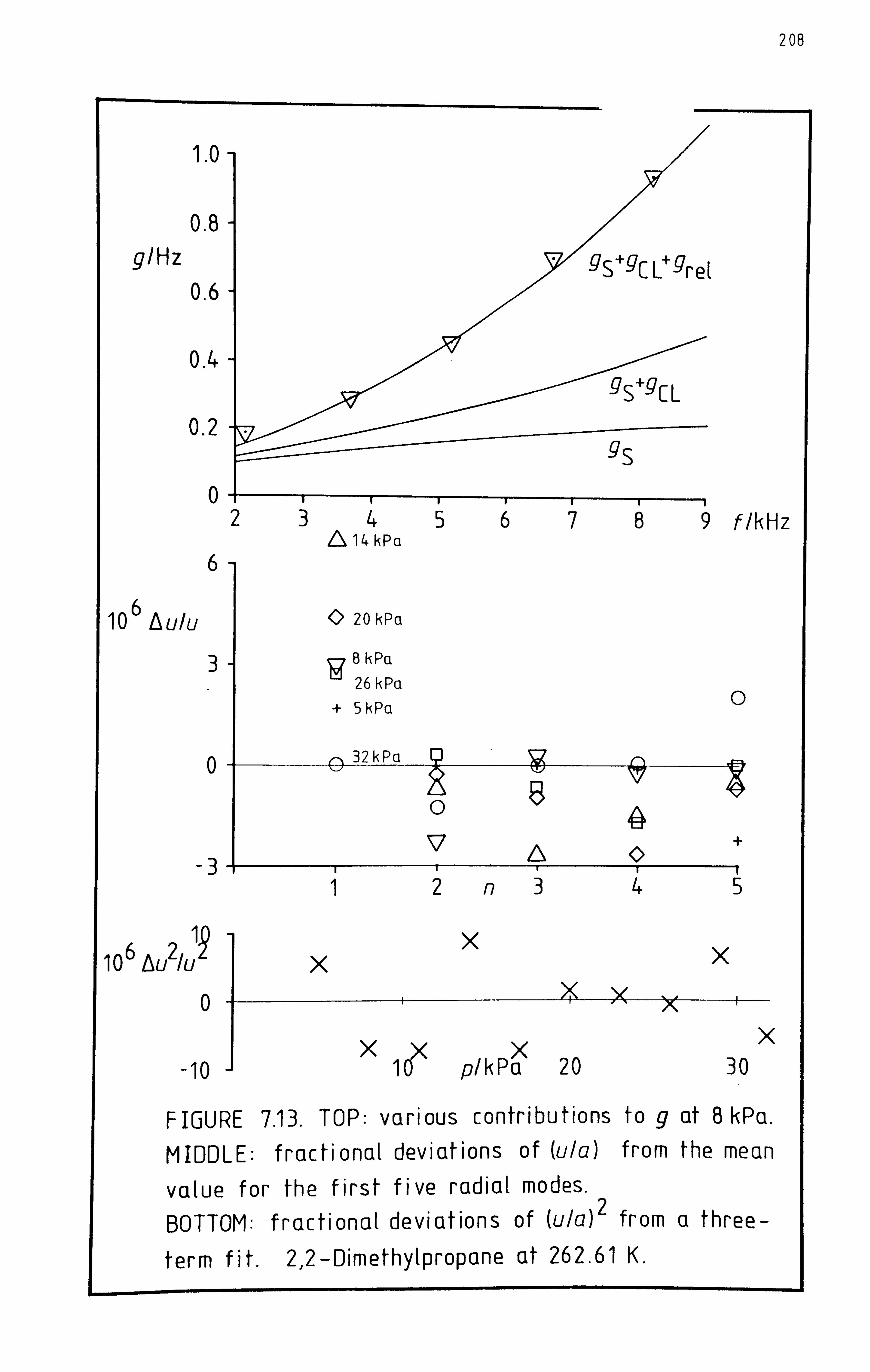
208

1.0-

0.8 - g/Hz

-qS +-qC Lý gr e1 0.6 -

0.4 - -qS+-qC L

0.2 - gS

0tIII 256789f /kHz Zý 14 kPa

6

10 6A U/U 20 kPa

38k PCL 26 kPci

+5 kPa 0

32kPa 0

0 17

-3 1 2n345

62xx 10 AU /U Ix

0 xxx

-10 Ji Cý pl k Pa 20 30

FIGURE 7.13. TOP: various contributions to g at 8 kPa.

MIDDLE: fractional deviations of (ula) from the mean

value for the first five radial modes. BOTTOM: fractional deviations of (ula)2 from a three-

term fit. 2.2-Dimethylprop(ine at 262.61 K.

20Y

TABLE 7.9 Analysis of (ula) 2 for 2,2-cimethylpropane at 298.15 K.

Two terms. Standard deviation of (u/a)2 = 424 s- 2

(A 0

/a 2)= (9.06786 ± 0.00014) x 10 6

s- 2

2 -2 -1 (A 1

la (-8.196 ±0.007) s. Pa

Three terms. Standard deviation of (ula) 2= 65 s- 2

(A 0

la 2)= (9.06619 ± 0.00004) x 10 6

s- 2

(A 1

/a 2)= (-7.963±0.005) s- 2. Pa- 1

(A 2

la 2)= (-6-33 ± 0.14) x 10- 6

s- 2. Pa-

Uncertainties are one standard deviation.

210

analysis using a= (6C. 13--7 ± 0.90230 mm (see chapter eight) are

Ao = (32 780.6 ±2 -5) m 2.

s- 27

A1= (-2.8791 ± 0- 0049) 22 x --3- m. s -Pa , and

A2 -': (-2.29 ± 0.14) x 13- 8 M2*S-2. Pa- 29

(7.5.10)

where the estimated uncertainties are based on 99 per cent confidence

intervals with 47 degrees of freedon. combined in quadrature with the

uncertainty in the molar mass of the argon calibration gas.

heat capacity derived from A0 is

Cpg (C H9 262.16 K) = (13.018 ± 0.319)Rg Pqm 5 12

and the second acoustic virial coefficient is

ýa (C 5H 12 , 262.16 K) = (---917.7±3. -) cm3. mol-i .

The molar

(7.5.11)

(7.5.12)

Thus it would appear to be possible to obtain ýas with an accuracy of 0.2

per cent even under conditions iNfiere the acc-, ssible range of pressures is -1

limited and a three-term fit is required. The value obtained for CP9 IR p1m

exceeds that extrapolated from the results of Hossenlopp and Scott

(using equation 6.6.5) bv 0.4 per cent. 22 This small difference probably

arises from the empirical nature of the extrapolation; the results

obtained at 298-15 K agree with Hossenlopp Is and Scott's direct measure-

ments to well within the estimated error in the latter.

211

APPENDIX A7.1

This appendix provides brief descriptions of the amplifiers

constructed in this work. Figure 7.14 is a circuit diagram of the power

amplifier used to drive the source transducer. The f irst stage consisted

of two type-759 power operational amplifiers coupled in a bridge arrange-

ment to give a total potential difference gain of 5. The signal was

further boosted by a 1: 12.6 step-up transformer to give an overall gain

of 63 (36 dB) between 0.04 and 25 kHz. Figure 7.14 also shows the

potential -dif f erence divider used to supply the reference signal for the

amplitude and phase measurements.

Capacitance transducers hace very high impedances at audio frequen-

cies; the commercial microphone used as the detector had its own built-in

F. E. T preamplifier with an output of 1 k-Q. However, this device only

serves as an impedance converter and provides no gain. A second pre-

amplifier, based on the ZN459CP integrated circuit, was used to boost

the output of the detector by af actor of 1000, and the circuit is shown

in figure 7.15.

The circuit diagram of the bandpass amplif ier is shown in figure

7.16. The input stage was generally used with unit gain so that the .

overall gain of the amplifier was 20 dB. Above 100 kHz and below 1 kHz,

the frequency response fell off at 30 dB per octave, but between 2 and

20 kHz the response was flat to ±0.01 dB.

REFERENCES

1. Greenspan, M. ; Moldover, 11. R. ; Waman, M. High Temp. High Pressure

1979,11,75.

2. Mehl, J. B. ; Moldover, 11. R. J. Chem. Phys. 1981,74,4062.

212

F IGURE 7.14. POWER AMPL IF IER

4ýSL

ttv

+ltv tiv

4 -z 04

-, 4 -m Z. �% m% 150 SL

so km- AA ý& A

UhiL -, Výý

0-(i7pr-" ttDC)v +0 r- 2-0c) v to MJL

F IGURE 7.15. PREAMPLIFIER

+ 57v -L7- VF

1 h3-

0. IPF 7

gin 21441z<%cfl -t- 11

0 EG, & 4.6

11

60

mýz

213

FIGURE 7.16 BANDPASS AMPLIFIER.

OVERALL SCH EME

E E in- .i nput high-pass >

I

I ow - Pass out Ms2, cl. c. e! stag filter fII te r 50ý1, d. c.

coupled. I I II

coupled.

variable g ain 1 kHz cut-off, 100 kHz cut-of f, 0,10,20, & 30 dB 30 dB/octave. 30 d13/octave.

f

passband gain 20 dB

INPUT STAGE

++ Iscv 'v

- S

E in+ lowiL 0-7 1 i

o. oi pF

ksL

0

Z.: 3 h SL

-B hsL

2-70

W5L it) 49 adLiA

I h5L

0- M. SL 1 In _sL

20

C. p

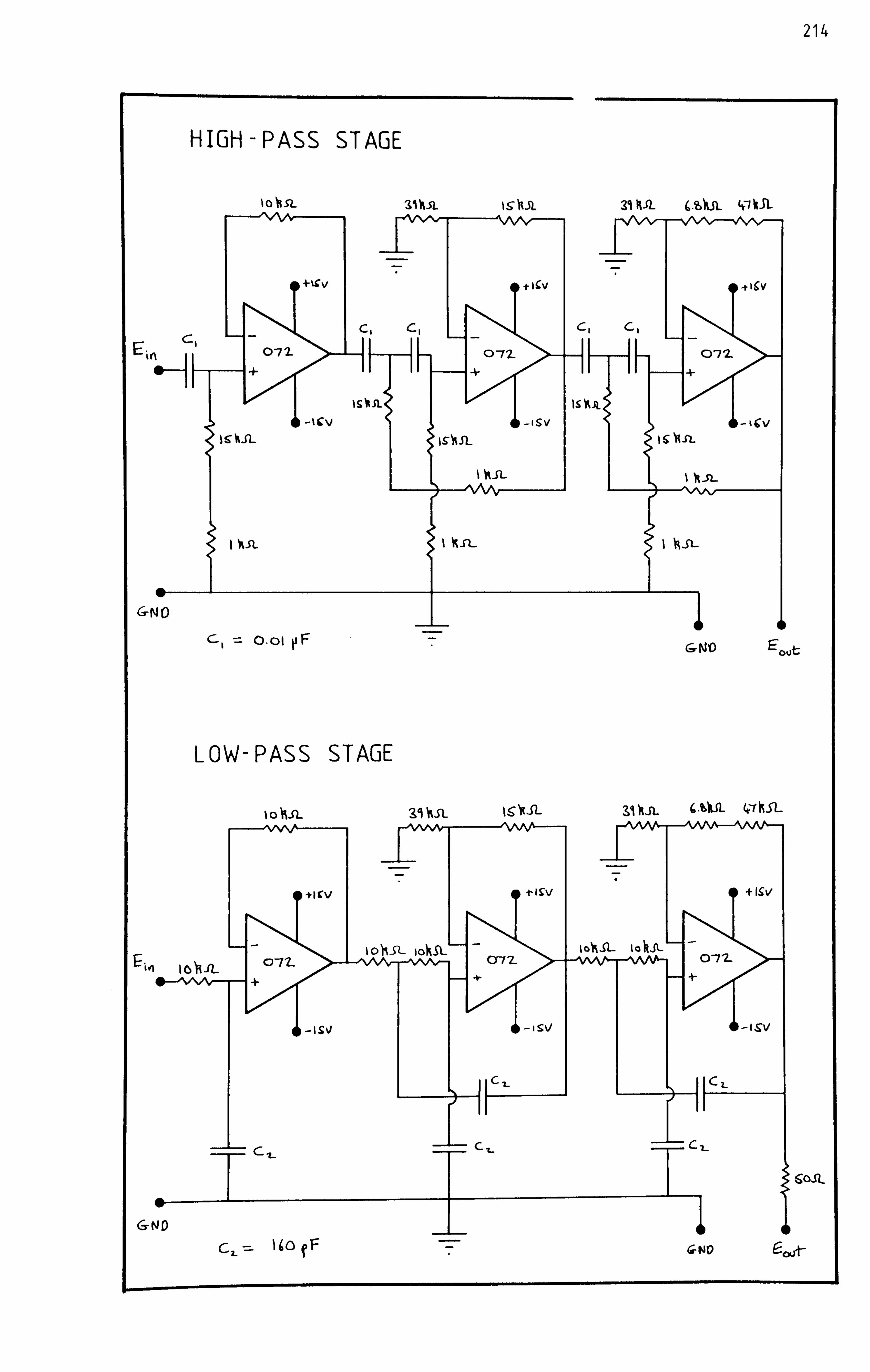
214

HIGH-PASS STAGE

10 ýSL 31 h5L Iýgýa 31 XJ(L C. AfL (t7ksL

+%Cv +Icv +16V

C, c CI

07 2. 1

0-72- ? 1

0 -7 *22-

-i SV -ICV c WIL lgýSL

I h5L YL

I WA I hsL

&N()

VF &NO

LOW-PASS STAGE

li WSL I. OSL hA 6.14ji

+Irv + 19V Io)lsz_ lohsL lo)%sL tokTý O, JL

CIL 0-77-

0- -+ 4.

C, _ T T 60SL GrND

I

C2_

7

111. )

3. Mehl, J. B. ; Moldover, M. R. J. Chem. Phys. 1982,779 455.

4. Mehl, J. B. ; Moldover, M. R. Proc. Eighth. Symp. on Thermophysical

Properties. Sengers, J. V: Editor. Amer. Soc. Mech. Eng. : New York,

1982, p. 134-141.

Greenspan, M. Unpublished work quoted in reference 2.

6. British Standard 1474. Formerly designated alloy HE 30.

7. The International Practical Temperature Scale of 1968, Amended

Edition of 1975. Metrologia 1976,12,7.

8. Mehl, J. B. J. Acoust. Soc. Am. 1978,64,1523.

9. Maitland, G. C. ; Rigby, M. ; Smith, E. B. ; Wakeham, W. A. Intermolecular

Forces Their Origin and Determination. Clarendon Press: Oxford, 1981.

569-571.

10. Aziz, R. A. ; Chen, H. H. J. Chem. Phys. 1977,67,5719.

EI-Hakeem, A. S. J. Chem. Phys. 1965,42,3132.

12. Ref erence 9, p. 582.

13. Golike, R. C. ; Thomas, L. B. J. Chem. Phys. 195 9 229 300.

14. Gammon, B. E. J. Chem. Phys. 1976,64,2556.

15. Gammon, B. E. ; Douslin, D. R. Proc. Fifth Symp. on Thermophysical

Properties. Bonilla, C. F. : Editor. Amer. Soc. Mech. Eng.: New, York,

1970, p. 107.

16. Diaz Pen'a, M. ; Esteban, F. An. Real Soc. Espan. Fis. Quim. , Ser. A

1966,62,347.

17. Parkinson, C. ; Gray, P. J. Chem. Soc. Faraday Trans. 1 1972,68,1065.

18. Prausnitz, J. M. ; Reid, R. C. ; Sherwood, T. K. The Properties of

Gases and Liquids. McGraw-Hill: New York, 1977, p. 473.

19. Reference 18, p. 481.

20. Ref erence 9, p. 573.

21. Owens, E. J. ; Thodas, G. Am. Inst. Chem. Eng. 1960,6,676.

22. Hossenlopp, I. A.; Scott, D. W. J. Chem. Thermodyn. 1981,13,415.

216

ER 8 PERI ii,. ' E 1, TALRESULT

8.1 INTROIXJCTION

S. 2 ARGON

8.3 2,2-DIIIETHYLPROP, ANE

8.1 IINITRODUCTION

The bulk of the experimental res-jits obtained in argon and 2,2-

dimethylpropane are reported in this c-4apter. In order to reduce the

information to a manageable proportion, the individual frequency

measurements at each temperature and pressure have been combined to yield

mean values of WIL) or (ula) . The results obtained in the cylindrical

resonator fall in to two groups: those belov, 295 K for which 6=0.158ý

and those above 295 K for which 5= There appears to be a

reversible change on the optimum value of c- that occurred when the

temperature passed through 295 K. The results obtained in the sphere

also fall into groups because the reso: -tator was disassembled several ,

times during the course of the meas-! re-ents and each reassembly resulted

in a sl'lght reduction of the ef f ective mean radius.

All quoted temperatures refer to the International Practical

Temperature Scale of 1968. Again, unless otherwise stated, all quoted

uncertainties are ± one standard deviation only.

7

The measurements from which the _atter are derived were made in

'at ý%as presented -: or e\amination at University previous i%ork, and til

College London as part of the B. Sc. decree in 1980.

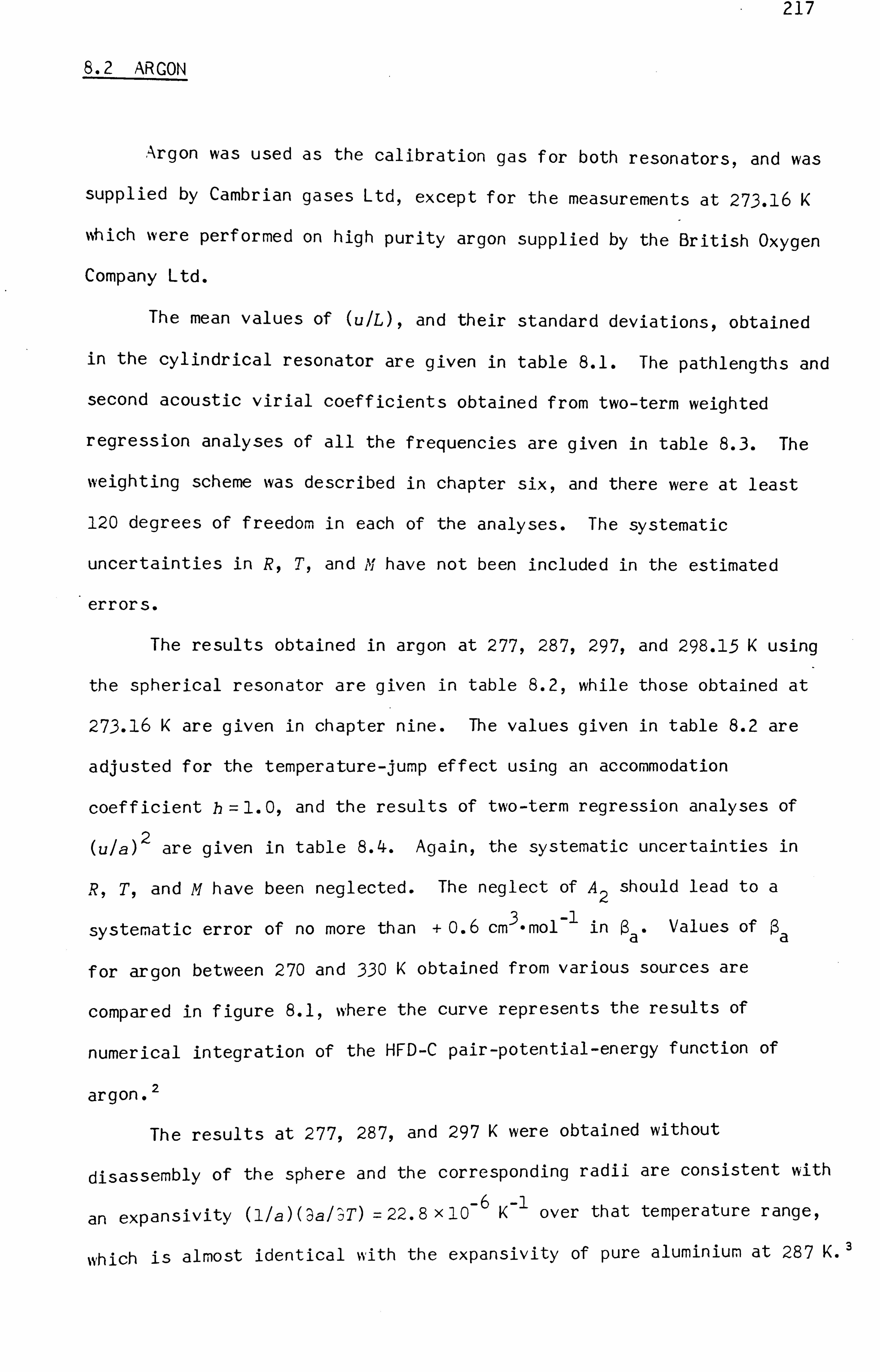
217

8.2 AR CON

Argon was used as the calibration gas f or both resonators, and was

supplied by Cambrian gases Ltd, except for the measurements at 273-16 K

ýsfiich were performed on high purity argon supplied by the British Oxygen

Company Ltd.

The mean values of WIL) , and their standard deviations, obtained

in the cylindrical resonator are given in table 8.1. The pathlengths and

second acoustic virial coefficients obtained from two-term weighted

regression analyses of all the frequencies are given in table 8.3. The

weighting scheme was described in chapter six, and there were at least

120 degrees of f reedom in each of the analyses. The systematic

uncertainties in R, T, and A have not been included in the estimated

errors.

The results obtained in argon at 277,2879 297, and 298.15 K using

the spherical resonator are given in table 8.2, while those obtained at

273-16 K are given in chapter nine. The values given in table 8.2 are

adjusted for the temperature-jump effect using an accommodation

coef f icient h=1.0, and the results of two-term regression analyses of

(Ula) 2 are given in table 8.4.

R, T, and M have been neglected.

Again, the systematic uncertainties in

The neglect of A2 should lead to a

systematic error of no more than + o. 6 cm3. mol-1 in ý a'

Values of ýa

for argon between 270 and 330 K obtained from various sources are

compared in figure 8.1, where the curve represents the results of

numerical integration of the HFD-C pair -potential -energy function of

argon.

The results at 277,287, and 297 K were obtained without

disassembly of the sphere and the corresponding radii are consistent with

an expansivity (11a) (9al'jT) = 22.8 x 10- 6

K- 1 over that temperature range,

which is almost identical with the expansivity of pure aluminium at 287 K. '

218

TABLE 8.1 ML) for argon at various temperatures and pressures.

T= 251.156 K T =290.262 K

p/kPa (u/L)/s- 1 p/kPa (u/L)/s- 1

90.137 2936.82 ±0 . 23 102.469 3156.01 ±0.19

86.996 2936.85 ±0 . 21 93.483 3155.93 ±0.20

77.849 2936.95 ±0 . 22 84.743 3155.89 ±0.18

68.845 2936.94 ±0 . 23 74.882 3155.79 ±0.20

59.288 2936.80 ±0 . 24 66.578 3155.77 ±0.22

50.744 2936.84 ±0 . 26 57.449 3155.66 ±0.20

41.805 2936.86 ±0 . 21 48.116 3155.61 ±0.23

33.330 2936.92 ±0 . 21 39.322 3155.53 ±0.25

24.676 2936.90 ±0 . 24 29.934 3155.46 ±0.27

21.292 3155.28 ±0.26

T =298.690 KT= 325.611 K

p/ jd: ) a (ulL)IS -1 p/kPa WIL) /5-1

97.660 3202.60 ±0.23 98.617 3342.29 ±0.19

86.845 3202.56 ±0.24 88.228 3342.14 ±0.18

74.791 3202.49 ±0.22 79.711 3341.98 ±0.21

65.327 3202.42 ±0.24 70.713 3341.88 ±0.16

56.103 3202.33 ±0.27 59.801 3341.69 ±0.18

43.264 3202.26 ±0.27 49.904 3341.59 ±0.20

30.629 3202.09 ±0.22 39.904 3341.45 ±0.21

151". 688 3202.04 ±0.32 27.673 3341.35 ±0.25

219

TABLE 8.2

T =277.000 K

Wa) for argon, at various temperatures and pressures.

p/kPa (Ula) /10 3s -1

200.0 5.154721 ±0.000012

170.0 5.154483 ±0.000013

140.0 5.154262 ± 0.000008

110.10 5.154036 ±0.000009

80.00 5.153816 ±0.000009

50.00 5.153606 ±0.000012

T =297.000 K

p/kPa (ula)110 3s -1

103.11

88.99

79.84

70.02

60-01

50.01

40.01

29.99

5.334860 ± 0.000011

5.334675 ±0.000012

5.334565 ± 0.000013

5.334444± 0.000012

5.334331 ± 0.000015

5.334211 ± 0.000012

5.334086 ±0.000014

5.333968 ± 0.000014

T =287.000 K

p/kPa (u/a)/10 3 571

247.8 5.246720 ±0.000022

207.6 5.246301 ±0.000018

168.4 5.245901 ± 0.000017

129.3 5.245506 ±0.000014

90.03 5.245108 ±0.000013

69.99 5.244913 ±0.000016

50.01 5.244714 ± 0.000015

30.01 5.244526± 0.000014

298.150 K

p/kPa (ula)110 3 s-

1

240.8 5.346910 ± 0.000011

200.9 5.346396 ±0.000012

161.0 5.345891 ±0.000010

121.0 5.345479 ±0.000009

100.02 5.345119 ±0.000012

79. OS 5.344858 ±0.000015

60.02 5.344637 ±0.000011

50.02 5.344503 ±0.000014

40.02 5.344380 ± 0.000017

35.02 5.344320 ±0.000012

30.02 5.344255 ±0.000019

25.00 5.344199 ± 0.000016

20.00 5.344130 ±0.000019

All values adjusted for the temperature-jump effect.

220

TABLE 8.3 ýa for argon and L for cylindrical resonator at various

temperatures.

TIK ýa / (cm 3. mol-

1 L/mm

251.143 0.3 ± 0.9 100.500 ±0.002

290.262 12.9 ± 1.0 100.569 ±0.002

298.690 12.1 ± 1.0 100.531 ±0.002

325.611 20.6 ± 1.3 100.593 ±0.002

TABLE 8.4 % for argon and a for spherical resonator at various

temperatures.

TIK ßa/ (CM 3. m01-1 )

273.160 5.61 ± 0.02

277.000 6.64 ± 0.06

287.000 9.19 ± 0.04

297.000 11.22± 0.08

298.150 11.64± 0.03

a/mm

60.1449 ±0.0001

60.1525 ± 0.0001

60.1663 ± 0.0001

60.1797 ±0.0001

60.1799 ±0.0001

Two-term fits adjusted for the temperature -jump effect.

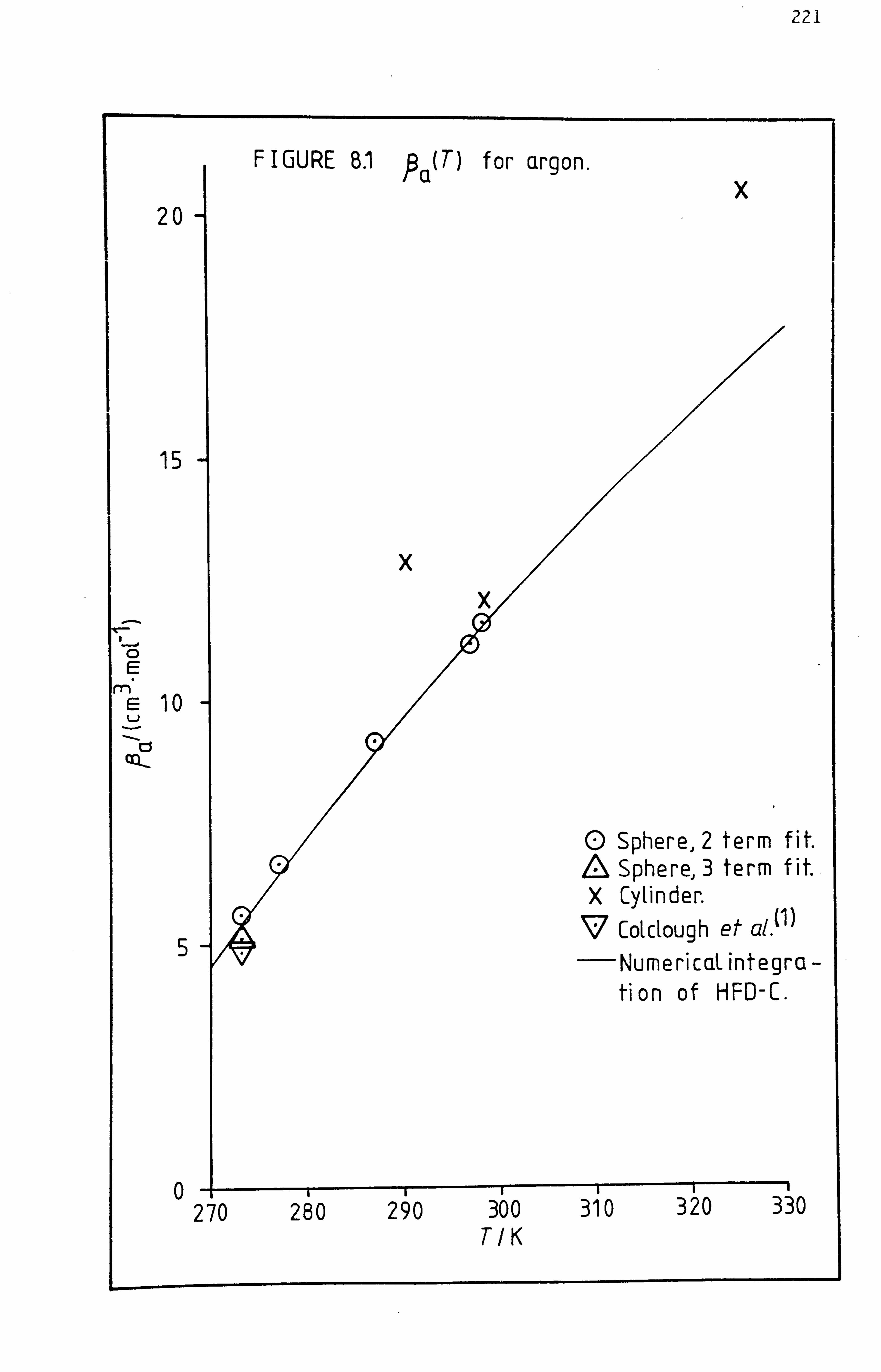
221

FI GURE 81 pla(T) f or argon. x

20

15

x x

E M

E 10

--- El 0

Sphere, 2 term fit. Sphere, 3 term f it.

X Cylinder Colclough ef al. ý')

5 - NumericaL integra - tion of HFD-C-

0 2 70 280 290 300 310 320 330

T/K

222

8.3 ýPAN E

All the measurements on 2,2-dimethylpropane were performed using

samples taken from a single cylinder supplied by Cambrian gases Ltd.

The chemical purity was investigated by gas chromatography using a 46 m

x 0.5 mm, surf ace-coated open-tubular column with a carbowax stationary

phase (SCOT type GSC/CW20M, 35 500 effective plates) operating at 340 K. The injector was operated at 355 K and the flame -ionization detector at 400 K. With the helium carrier gas flowing at 2 cm3. min-1,5 mm3 samples

of 2,2-dimethylpropane vapour were eluted in 240 s and a single impurity

was detected with a retention time 1.08 times that of 2,2-dimethylpropane.

The impurity peak was clearly resolved and, assuming equal sensitivity 4 of the detector, the mole fraction was (5±1) x10- . Samples that had

been used in the cylindrical resonator gave identical results to those

taken directly from the cylinder. Since the impurity was most probably

a hydrocarbon of similar molar mass to 2,2-dimethylpropane, the relative

effects on the measured heat capacities and acoustic virial coefficients

should be less than 0.05 per cent.

The results obtained with the cylindrical resonator along 20.

isotherms in the range 250 < TIK < 340 are given in table 8.5. In order to

avoid the adverse effects of adsorption, all the values reported here

were obtained at pressures belovi 80 per cent of the saturation pressure.

Measurements were attempted at high fractions of the saturation pressure,

and showed a significant apparent dispersion and increased attenuation.

For example, at 49 kPa and 265 K (96 per cent of the saturation pressure)

the value of WL) obtained near 60 kHz was lower than that obtained near

80 kHz by nearly 0.1 per cent.

The resonance frequencies have been analysed by fitting the first

three terms of equation (6.4.2) using the weighting scheme described in

chapter six. For the results obtained at temperatures below 295 K, the

223

TABLE 8.5 WL) for 29 2-dimethyl propane at various temperatures and pressures.

T= 251.245 K

p/kPa (u/L)/s- 1

22.151. 1744.35 ± 0.22

20.015 1746.48 ±0.23

17.362 1749.19 ±0.25

15.183 1751.34 ±0.27

13.184 1753.08 ±0.20

10.825 1755.39 ±0.30

T =255.056 K

P/kPa (ulL)Js- 1

25.443 1754.75 ±0 . 16 22.873 1757.22 ±0 . 21 19.723 1760.15 ±0 . 18 16.833 1762.76 ±0 . 21 13.900 1765.41 ±0 . 24 10.940 1768.06 ±0 . 31

7.970 1770.59 ±0 . 35

T =260.038 K

p/kPa (ulL)15- 1

33.056 1765.43 ±0.20

29.270 1768.75 ±0.23

24.696 1772.72 ±0.26

20.800 1776.15 ±0.27

16.548 1779.79 ±0.39

13.089 1782.84 ±0.41

9.394 1785.91 ±0.32

T =264.972 K

p/kPa (u1L) / s- 1

40.855 1776.13 ±0.13

36.450 1779.84 ±0.22

32.510 1783.15 ±0.19

28.403 1786.55 ±0.19

24.473 1789.73 ±0.17

20.147 1793.40 ±0.19

15.073 1797.44 ±0.17

10.212 1801.43 ±0.20

T =275.086 K

p/kPa (u/L)/s -1

61.398 1795.22 ± 0.13

55.195 1800.08 ± 0.13

48.869 1804.88 ± 0.13

42.513 1809.72 ± 0.13

38.458 1812.72 ± 0.14

34.496 1815.64 ± 0.17

30.406 1818.72 ± 0.15

T= 270.042 K

pjkPa (u/L)) 15 -1

48.070 1788.13 ± 0.16

44.362 1791.12 ±0.15

40.340 1794.32 ±0.15

36.642 1797.26 ±0.15

32.262 1800.69 ± 0.14

28.314 1803.72 ±0.17

24.068 1806.99 ± 0.21

19.701 1810.49 ±0.28

15.408 1813.56 ±0.18

10.263 1817.49 ±0.20

T =275.086 K (cont.

P/kPa (u1L) s

26.533 1821.57 ±0.16

22.624 1824.33 ±0.23

18.717 1827.32 ±0.23

14.884 1829.91 ±0.19

10.926 1832.73 ±0.26

7.111 1835.53 ± 0.14

T =275.066 K

p/kPa WIL JS -1

57.466 1798.28 ±0.16

51.245 1803.06 ±0.14

45.227 1807.62 ±0.16

38.357 1812.37 ±0.20

33.173 1816.75 ±0.15

26.456 1821.75 ±0.13

19.881 1826.67 ±0.14

224

TABLE 8.5 continued.

T= 280.241 K T =284.050 K T =290.039 K

p/kPa (u/L)/s- 1 p/kPa (u/L)/s-l p/kPa (u/L)IS-1

74.216 1803.91 ±0.14 79.544 1813.75 ± 0.12 99.214 1822.19 ±0.13 66.915 1809.39 ±0.14 70.492 1820.27 ± 0.17 90.781 1827.63 ±0.12 58.844 1815.32 ±0.15 61.911 1826.31 +0.12 82.230 1833.32 ±0.13 51.363 1820.79 +0.14 53.250 1832.37 +0.11 73.693 1839.11 ±0.14 43.574 1826.34 ±0.15 44.485 1838.46 +0.13 63.386 1846.03 ±0.14 35.854 1831.77 +0.15 35.494 1844.56 ±0.13 54. -2152 1852.11 ±0.11 28.005 1837.26 ±0.16 26.580 1850.59 ± 0.15 44.899 1858.06 ±0.13 20.252 1842.67 +0.15 17.770 1856.43 ±0.24 35.361 1864.25 ±0.13 20.261 1842.68 ±0.23 26.390 1869.91 ±0.18 14.771 1846.46 ±0.22 17.519 1875.65 +0.24

9.686 1849.84 ± 0.20

T =290.293 K T =294.963 K T =300.280 K

p/kPa (u/L)ls-l p/kPa WIL) /s -1 p/kPa (u/L)ls-l

87.818 1830.34 ±0.14 97.538 1840.28 ±0.17 101.042 1857.37 ±0.14

78.763 1836.63 ±0.13 86.860 1847.31 ±0.14 92.034 1862.96 ±0.14

70.832 1841.93 ±0.11 75.779 1854.24 ± 0.15 83.203 1868.35 ±0.13

62.107 1847.68 ±0.12 65.779 1860.55 +0.18 74.736 1873.53 ±0.13

54.172 1852.84± 0.14 56.528 1866.38± 0.14 65.967 1878.75. ± 0.14

43.153 1859.99 ±0.16 47.424 1872.05 ±0.16 57.259 1884.19± 0.14

34.673 1865.51± 0.14 40.116 1876.66± 0.20 48.117 1889.59± 0.13

26.220 1870.92 ±0.10 31.370 1881.96± 0.19 39.603 1894.54± 0.14

20.364 1874.68 ±0.16 23.365 1886.85 ±0.21 30.357 1899.97 +0.14

16.049 1891.13 ±0.21 20.266 1905.74 ±0.19

T= 304.176 K T =304.176 K (cont. )

p/kPa (ulL)ls- 1 p/kPa WIL)IS -1

96.319 1874.32 ±0.17 48.776 1902.02 ± 0.16

86.166 1880.24 ±0.15 39.486 1907.21 ±0.16

74.893 1886.86 ±0.16 29.730 1912.21 ± 0.19

67.170 1891.36 ±0.16 20.176 1918.04± 0.24

57.177 1897.23 ±0.16 11.145 1922.86± 0.42

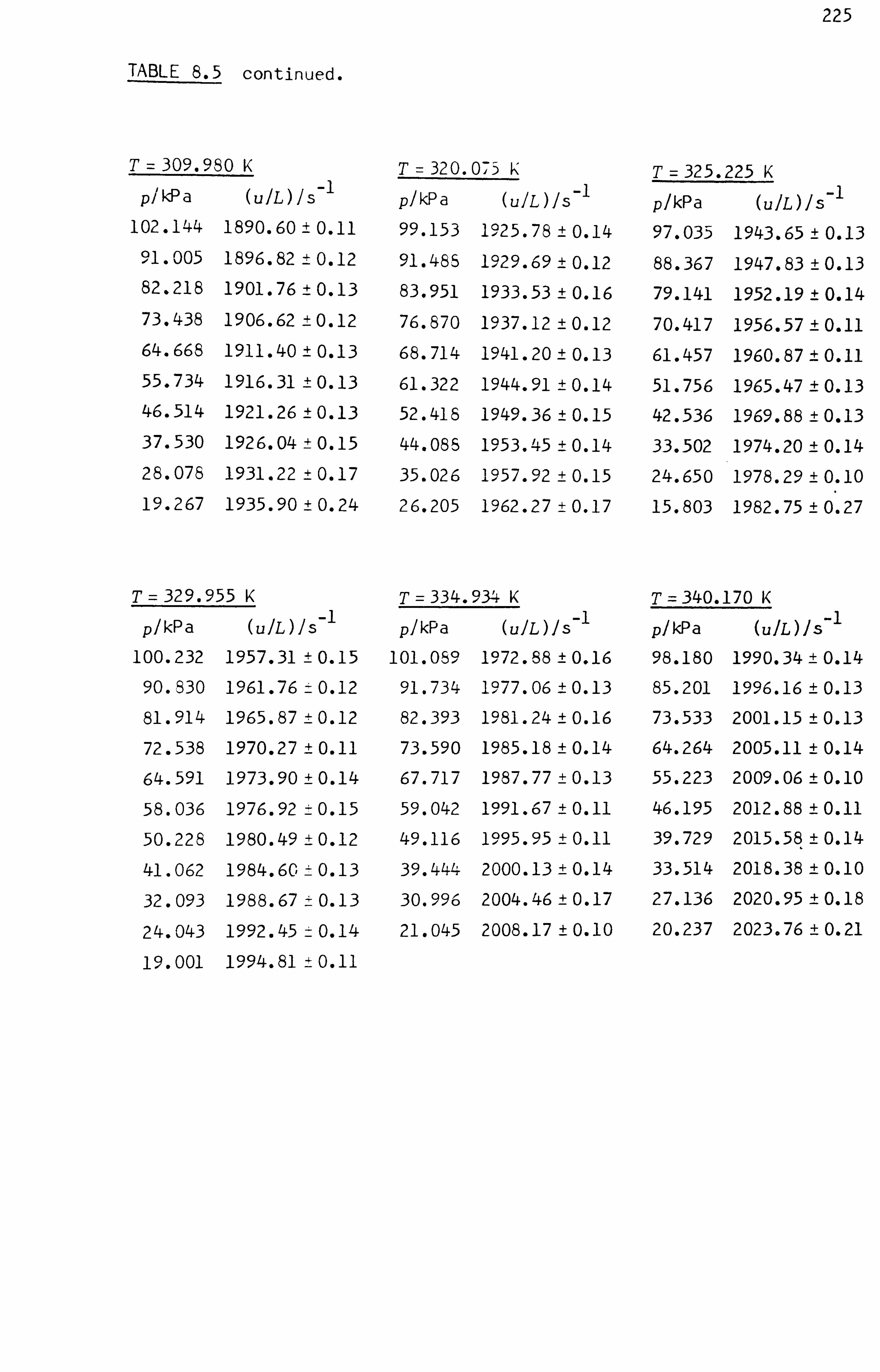
225

TABLE 8.5 continued.

T =309.980 K

P/ kpa (u1L) /. s-l 102.144 1890.60 ±0 . 11

51.005 C, 1896.82 ±0 . 12 82.218 1901.76 ±0 . 13

73.438 1906.62 ±0 . 12

64.668 1911.40 ±0 . 13

55.734 1916.31 ±0 . 13

46.514 1921.26 ±0 . 13

37.530 1926.04 ±0 . 15

28.078 1931.22 ±0 . 17

19.267 1935.90 ±0 . 24

T= 329.955 K

p/kPa (u7L)JS-l

100.232 1957.31 -+0.15 90.830 1961.76 0.12

81.914 1965.87 0.12

72.538 1970.27 ±O. 11

64.591 1973.90 ±O. 14

58.036 1976.92 4-0.15 50.228 1980.49 ±O. 12

41.062 1984.60 --' 0.13

32.093 1988.67 -; -0.13 24.043 1992.45 ---

0.14

19.001 1994.81 -, 0.11

T= 32 0.0-, 5K

pikPa (UIL)/5- 1

99.153 110125.78 ±0 . 14

91.485 1929.69 ±O . 12 83.951 1933.53 ±O . 16

76.870 1937.12 ±O . 12

68.714 1941.20 ±O . 13

61.322 1944.91 ±O . 14

52.418 1949.36 ±O . 15

44.085 1953.45 ±O . 14

35.026 1957.92 ±O . 15

26.205 1962.27 ±O . 17

T= 334.934 K

p/kPa (uJL)Js-l

101.059 1972.88 ±0.16

91.734 1977.06 ±0.13

82.393 1981.24 ±0.16

73.590 1985.18 ±0.14

67.717 1987.77 ±0.13

59.042 1991.67 ±0.11

49.116 1995.95 ±0.11

39.444 2000.13 ±0.14

30.996 2004.46 ±0.17

21.045 2008.17 ±0.10

T =325.225 K

p/kPa (ulL)ls-l

97.035 1943.65 ±0.13

88.367 1947.83 ±0.13 79.141 1952.19 ±0.14 70.417 1956.57 ±0.11

61.457 1960.87 ±0.11

51.756 1965.47 ±0.13

42.536 1969.88 ±0.13 33.502 1974.20 ±0.14

24.650 1978.29 ±0.10

15.803 1982.75 ±04127

340.170 K

p/kPa (u L) s -1

98.180 1990.34 ±0.14 85.201 1996.16 ±0.13 73.533 2001.15 ±0.13 64.264 2005.11 ±0.14 55.223 2009.06 ±0.10

46.195 2012.88 ±0.11

39.729 2015.58 ±0.14

33.514 2018.38 ±0.10

27.136 2020.95 ±0.18

20.237 2023.76 ±0.21

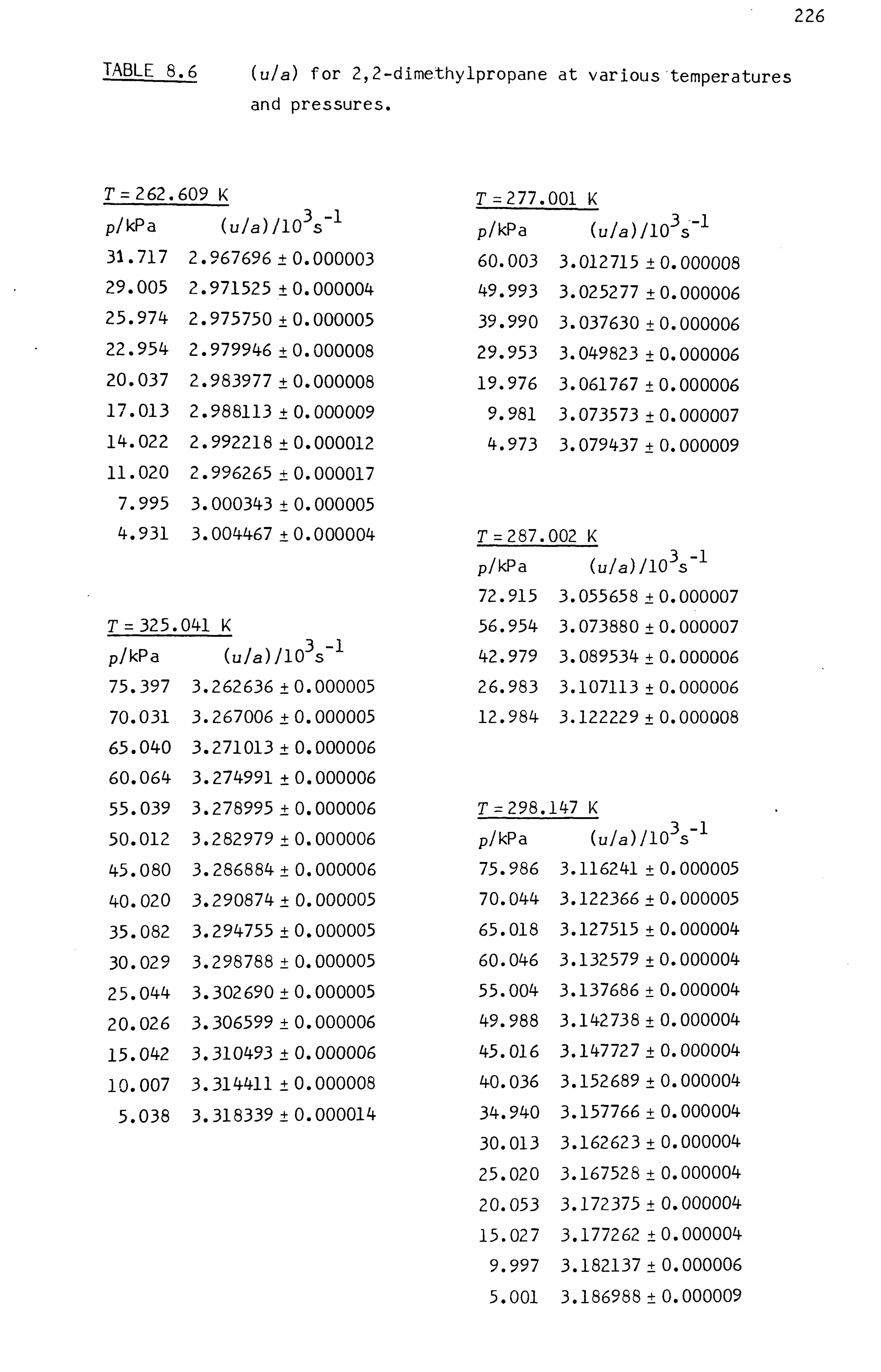
226

TABLE 8.6 (ula) for 2,2-dimethylpropane at various'temperatures

and pressures.

T =262.609 K

p/kPa (ula) /10 3 S-1

31.717 2.967696 ±0.000003 29.005 2.971525 ±0.000004 25.974 2.975750 ±0.000005 22.954 2.979946 ±0.000008 20.037 2.983977 ±0.000008 177.013 2.988113 ±0.000009 14.022 2.992218 ±0.000012 11.020 2.996265 ±0.000017

7.995 3.000343 ± 0.000005

4.931 3.004467 ±0.000004

T= 325.041 K

P/kPa (ula)710 3 s-

1

75.397 3.262636 ±0.000005 70.031 3.267006 ±0.000005 65.040 3.271013 ±0.000006 60.064 3.274991 ±0.000006 55.039 3.278995 ±0.000006 50.012 3.282979 ±0.000006

45.080 3.286884 ± 0.000006

40.020 3.290874 ± 0.000005

35.082 3.294755 ± 0.000005

30.029 3.298788 ±0.000005

25.044 3.302690 ±0.000005

20.026 3.306599 ±0.000006

15.042 3.310493 ± 0.000006

10.007 3.314411 ± 0.000008

5.038 3.318339 ± 0.000014

T=277.001 K

P/kPa (ula)110 35 --1

60.003 3.012 715 ± 0.000008

49.993 3.025277 ±0.000006 39.990 3.037630 +0.000006 29.953 3.049823 ±0.000006 19.976 3.061767 ±0.000006

9.981 3.073573 ±0.000007 4.973 3.079437 +0.000009

T= 287.

P/kPa 72.915

56.954

42.979

26.983

12.984

002 K

(u/a) /10 35 -1

3.055658 ±0.000007 3.073880 ±0.000007 3.089534 ±0.000006 3.107113 ±0.000006 3.122229 ±0.000008

T= 298.147 K

p/kPa (ula)110 35 -1

75.986 3.116241 ±0.000005 70.044 3.122366 ± 0.000005

65.018 3.127515 ±0.000004 60.046 3.132579 ±0.000004 55.004 3.137686 ±0.000004 49.988 3.142738 ± 0.000004

45.016 3.147727 ± 0.000004

40.036 3.152689 ± 0.000004

34.940 3.157766 +0.000004

30.013 3.162623 ±0.000004

25.020 3.167528 ±0.000004

20.053 3.172375 ± 0.000004

15.027 3.177262 ±0.000004

9.997 3.182137 ± 0.000006

5.001 3.186988 ± 0.000009

227

pathlengths were interpolated bet%%een the calibration results at 251.16

and 290.26 K while, for the remaining results, the interpolation was

between the values at 298.69 and 5. K (see table 8.3). Values of

Cpg IR, ý, and y obtained from these analyses are listed in table 8.7. PIM aa The estimated error limits are based on 99 per cent confidence intervals

with co degrees of freedom and, for the heat capacities, include the

uncertainties propagated from the calibration measurements and the

uncertainty in the molar masses (combined in quadrature). Values

obtained from unweighted regressions do not differ significantly from

those given in table 8.7.

The results obtained using the spherical resonator are given in

table 8.6, and the heat capacities and acoustic virial coefficients

derived from three-term fits are listed in table 8.8, where the quoted

error limits were calculated as for table 8.7. Full details of the

analyses are given in chapter seven. The radius a of the sphere at 277,

287, and 298.15 K ivas obtained by calibration measurements in argon at

those temperatures. The values required at 262.61 and 325.04 K were

extrapolated from the measurements in argon at 273-16 and 298-15 K

respectively using the expansivity of pure aluminium. 3

The values obtained for the second acoustic virial coefficient -are

plotted on f igure 8.2 and show good agreement between the two resonators

although there is much greater scatter in the results obtained using the

cylindrical resonator.

The ya Is obtained in the spherical resonator are plotted on figure

8.3 and the equation:

3 1. kPa-ý 9-4.4-8 x 10 -3exp(1600 KIT) -Y a

(Mcm -mol- = 0.42

fits the results with a standard deviation of o. o16 cM3. mo 1 -1. kP a-1 (with

two degrees of freedom) ; equation (1) v., as used to dray., the curve shown

228

TABLE 8.7 CP9 IR, ý, and 7y for 2,2-dimethylpropane'at various p9m aa temperatures obtained from unconstrained three-term fits. Cylindrical resonator.

TJK cpg m

IR ß /(cn, 3. mol-1 )

a -y /(cm3. m01-1. kpa-i ) p9 a

251.245 12.59 ± 0.29 -1886 ± 511 -11. 83± 15.10 255.056 12.67± 0.12 -1957± 173 -5. 63± 4.83 260.038 12.74± 0.10 -2050 ± 115 -0. 45± 2.52 264.972 12.94± 0.04 -1933± 40 -1. 00± 0.74 270.042 13.23± 0.04 -1782 ± 33 -1. 77± 0.52 275.066 13.27-+ 0.08 -1850± 52 0. 05 ± 0.68 275.086 13.47± 0.03 -1734± 15 -1. 24± 0.20 280.241 13.67± 0.03 -1670± 15 -1. 06± 0.16 284.050 13.83± 0.04 -1628± 17 -0. 90± 0.16 290.039 13.95± 0.04 -1610± 15 -0. 29± 0.11 290.293 14.00± 0.04 -1573± 15 -0. 67± 0.15

294.963 14.27 ± 0.04 -1534± 13 -0. 43± 0.10

300.280 14.50± 0.04 -1474 ± 12 -0. 49± 0.09

304.176 14.60± 0.04 -1427± 15 -0. 48± 0.12

309.980 14.87± 0.04 -1383± 12 -0. 32 ± 0.09

320.075 15.33± 0.04 -1288 ± 15 -0. 27± 0.07

325.225 1-5.45 ± 0.04 -1274 ± 12 -0. 10 ± 0.10

329.955 15.65 ± 0.04 -1234 ± 10 -0. 07 ± 0.09

334.934 15.84 ± 0.04 -1185 ± 15 -0. 18± 0.12 -

340.170 15.97 ± 0.04 -1152 ± 15 -0. 24 ± 0.12

TABLE 8.8 CP9 IR, ý, and y for 2,2-dimethylpropane at various PqM aa

temperatures obtained from unconstrained three-term fits.

Spherical resonator.

TIK Cpg IR Pým

ýal (cm3. mol-1) Ya /(cm3. mol-l-kPa -1 )

262.609 13. 018 ±0 . 019

277.001 13. 669 ±0 . 021

287.002 14. 087 ±0 . 023

298-147 14. 545 ±0 . 024

325.041 15. 600 ±0 . 028

-1917.7± 3.4

-1723.0± 1.9

-1601.3 ± 1.7

-1484.8 ± 1.1

-1260.5 ± 2.4

-1. 524± 0.090

-0- 980± 0.028

-0. 740± 0.018

-0. 530± 0.013

-0. 167± 0.028

229

F IGURE 8.2. P,, (T) for 2j2-dimethylpropcine from unconstrained three-term f its.

1-1000

1-1250

-1500

0 E m

E -u

-1750

1-2000

22504- 250

E) Cylindrical

resonator.

Spherical resonator.

260 270 280 290 300 310 320 330 340 TIK

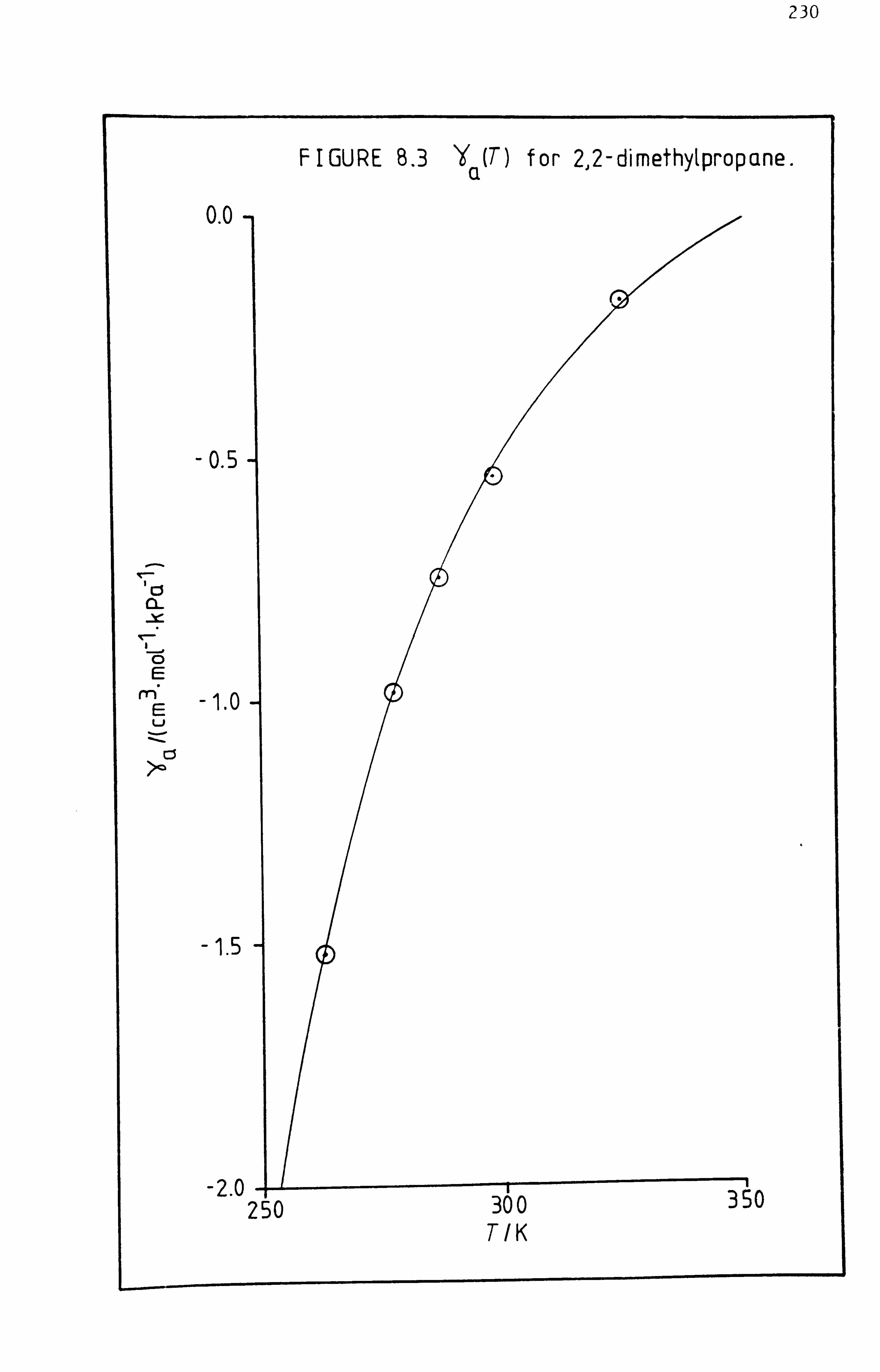
230

FIGURE 8.3 Y (T) for 2,2 - di methyl prop ane. cl 0.0

-0.5 -

cl

0 E m.

E -1.0 u

>Q.

-1.5

-2.0 250 300 3SO TIK

231

in figure 8.3. Values of -ý, a calculated from equation (1) Avere used to

systematically adjust the measured resonance frequencies which were then

reanalysed to obtain the final results listed in tables 8.9 (cylindrical

resonator) and 8.10 (spherical resonator), where the quoted error limits

were calculated as for table 8.7. While the constraint of A2 has little

effect on the already precise results of the spherical resonator, the

second acoustic virial coefficients calculated from the results of the

cylindrical resonator are much smoother, and this can be seen in f igure

8.4. The curve shown in figure 8.4 is based on a Taylor's series

expansion:

ý (T) =ý (T )+ 6Týa (TO) +[ W) 2 J2 ý"(T )+f W) 3J6)ý"'(T ) (8.3.2) aa01a0a0

in which 6T = (T -T0), T0 =325-041 K, and the first three temperature

derivatives of ýa and their standard deviations at T=TO, given by

(T 0)=

(7.20 ±0.19) cm3. mol-1. K- 1

ßll(T )= (-0.0766 ± 0.0180) cm3. mol-l-K -2 0

ß "(T )= (0- 00146 ± 0.0006C) cm3. mol-'-K-3 9 0

were determined by least-squares regression analysis of the f ive

(8.3.3)

determinations of ýa in the spherical resonator. The standard deviation

of those values from equation (2) is 0.9 cm3. mol-1 with two degrees of

freedom, and the maximum deviation is 1.0 cm3. mol-1 at 277 K. The

second acoustic virial coefficients determined in the cylindrical

resonator with ya constrained by equation (1) are in remarkably good

agreement with equation (2), except below 265 K where they are

increasingly mOre negative. If the three lowest temperatures in table

8.9 are neglected then the remaining values are lower than those of

equation ( 3) by an average of 6 cm3. mol-1, or about 0.4 per cent.

232

TABLE 8.9 CP9 PIM

IR and ýa for 212-dimethylpropane at various temperatures obtained from three-term fits with ^Ya constrained. Cylindrical resonator.

TIK Cpg IR m

/(cm3. mol-1 p9 a

251.245 12.41 ± 0.08 -2210.3± 47.3 255.045 12.60 ± 0.04 -2089.0 ±25.7 260.030 12.78 ± 0.04 -1996.1 ±18.2 264.967 12.96 ±0.03 -1910.5 ±6.8 270.040 13.20 ±0.03 -1815.1 ± 6.2 275.066 13.37 ±0.03 -1765.4± 7.0 275.086 13.45 ±0.03 -1747.6 ±3.4 280.241 13.66 ±0.03 -1683.2 ±2.9 284.050 13.81 ± 0.03 -1637.6 ±3.1 290.039 14.05 ±0.03 -1562.1 ±2.6 290.293 14.00 ±0.03 -1571.7 ±2.9 294.963 14.30 ±0.03 -1517.0 ±2.6 300.280 14.50 ±0.03 -1475.2 ±2.1 304.176 14.59 ±0.03 -1433.9 ±2.9 309.980 14.88 ± 0.03 -1380.2 ±2.1 320.075 15.31 ±0.03 -1298.1 ±2.3 325.225 15.47 ±0.03 -1265.0 ±2.3 329.955 15.67 ±0.03 -1227.5 ±2.1 334.934 15.84 ±0.03 -1195.0 ±3.1 340.170 15.97 ±0.03 -1174.4 ±2.6

TABLE 8.10 CP9 m

IR an dýa for 2,2-dimethylpropane at various temperatures Pý

obtained from three-term fits with ya constrained. Spherical resonator.

TIK Cpg IR /(cm3. mol-1 PIM a

262.609 13.018 ± 0.019

277.001 13.670 ±0.021

287.002 14.086 ±0.023

298.147 14.544 ± 0.024

325.041 15.601 ± 0.026

-1917.7 ±1.8

-1722.1 ±0.5

-1601.7 ±0.2

-1486.0 ±0.2

-1259.7 ±0.5

233

FIGURE 8.4. pc, (T) for 2,, 2-dimethy[propcine from

constrained three-term fits.

1-1000

1-1250

-1500

0 E m

E u

-1750

1-2000

-22504- 250

Cylindrical

resonator

260 270 280 290 300 T/K

310 320 330 340

Spherical

resonator.

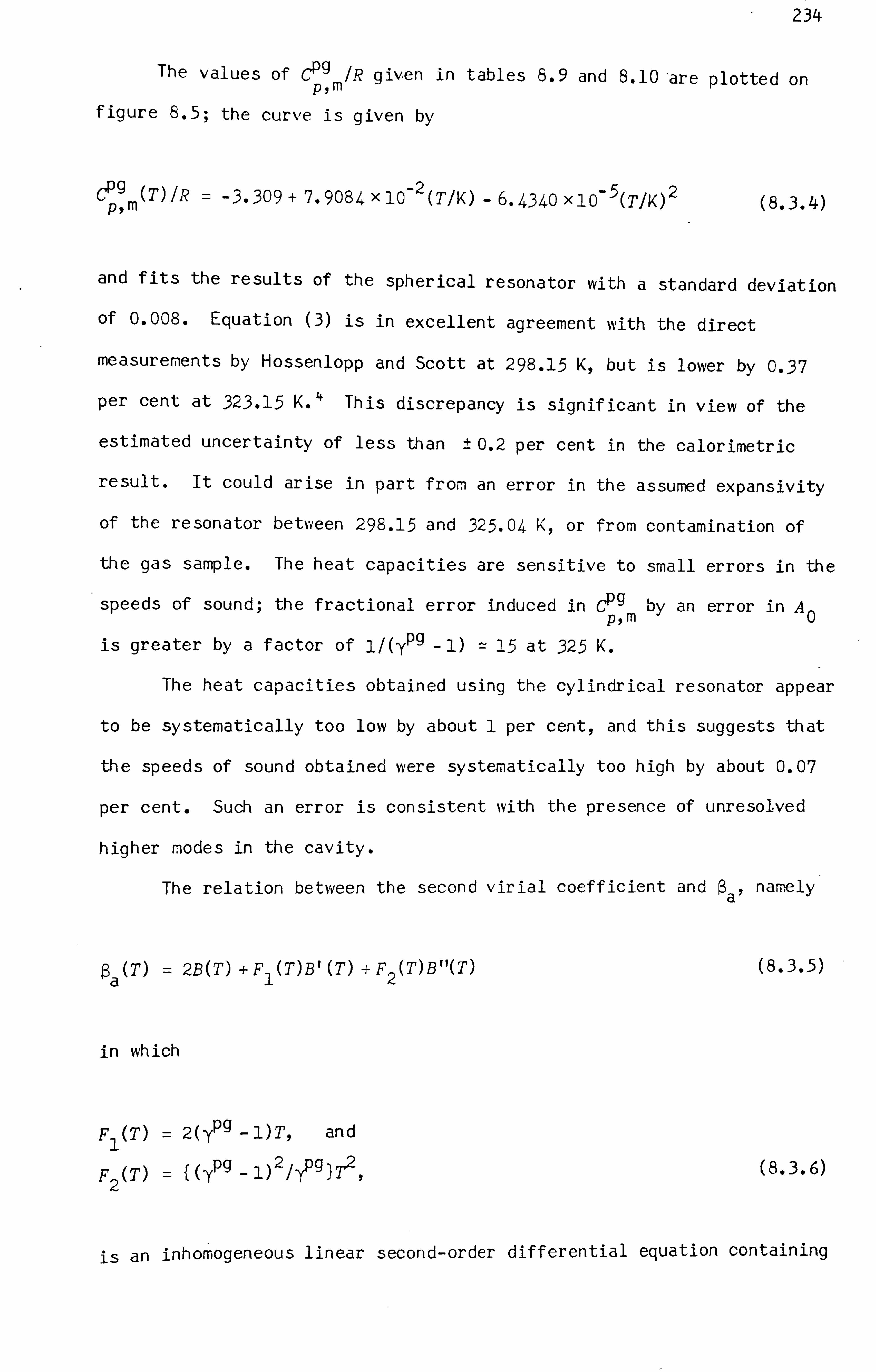
234

The values of Cpg IR given in tables 8.9 and 8.10 'are plotted on PIM figure 8.5; the curve is given by

Cpg (T) IR = -3.309 + 7.9084 x 10-2 (TIK) - 6.4340 x10- 5(TIK )2 (8.3.4) pem

and fits the results of the spherical resonator with a standard deviation

of 0.008. Equation (3) is in excellent agreement with the direct

measurements by Hossenlopp and Scott at 298-15 K, but is lower by 0.37 4 per cent at 323-15 K. This discrepancy is significant in view of the

estimated uncertainty of less than ± 0.2 per cent in the calorimetric

result. It could arise in part from an error in the assumed expansivity

of the resonator between 298-15 and 325.04 K, or from contamination of

the gas sample. The heat capacities are sensitive to small errors in the

speeds of sound; the fractional error induced in CP9 by an error in A Pým 0

is greater by a factor of J/ (yPg - 1) ! -- 15 at 325 K.

The heat capacities obtained using the cylindrical resonator appear

to be systematically too low by about 1 per cent, and this suggests that

the speeds of sound obtained were systematically too high by about 0.07

per cent. Such an error is consistent with the presence of unresolved

higher modes in the cavity.

The relation between the second virial coefficient and $a, na mely

(T) = 2B(T)+ F1 (T) B' (T) +F2 (T) B "M (8.3.5)

in which

F1 (T) = 2(ypg -1)T, and

F2 (T) = j( y pg _ 1)2/ypg)7,29 (8.3.6)

an inhomogeneous linear second-order differential equation containing

235

F

P9 F IGURE 8.5. Cý,; (TVP for 2., 2-dimethylpropcine.

16.0-

15.0-

ct

con ca- C. )_

14.0- equ. (8.3.4)

(D (D

(D

0

13.0-

12.0 250 2ýO 2iO 280 290 300 310 320 330 340

TIK (D Cytindriccit resonator & Spherica[ resonator.

--i

236

variable coefficients. In principle, if ýa (T), F1 (T), and F2 (T) were

knom functions then an exact particular solution Bp (T) of equation (5)

could be found and that would exactly specify ýa (T). However, the

general solution for B(T) is given by the sum of a particular solution

Bp (T) and the complementary solution BC(T) of the corresponding homo-

geneous equation in which ý(T) =0 and, to be general, the solution of the

homogeneous equation must involve two arbitrary constants. Thus equation

(5) cannot be solved unless boundary conditions are imposed in order to

specify these constants. Suitable boundary conditions are values of B

at two temperatures of values of B and BI (or even B") at a single

temperature. If such results are available from another source then an

approximate solution can be obtained for B(T) by numerical means using

values of W) and ypg(T) determined at a number of temperatures.

Alternatively, if the functional form of B(T) were known then the

numerical values of the constants in that form could be determined from

measurements of ýa (T) and ypg(T) at a sufficient number of temperatures,

without the need to draw on information from other sources. While the

exact functional form of B(T) is again unknown, empirical representations

are known that accurately fit second virial coefficients over limited

ranges of temperature. In an extended range of temperatures a less ,

empirical approach may be required, such as the use of ýa (T) to determine

a set of adjustable parameters in an assumed intermolecular pair-potential

-energy function. A very simple analysis of this type is to use the

Isquare-well potential' of equation (5.3.8). Substitution of the square-

well formula for B (equation 5.3.9) in equation (5) gives

i

a= 2a + 2bf 1- (c-IT) (? g

- 1) +f (y pg _ 1)2 /2yPg)(c/T)f2+ (c/T))Iexp(c/T),

(8.3.7)

where

237

a= (2TrLP/3) g39 b= (27TL. 03/3)(1- g3) , and c= (clk) - (8.3.8)

Equation (7) fits the five determinations of ýa made with the spherical

resonator with a standard deviation of 1.1 cm3. mol-i (two degrees of

freedom) when a, b, and c are adjusted in a non-linear regression analysis,

and the resulting expression for the second virial coefficient is

B(T)/cm3. mol-1 = 206.9 -187.08 exp(520 KIT). (8.3.9)

The values of yP9 determined in this work were used in the above analysis,

but replacement of the suspect value at 325 K with the value 1.0681

interpolated from the results of Hossenlopp and Scott has a negligible

effect on the virial coefficients.

Non-linear regression analysis can be avoided if B is assumed to

have a polynomial representation of the f orm:

B(T) (TIK)-79

which when substituted in (5) gives

(T) = 2y iai

ji + j(ypg - 1) + i(i - 1)f (y pg _ 1)2 /2-ypg) I (TIK)j.

(8.3.10)

(8.3.11)

The coefficients a. may then be determined by multiple linear regression 3

analysis. The series with j=0, -1, and -2 can be an accurate

representation of second virial coefficients andý in common with the

square-well f ormula, has the correct behaviour f or T -* 0. The same f ive

values of ýa are accommodated with a standard deviation of 1.0 cm3. mol-1

and give

B(T) /cm3. mol-1 =- 520.8+ 354 480 (TIK)-l - 1.36220 X10 8 (TIK) -2 ;

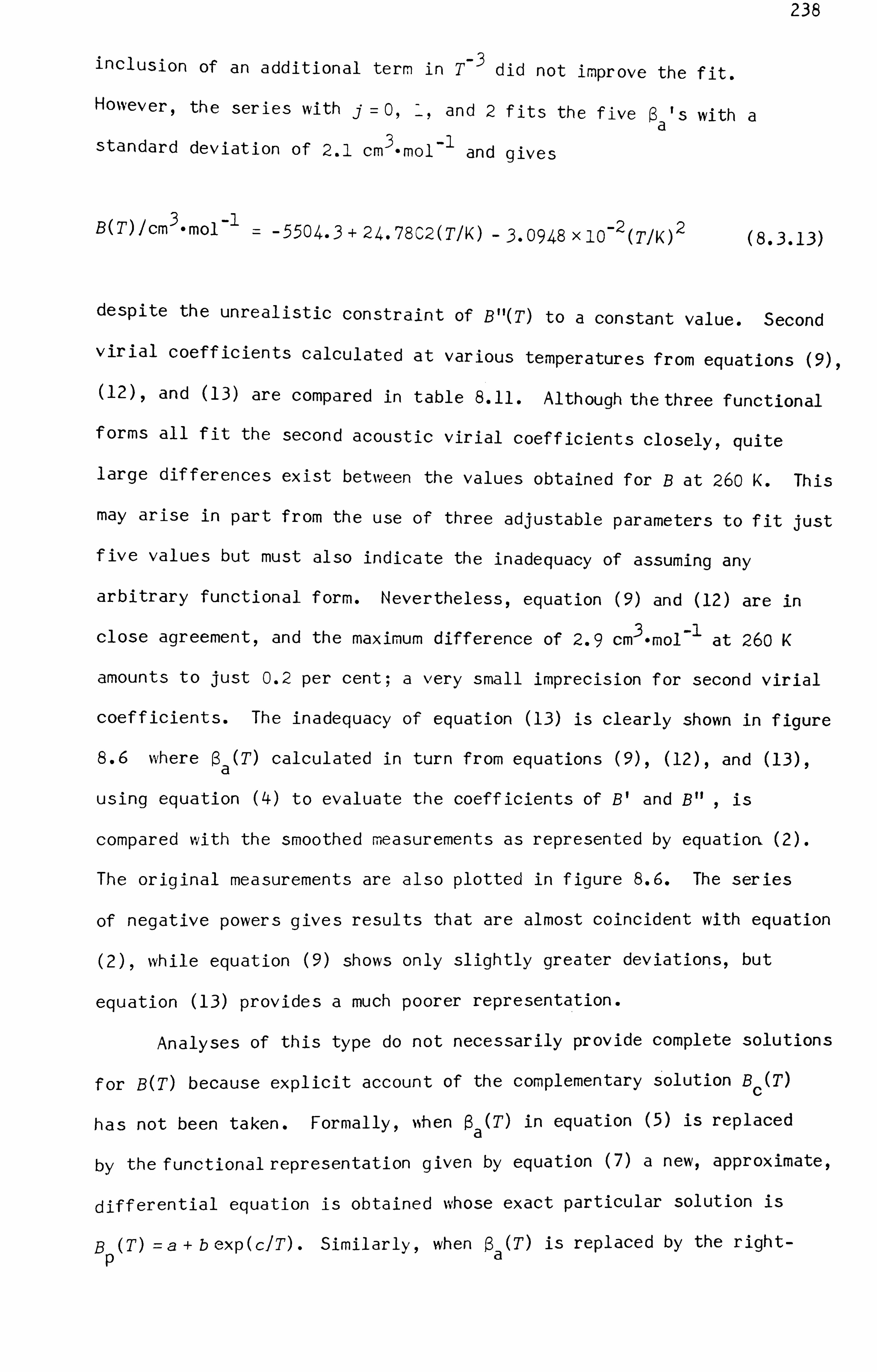
238

inclusion of an additional term in T- 3 did not improve the fit.

However, the series with j= 09 -, and 2f its the f ive ýa 's with a

standard deviation of 2.1 cm3. mol- 1

and gives

B(T) /cm3. mol-1 = -5504-3+24.7802(M) -3-0948 x 10-2 (TIK )2

despite the unrealistic constraint of B"(T) to a constant value. Second

virial coefficients calculated at various temperatures from equations (9),

(12), and (13) are compared in table 8.11. Although the three functional

forms all fit the second acoustic virial coefficients closely, quite

large differences exist between the values obtained for B at 260 K. This

may arise in part from the use of three adjustable parameters to fit just

f ive values but must also indicate the inadequacy of assuming any

arbitrary functional form. Nevertheless, equation (9) and (12) are in

close agreement, and the maximum difference of 2.9 cm 3.

mol-1 at 260 K

amounts to just 0.2 per cent; a very small imprecision for second virial

coefficients. The inadequacy of equation (13) is clearly shown in figure

8.6 where ýa (T) calculated in turn from equations (9), (12), and (13),

using equation (4) to evaluate the coefficients of BI and B" ý is

compared with the smoothed measurements as represented by equation. (2).

The original measurements are also plotted in figure 8.6. The series

of negative powers gives results that are almost coincident with equation

(2), while equation (9) shows only slightly greater deviations, but

equation (13) provides a much poorer representation.

Analyses of this type do not necessarily provide complete solutions

f or B(T) because explicit account of the complementary solution Bc (T)

has not been taken. Formally, ýshen ýa (T) in equation (5) is replaced

by the functional representation given by equation (7) a new, approximate,

differential equation is obtained whose exact particular solution is

Bp (T) =a +b exp WT) . Similarly, when ýa (T) is replaced by the right-

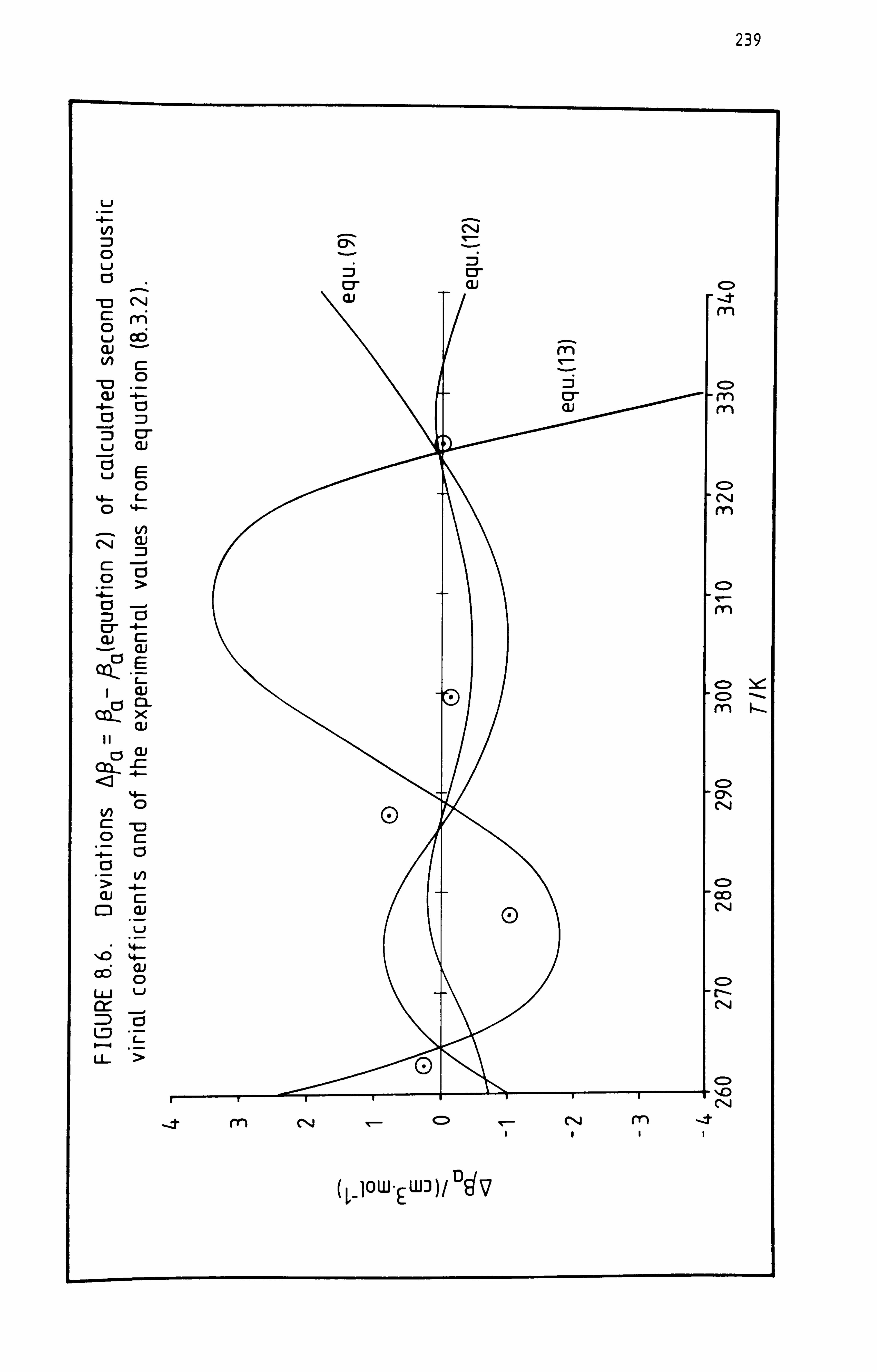
239

F'ý--

u

-I

C1.4 c7N

0 U C3 cr

CN cr ai CD

-. t

(Yi 0 m

u CX5 %Aj m

(A c: o

T- 1-7

_0 CU

-4. - cl

:3 cr cu

C> -M

rr) C) cr

u Cl)

uE 0

%&.. - C-- 0

C> C%4

CN CIJ -0

> C) m

cr (Ij C ýW c5

Cl m x ai CU

a) -C - < CD W0 C: -C: ) 0 C:

z0 0

V)

ou C: - co

CD Cu 0-4

; ai cc 0 C> UJ r-

C**-4

C- >

C>

C`14

m C111.4 m

(L-low-EWD)/'dv

240

hand side of equation (11) a new differential equation is obtained whose

exact particular solution is given by equation (10). The close agreement

between equation (12) and the experimental results is only proof that a

good approximation to the particular solution has been found.

In order to f ind the required complementary solution, the solution

of the homogeneous equation:

2B (T) +F (T) B' (T) +F (T) B "M c1c2c (8.3. lLi)

is required such that BP (T) +Bc (T) satisfies two independent initial or

boundary conditions. Unfortunately there are wide variations among the

published second virial coefficients of 2,2-dimethylpropane below 350 K

which make it very difficult to choose an initial value for B and quite

impossible to place any realistic constraint on an initial value of B' .

However, the heat capacity measurements by Hossenlopp and Scott provide

independent values of B" at two temperatures in the range studied here :4

B" (298-15 K) = (-0.089 ± 0.016) cm3. mol-l. K- 2

B" (323.15 K) = (-0- 056 ± 0.010) cm3. mol-1. K- 2 (8.3.15)

and hence by differentiation, the complementary solution accompanying

equation (12) must satisfy

6) cm3. mol-'-K- 2_

B" (298.15 K) = (-0.012 ± 0.01 - 0, and c

B" (323-15 K) = (-0-003 0.010) cm3. mol-l. K -2 _0 (8.3.16) c

Thus B" (323-15 K) and all higher derivatives at that temperature may c

be taken as zero, and differentiation of equation (5) then shows that

B' (323-15 K) =0 and hence that B (T) =0 for all T. The same result is cC

obtained'f or the complementary solution accompanying equation (9), but

241

equation (13) gives B"(T) = -0.062 cm 3-

mol -1 -K -2 f or all T and this p

differs sia-nificantl\, from the boundarv value at 298.15 K.

The use of functional forms can be completely avoided in a direct

numerical integration of equation (5) using the Adams method with

appropriate initial or boundary conditions. 12 This technique provides an

approximate solution of the exact differential equation, based on

Taylor's series expansions of B spanning the intervals between the

experimental temperatures, rather than the exact solutions of approximate

differential equations found above. A condition for numerical stability

is that the three terms in equation (5) must be of comparable magnitude,

but here at 325 K: 2B = -1439 cm 3.

mol-1, F1 B' = 204 cm 3.

mol-1, and

F2 B" = -25 cm 3.

mol-1 (from equation 12 ). Trial solutions using initial

values taken from equation (12) or equation (9) were indeed found to be

highly sensitive to the starting values. For substances with smaller heat

capacities the coefficients F1 and F2 would be much larger and this

instability would not arise.

Thus, in the absence of more precise boundary conditions, equation

(12) appears to be the best representation of the second virial

coefficients over the range of temperatures studied. Random errors in

a are about ±1 cm3. mol-i and should cause errors no greater thaQ that

in the derived second virial coefficients. Perhaps the small differences

(less than 3 cm'-mol between equations (9) and (12) represent the

likely systematic errors arising from the imposition of the chosen

functional form. The values of equation (12) are compared with second

virial coefficients taken from the literature in figure 8.7. There are

clearly wide discrepancies between the reported values but those of

Hamann and Lambert" lie close to the present results. The values

recommended by Dymond and Smith appear to be too low by about 70 m3. mol-1

at 300 K. Below that temperature, only the results obtained by

Hossenlopp and Scott are available for comparison. These are more

242

FIGURE 8.7. B(T) for 2)2-dimethytpropcine from various sources.

-600

-700

800 0 E

m E u cx)

-900

1-1000

1-1100

1200 4' 260

o reference 5., 2 term fits. Ei reference 5., 3 term fits.

,0 reference 6.

, ný reference 7. V reference 8.

o reference 9. X reference 10.

ref erence 11.

reference 4. 2 equation (8-3-12)

270 280 290 300 310 320 330 340 350 TIK

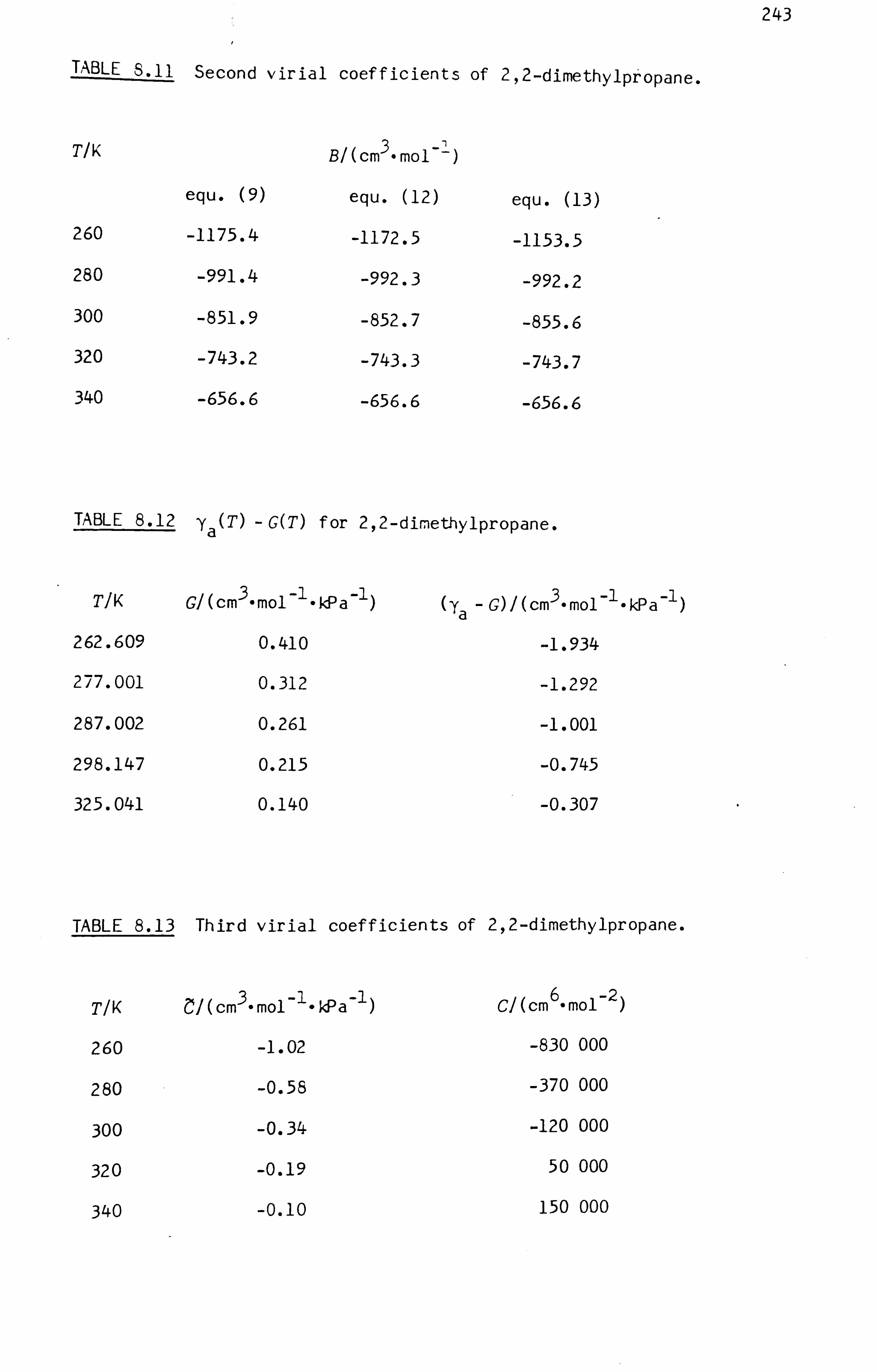
243 t

TABLE 8.11 Second virial coefficients of 2,2-dimethylpropane.

TIK B/(cm3. mol--')

equ. (9) equ. (12) equ. (13)

260 -1175.4 -1172.5 -1153.5 280 -991.4 -992.3 -992.2 300 -851.9 -852.7 -855.6 320 -743.2 -743.3 -743.7

340 -656.6 -656.6 -656.6

TABLE 8.12 ya (T) -G(T) for 2,2-dimethylpropane.

TIK GI (cm3. mol-1. kPa-1)

262.609 0.410

277.001 0.312

287.002 0.261

298.147 0.215

325.041 0.140

(ya- G)/(cm3. mol-l. kPa-1)

-1.934

-1.292

-1.001

-0.745

-0.307

TABLE 8.13 Third virial coefficients of 2,2-dimethylpropane.

TIK eý/ (cm3. mol -1. kP a-')

260 -1.02

280 -0.58

300 -0.34

320 -0.19

340 -0.10

CACM 6.

M01-2

-830 000

-370 000

-120 000

50 000

150 000

244

negative than equation (12) by betý,,, een 20 and 50 cm3. mol-i , and this is

consistent with the neglect of the third virial coefficient in that work.

The third virial coefficient can also be estimated in the range

of temperatures studied. ya is related to the coefficient ý in the

pressure explicit equation of state (equation 5.2.5) by

'ya = (ypg + 2)iý + 2(ypg - 1W! ' +{ (ypg - 1) 2 /2-y pg)T2ý!,, + G, (8.3.17)

where G(T) is the function defined by equation (5.2.16). Equation (12)

was used to calculate G at the five temperatures studied in the spherical

resonator, and the resulting values of G and ya-G are given in table

8.12; equation (9) yields virtually identical results. ý was constrained

to the form

iý =a+b exp WT) ,

which on substitution in (17) gives

(-Ya - G)I(Ypg + 2) a+ bjl - 21 (ypg - 1)/(YP9 + 2)} WT)

(8.3.18)

{ (Ypg _ 1) 2 /2? 9(ypg + 2))(c/T)12+ (c/T)) I exp(cjT)q

(8.3.19)

and the coefficients a, b, and c were determined by non-linear regression

analysis with the result:

iNT) /Cm 3. mol-l-kPa-

1=0.148 - 1.689 xlo-3exp(1700 KIT). (8.3.20)

Values of ýý and the third virial coef f icient C= RTý +B2 at various

temperatures are listed in table 8.13. Uncertainties arising from random

errors in the third acoustic virial coefficients are quite small;

245

equation (19) fits (y a-

G) %vith a standard deviation of'O. 015 cm3. mol-lo

kP a -1 . However, systematic errors arising from the neglect of the fourth

acoustic virial coefficient, and from the imposition of the chosen

functional form on Zý, may be rather larger. Variations amongst the

reported values of C are very large. For example at 303.2 K, Ewing and

Marsh give (-9.4±3.0) x 105 cm6. mol-2 5 Silderberg et al give (2.82 ±

0.14) x 10 5 cm3. mol-

297 while equations (12) and (20) yield C=-O. gxlO 5

cm 6

-mol -2 . Adsorption may well be responsible for the discrepancies

between the reported values, and the results obtained here should be

reliable to ±1x 10-5 cm6. mol- 2

40

REFERENCES

1. Colclough, A. R. ; Quinn, T. 3. ; Chandler, T. R. D. Proc. R. Soc.

Lond. 1979, A368,125.

2. Aziz, R. A.; Chen, H. H. J. Chem. Phys. 1977,65,5719.

3. Swenson, C. A.; Kroeger, F. R. J. Appl. Phys- 1977ý 489 853.

4. Hossenlopp, I. A.; Scott, D. W. J. Chem. Thermodyn. 1981,13,. 415.

5. Ewing, M. B. ; Marsh, K. N. J. Cbem. Thermodyn. 1979,11,793.

6. Dymond, J. H. ; Smith, E. B. The Virial Coefficients of Pure Gases

and Mixtures. Oxford University Press: Oxford, 1980

7. Silderberg, I. H. ; Lin, D. C. K. ; !, IcKetta, J. J. J. Chem. Eng. Data.

1967,129 22-6.

8. Perez Masia, A.; Diaz Pen'a, 11. ; Burriel Llunal J. A. An. R. Soc. Esp.

Fis. Quim. Ser. B 1964,60,229.

9. Heichelheim, H. R.; McKettaq J. J. Chem. Eng. Prog. Symp. Ser.

(Thermo dynami cs) 1963,59,23.

10. Ashton, H. M. ; Halberstadt, E. S. Proc. R. Soc. Lond. 1958, A245,373.

11. Han, ann", S. D. ; Lambert, J. A.; Thomas, R. B. Aust. J. Chem. 1955,81

149.

246

12. Sokolnikoff, I. S.; Redheffer, R. ý% ýJathematics of Physics and

Modern Engineering. I-Ic-Gra", Hill: ý', ýevv York, 1966, p. 690-695-

247

PTFP

9.1 INTRODUCTION

9.2 SAMPLE RESULTS

9.3 CONCLUSION

9.1 INTRODUCTION

METR0L0GICALAPP Ll CAT 10 NS

0FSPHERICALRES0NAT0R5

It was noted in chapter five that accurate measurements of A0 in

gases have applications in metrology. Probably the most challenging of

these is a redetermination of the gas constant because, for this purpose,

accurate knowledge of the mean molar mass of the sample gas is required.

In addition, an absolute measurement of A0 must be performed rather than

measurements of the ratio A0 (T 1

)1A 0

(T 2) that are sufficient in acoustic

thermometry. Thus use of a spherical resonator will require an accurate

measurement of its effective internal radius. Since the radial reýonance

frequencies are insensitive to small geometric imperfections in the

resonator, it would be sufficient to measure the volume of the cavity,

and this could be accomplished by weighing, f irst with the resonator

empty and then with it filled with a fluid of known density. It would

probably be most convenient to perform such measurements at room

temperature and then to measure the expansivity between that temperature

and the temperature of the triple point of water, T(s+l+g, H 2 0). If

water is used as the calibration fluid then its isotopic composition

must be known, but the density of standard mean ocean water is known

with a fractional uncertainty of only af ew parts per million at I

temperatures between 273.16 and 300 K. The density of mercury is known

248

with even higher precision, 2 and its use would avoid the problems of

dissolved air but a stainless-steel resonator would probably be required

to avoid corrosion. A calibration of the volume of the resonator used in

this work has not been attempted, mainly because it became apparent that

there was a misfit between the two halves. This increases the volume

available to the calibration fluid (perhaps by as much as 1x 10 -4 ) and

could have caused slow leakage during the lengthy weighing procedure.

Nor has the isotopic and chemical purity of the sample gas been

investigated in detail. Nevertheless detailed trial measurements of

the speed of sound in argon divided by the mean radius of the resonator

have been performed at temperatures very close to T(s+l+g, H 2 0). These

results are reported here and represent the highest precision that can

currently be attained with the equipment used.

9.2 SAMPLE RESULTS

The gas used in these measurements was research grade argon

supplied by the British Oxygen Company (B. O. C. special gases Ltd).

B. O. C. state that the total mole fraction of impurities is less than ,

5x 10- 6 and give the following assay:

Impurity B: N202H2 CO 2H20 Hydrocarbons

10 6xB2 <1 <1 0.5 1 0.5 1

(9.2.1)

and the combined influence of these is to increase A0 by no more than

5 xlO- 6. The gas used by Quinn et a, 3 in their acoustical redetermination

of R came from the same source and was found to have a molar mass

39.9476 ± 0.0002) g- --. iol Unless production techniques at B. O. C.

have been altered it seems unlikely that the molar mass of the gas used

249

in this work differs significantly from their value.

bef ore filling with the sample gas the system was baked under

vacuum for 48 h to reduce the risk of outgassing during the course of

the experiment. The pipework, valves, and Baratron were baked at 375 KI

while the temperature of the main vessel was held at 335 K (higher

temperatures would have depolarised the detector). The presure as

measured by the ionization gauge was reduced to 0.3 mPa, and the system

was then flushed three times with the gas before finally filling to 250

kPa. A high-purity stainless-steel pressure regulator was used with

the gas cylinder so that contamination with air during f illing was

avoided.

A new resistance measuring bridge was also obtained for this work

(Tinsely model 5840) with its own built-in thermostatically controlled

reference resistor. The thermometer was calibrated in a triple-point

cell before, during, and after these measurements and each time R0 was

found to be (25.56009±0.00001) Q when the measurement current was 1 mA

r. m. s. . Increasing the current by af actor of V2 resulted in an increase

of 150 ýf2 in the resistance of the thermometer, and exactly the same

self -heating ef f ect was f ound in the apparatus. Ethanol was used. in

the thermometer well to promote good thermal contact. The lower 200 mm

of the thermometer was inside the vessel (see figure 7.2) and the effect

of depth of immersion was checked by slowly raising the thermometer; no

change in the temperature was detected over the bottom 50 mm. The

precision of the temperature measurements was ± 0.1 mK and the total

uncertainty in the thermodynamic temperature should not exceed 0.3 W.

Methanol was added to the water bath to prevent freezing and to reduce

the viscosity; cooling was provided by a commercial refrigerator with

its heat-exchanger's coil immersed in the bath. Temperature gradients

in the bath around the vessel were again negligible.

Three sets of measurements were made covering a total of 30

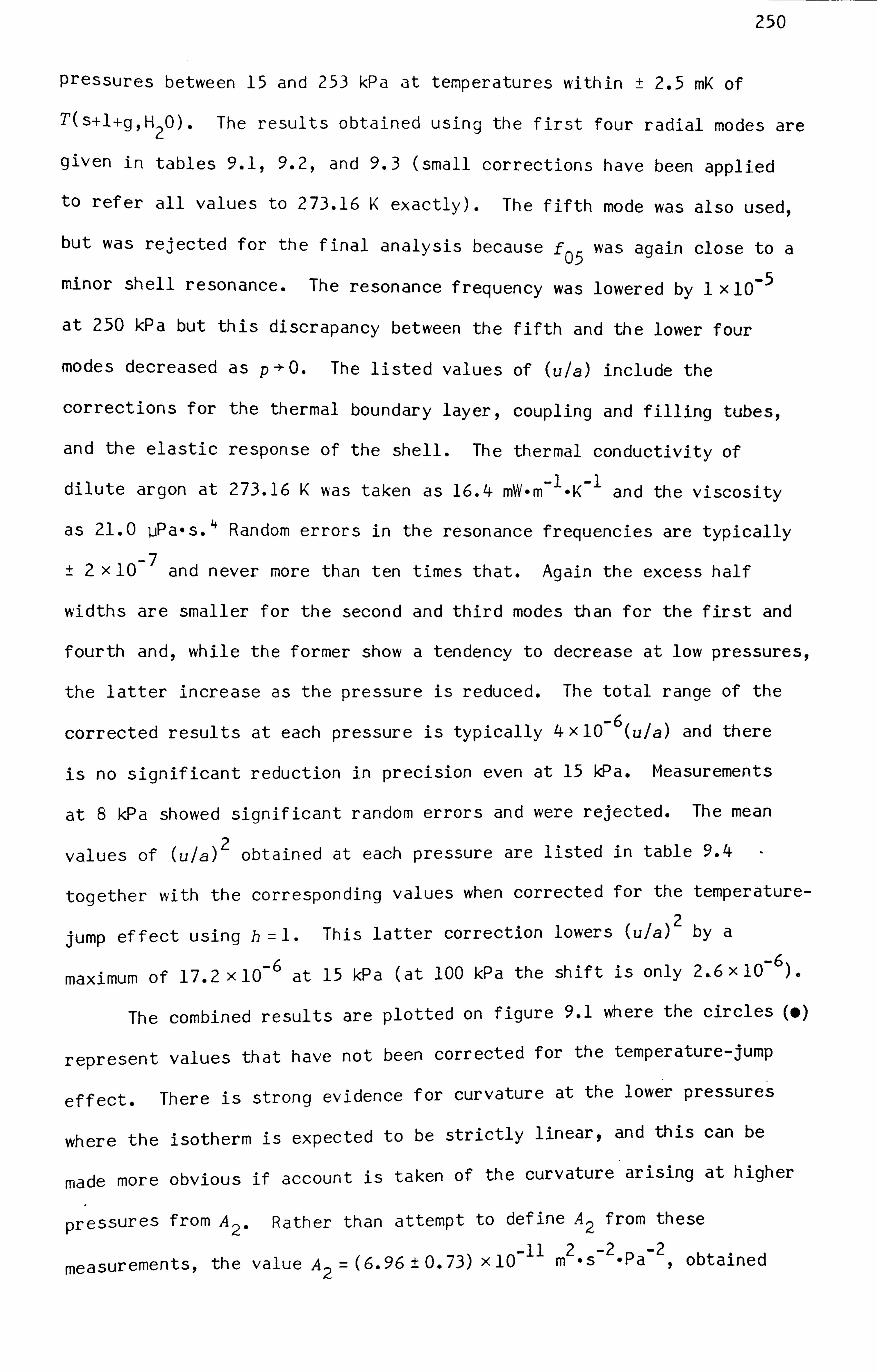
250

pressures between 15 and 253 kPa at temperatures within ± 2.5 mK of

T(s+l+g, H 2 0). The results obtained using the first four radial modes are

given in tables 9.1,9.2, and 9.3 (small corrections have been applied

to refer all values to 273.16 K exactly). The fifth mode was also used,

but was rejected for the final analysis because f 05 was again close to a

minor shell resonance. The resonance frequency was lowered by 1 xlO- 5

at 250 kPa but this discrapancy between the fifth and the lower four

modes decreased as p-ý-O. The listed values of (ula) include the

corrections for the thermal boundary layer, coupling and filling tubes,

and the elastic response of the shell. The thermal conductivity of

dilute argon at 273-16 K was taken as 16.4 mW-m- 1. K- 1

and the viscosity

as 21.0 ýPa- S. 4 Random errors in the resonance frequencies are typically

2X 10-7 and never more than ten times that. Again the excess half

widths are smaller for the second and third modes than for the first and

fourth and, while the former show a tendency to decrease at low pressures,

the latter increase as the pressure is reduced. The total range of the

corrected results at each pressure is typically 4x 10 -6 (ula) and there

is no significant reduction in precision even at 15 kPa. Measurements

at 8 kPa showed significant random errors and were rejected. The mean

values of (ula) 2 obtained at each pressure are listed in table 9.4 -

together with the corresponding values when corrected for the temperature-

jump ef f ect using h=1. This latter correction lowers (ula) 2 by

maximum of 17.2 x 10- 6 at 15 kPa (at 100 kPa the shift is only 2.6xlO- 6)-

The combined results are plotted on figure 9.1 where the circles(*)

represent values that have not been corrected for the temperature- jump

effect. There is strong evidence for curvature at the lower pressures

where the isotherm is expected to be strictly linear, and this can be

made more obvious if account is taken of the curvature arising at higher

pressures from A 2* Rather than attempt to define A2 from these

-11 2 -2 -2 measurements, the value A2 = (6.96 ± 0.73) x 10 m es . Pa 9 obtained

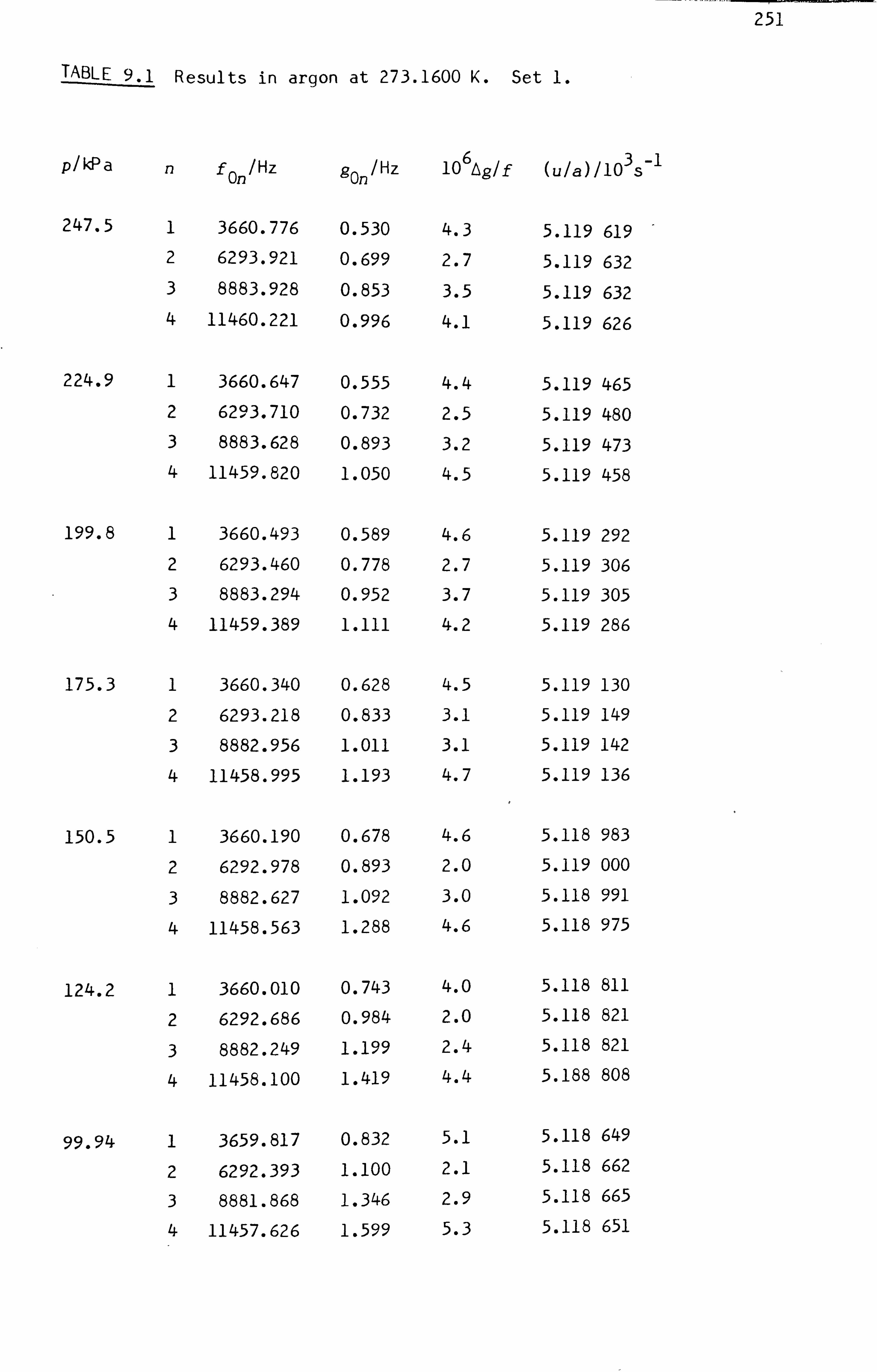
251

TABLE 9.1 Results in argon at 273.1600 K. Set 1.

p/kPa n f On /Hz gOn /Hz 10 6

AgIf (u/a)/10 3s -I

247.5 1 3660.776 0.530 4.3 5.119 619 2 6293.921 0.699 2.7 5.119 632 3 8883.928 0.853 3.5 5.119 632 4 11460.221 0.996 4.1 5.119 626

224.9 1 3660.647 0.555 4.4 5.119 465 2 62013.710 0.732 2.5 5.119 480 3 8883.628 0.893 3.2 5.119 473 4 11459.820 1.050 4.5 5.119 458

199.8 1 3660.493 0.589 4.6 5.119 292

2 6293.460 0.778 2.7 5.119 306

3 8883.294 0.952 3.7 5.119 305

4 11459.389 1.111 4.2 5.119 286

175.3 1 3660.340 0.628 4.5 5.119 130

2 6293.218 0.833 3.1 5.119 149

3 8882.956 1.011 3.1 5.119 142

4 11458.995 1.193 4.7 5.119 136

150.5 1 3660.190 0.678 4.6 5.118 983

2 6292.978 0.893 2.0 5.119 000

3 8882.627 1.092 3.0 5.118 991

4 11458.563 1.288 4.6 5.118 975

124.2 1 3660.010 0.743 4.0 5.118 811

2 6292.686 0.984 2.0 5.118 821

3 8882.249 1.199 2.4 5.118 821

4 11458.100 1.419 4.4 5.188 808

99.94 1 3659.817 0.832 5.1 5.118 649

2 6292.393 1.100 2.1 5.118 662

3 8881.868 1.346 2.9 5.118 665

4 11457.626 1.599 5.3 5.118 651

252

p/kPa n f On /Hz gOn /Hz 10 6

Ag/ f (u/a)/10 3 s-

1

75.00 1 3659.590 0.961 5.3 5.118 500

2 6292.051 1.276 2.4 5.118 510

3 8881.409 1.559 2.4 5.118 506

4 11457.085 1.866 6.0 5.118 500

50.00 1 3659.282 1.181 6.5 5.118 355 2 6291.604 1.568 1.6 5.118 364 3 8880.853 1.926 1.8 5.118 367 4 11456.426 2.342 8.4 5.118 364

25.00 1 3658.721 1.683 9.0 5.118 221

2 6290.831 2.258 1.9 5.118 229

3 8879.896 2.798 1.4 5.118 230

4 11455.354 3.405 7.6 5.118 248

TABLE 9.2 Results in argon at 273-1600 K. Set 2.

p/kPa n f On /Hz gOn /Hz 10 6 AgIf (ula)jlo 3

5- 1

240.0 1 3660.729 0.539 4.6 5.119 563*

2 6293.837 0.708 2.3 5.119 570

3 8883.803 0.868 3.6 5.119 565

4 11460.048 1.010 4.0 5.119 553

214.8 1 3660.586 0.569 4.6 5.119 397

2 6293.602 0.747 2.2 5.119 404

3 8883.486 0.913 3.2 5.119 402

4 11459.657 1.075 4.5 5.119 394

190.3 1 3660.440 0.603 4.3 5.119 235

2 6293.362 0.794 2.1 5.119 239

3 8883.155 0.974 3.5 5.119 236

4 11459.249 1.143 4.6 5.119 231

253

p/kPa n f On /Hz gon / Hz 6 10 41f 3 -1 (ula)110.5

164.8 1 3660.278 0.651 5.3 5.119 063 2 6293.104 0.854 2.2 5.119 070 3 8882.828 1.043 3.1 5.119 079 4 11458.811 1.228 4.5 5.119 062

139.5 1 3660.115 0.703 4.5 5.118 904 2 6292.848 0.931 2.5 5.118 913 3 8882.477 1.136 3.1 5.118 918 4 11458.385 1.336 4.3 5.118 907

114.9 1 3659.937 0.777 5.3 5.118 748 2 6292.571 1.028 2.7 5.118 755 3 8882.091 1.253 2.9 5.118 752 4 11457.909 1.487 5.2 5.118 741

90.00 1 3659.734 0.876 5.0 5.118 593 2 6292.263 1.162 2.3 5.118 601 3 8881.673 1.414 2.1 5.118 593 4 11457.426 1.691 5.5 5.118 597

65.00 1 3659.481 1.034 6.0 5.118 441

2 6291.888 1.370 1.8 5.118 449

3 8881.210 1.673 1.5 5.118 451

4 11456.844 2.004 5.2 5.118 445

40.00 1 3659.111 1.324 7.5 5.118 300

2 6291.364 1.765 2.2 5.118 308

3 8880.545 2.175 2.3 5.118 306

4 11456.087 2.617 6.5 5.118 314

15.00 1 3658.233 2.181 8.7 5.118 186

2 6290.166 2.948 -0.9 5.118 181

3 8879.106 3.731 2.9 5.118 189

4 11454.443 4.495 2.6 5.118 206

254

TABLE 9.3 Results in argon at 273-160C IK. Set 3.

pi F kP a n f On /Hz /Hz gO ic

-, glf 3 (ula)110 s- n

252.7 1 3660.804 0.525 4.5 5.119 651 2 6293.974 0.691 2.5 5.119 671 3 8883.971 0.843 3.3 5.119 654 4 11460.216 0.982 3.7 5.119 622

232.8 1 3660.693 0.547 4.0 5.119 521 2 6293.771 0.718 2.2 5.119 523

3 8883.717 0.885 4.1 5.119 521

4 11459.929 1.021 3.5 5.119 504

207.9 1 3660.542 0.579 4.7 5.119 347

2 6293.528 0.761 2.5 5.119 353

3 8883.381 0.931 3.5 5.119 348

4 11459.519 1.098 5.0 5.119 337

182.4 1 3660.391 0.617 4.7 5.119 183

2 6293.295 0.812 2.3 5.119 197

3 8883.049 0.990 2.9 5.119 184

4 11459.112 1.162 4.0 5.119 178

157.7 1 3660.238 0.662 4.6 5.119 025

2 6293.043 0.872 2.0 5.119 032

3 5882.731 1.066 3.0 5.119 033

4 11458.682 1.252 4.1 5.119 013

133.2 1 3660.070 0.721 4.8 5.118 863

2 6292.775 0.951 2.2 5.118 869

3 8882.379 1.159 2.6 5.118 875

4 11458.254 1.369 4.4 5.118 859

107.00 1 3659.876 0.804 5.1 5.118 697

2 6292.486 1.064 2.4 5.118 713

3 8881.975 1.294 2.3 5.118 707

4 11457.762 1.543 5.3 5.118 695

255

p/kPa n f On /Hz gOn /Hz 10 6

41f (ula) /10 3 5-1

82.03 1 3659.661 0.921 5.9 5.118 544 2 6292.154 1.219 2.5 5.118 554 3 8881.549 1.485 2.1 5.118 553 4 11457.251 1.775 5.5 5.118 545

57.00 1 3659.381 1.105 6.2 5.118 394 2 6291.748 1.467 1.9 5.118 405 3 8881.029 1.797 1.9 5.118 405 4 11456.630 2.151 5.4 5.118 400

32.00 1 3658.935 1.484 8.2 5.118 260 2 6291.119 1.990 3.2 5.118 267 3 8880.244 2.444 1.3 5.118 264 4 11455.741 2.961 6.8 5.118 267

TABLE 9.4 (ula) 2 for argon at 273-1600 K.

p/kPa (Ula) 2 /10 6s -2 (ula) 2 /10 6s -2t p/kPa (Ula) 2 /10 6s -2 (Ula) 2 /10 6s -2t

252.7 26.210 81 26.210 78 133.2 26.202 79 26.202 74 247.5 26.210 58 26.210 56 124.2 26.202 27 26.202 21

240.0 26.209 92 26.209 89 114.9 26.201 59 26.201 53

232.8 26.209 46 26.209 43 107.00 26.201 12 26.201 06

224.9 26.208 96 26.208 93 99.94 26.200 65 26.200 58

214.8 26.208 25 26.208 22 90.00 26.200 03 26.199 95

207.9 26.207 71 26.207 67 52.03 26.199 54 26.199 46

199.8 26.207 20 26.207 17 75.00 26.199 08 26.198 99

190.3 26.206 57 26.206 53 65.00 26.198 49 26.189 39

182.4 26.206 06 26.206 02 57.00 26.198 03 26.197 91

175.3 26.205 59 26.205 55 50.00 26.197 63 26.197 50

164.8 26.204 86 26.204 82 40.00 26.197 07 26.196 89

157.7 26.204 42 26.204 38 32.00 26.196 65 26.196 44

150.5 26.204 03 26.203 98 25.00 26.196 30 26.196 02

139.5 26.203 24 26.203 20 15.00 26.195 87 26.195 42

t These val ues corrected for the tempera ture-jump effect.

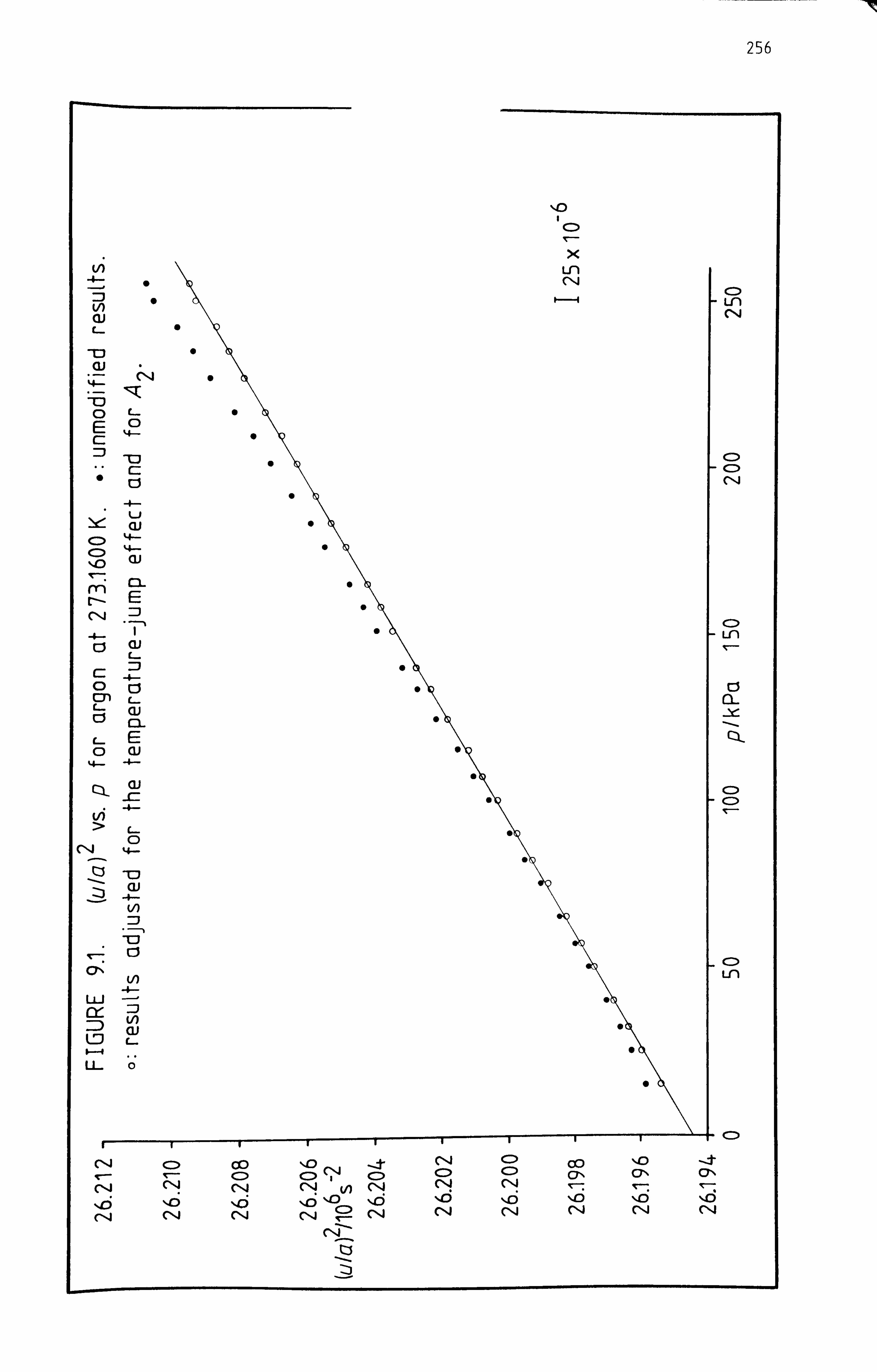
-IT

_0 Gi

ZZ: ýTD- 0 E

4

ýe

ry, t- (IS

4- c

c c c L c

L c

%4-

T-- (71

LL

LL

00 CD

CNý Cý4 C'14

%. 0 't

V) �cý %0 "b

Cý, 4 C"4

- ti Zi

Ic,

C> CC) 110 --t C) C: ) c7N ON lr-.

C) Ln CI*4

C> Ln 117--

0

QL

C)

C) Ln

256

257

by Colclough, Quinn, and Chandler using pressures up to 1.3 MPa, 5 has

been assumed and A0 and A1 constrained by

(u/a) 2_ (A 2

la 2 )p 2= (A 0

/a 2) +(A 1

/a 2 (9.2.2)

The estimated error in this value of A2 is based on three standard

deviations and corresponds to less than 5x 10- 6 (U/a) 2 at the maximum

pressure studied in this work. Equation (2) fits the results unmodified

for the temperature jump with a standard deviation of 3.5xlO- 6; the

resulting coefficients and their standard deviations are

(A 0

la 2 (26.19466 ± 0.00004) x 10 6

s- 2

and 222 (A

1 la )= (5.894 ± 0.023) x 10- s Pa (9.2.3)

Deviations of the measurements from the constrained quadratic fit are

shown in figure 9.2 and provide strong evidence for a systematic effect

increasing in proportion to a low power of (11p). It is unlikely that

this arises from outgassing from the walls of the resonator; the final

set of measurements (set 3) were performes over 2d and after 12 h at

50 kPa (ula) had changed by less than 5x 10- 7. In addition, the three

sets of measurem. nts are entirely consistent with a single isotherm.

Equation (2) fits the results corrected for the temperature jump with

a standard deviation of 1.7xlO- 6

and yields the following coefficients

and standard deviations :

(Aola 2) = (26.19445 ± 0- 000018 )x lo

6 s-

29 and

(A 1

/a 2)= (5-987 ± 0.011) x 10- 2 s-

2. pa-i 0 (9.2.4)

The value of (A 0

/a 2) is lower than that of equation (3) by 8.0 x 10- 6 and

has a standard deviation of only 0.7 x 10-6. Thus random errors in these

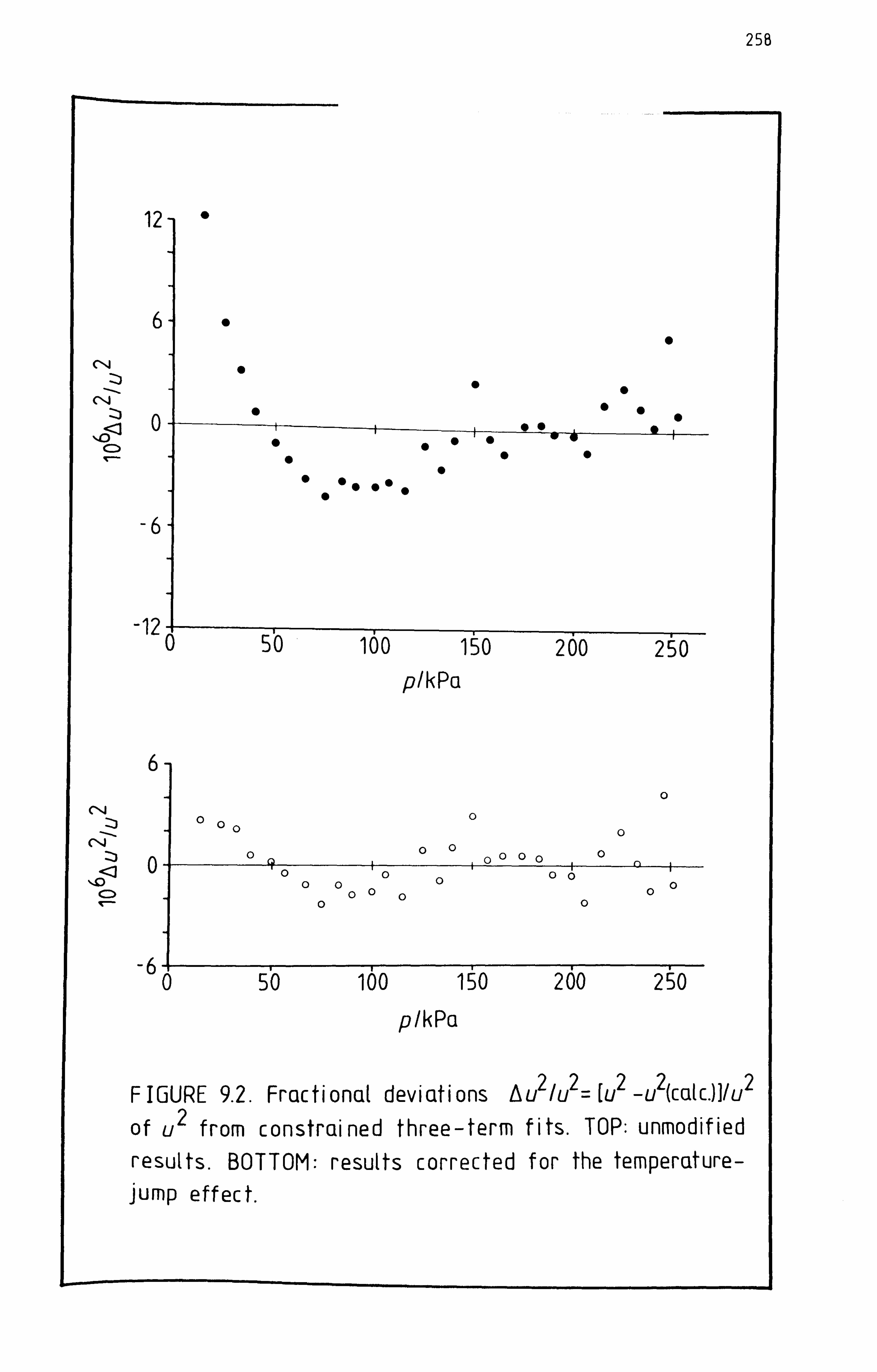
258

12

6

ý, o< C) qr-

-6

-12

A&

Iýw A- w %. If dL. -. 1 v

p/kPa

6 CN

Zi

"0< CD v-

-6

p/kPci

FIGURE 9.2. Fractionat deviations Au 2lu2= (U2 _u2(CcLtc. )]/u2

of u2 from constrained three-term fits. TOP: unmodified results. BOTTOM: results corrected for the temperature- jump effect.

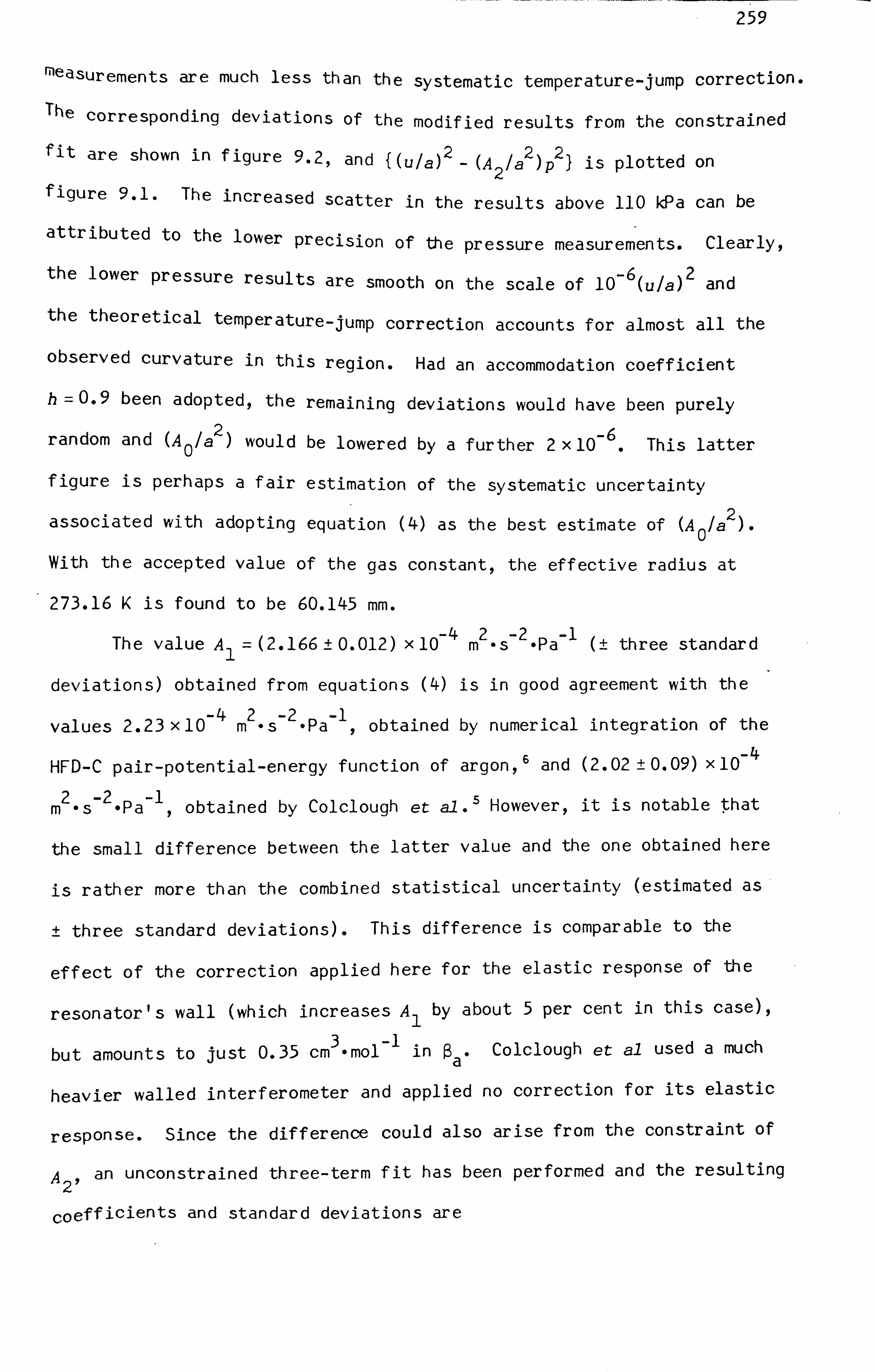
259

Measurements are much less than the systematic temperature-jump correction. The corresponding deviations of the modified results from the constrained fit are shown in figure 9.2, and { (u/a)2 _ (A

2 la 2)P2) is plotted on

f igure 9.1. The increased scatter in the results above 110 kPa can be

attributed to the lower precision of the pressure measurements. Clearly,

the lower pressure results are smooth on the scale of 10-6 (Ula) 2 and

the theoretical temper ature-jump correction accounts for almost all the

observed curvature in this region. Had an accommodation coefficient

h=0.9 been adopted, the remaining deviations would have been purely 26

random and (A 0

/a ) would be lowered by a further 2x 10- . This latter

figure is perhaps a fair estimation of the systematic uncertainty 2 associated with adopting equation (4) as the best estimate of (A

0 la

With the accepted value of the gas constant, the effective radius at

273.16 K is found to be 60.145 mm.

The value A1= (2.166 ± 0.012) x 10 -4 m2 -s -2-Pa-l (± three standard

deviations) obtained from equations (4) is in good agreement with the

values 2.23 x 10 -4 m2s -2. Pa- 1, obtained by numerical integration of the

HFD-C pair -potential -energy function of argon, 6 and (2.02 ± 0.09) x 10- 4

m2s -2 -Pa -1 , obtained by Colclough er al. -5 However, it is notable ýhat

the small difference between the latter value and the one obtained here

is rather more than the combined statistical uncertainty (estimated as

± three standard deviations). This difference is comparable to the

effect of the correction applied here for the elastic response of the

resonator's wall (which increases A1 by about 5 per cent in this case),

but amounts to just 0.35 cm 3

-mol- I in ý

a* Colclough et al used a much

heavier walled interferometer and applied no correction for its elastic

response. Since the difference could also arise from the constraint of

A 2' an unconstrained three-term fit has been performed and the resulting

coefficients and standard deviations are

260

(Ao/a2 )= (26.19450 ±0.00002 7)x 106 s- 21

(A /a2 x 10-2 -2. p, -1 I) :=(5.890 ± 0.0 46) 3, and

(A 2/a

2)= (2.28 ± 0.17) x 10-8 s-

2. pa- 2;

the standard deviation of the fit is 1.6 x 10-6.

(9.2.5)

This value of 0 does not differ significantly from that given by the first of equations (4), and the values of A1 and A2 are found to be:

A1= (2.13 ± 0.05) x 10-4 m 2.

s- 2. Pa-1, and

A2= (8.3 ± 1.8) x 10-11 m 2.

s- 2. Pa- 2. (9.2.6)

Both these estimates agree with those of Colclough, Quinn, and Chandler

to within the combined statistical uncertainties.

9.3 CONCLUSION

These results show that (A 0

/a 2) can be measured with a standard

deviation of about 1x 10-6 , and with systematic uncertainties

- r-

substantially less than 1x 10 -". The three sets of measurements are.

consistent with a single isotherm to within 1x 10- 6 (in as much as the

mean deviation of (ula) 2 from the combined isotherm is less than 1x 10- 6

for each set taken separately) and there was no evidence that the modest

precautions taken here against outgassing were insufficient. It would

be desirable in future work to use transducers that were either

physically isolated from the sample gas (by a diaphragm) or that could

withstand a higher baking temperature. A mass spectrometer would be

useful in assessing the chemical purity of the gas used. Higher

precision is required in the measurement of pressure, and it might be

better to perform the measurements between, say, 50 and 500 kPa in order

261

to avoid systematic uncertainties arising from the temperature-jump

correction.

It is disappointing to have no accurate knowledge of the mean

radius of the cavity. In future work it would be necessary to pay more

attention in the design of the resonator to the problems involved in

a calibration Of its volume by weighing. Misfit between the two halves

could have been avoided if, instead of meeting at an interlocking step,

they were simply butted together and aligned using the outer surf ace.

This would also make mechanical measurements of the depths of the hemi-

spheres much easier. Each half could be machined to a depth greater

than its radius of curvature, polished, and finally lapped down to the

correct depth. Any damage caused to the edge during polishing would

then be removed, and a water tight seal should be achieved.

REFERENCES

1. Menache, M. ; Girard, G. Metrologia 1973,9,63.

2. Cook, A. H. Phil. Trans. R. Soc. Lond. 1961, A254,125.

3. Quinn, T. J- ; C01clough, A. R. ; Chandler, T. R. D. Phil. Trans. R.

Soc. Lond. 1976, A283,367.

4. Kestin, J. ; Ro, S. T. ; Wakeham, W. A. J. Chem. Phys. 1972,56,4119.

Colclough, A. R. ; Quinn, T. J. ; Chandler, T. R. D. Proc. R. Soc. Lond.

1979, A368,125.

6. Aziz, R. A. ; Chen, H. H. J. Chem. Phys. 1977,67,5719.