
photocalorimetry - UCL Discovery
287
PHOTOCALORIMETRY: DEVELOPMENT OF METHODS TO ASSESS THE PHOTOSTABILITY OF PHARMACEUTICAL COMPOUNDS By MEENA DHUNA A THESIS SUBMITTED TO THE SCHOOL OF PHARMACY, UNIVERSITY OF LONDON IN PARTIAL FULFILMENT OF THE REQUIREMENTS FOR THE DEGREE OF DOCTOR OF PHILOSOPHY THE SCHOOL OF PHARMACY UNIVERSITY OF LONDON JULY 2008 i OF
-
Upload
khangminh22 -
Category
Documents
-
view
0 -
download
0
Transcript of photocalorimetry - UCL Discovery

PHOTOCALORIMETRY: DEVELOPMENT OF METHODS TO ASSESS THE
PHOTOSTABILITY OF PHARMACEUTICAL COMPOUNDS
By
MEENA DHUNA
A THESIS SUBMITTED TO THE SCHOOL OF PHARMACY, UNIVERSITY OF LONDON IN PARTIAL FULFILMENT OF THE REQUIREMENTS FOR
THE DEGREE OF DOCTOR OF PHILOSOPHY
THE SCHOOL OF PHARMACY UNIVERSITY OF LONDON
JULY 2008
iOF

ProQuest Number: 10104146
All rights reserved
INFORMATION TO ALL USERS The quality of this reproduction is dependent upon the quality of the copy submitted.
In the unlikely event that the author did not send a complete manuscript and there are missing pages, these will be noted. Also, if material had to be removed,
a note will indicate the deletion.
uest.
ProQuest 10104146
Published by ProQuest LLC(2016). Copyright of the Dissertation is held by the Author.
All rights reserved.This work is protected against unauthorized copying under Title 17, United States Code.
Microform Edition © ProQuest LLC.
ProQuest LLC 789 East Eisenhower Parkway
P.O. Box 1346 Ann Arbor, Ml 48106-1346

Declaration
This thesis describes research conducted in the School o f Pharm acy, U niversity o f London,
betw een 2004 and 2008 under the supervision o f Dr. Sim on G aisford and P ro f A nthony
Beezer. I certify that the research described is original and that any parts o f the w ork that
have been conducted by collaboration are clearly indicated. I also certify that I have w ritten
all the text herein and have clearly indicated by suitable citation any part o f this dissertation
that has already appeared in publication.
IXWu.t'to._______________ 3l^".|ulu 2008Signature ^ Date 3
II

Abstract
The m ain focus o f the research presented in this thesis is to develop a robust and easy-to-
use photocalorim eter to allow a quantitative assessm ent o f the photostability o f
pharm aceutical com pounds. As a result, a novel photocalorim eter was successfully
developed. Initially a X e-arc lam p was used as a light source, but this w as found to be
problem atic, rendering quantitative analysis o f data challenging. A novel approach using
light-em itting diodes (LEDs) as a light source w as developed; this approach dem onstrated
m uch potential in photostability testing. U sing the prototype system s a suitable m ethod to
allow m easurem ent o f the radiant energy delivered to the sam ple during a photochem ical
process w as investigated. The best system appeared to be the photodegradation o f 2-
n itrobenzaldehyde (2NB). A lthough prom ising as a test and reference reaction, it was found
that 2NB w as sensitive to non-photochem ical processes and the reaction was com plex
w hich m eans further w ork on its application in this area m ust be undertaken.
The application o f chem om etric analysis as an approach to interpret com plexity in
Isotherm al Calorim etric data was then studied. A three-step consecutive reaction w as used
to dem onstrate the applicability o f principal com ponent analysis to determ ine the num ber o f
reaction steps and reaction param eters in a process.
The application o f photocalorim etry for the study o f a know n photosensitive drug,
n ifedipine w as investigated. The photolysis o f n ifedipine in solution w as studied under full
spectrum lighting and under specific w avelengths for the determ ination o f causative
w avelength (s). The data showed the photodegradation o f n ifedipine to be particularly
sensitive at 360 nm. N o significant photosensitiv ity w as detected above 370 nm.
Finally a novel autobalance pow er supply, currently under developm ent, designed to
im prove the perform ance o f the photocalorim eter is described.
Ill

~ Acknowledgements ~
First and forem ost I w ould like to express m y deepest and heart-felt gratitude to m y
supervisors Dr. Sim on Gaisford and Prof. T ony B eezer for their guidance, encouragem ent
and inspiration throughout the course o f this PhD project. I feel privileged to have had the
opportunity to work with such high calibre academ ics and w ould like to thank them for all
their support and providing m e w ith opportunities to present m y w ork at num erous
international conferences.
I w ould also like to express m y gratitude tow ards the follow ing people who have
contributed trem endously to this project; Prof. Joe Connor, Mr. David C lapham (G SK
supervisor) and Dr. M ike O ’N eill for their useful advice and inform ative discussions, Mr.
John Frost for his engineering expertise in the construction o f the optical assem blies, Mr.
Chris C ourtice for his electronics expertise in the developm ent o f the LED system , and
G SK for financial support. M any thanks to m y colleagues and friends; Diane, Fang,
H isham , Peng, Em m a, M att, Hala, M o, Da, T iago, R eshm a and A hm ed for their m any
w ords o f encouragem ent, particularly in tim es o f despair and hurdles faced during m y PhD.
I am forever indebted to the love, support and blessings o f m y dearest M other and Father to
w hom I dedicate this PhD , for the hard w ork I have encountered over the past three years is
insignificant to the m any years o f hard w ork they have endured w ith m e during m y studies.
They have been the pinnacle o f m y strength throughout m y studies and have alw ays
believed in me. M any thanks to all m y fam ily and a special thank you to the Sehdev fam ily
for their am ple love and support.
Finally, I w ould like to thank m y beloved fiancé G agandeep Sehdev for his unconditional
love, support and understanding. Thank you for your im m ense encouragem ent and for the
countless tim es you have been there for m e in every possib le way, especially to share all
the highs, and lows, experienced throughout this PhD. Y ou are m y perfect life partner and I
tru ly love and respect you w ith all m y heart. I look forw ard to sharing the rest o f m y life
w ith you and to the start o f a new b eg in n in g ...
M eena D huna, Ju ly 2008
IV

FOR MY PARENTS
All that I am, or hope to be, I owe to my angels - Mother and Father.
V

- Contents -
CHAPTER 1: INTRODUCTION
1 Overview............................................................................................................................... 2
1.1 An Introduction to the Importance o f Pharmaceutical Stability Testing................ 4
1.2 An Introduction to the Photostability o f Pharmaceutical Com pounds.....................6
1.2.1 Current Analytical Methods for Photostability Testing o f Pharm aceuticals 8
1.3 Requirements for a reaction.............................................................................................11
1.3.1 Mechanistic factors........................................................................................................... 11
1.3.2 Thermodynamic factors................................................................................................... 11
1.3.3 Kinetic factors.................................................................................................................... 13
1.4 Calorimetry.........................................................................................................................18
1.4.1 The Principles o f Isothermal M icrocalorimetry......................................................... 21
1.4.2 Analysis o f Calorimetric Data........................................................................................25
1.4.2.1 Solid-state reactions..................................................................................................... 28
1.5 Photocalorimetry: Basic Concepts and Principles......................................................31
1.5.1 History and Development o f Photocalorimetry.......................................................... 34
1.5.1.1 Applications in Pharmaceutics.......................................................................................43
1.6 Summary.............................................................................................................................. 47
1.7 References............................................................................................................................48
Page VI
C H A PT E R 2: PHOTOCALORIMETRY; DESIGN AND DEVELOPMENT
2 Introduction............................................................................................................................56
2.1 The Original Photocalorimeter (prototype Mark I)................................................... 56
2.1.1 Investigating Baseline Stability o f Mark I - Light o ff............................................ 58
2.1.1.1 M ethod.................................................................................................................59
2.1.1.2 Results and Discussion.....................................................................................60
2.1.2 Investigating Baseline Stability o f Mark I - Light on .............................................. 61
2.1.2.1 M ethod.................................................................................................................61
2.1.2.2 Results and Discussion.....................................................................................62
2.1.3 Design Considerations and M odifications.................................................................64
2.1.3.1 Investigating baseline stability after modifications (light off).................69
2.1.3.2 Investigating the effect of light after modifications...................................72
2.2 Re-Designed Photocalorimeter (Prototype Mark II).................................................75
2.2.1 Various Design Components.......................................................................................... 77
2.2.1.1 Xenon (Xe) arc lam p........................................................................................ 78
2.2.1.2 Power Supply......................................................................................................80
2.2.1.3 Liquid-filled light guides..................................................................................81
2.2.1.4 Polka-Dot Beamsplitter....................................................................................83
2.2.1.5 First Surface M irrors......................................................................................... 84
2.2.1.6 Plano-convex lens..............................................................................................84
2.2.1.7 Plano-concave lens............................................................................................85
Page VII

2.2.2 Instrument Development............................................................................................... 85
2.2.3 Investigating baseline stability with the Mark II Photocalorimeter.......................90
2.2.3.1 The effect of light..............................................................................................92
2.2.4 Problems associated with xenon arc lam ps............................................................... 94
2.3 The Light-Emitting Diode Photocalorimeter (Mark III).........................................97
2.3.1 Response o f using a single LED on TAM output................................................... 100
2.3.2 LED Array......................................................................................................................103
2.4 Summary......................................................................................................................... 112
2.5 References.......................................................................................................................113
CHAPTER 3: ACTINOMETRY
3 Introduction..........................................................................................................................115
3.1 Actinometry...................................................................................................................... 115
3.2 Chemical Actinometry.................................................................................................... 118
3.2.1 The potential o f 2-nitrobenzaldehyde as a Chemical Actinometer...................... 120
3.2.2 Actinometric Concepts and Considerations..............................................................121
3.2.2.1 Relationship to Calorimetric D ata................................................................ 121
3.2.2.2 Determination o f Irradiance...........................................................................123
3.2.2.3 Determination o f Photon Flux...................................................................... 123
3.2.2.4 Determination o f Photon Energy..................................................................123
3.2.3 Determination o f rate constant (k) using ancillary m ethods..................................127
Page VIII
3.2.3.1 Photochemical Titration Analysis o f 2N B ..................................................127
3.2.3.2 pH measurements.............................................................................................129
3.2.4 Results and Discussions using Xe lamp (Mark II Photocalorimeter)..................131
3.2.4.1 Evaluation o f /rby Photochemical Titration Analysis............................. 131
3.2.4.2 Evaluation of k by pH measurements..........................................................134
3.2.4.3 Photocalorimetry o f 2NB using Xe lam p...................................................140
3.2.5 Results and Discussion using LED Mark III Photocalorimeter...........................143
3.2.5.1 Preliminary Tests - Application o f a single LED system ........................144
3.2.5.1.1 Evaluation o f k by pH m easurem ents.............................................. 144
3.2.5.1.2 Photocalorimetry o f 2NB using a single LED light source 146
3.2.5.1.3 Determination o f and application to obtain k - single LED 150
3.2.5.1.4 Determination o f irradiance and photon flux - single LED .......152
3.2.5.2 Application o f LED Array S ystem ............................................................. 157
3.2.5.2.1 Evaluation o f k by pH measurements - LED Array..................... 158
3.2.5.2.2 Photocalorimetry o f 2NB using LED array system .......................159
3.2.5.2.3 Determination o f AH and application to obtain k - LED Array 165
3 2.5.2.4 Determination of irradiance and photon flux - LED Array.......165
3.3 Spectroradiometry........................................................................................................... 169
3.3.1 Measurements from Xe lamp source.......................................................................... 173
3.3.1.1 Spectral Power Distribution (SPD)...............................................................173
3.3.1.2 Photon Flux measurements............................................................................174
Page IX
3.3.2 Measurements from LED Single light source......................................................... 178
3.3.2.1 Spectral Power Distribution........................................................................... 178
3.3.2.2 Photon flux........................................................................................................ 179
3.3.3 Measurements from LED Array.................................................................................180
3.3.3.1 Spectral Power Distribution........................................................................... 180
3.3.3.2 Photon Flux....................................................................................................... 182
3.4 Comparison o f actinometric methods............................................................................184
3.5 Summary..............................................................................................................................189
3.6 References........................................................................................................................... 192
CHAPTER 4: CHEMOMETRIC APPROACH TO COMPLEXITY
4 Introduction......................................................................................................................... 197
4.1 Chemometric analysis.......................................................................................................198
4.1.1 Chemometric approach to isothermal calorimetric data.........................................198
4.2 Data Simulation................................................................................................................. 201
4.3 Results and Discussion..................................................................................................... 208
4.3.1 Determination o f k following deconvolution............................................................ 211
4.3.1.1 Calculation o f /:i .............................................................................................. 211
4.3.1.2 Calculation o f 2 .............................................................................................. 213
4.3.2 Determination of A // following deconvolution....................................................... 217
4.3.2.1 Calculation o f A // using power-time data.................................................. 218
Page X

4.3.1.2 Calculation o f AH using heat-time data...................................................... 219
4.4 Summary..............................................................................................................................222
4.5 References........................................................................................................................... 224
CHAPTER 5: APPLICATIONS
5 Introduction......................................................................................................................... 227
5.1 Application o f photocalorimetry to the photodegradation o f nifedipine............ 228
5.1.1 Materials and M ethods..................................................................................................229
5.2 Results and Discussion..................................................................................................... 230
5.2.1 Photodegradation o f nifedipine under full spectrum light......................................230
5.2.2 Photodegrdation o f nifedipine under specific wavelength light............................233
5.3 Summary............................................................................................................................. 241
5.4 References...........................................................................................................................243
CHAPTER 6: SUMMARY AND FUTURE WORK
6 Summary and Future W ork.............................................................................................. 246
APPENDIX.............................................................................................................................252
Page XI
- List of Figures -
CHAPTER 1: INTRODUCTION
Figure
Figure
Figure
Figure
Figure
Figure
Figure
Figure
Figure
Figure
Figure
Figure
Figure
.1: Graphical representation o f activation energy....................................................15
.2: Schematic representations o f the first ice calorimeter......................................20
.3: The Isothermal Microcalorimeter, TAM and a calorimetric unit...................23
.4: The heat sinks surrounding the sample vessel................................................... 23
.5 Schematic of the basic components o f a photocalorimeter...............................32
.6: The first photocalorimeter designed by Magee et al (1939)........................... 35
.7: Photocalorimeter designed by Adamson e/ a / (1978).......................................37
.8: Photocalorimeter designed by Schaarschmidt and Lamprecht et al (1973)..39
.9; Photocalorimeter designed by Cooper and Converse (1976).......................... 40
.10: Photocalorimeter designed by Teixeira and Wadso (1990).......................... 41
.11: TAM photocalorimeter (one channel operation)..............................................42
.12: Schematic o f an irradiation cell constructed by Lehto et al (1999).............44
.13: Schematic design o f M orris’ (2004) photocalorimeter.................................. 45
CHAPTER 2: PHOTOCALORIMETRY; DESIGN AND DEVELOPMENT
Figure 2.1: The Mark I photocalorimeter and components.................................................. 57
Figure 2.2: Comparison o f baselines using the M ark I Photocalorimeter with the light
off......................................................................................................................................................60
Figure 2.3: Baseline response to light on and o ff...................................................................62
Page XII
Figure 2.4: Baseline response to repeat light on and off test............................................... 64
Figure 2.5: Original column....................................................................................................... 66
Figure 2.6: Re-designed colum n.................................................................................................66
Figure 2.7: Schematic diagram of the modified column with components........................ 67
Figure 2.8: Metal support bar used to position ampoules in equilibrium.......................... 69
Figure 2.9: Comparison o f baselines using the original and re-designed colunrn............70
Figure 2.10: Example o f a typical baseline signal using the modified colum n................ 71
Figure 2.11: Typical calorimetric output from 240 W light input.......................................72
Figure 2.12: Plot to show effect of substituting the sample cable with the third cable...74
Figure 2.13: A basic schematic of the proposed instrument re-design...............................76
Figure 2.14: Construction o f a xenon arc lamp.......................................................................78
Figure 2.15: Exploded view of a typical lamp housing with an arc lam p....................... 79
Figure 2.16: IR filter / Water cooling system .......................................................................... 80
Figure 2.17: Digital Power Supply used to provide constant power to the lamp.............81
Figure 2.18: Liquid light guides.................................................................................................82
Figure 2.19: Comparison o f packing fraction o f fibre bundles and liquid light guides...83
Figure 2.20: Polka-dot beamsplitters.........................................................................................83
Figure 2.21: First surface m irrors.............................................................................................. 84
Figure 2.22: Plano-convex lens..................................................................................................85
Figure 2.23: Plano-concave lens.................................................................................................85
Figure 2.24: The optical assembly............................................................................................. 86
Page XIII

Figure 2.25: Open view of light box..........................................................................................87
Figure 2.26: Upside down view of light box........................................................................... 87
Figure 2.27: Upside down view of light box showing shutter half-closed........................ 87
Figure 2.28: Liquid-light guide contained in specially constructed column insert 88
Figure 2.29: The re-designed photocalorimeter (Mark II).................................................... 89
Figure 2.30: Schematic of the re-designed photocalorimeter (Mark II).............................90
Figure 2.31 : Metal support bars used to aid support during column lowering................. 91
Figure 2.32: TAM output without light input using Mark II................................................92
Figure 2.33: The effect on the baseline by adjustment o f shuttering assembly to control
light input and response to baseline with light off post adjustment................................... 93
Figure 2.34: Magnified plot o f Figure 2.33 showing baselines with and without light
input post adjustment....................................................................................................................93
Figure 2.35: Light on/off tests showing a gradual decline in heat output caused by
deterioration in lamp performance............................................................................................. 96
Figure 2.36: A scatter plot to show the variation in power with the light on/off............ 96
Figure 2.37: Basic constmction o f an LED............................................................................. 98
Figure 2.38: Schematic of LED photocalorimeter - Mark III............................................100
Figure 2.39: Photocalorimetric response to light input from single LED....................... 102
Figure 2.40: LED assembled in specially made adapters..................................................104
Figure 2.41 : LED Array with circuit board........................................................................... 105
Figure 2.42: Basic diagram of LED circuit board with resistance for each LED...........106
Figure 2.43: Circuit diagram of LED switch board..............................................................106
Figure 2.44: Final LED Photocalorimeter (Mark III).......................................................... 107
Page X IV

Figure 2.45: A plot to show a comparison o f 5 different ampoule lowering methods.. 108
Figure 2.46: LED light response on TAM output................................................................. 110
CHAPTER 3: A C TIN O M ETRY
Figure 3.1 : The photoreaction o f 2-nitrobenzaldehye......................................................... 120
Figure 3.2: 20 mL stainless steel calorimetric ampoule......................................................124
Figure 3.3: Dimensions of a 20 mL calorimetric ampoule.................................................124
Figure 3.4: Distance o f optic tip from ampoule base...........................................................125
Figure 3.5: Photochemical titration o f 2-nitrobenzaldehyde to 2-nitrosobenzoic acid. 133
Figure 3.6: Changes in pH during the photolysis o f 2-nitrobenzaldehyde in the presence
and absence o f EDTA at 240 W ...............................................................................................137
Figure 3.7: Comparison o f the changes in pH using different methods o f 2NB solution
preparation at 240 W ..................................................................................................................138
Figure 3.8: Power-time data for the photodegradation o f 2NB at 240 W ....................... 140
Figure 3.9: Comparison o f power-time data for the photo degradation o f 2NB and the
photodegradation of 2NB with the addition o f EDTA........................................................ 141
Figure 3.10: Power-time data for the photodegradation of 2NB in the presence of
EDTA............................................................................................................................................. 142
Figure 3.11: Comparison o f pH-time profiles at different voltage inputs....................... 146
Figure 3.12: Power-time plots o f 2NB photolysis at 10 V ...............................................147
Figure 3.13: Power-time plots o f 2NB photolysis at 15 V ...............................................147
Figure 3.14: Power-time plots o f 2NB photolysis at 20 V ...............................................148
Page X V
Figure 3.15: Comparison o f power-time curves at 10, 15 and 20 V during 2NB
photolysis...................................................................................................................................... 149
Figure 3.16: Effect o f increasing LED voltage on power output o f TA M ...................... 149
Figure 3.17: pH-time profile using LED array system ........................................................159
Figure 3.18: Zero order response o f 2NB photodegradation at 15 V ............................... 161
Figure 3.19: Example o f a typical photocalorimetric output o f 2NB during a light on/off
test.................................................................................................................................................. 161
Figure 3.20: LED array photocalorimetric output o f 2NB at 15 V (1).............................162
Figure 3.21: LED array photocalorimetric output o f 2NB at 15 V (2).............................162
Figure 3.22: LED Array photocalorimetric output o f 2NB at 15 V (3)............................163
Figure 3.23: Avantes AvaSpec® 2048 fibre optic spectroradiometer............................... 170
Figure 3.24: Comparison o f Spectral Power Distribution o f Xe lamp (240 W) through
the sample and reference light guides......................................................................................174
Figure 3.25: Comparison o f the change in Photon Flux o f a Xe light source (240 W)
with different shutter positions.................................................................................................175
Figure 3.26: Unstable flux output obtained during irradiation by spectroradimetry ...177
Figure 3.27: Unstable TAM output during irradiation........................................................ 177
Figure 3.28: SPD o f LED single light source through the sample light guide............... 178
Figure 3.29: Comparison o f the change in photon flux from a single LED light source
with varying voltages..................................................................................................................179
Figure 3.30: Spectral Power Distribution o f 5 LEDs used to comprise array. Throughput
measured via light guide in sample side at 15 V .................................................................. 180
Figure 3.31: SPD through sample and reference light guides with the LED array 181
Figure 3.32: Graph showing variation in intensity o f the LEDs........................................ 182
Page XV I
Figure 3.33: Photon flux from a LED array through sample and reference light
guides.............................................................................................................................................182
Figure 3.34: Photon flux o f LED array as voltage is increased.........................................183
Figure 3.35 Coverage o f light across a glass ampoule from a Xe light so u rc e .............. 188
Figure 3.36 Representation o f light exposure across ampoule base taken shown in
photographic image taken from Figure 3.35.......................................................................... 188
CHAPTER 4: CHEMOMETRIC APPROACH TO COMPLEXITY
Figure 4.1: Representation o f a schematic data format suitable for deconvolution 200
Figure 4.2: Three step consecutive reaction scheme, where each step is first-order, .201
Figure 4.3: The simulation o f a three-step consecutive first o r d e r r e a c t i o n
scheme.......................................................................................................................................... 206
Figure 4.4: Simulated power-time outputs for each component step comprising the
overall three-step reaction..........................................................................................................207
Figure 4.5: Set o f simulated data entered into chemometrics software for PCA
analysis......................................................................................................................................... 208
Figure 4.6: Deconvoluted outputs from chemometric analysis showing the presence o f
three principal components.......................................................................................................209
Figure 4.7: Representation o f a In(intensity) vj time plot for a first-order reaction 212
Figure 4.8: Intensity-time and ln(intensity)-time plots o f deconvoluted data for Factor 1
representing step 1 (yf ^ B) in a three-step consecutive reaction.................................... 213
Figure 4.9: Simulated data for Step 2 (B —* C) representing determination o f tso at
13090 s when 50% o f the reaction has occurred.................................................................. 215
Figure 4.10: Simulated data for Step 2 (B —* C) representing determination o f reaction
time at various fractions o f reaction....................................................................................... 216
Page XVII

Figure 4.11: Simulated data for calculation o f 2 in a three-step consecutive reaction
using /max o f intermediate step..................................................................................................217
CHAPTER 5: APPLICATIONS
Figure 5.1: The chemical structures o f nifedipine and photoproducts.............................229
Figure 5.2: Comparison o f the calorimetric outputs for the photodegradation of
nifedipine and solvent system to show the photocalorimeter is sensitive to the nifedipine
photolysis......................................................................................................................................231
Figure 5.3: Power-time data for the photodegradation o f nifedipine in solution at 15 V
under full spectrum light............................................................................................................232
Figure 5.4: Power-time data for the photodegradation o f nifedipine in solution at 360
nm .................................................................................................................................................. 233
Figure 5.5: Power-time data for the photodegradation o f nifedipine in solution at 370
nm .................................................................................................................................................. 234
Figure 5.6: Power-time data for the photodegradation o f nifedipine in solution at 380
nm .................................................................................................................................................. 234
Figure 5.7: Power-time data for the photodegradation o f nifedipine in solution at 390
nm .................................................................................................................................................. 235
Figure 5.8: Power-time data for the photo degradation o f nifedipine in solution using a
white LED (400 - 700nm)........................................................................................................ 235
Figure 5.9: A comparison o f power-time data for the photodegradation o f nifedipine in
solution under full spectrum lighting and varying wavelength......................................... 236
Figure 5.10: Photon flux o f LEDs at varying wavelengths at 15 V ................................. 238
Figure 5.11: Comparison o f power and intensity data obtained for the photolysis o f
nifedipine from each LED........................................................................................................ 239
Page XVIII

CHAPTER 6: SUMMARY AND FUTURE WORK
Figure 6.1: A schematic to show a circuit o f the Autobalance Power Supply............... 248
Page XIX
- List of Tables -
CHAPTER 1: INTRODUCTION
Table 1.1: Differential and Integrated rate expressions for different reaction schemes..18
CHAPTER 2: PHOTOCALORIMETRY; DESIGN AND DEVELOPMENT
Table 2.1: Calorimetric outputs derived through linear regression fitting........................ 60
Table 2.2: Comparison of 5 calorimetric outputs with 240 W light input......................... 73
Table 2.3: LEDs peak wavelengths and part num bers........................................................ 103
Table 2.4: Voltage - Power Data of the LED photocalorimeter....................................... 110
CHAPTER 3: ACTINOMETRY
Table 3.1: Typical colour change of 2NB during photochemical titration......................132
Table 3.2: Amount o f product formed with tim e.................................................................. 132
Table 3.3: pH changes o f 2NB in the presence and absence o f EDTA at 240 W 136
Table 3.4: The amount o f product formed using a single LED......................................... 145
Table 3.5: Power output and rate constants obtained at different voltages..................... 148
Table 3.6: Thermo-kinetic parameters obtained from 2NB photolysis............................151
Table 3.7: Calculated rate constants with applied A7f.........................................................152
Table 3.8: Irradiance data for a single UV LED across 370 - 400 nm .............................153
Table 3.9: Summary o f Irradiance and Photon Flux data at each voltage....................... 157
Page X X

Table 3.10: The amount of product formed using the array LED system at 15 V 158
Table 3.11: Light on/off data for Experiment 1...................................................................163
Table 3.12: Light on/off data for Experiment 2 ...................................................................163
Table 3.13: Light on/off data for Experiment 3 ...................................................................164
Table 3.14: Overall power outputs determined during 2NB photolysis using the
calculated and average o f deflection m ethods.......................................................................164
Table 3.15: Thermo-kinetic parameters o f 2NB photolysis at 15 V with LED array
sy stem ...........................................................................................................................................165
Table 3.16: Summary o f Irradiance and Photon Flux data using LED A rray................ 168
Table 3.17: Photon flux at different shutter positions......................................................... 176
Table 3.18: Values o f photon flux at different vo ltages.....................................................183
Table 3.19: Comparison o f photon flux values using chemical actinometry and
spectroradiometry....................................................................................................................... 186
CHAPTER 5: APPLICATIONS
Table 5.1: Power data of nifedipine photolysis at 15 V under full spectrum...... 232
Table 5.2: Power data o f nifedipine photolysis at 15 V under full spectrum and
monochromatic lighting............................................................................................................. 236
Table 5.3: Photon flux values at different wavelengths and a percentage comparison of
the flux and power output..........................................................................................................238
Page X X I

- List of Abbreviations -
AH Change in enthalpy
AS Change in entropy
AG Change in Gibbs free energy
AU Change in internal energy
Quantum yield
X Wavelength
[ ] Concentration
2NB 2 -nitrobenzaldehyde
API Active Pharmaceutical Ingredient
Ao Initial amount of reactable material
A Cross-sectional area of solution exposed
c Speed o f light
DSC Differential Scanning Calorimetry
dq/dt (0 ) Thermal power
dx/dt Rate o f change in quantity o f products
Ea Activation energy
Ex Energy o f a photon o f wavelength X
EDTA Ethylenediamine tetraacetic acid
ESR Electron Spin Resonance
Eqn. Equation
Fig. Figure
Fo Photon flux
h Hours
Page XXII

h Planck’s constant
HPLC High Performance Liquid Chromatography
lo Irradiance
IC Isothermal Calorimetry
ICH International Conference on Harmonisation
If Forward current
IR Infra-red
lUPAC International Union of Pure and Applied Chemistry
J Joule
K Kelvin
k Rate constant
LED Light-Emitting Diode
LCMS Liquid Chromatography-Mass Spectrometry
LHS Left hand side
mcd millicandela
pW Micro-Watt
min Minutes
Na Avogadro’s number
n Order o f reaction
nm Nanometers
NM R Nuclear Magnetic Resonance
PCA Principal Component Analysis
P Pressure
Q Total heat evolved or absorbed by a process
q Time dependent heat-output
Page XX IIl

R Gas constant
REF Reference
Rs Resistance
s Seconds
SPD Spectral Power Distribution
TAM Thermal Activity Monitor
T Temperature
t Time
UV Ultra-Violet
VIS Visible
V Voltage
V Volume
Vf Forward voltage
Vs Power supply max voltage
W Watts
w Work done
X Amount o f material reacted
Xe Xenon
Page X X IV

- Chapter One -
Introduction

Chapter 1 : Introduction
1. Overview
One of the major challenges currently facing the pharmaceutical industry is the lack o f a
general analytical tool that will allow the determination o f the rate o f reaction for a wide
range o f materials, particularly in solid-state systems, during a photochemical process.
Most analytical approaches are hampered by a lack o f reliable instrumentation and rapid
testing protocols since the measurement o f photostability is commonly made separately
from the irradiation o f the sample. Such methods are not ideal, however, since the
stability data are not obtained in real-time. Moreover, it is the case that the vast majority
o f pharmaceutical photostability assays require a solid drug to be dissolved into a
solution phase before any stability data can be obtained. However, with this the ideal o f
real-time data collecting without removing any solid-state history o f the sample has
been lost. This increases both experimental complexity and the number o f assumptions
that must be made for the determination o f stability. The analytical challenge is,
therefore, to be able to measure the stability data in real-time, without altering the nature
o f the sample, over a short experimental time in order to predict long term stability. One
such technique that can be used to achieve this is photocalorimetry, primarily because
the experimental measurements (changes in heat) are made directly as the
photosensitive material in a solution-phase, semi-solid or solid-state system is
irradiated, and in combination with appropriate data analysis methodologies, allows for
the derivation of thermo-kinetic information to monitor photodegradative processes.
It is, therefore, the main objective o f the research, reported here, to be able to develop a
robust, compact and easy-to-use photocalorimeter to allow for the quantitative
assessment o f the photostability o f pharmaceutical compounds.
The relevant background information on photostability testing, principles o f calorimetry
and details o f how the technique can be adapted to monitor photodegradation materials
(photocalorimetry) are all introduced in this chapter. Subsequently, a comprehensive
account on the development of a novel LED photocalorimeter, the final design o f which
was arrived at through a series o f iterative prototype designs, is detailed in Chapter 2.
Details o f the instrument design, technicalities, operation and performance are also
given along with developments and modifications made to achieve the final design.
Following the construction o f a compact irradiation apparatus, the development o f
Page 2
Chapter 1 : Introduction
suitable methods for measuring the amount o f light delivered to a sample were
investigated in Chapter 3. For this, the potential o f 2-nitrobenzaldehyde, a chemical
actinometer, was studied for use as a chemical test and reference reaction as a means to
validate the performance o f the instrument.
For any reaction that takes place in the calorimeter a certain degree o f complexity
should be expected since heat is ubiquitous and, therefore, the calorimeter measures all
thermal processes that occur, without discriminating between individual processes. This
renders the quantitative interpretation o f calorimetric data cumbersome. Chapter 4
therefore focuses on the application o f chemometric analysis as an approach to
deconvolute the processes that exist into their individual reaction steps in order to aid
interpretation o f complexity in Isothermal Calorimetric data. Theoretical considerations
for the determination o f reaction parameters such as reaction enthalpy (A/T) and rate
constants {k) are discussed.
The final stage o f the project was then to demonstrate the applicability o f the
photocalorimeter with a well-known photosensitive drug, nifedipine i.e. a real-life
photolabile system. Chapter 5 investigates the photodegradation o f nifedipine in a
solution phase and describes the work conducted to analyse ‘causative wavelengths’ (a
specific wavelength or a particular wavelength range o f light at which photochemistry
occurs) o f the drug sample; an area that is of particular interest industrially.
In essence, the aims and objectives o f this thesis are to;
'T Build a robust and easy-to-use photocalorimeter; one with potential use for the
routine screening o f API’s (active pharmaceutical ingredients) for the
assessment o f photostability
# Validate the performance o f the photocalorimeter by quantification o f the
amount o f light delivered to a sample through the development o f a suitable
chemical test and reference reaction
# Apply chemometric analysis to multi-component systems for the quantitative
interpretation of complex Isothermal Calorimetric data
V Investigate the photostability o f a known photosensitive compound and screen
for its causative wavelength(s) across the UV-VIS region
Page 3

Chapter 1 : Introduction
1.1 An Introduction to the Importance of Pharmaceutical Stability Testing
For many years, the stability o f drugs and drug products has been an area o f research
that has received great practical interest.' The extent o f degradation can be influenced
by a number o f factors such as chemical degradation i.e., oxidation, hydrolysis or
reduction; photodegradation from UV light, mechanical degradations such as
compression, shearing or stretching, thermal degradation etc. For example, esters such
as aspirin and procaine are susceptible to solvolytic breakdown, whilst oxidative
decomposition occurs for substances such as ascorbic acid. Any o f the forms of
degradation can cause a change in the chemical and physical state o f the material. A
combination o f these stresses can add further complexity to the physicochemical
characteristics o f the product. For the myriad o f materials that exist, a change in the
chemical or physical state may be obvious, for example, rusting o f a metal, or
discolouring o f paint, etc. In such instances a major consideration that must be taken
into account in determining if a physical or chemical change is o f importance is the
length o f time over which such a change occurs. This is intuitively defined as the rate o f
reaction, and is dependent on how fast or slow a reaction process is. For example, the
oxidation o f iron under ambient conditions is a slow reaction which can take several
years. Conversely, the combustion o f butane in a fire is a reaction that takes place in
fractions of a second. In other cases, a change can be more serious resulting in a danger
to health, such as in the case o f pharmaceutical preparations, which can result in a
reduction in useful properties and loss in quality. Usually a loss o f drug potency is
observed, and this can have a detrimental effect on the quality and, more seriously,
safety o f the substance. It is therefore imperative to identify degradation products and
pathways to minimise or prevent the occurrence o f any pernicious processes. The rate of
degradation, therefore, must be determined to ensure stability over an acceptable period
o f time (product shelf-life). The product shelf-life is given in the form o f an expiration
date on the final product which is required to assure that drug products have the identity,
purity, structure and quality described on the label and package throughout its period o f
use under the storage conditions stated.
In order for a suitable shelf life to be determined, there are various stages o f testing that
are considered. During preformulation studies the drug undergoes a series o f different
stability tests to address its sensitivity toward many factors (temperature, light.
Page 4
Chapter 1 : Introduction
humidity, etc) and to determine the stability o f the drug over a long period o f time
(shelf-life). Under normal conditions, such tests may take months, or years, before any
degradation occurs. Necessarily, stability tests are often performed under “accelerated
or stressed” conditions i.e., elevated temperature or high relative humidity. Such tests
inevitably include photostability studies and are the primary focus o f the research
presented in this thesis.
Until recently, however, there was no established guideline for photostability testing of
drugs. As a result, testing procedures varied significantly among pharmaceutical
laboratories with every single issue being confronted in an independent manner.^'^ This
is reflected in a large discrepancy in photostability data as a result o f the diverse
approaches taken towards photostability testing in the absence o f regulatory guidelines.
Consequently, there is no general consensus on factors such as sample presentation,
radiation source, spectral exposure levels, exposure time, and dosage-monitoring
devices. Such variations make it difficult to correlate photostability results among
different research groups. In October 1993, the “Stability Testing o f New Drug
substances and Products” guideline was recommended for adoption by the International
Conference on Harmonisation (ICH). The European Union, Japan and USA agreed to
the harmonisation tripartite guideline which described the procedures for investigating
the effects o f temperature and humidity without testing for light-induced processes
during stability studies. More recently, photostability testing within the pharmaceutical
industry has become a requirement by the regulating authorities and has evolved
rapidly, particularly since the publication o f the ICH Q IB guideline on “Photostability
Testing o f New Drug Substances and Products” was implemented in Europe in 1996^
and in USA and Japan in 1997.^ The guidelines attempted to better standardise
photostability practices from a global perspective although in practice can lead to
various interpretations and results.^ Several attempts have also been made to provide an
overview o f the practical interpretation o f the guidelines and offer important insights
into satisfying the test requirements.'^"'^ The most recent guidelines “Photostability
testing o f new active substances and medicinal products” issued by ICH in 2002, state
that light testing should be an integral part o f stress testing.
At present, however, there is no requirement for quantification since the photostability
testing involves giving a simple pass/fail (stable/unstable) type decision as a means of
Page 5
Chapter 1 : Introduction
screening drug candidates early in the development process, giving no information
about the kinetics o f the process or about the factors that influence photostability.
Therefore there is a need in the pharmaceutical industry, at present, to have a general
analytical tool in place that is able to measure photostability o f a drug substance, or drug
product, as part o f a routine screening process, in a manner which is rapid and cost-
effective, using a minimum number o f samples and operator time. The analytical
challenge is, therefore, to address this knowledge gap, through the work presented in
this thesis, focussing specifically on photo stability testing, for the reasons given above.
1.2 An Introduction to the Photostability of Pharmaceutical Compounds
It has been well documented that the degradation o f pharmaceuticals under ultraviolet-
visible (UV-VIS) photon exposure can alter the properties o f different drug substances
and drug products.'^ Evidence o f such photochemical damage is observed by the
bleaching o f coloured compounds, such as paints and textiles, or as a discolouration of
colourless products. For example, a street map or magazine left in a car below the rear
window will undergo a noticeable colour change within a few weeks as a result o f direct
exposure to UV radiation in sunlight. This is caused by the photochemical decay of
cellulose fibres, from which paper is made, which react with water (naturally present in
the fibrous cellulose) and atmospheric oxygen. The interaction between the oxygen and
water, upon exposure to sunlight, leads to the formation o f hydrogen peroxide resulting
in a gradual oxidative breakdown of the cellulose. Consequently, since oxygen and
moisture cannot be eliminated, every precaution has to be taken to prevent the exposure
o f valuable articles o f paper or cellulose fibre to UV radiation with appropriate
packaging. Similarly, pharmaceuticals are no exception and require appropriate
measures o f protection against light exposure.
For pharmaceuticals, the most critical effect o f photodecomposition is a loss o f potency
o f the drug product. This can result, eventually, in a therapeutically inactive drug
product, or worse, the formation o f phototoxic products during storage and
administration. The inactive drug product can still act as a source o f free radicals or
form in-vivo phototoxic metabolites. As a result, the drug can still cause photo-induced
side effects after administration if the patient is exposed to light (photosensitisation).
Page 6

Chapter 1 : Introduction
In drug formulations, light does not only lead to the photodegradation o f the active drug
substance, but it can also alter the physicochemical properties o f the product e.g., the
product can become discoloured or cloudy in appearance, a loss in viscosity or a change
in the dissociation rate may be observed or a precipitate may be formed on dissolution.
Thus, it is important that an appropriate assessment o f photostability is performed for a
number o f reasons;'^ to determine whether the drug is stable in a particular formulation
and p a c k a g e ; t o determine the effects that light sources o f different wavelengths
produce; to determine if other factors like oxygen, pH, or heavy metals produce
different effects; and to estimate the potential in-vivo photosensitisation o f a drug from
its in-vitro photochemical behaviour.^
The European Pharmacopoeia prescribes light protection for a number of medical drugs.
The number o f photosensitive drugs is steadily increasing; consequently new
compounds are frequently being added to the list o f photolabile drugs. Therefore,
knowledge concerning photodegradation behaviour is o f growing importance.
Nowadays, however, there are also legal requirements concerning unknown impurities
and the structural elucidation of degradation products. This means that knowledge of
photo-instability o f a drug substance alone is not sufficient and there is a strong demand
to characterise the photodecomposition products and photochemical pathways.
Moreover, there is a need to investigate potential photo-induced side effects and
determine whether their cause is due to toxic photodegradation products or due to in-
vivo reactions such as photosensitisation. Although many drugs are found to decompose
on exposure to light the practical consequences may not necessarily be the same for all
compounds. Some drugs will decompose by only a small percentage after several weeks
exposure, while other substances (such as derivatives o f the drug nifedipine - an
extremely photolabile drug substance) have a photochemical half-life o f only a few
m in u tes .E stab lish in g the kinetics of a degradative process plays an important part in
characterising the nature o f the photoinstability. The rate o f a reaction is determined
with the objective o f establishing its dependence on concentration. Knowledge o f this
assists in deciding the development strategy of a drug formulation and in identifying
any limitations that the degradation rate places on the product.
Page 7

Chapter 1 : Introduction
1.2.1 Current Analytical Methods for Photostability Testing of Pharmaceuticals
As highlighted earlier, an assessment o f photostability is required as it provides a means
o f screening drug candidates early in the development process, and allows identification
o f photolabile drugs and photoproducts prior to a scale-up investment in development
and testing. Following the identification o f a photolabile drug, it may be possible to
develop a strategy for modification o f its molecular structure, provide appropriate
photo-protection o f some kind, or further development o f the photolabile drug may be
abandoned if stabilisation is unsuccessful. To help identify such photosensitive drugs, a
number o f analytical techniques can be employed. Ideally, the technique used must
permit the separation, detection and quantification o f all degradation products, even at
very low levels. In the cases of unknown impurities, the analytical method must provide
as much qualitative information as possible. Since there is no general analytical
procedure yet in place, the assessment o f photostability remains a complex problem.
Most analytical instruments employed in the measurement o f photostability are separate
from that where sample irradiation takes place i.e., the sample may be situated in a
photostability chamber for a known period o f time and is irradiated using a particular
light source. The irradiation should, ideally, be performed in wavelength regions and
intensities that relate to real conditions i.e. natural sun light. The sample is then
analysed using a specific analytical technique, such as chromatography or spectroscopy,
and photodegradation products are then analysed at particular time intervals. There are
many types o f analytical instruments widely available that are capable o f determining
the rates o f degradation. Each o f these analytical instruments has been specially
designed for a particular function and therefore varies in sensitivity and versatility. High
Performance Liquid Chromatography (HPLC)^''^^ and spectrophotometry^"* are the most
common analytical techniques currently utilised for monitoring photodegradation
processes.
Spectrophotometry is a relatively rapid and simple technique. Sample solutions are
directly exposed to a source o f radiation in a quartz cell. A portion o f the incident
radiation is absorbed by the sample; the remainder is transmitted to a detector and
subsequently analysed in the same cell obviating the need for further dilution or
treatment. The degradation products can be quantified providing there is a significant
absorption change and little interference from degradation products. Chromatographic
Page 8
Chapter 1 : Introduction
analysis such as HPLC is predominant in the pharmaceutical industry to assess drug
photostability. This is primarily attributed to the technique’s high separation ability,
high degree o f accuracy and precision, particularly in quantification, and the availability
o f a wide variety o f sensitive and specific detectors that accompany it. The technique is,
therefore, commonly used to determine the rate o f reactions by kinetic analysis.
There are many issues associated with such methods for stability testing o f drug
substances and products. A major drawback is the inability to collect long-term stability
data in “real-time” as the photoreaction proceeds. Chromatographic techniques are
insensitive to small changes in concentration as it requires that samples are taken for
analysis at regular intervals because continuous analysis o f a photodegradation process
is not possible. A kinetic study, therefore, would demand a long observation period
making it difficult to achieve reliable results if the degradation rate o f the reaction was
slow. HPLC requires that all components must be in solution; a solid-state drug
substance necessarily is dissolved in a suitable solvent and may exhibit totally different
properties from the original solid-state system since dissolution o f the sample before
analysis removes any solid-state history. This has an additional requirement that the act
o f dissolution o f the compound does not cause further degradation before the assay is
complete. In the majority o f cases, such a technique is time consuming, labour
intensive, due to extensive sample preparation, and involves destructive and invasive
sampling techniques. Examples o f other techniques^^’ ’ reported for photostability
studies include; infra-red spectroscopy nuclear magnetic resonance (NMR),^^
electron spin resonance (ESR),^° liquid chromatography-mass spectrometry (LCMS)^'
and colorimetry,^^ but these also suffer limitations similar to those already mentioned
above.
Because o f the limitations o f current analytical techniques, it is highly desirable to
develop techniques that can directly analyse photolytic processes that occur within the
“real” system, in a non-invasive manner to elucidate photostability data so as to predict
a product’s shelf-life. In order to achieve this, knowledge o f the kinetics and
thermodynamics o f the degradative reactions are required. Most analytical instruments,
mentioned above, that can quantitatively analyse a reaction will yield only kinetic
information, thus, other types o f analysis are required to enable the reaction to be fully
and properly characterised.
Page 9
Chapter 1 : Introduction
Calorimetry is one such technique that has found value for recognising subtle
differences in a reaction that are not apparent using any other technique. This is because
calorimetry exploits thermodynamic parameters common to all reactions, that is, the
changes in enthalpy (A//) that accompany all reactions and physical processes under
constant pressure conditions. A calorimeter is therefore a reporter o f heat and records
the changes in heat content o f a sample. The change can be monitored as a function o f
time so the rate of reaction can also be determined. In effect, the calorimeter is capable
o f yielding both thermodynamic and kinetic parameters during any chemical or physical
process. Calorimetry is adopted as the principle technique herein and is adapted to allow
for the study o f photostability o f pharmaceuticals.
In order to understand the principles o f calorimetry, it is necessary to appreciate the
basic requirements that must be met if a reaction is to proceed and the changes that
accompany a physico-chemical process.
Page 10
Chapter 1 : Introduction
1.3 Requirements for a Reaction
I f a reaction in its simplest form is considered, reactant A forms product B. The reaction
proceeds only if there is a reaction pathway available. In some cases, only one reaction
pathway may exist, but for many reactions there may be a number o f different pathways
and the reaction mechanism may become complex. In any case, there are three criteria
that must be fulfilled before a reaction can proceed via a particular pathway; the
reaction must be mechanically, kinetically, and thermodynamically feasible. If any of
the requirements are not met then the system is stable and reaction will not take place. If
conditions are altered, e.g., temperature, pressure, etc., then this can result in an unstable
system and a reaction may be able to take place.
1.3.1 Mechanistic factors
The first requirement relates to the physical properties o f the molecule or substance
undergoing a reaction. For this, the reactants must possess the ability to interact with
other species. In the absence of any interaction products will not be formed. The
reactant must contain reactable groups o f the correct physical form, i.e. the correct
chemical bonds within specific orientations, correct energy, etc., to allow interaction
with reactable groups o f other compounds.
1.3.2 Thermodynamic factors
The second requirement is that a reaction be thermodynamically feasible.
Thermodynamics is concerned with the study o f transformation o f energy. Most
chemical and physical processes are associated with an exchange o f heat energy
between a system and its surrounding. Everything in the universe except the system
under study is known as surroundings. The system is separated from the remainder of
the universe by a boundary. It is across this boundary that an exchange o f work, heat or
matter may take place. If a boundary allows energy (work and heat) and/or matter to be
exchanged with its surrounding then the system is described as open. If energy can be
transferred through the boundary, but not matter, then the system is closed. If neither
Page 11
Chapter 1 : Introduction
matter nor energy can be transferred through the boundary then the system is isolated
i.e., the system is completely isolated in every way from its surrounding.
The basic concepts o f thermodynamics are work, energy and heat. Energy is the
capacity o f a system to do work and it is when the energy o f a system changes, as a
result o f a temperature difference between it and its surrounding, that the energy change
occurs by a transfer o f heat. The loss o f heat from a system is described by an
exothermic process (and, hence, a change in heat is given a negative sign), and if the
system gains heat, it is described by an endothermie process (where the heat change is
given a positive sign).
The observations made using calorimetry are based upon the laws o f thermodynamics.
The first law of thermodynamics states that;
“Energy can be changed from one form to another, but it cannot be created nor
destroyed" and thus “the internal energy o f the system is constant unless it is altered by
doing work or by heat. "
The first law can be stated mathematically as;
A f/ = q + w Eqn. 1.1
where A t/ is the change in the internal energy (U is the total energy content o f a system
known as its internal energy), q represents the transfer o f heat to and from the system,
and w is the work done on or by the system.
If a system is kept under constant pressure, the enthalpy (H) is a direct measure o f the
heat content. The enthalpy is related to the internal energy and the work done by the
system in expansion against the atmosphere, PAV, by;
H = U ^ P V Eqn. 1.2
where P is the pressure and V is the volume of the system. Note that calorimeters
measure heat as a change in enthalpy, not a change in internal energy.
The second law of thermodynamics deals with the direction o f spontaneous change and
governs if a reaction takes place or not. This is determined by considering the Gibbs
function (AG), also termed Gibbs free energy. Developed by an American mathematical
Page 12
Chapter 1 : Introduction
physicist, Josiah Willard Gibbs, in the 1870s the Gibbs function is the most fundamental
thermodynamic parameter in any chemical reaction. It is comprised o f two terms; a
change in enthalpy (AH) and a corresponding change in entropy, (AS) at constant
pressure conditions only. The feasibility o f a reaction is dependent on the balance
between AH and AS and is governed by AG, and is described by Equation 1.3.
AG = AH —T AS Eqn. 1.3
For a reaction to take place AG must be negative, however, it is not an indication that
the reaction will take place at a given temperature and neither is it an indication o f the
rate at which that reaction will occur. A negative value o f AG suggests only that a
reaction is thermodynamically feasible. A positive AG is unfavourable and the reaction
will not occur under the defined conditions. In terms o f enthalpy an exothermic reaction
(-AH) is favoured as the reactant forms the product. The measurement of disorder is
known as the entropy where a positive entropy change (+A5) indicates an increase in the
disorder of the system. This is a favourable condition which determines if a reaction is
spontaneous as governed by the second law of thermodynamics, which states;^^
**Any spontaneous process that occurs in a system will lead to an increase in the total
entropy o f the system. ”
A spontaneous process is one that occurs naturally; without any intervention. A high
and negative value o f AG favours a spontaneous reaction. Reactions that are
spontaneous are often exothermic but the enthalpy change o f the system does not
determine spontaneity. It is only spontaneous if the entropy term is positive i.e. the TAS
term is larger than the AH term. Equilibrium thermodynamics however, gives no
information concerning the rate of reaction, i.e. the AG value can indicate if the reaction
is spontaneous, but does not indicate the rate at which equilibrium is achieved nor the
mechanisms by which the reaction occurs.
1.3.3 K inetic factors
The third requirement concerns the kinetic feasibility o f the reaction and is determined
by the reaction rate. The rate o f a reaction can vary from very fast to very slow and.
Page 13
Chapter 1 : Introduction
between these limits, there is a range o f rates that, in principle, is measurable. If the
reaction is extremely slow then the rate can be regarded as negligible since the extent of
degradation is far too small to reach detectable levels under storage conditions. The
maximum extent o f degradation allowable is usually 5% in two years (equating to a
half-life o f 27 years, assuming the reaction follows first order kinetics).
There are three main parameters that govern the rate o f the reaction; the quantity of
reactants available for reaction, the fraction o f the quantity available for the reaction that
possess sufficient energy to overcome the activation energy (Eg) barrier, and lastly, the
order o f the reaction (n). The relationship between the fraction o f molecules that can
react, the order o f reaction and the total number o f molecules that could react is
described by Equation 1.4.
^ = k { \ - x ) ’ Eqn. 1.4
Where; k is the rate constant, (Ao-x) is the quantity o f material that is available for the
reaction at time /, and n is the order o f the reaction. It should be noted that n may have
any value; integral or non-integral.
In order for a reaction to occur, the molecules must collide in the correct orientation and
possess a certain minimum amount o f energy, known as the activation energy (Eg) to
overcome a barrier to reaction if the reaction is to proceed. Eg is typically provided by
the heat o f a system i.e. as the translational, vibrational and rotational energy o f each
molecule, although sometimes by light or electrical fields. The rate o f a reaction
(Equation 1.4) has a dependence on temperature, which is solely provided from the rate
constant. Generally, the rate constants o f most chemical reactions increase rapidly as the
temperature is raised. For solution phase reactions, a rise o f 10°C near room temperature
can cause the rate o f a reaction to, typically, double or t r e b le .T h i s is because an
increased proportion o f the reactant molecules {Aq-x) possess sufficient (kinetic) energy
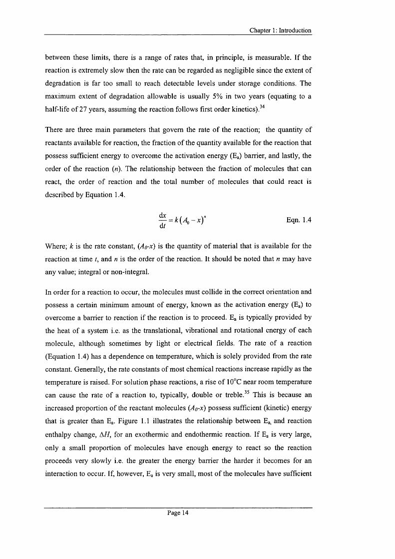
that is greater than Eg. Figure 1.1 illustrates the relationship between Eg, and reaction
enthalpy change. A //, for an exothermic and endothermie reaction. If Eg is very large,
only a small proportion o f molecules have enough energy to react so the reaction
proceeds very slowly i.e. the greater the energy barrier the harder it becomes for an
interaction to occur. If, however. Eg is very small, most o f the molecules have sufficient
Page 14
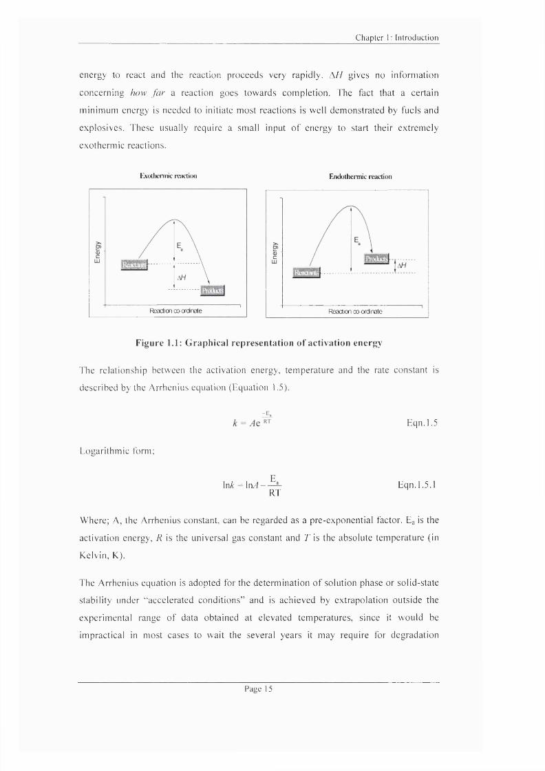
Chapter 1 : Introduction
energy to react and the reaction proceeds very rapidly. A // gives no information
concerning how far a reaction goes towards completion. The fact that a certain
minimum energy is needed to initiate most reactions is well demonstrated by fuels and
explosives. These usually require a small input o f energy to start their extremely
exothermic reactions.
Exothermic reaction Endothermie reaction
Reaction ccKxdnate Reaction co-ordinate
Figure 1.1: G raphical representation of activation energy
I he relationship between the activation energy, temperature and the rate constant is
described by the Arrhenius equation (Equation 1.5).
Eqn. 1.5
Logarithmic form;
\nk = \nART
Eqn. 1.5.
Where; A, the Arrhenius constant, can be regarded as a pre-exponential factor. Eg is the
activation energy, R is the universal gas constant and T is the absolute temperature (in
Kelvin, K).
The Arrhenius equation is adopted for the determination o f solution phase or solid-state
stability under “accelerated conditions” and is achieved by extrapolation outside the
experimental range o f data obtained at elevated temperatures, since it would be
impractical in most cases to wait the several years it may require for degradation
Page 15

Chapter 1 : Introduction
products to reach detectable levels under storage conditions. The activation energy o f
the reaction is determined at the higher temperatures and the Arrhenius relationship is
employed to calculate the degradation rates at any desired (lower) temperature via
extrapolation of data. The method is valid only if the mechanism of degradation remains
constant over the temperature o f both the experiment and the extrapolation. If the
Arrhenius relationship deviates from linearity outside the experimentally determined
region then there may be a change in mechanism and the method is invalidated.
The final parameter that influences the rate o f a reaction is the order o f reaction (n)
which is a power function and is related to the contribution that the reactant makes to
the rate o f reaction. Consider the following simple reaction;
aA + bB — cC + dD
It may be the case experimentally that the rate o f reaction is directly proportional to the
concentration o f A raised to the power a; Rate a [A]^. Similarly, if the rate o f reaction is
proportional to the concentration o f B then it is raised to the power b; Rate a [B]’’. For
example, a reaction order o f one (first order) can be expressed as Rate a [A]. If the
reaction order is two (second order), then the reaction rate is proportional to the
concentration of reactant available squared and expressed as Rate a [A]^. The overall
rate equation can be written as;
R atea[A ]'[B ]"
The rate o f reaction at a given time is then described by;
Rate = i[A ]*[B]‘'
In the example given above, the reactants A and B are raised to the power o f exponents
a and b, respectively, which define the reaction order. The order o f a reaction depends
on the reaction mechanism i.e., the sequence o f elementary steps that take place. The
overall reaction order («) is the summation with respect to the individual components,
i.e. « = a + b. Note that the order o f the reaction is not the same as the molecularity of
the reaction which provides information about the number o f molecules that take part in
an individual step within the overall reaction mechanism. A reaction, therefore.
Page 16
Chapter 1 : Introduction
proceeding from A to B must possess a reaction mechanism and be thermodynamically
and kinetically observable. The reaction will proceed only when these three criteria
have been met.
Reaction kinetics is the study o f reaction rates and its dependence upon concentrations
of the species involved. During a chemical reaction, the concentration (for a solution
phase system) or quantity (for a solid-state reaction) o f reactants decreases with time,
whilst the concentration/quantity o f the final product(s) increases with time. The
average rate o f reaction in terms o f a specific reactant or product within any given
interval o f time is defined as the change in concentration (or quantity) o f that reactant or
product (d[ ]) that occurs within the given time interval (dr), as described in Equation
1.6 .
Ra,e_d[reactanfl Eqn. 1.6dt dt
The reaction rate at any time, t, can be calculated from the concentration vs time curve.
This is achieved by drawing tangents to the curve and calculating the slope at that time.
Such a process can be laborious and inaccurate, particularly for slow reactions. (Note,
for negative slopes, the sign is changed when reporting the rate so that all reaction rates
are positive).
In effect, it is more appropriate to employ specific rate equations applicable to the
process under investigation. Rate equations can be derived for most chemical processes.
Such equations relate the rate o f reaction at any time t to the concentration o f the
reactants and products present at that time. Alternatively they can relate the rate of
reaction directly to time. For both cases the relationship is expressed through the rate
constant (k).
There are two types o f rate equation; the differential rate equation and the integrated
rate equation. The former express the rate o f reaction as a function o f concentration
and the latter expresses it as a function o f time. Most reactions follow either zero-, first,
or second-order kinetics, and thus obey a specific kinetic scheme. Third-order reactions
are rare and will not be discussed here. The differential and integrated rate expressions
commonly used to describe the three simple reaction orders are represented in Table
1 . 1 .
Page 17
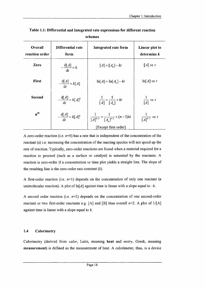
Chapter 1 : Introduction
Table 1.1: Differential and Integrated rate expressions for different reaction
schemes
Overall
reaction order
Differential rate
form
Integrated rate form Linear plot to
determine k
Zero
First
Second
.th
d[A]dt
= k
d[A]dt
= k[A]
[A] = [A ^'\-k t
ln[^] = \x\[A^]-kt
[A] vs t
\n[A] vs t
d[A]dt
d[A]dt
= k [ A f
= k[AY
1 1
[A] [A J+ kt
[A]
1 1— + ( n - \ ) k t
[ A r [ A J
[Except first order]
[A]n - \VS t
A zero-order reaction (i.e. n=0) has a rate that is independent o f the concentration o f the
reactant (s) i.e. increasing the concentration o f the reacting species will not speed up the
rate o f reaction. Typically, zero-order reactions are found when a material required for a
reaction to proceed (such as a surface or catalyst) is saturated by the reactants. A
reaction is zero-order if a concentration vs time plot yields a straight line. The slope of
the resulting line is the zero-order rate constant (k).
A first-order reaction (i.e. n=\) depends on the concentration o f only one reactant (a
unimolecular reaction). A plot o f ln[A] against time is linear with a slope equal to -k .
A second order reaction (i.e. n=2) depends on the concentration o f one second-order
reactant or two first-order reactants e.g. [A] and [B] thus overall «=2. A plot o f 1/[A]
against time is linear with a slope equal to k.
1.4 Calorimetry
Calorimetry (derived from calor, Latin, meaning heat and metry, Greek, meaning
measurement) is defined as the measurement o f heat. A calorimeter, thus, is a device
Page 18

Chapter 1 : Introduction
that can measure the heat change by a reaction as it proceeds. The change in heat can be
measured over time, which can yield information not only on the heat change
(thermodynamics) but also on the rate o f a reaction (kinetics). Since most chemical and
physical changes are accompanied by a change in heat content, or enthalpy, it is
possible, in principle, to study all chemical reactions using this technique. Calorimetry
is, thus, an extremely useful tool that can be used to monitor homogeneous and
heterogeneous reactions, such that both thermodynamic and kinetic information may be
obtained.
An early practical application in the realm o f calorimetry was pioneered by Lavoisier
and Laplace^^ who designed a simple calorimeter with the notion to study the
respiration o f a guinea pig. The calorimeter consisted o f a sample cell, surrounded by
ice, which was contained in an insulating jacket. A guinea pig was placed in an
insulated box packed with ice. Any heat evolved from the guinea pig’s enthalpy of
metabolism melted a certain quantity o f the surrounding ice. The resulting water was
collected, through a small outlet in the bottom o f the calorimeter, and weighed (Figure
1.2). The heat evolved calculations were based on Black’s prior discovery o f latent heat
- nowadays this term is generally obsolete and instead the modem practice is to use
enthalpy o f transformation. With knowledge o f the quantity o f water produced and the
latent enthalpy o f fusion o f water required to produce that amount of water, it is possible
to determine the equivalent heat output, g , (in Joules) for the process. By knowing the
body-mass o f the guinea pig, the change o f enthalpy for metabolism could then be
determined (in kJ kg''). This is a thermodynamic term, although it alone does not give
any useful information about the thermodynamic reactivity o f molecules. This is
because it is not possible to make direct comparisons in enthalpy between two reactions
unless the reagents in both reactions have the same molecular weight. It is also possible
to derive kinetic information from this process. If the mass o f water collected was
recorded periodically as a function o f time (min), then the rate o f metabolism could be
measured (J min ') consequently, giving a thermodynamic and kinetic evaluation for
respiration. At the end o f the experiment the guinea pig was released unharmed,
demonstrating that calorimetry can be a non-invasive and non-destructive technique.
Page 19

Chapter 1 : Introduction
Guinea Pig
Insulatingjacketcontaining ice
Outlet
Figure 1.2: Schematic representations of the first ice calorim eter.36
Nowadays, through the considerable advances made in the technology o f calorimeters,
there are several types o f calorimeters commercially available. Microcalorimeters,
designed for measuring in the micro-Watt range, are among the common type utilised
and can be categorised into three measuring priniciples:^^
1. Adiabatic m icrocalorim eters - there is no heat exchange between the calorimetric
vessel and its surroundings. These conditions are achieved by ensuring insulation
between the two entities. In most cases, semi-adiabatic (or isoperibol)
microcalorimeters are used since, in practice, true adiabatic conditions are difficult
to obtain which results in some heat-leak to the surroundings. In this case, it is
necessary to apply corrections to allow the return o f accurate data.
2. Power compensation m icrocalorim eters - the heat removed or gained during an
exothermic or endothermie process, respectively, is balanced by an opposing
Page 20

Chapter 1 : Introduction
electrical power; usually by using the Peltier effect current, such that the
calorimetric vessel is maintained at a given temperature.
3. Heat conduction microcalorimeters - any heat produced or absorbed in a reaction
flows to, or from, a surrounding “heat sink” which acts to maintain the system at a
constant temperature. These types o f microcalorimeters are known as isothermal.
The “Peltier effects plates” (thermopiles) are used as sensors for the heat flow
between the calorimetric vessels and surrounding heat sinks.
Isothermal heat conduction microcalorimetry is the principal microcalorimeter that has
been used throughout the studies presented herein.
1.4.1 The Principles of Isothermal Microcalorimetry
Isothermal microcalorimeters are surrounded by a heat sink that acts to maintain the
system at a constant temperature. Any heat produced or absorbed by the sample is
quantitatively exchanged with the heat sink (water bath). The microcalorimeter is used
in a differential mode, where a thermal energy change creates a small temperature
difference relative to the heat sink which forces heat to flow, either to, or from, the heat
sink, depending on whether the reaction being followed is exothermic or endothermie.
The magnitude of the temperature difference is directly proportional to the heat-flow
and thus to the rate o f the process under study. The thermopiles situated around the
sample are extremely sensitive, and are used to ensure the heat-flow is measured and
quantified. The potential generated by the thermopiles is then amplified and recorded as
heat-flow {Aqldt, thermal power in Watts) and is measured as a function of time.
There are a number o f isothermal microcalorimeters available, one such instrument is
the Thermal Activity Monitor, or TAM, manufactured by ThermoMetric AB (Jarfalla,
Sweden).
The TAM is a multichannel microcalorimeter comprised o f four separate channels, and
is therefore capable o f measuring four separate experiments simultaneously (Figure
1.3). The principle o f operation is simple; each channel has two identical chambers
Page 21
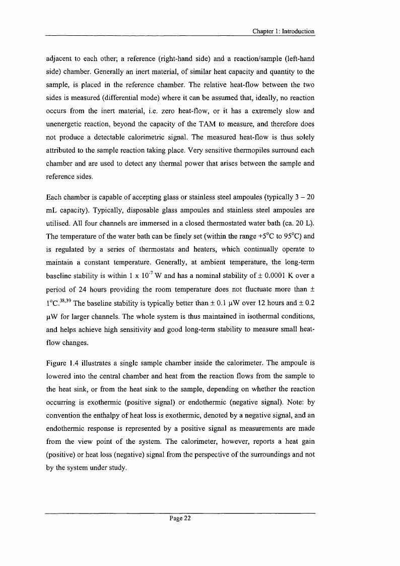
Chapter 1 : Introduction
adjacent to each other; a reference (right-hand side) and a reaction/sample (left-hand
side) chamber. Generally an inert material, o f similar heat capacity and quantity to the
sample, is placed in the reference chamber. The relative heat-flow between the two
sides is measured (differential mode) where it can be assumed that, ideally, no reaction
occurs from the inert material, i.e. zero heat-flow, or it has a extremely slow and
unenergetic reaction, beyond the capacity o f the TAM to measure, and therefore does
not produce a detectable calorimetric signal. The measured heat-flow is thus solely
attributed to the sample reaction taking place. Very sensitive thermopiles surround each
chamber and are used to detect any thermal power that arises between the sample and
reference sides.
Each chamber is capable o f accepting glass or stainless steel ampoules (typically 3 - 2 0
mL capacity). Typically, disposable glass ampoules and stainless steel ampoules are
utilised. All four channels are immersed in a closed thermo stated water bath (ca. 20 L).
The temperature o f the water bath can be finely set (within the range -t-5°C to 95°C) and
is regulated by a series o f thermostats and heaters, which continually operate to
maintain a constant temperature. Generally, at ambient temperature, the long-term
baseline stability is within 1 x 10’ W and has a nominal stability o f ± 0.0001 K over a
period o f 24 hours providing the room temperature does not fluctuate more than ±
fOc 38,39 baseline stability is typically better than ± 0 .1 pW over 12 hours and ± 0.2
pW for larger channels. The whole system is thus maintained in isothermal conditions,
and helps achieve high sensitivity and good long-term stability to measure small heat-
flow changes.
Figure 1.4 illustrates a single sample chamber inside the calorimeter. The ampoule is
lowered into the central chamber and heat from the reaction flows from the sample to
the heat sink, or from the heat sink to the sample, depending on whether the reaction
occurring is exothermic (positive signal) or endothermie (negative signal). Note: by
convention the enthalpy o f heat loss is exothermic, denoted by a negative signal, and an
endothermie response is represented by a positive signal as measurements are made
from the view point o f the system. The calorimeter, however, reports a heat gain
(positive) or heat loss (negative) signal from the perspective o f the surroundings and not
by the system under study.
Page 22
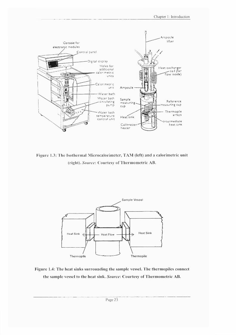
Chapter 1 : Introduction
C o n s o l e for e l e c t r o n i c m o d u l e s
C o n t r o l p ane l
Digi tal di splay
H o l e s f o r add i t i o n a l i o r i m e t r i c
un i t s
l o r i m e t r l c un i t
W a t e r b a t h
W a t e r b a t h c i r cu l a t i ng
p u m p
W a t e r b a t h m p c r a t u r c o n t r o l u n i t
A m p o u l el i f ter
m e a s u
H e a t e x c h a n g e r coi l ( f o r
f l o w m o d e )
Ca l i bnah e a t e r
R e f e r e n c e c a s u r i n g c up
T h e r m o p i l e a r r a y s
^ i n t e r m e d i a t e h e a t s ink
Figure 1.3: The Isotherm al M icrocalorim eter, TAM (left) and a calorim etric unit
(right). Source: Courtesy of Therm om etric AB.
Sam ple V essel
He a t SinkHeat Sink Heat Flow
ThermopileThermopile
Figure 1.4: The heat sinks surrounding the sample vessel. The therm opiles connect
the sample vessel to the heat sink. Source: Courtesy of Therm om etric AB.
Page 23
Chapter 1 : Introduction
The instrument is calibrated, usually by means o f an electrical calibration, prior to
sample measurement, which can be set over a range o f sensitivity scales; 3, 10, 30, 100,
300, 1000 or 3000
The TAM confers several advantages over other techniques; it has a combination of
versatility and sensitivity making it superior to many other analytical instruments. For
example, it has been reported that the TAM is 10,000 fold more sensitive than a
commercial Differential Scanning Calorimetry (such as a Perkin Elmer, DSC 7). " Its
high sensitivity comes from having an accurate and precise control o f temperature, such
that materials can be studied at ambient temperatures and the reaction environment can
be precisely controlled (pH, partial pressure, humidity etc).^^’ ’" ' It has been claimed
that the TAM has sufficient sensitivity to monitor slow reactions with lifetimes lasting
up to 10,000 years, and it has also been reported that the instrument can discriminate
between a reaction that has a first order rate constant o f 1 x 10'" s'* and 2 x 10'" s"'
after the collection o f 50 hours o f data.'^^’" Such a versatile system can be used together
with insertion vessels of different designs and functions ranging from simple closed
ampoules to stirred vessels fitted with injection tubes, devices facilitating dissolution,
electrodes, or optical cables. It is the latter design type that forms the focus of this
research.
The instrument has the ability to detect, and potentially quantify, the changes in a wide
range o f materials. For this, there are two requisites; firstly, the sample must produce a
sufficient quantity o f heat that can be detected by the thermopiles, and, secondly, the
sample (or a representative proportion o f it) must fit within the calorimetric vessel. The
TAM is non-invasive and non-destructive to the sample and so the reaction under study
is not influenced by the calorimeter, nor does the sample require any special treatment
or preparation prior to analysis. The instrument is also invariant to the physical form of
analysis; the sample can be solid, in solution, gaseous or a combination o f all phases.
This unique quality allows complex heterogeneous systems to be studied. Furthermore,
unlike other analytical techniques (e.g. UV spectroscopy), neither colour, optical
transparency nor the absence o f suspended matter are requirements. Since the
calorimeter records measurements as a function o f time, it is possible to capture data in
real-time, in a rapid manner, making it possible for small changes (both chemical and
physical) to be detected over a period o f time.
Page 24
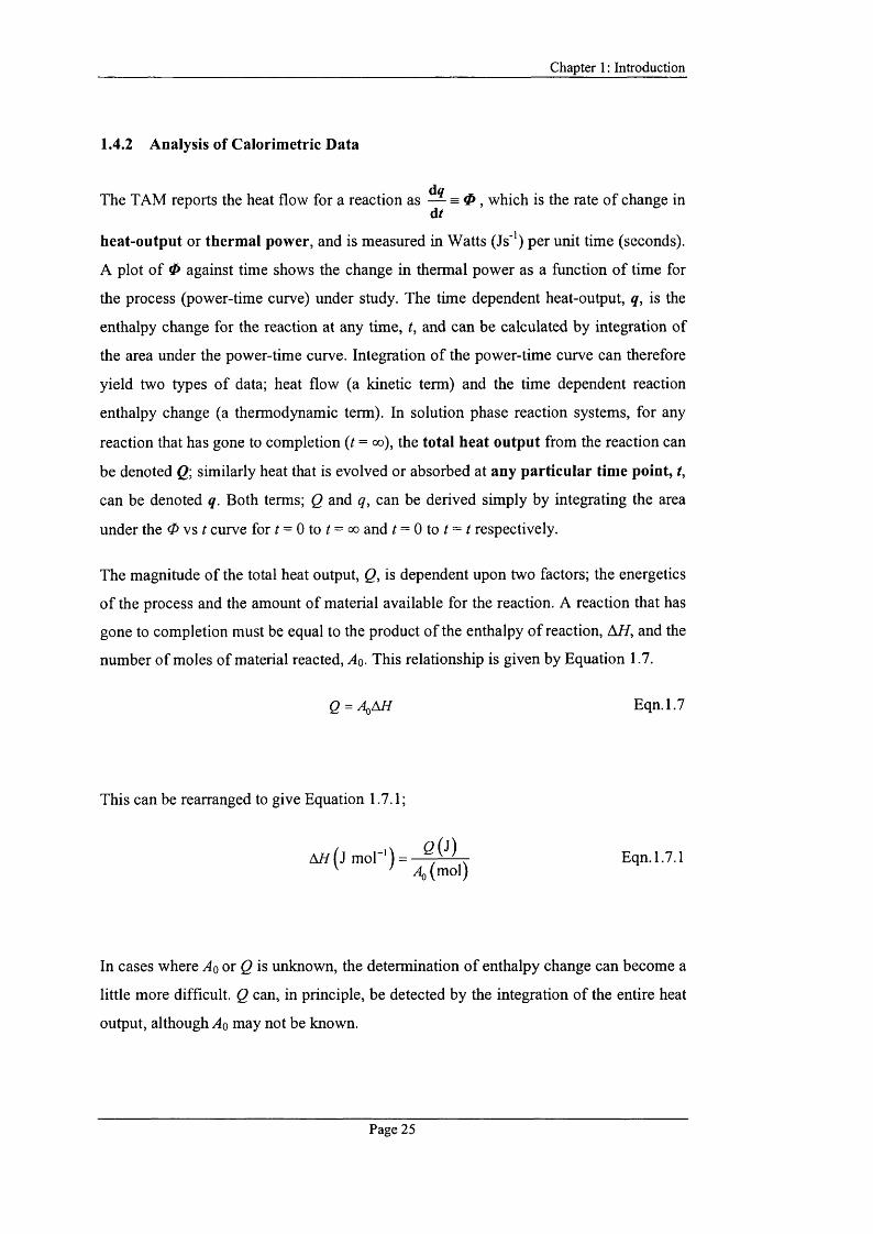
Chapter 1 : Introduction
1.4.2 Analysis of Calorimetric Data
The TAM reports the heat flow for a reaction as — = 0 , which is the rate o f change indt
heat-output or thermal power, and is measured in Watts (Js'’) per unit time (seconds).
A plot o f 0 against time shows the change in thermal power as a function o f time for
the process (power-time curve) under study. The time dependent heat-output, q, is the
enthalpy change for the reaction at any time, t, and can be calculated by integration of
the area under the power-time curve. Integration o f the power-time curve can therefore
yield two types o f data; heat flow (a kinetic term) and the time dependent reaction
enthalpy change (a thermodynamic term). In solution phase reaction systems, for any
reaction that has gone to completion (t = oo), the total heat output from the reaction can
be denoted Q; similarly heat that is evolved or absorbed at any particular time point, t,
can be denoted q. Both terms; Q and q, can be derived simply by integrating the area
under the 0 v s t curve for / = 0 to / = oo and t = 0 to t = t respectively.
The magnitude o f the total heat output, Q, is dependent upon two factors; the energetics
o f the process and the amount o f material available for the reaction. A reaction that has
gone to completion must be equal to the product o f the enthalpy o f reaction, AH, and the
number o f moles of material reacted, A q. This relationship is given by Equation 1.7.
Q = AqAH Eqn. 1.7
This can be rearranged to give Equation 1.7.1;
AH(J mol ') = . Eqn. 1.7.1 4 (mol)
In cases where A q or Q is unknown, the determination o f enthalpy change can become a
little more difficult. Q can, in principle, be detected by the integration o f the entire heat
output, although A q may not be known.
Page 25
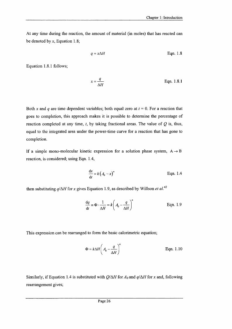
Chapter 1 : Introduction
At any time during the reaction, the amount o f material (in moles) that has reacted can
be denoted by x, Equation 1.8;
q = xA// Eqn. 1.8
Equation 1.8.1 follows;
X = ——— Eqn. 1.8.1ÙJJ
Both X and q are time dependent variables; both equal zero at = 0. For a reaction that
goes to completion, this approach makes it is possible to determine the percentage o f
reaction completed at any time, t, by taking fractional areas. The value o f Q is, thus,
equal to the integrated area under the power-time curve for a reaction that has gone to
completion.
If a simple mono-molecular kinetic expression for a solution phase system, A -> B
reaction, is considered; using Eqn. 1.4,
— = k{A„~x)" Eqn. 1.4df
then substituting for x gives Equation 1.9, as described by W illson et a lf^
d^ ^ 9— = O = kd/ A//
A - ^ \ Eqn. 1.9V A// '
This expression can be rearranged to form the basic calorimetric equation;
0 = A:A/f / 4 Eqn. 1.10
Similarly, if Equation 1.4 is substituted with Q /M I for/lo and q /àH for x and, following
rearrangement gives;
Page 26
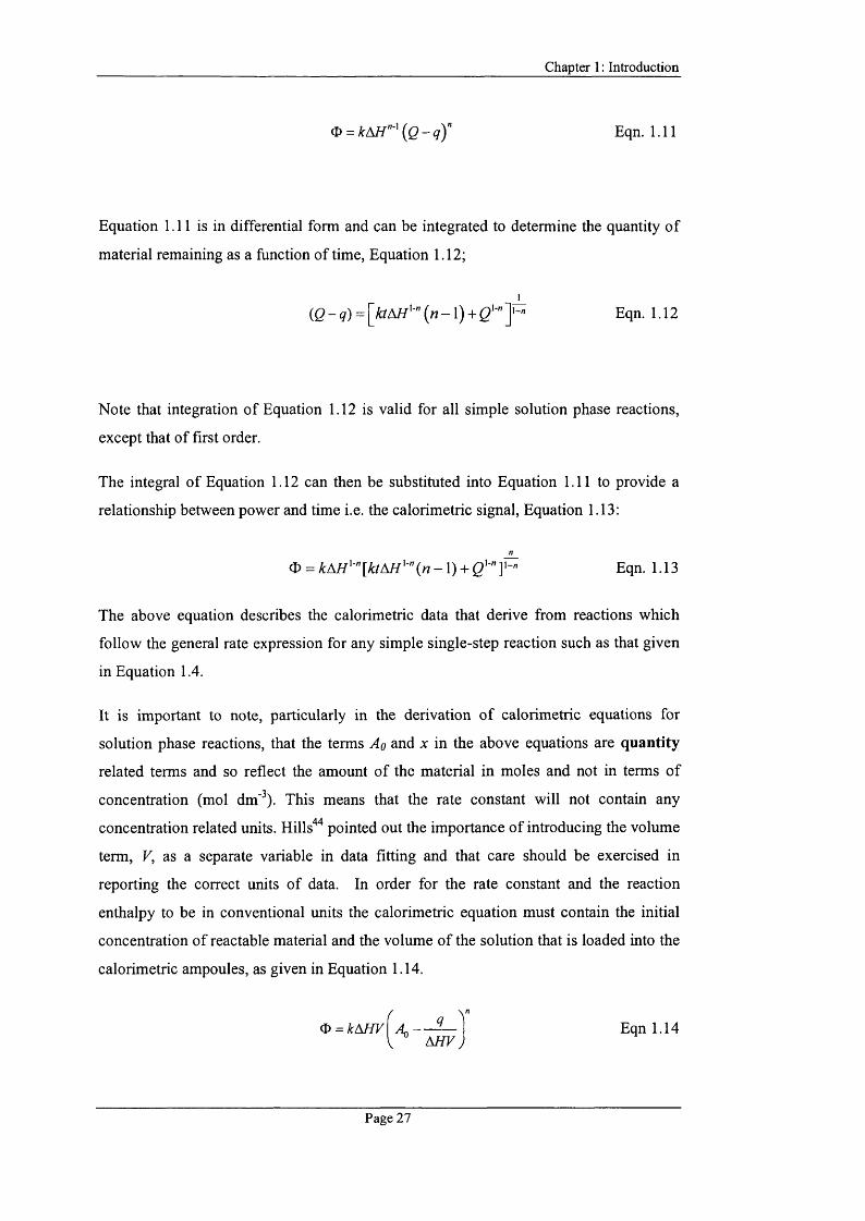
Chapter 1 : Introduction
<î> = kh H '-'{Q -q )" Eqn. 1.11
Equation 1.11 is in differential form and can be integrated to determine the quantity o f
material remaining as a function o f time, Equation 1.12;
I(Q -q ) = [faAW'-" (n -1 ) + g ‘’” Eqn. 1.12
Note that integration o f Equation 1.12 is valid for all simple solution phase reactions,
except that of first order.
The integral o f Equation 1.12 can then be substituted into Equation 1.11 to provide a
relationship between power and time i.e. the calorimetric signal. Equation 1.13:
0 = Â:A//'"[yt/A//'"(A7-l) + g ' ”p Eqn. 1.13
The above equation describes the calorimetric data that derive from reactions which
follow the general rate expression for any simple single-step reaction such as that given
in Equation 1.4.
It is important to note, particularly in the derivation o f calorimetric equations for
solution phase reactions, that the terms Aq and x in the above equations are quantity
related terms and so reflect the amount o f the material in moles and not in terms o f
concentration (mol dm'^). This means that the rate constant will not contain any
concentration related units. Hills' ' pointed out the importance o f introducing the volume
term, V, as a separate variable in data fitting and that care should be exercised in
reporting the correct units o f data. In order for the rate constant and the reaction
enthalpy to be in conventional units the calorimetric equation must contain the initial
concentration o f reactable material and the volume of the solution that is loaded into the
calorimetric ampoules, as given in Equation 1.14.
<t> = k m vA //F
Eqn 1.14
Page 27
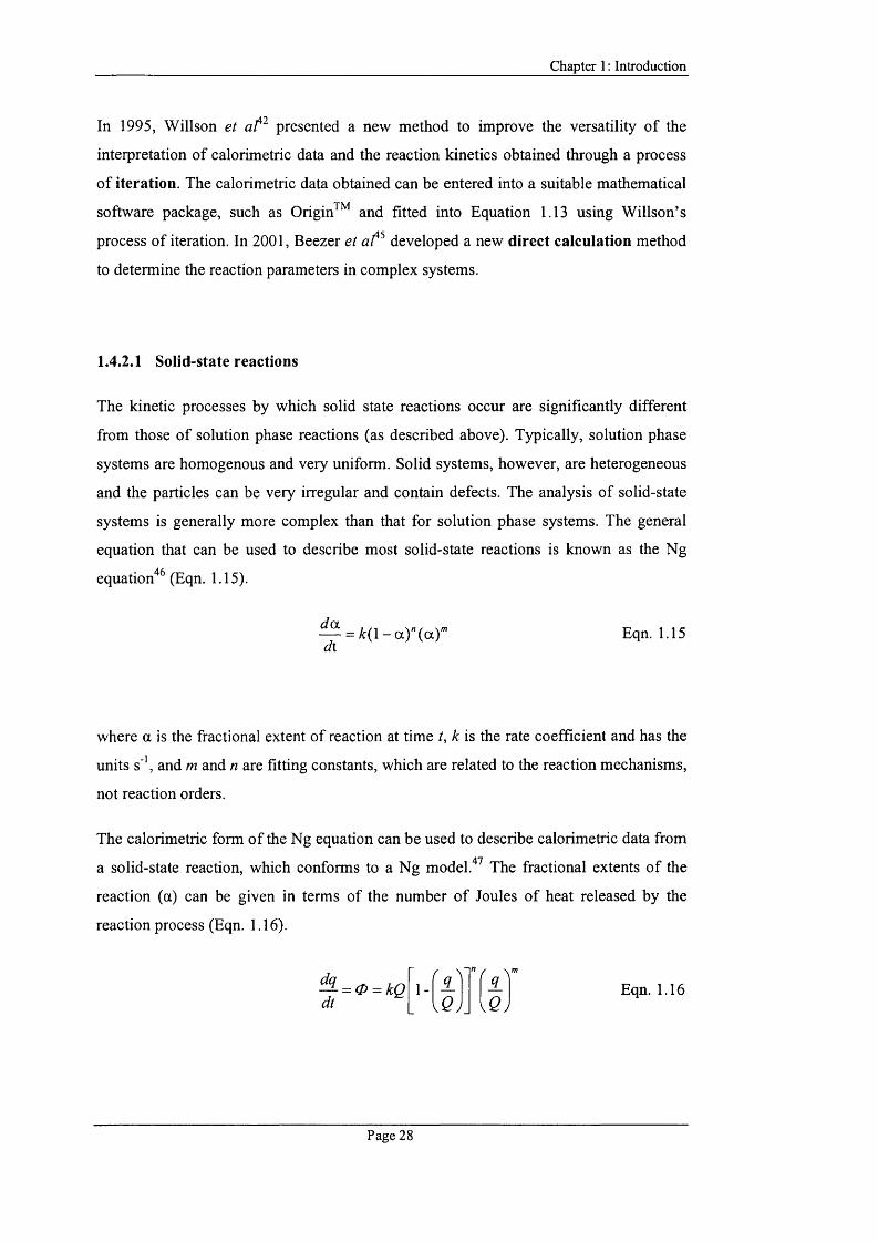
Chapter 1 : Introduction
In 1995, Willson et presented a new method to improve the versatility o f the
interpretation o f calorimetric data and the reaction kinetics obtained through a process
o f iteration. The calorimetric data obtained can be entered into a suitable mathematical
software package, such as Origin^'^ and fitted into Equation 1.13 using W illson’s
process o f iteration. In 2001, Beezer et a f^ developed a new direct calculation method
to determine the reaction parameters in complex systems.
1.4.2.1 Solid-state reactions
The kinetic processes by which solid state reactions occur are significantly different
from those o f solution phase reactions (as described above). Typically, solution phase
systems are homogenous and very uniform. Solid systems, however, are heterogeneous
and the particles can be very irregular and contain defects. The analysis o f solid-state
systems is generally more complex than that for solution phase systems. The general
equation that can be used to describe most solid-state reactions is known as the Ng
equation"^^ (Eqn. 1.15).
da.= k { \ - a y { a y Eqn. 1.15
where a is the fractional extent o f reaction at time t, k is the rate coefficient and has the
units s’', and m and n are fitting constants, which are related to the reaction mechanisms,
not reaction orders.
The calorimetric form o f the Ng equation can be used to describe calorimetric data from
a solid-state reaction, which conforms to a Ng model.'^^ The fractional extents o f the
reaction (a) can be given in terms of the number o f Joules o f heat released by the
reaction process (Eqn. 1.16).
dq~dt
= 0 = kQ S 'y Q j
Eqn. 1.16
Page 28
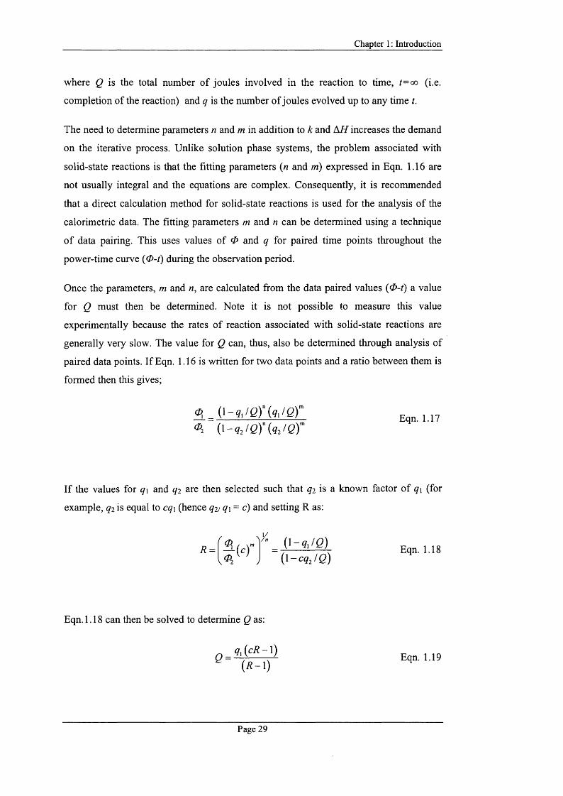
Chapter 1 : Introduction
where Q is the total number o f joules involved in the reaction to time, ?=oo (i.e.
completion of the reaction) and q is the number of joules evolved up to any time t.
The need to determine parameters n and m in addition to k and A // increases the demand
on the iterative process. Unlike solution phase systems, the problem associated with
solid-state reactions is that the fitting parameters {n and m) expressed in Eqn. 1.16 are
not usually integral and the equations are complex. Consequently, it is recommended
that a direct calculation method for solid-state reactions is used for the analysis o f the
calorimetric data. The fitting parameters m and n can be determined using a technique
o f data pairing. This uses values o f <P and q for paired time points throughout the
power-time curve {O-t) during the observation period.
Once the parameters, m and n, are calculated from the data paired values (0-^) a value
for Q must then be determined. Note it is not possible to measure this value
experimentally because the rates o f reaction associated with solid-state reactions are
generally very slow. The value for Q can, thus, also be determined through analysis of
paired data points. If Eqn. 1.16 is written for two data points and a ratio between them is
formed then this gives;
^ _ 0 - V e r U / g r Eqn. 1.170-?2/0)"(?2/ey
If the values for q\ and qi are then selected such that qj is a known factor o f q\ (for
example, qi is equal to cq\ (hence q2/q \ = c) and setting R as:
R =>
( i - g , / e )( l - c q j / g )
Eqn. 1.18
Eqn. 1.18 can then be solved to determine Q as:
Page 29
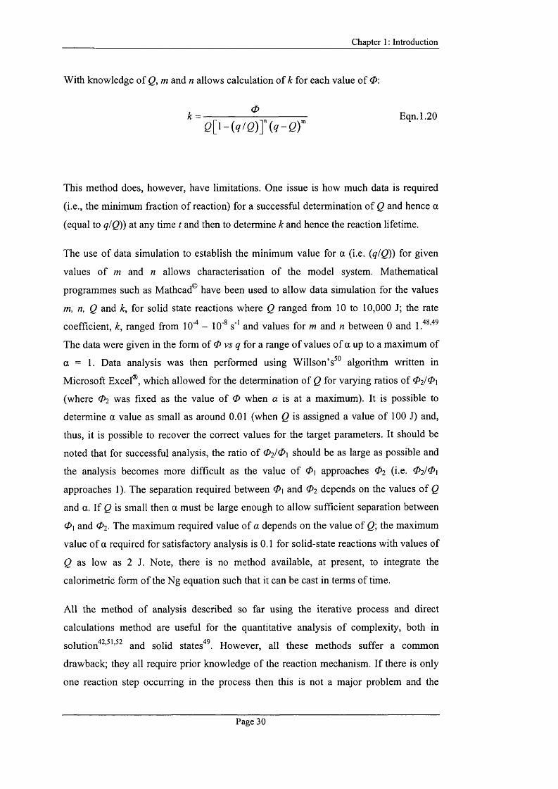
Chapter 1 : Introduction
With knowledge o f Q, m and n allows calculation o f k for each value o f O'.
k - -------------------- Eqn. 1.20e[i-(9/e)] ( q - Q T
This method does, however, have limitations. One issue is how much data is required
(i.e., the minimum fraction o f reaction) for a successful determination o f Q and hence a
(equal to qlQ)) at any time t and then to determine k and hence the reaction lifetime.
The use o f data simulation to establish the minimum value for a (i.e. {qlQ)) for given
values o f m and n allows characterisation of the model system. Mathematical
programmes such as Mathcad® have been used to allow data simulation for the values
m, n, Q and k, for solid state reactions where Q ranged from 10 to 10,000 J; the rate
coefficient, k, ranged from 1 0 - 10'^ s"' and values for m and n between 0 and
The data were given in the form o f O v s q for a range o f values o f a up to a maximum of
a = 1. Data analysis was then performed using W illson’s ® algorithm written in
M icrosoft Excel®, which allowed for the determination o f Q for varying ratios o f 02/0 \
(where O2 was fixed as the value o f O when a is at a maximum). It is possible to
determine a value as small as around 0.01 (when Q is assigned a value o f 100 J) and,
thus, it is possible to recover the correct values for the target parameters. It should be
noted that for successful analysis, the ratio o f 0 2 / ^ 1 should be as large as possible and
the analysis becomes more difficult as the value o f 0 \ approaches O2 (i.e. O2IO]
approaches 1). The separation required between 0 \ and O2 depends on the values o f Q
and a. If Q is small then a must be large enough to allow sufficient separation between
0 \ and O2 . The maximum required value o f a depends on the value o f 0 ; the maximum
value o f a required for satisfactory analysis is 0.1 for solid-state reactions with values of
Q as low as 2 J. Note, there is no method available, at present, to integrate the
calorimetric form o f the Ng equation such that it can be cast in terms o f time.
All the method of analysis described so far using the iterative process and direct
calculations method are useful for the quantitative analysis o f complexity, both in
solution"*^’ '’ and solid states^^. However, all these methods suffer a common
drawback; they all require prior knowledge o f the reaction mechanism. If there is only
one reaction step occurring in the process then this is not a major problem and the
Page 30

Chapter 1 : Introduction
equations described above can be used to quantitatively determine the reaction
parameters. The difficulty in analysing data arises when reactions comprising o f
multiple steps are studied. This is severely limiting for successful analysis to those
methods described above in cases where there is no prior knowledge o f the reaction
mechanism. It is possible to systematically fit the data to increasingly complex kinetic
models until a fit is obtained. Such an approach, however, is extremely time consuming
and requires the derivation o f many complex equations. It is also necessaiy to impose a
model on the system. Since calorimeters measure all the thermal events, without
discrimination, the resultant calorimetric data will reflect all the thermal processes form
each mechanistic step. Therefore, without prior knowledge o f the reaction mechanism,
the quantitative interpretation o f calorimetric data can be very complex in multi-
component systems. One approach o f determining individual reaction steps comprising
a complex reaction is the application o f chemometric analysis. Chapter 4 discusses the
potential application o f chemometric techniques such as principal component analysis
(PGA) as an approach to deconvolute complex reaction processes into their individual
components and the interpretation of complex Isothermal Calorimetric data for the
determination o f reaction parameters such as reaction enthalpy (A//) and rate constants
{k) are described.
On the whole, it has been described above that calorimetry has found much value for the
analysis o f pharmaceuticals and is unique among many analytical techniques. Therefore,
the set of qualities offered from calorimetry makes it an ideal candidate for the direct
study o f photochemical reactions for a range o f materials. This technique is known as
Photocalorimetry and is discussed below.
1.5 Photocalorimetry: Basic Concepts and Principles
Photocalorimetry has been under development for many years and is considered as an
extension o f classical calorimetry for the study o f the combined effects o f heat and
radiation.^^'^^ Many different types of photocalorimeters have been developed for
different purposes and their application has covered many fields ranging from
microbiology, organic chemistry, to materials science. It is the availability o f a wide
variety o f thermo-kinetic information from the calorimetric data that makes it possible
Page 31
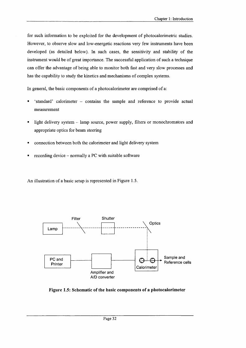
Chapter 1 : Introduction
for such information to be exploited for the development o f photocalorimetric studies.
However, to observe slow and low-energetic reactions very few instruments have been
developed (as detailed below). In such cases, the sensitivity and stability o f the
instrument would be o f great importance. The successful application o f such a technique
can offer the advantage o f being able to monitor both fast and very slow processes and
has the capability to study the kinetics and mechanisms o f complex systems.
In general, the basic components o f a photocalorimeter are comprised o f a:
■ ‘standard’ calorimeter - contains the sample and reference to provide actual
measurement
■ light delivery system - lamp source, power supply, filters or monochromators and
appropriate optics for beam steering
■ connection between both the calorimeter and light delivery system
■ recording device - normally a PC with suitable software
An illustration of a basic setup is represented in Figure 1.5.
Filter ShutterOptics
Sample and Reference cells
Amplifier and
Lamp
PC and Printer
Calorimeter
A/D converter
Figure 1.5: Schematic of the basic components of a photocalorimeter
Page 32
Chapter 1 : Introduction
There are two main methods used to introduce light into a calorimetric vessel; the first,
through a window made from glass or quartz, the other method is by use o f light guides
consisting o f fibres, fibre bundles or solid rods, (which can be made from a polymer,
quartz or glass). Nowadays liquid-filled flexible tubes are also available. These are
further discussed in Chapter 2. Flexible light guides can offer a great advantage for
instrument design and use. However, light transmission through a flexible guide may
vary significantly if its shape is changed. It is, therefore, essential that the light guide
has a well-defined and fixed position in the instrument.
In a photocalorimeter, a reaction is initiated when a sample is irradiated, by light o f an
appropriate wavelength from an external source, directly into the calorimeter via
flexible fibre optic light guides. All the light entering the calorimeter cell is either
absorbed by the sample or by the walls o f the calorimetric vessel. In the case of an inert
substance (reference), all the light energy is converted into heat and the calorimeter
measures the total light energy flux into the cell. I f however, the light induces a
photochemical reaction in the sample, an additional heat o f reaction is observed, over
and above the incident light energy itself. This causes the signal in the sample side in
the calorimeter to be out o f balance with that o f the reference side. Thus, by comparison
o f the photochemically active substance with some suitable inert reference, and by
determining the extent of the light-induced reaction, it is possible to measure directly:
(1) the change in heat energy (enthalpy) o f the sample produced by the isothermal
photochemical transformation and (2) the amount o f material, in moles, transformed in
the reaction.^"^
In a reference experiment the total amount o f radiation, Ep supplied to the photo-inert
substance is quantitatively transformed into heat, Q ' , and measured by the calorimeter,
as represented in Equation 1.21.
E ^ ^ Q ' Eqn. 1.21
Note; Equation 1.21 is only valid for the simplest case where no heat losses occur.
During a photochemical experiment, which now contains the photolyte under study, the
same amount of radiant energy is supplied to the calorimeter in conditions as close as
Page 33

Chapter 1 : Introduction
possible to those in the blank experiment. In this case, however, a photochemical
reaction does take place as shown below.
hv *A + _________ + . . . . --------------------- ^5 + . . .
Reactants — > Products
The photolyte. A, is activated by the radiation and it goes from the ground to an excited
state A *, which then undergoes the reaction.
In a photochemical experiment, a certain amount o f radiation, Ep, is quantitatively
transformed to heat energy, Q (associated with the formation o f the products during the
reaction) and measured by the calorimeter. An ideal situation, as that represented by a
reference experiment (Eqn. 1.21), only occurs where all the light energy is transformed
to heat. Components, such as stirrers, light guides, etc, in the photocalorimetric system,
can cause some loss of the incident radiation should be accounted for.
1.5.1 History and Development of Photocalorimetry
Interest in the thermodynamic examination o f materials sensitive to light using
calorimetric techniques has increased significantly since the late 1930’s. The first use of
the photocalorimeter was reported by Magee et al, 1939.^^ It was designed for the
thermal determination o f the quantum efficiency o f photosynthesis in algae (Chlorella
pyrenoidosa or Chlorella vulgaris). The photocalorimeter was comprised o f a
thermopile heat-conduction calorimeter using a small thin-walled quartz cell mounted in
an aluminium container with a double thermostat bath. A multi-junction thermocouple
was used; one thermopile was used as a sensor for the heat-flow, the other for the
measurement o f light transmittance. A schematic o f the instrument is shown in Fig. 1.8.
The determination of the thermal efficiency o f photosynthesising algae was conducted
using a 500 W projection lamp which introduced light through the front wall o f the
quartz cylinder. The thermal efficiency was calculated based on the rate o f heat
absorption by the process o f respiration and photosynthesis. The net amount o f radiation
dissipated as heat by the algae per unit time was then calculated between the two
processes.
Page 34

Chapter 1 : Introduction
Multi-junctionthermocouple
/A
Inner thermostat bath with stirrer
Q —Outer thermostat bath with stirrer '
Calorimeter and Thermopile
Figure 1.6: The first photocalorim eter designed by Magee et a! (1939)^^; A: end
view, B: side view in therm ostat
The same apparatus was later used to study the quantum yields and the influence o f
oxygen in the kinetics o f the photobromination o f hydrocarbons.'^^ Although the
apparatus was used to determine the overall enthalpy change associated with
photochemical reactions and to study the photochemical quantum yields o f the
organism, its design was elaborate and lacked determination o f long-term stability.
A fter thirty years, photocalorimetry steadily started to be developed. In the late sixties,
Seybold et al (1969)^^ investigated the quantum yield o f fluorescent dyes using a semi-
adiabatic double calorimeter. One o f the calorimetric vessels was charged with
fluorescent solution and the other vessel was charged with a black solution to allow the
m easurem ent o f the transmitted light.
it was during the eighties when development o f photocalorimeters rapidly increased and
the technique was applied to different fields. Many o f the instruments developed during
Page 35

Chapter 1 : Introduction
allow irradiation o f the sample. These were particularly important in the studies
concerning photopolymerisation.^®'^'^
In 1977, Olmsted et made further improvements to Seybold's photocalorimeter.
The fluorescence quantum yields were measured in a similar manner as reported by
Seybold (1969)^^ but solutions were prepared using spectrophotometric techniques. A
Dewar calorimetric vessel was equipped with quartz windows to allow passage o f light
from a 75 W Hg lamp source. A similar instrument was designed for photon flux
measurements o f s o l u t i o n s . I t consisted o f a Dewar vessel equipped with quartz
optical windows, a magnetic stirrer which assured thermal uniformity o f the solution, a
calibration heater and a thermistor used as a temperature sensor.
In 1978, Adamson et al (1978)^^ reported on a photocalorimeter, similar to the Olmsted
instrument, for the determination o f enthalpies o f photolysis o f trans-azobenzcne,
ferrioxalate and cobaltioxalate ions, hexacarbonylchromium and decarbonyldihenium.
The apparatus (depicted in Figure 1.7) included a glass reaction vessel and double-wall
container fitted with quartz windows for the incident light beam. Adamson and co
workers used the instrument, with slight modifications, to further study a series of other
systems.
Page 36
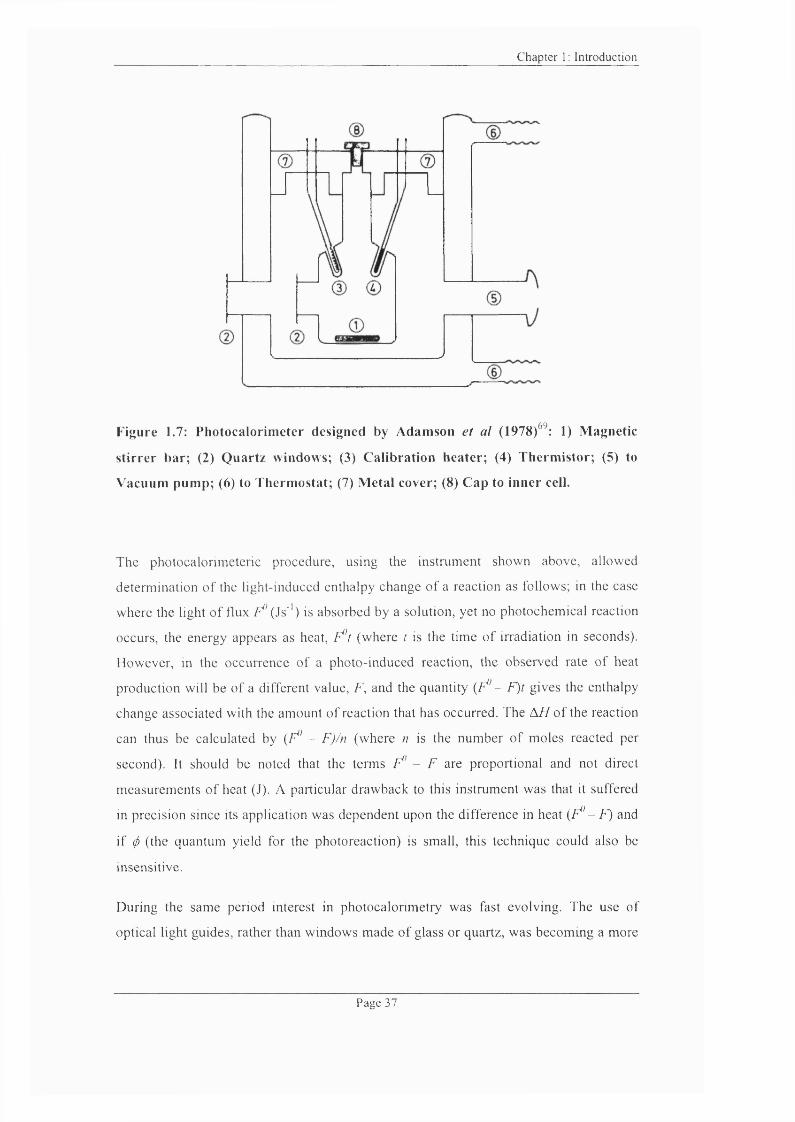
Chapter 1 : Introduction
Figure 1.7: Photocalorim eter designed by Adamson et a! (1978)^^: 1) Magnetic
s tirre r bar; (2) Q uartz windows; (3) Calibration heater; (4) Therm istor; (5) to
Vacuum pum p; (6) to Therm ostat; (7) M etal cover; (8) Cap to inner cell.
The photocalorim eteric procedure, using the instrument shown above, allowed
determ ination o f the light-induced enthalpy change o f a reaction as follows; in the case
where the light o f flux /^^(Js*') is absorbed by a solution, yet no photochemical reaction
occurs, the energy appears as heat, F ’t (where t is the time o f irradiation in seconds).
However, in the occurrence o f a photo-induced reaction, the observed rate o f heat
production will be o f a different value, F, and the quantity {F ’ - F)t gives the enthalpy
change associated with the amount o f reaction that has occurred. The A // o f the reaction
can thus be calculated by {F - F)/n (where n is the num ber o f moles reacted per
second). It should be noted that the terms F - F are proportional and not direct
m easurem ents o f heat (J). A particular drawback to this instrument was that it suffered
in precision since its application was dependent upon the difference in heat {F - F) and
if ({) (the quantum yield for the photoreaction) is small, this technique could also be
insensitive.
During the same period interest in photocalorim etry was fast evolving. The use o f
optical light guides, rather than windows made o f glass or quartz, was becoming a more
Page 37

Chapter 1 : Introduction
popular method to introduce light into the calorimetric vessel. A major advantage was
its practical applicability; optical light guides usually have a small aperture making
them more suitable for use with microcalorimeters.
The first report o f the use o f optical light guides as a means to introduce light into a
calorimetric vessel was by Schaarschmidt and Lamprecht^^'^^ who described two
different calorimeters fixed with two light guides designed for studies o f living yeast
cells. The first design comprised o f a quartz light guide, 10 mm diameter, used to
investigate the sensitivity o f yeast cells to UV radiation. The second design was fitted
with two thin light guides, 1 mm diameter, into a twin isothermal microcalorimeter. The
vessel was not designed as a photocalorimetric vessel, but its purpose was for the
simultaneous determination of heat production and optical densities o f yeast cell
suspensions. A schematic o f the instrument is represented in Figure 1.8.
M cllvaine and Langerman (1977)^^ used a semi-adiabatic titration calorimeter fitted
with a 6.5 mm fibre bundle in their calorimetric measurements o f luminescent bacteria.
The light generated by the micro-organisms was transmitted by the light guide to a
photomultiplier. Although not strictly a photocalorimeter since there is no irradiation
system, the work is still o f relevance. Langerman (1978)^^ also described a similar
instrument, where the calorimetric vessel was fitted with fibre optics, which was used
for the simultaneous determination o f heat evolution and light production.
Page 38
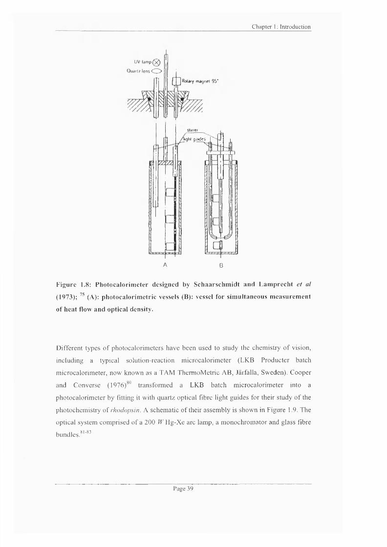
Chapter 1 ; Introduction
lighi guides
A B
Figure 1.8: Photocalorim eter designed by Schaarschm idt and Lam precht et al
(1973); (A): photocalorim etric vessels (B): vessel for sim ultaneous m easurem ent
of heat flow and optical density.
Different types o f photocalorimeters have been used to study the chemistry o f vision,
including a typical solution-réaction m icrocalorimeter (LKB Producter batch
microcalorimeter, now known as a TAM ThermoM etric A 3 , Jarfalla, Sweden). Cooper
and Converse (1976)^® transformed a LKB batch m icrocalorimeter into a
photocalorim eter by fitting it with quartz optical fibre light guides for their study o f the
photochem istry o f rhodopsin. A schematic o f their assembly is shown in Figure 1.9. The
optical system comprised o f a 200 W Hg-Xe arc lamp, a m onochrom ator and glass fibre
bundles. 81-83
P age 39
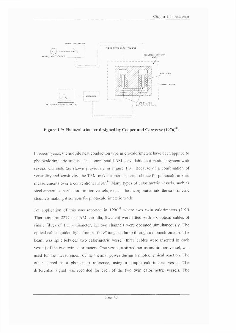
Chapter 1 ; Introduction
M ONO CH RO M A TO R
W — 'X e / Hg LIGHT S O U R C E .
AR E C O R D E R AND IN TEG RA TO R
4 AM PLIFIER
C O N TR O LLED TEM P BATH
L::"
F IB R E -O P T IC S LIGHT G U ID ES
SA f.IP LEA N D R E F E R E N C E CELLS
TH FRM O PII F S
Figure 1.9: Photocalorim eter designed by Cooper and Converse (1976)80
In recent years, thermopile heat conduction type m icrocalorimeters have been applied to
photocalorim eteric studies. The commercial TAM is available as a modular system with
several channels (as shown previously in Figure 1.3). Because o f a combination of
versatility and sensitivity, the TAM makes a more superior choice for photocalorimetric
m easurem ents over a conventional DSC.^" Many types o f calorimetric vessels, such as
steel ampoules, perfusion-titration vessels, etc, can be incorporated into the calorimetric
channels making it suitable for photocalorimeteric work.
An application o f this was reported in 1990^^ where two twin calorimeters (LKB
Thermom etric 2277 or TAM, Jarfalla, Sweden) were fitted with six optical cables o f
single fibres o f 1 mm diameter, i.e. two channels were operated simultaneously. The
optical cables guided light from a 100 f f tungsten lamp through a monochromator. The
beam was split between two calorimetric vessel (three cables were inserted in each
vessel) o f the two twin calorimeters. One vessel, a stirred perfusion/titration vessel, was
used for the measurement o f the thermal power during a photochem ical reaction. The
other served as a photo-inert reference, using a simple calorimetric vessel. The
differential signal was recorded for each o f the two twin calorimetric vessels. The
Page 4 0
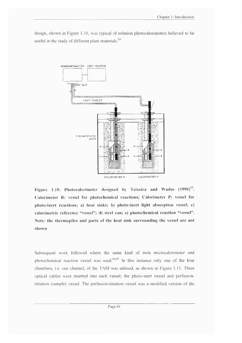
Chapter 1 : Introduction
design, shown in Figure 1.10, was typical o f solution photocalorim eters believed to be
useful in the study o f different plant materials.
kCNOCHROW ATCA LIGHT SC O RC E
1 I I
LjGmT CAGLES
t h e r m o s t a t i cBATM
Figure 1.10: Photocalorim eter designed by Teixeira and W adso (1990)^^.
C alorim eter R: vessel for photochemical reactions; C alorim eter P: vessel for
photo-inert reactions; a) heat sinks; b) photo-inert light absorption vessel; c)
calorim etric reference “vessel” ; d) steel can; e) photochemical reaction “vessel” .
Note: the therm opiles and parts of the heat sink surrounding the vessel are not
shown
Subsequent work followed where the same kind o f twin m icrocalorim eter and
photochem ical reaction vessel was used.^^’ In this instance only one o f the four
chambers, i.e. one channel, o f the TAM was utilised, as shown in Figure 1.11. Three
optical cables were inserted into each vessel; the photo-inert vessel and perfusion-
titration (sample) vessel. The perfusion-titration vessel was a modified version o f the
P age 41
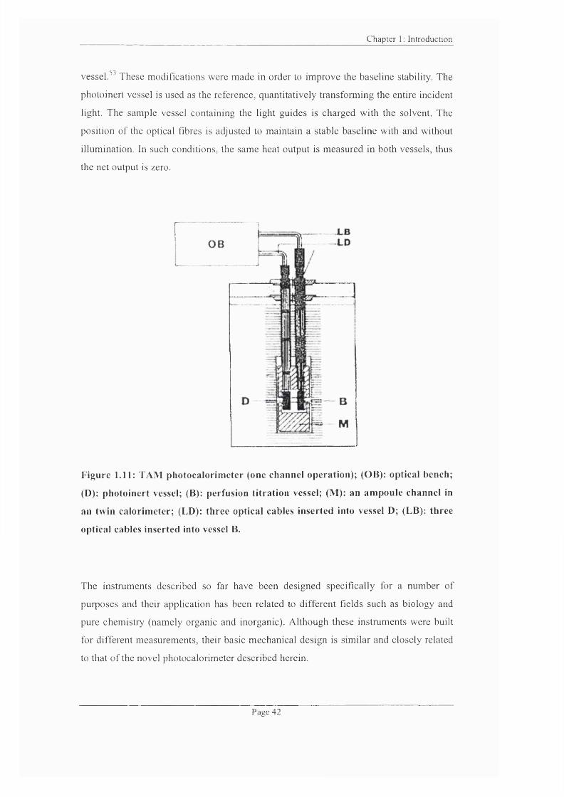
Chapter 1 : Introduction
vessel/^ These modifications were made in order to improve the baseline stability. The
photoinert vessel is used as the reference, quantitatively transform ing the entire incident
light. The sample vessel containing the light guides is charged with the solvent. The
position o f the optical fibres is adjusted to maintain a stable baseline with and without
illumination. In such conditions, the same heat output is measured in both vessels, thus
the net output is zero.
r
Figure 1.11: TA M photocalorim eter (one channel operation); (OB): optical bench;
(D): photoinert vessel; (B): perfusion titra tion vessel; (M ): an am poule channel in
an twin calorim eter; (LD): three optical cables inserted into vessel D; (LB): three
optical cables inserted into vessel B.
The instruments described so far have been designed specifically for a number of
purposes and their application has been related to different fields such as biology and
pure chemistry (namely organic and inorganic). Although these instruments were built
for different measurements, their basic mechanical design is sim ilar and closely related
to that o f the novel photocalorim eter described herein.
Page 42
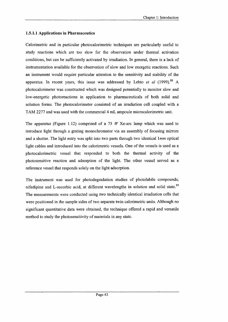
Chapter 1 ; Introduction
1.5.1.1 Applications in Pharmaceutics
Calorimetric and in particular photocalorimetric techniques are particularly useful to
study reactions which are too slow for the observation under thermal activation
conditions, but can be sufficiently activated by irradiation. In general, there is a lack of
instrumentation available for the observation o f slow and low energetic reactions. Such
an instrument would require particular attention to the sensitivity and stability o f the
apparatus. In recent years, this issue was addressed by Lehto et al (1999).^^ A
photocalorimeter was constructed which was designed potentially to monitor slow and
low-energetic photoreactions in application to pharmaceuticals o f both solid and
solution forms. The photocalorimeter consisted o f an irradiation cell coupled with a
TAM 2277 and was used with the commercial 4 mL ampoule microcalorimetric unit.
The apparatus (Figure 1.12) comprised o f a 75 W Xe-arc lamp which was used to
introduce light through a grating monochromator via an assembly o f focusing mirrors
and a shutter. The light entry was split into two parts through two identical 1mm optical
light cables and introduced into the calorimetric vessels. One o f the vessels is used as a
photocalorimetric vessel that responded to both the thermal activity o f the
photosensitive reaction and adsorption o f the light. The other vessel served as a
reference vessel that responds solely on the light adsorption.
The instrument was used for photodegradation studies o f photolabile compounds;
nifedipine and L-ascorbic acid, at different wavelengths in solution and solid state.^^
The measurements were conducted using two technically identical irradiation cells that
were positioned in the sample sides o f two separate twin calorimetric units. Although no
significant quantitative data were obtained, the technique offered a rapid and versatile
method to study the photosensitivity o f materials in any state.
Page 43
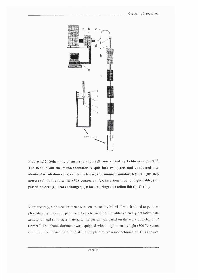
Chapter 1 : Introduction
J
s a m p l e v e s s e l s
Figure 1.12: Schematic of an irrad iation cell constructed by Lehto et al (1999) .
The beam from the m onochrom ator is split into two parts and conducted into
identical irrad iation cells; (a): lamp house; (b): m onochrom ator; (c): PC; (d): step
m otor; (e): light cable; (f): SMA connector; (g): insertion tube for light cable; (h):
plastic holder; (i): heat exchanger; (j): locking ring; (k): teflon lid; (I): O-ring.
M ore recently, a photocalorimeter was constructed by Morris^^ which aimed to perform
photostability testing o f pharmaceuticals to yield both qualitative and quantitative data
in solution and solid-state materials. Its design was based on the work o f Lehto et al
(1999)/^ The photocalorimeter was equipped with a high-intensity light (300 W xenon
arc lamp) from which light irradiated a sample through a monochromator. This allowed
Page 44
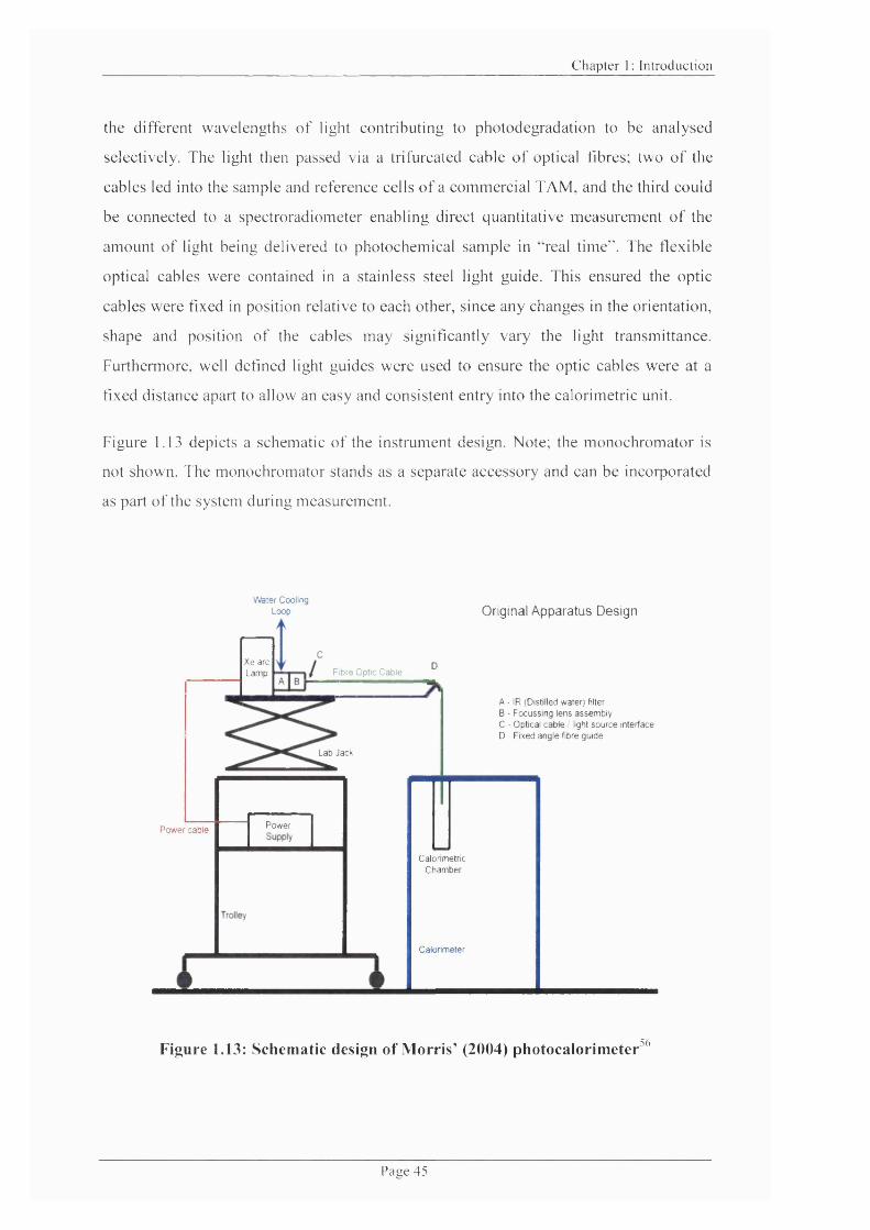
C hapter 1: In troduction
the d ifferent w avelengths o f light con tribu ting to photodegradation to be analysed
selectively . The light then passed via a trifurcated cable o f optical fibres; two o f the
cables led into the sam ple and reference cells o f a com m ercial TA M , and the third could
be connected to a spectroradiom eter enab ling direct quan tita tive m easurem ent o f the
am ount o f light being delivered to photochem ical sam ple in “real tim e 'f The flexible
optical cables w ere contained in a stain less steel light guide. T his ensured the optic
cables w ere fixed in position relative to each other, since any changes in the orientation,
shape and position o f the cables m ay sign ifican tly vary the light transm ittance.
Furtherm ore, well defined light guides w ere used to ensure the optic cables w ere at a
fixed distance apart to allow an easy and consisten t en try into the calorim etric unit.
F igure 1.13 depicts a schem atic o f the instrum ent design. N ote; the m onochrom ator is
not show n. The m onochrom ator stands as a separate accessory and can be incorporated
as part o f the system during m easurem ent.
W ater Cooling Loop Original Apparatus Design
A - IR (Distilled water) filter B - F ocussing lens assem bly 0 - Optical cab le / light source interface D - Fixed ang le fibre guide
Xe arc Lamp Fibre Optic C able
Lab Jack
PowerP ow er cable
CalorimetricC ham ber
Calorim eter
Figure 1.13: Schematic design of Morris’ (2004) photocalorimeter 56
P age 45
Chapter 1 : Introduction
The instrument was designed to study the rate o f photodegradation for a wide range of
pharmaceuticals, which can be used to yield information on the kinetic and
thermodynamic parameters for both solid and solution phase systems. The suitability of
the photodegradation o f 2-nitrobenzaldehyde and photoreduction o f potassium
ferrioxalate - an lUPAC recommended chemical calibrant - were investigated for
validating photoreactions in solution phase systems. The photodegradation o f nifedipine
was also proposed as a calibrant in the solid-state.
It is the photocalorimeter design o f Morris^^ that forms the basis o f the instrument
developed during this project. The instrument design and test applications are further
detailed in Chapter 2, 3 and 5. The former project, conducted by Morris^^, was
originally based at the University o f Greenwich, UK. Thereafter, the photocalorimeter
was transported, to its current location; The School o f Pharmacy, University o f London,
UK for further developmental work. This research follows on from M orris’^ work, and
extends on developments through design considerations to improve the performance of
the instrument.
Details o f the instrument design, technicalities, operation and performance are given in
Chapter 2 along with developments and modifications made to the system as the project
progressed.
Page 46
Chapter 1 : Introduction
1.6 Summary
This thesis is primarily concerned with the development o f a novel photocalorimeter to
study the photostability o f pharmaceutical compounds. In order to assess the
photostability o f a material, for the predication o f shelf life for instance, something
about the kinetics and thermodynamics o f the degradative reactions must be known.
Calorimetry is widely recognised as an alternative to classical analytical techniques, for
example, HPLC and spectrophotometry. Such techniques can be time consuming,
require extensive sample preparation, and involve destructive and invasive sampling
techniques. Calorimetry, on the other hand, offers many advantages; it is invariant to
physical form, rapid, non-invasive, non-destructive to the sample, and offers availability
o f a wide variety o f thermo-kinetic information from calorimetric data in real-time.
These qualities set the technique apart from most other analytical techniques commonly
used for stability studies. The extension o f calorimetry to monitor photodegradative
processes is therefore particularly interesting because the combined effects o f heat and
radiation can be studied.
Subsequent chapters will show the development o f a novel photocalorimeter and how
thermo-kinetic information can be exploited from the calorimetric data to monitor
photostability o f pharmaceuticals. This is considered through the development o f a
chemical test and reference reaction, 2-nitrobenzaldehyde, and the photodegradation o f
nifedipine in a solution phase system.
Page 47
Chapter 1 : Introduction
1.7 References
1 Carstensen, J.T., and Rhodes, C.T. (2000) Drug Stability Principles and Practices, Marcel Dekker
2 Anderson, N.H., Johnston, D., McLelland, M.A., and Munden, P. (1991)Photostability testing o f drug substances and drug products in UK pharmaceutical laboratories. J.Pharm.Biomed.Anal 9, 443-449
3 Tonnesen, H.H. (1991) Photochemical degradation o f components in drugformulations. I. An approach to the standardization o f degradation studies. Pharmazie 46, 263-265
4 Tonnesen, H.H., and Karlsen, J. (1995) Photochemical degradation o fcomponents in drug formulations. III. A discussion o f experimental conditions. Pharmeuropa 7, 137-141
5 Tonnesen, H.H., and Moore, D.E. (1993) Photochemical degradation of components in drug formulations. Pharm.Tech.Int 5, 27-33
6 Piechocki, J.T. (1998) Principles of chemical actinometry. In Drugs photochemistry and photostability (Albini, A., and Fasani, E., ed.). The Royal Society o f Chemisty
7 ICHQIB. (1997) Photostability Testing o f New Active Substances and Medicinal Products. EMEA, CPM P/ICH/2791/2795
8 ICHQIB. (1997) Photostability Testing o f New Drug Substances and Products. Fed. Reg. 62 (95), 27115-27122
9 Sequeira, P., and Vozone, C. (2000) Photostability studies o f drug substances and products. Practical implications of the ICH guideline. Pharm.Tech 24 (8), 30-35
10 Piechocki, J.T., Wolters, R.J. (1993) Use o f actinometry in photolysis stability studies. Pharm. Tech 17, 46-52
11 Piechocki, J.T., Wolters, R.J. (1994) Light stability studies: A misnomer. Pharm.Tech 18, 60-65
12 Nema, S., Washkuhn, R.J., and Beussink, D R. (1995) Photostability testing: an overview. Pharm.Tech. 19 (3), 170-185
13 Thatcher, S., Mansfield, R.K., Miller, R.B., Davis, C.W., and Baertschi, S.W. (2001) "Pharmaceutical photostability" A technical guide and practical interpretation o f the ICH guideline and its application to pharmaceutical stability- Part I. Pharm.Tech 25 (3), 98-110.
14 Thatcher, S., Mansfield, R.K., Miller, R.B., Davis, C.W., and Baertschi, S.W. (2001) "Pharmaceutical photostability" A technical guide and practical interpretation of the ICH guideline and its application to pharmaceutical stability- Part II. Pharm.Tech 25 (4), 58-64
Page 48
Chapter 1 : Introduction
15 Moore, D.E. (1987) Principles and practice o f drug photodegradation studies. J.Pharm.Biomed.Anal 5 (5), 441-453
16 Tonnesen, H.H. (2004) Photostability o f drugs and drug formulations, CRC press
17 Tonnesen, H.H. (2001) Formulation and stability testing o f photolabile drugs. Int.J.Pharm. 225, 1-14
18 Aman, W., and Thoma, K. (2002) The influence o f formulation and manufacturing process on the photostability o f tablets. Int.J.Pharm. 243, 33-41
19 Templeton, A C., Xu, H., Placek, J., and Reed, R.A. (2005) Implications of photostability on manufacturing, packaging, storage, and testing o f formulated pharmaceutical products. Pharm.Tech., 68-86
20 Thoma, K., and Klimek, R. (1991) Photostabilization o f drugs in dosage forms without protection from packaging materials. Int.J.Pharm. 67, 169-175
21 Andrisano, V., Bertucci, € ., Battaglia, A., and Cavrini, V. (1999) Photodegradation studies on Atenolol by liquid chormatogrpahy. J.Pharm.Biomed.Anal 21, 851-857
22 Andrisano, V., Bertucci, C., Battaglia, A., and Cavrini, V. (2000) Photostabilityof drugs: photodegradation o f melatonin and its determination in commercial formulations. J.Pharm.Biomed.Anal 23, 15-23
23 Brisaert, M., and Plaizier-Vercammen, J. (2000) Investigation on thephotostability o f a tretinion lotion and stabilisation with additives. Int.J.Pharm. 199, 49-57
24 Majeed, I.A., Murray, W.J., Newton, D.W., Othman, S, and Al-turak, W.A.(1987) Spectrophotometric study o f the photodecomposition kinetics of nifedipine. J.Pharm. Pharmacol 39, 1044-1046
25 Chang, H., Su, Y., and Chang, S. (2006) Studies on photostability o f butyrylated, milled wood lignin using spectroscopic analyses. Polymer Degradation and Stability 91, 816-822
26 Teraoka, R., Otsuka, M., and Matsuda, Y. (2004) Evaluation o f photostability of solid-state nicardipine hydrochloride polymorphs by using Fourier-transformed reflection-absorption infrared spectroscopy-effect o f grinding on the photostability o f crystal form. Int.J.Pharm. 286, 1-8
27 Chen, X., Peng, X., Cui, Z., Wang, B., Wang, L., and Zhang, R. (2006) Photostabilities of novel heptamethine 3H-indolenine cyanine dyes with different N-substituents. J.Photochem.Photobiol A. Chem 181, 79-85
28 Lipson, S.M., O'Brien, D.F., Byrne, H.J., Davey, A.P., and Blau, W.J. (2000) Investigation o f efficiency and photostability in polymer films. Synthetic Metals 111-112,553-557
Page 49
Chapter 1 : Introduction
29 Breier, A.R., Nudelman, N.S., Steppe, M., and Schapoval, E.E.S. (2008) Isolation and structure elucidation o f photodegradation products o f fexofenadine. J.Pharm.Biomed.Anal 46, 250-257
30 Chen, D., Zhou, J., Tian, Q. (1996) Mechanisms and structures o f free radicals in the photoreaction processes of o-substituted nitrobenzaldehydes. Journal o f Photochemistry and Photobiology A: Chemistry 98, 21-26
31 Silchenko, S., Schoneich, C., Carlson, B.J., and Stella, V. J. (2003)Photo stability o f 2-hydroxymethyl-4,8-dibenzo[ 1,2-b:5,4-b']dithiophene-4,8- dione (NSC 656240), a potential anticancer drug. Int.J.Pharm. 264, 97-105
32 Kojima, T., Onoue, S., Katoh, F., Teraoka, R., Matsuda, Y., Kitagawa,S., and Tsuhako, M. (2007) Effect o f spectroscopic properties on photostability of tamoxifen citrate polymorphs. Int.J.Pharm. 336, 346-351
33 Atkins, P.W. (1994) Physical Chemistry, 5th Ed. Oxford University Press
34 Buckton, G., Beezer A.E. (1991) The applications o f microcalorimetry in the field o f physical pharmacy. Int.J.Pharm. 72, 181-191
35 Cox, B.C. (1994) Modern liquid phase kinetics, Oxford University Press
36 Lavoisier, A.L., and De Laplace, P.S. (1784) M emoir o f heat. Histoire de VAcadémie Royale des Sciences 1780, 355
37 Wadso, L, Goldberg, R. N. (2001) Standards in isothermal microcalorimetry (lUPAC technical report). Pure.Appl.Chem 73, 1625-1639
38 Backman P, B.M., Briggner LE, Hagg S, Hallen D, Lonnbro P, Nilsson SO, Olofsson G, S chon A, Suurkuusk J, Teixeira C, and Wadso I. (1994) A system of microcalorimeters. Pure & Appl Chem 66 (3), 375-382
39 Suurkuusk, J., and Wadso, I. (1982) A multichannel microcalorimetry system. Chem Scripta 20, 155-163
40 Technical Specification, Thermometric AB, Note 22016.
41 Wadso, L. (2001) The isothermal heat conduction calorimeter: a versatile instrument for studying processes in physics, chemistry and biology. J.Chem.Edu. 78, 1080-1086
42 Willson, R., Beezer, A., Mitchell., J.C., and Watson, L. (1995) Determination o f thermodynamic and kinetic parameters from isothermal heat conduction microcalorimetry: applications to long-term reaction studies. J.Phys.Chem 99, 7108-7113
43 Willson, R.J. (1995) Ph.D Thesis. University o f Kent, UK.
44 Hills, A.K. (2001) Ph D Thesis. University o f Kent
Page 50
Chapter 1 : Introduction
45 Beezer, A., Morris, A C., O'Neill, M.A.A., Willson, R.J., Hills, A.K., Mitchell,J.C., and Connor, J.A. (2001) Direct determination o f equilibrium thermodynamic and kinetic parameters from isothermal heat conduction microcalorimetry. 5 105, 1212-1215
46 Ng, W.L. (1975) Thermal decomposition in solid-state. AustJ.C hem 28,1169- 1178
47 Beezer, A.E., Gaisford, S., Hills, A.K., Willson, R.J., Mitchell, J.C. (1999) Pharmaceutical microcalorimetry: applications to long-term stability studies. Int.J.Pharm. 179, 159-165
48 Beezer, A., O'Neill, M.A.A., Urakami, K., Connor, J.A., and Tetteh, J. (2004) Pharmaceutical microcalorimetry: recent advances in the study o f solid-state materials. Therm.Acta 420, 19-22
49 O'Neill, M.A.A., Beezer, A.E., Morris, A.C., Urakami, K., Willson, R.J.,Connor, J. (2003) Solid-state reactions from isothermal heat conduction microcalorimetry: Theoretical approach and evaluation via simulated data.J. Therm.Anal.Cal. 73, 709-714
50 Willson, R.J., and Beezer, A.E. (2003) A mathematical approach for the calculation o f reaction order for common solution phase reactions. Therm.Acta 402, 75-80
51 O'Neill, M.A.A. (2005) Recent Developments for the Analysis o f Data Obtained from Isothermal Calorimetry. Curr.Pharm.Biotechnol. 6, 205-214
52 Skaria, C.V., Gaisford, S., O'Neill, M.A.A., Buckton, G., Beezer, A.E. (2005) Stability assessment o f pharmaceuticals by isothermal calorimetry: two component systems. Int.J.Pharm. 292, 127-135
53 Teixeira, C., Wadso, I. (1990) A microcalorimeter system for photochemical processes in solution. J Chem Therm 22, 703-713
54 Teixeira, C., and Wadso, I. (1994) Solution photocalorimeters. Netsu Sokutei 21, 29-39
55 Teixeira, C. (1999) Photocalorimetry: methods and applications. 105-136
56 Morris, A C. (2004) Ph D Thesis. University o f Greenwich, Kent, UK.
57 Magee, J.L., De Witt, T.W., Smith, E.C., and Daniels, F. (1939) Aphotocalorimeter: The quantum efficiency o f photosynthesis in aglae. J.Am.Chem.Soc. 61, 3529-3533
58 Magee, J.L., Daniels, F. (1940) The heat o f photobromination o f the phenylmethanes and the cinnamic acid, and the influence o f oxygen. J.Am.Chem.Soc. 62, 2825-2833
Page 51

Chapter 1 : Introduction
59 Seybold, P.O., Gouterman, M., and Callis, J. (1969) Calorimetric, photometric and lifetime determinations o f fluorescein dyes. Photochem.Photobiol. 9, 229- 242
60 Appelt, B.K., and Abadie, M.J.M. (1985) Thermal analysis o f photocurable materials, Polym.comp. 25, 931-933
61 Appelt, B.K., and Abadie, M.J.M. (1988) Calorimeteric characterisation of photosensitive materials. Polym.Eng.Sci. 28, 367-371
62 Abadie M.J.M., A.B.K. (1989) Photocalorimetry o f light-cured dental composites. Dent.Mater 5, 6-9
63 Hoyle, C.E. (1992) Calorimetric analysis o f photopolymerization. Radiation curing 3, 57-133
64 Lecamp, L., Youssef, B., Bunel, C.,. (1997) Photo initiated polymerization o f a dimethacrylate oligomer: 1. Influence o f photoinitiator concentration, temperature and light intensity. Polymer 38, 6089-6096
65 Mardelli, M., and Olmsted III, J. (1977) Calorimetric determination o f the 9, 10-diphenyl-anthracene fluorescence quantum yield. J.Photochem 7, 277-285
66 Magde, D., Brannon, J. H., Cremers, T. L., Olmsted III, J. (1979) Absolute luminescence yield o f cresyl violet. A standard for the red. J.Phy.Chem 83, 696- 699
67 Olmsted III, J. (1979) Photon flux measurements using calorimetry.Rev.Soi.Instrum. 50, 1256-1259
68 Olmsted III, J. (1980) Photocalorimetric studies o f singlet oxygen reactions. J.Am.Chem.Soc. 102, 66-71
69 Adamson, A.W., Vogler, A., Kunkely, H., and Wachter, R. (1978) Photocalorimetry. Enthalpies o f photolysis o f ?ra«5-azobeneze, ferrioxalate and cobaltioxalate ions, chromium hexacarbonyl, and dirhenium decarbonyl. J Am ChemSoc. 100, 1298-1300
70 Nakashima, M., and Adamson, A.W. (1982) Photocalorimetry. 2. Enthalpies o fligand substitution reactions o f some group 6 metal carbonyl complexes in solutions. J.Phy.Chem 86, 2905-2909
71 Nakashima, M., and Adamson, A.W. (1982) Photocalorimetry. 3. Enthalpies o fsubstitution reactions o f some Cr (III) Ammines and Cr (III) and Co (III) Cyano complexes in aqueous solution. J.Phy.Chem 86 (2910-2912)
72 Harel, Y., and Adamson, A.W. (1986) Photocalorimetry. 4. Enthalpies of substitution reactions o f Rhodium (III) and Iridium (III) Pentaammine Halides and o f Ruthenium (II) Hexaammine. J.Phy.Chem 90, 6690-6693
Page 52
Chapter 1 : Introduction
73 Harel, Y., and Adamson, A.W. (1986) Photocalorimetry. 5. Enthalpies ofreaction o f M 2(CO)io (M = Mn, Re) compounds with Iodine in Cyclohexane solution at 25°C. J.Phy.Chem 90, 6693-6696
74 Harel, Y., and Adamson, A.W. (1987) Photocalorimetry. 6. Enthalpies ofisomerization o f Norbonadiene and o f substituted Norbonadienes to corresponding Quadricyclenes. J.Phy.Chem 91, 901-904
75 Schaarschmidt, B., and Lamprecht, I. (1973) UV-irradiation and measuring o f the optical density o f microorganisms in a microcalorimeter. Experientia 29, 505-506
76 Schaarschmidt, B., and Lamprecht, I. (1986) Simultaneous measurements of heat production and optical density in oscillating reactions. Thermochima Acta 105, 205-213
77 Lamprecht, I., Schaarschmidt, B., and Plesser, Th. (1987) Extended batch calorimetry on periodic chemical reactions. Thermochima Acta 119, 175-187
78 Mcllvaine, P., and Langerman, N. (1977) A calorimetric investigation of thegrowth o f the luminescent bacteria beneckea harveyi and photobacterium leiognathi. 17, 17-25
79 Langerman, N. (1978) The simultaneous determination o f heat changes and light production. Meth.Enzymol. LVIII (57), 540-549
80 Cooper, A., and Converse, C.A. (1976) Energetics o f primary process in visual excitation: Photocalorimetry o f rhodopsin in rod outer segment membranes. Biochem. 15, 2970-2978
81 Cooper, A. (1979) Energy uptake in the first step o f visual excitation. Nature282, 531-533
82 Cooper, A. (1982) Calorimetric measurements of light induced processes.Meth.Enzymol. 88, 667-673
83 Cooper, A., Dixon, S.F., Tsuda, M. (1986) Photoenergetics o f octopusrhodopsin. Eur.Biophys.J 13, 195-201
84 Beezer, A.E., Willson, R.J., Mitchell, J.C., Hills, A.K., Gaisford, S., Wood, E.,and Connor, J.A. (1998) Thermodynamic and kinetic parameters from isothermal heat conduction microcalorimetry. Pure Appl.Chem 70, 633-638
85 Wadso, I. (1995) Microcalorimetric techniques for the investigation o f living plant materials. Thermochima Acta 250, 285-304
86 Dias, A.R., Minas Da Piedade, M.E., Simoes, J.M., Simoni, J.A., Teixeira, C., Diogo, D., Yan, Y.M., and Pilcher, G. (1992) Enthalpies o f formation o f cis- azobenzene and fran^-azobeneze. J.Chem.Therm. 24, 439-447
Page 53

Chapter 1 : Introduction
87 Dias, P.B., Teixeira, C., Dias, A.R., Simoni, J.A., and Simoes, J.M. (1994)Photomicrocalorimetry: photosubstitution o f carbonyl by phosphites in [Mn (n^-
J.Organomet.Chem. 482, 111-118
88 Lehto, V.P., Salonen, J., and Laine, E. (1999) Real time detection of photoreactivity in pharmaceutical solids and solutions with isothermal microcalorimetry. Pharm.Research 16, 368 - 373
89 Lehto, V.P., Salonen, J. and Laine, E. (1999) A microcalorimetric study on the role o f moisture in photolysis o f nifedipine powder. J. Therm. Anal. Cal 56, 1305- 1310
Page 54

- Chapter Two -
Photocalorimetry:
Design and Development

Chapter 2: Photocalorimetry: D esign and Developm ent
2. Introduction
The aim o f this chapter is to provide a comprehensive account on the development o f a
novel photocalorimeter (Mark III) which was built through a series o f iterative
prototype designs. Details o f the instrument design, technicalities, operation and
performance are given along with developments and modifications made to the system
as the project progressed. Over the course o f the project two prototype designs were
built. The original design was developed by M orris’ and forms the basis o f the
subsequent re-designed photocalorimeters reported herein. For clarity, reference to each
design will be given as M ark I, II or III where the original photocalorimeter, that is the
design o f M orris’, is referred to as M ark I. The re-designed instrument (beam splitting
design) is referred to as M ark II, and the final design (LED photocalorimeter) is referred
to as Mark III.
2.1 The Original Photocalorimeter (prototype Mark I)
The design o f the Mark I photocalorimeter was briefly outlined in Chapter 1. Figure 2.1
gives detail o f the instrument design. Since the photocalorimeter was transported from
one location to another, it was imperative that the instrument was assembled and set-up
correctly prior to analysis as any change to the geometry o f the apparatus can lead to
differences in the light transmittance. It is therefore important that the instrument’s
geometry is securely fixed for consistency in data.
Page 56
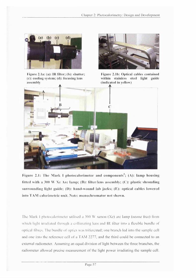
C h a p ter 2: P h o to c a lo r im e tr y : D e s ig n a n d D e v e lo p m e n t
[
Figure 2.1a: (a): IR filter; (b): shutter; (c): cooling system; (d): focusing lens assembly
Figure 2.1b: Optical cables contained within stainless steel light guide (indicated in yellow)
F igure 2.1: T he M ark I pho toca lo rim eter and co m p o n en ts '; (A): lam p housing
fitted w ith a 300 VV Xe A rc lam p; (B): filter/lens assem bly; (C): p lastic sh ro u d in g
su rro u n d in g light guide; (D): hand-w ound lab jacks; (E): op tical cables low ered
in to TA M calo rim etric unit. Note: m o n o ch ro m ato r not show n.
T he M ark I photocalorin ietcr utilised a 300 W xenon (X e) are lam p (ozone free) from
w hich light irradiated through a co llim ating lens and IR filter into a flexible bundle o f
optical fibres. T he bundle o f optics was trifurcated; one branch led into the sam ple cell
and one into the reference cell o f a TA M 2277, and the third eould be connected to an
external radiom eter. A ssum ing an equal d iv ision o f light betw een the th ree branches, the
rad iom ete r allow ed precise m easurem ent o f the light pow er irrad ia ting the sam ple cell.
P a g e 5 7
Chapter 2: Photocalorimetry: D esign and Developm ent
The calorimetric cells were standard stainless steel TAM ampoules (20 mL) and the
fibre-optic bundles were mounted through the ampoule lids. Individual fibre-optic
cables are relatively fragile and the amount o f light transmitted is dependent upon the
angle through which the bundle turns. The flexible bundles were long (1 m length) and
mounted in a stainless steel light guide (Fig. 2.1b) to which the calorimetric cells were
attached. This ensured the optic cables were fixed in position relative to each other and
kept in the same orientation to ensure a repeatable geometry to provide consistency in
performance. The metal light guide was encased in a detachable plastic shroud designed
to insulate the optic cables and minimise data fluctuations generated by heat conduction
since the calorimeter is sensitive to even minute heat flow changes. Two mechanical
hand-wound lab jacks mounted one on another were situated beneath the lamp housing
and components allowing the apparatus to be vertically raised and lowered for sample
loading and unloading, respectively. The light source components were placed onto a
heavy duty trolley (100 kg) designed to support the weight o f the light source equipment
and to match the vertical height o f the TAM. Figure 2.1 illustrates the photocalorimeter
and its design components. A monochromator stands as a separate accessory and could
easily be incorporated as part o f the assembly for selective wavelength studies.
Having reassembled the instrument, the first step was to investigate the baseline
response when the calorimetric cells were situated in the calorimeter. The baseline
stability o f the Mark I photocalorimeter was monitored in two ways; one to assess the
response o f the system without subjecting the calorimetric cells to light (light off), and
two, to assess the calorimetric response with the input o f light (light on). In any case, in
a differential system if the heat-flow on the sample and reference side is o f equivalence
then, ideally, there should be no net signal and hence result in a zero-power signal on
the TAM. It was hoped that the Mark I photocalorimeter would respond in such a
manner.
2.1.1 Investigating Baseline Stability of Mark I - Light off
Previously, one o f the fundamental problems experienced by M orris' with this system
was that o f achieving a stable and zero-baseline. It proved problematic to combine the
sensitivity o f the TAM with a large mass o f stainless steel light source equipment.
Page 58
Chapter 2: Photocalorimetry: D esign and Development
Initial tests performed showed baseline outputs to be non-zero and arbitrary. The values
reported were irreproducible, varying from -4 0 pW to -300 pW , and not zero as
anticipated. One attempt to reduce the irreproducibility revealed that shielding the optic
cables with foam based sheets (green shroud in Fig. 2.1) provided some level of
protection against external factors (such as the influence o f air-conditioning in the
laboratory) from interfering with the calorimetric output. This was shown to have a
marked response on the system reducing the baseline signal by -33% . However, this
shielding was still not sufficient enough for a zero baseline to be achieved suggesting
the system was still subject to heat loss.
To assess if this was still the case even after re-location o f the instrument and now in a
laboratory without air-conditioning, initial trials were made using the following
procedure to assess baseline stability with the light off.
2.1.1.1 Method
All experiments were performed at 298 K in a 2277 TAM (Thermometric Ltd), unless
otherwise stated. Electrical calibration checks (3000 pW ) were performed periodically
on the TAM. All data were recorded on the dedicated software package Digitam 4.1™
and analysed using Microcal Origin Pro 7.0™, unless otherwise stated.
Two empty 20 mL stainless steel calorimetric ampoules were used throughout, unless
otherwise stated. The ampoules were washed in ethanol and dried each time prior to use.
Each ampoule was clipped securely using a circlip onto the end o f a sample and
reference fibre optic cable. The ampoules were lowered into the TAM using the hand-
wound lab jacks and held in equilibrium for 30 minutes to allow the signal to settle from
a thermal shock before being lowered further into the measuring position. The
calorimetric response was then recorded and the baseline data were collected. Five
experiments were run in this manner and data were collected for approximately 2 hours.
The experimental set up remained unchanged for each experiment. Linear regression
fittings were performed on the data for the individual runs where the fit linear analysis
function on Microcal Origin Pro 7.0™ was used to determine the average power signal
after the signal reached plateau.
Page 59

C h a p ter 2: P h o to c a lo r im e tr y : D e s ig n a n d D e v e lo p m e n t
2.1.1.2 Results and D iscussion
Figure 2.2 is typical o f the base line response in the ealoriineter. T he data ob tained
though linear regression fitting is represented in T able 2.1. NB. All standard deviations
reported throughout w ere calculated using xon-i function w ith a 68% eonfldenee lim it
(ind icated as ± value alongside m ean value).
Linear Regression for Meth1 Data_Run1 :Y = A + B * X Parameter Value
100-1Error
77.208541.89578E-4
0.064191.3226E-5
3.Run 3
IQ_
Run 1
7 5 - Run 5
Run 27 0 -
6 5 -
Run 460 -
0 1000 2000 3000 4000 5000 6000 7000 8000
Time/ s
Figure 2.2: Comparison of baselines using the M ark I Photocalorimeter with the light off
Table 2.1: Calorimetric outputs derived through linear regression fitting
R un Pow er o u tp u t/ pVV1 77.22 72.63 83.04 61.35 76.2
M ean ± SD 74.1 ± 8 .1
Initial trials w ere not prom ising, a significant problem being that it proved im possib le to
get a repeatab le baseline signal w ith the light off. T he pow er ou tputs ob tained concur
w ith p rev ious observations,' in that a non-zero and irreproducib le baseline is exhibited .
P a g e 6 0

Chapter 2: Photocalorimetry: D esign and Developm ent
An initial thermal shock was observed for approx. the first 1500 seconds o f data
recording ranging from -70 pW to -9 8 pW. After the effects o f the thermal shock the
baseline settled to a plateau, as seen after ca. 1500 seconds, the offset equilibrium was
reached. The power signals were arbitrary and varied from -6 0 pW to -85 pW with an
average offset o f 74.1 ±8.1 pW derived though linear regression fitting. In a differential
system, ideally, a zero baseline signal would indicate equivalence in heat-flow o f the
sample and reference. Clearly, this was not the case and the irreproducible nature o f the
baselines suggested there was a significant loss o f heat from the calorimeter during
measurement. Furthermore, it was not possible even to zero the baseline signal by
manual adjustment using the voltage signals o f the amplifiers since the magnitude o f the
signal was far too large and outside the adjustable range o f the amplifiers. This
immediately indicated that there were problems with equivalence (of geometry) o f the
sample and reference sides and/or heat losses through conduction and convection. The
magnitude o f the irreproducibility o f the baseline signals would make it
difficult/impossible to determine accurate power signals for a sample undergoing a
photo-reaction. It was, therefore, essential to address this issue and it became necessary
to consider various design elements to ensure the repeatability o f the baseline signal.
(Section 2.1.3 details the various design considerations that were implemented in order
to achieve this). Moreover, further problems arose when the system was subjected to
light input (illustrated in Figure 2.3). This issue is discussed further in greater detail in
section 2.1.2 and section 2.1.3).
2.1.2 Investigating Baseline Stability of Mark I - Light on
The instrument’s response with the light on was tested. Several light on/off tests were
conducted to assess the repeatability o f the signal with the light on and off using the
following method.
2.1.2.1 Method
Two empty 20 mL stainless steel ampoules were lowered into the TAM and held in
equilibrium for 30 minutes before being lowered into the measuring position. The
Page 61
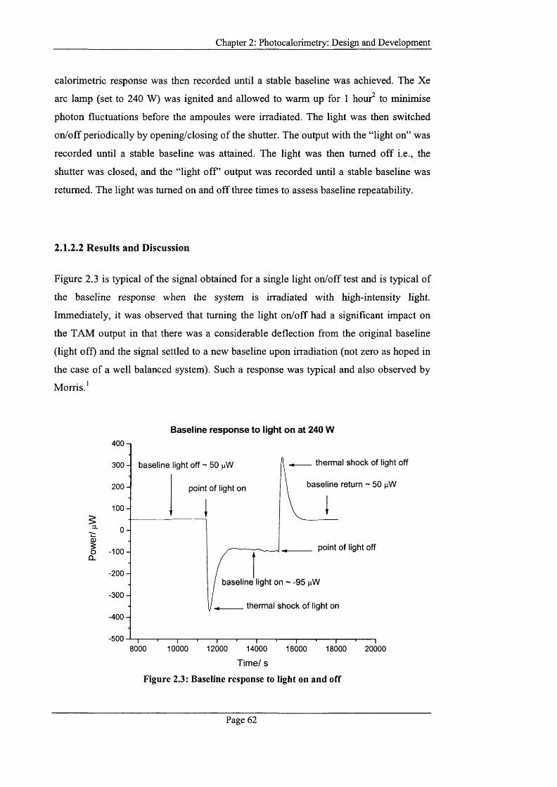
Chapter 2: Photocalorimetry: D esign and Developm ent
calorimetric response was then recorded until a stable baseline was achieved. The Xe
arc lamp (set to 240 W) was ignited and allowed to warm up for 1 houi^ to minimise
photon fluctuations before the ampoules were irradiated. The light was then switched
on/off periodically by opening/closing o f the shutter. The output with the “light on” was
recorded until a stable baseline was attained. The light was then turned o ff i.e., the
shutter was closed, and the “light o f f ’ output was recorded until a stable baseline was
returned. The light was turned on and off three times to assess baseline repeatability.
2.1.2.2 Results and Discussion
Figure 2.3 is typical of the signal obtained for a single light on/off test and is typical o f
the baseline response when the system is irradiated with high-intensity light.
Immediately, it was observed that turning the light on/off had a significant impact on
the TAM output in that there was a considerable deflection from the original baseline
(light off) and the signal settled to a new baseline upon irradiation (not zero as hoped in
the case o f a well balanced system). Such a response was typical and also observed by
Morris
Baseline response to light on at 240 W400-,
thermal shock of light off300 - baseline light off ~ 50
baseline return ~ 50 pW2 0 0 - point of light on
1 0 0 -
%
I0_point of light off
- 10 0 -
- 2 0 0 -
baseline light on - -95-300 —
thermal shock of light on-400-
-5008000 10000 12000 14000 2000016000 18000
Time/ s
Figure 2.3: Baseline response to light on and off
Page 62

Chapter 2: Photocalorimetry; D esign and Developm ent
As shown in Figure 2.3, the baseline initially settled to approx. 50 fiW. A thermal shock
was observed as the light was turned on and then the signal reached a minimum (lasting
approx. 30 minutes) before recovering and settling to a new baseline o f approx. -95 pW.
The light was then switched off and a positive thermal shock was observed before the
signal equilibrated to its original baseline value o f approx. 50 pW. The light was
switched on and off a two times further to assess the repeatability o f the signal (Figure
2.4).
600 Baseline response to 240 W light input
500
400
300
5 200 point of light on
%oCL
100
-100
-200point of light off
-300
-4003000 6000 9000 12000 15000 18000 21000 240000
Time/ s
Figure 2.4: Baseline response to repeat light on and off test
In each case the repeatability o f the signal when the light was switched on or off was
fairly consistent; an average baseline signal o f 54.02 ± 2.68 pW was derived when the
light was switched off, and with the light on the signal settled to a baseline o f ca. -90
pW giving an average deflection o f -91.09 ± 4.29 pW giving an overall deflection o f ca.
-145 pW. Such a difference is immediately indicative o f an imbalance in the light
delivery from the pair o f fibre optics. A deflection o f -145 pW suggested there is a
greater proportion o f light being delivered in the reference side. Ideally, if the amount o f
light output from each cable were equivalent then the net signal would be zero. Clearly,
Page 63
Chapter 2: Photocalorimetry: D esign and Developm ent
this was not the case and there was a significant difference in the input from each cable.
In combination, the magnitude o f the irreproducibility o f the baseline signals may
preclude using the instrument for samples producing small powers (note that the
standard specifications for a TAM, using micro-W att amplifiers, is a noise o f ±2 pW
and a baseline drift over 8 h o f ±2 pW for a 20 mL channel).^ It was therefore essential
to implement some design changes in order to try and minimise the baseline deflection
so that it is as close to a zero value as possible, and, moreover, to ensure that
reproducible outputs (within an acceptable range) are obtained each time the ampoules
are lowered into and raised from the TAM. Further design modifications were therefore
considered and implemented.
The immediate challenges, then, were to redesign the instrument in two phases:
-y To obtain a zero baseline with the light off
To obtain a zero baseline with the light on
2.1.3 Design Considerations and Modifications
One o f the main causes o f the irreproducible outputs was the way in which the system
was designed. Dealing with the inability to attain a zero baseline first, it was clear (from
the irreproducible data and through observation o f the way the ampoules fit into the
TAM) that the primary problem was the fixed geometry o f the sample and reference
ampoules relative to each other. The two ampoules could not be lowered into the TAM
properly and independently as the raising/lowering process o f the ampoule was very
much dependent on the mechanical hand-wound lab jacks. This meant that the sample
and reference ampoules were kept in a fixed position relative to the base o f the
calorimetric unit and hence any ill-alignment and/or imbalance between the two sides
would therefore also be fixed and difficult to control. The original reason for fixing the
geometry was to keep the fibre-optic bundles in a consistent position because o f their
fragility, but this became a limiting drawback on the instrument’s flexibility and ability
to align the ampoules correctly in the TAM. The irreproducible and non-zero outcomes
were a result o f an imbalance in the position o f the ampoules relative to the base o f the
calorimetric channel and it was the case that one ampoule was sat in a higher position
Page 64
Chapter 2: Photocalorimetry: D esign and Developm ent
than the other within the channel. As a result, there was a noticeable gap between the
top o f the column insert and calorimetric unit when situated in the measuring position.
The impact this had was that the instrument was subjected to a significant proportion o f
heat loss through air conduction and/or convection from the calorimetric chamber.
Unless aligned perfectly with the TAM, it would always be the case with this particular
design, that one ampoule would sit higher in its channel than the other and,
consequently, result in inconsistent data. It was therefore imperative to reconsider the
instrument design to provide better control o f the lowering and alignment o f the
ampoules into the TAM in order to counteract the imbalance o f the fit and reduce heat
escape.
In order to try and improve the baseline stability various design elements were revised
and re-designed. The first approach was to break the fixed geometry o f the sample and
reference ampoules allowing each ampoule to be inserted independently, as well as
simultaneously, into the TAM so that to ensure the fit was adequately air tight.
Modifications were also made to the various supporting lids surrounding the metal
colunrn which contained the fibre-optic cable. The original column used in the Mark I is
depicted in Figure 2.5.'
The fibre-optic cable is situated inside the metal column and it is surrounded with
plastic support lids at upper and lower ends o f the column. Plastic fittings (spacers)
were also placed at defined intervals down the length o f the vertical section o f the
colunrn to minimise the effect of air conduction within the calorimetric chamber, the
construction o f which were based on the design o f commercially available perfusion
shafts manufactured by Thermometric AB, Jarfalla, Sweden.'' The supporting lids at the
lower end o f the column were fixed in place and allowed for a 20 mL ampoule to be
freely suspended. It was because o f the fixed position o f the supporting lids that it was
not possible to adjust the position o f the ampoule relative to the base o f the calorimetric
chamber. This lead to an inequivalence in alignment between the sample and reference
sides which resulted in the irreproducible nature o f the baselines (as previously shown
in Figure 2.2). Necessarily, modifications were made and a new column with better
supporting lids was constructed, as shown in Figure 2.6.
All engineering work was undertaken at The School o f Pharmacy, University o f
London.
Page 65

C h a p ter 2; P h o to c a lo r im e tr y : D e s ig n a n d D e v e lo p m e n t
Figures 2.5 to 2.6b show a com parison o f the original and re-designed column. A
schem atic diagram o f the m odified colum n is also illustrated in Figure 2.7.
Fibre optic cable contained within carbon fibre rod
Supporting lidAmpoule lid
Fibre optic tip
Figure 2.5: Original column' Figure 2.6: Re-designed column
Fig 2.6a: Supporting lid at top of column Fig 2.6b: Supporting lids at end of column
P a n e 6 6
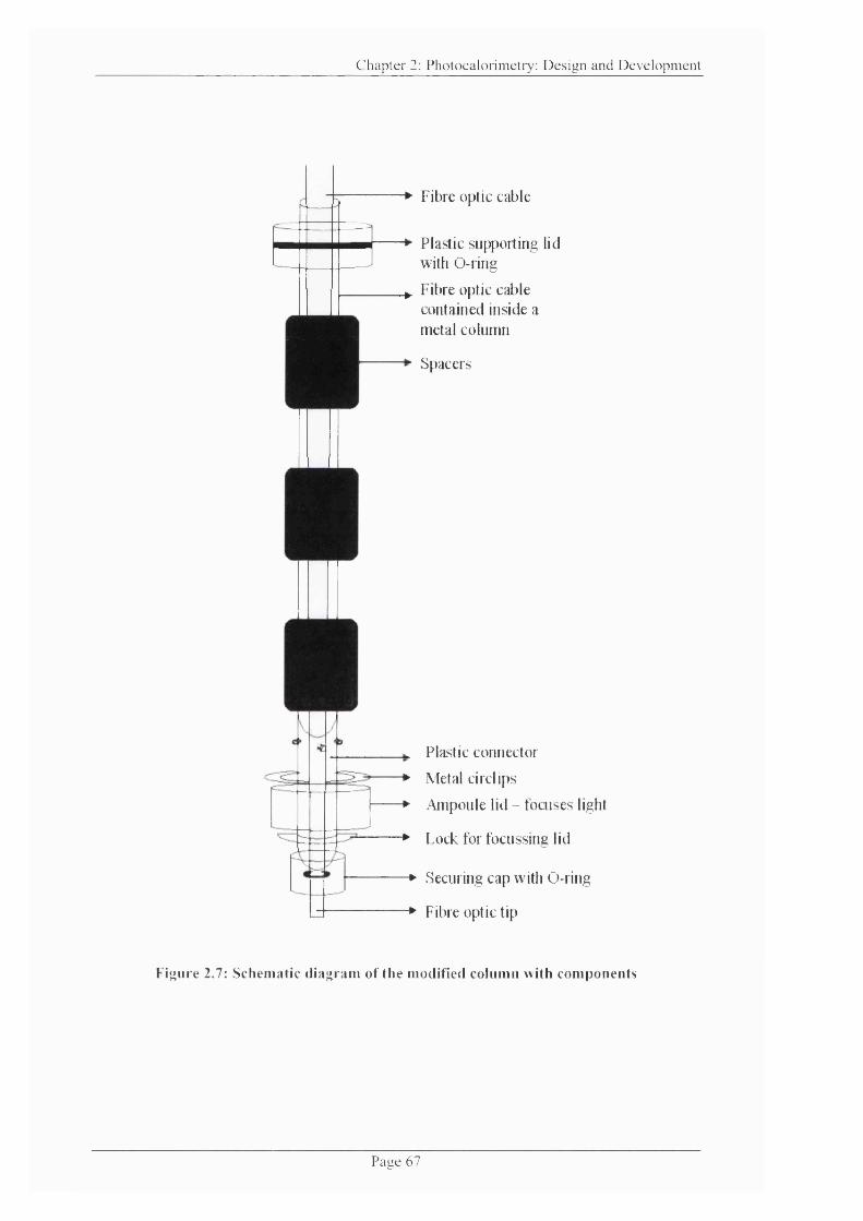
C h a p te r 2: P h o to c a lo r im e tr y ; D e s ig n a n d D e v e lo p m e n t
-► Fibre optic cable
Plastic supporting lid with O-ring
^ Fibre optic cable contained inside a rnetal column
Spacers
Plastic connector
■> Metal circlips
-► .Ampoule lid - focuses light
-► Lock for focussing lid
-► Securing cap with O-ring
-► Fibre optic tip
Figure 2.7; Schematic diagram of the modified column with components
P a g e 6 7
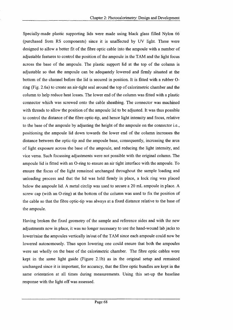
Chapter 2: Photocalorimetry: D esign and Developm ent
Specially-made plastic supporting lids were made using black glass filled Nylon 6 6
(purchased from RS components) since it is unaffected by UV light. These were
designed to allow a better fit o f the fibre optic cable into the ampoule with a number o f
adjustable features to control the position o f the ampoule in the TAM and the light focus
across the base o f the ampoule. The plastic support lid at the top of the column is
adjustable so that the ampoule can be adequately lowered and firmly situated at the
bottom of the channel before the lid is secured in position. It is fitted with a rubber O-
ring (Fig. 2.6a) to create an air-tight seal around the top o f calorimetric chamber and the
column to help reduce heat losses. The lower end o f the column was fitted with a plastic
connector which was screwed onto the cable sheathing. The connector was machined
with threads to allow the position o f the ampoule lid to be adjusted. It was thus possible
to control the distance o f the fibre optic-tip, and hence light intensity and focus, relative
to the base o f the ampoule by adjusting the height o f the ampoule on the connector i.e.,
positioning the ampoule lid down towards the lower end o f the column increases the
distance between the optic-tip and the ampoule base, consequently, increasing the area
o f light exposure across the base o f the ampoule, and reducing the light intensity, and
vice versa. Such focussing adjustments were not possible with the original column. The
ampoule lid is fitted with an O-ring to ensure an air tight interface with the ampoule. To
ensure the focus o f the light remained unchanged throughout the sample loading and
unloading process and that the lid was held firmly in place, a lock ring was placed
below the ampoule lid. A metal circlip was used to secure a 20 mL ampoule in place. A
screw cap (with an O-ring) at the bottom o f the column was used to fix the position of
the cable so that the fibre optic-tip was always at a fixed distance relative to the base of
the ampoule.
Having broken the fixed geometry o f the sample and reference sides and with the new
adjustments now in place, it was no longer necessary to use the hand-wound lab jacks to
lower/raise the ampoules vertically in/out o f the TAM since each ampoule could now be
lowered autonomously. Thus upon lowering one could ensure that both the ampoules
were sat wholly on the base o f the calorimetric chamber. The fibre optic cables were
kept in the same light guide (Figure 2.1b) as in the original setup and remained
unchanged since it is important, for accuracy, that the fibre optic bundles are kept in the
same orientation at all times during measurements. Using this set-up the baseline
response with the light off was assessed.
Page 68
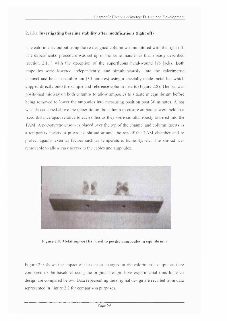
C h a p ter 2: P h o to c a lo r im e tr y : D e s ig n a n d D e v e lo p m e n t
2.1.3.1 Investigating baseline stability after modifications (light off)
The calorimetric output using the re-designed co lum n was rnonitored with the light off.
The experimental procedure was set up in the sam e m anner as that already described
(section 2.1.1) with the exception o f the superfluous hand-w ound lab jacks. Both
am poules were lowered independently, and sim ultaneously, into the calorimetric
channel and held in equilibrium (30 m inutes) using a specially m ade metal bar which
clipped directly onto the sam ple and reference co lum n inserts (Figure 2.8). The bar was
positioned m idw ay on both colum ns to allow am poules to situate in equilibrium before
being rem oved to lower the ampoules into m easuring position post 30 minutes. A bar
was also attached above the upper lid on the colum n to ensure am poules w ere held at a
fixed distance apart relative to each other as they were s im ultaneously lowered into the
TA M . A polystyrene case was placed over the top o f the channel and colum n inserts as
a tem porary m eans to provide a shroud around the top o f the TA M cham ber and to
protect against external factors such as tem perature, humidity, etc. T he shroud was
rem ovable to allow easy access to the cables and ampoules.
Figure 2.8: Metal support bar used to position ampoules in e(|uilibrium
Figure 2.9 shows the impact o f the design changes on the calorimetric output and are
com pared to the baselines using the original design. Five experimental runs for each
design are com pared below. Data representing the original design are recalled from data
represented in Figure 2.2 for comparison purposes.
P a s e 6 9
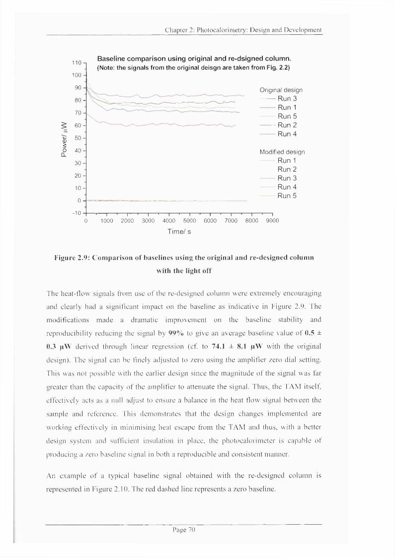
C h a p ter 2: P h o to c a lo r in ie tr y ; D e s ig n and D e v e lo p m e n t
^ B a s e l i n e comparison using original and re-dsigned column. (Note: the signals from the original deisgn are taken from Fig. 2.2)
100 -
I
9 0 -
80-
7 0 -
60 -
50 -
40 -
3 0 -
20 -
1 0 -
0 -
-10
Original design Run 3
Run 1 Run 5
— Run 2 Run 4
Modified design Run 1 Run 2 Run 3 Run 4 Run 5
-I— I— '— I— '— I— '— I— '— I— '— I— '— I— '— I— '— I0 1000 2000 3000 4000 5000 6000 7000 8000 9000
Time/ s
Figure 2.9: Comparison of baselines using the original and re-designed column
with the light off
The heat-flow signals from use o f the re-designed eolum n were extrem ely encouraging
and clearly had a significant impact on the baseline as indicative in Figure 2.9. The
modifications m ade a dramatic im provem ent on the baseline stability and
reproducibility reducing the signal by 99% to give an average baseline value o f 0.5 ±
0.3 pW derived through linear regression (cf. to 74.1 ± 8.1 pW with the original
design). T he signal can be finely adjusted to zero using the am plifier zero dial setting.
This was not possible with the earlier design since the m agnitude o f the signal was far
greater than the capacity o f the amplifier to attenuate the signal. Thus, the TA M itself,
effectively acts as a null adjust to ensure a balance in the heat flow signal between the
sample and reference. This demonstrates that the design changes im plem ented are
w orking effectively in m inim ising heat escape from the T A M and thus, with a better
design system and sufficient insulation in place, the photocalorim eter is capable o f
producing a zero baseline signal in both a reproducible and consistent manner.
An exam ple o f a typical baseline signal obtained with the re-designed colum n is
represented in Figure 2.10. The red dashed line represents a zero baseline.
P a g e 7 0

C h a p ter 2: P h o to c a lo r im e tr y ; D e s ig n a n d D e v e lo p m e n t
<DIQ_
0 . 0 - -
- 0.2 -
1-----'-----1---------'-1---------'-1---------'-1--------- '-1--------- '-1-----r1000 2000 3000 4000 5000 6000 7000 8000
Time/ s
Figure 2.10: Example of a typical baseline signal using the modified column
T he baseline was recorded over a period o f 2 hours. The obserxed drift during the first
2000 seconds was a m axim um o f +0.736 p W and a m in im um o f -0.057 pW . After this
period, the baseline settled to a plateau and an absolute m ax im um o f +0.736 p W and
m in im um o f -0.736 pw arising from the short-tem i spikes. An average baseline signal
o f +0.314 p W is derived in this case and is much lower than the range. Even i f the
absolute values were taken in the worst case, then it can be seen that the stability and
noise over the defined observation period is within ±1 p W declared well within the
m anufacturers quoted specifications o f ±2 p W for a 20 m L capacity.^
The design changes im plemented have m ade an im m ense im provem ent on the
calorimetric output m aking it possible to attain a zero baseline with the light off. Having
established a zero baseline with the light off, the next stage was to turn attention to the
instrum en t 's inability o f achieving a zero baseline with the light on.
P a a e 71
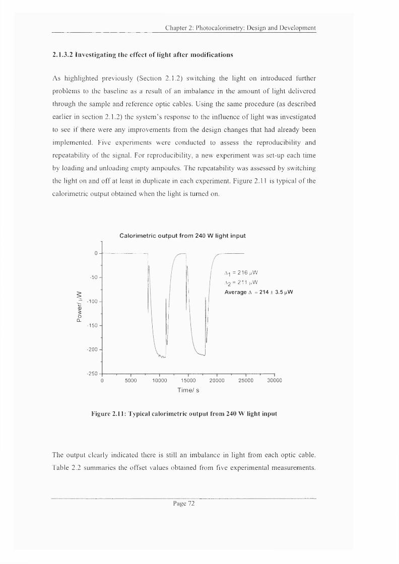
C hapter 2: P hotocalor im etry: D e s ig n and D ev e lo p m en t
2.1.3.2 Investigating the effect of light after modifications
As highlighted previously (Section 2.1.2) switching the light on introduced further
problems to the baseline as a result o f an imbalance in the amount o f light delivered
through the sample and reference optic cables. Using the same procedure (as described
earlier in section 2.1.2) the system’s response to the influence o f light was investigated
to see if there were any improvements from the design changes that had already been
implemented. Five experiments were conducted to assess the reproducibility and
repeatability o f the signal. For reproducibility, a new experiment was set-up each time
by loading and unloading empty ampoules. The repeatability was assessed by switching
the light on and off at least in duplicate in each experiment. Figure 2.11 is typical o f the
calorimetric output obtained when the light is turned on.
Calorimetric output from 240 W light input
= 2 1 6 pW
A2 = 2 1 1 pWAverage A = 214 ± 3.5 jiW
-50 -
^ - 1 0 0 -
$oQ_
-150 -
- 2 0 0 -
-2505000 10000 15000 20000 25000 300000
Time/ s
Figure 2.11: Typical calorimetric output from 240 W light input
The output clearly indicated there is still an imbalance in light from each optic cable.
Table 2.2 summaries the offset values obtained from five experimental measurements.
P age 72

Chapter 2: Photocalorimetry: D esign and Developm ent
The values were ~ 211 pW to ~ 227 pW with an average baseline deflection o f 217 ±
5.8 pW as observed across a series o f light on/off tests. In all cases, the experiment
began with a stable zero signal (ca. -0.24 ± 0.35 pW ) for the pair o f empty ampoules. At
the point o f light input, the system experiences a thermal shock between ~ 100 pW to ~
125 pW, due to intense heat generated by the lamp source, before settling at a baseline
o f about ~ -220 pW. When the light is switched o ff a similar thermal shock is observed
before the signal reached its original baseline.
Table 2.2: Comparison of 5 calorimetric outputs with 240 W light input
Experim ent Pow er output/ pW Ai A%
1 2 1 2 2132 216 2 1 1
3 219 2184 216 2 1 1
5 226 227M ean ± SD 217 ± 5 .8
The offsets were larger in this case than compared with those observed prior to making
the design changes on the column (cf. ~ -145 pW), possibly because any changes in the
geometry o f the instrument can alter the light transmission. The repeatability and
reproducibility o f the signal is fairly consistent, however, the magnitude o f the
deflection is far too large making it difficult or impossible to determine the instrument’s
performance particularly if the sample generated small powers. Thus it was essential to
implement further design changes principally to attenuate the light input by some means
so to balance the light input through the sample and reference cable. Before doing so, a
further experiment was conducted using the third cable (of the trifurcated cable serving
as a reference to an external actinometer) in order to ascertain if the third cable could
provide a better match o f the light throughput when used in conjunction with either the
sample or reference optic cable. The third cable was substituted for each o f the two
cables in turn to find the best matched pair. Conventionally, the sample cable is situated
in the left hand side (LHS) o f the TAM chamber and the right hand side (RHS) is
occupied by the reference cable. The third cable was alternated so that it occupied both
the LHS and RHS with its corresponding sample or reference cable. Figure 2.12 shows
Page 73
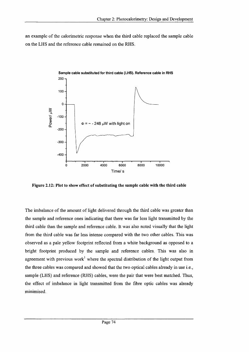
Chapter 2: Photocalorimetry: D esign and Developm ent
an example o f the calorimetric response when the third cable replaced the sample cable
on the LHS and the reference cable remained on the RHS.
Sample cable substituted for third cable (LHS). Reference cable in RHS200-,
1 0 0 -
I- 1 0 0 -I
CL(t> = - - 248 pW with light on
- 2 0 0 -
-400-
100000 2000 4000 6000 8000
Time/ s
Figure 2.12: Plot to show effect of substituting the sample cable with the third cable
The imbalance o f the amount o f light delivered through the third cable was greater than
the sample and reference ones indicating that there was far less light transmitted by the
third cable than the sample and reference cable. It was also noted visually that the light
from the third cable was far less intense compared with the two other cables. This was
observed as a pale yellow footprint reflected from a white background as opposed to a
bright footprint produced by the sample and reference cables. This was also in
agreement with previous work' where the spectral distribution o f the light output from
the three cables was compared and showed that the two optical cables already in use i.e.,
sample (LHS) and reference (RHS) cables, were the pair that were best matched. Thus,
the effect o f imbalance in light transmitted from the fibre optic cables was already
minimised.
Page 74
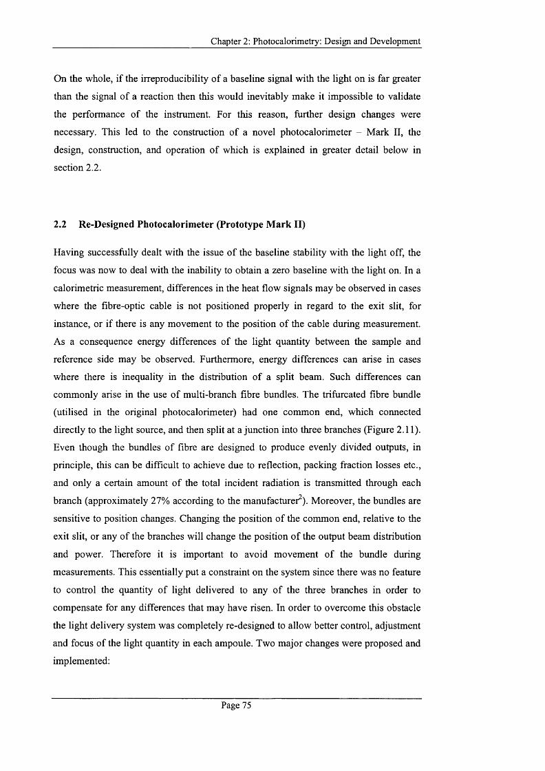
Chapter 2: Photocalorimetry: D esign and Developm ent
On the whole, if the irreproducibility o f a baseline signal with the light on is far greater
than the signal o f a reaction then this would inevitably make it impossible to validate
the performance o f the instrument. For this reason, further design changes were
necessary. This led to the construction o f a novel photocalorimeter - Mark II, the
design, construction, and operation o f which is explained in greater detail below in
section 2 .2 .
2.2 Re-Designed Photocalorimeter (Prototype Mark II)
Having successfully dealt with the issue o f the baseline stability with the light off, the
focus was now to deal with the inability to obtain a zero baseline with the light on. In a
calorimetric measurement, differences in the heat flow signals may be observed in cases
where the fibre-optic cable is not positioned properly in regard to the exit slit, for
instance, or if there is any movement to the position o f the cable during measurement.
As a consequence energy differences of the light quantity between the sample and
reference side may be observed. Furthermore, energy differences can arise in cases
where there is inequality in the distribution o f a split beam. Such differences can
commonly arise in the use o f multi-branch fibre bundles. The trifurcated fibre bundle
(utilised in the original photocalorimeter) had one common end, which connected
directly to the light source, and then split at a junction into three branches (Figure 2.11).
Even though the bundles o f fibre are designed to produce evenly divided outputs, in
principle, this can be difficult to achieve due to reflection, packing fraction losses etc.,
and only a certain amount o f the total incident radiation is transmitted through each
branch (approximately 27% according to the manufacturer^). Moreover, the bundles are
sensitive to position changes. Changing the position o f the common end, relative to the
exit slit, or any o f the branches will change the position o f the output beam distribution
and power. Therefore it is important to avoid movement o f the bundle during
measurements. This essentially put a constraint on the system since there was no feature
to control the quantity o f light delivered to any o f the three branches in order to
compensate for any differences that may have risen. In order to overcome this obstacle
the light delivery system was completely re-designed to allow better control, adjustment
and focus o f the light quantity in each ampoule. Two major changes were proposed and
implemented:
Page 75
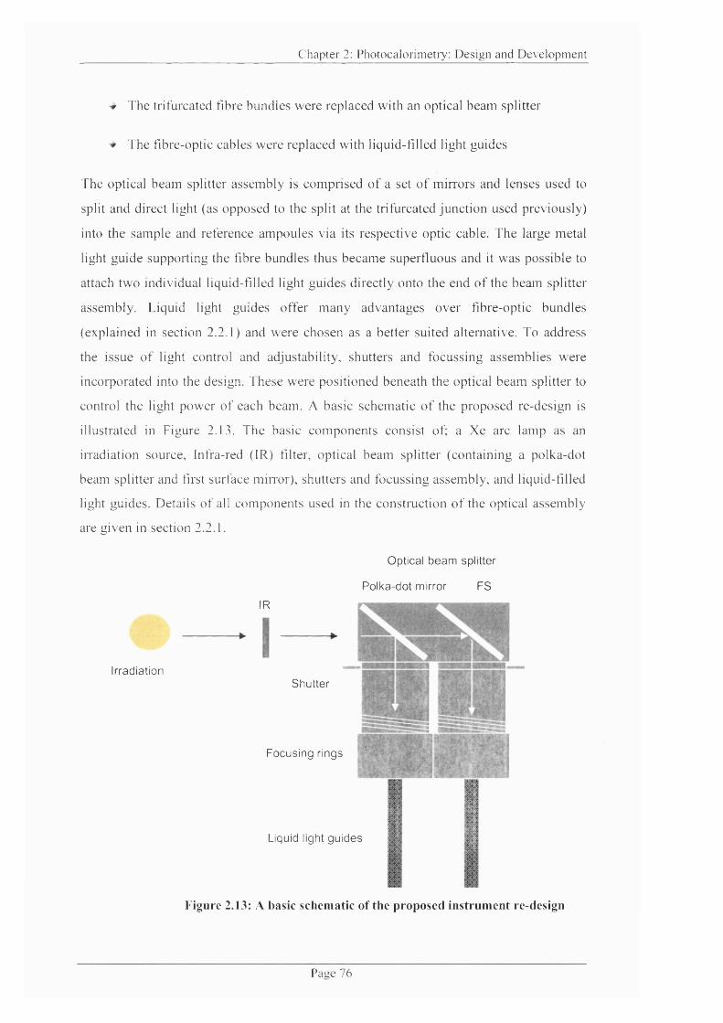
C h a p te r 2; P h o to c a lo r im e tr y : D e s ig n a n d D e v e lo p m e n t
^ The trifurcated rib re bundles were replaced with an optical beam splitter
f The ribre-optic cables w ere replaced with liquid-rilled light guides
The optical beam splitter assem bly is com prised o f a set o f m irrors and lenses used to
split and direct light (as opposed to the split at the trifurcated junction used previously)
into the sam ple and reference am poules via its respective optic cable. T he large metal
light gu ide supporting the fibre bundles thus becam e superfluous and it was possible to
attach two individual liquid-rilled light guides directly onto the end o f the beam splitter
assembly. Liquid light guides offer m any advantages over ribre-optic bundles
(explained in section 2.2.1) and were chosen as a better suited alternative. To address
the issue o f light control and adjustability, shutters and focussing assemblies were
incorporated into the design. T hese w ere positioned beneath the optical beam splitter to
control the light power o f each beam. A basic schem atic o f the proposed re-design is
illustrated in Figure 2.13. The basic com ponents consist of; a Xe arc lamp as an
irradiation source, Infra-red (IR) rilter, optical beam splitter (containing a polka-dot
beam splitter and first surface mirror), shutters and focussing assembly, and liquid-rilled
light guides. Details o f all com ponents used in the construction o f the optical assembly
are given in section 2.2.1.
Optical beam splitter
Polka-dot mirror PS
IR
IrradiationShutter
Focusing rings
Liquid light guides
Figure 2.13: A basic schematic of the proposed instrument re-design
P a g e 7 6
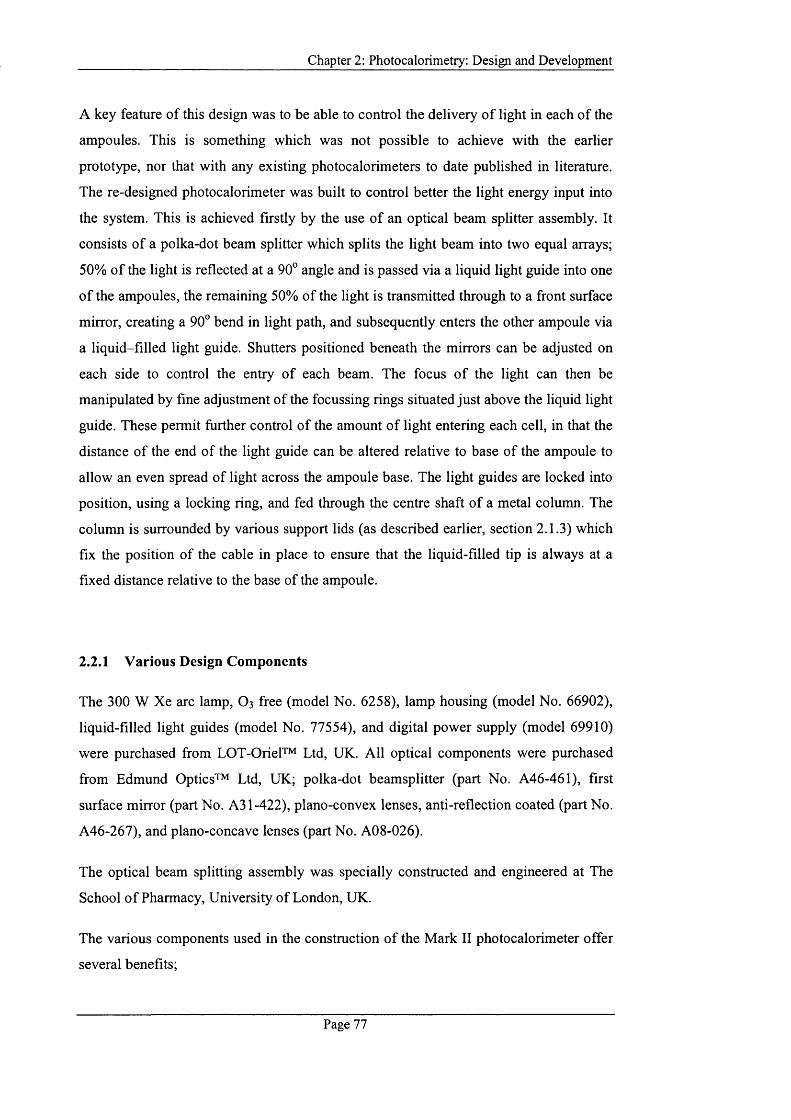
Chapter 2: Photocalorimetry: D esign and Developm ent
A key feature o f this design was to be able to control the delivery o f light in each o f the
ampoules. This is something which was not possible to achieve with the earlier
prototype, nor that with any existing photocalorimeters to date published in literature.
The re-designed photocalorimeter was built to control better the light energy input into
the system. This is achieved firstly by the use o f an optical beam splitter assembly. It
consists o f a polka-dot beam splitter which splits the light beam into two equal arrays;
50% o f the light is reflected at a 90° angle and is passed via a liquid light guide into one
o f the ampoules, the remaining 50% of the light is transmitted through to a front surface
mirror, creating a 90° bend in light path, and subsequently enters the other ampoule via
a liquid-filled light guide. Shutters positioned beneath the mirrors can be adjusted on
each side to control the entry o f each beam. The focus o f the light can then be
manipulated by fine adjustment o f the focussing rings situated just above the liquid light
guide. These permit further control o f the amount o f light entering each cell, in that the
distance o f the end o f the light guide can be altered relative to base o f the ampoule to
allow an even spread of light across the ampoule base. The light guides are locked into
position, using a locking ring, and fed through the centre shaft o f a metal column. The
column is surrounded by various support lids (as described earlier, section 2.1.3) which
fix the position o f the cable in place to ensure that the liquid-filled tip is always at a
fixed distance relative to the base of the ampoule.
2.2.1 Various Design Components
The 300 W Xe arc lamp, O3 free (model No. 6258), lamp housing (model No. 66902),
liquid-filled light guides (model No. 77554), and digital power supply (model 69910)
were purchased from LOT-Oriel™ Ltd, UK. All optical components were purchased
from Edmund Optics™ Ltd, UK; polka-dot beamsplitter (part No. A46-461), first
surface mirror (part No. A31-422), plano-convex lenses, anti-reflection coated (part No.
A46-267), and plano-concave lenses (part No. A08-026).
The optical beam splitting assembly was specially constructed and engineered at The
School o f Pharmacy, University o f London, UK.
The various components used in the construction o f the Mark 11 photocalorimeter offer
several benefits;
Page 77
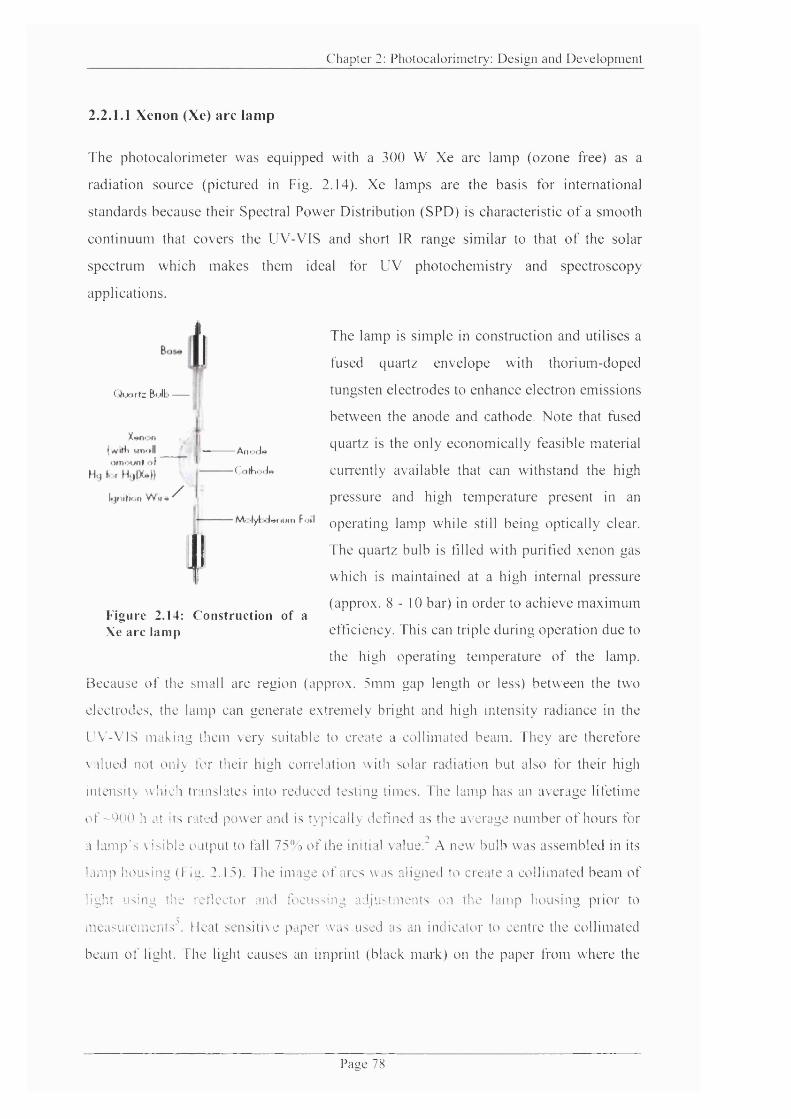
C h a p ter 2: P h o to c a lo r im e tr y : D e s ig n a n d D e v e lo p m e n t
2.2.1.1 X enon (Xe) a rc lam p
T he photocalorim eter was equipped with a 300 W X e are lam p (ozone free) as a
radiation source (pictured in Fig. 2.14). Xe lam ps are the basis for international
standards because their Spectral Power Distribution (SPD) is eharaeteristic o f a smooth
continuum that covers the UV-V IS and short IR range similar to that o f the solar
spectrum which m akes them ideal for UV photochem istry and spectroscopy
applications.
f t
Quürfz Bull*------
Xn< n(wifti sm all__omounf of
Hq tor Hq|)U))
Iqnition Wir*#
-A n o d e
-C o thode
/
IFigure 2.14: Construction of a Xe arc lamp
The lamp is s im ple in construction and utilises a
fused quartz envelope with thorium -doped
tungsten electrodes to enhance electron emissions
betw een the anode and cathode. N ote that fused
quartz is the on ly econom ically feasible material
currently available that can w ithstand the high
pressure and high tem perature present in an
/w>lyfc-knum Foil operating lamp while still being optically clear.
T he quartz bulb is filled with purified xenon gas
which is m aintained at a high internal pressure
(approx. 8 - 1 0 bar) in order to achieve m axim um
eftlciency. This can triple during operation due to
the high operating tem perature o f the lamp.
Because o f the small arc region (approx. 5m m gap length or less) betw een the two
electrodes, the lamp can generate extrem ely bright and high intensity radiance in the
U V -V lS m aking them very suitable to create a collimated beam. They are therefore
valued not only for their high correlation with solar radiation but also for their high
intensity which translates into reduced testing times. The lamp has an average lifetime
o f - 9 0 0 h at its rated pow er and is typically defined as the average num ber o f hours for
a lam p 's \ is ib le cuitput to fall 75% o f the initial value." A new bulb was assembled in its
lamp housing (Fig. 2 . 1 5). The im age o f arcs was aligned to create a collimated beam o f
light using the reflector and focussing adjustm ents on the lamp housing prior to
measLiremeiits'h Heat sensitive paper was used as an indicator to centre the collimated
beam o f light. The light causes an imprint (black mark) on the paper from where the
P a c e 78

C hapter 2: P hotocalor im etry: D e s ig n and D e v e lo p m en t
heat is produced. This type o f paper can commonly be found in superstores (receipt
paper) utilised in modem cash registers.
Note: Some lower power xenon lamps can be operated in a horizontal position. For the
purpose o f this particular construction, a vertical lamp was best suited.
8 4 KiKi&vCi
«f *lCf
MOP? PlCC
Figure 2.15: Exploded view of a typical lamp housing with an arc lamp
P age 79
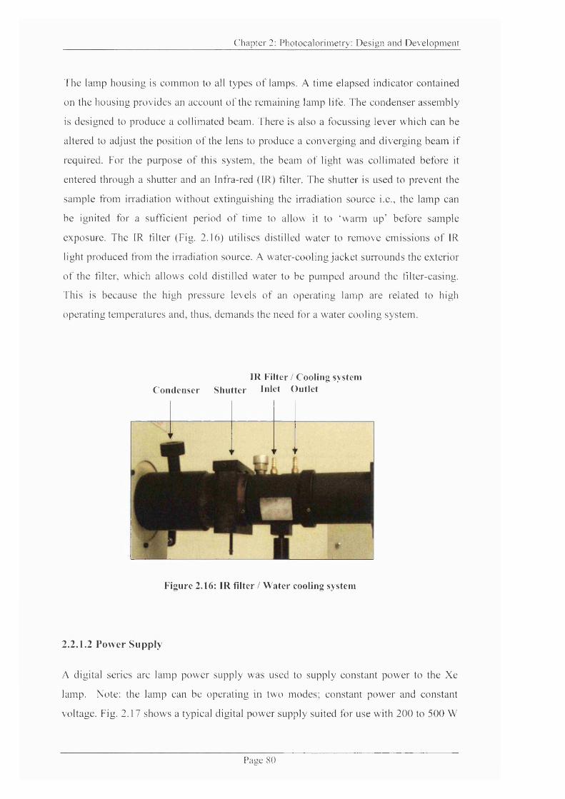
C h a p ter 2: P h o to c a lo r im e tr y : D e s ig n a n d D e v e lo p m e n t
T he lamp housing is com m on to all types o f lamps. A time elapsed indicator contained
on the housing provides an account o f the remaining lamp life. The condenser assem bly
is designed to produce a collimated beam. There is also a focussing lever which can be
altered to adjust the position o f the lens to produce a converging and diverging beam if
required. For the purpose o f this system, the beam o f light was collimated before it
entered through a shutter and an Infra-red (IR) filter. The shutter is used to prevent the
sam ple from irradiation without extinguishing the irradiation source i.e., the lamp can
be ignited for a sufficient period o f time to allow it to 'w arn i up ' before sample
exposure. The IR filter (Fig. 2.16) utilises distilled w ater to rem ove em issions o f IR
light produced from the irradiation source. A water-cooling Jacket surrounds the exterior
o f the filter, which allows cold distilled water to be pum ped around the filter-casing.
This is because the high pressure levels o f an operating lamp are related to high
operating tem peratures and, thus, dem ands the need for a w ater cooling system.
IR Filter / Cooling system Condenser Shutter Inlet Outlet
Figure 2.16: IR filter / Water cooling system
2 .2 . 1 . 2 Pow er Supply
A digital series arc lamp pow er supply was used to supply constant pow er to the Xe
lamp. Note: the lamp can be operating in two modes; constant pow er and constant
voltage. Fig. 2.17 shows a typical digital pow er supply suited for use with 200 to 500 W
P a g e 8 0

C h a p ter 2: P h o to c a lo r im e tr y ; D e s ig n a n d D e v e lo p m e n t
Xe arc lamps. The pow er output rating varies from 160 to 600 W. For a 300 W lamp,
the pow er supply allows the lamp to be operated at ± 20% o f its rating i.e. 240 W to 360
W.~ Typically, an operating pow er o f 240 W was set and the desired value was pre
selected before the lamp was ignited.
« ïi. » -■# — •
0 B0 0 ” ®
a SN e w p o r t
Figure 2.17: Digital Power Supply used to provide constant power to the lamp
2.2.1.3 L iquid-filled light guides
The bundles o f fibre optic cables w ere replaced with two single branched liquid-tilled
light guides in order to m axim ise light transmission (Fig. 2.18). T he liquid light guides
(3 m m core diameter, 1 m length) have excellent overall UV transm ission covering a
range o f 300 to 650 nm in the UV-VIS region. The liquid-filled light guides consist o f a
pressurised tube com prising o f Teflon cladding and are flexible in nature. The inner
core is filled with a transparent non-toxic liquid (patented), either an alcohol base or
aqueous salt solutions containing chlorides, fluorides or phosphates, are typically used
because o f their high light transm ittance properties. Both ends are sealed with short
silica fused windows.
Pa lie 81
C h a p ter 2: P h o to c a lo r im e tr y : D e s ig n a n d D e v e lo p m e n t
T he liquid light guides are ideal for UV-V IS
applications attributed primarily to two factors;
they have a large acceptance cone i.e., a large
diam eter allows for higher light throughput, but
m ore significantly, there are no packing fraction
losses. Unlike glass fibre optic bundles, they are
actually com posed o f liquid and therefore do not
suffer from packaging fraction losses-spacesFigure 2.18: Liquid light guides , ,
betw een fibres that can cause reduced coupling
efficiency, illustrated in Fig. 2.19. Their overall transm ission is therefore h igher than
that o f glass fibre bundles. Furthennore , repeated handling o f liquid light gu ides does
not result in the breakage typical o f glass bundles, which can effectively reduce
efficiency over time.
Overall, liquid light guides can offer m any advantages over bundles o f fibre optic:
f Higher transm ission in the UV, dow n to 300 nm
-r Higher transm ittance in the NIR
'T H igher overall transm ission than glass bundles
f No packing fraction loss or breakages
^ M ore uniform light throughput
^ Larger acceptance angles
f S igniticantly less expensive com pared to fibre bundles
P a g e 8 2
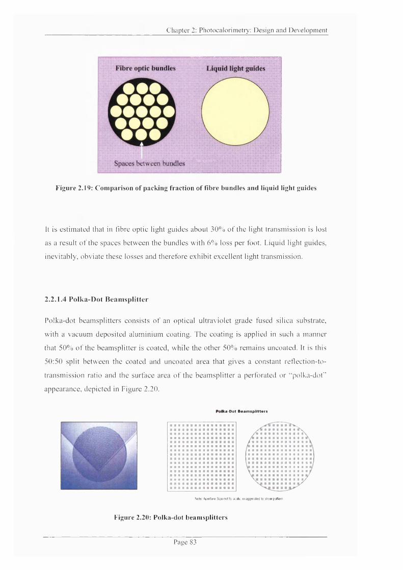
C h a p ter 2: P h o to c a lo r im e tr y ; D e s ig n a n d D e v e lo p m e n t
between bun î:q;i;:[g%Ÿ;!rT:gE;
Figure 2.19: Comparison of packing fraction o f fibre bundles and liquid light guides
It is estimated that in fibre optic light guides about 30% o f the light transm ission is lost
as a result o f the spaces betw een the bundles with 6% loss per foot. Liquid light guides,
inevitably, obviate these losses and therefore exhibit excellent light transmission.
2.2.1.4 P olka-D ot B eam splitter
Polka-dot beamsplitters consists o f an optical ultraviolet grade fused silica substrate,
with a vacuum deposited alum inium coating. T he coating is applied in such a m anner
that 50% o f the beam splitter is coated, while the other 50% remains uncoated. It is this
50:50 split between the coated and uncoated area that gives a constant retlection-to-
transm ission ratio and the surface area o f the beam splitter a perforated or "polka-dot"
appearance, depicted in Figure 2.20.
Note A pertiie Size not to scale exaggerated to show pattern
Figure 2.20: Polka-dot beamsplitters
P a g e 83

C h a p ter 2: P h o to c a lo r im e tr y : D e s ig n and D e v e lo p m e n t
W hen light is projected at the beamsplitter, the beam is split as the light rays that
encounter the uncoated surface are transmitted through with very little energy loss
whilst the rays that impact on the a lum inium coating are reflected. This effectively splits
evenly the input beam: 50% o f the incident light is reflected by the coated area and 50%
is transmitted through the glass (uneoated area).
A polka dot beamspliter (38mm^ diameter, 1.5 m m thickness) was placed at a 45" angle
into a specially constructed unit (described later) so that the beam reflected at a 90"
angle directly into the liquid light guide. Since this versatile beam splitter is not angle
sensitive, it is ideal for splitting energy from a radiant light source with no significant
d ivergence from diffraction.
2.2.1.5 F irs t Surface M irro rs
First surface mirrors (Fig. 2.21), also referred to
front surface m in o rs , are coated with enhanced
alum inium that provides > 90% image reflection in
the visible region. A reflection o f 95% can be
achieved depending on the wavelength o f light
used. A rectangular shaped m irror (38mm^
diameter, 3.2 m m thickness) was the ideal choice
and positioned behind the polka-dot beamsplitter since they are extrem ely useful in
applications where the m irror is m ounted at 45° to produce a 90° bend in light path.
rrI t f
Figure 2.21: First surface mirrors
2.2.1.6 Plano-convex lens
Tw o plano-convex lenses (PCX) w ere used to fonn part o f the focussing assembly
attached on to the lower end o f the beam splitter. Each lens was placed directly between
its respective shutter and liquid light guide; one on the sam ple side and the other on the
reference side. The lenses (25.4 mm diameter, 5.84 m m centre thickness) are UV Grade
m anufactured using synthetic fused silica and provide excellent transmission
characteristics. A broadband anti-reflection coated PCX lens was chosen for optimised
throughput in the ultraviolet spectrum.
P a u e 8 4
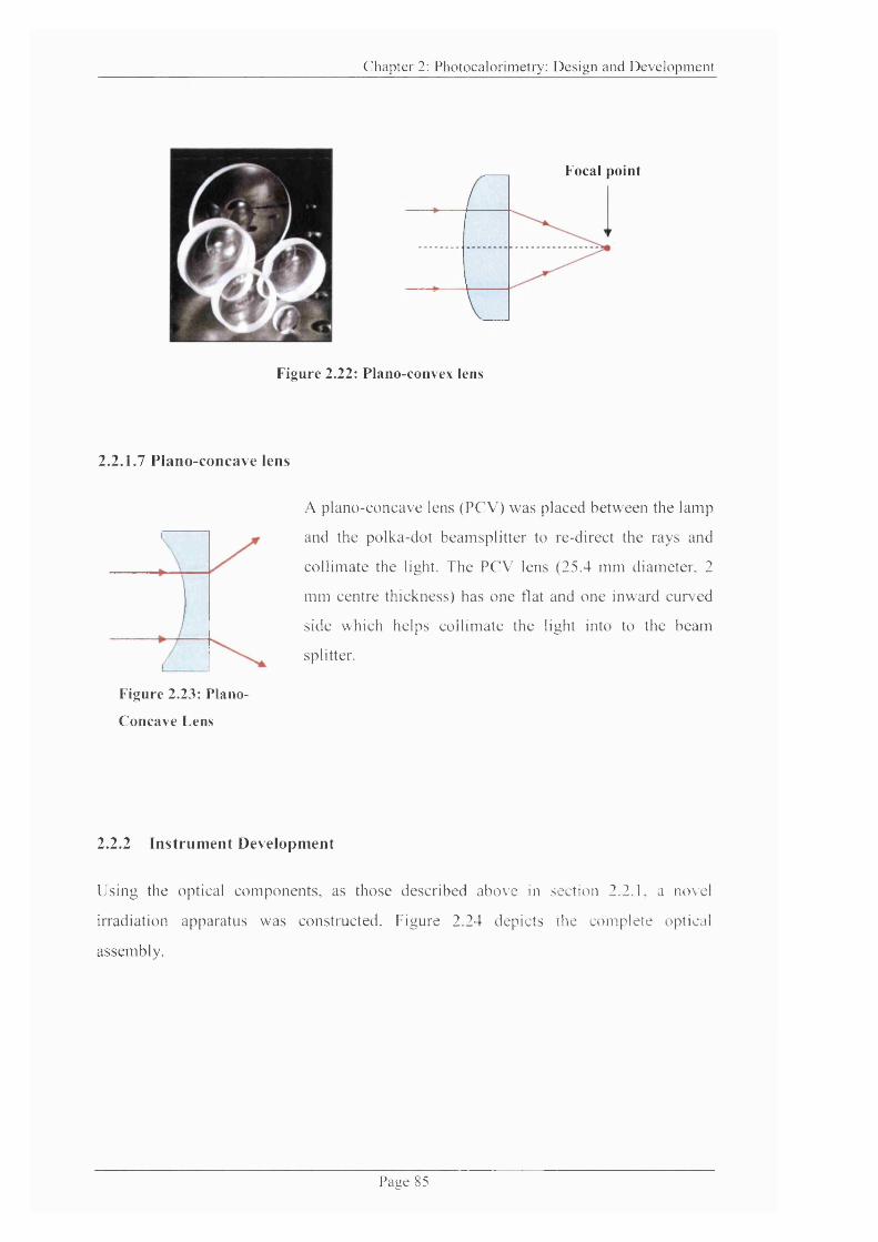
C h a p ter 2; P h o to c a lo r im e tr y : D e s ig n a n d D e v e lo p m e n t
Focal point
Figure 2.22: Plano-convex lens
2.2.1.7 P lano-concave lens
A plano-concave lens (PC V ) was plaeed betw een the lamp
and the polka-dot beamsplitter to re-direct the rays and
collimate the light. The PCV lens (25.4 m m diameter, 2
m m centre thickness) has one flat and one inward curxed
side whieh helps eollimate the light into to the beam
splitter.
Figure 2.23: Plano-
Concave Lens
2.2.2 In s tru m e n t D evelopm ent
Using the optical com ponents, as those described above in section 2.2.1, a novel
iiTadiation apparatus was constructed. Figure 2.24 depicts the com plete optical
assembly.
P a g e 85
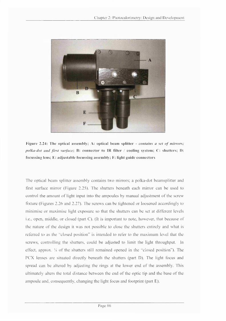
C h a p te r 2: P h o to c a lo r im e tr y : D e s ig n and D e v e lo p m e n t
® 0
Figure 2.24: The optical assembly; A: optical beam splitter - contains a set o f mirrors;
polka-dot and first surface; B: connector to IR filter / cooling system; C: shutters; D:
focussing lens; E: adjustable focussing assembly; F: light guide connectors
The optical beam splitter assem bly contains two mirrors; a polka-dot beam splitter and
first surface mirror (Figure 2.25). The shutters beneath each m irror can be used to
control the amount o f light input into the ampoules by manual adjustment o f the screw
fixture (Figures 2.26 and 2.27). The screws can be tightened or loosened accordingly to
m inim ise or m aximise light exposure so that the shutters can be set at different levels
i.e., open, middle, or closed (part C). (It is important to note, however, that because o f
the nature o f the design it was not possible to close the shutters entirely and what is
referred to as the "closed position" is intended to refer to the maximum level that the
screws, controlling the shutters, could be adjusted to limit the light throughput. In
effect, approx. % o f the shutters still remained opened in the "closed position"). The
PCX lenses are situated directly beneath the shutters (part D). The light focus and
spread can be altered by adjusting the rings at the lower end o f the assembly. This
ultim ately alters the total distance between the end o f the optic tip and the base o f the
am poule and, consequently, changing the light focus and footprint (part E).
P a g e 8 6
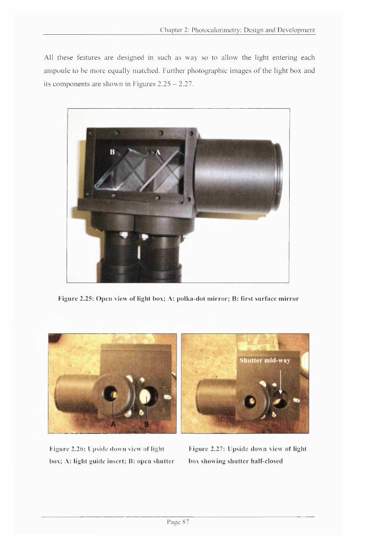
C h a p te r 2: P h o to c a lo r im e tr y : D e s ig n a n d D e v e lo p m e n t
All these features are designed in such as w ay so to allow the light entering each
am poule to be more equally matched. Further photographic im ages o f the light box and
its com ponents are shown in Figures 2.25 - 2.27.
Figure 2.25: Open view of light box; A: polka-dot mirror; B: first surface mirror
Shutter mid-wa\
Figure 2.26: Upside down \iew of light
box; A: light guide insert; B: open shutter
Figure 2.27: Upside down view of light
box showing shutter half-closed
P a g e 87

C h a p ter 2: P h o to c a lo r im e tr y : D e s ig n a n d D e v e lo p m e n t
T he light guides attach on to the end o f the beam splitter assem bly and are inserted
through the re-designed metal colum n (similar to that described earlier in section 2.1.3).
The co lum n was re-m ade to fit the d im ensions o f the new light guide. F igure 2.28
shows the final construction o f the colum n through which the liquid light guide is
inserted.
■
Figure 2.28: Liquid-light guide contained in specially constructed column insert
Paiic

C h a p ter 2: P h o to c a lo r im e tr y : D e s ig n a n d D e v e lo p m e n t
Figure 2.29: The re-designed photocalorimeter (Mark II)
With the overall construction o f the photocalorim eter complete, a metal frame network
was built around the T A M to support the light apparatus and provide instrument
stability. This enabled the light box and com ponents to be m ounted in a t'lxed position
relative to the T A M . T he final design is pictured in Figure 2.29 and a schematic o f the
irradiation apparatus built is illustrated in Figure 2.30.^
P a a e 89
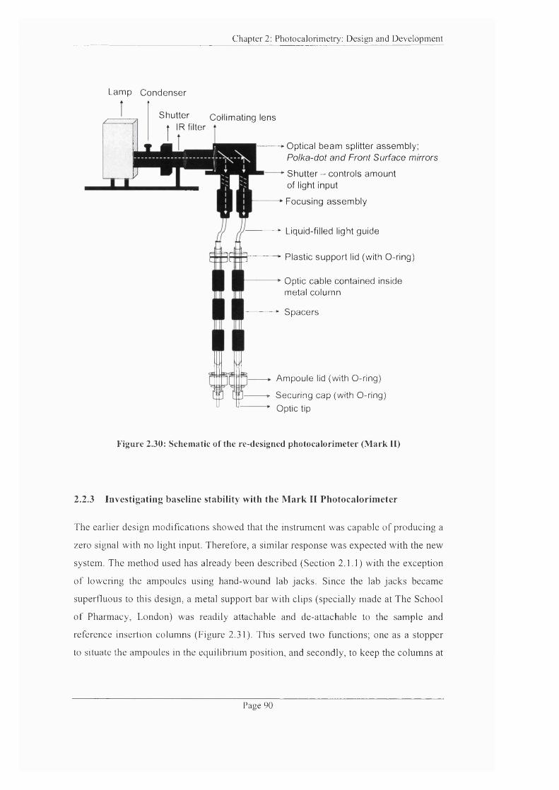
Chapter 2: Photocalorimetry: Design and Development
Lamp Condenser
Shutter Collimating lens t IR filter
Optical beam splitter assembly: P o lk a -d o t a n d F ron t S u r fa c e m irrors
Shutter - controls amount of light input
Focusing assembly
Liquid-filled light guide
Plastic support lid (with 0-ring)
Optic cable contained inside metal column
Spacers
Ampoule lid (with 0-ring)
Securing cap (with O-ring) * Optic tip
Figure 2.30: Schematic of the re-designed photocalorimeter (Mark II)
2.2.3 Investigating baseline stability with the Mark II Photocalorim eter
The earlier design modifications showed that the instrument was capable of producing a
zero signal with no light input. Therefore, a similar response was expected with the new
system. The method used has already been described (Section 2.1.1) with the exception
o f lowering the ampoules using hand-wound lab jacks. Since the lab Jacks became
superfluous to this design, a metal support bar with clips (specially made at The School
o f Pharmacy, London) was readily attachable and de-attachable to the sample and
reference insertion columns (Figure 2.31). This served two functions; one as a stopper
to situate the ampoules in the equilibrium position, and secondly, to keep the columns at
Page 90
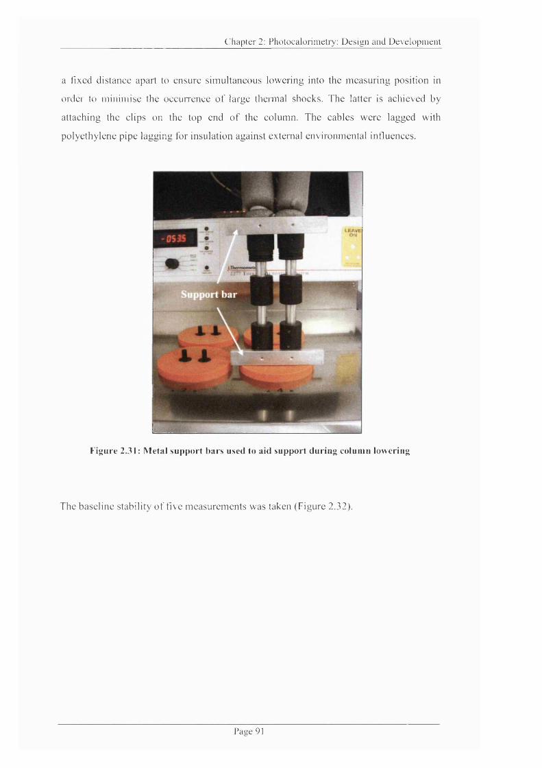
C h a p ter 2: P h o to c a lo r im e tr y ; D e s ig n a n d D e v e lo p m e n t
a fixed distance apart to ensure simultaneous lowering into the m easuring position in
order to m inim ise the occurrence o f large thennal shocks. The latter is achieved by
attaching the clips on the top end o f the column. The cables w ere lagged with
polyethylene pipe lagging for insulation against external environmental influences.
Figure 2.31: Metal support bars used to aid support during column lowering
The baseline stability o f five m easurem ents was taken (Figure 2.32).
P a g e 91
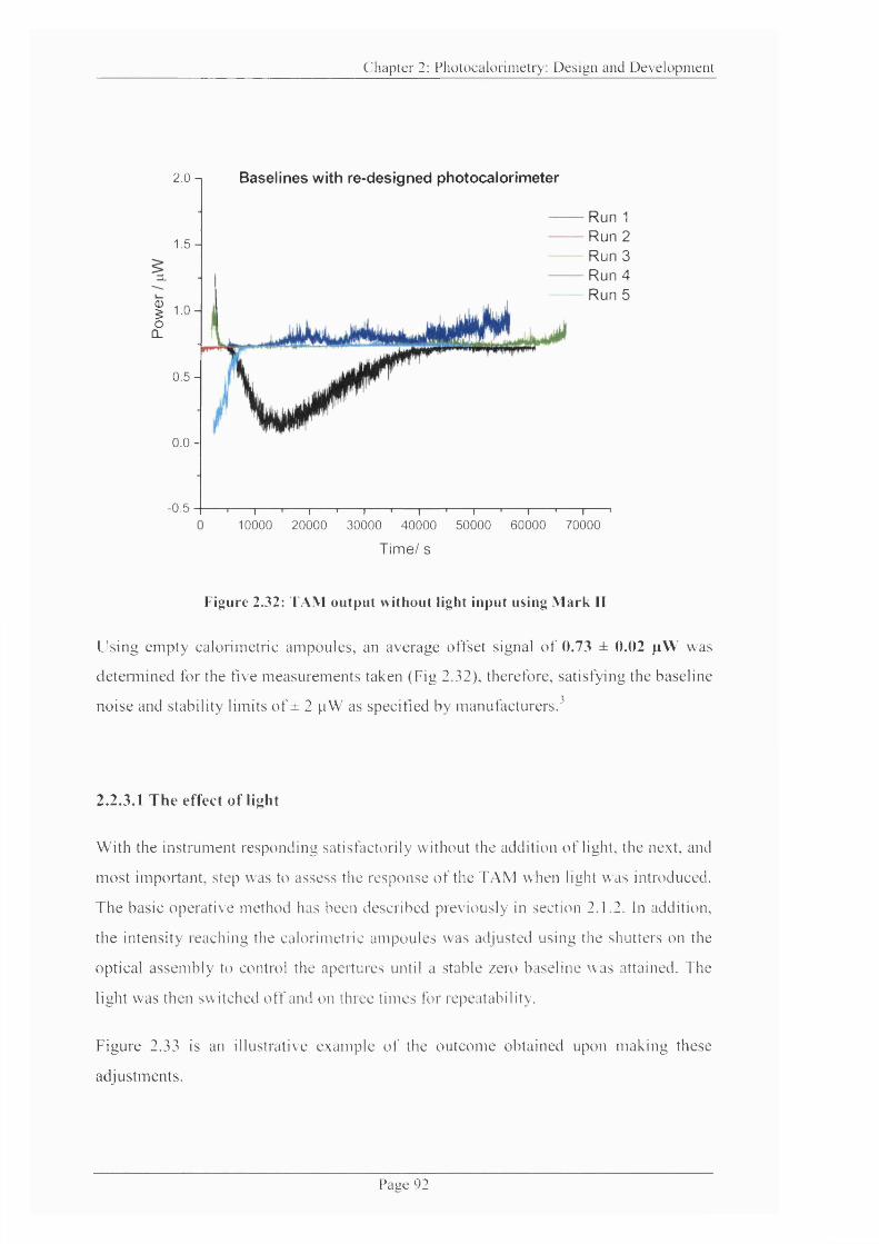
C h a p ter 2: P h o to c a lo r im e tr y : D e s ig n a n d D e v e lo p m e n t
2 .0 -
1.5-
^ 1.0 - o
CL
0.5-
0.0 -
-0.5
Baselines with re-designed photocalorimeter
Run 1 Run 2 Run 3 Run 4 Run 5
— I---------'--------- 1----------------'-1---------------- '-1---------------- '-1----------------'-1-------- '---------1—10000 20000 30000 40000 50000 60000 70000
Time/ s
Figure 2.32: TAM output without light input using M ark II
U sing em pty cal o h metric ampoules, an average offset signal o f 0.73 ± 0.02 juW was
d e tenn ined for the five m easurem ents taken (Fig 2.32), therefore, satisfying the baseline
noise and stability limits o f ± 2 p W as specified by manufacturers.^
2.2.3.1 T he effect of light
W ith the instrument responding satisfactorily without the addition o f light, the ne.xt, and
m ost important, step was to assess the response o f the T A M when light was introduced.
T h e basic operative method has been described previously in section 2.1.2. In addition,
the intensity reaching the calorimetric am poules was adjusted using the shutters on the
optical assem bly to control the apertures until a stable zero baseline was attained. The
light was then switched o f f and on three times for repeatability.
Figure 2.33 is an illustrative exam ple o f the ou tcom e obtained upon m aking these
adjustments.
P a g e 9 2

C h a p ter 2: P h o to c a lo r im e tr y : D e s ig n a n d D e v e lo p m e n t
120 The effect on the baseline by adjustment of shutters100
shutter adjustments
0o
CL -20
-40Light on
Light on-60
-80
100
-120300000 330000270000 360000 390000 420000
Time/ s
Figure 2.33: The effect on the baseline by adjustm ent of shuttering assembly to control
light input and response to baseline with light off post adjustment
1 0 0 -
5 0 -
I 0
S.
-50 -
- 1 0 0 -
_ J - ' ^
350000 1----360000
Heat output (pW)light off
-0.54 -0.38 -1.81
-0.91 ± 0.78
light on -0.07 -1.84 -3.06
-1.66 ± 1.50
370000
Time/ s
380000
Figure 2.34: Magnified plot of Figure 2.33 showing baselines with and without light input
post adjustment. The red line represents a zero heat output
P a g e 9 3
Chapter 2: Photocalorimetry; D esign and Developm ent
Initial trials showed a remarkable improvement to the baseline with the light on as
depicted in Figures 2.32 and 2.33. These also showed excellent repeatability upon
switching the light on and off after the shutters were initially set to exhibit a zero power
signal. In this case, an average signal o f 0.07 ± 0.06 pW was obtained with the light off
and -0.04 ± 0 .1 1 pW with the light on. These values are almost equal, evident o f an
overall net signal o f zero, and compare favourably with the manufacturers stated
baseline noise of ± 2 pW for a 20 mL ampoule capacity.
Being able to attain a zero baseline with the light on and off marked a significant step in
the project. With the fundamentals o f the design in place, the next step was then to
quantify the light being delivered to sample. This is known as Chemical Actinometry
and is further explained in Chapter 3 which details the measurements performed on an
ICH listed actinometer, 2-nitrobenzaldehyde (2NB).
2.2.4 Problem s associated with xenon arc lam ps
Over the course o f the project, it was noted that there was a significant decline in the
lamp performance over a short period o f time making it difficult to obtain consistent
experimental measurements.
Although xenon arc lamps are superb at mimicking solar spectral irradiance, there are a
number o f issues associated with them:
^ Short lamp life - because o f the extreme conditions inside the bulb, Xe lamps
typically have a lifetimes ranging from 200 to -2000 h (or 1 to 12 weeks o f
continuous operation). The 300 W Xe lamp used with the Mark 11
photocalorimeter served a lifespan o f -900 h (-5 weeks o f continuous
operation).
^ The lamps require power consumption o f several hundred watts to obtain
sufficient intensities. Smallest bulbs available are usually 50 or 75 W types and
the largest are usually 500 W.
Page 94

Chapter 2: Photocalorimetry: D esign and Developm ent
# Only a fraction o f the consumed power is emitted as light, while a large portion
is converted to heat, which must be dissipated. This usually requires the need for
expensive water cooling systems.
The arc within the bulb requires alignment each time upon striking. This can
alter the geometry, and hence transmission, of the light path to some degree.
# Their ignition requires high voltages (~ 30 kV). This is a potential shock hazard
and can cause strong electromagnetic interferences with other electronic
equipment.
# Because o f the high pressure inside the bulb (~ 8 to 10 bar), xenon lamps pose a
threat o f explosion if not handled properly.
All these factors combined can cause irregularity in the amount o f light delivered and
the intensity can vary across measurements. The changes in the light output can be
measured through actual photon flux measurements using a spectroradiometer. This is
known as Physical Actinometry (explained further in Chapter 3) where it was possible
to obtain spectral intensity and real time flux measurements.
The aging o f the lamp will cause deterioration in intensity levels, and evidently will
impact heavily on the power output on the TAM. Several light on/off tests, using empty
ampoules, were performed to assess the level o f deterioration after the lamp had
surpassed its recommended life span o f 900 h. The shutters were initially pre-defined to
give a zero baseline on the TAM. The light was then switched on and off to assess if the
baseline signal gave a repeatable signal at zero. An example o f the variability in the
TAM output is shown in Figure 2.35. In this example, the signal gradually drifts from
-4 0 pW in the first instance to -18 pW in the latter showing approx. 50% signal decline
over an irradiation period o f about 5 hours. In the case o f drug photodegradation, such
instability will significantly impact on the TAM output resulting to misleading data
interpretation.
Repeating the light on/off tests followed no set pattern and the outputs were arbitrary.
Figure 2.36 is representative o f the discrepancy associated in the power signal with light
input. The lamp power in all cases was set to 240 W.
Page 95

Chapter 2: Photocalorim etry; D esign and D evelopm ent
300-
2 0 0 - 4 0 p W3 7 p W
100 -
0o
CL
0 - - 1
- 100 -
- 200 -
-300-
6000 9000 12000 15000 18000 21000
Time/ s
Figure 2.35: Light on/off tests showing a gradual decline in heat output caused by
deterioration in lamp performance
50 n ■ Light on • Light off
40 -
30-
2 0 -
I 0 - -o
CL-10-
-30 -
-400 2 3 4 5 6 8 9 101 7
Experiment number
Figure 2.36: A scatter plot to show the variation in power with the light on/off
Page 96
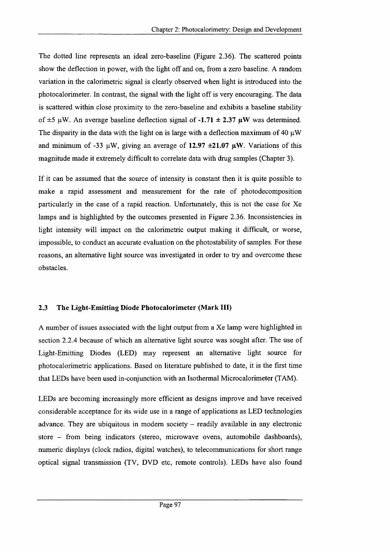
Chapter 2: Photocalorimetry: D esign and Developm ent
The dotted line represents an ideal zero-baseline (Figure 2.36). The scattered points
show the deflection in power, with the light off and on, from a zero baseline. A random
variation in the calorimetric signal is clearly observed when light is introduced into the
photocalorimeter. In contrast, the signal with the light off is very encouraging. The data
is scattered within close proximity to the zero-baseline and exhibits a baseline stability
o f ±5 pW. An average baseline deflection signal o f -1.71 ± 2.37 pW was determined.
The disparity in the data with the light on is large with a deflection maximum o f 40 pW
and minimum of -33 pW, giving an average o f 12.97 ±21.07 pW . Variations o f this
magnitude made it extremely difficult to correlate data with drug samples (Chapter 3).
If it can be assumed that the source o f intensity is constant then it is quite possible to
make a rapid assessment and measurement for the rate o f photodecomposition
particularly in the case o f a rapid reaction. Unfortunately, this is not the case for Xe
lamps and is highlighted by the outcomes presented in Figure 2.36. Inconsistencies in
light intensity will impact on the calorimetric output making it difficult, or worse,
impossible, to conduct an accurate evaluation on the photostability o f samples. For these
reasons, an alternative light source was investigated in order to try and overcome these
obstacles.
2.3 The L ight-E m itting Diode Photocalorim eter (M ark III)
A number o f issues associated with the light output from a Xe lamp were highlighted in
section 2.2.4 because o f which an alternative light source was sought after. The use o f
Light-Emitting Diodes (LED) may represent an alternative light source for
photocalorimetric applications. Based on literature published to date, it is the first time
that LEDs have been used in-conjunction with an Isothermal Microcalorimeter (TAM).
LEDs are becoming increasingly more efficient as designs improve and have received
considerable acceptance for its wide use in a range o f applications as LED technologies
advance. They are ubiquitous in modem society - readily available in any electronic
store - from being indicators (stereo, microwave ovens, automobile dashboards),
numeric displays (clock radios, digital watches), to telecommunications for short range
optical signal transmission (TV, DVD etc, remote controls). LEDs have also found
Page 97
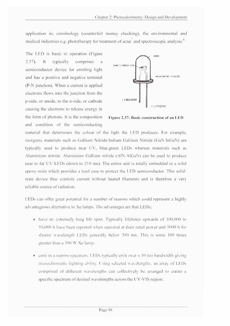
C h a p ter 2: P h o to c a lo r im e tr y : D e s ig n a n d D e v e lo p m e n t
application in; crim inology (counterfeit m oney checking), the environm ental and
m edical industries e.g. photo therapy for treatment o f acne^ and spectroscopic analysis.^
'iiMH CONDUCTOR
r?HHÜU I M m T P lA S n c
(*-)P05»TM
T he LED is basic in operation (Figure
2.37). It typieally eom prises a
sem iconduc to r device for emitting light
and has a positive and negative temiinal
(P-N junction). W hen a current is applied
electrons flows into the junction from the
p-side, o r anode, to the n-side, or cathode
causing the eleetrons to release energy in
the fo n n o f photons. It is the com position
and condition o f the sem ieonducting
material that de tenn ines the colour o f the light the LED produces. For example,
inorganic materials such as Gallium Nitride/Indium Gallium Nitride (G aN /lnG aN ) are
typically used to produce near UV, blue/green LEDs w hereas m aterials such as
A lum in ium nitride/ A lum inium Gallium nitride (A lN /A lG aN ) can be used to produce
near to far UV LEDs (dow n to 210 nm). T he entire unit is totally em bedded in a solid
epoxy resin which provides a hard case to protect the LED sem iconductor. This solid-
state device thus controls current w ithout heated filaments and is therefore a very
reliable souree o f radiation.
Figure 2.37: Basic construction of an LED
LEDs can offer great potential for a num ber o f reasons which could represent a highly
advantageous alternative to Xe lamps. The advantages are that LEDs;
r have an extrem ely long life span. Typically lifetimes upw ards o f 100,000 to
5(),()()0 h have been reported when operated at their rated pow er and 5000 h for
shorter wavelength LEDs generally below 380 nm. This is som e 100 times
greater than a 300 W Xe lamp.
r em it in a narrow-spectrum . LEDs typically emit over a 10 nm bandw idth giving
m onochrom atic lighting ability. Using selected wavelengths, an a n a y o f LEDs
com prised o f different w avelengths can collectively be arranged to create a
specific spectrum o f desired wavelengths across the UV-V IS region.
P a ^ e 98
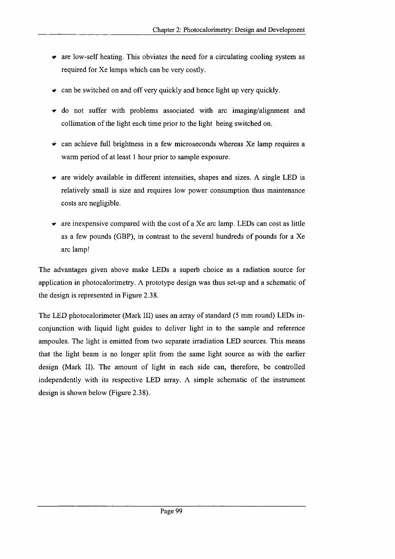
Chapter 2: Photocalorimetry: D esign and Developm ent
are low-self heating. This obviates the need for a circulating cooling system as
required for Xe lamps which can be very costly.
V can be switched on and off very quickly and hence light up very quickly.
'T do not suffer with problems associated with arc imaging/alignment and
collimation o f the light each time prior to the light being switched on.
w can achieve full brightness in a few microseconds whereas Xe lamp requires a
warm period o f at least 1 hour prior to sample exposure.
# are widely available in different intensities, shapes and sizes. A single LED is
relatively small is size and requires low power consumption thus maintenance
costs are negligible.
# are inexpensive compared with the cost o f a Xe arc lamp. LEDs can cost as little
as a few pounds (GBP), in contrast to the several hundreds o f pounds for a Xe
arc lamp!
The advantages given above make LEDs a superb choice as a radiation source for
application in photocalorimetry. A prototype design was thus set-up and a schematic o f
the design is represented in Figure 2.38.
The LED photocalorimeter (Mark III) uses an array o f standard (5 mm round) LEDs in
conjunction with liquid light guides to deliver light in to the sample and reference
ampoules. The light is emitted from two separate irradiation LED sources. This means
that the light beam is no longer split from the same light source as with the earlier
design (Mark II). The amount o f light in each side can, therefore, be controlled
independently with its respective LED array. A simple schematic o f the instrument
design is shown below (Figure 2.38).
Page 99
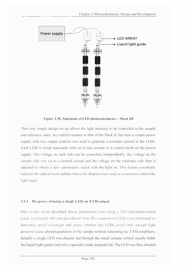
Chapter 2; Photocalorim etry: D esign and D evelopm ent
Power supply► LED ARRAY
-► Liquid light guide
Figure 2.38: Schematic of LED photocalorimeter - M ark III
This very sim ple design set-up allows the light intensity to be controlled in the sample
and reference sides, in a similar m anner to that o f the Mark II, but here a sim ple power
supply with two output controls was used to generate a constant current to the LEDs.
Each LED is wired separately with an in-line resistor to a control knob on the pow er
supply. T he voltage on each side can be controlled independently; the voltage on the
sam ple side was set to a desired current and the voltage on the reference side then is
adjusted to obtain a zero calori metric signal with the light on. This feature essentially
replaces the optical beam splitter where the shutters were used as a m eans to control the
light input.
2.3.1 R esponse of using a single LED on TA.M o u tp u t
Prior to the set-up described above, prelim inary tests using a 350 millcandela (mcd)
(peak w avelength 400 nm) (purchased from RS com ponents) LED were perfo im ed to
determ ine proot-of-concept and assess w hether the LEDs could emit enough light
pow er to cause photodegradation o f the sam ple without saturating the TA M amplifiers.
Initially a single LED was directly fed through the metal colum n (which usually holds
the liquid light guide) and into a specially m ade am poule lid. The LED was thus situated
P a g e 100

Chapter 2: Photocalorimetry: D esign and Developm ent
directly on top o f the sample inside the TAM channel. The data showed that the light
emitted was far too intense at 20 V due to the short distance between the LED and
sample. The voltage on the reference side was reduced until a power signal was
obtained within a detection limit o f 3000 pW set on the TAM amplifiers. This was
found to be around 5 V indicating that saturation o f the amplifiers occurred above 5 V.
However, at 5 V degradation o f photochemical materials may be insufficient, or far too
slow to attain quantifiable data, and also leaves little leeway to adjust the voltage on the
reference side. The LEDs were, therefore, situated outside the TAM channel and
connected to the liquid light guides to direct light into the ampoules. This increased the
distance between the light source and sample and hence reduced the light intensity to
the ampoule. In order to compensate for the loss in intensity. Ultra-bright high intensity
UV LEDs were purchased from RS components® (Part No: 454 - 4403).
The Mark III photocalorimeter was thus initially set up using extreme Ultra-bright super
UV LEDs (5 mm round) emitting a luminous intensity o f 10,000 mcd. These were
purchased from Ultraleds® Ltd and covered a narrow spectrum in the UV region (380 -
410 nm).
The TAM was electrically calibrated at 300 pW. The light was switched on after a zero
baseline with the light off was attained. The current on the sample and reference sides
were set to 10 V until a constant signal was observed. The reference side only was then
adjusted in order to obtain a zero signal with the light on.
Page 101

Chapter 2: Photocalorimetry: D esign and Developm ent
LED response on TAM output at 10 V
300 -
250 -
200 -
% Light on: ± 0.5 pW
ICL
150 -
100 -
50 -Time (s)
0 -
9000 10000 11000 12000 13000 14006500 7000 8000
Time/ s
Figure 2.39: Photocalorimetric response to light input from single LED. Inset figure
showing close up of baseline after light is switched on.
Figure 2.39 shows a very encouraging response from the LED on the TAM output. This
light test was conducted on empty ampoules to assess the stability o f the light. The
baseline stability with the LEDs was very encouraging with a stable signal being
exhibited ca 0.5 h after switching the light on. Several light tests performed gave an
average signal o f 0.4 ± 1.1 pW with the light on. The use o f the dial controls on the
power supply made it possible to adjust finely the amount o f light reaching the
ampoules to achieve a zero baseline.
Using this set-up, the light delivered was quantified using 2-nitrobenzaldeyde (2NB)
solution as a chemical actinometer (further discussed in the Chapter 3). In order to
assess if the system was responding accordingly, the photolysis o f 2NB was tested at 3
different voltages; 10 V, 15 V and 20 V, to evaluate if there was a direct correlation o f
increasing voltage to the power output o f the photodegradation o f 2NB. These results
are discussed in Chapter 3.
Page 102
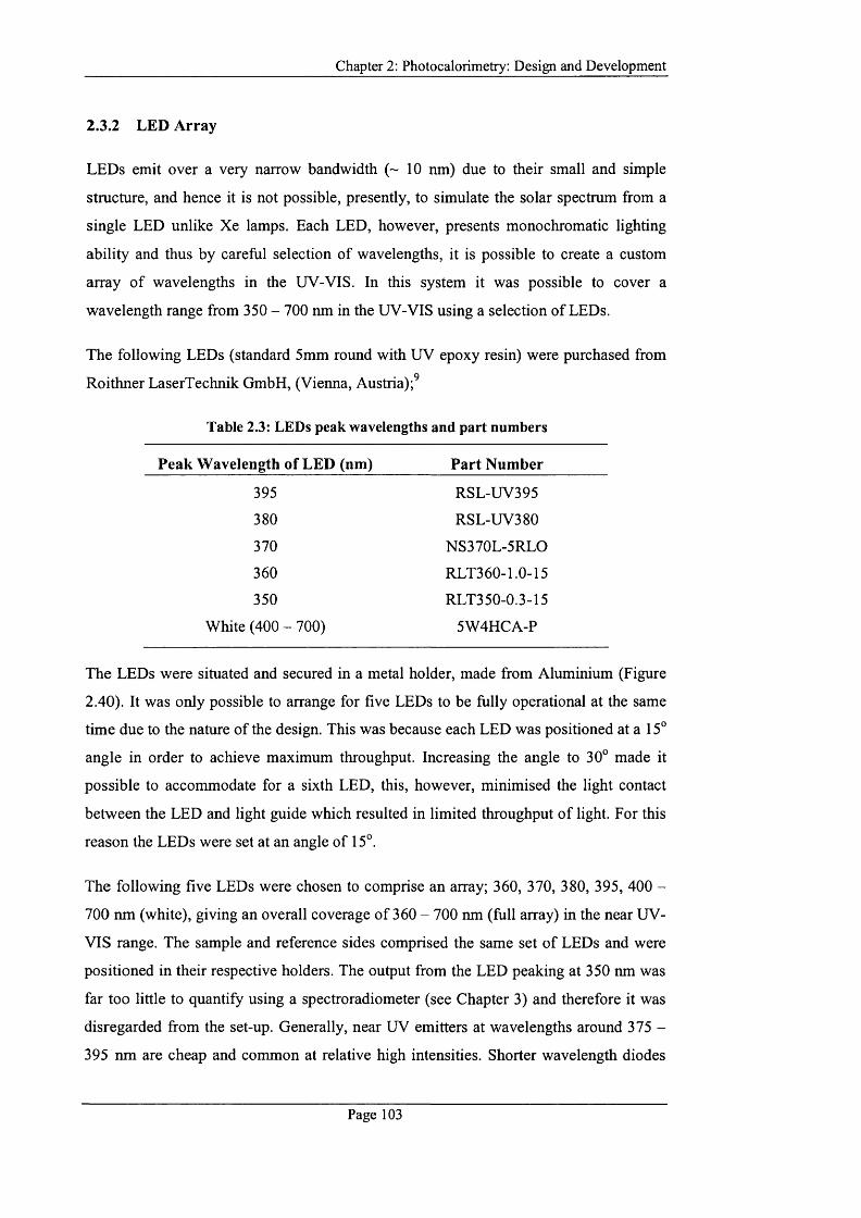
Chapter 2; Photocalorimetry: D esign and Developm ent
2.3.2 LED A rray
LEDs emit over a very narrow bandwidth (~ 10 nm) due to their small and simple
structure, and hence it is not possible, presently, to simulate the solar spectrum from a
single LED unlike Xe lamps. Each LED, however, presents monochromatic lighting
ability and thus by careful selection of wavelengths, it is possible to create a custom
array o f wavelengths in the UV-VIS. In this system it was possible to cover a
wavelength range from 350 - 700 nm in the UV-VIS using a selection o f LEDs.
The following LEDs (standard 5mm round with UV epoxy resin) were purchased from
Roithner LaserTechnik GmbH, (Vienna, Austria);^
Table 2.3: LEDs peak wavelengths and part numbers
Peak W avelength of LED (nm) P a rt N um ber
395 RSL-UV395
380 RSL-UV380
370 NS370L-5RLO
360 RLT360-1.0-15
350 RLT350-0.3-15
White (400 - 700) 5W4HCA-P
The LEDs were situated and secured in a metal holder, made from Aluminium (Figure
2.40). It was only possible to arrange for five LEDs to be fully operational at the same
time due to the nature o f the design. This was because each LED was positioned at a 15°
angle in order to achieve maximum throughput. Increasing the angle to 30° made it
possible to accommodate for a sixth LED, this, however, minimised the light contact
between the LED and light guide which resulted in limited throughput o f light. For this
reason the LEDs were set at an angle o f 15°.
The following five LEDs were chosen to comprise an array; 360, 370, 380, 395, 400 -
700 nm (white), giving an overall coverage o f 360 - 700 nm (full array) in the near UV-
VIS range. The sample and reference sides comprised the same set o f LEDs and were
positioned in their respective holders. The output from the LED peaking at 350 nm was
far too little to quantify using a spectroradiometer (see Chapter 3) and therefore it was
disregarded from the set-up. Generally, near UV emitters at wavelengths around 375 -
395 nm are cheap and common at relative high intensities. Shorter wavelength diodes
Page 103
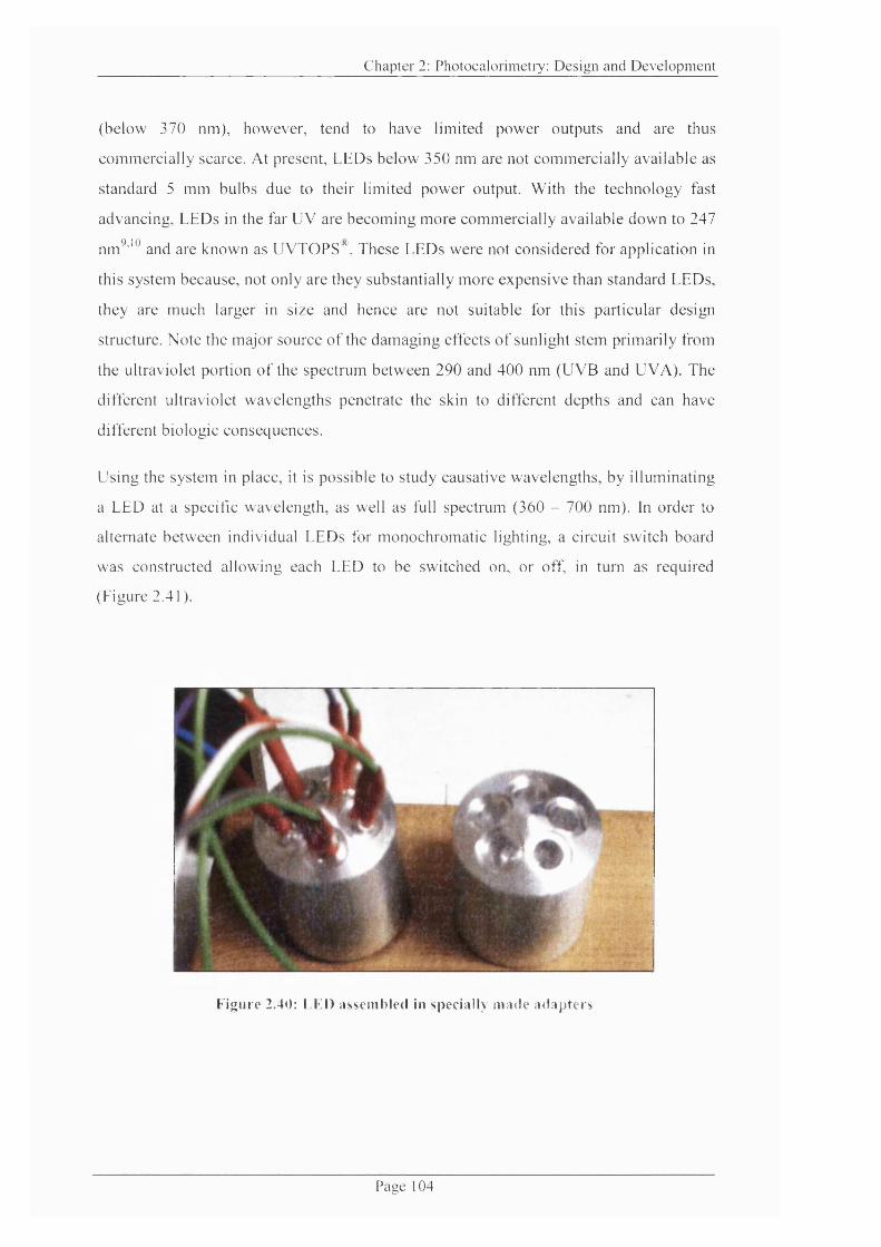
Chapter 2: Photocalorimetry: D esign and D evelopm ent
(below 370 nm), however, tend to have limited pow er outputs and are thus
com m ercially scarce. At present, LEDs below 350 nm are not com m ercially available as
s tandard 5 m m bulbs due to their limited pow er output. With the technology fast
advancing, LEDs in the far UV are becom ing m ore com m ercially available dow n to 247
nm*^’'* and are know n as U V T O PS^. These EEDs were not considered for application in
this system because, not only are they substantially m ore expensive than standard EEDs,
they are m uch larger in size and hence are not suitable for this particular design
structure. Note the m ajor source o f the dam aging effects o f sunlight stem primarily from
the ultraviolet portion o f the spectrum betw een 290 and 400 nm (U V B and UVA). The
different ultraviolet w avelengths penetrate the skin to different depths and can have
different b iologic consequences.
Using the system in place, it is possible to study causative w avelengths, by illum inating
a LED at a specific w avelength, as well as full spectrum (360 - 700 nm). In order to
alternate betw een individual EEDs for m onochrom atic lighting, a circuit switch board
was constructed allowing each LED to be switched on, or off, in turn as required
(Figure 2.41 ).
II
Figure 2.40: LEI) assembled in specially made adapters
Page 104

Chapter 2: Photocalorimetry; D esign and D evelopm ent
P rF L R L N
Figure 2.41: LED A rray with circuit board
A basic diagram o f the above circuit board is shown Figure 2.42. A circuit d iagram o f
the switch board is presented in Figure 2.43 and represents the current flow direction in
illum inating the LEDs. Each LED was wired with an in-line resistor built into the circuit
board to limit the current in the LED to a safe value. The resistance o f each LED was
detenn ined by O h m 's law (Equation 2.1 ) in accordance to its individual rated operating
power.
Eqn. 2.1
where;
R is the Resistance (Q or Ohm s)
is the Power Supply Max (V)
Vp is the Forward Voltage o f LED (V)
Ip (typ) is the Forward Current o f LED (A)
Page 105
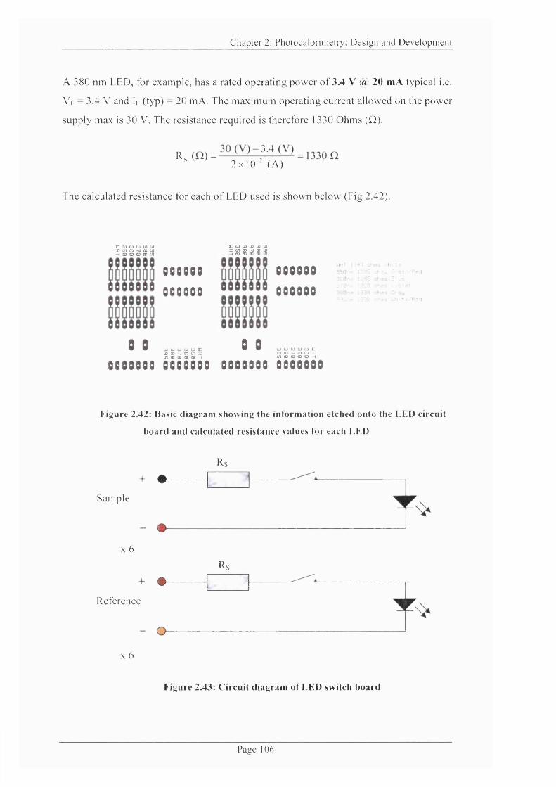
Chapter 2: Photocalorimetry: D esign and D evelopm ent
A 380 nm LED, for example, has a rated operating pow er o f 3.4 V @ 20 mA typical i.e.
Vp = 3.4 V and Ip (typ) = 20 mA. T h e m axim um operating current allowed on the pow er
supply m ax is 30 V. The resistance required is therefore 1330 O hm s (Q).
R = 3.4
" 2 x 1 0 - ’ (A )
The calculated resistance for each o f LED used is shown below (Fig 2.42).
%z w w w w wX in 07 03 COH eo 03 CB S3 01
0 0 0 0 0 00 0 0 0 0 0
C W W W CO COX Cn 07 -0 CD COH 03 S3 CD S c/1
0 0 0 0 0 00 0 0 0 0 0
U H T u n '..t , r . ?
!■ 1 2 2 5 -jl-'.-n:: Cr '=n TP 1
r 1285 B I '5 n n - 1 I 5 _ 0 o r iT .- j "
J i * - : - - . » ' ' i f - t -r-. -I" U P e j
0 0 Ü) W (O CO CO cCO 03 ->J 03 cn XCD CD S CD S H
0 0 CO CO CO CO CO [CO CD - 'j 03 c/1 Xcn CD S CD S3 -c
0 0 0 0 0 0 0 0 0 0 0 0 0 0 0 0 0 0 0 0 0 0 0 0 0 0 0 0
Figure 2.42: Basic diagram showing the information etched onto the LED circuit
board and calculated resistance values for each LED
+ #
Sam ple
Rs
X 6
+ m -
Reference
Rs
X 6
Eigure 2.43: Circuit diagram of LED switch board
Page 106

Chapter 2: Photocalorim etry: D esign and D evelopm ent
T he final design o f the LED photoealorim eter is presented in Figure 2.44.
Figure 2.44: Final LED Photoealorimeter (Mark III)
Having a n iv e d at the final instrumental setup, consideration to the experimental method
was given. The standard m ethod o f loading and lowering am poules into the isothennal
m icrocalorim eter has been followed previously and described in section 2.1.1. This
m ethod is com m only used where standard 3 mL am poules are employed. However, the
developm ent o f a new photoealorim eter has brought the opportunity to investigate the
best m ethod o f lowering 20 mL am poules into the TA M . T he am poules (20 mL
stainless steel. Therm om etric Ltd) and w ere tilled with 4 mL distilled water. Five
different m ethods o f lowering the am poules into the TA M were investigated; the best
method is governed by the one that m ost qu ick ly recovers from thennal shock to allow
m easurem ent o f thennal activity to com m ence once a stable baseline signal is achieved.
Pa^e 107
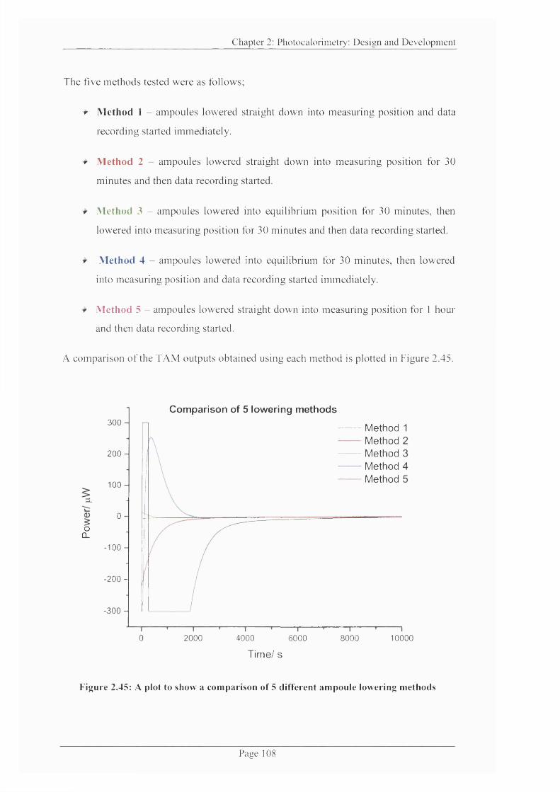
Chapter 2: Photocalorim etry: D esign and D evelopm ent
The five m ethods tested were as follows;
f Method I - am poules lowered straight dow n into m easuring position and data
recording started immediately.
f Method 2 - am poules lowered straight dow n into m easuring position for 30
m inutes and then data recording started.
f Method 3 - am poules lowered into equilibrium position for 30 minutes, then
lowered into m easuring position for 30 m inutes and then data recording started.
r Method 4 - ampoules lowered into equilibrium for 30 minutes, then lowered
into m easuring position and data recording started immediately.
y Method 5 - am poules lowered straight dow n into m easuring position for 1 hour
and then data recording started.
A com parison o f the T A M outputs obtained using each m ethod is plotted in Figure 2.45.
oCL
2000 4000 6000
Time/ s
Comparison of 5 lowering methods300- Method
MethodMethodMethodMethod
2 0 0 -
100 -
0
-100 -
-200 -
-300 -
8000 10000
Figure 2.45: A plot to show a comparison of 5 different ampoule lowering methods
Page 108
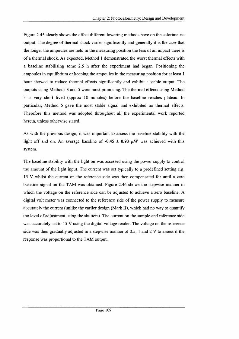
Chapter 2: Photocalorimetry: D esign and Developm ent
Figure 2.45 clearly shows the effect different lowering methods have on the calorimetric
output. The degree o f thermal shock varies significantly and generally it is the case that
the longer the ampoules are held in the measuring position the less o f an impact there is
o f a thermal shock. As expected, Method 1 demonstrated the worst thermal effects with
a baseline stabilising some 2.5 h after the experiment had began. Positioning the
ampoules in equilibrium or keeping the ampoules in the measuring position for at least 1
hour showed to reduce thermal effects significantly and exhibit a stable output. The
outputs using Methods 3 and 5 were most promising. The thermal effects using Method
3 is very short lived (approx 10 minutes) before the baseline reaches plateau. In
particular, Method 5 gave the most stable signal and exhibited no thermal effects.
Therefore this method was adopted throughout all the experimental work reported
herein, unless otherwise stated.
As with the previous design, it was important to assess the baseline stability with the
light off and on. An average baseline o f -0.45 ± 0.93 was achieved with this
system.
The baseline stability with the light on was assessed using the power supply to control
the amount o f the light input. The current was set typically to a predefined setting e.g.
15 V whilst the current on the reference side was then compensated for until a zero
baseline signal on the TAM was obtained. Figure 2.46 shows the stepwise manner in
which the voltage on the reference side can be adjusted to achieve a zero baseline. A
digital volt meter was connected to the reference side of the power supply to measure
accurately the current (unlike the earlier design (Mark II), which had no way to quantify
the level o f adjustment using the shutters). The current on the sample and reference side
was accurately set to 15 V using the digital voltage reader. The voltage on the reference
side was then gradually adjusted in a stepwise manner o f 0.5, 1 and 2 V to assess if the
response was proportional to the TAM output.
Page 109
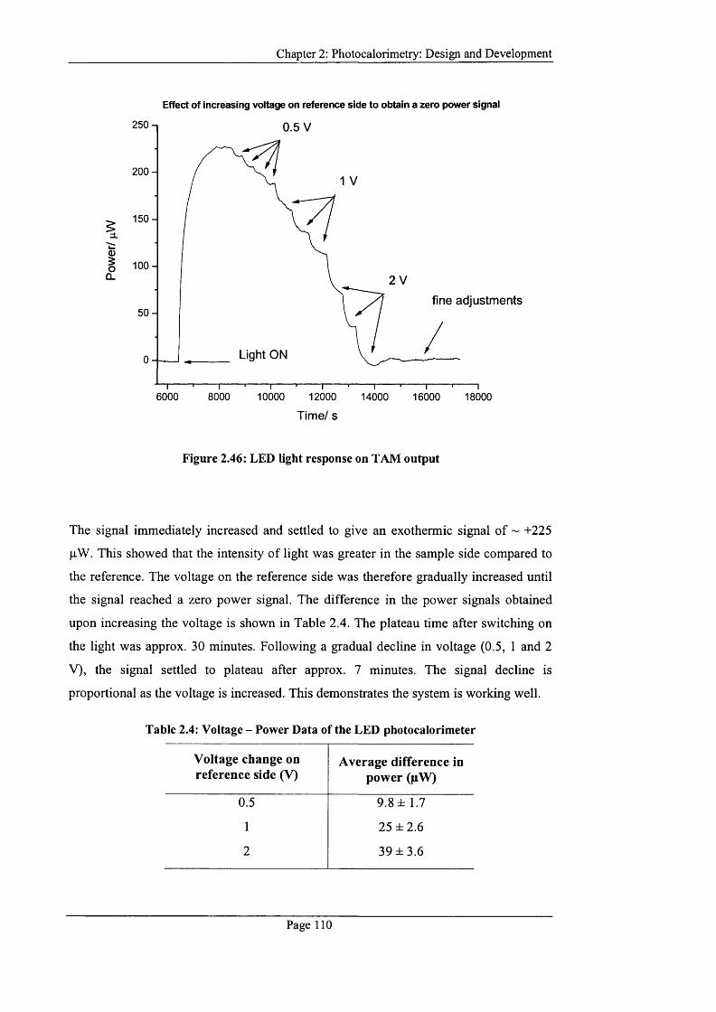
Chapter 2: Photocalorimetry: D esign and Developm ent
Effect of increasing voltage on reference side to obtain a zero power signal
250 n 0.5 V
2 0 0 -
150-IiI 100-Q_ 2 V
fine adjustments50-
Llght ON
6000 8000 10000 12000 16000 1800014000
Time/ s
Figure 2.46: LED light response on TAM output
The signal immediately increased and settled to give an exothermic signal o f ~ +225
pW. This showed that the intensity o f light was greater in the sample side compared to
the reference. The voltage on the reference side was therefore gradually increased until
the signal reached a zero power signal. The difference in the power signals obtained
upon increasing the voltage is shown in Table 2.4. The plateau time after switching on
the light was approx. 30 minutes. Following a gradual decline in voltage (0.5, 1 and 2
V), the signal settled to plateau after approx. 7 minutes. The signal decline is
proportional as the voltage is increased. This demonstrates the system is working well.
Table 2.4: Voltage - Power Data of the LED photoealorimeter
Voltage change on reference side (V)
Average difference in power (pW)
0.5 9 .8 + 1.7
1 25 + 2.6
2 39 + 3.6
Page 110
Chapter 2: Photocalorimetry: D esign and Developm ent
Several light on/off tests were performed to assess the system error o f the baseline when
the light is switched on. The measurements were conducted in the same manner as that
described above. Five measurements were taken in each case. The baseline
reproducibility for the five measurements taken with the light off gave an average signal
o f 1.18 ± 0.82 (with solvent ethanol/water mixture). The baseline deflection with
the light on was 2.37 ± 1.02 ^W . Any power signal generated outside these limits is
attributed to the photoreactivity o f the sample during irradiation.
W ith the development o f the instrument complete, the next stage was to establish
methods o f validation and quantification o f the light delivery during photodegradation
o f a sample. The methods employed were that of Physical and Chemical actinometry. A
spectroradiometer was used to characterise the performance o f the LEDs and establish
the intensity o f light emitted from the LEDs at each wavelength and as an array (360 -
700 nm). This work is explained in Chapter 3. This method o f calibration, however,
gives no information on the level o f exposure during irradiation o f a sample, and hence,
an in-situ validation o f instrumental parameters is preferable to an external calibration.
Thus, the suitability o f a number o f chemical actinometers (solution phase and solid-
state systems) was assessed in order to validate the performance of the
photoealorimeter. Chapter 3 details the Chemical Actinometry work undertaken in order
to achieve this using the photodegradation o f 2-nitrobenzaldehyde as a model solution
phase system.
Page 111

Chapter 2: Photocalorimetry: D esign and Developm ent
2.4 Summary
The design and development o f a novel easy-to-use and versatile photoealorimeter has
been successfully implemented. Two prototype designs were successfully developed;
both demonstrating much potential in application for photostability testing. The original
photoealorimeter, developed by Morris,' whilst useful for providing proof-of-concept
data was not ideal because it proved impossible to obtain a zero power signal with and
without irradiating the sample cell, rendering quantitative analysis o f data challenging.
Fundamental instrumental changes were therefore implemented. The instrument was re
designed using a beam splitter and liquid-filled light guides to direct light into the
calorimetric cells from a high intensity Xe arc lamp. Using a number o f shuttering and
focusing adjustments it became possible to improve the baseline signal and average
baselines o f 0.73 ± 0.02 (cf. to 74.1 ± 8.1 with the original design) and -1.66
± 1.50 (cf. 217 ± 5.8 with the original design) with the light o ff and on,
respectively, were attained. However, the challenges associated in obtaining consistent
quantitative data became apparent during photodegradation studies. This is primarily
because Xe lamps are notorious for their short life expectancy ensuing in a deterioration
in the performance o f the light intensity. Necessarily, an alternative light source was
investigated. Light-Emitting Diodes (LED) were chosen as a feasible alternative
primarily because they offer extremely long lifetimes. The monochromatic lighting
ability o f LEDs allows potential to study causative wavelength ranges o f photosensitive
samples. A selection of LEDs were used to design an array achieving coverage over 360
- 700 nm in the UV-VIS regions. A constant current input is used to balance the
delivery o f light in the sample and reference calorimetric cells using a variable DC
power supply in order to obtain a zero power signal on the TAM. With this system, the
average baseline offsets obtained were 1.18 ± 0.82 pW and 2.37 ± 1.02 pW with the
light o ff and on, respectively.
Overall, LEDs have demonstrated much potential in application to the successful
development o f a robust and rapid photoealorimeter for the assessment o f photostability.
Page 112

Chapter 2: Photocalorim etry: D esig n and D evelopm ent
2.5 R eferences
1 M orris, A .C. (2004) Ph.D Thesis. U niversity o f Greenwich, Kent, UK.
2 Oriel Light Sources C atalogue (2004).
3 Technical Specification, Therm om etric AB, N ote 22016.
4 Perfusion Shaft O perating Instructions, Therm om etric AB.
5 U niversal arc lam p housing m anual 66901-M, Spectra Physics Ltd.
6 Dhuna, M ., Beezer, A .E., M orris, A C., G aisford, S., OTSfeill, A .A .M ., H adgraft, J., Connor, J.A., Clapham , D., Frost, J. (2007) D evelopm ent o f an Isotherm al H eat-C onduction Photoealorim eter. R ev Sci Instrum 78 (doi:10.1063/1.2670220), 025105
7 Lee, S.Y ., You, C.E., Park, M .Y. (2006) B lue and red light com bination LED phototherapy for acne vulgaris in patients w ith skin phototype IV. Lasers Surg M ed 139, 180-188
8 Kern, C., Trick, S., Rippel, B., Platt, U. (2006) A pplicability o f light-em itting diodes as light sources for active differential optical absorption spectroscopy m easurem ents. A pplied Optics 45, 2077-2088
9 R oithner LaserTechnik Gm bH, http://w w w .roithner-laser.com
10 Sensor E lectronic Technology, Inc., http://w w w .s-et.com
P age 113

- Chapter Three -
Actinometry

Chapter 3: Actinometry
3. Introduction
In succession to the development o f the two prototype photocalorimeters (Mark II and
III), described in Chapter 2, the subsequent step was then to develop a suitable method
to allow measurement o f the radiant energy delivered to the sample during a
photochemical process - the study o f which is known as Actinometry. Since each
photoealorimeter was built with a different light source; one with a xenon (Xe) arc lamp
(Mark II) and the other with LEDs (Mark III), it was necessary to conduct actinometry
work for each system. The suitability o f the photodegradation o f 2-nitrobenzaldehyde as
a chemical test and reference reaction was studied in order to validate the performance
o f the instruments. Although the instrument is capable o f monitoring solid-state
systems, there are limited numbers o f solid-state test reference materials reported in the
literature' (a result o f the complexities involved in dealing with quantification). It is
important firstly to understand simple systems to test proof-of-concept. Necessarily, the
actinometry work detailed herein is considered for simple solution phase systems only.
Prior to the construction o f the LED photoealorimeter, initial actinometry development
work was carried out using the Xe lamp photoealorimeter. As the project progressed,
problems using the Xe lamp became evident through inconsistencies in the data
obtained and thus subsequent work was pursued solely with the LED photoealorimeter.
As mentioned in Chapter 2, prior to the development o f the LED array system, to test
proof-of concept, a single high intensity UV LED was used to conduct preliminary
actinometry work. Thereafter, the array system was used throughout. This chapter
therefore follows the actinometry work undertaken using three systems; xenon arc lamp
(Mark II), Single LED and Array o f LEDs (Mark III) and highlights the problems
encountered in using a high intensity xenon arc light source.
3.1 Actinometry
Actinometry provides a way by which quantification o f intensity, that is, the number of
photons in a beam, can be determined. It is vital to quantify the efficacy o f
photodegradative processes that may take place in order to evaluate the photostability o f
drugs and validate the performance o f the instrument. This essentially allows a means to
Page 115
Chapter 3: Actinometry
standardise photostability testing within different laboratories. An actinometer can be a
chemical system or a physical device which determines the number o f photons in a
beam integrally or per imit time. Typically, an intensity measurement o f a light source
by means o f physical actinometry is achieved using instruments such as a
spectroradiometer, radiometer, luxmeter, etc, which transform the energy o f incident
photons into measurable quantities. Although physical instrumentation can be very
convenient, their need for frequent recalibration is a hindrance to their widespread
application to quantification o f intensity. The devices can also be very expensive. More
importantly, they provide no information o f the number o f photons actually absorbed by
a sample during a photochemical process. For these reasons, an in-situ validation o f
instrumental parameters is preferable to external calibration. Thus, chemical test
reactions (or chemical actinometer systems) provide a suitable alternative because a
photochemical reaction of known characteristics (e.g. quantum yield) is monitored when
subjected to the same irradiation conditions as the test sample. This allows the
determination o f absolute intensity, that is, the number o f photons actually absorbed by
the sample, rather than the incident total.
Having a suitable chemical test and reference reaction in place is vital to ensure that the
instrument is operating properly and is functioning correctly. By maintaining regular
checks on the performance of the instrument, data from different laboratories or
different instruments can be compared and validated for regulatory purposes. Further
benefits include; traceability o f experimental data conducted on the same instrument,
training o f new operators on instrument use and analysis o f experimental data, and
trouble-shooting the causes o f poor/imprecise instrument performance. There are a
number o f requirements a suitable test reaction should fulfil; it should be robust, simple
to perform, require commonly available materials which are relatively easy to handle
and prepare and it should be applicable across a range o f instrumentation. There are
many suitable test reactions suggested in the literature for validating different types of
commercially available calorimeters.'"^ Such test and reference reactions have defined
values for their kinetic and thermodynamic parameters, which allow assessments to be
made o f the calorimeter’s performance. For example, the imidazole catalysed hydrolysis
o f triacetin is the adopted standard test method for quantitative chemical validation of
isothermal microcalorimeters as recommended by International Union o f Pure and
Applied Chemistry (lUPAC)^ since the reaction parameters have been well established.^
Page 116
Chapter 3: Actinometry
These data can be used to ensure the performance o f a particular type o f calorimeter
falls within specifications or to allow comparison o f the performance o f different
instrument designs. Similarly, for the validation o f the photoealorimeter, there are a
number o f test reactions discussed in literature and the lUPAC recommended test
reaction is the photoreduction o f potassium ferrioxalate.' However, the system is not
without its limitations and thus an alternative test reaction is investigated here; the
photodegradation of 2-nitrobenzaldehyde (2NB).
W hilst chemical actinometers are extremely useful for providing an in-situ validation o f
the photoealorimeter, the technique provides no information on spectral intensities of
the light source itself. Therefore, spectroradiometers can be used in combination with
chemical methods to provide useful information about the spectral irradiance o f a light
source across a range o f wavelengths, and when coupled with latest computer software
packages, the instrument can be used to perform a number o f additional functions such
as real-time recording o f irradiance data calculated in radiant flux (or photon flux) per
unit area (W/m^).
Chemical Actinometry (chemical photodegradation) and spectroradiometry
(instrumental approach) were the two principal actinometric techniques considered for
use with both the Xe lamp and LED photocalorimeters in order to allow a quantitative
measure o f the radiant energy reaching a given surface area (sample in the case o f a
chemical actinometer, or a photomultiplier tube in the case o f a spectroradiometer). This
measurement is known as the photon flux (Fq) or “light dose” and is expressed in units
o f watts per square meter (W/m^).
The photodegradation o f 2-nitrobenzaldehyde (2NB) was studied as a potential
chemical test and reference reaction for photocalorimetry and used to determine
quantitatively the photon flux o f a 300 W Xe lamp and LEDs (single and array
systems). Thereafter, photon flux measurements were taken by spectroradiometry. The
photon flux data obtained from the two actinometric techniques were then directly
compared for the two light sources.
Page 117

Chapter 3: Actinometry
3.2 Chem ical A ctinom etry
A chemical actinometer is useful as it can mimic the experimental situation o f the
sample o f interest i.e., the same illumination conditions are used. In particular, it gives a
response over the full range o f wavelengths to which the test sample is exposed
therefore allowing the measurement of the absolute number o f photons absorbed in a
sample. The data obtained from the degradation o f a chemical actinometer and its
correlation to irradiance within the defined wavelength range can then be used to
determine the photon flux (W/m^). Generally, a chemical actinometer has well defined
photodegradation characteristics including a well established quantum yield which is
constant across a wide range o f wavelengths. ^ is defined as a ratio o f the number o f
molecules consumed during photodegradation over the number o f photons absorbed per
unit volume per unit time;
, number o f drug molecules reactedY -----------------------------------------------number of photons absorbed
This provides a true constant describing the rate or efficacy o f a photoreaction. The rate
at which a reaction takes place is related to the rate at which the photons absorb and
thus it is possible to translate data obtained from the rate constant and quantum yield to
determine the photon flux to which the actinometer (and samples) is exposed.
Typically, most chemical actinometers are in the form of solutions, but there are a
number o f chemical actinometers available that are applicable to all types of
photoprocesses. These have been summarised in a technical report for the International
Union o f Pure and Applied Chemistry Commission on Photochemistry (lUPAC).' There
is no ideal standard actinometric system in place at present as it is technically
demanding and complicated to relate the photon absorption rate to a reaction rate that
can be applicable to all experimental settings.
M any methods and general principles o f chemical actinometry have been discussed in
the l i t e r a t u r e . T h e currently approved chemical actinometer recommended by the
International Committee o f Harmonisation (ICH) QIB guidelines'^ is quinine
hydrochloride dehydrate'^ (referred to quinine hereafter). Although simple in
preparation, it has several limitations and in recent years its integrity as a chemical
actinometer has been questioned; in addition to being wavelength dependent, it has been
Page 118
Chapter 3: Actinometry
shown to be sensitive to temperature, pH, and dissolved oxygen c o n t e n t ' M o r e o v e r ,
the major drawback is that the quantum yield for quinine photodecomposition has not
been d e t e r m i n e d . F o r these reasons, the suitability o f a quinine actinometer for use
in this work was disregarded. The ICH guidelines permit the use o f other actinometric
systems.
The photodecomposition o f Potassium Ferrioxalate has been widely used for many
y e a r s a n d is an lUPAC recommended chemical actinometer for
photocalorimetry'. However, a major drawback is that the photoreaction is very rapid in
relation to most drug photodecomposition processes when used with a wide range o f
wavelengths. The actinometer is reported to react sufficiently in 5 or 10 minutes, yet it
can take several hours o f exposure before a suitable change o f a drug sample is detected.
This creates a problem in cases where an output from a photon source is non-uniform
such as that with xenon arc lamps which can vary as much as 20% over a period o f 5 or
6 h o u r s . A n o t h e r drawback is that the procedure for sample preparation is technically
cumbersome and the actinometric solution is difficult to handle. This observation was
also supported by Morris^^ who studied the photodegradation o f potassium ferrioxalate
as a chemical test and reference reaction for the original photoealorimeter (Mark I)
mentioned in Chapter 2. The actinometer was found to be sensitive to dissolved oxygen
and required an inert atmosphere for solution preparation and storage. This limits the
usefulness o f potassium ferrioxalate as a chemical actinometer and it was felt that this
system was, therefore, not robust enough to be useful as a general test and reference
reaction. For these reasons, the potassium ferrioxalate actinometer was not investigated.
Hence, the suitability o f the photodegradation o f 2-nitrobenzaldehyde (2NB) as an
alternative chemical actinometer for solution-phase systems was studied. 2NB has been
suggested as a chemical actinometer for photostability testing as it is convenient and
easy to handle/prepare.^'^ Moreover, the 2NB system was also considered a better suited
alternative to that o f the lUPAC recommended ferrioxalate actinometer for
photocalorimetry by Morris.
Page 119

Chapter 3: Actinometry
3.2.1 The potential of 2-nitrobenzaldehyde as a Chemical Actinometer
The photodecomposition of 2-nitrobenzaldehyde (2NB) in solution was studied as a
potential chemical test and reference reaction for the validation o f the
photocalorimeters. This was investigated with both the Mark II and Mark III
photocalorimetric systems.
The use o f 2NB as a chemical actinometer has been studied for several years. Its
photochemistry was first described in the 1900s by Ciamician and Silber.^^ The
photoreaction of 2NB (Figure 3.1) proceeds via an intramolecular rearrangement
involving transfer of an -N O 2 oxygen atom to the aldehyde functionality yielding the 2-
nitrosobenzoic acid (2NBA) product.
2-nitrobenzaldehyde
+ H'
2-nitrosobenzoic acid 2-nitrosobenzoate anion
Figure 3.1: The photoreaction of 2-nitrobenzaldehye
In the early 1920’s, Bowen established a quantum yield o f 0.5 for the photolysis o f 2NB
in solid, solution and gaseous phases. This means that for a quantum yield o f 0.5, every
1 m ole o f photons (or einstein) will cause 0.5 moles o f 2NB to undergo conversion to a
photoproduct. Since then the quantum yield o f 0.5 in a range o f 300 - 410 nm in the UV
region has been confirmed by several o t h e r s . I n 1965, the use o f 2NB as a
convenient actinometer was proposed by Pitts^^ for atmospheric pollution studies and it
was also found that the quantum yield for conversion is wavelength and temperature
independent. In recent years, Allen et al "* extended the work o f Pitts ^*in adaptation for
photostability testing. It allowed the 2NB actinometer to perform a pass/fail assessment
for photostability o f a predetermined UV dose based on a simple visual colour change
o f the actinometric solution.
Page 120
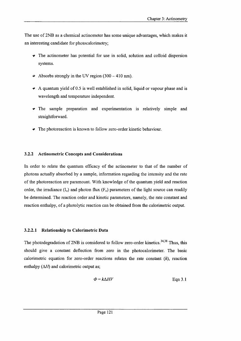
Chapter 3: Actinometry
The use o f 2NB as a chemical actinometer has some unique advantages, which makes it
an interesting candidate for photocalorimetry;
The actinometer has potential for use in solid, solution and colloid dispersion
systems.
^ Absorbs strongly in the UV region (3 0 0 -4 1 0 nm).
■ir A quantum yield o f 0.5 is well established in solid, liquid or vapour phase and is
wavelength and temperature independent.
^ The sample preparation and experimentation is relatively simple and
straightforward.
The photoreaction is known to follow zero-order kinetic behaviour.
3.2.2 Actinometric Concepts and Considerations
In order to relate the quantum efficacy o f the actinometer to that of the number of
photons actually absorbed by a sample, information regarding the intensity and the rate
o f the photoreaction are paramount. With knowledge o f the quantum yield and reaction
order, the irradiance (U) and photon flux (Fo) parameters o f the light source can readily
be determined. The reaction order and kinetic parameters, namely, the rate constant and
reaction enthalpy, o f a photolytic reaction can be obtained from the calorimetric output.
3.2.2.1 Relationship to Calorimetric Data
The photodegradation o f 2NB is considered to follow zero-order k i n e t i c s .T h u s , this
should give a constant deflection from zero in the photoealorimeter. The basic
calorimetric equation for zero-order reactions relates the rate constant (k), reaction
enthalpy (AH) and calorimetric output as;
0 = kAH V Eqn 3.1
Page 121

Chapter 3: Actinometry
where; 0 is the calorimetric output (W)
k is the rate constant (mol dm'^ s’’)
M i is the reaction enthalpy (J mol’’)
V is the volume o f the actinometer solution (dm^)
In order to relate the irradiance and, subsequently, the photon flux o f the light source to
the calorimetric output, there is a stipulation that either the rate constant or reaction
enthalpy be known. However, neither of these parameters is well established in the
literature. This puts a constraint on the system and requires the need for an ancillary
method o f investigation for the determination o f either k or M i. There is insufficient
information available in the literature to make an accurate calculation o f the bond
enthalpies associated in solution phase systems during the photolysis o f 2NB. Therefore
an auxiliary method for determining a value for k was sought. Since the
photodecomposition o f 2NB results in the formation o f an acidic product, 2NBA, it is
possible to derive a value for k with the knowledge o f the number o f moles o f product
formation and the irradiation time. This can be obtained by monitoring the changes in
pH as the photoproduct, 2-nitrosobenzoic acid, builds up as the actinometer solution is
irradiated or a simple titration with a basic solution (e.g. NaOH) can be performed to
determine the number o f moles o f acid [H^] formed. These measurements were taken
for the two light sources used; Xe arc lamp and an array o f LEDs (pH measurements
were taken for the LED light source only).
Once a value for k has been established, the irradiance and photon flux can be readily
determined following the procedure outlined” in section 3.2.2.2. All experimental
procedures are detailed in section 3.2.3.
Page 122
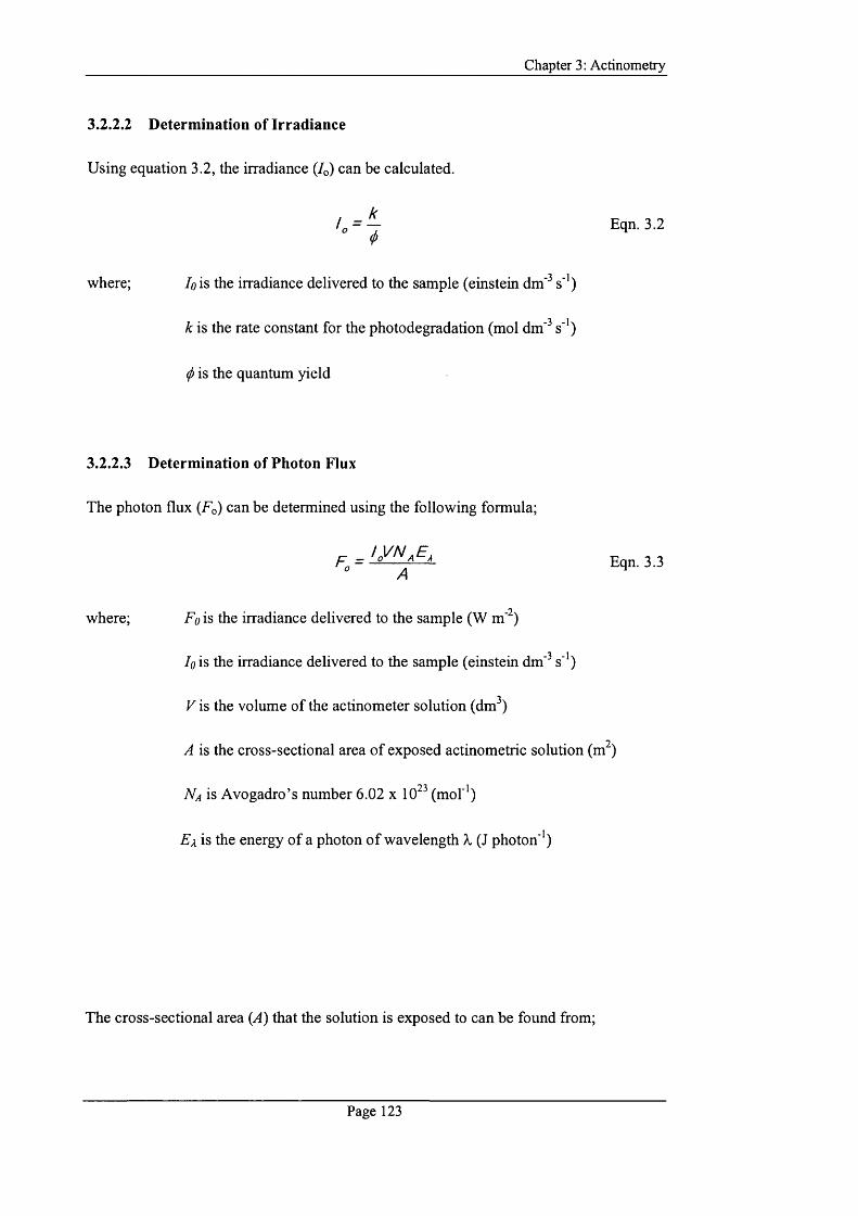
Chapter 3: Actinometry
3.2.2.2 Determination of Irradiance
Using equation 3.2, the irradiance (/q) can be calculated.
Io = ^ Eqn. 3.2(!>
where; h is the irradiance delivered to the sample (einstein dm'^ s’')
k is the rate constant for the photodegradation (mol dm’ s’')
^ is the quantum yield
3.2.2.3 Determination of Photon Flux
The photon flux (Fq) can be determined using the following formula;
_ L V N .E , A
Fo = T - Eqn. 3.3
-2\where; Fo is the irradiance delivered to the sample (W m’ )
Iq is the irradiance delivered to the sample (einstein dm’ s ')
V is the volume of the actinometer solution (dm^)
A is the cross-sectional area o f exposed actinometric solution (m^)
N a is Avogadro’s number 6.02 x 10^ (mol ')
is the energy o f a photon o f wavelength X (J photon ')
The cross-sectional area (A) that the solution is exposed to can be found from;
Page 123

C h a p ter 3: A c t in o m e tr y
where;
A = nr'
X is the radius o f the am poule (m)
Eqn. 3.4
The dim ensions o f a 20 m L ealorimetrie am poule (Fig. 3.2) w ere m easured aeeurately
using a m icrom eter in order to calculate the eross-seetional area o f the base (Fig. 3.3).
60.0
27.4
58.3
Fig. 3.2: 20 niL stainless steel calorimetric ampoule
Fig. 3.3: Dimensions (mm) of a 20 niL calorimetric ampoule
All dimensions are given in mm units; Inner diameter: 24.1, Outer diameter: 27.4,
Depth: 58.3, Height: 60.0.
Area (A) of ampoule base (in unit of ni ) is: ;r0 .01205" = 4 .5 6 x 10^ m
.’. Cross-sectional area of ampoule base used was 4.56 x 10' m .
The distance between the tip o f the liquid light guide and the base o f the am poule was
m easured at 24.3 mm (Fig. 3.4).
v-4
P a g e 124
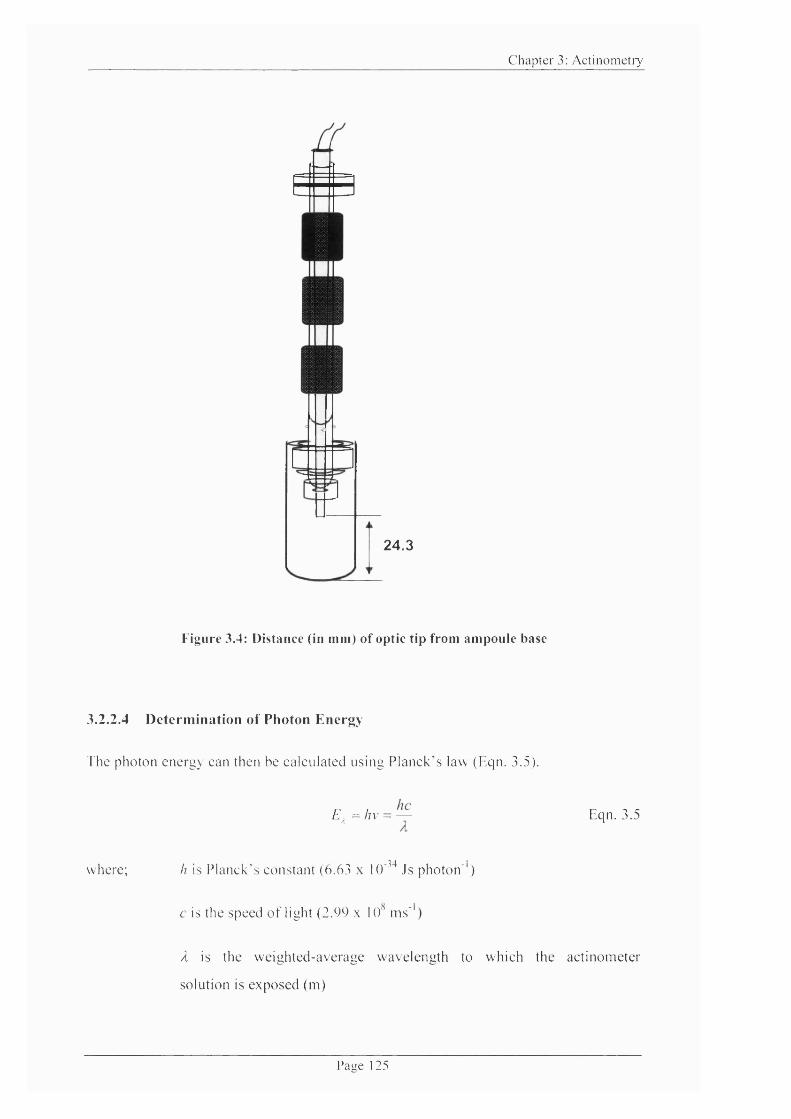
C h a p ter 3; A c t in o m e tr y
24.3
Figure 3.4: Distance (in mm) of optic tip from ampoule base
3.2.2.4 Determination of Photon Energy
The photon energy can then be calculated using P lanck 's law (Eqn. 3.5).
E , = l i v - — Eqn. 3.5
where; h is P lanck 's constant (6.63 10'^^ Js pho ton ' ')
c is the speed o f light (2.99 x 10 ms
À is the w eighted-average wavelength to which the actinom eter
solution is exposed (m)
P a u e 125
Chapter 3: Actinometry
The wavelength range o f interest is between 290 - 400 nm therefore the 2NB
actinometer solution should absorb all the photons between these ranges converting the
2NB to 2NBA with equivalent efficiency. However, when a polychromatic light source,
such as that of a Xe arc lamp is used, it emits a different number o f photons over the
period o f irradiation at each wavelength. The number o f photons that are released over a
specific bandwidth (e.g. 3 8 0 - 382 nm) will impact on the total energy flux in the 290 -
400 nm range i.e. the release o f a relatively large number o f photons at shorter
wavelengths may have higher energy photons compared to fewer photons at longer
wavelengths. It is, therefore, necessary to estimate a weighted-average photon energy
incident upon and absorbed by the actinometer solution. This estimation is required in
all cases where a polychromatic light source is used for photostability testing.
Typically, the weighted-average wavelength can be determined by examination o f the
energy distribution (spectroradiometric data) which is available either from
manufacturers o f the light source for the specific lamp used, or by in-house
measurement using spectroradiometry (discussed later section 3.3). The
spectroradiometric data are used to calculate the weighted-average wavelength for that
specific light source. These data were obtained using a spectroradiometer for the two
light sources; Xe arc lamp and LED. The energies expressed in units o f w W were
obtained over a narrow bandwidth in the wavelength range o f interest i.e. 290 - 400 nm
for the Xe lamp, 370 - 400 nm for the single LED system, and 350 - 400 nm for the
array o f LEDs used. If the wavelength range for the Xe lamp is taken as an example, the
weighted-average wavelength was determined by the product o f the wavelengths and
irradiance over each bandwidth summed over the wavelength range o f 290 - 400 nm
and divided by the irradiance over each bandwidth summed over 290 - 400 nm. This
can be expressed using the following formula;
400 nm
^ (À nm) (irradiance Wm'^)------------------------------ Eqn. 3.6
^ irradiance Wm290 nm
The weighted-average values obtained using the Xe lamp and LED light source were
determined in this manner and are given in section 3.3. These data were then used to
Page 126

Chapter 3: Actinometry
calculate a weighted-average photon energy value using Planck’s law as already
described (Eqn. 3.5).
3.2.3 Determination of rate constant (A) using ancillary methods
3.2.3.1 Photochemical Titration Analysis of 2NB
One o f the methods used to determine a zero-order rate constant for the
photodegradation o f 2NB was to measure the formation o f the photoproduct as a
function o f irradiation time using titration analysis. The photochemical reaction results
in a conversion o f the aldehyde functionality into an acid. Knowledge o f the irradiation
time, over which this photo lytic process occurs, can be used to calculate readily the acid
formation by means o f titration o f the actinometer solution with a basic solution
(NaOH). The endpoint o f the reaction can then be determined using an acid-base
indicator (phenolphthalein) so that a visible colour change (from yellow to pink) could
be detected. These measurements were performed with only the Mark II
photocalorimeter i.e. Xe lamp source.
Materials and Methods
2-Nitrobenzaldehyde (2NB, >98%) and Phenolphthalein indicator was purchased from
Sigma Aldrich UK. Sodium Hydroxide (GPR) was purchased from BDH Laboratory
Supplies Ltd, UK. Ethanol (99.7-100%) was purchased from Hayman Ltd, UK.
Deionised water was used throughout. All materials were used as received.
2NB Actinometer Solution Preparation
The actinometer solution was prepared using 0.1 M 2NB. 1.5112 g o f 2NB was weighed
and crushed using a pestle and mortar to aid dissolution o f the sample. The solid was
dissolved using 1:1 ethanol/de-ionised water solvent mixture and stirred for approx. 30
minutes using a magnetic stirrer until the solid had completely dissolved. The solution
was then made up to volume (100 mL).
Page 127
Chapter 3: Actinometry
Reference Photocalorimetric Experiment
It was necessary to perform a reference experiment to blank the instrument before
sample measurements were taken. This was required in order to obtain an overall net
zero power signal when the light was switched on.
This was achieved by placing 1:1 ethanol/de-ionised water solvent mixture (4 mL) in
both the sample and reference ampoules (20 mL stainless steel) prior to the sample
measurement. The ampoules were lowered into the TAM (described in Chapter 2) and
the Xe lamp was set to 240 W and switched on for at least one hour before irradiating
the solutions. The photocalorimeter’s optical arrangement using the shutters was set so
as to obtain a zero power output with the light on. The light on/off repeatability was
assessed in at least duplicate. The light was then switched off. Assuming that the
experimental set up remains unchanged throughout the measurements on the sample
tested, it would be the case that the net signal is zero and therefore any change is as a
result o f the photodegradation of the actinometer solution.
Sam ple Experiment - Titration M ethod
Exactly 4 mL o f the actinometric solution was pipetted into a 20 mL stainless steel
calorimetric ampoule. The Xe arc lamp (240 W) was switched on for at least one hour.
The actinometer solution was then irradiated for a known period o f time. The irradiated
sample was then transferred to a pyrex glass flask and approximately 30 pL 0.1% w/v
phenolphthalein indicator was added after the sample had been irradiated. The indicator
solution was prepared using 1:1 ethanol/de-ionised water. The actinometer solution was
titrated with 0.03 M NaOH using a 10 pL pipette until an endpoint (visible colour
change from yellow to pink) was reached. This photochemical titration method was
repeated for samples that were irradiated every 10 minutes up to 1 hour total exposure
time. A reference titration was performed with un-irradiated freshly prepared 2NB
solution representing t = 0. The volume o f NaOH used to reach the endpoint was used to
determine the number o f moles o f acid formed upon photolysis and plotted against
irradiation time. Consequently, a value o f the rate constant in mol dm'^ s'' can be
obtained by determining the gradient o f the plot.
Page 128
Chapter 3: Actinometry
3.2.3.2 pH measurements
Another method used to determine a rate constant o f the 2NB photolytic reaction was by
means o f pH measurements. The changes in pH were followed as the actinometer
solution was irradiated and used to determine the number o f moles o f acid formed [H^]
as a function o f irradiation time. These measurements were performed for both the Mark
II and Mark III photocalorimeters i.e. light sources; Xe lamp and array o f LEDs,
respectively.
Materials and Methods
2-Nitrobenzaldehyde (>98%) and ethylenediamine tetraacetic acid (EDTA) were
purchased from Sigma Aldrich UK. Ethanol (99.7 - 100%) was purchased from
Hayman Ltd, UK. Deionised water was used throughout. All materials were used as
received.
Reference Photocalorimetric Experiment
The actinometer solution (0.1 M 2NB) was prepared and a blank experiment was
performed. The method for the solution preparation and reference experiment method
for the Xe lamp photocalorimeter have already been described above in section 3.2.3.1).
The reference experiment using the LED photocalorimeter was performed in a similar
m anner to that o f the Xe lamp photocalorimeter. The calorimetric ampoules were loaded
with 1:1 ethanol/de-ionised water solvent mixture (4 mL) prior to the sample
measurement. The method o f lowering ampoules into the TAM has already been
described (Chapter 2). The voltage supplied to the sample and reference sides was set to
a desired voltage (e.g. 15 V). The full array o f LEDs (covering a wavelength range o f
360 - 700 nm) was switched on and the voltage on the reference side was then adjusted
until a zero calorimetric signal was obtained. Following the blank (reference)
experiment, the sample ampoule was replaced with the actinometer solution (the
methods o f which are given below for the Xe arc lamp and LED photocalorimeters).
Page 129
Chapter 3: Actinometry
Sample Experiment
The pH measurements were recorded with a Hamilton pH glass electrode;
electrochemical sensor (sensitive to 0.01 unit), which was connected to a Hanna pH
microcomputer HI9024. Buffer solutions at pH 4 and 8 were used to calibrate the pH
meter. A 4 mL aliquot o f the actinometer solution was pipetted into in a 20 mL stainless
steel calorimetric ampoule. The 2NB solution was then irradiated for a known period of
time and the pH was measured. The same sample solution was re-attached to the liquid
light guide for further UV exposure and the pH was determined again. This process was
repeated several times taking pH readings at every 10 min irradiation intervals for a
total exposure time of 3 hours. The rate constant was determined by following the
changes in pH as the amount o f photoproduct, 2NBA, built up as a function of
irradiation time.
All titration and pH experiments were conducted in at least in triplicate. For each new
experiment a fresh aliquot o f 2NB solution was taken from the stock solution. The
ampoule was washed with deionised water and ethanol and dried after each experiment.
The sample solution was maintained at a constant temperature o f 310 K by placing the
ampoule in a steel heat block.
All actinometry experiments were performed under dark conditions i.e. red light and all
solutions were contained in amber glassware that was foil wrapped.
Method for Photocalorimetric measurements
The method for the preparation o f 2NB solution and the procedure for the reference
experiment using the Xe lamp photocalorimeter have already been described in section
3.2.3.1.
The procedure for the reference experiment using the LED photocalorimeter has already
been described in section 3.2.3.2.
Page 130
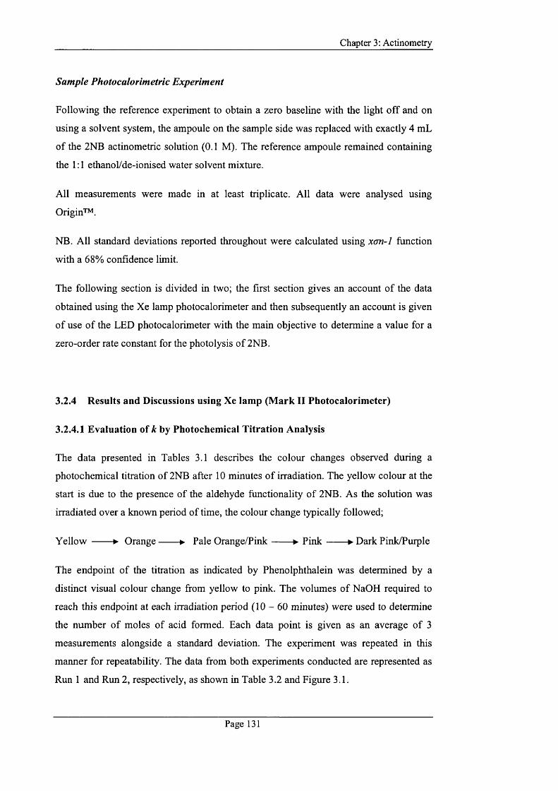
Chapter 3: Actinometry
Sample Photocalorimetric Experiment
Following the reference experiment to obtain a zero baseline with the light off and on
using a solvent system, the ampoule on the sample side was replaced with exactly 4 mL
of the 2NB actinometric solution (0.1 M). The reference ampoule remained containing
the 1:1 ethanol/de-ionised water solvent mixture.
All measurements were made in at least triplicate. All data were analysed using
Origin'^^.
NB. All standard deviations reported throughout were calculated using xcm-l function
with a 68% confidence limit.
The following section is divided in two; the first section gives an account o f the data
obtained using the Xe lamp photocalorimeter and then subsequently an account is given
o f use o f the LED photocalorimeter with the main objective to determine a value for a
zero-order rate constant for the photolysis o f 2NB.
3.2.4 Results and Discussions using Xe lamp (Mark II Photocalorimeter)
3.2.4.1 Evaluation of k by Photochemical Titration Analysis
The data presented in Tables 3.1 describes the colour changes observed during a
photochemical titration o f 2NB after 10 minutes o f irradiation. The yellow colour at the
start is due to the presence o f the aldehyde functionality o f 2NB. As the solution was
irradiated over a known period o f time, the colour change typically followed;
Y e llo w ► O range ► Pale O range/P ink ► P in k ► Dark Pink/Purple
The endpoint o f the titration as indicated by Phenolphthalein was determined by a
distinct visual colour change from yellow to pink. The volumes o f NaOH required to
reach this endpoint at each irradiation period ( 1 0 - 6 0 minutes) were used to determine
the number o f moles o f acid formed. Each data point is given as an average o f 3
measurements alongside a standard deviation. The experiment was repeated in this
manner for repeatability. The data from both experiments conducted are represented as
Run 1 and Run 2, respectively, as shown in Table 3.2 and Figure 3.1.
Page 131
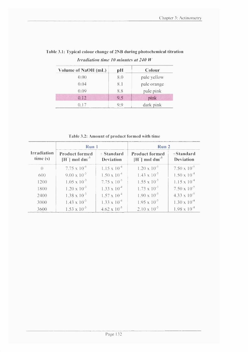
C h a p ter 3: A c t in o m e tr y
Table 3.1: Typical colour change of 2NB during photochemical titration
Irradiation time 10 m inutes at 240 W
Volum e of N aO H (m L) pH C olour
0.00 8.0 pale yellow
0.04 8.1 pale orange
0.09 8.8 pale pink
0.12 9.5 pink
0.17 9.9 dark pink
Table 3.2: Amount of product formed with time
Irra d ia tio n tim e (s)
R un 1 R un 2
P ro d u c t fo rm ed |H " | mol duT^
± S ta n d a rd D eviation
P roduct fo rm ed |H *| m o ld i n '
^ S ta n d a rdD eviation
0 7.75 X 10" 1.15 X 10" 1.20 X 10 ' 7.50 X 1 o '600 9.00 X 10'^ 1.50 X 10“ 1.43 X 10 ' 1.50 X 10“*1200 1.05 X 10'^ 7.75 X 10'^ 1.55 X 10"' 1.15 X lO"*1800 1.20 X 10'^ 1.33 X 10"* 1.73 X 10 ' 7.50.x 1 0 '
2400 1.38 X 10'^ 1.57 X 10"^ 1.90 X 10 ' 4.33 X 10 '3000 1.43 X 10'^ 1.33 X 10" 1.95 X 10 ' 1.30 X 10 *3600 1.53 X 10'^ 4.62 X 10'^ 2.10 X 10 ' 1.98 X 10“*
P a g e 132
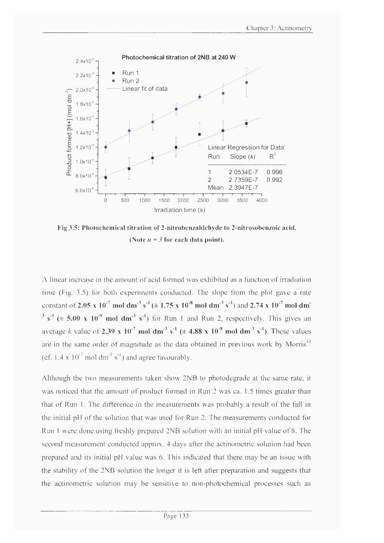
C h a p ter 3; A c t in o m e tr y
2 .4 x 1 0 -
2 .2x10 '-
2.0x10'-
1.8x10'-
1.6x10'-
1.4x10'-
1.2x10'-
1.0x10'-
8.0x10^-
6.0x10""-
Photochemical titration of 2NB at 240 W
■ Run 1 • Run 2
Linear fit of data
Linear Regression for Data: Run Slope {k) R^
12Mean
2.0534E-7 0.9962.7359E-7 0.9922.3947E-7
—I—500 1000 1500 2000 2500 3000 3500 4000
Irradiation time (s)
Fig 3.5: Photochemical titration of 2-nitrobenzaldehycie to 2-nitrosobenzoic acid.
(Note n = 3 for each data point).
A linear increase in the am ount o f acid fonned was exhibited as a function o f irradiation
tim e (Fig. 3.5) for both experim ents conducted. T he slope from the plot gave a rate
constant o f 2.05 x 10'^ mol dm'^ s ' (± 1.75 x 10 mol dnT s ') and 2.74 x 10^ mol dm
s ' (± 5.00 X 10'* mol dm s ') for Run 1 and Run 2, respectively. This gives an
average k value o f 2.39 x 10^ mol dm^ s ' (± 4.88 x 10" mol dm^ s '). T hese values
are in the sam e order o f m agnitude as the data obtained in previous work by Morris^^
(ef. 1.4 X 10'^ mol dm'^ s'") and agree favourably.
A lthough the two m easurem ents taken show 2N B to photodegrade at the sam e rate, it
was noticed that the am ount o f product formed in Run 2 was ca. 1.5 times greater than
that o f Run 1. The difference in the m easurem ents was probably a result o f the fall in
the initial pH o f the solution that was used for Run 2. T he m easurem ents conducted for
Run 1 w ere done using freshly prepared 2NB solution with an initial pH value o f 8. The
second m easurem ent conducted approx. 4 days after the actinometric solution had been
prepared and its initial pH value was 6. This indicated that there m ay be an issue with
the stability o f the 2NB solution the longer it is left after preparation and suggests that
the actinom etric solution m ay be sensitive to non-photochem ical processes such as
P a g e 133
Chapter 3: Actinometry
oxidation. A significant change in pH can have significant impact on the photostability
o f the solution and required further investigation.
Furthermore, this approach is somewhat tedious and problematic because the change in
colour occurred very rapidly with the addition o f very small quantities o f base (as
shown above in Table 3.1). Typically <0.3 mL o f base was a sufficient amount to reach
the reaction endpoint, for which reason, 10 pL o f base was added at a time to ensure
accuracy. Moreover, it should be noted that making a colour change observation under
subdued light i.e. dark room using red light, can be subjective and makes it difficult to
define accurately the true end point. Attempts to detect the endpoint under normal room
lighting within the laboratory to get a better visual o f the colour change to pink proved
more difficult because the reaction solution changed colour very rapidly; reverting the
colour from pink, back to orange and/or yellow. This suggests that the reaction was
unstable and undergoing a combined effect o f both 2NB photolysis and the
photodegradation of phenolphthalein.
In order to avoid such errors, and to investigate further the change in the solution pH as
observed with the photochemical titration data, another approach to determine a rate
constant was sought; the changes in the solution pH were monitored as the
photoreaction proceeded.
3.2.4.2 Evaluation of k by pH measurements
The changes in pH were followed every 10 minutes over an irradiation period o f three
hours. The number o f moles o f acid [H^] formed in a 4 mL sample solution was then
readily calculated using the pH formula; pH = - log [H^].
The data obtained are represented in Table 3.3 and Figure 3.6.
Over the course o f the experiments, it was found that the response obtained from the pH
data was unexpected. It can be seen that over an initial period o f ca. 100 min there was
very little change in the amount o f product formed. After this period, there was a sharp
linear increase with time. In terms o f the changes in pH; freshly prepared 2NB solution
gave an initial pH of 8 before gradually declining to pH 6 during the initial 100 min o f
Page 134
Chapter 3: Actinometry
exposure. As the sample was irradiated further, the rate o f change in pH became rapid
over which time the pH declined from 6 to 4, consistent with the formation o f 2-
nitrosobenzoic acid. The initial “lag phase” observed implies that an additional event
may be occurring prior to photodegradation into 2-nitrosobenzoic acid and, because of
the considerable curvature, it was not possible to determine a rate constant for the
reaction.
Suspecting that an oxidation process was responsible, based on observations from pH
and acid-base titration measurements, the experiment was repeated with the addition o f
a small quantity o f ethylenediamine tetraacetic acid (EDTA). In the event o f an
oxidation process, EDTA can be used as a chelating agent to remove any free metal ions
and so to prevent them catalysing oxidative processes. The metal ions may have
unavoidably been introduced into the solution as contaminants present in the deionised
water used and on the glassware.
The 2NB solution was prepared in the same manner as that described in section 3.2.3.1,
but in addition, approximately 50 mg of EDTA was added to the actinometric solution.
The pH measurements were conducted in the same manner over an irradiation period o f
3 hours.
The data obtained in the presence and absence o f EDTA is tabulated in Table 3.3 and
shown in Figure 3.6 for comparison.
Page 135
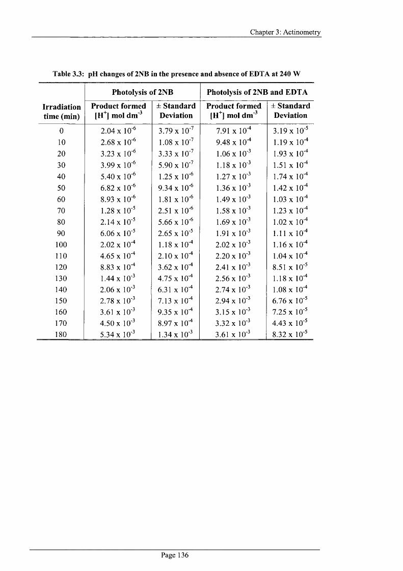
Chapter 3: A ctinom etry
Table 3.3: pH changes of 2NB in the presence and absence of EDTA at 240 W
Photolysis of 2NB Photolysis o f 2ND and EDTA
Irradiation Product formed ± Standard Product formed ± Standardtime (min) [H^] mol dm ^ Deviation [H^] mol dm^ Deviation
0 2.04 X 10*’ 3.79 X 10'' 7.91 X 10'" 3.19 X 10'"
10 2.68 X 10'^ 1.08 X 10 ' 9.48 X 10'" 1 .1 9 x 10'"
20 3.23 X lO'* 3.33 X 10 ' 1.06 X 10'" 1.93 X 10'"
30 3.99 X 10 '’ 5.90 X 10''' 1.18 X 10'" 1.51 X 10""
40 5.40 X 10'^ 1.25 X 10'* 1.27 X 10'" 1.74 X 10'"50 6.82 X 10'^ 9.34 X 10'’ 1.36 X 10" 1.42 X 10'"
60 8.93 X lO" 1.81 X 10" 1.49 X 10'" 1.03 X 10'"
70 1.28 X 10'^ 2.51 X 10'" 1.58 X 10'" 1.23 X 10'"
80 2.14 X 10 5.66 X 10'" 1.69 X 10'" 1.02 X 10'"
90 6.06 X 10 ^ 2.65 X 10'" 1.91 X 10'" 1.11 X 10'"100 2.02 X lO"” 1.18 X 10'" 2.02 X 10'" 1.16 X 10'"110 4.65 X 10“* 2.10X 10'" 2.20 X 10'" 1.04 X 10'"120 8.83 X lO"" 3.62 X 10'" 2.41 X 10'" 8.51 X 10'"
130 1.44 X 10'^ 4.75 X 10"" 2.56 X 10'" 1.18 X 10"*140 2.06 X 10'^ 6.31 X 10'" 2.74 X 10'" 1.08 X 10""150 2.78 X 10'^ 7.13 X 10'" 2.94 X 10'" 6.76 X 10'"160 3.61 X lO'^ 9.35 X 10'" 3 .15x10 '" 7.25 X 10'"170 4.50 X 10 ^ 8.97 X 10"" 3.32 X 10'" 4.43 X 10'"180 5.34 X 10'^ 1.34 X 10'" 3.61 X 10'" 8.32 X 10'"
P age 136
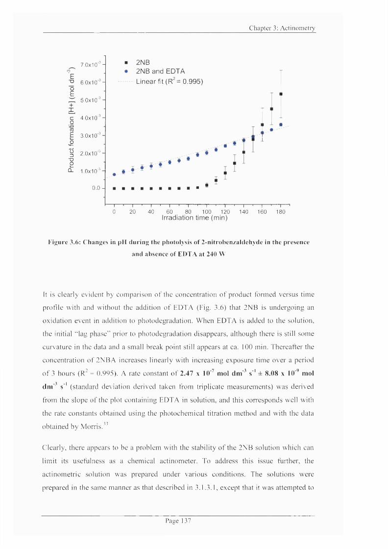
C h a p ter 3: A c t in o m e tr y
7 .0x10 'H
6.0x10 -0 EX 5.0x10" M +1c 4.0x10"- oC DE 3 .0x10 '- £"§ 2.0x10"'-
?Û- 1.0x10"'-
0.0 -
2NB2NB and EDTA Linear fit (R^= 0.995)
i Î
■ - *
I ' I ' I ' I ' I ' ! ' I ' I ' I ' I
0 20 40 60 80 100 120 140 160 180Irradiation time (min)
Figure 3.6: Changes in pH during the photolysis of 2-nitrobenzaldehyde in the presence
and absence of EDTA at 240 VV
it is clearly evident by comparison o f the concentration o f product formed versus time
profile with and without the addition o f ED TA (Fig. 3.6) that 2NB is undergoing an
oxidation event in addition to photodegradation. W hen EDTA is added to the solution,
the initial " lag phase" prior to photodegradation disappears, although there is still som e
cuiwature in the data and a small break point still appears at ca. 100 min. Thereafter the
concentration o f 2N B A increases linearly with increasing exposure time over a period
o f 3 hours (R^ = 0.995). A rate constant o f 2.47 x 10 mol dm s ' ± 8.08 x 10 mol
dm ^ s ' (standard deviation derived taken from triplicate m easurem ents) was derived
from the slope o f the plot containing E D TA in solution, and this corresponds well with
the rate constants obtained using the photochem ical titration m ethod and with the data
obtained by M o m s. 33
Clearly, there appears to be a problem with the stability o f the 2NB solution which can
limit its usefulness as a chemical actinometer. To address this issue further, the
actinom etric solution was prepared under various conditions. The solutions were
prepared in the same m anner as that described in 3.1.3.1, except that it was attem pted to
P a g e 137
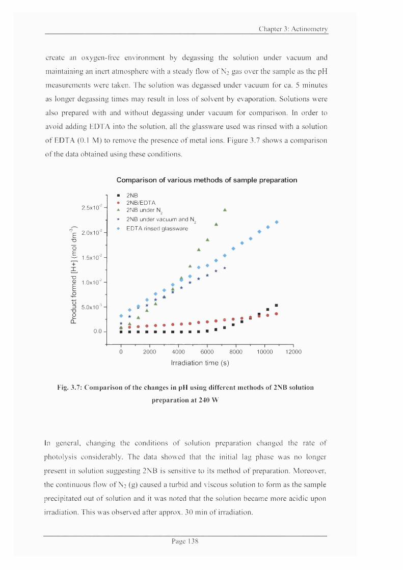
C h a p ter 3: A c t in o m e tr y
create an oxygen-free environm ent by degassing the solution under vaeuum and
m aintaining an inert a tm osphere with a s teady flow o f N? gas over the sam ple as the pH
m easurem ents w ere taken. The solution was degassed under vacuum for ca. 5 minutes
as longer degassing times m ay result in loss o f solvent by evaporation. Solutions were
also prepared with and without degassing under vacuum for comparison. In order to
avoid adding EDTA into the solution, all the glassw are used was rinsed with a solution
o f EDTA (0.1 M) to rem ove the presenee o f metal ions. Figure 3.7 shows a eomparison
o f the data obtained using these eonditions.
Comparison of various methods of sample preparation
ETDÔ£
X
2.5x1 OM
2 .0 x 1 0 -
1.5x10 -
1 1.0x10"
5.0x10o
-3
0 .0 -
■ 2NB• 2NB/EDTA ^ 2NB under* 2NB under vacuum and♦ EDTA rinsed glassware
* ♦ * * *
♦ • :. # # #
i t ............................................. . ■ "I #
2000 4000 6000 8000 1 ' 110000 12000
Irradiation time (s)
Fig. 3.7: Comparison of the changes in pH using different methods of 2NB solution
preparation at 240 \V
In general, changing the conditions o f solution preparation changed the rate o f
photolysis eonsiderably. The data showed that the initial lag phase was no longer
present in solution suggesting 2NB is sensitive to its m ethod o f preparation. M oreover,
the eontinuous flow o f N] (g) caused a turbid and viscous solution to fonn as the sample
precipitated out o f solution and it was noted that the solution becam e m ore acidic upon
irradiation. This was observed after approx. 30 m in o f irradiation.
P a n e 138
Chapter 3: Actinometry
The data indicate that the photodegradation o f 2NB may not follow a simple reaction
scheme as that shown in Fig. 3.1, which considers the photorearrangement o f 2NB into
2NBA as an irreversible process with no side-reactions occurring. However, several
investigators in recent years have suggested otherwise and different types o f reaction
processes have been p r o p o s e d .U s i n g analytical techniques such as Electron Spin
Resonance (ESR)"^ and Femtosecond Vibrational Spectrosopy'^' it has been postulated
that the formation o f mixed radicals, during the photochemical process, result in parallel
or secondary reactions occuring simultaneously with the photoisomerisation o f 2NB
into 2NBA. The extent to which the reactions occur is governed by the type o f light
source, experimental design and set-up, conditions o f sample preparation, intensity o f
light, etc, and so all these factors will influence the rate and extent of any
photodegradation process. Usually, there are two stages involved in a photochemical
reaction. These are; a primary reaction that occurs as a direct consequence o f photon
absorption, and thus involves the excited state o f molecules; the primary reaction will
then often be followed by secondary (thermal) reactions occurring from intermediate
products produced by primary processes (radicals, radical ions, etc). Such intermediates
can eventually react through ‘dark’ reactions to form final, stable products. The light
intensity will influence the extent to which the photodegradation occurs i.e., at a high
intensity level, secondary reactions may readily occur, but this may not necessarily be
the case at low intensity levels as it would take longer for the reaction to reach a
secondary stage and thus this will not be detected during the observed irradiation period.
Since an exhaustive study o f the photodegradation o f 2NB was not the main objective o f
this project, further work was not conducted. However, it is simply noted that there
appears to be complexity in the photochemical reaction o f 2NB and shows sensitivity to
non-photochemical processes which can limit its use as a chemical actinometer
particularly for use with high intensity xenon arc light sources. For its purpose o f use in
this work, it is important to note that care must be taken during preparation/handling
and use o f 2NB.
The next stage was then to study the response o f the photolysis o f 2NB in the
photocalorimeter.
Page 139
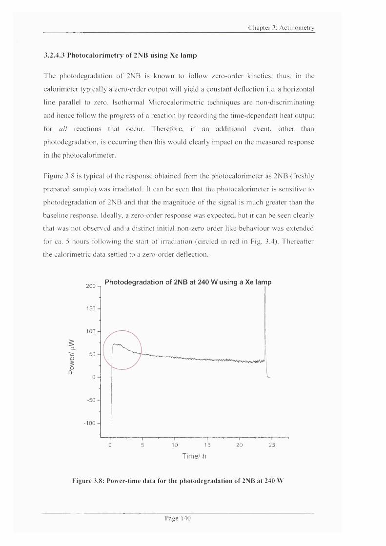
C h a p ter 3: A c t in o m e tr y
3.2.4.3 P ho tocalo rim etry of 2NB using Xe lam p
T he photodegradation o f 2NB is know n to follow zero-order kinetics, thus, in the
calorimeter typically a zero-order output will yield a constant deflection i.e. a horizontal
line parallel to zero. Isothennal M icrocalorim etric techniques are non-discrim inating
and hence follow the progress o f a reaction by recording the t im e-dependent heat output
for all reactions that occur. Therefore, i f an additional event, o ther than
photodegradation, is occurring then this w ould clearly impact on the m easured response
in the photocalorimeter.
Figure 3.8 is typical o f the response obtained from the photocalorim eter as 2NB (freshly
prepared sample) was irradiated. It can be seen that the photocalorim eter is sensitive to
photodegradation o f 2NB and that the m agnitude o f the signal is m uch greater than the
baseline response. Ideally, a zero-order response was expected, but it can be seen clearly
that was not observed and a distinct initial non-zero order like behaviour w as extended
for ca. 5 hours following the start o f irradiation (circled in red in Fig. 3.4). Thereafter
the calorimetric data settled to a zero-order deflection.
0oÛ-
2QQ Photodegradation of 2NB at 240 W using a Xe lamp
150
100
50
0
-50
-100
20 250 5 10 15
Time/ h
Figure 3.8: Power-time data for the photodegradation of 2NB at 240 VV
P a g e 1 4 0
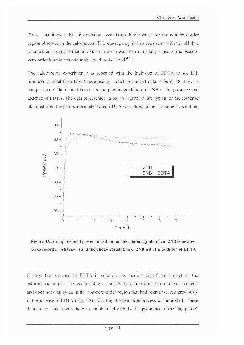
C h a p ter 3: A c t in o m e tr y
T hese data suggest that an oxidation event is the likely eause for the non-zero-order
region observed in the ealorimeter. This d iscrepancy is also consistent with the pH data
obtained and suggests that an oxidation event was the m ost likely cause o f the pseudo-
zero-order kinetic behaviour observed in the TAM."^'
T he calorimetric experim ent was repeated with the inclusion o f ED TA to see i f it
p roduced a notably different response, as noted in the pH data. Figure 3.8 show s a
com parison o f the data obtained for the photodegi adation o f 2NB in the presence and
absence o f EDTA. T he data represented in red in Figure 3.9 are typical o f the response
obtained from the photocalorim eter when E D TA was added to the actinom etric solution.
Q)o0_
90
60
30
2NB2NB + EDTA
0
-30
-60
-90
20 1 3 4 5 6 7
Time/ h
Figure 3.9: Comparison of power-time data for the photodegradation of 2NB (showing
non-zero-order behaviour) and the photodegradation of 2NB with the addition of EDTA
Clearly, the presenee o f EDTA in solution has m ade a s igniticant impact on the
calorim etric output. The reaction shows a steady deflection from zero in the calorimeter
and does not display an initial non-zero-order region that had been observed previously
in the absence o f ED TA (Fig. 3.8) indicating the oxidation process was inhibited. These
data are consistent with the pH data obtained with the d isappearance o f the "lag phase"
P a g e 141

C h a p ter 3: A c t in o m e tr y
(observed with 2NB alone) when E D TA was added to the solution. T he signal with
EDTA settled to give a stable deflection o f ca. 67 p W , although there is a slow drift in
the signal to ca. 63 p W after about 4 hrs o f irradiation (Fig. 3.9). This is also consistent
with the small variation noted in the pH m easurem ents containing EDTA. Repeat
measurem ents (Fig. 3.10) showed a sim ilar response, although, Run 3 in particular
show ed a larger drift than those for the first two experim ents suggesting the reaction
m ay still not he truly zero order. There are a num ber o f factors that could cause the
signal to drift such as com plexity in the reaction m echan ism , random noise caused by
small thermal fluctuations within solutions, long-tenn changes in the baseline as a result
o f environmental tem perature changes, and uncertainties in the variation o f the photon
energies produced from the polychrom atic photon source (xenon arc). It is estimated
that the output from xenon arc lamps can fluctuate as m uch as 20% over a period o f 5 or
6 h o u r s . T h e s e factors, therefore, can profoundly affect the output o f a sensitive T A M
and can introduce limits to the reproducibility o f the m easurem ents.
Photodegradation of 2NB in the prescence of EDTA80 -
60 -
40 -
20 -
- Run 1 Run 2 Run 3-20 -
i -40 -
-60 -
-80 -
-100 -
- 1 2 0 -
-140-
60 1 2 3 4 5 7
Time/ h
Figure 3.10: Power-time data for the photodegradation of 2NB in the presence of EDTA
P a iic 142
Chapter 3: Actinometry
Generally, the data have demonstrated that 2NB has sensitivity to non-photochemical
processes. W ith the inclusion o f EDTA, the initial oxidation process exhibited within
the first 5 hours o f irradiation appears to be inhibited, although there does still appear to
be some sensitivity shown towards either non-photochemical processes and/or factors
related to instrumental performance (such as those mentioned above). Under such
circumstances it became difficult to quantify accurately the “light dose” delivered to the
sample. Because o f the oxidation event, it was not possible to determine the photon flux
for the photolysis o f 2NB alone, but using the 2NB and EDTA data above (Fig. 3.10),
the photon flux can be estimated. These results are given in section 3.4 where the
photon flux data for all the light sources used are compared.
Furthermore, as mentioned in Chapter 2 (section 2.2.4), over the course o f the
measurements, there was a gradual decline in the performance o f the lamp which made
it difficult to obtain reproducible experimental measurements (Fig. 2.34 and further
explained in section 3.3.1.2). This then led on to the development o f an alternative
system where the use o f Light-Emitting Diodes was investigated as an alternative
photon source.
3.2.5 Results and Discussion using LED Mark III Photocalorimeter
Much o f the initial actinometry work, prior to the construction o f the custom-made array
o f LEDs used in the final set-up, was conducted using a single Ultra-bright UV LED
(10,000 mod). This was done in order to test proof-of-concept i.e., to assess if the
intensity o f light generated from a LED was sufficient enough to produce a detectable
power signal during a photochemical reaction. As the instrumental development work
progressed, the single LED was replaced with an array and subsequently actinometry
work was repeated using the LED array system. The set-up o f both these systems has
already been detailed in Chapter 2.
This section details the chemical actinometry work undertaken using, firstly, the single
LED system and subsequently the LED array photocalorimeter. The photodegradation
o f 2NB was followed for both the systems where a “light dose” delivered to the sample
was determined across 370 - 410 nm and 350 - 700 nm using the single LED system
and LED array system, respectively.
Page 143
Chapter 3; Actinometry
3.2.5.1 Preliminary Tests - Application of a single LED system
In order to quantify the photon flux between using the single LED system, the same
principles and sequence o f steps were followed as already described above (section
3.2.2). The first step was to determine a rate constant for the photodegradation o f 2NB,
then by applying it to the calorimetric output the irradiance and photon flux can be
readily determined.
The photon flux was determined using the photodegradation o f 2NB at 3 different
voltages; 10 V, 15 V, and 20 V. The rate constants were obtained by following the pH
changes at each input voltage. The process was then monitored in the photocalorimeter
and it was hoped that there would be a direct correlation between increasing voltage and
the power output o f the photodegradation o f 2NB.
The methods followed have already been described (section 3.2.3).
3.2.5.1.1 Evaluation of k by pH measurements
Figure 3.11 shows pH-time profiles for the photodegradation o f 2NB at 10, 15 and 20
V. A linear relationship between the amount o f product formed and the irradiation time
is observed. It can be seen that in this system, a lag phase is not observed in the first 100
min o f irradiation as in the case with the Xe lamp photocalorimeter. Xe lamps are
extremely powerful, far more intense than LEDs and, hence, it is thought that at such
intensity it may be the case that additional reactions (to photodegradation) are
occurring. There is already some evidence in the literature o f multiple (parallel or
simultaneous) reactions occurring as a result o f mixed radicals. It may be the case that
the Xe lamp is producing intensity that is far in excess o f that required to form 2NBA
alone and as a result initiating further reactions. It may be the case that the reaction may
not proceed this far with a single LED as the light intensity is far less. This may be why
a lag phase is observed within the first 100 min o f exposure using a Xe lamp and not
with the LED system.
Page 144

Chapter 3: A ctinom etry
Table 3.4: The am ount of product form ed using a single LED
Irradiation time (min)
102030
40
50
60
70
8090
100110120130
140
150
160
170
180
Amount of product formed [H^] (mol dm )
10 V
3.76 X 10 -3
5 .4 3 x 1 0 -3
5.95 X 10 -3
6.48 X 10 -3
6.48 X 10 -3
7.10 X 10"
7.73 X 10 -3
8.47 X 10
9.15 X 10
9.98 X 10
1.08 X 10
1 .1 2 x 10"
1.18 X 10
1.22 X 10
1.26 X 10
1.29 X 10
1.32 X 10
1.35 X 10
-3
-3
-3
-2
-2
-2
-2
-2
-2
-2
15 V
4.76 X 10 -3
6.48 X 10 -3
8.15 X 10 -3
9.88 X 10 -3
l . lO x 10'
1.22 X 10 -2
1.30 X 10⁻²
1.45 X 10 -2
1.58 X 10 -2
1.69 X 10
1.80 X 10
1 .9 3 x 1 0 '
2.08 X 10
2.08 X 10'
2.18 X 10 2.30 X 10
2.41 X 10'
2.50 X 10
-2
-2
-2
-2
-2
-2
20 V
5.22 X 10
7.21 X 10
8.67 X 10'
1.04 X 10
1.14 X 10
1.41 X 10
1.47 X 10
-3
-3
-2
-2
-2
-2
1.61 X 10'"
1.65 X 10
1.77 X 10
2.03 X 10
2.13 X 10
2.18 X 10
2.28 X 10
2.33 X 102.50 X 102.50 X 10
2.62 X 10
-2
-2
-2
-2
-2
-2
-2
-2
-2
-2
The slope o f the plots determ ined the follow ing rate constants; 9.2 x 10 \ 2.1 x 10 %
and 2.2 x 10' mol dm^ s '* at 10, 15, and 20 V, respectively (Fig. 3.11). As expected,
the rate o f reaction is faster as the voltage input is increased.
P age 145
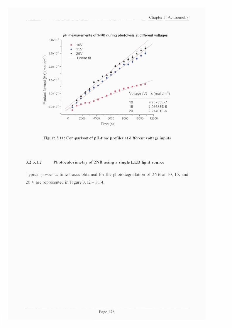
C h a p ter 3: A c t in o m e tr y
pH measurements of 2-NB during photolysis at different voltages
• 15VA 20V
Linear
■o0)E£o3■o2
1.0x10"- Voltage (V) k (mol dm' )
9.20733E-72.06688E-62.21401E-6
Q.5.0x10'-
0 2000 4000 6000 8000 10000 12000
Time (s)
Figure 3,11: Comparison of pH-time profiles at different voltage inputs
3.2.5.1.2 P ho tocalo rim etry o f 2NB using a single LED light source
Typical pow er \’5 time traces obtained for the photodegradation o f 2NB at 10, 15, and
20 V are represented in Figure 3 . 1 2 - 3 .1 4 .
P a g e 1 4 6
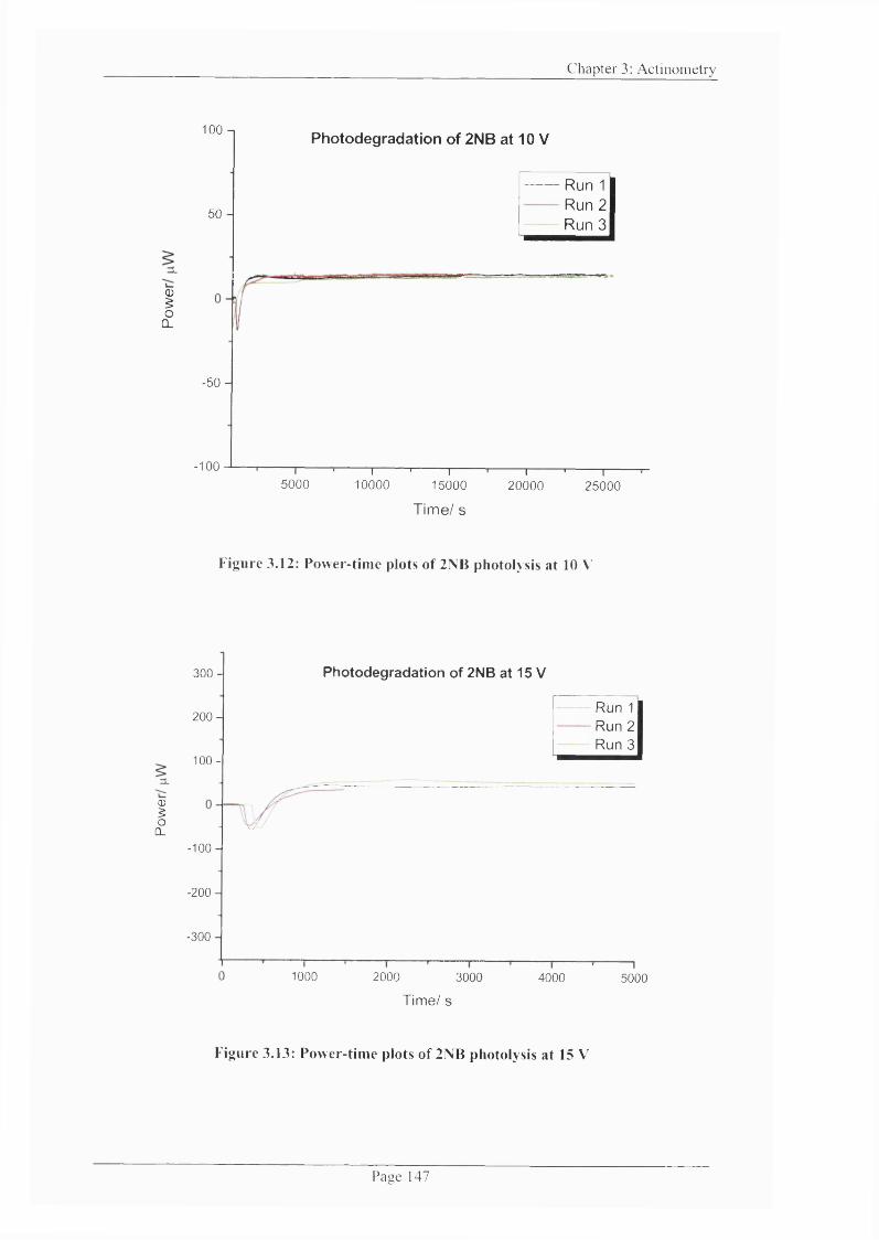
C h a p ter 3: A c t in o m e tr y
100 n
50 H
I-50 -
-100
Photodegradation of 2NB at 10 V
5000I ' I
10000 15000
Time/ s
Run 1Run 2Run 3
— I-------- '------ 1—20000 25000
Figure 3.12: Power-time plots of 2ND photolysis at 10 V
300-
2 0 0 -
100 -
<u$oQ_
- 1 0 0 -
- 2 0 0 -
-300-
V/
Photodegradation of 2NB at 15 V
1000 2000 3000
Time/ s
Run 1Run 2Run 3
4000 5000
Figure 3.13: Power-time plots of 2NB photolysis at 15 V
P a g e 147
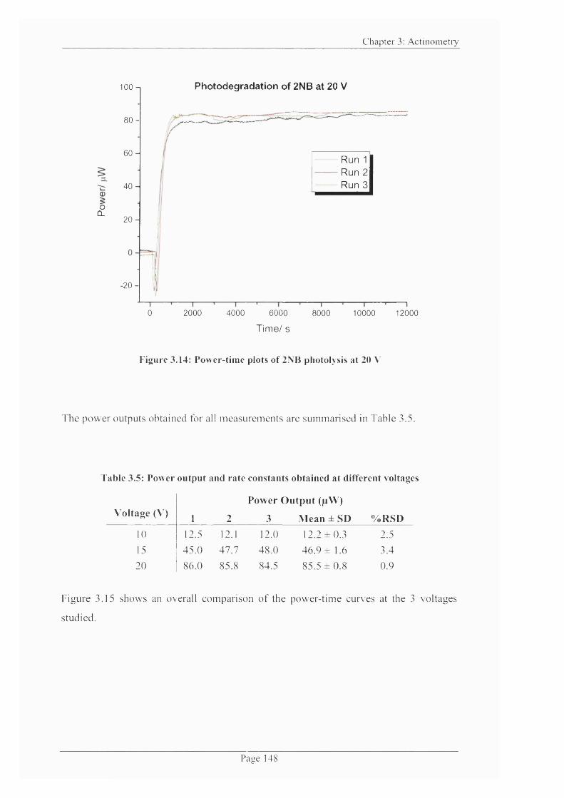
C h a p ter 3: A c t in o m e tr y
Photodegradation of 2NB at 20 V100 n
80 -
60 -Run 1 Run 2 Run 340 -
oo_
2 0 -
-20 -
0 2000 4000 6000 8000 10000 12000
T im e/ s
Figure 3.14: Power-time plots of 2NB photolysis at 20 V
The pow er outputs obtained for all m easurem ents are sum m arised in Table 3.5.
Table 3.5: Power output and rate constants obtained at different voltages
V oltage (V) 1 2
Pow er O u tp u t (pW )
3 M ean ± SD % R SD
10 12.5 12.1 12.0 12.2 ± 0 .3 2.5
15 45.0 47.7 48.0 46.9 ± 1.6 3.4
20 86.0 85.8 84.5 85.5 ± 0 .8 0.9
Figure 3.15 shows an overall com parison o f the power-tim e curves at the 3 voltages
studied.
P a g e 148
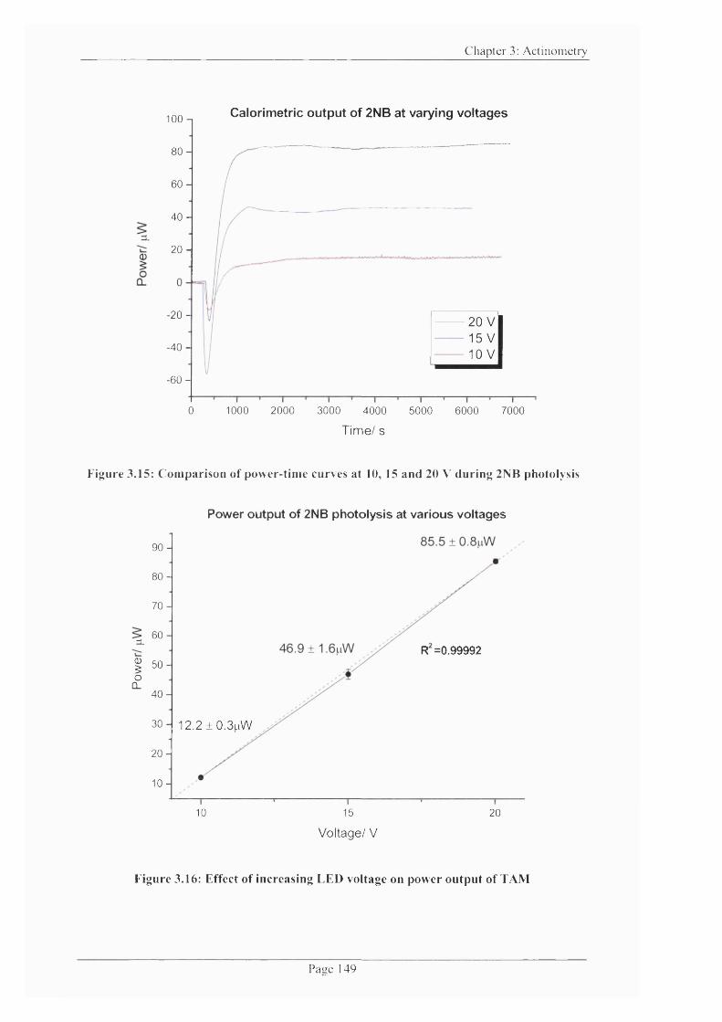
C h a p ter 3: A c t in o m e tr y
Calorimetric output of 2NB at varying voltages100 n
80 -
60 -
40 -
2 0 -
-20 - 20 V 15 V 10 V-40 -
-60 —
0 1000 2000 3000 4000 5000 6000 7000
Time/ s
Figure 3.15: Comparison of power-time curves at 10, 15 and 20 V during 2NB photolysis
Power output of 2NB photolysis at various voltages
90-
80-
70-
60 -R =0.99992
I 50-
S.40 -
30- 12.2±0.3uW
2 0 -
1 0 -
10 15 20
Voltage/ V
Figure 3.16: Effect of increasing LED voltage on power output of TAM
P a g e 1 4 9

Chapter 3: Actinometry
The data obtained are extremely encouraging. The first thing to note is that the outputs
show a constant deflection from zero in the calorimeter, evidence for zero-order
kinetics. Secondly, the voltage inputted to the system is directly proportional to the
power output o f the TAM. The higher the voltage, the larger the number o f moles that
react within the actinometer solution, and hence, the greater the power output in the
TAM. The relationship between the power output and voltage input is represented in
Figure 3.16 where measurements performed at 10 V, 15 V, and 20 V showed that the
heat output from the photolysis o f 2NB increased in proportion to the increase in
voltage supplied to the light source.
Generally, it can be seen that heat output is constant over the period o f irradiation using
the LEDs and the photoreaction does not exhibit the difficulties that were experienced
with the xenon arc lamp. The intensity o f the Xe arc lamp is very powerful compared to
the LEDs and it may be likely that the pseudo-zero order behaviour observed with 2NB
using the xenon lamp was caused as a result o f additional reactions occurring in the
solution. Moreover, another possible reason for this non-zero order behaviour could be
overheating o f the sample caused by the high heat output generated by xenon arc lamps,
and this also may lead to thermal decomposition processes that will complicate the
issue.
The above initial tests demonstrate that the system responds as hoped and, more
importantly, shows that LEDs have much potential in application to pharmaceutical
photostability testing.
3.2.5.1.3 D eterm ination of AJT and application to obtain k - single LED
Given the values o f k from the pH data and outputs (<P) from the calorimeter, the
enthalpy o f reaction (A//) can be determined using the zero-order calorimetric equation:
0 = kAH V (Eqn. 3.1)
Taking the measured response o f the first experiment at each voltage only. A // was
calculated by a simple re-arrangement o f Equation 3.1 :
Page 150

Chapter 3: Actinometry
A // — — Eqn. 3.1.1kV
The calculated values o f A // are given in Table 3.6. It can be seen from the data, that the
values for A // at 10, 15 and 20 V are not constant. According to Hess’ law, the A // o f a
reaction should remain constant regardless of the reaction mechanism by which the
chemical reaction occurs providing the products remain the same and the initial and
final concentration remains constant. If these conditions are met then A // o f the process
should remain constant as a function o f voltage input. This is not the case, as observed
from the data obtained. The value o f A // increases in succession to the increase o f
voltage supplied to the LEDs i.e., the values o f A // at 10, 15 and 20 V were determined
as 3533, 5625, and 9773 J/mol. This indicates that the different reactions are occurring
during the photodegradation o f 2NB and further suggests that there is complexity within
the photochemical process as already observed when using the Xe arc lamp. This also
supports claims o f complexity within the reaction as highlighted by o t h e r s . T h i s
limits the use o f 2NB as a chemical actinometer for application in photocalorimetry
since complexity in a reaction renders data analysis challenging.
The value o f A // in each case was kept constant at a given voltage and applied to
calculate a value o f k for all subsequent 2NB experiments conducted where it is
assumed there is no prior knowledge o f the rate constant. Re-arranging Equation 3.1 to
yield k gives;
k = — — Eqn. 3.1.2AHV
The calculated values for k are summarised for each measurement in Table 3.7.
Table 3.6: Thermo-kinetic parameters obtained from 2NB photolysis
Voltage (V) 0 (W ) AIT (J mol ') V (dm^) k (mol dm s ')*
1 0 13 X 10'^ 3533 0.004 9.2 X 10’
15 45 X 10'^ 5625 0.004 2 .1 X 1 0 *
2 0 86 X 10 * 9773 0.004 2 2 x 1 0 *
All values o f k in Table 3.6 were obtained from slope ofpH -tlm e profiles
Page 151
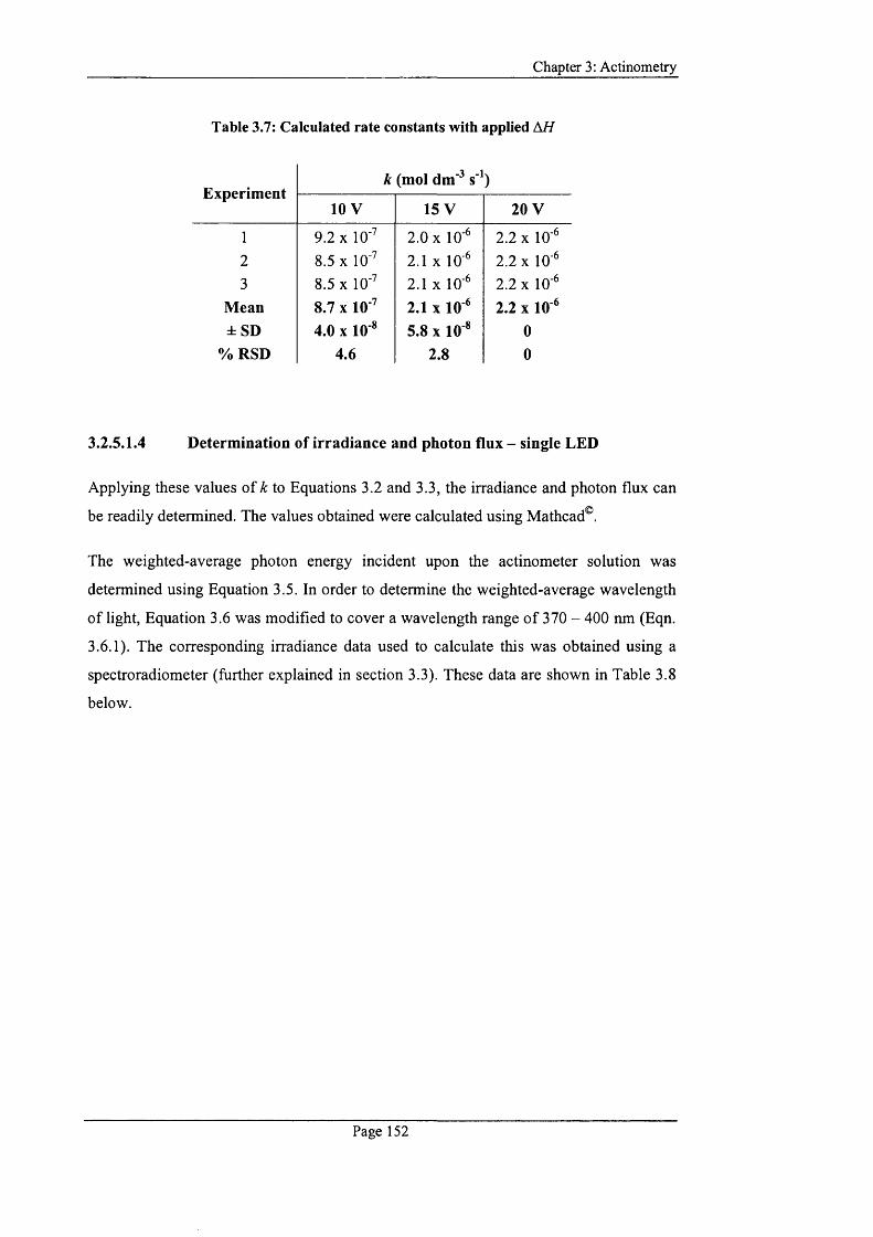
Chapter 3: Actinometry
Table 3.7: Calculated rate constants with applied A //
Experimentk (mol dm^ s'*)
10 V 15 V 20 V
1 9.2 X 10'7 2.0 X 10' 2.2 X 10 *2 8.5 X 10'7 2 .1 X 1 0 '^ 2 .2 X 10"*
3 8.5 X 10' 2 .1 X 1 0 '^ 2.2 X 10'*Mean 8.7 X 10 ^ 2.1 X 10* 2.2 X 10 *±SD 4.0 X 10 * 5.8 X 10 * 0
% RSD 4.6 2.8 0
3.2.5.1.4 Determination of irradiance and photon flux - single LED
Applying these values o f k to Equations 3.2 and 3.3, the irradiance and photon flux can
be readily determined. The values obtained were calculated using Mathcad®.
The weighted-average photon energy incident upon the actinometer solution was
determined using Equation 3.5. In order to determine the weighted-average wavelength
o f light, Equation 3.6 was modified to cover a wavelength range o f 370 - 400 nm (Eqn.
3.6.1). The corresponding irradiance data used to calculate this was obtained using a
spectroradiometer (further explained in section 3.3). These data are shown in Table 3.8
below.
Page 152
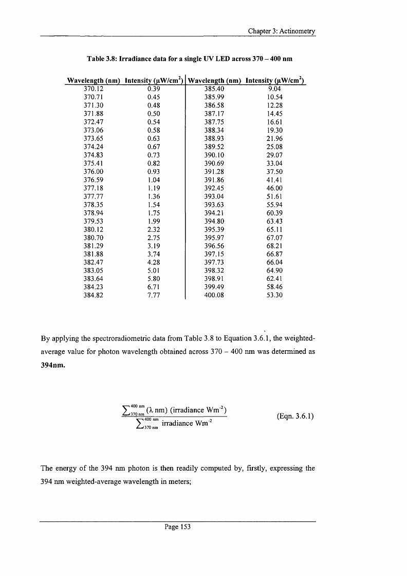
Chapter 3: Actinometry
Table 3.8: Irradiance data for a single UV LED across 370 - 400 nm
Wavelength (nm) Intensity (jnW/cm^) Wavelength (nm) Intensity (jiW/cm^)370.12 0.39 385.40 9.04370.71 0.45 385.99 10.54371.30 0.48 386.58 12.28371.88 0.50 387.17 14.45372.47 0.54 387.75 16.61373.06 0.58 388.34 19.30373.65 0.63 388.93 21.96374.24 0.67 389.52 25.08374.83 0.73 390.10 29.07375.41 0.82 390.69 33.04376.00 0.93 391.28 37.50376.59 1.04 391.86 41.41377.18 1.19 392.45 46.00377.77 1.36 393.04 51.61378.35 1.54 393.63 55.94378.94 1.75 394.21 60.39379.53 1.99 394.80 63.43380.12 2.32 395.39 65.11380.70 2.75 395.97 67.07381.29 3.19 396.56 68.21381.88 3.74 397.15 66.87382.47 4.28 397.73 66.04383.05 5.01 398.32 64.90383.64 5.80 398.91 62.41384.23 6.71 399.49 58.46384.82 7.77 400.08 53.30
By applying the spectroradiometric data from Table 3.8 to Equation 3.6.1, the weighted-
average value for photon wavelength obtained across 370 - 400 nm was determined as
394nm.
\ 400 nm^ 370nm (îrradiance Wm'^)
I400 nm
370 nmirradiance Wm
(Eqn. 3.6.1)
The energy o f the 394 nm photon is then readily computed by, firstly, expressing the
394 nm weighted-average wavelength in meters;
Page 153
Chapter 3: Actinometry
394 nm 1 m ^ _ _ 7
X 10 nm= 3.94 X 10 m
Then, applying the data to Eqn. 3.5, gives an average photon energy o f 5.03 x 10'*’ J
he (6.63 X 1 0 '' Js ')(2 .99 x 10' ms ')E = — = ^ ^ ----------------- ^ = 5 .0 3 x 1 0 '" J
À 3.94 X 10'" m
Therefore, on average a photon delivers 5.03 x 10"'^ J o f energy to the actinometric
solution where it is assumed that all photons in the range o f 370 - 400 nm convert 2NB
to 2NBA with equivalent efficiency.
The Irradiance (Iq) and Photon Flux (Fq) data as determined by Mathcad® are outlined in
the worksheets printed below and all data is summarised in Table 3.9.
Page 154
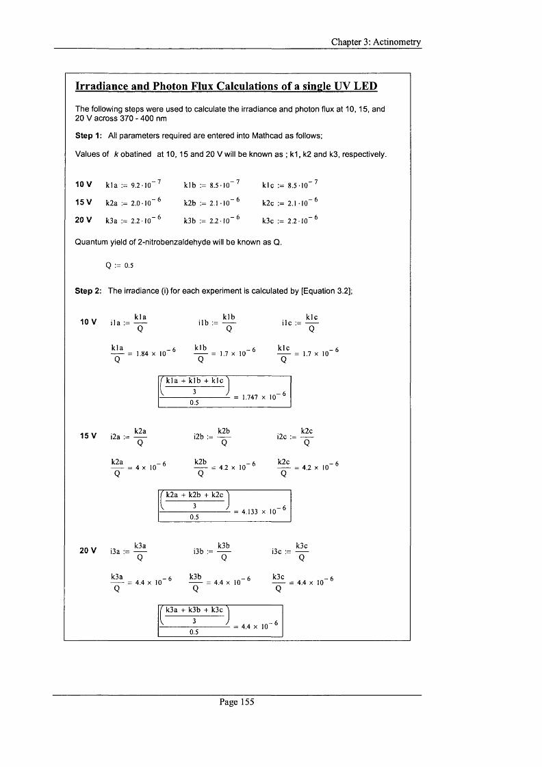
Chapter 3: Actinometry
Irradiance and Photon Flux Calculations of a single UV LED
The following steps were used to calculate the irradiance and photon flux at 10, 15, and 20 V across 370 - 400 nm
Step 1: All parameters required are entered into Mathcad as foiiows;
Values of k obatined at 10, 15 and 20 V will be known as ; k1, k2 and kS, respectively.
10 V k l a 9 . 2 1 0 “ ^
15 V k2a 2 . 0 - l 0 “ ^
20 V k3a 2.2 -10“ ^
k l b := 8 . 5 1 0 ' k i c := 8 . 5 1 0 - 7
k2b 2 1 10 k2c 2.1 10 ^
- 6k3b 2.2-10 k3c 2.2-10
Quantum yield of 2-nitrobenzaldehyde will be known as Q.
Q := 0.5
Step 2: The irradiance (i) for each experiment is calculated by [Equation 3.2];
10 V il a :=k l a
i lb :=k l b
i l ckIc
k l a _ 6 = 1.84 X 10Q
^ = 1.7 X 10 ^Q
k l a 4- k l b + k i c
0.5= 1.747 X 10 - 6
15 V i2a ;=k2a
i2bk2b
i2c :=k2c
— = 4 x 1 0 ^Q
= 4.2 X 10 ^Q
— = 4.2 X 10 ^Q
k2a + k2b + k2c
0.5= 4.133 X 10'
20 V I3a :=k3a
13b :=k3b
i3c :=k3c
k3a _ 6 = 4.4 X 10Q
k3b _ 6 = 4.4 X 10Q
= 4.4 x l O *Q
k3a + k3b + k3c
0.5= 4.4 X 10 - 6
Page 155
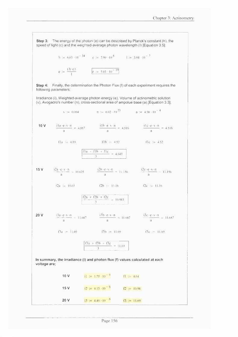
C h a p ter 3: A c t in o m e tr y
Step 3: The energy of the photon (e) can be described by Planck's constant (h), thespeed of light (c) and the weighted-average photon wavelength (I) [Equation 3.5];
h ;= 6.63 • 10 c := 2.99 10^ I 3.94 ■ It) - 7
( h e )e ;= 5.03 • 10
- 19
Step 4: Finally, the determination the Photon Flux (f) of each experiment requires thefollowing parameters;
Irradiance (i), Weighted-average photon energy (e), Volume of actinometric solution (v), Avogadro's number (n), cross-sectional area of ampolue base (a) [Equation 3.3];
V 0.004 n := 6.02 10 23 a := 4.56 ■ 10 - 4
10 V i l a e \ n= 4.887
i 1 h • e • V ■ n= 4.516
l i e ■ e ■ V • n= 4.516
f l a := 4.89 f i b := 4.52 f l c 4.52
f l a + f i b + f l c= 4.643
15 V i2a e v n= 10.625
i2b e v n= 11.156
i2c e V n= 11.156
f2a ;= 10.63 f2b := 11.16 f2c := 11.16
f2a + f2b + f2c
3= 10.983
20 V i3a e v n= 11.687
i3b - e - v - n= 11.687
Lie e v n= 11.687
13a := 11.69 D b 11.69 13c := 11.69
13 a + Ob + 13c= 11.69
In summary, the Irradiance (I) and photon flux (f) values calculated at each voltage are;
10 V
15 V
20 V
i l 1.75 ■ 10
i2 := 4.13 10
Î3 4.40 • 10
- 6
- 6
- 6
fl := 4.64
f2 ;= 10.98
O 11.69
P a g e 156
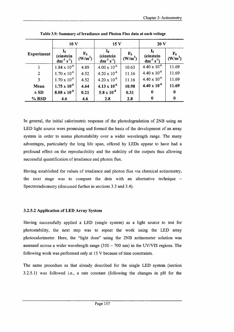
Chapter 3: Actinometry
Table 3.9: Summary of Irradiance and Photon Flux data at each voltage
Experiment
10 V 15 V 20 V
lo(einstein dm s ')
Fo(W/m^)
lo(einstein dm s ')
Fo(W/m^)
lo(einstein dm s ')
Fo(W/m^)
1 1.84 X 10'^ 4.89 4.00 X lO'G 10.63 4.40 X 10'^ 11.69
2 1.70 X 10'^ 4.52 4.20 X 10'^ 11.16 4.40 X 10'^ 11.69
3 1.70 X 10'^ 4.52 4.20 X 10'^ 11.16 4.40 X 10'^ 11.69
Mean 1.75 X 10^ 4.64 4.13 X 10^ 10.98 4.40 X lO ' 11.69±SD 8.08 X 10 * 0.21 5.8 X 10 * 0.31 0 0
% RSD 4.6 4.6 2.8 2.8 0 0
In general, the initial calorimetric response o f the photodegradation o f 2NB using an
LED light source were promising and formed the basis o f the development o f an array
system in order to assess photostability over a wider wavelength range. The many
advantages, particularly the long life span, offered by LEDs appear to have had a
profound effect on the reproducibility and the stability o f the outputs thus allowing
successful quantification of irradiance and photon flux.
Having established the values of irradiance and photon flux via chemical actinometry,
the next stage was to compare the data with an alternative technique -
Spectroradiometry (discussed further in sections 3.3 and 3.4).
3.2.5.2 Application of LED Array System
Having successfully applied a LED (single system) as a light source to test for
photostability, the next step was to repeat the work using the LED array
photocalorimeter. Here, the “light dose” using the 2NB actinometer solution was
assessed across a wider wavelength range (350 - 700 nm) in the UVA^IS regions. The
following work was performed only at 15 V because o f time constraints.
The same procedure as that already described for the single LED system (section
3.2.5.1) was followed i.e., a rate constant (following the changes in pH for the
Page 157
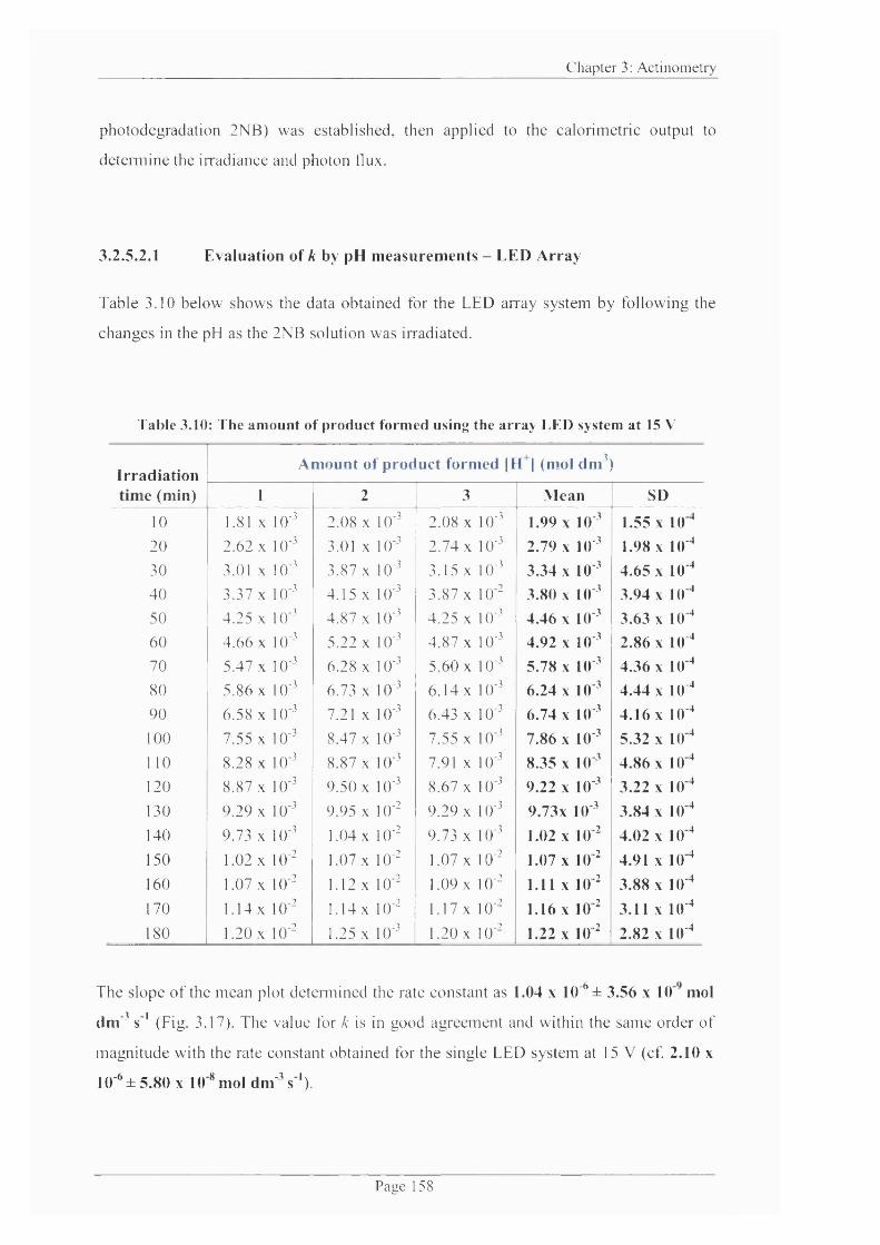
C h a p ter 3: A c t in o m e tr y
photodegradation 2N B) was established, then applied to the calorimetric output to
d e ten n in e the in ad ian ee and photon tlux.
3.2.5.2.1 E valuation of k by pH m easu rem en ts - LED A rray
T able 3.10 below shows the data obtained for the LED array system by following the
changes in the pH as the 2NB solution was irradiated.
Table 3.10: The amount of product formed using the array LED system at 15 V
I rra d ia tio nA m ount o f p ro d u c t fo rm ed |H | (mol dm^)
le (m in) 1 2 3 M ean SD
10 1.81 X 10^ Z 08 X 10-' 2.08 X 10’’ 1.99 X 10-' 1.55 X lO-*20 2.62 X 10^ 3.01 X 10-' 2 2 4 X IÜ-) 2.79 X 10-' 1.98 X 10-'30 3.01 X 10^ T 87 X 10-' 3.15 X 10'^ 3.34 X 10-' 4.65 X 10-*40 3 J 7 X 10^ 4.15 X 10-' 3 2 7 X 10- 3.80 X 10-' 3.94 X I0-"50 4 2 5 X 10^ 4 # 7 X 10-' 4 2 5 X 10-’ 4.46 X 10-' 3.63 X 10^60 4.66 X 10-' 5 2 2 X 10-' 4 2 7 X 10^ 4.92 X 10-' 2.86 X 10-*70 5.47 X 10-' 6 2 8 X 10-' 5 2 0 X 10'^ 5.78 X 10-' 4.36 X lO '80 5.86 X 10-' 6 2 3 X 10-' 6.14 X 10'^ 6.24 X 10-' 4.44 X lO"*90 6 2 # X 10-' 7.21 X 1()-' 6.43 X i c ’ 6.74 X lO ' 4.16 X 10-'100 7 2 5 X 10-' 8.47 X 10-' 7 2 5 X i c ’ 7.86 X 10-' 5.32 X 10-'110 8 2 8 X 10'' 8 # 7 X 10-' 7.91 X 10^ 8.35 X 1 0 ' 4.86 X 10-'120 8 # 7 X 10*' 9 2 0 X U)-' 8 2 7 X 10-' 9.22 X 10-' 3.22 X 10-'130 9 2 9 X 10"' 9 2 2 X 10-' 9 2 9 X 10-' 9.73x 10-' 3.84 X lO"'140 9 2 3 X 1()-' 1.04 X 10-' 9.73 X 10-' 1.02 X 1 0 ' 4.02 X lO '150 1.02 X 1()-' 1.07 X 1()-' 1.07 X 10-' 1.07 X lO ' 4.91 X 10-'160 1.07 X 10-' 1.12 X lO ' L09 X 10-' 1.11 X 1 0 ' 3.88 X 10^170 1.14 X 10-' 1.14 X 10-' 1.17 X IQ-' 1.16 X 1 0 ' 3.11 X 10"'
180 1.20 X 10-' 1.25 X 1()-' 1.20 X IQ-' 1.22 X 1 0 ' 2.82 X 10-'
T he slope o f the m ean plot detem iined the rate constant as 1.04 x 10’ ± 3.56 x 10 mol
d m ^ s ' (Fig. 3.17). The value for k is in good agreem ent and within the sam e order o f
m agnitude with the rate constant obtained for the single LED system at 15 V (cf. 2.10 x
10 '^± 5 .80 X 10 * mol dnT^s ').
P a g e 158

C h a p ter 3: A c t in o m e tr y
pH measurements of 2NB under full array LED exposure at 15 V
1.4x10''-
1.2x10' -
1.0x10''0 £T 8.0x10'' Xc■ê 6.0x10'' ro1
£ 4.0x10'' o3"O^ 2.0x10''
0.0
i
data point Linear fit
Y = A + B * X
Param eter Value Error
A 0 .0 0 1 2 6 4 .55683E -5B 1.04169E-6 1 .44342E -8
R SD N P
0.9991 0 .74105 19 < 0.0001
2000 4000 6000 8000
Irradiation time (s)
10000 12000
3.2.S .2.2
Figure 3.17: pH-time profile using LED array system
P hotocalorim etry o f 2N B using LED array system
The photodegradation o f 2NB was m onitored using the LED array photocalorim eter.
Figure 3.18 is typical o f the response observed over o f period o f about 5 hours o f
irradiation. During this period, a constant deflection from zero in the m icrocalorim eter
is obser\'cd therefore showing the actinom eter to follow zero-order kinetics. At an input
o f 15 V, the output response o f the T A M is ca. 21.5 pW . This value was deduced from
an average o f data points over the irradiation period. The signal is very steady with only
small fluctuations (± 1 pW).
In order to assess the repeatability o f the signal under irradiation, the light was switched
on and o f f a num ber o f times for a defined period o f 30 min each time. S ince the
photodegradation o f 2N B follows zero order kinetics, the heat output should remain
constant over the time period for which the sam ple is exposed to light and unchanged at
the time intervals during the light on and o f f process. By perform ing a series o f light
P a g e 1 5 9

Chapter 3: Actinometry
on/off tests in this manner, the total heat, 0 , given out by the reaction over the
irradiation period can be calculated by integrating the area under the calorimetric curve
from the start o f irradiation ( on) to the end o f measurement (tend)- The measurable time
frame of irradiation is defined as ton - tofr = tm i.e. the duration from where the light is
switched on ( on) to when it is switched off ( ofr)- The calorimetric data can be used to
determine the heat output {Q in Joules) and total heat flow ( 0 in Watts) during the
photodegradation of 2NB.
Figure 3.19 is typical o f the response obtained during a light on/off test o f 2NB and
illustrates the time points taken from which the Q and 0 can be calculated. Integrating
the area under the curve from ton to end gives the value for Q in Joules. Dividing Q by
the irradiation period, An- (in seconds) determines the value for 0 in Js ' (or Watts) for
the photoreaction.
Integrating the cumulative area;
on end Q
Defining irradiation period;
Therefore, the total heat flow is determined by;
From the calorimetric outputs represented in Figures 3.20 - 3.22, the total heat flow was
calculated by following the procedure given above. Three experiments were carried out
and each measurement shows the response obtained as the sample was repeatedly (in
triplicate) exposed/not exposed to irradiation for a period o f approx. 30 min. The heat
flow for each light on/off test was determined using the above calculation method. The
deflection o f the power output was also measured by taking an average o f the data
points after the signal had settled and compared to that o f the calculated output. The
data for each experiment are summarised in Tables 3.11 - 3.14 where the heat flow
using the calculated method and an average o f the data points from the calorimetric plot
are defined as 0 calc and 0 average, respectively.
Page 160
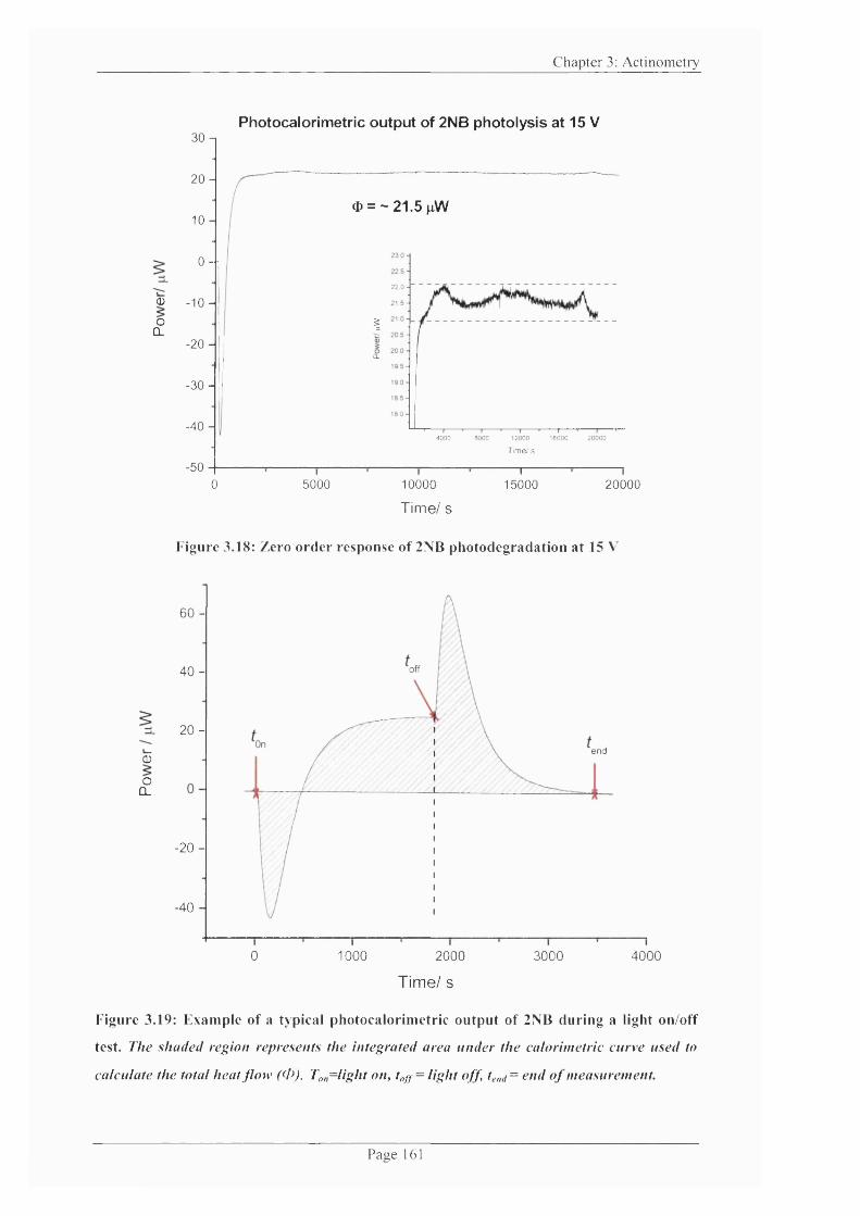
C h a p ter 3: A c t in o m e tr y
30 -
2 0 -
10 -
0-1
0 - 1 0 -
o CL
-20 -
-30 —
-40 -
-50
Photocalorimetric output of 2NB photolysis at 15 V
CD = -21.5 pW
22 0
%
CL
4000 8000 12000 16000 20000
Time/ s
0 5000 10000
Time/ s
I15000 20000
Figure 3.18: Zero order response of 2NB photodegradation at 15 \
60 -
off40 -
20 -
e n d0O
CL
-20 -
-40 -
0 1000 2000 3000 4000
Tim e/ s
Figure 3.19: Example of a typical photocalorimetric output of 2NB during a light on/off
test. The shaded region represents the integrated area under the calorimetric curve used to
calculate the total heat flow (0 ) . T„„=light on, t„ff= light off, te„d= end of measurement.
P a g e 161
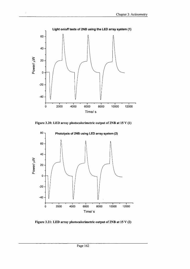
Chapter 3: Actinometry
Light on/off tests of 2NB using the LED array system (1)
6 0 -
4 0 -
% 2 0 -
I0_
- 2 0 -
-4 0 -
0 2000 4000 6000 10000 120008000
Time/ s
Figure 3.20: LED array photocalorimetric output of 2NB at 15 V (1)
80 n Photolysis of 2NB using LED array system (2)
60 -
40 -
%2 0 -I
CL
- 2 0 -
-40 -
10000 120002000 4000 6000 80000
Time/ s
Figure 3.21: LED array photocalorimetric output of 2NB at 15 V (2)
Page 162
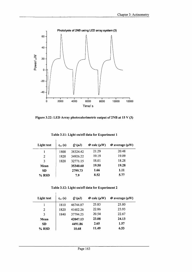
Chapter 3: Actinometry
Photolysis of 2NB using LED array system (3)
ICL
-20
-40
0 2000 4000 6000 10000 120008000
Time/ s
Figure 3.22: LED Array photocalorimetric output of 2ND at 15 V (3)
Table 3.11: Light on/off data for Experiment 1
Light test Arr (S) 6 W ) 0 calc (pW) 0 average (pW)
1 1800 38324.42 21.29 20.482 1820 34926.22 19.19 19.093 1820 32771.15 18.01 18.28
Mean 35340.60 19.50 19.28SD 2799.73 1.66 1.11
% RSD 7.9 8.52 5.77
Table 3.12: Light on/off data for Experiment 2
Light test Arr (s) Q W 0 calc (pW) 0 average (pW)
1 1810 46744.87 25.83 25.802 1820 41602.26 22.86 23.933 1840 37794.25 20.54 22.67
Mean 42047.13 23.08 24.13SD 4491.86 2.65 1.57
% RSD 10.68 11.49 6.53
Page 163
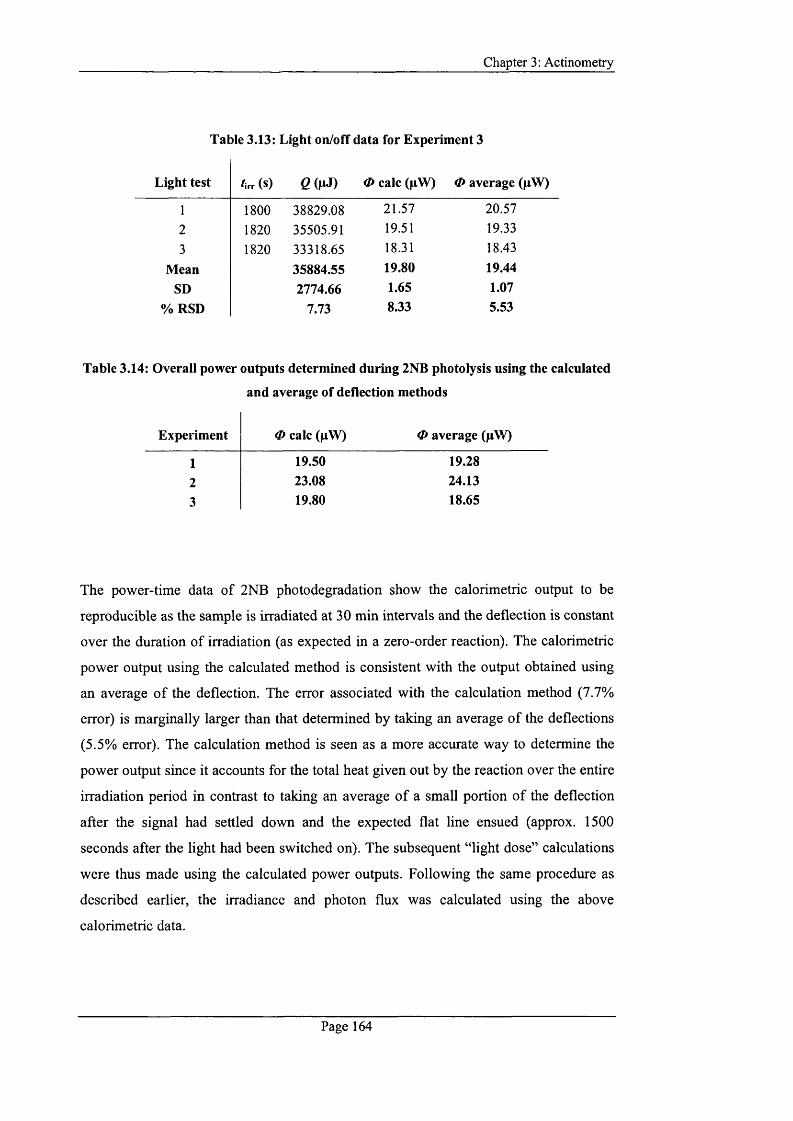
Chapter 3: Actinometry
Table 3.13: Light on/off data for Experiment 3
Light test t\vr (S) Q W 0 calc (pW) 0 average (pW)
1 1800 38829.08 21.57 20.57
2 1820 35505.91 19.51 19.33
3 1820 33318.65 18.31 18.43
Mean 35884.55 19.80 19.44SD 2774.66 1.65 1.07
% RSD 7.73 8.33 5.53
Table 3.14: Overall power outputs determined during 2NB photolysis using the calculated
and average of deflection methods
Experiment 0 calc (pMT 0 average (pW)
1 19.50 19.282 23.08 24.133 19.80 18.65
The power-time data of 2NB photodegradation show the calorimetric output to be
reproducible as the sample is irradiated at 30 min intervals and the deflection is constant
over the duration o f irradiation (as expected in a zero-order reaction). The calorimetric
power output using the calculated method is consistent with the output obtained using
an average o f the deflection. The error associated with the calculation method (7.7%
error) is marginally larger than that determined by taking an average o f the deflections
(5.5% error). The calculation method is seen as a more accurate way to determine the
power output since it accounts for the total heat given out by the reaction over the entire
irradiation period in contrast to taking an average o f a small portion o f the deflection
after the signal had settled down and the expected flat line ensued (approx. 1500
seconds after the light had been switched on). The subsequent “light dose” calculations
were thus made using the calculated power outputs. Following the same procedure as
described earlier, the irradiance and photon flux was calculated using the above
calorimetric data.
Page 164
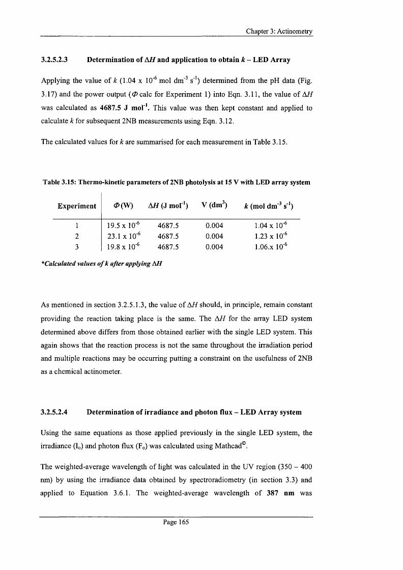
Chapter 3: Actinometry
3.2.5.2.3 Determination of à H and application to obtain k - LED Array
Applying the value o f k (1.04 x 10'^ mol dm'^ s’') determined from the pH data (Fig.
3.17) and the power output ( 0 calc for Experiment 1) into Eqn. 3.11, the value o f A77
was calculated as 4687.5 J mol '. This value was then kept constant and applied to
calculate k for subsequent 2NB measurements using Eqn. 3.12.
The calculated values for k are summarised for each measurement in Table 3.15.
Table 3.15: Thermo-kinetic parameters of 2NB photolysis at 15 V with LED array system
Experiment 0 (W ) A ^ (J m o l') V (dm^) k (mol dm^ s’')
1 19.5 X 10’* 4687.5 0.004 1.04 X 10’*2 23.1 X 10’* 4687.5 0.004 1.23 X 10 *3 19.8 X 10 * 4687.5 0.004 1.06.x 10*
*Calculated values o f k after applying M I
As mentioned in section 3.2.5.1.3, the value o f M i should, in principle, remain constant
providing the reaction taking place is the same. The M i for the array LED system
determined above differs from those obtained earlier with the single LED system. This
again shows that the reaction process is not the same throughout the irradiation period
and multiple reactions may be occurring putting a constraint on the usefulness of 2NB
as a chemical actinometer.
3.2.5.2.4 Determination of irradiance and photon flux - LED Array system
Using the same equations as those applied previously in the single LED system, the
irradiance (L) and photon flux (Fo) was calculated using Mathcad®.
The weighted-average wavelength o f light was calculated in the UV region (350 - 400
nm) by using the irradiance data obtained by spectroradiometry (in section 3.3) and
applied to Equation 3.6.1. The weighted-average wavelength o f 387 nm was
Page 165

Chapter 3: Actinometry
determined. Applying Equation 3.5, the average photon energy o f 4.54 x 10 J was
calculated where it is assumed that all photons in the range 350 - 400 nm convert 2NB
to 2NBA with equivalent efficiency.
The values for Iq and Fq as determined by Mathcad® are outlined in the worksheets
printed below and all data is summarised in Table 3.16.
Page 166
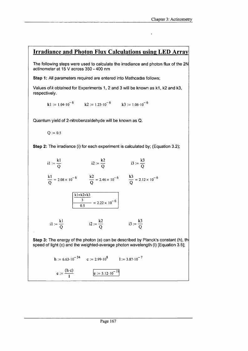
Chapter 3: Actinometry
Irradiance and Photon Flux Calculations using LED Array
The following steps were used to calculate the irradiance and photon flux of the 2N actinometer at 15 V across 350 - 400 nm
Step 1: All parameters required are entered into Mathcacfes follows;
Values of/c obtained for Experiments 1, 2 and 3 will be known as k1, k2 and k3, respectively.
k l := 1.04 10- 6 k2 := 1.23-10" k3 := 1.06-10"
Quantum yield of 2-nitrobenzaldehyde will be known as Q.
Q := 0.5
Step 2: The irradiance (i) for each experiment is calculated by; (Equation 3.2);
12 :=k2
o'
— = 2 .08x10 — = 2 .4 6 x 1 0 ^ — = 2 .1 2 x 1 0 ^Q Q Q
kl+ k 2 + k 3
= 2.22 X 10 ^0.5
" 412 :=
k213 :=
k3
Step 3: The energy of the photon (e) can be described by Planck's constant (h), th speed of light (c) and the weighted-average photon wavelength (I) [Equation 3.5];
h := 6.63-10- 3 4 c := 2.99-10 1 := 3.87-10- 7
e :=(h-c)
e := 5.12-10-
Page 167

C h a p te r 3: A c t in o m e tr y
Step 4: Finally, the determ ination for the Photon Flux (f) o f each experim ent require the following parameters;
Irradiance (i), W eighted-average photon energy (e), Volume of actinom etric solutior (v), Avogadro's number (n), cross-sectional area of ampolue base (a) [Equation 3.3
V := 0.004 n := 6.02 1023 a := 4.54-10- 4
i l e v n i2-e-v-n i3-e-v-n------------ = 5.009 = 5.924 = 5.105
n ;= 5.01 12 := 5.92 13 := 5.11
fl + 1 2 + 13= 5.347
In summary, the irradiance (i) and photon flux (f) values calculated using the LED array photocalorimeter at 15 V were;
i := 2.22-10- 6 f := 5.35
Table 3.16: Siimniarv of Irradiance and Photon Flux data using LEI) Arrav
E xperim en tlo
(einstein dm'^ s ')F»
(VV/m-)
1 2.08 X 10^ 5.012 2.46 X 10'" 5.92
3 2 4 2 X 10^ 5.11
M ean 2 . 2 2 X 10^ 5.35
± S D 2.09 X 10^ 0.50
% RSD 9.4 9.3
The 2NB actinom eter has been successfully applied to detem iine the radiant intensity
using the LED array photocalorimeter. T he next step was then to d e ten u ine the photon
tlux value in real-time using spec troradiom etry (section 3.3) and to see how they
compare.
P a g e 168
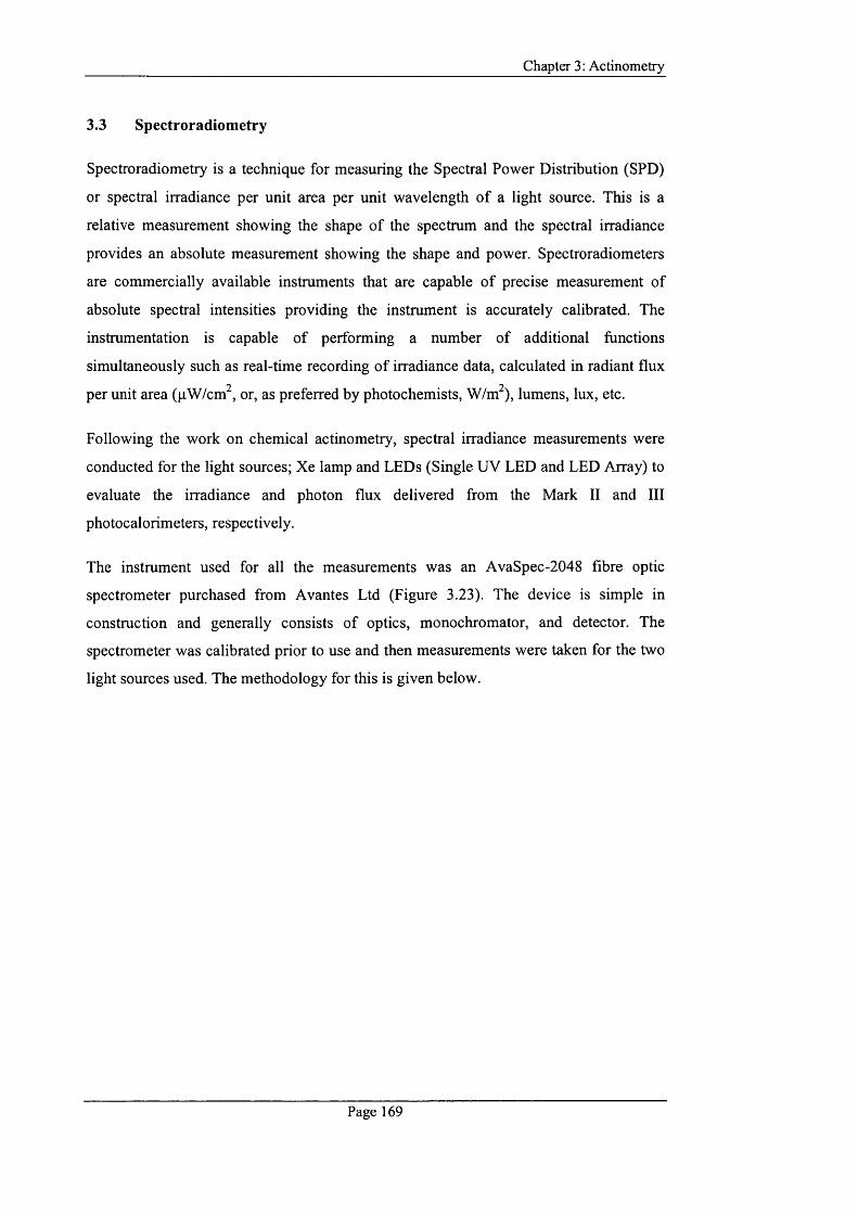
Chapter 3: Actinometry
3.3 Spectroradiometry
Spectroradiometry is a technique for measuring the Spectral Power Distribution (SPD)
or spectral irradiance per unit area per unit wavelength o f a light source. This is a
relative measurement showing the shape o f the spectrum and the spectral irradiance
provides an absolute measurement showing the shape and power. Spectroradiometers
are commercially available instruments that are capable o f precise measurement of
absolute spectral intensities providing the instrument is accurately calibrated. The
instrumentation is capable o f performing a number o f additional functions
simultaneously such as real-time recording o f irradiance data, calculated in radiant flux
per unit area (pW/cm^, or, as preferred by photochemists, w W ) , lumens, lux, etc.
Following the work on chemical actinometry, spectral irradiance measurements were
conducted for the light sources; Xe lamp and LEDs (Single UV LED and LED Array) to
evaluate the irradiance and photon flux delivered from the Mark II and III
photocalorimeters, respectively.
The instrument used for all the measurements was an AvaSpec-2048 fibre optic
spectrometer purchased from Avantes Ltd (Figure 3.23). The device is simple in
construction and generally consists o f optics, monochromator, and detector. The
spectrometer was calibrated prior to use and then measurements were taken for the two
light sources used. The methodology for this is given below.
Page 169
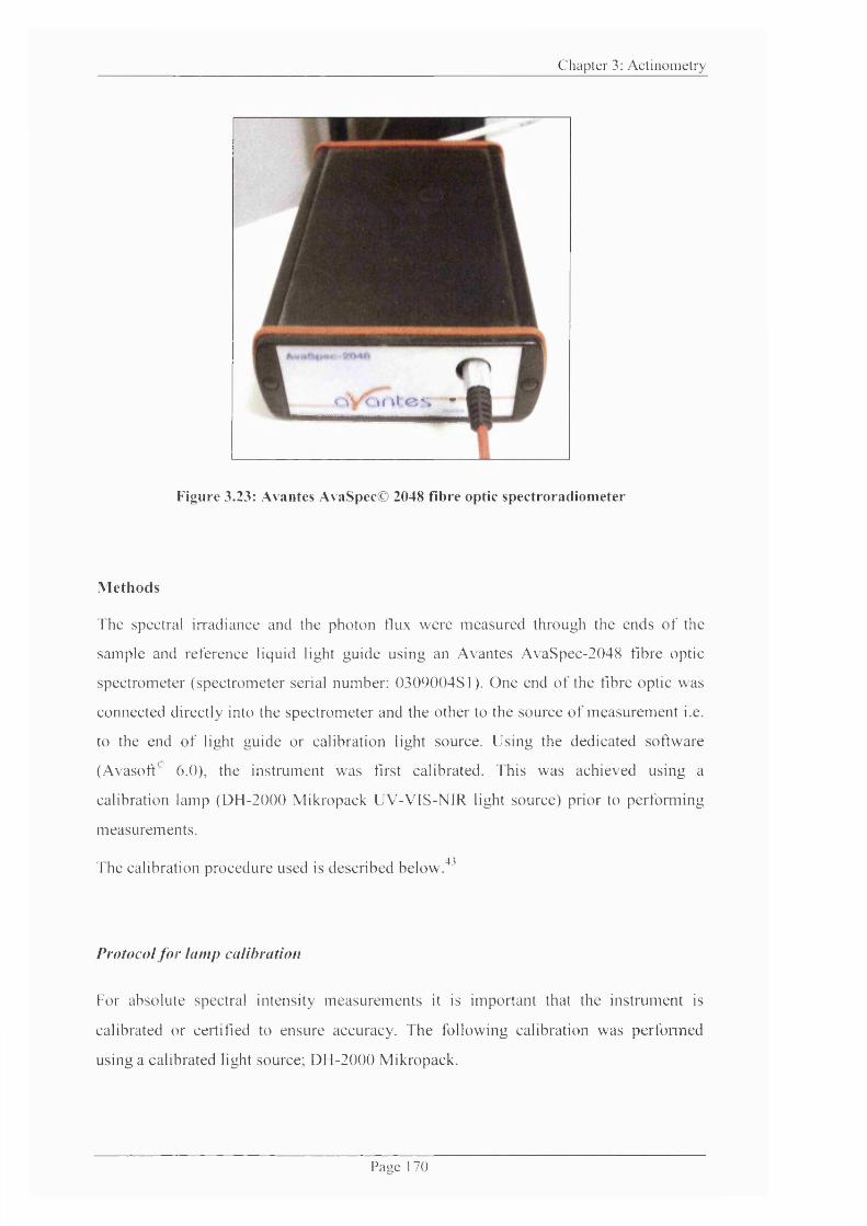
C h a p ter 3: A c t in o m e tr y
t i V f i n l c s •
Figure 3.23: Avantes AvaSpec© 2048 fibre optic spectroradiom eter
M ethods
The spectral irradiance and the photon tlux w ere m easured through the ends o f the
sample and reference liquid light guide using an Avantes A vaSpec-2048 fibre optic
spectrometer (spectrom eter serial number: 0309004S1). O ne end o f the fibre optic was
connected directly into the spectrom eter and the other to the source o f rneasurem ent i.e.
to the end o f light guide or calibration light source. Using the dedicated software
(Avasoff® 6.0), the instrument was first calibrated. This was achieved using a
calibration lamp (D H -2000 M ikropack U V -V IS-N IR light source) prior to perform ing
measurements.
The calibration procedure used is described below. 43
Protocol for lamp calibration
For absolute spectral intensity m easurem ents it is important that the instrument is
calibrated or certified to ensure accuracy. The following calibration was perfom ied
using a calibrated light source; D H-2000 M ikropack.
P a g e 170

Chapter 3: Actinometry
Note: the DH-2000 Mikropack is a calibrated light source for use in the UV/VIS/NIR
spectral range (205-1095 nm).
1. One end o f a fibre optic was connected to the spectroradiometer input port and
the other to the calibration lamp source.
2. The absolute irradiance application on the AvaSoft 6.0 programme was started
and “Perform Intensity Calibration” was selected.
3. Parameters such as channel to be calibrated, calibration lamp file and diameter
o f the fibre optic used were entered appropriately.
4. The DH-2000 Mikropack reference light source was switched on for 15 minutes
to warm up and the fibre tip was inserted directly in the light source.
5. The option to “Start Intensity Calibration” was then selected.
6. The integration time was adjusted so that the maximum count over the
wavelength range was about 15000 counts.
7. The smoothing parameters were adjusted to optimise smoothing for the fibre
diameter used.
8. The calibration lamp was turned off. A dark reference was saved.
9. The calibration was saved (“Save Intensity Calibration”). The calibration was
saved with the extension *fbr since the calibration was performed with a bare
fibre optic.
10. The irradiance mode was selected. The system was then ready to take
measurements.
The same intensity calibration was loaded prior to measurements. A dark spectrum was
saved before switching to irradiance mode.
Page 171

Chapter 3: Actinometry
Parameters used during measurements
Avasoft® parameters for intensity measurements were set as follows;
Integration time: 2 ms
Average no. o f scans: 3
Num ber o f pixels used for smoothing: 6
Note: Using a long integration time, the detector was exposed to too much light during a
single scan, which meant it was not possible for a signal to be detected. A shorter
integration time was chosen to minimise the signal for detection such that a maximum
count over the wavelength range was around 15000 counts.
Experimental measurements
M easurements were taken from the sample and reference light guides. The method for
measuring the SPD (absolute irradiance) and photon flux using the spectrometer was
relatively straightforward;
1. An end of the light guide was connected directly to an end of the fibre optic of
the spectrometer. The cables were held together during measurements by a
specially constructed attachment punched with holes to fit both ends o f the
cables securely.
2. In the case o f the Xe lamp set to a defined power setting (240 W), a warm up
period o f 1 hour was allowed before taking measurements. A warm up period o f
this length was not necessary with the LED system as LEDs are capable of
achieving full brightness within a few milliseconds.
3. The light was exposed to the spectroradiometer. The SPD was measured and
photon flux readings were taken over a period o f approx. 1 hour before the light
was switched off.
All data were imported as an ASCII file into Origin™.
Page 172
Chapter 3: A ctinom etry
The set-up o f the photocalorim eters rem ained unchanged from previous actinom etry
experim ents (described in section 3.2.3). These param eters rem ained the sam e
throughout the follow ing experim ents, unless stated otherw ise.
3.3.1 Measurements from Xe lamp source
3.3.1.1 Spectral Power Distribution (SPD)
The light distribution from the sam ple and reference cables was very encouraging
because, firstly, it can be seen that there w as a relatively large spectral output in the UV
and V isible regions: characteristic o f Xe lam ps. Secondly, the output spectra betw een
the sam ple and reference SPD were very well m atched, as show n by the overlays o f the
SPD m easurem ents (Fig. 3.24).
The integrated areas under each spectrum (determ ined from Fig. 3.19) were:
Sample: 12391.2 pW /cm ^/nm Reference: 11782.1 pW /cm ^/nm
There is a sim ilarity o f 95% in the distribution betw een the sam ple and reference sides.
This indicates the split o f the light via the beam splitter is proportional through each
cable.
Page 173

C h a p ter 3: A c t in o m e tr y
Integration of Sample from zero; I = 1 ->1633
Integration of Ref from zero: i = 1 ->1633x= 173.12-> 1100.11Area Peak at Width Height
120-1 X = 173.12 -> 1100.11Area Peak at Width Height
1 0 0 - 11782.1 826.9 470.0 93.212391.2 826.4 467.1 109.i
c 8 0 - SampleReference
60 -
40 -
2 0 -
0
T T 1200 400 600
/. (nm)
800 1000 1200
Figure 3.24: Comparison of Spectral Power Distribution of Xe lamp (240 \V) through the
sample and reference light guides
3.3.1.2 Photon Flux m easu rem en ts
T he photon tlux in real-time was m easured through the sam ple side. T he m easurem ents
w ere taken after the shutters on the beam splitter were adjusted so that a zero baseline
signal was attained on the TA M . This setting will be know n as the pre-detlned level. It
is using this set-up that all chemical ac tinom etry work (on the M ark II) was conducted
i.e., the sam ple was irradiated. Thus, under the sam e set-up conditions, in principle, it is
possible to evaluate and com pare the tlux data obtained by the spec troradiom eter with
that obtained through chemical actinometry. M easurem ents were also taken by adjusting
the position o f the shutters on the beam splitter so as to give an idea o f the absolute
m ax im um and absolute m inim um radiant pow er that the system was capable o f
producing. Altering the position o f the shutter will impact on the extent o f tlux output.
Thus, the flux was evaluated at different shutter positions and the output from the
sam ple side was recorded with the shutter set in the following positions; 1) O pen, 2)
M id-way, 3) Pre-defmed level (so that a zero baseline signal on T A M was achieved
prior to sam ple analysis), and 4) Closed. Note, as m entioned in C hapter 2, the "closed
P ajic 1 7 4
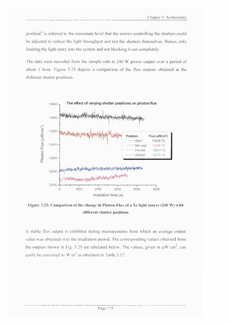
C h a p ter 3: A c t in o m e tr y
position” is re fen ed to the maxirnum level that the screws controlling the shutters could
be adjusted to reduce the light throughput and not the shutters themselves. Hence, only
limiting the light entry into the system and not b locking it out completely.
The data were recorded from the sam ple side at 240 W pow er output over a period o f
about 1 hour. Figure 3.25 depicts a com parison o f the tlux outputs obtained at the
different shutter positions.
13600 -1 The effect of varying shutter positions on photon flux
1 3 4 0 0 -
u 13200
3 13000
1 2 8 0 0 -
1 2 6 0 0 -
12400
Position Flux (nW/cmh
Open 13438.73
Mid-way 13166.79
Pre-set 12627.72
Closed 12472 16
,.bA'—I-------'-------1-------'------- 1----1000 2000 3000
Irradiation time (s)
4000 5000
Figure 3.25: Comparison of the change in Photon Flux of a Xe light source (240 W) with
different shutter positions
A stable tlux output is exhibited during m easurem ents from which an average output
value w as obtained over the irradiation period. T he corresponding values ob tained from
the outputs shown in Fig. 3.25 are tabulated below. The values, given in p W /c m “, can
easily be converted to W /m “ as tabulated in Table 3.17.
P a g e 1 75
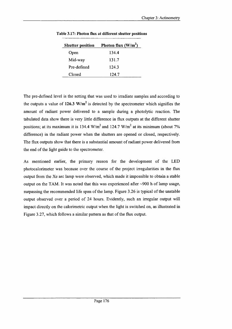
Chapter 3: Actinometry
Table 3.17: Photon flux at different shutter positions
S hutter position Photon flux (W/m^)
Open 134.4
Mid-way 131.7
Pre-defined 124.3
Closed 124.7
The pre-defined level is the setting that was used to irradiate samples and according to
the outputs a value o f 126.3 W/m^ is detected by the spectrometer which signifies the
amount o f radiant power delivered to a sample during a photolytic reaction. The
tabulated data show there is very little difference in flux outputs at the different shutter
positions; at its maximum it is 134.4 W/m^ and 124.7 W/m^ at its minimum (about 7%
difference) in the radiant power when the shutters are opened or closed, respectively.
The flux outputs show that there is a substantial amount o f radiant power delivered from
the end of the light guide to the spectrometer.
As mentioned earlier, the primary reason for the development o f the LED
photocalorimeter was because over the course o f the project irregularities in the flux
output from the Xe arc lamp were observed, which made it impossible to obtain a stable
output on the TAM. It was noted that this was experienced after ~900 h o f lamp usage,
surpassing the recommended life span of the lamp. Figure 3.26 is typical o f the unstable
output observed over a period o f 24 hours. Evidently, such an irregular output will
impact directly on the calorimetric output when the light is switched on, as illustrated in
Figure 3.27, which follows a similar pattern as that of the flux output.
Page 176
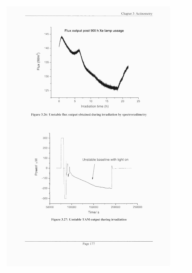
C hapter 3: A ctin o m etry
145-
140-
135-
130-
125-
Flux output post 900 h Xe lamp useage
"T~10
-J—15
—T—20
—I 25
Irradiation time (h)
Figure 3.26: Unstable flux output obtained during irradiation by speetroradimetry
300-
2 0 0 -
1 0 0 -I Unstable baseline with light on
moo_
- 1 0 0 -
- 2 0 0 -
-300-
50000 100000 150000 200000 250000
Time/ s
Figure 3.27: Unstable TAM output during irradiation
P age 177
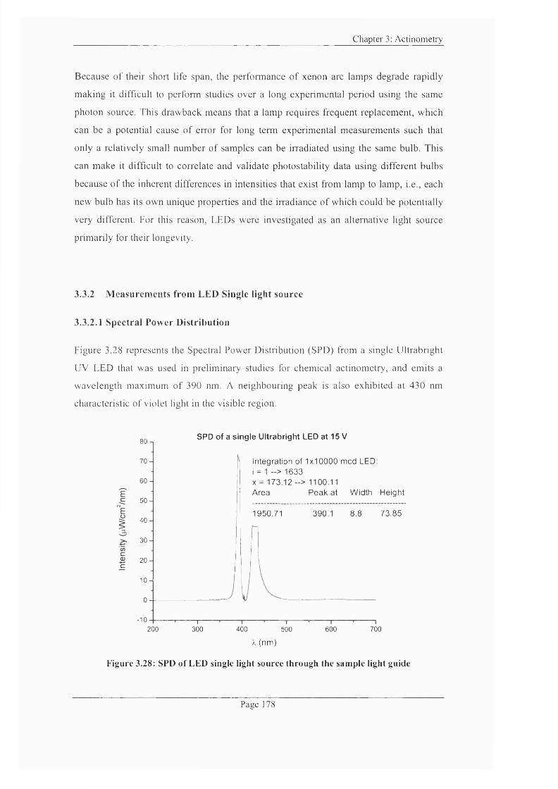
C hapter 3: A c tin o m etry
Because of their short life span, the performance o f xenon arc lamps degrade rapidly
making it difficult to perform studies over a long experimental period using the same
photon source. This drawback means that a lamp requires frequent replacement, which
can be a potential cause o f error for long term experimental measurements such that
only a relatively small number o f samples can be irradiated using the same bulb. This
can make it difficult to correlate and validate photostability data using different bulbs
because o f the inherent differences in intensities that exist from lamp to lamp, i.e., each
new bulb has its own unique properties and the irradiance o f which could be potentially
very different. For this reason, LEDs were investigated as an alternative light source
primarily for their longevity.
3.3.2 M easurem ents from LED Single light source
3.3.2.1 Spectral Power Distribution
Figure 3.28 represents the Spectral Power Distribution (SPD) from a single Ultrabright
UV LED that was used in preliminary studies for chemical actinometry, and emits a
wavelength maximum of 390 nm. A neighbouring peak is also exhibited at 430 nm
characteristic of violet light in the visible region.
8 0 -
7 0 -
60 -
5 0 -
40 -
3 0 -
2 0 -
10H
0
-10
SPD of a single Ultrabright LED at 15 V
Integration of 1x10000 mod LED:I = 1 -> 16 3 3X = 173.12 -> 1100.11Area Peak at Width Height
1950.71 390.1 8.8 73.85
200—I—300 400 500
X (nm)
600 700
Figure 3.28: SPD of LED single light source through the sample light guide
P age 178
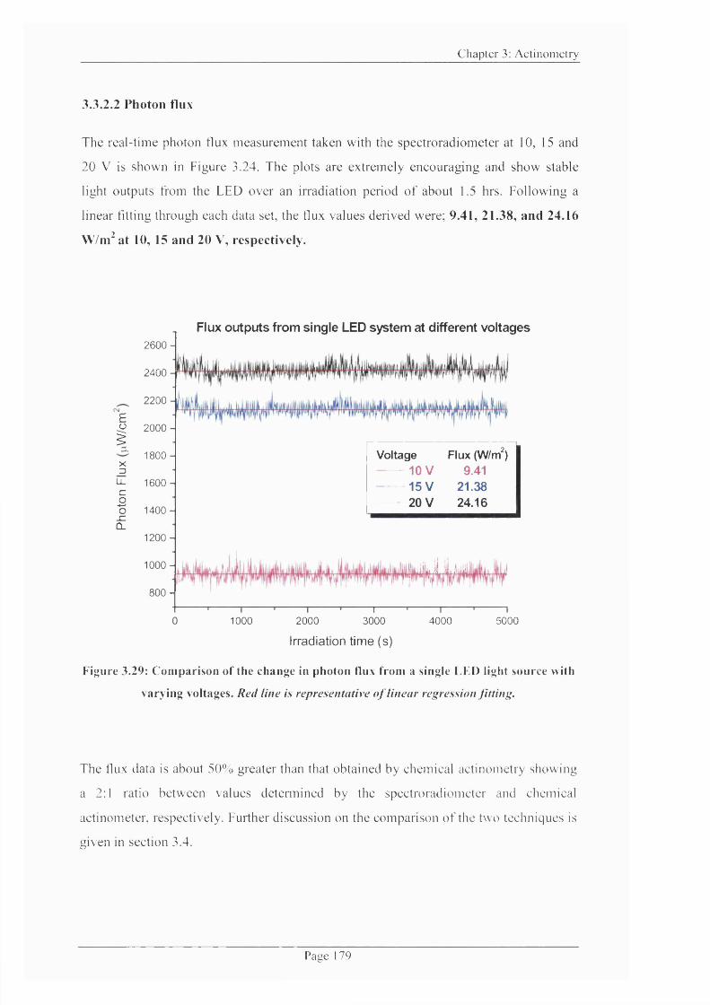
C h a p ter 3: A c t in o m e tr y
33 .2 .2 Photon flux
The real-time photon flux m easurem ent taken with the spectroradiom eter at 10, 15 and
20 V is shown in Figure 3.24. T he plots are extrem ely encouraging and show stable
light outputs from the LED over an irradiation period o f about 1.5 hrs. Following a
linear fitting through each data set, the flux values derived were; 9.41, 21.38, and 24.16
W/m^ at 10, 15 and 20 V, respectively.
Flux outputs from single LED system at different voltages2 6 0 0 -
2 4 0 0 -
2 2 0 0 -
Eo 2 0 0 0 -g=L
X1 8 0 0 -
DLL 1 6 0 0 -c2o
s z1 4 0 0 -
CL1 2 0 0 -
1 0 0 0 -
8 0 0 -
Voltage Flux (W/m')— 10 V 9.41
------15V 21.38------ 20 V 24.16
1000 2000
Irradiation time (s)
C A , j 'i ; uy
T '3 0 0 0
" 14 0 0 0 5 0 0 0
Figure 3.29: Comparison of the change in photon flux from a single LED light source with
varying voltages. Red line is representative o f linear regression fitting.
The flux data is about 50% greater than that obtained by chemical ac tinom etry show ing
a 2:1 ratio between values de tenn ined by the spectroradiom eter and chemical
actinometer, respectively. Further discussion on the com parison o f the two techniques is
given in section 3.4.
P a g e 179
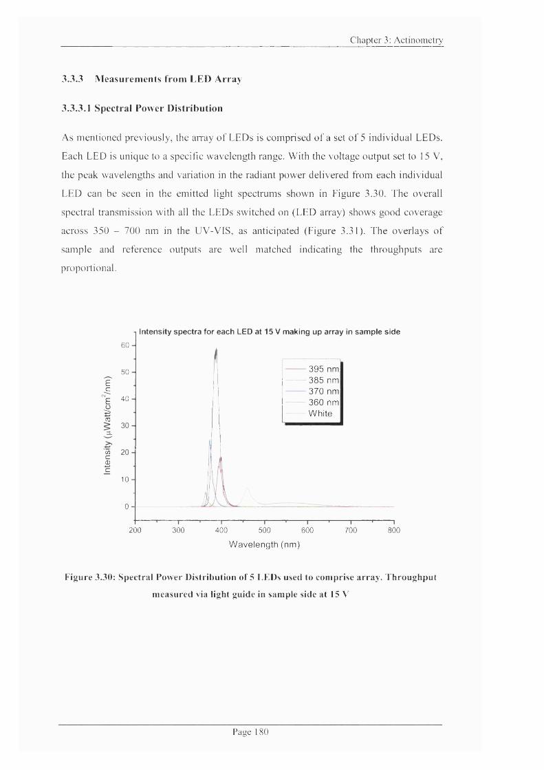
C h a p ter 3: A c t in o m e tr y
3.3.3 Measurements from LED Array
3.3.3.1 Spectral Power Distribution
As m entioned previously, the array o f LEDs is com prised o f a set o f 5 individual LEDs.
Each LED is unique to a specific w avelength range. W ith the voltage output set to 15 V,
the peak wavelengths and variation in the radiant pow er delivered from each individual
LED can be seen in the emitted light spectrums show n in Figure 3.30. T h e overall
spectral transmission with all the LEDs switched on (LED array) shows good coverage
across 350 - 700 nm in the UV-VIS, as anticipated (Figure 3.31). T he overlays o f
sam ple and reference outputs are well m atched indicating the throughputs are
proportional.
EcEaCD
Ü)cBc
60
50
40
10
0
Intensity spectra for each LED at 15 V making up array in sample side
395 nm 385 nm
370 nm 360 nm White
T2 0 0 300 4 0 0 500 600
Wavelength (nm)
700 800
Figure 3.30: Spectral Power Distribution of 5 LEDs used to comprise array. Throughput
measured via light guide iu sample side at 15 V
P a u e 180
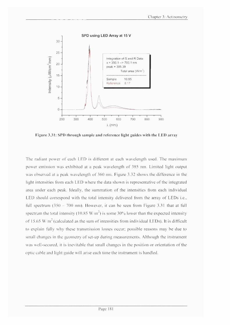
C h a p ter 3: A c t in o m e tr y
SPD using LED Array at 15 V30-1
2 5 -
2 0 -
1 5 -
Integration of S and R Data: X = 350.1 > 700.1 nm peak = 395.39
Total area (W/m^]
Sam ple 10.85 R eference 8.17
1 0 -
500 600
X (nm)
r700 800 900
Figure 3.31: SPD through sample and reference light guides with the FED array
The radiant pow er o f each LED is different at each w avelength used. T he m axim um
power em ission was exhibited at a peak w avelength o f 385 nm. Limited light output
was observed at a peak wavelength o f 360 nm. Figure 3.32 shows the difference in the
light intensities from each LED where the data show n is representative o f the integrated
area under each peak. Ideally, the sum m ation o f the intensities from each individual
LED should correspond with the total intensity delivered from the array o f LEDs i.e.,
full spectrum (350 - 700 nm). However, it can be seen from Figure 3.31 that at full
spectrum the total intensity (10.85 W/m") is som e 30% lower than the expected intensity
o f 15.65 W /m “ (calculated as the sum o f intensities from individual LEDs). It is dift'icult
to explain fully w hy these transmission losses occur; possible reasons m ay be due to
small changes in the geom etry o f set-up during measurem ents. A lthough the instrument
was well-secured, it is inevitable that small changes in the position or orientation o f the
optic cable and light guide will arise each time the instrument is handled.
P a g e 181

C h a p ter 3: A c t in o m e tr y
Graph to show variation in intensity of each LED10.85 □
1 0 -
7.49
EI>>(/)c
c 2.99 2.69
1.920.56
3 9 5 4 0 0 -7 0 0 3 5 0 -7 0 0
W hite Full Spectrum
3 6 0 3 7 0
Peak Wavelength (nm)
Figure 3.32: Graph showing variation in intensity of the LEDs
3.3.3.2 Photon Flux
Comparison of flux in 8 and R sides at 15 V using LED array1200-1
Flux (W/m')S a m p le 1 0 .5 9
R e fe r e n c e 9 .6 9
1150 - Side
1 1 0 0 -
Eo 1050-
X3 1000 -
c2o
Q.9 50 -
900 -
850 -
8000 200 400 600 800 1000 1200 1400 1600 1800 2000
Irradiation time (s)
Figure 3.33: Photon flux from a LED array through sample and reference light guides
P a u e 182
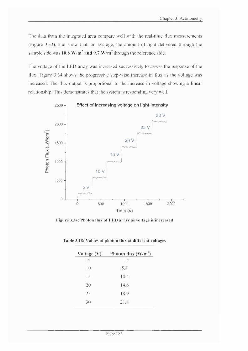
C h a p ter 3; A c t in o m e tr y
The data from the integrated area com pare well with the real-time tlux m easurem ents
(Figure 3.33), and show that, on average, the am ount o f light delivered through the
sam ple side was 10.6 W/ni^ and 9.7 W/m^ through the reference side.
The voltage o f the LED array was increased successively to assess the response o f the
tlux. Figure 3.34 shows the progressive step-wise increase in flux as the voltage was
increased. T he flux output is proportional to the increase in voltage show ing a linear
relationship. This demonstrates that the system is responding very well.
2500 -
2000 -
1500 ^
1000 -
500-
Effect of increasing voltage on light Intensity
30 V
5 V
10 V
15 V
20 V
25 V
500 1000
Tim e (s)
1500 2000
Figure 3.34: Photon flux of LED array as voltage is increased
Table 3.18: Values of photon flux at different voltages
V oltage (V) Photon flux (W/m^)5 1.5
10 5.8
15 10.4
20 14.6
25 1&9
30 2L8
P a g e 183
Chapter 3: Actinometry
3.4 C om parison of actinom etric m ethods
Two different actinometeric techniques; chemical actinometry and spectroradiometry,
have been used to quantify the amount o f light exposure for two types of lamp sources;
Xe arc lamp and LEDs (single and array system). Having studied the two techniques
with two different light sources, it was possible to determine successfully the photon
flux for each system. Although because o f the additional oxidation event that was
observed the during the chemical actinometry work, it was not possible to determine the
photon flux for the photolysis o f 2NB alone. The flux value, however, can be estimated
for the 2NB/EDTA photoreaction since the oxidation process was inhibited. Following
the same calculation outline as that already described for the LED systems above
(section 3.2.1.3), the flux values for the Xe arc lamp for the 2NB/EDTA data (Fig. 3.9)
was determined. The 2NB/EDTA data shown in Fig. 3.10 showed that generally the
power signal settled to a constant deflection after approx. 1 hour o f irradiation. The O
signal for each measurement were as follows; 67, 62 and 57 pw for Runs 1, 2, and 3
respectively, giving an average o f 62 pW ± 5 pW . Applying the value o f k obtained
from the pH data with 2NB/EDTA (2.47 x 10'^ mol dm'^ s '') into Eqn. 3.11, the value
for A // was calculated as 62753 J m ol''. This value, again, differs from those
determined by the LED single and array photocalorimeters. Moreover, it is also not in
agreement with the value o f A // determined by Morris^^ (cf. 202464 J mol ') using the
Mark 1 photocalorimeter showing the photoreaction exhibits complexity. The irradiance
and photon flux values were determined, and the calculation are outlined in the
Mathcad® worksheets below.
Page 184

C h a p ter 3: A c t in o m e tr y
Irradiance and Photon Flux calculations using xenon arc lamp
The following steps were used to calculate the irradiance and photon flux for the photodegradation of 2NB containing EDTA at 240 W across 290 - 400 nm
Step 1: All parameters required are entered into Mathcad as follows;
The rate constant determined through pH measurements will be known as k.
k := 2 .4 7 .1 0 "^
Quantum yield of 2-nitrobenzaldehyde will be known as Q.
Q := 0.5
Step 2: The irradiance (i) for each experiment is calculated by; (Equation 3.2);
i = 4.94 X 10 i ;= 4.94-10
Step 3: The energy of the photon (e) can be described by Planck's constant (h), the speed of light (c) and the weighted-average photon wavelength (I) [Equation 3.5];
h := 6.63-10 c := 2.99-10^ 1 := 3.52-10 ^
(h e ) e : = ------- e := 5.63-10
Step 4: Finally, the determination for the Photon Flux (f) of each experiment requires the following parameters;
Irradiance (i), Weighted-average photon energy (e), Volume of actinometric solution (v), Avogadro's number (n), cross-sectional area of ampolue base (a) [Equation 3.3];
v ;= 0.004 n 6 . 0 2 - a := 4.56-10“ “
i-e-v-n = 1.469 f := 1.47
Overall, the values for f, and Fq as de tenn ined by M athead^ were; 4.94 x 10'^ einstein
d m ^ s ' and 1.47 W /m^, respeetively.
P a a e 185
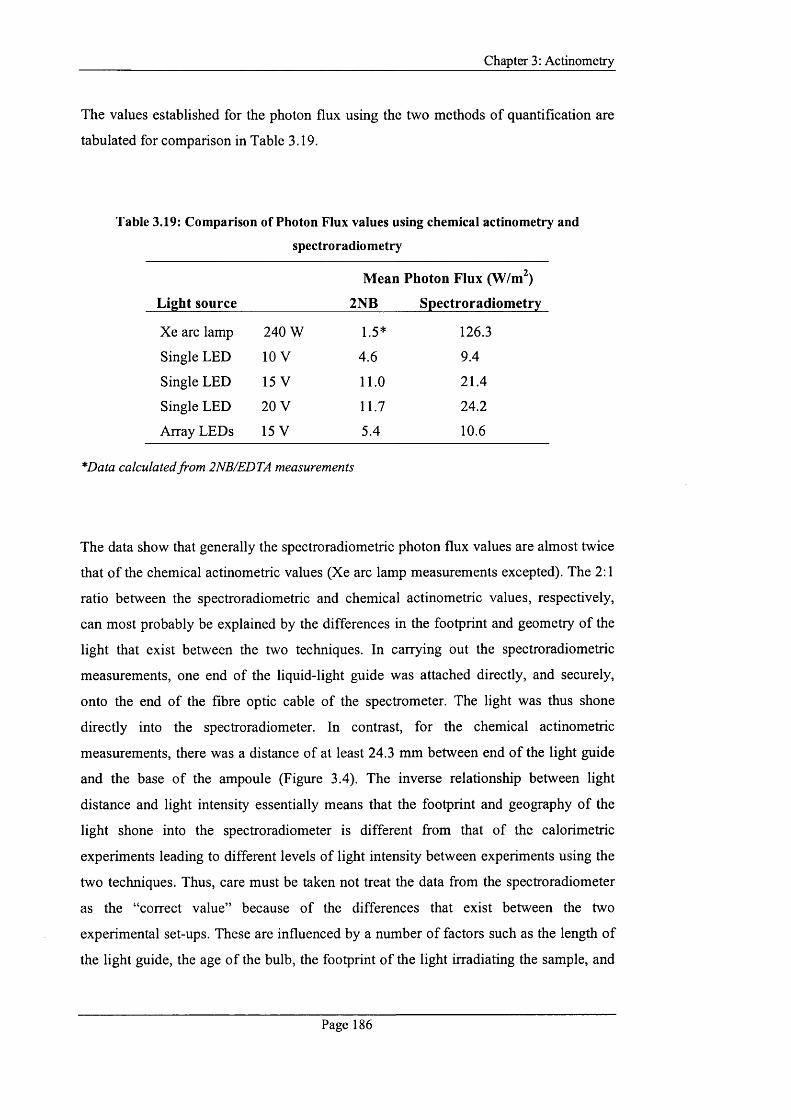
Chapter 3: Actinometry
The values established for the photon flux using the two methods o f quantification are
tabulated for comparison in Table 3.19.
Table 3.19: Comparison of Photon Flux values using chemical actinometry and
spectro radio metry
Light source
M ean Photon Flux (W/m^)
2NB Spectroradiom etry
Xe arc lamp 240 W 1.5* 126.3
Single LED 10 V 4.6 9.4
Single LED 15 V 11.0 21.4
Single LED 20 V 11.7 24.2
Array LEDs 15 V 5.4 10.6
*Data calculated from 2NB/EDTA measurements
The data show that generally the spectroradiometric photon flux values are almost twice
that o f the chemical actinometric values (Xe arc lamp measurements excepted). The 2:1
ratio between the spectroradiometric and chemical actinometric values, respectively,
can most probably be explained by the differences in the footprint and geometry o f the
light that exist between the two techniques. In carrying out the spectroradiometric
measurements, one end o f the liquid-light guide was attached directly, and securely,
onto the end o f the fibre optic cable o f the spectrometer. The light was thus shone
directly into the spectroradiometer. In contrast, for the chemical actinometric
measurements, there was a distance o f at least 24.3 mm between end o f the light guide
and the base o f the ampoule (Figure 3.4). The inverse relationship between light
distance and light intensity essentially means that the footprint and geography of the
light shone into the spectroradiometer is different from that o f the calorimetric
experiments leading to different levels o f light intensity between experiments using the
two techniques. Thus, care must be taken not treat the data from the spectroradiometer
as the “correct value” because o f the differences that exist between the two
experimental set-ups. These are influenced by a number o f factors such as the length o f
the light guide, the age o f the bulb, the footprint o f the light irradiating the sample, and
Page 186
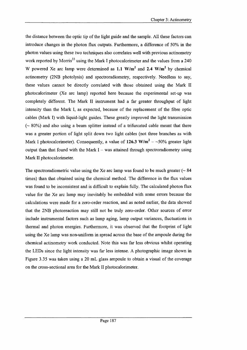
Chapter 3: Actinometry
the distance between the optic tip of the light guide and the sample. All these factors can
introduce changes in the photon flux outputs. Furthermore, a difference o f 50% in the
photon values using these two techniques also correlates well with previous actinometry
work reported by Morris^^ using the Mark I photocalorimeter and the values from a 240
W powered Xe arc lamp were determined as 1.1 W/m^ and 2.4 W/m^ by chemical
actinometry (2NB photolysis) and spectroradiometry, respectively. Needless to say,
these values cannot be directly correlated with those obtained using the Mark II
photocalorimeter (Xe arc lamp) reported here because the experimental set-up was
completely different. The Mark II instrument had a far greater throughput o f light
intensity than the Mark I, as expected, because o f the replacement o f the fibre optic
cables (Mark I) with liquid-light guides. These greatly improved the light transmission
(~ 80%) and also using a beam splitter instead o f a trifurcated cable meant that there
was a greater portion o f light split down two light cables (not three branches as with
Mark I photocalorimeter). Consequently, a value o f 126.3 W/m^ — 50% greater light
output than that found with the Mark I - was attained through spectroradiometry using
Mark II photocalorimeter.
The spectroradiometric value using the Xe arc lamp was found to be much greater (~ 84
times) than that obtained using the chemical method. The difference in the flux values
was found to be inconsistent and is difficult to explain fully. The calculated photon flux
value for the Xe arc lamp may inevitably be embedded with some errors because the
calculations were made for a zero-order reaction, and as noted earlier, the data showed
that the 2NB photoreaction may still not be truly zero-order. Other sources o f error
include instrumental factors such as lamp aging, lamp output variances, fluctuations in
thermal and photon energies. Furthermore, it was observed that the footprint o f light
using the Xe lamp was non-uniform in spread across the base o f the ampoule during the
chemical actinometry work conducted. Note this was far less obvious whilst operating
the LEDs since the light intensity was far less intense. A photographic image shown in
Figure 3.35 was taken using a 20 mL glass ampoule to obtain a visual o f the coverage
on the cross-sectional area for the Mark II photocalorimeter.
Page 187
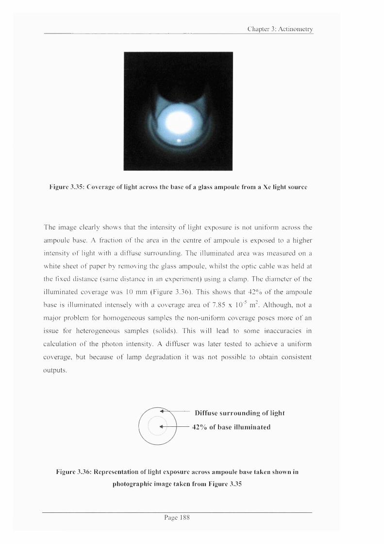
C h a p ter 3; A c t in o m e tr y
Figure 3.35: Coverage of light across the base of a glass ampoule from a Xe light source
The im age clearly shows that the intensity o f light exposure is not un ifonn across the
am poule base. A fraction o f the area in the centre o f am poule is exposed to a h igher
intensity o f light with a diffuse surrounding. The illuminated area was m easured on a
white sheet o f paper by rem oving the glass ampoule, whilst the optic cable was held at
the fixed distance (sam e distance in an experim ent) using a elamp. T he d iam eter o f the
illuminated coverage was 10 m m (Figure 3.36). This shows that 42% o f the am poule
base is illuminated intensely with a coverage area o f 7.85 x 10" m “. Although, not a
m ajor problem for hom ogeneous sam ples the non-un ifonn coverage poses m ore o f an
issue for heterogeneous samples (solids). This will lead to som e inaccuracies in
calculation o f the photon intensity. A diffuser was later tested to achieve a un ifonn
coverage, but because o f lamp degradation it was not possible to obtain consistent
outputs.
Diffuse surrounding of light
42% of base illuminated
Figure 3.36: Representation of light exposure across ampoule base taken shown in
photographic image taken from Figure 3.35
P a g e 1
Chapter 3: Actinometry
3.5 Sum m ary
Quantification o f a photon source is important in the evaluation o f photostability o f drug
substances and drug products. Actinometry offers a way o f quantifying intensity, that is,
the number o f photons in a beam, by means o f chemical or physical systems. Chemical
actinometers are a preferred choice to external calibrations because they provide an in-
situ validation o f the instrument and information o f the number o f photons actually
absorbed by a sample during a photochemical process. For reliability and validity o f
experimental data, a suitable chemical actinometer, ideally, needs to be one that is
robust, has a simple reaction mechanism, and exhibits low-sensitivity to non
photochemical processes. The photodegradation o f 2-nitrobenzaldehyde (2NB), an ICH
listed actinometer, was studied as a potential chemical test and reference reaction for
validation o f performance of the Xe arc lamp and LED (single and array)
photocalorimeters.
It has been demonstrated in this chapter that o f the two light sources used it proved
difficult to obtain consistent photochemical data from the Xe arc lamp. Data obtained
from the pH and photocalorimetric measurements showed non-zero order behaviour for
the photodegradation o f 2NB using the powerful Xe arc lamp. This suggested that 2NB
is likely to be sensitive to non-photochemical processes. With the inclusion o f a small
amount o f EDTA it was possible to inhibit the additional reaction that occurred
suggesting an oxidation process was a likely cause o f the non-zero order behaviour that
was observed, although there was still some evidence o f pseudo-zero-order behaviour
even in the presence o f EDTA. This is indicative o f complexity within the reaction and
it is the first time that complexity for the photodegradation o f 2NB has been detected
calorimetrically, although complexity has been highlighted by several others in the
l i t e r a t u r e . T h e data obtained are, however, in discordance with those obtained by
Morris^^ using the Mark I photocalorimeter. This is not surprising because with the new
experimental design and set-up (Mark II), the light intensity was essentially twice that
compared with the earlier model.
The non-zero behaviour observed calorimetrically was more prominent using the Xe arc
lamp than the LED systems because the intensity o f LEDs is far less than that generated
by the Xe arc lamp. The magnitude o f the radiant intensity from the xenon lamp is some
12 times greater than that o f the LED array as determined by the spectroradiometric
Page 189
Chapter 3: Actinometry
values. The radiant intensity produced by the LEDs is, however, sufficient to cause the
photodegradation o f 2NB and to produce a detectable calorimetric signal. The high
intensity can potentially cause additional secondary or thermal decomposition processes
to occur. Since the calorimeter measures all thermal processes, discriminating between
the types o f reactions that may occur is very complicated. Furthermore, the
disadvantages associated in combining a powerful xenon arc lamp with the sensitivity o f
an isothermal microcalorimeter outweigh those o f applying LEDs to the instrument.
Namely, the short lamp life, variable output, and high heat output generated from xenon
arc lamps, all hinder the performance o f the instrument leading to erroneous
photostability data.
The applicability o f LEDs as a light source for photocalorimetric measurements has
shown much potential and the results are extremely encouraging. It has been
demonstrated that it is possible to quantify successfully the photon flux o f the single and
array LEDs system using both chemical actinometry and spectroradiometry. W ith both
systems, the 2NB actinometer followed zero-order kinetics (represented by a constant
calorimetric deflection), subsequently leading to the derivation o f reaction parameters
such as k, AH, Iq and Fq. The single LED system showed excellent correlation between
the voltage input and calorimetric output (0 ); the signal increased linearly in proportion
to the three voltages tested; 10,15 and 20 V. All data showed very good stability and
repeatability (<5% error). Similar results were obtained for the LED array system tested
at 15 V (<10% error).
The complexity observed with 2NB using the xenon arc lamp and LED system evident
through the variation in the value o f A H obtained, which should, in principle, remain
constant regardless o f the reaction mechanism providing the products remain the same
and the initial and final concentration remains constant. The values o f A H were found
not to be constant suggesting that the photoreaction o f 2NB is complex with more than
one reaction occurring and because o f which the resultant irradiance and photon flux
data determined may be erroneous. Thus, it has been shown that 2NB is sensitive to
non-photochemical processes and the reaction is complex which limits the usefulness o f
2NB as a suitable chemical test and reference reaction for photocalorimetry and
validation o f instrument performance.
Page 190

Chapter 3: Actinometry
It should be kept in mind that the photon fluxes values obtained from chemical
actinometry and spectroradiometry typically showed a difference o f 1:2, respectively.
Although, spectroradiometry is very useful for information o f spectral intensities,
chemical actinometers remain the preferred method o f choice because they provide in-
situ validation.
Overall, it is apparent from the data obtained that the applicability o f LEDs as a light
source in photocalorimetry is promising for the assessment o f photostability testing.
Page 191
Chapter 3: Actinometry
3.6 References
1 Kuhn, H.J., Braslavsky, S.E., and Schmidt, R. (2004) Chemical Actinometry. Pure Appl.Chem 76, 2105-2146
2 Wadso, I., Goldberg, R. N. (2001) Standards in isothermal microcalorimetry (lUPAC technical report). Pure.Appl.Chem 73, 1625-1639
3 Beezer, A., Hills, A.K., O'Neill, M.A.A., Morris, A C., Kierstan, K.T.E., Deal, R.M., Waters, L.J., Hadgraft, J., Mitchell, J.C., Connor, J.A., Orchard, J.E., Willson, R.J., Hofelich, T.C., Beaudin, J., Wolf, G., Baitalow, F., Gaisford, S., Lane, R.A., Buckton, G., Phipps, M.A., W inneke, R.A., Schmitt, E.A., Hansen, L.D., O'Sullivan, D., and Parmar, M.K. (2001) The imidazole catalysed hydrolysis o f triacetin: an inter- and intra-laboratory development of a test reaction for isothermal heat conduction microcalorimeters used for determination o f both thermodynamic and kinetic parameters. Therm. Acta 380, 13-17
4 O'Neill, M.A.A., Beezer, A.E., Labetoulle, C., Nicolaides, L., Mitchell, J.C., Orchard, J.A., Connor, J.A.,Kemp, R.B., Olomolaiye, D. (2003) The base catalysed hydrolysis o f methyl paraben: a test reaction for flow microcalorimeters used for the determination o f both kinetic and thermodynamic parameters. Therm.Acta 399, 63-71
5 Ramos, R., Gaisford, S., Buckton, G., Royall, P.G., Yff, B.S.S., O'Neill, M. (2005) A comparison o f chemical reference materials for solution calorimeters. Int.J.Pharm. 299, 73-83
6 O'Neill, M.A.A., Gaisford, S., Beezer, A.E., Skaria, C.V., Sears, P. (2006) A comparison o f the performance o f calorimeters. Application of a test and reference recation. J.Therm.Anal.Cal. 84, 301-206
7 Kuhn, H.J., Braslavsky, S.E., and Schmidt, R. (1989) Chemical Actinometry. Pure Appl.Chem 61, 187-210
8 Piechocki, J.T. (1998) Principles of chemical actinometry. In Drugs photochemistry and photostability (Albini, A., and Fasani, E., ed.), The Royal Society o f Chemisty
9 Piechocki, J.T., Wo Iters, R.J. (1993) Use o f actinometry in photolysis stability studies. Pharm.Tech 17, 46-52
10 Gauglitz, G., and Hubig, S.M. (2007) Chemical Actinometry. In Pharmaceutical photostability and stabilization technology (Vol. 163) (Piechocki, J.T., and Thoma, K., ed.). Informa Healthcare
11 Willet, K., and Hites, R. A. (2000) Chemical actinometry: Using o- Nitrobenzaldehyde to measure lighht intensity in photochemical experiments. J.Chem.Edu. 77, 900-902
Page 192
Chapter 3: Actinometry
12 Theweleit, E., and Kunze, W. (1987) Methods and applications o f photocalorimetry. Kunststoffe 77, 23-25
13 Teixeira, C. (1999) Photocalorimetry: Methods and Applications in Energetics o f Stable Molecules and Reactive Intermediates., M. E. Minas da Piedade, Ed. 105-136
14 Thatcher, S., Mansfield, R.K., Miller, R.B., Davis, C.W., and Baertschi, S.W. (2001) "Pharmaceutical photostability" A technical guide and practical interpretation of the ICH guideline and its application to pharmaceutical stability - Part II. Pharm. Tech 25, 58-64
15 Rabek, J.F. (1982) Experimental methods in photochemistry and photophysics. Part 2. John Wiley and Sons
16 ICHQIB. (1997) Photostability Testing o f New Active Substances and Medicinal Products. EMEA, CPM P/ICH/2791/2795
17 Drew, H. (1998) Quinine photochemistry: A proposed chmical actinometer system to monitor UV-A exposure in photostability studies o f pharmaceutical drug substances and products. Pharm.Forum 24, 6334-6346
18 Christensen, K.L., Christensen, J.,Frokjaer S., Langballe, P.,and Hansen, L. (2000) Influence o f temperature and storage time after light exposure on the quinine monohydrochloride chemical actinometric system. Eur.J.Pharm.Sci 9, 317-321
19 Tonnesen, H.H., and Karlsen, J. (1995) Photochemical degradation o f components in drug formulations. III. A discussion o f experimental conditions. Pharmeuropa 7, 137-141
20 Sequeira, F., and Vozone, C. (2000) Photostability studies o f drug substances and products. Practical implications of the ICH guideline. Pharm. Tech 24 (8), 30-35
21 Baertschi, S.W. (1997) Commentary on the quinine actinometry system described by the ICH draft guidelines on photostability testing on new drug substances and products. Drug Stab. 1, 193-195
22 Moore, D.E. (1996) Standardization o f photodegradation studies and kinetic treatment o f photochemical reactions. In Photostability o f drug and drug form ulations (Tonnesen, H.H., ed.), Taylor and Francis
23 Adamson, A.W., Vogler, A., Kunkely, H., and Wachter, R. (1978) Photocalorimetry. Enthalpies o f photolysis o f /ra«5-azobeneze, ferrioxalate and cobaltioxalate ions, chromium hexacarbonyl, and dirhenium decarbonyl. J Am ChemSoc. 100, 1298-1300
24 Almmand, A.J., and Webb, W.W. (1929) The photolysis o f potassium ferrioxalate solutions. Part I. experimental. J. Chem. Soc, 1518-1531
Page 193

Chapter 3: Actinometry
25 Almmand, A.J., and Webb, W.W. (1929) The photolysis o f potassium ferrioxalate solutions. Part II. discussion. J. Chem. Soc., 1531-1537
26 Cooper, G.D., and DeGraff, B.A. (1971) On the photochemistry o f the ferrioxalate system. J.Phys.Chem 75, 2897-2902
27 Fernandez, E., Figuera, J.M. and Tobar, A. (1979) Use o f potassium ferrioxalate actinometer below 254 nm. J.Photochem 11, 69-71
28 Hatchard, C.G., and Parker, C.A. (1956) A new sensitive chemical actinometer II. Potassium ferrioxalate as a standard chemical actinometer. Proa. R. Soc. London, Ser. 235, 518-536
29 Nicodem, D.E., and Aquilera, O.M.V. (1983) Standardization o f the potassium ferrioxalate actinometer over the temperature range 5-80 °C. J.Photochem 21, 189-193
30 Parker, C.A. (1953) A new sensitive chemical actinometer I. Some trials with potassium ferrioxalate. Proc. R. Soc. London, Ser. 220, 104-116
31 Parker, C.A. (1954) Induced Autoxidation o f oxalate in relation to the photolysis o f potassium ferrioxalate. Trans. Faraday Soc. 50, 1213-1221
32 Oriel Light Sources Catalogue (2004).
33 Morris, A C. (2004) Ph.D Thesis. University o f Greenwich, Kent, UK.
34 Allen, J.M., Allen, S.K., and Baertschi, S.W. (2000) 2-Nitrobenzaldehyde: a convenient UV-A and UV-B chemical actinometer for drug photostability testing. J.Pharm.Biomed.Anal 24, 167-178
35 Ciamician, G., and Silber, P. (1901) Chem.Ber. 34, 2040-2046
36 Pitts, J.N., Wan, J.K.S., and Schuk, E.A. (1963) Photochemical studies in an alkali halide matrix I. An a-Nitrobenzaldehyde actinometer and its application to a kinetic study o f the photoreduction o f Benzophenone by Benzhydrol in a pressed potassium bromide disk. 86, 3606-3610
37 Leighton, P.A., Lucy, F.A. J. Chem. Phys. 2, 756-761
38 Pitts, J.N., Vernon, J.M., and Wan, J.K.S. (1965) A rapid actinometer for photochemical air pollution studies. Int. J. A ir Wat. Pollu. 9, 595-600
39 Trench, A.J., and Coppens, P. (1963) Free radicals formed from o-substituted nitro compounds. J.Phys.Chem 67, 1378
40 Chen, D., Zhou, J., Tian, Q. (1996) Mechanisms and structures o f free radicals in the photoreaction processes of o-substituted nitrobenzaldehydes. Journal o f Photochemistry and Photobiology A: Chemistry 98, 21-26
Page 194

Chapter 3: Actinometry
41 Laimgmber, S., Schreier, W.J., Shrader, T., Koller, F., Zinth, W., and Gilch, P. (2005) The photochemistry o f a-Nitrobenzaldehyde as seen by Femtosecond Vibrational Sp&ctroscopy. Angew.Chem.Int Ed. 44, 7901-7904
42 Dhuna, M., Beezer, A.E., Morris, A.C., Gaisford, S., O'Neill, A.A.M., Hadgraft, J., Connor, J.A., Clapham, D., Frost, J. (2007) Development of an Isothermal Heat-Conduction Photocalorimeter. Rev Sci Instrum 78(doi: 10.1063/1.2670220), 025105
43 Avasoft for Avaspec (2003) Spectroradiaometer operator manual.
Page 195

- Chapter Four -
Chemometric approach to
complexity
Chapter 4: Chemometric approach to com plexity
4. Introduction
Many pharmaceutical formulations (tablets, creams, lotions, etc) are complex multi-
component systems. Often it is likely that their stability is dependent on the degradation
kinetics o f several independently degrading components and not just on the behaviour
of the active pharmaceutical ingredient alone. Moreover, the degradation reaction
mechanisms in such multi-component systems are numerous, and include parallel,
consecutive and/or a combination o f such processes. Very often it is the case that the
complexities in these systems are difficult to analyse using conventional analytical
techniques.
The principles o f Isothermal Calorimetry (IC) and the analysis o f calorimetric data for
simple systems were introduced in Chapter 1. Chapters 2 and 3 subsequently
demonstrated how the technique can be extended to monitor photodegradative
processes, and to determine quantitatively the radiant flux delivered to a sample in a
simple photochemical process. Dealing with complex behaviours poses a far greater
problem, even more so for photosensitive reactions, because the combined effects of
heat and radiation adds to the complexity. Although photocalorimetry shows promise
for the study of complex reaction systems, the interpretation and correlation o f data can
be especially problematic.' Even when non-photochemical processes are studied, the
interpretation o f complexity in isothermal calorimetric data is not straightforward, since
the calorimeter measures all thermal processes that occur, without discriminating
between individual processes. The observed power signal is therefore a summation of
the powers arising from each individual event that occurs (which can be physical as well
chemical change).
The challenge, however, lies in deconvoluting the observed power signal into its
individual component parts to help identify the degradation kinetic behaviour for each
individual process. A number o f methods for quantitative analysis o f complexity, both
in solution^'"^ and solid states^ have been described. However, for complex reactions,
these approaches require prior knowledge o f the reaction mechanism.
One alternative approach to the problem of complexity in multivariate data sets is the
application o f chemometric analysis. It is the purpose o f this chapter to analyse the
Page 197

Chapter 4: Chemometric approach to com plexity
potential application of chemometric analysis for interpretation o f complex isothermal
calorimetric data focusing specifically on consecutive reaction schemes.
4.1 Chemometric analysis
Chemometric analysis is the application of mathematical or statistical methods to
extract information from multivariate chemical data. It involves the application of
techniques such as principal component analysis (PCA) to deconvolute the overall
process into the constituent individual processes. The PCA approach allows a way of
identifying patterns in data and expressing the data in such a way as to highlight their
similarities and differences. The patterns are searched from a matrix o f data containing
at least three different variables and offer the significant advantage o f being model-free.
Hence, PCA is recognised as a powerful tool for analysing complex data.
The use o f chemometrics has been well established for spectroscopic analysis^'^ and
many commercially software packages are available (for example, DiKnow Ltd, U.K.
and Infometrix Inc, U.S.A.). The data outputted from the chemometric software is, thus,
in the form of intensity (arbitrary units) versus time. Chemometric analysis has also
been well established for the interpretation o f non-isothermal (scanning) calorimetric
data, where it is the changes in temperature during the experiment that gives rise to
complexity in the data.^’'° However, at present, with little information available in
literature, there is no chemometric package written specifically for the analysis o f IC
data, hence limiting the use o f IC as a quantitative tool. The main focus o f this chapter
is to address this knowledge gap by adapting chemometric analysis to the analysis of
complex IC data sets so to enable IC to fulfil its true potential as a quantitative tool.
4.1.1 Chemometric approach to isothermal calorimetric data
IC provides no direct molecular information about the reactions that occur, and so there
is a need to find a matrix that can yield the number o f processes and the reaction order.
In order to test the appropriateness o f the analysis, there is the requirement that all the
reaction orders o f each process are integral. Subsequent analysis can then be performed
Page 198
Chapter 4: Chemometric approach to com plexity
to recover kinetic and thermodynamic parameters once the number and reaction orders
o f individual processes are known.
In terms o f pattern analysis, since the overall power signal is a summation o f the
individual processes, each component will have a unique maximum over the time
course o f experiment at a set temperature. This suggests that the data could potentially
be analysed by a multivariate method provided a suitable matrix can be generated. The
successful application o f chemometric analysis to spectroscopic systems is primarily
because the technique generates large quantities of data (intensity) as a function o f other
variables such as wavenumber, pH, temperature, time, etc. Conventionally, a matrix o f
data consists o f at least three variables to facilitate pattern searching or multivariate type
analysis. This type of data matrix has x, y and z properties which describes the
information as row, column and intensity, respectively. 1C output data, however, consist
o f only two variables, that is, power and time (at a fixed temperature). There is, thus, a
need to introduce a third variable component from the system. Selecting a third
component is a little more problematic with available calorimetric instruments and it is
uncertain as to what form this third variable should take. One option is to record a large
number o f replicate runs o f the same experiment. These replicate runs will naturally
encompass some small differences between measurements i.e., variations in sample
mass will introduce some small changes." In effect, each run will vary from the other in
the total power output making it suitable as a third variable and possibly permit
successful chemometric analysis. In terms o f the data matrix for the calorimetric
measurements, the variables in the power-time data results in t time points and P
powers. The third variable (intensity) provides S sets o f data for the replicate runs o f the
same sample. A simple schematic representation o f the data format suitable for
deconvolution using these three variables is illustrated in Figure 4.1."
In order to construct a suitable trivariate data matrix, M, which can be subjected to
chemometric analysis for deconvolution, would require at least 2« + 2 repeat runs (i.e.,
5" = 2» + 2) to allow analysis, where n is the number o f species that evolve in a reaction
process. "
Page 199
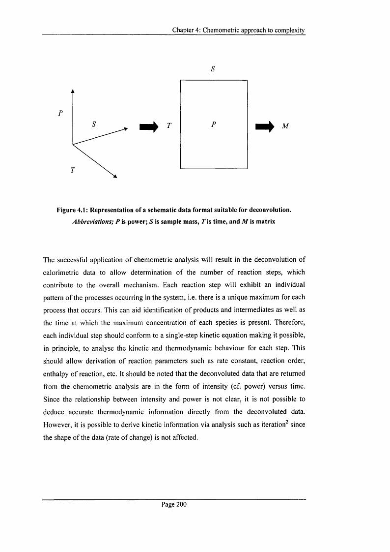
Chapter 4: Chemometric approach to complexity
P
M
Figure 4.1: Representation of a schematic data format suitable for deconvolution.
Abbreviations; P is power; S is sample mass, T is time, and M is matrix
The successful application o f chemometric analysis will result in the deconvolution o f
calorimetric data to allow determination o f the number o f reaction steps, which
contribute to the overall mechanism. Each reaction step will exhibit an individual
pattern o f the processes occurring in the system, i.e. there is a unique maximum for each
process that occurs. This can aid identification o f products and intermediates as well as
the time at which the maximum concentration o f each species is present. Therefore,
each individual step should conform to a single-step kinetic equation making it possible,
in principle, to analyse the kinetic and thermodynamic behaviour for each step. This
should allow derivation o f reaction parameters such as rate constant, reaction order,
enthalpy o f reaction, etc. It should be noted that the deconvoluted data that are returned
from the chemometric analysis are in the form o f intensity (cf. power) versus time.
Since the relationship between intensity and power is not clear, it is not possible to
deduce accurate thermodynamic information directly from the deconvoluted data.
However, it is possible to derive kinetic information via analysis such as iteration^ since
the shape o f the data (rate o f change) is not affected.
Page 200
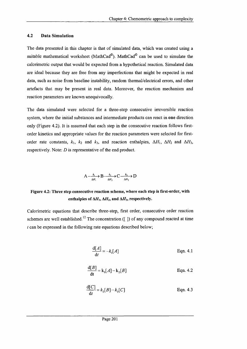
Chapter 4: Chemometric approach to com plexity
4.2 D ata Sim ulation
The data presented in this chapter is that o f simulated data, which was created using a
suitable mathematical worksheet (MathCad®). MathCad® can be used to simulate the
calorimetric output that would be expected from a hypothetical reaction. Simulated data
are ideal because they are free from any imperfections that might be expected in real
data, such as noise from baseline instability, random thermal/electrical errors, and other
artefacts that may be present in real data. Moreover, the reaction mechanism and
reaction parameters are known unequivocally.
The data simulated were selected for a three-step consecutive irreversible reaction
system, where the initial substances and intermediate products can react in one direction
only (Figure 4.2). It is assumed that each step in the consecutive reaction follows first-
order kinetics and appropriate values for the reaction parameters were selected for first-
order rate constants, k\, kj and k ,, and reaction enthalpies, A //i, A/ / 2 and
respectively. Note: D is representative o f the end product.
13- - S L _ > I )A//| A/Zi AW3
Figure 4.2: Three step eonsecutive reaction scheme, where each step is first-order, with
enthalpies of AiT,, and respectively.
Calorimetric equations that describe three-step, first order, consecutive order reaction
schemes are well established.'^ The concentration ([ ]) o f any compound reacted at time
t can be expressed in the following rate equations described below;
^ = Eqn, 4.1d(
^ = k ,[ / l ] -k j [B ] Eqn, 4,2dt
^ = Eqn, 4,3
Page 201
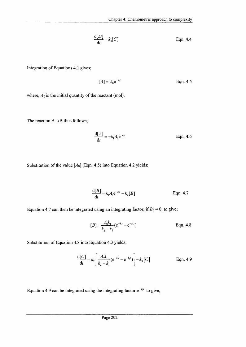
Chapter 4: Chemometric approach to com plexity
d[D]dt
= U C ] Eqn. 4.4
Integration o f Equations 4.1 gives;
[A] = A^e Eqn. 4.5
where; A q is the initial quantity o f the reactant (mol).
The reaction A—>B thus follows;
dt— k^A^Q Eqn. 4.6
Substitution o f the value [A q] (Eqn. 4.5) into Equation 4.2 yields;
d[B]dt
Eqn. 4.7
Equation 4.7 can then be integrated using an integrating factor, if Bo = 0, to give;
k i - KEqn. 4.8
Substitution o f Equation 4.8 into Equation 4.3 yields;
d[C]dt k ^ - k ,
- k ^ [ C \ Eqn. 4.9
Equation 4.9 can be integrated using the integrating factor e to give;
Page 202

Chapter 4: Chemometric approach to com plexity
[C] =- k -,1
- k - A
\ f +
y ~ ^3^2 3 1 y^2^,4)6
-k it
—k^kj + ^ 3 ^ 2 ~ ^3^1 + ^ i y
Eqn. 4.10
The sum o f the reactant concentrations must equal A q (if B, C and D are not present
initially) and it follows that;
Eqn. 4.11
Thus gives Equation 4.12;
^2^i4)6
"2 ''•1
y —k^kj ~~ k^ k j + k-^k j
k- k 4)6 - k i t
y —âT| 2 ^3^2 ” k^k + k J
+ ^2^14)6
\ - ^ 1^2 “ ^3^2 + ^ 2 + ^3^1 y
4^l4)6—k-tt
Eqn. 4.12
Differentiation o f Equation 4.12 gives;
dl
+
( k , - k , )
k lk ,A ,e ^“22
-tv
A / +
^2^|%6 -A:,/
—k^kj + k^k2 — 3 1 + A: j y
k2k AQk Q ^2^14)^36
-A:,A:2 + ^ 3 ^ 2 “ ^ 3 ^ 1 + &i
Eqn. 4.13
In terms o f calorimetric data, the power associated with each reaction step (based on the
equations above) is given in Equations 4.14 to 4.17. These equations can be used to
simulate power-time data for each reaction step, i.e., AXo B ,B to C, and C to D, where;
Page 203
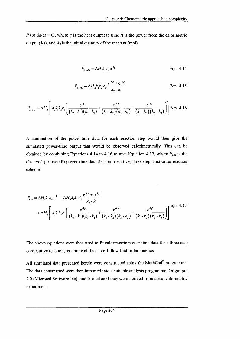
Chapter 4: Chemometric approach to com plexity
P (or dqldit = O, where q is the heat output to time t) is the power from the calorimetric
output (J/s), and A q is the initial quantity o f the reactant (mol).
-Ll Eqn. 4.14
e'*'' + e'*-'
kj ~KEqn. 4.15
+ + •e-4'
{ K - K ) [ K - K ) { K - K ) {k, - k^) {k, - k, ) [k^ - k , )Eqn. 4.16
A summation of the power-time data for each reaction step would then give the
simulated power-time output that would be observed calorimetrically. This can be
obtained by combining Equations 4.14 to 4.16 to give Equation 4.17, where fobs is the
observed (or overall) power-time data for a consecutive, three-step, first-order reaction
scheme.
ç-k,t + Q-k.J
&2-&I
+ A / / , +Q-ht
+
Eqn. 4.17
The above equations were then used to fit calorimetric power-time data for a three-step
consecutive reaction, assuming all the steps follow first-order kinetics.
All simulated data presented herein were constructed using the MathCad® programme.
The data constructed were then imported into a suitable analysis programme, Origin pro
7.0 (Microcal Software Inc), and treated as if they were derived from a real calorimetric
experiment.
Page 204
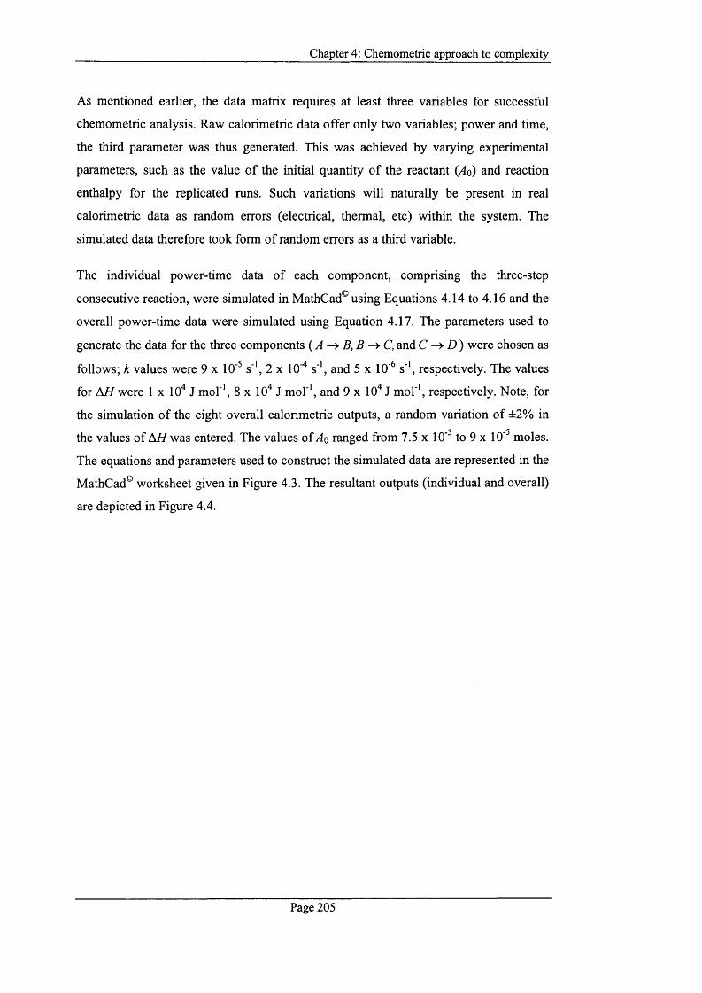
Chapter 4: Chemometric approach to com plexity
As mentioned earlier, the data matrix requires at least three variables for successful
chemometric analysis. Raw calorimetric data offer only two variables; power and time,
the third parameter was thus generated. This was achieved by varying experimental
parameters, such as the value o f the initial quantity o f the reactant ( A q) and reaction
enthalpy for the replicated runs. Such variations will naturally be present in real
calorimetric data as random errors (electrical, thermal, etc) within the system. The
simulated data therefore took form o f random errors as a third variable.
The individual power-time data o f each component, comprising the three-step
consecutive reaction, were simulated in MathCad® using Equations 4.14 to 4.16 and the
overall power-time data were simulated using Equation 4.17. The parameters used to
generate the data for the three components ( ^ —> 5, i? -> C, and C ^ D ) were chosen as
follows; k values were 9 x 10" s ', 2 x 10^ s '', and 5 x 1 0 '^ s '', respectively. The values
for A // were I x l O ^ J mol ', 8 x 10 J mol ', and 9 x 10 J mol ', respectively. Note, for
the simulation o f the eight overall calorimetric outputs, a random variation o f ±2% in
the values o f A // was entered. The values o f A q ranged from 7.5 x 10'^ to 9 x 10'^ moles.
The equations and parameters used to construct the simulated data are represented in the
MathCad® worksheet given in Figure 4.3. The resultant outputs (individual and overall)
are depicted in Figure 4.4.
Page 205

Chapter 4: Chemometric approach to com plexity
The simulation of a three-step A to B to C to D consecutive reaction scheme:
A := 7.5-10-5 kl := 910 -5
t := 0,10.. 100000 HI := 1.0-10
k2 := 2-10
H2 := 8.0-10
The reaction for A to B (step 1) can be described by;
-k l ta(t) := A HI kl -e
The reaction for B to C (step 2) can be described by;
b(t) := A-kl k2 H2-kl-t -k2-t e - e
k 2 - k l
The reaction for C to D (step 3) can be described by;
c(t) := H3 A-kl-k2-k3-kl-t -k2-t
k3 := 5-10
H3 := 9.0-10
-k3-t
(k 2 -k l ) - (k 3 -k l ) (k l-k 2 ) - (k 3 -k 2 ) (kl - k3)-(k2 - k3) _
Figure 4.3: The simulation of a three-step consecutive first order reaction
scheme.
Page 206
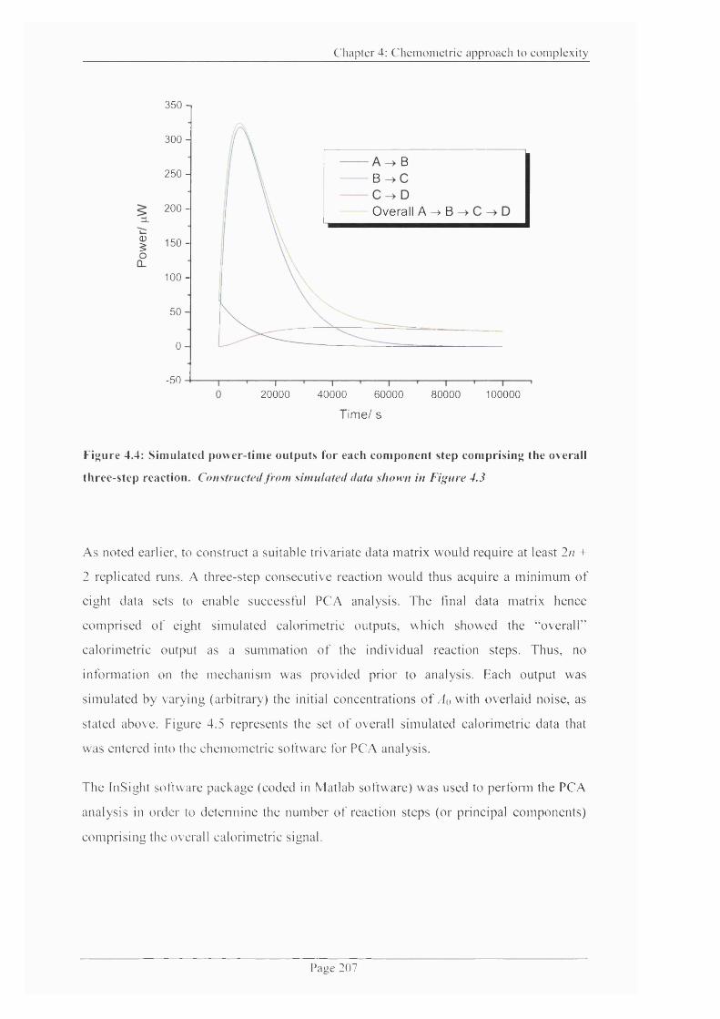
C h a p ter 4: C h e m o m e tr ic a p p ro a c h to c o m p le x ity
C D
IQ_
3 5 0 -
300 -
250 -
200 -
150-
1 0 0 -
5 0 -
0 -
-50
BB
Overall A ^ B
20000 40000 60000
Time/ s
80000 100000
Figure 4.4: Simulated power-time outputs for each component step comprising the overall
three-step reaction. Constructed from simulated data sltoyvn in Figure 4.3
As noted earlier, to construct a suitable trivariate data matrix would require at least In +
2 replicated runs. A three-step consecutive reaction w ould thus acquire a m in im um o f
eight data sets to enable successful PC A analysis. T he final data matrix hence
com prised o f eight s im ulated calorimetric outputs, which show ed the "overall"
ca lorimetric output as a sum m ation o f the individual reaction steps. Thus, no
infonnation on the m echanism was provided prior to analysis. Each output was
sim ulated by varying (arbitrary) the initial concentrations o f Ao with overlaid noise, as
stated above. Figure 4.5 represents the set o f overall s im ulated calorimetric data that
was entered into the chem om etr ic software for PCA analysis.
The InSight software package (coded in Matlab software) was used to perfonu the PCA
analysis in order to de tem iine the num ber o f reaction steps (or principal com ponents)
com pris ing the overall calorimetric signal.
P atie 2 0 7

C h a p ter 4: C h e m o m e tr ic a p p ro a c h to c o m p le x ity
400-
350 -
300 -
250-
I 200 -o
CL 150 -
1 0 0 -
50 -
0 -
----1----20000 40000 60000
Time/ s
80000 100000
Figure 4.5: Set of simulated data entered into chemometrics software for PCA analysis'
4.3 Results and Discussion
PCA analysis allows for the deconvolution o f a process into its individual components.
The simulated pow er-tim e data that were used to create a suitable matrix w ere that for a
three-step reaction system. Hence, successful PCA analysis should, in principle, result
in the detection o f sam e num ber o f com ponents as the model used to generate the data
i.e. three principal com ponents, noting that the num ber o f principal com ponents
determ ined did not require prior know ledge o f reaction m echanism.
The type o f PCA analysis perfonned to analyse the deconvoluted data matrix was that
o f factor ana lys is ." Factor analysis uses various tbm is o f m athem atical scrutiny to
detem iine if the data have any real chemical or physical m ean ing following the
deconvolution into its principal com ponents (or abstract factors). This fomi o f analysis
was used for deconvolution based on the assum ption that the pow er signal at the time /
is a linear sum o f all the species present at that m om ent, and that the signal is
proportional to the sam ple mass in the ca lo r im ete r."
P a g e 2 0 8
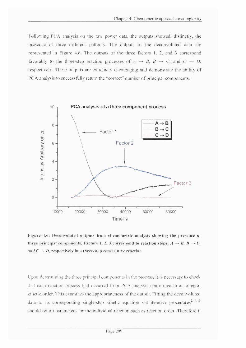
C h a p ter 4: C h e m o m e tr ic a p p ro a c h to c o m p le x i t y
Following PCA analysis on the raw pow er data, the outputs showed, distinctly, the
p resence o f three different patterns. The outputs o f the deconvoluted data are
represented in Figure 4.6. The outputs o f the three factors 1, 2, and 3 correspond
favorably to the three-step reaction processes o f /t C, and C ^ D,
respectively. These outputs are ex trem ely encouraging and dem onstra te the ability o f
PCA analysis to successfully return the "correct" num ber o f principal com ponents.
PCA analysis of a three component process10 n
Factor 1c/5
c=3
Factor 22
<
C Oc03C
Factor 3
10000 20000 30000 40000 50000 60000
Time/ s
Figure 4.6: Deconvoluted outputs from chemometric analysis showing the presence of
three principal components. Factors 1, 2, 3 correspond to reaction steps; A B, B ^ C,
and C —* D, respectively in a three-step consecutive reaction
Upon detem iin ing the three principal com ponents in the process, it is necessary to check
that each reaction process that o ccu n ed from PCA analysis confom ied to an integral
kinetic order. This exam ines the appropriateness o f the output. Fitting the deconvolu ted
data to its corresponding single-step kinetic equation via iterative procedures"’
should return parameters for the individual reaction such as reaction order. T herefore it
P atic 2 0 9
Chapter 4: Chemometric approach to com plexity
is possible to check if the individual processes are o f integral order. It was found that
the returned values from the fittings using deconvoluted data were not integral. This is
not surprising since outputs from real calorimetric data are embedded with random
errors as mentioned earlier. This, in effect, will introduce some uncertainty into the
returned order values. Moreover, the deconvoluted data were a composite response o f
eight repeat data sets, which is likely to introduce further errors to the analysis.
In general, it has been demonstrated, from the simulated data above, that chemometric
analysis shows much potential in the treatment o f complex IC data to determine the
number o f reaction processes in complex reaction schemes. Whilst the analysis was
successful for simulated IC data, the challenge is in the PCA analysis o f real-systems
and the determination o f reaction parameters thereafter. This has recently been
successfully demonstrated for a two-step consecutive, first-order, reaction process for
the degradation o f potassium hydroxylamine disulfonate in solution.'^ PCA analysis
was used to deconvolute successfully the IC data showing the presence o f two principal
components (two step reaction) which corresponded to the hydrolysis o f the disulfonate
to hydroxylamine monosulfonate and then into hydroxylamine by a two-step
consecutive reaction. The data were subjected to kinetic modelling using an iterative
procedure, before and after deconvolution in order to compare kinetic and
thermodynamic information obtained for the individual steps. Although the rate
constant was successfully obtained for the two-step process, the challenge is in
obtaining thermodynamic information such as A//. Since the chemometric software was
written specifically for spectroscopic analysis, there is a lack o f knowledge o f the
relation between power and intensity and hence it is difficult to determine accurately
values for A/7 for real systems using iterative procedures. This knowledge gap is
addressed in section 4.3.2, where theoretical consideration using two approaches is
given for the determination o f reaction enthalpies in a two-step, first-order, consecutive
reaction, which, in principle, can be applied to real systems. Note: The theoretical
approach is not limited to two-step reaction schemes, and can be extended to multi-step
reaction processes using the same principles.
Having deconvoluted the three-step reaction (shown above), the next step was then to
establish whether it was possible to determine quantitatively reaction parameters, k, and
reaction enthalpy, A77 from the chemometric outputs.
Page 210

Chapter 4: Chemometric approach to com plexity
One approach that was considered for analysis was based on analysing fractional extents
o f the reaction obtained from the chemometric outputs to determine reaction parameters
such as rate constant, k, and reaction enthalpy, AT/. The deconvoluted data from PCA
analysis does not have a defined y-axis (as shown in Fig. 4.6). Since the software used
was designed specifically for spectroscopic analysis, the y-axis is plotted as an arbitrary
intensity (a result o f the fact that no calibration curve is used for a deconvolution
process). If analysis based on fractions of the reaction is considered, this will normalise
the y-axis data. Determining a value for k should then be relatively straightforward since
they are time dependent (and the x-axis, time, is unaffected by the deconvolution
process). This, however, is not the case for the determination o f A // since its value is
power dependent.
A mathematical approach which can determine both parameters {k and A//) was thus
considered for a three-step, first-order, consecutive reaction scheme (shown above in
Fig. 4.2). Note: extension to multi-step schemes can be readily achieved using the same
principles.
4.3.1 Determination of k following deconvolution
4.3.1.1 Calculation of k\
Determining a value o f k\ for the first principal component (A) is relatively
straightforward. A plot o f In(intensity) versus time for a reaction following first-order
kinetics should be linear, and the slope of the plot gives the rate constant (Fig. 4.7).
Page 211
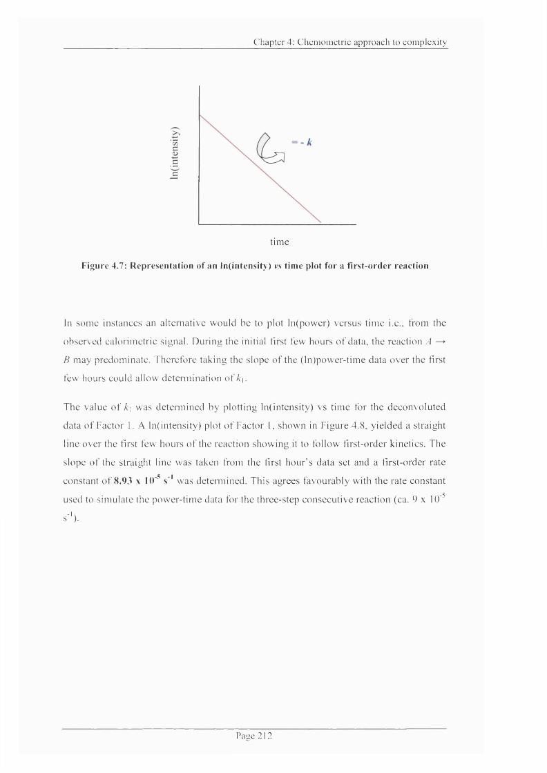
C h a p ter 4: C h e m o m e tr ic a p p ro a c h to c o m p le x ity
t ime
Figure 4.7: Representation of an In(intensity) vs time plot for a first-order reaction
in som e instances an alternative would be to plot In(power) versus time i.e., from the
observed calorimetric signal. During the initial first few hours o f data, the reaction A —>■
B m ay predominate . Therefore taking the slope o f the (In)power-time data over the first
few hours could allow detennina tion o f k\.
The value o f k\ was determ ined by plotting In(intensity) vs time for the deconvoluted
data o f Factor 1. A ln(intensity) plot o f Factor 1, shown in Figure 4.8, yielded a straight
line over the first few hours o f the reaction show ing it to follow tlrst-order kinetics. The
slope o f the straight line was taken from the first h ou r 's data set and a t'lrst-order rate
constant o f 8.93 x 10^ s ' was detemiined. This agrees favourably with the rate constant
used to simulate the pow er-tim e data for the three-step consecutive reaction (ca. 9 x 10'^
s ' ') .
P a g e 2 1 2
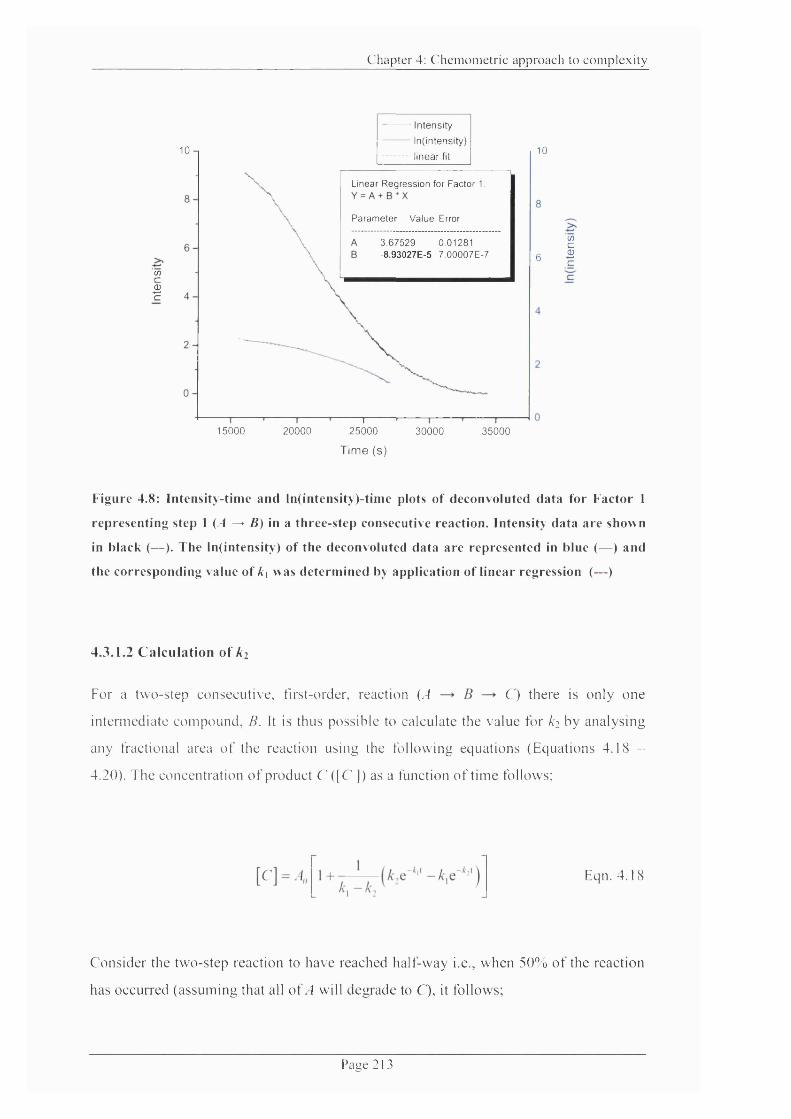
C h a p ter 4: C h e m o m e tr ic a p p ro a ch to c o m p le x i t y
Intensity
In(intensity)
linear fit10-1
Linear R egression for Factor 1 :
Param eter Value Error
3 .67529 -8.93027E-5 7.00007E -7
0.01281
COcBc
1 5 0 0 0 20000 2 5 0 0 0 30000 3 5 0 0 0
10
CO
e I
Time (s)
Figure 4.8: Intensity-time and ln(intensity)-tinie plots of deconvoluted data for Factor 1
representing step 1 {A ^ fi) in a three-step consecutive reaction. Intensity data are shown
in black (— ). The In(intensity ) of the deconvoluted data are represented in blue (— ) and
the corresponding value of k\ was determined by application of linear regression (—)
4.3.1.2 Calculation of A?
For a two-step consecutive, first-order, reaction (/I ( ') there is only one
intem iediate com pound, B. It is thus possible to calculate the value for A2 by analysing
any fractional area o f the reaction using the following equations (Equations 4.18 -
4.20). The concentration o f product C ([C ]) as a function o f time follows;
Eqn. 4.18
C onsider the two-step reaction to have reached half-way i.e., when 50% o f the reaction
has occurred (assum ing that all o f A will degrade to Q , it follows;
P a g e 2 1 3

Chapter 4: Chemometric approach to com plexity
[C] = ^ Eqn. 4.19
If the fraction o f the reaction (F) is taken at the time at which 50% of the reaction has
occurred ( 50), then Equation 4.20 follows;
F = 0.5 = 1 + - ^ - ^ [ ( ^ 2 6 -*''» - )] Eqn. 4.20
It should be noted that this method is valid for any fraction o f the reaction providing the
reaction has progressed to completion during the experimental time frame. The value
for kl can then be calculated by iteration since k\ is now known.
In order to determine a value of ki using the above equations, data were simulated using
MatchCad® for a two-step consecutive, first-order, reaction. The same data as those
used to generate the three-step process (Fig. 4.3) were used, except that in this case the
third step was not required. The data were imported into Origin and the value o f was
determined for the second step by taking the time at which the fraction o f the reaction
was 50%. The data are represented in Figure 4.9 and shows that the time of /50
determined was 13090 s.
The value o f 13090 s was applied as the ^50 to Equation 4.20 and returned a
corresponding value o f 0.5, as shown in Figure 4.10. This is in accordance with
analysing 50% o f the reaction. As mentioned before, the fraction o f reaction analysed is
not limited to 50% as illustrated in Figure 4.10 where fractions at 25% and 75%, for
example, were taken after accurately determining the corresponding value o f tis and 75,
respectively.
Page 214

Chapter 4: Chemometric approach to com plexity
350 n BtoC
3 0 0 - Integration of total area: I = 1 - > 10001 x = 0 - > 100000 Area2 5 0 - Peak at Width Height
6.79846E6 7100 18700 318.4
% Integration of area at 50%:1 = 1 -> 1 3 1 0 X = 0 - > 13090
Peak at Width HeightICL
1 5 0 -
Area
1 0 0 -3.39954E6 7100 11440 318.4
5 0 -
-500 20000 60000 80000 10000040000
Time/s
Figure 4.9: Simulated data for Step 2 (B C) representing determination of 50 at 13090 s
when 50% of the reaction has occurred
Page 215

Chapter 4: Chemometric approach to com plexity
Calculation of k2 for step 2 (B to C) in a two-step consecutive process
A := 7.5-10 k l : = 9 10 k2 2-10
HI := 1 .0 -1 o'* H 2 : - 8.0-1 o'*
t := 0 ,1 0 . . 100000 150 := 13090 125 ^ 7360 175 := 21560
The fraction of the reaction at tgo then follows Equation 4.20;
, + _ l_ (k 2 ,c -k " S 0 -k ,.e -U '5 % 0 .5k l - k 2
Similarly, the fraction of the reaction at t2 s follows;
kl - k 2
And at 17 5 follows;
, , _ L _ ( k 2 .e - ^ " ’= -k |.e - '^ " % 0 .7 5 kl - k2
k2 can then be determined at 50% (for example) using the equation below;
k2 := 0 .0 0 0 0 0 1 ,0 .0 0 0 0 0 2 ..0 .0 1
f(k ) :=k - k l
Figure 4.10: Simulated data for Step 2 (B Q representing determination of reaction
time at various fractions of reaction
If there are more than two consecutive steps, then the rate constant for the final step o f
the reaction can be obtained in the same manner as above. An alternative method to
determine kj for a reaction o f more than two-steps in the reaction process is to determine
the maximum yield o f each intermediate product and this is determined from the tmax- In
Page 216
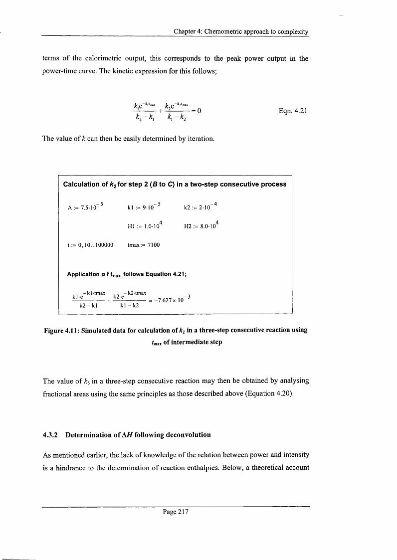
Chapter 4: Chemometric approach to com plexity
terms o f the calorimetric output, this corresponds to the peak power output in the
power-time curve. The kinetic expression for this follows;
The value of k can then be easily determined by iteration.
Calculation of ^2 for step 2 (B to C) in a two-step consecutive process
A 7 . 5 1 0 ^ kl := 9 10 ^ VI := 2 1 0 ^
HI ;= I.O IO" H2 := 8.0 lo"^
t := 0,10.. 100000 tmax:=7100
Application o f tnax follows Equation 4.21;
, , - k l tmax , _ - k2 tmax^ ^ = - 7 . 627 X 10- '
k 2 - k l k l - k 2
Figure 4.11: Simulated data for calculation of in a three-step consecutive reaction using
tmax of intermediate step
The value o f k}, in a three-step consecutive reaction may then be obtained by analysing
fractional areas using the same principles as those described above (Equation 4.20).
4.3.2 Determination of \ H following deconvolution
As mentioned earlier, the lack o f knowledge o f the relation between power and intensity
is a hindrance to the determination o f reaction enthalpies. Below, a theoretical account
Page 217
Chapter 4: Chemometric approach to com plexity
is given which considers two approaches for the determination o f A // for a two-step,
tlrst-order, consecutive reaction.
Once the rate constants are determined, the reaction enthalpies can be readily
determined in one o f two w ay s"’’ ; (1) taking two points from the power-time data or
(2) taking two points from the heat-time data (i.e. integrated power-time data). Both
methods can be applied to simulated data; the power-time method is simpler, but is
more subject to random noise error. Thus it is likely that, in practice, the heat-time
method will be more robust because it averages data over the chosen time periods
selected, hence minimising random errors.
4.3.2.1 Calculation of A /f using pow er-tim e data
In a two-step consecutive, first-order reaction the power output for the reaction is given
by the summation of Equations 4.14 and 4.15;
^ + k,k,AH,A„ ^ \ -- Eqn. 4.22d/ Xj — Xj
From the power-time data generated using Equation 4.22, two power outputs (P\ and
P 2) can then be selected at two respective time points (t\ and 2). This gives;
P = — J — Eqn. 4.23
Q-k]i2 _ Q- 2‘2
P2 = k^àH^A^çT'" '- + k^k^AHjA^ — - — -— Eqn. 4.24kl ~ ^1
Equation 4.23 can be re-written to make A//i the subject;
Page 218
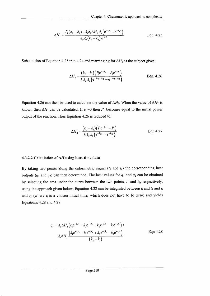
Chapter 4: Chemometric approach to com plexity
Substitution o f Equation 4.25 into 4.24 and rearranging for AH 2 as the subject gives;
Equation 4.26 can then be used to calculate the value o f AHj. When the value o f AH2 is
known then AH\ can be calculated. If t\ =0 then P\ becomes equal to the initial power
output o f the reaction. Thus Equation 4.26 is reduced to;
4.3.2.2 C alculation of M l using heat-tim e data
By taking two points along the calorimetric signal {t\ and 2) the corresponding heat
outputs (q\ and ^2) can then determined. The heat values for q\ and q2 can be obtained
by selecting the area under the curve between the two points, t\ and 2 , respectively,
using the approach given below. Equation 4.22 can be integrated between t\ and t\ and t\
and t2 (where t\ is a chosen initial time, which does not have to be zero) and yields
Equations 4.28 and 4.29.
9, = 4 ,A//, [ k , e -A ,e“'*') +
( + k . s * - L e ’ ''*' ) Eqn 4.28
M -
Page 219
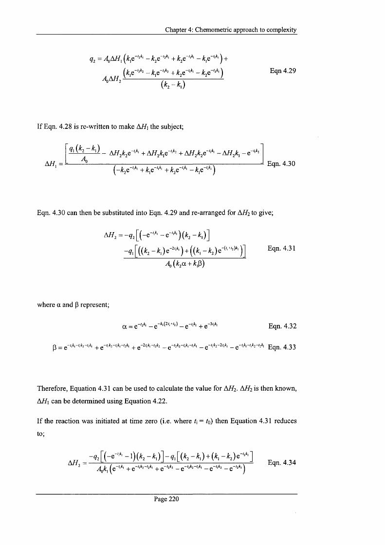
Chapter 4: Chemometric approach to com plexity
Eqn 4.29
( ^ 2 ~ K )
If Eqn. 4.28 is re-written to make A//i the subject;
A/7, =
- -A/Zj/fc, -e"''*"Eqn. 4.30
Eqn. 4.30 can then be substituted into Eqn. 4.29 and re-arranged for Ai/2 to give;
Eqn. 4.31
\ { k ^ a + k,^)
where a and p represent;
Eqn. 4.32
Therefore, Equation 4.31 can be used to calculate the value for A //2 . A/ / 2 is then known,
A//i can be determined using Equation 4.22.
If the reaction was initiated at time zero (i.e. where t\ = Iq) then Equation 4.31 reduces
to;
A / / . =_ - ^ 2 [(-G - 1)(A:2 [ ( ^ 2 -A:,)-h(A:, -A i je
-'1*1 _|_ g-'l*2-'2*l _|_ g“'2*2 _g-'2*2“'l*l _ g “'l*2 _Q~'2^lj Eqn. 4.34
Page 220

Chapter 4: Chemometric approach to com plexity
It should be noted that in most calorimetric experiments there is a delay between the
initiation time o f the reaction and data recording because it takes some time (ca. 30 - 40
min) to reach thermal equilibrium after the ampoules have been lowered into the
calorimeter. In the case o f long term reactions the data lost is negligible and for short
term reactions extrapolation o f data to the initiation time is p o s s ib le .G e n e r a l ly , in
either case, Equations 4.27 and 4.34 can be used to determine a value for
Page 221
Chapter 4: Chemometric approach to com plexity
4.4 Sum m ary
Extracting quantitative reaction parameters from complex isothermal calorimetric data
can be a difficult task primarily because the calorimeter measures all thermal processes
(both to physical and chemical changes) that occur in a reaction. The challenge is
therefore to deconvolute the observed calorimetric signal into its individual component
parts and allow the determination of quantitative reaction parameters for each reaction
step. The application of chemometric analysis offers a model-free approach to the
problem of complexity in isothermal calorimetric data; i.e., no prior knowledge o f the
reaction mechanism is required.
In this chapter, it has been shown that the use o f chemometric analysis, using principal
component analysis (PCA), has much potential in the interpretation o f complex
isothermal calorimetric data. The deconvolution o f a three-step, first-order, consecutive
reaction was successfully demonstrated using this model-free approach. Successful
deconvolution o f the process resulted in the production o f three distinct patterns of
reaction that contributed towards the overall process. PCA analysis o f the data matrix
successfully returned the correct number o f principal components corresponding
favourably with the three-step reaction process. Using simulated data it was possible to
construct successfully a suitable trivariate data matrix where two of the required
variables consisted o f power and time, which were obtained from raw calorimetric data.
The third variable in the matrix was generated by running a number o f replicate runs of
the same experiments where each replicate run had a small variation in the number of
moles o f compound and, hence, the total power output. Using appropriate kinetic
models, it was possible to determine reaction parameters such as rate constants for the
individual steps contributing the overall process. However, the determination o f reaction
enthalpies is more difficult because the relation between the recovered intensity
(chemometric output) and the power components o f the calorimetric data (TAM output)
requires further understanding. The theoretical approach considers one o f two ways in
which the reaction enthalpies in multi-component systems can be determined, which, in
principle, can be applied to real systems.
The application o f chemometric analysis to isothermal calorimetric data is relatively
new and the need to generate a third variable (to create a suitable matrix) with a large
number o f replicate runs can be challenging in cases where a new drug compound is in
Page 222

Chapter 4: Chemometric approach to com plexity
limited quantity. Nevertheless, the use o f chemometrics is an extremely useful tool
because the distinction o f the contributing factors to the overall calorimetric signal
reduces the burden on any further kinetic/thermodynamic analysis o f the data by
allowing an appropriate kinetic model to be employed in an iterative analysis.
Page 223
Chapter 4: Chemometric approach to com plexity
4.5 References
1 Glass, B.D., Novak, C. S., and Brown, M E. (2004) The thermal and photostability o f solid pharmaceuticals. J.Therm.Anal.Cal. 77, 1013-1036
2 Willson, R., Beezer, A., Mitchell., J.C., and Watson, L. (1995) Determination of thermodynamic and kinetic parameters from isothermal heat conduction microcalorimetry: applications to long-term reaction studies. J.Phys.Chem 99, 7108-7113
3 O'Neill, M.A.A. (2005) Recent Developments for the Analysis o f Data Obtained from Isothermal Calorimetry. Curr.Pharm.Biotechnol. 6, 205-214
4 Skaria, C.V., Gaisford, S., O'Neill, M.A.A., Buckton, G., Beezer, A.E. (2005) Stability assessment o f pharmaceuticals by isothermal calorimetry: two component sysiQvas. IntJ.Pharm. 292, 127-135
5 O'Neill, M.A.A., Beezer, A.E., Morris, A C., Urakami, K., Willson, R.J.,Connor, J. (2003) Solid-state reactions from isothermal heat conduction microcalorimetry: Theoretical approach and evaluation via simulated data. J.Therm.Anal.Cal. 73, 709-714
6 Dias, M., Hadgraft, J., Raghavan, S.L., Tetteh, J. (2003) The effect o f solvent on permeant diffusion through membranes studied using ATR-FTIR and chemometric data analysis. J.Pharm.Sci 93, 186-196
7 Geladi, P. (2003) Chemometrics in spectroscopy. Part 1. Classical chemometrics. Spectrochimica Acta 58 (Part B), 767-778
8 Geladia, P., Sethson, B., Nystrom, J., Lillhonga, T., Lestander, T., Burger, J. (2004) Chemometrics in spectroscopy. Part 2. Examples. Spectrochimica Acta 59 (Part B), 1347- 1357
9 Brown, M.E., Maciejewski, M., Vyazovkin, S., Nomen. R., Sempere, J., Burnham., A., Opfermann, J., Strey, R., Anderson, H.L., Kemmler, A., Keuleers, R., Janssens, J., Desseyn, H.O., Chao-Rui Li., Tangi, B. T., Roduit, B., Malek, J., Mitsuhashi, T. (2000) Computational aspects o f kinetic analysis Part A: The ICTAC kinetics project-data, methods and results. Therm.Acta 355, 125-143
10 Galwey, A.K. (2003) Perennial problems and promising prospects in the kinetic analysis o f nonisothermal rate data. Therm.Acta 407, 93-103
11 Gaisford, S., and O'Neill, M.A.A. (2007) Pharmaceutical Isothermal Calorimetry, Informa Healthcare
12 Gaisford, S. (1997) Ph.D Thesis. University o f Kent, UK
13 O'Neill, M.A.A., Beezer, A.E., Tetteh, J., Gaisford, S., Dhuna, M. (2007) Application o f Chemometric Analysis to Complexity in Isothermal Calorimetric Data. J. Phys. Chem. B
14 Willson, R.J. (1995) Ph.D Thesis. University o f Kent, UK.
Page 224

Chapter 4: Chemometric approach to com plexity
15 Willson, R., Beezer, A., Hills, A.K., and Mitchell., J.C. (1999) The imidazole catalysed hydrolysis o f triacetin: a medium term chemical calibrant for isothermal microcalorimeters. Therm.Acta 325, 125-132
16 Skaria, C.V. (2007) Ph.D Thesis. The School o f Pharmacy, University o f London, UK.
17 Beezer, A., Morris, A C., O'Neill, M.A.A., Willson, R.J., Hills, A.K., Mitchell, J.C., and Connor, J.A. (2001) Direct determination o f equilibrium thermodynamic and kinetic parameters from isothermal heat conduction microcdXonrnQtiy. J.Phys.Chem B 105, 1212-1215
18 O'Neill, M.A.A. (2002) Ph.D Thesis. University o f Greenwich, UK
Page 225

- Chapter Five -
Applications
Chapter 5; Applications
5. Introduction
Following on from the development o f the photocalorimetric systems (described in
Chapter 2) and having established a suitable method for actinometry allowing
quantitative measurements o f photon flux and irradiance (described in Chapter 3), the
next step was to apply the instrument to known photosensitive materials.
Chapter 2 detailed the development o f two prototype photocalorimetric systems; one
design consisted o f a 300 W Xe arc lamp and the latter used solid-state LED lighting.
Because o f the design problems inherent in using a Xe arc lamp, the data (shown in
Chapters 2 and 3) showed conclusively that the design did not produce satisfactory data.
As a result, the experimental measurements presented in this chapter, therefore, were
conducted using solely the LED photocalorimeter.
One o f the objectives for developing the LED photocalorimeter was that it allowed the
opportunity to create a ‘custom’ light spectrum by selecting a range o f LEDs that were
specific to a particular wavelength. Since each LED emits over a very narrow
wavelength range and the fact that a number o f LEDs are arranged in an array mean that
the photocalorimeter can be used to determine the causative wavelength o f degradation
o f a sample, because it is possible selectively to switch on each LED individually.
This chapter describes the application o f the novel LED photocalorimeter for
photostability testing of a well known photosensitive drug, nifedipine. The main
objectives are;
'T to study the photosensitivity o f nifedipine in solution phase and the response of
the photocalorimetric output
^ to determine the photostability o f nifedipine across the UV-VIS range using full
spectrum lightening (limited to 350 - 700 run)
^ to determine a causative wavelength range(s) o f nifedipine photodegradation
Page 227
Chapter 5 : Applications
5.1 Application of pbotocalorimetry to the photodegradation of nifedipine
Nifedipine (dimethyl l,4-dihydro-2,6-dimethyl l-4-(2-nitrophenyl) pyridine-3,5-
dicarboxylate, C 17H 18N 2O6) is a well-known photoliable substance. It has been used
commonly as a calcium channel blocker, which is useful in hypertension therapy.’ It has
also been used as a vasodilator to regulate blood pressure,’’ prevention o f myocardial
ischemia,^ and for the prevention o f post-partum preeclampsia-eclampsia (pregnancy
induced hypertension).'’’ Other uses include treatment o f high altitude pulmonary
oedema,*^ atherosclerosis,^ and cocaine-addiction.^
The photodegradation o f nifedipine has been widely studied in solutions^"'^ and solid
s t a t e .N i f e d i p i n e has also found use as a test drug for photostability testing in the
development o f new photon sources for irradiation la m p s .M o re o v e r , various
strategies to protect nifedipine from light have also been studied intensively.^’’" ^
Nifedipine is highly photosensitive and decomposes into two major products, nitro-and
nitroso-derivatives under UV light, in the solution phase." The photoproducts are
represented in Figure 5.1. In the solid-state up to four decomposition products have
been reported when exposed to UV l i g h t . I n addition to the two major products, the
third and fourth photoproducts are minor. The third photoproduct has been identified as
an azoxybenzene, whilst the fourth has been observed in trace amounts and yet remains
unidentified.'^ The most thermodynamically stable form is the nitro-derivative, 4-(2-
nitrophenyl)-2,6-dimethyl-3,5-dimethoxycarbonylpyridine, which corresponds to a
dehydrogenated form o f nifedipine (Product I). The nitroso-derivative, 4-(2-
nitrosophenyl)-2,6-dimethyl-3,5-dimethoxycarbonylpyridine, and the azoxy-derivative,
2,2'-bis-(2,6-dimethyl-3,5-dimethoxycarbonylpyridine-4-yl)azoxybenzene (Products II
and III, respectively) are metastable. The photoreactivity o f nifedipine is a result o f the
co-presence o f the hydrogen abstracting group and an easily asbtractable benzylic
hydrogen. Upon exposure to sunlight, the nitro group is reduced to a nitroso group while
the ring oxidises. However, under exposure to UV light, the nitroso group is reoxidised
to reform the nitro group. The kinetics o f nifedipine photodegradation are strongly
dependent on light intensity, and wavelength distribution o f the used radiation source.
Page 228
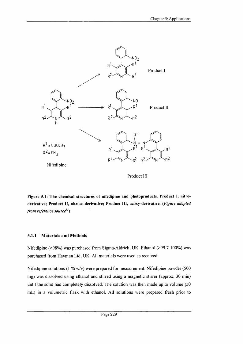
Chapter 5: Applications
Product I
N = NR' R
Product II
=C00CH3
r 2=CH
Nifedipineif R^
Product III
Figure 5.1: The chemical structures of nifedipine and photoproducts. Product I, nitro-
derivative; Product II, nitroso-derivative; Product III, azoxy-derivative. {Figure adapted
from reference source'^)
5.1.1 M aterials and M ethods
Nifedipine (>98%) was purchased from Sigma-Aldrich, UK, Ethanol (>99.7-100%) was
purchased from Hayman Ltd, UK. All materials were used as received.
Nifedipine solutions (1 % w/v) were prepared for measurement. Nifedipine powder (500
mg) was dissolved using ethanol and stirred using a magnetic stirrer (approx. 30 min)
until the solid had completely dissolved. The solution was then made up to volume (50
mL) in a volumetric flask with ethanol. All solutions were prepared fresh prior to
Page 229

Chapter 5: Applications
measurement light under a red light in a dark room. Amber glass volumetric flasks were
used throughout and were wrapped in aluminium foil to protect from stray light.
All photocalorimetric measurements were performed using the LED photocalorimeter at
37°C. Prior to sample measurements, a reference experiment was conducted for each
LED used in order to achieve an overall net zero power signal on the TAM when the
light was switched on at a chosen wavelength. This was achieved by pipetting 4 mL of
ethanol in both the sample and reference calorimetric ampoules (20 mL stainless steel).
The ampoules method of lowering into the TAM following the lowering method
described in Chapter 2 (Section 2.3.2). The voltage supplied to the sample and reference
sides was preset to 15 V. The light was then switched on and the voltage on the
reference side was adjusted until a zero calorimetric signal (±2 pW) was obtained.
Following the reference experiment, the sample ampoule was replaced with nifedipine
solution (4 mL) and the photodegradation o f nifedipine was monitored. Using this
procedure, the photodegradation o f nifedipine in solution was monitored at 15 V under
full spectrum (350 - 700 nm) coverage i.e. switching on all the LEDs comprising the
array, and using monochromatic wavelength, i.e. 360 nm, 370 nm, 380 nm, 395 nm, and
400 - 700 nm. Each LED at a chosen wavelength was blanked with the reference
solution individually before sample measurements at the same wavelength commenced.
All measurements were taken in triplicate thus the standard deviations are given as n=3.
Photon flux values were recorded step-wise for each LED measurement using an
Avantes spectrometer (already described in Chapter 3, Section 3.2). Each LED was
switched on successively (15 V) and the photon flux was recorded in real-time.
5.2 Results and Discussion
5.2.1 Photodegradation of nifedipine under full spectrum light
Figure 5.2 is typical o f the calorimetric output obtained for the photodegradation o f
nifedipine under full spectrum light i.e. covering a wavelength range o f 350 - 700 nm.
From the observed calorimetric outputs the magnitude o f the signal is far greater than
the baseline response o f the reference experiment, which contained the solvent (ethanol)
Page 230
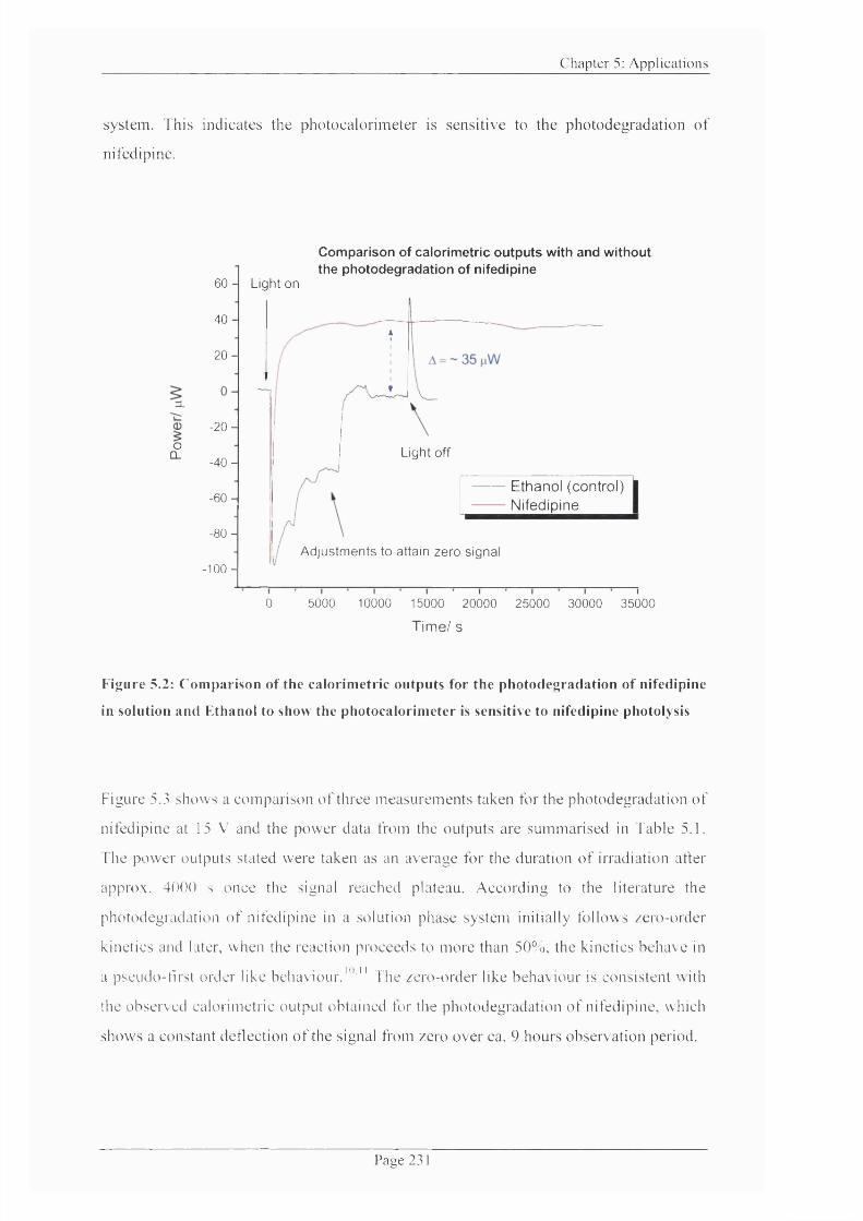
C h a p ter 5; A p p lic a t io n s
system. This indicates the photocalorim eter is sensitive to the photodegradation o f
nifedipine.
Comparison of calorimetric outputs with and withoutthe photodegradation of nifedipine
60 - Light on
40 -
2 0 -
oCL
-20 -
Light off-40 -
Ethanol (control) Nifedipine_____-60 -
-80 -Adjustments to attain zero signal
- 1 0 0 -
0 5000 10000 15000 20000 25000 30000 35000
Time/ s
Figure 5.2: Comparison of the calorimetric outputs for the photodegradation of nifedipine
in solution and Ethanol to show the photocalorimeter is sensitive to nifedipine photolysis
Figure 5.3 shows a com parison o f three m easurem ents taken for the photodegradation o f
nifedipine at 15 V and the power data from the outputs are sum m arised in Table 5.1.
The pow er outputs stated were taken as an average for the duration o f iiTadiation after
approx. 40()() s once the signal reached plateau. A ccord ing to the literature the
photodegradation o f nifedipine in a solution phase system initially follows zero-order
kinetics and later, when the reaction proceeds to m ore than 50%, the kinetics behave in
a pseudo-til St order like behav iou r ." ’ " The zero-order like behaviour is consistent with
the observed calorimetric output obtained tor the photodegradation o f nifedipine, which
show s a constant deflection o f the signal from zero over ca. 9 hours observation period.
P a g e 231

C h a p ter 5: A p p lic a t io n s
iS.
60 -
40 -
20 -
0 -
-20 -
-40 -
-60 -
-80 -
- 1 0 0 -
Photodegradation of Nifedipine under full spectrum light at 15 V
Run 1Run 2Run 3
-120-1-0
— I— f-5
Time/ h
1 ' 1 ' !
8 9 10
Figure 5.3: Povver-tinie data for the photodegradation of nifedipine in solution at 15 V
under full spectrum light
Table 5.1: Power data of nifedipine photolysis at 15 V under full spectrum
Run Pow er signal (iiW )1 35.72
2 37.%
3 33.65
Mean 35.78
± SD 2.15
% RSD (error) 6 %
The calorimetric response o f nifedipine show ed a constant detlec tion over the
irradiation period thus following zero-order like kinetic behaviour. However, any
predictions about the reaction enthalpy, rate constant and duration o f the photoreaction
to com pletion are im possible to predict, w ithout ancillary m ethods, because o f the lack
o f know ledge o f the changes in concentration. Further experim ents are therefore
P atic 2 3 2

C h a p te r 5: A p p lic a t io n s
required in this area to establish sueh reaction param eters before the photocalorim eter
can be used to produce reliable quantitative data. Thus, it is s im ply noted here that the
preliminary tests pe rfonned shows that the photocalorim eter is w ork ing satisfactorily
and is capable o f m onitoring the photosensitivity o f nifedipine.
5.2.2 Photodegradation of nifedipine under monochromatic light
Following the photodegradation o f nifedipine under full spectrum light, the application
o f the individual LEDs that com prise the array w as tested to observe the
photodegradation o f nifedipine under specific wavelengths.
Figure 5.4 to 5.8 show the calorimetric outputs for the photoreaetiv ity o f nifedipine at
peak w avelengths o f 360, 370, 380, 395 and 400 - 700 nm (white LED), respectively.
Figure 5.9 shows a com parison o f the pow er outputs obtained under specit'ie and full
array lighting. All the pow er data from the outputs are sum m arised in Table 5.2 where
the values given are an average (after approx. 4000 s as the signal reached plateau) o f
the three measurem ents.
ioCL
Run 1 Run 2 Run 3
Photolysis of Nifedipine at 360 nm20
18
16
14
12
10
8
6
4
2
0
•2
■4
0 5000 10000 15000 20000 25000 30000 35000 40000
Time/ s
Figure 5.4: Power-time data for the photodegradation of nifedipine in solution at 360 nm
P a g e 2 3 3
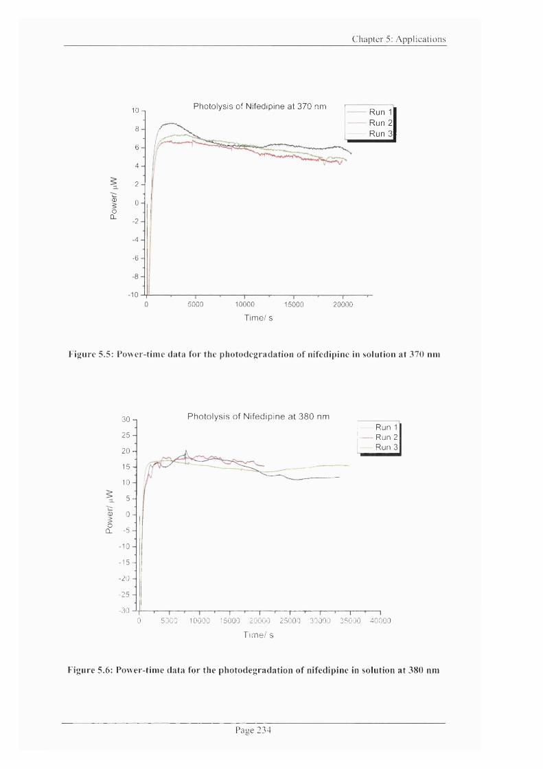
C h a p ter 5: A p p lic a t io n s
<D$o
CL
5000 10000 15000
Time/ s
Photolysis of Nifedipine at 370 nm1 0 - 1 Run 1
Run 2 Run 38
6
4
2
0
■2
-4
-6 -
20000
Figure 5.5: Power-time data for the photodegradation of nifedipine in solution at 370 nm
Photolysis of Nifedipine at 380 nm3 0 -, Run 1- Run 2
Run 32 5 -
2 0 -
15 -
1 0 -
iCL -5 -
- 2 0 -
-2 5 -
-300 5000 10000 15000 20000 25000 30000 35000 40000
Time/ s
Figure 5.6: Power-time data for the photodegradation of nifedipine in solution at 380 nm
P a g e 2 3 4

C h a p te r 5: A p p lic a t io n s
1 0-, Photolysis of Nifedipine at 395 nm Run 1 Run 2 Run 3
-2 -I0_ - 4 -
- 6 -
- 1 0 -
- 1 2 -
- 1 4 -
0 5000 10000 15000 20000 25000 30000 35000
Time/ s
Figure 5.7: Power-time data for the photodegradation of nifedipine in solution at 390 nm
Photolysis of Nifedipine using the white LED
Run 1 Run 2 Run 3
ICL
- 6 -
-8 -
0 5000 10000 15000 20000 25000 30000 35000 40000
Time/ s
Figure 5.8: Power-time data for the photodegradation of nifedipine in solution using a
w hite LED (400 - 700nni)
Page 235
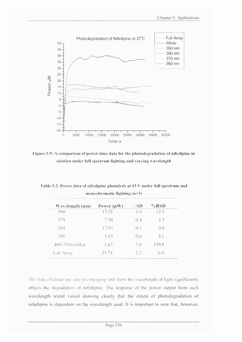
C h a p ter 5: A p p lic a t io n s
Photodegradation of Nifedipine at 37°C Full Array White 390 nm 380 nm 370 nm 360 nm
50 n45-
40-
35-
30-
25-
2 0 -
IoQ_
15-
1 0 -
0 - i
-5-
- 1 0 -
-15-
-200 5000 10000 15000 20000 25000 30000 35000 40000
Time/ s
Figure 5.9: A comparison of power-time data for the photodegradation of nifedipine in
solution under full spectrum lighting and varying wavelength
Table 5.2: Power data of nifedipine photolysis at 15 \ under full spectrum and
monochromatic lighting (n=3)
W avelength (nm ) Pow er (juW) ± SD % R SD369 13.21 1.6 12.1
370 7.58 0.4 5.3
380 17.07 0.1 0.6
305 3.13 0.6 5.1
400-700 (w hite) 1.67 2.0 1 10.8
Full Array 35.78 2.2 6.0
The data obtained are very encouraging and show the wavelength o f light s ignitlcantly
affects the degradation o f nifedipine. 1 he response o f the pow er output from each
w avelength tested varied show ing clearly that the extent o f photodegradation o f
nifedipine is dependent on the w avelength used. It is important to note that, however,
P a e e 2 3 6

Chapter 5: Applications
that the intensity o f each LED is different from each other (shown below) and therefore
the observed power output is not only a result o f nifedipine photodegradation but is also
governed by the amount o f radiant energy that is delivered to the sample during
irradiation. Different levels o f radiant energy will impact on the calorimetric output.
Since the radiant energy differs in each LED it is not possible to directly compare the
extent o f the power outputs that occurred during the photoreaction at each o f the
wavelengths tested.
It can be seen from the power-time profiles that the nifedipine photoreaction is best
described as pseudo-zero-order kinetics under full spectrum lighting using the LED
array and using specific wavelengths. However, it should be kept in mind that many
variables such as external temperature surrounding the light guides and LED assembly,
fluctuations inherent in photon delivery from LEDs, lamp life deterioration, changes in
instrument geometry between sampling, sample mass variation, etc, can collectively
contribute to instabilities in the calorimetric power signal during measurements, which
consequently can markedly affect the kinetics o f the reaction.
The maximum photodegradation o f nifedipine was found at 380 nm and 360 nm,
followed by degradation at 370 nm. The least photosensitivity to nifedipine and most
variability in the calorimetric response were found in a wavelength range o f 400 - 700
nm using the white LED. This is consistent with previous work” ’'^ where studies have
shown that the photodegradation o f nifedipine does not appear to be caused by any
specific wavelength in the visible range (typically 400 - 700 nm). This is in agreement
with the power signals obtained which show minimal deflection from the baseline and
range within ± 4 pW. Since the magnitude o f the signal is very small and unstable, it is
difficult to discriminate whether the signal is attributed to photosensitivity o f reaction,
variability in factors such as baseline noise (typically ± 2 pW), flux fluctuation, etc,.
Consequently, any photosensitivity o f nifedipine in the visible range is not obvious from
these data.
The extent o f the calorimetric response to nifedipine photodegradation is not only
dependent on the wavelength used, but also on the intensity o f the LED. As mentioned
in Chapter 3, each o f the LEDs comprising the array differs in intensity. The real-time
measurements recorded with the spectroradiometer show the flux distribution o f each
Page 237
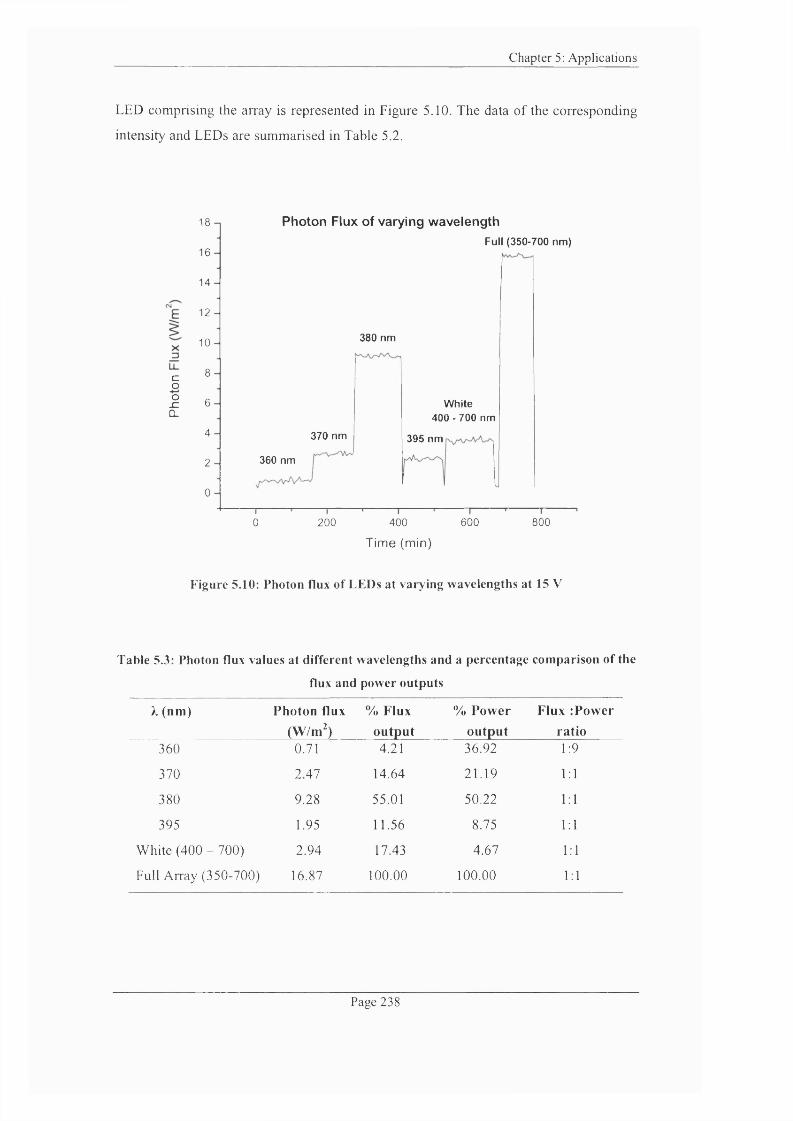
C hapter 5; A p p lica tio n s
LED comprising the array is represented in Figure 5.10. The data o f the corresponding
intensity and LEDs are summarised in Table 5.2.
coo
. cc_
Photon Flux of varying wavelength18Full (350-700 nm)
16
14
12
380 nm10
8
6 White 400 - 700 nm
4 370 nm 395 nm
360 nm2
0
0 200 400 600 800
Time (min)
Figure 5.10: Photon flux of LEDs at varying wavelengths at 15 V
Table 5.3: Photon flux values at different wavelengths and a percentage comparison of the
flux and power outputs
X (nm) Photon flux (W/m^)
% Flux output
% Power output
Flux iPower ratio
360 0.71 4.21 36.92 1:9
370 2.47 14.64 21.19 1:1
380 9.28 55.01 50.22 1:1
395 1.95 11.56 8.75 1:1
White (400 - 700) 2.94 17.43 4.67 1:1
Full Array (350-700) 16.87 100.00 100.00 1:1
Page 238
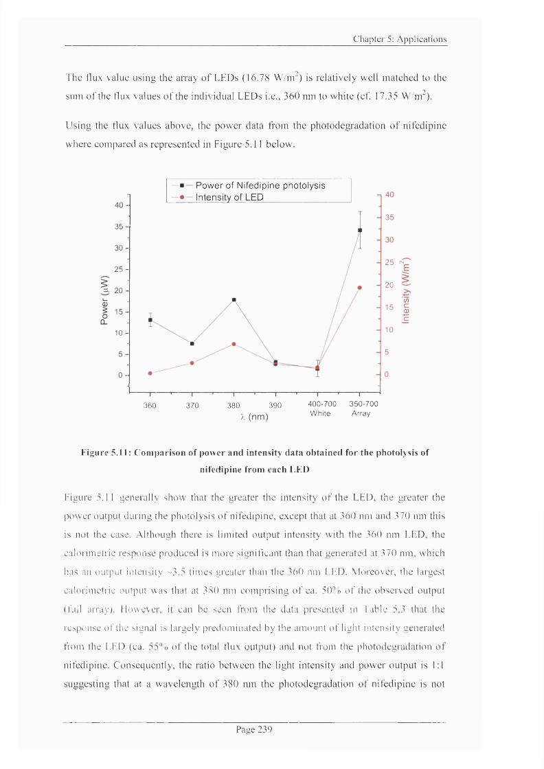
C h a p te r 5: A p p lic a t io n s
The flux value using the array o f LEDs (16.78 W/m^) is relatively well m atched to the
sum o f the tlux values o f the individual LEDs i.e., 360 nm to white (cf. 17.35 W/m").
Using the tlux values above, the pow er data from the photodegradation o f n ifedipine
where com pared as represented in Figure 5.11 below.
360
— Power of Nifedipine photolysis — intensity of LED____________
35-
30 -
25 -
20
10 -
25
cBc
370 380 390/. (nm)
400-700 350-700W hite Array
Figure 5.11: Comparison of power and Intensity data obtained for the photolysis of
nifedipine from each LEI)
Figure 5.1 1 generally show that the greater the intensity o f the LED, the greater the
pow er output during the photolysis o f nifedipine, except that at 360 nm and 370 nm this
is not the case. A lthough there is limited output intensity with the 360 nm LED, the
calorimetric response produced is more significant than that generated at 370 nm, which
has an output intensity -3 .5 times greater than the 360 nm LED. M oreover, the largest
calorimetric output was that at 380 nm com prising o f ca. 503o o f the observed output
(full array). However, it can be seen from the data presented in fab le 5.3 that the
response o f the signal is largely predominated by the am ount o f light intensity generated
from the LED (ca. 55% o f the total tlux output) and not from the photodegradation o f
nifedipine. Consequently , the ratio between the light intensity and pow er output is 1:1
suggesting that at a wavelength o f 380 nm the photodegradation o f nifedipine is not
P a g e 2 3 9
Chapter 5 : Applications
notably different from that at 370 nm and above. In contrast, it is only at the wavelength
o f 360 nm that the photodegradation o f nifedipine is more prominent where the
observed power output is ~8 times greater than that o f its light intensity (ratio o f 1:8).
This suggests nifedipine has is particularly sensitive at a wavelength o f ca. 360 nm.
These data are very encouraging and agree favourably with previous studies'
which have shown nifedipine to have maximum absorbance peak at 360 nm. In
addition, the literature also reports an absorption peak at 237 n m ," ’ "' but because o f the
nature o f the instrument design it was not possible to study wavelengths below 350 nm.
This can be a hindrance in a screening process for any photolabile drug which could
potentially degrade below 350 nm. Thus, the focus o f future work in this area therefore
requires further engineering improvements to incorporate such wavelengths.
One way of dealing with the different levels o f intensity can be to compensate for it
with the voltage supplied to the LEDs. The adjustment o f the voltage input to the each
LED can be independently controlled until a desired intensity level is attained. This can
be readily monitored on the spectroradiometer. Further engineering work is currently
underway at The School o f Pharmacy, University of London, in order to address this
issue where an automated power supply is being constructed which can electronically
balance the power outputs and intensity of each LED.
Page 240

Chapter 5 : Applications
5.3 Sum m ary
The LED photocalorimeter has shown much potential to monitor the photostability of
nifedipine. Preliminary tests have shown that the instrument is working satisfactorily
and has demonstrated much potential for the determination o f nifedipine
photodegradation under full spectrum and specific wavelengths o f light for screening of
causative wavelengths.
Having monitored the photodegradation o f nifedipine at specific wavelengths; 360 nm,
370 nm, 380 nm, 395 nm and a wavelength range in the visible region (400 - 700 nm),
the data showed that nifedipine photodegradation was most prominent at 360 nm. This
was most noticeable since at limited intensity output, the magnitude o f the calorimetric
response using the 360 nm LED was much greater than those at 370 nm and above. As a
result, the magnitude o f the observed power output was 8 times greater than that o f its
light intensity. Since the intensity levels differ in each LED it was not possible directly
to compare the extent o f the power outputs that occurred during the photoreaction at
each o f the wavelengths tested. An automated power supply is, however, currently
under development which can adjust the LED intensity to reach a desirable level.
In general, the data showed that nifedipine is not sensitive to photodecomposition at
wavelengths above 370 nm, particularly in the visible region (between 400 - 700 nm)
where no obvious photosensitivity was detected by the photocalorimeter. These data
support the findings for causative wavelength studies as those reported in
literature’ and thus is a good indication that the instrument is working
appropriately.
Although the initial trials using LEDs as a light source for the photodegradation of
nifedipine are promising, the real challenge would, however, lie in deriving quantitative
thermodynamic and kinetic parameters for the photoreaction in solution-phase and
solid-state systems. Further work in this area is required with the need to use ancillary
methods for the derivation o f reaction parameters such as the rate constant. There is also
a need for further instrumental development to allow for the investigation o f causative
wavelengths below 350 nm.
It should be anticipated that all degradation reactions are complex. This is also evident
from the power-time profiles obtained from the nifedipine photodegradation using
Page 241

Chapter 5 : Applications
specific wavelengths where pseudo-zero order like behaviour was observed. An
interesting and useful tool for data analysis o f nifedipine that can be used for future
applications is based on the chemometric approach (as discussed in Chapter 4).
Although not fully established yet, the chemometric approach is able to deconvolute
complex reaction data.
Overall, the results show that the photocalorimeter is capable o f detecting and
responding accordingly to a selection o f wavelengths providing a rapid method of
screening nifedipine for causative wavelength in the range o f 350 - 700 nm in real-time.
Page 242

Chapter 5 : Applications
5.4 References
1 Yamagishi, S., and Nakamura, K. (2007) Revival o f nifedipine, a dihydropyridine-based calcium blocker. M edical Hypotheses 68, 565-567
2 Lubsen, J., Voko, Z., Poole-Wilsond, P.A., Kirwan B., and Brouwer, S. (2007)Blood pressure reduction in stable angina by nifedipine was related to stroke and heart failure reduction but not to coronary interventions. Journal o f Clinical Epidemiology 60, 720-726
3 Seitelberger, R., Zwolfer, W., Huber, S., Schwarzacher, S., Binder, T.M.,Peschl, P., Spatt, J., Holzinger, C., Podesser B., and Buxbaum, P.,. (1991) Nifedipine reduces the incidence o f myocardial infarction and transient ischemia in patients undergoing coronary bypass grafting. Circulation 83, 460-468
4 Sambrooka, A.M., Small, R.C. (2008) The treatment of hypertension in pregnancy. Anaesthesia and Intensive Care Medicine 9, 128-131
5 Podymow, T., and August, P. (2007) Hypertension in Pregnancy. Advances in Chronic Kidney Disease 14, 178-190
6 Maggiorini, M. (2006) High altitude-induced pulmonary oedema. Cardiovascular Research 72, 41-50
7 Yamagishi, S.., and Nakamura, K. (2007) Prevention o f diabetic vascular calcification by nifedipine, a dihydropyridine-based calcium channel blocker. M edical Hypotheses 68, 1096-1098
8 Calcagnetti, D.J., Keck, J., Quatrella, L.A., and Schechter, M.A. (1995) Blockade o f cocaine-induced conditioned place preference: Relevance to cocaine abuse therapeutics. Life Sciences 56, 475-483
9 Matsuura, 1., Imaizumi, M., and Sugiyama, M. (1990) Method o f kinetic analysis o f photodegradation: Nifedipine in solutions. Chem.Pharm.Bull 38, 1692-1696
10 Shamsipur, M., Bahram, H., Akhond, K.J., Ramin, M. (2003) A study o f the photo-degradation kinetics o f nifedipine by multivariate curve resolution analysis. J.Pharm.Biomed.Anal 31, 1013-1019
11 Majeed, I.A., Murray, W.J., Newton, D.W., Othman, S, and Al-turak, W.A. (1987) Spectrophotometric study o f the photodecomposition kinetics of nifedipine. J.Pharm.Pharmacol 39, 1044-1046
12 Lehto, V.P., Salonen, J., and Laine, E. (1999) Real time detection of photoreaetivity in pharmaceutical solids and solutions with isothermal microcalorimetry. Pharm.Research 16, 368 - 373
13 Matsuda, Y., Teraoka, R., and Sugimoto, I. (1989) Comparative evaluation o f photostability o f solid-state nifedipine under ordinary and intensive light irradiation conditions. Int. J.Pharm. 54, 211-221
Page 243

Chapter 5 : Applications
14 Lehto, V.P., Salonen, J. and Laine, E. (1999) A microcalorimetric study on the role o f moisture in photolysis o f nifedipine powder. J.Therm. Anal.Cal. 56, 1305- 1310
15 Marciniec, B., and Rychcik, W. (1994) Kinetic analysis o f nifedipine photodegradation in the solid state. Pharmazie 49, 894-897
16 Vippagunta, S.R., Maul, K.A., Tallavajhala, S., and Grant, D.J.W. (2002) Solid- state characterisation o f nifedipine solid dispersions. Int. J.Pharm. 236, 111-123
17 Aman, W., and Thoma, K. (2002) The influence o f formulation and manufacturing process on the photostability o f tablets. Int. J.Pharm. 243, 33-41
18 Morris, A C. (2004) Ph.D Thesis. University o f Greenwich, Kent, UK.
19 Matsudo, M., Machida, Y., Furuichi, H., Nakama, K. and Takeda, Y. (1996) Suitability o f photon sources for photostability testing o f pharmaceutical products. Drug stab. 1, 179-187
20 Thoma, K., and Klimek, R. (1991) Photostabilization o f drugs in dosage forms without protection from packaging materials. Int.J.Pharm. 67, 169-175
21 Tonnesen, H.H. (1991) Photochemical degradation o f components in drug formulations. I. An approach to the standardization o f degradation studies. Pharmazie 46, 263-265
22 Tonnesen, H.H. (2001) Formulation and stability testing o f photolabile drugs. Int.J.Pharm. 225, 1-14
23 Béchard, S R., Quaraishi, O., and Kwong, E. (1992) Film coating: effect o f titanium dioxide concentration and film thickness on the photostability of mÏQà.vç'mQ. Int.J.Pharm. 87, 133-139
24 Tronchin, M., Callegarin, F., Elisei, F., Mazzucato, U., Reddi, E., Jori, G. (1998) A comparison between the photochemical and photosensitising properties o f different drugs. In Drugs: Photochemistry and Photostability (Albini, A., and Fasani, E., ed.). The Royal Society of Chemistry
Page 244

- Chapter Six -
Summary and Future Work
Chapter 6: Summary and Future Work
6. Summary and Future Work
It has been shown through the work presented in this thesis that photocalorimetry is a
useful and versatile tool, which offers much potential for the routine screening o f APIs
in the assessment o f photostability. The overall outcome is extremely encouraging in
that a photocalorimeter was successfully developed, which can be used to derive
thermo-kinetic information for a system during a photochemical process.
The development o f a novel photocalorimeter, which utilises an array o f light-emitting
diodes (LEDs), has been demonstrated in Chapter 2. This was built through a series of
iterative prototype designs in order to achieve the final design. It was shown that
although the original photocalorimeter (developed as part o f a former PhD project
which utilised a xenon arc light source) was useful for providing proof-of-concept data,
it was not ideal because it proved impossible to obtain a zero power signal with and
without irradiating the sample cell, rendering quantitative analysis o f data challenging.
Subsequent re-development of the instrument was extremely encouraging and resulted
in reducing the baseline signal with the light off and on. The unique shuttering and
focussing assemblies featured on the optical beam splitter allowed the light to be
adjusted, whilst the power output was being monitored on the TAM, until a zero power
signal was obtained. However, over the course o f the project, it was shown that the
challenges associated in obtaining consistent quantitative data using a xenon arc lamp
became apparent, primarily because of the rapid deterioration in performance o f the
light source. The use o f LEDs as an alternative showed greater applicability as a light
source for the photocalorimeter. Selecting a number o f LEDs made it possible to
construct an array o f wavelengths in the UV-VIS range. The system was designed so
that LEDs could be used all together (full spectrum) or independently within a
wavelength range o f 360 - 700 nm; the latter allowing the study o f causative
wavelength (s) by illumination o f a LED at a specific wavelength. The baseline signal
can be adjusted, in a similar manner to the earlier design, by balancing the voltage input,
and hence light intensity, on the power supply so that a zero calorimetric power output
can be obtained.
One o f the issues associated with the LED photocalorimeter is that each LED within the
array exhibits a different level o f intensity (as highlighted in Chapters 3 and 5). This
Page 246

Chapter 6: Summary and Future Work
was captured in the spectroradiometric data. Different LED intensities make it difficult
to assess if the measured calorimetric response is a result o f the photodegradation o f the
sample that takes place or from the associated radiant energy o f the LED, which will
also impact on the calorimetric output. One way to deal with this is to establish a level
o f intensity that is proportional between the LEDs by controlling independently the
voltage supplied to each LED until a desired intensity level is attained. Further
instrumental developments are currently under development in order to address this
issue as part o f the future work required in this area. An automated electronic-balancing
power supply which enables the autobalance o f the power signals in the sample and
reference sides is currently under development as an accessory to the photocalorimeter
at The School o f Pharmacy, University o f London. The autobalance power supply
allows an electronic balance o f the sample and reference power outputs so that a zero
calorimetric signal can be obtained. This is achieved by increasing or decreasing the
voltage supplied to the reference LED whilst the sample LED is at a fixed voltage in
order to compensate for the difference in intensities, and hence power output, that exist
between the two sides. A schematic o f the autobalance power supply is give below in
Figure 6.1 along with the workings o f the system.
Page 247
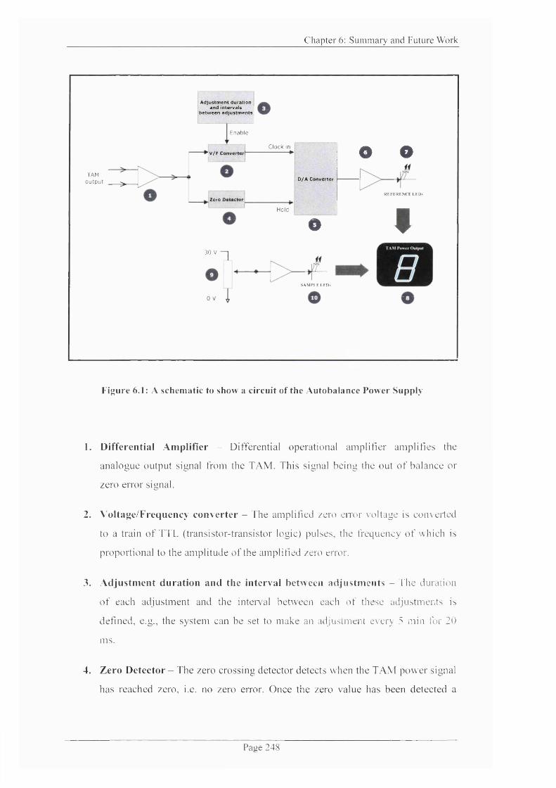
C h a p ter 6: S u m m a ry a n d F u tu re W ork
A djustm ent duration and in tervals i
be tw een adjustm ents!
E n ab le
►jv/F Cqnvertw f
T A Mo u tp u t ____ ^
_ Zero D etector
30 V 1
Clock In
D/A Converter
Hold
O
SA M PI.F. l .F D t
O O
R E FE R E N C E LED s
#
Figure 6.1: A schematic to show a circuit of the Autobalance Power Supply
1. D ifferen tia l A m plifier - Differential operational am plifier am plifies the
ana logue output signal from the TA M . This signal being the out o f balance or
zero error signal.
2. V oltage/F requency co n v e rte r - The amplified zero e n o r voltage is converted
to a train o f T T L (transistor-transistor logic) pulses, the frequency o f which is
proportional to the am plitude o f the amplified zero error.
3. A d ju s tm en t d u ra tio n and the in terval betw een ad ju stm en ts - T he duration
o f each adjustment and the in te n a l between each o f these adjustm ents is
defined, e.g., the system can be set to m ake an adjustment every 5 min for 20
ms.
4. Z ero D etector - The zero crossing detector detects when the T A M pow er signal
has reached zero, i.e. no zero error. O nce the zero value has been detected a
P atïe 2 4 8
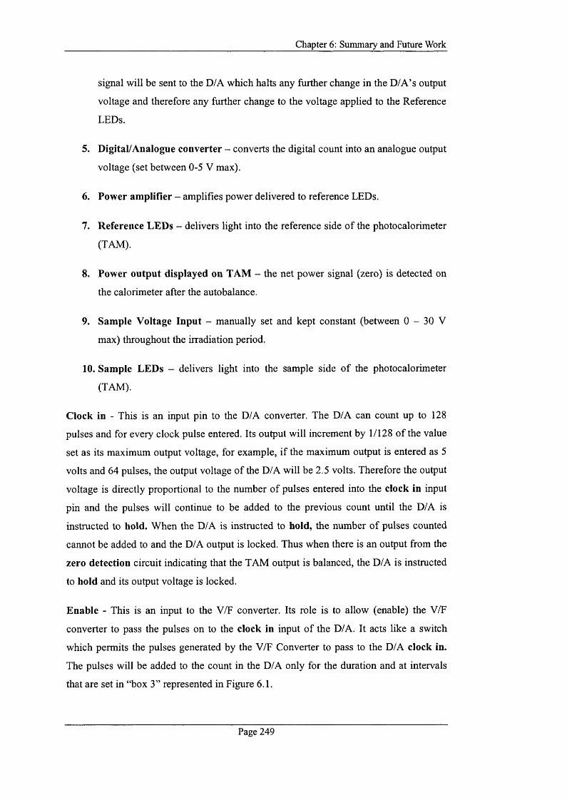
Chapter 6: Summary and Future Work
signal will be sent to the D/A which halts any further change in the D/A’s output
voltage and therefore any further change to the voltage applied to the Reference
LEDs.
5. Digital/Analogue converter - converts the digital count into an analogue output
voltage (set between 0-5 V max).
6. Power amplifier - amplifies power delivered to reference LEDs.
7. Reference LEDs - delivers light into the reference side o f the photocalorimeter
(TAM).
8. Power output displayed on TAM - the net power signal (zero) is detected on
the calorimeter after the autobalance.
9. Sample Voltage Input - manually set and kept constant (between 0 - 30 V
max) throughout the irradiation period.
10. Sample LEDs - delivers light into the sample side o f the photocalorimeter
(TAM).
Clock in - This is an input pin to the D/A converter. The D/A can count up to 128
pulses and for every clock pulse entered. Its output will increment by 1/128 o f the value
set as its maximum output voltage, for example, if the maximum output is entered as 5
volts and 64 pulses, the output voltage o f the D/A will be 2.5 volts. Therefore the output
voltage is directly proportional to the number o f pulses entered into the clock in input
pin and the pulses will continue to be added to the previous count until the D/A is
instructed to hold. When the D/A is instructed to hold, the number o f pulses counted
cannot be added to and the D/A output is locked. Thus when there is an output from the
zero detection circuit indicating that the TAM output is balanced, the D/A is instructed
to hold and its output voltage is locked.
Enable - This is an input to the V/F converter. Its role is to allow (enable) the V/F
converter to pass the pulses on to the clock in input o f the D/A. It acts like a switch
which permits the pulses generated by the V/F Converter to pass to the D/A clock in.
The pulses will be added to the count in the D/A only for the duration and at intervals
that are set in “box 3” represented in Figure 6.1.
Page 249
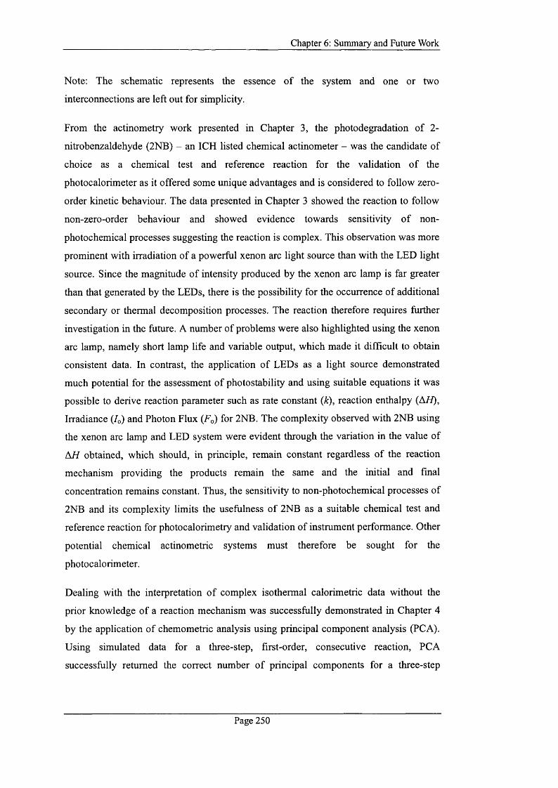
Chapter 6: Summary and Future Work
Note: The schematic represents the essence o f the system and one or two
interconnections are left out for simplicity.
From the actinometry work presented in Chapter 3, the photodegradation o f 2-
nitrobenzaldehyde (2NB) - an ICH listed chemical actinometer - was the candidate of
choice as a chemical test and reference reaction for the validation o f the
photocalorimeter as it offered some unique advantages and is considered to follow zero-
order kinetic behaviour. The data presented in Chapter 3 showed the reaction to follow
non-zero-order behaviour and showed evidence towards sensitivity o f non
photochemical processes suggesting the reaction is complex. This observation was more
prominent with irradiation o f a powerful xenon arc light source than with the LED light
source. Since the magnitude o f intensity produced by the xenon arc lamp is far greater
than that generated by the LEDs, there is the possibility for the occurrence o f additional
secondary or thermal decomposition processes. The reaction therefore requires further
investigation in the future. A number of problems were also highlighted using the xenon
arc lamp, namely short lamp life and variable output, which made it difficult to obtain
consistent data. In contrast, the application o f LEDs as a light source demonstrated
much potential for the assessment o f photostability and using suitable equations it was
possible to derive reaction parameter such as rate constant (k), reaction enthalpy (A//),
Irradiance (/o) and Photon Flux (Fo) for 2NB. The complexity observed with 2NB using
the xenon arc lamp and LED system were evident through the variation in the value of
A // obtained, which should, in principle, remain constant regardless o f the reaction
mechanism providing the products remain the same and the initial and final
concentration remains constant. Thus, the sensitivity to non-photochemical processes of
2NB and its complexity limits the usefulness o f 2NB as a suitable chemical test and
reference reaction for photocalorimetry and validation o f instrument performance. Other
potential chemical actinometric systems must therefore be sought for the
photocalorimeter.
Dealing with the interpretation o f complex isothermal calorimetric data without the
prior knowledge o f a reaction mechanism was successfully demonstrated in Chapter 4
by the application o f chemometric analysis using principal component analysis (PCA).
Using simulated data for a three-step, first-order, consecutive reaction, PCA
successfully returned the correct number o f principal components for a three-step
Page 250
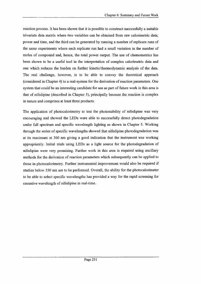
Chapter 6; Summary and Future Work
reaction process. It has been shown that it is possible to construct successfully a suitable
trivariate data matrix where two variables can be obtained from raw calorimetric data;
power and time, and the third can be generated by running a number o f replicate runs of
the same experiments where each replicate run had a small variation in the number of
moles o f compound and, hence, the total power output. The use o f chemometrics has
been shown to be a useful tool in the interpretation o f complex calorimetric data and
one which reduces the burden on further kinetic/thermodynamic analysis o f the data.
The real challenge, however, is to be able to convey the theoretical approach
(considered in Chapter 4) to a real-system for the derivation o f reaction parameters. One
system that could be an interesting candidate for use as part o f future work in this area is
that o f nifedipine (described in Chapter 5), principally because the reaction is complex
in nature and comprises at least three products.
The application o f photocalorimetry to test the photostability o f nifedipine was very
encouraging and showed the LEDs were able to successfully detect photodegradation
under full spectrum and specific wavelength lighting as shown in Chapter 5. Working
through the series o f specific wavelengths showed that nifedipine photodegradation was
at its maximum at 360 nm giving a good indication that the instrument was working
appropriately. Initial trials using LEDs as a light source for the photodegradation of
nifedipine were very promising. Further work in this area is required using ancillary
methods for the derivation o f reaction parameters which subsequently can be applied to
those in photocalorimetry. Further instrumental improvement would also be required if
studies below 350 nm are to be performed. Overall, the ability for the photocalorimeter
to be able to select specific wavelengths has provided a way for the rapid screening for
causative wavelength o f nifedipine in real-time.
Page 251

Appendix
The work reported in this thesis has been published in the following journals:
Dhuna, M ., Beezer, A .E ., M orris, A .C ., G aisford, S., O 'N eill, M .A .A ., Hadgraft, J.,
Connor, J.A ., C lapham , D., Frost, J. (2007) D evelopm ent o f an Isotherm al Heat-
C onduction Photocalorim eter. R ev Sci Instrum 78 (do i:l 0.1063/1.2670220), 025105
O 'N eill, M .A .A ., Beezer, A .E., Tetteh, J., Gaisford, S., Dhuna, M . (2007) A pplication o f
C hem om etric A nalysis to C om plexity in Isotherm al Calorim etric Data. J. Phys. Chem. B
111 ,8145-8149
Page 252
REVIEW OF SCIENTIFIC INSTRUMENTS 78 , 025105 (2007)
Development of an isothermal heat-conductlon photocalorimeterMeena Dhuna and Anthony E. BeezerThe School o f Pharmacy, University o f London, 29-39 Brunswick Square,London WCIN lAX, United Kingdom
Andrew C. MorrisMedway Sciences, University o f Greenwich, Medway Campus, Chatham Maritime,Kent ME4 4TB, United Kingdom
Simon Gaisford,M ichael A. A. O’Neill,* ' and Jonathan HadgraftThe School o f Pharmacy, University o f London, 29-39 Brunswick Square,London WCIN I AX, United Kingdom
Joseph A. ConnorMedway Sciences, University o f Greenwich, Medway Campus, Chatham Maritime,Kent ME4 4TB, United Kingdom
David ClaphamGlaxoSmithKline. New Frontiers Science Park, Harlow, Essex CM 19 SAW, United Kingdom
John FrostThe School o f Pharmacy. University o f London, 29-39 Brunswick Square,London WCiN lAX, United Kingdom
(Received 31 December 2006; accepted 21 January 2007; published online 22 February 2007)
Assessing photostability (particularly of pharmaceuticals) is of growing importance, but hampered by a lack of reliable, rapid experimental testing protocols and instrumentation. In particular, most approaches require irradiation of the sample separately from the analytical measurement, which increases both experimental complexity and the number of assumptions that must be made when calculating stability. One technique that may obviate this is photocalorimetry, principally because the reporter of change (heat) is measured directly as a sample is irradiated. Although not a new idea, the design challenges of photocalorimeters are complex, primarily because light power is being introduced to the calorimeter which can thus both saturate the amplifiers and swamp the response of the sample. Careful instrument design is thus paramount. The aim of this work was to develop a robust, compact, and easy to use photocalorimeter with the immediate focus of developing photostability assays for pharmaceuticals. The final instrument design, arrived at through a series of iterative design modifications, is based on a twin differential heat-conduction principle and achieves an average base line deflection of -0.04±0.11 yaW with light irradiating the sample cell. The perfomnance capabilities of the instrument were demonstrated using a model system; the photodegradation of 2-nitrobenzaldehyde in solution. © 2007 American Institute of Physics.[DOI; 10.1063/1.2670220]
I. INTRODUCTION
There are a number of reasons why assessment of photostability is desirable; to quantify the stability of a molecule or product under “white light’’ conditions, to determine stability as a function of wavelength (which may give mechanistic information on the degradation reaction), to develop packaging materials that can ameliorate the effects of photodegradation, and (phamiaceutically) to estimate the in vivo photosensitizing potential of a drug from its in vitro photostability (photolabile drugs are often used for chemotherapy, for instance).
“’Author to whom correspondence should be addressed; FAX: + 4 4 (0)20 7753 5942; electronic mail: [email protected]
’’’Present address: Department of Pharmacy and Pharmacology, University of Bath, Bath, BA2 7AY, United Kingdom.
in spite of the existence of the International Conference on Harmonisation (ICH) QIB guideline on photostability testing, there are in practice a number of methods in existence practically to perform a photostability test. Most methods irradiate samples separately from the analytical instrument used to quantify any degradation that does occur. It is also difficult to quantify photostability of multicomponent products because the analyte(s) must be isolated prior to measurement. Photocalorimetry (the measurement of the heat change when a sample is irradiated) offers a direct method with which to assess photostability, because the data recorded (power as a function of time) are acquired in real time, in a noninvasive manner, and are easily interpreted in (at least) a qualitative fashion (although quantitative interpretation is also achievable).
Although the principle of photocalorimetry has been known for many decades,' the design challenges inherent
0034-6748/2007/78(2)/025105/5/$23.00 78, 025105-1 © 2007 American Institute of Physics
D o w n lo a d e d 25 Feb 20 0 7 to 8 4 .6 5 .6 4 .1 5 1 . R ed istr ib u tion su b je c t to AIR lic e n s e or co p y r ig h t, s e e h ttp ://rsi.a ip .org /rsi/cop yrlgh t.J sp
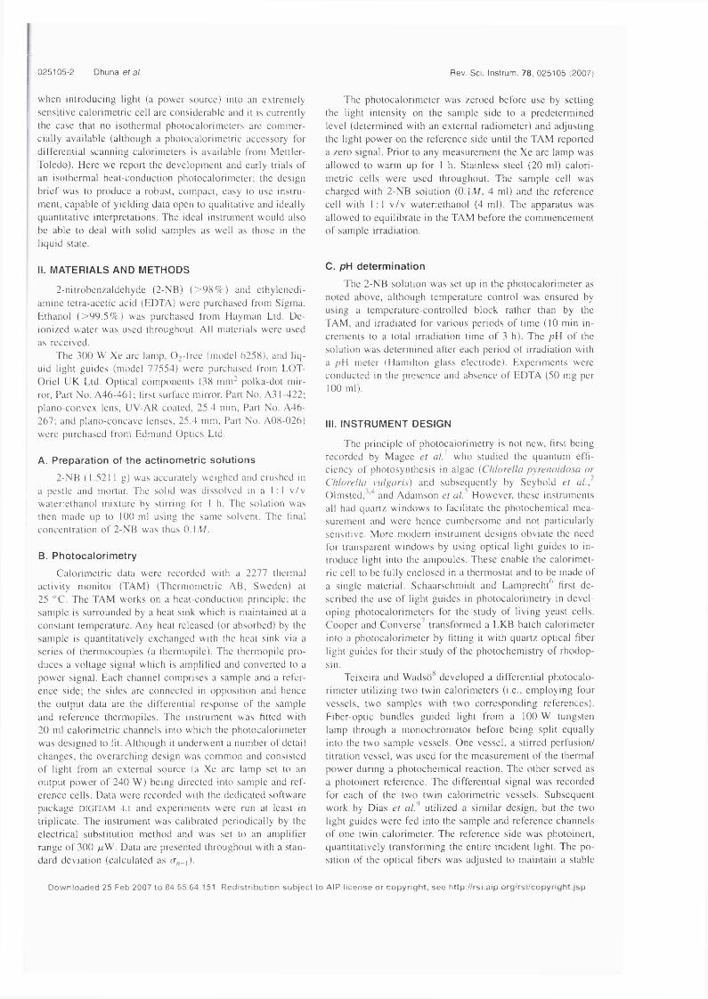
025105-2 Dhuna ef a/. Rev. Sci. Instrum. 78, 025105 (2007)
w hen in lroducing light (a pow er source) into an e.xtreniely sen sitive calorim etric cell arc considerable and it is currently the case that no isotherm al photocalorim eters are com m ercia lly ava ilab le (although a photocalorim etric accessory tor dilTerential scann ing calorim eters is ava ilab le from M ettler- T oledo). Here w e report the d evelop m en t and early trials o f an isotherm al heat-conduction photocalorim eter; the d esign brief w as to produce a robust, com pact, easy to use instrum ent, capab le o f y ie ld in g data open to qualitative and ideally quantitative interpretations. The ideal instrum ent w ou ld a lso be able to deal w ith so lid sam ples as w ell as those in the liquid state.
II. MATERIALS AND METHODS
2-n itrobenzaldehyde (2 -N B ) ( > 9 8 % ) and eth y len ed i- am ine tetra-acetic acid (ED TA ) w ere purcha.sed from S igm a. Ethanol ( > 9 9 .5 % ) w as purchased from Hay man Ltd. D e ion ized w ater w as used throughout. A ll m aterials w ere used as received .
The 3 0 0 W X e arc lamp, O i-free (m odel 6 2 5 8 ), and liq uid light gu id es (m odel 7 7 5 5 4 ) w ere purchased from LOT- Oriel U K Ltd. O ptical com ponents (38 m n r polka-dot m irror, Part N o. A 4 6 -4 6 1 ; first surface mirror. Part N o. A 3 1 -4 2 2 ; p la n o-con vex lens, U V -A R coated , 2 5 .4 m m . Part N o. A 46- 267; and p lan o-con cave len ses, 25 .4 m m . Part N o. A 0 8 -0 2 6 ) w ere purchased from Edm und O ptics Ltd.
A. P rep a ra t ion of th e ac t in om etr ic so lu t io n s
2 -N B ( 1.5211 g) w as accurately w eigh ed and crushed in a pestle and mortar. The solid w as d isso lved in a 1: 1 v /v w atericthanol m ixture by stirring for I h. T he solution w as then m ade up to 100 ml using the sam e so lvent. The final concentration o f 2 -N B w as thus 0. IA7.
B. P h o toca lo r im e try
C alorim etric data were recorded with a 227 7 thermal activ ity m onitor (TA M ) (T herm om etric A B , S w ed en ) at 25 °C . T he TAM w orks on a heat-conduction principle; the sam ple is surrounded by a heat sink w hich is m aintained at a constant temperature. A ny heat released (or absorbed) by the sam p le is quantitatively exch an ged with the heat sink via a series o f therm ocouples (a therm opile). The therm opile produ ces a voltage signal w h ich is am plified and converted to a pow er signal. Each channel com p rises a sam ple and a referen ce side; the sid es arc con n ected in opposition and hence the output data are the differential response o f the sam ple and reference therm opiles. The instrum ent w as fitted with 20 ml calorim etric channels into w hich the photocalorim eter w as d esign ed to fit. A lthough it underwent a number o f detail ch a n ges, the overarching d esign w as com m on and consisted o f light from an external source (a X e arc lam p set to an output pow er o f 2 4 0 W ) being directed into sam ple and reference ce lls . Data w ere recorded with the ded icated softw are p ackage d i g i t a m 4 . i and experim ents w ere run at least in triplicate. The instrum ent w as calibrated period ically by the electrica l substitution m ethod and w as set to an am plifier range o f 300 yuW. Data are presented throughout with a standard deviation (calcu lated as (r„_,).
The photocalorim eter w as zeroed before use by setting the light in tensity on the sam ple sid e to a predeterm ined level (determ ined with an external radiom eter) and adjusting the light p ow er on the reference side until the TA M reported a zero signal. Prior to any m easurem ent the X e arc lam p w as allow ed to warm up for 1 h. S ta in less steel (2 0 ml) ca lorim etric ce lls w ere used throughout. T he sam ple ce ll w as charged with 2 -N B solu tion (0 .1 4 /, 4 m l) and the reference ee ll w ith 1:1 v / v w ateriethanol (4 m l). T he apparatus w as a llow ed to equilibrate in the TAM before the com m en cem en t o f sam ple irradiation.
C. pH de te rm in a t io n
T he 2 -N B solu tion w as set up in the photocalorim eter as noted above, although tem perature control w as ensured by using a tem perature-controlled b lock rather than by the TA M , and irradiated for various periods o f tim e (10 m in increm ents to a total irradiation tim e o f 3 h). T he pW o f the solu tion w as determ ined after each period o f irradiation with a p \ \ m eter (H am ilton g lass e lectrod e). E xperim ents w ere conducted in the presence and absence o f ED T A (50 m g per 100 m l).
Ill, INSTRUMENT DESIGN
The principle o f photocalorim etry is not new , first being recorded by M agee et a/. ' w h o studied the quantum effic ien cy o f p h otosyn th esis in algae (Chlorella pyrenoido.sa or ChloreUa vulgaris) and subsequently by S eyb o ld et al.,~ O l m s t e d ,a n d A dam son et al.^ H ow ever, these instrum ents all had quartz w in d o w s to facilitate the photochem ica l m easurem ent and w ere hence cum bersom e and not particularly sen sitive . M ore m odern instrum ent d esig n s ob viate the need for transparent w in d o w s by using optical light gu id es to in troduce light into the am poules. T hese enable the ca lorim etric ce ll to be fu lly en c lo sed in a therm ostat and to be m ade o f a sin g le m aterial. Schaarschm idt and Lamprecht^’ first d escribed the use o f light gu ides in photocalorim etry in d e v e lop ing photocalorim eters for the study o f liv in g yeast ce lls . C ooper and C on verse' transform ed a LK B batch calorim eter into a photocalorim eter by fitting it w ith quartz optical fiber light gu id es for their study o f the photochem istry o f rhodop- sin.
Teixeira and Wadso^' d evelop ed a d ifferential p h otoca lo rim eter u tiliz in g tw o twin ca lorim eters (i.e ., em p lo y in g four v e sse ls , tw o sam p les w ith tw o corresponding references). Fiber-optic bundles gu ided light from a 100 W tungsten lam p through a m onochrom ator before being split equally into the tw o sam ple v esse ls . O ne v esse l, a stirred perfusion / titration v esse l, w as used for the m easurem ent o f the thermal pow er during a p h otoch em ica l reaction. T he other served as a photoinert reference. T he d ifferential signal w as recorded for each o f the tw o tw in calorim etric v esse ls . Subsequent work by D ias et al.' u tilized a sim ilar d esign , but the tw o light gu ides w ere fed into the sam ple and reference channels o f one twin calorim eter. T he reference sid e w as photoinert, quantitatively transform ing the entire incident light. The p o sition o f the optical libers w as adjusted to m aintain a stable
D ow n load ed 25 Feb 2007 to 84 ,65 .64 .151 . R edistribution su b je c t to AlP l ic e n s e or cop yr igh t, s e e h ttp ://rsi.a ip .org /rsi/cop yrigh t.jsp
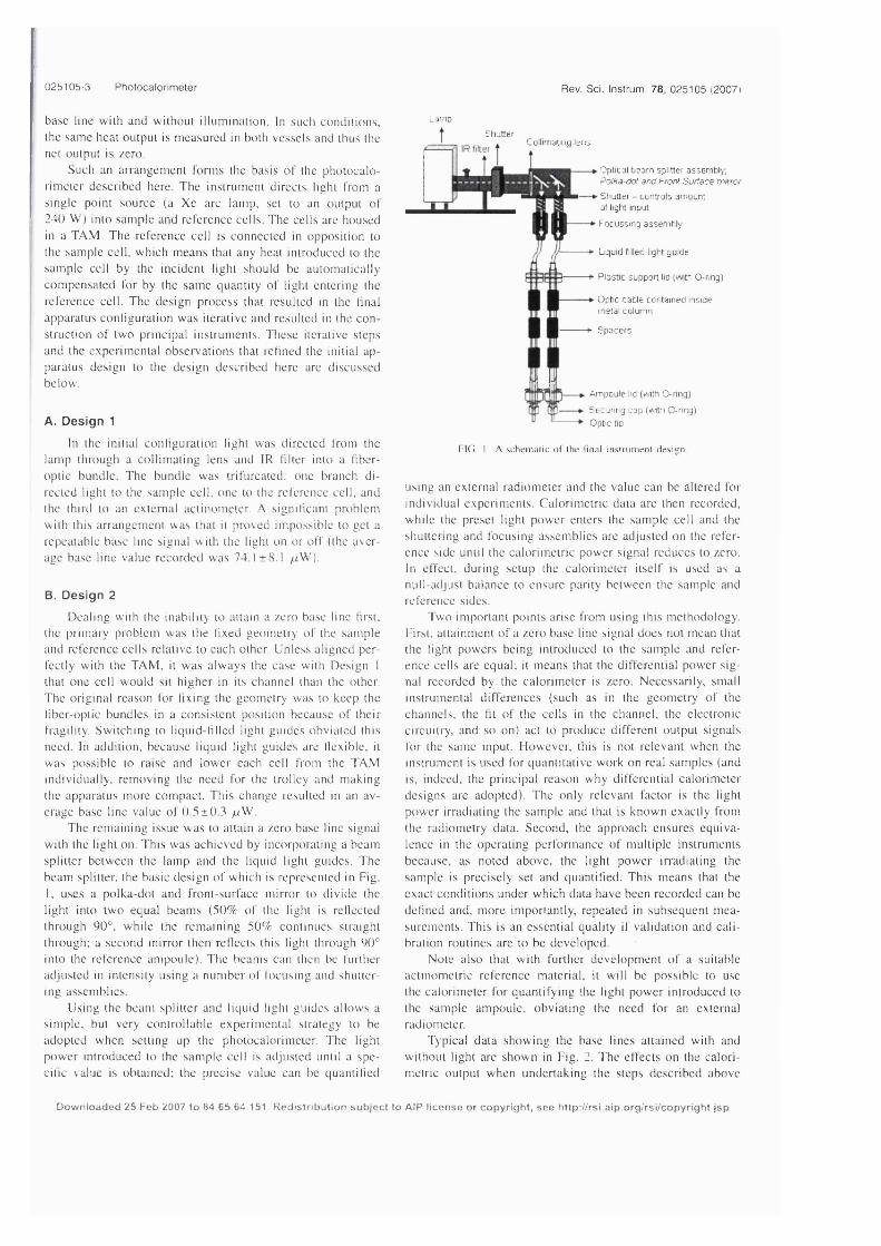
025105-3 Photocalorimeter Rev. Soi. Instrum. 78, 025105 (2007)
base line w ith and w ithout illum ination . In such con d ition s, the sam e heat output is m easured in both v e sse ls and thus the net output is zero.
Such an arrangem ent form s the basis o f the p h otoca lo rim eter described here. T he instrum ent directs light from a sin g le point source (a X e arc lam p, set to an output o f 240 W ) into sam ple and reference ce lls . The c e lls arc housed in a TAM . T he reference ce ll is connected in op p osition to the sam ple ce ll, w h ich m eans that any heat introduced to the sam ple ce ll by the incident light should be autom atically com p en sated for by the sam e quantity o f light entering the reference ce ll. T he design p rocess that resulted in the final apparatus configuration w as iterative and resulted in the c o n struction o f tw o principal instrum ents. T h ese iterative steps and the experim ental ob servation s that refined the initial apparatus d esign to the d esign described here are d iscu ssed below .
A. Design 1
In the initial configuration light w as directed from the lamp through a co llim atin g lens and IR filter into a fiberoptic bundle. T he bundle w as trifurcated: one branch d irected light to the sam ple ce ll, one to the reference ce ll, and the third to an external actinom cter. A sign ificant problem with this arrangem ent w as that it proved im possib le to get a repeatable base line signal w ith the light on or o ff (the average base line value recorded w as 74.1 ± 8 .1 /zW ).
B. Design 2
D ealin g with the inability to attain a zero base line first, the primary problem w as the lixed geom etry o f the sam ple and reference c e lls relative to each other. U n less a ligned perfectly w ith the TA M , it w as a lw ays the case with D esign 1 that on e ce ll w ou ld sit h igher in its channel than the other. T he original reason for fix ing the geom etry w as to keep the fiber-optic bundles in a con sisten t position because o f their fragility. S w itch in g to liqu id -filled light gu id es obviated this need. In addition, becau se liquid light gu id es are flexib le, it w as p oss ib le to raise and low er each cell from the TAM ind ividually , rem oving the need for the trolley and m aking the apparatus m ore com pact. This change resulted in an av erage base line value o f 0 .5 ± 0 .3 yuW.
T he rem aining issue w as to attain a zero base line signal w ith the light on. T h is w as ach ieved by incorporating a beam splitter betw een the lam p and the liquid light gu ides. T he beam splitter, the basic d esign o f w hich is represented in Fig. I. uses a polka-dot and front-surface mirror to d iv ide the light into tw o equal beam s (50% o f the light is reflected through 9 0 ° . w h ile the rem ain ing 50% con tinu es straight through: a secon d mirror then reflects this light through 90° into the reference am poule). T he beam s can then be further adjusted in intensity using a num ber o f focu sin g and shuttering assem b lies.
U sin g the beam splitter and liquid light gu id es a llow s a sim p le , but very contro llab le experim ental strategy to be adopted w hen setting up the phoiocalorim etcr. T he light pow er introduced to the sam ple ce ll is adjusted until a sp e cific value is obtained; the precise value can be quantified
Lamp
S hatte rCoilirDatint) lens
OpPcal b eam splitter assembl>', Polka-M and Front Surface mirror
■ S hu tter - contro ls am ount of light Input
F o cu ssin g a ssem b ly
Liquicl-fillec light guide
P lastic support lid (with 0-ring)
Optic cab le con ta ined inside m etal colum n
S p a c e rs
Am poule lie (>vith 0 -ring)
S ecuring cap (m th 0 -ring) Optic tip
FIG. I. A schematic of the final instrument design.
using an external radiom eter and the value can be altered for individual experim ents. C alorim etric data are then recorded, w h ile the preset light pow er enters the sam ple ce ll and the shuttering and focu sin g a ssem b lie s are adjusted on the referen ce side until the calorim etric pow er signal reduces to zero. In e ffect, during setup the ca lorim eter itse lf is used as a null-adjust balance to ensure parity betw een the sam ple and reference sides.
T w o important points arise from using this m ethodology. First, attainm ent o f a zero base line signal d o es not m ean that the light pow ers being introduced to the sam ple and referen ce ce lls are equal; it m eans that the differentia l pow er s ig nal recorded by the ca lorim eter is zero. N ecessar ily , sm all instrum ental d ifferen ces (such as in the geom etry o f the chan n els, the ht o f the c e lls in the channel, the electron ic circuitry, and so on) act to produce different output signals for the sam e input. F low ever, this is not relevant when the instrument is used for quantitative work on real sam p les (and is, indeed, the principal reason w hy d ifferential calorim eter d esign s are adopted). T he on ly relevant factor is the light pow er irradiating the sam ple and that is know n exactly from the radiom etry data. S econ d , the approach ensures eq u iva lence in the operating perform ance o f m ultip le instrum ents because , as noted ab ove, the light pow er irradiating the sam p le is precisely set and quantified . T h is m eans that the exact con d ition s under w hich data have been recorded can be defined and, m ore im portantly, repeated in subsequent m easurem ents. T his is an essen tia l quality if validation and c a libration routines are to be d evelop ed .
N ote a lso that w ith further d evelop m en t o f a suitable actinom etric reference m aterial, it w ill be p ossib le to use the calorim eter for q uantify ing the light p ow er introduced to the sam ple am pou le, obviating the need for an external radiometer.
T ypical data sh o w in g the base lin es attained with and w ithout light are show n in F ig. 2. T he e ffe cts on the ca lorim etric output w hen undertaking the steps described above
D ow n load ed 25 Feb 2007 to 84 .65 .64 .151 . R edistribution su b jec t to AlP lic e n s e or cop yrigh t, s e e h ttp ://rsi.a ip .org /rsi/cop yrigh t.jsp
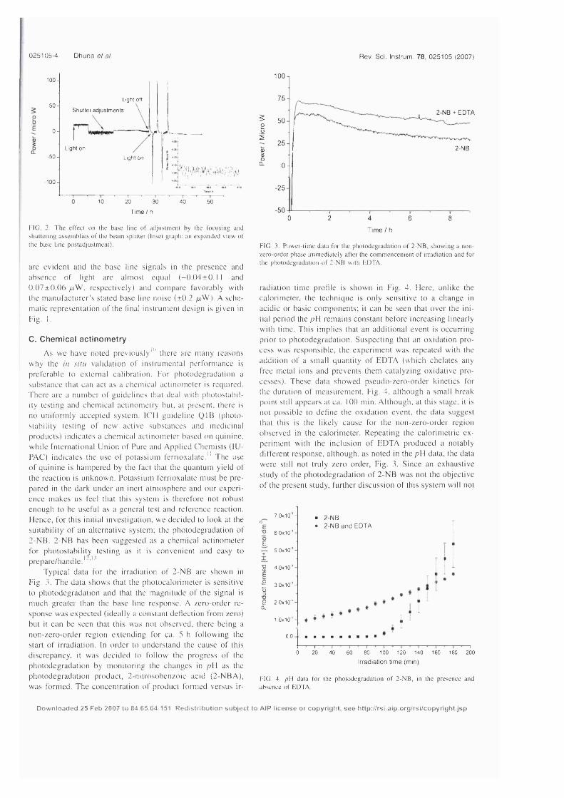
025105-4 Dhuna et al. Rev. Sci. Instrum. 78, 025105 (2007)
100
50-
0 -
-50-
- 1 00 -
Light off
S hu tte r ad justm en ts
L ig h t o n
Light on
fS /'------
10 20 30
Time / h40 50
FIG. 2. The effect on the ba.se line of adjustment by the focusing and shuttering as.semblies of the beam splitter (Inset graph: an e,xpanded view of the base line postadjustment).
are ev id en t and the base line sign a ls in the presence and absence o f light are alm ost equal ( - 0 . 0 4 ± 0 . 11 and () .0 7 ± 0 .0 6 /zW , resp ective ly ) and com pare favorably with the m anufacturer’s stated base line no ise (± 0 .2 /jl'W). A sc h e m atic representation o f the final instrum ent design is g iven in
Fig. 1.
C. Chemical actlnometryA s w e have noted previously '" there are m any reasons
w hy the /// situ validation o f instrum ental perform ance is preferable to external calibration. For photodegradation a substance (hat can act as a chem ical actinom cter is required. There are a num ber o f gu id elin es that deal w ith photostab ility testing and chem ical actlnom etry but, at present, there is no uniform ly accepted system . ICU gu id eline Q IB (photostability testing o f new active substances and m edicinal products) indicates a chem ical actinom cter based on quinine, w h ile International U n ion o f Pure and A pplied C hem ists (lU - PAC) ind icates the use o f potassium ferrioxalatc." The use o f qu inine is ham pered by the fact that the quantum yield o f the reaction is unknow n. Potassium fcrrioxalate m ust be prepared in the dark under an inert atm osphere and our exp erien ce m akes us feel that this system is therefore not robust enough to be useful as a general test and reference reaction. H ence, for this initial investigation , w e decided to look at the su itab ility o f an alternative system ; the photodegradation o f 2 -N B . 2 -N B has been su ggested as a chem ical actinom cter for photostability testing as it is con ven ien t and easy to prepare/handle.'” ' ^
Typical data for the irradiation o f 2 -N B are show n in Fig. 3. T he data sh ow s that the photocalorim eter is sen sitive to photodegradation and that the m agnitude o f the signal is m uch greater than the base line response. A zero-order resp on se w as exp ected (idea lly a constant d eflection from zero) but it can be seen that this w as not observed , there being a non-zero-order region exten d ing for ca. 5 h fo llo w in g the start o f irradiation. In order to understand the cause o f this discrepancy, it w as decided to fo llo w the progress o f the photodegradation by m onitoring the ch an ges in p \ \ as the photodegradation product, 2 -n itrosobenzo ic acid (2 -N B A ), w as form ed. T he concentration o f product form ed versus ir-
100-,
75-
5 50-2o5
25-1g 0-
-25-
-50-0
2-NB + EDTA
2-NB
2 4 6 8
Time / h
FIG. 3. Power-time data for the photodegradation of 2-NB, showing a non- zero-order phase immediately after the commencement of irradiation and tor the photodegradation of 2-NB with EfTTA.
radiation tim e profile is show n in F ig. 4. H ere, unlike the calorim eter, the technique is on ly sen sitiv e to a change in acid ic or basic com ponents; it can be seen that over the in itial period the /?H rem ains constant before increasing linearly w ith tim e. T h is im plies that an additional event is occurring prior to photodegradation . S u sp ectin g that an oxidation process w as responsib le , the experim ent w as repeated with the addition o f a sm all quantity o f ED TA (w hich ch elates any free metal ions and prevents them cata lyzin g ox id ative proce sse s ). T h ese data sh ow ed pseudo-zero-ordcr k inetics for the duration o f m easurem ent. Fig. 4 . although a sm all break point still appears at ca. 100 m in. A lthough , at this stage, it is not p ossib le to define the ox idation even t, the data suggest that this is the likely cause for the non-zero-order region observed in the calorim eter. R epeating the calorim etric e x perim ent with the inclusion o f ED T A produced a notably different response, although, as noted in the pW data, the data w ere still not truly zero order. F ig. 3. S in ce an exhaustive study o f the photodegradation o f 2 -N B w as not the objective o f the present study, further d iscu ssion o f this system w ill not
7 0x10 ' -
6 0x10’ -
E5 0x10 ’ -
^ 4 0x10*-
f 3 0x10'*-g2 2 0x1 O'*-
CL
1 0x10’ -
00
" 2-NB• 2-NB a n d EDTA
I '
0 20 40 60 80 100 120 140 160 180 200
Irradiation tim e (min)
FIG. 4 i>\\ data for the photodegradatioii of 2-NB, in the presence and absence of EDTA.
D ow n load ed 25 Feb 2007 to 84 .65 .64 .151 , R ed istribution su b je c t to AlP l ic e n se or cop yrigh t, s e e h ttp ://rsi.a ip .org /rsi/cop yrigh t.jsp
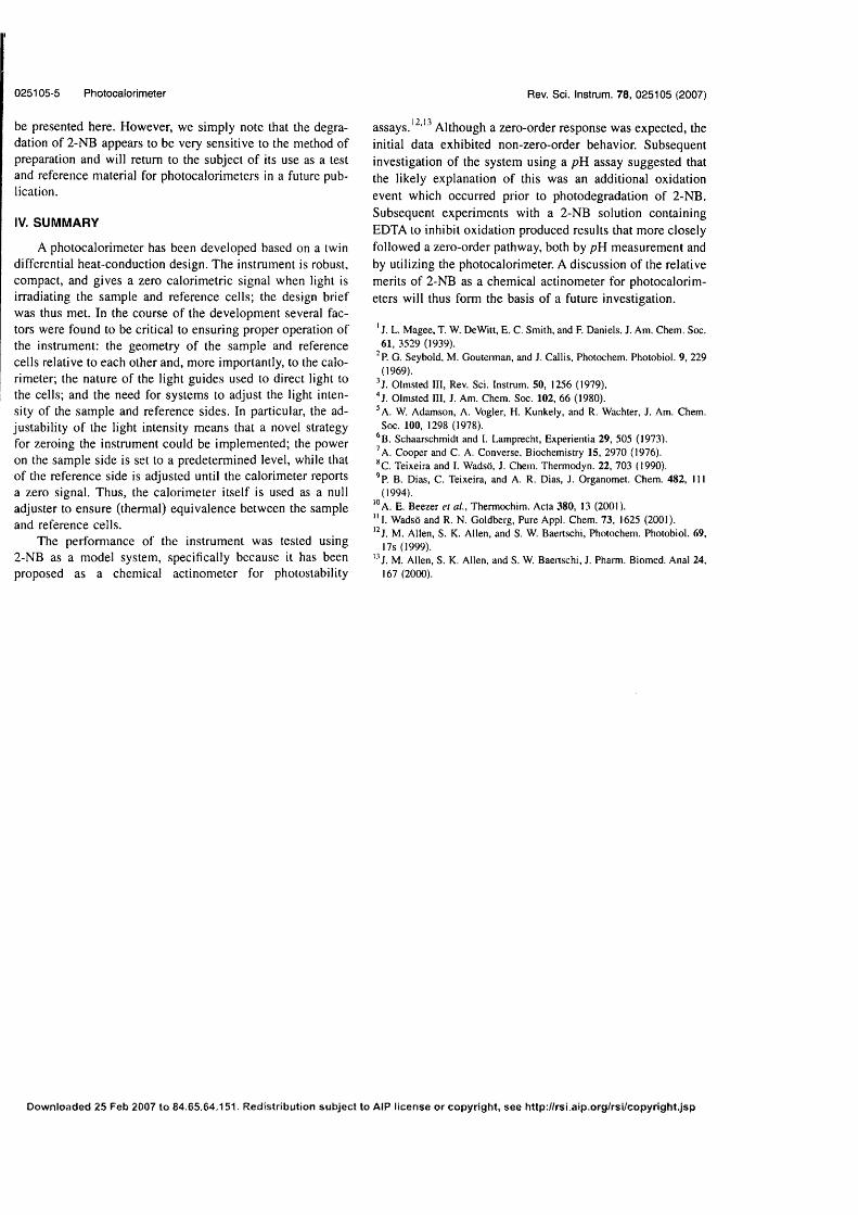
02 5 1 0 5 -5 Photocalorim eter
be presen ted here. H ow ever, we sim ply no te that the degradation o f 2 -N B appears to be very sensitive to the m ethod o f prepara tion and will re turn to the su b jec t o f its use as a test and reference m aterial for p h o to ca lo rim ete rs in a future publication.
IV. SUMMARY
A p h o to ca lo rim ete r has been d ev eloped based on a twin d ifferen tia l h ea t-conduction design . T h e in strum en t is robust, com pact, and g ives a zero ca lo rim etric signal w hen light is iiTadiating the sam ple and refe ren ce cells; the design b rief w as thus m et. In the course o f the dev e lo p m en t several factors w ere found to be critical to en su ring p ro p er operation o f the in strum ent: the geom etry o f the sam ple and reference cells re la tive to each o ther and, m ore im portantly , to the ca lo rim eter; the na tu re o f the ligh t g u ides used to d irec t light to the cells; and the need fo r system s to ad just the light in ten sity o f the sam p le and reference sides. In particu lar, the ad ju stab ility o f the light in tensity m eans that a novel strategy for zero ing the instrum en t cou ld be im p lem en ted ; the pow er on the sam ple side is set to a p red eterm in ed level, w hile that o f the re ference side is ad justed until the ca lo rim ete r reports a zero signal. T h u s, the ca lo rim ete r itse lf is used as a null ad ju s te r to en su re (therm al) equ iv a len ce be tw een the sam ple and reference cells.
T he p e rfo rm an ce o f the in strum en t w as tested using 2-N B as a m odel system , specifically because it has been proposed as a chem ical actin o m c te r for photostab ility
Rev. Sci. Instrum. 78 , 0 2 5 1 0 5 (2007)
12,13assays. A lthough a zero -o rd er resp o n se w as expec ted , the initial da ta exh ib ited non-zero -o rd er behavior. S ubsequent investigation o f the system using a p R assay suggested that the likely ex p lanation o f this was an add itional ox idation even t w hich occurred p rio r to ph o to d eg rad atio n o f 2-N B . S u bsequen t exp erim en ts w ith a 2 -N B so lu tion con ta in ing ED TA to inh ib it ox idation p roduced resu lts that m ore c losely follow ed a zero -o rd er pathw ay, both by p H m easurem en t and by u tilizing the pho tocalorim eter. A d iscussion o f the re la tive m erits o f 2-N B as a chem ical actin o m cte r fo r p h o to ca lo rim eters w ill thus form the basis o f a fu ture investigation .
' J. L. Magee, T. W. De Witt, E. C. Smith, and F. Daniels. J. Am. Chem. Soc. 61. 3529 (1939).
^P. G. Seybold, M. Gouterman, and J. Callis, Photochem. Photobiol. 9, 229 (1969).
^J. Olmsted III, Rev. Sci. Instrum. 50, 1256 (1979)." j. O lmsted III, J. Am. Chem. Soc. 102, 66 (1980). A. W. Adamson, A. Vogler, H. Kunkely, and R. W achter, J. Am. Chem. Soc. 100, 1298 (1978).
*B. Schaarschmidt and I. Lamprecht, Experientia 29, 505 (1973).’ a . Cooper and C. A. Converse, Biochemistry 15, 2970 (1976).*C. Teixeira and I. Wadsb, J. Chem. Thermodyn. 22, 703 (1990).’ p. B. Dias, C. Teixeira, and A. R. Dia.s, J. Organomet. Chem. 482, 111
(1994).'°A . E. Beezer et a l., Thermcx:him. Acta 380, 13 (2001)." 1. W adsb and R. N. Goldberg, Pure Appl. Chem. 73, 1625 (2001).'^J. M. Allen, S. K. Allen, and S. W. Baertschi, Photochem. Photobiol. 69,
17s (1999).'■ J. M. Allen, S. K. Allen, and S. W. Baert.schi, J. Pharm. Biomed. Anal 24,
167 (2000).
D o w n lo a d ed 25 Feb 2 0 0 7 to 8 4 .6 5 ,6 4 ,1 5 1 . R ed istrib u tion s u b je c t to AIR l ic e n s e or co p y r ig h t, s e e h ttp ://rs i.a ip .o rg /rs i/co p y r ig h t.jsp

J. Phys. Chem. B 2 007 , I I I . 8 1 4 5 - 8 1 4 9 8145
Application of Chemometric Analysis to Complexity in Isothermal Calorimetric Data
Michael A.A. O’Neill,*’ Anthony E Beezer, John Tetteh,§ Simon Gaisford,^ and Meena Dhuna*Department of Pharmacy and Pharmacology. University of Bath. Claverton Down, Bath BA2 7AY. U.K., School of Pharmacy, University of London, 29-39 Brunswick Square, London WCIN I AX, U.K., and University of Greenwich, School of Sciences, Central Avenue, Chatham Maritime, ME4 4TB, U.K.Received: January 5, 2007; In Final Form: April 16, 2007
T h e interpretation o f c o m p le x ity in isotherm al ca lorim etric data is d em and in g . T he ob served p o w er sig n a l is a c o m p o site o f the p o w ers arisin g from each o f the ind iv id u al ev en ts occu rrin g (w h ich can in v o lv e p h y sica l, as w e ll as ch em ica l, ch an ge). T he ch a llen g e , therefore, lies in d eco n v o lu tin g the o b served data into their co m p o n e n t parts. H ere, w e d iscu ss the potentia l u se o f ch em om etric a n a ly sis , b eca u se it o ffer s the s ig n ifica n t ad van tage o f b e in g m o d e l-free , u sin g principal com p on en t a n a ly sis to d eco n v o lu te data. U s in g m odel data, w e d isco v e red that the so ftw are required a m inim um trivariate data m atrix to be constructed . T w o variab les, p o w er and tim e, w ere a va ilab le from the raw data. S e lectio n o f a third variab le w as m ore p rob lem atic , but it w a s found that b y running m u ltip le exp erim en ts the sm all variation in the num ber o f m o le s o f com p oun d in each ex p erim en t w a s su ffic ien t to a llo w a su cc ess fu l a n a lysis . In general w e n oted that it required a m inim um 2/7 + 2 repeat ex p erim en ts to a llo w an a ly sis (w here n is the num ber o f reaction p ro cesses ). T h e data outputted from the ch em o m etr ic so ftw are w ere o f the form in tensity (arbitrary un its) versu s tim e, re flec tin g the fact that the so ftw a re w a s w ritten for an a ly sis o f sp ec troscop ic data. W e p ro v id e a m ath em atica l treatm ent o f the data that a llo w s recovery o f both reaction enthalpy and rate constants. T he study dem onstrates that ch em om etrie a n a ly sis is a p ro m isin g approach for the interpretation o f co m p lex ca lorim etr ie data.
in tr o d u ctio n
Q uantitatively analyzing isotherm al calorim etric data is not straightforward w hen m ore than one event contributes to the measured signal, because heat is ubiquitous and the calorim eter sim ply m easures the net heat change. In som e instances experim ental design can be used to isolate (and hence investigate) each process, but increasingly it is desirable to study “w h o le” system s. Thus, m ethods o f dealing with com plexity in calorim etric data m ust be developed .
W e have proposed a num ber o f m ethods for quantitative analysis o f com plexity , both in solution'"^ and solid states. W e have a lso discussed a m ethod for the direct calculation o f reaction parameters in com plex systems.*’ H ow ever, these approaches shared the com m on drawback o f requiring k n ow ledge o f the reaction m echanism . An alternative approach to the problem o f com plexity in data is the application o f chem om etric procedures via techniques such as principal com ponent analysis (PCA).^"^ C hem om etric analyses are w ell established for spectroscopic data, and there are m any com m ercially available software packages for this purpose (from , for exam ple, D iK now Ltd, U .K . and Infom etrix Inc, U .S .A .). C hem om etric analysis has been applied to the interpretation o f non-isotherm al ca lo rimetric data (in particular to so lid -state system s) w here the com plex ity arises from the underlying (applied) change in temperature over the course o f the experim ent as w ell as any m ultistep chem ical/physical processes. Such analyses are d esigned to recover the “kinetic trilogy” (rate constant, k, reaction
* CoiTesponding author. E-mail: mon20@ bath.ac.uk. Telephone: + 44(0) 1225 386797. Fax: + 44 (0) 1225 386114.
University o f Bath.t University o f London.S University o f Greenwich.
order, n, and activation energy, E ,). D ebate ex ists as to the best chem om etric approach for the analysis o f scanning calorim etric data, with a study dedicated to the com parison o f the different m ethods being available: the IC TAC K inetics Project.®"'^ H owever, cunently there exists no chem om etric package written specifica lly for the analysis o f isotherm al calorim etric data; addressing this significant know ledge gap is the focus o f this paper.
W e d iscuss here the potential application o f chem om etric analysis for interpretation o f com plex isotherm al calorim etric data. The primary issue to be addressed is to determ ine unequivocally the number o f reaction processes; since there is no (direct) m olecular information in isothennal calorimetric data there is a need to find a matrix that can yield the number o f processes and the reaction order. Subsequent analysis can be performed to recover kinetic and therm odynam ic parameters. A s a check on the appropriateness o f analysis, there is a requirement that all reaction orders are integral. T his paper is concerned with show ing that this analysis is possib le . For the purposes o f d iscussion , this paper focuses on consecutive reaction schem es, but w e w ill return to the subject o f m ore com plex pathways in a future publication.
E x p er im en ta l M eth od s
C h em o m etr ic A n a ly sis . The m easured pow er from the calorim eter is the sum o f the pow er outputs for each constituent reaction at defined tim es. The initial purpose o f a m eaningful chem om etric analysis m ust then be to determ ine the number o f reaction processes that eom prise the overall data. A test o f sueh deconvolution is that the reaction order o f each process is integral. O nce the number and orders o f individual processes
1 0 .1021/jp0700985 CGC: $ 3 7 .0 0 © 2007 Am erican C hem ical SocietyPublished on W eb 06 /22 /2007
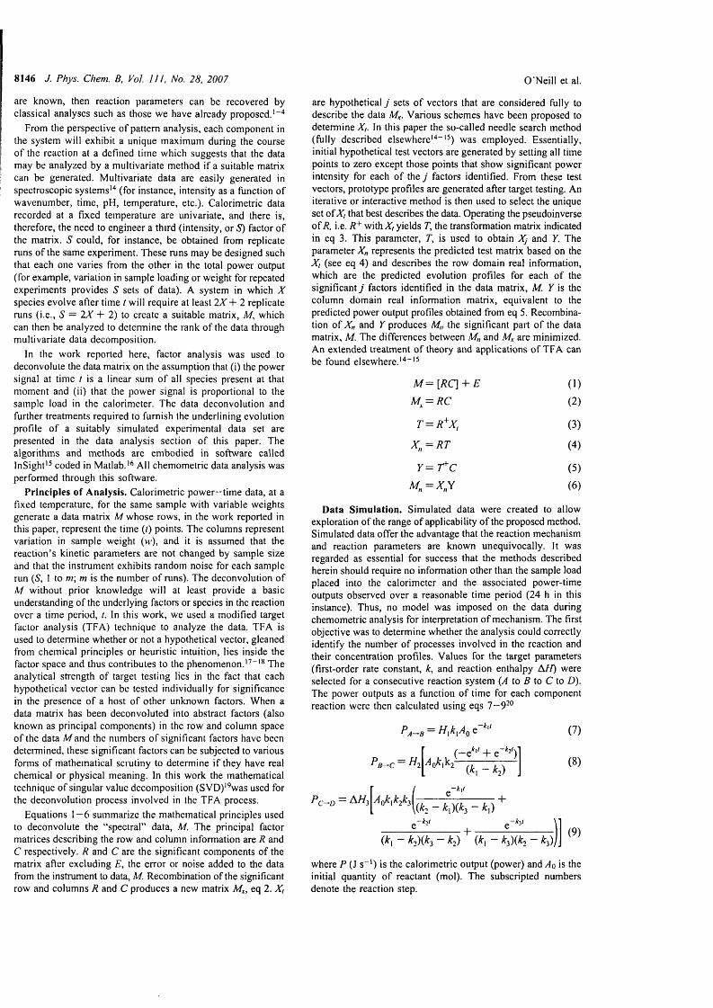
8146 J. Phys. Chem. B, Vol. I l l , No. 28. 2007 O 'N e ill e t al.
are know n, then reaction parameters can be recovered by classical analyses such as those w e have already proposed.
From the perspective o f pattern analysis, each com ponent in the system w ill exhibit a unique m axim um during the course o f the reaction at a defined time w hich suggests that the data m ay be analyzed by a m ultivariate m ethod i f a suitable matrix can be generated. M ultivariate data are easily generated in spectroscopic system s'" (for instance, intensity as a function o f w avenum ber, tim e, pH, temperature, etc.). C alorim etric data recorded at a fixed temperature are univariate, and there is, therefore, the need to engineer a third (intensity, or S) factor o f the matrix. S could , for instance, b e obtained from replicate runs o f the sam e experim ent. T hese runs m ay be designed such that each one varies from the other in the total pow er output (for exam ple, variation in sam ple loading or w eight for repeated experim ents provides S sets o f data). A system in w hich X sp ec ies ev o lv e after tim e t w ill require at least 2 % + 2 replicate runs (i.e ., S = 2 X + 2) to create a suitable matrix, M, which can then be analyzed to d etennine the rank o f the data through m ultivariate data decom position.
In the work reported here, factor analysis w as used to deconvolute the data matrix on the assumption that (i) the power signal at tim e / is a linear sum o f all sp ec ies present at that m om ent and (ii) that the pow er signal is proportional to the sam ple load in the calorim eter. The data deconvolution and further treatments required to furnish the underlining evolution profile o f a suitably sim ulated experim ental data set are presented in the data analysis section o f this paper. The algorithm s and m ethods are em bodied in softw are called InSight'^ coded in Matlab.'^ A ll chem om etric data analysis was perform ed through this software.
P r in c ip les o f A n a ly sis . Calorim etric pow er—tim e data, at a fixed temperature, for the sam e sam ple with variable w eights generate a data matrix M w h ose row s, in the work reported in this paper, represent the time (/) points. The colum ns represent variation in sam ple w eight (w ), and it is assum ed that the reaction’s kinetic parameters are not changed by sam ple size and that the instrument exhibits random noise for each sam ple run (S, 1 to m\ m is the number o f runs). The deconvolution o f A/ w ithout prior know ledge w ill at least provide a basic understanding o f the underlying factors or species in the reaction over a tim e period, t. In this w ork, w e used a m odified target factor analysis (T FA ) technique to analyze the data. TFA is used to determ ine whether or not a hypothetical vector, gleaned from chem ical principles or heuristic intuition, lies inside the factor space and thus contributes to the phenomenon.'^""* The analytical strength o f target testing lies in the fact that each hypothetical vector can be tested individually for sign ificance in the presence o f a host o f other unknown factors. W hen a data matrix has been deconvoluted into abstract factors (a lso known as principal com ponents) in the row and colum n space o f the data A /and the numbers o f sign ificant factors have been determ ined, these significant factors can be subjected to various forms o f mathem atical scrutiny to determ ine i f they have real chem ical or physical m eaning. In this work the m athem atical technique o f singular value decom position (SV D )'^w as used for the deconvolution process in volved in the TFA process.
Equations 1 —6 sum m arize the mathem atical principles used to deconvolu te the “spectral” data, M. The principal factor m atrices describing the row and colum n information are R and C respectively . R and C are the sign ificant com ponents o f the matrix after exclud ing E, the error or noise added to the data from the instrument to data, M. Recom bination o f the significant row and colum ns R and C produces a new matrix A/,, eq 2. X,
are hypothetical j sets o f vectors that are considered fully to describe the data Mx- V arious schem es have been proposed to determ ine X,. In this paper the so-called needle search method (fu lly described elsewhere'""'^) w as em ployed. Essentially, initial hypothetical test vectors are generated by setting all time points to zero except those points that show significant pow er intensity for each o f the j factors identified. From these test vectors, prototype profiles are generated after target testing. An iterative or interactive m ethod is then used to se lect the unique set ofX i that best describes the data. Operating the pseudoinverse of/? , i.e. R^ w ith yields T, the transformation matrix indicated in eq 3. This parameter, T, is used to obtain Xj and Y. The parameter X„ represents the predicted test matrix based on the Xt (see eq 4 ) and describes the row dom ain real information, which are the predicted evolution profiles for each o f the sign ificant j factors identified in the data matrix, M. Y is the colum n dom ain real inform ation m atrix, equivalent to the predicted power output profiles obtained from eq 5. Recom bination o f X„ and Y produces M„ the sign ificant part o f the data matrix, M. The d ifferences betw een M„ and Mx are m inim ized. An extended treatment o f theory and applications o f TFA can be found elsewhere.'""'^
Af= [/?q + £ M ^^RC
T = R ^ X ,
X„ = R T
Y= r^c A£ = x y
( 1 )
(2)
(3)
(4 )
(5)
(6)
D ata S im u la tio n . Sim ulated data w ere created to allow exploration o f the range o f applicability o f the proposed method. Simulated data offer the advantage that the reaction m echanism and reaction parameters are known unequivocally . It w as regarded as essential for su ccess that the m ethods described herein should require no information other than the sam ple load placed into the calorim eter and the associated pow er-tim e outputs observed over a reasonable tim e period (24 h in this instance). Thus, no m odel w as im posed on the data during chem om etric analysis for interpretation o f m echanism . The first objective w as to determ ine whether the analysis could correctly identify the number o f processes involved in the reaction and their concentration profiles. V alues for the target parameters (first-order rate constant, k, and reaction enthalpy A //) were selected for a con secu tive reaction system (A to 5 to C to D). The pow er outputs as a function o f tim e for each com ponent reaction w ere then calculated using eqs 7 - 9 - °
-k\i
( - e * ' ' + e"*:')
(7)
(8)
P c-o — ^ 7/3
-k\!
{k. - k{){ky - A',)+
-F(A, - A2)(A3 - An) (A, - A3)(An - A3) (9)
w here P (J s" ') is the calorim etric output (pow er) and Ao is the initial quantity o f reactant (m ol). The subscripted numbers denote the reaction step.
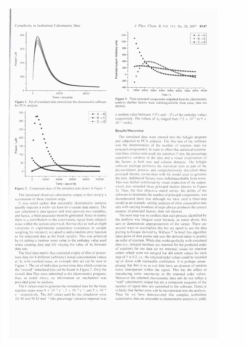
C o m p le x i t y in Isothermal Calorim etr ic Data J. Phys. Chem . B, Vol. I l l , No. 28, 2007 8 1 4 7
400 -
300 -
%
IQ.2 0 0 -
1 0 0 -
0 40000 80000
Tim e / s e c o n d s
F ig u re I. Set o f sim ulated data entered into the chem om etric software for PGA analysis.
350-
300
250-i
2 0 0 -
I 150 4
1 0 0 -
50
0-
— A ^ B B ^ C
- 4 . - C ->D
0 20000 40000 60000 80000 100000
Time / secon d sF ig u re 2. C om ponent steps o f the sim ulated data shown in Figure 1.
The simulated observed calorimetric output is then sim ply a sum m ation o f these reaction steps.
It was noted earlier that successful chem ometric analysis usually requires a multi- (at least tri-) variatc data matrix. The raw calorimetric data (power and time) provide two variables, and hence, a third parameter must be generated. S ince in reality there is a contribution to the calorimetric signal from inherent noise within the system (electrical, thermal etc) as well as slight variations in experimental parameters (variations in sam ple w eighing for instance), w c opted to add a random error function to the simulated data as the third variable. This was achieved by (i) adding a random noise value to the enthalpy value used when creating data and (ii) varying the value o f between data sets.
The final data matrix thus consisted sim ply o f Hies o f pow ertime data for 8 different (arbitrary) initial concentration values o f Ao with overlaid noise; an exam ple data set can be seen in Figure 1. The set o f individual power-tim e data which com prise the “overall” simulated data can be found in Figure 2. Only the overall data files were submitted to the chem om etric program; thus, as noted above, no information on m echanism was provided prior to analysis.
The k values used to generate the simulated data for the three reaction steps were 9 x 10'^ s" ', 2 x 10"^ s “ ', and 5 x 10~ ' s ' respectively. The A f / values used for the simulation were 10, 80 and 90 kJ m ol"' (the percentage variation imposed was
1200- — A -> B■ - t - B
1000- C D
• • • • • • •
0 10000 20000 30000 40000 50000 60000 70000 80000 90000
Time / s
F igu re 3. Three principal com ponents outputted from the chem ometric analysis (further factors w ere indistinguishable from noise, data not shown).
a random value betw een + 2% and —2% o f the enthalpy value) respectively. The values o f Ao ranged from 7.5 x 10"^ to 9 x 10“ m oles.
R esu lts/D iscussion
The simulated data w ere entered into the InSight program and subjected to PCA analysis. The first test o f the software w as the determination o f the number o f reaction steps (or principal components). In order to effect this statistical examination three criteria were used; the statistical F-test, the percentage cum ulative variance in the data and a visual examination o f the factors in both row and colum n domains. The InSight software package performs the statistical tests as part o f the deconvolution process and com prehensively described three principal factors, co-incident with the model used to generate the data. Additional factors were indistinguishable from noise. This was further confirm ed by visual inspection o f the output, which also revealed three principal factors (shown in Figure 3). Thus, the first objective stated earlier, the ability o f the software to detennine the number o f principal com ponents, was demonstrated (note that although we have used a three-step m odel as an exam ple, similar analyses o f other consecutive data sets with varying numbers o f steps always produces the correct number o f principal factors; data not shown).
The next step was to confirm that each process identified by the analysis was integral order because, as noted above, this acts to demonstrate appropriateness o f the output. There are several w ays to accom plish this but w e opted to use the data pairing technique derived by Willson.^' In brief this algorithm takes pairs o f data points and uses the derived ratios to predict an order o f reaction. W hile this works perfectly with simulated data (i.e.. integral numbers are returned for the predicted order o f reaction) for our data set w e returned values for reaction orders which were not integral but did return values for each step o f 1 ± 0.2. i.e., the returned order values could be rounded up or down with reasonable confidence. It is perhaps unsurprising that this is so as real data have an elem ent o f random noise interspersed within the signal. This has the et'fect o f introducing som e uncertainty to the returned order values. M oreover the returned chem ometric data sets do not retlect a “real” calorimetric output but are a com posite response o f the number of repeat data sets submitted to the software. H ence it is likely that further error will be incorporated into the analysis. Thus far w e have demonstrated that com plex isothennal calorimetric data are amenable to chemometrie analysis to yield.
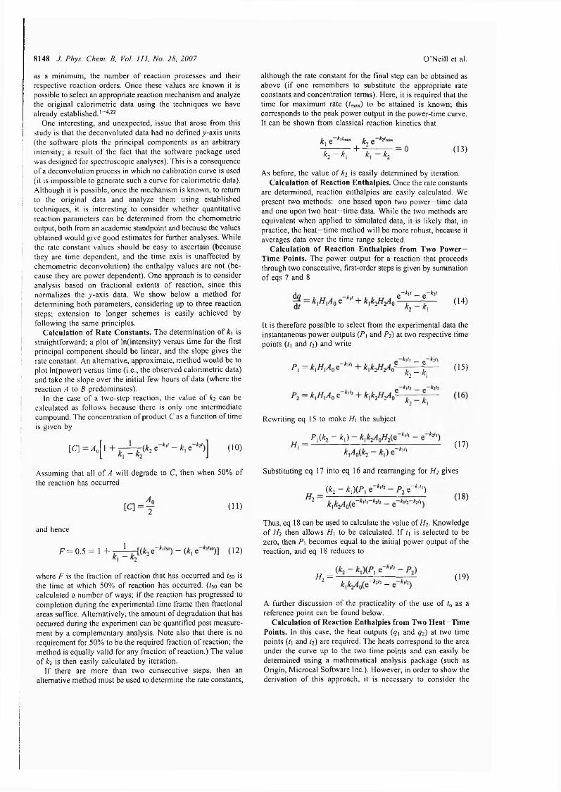
8148 J. Phys. Chem. B, Vol. I l l , No. 28, 2007 O ’N eill e t al.
as a m inim um , the number o f reaction processes and their respective reaction orders. Once these values are known it is possible to select an appropriate reaction mechanism and analyze the original calorimetric data using the techniques w e have already established.'
One interesting, and unexpected, issue that arose from this study is that the deconvoluted data had no defined )/-axis units (the softw are plots the principal com ponents as an arbitrary intensity; a result o f the fact that the software package used was designed for spectroscopic analyses). This is a consequence o f a deconvolution process in which no calibration curve is used (it is im possible to generate such a curve for calorimetric data). Although it is possible, once the m echanism is known, to return to the original data and analyze them using established techniques, it is interesting to consider whether quantitative reaction parameters can be determined from the chem om etric output, both from an academic standpoint and because the values obtained would g ive good estim ates for further analyses. W hile the rate constant values should be easy to ascertain (because they are time dependent, and the tim e axis is unaffected by chem om etric deconvolution) the enthalpy values are not (because they are power dependent). One approach is to consider analysis based on fractional extents o f reaction, since this norm alizes the y -ax is data. W e show below a method for delennin ing both parameters, considering up to three reaction steps; extension to longer schem es is easily achieved by fo llow ing the sam e principles.
C alcu lation o f R ate C on stan ts. The determination o f is straightforward; a plot o f In(intensity) versus time for the first principal com ponent should be linear, and the slope g ives the rate constant. An alternative, approximate, method would be to plot In(power) versus time (i.e ., the observed calorimetric data) and take the slope over the initial few hours o f data (where the reaction A io B predominates).
In the case o f a tw o-step reaction, the value o f kz can be calculated as fo llow s because there is only one intermediate compound. The concentration o f product C as a function o f time is given by
[C ] — A q ( 10)
A ssum ing that all o f A w ill degrade to C, then when 50% o f the reaction has occurred
( 1 1 )
and hence
F = 0 . 5 = 1 + ( 12)
where F is the fraction o f reaction that has occurred and /so is the tim e at which 50% o f reaction has occurred. ( / 5 0 can be calculated a number o f ways; i f the reaction has progressed to com pletion during the experimental tim e frame then fractional areas suffice. Alternatively, the amount o f degradation that has occuned during the experiment can be quantified post measurement by a com plem entaiy analysis. N ote also that there is no requirement for 50% to be the required fraction o f reaction; the method is equally valid for any fraction o f reaction.) The value o f kz is then easily calculated by iteration.
If there are more than two consecutive steps, then an alternative method must be used to determine the rate constants.
although the rate constant for the final step can be obtained as above ( i f one remembers to substitute the appropriate rate constants and concentration terms). Here, it is required that the time for m aximum rate (r^ax) to be attained is known; this corresponds to the peak power output in the power-tim e curve. It can be shown from classical reaction kinetics that
k-, - k.+
A:, — k-,= 0 (13)
A s before, the value o f kj is easily determined by iteration.C alculation o f R eaction E nthalp ies. O nce the rate constants
are determined, reaction enthalpies are easily calculated. W e present two methods: one based upon tw o pow er—time data and one upon tw o heat—time data. W hile the two methods are equivalent w hen applied to sim ulated data, it is likely that, in practice, the heat—time method w ill be more robust, because it averages data over the time range selected.
C alcu lation o f R eaction E n th a lp ies from T w o P o w e r - T im e P oin ts. The power output for a reaction that proceeds through two consecutive, first-order steps is given by summation o f eqs 7 and 8
-k\i
/r, - k,(1 4 )
It is therefore possib le to select from the experimental data the instantaneous pow er outputs (Pi and Pz) at two respective time points and A) and write
P, = ^ ^------ (1 5 )2-*1
Rewriting eq 15 to make H\ the subject
f ,(4 - *,) -//, = (1 7 )
Substituting eq 17 into eq 16 and rearranging for H} g ives
( t , - t , ) ( f , e - ^ ' " )
Thus, eq IS can be used to calculate the value o f Hz. Knowledge o f Hz then allow s H\ to be calculated. If t\ is selected to be zero, then P\ becom es equal to the initial power output o f the reaction, and eq 18 reduces to
H, = -klh _ (1 9 )
A further d iscussion o f the practicality o f the use o f to as a reference point can be found below .
C alculation o f R eaction E nthalpies from T w o H eat—T im e Points. In this case, the heat outputs {q\ and qz) at two time points (/[ and (2 ) are required. The heats correspond to the area under the curve up to the two time points and can easily be determined using a mathematical analysis package (such as Origin, M icrocal Software Inc.). However, in order to show the derivation o f this approach, it is necessary to consider the
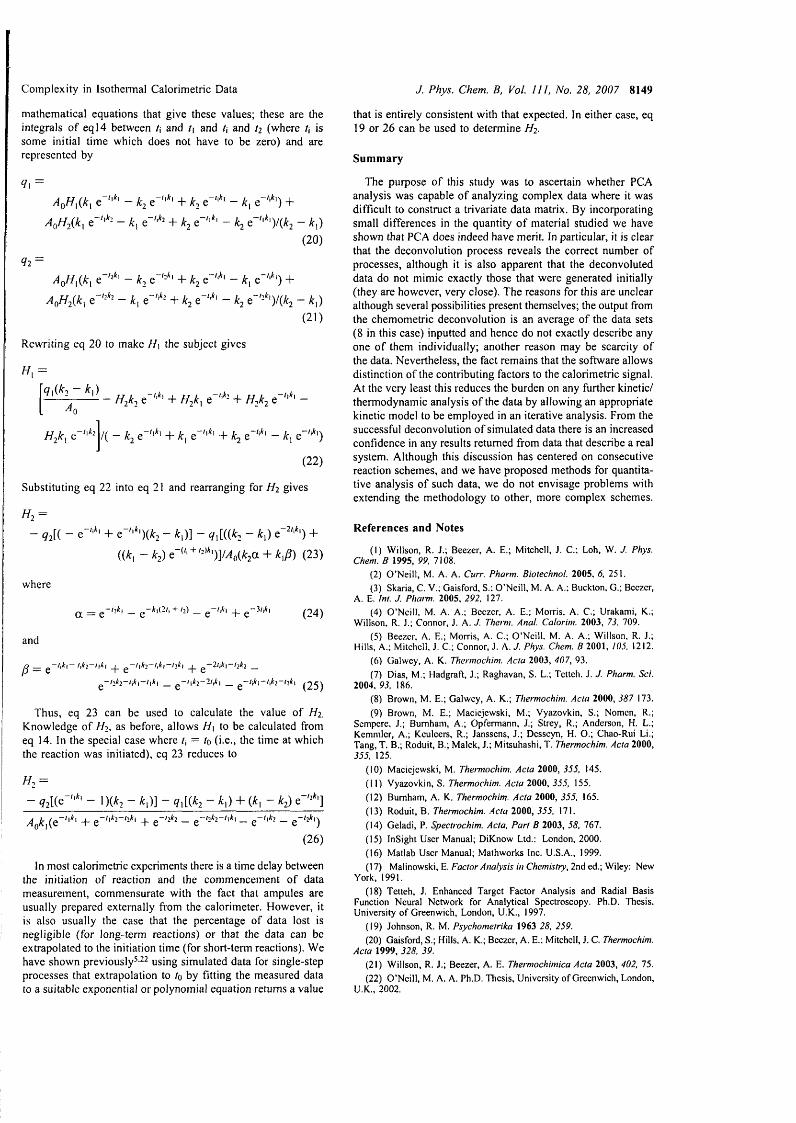
C o m p le x ity in IsotheiTnal C a lo rim etric D ata J. Phys. Chem. B, Vol. H I . No. 28, 2007 8149
m athem atical equations that g iv e these values; these are the integrals o f e q l4 betw een /, and t\ and h and h (w here /; is som e initial tim e which does not have to be zero) and are represented by
+ k. e""'' - A, +- k, e"':*: + k - k e""* ')# - k,)
(20)
92 —/4q//|(A:, e — k jC + A:2 e e '" ') +
A ik, e-''*: - k, + k e"''*' - k e''='^')/(^2 - k,)(2 1 )
R ew riting eq 2 0 to m ake H\ the subjeet g ives
9 i( 2 - ^|)— H^k-i e + H^k e + H-Mj e —
/ / 2 A', e “ 0 * 2 /( - ^2 + k, e"''*' + 2 - A:, e""*')
(22)
Substituting eq 22 into eq 21 and rearranging for H 2 g ives
H 2 —
- q ii - e-"'' + - t,)] - - i,) e-"'*) +((t, - t2 )e -" ' + '* ) ] /W # ;a + A,A (23)
w here
and
e '
a _ g “ 0*i _ g “ *i(2o + 0) _ g “ 0*1 g “ 30*i ^ 2 4 )
0 * i“ 0*2“ 0 * i g “ /|*2 “ 0 * i“ O*i g “ 2 0 *i“ O*2 _
g “ 0 *2 “ ' i * l“ 0 * l _ g “ 'l*2 “ 2/,*l _ g “ 0 * l“ 0*2“ '2*l ^ 2 5 )
Thus, eq 23 can be used to calculate the value o f Hi, K now ledge o f / / ] . as before, a llow s H\ to be calculated from eq 14. In the special case where t\ — lo (i.e ., the tim e at w hich the reaction w as initiated), eq 23 reduces to
/ / .=~ 9 2 [(6 ~ 1)(^2 ~ ^ |) ] ~ 9 |[ (^ 2 ~ ^ 1) + (^1 ~ ^2) G
(26)
In m ost calorimetric experim ents there is a time delay between the initiation o f reaction and the com m encem ent o f data m easurem ent, com m ensurate w ith the fact that am pules are usually prepared externally from the calorim eter. H ow ever, it is a lso usually the case that the percentage o f data lost is n eglig ib le (for long-term reactions) or that the data can be extrapolated to the initiation time (for short-term reactions). W e have show n previously^-^^ using sim ulated data for single-step processes that extrapolation to to by fitting the measured data to a suitable exponential or polynom ial equation returns a value
“ (2*11
that is entirely consistent with that expected. In either case, eq 19 or 2 6 can be used to determ ine Hj.
S u m m a ry
The purpose o f this study w as to ascertain whether PCA analysis w as capable o f analyzing com plex data w here it w as difficu lt to construct a trivariate data matrix. B y incorporating sm all d ifferences in the quantity o f material studied w e have show n that PCA does indeed have merit. In particular, it is clear that the deconvolution process reveals the correct number o f processes, although it is a lso apparent that the deconvoluted data do not m im ic exactly those that w ere generated initially (they are how ever, very c lose). The reasons for this are unclear although several possibilities present them selves; the output from the chem om etric deconvolution is an average o f the data sets (8 in this case) inputted and hence do not exactly describe any one o f them individually; another reason m ay be scarcity o f the data. N evertheless, the fact rem ains that the softw are allow s distinction o f the contributing factors to the calorim etric signal. At the very least this reduces the burden on any further kinetic/ therm odynam ic analysis o f the data by a llow ing an appropriate kinetic m odel to be em ployed in an iterative analysis. From the successfu l deconvolution o f sim ulated data there is an increased confidence in any results returned from data that describe a real system . A lthough this d iscussion has centered on consecutive reaction schem es, and w e have proposed m ethods for quantitative analysis o f such data, w e do not en visage problem s with extending the m ethodology to other, m ore com plex schem es.
R eferen ces an d N otes
(1) Willson, R. J.; Beezer, A. E.; Mitchell, J. C.; Loh, W. J. Phys. Chem. B 1995, 99. 7108.
(2) O ’Neill, M. A. A. Curr. Pharm. Biotechnol. 2005, 6, 251.(3) Skaria, C. V.; Gaisford, S.; O ’Neill, M. A. A.; Buckton. G.; Beezer,
A. E. Int. J. Pharm. 2005, 292, 127.(4) O ’Neill, M. A. A.; Beezer, A. E.; M om s. A. C.; Urakami, K.;
Willson. R. J.; Connor, J. A . ./. Therm. Anal. Calorim. 2003, 73. 709.(5) Beezer, A. E.; Morris, A. C,; O ’Neill, M. A. A.; Willson, R. J.;
Hills, A.; Mitchell, J. C.; Connor, J. A. J. Phys. Chem. B 2001, 105, 1212.(6) Galwey, A. K. Thermochim. Acta 2003, 407, 93.
(7) Dias, M.; Hadgraft, J.; Raghavan, S. L.; Tetteh. J. J. Pharm. Sci. 2004, 93. 186.
(8) Brown, M. E.; Galwey, A. K.; Thermochim. Acta 2000, 387 173.(9) Brown, M. E.; M aeiejewski, M.; Vyazovkin, S.; Nomcn, R.;
Sempere, J.; Burnham, A.; Opfermann, J.; Strey, R.; Anderson, H. L.; Kcmmlcr, A.; Kculeers, R.; Janssens, J.; Desseyn, H. O.; Chao-Rui Li.; Tang, T. B.; Roduit, B.; M alek, J.; M itsuhashi, T. Thermochim. Acta 2000, 355. 125.
(10) M aeiejewski, M. Them ochim . Acta 2000, 355. 145.(11) Vyazovkin, S. Thermochim. Acta 2000, 355. 155.(12) Burnham, A. K. Thermochim. Acta 2000, 355. 165.(13) Roduit, B. Thermochim. Acta 2000, 355. 171.
(14) Geladi, P. Spectrochim. Acta. Part B 2003, 58, 767.(15) InSight User M anual; DiKnow Ltd.: London, 2000.(16) Matlab User M anual; M athworks Inc. U.S.A., 1999.(17) Malinowski, E. Factor Analysis in Chemistry, 2nd ed.; Wiley: New
York, 1991.(18) Tetteh, J. Enhanced Target Factor Analysis and Radial Basis
Function Neural Network for Analytical Spectroscopy. Ph.D. Thesis. University o f Greenwich, London, U.K., 1997.
(19) Johnson, R. M. Psychometrika 1963 28. 259.(20) Gaisford, S.; Hills. A. K ; Beezer, A. E.: Mitchell, J. C. Thermochim.
Acta 1999, 328. 39.(21) W illson, R. J.; Beezer, A. E. Thermochimica Acta 2003, 402, 75.(22) O ’Neill, M. A. A. Ph.D. Thesis, University o f Greenwich, London,
U.K., 2002.