
thesis.pdf - UCL Discovery
244
Genetics, Evolution and Environment University College London E XPERIMENTAL AND C OMPUTATIONAL A PPROACHES REVEAL M ECHANISMS OF E VOLUTION OF G ENE R EGULATORY N ETWORKS UNDERLYING E CHINODERM S KELETOGENESIS David Viktor Dylus Research Project submitted in partial fulfillment of the requirements for the degree of PhD in Systems Biology. Supervisor: Dr. Paola Oliveri Second supervisor: Dr. Eugene Schuster London, June 2015
-
Upload
khangminh22 -
Category
Documents
-
view
3 -
download
0
Transcript of thesis.pdf - UCL Discovery

Genetics, Evolution and Environment
University College London
EXPERIMENTAL AND COMPUTATIONAL APPROACHES REVEAL
MECHANISMS OF EVOLUTION OF GENE REGULATORY
NETWORKS UNDERLYING ECHINODERM SKELETOGENESIS
David Viktor Dylus
Research Project submitted in partial fulfillment of
the requirements for the degree of PhD in Systems
Biology.
Supervisor: Dr. Paola Oliveri
Second supervisor: Dr. Eugene Schuster
London, June 2015

I, David Viktor Dylus, confirm that the work presented in this thesis is my own. Where infor-
mation has been derived from other sources, I confirm that this has been indicated in the thesis.

ABSTRACT
The evolutionary mechanisms in distantly related animals involved in shaping complex gene
regulatory networks (GRN) that encode morphologically similar structures remain elusive. In this
context, echinoderm larval skeletons found only in brittle stars and sea urchins out of the five
classes provide an ideal system. Here, we characterise for the first time the development of the
larval skeleton in the poorly described class of echinoderms, the ophiuroid Amphiura filiformis,
and we compare it systematically with the well-established sea urchin.
In the first part of this study, we show that ophiuroids and euechinoids, that split at least 480
Million years ago (Mya), have remarkable similarities in tempo and mode of skeletal development.
Despite morphological and ontological similarities, our high-resolution study of the dynamics of
regulatory states using 24 sea urchin candidates highlights that gene duplication, protein func-
tion diversification and cis-regulatory element evolution all contributed to shape the regulatory
program for larval skeletogenesis in different branches of echinoderms. Our data allows to com-
ment on the independent or homologous evolution of the larval skeleton in light of the recently
established phylogeny of echinoderm classes.
In the second part of this study, we employ mRNA sequencing to establish a transcriptome
and analyse its content quantitatively and qualitatively. We identify a core set of skeletogenic
genes that is highly conserved using various comparative genomic analyses including other three
classes of echinoderms. Additionally, from a differential screen on samples with inhibited skeleton
we obtain a list of candidates specific for brittle star skeleton development and analyse their
expression using experimental techniques. Finally, we provide access to all transcriptomic and
iii

ABSTRACT iv
expression data via a customised web interface.
In conclusion, we establish the brittle star A. filiformis as new developmental model system
and provide novel insights into evolution of GRNs.

ACKNOWLEDGMENTS
In this thesis I am summarising nearly 4 years of work in echinoderm biology. Throughout this
years, I have learned so much personally and professionally that when reflecting on it, my mind
seems incapable of comprehending all the things I have experienced. I am extremely grateful
to CoMPLEX/UCL, to have been given the opportunity to work in science, to think without any
concern of economical value about theories and enjoy the liberty of my own thoughts. On this
journey I was accompanied by many people and it seem impossible for me to thank all of them
in the way they would deserve to be thanked. Surely, only due to their companionship, whether
relaxing after a day of struggle or exciting with an intense scientific discussion, I was able to
reach this point. Nevertheless, some people have to be thanked because their contribution is
directly linked to this adventure. First, I would like to thank Jack Paget and Monica Marinescu for
supporting me when I first applied here in London and Ruggero Cortini and Francessco Massucci
for spending a first real ”gentleman’s” year with me in London. Then I would like to thank all my
friends here in London that had to endure my various moods and gave support in good and bad
times. Especially, I am grateful to everyone from the Roberto Mayor Lab and the Max Telford Lab
throughout the years 2010 to 2015. Additionally, I am very thankful to everyone from the Kentish
Town community.
Throughout my PhD, I was given the opportunity to teach several students, with whom I formed
a symbiotic relationship. They helped me and I tried to support their projects in the best possible
way. For this I am very thankful to Matt Pilgrim, Yan-kay Ho, Thomas Mullan, Alun Jones, Pantelis
Nicola and Luisana Carballo. Moreover, at this point I would also like to thank Patrick Toolan-Kerr
and Helen Robertson for valuable comments on the manuscript.
v

Experimental work is performed alone, but a laboratory needs team work. I am, especially,
thankful to Anna Czarkwiani and Libero Petrone. We struggled, we laughed, we learned, we
enjoyed and we worked together. I am more than thankful that you two were my two ”Lab-mates”
throughout these years. I also would like to thank at this point Avi Lerner for struggling to teach
an engineer in basic experimental techniques.
Most importantly, I would like to thank my supervisor Dr. Paola Oliveri for the patience in my
first attempts in experimental biology, the addicting enthusiasm and the always open mind for
questions of any kind, which allowed me to grow quickly into the exciting field of developmental
biology and especially gene regulatory networks. I truly hope, that our professional and personal
collaboration will never end. Furthermore, I would like to thank also Dr. Eugene Schuster who
pointed me always at the right moment into the right direction helping me to never loose my aims
out of sight.
Finally, I would like to thank the one person that was always there, kept me stable when I was
insecure, pushed me when needed, put me back on track when I was flying and never gave up
believing in me, Maria Kotini. I owe you the most for these years and there are no words that are
able to express the gratitude I feel. Thank you.
David Dylus

ACKNOWLEDGMENTS vii
Fur meine Eltern und meinen Bruder.

CONTENTS
Abstract . . . . . . . . . . . . . . . . . . . . . . . . . . . . . . . . . . . . . . . . . . . . . . iii
Acknowledgments . . . . . . . . . . . . . . . . . . . . . . . . . . . . . . . . . . . . . . . . v
List of figures . . . . . . . . . . . . . . . . . . . . . . . . . . . . . . . . . . . . . . . . . . . xii
List of tables . . . . . . . . . . . . . . . . . . . . . . . . . . . . . . . . . . . . . . . . . . . . xv
Abbreviations . . . . . . . . . . . . . . . . . . . . . . . . . . . . . . . . . . . . . . . . . . . xvii
Chapter 1: Introduction . . . . . . . . . . . . . . . . . . . . . . . . . . . . . . . . . . . . . 1
1.1 Networks in biology . . . . . . . . . . . . . . . . . . . . . . . . . . . . . . . . . . . 1
1.1.1 Types of biological networks . . . . . . . . . . . . . . . . . . . . . . . . . . 2
1.1.2 The regulatory genome . . . . . . . . . . . . . . . . . . . . . . . . . . . . . 4
1.1.3 Gene regulatory networks . . . . . . . . . . . . . . . . . . . . . . . . . . . . 8
1.1.4 Construction of GRNs . . . . . . . . . . . . . . . . . . . . . . . . . . . . . . 11
1.1.5 Modelling of GRNs . . . . . . . . . . . . . . . . . . . . . . . . . . . . . . . . 13
1.2 Evolution of gene regulatory networks . . . . . . . . . . . . . . . . . . . . . . . . . 17
1.2.1 Towards a theory of GRN evolution . . . . . . . . . . . . . . . . . . . . . . . 17
1.2.2 Mechanisms of GRN evolution . . . . . . . . . . . . . . . . . . . . . . . . . 21
1.3 Phylogeny of echinoderms . . . . . . . . . . . . . . . . . . . . . . . . . . . . . . . 27
1.4 Echinoderm development as model for GRN evolution . . . . . . . . . . . . . . . . 31
1.4.1 Morphological observations . . . . . . . . . . . . . . . . . . . . . . . . . . . 31
1.4.2 Early specification and the double negative gate . . . . . . . . . . . . . . . 32
1.4.3 Stabilization of skeletogenic fate . . . . . . . . . . . . . . . . . . . . . . . . 36
1.4.4 Cell movements and skeletogenic differentiation genes . . . . . . . . . . . 39
1.5 The brittle star Amphiura filiformis . . . . . . . . . . . . . . . . . . . . . . . . . . . 41
1.6 Modern approaches in new organisms . . . . . . . . . . . . . . . . . . . . . . . . . 43
1.6.1 mRNA sequencing . . . . . . . . . . . . . . . . . . . . . . . . . . . . . . . . 43
1.6.2 Bio-informatics for transcriptomics . . . . . . . . . . . . . . . . . . . . . . . 45
Chapter 2: Hypothesis . . . . . . . . . . . . . . . . . . . . . . . . . . . . . . . . . . . . . . 50
viii

CONTENTS ix
I Evolution of gene regulatory network for specification of skeletogenic lin-eage in Echinoderms 53
Chapter 3: Methods . . . . . . . . . . . . . . . . . . . . . . . . . . . . . . . . . . . . . . . 54
3.1 Embryological techniques . . . . . . . . . . . . . . . . . . . . . . . . . . . . . . . . 54
3.1.1 Animal collection and embryo culture for the brittle star Amphiura filiformis . 54
3.1.2 Animal collection and embryo culture for the sea urchin Strongylocentrotus
purpuratus . . . . . . . . . . . . . . . . . . . . . . . . . . . . . . . . . . . . 55
3.1.3 Staining of skeletal elements using calcein . . . . . . . . . . . . . . . . . . 56
3.2 Bioinformatic Techniques . . . . . . . . . . . . . . . . . . . . . . . . . . . . . . . . 56
3.2.1 Primer design . . . . . . . . . . . . . . . . . . . . . . . . . . . . . . . . . . . 56
3.2.2 Phylogenetic analysis . . . . . . . . . . . . . . . . . . . . . . . . . . . . . . 57
3.3 Molecular techniques . . . . . . . . . . . . . . . . . . . . . . . . . . . . . . . . . . 58
3.3.1 RNA Extraction . . . . . . . . . . . . . . . . . . . . . . . . . . . . . . . . . . 58
3.3.2 cDNA Synthesis . . . . . . . . . . . . . . . . . . . . . . . . . . . . . . . . . 59
3.3.3 Quantitative polymerase chain reaction (QPCR) . . . . . . . . . . . . . . . 60
3.3.4 Embryo fixation . . . . . . . . . . . . . . . . . . . . . . . . . . . . . . . . . . 61
3.3.5 Molecular cloning . . . . . . . . . . . . . . . . . . . . . . . . . . . . . . . . 61
3.3.6 Synthesis of antisense RNA probes . . . . . . . . . . . . . . . . . . . . . . 65
3.3.7 Whole mount in situ hybridization (WMISH) . . . . . . . . . . . . . . . . . . 65
3.4 Microinjection of sea urchin zygotes . . . . . . . . . . . . . . . . . . . . . . . . . . 68
3.4.1 Preparation . . . . . . . . . . . . . . . . . . . . . . . . . . . . . . . . . . . . 68
3.4.2 Constructs used for injections . . . . . . . . . . . . . . . . . . . . . . . . . . 68
3.4.3 Microinjection procedure . . . . . . . . . . . . . . . . . . . . . . . . . . . . 70
3.5 Microscopy and image analysis . . . . . . . . . . . . . . . . . . . . . . . . . . . . . 72
3.5.1 Differential interference contrast (DIC) & epi-fluorescent microscopy . . . . 72
3.5.2 Confocal microscopy . . . . . . . . . . . . . . . . . . . . . . . . . . . . . . . 72
Chapter 4: Results . . . . . . . . . . . . . . . . . . . . . . . . . . . . . . . . . . . . . . . . 73
4.1 The development of Amphiura filiformis . . . . . . . . . . . . . . . . . . . . . . . . 74
4.1.1 Comparison of developmental timing between Amphiura filiformis and Strongy-
loncentrotus purpuratus . . . . . . . . . . . . . . . . . . . . . . . . . . . . . 77
4.2 Identification of skeletogenic mesodermal cells in brittle star . . . . . . . . . . . . . 79
4.3 Comparison of sea urchin and brittle star skeletogenesis . . . . . . . . . . . . . . . 82
4.3.1 Early regulatory inputs initiating the GRN for larval skeletogenesis . . . . . 83
4.3.2 Identification of a brittle star ortholog of the sea urchin Spu-pmar1 . . . . . 84

CONTENTS x
4.3.3 Evolutionary origin of the pplx/pmar1 genes . . . . . . . . . . . . . . . . . . 89
4.3.4 The initial specification of A. filiformis skeletogenic mesoderm lineage . . . 95
4.3.5 High-resolution gene expression of regulatory genes reveals major differ-
ences between sea urchin and brittle star skeletogenic GRNs . . . . . . . . 98
4.3.6 Other transcription factors of skeletogenic GRN in brittle star and sea urchin 103
4.3.7 Dynamic regulatory states during A. filiformis mesoderm development . . . 106
Chapter 5: Discussion . . . . . . . . . . . . . . . . . . . . . . . . . . . . . . . . . . . . . . 110
5.1 Evolution of GRN by protein function diversification . . . . . . . . . . . . . . . . . . 110
5.2 Evolution of GRN by changes in cis-regulation . . . . . . . . . . . . . . . . . . . . 113
5.3 Common regulatory state for skeletogenesis . . . . . . . . . . . . . . . . . . . . . 116
5.4 Independent or common evolution of larval skeleton? . . . . . . . . . . . . . . . . . 117
II A global view on Amphiura filiformis skeletogenesis 119
Chapter 6: Methods . . . . . . . . . . . . . . . . . . . . . . . . . . . . . . . . . . . . . . . 120
6.1 Experimental . . . . . . . . . . . . . . . . . . . . . . . . . . . . . . . . . . . . . . . 120
6.1.1 mRNA Samples and Extraction . . . . . . . . . . . . . . . . . . . . . . . . . 120
6.1.2 mRNA sequencing . . . . . . . . . . . . . . . . . . . . . . . . . . . . . . . . 120
6.2 Computational Procedures . . . . . . . . . . . . . . . . . . . . . . . . . . . . . . . 121
6.2.1 Required Software . . . . . . . . . . . . . . . . . . . . . . . . . . . . . . . . 121
6.2.2 Quality evaluation of reads . . . . . . . . . . . . . . . . . . . . . . . . . . . 122
6.2.3 Assembly of combined samples . . . . . . . . . . . . . . . . . . . . . . . . 122
6.2.4 Assembly of individual samples . . . . . . . . . . . . . . . . . . . . . . . . . 123
6.2.5 Post Assembly procedures . . . . . . . . . . . . . . . . . . . . . . . . . . . 123
6.2.6 Other Echinoderm Datasets . . . . . . . . . . . . . . . . . . . . . . . . . . . 124
6.2.7 Quality Assessment . . . . . . . . . . . . . . . . . . . . . . . . . . . . . . . 124
6.2.8 Annotation . . . . . . . . . . . . . . . . . . . . . . . . . . . . . . . . . . . . 124
6.2.9 Gene Ontology (GO) . . . . . . . . . . . . . . . . . . . . . . . . . . . . . . . 125
6.2.10 Abundance Estimation . . . . . . . . . . . . . . . . . . . . . . . . . . . . . . 125
6.2.11 Differential Analysis . . . . . . . . . . . . . . . . . . . . . . . . . . . . . . . 126
6.2.12 Expression clustering of time-series data . . . . . . . . . . . . . . . . . . . 126
6.2.13 Orthology analysis . . . . . . . . . . . . . . . . . . . . . . . . . . . . . . . . 126
Chapter 7: Results . . . . . . . . . . . . . . . . . . . . . . . . . . . . . . . . . . . . . . . . 128
7.1 mRNA sequencing: Samples and Reads . . . . . . . . . . . . . . . . . . . . . . . . 128

CONTENTS xi
7.2 Assembly of the A. filiformis transcriptome . . . . . . . . . . . . . . . . . . . . . . . 131
7.3 Transcriptome quality and datasets for comparison . . . . . . . . . . . . . . . . . . 136
7.4 Echinomics: Annotation and Comparison . . . . . . . . . . . . . . . . . . . . . . . 139
7.4.1 Comparison of echinoderm gene sets based on sea urchin gene ontology . 140
7.4.2 Comprehensive comparison of gene set involved in skeletogenesis . . . . . 144
7.5 Quantification of A. filiformis transcriptome . . . . . . . . . . . . . . . . . . . . . . 148
7.5.1 Clustering of expression profiles . . . . . . . . . . . . . . . . . . . . . . . . 151
7.6 Unbiased approach to detect genes participating in larval skeletogenesis of A. fili-
formis . . . . . . . . . . . . . . . . . . . . . . . . . . . . . . . . . . . . . . . . . . . 155
7.6.1 Differential gene expression analysis . . . . . . . . . . . . . . . . . . . . . . 157
7.7 Novel Genes in A. filiformis larval skeletogenesis . . . . . . . . . . . . . . . . . . . 158
Chapter 8: Discussion . . . . . . . . . . . . . . . . . . . . . . . . . . . . . . . . . . . . . . 164
8.1 De novo Transcriptomics . . . . . . . . . . . . . . . . . . . . . . . . . . . . . . . . . 164
8.1.1 Amphiura filiformis assembly and quality . . . . . . . . . . . . . . . . . . . . 165
8.2 Evolutionary implications for larval skeletogenesis . . . . . . . . . . . . . . . . . . 167
8.2.1 Comparison to other echinoderms . . . . . . . . . . . . . . . . . . . . . . . 167
8.2.2 Evolution of skeletogenic differentiation genes . . . . . . . . . . . . . . . . 168
8.2.3 Conservation of fgf and vegf signalling . . . . . . . . . . . . . . . . . . . . . 170
8.2.4 Novel skeletogenic genes in the brittle star larval skeleton development . . 172
8.3 Data Access through Website . . . . . . . . . . . . . . . . . . . . . . . . . . . . . . 174
Chapter 9: Conclusion . . . . . . . . . . . . . . . . . . . . . . . . . . . . . . . . . . . . . . 177
Appendix A: Part I . . . . . . . . . . . . . . . . . . . . . . . . . . . . . . . . . . . . . . . . . 181
Appendix B: Part II . . . . . . . . . . . . . . . . . . . . . . . . . . . . . . . . . . . . . . . . 187
List of references . . . . . . . . . . . . . . . . . . . . . . . . . . . . . . . . . . . . . . . . . 205

LIST OF FIGURES
Figure Page
1.1 Types of networks . . . . . . . . . . . . . . . . . . . . . . . . . . . . . . . . . . . . 2
1.2 Definition of a gene and DNA binding motif . . . . . . . . . . . . . . . . . . . . . . 4
1.3 Types of networks . . . . . . . . . . . . . . . . . . . . . . . . . . . . . . . . . . . . 6
1.4 Schematic of a GRN . . . . . . . . . . . . . . . . . . . . . . . . . . . . . . . . . . . 8
1.5 Experimental procedure to construct a gene regulatory network . . . . . . . . . . . 10
1.6 GRN modelling using BioTapestry . . . . . . . . . . . . . . . . . . . . . . . . . . . 12
1.7 Types of networks . . . . . . . . . . . . . . . . . . . . . . . . . . . . . . . . . . . . 14
1.8 Example of kernel . . . . . . . . . . . . . . . . . . . . . . . . . . . . . . . . . . . . 18
1.9 Theory of GRN evolution . . . . . . . . . . . . . . . . . . . . . . . . . . . . . . . . 19
1.10 Cis-regulatory module evolution . . . . . . . . . . . . . . . . . . . . . . . . . . . . . 22
1.11 Protein evolution by gene duplication . . . . . . . . . . . . . . . . . . . . . . . . . . 24
1.12 Echinodermata Phylogenesis . . . . . . . . . . . . . . . . . . . . . . . . . . . . . . 27
1.13 Larval stages of echinoderms . . . . . . . . . . . . . . . . . . . . . . . . . . . . . . 29
1.14 Schematic development of three classes of echinoderms . . . . . . . . . . . . . . 33
1.15 GRN for larval skeletogenesis in sea urchin 6hpf and 10hpf . . . . . . . . . . . . . 34
1.16 GRN for larval skeletogenesis in sea urchin 15hpf and 24hpf . . . . . . . . . . . . 37
1.17 Adult Brittle Stars . . . . . . . . . . . . . . . . . . . . . . . . . . . . . . . . . . . . . 41
1.18 RNA sequencing . . . . . . . . . . . . . . . . . . . . . . . . . . . . . . . . . . . . . 44
3.1 Synthetic Afi-pplx construct . . . . . . . . . . . . . . . . . . . . . . . . . . . . . . . 69
3.2 Spu-phb1 constructs . . . . . . . . . . . . . . . . . . . . . . . . . . . . . . . . . . . 69
4.1 High-resolution developmental time-line of A. filiformis . . . . . . . . . . . . . . . . 76
4.2 Comparison between A. filiformis and S. purpuratus development . . . . . . . . . . 79
4.3 Skeletogenic cells in the brittle star A. filiformis . . . . . . . . . . . . . . . . . . . . 81
4.4 Expression of Afi-otx, Afi-wnt8 and Afi-blimp1 . . . . . . . . . . . . . . . . . . . . . 82
4.5 Afi-pmar1 phylogeny . . . . . . . . . . . . . . . . . . . . . . . . . . . . . . . . . . . 86
xii

LIST OF FIGURES xiii
Figure Page
4.6 Afi-pplx is expressed similarly to Spu-pmar1 . . . . . . . . . . . . . . . . . . . . . . 88
4.7 Afi-pmar1 injection statistics . . . . . . . . . . . . . . . . . . . . . . . . . . . . . . . 90
4.8 Spu-pmar1 as gene duplication of Spu-phb1 . . . . . . . . . . . . . . . . . . . . . 91
4.9 Expression of mesodermal genes in early stages of development . . . . . . . . . . 95
4.10 Afi-hesC is not a global repressor in brittle star . . . . . . . . . . . . . . . . . . . . 96
4.11 Expression pattern of genes part of the interlocking loop . . . . . . . . . . . . . . . 99
4.12 Expression pattern of Afi-dri and Afi-foxB . . . . . . . . . . . . . . . . . . . . . . . 101
4.13 Expression of other skeletogenic specification orthologs . . . . . . . . . . . . . . . 103
4.14 The endomesodermal regulatory states of the brittle star A. filiformis . . . . . . . . 106
4.15 Expression of Afi-gcm, Afi-gataC and Afi-gataE . . . . . . . . . . . . . . . . . . . . 107
5.1 Summary of GRN changes . . . . . . . . . . . . . . . . . . . . . . . . . . . . . . . 112
5.2 Evolution of echinoderm larval skeletogenesis . . . . . . . . . . . . . . . . . . . . . 114
7.1 Quality of samples and reads for transcriptome . . . . . . . . . . . . . . . . . . . . 129
7.2 Assembly pipeline . . . . . . . . . . . . . . . . . . . . . . . . . . . . . . . . . . . . 132
7.3 Test for computational loss of digital normalisation . . . . . . . . . . . . . . . . . . 133
7.4 Full length distribution . . . . . . . . . . . . . . . . . . . . . . . . . . . . . . . . . . 137
7.5 Echinoderm gene set . . . . . . . . . . . . . . . . . . . . . . . . . . . . . . . . . . 140
7.6 Gene Ontology classification . . . . . . . . . . . . . . . . . . . . . . . . . . . . . . 141
7.7 Conservation of skeletogenic genes in echinoderms . . . . . . . . . . . . . . . . . 145
7.8 Gene Ontology classes for skeletogenic candidates . . . . . . . . . . . . . . . . . 147
7.9 WMISH of orthologs to sea urchin downstream skeletogenic genes . . . . . . . . . 149
7.10 QPCR vs transcriptome analysis . . . . . . . . . . . . . . . . . . . . . . . . . . . . 150
7.11 Fuzzy clustering of time-courses . . . . . . . . . . . . . . . . . . . . . . . . . . . . 152
7.12 Conservation of Fgf and Vegf signalling between brittle star and sea urchin . . . . 154
7.13 Differential analysis of samples with and without larval skeleton . . . . . . . . . . . 156
7.14 QPCR experiment on inhibited samples . . . . . . . . . . . . . . . . . . . . . . . . 160
7.15 Novel genes in skeletogenesis . . . . . . . . . . . . . . . . . . . . . . . . . . . . . 162
8.1 Novel Genes in skeletogenesis . . . . . . . . . . . . . . . . . . . . . . . . . . . . . 175
9.1 Molecular characteristics of skeleton development mapped on phylogenetic tree . 178
B.1 Sea urchin msp130 genes on scaffolds . . . . . . . . . . . . . . . . . . . . . . . . 197

LIST OF FIGURES xiv
Figure Page
B.2 Sea urchin spicule matrix genes on scaffolds . . . . . . . . . . . . . . . . . . . . . 199
B.3 Gene ontology loss after grouping into ECs . . . . . . . . . . . . . . . . . . . . . . 200
B.4 Line plots for fuzzy clusters . . . . . . . . . . . . . . . . . . . . . . . . . . . . . . . 201
B.5 Blast2GO top hit distributions for differentially expressed samples . . . . . . . . . . 202
LIST OF TABLES
Table Page
3.1 PCR reactions . . . . . . . . . . . . . . . . . . . . . . . . . . . . . . . . . . . . . . 63
3.2 PCR cycling . . . . . . . . . . . . . . . . . . . . . . . . . . . . . . . . . . . . . . . . 63
3.3 Fusion-PCR cycling . . . . . . . . . . . . . . . . . . . . . . . . . . . . . . . . . . . 70
4.1 Injection statistics for embryos imaged after 24hpf . . . . . . . . . . . . . . . . . . 93
4.2 Injection statistics for embryos imaged after 48hpf . . . . . . . . . . . . . . . . . . 93
7.1 Samples and reads for assembly . . . . . . . . . . . . . . . . . . . . . . . . . . . . 130
7.2 Contig statistics . . . . . . . . . . . . . . . . . . . . . . . . . . . . . . . . . . . . . . 135
7.3 Length distributions . . . . . . . . . . . . . . . . . . . . . . . . . . . . . . . . . . . 135
7.4 CEGMA test for completeness of dataset . . . . . . . . . . . . . . . . . . . . . . . 138
7.5 Annotation . . . . . . . . . . . . . . . . . . . . . . . . . . . . . . . . . . . . . . . . 139
A.1 Degenerate primers for cloning . . . . . . . . . . . . . . . . . . . . . . . . . . . . . 181
A.2 Primers for cloning . . . . . . . . . . . . . . . . . . . . . . . . . . . . . . . . . . . . 182
A.2 Primers for cloning . . . . . . . . . . . . . . . . . . . . . . . . . . . . . . . . . . . . 183
A.3 Primers for injection constructs . . . . . . . . . . . . . . . . . . . . . . . . . . . . . 183
A.4 Primers for QPCR . . . . . . . . . . . . . . . . . . . . . . . . . . . . . . . . . . . . 184
A.5 Sequence information . . . . . . . . . . . . . . . . . . . . . . . . . . . . . . . . . . 185
A.6 Time-courses . . . . . . . . . . . . . . . . . . . . . . . . . . . . . . . . . . . . . . . 186
B.1 Adapter sequences . . . . . . . . . . . . . . . . . . . . . . . . . . . . . . . . . . . . 188
B.2 Contig statistics for individual assemblies . . . . . . . . . . . . . . . . . . . . . . . 189
B.3 Subclasses for bio-mineralisation gene ontology . . . . . . . . . . . . . . . . . . . 189
B.4 Contig statistics . . . . . . . . . . . . . . . . . . . . . . . . . . . . . . . . . . . . . . 190
B.5 Naming SU5402 QPCR experiment . . . . . . . . . . . . . . . . . . . . . . . . . . 191
B.6 Sources of species sequences . . . . . . . . . . . . . . . . . . . . . . . . . . . . . 192
B.7 Primers for cloning . . . . . . . . . . . . . . . . . . . . . . . . . . . . . . . . . . . . 193
B.7 Primers for cloning . . . . . . . . . . . . . . . . . . . . . . . . . . . . . . . . . . . . 194
B.8 Primers for QPCR . . . . . . . . . . . . . . . . . . . . . . . . . . . . . . . . . . . . 195
B.9 Time-courses . . . . . . . . . . . . . . . . . . . . . . . . . . . . . . . . . . . . . . . 196
xv

LIST OF TABLES xvi
B.10 Expression of genes used in part II . . . . . . . . . . . . . . . . . . . . . . . . . . . 198

ABBREVIATIONS
GRN Gene regulatory network
TF Transcription factor
CRE cis-regulatory elements
ODE Ordinary differential equation
Mya Million years ago
SM Skeletogenic mesoderm
DNG Double negative gate
CNE Conserved non-coding element
PMC Primary mesenchyme cell
NSM Non-skeletogenic mesoderm
IL Interlocking loop
EMT Epithelical to mesenchyme transition
EST Expressed sequence tag
SW Sea water
FSW Filtered sea water
FASW Filtered artificial sea water
PABA Para Amino Benzoic Acid
PCR Polymerase chain reaction
QPCR Quantitative polymerase chain reaction
RACE Rapid amplification of cDNA ends
nr non-redundant
xvii

ABBREVIATIONS xviii
OMA Orthology matrix approach
WMISH Whole mount in situ hybridisation
HB Hybridisation buffer
FISH Fluorescent whole mount in situ hybridisation
hpf Hours post fertilisation
aa Amino acid
HD Homeodomain
eh1 Engrailed homology domain
ORF Open reading frame
CEG Core eukaryotic genes
ZNF Zinc finger genes
Afi Amphiura filiformis
Ame Antedon mediterranea
Spu Strongyloncentrotus purpuratus
Pmi Patiria miniata
EC Expression cluster
RIN RNA integrity number
IT Initial transcriptome
RT Reference transcriptome
CEGMA Core eukaryotic gene mapping approach
GO Gene ontology

Chapter 1
INTRODUCTION
1.1 Networks in biology
All organisms throughout the tree of life share one common feature: the genome. The genome
is the sum of all genetic material of an organism and includes coding and non-coding sequences
of DNA. Coding sequences are templates for mRNA transcription that themselves largely form
templates for translation to proteins, which ultimately are involved in all chemical and physical
activities within an organism. Proteins are the ”workhorse” of life. On the other hand, within non-
coding regions are short regulatory stretches of DNA that regulate whether and how much of a
gene is transcribed. Both, coding and non-coding DNA, are linked and dependent on each other.
Between organisms, the number of genes and complexity of gene regulation varies (Alberts et al.,
2002; Ponting et al., 2011). For example, the smallest genome of the eubacteria Mycoplasma
genitalium contains 524 genes1, compared with ∼20,000 genes in the human genome, up to the
largest genome found to date in the loblolly pine tree Pinus taeda with ∼60,000 genes (Zimin
et al., 2014). In addition, in a recent study a comparison of functional sequences between human
and fly genomes found that a higher proportion of non-coding sequence than coding sequence is
under positive selection, and that this proportion is increased with the complexity of the organism
(Ponting et al., 2011). In order to understand the complexity of interactions between biological
components, theoretical approaches led to the establishment of biological networks. Biological
networks consist of nodes, i.e. genes, proteins or metabolites and linkages that describe interac-
1UCSC Genome Browser http://archaea.ucsc.edu/cgi-bin/hgGateway?db=mycoGeni
1

Chapter 1: INTRODUCTION 2
Figure 1.1: Types of networks. (A) Random network. (B) Scale free network showing hubs in
blue. (C) Hierarchical network of different modules (triangles with different colours). Figure was
taken from Barabasi and Oltvai (2004).
tions between two nodes that are of physical and/or regulatory nature (addressed below in detail).
These networks allow to comprehend biological processes on a systems level, and are especially
important where looking just at a single component will not be sufficient to draw conclusions about
the observed changes. Therefore, they are applied in development, immunity, cancer and plant
biology to give some examples (reviewed in Krouk et al. (2013); Madhamshettiwar et al. (2012);
Singh et al. (2014); Davidson (2011)).
1.1.1 Types of biological networks
Various types of interactions exist in biology and thus various types of networks can be mod-
elled. Examples of these include metabolic networks describing irreversible chemical reactions
(Jeong et al., 2000); protein interaction networks describing binding of protein complexes (Li et al.,
2004); and genetic networks (Featherstone and Broadie, 2002) in which the nodes are individ-
ual genes and links are derived from correlations of expression data (reviewed in Barabasi and
Oltvai (2004)). In network theoretical terms they can all be considered as scale-free networks
(Figure 1.1). ”Scale-free” means that the connectivity of each node does not follow a uniform dis-
tribution (similar number of connections on each node), but more a power-law distribution, which
means that most nodes have only a few linkages and a few nodes have many linkages. In lit-

Chapter 1: INTRODUCTION 3
erature, nodes with many linkages are often referred to as hubs. Examples of different types of
networks are shown in Figure 1.1. The only network type that does not follow a ”scale free” notion
are transcription factor networks. While outgoing links show that a few transcription factors regu-
late most genes and many only a few (a characteristic for ”scale free”), incoming links show that
most genes are regulated by one to three transcription factors (reviewed in Barabasi and Oltvai
(2004)). The main focus in this thesis will be on transcriptional regulatory networks which are here
referred to as gene regulatory networks (GRN; see below). Interestingly, it was hypothesised that
throughout evolution, new nodes are added to hubs rather than to low connected nodes (Barabasi
and Albert, 1999). This was shown to be true in protein interaction networks, where gene duplica-
tions produce novel proteins with similar ancestral binding properties and thus, add novel linkages
with higher probability to their previous binding partners (Pastor-Satorras et al., 2003). Addition-
ally, this finding is consistent with cross genome comparative studies, which revealed that hubs
are highly conserved throughout evolution (Eisenberg and Levanon, 2003). These results provide
an explanation for the existence and maintenance of the ”scale-free” nature of biological networks
throughout evolution (reviewed in Barabasi and Oltvai (2004)).
In order to be able to analyse large complex networks, structural properties of different types
of networks have been investigated. In a comparison of networks originating from world wide
web, ecological food webs and gene interactions from yeast and bacteria, Milo et al. (2002) found
that within each of these networks some sub-circuits with a few nodes are overrepresented. This
discovery led to the definition of a motif (Shen-Orr et al., 2002; Alon, 2007; Davidson, 2010). A
network motif is a sub-graph that occurs more frequently than would be expected at random.
Importantly, the overrepresentation of different motifs within different types of networks varies.
Milo et al. (2002) showed that in gene regulatory networks of yeast or bacteria, three node feed-
forward loop motifs were found more often, whereas ecological food webs contained more three
node chain motifs. Feed-forward loops are where one node controls another and both, the first
and second node, control a third one. Three node chains are when a first node inputs to a second
Chapter 1: INTRODUCTION 4
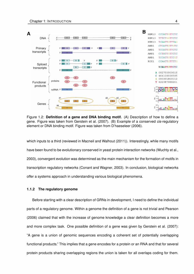
Figure 1.2: Definition of a gene and DNA binding motif. (A) Description of how to define a
gene. Figure was taken from Gerstein et al. (2007). (B) Example of a conserved cis-regulatory
element or DNA binding motif. Figure was taken from D’haeseleer (2006).
which inputs to a third (reviewed in Macneil and Walhout (2011)). Interestingly, while many motifs
have been found to be evolutionary conserved in yeast protein interaction networks (Wuchty et al.,
2003), convergent evolution was determined as the main mechanism for the formation of motifs in
transcription regulatory networks (Conant and Wagner, 2003). In conclusion, biological networks
offer a systems approach in understanding various biological phenomena.
1.1.2 The regulatory genome
Before starting with a clear description of GRNs in development, I need to define the individual
parts of a regulatory genome. Within a genome the definition of a gene is not trivial and Pearson
(2006) claimed that with the increase of genome knowledge a clear definition becomes a more
and more complex task. One possible definition of a gene was given by Gerstein et al. (2007):
”A gene is a union of genomic sequences encoding a coherent set of potentially overlapping
functional products.” This implies that a gene encodes for a protein or an RNA and that for several
protein products sharing overlapping regions the union is taken for all overlaps coding for them.

Chapter 1: INTRODUCTION 5
Moreover, the union must be logical, which implies that it must be done separately for final protein
and RNA products, thus allowing the existence of multiple genes on the same overlapping stretch
of DNA (Figure 1.2 A). Importantly, regulatory regions are not included in this definition, because
they can be shared between multiple genes (Gerstein et al., 2007).
What about gene content of a genome? Due to the high variation of genes throughout evolu-
tion it is better to think about gene content in terms of gene families. These are sets of several
genes with similar biochemical functions that are formed by the duplication of a single original
gene. Recently published work on three spiralian genomes revealed that the common ancestor of
all bilatarians likely contained at least 8,756 gene families and that through subsequent gene du-
plication within bilatarians these families conservatively account for 47 to 85% of genes in extant
organisms (70% of human genes) (Simakov et al., 2013). Interestingly, humans retain 7,553 of
these gene families and evolved 2,796 new ones (Demuth et al., 2006). A well-studied example
for this is the C2H2 family of zinc finger genes. A comparative study of Drosophila melanogaster,
Caenorhabditis elegans, and humans revealed that at least one gene of each C2H2 subfamily was
present in all of them. However, differences were observable within each subfamily (variations in
paralogous number) (Knight and Shimeld, 2001). Moreover, the conservation of these subclasses
was recently expanded to include all eukaryotes (Seetharam and Stuart, 2013). Other examples
of conserved gene families are Ets and Forkhead transcription factors (Wang and Zhang, 2008;
Carlsson and Mahlapuu, 2002) and Fgf signalling molecules (Oulion et al., 2012). Due to the
high level of conservation of gene families across the Bilataria, Erwin and Davidson (2002) postu-
lated that bilaterians share a similar regulatory ”toolkit”, which was found to be particularly true for
genes participating in development (Carroll, 2008). As a consequence, the individual differences
in expansion and reduction of genes within one family were associated with being responsible for
the differences in body plans throughout the bilaterians (Davidson, 2006; Degnan et al., 2009).
The other part of the genome consists of non-coding sequence motifs, which are short stretches
of DNA that exhibit some sort of biological function (Figure 1.2 B). They can be binding sites for
Chapter 1: INTRODUCTION 6
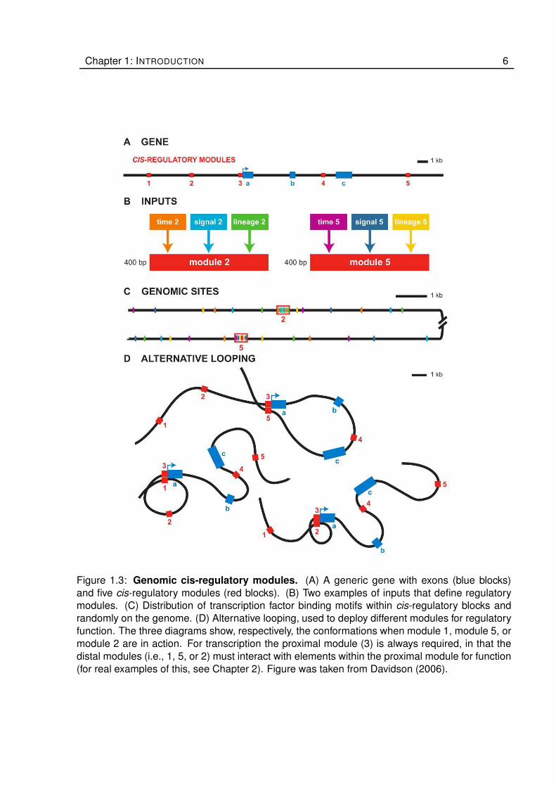
Figure 1.3: Genomic cis-regulatory modules. (A) A generic gene with exons (blue blocks)
and five cis-regulatory modules (red blocks). (B) Two examples of inputs that define regulatory
modules. (C) Distribution of transcription factor binding motifs within cis-regulatory blocks and
randomly on the genome. (D) Alternative looping, used to deploy different modules for regulatory
function. The three diagrams show, respectively, the conformations when module 1, module 5, or
module 2 are in action. For transcription the proximal module (3) is always required, in that the
distal modules (i.e., 1, 5, or 2) must interact with elements within the proximal module for function
(for real examples of this, see Chapter 2). Figure was taken from Davidson (2006).

Chapter 1: INTRODUCTION 7
transcription factors (here referred to as cis-regulatory motifs) at the DNA level, or recognition
sites for the splicing machinery on RNA level (reviewed in Matlin et al. (2005) or others). In this
thesis, I will focus specifically on DNA binding motifs. One way to identify computationally DNA
binding motifs is by phylogenetic foot-printing, in which large portions of genomes of evolutionary
related species are aligned to each-other and the sequences of interest identified as highly con-
served stretches of non-coding sequence (Ganley et al., 2008). Once identified, they can then
be experimentally validated by point mutations on reporter constructs. Generally, the main func-
tion of DNA motifs is to regulate gene expression. Regulation of gene expression requires two
components: first are cis-regulatory modules that conditionally control spatial and temporal gene
expression. They are usually within the vicinity (but not always) of a gene to be regulated. The
second components are the trans-regulatory elements, which are sequence specifc DNA-binding
proteins and collectively constitute the regulatory states, i.e. the sum of active transcription factors
within a cell at a given time. cis-regulatory modules can be further divided into enhancers and
silencers and represent inputs that provide an instruction for the basal transcription of a gene.
These instructions define whether a gene should be active, silenced and can also specify the
rate of transcription. All three factors depend on the occupancy of a given cis-regulatory module
and type of trans-regulatory elements. An example of such is provided in Figure 1.3. In functional
terms cis-regulatory modules can be thought of as processing functions for transcription of a gene
that follow logical operators (Bolouri and Davidson, 2002; Istrail and Davidson, 2005). Depending
on the input, i.e. regulatory state, concentrations of transcription factors and the physical state
of the chromosome, occupancy of a cis-regulatory module defines the state of transcription of
a gene. Therefore, if the initial state, including all the processing functions and the time delay
created between transcription to translation is known, it should be theoretically possible to predict
all the states of a cell throughout time. This was shown in developmental context by Peter et al.
(2012) and is described in more detail below. In summary, a genome is composed of many parts,
each of which has some functional meaning. Historically, everything that was non-coding for pro-

Chapter 1: INTRODUCTION 8
Figure 1.4: Schematic of a GRN. Diagram explaining the different parts and their interactions of
a developmental GRN. This figure was taken from Davidson (2006).
teins was considered ”junk” DNA. But with the accumulation of data, recently it was estimated
that around 80% of the genome suits some functional purpose (Pennisi, 2012).
Now that I have described the individual components of a GRN, I will address the structure
and construction of GRNs in a developmental context.
1.1.3 Gene regulatory networks
Developmental GRNs are maps of gene interactions that logically describe the formation of
various morphological features throughout development. They explain the generation of regula-
tory states within different territories and link causally the genome with the developmental pro-
cess. The nodes in a GRN are genes and their cis-regulatory apparatuses. The activity of a gene
(enhanced or silenced) is controlled by the cis-regulatory sequence and is thus determined by the
presence of a set of transcription factors with the ability to recognise it in the nucleus. In this way
the linkages of the individual nodes are established. Development is a dynamic process in which
multiple cell types are formed from a single cell. Davidson (2006) described this increase of com-
plexity by the continuing generation of new regulatory states in individual spatial domains of the
embryo produced by their underlying genetic subprogram. Thus, once it is know, which part of the
embryo will give rise to which final cell type, a single GRN for this cell-type can be constructed.

Chapter 1: INTRODUCTION 9
This implies that for the whole embryo, different territories (sub-GRNs) are connected through
signalling. During development individual parts are employed in an hierarchical manner. Firstly, a
cascade of transcription factors (TF) is activated by maternal factors in order to specify precisely
the position and attributes of cells that will later form various body parts. Feedback loops stabilise
the regulatory states (set of expressed genes in a specific cell type) and increase robustness of
the developmental process. In this way a specific cell fate is ”locked-down”. Signalling pathways
link the individual sub-GRNs for specific cell types throughout the embryo and ensure their correct
placement. Once the specification is completed, a group of differentiation genes is activated at
the periphery of the GRN. The composition of these genes decides the final cell type and thus
its function in an organism. Moreover, differentiation genes are the final output of the GRN and
have no regulatory capabilities, i.e. do not bind any cis-regulatory elements (CRE), and thus do
not effect transcription of other genes. Moreover, they are large in number and consistent with the
partially ”scale-free” architecture described above. A schematic representation of this process in
presented in Figure 1.4. In this way GRNs have the ability to link the process of development
directly to the genome. The most complete GRN described so far is for the endomesoderm de-
velopment in the sea urchin Strongyloncentrotus purpuratus and in particular for the formation of
the larval skeleton (Oliveri et al., 2008; Rafiq et al., 2012, 2014). Since this is fundamental for
the comparative analysis of this study, later it will be described in detail. One key characteristic of
GRNs in development is their modular structure and the re-usability of specific sub-circuits. These
are not the same as previously described motifs (e.g. feed-forward loops), because a sub-circuit
has to have a clearly definable function for a developmental process. This, however, is not the
case for all generally known motifs. Examples for such functions are the separation of a space or
the ”lock-down” of a cell fate (reviewed Davidson (2010)).

Chapter 1: INTRODUCTION 10
Figure 1.5: Experimental procedure to construct a gene regulatory network. On the left are
the individual steps and on the right the assembly of GRN. This figure was taken from Materna
and Oliveri (2008).

Chapter 1: INTRODUCTION 11
1.1.4 Construction of GRNs
In order to establish a GRN Materna and Oliveri (2008) laid out a protocol describing the
individual steps. This protocol generally follows five steps and is schematically presented in Fig-
ure 1.5. First, all embryological information are collected and laid out in a process diagram.
This includes knowledge about cell lineages, cell specification, divisions and morphological fea-
tures. Then, a territory or cell type is chosen and all genes expressed within a timeframe of
interest are identified. This identification can occur through candidate approach, by compiling a
list of orthologs that are used in a close relative species in a similar territory, or identified using
genome wide screens, e.g. next generation sequencing approaches. Once a list of candidates
is compiled, the spatial and temporal expression details have to be resolved in high resolution.
All genes that are found to be active and expressed in the territory, then form the nodes of the
network. Third, identified candidates are perturbed in their expression and function by antisense
morpholino, RNAi, genome editing, overexpression or other methodologies. Fourth, the perturbed
samples are screened for differential expression of other genes analysed and affected genes are
connected, thus forming the functional linkages and establishing the network architecture. Finally,
cis-regulatory analysis is performed on affected genes in order to confirm the direct or the indirect
effect of perturbation.
In order to represent and to integrate all of this type of data, Longabaugh et al. (2005) devel-
oped a methodology for computational representation. The software BioTapestry2 (Longabaugh
et al., 2005), allows the integration of all the collected data and the formation of a GRN that is
capable of representing the activity of individual nodes in individual embryonic cell types in time
(Longabaugh, 2012). In order to be able to incorporate the fact that the same gene can partic-
ipate for the specification of multiple territories Arnone et al. (1997) introduced the concept of
view from the nucleus and view from the genome. The view from the nucleus provides a way of
incorporating the pleiotropy of a single gene (Figure 1.6). In contrast the view from the genome
2http://www.biotapestry.org

Chapter 1: INTRODUCTION 12
Figure 1.6: GRN modelling using BioTapestry. On the top is depict the view from the genome,
incorporating every gene only once thus neglecting the expression in different spatial domains
(i.e. different cells). On the bottom is the view from the nucleus with two regions A and B. As
seen gene A is part of both regions, due to expression in multiple regions. Inputs are modelled as
constants and different regions can only communicate through signalling as depict by the linkage
between regions with two arrows. This figure was taken from Longabaugh (2012).

Chapter 1: INTRODUCTION 13
contains a single representation of each gene and neglects the spatiality within an embryo.
1.1.5 Modelling of GRNs
GRNs are a useful tool for understanding the cause and effect of developmental complexity.
As described above, they are formed by the integration of various types of experimental evidence.
Once such a network is obtained, mathematical models can be applied for analysis and pred-
ication of network behaviour. Various modelling approaches for biological networks exist and I
will briefly discus continuous modelling using ordinary differential equations (ODE) and in more
detail modelling using boolean approaches (reviewed in (Karlebach and Shamir, 2008; Tomlin
and Axelrod, 2007; Vijesh, 2013)). Stochastic modelling represents a third type, but will not be
discussed further (for review in a developmental context (Raj and van Oudenaarden, 2008)). In
the context of modelling, I am discussing the application of continuous and boolean approaches
assuming the network structure is already given. This is different from using statistical modelling
to infer network structure, e.g. from time series expression and/or perturbation data. Usually,
ODE models have one equation for each gene that describes the temporal behaviour caused by
incoming and outgoing inputs of other genes. The rate of input and output is defined by chemical
kinetics (Figure 1.7 A). This approach was used to model the whole endomesoderm development
in the sea urchin (Kuhn et al., 2009). Neglecting changes in space (embryo divides and creates
new territories in time) and assuming static signalling, the authors constructed a model where
each equation represented the dynamical change of expression of a single gene. Using in silico
perturbations, Kuhn et al. (2009) were capable of recapitulating less than half of experimental
perturbations with their model (48%). Although it was stated in (Kuhn et al., 2009) that a lot of
measurements - especially to determine the kinetic constants - were missing, and that for only
one gene (Endo16 (Bolouri and Davidson, 2002)) a detailed cis-regulatory logic analysis exists, it
was concluded that the current endomesoderm GRN is incomplete. On the contrary, it was shown
for other models, e.g. cell-cycle in the bacterium Caulobacter crescentus (Li et al., 2008c) that

Chapter 1: INTRODUCTION 14
Figure 1.7: Different approaches of GRN modelling. (A) Modelling using differential equations.
Each node is represented by one equation. kx are the kinetic rate constants. Incoming con-
nections are added and outgoing are subtracted. Repression is modelled using Michaelis Menten
kinetics. (B) Boolean network model of three genes a,b and c. The circles represent the individual
state and the squares represent the regulation functions. This figure was taken from Karlebach
and Shamir (2008).

Chapter 1: INTRODUCTION 15
when enough data is available, the experimentally obtained gene expression patterns are con-
sistent with the model (reviewed in (Karlebach and Shamir, 2008)). Therefore, whether the GRN
topology is actually correct, but not enough data is available to support it, or the GRN topology is
wrong remained open.
A more simplified approach of modelling is through boolean approaches, also called logic
models (Figure 1.7 B). Boolean logic has only two states, which can be defined as 1 (active) and
0 (inactive). For GRNs each gene can have only one of such states in a specific territory at a spe-
cific time, and thus the state of a specific territory can be summarised in a vector in which each
element represents the activity of a single gene in a specific territory. It follows that the state of a
whole embryo at all time points can be represented as a matrix. In this way, changes in time are
assumed to occur synchronously in discrete time steps. The update of this model occurs through
functions that are defined by logical operations, e.g. AND, OR, NOR (reviewed in (Karlebach
and Shamir, 2008)). In the context of development a specific cell type is defined by the current
regulatory state. The regulatory state is equivalent to a boolean vector of 1’s and 0’s describing
the activity of a gene in a cell type. Maternal inputs provide the first input into the model and once
all the regulatory functions are defined the model should accurately predict the regulatory states
in different territories. Such a model is thus similar to an automaton. One argument for use of
boolean models in developmental biology is that one embryonic space defines the future cell type
and this embryonic space is defined by a regulatory state, thus being boolean in nature (Peter
et al., 2012). Recently, this approach was applied to the endomesoderm development of the sea
urchin (Peter et al., 2012; Faure et al., 2013). This model used the GRN for endomesoderm devel-
opment as a basis for modelling (Peter and Davidson, 2009). The logical functions were derived
from perturbation experiments and cis-regulatory analysis. Additionally, conditions for signalling
between adjacent cells were included. The time step was defined as 3 hours (based on the de-
lay between transcription to translation (Bolouri and Davidson, 2003)). With minor exceptions the
model was capable of reproducing the individual regulatory state activity in the embryo throughout

Chapter 1: INTRODUCTION 16
time. Additionally, in silico perturbations were consistent with experimentally observed changes
of spatial expression. However, these results are not very surprising since the logical regulatory
functions for each gene were derived from perturbation experiments in the first place. Although it
is quite remarkable that spatial regulatory states can be captured using such a simplified model,
some transcription factors that have two different types of regulatory output depending on the
concentrations of their inputs (Damle and Davidson, 2011), cannot be incorporated with such an
approach. Since binary logic works with ON and OFF states it cannot incorporate dependencies
of TF concentrations.

Chapter 1: INTRODUCTION 17
1.2 Evolution of gene regulatory networks
GRNs provide a causal explanation for the development of an embryo. Assuming that this is
true, it follows that the mechanism that shapes GRNs in order to produce a viable and fit organism
is evolution itself. Thus, changes throughout the animal kingdom should be found as changes in
the nodes and wiring of a network and the architectural properties of different species should be
reflected along the phylogenetic tree. Remarkably, without clear evidence on cis-regulation, this
hypothesis was already postulated over 40 years ago (Britten and Davidson, 1969).
1.2.1 Towards a theory of GRN evolution
One of the first studies addressing this process in echinoderms was presented by Hinman
et al. (2003), where the GRN for endomesoderm formation was compared between star fish
Patiria miniata and sea urchin Strongyloncentrotus purpuratus, species that shared a last com-
mon ancestor at least 480 million years ago (Mya) (Pisani et al., 2012). A five-gene feedback
loop for endoderm specification was found to be highly conserved in both species (Figure 1.8).
However, whereas in star fish the gene Pmi-tbr receives inputs from the feedback loop leading to
endoderm specification, in sea urchin the gene Spu-tbr is restricted to skeletogenic mesoderm
(SM) specification. The conservation of this feedback loop and the differences in the tbr gene led
to the theory that GRNs are modular, and that certain parts are under different selective pressure
than others. Parts that are highly conserved between species - and even families - were defined
as kernels (Figure 1.8). Furthermore, it raised the hypothesis that individual parts of the net-
work can be linked to different strengths of selection (Davidson, 2006). Kernels are believed to be
responsible for Phylum to Superphylum characters, while more evolutionary liable plug-ins and in-
put/output switches are thought to define the animal class, order or family and are shown through
size or morphological patterning. Alterations and deployment of differentiation genes should de-
fine the functional abilities of a body and can give rise to speciation. Examples of each class
are presented for the sea urchin dGRN in Chapter 5 in (Davidson, 2006) and are summarized

Chapter 1: INTRODUCTION 18
Figure 1.8: Example of a kernel. On top the GRN for endoderm formation in the sea urchin. In
the centre the GRN for endoderm formation in the starfish and at the bottom the GRN showing
commonalities between the sea urchin and starfish. This image was adapted from Davidson and
Erwin (2006).

Chapter 1: INTRODUCTION 19
CHANGES IN CLASS
OF NETWORK SUBCIRCUIT:
EVOLUTIONARY
CONSEQUENCES:
Figure 1.9: Theory of GRN evolution. Diagram showing how changes in different parts of a
GRN can be linked to evolutionary events along a phylogenetic tree. This figure was taken from
Davidson (2006).
in Figure 1.10. Interestingly, several years later a study in the annelid Capitella teleta found the
conservation of expression of orthologous genes to foxA, otx, bra, blimp1 and gataE in endoderm
formation (Boyle et al., 2014) as in the development of the sea urchin. This study thus provided
further evidence for this feedback loop to be an ancient module or kernel.
In order to explore whether certain characteristics are under less selective constraints, Hin-
man et al. (2007) investigated what is happening up- and down-stream of the conserved module
of the endoderm network (Hinman et al., 2003). She showed that the employment of Delta-Notch
signalling in starfish is different from sea urchin and that different downstream genes are tar-
geted by the kernel described above. The gene Spu-tbr is completely uninvolved in endoderm
specification in sea urchin and investigations showed that a change in a regulatory motif for the
transcription factor Spu-otx made a co-option of Spu-tbr into the SM lineage possible (Hinman
et al., 2007). On the other side, in sand dollar tbr was found to participate in endoderm and SM

Chapter 1: INTRODUCTION 20
lineage (Minemura et al., 2009). This observation lead to the conclusion that very recently the
evolution of the regular sea urchin re-deployed this gene into the SM lineage and lost its endoder-
mal function. In a comparative study between sea urchin juvenile and embryo Spu-tbr was found
to participate only in embryo skeletogenesis (Gao and Davidson, 2008). More detailed studies on
the regulation of this gene revealed two distinct modes of expression (Wahl et al., 2009). Spu-tbr
is first repressed by Spu-hesC, and maintained at stable levels by a positive input of Spu-ets1/2
following ingression (Wahl et al., 2009). ets1/2 is present in embryonic development of all stud-
ied echinoderms, but only in echinoids and ophiuroids it is expressed in the SM lineage (Koga
et al., 2010), and thus likely to participate in the GRN for this cell type. Spatial expression data
of ets1/2 alone, however, are not enough to discriminate the functional difference of endomeso-
derm to skeletogenic mesoderm (Koga et al., 2010). Other three regulatory genes of sea urchin
larval skeleton development -Spu-tel, Spu-foxB, and Spu-foxO- were not found to participate in
the juvenile (Gao and Davidson, 2008). On the contrary, other SM genes were expressed in
cells of skeletal elements in both sea urchin juvenile and embryo (Killian and Wilt, 2008; Gao and
Davidson, 2008). This observation along with the fact that orthologs of these genes are also ex-
pressed in cells associated with spines and other skeletal elements of juvenile star fish led to the
hypothesis that the whole GRN responsible for development of the skeleton was co-opted from
the adult into the embryo in sea urchin (Gao and Davidson, 2008) and this process included the
addition of Spu-tel, Spu-foxB, Spu-foxO and Spu-tbr (Gao and Davidson, 2008). Strikingly, it is
theoretically possible to co-opt the adult GRN for skeletegoenes in only two steps. First, a CRE
for the repressor Spu-hesC has to be added on Spu-alx1, Spu-ets1/2 and Spu-tbr and second
Spu-hesC has to be put under the control of another repressor Spu-pmar1, thus creating the
double negative gate (DNG; xplained below in detail). Using a modelling approach, it was shown
that few beneficial mutations can lead to an orchestrated gene-expression change and produce a
viable phenotype (Crombach and Hogeweg, 2008). In order for this change to happen, work on
alx1 in holothuroids showed that first the mesoderm had to be separated into distinct territories

Chapter 1: INTRODUCTION 21
(McCauley et al., 2012). Once mutations in CRE changed these territories the adult skeleton
was then able to be co-opted into the embryo. In this context the evolution of micromeres remains
unanswered but it was hypothesized that it evolved in parallel to the DNG in sea urchin (Ettensohn,
2009). The network part downstream of the DNG, containing Spu-hex, Spu-erg and Spu-tgif, is
conserved between star fish and sea urchin, even though the input is likely to a completely dif-
ferent set of genes (McCauley et al., 2010). This recursively wired feedback loop seems to be
ancestrally derived (McCauley et al., 2010), and is a good example of how in evolutionary time
some linkages are more conserved than others. Furthermore, it shows how a complete module
can be recruited to participate in a different cellular context.
Downstream of this specification part of the network are the bio-mineralisation genes. They
are part of the differentiation tier and are assumed to be under fewer selective constraints (Erwin
and Davidson, 2009). Sea urchin seems to use a unique set of genes for skeletogenesis, with
no counterparts found in vertebrates (Livingston et al., 2006). Only hemichordates have a very
small number of sea urchin bio-mineralisation orthologs, but their molecular involvement in skele-
togenesis remains still to be addressed (Cameron and Bishop, 2012). Depending on the network
hierarchy changes in linkages are under different selective pressures and the differentiation tier
is considered fast evolving (Erwin and Davidson, 2009; Hinman et al., 2009). Whilst a lot of ev-
idence across echinoderms has been accumulated to make the theory of evolution on a GRN
level plausible, up to now very little work has been done on brittle stars, the only other class of
echinoderm that develops an elaborate skeleton in the larva.
1.2.2 Mechanisms of GRN evolution
Although many studies in different organisms analyzed the complex developmental GRNs
(reviewed in (Levine and Davidson, 2005)), little is known about the mechanisms of successful
rewiring during evolution and most studies, with few exceptions (McCauley et al., 2012; Garfield
et al., 2013), remain at the level of single nodes. Comparative developmental and genomic studies

Chapter 1: INTRODUCTION 22
Figure 1.10: Cis-regulatory module evolution. (A) Domain 1 and 2, which have different reg-
ulatory states, drive the expression of gene A differently. Expression of gene A is dependent on
occupancy of the cis-regulatory module. Gene A is here expressed in domain 1 but not 2. Two
possible scenarios of cis-regulatory mutations are shown: 1) appearance of new sites within the
module by internal nucleotide sequence change. 2) a module from elsewhere is transposed into
the DNA near gene A with new sites. While in both cases the output in domain 1 is not effected,
the new sites allow expression of gene A in domain 2. (B) Possible effects of activity of gene A in
a new context. This figure was taken from Peter and Davidson (2011).
over the past two decades clearly showed that developmental regulatory genes are remarkably
conserved among animal phyla, suggesting that phenotypic differences between organisms are
achieved through variation of gene expression and thus, GRN architecture (Peter and Davidson,
2011).
1.2.2.1 Re-wiring by cis-regulatory element evolution
Changes in GRN architecture are mostly obtained through modifications in expression of reg-
ulatory genes, thus putting changes in the cis-regulatory apparatuses of regulatory genes as

Chapter 1: INTRODUCTION 23
the main mechanisms of GRN evolution (Davidson, 2006; Peter and Davidson, 2011; McLean
et al., 2011; Wray, 2007). The highly evolutionary conserved kernels, likely rely on conservation
of cis-regulatory control of the genes they are formed of. The finding of conserved non-coding
elements (CNE) in the regulatory apparatus of several developmental genes encoding for tran-
scription factors supports the existence of such kernels (Royo et al., 2011; Parker et al., 2011;
Nelson and Wardle, 2013). On the other hand, fast evolving network linkages were identified
when comparing closely related species. A study of five closely related vertebrate species using
ChipSeq of two transcription factors gave support to both claims (Schmidt et al., 2010). Whereas
only a small fraction of cis-regulatory sequence was found to be conserved, the majority exhib-
ited a high turnover rate. Changes in cis-regulatory sequence have been also been confirmed to
be responsible for morphological variation. For example, it has been shown that changes in the
expression of the Drosophila yellow gene cause differences in wing pigmentation (Prud’homme
et al., 2006), and recently the evolutionary path for these differences has been resolved. First,
a novel cis-regulatory module for pigmentation differentiation genes evolved downstream of the
distaless (Dll) gene, and then species-specific diversification occurred changing the spatial ex-
pression of Dll in different species and thus changing the wing pigmentation (Arnoult et al., 2013).
In another study, specific deletion in the cis-regulatory sequence of the human androgen receptor
gene was linked with the loss of sensory vibrissae and penile spine (McLean et al., 2011; Reno
et al., 2013). Moreover, it has been shown that novel, more complex morphological features, can
originate by co-option of an existing regulatory circuit into a new developmental time or location,
as in the before mentioned echinoderm larval skeleton (Gao and Davidson, 2008). Thus, cis-
regulatory changes in developmental regulatory genes have been considered the major driving
force of GRNs evolution.

Chapter 1: INTRODUCTION 24
Figure 1.11: Protein evolution by gene duplication. Diagram shows different evolutionary sce-
narios after gene duplication. The coloured blocks represent different protein domains. This figure
was taken from wikipedia.org.
1.2.2.2 Re-wiring by protein evolution
Alteration on CRE represent only one side of GRN evolution; important evolutionary changes
have also been reported at the protein level, where non-synonymous variation or the variation
of short linear domains can be clearly linked to the evolution of new function or specificity of
interaction (for review Wagner and Lynch (2008)). The simplest way of protein evolution is by
mutations on non-synonymous sites. An example of this is the Drosophila ubx gene, which
specifically evolved a repressor domain that is absent in other athropods but important for the
evolutionary transition of limb patterning (Grenier and Carroll, 2000; Galant and Carroll, 2002;
Ronshaugen et al., 2002). Another possibility of protein evolution is through gene duplication.
Once duplication occurs, the relaxed selective pressure on the gene duplicate allows for evolu-
tionary changes by mutations Figure 1.11. In the most common scenario the duplicate becomes
non-functional. However, two possibilities exist that can create a functional protein out of the
duplicate: neo-functionalisation and sub-functionalisation. In neo-functionalisation the gene du-
plicate receives a novel function, whereas the template retains its ancestral role. An example
of neo-functionalisation is found in the bicoid gene that evolved as duplication of the hox3 para-

Chapter 1: INTRODUCTION 25
log gene zen. Whereas zen maintained its ancestral function, relaxed selective pressure on bcd
allowed protein changes responsible for recognition of new DNA motifs and consequently regula-
tion of new target genes, facilitating the evolution of a new role as morphogen in anterior-posterior
patterning (reviewed in McGregor (2005)).
On the other hand, in sub-functionalisation, following gene duplication both copies undergo
changes to give rise to two novel proteins. One example for this process is the B-Myb gene in
vertebrates, which underwent two rounds of gene duplication. The first round of duplication gave
rise to A/C-Myb through neo-functionalisation (Davidson et al., 2005), shown using a functional
equivalence assay where only the vertebrate B-Myb could rescue the phenotype in Drosophila
melanogaster lacking its endogenous Myb gene. The second duplication event gave rise to A-Myb
and C-Myb, both having differences in protein domains and both not being able to rescue the D.
melanogastor lacking Myb phenotype (Davidson et al., 2013; Ganter and Lipsick, 1999) exemplify-
ing sub-functionalisation. Importantly, Jarvela and Hinman (2015) argued that transcription factor
evolution occurs mostly due to the modularity of a protein having different domains that are re-
sponsible for different functions. Other examples for mechanisms of neo- or sub-functionalisations
are exon shuffling, where different exons are exchanged to create hybrid proteins, and changes
in binding domains allowing the duplicate to bind to a different cis-regulatory sequence (reviewed
in Jarvela and Hinman (2015)). While both these mechanisms have been shown as participating
in GRN evolution, (Carroll, 2008) argues that gene duplications generating a new node in a GRN
are rare, especially for genes that play crucial roles in development.
Nevertheless, protein evolution does not always have to be preceded by gene duplication as
shown for the CEBPB gene in mammals (Lynch et al., 2011). In a study comparing the CEBPB
gene from mammals with and without a placenta, three amino acid substitutions were found to
be responsible for reversing the response of CEBP to GSK-3b-mediated phosphorylation from
repression to activation, and thus changing its response to this signalling pathway (Lynch et al.,
2011).

Chapter 1: INTRODUCTION 26
Despite claims that protein evolution is less important for evolution of the animal body plan
several examples demonstrate showing how novelty has arisen using this mechanism.

Chapter 1: INTRODUCTION 27
1.3 Phylogeny of echinoderms
Figure 1.12: Schematic representation of the two major phylogenetic propositions for the
echinodermata group. (A) Asterozoan hypothesis. The Asteroidea and the Ophiuroidea share
a common ancestor and the Echinoidea and the Holothuroidea share another. These two sub-
groups evolved from one common ancestor. (B) Cryptosyringid hypothesis. The Echinoidea and
the Holothuroidea share a common ancestor. This group evolved from the same ancestor as the
Ophiuroidea. Figure was taken from (Littlewood et al., 1997).
To address questions about evolution in development it is important to understand the phy-
logenetic context of the animals of choice. In this thesis I am making use of the class of Echin-
odermata. Echinoderms belong to the deuterostomes and, along with the hemichordates, form
a sister-group to the chordates3. Due to their distinct morphology and their mineralized skeletal
elements, echinoderms have an excellent fossil record. This, in combination with other type of
data, i.e. molecular phylogenies and clock estimates, have allowed the exact moment of diver-
gence from hemichordates to be pinpointed to around 570 Mya (Erwin et al., 2011; Smith et al.,
2013; Pisani et al., 2012). Within the Echinodermata, the criniods are the basal out-group (Paul
and Smith, 1984). The asteroids, ophiuroids, holothuroids and echinoids form a monophyletic
group called Eleutherozoa. Echinoids are further divided in euechinoids and cidaroids, that latter
is commonly known as pencil urchin. In phylogeny, the grouping between the holothuroids and
echinoids is widely accepted in the science community and is based on concurrent results in all
studies described below. More prevalent is the question of how to place the ophiuroids and aster-
oids in the Eleutherozoa. The two main hypothesis that have been discussed over the years are
the Asterzoan hypothesis (Figure 1.12 A) and the Cryptosingrid hypothesis (Figure 1.12 B). In the
3http://www.tolweb.org/

Chapter 1: INTRODUCTION 28
Asterzoan hypothesis, asteroids and ophiuroids form together an sister-group to echinoids and
holothuroids, whereas in the Cryptosingrid hypothesis asteroids from an out-group to ophioroids
that form an out-group to echinoids and holothuroids. In the earliest work morphological studies
strongly supported the Cryptosingrid hypothesis (Hyman, 1955). First molecular analysis using ri-
bosomal RNA, on the other hand, were inconclusive owing to strong phylogenetic signal in favour
for both hypothesis (Littlewood et al., 1997). An analysis based on 13 protein coding sequences of
23 Eleutherozoan mitochondrial genomes gave equal support for the two mentioned hypotheses
and also for an adapted cryptosingrid hypothesis where ophiuroids and asteroids exchange their
position (Perseke et al., 2010). Other work on protein-coding genes and ribosomal sequences
(Smith, 1997) and additional morphological characteristics (Janies, 2001) gave support for both
hypothesis and were unable to resolve the dispute regarding the correct phylogeny of the echino-
dermata. The difficulties in establishing a unifying phylogeny were due to the choice of analytical
method and the fact that the early split of the different species was causing long branch attraction
errors (Felsenstein, 1978; Pisani et al., 2012; Janies et al., 2011). With the rise of next generation
sequencing methodologies new approaches, as well as more complete sampling of the phyloge-
netic tree, could be used to address this problems. The first analysis that was able to account for
these errors and provided a clear solution strongly supporting the Asterozoa hypothesis was re-
ported by Telford et al. (2014). A probabilistic Bayesian phylogenetics approach was used on 219
genes in 15 species including all four groups. The Asterozoa grouping was further supported in a
recent study of 185 genes that included data on 14 hemichordates and 19 echinoderms (Cannon
et al., 2014) and another study incorporating fossil records and 61 different taxa (O’Hara et al.,
2014), and a study including 23 de novo transcriptomes from every echinoderm class (Reich
et al., 2015).
Most echinoderms undergo metamorphosis and develop the adult animal within a self-sustained
larva. Interestingly, the types of larva vary between the individual classes. Ophiuroids and echi-
noids both develop into a pluteus type larvae (Hyman, 1955). The pluteus larvae is charac-

Chapter 1: INTRODUCTION 29
HolothuroidEchinoid Ophiuroid Asteroid CrinoidA
B
Figure 1.13: Larval types in echinoderms. (A) Asteroids, holothuroids and crinoids have a
dipleurula type larvea without a skeleton, whereas ophiuroids and echinoids have a pluteus type
larvae with skeleton. (B) Phylogeny based on Asterzoan hypothesis and variations of larval types
in echinoderms. Image of ophiuroid larvae was taken from http://arkive.org. Image of
crinoid larvae was taken from http://scaa.usask.ca. Images of asteroid and echinoid lar-
vae were taken from http://cifonauta.cebimar.usp.br. Image of holothuroid larvae was
taken from http://commons.wikimedia.org. Figure B was taken from Hinman and Cheatle
Jarvela (2014)

Chapter 1: INTRODUCTION 30
terised by a mesodermally derived skeleton that supports feeding and cilia mediated swimming
behaviour. Asteroids develop into a bipinnaria larvae with two ciliated bands: one in front of the
mouth, and the other behind it and around the edge of the body. The larva of holothuroids is
known as an auricularia larva, because the ciliated band of the dipleurula larva of holothuroids
becomes sinuous and lobed, thus resembling a human ear. Both these types of larvae can be
characterized as dipleurula type larvae, owing to their bilateral symmetry (Figure 1.13) (Hyman,
1955). Additionally, in contrast to asteroids that do not form any skeleton in the larva, holothuroids
do form small spicules that do not aggregate to extend into a full skeleton. In the out-group to the
Eleutherozoa, the crinoids, some species also develop a dipleurula type larva, whereas others a
doliolaria larva (Nakano et al., 2003, 2009). A doliolaria larva is characterized by large quantities
of yolk and several ciliated bands arranged in hoops around the body. The occurrence of an au-
ricularia larva in crinoids suggests that the plutei forms of echinoids and ophiuroids are derived
features. This is supported by the fact that hemichordates develop through a tornaria larvae that
is similar to the dipleurula type (Tagawa et al., 1998). Thus, one of the main differences within
the echinoderms is the development of the larval skeleton. Importantly, all echinoderms have an
adult skeleton. This posses the question as to when exactly the larval skeleton evolved within
the Eleutherozoa. The two possibilities are convergent evolution, where echinoids and ophiuroids
evolved a skeleton independently, or ancestral evolution, where holothuroids reduced the skeleton
and asteroids lost it. This unique phylogenetic arrangement of larval forms that are well studied
and described offers, thus, an ideal opportunity to investigate differences between convergent
and ancestral evolution.
Chapter 1: INTRODUCTION 31
1.4 Echinoderm development as model for GRN evolution
Although echinoderms develop into two main types of larva, they all have conserved patterns
of early development with only a few distinct differences (Figure 1.14). As mentioned above,
only ophiuroids, echinoids and holothuroids give rise to spicules, whereas asteroids do not. The
spicules are formed from a subpopulation of cells derived from the mesoderm (McCauley et al.,
2012). While the mesoderm is the most well studied part of the embryo in echinoderms excluding
ophiuroids (McCauley et al., 2012; Oliveri et al., 2008; Rafiq et al., 2012, 2014), it is not yet
possible to answer the question about convergent or derived evolution of the larval skeleton.
In order to be able to address the question about its evolution, I will first describe in detail the
development and GRN for this cell type in echinoids and complete this description on occasions
where studies exist in other classes of echinoderms.
1.4.1 Morphological observations
Already prior to fertilization the animal-vegetal axis is established in the sea urchin embryo by
a gradual accumulation of β-catenin at the vegetal side (Angerer and Angerer, 2003; Horstadius,
1973). Following fertilization, after three rounds of equal cleavages the cells at the animal side of
the embryo divide meriodinally to produce a ring of 8 mesomeres. In contrast, the blastomeres at
the vegetal side divide asymmetrically, producing 4 macromeres and 4 micromeres. This unequal
division pattern is found only in euechinoids. Starfish, sea cucumbers and brittle stars, on the
other hand, divide equally. During the 5th cleavage another asymmetric division of micromeres
gives rise to 4 small micromeres at the vegetal pole and 4 large micromeres above them. A
fate map exists for all 4 tiers that are present at the 60-cell stage (Logan and McClay, 1997).
While the 4 small micromeres will divide only once more and will give rise to the germ cells, the
large micromeres will give rise to the skeleton. These are often referred to as SM or primary
mesenchyme cells (PMCs). Descendants from the macromeres (veg2 cells) will give rise to the
endoderm and non-skeletogenic mesoderm (NSM), including pigment cells, blastocoelar cells,

Chapter 1: INTRODUCTION 32
muscle cells, and coelomic pouch cells. Above the cells part of veg2 is the veg1 territory, which
gives rise to endoderm and some ectoderm. The animal half of the embryo gives rise to the
ectodermal territories and is not the subject of this study, but I refer the interested reader to
(Duboc and Lepage, 2008; Lapraz et al., 2009). Arguably, the micromeres/PMCs represent the
best-studied cell type in any species. Within the echinoderms, micromeres are found only in the
echinoids, and although the ophiuroid develops an extended larval skeleton it does so without the
formation of micromeres (Yamashita, 1985). In sea urchin, specification of these cells happens
before ingression in 16 to 32 progenitor cells. Once specified, the PMC undergo epithelial to
mesenchymal transition and ingress into the blastocoel. The PMCs then divide once more and
migrate towards two ventro-lateral clusters next to the location of archenteron invagination. This
is the position where the cells are fused (Hodor and Ettensohn, 1998) and give rise to tri-radiate
spicules that extend to give the larvae its pluteus shape (reviewed in Lyons et al. (2012)). This
is similarly observed in brittle stars. Although holothuroids have PMCs that ingress and give rise
to spicules, these do not secrete biomineralized rods and thus do not form an extended skeleton
(McCauley et al., 2012). Asteroids do not have cells that ingress at blastula stage from the vegetal
pole of the embryo and as mentioned earlier do not form any skeleton in the larva (Figure 1.14).
1.4.2 Early specification and the double negative gate
Throughout the first cleavages in sea urchin the three genes Spu-otx, Spu-wnt8 and Spu-
blimp1 are initiated through a gradual enrichment of nuclearised β-catenin at the vegetal side of
the embryo (Logan et al., 1999). At the same time, the gene Spu-soxB1 - an antagonist of β-
catenin - enters the nuclei of all blastomeres but the micromeres (Kenny et al., 1999) and Spu-otx
is initially nuclearised only in the micromeres (Chuang et al., 1996). By fifth cleavage nuclearised
β-catenin is bound to Spu-TCF where it activates, along with maternal Spu-Blimp1, the expression
of Spu-wnt8 using an AND promoter logic (Smith et al., 2007). After the next division Spu-wnt8
feedbacks and enhances the levels of β-catenin/TCF. Additionally, maternally abundant Spu-Otx

Chapter 1: INTRODUCTION 33
Figure 1.14: Schematic development of three classes of echinoderms. Figure was taken from
Hinman and Cheatle Jarvela (2014).

Chapter 1: INTRODUCTION 34
Figure 1.15: GRN for larval skeletogenesis in sea urchin 6hpf and 10hpf. Left the GRN for
6hpf with according expression patters and to the right GRN for 10hpf with according expression
patterns. Snapshots of GRNs were obtained from http://biotapestry.org

Chapter 1: INTRODUCTION 35
starts zygotic expression of Spu-blimp1 (Li et al., 1997). These events establish the distinction of
endomesoderm from ectoderm along the animal-vegetal axis. Additionally, three distinct territoiris
are formed: the micromeres, other mesoderm and endoderm. Interestingly, in starfish a gradual
enrichment of nuclearised β-catenin has also been shown to be involved in the separation of
embryonic territories in a dose-dependent manner (McCauley et al., 2014).
In order to specify the micromeres in sea urchin to become skeletogenic, nuclearised β-
catenin/TCF and Spu-blimp1 activate the expression of Spu-pmar1. Once translated, Spu-blimp1
and Spu-pmar1 repress the expression of Spu-hesC in these cells. Thus, Spu-hesC is expressed
everywhere but in the micromeres. Overexpression of Spu-pmar1 or knock-down of Spu-hesC
transforms all cells to a skeletogenic fate (Oliveri et al., 2002; Revilla-i Domingo et al., 2007)
and thus confirms the repressive action. This is consistent with an upregulation of all genes
downstream of Spu-hesC. These genes are Spu-alx1 (Ettensohn et al., 2003), Spu-ets1/2 (Oliv-
eri and Davidson, 2004; Kurokawa et al., 1999), Spu-tbr (Croce et al., 2001; Fuchikami et al.,
2002), Spu-delta (Oliveri and Davidson, 2004), Spu-tel (Rizzo et al., 2006) and the transiently
active Spu-soxC (Howard-Ashby et al., 2006). All of them are expressed at this stage in the
micromeres and most provide direct inputs into the differentiation cascade. Importantly, knock-
down of Spu-pmar1 causes upregulation of Spu-hesC (Smith and Davidson, 2009). Therefore,
these two genes plus the intermediate targets of Spu-hesC form a double negative gate. This
mechanism puts the skeletogenic fate into the micromeres and is a logical mechanism for space
separation (Davidson, 2010). The GRN and expression pattern are shown in Figure 1.15.
Interestingly, so far the pmar1 gene has only been reported in euechinoids, and the expres-
sion pattern of orthologs to hesC show a lot of variation in echinoderms (McCauley et al., 2010;
Yamazaki et al., 2014). In the asteroid Patiria miniata Pmi-hesC is co-expressed with orthologous
of sea urchin downstream genes in the mesoderm. Functional studies additionally confirmed the
absence of a repressive function for Pmi-ets1/2 and Pmi-erg even though its function as a re-
pressor was confirmed in ecotodermal territories (McCauley et al., 2010). This makes a similar

Chapter 1: INTRODUCTION 36
repression mechanism downstream of nuclearised β-catenin unlikely. Similarly, in the cidaroid
Prionocidaris baculosa Pba-hesC is co-expressed with its downstream genes and knock-down
experiments show no repressive effect on Pba-alx1, Pba-ets1/2 and Pba-tbr (Yamazaki et al.,
2014). Interestingly, only knock-down of Pba-alx1 showed a phenotype with abolished skeletoge-
nesis in this class of euechinoids (Yamazaki et al., 2014).
In order to repress an alternative fate of the SM lineage in echinoids, Alx1 is repressing Spu-
gcm. Downstream of the DNG, Delta signals to the adjacent cells through Notch and activates
Spu-gcm in NSM lineage. Spu-gcm is one of the major drivers in the non-skeletogenic mesoderm
(NSM) lineage and targets downstream Spu-pks a gene encoding for an enzyme involved in
the formation of pigment cells in sea urchin (Ransick and Davidson, 2006; Calestani et al., 2003).
Knock-down of Spu-alx1 transfates the SM-lineage into the NSM-lineage and causes upregulation
of Spu-gcm, whereas mRNA overexpression of Spu-alx1 causes a reduction of gcm (Oliveri et al.,
2008). Many genes directly regulated by the double negative gate have been further verified
by cis-regulatory anlaysis (Damle and Davidson, 2011). Interestingly, Spu-alx1 shows a very
steep increase of mRNA levels once it is activated and Damle and Davidson (2011) showed that
stabilization of mRNA levels of this gene are achieved by self-regulation through a concentration
dependent dimerization mechanism.
1.4.3 Stabilization of skeletogenic fate
Once initiated, the skeltogenic program progress to a stabilization step, where Spu-Ets1/2
inputs into Spu-erg the first gene of an interlocking loop (IL). Spu-Erg activates expression of
Spu-tgif and Spu-hex. Spu-Tgif inputs into Spu-hex that once translated inputs into Spu-erg,
thus closing the loop (Oliveri et al., 2008). The role of this highly connected feedback loop is
to ”lock down” the skeletogenic fate of these cells. In total there are 4 feedback-loops between
these three genes: One between Spu-erg and Spu-hex, another one between Spu-hex and Spu-
tgif, one between the three of them and a final self feedback for Spu-tgif. Thus, this intertwined

Chapter 1: INTRODUCTION 37
Figure 1.16: GRN for larval skeletogenesis in sea urchin 15hpf and 24hpf. Left the GRN for
15hpf with according expression patters and to the right GRN for 24hpf with according expression
patterns. Snapshots of GRNs were obtained from http://biotapestry.org

Chapter 1: INTRODUCTION 38
nature of this sub-circuit has the ability to dynamically stabilise the regulatory state downstream
of themselves. Knock-down experiments on any of these three genes show a drastic down-
regulation on the other two (Oliveri et al., 2008). Moreover, knock-down experiments of Spu-tbr,
Spu-hex and Spu-tgif show no effect on ingression but an effect on bio-mineralisation (Oliveri
et al., 2008). Interestingly, the order of activation of these genes is reflected in their time-courses
(Materna et al., 2010). Expression pattern in an holothuroids and additional functional studies in
an asteroid suggest a conservation of these IL in the mesoderm (McCauley et al., 2010, 2012) of
these classes.
Spu-tgif and Spu-erg not only participate in this IL, but also have effects on genes upstream.
cis-regulatory analysis using bacterial artificial chromosomes for the Spu-tbr locus showed that
late in development (mesenchym blastula) Spu-Erg, now expressed only in the NSM lineage, has
a repressive effect on this gene, ensuring expression of Spu-tbr only in the SM lineage (Wahl
et al., 2009). Spu-Tgif with Spu-Ets1/2 on the other hand, both drive the expression of Spu-alx1
in the SM lineage, which directly drives expression of downstream bio-mineralisation genes.
Additionally, Spu-Alx1 and Spu-Tbr provide inputs into two further transcription factors, Spu-
dri and Spu-foxB, that themselves input into the differentiation gene batteries. Oliveri et al. (2008)
showed with a high-throughput knock-down study that most of these genes produce a phenotype
with inhibited skeleton and are thus essential for this developmental process. Consistently, genes
active at the top of the GRN hierarchy showed a more severe phenotype than other genes (Oliveri
et al., 2008). In this way it is possible to determine the individual roles in morphological changes,
e.g knock-down of Spu-alx1 disrupts ingression of PMCs, whereas knock-down of Spu-hex ef-
fects only the bio-mineralisation process. Two recent studies extended this network. A nanostring
analysis of embryos with and without PMCs revealed the involvement of two other TF in skele-
togenesis (Rafiq et al., 2014; Barsi et al., 2014). These are Spu-nk7, Spu-mitf and Spu-alx4,
which are first expressed just prior to mesenchyme blastula stage in SM cells and are all affected
by knock-down of either Spu-ets1/2 or Spu-alx1. Their late expression suggests, an involvement

Chapter 1: INTRODUCTION 39
as drivers of epithelical to mesenchyme transition (EMT) or the skeletogenic downstream genes.
In another sea urchin Lytechinus varigatus the canonical EMT genes Lva-twi and Lva-sna were
found to be involved in this process (Saunders and McClay, 2014). However, no detectable ex-
pression of Spu-twi mRNA levels in S. purpuratus suggests no involvement in this species (Tu
et al., 2014), and therefore have not been included into S. purpuratus GRN model (Figures 1.15
and 1.16).
1.4.4 Cell movements and skeletogenic differentiation genes
Once specification and stabilisation of fate of the PMCs are completed, the cells ingress into
the blastocoel through EMT. The ingressed cells extend long filopodia that touch all the surround-
ing cells and migrate towards two ventro-lateral clusters next to the archenteron. At this moment,
both vegf and fgf ligands are expressed in the ectoderm in cells close to these clusters shown
in the sea urchin Paracentrotus lividus and Lytechinus varigatus (Duloquin et al., 2007; Rottinger
et al., 2008; Adomako-Ankomah and Ettensohn, 2013). Whereas the receptors vegfR and fgfR2
are expressed in the PMCs, experiments inhibiting either the fgf/fgfR2 or the vegf/vegfR pathway
showed incorrect positioning of the PMCs and thus abnormalities in skeleton development. Fur-
thermore, the extension of the skeleton towards the animal pole was shown also to be dependent
on vegf/vegfR signalling (Adomako-Ankomah and Ettensohn, 2013). Inhibition of vegfR in sea
urchin does not down-regulate all differentiation genes (Duloquin et al., 2007), but sufficient to
inhibit skeleton formation. This signalling, can thus be understood as a sort of checkpoint. If the
cells are in the right positions, then an additional signalling input will trigger the activation of some
bio-mineralisation components such that a correct skeleton can be formed.
Interestingly, many downstream genes are already transcribed before ingression of PMCs,
e.g. msp130r1 (Illies et al., 2002), p19 (Costa et al., 2012), sm50 (Oliveri and Davidson, 2004)
and more; while others such as sm30 (Wilt et al., 2013) will only be express late when bio-
mineralisation is formed. This indicates that transcription of these genes in the correct proportions

Chapter 1: INTRODUCTION 40
is needed in order to physically assemble the skeleton. As mentioned earlier, this is the final tier
of the hierarchical GRN. Consistent with the scale-free nature of such networks, recently, the
differentiation cascade has been extensively enlarged. Whereas the regulatory part consists of
roughly 24 genes (based on Oliveri et al. (2008); Barsi et al. (2014)), studies using proteomic or
next generation sequencing approaches identified around ∼1000 genes expressed or involved in
this process (Rafiq et al., 2012; Mann et al., 2010a,b) and for many of those a linkage of was
detected by inhibition of either alx1 or ets1/2 (Rafiq et al., 2014).

Chapter 1: INTRODUCTION 41
Figure 1.17: Adult Brittle Stars. Oral view of (A) male and (B) female A. filiformis adults. (B) The
gametes of different color are produced in the trophic gonads within the bursae.
1.5 The brittle star Amphiura filiformis
The brittle star Amphiura filiformis (Muller, 1776) is part of the Ophiuroidea taxon and belongs
to the burrowing brittle stars, described by (Buchanan, 1964). A. filiformis is radially symmetric, a
characteristic shared by all the echinoderms. Male and female adults exhibit sexual dimorphism
only during the reproductive seasons when their gonads are present at the oral side (Peterson
et al., 2000) of the animal, shown in Figure 1.17. They are otherwise indistinguishable between
each other. This type of brittle stars are suspension feeders and collect food in the sea by expos-
ing one arm out of the mud and transporting sea particles along the arm into the mouth located
at the central disk of the animal (Buchanan, 1964; Loo et al., 1996). A. filiformis has its repro-
ductive season from mid summer to beginning of autumn in the North Western European waters
(Bowmer, 1982). In Sweden the reproductive peak is reached between June to August (Skold
et al., 1994). During this period the brittle star rises from the mud and lift up from the surface
contracting its five arms. The central disk is lifted and the gonads on the oral part of the body are
released into the water.
Very little is known about development of brittle stars and all studies performed are scattered
among various species. Cell lineage studies were performed in Ophiopholis aculuata, showing

Chapter 1: INTRODUCTION 42
that brittle stars do not form micromeres and that at 8 cell stage their skeletogenic lineage is not
yet segregated from other endomesodermal lineages (Primus, 2005). Despite their very similar
appearance, the pluteus larvae of these two echinoderm classes show several differences: specif-
ically their calcified structures have different sensitivity to ocean acidification (reviewed in (Dupont
et al., 2010)). On the other side, a transcriptome analysis of a Ophiocoma wendtii gastrula stage
identified several genes orthologous to sea urchin skeletogenic genes suggesting a similar molec-
ular make up of these structures (Vaughn et al., 2012). Furthermore, the only embryonic gene
expression studies reported so far have been carried out in the brittle star species Amphipholis
kochii on a transcription factor, ets1/2, and two signalling molecules, vegf and vegfR. The expres-
sion patterns in the brittle star and in sea urchin embryos are remarkably similar, supporting the
similarities of larval skeleton development between brittle stars and sea urchins (Hirokawa et al.,
2007; Koga et al., 2010).

Chapter 1: INTRODUCTION 43
1.6 Modern approaches in new organisms
As seen in the last section, in comparison to sea urchin developmental biology, information
about brittle stars is very sparse. In order to establish molecular tools and quickly advance the
knowledge about brittle star developmental biology, next generation mRNA sequencing provides
a fast method to obtain information about whole organism genes and expression. In this section, I
will describe the general principles behind mRNA sequencing with focus on the Illumina platform
that was also used for this study. I will briefly discuss various bio-informatics strategies for de
novo assembly and quantification.
1.6.1 mRNA sequencing
RNA sequencing allows the measurement of gene content and expression of all RNA in a
sample of interest. Samples can be whole organism or different cell types. For next generation
sequencing the general experimental procedure can be summarised as follows. A library of cD-
NAs, with attached adapters on both ends is prepared from extracted mRNA. To sequence this
library in a high-throughput manner the individual cDNAs are fragmented into shorter pieces. This
library is then sequenced, either amplified or not amplified. In Illumina sequencing the fragmented
sequences with adapters are then processed on a flow cell. The basepair composition is detected
by primer ligation on the free end and extension of the fragment, for which a distinct fluorescent
signal is released during the addition of each basepair onto the fragment. Sequences are ob-
tained either from one end (single-end sequencing) or from both ends (paired-end sequencing).
Depending on sequencing technology and experimental set up the reads are usually 30-400bp
long (reviewed in (Wang et al., 2009)). In general, RNA-seq is a powerful approach to obtain data
at a whole transcriptome level with unprecedented sensitivity and accuracy (Ozsolak and Milos,
2011; Wang et al., 2009; Marguerat and Bahler, 2010; Wilhelm and Landry, 2009). Compared
with expressed sequence tag (EST) sequencing and microarray chips, RNA-seq has a substan-
tially higher dynamic range, has single-nucleotide resolution and allows reliable identification of

Chapter 1: INTRODUCTION 44
Figure 1.18: RNA sequencing. Figure displays procedure for RNA sequencing. ORF stands for
open reading frame. Figure was taken from Wang et al. (2009).

Chapter 1: INTRODUCTION 45
rare transcripts and alternative splicing (Wang et al., 2009; Marguerat and Bahler, 2010; Wilhelm
and Landry, 2009; Marioni et al., 2008).
1.6.2 Bio-informatics for transcriptomics
1.6.2.1 Assembly
The purpose of RNA-seq for organisms lacking a genome is two fold. First, one wants to
obtain information about sequences of the RNA molecules, and second, about their quantity in
the sample. The starting point of any transcriptome analysis are the reads. Reads are sequences
with single-letter base calls and their numeric quality value for each base call (Ewing and Green,
1998). Before starting the assembly, reads are usually pre-processed (low quality basepairs are
removed and adapters are trimmed). There are several tools available facilitating this process,
i.e. Trimmomatic (Bolger et al., 2014), CutAdapt (Martin and Wang, 2011) and more (comparison
in (Chen et al., 2014)). Importantly, it has been shown that this pre-processing step improves the
assembly and re-alignment rate (Del Fabbro et al., 2013; Bolger et al., 2014).
In order to find what genes are expressed in a sample the processed reads can be either re-
aligned to a genome, if available, or assembled de novo. In general, an assembly groups reads
into contigs. Due to their short read length, full-length assembly of transcripts is computationally
challenging. As such, assembly of a transcriptome cannot be compared to the assembly of a
genome due to the following reasons: 1) The abundance of different transcripts varies in mRNA
samples causing variation in transcript sequencing depth (Martin and Wang, 2011). DNA se-
quencing depth, on the other hand, is expected to be the same across a genome. 2) Genome
assembly does not have to deal with splice variants as does transcriptome assembly. Thus, tran-
scriptome assembly requires several transcripts to be assembled for the same locus (Chang et al.,
2015).
Before the development of assembly programs specifically designed for de novo transcrip-
tomes, genome derived assemblers were applied i.e. ABySS (Birol et al., 2009), SOAPdenovo (Li

Chapter 1: INTRODUCTION 46
et al., 2009a), Oases (Schulz et al., 2012), and SOAPdenovo-Trans (Xie et al., 2014). However,
these performed poorly due to the different assumptions underlying a genome versus a transcrip-
tome. In cases where a closely related species is available, Vijay et al. (2013) showed in an in
silico study that direct re-alignment of reads performs better than de novo assembly. Neverthe-
less, for cases where a reference genome is available other approaches are better suited, but are
not discussed further here (reviewed in (Martin and Wang, 2011)). Grabherr et al. (2011) released
the first assembly software specifically designed for a transcriptome problem called Trinity. Trinity
first assembles large contigs directly from the reads, then it builds many de Brujin graphs from
these contigs and finally searches for all the paths in these graphs that represent splicing isoforms
(Grabherr et al., 2011). In de Brujin graphs a node represents a word and is connected to other
nodes that shares the same word but differ in one letter either at the beginning or the end of the
word. These words are also called k-mers, where k defines the length of the word. A drawback of
Trinity is its false-positive rate that is generated due to its sensitivity to detect splice-variants. This
has been shown to be dependent on the length of k. Generally, smaller k values perform better
for transcripts that are lowly expressed or are shorter and higher k values for transcripts that are
highly expressed or are longer. Therefore, novel assembly strategies have been released incor-
porating different lengths of k-mers in the assembly, i.e. Trans-ABySS (Robertson et al., 2010),
Oases-M (Schulz et al., 2012) (multiple-k version of Oases), IDBA-Tran (Peng et al., 2013) and
Bridger (Chang et al., 2015). Recently, Chang et al. (2015) compared several of these assem-
blers in terms of accuracy and number of full length reconstructed references on three mammalian
datasets (dog, human and mouse). For accuracy Bridger outperformed the other assemblers and
for full length reconstructed sequences Bridger performed comparably to Trinity.
Another approach to circumvent non-uniformity of RNA-seq reads is to normalise the pro-
cessed reads in silico before assembly. Brown et al. (2012) developed such an approach to in
silico to normalise the reads, called digital normalisation. This method organises the coverage
of transcripts by removal of highly redundant reads, thereby removing the majority of errors and

Chapter 1: INTRODUCTION 47
decreasing sampling variation. Additionally, Lowe et al. (2014) showed that the reduced amount
of reads decreases the assembly time. In conclusion, many strategies exist for de novo tran-
scriptome assembly that get continuously updated and extended with new software, ultimately
improving the transcript recovery in terms of accuracy and completeness.
1.6.2.2 Quantification
Once the contigs are successfully assembled, it is possible to quantify the transcriptome by
re-alignment of the processed reads. Due to fact that de novo assemblers produce much more
isoforms of a gene than actually exist, mapping of reads is not an easy task if no reference
genome is available. Generally, quantification involves two steps: first, the reads are re-aligned
on the reference and second, abundance is estimated for isoforms and genes based on the
mapping.
For the alignment of reads, the two major approaches are spliced and unspliced aligning. The
first will not be discussed here any further because it only applies when a reference genome is
available (reviewed in Garber et al. (2011)). Unspliced aligners can be grouped into two cate-
gories. The first are based on Burrows-Wheeler transformations. This transformation compacts
the transcriptome in a data structure that is very efficient when searching for perfect matches
(Burrows and Wheeler, 1994; Ferragina and Manzini, 2001). Examples for such aligners are
BOWTIE (Langmead et al., 2009) and BWA (Li and Durbin, 2009). Unfortunately, the perfor-
mance of this method decreases exponentially with the number of mismatches. This exponential
decrease is caused by its iterative search for perfect matches (Langmead et al., 2009; Li et al.,
2009b; Li and Durbin, 2009). Thus, it is as reliable as the quality of the reference. The other
alignment procedure is based on ”seed methods” (Homer et al., 2009; Jiang and Wong, 2008;
Li et al., 2008a,b; Lunter and Goodson, 2011; Smith and Davidson, 2008). This method finds
matches for short subsequences, termed ”seeds”, under the assumption that at least one seed
in a read will perfectly match the reference. Each seed is then used to narrow candidate regions

Chapter 1: INTRODUCTION 48
where more sensitive methods (such as Smith-Waterman) can be applied to extend seeds to full
alignments. This type of unspliced aligner are perfectly suited to map reads against a reference
from a distant species (Garber et al., 2011). On the other hand, if an ideal reference is available,
Burrow-Wheeler methods outperform seed-based methods (Garber et al., 2011).
Once the reads are successfully aligned onto a reference, in a next step the abundance is cal-
culated. The simplest way of calculating abundance is by counting the number of reads that map
uniquely to each contig (Marioni et al., 2008; Nagalakshmi et al., 2008), and by taking into account
how well a contig can be aligned to (Morin et al., 2008). This approach, however, comes with sev-
eral drawbacks. For example, the count can be incorrectly estimated for individual isoforms (Wang
et al., 2010) because the same read can be mapped onto several contigs and others. In order to
compensate for this problem several methods have been developed, but most of them rely on a
genome as reference. However, two methods exist that have the ability to work only with a refer-
ence transcriptome. They are RSEM (Li and Dewey, 2011) and CORSET (Davidson and Oshlack,
2014). Both use BOWTIE as an aligner for the reads before calculating expression values. RSEM
uses a maximum likelihood approach to address read-mapping uncertainty and estimates the
number of fragments that are derived from a given contig (Li et al., 2009a). Thus, RSEM is com-
pensating for the ability of a read to be aligned to multiple genes or isoforms. Especially, reliable
results are obtained for the gene count (sum of isoform counts) and it has been shown that RSEM
performs equally or better to other quantification methods (Li and Dewey, 2011). However, the
RSEM gene counts rely on a pre-computed list of which isoforms belong to which genes. Trinity
by default, outputs each contig (isoform) with an identifier as to which cluster of contigs (gene) it
belongs to. More precisely, a gene is all paths with overlaps from the de Brujin graph. Other ways
of clustering exist and can also be applied, e.g. UCLUST (Edgar, 2010) or CD-HIT (Fu et al.,
2012). These clustering approaches group genes by a user defined sequence similarity and do
not perform well with splice variants. An implementation for transcriptome quantification, including
the clustering of contigs into genes before estimation of count values, is included in the CORSET

Chapter 1: INTRODUCTION 49
procedure. Corsets hierarchically clusters the contigs based on the proportion of shared reads
and expression patterns if mutliple samples are available. In this way expression pattern clus-
tering allows discrimination between paralogs. Corset was shown to outperform other clustering
approaches in terms of recall (the ratio of true positives over true positives plus false negatives)
and precision (the ratio of true positives over true positives plus false positives) for assemblies
of yeast, chicken and human using either Trinity or Oases assemblies (Davidson and Oshlack,
2014). In particular, for differential expression analysis Corset showed much more reliable results
than other approaches.

Chapter 2
HYPOTHESIS
In development, a single cell divides and creates new territories that communicate with each other
through signalling and get specified by a unique combination of active regulatory genes until their
final fate is reached. These events are observed in changes of quantitative and spatial expression
of genes in time but also in the spatial arrangement of the embryo. As I have introduced, one way
to incorporate changes in space and time is by modelling development with GRNs. Because
GRNs provide a system level understanding of development they provide a unique opportunity to
study evolution in terms of re-wiring.
The general aim of this study consists in understanding mechanisms of GRN re-wiring during
evolution. In order to study evolutionary changes in body plan, two points are of major importance.
First a well-established GRN is needed and second a class of animals that develop similarly but
have maintained, lost or acquired a morphological character. Echinoderms fulfil both conditions:
1) The GRN for S. purpuratus development is the most extensively studied in all developmental
systems (Oliveri et al., 2008; Rafiq et al., 2012, 2014; Barsi et al., 2014) and particular attention
has been given to endomesoderm formation for which other echinoderm classes (star fish and
sea cucumber) have been included. 2) The extended larval skeleton that forms from a subset of
mesodermal cells is only to be found in two out of the four classes of the Eleutherozoa. Compared
to other studies in closely related species, echinoderms allow to study the evolution of GRNs
throughout the whole phylum.
To complete the picture a detailed molecular characterisation of brittle stars was missing.
50

Chapter 2: HYPOTHESIS 51
Therefore, in this thesis, I am filling an important gap in echinoderm comparative GRN studies.
More specifically, in this study I am introducing the brittle star Amphiura filiformis as novel devel-
opmental system and I am dissecting for the first time the cellular events and molecules involved
in mesoderm development. I then analyse the results in context of echinoderm evolution and gen-
eral mechanisms of GRN evolution. Based on the initial hypotheses that the development of the
larval skeleton in ophiuroids and echinoids is morphologically similar but is exectued by different
GRNs, mostly due to a 480 million years of independent evolution, I designed an experimental
approach divided in two major parts aimed at identifying differences and similarities in the GRN
nodes underlying mesoderm development and more specifically the development of the larval
skeleton.
First I describe a candidate gene approach based on isolation and high-resolution charac-
terization of orthologs to sea urchin skeletogenic and mesodermal genes along with A. filiformis
morphological observation, with the aim to answer the following questions:
• What is the developmental mode (stages of development and speed in natural conditions)
of A. filiformis?
• Which cells are giving rise to the larval skeleton?
• What is the dynamic of regulatory states of these cells during development?
• What similarities and differences in GRNs between S. purpuratus and A. filiformis can be
identified?
Second, I describe an unbiased approach that is based on a de novo developmental transcrip-
tome in the brittle star and differential screening in embryos with impaired skeleton development,
with the aim to build a global view of mesoderm development in A. filiformis and answer to the
following questions:
• What genes are expressed in A. filiformis development?

Chapter 2: HYPOTHESIS 52
• Which orthologs to S. purpuratus genes are present in the brittle star?
• What is the core set of genes involved in skeleton formation in echinoderms?
• What genes are unique for the brittle star development of the larval skeleton?
I finally, bring my findings in an evolutionary context with the aim to address the unsolved
question of independent or common origin of larval skeleton in echinoderms.

Part I
Evolution of gene regulatory network
for specification of skeletogenic
lineage in Echinoderms
53

Chapter 3
METHODS
3.1 Embryological techniques
3.1.1 Animal collection and embryo culture for the brittle star Amphiura filiformis
Animal collection and embryo culture were set up similar to the protocol described in (Dupont
et al., 2009). Adult animals of Amphiura filiformis were collected during their reproductive season
(July-August) in the Gullmarsfjord, Sweden. Sediment from the bottom of the fjord was collected
at various locations in the vicinity of the Kristineberg marine station (Sven Loven Centre for Marine
Science, Sweden) using a boat equipped with an Ekman Sediment Sampler. The animals buried
in the softer upper part of the sediment were moved with a spade into buckets on the boat and
residual mud was discarded back into the fjord. At the marine station all animals were kept in
buckets with sediment under constant sea water (SW, salinity between 30-35ppt salt) flow for
long term storage. For usage the animals were sieved from the mud and kept in buckets under
constant SW flow at 14◦C in a thermostatic chamber. Food for the animals was provided by the
highly rich organic matter present in the mud.
To induce spawning in A. filiformis 5 male and 15 females were put together into a beaker. The
animals were heat-shocked at 28◦C for 15min while exposed to sunlight and then transferred back
to 14◦C SW and kept in the dark at a constant temperature of 14◦C. The animals were observed
approximately every 10min for any sign of spawning. Once spawning occurred the eggs were
checked for the presence of a fertilisation membrane under a dissecting-scope and fertilisation
efficiency was estimated. Fertilised embryos (E) were washed several times with filtered sea water
54

Chapter 3: METHODS 55
(FSW) to remove debris and excess of sperm. If only males spawned, the animals were left in
the beaker for longer to induce female spawning. Sperm were also collected dry by dissecting the
male bursae and kept on ice for several hours. To activate the sperm a single bursa was squeezed
in FSW to release the sperm. The active sperm were then added to the unfertilised eggs when
only females had spawned. For each culture fertilisation efficiency and number of embryos were
estimated and the culture was diluted to 10 embryos per ml for optimal development at 14◦C.
In the following steps the desired number of embryos (1,000 E to 10,000 E) was concentrated
using a 70µm nitex mesh and then transferred into 1.5-2ml Eppendorf tubes for further treatments.
In cases where embryos developed in plates, the concentration step with the Nitex mesh, was
skipped. Depending on the purpose of a culture small adjustments had to be made. To soften the
fertilisation membrane, when pre-hatching embryos were needed, Trypsin (Sigma) (cf = 1mg/ml
in FSW) was added to the fertilised eggs for two hours, followed by several washes. For post-
hatching embryos no such procedure was necessary.
3.1.2 Animal collection and embryo culture for the sea urchin Strongylocentrotus purpu-
ratus
Adult sea urchins of the species Strongylocentrotus purpuratus were obtained from Pat Leahy
(Kerchoff Marine Laboratory, California Institute of Technology, USA). On arrival, the animals were
kept in large tanks of artificial seawater (∼36ppt salt, Instant Ocean Acquarium Sea Salt Mixture)
at 12-13◦C, and fed regularly with seaweed (Ulva lactuca) from the Mediterranean sea.
When sea urchin embryos or larvae were required, mature adults were initially induced to
spawn by vigorous shaking and, if necessary, intracoelomic injection of 0.55M KCl into the soft
tissue around the mouth. Because sea urchins show no sexual dimorphism, it is only possible
to identify male and female individuals after spawning. Eggs were collected by placing a female
upside-down in a glass beaker filled with filtered artificial seawater (FASW). FASW was made
up by 28.3g NaCl, 0.77g KCl, 5.41g MgCl2.6H2O, 3.42g MgSO4, 0.2g NaHCO3, 1.56g CaCl2

Chapter 3: METHODS 56
dehydrate in 1 litre of deionized H20 and pH adjusted to 8.2 and a salinity of 34 ppt. This was then
filtered through a 0.45µm filter unit (Nalgene) and allowed to settle by gravity. All glassware and
plastic used for animals and embryos cultures were kept free from any detergent and washed only
with deionized H2O as detergent can disturb normal development of the embryos. Concentrated
sperm (dry sperm) was collected using a pipette and kept on ice until it was used for fertilisation
or alternatively, stored at 4◦C for up to two weeks. Collected eggs were passed through a 70µm
nitrex mesh to remove debris and washed twice with FASW. Sperm was activated by dilution of
5-10µl of concentrated sperm in 10ml of FASW and used to fertilise the eggs.
Embryos that were required for microinjection or were fixed before hatching, were fertilised
in 2mM Para Amino Benzoic Acid (PABA) in FASW, to avoid the hardening of the fertilisation
membrane. Successful fertilisation was checked by elevation of the fertilisation membrane and
then two washes were carried out to remove remaining sperm. Developing embryos were cultured
in FASW at 15◦C and a mixture of Streptomycin (50 µg/ml) and Penicillin (20U/ml) were used as
antibiotics to stop bacterial growth.
3.1.3 Staining of skeletal elements using calcein
Calcein was added at a final concentration of 100µg/ml to embryo culture and incubated for
several hours, following several washes with FSW. Embryos were imaged at various time-points.
3.2 Bioinformatic Techniques
3.2.1 Primer design
3.2.1.1 General design
Cloning and QPCR primers were designed using primer31, described in (Rozen and Skalet-
sky, 2000) with the following changes from default parameters:
Max 3 Stability: 8 (instead of 9),
1http://bioinfo.ut.ee/primer3/

Chapter 3: METHODS 57
Max Poly-X: 3 (instead of 4),
Product size range QPCR: 120-180nt,
Product size range cloning: >500nt.
All primers were mapped back onto sequence and checked for similarity against other genes
using blastn against a database for the species of interest. All primers sequences used in this
study are listed in Appendix A.
3.2.1.2 Degenerate primers
Before the availability of sequencing data, primers were designed by multi-alignment using
ClustalW2 (Thompson et al., 2002) of orthologous sequences that were obtained from GenBank3.
Degenerate primers were chosen from regions that were highly conserved with a length bigger
than 20bp.
3.2.1.3 RACE primers
Primers for rapid amplification of cDNA ends (RACE) were designed using primer3, as de-
scribed above. For each sequence two primer-pairs were obtained (outer and inner). Outer
primers were designed as above. Inner primers, also called nested primers, were designed by
either moving the outer primer by at least 5bp in 5’ to 3’ direction or by taking the sequence within
the outer primer as input to primer3 (Rozen and Skaletsky, 2000).
3.2.2 Phylogenetic analysis
3.2.2.1 Identification of orthologs
Orthologs to a list of sea urchin skeletogenic genes were identified using a blast search against
a Amphiura filiformis database of a development transcriptome (see Part II). Obtained candidates
were reciprocally confirmed as potential orthologs against a S. purpuratus peptide database using
2http://www.ebi.ac.uk/Tools/msa/clustalw2/
3http://www.ncbi.nlm.nih.gov/genbank/

Chapter 3: METHODS 58
blast. Blast e-value was set to 1e-6 in both cases. For details see main text.
3.2.2.2 Phylogenetic gene tree re-construction
To specifically determine orthology of genes, a number of genes was selected using a BLAST
search on various echinoderms, deuterostomes and the non-redundant (nr) database. Sequence
alignments on their amino-acid sequences were performed using MAFFT4 v7 (Pfaffl et al., 2004)
with default parameters. Most conserved alignments were selected using GBlocks5 (Talavera and
Castresana, 2007) with all options activated for less stringent selection (Selected options: ”Allow
smaller final blocks”, ”Allow gap positions within the final blocks” and ”Allow less strict flanking
positions”). Phylogenetic tree was estimated with MEGA6 (Tamura et al., 2011) using a JTT
model with gamma distribution, invariant sites with 500 bootstraps and with PhyloBayes7 (Lartillot
and Philippe, 2004, 2006; Lartillot et al., 2007) using a CAT-GTR model. PhyloBayes was run until
the largest discrepency observed across all bipartitions was below 0.1.
3.3 Molecular techniques
3.3.1 RNA Extraction
Total RNA samples were extracted from embryos of different developmental stages. After a
brief spin of 30sec at max speed the remaining FSW was removed, leaving a compact pellet of
embryos at the bottom of the tube, which was resuspended in at least 10 volumes of RLT (Qiagen).
This was followed by extensive vortexing (1min at least), in order to completely lyse the embryos.
Initially, the samples were stored at -80◦C for later RNA extraction. For each sample it was noted
how many embryos were used. For each RNA extraction we used at least 100 E applying the
Ambion RNAqueous Micro kit (Life Technologies). For the extraction to 1 volume of RLT, 1 volume
of lysis buffer was added, then the mix was vortexed and finally incubated at 65◦C for 10min,
4http://mafft.cbrc.jp/alignment/software/
5http://molevol.cmima.csic.es/castresana/Gblocks_server.html
6http://www.megasoftware.net7http://www.atgc-montpellier.fr/phylobayes/

Chapter 3: METHODS 59
then on ice for 5min. After this step the rest of the RNA extraction followed the manufacturers
protocol. For every sample DNAse treatment was carried out as described in the protocol. After
each extraction the concentration of RNA was measured using the spectrophotometer Nanodrop
2000c. For 1000 E we usually extracted 0.7µg to 1.5µg.
3.3.2 cDNA Synthesis
3.3.2.1 cDNA synthesis for QPCR
For quantitative polymerase chain reaction (QPCR) the extracted total RNA from 1,000 E was
reverse transcribed into cDNA using the iScript cDNA Synthesis Kit (BioRad) according to man-
ufacturer instructions. The cDNA was synthesised in a 20 l reaction from up to 1 g of total RNA,
which uses a mixture of both oligo(dT) and random primers in order to guarantee an unbiased
copy of different target sequences. The reagents were kept on ice but the reaction was set up
at room temperature according to manufacturers instructions. The reaction was incubated in a
BioRad thermal cycler using the following conditions: 25◦C for 5min, 42◦C for 30min, 85◦C for
5min, and finally 4◦C forever. All samples were diluted to a final concentration of 2 embryos/µl.
To estimate absolute abundance levels of transcripts per embryo the Ambion TaqMan Cells-to-CT
Control Kit (Life Technologies) was used as a spike-in control. In a solution of 1,000 E in 100µl
of RLT 1,000,000 XenoRNA transcripts were added, for an equivalent of 1,000 transcripts per
embryo, followed by the extraction procedure described in chapter 3.3.1. QPCR was performed
on an ABI 7900HT machine.
3.3.2.2 cDNA synthesis for regular cloning
For regular cloning cDNA was synthesised as for QPCR, but was diluted to 10 ng/µg using
DEPC H2O and stored at 20◦C.

Chapter 3: METHODS 60
3.3.2.3 cDNA synthesis for RACE
For RACE (see below), a cDNA library was prepared using the FirstChoice RLM-RACE Kit
(Life Technologies). 5’ and 3’ libraries for RACE were produced using total RNA from 5hpf, 25hpf
and 72hpf. For the 5’ library, for each time point 10µg of total RNA were used . Briefly, the 5’
library is made by first removal of 5’ PO4 from degraded RNA and DNA, followed by cap removal
from full-length mRNA, then adapter ligation on the 5’ end of the mRNA and reverse transcription
with random decamers. All reactions were set up according to manufacturers instructions. The
3’ library was set up using 1µg of total RNA. For this reaction the RNA was directly reverse
transcribed, in which the random decamers were replaced with the 3’RACE adapaters. This
reaction was set up according to manufacturer instructions.
3.3.3 Quantitative polymerase chain reaction (QPCR)
All QPCR experiments followed the guideline presented in (Materna et al., 2013; Rast et al.,
2000). All combinations of primers and cDNA were set up on at least 3 technical replicates
on a 384 well plate using 9µl of reaction containing a cDNA amount corresponding to 1 E and
Ambion Power SYBR Green reaction mix (Life Technologies). H2O was used instead of cDNA for
negative control. For time-course the internal standard Afi-16S was used, whereas for differential
expression Afi-UCE (ortholog to sea urchin ubiquitin SPU 023613) was used. For the spike-in
control the primer set part of the Ambion TaqMan Cells-to-CT Control Kit (Life Technologies) was
used. Other internal standards were tested using the bestkeeper analysis (Pfaffl and Pfaffl, 2001)
including the spike-in control (Afi-16S and Afi-UCE vs bestkeeper showed high correlation >0.82)
and both genes showed the highest correlation against the spike-in (Afi-16S: 0.94; Afi-UCE : 0.78).
The final primer concentration for all experiments was 0.3µM for each primer. The PCR was done
as two steps PCR: after an initial denaturation step at 95◦C for 10 min, 40 cycles of 1 min at
60◦C and 15 sec at 95◦C, a final dissociation step was added to ensure a single fragment was
amplified. Quality of QPCR results was evaluated using dissociation curves.

Chapter 3: METHODS 61
QPCR counts the cycle number at the threshold (Ct) for successful amplification by means of
fluorescence detection. Normally, successfully amplified fragments have a Ct between 12 to 31.
The water negative control was usually expected to be undetected or to have a Ct value at least 4
times bigger than the sample. After 32 cycles, the technological error makes it difficult to assess
reliable amplification. The relative transcript abundance was estimated using the following set of
equations.
∆Ct = Ct(Gene)− Ct(Internal Standard) (3.3.1)
FC = 1.9(−∆Ct) (3.3.2)
Expression = 1, 000, 000 · FC (3.3.3)
The fold change (FC) is calculated by assuming an amplification efficiency of 1.9, however, in
theory PCR should double the transcripts under optimal conditions. Expression was calculated
by multiplication with 1,000,000 to shift all values towards whole numbers.
3.3.4 Embryo fixation
All embryos of different developmental stages were fixed in a solution containing 4% PFA,
32.5% FSW, 32.5mM MOPS pH7, 162.5mM NaCl final concentrations (cf ) overnight at 4◦C. The
fixation step was followed by 3 washes in MOPS buffer (cf : 0.1M MOPS pH7, 0.5M NaCl and
0.1% Tween-20) on ice or at 4◦C. The embryos were stored indefinitely in 80% EtOH at -20◦C.
3.3.5 Molecular cloning
The general strategy for cloning can be summarised as follows: before sequencing data was
available degenerate cloning was used as means to ”fish out” genes. If the obtained fragment
was longer than 500bp, then it was immediately used for further procedures. If it was shorter
than 500bp, RACE was applied to obtain longer fragments. Once sequencing data was available
regular cloning was used to obtain fragments of interest. For the genes Afi-ets1/2, Afi-tbr, Afi-

Chapter 3: METHODS 62
alx1, Afi-foxB and Afi-dri cloning was performed using degenerate primers, listed in Appendix A
and subsequent RACE when needed. All other genes were cloned using primers designed on
fragments which were determined using the reciprocal blast search with sea urchin candidate
genes in an A. filiformis transcriptome database, described in part II.
3.3.5.1 Polymerase chain reaction (PCR)
Independent of cloning method, all PCR reactions were set up using the High Fidelity kit (Kapa
or Roche) and performed on a BIO RAD C1000 Thermal Cycler. The cycling conditions were used
as described by the individual PCR-kits. Annealing temperature was set as a gradient between
50-65◦C. In general 30sec per 500bp were used for extension times. If known, a stage of cDNA
was used as template in which the gene of interest showed peak of expression. For fragments
with unresolved temporal expression pattern a cDNA mix was used containing the stages 2hpf,
12hpf, 24hpf, 36hpf, 48hpf and 72hpf. Each PCR reaction ran for 30-40 cycles. Cycling conditions
for cloning with Roche and KAPA were set as described by the manufacturer. All PCR reaction
set-ups are described in Table 3.1.
3.3.5.2 PCR for RACE
For RACE, PCR was performed twice. The first reaction was performed using as forward
primer the outer primers, one designed on the fragment of interest and one provide by the RLM
RACE kit. Outer RACE used either the 5’ or the 3’ cDNA library as template. The resulting
reaction was cleaned using the Nucleospin Gel and PCR Clean up kit (Machinery and Nagel) and
subsequently used as template for the second reaction using the inner primers, one designed and
the other part of the RLM RACE kit. Extension times for RACE were predicted based on alignment
of A. filiformis transcript to S. purpuratus exon sequence. Each PCR reaction was performed as
shown in Table 3.1. With cycling conditions as described above. RACE primers can be found in
the manual of the FirstChoice RLM-RACE Kit (Life Technologies).

Chapter 3: METHODS 63
Table 3.1: PCR reactions
Ingredients Cloning
Roche
Colony In-
vitrogen
Probe
Roche
Ingredients Cloning
Kapa
10X Buffer 5µl† 2µl 5µl 5X Buffer 10µl
MgCl2 - 0.75mM 1.5mM MgCl2 -
dNTP 200µM 200µM 200µM dNTP 300µM
Forward Primer 0.4µM 0.4µM 0.3µM Forward Primer 0.3µM
Reverse Primer 0.4µM 0.4µM 0.3µM Reverse Primer 0.3µM
cDNA 10ng 2µl†† 2ng cDNA 4E
Taq 1.4U 1U 1.75U Taq 1U
H2O up to 50µl up to 20µl up to 50µl H2O up to 50µl†10X Buffer with 15mM MgCl2††2 µl of a single colony inoculated for one hour at 37◦C in 20µl LB-Broth
Table 3.2: PCR cycling
Procedure Steps Colony
PCR
Probe
Template
1 Initial Denaturation 95◦C 5min 95◦C 5min
2 Denaturation 94◦C 5min 94◦C 5min
3 Annealing 55◦C 30sec 55◦C 30sec
5 Elongation 72◦C Xsec 72◦C
GO TO 2 25times 30times
6 Final Elongation 72◦C 5min 72◦C 5min
7 Cooling 0◦C ∞ 0◦C ∞

Chapter 3: METHODS 64
3.3.5.3 Ligation, transformation and plasmid extraction
Finished PCR runs were checked on an agarose gel (0.8-1.2%) and visualised with ethidium
bromide for successful amplification. Fragment length was estimated on the same gel using a
Invitrogen 1kb DNA Plus Ladder (Life Technologies). The successfully amplified fragments were
either PCR purified or gel extracted using the Nucleospin Gel and PCR Clean up kit (Machinery
and Nagel). The purified fragments were then ligated into either pGEMt-easy (Promega), Topo
pcr II (Life Technologies) when amplified with High Fidelity (Roche) or Topo pcr II Blunt (Life Tech-
nologies) or pcr Blunt (Life Technologies) vector when amplified with High Fidelity kit (Kapa). All
the ligations were transformed using either Subcloning Efficiency Invitrogen DH5α Competent
Cells (Life Technologies) or One Shot Top10 Chemically Competent E. Coli (Life Technologies)
following manufacturers instructions. After each transformation selected colonies were individu-
ally picked and inoculated in 20µl LB Broth plus the selective antibiotic (Ampicillin cf 100µ/ml,
Kanamycin: cf 50µ/ml), corresponding to the used vector, for roughly one hour at 37◦C. To check
for incorporation of gene fragment colony PCR on the selected colonies with T7 and Sp6 primers
and the Invitrogen Taq polymerase (Life Technologies) was used. The Invitrogen polymerase am-
plifies with a speed of 1000bp per 30sec and was adjusted based on observed cloning fragment
length to each individual sample. Reaction set up can be found in Table 3.1 and cycling conditions
in Table 3.2. Colonies with plasmid and fragment were selected for growing overnight in 4ml LB
Broth plus the according antibiotic (Ampicillin cf 100µ/ml, Kanamycin: cf 50µ/ml). 500ml of suc-
cessfully grown colonies were stored with 500ml 50% Glycerol at -80◦C as stock and the rest was
applied for plasmid DNA purification using the Nucleospin Plasmid Kit (Machinery and Nagel).
All plasmids were checked using EcoRI digestion (Promega) for incorporation and correct size
of the fragment following manufacturers instructions. For sequencing 10µl of successfully cloned
fragments incorporated in a plasmid were diluted to 100ng/µl and send for sequencing at the UCL
Cancer Institute and Wolfson Institute for Biomedical Research. A summary of all the primers can
be found in Appendix A.

Chapter 3: METHODS 65
3.3.6 Synthesis of antisense RNA probes
Templates for RNA transcription were prepared using PCR on plasmids diluted to 2ng/µl with
primers outside of the T7 or SP6 promoter sites such as M13-forward and M13-reverse (for se-
quences see appendix). This PCR reaction was performed using the Invitrogen Taq DNA Poly-
merase (Life Technologies). Reaction set up can be found in Table 3.1 and cycling conditions
in Table 3.2. Most of the genes were labeled with DIG using the 10X DIG RNA labelling mix
(Roche) and were transcribed in antisense direction using either T7 RNA polymerase or SP6
RNA polymerase (Roche), according to the orientation of the cloned fragment as determined by
sequencing result. Depending on the probe orientation, a 20µl reaction included 500ng of DNA
template, 1.6µl of enzyme (2U/µl), 0.4µl of RNAsin (1U/µl) and 2µl of 10X DIG RAN labelling mix
and was incubated for longer than 3hr at 37◦C. Afterwards the DNA template was removed by
incubating for 15min at 37◦C with 1µl DNAse I (Roche; 1U/µl). Transcription reaction was diluted
to 50µl and precipitated with 0.5 volume of 7.5M LiCl overnight. For co-expression analysis some
probes were labeled with DNP using the Label IT Nucleic Acid Labelling Reagents (Mirus). Ini-
tially a cold antisense transcript was produced as described above, without 10X DIG and with
ribo-nucleotides (Promega; cf 4mM). The DNP labelling was performed on 2.5 µg of cold tran-
script accordingly to manufacturers instructions. All DNP labeled probes were purified using the
G50 Quick Spin columns (Roche) as instructed by the manufacturer. The quality and quantity of
each probe was checked on an agarose gel and through spectrophotometry. Each probe was
diluted to a final concentration of 50ng/µl and stored at -80◦C.
3.3.7 Whole mount in situ hybridization (WMISH)
3.3.7.1 Enzymatic WMISH
The whole mount in situ hybridisation protocol presented here is an adaptation of the protocol
presented in (Croce, 2010). It shows similarities to protocols used in star fish and sea urchins but
has differences in hybridisation temperature, number of washes and concentration of antibodies

Chapter 3: METHODS 66
(Ransick, 2004). Depending on whether the protocol was performed in 1.5ml tubes or 96 well
plates all washes were done either in 1ml or 200 µl respectively. Embryos stored in 80% EtOH
were first rehydrated using 70%, 50% and 25% EtOH washes, subsequently 4-5 washes with
TBST (cf : 0.2M Tris pH7.5, 0.15M NaCl, 0.1% Tween-20) were applied. This was followed with a
1:1 wash in TBST and fresh hybridisation buffer (HB; cf : 50% De-ionized formamide, 10% PEG,
0.6M NaCl, 0.02M Tris pH7.5, 0.5mg/ml yeast RNA, 0.1% Tween-20, 5mM EDTA, 1X Denhardt’s).
The embryos were then pre-hybridised in HB for 1 hour at 55◦C without probe. To a fresh HB each
probe was added at a final concentration of 0.05 ng/µl and then denatured as follow: first 10min
at 95◦C, then 10min on ice and finally at 55◦C until the HB probe mix reached the temperature of
the embryos that were in the pre-hybridisation step. Finally, HB was replaced with HB including
the probe and embryos were left to hybridise overnight at 55◦C. After completion of hybridisation
a series of washes was performed. First embryos were washed with a gradient of 75%, 50%
and 25% of HB in TBST, then twice in TBST and finally twice in 1X SSC and once in 0.1X
SSC. All these washes were done at 55◦C. After the final 0.1X SSC wash, the embryos were
washed twice in TBST at room temperature. For antibody detection the embryos were initially
incubated in blocking buffer (BB; TBST with 5% Goat Serum) for at least half an hour. Then the
alkaline phosphates (AP) conjugated antibodies, either Anti-Dig AP (Roche) or TSA Anti-DNP
AP (PerkinElmer) at a dilution 1:1000 in BB, were applied. The Anti-Dig AP was incubated for
1 hour at room temperature and the Anti-DNP AP overnight at room temperature. Excess of
antibody was removed with 5 TBST washes at room temperature. Embryos were washed twice
with alkaline phosphate buffer (AP; cf : 0.1M Tris pH9.5, 0.1M NaCl, 0.05M MgCl2, 0.1% Tween-
20, 1mM Levamisole) and the chromogenic probes detected using 10µl NBT/BCIP mix (Roche)
with 10% dimethylformamide in a final volume of 1ml AP . The staining was stopped with 2 washes
TBSTE (1mM EDTA in TBST) and 3 washes with TBST. The embryos were stored in 30% or 50%
Glycerol. Embryos were imaged using the Zeiss AxioZoom M1 light microscope.

Chapter 3: METHODS 67
3.3.7.2 Multi-colour fluorescent WMISH
The multi-colour fluorescent WMISH protocol (FISH) follows an adapted version of the protocol
presented in (Andrikou et al., 2013). WMISH was performed in 1.5ml tubes (Eppendorf) with 1ml
washes. Embryos stored in 80% EtOH were first rehydrated using 70%, 50% and 25% EtOH
washes, and subsequently washed 3 times with MABT (cf : 0.1M Maleic Acid pH7.5, 0.15M NaCl,
0.1% Tween-20). This was followed by a single wash in 1:1 MABT with HB (the same as for the
enzymatic WMISH). Pre-hybridisation was performed for 3 hours in HB without probe. To a fresh
HB two probes were added at a final concentration of 0.05 ng/µl each and then denatured as
follow: first 10min at 95◦C, then 10min on ice and finally at 55◦C until the HB probe mix reached
the temperature of the embryos that were in the pre-hybridisation step. Finally, HB was replaced
with HB including the probe and the hybridisation was done for at least 2 days to a maximum
of 1 week at 55◦C. Once hybridisation completed, the HB with probe was replaced with new HB
without and post-hybridisation for 3hr was performed. This was followed by 3 washes of MABT
and blocking with the Perking Elmer blocking reagent dissolved in MABT (0.5%) 30min at room
temperature. The first antibody, either TSA Anti-DNP-HRP and TSA Anti-DIG-POD (PerkinElmer),
was applied overnight at room temperature at a concentration of 1:1000 in the blocking buffer
provided by the TSA kit. The first antibody was removed by 3 washes with MABT, followed by a
100µl wash with the amplification buffer (PerkinElmer). The weaker expressed gene was stained
first for 15min with TSA-Cy3 in amplification buffer 1/400 (total volume 100µl). Subsequently,
5 washes of MABT were applied to remove the staining solution, followed by a single wash of
1%H2O2 in MABT for 30min and another 5 washes in MABT. Afterwards, the embryos were
blocked for 30min as before and the second antibody was applied overnight at room temperature.
Subsequently, the embryos were washed 5 times with MABT and incubated in amplification buffer
(100µl) without fluorophore for 15min. Then, the embryos were incubated with 100µl amplification
buffer with TSA-Cy5 (PerkinElmer) for 15min, followed by another 5 washes in MABT. A nuclear
counter staining with DAPI (Roche, cf : 1µg/ml) was done at the moment of observation. This 3

Chapter 3: METHODS 68
colour version allowed the counting of expression in individual cells and the estimation of cells
showing co-expression of multiple genes. Embryos were imaged using the Leica SP2 or SP8.
3.4 Microinjection of sea urchin zygotes
3.4.1 Preparation
For microinjection of sea urchin embryos, unfertilised eggs had to be immobilised on protamine-
coated plates (60 mm plastic Petri-dish lids (Flacon) were filled for one minute with 1% W/V pro-
tamine sulphate (Sigma) solution in distilled H2O). Following protamine coating, the lids were
washed thoroughly with distilled water to remove excess solution, and air-dried overnight at room
temperature.
Needles for microinjection were prepared from 1.0 mm outside diameter, 0.75 mm inside
diameter, borosilicate glass supplied by Sutter Instrument Co. Novato, CA. Fine-tipped microin-
jection needles were pulled on a Sutter PO97 micropipette puller (P=300; H=560; Pu=140; V=80;
T=200). To avoid clogging of needles, all solutions to be microinjected were centrifuged for 5-
15min at maximum speed.
Glass Pasteur pipettes were pulled in a Bunsen flame and broken off at the end to obtain the
desired size for the collection of eggs and embryos. The internal diameter of a rowing pipette
should be roughly the same as the egg diameter ( 70µm) to warrant optimal rowing of eggs.
3.4.2 Constructs used for injections
3.4.2.1 Afi-pplx in expression vector for mRNA injection
For injection of Afi-pplx in sea urchin embryos, a fragment with a synthetic stop-codon (Fig-
ure 3.1) was cloned into pBluescript RN3 expression vector (Lemaire et al., 1995), similar to its
ortholog of Spu-pmar1 described in (Oliveri et al., 2002). Primers can be found in Appendix A. The
cloned product was linearised using template PCR with M13F and M13R primers, as described in
Table 3.1. Capped mRNA for injection was prepared using the Ambion T3 mMessage mMachine

Chapter 3: METHODS 69
Afi-pplx-synthetic 743bp...CCCCATCTGCAGTGTACCCAAGTTTTGA---------
Afi-pplx-original 743bp...CCCCATCTGCAGTGTACCCAAGTTTTCATCTGTTTCG
Afi-pplx-synthetic ------------------------------------------
Afi-pplx-original AGAGTGGAACCCGTCACCAATGTAGTGGACGTTTGCCAGTAA
Figure 3.1: Construct to test conserved function of the Spu-pmar1 ortholog Afi-pplx in sea
urchin embryos.
Sp-phb1 (Scaffold 2330)
E1 E2 E3
250 bp
HD
CDS
UTR
5’-Ex1-I1::GFP
GFP
5’::GFPGFP
Figure 3.2: Constructs to test regulatory regions of Spu-phb1. Squares show exonic regions
and green square shows fused GFP region.
Kit (Life Technologies) in 20µl final volume (cf : 1µg Template, 1X T3 NTP/CAP, 1X Buffer, 1X
T3 enzyme) and incubated for around 2hr at 37◦C. For the final 15min of this incubation and to
remove residual DNA 1µl of DNAse I (Roche) was added. This was followed by addition of 60µl
of DEPC H2O and Phenol/Chloroform extraction. The extracted product was purified using G50
Quick Spin columns (Roche) as instructed by the manufacturer and precipitated overnight using
0.5 volume of 7.5M NH4AC and 2.5 volumes of 100%EtOH at -20◦C. The precipitated mRNA was
washed twice with 80%EtOH, then air-dried and re-suspended in 50µl DEPC H2O. Concentra-
tion was checked using spectrophotometry. For long term storage aliquots containing 2.5µg were
made, re-precipitated as described above and stored at -20◦C.
3.4.2.2 Spu-phb1 fragments in GFP vector for DNA injection
In order to identify the cis-regulatory region of Spu-phb1 that is responsible of driving expres-
sion in skeletogenic cells, we cloned two genomic fragments of Spu-phb1. The first contained
roughly 2kb upstream of its transcription start site, Exon1 and Intron1 and the second just the
upstream region (Figure 3.2). These fragments were fused to the GFP reporter in frame using

Chapter 3: METHODS 70
Table 3.3: Fusion-PCR cycling
Procedure Steps Fusion PCR
1 Initial Denaturation 95◦C 5min
2 Annealing 55◦C 30sec
3 Elongation 72◦C 15min add primers in the end
4 Denaturation 95◦C 30sec
5 Annealing 55◦C 30sec
6 Elongation 72◦C Xsec depending on length
GO TO 4 35times
7 Final Elongation 72◦C 5min
8 Cooling 4◦C ∞
a 2-fragment fusion PCR. The GFP and the Spu-phb1 fragments were first individually amplified
and purified as previously described. For the fusion, both fragments were added in a 1:1 ratio of
molecules for which the shorter one contained at least 20ng. First, a reaction was set up as in
Table 3.1 using HiFi (Roche) without the primers in order to fuse both fragments using the cycling
conditions as described in Table 3.3. Then the nested primers (see Appendix A) were added and
the normal cycling continued. Successfully fused fragments were PCR purified using PCR Clean
up kit (Machinery and Nagel) and concentration was measured using the Nanodrop 2000c. For
further use, fused fragments were sub-cloned into pGEMT-easy vector (Promega) as described
in chapter 3.3.5. The quality of the fusion constructs was controlled by sequencing.
3.4.3 Microinjection procedure
Eggs and sperm were collected from adult urchins, and a small fertilisation test was carried
out to make sure the gametes were healthy. For microinjection, eggs were de-jellied by passing
through a 60µm nitrex mesh several times and stored at 15◦C in ASW. The eggs were then rowed
using a pulled glass pasteur pipette onto protamine-coated plates and kept covered at 15◦C in
2 mM PABA-ASW until injection. The microinjection needles were loaded with injection solution.
The rowed embryos were then fertilised and injected with the appropriate DNA construct or syn-
thetic mRNA using a picospitzer III. Following injection, embryos were incubated in protamine
plates in SW containing a mixture of Streptomycin (50µg/ml) and Penicillin (20U/ml) at 15C, until

Chapter 3: METHODS 71
15 hours (just before hatching). Directly after hatching embryos were transferred into plates filled
with a fresh mixture of Streptomycin (50µg/ml) and Penicillin (20U/ml) in FASW. Once the desired
stage was reached, a desired number of embryos was used for further procedures.
3.4.3.1 Afi-pplx mRNA injection experiment
Injection solutions (cf : 11ng/µl, 120mM KCl) were prepared in a final volume of 5µl DEPC
H2O. Next to Afi-pplx mRNA we injected newly transcribed Spu-pmar1 mRNA (Oliveri et al., 2002,
2003) as positive and Spu-foxA-GFP mRNA (Oliveri et al., 2006) or Spu-pmar1-GFP mRNA as
negative controls. For each mRNA roughly 200 Embryos were injected and phenotypic changes
were observed and counted at 24hpf and 48hpf. Additionally, at 24hpf some of the embryos were
fixed for WMISH. Two-sample t-test was used to assess equality of means.
3.4.3.2 Spu-phb1 mRNA injection experiment
Injection solutions (cf : 1000mol/2pl DNA, 100ng/µl Carrier DNA, 120mM KCL) were prepared
in a final volume of 5µl DEPC H2O. In addition to the two DNA constructs, a hatching enzyme
(HE-GFP) DNA was injected as positive control (Bogarad et al., 1998) and the EpGFP construct
without promoter as negative control. To test for localization in skeletogenic cells, additionally to
each DNA construct the regulatory region γ(2) module of Spu-tbr fused with RFP was injected
(Wahl et al., 2009). In two independent replicas more than 100 embryos per construct were
injected and at least 25 embryos for each construct pair were imaged for three channels (DIC,
488 and Cy3 filters) using 20-40X on a Zeiss AxioZoom M1 light microscope. Images were taken
at 24hpf and 48hpf. All images were analysed for presence of GFP and RFP. Two-sample t-test
was used to assess equality of means.

Chapter 3: METHODS 72
3.5 Microscopy and image analysis
3.5.1 Differential interference contrast (DIC) & epi-fluorescent microscopy
5-10 embryos, stored in glycerol, were collected using a glass pasteur pipette and deposited
to 37µl of glycerol on a microscope slide under a dissecting scope (Zeiss). Small balls of plas-
ticine were placed on the four corners of a cover slip (22x22mm), in order to lift it from the slide,
which was carefully placed over the solution containing the embryos. In some cases, the slide
was sealed using transparent nail varnish. Bright-field and DIC images were taken with a Zeiss
AxioImager M1 coupled to a Zeiss AxioCam HRc using 20X and 40X magnification. Images were
usually taken at different focal planes and often the same embryo was rolled to enable images
to be taken from different perspectives. Photoshop CS4 (Adobe) was used to make basic ad-
justments to brightness and contrast, and for cropping. For fluorescent stained embryos, each
embryo was imaged multiple times using different channels and DIC. Photoshop was then used
for basic image processing and adjustments in order to merge the multiple channels into the same
image using liner dodge tool.
3.5.2 Confocal microscopy
Up to 10 E were collected using a glass pasteur pipette and deposited to 37µl of glycerol
or MOPS buffer on a microscope slide. Cover slips (22x22mm) were carefully placed on top of
the embryos and sealed with nail varnish. Images were collected using an Leica SP2 or SP8
confocal microscope, with more than 30 Z-stacks for all channels required for each embryo. Op-
tical sections were stacked and analysed using Fiji/ImageJ8 software package (Schindelin et al.,
2012) and cell counts were obtained using the Cell-Counter plugin. The final merged images
were produced using Photoshop CS4 (Adobe).
8http://fiji.sc/Fiji

Chapter 4
RESULTS
In Part I of this thesis I will introduce the brittle star Amphiura filiformis as a developmental system
to study GRN evolution. Firstly, I will start of by describing our pioneering observations on the
development of the brittle star Amphiura filiformis in detail and its comparison with the sea urchin
Strongyloncentrotus purpuratus development as a reference species. Using marker genes, I will
explain how I identified cells that exhibit a skeletogenic molecular signature from early blastula
stage onwards. Then I will shift to a high-resolution spatio-temporal expression analysis, in which
I will show an analysis of 24 sea urchin skeletogenic specification orthologs in the brittle star and
a comparison of those to their sea urchin counterpart in terms of spatial expression and dynamics
of spatial expression over time, highlighting commonalities and differences. This part will lay the
foundation for the transcriptome analysis conducted in Part II.
73

Chapter 4: RESULTS 74
4.1 The development of Amphiura filiformis
Before starting with a molecular dissection of the A. filiformis skeletogenesis process it is
important to clearly understand the timing and mode of development of this evolutionary relevant
echinoderm. Because no data were available in literature for this species, we studied this process
for the first time. Every gravid induced female that was collected around the Kristineberg marine
station (Sweden), spawns a few thousand mature eggs ready to be fertilised. If the culture is
set up using a single male and a single female, the zygotes develop synchronously (for culturing
details see chapter 3.1.1). After fertilisation (Figure 4.1 A), the embryo divides equally into a two
cell stage roughly 2 hours post fertilisation (hpf) (Figure 4.1 B). The second division gives rise to
a tetrahedral positioning of cells where the two cleavage planes are perpendicular to each other
(Figure 4.1 C) and occurs at 3hpf, similarly observed in another species of brittle star Ophiopholis
aculeata (Primus, 2005). This is followed by another equal division creating 8 cells that are similar
in orientation and in size (Figure 4.1 D). The embryo continues to divide equally for another six
divisions (no obvious morphological differences are distinguishable during the cleavages) and
reaches blastula stage at ∼12hpf (as shown in Figure 4.1 K). In this moment the blastocoel
expands and is surrounded by a single cell layer of tightly connected cells, the embryo is still
spherical and its anatomical orientation is not yet definable. In the early stages of development
the embryo shows proportionally large cell nuclei, suggesting an early and extensive start of
transcription, consistent with the observation that some transcription factors show a significant
rise in mRNA levels early in development (see below). At ∼15hpf a break out of the fertilisation
envelope is observed at which moment the cilia start to beat (Figure 4.1 M and N) and the embryo
begins to swim slowly. As the embryo continues to develop, the first morphological differences
become clear, it elongates along the animal-vegetal axis and flattens in the vegetal plate, resulting
in a bullet-shaped form. Around ∼20hpf a group of cells detach from the vegetal plate of the
embryo and ingress into the blastocoel, where they remain in a basal position adjacent to the

Chapter 4: RESULTS 75
A 0hpf B 2hpf C 3hpf D 4hpf E 5hpf
F 6hpf G 7hpf H 8hpf I 9hpf J 10hpf
K 13hpf L 14hpf M 15hpf N 16hpf O 18hpf
P 20hpf Q 21hpf R 22hpf S 23hpf T 24hpf
U 26hpf V 27hpf W 31hpf X 36hpf X' 36hpf
Y 38hpf Z 40hpf Z' 40hpf a 45hpf b 48hpf
c 56hpf d 66hpf e 68hpf f 96hpf f' 96hpf

Chapter 4: RESULTS 76
vegetal plate (Figure 4.1 P). I call this stage mesenchyme blastula (MBl). During the mesenchyme
blastula stage the cells at the animal side of the embryo (opposite to the vegetal plate) start to
thicken, reducing the blastocoelar space (Figure 4.1 Q). Few hours after the first cells ingress
into the blastocoel a second set of cells begins ingression from the vegetal plate. Shortly after,
the invagination of the gut (archenteron) starts at 30hpf (Figure 4.2 W), and gastrulation begins.
During the next hours of development two spicules of a tri- to tetraradiate shape will form at the
base of the archenteron and their extension will ultimately give rise to the characteristic pluteus
larvae (Figure 4.1 X-f). The extension of the spicules is guided by the skeletogenic mesodermal
cells (SM) which secrete all necessary biomineralization components in the extracellular space
(Figure 4.1 f’ yellow arrows). The secreted bio-mineralization proteins drive the assembly of the
calcite skeleton structure. Once the archenteron reaches its target in the oral ectoderm the mouth
opens and the larva is now able to feed by 65hpf forming the complete pluteus larvae (Figure 4.1
f). A detailed description of early brittle star development can be found only for another species
of brittle star Ophiopholis aculeata in (Primus, 2005) and shows remarkable similarity with what
we have observed in A. filiformis.
Figure 4.1 (preceding page): High-resolution developmental time-line of A. filiformis reveals
distinct stages of morphological change. (A-I) Cleavage stages with equal cell divisions. At
late cleavages, a hollow blastocoel becomes visible at the center. (J-O) Blastula stage embryos.
Between 14hpf to 16hpf hatching occurs as visualized by the disappearance of the outer most fer-
tilisation membrane. Embryos acquire a characteristic bullet shape. Animal to vegetal orientation
is visible through thickening of cells at vegetal side of embryo. (P-V) Mesenchyme blastula stage
is characterized by ingression into the blastocoel of first and second round of mesenchymal cells
from the vegetal plate. At the end of this stage and before gastrulation becomes clear (27hpf)
the blastocoel is engulfed with mesenchymal cells, due also to a contraction of the blastocoelar
space. (W-Z) Gastrula stages are characterized by the invagination of the archenteron. Mes-
enchymal cells in the blastocoel form two lateral clusters that give rise to primordia of spicules
(yellow arrows in X’ and Z’). (a-e) Extension of skeleton and bending of gut in order to create a
second opening characterize stages here called prism for analogy with sea urchin development.
(f) Pluteus larva with extended skeleton. Mesenchymal cells are juxtaposed and periodically
distributed along the length of the skeleton rods (yellow arrows in f’). They are likely the cells
responsible for the deposition of the bio-mineralised skeleton. Developmental time, in standard
laboratory conditions (see Methods), is indicated in hours post fertilisation (hpf). Embryos were
imaged in vivo. All scale bars are 50µm.

Chapter 4: RESULTS 77
4.1.1 Comparison of developmental timing between Amphiura filiformis and Strongylon-
centrotus purpuratus
In order to better understand the evolution of the GRN encoding for larval skeletogenesis,
we first have to compare the development between two classes of echinoderms taken into con-
sideration, which develop extended skeleton producing a pluteus larva. For this reason, here
we compare side by side the ophiuroid A. filiformis and the echinoid S. purpuratus, to pinpoint
their developmental similarities and differences. Based on our in vivo observations (Figure 4.1),
and on the extensive knowledge available for sea urchin development, we constructed a timeline
highlighting the developmental speed and stages between these two species (Figure 4.2 B). This
timeline shows that brittle star and sea urchin development shares the same sequence of events
and that both species undergo similar morphological stages (compare Figure 4.2 A with Figure 4.2
C). In particular, the development of the larval skeleton is remarkably similar; both animals have
a mesenchyme blastula stage, where the ingressing mesenchymal cells accumulate at gastrula
stage in lateral clusters, next to archenteron where the spicules are formed (Figure 4.2 A and C).
While this process is overall strikingly similar, some differences can be observed when looking in
depth: 1) brittle stars do not form micromeres and have exclusively equal cell division; 2) after
hatching, the brittle star obtains a bullet shape form whereas the sea urchin stays spherical; 3)
ingression of different mesenchymal cells into blastocoel happens almost simultaneously in brittle
star whereas in sea urchin this process is clearly time-separated; 4) gastrulation in this brittle
star is faster than in sea urchin; and 5) under comparable conditions brittle stars reach a feeding
pluteus larval stage earlier (Figure 4.2 B). Due to the absence of micromeres in brittle stars the
skeletogenic lineage is morphologically not evident, thus, raising several questions: which part
of the embryo gives rise to the precursor cells of the skeletogenic lineage and at what stage of
development is this lineage clearly separated from others.

Ch
ap
ter
4:
RE
SU
LT
S7
8
Am
ph
iura
filiform
is
Fertilization
01
02
03
0
Pluteus
40
50
hp
f
1st cleavage
End of cleavage
Hatching
SM ingression
Thickening of cells
contraction of blastocoel
Cle
ava
ge
Bla
stu
laMe
se
nch
ym
e
Bla
stu
la
Ga
stru
laP
rism
VL Spicule primordia
AV Elongation
Vegetal plate
Fertilization
01
02
03
0
Pluteus
40
50
60
hp
f
1st cleavage
End of cleavage
Hatching
SM ingression
Beginning of
gastrulation
Large micromeres
Cle
ava
ge
Bla
stu
laM
ese
nch
ym
e
Bla
stu
la
Ga
stru
la
Pris
m
First NSM ingression
Second NSM
ingression
VL Spicule primordia
Stro
ng
ylo
ce
ntro
tus p
urp
ura
tus
60
Elongation of
Spicules
NSM ingression
Embryo flattening
End of cleavageEnd of cleavageEnd of cleavage
10
Hatching
Bla
stu
la
SM ingressionSM ingression
Me
se
nch
ym
e
VL Spicule primordiaVL Spicule primordiaVL Spicule primordiaVL Spicule primordia
Ga
stru
la
VL Spicule primordiaVL Spicule primordiaVL Spicule primordia
Bla
stu
la
Me
se
nch
ym
e
Amphiura
filiformis
Strongylocentrotus
purpuratus
C B AM
Bl
GP
lB
lC
l
MB
lG
Pl
Bl
Cl

Chapter 4: RESULTS 79
4.2 Identification of skeletogenic mesodermal cells in brittle star
To identify the cells belonging to the skeletogenic lineage and their earliest appearance I anal-
ysed the expression of genes known to be involved in both adult and larval skeletogenesis in
other echinoderms. Based on the expectation that skeletogenic genes should be expressed in
the lateral clusters of the A. filiformis gastrula stage, where the spicules are formed (Figure 4.3
A and Figure 4.1 X’ yellow arrow), I first studied the expression of orthologous genes exclusively
expressed in sea urchin skeletogenic cells throughout development (Ettensohn et al., 2003; Costa
et al., 2012; Rafiq et al., 2012; Gao and Davidson, 2008). These genes are Afi-alx1, Afi-jun and
Afi-p19 (Figure 4.3 B), which indeed are expressed in the same location as where A. filiformis
skeleton primordia appear (Figure 4.3 B gastrula stage). In order to establish the onset of ex-
pression of these skeletogenic lineage specific genes, I performed QPCR on mRNA samples
collected every three hours (Table A.6). I observed zygotic expression of Afi-alx1 and Afi-p19
at 12hpf, while the maternally abundant Afi-jun showed a decrease in the first 9hrs of develop-
ment until its zygotic expression was raised back at 12hpf (Figure 4.3 D and Table A.6). The
fact that all the three genes start their zygotic expression at early blastula stage suggests that
the specification of this cell lineage might occur at this moment in development. Whole mount in
situ hybridization (WMISH) of Afi-alx1 at early blastula stage showed expression in roughly 8+−1
(n=3) cells grouped together on one side of the embryo (Figure 4.3 B). Afi-alx1 positive cells are
located in the vegetal plate of the late blastula and possibly divide once more (Figure 4.3 B). As
expected, I found consistent expression of all three genes at blastula stage in 18+−3 (n=17) cells
at the vegetal pole of the hatched blastula stage embryo (Figure 4.3 B), suggesting co-expression
in the same cells, confirmed by double FISH of Afi-alx1 and Afi-p19 at this stage (Figure 4.3 C). At
Figure 4.2 (preceding page): Comparison between A. filiformis and S. purpuratus devel-
opment. (A) Representative stages of brittle star development. (B) Timeline comparison be-
tween brittle star and sea urchin, showing similarities and differences in the development of these
two organisms. (C) Representative stages of sea urchin development (kindly provided by Libero
Petrone). Cl - cleavage; Bl - blastula; MBl - mesenchyme blastula; G - gastrula; Pl - pluteus.

Chapter 4: RESULTS 80
Afi-a
lx1
Afi-p
19
Afi-ju
n
Bl Bl-VV MBl G
Calcein
30hpf
EBlCl
A
B
C D
Afi-a
lx1
Afi-p
19
42hpf 48hpf 75hpf 96hpf
Calcein Calcein
Bl
i
ii
iii
Afi−jun Afi−p19 Afi−alx1
0
30
60
90
120
0 10 20 30 40 0 10 20 30 40 0 10 20 30 40
Time (hpf)
Re
lati
ve
Ex
pre
ss
ion

Chapter 4: RESULTS 81
mesenchyme blastula stage all these genes continue to mark the first ingressed cells (Figure 4.3
B). This strongly suggests that as in sea urchin, the primary mesenchyme cells are likely to be the
precursors of the skeletal cells and, thus, are named skeletogenic mesodermal cells (SM). Our
expression data indicate that the regulatory program for skeletogenesis in A. filiformis is already
defined at early blastula stage. It is characterized by the presence of a specific regulatory state,
which includes Afi-alx1 and Afi-jun, and it is segregated from other cell lineage programs.
Figure 4.3 (preceding page): Skeletogenic cells in the brittle star A. filiformis. (A) Different
stages of skeleton development in the brittle star. The first spicules appear at 30hpf and form a tri-
or tetraradiate structure as seen in 42hpf that is getting extended until the characteristic pluteus
larva is formed, as displayed at 48hpf, 75hpf and 96hpf. In green the newly formed skeleton is
stained with calcein and in blue the cell nuclei are marked with DAPI. Larva at 96hpf was imaged
with on a dark field. (B) WMISH in different stages of brittle star development showing expression
of orthologs to genes exclusively expressed in skeletogenic cells in the sea urchin. The first gene
showing restricted expression in skeletogenic cells is Afi-alx1 at early blastula. At this stage Afi-
p19 and Afi-jun are still ubiquitosly expressed. From blastula stage onwards all three genes are
co-expressed in a subset of cells at the vegetal side of the embryo and importantly, at gastrula
stage in the same location where the spicules appear. (C) Double FISH showing co-expression
of Afi-alx1 and Afi-p19 in cells at the vegetal pole of the embryo. (D) Time-courses obtained
by QPCR showing each gene normalized by its peak of expression. Error bars show standard
deviation of three technical replicas. Cl - cleavage; EBl - early blastula; Bl - blastula; Bl-VV -
blastula vegetal view; MBl - mesenchyme blastula; G - gastrula.

Chapter 4: RESULTS 82
Cl Bl MBl G PlA
fi-o
txA
fi-w
nt8
Afi-b
limb
1
Figure 4.4: Expression of Afi-otx, Afi-wnt8 and Afi-blimp1 shows major differences in trans-
lation of maternal cues for SM specification. All expression patterns shown were obtained us-
ing WMISH. Afi-otx is ubiquitously expressed during cleavage stage and gets then cleared from
vegetal and apical areas forming a band of expression at the ectoderm through blastula to gas-
trula stage. During pluteus stage expression is restricted to the mid-gut and some single cells
close to the mouth area, possibly neurons. Afi-wnt8 shows specific expression during cleavage
stage in a group of cells. From blastula to mesenchyme blastula stages it is expressed as circle
at the vegetal half of the embryo and is also expressed in the gut during gastrulation. At pluteus
stage Afi-wnt8 is expressed in the mid-gut. Afi-blimp1 is expressed as a ring above the vegetal
plate from blastula stage onwards and get restricted to the blastopore area at mid-gastrula stage.
At pluteus Afi-blimp1 expression is similar to the other two genes. Top right corners of Afi-blimp1
blastula and mesenchyme blastula stage embryos show image focused on ectodermal cell layer
with visible staining in these cells.
4.3 Comparison of sea urchin and brittle star skeletogenesis
Based on the fact that I identified the lineage with skeletogenic mesodermal signature in brittle
stars, I can now start to compare activity and expression of sea urchin orthologs of the larval
skeleton GRN in brittle star.

Chapter 4: RESULTS 83
4.3.1 Early regulatory inputs initiating the GRN for larval skeletogenesis
In sea urchin the specification of micromeres, the cell-type destined to form the larval skeleton,
is performed by a set of three genes, Spu-otx, Spu-wnt8 and Spu-blimp1, and initiated through a
gradual enrichment of nuclearized β-catenin at the vegetal side of the embryo throughout the first
cleavages (Logan et al., 1999). There, by fifth cleavage nuclearized β-catenin is bound to TCF
where it activates, with maternal Spu-blimp1, the expression of Spu-wnt8 using an AND promoter
logic (Smith et al., 2007). By sixth cleavage zygotic expression of Spu-blimp1 is observed, which
is activated by an enhanced level of β-catenin/TCF through Spu-wnt8 and maternally abundant
Spu-otx (Li et al., 1997). In this moment maternal Spu-otx and nuclearized β-catenin/TCF are
activating the expression of Spu-pmar1 only in the mircromeres, whereas expression of Spu-hesC
is inhibited in these cells by repression of Spu-blimp1 and Spu-pmar1. By blastula stage Spu-
blimp1 and Spu-wnt8 are no longer expressed in the SM lineage and form a torus surrounding
the micromeres in a pre-endoderm territory (Livi and Davidson, 2007; Wikramanayake et al.,
2004). The recursive wiring of Spu-blimp1 and Spu-wnt8 enforces their co-expression for the rest
of development. In sea urchin and starfish multiple alternative transcripts have been identified for
otx, each of which has a different domain of expression (Li et al., 1997; Hinman et al., 2003). To
avoid confusion, I will describe only one of the isoforms (for starfish Pmi-otx-β − α and for sea
urchin Spu-otxβ1/2). Importantly, in sea urchin and in starfish expression of the otx is initially
ubiquitous. Throughout blastula and mesenchyme blastula stages it gets restricted to a band of
ectodermal cells, clearing from the vegetal plate in both and from the apical plate only in sea
urchin. Subsequently, otx becomes restricted to gut later in development (Li et al., 1997; Hinman
et al., 2003). But how are these genes expressed in the brittle star?
The first important and obvious difference from the sea urchin is morphological. That is the
absence of micromeres in the brittle star, suggesting differences in the mechanisms for early seg-
regation of skeletogenic cells. Despite this morphological difference, I investigated whether the
cells at the vegetal side of the A. filiformis embryo undergo similar initiation mechanisms. For

Chapter 4: RESULTS 84
this purpose I cloned orthologous genes to Spu-blimp1, Spu-wnt8 and Spu-otx and resolved their
expression throughout various stages of development using WMISH (Figure 4.4). The only gene
showing restricted specific expression to a subset of all cells throughout cleavage is Afi-wnt8,
while Afi-otx shows ubiquitous expression and Afi-blimp1 no expression at all (Figure 4.4). The
absence of expression throughout cleavage stages of Afi-blimp1 is supported by the low expres-
sion values observed in the mRNA seq dataset (see Part II). Interestingly, Afi-blimp1 shows no
expression in skeletogenic cells throughout any stage of development tested, however, conserved
expression with sea urchin is visible from blastula stage onward in pre-endoderm territory, sug-
gesting the absence in SM specification in brittle star. Unlike Afi-blimp1, the genes Afi-otx and
Afi-wnt8 can both participate in the early specification of SM during cleavage stage. However,
only Afi-wnt8 stays enriched throughout blastula stage in SM cells at the vegetal plate and re-
mains then active in the vegetal half of the embryo until it is restricted to the mid-gut of the pluteus
larvae. Expression of Afi-otx seems to be highly conserved with sea urchin, indicating a similar
role in development. Taken together, especially the absence of Afi-blimp1 in skeletogenic cells
makes a similar wiring of SM initiation by this maternal factor as in sea urchin unlikely and is
consistent with the absence of micromeres in brittle star.
4.3.2 Identification of a brittle star ortholog of the sea urchin Spu-pmar1
In sea urchin the skeletogenic program is initiated by the zygotic expression of the paired-like
homeodomain transcriptional repressor Spu-pmar1, which starts to be expressed as early as 4th
cleavage only in micromeres (Oliveri et al., 2003) where it is engaged with HesC in a double neg-
ative gate (DNG). Spu-hesC additionally receives a repressive input by Spu-blimp1 in these cells.
A brittle star pmar1 was reported to be present in the developmental transcriptome of Ophiocoma
wenditii, however a closer look into this sequence revealed that no orthology statements could
be made (Vaughn et al., 2012). Using a reciprocal blast approach I identified a sequence with
closest similarity to Spu-pmar1c in an A. filiformis developmental transcriptome (see Part II). In

Chapter 4: RESULTS 85
0.2
Pli-Pmar1F
Pmi-Phb1
Spu-Pmar1d
Af i -Arxl
Spu-Phb1
Sko-Phb1
Lva-Pmar1G
Lva-Phb1
Afi-Chx10
Hpu-micro1
Lva-Gsc
Lva-Otx
Spu-Pmar1a
Pli-Pmar1D
Lva-Pmar1F
Pli-Pmar1E
Pmi-Otx
Pli-Pmar1C
Pmi-Gsc
Afi-Pplx
Lva-Pmar1H
Spu-Pmar1c
Lva-Pmar1D
Afi-Phb1
Lva-Pmar1C
Spu-Chx10
Af i -Otx
Spu-Arxl
Spu-Otx
Pmi-Chx10
Spu-GsC
Pmi-Arxl
Lva-Pmar1A
Pli-Pmar1A
Lva-Pmar1E
Afi-Gsc
Lva-Pmar1B
Lva-Pmar1I0.57/0.82
0.82/0.92
0.89/0.56
0.96/0.85
1/1
1/1
1/0.94
0.89/1
Pli-Pmar1F
Spu-Pmar1d
Lva-Pmar1G
Hpu-micro1
Spu-Pmar1a
Pli-Pmar1D
Lva-Pmar1F
Pli-Pmar1E
Pli-Pmar1C
Lva-Pmar1H
Spu-Pmar1c
Lva-Pmar1D
Lva-Pmar1C
Lva-Pmar1A
Pli-Pmar1A
Lva-Pmar1E
Lva-Pmar1B
Lva-Pmar1I
Pmi-Phb1
Spu-Phb1
Sko-Phb1
Lva-Phb1
Afi-Phb1
Afi-Chx10
Spu-Chx10
Pmi-Chx10
Lva-Gsc
Pmi-Gsc
Spu-GsC
Afi-Gsc
Af i -Arxl
Spu-Arxl
Pmi-Arxl
6/0.856/0.85
Lva-Otx
Pmi-Otx
Af i -Otx
Spu-Otx
HD (Q50) eh1
HD (H50)
HD (Q50)
HD (H50)
eh1
Pmar1
Phb1
Pplx
Chx10
Gsc
Arxl
Otx

Chapter 4: RESULTS 86
order to better understand its true evolutionary relationship with the Pmar1 genes I used a phylo-
genetic approach. First, I used a blastx search against the non-redundant database and selected
genes, part of several classes of paired-like homeodomain, from various echinoderms and a hemi-
chordate as outgroup. Second, I obtained a multiple alignment of the protein coding sequences
using MAFFT (Pfaffl et al., 2004) and removed un-alignable sequences with GBLOCKS (Talavera
and Castresana, 2007). Finally, I computed trees using a maximum likelihood and a Bayesian
approach. Depending on the sequences used and the method, the A. filiformis sequence was
consistently placed as sistergroup to the sea urchin Pmar1 (Figure 4.5) or within the Phb1 genes.
For this reason we decided to name the gene pmar1-phb1-like-homeobox (pplx). Interestingly, I
was unable to find any pmar1 close hit in the available starfish (Patiria miniata) and hemichordate
(Saccoglossus kowalewskii) genomic sequences, although a phb1 sequence was present. Our
phylogeny clearly reveals that: 1) the phb1 and the pmar1 + pplx1 genes form a distinct class of
paired-like homeodomain, supported by high bootstrap values in all analysis; 2) in sea urchins the
pmar1 genes have been extensively duplicated (The Lvpmar1 and Plhbox12 partial locus; Sea
Urchin Genome Project BAC Clone #170H13 and #020N20 respectively).
Figure 4.5 (preceding page): Phylogenetic tree of paired-like homeodomains in echino-
derms supports orthology of Afi-pplx to sea urchin pmar1 genes. First value on branch
was computed using a maximum likelihood approach and second value using a Bayesian ap-
proach. Sequences were identified using a blast search (e-value: 1e-6) of Spu-Pmar1 peptide
sequence against various echinoderm databases and a database of the hemichordate Saccoglo-
sus kowalevskii. Amino acid sequences were aligned with MAFFT and trimmed using GBlocks,
maintaining just the homeodomain regions for tree reconstruction. Phylogenetic tree was es-
timated with MEGA using a JTT model with gamma distribution and invariant sites using 500
bootstraps (first value on branch) and with PhyloBayes using a CAT-GTR model (diff=0.013) (sec-
ond value on branch). Otx, Arlx, Gsc and Chx10 paired-like homeodomain proteins are used as
outgroup. All Pmar1 sequences were obtained from (The Lvpmar1 and Plhbox12 partial locus;
Sea Urchin Genome Project BAC Clone #170H13 and #020N20 respectively). On the right col-
umn are schematically represented the predicted Pmar1, Pplx and Phb1 proteins with identified
functional domains. Orange, homeodomain (HD); green, engrailed homology domain (eh1). In
parenthesis is specified the recognition amino acid (amino acid number 50 of the homeodomain),
which is a Histidine (H) in Pplx and likely confers a different specificity of binding to the DNA
compared to the the Q50 Pmar1 proteins. Lva: Lytechinus variegatus; Pli: Paracentrotus lividus;
Hpu: Hemicentrotus pulcherrimus; Spu: Strongyloncentrotus purpuratus; Afi: Amphiura filiformis;
Pmi: Patiria miniata; Sko: Saccoglossus kowalevskii.

Chapter 4: RESULTS 87
Cl Bl MBl G
Re
lati
ve E
xpre
ssio
n
Time (hpf )0 10 20 30 40
Afi-pplx
Spu-pmar1
Afi-p
plx
Bl Bl-VV MBlEBlCl
MBl Bl
Sp
u-d
elta
B
Pmar1GFP Afi-pplx Afi-pplxSpu-pmar1 Spu-pmar1
A
C D
1.00
0.75
0.50
0.25
0.00

Chapter 4: RESULTS 88
Importantly, the temporal and spatial expression of Afi-pplx shows a remarkable degree of
similarity to the sea urchin Spu-pmar1 (Figure 4.6 A and B). Afi-pplx is transiently expressed only
in the zygote, starting its expression at late cleavage stage in a group of 10+−3 (n=7) blastomeres
(Figure 4.6). It has a maximum level of expression at early blastula stage, when it is clearly
expressed in 20+−5 cells (n=4) at the vegetal plate, then in 35+−6 cells (n=7) at blastula stage
(Fig 2. D), dropping down to undetectable levels by mesenchyme blastula (Figure 4.6). However,
protein domain and sequence comparison analyses revealed an important difference between
the Spu-pmar1 and the Afi-pplx : the absence in the brittle star protein of two engrailed homology
motif 1 (eh1), which are necessary for the Spu-pmar1 repressive function (Oliveri et al., 2002).
It has been shown that this protein motif can be easily acquired and lost throughout evolution
(Copley, 2005). In Afi-pplx, moreover, the amino-acid (aa) 50 of the homeodomain, known as the
recognition aa, is an Histidine instead of a Glutamine (Figure 4.5). Thus, I hypothesized that Afi-
pplx is functionally not similar with Spu-pmar1 and unlikely acts as transcriptional repressor. To
test the functional divergence of Afi-pplx, we injected in two independent experiments an Afi-pplx
synthetic mRNA into sea urchin fertilized eggs (see methods for details). Previously, it was shown
that ectopic expression of Spu-pmar1 lead to re-specification of every cell of the embryo into
Figure 4.6 (preceding page): Afi-pplx is expressed similarly to Spu-pmar1, but does not
function as repressor in sea urchin embryos. (A) WMISH showing the expression of Afi-pplx
during development. Expression of Afi-pplx is consistently restricted to 10+−3 cells (n=7) at late
cleavage stage, 20+−5 cells (n=4) at early blastula and 35+−6 cells (n=7) at the vegetal pole of
the blastula stage embryo. Consistently to the quantitative time course data (Table A.6), from
mesenchyme blastula stage onwards Afi-pplx is no longer detectable. (B) Time-line compari-
son of Spu-pmar1 and Afi-pplx transcript abundance normalized to stages of development (see
Appendix A) and to their individual peaks of expression shows high correlation of expression
dynamic (cross-correlation: 0.801). For brittle time-courses error bars represent standard de-
viation of two experimental replicas. (C-D) Injection in sea urchin embryos of synthetic mRNA
for Spu-pmar1, Afi-pplx and GFP control. (C) Phenotypic observation at mesenchyme blastula
stage shows no observable phenotype in embryos injected with Afi-pplx-mRNA, while injection
of Spu-pmar1-mRNA induces skeletogenic fate in all cells. (D) WMISH of Spu-delta shows re-
stricted expression in skeletogenic cells in embryo injected with Afi-pplx-mRNA shows expression.
WMISH of Spu-delta on Spu-pmar1-mRNA injected embryos shows expansion of Spu-delta ex-
pression to the whole embryo. VV - vegetal view, Cl cleavage, EBl early blastula, Bl blastula,
MBI mesenchyme blastula.

Chapter 4: RESULTS 89
skeletogenic fate (Oliveri et al., 2002), due to the repressive action of Spu-Pmar1 on Spu-hesC
gene in every cell of the embryo. This is also visible at molecular level by the activation of ectopic
expression of genes immediately regulated by the double negative gate (DNG), such as Spu-
delta. As predicted, mRNA ectopic expression of Afi-pplx in sea urchin embryos, in similar amount
to Spu-pmar1, does not show re-specification of cells consistent with no observable expansion
of Spu-delta expression in injected embryos (Figure 4.6 D). This indicates that Afi-pplx, once
introduced in the sea urchin, is not capable of repressing the target gene Spu-hesC and, thus,
operates differently from Spu-pmar1 (Figure 4.6).
Interestingly, Afi-pplx-mRNA injected sea urchin embryos show a reduced skeleton at later
stage (Figure 4.7), possibly due to a partial competition with endogenous Spu-pmar1 but lack of
repressive function. To control for possible phenotype due to injection procedure, we injected syn-
thetic RNA encoding for GFP at levels higher than the Spu-pmar1 and Afi-pplx mRNAs. These
data point to a different regulatory mechanism of initiation of the skeletogenic program in sea
urchin and brittle star and suggest a lack of pmar1/hesc double negative gate in the early regula-
tory network of A. filiformis skeletogenic lineage.
4.3.3 Evolutionary origin of the pplx/pmar1 genes
Our phylogenetic analysis revealed that the sister groups of Phb1 and Pmar1+Pplx genes
likely derived from a common ancestor (Figure 4.5). When looking in depth into the sea urchin
gene structure it is evident that Spu-phb1 consists of three exons, whereas Spu-pmar1 has only
two. Interestingly, the two exons of Spu-pmar1 have similar lengths to the last two exons of Spu-
phb1 (Spu-pmar1-exon1 with 342bp and Spu-phb1-exon2 with 314bp and Spu-pmar1-exon2 with
658bp and Spu-phb1-exon3 with 1253bp) (Figure 4.8 A), which encode for the homeodomain,
and in both cases the last exon starts with the VWFQNRR aa sequence, which is part of the
homeodomain. This is conserved for all paired-class homeobox genes (Galliot et al., 1999).
Interestingly, the sea urchin Spu-phb1 is initially expressed in the SM lineage (micromeres) from

Chapter 4: RESULTS 90
Afi-pplx
48hpf
GFP
48hpf
Afi-pplx-mRNA
Spu-pmar1-mRNA
GFP-mRNA
#PMC 24hpf
Skel. Branched 48hpf Skel. Extended 48hpf Skel. Symmetric 48hpf
Gut 48hpf Pigment Cells 48hpfLegend
100
100
100
50
50
50
0
0
0
A B
C
D
% o
f e
mb
ryo
s w
ith
extr
a P
MC
% E
mb
ryo
s%
Em
bry
os
Figure 4.7: Afi-pplx is functionally different from the sea urchin pmar1 repressor. All bar-
graphs are percentage of embryos displaying a particular phenotype. (A-D) Synthetic mRNA
for Afi-pplx or Spu-pmar1 is injected into fertilised egg and embryos are observed for specific
phenotype at mesenchyme blastula (24 hpf) and late gastrula (48 hpf). (A) Injection statistics at
mesenchyme blastula stage of two biological replicas showing normal number of mesenchymal
ingressing cells in Afi-pplx-mRNA injected embryos (n1=38, n2=33) and GFP-mRNA injected con-
trols (n1=16, n2=30), on the contrary in Spu-pmar1-mRNA injected embryos (n1=50, n2=29) the
blastocoel fill up with primary mesenchymal cells. #PMC indicates the percentage of embryos
that showed a number of more than normal PMCs. (B) Representative Afi-pplx-mRNA injected
embryo at late gastrula stage (48 hpf) shows reduced skeleton, consistently with a translation of
the Afi-Pplx protein and a partial displacement of the endogenous Spu-Pmar1. Representative
of GFP-mRNA injected embryo shows normal development and expression of GFP. (D) Injection
statistic of specific phenotypic characters of two biological replicas at gastrula stage confirms the
skeleton of Afi-pplx-mRNA injected embryos (n1=35, n2=29) as the only territory affected similar
to Spu-pmar1-mRNA (n1=39, n2=30). GFP-mRNA control embryos show normal development
(n1=21, n2=32). The graphs indicate the percentage of embryos at 48 hpf scored for fully Skel.
Branched (showing triradiate structure); Skel. Extended (extension of skeleton compared to con-
trol); Skel. Symmetric (showing a similar skeleton of both sides of the two ventro-lateral clusters);
Gut (normal developing archenteron compared to control); and Pigment Cells (normal number of
pigment cells compared to control). Error bar represents standard deviation of two independent
biological replicas. GFP-mRNA is the average between Spu-foxA::GFP and Spu-pmar1::GFP
mRNA constructs.

Chapter 4: RESULTS 91
Sp
u-p
hb
1
HE5’5’-Ex1-In1 GFP
Bl Bl-VV MBl G
Bl MBl G
Afi-p
hb
1
B
C
D
Tb
r::R
FP
Tb
r::R
FP
24
hp
f4
8h
pf
250 bp
Sp-phb1 (Scaffold 2330)
Sp-pmar1c (Scaffold 370)
HD
E1
E1
E2
E2
E3
Otx
TBP
Sox
FoxO
Tcf/Lef
Intron 1 CDS
A
Figure 4.8: Spu-pmar1 as possible gene duplication of Spu-phb1. (A) Comparison of gene
structures of Spu-pmar1 and Spu-phb1, with potential binding sites on intron 1 of Spu-phb1. (B)
WMISH of Spu-phb1 shows localised expression in SM cells from blastula to mesenchyme blas-
tula stage and gets then restricted to cells part of the archenteron. (C) Microinjection experiment
to determine regulatory control region of Spu-phb1 that drives expression in SM cells. Positive
control is hatching enzyme (HE), 5’-Ex1-In1 is the 5’ region infront of and with exon 1 and intron 1
of Spu-phb1 and 5’ is just the 5’ region of Spu-phb1. Constructs are described in detail in chapter
3.4.2.2. Images are representatives of most commonly observed phenotypes at 24hpf and 48hpf.
(D) WMISH of Afi-phb1 in brittle star embryos, shows expression as torus at the vegetal half of
the embryo similar to sea urchin, but without expression in SM lineage througout development.

Chapter 4: RESULTS 92
cleavage to mesenchyme blastula stage and is then expressed only at the blastopore-side of
the invaginating archenteron (Figure 4.8). In contrast, Spu-pmar1is only transiently expressed in
SM lineage and turned off during mesenchyme blastula stage (Oliveri et al., 2002). Thus, both
genes are expressed in the same SM territory during early development and might be regulated
in the same way. Therefore, it is conceivable that if the sea urchin Spu-pmar1 derived as gene-
duplication of exons two and three of Spu-phb1 the cis-regulatory control region for expression
in the SM lineage could be found in intron one of the Spu-phb1, which became the upstream
region of Spu-pmar1. We first, used two online resources, TransFac (Biobase) and ConSite that
uses the Jasper database, to predict potential binding sites present in the first intron of Spu-phb1.
Interestingly, both analysis identified potential binding sites for Otx, TCF/Lef and Sox genes, next
to several TATA-box elements (Figure 4.8 A). This is particularly interesting since it has been
shown that the Spu-pmar1 gene is regulated by Otx and Tcf/Lef elements (Oliveri et al., 2008;
Smith et al., 2007).
In order to evaluate whether intron 1 contains the regulatory region for expression in the SM
lineage, I prepared two Spu-phb1::GFP fusion constructs (Figure 3.2) and checked their expres-
sion in injected sea urchin embryos at two stages of development. The first construct contained a
fragment just upstream of the Spu-phb1 gene in front of the GFP reporter and the other the same
fragment plus the start of the transcription up to mid of exon 2. Both constructs consistently drive
the expression of the GFP reporter above the background level (two tailed t-test p<0.01), deter-
mined by the EpGFPII construct that contains only the basal promoter of Spu-endo16 (Cameron
et al., 2004) at mesenchyme blastula stage (24 hpf). However, both are expressed way below the
HE reporter construct (Bogarad et al., 1998) that is expressed ubiquitously, thus suggesting the
presence of regulatory sequence that drive localised expression of the GFP. My analysis revealed
that both constructs showed no differences in expression pattern observed in different territories
of the embryo (Figure 4.8 A and Table 4.2). Additionally, I never observed co-expression with
the PMC marker tbr (Wahl et al., 2009). Both constructs were expressed in more embryos in

Chapter 4: RESULTS 93
Table 4.1: Injection statistics for embryos imaged after 24hpf
Name GFP 1 Patch GFP>1 Patch RFP Replicates
(% +− sd)† (% +
− sd) (% +− sd) (n1/n2/n3)
HE 38.57+−6.57 54.52+−7.56 5.80+−5.02 (26/23/23)
5’Phb1 55.34+−3.13 7.06+−0.14 0 (29/14/14)
5’-Ex1-I1-Phb1 43.21+−4.48 9.48+−0.17 20.83+−18.04 (31/32/32)
epGFP 13.32+−4.85 0.9+−1.56 0.9+−1.56 (37/19/19)†Percentage of embryos displaying phenotype and standard deviation of three biological replicas (n1/n2/n3)
Table 4.2: Injection statistics for embryos imaged after 48hpf
Name GFP RFP Replicates
PMC GUT Else PMC Else
(% +− sd)† (% +
− sd) (% +− sd) (% +
− sd) (% +− sd) (n1/n2)
HE 67.11+−24.19 51.32+−1.86 5.26+−7.44 3.12+−4.42 21.38+−22.79 (16/19)
5’Phb1 67.41+−12.15 79.18+−4.49 2+−2.83 0 29.76+−8.82 (17/25)
5’-Ex1-I1-Phb1 42.98+−13.65 82.11+−2.98 0 16.67+−23.57 31.05+−15.63 (15/19)
EpGFPii 51.39+−13.75 49.31+−40.27 0 5.56+−7.86 54.86+−0.98 (24/18)†Percentage of embryos displaying phenotype and standard deviation of two biological replicas (n1/n2)
the gut (Figure 4.8 A and Table 4.2), indicating that the cis-regulatory element for gut expression
is probably located in the 5’ region of the Spu-phb1 gene. A two-tailed t-test however could not
support the higher levels of expression in the gut compared to the background (p>0.05). In order,
to fully understand whether the intron 1 of the Spu-phb1 gene can drive expression in SM lineage,
another experiment has still to be conducted, using this intron1 solely upstream of a GFP reporter
construct. This will be performed in future.
Based on the fact that Spu-phb1 is expressed in SM in sea urchin I investigated whether
this expression pattern is conserved in brittle star. I did not observe Afi-phb1 expression in SM
throughout the developmental stages tested. Interestingly, similar to sea urchin Afi-phb1 was
expressed in a ring of cells from blastula to mesenchyme blastula stage and later on in the gut
(Figure 4.8). The absence of Afi-phb1 in SM comprises another difference between the GRNs for
larval skeletogenesis of the two species.

Chapter 4: RESULTS 94
A Afi-hesC
EBl
B Afi-ets1/2
Cl
C Afi-ets1/2
EBl
D Afi-delta
Cl
E Afi-delta
EBl
F
VV
Afi-delta
EBl
G Afi-pplx Afi-delta
EBl
Gi
Gii
Giii
H
I
Afi-foxA Afi-foxA Afi-foxA Afi-hesCAfi-foxA
MBlGMBlBl
Afi−delta Afi−ets1/2
Afi−hesC Afi−tbr0
60
120
0
60
120
0 10 20 30 40 0 10 20 30 40
Time (hpf)
Re
lati
ve
Ex
pre
ss
ion

Chapter 4: RESULTS 95
4.3.4 The initial specification of A. filiformis skeletogenic mesoderm lineage
As already mentioned in S. purpuratus and other euechinoids the micromere restricted Spu-
pmar1 represses the expression of the globally expressed repressor Spu-hesC forming a NOT
logical gate (Oliveri et al., 2008, 2003; Revilla-i Domingo et al., 2007). Directly downstream of
this NOT gate, Spu-hesC represses a cohort of genes encoding for TF (Spu-ets1/2, Spu-alx1,
Spu-tbr and Spu-soxC) and signalling molecules (Spu-delta), which run on ubiquitous activators,
thus restricting their spatial activity into the skeletogenic lineage. The sequential connection of
two NOT logical inputs results in a double negative gate (DNG). The genes downstream of Spu-
hesC drive forward the skeletogenic program up to the activation of differentiation gene batteries
(Oliveri et al., 2008). Although, I showed that Afi-pplx, the closest gene to sea urchin Spu-pmar1,
is likely to function not as a transcriptional repressor and, thus, is not part of a DNG, I cannot
exclude that Afi-hesC might still be responsible for spatially restricting the expression of the same
downstream genes via its repressive action.
To investigate this possibility I isolated and analyzed the spatio-temporal expression of Afi-
hesC and its immediate downstream genes Afi-ets1/2, Afi-alx1, Afi-tbr and Afi-delta. At the se-
quence level Afi-hesC shows conservation of all its distinctive domains, including the VRPW
repressor domain making it likely to retain a transcriptional repressor function. Even though it
Figure 4.9 (preceding page): Expression of mesodermal genes in early stages of A. filiformis
development identifies only Afi-delta localised at early blastula stage in the same cells as
Afi-pplx. (A-G) Single and double fluorescent WMISH. Afi-hesC (A) is not visible at cleavage
stage, while Afi-ets1/2 (B-C) is ubiquitously expressed at cleavage and early blastula stage. (D-
F) Afi-delta spatial expression in early embryo stages. Although, quantitative data (Table A.6)
show low levels of expression of Afi-delta, WMISH (D) fail to detect a localised expression before
early blastula stage when it gets restricted to 19+−6 cells (n=5). (G) Double WMISH showing Afi-
delta and Afi-pplx co-expressed at early blastula stage. Developmental stages are indicated at
the bottom right corner of each image and probes at the top tight. (H) Time-courses for expres-
sion of mesodermal genes throughout development. Afi-tbr is the only gene with no maternal
contribution. Error bars represent standard deviation of three technical replicas. (I) Expression
pattern of Afi-foxA for different stages of development and double FISH showing that whereas
Afi-hesC gets expressed in the center of the vegetal plate Afi-foxA remains in a torus surrounding
Afi-hesC expression. Cl - cleavage; EBl - early blastula; Bl - blastula; MBl - mesenchyme blastula;
G - gastrula; VV - vegetal view.

Chapter 4: RESULTS 96
Afi-h
esC
Afi-e
ts1
/2A
fi-t
br
Afi-d
elta
Afi-hesCBlA B
VV
VV
VV
SVV
i
i
i
i
Bl
Bl
Bl
Bl
VV
i
i
i
i
MBl
Afi-f
oxA
Afi-e
ts1
/2A
fi-t
br
Afi-d
elta
Figure 4.10: A. filiformis hesC is not the global repressor that restricts the skeletogenic fate
to SM cells only at the vegetal pole. (A) Single WMISH for blastula and mesenchyme blastula
stage embryos. (B) Double fluorescent WMISH on blastula stage embryos. Afi-hesC expression
is restricted to a ring of cells in the vegetal half and co-expressed with the endomesodermal
marker Afi-foxA. Afi-ets1/2, Afi-tbr and Afi-delta are co-expressed with Afi-hesC in one cell layer
(yellow area) at the vegetal plate of the embryo at blastula stage and completely co-expressed
at mesenchyme blastula stage. VV - vegetal view, SVV - semi vegetal view, Bl - blastula, MBl -
mesenchyme blastula.
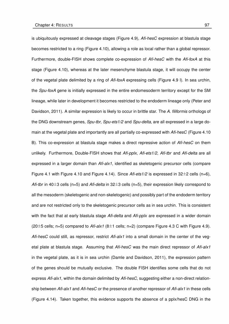
Chapter 4: RESULTS 97
is ubiquitously expressed at cleavage stages (Figure 4.9), Afi-hesC expression at blastula stage
becomes restricted to a ring (Figure 4.10), allowing a role as local rather than a global repressor.
Furthermore, double-FISH shows complete co-expression of Afi-hesC with the Afi-foxA at this
stage (Figure 4.10), whereas at the later mesenchyme blastula stage, it will occupy the center
of the vegetal plate delimited by a ring of Afi-foxA expressing cells (Figure 4.9 I). In sea urchin,
the Spu-foxA gene is initially expressed in the entire endomesoderm territory except for the SM
lineage, while later in development it becomes restricted to the endoderm lineage only (Peter and
Davidson, 2011). A similar expression is likely to occur in brittle star. The A. filiformis orthologs of
the DNG downstream genes, Spu-tbr, Spu-ets1/2 and Spu-delta, are all expressed in a large do-
main at the vegetal plate and importantly are all partially co-expressed with Afi-hesC (Figure 4.10
B). This co-expression at blastula stage makes a direct repressive action of Afi-hesC on them
unlikely. Furthermore, Double-FISH shows that Afi-pplx, Afi-ets1/2, Afi-tbr and Afi-delta are all
expressed in a larger domain than Afi-alx1, identified as skeletogenic precursor cells (compare
Figure 4.1 with Figure 4.10 and Figure 4.14). Since Afi-ets1/2 is expressed in 32+−2 cells (n=6),
Afi-tbr in 40+−3 cells (n=5) and Afi-delta in 32+−3 cells (n=5), their expression likely correspond to
all the mesoderm (skeletogenic and non-skeletogenic) and possibly part of the endoderm territory
and are not restricted only to the skeletogenic precursor cells as in sea urchin. This is consistent
with the fact that at early blastula stage Afi-delta and Afi-pplx are expressed in a wider domain
(20+−5 cells; n=5) compared to Afi-alx1 (8+−1 cells; n=2) (compare Figure 4.3 C with Figure 4.9).
Afi-hesC could still, as repressor, restrict Afi-alx1 into a small domain in the center of the veg-
etal plate at blastula stage. Assuming that Afi-hesC was the main direct repressor of Afi-alx1
in the vegetal plate, as it is in sea urchin (Damle and Davidson, 2011), the expression pattern
of the genes should be mutually exclusive. The double FISH identifies some cells that do not
express Afi-alx1, within the domain delimited by Afi-hesC, suggesting either a non-direct relation-
ship between Afi-alx1 and Afi-hesC or the presence of another repressor of Afi-alx1 in these cells
(Figure 4.14). Taken together, this evidence supports the absence of a pplx/hesC DNG in the

Chapter 4: RESULTS 98
brittle star as a mechanism of SM specification.
4.3.5 High-resolution gene expression of regulatory genes reveals major differences be-
tween sea urchin and brittle star skeletogenic GRNs
Downstream of the initial tier of regulatory genes activated by the DNG, the SM network in
sea urchin is stabilised by an interlocking loop (IL) engaging the three genes Spu-tgif, Spu-erg
and Spu-hex in a recursively wired positive feed-back loop (Oliveri et al., 2008). Interestingly, it
has been shown that the skeletogenic IL is conserved in mesodermal cells of starfish, a species
that does not form a larval skeleton (McCauley et al., 2010), suggesting an ancestral function
not directly linked to larval skeletogenesis. I isolated the orthologs of these three genes and
studied their expression using QPCR and WMISH during A. filiformis development. In brittle star
Afi-tgif, Afi-erg and Afi-hex are expressed only or enriched in a group of cells at the vegetal plate
at blastula stage, similar to sea urchin and starfish, but with some differences in the pattern of
co-expression (Figure 4.11 A). In brittle star Afi-erg is expressed in a smaller domain nested
within Afi-hex- and Afi-tgif -expressing cells (Figure 4.11 A). Afi-tgif is ubiquitously expressed at
low levels and enriched only at blastula stage in the cells at the vegetal pole (Figure 4.11 A). This
suggests a transient function of the IL in Afi-erg positive cells of the vegetal plate only at blastula
stage. Whereas, Afi-erg stays active in SM until gastrula (Figure 4.11 A), Afi-hex even though
active in SM throughout blastula is turned off from SM as soon as they enter the blastocoel at
mesenchyme blastula (Figure 4.11 A) and cannot, thus, act as a driver of skeletogenic genes at
later stages. It is important to notice that at mesenchyme blastula stage these same three genes
are now co-expressed in the non-skeletogenic mesoderm (NSM) and thus possibly re-establish
an IL in this cell type (Figure 4.11 A). The comparison of high-resolution temporal expression
patterns in the two species considered here can pinpoint the differences and similarities of initial
inputs responsible for the onset of these genes. In sea urchin the three genes are activated in
the following order: Spu-hex then Spu-erg and finally Spu-tgif, in all cases needing the prior for

Chapter 4: RESULTS 99
Afi-t
gif
Afi-e
rgA
fi-h
ex
Bl MBl G PlA
BAfi-erg Afi-hex Afi-tgif
0
50
100
150
0 10 20 30 40 0 10 20 30 40 0 10 20 30 40
Time (hpf)
Spu-erg Spu-hex Spu-tgif
0
50
100
150
0 10 20 30 40 0 10 20 30 40 0 10 20 30 40
Re
lati
ve
Ex
pre
ssio
n 1
1
2
2 3
3
Figure 4.11: Expression pattern of genes part of the interlocking loop. (A) Expression pattern
of Afi-tgif, Afi-erg, Afi-hex at different stages of development obtained by WMISH. All genes part
of the interlocking loop show expression in skeletogenic mesodermal cells during blastula stage.
However only, Afi-erg prevails expression in SM cells until mesenchyme blastula. (B) Time-line
comparison of the three genes shows re-shuffling of activation order in A. filiformis (top) compared
to S. purpuratus (bottom). Error bars for the brittle star time courses show standard deviation of
three technical replicas. Data from the bottom was obtained from Materna et al. (2010). VV-
vegetal view, Bl blastula, MBl mesenchyme blastula, G gastrula.

Chapter 4: RESULTS 100
the activation of the successor (Figure 4.11 B dashed lines). Interestingly, in brittle star the order
of activation is re-shuffled (Figure 4.11 B), where Afi-tgif and Afi-erg are activated first and Afi-
hex last. Giving the fact that the precise gene expression is the direct outcome of the regulatory
inputs, the differing order of onset of expression suggests potentially different initial inputs as well
as different wiring of the IL in brittle star compared to sea urchin. It is important to notice that
orthologs of main drivers of the sea urchin IL Spu-tbr and Spu-ets1/2 in brittle star are expressed
not only in SM lineage, but also in a wider mesodermal area consistent with the expression of Afi-
hex and Afi-tgif, but not Afi-erg. This implies that Afi-erg requires extra input(s) to be restricted in a
subset of cells at blastula stage. These data are in agreements with an ancient pan-mesodermal
role of the hex-erg-tgif IL as seen in starfish rather than a dedicated SM function as evolved in
euechinoids (McCauley et al., 2010).
During sea urchin skeletogenesis two extra TF, Spu-foxB and Spu-dri regulated by the gene
directly downstream of the DNG (ets1/2, alx1 and tbr), are necessary for the expression of some
of the differentiation genes (Amore et al., 2003; Minokawa et al., 2004). In some cases their
direct inputs have been verified by promoter analysis (Amore and Davidson, 2006). Whereas
Spu-foxB is only employed in larval skeletogenesis in sea urchin, Spu-dri is also expressed in the
adult skeletogenic domain (Gao and Davidson, 2008). These, however, are neither involved in
larval nor adult skeletogenesis in the brittle star (Czarkwiani et al., 2013), confirmed by WMISH
and QPCR (Figure 4.12 and Table A.6). Taken together our data show major differences in the
architecture of the A. filiformis skeletogenesis GRN downstream of the DNG compared to sea
urchin. Indeed, the IL, while possibly still active in brittle star, is likely to be initiated by different
inputs. Additionally, the late skeletogenic regulators, Afi-foxB and Afi-dri, are not responsible for
driving the expression of any skeletogenic differentiation genes.

Chapter 4: RESULTS 101
B
Afi-d
riA
fi-f
oxB
Bl MBl G PlA
Afi−dri Afi−foxB
0
50
100
150
0 10 20 30 40 0 10 20 30 40
Time (hpf)
Re
lati
ve
Ex
pre
ss
ion
Figure 4.12: Expression of other orthologs part of the skeletogenic GRN in A. filiformis. (A)
Expression pattern of Afi-dri and Afi-foxB in various stages of development, obtained by WMISH.
Both genes show no expression in cells belonging to the skeletogenic lineage throughout devel-
opment. (B) Time-series data shows temporal expression of both genes obtained by QPCR and
normalised by the individual peak of expression. Time-series data shows consistent occurrence
of expression with WMISH data. Error bars show standard deviation of three technical replicas.
Cl - Cleavage; Bl - blastula; MBl - mesenchyme blastula; G - gastrula.

Chapter 4: RESULTS 102
Bl MBl G Pl
Afi-n
k7
AA
fi-s
na
Afi-t
wi
BBl MBl G Pl
Bl MBl G Pl
Afi-l1
CBl MBl G Pl
Sp
u-s
oxC
Cl Bl MBl G
D
Afi-s
oxC
Bl MBl G Pl

Chapter 4: RESULTS 103
4.3.6 Other transcription factors of skeletogenic GRN in brittle star and sea urchin
Recently, several new genes have been found to participate in the GRN for larval skeletoge-
nesis of sea urchin. These genes are Spu-nk7, Lva-sna, Lva-twi, Spu-soxC and Spu-l1. In spite
of their discovery, so far a detailed functional analysis of their connections within the skeletogenic
GRN has not been performed. Whilst this makes a detailed comparative analysis of GRN rewiring
between sea urchins and brittle stars challenging, I am still able to compare the regulatory states
and analyze the evolutionary implications.
A recent study using an mRNA sequencing differential screen between embryos with and with-
out PMCs identified the TF Spu-nk7 as a novel candidate for the larval skeletogenesis GRN in
sea urchin (Rafiq et al., 2014). WMISH of Spu-nk7 in sea urchin confirmed its activity during SM
specification showing restricted expression of this gene in SM lineage from mesenchyme blastula
stage onwards (Rafiq et al., 2014). This indicates a role as late driver gene for the differentiation
cascade in sea urchin. In order to see whether the ortholog of this TF exhibited similar expression
in brittle star I performed WMISH of Afi-nk7 on various developmental stages (Figure 4.13 A).
In A. filiformis this gene shows strong expression by blastula stage, stays restricted to SM lin-
Figure 4.13 (preceding page): Expression of other skeletogenic specification orthologs. Ex-
pression patterns obtained using WMISH. (A) Afi-nk7 is expressed in SM during blastula and
mesenchyme blastula stage. It gets restricted to the tip of the archenteron during gastrulation
and ends up finally in two symmetric areas close to the mouth. (B) Expression of the EMT genes
Afi-sna and Afi-twi. Afi-sna is first expressed in SM lineage from mesenchyme blastula stage
onwards and gets restricted to some cells at the ectoderm around archenteron area until it ends
up to be expressed in scattered cells in the pluteus. Afi-twi shows first expression in the tip of the
archenteron during gastrulation and is gets restricted to the coelomic pouch during pluteus stage.
(C) Afi-l1 starts expression at blastula stage in SM cells and continues through mesenchyme
blastula stage. During gastrulation expression is ubiquitous and enriched in the gut until it gets
restricted to the mid and hind gut with additional scattered cells at pluteus stage. (D) Comparision
of soxC expression in A. filiformis and S. purpuratus. In brittle star expression is restricted to one
side of the embryo incorporating the cells in the SM lineage with additional enriched expression
is scattered cells in the ectoderm, marking potential neuronal percursors. During mesenchyme
blastula stage it gets restricted to a ring at the vegetal plate. Expression stays restricted to the tip
of the archenteron and some scattered ectodermal cells during gastrulation until only scattered
cells at pluteus stage show expression. In sea urchin expression is visible in micromeres during
cleavage and then in the vegetal plate during blastula stage. Mesenchyme blastula and gastrula
stages show similar expression to brittle star. Cl - Cleavage; Bl - blastula; MBl - mesenchyme
blastula; G - gastrula; Pl - pluteus.

Chapter 4: RESULTS 104
eage throughout mesenchyme blastula and changes activity to the tip of the archenteron during
gastrulation. Finally, Afi-nk7 ends up in a yet undefined territory at pluteus stage, on both sides
symmetrically close to the mouth region (Figure 4.13 A). This suggests that compared to sea
urchin Afi-nk7 is only transiently involved in SM cells and is probably not essential to drive the
differentiation cascade as in sea urchin in later stages of development.
In order for the skeleton to be formed in the lateral clusters the skeletogenic cells have to
ingress from the vegetal plate into the blastocoel. This process is commonly referred to as epithe-
lial to mesenchymal transition (EMT). A recent study in the sea urchin L. varigatus linked com-
ponents of the GRN for larval skeletogenesis with the process of EMT (Saunders and McClay,
2014). The genes twist (twi) and snail (sna) have been identified in many taxa as participants
in epithelial to mesenchymal transition (Yang et al., 2004; Peinado et al., 2004) and knockdown
experiments in the sea urchin L. varigatus showed their involvement specifically in the process of
de-adhesion (Saunders and McClay, 2014). WMISHs in sea urchin show that both Lva-twi and
Lva-sna are expressed in SM from blastula to mesenchyme blastula stage. Later Lva-sna is ex-
pressed in NSM during gastrulation and then again SM in later stages (Wu and McClay, 2007),
while Lva-twist always remain expressed in SM throughout development and is also activated in
NSM and endoderm territories at gastrula stage (Wu et al., 2008). Consistent with the expression
pattern observed, knockdown of both genes showed inhibition of EMT in sea urchin (Saunders
and McClay, 2014). In brittle star, Afi-sna starts to be expressed at the vegetal plate during ingres-
sion of cells at mesenchyme blastula stage and is then restricted to the archenteron (Figure 4.13
B). On the other hand, Afi-twi first shows expression during gastrulation at the tip of the archen-
teron and gets then restricted to a subset of cells at one side of the gut, potentially marking the
coelomic pouch. The expression of Afi-sna indicates a potential involvement in EMT, although,
the inactivity of Afi-twi argues for a different mechanism compared to the sea urchin L. varigatus.
Interestingly, in another species of sea urchin S. purpuratus quantification of a developmental
transcriptome shows no expression of Spu-twi until gastrula stage (Tu et al., 2014) allowing the

Chapter 4: RESULTS 105
hypothesis that EMT in sea urchins might have various mechanisms depending on the species.
My data support closer similarity with S. purpuratus than L. varigatus in the context of EMT.
Another gene that is included in the sea urchin GRN for larval skeletogenesis is the neuro-
fascin gene Spu-l1, which was proposed to act as binding partner to Spu-vegfR in order to facili-
tate the ectodermal Spu-vegf signalling for cell guidance during migration. Even though present
in the GRN in sea urchin, I could not find any evidence for its involvement. Since it was included in
my candidate list I cloned its ortholog in brittle star. WMISH showed enriched expression of Afi-l1
during blastula stage in the vegetal pole and in SM cells during mesenchyme blastula. During
gastrula stage, expression was restricted to the tip of the archenteron and remained visible in
the gut region at pluteus stage (Figure 4.13 C). Assuming that the role proposed in sea urchin is
correct, these results suggest conservation in the brittle star GRN for its early activity.
Finally, I looked into Spu-soxC. Previous work in our lab found this gene to be involved in SM
specification throughout development (Figure 4.13 D), but despite being placed in the GRN for
larval skeletogenesis no inputs and outputs have been identified (Oliveri et al., 2008). In order to
complete my analysis of selected sea urchin skeletogenic candidates in brittle star, I analysed the
expression pattern in different stages of development using WMISH. In brittle star Afi-soxC shows
enriched expression in the vegetal half of the embryo during blastula stage and is expressed on
one side of the ectoderm with strong expression in single cells (Figure 4.13 D). At mesenchyme
blastula stage the expression becomes more specific in single cells of the ectoderm and in a ring
of cells at the vegetal plate. At gastrula stage the expression of Afi-soxC is similar to Spu-soxC,
with scattered cells in the ectodermal field and expression at the tip of the archenteron, and the
subsequent restriction to scattered cells during pluteus stage.
Taken together, the genes Afi-l1, Afi-sna, Afi-nk7 and Afi-soxC are all expressed during blas-
tula stage in the vegetal plate and can thus be placed in the GRN for larval skeletogenesis in brittle
star. However I observe differences in spatial activity over time, suggesting a stage-dependent
re-wiring.

Chapter 4: RESULTS 106
A Afi-alx1 Afi-pplx
Bl
Ai
Aii
Aiii
B Afi-alx1 Afi-hesC
Bl
Bi
Bii
Biii
C Afi-alx1 Afi-foxA
Bl
Ci
Cii
Ciii
D Afi-alx1 Afi-ets1/2
Bl
Di
Dii
Diii
E Afi-alx1 Afi-tbr
Bl
Ei
Eii
Eiii
F Afi-alx1 Afi-delta
Bl
Fi
Fii
Fiii
Figure 4.14: The endomesodermal regulatory states of the brittle star A. filiformis at blas-
tula stage. (A-F) Double FISH using Afi-alx1 expression as marker for SM cells. (A) Afi-pplx is
expressed in a wider domain than Afi-alx1. (B) Afi-hesC is expressed as ring around the vegetal
pole of the embryo and is surrounding Afi-alx1. The area in yellow shows cells in the vegetal
plate that do not express neither Afi-hesC nor Afi-alx1.(C) Expression of Afi-foxA and Afi-alx1
during blastula stage is similar to (B) and consistent to the complete co-expression of Afi-hesC
and Afi-foxA at this stage (Figure 4.10 B). (D-F) Afi-ets1/2, Afi-tbr and Afi-delta are expressed in
a large domain in the vegetal plate larger than Afi-alx1. Cell nuclei are stained with DAPI (blue).
Bl blastula
4.3.7 Dynamic regulatory states during A. filiformis mesoderm development
In sea urchin and sea cucumber the skeletogenic mesoderm is formed within the mesoderm
by a subpopulation of cells and it is therefore important to investigate not only the SM lineage but
also the cells surrounding it. A recent study aimed to compare the development of mesoderm in
different classes of echinoderms, excluding brittle stars, and showed a great degree of conser-
vation of the blastula mesodermal regulatory state (McCauley et al., 2012), although the relative
positioning of the different mesodermal cells within the vegetal plate shows certain variability.
To better understand the disposition of the SM within the mesodermal field I performed a series

Chapter 4: RESULTS 107
Afi-g
ata
EA
fi-g
ata
CA
fi-g
cm
Bl MBl G Pl
Figure 4.15: . Expression during A. filiformis development of sea urchin orthologous genes
involved in early specification of non skeletogenic mesoderm. WMISH at different develop-
mental stages. Afi-gcm is not detectable by WMISH at any of the stages analysed, consistent with
QPCR expression levels (compare Table A.6). Afi-gataC expression becomes detectable at mes-
enchyme blastula stage in NSM cells and it stays active at the tip of the archenteron at gastrula
stage. Afi-gataE expression becomes active in a similar fashion to Afi-gataC at mesenchyme
blastula stage. At the beginning of gastrulation it marks the secondary mesenchyme cells and
the cells at the tip of the archenteron. Different to Afi-gataC, Afi-gataE is additionally expressed
in cells at the base of the archenteron. Both Afi-gataC, Afi-gataE are not expressed at blastula
stage. Bl - blastula; MBl - mesenchyme blastula; G - gastrula; Pl - pluteus.

Chapter 4: RESULTS 108
of WMISH on orthologs of non-skeletogenic mesoderm (NSM) specification in sea urchin, using
Afi-alx1 as a landmark for SM and Afi-hesC and Afi-foxA as the outer boundary (Figure 4.14). The
TF orthologs to non-skeletogenic mesoderm specification genes (gataE, gataC and gcm) are not
expressed during blastula stage in A. filiformis, confirmed by QPCR and WMISH (Figure 4.15 and
Table A.6). Interestingly the SM is eccentric to the boundary delimited by Afi-hesC, creating yet
a third mesodermal domain of unknown function (Figure 4.14). At mesenchyme blastula stage,
once the SM cells ingress into the blastocoel and leave the vegetal plate, the NSM orthologs Afi-
gataE and Afi-gataC are expressed in the entire vegetal plate (Figure 4.15) along with Afi-hesC
(Figure 4.14) and other mesodermal genes (i.e. tbr, ets1/2, tgif, erg, hex and delta). Importantly,
although I successfully isolated a Afi-gcm cDNA clone, from my quantitative and spatial analysis
it is clear that Afi-gcm is not expressed throughout the stages analysed (up to late gastrula) and
that it is not involved in early mesodermal cell specification (Figure 4.15, Table A.6 and transcrip-
tomic data). Whereas in sea urchin the expression of Spu-gcm in NSM and the repression of
Spu-gcm by Spu-alx1 in the skeletogenic lineage plays a crucial role in the spatial separation of
these two types of mesoderm, this mechanism might rely on different regulatory genes or might
be completely absent in brittle stars. Indeed, brittle star larvae do not present any obvious pig-
ment cells. The late expression of Afi-gataE and Afi-gataC also highlight major differences in the
mesodermal regulatory states and suggests that NSM specification and patterning might occur at
later stages compared to sea urchin.
Given that cell specification is not a single step process and that several genes contribute
dynamically to different aspects of this biological process, it is essential to study the dynamics of
regulatory states. To this purpose and to better understand the timing of mesodermal cell lineage
separation in A. filiformis, the dynamics of their regulatory states and their spatial arrangement
within the vegetal plate, I built a cellular resolution map of the different mesodermal regulatory
states up to mesenchyme blastula stage based on the spatial data so far described integrated
with quantitative data (Table A.6) and double FISH. My analysis (Figure 5.1) revealed that:

Chapter 4: RESULTS 109
1. Only two genes (Afi-pplx and Afi-delta) have localized expression in a group of cells already
visible by the end of cleavage stage (Figure 4.6 and Figure 4.9). These two genes are
consistently co-expressed in ∼8 cells (n=2).
2. Most of the mesodermal genes, including the SM genes, start their zygotic expression
around early blastula stage (12 hpf), suggesting that the initiation of mesoderm specification
occurs at this stage (Table A.6).
3. At free-swimming blastula stage a cohort of regulatory genes are expressed in all meso-
dermal cells and likely specify a pan-mesodermal state. They are Afi-tbr, Afi-ets1/2, Afi-tgif,
Afi-hex, Afi-pplx and Afi-delta.
4. At this stage (14-15 hpf) at least three distinct domains, characterised by a unique combina-
tion of transcription factors genes, are identified in the vegetal half of the embryo. A distinct
SM domain in a population of roughly 16 cells is marked by the expression of Afi-alx1, Afi-jun
and Afi-erg. A one cell-wide ring domain, expressing also Afi-foxA and Afi-hesC, surrounds
the SM domain plus a small domain expressing only the pan-mesodermal genes.
5. By mesenchyme blastula the SM and the NSM are now completely segregated although
both express pan mesodermal genes. The first is constituted by mesenchymal cells, which
are ingressed into the blastocoel and express Afi-alx1 and Afi-jun as distinctive markers.
The second (NSM) remains in the vegetal plate of the blastula epithelium and is distin-
guished by the expression of Afi-hesC, Afi-delta, Afi-hex, Afi-tgif, Afi-gataC and Afi-gataE.

Chapter 5
DISCUSSION
In the pluteus larvae of sea urchins and brittle stars the extended mineralized skeleton is formed
by a sub-population of mesodermal cells specifically expressing the transcription factors alx1 and
jun. These skeletogenic cells ingress as mesenchymal cells into the blastocoel before gastru-
lation. Despite the morphological similarities of the skeleton and its mode of development in
both echinoderm classes, I reveal several differences in GRN architecture using a high-resolution
multi-gene expression analysis (summarized in Figure 5.1 B). Foremost, side-by-side compari-
son of brittle star and sea urchin mesodermal regulatory states reveals that many differences in
network architecture are apparent at the level of the initiation of the expression of skeletogenic
genes, and at the level of the regulation of the differentiation gene batteries. This is consistent
with the hourglass model of evolution (von Bear, 1828; Kalinka et al., 2010), in which evolutionary
plasticity of network linkages differs depending on their position in the network hierarchy (early-,
mid- or late-,). Our analysis also shows that gene duplication, protein function diversification,
and cis-regulatory evolution took place over 480 million years of evolution to shape the larval
skeletogenic networks as we see them now in the echinoderm classes which develop pluteus-like
larvae.
5.1 Evolution of GRN by protein function diversification
Skeletogenesis in the regular sea urchin is unlocked at cleavage stage by the action of the
pmar1/hesC DNG. In this study, I identified in a developmental transcriptome of A. filiformis (see
110

Chapter 5: DISCUSSION 111
Maternal InputsMat cβ
HesC
Ubiq
Mat Otx
Ubiq
Pmar1/Pplx
Maternal Ets
Alx1
FoxB
Ets1 Tbr
Dri
Diffe
ren
tia
tio
n g
en
es
P19Msp130LSm27
Sm30
Sm50
Alx
1
Fo
xB
Ets
1
TB
r
Dri
Ve
gf-
R
Ske
. sp
ecific
atio
n g
en
es
Mic
rom
ere
s
sp
ecific
atio
n g
en
es
Jun
?
ErgHex Tgif
Gcm Delta
pmar1
pplx
delta
pmar1
alx1
ets1/2
tbr
delta
pmar1 erg
alx1 hex
ets1/2 tgif
tbr dri
delta foxb
jun gcm
gata4/5/6
foxA
gcm
gata4/5/6
foxA
alx1 erg
ets1/2 tgif
tbr dri
jun foxb
gata1/2/3
erg
+hesC
+foxA
+alx
+jun
+erg pplx
delta
tbr
ets 1/2
hex
tgif
Sea urchinS. purpuratus
Brittle starA. filiformis
foxA
hesC
delta
tbr
ets 1/2
erg
tgif
gataC
gataE
hex
alx
jun
tbr
ets1/2
ergLV LV VV
A B C
Blimb1Wnt8
SoxC
L1
Ubiq
Ubiq
gcm
gata4/5/6
foxA

Chapter 5: DISCUSSION 112
Part II) and by phylogeny an ortholog of the sea urchin Pmar1, named here Afi-pplx. This ortholog
was also identified in a transcriptomic study in the brittle star Ophiocoma wendtii (Vaughn et al.,
2012). While being an ortholog I showed with a cross-species analysis that Afi-pplx is functionally
not equivalent to its sea urchin counterpart Spu-pmar1. According to the gene phylogeny (Fig-
ure 4.5), gene duplication and protein function diversification events are likely to have occurred
to shape the sea urchin Pmar1 into a potent repressor of the DNG. My protein phylogeny (Fig-
ure 4.5) and gene expression data (Figure 4.6) support a likely ancient duplication of the phb1
gene, which led to the emergence of the pplx/pmar1 gene expressed at the vegetal plate of the
early embryo of the last common ancestor of sea urchins and brittle stars, 480 Mya. If duplicated
from the phb1 gene, we hypothesised that the regulatory region driving expression in the SM
lineage would be located in intron 1. Although our co-injection experiments with an SM marker
could not sustain our hypothesis, we found a regulatory element that is driving expression in other
territories. The functional non-equivalence of Spu-pmar1 and Afi-pplx might have been caused by
Figure 5.1 (preceding page): Dynamic of mesodermal regulatory states in A. filiformis blas-
tula and summary diagram highlighting inferred differences of skeletogenic lineage GRN
architecture relative to sea urchin. (A) Regulatory states for the mesodermal territories are
shown on cellular maps of cleavage (Cl), pre hatching blastula (EBl), hatched blastula (Bl) and
mesenchyme blastula (MBl). In grey all cells not part of the skeletogenic lineage marked by hesC.
In dark green the micromeres and then the SM lineage marked by pmar1 and then additionally
at EBl by alx1, ets1/2, tbr and delta. At Bl stage, additionally jun, erg, hex, tgif, dri and foxB get
activated. At MBl stage only the genes pmar1, hex and delta stop being part of the SM lineage. In
blue the endomesodermal marker foxA. In light green the NSM marker genes gcm and gata4/5/6.
At MBl stage the NSM is split in two territories orange marked by gata1/2/3 and erg and light
green. (B) S. purpuratus SM-GRN architecture (http://sugp.caltech.edu/endomes/) of
the genes analysed in this study. In gray are nodes and regulatory linkages not taking place in A.
filiformis SM specification, based on the observations in Figure 4.1 - Figure 4.15. In colour are
the nodes and connections potentially conserved in A. filiformis. Regulatory genes in red dashed
square are not expressed in skeletogenic cells during A. filiformis adult arm regeneration (Czark-
wiani et al., 2013). (C) Regulatory states for the mesodermal territories are shown on cellular
maps of pre hatching blastula (EBl), hatched blastula (Bl) and mesenchyme blastula (MBl). The
light green cells represent the mesoderm initially identified by the expression of pplx and delta;
and later expressing the pan-mesodermal genes ets1/2, tbr, hex and tgif. The dark green repre-
sent the SM cells expressing the skeletogenic marker genes alx, jun and p19; blue dots represent
the expression of hesC and foxa within the mesoderm territory, while blue cells represents the
endodermal territory that surrounds the mesoderm. At blastula stage the SM is clearly separated
by the rest of NSM, while the segregation of NSM and endoderm occurs at MBl stage. Genes
expressed in each territory are listed.

Chapter 5: DISCUSSION 113
relaxed selective pressure on the duplicant, thus allowing the diversification of the protein function
by the acquisition and loss of short linear protein motifs (i.e. eh1). These are reported as easily
evolvable (Copley, 2005). The presence in all euechinoid species analyzed of several almost iden-
tical copies of pmar1 (Figure 4.5) arrayed in tandem in the same fragment of DNA (Sea Urchin
Genome Project BAC Clones #170H13 and #020N20; GeneBank AC131562) suggests a further
gene duplication event that possibly occurred concomitant with the emergence of the stereotyp-
ical quartet of micromeres at the vegetal pole of the euechinoid embryo. The pmar1/pplx gene
type has so far been identified only in euechinoids and ophiuroids, probably due to limited se-
quence resources available for other echinoderm species. Most publicly available data consist of
transcriptome data of specific developmental stage(s) and do not sample early embryonic stages,
when the pmar1/pplx gene is likely to be expressed. An exception is given by the draft of the
starfish P. miniata genome (Cameron et al., 2009), for which we can state confidently that no
pmar1/pplx gene is present, although a clear phb1 gene is identified (Figure 4.6). Our evolution-
ary scenario in light of recent echinoderm phylogeny (Telford et al., 2014; O’Hara et al., 2014;
Cannon et al., 2014) implies the loss of the pmar1/pplx gene at least in the Asteroidea lineage,
although we cannot exclude the alternative hypothesis of independent duplication of pmar1 and
pplx genes respectively in the Echinoidea and Ophiuroidea lineages. Both scenarios, however,
point at the high plasticity of the pmar1/pplx node in the GRN underlying echinoderm mesoderm
specification.
5.2 Evolution of GRN by changes in cis-regulation
High-resolution expression data of Afi-hesC and its immediate targets (Afi-et1/2, Afi-tbr, Afi-
delta) integrated with the echinoderm phylogeny allows the reconstruction of the nature and timing
of the molecular changes occurred to setup the DNG responsible for the precocious specification
of skeletogenic fate in micromeres in the euechinoid lineage (Figure 5.1 A and C). As laid out in
Figure 5.2, the predicted changes in cis-regulatory apparatus of ets1/2, delta and tbr to become

Chapter 5: DISCUSSION 114
Eleutherozoa
pmar1
hesC
alx1
ets1/2
tbr
delta
pmar1
hesC
alx1
ets1/2
tbr
delta ?
pmar1
hesC
pplx
hesC hesC
alx1
ets1/2
tbr
delta
? ??
SM
alx1
ets1/2
tbr
delta ?
SM/NSM
alx1
ets1/2
tbr
delta
SM/NSM NSM SM/NSM
~480 MyaTandem duplication of pmar1 genes
Co-expression of hesC, ets, tbr, delta
foxB in ske cells
dri not in ske cells
alx, ets1/2 and jun in adult ske cells
~250 Mya
Euechinoidea
(S. purpuratus)Cidaroidea
(P. baculosa)
Holothuroidea
(P. parvimensis)
Ophiuroidea
(A. filiformis)
Asteroidea
(P. miniata)
Figure 5.2: Evolution of echinoderm larval skeletogenesis. Simplified phylogeny of Eleuthero-
zoa derived from recent phylogenomic studies (Telford et al., 2014; O’Hara et al., 2014; Cannon
et al., 2014) summarizing in different classes our knowledge of key features relevant for larval
skeleton development. Box on top indicate the skeletogenic mesoderm (SM, black) or the non-
skeletogenic mesoderm (NSM, orange) and inside the boxes are depicted the key regulators of
the euechinoid DNG. Red boxes indicate extended larval skeleton. HesC is in gray, instead of
blue, when not expressed in skeletogenic cells. Question mark indicates no data is available on
the presence and/or the expression of a specific node in a specific lineage. Dashed line, indicate
possible indirect linkage. Regulatory linkages in A. filiformis are based on the observations in this
study, in other species are described in (Oliveri et al., 2008; McCauley et al., 2012, 2010; Gao
and Davidson, 2008; Czarkwiani et al., 2013; Yamazaki et al., 2014).

Chapter 5: DISCUSSION 115
negatively regulated by HesC, and for the hesC gene to become repressed by Pmar1 (Gao and
Davidson, 2008), likely occurred in the euechinoid lineage once split from the cidaroid sister group.
Support for this is given by the pencil urchin (cidaroids) hesC, the expression of which is not
consistent with a function in a DNG at the top of the skeletogenic regulatory cascade (Yamazaki
et al., 2014). In cidaroids as well as in asteroids (McCauley et al., 2010) and ophiuroids (this
study) hesC is coexpressed with its sea urchin immediate targets, ets1/2, tbr and delta, which
are expressed in all mesodermal cells and not restricted only to the skeletogenic lineage as in
sea urchin (Figure 5.1 B). This implies that ets1/2, tbr and delta in A. filiformis, as well as other
classes, cannot be directly repressed by HesC and that a different mechanism must exist to drive
their precise spatial expression pattern. A possible molecular mechanism emerged recently in
starfish, where expression of these genes was shown to be regulated by sustained high levels of
nuclear β-catenin (McCauley et al., 2014). It is interesting to notice that the expression pattern
of hesC is dramatically different in the species studied so far (and belonging to different classes)
ranging from a ubiquitous expression excluded only from a few mesodermal cells (euechinoids) to
a restricted ring of cells in the vegetal half of the embryo (ophiuroids), or an ubiquitous expression
excluded from the endodermal cells (asteroids), highlighting the high evolutionary plasticity of the
hesC cis-regulatory apparatus.
Other substantial differences between the sea urchin and the brittle star are identified at the
periphery of the skeletogenic network, at the level of the downstream differentiation genes, which
in A. filiformis are not regulated by the TF Afi-FoxB and Afi-Dri either in the larva or in the adult
(Amore and Davidson (2006); Czarkwiani et al. (2013) and our unpublished data). Whilst the
expression of foxB exclusively in skeletogenic cells of euechinoid embryos supports a cooption
of this gene in the larval skeletogenesis of sea urchins, the absence of dri function in the brittle
star skeleton GRN is specific to ophiuroids, given the fact that in both sea urchin and starfish
dri is expressed in association with skeletogenic cells (Gao and Davidson, 2008). Accordingly,
extensive rewiring at the level of cis-regulatory apparatus of several differentiation genes as well

Chapter 5: DISCUSSION 116
as foxb and dri themselves must have occurred to change the expression in the two classes of
echinoderms.
5.3 Common regulatory state for skeletogenesis
The precise spatio-temporal expression of a developmental gene is controlled by its own cis-
regulatory apparatus, which is capable of integrating multiple inputs (i.e. transcription factors)
present in a given combination (regulatory state). Therefore, if no changes occur in the inputs or in
the cis-regulatory apparatus of a developmental gene during evolution, the expression pattern of
orthologous genes will be maintained in related species. Our experimental approach is designed
to pinpoint regulatory differences in the skeletogenic GRN of sea urchin and brittle star, which
result in different spatial or temporal expression of orthologous genes in the two species, given
an identical regulatory state. Conversely, we assume in a conservative way that when similar ex-
pression patterns are observed, the regulatory functional connections are conserved (Figure 5.2),
therefore we might actually underestimate the amount of architectural differences between the
two networks in the two classes of echinoderms. Although functional studies are needed for val-
idation, expression of alx1 and jun at blastula stage, along with the pan-mesodermal regulatory
genes ets1/2, tbr, tgif, hex and erg, is a common feature of the initial state of the skeletogenic
program in both sea urchin and brittle star, as well as in sea cucumbers (McCauley et al., 2012),
which produce small mineralized spicules. This set of regulatory genes is likely to constitute the
core of a cis-regulatory module essential to set up the right combinatorial code responsible for
echinoderm larval skeletogenesis. A direct consequence of this hypothesis is that many of the
downstream genes should be directly regulated by Alx1 and other mesodermal TFs in a combina-
torial fashion, and thus be expressed long before the mineralized skeleton is formed. Indeed, in
sea urchin as well as in brittle star (data not shown) several mineralization genes are already ex-
pressed at blastula stage, and genome wide analyses identify alx1 and ets1/2 as major controllers
of these differentiation genes (Rafiq et al., 2014, 2012). Furthermore, these two transcription fac-

Chapter 5: DISCUSSION 117
tors along with jun are expressed in the plesiomorphic adult skeleton of brittle star (Czarkwiani
et al., 2013), starfish and sea urchin (Gao and Davidson, 2008) (Figure 5.2).
5.4 Independent or common evolution of larval skeleton?
My data reveal substantial differences in the regulatory programs underlying the development
of mineralized skeleton in the morphologically similar pluteus larvae of sea urchins and brittle
stars. Adult calcitic endoskeleton is a plesiomorphic character of echinoderms, also apparent
in ancient extinct species (Bottjer et al., 2006). It has been proposed that the sea urchin larval
skeleton evolved by a simple co-option of an ancient adult skeletogenic GRN module (Gao and
Davidson, 2008), consistent with the expression of many skeletogenic regulatory genes also in
the adult skeleton, as already discussed. What about ophiuroid larval skeleton? Did it originate
with the same co-option event of sea urchin or with an independent co-option event? To ad-
dress this question two key aspects need to be considered: 1) the phylogenetic relationship of
the five echinoderm classes; 2) the developmental-specific network nodes rather than the regu-
latory genes also expressed in adults and being part of an ancient skeletal GRN module. The
recent availability of transcriptomic and genomic data from several echinoderm species gave rise
to several phylogenomic analyses based on large data-set including representative of all echin-
oderm extant classes (Telford et al., 2014; O’Hara et al., 2014; Cannon et al., 2014). All these
extensive molecular phylogenies converge on the consensus tree (Figure 5.2), in which echino-
derms and holothurians form a distinct clade (Echinozoa) from the ophiuroids and asteroids clade
(Asterozoa) and all the crinoids are sister taxa to these four classes (Eleutherozoa). In the light
of this recent phylogeny (Telford et al., 2014; O’Hara et al., 2014; Cannon et al., 2014) my data,
advocates for the the independent evolution of this distinctive larval character. If independently
originated, a similar co-option would have occurred during brittle star larval evolution, although us-
ing different developmental genes. In fact, many sea urchin specific skeletogenic developmental
genes, such as pmar1, foxb, dri, are not part of the A. filiformis larval skeletogenic GRN. On the

Chapter 5: DISCUSSION 118
other hand, in the case of a single co-option event for common evolution the role of developmental
genes should have been at least partially conserved (e.g. pmar1, hesC and foxB) between brittle
star and sea urchin. Despite this, the ancient split (roughly 480 Mya) of all classes and their long
branches of independent evolution make the exclusion of divergent evolution as an alternative
scenario difficult. In this case the larval skeleton would have originated only once at the base of
the Eleutherozoa and would have been lost in asteroids and reduced in holothurians. Importantly,
independent of common or independent evolution, it is likely that the co-option happened through
the same genes alx1 and jun and thus at the same tier of the GRN in both echinoderm classes.
This implies that the cis-regulatory control initiating the expression of alx1, and possibly jun, in a
subset of mesodermal cells, should reveal the exact evolutionary nature of sea urchin and brittle
star larval skeleton and this would be a prime focus for future investigations.

Part II
A global view on Amphiura filiformis
skeletogenesis
119

Chapter 6
METHODS
6.1 Experimental
6.1.1 mRNA Samples and Extraction
6.1.1.1 Time-series
For the mRNA sequencing of different stages of development (time-series), samples were
collected from the fertilisation of a single male and female at 09hpf, 18hpf, 27hpf, and 39hpf.
6.1.1.2 Skeleton inhibition experiment
To inhibit the formation of the larval skeleton the drug SU5402 (Sigma) was used. A working
dilution of this drug in DMSO was added at 18hpf to a final concentration of cf=20µM. At 27hpf
three samples were collected one treated, one just with DMSO and one untreated sample in
filtered sea water (FSW). The 27hr FSW sample was additionally used for the time-series.
6.1.1.3 mRNA extraction
Total RNA extraction for all samples was performed as described in Chapter 3.3.1 and the
samples were eluted in 5mM Tris pH 8.5. The quality of extraction and concentrations were
checked with NanoDrop 2000 and Bioanalyser 2100, all the samples had a RIN>8.
6.1.2 mRNA sequencing
The libraries were prepared using the TruSeq RNA library preparation protocol. The sam-
ples were sequenced with the Illumina v3 chemistry using the multiplex paired-end sequencing
120

Chapter 6: METHODS 121
protocol. The protocol uses oligo dT beads to enrich for poly-A tailed mRNA species during the
process. Long non-coding and rRNA species are mostly eliminated during this process. The
sequencing was performed on an Illumina HiSEQ 2500 with 100bp paired-end reads. To reach
optimal coverage we sequenced 2 lanes multiplexing the 6 samples. The library preparation and
the sequencing were all done at the Sickkids Hospital Toronto, Canada.
6.2 Computational Procedures
If not otherwise stated, all computational work was performed on an Apple Mac Os X 10.6
server with 24 cores and 64GB of memory.
6.2.1 Required Software
In order to assemble a transcriptome the following software packages were used:
FastQC: Quality measuring of reads (http://www.bioinformatics.babraham.ac.
uk/projects/fastqc/).
Trimmomatic: Filtering of Adapter, Trimming of low quality basepairs (http://www.usadellab.
org/cms/?page=trimmomatic).
Screed: Short read sequence utilities (https://github.com/ged-lab/screed).
Khmer: Library toolkit for k-mer based dataset analysis and transformation (https://
github.com/ged-lab/khmer).
Trinity: Assembly for deNovo transcriptoms (http://trinityrnaseq.sourceforge.
net/).
libgtextutils: Text utils library (http://hannonlab.cshl.edu/fastx_toolkit/).
fastx: Collection of command line tools for short read FASTAFASTQ file processing (http:
//hannonlab.cshl.edu/fastx_toolkit/).

Chapter 6: METHODS 122
Transdecoder: Tool for open reading frame extraction (https://transdecoder.github.
io).
mpiBlast: Blast programme for use on multicore cluster (http://www.mpiblast.org).
CEGMA: Tool used to identify core eukaryotic genes in our dataset (http://korflab.
ucdavis.edu/datasets/cegma/).
R: Programming environment for statistical analysis (http://www.r-project.org).
R-shiny: Environment to integrate R analysis dynamically in web environment (http://
shiny.rstudio.com).
Blast2GO: Environment to perform gene ontology classification (https://www.blast2go.
com).
PFAM: Protein family databases used for unbiased detection of homologous protein do-
mains of amino acid sequences (http://pfam.xfam.org).
HMMER: Tool to find protein domains using hidden markov models (http://hmmer.janelia.
org).
Detailed descriptions can be found on the individual webpages about installation and applica-
tion.
6.2.2 Quality evaluation of reads
Quality of reads was checked using the FastQC package. This package offers a user interface
and produces html-pages as result output (see attached CD).
6.2.3 Assembly of combined samples
The assembly pipeline (Figure 7.2) and annotation of the combined dataset followed a set of
unified protocols described in (Brown et al., 2013). All files containing reads were obtained in fastq

Chapter 6: METHODS 123
format and each sample was split into multiple files. In order not to handle too many files we con-
catenated the files for each sample and read direction. This resulted in 2 files for each sample. All
procedures up to the actual assembly were performed on those 12 fastq files (2 files per sample).
Each of the 12 files containing reads was trimmed for adapters and for low quality sequences us-
ing Trimmomatic v0.27 (ILLUMINACLIP:Adapters.fasta:2:30:10; HEADCROP:12) (Bolger et al.,
2014) followed by quality filtering using the FASTX-Toolkit (v0.0.13.2; fastq quality filter Q33 q
30 p 50). The quality filtered and trimmed reads were then digitally normalised (Brown et al.,
2012). Once all filtering and the digital normalisation was completed reads from all stages were
pulled together and the transcriptome was assembled using the trinity package with standard pa-
rameters (v2013-02-25) (Grabherr et al., 2011). This assembly resulted in a 629,470 sequences
constituting the initial transcriptome (IT).
6.2.4 Assembly of individual samples
In addition to the combined assembly we performed assemblies on each individual sample
separately. Similarly to that described in Chapter 6.2.3, we used for each assembly the 2 con-
catenated fastq files containing all reads for each sample and read direction. All reads were pre-
processed by trimming of adapters and discarding of low quality sequences using Trimmomatic
v0.27 (ILLUMINACLIP:Adapters.fasta:2:30:10) (Bolger et al., 2014). The trimmed and quality
filtered reads were then assembled using the Trinity package with standard parameters (v2013-
02-25) (Grabherr et al., 2011)), without previous digital normalization.
6.2.5 Post Assembly procedures
We post processed the IT by extraction of partial and complete open reading frames (ORFs)
with a minimum length of 100 amino acids that were predicted using the TransDecoder (ver-
sion rel16JAN2014) script. Potential bacterial contaminants were obtained using mpiBlast (v.1.6)
(Darling et al., 2003) with e-value 1e-20 and crosschecked with hits obtained against UniProtKB-

Chapter 6: METHODS 124
SwissProtDB with the same e-value using a custom R-script. Searches with mpiBlast were run
on the Legion HPC cluster at UCL on at least 40 cores. Sequences with higher similarity to the
bacterial database were removed from the dataset. The cleaned ORF dataset represents the
reference transcriptome (RT).
6.2.6 Other Echinoderm Datasets
The assembled transcriptome of the crinoid Antedon mediterranea (Elphick et al., 2015) was
kindly provided by the Elphick Laboratory (Queen Mary University, London). A genome and tran-
scriptome data for the asteroid Patiria miniata was acquired from the Echinodermata website
(http://echinobase.org). To obtain a complete picture of coding sequences we combined
both genomic derived coding sequences and transcriptome sequences for the star fish.
6.2.7 Quality Assessment
Length distributions and N50 values were calculated using a custom R script1. Completeness
of our transcriptome was estimated using CEGMA (v2.5) (Parra et al., 2007). Full-length distri-
butions were estimated by considering all unique hits determined by blastx (1e-20) against the
UniProtKB-SwissProt database and application of the analyze blastPlus topHit coverage.pl perl
script that is part of Trinity.
6.2.8 Annotation
All BLAST searches were performed using a local ncbi-blast (v2.2.25) with e-value of 1e-6.
The RT was annotated against the sea urchin Strongyloncentrotus purpuratus transcriptome se-
quences and against the non-redundant (nr) database. One directional blast identified presumed
homologs and reciprocal blast identified presumed orthologs. Gene ontology classification was
performed based on a previously sea urchin specific classification (Tu et al., 2012). For con-
sistency, sequences obtained for the starfish Patiria miniata (echinobase.org) and the crinoid
1http://faculty.ucr.edu/˜tgirke/Documents/R_BioCond/My_R_Scripts/contigStats.R

Chapter 6: METHODS 125
Antedon mediterranea (Elphick et al., 2015) were annotated using the same combination of one-
directional and reciprocal blast (e-value 1e-6) against the sea urchin transcriptome database.
6.2.9 Gene Ontology (GO)
6.2.9.1 Echinoderm gene ontology
Echinoderm gene ontology searches were performed using the gene ontology established for
the sea urchin (Tu et al., 2012). GOs were transformed into the WHL22 annotation as part of the
sea urchin transcriptome + genome (Tu et al., 2014).
6.2.9.2 General GO
A general GO analysis was performed for the differentially expressed samples using Blast2GO.
The initial blastx (e-value 1e-3) step against the nr database was run locally on the legion cluster
HPC with mpiblast. All other steps were performed using the Blast2GO tool.
6.2.10 Abundance Estimation
The quality filtered trimmed reads were re-aligned on the reference transcriptome using Bowtie
(v0.12.9) (Langmead, 2010) with parameters set as in RSEM (v1.2.11). The bowtie output was
loaded into CORSET in order to obtain counts for expression clusters (ECs) of contigs that shared
reads, rather than individual contigs (Davidson and Oshlack, 2014). This is equivalent to a poten-
tial gene count adding up all isoform counts. Normalisation by internal standard was performed
as follows: First, individual ECs were normalised by their peak of expression in the time-course
data (9hpf, 18hpf, 27hpf and 39hpf); then, for each EC the standard deviation between the indi-
vidual time-points was calculated and ECs with standard deviation below 0.01 were chosen as
internal standard. Finally, an average of these 331 ECs was used as a normalisation factor, each
EC was divided by this normalisation factor and multiplied by 1,000,000. All downstream analysis
was performed using customised R and bash scripts. In order to make statements about annota-
tion content in the individual EC, the most frequent annotations for each expression cluster were

Chapter 6: METHODS 126
considered, giving orthologous annotation priority over homologous.
6.2.11 Differential Analysis
Differential analysis was conducted on all three 27hr samples. To obtain high probability true
positives of significantly affected ECs, we used a combination of GFOLD (Feng et al., 2012), a
procedure specifically designed for data without a second replica and the assumptions that we
only considered clusters with an expression value bigger than 2 and a log fold change bigger
than 1.6 or smaller than -1.6. Due to lack of a biological replica, our approach was used to find
potential candidates and their statistical validity was controlled on at least one other biological
replica with QPCR (described in chapter 3.3.3).
6.2.12 Expression clustering of time-series data
To sort expression clusters by their individual trajectories we applied the fuzzy clustering al-
gorithm (Futschik and Carlisle, 2005). We used 27 fuzzy clusters, based on the assumption that
between 4 time points we have at 3 times either an increase, decrease or constant changes in
expression. (Note here the difference between a fuzzy cluster and an expression cluster: A fuzzy
clusters describes a group of expression clusters that share similar trajectories over time.) Since
fuzzy clustering does not allocate each transcript always to the same cluster, we repeated this
algorithm 100 times to find, for each EC, the most probable fuzzy cluster membership.
6.2.13 Orthology analysis
To infer orthology of a subset of genes, where the reciprocal blast approach was inconclusive,
we applied the following strategy. First we obtained sequences for various species of echinoderms
(Table B.6). If no protein data was available we used TransDecoder to extract the longest open
reading frames. Then we applied hmmer on the Pfam-A database for each species to detect
protein domains, and extracted sequences that belong to a specifc PFAM ID using a custom
R-script. The extracted sequences were then used as input for phylogenetic analysis or the

Chapter 6: METHODS 127
orthology matrix algorithm (Altenhoff et al., 2014).
6.2.13.1 Orthology through Orthologous Matrix (OMA)
Pre-computed all vs all for the species Mus musculus, Branchiostoma floridae, Cavia por-
cellus, Ciona intestinalis, Ciona savignyi, Dipodomys ordii, Latimeria chalumnae, Ochotona prin-
ceps, Oryctolagus cuniculus, Rattus norvegicus, Spermophilus tridecemlineatus and Strongy-
loncentrotus purpuratus datasets were obtained from http://omabrowser.org/oma/home/.
Sequences were prepared for inclusion into OMA using a custom R-script. The OMA algorithm
was run on the Legion HPC cluster and sequences of interest were queried for inclusion into
orthologous groups.

Chapter 7
RESULTS
In part I, I have shown that the development of the larval skeleton in sea urchin and brittle stars
involves two GRNs with considerable differences, through a study using sea urchin skeletogenic
candidates. This approach, however, was limited to a pre-defined list of candidates and did not
allow finding genes that are specific for brittle star or sea urchin skeletogenesis. Here, I am
addressing the evolution of this feature in an unbiased way using a transcriptomic approach. In
this part of my thesis, I will describe how we obtained, assembled and analysed a developmental
transcriptome in order to obtain a global view of A. filiformis development and to detect novel,
currently undescribed, candidates for brittle star skeletogenesis.
7.1 mRNA sequencing: Samples and Reads
To obtain a good idea of the dynamics of gene expression throughout development we de-
cided to sequence mRNA from a cleavage stage (09hr), a blastula stage (18hr), a mesenchyme
blastula stage (27hr), and a late gastrula stage (39hr). Additionally, we collected samples at
mesenchyme blastula stage (27hr) where skeleton formation was inhibited (see below for de-
tails). After mRNA extraction we analysed the quality of our samples using the BioAnalyzer 2100
(Agilent Technologies) (Figure 7.1 A). The BioAnalyzer measures degradation of RNA, using the
whole electrophoresis trace of all the RNA in a sample and returns an RNA integrity number
(RIN) (Lightfoot, 2002). The RIN can be between 1 (lowest quality) and 10 (highest quality). We
obtained RINs between 9.4 to 10.0 (Figure 7.1 A), showing that our samples are of high quality.
128

Chapter 7: RESULTS 129
1 5 9 95-9975-7955-5935-3915-19
Position in read (bp)
0
20
28
40
Qu
alit
y s
co
res a
cro
ss a
ll b
ase
s
27hr SU5402 27hr FSW 27hr DMSO
1 5 9 95-9975-7955-5935-3915-19 1 5 9 95-9975-7955-5935-3915-19
Position in read (bp) Position in read (bp)
09hr 18hr 39hr
1 5 9 95-9975-7955-5935-3915-19
Position in read (bp)
1 5 9 95-9975-7955-5935-3915-19
Position in read (bp)
1 5 9 95-9975-7955-5935-3915-19
Position in read (bp)
0
20
28
40
Qu
alit
y s
co
res a
cro
ss a
ll b
ase
s
4000
2000
1000
500
200
25
28S
18S
9h
r
18
hr
27
hr
FS
W
27
hr
DM
SO
27
hr
SU
54
02
39
hr
A
B
Figure 7.1: High quality RNA samples resulted in high quality reads. (A) Bioanalyser image
and electropherogram of six samples sent for sequencing. The ribosomal RNAs 18S and 28S
show little to no degradation. The Y-axis indicates the fluorescence (FU) and the x-axis indicates
the molecular weight of the RNA in nucleotides (nt). (B) All samples have high quality reads
(average of basepair quality within green area), as determined by FastQC.

Chapter 7: RESULTS 130
Table 7.1: Samples and reads for assembly
Sample Reads Duplication
Level
DigiNorm Post-DigiNorm
Duplication
Level
Assembly
Percentage†
09hpf 110,346,804 53.78% 38,316,233 29.45% 34.72%
18hpf 117,679,784 55.39% 39,997,943 28.81% 33.99%
27hpf 126,343,356 55.38% 41,364,607 31.78% 32.74%
27hpf-DMSO 124,834,432 57.62% 40,916,321 32.07% 32.78%
27hpf-SU 107,636,502 53.76% 39,610,310 29.97% 36.80%
39hpf 128,647,022 54.61% 44,834,020 29.8% 34.85%
Total 715,487,900 245,039,434 34.25%†Equals Post-DigiNrom Duplication Level/Reads*100
For the sequencing we decided to use 100bp paired-end reads and to multiplex our 6 samples
on 2 lanes of the Illumina HiSeq 2500 machine. The sequencing resulted in ∼100Million reads
per sample (Table 7.1). Once I obtained the reads, I assessed the read quality using FastQC, a
software package that establishes multiple measures of quality for a subset of all reads. Several
of these measures are produced and all of them can be found in the attached CD. Here, I will
limit description of one measure, which is the quality scores across all bases. This measure
assesses the probability of a base being correct in a 100bp long read. The quality score for
each base ranges from -5 to 40 and is defined as Qphred=-10log10(p), where p is the estimated
probability of a base call being wrong. Thus, for example a Qphred of 20 corresponds to a
99% probability of a correctly identified base. The reads for each sample were of highest quality
in the centre of their 100bp length (20-80bp) (Figure 7.1 B) and quality dropped at the edges.
Despite the quality drop at the edges, the quality of our reads remained within a region that can be
considered as of high quality (a score above 30 corresponding to a 99.9% probability of a correctly
identified base). Generally, we obtained satisfying statistics for quality and length distribution,
however FastQC estimated a duplication level of more than 50% per sample (Table 7.1). Such
a high duplication level is an indicator that during the library preparation long non-coding and
rRNAs have not been removed very efficiently. The processing of reads prior to assembly intends
to remove overrepresented sequences, thus decreasing the duplication level (explained below).

Chapter 7: RESULTS 131
Taken together, we sent high quality samples for sequencing and received in return high quality
reads; a good basis to assemble sequences for further analysis.
7.2 Assembly of the A. filiformis transcriptome
To obtain all the genes expressed throughout the 4 developmental stages I assembled a ref-
erence transcriptome by joining the reads from each sample and following the khmer-protocols
v0.84 (Brown et al., 2013) (Figure 7.2). These protocols offer clear guidelines for de novo as-
sembly, annotation and quantification of mRNA sequencing data. Following the assembly part, I
first trimmed all reads for Illumina adapters (Table B.1) and low quality basepairs, and then ap-
plied digital normalisation to remove overrepresented reads and erroneous k-mers (Brown et al.,
2012). Digital normalisation distributes the reads uniformly and thus lowers the duplication levels.
In our case I observed a reduction from ∼50% to ∼30% of duplication levels (Table 7.1). Once all
the reads were pre-processed, I ended up with ∼245 million reads, which are around 34% of the
original read number (Table 7.1). For the assembly I decided to apply Trinity; shown to perform
better than other options in terms of gene recovery (Grabherr et al., 2011). After the computation
completed I obtained 629,470 (N50: 1,094) sequences, which are here referred to as the initial
transcriptome (IT). In order to assess whether digital normalisation removed essential transcripts,
I attempted to assemble the combined reads without it. My attempt, however, remained unsuc-
cessful due to the high memory requirements of trinity when working with ∼700 Mio reads. Thus,
I assembled a transcriptome for each stage of development individually, omitting digital normal-
isation, to test for potential loss of data. An estimation of the basic statistics for the individual
samples showed N50 values between 935bp to 1,352bp, comparable to the IT (Table B.2). How-
ever, whereas the transcriptomes of the individual samples contained 180.000-370.000 contigs
the IT has nearly two times as many (Table B.2). I estimated the number of transcripts that were
contained from each individual transcriptome in our IT using a blastn (evalue: 1e-20) search.
The initial transcriptome contained more than 94% of sequences of the individual transcriptomes

Chapter 7: RESULTS 132
• Illumina Hiseq 2500
• 2 lanes
• 100bp paired end readsSequencing
• Remove low quality reads
• Concatenate all samplesPre-
processing
• Discard duplicates
• Keep low-coverage reads
• Remove erroneous k-mersDigital
normalization
• Filter for protein coding
• Remove Bacterial contaminationPost-
processing
• Compute transcript families (tf )
• AnnotateClustering
~710Mio reads
~670Mio reads
~240Mio reads
~600.000seqs
~91.000seqs
~68.000tf
• TrinityAssembly
• Re-align reads
• Compute values for expression
clusters (ECs)Quanti!cation
~38.000ECs
Figure 7.2: Assembly pipeline and downstream procedures for combined dataset

Chapter 7: RESULTS 133
0
25
50
75
100
09
hr
18
hr
27
hr D
MS
O
27
hr F
SW
27
hr S
U
39
hr
Individual Transcriptomes
Pe
rce
nta
ge
of
ide
nti
�e
d s
eq
ue
nce
s
Figure 7.3: Digital normalisation does not bias our samples. Blastn search of individually as-
sembled transcriptomes against the combined assembled transcriptome with digital normalisation
step (IT), shows preservation of more than 94% of contigs of each individual transcriptome in the
IT.
(Figure 7.3), leading us to conclude that our assembly correctly captured the majority of genes
expressed throughout all stages used and that no computational artefacts were introduced with
the inclusion of digital normalisation.
Using a set of assumptions previously presented for the sea urchin (Tu et al., 2012) and our
main interest in protein coding sequence, I filtered the IT for all open reading frames that had
an uninterrupted coding region larger than 300bp, reducing our dataset to 92.750 sequences. I
removed contaminates through the application of a blastx search against 12,537,847 bacterial
peptides and cross-examination with a blastx result against the Uniprot-SwissProt DB without
bacterial sequences (both e-value: 1e-20). This resulted in isolating 91,311 (N50: 1,410) un-
contaminated contigs, constituting our reference transcriptome (RT) (Table 7.2). Interestingly, in
sea urchin, only around 29,000 transcripts are present, however, the brittle star RT has three
times as many. The number of contigs produced by de novo transcriptome assemblers is typi-
cally large as assemblers cannot differentiate between isoforms of the same gene and thus report
each separately. Moreover, artefacts such as repeats, sequencing errors, variation in coverage

Chapter 7: RESULTS 134
or genetic variation within a diploid individual, create contigs that are not truly representative of
different isoforms. As a result, transcriptome assemblers often report repeated contigs that differ
only by a SNP, indel or fragmented versions of a transcript. Moreover, simulation studies using
error-free reads showed that de novo assemblers inevitably produce multiple contigs for the same
gene (Vijay et al., 2013). To account for this type of variation but not to lose sequences I clustered
similar contigs that differ due to SNPs or indels into transcript families that share a protein identity
of 97%. I identified 67,945 transcript families, which I used to assign unique identifiers to each
contig, for example Afi.id120.tr61000 with an ID from 1 to 91,311 (number of contigs) and a TR
from 1 to 67,945 (number of transcript families). On average this approach grouped 1.3 contigs
to 1 transcript family. Unfortunately, splice variants and other artefacts are not incorporated into
this type of clustering, resulting in a number still larger than the sea urchin assembly.

Ch
ap
ter
7:
RE
SU
LT
S1
35
Table 7.2: Contig statistics
Species N25 N50 N75 Longest Mean Median Shortest Contigs
Amphiura filiformis IT 2,194 1,094 538 32,304 746 452 201 629,470
Amphiura filiformis RT 2,601 1,410 639 18,993 925 525 297 91,311
Strongyloncentrotus purpuratus 6,297 4,108 2,438 22,850 2,821 2,139 400 29,072
Patiria miniata 1,131 474 351 23,898 524 369 63 263,867
Antedon mediterranea 1,508 443 186 36,836 302 156 100 607,455
Table 7.3: Length distributions
Species #>1000bp #>2000bp #>3000bp
Amphiura filiformis IT 126,697 40,699 16,887
Amphiura filiformis RT 25,637 9,096 3,795
Patiria miniata 21,671 5,453 1,912
Antedon mediterranea 26,884 10,452 4,891
Strongyloncentrotus purpuratus 22,596 15,392 10,425

Chapter 7: RESULTS 136
7.3 Transcriptome quality and datasets for comparison
Differences in samples, sequencing technology and assembly strategy make gene content
comparisons from different species problematic. Therefore, quantity and quality measures are
important in order to make meaningful statements in relation to the properties of the individual
datasets. To assess the evolutionary conservation of gene content within echinoderms, I col-
lected alongside the ophiuroid Amphiura filiformois (this study), datasets from the crinoid Antedon
mediterranea (Ame), the asteroid Patiria miniata (Pmi) and the euechinoid Strongyloncentrotus
purpuratus (Spu). Of these, only the sea urchin dataset has a well-curated genome and was
recently improved by additional deep coverage transcriptome data (Sea Urchin Genome Consor-
tium, 2006; Tu et al., 2012). Thus, it is used here as reference for comparative analysis (Table 7.2).
The crinoid dataset is a transcriptomic dataset from adult arms that contain skeletal elements and
the asteroid is a combined dataset of transcriptome and genome derived contigs. The first ob-
servable difference between the datasets is that all species have major differences in N50 values.
N50 is a statistic that describes the length for which a collection of all contigs of that length or
longer contains at least half of the sum of the lengths of all contigs. In other words a smaller
number of sequences with a higher number of mean length will have a higher N50 value. The sea
urchin has the highest N50 value (N50: 4208) followed by our assembly (N50: 1410) (Table 7.2).
Ame (N50: 474) and Pmi (N50: 474), on the other hand, have lower but similar values for the N50
statistic (Table 7.2). Despite these differences, all datasets have similar numbers of sequences
that are longer than 1000bp (Pmi: 21,671; Ame: 26,884; Spu: 22,596; and Afi: 25,637) (Ta-
ble 7.3). This observation led me to conclude that the low N50 value of Ame and Pmi is masked
by the high number of contigs (Pmi: 263,867 and Ame: 607,455) with many of small size.
The reference dataset of the sea urchin constitutes of 29,000 contigs, however, we have
3 times as many for Afi (91,311), 10 times as many for Pmi (263,867) and even more in Ame
(607,455). Similar to Afi, I also clustered the contigs of Pmi, Ame and Spu using a protein identity

Chapter 7: RESULTS 137
S. purpuratus A. mediterranea
A. filiformis P. miniata
0
2500
5000
7500
10000
12500
0
2500
5000
7500
10000
12500
0 25 50 75 100 0 25 50 75 100
percentage
Nu
mb
er
of
un
iqu
e h
its
Species: SPU AME AFI PMI
Figure 7.4: Full length contig analysis for four representative species of the Echinodermata.
The brittle star AFI has the best >90% alignment coverage with 4,373 contigs, followed by sea
urchin SPU with 2,748 contigs, then by sea lily AME with 2,234 contigs and by starfish PMI with
1,838 contigs. Values were obtained by blastx of each dataset against the SwissProt DB (evalue:
1e-20) and estimation of number of unique hits per percentage of alignment coverage.
of 97% and identified for Pmi 60,841, for Ame 598,777 and for Spu 22,112 transcript families.
The estimated 22,112 transcript families in sea urchin are comparable to previously reported
gene number estimates of 21,092 (Tu et al., 2012). Interestingly, while the star fish dataset is a
combination of genome and transcriptome, I obtained a comparable number of transcript families
to the brittle star (Afi: 67,945). The high number of clusters from the Ame contigs, on the other
hand, is possibly due to the introduction of spacer nucleotides (NNNs) during the assembly in
regions where a contig could not be fully assembled, and is thus an artefact of the clustering.
In order to determine how many contigs are nearly fully assembled (Figure 7.4) I performed

Chapter 7: RESULTS 138
Table 7.4: CEGMA test for completeness of dataset
Species # complete 248 CEGs # partial 248 CEGs
Strongyloncentrotus purpuratus 209 246
Amphiura filiformis 205 238
Patiria miniata 193 240
Antedon mediterranea 221 246
a blastx (evalue 1e-20) search of each dataset against the Uniprot SwissProt DB and checked
how many unique hits are covered by more than 90% of their sequence length with an uniprot
sequence. Surprisingly, our RT showed an even higher number of more than 90% completely
assembled transcripts than the well-established sea urchin dataset (compare Afi: 4,373 to Spu:
2,748) as well as both the crinoid and asteroid. The crinoid and asteroid have fewer than the other
two, but are close to eachother (Pmi: 1,838 and Ame: 2,234). For transcripts that are covered
by more than 40% of their length, the Pmi dataset (8,958) catches up to Spu contigs (9,063)
and is even higher than Ame (8,010). The fact that the brittle star has the highest number of
contigs with greater than 90% assembly is surprising, since one would expect less by sequencing
of only developmental stages. A possible explanation is that our transcriptome might still contain
residual human and/or other types of contamination. However, a detailed look into the first 100 Afi
sequences that were covered by 100% by a human equivalent did not return a human sequence
when using a blastn search. Another possibility might be that splice variants of one gene map to
different closely related genes in the the Uniprot SwissProt DB, causing an artificial increase of
this number.
One way to evaluate the completeness of genome or transcriptome assemblies is to scan
all contigs for core eukaryotic genes, based on the assumption that the more genes are found,
the more complete the dataset is. To perform such a test I applied the core eukaryotic gene
mapping approach (CEGMA) and found for all datasets between 78% to 89% of 248 complete
ultra-conserved core eukaryotic genes (CEG) and between 95% to 99% of 248 partial ultra-
conserved core eukaryotic genes (Table 7.4). Interestingly, contrary to all other tests, the Ame

Chapter 7: RESULTS 139
Table 7.5: Annotation
Species evalue recip-
rocal
BLAST
single
BLAST
other† total #Spu se-
quences
#Query
sequences
Amphiura filiformis 1e-6 9,779 41,492 1,399 52,670 13,655 91,311
Patiria Miniata 1e-6 10,208 77,576 111,068 198,852 16,209 263,867
Antedon mediterranea 1e-6 9,164 26,997 1,140 37,301 12,980 607,454
Strongyloncentrotus purpuratus 1e-6 26,395 2,675 1 29,071 26,475 29,072†Others are sequences that were automatically annotated because of the contigs belonging to a transcript family found an ortholog
dataset performed best followed by Spu, then Afi and finally Pmi.
Finally, for the brittle star I assessed the sequence quality of individual contigs by comparing
our RT with 30 clones containing coding and UTR regions (cumulative length of 22,874bp), se-
quenced using Sanger dideeoxy sequencing technology. I used a blastn (evalue: 1e-20) search
and obtained an average percentage of identity of 98.6%. On an average alignment length of
618bp the RT had 7.4 mismatches resulting in a polymorphism level of 1.2%; a value to be ex-
pected based on the fact that clones were obtained from various batches of cDNA. Taken together,
I have established a high quality brittle star transcriptome and put it into context with data obtained
for other echinoderms, allowing for a relative comparison of these species.
7.4 Echinomics: Annotation and Comparison
Since the closest species with a high quality genome (with more than 10,000 genes manu-
ally curated) is the sea urchin S. purpuratus that was recently updated with transcriptomic data
(Tu et al., 2012), I used it for annotation of all the other echinoderm species used here. For the
annotation I followed the khmer-protocols v0.84 (Brown et al., 2013). In this way with tblastx
(evalue: 1e-6) reciprocally identified sequences were classified as orthologs and unidirectional
identified sequences as homologs. Additionally, contigs that were grouped together to the same
transcript family received the same annotation if no blast results were obtained. With this strat-
egy I was able to annotate ∼58% of Afi sequences and ∼75% Pmi, however only ∼6% of Ame
sequences. The low value for Ame might be caused due to many small sequences being part
of the UTR regions and thus, are not identifiable. Detailed annotation statistics are presented in

Chapter 7: RESULTS 140
1,787 2,274
1,3151,1111,127
3,193
AFIAME
SPU
PMI
29072 Strongyloncentrotus purpuratus genes
Σ: 19762
8,955
Figure 7.5: Echinoderm gene set. Venn diagram showing overlap of sea urchin found genes in
the individual species. Afi - Amphiura filiformis, Pmi - Patiria miniata, Ame - Antedon mediter-
ranea, Spu - Strongyloncentrotus purpuratus, Brown - Echinoderm Core (overlap of all four
species).
Table 7.5. Importantly, the combined dataset of genome and transcriptome for Pmi contained the
most unique sea urchin sequences (16,209), followed by brittle star (13,655) and sea lily (12,980).
As positive control I annotated the Spu dataset against itself and found 91% true positives. The
residual 9% were annotated by already found transcripts and are potentially wrongly identified due
to recent gene duplications or splice variants Table 7.5. In order to find core echinoderm genes
I computed the overlap of these four species and found 8,955 genes that were shared between
all (Figure 7.5). Interestingly, each species contained subset of genes that was not present in the
other (Figure 7.5). In total I find 19,762 out of 29,072 genes of the sea urchin in at least one of
the other three datasets.
7.4.1 Comparison of echinoderm gene sets based on sea urchin gene ontology
A recent study explored in detail a developmental transcriptome of S. purpuratus in terms of
gene content and established echinoderm specific ontology classifications (Tu et al., 2012). Since

Chapter 7: RESULTS 141
Species
Species Afi Pmi Ame Spu
AfiPm
i
Ame
SpuEch
i
Echi
AfiPm
i
Ame
SpuEch
iAfi
Pmi
Ame
SpuEch
iAfi
Pmi
Ame
SpuEch
i
27
3
29
7
25
0 41
5
19
5 38
37
32
57
28
23 3
4
26
56
20
15
1
17
4
16
0 20
0
13
2
91 10
3
93 1
16
81 18
4
19
4
19
0 23
6
16
5
25
3
30
4
24
5
43
5
17
8
31 32
28 3
6
26
15
6
16
2
15
7 20
1
13
4 15
14
13 1
6
12
11
3 15
0
12
5 19
0
85
18
2
20
8
18
2 24
8
16
2
14 2
1
20 2
6
13 28
4
30
1
24
8
49
0
19
7 28
1
30
5
27
5 36
6
24
7
11
73
13
02
11
88
16
84
94
2
13
6
15
2
12
9 21
6
10
1 25
9 32
7
27
5 38
3
22
1
39 42
39
67
28
74 77
76 9
4
61
19
7
21
9
19
1 25
1
17
8
30
4
32
6
29
7 37
0
26
9 36
35
35 40
31
19
2
16
8
13
7
26
8
12
0
Adhesion Apoptosis Biomineralization CalciumToolkit
CellCycle Cytoskeleton Defensome DNAReplication
EggActivation GermLineDeterminant GPCRRhodopsin GTPase
Histone Immunity Kinase Metabolism
Metalloprotease Nervous Oogenesis Phosphatase
Signaling TF TranslationFactor ZNF
0.0
0.5
1.0
1.5
0.0
0.5
1.0
1.5
0.0
0.5
1.0
1.5
0.0
0.5
1.0
1.5
0.0
0.5
1.0
1.5
0.0
0.5
1.0
1.5
Fra
cti
on
Figure 7.6: Gene Ontology classification of echinoderms. Annotated sequences were queried
for sequences with assigned gene ontology classes established for sea urchin and numbers rep-
resent the sum of sequences belonging to one of the 24 GO classes. Afi - Amphiura filiformis,
Pmi - Patiria miniata, Ame - Antedon mediterranea, Spu - Strongyloncentrotus purpuratus, Echi -
Echinoderm Core (overlap of all four species).

Chapter 7: RESULTS 142
these classes were established using the old sea urchin genome derived peptides (Sea Urchin
Genome Consortium, 2006) I transformed these to the new transcriptome derived sequences (Tu
et al., 2012)(see attached CD). The high quality RT and consistent post assembly data treatment
of all species allowed me to apply these ontology classes and thereby compare abundance of
specific functional classes with other echinoderms. I queried the annotations of the three species
for sea urchin transcripts that belonged to a gene ontology class (Figure 7.6). From the total
number of sea urchin transcripts with functional groups (6,461) I find 4,499 in brittle star, 4,411 in
the sea lily, and 4,984 in the starfish. I observe a similar trend to the annotations with Pmi having
most, Afi second and Ame least. Independently of this minor skew in annotations I am still able
to find highly conserved classes in all 3 species (>75% each against sea urchin, sd<0.5). These
classes are: Cytoskeleton, Transcription Factors (TF), EggActivation, Kinases, Phosphotases
and TranslationFactor. On the other hand, less conserved classes are (at least one <65% and
sd>0.05) include genes encoding GPCRRhodopsin, Defensome, Immunity, Adhesion, Biominer-
alisation, Metalloprotease, Apoptosis, zinc finger genes (ZNF) and Histones. Interestingly, the
classes of Biomineralisation, Histones and ZNF showed the highest level of variation between
the three groups (sd>0.1) and although Afi had fewer annotated genes than Pmi, I found higher
conservation of ZNFs in the brittle star. Consistent with the annotation in all classes I observe
some variation of genes found in one versus the other. This is shown by calculating the number
of genes belonging to each class that are shared among all four species (Figure 7.6 brown bars).
I refer to this subset as core echinoderm genes, due to the fact that the samples for all species
were collected from different tissues, but are still shared between each other. Thus, especially
these genes should have multiple roles throughout the lifetime of these echinoderms and are
likely involved in basic cellular mechanisms. In total I find 3,226 genes with GO annotation in this
core. One example of such a gene is MyoD (SPU 021119). While being present in Ame, Pmi
and Spu it was not found in my analysis in brittle star, even though it was previously identified in
a trancriptome from brittle star regenerating arms. This also consistent with the fact that in sea

Chapter 7: RESULTS 143
urchin this gene starts its activity during gastrulation, at the onset of muscle formation (Andrikou
et al., 2013; Tu et al., 2014). This additionally indicates that muscle formation might start after
39hpf in brittle star.
Since we are centrally interested in skeleton formation in these classes I examined in detail;
TFs, signalling molecules and also genes involved in bio-mineralisation. I identified 304/370 tran-
scription factors in the brittle star dataset with similar numbers in the crinoid 297/370 and the
starfish 326/370. Assuming that the absolute number of TFs should be similar in echinoderms, I
found 82% of TFs were employed in A. filiformis development; a number comparable to estimates
for sea urchin development (∼80% of 283 transcription factors by late gastrula (Howard-Ashby
et al., 2006)). I obtained most TFs in the starfish class, consistent with the fact that this dataset
is a combination of a genome and transcriptome and thus, is not limited to genes only expressed
during a particular time or tissue. The fact that all datasets were collected from different samples
is seen in the number of TFs 269/370 that are overlapping in the four species, which is lower than
what is present in the individuals. Generally, a similar degree of conservation is observed in sig-
nalling molecules ∼76-87%. However, whilst showing a higher degree of variation between each
other (sd>0.05), I observed the same trend as for the annotation. The high level of TF and sig-
nalling molecule conservation indicates, as expected that echinoderms share a similar regulome.
In contrast, I generally found fewer conserved genes in the bio-mineralisation class ∼41-60%.
Interestingly, when looking more thoroughly in this class, I found that most genes unique to the
echinoids, belonged to the 14 spicule matrix genes (Afi: 1, Pmi: 5, Ame: 1), a specific type of
C-lectin proteins containing a distinctive proline-rich domain (Livingston et al., 2006), and the 9
msp130 genes (Afi: 2, Pmi: 3, Ame: 4), which are glycosylated extracellular proteins (Anstrom
et al., 1987). More than 50% genes encoding collagens, cyclophilins and carbonic anhydrases
are, in contrast, present in all of the clades (Table B.5). Whereas the latter might comprise a
core set for bio-mineralisation, the former might have evolved via echinoid-specific gene duplica-
tions. This is further supported by the fact that several spicule matrix genes, as well as msp130

Chapter 7: RESULTS 144
genes, are in close vicinity to each other in the Spu genome (Figures B.2 and B.1), suggesting
tandem duplication, and that for all three species I find the same two transcripts in our annotation
(for spicule matrix genes: Spu-C-lectin and for msp130 genes: Spu-Msp130r6). Interestingly, 5
spicule matrix genes are found in star fish; a clade without larval skeleton. A detailed analysis
of these sequences, using blastx, showed conservation of the proline rich repeat regions (Liv-
ingston et al., 2006) and equal similarity to many other sea urchin candidates. Thus, these 5
candidates might be an artefact of the annotation procedure. In summary, consistent with prior
findings, echinoderms share a similar regulome and exhibit differences in the differentiation bat-
tery of genes. Furthermore, my search indicates that the sea urchin class of bio-mineralisation
genes contains few genes and many of them sea urchin specific which raises the possibility that
this class of genes is incomplete.
7.4.2 Comprehensive comparison of gene set involved in skeletogenesis
To obtain a more comprehensive picture of the genes involved in skeleton formation I gathered
1006 sea urchin skeletogenic candidates based on a literature search. This extended candidate
list was compiled from proteomic studies based on skeletal elements obtained from adults and
larvae (Mann et al., 2010a), a differential analysis of sea urchin mesenchyme blastula embryos
where SM cells were removed (Rafiq et al., 2014), and a large-scale morpholino analysis (Oliv-
eri et al., 2008). Similar to the GO classes, I transformed the old identifiers to the new list of
sea urchin transcripts and obtained 901 candidates (see attached CD). In these 901 candidates,
37 are TFs and 32 are signalling molecules (Figure 7.8). Moreover, this dataset includes 41/56
genes previously classified as bio-minelization genes in the sea urchin GO classes, in which
14 sequences were lost when translating from the old to the new identifiers. The 901 candi-
dates are here referred to as the skeletogenic gene set. I searched our annotated species for
these candidates in order to find a core set of skeletogenic genes and possibly identify a subset
specifically used in the development of the larval skeleton in echinoids and ophiuroids. Similar

Chapter 7: RESULTS 145
49451 62
293719
65
AFIAME
SPU
PMI
A 901 Skeletogenic genes
27856 70
413435
99
AFIAME
SPU
PMI
1000x901 Random genes
Σ: 757 Σ: 613
Afi-mt14-
mmpL5Afi-KirrelLAfi-lrr/Igr_10Afi-p58bAfi-msp130L
MB
lG
B
Figure 7.7: Conservation of skeletogenic genes in echinoderms. (A) Annotated species
datasets were queried for a sea urchin list of skeletogenic genes or 1000 times random genes
and overlaps were estimated. All species share 494 skeletogenic genes which represents a
set of genes higher conserved than a randomly picked set of genes that share 278 in average
(χ2 proportion test: p<0.001). (B) Several orthologs to the downstream genes of the sea urchin
skeletogenic list are also expressed in SM lineage in brittle star. Expression pattern were obtained
using WMISH. MBL - mesenchyme blastula stage, G - gastrula stage.

Chapter 7: RESULTS 146
to the trend observed in the annotation, I found the fewest skeletogenic genes in Ame (601/901),
more in Afi (622/901) and most in Pmi (672/901) (Figure 7.7 A). In order to determine whether I
could detect groups of genes that share more genes between two or three species, I computed
species overlaps and compared these with 901 genes selected 1,000 times randomly (Figure 7.7
A). Interestingly, no clear interspecies bias was observable, suggesting no particular common-
alities present in the species that develop extended larval skeleton (echinoids and ophiuroids).
However, the skeletogenic list of candidates shared between all four groups seemed to be more
highly conserved than a set of random genes (compare 494/757 to 278/613, χ2 proportion test
p<0.001).
To investigate what type of genes are part of this list, I applied the GO classification to the
901 skeletogenic candidates and the 494 core genes (Figure 7.8). I found 519/901 skeletogenic
genes with GO classification and 348/494 core skeletogenic genes that are shared by all four
organisms. The class of bio-mineralisation showed the biggest loss and only includes 10/41 that
are shared by all four species, in line with our previous finding that this GO class contains many
sea urchin specific genes. All other classes did not loose more than half of the genes that have a
GO classification in the core set. The core of skeletogenic TFs consists of 32/37 genes. Of these
5 missing are TF like pmar1/pplx that so far has only been identified in brittle stars (see part I for
details) and sea urchins or MyoD that is not present in Afi (explained above in detail).
From our list of skeletogenic candidates I selected several in order to confirm expression
in SM lineage in brittle star. These genes are Afi-msp130L, Afi-p58b, Afi-kirrelL, Afi-lrr/Igr 10,
Afi-mt14-mmpL5 (Figure 7.7 B) and others (Figure 7.9 A). All of them, except Afi-msp130L and
Afi-mt14-mmpL5 that were only present in brittle star next to sea urchin, were found in all four
species. Furthermore, from these genes Afi-msp130L (AfiCDS.id75849.tr3754) showed the low-
est conservation and was only grouped as orthologous to Spu-msp130L before the genome was
updated with transcriptomic data (Tu et al., 2012). The only shared characteristic are several
repeats of the QG amino acids. A more detailed analysis using blastx against the non-redundant

Chapter 7: RESULTS 147
75
43
41
5
2 1
57
41
10
56
26
19
20
0
2 1
11
6
28
25
23
6
24
13
43
5
0 0
36
17
13
20
1
0 0
16
1 1
19
0
31
29
24
8
13
6
26
46
34
49
0
21
19
36
6
49
30
16
84
28
14
21
6
17
13
38
3
13
7
67
6 5
94
32
26
25
1
37
32
37
0
6 3
40
4 4
26
8
Adhesion Apoptosis Biomineralization CalciumToolkit
CellCycle Cytoskeleton Defensome DNAReplication
EggActivation GermLineDeterminant GPCRRhodopsin GTPase
Histone Immunity Kinase Metabolism
Metalloprotease Nervous Oogenesis Phosphatase
Signaling TF TranslationFactor ZNF
0.0
0.5
1.0
1.5
0.0
0.5
1.0
1.5
0.0
0.5
1.0
1.5
0.0
0.5
1.0
1.5
0.0
0.5
1.0
1.5
0.0
0.5
1.0
1.5
Skell-all
Skell-co
reSpu
Gene-sets
Fra
cti
on
Gene-sets Skel-all Skell-core Spu
Skell-all
Skell-co
reSpu
Skell-all
Skell-co
reSpu
Skell-all
Skell-co
reSpu
Figure 7.8: Gene Ontology for sea urchin skeletogenic genes. Annotated sequences of the
skeletogenic list were queried for sequences with assigned gene ontology classes and numbers
represent the sum of found genes belonging to one of the 24 GO classes. Skell-all - All skele-
togenic genes (901), Skell-core - Core skeletogenic genes (494), Spu - All Strongyloncentrotus
purpuratus genes with GO classification.

Chapter 7: RESULTS 148
database however did not result in any hits and interpro did not find any conserved protein do-
mains. Since no other annotation was available, I decided to keep the naming as Afi-msp130L.
Most of the selected genes (9/13) show expression in the SM lineage in brittle star (Figure 7.7 B
and Figure 7.9 A), whereas others (5/13) are either ubiquitously expressed or show no expres-
sion at all in the SM lineage (Figure 7.9 B). Genes expressed in both species in the SM lineage
are likely part of the ancient adult skeletogenic module originated at the base of Eleutherozoa
or echinoderms (if conserved in all the species analysed) and are likely to be expressed also in
adult skeletogenesis, whereas the others might have been co-opted into this cell type in the sea
urchins.
7.5 Quantification of A. filiformis transcriptome
Another advantage of mRNA sequencing is that next to information about the sequence of a
contig, additional quantitative data is preserved. However, due to the high level of contig redun-
dancy, shrewd methods have to be used in order to obtain realistic values for gene expression.
Here, I used the CORSET algorithm (Davidson and Oshlack, 2014). This algorithm removes se-
quences for which less than 10 reads could be aligned to, forming expression clusters (EC) of
contigs that share the same reads and results in expression values for each EC. These ECs are
equivalent to potential gene counts and represent clusters that compensate for many redundancy
artefacts described above (see 7.2). In this way 81,457 of Afi contigs were grouped to 37,999
ECs (min: 1seq, max: 66seq, mean: ∼2.1seq per cluster). In order to normalise the dataset
between the individual samples I obtained, all ECs of the time series data set with expression
values above 5 and normalised those by their individual peaks of expression. Each normalized
EC that had a standard deviation between the 4 time-points (9hr, 18hr, 27hr, and 39hr) smaller
than 0.01, which can be considered as constantly expressed, was used for the list of internal stan-
dards (331 ECs). I used the average value of this list as a normalisation factor. Because some
ECs contained more than one annotation, I annotated each EC by their most frequent one giving

Chapter 7: RESULTS 149
Afi-p58a Afi-c-lectin Afi-ttrspn_19 Afi-slc4a10/nbc
MB
lG
Afi-cebpa Afi-picalmL Afi-adam/tsl6 Afi-007098
MB
lG
A
B
Figure 7.9: Expression of orthologs of sea urchin skeletogenic genes in brittle star. (A)
Candidates that show restricted expression to SM lineage in brittle star. (B) Other orthologs to
the downstream genes of the sea urchin skeletogenic show absent or enriched expression in
SM lineage in brittle star. Expression pattern were obtained using WMISH. MBL - mesenchyme
blastula stage, G - gastrula stage.

Chapter 7: RESULTS 150
Afi−alx1 Afi−c-lectin Afi−delta
Afi−dri Afi−elavL Afi−erg
Afi−ets12 Afi−fgf9/16/20 Afi−fgfR1
Afi−fgfR2 Afi−foxA Afi−foxB
Afi−foxO Afi−gataC Afi−gataE
Afi−gcm Afi−hesC Afi−hex
Afi−jun Afi−l1 Afi−otx
Afi−p19 Afi−p58a Afi−p58b
Afi−phb1 Afi−pplx Afi−tbr
Afi−tgif Afi−vegf2 Afi−vegfR
Afi−wnt8
0.0
0.5
1.0
0.0
0.5
1.0
0.0
0.5
1.0
0.0
0.5
1.0
0.0
0.5
1.0
0.0
0.5
1.0
0.0
0.5
1.0
0.0
0.5
1.0
0.0
0.5
1.0
0.0
0.5
1.0
0.0
0.5
1.0
09hr 18hr 27hr 39hr
Time
Re
lati
ve
Method QPCR Transcriptome
r2=0.84
Figure 7.10: Comparison of QPCR vs Transcriptome shows high correlation. Comparison
of normalised expression of QPCR and Transcriptome results in an average correlation r2 =0.84.
Low correlation is observed for Afi-gcm, however consistent with low absolute values for expres-
sion in both approaches.

Chapter 7: RESULTS 151
orthologs priority over homologs. This caused a reduction of overall annotations from 13,656 to
11,695, however maintaining most reciprocally identified sequences 9,429/9,779. To understand
in more detail the underlying causes for this reduction I looked into TF genes. I found ECs that
consistent of several contigs with varying annotations. Due to the majority selection, where only
the overrepresented annotation was kept or the one identified reciprocally, overall some annota-
tions were lost. Moreover, some annotations belonged to contigs for which less than ten reads
were aligned and thus removed. A summary for losses of GO classes is presented in Figure B.3
and the reasons for loss of TF annotations are presented in Table B.4. Despite this computational
artefact, this method allowed me to compare normalised transcriptome expression values with
normalised QPCR data. A comparison of 29 genes between QPCR and our RT showed a high
level of correlation (r2 =0.84), indicating the validity of our quantification method (Figure 7.10) for
the retained genes. Interestingly, Afi-gcm was found not to be correlated (r2 =-0.54), consistent,
however, with the fact that accuracy decreases for low-expressed genes (Figure 7.10).
7.5.1 Clustering of expression profiles
In order to obtain a global view of time-series expression during development I used a fuzzy
clustering approach that assigns each EC to one out of 27 fuzzy clusters. This algorithm assigned
to 37900 ECs, 27 fuzzy clusters. 99 ECs were removed because whilst being expressed in the
inhibited samples, interestingly, they were not active throughout our 4 developmental time points.
I optimised the membership of each EC to a specific fuzzy cluster by re-iterating the algorithm
100 times. Each EC was then assigned to its most probable cluster. I then manually sorted
the 27 clusters into 4 types of dynamical behaviour: EARLY with 10,593 f-clusters, LATE with
9,968 f-clusters, INTERMEDIATE with 8,531 f-clusters and BI-MODAL with 8,808 f-clusters (Fig-
ure 7.11). EARLY f-clusters contained ECs that showed decreasing expression across the first 3
time-points. In these f-clusters I expected to find genes that are responsible for early specification
and are only transiently active and maternal genes, already present in the unfertilised egg. In to-

Chapter 7: RESULTS 152
9hpf 27hpf18hpf 39hpf
01
05
15
21
22
24
26
EA
RLY
04
03
07
09
10
17
20
LA
TE
12
02
08
11
14
23
25
INT
ER
ME
DIA
TE
06
16
13
18
19
27
BI-
MO
DU
LE
1.5
-1.5
Normalized expression
Figure 7.11: Fuzzy Clustering of temporal gene expression pattern. The 27 clusters were
manually grouped in terms of activity. EARLY is active at 9hpf of development and then decreases.
LATE exhibits an increasing trajectory. INTERMEDIATE has a peak of expression in either 18hpf
or 27hpf and finally BI-MODULE shows two peaks of expression.

Chapter 7: RESULTS 153
tal I found 60/289 TFs and 105/561 skeletogenic genes that showed a decreasing trajectory over
the 4 time-points. However, none of them included a gene with a well studied skeletogenic func-
tion in either organism. In order to form the extended larval skeleton we expected skeletogenic
genes to show an increasing pattern and indeed most skeletogenic genes are in fact part of the
LATE group 287/561. Moreover, this group contains most of the active TFs, consistent with the
increasing complexity of cell specification over time 133/289. In this group I, additionally, find the
bio-mineralisation genes Afi-p19(Cah10L), Afi-p58a, Afi-p58b, Afi-ttrspn 19, Afi-slc4a10/nbc and
Afi-c-lectin. All are expressed in skeletogenic cells in brittle star throughout gastrulation and their
orthologs have been shown to be essential in sea urchin larval skeletogenesis (Figure 7.7 B and
Figure 7.9). In the INTERMEDIATE group were genes whose expression trajectories peak either
at 18hpf or 27hpf and then decrease steadily. Indeed, we found Afi-pplx as part of f-cluster 8
(peak at 18hpf) a gene that was confirmed with WMISH and QPCR to have only transient activity
in mesodermal cells throughout development (see part I). Additionally, I found Afi-alx1, Afi-tbr,
Afi-gataC and Afi-erg; TFs involved in the separation of regulatory states in the mesoderm. In
total this group comprises 66/289 TFs and 68/561 skeletogenic genes. The final group, called
BI-MODULE consists of two expression peaks throughout the 4 time-points and contains 30/289
TF and 101/561 skeletogenic genes. This group contains genes that potentially that have two dif-
ferent roles throughout development. Examples of such a genes are Afi-hesC and Afi-delta which
are first expressed in the mesodermal area at the vegetal side of the embryo and then in two
different territories scattered in the ectoderm and at the tip of the archenteron throughout gastru-
lation. Based on the fact that our 4 time-points correspond to 4 different stages of development,
our grouping shows consistent activity of TF involved in multiple stages of cell specification.

Chapter 7: RESULTS 154
Afi-f
gf4
/5/6
Afi-f
gf9
/16
/20
Afi-f
gfR
1
Afi-f
gfR
2A
fi-v
eg
f3A
fi-v
eg
fR
Bl MBl G Bl MBl G
DMSO SU5402
Col
lect
for m
RNA
Add S
U54
02
18hpf 27hpf
Fertilizat
ion
A
B
FSW
EP
l
Figure 7.12: Conservation of fgf and vegf signalling in brittle star. (A) Expression analysis
of key orthologous genes of the fgf and vegf signalling pathway in sea urchin. Along with to the
orthologs of FGF signalling genes identified in sea urchin, a single ligand Afi-fgf9/16/20 and two
receptors Afi-fgfR1 and Afi-fgfR2, we identified in brittle star another ligand Afi-fgf4/5/6. Expres-
sion of the three genes present also in the sea urchin genome is comparable to what described in
euechinoids. The same applies for the vegf genes: Afi-vegf3 and Afi-vegfR. (B) Set up of SU5402
inhibition experiment and in vivo imaging showing the absence of skeleton in treated samples. Bl
- blastula stage, MBl - mesenchyme blastula stage, G - gastrula stage, EPl - early pluteus stage.

Chapter 7: RESULTS 155
7.6 Unbiased approach to detect genes participating in larval skeletogenesis of
A. filiformis
After thoroughly analysing our dataset based on the sea urchin annotation as a reference point
I moved on to find genes that are specific for brittle star larval skeletogenesis. While looking in
depth for similar spatial expression in the brittle star, of sea urchin skeletogenic orthologs, I found
potential conservation of the FGF and VEGF signalling pathways. In both animals the fgfR2
and vegfR are expressed in SM cells whereas their ligands show expression in the ectoderm
close to the SM cells (Figure 7.12 A) (Rottinger et al., 2008). In sea urchin the VEGF-signalling
pathway is essential for the correct localisation of the SM cells, once ingression into the blastocoel
occurs (Duloquin et al., 2007; Adomako-Ankomah and Ettensohn, 2013). Moreover, knockdown
experiments in sea urchin using either morpholinos or chemical drugs showed that fgfR2 and
vegfR are essential components for the expression of skeletogenic downstream genes (Duloquin
et al., 2007; Adomako-Ankomah and Ettensohn, 2013; Rottinger et al., 2008). Based on the
conservation of spatial expression we hypothesised that an inhibition of these pathways would
also produce a similar effect on skeletogenesis in brittle star. We applied the drug SU5402, an
fgfR and/or vegfR inhibitor, to Afi and indeed observed a drastically inhibition in the formation of
spicules throughout development (Figure 7.12 B). In order to detect whether a similar effect is
observed on skeletogenic differentiation genes, and to find novel brittle star specific skeletogenic
genes, we collected samples for mRNA sequencing. To circumvent the early specification and to
focus our attention on late differentiation genes we added the drug at 18hpf (late blastula stage),
shortly before the SM cells start ingression, and collected mRNA at 27hpf (late mesenchyme
blastula stage). As negative controls we used the solvent DMSO and filtered seawater (FSW).
All samples were realigned to the RT and quantification was performed as described in chapter
6.2.10.

Chapter 7: RESULTS 156
+1.6
−1.6
−5
0
5
0 5 10
(1/2)log2(DMSO SU5402)
log
2(D
MS
O/S
U5
40
2)
effect Detectable Gfold Uneffected QPCR
FSW
DMSO
SU5402
Afi-αcoll Afi-tr4886Afi-alx/ArxAfi-msp130LAfi-ttrspn_19
A
B
Figure 7.13: Differential analysis for SU5402 treated samples and WMISH analysis on
treated embryos. (A) MA-plot showing upregulated samples on top and downregulated samples
on the bottom. (B) WMISH on embryos treated with SU5402 that were fixed at gastrula stage.
Afi-αcoll was used as negative control and no change in expression is observed. Afi-ttrspn 19,
Afi-msp130L and Afi-tr4886 are downregulated and Afi-alx/arx is upregulated in SU5402 treated
samples. All embryos shown are at gastrula stage.

Chapter 7: RESULTS 157
7.6.1 Differential gene expression analysis
Once the quantification was completed and normalisation was applied as previously described,
I combined two approaches to detect differentially expressed ECs: 1) GFOLD, an algorithm that
ranks ECs by posterior probibilities using a reliable statistics for expression changes (Feng et al.,
2012), and 2) the criterion that significant up or down regulation in QPCR can only be detected
above or below a log fold change of +−1.6 (Figure 7.13) (Materna and Oliveri, 2008), which cor-
responds roughly to 3 folds of difference of level of expression. With these criteria, I found 140
downregulated and 2,366 upregulated ECs. In the upregulated ECs, 1,434 were annotated with
sea urchin, of which 6 were TFs and 70 skeletogenic genes. Interestingly in these upregulated
ECs, I observed a high degree of annotation redundancy (mulitple ECs annotated to the same
gene). In the 1,434 ECs I found only 897 annotations. Of these, 210 annotations occured more
than once. In order to investigate the 2,366 ECs more fully, I used the Blast2GO tool (Conesa and
Gotz, 2008). First, I applied a blastx search (evalue: 1e-3) against the non-redundant database,
obtaining 1,784/2,366 hits (species distribution Figure B.5). Of these 1,784, 1,368 sequences
were annotated with an according GO category. Gene ontology analysis showed that most of
these sequences could be grouped for biological processes to cellular process, molecular func-
tion to catalytic activity and for cell compartment to cell (more details in Figure B.5). Interestingly,
we identified the gene Afi-vegf2, a different Afi-vegf gene from the one shown in Figure 7.12, to be
significantly upregulated. This gene is normally not expressed during development, as indicated
by our transcriptome expression profile, but seems to be activated by treatment with SU5402
(Figure 7.14).
Based on the fact that inhibition of vegf-signalling in sea urchin led to significant downregula-
tion of skeletogenic differentiation genes (Adomako-Ankomah and Ettensohn, 2013), we focused
our attention on the downregulated ECs. There, 101 are annotated with a sea urchin gene of
which 3 are TFs and 16 are skeletogenic genes. We selected 35 downregulated and 3 upreg-
ulated genes to to validate our result by QPCR on at least one other biological replica. 76%

Chapter 7: RESULTS 158
(Figure 7.14 yellow and green) of the selected candidates were confirmed by QPCR and are thus
significantly differentially expressed in SU5402 treated samples (false positive 24% Figure 7.14
white). To better understand if our cut-off value of log fold change of +−1.6 was too stringent, we
also selected several downregulated borderline ECs to be validated by QPCR, however, not one of
them was significantly downregulated in any sample (Figure 7.14 grey). This supports our quan-
tification strategy. We, additionally tested 5 genes with WMISH (Figure 7.13 B). Two out of the five
genes, Afi-msp130L and Afi-ttrspn 19 are expressed in SM in brittle star and their orthologs are
essential for skeleton formation in sea urchin. Afi-tr4886, explained below in detail, is expressed
in the ectoderm close to where the spicules are formed, a position similar to the vegf ligand (Fig-
ure 7.12). All three show a dramatic reduction of the chromogenic signal of the WMISH in the
inhibited samples, consistent with the transcriptome and QPCR data. One homeo-domain arista-
less TF Afi-alx/arx (AfiCDS.id68571.tr6658) similar to sea urchin sequence (WHL22.490216), the
role of which is yet to be determined in the development in both organisms, showed significant
upregulation in brittle star SU5402 treated samples. As a negative control we used Afi-αcoll, a
gene enriched in SM in brittle star, which was not shown to be affected using QPCR, WMISH
and our transcriptomic analysis. Our differential screen, thus, allows the detection of genes that
participate in the process of larval skeletogenesis in the brittle star and downregulation of several
genes expressed in the skeleton is consistent with the observed phenotype.
7.7 Novel Genes in A. filiformis larval skeletogenesis
The inhibition of vegf signalling by Axitinib in sea urchin leads to a phenotype without skele-
ton and the downregulation of several skeletogenic genes (Adomako-Ankomah and Ettensohn,
2013). We observed a similar phenotype using another fgf/vegf inhibitor in brittle stars (Fig-
ure 7.12 B). Based on the observation that a reduction of skeleton is caused by downregulation
of skeletogenic differentiation genes in sea urchin (Adomako-Ankomah and Ettensohn, 2013),
our analysis should allow detection of species-specific genes for skeleton development in brittle

Chapter 7: RESULTS 159
AfiCDS.id384.tr29965 Afi-tecp1 AfiCDS.id81632.tr60441 Afi-trim2 Afi-soxD1 Afi-egr AfiCDS.id63133.tr10933
Afi-trim2_1 Afi-rreb1 AfiCDS.id43930.tr1339 Afi-tr25409 Afi-009748 Afi-004896 AfiCDS.id4578.tr38894 Afi-tacr2L_1 AfiCDS.id75617.tr19326
Afi-mt6/mmpL Afi-A2m_1 Afi-018426 Afi-gldc Afi-fn3/egff_1 AfiCDS.id58703.tr6207 Afi-e2f7 AfiCDS.id41059.tr61404 Afi-tropmyh
Afi-014236 Afi-caraX Afi-αcoll AfiCDS.id59305.tr68751 Afi-mad Afi-tle1/groucho AfiCDS.id70646.tr9107 Afi-vegfR AfiCDS.id5605.tr49815
Afi-dusp1 Afi-hypp_2281 Afi-colf_3 Afi-77kDamaps Afi-trim2-2 AfiCDS.id44038.tr10735 Afi-egfiL_2 Afi-018662 Afi-agrnL
Afi-sr/fu/igr AfiCDS.id10236.tr3203 Afi-erg Afi-alx/arx Afi-fbn2L_1 AfiCDS.id64819.tr39976 Afi-ttrspn_19 Afi-mt14/mmpL7
Afi-p58-b Afi-p58-a AfiCDS.id53027.tr45279 AfiCDS.id52181.tr20375 Afi-fn3/igf_29 AfiCDS.id4513.tr62663 Afi-sept4 Afi-spcat3l Afi-dcst2-3
Afi-tr4886 Afi-kirrelL Afi-slc4a10 Afi-msp130r6 Afi-cebpa Afi-vegf2
−4
−2
0
2
4
−4
−2
0
2
4
−4
−2
0
2
4
−4
−2
0
2
4
−4
−2
0
2
4
−4
−2
0
2
4
−4
−2
0
2
4
−4
−2
0
2
4
log2(DMSO/SU5402)
Replicate Transcriptome 19.07.2012 10.07.2013 14.07.2013 02.08.2014
AfiCDS.id48303.tr39358 AfiCDS.id84973.tr13659
Afi-msp130L

Chapter 7: RESULTS 160
star. Due to the unbiased nature of a transcriptomic approach, we obtain 123/140 downregu-
lated ECs, not defined as skeletogenic. Interestingly, of these 123 ECs, 39 do not have a sea
urchin homolog. To obtain a more detailed idea of these ECs, we used Blast2GO with a blastx
search (e-value: 1e-3) against the non-redundant database. The top hit distribution showed that
most of the ECs are homologs to S. purpuratus (64/140) followed by Saccoglossus kowalevskii
(16/144) and Branchiostoma floridae (5/144) (SFig. 5). At this e-value 25 ECs did not find any
homolog in the database. Additionally, I performed an interproscan for all sequences to search
for protein domains. Out of 25 ECs, I found 17 with recognisable protein domains. In order to
check whether some candidates are involved in SM lineage throughout development we selected
four candidates for cloning and WMISH analysis. Three of these four are expressed in SM cells,
whereas one shows expression comparable to Afi-vegf3 (Figure 7.15 A). Two of these sequences
could not be annotated with our approach. The first one, Afi-tr4886 is highly conserved to Ne-
matostella vectencis (e-value: 1e-104) and P. miniata (e-value: 1e-178) sequences but is not
found in S. purpuratus and is, moreover, not present in any vertebrate. This sequence belongs
to the metallo-dependent hydrolase superfamily and can be characterised as amidohydrolase,
as predicted by interproscan (Figure 7.15). Interestingly, many prokaryotes possess genes with
an amidohydrolase domains and a blastx of Afi-tr4886 finds, after N. vecetencis, many bacterial
species. Expression pattern analysis shows similarities to Afi-vegf3 and Afi-fgf9/16/20 indicating
a possible involvement in signalling between the ectoderm and the SM cells (Figure 7.14 B). The
second not annotated sequence Afi-tr25409 is not found in any public blast database, but is also
present in a database established for the regenerating arm of A. filiformis (Purushothaman et al.,
2014) and in the crinoid A. mediterranea. Using interproscan we found sequence characteristics
Figure 7.14 (preceding page): QPCR experiment on inhibited samples. Barplots of the different
replicates obtained by QPCR. In grey are samples that have not been found to be affected in the
transcriptome and QPCR. In white are the samples affected in the transcriptome but not in QPCR.
In yellow are the genes that were repeated with QPCR on the same samples that were used for the
transcriptome. And in green are the samples that were repeated on at least one other biological
replica.

Chapter 7: RESULTS 161
of being a membrane bound protein and containing regions with signal peptide signature (Fig-
ure 7.14 B). Moreover, its clear expression in the cells of the SM lineage suggests an involvement
in skeleton development in the brittle star. In conclusion, we were able to detect two novel brittle
star specific genes that are potentially involved in the skeleton formation of the A. filiformis pluteus
larvae.
The other two sequences tested showed close similarity to Spu-rreb1 (AfiCDS.id62604.tr47807)
and Spu-caraX (AfiCDS.id10597.tr30892) and are both expressed in the SM lineage in brittle
stars (Figure 7.15 A). Rreb1 (ras-responsive element-binding protein 1) is a C2H2 zinc finger
transcription factor (Figure 7.15 B). While its sea urchin ortholog is not part in our list of skele-
togenic genes it is reported to be transiently expressed in sea urchin SM (Materna et al., 2006).
Since the reported expression pattern contained a lot of noise, I repeated this WMISH in sea
urchin. Importantly, I did not see expression in SM lineage during mesenchyme blastula or early
gastrula stage, a striking difference compared to A. filiformis expression (Figure 7.15).
The other gene caraX belongs to the class of carbonic anhydrases that is a class involved
in bio-mineralisation in many species (Voigt et al., 2014). Our annotation using tblastx was not
able to clearly resolve the orthology relationship of the A. filiformis sequence to one of the six po-
tential sea urchin cara genes. Hence, we collected cara sequences from 31 echinoderm species
and performed a phylogenetic analysis. Unfortunately, no single tree converged to a satisfying
optimum. Therefore, I applied the Orthology MAtrix algorithm (Altenhoff et al., 2014) with these
species and several pre-computed all vs all species retrieved from the online database Table B.6.
The OMA analysis did not group Afi-caraX to any orthologous group and even the skeleton spe-
cific sea urchin Spu-cara7LA was not grouped with its mouse counterpart. Only three out of six
cara genes are reported to participate in skeletogenesis in sea urchin. This might indicate a high
dynamicity of this class of genes during evolution. Since, orthology reconstruction will need fur-
ther attention I left it open and denoted this cara gene as Afi-caraX. Importantly, WMISH of this
brittle star Afi-caraX gene shows expression in SM lineage, indicating a role as potential skele-

Chapter 7: RESULTS 162
Afi-tr4886Afi-rreb1 Afi-caraX Afi-tr25409
MB
lG
C2H2 Zinc !nger domain
Signal peptide domain Alpha carbonic anhydraseCytoplasmic domain Transmembrane domain
A!-Rreb1
A!-CaraX
A!-Tr25409
A!-Tr4886
Amidohydrolase domainMetall dependent hydrolase, composite domain
Legend
A
D
50aa
B C Spu-rreb1
MB
lE
G
Afi−rreb1 Afi−tr25409
Afi−tr4886
0
50
100
0
50
100
0 10 20 30 40
Time (hpf)
Re
lati
ve
Ex
pre
ss
ion
Figure 7.15: Novel genes in skeletogenesis. (A) Expression pattern of genes not yet implicated
in skeletogenesis in echinoderms, obtained using WMISH. (B) QPCR time-courses showing tem-
poral activity of genes. Time-courses are in relative expression, normalised to the individual peak
of expression. Error bars represent standard deviation of three technical replicas. The two un-
described genes Afi-tr4886 and Afi-tr25409 show consistent with WMISH a rise of expression in
later stages, whereas Afi-rreb1 seems to have two modes of activity. (C) WMISH of Spu-rreb1
in sea urchin show no expression in SM lineage. (D) Gene maps showing the different protein
domains of the individual genes, obtained by InterProScan. MBl - mesenchyme blastula stage,
EG - early gastrula, G - gastrula stage.

Chapter 7: RESULTS 163
togenic differentiation gene. Taken together, our differential analysis allowed us to detect novel
genes involved in brittle star skeletogenesis.

Chapter 8
DISCUSSION
In this part II, I have presented how we characterised gene expression in the brittle star Amphiura
filiformis using an unbiased de novo transcriptome strategy. I also showed how we incorporated
samples from 4 key stages of development along with samples where skeleton formation was
inhibited to generate a reference transcriptome. This is, and will be used as a reference for
future work on this species. I have initially focused my analysis on sequence information of the
contigs from Chapter 7.3 to Chapter 7.4. To put my RT into an evolutionary context with other
echinoderms, I collected data from the crinoid Antedon mediterranea, the asteroid Patiria miniata,
and the euechnioid Strongyloncentrotus purpuratus. For all 4 species, I computed quality metrics
and performed an annotation with the same strategy and parameters. I, moreover, evaluated
the conservation of groups of genes with the sea urchin as reference using the euechinoid gene
ontology and a manually curated set of euechinoid genes found to be involved in skeletogenesis.
Secondly, I used the quantity information of the reads to characterise the brittle star transcriptome
in terms of the dynamics of expression over time. Finally, I described how I used a differential
analysis of samples with and without skeleton to find novel genes for the development of the
skeleton that are specific to the brittle star.
8.1 De novo Transcriptomics
The constant improvement of high-throughput sequencing technology and associated de-
crease in sequencing price have accelerated exponentially the increase of genomes and tran-
164

Chapter 8: DISCUSSION 165
scriptomes for individual species (van Nimwegen, 2003). mRNA sequencing especially is a
cost-effective and experimentally feasible approach to obtain a systems perspective of any novel
species in a short amount of time. In 2013, for our study, 2 lanes of Illumina HiSeq 2500 with
library preparation for 6 samples were priced at around £2,000 and experimentally, it was possi-
ble to obtain reads in less than 2 months. The fast experimental procedure stands in contrast to
the long and complicated bio-informatics analysis that is, thus creating a major bottleneck. First,
high-throughput sequencing is a big data problem (our run on 2 lanes of this platform produced
250GB of data). State of the art assemblers (i.e. Trinity, SoapDENOVO) demand a lot of memory
(mouse data: ∼53mio 76bp paired end reads needed 100GB of memory (Chang et al., 2015))
and need thus special hardware or high performance clusters. Second, constantly novel read-
filtering, assembly, and quantification tools appear. However, only little comparative studies exist
in order to choose the right strategy for the right problem, and it has been shown that for different
datasets assembler and input parameters influence transcriptome quality (Chang et al., 2015; Li
et al., 2014).
8.1.1 Amphiura filiformis assembly and quality
For the assembly of the brittle star A.filiformis mRNA sequencing data, I used a strategy with
digital normalisation followed by application of the Trinity assembler. At the moment of assembly
(October 2013), Trinity outperformed all other available assembly programmes in terms of full-
length gene recovery (Grabherr et al., 2011). Our approach with digital normalisation allowed us
to obtain a reference transcriptome that incorporated all 6 samples within 4 weeks of computation
on a server with only 64GB of memory. This is in concurrence with observations in two closely
related ascidians, for which a systematic comparison of assembly with and without digital nor-
malisation showed no inclusion of computational artefacts, but a reduction of time and resources
needed for the assembly (Lowe et al., 2014). This type of digital normalisation is similar to the
in silico fragment normalisation part of trinity (Haas et al., 2013), which showed a higher degree

Chapter 8: DISCUSSION 166
of full length recovered transcripts for a smaller amount of reads. My test excluding digital nor-
malisation and individual assembly confirmed the recovery of more than 94% of each individual
transcriptome in our reference. The comparison with previously obtained clones confirmed the
high quality of our reference, and suggested a single nucleotide polymorphism of 1.2% within
coding region of A. filiformis. Additionally, our transcriptome exhibited the highest number of more
than 90% completely assembled transcripts when compared to other genome and transcriptome
datasets. The extraction of open reading frames reduced the total number of contigs 7 times from
600,000 to 90,000 and increased the N50 value without effecting gene recovery, as shown in the
CEGMA test and annotation statistics. The question arises: What are the lost contigs? Efforts
to establish a genome for A. filiformis are on the way and one possibility is that they are part of
non-coding sequence (i.e. introns and UTR regions) or partially or wrongly assembled transcripts.
Indeed, a study of the sea urchin transcriptome (Tu et al., 2012) shows that the majority of the
sequence of a mature transcript corresponds to UTRs. However, this remains to be addressed
in future work, once a genome is available. Interestingly, whereas on the initial transcriptome
around 65% of reads could be re-aligned, a re-alignment of only around 20% was observed when
performed against the RT. This, however, poses a reduction only of 3 times compared to the 7
times reduction of number of contigs. Nevertheless, the high correlation between QPCR data and
transcriptome shows correct recovery of gene quantity. Additionally, out of 69 genes tested in the
differential screen only ∼15% are false positives. Collectively, these suggest that our transcrip-
tome and our quantification strategy correctly characterises gene expression of the A. filiformis
developing embryo. The constant development of new de novo assemblers (Peng et al., 2013;
Chang et al., 2015) and a novel metric for quality assessment (Li et al., 2014) pave the way for
an even better assembly of our high quality reads leading to a new and updated version. Several
novel de novo assemblers (e.g. Bridger (Chang et al., 2015)) shows a reduction in computation
time and allows, hence to establish several versions of different assemblies with different param-
eters for comparative analysis. This approach can be coupled with digital normalisation. A novel

Chapter 8: DISCUSSION 167
statistical tool for quality assessment, RSEM-eval, can then be used to test different versions of
assemblies for transcriptome quality in terms of complete gene recovery (Li et al., 2014). In con-
clusion, with the development of novel tools for de novo transcriptomics better assemblies will be
made available.
8.2 Evolutionary implications for larval skeletogenesis
In order to obtain an evolutionary overview of gene content in echinoderms, I obtained se-
quence dataset for 3 key species: the crinoid Antedon mediterranea, the asteroid Patiria mini-
ata and the euechinoid Strongyloncentrotus purpuratus. Excluding holothuriods, I am therefore
covering most clades along the echinoderm phylogeny. With inclusion of the crinoid Antedon
mediterrane I can draw conclusions about ancestrally derived genes. Importantly, ophiuroids and
echinoids develop a skeleton in the larvae whereas the other two do not and thus, set up a unique
opportunity to study the development of this feature using a comparative analysis.
8.2.1 Comparison to other echinoderms
All datasets have been generated using different approaches. Therefore, to draw conclusions
about gene content, I systematically applied several quality measures using various methodolo-
gies. For the annotation, I chose S. purpuratus as reference. This sea urchin dataset is the
closest species that due to constant improvements, increase of coverage and the recent addition
of transcriptomic data (Tu et al., 2012), has the most refined dataset.
In general, in a multi-species genetic comparative analysis, statements about gene loss are
difficult to sustain and it is thus easier to look at commonalities, especially when transcriptomic
data are used. Nevertheless, gene-loss can only be addressed if a well curated quality genome
is available and should otherwise be considered an artefact of low quality data. In this context,
the assessment of transcriptome completeness using CEGMA alone can be misleading since the
CEGMA families are enriched with metabolic and cellular function genes and consequently in-

Chapter 8: DISCUSSION 168
troduce a slight bias in completeness (Parra et al., 2007). However, in my comparative analysis
both transcriptomic datasets from ophiuroid and crinoid show similar levels of reciprocally iden-
tified sea urchin hits to the combined genome and transcriptome dataset for asteroid (AFI: 33%
and AME: 32% compared to PMI: 35%). This suggests a similar level of gene recovery for all
three species and is consistent with the CEGMA result. Many of the sea urchin GO classes show
a high level of conservation in echinoderms. However, there is some variation in which genes
are found individually (compare echinoderm core genes with the individual species Figure 7.6).
This is probably caused by the difference in origin of the samples, e.g. stage of lifecycle, tissue.
For highly conserved genes, e.g. TFs and signalling molecules, I expect to find an even higher
number once for all species good quality genome data is available, while it is possible that for
rapidly evolving functional classes, such as immunity genes, the recovery might remain low. My
findings show for the first time that echinoderms have a conserved regulome, as proposed by
Howard-Ashby et al. (2006); Erwin and Davidson (2002).
8.2.2 Evolution of skeletogenic differentiation genes
My analysis using 901 skeletogenic genes revealed a conserved toolkit of 494 genes, here
referred to as the potential core of skeletogenic genes. Of these 901, only 37 account for TFs
and 32 for signalling molecules, which is less than 10% of the total. Therefore, 90% of genes
must belong to the differentiation tier of a GRN. Davidson and Erwin (2006) hypothesised that
the final tier of a GRN, the one that drives the differentiation gene batteries, is under the least
selection pressure and is therefore rapidly evolving and responsible for speciation. However,
our analysis identified 436/494 core skeletogenic genes that are not TFs or signalling molecules
and can, thus, be considered as part of the differentiation gene cassette. A closer look into
these 436 genes using the sea urchin GO revealed that most categories are highly conserved,
but metalloproteases and biomineralization genes are not. This observation indicates that solely
looking into this two categories can produce a biased picture of evolution of the differentiation

Chapter 8: DISCUSSION 169
genes within the GRN for larval skeleton development.
How can we explain the variation in the biomineralization class? The biomineralization genes
are grouped in 6 categories of which collagens, cyclophillins, carbonic anhydrases and an un-
named category are highly conserved in our selected representatives of the 4 classes of echino-
derms. Of these 6 categories, msp130 and spicule matrix show a high level of variation. First, of
the 9 sea urchin msp130 genes only 2 are found within the core. An in depth look into the brittle
star transcriptome revealed that there are 6 msp130 contigs that are different on the nucleotide
level. Furthermore, all 6 map to the same sea urchin msp130 gene (see appendix). The starfish
and sea lily show a comparable situation. This observation indicates that a potential clade spe-
cific expansion took place. Be that as it may, only a thorough phylogenetic analysis can resolve
the orthology of these 6 brittle star msp130 genes and will be performed in future studies. Sec-
ond, out of the 14 spicule matrix genes in sea urchin, I found only one that is conserved in all
four species. Thus, spicule matrix genes, characterised by a C-lectin domain and a conserved
proline-rich domain, are absent in all classes other than echinoids. These genes are considered
an echinoid invention and support for this hypothesis is given by the following observations: First,
a proteomic study of skeletal elements in another species of brittle star Ophiocoma wendtii did not
find orthologs to these genes (Seaver and Livingston, 2015). However, other potential candidates
of c-lectin type genes for brittle star skeletogenesis were obtained, which are also present in our
transcriptome of A. filiformis and expressed during larval skeletogenesis (Figure 7.9). Second, the
identified spicule matrix genes in star fish turned out to be artefacts of the annotation and seem
not to be present (explained in detail in chapter 7.4.1). Third, they are present in the cidaroid
Eucidaris tribuloides and fourth they appear in tandem in the S. purpuratus genome. Moreover,
no such gene was found in the hemichordate Saccoglossus kowalevskii (Cameron and Bishop,
2012) and is confirmed by the absence of spicule matrix genes in our crinoid. Both spicule matrix
genes and msp130 genes have been highly duplicated in sea urchin, as seen in the many tandem
duplications, and the presence of both in the pencil urchin Eucidaris tribuloidis (Cameron et al.,

Chapter 8: DISCUSSION 170
2009) suggests their evolution already in the common ancestor of cidaroids and euechinoids. My
inability to find these genes in brittle star and star fish, indicates that they specifically evolved for
echinoid larval skeletogenesis. However, only the inclusion of holothuroids will allow to pinpoint
the exact moment of evolution of these two subcategories of biomineralization genes.
Taken together, this data suggests that the skeletogenic GRN potentially consists of 494 core
skeletogenic genes that are highly conserved. Consistent with all echinoderms having an adult
with a skeleton formed by similar ossicle units, the stereom (Bottjer et al., 2006), this indicates
that the GRN for adult skeletogenesis is selected for. This is additionally supported by comparing
expression patterns of several genes in juvenile or adult stages (Gao and Davidson, 2008; Morino
et al., 2012; Czarkwiani et al., 2013), which show a high degree of conservation in cells that
participate in adult skeletogenesis. Additionally, in brittle star development most differentiation
genes show an increasing trajectory over time consistent with their role in the final differentiation
of the biominerale structure. The conservation of many differentiation genes and their temporal
expression patterns argues that the larval skeleton is a synapomorphy in echinoderms and was
therefore lost in starfish and reduced in sea cucumber. Moreover, this data suggest that a top-
down theory of evolution based solely on the GRN hierarchical properties might be too simplistic
to account for the high level of highly conserved differentiation genes.
8.2.3 Conservation of fgf and vegf signalling
In the sea urchin, activity of the vegf3/vegfR pathway exhibits a crucial checkpoint to guide
cell migration and initiate biomineralization (Duloquin et al., 2007). Crinoids, ophiuriods, asteroids
and echinoids all have three Vegf ligands and one VegfR receptor. Additionally, all of them have
at least two Fgf ligands and two FgfR receptors (Rottinger et al., 2008). Consistent with the sea
urchin (Tu et al., 2014), in brittle star only vegf3 of the three vegf ligands is expressed at detectable
levels throughout embryogenesis (Appendix B). Spatially, euechinoids and ophiuroids exhibit
similar expression of vegf3, vegfR, fgf9/16/20 and fgfR2. vegfR expression is also confirmed in

Chapter 8: DISCUSSION 171
another species of brittle star Amphipholis kochii (Morino et al., 2012). In asteroids expression of
vegf-signalling genes is not observed in the embryo, however vegfR is expressed in mesenchymal
cells and vegf3 in the epidermis of the juvenile starfish (Morino et al., 2012). No data exists on
fgf-signalling in this clade. In sea urchin juvenile vegfR is expressed in the SM lineage (Gao
and Davidson, 2008) and no information exists for the vegf ligand or fgf-signalling components.
In the regenerating arms of the brittle star adult Afi-vegf and Afi-fgf9/16/20 are expressed in
the epithelium and Afi-vegfR and Afi-fgfR2 in cells of the sub-epithelial layer where the spicules
(skeletal primordia) are formed (Anna Czarkwiani personal communication). These data show
that vegf/vegfR signalling is also part of the adult skeletogenic program.
Morino et al. (2012) proposed two distinct heterochronic events during the co-option of this
subcircuit into the larvae: the activation of vegfR in the SM lineage and the activation of the vegf3
ligand in the ectoderm, within a band in the vegetal half of the embryo. Importantly, according
to the best supported current phylogeny (asterozoa) (Telford et al., 2014; O’Hara et al., 2014;
Cannon et al., 2014), two steps, each in a different territory, would make the independent evo-
lution of brittle star and sea urchin larval skeletogenesis less parsimonious and instead support
synapomorphy of the larval skeleton. This hypothesis would assume that starfish lost such sig-
nalling, although, such a loss would only need to remove either vegfR in the SM lineage or vegf
in the ectoderm to abolish expression of the other by purifying selection (Morino et al., 2012).
Contrastingly, Adomako-Ankomah and Ettensohn (2013) showed a co-dependence of vegf and
fgf signalling and Rottinger et al. (2008) suggested that this is reciprocal between ectoderm and
SM lineage. Furthermore, Duloquin et al. (2007) showed that knockdown of vegf in the ecto-
derm dramatically reduce the expression of vegfR in SM cells, supporting a co-dependence of
ligand/receptor system. Such co-dependence allows for the possibility that this signalling path-
way is set in place just by the activation of the general skeletogenic module in the mesoderm of
the embryo. Unfortunately, an answer to this question would require many further experiments.
First it would be important to know what is upstream of the ligands vegf3 and fgf9/19/20. Second,

Chapter 8: DISCUSSION 172
the location of the node for fgfR2 should be identified in the sea urchin GRN for larval skeletoge-
nesis. Third, investigation of fgf signalling in starfish would be critical to understand whether one
part of this mechanism would already be in place. Fourth, experiments in the sea cucumber could
give further support for one of the two evolutionary scenarios of larval skeleton in echinoderms.
Interestingly, our differential screen did not show any type of effect on the fgf/vegf genes, which
contrasts to that observed in sea urchin using another tyrosine kinase inhibitor. One reason
for the observed difference might be the experimental methodology. Whereas we added the
SU5402 drug at 18hpf (late blastula stage) and collected 9hrs later at late mesenchyme blastula
stage, Adomako-Ankomah and Ettensohn (2013) added the Axitinib drug at late cleavage stages
and collected at mid gastrula stage (48hpf). Here, it would be important to perform a similar
experiment in sea urchin as performed in brittle star and check for effects on the canonical fgf/vegf
genes. Interestingly, my differential screen identified one gene of the vegf family: Afi-vegf2. This
ligand is normally not expressed during development in sea urchin and brittle stars, but showed
a significant upregulation at 27hpf in brittle star. A spatial analysis for this gene at this stage
might help to elucidate whether the upregulation is observed in a specific territory, and should be
performed in future.
In conclusion, resolving this signalling pathway will be crucial in establishing the evolutionary
mode of this feature.
8.2.4 Novel skeletogenic genes in the brittle star larval skeleton development
Our differential screen was designed to find genes specifically involved in larval skeletogenesis
in the brittle star. I identified 123 out of 140 downregulated genes that are not part of the 901 sea
urchin skeletogenic genes, thus being candidates for brittle star skeletogenesis. Seven out of 8
tested genes are expressed in skeletogenic cells throughout brittle star development and only one
is expressed in the ectoderm, close to the lateral clusters where the spicules are formed. From the
7 skeletogenic genes 4 are not found in the list of 901 skeletogenic sea urchin genes. Thus, they

Chapter 8: DISCUSSION 173
are brittle star specific genes. Interestingly, in contrast to inhibition experiments in sea urchin of
fgf/vegf signalling, where no msp130 gene was found to be down-regulated, I identify two potential
msp130 genes in brittle star. While this might be caused by the different experimental setup
(Adomako-Ankomah and Ettensohn, 2013) (as explained above), other perturbation experiments,
e.g. knockdowns on fgf/fgfR genes, vegf/vegfR genes and inhibition of vegf-singalling, did not
show any inhibition of msp130 genes in sea urchin (Duloquin et al., 2007; Rottinger et al., 2008;
Adomako-Ankomah and Ettensohn, 2013). This, combined with the absence of spicule matrix
genes in brittle star, indicates that if a checkpoint in the GRN for larval skeletogenesis in brittle
star exists similar to sea urchin, then this checkpoint might potentially involve the msp130 genes
instead of the spicule matrix genes.
The first of the four novel genes is Afi-caraX, which belongs to the carbonic anhydrases. In sea
urchin, there are 6 different carbonic anhydrases (Killian and Wilt, 2008) of which 4 are expressed
at significant levels during development (Tu et al., 2014). I identify in brittle star around 11 carbonic
anhydrases that have different sequences, out of which 7 are expressed at significant levels in
our developmental transcriptome. However, of these 11 there is a high degree of sequence
redundancy. 4 are annotated with Spu-cara7LB, 3 with Spu-cara7LA, 2 with Spu-cara14LA, 1
with Spu-cara8LA and 1 with Spu-cara12LB. Thus, I conclude that our reciprocal blast approach
was not able to resolve orthology and only a phylogenetic analysis will be able to address this
conundrum. It would be important to look in both species for their expression pattern. Additionally,
spatial and temporal expression analysis in the starfish embryo will help to answer such important
evolutionary questions.
From the other three, only the ortholog to Afi-rreb1 has been previously described in sea
urchin. Rreb1 is a ras responive zinc finger transcription factor. In sea urchin this gene was re-
ported to be expressed in the SM lineage briefly at blastula stage, however no evidence for this
was provided (Materna et al., 2006). My repeat of this experiment did not support this claim.
Expression of this gene is very different from brittle star: during brittle star development Afi-rreb1
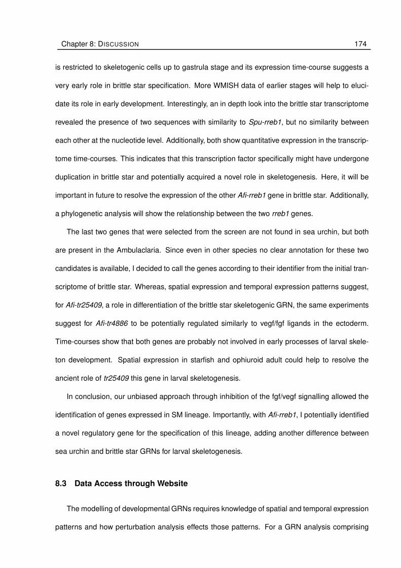
Chapter 8: DISCUSSION 174
is restricted to skeletogenic cells up to gastrula stage and its expression time-course suggests a
very early role in brittle star specification. More WMISH data of earlier stages will help to eluci-
date its role in early development. Interestingly, an in depth look into the brittle star transcriptome
revealed the presence of two sequences with similarity to Spu-rreb1, but no similarity between
each other at the nucleotide level. Additionally, both show quantitative expression in the transcrip-
tome time-courses. This indicates that this transcription factor specifically might have undergone
duplication in brittle star and potentially acquired a novel role in skeletogenesis. Here, it will be
important in future to resolve the expression of the other Afi-rreb1 gene in brittle star. Additionally,
a phylogenetic analysis will show the relationship between the two rreb1 genes.
The last two genes that were selected from the screen are not found in sea urchin, but both
are present in the Ambulaclaria. Since even in other species no clear annotation for these two
candidates is available, I decided to call the genes according to their identifier from the initial tran-
scriptome of brittle star. Whereas, spatial expression and temporal expression patterns suggest,
for Afi-tr25409, a role in differentiation of the brittle star skeletogenic GRN, the same experiments
suggest for Afi-tr4886 to be potentially regulated similarly to vegf/fgf ligands in the ectoderm.
Time-courses show that both genes are probably not involved in early processes of larval skele-
ton development. Spatial expression in starfish and ophiuroid adult could help to resolve the
ancient role of tr25409 this gene in larval skeletogenesis.
In conclusion, our unbiased approach through inhibition of the fgf/vegf signalling allowed the
identification of genes expressed in SM lineage. Importantly, with Afi-rreb1, I potentially identified
a novel regulatory gene for the specification of this lineage, adding another difference between
sea urchin and brittle star GRNs for larval skeletogenesis.
8.3 Data Access through Website
The modelling of developmental GRNs requires knowledge of spatial and temporal expression
patterns and how perturbation analysis effects those patterns. For a GRN analysis comprising

Chapter 8: DISCUSSION 175
B
C D
A
Figure 8.1: R-shiny web application allows access to all transcriptomic and spatial data
presented in this thesis. (A) Layout of the webpage. (B) Example for access to WMISH data.
(C) Example for access to time-course data. (D) Example for access to differential expression
data.

Chapter 8: DISCUSSION 176
a few genes, the integration of such is a relatively simple task. In a systems biology perspec-
tive, however, where hundreds or thousands of genes are considered simultaneously, it is easy
to lose track of the important details of few or single genes. This is especially when working
on novel systems with little to no access to the established data. Thus, I developed a website
using R-shiny that allows to query different type of information (Figure 8.1), similar to (Tu et al.,
2014). Using the statistical programming language R as the backbone, my website provides a
platform to easily query and find genes of interest. It gives access to annotations, expression
levels, sequence information, differential screening and spatial expression patterns. Contigs can
be queried by annotation, expression cluster id, contig id and additionally by gene ontology class.
Thus, for example one can easily access all transcription factors sequences and their expression
temporarily and spatially (when available). Moreover, the website is programmed in a way that
extension of spatial expression patterns is created by adding a folder with the contig id and the
individual pictures as JPEG files. In future work, this website will be extended with the regenera-
tion data produced in our laboratory and will thus create a unique resource to establish the brittle
star Amphiura filiformis as developmental and regenerative model system.

Chapter 9
CONCLUSION
Although many studies have investigated the GRNs for mesoderm formation in echinoderms and
especially larval skeletogenesis, so far no systematic study of brittle stars has been available. In
this thesis I introduce the brittle star Amphiura filiformis as novel model system to study larval
skeleton evolution in echinoderms and more specifically mechanisms of evolution of the animal
body plan. I demonstrate, consistent with my initial hypothesis (see chapter 2) that two different
GRNs underlie development of the larval skeleton. My genomic/transcriptomic comparison sug-
gests that the gene content for skeleton formation in echinoderms is highly conserved, laying the
foundation for the identification of an ancient module responsible for the synapomorphic character
of echinoderms: the adult bio-mineralised skeleton. Furthermore, my in-depth characterisation of
the SM regulatory state suggests that wiring between the genes involved in skeletogenic meso-
derm (SM) specification shows several differences. Consistent with the hourglass theory (von
Bear, 1828), the initiation tier of the larval skeleton GRN is not conserved between brittle star
and sea urchin. Differences are found in: maternal initiation through Afi-wnt8 and Afi-blimp1, the
double negative gate and fate-exclusion by repression of Afi-gcm by Afi-alx1. On the other hand,
the middle part of the GRN is largely similar: expression patterns of tgif, hex, and erg suggest a
conserved sub-circuit across the Eleutherozoa. In addition expression pattern analysis indicate
that vegf/fgf signalling is an essential and conserved part of the skeletogenic GRN. Finally, the
tier directly before the differentiation cascade is quite different. The two drivers of skeletogenic
differentiation genes Afi-foxB and Afi-dri are not expressed in the skeletogenic mesoderm lineage
177

Chapter 9: CONCLUSION 178
Eleutherozoa
~480 Myapmar1 as repressor of hesC
Co-expression of hesC, ets, tbr, delta
foxB
dri
alx, ets1/2 and jun
~250 Mya
Euechinoidea
(S. purpuratus)Cidaroidea
(P. baculosa)
Holothuroidea
(P. parvimensis)
Ophiuroidea
(A. filiformis)
Asteroidea
(P. miniata)
Spicule matrix genes
msp130, cara, p19
494 core skeletogenic genes
vegfR, fgfR2
rreb1
Specification
Differentiation
tr25904
alx1 repression of gcm
erg, tgif, hex interlocking loop
present in ske cellsabsent in ske cellspresent in mesoderm cellsabsent in mesoderm cells
Legend
Figure 9.1: Molecular characteristics of skeleton development mapped in Eleutherozoa.
On top are images of adults and below corresponding larvae. In light blue are the skeletogenic
features of each larva. Boxes represent the molecular characters. Surrounded by a grey box
are characters involved in the specification part of the GRNs (i.e. regulatory genes). Surrounded
by a green box are genes in the differentiation part of the GRN. For branches lacking boxes no
data was available. Branch for asteroids shows rounded boxes due to the lack of a SM lineage.
The cladogram represents the currently best supported phylogeny (Telford et al., 2014; O’Hara
et al., 2014; Cannon et al., 2014). Molecular data collected along the tree are based on the
observations in this study and in other studies (Oliveri et al., 2008; McCauley et al., 2012, 2010;
Gao and Davidson, 2008; Czarkwiani et al., 2013; Yamazaki et al., 2014; Rottinger et al., 2008;
Duloquin et al., 2007; Adomako-Ankomah and Ettensohn, 2013; Seaver and Livingston, 2015;
Livingston et al., 2006).

Chapter 9: CONCLUSION 179
in the brittle star. Additionally, a novel skeletogenic gene Afi-rreb1 has been identified and might
be specific for brittle star SM lineage specification. From a GRN prospective, 480Mya of indepen-
dent evolution were sufficient to accumulate various differences with different mechanisms. Gene
duplication was used to expand the gene repertoire in sea urchin of pmar1, sm, and msp130
genes. Additionally, protein function diversification was employed for the ortholog to sea urchin
Spu-pmar1, Afi-pplx, in terms that it lacks two domains that are responsible for its repressive ac-
tion. Finally, the presence and absence of genes in the SM lineage hints towards DNA binding
motif evolution and is shown by the differences in expression pattern of the genes foxB, dri, rreb,
and nk7 between sea urchin and brittle star. In summary, in 480Mya of evolution all types of
mechanisms are used for GRN diversification.
My second hypothesis (see chapter 2) relates to the question of how the larval skeleton
evolved in echinoderms. As discussed in chapter 5 my observations strongly support the in-
dependent co-option of the larval skeleton in ophiuroids and echinoids, based on the differences
of which and how specification genes are employed in the SM lineage throughout sea urchin
and brittle star development, as described above. On the other the transcriptomic comparison
in Part II showed many commonalities even with crinoids thus pointing towards an ancestral co-
option event at the base of the Eleutherozoa. Nevertheless, while my project greatly increased
the knowledge to address this question, more studies in holothuroids and asteroids are needed
in order to undoubtedly resolve how the larval skeleton evolved in this phylum. For this several
experiments have to be performed. Firstly, it would be important to reconstruct the ancestral
regulatory state for the SM lineages of larvae and adult. A comparison between the adult and
larval GRNs could help to pinpoint the true ancestral part of the GRN and the co-opted elements,
and therefore clarify which genes are expressed only during larval development. Moreover, which
genes are actually part of an early mesoderm specification mechanism versus pan-skeletogenic
genes. One example of such, is the gene alx1, which is restricted to SM lineage in echinoids,
holothuroids and ophiuroids but expressed in all mesoderm in asteroids during embryonic devel-

Chapter 9: CONCLUSION 180
opment. Therefore, either alx1 is a pan-mesodermal gene and got specifically restricted to the
SM lineage during the co-option event, and its ancestral state would be represented by the as-
teroid as hypothesised by McCauley et al. (2012), or as being part an adult ancestral ske-GRN
was part of the co-opted genes and represents a vestige in the asteroid. Indeed data show that
in both, adult and embryo, it is one of the first markers of skeletogenic cells (Gao and Davidson,
2008; Czarkwiani et al., 2013). For this gene, a cis-regulatory analysis in sea urchin and star fish
would reveal the necessary changes to be employed into the SM lineage. As seen in the phylo-
genetic tree in Figure 9.1, many other studies in the holothurian and asteroidian branches could
give further support for independent or derived evolution. The presence and absence of foxB and
dri in holothuroids, asteroids and cidaroids could resolve whether the inclusion of these genes
into the skeletogenic GRN is a synapomorphy of euechinoids alone. Additionally, an investigation
of FGF/VEGF signalling in holothuroids would show whether the positioning of the SM lineage in
this branch is guided by the same mechanism. Especially, more transcriptomic and genomic data
is needed in this branch of echinoderms.
In conclusion, my study establishes the brittle star Amphiura filiformis as a key developmental
system for a detailed comparative analysis of the gene regulatory networks acting in skeletogenic
lineages in distantly related echinoderms. My work not only brings new evidence to a long-
debated issue on the evolutionary origin of echinoderm larval skeleton, but also clarifies specific
mechanisms of GRN diversification, which sees not only the evolution of cis-regulatory elements,
but also gene duplication, and protein function diversification as equally important mechanisms.

Appendix A
PART I
Table A.1: Degenerate primers for cloning
Gene Name DEG Primer Seq
Afi-alx1 F: AAYCGNACNACNTTYACNTCNTAY
R: RAANGCYTCNCGYTTNCGCCAYTT
Afi-ets1/2 F: GGNTCNGGNCCNATHCARCTNTGG
R: RTCRCANACRAANCGRTANACRTA
Afi-foxB F: AAYACNCARMGNTGGCARAAY
R: GATGATRTTYTCGATRGTGAA
Afi-tbr F: ATHACNAARCARGGNMGRMGRATG
R: RTCRTARTTRTCYCKRAANCCYTT
Afi-dri F: ACNTTYGARGARCARTTYAA
R: RTCDATNGCNGCYTGNAGYTC
181

Appendix A: PART I 182
Table A.2: Primers for cloning
Gene Or. Sequene Length GenBank
Afi-alx1 F Czarkwiani et al 2013 634bp KC788414
R
Afi-jun 5O ACCATGGACGGATCAAACAT 429bp KM816839
5I GCCATTTAGCTCTGCGATTT
Afi-p19 3O TCGCATAGGTCTTGGGAAAC 697bp KM816840
3I CCCTCCAACAGACCAAGAAA
Afi-pplx F GCTTCGTGAGAAAGCGATGC 799bp KM816841
R TAGCTTGGCAAGTTCACGGG
Afi-pplx F GCTCCAACGAGAGCGAA 948bp KM816841
R TCAAAACTTGGGTACACTGCAGATGG
Afi-hesC 3O TGTTTCCTGGAAGCTGTGTG 1414bp KM816842
3I CATTGTCTTTGCCCTTGTT
Afi-delta F TGCAACGGATCAGGCTCAAT 2156bp KM816843
R GGCGATGAGTCCGGTGTATT
Afi-ets1/2 F Czarkwiani et al 2013 671bp KC788415
R
Afi-tbr F Czarkwiani et al 2013 1127bp KC788418
R
Afi-erg F GCGCATCGTGGTCAAATACC 2149bp KM816844
R GCTTGACGCAACTTGGGAAG
Afi-hex F TTGTCAAGTGGGCAGTTCGT 1243bp KM816845
R CTTTGGCACAACAGCACTGG
Afi-tgif F TCGCCAAAGCTAGCTGTCAA 1305bp KM816846
R CCGAGTCTGACTTCAGCTTCAT
Afi-dri 5O GTCTTCCCTCACGACGATTG 1482bp KM816847
5I CTCACGACGATTGCCATCTA
Afi-foxB F Czarkwiani et al 2013 424bp KC788416
R
Afi-gataC F Czarkwiani et al 2013 1021bp KC788417
R
Afi-gataE F TCAATTCAACTGGAGATAGCGC 1736bp KM816848
R GAGAGTTGCCGATGTGTGTC
Afi-gcm F TCTCTGCGACAAATCCTGCC 1156bp KM816849
R CTCATCGCGCTTGTATTGCT
Afi-phb1 F CAACCAACCAAAGCTGAGCC 910bp KM816850
R TGGAGGAGCAGATGTCTTGG
Afi-foxA F CCGGCTGAGTTCTCGAGTTT 1788bp KM816851
R TTGTTTGCGCTGTGGCTAAC
Afi-soxC F CGTGTCAATGGCAAGCTAGA
R GGGACACGTTCTGGAGTCTG
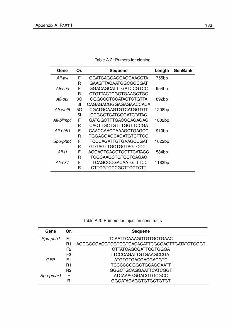
Appendix A: PART I 183
Table A.2: Primers for cloning
Gene Or. Sequene Length GenBank
Afi-twi F GGATCAGGAGCAGCAACCTA 755bp
R GAAGTTACAATGGCGGCGAT
Afi-sna F GGACAGCATTTGATCCGTCC 954bp
R CTGTTACTCGGTGAAGCTGC
Afi-otx 3O GGGCCCTCCATACTCTGTTA 892bp
3I CAGAGACGGGAGAGAACCACA
Afi-wnt8 5O CGATGCAAGTGTCATGGTGT 1208bp
5I CCGCGTCATCGGATCTATAC
Afi-blimp1 F GATGGCTTTGACGCAGAGAG 1802bp
R CACTTGCTGTTTGGTTCCGA
Afi-phb1 F CAACCAACCAAAGCTGAGCC 910bp
R TGGAGGAGCAGATGTCTTGG
Spu-phb1 F TCCCAGATTGTGAAGCCGAT 1022bp
R GTGAGTTGCTGGTAGTCCCT
Afi-l1 F AGCAGTCAGCTGCTTCATACC 584bp
R TGGCAAGCTGTCCTCAGAC
Afi-nk7 F TTCAGCCCGACAATGTTTCC 1183bp
R CTTCGTCCCGCTTCCTCTT
Table A.3: Primers for injection constructs
Gene Or. Sequene
Spu-phb1 F1 TCAATTCAAAGGTGTGCTGAAC
R1 AGCGGCGACGTCGTCGTCACACATTCGCGAGTTGATATCTGGGT
F2 GTTATCAGCGATTCGTGGGA
F3 TTCCCAGATTGTGAAGCCGAT
GFP F1 ATGTGTGACGACGACGTC
R1 TCCCCCGGGCTGCAGGAATT
R2 GGGCTGCAGGAATTCATCGGT
Spu-pmar1 F ATCAAAGGGACGTGCGCC
R GGGATAGAGGTGTGCTGTGT
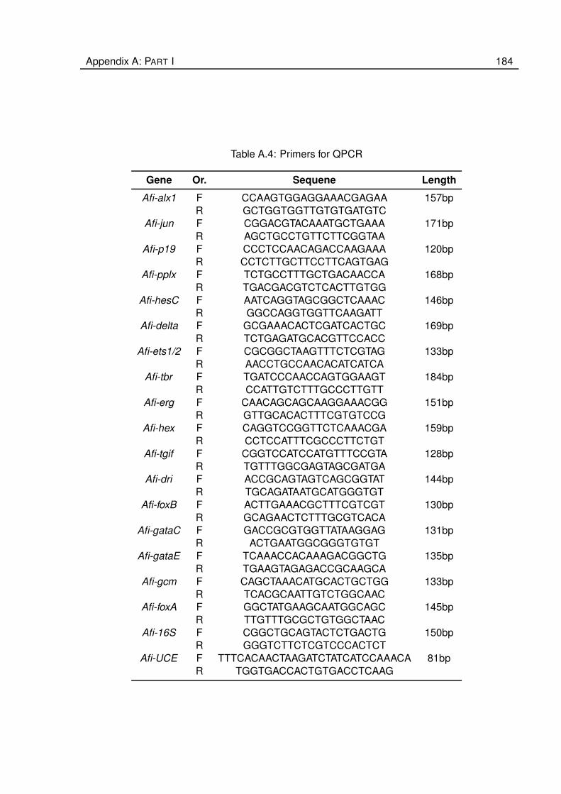
Appendix A: PART I 184
Table A.4: Primers for QPCR
Gene Or. Sequene Length
Afi-alx1 F CCAAGTGGAGGAAACGAGAA 157bp
R GCTGGTGGTTGTGTGATGTC
Afi-jun F CGGACGTACAAATGCTGAAA 171bp
R AGCTGCCTGTTCTTCGGTAA
Afi-p19 F CCCTCCAACAGACCAAGAAA 120bp
R CCTCTTGCTTCCTTCAGTGAG
Afi-pplx F TCTGCCTTTGCTGACAACCA 168bp
R TGACGACGTCTCACTTGTGG
Afi-hesC F AATCAGGTAGCGGCTCAAAC 146bp
R GGCCAGGTGGTTCAAGATT
Afi-delta F GCGAAACACTCGATCACTGC 169bp
R TCTGAGATGCACGTTCCACC
Afi-ets1/2 F CGCGGCTAAGTTTCTCGTAG 133bp
R AACCTGCCAACACATCATCA
Afi-tbr F TGATCCCAACCAGTGGAAGT 184bp
R CCATTGTCTTTGCCCTTGTT
Afi-erg F CAACAGCAGCAAGGAAACGG 151bp
R GTTGCACACTTTCGTGTCCG
Afi-hex F CAGGTCCGGTTCTCAAACGA 159bp
R CCTCCATTTCGCCCTTCTGT
Afi-tgif F CGGTCCATCCATGTTTCCGTA 128bp
R TGTTTGGCGAGTAGCGATGA
Afi-dri F ACCGCAGTAGTCAGCGGTAT 144bp
R TGCAGATAATGCATGGGTGT
Afi-foxB F ACTTGAAACGCTTTCGTCGT 130bp
R GCAGAACTCTTTGCGTCACA
Afi-gataC F GACCGCGTGGTTATAAGGAG 131bp
R ACTGAATGGCGGGTGTGT
Afi-gataE F TCAAACCACAAAGACGGCTG 135bp
R TGAAGTAGAGACCGCAAGCA
Afi-gcm F CAGCTAAACATGCACTGCTGG 133bp
R TCACGCAATTGTCTGGCAAC
Afi-foxA F GGCTATGAAGCAATGGCAGC 145bp
R TTGTTTGCGCTGTGGCTAAC
Afi-16S F CGGCTGCAGTACTCTGACTG 150bp
R GGGTCTTCTCGTCCCACTCT
Afi-UCE F TTTCACAACTAAGATCTATCATCCAAACA 81bp
R TGGTGACCACTGTGACCTCAAG

Ap
pe
nd
ixA
:P
AR
TI
18
5
Table A.5: Sequence information
Name tblastx rec. blast OMA Phylogeny Transcirptome ID Spu ID Note
evalue/score/pident
Afi-wnt8 2e-90/208/50% Yes Yes No AfiCDS.id55172.tr11092 SPU 020371-Sp-Wnt8-WHL22.8923
Afi-otx 8e-35/147/82% Yes No No AfiCDS.id6059.tr24500 SPU 010424-Sp-Otx-WHL22.532435
Afi-blimp1 1e-137/281/76% Yes No No AfiCDS.id25396.tr42615 SPU 027235-Sp-Blimp1-WHL22.5073
Afi-pplx 9e-13/73/58% Yes No Yes AfiCDS.id36883.tr33539 SPU 015828-Sp-Pmar1c-WHL22.462256
Afi-alx1 2e-69/153/89% Yes Yes No AfiCDS.id52740.tr55899 SPU 022817-Sp-Alx1 1-WHL22.731056
Afi-jun 2e-90/193/90% Yes Yes No AfiCDS.id55428.tr60572 SPU 003102-Sp-Jun-WHL22.318085
Afi-p19 2e-12/72/42% Yes Yes No AfiCDS.id6273.tr13385 SPU 004135-Sp-Cah10L-WHL22.642603
Afi-hesC 1e-44/112/72% Yes Yes No AfiCDS.id79437.tr59210 SPU 021608-Sp-HesC-WHL22.235339
Afi-foxA 1e-109/303/84% Yes Yes No AfiCDS.id85717.tr16742 SPU 006676-Sp-FoxA-WHL22.439762
Afi-gataC 1e-73/159/79% Yes Yes No AfiCDS.id61260.tr63157 SPU 027015-Sp-GataC-WHL22.660411
Afi-gataE 8e-77/269/88% Yes No No AfiCDS.id38615.tr1992 SPU 010635-Sp-Gatae-WHL22.78013
Afi-gcm 2e-48/170/69% Yes No No AfiCDS.id38146.tr47389 SPU 006462-Sp-Gcm-WHL22.54333
Afi-erg 1e-171/342/87% Yes Yes No AfiCDS.id64071.tr2242 SPU 018483-Sp-Erg-WHL22.552472
Afi-ets1/2 0/323/99% Yes Yes No AfiCDS.id20811.tr66263 SPU 002874-Sp-Ets1/2-WHL22.238821
Afi-tbr 1e-109/394/73% Yes No No AfiCDS.id43541.tr66231 SPU 025584-Sp-Tbr-WHL22.503644
Afi-hex 6e-53/188/97% Yes No No AfiCDS.id81692.tr22161 SPU 027214-none-WHL22.626418 SPU 027214 = SPU 027215
Afi-tgif 6e-44/171/85% Yes No No AfiCDS.id49825.tr1310 SPU 018126-Sp-Tgif-WHL22.614286
Afi-foxB 1e-91/325/93% Yes Yes No AfiCDS.id1937.tr11127 SPU 004551-Sp-FoxB-WHL22.743430
Afi-dri 6e-48/114/70% Yes No No AfiCDS.id16344.tr60844 SPU 005718-Sp-Dri 2-WHL22.544150
Afi-soxC 1e-105/232/83% Yes Yes No AfiCDS.id33804.tr61034 SPU 002603-Sp-SoxC-WHL22.622787
Afi-twi 8e-56/215/87% Yes No No AfiCDS.id89079.tr60007 SPU 030059-Sp-Twi-WHL22.118674
Afi-sna 2e-90/321/82% Yes Yes No AfiCDS.id32534.tr38806 SPU 001113-Sp-Sna-WHL22.131363
Afi-nk7 2e-58/191/76% Yes No No AfiCDS.id63655.tr58557 SPU 022573-Sp-Nk7-WHL22.567485
Afi-l1 1e-147/99/34% Yes Yes No AfiCDS.id37274.tr11372 SPU 000125-none-WHL22.236839 SPU 000125 = SPU 021428

Ap
pe
nd
ixA
:P
AR
TI
18
6
Table A.6: Time-courses
Gene 0hpf 3hpf 6hpf 9hpf 12hpf 15hpf 18hpf 21hpf 24hpf 27hpf 30hpf 33hpf 36hpf 39hpf 42hpf
Afi-alx1 0 0 0 3 63 67 101 165 141 100 79 122 88 68 60
Afi-p19 0 0 0 4 66 199 479 1084 907 1216 1578 2281 2078 1603 1597
Afi-jun 1143 830 1614 487 690 476 1072 1993 1370 695 1789 1385 992 1204 1866
Afi-pplx 9 11 50 233 482 206 143 127 22 15 43 27 19 13 17
Afi-hesC 44 15 4 3 21 12 36 42 41 27 76 168 NA NA NA
Afi-ets12 1686 3396 3215 2455 2250 979 1130 1972 1887 1694 2128 5158 3466 2882 3392
Afi-tbr 36 43 33 14 48 132 305 805 993 673 1447 1292 NA NA NA
Afi-delta 75 95 64 72 313 265 209 201 148 148 204 429 343 214 250
Afi-tgif 89 283 0 125 461 359 309 545 476 348 1358 1170 1145 627 1098
Afi-erg 14 20 31 53 138 120 428 592 625 312 625 737 614 458 573
Afi-hex 5 7 4 4 75 108 379 852 659 610 923 1531 930 775 894
Afi-dri 1 1 1 0 0 5 19 26 34 28 25 21 49 51 39
Afi-foxB 0 0 0 0 0 1 2 37 12 15 81 145 174 124 220
Afi-gcm 3 5 6 27 24 7 12 7 11 13 21 15 11 7 22
Afi-gataC 0 0 1 1 1 4 3 24 47 67 105 145 82 52 40
Afi-gataE 1 12 12 7 17 13 23 117 81 157 376 740 1130 861 1057
Afi-foxA 1 6 8 4 11 41 233 980 1152 790 2315 3888 3043 2914 4248
Afi-otx 528 1340 1049 728 926 477 984 1696 2143 1093 2989 2128 NA NA NA
Afi-phb1 0 0 7 57 537 649 842 698 595 355 797 1124 913 609 663
Afi-wnt8 0 2 28 137 281 147 178 144 97 62 109 61 51 80 55

Appendix B
PART II
187

Ap
pe
nd
ixB
:P
AR
TII
18
8
Table B.1: Adapter sequences
Adapter Sequence Sample
TruSeq Universal AATGATACGGCGACCACCGAGATCTACACTCTTTCCCTACACGACGCTCTTCCGATCT 9hr, 18hr, 27hr, 27hr-
DMSO, 27hr-SU, 39hr
MultiplexingA GATCGGAAGAGCACACGTCT 9hr, 18hr, 27hr, 27hr-
DMSO, 27hr-SU, 39hr
MultiplexingR GATCGGAAGAGCACACGTCTGAACTCCAGTCAC 9hr, 18hr, 27hr, 27hr-
DMSO, 27hr-SU, 39hr
TruSeq Adapter 2 GATCGGAAGAGCACACGTCTGAACTCCAGTCACCGATGTATCTCGTATGCCGTCTTCTGCTTG 9hr
FastQC Identified CTCCTATTTATTTCCTCAAAAAAAAGCTATCACAAAACTCGAAAAGCATA 9hr
TruSeq Adapter 4 GATCGGAAGAGCACACGTCTGAACTCCAGTCACTGACCAATCTCGTATGCCGTCTTCTGCTTG 18hr, 27hr
FastQC Identified CTCCTATTTATTTCCTCAAAAAAAAGCTATCACAAAACTCGAAAAGCATA 18hr, 27hr-DMSO,
27hr-SU, 39hr
FastQC Identified CCCTCTTTCAAAAGTCCTTTCGTACAAGAAGAAATTTTAAGGAAGTAGAT 18hr, 27hr-DMSO,
27hr-SU
FastQC Identified CAAAAACAACGCCTTCGGATTTTGATCGTAAGGTTCTGCCTGCCCGGTGA 18hr
FastQC Identified CTCCTATTTATTTCCTCAAAAAAAAGCTATCACAAAACTCGAAAAGCATA 27hr
TruSeq Adapter 5 GATCGGAAGAGCACACGTCTGAACTCCAGTCACACAGTGATCTCGTATGCCGTCTTCTGCTTG 27hr
TruSeq Adapter 6 GATCGGAAGAGCACACGTCTGAACTCCAGTCACGCCAATATCTCGTATGCCGTCTTCTGCTTG 27hr-DMSO
TruSeq Adapter 7 GATCGGAAGAGCACACGTCTGAACTCCAGTCACCAGATCATCTCGTATGCCGTCTTCTGCTTG 27hr-SU
TruSeq Adapter 12 GATCGGAAGAGCACACGTCTGAACTCCAGTCACCTTGTAATCTCGTATGCCGTCTTCTGCTTG 39hr

Appendix B: PART II 189
Table B.2: Contig statistics for individual assemblies
Sample N25 N50 N75 Longest Mean Median Shortest Contigs
09hr 2,203 1,146 559 21,167 765 463 201 285,536
18hr 2,314 935 395 16,924 627 343 201 179,679
27hr FSW 2,530 1,345 626 20,576 835 482 201 314,188
27hr DMSO 2,594 1,352 632 22,055 842 486 201 292,331
27hr SU 2,408 1,258 585 20,474 796 461 201 334,802
36hr 2,234 1,120 536 20,535 747 445 201 359,728
Table B.3: Subclasses for bio-mineralisation gene ontology
Subclasses Afi Pmi Ame Spu
Carbonic Anhydrase 3 3 3 3
Collagen 10 15 9 15
Cyclophilin 7 7 9 11
MSP130 2 3 4 9
Spicule Matrix 1 5 1 14
Other 0 1 0 4
Total 23 34 26 56

Ap
pe
nd
ixB
:P
AR
TII
19
0
Table B.4: Contig statistics
WHL ID Reason for exclusion Notes
WHL22.609261 408b only homolog
WHL22.117376 321bp only homolog
WHL22.714669 456bp ortholog but deeper analysis shows that is artefact
WHL22.632079 not strong enough expressed to be part of EC
WHL22.437349 not strong enough expressed to be part of EC
WHL22.585512 recent gene duplication (see SPU scaffold:551)
WHL22.568711 not strong enough expressed to be part of EC
WHL22.486796 327bp only homolog part of cluster with more individuals that belong to WHL22.82981
WHL22.485384 not strong enough expressed to be part of EC
WHL22.15174 not strong enough expressed to be part of EC
WHL22.40034 ¡450bp part of cluster with more individuals that belong to WHL22.622033
WHL22.636100 algorithm chose WHL22.674225 instead with same probility mistake in sea urchin transcirptome are actually both the same transcript
WHL22.635901 algorithm chose WHL22.310280 instead with same probility
WHL22.608861 algorithm chose WHL22.608876 instead with same probility are actually the same gene one transcript however is not part of the GO table
WHL22.496011 not strong enough expressed to be part of EC

Appendix B: PART II 191
Table B.5: Naming SU5402 QPCR experiment
Name ID Expression Cluster Annotation
Afi-egfiL 2 AfiCDS.id85082.tr39719 Cluster-25982.2 SPU 003872-Sp-EgfiL 2-WHL22.289903.3
Afi-tropmyh AfiCDS.id21782.tr976 Cluster-18373.0 SPU 015849-Sp-Tropmyh-WHL22.432759.1
Afi-alx/arx AfiCDS.id68561.tr6658 Cluster-30632.0 SPU 030703-none-WHL22.490216.0
Afi-vegf2 AfiCDS.id11730.tr8523 Cluster-7997.0 SPU 005737-Sp-Vegf2-WHL22.194484.0
Afi-tacr2L AfiCDS.id92119.tr44548 Cluster-15622.0 SPU 010179-Sp-Tacr2L 1-WHL22.581307.0
Afi-fn3/igf 29 AfiCDS.id62424.tr60943 Cluster-4641.0 SPU 004746-Sp-Fn3/Igf 29-WHL22.147868.1
AfiCDS.id81632.tr60441 AfiCDS.id81632.tr60441 Cluster-11727.4
Afi-ttrspn 19 AfiCDS.id30755.tr5407 Cluster-31209.0 SPU 025068-Sp-Ttrspn 19-WHL22.748368.1
Afi-e2f7 AfiCDS.id13713.tr42693 Cluster-17970.0 SPU 023346-Sp-E2f7-WHL22.755786.0
Afi-slc4a10 AfiCDS.id61902.tr45342 Cluster-7256.0 SPU 025515-Sp-Slc4a10-WHL22.12691.2
Afi-p58-a AfiCDS.id40036.tr13789 Cluster-3715.1 SPU 000439-Sp-p58-a-WHL22.23776.0
Afi-αcoll AfiCDS.id28173.tr18060 Cluster-21780.0 SPU 026008-Sp-FcolI/II/IIIf-WHL22.541149.0
Afi-p58-b AfiCDS.id28024.tr11245 Cluster-3715.0 SPU 000438-Sp-p58-b-WHL22.23620.0
AfiCDS.id384.tr29965 AfiCDS.id384.tr29965 Cluster-10558.1
Afi-sept4 AfiCDS.id4418.tr33430 Cluster-5808.0 SPU 003696-Sp-Sept4-WHL22.624760.0
Afi-mt6 mmpL AfiCDS.id21881.tr9218 Cluster-16461.0 SPU 005576-Sp-Mt6 mmpL-WHL22.35130.0
AfiCDS.id10236.tr3203 AfiCDS.id10236.tr3203 Cluster-28643.1 SPU 005576-Sp-Mt6 mmpL-WHL22.35130.0
Afi-spcat3l AfiCDS.id57192.tr60565 Cluster-5917.0 SPU 001545-Sp-Spcat3l-WHL22.670777.0
Afi fn3/egff 1 AfiCDS.id3884.tr60838 Cluster-17570.0 SPU 011180-Sp-Fn3/Egff 1-WHL22.516341.0
Afi-soxD1 AfiCDS.id37686.tr6742 Cluster-13113.1 SPU 004217-Sp-SoxD1-WHL22.118185.2
Afi-vegfR AfiCDS.id52869.tr20202 Cluster-23512.1 SPU 000310-Sp-Pdgfr/vegfrL-WHL22.240520.0
AfiCDS.id52181.tr20375 AfiCDS.id52181.tr20375 Cluster-4513.0
AfiCDS.id41059.tr61404 AfiCDS.id41059.tr61404 Cluster-18217.0 SPU 009642-Sp-Rreb1-WHL22.421612.0
Afi-a2m 1 AfiCDS.id66422.tr18763 Cluster-16526.0 SPU 025922-Sp-A2m 1-WHL22.306546.0
Afi-hypp 2281 AfiCDS.id89402.tr3094 Cluster-2493.0 SPU 016833-Sp-Hypp 2281-WHL22.347032.0
Afi-cara7LA AfiCDS.id10597.tr30892 Cluster-20452.0 SPU 012518-Sp-Cara7LA-WHL22.446073.1
Afi-erg AfiCDS.id90393.tr2237 Cluster-29925.0 SPU 018483-Sp-Erg-WHL22.552472.1
AfiCDS.id84973.tr13659 AfiCDS.id84973.tr13659 Cluster-12844.62
Afi-009748 AfiCDS.id65088.tr20037 Cluster-15262.0 SPU 009748-none-WHL22.397555.0
Afi-msp130L AfiCDS.id75849.tr3754 Cluster-27881.0 BEFORE SEA URCHIN GENOME UPDATE
Afi-tr25409 AfiCDS.id88683.tr31926 Cluster-1517.1
Afi-tr4886 AfiCDS.id5647.tr1291 Cluster-7020.0
Afi-kirrelL AfiCDS.id74191.tr58590 Cluster-720.0 SPU 024995-Sp-KirrelL-WHL22.699052.0
AfiCDS.id44038.tr10735 AfiCDS.id44038.tr10735 Cluster-25746.0
Afi-tle1/groucho AfiCDS.id4947.tr10732 Cluster-22948.0 SPU 017807-Sp-Tle1/Groucho-WHL22.510742.0
Afi-77kDamaps AfiCDS.id4682.tr16558 Cluster-25122.0 SPU 005744-Sp-77kDamaps-WHL22.325883.0
Afi-0914236 AfiCDS.id31785.tr21 Cluster-20113.3 SPU 014236-none-WHL22.470491.3
AfiCDS.id58703.tr6207 AfiCDS.id58703.tr6207 Cluster-17600.0
Afi-018662 AfiCDS.id61413.tr281 Cluster-26614.0 SPU 018662-none-WHL22.220192.0
AfiCDS.id48303.tr39358 AfiCDS.id48303.tr39358 Cluster-12844.127 NA-NA-WHL22.470012.13
Afi-cebpa AfiCDS.id63703.tr20911 Cluster-7531.0 SPU 001657-Sp-Cebpa-WHL22.255599.0
Afi-tr4886 AfiCDS.id70646.tr9107 Cluster-23056.1
Afi-004896 AfiCDS.id29222.tr34323 Cluster-1541.0 SPU 004896-none-WHL22.381788.2
Afi-trim2 1 AfiCDS.id8707.tr37166 Cluster-1364.0 SPU 007912-Sp-Trim2 1-WHL22.742590.0
Afi-fbn2L 1 AfiCDS.id12160.tr20206 Cluster-30786.1 SPU 008613-Sp-Fbn2L 1-WHL22.324858.1
AfiCDS.id64819.tr39976 AfiCDS.id64819.tr39976 Cluster-30937.0 NA-NA-WHL22.699079.0
AfiCDS.id4578.tr38894 AfiCDS.id4578.tr38894 Cluster-15464.0 SPU 009708-Sp-Trim2-WHL22.300164.0
Afi-egr AfiCDS.id86638.tr27818 Cluster-13125.0 SPU 015358-Sp-Egr-WHL22.280477.0
AfiCDS.id53027.tr45279 AfiCDS.id53027.tr45279 Cluster-4270.0
Afi-trim2-2 AfiCDS.id28262.tr65992 Cluster-2571.0 SPU 006071-Sp-Trim2-2-WHL22.674919.0
Afi-dcst2-3 AfiCDS.id51828.tr30296 Cluster-672.0 SPU 005390-Sp-Dcst2-3-WHL22.60281.0
Afi-dusp1 AfiCDS.id48508.tr53384 Cluster-24220.0 SPU 021143-Sp-Dusp1-WHL22.221547.1
Afi-rreb1 AfiCDS.id62604.tr47807 Cluster-13724.0 SPU 009642-Sp-Rreb1-WHL22.421612.0
Afi-mad AfiCDS.id51560.tr55093 Cluster-22670.0 SPU 006583-Sp-Mad-WHL22.80541.0
AfiCDS.id43930.tr1339 AfiCDS.id43930.tr1339 Cluster-14335.0 NA-NA-WHL22.476817.0
Afi-trim2 AfiCDS.id537.tr30881 Cluster-1215.0 SPU 009708-Sp-Trim2-WHL22.300164.0
AfiCDS.id75617.tr19326 AfiCDS.id75617.tr19326 Cluster-15634.0
AfiCDS.id5605.tr49815 AfiCDS.id5605.tr49815 Cluster-24029.0 NA-NA-WHL22.110836.1
AfiCDS.id4513.tr62663 AfiCDS.id4513.tr62663 Cluster-5507.0
Afi-018426 AfiCDS.id76901.tr2369 Cluster-1724.0 SPU 018426-none-WHL22.372181.0
Afi-colf 3 AfiCDS.id53870.tr61382 Cluster-25105.0 SPU 011736-Sp-Colf 3-WHL22.97140.0
AfiCDS.id59305.tr68751 AfiCDS.id59305.tr68751 Cluster-21880.0
Afi-gldc AfiCDS.id77794.tr828 Cluster-17333.2 SPU 027673-Sp-Gldc-WHL22.765838.1
Afi-mt14/mmpl7 AfiCDS.id40247.tr45766 Cluster-3261.0 SPU 028748-Sp-Mt1-4/MmpL7-WHL22.312033.0
Afi-sr/fu/igr AfiCDS.id35420.tr36288 Cluster-28510.0 SPU 006068-Sp-Sr/Fu/Igr-WHL22.362474.1
Afi-agrnL AfiCDS.id36042.tr36266 Cluster-27739.0 SPU 017586-Sp-AgrnL-WHL22.218450.1
AfiCDS.id63133.tr10933 AfiCDS.id63133.tr10933 Cluster-13564.0 NA-NA-WHL22.555967.0
Afi-tcep1 AfiCDS.id1705.tr9893 Cluster-11257.0 SPU 006406-Sp-Tecp1-WHL22.573138.0
Afi-msp130r6 AfiCDS.id80760.tr10976 Cluster-7482.0 SPU 014492-Sp-Msp130r6-WHL22.405717.2

Ap
pe
nd
ixB
:P
AR
TII
19
2
Table B.6: Sources of species sequences
Species ID Class Source
Amphiura filiformis AFI Ophiuroidea this study
Aplysia californica ACAL Mollusc http://www.ncbi.nlm.nih.gov/Traces/wgs/?val=GBCZ01
Apostichopus japonicus AJAP Holothuroidea http://datadryad.org/resource/doi:10.5061/dryad.kj4n8
Asterias amurensis AAMU Asterinidae http://echinobase.org
Asterias forbesi AFOR Asterinidae http://www.ncbi.nlm.nih.gov/Traces/wgs/?val=GAUS01
Asterias rubens ARUB Asterinidae http://www.ncbi.nlm.nih.gov/Traces/wgs/?val=GAUU01
Astrotoma agssizi AAGS Ophiuroidea http://www.ncbi.nlm.nih.gov/sra/SRX798213[accn]
Echinarachnius parma EPAR Echinoidea http://www.ncbi.nlm.nih.gov/Traces/wgs/?val=GAVF01
Echinaster spinulosus ESPI Asterinidae http://www.ncbi.nlm.nih.gov/Traces/wgs/?val=GAVE01
Eucidaris tribuloides ETRI Echinoidea http://echinobase.org
Evechinus chloroticus ECHL Echinoidea http://mrna.otago.ac.nz/Kina/
Heliocidaris erythrogramma HERY Echinoidea http://www.ncbi.nlm.nih.gov/sra/SRX505743
Henricia species HSPE Asterinidae http://www.ncbi.nlm.nih.gov/Traces/wgs/?val=GAVP01
Holothuria glaberrima HGLA Holothuroidea http://www.researchgate.net/publication/264534267_H_glaberrima_RNC_transcriptome_Contigs.fasta
Leptasterias species LSPE Asterinidae http://www.ncbi.nlm.nih.gov/Traces/wgs/?val=GAVC01
Luidia clathrata LCLA Asterinidae http://www.ncbi.nlm.nih.gov/Traces/wgs/?val=GAVQ01
Lytechinus variegatus LVAR Echinoidea http://echinobase.org
Marthasterias glacialis MGLA Asterinidae http://www.ncbi.nlm.nih.gov/Traces/wgs/?val=GAVI01
Ophiocoma echinata OECH Ophiuroidea http://www.ncbi.nlm.nih.gov/Traces/wgs/?val=GAUQ01
Ophionotus victoriae OVIC Ophiuroidea http://www.ncbi.nlm.nih.gov/sra?LinkName=biosample_sra&from_uid=997899
Oxycomanthus japonicus OJAP Crinoidea http://www.ncbi.nlm.nih.gov/Traces/wgs/?val=GAZO01
Parastichopus californicus PCAL Holothuroidea http://www.ncbi.nlm.nih.gov/Traces/wgs/?val=GAVO01
Parastichopus parvimensis PPAR Holothuroidea http://echinobase.org
Patiria miniata PMIN Asterinidae http://echinobase.org
Patiria miniata PMIN Asterinidae http://www.ncbi.nlm.nih.gov/Traces/wgs/?val=GAWB01
Patiria pectinifera PPEC Asterinidae http://www.ncbi.nlm.nih.gov/Traces/wgs/?val=GAVK01
Pisaster ochraceus POCH Asterinidae http://www.ncbi.nlm.nih.gov/Traces/wgs/?val=GAVN01
Sclerodactyla briareus SBRI Holothuroidea http://www.ncbi.nlm.nih.gov/Traces/wgs/?val=GAUT01
Sphaerechinus granularis AAMU Echinoidea http://www.ncbi.nlm.nih.gov/Traces/wgs/?val=GAVR01
Sterechinus neumayeriv SNEU Echinoidea http://trace.ncbi.nlm.nih.gov/Traces/sra/?run=SRR1765201
Strongylocentrotus purpuratus SPUR/TRSPU Echinoidea http://echinobase.org
Antedon mediterranea AMED Crinoidea Elphick Laboratory

Appendix B: PART II 193
Table B.7: Primers for cloning
Gene Or. Sequene Length GenBank
Afi-msp130L F CGTCTTACTCGTACCAGCCT 878bp
R CTACTCCTGCTGCTGTTCCT
Afi-p58b F TGCTAAAGGAGGTGCTAAGGA 702bp
R AATTCCTCCTCCAGCTCGTC
Afi-lrr/Igr 10 F TACGGCTTGGAGATCTGGAC 1316bp
R CGCAGATTCGGTAGTGCAAA
Afi-kirrelL F GGTGAAACCGCAACTCTGAA 1647bp
R TGTTGAGTTCGTATCTGCGC
Afi-mt14-mmpL5 F ATCAAGAGTCCTAGGTGCGG 606bp
R GTTGGTTGGTGTATTCGGTGT
Afi-p58a F CCGTTCGAAACTAAGCATCGT 600bp
R AGGTACCAGCTTTACTCTTGTT
Afi-picalmL F AACACACAATTACCGGCTCC 1500bp
R CCTGCCTCGTGATATCCAGA
Afi-adam/tsl6 F GATCCCGACGGTGGTAGTAG
R GTCCTGGTACCACTTCCACA
Afi-007098 F ATGGGAATGTAGCCGATGTG 743bp
R TGACAAACTCTCTGACAGTCTGA
Afi-c-lectin F AGCAGCAATGAAGGTCTGGT 1317bp
R AAGACTGGAAGAAAACAAGA
Afi-ttrspn 19 F GGCGCTCGATGGCTGTTC 716bp
R GAGGCTGTTTCCGTAAATCTTGA
Afi-scl4a10 F CGATCCCTACTCGGTTCCTC 988bp
R TCGCAGTCTTCCATAGCGAT
Afi-fgf9/16/20 F TGGTGTCAGTGCTAGCTTGA 1397bp
R TTTGCTTTCGTCCTTGCTCC
Afi-fgf4/5/6 3O CGTCTCTGATGAACGCAATC 564bp
3I TTTGCTATGCTCAAAGTGTCGT
Afi-fgfR1 F ATGGGAATGTAGCCGATGTG 743bp
R TGACAAACTCTCTGACAGTCTGA
Afi-fgfR2 3O CCATTGAGTCTTGGGCTGAT 759bp
3I CACTGGGTGCCAGACCTTAT
Afi-vegf3 F CCAATAGTCATGGCACGGTG 1152bp
R GTTTAGGCATGGTGGTGTGG
Afi-vegfR F TTGTTGCGTTCCAGACTGTG 1834bp
R GGACATTACGAGCTGCCAAG
Afi-alphacoll F (Burns et al. 2011) 3000bp JG391435
R
Afi-alx/arx F GGGAAAGCGTCGACAAGATC 1008bp
R CGGTGCAAATGATCGGTGAT

Appendix B: PART II 194
Table B.7: Primers for cloning
Gene Or. Sequene Length GenBank
Afi-tr4886 F ATCTTGCTGCACCAACCTTG 862bp
R ACCACTAGATCGGCTTGCTT
Afi-rreb1 F TCAACTGCCAACGTCACATG 893bp
R CTTAGCTGCCGTCTGAGAGT
Afi-caraX F ACTTCTCTTTGGTCCGTCGA 1207bp
R TATAGCGGTACCTGCGTTGT
Afi-tr25409 F ATCTCTAGCTTTCCCAGGCC 582bp
R CACCAATAGCTGTGCCCAAA

Appendix B: PART II 195
Table B.8: Primers for QPCR
Gene FP RP Length
Afi-egfiL 2 GCCGCTGTCCAGAATCTTTC TCAGGATCGTTGCAGACACA 139bp
Afi-tropmyh GCAGGCAAGAGTGGAAGAAC GCATCTCGCAGTTGTGTCTC 147bp
Afi-alx/arx CAATGATGCGGGACCATGTT CCATGACTTGTTGCCGCTAA 112bp
Afi-vegf2 GTCGTCCCAAACATGTCACA TACAAGGCTTAACTCGGGCA 138bp
Afi-tacr2L CCAGTCTACCCTCACCACAG AGACACAGACCTCTCCAAGC 140bp
Afi-fn3/igf 29 CATCCCGACCACAATGATGG ATTCCACCGATAAACAGCGC 146bp
AfiCDS.id81632.tr60441 CGCAACCAGTCCTGATCAAG CGGTCTGGAAGGTAGTCGAA 122bp
Afi-ttrspn 19 CATCGCTGCTATGGGTTTCA TGTCCCATGCCCTTGTAAGT 125bp
Afi-e2f7 CAGCTCCAAGTAGTCCTGCT CTGTTGCATGCGTTCCTTCT 149bp
Afi-slc4a10 CCGCTCTCATTGCCTTCATC CTGATGGTTCACAGACGCAG 141bp
Afi-p58-a CTCGGCCAGTCTCAGTACAT TGCCGCCATGTATTCCAAAC 101bp
Afi-αcoll GGGAGGAACACAAGGACAAA CTCCACGTTCTCCATCCTGT 152bp
Afi-p58-b TTGAACAATATGTCGCCGGC ACTTGTGGGAAATCAACGCC 147bp
AfiCDS.id384.tr29965 TGGACTCCAGCCCATCATTT CCGTGTGTTGATCCTTGCAA 141bp
Afi-sept4 CGGATGACCTTCAAAGAACCG ACTATGGCTAGCGTGACTCC 113bp
Afi-mt6 mmpL ACTACCGTTACAACAGCCGT AACGGTAGTAGTTGTCGCCA 150bp
AfiCDS.id10236.tr3203 TGCCGATGATGCCAGGATAT AGGAAGAAATGGCAGCAACG 111bp
Afi-spcat3l TGGACGTTAGCCTGTGTGAT GTCCTGGTACCACTTCCACA 143bp
Afi-fn3/egff 1 AGCCCGAATCACAGTACACA AGGGCCATGAATGTCAGTGA 149bp
Afi-soxD1 TGGTGTGGGCTAAGGAAGAG GCTGAGACGTGCTTGTTCTT 150bp
Afi-vegfR GATGAAACCACGGCAACAGT CGCCAAGAACAACAGACACA 116bp
AfiCDS.id52181.tr20375 CCACTATGCGTTCAATGCCA TGTCTCACTGGAAGCCTCTG 115bp
AfiCDS.id41059.tr61404 CACACCTGGAGACGATGAGA CTTAGCTGCCGTCTGAGAGT 133bp
Afi-a2m 1 GCCGCGATCCATTTGAAATC GGTAGCATCTCGAGGACCAA 113bp
Afi-hypp 2281 ACCACCAAGCAGACGTCATA TTCGTTGAGCTGTTCCTTGC 128bp
Afi-caraX GCGGTGACTACGCGAATTAC GTGTATAGCGGTACCTGCGT 110bp
Afi-erg CAACAGCAGCAAGGAAACG GTTGCACACTTTCGTGTCCG 151bp
AfiCDS.id84973.tr13659 GCAAGTATGGATGTGTCGGC ACGTCTTCCTCGACCAGATC 141bp
Afi-009748 ATTGCGTCAACCAGATTCCG TAAGGACCTCAACAGCGTGT 146bp
AfiCDS.id75849.tr3754 ACCGAGTCAACATGGTCGAT CACTGGATTGGGCATGATCG 132bp
Afi-tr25409 TGCCAATAACGAAGCTGGAC CACCAATAGCTGTGCCCAAA 131bp
Afi-tr4886 TGCACCACTATTGACGAGGT ACCACTAGATCGGCTTGCTT 113bp
Afi-kirrelL GCGGTGAAACTTCCATTCCA TCCCTGACCTGGCCAAATAG 128bp
AfiCDS.id44038.tr10735 GGTTTGTCTCCTTCTTCCGC CGCCATTGGTTGCACGTATA 133bp
Afi-tle1/groucho ACAACACCCTTTACCGCATG GGTCCCGAGTTCATCATTGC 135bp
Afi-77kDamaps TCTGGGATTGGGCCAAAGAA CCATCAAACGCCCAGAAGAG 142bp
Afi-0914236 CGAAAGTGGCAGTCGAGTTT CAAGCCCACCTCTGTTTCAC 131bp
AfiCDS.id58703.tr6207 CTGCATGTGGAGCCTAAACC ATGCCCAACTTTGCCACAAT 114bp
Afi-018662 GGACCATTGGAGCAGAAACC TCGGACTGTTCTTGCTCTGT 136bp
AfiCDS.id48303.tr39358 CATCAATGTCCGCACCACC GACGTTGGAGGTGTAAAGCC 112bp
Afi-cebpa GCTAAACGAGGAAGAGCACG AGCTCATCTACCCGCTTCTG 146bp
Afi-tr4886 GCAACCTGCGTTCCTTCTTT GTTCGCGAGCCTTTCATGAA 140bp
Afi-004896 CCTTCGGCACACTCAATGAA GACCACATCCAACACGTGTC 121bp
Afi-trim2 1 CTAGCACTAAACCCAAGCCG AACCCTAGAAGTGTCAGCCC 137bp
Afi-fbn2L 1 CCACGTGTTGTCAACCCATT GAAAGTACCAGTTCCGCGAC 138bp
AfiCDS.id64819.tr39976 AACTACGCTTGTCTTGCACG GCTGTATGCGTCGATGGTTT 113bp
AfiCDS.id4578.tr38894 GCGAGACCTGCAAGATAACC GTAACGAGTCTGCCTGTTCG 114bp
Afi-egr CCTCTCTCAAGTCGCACTGA GTACCTGTCACGGCCATAGA 138bp
AfiCDS.id53027.tr45279 CTCGTAACGCTACTCTGCCT AGAAACCACTGATGCGGAGA 113bp
Afi-trim2-2 ATGAAGCGGACCCTCTTGAA CTGCGGTTTCTCTTGCGATT 118bp
Afi-dcst2-3 AATCATTTGGAGCGGCGATC GTTTGTTGTGGCTCGGTCTT 118bp
Afi-dusp1 AGTCGATCGGCTACTGTCTG CATGAAGGCGAGATTGGGTG 120bp
Afi-rreb1 GAGGATGAGCAGATACCGCT GCTCTACACTGTTGCATCGG 124bp
Afi-mad TCATCACGCCACACTACACT TCTCTGTTCCCTTGCTAACTGT 117bp
AfiCDS.id43930.tr1339 CCCACACCACCCAAATGAAA TCTGTGTTGTAACGGTGCTG 118bp
Afi-trim2 GACTGCGAGAAGAAAGAGCG TCCCAACTCTTGCTCTCTGA 118bp
AfiCDS.id75617.tr19326 TCAGAGAGCGGAGGAGTAGT TCTGTCGTATGTGGTTCCGT 146bp
AfiCDS.id5605.tr49815 AGCAACTCCGGCATAGGTAA TGTCTGATCTCGTTGAGTGCT 116bp
AfiCDS.id4513.tr62663 TTGTTACGATGGAGAGCGGT CATACCACCGCTAACATGGC 137bp
Afi-018426 GGGAAAGGAACAACAGCCAA ATCTGGTCTCTCTGCCCAAA 121bp
Afi-colf 3 TGGCGAAGTATTCCTCCGAT ATACCAACTCGATCCTCCGG 111bp
AfiCDS.id59305.tr68751 GTGACGCAGCTGAAAGTGAA GGTGCAAGTGACAGAGTAGC 139bp
Afi-gldc TCCAGATACAGAGGGCTCCA CCTGGTGGTTGGATAAGGGT 120bp
Afi-mt14/mmpl7 CAAAGGGTTCAGCGTCGTC CCATGGCGATCCCTATCCTT 119bp
Afi-sr/fu/igr CTGGTGTACGATGTTCCGGA CGGCAGTCTTCAGAGCAAAG 115bp
Afi-agrnL CACCTGCAAACGTACCAACA GCTCCTCCATCATCGCATTG 115bp
AfiCDS.id63133.tr10933 CTCGTGAAACAAGGAAGGGC ACCCGGTGATGGATTGACTT 119bp
Afi-tcep1 TGTGCCACTATCCGTACCAG TTGTTCTCCGCATCCAGTTG 136bp
Afi-msp130r6 GGACTGATGCGAAGAGAGGT TCTAGCCGACCTAAACGAGC 112bp
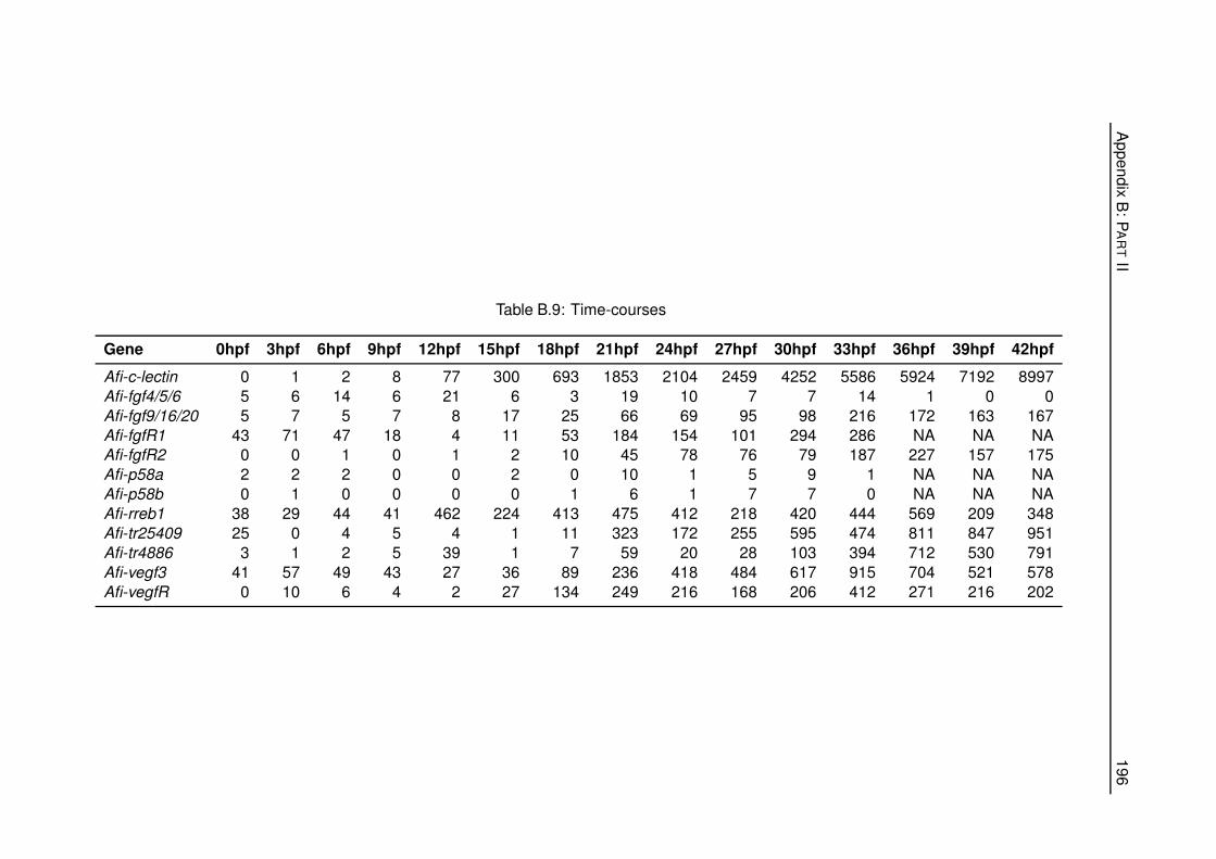
Ap
pe
nd
ixB
:P
AR
TII
19
6
Table B.9: Time-courses
Gene 0hpf 3hpf 6hpf 9hpf 12hpf 15hpf 18hpf 21hpf 24hpf 27hpf 30hpf 33hpf 36hpf 39hpf 42hpf
Afi-c-lectin 0 1 2 8 77 300 693 1853 2104 2459 4252 5586 5924 7192 8997
Afi-fgf4/5/6 5 6 14 6 21 6 3 19 10 7 7 14 1 0 0
Afi-fgf9/16/20 5 7 5 7 8 17 25 66 69 95 98 216 172 163 167
Afi-fgfR1 43 71 47 18 4 11 53 184 154 101 294 286 NA NA NA
Afi-fgfR2 0 0 1 0 1 2 10 45 78 76 79 187 227 157 175
Afi-p58a 2 2 2 0 0 2 0 10 1 5 9 1 NA NA NA
Afi-p58b 0 1 0 0 0 0 1 6 1 7 7 0 NA NA NA
Afi-rreb1 38 29 44 41 462 224 413 475 412 218 420 444 569 209 348
Afi-tr25409 25 0 4 5 4 1 11 323 172 255 595 474 811 847 951
Afi-tr4886 3 1 2 5 39 1 7 59 20 28 103 394 712 530 791
Afi-vegf3 41 57 49 43 27 36 89 236 418 484 617 915 704 521 578
Afi-vegfR 0 10 6 4 2 27 134 249 216 168 206 412 271 216 202

Appendix B: PART II 197
Sca
ffo
ld:3
43
Sca
ffo
ld:3
58
Sca
ffo
ld:3
11
Sca
ffo
ld:3
10
Figure B.1: Sea urchin msp130 genes on Scaffolds.

Appendix B: PART II 198
Table B.10: Expression of genes used in part II
EC Name 9hr 18hr 27hr 39hr Fuzzy Cluster
Cluster-10558.1 AfiCDS.id384.tr29965 0 14 250 845 17
Cluster-11257.0 Afi-tcep1 772 356 481 604 15
Cluster-11727.4 AfiCDS.id81632.tr60441 6 7 544 1446 17
Cluster-1215.0 Afi-trim2 0 0 2 1 4
Cluster-12844.127 AfiCDS.id48303.tr39358 48 105 226 142 9
Cluster-12844.62 AfiCDS.id84973.tr13659 34 58 161 90 14
Cluster-13113.1 Afi-soxD1 48 3 58 20 27
Cluster-13125.0 Afi-egr 16 47 89 98 20
Cluster-13564.0 AfiCDS.id63133.tr10933 0 1 5 178 7
Cluster-1364.0 Afi-trim2 1 0 0 18 23 3
Cluster-13724.0 Afi-rreb1 3 167 128 44 11
Cluster-14335.0 AfiCDS.id43930.tr1339 5 7 5 9 16
Cluster-1517.1 Afi-tr25409 0 1 115 210 17
Cluster-15262.0 Afi-009748 23 5 24 27 3
Cluster-1541.0 Afi-004896 0 0 19 42 17
Cluster-15464.0 AfiCDS.id4578.tr38894 0 0 26 14 4
Cluster-15622.0 Afi-tacr2L 0 0 0 1 13
Cluster-15634.0 AfiCDS.id75617.tr19326 0 0 10 21 17
Cluster-16461.0 Afi-mt6 mmpL 94 2805 1712 3079 18
Cluster-16526.0 Afi-a2m 1 201 115 140 174 15
Cluster-1724.0 Afi-018426 0 35 18 11 23
Cluster-17333.2 Afi-gldc 471 44 58 53 1
Cluster-17570.0 fn3/egff 1 1 34 333 75 14
Cluster-17600.0 AfiCDS.id58703.tr6207 150 125 39 22 24
Cluster-17970.0 Afi-e2f7 758 1329 283 254 26
Cluster-18217.0 AfiCDS.id41059.tr61404 1 58 39 12 11
Cluster-18373.0 Afi-tropmyh 272 37 35 38 1
Cluster-20113.3 Afi-0914236 110 199 162 171 18
Cluster-20452.0 Afi-caraX 0 1 122 186 3
Cluster-21780.0 Afi-αcoll 29 26 2466 7638 17
Cluster-21880.0 AfiCDS.id59305.tr68751 0 0 7 27 17
Cluster-22670.0 Afi-mad 8 19 30 49 20
Cluster-22948.0 Afi-tle1/groucho 286 70 172 122 19
Cluster-23056.1 Afi-tr4886 0 3 108 230 17
Cluster-23512.1 Afi-vegfR 1 71 93 44 2
Cluster-24029.0 AfiCDS.id5605.tr49815 7 1 4 1 19
Cluster-24220.0 Afi-dusp1 82 37 55 50 19
Cluster-2493.0 Afi-hypp 2281 0 8 124 11 27
Cluster-25105.0 Afi-colf 3 0 1 3 8 17
Cluster-25122.0 Afi-77kDamaps 152 82 181 215 3
Cluster-2571.0 Afi-trim2-2 0 1 51 33 4
Cluster-25746.0 AfiCDS.id44038.tr10735 6 9 29 71 17
Cluster-25982.2 Afi-egfiL 2 1 1 0 2 6
Cluster-26614.0 Afi-018662 399 353 116 181 24
Cluster-27739.0 Afi-agrnL 0 0 9 1 27
Cluster-27881.0 AfiCDS.id75849.tr3754 0 0 375 1410 17
Cluster-28510.0 Afi-sr/fu/igr 0 3 4 7 20
Cluster-28643.1 AfiCDS.id10236.tr3203 105 2839 1710 3157 18
Cluster-29925.0 Afi-erg 10 363 218 168 11
Cluster-30632.0 Afi-alx/arx 0 2 0 2 6
Cluster-30786.1 Afi-fbn2L 1 1 0 18 189 7
Cluster-30937.0 AfiCDS.id64819.tr39976 0 1 26 100 17
Cluster-31209.0 Afi-ttrspn 19 0 75 179 106 9
Cluster-3261.0 Afi-mt14/mmpl7 0 0 2 6 17
Cluster-3715.0 Afi-p58-b 0 12 235 206 3
Cluster-3715.1 Afi-p58-a 0 10 157 120 4
Cluster-4270.0 AfiCDS.id53027.tr45279 0 2 23 20 3
Cluster-4513.0 AfiCDS.id52181.tr20375 0 0 1 0 14
Cluster-4641.0 Afi-fn3/igf 29 0 4 38 56 3
Cluster-5507.0 AfiCDS.id4513.tr62663 0 0 3 19 7
Cluster-5808.0 Afi-sept4 1 46 93 63 9
Cluster-5917.0 Afi-spcat3l 3 319 308 402 10
Cluster-672.0 Afi-dcst2-3 0 0 39 96 17
Cluster-7020.0 Afi-tr4886 0 3 84 188 17
Cluster-720.0 Afi-kirrelL 0 0 24 78 17
Cluster-7256.0 Afi-slc4a10 5 54 1272 2295 20
Cluster-7482.0 Afi-msp130r6 2 8 276 1031 17
Cluster-7531.0 Afi-cebpa 28 176 246 275 10
Cluster-7997.0 Afi-vegf2 0 1 1 10 7

Appendix B: PART II 199
Scaffold:4453
Scaffold:1119
Scaffold:878
Scaffold:317
Scaffold:903
Figure B.2: Sea urchin spicule matrix genes on scaffolds.

Appendix B: PART II 200
27
3
22
4 41
5
38
36
57
23
21
56
15
1
13
2 20
0
91
86 1
16
18
4
16
5 23
6
25
3
21
2 43
5
31
29 36
15
6
14
2 20
1
15
15 16
11
3
93
19
0
18
2
17
0 24
8
14
13
26
28
4
24
8 49
0
28
1
25
8 36
6
11
73
10
60
16
84
13
6
11
5 21
6
25
9
22
4 38
3
39
35
67
74
68 9
4
19
7
18
6 25
1
30
4
28
9
37
0
36
36 40
19
2
18
0 26
8
Adhesion Apoptosis Biomineralization CalciumToolkit
CellCycle Cytoskeleton Defensome DNAReplication
EggActivation GermLineDeterminant GPCRRhodopsin GTPase
Histone Immunity Kinase Metabolism
Metalloprotease Nervous Oogenesis Phosphatase
Signaling TF TranslationFactor ZNF
0.0
0.5
1.0
1.5
0.0
0.5
1.0
1.5
0.0
0.5
1.0
1.5
0.0
0.5
1.0
1.5
0.0
0.5
1.0
1.5
0.0
0.5
1.0
1.5
Afi Afi-ECs Spu Afi Afi-ECs Spu Afi Afi-ECs Spu Afi Afi-ECs Spu
Species
Fra
cti
on
Species Afi Afi-ECs Spu
Figure B.3: Gene ontology loss after grouping into ECs.

Appendix B: PART II 201
01 0521 22 15
24 26 200910
17 03 07 2304
19 27
25 02 1408 11
12 181613 06
Early
Late
Intermediate
B-module
Cluster Groups:
Figure B.4: Line plots for fuzzy clusters.

Appendix B: PART II 202
Top-Hit Species Distribution
0 5 10 15 20 25 30 35 40 45 50 55 60 65
BLAST Top-Hits
Strongylocentrotus purpuratus
Saccoglossus kowalevskii
Branchiostoma floridae
Nematostella vectensis
Amphimedon queenslandica
Danio rerio
Crassostrea gigas
Hydra vulgaris
Ornithodoros moubata
Mesocentrotus nudus
Oryzias latipes
Zonotrichia albicollis
Pediculus humanus
Tupaia chinensis
Alligator sinensis
Stegastes partitus
Xenopus (Silurana)
Haplochromis burtoni
Patiria miniata
Xenopus laevis
Anolis carolinensis
Chinchilla lanigera
Aplysia californica
Trichoplax adhaerens
Sp
ecie
s
A
B
Down-regulated
Top-Hit Species Distribution
0 50 100 150 200 250 300 350 400 450 500 550 600 650
BLAST Top-Hits
Strongylocentrotus purpuratus
Saccoglossus kowalevskii
Branchiostoma floridae
Nematostella vectensis
Crassostrea gigas
Capitella teleta
Ciona intestinalis
Danio rerio
Lottia gigantea
Amphimedon queenslandica
Stegodyphus mimosarum
Xenopus (Silurana)
Aplysia californica
Oreochromis niloticus
Hydra vulgaris
Takifugu rubripes
Oncorhynchus mykiss
Stegastes partitus
Tribolium castaneum
Oryzias latipes
Latimeria chalumnae
Astyanax mexicanus
Rhizophagus irregularis
Diaphorina citri
Peromyscus maniculatus
Callorhinchus milii
Bombyx mori
Anolis carolinensis
Trichomonas vaginalis
others
Sp
ecie
s
Up-regulated
Figure B.5: Blast2GO top hit distributions for differentially expressed samples.

Ap
pe
nd
ixB
:P
AR
TII
20
3
Msp130 alingment
AFIL.CDS.id75849.tr3754 ............................................MRFLAVLLVPAFI...........................GFVSAQMWGQG 24AFIL.CDS.id31285.tr33531 ............................................................................................... 0AFIL.CDS.id36066.tr22676 MSR......FYPYFAFIVCSVL..............KVHA.TYKLQFYSTLYLPSFYNNQG...NPGYEYGGDAIEHAVYDGKDGLVYTA..... 66WHL22.405650.1-pep ............................................................................................... 0AFIL.CDS.id29326.tr58595 MTSSWTKNVFFGLFVLCVCWMTVLCEDEDEETSQEETFHGTAIVLKPLSQQYVPYDHVKTGDDTDAQYGIGMNAIDASACDVTTGFVYTA..... 90AFIL.CDS.id7622.tr36298 MAF......RQALFVTVYLLPFALVHSSD............QIYLKPHSNIYLPYAYDPDG..ITGLYGIDKAAVEQSAYDRSTGIVYAA..... 70AFIL.CDS.id80760.tr10976 MAT.......LRIFLISLLLALLTQDSYS............AVILKPVSSINIPFAYDVGG...TGSYGIESGAVEQSAYDEESGLVYTA..... 68consensus * * * * * * * * ** * ** *
AFIL.CDS.id75849.tr3754 HGQGGINYPDRGR......................................APGGSSRQRYQNVWNNA........................... 54AFIL.CDS.id31285.tr33531 ............................................................................................... 0AFIL.CDS.id36066.tr22676 .GDAFINVIDVSNIQSPRILHY.QEVTTDTPVVALCGPFVAFLSKSSVADFEDG...TLSIYNKYNRAKEGVFEKVMNVTVGPEPESIAFTPDCG 156WHL22.405650.1-pep ......................................................................................MLHFSHDCR 9AFIL.CDS.id29326.tr58595 .GAKYIHIVDFSKATNPSLMYK.KELNEKVSDIEVCGSKVAFLIDG.....NPG...RVDIYNLYNSEKNTFELNTTIAEVGFGPSAMIFADNCN 175AFIL.CDS.id7622.tr36298 .GASYIHIVDYNNVTNPVIIDKIPTYSRPITDAEQCGSKVAFTVEALTPD.QPG...EVHVYHVYNKITGEFKMAYMPFAVGFGPDMLQFTPNCD 160AFIL.CDS.id80760.tr10976 .GNAFIHVVDYSNISNPILLD..AYTSGPVNDVELCGRRVAFALTGSPRD.QPG...EVHVYNLYDRSLRDLVLAFR.ITVGFEPDMLHFTKDCN 155consensus * * * * ** *** ** ** ** ** * * *
AFIL.CDS.id75849.tr3754 .........PARQQGGGVNYPNAG..TAPGAGGSSR....QGQNGWNNYVPAN..NAPGLN.APGFNAPN.......VNGINQVEVGRAP...LP 121AFIL.CDS.id31285.tr33531 ..................................................................................WPYKGEISS..VP 11AFIL.CDS.id36066.tr22676 MAVVANAGTPEVNLL..................GTDIIDPEGSVSIITFDGGDLSKPPTANDKVNFVKFNARWQEYVSRGVRFVYKGQISTQNIR 233WHL22.405650.1-pep TIVIANEGEAAQNA..................DQTEFINREGSISIIRLSVDG...STFTSTLINLTQFNDRSDEYVARGVRYPYHGELDG..AN 81AFIL.CDS.id29326.tr58595 EIAVANEGGPYED....................NGNFVDPEGSVGIIHL.DGD...KPTLN.ILDFTKFNDRSGEFVANGVRWPYPNQ....... 238AFIL.CDS.id7622.tr36298 TIIVANEASPYET....................QQRVIDPEGSVSIIKF..GD...QNSVS.TIDFKSFNQRADEYVMKGVRWHYKGQLGT...P 226AFIL.CDS.id80760.tr10976 TIVVANEASPFATASGPATGPATGPATGPASGPASDIVDPEGSVSIIRFQQSS...QPVVT.TLNFTAFNDRVAEYEAKGIRRGYKGEISS..MP 244consensus * ***** * ********* * * * ** * *** *** *** *
AFIL.CDS.id75849.tr3754 GGSSRGL.......NGW.DTAPVVNQQPISGRTNHQNVGAAPVGQGGS.SGGRYIPDGPVQTGMSNRVNMVDAGTAPEQG...........NSPN 196AFIL.CDS.id31285.tr33531 STFSQNLEPEYITFNYD.ESKAYIALQ........ENNAVAEIDINTN.KVVDLYS.....LGTKSWNSLLLDPSDKDSGLLLQNWDIFSLRQPD 91AFIL.CDS.id36066.tr22676 TFLSQDLTPEYVVLNSQ.GTKAYVGLQ........INNAIAVIDIATK.SVEEIYP.....LGTKSWANLDIDVSDQDGGIKFTRWPIKTLYQPD 313WHL22.405650.1-pep ETFAQNLEPEYITYNYD.DTKAFVGLQ........ENNAIAVVDLLAG.EIEDIYP.....LGEKSWLNLDLDASDRDGGIMFRRNNISSFYQPD 161AFIL.CDS.id29326.tr58595 TTFSQAMEPESITLNTELGTVAYVSLQ........ENNGIAVVDLLLDGVIEYIHA.....LGTKSWENYFIDTSDKDKGIKFNRYDIYSFYQPD 320AFIL.CDS.id7622.tr36298 GTFSQSLEPEFVTLNGN.GTKAYITLQ........ENNAIAEVNLETE.TIDEIYS.....LGVKDWNRLLLDSSDADQGINFQSYDMSSLRMPD 306AFIL.CDS.id80760.tr10976 STFSQSLEPEYVTFNED.ESKAYIALQ........ENNAIAEVNLLTD.TIDELYP.....LGVKSWQDLVLDPSDRDSGINLQSYDILSLYQPD 324consensus **** ***** * ! *******! *!***! *** * * *** *! *** ** ** ** * !* * ** ****!*
AFIL.CDS.id75849.tr3754 SGEFLWDTAGTGTGALATNDHAQSSGTALGTNN.RAGAAWGTGAGAGGSSRGGNGNAPAYAGTGGSSGAAGNAPLGGALLTDRDSQNAGRADQVK 290AFIL.CDS.id31285.tr33531 AIKYI...EVSGEGYLITANEGEGLEYA......AGSKEWAEFE.RGEYFFENDLLSDL.VSSEMSNNLDKEAKLGRLRLSTNEGQNHLNPSLYD 175AFIL.CDS.id36066.tr22676 ELRYF...DVGGTGYIVTANEGDPFHVKI....KSLQREWTDAA.AGGEFL.DAELSPN.LNPVIRKALNDSTALKFYEFSTIDGLDEN..GLLQ 396WHL22.405650.1-pep GIKYF...EVDGVGYIITANEGDSFDYE......LGTEKWAEDQ.RGKKFKAGDFA.ET.FDNELIGKLGDDDMLGRLAFSKVDGLDS..SGKFE 242AFIL.CDS.id29326.tr58595 GIQFF...EVDGVGYVAAANEGETTSFT......KDGQEYNEVQ.MGKDFITNDQLADS.VSPELREALKDDRLLGRLEFSNVDGMNVNDSSKFE 404AFIL.CDS.id7622.tr36298 SARFL...AFKGNGYIITADEGDTLELEL.....PDGRQWTDVK.RGRRLLEENHLSSD.IDQSLRTALADDSILGRLQFSIIDGLSETEANKIS 391AFIL.CDS.id80760.tr10976 SIKFF...EFNGHGYIATGNEGGTIKLE......AGARSWTDAK.RGGKLVKDRQISPN.MDAGLQAALSDNARLGRLEFSVIDGLSSSYPTKIE 408consensus * ** ** ! !** ***** *** * *!* * ** * ** * * !*** ** *** *
AFIL.CDS.id75849.tr3754 GAASFGGTAAGVVIAV..................................................................LVLVGVVGVAAVV 319AFIL.CDS.id31285.tr33531 NFYMFGSRGFSIFKTSDFSLVFDSGDEVERMMAVYYPKVFNGNTKPDESDIESAEDLMDSRSDNQGPECETLEIGELNG................ 254AFIL.CDS.id36066.tr22676 ELHGFGGRGISVYRASDFTQVYDSGDALAKMQATVYPVVFNAD...DEPSDQSPRQLMDKRSTKQGVDCESLEIGVIGN.DRLIFVGADRIGTLM 487WHL22.405650.1-pep KLYFFGARGFSIFRASDITLVYDSGDEVEKMIAKFYPDVFNTNTKSDDPVIESPADLFDKRSDNLGPECESVEIGELGG.RRIIFIGVDRTSAIL 336AFIL.CDS.id29326.tr58595 KLHFFGGRGISVFLASDMSLVWESDYIAEFMQTVLYPDTFNANLDVENADKQTPKDMMDMQSPSKGPECESIEGGEYNG.TRVLFSGMEGNSAIM 498AFIL.CDS.id7622.tr36298 RLHFPGSRGISVFRAEGMSLLWDSGNLVETIHAKDYASTFNGNTKPDDPAKESPSDLKDTRSDDQGPECESLAIGELDDGTRLVFVGVDRSSSIL 486AFIL.CDS.id80760.tr10976 RLHTFGGRGMSIFRADDMSLLWDSKDMIEKLHSELYPSTFNGNSKPDDPNTETPDDLVDKRSDNNGPECQAITMGELEDNTRLLFLGIGRSSAIA 503consensus ** *!*** ******* *** **** * * * ** **** * * * *** ** * *** ****** ***** ** * * * ***

Ap
pe
nd
ixB
:P
AR
TII
20
4
AFIL.CDS.id75849.tr3754 LVKQR.......................................................................................... 324AFIL.CDS.id31285.tr33531 ............................................................................................... 254AFIL.CDS.id36066.tr22676 IFRLD...KNSYTPK..LESIYRNGSTNRPISDLFKDQDLNDAAPEALTFIPGKTNSDQSFPILMVAGTESGTLSFYRIVNEG............ 565WHL22.405650.1-pep VYSLE...SGEIV..PTFETVYRAGGRNDTFQNLLDDRNLGDLDPEDLKFIPASV.SVTGVPMLMVTSAVSGTISLYEVYDD............. 412AFIL.CDS.id29326.tr58595 VFSFA...QGSVEPK..FESIYRHGGIDKPFQKLLDEQNLGDLNPEELKFIPAEY.SSTGGPLLLVTGTFSGTLAMYEITEEYWEAPTDLPPHIF 587AFIL.CDS.id7622.tr36298 IFSVD...EVGAEPRLEFQSILRDGGVDDTFNVLLENRNLGNLDPEDLRFIPAAF.SPTNKPLLLVTSAVSGTLAMYEVVKD............. 564AFIL.CDS.id80760.tr10976 VFRIEATFESGHEPVLEFESLYRAGGTNQTFSTLLENENIGNLDPEDLRFIPAAK.SPTGKPLLLVTGTTSGNLVMYEVIDMS........PQ.. 587consensus * * *** ** ** * ** *** * ** * **** * * * * ** **** **
AFIL.CDS.id75849.tr3754 .......ASRM............MVQQV...... 333AFIL.CDS.id31285.tr33531 .................................. 254AFIL.CDS.id36066.tr22676 .SGAGCRAPMIHISIVVALL..VLVKCIV....X 592WHL22.405650.1-pep .................................. 412AFIL.CDS.id29326.tr58595 ELGKTPFEMYIHVX.................... 601AFIL.CDS.id7622.tr36298 .TGPGSGGESIHTWNVVILSMWL..MWLIIARQX 595AFIL.CDS.id80760.tr10976 .TGDNGFGSRISSS..ILLTFFLLVGQMILSR.X 617consensus * * *

LIST OF REFERENCES
Ashrifia Adomako-Ankomah and Charles a Ettensohn. Growth factor-mediated mesodermal
cell guidance and skeletogenesis during sea urchin gastrulation. Development (Cambridge,
England), 140(September):4214–25, 2013.
Bruce Alberts, Alexander Johnson, Julian Lewis, Martin Raff, Keith Roberts, and Peter Walter.
Molecular Biology of the Cell. 2002.
Uri Alon. An Introduction to Systems Biology: Design Principles of Biological Circuits, volume 10.
2007.
a. M. Altenhoff, N. Kunca, N. Glover, C.-M. Train, a. Sueki, I. Pili ota, K. Gori, B. Tomiczek,
S. Muller, H. Redestig, G. H. Gonnet, and C. Dessimoz. The OMA orthology database in 2015:
function predictions, better plant support, synteny view and other improvements. Nucleic Acids
Research, 43(D1):D240–D249, 2014.
Gabriele Amore and Eric H. Davidson. cis-Regulatory control of cyclophilin, a member of the
ETS-DRI skeletogenic gene battery in the sea urchin embryo. Developmental Biology, 293:
555–564, 2006.
Gabriele Amore, Robert G Yavrouian, Kevin J Peterson, Andrew Ransick, David R McClay, and
Eric H Davidson. Spdeadringer, a sea urchin embryo gene required separately in skeletogenic
and oral ectoderm gene regulatory networks. Developmental Biology, 261(1):55–81, 2003.
Carmen Andrikou, Edmondo Iovene, Francesca Rizzo, Paola Oliveri, and Maria Ina Arnone.
Myogenesis in the sea urchin embryo: the molecular fingerprint of the myoblast precursors.
EvoDevo, 4(1):33, 2013.
Lynne M Angerer and Robert C Angerer. Patterning the sea urchin embryo: gene regulatory
networks, signaling pathways, and cellular interactions. Current topics in developmental biology,
53:159–198, 2003.
J a Anstrom, J E Chin, D S Leaf, a L Parks, and R a Raff. Localization and expression of
msp130, a primary mesenchyme lineage-specific cell surface protein in the sea urchin embryo.
Development (Cambridge, England), 101(2):255–265, 1987.
M I Arnone, L D Bogarad, a Collazo, C V Kirchhamer, R a Cameron, J P Rast, a Gregorians,
and E H Davidson. Green Fluorescent Protein in the sea urchin: new experimental approaches
205

LIST OF REFERENCES 206
to transcriptional regulatory analysis in embryos and larvae. Development, 124(22):4649–4659,
1997.
Laurent Arnoult, Kathy F Y Su, Diogo Manoel, Caroline Minervino, Justine Magrina, Nicolas
Gompel, and Benjamin Prud’homme. Emergence and diversification of fly pigmentation through
evolution of a gene regulatory module. Science (New York, N.Y.), 339(6126):1423–6, 2013.
Albert-Laszlo Barabasi and Reka Albert. Emergence of scaling in random networks. Science,
286(October):11, 1999.
Albert-Laszlo Barabasi and Zoltan N Oltvai. Network biology: understanding the cell’s functional
organization. Nature reviews. Genetics, 5(2):101–13, February 2004.
Julius C. Barsi, Qiang Tu, and Eric H. Davidson. General approach for in vivo recovery of cell
type-specific effector gene sets. Genome Research, 24(5):860–868, 2014.
Inanc Birol, Shaun D. Jackman, Cydney B. Nielsen, Jenny Q. Qian, Richard Varhol, Greg Stazyk,
Ryan D. Morin, Yongjun Zhao, Martin Hirst, Jacqueline E. Schein, Doug E. Horsman, Joseph M.
Connors, Randy D. Gascoyne, Marco A. Marra, and Steven J M Jones. De novo transcriptome
assembly with ABySS. Bioinformatics, 25(21):2872–2877, 2009.
L D Bogarad, M I Arnone, C Chang, and E H Davidson. Interference with gene regulation in
living sea urchin embryos: transcription factor knock out (TKO), a genetically controlled vector
for blockade of specific transcription factors. Proceedings of the National Academy of Sciences
of the United States of America, 95(25):14827–14832, 1998.
Anthony M. Bolger, Marc Lohse, and Bjoern Usadel. Trimmomatic: A flexible trimmer for Illumina
sequence data. Bioinformatics, 30:2114–2120, 2014.
Hamid Bolouri and Eric H Davidson. Modeling DNA sequence-based cis-regulatory gene net-
works. Developmental biology, 246(1):2–13, 2002.
Hamid Bolouri and Eric H Davidson. Transcriptional regulatory cascades in development: initial
rates, not steady state, determine network kinetics. Proceedings of the National Academy of
Sciences of the United States of America, 100(16):9371–9376, 2003.
David J Bottjer, Eric H Davidson, Kevin J Peterson, and R Andrew Cameron. Paleogenomics of
echinoderms. Science, 314:956–960, 2006.
T Bowmer. Reproduction in Amphiura filiformis (Echinodermata: Ophiuroidea): Seasonality in
Gonad Development. Marine Biology, 290:281–290, 1982.
Michael J Boyle, Emi Yamaguchi, and Elaine C Seaver. Molecular conservation of metazoan
gut formation: evidence from expression of endomesoderm genes in Capitella teleta (Annelida).
EvoDevo, 5(1):39, 2014.

LIST OF REFERENCES 207
R.J. J Rj Britten and E.H. H Eh Davidson. Gene regulation for higher cells: a theory. Science,
165(3891):349–357, 1969.
C. Titus Brown, Adina Howe, Qingpeng Zhang, Alexis B. Pyrkosz, and Timothy H. Brom. A
Reference-Free Algorithm for Computational Normalization of Shotgun Sequencing Data. arXiv,
1203.4802:1–18, 2012.
C Titus Brown, Camille Scott, Michael R Crusoe, Leigh Sheneman, Josh Rosenthal, and Adina
Howe. khmer-protocols 0.8.4 documentation., 2013.
John B. Buchanan. A Comparative Study of Some Features of the Biology of Amphiura Filiformis
and Amphiura Chiajei [Ophiuroidea] Considered in Relation to their Distribution. Journal of the
Marine Biological Association of the United Kingdom, 44(03):565–576, 1964.
M Burrows and DJ Wheeler. A block-sorting lossless data compression algorithm. Algorithm,
Data Compression, (124):18, 1994.
Cristina Calestani, Jonathan P Rast, and Eric H Davidson. Isolation of pigment cell specific
genes in the sea urchin embryo by differential macroarray screening. Development (Cambridge,
England), 130(19):4587–4596, 2003.
C. B. Cameron and C. D. Bishop. Biomineral ultrastructure, elemental constitution and genomic
analysis of biomineralization-related proteins in hemichordates. Proceedings of the Royal Soci-
ety B: Biological Sciences, 279(1740):3041–3048, 2012.
R. Andrew Cameron, Paola Oliveri, Jane Wyllie, and Eric H. Davidson. cis-Regulatory activity
of randomly chosen genomic fragments from the sea urchin. Gene Expression Patterns, 4(2):
205–213, 2004.
R. Andrew Cameron, Manoj Samanta, Autumn Yuan, Dong He, and Eric Davidson. SpBase: The
sea urchin genome database and web site. Nucleic Acids Research, 37(SUPPL. 1):750–754,
2009.
Johanna T Cannon, Kevin M Kocot, Damien S Waits, David a Weese, Billie J Swalla, Scott R
Santos, and Kenneth M Halanych. Report Phylogenomic Resolution of the Hemichordate and
Echinoderm Clade. Current Biology, 24(23):1–6, 2014.
Peter Carlsson and Margit Mahlapuu. Forkhead transcription factors: key players in development
and metabolism. Developmental biology, 250(1):1–23, 2002.
Sean B. Carroll. Evo-Devo and an Expanding Evolutionary Synthesis: A Genetic Theory of
Morphological Evolution. Cell, 134(1):25–36, 2008.
Zheng Chang, Guojun Li, Juntao Liu, Yu Zhang, Cody Ashby, Deli Liu, Carole L Cramer, and
Xiuzhen Huang. Bridger: a new framework for de novo transcriptome assembly using RNA-seq
data. Genome Biology, 16(1):1–10, 2015.

LIST OF REFERENCES 208
Xiao Chen, John R Bracht, Aaron David Goldman, Egor Dolzhenko, Derek M Clay, Estienne C
Swart, David H Perlman, Thomas G Doak, Andrew Stuart, Chris T Amemiya, Robert P Sebra,
and Laura F Landweber. The Architecture of a Scrambled Genome Reveals Massive Levels of
Genomic Rearrangement during Development. Cell, 158(5):1187–1198, 2014.
Chin Kai Chuang, Athula H. Wikramanayake, Chai An Mao, Xiaotao Li, and William H. Klein.
Transient appearance of Strongylocentrotus purpuratus Otx in micromere nuclei: Cytoplasmic
retention of SpOtx possibly mediated through an α- actinin interaction. Developmental Genetics,
19(3):231–237, 1996.
Gavin Conant and Andreas Wagner. Convergent evolution of gene circuits. Nature genetics, 34
(3):263–264, 2003.
Ana Conesa and Stefan Gotz. Blast2GO: A comprehensive suite for functional analysis in plant
genomics. International Journal of Plant Genomics, 2008, 2008.
Richard R Copley. The EH1 motif in metazoan transcription factors. BMC genomics, 6:169,
2005.
Caterina Costa, Konstantinos Karakostis, Francesca Zito, and Valeria Matranga. Phylogenetic
analysis and expression patterns of p16 and p19 in Paracentrotus lividus embryos. Development
Genes and Evolution, 222:245–251, 2012.
J Croce. Dynamics of Delta/Notch signaling on endomesoderm segregation in the sea urchin
embryo. Development, 137:83–91, 2010.
J Croce, G Lhomond, J C Lozano, and C Gache. ske-T, a T-box gene expressed in the skele-
togenic mesenchyme lineage of the sea urchin embryo. Mechanisms of development, 107(1-2):
159–162, 2001.
Anton Crombach and Paulien Hogeweg. Evolution of evolvability in gene regulatory networks.
PLoS Computational Biology, 4(7), 2008.
Anna Czarkwiani, David V Dylus, and Paola Oliveri. Expression of skeletogenic genes during
arm regeneration in the brittle star Amphiura filiformis. Gene Expression Patterns, 13:464–472,
2013.
Sagar Damle and Eric H. Davidson. Precise cis-regulatory control of spatial and temporal ex-
pression of the alx-1 gene in the skeletogenic lineage of s. purpuratus. Developmental Biology,
357:505–517, 2011.
Aaron E Darling, Lucas Carey, and Wu-chun Feng. The Design, Implementation, and Evaluation
of mpiBLAST. Proceedings of ClusterWorld, 2003:13–15, 2003.

LIST OF REFERENCES 209
Colin J. Davidson, Rabindra Tirouvanziam, Leonard a. Herzenberg, and Joseph S. Lipsick. Func-
tional evolution of the vertebrate Myb gene family: B-Myb, but neither A-Myb nor c-Myb, comple-
ments Drosophila Myb in hemocytes. Genetics, 169(1):215–229, 2005.
Colin J Davidson, Erin E Guthrie, and Joseph S Lipsick. Duplication and maintenance of the
Myb genes of vertebrate animals. Biology open, 2(2):101–10, 2013.
E H Davidson. The regulatory genome: gene regulatory networks in development and evolution,
volume 310. 2006.
Eric H Davidson. Emerging properties of animal gene regulatory networks. Nature, 468:911–
920, 2010.
Eric H. Davidson. Evolutionary bioscience as regulatory systems biology. Developmental Biol-
ogy, 357(1):35–40, 2011.
Eric H. Davidson and Douglas H. Erwin. Gene regulatory networks and the evolution of animal
body plans. Science, 311:796–800, 2006.
Nadia M Davidson and Alicia Oshlack. Corset: enabling differential gene expression analysis for
de novo assembled transcriptomes. Genome Biology, 15:410, 2014.
Bernard M. Degnan, Michel Vervoort, Claire Larroux, and Gemma S. Richards. Early evolution of
metazoan transcription factors. Current Opinion in Genetics and Development, 19(6):591–599,
2009.
Cristian Del Fabbro, Simone Scalabrin, Michele Morgante, and Federico M. Giorgi. An extensive
evaluation of read trimming effects on illumina NGS data analysis. PLoS ONE, 8(12):1–13, 2013.
Jeffery P Demuth, Tijl De Bie, Jason E Stajich, Nello Cristianini, and Matthew W Hahn. The
evolution of mammalian gene families. PloS one, 1(1):e85, 2006.
Patrik D’haeseleer. What are DNA sequence motifs? Nature biotechnology, 24(4):423–425,
2006.
Veronique Duboc and Thierry Lepage. A conserved role for the nodal signaling pathway in the
establishment of dorso-ventral and left-right axes in deuterostomes. Journal of Experimental
Zoology Part B: Molecular and Developmental Evolution, 310(1):41–53, 2008.
Louise Duloquin, Guy Lhomond, and Christian Gache. Localized VEGF signaling from ectoderm
to mesenchyme cells controls morphogenesis of the sea urchin embryo skeleton. Development,
134:2293–2302, 2007.
S. Dupont, O. Ortega-Martınez, and M. Thorndyke. Impact of near-future ocean acidification on
echinoderms. Ecotoxicology, 19:449–462, 2010.

LIST OF REFERENCES 210
Sam Dupont, William Thorndyke, Michael C. Thorndyke, and Robert D. Burke. Neural develop-
ment of the brittlestar Amphiura filiformis. Development Genes and Evolution, 219(3):159–166,
2009.
Robert C. Edgar. Search and clustering orders of magnitude faster than BLAST. Bioinformatics,
26(19):2460–2461, 2010.
Eli Eisenberg and Erez Y Levanon. Preferential attachment in the protein network evolution.
Physical review letters, 91(13):138701, 2003.
Maurice R. Elphick, Dean C. Semmens, Liisa M. Blowes, Judith Levine, Christopher J. Lowe,
Maria I. Arnone, and Melody S. Clark. Reconstructing SALMFamide Neuropeptide Precursor
Evolution in the Phylum Echinodermata: Ophiuroid and Crinoid Sequence Data Provide New
Insights. Frontiers in Endocrinology, 6(February):1–10, 2015.
D. H. Erwin, M. Laflamme, S. M. Tweedt, E. a. Sperling, D. Pisani, and K. J. Peterson. The
Cambrian Conundrum: Early Divergence and Later Ecological Success in the Early History of
Animals. Science, 334(6059):1091–1097, 2011.
Douglas H Erwin and Eric H Davidson. The last common bilaterian ancestor. Development
(Cambridge, England), 129(13):3021–3032, 2002.
Douglas H Erwin and Eric H Davidson. The evolution of hierarchical gene regulatory networks.
Nature Reviews Genetics, 10:141–148, 2009.
Charles a Ettensohn. Lessons from a gene regulatory network: echinoderm skeletogenesis pro-
vides insights into evolution, plasticity and morphogenesis. Development (Cambridge, England),
136(1):11–21, 2009.
Charles A Ettensohn, Michele R Illies, Paola Oliveri, and Deborah L De Jong. Alx1, a member
of the Cart1/Alx3/Alx4 subfamily of Paired-class homeodomain proteins, is an essential compo-
nent of the gene network controlling skeletogenic fate specification in the sea urchin embryo.
Development, 130(13):2917–2928, 2003.
Brent Ewing and Phil Green. Base-calling of automated sequencer traces using phred. II. Error
probabilities. Genome Research, 8(3):186–194, 1998.
Emmanuel Faure, Isabelle S Peter, and Eric H Davidson. A new software package for predictive
gene regulatory network modeling and redesign. Journal of computational biology : a journal of
computational molecular cell biology, 20(6):419–23, 2013.
David E. Featherstone and Kendal Broadie. Wrestling with pleiotropy: Genomic and topological
analysis of the yeast gene expression network. BioEssays, 24(3):267–274, 2002.
J. Felsenstein. Cases in which Parsimony or Compatibility Methods will be Positively Misleading.
Systematic Biology, 27(4):401–410, 1978.

LIST OF REFERENCES 211
Jianxing Feng, Clifford A. Meyer, Qian Wang, Jun S. Liu, X. Shirley Liu, and Yong Zhang.
GFOLD: A generalized fold change for ranking differentially expressed genes from RNA-seq
data. Bioinformatics, 28(21):2782–2788, 2012.
Paolo Ferragina and Giovanni Manzini. An experimental study of a compressed index. Informa-
tion Sciences, 135(1-2):13–28, 2001.
Limin Fu, Beifang Niu, Zhengwei Zhu, Sitao Wu, and Weizhong Li. CD-HIT: Accelerated for
clustering the next-generation sequencing data. Bioinformatics, 28(23):3150–3152, 2012.
Takuya Fuchikami, Keiko Mitsunaga-Nakatsubo, Shonan Amemiya, Toshiya Hosomi, Takashi
Watanabe, Daisuke Kurokawa, Miho Kataoka, Yoshito Harada, Nori Satoh, Shinichiro Kusunoki,
Kazuko Takata, Taishin Shimotori, Takashi Yamamoto, Naoaki Sakamoto, Hiraku Shimada, and
Koji Akasaka. T-brain homologue (HpTb) is involved in the archenteron induction signals of
micromere descendant cells in the sea urchin embryo. Development (Cambridge, England), 129
(22):5205–5216, 2002.
Matthias E Futschik and Bronwyn Carlisle. Noise-robust soft clustering of gene expression time-
course data. Journal of bioinformatics and computational biology, 3:965–988, 2005.
Ron Galant and Sean B Carroll. Evolution of a transcriptional repression domain in an insect
Hox protein. Nature, 415(6874):910–913, 2002.
Brigitte Galliot, Colomban De Vargas, and David Miller. Evolution of homeobox genes: Q 50
Paired-like genes founded the Paired class. Development Genes and Evolution, 209(3):186–
197, 1999.
AustenR.D. Ganley, Takehiko Kobayashi, and Peter Little. Phylogenetic Footprinting to Find
Functional DNA Elements. volume 395 of Methods in Molecular Biology, pages 367–379. Hu-
mana Press, 2008.
B Ganter and J S Lipsick. Myb and oncogenesis. Advances in cancer research, 76:21–60, 1999.
Feng Gao and Eric H Davidson. Transfer of a large gene regulatory apparatus to a new develop-
mental address in echinoid evolution. Proceedings of the National Academy of Sciences of the
United States of America, 105(16):6091–6096, 2008.
Manuel Garber, Manfred G Grabherr, Mitchell Guttman, and Cole Trapnell. Computational meth-
ods for transcriptome annotation and quantification using RNA-seq. Nature methods, 8(6):469–
477, 2011.
David A. Garfield, Daniel E. Runcie, Courtney C. Babbitt, Ralph Haygood, William J. Nielsen, and
Gregory A. Wray. The Impact of Gene Expression Variation on the Robustness and Evolvability
of a Developmental Gene Regulatory Network. PLoS Biology, 11(10):e1001696, 2013.

LIST OF REFERENCES 212
Mark B. Gerstein, Can Bruce, Joel S. Rozowsky, Deyou Zheng, Jiang Du, Jan O. Korbel, Olof
Emanuelsson, Zhengdong D. Zhang, Sherman Weissman, and Michael Snyder. What is a gene,
post-ENCODE? History and updated definition. Genome Research, 17(6):669–681, 2007.
Manfred G Grabherr, Brian J Haas, Moran Yassour, Joshua Z Levin, Dawn a Thompson, Ido
Amit, Xian Adiconis, Lin Fan, Raktima Raychowdhury, Qiandong Zeng, Zehua Chen, Evan
Mauceli, Nir Hacohen, Andreas Gnirke, Nicholas Rhind, Federica di Palma, Bruce W Birren,
Chad Nusbaum, Kerstin Lindblad-Toh, Nir Friedman, and Aviv Regev. Full-length transcriptome
assembly from RNA-Seq data without a reference genome. Nature biotechnology, 29(7):644–
652, 2011.
J K Grenier and S B Carroll. Functional evolution of the Ultrabithorax protein. Proceedings of
the National Academy of Sciences of the United States of America, 97(2):704–709, 2000.
Brian J Haas, Alexie Papanicolaou, Moran Yassour, Manfred Grabherr, Philip D Blood, Joshua
Bowden, Matthew Brian Couger, David Eccles, Bo Li, Matthias Lieber, Matthew D Macmanes,
Michael Ott, Joshua Orvis, Nathalie Pochet, Francesco Strozzi, Nathan Weeks, Rick Westerman,
Thomas William, Colin N Dewey, Robert Henschel, Richard D Leduc, Nir Friedman, and Aviv
Regev. De novo transcript sequence reconstruction from RNA-seq using the Trinity platform for
reference generation and analysis. Nature protocols, 8(8):1494–512, 2013.
Veronica F Hinman and Alys M Cheatle Jarvela. Developmental gene regulatory network evolu-
tion: insights from comparative studies in echinoderms. Genesis (New York, N.Y. : 2000), 52(3):
193–207, March 2014.
Veronica F Hinman, Albert T Nguyen, R Andrew Cameron, and Eric H Davidson. Develop-
mental gene regulatory network architecture across 500 million years of echinoderm evolution.
Proceedings of the National Academy of Sciences of the United States of America, 100(23):
13356–13361, 2003.
Veronica F. Hinman, Albert Nguyen, and Eric H. Davidson. Caught in the evolutionary act:
Precise cis-regulatory basis of difference in the organization of gene networks of sea stars and
sea urchins. Developmental Biology, 312:584–595, 2007.
Veronica F. Hinman, Kristen a. Yankura, and Brenna S. McCauley. Evolution of gene regulatory
network architectures: Examples of subcircuit conservation and plasticity between classes of
echinoderms. Biochimica et Biophysica Acta - Gene Regulatory Mechanisms, 1789(4):326–332,
2009.
Taiji Hirokawa, Mieko Komatsu, and Yoko Nakajima. Development of the nervous system in the
brittle star Amphipholis kochii. Development Genes and Evolution, 218(1):15–21, 2007.
P G Hodor and C a Ettensohn. The dynamics and regulation of mesenchymal cell fusion in the
sea urchin embryo. Developmental biology, 199(1):111–124, 1998.

LIST OF REFERENCES 213
Nils Homer, Barry Merriman, and Stanley F. Nelson. BFAST: An alignment tool for large scale
genome resequencing. PLoS ONE, 4(11), 2009.
S Horstadius. Experimental embryology of echinoderms. Clarendon Press, 1973.
Meredith Howard-Ashby, Stefan C. Materna, C. Titus Brown, Qiang Tu, Paola Oliveri, R. An-
drew Cameron, and Eric H. Davidson. High regulatory gene use in sea urchin embryogenesis:
Implications for bilaterian development and evolution. Developmental Biology, 300:27–34, 2006.
L H Hyman. The Invertebrates: Echinodermata. 1955.
Michele R. Illies, Margaret T. Peeler, Anna M. Dechtiaruk, and Charles a. Ettensohn. Identifica-
tion and developmental expression of new biomineralization proteins in the sea urchin Strongy-
locentrotus purpuratus. Development Genes and Evolution, 212(9):419–431, 2002.
Sorin Istrail and Eric H Davidson. Logic functions of the genomic cis-regulatory code. Proceed-
ings of the National Academy of Sciences of the United States of America, 102(14):4954–4959,
2005.
Daniel Janies. Phylogenetic relationships of extant echinoderm classes. Canadian Journal of
Zoology, 79(7):1232–1250, 2001.
Daniel a. Janies, Janet R. Voight, and Marymegan Daly. Echinoderm phylogeny including xylo-
plax, a progenetic asteroid. Systematic Biology, 60(4):420–438, 2011.
Alys M Cheatle Jarvela and Veronica F Hinman. Evolution of transcription factor function as a
mechanism for changing metazoan developmental gene regulatory networks. EvoDevo, 6(1):
1–11, 2015.
H Jeong, B Tombor, R Albert, Z N Oltvai, and a L Barabasi. The large-scale organization of
metabolic networks. Nature, 407(6804):651–654, 2000.
Hui Jiang and Wing Hung Wong. SeqMap: Mapping massive amount of oligonucleotides to the
genome. Bioinformatics, 24(20):2395–2396, 2008.
Alex T Kalinka, Karolina M Varga, Dave T Gerrard, Stephan Preibisch, David L Corcoran, Julia
Jarrells, Uwe Ohler, Casey M Bergman, and Pavel Tomancak. Gene expression divergence
recapitulates the developmental hourglass model. Nature, 468(7325):811–814, 2010.
Guy Karlebach and Ron Shamir. Modelling and analysis of gene regulatory networks. Nature
reviews. Molecular cell biology, 9(10):770–780, 2008.
a P Kenny, D Kozlowski, D W Oleksyn, L M Angerer, and R C Angerer. SpSoxB1, a maternally
encoded transcription factor asymmetrically distributed among early sea urchin blastomeres.
Development (Cambridge, England), 126(23):5473–5483, 1999.

LIST OF REFERENCES 214
Christopher E. Killian and Fred H. Wilt. Molecular aspects of biomineralization of the Echinoderm
endoskeleton. Chemical Reviews, 108(11):4463–4474, 2008.
R D Knight and S M Shimeld. Identification of conserved C2H2 zinc-finger gene families in the
Bilateria. Genome biology, 2(5), 2001.
Hiroyuki Koga, Mioko Matsubara, Haruka Fujitani, Norio Miyamoto, Mieko Komatsu, Masato
Kiyomoto, Koji Akasaka, and Hiroshi Wada. Functional evolution of Ets in echinoderms with
focus on the evolution of echinoderm larval skeletons. Development Genes and Evolution, 220
(3-4):107–115, 2010.
Gabriel Krouk, Jesse Lingeman, Amy Marshall Colon, Gloria Coruzzi, and Dennis Shasha. Gene
regulatory networks in plants: learning causality from time and perturbation. Genome biology,
14(6):123, 2013.
Clemens Kuhn, Christoph Wierling, Alexander Kuhn, Edda Klipp, Georgia Panopoulou, Hans
Lehrach, and Albert J Poustka. Monte Carlo analysis of an ODE Model of the Sea Urchin
Endomesoderm Network. BMC systems biology, 3:83, 2009.
Daisuke Kurokawa, Takashi Kitajima, Keiko Mitsunaga-Nakatsubo, Shonan Amemiya, Hiraku
Shimada, and Koji Akasaka. HpEts, an ets-related transcription factor implicated in primary
mesenchyme cell differentiation in the sea urchin embryo. Mechanisms of Development, 80(1):
41–52, 1999.
B Langmead, C Trapnell, M Pop, and S L Salzberg. Ultrafast and memory-efficient alignment of
short DNA sequences to the human genome. Genome Biol, pages 1–10, 2009.
Ben Langmead. Aligning short sequencing reads with Bowtie. Current Protocols in Bioinformat-
ics, 2010.
Francois Lapraz, Lydia Besnardeau, and Thierry Lepage. Patterning of the dorsal-ventral axis in
echinoderms: Insights into the evolution of the BMP-chordin signaling network. PLoS Biology, 7
(11), 2009.
Nicolas Lartillot and Herve Philippe. A Bayesian mixture model for across-site heterogeneities in
the amino-acid replacement process. Molecular Biology and Evolution, 21(6):1095–1109, 2004.
Nicolas Lartillot and Herve Philippe. Computing Bayes factors using thermodynamic integration.
Systematic biology, 55:195–207, 2006.
Nicolas Lartillot, Henner Brinkmann, and Herve Philippe. Suppression of long-branch attraction
artefacts in the animal phylogeny using a site-heterogeneous model. BMC evolutionary biology,
7 Suppl 1:S4, 2007.

LIST OF REFERENCES 215
P Lemaire, N Garrett, and J B Gurdon. Expression cloning of Siamois, a Xenopus homeobox
gene expressed in dorsal-vegetal cells of blastulae and able to induce a complete secondary
axis. Cell, 81(1):85–94, 1995.
Michael Levine and Eric H Davidson. Gene regulatory networks for development. Proceedings
of the National Academy of Sciences of the United States of America, 102:4936–4942, 2005.
B. Li, N. Fillmore, Y. Bai, M. Collins, J. a. Thomson, R. Stewart, and C. Dewey. Evaluation of de
novo transcriptome assemblies from RNA-Seq data. Genome Biology, pages 1–21, 2014.
Bo Li and Colin N Dewey. RSEM: accurate transcript quantification from RNA-Seq data with or
without a reference genome. BMC bioinformatics, 12:323, 2011.
Bo Li, Victor Ruotti, Ron M. Stewart, James a. Thomson, and Colin N. Dewey. RNA-Seq gene
expression estimation with read mapping uncertainty. Bioinformatics, 26(4):493–500, 2009a.
Heng Li and Richard Durbin. Fast and accurate short read alignment with Burrows-Wheeler
transform. Bioinformatics, 25(14):1754–1760, 2009.
Heng Li, Jue Ruan, and Richard Durbin. Mapping short DNA sequencing reads and calling
variants using mapping quality scores. Genome Research, 18(11):1851–1858, 2008a.
Ruiqiang Li, Yingrui Li, Karsten Kristiansen, and Jun Wang. SOAP: Short oligonucleotide align-
ment program. Bioinformatics, 24(5):713–714, 2008b.
Ruiqiang Li, Chang Yu, Yingrui Li, Tak Wah Lam, Siu Ming Yiu, Karsten Kristiansen, and Jun
Wang. SOAP2: An improved ultrafast tool for short read alignment. Bioinformatics, 25(15):
1966–1967, 2009b.
Shenghua Li, Paul Brazhnik, Bruno Sobral, and John J. Tyson. A quantitative study of the division
cycle of Caulobacter crescentus stalked cells. PLoS Computational Biology, 4(1):0111–0129,
2008c.
Siming Li, Christopher M Armstrong, Nicolas Bertin, Hui Ge, Stuart Milstein, Mike Boxem, Pierre-
Olivier Vidalain, Jing-Dong J Han, Alban Chesneau, Tong Hao, Debra S Goldberg, Ning Li,
Monica Martinez, Jean-Francois Rual, Philippe Lamesch, Lai Xu, Muneesh Tewari, Sharyl L
Wong, Lan V Zhang, Gabriel F Berriz, Laurent Jacotot, Philippe Vaglio, Jerome Reboul, Tomoko
Hirozane-Kishikawa, Qianru Li, Harrison W Gabel, Ahmed Elewa, Bridget Baumgartner, Debra J
Rose, Haiyuan Yu, Stephanie Bosak, Reynaldo Sequerra, Andrew Fraser, Susan E Mango,
William M Saxton, Susan Strome, Sander Van Den Heuvel, Fabio Piano, Jean Vandenhaute,
Claude Sardet, Mark Gerstein, Lynn Doucette-Stamm, Kristin C Gunsalus, J Wade Harper,
Michael E Cusick, Frederick P Roth, David E Hill, and Marc Vidal. A map of the interactome
network of the metazoan C. elegans. Science (New York, N.Y.), 303(5657):540–543, 2004.

LIST OF REFERENCES 216
X Li, C K Chuang, C a Mao, L M Angerer, and W H Klein. Two Otx proteins generated from
multiple transcripts of a single gene in Strongylocentrotus purpuratus. Developmental biology,
187(2):253–266, 1997.
Samar Lightfoot. Quantitation comparison of total RNA using the Agilent 2100 bioanalyzer , ribo-
green analysis and UV spectrometry Application. Agilent Technologies, 2002.
D. T. J. Littlewood, a. B. Smith, K. a. Clough, and R. H. Emson. The interrelationships of the
echinoderm classes: morphological and molecular evidence. Biological Journal of the Linnean
Society, 61(3):409–438, 1997.
Carolina B. Livi and Eric H. Davidson. Regulation of spblimp1/krox1a, an alternatively transcribed
isoform expressed in midgut and hindgut of the sea urchin gastrula. Gene Expression Patterns,
7(1-2):1–7, 2007.
B. T. Livingston, C. E. Killian, F. Wilt, a. Cameron, M. J. Landrum, O. Ermolaeva, V. Sapo-
jnikov, D. R. Maglott, a. M. Buchanan, and C. a. Ettensohn. A genome-wide analysis of
biomineralization-related proteins in the sea urchin Strongylocentrotus purpuratus. Develop-
mental Biology, 300:335–348, 2006.
C Y Logan and D R McClay. The allocation of early blastomeres to the ectoderm and endoderm
is variable in the sea urchin embryo. Development (Cambridge, England), 124(11):2213–2223,
1997.
C Y Logan, J R Miller, M J Ferkowicz, and D R McClay. Nuclear beta-catenin is required to
specify vegetal cell fates in the sea urchin embryo. Development (Cambridge, England), 126(2):
345–357, 1999.
W. J R Longabaugh, Eric H. Davidson, and Hamid Bolouri. Computational representation of
developmental genetic regulatory networks. Developmental Biology, 283(1):1–16, 2005.
WilliamJ.R. Longabaugh. BioTapestry: A Tool to Visualize the Dynamic Properties of Gene
Regulatory Networks. volume 786 of Methods in Molecular Biology, pages 359–394. Humana
Press, 2012.
Lars Ove Loo, Per R. Jonsson, Mattias Skold, and Orjan Karlsson. Passive suspension feeding in
Amphiura filiformis (Echinodermata: Ophiuroidea): Feeding behaviour in flume flow and potential
feeding rate of field populations. Marine Ecology Progress Series, 139(1-3):143–155, 1996.
Elijah K Lowe, Billie J Swalla, and C Titus Brown. Evaluating a lightweight transcriptome assem-
bly pipeline on two closely related ascidian species. PeerJ PrePrints, 2:e505v1, 2014.
Gerton Lunter and Martin Goodson. Stampy: A statistical algorithm for sensitive and fast map-
ping of Illumina sequence reads. Genome Research, 21(6):936–939, 2011.

LIST OF REFERENCES 217
Vincent J Lynch, Robert D Leclerc, Gemma May, and Gunter P Wagner. Transposon-mediated
rewiring of gene regulatory networks contributed to the evolution of pregnancy in mammals.
Nature Genetics, 43(11):1154–1159, 2011.
Deirdre C. Lyons, Stacy L. Kaltenbach, and David R. Mcclay. Morphogenesis in sea urchin
embryos: Linking cellular events to gene regulatory network states. Developmental Biology, 1:
231–252, 2012.
Lesley T Macneil and Albertha J M Walhout. Gene regulatory networks and the role of robust-
ness and stochasticity in the control of gene expression. Genome research, 21(5):645–57, May
2011.
Piyush B Madhamshettiwar, Stefan R Maetschke, Melissa J Davis, Antonio Reverter, and Mark a
Ragan. Gene regulatory network inference: evaluation and application to ovarian cancer allows
the prioritization of drug targets. Genome Medicine, 4(5):41, 2012.
Karlheinz Mann, Albert J Poustka, and Matthias Mann. Phosphoproteomes of Strongylocentro-
tus purpuratus shell and tooth matrix: identification of a major acidic sea urchin tooth phospho-
protein, phosphodontin. Proteome Science, 8:6, 2010a.
Karlheinz Mann, Fred H Wilt, and Albert J Poustka. Proteomic analysis of sea urchin (Strongy-
locentrotus purpuratus) spicule matrix. Proteome science, 8:33, 2010b.
Samuel Marguerat and Jurg Bahler. RNA-seq: From technology to biology. Cellular and Molec-
ular Life Sciences, 67(4):569–579, 2010.
John C. Marioni, Christopher E. Mason, Shrikant M. Mane, Matthew Stephens, and Yoav Gilad.
RNA-seq: An assessment of technical reproducibility and comparison with gene expression
arrays. Genome Research, 18(9):1509–1517, 2008.
Jeffrey a Martin and Zhong Wang. Next-generation transcriptome assembly. Nature reviews.
Genetics, 12(10):671–682, 2011.
Stefan C Materna and Paola Oliveri. A protocol for unraveling gene regulatory networks. Nature
protocols, 3(12):1876–1887, 2008.
Stefan C. Materna, Meredith Howard-Ashby, Rachel F. Gray, and Eric H. Davidson. The C2H2
zinc finger genes of Strongylocentrotus purpuratus and their expression in embryonic develop-
ment. Developmental Biology, 300:108–120, 2006.
Stefan C. Materna, Jongmin Nam, and Eric H. Davidson. High accuracy, high-resolution preva-
lence measurement for the majority of locally expressed regulatory genes in early sea urchin
development. Gene Expression Patterns, 10(4-5):177–184, 2010.

LIST OF REFERENCES 218
Stefan C Materna, S Zachary Swartz, and Joel Smith. Notch and Nodal control forkhead factor
expression in the specification of multipotent progenitors in sea urchin. Development, 140(8):
1796–1806, April 2013.
Arianne J Matlin, Francis Clark, and Christopher W J Smith. Understanding alternative splicing:
towards a cellular code. Nature reviews. Molecular cell biology, 6(5):386–398, 2005.
B. S. McCauley, E. Akyar, H. R. Saad, and V. F. Hinman. Dose-dependent nuclear beta-catenin
response segregates endomesoderm along the sea star primary axis. Development, 142:207–
217, 2014.
Brenna S McCauley, Erin P Weideman, and Veronica F Hinman. A conserved gene regulatory
network subcircuit drives different developmental fates in the vegetal pole of highly divergent
echinoderm embryos. Developmental biology, 340(2):200–208, 2010.
Brenna S McCauley, Erin P Wright, Cameron Exner, Chisato Kitazawa, and Veronica F Hinman.
Development of an embryonic skeletogenic mesenchyme lineage in a sea cucumber reveals the
trajectory of change for the evolution of novel structures in echinoderms. EvoDevo, 3:17–27,
2012.
Alistair P. McGregor. How to get ahead: the origin, evolution and function of bicoid. BioEssays,
27(9):904–913, 2005.
Cory Y McLean, Philip L Reno, Alex A Pollen, Abraham I Bassan, Terence D Capellini, Catherine
Guenther, Vahan B Indjeian, Xinhong Lim, Douglas B Menke, Bruce T Schaar, Aaron M Wenger,
Gill Bejerano, and David M Kingsley. Human-specific loss of regulatory DNA and the evolution
of human-specific traits. Nature, 471(7337):216–219, 2011.
R Milo, S Itzkovitz, N Kashtan, and D Chklovskii. Network Motifs : Simple Building Blocks of
Complex Networks. Science, 298(October):11–14, 2002.
Keiko Minemura, Masaaki Yamaguchi, and Takuya Minokawa. Evolutionary modification of T-
brain (tbr) expression patterns in sand dollar. Gene Expression Patterns, 9(7):468–474, 2009.
Takuya Minokawa, Jonathan P. Rast, Cesar Arenas-Mena, Christopher B. Franco, and Eric H.
Davidson. Expression patterns of four different regulatory genes that function during sea urchin
development. Gene Expression Patterns, 4:449–456, 2004.
Ryan D. Morin, Matthew Bainbridge, Anthony Fejes, Martin Hirst, Martin Krzywinski, Trevor J.
Pugh, Helen McDonald, Richard Varhol, Steven J M Jones, and Marco A. Marra. Profiling
the HeLa S3 transcriptome using randomly primed cDNA and massively parallel short-read se-
quencing. BioTechniques, 45(1):81–94, 2008.

LIST OF REFERENCES 219
Yoshiaki Morino, Hiroyuki Koga, Kazunori Tachibana, Eiichi Shoguchi, Masato Kiyomoto, and
Hiroshi Wada. Heterochronic activation of VEGF signaling and the evolution of the skeleton in
echinoderm pluteus larvae. Evolution and Development, 14:428–436, 2012.
O. F. Muller. Zoologica Danicae Prodromus seu Animalium Daniae et Norvegiae indigenarum
characters, nomine, et synonyma imprimis popularium. 1776.
Ugrappa Nagalakshmi, Zhong Wang, Karl Waern, Chong Shou, Debasish Raha, Mark Gerstein,
and Michael Snyder. The transcriptional landscape of the yeast genome defined by RNA se-
quencing. Science (New York, N.Y.), 320(5881):1344–1349, 2008.
Hiroaki Nakano, Taku Hibino, Tatsuo Oji, Yuko Hara, and Shonan Amemiya. Larval stages of a
living sea lily (stalked crinoid echinoderm). Nature, 421(6919):158–160, 2003.
Hiroaki Nakano, Yoko Nakajima, and Shonan Amemiya. Nervous system development of two
crinoid species, the sea lily Metacrinus rotundus and the feather star Oxycomanthus japonicus.
Development Genes and Evolution, 219(11-12):565–576, 2009.
Andrew C Nelson and Fiona C Wardle. Conserved non-coding elements and cis regulation:
actions speak louder than words. Development, 140(7):1385–1395, 2013.
TimothyD D O’Hara, AndrewF F Hugall, Ben Thuy, and Adnan Moussalli. Phylogenomic res-
olution of the class ophiuroidea unlocks a global microfossil record. Current Biology, 24(16):
1874–9, August 2014.
P Oliveri, E Davidson, and David R McClay. Activation of pmar1 controls specification of mi-
cromeres in the sea urchin embryo. Developmental Biology, 258:32–43, 2003.
Paola Oliveri and Eric H. Davidson. Gene regulatory network controlling embryonic specification
in the sea urchin. Current Opinions Genetic Development, 14(4):351–360, 2004.
Paola Oliveri, Deanna M Carrick, and Eric H Davidson. A regulatory gene network that directs
micromere specification in the sea urchin embryo. Developmental Biology, 246:209–228, 2002.
Paola Oliveri, Katherine D Walton, Eric H Davidson, and David R McClay. Repression of meso-
dermal fate by foxa, a key endoderm regulator of the sea urchin embryo. Development (Cam-
bridge, England), 133(21):4173–4181, 2006.
Paola Oliveri, Qiang Tu, and Eric H Davidson. Global regulatory logic for specification of an
embryonic cell lineage. Proceedings of the National Academy of Sciences of the United States
of America, 105(16):5955–5962, April 2008.
Silvan Oulion, Stephanie Bertrand, and Hector Escriva. Evolution of the FGF Gene Family.
International journal of evolutionary biology, 2012:298147, 2012.

LIST OF REFERENCES 220
Fatih Ozsolak and Patrice M Milos. NIH Public Access. Nature Reviews Genetics, 12(2):87–98,
2011.
Hugo J Parker, Paul Piccinelli, Tatjana Sauka-Spengler, Marianne Bronner, and Greg Elgar.
Ancient Pbx-Hox signatures define hundreds of vertebrate developmental enhancers. BMC Ge-
nomics, 12:637, 2011.
Genis Parra, Keith Bradnam, and Ian Korf. CEGMA: A pipeline to accurately annotate core
genes in eukaryotic genomes. Bioinformatics, 23:1061–1067, 2007.
Romualdo Pastor-Satorras, Eric Smith, and Ricard V. Sole. Evolving protein interaction networks
through gene duplication. Journal of Theoretical Biology, 222(2):199–210, 2003.
C R C Paul and A B Smith. The early radiation and phylogeny of echinoderms. Biological
Reviews of the Cambridge Philosophical Society, 59:443–481, 1984.
Helen Pearson. Genetics: what is a gene? Nature, 441(7092):398–401, 2006.
Hector Peinado, Francisco Portillo, and Amparo Cano. Transcriptional regulation of cadherins
during development and carcinogenesis. Int J Dev Biol., 48(5-6):365–375, 2004.
Yu Peng, Henry C M Leung, Siu Ming Yiu, Ming Ju Lv, Xin Guang Zhu, and Francis Y L Chin.
IDBA-tran: A more robust de novo de Bruijn graph assembler for transcriptomes with uneven
expression levels. volume 29, pages 326–334, 2013.
E Pennisi. ENCODE Project Writes Eulogy for Junk DNA. Science, 337(6099):1159–1161, 2012.
Marleen Perseke, Detlef Bernhard, Guido Fritzsch, Franz Brummer, Peter F. Stadler, and Martin
Schlegel. Mitochondrial genome evolution in Ophiuroidea, Echinoidea, and Holothuroidea: In-
sights in phylogenetic relationships of Echinodermata. Molecular Phylogenetics and Evolution,
56(1):201–211, 2010.
Isabelle S. Peter and Eric H. Davidson. Modularity and design principles in the sea urchin embryo
gene regulatory network. FEBS Letters, 583(24):3948–3958, 2009.
Isabelle S Peter and Eric H Davidson. A gene regulatory network controlling the embryonic
specification of endoderm. Nature, 474(7353):635–639, 2011.
Isabelle S Peter, Emmanuel Faure, and Eric H Davidson. Predictive computation of genomic
logic processing functions in embryonic development. PNAS, 109(41):16434–16442, 2012.
Kevin J. Peterson, Cesar Arenas-Mena, and Eric H. Davidson. The A/P axis in echinoderm
ontogeny and evolution: Evidence from fossils and molecules. Evolution and Development, 2(2):
93–101, 2000.

LIST OF REFERENCES 221
M W Pfaffl and M W Pfaffl. A new mathematical model for relative quantification in real-time
RT-PCR. Nucleic acids research, 29(9):e45, 2001.
Michael W Pfaffl, Ales Tichopad, Christian Prgomet, and Tanja P Neuvians. Determination of sta-
ble housekeeping genes, differentially regulated target genes and sample integrity: BestKeeper
Excel-based tool using pair-wise correlations. Biotechnology Letters, 26(6):509–515, 2004.
Davide Pisani, Roberto Feuda, Kevin J. Peterson, and Andrew B. Smith. Resolving phylogenetic
signal from noise when divergence is rapid: A new look at the old problem of echinoderm class
relationships. Molecular Phylogenetics and Evolution, 62(1):27–34, 2012.
Chris P Ponting, Christoffer Nella ker, and Stephen Meader. Rapid turnover of functional se-
quence in human and other genomes. Annual review of genomics and human genetics, 12:
275–299, 2011.
Alexander E. Primus. Regional specification in the early embryo of the brittle star Ophiopholis
aculeata. Developmental Biology, 283(2):294–309, 2005.
Benjamin Prud’homme, Nicolas Gompel, Antonis Rokas, Victoria A Kassner, Thomas M
Williams, Shu-Dan Yeh, John R True, and Sean B Carroll. Repeated morphological evolution
through cis-regulatory changes in a pleiotropic gene. Nature, 440(7087):1050–1053, 2006.
Sruthi Purushothaman, Sandeep Saxena, Vuppalapaty Meghah, Cherukuvada V Brahmendra,
Olga Ortega-martinez, Sam Dupont, and Mohammed Idris. Transcriptomic and proteomic anal-
yses of Amphiura filiformis arm tissue-undergoing regeneration. Journal of Proteomics, 112:
113–124, 2014.
K. Rafiq, M. S. Cheers, and C. A. Ettensohn. The genomic regulatory control of skeletal mor-
phogenesis in the sea urchin. Development, 139(3):579–590, 2012.
Kiran Rafiq, Tanvi Shashikant, C. Joel McManus, and Charles A. Ettensohn. Genome-wide
analysis of the skeletogenic gene regulatory network of sea urchins. Development, 141(4):950–
961, 2014.
Arjun Raj and Alexander van Oudenaarden. Stochastic gene expression and its consequences.
Cell, 135(6):216–226, 2008.
A Ransick. ScienceDirect.com - Methods in Cell Biology - Detection of mRNA by In Situ Hy-
bridization and RT-PCR. Methods in cell biology, 2004.
Andrew Ransick and Eric H. Davidson. cis-regulatory processing of Notch signaling input to the
sea urchin glial cells missing gene during mesoderm specification. Developmental Biology, 297
(2):587–602, 2006.

LIST OF REFERENCES 222
J P Rast, G Amore, C Calestani, C B Livi, A Ransick, and E H Davidson. Recovery of develop-
mentally defined gene sets from high-density cDNA macroarrays. Developmental biology, 228
(2):270–286, December 2000.
Adrian Reich, Casey Dunn, Koji Akasaka, and Gary Wessel. Phylogenomic Analyses of Echin-
odermata Support the Sister Groups of Asterozoa and Echinozoa. PLOS One, pages 1–11,
2015.
Philip L. Reno, Cory Y. McLean, Jasmine E. Hines, Terence D. Capellini, Gill Bejerano, and
David M. Kingsley. A penile spine/vibrissa enhancer sequence is missing in modern and extinct
humans but is retained in multiple primates with penile spines and sensory vibrissae. PLoS
ONE, 8, 2013.
Roger Revilla-i Domingo, Paola Oliveri, and Eric H Davidson. A missing link in the sea urchin
embryo gene regulatory network: hesC and the double-negative specification of micromeres.
Proceedings of the National Academy of Sciences of the United States of America, 104(30):
12383–12388, 2007.
Francesca Rizzo, Montserrat Fernandez-Serra, Paola Squarzoni, Aristea Archimandritis, and
Maria I. Arnone. Identification and developmental expression of the ets gene family in the sea
urchin (Strongylocentrotus purpuratus). Developmental Biology, 300(1):35–48, 2006.
Gordon Robertson, Jacqueline Schein, Readman Chiu, Richard Corbett, Matthew Field,
Shaun D Jackman, Karen Mungall, Sam Lee, Hisanaga Mark Okada, Jenny Q Qian, Malachi
Griffith, Anthony Raymond, Nina Thiessen, Timothee Cezard, Yaron S Butterfield, Richard New-
some, Simon K Chan, Rong She, Richard Varhol, Baljit Kamoh, Anna-Liisa Prabhu, Angela Tam,
YongJun Zhao, Richard a Moore, Martin Hirst, Marco A Marra, Steven J M Jones, Pamela a
Hoodless, and Inanc Birol. De novo assembly and analysis of RNA-seq data. Nature methods,
7(11):909–912, 2010.
Matthew Ronshaugen, Nadine McGinnis, and William McGinnis. Hox protein mutation and
macroevolution of the insect body plan. Nature, 415(6874):914–917, 2002.
Eric Rottinger, Alexandra Saudemont, Veronique Duboc, Lydia Besnardeau, David McClay, and
Thierry Lepage. FGF signals guide migration of mesenchymal cells, control skeletal morphogen-
esis [corrected] and regulate gastrulation during sea urchin development. Development (Cam-
bridge, England), 135(2):353–365, 2008.
Jose Luis Royo, Ignacio Maeso, Manuel Irimia, Feng Gao, Isabelle S Peter, Carla S Lopes, Sal-
vatore D’Aniello, Fernando Casares, Eric H Davidson, Jordi Garcia-Fernandez, and Jose Luis
Gomez-Skarmeta. Transphyletic conservation of developmental regulatory state in animal evo-
lution. Proceedings of the National Academy of Sciences of the United States of America, 108
(34):14186–14191, 2011.
LIST OF REFERENCES 223
S Rozen and H Skaletsky. Primer3 on the WWW for general users and for biologist programmers.
Methods in molecular biology (Clifton, N.J.), 132:365–386, 2000.
Lindsay R Saunders and David R McClay. Sub-circuits of a gene regulatory network control a
developmental epithelial-mesenchymal transition. Development (Cambridge, England), 141(7):
1503–13, 2014.
Johannes Schindelin, Ignacio Arganda-Carreras, Erwin Frise, Verena Kaynig, Mark Longair, To-
bias Pietzsch, Stephan Preibisch, Curtis Rueden, Stephan Saalfeld, Benjamin Schmid, Jean-
Yves Tinevez, Daniel James White, Volker Hartenstein, Kevin Eliceiri, Pavel Tomancak, and
Albert Cardona. Fiji: an open-source platform for biological-image analysis. Nature Methods, 9
(7):676–682, 2012.
Dominic Schmidt, Michael D Wilson, Benoit Ballester, Petra C Schwalie, Gordon D Brown, Aileen
Marshall, Claudia Kutter, Stephen Watt, Celia P Martinez-jimenez, Sarah Mackay, Iannis Talian-
idis, Paul Flicek, and Duncan T Odom. Five-Vertebrate ChIP-seq Reveals the Evolutionary
Dynamics of Transcription Factor Binding. Science, 1036(May):1036–1041, 2010.
Marcel H. Schulz, Daniel R. Zerbino, Martin Vingron, and Ewan Birney. Oases: Robust de
novo RNA-seq assembly across the dynamic range of expression levels. Bioinformatics, 28(8):
1086–1092, 2012.
Sea Urchin Genome Consortium. The Genome of the Sea Urchin. Science, 314(February):
941–952, 2006.
Ryan W Seaver and Brian T Livingston. Examination of the skeletal proteome of the brittle
star Ophiocoma wendtii reveals overall conservation of proteins but variation in spicule matrix
proteins. Proteome Science, 13(1):1–12, 2015.
Arun Seetharam and Gary W Stuart. A study on the distribution of 37 well conserved families of
C2H2 zinc finger genes in eukaryotes. BMC genomics, 14(1):420, 2013.
Shai S Shen-Orr, Ron Milo, Shmoolik Mangan, and Uri Alon. Network motifs in the transcriptional
regulation network of Escherichia coli. Nature genetics, 31(1):64–68, 2002.
Oleg Simakov, Ferdinand Marletaz, Sung-Jin Cho, Eric Edsinger-Gonzales, Paul Havlak, Uffe
Hellsten, Dian-Han Kuo, Tomas Larsson, Jie Lv, Detlev Arendt, Robert Savage, Kazutoyo Os-
oegawa, Pieter de Jong, Jane Grimwood, Jarrod a Chapman, Harris Shapiro, Andrea Aerts,
Robert P Otillar, Astrid Y Terry, Jeffrey L Boore, Igor V Grigoriev, David R Lindberg, Elaine C
Seaver, David a Weisblat, Nicholas H Putnam, and Daniel S Rokhsar. Insights into bilaterian
evolution from three spiralian genomes. Nature, 493(7433):526–31, 2013.
Harinder Singh, Aly a. Khan, and Aaron R. Dinner. Gene regulatory networks in the immune
system. Trends in Immunology, 35(5):211–218, 2014.

LIST OF REFERENCES 224
Mattias Skold, Lars-ove Loo, and Rutger Rosenberg. Amphiura filiformis population 1 L. Marine
Ecology Progress Series, 103:81–90, 1994.
Andrew B. Smith. Echinoderm Larvae and Phylogeny. Annual Review of Ecology and System-
atics, 28(1):219–241, 1997.
Andrew B Smith, Samuel Zamora, and J Javier Alvaro. The oldest echinoderm faunas from
Gondwana show that echinoderm body plan diversification was rapid. Nature communications,
4:1385, 2013.
Joel Smith and Eric H Davidson. Gene regulatory network subcircuit controlling a dynamic
spatial pattern of signaling in the sea urchin embryo. Proceedings of the National Academy of
Sciences of the United States of America, 105:20089–20094, 2008.
Joel Smith and Eric H Davidson. Regulative recovery in the sea urchin embryo and the stabilizing
role of fail-safe gene network wiring. Proceedings of the National Academy of Sciences of the
United States of America, 106(43):18291–18296, 2009.
Joel Smith, Christina Theodoris, and Eric H Davidson. A gene regulatory network subcircuit
drives a dynamic pattern of gene expression. Science, 318(5851):794–797, 2007.
K Tagawa, a Nishino, T Humphreys, and N Satoh. The Spawning and Early Development of
the Hawaiian Acorn Worm (Hemichordate), Ptychodera flava. Zoological science, 15(1):85–91,
1998.
Gerard Talavera and Jose Castresana. Improvement of phylogenies after removing divergent
and ambiguously aligned blocks from protein sequence alignments. Systematic biology, 56(4):
564–577, August 2007.
Koichiro Tamura, Daniel Peterson, Nicholas Peterson, Glen Stecher, Masatoshi Nei, and Sudhir
Kumar. MEGA5: Molecular evolutionary genetics analysis using maximum likelihood, evolu-
tionary distance, and maximum parsimony methods. Molecular Biology and Evolution, 28(10):
2731–2739, 2011.
M. J. Telford, C. J. Lowe, C. B. Cameron, O. Ortega-Martinez, J. Aronowicz, P. Oliveri, and
R. R. Copley. Phylogenomic analysis of echinoderm class relationships supports Asterozoa.
Proceedings of the Royal Society B: Biological Sciences, 281:20140479–20140479, 2014.
Julie D Thompson, Toby J Gibson, and Des G Higgins. Multiple sequence alignment using
ClustalW and ClustalX. Current Protocols in Bioinformatics, Chapter 2:Unit 2.3, 2002.
Claire J Tomlin and Jeffrey D Axelrod. Biology by numbers: mathematical modelling in develop-
mental biology. Nature reviews. Genetics, 8(5):331–340, 2007.

LIST OF REFERENCES 225
Qiang Tu, R. Andrew Cameron, Kim C. Worley, Richard a. Gibbs, and Eric H. Davidson. Gene
structure in the sea urchin Strongylocentrotus purpuratus based on transcriptome analysis.
Genome Research, 22:2079–2087, 2012.
Qiang Tu, R. Andrew Cameron, and Eric H. Davidson. Quantitative developmental transcrip-
tomes of the sea urchin Strongylocentrotus purpuratus. Developmental Biology, 385(2):160–
167, 2014.
Erik van Nimwegen. Scaling laws in the functional content of genomes. Trends in Genetics, 19
(9):479–484, 2003.
Roy Vaughn, Nancy Garnhardt, James R Garey, W. Kelley Thomas, and Brian T Livingston.
Sequencing and analysis of the gastrula transcriptome of the brittle star Ophiocoma wendtii.
EvoDevo, 3(1):19, 2012.
Nagarjun Vijay, Jelmer W. Poelstra, Axel Kunstner, and Jochen B W Wolf. Challenges and strate-
gies in transcriptome assembly and differential gene expression quantification. A comprehensive
in silico assessment of RNA-seq experiments. Molecular Ecology, 22(3):620–634, 2013.
Nedumparambathmarath Vijesh. Modeling of gene regulatory networks: A review. Journal of
Biomedical Science and Engineering, 06(February):223–231, 2013.
Oliver Voigt, Marcin Adamski, Kasia Sluzek, and Maja Adamska. Calcareous sponge genomes
reveal complex evolution of α-carbonic anhydrases and two key biomineralization enzymes. BMC
Evolutionary Biology, 14:1–18, 2014.
K E von Bear. Entwicklungsgeschichte der Thiere: Beobachtung und Reflexion. Borntrager:
Konigsberg., 1828.
Gunter P. Wagner and Vincent J. Lynch. The gene regulatory logic of transcription factor evolu-
tion. Trends in Ecology and Evolution, 23(7):377–385, 2008.
Mary E. Wahl, Julie Hahn, Kasia Gora, Eric H. Davidson, and Paola Oliveri. The cis-regulatory
system of the tbrain gene: Alternative use of multiple modules to promote skeletogenic expres-
sion in the sea urchin embryo. Developmental Biology, 335(2):428–441, 2009.
Xi Wang, Zhengpeng Wu, and Xuegong Zhang. Isoform abundance inference provides a more
accurate estimation of gene expression levels in RNA-seq. Journal of bioinformatics and com-
putational biology, 8 Suppl 1:177–192, 2010.
Zhipeng Wang and Qin Zhang. Genome-wide identification and evolutionary analysis of the
animal specific ETS transcription factor family. Evolutionary bioinformatics online, 5:119–131,
2008.
Zhong Wang, Mark Gerstein, and Michael Snyder. RNA-Seq: a revolutionary tool for transcrip-
tomics. Nature reviews. Genetics, 10(1):57–63, 2009.

LIST OF REFERENCES 226
Athula H. Wikramanayake, Robert Peterson, Jing Chen, Ling Huang, Joanna M. Bince, David R.
McClay, and William H. Klein. Nuclear β-catenin-dependent Wnt8 signaling in vegetal cells of the
early sea urchin embryo regulates gastrulation and differentiation of endoderm and mesodermal
cell lineages. Genesis, 39:194–205, 2004.
Brian T. Wilhelm and J. R. Landry. RNA-Seq-quantitative measurement of expression through
massively parallel RNA-sequencing. Methods, 48(3):249–257, 2009.
Fred Wilt, Christopher E. Killian, Lindsay Croker, and Patricia Hamilton. SM30 protein function
during sea urchin larval spicule formation. Journal of Structural Biology, 183(2):199–204, 2013.
Gregory A Wray. The evolutionary significance of cis-regulatory mutations. Nature reviews.
Genetics, 8:206–216, 2007.
Shu-Yu Wu and David R McClay. The Snail repressor is required for PMC ingression in the sea
urchin embryo. Development (Cambridge, England), 134(6):1061–1070, 2007.
Shu Yu Wu, Yu Ping Yang, and David R. McClay. Twist is an essential regulator of the skele-
togenic gene regulatory network in the sea urchin embryo. Developmental Biology, 319(2):
406–415, 2008.
S Wuchty, Z N Oltvai, and a L Barabasi. Evolutionary conservation of motif constituents in the
yeast protein interaction network. Nature genetics, 35(2):176–179, 2003.
Yinlong Xie, Gengxiong Wu, Jingbo Tang, Ruibang Luo, Jordan Patterson, Shanlin Liu, Weihua
Huang, Guangzhu He, Shengchang Gu, Shengkang Li, Xin Zhou, Tak Wah Lam, Yingrui Li, Xun
Xu, Gane Ka Shu Wong, and Jun Wang. SOAPdenovo-Trans: De novo transcriptome assembly
with short RNA-Seq reads. Bioinformatics, 30(12):1660–1666, 2014.
Masakane Yamashita. Embryonic development of the brittle star Amphipholis kochii in laboratory
culture. Biol Bull, 169(1):131–142, 1985.
Atsuko Yamazaki, Yumi Kidachi, Masaaki Yamaguchi, and Takuya Minokawa. Larval mes-
enchyme cell specification in the primitive echinoid occurs independently of the double-negative
gate. Development, 141:2669–79, 2014.
Jing Yang, Sendurai A. Mani, Joana Liu Donaher, Sridhar Ramaswamy, Raphael A. Itzykson,
Christophe Come, Pierre Savagner, Inna Gitelman, Andrea Richardson, and Robert A. Wein-
berg. Twist, a master regulator of morphogenesis, plays an essential role in tumor metastasis.
Cell, 117(7):927–939, 2004.
Aleksey Zimin, Kristian a. Stevens, Marc W. Crepeau, Ann Holtz-Morris, Maxim Koriabine, Guil-
laume Marcais, Daniela Puiu, Michael Roberts, Jill L. Wegrzyn, Pieter J. de Jong, David B.
Neale, Steven L. Salzberg, James a. Yorke, and Charles H. Langley. Sequencing and assembly
of the 22-Gb loblolly pine genome. Genetics, 196(3):875–890, 2014.