2809644711

REFERENCE ONLY

UNIVERSITY OF LONDON THESIS

COPYRIGHT

Name of Author M ( CO L M ° /t O V c K

This is a thesis accepted for a Higher Degree of the University of London. It is an unpublished typescript and the copyright is held by the author. All persons consulting this thesis must read and abide by the Copyright Declaration below.

COPYRIGHT DECLARATIONI recognise that the copyright of the above-described thesis rests with the author and that no quotation from it or information derived from it may be published without the prior written consent of the author.

Theses may not be lent to individuals, but the Senate House Library may lend a copy to approved libraries within the United Kingdom, for consultation solely on the premises of those libraries. Application should be made to: Inter-Library Loans, Senate House Library, Senate House, Malet Street, London WC1E 7HU.

REPRODUCTIONUniversity of London theses may not be reproduced without explicit written permission from the Senate House Library. Enquiries should be addressed to the Theses Section of the Library. Regulations concerning reproduction vary according to the date of acceptance of the thesis and are listed below as guidelines.

A. Before 1962. Permission granted only upon the prior written consent of theauthor. (The Senate House Library will provide addresses where possible).

B. 1962-1974. In many cases the author has agreed to permit copying uponcompletion of a Copyright Declaration.

C. 1975-1988. Most theses may be copied upon completion of a CopyrightDeclaration.

D. 1989 onwards. Most theses may be copied.

T' ' “ is comes within category D.

LOANS

This copy has been deposited in the Library of

This copy has been deposited in the Senate House Library, Senate House, Malet Street, London WC1E 7HU.

Single and Two-Photon FluorescenceStudies of Linear and Non-Linear Optical

Chromophores

Nick Nicolaou

Submitted for the degree of Doctor of Philosophy

University o f London 2008

Department o f Physics and Astronomy

University College London

UMI Number: U591638

All rights reserved

INFORMATION TO ALL USERS The quality of this reproduction is dependent upon the quality of the copy submitted.

In the unlikely event that the author did not send a complete manuscript and there are missing pages, these will be noted. Also, if material had to be removed,

a note will indicate the deletion.

Dissertation Publishing

UMI U591638Published by ProQuest LLC 2013. Copyright in the Dissertation held by the Author.

Microform Edition © ProQuest LLC.All rights reserved. This work is protected against

unauthorized copying under Title 17, United States Code.

ProQuest LLC 789 East Eisenhower Parkway

P.O. Box 1346 Ann Arbor, Ml 48106-1346

I Nick Nicolaou declare that the work presented in this thesis is my own. Where

information has been derived from other sources, I confirm that this has been indicated

in the thesis appropriately.

Signed

To my niece, Poppy

iii

“In that book which is My memory...On the first page That is the chapter when 1 first met you Appear the words...Here begins a new life ”

Abstract

The subject matter presented in this thesis concerns the structural and dynamic studies

of new fluorescent probe molecules and the application of polarised fluorescence

techniques and analysis to molecular motion, order and solvation in a highly ordered

environment.

Chapter 1 reviews recent group research providing a context to the work in this thesis,

whilst Chapters 2 and 3 concern the study o f fluorescent probe dynamics. Time resolved

photoselection techniques were used to probe the order and full angular motion of

Coumarin 6 and Coumarin 153 in the nematic and isotropic phases of the liquid crystal

5CB. The uptake of coumarin molecules into this host differs from previously studied

(Xanthene) probes - in particular, Coumarin 6 is seen to adopt a disruptive position

within the alkyl tails due to its size and hydrophobic nature; this is discussed in Chapter

2 .

Furthermore, Coumarin 153 undergoes a substantial increase in dipole moment upon

electronic excitation; this led to a unique study of time dependent solvation dynamics in

both a globally and locally structured environment. The presence of strong solvent-

solute interactions necessitated the development of a new approach to the analysis of

time resolved polarised fluorescence in ordered systems. This approach and the study of

time dependent solvation dynamics in the isotropic and nematic phases of 5CB is

presented in Chapter 3.

Structural studies of new two-photon fluorescent probes in collaboration with CNRS

Rennes and Los Alamos are described in the final two chapters. Large two-photon

resonances in the green-visible were observed together with a fuller characterisation of

those in the near IR. Polarised two-photon absorption and anisotropy measurements

were used to examine the structure of the two-photon resonances. Finally, the stimulated

emission depletion dynamics o f a branched two-photon fluorophore were investigated

and found to differ markedly from conventional (non-degenerate) fluorophores.

Acknowledgments

It is unlikely that I will be in this position again so I would like to take this very rare

opportunity to express my gratitude to a number of people. Heartfelt thanks to my

supervisor Dr Angus Bain for his excellent guidance and support. To Dr Richard Marsh,

for omniscient guidance and Dr Daven Armoogum for an understanding way beyond

the call of duty, I am deeply indebted to you both. To Tom good luck with the final run-

in, Ricky V, keep on producing and Nick, good luck in finishing. Finally to Dr Stan

Zochowski “chief’, thanks for showing genuine interest during my apprenticeship.

My family have stood beside me throughout this time and I would like to thank-you for

your love, patience and understanding Ma, Pa, Sis, Andy and Chris. To my dear friends

who have supported throughout, you know who you are so no need for name checks.

Yes indeed, it is done, so crack open the Macallan. Mum-Raa!!

And finally, to my beloved Marcie, who has devoted much in my pursuit of self-

fulfilment, thank-you so much for the love, understanding and tolerance you have

shown. Your role in the completion of my work cannot be overstated.

Table of ContentsABSTRACT v

TABLE OF CONTENTS vii

LIST OF FIGURES x

LIST OF TABLES xiii

LIST OF COLLABORATORS xiv

CHAPTER 1Photophysics of Molecular Probes 1

1.1 Introduction 11.2 Molecular Fluorescence 11.3 Polarized Photoselection, Fluorescence Anisotropy and Isotropic 4

Rotational Diffusion1.4 Probe Behaviour in Highly Ordered Environments 101.5 Time Resolved Two-Photon Excited Fluorescence 141.6 Stimulated Emission Depletion (STED) 141.7 Chapters Overview 16References for Chapter 1 17

CHAPTER 2 19Studies in the Nematic and Isotropic Phase of 5-Cyanobiphenyl Part I: Coumarin 6

2.1 Introduction 192.2 Fluorescence Probes 20

2.2.1 Coumarin 202.2.2 Coumarin 6 212.2.3 Oxazine 4 22

2.3 Liquid Crystals 232.3.1 4-n-pentyl-4’-cyanobiphenyl: 5CB 26

2.4 Theory of Ultrashort Laser Pulse Selection 282.5 Emission of Fluorescence: Anisotropy 322.6 Variable Angle Photoselection in Anisotropic Media 352.7 Molecular Relaxation Dynamics in Ordered Environments 402.8 Time Dependent Fluorescence Anisotropy 412.9 Phase Transition Characteristics and Isotropic Orientational Dynamics 42

Of Nematic Liquid Crystals2.9.1 Phase Transitions 42

2.10 Local Ordering of Fluorescence Probes in the Isotropic Phase of 48 Nematic Liquid Crystals

2.11 Experiment 502.12 Coumarin 6 and Oxazine 4 in Ethylene Glycol: Results 532.13 Fluorescence Signals in Anisotropic Media 55

2.13.1 Depolarisation Factor A 572.13.2 Fluorescence Intensity Decay Analysis in Nematic 5CB 582.13.3 Determination of the Optical Correction Factor k 59

vii

2.14 Nematic Order of Coumarin 6 in 5CB 602.15 Cone Model: Modification of Existing Analytical Techniques 622.16 Coumarin 6 Orientational Relaxation Dynamics in Nematic 5CB 66

2.16.1 Determination of the Cylindrically Asymmetric Relaxation time T22 662.17 Orientational Dynamics and Local Order of Coumarin 6 in Isotropic 70

5CB:2.17.1 Results 70

2.18 Conclusion 76References for Chapter 2 78

CHAPTER 3 81Studies in the Nematic and Isotropic Phase of 5-Cyanobiphenyl Part II: Coumarin 153

3.1 Introduction 813.2 Coumarin 153 in Ethylene Glycol: Results 833.3 Coumarin 153 in 5CB: Experiment 853.4 Correction Factor k 873.5 Nematic Order of Coumarin 153 in 5CB 883.6 Orientational Relaxation Dynamics of Coumarin 153 in 5CB 913.7 Orientational Dynamics and Local Order o f Coumarin 153 in 92

Isotropic 5CB: Results3.8 Lifetime Behaviour in the Nematic Phase of 5CB 963.9 Coumarin 153: Results for Blue and Red Edge Filtered Emission 97

In the Nematic Phase o f 5CB3.10 Coumarin 153: Results for Blue and Red Edge Filtered Emission 100

In the Isotropic Phase o f 5CB3.11 Blue and Red Edge Lifetime Analysis 1013.12 Conclusion 105References for Chapter 3 107

CHAPTER 4 108Two-Photon Transitions in Quadrupolar and Branched Chromophores

4.1 Introduction 1084.2 Quadrupolar and Branched Two-Photon Fluorescent Probes 1114.3 Absorption and Fluorescence Properties of Quadrupolar and 114

Branched Fluorophores4.4 Two-Photon Photoselection and Fluorescence Anisotropy 1154.5 Measurement of Two-Photon Absorption Cross-Sections 1204.6 p-Bis (o-methylstyryl)-benzene (bis-MSB): Calibration Sample 1224.7 Experimental Procedure 1234.8 Results 1254.9 Polarised Two-Photon Absorption and Fluorescence Measurements 130

4.9.1 Experimental 1304.9.2 Results 133

4.10 Conclusions 137References for Chapter 4 138

CHAPTER 5 140Stimulated Emission Depletion Dynamics in a Branched Quadrupolar Chromophore

viii

5.1 Introduction 1405.2 Two-Photon Excited Stimulated Emission Depletion 1405.3 Experimental Procedure 1475.4 Results 1495.5 Discussion 1515.6 Conclusions 153References for Chapter 5 155

APPENDIX I 156APPENDIX I.II 160APPENDIX II 162APPENDIX III 168APPENDIX IV 169APPENDIX V 170APPENDIX VI 173

ix

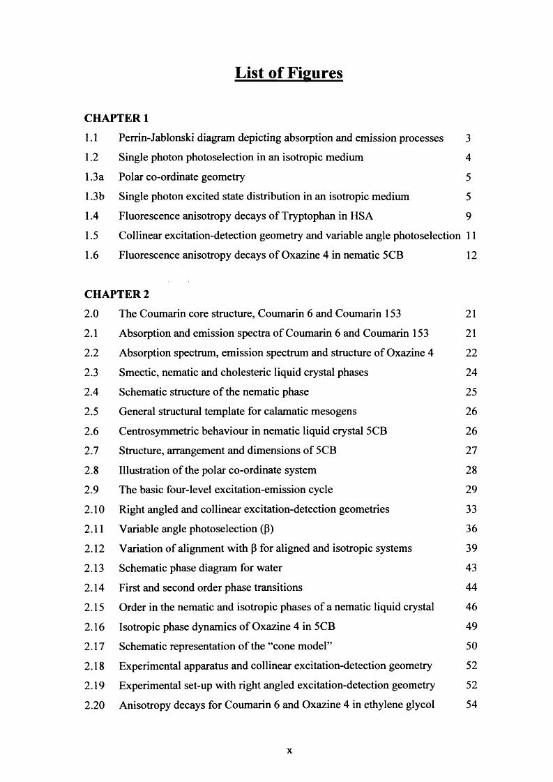
List of Figures

CHAPTER 1

1.1 Perrin-Jablonski diagram depicting absorption and emission processes 3

1.2 Single photon photoselection in an isotropic medium 4

1.3a Polar co-ordinate geometry 5

1.3b Single photon excited state distribution in an isotropic medium 5

1.4 Fluorescence anisotropy decays of Tryptophan in HSA 9

1.5 Collinear excitation-detection geometry and variable angle photoselection 11

1.6 Fluorescence anisotropy decays of Oxazine 4 in nematic 5CB 12

CHAPTER 2

2.0 The Coumarin core structure, Coumarin 6 and Coumarin 153 21

2.1 Absorption and emission spectra of Coumarin 6 and Coumarin 153 21

2.2 Absorption spectrum, emission spectrum and structure of Oxazine 4 22

2.3 Smectic, nematic and cholesteric liquid crystal phases 24

2.4 Schematic structure o f the nematic phase 25

2.5 General structural template for calamatic mesogens 26

2.6 Centrosymmetric behaviour in nematic liquid crystal 5CB 26

2.7 Structure, arrangement and dimensions of 5CB 27

2.8 Illustration of the polar co-ordinate system 28

2.9 The basic four-level excitation-emission cycle 29

2.10 Right angled and collinear excitation-detection geometries 33

2.11 Variable angle photoselection (P) 36

2.12 Variation of alignment with p for aligned and isotropic systems 39

2.13 Schematic phase diagram for water 43

2.14 First and second order phase transitions 44

2.15 Order in the nematic and isotropic phases of a nematic liquid crystal 46

2.16 Isotropic phase dynamics of Oxazine 4 in 5CB 49

2.17 Schematic representation o f the “cone model” 50

2.18 Experimental apparatus and collinear excitation-detection geometry 52

2.19 Experimental set-up with right angled excitation-detection geometry 52

2.20 Anisotropy decays for Coumarin 6 and Oxazine 4 in ethylene glycol 54

x

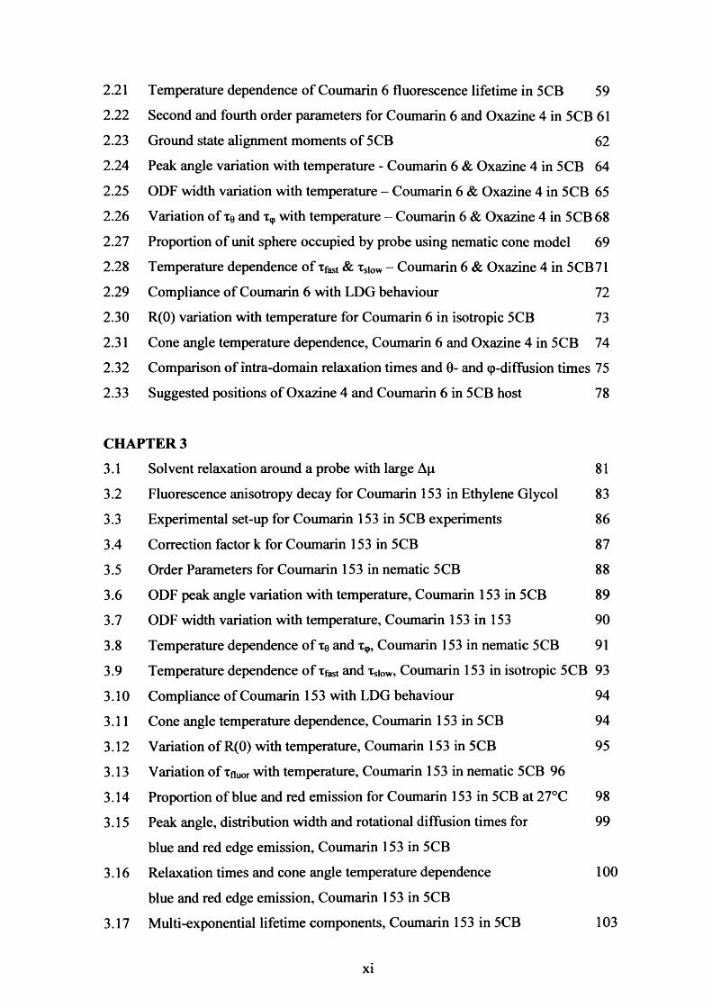
2.21 Temperature dependence o f Coumarin 6 fluorescence lifetime in 5CB 59

2.22 Second and fourth order parameters for Coumarin 6 and Oxazine 4 in 5CB 61

2.23 Ground state alignment moments of 5CB 62

2.24 Peak angle variation with temperature - Coumarin 6 & Oxazine 4 in 5CB 64

2.25 ODF width variation with temperature - Coumarin 6 & Oxazine 4 in 5CB 65

2.26 Variation of Te and with temperature - Coumarin 6 & Oxazine 4 in 5CB 68

2.27 Proportion of unit sphere occupied by probe using nematic cone model 69

2.28 Temperature dependence o f Tfast & tsiow - Coumarin 6 & Oxazine 4 in 5CB71

2.29 Compliance o f Coumarin 6 with LDG behaviour 72

2.30 R(0) variation with temperature for Coumarin 6 in isotropic 5CB 73

2.31 Cone angle temperature dependence, Coumarin 6 and Oxazine 4 in 5CB 74

2.32 Comparison o f intra-domain relaxation times and 0- and <p-diffusion times 75

2.33 Suggested positions of Oxazine 4 and Coumarin 6 in 5CB host 78

CHAPTER 3

3.1 Solvent relaxation around a probe with large Ap 81

3.2 Fluorescence anisotropy decay for Coumarin 153 in Ethylene Glycol 83

3.3 Experimental set-up for Coumarin 153 in 5CB experiments 86

3.4 Correction factor k for Coumarin 153 in 5CB 87

3.5 Order Parameters for Coumarin 153 in nematic 5CB 88

3.6 ODF peak angle variation with temperature, Coumarin 153 in 5CB 89

3.7 ODF width variation with temperature, Coumarin 153 in 153 90

3.8 Temperature dependence o f xe and x9, Coumarin 153 in nematic 5CB 91

3.9 Temperature dependence o f Xfast and xS|0w, Coumarin 153 in isotropic 5CB 93

3.10 Compliance of Coumarin 153 with LDG behaviour 94

3.11 Cone angle temperature dependence, Coumarin 153 in 5CB 94

3.12 Variation of R(0) with temperature, Coumarin 153 in 5CB 95

3.13 Variation of XfiUOr with temperature, Coumarin 153 in nematic 5CB 96

3.14 Proportion of blue and red emission for Coumarin 153 in 5CB at 27°C 98

3.15 Peak angle, distribution width and rotational diffusion times for 99

blue and red edge emission, Coumarin 153 in 5CB

3.16 Relaxation times and cone angle temperature dependence 100

blue and red edge emission, Coumarin 153 in 5CB

3.17 Multi-exponential lifetime components, Coumarin 153 in 5CB 103

3.18 Proportions of each lifetime component as a fraction of total emission 103

3.19 Fits to C l53 data using two and three exponential components 104

3.20 Suggested position of Coumarin 153 molecule in 5CB host 106

CHAPTER 4

4.1 Direct comparison between single and two-photon absorption from a

fluorescent probe

109

4.2 Structures of two-photon polyenes from the Blanchard-Desce group 112

4.3 Molecular structure of OM49, TM11, BH101 and OM77 113

4.4 Absorption and emission spectra of OM49, TM11, BH101 and OM77 113

4.5 Jablonski diagram of two-photon excited fluorescence pathways 116

4.6 Excitation-detection geometries for linearly and circularly polarised

two-photon excitation

118

4.7 Two-photon absorption cross-section, bis-MSB in cyclohexane 123

4.8 Experimental set-up for steady state detection of TPE fluorescence 124

4.9 Two-photon absorption spectra for BH101, OM49, TM11 and OM77 126

4.10 Calculated TP A for BH101, TM11 and OM49 127

4.11 Theoretical TPA for OM77 129

4.12 Experimental TPA cross-sections normalised for OM77 and BH101 129

4.13 Experimental set-up for two-photon fluorescence anisotropy 132

4.14 R(0)l , R(0)c and Q for BH101, TM11, OM49 and OM77 133

4.15 S, D and TPA plots for BH101, TM11, OM49 and OM77 135

4.16 R(0)l , R(0)c, R(0)l/R(0)c and Q for OM49 136

CHAPTER 5

5.0 Jablonski diagram illustrating two-photon excited STED 141

5.1 Effects of STED on excited state population and fluorescence anisotropy 142

5.2 Comparison of single and two-photon transition probabilities 143

5.3 Population removal saturation curves for various values of Xp/Tr 147

5.4 Schematic diagram o f experimental apparatus used for STED experiments 148

5.5 Absorption, emission and choice of Dump wavelength for OM77 149

5.6 Fd and Ar variation with Dump energy for OM77 150

5.7 Saturation curve fit to STED data for OM77 in toluene 151

5.8 Theoretical saturation curve with predicted alignment change for OM77 152

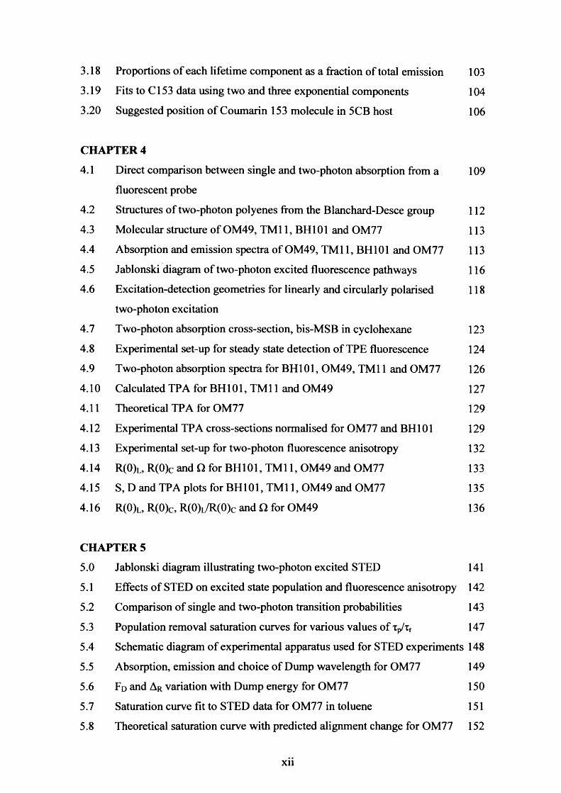
List of Tables

Table 2.1 Photophysical Properties of Oxazine 4 23

Table 2.2 Lifetime and Rotational Anisotropy Decays for Coumarin 6 and 55

Oxazine 4 in Ethylene Glycol

Table 3.1 Photophysical and Hydrodynamic Properties of Coumarin 6 and 83

Coumarin 153

Table 3.2 Lifetime and Rotational Anisotropy Decays for Coumarin 6 and 84

Coumarin 153 in Ethylene Glycol

Table 4.1 Two-Photon Cross-Sections of Natural and Synthetic Fluorescent 110

Probes

Table 4.2 Photophysical Properties of Quadrupolar and Octupolar 114

Chromophores Measured in Toluene

Table 4.3 Two-Photon Absorption Properties for OM77, BH101, OM49 and 130

TM11 in Toluene

xiii

List of Collaborators

Experiment: Two-Photon Absorption Cross-Section Measurements of Quadrupolar and

Branched Chromophores.

Collaborators: Dr Richard Marsh, Dr Martinus Werts, Mr Nick Leonczek.

Experiment: Two-Photon Transition Tensor Measurements of Quadrupolar and

Branched Chromophores.

Collaborators: Dr Richard Marsh.

Experiment: Two-Photon Excited Stimulated Emission Depletion Measurements of a

Branched Chromophore.

Collaborators: Dr Daven Armoogum, Dr Richard Marsh.

xiv

Chapter 1Photophysics o f Molecular Probes

1.1 Introduction

The work in this thesis describes the development and application of polarised single

and two-photon time resolved photoselection techniques to investigate the electronic

structure, order and dynamical properties of fluorescent probes.

The past twenty years has seen great change in the application of fluorescence

techniques primarily reserved for use as research tools in the physical sciences.

Fluorescence is now an interdisciplinary methodology not only applied in the fields of

physics and chemistry, but also in the life sciences. As a result the application of

fluorescent probes has become widespread and varied.

1.2 Molecular Fluorescence

Various physical and chemical parameters such as viscosity, pH, temperature, polarity,

electric potential, quenchers, pressure and hydrogen bonds [1] have a profound

influence on the fluorescence o f a probe molecule. These effects are manifest for

example by the time dependent and steady state fluorescence spectra, the fluorescence

lifetime and the fluorescence polarisation. Thus the assimilation of a probe can provide

specific information on the local environment of a host such as the orientational order

and rotational dynamics in a liquid crystal [2, 3], the structural changes and

conformational transitions and dynamics in biological membranes, in proteins and in

living cells [4].

The absorption and emission processes which take place when a probe molecule

absorbs electromagnetic radiation can be depicted by means of a Perrin-Jablonski

energy level diagram as shown in figure 1.1. In single photon excitation a molecule

absorbs a photon of appropriate energy such that it is raised from its lowest ground state

vibrational level to one of several vibrational levels of the first excited singlet state

1

(So—►Si) In a condensed medium such as a liquid or solid a molecule in a high

vibrational state collides repeatedly with neighbouring molecules rapidly losing its

excess vibrational energy (vibrational relaxation occurs in ~10'12s). Providing the

competing rate constants are small compared with radiative relaxation to the ground

state then there is a high probability for emission of fluorescence [5]. For isolated

molecules the subsequent emission spectrum can be sub-divided into three types of

transition between the molecular quantum states. For any given molecular electronic

state, the level is sub-divided into groups separated by approximately equal energy

levels. These levels correspond to successive states of vibration of the nuclei. The

vibrational level is further sub-divided into a fine structure of levels ascribed to the

different states of rotation of the molecule. The energy separation between adjacent

rotational levels (~ 0.00 lev-0.000 lev), and vibrational levels (~ O.lev) is small [6]. At

ambient temperatures these levels become populated according to Boltzmann statistics

so at any given wavelength it is possible to excite a multitude of ro-vibronic ground to

excited state transitions. The characteristic shape of the emission spectra for different

fluorescent compounds is dependant upon the individual vibrational levels in the ground

and excited states. Compounds which possess vibrational structure will have emission

spectra characterised by patterns of maxima (peaks) and minima (troughs). In the

condensed phases the emission spectrum of a molecular probe is devoid o f detailed

structure due to the density of the vibrational states, the numerous solvent-solute

collisions and ultrafast relaxation dynamics [7].

The absorption and emission spectra can be considered as depicting the vibrational state

density of the first excited state and the vibrational state density of the ground state

respectively. For absorption and emission spectra which possess similarly structured

intensity patterns the spectra are deemed to possess mirror symmetry. Due to fast

relaxation in the excited state, emission energy is less than that o f absorption. Therefore

emission resulting from single photon excitation is at longer wavelengths than

absorption. This is known as the Stokes shift.

Not all transitions are equally probable when considering the possible transitions from

the vibrational levels of one electronic state to vibrational levels of another electronic

state (e.g. Sq—►Si). Selection rules govern the possible transitions and the transition

2

probabilities are dependent upon the overlap between the vibrational wavefunctions of

the two states (Franck-Condon factor).

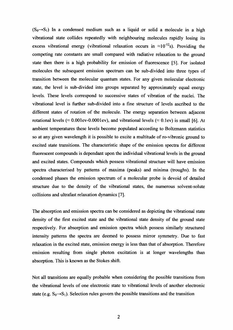
Vibrational Relaxation (lO"12s)

InternalConversion (lO '12s)

IntersystemCrossing

(I010s)

Absorption (10 15s)

Fluorescence( I 0 9s)

Phosphorescence (10 3s)

Figure 1.1: A Perrin-Jablonski diagram in which So, St, S2... denote singlet states and Tt a triplet

state. Singlet states possess net spin angular momentum 0 whilst triplet states possess net spin

angular momentum 1. Radiative relaxation to the ground state is highly improbable from states of

different electron spin multiplicity. Arrows pointing upwards represent possible absorption

transitions between singlet states. Emission from the triplet state Tj represents phosphorescence

and occurs on a timescale very much longer than emission from singlet states.

The process o f fluorescence is one possible pathway by which a molecule can return to

the ground state once excited. However, many alternative de-excitation pathways exist

such as internal conversion, intersystem crossing, intramolecular charge transfer,

collisional depopulation and conformational change [1].

The fluorescence lifetime and quantum yield are particularly important features of a

fluorophore. The quantum yield is defined as the number of emitted photons relative to

the number of absorbed photons. Fluorescence dye probes such as rhodamine6G

possess quantum yields in excess of 95% at room temperature [6]. The fluorescence

lifetime is defined as the interval during which the intensity of fluorescence has fallen to

\/e o f its maximum value. This characteristic is particularly important as it determines

3

the average length of time an excited molecule can interact with its environment and

therefore defines the time window available for observation of dynamic processes.

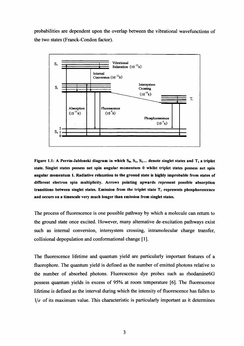
1.3 Polarised Photoselection, Fluorescence Anisotropy and Isotropic

Rotational Diffusion

Most experiments involving fluorescence are carried out using polarized light sources

[3]. In this situation the fluorescence emission after excitation is also polarized. The

polarized emission is a result o f the interaction between the transition dipole moment of

the fluorophore and the electric vector o f the excitation source. The transition dipole

moment is oriented relative to the molecular axis, so in an isotropic environment where

the molecules are randomly distributed the transition dipole moments are also oriented

randomly. Those fluorophores which possess transition dipole moments aligned parallel

to the electric vector of the excitation source are then preferentially excited as shown in

figure 1.2.

• / I1 . # »# % « • '- %

Unexcited Molecule

/Isotropic Media

4 >COS^0 D-

pliotosdection

E

VVertically Polarised

Light

Figure 1.2: A schematic representation of single-photon photoselection in an isotropic medium. The

probability of absorption is dependent on the orientation of the transition dipole moment relative to

the electric vector of the of the excitation source. Those fluorophores which possess absorption

dipoles which make a small angle with respect to the E field will be preferentially excited relative to

those oriented close to the perpendicular plane.

J % 9 i % ■• ,< * I

* * * $ i » v - ,

j !

The electric dipole moment need not necessarily be aligned precisely parallel to the

electric vector of the excitation source to absorb light. As the probability of excitation is

4

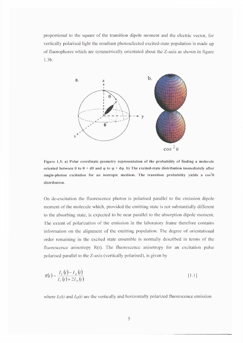
proportional to the square o f the transition dipole moment and the electric vector, for

vertically polarised light the resultant photoselected excited-state population is made up

o f fluorophores which are symmetrically orientated about the Z-axis as shown in figure

1.3b.

♦i

x

cos 2e

Figure 1.3: a) Polar coordinate geom etry representation o f the probability o f Finding a molecule

oriented between 0 to 0 + d0 and <p to <p + d<p. b) The excited-state distribution im mediately after

single-photon excitation for an isotropic medium. The transition probability yields a cos20

distribution.

On de-excitation the fluorescence photon is polarised parallel to the emission dipole

moment o f the molecule which, provided the emitting state is not substantially different

to the absorbing state, is expected to be near parallel to the absorption dipole moment.

The extent o f polarization o f the emission in the laboratory frame therefore contains

information on the alignment o f the emitting population. The degree o f orientational

order remaining in the excited state ensemble is normally described in terms o f the

fluorescence anisotropy R(t). The fluorescence anisotropy for an excitation pulse

polarised parallel to the Z-axis (vertically polarised), is given by

*(')= Ij7 T" A [ '• ']/„(«)+2/„(»)

where Iy(t) and Ih(0 are the vertically and horizontally polarized fluorescence emission

5

intensities respectively. For a cylindrically symmetric system these are given by [1]

[1.2a]

[1.2b]

Here N,,:x(t) is the excited state population remaining at time t following excitation.

From symmetry considerations it can be shown that the fluorescence anisotropy is

proportional to the degree of second-order alignment present in the excited state [8, 9]:

where Pex is the probability of finding the molecule aligned between the polar angles 0

to 0 + d0 and (p to (p + d(p (figure 1.3a) and Y*2o is a spherical harmonic o f the form

initial single-photon maximum anisotropy is 2/5 [1].

In the condensed phase molecules cannot undergo free rotation as in the gas phase but

assumed to occur in small steps resulting in the randomisation of the ensemble of

molecular orientations (Appendix II). Due to the continuous interactions with their

neighbours molecules rotating in a liquid experience friction. This can be described by

simple hydrodynamic theory where the behaviour is related to the size and shape of the

fluorescent molecule and the relative viscosity o f the local environment. Effects on the

[1.3]

[1.4]

Inserting equation 1.3 into 1.4 yields

[1.5]

where ( ) denotes an average over the distribution. For an isotropic distribution the

I tare subject to rapid solute-solvent collisions 10* s' [7]. In this case the reorientation is

6

rotational dynamics o f the molecule depend on the boundary conditions, which are

broadly classified as either stick or slip depending on the degree to which molecular

rotation involves cooperative movement o f the surrounding solvent (this is discussed in

state and causes a displacement o f the emission dipole and the extent of the fluorescence

depolarization caused by rotational diffusion, yields information on the motion of the

fluorescent molecule in the host environment. If the absorption and emission transition

dipole moments are approximately parallel and lie along or in the vicinity of the

molecular axis, then the diffusion approximates to that of a symmetric rotor [10]. In this

case the fluorescence anisotropy is given by

seen that the rotational diffusion time is proportional to the molecular hydrodynamic

volume V and the solvent viscosity rj. It is also inversely proportional to the thermal

energy kT. The molecular shape factor f and the boundary coefficient C, which accounts

The rotational dynamics described above refer to an isotropic fluid, where rotational

diffusion is relatively straightforward and diffusion times for small molecular probes

vary from a few nanoseconds to several hundred picoseconds [5]. This is not the case

for fluorescent probes used to investigate locally structured environments such as

membranes or the mesophases o f a liquid crystal. Similarly complex behaviour occurs

detail in Chapter 2). Such rotational diffusion occurs during the lifetime of the excited

R(t) = /?(o)exp — - [1.6]

where trot is the rotational diffusion time given by

[1.7]

and D is defined as the rotational diffusion coefficient (s'1). From equation 1.8 it can be

for the interaction between the solvent and solute, are two constants which modify the

relationship giving the rotational diffusion time as

[1.8]

7

with naturally occurring fluorescent probes found in large molecules such as proteins. In

these environments, the fluorescent probe is no longer free to rotate, but is in fact

restricted by the local geometry of the media. Although the overall orientational

distribution of the macro environment is isotropic, the steady state orientational

distribution of the fluorescent probe locally, is no longer isotropic. These characteristics

are manifest in bi-exponential anisotropy decays indicating degrees of local order and

global order within the host environment. Providing the local and global rotational

diffusion times are independent o f each other, the fluorescence anisotropy is defined as

the product of the correlation function [2]:

R(t) = expV T S1X)W j

(*(0) Rdomain )exPV T FAST J

+ R1X)MAIN [1.9]

where R ( 0 ) and R dom ain are the limiting values o f the anisotropy in the absence of

motion of the domains. The ratio of the two pre-exponential factors in equation 1.9

reveals the degree of the local restricted motion of the fluorescent probe. These factors

can be used to determine the angular width o f the probe environment from equation

1. 10.

J ^ 4 [eos^ ( , + c o s ^ )] [ 1 1 0 ]

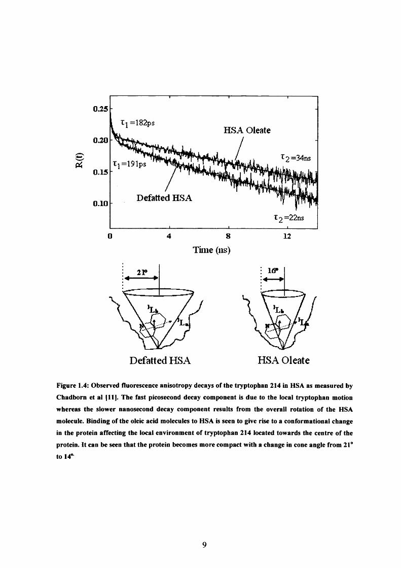
From such R(t) measurements it is possible to determine conformational changes and

local structure in complex protein molecules such as Human Serum Albumin (HSA).

Human serum albumin (HSA) is the most abundant protein found in plasma and

performs many important functions including the transport, distribution and metabolism

of many endogenous and exogenous ligands (e.g. fatty acids, amino acids, steroids and

numerous pharmaceuticals) [10, 11]. Studies undertaken by Chadbom et al revealed the

ligand dependent conformational changes induced by binding Oleic acid to the protein

[11]. The results revealed that that the presence of the Oleate increased the rotational

diffusion time of the protein and decreased the restricted rotational motion o f the

tryptophan probe [11] confirming that structural change in HSA could be induced by

ligand binding (Figure 1.4).

8

0.25

=182psHSA Oleate

0.20

Tj=191ps0.15

Defatted HSA0.10

X o =2 2ns

0 4 8 12

Time (ns)

Defatted HSA HSA Oleate

Figure 1.4: Observed fluorescence anisotropy decays of the tryptophan 214 in HSA as measured by

Chadborn et al [11]. The fast picosecond decay component is due to the local tryptophan motion

whereas the slower nanosecond decay component results from the overall rotation of the HSA

molecule. Binding of the oleic acid molecules to HSA is seen to give rise to a conformational change

in the protein affecting the local environment of tryptophan 214 located towards the centre of the

protein. It can be seen that the protein becomes more compact with a change in cone angle from 21°

to 14°

9

1.4 Probe Behaviour in Highly Ordered Environments

Highly ordered systems are found throughout nature and the presence o f order can have

a profound effect on the intrinsic properties and behaviour of a system. The optical [13]

and photophysical behaviour [14], the chemical reactivity [15] and the molecular

dynamics of a system [16] all depend on the degree of order. In biological systems

membranes contain highly organized molecular assemblies that mediate important

processes such as energy transduction, active transport, nerve impulse conduction,

sensory reception, and hormonal integration [17]. In the ordered environment o f liquid

crystals the ability for the molecules to respond to external electric fields has generated

industrial applications in the form o f liquid crystal displays, optical imaging and

recording. The probing of molecular order to obtain structural, functional and dynamical

information is therefore of considerable scientific interest and the use of time resolved

photoselection techniques, have facilitated studies in the behaviour o f ordered

environments.

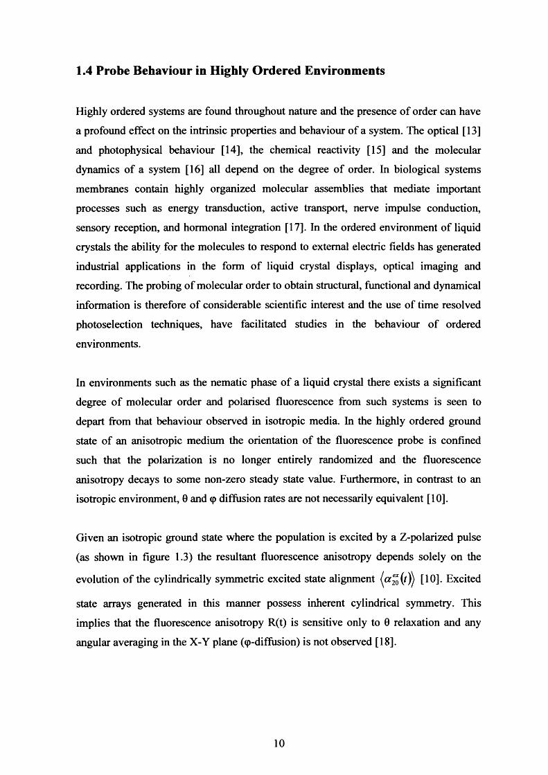
In environments such as the nematic phase of a liquid crystal there exists a significant

degree o f molecular order and polarised fluorescence from such systems is seen to

depart from that behaviour observed in isotropic media. In the highly ordered ground

state of an anisotropic medium the orientation of the fluorescence probe is confined

such that the polarization is no longer entirely randomized and the fluorescence

anisotropy decays to some non-zero steady state value. Furthermore, in contrast to an

isotropic environment, 0 and <p diffusion rates are not necessarily equivalent [10].

Given an isotropic ground state where the population is excited by a Z-polarized pulse

(as shown in figure 1.3) the resultant fluorescence anisotropy depends solely on the

evolution of the cylindrically symmetric excited state alignment [10]. Excited

state arrays generated in this manner possess inherent cylindrical symmetry. This

implies that the fluorescence anisotropy R(t) is sensitive only to 0 relaxation and any

angular averaging in the X-Y plane (<p-diffusion) is not observed [18].

10

In an isotropic system 0 and <p diffusion is wholly equivalent. In an anisotropic

environment this is not necessarily the case. By varying the excitation polarisation angle

P with respect the laboratory fixed axis (figure 1.5), the preparation o f cylindrical

asymmetric ^ a 2 ( ' M 3 8 we^ 2 8 cylindrically symmetric (a ^ ( 0 ) initial

probe alignment is possible [8 , 12]. In the example of a doped nematic liquid crystal

aligned parallel to the laboratory Z-axis (described in Chapter 2) an excitation

polarisation angle P=0° creates a cylindrically symmetric excited state with respect to

the nematic director n. Relaxation of this distribution can be observed only in 0

averaging.

AMIv(t)

DetectionSystem

ExcitationPulse

NematicSample

Figure 1.5: Experimental arrangement for time resolved photoselection using a variable polarised

excitation pulse. Photoselection is achieved using single-photon excitation in a 180° excitation-

detection geometry. Variation of the polarisation angle p is with respect to the nematic director n.

The vertically (lv) and horizontally (1H) polarised emission intensities are used to construct the

fluorescence anisotropy R(t, P). The technique is described in detail in Chapter 2.

In contrast, for p=90° a significant degree of asymmetric excited state alignment is

created which principally relaxes by cp diffusion. Given an arbitrarily ordered excited

state it is possible to determine the fluorescence anisotropy based on the degrees of

symmetric and asymmetric probe alignment, which in the coordinate system (Zi) as

defined in figure 1.5, is given by equation 1.11 [8 ]:

11

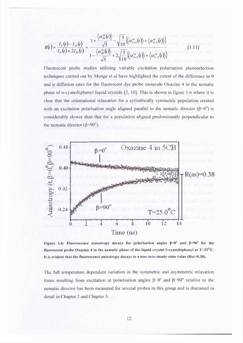
Fluorescent probe studies utilising variable excitation polarisation photoselection

techniques carried out by Monge et al have highlighted the extent of the difference in 0

and cp diffusion rates for the fluorescent dye probe molecule Oxazine 4 in the nematic

phase of n-cyanobiphenyl liquid crystals [2, 10]. This is shown in figure 1.6 where it is

clear that the orientational relaxation for a cylindrically symmetric population created

with an excitation polarisation angle aligned parallel to the nematic director (P=0°) is

considerably slower than that for a population aligned predominantly perpendicular to

the nematic director (p=90°).

Oxazine 4 in 5CB0.48-

II

°oII

CCLr

oo

0.32-04o430

1 0 2 J '

10 12 146 82 40

T im e (n s )

Figure 1.6: Fluorescence anisotropy decays for polarisation angles 0=0° and p=90° for the

fluorescent probe Oxazine 4 in the nematic phase o f the liquid crystal 5-cyanobiphenyl at T=25°C.

It is evident that the fluorescence anisotropy decays to a non-zero steady state value (Rss=0.38).

The full temperature dependent variation in the symmetric and asymmetric relaxation

times resulting from excitation at polarisation angles p=0° and p=90° relative to the

nematic director has been measured for several probes in this group and is discussed in

detail in Chapter 2 and Chapter 3.

12

From the anisotropy decays created via time resolved single-photon excited

fluorescence in a highly aligned environment, it is not only possible to determine the

excited state rotational relaxation times of a fluorescence probe but also the ground state

order parameters and [9] (Appendix I). However symmetry

constraints limit the sensitivity of single-photon emission to the K=2 alignment

moments of an excited state configuration, irrespective of its overall orientational

distribution [3, 8 ]. The direct measurement of higher ground state alignment moments

(K=6 ) is only possible if the interaction of the electric field with the aligned molecular

population is defined by a higher order interaction such as two-photon excitation. To

this end Monge and Armoogum [2, 18] have combined both single and two-photon

fluorescence anisotropy measurements to determine the previously concealed (K=6 )

moments of the ground state probe distribution function.

Studies by Monge [2] were extended to the isotropic phase of n-cyanobiphenyls where

bi-exponential fluorescence anisotropy decays were recovered showing evidence of fast

intra-domain relaxation (xf) within a more slowly relaxing pseudo-domain structure (xs)

(details of which are shown in Chapter 2). This structure is evident across much of the

isotropic phase. It is only at high temperatures (up to 50°C above the nematic-isotropic

phase transition temperature T ni) where mono-exponential fluorescence anisotropy

decays are apparent reflecting behaviour indicative of a globally isotropic environment.

The presence of a pseudo-domain structure was revealed for all the cyanobiphenyls

studied. Furthermore, the inter- and intra- domain probe relaxation times show a

temperature dependence which was in good agreement with the predictions of theory

developed on the dynamics of liquid crystals [2 ].

13

1.5 Time Resolved Two-Photon Excited Fluorescence

Two-photon absorption is a non linear optical process which provides a variety o f new

capabilities in various scientific fields. The first quantum calculations were performed

by Maria Goppert-Mayer in 1931, who predicted that a molecule could absorb two-

photons simultaneously in the same quantum event [19]. The probability o f two-photon

excitation is sensitive to different molecular and ensemble parameters than single

photon. As well as a quadratic dependence on the intensity of the exciting laser light, its

temporal properties are also important [7]. The transition also can not be characterized

by a single absorption dipole moment, the orientational dependence of the transition

probability is instead described by the transition tensor [20]. (These differences are

discussed in greater detail in Chapter 4).

Due to these inherent differences compared to single photon absorption two-photon

excited fluorescence is strongly dependent on the focal properties of the excitation

source. Two-photon absorption is maximised in the Rayleigh region of a focused

Gaussian beam [4]. This inherent depth resolution has made two-photon fluorescence a

highly useful tool in the life sciences especially in fluorescence microscopy [21]. As a

result there has been considerable effort in recent years to produce fluorophores with

high two-photon absorption cross-sections and optimised fluorescence yields [22]. In

this respect the work of Blanchard-Desce and co-workers at the CNRS Institute, Rennes

has been particularly successful and involves the design and synthesis of an extensive

series of quadrupolar and octupolar push-push (electron donating) and push-push

(electron withdrawing) polyenes [22, 23, 24, 25].

1.6 Stimulated Emission Depletion (STED)

The technique of far-field fluorescence light microscopy has been plagued by the

diffraction resolution limit, the fundamental limit below which it is impossible to

distinguish between two objects. The research of Ernst Abbe put a minimum limit on

the distance over which it is possible to distinguish between two objects using light

microscopy as approximately 1/3A. where X is the wavelength of light [26]. This intrinsic

property of far field microscopy has been found to be particularly restraining in the case

14

of fluorescence imaging of biological specimens such as live cells. However recent

research has shown that these limits can be overcome by combining fluorescence

microscopy with stimulated emission depletion (STED) [27] the principle of which is

outlined as follows (a detailed explanation is given in Chapter 5). For single-photon

stimulated emission depletion the excitation or ‘pump’ pulse is focused into the sample,

producing an excited state population which is manifest by an ordinary diffraction

limited spot. The ‘pump’ pulse is followed by a time-delayed, red-shifted depletion or

‘dump’ pulse. By spatially displacing the ‘pump’ and ‘dump’ pulses, it is possible to

form an intense, localized fluorescent region in the sample. The volume from which

spontaneous emission then follows is effectively restricted and with appropriate spatial

and temporal shaping of the ‘dump’ pulse, the fluorescent spot can be progressively

narrowed down, theoretically without limit so breaking the fundamental diffraction

barrier. Although STED microscopy to date has been limited to single-photon excited

states, the engineering and development o f chromophores optimised for two-photon

absorption which have proven STED capabilities, coupled with advancements in

precision imaging may provide improved optical microscopy techniques and enhanced

biological imaging.

Further advances in stimulated emission depletion techniques have recently been

demonstrated by Armoogum et al who have developed a new approach to time resolved

fluorescence spectroscopy based on stimulated emission depletion o f two-photon

excited states [18, 28]. In combining streak camera measurements of excited state

population depletion and two-photon fluorescence anisotropy measurements, the

stimulated emission cross section and the ground state vibrational relaxation time has

been measured in the fluorescent dye probes rhodamine 6 G and fluorescein. The studies

have been further extended to incorporate high two-photon absorption cross section

push-push polyenes [29] and enhanced green fluorescent protein (EGFP) [30]. STED

has also been used as a way of probing higher order excited state moments ( a ^ [18]

whereby the normal electric dipole selection rules which restrict the amount of

information available in conventional single-photon fluorescence spectroscopy are

circumvented allowing access to previously 'hidden' information on molecular structure,

dynamics and geometry.

15

1.7 Chapters Overview

Time resolved photoselection techniques rely on the fluorescent properties of well

characterised fluorophores to study the local environment of molecular systems. As a

consequence of the strong influence of the host medium, fluorescent probes that have

readily interpretable photophysical properties can be specifically inserted into ordered

environments to reveal facets o f their structure and dynamics. Experiments detailed

within Chapter 2 and Chapter 3 have been carried out using such time resolved

photoselection techniques, to measure the molecular order and molecular dynamics of

the nematic liquid crystal 4-n-pentyl-4’-cyanobiphenyl (5CB) whilst doped with the

coumarin fluorescent dye probe derivatives Coumarin 6 and Coumarin 153. Previous

work in the group has concentrated on the behaviour of four common Xanthene dyes in

5CB: Rhodamine B, Rhodamine 6 G, Oxazine 4 and Oxazine 1. Although Coumarin 6

shows similar characteristics and is well described by conventional models, Coumarin

153 in contrast exhibits substantial solvatochromic effects.

Studies have been carried out to investigate the structural and photophysical properties

of several quadrupolar and octupolar chromophores in the solvent toluene. The

wavelength dependence of the two-photon absorption cross-section o f several

quadrupolar and octupolar push-push polyenes has been investigated. These

measurements have been combined with wavelength dependent two-photon

fluorescence anisotropy measurements yielding information on the structure of the two-

photon transition tensor. These detailed investigations are outlined in Chapter 4.

Furthermore, by combining anisotropy measurements with stimulated emission

depletion measurements the stimulated emission cross-section and ground state

vibrational relaxation time for a branched octupolar derivative (OM77) has been

determined. This study is detailed in Chapter 5.

16

References

[1] Bernard Valeur “Molecular Fluorescence; Principles and Applications” Second

Reprint, Wiley-VCH (2005)

[2] E M Monge, Ph. D. Thesis, University College London (2003)

[3] A J Bain and A.J. McCaffery, J. Chem. Phys., 83, 2627 (1985)

[4] B Larijani and A J Bain, “Biological Applications o f Single and Two-Photon

Fluorescence” in “Biological Chemistry” Eds B Larijani, C A Rosser and R

Woscholski, Wiley London (2006)

[5] J R Lakowicz, “Principles o f Fluorescence Spectroscopy” Second Edition, Kluwer

Academic (1999)

[6 ] I B Berlmann, “Handbook o f Fluorescence Spectra o f Aromatic Molecules ” Second

Edition, Academic Press, NewYork (1971)

[7] G R Fleming, “Chemical Applications o f Ultrafast Spectroscopy” Clarendon (1986)

[8 ] A J Bain, P Chandna and J Bryant, J. Chem. Phys., 112,10418 (2000)

[9] D L Andrews and A A Demidov (Ed.) “An Introduction to Laser Spectroscopy”

Second Edition, Kluwer (2002)

[10] J Bryant, Ph. D. Thesis, University of Essex, (2000)

[11] N Chadbom, J Bryant, A.J.Bain and P. O’Shea, Biophysical J., 76, 2198 (1999)

[12] A J Bain, P Chandna, G Butcher and J Bryant, J. Chem. Phys., 112, 10435 (2000)

[13] W R Thomkins, M S Malcut, R W Boyd and J E Sipe, J. Opt. Soc. Am., 6, 757

(1990)

[14] D L Andrews and D Juzelinas, J. Chem. Phys., 95, 5513 (1995)

[15] P A Anfinrud, D E Hart and W S Struve, J. Phys. Chem., 92,4067 (1988)

[16] H J Loesch, E Stenzel and B Wustenecker, J. Phys. Chem., 95, 3841 (1991)

[17] J Yguerabide and L Stryer, Proc. Nat. Acad. Sci. 6 8 , 1217 (1971)

[18] D A Armoogum, Ph. D. Thesis, University College London (2004)

[19] C Xu and W W Webb, J. Opt. Soc. Am. B., 3, 481 (1996)

[20] P N Butcher and D Cotter, “The Elements o f Nonlinear Optics” Cambridge

University Press, Cambridge (1998)

[21] W Denk, J H Strickler and W W Webb, Science., 248, 73 (1990)

[22] F Terenziani, C Le Droumaguet, C Katan, O Mongin, M H V Werts, S Tretiak and

M Blanchard-Desche. SPIE-Int. Soc. Opt. Eng., 5935 (2005)

17

[23] C Katan, F Terenziani, O Mongin, M H V Werts, L.Porres, T Pons, J Mertz, S

Tretiak and M Blanchard-Desche, J. Chem. Phys. A., 109, (2005)

[24] C Katan, F Terenziani, O Mongin, M H V Werts, C Le Droumaguet, L Porres, T

Pons, J Mertz, S Tretiak and M Blanchard-Desche, J. Phys. Chem. A., 109, 13, (2005)

[25] L Porres, C Katan, O Mongin, T Pons, J Mertz and M Blanchard-Desche, J. Mol.

Struct., 704, (2004)

[26] R Kopelman and W Tan, Science., 262, 1382 (1993)

[27] O Mongin, L Porres, M Chariot, C Katan and M Blanchard-Desche. Chem. Eur. J.,

13 (2007)

[28] R J Marsh, D A Armoogum and A J Bain, Chem. Phys. Lett., 366, 398 (2002)

[29] R J Marsh, N D Leonczek, D A Armoogum, O Mongin, L Porres, M Blanchard-

Desche and A J Bain, SPIE-Int. Soc. Opt. Eng., 5510 (2004)

[30] T Masters, D A Armoogum, R J Marsh and A J Bain, to be published

18

Chapter 2Studies in the Nematic and Isotropic Phase o f 5-Cyanobiphenyl

Part I: Coumarin 6

2.1 Introduction

In the next two chapters short picosecond pulsed photoselection and time resolved

fluorescence polarisation and intensity measurements are used to investigate the

behaviour of two coumarin probes in the isotropic and nematic phases of 5-

cyanobiphenyl (5CB). Previous work in the group has concentrated on the alignment

and rotational dynamics of ionic fluorescent probes such as Rhodamine 6 G, Rhodamine

B, Oxazine 1 and Oxazine 4 [1, 2]. Coumarin dyes, whilst polar, are non-ionic and

hydrophobic in nature; consequently the nature of their positioning into a cyanobiphenyl

host should be substantially different to that of an ionic fluorophore with a greater

propensity to association with the alkyl tail environment of the 5CB molecules.

Coumarin 6 (C6 ) and Coumarin 153 (C l53) whilst possessing the same fluorescent core

differ substantially both in shape and excited state properties. Both probes have

significant ground state dipole moments (7D for C6 and 6 .6 8 D for C l53 [3]). However,

in contrast to Coumarin 6 , on excitation to the Si state C l53 experiences a substantial

increase in dipole moment of c.a. 90% (see table 2.0). In non-ordered solvents this leads

to a time-dependent Stokes shift due to reorganisation o f the solvent in reaction to the

new excited state dipole moment. Such effects are well understood in C l53 which has

been the subject of numerous experimental and theoretical studies over recent years [4-

10]. However, solvation dynamics in an ordered environment have until now not been

studied experimentally.

Substantial solvent-solute reorganisation in an ordered system presents a number of

experimental challenges and the use of fluorescence anisotropy measurements may be

compromised. For this reason the experimental studies and analysis of Coumarin 6 and

Coumarin 153 fluorescence data are substantially different. Coumarin 6 undergoes a

much smaller increase in dipole moment (c.a. ID) and can be treated in an analogous

manner to experiments using non-strongly solvating ionic dyes (Rhodamine 6 G,

19

Rhodamine B, Oxazine 1 and Oxazine 4). Experiments on Coumarin 6 are covered in

this chapter and a modified procedure involving global analysis of polarised intensity

decays for Coumarin 153 are covered in Chapter 3.

2.2 Fluorescence Probes

Time resolved photoselection techniques rely on the fluorescent properties of well

characterised fluorophores to study the local environment of molecular systems. As a

consequence of the strong influence of the host medium, fluorescent probes that have

readily interpretable photophysical properties can be specifically inserted into ordered

isotropic environments to reveal facets o f their structure and dynamics. It is therefore

desirable to investigate molecular systems with a variety of fluorescent probes

characterized by different photophysical properties. The properties of a system can be

measured directly if naturally occurring fluorescent species exist within the system;

however such intrinsic fluorescent probes are limited. Some of the few existing

examples are green fluorescent protein, tryptophan and tyrosine. Where the molecule is

non-fluorescing or has low quantum yield then extrinsic probes such as rhodamine and

oxazine are attached to the media and their properties are measured indirectly.

2.2.1 Coumarin

The role o f coumarin fluorescent dyes in spectroscopy had traditionally been limited to

laser dye applications; however with the rapid rise in the use of solid-state laser

technology coumarin derivatives are now increasingly utilised as fluorescence probes.

Coumarins are formed by fusing benzene with an auxochromic non-fluorescing a-

pyrone [1 1 ], and although they are themselves poor emitters with low quantum yield,

appropriate substitution can form fluorescent compounds which emit in the blue-green

region of the visible spectrum. The two coumarin derivatives employed in this thesis are

the 7-aminocoumarins Coumarin 6 and Coumarin 153. The fluorescence yield for 7-

aminocoumarins depends on the pattern of substitution o f the amine function [12]. The

molecular structure o f the parent chromophore along with the derivatives is shown in

figure 2.0. Coumarin 6 is formed with substitution of position 7 by the delocalising

substituent group N(HsC2)2 and substitution of position 3 with the electron donating

benzothiazol group. Coumarin 153 is formed with substitution of position 4 by the

20

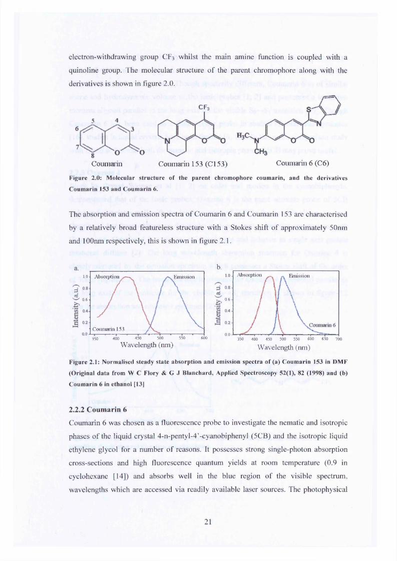
electron-withdrawing group CF3 whilst the main amine function is coupled with a

quinoline group. The molecular structure of the parent chromophore along with the

derivatives is shown in figure 2 .0 .

Coumarin Coumarin 153 (C l53) Coumarin 6 (C6 )

Figure 2.0: M olecular structure o f the parent chrom ophore coumarin, and the derivatives

Coumarin 153 and Coumarin 6.

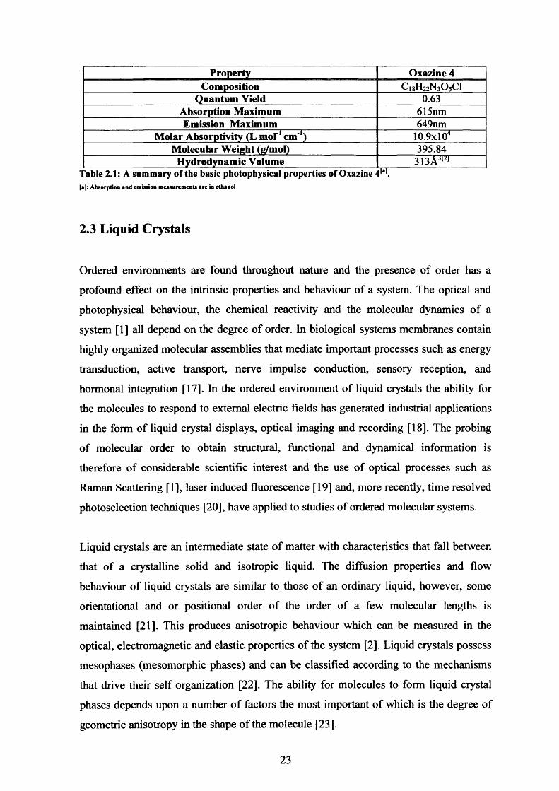
The absorption and emission spectra of Coumarin 6 and Coumarin 153 are characterised

by a relatively broad featureless structure with a Stokes shift of approximately 50nm

and lOOnm respectively, this is shown in figure 2.1.

Absorption Emission1.0

3cc06

Coumarin 153o.o

450 500 550 600400350

b.

Wavelength (nm)

Absorption Emission

0 . 6 -

0.0350 400 450 500 550 600 650 700

Wavelength (nm)

Figure 2.1: Normalised steady state absorption and emission spectra o f (a) Coumarin 153 in DM F

(Original data from W C Flory & G J Blanchard, Applied Spectroscopy 52(1), 82 (1998) and (b)

Coumarin 6 in ethanol [13]

2.2.2 Coumarin 6

Coumarin 6 was chosen as a fluorescence probe to investigate the nematic and isotropic

phases of the liquid crystal 4-n-pentyl-4’-cyanobiphenyl (5CB) and the isotropic liquid

ethylene glycol for a number of reasons. It possesses strong single-photon absorption

cross-sections and high fluorescence quantum yields at room temperature (0.9 in

cyclohexane [14]) and absorbs well in the blue region of the visible spectrum,

wavelengths which are accessed via readily available laser sources. The photophysical

21

behaviour of Coumarin 6 is highly receptive to the polarity and viscosity of the solvent

host [14] which makes it a good candidate for fluorescence experiments requiring low

concentration molecular probes. Though spectrally different, Coumarin 6 is of similar

shape and hydrodynamic volume to the ionic probes [1 , 2 ] and possesses a transition

moment aligned parallel to the long axis for the visible So—►Si transition [15]. Though

Coumarin 6 has been used as a fluorescence probe in studies of rotational dynamics

[16], studies in liquid crystals have been limited [6 , 16]. To this end a comparison study

with Oxazine 4 across both the nematic and isotropic phase of 5CB may prove useful.

2.2.3 Oxazine 4

Work by Bryant, Monge et al [1, 2] on order and motion in the cyanobiphenyls,

demonstrated that of the ionic probes, Oxazine 4 is the most accurate probe of 5CB

order and correlates well with the local ordering of 5CB in the nematic phase. As such

Oxazine 4 has been chosen as the probe molecule best suited for comparison with

Coumarin 6 . Oxazine 4 is a planar, rigid molecule and behaves as single axis prolate

rotational diffuser [2]. The long wavelength absorption spectrum for Oxazine 4 is

closely mirrored by the emission spectrum which possesses a Stokes shift o f the order

of 30nm (figure 2.2). The transition dipole moment for Oxazine 4 is oriented parallel to

the long axis of the molecule for the visible So—►Si transition as shown in figure 2.2

with the absorption and emission spectrum [2 ].

Emission

0.8

0>43co£

0 4

Oxazine 4700650600550

NHC2HHjCjHN► CIO.

Wavelength (nm)

Figure 2.2: The absorption and emission spectra of Oxazine 4. The molecular structure and transition dipole moment direction are also shown.

22

PropertyComposition

Oxazine 4_____C18H22N3O5CI

Quantum Yield 0.63Absorption Maximum 615nmEmission Maximum 649nm

Molar Absorptivity (L mol'1 cm'1) 10.9x104

Molecular Weight (g/mol) 395.84Hydrodynamic Volume 313A^J

Table 2.1: A summary of the basic photophysical properties of Oxazine 41*1.|a): Absorption and emission measurements are in ethanol

2.3 Liquid Crystals

Ordered environments are found throughout nature and the presence of order has a

profound effect on the intrinsic properties and behaviour of a system. The optical and

photophysical behaviour, the chemical reactivity and the molecular dynamics of a

system [1] all depend on the degree of order. In biological systems membranes contain

highly organized molecular assemblies that mediate important processes such as energy

transduction, active transport, nerve impulse conduction, sensory reception, and

hormonal integration [17]. In the ordered environment of liquid crystals the ability for

the molecules to respond to external electric fields has generated industrial applications

in the form of liquid crystal displays, optical imaging and recording [18]. The probing

of molecular order to obtain structural, functional and dynamical information is

therefore of considerable scientific interest and the use of optical processes such as

Raman Scattering [1], laser induced fluorescence [19] and, more recently, time resolved

photoselection techniques [2 0 ], have applied to studies of ordered molecular systems.

Liquid crystals are an intermediate state of matter with characteristics that fall between

that of a crystalline solid and isotropic liquid. The diffusion properties and flow

behaviour of liquid crystals are similar to those of an ordinary liquid, however, some

orientational and or positional order of the order of a few molecular lengths is

maintained [21]. This produces anisotropic behaviour which can be measured in the

optical, electromagnetic and elastic properties of the system [2]. Liquid crystals possess

mesophases (mesomorphic phases) and can be classified according to the mechanisms

that drive their self organization [22]. The ability for molecules to form liquid crystal

phases depends upon a number o f factors the most important of which is the degree of

geometric anisotropy in the shape of the molecule [23].

23

The liquid crystal may pass through several mesophases before transformation to the

isotropic state. They are generally composed of rod-like molecules and are broadly

classified as nematic, smectic or cholesteric depending on the difference in the degree of

orientational and/or positional ordering of the constituent molecules as shown in figure

2.3.

Smectic Nematic Cholesteric

Figure 2.3: Illustration o f the positional and orientational ordering in the nem atic, sm ectic and

cholesteric liquid crystal phases. The nem atic state is characterised by molecules that have no

positional order but tend to point in the sam e direction along the nematic director n. In the sm ectic

state, the molecules maintain the general orientational order o f nem atics, but also tend to align

themselves in layers or planes. The cholesteric liquid crystal phase is typically com posed o f nem atic

mesogenic molecules containing a chiral center which produces interm olecular forces that favour

alignm ent between molecules at a slight angle to each other.

Thermotropic liquid crystals are characterised by thermally induced phase transitions

and the intermediate states develop only as a result of thermal processes. Lyotropic

liquid crystals are defined by phase transitions induced by changes in solvent

concentration and temperature. These molecules are essentially surfactants made up of

two distinct parts, a tail which is essentially hydrophobic and a head which is

hydrophilic. Lyotropic molecules are able to form ordered structures in both polar and

non polar solvents. Common examples of lyotropic liquid crystals are soap and

phospholipids [2 2 ].

The simplest of all the mesophases is the nematic phase. The nematic phase is

characterised by a high degree of long-range orientational order with no long range

24

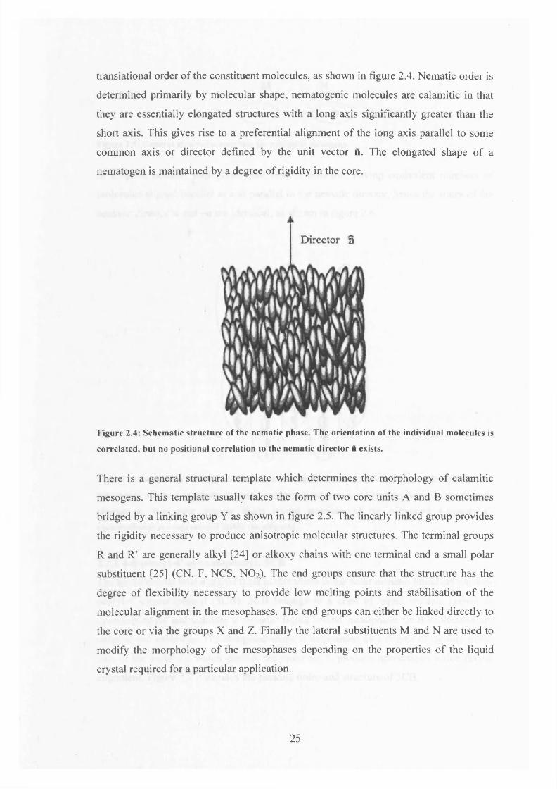
translational order of the constituent molecules, as shown in figure 2.4. Nematic order is

determined primarily by molecular shape, nematogenic molecules are calamitic in that

they are essentially elongated structures with a long axis significantly greater than the

short axis. This gives rise to a preferential alignment of the long axis parallel to some

common axis or director defined by the unit vector n. The elongated shape of a

nematogen is maintained by a degree of rigidity in the core.

Director n

Figure 2.4: Schem atic structure o f the nem atic phase. The orientation o f the individual m olecules is

correlated, but no positional correlation to the nematic director A exists.

There is a general structural template which determines the morphology of calamitic

mesogens. This template usually takes the form of two core units A and B sometimes

bridged by a linking group Y as shown in figure 2.5. The linearly linked group provides

the rigidity necessary to produce anisotropic molecular structures. The terminal groups

R and R’ are generally alkyl [24] or alkoxy chains with one terminal end a small polar

substituent [25] (CN, F, NCS, NO2). The end groups ensure that the structure has the

degree of flexibility necessary to provide low melting points and stabilisation of the

molecular alignment in the mesophases. The end groups can either be linked directly to

the core or via the groups X and Z. Finally the lateral substituents M and N are used to

modify the morphology of the mesophases depending on the properties of the liquid

crystal required for a particular application.

25

R - X

Figure 2.5: General structural tem plate for calam itic m esogens.

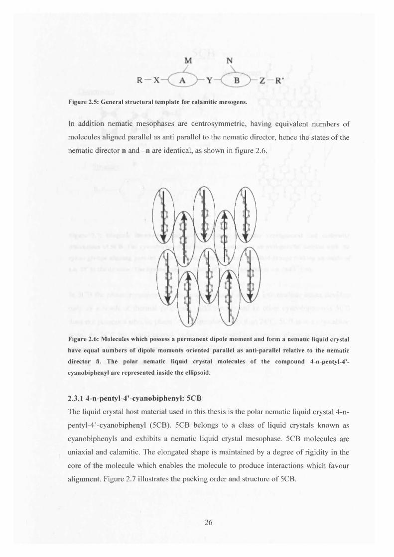
In addition nematic mesophases are centrosymmetric, having equivalent numbers of

molecules aligned parallel as anti parallel to the nematic director, hence the states of the

nematic director n and -n are identical, as shown in figure 2 .6 .

Figure 2.6: M olecules which possess a perm anent dipole m oment and form a nem atic liquid crystal

have equal numbers o f dipole m om ents oriented parallel as anti-parallel relative to the nem atic

director fi. The polar nem atic liquid crystal m olecules o f the com pound 4-n-pentyl-4’-

cyanobiphenyl are represented inside the ellipsoid.

2.3.1 4-n-pentyl-4’-cyanobiphenyl: 5CB

The liquid crystal host material used in this thesis is the polar nematic liquid crystal 4-n-

pentyl-4’-cyanobiphenyl (5CB). 5CB belongs to a class of liquid crystals known as

cyanobiphenyls and exhibits a nematic liquid crystal mesophase. 5CB molecules are

uniaxial and calamitic. The elongated shape is maintained by a degree of rigidity in the

core of the molecule which enables the molecule to produce interactions which favour

alignment. Figure 2.7 illustrates the packing order and structure of 5CB.

26

.Arrangement

Figure 2.7: Diagram illustrating m olecular structure, m olecular arrangem ent and m olecular

dim ensions o f 5CB. The cyanobiphenyl m olecules are ordered in an anti-parallel fashion with the

cyano groups aligning parallel to the nem atic director n and the alkyl groups m aking an angle of

c.a. 38° to the director. The hydrodynam ic volum e o f a 5CB m olecule is c.a. 264A3 [26).

In 5CB the phase transitions are thermally induced and the intermediate states develop

only as a result of thermal processes. Additionally unlike other cyanobiphenyls 5CB

does not possess a smectic phase. At temperatures less than 24°C, 5CB is in a crystalline

state. At 24°C the liquid crystal undergoes a crystalline-nematic phase transition and

remains in the nematic state up to 35.3°C [26]. At this temperature the liquid crystal

undergoes a second phase transition and becomes isotropic.

Structure

■— 0-0

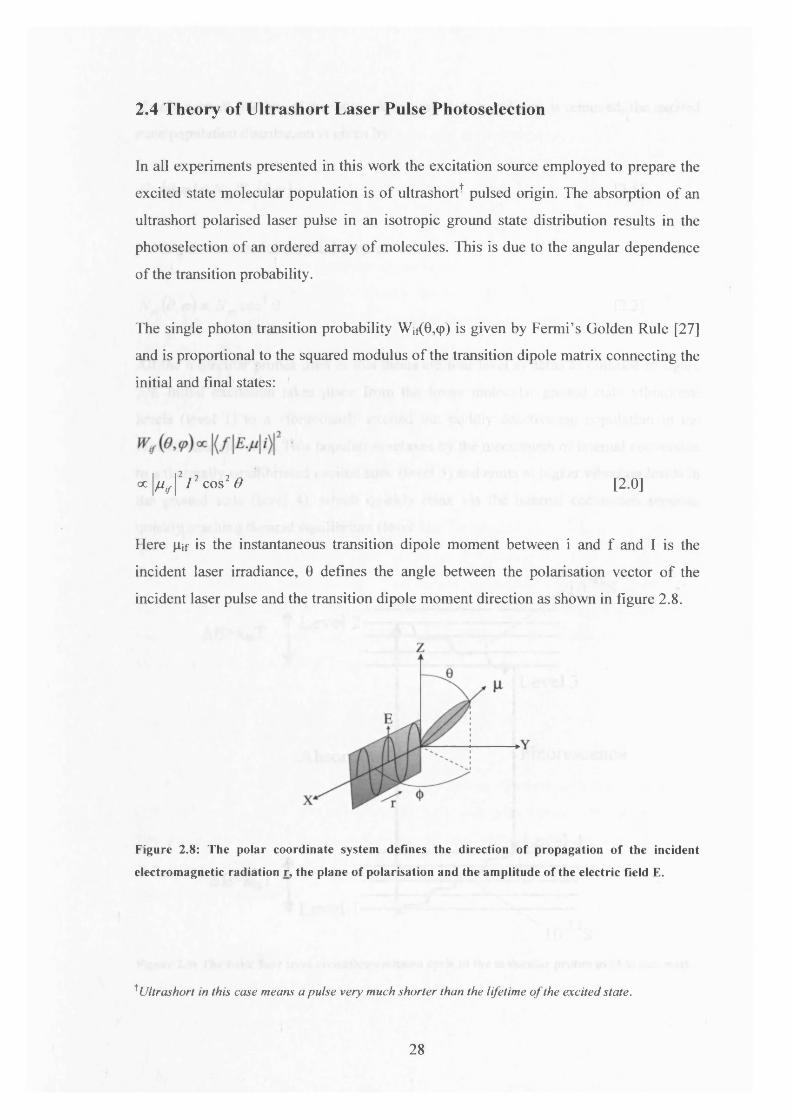
Dimensions

27

2.4 Theory of Ultrashort Laser Pulse Photoselection

In all experiments presented in this work the excitation source employed to prepare the

excited state molecular population is of ultrashort+ pulsed origin. The absorption of an

ultrashort polarised laser pulse in an isotropic ground state distribution results in the

photoselection of an ordered array of molecules. This is due to the angular dependence

of the transition probability.

The single photon transition probability Wjf(0,q>) is given by Fermi’s Golden Rule [27]

and is proportional to the squared modulus of the transition dipole matrix connecting the

initial and final states:

oc|//,r |2 / 2 cos2 0 [2 .0 ]

Here gif is the instantaneous transition dipole moment between i and f and I is the

incident laser irradiance, 0 defines the angle between the polarisation vector of the

incident laser pulse and the transition dipole moment direction as shown in figure 2 .8 .

Figure 2.8: The polar coordinate system defines the direction o f propagation o f the incident

electrom agnetic radiation r, the plane o f polarisation and the am plitude o f the electric Held E.

+Ultrashort in this case means a pulse very much shorter than the lifetime o f the excited state.

28

If only a small fraction of the isotropic ground state population is removed, the excited

state population distribution is given by

[2 1]

For Z-polarised excitation this becomes

tf„(0,?>)«:Arp cos20 [2.2]

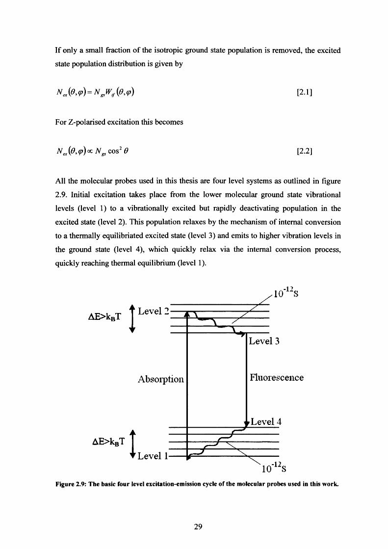
All the molecular probes used in this thesis are four level systems as outlined in figure

2.9. Initial excitation takes place from the lower molecular ground state vibrational

levels (level 1 ) to a vibrationally excited but rapidly deactivating population in the

excited state (level 2). This population relaxes by the mechanism of internal conversion

to a thermally equilibriated excited state (level 3) and emits to higher vibration levels in

the ground state (level 4), which quickly relax via the internal conversion process,

quickly reaching thermal equilibrium (level 1 ).

AE>kBT

AE>kBT

10 “S

Level 2

Level 3

FluorescenceAbsorption

i r Level 4

Level 1-12

Figure 2.9: The basic four level excitation-emission cycle of the molecular probes used in this work.

29

Assuming that the rate of transfer from level 1 to level 2 is very fast, the change in

population of level 3 can be given in the form of a rate equation as

[2.3]

where o is the single photon absorption cross-section (cm ) and 7 34 is the spontaneous

emission from the low lying vibrational levels in Si (level 3) to the high lying ground

state vibrational levels in So (level 4). As the excitation is weak (N3« N i ) and the pulse

duration is ultrashort, then integrating over I(t) gives

where Ep is the laser pulse energy and A is the area of illumination. Equation 2.5

defines the transition probability for single photon absorption, also known as the

transition saturation parameter S where in the weak excitation limit S « l . For

experiments undertaken in Chapter 2 and Chapter 3 for typical excitation pulse

parameters of o^l0'16cm '2, Ep~1.6xlO'14J, h^6.6xl0-34, v^5xl0 14s_1 and A~10"5cm"2, the

saturation parameter was found to be

Given that the ground state orientational distribution function is isotropic such that

then the excited state orientational distribution function directly follows the form of the

[2.4]

[2.5]

— * --------------u— ii------ r w 5 x l°hvA 33 ^10 xlO jcIO J

PGS(0,cp) is independent of 0 and cp (Appendix I) and excitation is in the weak regime

transition probability Wjf(0,<p) stated in equation 2.0. Expressing cos20 in terms of

spherical harmonics gives

[2.6]

30

In the limit of weak excitation the photoselected excited state population Nex is given by

[2.7]

The orientational distribution function P{0,q>) in terms of a spherical harmonic

expansion is given by (Appendix 1)

*p) ~ ^ k q i p K Q ) ^ K Q ( » t y ) [2.8]

Substituting equations 2.6 and 2.7 into equation 2.8 and equation 2.2 yields for Pex(0,(p)

and Nex(0,cp)'

pje,<p)=c-v /4Ity«,(0><p )+ j ^ ¥2o(0<<p ) [2.9]

N j p , p ) = CN. rm (0 ’V > )+ jjy2o fa ? ) [2 .10]

where C is a constant of proportionality. Integrating over all angular coordinates and

normalising to unity yields the total excited state population as

o osin QdOdcp [2.11]

therefore

c =—n.4 71

[2.12]

and

P M < p ) = - 4-s /4It

yo o ( ^ ) + - J ^ Y2o(^9>) [2.13]

31

The excited state orientational distribution function created from an isotropic ground

state distribution is thus characterised by population (Yoo(0,<p)) and cylindrically

symmetric alignment moments (Y2o(0,(p)).

2.5 Emission of Fluorescence: Anisotropy

In time-resolved fluorescence depolarisation experiments linearly polarized light is used

to photoselect, via ultrashort pulsed excitation, an initially ordered excited state

population. This population has an anisotropic distribution of absorption and emission

transition dipole moments [1]. The orthogonally polarized emission components are

then no longer equivalent. The depolarisation function, the fluorescence anisotropy, is

defined in terms of two experimental quantities, these are the time dependent

fluorescent intensities polarised parallel (I||) and perpendicular ( I _ l ) to the excitation

polarisation direction. The detection of the two orthogonally polarized emission

intensities are used to construct the fluorescence anisotropy as follows

12141

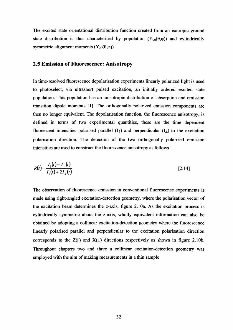
The observation of fluorescence emission in conventional fluorescence experiments is

made using right-angled excitation-detection geometry, where the polarisation vector of

the excitation beam determines the z-axis, figure 2.10a. As the excitation process is

cylindrically symmetric about the z-axis, wholly equivalent information can also be

obtained by adopting a collinear excitation-detection geometry where the fluorescence

linearly polarised parallel and perpendicular to the excitation polarisation direction

corresponds to the Z(||) and X(_l) directions respectively as shown in figure 2.10b.

Throughout chapters two and three a collinear excitation-detection geometry was

employed with the aim of making measurements in a thin sample

32

Sample

pnem Polansgt Lasci Pulse

Emission Fluorescence

9()P G eom etry

Wt)Sample

180 Geometrv

:(t)

Figure 2.10: Geom etries for the experim ental m easurem ent o f fluorescence anisotropy in isotropic

or cylindrically sym m etric environm ents, (a) The conventional geom etry where the orthogonal

com ponents are collected at 90° to the excitation direction, (b) The 180° geom etry w here

fluorescence is collected collinear to the excitation direction.

In the laboratory frame, the intensity of the linearly polarised emission fluorescence

(defined by a linear polarisation vector, e j of the Sj—>So transition is given by [4]

2 xx

sin 0d0d(p [2.15]o o

where B is a constant of proportionality, and the initial and final molecular states are

defined by |/) and | / ) respectively. For the vertical (Z) and horizontal (X) components

of fluorescence, et is given by

ev = cos 9 eH =sin#sin^>

[2.16]

33

where 0 and (p are polar coordinates defined in figure 2.8. Applying these expressions to

equation 2.11 and further expressing Nex(0,<p,t) in terms of the orientational distribution

function, the vertical and horizontal components of fluorescence intensity are given as

2 n x

Iv ( t)=BNa ( t ^ fi\ JJcos2 OP^e.y^sinOdOdq)o o2x71

i h(<)= BN<A‘\ v r\ J Jsin2 6>sin2 cpPje,(p,t) sin OdOd(p

[2.17]

0 0

Expressing the emission probability in terms of spherical harmonics [2] and expanding

the orientational distribution function in terms of the orientational coefficients, the

emission intensities can be rewritten as

2 x x

i y i f )= B N ex{t}nfiI ~ I ( c “ (0) j f r Ke(0,<p\ Ym{e,<p)+ n = Y j e , 9 )5 KQ 0 0 L V 5

sin OdOdcp

a/4 ~7t2 x x

^ - £ < C “ (/)) f j r K (0 ,V)KQ 0 0

— !=Y20(&,9 ) sin 0d0d<pV 5

+ J ^ j{ r 22(0 ,<p)+r2_2(0 , 9 )}

[2.18]

The solution of these integrals yields [2]

a/4~nI l, ( ‘) = B N ex( t \ n f,

/ „ ( » ) = B A U ' K . 3

3

a / 4 ~7t

(c£)+-^(c;(0)

(cs) ■- (cs ( < ) ) + ( / ) ) + (c-

[2.19a]

[2.19b]

34

The polarised components of the fluorescence intensity evolve according to the time

invariant population term ( c ^ and the time dependent ^ C 22 ( ') + < £ , (f))} and

(C2“ (t^j moments. By normalising each moment to the population term and substituting

the fluorescence intensity components into equation 2.12, the expression for the

fluorescence anisotropy is given by,

-J= ( « ; ( t))- 4 = {f)) + (« » if))}R(l) = — --------- V3°--------------------------- [2.20]

u / \ ( ^ w )where {aKQ) = -j—-y .

As can be seen from equation 2.20 and outlined in Chapter 1, the fluorescence

anisotropy can be defined in terms of the orientational distribution of the photoselected

excited state. This expression further shows that from a single photon photoselected

excited state, the fluorescence anisotropy is sensitive only to the K=2 (alignment)

moments of the population, and depends on a cylindrically symmetric moment (Q=0)

and cylindrically asymmetric moment (Q=±2). The evolution of these moments is

determined by the diffusive nature of molecular motion in the liquid phase. The non-

equilibrium photoselected excited state order is dissipated due to randomising collisions

with solvent molecules.

2.6 Variable Angle Photoselection in Anisotropic Media

In conventional time resolved fluorescence anisotropy experiments in isotropic

environments, the laboratory z-axis is determined by the excitation polarisation vector

of the excitation pulse and only cylindrically symmetric degrees of excited state

alignment are created. Furthermore the cylindrical symmetry inherent within the excited

state arrays means R(t) is invariant to any angular variation in the XY plane (cp rotation).

It is possible however, to create cylindrically asymmetric excited state alignment by

varying the excitation polarisation angle p with respect to the laboratory axis as defined

35

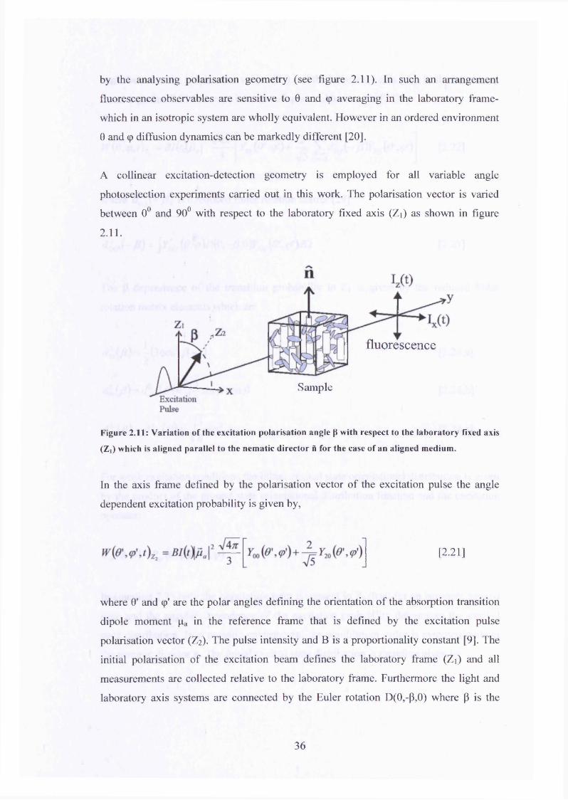
by the analysing polarisation geometry (see figure 2.11). In such an arrangement

fluorescence observables are sensitive to 0 and cp averaging in the laboratory frame-

which in an isotropic system are wholly equivalent. However in an ordered environment

0 and <p diffusion dynamics can be markedly different [20].

A collinear excitation-detection geometry is employed for all variable angle

photoselection experiments carried out in this work. The polarisation vector is varied

between 0° and 90° with respect to the laboratory fixed axis (Z\) as shown in figure

2 .11.

fluorescence

Sample

Figure 2.11: Variation o f the excitation polarisation angle p with respect to the laboratory fixed axis

(Zt) which is aligned parallel to the nem atic director ft for the case o f an aligned medium.

In the axis frame defined by the polarisation vector of the excitation pulse the angle

dependent excitation probability is given by,

[2.21]

where 0' and cp' are the polar angles defining the orientation of the absorption transition

dipole moment pa in the reference frame that is defined by the excitation pulse

polarisation vector (Z2). The pulse intensity and B is a proportionality constant [9]. The

initial polarisation of the excitation beam defines the laboratory frame (Zi) and all

measurements are collected relative to the laboratory frame. Furthermore the light and

laboratory axis systems are connected by the Euler rotation D(0,-P,0) where p is the

36

angle between the polarisation vector (Z2) and the laboratory axis (Zi). In the laboratory

frame equation 2.21 becomes in terms of spherical harmonics [20]

W { e , q > A = B l { f \ j L aI2 4 ^ yM( 0 > ' ) + ^ X d h (- P K . <p ')V5 0=-2[2.22]

where d l0 ( - ft) is a reduced Euler rotation matrix [29]

d w ( - f i ) = [2.23]

The p dependence of the transition probability in Z\ is given by the reduced Euler

rotation matrix elements which are

4 ( /0 = ^ ( 3 c o s 2/9 - l ) [2.24.a]

4 (A)= ^-,oO )= j | s i n /?cos/? [2.24.b]

4 (A) = 4 o (/?)= i ^ s i n 2/? [2.24.c]

For weak excitation conditions the initial excited state orientational distribution is given

by the product of the ground state orientational distribution function and the excitation

operator:

= [2.25]

In equation 2.25 only the population term is present in Pgs(0,<p) for an isotropic ground

state and the angular dependence o f the excitation probability determines the excited

state distribution. In a nematic environment the equilibrium order is symmetric about

the nematic director n. The initial excited state distribution is therefore given by

37

p „ (o ,p ,p ,t = 0 ) = T 7 =3 V K'even J O

[2.26]

where C is a constant of proportionality, and the moments of the excited state

orientational distribution function are given by [2 2 ]

(C“ (O)) = C ^ X ( C £ O)<*0 |

which yields for Pex(9,<p) [22].

no (*» ?>)+j = Z dig. ( - (0 , p) K'O)

[2.27]

Pa (e ,< p )= c± JL £ ( ( c „ ) r „ ( M l U M + ^ L , l 2 <4 ( /O n , ( M3 *:=2,4,6. L V5

[2.28]

The excited state moments observable in fluorescence measurements are given by

(« S (M ) 5 (3cos2 P - ')+ ^ 713005' ^ - > } ) + (3cosv - 1)

Vsl + ^ * ^ ( 3 c o s 2 / ? - l )

v5

(ttg(0,/3)) + (tt";(0,/?)) V30

- s in 2 /? 1 0 « ) , ( O7V5 7

^ ( O ^ c o s 2^ - ! ) v 5

[2.29]

[2.30]

and combining equations 2.29 and 2.30 yields the initial fluorescence anisotropy

— (cos2 p - sin2 /?)+V?

1 + — cos2 /? 7

+ ^ ^ ( l 9 c o s 2 y ? -7 ) 35 v 7

2 . 2 / , . ( O1 + — sin P +5 V5

25cos2 /7 -11 + (“J >2SinV

[2.31]

35

38

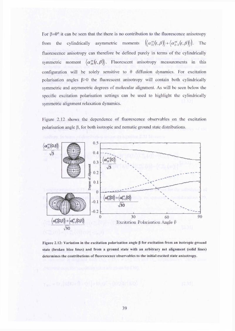
For p=0° it can be seen that the there is no contribution to the fluorescence anisotropy

from the cylindrically asymmetric moments ( ( # 2 (*> P f)+ (a ('./?)))• The

fluorescence anisotropy can therefore be defined purely in terms of the cylindrically

symmetric moment Fluorescent anisotropy measurements in this

configuration will be solely sensitive to 0 diffusion dynamics. For excitation

polarisation angles p> 0 the fluorescent anisotropy will contain both cylindrically

symmetric and asymmetric degrees of molecular alignment. As will be seen below the

specific excitation polarisation settings can be used to highlight the cylindrically

symmetric alignment relaxation dynamics.

Figure 2.12 shows the dependence of fluorescence observables on the excitation

polarisation angle p, for both isotropic and nematic ground state distributions.

Excitation Polarisation Angle Pa/30

Figure 2.12: Variation in the excitation polarisation angle p for excitation from an isotropic ground

state (broken blue lines) and from a ground state with an arbitrary net alignm ent (solid lines)

determines the contributions o f fluorescence observables to the initial excited state anisotropy.

39

2.7 Molecular Relaxation Dynamics in Ordered Environments

If rapid collisions occur between probe and host molecules whilst in a fluid environment

[28] and each collision event is restricted to only a small angular variation, then the

molecular dynamics are well described by the Debye small step diffusion model

(Appendix II). However in an anisotropic medium the model must be modified, thereby

considered as a static perturbation H' in the isotropic excited state according to [29]

4 n , (*, V, t) = [ o v 2 + //']/>„ (0, <p,t) [2.32]at

If H' is to be considered a perturbation, then to a first order approximation, DV2 must

be very much larger than H \ Furthermore H' must retain the initial symmetry of the

medium. In terms of distribution moments equation 2.32 becomes

( ' ) ) - (C“e (“ )>} = (KQ\DV2 +H' \KQ){(c?e ( / ) ) - (c“ («))} ........ , [2.33]I { K Q \ H ' \ k q ) { ( c ~ q. (0 ) - ( C “e. (55))}

K '*KQ‘*Q

Treating equation 2.33 in terms of a first order perturbation allows for the calculation of

the orientational relaxation dynamics based entirely on symmetry considerations [29,

30] giving

(c? 0 ( t ) ) - (C“ (ss)) = [(C “ (0)} - (c» (ss))]e*p(-rKOt)

( c k q (t)) = ( Q q (0 ) )e x p (-rKOt)

In environments defined by axial symmetry, the diffusion tensor in the laboratory frame

of reference is diagonal with Dxx = Dyy * Dzz (Dy and Dj_, respectively). Under these

circumstances the ykq decay rates are given by [30],

y KQ= D i [K(K + l ) - Q 2] + D ||Q 2 +(K Q |H '|K Q ) [2.35]

40

As the perturbation is small in the first order approximation, the dominant mechanism

in orientational relaxation is due to the presence of anisotropic viscosity, this

phenomena in turn yields unequal values o f D|j and Dx

y 2 0 =

y 22 = 2 D± + 4 D

2.8 Time Dependent Fluorescence Anisotropy

Considering the first order relaxation dynamics outlined in section 2.5, the rate of

change o f displacement of a particular excited state moment from its equilibrium

position obeys first order kinetics:

^ [ ( a “ ( , ) ) - ( « “ («■))]= - r * e [ ( < e ( / ) ) - ( < , ( » ) ) ] [2.38]

where (ss) denotes the steady state value o f the moment. Equation 2.38 has a solution of

the form

( < q(i )) = \ a KQ (°)} - (< (! ("))}exp(- r KQt)+ {a KQ (“ )) [2.39]

From equation 2.20, the fluorescence anisotropy is dependent upon the ( a 20)

{ (« £ )+ (« I 2 } moments, and from equation 2.5 in Appendix I.II, the steady state

distribution function is characterised by moments of even rank K and projection Q of

zero for an axially symmetric medium. That is (a 2±2 (ss^ =0, which yields for the time

dependent fluorescence anisotropy

R ( t ) = J£2--------------------------- — ------------------ ^ --------------------------------i + J = [ ( « 2 (0 )}+ ( < 2 (0 ) ) ^ >

[2-40]

[2.36]

[2.37]

41

which upon substitution of equations 2.29 and 2.30 and = ( a ^ }/V5 gives the

expression

* M )= -

(3co^ . {7+6 6 }+^ fccos2 /?+s ) - *„(] + afccos2 - 1))

- - s in 2 - y “ + * Jexj4-r22f )+ /^ (l+ ^ c o s 2 / ? - 1))

(l+ o^cos2 P - 1))+1 sin2 / / l - y a + “ je x ^ - Tij)

d r r J )

[2.41]

where a = (a fQ / 4 $ and b = ( a ^ are the normalised ground state alignment

moments. From the p dependence o f the initial fluorescence anisotropy equation 2.41

allows for the degree? of ( a ^ (ss^ (quadrupolar) and ( a ^ (ss^) (hexadecapolar)

alignment to be determined.

2.9 Phase Transition Characteristics and Isotropic Orientational

Dynamics of Nematic Liquid Crystals

2.9.1 Phase Transitions

It is well known that any substance of fixed chemical composition can exist in several

homogeneous forms. Such macroscopic states which exist under specific conditions are

called phases and are defined by the distinct arrangement of the constituent molecules

and differ in their thermal, optical and mechanical properties [31, 32, 33]. The phases of

a material can be represented pictorially in a phase diagram as shown in figure 2.13.

Along the boundary line a substance can coexist in several phases simultaneously,

although the properties of the material change discontinuously. In fluid systems defined

with state variables pressure and temperature (p, T ), phase transitions occur when a

thermodynamic potential such as the Gibbs free energy (F) of one state of matter ceases

to be in equilibrium with another [34]. Evidence of a phase transition is signaled by a

singularity in the Gibbs free energy given by

F = H + PV - T S [2.42]

where H is the enthalpy, T the temperature and S the entropy.

42

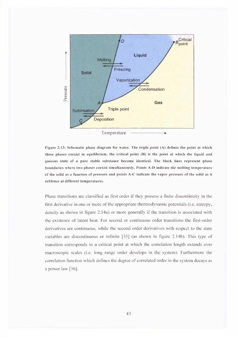
Criticalpoint

/ Liquid/■*T....►7 _ .( Freezing

Vaporization

Melting

Solid

o:3■y.

£

Condensation

GasTriple pointSublimation

Deposition

Temperature *

Figure 2.13: Schematic phase diagram for water. The triple point (A) defines the point at which

three phases coexist in equilibrium, the critical point (B) is the point at which the liquid and

gaseous state o f a pure stable substance become identical. The black lines represent phase

boundaries where two phases coexist sim ultaneously. Points A-D indicate the melting tem perature

of the solid as a function of pressure and points A-C indicate the vapor pressure o f the solid as it

sublimes at different temperatures.

Phase transitions are classified as first order if they possess a finite discontinuity in the

first derivative in one or more o f the appropriate thermodynamic potentials (i.e. entropy,

density as shown in figure 2.14a) or more generally if the transition is associated with

the existence o f latent heat. For second or continuous order transitions the first-order

derivatives are continuous, while the second order derivatives with respect to the state

variables are discontinuous or infinite [35] (as shown in figure 2.14b). This type o f

transition corresponds to a critical point at which the correlation length extends over

macroscopic scales (i.e. long range order develops in the system). Furthermore the

correlation function which defines the degree o f correlated order in the system decays as

a power law [36].

43

V(i)

a. First Order Transitions

(ii)S

i

o

(iii)G

G

b. Second Order Transitions

Cp.s

X T

(ill)

/

Figure 2.14: First and second order phase transitions (a). There is a finite d iscontinuity in the first

order derivatives in (i) and (ii) at the phase transition w hereas the G ibbs free energy potential (iii)

is continuous in the transition (b). The first order derivatives w ith respect the free energy and

associated quantities are continuous in (i) and (ii) how ever the second derivative w ith respect the

specific heat at constant pressure (iii) is not continuous and is seen to diverge at Tc -

A fter P Papon, J Leblond and P H E M eijer, Springer (2006)

2.9.2. Phase Transitions in Liquid Crystals

The phenomenological model provided by the theory of Landau-De-Gennes best

describes the thermodynamic behaviour of liquid crystals in the vicinity of the nematic-

isotropic (N-I) phase transition. The theory predicts the development of the order

parameter <S> in the vicinity of the N-I transition i.e. as <S> approaches 0, by

considering a Taylor expansion of the excess Gibbs free energy F, as a function of <S>

[37],

F = F0 + K(t Xs ) + ^ A ( S ) 2 - I f i ( S ) 3 + ic < S )4..., [2.43]

where K, B and C are constants. In the vicinity of the transition A varies as [34]

44

A = A j p - T ' ) [2.44]

where Ao and T* are constants and T* is the second order phase transition temperature

known as the virtual temperature and lies below the phase transition temperature TNi

(typically 1-2K below TNi [38]) which is constant for a particular dye-host solution. The

states of equilibrium of the system must satisfy the following equations

dF d 2F= 0 , ------- > 0 [2.45]

d(s ) d{sy

so the minimum of the free energy F can be obtained by evaluating the first derivative

of the free energy with respect the order parameter S [39] giving an expression,

neglecting higher order terms, of the order parameter at Tni of,

s m = I ? [2.46]

By further considering that the virtual temperature lies below the phase transition

temperature we can write [40]

Tn, = T' + [2.47]“ 9A0C

Since the nematic-isotropic phase transition is a weak first order transition [2] for

calamitic molecules such as 5CB, the magnitude of B is small [39]. Therefore the value

of (Tni - T *) is expected to be small also.

Though the order parameter reduces to zero at the nematic-isotropic phase transition,

(i.e. such that it is zero above T n i) , an appreciable degree of order persists above the

phase transition and extends over a microscopic distance, 0 < S < ^ ( r) , where <^(t) is

the correlation length. In the isotropic phase a liquid crystal sample is macroscopically

isotropic but microscopically anisotropic. When considering a distance scale short

45

compared to a correlation length the local structure is like that o f a nematic liquid

crystal, creating what can be described as pseudo-nematic domains. These domains of

local order however are not correlated to one another, as shown in figure 2.15.

Nematic Phase Isotropic Phase

Figure 2.15: Illustration o f the contrast in order in the nematic and isotropic phase o f a nematic

liquid crystal. For the nematic phase order persists over macroscopic distances whereas for the

isotropic phase local order persists over distances which are larger than the m olecular size.

The existence o f pseudo-nematic domains in liquid crystals such as 5CB and MBBA

has been confirmed from dynamic light scattering [41] and electric birefringence

experiments [42]. The domain sizes vary typically from 10-20 molecular lengths to

approximately 200A near the phase transition temperature [43]. This is in accordance

with predictions made by the theory o f Landau-De-Gennes whereby the correlation

length ^ is described in terms o f the molecular length and the virtual temperature T* as

As a result o f the existence o f local domains, the orientational relaxation dynamics o f

nematogens in the isotropic phase o f liquid crystals is complex. Recently a series o f

time resolved polarised fluorescence experiments designed to measure the molecular

ordering and orientational dynamics in the isotropic phase o f 5CB have been carried out

by the group [1, 2]. These studies along with studies by Gootke et al [44, 45] have

revealed that the dynamics can be divided into two timescales, a long (nanosecond) time

and short time o f the order o f several hundred picoseconds.

[2.48]

46

On a long time scale the orientational relaxation of the pseudo-nematic domains is

exponential in nature and is highly temperature dependent. The nanosecond dynamics

are described by an exponential functional form predicted by the theory of Landau-De-

Gennes [46]. The function decays with relaxation time tldg which diverges at the

virtual transition temperature T* as

' u x i = [2 -4 9 ]

where Veg is the nematogen effective volume, rj(T) is the viscosity and T is the

temperature. Pseudo-nematic domains of this nature are seen to persist up to

approximately 70°C above the nematic-isotropic phase transition temperature [1,2, 47].

The observed short time dynamics are attributed to the collective motions of the

nematogens within the pseudo-nematic domains. The dynamics do not follow Landau-

De-Gennes behaviour and are instead described in terms of a power law decay. They are

found to be temperature independent up to c.a. T n i+ 70°C . The temperature

independence associated with the fast reorientation can be explained by expressing the

free energy of the isotropic phase as an expansion in terms of S(q), where q is the

wavevector which describes the fluctuations in the order parameter S due to the

uncorrelated domains [40]. This leads to the dispersion relation [1]

[2 .5 0 ]

By taking limits of the fluctuation wave vectors q corresponding to length scales from

molecular size to domain correlation length, this approach reproduces the slow

orientational component (consistent with Landau-De-Gennes theory) [40] as well as

recovering the fast component of the reorientation. In the limit of q § » l the fluctuation

mode relaxation time ( i f ) becomes

— = ^ L [2.51]T f Tj

47

where D is a constant. The fast dynamics that are observed on a time scale short

compared to the slow orientational dynamics (tug) are referred to in terms of intra­

domain relaxation. Recently Fayer and co workers (using analysis based on density

functional theory as previously proposed by Bagchi [47]) have presented a revised

model in which longer temporal scales are considered [44]. From this a linear

relationship has been established between what can be described as intermediate times

(relative to the long (nanosecond) and short (picosecond) times) Tfast and viscosity given

by

effFAST kHT

[2 .5 2 ]

2.10 Local Ordering of Fluorescence Probes in the Isotropic Phase of

Nematic Liquid Crystals

The local order and restricted dynamics of ionic probes in the isotropic phase of

cyanobiphenyls have been studied in detail by Bryant, Monge and co-workers [1 , 2 ] .

For all systems studied within a temperature range of Tni to T n i+ 5 0 K the fluorescence

anisotropy whilst decaying to an isotropic background (Rss=0) was strongly bi­

exponential in stark contrast to the single exponential decays obtained for the probes in

non-self organising solvents. Close to T ni, anisotropy decays were characterised by

‘fast’ and ‘slow’ relaxation (c.a. 2 .3 - 1 .8 ns and 1 6 -1 .8 ns) with the onset of a single

exponential decay at temperature above T n i+ 5 0 K as shown in figure 2 .1 6 . Below this

‘isotropic’ temperature the variation in the two decay times was distinctly different,

indicating the presence of two independent orientational relaxation mechanisms.

Fluorescence intensity decays across the isotropic phase, as in the nematic phase, were

seen to fit well to single exponential decays.

48

Oxazine 4 in 5CB16-slow

(~16ns -1.8ns)14-“ 1 2 -

8 -

6 -•c

fast (~2.3ns -1.8ns)

o 10 20 30 40 50 60

Figure 2.16: Isotropic phase dynamics of Oxazine4 in 5CB. The fluorescence anisotropy is bi­

exponential corresponding to restricted rotational diffusion within an isotropically diffusing

domain structure. Normal (mono-exponential) orientational relaxation is observed for T>TNi+50°C.

Given highly restricted rotational diffusion of probe molecules in the nematic phase

within a fixed (or extremely slowly diffusing) host environment the isotropic phase

dynamics were modeled assuming fast restricted rotational diffusion within a more

slowly diffusing pseudo-nematic domain structure. In this limit, anisotropy dynamics

should resemble that of a fluorescent probe constrained in a slowly diffusing host.

/?(r) = exp( * \ ~

— t(*(0 ) — R d o m a in )exP

— t+ R DOMAIN

k. t s l o w K*FAST j

[2.53]

Where R(0) and R d o m a in are the limiting values o f the anisotropy in the absence of

domain motion. With the loss o f local structure R d o m a in tends to zero and the times Tfast

and Tsiow converge yielding a single exponential functional form for equation 2.53. Local

probe order within the domain structure can be deduced from a consideration of the

long-time behaviour of the orientational correlation function [49, 50] in which a local

order parameter S ( < P 2>iocai) is given by

o _ I R DOMAli

49

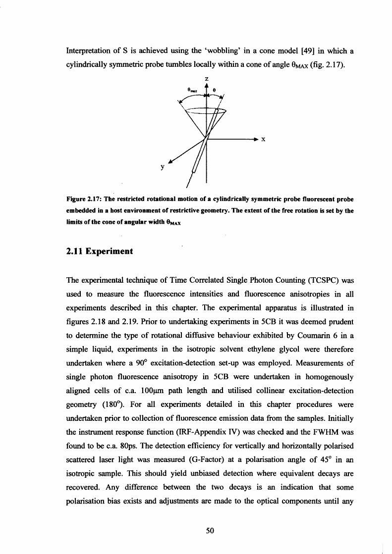
Interpretation of S is achieved using the ‘wobbling’ in a cone model [49] in which a

cylindrically symmetric probe tumbles locally within a cone of angle Gm a x (fig. 2.17).

z

-► x

y

Figure 2.17: The restricted rotational motion of a cylindrically symmetric probe fluorescent probe

embedded in a host environment of restrictive geometry. The extent of the free rotation is set by the

limits of the cone of angular width Om a x

2.11 Experiment

The experimental technique of Time Correlated Single Photon Counting (TCSPC) was

used to measure the fluorescence intensities and fluorescence anisotropies in all

experiments described in this chapter. The experimental apparatus is illustrated in

figures 2.18 and 2.19. Prior to undertaking experiments in 5CB it was deemed prudent

to determine the type of rotational diffusive behaviour exhibited by Coumarin 6 in a

simple liquid, experiments in the isotropic solvent ethylene glycol were therefore

undertaken where a 90° excitation-detection set-up was employed. Measurements of

single photon fluorescence anisotropy in 5CB were undertaken in homogenously

aligned cells o f c.a. 1 0 0 pm path length and utilised collinear excitation-detection

geometry (180°). For all experiments detailed in this chapter procedures were

undertaken prior to collection o f fluorescence emission data from the samples. Initially

the instrument response function (IRF-Appendix IV) was checked and the FWHM was

found to be c.a. 80ps. The detection efficiency for vertically and horizontally polarised

scattered laser light was measured (G-Factor) at a polarisation angle of 45° in an

isotropic sample. This should yield unbiased detection where equivalent decays are

recovered. Any difference between the two decays is an indication that some

polarisation bias exists and adjustments are made to the optical components until any

50

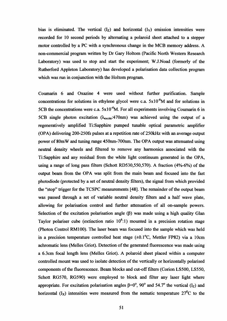
bias is eliminated. The vertical (Iz) and horizontal (Iy) emission intensities were

recorded for 1 0 second periods by alternating a polaroid sheet attached to a stepper

motor controlled by a PC with a synchronous change in the MCB memory address. A

non-commercial program written by Dr Gary Holtom (Pacific North Western Research

Laboratory) was used to stop and start the experiment; W.J.Noad (formerly of the

Rutherford Appleton Laboratory) has developed a polarisation data collection program

which was run in conjunction with the Holtom program.

Coumarin 6 and Oxazine 4 were used without further purification. Sample

concentrations for solutions in ethylene glycol were c.a. 5x1 O^M and for solutions in

5CB the concentrations were c.a. 5x1 O^M. For all experiments involving Coumarin 6 in

5CB single photon excitation (XeXcite:470nm) was achieved using the output of a

regeneratively amplified Ti: Sapphire pumped tunable optical parametric amplifier

(OPA) delivering 200-250fs pulses at a repetition rate of 250kHz with an average output

power of 80mW and tuning range 450nm-700nm. The OPA output was attenuated using

neutral density wheels and filtered to remove any harmonics associated with the

Ti:Sapphire and any residual from the white light continuum generated in the OPA,

using a range of long pass filters (Schott RD530,550,570). A fraction (4%-6%) of the

output beam from the OPA was split from the main beam and focused into the fast

photodiode (protected by a set of neutral density filters), the signal from which provided

the “stop” trigger for the TCSPC measurements [48]. The remainder of the output beam

was passed through a set of variable neutral density filters and a half wave plate,

allowing for polarisation control and further attenuation of all on-sample powers.

Selection of the excitation polarisation angle (p) was made using a high quality Gian

Taylor polariser cube (extinction ratio 106 :1) mounted in a precision rotation stage

(Photon Control RM100). The laser beam was focused into the sample which was held

in a precision temperature controlled heat stage (±0.1 °C, Mettler FP82) via a 10cm

achromatic lens (Melles Griot). Detection o f the generated fluorescence was made using

a 6.3cm focal length lens (Melles Griot). A polaroid sheet placed within a computer

controlled mount was used to isolate detection of the vertically or horizontally polarised

components of the fluorescence. Beam blocks and cut-off filters (Corion LS500, LS550,

Schott RG570, RG590) were employed to block and filter any laser light where

appropriate. For excitation polarisation angles P=0°, 90° and 54.7° the vertical (Iz) and

horizontal (Ix) intensities were measured from the nematic temperature 27°C to the

51

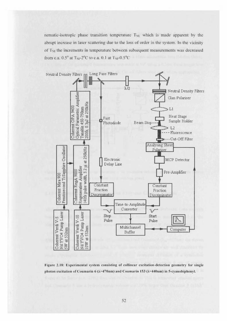
nematic-isotropic phase transition temperature Tni, which is made apparent by the

abrupt increase in laser scattering due to the loss o f order in the system. In the vicinity

o f Tni the increments in temperature between subsequent measurements was decreased

from c.a. 0.5° at Tni-2°C to c.a. 0.1 at T ni-0.5°C

Neutral Density Filters Long Pass Filters

Neutral Density Filters

Gian Polariser

Heat Stage Sample Holder

Fast Photodiode Beam Stop

L2 Fluorescence

s— Cut-Off FilterAnalysing Sheet

P olans er

Electronic I Delay Line

MCP Detector

Pre-Amplifier

Constant Fraction

Discriminator

Constant Fraction

Discriminator

o Pi ~Time -to - Amplitude

Converter

Multichannel Buffer

Computer

Figure 2.18: Experimental system consisting o f collinear excitation-detection geometry for single

photon excitation of Coumarin 6 (X=470nm) and Coumarin 153 (>.=440nm) in 5-cyanobiphenyl.

52

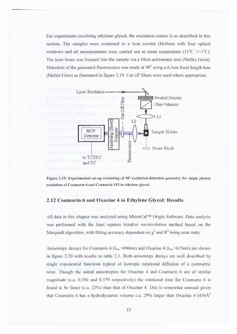
For experiments involving ethylene glycol, the excitation source is as described in this

section. The samples were contained in a 1cm cuvette (Hellma) with four optical

windows and all measurements were carried out at room temperature (21°C +/-1°C).

The laser beam was focused into the sample via a 10cm achromatic lens (Melles Griot).

Detection o f the generated fluorescence was made at 90° using a 6.3cm focal length lens

(Melles Griot) as illustrated in figure 2.19. Cut off filters were used where appropriate.

Laser ExcitationNeutral Density

Gian Polariser

Wi

I

Sample Holder

c±= i Beam Block

to TCSPC and PC

Figure 2.19: Experimental set-up consisting o f 90° excitation-detection geometry for single photon

excitation o f Coumarin 6 and Coumarin 153 in ethylene glycol.

2.12 C o u m a r i n 6 and O xazine 4 in Ethylene G lycol: R esults

All data in this chapter was analysed using MicroCal™ Origin Software. Data analysis

was performed with the least squares iterative reconvolution method based on the

Marquadt algorithm, with fitting accuracy dependent on x2 and R2 being near unity.

Anisotropy decays for Coumarin 6 (A x=490nm) and Oxazine 4 (A*x=615nm) are shown

in figure 2.20 with results in table 2.1. Both anisotropy decays are well described by

single exponential functions typical o f isotropic rotational diffusion o f a symmetric

rotor. Though the initial anisotropies for Oxazine 4 and Coumarin 6 are o f similar

magnitude (c.a. 0.390 and 0.379 respectively) the rotational time for Coumarin 6 is

found to be faster (c.a. 22%) than that o f Oxazine 4. This is somewhat unusual given

that Coumarin 6 has a hydrodynamic volume c.a. 29% larger than Oxazine 4 (436A3

53

and 313A3 respectively). According to the hydrodynamic model o f Stokes-Einstein-

Debye (SED) the rotational reorientation time depends on the size and shape o f the

rotating molecule and the bulk viscosity o f the solvent as given by [1,49]

P ) P -55]

where r| is the solvent viscosity, V is the Van Der Waals volume of the probe molecule,

/ i s the shape factor to account for the nonspherical shape o f the probe [51], k and T are

Boltzmann's constant and absolute temperature respectively and C is the boundary

condition the exact value o f which depends on the axial ratio o f the molecule and

satisfies the inequality 0<C<1 [52]. SED accounts for the observed reorientation in

terms of the broad limits set by ‘slip’ and ‘stick’ boundary conditions. The observed

reorientation times may be accounted for in terms o f solute-solvent hydrogen bonding.

The hydrophobic nature o f Coumarin 6 perturbs the solvent molecules in the immediate

vicinity o f the solute such that the free volume available for rotation increases. As a

result the resistance to motion is reduced. In contrast the ionic nature o f Oxazine 4

reacts with the hydrophilic solvent molecules resulting in ‘stick’ boundary conditions

where there is cooperative motion between solvent and solute molecules.

0.5C o u m a r in 6 in E t h y le n e G ly c o l

Sf 0.3t = 2 .3 3 5 + / - 0 .0 4 5 n s -

20

0.1

0.0

-0.1 -

10 12 14-2 0 2 4 6 8

O x a z i n e 4 in E t h y le n e G l y c o l

02- t = 2 . 9 9 3 + / - 0 . 0 3 7 n s

-0.1-2 0 2 4 6 8 10 12 14

Time (ns) Time (ns)

Figure 2.20: Anisotropy decays for (a) Coumarin 6 and (b) Oxazine 4 in the isotropic solvent

ethylene glycol at room temperature (T=210+/-1°C). Both fit to single exponential decays indicating

that the emission dipole moments are parallel to the long axis o f the molecules.

54

Probe Solvent Conc(M)

^EXCITE(nm)

TLIFE(ns)

R(0) Tr o t (ns)

Coumarin 6 EthG 5x1 O’6 490 2.359 +/- 0.002

0.379 +/- 0.004

2.335 +/- 0.045

Oxazine 4 EthG 5X10"6 615 2 .9 1 6 + /-0.001

0.390 +/- 0.003

2.993 +/- 0.037

Table 2.2: Summary of lifetime and rotational anisotropy decays for Coumarin 6 and Oxazine 4 in

ethylene glycol.

2.13 Fluorescence Signals in Anisotropic Media

In the nematic phase of cyanobiphenyl liquid crystals, the constituent molecules are

highly aligned. This creates optical anisotropy (birefringence) of the medium and

anisotropic local field effects which have a significant influence on the emitted

intensities. Fluorescent probe studies within such media are complicated by these

factors.

The transmission of light (T) through a boundary between two media with different

refractive indices can be expressed in terms of a Fresnel coefficient given by [53]

T. = 4 n en g/ ( n e + n g)'

To = 4 n on g/ ( n 0 + n g)'

[2.56a]

[2.56b]

Where ne and no are the extraordinary and ordinary refractive indices of the aligned

media respectively and ng is the refractive index of the cell wall.

In the presence of an anisotropic electric field the ordinary and extraordinary polarised

components of the fluorescence emission experience a total intensity modification due

to the local field anisotropy [54] as

I z (observed ) oc / z (/)(«e2 + 2 )

1 x (observed ) oc M 0 ( « 2 + 2 )

[2.57a]

[2.57b]

55

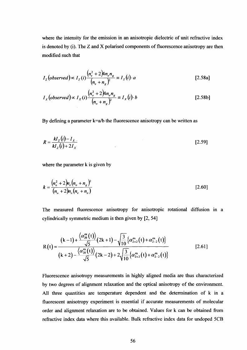
where the intensity for the emission in an anisotropic dielectric of unit refractive index

is denoted by (i). The Z and X polarised components of fluorescence anisotropy are then

modified such that

I z (observed) oc 1 z = I z (/)• a [2.58a]\ n e + n J

. . (n2 + 2j4w/7„ / xI x (observed)cc I x (i) —^ ^ — = I x (i)-b [2.58b]

\ n o + n J

By defining a parameter k=a/b the fluorescence anisotropy can be written as

R = kIzj f} [2.59]kl2(i)+21x

where the parameter k is given by

(n2 + 2 Xi (n + n Vk = V g- x [2.60]

(n0 +2K ( ne +no)

The measured fluorescence anisotropy for anisotropic rotational diffusion in a

cylindrically symmetric medium is then given by [2, 54]

(k _ + K f $ ( 2 k + 1) - ^ { « r +2 ( t ) + « - (t)}

(k + 2 ) _ l ^ y / ( 2 k - 2 ) + 2 ^ { a - 2 ( t) + (t)}

Fluorescence anisotropy measurements in highly aligned media are thus characterized

by two degrees of alignment relaxation and the optical anisotropy of the environment.

All three quantities are temperature dependent and the determination of k in a

fluorescent anisotropy experiment is essential if accurate measurements o f molecular

order and alignment relaxation are to be obtained. Values for k can be obtained from

refractive index data where this available. Bulk refractive index data for undoped 5CB

56

for a wide range of wavelengths and temperatures has been measured by Wu et al [55].

However in the study of doped liquid 5CB and in general ordered systems for which

within the context of a time resolved fluorescence experiment

2.13.1 Depolarisation Factor A

The maximum theoretical value of the initial fluorescence anisotropy in an isotropic

medium following single photon excitation is 0.4 [15] however experimentally this

value is found to be less. The depolarisation of fluorescence can be attributed to a

number of molecular and experimental factors such as the absorption and emission

transition dipole moments being non-parallel self-absorption due to high sample

concentration, imperfect optical alignment and scattering [56]. The effect of these

factors is to modify the alignment components from their true values by an amount

defined by the parameter A given by

Determination of A can be achieved by measuring the variation in the initial

fluorescence anisotropy with excitation polarisation angle for an isotropic sample [2 ].

From 2.31 R(0,p) in an isotropic sample is defined by

1 + — sin" b 5

The value of A for Coumarin 6 in 5cb was determined by raising the temperature to

10°C above the nematic-isotropic phase transition temperature Tni and fitting data

collected at R(0,p) (where p=0o,35.3°,45o,54.7° and 90°) to equation 2.63.This yields a

value of 0.844.

refractive index data is not readily available it is advantageous to be able to measure k

[2.63]

57

2.13.2 Fluorescence Intensity Decay Analysis in Nematic 5CB

In a cylindrically symmetric medium measurement of the total fluorescence intensity

Iz+ 2 Ix yields a fluorescence signal which only contains population terms [5 7 ] . For a

nematic liquid crystal the presence of birefringence (differential reflection losses)

coupled with local field effects perturbs the fluorescence observables such that the total

intensity for Z-polarised excitation ((3=0° relative to the nematic director) is [2]

I z + 21 x (ft = 0" )= A expf \ - t

\ Tf J

k + 2 2 { k - \ )

A + S( a 2“ (/? = 0 V )) [2.64]

where A is a proportionality constant. In the nematic phase of liquid crystals k>l

therefore the alignment term is non-vanishing and will make a small contribution to the

fluorescence signal. The full time dependence of equation 2.64 is given by

I z + 21x (ft = 0°) = A expr \ - t

Kr f J

k + 2 l (k - 1) A + V5

[(a“ (0 ) ) - ( a “ («))]exp[ —Vr 20

+ (("2“ (■” )))

[2.65]

= A expr

- t

\ r f j

k + 2 2(k - 1)

I + V5r {i , 0 = O°) [2.66]

The Z-polarised component of fluorescence emission following excitation at p=54.7° is

given by [2 ]

+ f )I z {p = S A T ) = A exp| - f- I I (f. p = 54.7“)) [2.67]

where A' is a constant of proportionality. With an excitation polarisation angle of

p=54.7° and a cylindrically symmetric ground state, the initial excited state cylindrically

symmetric alignment is equal to that of the equilibrium alignment in the ground state

[2]. From equation 2.39, the fluorescence intensity can then be given by

58

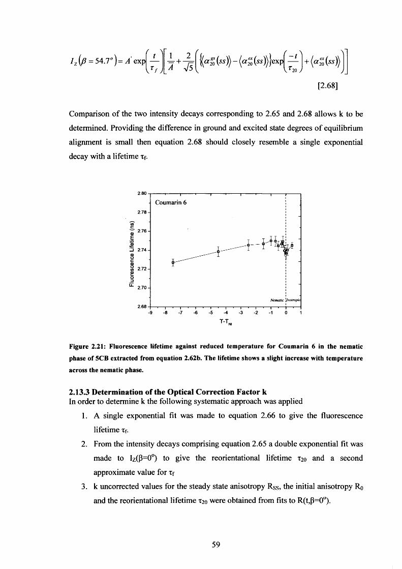
I z (p = 54.1°)= A expr \ t

\ Tf J= + M ) - (“ 2“ (“ ))}exp^^- + ( a ° (ss))

[2.68]

Comparison of the two intensity decays corresponding to 2.65 and 2.68 allows k to be

determined. Providing the difference in ground and excited state degrees of equilibrium

alignment is small then equation 2 . 6 8 should closely resemble a single exponential

decay with a lifetime Xf.

2.80

Coumarin 62.78-2.76-

□ 2.74-2.72-

U- 2.70-Nematic \lsotropic

2.68■7 -6 ■5 -4 3 2-9 -8 1 0 1

Figure 2.21: Fluorescence lifetime against reduced temperature for Coumarin 6 in the nematic

phase of 5CB extracted from equation 2.62b. The lifetime shows a slight increase with temperature

across the nematic phase.

2.13.3 Determination of the Optical Correction Factor kIn order to determine k the following systematic approach was applied

1. A single exponential fit was made to equation 2.66 to give the fluorescence

lifetime Xf.

2. From the intensity decays comprising equation 2.65 a double exponential fit was

made to Iz(P=0°) to give the reorientational lifetime X20 and a second

approximate value for Xf

3. k uncorrected values for the steady state anisotropy Rss, the initial anisotropy Ro

and the reorientational lifetime X20 were obtained from fits to R(t,p=0°).

59

4. Custom functions generated in Origin based on the intensity components of

equation 2.65 were then used to find k. As it was necessary to determine three

parameters accurately (R ss, Ro and T20) the values found in steps two and three

were used as initial approximate values. Accurate determination of the

fluorescence lifetime has been achieved in step 1 and this value was fixed for

both fits. All other parameters were allowed to float within the constraints of the

errors found in the initial fits. In simultaneously fitting the functions global

analysis was possible and accurate determination of the correction factor k was

made by taking ratio of the pre-exponential factors generated as a result of

fitting three parameters to the customised fitting function.

This method has since been superseded with the purchase of global analysis software

allowing for determination of all parameters without the need for separate simultaneous

fitting.

2.14 Nematic Order of Coumarin 6 in 5CB

The initial fluorescence anisotropies for excitation polarisation angles of (3=0° and

p=90° were measured for Coumarin 6 . These anisotropies when combined with the

nematic correction factor k and the depolarisation factor A yield values of the K= 2 and

K=4 moments of the ground state distribution function. A Mathematica program written

in collaboration with Dr Richard Marsh allows for the determination of the K=2 and

K=4 moments of 5CB. The results are shown in figure 2.22a for Coumarin 6 and 2.22b

for Oxazine 4, as a function of reduced temperature (T -T ni).

It is clear that Coumarin 6 has similar alignment to that of Oxazine 4, characterised by

positive values of ( a ^ )/V 5 and negative values of ( a ^ . The value of ( a ^ )/V 5

decreases gradually with temperature to Tni-0.5 where there is a sudden collapse to zero

at Tni. This behaviour is mirrored by the K=2 moment of 5CB as shown in figure 2.23.

As with Oxazine 4, Coumarin 6 shows a notable increase in the negative value of

with increasing temperature, which persists to within close vicinity o f the nematic-

isotropic phase transition temperature (Tni-0.2) where there is a sudden collapse to zero

(isotropic) at Tni-

60

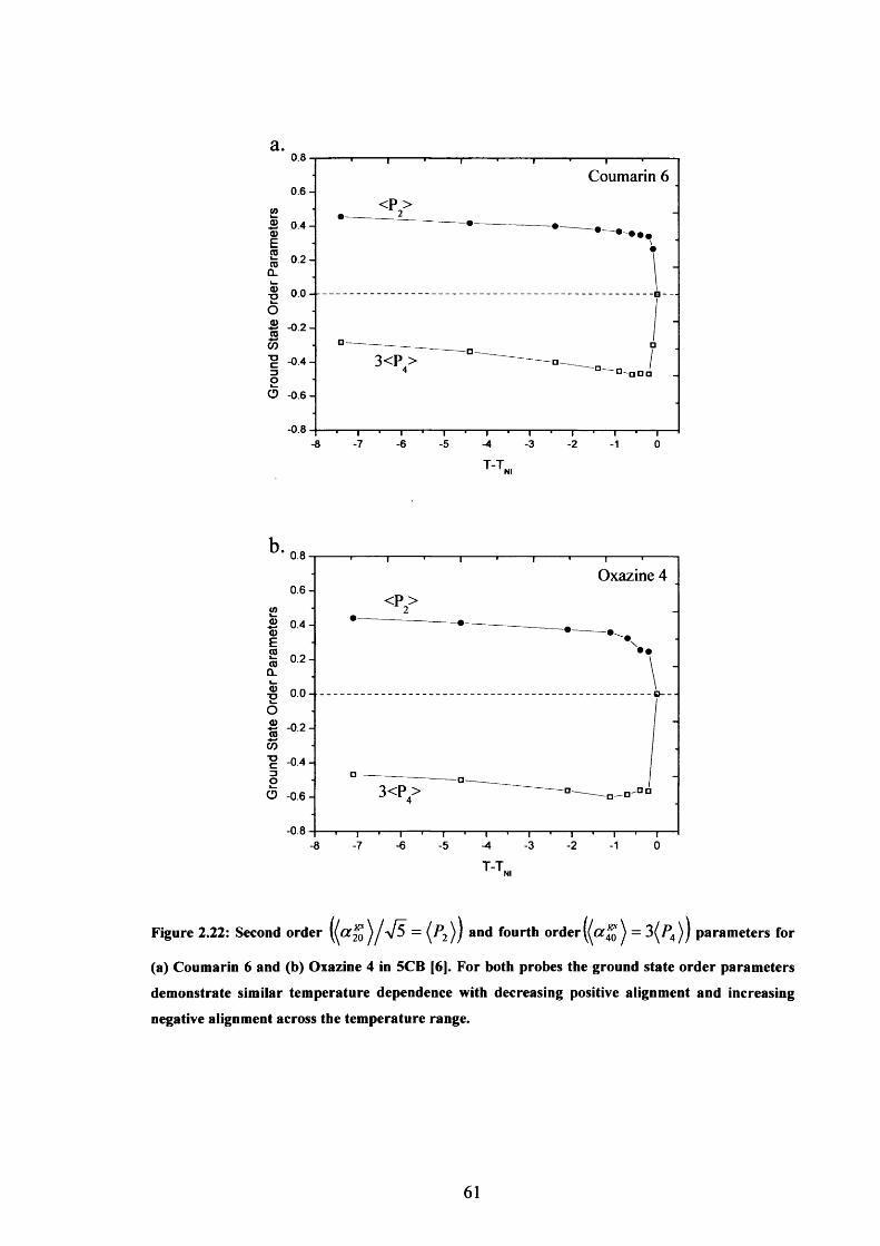
a.0.8

Coumarin 60.6-

<P>0.4 -0.2 -

■§ 0.0--

- 0 .2 -

"2 -0.4 - 3<P >

O - 0 . 6 -

- 0.8•7 6 5 -3-8 -4 2 1 0

0.8

Oxazine 40.6 -

<P>

0. 2 -

0 .0 - o—

- 0 .2 -

-0.4 -3<P>O - 0 . 6 -

- 0.8-6 3 2 1 0-8 -7 5 ■A

Figure 2.22: Second order ««S}/V5=(A>) and fourth order parameters for

(a) Coumarin 6 and (b) Oxazine 4 in SCB [6]. For both probes the ground state order parameters

demonstrate similar temperature dependence with decreasing positive alignment and increasing

negative alignment across the temperature range.

61

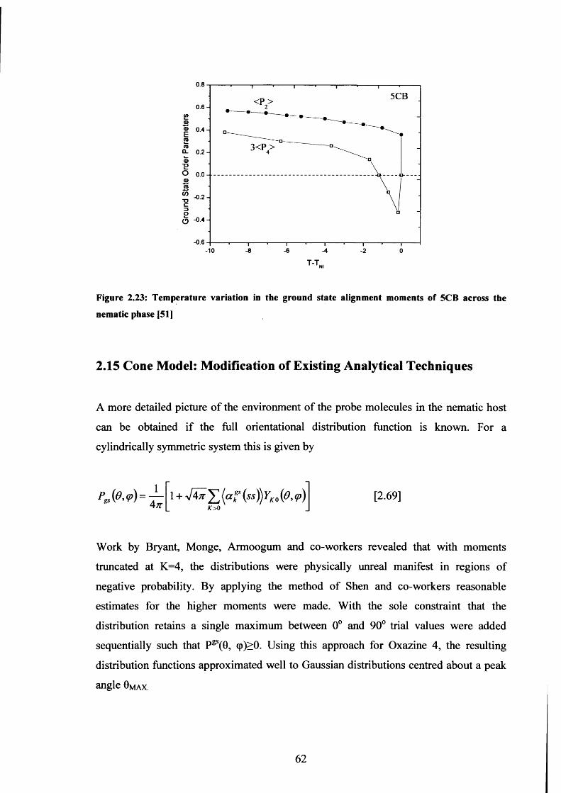
0.8

5CB<P>0 .6 -

3<P >

-0 .2 -

<5 -0.4-

- 0.6-10 -8 -6 -4 ■2 0

Figure 2.23: Temperature variation in the ground state alignment moments of 5CB across the

nematic phase [51]

2.15 Cone Model: Modification of Existing Analytical Techniques

A more detailed picture of the environment of the probe molecules in the nematic host

can be obtained if the full orientational distribution function is known. For a

cylindrically symmetric system this is given by

1 + a/4h £ [ a f (s s ) ) y ko (0 , <p)K > 0

[2.69]

Work by Bryant, Monge, Armoogum and co-workers revealed that with moments

truncated at K=4, the distributions were physically unreal manifest in regions of

negative probability. By applying the method of Shen and co-workers reasonable

estimates for the higher moments were made. With the sole constraint that the

distribution retains a single maximum between 0° and 90° trial values were added

sequentially such that Pgs(0, cp)>0. Using this approach for Oxazine 4, the resulting

distribution functions approximated well to Gaussian distributions centred about a peak

angle Om a x .

62

In order to better relate the order in the nematic phase to that in the isotropic phase a

cone model has been adapted whereby the probability distribution in 0 resembles a cone

where 0i — 0 m a x — 1/2 0 fw and 0 2 — 0 m a x + j/2 0 fw and K — 2,4.

A Mathematica program has been written in collaboration with Dr R Marsh which

allows determination of the peak angle (0 m a x ) and full width half maximum (A 0 fw h m )

of the distribution functions based on equation 2.70 (Appendix III). The temperature

dependent variation in the peak angle (0 m a x ) of the ground state distribution function of

Coumarin 6 in the nematic phase of 5CB is shown in figure 2.24a. Equation 2.70 has

been applied to re-analyse data from measurements of Oxazine 4 in the nematic phase

of 5CB (Bryant, Monge and co-workers) and is presented in figure 2.24b. For Coumarin

6 0 m a x is found to vary between 32.6° and 42.2° across the nematic temperature range.

The peak angle maintains a near positive linear dependence (c.a.l.l°/°C) though in close

vicinity of TNi the peak angle decreases (c.a. 2°).Oxazine 4 also maintains a near linear

dependence (c.a.0.5°/°C) however in contrast to Coumarin 6 , 0 m a x peaks sharply in the

vicinity of Tni (c.a. 4-5°). In the nematic phase, the 5CB molecules are ordered in an

anti-parallel fashion; the cyano groups aligning parallel to the nematic director with the

alkyl groups making an angle (0a l k y l ) of c.a. 38° to n [6 ], (figure 2.4). It is interesting

to note that for Coumarin 6 0 m a x is oriented at an angle greater than 0 a l k y l for most of

the nematic temperature range whereas Oxazine 4 maintains a peak angle close to

0ALKYL-

with equal probability of being between two limits described as 0 m a x - ^ O fw h m and

9 m a x + ^ Q fw h m given by

[2.70]

63

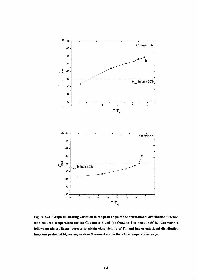
a. 48Coumarin 6

4 6-4 4-4 2-4 0-o

<X>

3 8--0 , in bulk 5CB

alkyl

3 6-3 4-

•5 -4 -3 2 1 0

O xazine 44 4-4 2-4 0-

X« 3 8-in bulk 5CBCD

alkyl

3 6-3 4-3 2-

-7 -6 5-8 -4 -3 -2 1 0 1

Figure 2.24: Graph illustrating variation in the peak angle of the orientational distribution function

with reduced temperature for (a) Coumarin 6 and (b) Oxazine 4 in nematic 5CB. Coumarin 6

follows an almost linear increase to within close vicinity of TNi and has orientational distribution

functions peaked at higher angles than Oxazine 4 across the whole temperature range.

64

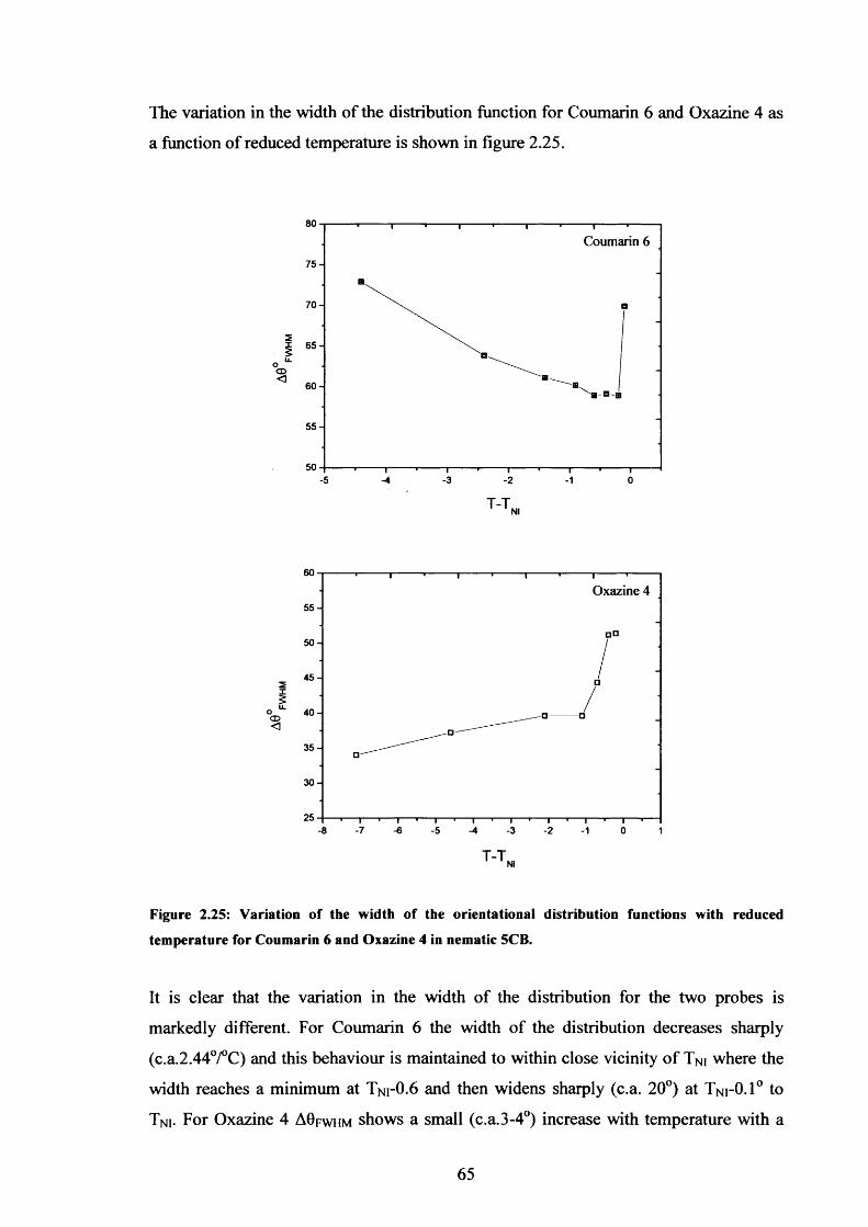
The variation in the width of the distribution function for Coumarin 6 and Oxazine 4 as

a function of reduced temperature is shown in figure 2.25.

80

Coumarin 6

7 5 -

7 0 -

6 5 -u_o

CD<6 0 -

55 -

-5 -4 3 2 1 0

Oxazine 45 5 -

□ □5 0 -

4 5 -

4 0 -o<X><3 5 -

3 0 -

•7 -6 0-8 5 -4 3 2 1 1

Figure 2.25: Variation of the width of the orientational distribution functions with reduced

temperature for Coumarin 6 and Oxazine 4 in nematic 5CB.

It is clear that the variation in the width of the distribution for the two probes is

markedly different. For Coumarin 6 the width of the distribution decreases sharply

(c.a.2.44°/°C) and this behaviour is maintained to within close vicinity of T ni where the

width reaches a minimum at T ni-0 .6 and then widens sharply (c.a. 20°) at T ni-0 .1 ° to

T ni- For Oxazine 4 AGfwhm shows a small (c.a.3 -4°) increase with temperature with a

65

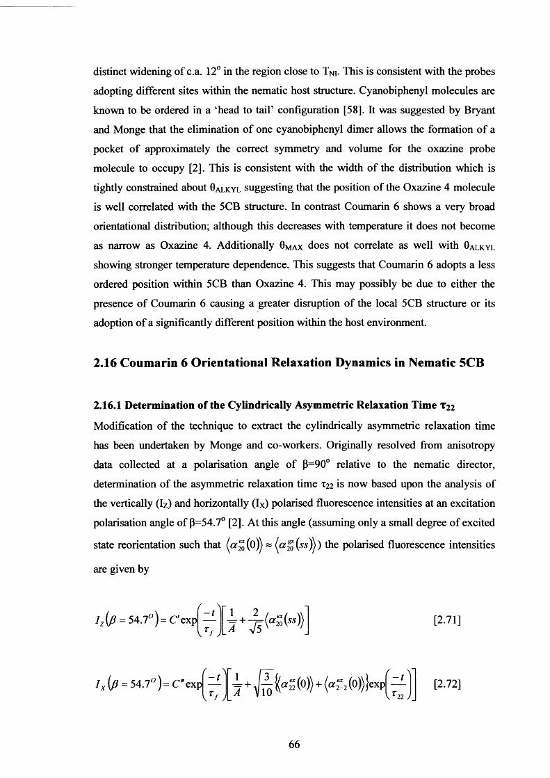
distinct widening of c.a. 12° in the region close to Tni- This is consistent with the probes

adopting different sites within the nematic host structure. Cyanobiphenyl molecules are

known to be ordered in a ‘head to tail’ configuration [58]. It was suggested by Bryant

and Monge that the elimination of one cyanobiphenyl dimer allows the formation o f a

pocket of approximately the correct symmetry and volume for the oxazine probe

molecule to occupy [2]. This is consistent with the width of the distribution which is

tightly constrained about Galkyl suggesting that the position of the Oxazine 4 molecule

is well correlated with the 5CB structure. In contrast Coumarin 6 shows a very broad

orientational distribution; although this decreases with temperature it does not become

as narrow as Oxazine 4 . Additionally Gmax does not correlate as well with Galkyl

showing stronger temperature dependence. This suggests that Coumarin 6 adopts a less

ordered position within 5CB than Oxazine 4 . This may possibly be due to either the

presence of Coumarin 6 causing a greater disruption of the local 5CB structure or its

adoption of a significantly different position within the host environment.

2.16 Coumarin 6 Orientational Relaxation Dynamics in Nematic 5CB

2.16.1 Determination of the Cylindrically Asymmetric Relaxation Time T22

Modification of the technique to extract the cylindrically asymmetric relaxation time

has been undertaken by Monge and co-workers. Originally resolved from anisotropy

data collected at a polarisation angle of p=90° relative to the nematic director,

determination of the asymmetric relaxation time T22 is now based upon the analysis of

the vertically (Iz) and horizontally (Ix) polarised fluorescence intensities at an excitation

polarisation angle of p=54.7° [2]. At this angle (assuming only a small degree of excited

state reorientation such that (a ^ ( 0 « (a fl (ssjj) the polarised fluorescence intensities

are given by

/*(/? = 54.7°) = C"exp - ta 22 ( 0 ) ) + ( < * “ 2 ( o ) ) } e x p f [2.72]

22 /

Iz {p = 54.7°) = C' exp

66

The ratio of the two intensities solely contains the asymmetric alignment dynamics T22

— (/? = 54.7°)= C'I 7

A + V10a S (0 )) + {a 2-2 (o))}expJ -

Vr 22 )1 J L A + S

<«sH[2.73]

The variation in xe and x9 with reduced temperature for Coumarin 6 is shown in figure

2.26 along with the values of xe and x9 for Oxazine 4 in 5CB as per Monge, Bryant and

co-workers.

The cylindrically symmetric (X20) times were determined from equation 2.6 the

cylindrically asymmetric times (X22) were determined using equation 2.73. Providing the

orientational distributions are dominated by anisotropic friction, the small 0 dependence

present in X22 can be removed yielding a pure cp diffusion time [2, 15] through the

equation

_ _ 2t20t229 3r - t20 1 22

[2.74]

The reorientational lifetimes (xe and x<p) for Coumarin 6 are approximately equal (within

experimental error bars) indicating that the relaxation of the symmetric alignment (0-

diffusion) is very similar to that of the asymmetric alignment (cp-diffusion). This is

somewhat unusual as it demonstrates behaviour expected in a wholly isotropic medium

where 0-diffusion and cp-diffusion are necessarily equal. This is not generally the case

for an ordered medium where symmetry considerations of perturbed rotational diffusion

demand that the two times are unequal [20]. Only in the region of the phase transition

temperature does Coumarin 6 show any change as xe decreases in the approach to Tni.

This is in marked contrast to 0 and cp motion for Oxazine 4 where xe and x9 are clearly

different and described by approximately temperature independent cp-diffusion (similar

to that seen in Coumarin 6) although it slows in the approach to T ni, and 0-diffusion

which is considerably slower and decreases across the nematic temperature range

converging with x<p at T n i.

67

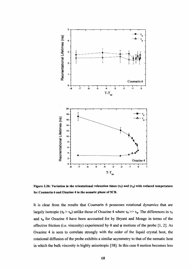
<1)oc

Coumarin 6

-8 -3

T-TNl

</)c{/)a>E.a>

(Ocoroca>’i_oa)DC

20

1 8 -

1 6 -

1 4 -

1 2 -

1 0 -

4 -

2-Oxazine 4

-5 -4 -2-7 -3 1 0 18 -6

T-TNl

Figure 2.26: Variation in the orientational relaxation times (re) and (t ,) with reduced temperature

for Coumarin 6 and Oxazine 4 in the nematic phase of 5CB.

It is clear from the results that Coumarin 6 possesses rotational dynamics that are

largely isotropic (xe ~ x<p) unlike those of Oxazine 4 where xe » x<p. The differences in xe

and Xq, for Oxazine 4 have been accounted for by Bryant and Monge in terms of the

effective friction (i.e. viscosity) experienced by 0 and cp motions of the probe [1,2]. As

Oxazine 4 is seen to correlate strongly with the order of the liquid crystal host, the

rotational diffusion of the probe exhibits a similar asymmetry to that of the nematic host

in which the bulk viscosity is highly anisotropic [58]. In this case 0 motion becomes less

restricted whilst the slowing of cp motion was accounted for in terms of the uncorrelated

motion of different segments of the tails of individual cyanobiphenyl molecules whose

interference acts to hinder cp-diffusion [1,2]. This is not the case for Coumarin 6 where

the difference in 0 and cp motion appears negligible, indicative of a much more isotropic

environment for the probe. Additionally 0-diffusion is observed to be much faster than

for Oxazine 4 at a rate more akin to unrestricted diffusion in a simple liquid (section

2.12). The slow 0-diffusion times for Oxazine 4 were attributed to the tight structural

constraints on the probe leading to predominantly ‘stick’ dynamics. The much faster 0-

diffusion times coupled with the isotropic diffusional behaviour for Coumarin 6

however suggest predominantly ‘slip’ boundary conditions.

The diffusion dynamics discussed above combined with the lower orientational

constraints compared with Oxazine 4 suggest that Coumarin 6 occupies a much less

structured environment with much greater orientational freedom. This can be further

highlighted by a plot of the proportion of orientational space the molecule can occupy

as shown in figure 2.27.

100

9 0 -

8 0 -

6 0 - □ □5 0 -

4 0 -

3 0 -

2 0 -

Coumarin 6 Oxazine 4

1 0 -

-5 -4 3 ■2-7 -6 1 0-8

Figure 2.27: Graph showing proportion of unit sphere occupied by the probe using the cone model.

It is evident that Coumarin 6 is in a much less restricted environment than Oxazine 4 and is

temperature invariant

69

This plot combined with the experimental results above strongly suggest that Oxazine 4

is in a much more restrictive environment than Coumarin 6 and that this environment is

sensitive to the temperature dependent anisotropic behaviour of the host. In contrast

Coumarin 6 appears to adopt a position within the local environment which is

insensitive to the behaviour of the 5CB molecules across the nematic phase. A possible

reason for this is the up-take of the probe into the alkyl tail region of the liquid crystal

host possibly combined with distortion of the local nematic structure due to the larger

size and hydrophobic nature of Coumarin 6.

2.17 Orientational Dynamics and Local Order of Coumarin 6 in

Isotropic 5CB

2.17.1 Results

For all experiments undertaken in the isotropic phase o f 5CB, the phase transition was

identified by a sudden loss in scattered laser light from the sample and confirmed when

the fluorescence anisotropy R(t, (3) was seen to decay to zero irrespective o f polarisation

angle p. Subsequent measurements were carried out with the polarisation angle set at

P=0° as 0 and cp diffusion are equivalent in an isotropic environment.

The orientational lifetimes showing the behaviour of both the fast component Tfast and

slow component xsiow of the fluorescence anisotropy decays of both dyes as a function of

reduced temperature across the isotropic phase of 5CB is shown in figure 2.28.

70

Coumarin 61 2 -

slow10-cn c(DE

(DCoJo

fasto-

10 20 30 40 500 60

O©o'

Oxazme 4

T-T.,

Figure 2.28: Variation with temperature in the fast and slow orientational relaxation times (T fast and

Tjiow) for Coumarin 6 and Oxazine 4 in 5CB.

The slow overall diffusion time (xsiow) variation with temperature is related to the

temperature dependent shear viscosity of the liquid crystal in the isotropic phase by

± * ( T K + rkH [ T - T ' ) 0

[2.75]

where V efr is the hydrodynamic volume of the Coumarin 6 dye molecule, To is the free

rotor correlation time, ke the Boltzmann constant and T* is the virtual transition

71

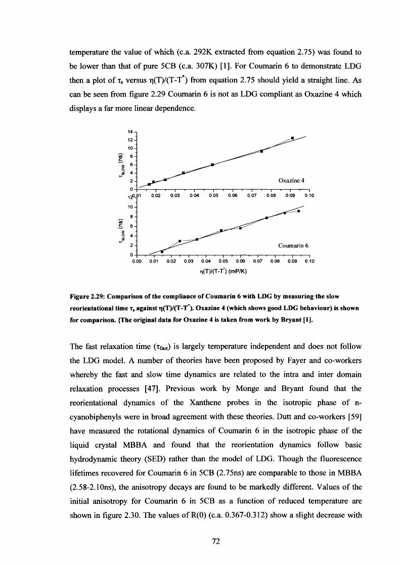
temperature the value of which (c.a. 292K extracted from equation 2.75) was found to

be lower than that of pure 5CB (c.a. 307K) [1]. For Coumarin 6 to demonstrate LDG

then a plot of xs versus q(T)/(T-T*) from equation 2.75 should yield a straight line. As

can be seen from figure 2.29 Coumarin 6 is not as LDG compliant as Oxazine 4 which

displays a far more linear dependence.

14-i12-10-8-V)c.6-

Oxazine 42-

0.03 0.04 0.05 0.06 0.07 0.08 0.09 0.100.02

coc 6-

Coumarin 62-

0.00 0.01 0.02 0.03 0.04 0.05 0.06 0.07 0.08 0.09 0.10

n(TV(T-T) (mP/K)

Figure 2.29: Comparison of the compliance of Coumarin 6 with LDG by measuring the slow

reorientational time t s against q(T)/(T-T*). Oxazine 4 (which shows good LDG behaviour) is shown

for comparison. {The original data for Oxazine 4 is taken from work by Bryant [1].

The fast relaxation time (ifast) is largely temperature independent and does not follow

the LDG model. A number of theories have been proposed by Fayer and co-workers

whereby the fast and slow time dynamics are related to the intra and inter domain

relaxation processes [47]. Previous work by Monge and Bryant found that the

reorientational dynamics of the Xanthene probes in the isotropic phase of n-

cyanobiphenyls were in broad agreement with these theories. Dutt and co-workers [59]

have measured the rotational dynamics of Coumarin 6 in the isotropic phase of the

liquid crystal MBBA and found that the reorientation dynamics follow basic

hydrodynamic theory (SED) rather than the model of LDG. Though the fluorescence

lifetimes recovered for Coumarin 6 in 5CB (2.75ns) are comparable to those in MBBA

(2.58-2.10ns), the anisotropy decays are found to be markedly different. Values of the

initial anisotropy for Coumarin 6 in 5CB as a function of reduced temperature are

shown in figure 2.30. The values of R(0) (c.a. 0.367-0.312) show a slight decrease with

72

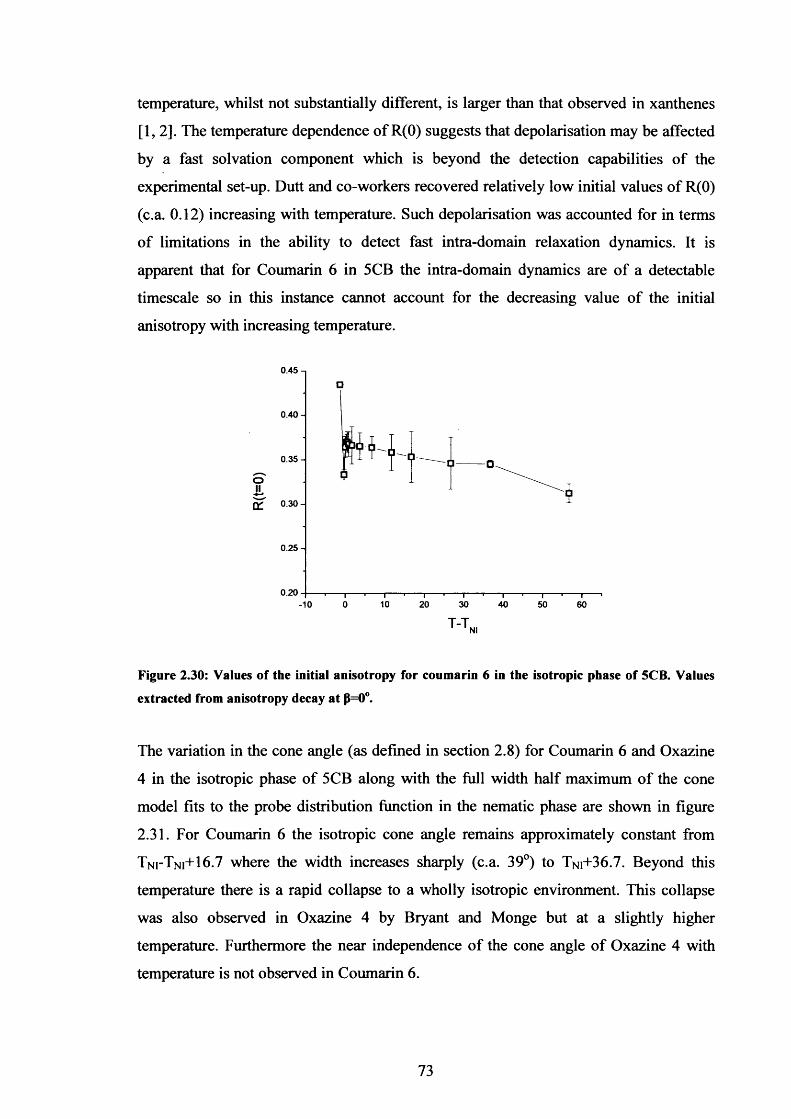
temperature, whilst not substantially different, is larger than that observed in xanthenes

[1,2]. The temperature dependence of R(0) suggests that depolarisation may be affected

by a fast solvation component which is beyond the detection capabilities of the

experimental set-up. Dutt and co-workers recovered relatively low initial values of R(0)

(c.a. 0.12) increasing with temperature. Such depolarisation was accounted for in terms

of limitations in the ability to detect fast intra-domain relaxation dynamics. It is

apparent that for Coumarin 6 in 5CB the intra-domain dynamics are of a detectable

timescale so in this instance cannot account for the decreasing value of the initial

anisotropy with increasing temperature.

0.45

0.40-

0.35-

OII

0.25-

0.2010 20 30 40-10 0 50 60

Figure 2.30: Values of the initial anisotropy for coumarin 6 in the isotropic phase of 5CB. Values

extracted from anisotropy decay at p=0°.

The variation in the cone angle (as defined in section 2 .8 ) for Coumarin 6 and Oxazine

4 in the isotropic phase of 5CB along with the full width half maximum of the cone

model fits to the probe distribution function in the nematic phase are shown in figure

2 .3 1 . For Coumarin 6 the isotropic cone angle remains approximately constant from

T ni-T ni+ 1 6 .7 where the width increases sharply (c.a. 3 9 °) to T ni+ 3 6 .7 . Beyond this

temperature there is a rapid collapse to a wholly isotropic environment. This collapse

was also observed in Oxazine 4 by Bryant and Monge but at a slightly higher

temperature. Furthermore the near independence of the cone angle of Oxazine 4 with

temperature is not observed in Coumarin 6.

73

180- Nematic Isotropic

160-

140-co0)0) 120 -

05 <UQ 1 0 0 -

©o>c<<Dc

8 0 -

6 0 -OO 4 0 -

20-Coumarin 6 ‘

20-10 0 10 30 40 50 60

180 - Nematic Isotropic

160-

140-

O ) 1 2 0 -

a> 1 0 0 - O)

6 0 - l-o— I40

O xazine 420

20 30-10 0 10 40 50 60

Figure 2.31: Cone angle for Coumarin 6 and Oxazine 4 in 5CB as a function of reduced

temperature in both the nematic and isotropic phases of 5CB. Also shown is the FWHM angle

dependence of the probe molecules in the nematic phase.

This would tend to indicate the local environment around Oxazine 4 is not sufficiently

changing as the size of the pseudo-domains reduces with temperature. Conversely

Coumarin 6 seems to have even greater orientational freedom as the correlation length

reduces. A second notable difference in the behaviour of the two probes is seen in the

rotational diffusion times at the phase transition as shown in figure 2.32. For Oxazine 4

74

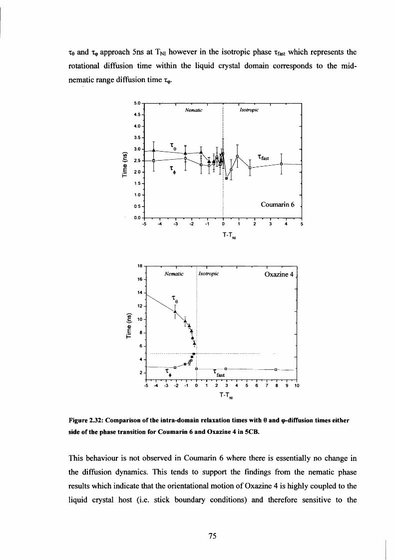
xe and x<p approach 5ns at T ni however in the isotropic phase Tfast which represents the

rotational diffusion time within the liquid crystal domain corresponds to the mid­

nematic range diffusion time xr

5.0IsotropicNematic

4 .5 -

4 .0 -

3 .5 -

3 .0 -'w■S 2 .5 - a>■i 2.0 -h-

1 .5-

Coumarin 60 .5 -

0.0■2•5 -4 ■3 ■1 0 1 2 3 4 5

Isotropic Oxazine 4Nematic1 6 -

1 4 -

12-

1 0 -

a>E 8-K-

6-

4 -

2- fast

-5 -4 -3 -2 -1 0 1 2 3 4 5 6 7 8 9 10

Figure 2.32: Comparison of the intra-domain relaxation times with 0 and <p-diffusion times either

side of the phase transition for Coumarin 6 and Oxazine 4 in 5CB.

This behaviour is not observed in Coumarin 6 where there is essentially no change in

the diffusion dynamics. This tends to support the findings from the nematic phase

results which indicate that the orientational motion of Oxazine 4 is highly coupled to the

liquid crystal host (i.e. stick boundary conditions) and therefore sensitive to the

75

structural changes at the phase transition. In contrast Coumarin 6 is in a more isotropic

and possibly distorted environment that does not change significantly through the phase

transition.

Bryant and Monge also studied other Xanthene probes in 5, 6 and 7 CB and similar

behaviour was observed as for Oxazine 4 in 5CB. A slight departure form this

behaviour was observed for Rhodamine B which showed a smaller difference between 0

and cp-diffusion times and a slightly larger centre angle. These differences are small

when compared to those of Coumarin 6 in this work.

2.18 Conclusion

To the best of our knowledge this study represents the first investigation of the full

angular motion and molecular order of Coumarin 6 in a highly aligned nematic liquid

crystal. Coumarin 6 dynamics are seen to depart considerably from those of Oxazine 4

in the nematic phase. Rotational diffusion with respect to the (global) nematic director

is seen to be both fast and isotropic with This indicates the predominance of slip

boundary conditions. The width of the distribution function further suggests that the

orientation of Coumarin 6 is only weakly correlated to the liquid crystal host unlike

Oxazine 4 and other Xanthene dyes [1, 2]. Isotropic phase behaviour further supports

these conclusions. Both the poor LDG behaviour and lack of sensitivity of the dynamics

to the phase transition also suggest poor correlation between probe and host.

As described in section 2.3 the defining characteristics of the nematic phase of a liquid

crystal is the strong propensity of the individual molecules to self-align with each other.

This is manifest by a high degree of anisotropy in both bulk and microscopic properties.

Oxazine 4 is seen to closely follow this behaviour and the corresponding changes with

temperature. It has been argued by Bryant and Monge, supported by further analysis in

this work that Oxazine 4 occupies a position between the phenyl cores of the 5CB

molecules with little disruption to the surrounding structure, hence the strong

correlation with the host. This is consistent with the hydrophilic nature of Oxazine 4. In

contrast Coumarin 6 does not show anisotropic diffusional behaviour or the associate

temperature dependence, coupled with much greater orientational freedom. It is

76

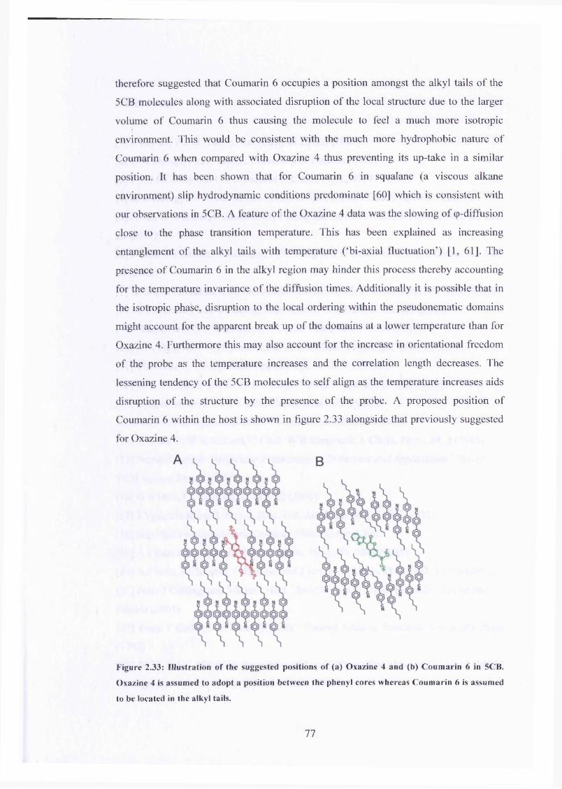
therefore suggested that Coumarin 6 occupies a position amongst the alkyl tails of the

5CB molecules along with associated disruption of the local structure due to the larger

volume of Coumarin 6 thus causing the molecule to feel a much more isotropic

environment. This would be consistent with the much more hydrophobic nature of

Coumarin 6 when compared with Oxazine 4 thus preventing its up-take in a similar

position. It has been shown that for Coumarin 6 in squalane (a viscous alkane

environment) slip hydrodynamic conditions predominate [60] which is consistent with

our observations in 5CB. A feature of the Oxazine 4 data was the slowing of cp-diffusion

close to the phase transition temperature. This has been explained as increasing

entanglement of the alkyl tails with temperature (‘bi-axial fluctuation’) [1, 61]. The

presence of Coumarin 6 in the alkyl region may hinder this process thereby accounting

for the temperature invariance of the diffusion times. Additionally it is possible that in

the isotropic phase, disruption to the local ordering within the pseudonematic domains

might account for the apparent break up of the domains at a lower temperature than for

Oxazine 4. Furthermore this may also account for the increase in orientational freedom

of the probe as the temperature increases and the correlation length decreases. The

lessening tendency of the 5CB molecules to self align as the temperature increases aids

disruption of the structure by the presence of the probe. A proposed position of

Coumarin 6 within the host is shown in figure 2.33 alongside that previously suggested

for Oxazine 4.

Figure 2.33: Illustration o f the suggested positions o f (a) Oxazine 4 and (b) Coumarin 6 in 5CB.

Oxazine 4 is assumed to adopt a position between the phenyl cores whereas Coumarin 6 is assumed

to be located in the alkyl tails.

77

References

[1] J. Bryant, Ph. D. Thesis, University of Essex, (2000)

[2] E M Monge, Ph.D. Thesis, University of London (2003)

[3] P K McCarthy and G J Blanchard J. Chem. Phys., 97, 47 (1993)

[4] M L Homg, J A Gardecki and M Maroncelli, J. Phys. Chem. A, 101, 6 (1997)

[5] H Jin, G A Baker, S Arzhantsev, J Dong and M Maroncelli, J. Phys. Chem. B., I l l ,

25 (2007)

[6] J Rau, C Ferrante, E Kneuper, F-W Deeg and C Brauchle, J. Phys. Chem. A., 105,

24(2001)

[7] N. Ito, S. Arzhantsev, M. Heitz, and M. Maroncelli, J. Phys. Chem. B., 108, 18 2004

[8] M. El-Kemary and W. Rettig, Phys. Chem. Chem. Phys., 5, 5221 (2003)

[9] V Kapko and D V Matyushov, J. Chem. Phys, 124, 114904 (2006)

[10] K A Nguyen, P N Day and R Pachter, J. Chem. Phys., 126, 094303 (2007)

[11] Theodore G. Pavlopoulos, Applied Optics., 36, 21 (1997)

[12] G. A. Reynolds and K. H. Drexhage, Optics Commun., 13, 222 (1975)

[13] Oregon Medical Laser Center PhotoChemCAD Spectra

URL: http://omlc. ogi. edn/spectra/PhotochemCAD/html/index. html

[14] G Jones II, W R Jackson, C Choi, W R Bergmark, J. Chem. Phys., 89, 2 (1985)

[15] Bernard Valeur “Molecular Fluorescence; Principles and Applications” Wiley-

VCH Second Reprint (2005)

[16] G B Dutt, J. Chem. Phys., 119, 22 (2003)

[17] J Yguerabide and L Stryer, Proc. Nat. Acad. Sci. 68(6), 1217 (1971)

[18] http://plc.cwru.edu/tutorial/enhanced/files/textbook.htm

[19] A J Bain and A J McCaffrey, J. Chem. Phys., 83, 2641 (1985)

[20] A J Bain, P Chandna, G Butcher and J Bryant, J. Chem. Phys., 112, 10435 (2000)

[21] Peter J Codings and Michael Hird “Introduction to Liquid Crystals” Taylor and

Francis (2004)

[22] Peter J Codings “Liquid Crystals” Second Edition, Princeton University Press

(1992)

[23] W H de Jeu “Physical Properties o f Liquid Crystalline Materials” Liquid Crystal

Monographs Volume 1, Gordon and Breach (1980)

78

[24] G W Gray and K J Harrison, UK Patent 1 433 130

[25] H Kelker and B Scheurle, Angew. Chem., 8, 884 (1969)

[26] LiqCryst Online http://liqcryst.chemie.uni-hamburg.de/lolas-www/main.html

[27] P W Atkins, “Molecular Quantum Mechanics ” Second Edition, Oxford University

Press (1992)

[28] G R Fleming and M Cho, Ann. Rev. Phys. Chem., 47, 109 (1996)

[29] A J Bain, P Chandna, G Butcher and J Bryant, J. Chem. Phys. 112, 10418 (2000)

[30] D.L. Andrews and A.A. Demidov (Ed.) “An Introduction to Laser Spectroscopy”

Second Edition, Kluwer, (2002)

[31] M de Podesta “Understanding the Properties o f Matter” Second Edition, Taylor

and Francis (2002)

[32] W D Callister Jr, “Materials Science and Engineering” (5th Ed.), Wiley (2000)

[33] B H Flowers and E Mendoza, “Properties o f Matter” Third Edition, Wiley (1991)

[34] S Elliott “The Physics and Chemistry o f Solids ” Wiley (2005)

[35] F Mandl “StatisticalPhysics” Second Edition, Wiley (1994)

[36] P Papon, J Leblond and P H E Meijer “The Physics o f Phase Transitions” Second

Edition, Springer (2006)

[37] D Demus, J Goodby, G W Gray, H-W Spiess and V Vill “Handbook o f Liquid

Crystals Volume 2A” First Edition Wiley-VCH (1998)

[38] J Bryant and A J Bain, Chem. Phys. Lett., 286, 121 (1998)

[39] S Chandrasekhar “Liquid Crystals” Second Edition, Cambridge University Press

(1992)

[40] A Sengupta and M D Fayer, J. Chem. Phys., 102, 10 (1995)

[41] W Stinson and J D Lister, Phys. Rev. (Lett)., 25, 503 (1970)

[42] H J Coles, Mol. Crystl. Liq. Cryst (Lett)., 49, 67 (1978)

[43] F W Deeg, J J Stankus, S R Greenfield, V J Newell and M D Fayer, J. Chem.

Phys., 90, 6893 (1989)

[44] S.D. Gottke, D.D. Brace, H. Cang, B. Bagchi and M.D. Fayer, J. Chem. Phys. 116,

360 (2002)

[45] S.D. Gottke, H. Cang, B. Bagchi and M.D. Fayer, J. Chem. Phys. 116, 6339 (2002)

[46] K Kinosita, S Kawato and A Ikagami, Biophys. J., 20, 289 (1977)

[47] J J Stankus, R Torre, C D Marshall, S R Greenfield, A Sengupta, A Tokmakoff,

M.D. Fayer, Chem. Phys. (Lett)., 194,213 (1992)

79

[48] D V O’Connor and D V Phillips, “Time Correlated Single Photon Counting”

Academic Press (1984)

[49] P Debye, “Polar Molecules ”, Dover, New York (1929)

[50] G Vertogen and B W van der Meer, Phys. Rev. A 19, 370-374 (1979)

[51] F Perrin, J .Phys. Radium., 5, 497 (1934)

[52] C M Hu and R Zwanzig, J Chem. Phys., 60, 4354 (1974)

[53] D M Brink and G R Satchler, “Angular Momentum ” Second Edition, Clarendon

Press, (1968)

[54] S D Durbin and Y R Shen, Phys. Rev. A., 30(3), 1419 (1984)

[55] S T W u a n d C S W u , Opt. Eng., 32(8), 1775 (1993)

[56] J R Lakowicz, “Principles o f Fluorescence Spectroscopy” Second Edition, Kluwer

Academic, (1999)

[57] A. J. Bain and A. J. McCaffery, J. Chem. Phys., 80, 5893 (1984)

[58] A Arcioni, F Bertinelli, R Tarroni and C Zannoni, Molecular Physics., 61 (5), 1161

(1987)

[59] G B Dutt, J. Phys., Chem 119, 22 (2003)

[60] G B Dutt and A Sachdeva, J. Chem. Phys., 118, 18 (2003)

[61] S V Dvinskikh, I Furo, H Zimmerman and A Maliniak, Phys. Rev. E., 65, 061701

(2002)

80

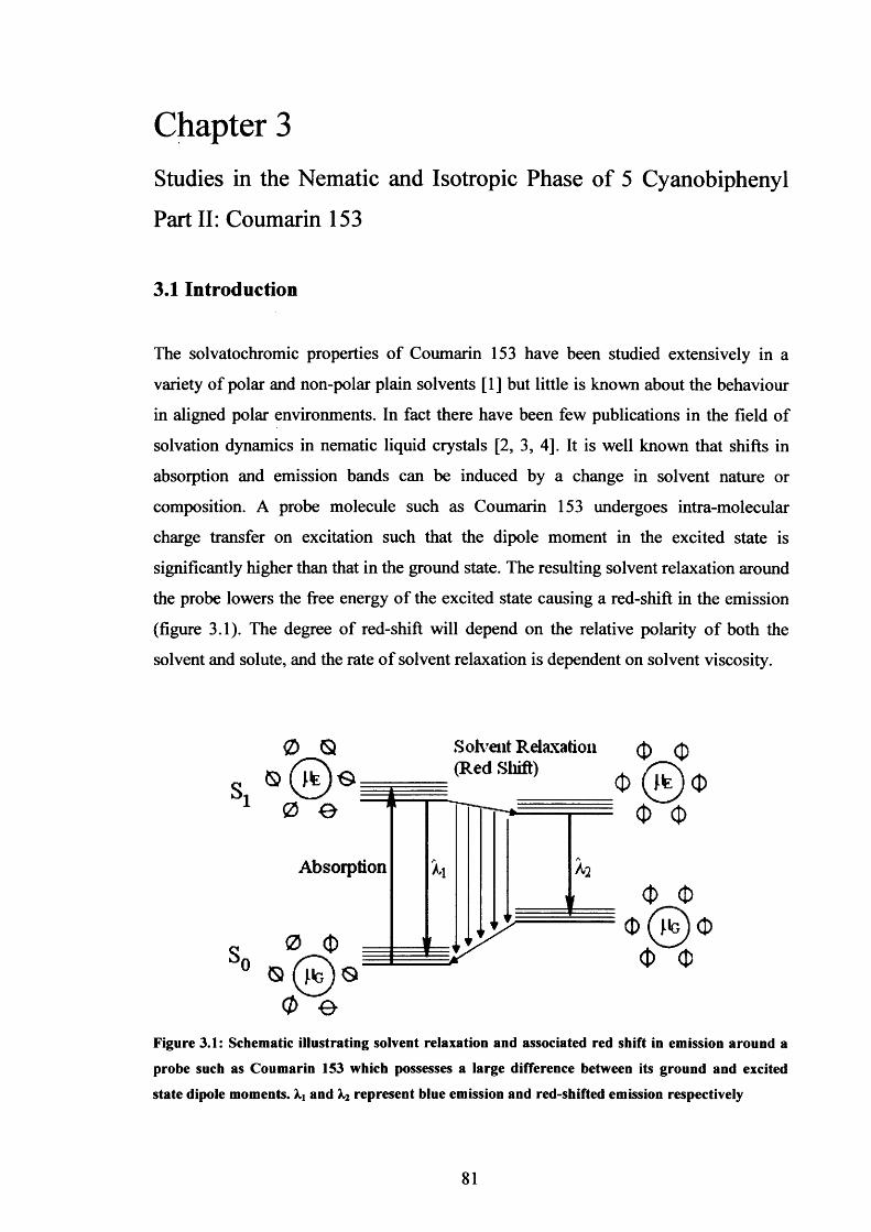
Chapter 3Studies in the Nematic and Isotropic Phase of 5 Cyanobiphenyl

Part II: Coumarin 153

3.1 Introduction

The solvatochromic properties of Coumarin 153 have been studied extensively in a

variety of polar and non-polar plain solvents [1] but little is known about the behaviour

in aligned polar environments. In fact there have been few publications in the field of

solvation dynamics in nematic liquid crystals [2, 3, 4]. It is well known that shifts in

absorption and emission bands can be induced by a change in solvent nature or

composition. A probe molecule such as Coumarin 153 undergoes intra-molecular

charge transfer on excitation such that the dipole moment in the excited state is

significantly higher than that in the ground state. The resulting solvent relaxation around

the probe lowers the free energy of the excited state causing a red-shift in the emission

(figure 3.1). The degree of red-shift will depend on the relative polarity o f both the

solvent and solute, and the rate of solvent relaxation is dependent on solvent viscosity.

Solvent Relaxation (Red Shift)

s i

Absorption

Figure 3.1: Schematic illustrating solvent relaxation and associated red shift in emission around a

probe such as Coumarin 153 which possesses a large difference between its ground and excited

state dipole moments. Xi and X2 represent blue emission and red-shifted emission respectively

81

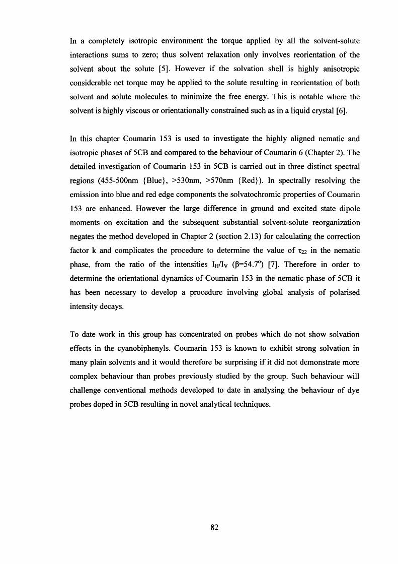
In a completely isotropic environment the torque applied by all the solvent-solute

interactions sums to zero; thus solvent relaxation only involves reorientation of the

solvent about the solute [5]. However if the solvation shell is highly anisotropic

considerable net torque may be applied to the solute resulting in reorientation of both

solvent and solute molecules to minimize the free energy. This is notable where the

solvent is highly viscous or orientationally constrained such as in a liquid crystal [6].

In this chapter Coumarin 153 is used to investigate the highly aligned nematic and

isotropic phases of 5CB and compared to the behaviour of Coumarin 6 (Chapter 2). The

detailed investigation of Coumarin 153 in 5CB is carried out in three distinct spectral

regions (455-500nm {Blue}, >530nm, >570nm {Red}). In spectrally resolving the

emission into blue and red edge components the solvatochromic properties of Coumarin

153 are enhanced. However the large difference in ground and excited state dipole

moments on excitation and the subsequent substantial solvent-solute reorganization

negates the method developed in Chapter 2 (section 2.13) for calculating the correction

factor k and complicates the procedure to determine the value of T22 in the nematic

phase, from the ratio of the intensities I h / I v (p=54.7°) [7]. Therefore in order to

determine the orientational dynamics of Coumarin 153 in the nematic phase of 5CB it

has been necessary to develop a procedure involving global analysis of polarised

intensity decays.

To date work in this group has concentrated on probes which do not show solvation

effects in the cyanobiphenyls. Coumarin 153 is known to exhibit strong solvation in

many plain solvents and it would therefore be surprising if it did not demonstrate more

complex behaviour than probes previously studied by the group. Such behaviour will

challenge conventional methods developed to date in analysing the behaviour of dye

probes doped in 5CB resulting in novel analytical techniques.

82

Coumarin 6 Coumarin 153Composition C20H18N2O2S c 16h 14n o 2F3 •

Quantum Yield 0.78l8J 0.90lV)Absorption Maximum 458nm 423nmEmission Maximum 505nm 530nmMolar Absorptivity (L m ol1 cm 1)

5.4x104 1.89xl04

Molecular Weight (g/mol) 350.43 309.29Hydrodynamic Volume 436,V 1’ _ 2 4 6 * ^Ground State Dipole M om ent1,21 7.00D 6.68DExcited State Dipole Moment *121 8.60D 13.64D

1.60D 6.96D

Table 3.1: The photophysical and hydrodynamic properties o f Coumarin 6 and Coum arin 153

3.2 Coumarin 153 in Ethylene Glycol: Results

All measurements in section 3.2 have been carried out using the same experimental set­

up described in section 2.11 and the results analysed in the same manner using

MicroCal™ Origin software. A single photon excitation wavelength of 470nm was

chosen and a long pass filter (Schott RD530) was used to isolate all emission long of

530nm. The anisotropy decay for Coumarin 153 in ethylene glycol is shown in figure

3.2.

C o u m arin 153 in E th y len e G lyco l0 .4 -

5 f 0 .3 ->*Q.01 t =0.985+/-0.012ns0.2 -

I 8£ 0.1 -

I 0.0-

-0.10 2 6 8 10-2 4 12 14

Time (ns)

Figure 3.2: Single photon anisotropy decay for Coumarin 153 in the isotropic solvent ethylene

glycol at room temperature (T=2I°+/-1°C) using an excitation wavelength o f 470nm and emission

filtered long o f 530nm. The decay fits a single exponential function indicating isotropic rotational

diffusion.

83

It can be seen that the anisotropy decay for Coumarin 153 fits well to a single

exponential function typical of diffusion in a simple isotropic liquid. Maroncelli et al

have undertaken fluorescence up-conversion studies for Coumarin 153 in ethylene

glycol [1] and found non-exponential anisotropy decays comprising a very fast

picosecond component (44ps) coupled with a slow longer time component (880ps) of

similar magnitude to that recovered in this experiment (985ps). The rationale for such

findings was described in terms of the non-Markovian nature of the friction on the

rotational motion of the probe molecule. Values of the initial anisotropy R(0) are similar

(0.380) to those found by Maroncelli and co-workers (0.369). It may still be possible

that a faster component is present in the anisotropy decay which cannot be resolved due

to the limitations in the single photon counting system. The rotational diffusion times

for Coumarin 153 were found to be considerably faster than those of Coumarin 6 (c.a.

60%). This is consistent with the ‘slip’ and ‘stick’ hydrodynamic theory proposed by

Stokes-Einstein-Debye (SED). In this instance Coumarin 153 has a rotational time

which is approximately 60% faster than that of Coumarin 6 whilst possessing a

hydrodynamic volume approximately twice as small (table 3.2).

Probe Solvent ^ e x c it e

(nm)T l i f e (ns) r(0) T r o t (ns)

Coumarin 153 Eth-Gly 470 3.539 +/- 0.003 0.380 +/- 0.003 0.985+/-0.012Coumarin 6 Eth-Gly 490 2.359 +/- 0.002 0.379 +/- 0.004 2.335 +/- 0.045

Concentration iTVf): 5x1 O'6Table 3.2: Summary of lifetime and rotational anisotropy decays for Coumarin 6 and Coumarin

153 in ethylene glycol.

84

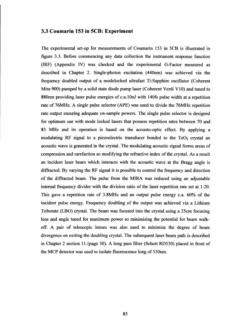
3.3 Coumarin 153 in 5CB: Experiment

The experimental set-up for measurements of Coumarin 153 in 5CB is illustrated in

figure 3.3. Before commencing any data collection the instrument response function

(IRF) (Appendix IV) was checked and the experimental G-Factor measured as

described in Chapter 2. Single-photon excitation (440nm) was achieved via the

frequency doubled output of a modelocked ultrafast Ti: Sapphire oscillator (Coherent

Mira 900) pumped by a solid state diode pump laser (Coherent Verdi V10) and tuned to

880nm providing laser pulse energies of c.a.l0nJ with 140fs pulse width at a repetition

rate of 76MHz. A single pulse selector (APE) was used to divide the 76MHz repetition

rate output ensuring adequate on-sample powers. The single pulse selector is designed

for optimum use with mode locked lasers that possess repetition rates between 70 and

85 MHz and its operation is based on the acousto-optic effect. By applying a

modulating RF signal to a piezoelectric transducer bonded to the TeC>2 crystal an

acoustic wave is generated in the crystal. The modulating acoustic signal forms areas of

compression and rarefaction so modifying the refractive index of the crystal. As a result

an incident laser beam which interacts with the acoustic wave at the Bragg angle is

diffracted. By varying the RF signal it is possible to control the frequency and direction

of the diffracted beam. The pulse from the MIRA was reduced using an adjustable

internal frequency divider with the division ratio of the laser repetition rate set at 1:20.

This gave a repetition rate of 3.8MHz and an output pulse energy c.a. 60% of the

incident pulse energy. Frequency doubling of the output was achieved via a Lithium

Triborate (LBO) crystal. The beam was focused into the crystal using a 25cm focusing

lens and angle tuned for maximum power so minimising the potential for beam walk-

off. A pair of telescopic lenses was also used to minimise the degree of beam

divergence on exiting the doubling crystal. The subsequent laser beam path is described

in Chapter 2 section 11 (page 50). A long pass filter (Schott RD530) placed in front of

the MCP detector was used to isolate fluorescence long of 530nm.

85

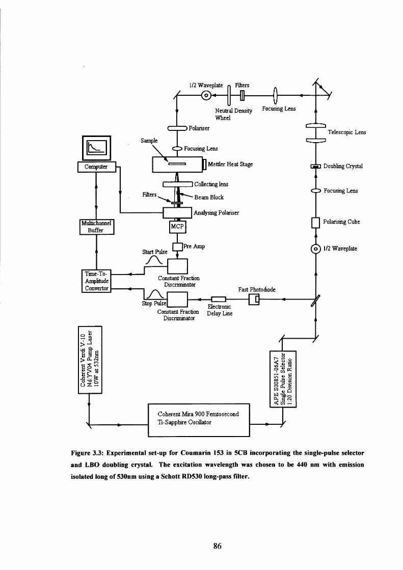
1/2 Waveplate n Filters

Neutral Density Focusing Lens Wheel

) PolariserTelescopic Lens

Focusing Lens

Computer |- Metder Heat Stage Doubling Crystal

] Collecting lens

• Beam BlockFilters

Analysing Polariserf | Polarising CubeMultichannel

BufferMCP

( o ) 1/2 WaveplateStart Pulse

/ \Time-To-AmpHtudeConvertor

Constant Fraction Discriminator

Fast Photodiode1Z \JStop Pulse Electronic

Constant Fraction Deiay Lme Discriminator

J> CL. CMt* £ ^ «o td o « it* . c/a

O 2 S

Coherent Mira 900 Femtosecond Ti-Sapphire Oscillator

Figure 3.3: Experimental set-up for Coumarin 153 in 5CB incorporating the single-pulse selector

and LBO doubling crystal. The excitation wavelength was chosen to be 440 nm with emission

isolated long of 530nm using a Schott RD530 long-pass filter.

86

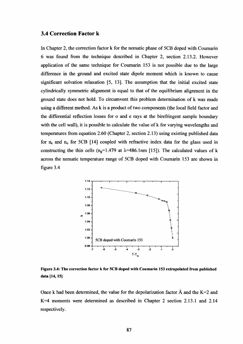
3.4 Correction Factor k

In Chapter 2, the correction factor k for the nematic phase of 5CB doped with Coumarin

6 was found from the technique described in Chapter 2, section 2.13.2. However

application of the same technique for Coumarin 153 is not possible due to the large

difference in the ground and excited state dipole moment which is known to cause

significant solvation relaxation [5, 13]. The assumption that the initial excited state

cylindrically symmetric alignment is equal to that of the equilibrium alignment in the

ground state does not hold. To circumvent this problem determination of k was made

using a different method. As k is a product of two components (the local field factor and

the differential reflection losses for o and e rays at the birefringent sample boundary

with the cell wall), it is possible to calculate the value of k for varying wavelengths and

temperatures from equation 2.60 (Chapter 2, section 2.13) using existing published data

for ne and no for 5CB [14] coupled with refractive index data for the glass used in

constructing the thin cells (ng= 1.479 at A,=486.1nm [15]). The calculated values of k

across the nematic temperature range of 5CB doped with Coumarin 153 are shown in

figure 3.4

1.14

1.1 2 -

1.1 0 -

1.08-

1.06-

1.04-

1 .0 2 -

1.0 0 -5CB doped with Coumarin 153

0.98-7 -6 -5 -4 3 2 1 0

Figure 3.4: The correction factor k for 5CB doped with Coumarin 153 extrapolated from published

data (14,15]

Once k had been determined, the value for the depolarization factor A and the K=2 and

K=4 moments were determined as described in Chapter 2 section 2.13.1 and 2.14

respectively.

87

3.5 Nematic Order of Coumarin 153 in 5CB

The variation in the ground state order parameters as a function of reduced temperature

for Coumarin 153 in 5CB are shown in figure 3.5. The procedure to determine the peak

angle ( 0 m a x ) and width of the distribution (A 0 Fwhm) is described in Chapter 2, section

2.15.

£2a)a>E(0i_(0CLi_a)-oO0)TO55■oc3o1—0

Coumarin 153

o .o -

- 0 .8 -

3<P4>

T-T

Figure 3.5: Second order H)/Vs = ( p2)) and fourth order ( ( « ' ) = 3 (P 4)J parameters for

Coumarin 153 in 5CB. It is evident that both order parameters are at variance to those of

Coumarin 6 and Oxazine 4.

Coumarin 153 is characterised by positive values of ( a ^ )/V5 though the degree of

K=2 alignment in the nematic host is considerably lower (c.a. 12%) when compared to

that of Coumarin 6 (c.a. 45% ). The degree of positive alignment is constant to T ni-0 .5

where there is an abrupt collapse to zero at Tni- The degree of negative alignment

also shows little variation to within close vicinity of the phase transition

The temperature dependent variation in the peak angle ( 0 m a x ) of the ground state

distribution function of Coumarin 153 in the nematic phase of 5CB, compared to that of

Coumarin 6 is shown in figure 3.6. The peak angle for the orientational distribution

function of Coumarin 153 in 5CB shows little temperature dependence (c.a. 51.75±0.5°)

across the nematic temperature range to within close vicinity of T Ni (T Ni-0 .5 ) where

there is a small fluctuation (±1°). It is further apparent that Coumarin 153 maintains a

88

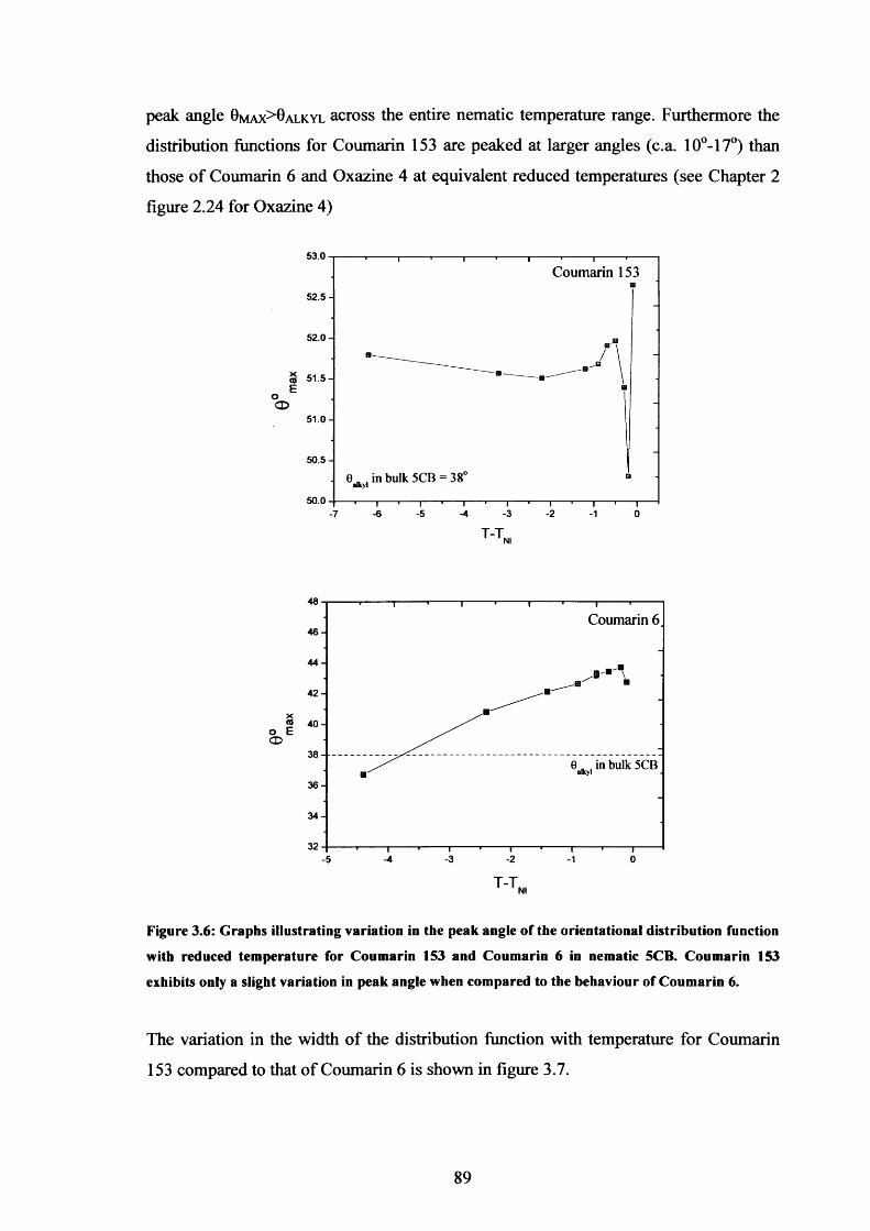
peak angle Bm a x > 0 a l k y l across the entire nematic temperature range. Furthermore the

distribution functions for Coumarin 153 are peaked at larger angles (c.a. 10°-17°) than

those of Coumarin 6 and Oxazine 4 at equivalent reduced temperatures (see Chapter 2

figure 2.24 for Oxazine 4)

53.0

Coumarin 15352.5-

52.0-

X(0Eo

CD51.0-

50.5-

in bulk 5CB = 38°alkyl

50.05 -4 3 2-6 1 0-7

48

Coumarin 64 6 -

4 4 -

4 2 -

x« 4 0 -

o E CD

38 -in bulk 5CB

alkyl

36 -

3 4 -

3 25 -4 1 0

Figure 3.6: Graphs illustrating variation in the peak angle of the orientational distribution function

with reduced temperature for Coumarin 153 and Coumarin 6 in nematic 5CB. Coumarin 153

exhibits only a slight variation in peak angle when compared to the behaviour of Coumarin 6.

The variation in the width of the distribution function with temperature for Coumarin

153 compared to that of Coumarin 6 is shown in figure 3.7.

89

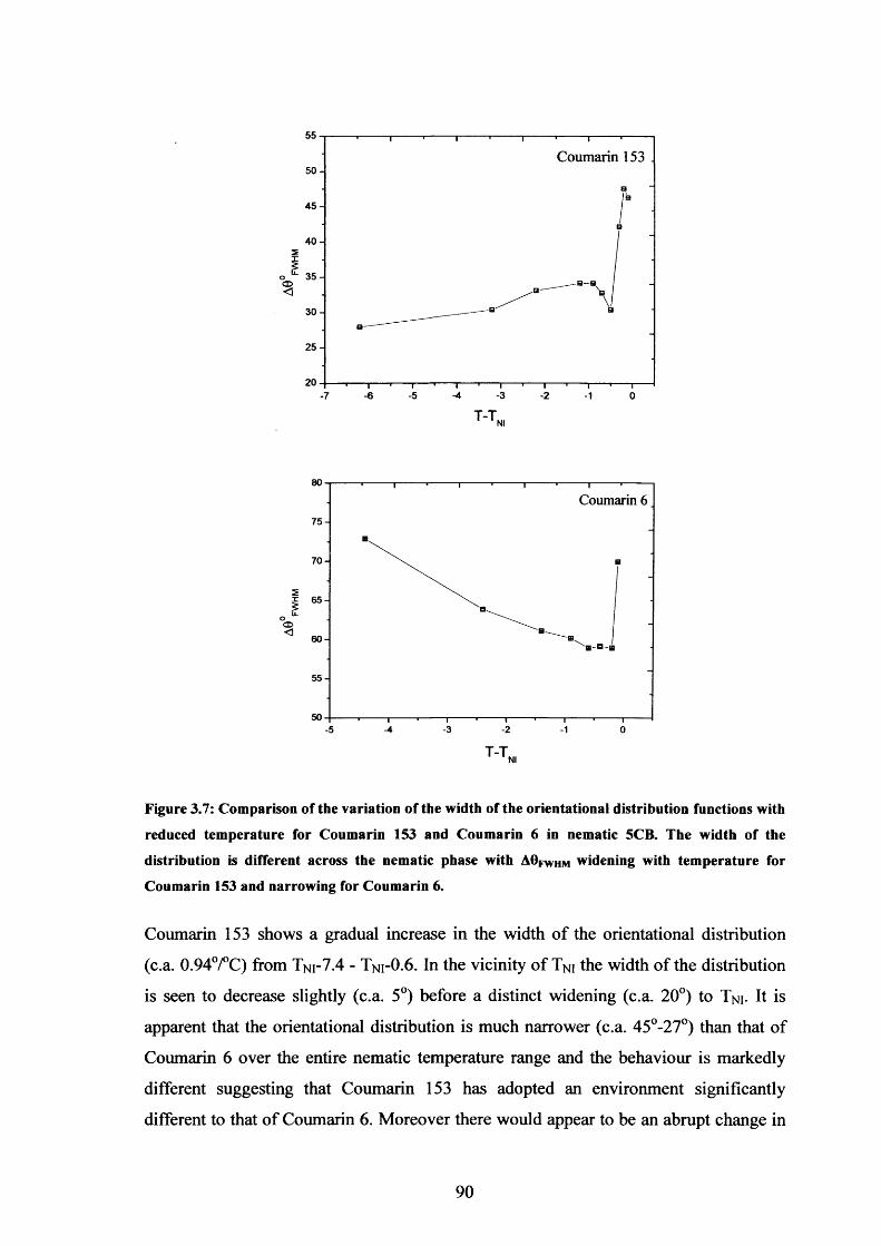
55

Coumarin 153 .5 0 -

4 5 -

4 0 -

3 5 -<X>

3 0 -

2 5 -

20-4 ■3-7 -6 -5 -2 01

80

Coumarin 675-

70-

2x£u.o<X>< 60-

55-

503 2•5 -4 ■1 0

Figure 3.7: Comparison of the variation of the width of the orientational distribution functions with

reduced temperature for Coumarin 153 and Coumarin 6 in nematic 5CB. The width of the

distribution is different across the nematic phase with AOpwhm widening with temperature for

Coumarin 153 and narrowing for Coumarin 6.

Coumarin 153 shows a gradual increase in the width of the orientational distribution

(c.a. 0.94°/°C) from Tni-7.4 - Tni-0.6. In the vicinity of TNi the width of the distribution

is seen to decrease slightly (c.a. 5°) before a distinct widening (c.a. 20°) to TNi- It is

apparent that the orientational distribution is much narrower (c.a. 45°-27°) than that of

Coumarin 6 over the entire nematic temperature range and the behaviour is markedly

different suggesting that Coumarin 153 has adopted an environment significantly

different to that of Coumarin 6. Moreover there would appear to be an abrupt change in

90

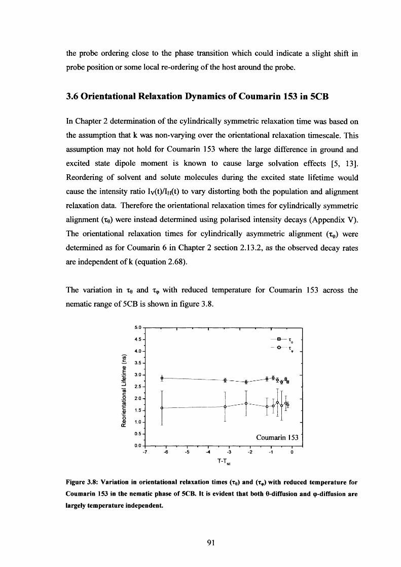
the probe ordering close to the phase transition which could indicate a slight shift in

probe position or some local re-ordering of the host around the probe.

3.6 Orientational Relaxation Dynamics of Coumarin 153 in 5CB

In Chapter 2 determination of the cylindrically symmetric relaxation time was based on

the assumption that k was non-varying over the orientational relaxation timescale. This

assumption may not hold for Coumarin 153 where the large difference in ground and

excited state dipole moment is known to cause large solvation effects [5, 13].

Reordering of solvent and solute molecules during the excited state lifetime would

cause the intensity ratio Iv (t) /lH (t) to vary distorting both the population and alignment

relaxation data. Therefore the orientational relaxation times for cylindrically symmetric

alignment (xe) were instead determined using polarised intensity decays (Appendix V).

The orientational relaxation times for cylindrically asymmetric alignment (x<p) were

determined as for Coumarin 6 in Chapter 2 section 2.13.2, as the observed decay rates

are independent of k (equation 2.68).

The variation in xe and x<p with reduced temperature for Coumarin 153 across the

nematic range of 5CB is shown in figure 3.8.

5.0

4 .5 -

4 .0 -tnc 3 .5 -a>E 3 .0 -2_l 2 .5 -(0co 2 .0 -

<0 6o-c<D

0a)010 .5 - Coumarin 153o.o

-7 -6 •5 -4 -3 2 ■1 0

Figure 3.8: Variation in orientational relaxation times (xe) and (tv) with reduced temperature for

Coumarin 153 in the nematic phase of 5CB. It is evident that both 6-diffusion and <p-diffusion are

largely temperature independent

91

As with Coumarin 6, the diffusion dynamics (xe and x<p) of Coumarin 153 show little

temperature dependence remaining largely constant across the nematic temperature

range. However, Coumarin 153 shows distinct anisotropic diffusional behaviour with

xe>Xq, across the nematic temperature range with no convergence at T Ni, unlike that seen

with Oxazine 4. The results show no indication of slowing of the (p-diffusion times with

temperature (‘bi-axial fluctuations’) as mentioned in the previous chapter. Both

Coumarin 6 and Coumarin 153 are highly hydrophobic [2, 8, 16]. Coumarin 153 would

therefore also be expected to position itself within the alkyl tail region. A similarly large

9max to Coumarin 6 is consistent with this assumption. However, the much lower

hydrodynamic volume of Coumarin 153 [1] (table 3.1) is expected to cause far less

disruption of the nematic structure. This may well explain the extremely narrow angular

distribution and the observation of some anisotropy in the diffusion dynamics as the

orientation of the probe is still partially correlated to the host. The much lower volume

of Coumarin 153 would normally suggest faster orientational diffusion than Coumarin 6

(table 3.2). The similar rates of diffusion for the two probes in 5CB, but with some

directional anisotropy for Coumarin 153, would suggest that although ‘slip’ conditions

prevail they are not as predominant as they are for Coumarin 6. Rau et al [2] measured

rotational diffusion dynamics for Coumarin 153 in isotropic 8-cyanobiphenyl (8CB) and

have suggested that slip conditions prevail.

3.7 Orientational Dynamics and Local Order of Coumarin 153 in

Isotropic 5CB: Results

The variation in fast and slow rotational times for Coumarin 153 in the isotropic phase

of 5CB is shown in figure 3.9. It is unclear whether the slow overall diffusion time

follows a Landau-de Gennes type dependence of the form described by equation 2.47.

An initial indication of LDG compliance is the virtual phase transition temperature T*

which was found to be c.a.290K. This is well below that expected in 5CB (307K [7]).

92

Coumarin 1535 -

V)c4 -0)

Ei-

3 -(0

2-

fast

200 10 30 40 50

T-T

Figure 3.9: Temperature dependence of the fast (Tfast) and slow (tS|0W) orientational relaxation times

for Coumarin 153 in 5CB. There is evidence of a decreasing fast orientational relaxation time (Tfast)

which is not apparent in Coumarin 6 in 5CB or Oxazine 4 in 5CB.

The slow rotational time variation with temperature is related to the temperature

dependent shear viscosity of the liquid crystal in the isotropic phase by [17]

r?(T)Vef

kB{ T - T ' )+ Tr [3.1]

where Veff is the hydrodynamic volume o f the dye molecule, To is the free rotor

correlation time and ke the Boltzmann constant. If Coumarin 153 is to demonstrate

LDG behaviour then a plot of Ts versus r|(T)/(T-T*) should yield a straight line. As can

be seen from figure 3.10 the linear dependence is less marked when compared to that of

Oxazine 4 which shows good LDG compliance. Unlike Coumarin 6 and Oxazine 4 the

fast relaxation time (Tfast) does show some temperature dependence, decreasing from c.a.

2.2ns at Tni to c.a. 0.5ns at Tni + 46°C.

The variation in the cone angle for Coumarin 153 in the isotropic phase of 5CB is

shown in figure 3.11. The nematic phase orientational distribution function width is also

shown.

93

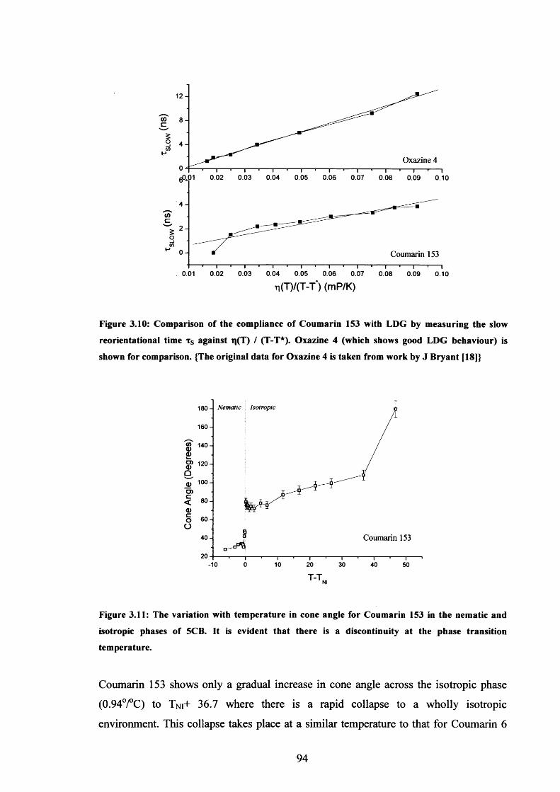
§o_Jc/jH

Oxazine 4

1.01 0.02 0.03 0.04 0.05 0.06 0.07 0.08 0.09 0.10

(/)c2-

Coumarin 153

0.02 0.03 0.04 0.05 0.060.01 0.07 0.08 0.09 0.10

Figure 3.10: Comparison of the compliance of Coumarin 153 with LDG by measuring the slow

reorientational time ts against i)(T) / (T-T*). Oxazine 4 (which shows good LDG behaviour) is

shown for comparison. {The original data for Oxazine 4 is taken from work by J Bryant [18]}

Nematic Isotropic180-

160-

« 140-

O ) 1 2 0 -

100 -

o>8 0 -

6 0 -

Coumarin 1534 0 -

20-10 o 10 20 30 40 50

Figure 3.11: The variation with temperature in cone angle for Coumarin 153 in the nematic and

isotropic phases of 5CB. It is evident that there is a discontinuity at the phase transition

temperature.

Coumarin 153 shows only a gradual increase in cone angle across the isotropic phase

(0.94°/°C) to T Ni+ 36.7 where there is a rapid collapse to a wholly isotropic

environment. This collapse takes place at a similar temperature to that for Coumarin 6

94

(figure 2.31). However, there is evidence of a discontinuity at T n i, in stark contrast to

the behaviour of Coumarin 6 which increases sharply in the vicinity of T n i but does not

show any discontinuity at the phase transition. If the probe was more highly correlated

with the liquid crystal host it would be expected to show sensitivity to the structural

changes at the phase transition [19]. Furthermore the reduction of the correlation length

with temperature in the isotropic phase does not give rise to the same degree of

broadening in the cone angle as seen with Coumarin 6. These two factors further

support the idea that Coumarin 153 causes less disruption to the local nematic ordering

of the host than Coumarin 6.

The temperature variation in the initial fluorescence anisotropy for Coumarin 153 in the

isotropic phase of 5CB is shown in figure 3.12. It is evident that across the isotropic

phase the initial anisotropy is significantly lower than that for Oxazine 4 in ethylene

glycol (c.a. 0.39) and Coumarin 6 (c.a. 0.38) (Chapter 2, figure 2.20). Departure of the

initial fluorescent anisotropy from 0.4 can arise from non-parallel absorption and

emission transition dipole moments [5] or from fast orientational relaxation which

occurs on a sub-instrument response time [1]. Fast (sub picosecond) orientational

relaxation of Coumarin 153 has been observed in a number of solvents. The decrease in

the measured initial anisotropy with increasing temperature for Coumarin 153 in the

isotropic phase of 5CB would indicate that orientational relaxation on a timescale

shorter than c.a. 83ps (fwhm of the instrument response function) is taking place.

0.45 -.

0.40-

0.35-

0.30-oOII 0.25- dOII 0 .2 0 -

0.15-

0. 10 -

0.05- Coumarin 153o.oo

10 20 40 500 30

Figure 3.12: Variation in R(0) with reduced temperature for Coumarin 153 in 5CB.

95

3.8 Lifetime Behaviour in the Nematic Phase of 5CB

As shown in Chapter 2 section 2.13.2, given an excitation polarisation angle of (3=54.7°

and assuming a cylindrically symmetric ground state, the initial excited state

cylindrically symmetric alignment is equal to that of the equilibrium alignment in the

ground state [20] the fluorescence intensity from equation 2.68 is given by

A Vl z {fi = 54.7°)= A exp

r \ t

\ Tf j{(“ 1 (°)) - (“ S (•S-S))}eXP| — + (a 20 (« ))

Vr20 J[3.2]

For ground and excited state degrees of alignment that are close to or equal the time

dependence of equation 3.2 will be dominated by population decay. Providing the

alignment change is slowly varying and small then equation 3.2 should closely resemble

the population decay. Unlike the analysis of Coumarin 6 and Oxazine 4, the decay is not

well described by a single exponential. This is evident in undeconvoluted data analysis

using MicroCal™ Origin software where the decays are in fact described by three

exponential times. A c.a. 6ns slow component which showed little variation across the

nematic temperature, a c.a. 3ns fast component which exhibited a slight decrease with

increasing temperature and a c.a. 500ps rapid component. The temperature variation of

the three times along with the pre-exponential factors is shown in figure 3.13.

8-i RapidFastSlow

Coumarin 1537 -

6-

5 -

'tn 4 - c<DEl- 2-

2-5 -4 3 1 0■7 -6

Figure 3.13: The fluorescence lifetime as a function of reduced temperature for Coumarin 153 in

the nematic phase of 5CB along with the pre-exponential factors for each time. There is clear

evidence of multi exponential decays.

96

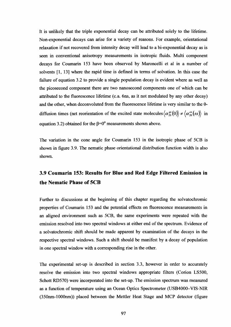
It is unlikely that the triple exponential decay can be attributed solely to the lifetime.

Non-exponential decays can arise for a variety o f reasons. For example, orientational

relaxation if not recovered from intensity decay will lead to a bi-exponential decay as is

seen in conventional anisotropy measurements in isotropic fluids. Multi component

decays for Coumarin 153 have been observed by Maroncelli et al in a number of

solvents [1, 13] where the rapid time is defined in terms of solvation. In this case the

failure of equation 3.2 to provide a single population decay is evident where as well as

the picosecond component there are two nanosecond components one of which can be

attributed to the fluorescence lifetime (c.a. 6ns, as it not modulated by any other decay)

and the other, when deconvoluted from the fluorescence lifetime is very similar to the 0-

diffusion times (net reorientation of the excited state molecules (a fl (o) * in

equation 3.2) obtained for the p=0° measurements shown above.

The variation in the cone angle for Coumarin 153 in the isotropic phase of 5CB is

shown in figure 3.9. The nematic phase orientational distribution function width is also

shown.

3.9 Coumarin 153: Results for Blue and Red Edge Filtered Emission in

the Nematic Phase of 5CB

Further to discussions at the beginning of this chapter regarding the solvatochromic

properties of Coumarin 153 and the potential effects on fluorescence measurements in

an aligned environment such as 5CB, the same experiments were repeated with the

emission resolved into two spectral windows at either end of the spectrum. Evidence of

a solvatochromic shift should be made apparent by examination of the decays in the

respective spectral windows. Such a shift should be manifest by a decay of population

in one spectral window with a corresponding rise in the other.

The experimental set-up is described in section 3.3, however in order to accurately

resolve the emission into two spectral windows appropriate filters (Corion LS500,

Schott RD570) were incorporated into the set-up. The emission spectrum was measured

as a function of temperature using an Ocean Optics Spectrometer (USB4000-VIS-NIR

(350nm-1000nm)) placed between the Mettler Heat Stage and MCP detector (figure

97

3.2). Any background contamination o f the emission spectrum was minimised by

carrying out all measurements in low light with data collected for an integration time of

10s at each temperature. The spectral windows were then chosen appropriately. Figure

3.13 shows the emission spectrum and the proportion o f the emission in the spectral

windows as a function o f temperature. These windows were chosen to be 455-500nm

(blue edge) and >570 nm (red edge). The temperature dependent emission spectrum is

shown in figure 3.14 along with the emission windows. Though there is evidence of

discontinuity at and around the phase transition temperature, this can be accounted for

in terms o f the characteristic beam scatter around T ni, the degree o f which is

wavelength dependent. It is apparent therefore that there is negligible temperature

dependence to the emission.

(0T52 . 0.25COo® 0.20 o>2| 0 , 5

Coumarin 153

Blue Edge Red Edge Total

* • • •-

. . J• • • • • • «-

0.101 1----1----.----1----1----1----1----,----1----1----■----,----1----,----,--- p2 0 3 0 4 0 5 0 6 0 7 0 8 0 9 0 100

Temperature

350Coumarin 153blue

300- green

250-

* 200-c 150- red

100-50-

-50300 350 400 450 500 550 600 650 700 750

Wavelength (nm)

Figure 3.14: The proportion o f emission in the blue and red windows as a function o f temperature

shown with the emission spectrum for Coumarin 153 in 5CB at T=27°C. The blue (455-500nm) and

red (>570 nm) edge spectral windows are shown alongside the emission window originally selected

(>530nm).

98

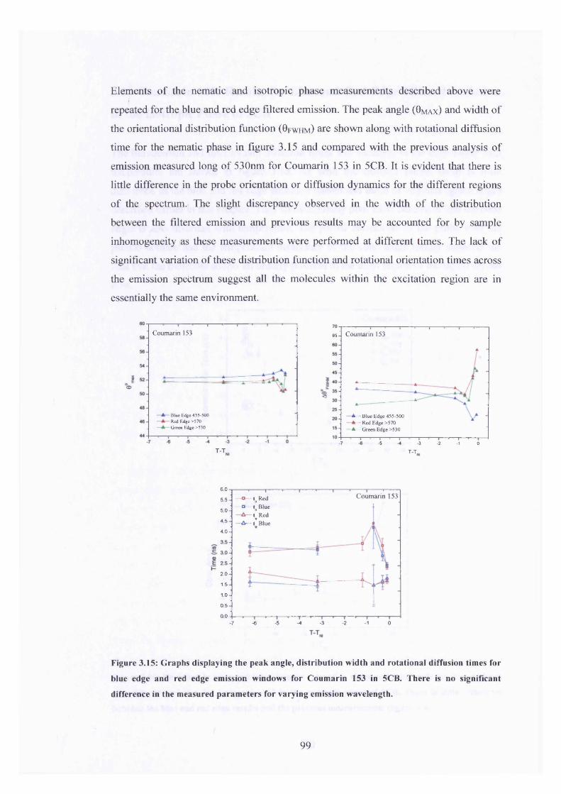
Elements of the nematic and isotropic phase measurements described above were

repeated for the blue and red edge filtered emission. The peak angle ( 0 m a x ) and width of

the orientational distribution function (O f w h m ) are shown along with rotational diffusion

time for the nematic phase in figure 3.15 and compared with the previous analysis of

emission measured long of 530nm for Coumarin 153 in 5CB. It is evident that there is

little difference in the probe orientation or diffusion dynamics for the different regions

of the spectrum. The slight discrepancy observed in the width of the distribution

between the filtered emission and previous results may be accounted for by sample

inhomogeneity as these measurements were performed at different times. The lack of

significant variation of these distribution function and rotational orientation times across

the emission spectrum suggest all the molecules within the excitation region are in

essentially the same environment.

Coumarin 153

Blue Edge 455-500 Red Edge >570 Green Edge >530

Coumarin 15365

<i

-A— Blue Edge 455-500 -A— Red Edge >570 -A— Green Edge >530

-7 -5 -3 -2 -1 0T-T T-T„

6.0Coumarin 153— * — % Red

—O— te Blue —A — t^Red —A — t Blue

5.5

5.0

4.5

4.0

2.0

1.5

1.0

0.5

0.0-7 -6 -5 -4 -3 -2 •1 0

Figure 3.15: Graphs displaying the peak angle, distribution width and rotational diffusion times for

blue edge and red edge emission windows for Coumarin 153 in 5CB. There is no significant

difference in the measured parameters for varying emission wavelength.

99

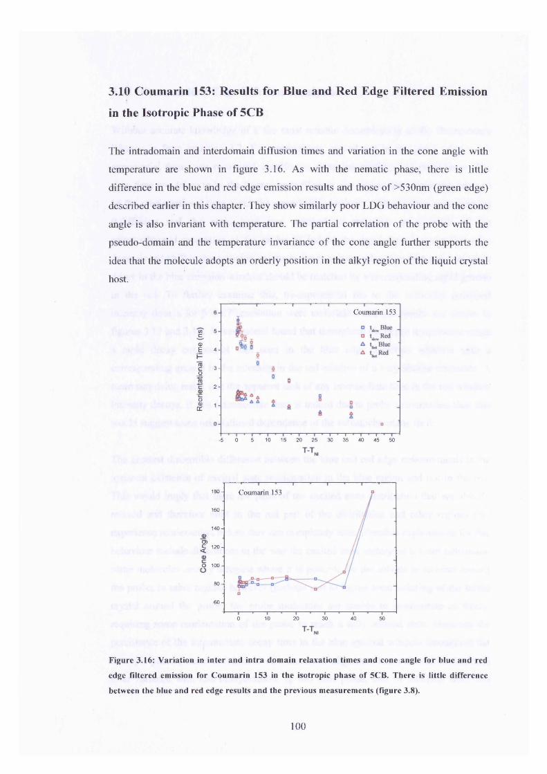
3.10 Coumarin 153: Results for Blue and Red Edge Filtered Emission

in the Isotropic Phase of 5CB

The intradomain and interdomain diffusion times and variation in the cone angle with

temperature are shown in figure 3.16. As with the nematic phase, there is little

difference in the blue and red edge emission results and those of >530nm (green edge)

described earlier in this chapter. They show similarly poor LDG behaviour and the cone

angle is also invariant with temperature. The partial correlation of the probe with the

pseudo-domain and the temperature invariance of the cone angle further supports the

idea that the molecule adopts an orderly position in the alkyl region of the liquid crystal

host.

Coumarin 153

wc0)E 4 -

05Co

3-

ro2-c

o<t>CH

5 10 15 20 25 30 36 40 45 50-5 0

180 - Coumarin 153

160-

140 -

CD5 120 -

O 1 0 0 -

80-

60-

0 10 20 30 40 50

Figure 3.16: Variation in inter and intra domain relaxation times and cone angle for blue and red

edge filtered emission for Coumarin 153 in the isotropic phase of 5CB. There is little difference

between the blue and red edge results and the previous measurements (figure 3.8).

100

3.11 Blue and Red Edge Lifetime Analysis

Without accurate knowledge of k the most reliable determination of the fluorescence

lifetime is from equation 3.2. For experiments carried out in the green edge a tri­

exponential decay was recovered, manifest in slow, intermediate and rapid times. The

slow time was taken to be the fluorescence lifetime, the intermediate time was taken to

be the reorientational time given the remarkable similarity with the time recovered for

0-diffrision and the rapid time was ascribed to solvation as a result of the

solvatochromic properties of the probe. If indeed the rapid time is indicative of a

dynamic red-shift in the emission spectrum due to solvent relaxation then rapid intensity

decay in the blue emission window should be matched by a corresponding rapid growth

in the red. To further examine this, tri-exponential fits to the vertically polarised

intensity decays for p=54.7° excitation were undertaken and the results are shown in

figures 3.17 and 3.18. It was indeed found that throughout the entire temperature range

a rapid decay component was seen in the blue edge detection window with a

corresponding growth in the intensity in the red window of a very similar timescale. A

more surprising result was the apparent lack of any intermediate time in the red window

intensity decays. If this intermediate time is indeed due to probe reorientation then this

would suggest some orientational dependence of the solvatochromatic shift.

The greatest discernible difference between the blue and red edge measurements is the

apparent existence of excited state reorientation in the blue region and not in the red.

This would imply that there are parts of the excited state distribution that are already

relaxed and therefore emit in the red part of the distribution and other regions that

experience reorientation before they can completely relax. Possible explanations for this

behaviour include differences in the way the excited state undergoes solvent relaxation:

some molecules occupy a region where it is possible for the solvent to reorient around

the probe; in other regions however (perhaps due to higher local ordering of the liquid

crystal around the probe) the probe molecules are unable to re-orientate as freely,

requiring some reorientation of the probe to reach a fully relaxed state. However the

persistence of the intermediate decay time in the blue spectral window throughout the

isotropic phase (where the absence of k means no alignment terms should be detected)

is at variance with this interpretation. In this host phase, loss of intensity from this

101

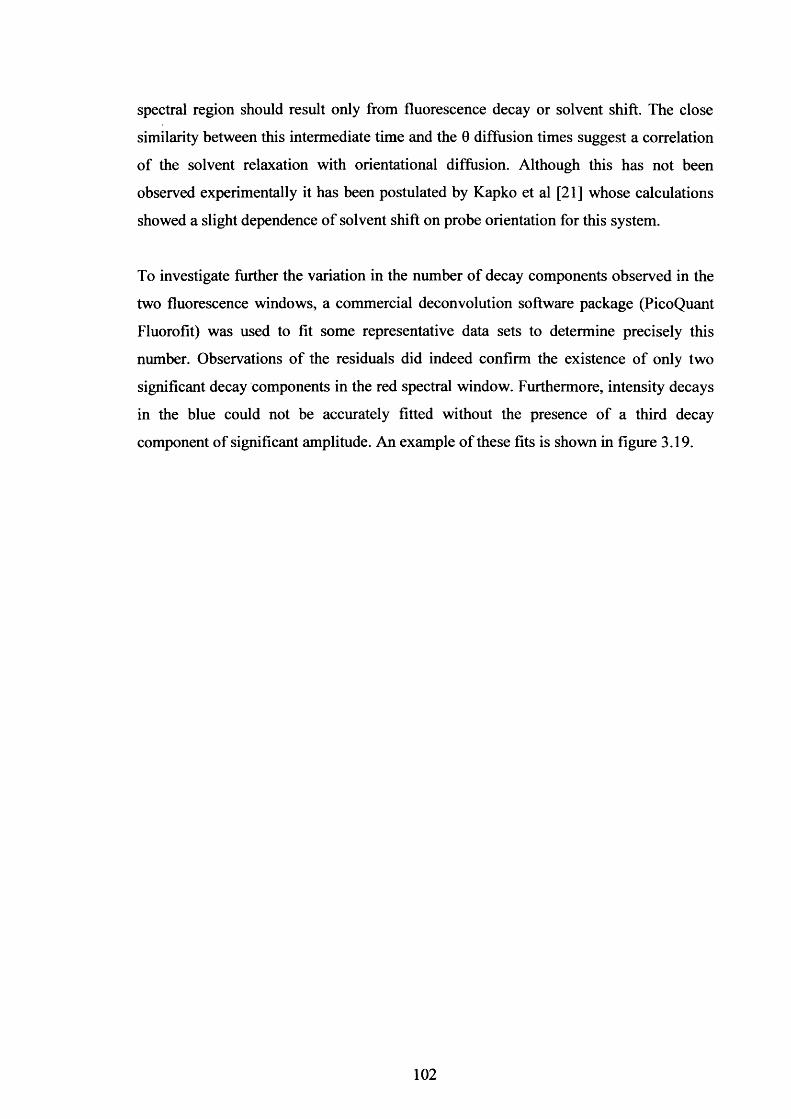
spectral region should result only from fluorescence decay or solvent shift. The close

similarity between this intermediate time and the 0 diffusion times suggest a correlation

of the solvent relaxation with orientational diffusion. Although this has not been

observed experimentally it has been postulated by Kapko et al [21] whose calculations

showed a slight dependence of solvent shift on probe orientation for this system.

To investigate further the variation in the number of decay components observed in the

two fluorescence windows, a commercial deconvolution software package (PicoQuant

Fluorofit) was used to fit some representative data sets to determine precisely this

number. Observations of the residuals did indeed confirm the existence of only two

significant decay components in the red spectral window. Furthermore, intensity decays

in the blue could not be accurately fitted without the presence of a third decay

component of significant amplitude. An example of these fits is shown in figure 3.19.

102

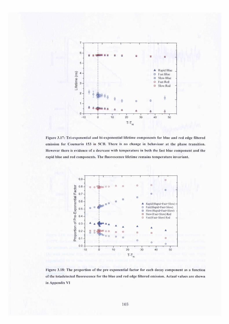
6-

5 -

Rapid Blue Fast Blue Slow Blue Fast Red Slow Red

V)c<uEILi

0 10 20 30-10 40 50

Figure 3.17: Tri-exponential and bi-exponential lifetime components for blue and red edge filtered

emission for Coumarin 153 in 5CB. There is no change in behaviour at the phase transition.

However there is evidence of a decrease with temperature in both the fast blue com ponent and the

rapid blue and red components. The fluorescence lifetime remains temperature invariant.

oo<u

c0)c0CLXLB1CL<*—Oco■c.oCLO

0 .9 -

0 .8 - o o

0 .7 -

0.6-Rapid/(Rapid+Fast+Slow) - Fast/(Rapid+Fast+Slow) Slow/(Rapid+Fast+Slow) ■ Slow/(Fast+Slow) Red Fast/(Fast+Slow) Red

□0 .5 -

0 .4 -

0 .3 -

0.2- □o □ □

o o0.1 -

0.0 tT T-10 10 20

T-T30 40 50

Nl

Figure 3.18: The proportion o f the pre exponential factor for each decay component as a function

of the totadetected fluorescence for the blue and red edge filtered emission. Actual values are shown

in Appendix VI

103

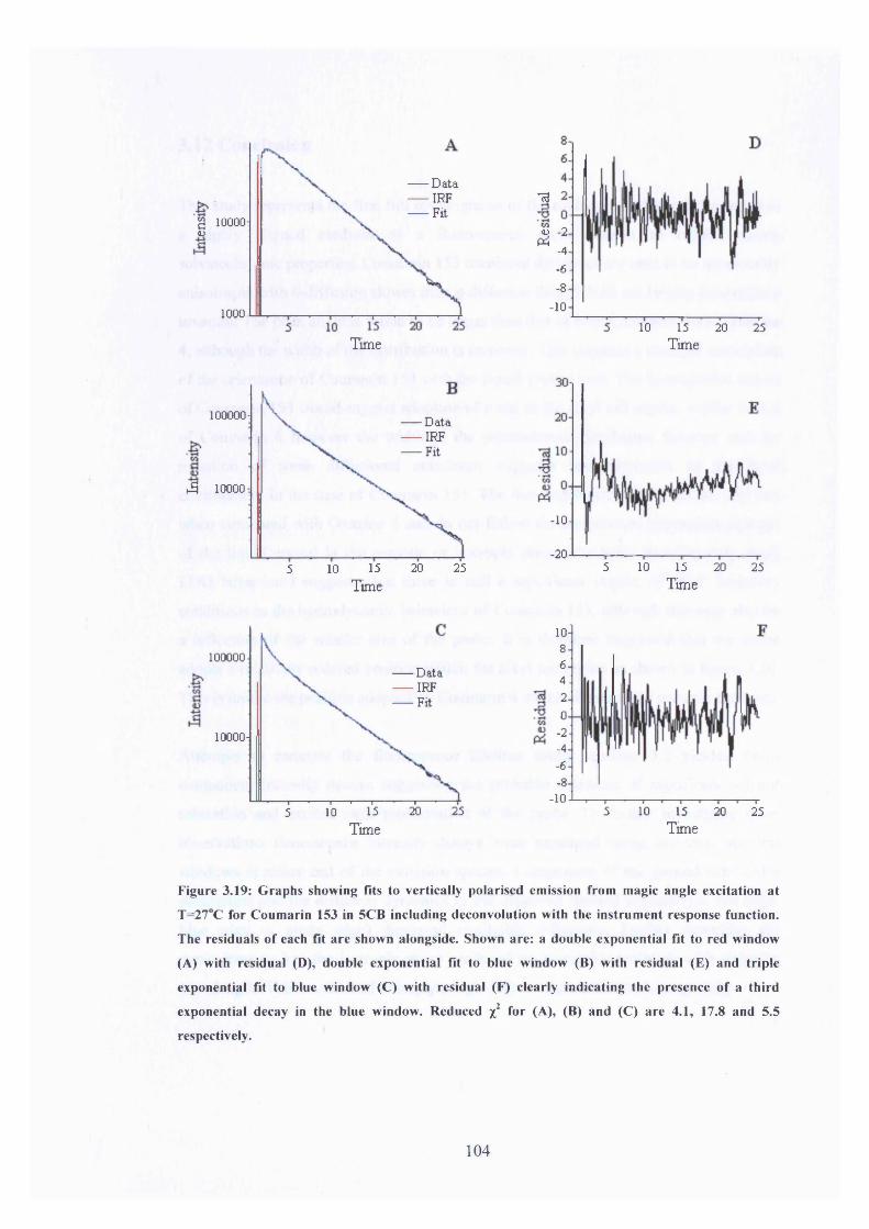
Data IRF Fit

g 10000<L)

1000

Time

13

3 ~2* -4

-6-8

-10

10 15 20 25

Time

100000- Data IRF Fit

& 10000 -

2515 20105

-10

-205 10 15 20 25

Time Time

100000 Data IRF Fit

10000-

20 25155 10

10864

20-2-4

-6-8

-105 10 15 20 25

Time Time

Figure 3.19: Graphs showing fits to vertically polarised emission from magic angle excitation at

T=27°C for Coumarin 153 in 5CB including deconvolution with the instrument response function.

The residuals o f each fit are shown alongside. Shown are: a double exponential fit to red window

(A) with residual (D), double exponential fit to blue window (B) with residual (E) and triple

exponential fit to blue window (C) with residual (F) clearly indicating the presence o f a third

exponential decay in the blue window. Reduced x2 for (A), (B) and (C) are 4.1, 17.8 and 5.5

respectively.

104

3.12 Conclusion

This study represents the first full investigation of the molecular order and dynamics in

a highly aligned medium of a fluorescence probe known to exhibit strong

solvatochromic properties. Coumarin 153 rotational dynamics are seen to be measurably

anisotropic with 0-diffiision slower than cp diffusion though both are largely temperature

invariant The peak angle is found to be larger than that of both Coumarin 6 and Oxazine

4, although the width of the distribution is narrower. This suggests a stronger correlation

of the orientation of Coumarin 153 with the liquid crystal host. The hydrophobic nature

of Coumarin 153 would suggest adoption of a site in the alkyl tail region, similar to that

of Coumarin 6 however the width of the orientational distribution function and the

retention of some diffusional anisotropy suggests less distortion of the local

environment in the case of Coumarin 153. The fact that 0-diffusion times are still fast

when compared with Oxazine 4 and do not follow the temperature dependent changes

of the liquid crystal in the nematic or isotropic phase (the latter showing only weak

LDG behaviour) suggests that there is still a significant degree of ‘slip’ boundary

conditions in the hydrodynamic behaviour of Coumarin 153, although this may also be

a reflection of the smaller size of the probe. It is therefore suggested that the probe

adopts a relatively ordered position within the alkyl tail region as shown in figure 3.20.

This is unlike the position adopted by Coumarin 6 which significantly perturbs the host.

Attempts to measure the fluorescence lifetime using equation 3.2 yielded multi

component intensity decays suggesting the probable existence of significant solvent

relaxation and excited state reorientation of the probe. To further investigate these

observations fluorescence intensity decays were measured using narrower spectral

windows at either end of the emission spectra. Comparison of the ground state order

parameters and the diffusion dynamics in the observed spectral regions (i.e. red edge,

blue edge or green edge) displayed negligible difference. Further extending the

measurements into the isotropic phase produced no noticeable variation with emission

wavelength. This would tend to imply a high degree of ground state homogeneity

105

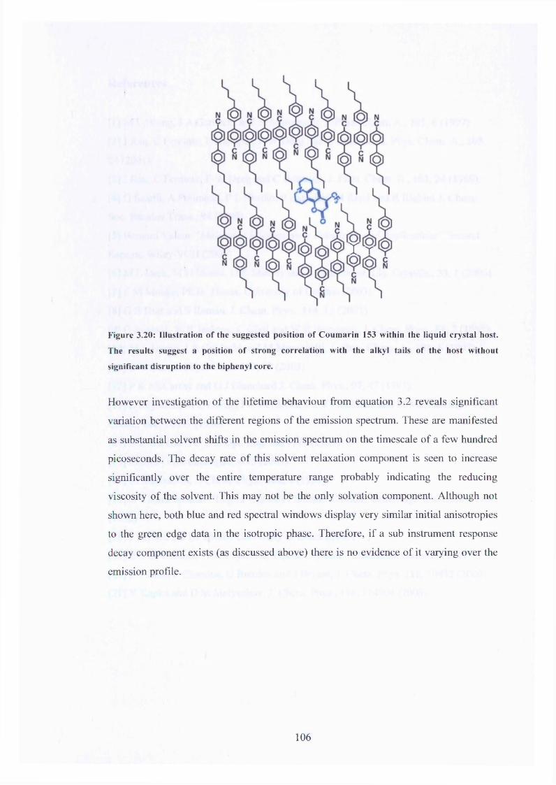
T r

Figure 3.20: Illustration o f the suggested position o f Coum arin 153 within the liquid crystal host.

The results suggest a position o f strong correlation with the alkyl tails o f the host without

significant disruption to the biphenyl core.

However investigation of the lifetime behaviour from equation 3.2 reveals significant

variation between the different regions of the emission spectrum. These are manifested

as substantial solvent shifts in the emission spectrum on the timescale of a few hundred

picoseconds. The decay rate of this solvent relaxation component is seen to increase

significantly over the entire temperature range probably indicating the reducing

viscosity of the solvent. This may not be the only solvation component. Although not

shown here, both blue and red spectral windows display very similar initial anisotropies

to the green edge data in the isotropic phase. Therefore, if a sub instrument response

decay component exists (as discussed above) there is no evidence of it varying over the

emission profile.

106

References

[1] M L Homg, J A Gardecki and M Maroncelli, J. Phys. Chem. A., 101, 6 (1997)

[2] J Rau, C Ferrante, E Kneuper, F-W Deeg and C Brauchle, J. Phys. Chem. A., 105,

24 (2001)

[3] J Rau, C Ferrante, F-W Deeg and C Brauchle, J. Phys. Chem. B., 103, 24 (1999)

[4] G Saielli, A Polimeno, P L Nordio, P Bartolini, M Ricci and R Righini J. Chem.

Soc, Faraday Trans., 94 (1998)

[5] Bernard Valeur “Molecular Fluorescence; Principles and Applications” Second

Reprint, Wiley-VCH (2005)

[6] M L Dark, M H Moore, D K Shenoy and R Shashidhar, Liq. Crystals., 33, 1 (2006)

[7] E M Monge, Ph.D. Thesis, University of London (2003)

[8] G B Dutt and S Raman, J. Chem. Phys., 114, 15 (2001)

[9] G Jones II, W R Jackson, C Choi and W R Bergmark, J. Chem. Phys., 89, 2 (1985)

[10] M L Homg, J A Gardecki and M Maroncelli, J. Phys. Chem. A., 101, 6 (1997)

[11] G B Dutt, J. Phys. Chem 119, 22 (2003)

[12] P K McCarthy and G J Blanchard J. Chem. Phys., 97, 47 (1993)

[13] L Reynolds, M L Homg, J A Gardecki, S J V Frankland and M Maroncelli, J. Phys.

Chem., 100, 10337 (1996)

[14] S T W u a n d C S W u , Opt. Eng. 32, 1775 (1993)

[15] Melles Griot Catalogue, 4.15 (2007)

[16] M Maroncelli, J. Chem. Phys., 106, 4 (1997)

[17] S Chandrasekhar “Liquid Crystals” Second Edition, Cambridge University Press

(1992)

[18] J Bryant, Ph. D. Thesis, University of Essex (2000)

[19] P G de Gennes, “The Physics o f Liquid Crystals” Clarendon, Oxford (1974)

[20] A J Bain, P Chandna, G Butcher and J Bryant, J. Chem. Phys. 112, 10435 (2000)

[21] V Kapko and D M Matyushov, J. Chem. Phys., 124, 114904 (2006)

107

Chapter 4Two-Photon Transitions in Quadrupolar and Branched

Fluorophores

4.1 Introduction

The development of high quantum yield fluorescent probes with enhanced two-photon

absorption cross-sections has attracted significant interest in recent years This stems

from advances in broadband and tunable femtosecond near-infra red laser systems and

their use in scanning fluorescence microscopy [1-3]. Two-photon excitation is an

intensity dependent process and for a focused Gaussian laser beam the transition

probability peaks sharply in the Rayleigh range about the beam waist. Two-photon

excited fluorescence thus offers inherent optical sectioning. In contrast, single-photon

excited fluorescence requires a confocal optical geometry which rejects the significant

degree of fluorescence that is excited from other regions of the sample. The difference

between the two excitation techniques can be clearly seen in figure 4.1. Near infra-red

two-photon fluorescence in principle affords greater penetration of biological samples,

reduced photodamage [4] and with excitation confined to a small (ca. femtolitre)

confocal volume [5]. In practice however the two-photon absorption cross-sections of

naturally occurring fluorescent chromophores are not large, nor are those for

conventional (synthetic) probes optimised for single-photon absorption and spontaneous

emission (see table 4.1). There is therefore a need to engineer molecules with high two-

photon cross-sections in the near infra-red coupled with efficient single- photon

fluorescence from the emitting state.

Two-photon absorption is a third order nonlinear optical process and thus common to all

molecules [6]. From quantum mechanical considerations the two-photon absorption rate

(s'1) is given by

a(Vfr)G<2)™ - 2(h v f [ 1

where c/2) is the two photon absorption cross-section (cm4s photon'1), I(t) is the

108

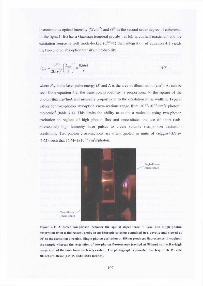
instantaneous optical intensity (Wcm*2) and G(2) is the second order degree of coherence

of the light. If I(t) has a Gaussian temporal profile x at full width half maximum and the

excitation source is well mode-locked (G(2- l ) then integration of equation 4.1 yields

the two-photon absorption transition probability

P = aTPA

(2) r V V 0.664

2 ( M 2

pTP x [4.2]

where E tp is the laser pulse energy (J) and A is the area of illumination (cm2). As can be

seen from equation 4.2, the transition probability is proportional to the square of the

photon flux Ejp/huA and inversely proportional to the excitation pulse width x. Typical

values for two-photon absorption cross-sections range from 10"50-10-48 cm4s photon'1

molecule1 (table 4.1). This limits the ability to excite a molecule using two-photon

excitation to regions of high photon flux and necessitates the use of short (sub­

picosecond) high intensity laser pulses to create suitable two-photon excitation

conditions. Two-photon cross-sections are often quoted in units of Goppert-Meyer

(GM), such that lGM=lxlO'50 cm4s/photon.

Single-Photon Fluorescence

Two-PhotonFluorescence

Figure 4.1: A direct com parison between the spatial dependence o f two- and single-photon

absorption from a fluorescent probe in an isotropic solution contained in a cuvette and viewed at

90° to the excitation direction. Single-photon excitation at 488nm produces fluorescence throughout

the sample whereas the restriction o f two-photon fluorescence (excited at 800nm ) to the Rayleigh

range around the laser focus is clearly evident. The photograph is provided courtesy o f Dr M ireille

Blanchard-Desce (CNRS UM R 6510 Rennes).

109

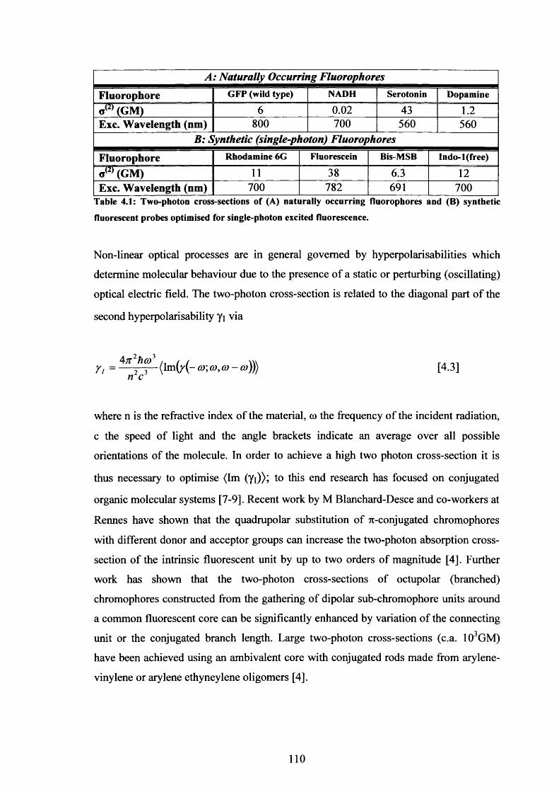
A: Naturally Occurrittg Fluorophores

Fluorophore GFP (wild type) NADH Serotonin Dopamine

w(2) (GM) 6 0.02 43 1.2Exc. Wavelength (nm) 800 700 560 560

B: Synthetic (single-photon) Fluorophores

Fluorophore Rhodamine 6G Fluorescein Bis-MSB Indo-l(free)

«<2) (GM) 11 38 6.3 12Exc. Wavelength (nm) 700 782 691 700

Table 4.1: Two-photon cross-sections of (A) naturally occurring fluorophores and (B) synthetic

fluorescent probes optimised for single-photon excited fluorescence.

Non-linear optical processes are in general governed by hyperpolarisabilities which

determine molecular behaviour due to the presence of a static or perturbing (oscillating)

optical electric field. The two-photon cross-section is related to the diagonal part of the

second hyperpolarisability Yi via

r, = 4;z tlf - (lrn(y(-CO,CO,a-co))) [4.3]n c

where n is the refractive index of the material, © the frequency of the incident radiation,

c the speed of light and the angle brackets indicate an average over all possible

orientations of the molecule. In order to achieve a high two photon cross-section it is

thus necessary to optimise (Im (Yi)); to this end research has focused on conjugated

organic molecular systems [7-9]. Recent work by M Blanchard-Desce and co-workers at

Rennes have shown that the quadrupolar substitution of ^-conjugated chromophores

with different donor and acceptor groups can increase the two-photon absorption cross-

section of the intrinsic fluorescent unit by up to two orders of magnitude [4]. Further

work has shown that the two-photon cross-sections of octupolar (branched)

chromophores constructed from the gathering of dipolar sub-chromophore units around

a common fluorescent core can be significantly enhanced by variation of the connecting

unit or the conjugated branch length. Large two-photon cross-sections (c.a. 10 GM)

have been achieved using an ambivalent core with conjugated rods made from arylene-

vinylene or arylene ethyneylene oligomers [4].

110

The work in this chapter consists of two studies undertaken in collaboration with the

Blanchard-Desce group; firstly the measurement of two-photon cross-sections for a

series of quadrupolar fluorophores and a branched quadrupolar fluorophore was

extended to shorter wavelengths (typically 700nm to 540nm) that lie outside the

TiiSapphire tuning range - this was achieved using a tunable ultrafast optical parametric

amplifier. These measurements were accompanied by theoretical time-dependent

density functional calculations of wavelength dependence of the two-photon transition

undertaken at Rennes and at Los Alamos National Laboratory by Tretiak and co­

workers. Subsequent to these studies a high repetition rate optical parametric oscillator

and TiiSapphire laser (in conjunction with time correlated single-photon counting) was

used to investigate the difference in the two-photon cross-sections for linearly and

circularly polarised excitation as a function of wavelength (infra red-visible region), and

the degree of initial fluorescence anisotropy created in both excitation processes. These

measurements can be used to provide information on the structure of the two-photon

transition tensor; significant structural differences were observed between branched and

unbranched fluorophores, which can be attributed to delocalisation of the excitation

over the branched structure rather than localisation on a single arm.

4.2 Quadrupolar and Branched Two-Photon Fluorescent Probes

The molecules studied in this thesis were three quadrupolar species: OM49, TM11 and

BH101, and a branched system: OM77. These are representative of the design strategy

employed by the Blanchard-Desce Group to both tailor and optimise the two-photon

absorption and single-photon fluorescence emission of a molecular system. The

principle is to engineer the absorption and emission properties of an ultraviolet

absorbing and emitting core with the addition of electron donating end groups coupled

to the core by the appropriate molecular linkers (figure 4.3). OM49 and TM11 both

contain a biphenyl fluorescent core with the same electron donating end groups and

differ only in the connector (acetylenic vs. ethylinic) between these and the core. The

change in linker from triple bond (acetylenic) to a double bond (ethylinic) gives rise to a

red shift in single-photon absorption and emission spectra with a rise in fluorescence

lifetime. A change in the fluorescent core from biphenyl to the planar and rigid fluorene

system (BH101) is accompanied by a red shift (bathochromic) in the single-photon

111

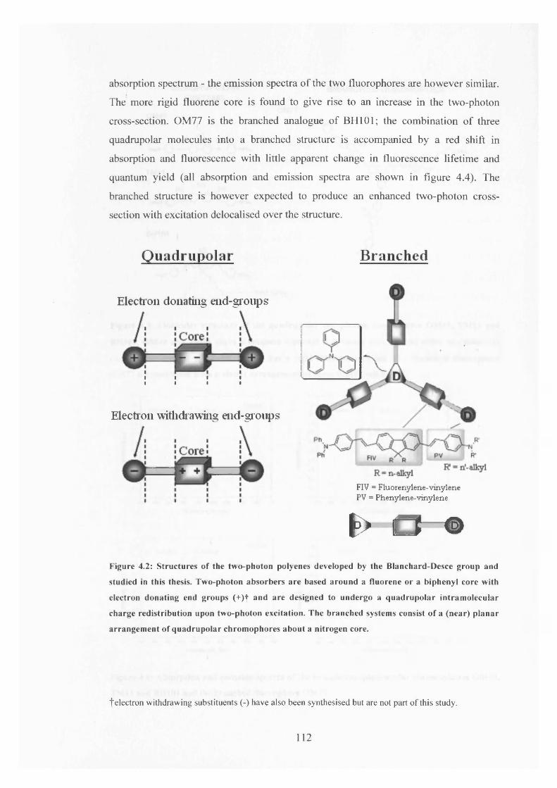
absorption spectrum - the emission spectra of the two fluorophores are however similar.

The more rigid fluorene core is found to give rise to an increase in the two-photon

cross-section. OM77 is the branched analogue of BH101; the combination of three

quadrupolar molecules into a branched structure is accompanied by a red shift in

absorption and fluorescence with little apparent change in fluorescence lifetime and

quantum yield (all absorption and emission spectra are shown in figure 4.4). The

branched structure is however expected to produce an enhanced two-photon cross-

section with excitation delocalised over the structure.

Quadrupolar Branched

Electi on donating end-gronps

I I I I■ I i I

Electron withdrawing end-groups

b □ ©Figure 4.2: Structures o f the two-photon polyenes developed by the Blanchard-Desce group and

studied in this thesis. Two-photon absorbers are based around a fluorene or a biphenyl core with

electron donating end groups (+ )f and are designed to undergo a quadrupolar intramolecular

charge redistribution upon two-photon excitation. The branched systems consist o f a (near) planar

arrangement of quadrupolar chromophores about a nitrogen core.

t e l e c t r o n w it h d r a w in g s u b s t i t u e n t s ( - ) h a v e a l s o b e e n s y n t h e s i s e d b u t a r e n o t p a r t o f t h i s s t u d y .

FIV = Fluorenylene-vinylene PV = Phenylene-vinylene

112

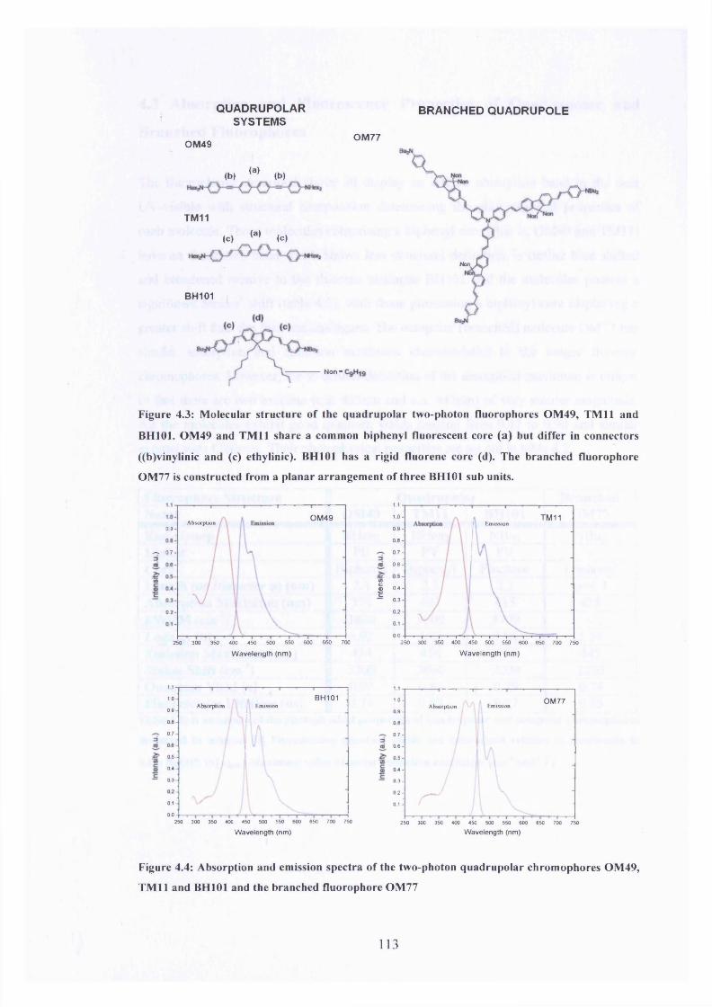
QUADRUPOLARSYSTEMS

OM49

TM11

<b) (a) (b)

(c) (a) (c)

BH101

BRANCHED QUADRUPOLE

OM77

Non =

Non

Figure 4.3: M olecular structure o f the quadrupolar two-photon fluorophores OM 49, TM11 and

BH101. OM 49 and TM11 share a common biphenyl fluorescent core (a ) but differ in connectors

((b)vinylinic and (c) ethylinic). BH101 has a rigid fluorene core (d). The branched fluorophore

OM 77 is constructed from a planar arrangem ent of three BH101 sub units.

O M 49Absorption

0 9

~ 0.7

0.2

250 300 350 400 450 500 550 600 650 700

<n

i

1.1

TM1110Emission

0 9

0 8

0.7

0.6

0.4

0 3

02010.0

250 300 350 400 450 500 550 600 650 700 750

W avelength (nm) W avelength (nm)

11BH1011.0

Absorption Emission0.9

0 80.7

0 6

0 504

0 3

010.0

250 300 350 400 450 500 550 600 650 700 750

1.1

1.0 OM77EmissionAbsorption

0 9

0 8

0.7

0.6

0.5

0 4

0.3

0.2

0 1

250 300 350 400 450 500 550 600 650 700 750

W avelength (nm) Wavelength (nm)

Figure 4.4: Absorption and emission spectra o f the two-photon quadrupolar chrom ophores OM 49,

TM11 and BH101 and the branched fluorophore OM 77

113

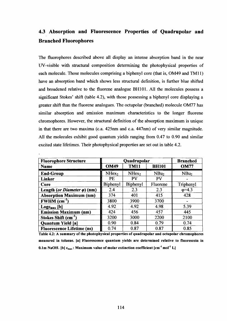
4.3 Absorption and Fluorescence Properties of Quadrupolar and

Branched Fluorophores

The fluorophores described above all display an intense absorption band in the near

UV-visible with structural composition determining the photophysical properties of

each molecule. Those molecules comprising a biphenyl core (that is, OM49 and TM11)

have an absorption band which shows less structural definition, is further blue shifted

and broadened relative to the fluorene analogue BH101. All the molecules possess a

significant Stokes’ shift (table 4.2), with those possessing a biphenyl core displaying a

greater shift than the fluorene analogues. The octupolar (branched) molecule OM77 has

similar absorption and emission maximum characteristics to the longer fluorene

chromophores. However, the structural definition of the absorption maximum is unique

in that there are two maxima (c.a. 425nm and c.a. 447nm) of very similar magnitude.

All the molecules exhibit good quantum yields ranging from 0.47 to 0.90 and similar

excited state lifetimes. Their photophysical properties are set out in table 4.2.

Fluorophore Structure Quadrupolar BranchedName OM49 TM11 BH101 OM77End-Group 1 NHex2 NHex2 NBu2 N B u2Linker PE PV PV -

Core Biphenyl Biphenyl Fluorene TriphenylLength (or Diameter q>) (nm) 2.4 2.3 2.3 cp=4.3Absorption Maximum (nm) 374 401 415 428FWHM (cm 1) 3800 3900 3700 -

Log£m„ |b| 4.92 4.92 4.98 5.39Emission Maximum (nm) 424 456 457 445Stokes Shift (cm 1) 3200 3000 2200 2100Quantum Yield [a] 0.90 0.84 0.79 0.74Fluorescence Lifetime (ns) 0.74 0.87 0.87 0.85

Table 4.2: A summary of the photophysical properties of quadrupolar and octupolar chromophores

measured in toluene, (a] Fluorescence quantum yields are determined relative to fluorescein in

0.1m NaOH. [b] £mai: Maximum value of molar extinction coefficient [cm1 mol'1 L|

114

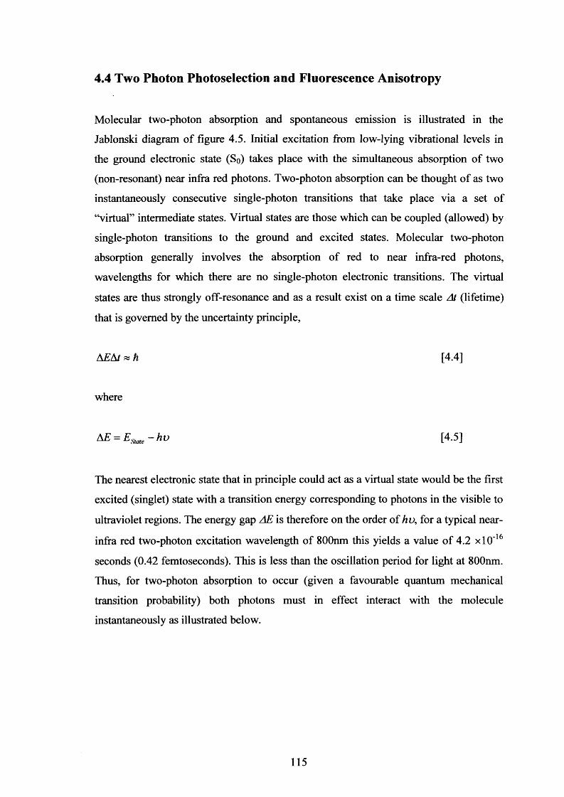
4.4 Two Photon Photoselection and Fluorescence Anisotropy

Molecular two-photon absorption and spontaneous emission is illustrated in the

Jablonski diagram of figure 4.5. Initial excitation from low-lying vibrational levels in

the ground electronic state (So) takes place with the simultaneous absorption of two

(non-resonant) near infra red photons. Two-photon absorption can be thought of as two

instantaneously consecutive single-photon transitions that take place via a set of

“virtual” intermediate states. Virtual states are those which can be coupled (allowed) by

single-photon transitions to the ground and excited states. Molecular two-photon

absorption generally involves the absorption of red to near infra-red photons,

wavelengths for which there are no single-photon electronic transitions. The virtual

states are thus strongly off-resonance and as a result exist on a time scale At (lifetime)

that is governed by the uncertainty principle,

AEAt» h [4.4]

where

AE = Esuu- h v [4.5]

The nearest electronic state that in principle could act as a virtual state would be the first

excited (singlet) state with a transition energy corresponding to photons in the visible to

ultraviolet regions. The energy gap AE is therefore on the order of hu, for a typical near-

infra red two-photon excitation wavelength of 800nm this yields a value of 4.2 xlO’16

seconds (0.42 femtoseconds). This is less than the oscillation period for light at 800nm.

Thus, for two-photon absorption to occur (given a favourable quantum mechanical

transition probability) both photons must in effect interact with the molecule

instantaneously as illustrated below.

115

IC

EXCITATION FLUORESCENCE

Figure 4.5: A Jablonski diagram showing the excitation and relaxation pathways in two-photon

excited fluorescence. Excitation occurs from the molecular ground state So via a virtual state |n) to

an excited singlet state S„. This is followed by rapid (tiC: sub-picosecond) internal conversion and

vibrational relaxation to lower vibrational levels of St. Spontaneous emission (nanoseconds) takes

place to high vibrational levels in the ground state with fast (tr sub-picosecond) collisional

relaxation returning molecules to the initially populated levels.

The initially excited state (Sn) undergoes rapid (sub-picosecond) internal conversion and

vibrational relaxation in collisions with surrounding solvent molecules leading to the

population of lower vibrational levels in Si. In the absence of external perturbations the

population in Si decays by spontaneous emission (as in the case of single-photon

excitation from So to Si) to upper vibrational levels of So consistent with the Franck-

Condon principle. Solvent ‘cooling’ of the vibrationally hot ground state population is

correspondingly rapid. As well as possessing an intensity dependent transition

probability, two-photon excitation is also distinct from single-photon excitation in that

the absorption probability is polarisation dependent. A fundamental property of single­

photon transitions in an isotropic medium is that the transition probability is

independent of the polarisation of the incident light [10]; this restriction is relaxed in

ordered systems as seen in Chapters 2 and 3 where there is a direct correspondence

between the molecular and laboratory frames of reference. However for two-photon

116

absorption the transition does not involve a simple dipolar rearrangement of electronic

charge density; rather, it involves products of the allowed single-photon transition

dipoles between the ground intermediate and final states. In quantum mechanical terms

the cross-section for the absorption of two photons of polarisations a and ft between

states |g) and \e) is proportional to the squared modulus of the tensor W ^ e defined

by a sum of transitions involving the intermediate (virtual) states |« ) ,

w g e\aPa • (g |r| n)(ri |r| e) • P ft- (g \r\n)(n \r\ e) • a

L> -L> + iT[4.6]

where un and Tn are the transition frequency and homogeneous linewidth of

respectively. In the molecular frame of reference the transition tensor can have 9

elements S ab where A, B=X, Y or Z,

\w g~*e\ = aP ~ 2 XA,B=X,Y,Z

[4.7]

For the absorption of two identical photons S a b = Sba- For planar aromatic molecules the

two-photon transition is dominated by moments in the plane (XY) of the molecule. The

relative absorption strengths for linearly and circularly polarised two-photon absorption

define the parameter Q which can be determined from the integrated fluorescence

intensity for linearly and circularly polarised absorption as shown in figure 4.6.

The total fluorescence intensity can be obtained from a ‘magic angle’ polarisation

measurement at 54.7° to the symmetry axis (axis of cylindrical symmetry for the

transition).

117

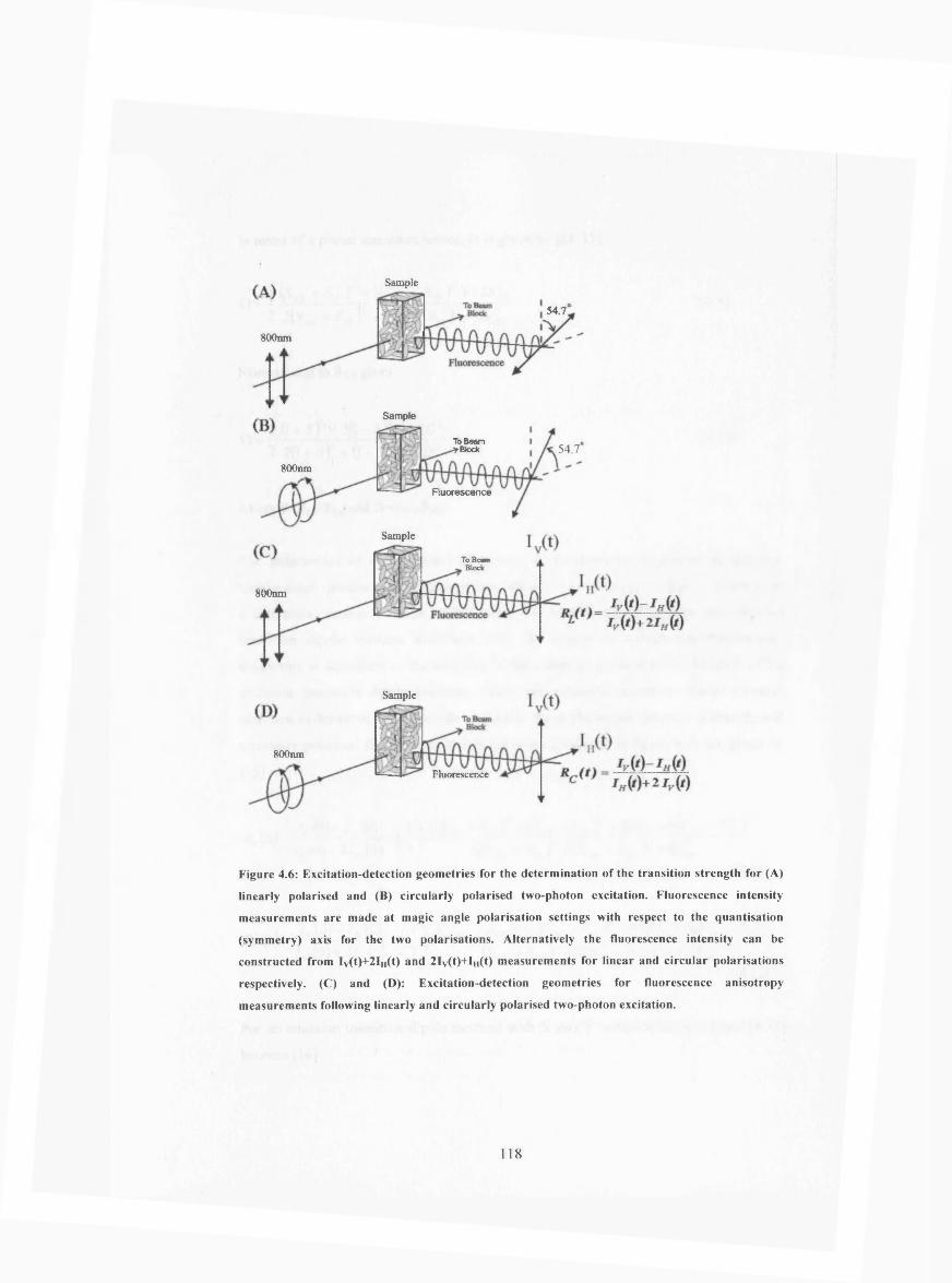
Sample

54.7

800nm

Sample

To Beam * Block 54.7

800nm

Fluorescence

Sample

To Beam , Block

800nm

Sample

800nm

Fluorescence

Figure 4.6: Excitation-detection geom etries for the determ ination o f the transition strength for (A)

linearly polarised and (B) circularly polarised two-photon excitation. Fluorescence intensity

m easurem ents are made at magic angle polarisation settings with respect to the quantisation

(sym m etry) axis for the two polarisations. A lternatively the fluorescence intensity can be

constructed from Iv(t)+2In(t) and 2Iv(t)+IH(t) m easurem ents for linear and circular polarisations

respectively. (C) and (D): Excitation-detection geom etries for fluorescence anisotropy

m easurem ents following linearly and circularly polarised two-photon excitation.

118

In terms of a planar transition tensor, Q is given by [11-13]

n 1 fa, + s„ Y + 3 )2 + 12^2 2 ^ + S , , ) 2 + ( $ „ - $ „ )*+35*,

Normalising to Sxx gives

^ 1 (l + S)2 + 3 ( l - S ) 2 +12D 2fi = —------- ---------------------------------------- T4 101

2 2(l + S)2 + (l - S)2 + 4£>2 1 1

where S —S yy^xx and D—Sxy/Sxx•

The polarisation of two-photon fluorescence is an important experimental quantity.

Unlike single-photon excited fluorescence which (in an isotropic medium) departs from

a theoretical maximum value of 0.4 solely due to different absorption and emission

transition dipole moment directions [14], the degree of two-photon fluorescence

anisotropy is dependent on the structure of the transition tensor and the direction of the

emission transition dipole moment. Using the emission transition dipole moment

direction to define the X axis of the molecular frame the initial (time-zero) linearly and

circularly polarised fluorescence anisotropies (as measured in figure 4.5) are given by

[15]

R (0) Iy (0) - M o ) n 2(s„ + s„ y + (sxx - s„ )2 + 4 s2„ + 9 (s2xx - s2n)- 2{SXX + S n )1 +{Sx x - S YY)l +4S)!V

[4.11]/,.(0) + 2/„(0)

/ , ( o ) - / „ ( o ) r n ~3(SXX -S y y )2 - (.S „ + S tr y + 1 2 ^ + 6(s2xx - S 2r )'/„(<)) + 27,(0) I 7 J (sxx +s„y+ 3 ( s ^ -s„Y +nsly

[4.12]

For an emission transition dipole moment with X and Y components [4.11] and [4.12]

become [16]

119

* i ( 0 ) = f - 1J )

1 +9 (1 - S 2 \cos2 9 - sin2 d)+ 4£>(l + S)sin cosfl

2(1+ S)2 + (l - S )2 + 4 D 2[4.13]

«c(0)=f 1 \

1 +6[(l - S 2 \cos2 6 - sin 2 fl)+ 4£>(l + 5l)singcos6>|- 2(l + S')2

(1 + ,S’)2 + 3(l - S )2 +12 O 2[4.14]

For the simplest two-photon transition tensor S and D have zero values (i.e. Sxx is the

sole non-zero element), yielding

3 cos2 0 - 1, /?,.(o)=

2 ^—

V7J 2 V7)[(3cos2 6* — 1)]

2[4.15]

These are recognisable as the values obtained for two sequential single-photon

transitions via a ‘real’ intermediate state with parallel (absorption) transition dipole

moments at an angle 0 to the emission transition dipole moment. Such a one

dimensional situation might be approximated by a linear molecule but in a system with

significant two dimensional charge displacement S and D should be significant. For

example, for a system with S~l,

Q =2 + 6 ZT 8 + 4 D :

1 +8T>sin#cos#

8 + 4 D 2 Rc(0)= 1 +12Z )sin#cos#- 2

1 + 3D 2

[4.16]

4.5 Measurement of Two-Photon Absorption Cross-Sections

Although it is possible to measure the two-photon absorption cross-section of a

fluorophore directly by measuring the amount of light absorbed by the sample, this

procedure is highly problematic as the need for high incident powers leads to saturation,

photobleaching, stimulated emission and self-quenching [17]. These factors greatly

complicate the interpretation of such measurements. Alternatively two-photon

absorption cross-sections can be determined by measuring the two-photon fluorescence

signal generated via two-photon absorption. The resulting two-photon excitation (TPE)

120

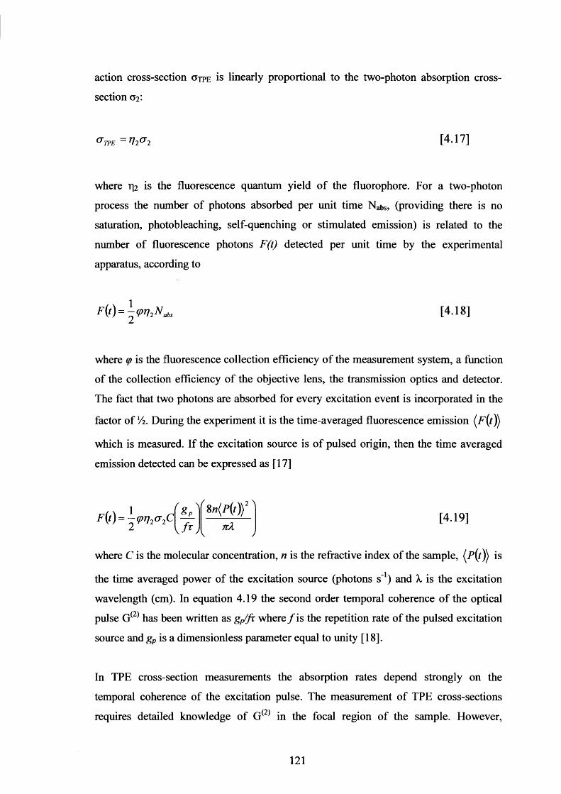
action cross-section gtpe is linearly proportional to the two-photon absorption cross-

section 0 2 :

TPE = rj2cr2 [4.17]

where r|2 is the fluorescence quantum yield of the fluorophore. For a two-photon

process the number of photons absorbed per unit time NabS, (providing there is no

saturation, photobleaching, self-quenching or stimulated emission) is related to the

number of fluorescence photons F(t) detected per unit time by the experimental

apparatus, according to

F(t) = ^<pri2N<lbs [4.18]

where (p is the fluorescence collection efficiency of the measurement system, a function

of the collection efficiency of the objective lens, the transmission optics and detector.

The fact that two photons are absorbed for every excitation event is incorporated in the

factor of V2. During the experiment it is the time-averaged fluorescence emission (F(t))

which is measured. If the excitation source is of pulsed origin, then the time averaged

emission detected can be expressed as [17]

F(l)=^<Pr?2f:r2C8n(P{t))2 ]

\ . f T) ri/1V 7[4.19]

where C is the molecular concentration, n is the refractive index of the sample, is

the time averaged power of the excitation source (photons s '1) and A, is the excitation

wavelength (cm). In equation 4.19 the second order temporal coherence of the optical

pulse G(2) has been written as g /fc w here /is the repetition rate of the pulsed excitation

source and gp is a dimensionless parameter equal to unity [18].

In TPE cross-section measurements the absorption rates depend strongly on the

temporal coherence of the excitation pulse. The measurement of TPE cross-sections

requires detailed knowledge of G(2) in the focal region of the sample. However,

1 2 1

obtaining this information is complicated and alternative methods have been developed

to allow accurate determination of the TPE action cross-sections. The fluorescence

signal of a standard calibration sample of known TPE action cross section and emission

spectrum can be used to calibrate the fluorescence signal for the new molecular

fluorophore. By taking the ratio of the two signals it is possible to determine the value

of the TPE action cross section of the new fluorophore without accurate knowledge of

G(2). The value of G(2) at any given excitation wavelength is the same for both the

calibration sample and the new fluorophore and from equation 4.19, the ratio of the time

averaged fluorescence that is detected becomes

( F ( / ) L M i c a ? r .(Fit^i) C IP ( X' 2 L\ ' '/new newH2new 2new new'Hnew \ new V

where (Pcai(t)) and (Pnew(/)) are the incident powers for the calibration sample and the

new fluorophore. Rearranging equation 4.20 gives the TPE action cross-section of the

fluorophore under investigation as

( 2 A, cat 2cal ^ 2 cal l e a ! ( P CM new r a Oi lVlnewV PIlnew ~ ^ 2 I tt(A \ L *ZAJ

Vm C m . Vnc* ( P ^ i t ) ) \ F (‘L / )

4.6 p-Bis (o-methylstyryl)-benzene (bis-MSB): Calibration Sample

All two-photon absorption cross-section measurements described in this chapter were

calibrated relative to the absolute two-photon absorption (TPA) cross section of the

reference compound p-Bis (o-methylstyryl)-benzene (bis-MSB) in cyclohexane. The

two-photon absorption properties of bis-MSB have been well documented [19]. The

compound is characterized by an absorption spectrum ranging from 470-720nm, a pure

power squared dependence (i.e. no single-photon or sequential two-photon processes)

across the wavelength range examined (540-700nm) and a fluorescence quantum yield

of 0.95 (cyclohexane) at ambient temperatures. Significantly the compound possesses a

satisfactory two-photon absorption cross-section (72GM at 570nm) which avoids the

1 2 2

use of high powers for sample excitation. The TPA cross sections for the wavelength

range 540-700nm are shown in figure 4.7.

bis-MSB in Cyclohexane

Wavelength (nm)

Figure 4.7: Graph of the two-photon absorption cross-section for bis-MSB in the solvent

cyclohexane for the wavelength range 540-700nm. (Supplied by Dr M Wertz Rennes)

4.7 Experimental Procedure

The experimental apparatus designed to measure the two-photon absorption cross

section of OM49, TM11, BH101 and OM77 from 540-700nm is illustrated in figure 4.8.

It is based on a regeneratively amplified TiiSapphire pumped tunable optical parametric

amplifier delivering 200-250fs pulses at a repetition rate of 250kHz with an average

power of 70mW. The output power was controlled using neutral density wheels and

filtered using a range of long pass filters (Schott RD530-665) to remove any harmonics

associated with the TiiSapphire and any residual fundamental TiiSapphire radiation

from the white light continuum. The OPA output was chopped at 220Hz by an optical

chopper (Stanford SR540), passed through a 2.5mm aperture and focused into a 45pi

optical cuvette (Hellma) using a 25mm achromatic lens (Melles Griot). Detection of the

generated fluorescence was made at 90° using a 25mm focal length lens and passed

through an analyzing polarizer (Polaroid) set for magic angle detection (54.7°) to the

excitation polarization. Short pass filters (Corion LS500 and LS550) were employed to

filter any scattered laser light where appropriate. Emitted fluorescence signals were

detected using a photomultiplier (Hamamatsu 943-02) coupled to a lock-in amplifier

(Stanford SRS 540).

123

Corrections to the fluorescence signals were made for differences in the spectral overlap

between the emitted fluorescence and the spectral sensitivity of the detector (300-

700nm). To confirm that single-photon absorption was not contributing to the signal,

the quadratic dependence of the fluorescence intensity on the excitation intensity was

verified for each sample at each wavelength, by measuring the fluorescence signal

before and after placing an appropriate filter (NG5-50% Transmission) in the beam

path.

/

NeutralDensityWheel

\

L fLong Pass Fillers Polarising Cube

Stanford Research SR530 Lock-In Amplifier

Short Pass Filters (LS500, LS550)

Focusing Lens (25mm)

Hamamatsu 943-02 Detector (300-700nm)

Coherent V -18 Nd:YVC>4 Pump Laser 18W at 532nm

1Coherent Mira900 Femtosecond Ti:Sapphire Oscillator

Optical Chopper

Polanser

1Stanford Research SR540 Chopper Control Box Frequency 220Hz

Sample Holder HeDma Cuvette (45|il)

\

11 1 Coherent OPA9400 Optical Parametric Amplifier Wavelength Range 450-750nm 200ft 0.3|J at 250kHz

Coherent RegA9000 Regenerative Amplifier 140fs pulse width, 3.2|4jat 250kHz

■ y

Figure 4.8: Experimental set-up for the steady state detection o f two-photon excited fluorescence.

In this arrangement the pulsed optical beam is chopped and the reference output is used to lock the

lock-in amplifier to the chopper frequency. The sensitivity o f the lock-in am plifier allows for

measurement o f reference signals otherwise lost in background noise.

124

4.8 Results

Experimental TP A spectra of OM49, TM11 and BH101 are shown in figure 4.9a. The

lowest energy TPA maximum of each of the three chromophores is significantly blue

shifted with respect to twice the one-photon absorption maximum and occurs between

690-760nm. The notable feature of the visible cross-section measurements is the growth

of a very substantial resonance at wavelengths shorter than 600nm in TM11 and BH101

which significantly exceeds their respective near infrared cross-section maxima.

Towards 540nm OM49 shows a steady increase in cross-section with values comparable

to that observed at 700nm; however no distinct resonant peak was observed. A very

similar shape for the TPA spectrum was observed for the branched chromophore OM77

but the magnitude of the cross-section was substantially higher, as shown in figure 4.9b.

Theoretical calculations of the TPA cross-sections for these chromophores were

performed by Tretiak and co-workers [20]. and are displayed in figure 4.10.

It can be seen that BH101 and TM11 show stronger resonances in similar positions to

those predicted by calculation. They disagree however on the relative magnitude of the

two resonances. Calculations suggest [20] that the resonance in the red-IR region for

OM49 is significantly blue shifted when compared to that of TM11 and BH101,

something that is also seen in the experimental measurements of OM49, although this

resonance is seen to be considerably weaker than predicted. The experimental results for

BH101, TM11 and OM77 all show a very strong resonant increase in the TPA cross-

section close to the single-photon absorption band in these molecules. For all these

measurements a quadratic dependence of the fluorescence signal with excitation energy

was observed and (with the exception of OM77, for reasons discussed later) initial

anisotropies substantially above the single-photon limit were seen, suggesting the

dominant excitation mechanism was two-photon absorption. The absorption band for

OM49 is substantially blue shifted from the other chromophores. If a similar resonance

in the TPA spectrum of OM49 were to exist it would be beyond the range of this

experiment. The possibility of a large second resonance in the blue region can be seen in

the calculated TPA spectrum.

125

4000

3500-

' c 3000-po

£ 2CL 2500-</)

E 2000-o

So 1500-

1000-CJ

500-

— BH101 ■ TM11

O M 49

\ \ J \■ ■ ■ ■ ■ ■ V

"■ ■ l l S ■ ■■i I I m ■■ ■■■■■■ 1 > n , a h i | ,

- I * 1 » 1— •— I— •— I . ■ T ■ ■ f * ~ T " ■550 600 650 700 750 800

Wavelength (nm)850 900 950

OM7712000 -

10000 -

8 0 0 0 -

6 0 0 0 -

4 0 0 0 -

2 00 0 -

t -----■-----1---------1-1---------’-1--------- i-1--------- 1-1-----'-----r600 650 700 750 800 850 900 1000

Wavelength (nm)

Figure 4.9 The measured two-photon absorption spectra for (a) BH101, OM 49 and TM 11, and (b)

OM 77 for the wavelength range 540nm-960nm . The cross-section data at wavelengths above 700nm

were measured by the Rennes group. Cross-section data for wavelengths 540nm-700nm measured

in collaboration with N.Leonczek.

126

In line with theoretical predictions (figure 4.10) [20] the fluorene cored molecule

BH101 shows the highest TPA maximum cross-sections in both the visible green-

yellow (c.a.3500GM at 560nm) and red-NIR regions (c.a.ll50GM at 740nm). There is

no difference in the relative ranking of the chromophores in terms of the TPA responses

for either region.

- BH101- TM11- OM49

500 600 700 800X (rnn)

Figure 4.10 Calculated two-photon cross-sections for BH101, TM11 and O M 77 (S. Tretiak, Los

Alamos and C Katan, Rennes).

Both experiment and theory demonstrate that the three quadrupoles also display very

large TPA responses in the green-yellow part of the visible spectrum (figures 4.9a and

4.10), perhaps due to the contribution of additional higher lying two-photon allowed

excited states [20]. BH101, which showed the highest experimental TPA maximum

cross-section in the red-near infrared region, also shows the largest TPA cross-section in

the visible yellow-green region. Interestingly, the relative ranking in TPA activity in the

quadrupolar series is the same in the visible yellow-green region as in the visible red-

near infrared region. However the difference in TPA response between the

chromophores is even more pronounced in that region. Indeed, BH101 shows a TPA

cross-section at 560nm of about 3500GM, which is about 3 times larger than its

maximum TPA cross-section in the NIR. By comparison OM49 shows similar

maximum TPA activity in the two distinct spectral regions (i.e. yellow-green and red-

NIR) while TM11 shows a TPA cross-section at 560 nm which is 5 times larger that its

maximum TPA cross-section in the NIR (i.e. about 1500GM). Since quadrupoles TM11

and BH101 have the same number of 7i-electrons in the conjugated system as well as the

127

same number of effective electrons [16], this indicates that the geometrical

conformation (i.e. the planar fluorene core in BH101), favouring increased conjugation,

leads to dramatically higher TPA responses in the green-yellow region.

The branched chromophore OM77 has the highest TPA cross-section (c.a.ll900GM at

560nm) over both the visible green-yellow and red-NIR range. The TPA spectrum

shows a broad band in the NIR region and as with the quadrupolar chromophores the

first TPA maximum is significantly blue-shifted with respect to twice the one photon

maximum (table 4.2). Interestingly the maximum TPA cross-section of OM77 in the

red-NIR range is about 3 times smaller (3600GM at 740nm) than its maximum value in

the green-yellow region (c.a. 11700GM). This is similar to the difference between the

TPA maximum cross-section in the green-yellow and red-NIR regions for BH101.

Theoretical calculations of the two photon absorption cross-section for OM77 are

shown in figure 4.11; these qualitatively agree with the measured cross-section data in

figure 4.9a, all the calculations overestimate the red-near IR cross-sections o f the four

fluorophores and underestimate the cross-sections observed in the green-yellow; the

former is attributed to the choice of line width for the transition in the calculations, and

a limited treatment of solvent effects; the latter, principally by the practical limitations

to the number of excited states that could be included in the calculation [20]. The

effective enhancement in the TPA cross-section for OM77 over BH101 can be

visualised by normalising to the number of quadrupolar branches and the resulting

cross-sections are displayed in figure 4.12. The TPA magnitude shows almost additive

behaviour near the first TPA maximum but with a sizeable enhancement in the NIR and

visible sides indicating the utility of the branching strategy in the design of two-photon

absorbers. Differences between the structure of the transition tensor between BH101

and OM77 in the NIR transition are marked and will be discussed further below. A

summary of the measured two-photon cross-section data for the four compounds are

displayed in table 4.3.

128

© 10 O

X(nm)Figure 4.11: Theoretical two-photon absorption spectrum of OM77 calculated by C Katan and S

Tretiak |20|.

4OM77

M BH1013

2

1<N

0 900700 800600X (ru n )

Figure 4.12: Experimental TPA cross-sections normalised for the number of branches of OM77 (3)

and BH101 (1).

129

Fluorophore* OPA A MAX

(nm)

TPA A MAX

(nm)

- 1 TPA 02 at a MAX

(GM)

Wavelength Range

540nm-700nm1 TPA A MAX

(nm)02MAX

(GM)[a|

OM49 374 720 464 540 529

TM11 401 730 926 540 2901

BH101 415 730 1260 560 3527

OM77 408 740 3615 560 11712

Table 4.3: Summary of the two-photon absorption properties for OM49, TM11, BH101 and OM77

in toluene.

4.9 Polarised Two Photon Absorption and Fluorescence Measurements

As discussed above the two-photon absorption anisotropy ratio Q together with the

initial fluorescence anisotropies for linear and circular polarisation (R l(0 ) and Rc(0))

give information on the relative magnitudes of the elements of the two-photon transition

tensor. Measurements of Q , R l(0 ) and Rc(0) were performed over 540-820nm for the

three quadrupolar systems and OM77.

4.9.1 Experiment

The experimental apparatus used to measure the linear and circular anisotropy decays

and intensity decays is illustrated in figure 4.13. All intensity and anisotropy decays for

linearly and circularly polarised fluorescence emission were collected at 90° and

analysed by TCSPC (as described in Chapter 2). Measurements were made of solutions

at concentrations of 5x1 O^M and all measurements were carried out at room

temperature (T=20°±1°C). Two complementary experimental set-ups were used to span

the two-photon excitation wavelength range 540-840nm. For the wavelength range 540-

750nm two-photon excitation was achieved using the output of an Optical Parametric

Oscillator (APE-Mira-OPO) synchronously pumped by a modelocked TiiSapphire

oscillator (Mira-Coherent). This system delivered l-2ps pulses at a repetition rate of

76MHz with an average pulse energy of 2nJ and tuning range 505nm-750nm. For the

wavelength range 750-840nm, two-photon excitation was achieved using a TiiSapphire

oscillator (Coherent) providing lOOfs pulses at 76MHz with an average pulse energy of

130

InJ and tuning range 750-900nm. The subsequent beam path is identical for both

wavelength ranges in that a single pulse selector (APE) was used to select a portion of

the 76MHz repetition rate (as described in Chapter 3), the division ratio of which was

set at 1:20 giving a repetition rate of 3.8MHz and an output pulse energy c.a. 60% of the

incident pulse energy. The output power was controlled using neutral density wheels

and filtered using a range of short pass (LS700) and long pass (OG645) filters where

appropriate. The beam was focused into a 45pi small volume cuvette (Hellma) with

three optical windows using a 25mm achromatic lens (Melles Griot). Detection of the

generated fluorescence was made at 90° using a 6.3cm focal length lens (Melles Griot).

A polaroid sheet placed within a computer controlled mount was used to isolate

vertically or horizontally polarised components of the fluorescence. In order to obtain

circularly polarised light an adjustable phase retardation plate (Alphalas) was introduced

to the set-up. Production of fully circularly polarized light was obtained by adjusting the

retardation plate such that on rotating an analysing polarizer in the beam path through

360°, the transmitted power remained constant.

In order to determine Q, fluorescence population decays were obtained from ‘magic

angle’ settings of the analysing polariser relative to the cylindrical symmetry axis of the

excitation process. This corresponded to a setting of 54.7° from vertical for linear

polarisation or 35.3° from vertical for circular polarisation as illustrated in figure 4.5. To

obtain an accurate value of Q, a sequence of alternating linearly polarised and circularly

polarised measurements were carried out for each sample. The value of Q at each

excitation wavelength was calculated from the integrated fluorescence intensities as

described by equation 4.8. Measurement of the linearly and circularly polarised

fluorescence anisotropy decays was performed by alternating collection of Iy(t) and

IH(t) decays as described in Chapter 2.

131

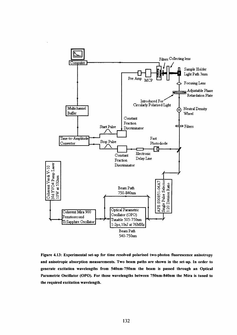
Filters Collecting lens

Sample Holder Light Path 3mm

— dHU-PreAmp M cp

c p Focusing Lens

. l- ■ Adjustable Phase Retardation Plate

Introduced For Circularly Polarised Light

(S) Neutral Density T Wheel

ConstantFractionDiscriminator FiltersStart Pulse

/ \FastPhotodiodeStop Pulse

I / \Electronic Delay line

ConstantFractionDiscriminator

Beam Path 750-84Onm

MultichannelBuffer

Coherent Mira 900 Femstosecond TiiSapphire Oscillator

O %

Optical Parametric Oscillator (OPO) Tunable 505-750nm l-2ps,10nJ at76MHz

Beam Path 540-750nm

Figure 4.13: Experimental set-up for time resolved polarised two-photon fluorescence anisotropy

and anisotropic absorption measurements. Two beam paths are shown in the set-up. In order to

generate excitation wavelengths from 540nm-750nm the beam is passed through an Optical

Parametric Oscillator (OPO). For those wavelengths between 750nm-840nm the Mira is tuned to

the required excitation wavelength.

132

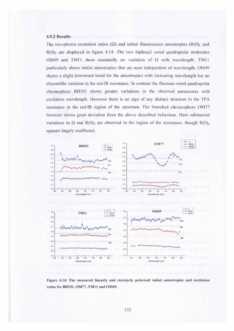
4.9.2 Results

The two-photon excitation ratios (Q) and initial fluorescence anisotropies (R(O)l and

R(0)c are displayed in figure 4.14. The two biphenyl cored quadrupolar molecules

OM49 and TM11 show essentially no variation of Q with wavelength. TM11

particularly shows initial anisotropies that are near independent of wavelength. OM49

shows a slight downward trend for the anisotropies with increasing wavelength but no

discernible variation in the red-IR resonance. In contrast the fluorene cored quadrupolar

chromophore BH101 shows greater variations in the observed parameters with

excitation wavelength. However there is no sign of any distinct structure in the TPA

resonance in the red-IR region of the spectrum. The branched chromophore OM77

however shows great deviation from the above described behaviour. Here substantial

variations in Q and R(0)c are observed in the region of the resonance, though R(0)l

appears largely unaffected.

OM77

0.7-2/3

4/70.5-

2/50 3 -

0 2 -

550 650 700500 600 750 800 850

BH1011.0

0.9

0.8

0.72/3

0.64/7

05

0.4 2/503

02

010.0

650 700 750 800 850500 550 600

Wavelength (nm) Wavelength (nm)

0 .8 -

0.7-

0 .6 -

0 5-

TM11— o 0.8-| OM49*-R(0)L |-O -R (0)C—o—R(0)C

500 550 600 650 700 750 800 850

Wavelength (nm)

550 600 650 700 750 800 850

Wavelength (nm)

Figure 4.14: The measured linearly and circularly polarised initial anisotropies and excitation

ratios for BH101, OM77, TM11 and OM49.

133

This behaviour might be explained by closer inspection of equation 4.13: if the tensor

element is assumed to be 1 corresponding to equivalent excitation along X and Y in the

molecular frame, the dependence on the other tensor element is removed and an

expression for R (0 )l reduces to

[4.22]

and the corresponding expression for Q and R(0)c are

Q =1 + 3 D 2 4 + 2 D ‘

[4.23]

M o )= 1 +- 2

1 + 37T[4.24]

Indeed, a constant value of R(0)~l/7 is what is observed for OM77.

A full determination of the tensor elements S and D within the planar tensor

approximation was performed by simultaneous solution of 4.10, 4.13 and 4.14 [21]. The

values of S and D for each equation pair was used to predict the value of the third

observable parameter. The success of this prediction was used as an indication of the

validity of the planar approximation and an average of the three solutions for S and D

was taken. The variance of these parameters for the four chromophores is shown in

figure 4.15 along with a scaled representation of the TPA cross-section.

The wavelength dependence of the tensor elements is markedly different for the

chromophores based on the different fluorescent cores. The two phenyl core molecules

(OM49 and TM11) demonstrated very little sensitivity to the resonance in the TPA

cross-section. However for BH101, although the element remains largely invariant to

excitation wavelength, the D element appears to show some variation in the red-IR

resonance. The difference in the behaviour of the two tensor elements for OM77 is

clearly evident. The S element remains close to 1 through the entire excitation

134

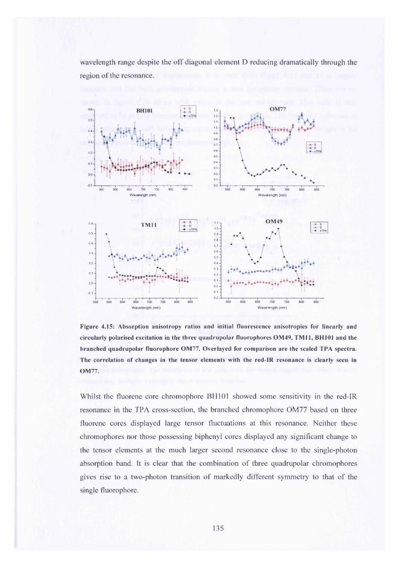
wavelength range despite the off diagonal element D reducing dramatically through the

region of the resonance.

0 5 -

0.4-

0.3-

0.2 -

BH101 ~9-S - * - D — oTPA

1-3*]1.2 -

1 .1 -

1.0 -

0.9-

0 .8 -

0.7-

0 .0 -

0.5-

0.4-

0.3-

0 .2 -

0.1 -

0.0 --i ----1---- •----1---- 1---- 1----•---- i----■---- r~550 600 650 700 750 800 850

Wavelength (nm) Wavelength (nm)

OM77

0.6

0.5 •\0.4 •\0.3

0.2 V0.1 - .V0.0-

V w

-0.1 -

TM11

1 r

1 1 11.0-

0 .9-

0.8-

0 .7- •

0 .6-

0 .5 -

0 4 -

0 .3-

0 .2-

1

0 .1-\ ]

0 .0- T-0.1 -

-0.2-

OM49

7 \ i \

.........

Wavelength (nm) W avelength (nm)

Figure 4.15: Absorption anisotropy ratios and initial fluorescence anisotropies for linearly and

circularly polarised excitation in the three quadrupolar fluorophores OM 49, TM 11, BH101 and the

branched quadrupolar fluorophore OM 77. Overlayed for comparison are the scaled TPA spectra.

The correlation of changes in the tensor elements with the red-IR resonance is clearly seen in

OM77.

Whilst the fluorene core chromophore BH101 showed some sensitivity in the red-IR

resonance in the TPA cross-section, the branched chromophore OM77 based on three

fluorene cores displayed large tensor fluctuations at this resonance. Neither these

chromophores nor those possessing biphenyl cores displayed any significant change to

the tensor elements at the much larger second resonance close to the single-photon

absorption band. It is clear that the combination of three quadrupolar chromophores

gives rise to a two-photon transition of markedly different symmetry to that of the

single fluorophore.

135

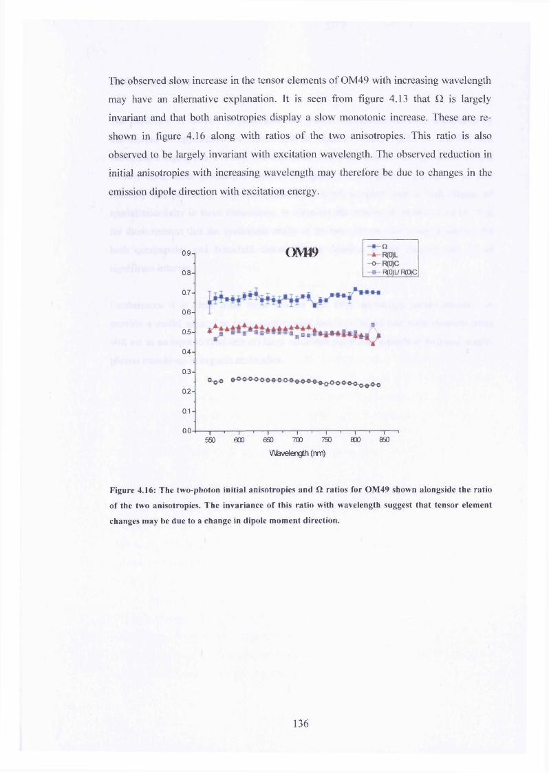
The observed slow increase in the tensor elements of OM49 with increasing wavelength

may have an alternative explanation. It is seen from figure 4.13 that Q is largely

invariant and that both anisotropies display a slow monotonic increase. These are re­

shown in figure 4.16 along with ratios of the two anisotropies. This ratio is also

observed to be largely invariant with excitation wavelength. The observed reduction in

initial anisotropies with increasing wavelength may therefore be due to changes in the

emission dipole direction with excitation energy.

0.9-1

0.8

0.7

0.6 h

0.5

0.4

0.3

02

0.1

0.0

OJVB9RfCIL/ ROC

» . l1 -ss

V\fevelength (nm)

TV

—i— »— i— 1— i— »— i— ■— i— ■— i— ■— i—550 600 650 700 750 800 850

Figure 4.16: The two-photon initial anisotropies and i l ratios for OM 49 shown alongside the ratio

of the two anisotropies. The invariance o f this ratio with wavelength suggest that tensor element

changes may be due to a change in dipole moment direction.

136

4.10 Conclusion

The explosion of interest in molecular two-photon absorption has been stimulated by

the myriad of applications it offers both in material science [22, 23, 24, 25] and

biological imaging [26, 27, 28]. The search for two-photon absorbers optimised for use

in low cost, mass production systems designed for two-photon excitation at low

intensity and providing improved penetration depth coupled with a high degree of

spatial selectivity in three dimensions, is currently the subject of intense research. It is

for these reasons that the systematic study of the two-photon absorption properties for

both quadrupolar and branched chromophores detailed in this chapter may be of

significant interest.

Furthermore it is clear from these studies that TPA anisotropy measurements can

provide a useful adjunct to cross-section data and it is hoped that such measurements

will act as an input to (and test of) large scale computational models o f two-and single­

photon transitions in organic molecules.

137

References

[1] P Schwille, U Haupts and S Maiti, WW Webb, Biophys J., 77, 2251 (1999)

[2] J D Bhawalker, N D Kumar, C F Zhao and N P Prasad, J. Clin. Laser Med. Surg., 15

(1997)

[3] W Denk and J H Strickler, W W Webb, Science., 248, 73 (1990)

[4] O Mongin, L Porres, M Chariot, C Katan and M Blanchard-Desche. Chem. Eur. J.,

13 (2007)

[5] B Larijani and A J Bain, “Biological Applications o f Single and Two-Photon

Fluorescence” in “Biological Chemistry”, Eds B Larijani, C A Rosser and R

Woscholski, Wiley London (2006)

[6] P N Butcher and D Cotter “The Elements o f Nonlinear Optics” Cambridge

University Press (1990)

[7] F Terenziani, C Le Droumaguet, C Katan, O Mongin, M H V Werts, S Tretiak, M

Blanchard-Desche. SPIE-Int. Soc. Opt. Eng., 5935 (2005)

[8] M Albota, D Beljonne, J-Luc Bredas, J E. Ehrlich, J-Ying Fu, A A. Heikal, S E.

Hess, T Kogej, M D. Levin, S R. Marder, D McCord-Maughon, J W. Perry, H Rockel,

M Rumi, G Subramaniam, W W Webb, X-Li Wu and C Xu, Science. 281, 1653, (1998)

[9] J Fu, L A. Padilha, D J Hagan, E W Van Stryland, O V Przhonska, M V Bondar, Y

L Slominsky and A D Kachkovski, J. Opt. Soc. Am. B. 24, 1 (2007)

[10] D M Brink and G R Satchler “Angular Momentum” Third Edition, Oxford

Publications (1994)

[11] W M McClain, J. Chem. Phys., 55, 2789 (1971)

[12] C Z Wan and C K Johnson, Chem. Phys., 179 513 (1994)

[13] P R Callis, J. Chem .Phys., 99, 27 (1993)

[14] Bernard Valeur “Molecular Fluorescence; Principles and Applications” Second

Reprint, Wiley-VCH (2005)

[15] S W Pauls, J F Hedstrom and C K Johnson, Chem. Phys. 237,205 (1998)

[16] A J Bain to be published

[17] M A Albota, C Xu and W W Webb, Applied Optics., 37, 31 (1998)

[18] C Xu and W W Webb, J. Opt. Soc. Am. B., 13, 3 (1996)

[19] F Terenziani, C Le Droumaguet, C Katan, O Mongin, M H V Werts, S Tretiak and

M Blanchard-Desche. SPIE-Int. Soc. Opt. Eng., 5935 (2005)

138

[20] C. Katan, S. Tretiak,. M. H. V. Werts, A. J. Bain, R. J. Marsh, N. Leonczek, N.

Nicolaou, E. Badaeva, O. Mongin and M. Blanchard-Desce, J. Phys. Chem. B., I l l ;

9468 (2007)

[21] The analysis takes the emission dipole moment direction to define X in the

molecular frame (cosO= 1 in equations 4.12 and 4.13)

[22] A. S. Dvornikov and P. M. Rentzepis, Opt. Commun., 119, 341 (1995)

[23] S M Kuebler, K L Braun, W Zhou, J K Cammack, T Yu, C K Ober, S R Marder

and J W Perry, J. Photochem. Photobio. A: Chemistry, 158, 163 (2003)

[24] C C Corredor, K D Belfield, M V Bondar, O V Przhonske, F E Hernandez and O D

Kachkovsky, J J Photochem., 184, 174 (2006)

[25] D A. Parthenopoulos and P. M. Rentzepis, Science., 245, 843 (1989)

[26] J C Malone, A F Hood, T Conley, J Numberger, L A Baldridge, J L Clendenon, K

W Dunn, C L Phillips and J. Cutan. Pathol., 29, 453 (2002)

[27] M D Cahalan, I Parker, S H Wei and M J Miller, Nat. Rev. Immunol., 2, 872

(2002)

[28] J M Squirrell, D L Wokosin, J G White and B D Bavister, Nat. Biotechnol., 17,

763 (1999)

139

Chapter 5Stimulated Emission Depletion Dynamics in a Branched

Quadrupolar Chromophore

5.1 Introduction

In this chapter stimulated emission depletion dynamics are investigated in the branched

fluorophore OM77. Stimulated emission depletion (STED) refers to the technique by

which an excited state fluorescent population of molecules is partially depleted by

stimulating transitions to the ground electronic state. STED was originally developed as

a high resolution technique in molecular spectroscopy allowing access to highly

vibrationally excited levels in the ground electronic states of molecules which are

inaccessible to direct excitation [1]. The development of time resolved condensed phase

STED techniques [2-4] enabled work to probe condensed phase relaxation dynamics in

excited electronic states and high vibrational levels of ground electronic states [5-7].

Subsequently STED has attracted interest as an advanced tool in fluorescence

microscopy permitting three dimensional imaging with sub-wavelength resolution [8,

9]. STED techniques were recently extended to two-photon excited states by the group

where it was shown that time resolved STED techniques are sensitive to excited state

properties (alignment) that are hidden from spontaneous emission (unperturbed

fluorescence) [10] and in particular that it is possible to measure hexadecapole

alignment relaxation (a ^ (tfj from STED depolarization data [11] and polarization

sensitive saturation measurements [12].

5.2 Two-Photon Excited Stimulated Emission Depletion

The principles of two-photon excited STED are depicted shown in figure 5.0. Initial

excitation (‘Pump’) occurs from low lying vibrational levels in the So ground state via

the simultaneous absorption of two (non-resonant) near infra-red photons (c.a. 800nm).

140

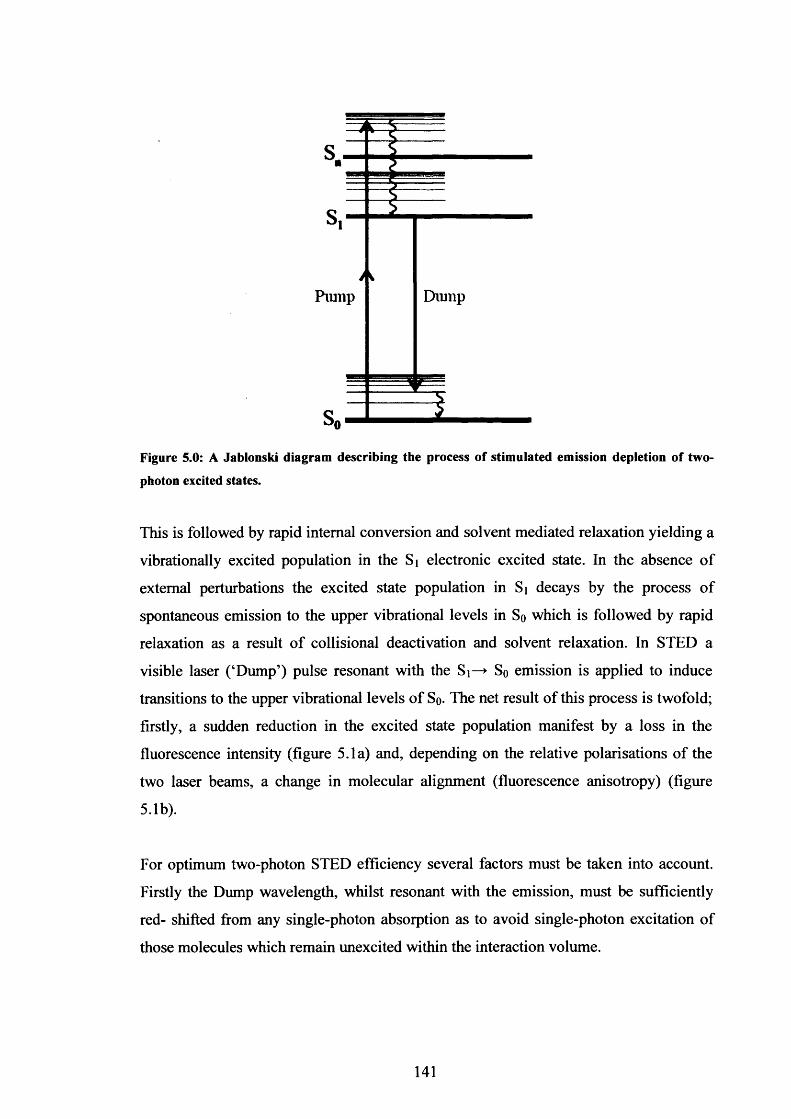
DumpPump

Figure 5.0: A Jablonski diagram describing the process of stimulated emission depletion of two-

photon excited states.

This is followed by rapid internal conversion and solvent mediated relaxation yielding a

vibrationally excited population in the Si electronic excited state. In the absence of

external perturbations the excited state population in Sj decays by the process of

spontaneous emission to the upper vibrational levels in So which is followed by rapid

relaxation as a result of collisional deactivation and solvent relaxation. In STED a

visible laser (‘Dump’) pulse resonant with the Si—► So emission is applied to induce

transitions to the upper vibrational levels of So. The net result of this process is twofold;

firstly, a sudden reduction in the excited state population manifest by a loss in the

fluorescence intensity (figure 5.1a) and, depending on the relative polarisations of the

two laser beams, a change in molecular alignment (fluorescence anisotropy) (figure

5.1b).

For optimum two-photon STED efficiency several factors must be taken into account.

Firstly the Dump wavelength, whilst resonant with the emission, must be sufficiently

red- shifted from any single-photon absorption as to avoid single-photon excitation of

those molecules which remain unexcited within the interaction volume.

141

a.

oo

cz

1Pm0)

X!JD*

PQ

510

Depletion field off

410

84 6 100

Time ( i i s )

b.

p4PMOr—i

O • 3

0.6

0.4

§ 0253o-A0>O

-5 0.0PM

-R(0)=0.54

\ \

A R = 0 .1 8

A t = 6 3 6 p s

I\ , Depletion field off

Depletion

4 6

Tune (ns)10

Figure 5.1: Diagram showing the effect o f depletion - ‘Dum ping’ of the excited state population

following two-photon excitation ‘Pum ping’ for fluorescein in ethylene glycol [10]. (a) For a Pump-

Dump delay set at 636ps, the fraction rem aining in the excited state population is reduced by a

factor o f two. (b) The selective removal o f molecules which are oriented parallel to the Dump pulse

polarisation causes an abrupt change in fluorescence anisotropy R(t).

Secondly, for two-photon excitation in an isotropic medium (given a favourable

transition tensor as discussed in Chapter 4) the angular distribution of molecular

transition dipole moment directions in the laboratory frame is more sharply peaked than

for single photon excitation (figure 5.2). Depletion of the excited state is maximised for

parallel ‘Pump’ and ‘Dump’ polarisations [10, 11]. Finally, the time separation between

142

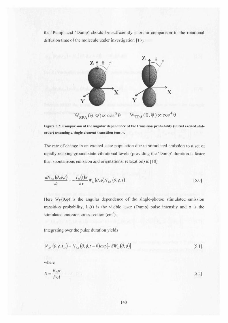
the ‘Pump’ and ‘Dump’ should be sufficiently short in comparison to the rotational

diffusion time of the molecule under investigation [13].

z * e

■>X

Y

W ( 0 , ) OC COS ~ 0 ^ T P A ( ^ ■> ^ ^OS ®

Figure 5.2: Comparison o f the angular dependence o f the transition probability (initial excited state

order) assuming a single elem ent transition tensor.

The rate of change in an excited state population due to stimulated emission to a set of

rapidly relaxing ground state vibrational levels (providing the ‘Dump’ duration is faster

than spontaneous emission and orientational relaxation) is [10]

Here Wo(0,cp) is the angular dependence of the single-photon stimulated emission

transition probability, Io(t) is the visible laser (Dump) pulse intensity and o is the

w D ( e j ) N E X ( o M [5.0]d t h v

stimulated emission cross-section (cm2).

Integrating over the pulse duration yields

M e x (0 ’ M > ) = N ex 0)exp[- ^)] [5.1]

where

[5.2]hvA

143

in this case Ed is the pulse energy, and A is the pulse area. In the limit of weak

stimulated emission depletion ( S « l ) equation 5.1 becomes

JV** N EX{0 , ^ t = 0X1 - s w „ ( e ^ ) \

For Z (Vertically) polarised ‘Dump’ pulses this becomes

(0 4 ,1 „ )= n (0 4 , t = o)[i - s cos2 e \

[5.3]

[5.4]

Prior to STED the initial excited state orientational distribution at time t for isotropic

rotational diffusion following two-photon excitation is given by

N E X (^ » f a t d ) ~ N e x eX P M 1

UJ a/4 nT™ + ^ = Y 20 exp

■ " ' 7 V5

and for single-photon excitation is given by

V r 20 J+ TTl"40eXP

^ - 10/ ^

3 TV J l 2o y[5.5]

r - tT fv /

1

V r 20 J[5.6]

After the onset of stimulated emission depletion the altered excited state population is

given by [10]

N D( 0 j ) = N°ex 1 - Scos2 6)= N qhx (0,<p9A 1 - -f 2 A ^0 0 + ^ 2 0

V 5[5.7]

Integrating over the orientational distribution and rearranging equation 5.7 gives the

fraction of the population remaining ( F r ) in terms of the anisotropy prior to ‘Dumping’

(Ru):

l (1+2 Rg)S 3

[5.8]

144

The ‘Dumped’ anisotropy Rd is given by [10]

(3 - ( l + 2R,, )S')

K ( o ) ) s[5.9]

From equation 5.9 it can be seen that the Dumped anisotropy is dependent on (a ^

which is not observed in unperturbed conventional experiments.

In the limit of fast ground state relaxation and in the regime of weak depletion of the

excited state population, STED dynamics can be modelled analytically. Analytic

solutions to the coupled rate equations, (equations which describe the evolution of the

excited (N e x ) and upper vibrational ( N g s ) states) are possible providing there is strong

saturation of the ‘Dump’ transition [10, 11, 12]. Given these conditions and providing

the ‘Dump’ pulse is significantly shorter than any spontaneous emission or molecular

reorientation, the rate equations for STED are given by [10]

where N Ex (0,t) and N o s (0,t) are the ground and excited state populations and t r is the

ground state vibrational relaxation time. By assuming a square ‘Dump’ pulse, (constant

Dump intensity over a time duration Tp), it is possible to obtain analytic solutions to the

rate equations which yield the fractional population remaining (Fr) after depletion of the

excited state as a function of the saturation parameter S for given ratios of tfI tr [10].

Given that in the upper ground state vibrational levels the initial population distribution

is negligible, then the excited state population evaluated at t=xp is given by [10]

d N ‘ * { e ' l ) = J J ^ M ( N r x ( e , t ) ~ n gs { e , t ) )at hv

[5.10]

dN<JS(0 ,t)_ /„ (/)[5.11]

dt

) \ i r «\ — (ed - \)+ d (e d + l) l [5.12]

145

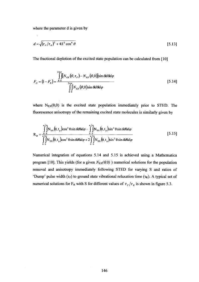
where the parameter d is given by

rf = 1/(rP/ r R)2 +4.S'2 cos4 8 [5.13]

The fractional depletion of the excited state population can be calculated from [10]

InicJ (0 , TP) ~ N PX (#,0)]sin 6d6d(pF o = ( 1 - F r ) = ^ ^ ------------------------------------------ [5 .14 ]

| JXat (0,O)sin 6d6d(p0 0

where N ex(0 ,0 ) is the excited state population immediately prior to STED. The

fluorescence anisotropy of the remaining excited state molecules is similarly given by

ft 2ft

f fNEX(0,t )cos20sin<W0[fy>- f i*NEX(o,t )sin2tts'm ftlddq/ r d = j >j >----------------------------------------------^ ----------------------------------------- [5 .1 5 ]

U f t 2 f t f t 2 j i

J J n ex(0, tp )cos2 0 sin QdQdcp + 2 | | N EX(0> tp)sin2 Gsin OdQdtp

Numerical integration of equations 5 .1 4 and 5 .1 5 is achieved using a Mathematica

program [10]. This yields (for a given NEx(0,0) ) numerical solutions for the population

removal and anisotropy immediately following STED for varying S and ratios of

‘Dump’ pulse width (xP) to ground state vibrational relaxation time ( t r ) . A typical set of

numerical solutions for F r with S for different values of rP / r R is shown in figure 5 .3 .

146

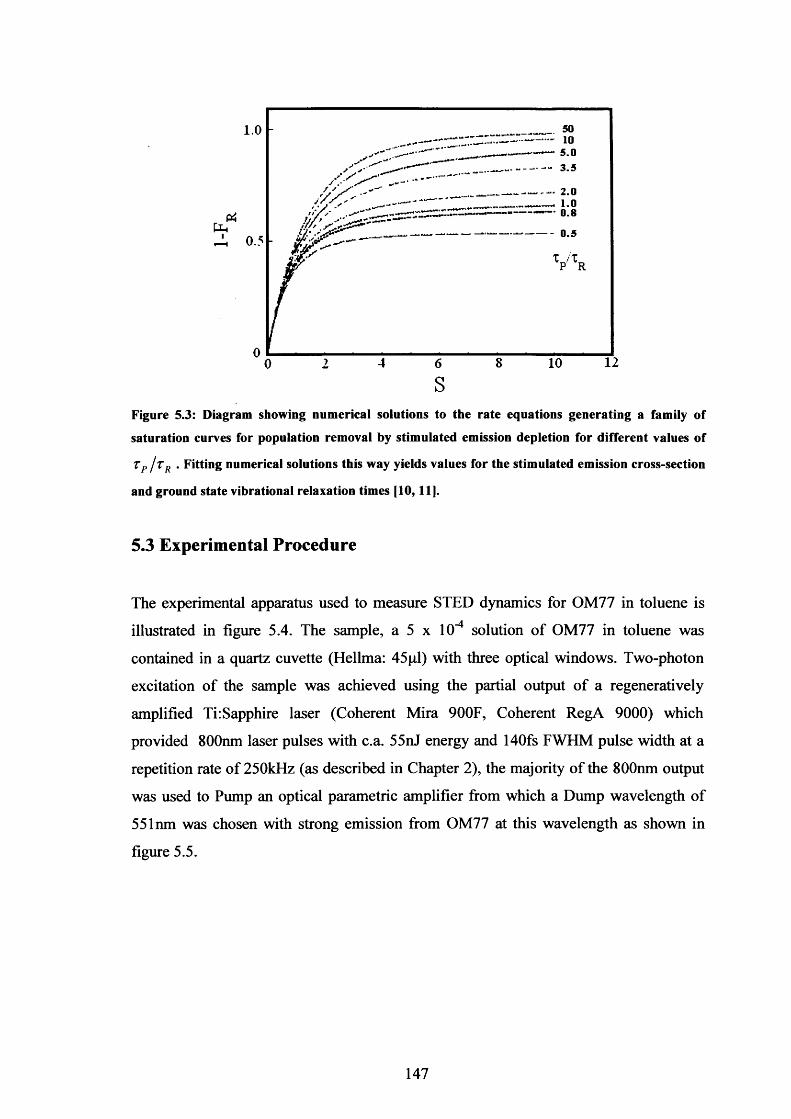
1.0 50

5.03.5

1.00.8

0.50.5

sFigure 5.3: Diagram showing numerical solutions to the rate equations generating a family of

saturation curves for population removal by stimulated emission depletion for different values of

Tp / t r . Fitting numerical solutions this way yields values for the stimulated emission cross-section

and ground state vibrational relaxation times [10,11].

5.3 Experimental Procedure

The experimental apparatus used to measure STED dynamics for OM77 in toluene is

illustrated in figure 5.4. The sample, a 5 x 10"4 solution of OM77 in toluene was

contained in a quartz cuvette (Hellma: 45pi) with three optical windows. Two-photon

excitation of the sample was achieved using the partial output of a regeneratively

amplified Ti:Sapphire laser (Coherent Mira 900F, Coherent RegA 9000) which

provided 800nm laser pulses with c.a. 55nJ energy and 140fs FWHM pulse width at a

repetition rate of 250kHz (as described in Chapter 2), the majority of the 800nm output

was used to Pump an optical parametric amplifier from which a Dump wavelength of

551nm was chosen with strong emission from OM77 at this wavelength as shown in

figure 5.5.

147

Pulse StretcherTi:Sapphire Regenerative Ampifier 140fs pulses at 250kHz 800nm, 13uJ

Ti:Sapphire Oscillator 100fs pulses at 76MHz 760-840nm, 8nJ

ND:YV04 Laser 18W at 532nm

ControlPC

Optical Parametric Ampifier200fs pulses, 250kHz 450-750nm, 0.3uJ

(Grating Pair)DUMP

PUMP

Waveplates & Filters

— D—

J Variable delay I (3.4 fs resolution)

Fluorescence

BeamCombiner

Streak CameraSample(cuvette)

Rotating Polariser & Filters

Figure 5.4: Schematic diagram o f the experim ental apparatus used for STED. Collection o f

fluorescence is made using 90° excitation-detection geom etry.

The OPA pulses were temporally stretched using a grating pair to prevent ‘Dump’

induced two-photon fluorescence. The ‘Pump’ and ‘Dump’ wavelengths were

monitored using a laser spectrum analyser (IST-Rees) and the pulse widths measured

using a scanning autocorrelator (APE Pulse Check). Broadband half waveplates

(Melles-Griot) were used to control the ‘Pump’ and ‘Dump’ beam polarisations. A

variable optical delay line (Time and Precision) allowed scanning of the Pump-Dump

separation which was set at 200ps. Adjustment of the ‘Pump’ and ‘Dump’ powers were

made using neutral density wheels and measured by a precision power meter (Anritsu).

To ensure that both ‘Pump’ and ‘Dump’ beams were incident on the same spot in the

sample, both beams were spatially overlapped prior to the sample using a broadband

dichroic beam combiner (CVI Optics). The beams were passed through an aperture of

fixed diameter (2.2mm) and focused into the sample using a 2.54 achromatic lens

(Melles-Griot). Any scattered laser light was blocked using appropriate short-pass filters

(Corion LS550) and glass infra-red cut-off filters (Schott BG39). A long-pass glass cut­

off filter (OG530) was placed before the sample to ensure the ‘Dump’ pulse was not

contaminated by remnants of white light from the continuum generated in the OPA.

148

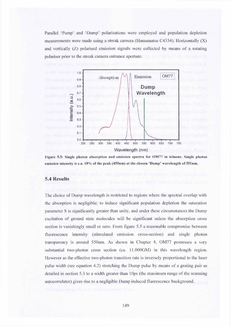
Parallel ‘Pump’ and ‘Dump’ polarisations were employed and population depletion

measurements were made using a streak camera (Hamamatsu C4334). Horizontally (X)

and vertically (Z) polarised emission signals were collected by means of a rotating

polariser prior to the streak camera entrance aperture.

1 0OM77Absorption0.9

DumpW avelength

08

07

06

2 ? 0.5

0.2

0.1

0 .0 -

200 250 300 350 400 450 500 550 600 650 700 750

W avelength (nm)

Figure 5.5: Single photon absorption and em ission spectra for OM 77 in toluene. Single photon

emission intensity is c.a. 18% o f the peak (455nm ) at the chosen ‘Dum p’ wavelength o f 551nm.

5.4 Results

The choice of Dump wavelength is restricted to regions where the spectral overlap with

the absorption is negligible; to induce significant population depletion the saturation

parameter S is significantly greater than unity, and under these circumstances the Dump

excitation of ground state molecules will be significant unless the absorption cross

section is vanishingly small or zero. From figure 5.5 a reasonable compromise between

fluorescence intensity (stimulated emission cross-section) and single photon

transparency is around 550nm. As shown in Chapter 4, OM77 possesses a very

substantial two-photon cross section (ca. 11.000GM) in this wavelength region.

However as the effective two-photon transition rate is inversely proportional to the laser

pulse width (see equation 4.2) stretching the Dump pulse by means of a grating pair as

detailed in section 5.3 to a width greater than lOps (the maximum range of the scanning

autocorrelator) gives rise to a negligible Dump induced fluorescence background.

149

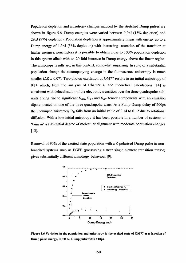
Population depletion and anisotropy changes induced by the stretched Dump pulses are

shown in figure 5.6. Dump energies were varied between 0.2nJ (15% depletion) and

29nJ (97% depletion). Population depletion is approximately linear with energy up to a

Dump energy of 1.3nJ (56% depletion) with increasing saturation of the transition at

higher energies; nonetheless it is possible to obtain close to 100% population depletion

in this system albeit with an 20 fold increase in Dump energy above the linear region.

The anisotropy results are, in this context, somewhat surprising. In spite of a substantial

population change the accompanying change in the fluorescence anisotropy is much

smaller (AR = 0.07). Two-photon excitation of OM77 results in an initial anisotropy of

0.14 which, from the analysis of Chapter 4, and theoretical calculations [14] is

consistent with delocalisation of the electronic transition over the three quadrupolar sub­

units giving rise to significant S x x , S yy and S xy tensor components with an emission

dipole located on one of the three quadrupolar arms. At a Pump-Dump delay of 200ps

the undumped anisotropy Ru falls from an initial value of 0.14 to 0.12 due to rotational

diffusion. With a low initial anisotropy it has been possible in a number of systems to

‘bum in’ a substantial degree of molecular alignment with moderate population changes

[13].

Removal of 90% of the excited state population with a Z-polarised Dump pulse in non­

branched systems such as EGFP (possessing a near single element transition tensor)

gives substantially different anisotropy behaviour [9].

1.0

0.8 -

0.6 -

0.4-

0 .2 -

o.o

97% Population Depletion

□ Fraction Depleted FQ • Anisotropy Change AR

Approximately - Linear

Depletion

. i l l i I { { }

- T~ 10

I15

I20

—I— 25 30

Dump Energy (nJ)

Figure 5.6 Variation in the population and anisotropy in the excited state of OM77 as a function of

Dump pulse energy, Ru=0.12, Dump pulsewidth >10ps.

150

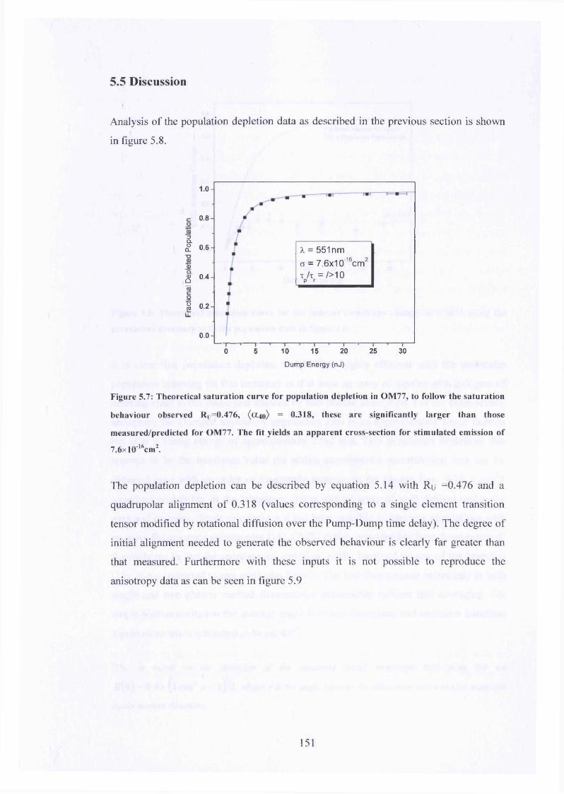
5.5 Discussion

Analysis of the population depletion data as described in the previous section is shown

in figure 5.8.

1.0 -

0.8

m3Q.S. 0-6 X = 551 nm

a = 7.6x10~16cm: t / t =/>10

Q)| 0.4(0

I 0.2LL

0 . 0 -

10 15 20 25 300 5Dump Energy (nJ)

Figure 5.7: Theoretical saturation curve for population depletion in OM 77, to follow the saturation

behaviour observed Ru=0.476, ( 0I40) = 0.318, these are significantly larger than those

measured/predicted for OM 77. The fit yields an apparent cross-section for stim ulated emission o f

7.6x10'16cm2.

The population depletion can be described by equation 5.14 with Ru =0.476 and a

quadrupolar alignment of 0.318 (values corresponding to a single element transition

tensor modified by rotational diffusion over the Pump-Dump time delay). The degree of

initial alignment needed to generate the observed behaviour is clearly far greater than

that measured. Furthermore with these inputs it is not possible to reproduce the

anisotropy data as can be seen in figure 5.9

151

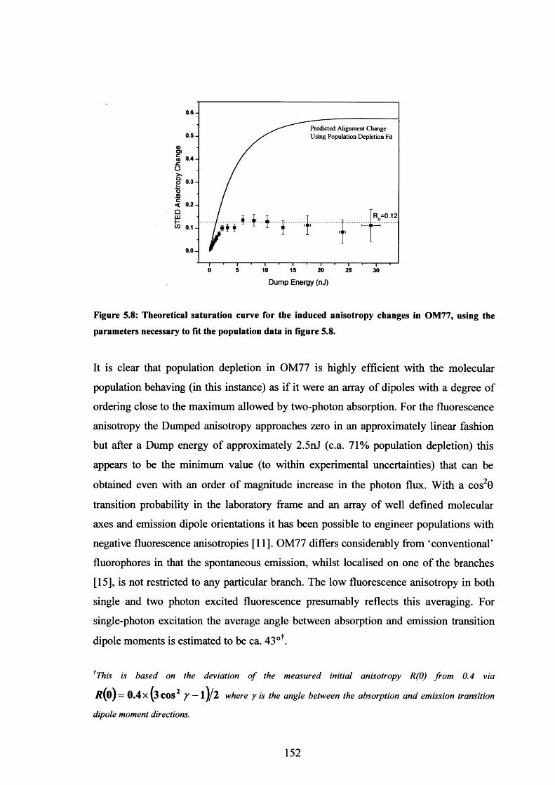
0.6 -

Predicted Alignment Change Using Population Depletion Fit

HH

R=0.12

0 5 10 15 20 25 30

Dump Energy (nJ)

Figure 5.8: Theoretical saturation curve for the induced anisotropy changes in OM77, using the

parameters necessary to fit the population data in figure 5.8.

It is clear that population depletion in OM77 is highly efficient with the molecular

population behaving (in this instance) as if it were an array of dipoles with a degree of

ordering close to the maximum allowed by two-photon absorption. For the fluorescence

anisotropy the Dumped anisotropy approaches zero in an approximately linear fashion

but after a Dump energy of approximately 2.5nJ (c.a. 71% population depletion) this

appears to be the minimum value (to within experimental uncertainties) that can be

obtained even with an order of magnitude increase in the photon flux. With a cos20

transition probability in the laboratory frame and an array of well defined molecular

axes and emission dipole orientations it has been possible to engineer populations with

negative fluorescence anisotropies [11]. OM77 differs considerably from ‘conventional’

fluorophores in that the spontaneous emission, whilst localised on one of the branches

[15], is not restricted to any particular branch. The low fluorescence anisotropy in both

single and two photon excited fluorescence presumably reflects this averaging. For

single-photon excitation the average angle between absorption and emission transition

dipole moments is estimated to be ca. 43ot.

^This is based on the deviation o f the measured initial anisotropy R(0) from 0.4 via

where y is the angle between the absorption and emission transition

dipole moment directions.

152

If for any given excited molecule the location of the transition dipole moment along a

particular branch is not determined until the moment of (spontaneous) emission then

stimulated emission would be expected to ‘force’ emission along the branch with the

most favourable angular orientation to the Dump polarisation. In non-degenerate

transitions i.e. with a ‘unique’ direction in the molecular frame the molecular alignment

dependence of STED and the fluorescence anisotropy are the same. The clear evidence

we have for OM77 is that this is not the case. The effective molecular alignment is

apparently enhanced by selection of the most appropriately aligned quadrupolar branch

- an ‘option’ not available to single chromophore systems. Now considering the small

anisotropy changes that are observed, efficient internal photoselection (which as argued

above, is insensitive to the low degree of apparent molecular alignment) will, unless the

molecular orientation (i.e. the plane of OM77) of the removed molecules were such that

they would have made a significant contribution to Z-polarised emission in the

laboratory frame (e.g. with an end on orientation to the emission collection direction for

instance) the fluorescence anisotropy will see little change.

5.6 Conclusions

In addition to possessing a substantial two photon cross section OM77 appears to be

well suited to photo-engineering STED. The effective alignment of the molecules for

stimulated depletion appears to be significantly larger than that predicted by the

spontaneous emission anisotropy which involves the averaging of the emission

probability over the three branches of the fluorophore. The fluorescence anisotropy of

the depleted distribution is however resilient to strong depletion which gives rise to

significant change in systems where the transition dipole moment direction is well

defined in the molecular frame. It is clear that STED depletion dynamics in branched

systems cannot be described by the conventional models that have worked well for non­

degenerate fluorophores. It will be particularly interesting to study population and

anisotropy dynamics in branched systems such as OM77 at Pump-Dump delays where

significant orientational relaxation has taken place and the excited state more closely

approximates an isotropic ensemble. The creation of fluorescence anisotropy from an

isotropic ensemble of branched chromophores may prove challenging! In this light a

153

combination of two and single-photon STED experiments would also be useful as

higher degrees of molecular alignment are not initially present in the latter.

154

References

[1] D E Reisner, R W Field, J L Kinsey and H-L Dai, J. Chem. Phys., 80, 5968 (1984)

[2] I Gryczynski, J Kusba and J R Lackowicz, J. Chem. Phys., 98, 8886 (1994)

[3] J Kusba, V Bogdanov, I Gryczynski and J R Lakowicz, Biophys. J., 67, 2024 (1994)

[4] J R Lakowicz, “Principles o f Fluorescence Spectroscopy ” Second Edition, Kluwer

Academic (1999)

[5] G Haran, E A Morlino, J Mathes, R Callendar and R M Hochstrasser, J. Phys.

Chem. A., 103, 2202 (1999)

[6] P Changenety-Barret, C T Choma, E F Gooding, W F DeGrado and R M

Hochstrasser J. Phys. Chem. B., 104, 9322 (2000)

[7] S. A. Hambir, Y. Jiang and G. J. Blanchard, J. Chem. Phys., 98, 6075 (1993).

[8] T A Klar, S Jakobs, M Byba, A Egner and S W Hell, Proc. Nat. Acad. Sci. (USA)

97, 8206 (2000)

[9] S W Hell and J Wichmann, Opt. Lett., 19, 780 (1994)

[10] R J Marsh, D A. Armoogum and A J Bain, Chem. Phys. Lett., 366, 398 (2002)

[11] A J Bain, R J Marsh, D A Armoogum, L Porres O Mongin and Mireille Blanchard-

Desce, BioChem. Soc. Trans., 31, 1047 (2003)

[12] T Masters, D A Armoogum R J Marsh and A J Bain, to be published

[13] D A Armoogum, PhD thesis, University College London, (2004)

[14] C Katan, S Tretiak, M H V Werts, A J Bain, R J Marsh, N Leonczek, N Nicolaou,

E Badaeva, O Mongin and M Blanchard-Desce, to be published

[15] C Katan, S Tretiak, M H V Werts, A J Bain, R J Marsh, N Leonczek, N Nicolaou,

E Badaeva, O Mongin and M Blanchard-Desce, J. Phys.Chem. B., Ill, 9468 (2007)

155

Appendix I.I

The Orientational Distribution Function

By defining the order parameter using a polar coordinate system the orientational

distribution function P{6, (p) represents the probability of finding the molecule oriented

between 0 and d0 and (p and dtp (figure 1.0).

z♦

X

Figure 1.0: The spherical polar coordinate system used to define the orientational distribution

function P(0,<p).

The orientational distribution function can be expanded in terms of a complete set of

orthonormal basis functions. An expansion of the orientational distribution function in

terms of spherical harmonics is most convenient in describing the molecular order

created by the interactions between the light and molecule. The function also best

defines the restricted environment of the experimental observables.

The orientational distribution function P(0,(p) in terms of a spherical harmonic

expansion is given by

P(e,<p) = l KQ{CKQ)YKQ(0,q>) [1.1]

Where the expansion coefficients (CKQ ) define the moments of the distribution and

their magnitude and sign determine the form of P{0,(p). YKQ (#, (p) is a spherical

harmonic of rank K and projection Q where Q takes 2K + \ values in integer steps

156

from +K to -K . Spherical harmonics are constructed from Legendre Polynomials

P K0 (cosO)) as:

/ 2 L U x S ) ~ ^ (co sff)e^ [U 1

The orientational distribution function can be written in terms of spherical harmonics as

2 n n

J j K e (0> (0> ) sin 0d 0d<p = S KK.S,K>. [1.3]0 0

where

[i4]

the moments of the expansion can then be found from [1]

I n n

{'c kq)= J J K o i0 ’ <p)r(6,<p)sm 9d(klrp [1.5]0 0

The graphical representations of several spherical harmonics together with their

functional forms are shown in table 1.0:

157

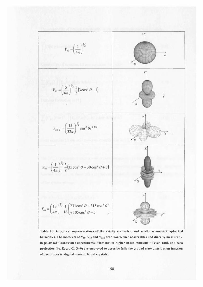
Table 1.0: Graphical representations o f the axially sym metric and axially asym m etric spherical

harmonics. The moments o f Yoo, Y20 and are fluorescence observables and directly m easurable

in polarised fluorescence experiments. Moments o f higher order moments o f even rank and zero

projection (i.e. KEVEn>2, Q=0) are employed to describe fully the ground state distribution function

of dye probes in aligned nematic liquid crystals.

158

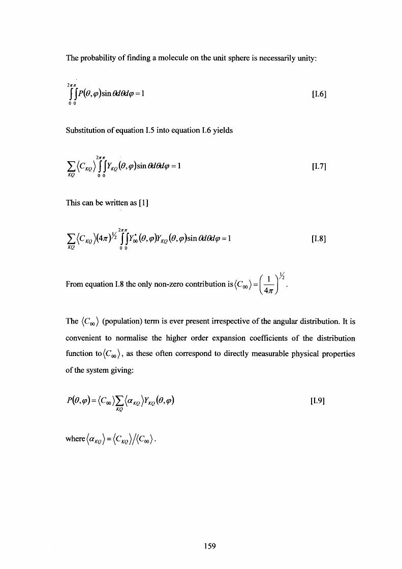
The probability of finding a molecule on the unit sphere is necessarily unity:

2 1C1C

sin OdOd(p = 1o o

Substitution of equation 1.5 into equation 1.6 yields

[1.6]

2itxZ ( c «e) f j ¥KQ(0,p)sinM&l4> = 'lKQ 0 0

[1.7]

This can be written as [1]

litre

X ( C KQ J i y oo (0> <p)ykq (<?>0»)sin OdQdcp =m oo

[1.8]

From equation 1.8 the only non-zero contribution is C00) =v4 7tj

The (Cqq ) (population) term is ever present irrespective of the angular distribution. It is

convenient to normalise the higher order expansion coefficients of the distribution

function to (Cm), as these often correspond to directly measurable physical properties

of the system giving:

P(0,<p) = (Coo) '£ ( a l;Q)YKQ(0,<p)KQ

[1.9]

where (or*g ) = (CKQ )/(C w}.

159

Appendix I.II

Orientational Distribution Function for Nematic Liquid Crystals:

Order ParametersAs a molecule undergoes diffusion in the nematic phase of a liquid crystal there is a

tendency for one of the molecular axes to point along a preferred direction. This

preferential orientation is denoted by the unit vector n. The tendency for the molecules

to align along a preferred direction n gives rise to an orientational distribution function

that is not uniform over the unit sphere. The nematic phase is more ordered than the

isotropic phase and to describe the degree of order quantitavely an order parameter must

be defined such that it is non-zero in the nematic phase and vanishes in the isotropic

achieved by examining the inherent symmetry of the system under consideration. In the

nematic phase of liquid crystals, there exists axial symmetry with respect to the

orientation of the nematic director n, which defines the laboratory fixed Z-axis.

Z. For a nematic liquid crystal, P(0,cp) will only have non-zero moments for Q=0. As

nematic liquid crystals are invariant to inversion of the nematic director i.e. P(0,cp) =

P(n-0,cp), moments where K is even will be present in the expansion of P(0,<p).

Applying the symmetry conditions the orientational distribution function becomes

p{e, ) = (Co,, )[y00 (<9, <p) + ( a 20 }y20 (e , < p )+ { a w )y40 {e, ( p ) + { a M)Ym (e , < p)+ .. ]

[1.10]

phase.

To fully describe P(0,(p) the number of order parameters (a KQ must be reduced. This is

Spherical harmonics with Q=0 are cp independent and so are invariant to rotation about

1+ £ ( 4 n )T(ai0) ^ 0( MK)O(EVEN)

160

Which in terms of Legendre polynomials PK (0) becomes [2]

p(e,<p)4 n

1 + X (4 0 )2 PK{0)K)O(EVEN) (2K + 1)

[1 .1 2 ]

As Q=0 there is no cp dependence and we can therefore write

P{0,<p) = \ 1+ X ( 4 0 ) 1 - ^ - ; - / * , ( < ? )K)O(EVEN) (2K + \)

[1.13]

The (a KQ j(2K + l )2 coefficients represent the order parameters of the system. For a

fully aligned nematic system, all molecules are oriented along the nematic director n,

yielding

( a „ ) = 4 n i y „ ( « = M [1.14]

The degree of alignment ( a 20) of a fully ordered array is thus V 5.

References

[1] A J Bain, P Chandna, and J Bryant, J. Chem. Phys. 112, 10418 (2000)

[2] D M Brink and G R Satchler, “Angular Momentum” Second Edition, Clarendon

Press, (1968)

161

Appendix II

DiffusionThe potential for diffusive flux Jx in an arbitrary direction x is proportional to the

number density N(x,t) per unit distance dx [1]

where D is a proportionality constant known as the diffusion coefficient. The negative

sign indicates the flow of matter in the direction of decreasing concentration. The

conservation of mass applied to a restricted volume differential element formed by

arbitrary area A and thickness dx can be expressed by

Combining this expression with equation II. 1 and assuming D to be independent of

concentration yields an expression for the time evolution of concentration - the

diffusion equation:

dN (x,t)_ d { jx) [II.2]dt dx

dN(x,t) d 2 N (x,t)dt dx2

[II.3]

yielding solution [2]

N(x,t)=

This describes the spatial and temporal evolution of the particle concentration with

initial conditions that all particles are concentrated in the YZ plane x=0 for t=0. Since

162

diffusion will occur in directions +x and -x , the mean displacement at any time is zero,

so particle spread is measured via the mean square displacement:

[II.5]

yielding the Einstein-Smoluchowski equation [3]

[II.6]

(x2) = 2 Dt

Brownian motion [4] defines the random movements of a particle arising from a

variable pressure difference caused by the continuous collisions on all sides of the

particle by neighbouring particles. The application of Newtonian mechanics to a

Brownian particle of mass M and velocity v experiencing a fluctuating force B(t) yields

Langevin’s equation:

M - = -M £v + B(t) dt

where § is the microscopic friction constant [5]. Multiplication by x /M gives

xx = -<!pcx + xM

[11*9]

Upon the substitutions x 2 = 2xx and x 2 = 2(x)2 + 2xx this becomes

[11.10]

163

Using the equipartition theorem the average kinetic energy can be written as [6]

± M { x 2 ) = U bT [11.11]

where kB is Boltzmanns’ constant, T is the absolute temperature and ( ) denotes an

average in time. If the average value of the fluctuating force is zero, the substitution of

(x2 into a time average form of equation II. 10 gives

,2

dxdd

(*2) - S t M ) e11-12]dt

Einstein’s solution to this equation is written as [6]

In the very short time regime, t « ^ ‘1 and (x 2 j « (kBT /M )t2 so the particles move with

thermal velocity ^ 2 kBT /M . At longer times the dominant process is Brownian motion

and

(x2)* (2 kBT/MZ)t [11.14]

Combining this equation with equation II.7 allows the macroscopic diffusion coefficient

D to be written in terms of the microscopic frictional force constant:

D = ^ ~ [11.15]

For a spherical molecule of radius R in a medium with viscosity rj, the frictional

coefficient can be expressed by applying Stokes’ law [7]:

164

£ = 6 7CTjR [11.16]

and the diffusion coefficient becomes

[IU7]6 ktjR

In the Brownian motion description, diffusion can be separated into independent

translational and rotational motion. Equation II.7 expressed the translational diffusion

coefficient in terms of the mean square displacement in time along one spatial (x)

dimension. Extending this to three dimensional space yields

(r2) m =6DlmJ [11.18]

Similarly, the rotational diffusion coefficient can be expressed in terms of the mean

square angular displacement (O2 with time by

(&2) = 4Drolt [11.19]

Furthermore, in the same way that the translational frictional coefficient for a particle

with diffusion velocity v can be described by a force f=- tranSv, so too can the rotational

frictional coefficient be described in terms of a torque T acting on a particle with

rotational velocity D, such that

T = S „ Q [11.20]

Applying the Langevin equation to rotational Brownian motion yields [2]

[11.21]‘o rot

165

Up to this point it has been assumed that diffusing molecules can be described by an

isotropic diffusion coefficient. In reality this is not the case; for non-spherical

molecules, the diffusion coefficient is not a scalar quantity but a second rank tensor [8]

with up to three independent components Dx, Dy, and Dz. For uniaxial molecules such

as nematic liquid crystals two of the three principle axes are equivalent, resulting in two

independent diffusion coefficients Dj. and Dy which correspond to 0 and (p diffusion

respectively:

D± =DX= Dy (0 diffusion) [11.22]

D{] = Dz (cp diffusion) [11.23]

The temporal evolution of the excited state distribution function moments with rank K

and projection Q in an isotropic system is given by:

= (C“e (°))exP[- DK(K + >>] [U'24]

where D is the diffusion coefficient. The time dependent diffusion dynamics can be

written as:

( c “e (0) - ( e t a («)) = {C kq ( 0 ) ) - ( c “ (™))}exp(- r J ) [11.25]

where

7kq=D{KQ\V1\KQ) [11.26]

Expressing V2 in terms of normalised angular momentum operators (in units of h)

yields

V2 = - ( j J + J 2y + J 2z ) = - J 2 [11.27]

166

where J x , J Y and J z are the generators of infinitesimal rotation about the x, y and zA A ^ A

laboratory axes respectively. In terms of polar co-ordinates J x + J Y corresponds to 0

diffusion and J \ corresponds to <p diffusion. Expressing j \ + J] in terms of angular

momentum raising and lowering operators yields

J \ + j ) = i [ j j _ + J _ J +} [11.28]

Z)V2 contains both 0 and (p diffusion operators, which can be expressed as follows:

yKQ{e)= D {9X K Q \±{jJ_ + J _ J ^ K Q ) = d \ k (K + \ ) - Q 1] [11.29]

y KQ {cp) = D(<p\KQ | J \ | KQ) = D,Q2 [11.30]

Applying equations 11.29 and 11.30 to equation 11.24 yields the following diffusion rates

for the fluorescence observable moments ( c^ ( t f j and ( c ^ (0) + ( t erms of

0 and cp diffusion:

y20 = 2(3)D± + 0Z), = 6D± (0 diffusion only) [II.31 ]

y 22 - Y2-2 - 2D± + 4Dp (0 and cp diffusion) [11.32]

References

1] A Fick, Pogg. Annin., 94, 59 (1855)

2] D A Armoogum, Ph.D. Thesis, University College London (2004)

3] A Einstein, Ann. D. Physik. 17, 549 (1905)

4] R Brown, Philos. Mag. 4, 161 (1828)

5] N V Brilliantov, V P Denisoc and P L Krapivsky, Physica A, 175, 293 (1991)

6] C E Hecht, “Statistical Thermodynamics & Kinetic Theory ” Freeman, New York,

1990)

7] W P Crummett and A B Western, “ University Physics ”, WCB (1994)

8] A J Bain, P Chandna, and J Bryant, J. Chem. Phys. 112, 10418 (2000)

167

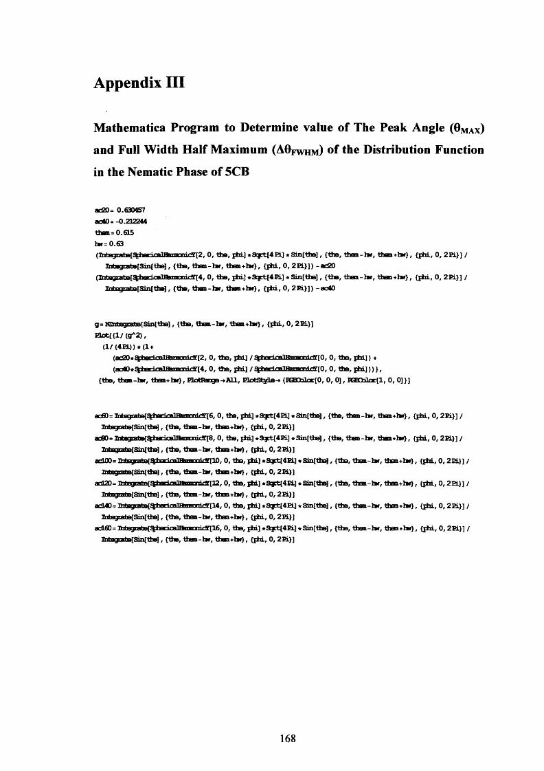
Appendix III

Mathematics Program to Determine value of The Peak Angle ( B m a x )

and Full Width Half Maximum ( A O f w h m ) of the Distribution Function

in the Nematic Phase of 5CB

ac20= 0.630457 ao40= -0.232244 them =0.615 to =0.63(iv»t» ^ [ y airiralifcnTnr>rirfy'[9f 0, the, phi] *Sqp&[4Pi] * Srnfthe], {thB, them -to, them + t o } , {phi, 0, 2PL}] /

Xabegcabe[Sin[1he], {the, them-t o , them*to}, {phi, 0, 2Ei}]) -ac20 (Tr»t» -Ate [.yicgnneiiTfariirOTriy[Af o, the, phi] *Scpt[4Pi] * Sin[thB], {the, them -to, than*t o } , {phi, 0, 2 Pi}] /

InfaBgrataa[Sin[tha], {the, them -to, them+to } , {phi, 0, 2PL}]) -ao40

g= NDntBQratB[Sin[thB], {the, them -to, them+t o } , {phi, 0 , 2 Pi}]P lo t[{ l/ ( ^ 2 ) ,

(1/ (4Pi)) * (1 +

o, the, phi] / qftfirimlBffliimirirtO, 0, the, phi]) + (ao40*3fbeei£al&a3icni££[4, 0, the, phi] / .yiffHrn1ttowgiTirar[0, 0, the, ph i]))} ,

{the, them -to, than+to}, PLotRange-»All, PlotStyle-+ {BGBCblcr[0, 0, 0 ], FGBOcOcr[l, 0, 0]}]

ac60= M»qrahe{^ hBrina1HigiigTrif^6, 0, the, phi] *Scpt(4Pi] * Sin[thB], {the, than-to, than+to}, {phi, 0, 2 Pi}] / lhbagcaba[Sin[tha], {the, than-to, them+to } , {phi, 0 ,2 Pi}]

adB0= lVrfB[y7iti %harirHlThrnmiry[8, 0, the, phi] *Scpt[4Pi] *Sm[the], {the, than-to, them+to } , {phi, 0 ,2 Pi}] / 3htegEatB[Sin[the], {thB, them-to, than+to}, {phi, 0 ,2 Pi}]

arlflQ= TtitBgpMhe{£|hBrifallhnnnnifar[10, 0, the, phi] *Syt{4Pi] *Sin[thai|, {the, than-to, than+to}, {phi, 0 ,2 Pi}] / IhtBgmto[ffln[thB], {the, than-to, them+to } , {phi, 0, 2 Pi}]

aril20= Thbegia tBt. harimlJtirnrrTirift^ , 0, the, phi] *Syt{4Pi] * Sin[the], {the, than-to, than+to}, {phi, 0 ,2 Pi}] / lhtogratB[Sm{the], {the, than-to , than+to}, {phi, 0 ,2 Pi}]

ad40= Thtegi3tB[£phFrimlBwnnTirif[14, 0, thB, phi] *9yt{4Pi] * Smfthe], {the, than-to, than+to}, {phi, 0, 2 Pi}] / 3hbagratB[Sin{the], {the, than-to, than+to}, {phi, 0 ,2 Pi}]

adL60= Thtegi7rtia[6ph^mlTtTmTriry[16, 0, the, phi] *Scp±[4Pi] * Stin[the], {the, than-to, than+to}, {phi, 0 ,2 Pi}] / lhhngrahe[Sin{thB], {the, than-to , than+to}, {phi, 0 ,2 Pi}]

168

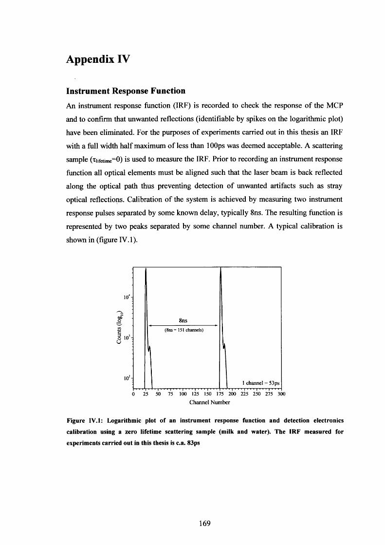
Appendix IV

Instrument Response FunctionAn instrument response function (IRF) is recorded to check the response of the MCP

and to confirm that unwanted reflections (identifiable by spikes on the logarithmic plot)

have been eliminated. For the purposes of experiments carried out in this thesis an IRF

with a full width half maximum of less than lOOps was deemed acceptable. A scattering

sample (xiifetime=0) is used to measure the IRF. Prior to recording an instrument response

function all optical elements must be aligned such that the laser beam is back reflected

along the optical path thus preventing detection of unwanted artifacts such as stray

optical reflections. Calibration of the system is achieved by measuring two instrument

response pulses separated by some known delay, typically 8ns. The resulting function is

represented by two peaks separated by some channel number. A typical calibration is

shown in (figure IV. 1).

104 -

n b

00 8nsC/5

c3 1 /5 3o 10 -

o

(8ns = 151 channels)

i o 2 -

1 channel = 53psi 1 *1 ' ■ i ' ■ ■ .................. i , . i ] 11' . i , 1 1 1 , i , i , , , i

0 25 50 75 100 125 150 175 200 225 250 275 300Channel Number

Figure IV.l: Logarithmic plot of an instrument response function and detection electronics

calibration using a zero lifetime scattering sample (milk and water). The IRF measured for

experiments carried out in this thesis is c.a. 83ps

169

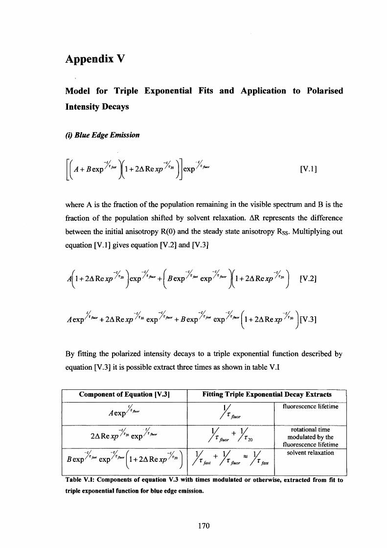
Appendix V

Model for Triple Exponential Fits and Application to Polarised

Intensity Decays

(i) Blue Edge Emission

- t / \A + Bexp /r fast \ + 2ARexp t20 exp *Jluor [V.l]

where A is the fraction of the population remaining in the visible spectrum and B is the

fraction of the population shifted by solvent relaxation. AR represents the difference

between the initial anisotropy R(0) and the steady state anisotropy Rss- Multiplying out

equation [V.l] gives equation [V.2] and [V.3]

A^l + 2ARe x p ^ 20 j exp '/*>or + 2? exp exp/*>or j^l + 2AR e x p ^ 20 j [V.2]

/ - / -*/ ~z ~z ( -v \A exp/Tflmr + 2A Re xp /TlQ exp ' Tp" + B exp ' T** exp /J>or 1 + 2A Re xp /T2a [V.3]

V J

By fitting the polarized intensity decays to a triple exponential function described by

equation [V.3] it is possible extract three times as shown in table V.l

Component of Equation [V3] Fitting Triple Exponential Decay Extracts

zA exp /Tflx°r Jluor

fluorescence lifetime

~Z -y 2ARe x p /T2S> exp7Tfhor X +x/ 1 Jluor / 1 20

rotational time modulated by the

fluorescence lifetime-y -y ( -y \

B exp/Tfasl exp/T/!uor 1 + 2 A Re xp /T20V /

X +X X/ Jast / Jluor / fastsolvent relaxation

Table V.l: Components of equation V.3 with times modulated or otherwise, extracted from lit to

triple exponential function for blue edge emission.

170

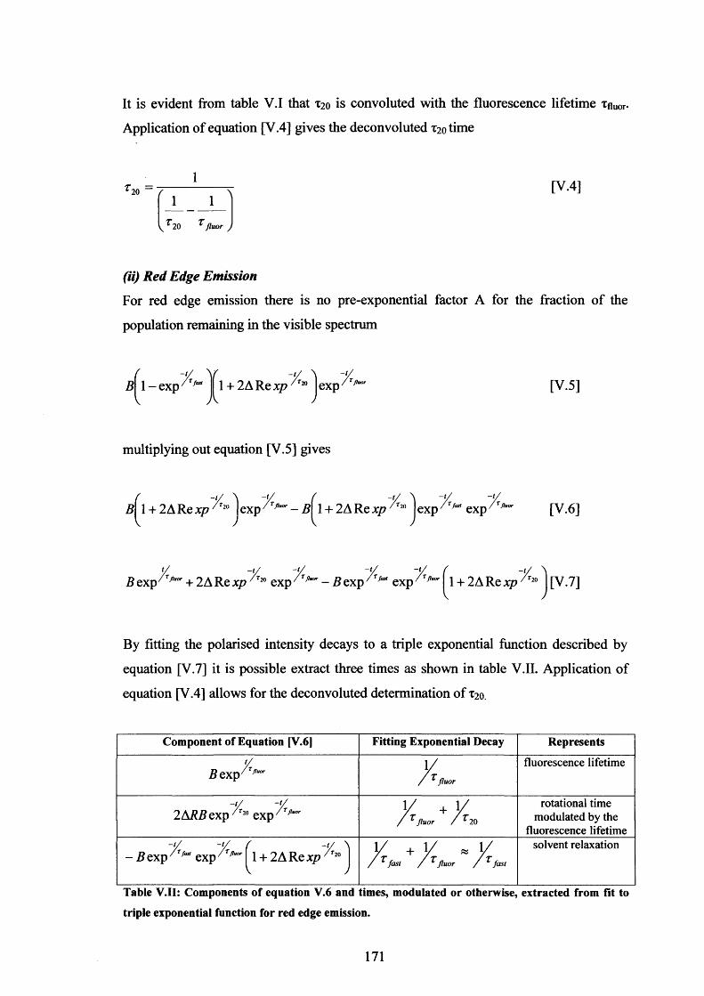
It is evident from table V.l that T20 is convoluted with the fluorescence lifetime TflUOr.

Application of equation [V.4] gives the deconvoluted X2otime

^20 —1 1

yT20 flu or j

[V.4]

(ii) Red Edge Emission

For red edge emission there is no pre-exponential factor A for the fraction of the

population remaining in the visible spectrum

B 1 - exp Afast 1 + 2 A Re xp /f2° exp ' T-* flu o r [V.5]

multiplying out equation [V.5] gives

B- t / \

1 + 2 A Re xp Al<i exp /Tfluor - B 1 + 2 A Re xp | exp /Tfast exp / Tfluor [V.6]/ V

- t / - t /

v - / ~Z ~Z ~Z ( ~z \B e x p 'Tjlmr + 2A Re xp /r2° exp - B exp /r/a” exp /Tj,uor 1 + 2A Re xp ^ 20 [V.7]

V J

By fitting the polarised intensity decays to a triple exponential function described by

equation [V.7] it is possible extract three times as shown in table V.II. Application of

equation [V.4] allows for the deconvoluted determination of X20

Component of Equation [V.6] Fitting Exponential Decay Represents

Bexp7 fluorflu or

fluorescence lifetime

~z ~z2A R 8exp/r20 exp /T/w X +x/ 1 flu or / 4 20rotational time

modulated by the fluorescence lifetime

- / - / ( -v \- B exp /r/aa exp /Tfluor 1 + 2 A Re xp A l°

\X +X KX/ fa s t / 1 flu or / fa s t

solvent relaxation

Table V.II: Components of equation V.6 and times, modulated or otherwise, extracted from fit to

triple exponential function for red edge emission.

171

Triple exponential functions are fitted to the vertically and horizontally polarised

intensity decays for excitation polarisation angles of P=0°, p=90° and p=54.7° allowing

for determination of X20, Tfluor and Xfast- Convoluted times are shown in table V.III.

Phase-Nematic Intensity (Vertical)Lambda (nm) p=o° P=54.7° p=90°

Excitation Emission Tl X2 x3 Tl *2 x3 Tl x2 x3440 455-500 0.5854 1.9051 5.7355 0.6287 2.0052 5.7567 0.5512 1.8393 5.7525440 >530 0.3046 2.5392 5.8347 0.3476 Part* 5.7895 0.5117 1.9583 5.8234440 >570 0.4891 2.3639 5.8111 0.5118 N/A 5.7992 0.5276 1.6942 5.8307

Intensity (Horizontal)Lambda (nm) p=o° P=54.7° p=90°

Excitation Emission Xj X3 Tl x2 x3 Xl X2 X3440 455-500 0.5547 1.9148 5.7438 0.6170 1.9820 5.7287 0.5419 1.8122 5.7248440 530 0.5851 N /A 5.7946 0.4091 2.9587 5.8485 0.3015 2.1887 5.7968440 >570 0.6435 N /A 5.8360 0.5031 3.0206 5.8481 0.3625 2.6447 5.8200

Table V.III: Convoluted times for xfasl(Ti), t 20( t 2) , and Tflnor(T3) from triple exponential fits to

vertically and horizontally polarised intensity decays at excitation polarization angles o f p=0°, p=90°

and p=54.7. It is evident that for vertically polarised intensity decays at excitation polarisation

angle p=54.7° and horizontally polarised intensity decays at excitation polarization angle p=0° it is

not possible to fit a triple exponential function to the intensity decays. Instead a double exponential

fit is made.

172

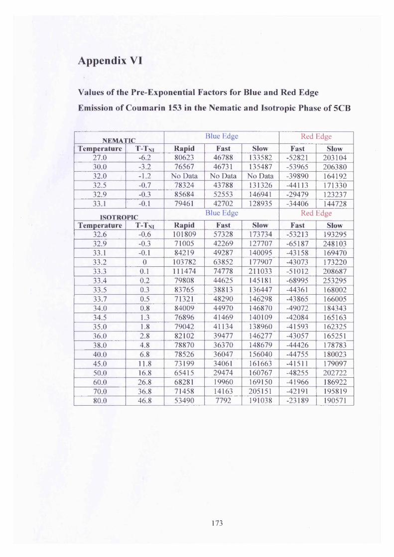
Appendix VI

Values o f the Pre-Exponential Factors for Blue and Red Edge

Emission o f Coumarin 153 in the Nematic and Isotropic Phase o f 5CB

NEMA1r i cBlue Edge Red Edge

Temperature T-Tni Rapid Fast Slow Fast Slow27.0 -6.2 80623 46788 133582 -52821 20310430.0 -3.2 76567 46731 135487 -53965 20638032.0 -1.2 No Data No Data No Data -39890 16419232.5 -0.7 78324 43788 131326 -44113 17133032.9 -0.3 85684 52553 146941 -29479 12323733.1 -0.1 79461 42702 128935 -34406 144728

ISOTROPIC Blue Edge Red EdgeTemperature T-Tni Rapid Fast Slow Fast Slow

32.6 -0.6 101809 57328 173734 -53213 19329532.9 -0.3 71005 42269 127707 -65187 24810333.1 -0.1 84219 49287 140095 -43158 16947033.2 0 103782 63852 177907 -43073 17322033.3 0.1 111474 74778 211033 -51012 20868733.4 0.2 79808 44625 145181 -68995 25329533.5 0.3 83765 38813 136447 -44361 16800233.7 0.5 71321 48290 146298 -43865 16600534.0 0.8 84009 44970 146870 -49072 18434334.5 1.3 76896 41469 140109 -42084 16516335.0 1.8 79042 41134 138960 -41593 16232536.0 2.8 82102 39477 146277 -43057 16525138.0 4.8 78870 36370 148679 -44426 17878340.0 6.8 78526 36047 156040 -44755 18002345.0 11.8 73199 34061 161663 -41511 17909750.0 16.8 65415 29474 160767 -48255 20272260.0 26.8 68281 19960 169150 -41966 18692270.0 36.8 71458 14163 205151 -42191 19581980.0 46.8 53490 7792 191038 -23189 190571

173