Corrosion_fatigue_and_fracture.pdf - UCL Discovery
321
CORROSION FATIGUE AND FRACTURE MECHANICS OF HIGH STRENGTH JACK UP STEELS Peter Terence Myers Submitted for the Degree of Doctor of Philosophy Department of Mechanical Engineering University College London February 1998
-
Upload
khangminh22 -
Category
Documents
-
view
1 -
download
0
Transcript of Corrosion_fatigue_and_fracture.pdf - UCL Discovery
CORROSION FATIGUE AND FRACTURE MECHANICS OF HIGH
STRENGTH JACK UP STEELS
Peter Terence Myers
Submitted for the Degree of
Doctor of Philosophy
Department of Mechanical Engineering
University College London
February 1998

ProQuest Number: U641859
All rights reserved
INFORMATION TO ALL USERS The quality of this reproduction is dependent upon the quality of the copy submitted.
In the unlikely event that the author did not send a complete manuscript and there are missing pages, these will be noted. Also, if material had to be removed,
a note will indicate the deletion.
uest.
ProQuest U641859
Published by ProQuest LLC(2015). Copyright of the Dissertation is held by the Author.
All rights reserved.This work is protected against unauthorized copying under Title 17, United States Code.
Microform Edition © ProQuest LLC.
ProQuest LLC 789 East Eisenhower Parkway
P.O. Box 1346 Ann Arbor, Ml 48106-1346
ABSTRACT
Jack up platforms are self elevating mobile units used fo r drilling and production
of offshore oil and gas reserves. These platforms utilise high strength weldable
steels fo r the fabrication of the truss leg structures. The yield strength of these
steels is typically around lOOMPa compared with 350MPa in standard fixed
jacket structures. Concern regarding the performance of such steels was
heightened by the discovery of cracking in and around the spud can of several
jack up platforms operating in the North Sea. It is thought that the higher strength
steels are more susceptible to material degradation due to Hydrogen
Embrittlement.
An experimental investigation has been performed to investigate and quantify the
magnitude of such deleterious effects. Seven fatigue tests have been performed on
large scale welded tubular joints fabricated from SE702, a 690MPa steel
commonly used in jack up construction. Cathodic protection levels of -SOOmV and
-lOOOmV (versus Ag/AgCl) were used. Evidence from these tests suggests that this
particular steel performs at least as well as lower strength steels in air and under
cathodic protection.
The shape of the tubular joints in jack up structures can be significantly different
from those found in conventional fixed structures. This can have a significant
effect on the stress distribution at the intersection of the tubular members.
Accurate knowledge of the stresses at the intersection is needed fo r design and
assessment purposes. Although the stress distribution in unstiffened joints has
been heavily researched, little work has been done fo r joints representative of jack
up legs. For this reason an extensive thin shell finite element investigation has
been performed to determine the stress distribution across a wide range of jack up
leg geometries. The distribution of stresses at the surface and through the
thickness of the chord members has been quantified. The results show that the ‘hot
spot' SCF can be reduced by as much as 50% compared to the corresponding
unstiffened joint.
The results of this stress analysis study have been integrated into a fatigue
fracture mechanics analysis of jack up representative geometries. Additionally,
contemporary fracture mechanics models have been assessed against fracture
mechanics data extracted from the experimental fatigue rests.
- 1 -

ACKNOWLEDGEMENTS
I wish to acknowledge the advice and guidance of my supervisors. Professor W. D.
Dover and Dr. F. P. Brennan whose faultless supervision has helped bring the best
out of this work.
Additionally I would like to thank my colleagues at the NDE Centre, especially
Linus Etube, Efrain Rodriguez Sanchez and Farid Ud-Din who have all helped
relieve my workload whilst I was writing this thesis. The assistance of the staff in
the Mechanical Engineering workshop is also gratefully recognised.
Finally I would like to thank EPSRC whose financial support made this work
possible.
- 2

TABLE OF CONTENTS
ABSTRACT............................................................................................................... 1
ACKNOWLEDGEMENTS......................................................................................2
TABLE OF CONTENTS...........................................................................................3
LIST OF FIGURES................................................................................................... 8
LIST OF TABLES................................................................................................... 18
NOMENCLATURE.................................................................................................20
1. In t r o d u c t io n a n d B a c k g r o u n d ............................................................................ 23
1.1 Introduction..................................................................................................... 23
1.2 Background to Fatigue of Tubular Joints.......................................................24
1.3 The Jack Up Platform...................................................................................... 27
1.3.1 The Jack Up Concept................................................................................28
1.3.2 Jack Up Leg Design..................................................................................28
1.3.3 Weld Procedures....................................................................................... 30
1.4 Loads Experienced by Jack Up Platforms......................................................30
1.5 The Use of High Strength Steels Offshore......................................................32
1.6 The Tubular Joint Intersection........................................................................ 33
1.7 Stress Analysis of Tubular Joints.....................................................................34
1.7.1 Stress Concentration Factors (SCF) in Tubular Joints............................ 37
1.7.2 Parametric Equations for Prediction of SCF...........................................40
1.7.3 Stress Distribution in Tubular Y and T Joints.........................................44
1.7.4 Comparison of Parametric SCF Prediction.............................................. 44
1.7.5 Ratio of Bending to Membrane Stress in Tubular Joints.........................46
1.8 Fatigue Design Guidance for Tubular Joints...................................................47
1.8.1 Development of U.K. Fatigue Guidance.................................................. 48
1.8.2 Development of the T-Curve....................................................................48
- 3 -
1.8.3 Analysis of Experimental Data to Produce S-N Curve...........................50
1.8.4 Allowance Factors to be Used in Conjunction with the Basic S-N Curve.52
1.8.5 Design Code Treatment of High Strength Steels.................................... 55
1.9 Linear Elastic Fracture Mechanics................................................................. 56
1.10 Stress Intensity Factor Solutions for Welded Joints.................................... 61
1.11 Factors Affecting Fatigue Crack Growth in Tubular Joints.........................63
1.12 Environment Assisted Fatigue Mechanisms................................................. 64
1.12.1 Free Corrosion........................................................................................65
1.12.2 Cathodic Protection................................................................................ 66
1.13 Effect of Environment on Fatigue Crack Growth Rate............................... 73
1.14 Effect on Environment on the Fatigue Lives of Welded Joints................... 75
1.15 Aims and Objectives......................................................................................77
1.16 References...................................................................................................... 80
2. E x pe r im e n t a l Fa t ig u e T e stin g o f W e l d e d T u bu l a r J o in t s ............ 117
2.1 Introduction................................................................................................... 117
2.2 Tubular Joint Test Specimens....................................................................... 117
2.2.1 Dimensions..............................................................................................118
2.2.2 Specimen Fabrication..............................................................................119
2.2.3 Material Properties..................................................................................120
2.2.4 Mechanical Properties of SE702.............................................................121
2.3 Experimental Set Up...................................................................................... 122
2.3.1 Applied Loading...................................................................................... 122
2.3.2 Fatigue Crack Monitoring...................................................................... 123
2.3.3 Environment Chamber............................................................................ 128
2.3.4 Test Control and Data Acquisition........................................................ 129
2.4 Experimental Stress Analysis........................................................................ 130
2.4.1 Strain Gauge Siting...............................................................................132
- 4 -

2.4.2 Determination of SCF’s...........................................................................133
2.4.3 Experimental SCF Results...................................................................... 134
2.5 Fatigue Test Programme................................................................................136
2.5.1 Test Parameters...................................................................................... 137
2.5.2 ACPD Data Analysis...............................................................................138
2.5.3 Crack Shape.............................................................................................140
2.6 Fatigue Test Results...................................................................................... 140
2.6.1 S-N Data.................................................................................................. 141
2.6.2 Crack Growth Curves.............................................................................143
2.6.3 Fatigue Crack Growth Rates..................................................................144
2.6.4 Fatigue Crack Initiation.......................................................................... 145
2.6.5 Crack Shape Development..................................................................... 146
2.7 Examination of Fracture Surfaces.................................................................146
2.8 Discussion...................................................................................................... 147
2.9 Conclusions.................................................................................................... 149
2.10 References.................................................................................................... 151
3. St r e ss C o n c e n t r a t io n s in T u bu l a r J o in t s w it h R a c k / R ib P la t e
St if f e n e d C h o r d M em be r s U sin g Th e Fin it e E l e m e n t M e t h o d ........... 181
3.1 Introduction................................................................................................... 181
3.2 Scope..............................................................................................................181
3.3 Stress Analysis of Stiffened Tubulars............................................................182
3.4 Mesh Generation for Tubular Joints with Longitudinal Stiffeners.............. 186
3.5 Boundary Conditions..................................................................................... 190
3.6 Convergence and Model Verification............................................................190
3.7 Finite Element Investigation.......................................................................... 191
3.7.1 Effect of Rack Plate Thickness on SCF Distribution.......................... 191
- 5

3.7.1.1 Results........................................................... 191
3.7.2 Effect of Rack and Rib Plate Geometry on the SCF............................. 193
3.7.2.1 Results................................................................................................194
3.7.3 Investigation of Mechanisms Using Boundary Conditions....................197
3.7.3.1 Results................................................................................................197
3.7.4 Effect of a Continuous Thickness Rack Plate Across a Range of Joint
Parameters.........................................................................................................199
3.7.4.1 Results................................................................................................200
3.8 Conclusions and Recommendations............................................................. 201
3.9 References......................................................................................................203
4. T h e E f fe c t o f a Ra c k / Rib Pl a t e o n t h e D e g r e e o f T h r o u g h
T h ic k n e ss B e n d in g in Ja c k U p C h o r d s .................................................................. 233
4.1 Introduction...................................................................................................233
4.2 Scope............................................................................................................. 233
4.3 Through Thickness Stress Distributions in Tubular Joints...........................234
4.3.1 The Importance of Through Thickness Stress Distribution.................. 235
4.3.2 Determination of Through Thickness Stress Distribution.................... 239
4.4 Mesh Generation and Boundary Conditions................................................ 239
4.5 Convergence and Model Verification........................................................... 242
4.6 Finite Element Investigation.......................................................................... 243
4.6.1 Effect of Rack Plate Thickness on Through Thickness Stress
Distributions.....................................................................................................243
4.6.1.1 Results................................................................................................243
4.6.2 Effect of Rack and Rib Plate Geometry on Through Thickness Stress
Distributions.....................................................................................................245
4.6.2.1 Results................................................................................................245
4.6.3 Effect of Continuous Thickness Rack on Through Thickness Stress
Distributions Across a Range of Joint Parameters..........................................248
- 6 -
4.6.3.1 Results................................................................................................249
4.7 Discussion...................................................................................................... 250
4.8 Conclusions and Recommendations............................................................. 251
4.9 References...................................................................................................... 253
5. F r a c t u r e M ec h a n ic s M o d e l l in g o f Ja c k U p C h o r d D e f e c t s 276
5.1 Introduction...................................................................................................276
5.2 Stress Intensity Factors in Tubular Joints.....................................................277
5.3 Y Factor Predictions Using Empirical Models............................................. 278
5.3.1 Extraction of Y Factors from Crack Growth Data............................... 278
5.3.2 AVS Model............................................................................................. 279
5.3.3 TPM Model............................................................................................ 281
5.3.4 Modified AVS Model............................................................................. 282
5.3.5 Evaluation of Experimentally Derived Models......................................283
5.3.6 Fatigue Crack Growth Predictions.........................................................284
5.4 Finite Element Based Models........................................................................285
5.5 Flat Plate Derived Models............................................................................. 288
5.5.1 Newman-Raju Equations........................................................................288
5.5.2 Correction for Load Shedding............................................................... 291
5.5.3 Correction for Non Uniform Stress Distribution.................................. 292
5.5.3.1 Albrechts Method for Calculation of SIF’s ......................................292
5.5.4 Crack Shape Correction.........................................................................294
5.6 Effect of Rack Plate on Fatigue Crack Growth Predictions....................... 295
5.7 Conclusions....................................................................................................297
5.8 References......................................................................................................299
6. Su m m a r y , C o n c lu sio n s a n d Re c o m m e n d a t io n s ......................................... 315
7 -
L IS T O F F IG U R E S
C h a p te r O n e Page
Figure 1.1 Schematic of a typical jack up rig................................. 93
Figure 1.2 The four main chord designs.......................................... 94
Figure 1.3 Split tubulars with double racks. Range of chord sizes
and shapes..................................................................... 94
Figure 1.4 Tubular chords with central racks. Range of chord
shapes and sizes............................................................. 95
Figure 1.5 Tubular chords with offset racks. Range of chord
shapes and sizes............................................................. 95
Figure 1.6 Leg plan schematic showing main components 96
Figure 1.7 General view of jack up leg showing rack detail 96
Figure 1.8 Complex nature of leg bracing and span breakers in a
modern jack up.............................................................. 97
Figure 1.9 Overlapped bracing and weld detail in a modem jack
up leg............................................................................... 97
Figure 1.10 Common tubular joint configurations............................. 98
Figure 1.11 T joint parametric notation.............................................. 98
Figure 1.12 Jack up transportation modes.......................................... 99
Figure 1.13 The three tubular joint loading modes............................. 99
Figure 1.14 T joint response to axial loads.......................................... 100
Figure 1.15 Weld toe terminology...................................................... 100
Figure 1.16 UKOSRP and ECSC definition of Hot Spot Stress 101
Figure 1.17 Regions of strain linearity used to determine hot spot
stress................................................................................ 101
Figure 1.18 Modelling the weld intersection using thick shell
elements.......................................................................... 102
Figure 1.19 Thin shell FEA modelling of a tubular joint intersection 103
Figure 1.20 T joint stress distributions for axial, IPB and OPB
loading modes................................................................. 104
- 8
Figure 1.21 Parametric chord crown SCF prediction dependency
on Alpha......................................................................... 104
Figure 1.22 Parametric chord crown SCF prediction dependency
on Beta............................................................................ 105
Figure 1.23 Parametric chord crown SCF prediction dependency
on Gamma...................................................................... 105
Figure 1.24 Parametric chord crown SCF prediction dependency
on Tau.............................................................................. 106
Figure 1.25 Parametric chord saddle SCF prediction dependency
on Alpha......................................................................... 106
Figure 1.26 Parametric chord saddle SCF prediction dependency
on Beta............................................................................ 107
Figure 1.27 Parametric chord saddle SCF prediction dependency
on Gamma...................................................................... 107
Figure 1.28 Parametric chord saddle SCF prediction dependency
on Tau.............................................................................. 108
Figure 1.29 16mm 50D fatigue life data together with mean and
design S-N curves.......................................................... 108
Figure 1.30 Thickness effect illustrated by 16 and 32mm fatigue life
data.................................................................................. 109
Figure 1.31 Nested T curves from thickness effect allowance 109
Figure 1.32 S-N curves for 16mm plates and tubulars in sea water
(free corrosion) and optimum cathodic protection 110
Figure 1.33 Cartesian co-ordinates for near crack analyses.............. 110
Figure 1.34 The three modes of crack growth................................... I l l
Figure 1.35 The three stages of fatigue crack growth...................... I l l
Figure 1.36 SIF development in tubular joints and welded plates.... 112
Figure 1.37 Crack depth development in tubulars and welded plates 112
Figure 1.38 The electrochemical corrosion process........................... 113
Figure 1.39 Impressed current cathodic protection........................... 113
- 9
Figure 1.40 Effect of CP potential on fatigue crack growth rate
(O.lHz, R<=0.1)............................................................. 114
Figure 1.41 Schematic da-dN plot showing plateau growth rate
region under CP conditions.......................................... 114
Figure 1.42 Independence of crack growth rate to AK in X65
under CP conditions...................................................... 115
Figure 1.43 High strength steel crack growth rates from Billingham
etal................................................................................. 116
Chapter TwoFigure 2.1 Nominal specimen dimensions for tubular welded T
joints................................................................................ 161
Figure 2.2 Position of seam welds in tubular T Joints...................... 161
Figure 2.3 Photograph of seam and intersection weld..................... 162
Figure 2.4 Definition of weld leg lengths......................................... 162
Figure 2.5 Isometric view of test rig................................................ 163
Figure 2.6 ACPD theory and notation.............................................. 163
Figure 2.7 Typical un-modified ACPD crack development data... 164
Figure 2.8 Typical modified ACPD crack development data 164
Figure 2.9 Experimental test setup.................................................. 165
Figure 2.10 Terminology for specimen / actuator alignment 165
procedure........................................................................
Figure 2.11 Strain gauge positions for experimental stress analysis. 166
Figure 2.12 Experimental stress analysis results................................. 166
Figure 2.13 S-N data from tubular joint tests on
SE702............................................................................. 167
Figure 2.14 Crack Growth Curve for Test ‘T T ................................. 167
Figure 2.15 Crack Growth Curve for Test ‘T2’ ................................. 168
Figure 2.16 Crack Growth Curve for Test T 3 ’ ................................. 168
Figure 2.17 Crack Growth Curve for Test ‘T4’ ................................. 169
Figure 2.18 Crack Growth Curve for Test ‘T6’ ................................. 169
- 10 -
Figure 2.19 Comparison of Fatigue Crack Growth Curves.............. 170
Figure 2.20 Crack Growth Rates recorded during Test T1............. 170
Figure 2.21 Crack Growth Rates recorded during Test T2............. 171
Figure 2.22 Crack Growth Rates recorded during Test T3............. 171
Figure 2.23 Crack Growth Rates recorded during..Test T4............. 172
Figure 2.24 Crack Growth Rates recorded during..Test T6............. 172
Figure 2.25 Comparison of Crack Growth Rates............................... 173
Figure 2.26 Early crack growth profiles showing initiation in a
typical test........................................................................ 173
Figure 2.27 Early crack growth data showing initiation in a typical
test................................................................................... 174
Figure 2.28 Ratio of initiation to total fatigue lives........................... 174
Figure 2.29 Initiation to propagation lives normalised to the T
curve................................................................................ 175
Figure 2.30 Graphical representation of the ratio of initiation to
propagation life............................................................... 175
Figure 2.31 Crack shape data.............................................................. 176
Figure 2.32 S-N curve showing all SE702 tubular joint data 177
Figure 2.33 Difference between axial and OPB loading modes for
50D steels........................................................................ 178
Figure 2.34 Life conversion factors for axial to OPB loading modes 178
Figure 2.35 S-N curve showing modified T joint results using
loading mode modification factor.................................. 179
Figure 2.36 Comparison of results with nominally identical
specimens made from lower strength steels................. 180
Figure 2.37 Comparison of results with database of cathodically
protected 50D specimens............................................... 180
Chapter Three
Figure 3.1 Tubular joint showing position of stiffener.................... 208
Figure 3.2 Tubular joint showing dual thickness stiffener.............. 208
- 11 -

Figure 3.3 Tubular joint showing non continuous stiffener.............. 209
Figure 3.4 Tubular joint with internal ring stiffeners...................... 209
Figure 3.5 Tubular joint with doubler plate..................................... 210
Figure 3.6 Sample T joint finite element mesh................................. 210
Figure 3.7 Effect of normalised stiffener thickness on SCF
distribution in an axially loaded T joint.......................... 211
Figure 3.8 Effect of normalised stiffener thickness on SCF
distribution for axially loaded Y joint............................. 211
Figure 3.9 Effect of plate thickness on Normalised SCF
distribution for axially loaded T joint............................. 212
Figure 3.10 Effect of plate thickness on normalised SCF
distribution for axially loaded Y joint............................. 212
Figure 3.11 Effect of plate thickness on SCF for IPB loaded T joint 213
Figure 3.12 Effect of plate thickness on SCF for IPB loaded Y
joint.................................................................................. 213
Figure 3.13 Effect of plate thickness on SCF distribution for OPB
loaded T joint.................................................................. 214
Figure 3.14 Effect of plate thickness on SCF distribution for OPB
loaded Y joint.................................................................. 214
Figure 3.15 Effect of plate thickness on SCF distribution for OPB
loaded T joint.................................................................. 215
Figure 3.16 Effect of plate thickness on SCF distribution for OPB
loaded Y joint.................................................................. 215
Figure 3.17 Effect of plate thickness on saddle SCF for Axial and
OPB loaded T & Y joints............................................... 216
Figure 3.18 Terminology and notation used to describe models
with non-continuous stiffeners...................................... 216
Figure 3.19 Effect of rib plate on axially loaded T joint.................... 217
Figure 3.20 Effect of rib plate on axially loaded T joint.................... 217
Figure 3.21 Effect of rib plate on axially loaded T joint.................... 218
- 12 -
Figure 3.22 Effect of rib plate on OPB loaded T joint....................... 218
Figure 3.23 Effect of rib plate on OPB loaded T joint....................... 219
Figure 3.24 Effect of rib plate on OPB loaded T joint....................... 219
Figure 3.25 Effect of rack plate thickness for axially loaded joint... 220
Figure 3.26 Effect of rack plate thickness for OPB loaded joint 220
Figure 3.27 Effect of rack plate depth for axially loaded joint 221
Figure 3.28 Effect of rack plate depth for OPB loaded joint 221
Figure 3.29 Case 1 - Chord deformation restrained in all degrees of
freedom along line shown............................................... 222
Figure 3.30 Case 2 - Chord deformation restrained in Z direction
along line shown.............................................................. 222
Figure 3.31 Case 3 - Chord deformation restrained in Z direction
and rotation about X axis along line shown.................. 223
Figure 3.32 Case 4 - Chord deformation restrained in Z direction
and rotation about Y axis along line shown.................. 223
Figure 3.33 Case 5 - Chord deformation restrained in Z direction
and rotations about X and Y axes along line shown.... 224
Figure 3.34 Case 6 - Chord deformation restrained in rotations
about X axis along line shown........................................ 224
Figure 3.35 Case 7 - Chord deformation restrained in Y and Z
direction and rotations about X axis along line shown.. 225
Figure 3.36 Simulation of the effect of a stiffener using boundary
conditions....................................................................... 225
Figure 3.37 Simulation of the effect of a stiffener using boundary
conditions....................................................................... 226
Figure 3.38 Simulation of the effect of a stiffener using boundary
conditions....................................................................... 226
Figure 3.39 Simulation of the effect of a stiffener using boundary
conditions....................................................................... 227
Figure 3.40 Effect of Alpha on an axially loaded T joint.................. 227
- 13 -

Figure 3.41 Effect of Alpha on an OPB loaded T joint...................... 228
Figure 3.42 Effect of Beta on an axially loaded T joint...................... 228
Figure 3.43 Effect of Beta on an OPB loaded T joint....................... 229
Figure 3.44 Effect of Gamma on an axially loaded T joint................ 229
Figure 3.45 Effect of Gamma on an OPB loaded T joint................... 230
Figure 3.46 Effect of Tau on an axially loaded T joint...................... 230
Figure 3.47 Effect of Tau on an OPB loaded T joint......................... 231
Figure 3.48 Effect of Theta on an axially loaded T joint................... 231
Figure 3.49 Effect of Theta on an OPB loaded T joint...................... 232
Chapter Four
Figure 4.1 Tubular T joint showing position of constant thickness
stiffener........................................................................... 256
Figure 4.2 Tubular joint showing dual thickness stiffener.............. 256
Figure 4.3 Tubular joint showing non conditions stiffener 257
Figure 4.4 Effect of loading mode using experimental database
results............................................................................... 257
Figure 4.5 Through thickness stress distribution.............................. 258
Figure 4.6 Examples of various values of the DoB parameter 258
Figure 4.7 Change of bending and membrane stress component at
the cracked section from experimental measurements
on a large scale, axially loaded tubular joint.................. 259
Figure 4.8 Deformed mesh for axially loaded T joint....................... 259
Figure 4.9 Validation of FE model using acrylic model results 260
Figure 4.10 Comparison of thick and thin shell model DoB results.. 260
Figure 4.11 DoB values for a range of rack thicknesses under axial
loading............................................................................. 261
Figure 4.12 DoB values for a range of rack thicknesses under OPB
loading............................................................................. 261
Figure 4.13 DoB values for a range of rack thicknesses under IPB
loading............................................................................. 262
- 14
Figure 4.14 Normalised DoB values under Axial loading................. 262
Figure 4.15 Normalised DoB values under OPB loading.................. 263
Figure 4.16 Normalised DoB values under IPB loading.................... 263
Figure 4.17 Summary of normalised DoB data for tubular joints
with rack plates............................................................... 264
Figure 4.18 Terminology and notation used to describe models
with non-continuous stiffeners...................................... 264
Figure 4.19 Effect of rib plate on DoB in an axially loaded T joint.. 265
Figure 4.20 Effect of rib plate on DoB in an axially loaded T joint.. 265
Figure 4.21 Effect of rib plate on DoB in an axially loaded T joint.. 266
Figure 4.22 Effect of rib plate on DoB in an OPB loaded T joint.... 266
Figure 4.23 Effect of rib plate on DoB in an OPB loaded T joint.... 267
Figure 4.24 Effect of rib plate on DoB in an OPB loaded T joint.... 267
Figure 4.25 Effect of rib plate on DoB in an IPB loaded T joint 268
Figure 4.26 Effect of rib plate on DoB in an IPB loaded T joint 268
Figure 4.27 Effect of rib plate on DoB in an IPB loaded T joint 269
Figure 4.28 Dependency of DoB on ratio of chord length and
diameter (Alpha)............................................................. 270
Figure 4.29 Dependency of DoB on ratio of brace and chord
diameters (Beta).............................................................. 271
Figure 4.30 Dependency of DoB on ratio of chord diameter to
thickness (Gamma).......................................................... 272
Figure 4.31 Dependency of DoB on ratio of brace to chord
thickness (Tau)............................................................... 273
Figure 4.32 Dependency of DoB on brace angle (Theta).................. 274
Figure 4.33 Measure of accuracy of ‘Saddle’ parametric equation
of Connolly e ta l.............................................................. 275
Figure 4.34 Measure of accuracy of ‘Hot Spot’ parametric
equation of Connolly et at............................................... 275
- 1 5 -

Chapter 5
Figure 5.1 Centre cracked infinite plate........................................... 302
Figure 5.2 Yexp factors for Test T l ’ ............................................... 302
Figure 5.3 Yexp Factors for Test T2................................................ 303
Figure 5.4 Comparison of empirical SIF models with Y xp results
from Test T l .................................................................... 303
Figure 5.5 Comparison of empirical SIF models with Y xp results
from Test T2.................................................................... 304
Figure 5.6 Fracture mechanics crack growth results for Test T l. . . 304
Figure 5.7 Fracture mechanics crack growth results for Test T2 ... 305
Figure 5.8 Power Law fit for Yexp data from Test T l ................... 305
Figure 5.9 Power Law fit for Yexp data from Test T2................... 306
Figure 5.10 Chong Rhee Y Factors for Test T l ............................... 306
Figure 5.11 Chong Rhee Y Factors for Test T2............................... 307
Figure 5.12 Notation used by Newman Raju Equations.................. 307
Figure 5.13 Y Factors using flat plate based solutions for Test T l. 308
Figure 5.14 Y Factors using flat plate based solutions for Test T2. 308
Figure 5.15 SCF due to weld for tensile loading............................... 309
Figure 5.16 SCF due to weld for bending loading............................. 309
Figure 5.17 Albrechts Method for Calculating Yg............................ 310
Figure 5.18 Correction Factors (Yg) for non-uniform stress
distribution...................................................................... 311
Figure 5.19 Crack shape correction factors........................................ 311
Figure 5.20 AVS Model prediction of the effect of a rack plate on
crack propagation........................................................... 312
Figure 5.21 Modified AVS Model prediction of the effect of a rack
plate on crack propagation............................................. 312
Figure 5.22 AVS Model propagation lives normalised to that of the
unstiffened Joint.............................................................. 313
1 6 -

Figure 5.23 Crack shape development used with Newman Raju
model, derived from experimental data......................... 313
Figure 5.24 Effect of rack plate on crack propagation lives using
modified Newman Raju................................................... 314
17 -
L IS T O F T A B L E S
C h a p te r O n e Page
Table 1.1 Jack up design features.................................................... 90
Table 1.2 Jack up leg populations................................................... 90
Table 1.3 Truss leg design breakdown........................................... 91
Table 1.4 Recommended parametric equation for axially loaded
T joints...................................................................... 91
Table 1.5 Default geometric parameters used in model
Comparison............................................................... 91
Table 1.6 UK guidance S-N curves........................................... 92
Table 1.7 1984 Guidance on environmental effects....................... 92
Table 1.8 1990 Guidance on environmental effects....................... 92
C h a p te r T w o
Table 2.1 Ultrasonically measured wall thicknesses............... 154
Table 2.2 Seam welding details............................................... 154
Table 2.3 Intersection weld details........................................... 155
Table 2.4 Weld leg lengths....................................................... 155
Table 2.5 Chemical composition of SE702............................. 156
Table 2.6 Mechanical properties of SE702.............................. 156
Table 2.7 Measured mechanical properties............................. 156
Table 2.8 SE702 Charpy test data............................................ 157
Table 2.9 SE702 hardness data................................................ 157
Table 2.10 ACPD probe site locations...................................... 158
Table 2.11 Experimental SCF results from previous test
programme using same geometry........................... 158
Table 2.12 Experimental SCF results and parametric predictions... 159
Table 2.13 Original and revised test programme details........... 159
Table 2.14 S-N data for SE702.................................................. 160
- 18
Table 2.15 Summary of initiation data for all tests.............. 160
Table 2.16 Experimental results for parallel variable amplitude
study on SE702 Y joints.................................... 160
Chapter Three
Table 3.1 Non-dimensional joint parameters...................... 205
Table 3.2 Results of convergence study............................. 205
Table 3.3 Boundary conditions used to simulate the effect of a
rack/rib plate...................................................... 205
Table 3.4 Effect of Alpha on relative SCF....................................... 206
Table 3.5 Effect of Beta on relative SCF........................................ 206
Table 3.6 Effect of Gamma on relative SCF.................................. 206
Table 3.7 Effect of Tau on relative SCF.......................................... 206
Table 3.8 Effect of Theta on relative SCF....................................... 207
Chapter FourTable 4.1 Finite element model joint parameters................ 255
Table 4.2 Validation of FE model results........................... 255
Chapter Five
Table 5.1 Average stress parameters for different rack plate
thicknesses......................................................... 301
Table 5.2 Input parameters for adapted Newman Raju model
testing rack plate effect..................................... 301
- 1 9 -
NOMENCLATURE
û
4)
0
K.
4 x
(j)y
A
aa
A ,j
ACPD
Ag/AgCl
ASP
AVS
Pc
G, m
Cl, C2, C3, rrii, m2
CP
CPU
D
d
di
da/dN
Ac
DoB
A r
Brace angle
Relative permeability
Complete elliptical integral of second kind
Parameti'ic angle around intersection
Permeability of free space
Rotation about x
Rotation about y
Brace cross sectional area
Joint geometry factor, 2L/D
Crack Depth
AVS model parameters
Alternating Current Potential Drop
Silver / silver chloride reference electrode
Average stress parameter
Average stress model
Joint geometi-y factor, d/D
Surface crack half length
Paris Law constants
Empii'ical constants in crack growth law
Cathodic protection
Central processing unit
Chord diameter
Brace diameter
1-D crack depth
Crack Growth Rate
Cross crack probe spacing
Degree of Bending
Reference probe spacing
- 2 0 -
F Brace axial force
f AC frequency
Y Joint geometry factor, D/2T
Hv Vickers hardness
IPB In-Plane Bending
Ky SCF Correction Factor for stiffened tubulars
Ka / Kb Punching shear equation coefficients
Ka / Q’ Factors in Lloyds Register SCF Eqn.
Ki S-N Curve intercept
Ki Mode I SIF
Kn Mode II SIF
Kffl Mode II I SIF
L Chord length
1 Brace length
m Gradient of S-N curve
M, B, k, p TPM model parameters
Mx ACPD modifier
N Number of cycles
Ni Fatigue initiation life
Nt Total fatigue life
NT Life predicted by T Curve
OPB Out-of-Plane Bending
PWHT Post weld heat treatment
r Distance from crack tip
R Apphed stress ratio
a Stress / Conductivity
S Hot spot stress range
Ga Brace nominal axial stress
Cb Brace nominal bending stress / Bending stress
-21 -

S b Stress Range at Reference thickness, te
SCE Calomel reference electrode
SCF Stress concentration factor
SCFav Average intersection stress concentration factor
SCFh Hot spot stress concentration factor
SIF Stress Intensity Factor
Membrane stress
^nom Brace nominal stress
Gt Total stress, (Tm+Gg
G y y Crack opening stress
z Joint geometry factor, t/T
T Chord thickness
t Brace thickness
tl Rack plate thickness
a Rib plate thickness
te Reference thickness
Te Equivalent thickness
TPM Two phase model
Vc, Vci, Vc2 Cross crack potential drop
V r , V r i , V r2, V io Reference potential drop
Y SIF modification factor
z Rack plate depth
2 2 -

Chapter 1 - Introduction and Background to Fatigue of Tubular Joints
Chapter One
1. Introduction and Background
1.1 Introduction
High strength weldable steels, defined as having a yield point above 450MPa are
being used in ever increasing tonnages offshore. Unfortunately, information on the
properties of these steels is limited and this is reflected in the restrictions on the
applicability of S-N curves to relatively low yield strength steels and maximum
permissible yield ratio specified by offshore design codes. This has to some extent
limited the designers ability to maximise the potential benefits offered by high
strength steels.
One area where the use of high strength weldable steels is well established is in the
construction of jack up rig legs. These steels are utilised extensively in the
fabrication of the chord, rack and spud cans of these self elevating mobile units.
Concern about the performance of these steels in the severe environmental and
loading conditions in the North Sea was heightened by the discovery of cracking in
and around the spud cans of jack ups operating in the North Sea in the late 1980’s
[1.1].
Data from large scale welded tubular joint fatigue tests performed under
representative environmental conditions (i.e. sea water with cathodic protection
and overprotection) is needed if confidence is to be gained regarding the
performance of these steels offshore.
Experimental investigations performed as part of this PhD thesis aim to address
some of the shortfall in data for high strength weldable steels. The fatigue tests
presented in this thesis are amongst the highest strength large scale steel welded
tubular joints tested under conditions of cathodic protection performed world
wide. As such it is hoped that the current investigation will promote discussion and
2 3 -

Chapter 1 - Introduction and Background to Fatigue of Tubular Joints
further experimental investigations to enable the advantages and limitations of such
steels to be quantified.
1.2 Background to Fatigue of Tubular Joints
Fatigue and corrosion fatigue behaviour of tubular joints has been researched
extensively over the last two decades. This research has taken many forms
including full scale tubular welded joint fatigue tests, small scale tubular welded
joint fatigue tests, welded plate tests, simple specimen tests and finite element
analysis. All of the above wiU be discussed in detail in this Chapter. The individual
contribution of each of the techniques to the current knowledge of the (corrosion)
fatigue behaviour of tubular joints will be assessed.
The vast majority of this research has been focused on steels representative of
those used in the tubular connections of fixed jacket structures. One such steel,
BS4360 Gr5()D [1.2] (or BS7191 Gr355D [1.3]) has been the standard for the
construction of many fixed jacket platforms and thus has been by far the most
widely researched and the norm for laboratory tubular joint fatigue tests. As a
direct result, large amounts of data already exist for these medium strength
weldable steels. The pertinent conclusion drawn from this body of data by
researchers across Europe and to a lesser extent USA and Japan will be presented
in this Chapter. This will serve as a basis for assessing the performance of the steel
under investigation in this thesis.
The above mentioned body of data has allowed the formulation of fracture
mechanics models to predict the (corrosion) fatigue behaviour of welded tubular
joints. These models are of differing complexity and to a large extent accuracy. The
more widely recognised of the models will be presented and assessed in Chapter 5.
These models wül be compared against the results of the fatigue test programme
conducted for this PhD study.
- 2 4 -
Chapter 1 - Introduction and Background to Fatigue of Tubular Joints
The impetus for this research programme stems from the concerns regarding the
changing role envisaged for offshore jack up structures which utilise these higher
strength steels in the lattice leg structure. A typical jack up platform will be
described in detail later in the chapter with an emphasis on the leg structure and
chord design. Traditionally jack up rigs have been utilised for short term drilling
assignments. Such assignments last for a period of a few months at a single site
before the legs are raised out of the water and the vessel moved to a new site or to
dock. This short assignment cycle allows regular NDT (non destructive testing)
inspections to be undertaken with relative ease, with remedial action taken if
necessary. AH of this can be done with the legs fully raised out of the water
eliminating the need for expensive diving procedures and hyperbaric welding
operations.
Secondly the mobile nature of these rigs implies that they are likely to be operating
in differing water depths throughout their operational lives. The implications of
which are important if one considers the effect on the fatigue loading of individual
tubular connections in the leg lattice. It is thought to be likely that the most fatigue
critical location in the leg would be related to the position of the topside platform
along the leg lattice i.e. the water depth. Thus the most highly stressed region of
the leg structure at one water depth is unlikely to be the same when the rig is
operating in a greater or shallower water depth. This is in contrast to a jacket
structure where the most highly stressed regions are most likely to remain
stationary during the life of the structure, hence broadly speaking, most susceptible
to fatigue damage. A further area of concern for jack ups is near the spud can
where high bending stresses can be present under conditions of high fixity.
Thus mobile jack up rigs may be considered to be in a fortunate position as far as
fatigue is concerned and designers of such structures have in the past been more
occupied in ultimate strength design of the legs under the maximum operational
and environmental loads envisaged during the lifetime of the structure.
-25
Chapter 1 - Introduction and Background to Fatigue of Tubular Joints
This however is now changing as jack ups are being prepared for a new role as
production platforms rather than mobile drilling rigs. Compared to the more
traditional production platform designs, jack up structures are relatively cheap in
terms of construction and installation. Indeed a jack up can be considered as being
self installing, thus removing the need for expensive heavy lift equipment etc.
required during traditional jacket platform installations. As a direct result of this
B.P.’s ground breaking Harding platform, a jack up currently being used for
production purposes is expected to be one of the most economical platforms in
terms of cost per barrel in the whole of the North Sea [1.4]. The success of this
platform is likely to lead to wider use of this concept for the exploitation of more
marginal fields.
This however removes the beneficial effect of short term assignments and varying
water depths mentioned previously. A production jack up must be designed in
terms of fatigue life as well as ultimate strength considerations. A fatigue life equal
or greater than the anticipated viable field life, often around 35 years, must be
demonstrated. Areas likely to suffer fatigue damage are to be highlighted at this
stage. Inspection schedules must be planned accordingly and of course inspection,
repair and maintenance tasks are subject to the same underwater difficulties and
expense as fixed jacket structures.
A further complication arises from material choice for the leg structure. Weight
considerations demand the use of thinner section, higher strength steels. The use of
thinner section implies higher nominal stress levels, further amplifying the need for
accurate fatigue crack growth data on such steels in representative environments.
Unfortunately the fatigue and corrosion fatigue behaviour of these steels is much
less well understood compared to the heavily researched BS4360Gr50D. One must
consider the effects of variable amplitude loading, cathodic protection level, weld
profile, corrosive sea water environment including the presence of Sulphate
Reducing Bacteria (SRB) and material susceptibility to Hydrogen Embrittlement
2 6 -
Chapter 1 - Introduction and Background to Fatigue of Tubular Joints
caused by Hydrogen generated by the C.P. system and the aforementioned SRB’s
present in many seabed muds.
The current investigation aims to address a part of this shortfall of data for such
steels. It is not possible in the limited time available to quantify all the effects
identified above, e.g. SRB’s were not present in the sea water used in the corrosion
fatigue tests. This work does however, form a valuable insight into the effect of
cathodic protection on large scale tubular joint corrosion fatigue behaviour. It is
the first time that such a programme has been undertaken on this scale using this
particular steel.
The seriousness of the problem in hand is highlighted in [1.5]. It is noted that
fatigue, especially of the leg and other components fabricated from higher strength
steel, will become more dominant in the determination of the useful life of jack up
rigs, as they move towards operating in more extreme conditions for longer
periods.
Massie et al [1.5] quote a recent analysis of the jack up failure statistics from the
World Offshore Accident Databank and notes that jack ups appear to be between
30 and 60 times more accident prone than fixed structures. This alarming accident
rate is by no means solely attributable to fatigue. However leg fatigue failure is
quoted as a significant cause together with “punch through” during installation and
insufficient deck clearance during storm conditions.
1.3 The Jack Up Platform.
The jack up platform will be described here in some detail. Special emphasis will be
placed on the leg structure and chord design as these are central to the current
investigation.
2 7 -
Chapter 1 - Introduction and Background to Fatigue of Tubular Joints
It should be noted at this stage that jack up platforms can vary enormously from
design to design and no single variety can be considered fully representative. An
attempt will be made to present the main variations found in each of the categories
described above together, where possible with a distribution of the occurrences in
the world jack up population.
1.3.1 The Jack Up Concept
Offshore jack up platform evolution can be traced back to posted barges operating
in 5-6 metres of water in the Mississippi Delta. The 15 years preceding 1970 saw
the greatest advances in jack up design with impressive improvements in operating
capabilities such as load carrying capability and increased water depths. A close
look at the evolution of jack ups shows how each designer produced individual
solutions to the design problems they faced. This is illustrated by the great array in
features found on jack ups produced in this period. Some of the major differences
are summarised in Table 1.1 [1.6].
Designs have now consolidated somewhat and jack ups are usually 3 legged
structures often capable of operating in water depths of over 100m. A schematic
view of a typical jack up is shown in Figure 1.1. Despite this rationalisation there
still exists many differences in the leg design found in current structures.
1.3.2 Jack Up Leg Design
The majority of modern jack ups now have three legs which can be raised and
lowered independently. This design has evolved over the years from the very early
designs that often had many more legs, one design specified 2 2 legs.
Of most interest is the detailed leg design. Some jack ups, usually for use in calm
shallow waters have square or circular closed section legs. More severe
environments require the more familiar truss type design to be employed. A survey
of Noble Demons mobile rig data hbrary [1.7, 1.8] is summarised in Tables 1.2 and
1.3.
-28
Chapter 1 - Introduction and Background to Fatigue of Tubular Joints
Of these designs only the three tubular chord designs will be further considered
despite the triangular chord being the single most popular design. This is due to it
being the preferred design of one of the worlds largest jack up manufacturers,
Marathon Le Tourneau. However, the triangular chord design bears little
resemblance to the remaining three tubular designs which are all essentially
variations on a theme. Only tubular specimens are considered in this study.
Full details of the leg design survey can be found in [1.7]. The major structural
dimensions are detailed along with the material properties of the chord and rack in
individual designs. The four main chord designs are shown schematically in Figure
1.2. Typical dimensions are for jack up chord details are given by Stacey et al [1.9]
who notes that rack plate typically varies between 150 and 250mm, whilst the
chords often have a diameter of between 800 and 1200mm and a thickness of 35 to
80mm. Some of the chord designs have been drawn to scale [1.7] to illustrate the
wide variety of shapes and sizes currently used in chord designs. These are shown
in Figures 1.3, 1.4 and 1.5.
Common design details that further complicate the analysis of the fatigue behaviour
of jack up legs include webs, stiffeners and overlapped joints at brace to brace and
chord to brace connections. A plan view of a typical leg is illustrated in Figure 1.6.
Also shown in this figure are the Leg Guides. Leg guides are found at the upper
and lower hull / leg intersection points at each chord and restrict the deformation
of the leg as it passes through the hull. The potential importance of leg guides is
highlighted in Chapter 4.
A recent visit to a ‘Harsh Environment’ jack up in an operational condition in the
North Sea allowed the close inspection of the leg structure. Of particular interest
were the weld details, cathodic protection system and rack geometry. The jack up
in question was constructed in Singapore and is one of the most modern jack ups
currently operating in the North Sea. A general view of the leg structure illustrating
2 9 -

Chapter 1 - Introduction and Background to Fatigue of Tubular Joints
the rack detail is shown in Figure 1.7. Note the jack house at the bottom of the
picture in Figure 1.7. The jack house contains the leg jacking mechanism, in this
case large electric motors and a hydraulic jack and chock system which mates with
the rack teeth when the jack up is in location. This allows the load to be taken off
the jacking mechanism. Each of the three legs has its own jack house which can be
controlled independently from the bridge. The complex nature of the bracing and
span breaker configuration is illustrated in Figure 1.8 and overlapped chord / brace
intersection are shown in Figure 1.9.
1.3.3 Weld Procedures
The weld procedures followed during construction of jack up legs often stipulate
that all welding is to be carried out to AWS D l. l [1.10]. Weld preparation and
run layout schematics followed during construction show great similarity to the
procedures adopted for the fabrication of the specimens to be utilised in the
experimental element of this study. The weld procedures used for the fabrication of
the T joint test specimens can be found in Chapter 3.
1.4 Loads Experienced by Jack Up Platforms
The loads experienced by jack up platforms arise from a number of sources but can
be divided in to two main categories [1.11]. These categories are operationally
derived loads and loads due to towing and transportation. Operational loads
include wind, wave and current loads together with platform weight, leg weight
and additional topside loads. Towing , or more generally transportation of jack ups
occurs with the legs fully raised out of the water. Two types of jack up
transportation are possible. These are the Wet Tow where the jack up sails under its
own power or is towed by tugs and the Dry Tow where the jack up rides on a
Piggy Back Vessel with its hull raised completely out of the water. The two
transportation modes are illustrated in Figure 1.10. In the towing modes the loads
arise from inertia forces from the motion of the platform and the self weight of the
leg.
-3 0

Chapter 1 - Introduction and Background to Fatigue of Tubular Joints
The differences in jack up response to wave loading are highlighted by Kam and
Birkinshaw [1.11]. In particular attention is drawn to the non-linear dynamic
response of jack ups in different sea states. It is stated that a framework is required
for generating “typical” fatigue loading experienced by tubular components in jack
up rigs. Four features of this framework were identified for inclusion as follows:
a) the simulation of a random sequence of multiple sea states;
b) the simulation of random load histories within each sea state according to given
multiple peak power spectra and the spectra should reflect the non-linear
features of the dynamic response of jack ups;
c) the simulation of transport loading under different conditions, and
d) a machine independent simulation framework.
A random load history for the fatigue testing (and remaining life analysis) specific
to jack up structures has been developed at UCL [1.12]. Known as JOSH (Jack up
Offshore Standardised load History) this framework accurately models the dynamic
load response of jack up rigs. Each of the four points detailed above has been
included except for the transit loading. This has been omitted for a number of
reasons namely the lack of data on loads experienced during towing and the fact
that the impetus behind this study is the use of jack ups for long term production.
Obviously in this instance towing loads will only occur as the platform is
transported from its point of construction to its operational site and as such are
significantly less important. Additionally transportation induced loading will cause
damage at different parts of the structure and therefore is omitted from fatigue
analysis.
Ohta et al [1.13] present an innovative, accurate and time saving method for the
structural analysis of jack up leg lattices. A detailed description of this method is
beyond the scope of this Chapter but interested parties are referred to this paper.
31 -

Chapter 1 - Introduction and Background to Fatigue of Tubular Joints
1.5 The Use of High Strength Steels Offshore
Traditional jacket construction has utilised steels restricted to yield strengths of
approximately 350MPa. Recently, however some higher strength steels of around
450MPa have accounted for up to 25% of the total structural weight [1.14]
although this is thought to be mainly confined to topside apphcations and bracing
in non fatigue critical locations.
High strength steels have improved significantly in recent years in terms of their
weldabihty. Traditional high strength steels of the Ni-Cr-Mo type used rich
chemistries to achieve the desired strength levels and are well known as being
difficult and expensive to weld.
The improved properties of modern high strength steels have been achieved using
the following principles [1.15]:
a) Relatively low carbon content which is beneficial to parent plate toughness and
weldabihty. Plate hardness increases with increasing carbon content.
b) Improved strength and toughness through grain refinement
c) Addition of strengthening microaUoying elements (V, Nb, Al) during steel
processing, sohd solution strengthening or transformation strengthening using
Mn, Ni, Cr, and Mo.
d) Reduced sulphur and phosphorous leading to increased toughness and
improved homogeneity in through thickness properties. Resistance to lamellar
tearing during welding is also improved.
Healy et al [1.16] have examined a group of 5 steels of yield strength
approximately equal to 690MPa. The composition, process route and weldabihty
of these steels were examined. The steels investigated were Q2N, 0X812, SE702,
DSE 690V, and HSLAIOO. Q2N is a traditional Ni-Cr-Mo developed primarily for
UK Naval use. 0X812, SE702 and DSE690V are modern, boron treated.
- 3 2 -

Chapter 1 - Introduction and Background to Fatigue of Tubular Joints
microalloyed, quenched and tempered European high strength steels with
significantly leaner chemistries than Q2N. HSLAIOO also follows the quenched and
tempered route but uses a copper precipitation strengthening technique and
reduced carbon levels (0.06%) to achieve its strength levels. It was concluded that
the modern high strength steels (0X812, SE702 and HSLAIOO) possess the
necessary combination of material properties and weldabihty to be considered as
suitable materials for offshore construction. Lower hardenabihty and reduced cold
cracking susceptibihty was noted for these steels. It was also concluded that further
research effort needs to be directed towards matching strength consumables to
overcome welding process limitations.
1.6 The Tubular Joint Intersection
Tubular joints are a common component in structural engineering and especially so
in offshore structures. A number of reasons exist for their popularity ranging from
aesthetic properties in building design and architectural circles through to the
minimisation of wave and wind forces offshore. The intersection between tubular
members has proved an interesting problem for the fatigue speciahst, stress analyst
and mathematician alike.
Tubular joint configurations are often described by the letters of the alphabet to
which their shapes approximate. For example a single brace attached
perpendicularly to the chord may be described as a T-joint. The same joint with an
inclined brace can be denoted as a Y-joint. Some of the more common brace /
chord configurations are shown in Figure 1.11. Only the simple T-joint will be
analysed in this study.
The parametric notation describing the dimensions of a T-joint are presented in
Figure 1.12. The non-dimensional parameters are utilised in parametric equations
developed to describe the stress distribution in tubular joints. The stress
distribution in many joint configurations have been investigated using a variety of
- 3 3 -
Chapter 1 - Introduction and Background to Fatigue of Tubular Joints
experimental and analytical techniques. The most important research in terms of
stress distribution in T-joints will be presented here.
Welded tubular joints are known to suffer high stress concentrations around the
brace / chord intersection. These concentrations are such that modest nominal
stresses due to wind, wave or operational loading can contribute to fatigue
damage. This problem is compounded by the fact that these stress concentrations
are co-incident with the weld toe region of the intersection. The untreated weld toe
has been shown to provide a ready source of sharp defects likely to assist fatigue
crack initiation [1.17] and this important area will be dealt with in greater detail
later in this Chapter.
1.7 Stress Analysis of Tubular Joints
It is therefore of utmost importance to the designer to know, accurately the stress
concentration distribution around a welded intersection. Early attempts to produce
purely analytical solutions to this problem floundered as the complicated
intersection geometry meant unacceptable simplifications had to be made to the
established membrane theory being applied. Donnell (1934) [1.18] and Flugge
(1960) [1.19] both attempted to utilise classical thin shell theory. Roarkes’ [1.20]
empirical formulae for stresses and deflections in cylinders were utilised by Biljaard
(1954) [1.21] and Toprac (1966) [1.22] to develop expressions for the stress in T
and double T joints. Further efforts by Hoff (1953) [1.23] and Kempner (1957)
[1.24] advanced the earlier efforts of Donnell. The most complete analysis and the
first to explicitly include the brace in the model was completed by Dundrova in
1965 [1.25]. The design code of the American Welding Society [1.10] was forced
to specify simpler analysis to be utilised in the design of tubular joints. The
Punching Shear Stress concept whereby the nominal average shear stress through
the thickness of the chord around the intersection was used as the design criteria
was one such tool. The punching shear stress approach has been shown to give
conservative results [1.26] and can be determined from the following equation.
-3 4
Chapter 1 - Introduction and Background to Fatigue of Tubular Joints
This is given for completeness only and will not be discussed in detail as its
relevance is purely historical.
sintjp {1.1)
where T and t are the chord and brace thickness’ respectively; a A and aB
are the brace nominal axial and bending stresses; KA and KB are correction
factors; and tp is the angle between brace and chord.
The maximum stress level around the intersection is traditionally known as the Hot
Spot Stress. This location of this Hot Spot Stress is dependant on the joint shape
and loading mode. Any loading arrangement applied at the brace end of a tubular
can be resolved into three principal loading modes. These are Axial, In-Plane
Bending and Out-of- Plane Bending and are illustrated in Figure 1.13.
The stresses at the weld toe of a tubular joint ( brace and chord side ) can be
divided into three main components. The first arises from the basic structural
response of the joint to the applied load, this is known as the nominal stress. For
axially loaded joints this is given simply by:
Gnom = F / A (1.2)
Considering the differing deformation responses to an applied load allows the
second of the stress components to be visualised. For simplicity and immediate
relevance consider the case of an axial load applied to the brace of a tubular T-
joint. the brace will extend slightly under this applied load whereas the chord will
be forced to deform locally to maintain contact with the brace in the welded region.
Large bending stresses can result from this deformation along with a redistribution
of the associated membrane stress. The deformation of the chord and brace under
load is shown in Figure 1.14.
-35

Chapter 1 - Introduction and Background to Fatigue of Tubular Joints
Geometric discontinuity due to the weld toe is the source of the third and final
component of the stress distribution at the intersection. The change in section gives
rise to local stresses, which although not penetrated far through the thickness do
produce a region of stress tri-axiality at the weld toe. Kare [1.27] have shown the
local stress to be dependant on weld toe geometry and is increased by a larger weld
angle, a and decreasing the toe radius, r (i.e. a sharper notch). The weld toe
terminology is illustrated in Figure 1.15.
The localised nature of the notch effect makes it difficult to measure
experimentally. Large stress gradients at the weld toe mean a small error in the
positioning of a strain gauge can significantly affect the result. As stated
previously, the severity of the notch effect is dependant on the weld angle and toe
radius. However even the most carefully controlled welding will produce a
distribution of weld angles and toe radii with corresponding range of weld toe
stresses.
The presence of web plates, ring stiffeners and doubler plates which are all
common features of tubular joint design further complicate the stress distribution
and can have a significant effect on the stress distribution found at the intersection.
For this reason an extensive finite element stress analysis has been performed in an
attempt to quantify the effect of the rack plate on the stress concentration factors
at the intersection of the brace and chord. The rack plate has been shown to be a
common feature of jack up chord design in Section 1.3.2. The results of this
investigation are presented in Chapter 3. For this reason previous work on the
determination of stress distributions in simple tubular joints and the development of
parametric equations will be discussed in more detail than might otherwise be
necessary for the analysis of tubular joint fatigue test results.
3 6 -
Chapter 1 - Introduction and Background to Fatigue of Tubular Joints
1.7.1 Stress Concentration Factors (SCF) in Tubular Joints.
Before the stress distribution in tubular joints can be discussed in detail it is
important to define the stress concentration factor. Stress distributions and hot spot
stresses are usually defined in terms of stress concentration factors where:
(T = (T ,_x ^ C F (1.3)
cr Stress at point of interest around intersection
cTnom Nominal brace response to applied load
It is important to appreciate that the SCF at any angular position around the
intersection can be greatly influenced by the point at which the stress measurement
is taken due to the large stress gradient at the weld toe. Thus in the interests of
reproducibility it is important that a standard definition of SCF be adopted.
However a review of the literature reveals several such SCF definitions exist in
world-wide design codes and guidance documents which would result in differing
SCF for exactly the same Joint. This should be borne in mind when comparing
stress analysis results from different studies. A summary of the SCF definitions in
the design codes and standards is given by the Underwater Engineering Group
[1.28]. A summary of the relevant sections is given here.
(:) API RP-2A
The SCF is defined by API [1.29] as:
that 'which would be measured by a strain gauge element adjacent to and
perpendicular to the toe of the weld after stable strain cycling has been
achieved.
(ii) AWS D l.l (1984)
Similar to API the AWS [1.10] definition is:
3 7 -
Chapter 1 - Introduction and Background to Fatigue of Tubular Joints
the stress on the outside surface of intersecting members at the toe of the
weld joining them, measured after shakedown in a model or prototype
connection or calculated with the best available theory.
(iii) BS6235:1982
This British Standard document [1.30] is no longer used but is included here since
it was the first standard to require that the measured stress was not influenced by
the concentrating effect of the weld profile.
(iv) Norwegian Petroleum Directorate
The NPD [1.31] document simply states:
the hot spot stress can be obtained by multiplying the nominal stress by the
SCF.
(v) Det Norske Veritas
DnV [1.32] suggest that SCF’s may be obtained from relevant analysis. Individual
SCF’s for stress components are also permitted. DnV places a lower bound of 2.5
on SCF’s.
(vi) Lloyds Register of Shipping
This document [1.33] is the only one to recommend the use of parametric
equations for determining SCF’s. Wordsworth and Smedley [1.34] are specified for
T and X joints and Kuang [1.35] for K and KT joints. A lower bound SCF of 1.5 is
given compared to 2.5 for DnV. For other joint types blanket SCF’s are given.
Brace Side SCF =6.0 (1.4)
ChordSide (1.5)
- 3 8 -
Chapter 1 - Introduction and Background to Fatigue of Tubular Joints
1 Tr 1 / sin0where: Ka = ------------------------------- (1.6)
Q’P= 1 forp<=().6
= 0.3/p(l-0.833p) forp>0.6
The appropriate parametric equations will be presented in the next section.
(vii) UK DoE Guidance Notes
The definition of hot spot stress used in this document was drafted by the review
panel of the United Kingdom Offshore Steels Research Programme (UKOSRP).
This definition was adopted in the UK guidance notes [1.36] now published by the
U.K. Health and Safety Executive [1.37]. This definition is the closest to a world
wide standard currently available and wül be adopted for this study. The UK
definition of hot spot SCF ( hence all SCF since hot spot SCF is simply the greatest
SCF around the intersection) as presented below fulfils the following necessary
criteria:
a) Effects of chord and brace geometry.
b) Stiffening effects of welds.
c) Stress concentrating effects of the notch omitted,
d) Experimentally reproducible.
The hot spot stress is defined as :
the greatest value around the brace chord intersection of the extrapolation
to the weld toe of the geometric stress distribution near the weld toe. This
‘hot spot’ stress incorporates the overall effects of joint geometry ( i.e.
relative sizes of brace and chord) but omits the stress concentrating
influence of the weld itself which results in a local stress distribution.
- 3 9 -

Chapter 1 - Introduction and Background to Fatigue of Tubular Joints
The stress distribution is shown schematically in Figure 1.16 illustrating the ECSC /
UKOSRP definition of hot spot stress as used in the current U.K. design guidance.
The limits of the linear strain region differ around the intersection. These are
defined for the crown and saddle position in both brace and chord in the U.K.
D.o.E. guidance reproduced in Figure 1.17.
Some joint shapes have been shown to exhibit non linear strain distributions in
certain areas. Many researchers are said to use curvilinear extrapolation in these
circumstances
A further discrepancy between the codes can be found regarding the use of
parametric equations. UK DoE states that parametric formulae should be use with
caution in view of their inherent limitations.
This situation is currently being reviewed and the new fatigue guidance is likely to
permit the use of certain parametric equations for specific joint types and loading
configurations. The recommended equations have been validated against a database
of results from large scale steel models and some acrylic model data. The
recommendations applicable to axially loaded T joints is shown in Table 1.4 It is
noted that the use of parametric formulae not included in the above Table may lead
to underprediction of SCF’s.
1.7.2 Parametric Equations for Prediction of SCF
Only those parametric equations recommended in Table 1.4 will be presented here.
The results of the SCF predictions of each of the parametric equations will be
compared with the experimentally measured SCF’s in Chapter Two.
Wordsworth and Smedley produced the oldest of the recommended parametric
equations (1978) [1.34] and as such they are widely recognised and utilised.
- 4 0 -
Chapter 1 - Introduction and Background to Fatigue of Tubular Joints
Comparison with the SCF database has shown the equations to underpredict the
SCF at the chord crown and brace saddle positions. A tendency to return
conservative values at the brace crown position has also been identified.
The data used in the derivation of the parametric equations was obtained from
strain gauged acrylic joint tests with the general stress distributions being
determined by brittle lacquer techniques. Two steel joints were also tested as part
of UKOSRP.
A limitation of acrylic models is the lack of weld in the model. A correction is
therefore recommended to compensate for this omission in the data used in the
derivation of the original formula. The correction factor is only applicable to T and
90° X joints on the chord side.
The parametric equations of Efthymiou and Durkin are derived from the results of
a Finite Element stress analysis utilising a purpose built software package for the
analysis of tubular joints [1.38]. This package used 16 node thick shell elements to
model the tube walls and 8 node shell elements to model the weld. Modelling the
weld and intersection region using thick shell elements is illustrated in Figure 1.18.
By using 3 dimensional elements, extrapolation of the stresses to the weld toe can
be carried out according to the ECSC/UKOSRP recommendations previously
discussed. Other studies using thin shell elements give SCF’s at the chord / brace
midplane intersection which is quite different. It is stated that the SCF predictions
from the analysis fall within the scatter of experimental steel model SCF data.
Parametric equations were produced giving the hot spot SCF’s for the extreme
boundary conditions of fully built in and simply supported chord ands under axial,
IPB and OPB brace loads. Both crown and saddle positions are covered. The
equations are valid for long chord conditions (a > 12). For shorter chords
correction factors must be applied.
41 -
Chapter 1 - Introduction and Background to Fatigue of Tubular Joints
Interrupting the natural decay in chord ovalisation by using short chord lengths
reduces SCF’s at the chord and brace saddles. Crown SCF’s remain unaffected
apart from the expected change due to bending moment differences as a result of
the changed chord length.
The Underwater Engineering Group (1985) [1.28] approach involved a detailed
comparison of the most widely accepted parametric equations available at the time.
For T joints these included Kuang, Gibstein and the previously discussed
Wordsworth and Smedley. It should be noted that the Efythmiou and Durkin
equations were not available at the time of the UEG publication.
It is noted that the various equations have been produced from different analysis
methods and assumptions. Again the chord length utilised in the original analysis is
highlighted as being a direct influence on the SCF values obtained. It is stated that
the majority of the original analysis was carried out using chord lengths sufficient
to eliminate any interaction between the chord ends and the brace chord
intersection. UEG note that the crown position SCF is most susceptible to the
chord length effects. It should be clarified at this point that this is simply the
expected response to the increased bending moment experienced due to the longer
chord. It is not directly related to the chord ovalisation phenomena that effect the
saddle positions when one considers short chord effects. Each set of equations is
compared to experimental data from strain gauged steel models. An immediate
disadvantage with the Kuang and Gibstein models was discovered to be the limited
validity range of each set of equations. Only 3 for Kuang and 4 for Gibstein of the
2 2 steel model results met all the parametric limitations.
The Wordsworth and Smedley equations are identified as being the most reliable.
Evidence is presented for increasing the validity range of these equations from 8 <
a < 40 to 2.5 < a < 40. UEG recommends the Wordsworth and Smedley equations
- 4 2 -

Chapter 1 - Introduction and Background to Fatigue of Tubular Joints
be utilised in conjunction with specified geometric multipliers to compensate for
modelling deficiencies discovered during the analysis.
The Lloyds Register equations [1.39] hail from a UK Department of Energy
sponsored project, “Stress Concentration Factors for Simple Tubular Joints”
completed in 1990. The equations are based on existing steel and acrylic model
databases.
The equations were derived using a least squares multi-variable least squares curve
fitting procedure to the database SCF results. Included in these equations are
design safety factors, chord ovalisation effects due to short chord lengths,
stiffening factors due to the presence of an unloaded brace adjacent to the brace
under consideration and influence factors for adjacent loaded braces.
Hellier Connolly and Dover [1.40] completed an extensive FFA analysis in 1990 of
more than 900 thin shell models. These differ from those used by Efthymiou and
Durkin in that the weld was not explicitly modelled. The use of thin shell elements
means that in effect the mid-planes of the brace and chord are modelled. The
material thickness exists purely as a mathematical entity in the stiffness
calculations. This is shown graphically in Figure 1.19.
This error is thought to result in an overestimated SCF compared to steel model
results with the error on the brace side likely to be greater than that of the chord.
For the case in hand of an axially loaded T-joint, 5 parametric equations were
produced, namely:
a) SCF at both crown positions ((()=0 and 180)
b) SCF at Saddle Position
c) Hot Spot SCF
d) Angular Hot Spot Location
4 3 -

Chapter 1 - Introduction and Background to Fatigue of Tubular Joints
Hellier et al used the same finite element models to produce parametric models of
other important areas in stress analysis of tubular joints. Two important areas were
tackled and are described separately in Sections 1.7.3 and 1.7.5 .
1.7.3 Stress Distribution in Tubuiar Y and T Joints
The parametric equations developed by Hellier et al for the SCF’s at discrete
locations around the intersection are utilised in expressions developed to describe
the SCF variation around the intersection [1.41]. This allows the determination of
the SCF at any location around the intersection from a knowledge of the SCF at
the crown, saddle and hot spot locations. Expressions have been developed for
axial, IPB and OPB loading modes for both Y and T joints. Only those applicable
to T joints will be presented here. The stress distribution for an axially loaded T
joint is symmetrical about the saddle position with the hot spot located at the
saddle point. The predicted stress distributions for axial, IPB and OPB loading for
the tubular specimens used in this study are plotted in Figure 1.20.
1.7.4 Comparison of Parametric SCF Prediction
Each of the parametric models previously detailed have been plotted across the
specified validity limits of each geometrical parameter enabling a direct comparison
of the SCF predictions.
For the purposes of this comparison all geometrical parameters were held constant
bar the parameter to which the models response was being tested. The default
values for the constant geometrical terms were taken as those for the test specimen
in this programme as shown in Table 1.5.
- 44 -
Chapter 1 - Introduction and Background to Fatigue of Tubular Joints
It should be noted that the default alpha value hes slightly outside the specified
validity limits for Wordsworth and Smedley. This limit was subsequently extended
by UEG and thus the effect is not thought to be significant.
Efthymiou and Durkins’ pinned chord end model tends to produce the highest
chord crown SCF prediction in Figures 1.21, 1.22, 1.23 and 1.24. A much stronger
dependancy on alpha for this model is also noted in Figure 1.21. This would be
expected from simple beam bending considerations for simply supported and built
in beams. It is also noted from this Figure that the UCL equations show almost no
dependancy on alpha for the chord crown position. This reflects the fully restrained
boundary conditions used in the original FEA analysis. Figure 1.22 shows the
predicted responses to beta bounded by the two Efthymiou models. Wordsworth
shows a linear relationship with beta predicting lower SCFs at high beta values.
Note the Wordsworth and UEG models are co-incident for this combination of
parameters since gamma is less than twenty thus the correction factor is unity. The
effect of the correction factor can be seen in Figure 1.23 at higher values of gamma
( greater than 2 0 ).
The predicted SCFs at the chord saddle are shown in Figures 1.25, 1.26, 1.27 and
1.28. All models show a linear or near linear dependency on alpha above an alpha
of approximately ten. Figure 1.25 illustrates the strong dependency of the
Efthymiou models below this value. The UCL equations predict significantly higher
SCFs for a given alpha. Contrary to the situation at the chord crown, intermediate
values of beta are shown to result in the highest SCFs in Figure 1.26. Again the
UCL equations predict the highest SCF values.
The UEG equations extend the validity of their equations past the usual upper
gamma limit of 32 to a maximum of 40. A very strong relationship between chord
saddle SCF and gamma values above 32 for the UEG equation is shown in Figure
1.27. SCFs above 50 are predicted for the highest gamma. At lower gamma values
the UEG model lies within the scatter of the other models.
- 4 5 -
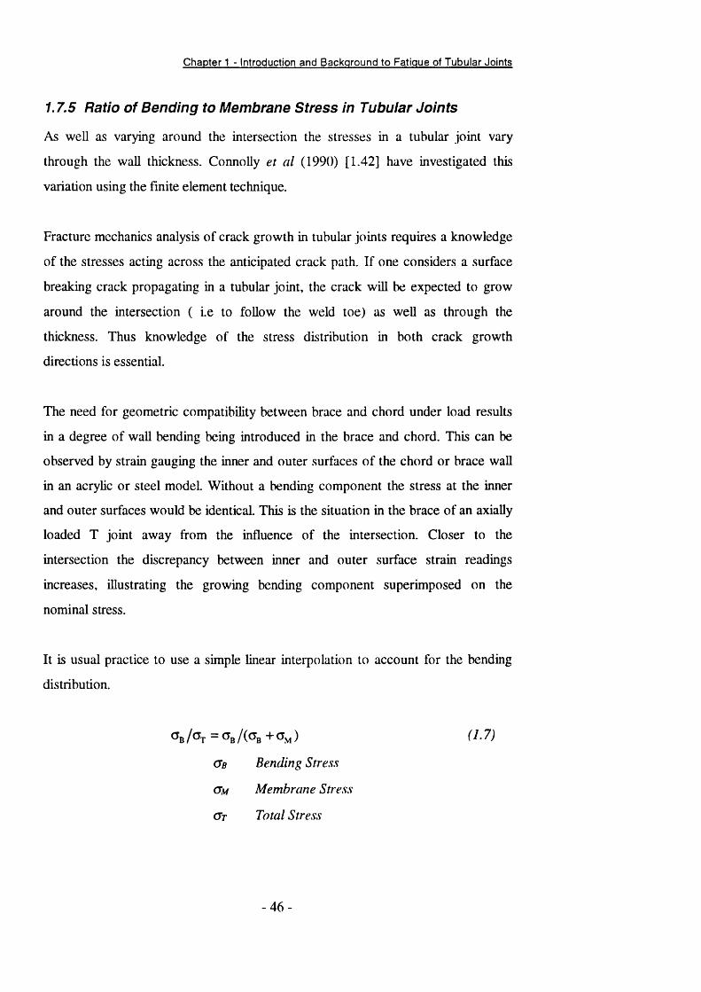
Chapter 1 - Introduction and Background to Fatigue of Tubular Joints
1.7.5 Ratio of Bending to Membrane Stress In Tubular Joints
As well as varying around the intersection the stresses in a tubular joint vary
through the wall thickness. Connolly et al (1990) [1.42] have investigated this
variation using the finite element technique.
Fracture mechanics analysis of crack growth in tubular joints requires a knowledge
of the stresses acting across the anticipated crack path. If one considers a surface
breaking crack propagating in a tubular joint, the crack will be expected to grow
around the intersection ( i.e to follow the weld toe) as well as through the
thickness. Thus knowledge of the stress distribution in both crack growth
directions is essential.
The need for geometric compatibility between brace and chord under load results
in a degree of wall bending being introduced in the brace and chord. This can be
observed by strain gauging the inner and outer surfaces of the chord or brace wall
in an acrylic or steel model. Without a bending component the stress at the inner
and outer surfaces would be identical. This is the situation in the brace of an axially
loaded T joint away from the influence of the intersection. Closer to the
intersection the discrepancy between inner and outer surface strain readings
increases, illustrating the growing bending component superimposed on the
nominal stress.
It is usual practice to use a simple linear interpolation to account for the bending
distribution.
Ob /O t = O b / (O b + O m ) f J ' /V
Ob Bending Stress
Cm Membrane Stress
C t Total Stress
4 6 -

Chapter 1 - Introduction and Background to Fatigue of Tubular Joints
The stiffening of a rack plate as found in jack up chords may affect the through
thickness stress distribution in the chord wall and thus the degree of bending
predicted by the parametric equations for simple joint shapes may not be
applicable. An comprehensive Finite Element investigation of jack up chord
geometries is presented in Chapter 4. The degree of bending found in such chord
shapes has been quantified and compared with comparable tubular joints without
the rack plate. The UCL Bending to Membrane parametric equations applicable to
T and Y joints will be discussed in detail in Chapter 4.
1.8 Fatigue Design Guidance for Tubular Joints
As with all major world-wide fatigue design codes for tubular welded joints, the
United Kingdom guidance specifies a curve, known as an S-N curve to enable the
designer to predict the safe operational life of a welded tubular intersection. Stress-
Life (S-N) curves for tubular joints plot the Hot Spot Stress on the ordinate axis
against the number of cycles to failure on the abscissa. Construction of an S-N
curve requires a large amount of experimental data from fatigue tests on
representative geometries and materials. Acquisition of this data is expensive and
time consuming as each test generates only a single data point. For this reason the
first published S-N curve for welded tubular joints was based on the results of
small scale fatigue tests on T and K joints. This was published by the American
Welding Society in the Structural Welding Code AWS D l. l [1.10] in 1972. The S-
N curve in this code ( and its subsequent modifications ) is known as the X-Curve.
The first U.K. fatigue guidance [1.43] contained the Q-Curve which was based on
the same database of results as A.W.S.’s X-Curve.
Two attempts were made to correlate the observed experimental fatigue lives with
loading conditions. Initially a nominal chord stress was used with fixed stress
concentration factors of 16 for T joints and 7.5 for the K joints. The second and
more successful approach used the now familiar hot spot stress concept which has
since become the standard approach. Care must be exercised that the hot spot
-47
Chapter 1 - Introduction and Background to Fatigue of Tubular Joints
stress is calculated in accordance with the définitions laid out in the code being
used as these vary from code to code.
1.8.1 Development of U.K. Fatigue Guidance.
Since the first United Kingdom fatigue design guidance was published by the
Department of Energy (DoE) in the form of the Q-Curve, two major revisions have
taken place. The first in 1984 [1.44] re-defined the recommended S-N Curve
following concerns that the Q-curve may be unconservative under certain
conditions. This was highlighted by results from the United Kingdom Offshore
Steels Research Programme (UKOSRP) and the European Coal and Steel
Community sponsored research programme [1.45,1.46]. The fatigue guidance was
revised using a screened database of experimental results from full scale tests on
tubular joints from world-wide test programmes. The S-N curve recommended in
this revision became known as the T-Curve. The screening and statistical analysis
procedure used during the development of this curve will be discussed in more
detail in the next section.
Experimental data arising in the period 1984 to 1990 has allowed further additions
and amendments to be made to the fatigue guidance. The major differences
between the 1984 and 1990 documents will be highlighted and the experimental
evidence behind these changes examined.
1.8.2 Development of the T-Curve
Experimental data from world-wide test programmes has shown the Q-Curve to be
inadequate under certain conditions. The Q-Curve was derived from small scale
tubular joint fatigue test results. The welds on these small specimens are now
considered to be disproportionately large compared to the joint geometry, both of
which are far removed from that found in offshore structures ( except perhaps for
the tubular connections found in crane booms ). Sufficient data from full scale
welded tubular joint tests had been gathered to enable an S-N curve to be
constructed without having to resort to small scale test data. However the test
- 4 8 -
Chapter 1 - Introduction and Background to Fatigue of Tubular Joints
programmes from which this data was gathered were undertaken throughout the
world and under a wide variety of conditions. It was important that a consistent
database was developed by implementing a suitable screening procedure to exclude
results from tests that may be non typical.
Any tests falling into one of the following categories were excluded from the final
statistical analysis.
a) Specimens tested in sea water with or without cathodic protection (C.P.).
b) Specimens subjected to variable amplitude loading.
c) Specimens which were stress relieved
d) Specimens unbroken at the end of the test.
e) Specimens which after being unbroken at the end of the first test were retested
at a higher stress.
In addition all joints with a wall thickness of less than 16mm were ignored. The
complete database used in the construction of the 1984 guidance S-N curve can be
found in [1.47].
This definition of failure for a cracked tubular joint has been the topic of much
discussion. Several stages can be identified in the life of a fatigue cracked tubular
joint from first crack initiation at the hot spot through to complete severance of the
brace member. Four définitions of failure are proposed:[1.48]
Ni First discernible surface cracking as noted by any available
method. This stage is considered to have passed if the initial
surface length is greater than 2 0 mm.
N] Intermediate surface cracking as detected by visual
examination without the use of crack enhancement fluids or
optical aids. If NDT techniques indicate a surface length of
- 4 9 -
Chapter 1 - Introduction and Background to Fatigue of Tubular Joints
greater than 30mm then this stage is considered to have
passed.
N 3 First through wall cracking as detected either visually or more
accurately noting loss of internal pressure or by monitoring of
strain gauges positioned adjacent to the deepest part of the
crack.
N4 End of test as occasioned by complete severance of the brace
member, extensive cracking leading to loss of load symmetry
or exhaustion of actuator stroke.
The definitions of failure in the earlier (1984) guidance are slightly different and
care should be taken that consistent definitions of failure are being used when
comparing results from different test programmes.
The number of cycles to first through wall cracking ( N? ) has been adopted as the
standard definition of failure as this is thought to be subject to smaller errors than
both Ni and N2. The final definition, N4 was discounted since a joint having
reached this condition is unlikely to be repairable and may well have shed load to
other joints causing further remote damage. Furthermore N3 can be accurately
measured using Alternating Current Potential Drop Techniques (A.C.P.D.), loss of
sea water in environmental tests or a pressure drop in internally pressurised chord
members.
1.8.3 Analysis of Experimental Data to Produce S-N Curve
The statistical analysis used in the derivation of the 1984 guidance required that the
experimental data be divided into subsets of approximately equal wall thickness.
Only the subsets for 16mm and 32mm wall thickness joints existed in sufficient
numbers to allow a meaningful statistical analysis to be undertaken. These data
subsets were analysed individually and as a whole, the final S-N curve was based
upon the mean of the 32mm data minus two standard deviations of the 16mm data,
representing a probability of failure of 2.3%. This combination was chosen to
- 5 0 -

Chapter 1 - Introduction and Background to Fatigue of Tubular Joints
reflect the reduced performance of the 32mm data and the greater scatter in the
16mm endurance data.
During the derivation of the 1990 guidance the experimental data was again sub
divided in to groups of approximately equal wall thickness. However for the 1990
guidance it was decided that only one wall thickness should be used in the
construction of the S-N curve. The 16mm data set was chosen since it was the
largest and it covered the most diverse range of joint geometry’s and loading
modes.
To remain consistent with the earlier guidance the best fit relationship was
calculated according to (1.8).
Logio(N) = Log,o(K,)-mLogi„(S) {1.8}
where:
N Number of cycles to failure
Ki Constant
m Gradient of S-N curve
S Hot Spot Stress (MPa)
In addition the slope was fixed at -1/3 as in previous guidance and other recognised
fatigue standards [1.49]. The design line was taken as two standard deviations of
the 16mm data below the calculated best fit line. Again this represents a 2.3%
probability of failure. A change of slope to -1/5 is implemented to represent an
endurance limit. An absolute endurance limit is not specified ( i.e S-N curve turns
horizontal ) since under variable amplitude loading even the small load cycles can
become damaging in the later stages of the joint life. The best fit and design curves
are summarised in Table 1.6.
The 16mm experimental data used in the analysis is plotted in Figure 1.29 together
with the mean and design S-N Curves.
51 -

Chapter 1 - Introduction and Background to Fatigue of Tubular Joints
1.8.4 Allowance Factors to be Used in Conjunction with the Basic S-
N Curve.
Only constant amplitude tests carried out in air are utilised in the construction of
the S-N curve. However effects such as environment have been shown to
significantly alter the observed fatigue life. These effects are accounted for by a
factor on life applied to the base line, constant amplitude air life as given by the
design S-N curve. Each of the allowances specified in the current guidance will be
examined below.
(i) The Thickness Effect on Fatigue Life
It has long been recognised that parent plate thickness has an effect on the fatigue
life of welded joints. The 1984 guidance [1.44], based on welded plate specified
the relationship given in (1.9).
s = s. (1.9)V /
where:
Sb Stress range at reference thickness, te
tB Reference thickness (32mm for tubulars)
t Plate / joint thickness
S Stress range resulting in same fatigue
endurance at thickness, t
The above relation was based on an initial suggestion for the form of the thickness
effect correction by Gurney [1.50].
Analysis of more recent tubular joint data has confirmed the existence of a
thickness effect in welded tubular joints. Plotting the endurance results in Figure
1.30 for the 16mm and 32mm joints illustrates this clearly.
- 5 2 -
Chapter 1 - Introduction and Background to Fatigue of Tubular Joints
Utilising the best fit S-N curves for the 16mm and 32mm data previously presented
leads to a thickness correction exponent of 0.29, somewhat higher than value of
0.25 used previously. The current guidance (1990)[1.48] thus recommends a
thickness correction exponent of 0.3 and a shift of the reference thickness for
tubulars from 32mm to 16mm since the thickness effect has been shown to persist
in joints thinner than 32mm.
Thus the recommended correction is given by (1.10).
S = Sb i lAQ)\ t y
where the nomenclature is the same as in (1.9) except that the base
thickness, te is now 16mm.
The thickness correction factor can be represented by a family of nested T-Curves
as shown in Figure 1.31. It is noted that the guidance could be overconservative
for certain geometry’s and loading modes. Allowance is made for less onerous
thickness correction exponents derived from analysis of appropriate experimental
data or from a validated fracture mechanics procedure.
Baerheim et al [1.51] note that the same thickness effect is to be included in the
new ISO code [1.52]. The ISO code is based on the API RP2A LFRD
specification but is likely to contain significant portions of the HSE guidance e.g.
S-N curve for tubular joints.
(ii) The Effect of Environment on Fatigue Life
The in service environment of a tubular joint is very likely to be different to that of
the dry air laboratory conditions in which the experimental data used to construct
the T-curve was generated. Three specific environments can be identified.
- 5 3 -
Chapter 1 - Introduction and Background to Fatigue of Tubular Joints
Air Environment
Intermittent Immersion
Constant Immersion
Tubular connections situated at or close to the
topside deck level most closely resemble the
laboratory air environment although the air is
likely to contain high levels of moisture and salt.
Connections located in the tidal zone or splash
zone will be subjected to repeated cycles of
immersion in sea water an air environments.
Joints situated below the lowest mean tide level
will be constantly immersed in sea water. These
joints are usually protected with a painted /
sprayed coating, some form of C.P. system or a
combination of the two.
A number of tubular joints have now been tested in air or sea water environments
both with cathodic protection [1.53, 1.54, 1.55] and without cathodic protection (
free corrosion) [1.56, 1.57, 1.58, 1.59]. The results of these tests have been used
to modify the previous guidance (1984). The 1984 guidance dealing with
environmental effects is summarised in Table 1.7
Experimental data from environmental fatigue tests on tubular joints and flat plates
can be expressed in terms of Environmental Reduction Factors (E.R.F.’s). E.R.F.’s
are defined as the ratio of the fatigue endurance in air to the endurance in the
specified environment. The endurance in air is calculated from the best fit S-N
curve for 16mm joints. Data from other joint thicknesses must be normalised using
a thickness correction exponent of 0.3 as discussed in the previous section.
The following conclusions were drawn from the data used during the 1990
guidance revision.
- 5 4 -
Chapter 1 - Introduction and Background to Fatigue of Tubular Joints
a) The detrimental effect of sea water environment with optimum cathodic
protection decreases with increasing endurance (i.e. with lower hot spot stress).
b) With optimum cathodic protection little effect is seen at lives greater than 10
cycles.
c) A freely corroding environment (i.e. sea water without cathodic protection) has
an increasingly detrimental effect with increasing endurance (i.e. decreasing hot
spot SCF).
The 1990 design guidance notes [1.48] have been modified to include the above
effects which were not accurately modelled in the previous 1984 design guidance
[1.47]. The revised guidance on the effect of environment on fatigue life of tubular
joints is summarised in Table 1.8.
The S-N curves for 16mm tubulars in free corrosion and sea water with optimum
cathodic protection are shown in Figure 1.32.
1.8.5 Design Code Treatment of High Strength Steeis
There is a distinct lack of published guidance in the form of design codes dealing
with the use of high strength steels offshore. Most codes place an upper limit on
material yield strength beyond which the S-N curves are no longer valid. The
reasons for this caution are simple and sound. Examination of the total number of
tubular joint fatigue tests performed using high strength steels (i.e. yield point
above 450 MPa) [1.9] shows that approximately 85% of these tests used steels
with a yield stress less than 500MPa. Of the total number of tests (approximately
180), less than 5 were performed in sea water under cathodic protection and no CP
tests have been performed for steels with yield stresses above 586 MPa. Although
it is likely that a number of tests have been completed since this review was
performed, it is likely that this limited database would be further restricted by
discarding tests performed under non representative conditions as was done for the
lower strength steels. It is extremely difficult therefore for the design codes and
- 55 -
Chapter 1 - Introduction and Background to Fatigue of Tubular Joints
standards to make safe recommendations on the use of such steels without a co
ordinated research effort.
The S-N curve of the UK design guidance [1.48] is restricted to steels with
minimum yield strength of up to 400 MPa for tubular joints. However allowance is
made for the use of higher strength steels if the S-N performance is validated from
experimental investigations such as the one presented in this thesis. The other
major design code to specifically cater for high strength steels is the DNV Rules
for Mobile Units [1.60] which contains a ‘extra high strength’ grade covering steels
with yield strengths up to 690MPa. The DNV Rules also permit CP levels of -
lOOOmV compared with the more conservative -850mV limit imposed by the HSE.
A further restriction on the use of high strength steels takes the form of a limitation
on the yield to ultimate ratio (YR) as discussed in [1.61]. The HSE guidance
recommends a limit of the YR to below 0.7 whilst API RP-2A specifies 2/3. The
reason for the YR limitations is to avoid the possibility of underestimating the
static strength of tubular joints fabricated from different steels.
1.9 Linear Elastic Fracture Mechanics
The fracture process can be considered to occur on several different scales ranging
from the initiation of microscopic defects of sizes comparable to the molecular
scale to the formation of visible macrocracks whose lengths can vary from a few
millimeters to several kilometers in the case of fractured gas pipelines. Fracture
mechanics applies the theory of continuum mechanics to the fracture process in an
attempt to explain and predict the behaviour of cracked bodies. Fracture
Mechanics has been described as “..the applied mechanics of crack growth from a
flaw” [1.62]
The presence of a crack in a body represents a stress singularity. This leads to
localised inelastic deformation upon loading of the body due to the high stresses at
- 56 -

Chapter 1 - Introduction and Background to Fatigue of Tubular Joints
the crack tip. In situations where the inelastic effects are small compared to the
crack size and characteristic length of the cracked body, linear theory can be
implemented to simplify the analysis. This is known as linear elastic fracture
mechanics (LEFM). The development and use of LEFM concepts is discussed
here. When conditions of small scale yielding are violated then the use of LEFM is
invalid and one must adopt different parameters which can be described under the
heading elastic plastic fracture mechanics (EPFM). Elastic plastic fracture
mechanics parameters include strain based parameters such as that proposed by
Tomkins [1.63], modified stress intensity factors which utilise cyclic strain range
information [1.64, 1.65], the cyclic J integral of Rice [1.66], or the CTOD criteria
suggested by Wells [1.67]. Only during early crack growth when the fatigue crack
is ‘short’ are the small scale yielding conditions likely to be violated. The behaviour
and characterisation of early fatigue crack growth in welded tubular joints has been
extensively investigated by Monahan [1.68]. Discussion at this stage will be limited
to the stress intensity factor.
Fundamental to fracture mechanics is an understanding of the stress / strain field
surrounding a crack tip. Considering the area surrounding the crack tip, where r is
the distance from the crack tip, it can be shown that the displacement is
proportional to the square root of the distance from the crack tip. Furthermore the
associated strain, where the strain is the rate of change of displacement with
respect to distance from the crack tip, must be proportional to the inverse of the
square root of the distance from the crack tip. The elastic stress field surrounding
the crack tip is directly proportional to the strain.( 1 . 1 1 )
‘"yy“7r
Thus as one approaches the crack tip the elastic stress attempting to pull the crack
faces apart approaches infinity. In practice this is not the case since the material
will deform plastically in a region local to the crack tip and the applied load
5 7 -
Chapter 1 - Introduction and Background to Fatigue of Tubular Joints
redistributed across the elastic ligament. The cartesian notation for the components
of stress acting upon an element near the crack tip are illustrated in Figure 1.33.
The full solutions for the stress and displacement tields near to a crack tip in an
elastic body can be found in any elementary text on fracture mechanics.
A constant of proportionality can been introduced into (1.11). This is known as the
Stress Intensity Factor, K. The stress intensity factor is essentially a measure of
how quickly the stress rises as the crack tip is approached. The crack tip stress field
is therefore given by ( 1 .1 2 ).
Note the subscript I attached to the stress intensity factor symbol in (1.12) denotes
the mode of crack surface displacement under consideration.
Three basic modes exist that can cause crack growth.
a) The opening mode. This is the most common loading mode and is the mode
that will be uniquely considered here unless specified here.
b) The edge sliding mode. The surfaces of the crack move normal to the crack
front and the crack remains planar.
c) The tearing mode. The crack surfaces slide relative to each other, parallel to
the crack front and remaining planar.
These modes are perhaps best understood via graphical representation as shown in
Figure 1.34.
The stress and displacement fields in the vicinity of any crack tip are identical. Thus
for equal values of stress intensity factor, K, the stress and displacement fields are
identical for a crack in a simple laboratory specimen and a crack in a complex
-58

Chapter 1 - Introduction and Background to Fatigue of Tubular Joints
machine component. Thus the stress intensity factor characterises the crack tip
environment regardless of geometry and loading conditions. This enables K to
characterise the residual strength of a cracked body. The value of K at which a
crack begins to propagate is known as the fracture toughness, Kc. Under
conditions of plane strain the fracture toughness can be considered as a material
property and is denoted by Kic.
The definition of K as shown in (1.12) is strictly only valid for a two dimensional
centre cracked infinite plate under a uniform tensile stress. Modifications are
required for other configurations, crack geometries and loading systems. These
modifications usually take the form of (1.13).
K = Y a ^ (1.13)
where a is the surface stress in the uncracked component, a is the crack depth and
Y is the modification factor. This factor has been determined by analytical or
experimental methods for a large number of geometric configurations. For example
the stress intensity factor for an edge crack in a semi infinite plate under tension or
pure bending is given by (1.14).
K = U2(jyf7m (1.14)
In this instance Y=1.12 and remains constant i.e. it is independent of the crack size.
In many cases, including tubular joints the Y Factor is a function of crack size.
Fatigue cracking of tubular joints is an especially complex problem since the
surface crack path is usually constrained to the weld toe and the through thickness
cracking can also be curved. This warped shape can often lead to a mixed mode
component of crack growth even for pure mode I loading. The crack growth
behaviour in this case might not be adequately described using mode I stress
intensity factors. In practice much of the difficulty involved in producing a fracture
59

Chapter 1 - Introduction and Background to Fatigue of Tubular Joints
mechanics solution lies in determining Y. Several models have been produced that
attempt to predict the shape of the Y curve for tubular joints.
Since the stress intensity is effectively a single all encompassing description of the
crack tip stress state it is a likely candidate for describing fatigue crack growth
behaviour. Indeed it was discovered that fatigue crack growth data could be
described by utilising the stress intensity factor range, AK where AK=Kmax-Kmm
where K ax and Kmm are the maximum and minimum values of stress intensity factor
during a full fatigue cycle. Many fatigue crack growth laws have been developed of
varying complexity. One of the simplest and most widely used of these models was
developed by Paris and Erdogan [1.69].(1.15)
— = C(AK)"' (1.15)(IN
where:
da/dN Fatigue Crack Growth Rate (m/cycle)
C,m Material Constants (Paris Constants)
AK Stress Intensity Factor Range.
In general fatigue crack growth can be divided into three regions. I, II, and I I I as
shown in Figure 1.35. Stage I crack growth is a region of very low growth rates
where the growth rates are not accurately predicted by (1.15). Reducing the value
of stress intensity factor range in this region leads to a point where crack growth
no longer occurs. This is known as the threshold value of stress intensity factor
range and is denoted by AKth. Fatigue crack growth in Region I is heavily
influenced by microstructural and mean stress effects. Stage I I consists of a linear
Log(AK) - Log(daZdN) relationship. This is the region described by most fatigue
crack growth models, including the Paris - Erdogan law described above. Crack
growth rates in this region are relatively insensitive to microstructural or mean
stress effects. Region II I consists of accelerating, rapid unstable crack growth and
is generally dependant on microstructure, mean stress and component thickness.
- 6 0 -
Chapter 1 - Introduction and Background to Fatigue of Tubular Joints
Other crack growth models attempt to cover all three regions of the sigmoidal
da/dN - AK curve. One such model is that of Saxena et al [1.70] which, for a given
constant load ratio defined the relationship between crack growth rate and stress
intensity factor range as (1.16)
da/dN (AA-)"- (NK)"^
where Ci, mi, C2, m2 are empirical constants, R is the load ratio and Kc is the
fracture toughness as described above. The constants m% and m2 represent the
slopes of the straight lines describing Regions I and 11 and Ci and C2 are the
intercepts of the straight lines when the stress intensity factor range is unity. The
crack growth model of Saxena et al has previously been used in fatigue fracture
mechanics models for welded tubular joints [1.71].
The number of cycles required to propagate a crack from a given initial to a final
crack length can be determined by rearranging (1.15) and integrating between the
specified crack sizes (1.17). In practice this integration is often done using a
numerical integration procedure as the expression for AK is rarely a closed form
solution.
.= 1 : '= (1-17)
1.10 Stress Intensity Factor Solutions for Welded Joints
The general shape of the Y factor curve defining the stress intensity factor
development during the fatigue life of a welded tubular joint is now known from
experimental crack growth measurements taken during full scale tubular joint tests.
This differs significantly from the Y factor function for a similar crack in a flat plate
-61 -

Chapter 1 - Introduction and Background to Fatigue of Tubular Joints
due to the differing structural restraint conditions between the determinate flat
plate and the indeterminate tubular joint. Several attempts have been made to
model fatigue crack growth in tubular joints using a variety of methods. Haswell &
Hopkins [1.72] have grouped these attempts into four categories, namely;
a) Semi Empirical Models
b) Plate Models
c) Cylindrical Models
d) Numerical Models
It is noted by Haswell [1.73] that no accepted bench mark solution exists for any
type of tubular joint making absolute comparisons of the accuracy of models
impossible. The closest to an accepted solution is the empirical data generated from
the crack growth measurements from full scale welded tubular joint tests. It was
found that all models, analytical, numerical or semi empirical were representative of
the observed behaviour of tubular joints but variations introduced by the
assumptions and boundary conditions used in the formulation of the models
resulted in unquantified variations in the predicted stress intensity factors. Adapted
plate models of Thorpe [1.74] and Burdekin et al [1.75] provide upper and lower
bounds respectively to the stress intensity factor solutions for cracked tubular
joints. Haswell concluded that although simple plate models and FE analysis of full
scale joints have proved reasonable methods for determining SIF’s, fracture
mechanics of tubular joints is not a well researched area and should be treated with
caution. The development of fracture mechanics models used to predict the crack
growth behaviour will be treated in detail in Chapter Six.
The stress intensity factor experienced at the deepest point of a fatigue crack in a
tubular joint is known to be significantly different from that of a similar defect in a
flat welded plate. The stress intensity factor experienced in a tubular joint rises
rapidly followed by plateau where the SIF remains almost constant for most of the
life. By contrast the SIF in the flat plate continues to rise rapidly once a fatigue
- 6 2 -
Chapter 1 - Introduction and Background to Fatigue of Tubular Joints
crack has initiated, as illustrated in Figure 1.36. This has important (albeit obvious)
implications for the crack growth behaviour in these two specimen types. Once a
fatigue crack has developed in a flat plate a significant proportion of its life has
already expired and relatively little time remains for remedial action to be taken.
Tubular joints are fortunate in that the ratio of the initiation to total life is relatively
small and the presence of a defect is not necessarily an immediate threat to the
integrity of the joint. The differing crack growth behaviour is shown in Figure 1.37.
1.11 Factors Affecting Fatigue Crack Growth in Tubular Joints
It is known that the behaviour of a propagating fatigue crack can be significantly
altered by the environment in which it is located. This is shown by the penalty
factors on life for joints in sea water imposed by the S-N design codes. A number
of other factors can also significantly affect the development of fatigue defects.
Several parameters, both mechanical and electrochemical have been identified as
having a significant effect on the fatigue behaviour of welded joints. It is felt that
the most relevant factors can be covered by the following topics;
a) Environmental Effects
b) Mean Stress
c) Precipitate Induced Crack Closure
d) Variable Amplitude Loading
e) Welding and Fabrication
It is recognised that in several areas the above categories overlap, e.g. mean stress
and crack closure. However, breakdown of the effects into the above categories is
considered appropriate providing that the areas of interdependency are recognised.
This thesis is concerned primarily with the corrosion fatigue characteristics of high
strength steel tubular joints. It is the difference in behaviour of tubular joints
63

Chapter 1 - Introduction and Background to Fatigue of Tubular Joints
fabricated from different strength steels that is under examination here rather than
tubular joint fatigue behaviour per se. As such the discussion here will be centred
around the environmental effects such as anodic dissolution, hydrogen
embrittlement and calcareous deposits within the crack as these are thought to be
the competing mechanisms responsible for differences in behaviour. It is however
recognised that a number of other factors and mechanisms exist and are needed to
fully describe the complex behaviour of fatigue crack growth in welded tubular
joints. A more general and detailed discussion of the factors controlling crack
growth behaviour in tubular joints is presented elsewhere [1.68, 1.76].
The competing environmental mechanisms wiU be presented together with
experimental evidence from medium (50D) and high strength steels where
available.
1.12 Environment Assisted Fatigue Mechanisms
Steel welded joints can be considered for the purposes of this review to operate in
one of four environments namely;
a) Laboratory Air
b) Free Corrosion (artificial or natural sea water)
c) Adequate Cathodic Protection (-850mV Ag/AgCl)
d) Cathodic Over-Protection (>-1.0V Ag/AgCl)
It is recognised that it could be argued that for the high strength steels considered
in this thesis that CP levels of less than l.OV or even less than 900mV could be
considered as overprotection. However the majority of data reviewed here was
generated using lower strength steels and for the purposes of discussion the above
categories are felt to be convenient and representative.
- 64

Chapter 1 - Introduction and Background to Fatigue of Tubular Joints
1.12.1 Free Corrosion
Steel surfaces immersed in a marine environment without or with inadequate
cathodic protection will suffer material loss due to corrosion. As well as general
material loss seen in terms of loss of section thickness, the corrosive attack can
also be localised leading to pitting.
Prior to considering how corrosion affects the fatigue behaviour, the
electrochemical process of anodic dissolution (corrosion) will first be considered.
A more comprehensive account of corrosion reactions and reaction kinetics can be
found in [1.77]. In aerated sea water, iron ions are released into the aqueous
environment according to the reaction.
2Fe + O2 + 2 H2O ^ 2Fe^ + 40H (1.18)
This is illustrated in Figure 1.38. The iron ions usually oxidise further and then
react with hydroxyl ions to produce ‘rust’ (Fe(OH)3). From the previous figure it
can be seen that the oxidation reaction responsible for the removal of iron ions
from the surface of the steel also releases electrons. This is the anodic reaction.
The water reduction reaction (the cathodic reaction) consumes these electrons at
the same rate. In practice the cathodic reaction is usually rate limiting, controlled
by the supply of oxygen and thus limited by flow rate and oxygen concentration in
the sea water.
The rate of metal loss due to corrosion of steel in a marine environment has been
put at 0.13 mm/yr [1.78]. This is said to be representative for fully immersed (i.e.
not splash zone) clean steel. Importantly however, it is noted that pits can develop
at three to ten times this rate. Splash zone corrosion rates can be many times higher
due to increased availability of oxygen.
The effect of free corrosion conditions on the fatigue life can be considered in two
parts. Firstly the localised corrosion (pitting) has been shown to reduce the
6 5 -
Chapter 1 - Introduction and Background to Fatigue of Tubular Joints
initiation life by forming effective stress concentrations at the weld toe.
Furthermore, free corrosion can change the characteristic crack shape by inducing
a more general distribution of initiated cracks along the weld toe. These defects
can coalesce to form long shallow defects or edge cracks in plate joints [1.79].
Secondly the crack growth rates can be increased simply via the removal of
material at the crack tip by anodic dissolution. This is thought to be the most
plausible explanation for the increased crack growth rates found under free
corrosion. Excessive dissolution at the crack tip has been said to retard crack
growth via crack tip blunting. This is not thought to be a significant consideration
for the current investigation.
Oxygen supply has already been identified as a rate limiting step in the corrosion
process. Scott and Silvester [1.80] studied fatigue crack growth rates in 50D
compact tension specimens using two natural sea water environments. One was air
saturated (7-8 mg/1) and the other had a much lower oxygen concentration of
lmg/1. The lower oxygen levels result in slightly slower crack growth rates.
Importantly, no significant effect of oxygen concentration was found for CP levels
lower (more negative) than -800mV. This suggests that the increase in crack
growth rates under free corrosion conditions is due to anodic dissolution
mechanisms at the crack tip.
1.12.2 Cathodic Protection
The principle behind cathodic protection is as simple as it is effective. Cathodic
protection moves the anodic oxidation reaction away from the steel surface and on
to an external anode. The steel surface is transformed into the cathode in the
electrochemical system and supports only cathodic reduction reactions. To achieve
this the surface of the steel is flooded with electrons to suppress the anodic
oxidation reaction. Two methods are available to achieve this and they are known
as the Sacrificial Anode method and the Impressed Current method.
- 66

Chapter 1 - Introduction and Background to Fatigue of Tubular Joints
In the sacrificial anode method, a metal less noble (more negative) than steel is
placed in electrical contact with the steel in the aqueous environment. Aluminium,
zinc or magnesium are suitable materials. These metals will corrode in preference
to the steel and supply electrons to support the cathodic reactions on the steel
surface. The impressed current method uses an external power source to lower the
potential of the steel surface. Noble metals are often used as the anode in
impressed current systems, sustaining anodic reactions other than the dissolution of
metal ions. This has the advantage that the anode is not consumed and does not
need to be replaced. The impressed current CP system is shown schematically in
Figure 1.39.
At the negative (electron rich) steel surface two reduction reactions are possible in
sea water, namely the reduction of dissolved oxygen (1.19)
O2 + 2 H 2O + 4e' 40H (1.19)
and the reduction of water ( 1 .2 0 )
H 2O + e —>Had.sorbcd + O H ( 1 . 2 0 )
It is the reduction of water reaction that is of most significance here as the
hydrogen atoms can diffuse through the steel lattice structure. Hydrogen is known
to promote brittle behaviour of normally ductile materials.
Discussion of the effect of cathodic protection an the fatigue crack growth process
can be divided into two distinct topics:
a) Effects due to hydrogen
b) Effects of precipitated mineral deposits (calcareous deposits)
(i) Hydrogen based effects
67

Chapter 1 - Introduction and Background to Fatigue of Tubular Joints
The production of hydrogen as a by product of cathodic protection has already
been discussed. Significant evidence exists to suggest that interstitially absorbed
hydrogen can adversely alter the ductility of some steels. High strength steels are
generally thought to be more susceptible than lower strength grades.
Loss of ductility due to the presence of hydrogen is commonly termed hydrogen
embrittlement. The term “hydrogen embrittlement” is used to cover a wide range
of observations where unusual material behaviour is observed where hydrogen gas
may be present. The effects of hydrogen are generally seen in parameters such as
elongation and reduction of area in tensile tests and fracture toughness values that
are highly dependant on strain rate.
The exact mechanism by which hydrogen causes the degradation of material
properties is not too clear. However it seems obvious from the literature that the
mechanism involves the transportation of hydrogen to a tri-axially stressed crack
tip or notch root. An increase in brittle fracture modes on the fracture surfaces of
cathodicaUy protected specimens helps to confirm hydrogen embrittlement as the
mechanism responsible for increased growth rates under CP conditions [1.81,
1.82]
A discussion on the theories behind hydrogen embrittlement is given by Cottis
[1.83] who notes that five main theories have been proposed to account for the
observed effect of hydrogen on high tensile steels.
(i) Pressure Theory. Hydrogen enters the metal lattice and migrates towards voids
and defects within the metal. Once at these sites the hydrogen forms pockets of
very high pressure gas. Blistering of pipelines carrying sour crude oil has been
known to occur lending some support to this theory. However experimental
evidence [1.84] on high strength steels has shown hydrogen embrittlement to occur
in low pressure (0.001 atm) hydrogen gas environments. In these instances it is hard
-68

Chapter 1 - Introduction and Background to Fatigue of Tubular Joints
to imagine the formation of high pressure pockets of gas suggesting that some
other mechanism may be (additionally) operative.
(ii) Decohesion Theory. This theory states that hydrogen weakens interatomic
bonds in steel facilitating grain boundary separation of cleavage crack growth.
(iii)Surface Energy Theory. Hydrogen lower the surface energy of newly formed
cracks thus reducing the SIF needed for brittle fracture.
(iv) Hydride Formation Theory. The presence of hydrogen causes the formation
of brittle hydride phases at the crack tip. However little evidence exists of hydride
formation in steels.
(v) Local Plasticity Theory. Hydrogen reduces the stress required for dislocation
movement.
Although experimental evidence exists to support each of the theories, it is thought
that the effect of hydrogen can be distilled down to the following:[1.83]
1) Hydrogen can decrease the strength of the metal - metal bond thus facilitating
brittle fracture.
2) Hydrogen can increase the stress required to emit dislocations from the crack
tip, making ductile failure more difficult.
Anodic dissolution has been shown to be responsible for the increased crack
growth rates under free corrosion conditions. This mechanism is not thought to be
significant in the case of cathodic protection since the oxidation reactions
responsible for the dissolution of iron ions should be suppressed at the potentials
under consideration here. Measurement of the potential at the crack tip of actual
and simulated cracks has shown that polarisation of the specimen is virtually as
- 6 9 -

Chapter 1 - Introduction and Background to Fatigue of Tubular Joints
effective at changing the potential within the crack as upon the external surface
[1.85].
The simultaneous application of mechanical strain and hydrogen charging appears
to be essential to the mechanism of hydrogen embrittlement. This is shown by slow
strain rate tensile tests in air using specimens which had previously been allowed to
soak under CP conditions in sea water [1.86]. After 100 hours exposure the
specimens were removed from the sea water and subjected to a tensile test in air.
The results show no loss of ductility occurs when the straining and hydrogen
charging are not simultaneous.
The dynamic strain rate is clearly an important variable in determining the potential
susceptibility to fatigue crack growth rate enhancement under cathodic protection
conditions. The effect of strain rate has been investigated by Proctor [1.87] who
performed tensile tests on X65 Linepipe steel in 3.5% NaCl solution at very
negative levels of CP. The results show increasingly ductile behaviour as the strain
rate increases. This has implications for the waveform used during testing with the
rise time being of particular importance. This has been demonstrated by examining
the crack growth rates of specimens subjected to square, sinusoidal and triangular
waveforms in 3.5% NaCl solution [1.88]. The triangular and sinusoidal growth
rates were similar to each other and consistently faster than the average of the air
data . However the square waveform resulted in a significantly lower growth rate,
only marginally faster than in air. This can also be translated into an effect of
frequency with the effect of environment likely to decrease with increasing
frequency. Atkinson and Lindley [1.89] came to much the same conclusion using
triangular and positive and negative saw tooth waveforms. It is postulated that
during dynamic straining new material is being exposed to the environment via the
disruption of passivating layers allowing the dissolution of iron ions to take place in
free corrosion and the adsorption of hydrogen under CP conditions. The
passivating layers are therefore assumed to reform rapidly once the peak load in
each cycle has been reached.
- 7 0 -
Chapter 1 - Introduction and Background to Fatigue of Tubular Joints
Naturally, any mechanism that encourages the absorbtion of adsorbed hydrogen
(rather than harmlessly bubbling away as a gas) is likely to magnify the measured
effects of hydrogen embrittlement. Sulphate Reducing Bacteria, common in natural
sea water environments are known to promote the absorbtion of hydrogen.
Cowling et al have studied the role of SRB extensively for 50D type steels [1.90].
The promotion of corrosion and corrosion fatigue by SRB’s is said to be due to the
following processes:
1) The ease with which SRB’s reduce sulphate ions to sulphide ions which rapidly
hydrolyse to form hydrogen sulphide.
2 ) T h e use b y th e b a c te r ia o f h y d ro g e n as an e n e rg y s o u rc e , th u s p ro d u c in g
c a th o d ic d e p o la r is a t io n (p ro m o t in g co iT O s ion ).
3) Enhanced hydrogen embrittlement due to increased permeation of atomic
hydrogen into bulk metal.
Tests were performed on 25mm thick, three point bend specimens at a CP level of
-850mV. Enhanced corrosion fatigue crack growth rates occur across a limited
range of AK and is noted as being increased by up to an order of magnitude. This is
the same region where enhanced crack growth rates due to cathodic protection are
found. Robinson and KilgaUon [1.91] have investigated the effect of SRB’s on
hydrogen damage in high strength steels. The general conclusion that SRB’s
considerably increased the level of absorbed hydrogen and thus the possibihty of
increased embrittlement was confirmed.
(ii) Calcareous Deposits
When a steel surface is cathodicaUy polarised in a natural or artificial sea water,
calcium and magnesium based mineral deposits can form on the surface of the steel
[1.92]. Oxygen reduction reactions at the steel surface increase the pH of the
solution adjacent to the steel. Other reactions also occur which have the same
71 -

Chapter 1 - Introduction and Background to Fatigue of Tubular Joints
effect. The increased alkalinity at the surface impedes the entry of into the metal
hydrogen by affecting the reduction reactions at the surface thus limiting the effect
of hydrogen embrittlement [1.93].
A further effect of this layer of more alkaline sea water adjacent to the steel is to
promote the following precipitation reactions:
O H - + H C O j- - 4 H 2O + C O j^ - ( 1 . 2 1 )
pptCO3" + ^ CaCOj (1.22)
CGj^' + Mg'^^MgCGjrp, (1.23)
2GH + Mg'+ Mg(GH )2 pp, ( 1.24)
Hodgkeiss et al [1.85] and Maahn [1.94] have both investigated the pH of the
solution within a fatigue crack. Both investigations noted that the pH within the
crack is commonly more alkaline than the pH of the bulk solution. The pH inside
the crack is typically between 10 and 13. This has been confirmed by the formation
of Mg(OH )2 within the confines of cathodicaUy polarised fatigue cracks.
Magnesium hydroxide does not form at pH more acidic than 10. Magnesium
hydroxide has been shown to form at a faster rate than calcium carbonate [1.95]
and results in a harder and stronger precipitate.
Formation of these precipitates, known as ‘calcareous deposits’ within a fatigue
crack has been shown to reduce the effective SIF range by wedging the crack open
at the lower loads in the fatigue cycle. This precipitate induced crack closure is
known to increase the minimum value of crack opening in a cycle whilst leaving the
maximum unchanged.
It is also thought that the calcareous deposits on the surface of the steel may inhibit
the entry of hydrogen into the steel by restricting the supply of water at the steel
surface therefore slowing the rate of water reduction and hydrogen evolution.
-72
Chapter 1 - Introduction and Background to Fatigue of Tubular Joints
1.13 Effect of Environment on Fatigue Crack Growth Rate
The electrochemical process of corrosion and cathodic protection have been
outlined. The mechanisms by which these environments are thought to affect
fatigue crack growth rates were also discussed. It is now appropriate to examine
the magnitude of these rate changes by reviewing experimental evidence.
Thorpe and Ranee [1.96] and Cowling and Appleton [1.97] have performed
extensive studies on the fatigue crack growth rates on 50D type steels. Fatigue
crack growth rates at a given value of AK are known to fluctuate with the level of
cathodic polarisation. In general it seems that the lowest growth rates occur at
approximately the same potential that just prevents anodic dissolution (0.8-0.85V
Ag/AgCl). More anodic potentials are thought to produce higher crack growth
rates due to increased anodic dissolution at the crack tip. Polarisation to more
cathodic potentials has been shown to increase growth rates by a factor of up to
six. Hydrogen embrittlement is thought to be the mechanism responsible for the
increased growth rates in this region as Neilsen and Maahn [1.98] showed the
hydrogen permeation current in 50D to exhibit a near logarithmic dependancy on
applied potential. It should be noted that none of the above environments restore
the growth rates found in air. This is summarised in Figure 1.40.
Under free corrosion conditions the growth rate depends on stress ratio with
increasing stress ratios resulting in increasing crack growth rates up to R ratios of
around 0.5 to 0.7 [1.96]. The increase was found to be the same for all AK.
Cowling et al [1.97] however failed to find the same dependency of crack growth
rates on R under free corrosion conditions. Austin [1.76] suggested the difference
could be caused by crack closure effects due to corrosion products within the crack
in the experiments by Scott and Thorpe. This appears to be a plausible theory and
would explain the diminishing effect as the crack opening increased with mean
stress.
- 7 3 -
Chapter 1 - Introduction and Background to Fatigue of Tubular Joints
Application of cathodic potential has repeatedly resulted in a plateau crack growth
region where the crack growth rate is independent of AK. This is illustrated
schematically in Figure 1.41. This behaviour has been found in 50D (e.g. Scott et
at. Cowling et al) and by Vosikovsky [1.99] for pipeline steels. Crack growth data
obtained by Vosikovsky for X65 type steels under cathodic protection at the zinc
potential shows the plateau behaviour clearly in Figure 1.42.
The effect of calcareous deposits is generally seen at lower values of AK. The
effect of calcareous deposits can be investigated by testing in ASTM sea water and
3.5% NaCl. The NaCl solution does not contain the magnesium and calcium
compounds needed to form calcareous deposits.
Such tests have been performed by Eggen and Bardai [ 1.100] on 30mm thick 50D
SEN specimens. A large difference in behaviour was found between the NaCl and
ASTM solution tests. At very low AK the behaviour is similar but at higher stress
intensity factor ranges (>8 MPaVm) the growth rates are significantly less in the
ASTM sea water. This behaviour was found at a stress ratio of 0.1. However
increasing the mean stress so that R=0.7 reduced the difference between the
environments to a much lower level for all AK. This presents clear evidence that
the formation of calcareous deposits within a crack can have significant benefits on
the fatigue crack growth rate.
Billingham and Laws [1.101] examined a number of steels with yield strengths
between 460 and 640 MPa in order to assess their suitability for offshore use in
terms of weldability and fatigue performance. The steels were produced via a
variety of processing routes including quenched and tempered and controlled
rolled. It was found that the high strength steels tested suffer from enhanced
fatigue crack growth rates with increasing negative polarisation. Growth rates at a
CP level of -llOOmV (SCE) were between 2 and 10 times faster than at -800mV.
This is illustrated in Figure 1.43. Increasing components of cleavage type facets on
-74

Chapter 1 - Introduction and Background to Fatigue of Tubular Joints
the fracture surface were noted at the more negative potential providing evidence
of hydrogen embrittlement mechanisms playing a significant role. It was concluded
that all the steels tested performed as well as or slightly better than conventional
350MPa steels.
1.14 Effect on Environment on the Fatigue Lives of Welded Joints
The first significant systematic investigation into the effect of environment on the
fatigue behaviour of welded joints was the United Kingdom Offshore Steels
Research Project - Phase I (UKOSRPI) [1.45]. The results suggested the following
environmental effects which were subsequently used for the basis of the design
guidance.
1. Free corrosion can reduce endurance by a factor of two
2 . Cathodic protection can restore the in air life
3. Under free corrosion conditions, fatigue damage continues to occur even below
the air fatigue limit.
It has know been recognised that the above conclusions can lead to non
conservative life estimates in some cases mainly due to the fact that recent tests
have shown that cathodic protection does not always restore the in air life.
Austin [1.76] has considered a significant amount of data generated under free
corrosion conditions outside UKOSRPI and he concludes that a factor of 2.5
would seem appropriate to account for the effect of environment. The data
considered included both plate and tubular joint tests. Additionally, higher
reduction factors were noted for post weld heat treated joints (PWHT) leading to
the conclusion that free corrosion conditions can negate the beneficial effect of
PWHT. A similar review [1.102] suggests the ratio between air and fatigue lives is
closer to 2.2. Additionally a distinct laboratory bias was noted in the results with
the UKOSRP falling towards the higher end of the scatter band.
75
Chapter 1 - Introduction and Background to Fatigue of Tubular Joints
The application of ‘adequate’ levels of cathodic protection make the trends less
clear as the reduction factor changes with apphed stress range. Several research
programmes testing welded plate joints suggest that fatigue hves are always at least
as long as those in air (reduction factor < 1 ) especially so at lower stress ranges e.g.
[1.103, 1.104]. However a significant amount of data has also been generated
suggesting that welded plates with adequate levels of CP result in hves between 2
and 3 times shorter than in air. In general it appears that the SN curve is rotated
counter clockwise resulting in lives longer than air only at low stress ranges.
Vosikovsky and Tyson [1.103] noted that the scatter in the CP data was increased
compared to the free corrosion data and that the noted laboratory bias was even
stronger than for free corrosion conditions. The best fit of all the adequate CP data
reviewed (from Canadian, Japanese, ECSC Dutch, ECSC German and UKOSRP)
showed a neghgible effect of CP on hves compared to those found in air. However
exclusion of the UKOSRP generated data from the analysis results in an average
reduction factor on life of 1.5.
The most plausible explanation of the bias is identified as the weld procedures used
to deposit the weld toe bead. Corrosion fatigue is thought to be more sensitive to
weld toe quahty than fatigue in air. Vosikovsky et al [1.105] monitored the number
of initiation sites and found that in general the number of sites increased under free
corrosion and decreased under CP than found in air tests. Examination of the
relationship between the resulting fatigue hves and the number of initiation sites
shows that the tests with few initiation sites produced significantly longer hves.
Thus the transition to an edge crack (in plates) is delayed and the defects grow as
semi-eUiptical fatigue cracks throughout most of the test. AdditionaUy, semi
elhptical defects are more susceptible to the beneficial effects of reduced stress
intensity factor due to crack wedging effects of calcareous deposits that may form
on the crack surfaces under CP conditions. The random variation of the number of
-76
Chapter 1 - Introduction and Background to Fatigue of Tubular Joints
initial defects severe enough to initiate a fatigue crack under CP conditions also
explains the increased scatter observed on the CP results.
Tubular joints performed as part of UKOSRPII [1.46] did not exhibit the same
beneficial effect of adequate CP levels found in UKOSRPI [1.45] plate tests.
Consideration of experimental data from various world wide sources [1.105]
suggests a factor of two on the corresponding air life accounts for the application
of adequate CP levels. The beneficial effect at lower stress ranges found for welded
plate tests was not found for welded tubular joints.
Cathodic over protection is limited mainly to welded plate tests and tends to show
a similar trend to the lower CP levels but with a greater reduction in life longer
lives are needed before the results approach the in air results. Smith [1.106]
performed ten fatigue tests on tubular joints fabricated from the high strength steel
API 5L X85. Five of the tests were performed with CP levels of -KXXlmV
Ag/AgCl. This steel has a yield strength of approximately 600MPa and is
commonly used in jack up construction. Smith concludes that the results of the
tests fell within the scatter of the tests used in the derivation of the UK fatigue
guidance and above the design curve. No comparison between the relative
endurance found from the air and CP tests is given. The welding procedure used
during the fabrication of some of the specimens was un-representative of those
used in previous tubular joint fatigue tests (weave rather than stringer beads) and
the through thickness crack paths highly unusual making interpretation of the
results difficult.
1.15 Aims and Objectives
The primary aim of this thesis is the study of fatigue crack growth behaviour of
large scale welded tubular joints fabricated using a high strength steel typical of the
modern micro-alloyed, quenched and tempered steels. Such steels potentially offer
significant advantages for offshore construction. Thinner sections may allow lower
fabrication costs to be realised due to reduced welding requirements and lighter
-77

Chapter 1 - Introduction and Background to Fatigue of Tubular Joints
structures can lead to reduced installation costs for jackets and topsides. Although
concerns about the weldability of such steels have largely been dispersed there still
exists a lack of published data on the fatigue behaviour of these steels, particularly
under cathodic protection conditions. A need for fatigue data from representative
geometries in realistic environments has been demonstrated in this Chapter. In an
attempt to satisfy a part of the shortfall of data, seven large scale welded tubular
joint fatigue tests have been performed. Two tests have been undertaken in a
laboratory air environment and the remaining five under conditions of cathodic
protection. Cathodic protection levels of -800 and -lOOOmV (Ag/AgCl) were used.
The results are presented in Chapter Two in S-N format and the fatigue crack
growth behaviour examined.
Currently the only offshore application for such steels is the fabrication of chord
and racks for mobile jack up platforms. The various designs of jack up platform
legs were presented in detail in this Chapter. It was noted that the stiffening effect
of the rack plate may well affect the stress distribution around the intersection of
brace and chord. The importance of the accurate knowledge of the intersection
stress distribution for the determination of fatigue life by S-N and fracture
mechanics methods has been demonstrated in this Chapter. For this reason an
extensive finite element stress analysis of uncracked tubular joints has been
performed on geometries representative of jack up platform construction. The
results of this investigation have been analysed in terms of the surface stress
concentration factor (SCF) for axial, in plane and out of plane bending loadcases.
The effect across a range of joint geometries has been quantified and an
investigation into the mechanism by which these changes are affected. This is
presented in Chapter Three.
The through thickness stress distribution is an important input parameter for
fracture mechanics models and is the subject of Chapter Four. The results of the
finite element study have been used to quantify the change in through thickness
degree of bending (DoB) caused by the rack plate. This is achieved by comparison
- 7 8 -
Chapter 1 - Introduction and Background to Fatigue of Tubular Joints
with the DoB found from tmite element models of the equivalent unstif'fened joint
and DoB predictions from parametric equations.
The topic of fracture mechanics modelling of fatigue crack growth in welded
tubular joints is dealt with in Chapter Five. By presenting a review of previous
attempts to predict the crack growth behaviour in tubular joints and taking into
account the information gained from the current experimental investigation,
contemporary models are investigated. The magnitude of the potential effect of the
rack plate on the subsequent crack growth in jack up chords is assessed by altering
the input parameters to the fracture mechanics models to reflect the geometry.
Finally the accuracy of the SIF solution for welded tubular T joints given in the
revised BS:PD6493 is assessed using the results obtained from the experimental
investigation.
A summary of the achievements and conclusions derived from the work presented
in this PhD Thesis are given in Chapter Six. Recommendations for future work are
also highlighted.
79
Chapter 1 - Introduction and Background to Fatigue of Tubular Joints
1.16 References
[1.1] Davey, V.S., ''Hydrogen Assisted Cracking of High Strength Steels in the
Legs of Jack Up Rigs’", Health and Safety Executive, Offshore Safety
Division, September 1991
[1.2] British Standards Institution. “Weldable Structural Steels “, BS4360:1990
[1.3] British Standards Institution. “Weldable Structural Steels fo r Fixed Offshore
Structures” , BS7191:1989
[1.4] Offshore Engineer, October 1995. ''Harding. A New Role For Jack Ups”
[1.5] Massie, WW, Liu, P. “The Jack Up Durability Problem”, European
Petroleum Conference , Society of Petroleum Engineers, 1990, v l, pp207-
305
[1.6] Denton, A.A. “The Jack Up Drilling Platform (Ed. L.F. Boswell) 1986.
Chapter 1. ”
[1.7] Dyer,A. MSc Thesis, Dept, of Mechanical and Process Engineering,
University of Sheffield, 1993.
[1.8] Recommended Practice for Site Specific Assessment of Mobile Jack Up
Units. 1st Edition, May 1994.
[1.9] Stacey, A., Sharp, J.V., and King, R.N., “High Strength Steels used in
Offshore Installations”, Proc. Offshore Mechanics and Arctic Engineering
1996, v3, pp417-433.
[1.10] American Welding Society. “Structural Welding Code.” AWS D l. 1,-84,
1984
[1.11] Kam, J.C.P., Birkinshaw, M. “The simulation of Wave Induced Fatigue
Loading of Jack Up Tubular Components”, OMAE 1993, vlllb, pp 529-535
[1.12] Etube, L. ''Variable Amplitude Corrosion Fatigue and Fracture Mechanics
of High Strength Weldable Jack Up Steels”, PhD Thesis (to be submitted to
the University of London), UCL, 1998
[1.13] Ohta, T, Yamauchi, H and Toriumi, M. “Design Method o f Leg Structure of
Jack Up Rigs”, Proc. First Int. Offshore and Polar Engineering Conference,
- 8 0 -
Chapter 1 - Introduction and Background to Fatigue of Tubular Joints
Edinburgh, 11-16 August 1991, ppl38-142..
[1.14] Billingham, J., Spurrier, J., “Programme Suinmary and Conclusions"", High
Strength in Offshore Engineering, MTD Publication 95/100, pp7-8, 1995
[1.15] Healy, J., Billingham, J. “Increased use of High Strength Steels in Offshore
Engineering"", Welding and Metal Fabrication, pp265-273, July 1993
[1.16] Healy, J., Billingham, J., Chubb, J.P., Jones, R.L., Galsworthy, J. “Weldable
High Strength Steels for Naval Construction", Proc. Offshore Mechanics
and Arctic Engineering, v3, ppl89-198, 1993
[1.17] Watkinson, P., Bodger, P. H., and Harrison, J. D., “The Fatigue Strength of
High Strength Steels and Methods fo r its Improvement”. Proc. Conf. on
Fatigue of Welded Structures, The Welding Institute, Cambridge. 1971
[1.18] Donnell, L.H .“ Stability of Thin Walled Tubes Under Torsion” National
Advisory Committee on Aeronautics (NASA)Report No. 479, 1934
[1.19] Flugge, W. “ Statik iind Dynamik der Schalen. "Springer, Berlin, 1934
[1.20] Roarke, R.J. and Warren, C.Y. “ Formulae fo r Stress and Strain.’" 5ih Ed.,
McGraw Hill-Kogakusha, Tokyo, Japan
[1.21] Biljaard, P.P. “ Stresses from Radial Loads in Cylindrical Pressure
Vessels.” The Welding Journal 33(12), Research Supplement 1954, 6155-
6235.
[1.22] Toprac, A.A. et al. “ Welded Tubular Connections: An Investigation of
Stresses in T-Joints. “ Welding Journal, Jan 1966
[1.23] Hoff, N.J. et al. “ Deformation and Stresses in Circular Cylindrical Shells
Caused by Pipe Attachments. ” Knolls Atomic Power Research Laboratory.
Reports KAPL 921, 923, 924, 925, 926 and 1025, Nov 1953.
[1.24] Kempner, J. et al “ Tables and Curves fo r Defornuition and Stresses in
Circular Cylindrical Shells Under Localised Loading. "Journal of
Aeronautical Science. v24, n2, ppl 19-129, feb. 1957.
[1.25] Dundrova, V. “ Stresses at Intersection of Tubes: cross and T Joints.
Structures Fatigue Research Lab., Dept. Of Civil Engineering, University of
Texas, Austin, July 1965.
- 8 1 -

Chapter 1 - Introduction and Background to Fatigue of Tubular Joints
1.26] Dover, W.D. “ Fatigue Fracture Mechanics Analysis of Offshore
Structures” Int. Journal of Fatigue, April 1981.
1.27] Kare, R.F., Influence of Weld Profile on Fatigue Crack Growth in Tubular
Welded Joints, PhD Thesis, City University, London, 1989
1.28] CIRIA Underwater Engineering Group. ”Design of Tubular joints for
Offshore Structures. ” Volume 2, Section C.5
1.29] American Petroleum Institute. ''Recommended Practice fo r Planning,
Designing and Constructing Fixed Offshore Platforms. ” API - RP2A, 20th
E d .1993
1.30] British Standards Institution. "Code of Practice fo r Fixed Offshore
Structures.” BS6235:1982
1.31] Norweigan Petroleum Directorate (N.P.D.) "Regulations for the Structural
Design of Fixed Structures on the Norweigan Continental Shelf, 1977”
1.32] Det Norske Veritas. "Rules for the Design, Construction and Inspection of
Fixed Offshore Structures. ” DnV, 1977
1.33] Lloyds Register of Shipping "Fatigue Analysis of Fixed Steel Platform
Welded Tubular Joints. ” Fatigue Appendix, Issue 5, July 1980.
1.34] Wordsworth , A C. and Smedley, C.P. "Stress Concentrations in Unstiffened
Tubular Joints.” Paper 31, European Offshore Steels Research Seminar,
Cambridge, U.K. November 1978.
1.35] Kuang, J.G., Potvin, A.B. and Leick, R.D. "Stress Concentrations in
Tubular Joints. ” Society of Petroleum Engineers, 1977
1.36] Department of Energy, "Offshore Installations: Guidance on Design and
Construction.” HMSG, April 1984
1.37] Health and Safety Executive "Offshore Installations Guidance Notes (
Consolidated Edition ) ” June 1990.
1.38] Efthymiou, M and Durkin, S. "Stress Concentrations in T/Y and Gap /
Overlap K Joints. ” Behaviour of Offshore Structures. Amsterdam 1985.
[1.39] Smedley. P., Fisher, P., "Stress Concentration Factors for Simple Tubular
Joints”, Proc. First Int. Offshore and Polar Engineering Conference, 11-16
8 2 -

Chapter 1 - Introduction and Background to Fatigue of Tubular Joints
August 1991, pp475-483
[1.40] Hellier, A.K., Connolly, M.P. and Dover, W.D. ''Stress Concentration
Factors for Tubular Y and T Joints. ” Int. J. Fatigue, vl2, nl, ppl 3-23.
[1.41] Hellier, A.K., Connolly, M.P., Kare, R.F. "Prediction of the Stress
Distribution in Tubular Y and T Joints. ’’ Int. J. Fatigue. vl2, nl, p25-33.
[1.42] Connolly, M.P., Hellier, A.K., Dover, W.D. and Sumoto, J. "A Parametric
Study of the Ratio of Bending / Membrane Stress in Tubular Y and T
Joints'" Int. J. Fatigue. vl2, nl, pp 3-11.
[ 1.43] UK Department of Energy, “ Offshore Installations, Guidance on Design
and Construction 2nd Edition, 1977
[1.44] UK Department of Energy, “ Offshore Installations, Guidance on Design
and Construction ", 3rd Edition, 1984
[1.45] UK Department of Energy, "United kingdom Offshore Steels Research
Project - Plase I, Final Report ”, OTH 88 282, 1988.
[1.46] UK Department of Energy, "United kingdom Offshore Steels Research
Project - Plase II, Final Summary Report ”, OTH 87 265, 1987.
[1.47] UK Department of Energy, “ Background to New Fatigue Design Guidance
for Steel Welded Joints in Offshore Structures, ” 1983
[1.48] UK Department of Energy, “ Background to New Fatigue Design Guidance
for Steel Joints and Connections in Offshore Structures, ” 1990
[1.49] British Standards Institution, "Steel, Concrete and Composite bridges.”,
BS5400 Pt. 10, Code of Practice for Fatigue
[1.50] Gurney, T.R., "The Influence of Thickness on the Fatigue Strength of
Welded Joints.” Int. Conf. on Behaviour of Offshore structures. Paper 41,
London 1979.
[1.51] Baerheim, M, Stacey, A., Nichols, N, "Proposed Fatigue Revisions in the
New ISO Code fo r Offshore Structures”, Proc. Offshore Mechanics and
Arctic Engineering, v3, pp513-519, 1996
[1.52] ISO, ISO 13819-2, "Petroleum and Natural Gas Industries - Offshore
Structures, Part 2: Fixed Steel Structures.”, To be published
- 8 3 -
Chapter 1 - Introduction and Background to Fatigue of Tubular Joints
[1.53] Dover, W.D.. and Wilson, T.J., “ Corrosion Fatigue of Tubular Welded T-
Joints”, paper C l36/86, Proc. Int. Conf. on Fatigue and Crack Growth in
Offshore Structures, Institute of Mechanical Engineers, London 1986.
[1.54] Dover, W.D., Sham, W.P., and Peet, C., “Random Load Corrosion Fatigue
of Tubular Welded T-Joints”, Proc. Conf. on Fatigue of Offshore
Structures, London, 19-20 September 1988.
[1.55] Gerald, J. et al, “Corrosion Fatigue Tests on High Strength Steel Tubular
X-Nodes with Improved Welds”, Paper TS15, Proc. Third Int. ECSC
Offshore Conference on Steel in Marine Structures, Delft, June 15-18, 1987.
[1.56] de Back, J. and Vaessen, G. H. G ., “Effect o f Plate Thickness, Temperature
and Weld Toe Profile on the Fatigue and Corrosion Fatigue behaviour of
Welded Offshore Structures: Parts I and 11”, Final Report on ECSC
Convention 7210-KG/601 (F7.4/81), Stichting Materiaalonderzoek in de
Zee, May 1984.
[1.57] Wylde, J.G. and Yamamoto, N., “ Sea water Corrosion Fatigue Tests on
Steel Tubular Joints” , Paper 7921.01/87/589.2, The Welding Institute ,
March 1988.
[1.58] Hara, M., et al, “ Corrosion Fatigue Strength of 490 MPa Class High-
Strength Steels Produced by the Thermo Mechanical Control Process”,
Paper OTC 5311, Proc. 18th Offshore Technology Conference, Houston, 5-
8 May 1986.
[1.59] de Back, J., and Vaessen, G. H. G., “Fatigue and Corrosion Fatigue
Behaviour of Offshore Steel Structures. ”, Final Report on ECSC
Convention 7210-KB/6/602 (J.7.1 f/16), ), Stichting Materiaalonderzoek in
de Zee, April 1981.
[1.60] Rules for Classification, Mobile Offshore Units, Det Norske Veritas, Oslo,
July 1989
[1.61] Billingham, J., Healy, J., and Bolt, H., “The Question of High Yield /
Ultimate Ratio in High Strength Steels”, High Strength Steels in Offshore
Engineering, MTD Publication 95/100
- 8 4 -
Chapter 1 - Introduction and Background to Fatigue of Tubular Joints
[1.62] Pook, L.P. “Linear, Fracture Mechanics - What It Is, What It Does ”,
National Engineering Laboratory, East Kilbride, Glasgow, August 1970
[1.63] Tomkins, B., “Fatigue Crack Propagation - An Analysis”, Philosophical
Magazine, v l 8 , ppl041-1066 (1968)
[1.64] Gowda, C.V.B, Topper, T.H., “Crack Propagation in Notched M ild Steel
Plates Subjected to Inelastic Strains.”, Cychc Stress Strain Behaviour -
Analysis, Experimentation, and Faüure Prediction, ASTM STP 519, pp. 170-
184, 1973
[1.65] El Haddad, M.H., Smith, K.N., Topper, T.H., “A Strain Based Intensity
Factor Solution fo r Short Fatigue Cracks Initiating from Notches”, Fracture
Mechanics, ASTM STP 677, pp274-289, 1979
[1.66] Rice, J R., “A Path Independent Integral and the Approximate Analysis of
Strain Concentration by Notches and Cracks.”, Journal of Applied
Mechanics, v35, pp.379-386, 1968.
[1.67] Wells, A.A., “Unstable Crack Propagation in Metals: Damage and Fast
Fracture”, Proc. Crack Propagation Symposium, Cranfield, vl., pp 210-230,
1961
[1.68] Monahan, C.C., “Early Fatigue Crack Growth in Ojfshore Structures”, PhD
Thesis, UCL, 1994
[1.69] Paris, P. C. and Erdogan, F. “A Critical Analysis of Crack Propagation
Laws”, J. Bas. Engng, 1963, 85(4), 528-534.
[1.70] Saxena, A., Hudak, S.J., Jouris, G.M., “A Three Component Model for
Representing Wide Range Fatigue Crack Growth Rate Behaviour”,
Engineering Fracture Mechanics, vl2, pp. 113-118, 1979
[1.71] Gowda, S.S., Helenius, A., “Fatigue Crack Growth Analysis of Welded
Tubular Joints of Offshore Structures”, Proc. Int. Conf. Offshore Mechanics
and Arctic Engineering, v3, pp575-582, 1988
[1.72] HasweU, J and Hopkins, P. “A Review of Fracture Mechanics Models of
Tubular Joints” Fatigue Fract. Eng. Mater. Struct., vl4, n5 pp483-497,
1991
-85
Chapter 1 - Introduction and Background to Fatigue of Tubular Joints
[1.73] HasweU, J. “Simple Models fo r Predicting Stress Intensity factors for
Tubular Joints” Fatigue Fract. Eng. Mater. Struct., vl4, n5 pp499-513,
1991
[1.74] Thorpe, T. W. “A Simple Model of Fatigue Crack Growth in Welded
Joints”, Offshore Technology Report, OTH 86 225.
[1.75] Burdekin , F. M., Chu, W. H., Chan, W. T. W. and Manteghi, S. “ Fracture
Mechanics Analysis of Fatigue Crack Propagation in Tubular Joints”,
International Conference on Fatigue and Crack Growth in Offshore
Structures, April 1986, IMechE, C 141/86
[1.76] Austin, J, A., “The Role of Corrosion Fatigue Crack Growth Mechanisms
in Predicting the Fatigue Life o f Offshore Tubular Joints”, PhD Thesis,
UCL, October 1994
[1.77] MTD Ltd., “Design and Operational Guidance on Cathodic Protection of
Offshore Structures, Subsea Installations and Pipelines.”, Publication
90/102, 1990
[1.78] Rowlands, J.C., “Corrosion”, Ed. Newnes, L.L., Butterworth, London 1976
[1.79] Lambert, S B ., “Effect of Sea water on Fatigue Crack Shape Development.”,
Proc. 11 Offshore Mechanics and Arctic Engineering Conference, Calgary
1992.
[1.80] Scott, P.M., Silvester, P.R.V., “The Influence of Sea Water on Fatigue
Crack Propagation Rates in Structural Steel”, UKOSRP 3/03, December
1975.
[1.81] Saenz de Santa Maria, M., Proctor, R.. “Environmental Cracking
(Corrosion Fatigue and Hydrogen Embrittlement) of X-70 Linepipe steel”.
Fatigue and Crack Growth in Offshore Structures, Proc. IMechE, C l37/86,
1986
[1.82] Thorpe, T.W, Scott, P.M., Ranee, A., Silvester, D. “Corrosion Fatigue of
BS 4360:50D Structural Steel in Sea Water", Int.J.Fatigue, v5,n3,ppl23-
133,1983
[1.83] Cottis, R.A., “Stress Corrosion Cracking in High Strength Steels.”,
- 8 6 -
Chapter 1 - Introduction and Background to Fatigue of Tubular Joints
Corrosion, Ed. Shrier, Jarman, Burstein, 3"‘. Ed. 1994
[1.84] Oriana, R.A., Josephic, P.H., Acta Metall, v22. p i06.5, 1974
[1.85] Hodgkeiss, T.H., Cannon, M.J. ''Corrosion Fatigue of Steels in Sea Water;
Studies of Crack Tip Electrochemistry'", Dept. Mechanical Engineering,
Glasgow University, Project GL/MM6
[1.86] Scully, J.R., Morgan, P.J., "The Hydrogen Embrittlement Susceptibility of
Ferrous Alloys: The Influence of Strain on Hydrogen Entry and Transport"",
Hydrogen Embrittlement: Prevention and Control, ASTM STP 962, Ed.
Raymond, L. ASTM, pp387-402, 1988
[1.87] Proctor, R. P. M., "Detrimental Effects of Cathodic Protection:
Embrittlement and Cracking Phenomena"", Cathodic Protection: Theory and
Practice, Ed. Ashworth, V and Booker, C.J.L., 1986
[1.88] Barsom, J.M., "Effect of Cyclic Stress Form on Corrosion Fatigue Crack
Propagation Below KISCC in High Strength Steel"", Corrosion Fatigue:
Chemistry, Mechanics and Microstructure, NACE Handbook 2, 1973.
[1.89] Atkinson, J.D., Lindley, T.C., "The Influence of Environment on Fatigue"",
IMechE Proc., v4, 65-74, 1977
[1.90] Cowling, M.J., "Corrosion Fatigue In a Biologically Active Marine
Environment"", Fatigue Crack Growth In Offshore Structures, Ed. Dover,
Dharmavasan, Brennan, Marsh.p77-106, EMAS 1995
[1.91] Robinson, M.J., Kilgallon, P. "Cracking of Welded High Strength Low Alloy
Steels Controlling the Damaging Effects of Sulphate Reducing Bacteria"",
High Strength Steels in Offshore Engineering, MTD Publication 95/100,
1995
[1.92] Hopkins, R., Monahan, C. "Calcareous Deposits and the Fatigue Crack
Growth Behaviour of Offshore Steels Under Cathodic Protection in
Seawater"", Proc. Cathodic Protection: A + or - in Corrosion Fatigue?,
ppl07-133. Nova Scotia, 1986
[1.93] Scott, P., Thorpe, D., Silvester, D "Rate Determining Processes for
Corrosion Fatigue Crack Growth in Ferriric Steels in Sea Water"",
87
Chapter 1 - Introduction and Background to Fatigue of Tubular Joints
Corrosion Science, v23, n6, (1983)
[1.94] Maahn, E., ''Crack Tip Chemistry Under Cathodic Protection and its
Influence on Fatigue Crack GrowthC, Proc. Cathodic Protection: A + or -
In Corrosion Fatigue, Ed. Vosikovsky, O., Leewis, K, CANMET, Halifax,
Canada, 1986
[1.95] Habashi, M., Philiponneau, G., Widawski, S., Galland, J., "Interactions
between Fatigue Crack Growth Rate and Kinetics of Magnesium and
Calcium Deposit Formation at the Crack Tip of M ild Steel Cathodically
Polarised in Sea Water.”, Int. Conf of Fracture, New Delhi, 1984
[1.96] Thorpe, T., Rance, A., "Corrosion Fatigue Crack Growth in BS 4360:50D
Structural Steel in Sea Water Under Narrow Band Variable Amplitude
Loading”, Offshore Technology Report, OTH 86 232, 1986
[1.97] Cowling , M.J., Appleton, R.J., "Corrosion Fatigue of a C-Mn Steel in Sea
water Solutions”, Fatigue and Crack Growth in Offshore Structures, proc.\
IMechE, C145/86, 1986
[1.98] Neilsen, HP., Maahn, E., "Environmental Effects in Fatigue Crack
Initiation”, Proc. 3"** Int Conf. On Steel in Marine Structures, Delft, 1987
[1.99] Vosikovsky, O., J.Engng. Mater. Tech., Trans ASME, 102, 1975
[1.100] Eggen, T.G. , Bardai, E. "Corrosion Fatigue Crack Growth Rates in
Offshore Structural Steels”, Proc. Offshore Mechanics and Arctic
Engineering, v3, p207-213, 1993
[1.101] Billingham, J, Laws, P., "High Strength Micro-alloyed Steel fo r Use
Offshore - Materials and Welding Considerations”, High Strength Steels in
Offshore Engineering, MTD publication, 95/100
[1.102] Bignonnet, A., "Corrosion Fatigue of Steel in Marine Structures”, Proc.
Cathodic Protection: A 4- or - In Corrosion Fatigue, Ed. Vosikovsky, O.,
Leewis, K, CANMET, Halifax, Canada, 1986
[1.103] Vosikovsky, O, Tyson, W.R., "Effects of Cathodic Protection on Fatigue
Life of Steel Welded Joints in Seawater”, Cathodic Protection: a + or - in
Corrosion Fatigue, CANMET, 1986
-88
Chapter 1 - Introduction and Background to Fatigue of Tubular Joints
[1.104] Burnside , O. H., et a i, “Long Term Corrosion Fatigue of Welded Marine
Steels'’, Southwest Research Institute, March 1984
[1.105] Vosikovsky, O, Bell, R., Bums, D.J., Mohaupt, U.H., “Effects of Cathodic
Protection and Thickness on Corrosion Fatigue Life of Welded Plate T-
Joints”, Paper TS4, Proc. 3""* Int. Conf on Steel in Marine Structures, Delft,
1987
[1.106] Smith, A.T., “The Effect of Cathodic Over-protection on the Corrosion
Fatigue Behaviour of A P I 5L X85 Grade Welded Tubular Joints.”, PhD
Thesis, City University, London, 1995
- 8 9 -

Chapter 1 - Introduction and Background to Fatigue of Tubular Joints
Design Feature VariationsHull Shape Triangular
RectangularOctagonal
Legs Between 3 and 22 in number Truss type Tubular section Independent adjustment Mat supported Slanted legs
Jacking System Rack and Pinion ( Electric and Hydraulic versions )HydraulicPneumatic
Operating Modes Self containedTender assistedDrilling constructionIntegrated spud cansRemovable spud cansHelideck in top of legHelideck on accommodation moduleHelideck cantilevered outboard
Moving Mode Non-propelled Self-propelled Propulsion assisted Sail assistedOn-board leg removal capability
T a b l e 1 . 1 J a c k U p D e s i g n F e a t u r e s .
Jack Up Type No. o f RigsTruss Type Legs 303Single Chord Legs 113Leg Design Unknown 53Total 469
T a b l e 1 . 2 J a c k u p l e g p o p u l a t i o n s
- 9 0 -
Chapter 1 - Introduction and Background to Fatigue of Tubular Joints
Chord Design No. o f RigsTriangular chords (Le Tourneau type) 142Split tubular with double rack (F&G type) 43Tubular chord with central double rack 36Tubular chord with offset double rack 33Tubular chord with pinholes 20Other designs 22Chord design unknown 7Total no. of truss leg rigs 303
T a b l e 1 . 3 T r u s s l e g d e s i g n b r e a k d o w n
LoadingMode
Position Words. Efthy. Kuang U.E.G. LR. U.C.L
Chord Saddle / / X / y X
Axial Chord Crown X / N/A X y X
Brace Saddle X / X X y yBrace Crown c / c / N/A y c X y c
Key:y Recommended Words. Wordsworth Eqns. [1.34]y c Recommended but conservative Efthy Efthymiou Eqns. [1.38]N/A No equation for current
loadcaseUEG UEG Eqns [1.28]
X Not Recommended UCL UCL Eqns [1.40]
T a b l e 1 . 4 R e c o m m e n d e d p a r a m e t r i c e q u a t i o n s f o r a x i a l l y l o a d e d T j o i n t s
Parameter Defaulta 7.263 0.71Y 14.28X 10 90°
T a b l e 1 . 5 D e f a u l t G e o m e t r i c P a r a m e t e r s U s e d i n M o d e l C o m p a r i s o n
-91

Chapter 1 - Introduction and Background to Fatigue of Tubular Joints
S-N Curve Equation16mm Best Fit Curve (m=3) 32mm Best Fit Curve (m=3)
Log(N) = 12.942 - 3Log(S) Log(N)= 12.684- 3Log(S)
Basic design Curve (N<1E7) (N>1E7)
Log(N)= 12.476- 3Log(S) Log(N) = 16.127 - 5Log(S)
T a b l e 1 . 6 U K G u i d a n c e S - N C u r v e . s
Environment 1984 Design GuidanceFree Corrosion Penalty factor of 0.5 on the in air life.
No change in slope at 1E7 cycles.Adequate C.P. Use in air S-N curve
T a b l e 1 . 7 1 9 8 4 G u i d a n c e o n E n v i r o n m e n t a l E f f e c t s
Environment Joint Type Validity GuidanceFree Corrosion Plates All Lives Penalty factor of 1/3 for all geometry’s
No change in slope at lO' cycles.Tubulars All LivesSea water with Optimum C.P.
Plates < 10' Penalty factor of 1/3 on life Penalty factor of 1/2 on life Use in-air S-N curve Use in-air S-N curve
Tubulars < 10'Plates > 10'Tubulars > 10'
T a b l e 1 . 8 1 9 9 0 G u i d a n c e o n E n v i r o n m e n t a l E f f e c t s .
9 2 -
Chapter 1 - Introduction and Background to Fatigue of Tubular Joints
Jacking Unit
ZS
I
Leg Guides
F i g u r e 1 . 1
S c h e m a t i c o f a t y p i c a l J a c k U p R i g
- 9 3 -
Chapter 1 - Introduction and Background to Fatigue of Tubular Joints
Tubular Chotd Central Rack Sp lit Tubular Chord
Tubular Chord Offset Racks Triangu lar Chord Single Rack
F i g u r e 1 . 2
T h e f o u r m a i n c h o r d d e s i g n s
O w - 1:2) 44 0 * 1.00 ##Cf#
F i g u r e 1 . 3
S p l i t t u b u l a r s w i t h d o u b l e r a c k s . R a n g e o f c h o r d s h a p e s a m i s i z e s
- 9 4 -
Chapter 1 - Introduction and Background to Fatigue of Tubular Joints
^ 1
Scalt - 1:25 60 mm -
Ak J w
©W W
1 1, / f A1 1
w1 . 0 0 m e t re
1 1
w( . I I I
o.e # 2 1 #.so 0.7S 1.00
F i g u r e 1 . 4
T u b u l a r c h o r d s w i t h c e n t r a l r a c k s . R a n g e o f c h o r d s h a p e s a m i s i z e s
Scale - 1:25 40 mm - 1.00 metremetre*
1 T0.0 0.25 0.50 0.75 1.00
F i g u r e 1 . 5
T u b u l a r c h o r d s w i t h o f f s e t r a c k s . R a n g e o f c h o r d s h a p e s a n d s i z e s
- 9 5 -
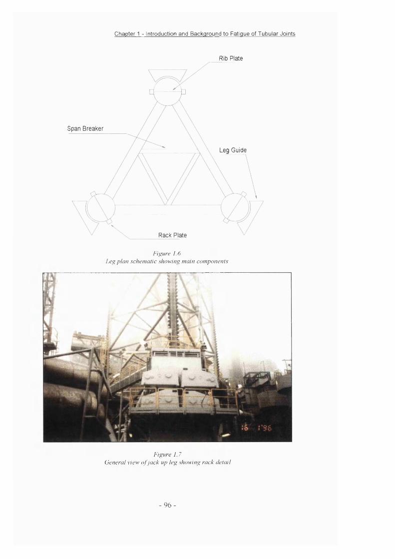
Chapter 1 - Introduction and Background to Fatigue of Tubular Joints
Rib Plate
s p a n Breaker
Leg Guide
Rack Plate
F i g u r e 1 . 6
I . e g p l a n s c h e m a t i c s h o w i n g m a i n c o m p o n e n t s
F i g u r e 1 .7G e n e r a l v i e w o f j a c k u p l e g s h o w i n g r a c k d e t a i l
- 96 -
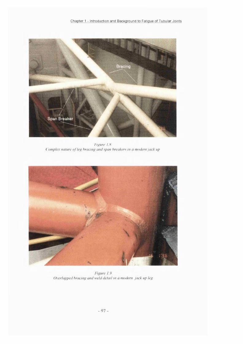
Chapter 1 - Introduction and Background to Fatigue of Tubular Joints
F i g u r e 1 . 8
C o m p l e x n a t u r e o f l e g b r a c i n g a n d s p a n b r e a k e r s i n a m o d e r n j a c k u p
F i g u r e 1 . 9
O v e r l a p p e d b r a c i n g a n d w e l d d e t a i l i n a m o d e r n j a c k u p l e g
- 9 7 -

Chapter 1 - Introduction and Background to Fatigue of Tubular Joints
R Piggy Back Vessel
Wet Tow Dry Tow
F i g u r e 1 . 1 0
J a c k u p t r a n s p o r t a t i o n m o d e s
Y JointT Joint
DT Joint Multiplane Joint
F i g u r e 1 . 1 1
C o m m o n t u b u l a r j o i n t c o n f i g u r a t i o n s
- 9 8 -

Chapter 1 - Introduction and Background to Fatigue of Tubular Joints
C row n
T
SaddleD
F i g u r e 1 . 1 2
T - J o i n t p a r a m e t r i c n o t a t i o n
Axial
O ut of P la ne Bend ing (O R B ) n P la n e Bending ( IP B )
F i g i a e 1 . 1 3
T h e t h r e e t u b u l a r j o i n t l o a d i n g m o d e s
- 9 9 -
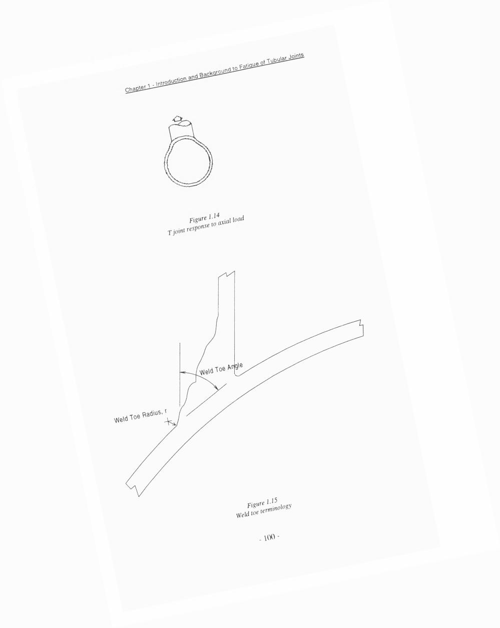
. -
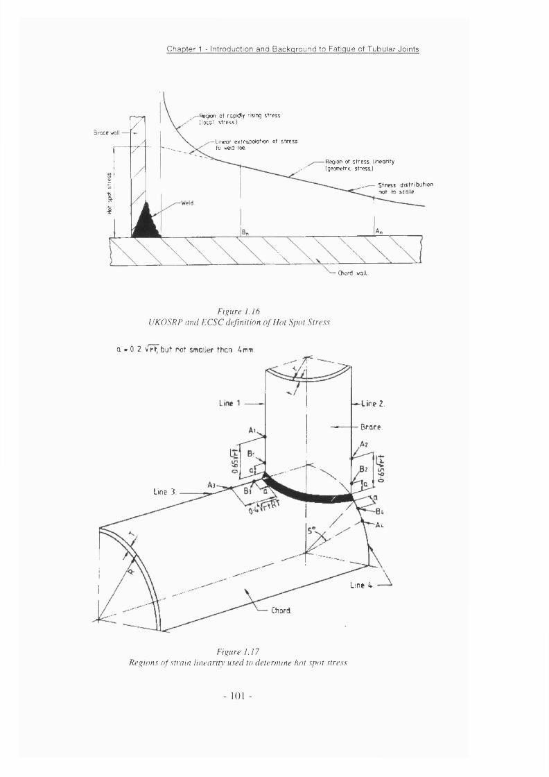
Chapter 1 - Introduction and Background to Fatigue of Tubular Joints
Brace wall — 7//
1 /iÎLà
-Regnn of ropidfy rrsinq stress (local stress)
Region of stress linearity I geometric stress ]
—Linear extrapotation of stress to weld toe
Stress distributionnot to scale
Chord wall.
F i g u r e 1 . 1 6
U K O S R P a n d E C S C d e f i n i t i o n o f H o t S p o t S t r e s s
Q ■ 0 2 Vrl; b jf riot smaller than 4mm
Line 2
B race
Line 3.
•Au
Line 4
Chord.
F i g u r e 1 . 1 7
R e g i o n s o f s t r a i n l i n e a r i t y u s e d t o d e t e r m i n e h o t s p o t s t r e s s
- 101 -
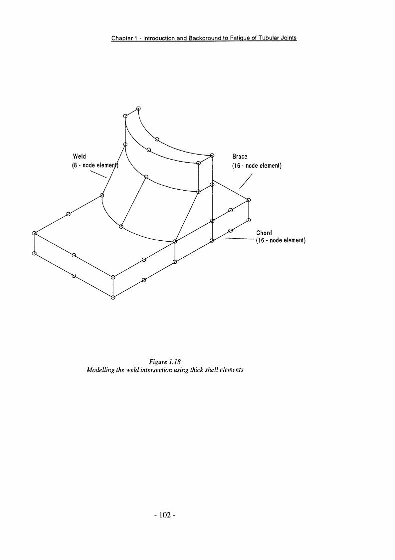
Chapter 1 - Introduction and Background to Fatigue of Tubular Joints
Weld(8 ■ node elemenJ
Brace(16 ■ node element)
Chord(16 - node element)
F i g u r e 1 . 1 8
M o d e l l i n g t h e w e l d i n t e r s e c t i o n u s i n g t h i c k s h e l l e l e m e n t s
- 102 -
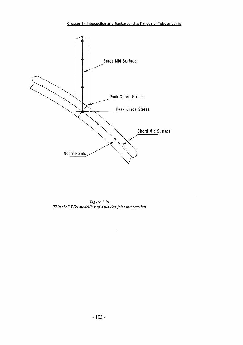
Chapter 1 - Introduction and Background to Fatigue of Tubular Joints
Brace Mid Surface
Peak Chord Stress
Peak Brace Stress
Chord Mid Surface
Nodal Points
F i g u r e 1 . 1 9
T h i n s h e l l F E A m o d e l l i n g o f a t u b u l a r j o i n t i n t e r s e c t i o n
- 103
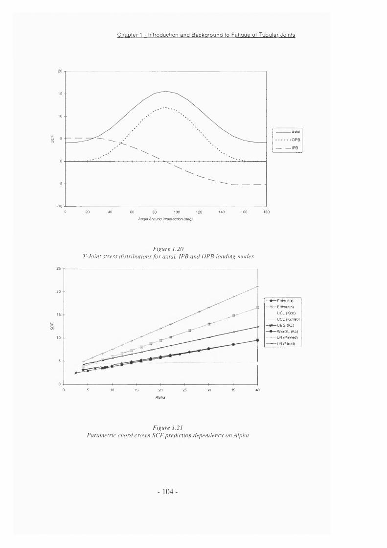
Chapter 1 - Introduction and Background to Fatigue of Tubular Joints
15 --
10 - -
-100 20 40 60 80 100 120 140 160 180
Angle Around Intersection (deg)
F i g u r e 1 . 2 0
T - . f o i n t . s t r e s . s d i s t r i b u t i o n s f o r a x i a l , I P B a m i O P B l o a d i n g m o d e s
20 - -
10 - -
5 --
0 5 3510 15 20 25 30 40
— Elthy (fix)
—>W— Efthy(pin)
UCL (KcO)
UCL (Kc180)
- 4 * — UEG (Kc)
Wofds. (Kc) —'— LR (Pinned)
—— LR (Fixed)
Alpha
Figure I .2 IParametric chord crown SCF prediction depemlencv on Alpha
- 104 -
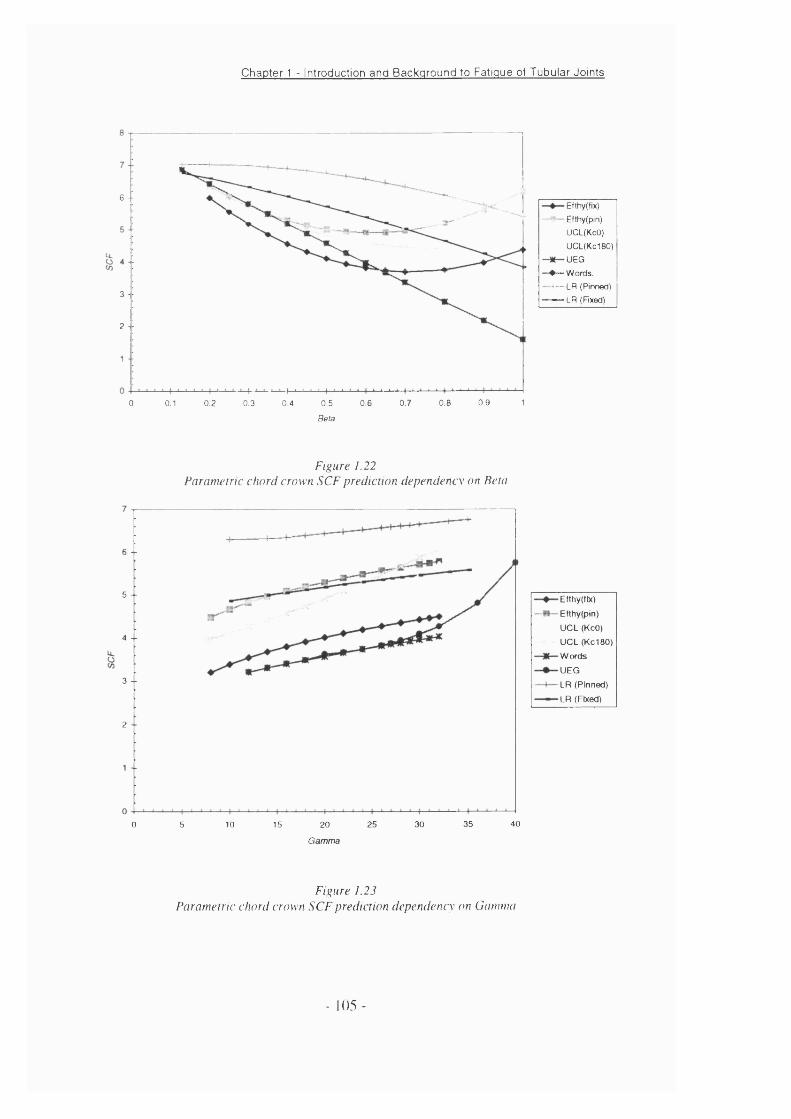
Chapter 1 - Introduction and Background to Fatigue of Tubular Joints
6 - -
3 --
2
0.90.5 0.6 0.7 0.00 0.1 0.2 0.3 0.4
Efthy(fix)
Efthy(pin)
UCL(KcO)
UCL(Kc180)
UEG
-# — W ords.
_.i— |_n (Pinned)
— LR (Axed)
Beta
F i g u r e 1 . 2 2
P a r a m e t r i c c h o r d c r o w n S C F p r e d i c t i o n d e p e n d e n c y o n B e t a
6 - -
5 --
4 - -
3 --
2 --
35 400 5 10 15 20 25 30
Efthy(tix)
Efthy(pin)
UCL (KcO)
UCL (KciaO)
Words
UEG
LR (Pinned)
LR (Fixed)
G am m a
Figure 1.23Parametric chord crown S C F prediction dependency on Gamma
- 105 -
Chapter 1 - Introduction and Background to Fatigue of Tubular Joints
3 --
2 --
0.7 0 8 0.9 10 0.1 0.2 0.3 0.4 0.5 0.6
— Eflhy(fix) —4 — Efthy(pin)
UCL(KcO)
UCL(KclBO)
UEG
—# — Words
— !— LR (Pinned)
— LR (Fixed)
Tau
F i g u r e 1 . 2 4
P a r a m e t r i c c h o r d c r o w n S C F p r e d i c t i o n d e p e n d e n c y o n T a u
20
10-“
16 --
14 --
12 - -
§ 10 -
6 - -
4 --
2 -
35 400 S 10 IS 20 25 30
Alpha
Figure 1.25Parametric chord saddle SCF prediction deperuiency on Alpha
■ Efthy (fix) -Efthy (pin)
UCL (Ks)
UCL (Khs)
-U EG (Ks)
- Words. (Ks)
-LR (Pinned)
-LR (Fixed)
- 106 -
Chapter 1 - Introduction and Background to Fatigue of Tubular Joints
20 - ■
15 --
10 - -
5 --
0.90 0.1 0.2 0.3 0.4 0.5 0.6 0.7 0.8 1Beta
F i g u r e 1 . 2 6
P a r a m e t r i c c h o r d . s a d d l e S C F p r e d i c t i o n d e p e n d e n c y o n B e t a
60
50 --
40 --
U 30 --
20 - -
10 - -
4025 350 5 10 15 20 30
G am m a
F i g u r e 1 . 2 7
P a r a m e t r i c c h o r d s a d d l e S C F p r e d i c t i o n d e p e n d e n c y o n G a m m a
- Efthy(fix)
- Efthy(pin)
UCL (Ks)
UCL (Khs)
-UEG
•W ords.
■ LR (Pinned)
-LR (Fixed)
Ellhy((ix)
Efthy(pln)
UCL (Ks) UCL (Khs)
UEG
Words
LR (Pinned)
LR (Fixed)
- 107 -
Chapter 1 - Introduction and Background to Fatigue of Tubular Joints
1 6 - -
1 4 - -
12 - -
10 - -
6 --
0 0.2 0.70.1 0.3 0.4 0.5 0.6 0.8 0.9 1
Efthy(fix)
Efthy(pin)
UC L(Ks)
UCL(Khs)
-4*— UEG
W ords
— LR (Pinned)
LR (Fixed)
Tau
F i g u r e 1 . 2 8
P a r a m e t r i c c h o r d s a d d l e S C F p r e d i c t i o n d e p e r u i e n c y o n T a u
% 100 cc
I
101.00E-MD4
N
I.OOE-mS I.OOE-rOe 1.00E-k07
Endurance (Cyctes)
I 16mm SOD Data
- - 16mm Mean
Design T Curve
i.ooE-me i.ooE-f09
F i g u r e 1 . 2 9
1 6 m m 5 0 D f a t i g u e l i f e d a t a t o g e t h e r w i t h m e a n a n d d e s i g n S - N c u r \ ' e s
- 108 -
Chapter 1 - Introduction and Background to Fatigue of Tubular Joints
1000
I 16mm 500 Data
32mm 500 Data
- 16mm Mean
-D es ign T Curve
I 100
:cn
1.00E+05 1.00E+06 1.00E+07 1.00E+08Endurance (Cycles)
F i g u r e 1 . 3 0
T h i c k n e s s e f f e c t i l l u s t r a t e d b y I 6 m m a n d 3 2 m m f a t i g u e l i f e d a t a
1000
IS, 16mmI ;
— 32mm100
I 48mm
II
72mm
1 OOE+03 1 006*08 1 006+09
Lfe (cycles)
F i g u r e 1 . 3 1
N e s t e d T c u r v e s f r o m t h i c k n e s s e f f e c t a l l o w a n c e
- 109 -

Chapter 1 - Introduction and Background to Fatigue of Tubular Joints
! I 1 I 1 1 1 1tl 1 1 M M- - - -50D 16mm mean
r' Air Curve
'■
-- -
— - - -
c 1005
10
1 00 E+04 1.00E+05 1.00E+06
Endurance (Cycles)
F i g u r e 1 . 3 2
S - N c u r v e s f o r 1 6 m m p l a t e s a n d t u h u l a r s i n s e a w a t e r ( f r e e c o r r o s i o n ) a n d o p t i m u m c a t h o d i c
p r o t e c t i o n
Crack Tip
F i g u r e 1 . 3 3
C a r t e s i a n c o - o r d i n a t e s f o r n e a r c r a c k a n a h ' s e s
- 1 1 0 -

Chapter 1 - Introduction and Background to Fatigue of Tubular Joints
Mode 1
Mode
Mode
F i g u r e 1 . 3 4
T h e t h r e e m o d e s o f c r a c k g r o w t h
Paris Law
Region 3Region 2Region 1
da I dN
AK
F i g u r e 1 . 3 5
T h e t h r e e s t a g e s o f f a t i g u e c r a c k g r o w t h
- I l l -
Chapter 1 - Introduction and Background to Fatigue of Tubular Joints
W elded P la teo
Tubular JointC
CO
1.00.0 0.5
Non Dimensional C rack Depth, a/t
F i g u r e 1 . 3 6
S i r d e v e l o p m e n t i n t u b u l a r j o i n t s a n d w e l d e d p l a t e s
caCLa>o
Tubular JointO05O
W elded Pla
1.00.0 0.5
Fraction of fatigue life
F i g u r e 1 . 3 7
C r a c k d e p t h d e v e l o p m e n t i n t u b u l a r J o i n t s a n d w e l d e d p l a t e s
- 112
Chapter 1 - Introduction and Background to Fatigue of Tubular Joints
C o r r o s i v eenvironm ent
2 0 H ' 2 0 H "
S u r f a c e
F i g u r e 1 . 3 8
E l e c t r o c h e m i c a l c o r r o s i o n p r o c e s s [ 1 . 7 7 ]
P ro te c te d S tru c tu re
\
P o w e r S u p p ly
4e-
Og+2HgO
O H '
4cr
2 C I.
Im p re s s e d C u rre n t A n o d e
F i g u r e 1 . 3 9
I m p r e s s e d C u r r e n t C a t h o d i c P r o t e c t i o n [ 1 . 7 7 ]
- 1 1 3 -
Chapter 1 - Introduction and Background to Fatigue of Tubular Joints
6 -■
5 -- Free Corrosion
4 --
3 --
2 - -
Normal CP
"Crack propagation rale in air
Scatter band in air
- 0.6 -0.7 -0.8 -0.9CP Potential (Ag/Agcl) V
- 1.1 - 1.2
F i g u r e 1 . 4 0
E f f e c t o f C P p o t e n t i a l o n f a t i g u e c r a c k g r o w t h r a t e ( 0 . 1 H z , R < = 0 . 1 )
1E-6
^ I E - 7
E-8
o
1E -1 0
1 10010
Stress Intensity Factor R ange (M P a m ^ O .5 )
F i g u r e 1 . 4 1
S c h e m u t i c d a / c I N - A K p l o t . s h o w i n g p l a t e a u g r o w t h r a t e r e g i o n u n d e r C P c o n d i t i o n s
- 1 1 4 -

Chapter 1 - Introduction and Background to Fatigue of Tubular Joints
10
voaiKOvsxr
pi^euNe sreet x»a CÂTHOOIC P K O r e c T i o H ziMC p orenT i L
- 810uNEE
Ht
-a10 0 1 H i
iSJiuy10
(0 0 Mi
-71020 30 50 70 1002 4 6 B 10
AK STRESS INTENSITY (MPaVmJ
F i g u r e 1 . 4 2
I n d e p e n d e n c e o f c r a c k g r o w t h r a t e t o A K i n X 6 5 u n d e r C P C o n d i t i o n s
- 115 -

--
CL
E
en ru CL OCL
-k :
Chapter 1 - Introduction and Background to Fatigue of Tubular Joints
6 5 5 F MZSE 5 0 0
O H S L A 8 0X HS 4 2 0• 4 5 0 EM 2o X A O O 5 0 0
12 U 16 18AK
20 22 24
(a) -950mV
55 F M2 SE 5 0 0 H S L A 80 HS 4 2 0 4 5 0 EMZ X AO Q 5 0 0 TiO
8
2
012 1614 2220
AK
(b) -1100mV
F i g u r e 1 . 4 3
H i g h s t r e n g t h s t e e l c r a c k g r o w t h r a t e s f r o m B i l l i n g h a r n e t a l
- 1 1 6 -
Chapter 2 - Experimental Fatigue Testing of W elded Tubular Joints
Chapter Two
2. Experimental Fatigue Testing of Welded Tubular Joints
2.1 Introduction
Large scale tubular joint fatigue tests have been performed for a number of
decades. The expense and difficulty involved in testing such specimens is Justified
on the grounds that the crack growth behaviour of tubular joints is unique and
complex and to date all attempts at reproducing the fatigue crack growth
behaviour in tuhulars using simple welded specimens have failed.
The amount of information that it is now possible to extract from each test has
increased enormously in recent years. It is hoped that the fracture mechanics
models proposed to predict the crack growth behaviour can be refmed and made
more accurate and reliable using information gained from tests such as these.
The current test programme will be described in detail. This will include all
hardware, software and procedures used during the preparation and execution of
each test. The extraction and analysis of the raw data will be described and all
relevant results will be presented. The information presented here will be used in
Chapter 5 to critically assess the capability of the current state of the art in terms of
fatigue fracture mechanics models used for predicting the fatigue crack growth
behaviour of these joints.
2.2 Tubular Joint Test Specimens
The test specimens will be described in this section. This will include the nominal
and actual joint dimensions, mechanical and chemical properties of the parent plate
and weld metal as well as the weld procedures and consumables used during
fabrication.
117 -
Chapter 2 - Experimental Fatigue Testing of W elded Tubular Joints
2.2.1 Dimensions
The six specimens tested during this investigation were all T-shaped large scale
tubular welded joints. The nominal specimen dimensions are illustrated in Figure
2.1. Also included are the non-dimensional parameters commonly used to describe
tubular joints. Non dimensional parameters are particularly useful for presentation
of SCF’s in parametric form.
The specimen dimensions have been chosen to allow direct comparison with earlier
tubular joint test programmes performed at UCL using lower strength steels. In
addition, modifications to the fatigue test rig are minimised.
The actual specimen dimensions agree closely with the nominal values in all cases.
A small degree of out of roundness of the members was detected due to the
method of manufacture of the tubes (see Section 2.2.2).
The greatest manufacturing inaccuracy in terms of percentage differences was
found to be the wall thickness of the brace and chord. The wall thickness was
measured ultrasonically using a SONATEST STEELGAGE M at six sites around
the intersection of the brace and chord of each specimen. In each case the wall
thickness was found to be greater than the nominal 16mm. The CLi specified
tolerance for rolling SE702 to 16mm is 0.8mm, in the ranges 4-/-0.4mm and 0 to
+0.8mm [2.1]. The ultrasonically measured wall thicknesses are given in Table 2.1.
The thicker brace values at the saddle are due to the presence of a seam weld
running the length of the brace. Ultrasonic measurements of wall thickness were
also taken at intervals around the chord ends. This was performed in order to
confirm the accuracy of the technique on this particular steel geometry
configuration as Vernier measurements of the thickness can also be taken at this
point. Comparison of the two methods shows the maximum difference to be
0.1mm.
- 118 -

Chapter 2 - Experimental Fatigue Testing of W elded Tubular Joints
The potential significance of variations in wall thickness was highlighted by Austin
[2.2]. The parametric formulation of Kuang was used to calculate the SCF and a
single segment SN curve with a negative inverse slope of 3 to determine the
corresponding endurance. Using this data Austin found that the scatter in tubular
joint endurance data could be entirely accounted for by variations in wall thickness
alone. Although this may be the case from theoretical considerations it is not
suggested here that this is the sole or even dominant source of scatter from
experimental data.
2.2.2 Specimen Fabrication
Unlike earlier tubular joint test programmes at UCL the tubular members were not
fabricated from seamless tubing. In this instance both the brace and chord were
rolled in two halves and subsequently seam welded together. The position of the
seam welds are illustrated in Figure 2.2. This is not thought to be significant in
terms of the subsequent fatigue performance of the specimens. The weld details are
given in Table 2.2 for the seam welding.
The post weld heat treatment specified is only applicable to the seam welds used to
form the tubes. It is important to note that no PWHT was specified for the
completed joints.
Of more significance is the welding of the intersection between the brace and
chord. It has been shown in Chapter 1 that the weld detail exerts a significant effect
on the fatigue life. It was imperative therefore that the welding was representative
of that used in the construction of offshore structures. The welding contractor,
PAUMECA S. A. of Le Breuil, France was involved in the construction of the BP
Harding Jack Up. Weld procedures from previous tubular joint specimens
fabricated by Highland Fabricators for UCL and colour photographs of the weld
detail were also supplied to PAUMECA. Additionally the contractor was visited
during the welding of the first joint. It was noted that the contractor intended to
- 119 -
Chapter 2 - Experimental Fatigue Testing of W elded Tubular Joints
undertake inter-run grinding to improve the weld profile. This was thought to be
unrepresentative and as such the contractor was requested to modify his procedure.
No inter-run or weld toe grinding was subsequently performed. The run sequences,
welding speed and joint preparation were recorded by PAUMECA. The
intersection welding details are given in Table 2.3. The preheat values of 125°C
and welding heat input of 1.5KJ/mm have been shown to avoid cold cracking
problems in SE702 [2.3].
A photograph of the intersection and seam weld of a representative joint is shown
in Figure 2.3. All welds successfully passed a full ultrasonic inspection in
accordance with the French standard NFP22-471 [2.4].
Chord and brace weld leg lengths have been measured using a weld profile gauge.
The definition of weld leg lengths is illustrated in Figure 2.4. The weld profile was
measured at five sites around both saddles on the chord and brace side. The
measured leg lengths are given in Table 2.4.
The Dime Test [2.5] was performed on all welds and no weld completely failed the
test. However all joints failed at certain points around the intersection, some near
to the saddle region. No correlation between these regions and the subsequent
fatigue crack initiation site were found.
2.2.3 Material Properties
The use of state of the art steel making processes allows the manufacturer to
guarantee high performance material properties to within close limits. This is due
to the very low levels of sulphur, hydrogen, high cleanliness due to low oxygen
content and very precise chemical composition. Guaranteed and actual chemical
compositions for SE702 are detailed in Table 2.5. A sample of steel cut from one
of the tuhulars has been analysed independently [2.6].
- 120
Chapter 2 - Experimental Fatigue Testing of W elded Tubular Joints
It can be seen that the CLi’s chemical analysis of the current batch of steel meets
the specified standard for each of the alloying elements except for manganese
which is higher than the guaranteed maximum. Manganese acts as a de-oxidiser,
lowers the transition temperature and acts as a hardenability agent. The
discrepancy is not thought to be significant in terms of this study.
The independent analysis agrees well with the CLi analysis of the same batch of
steel. Again manganese is the only element which falls outside the specified
composition. A ll other elements meet the specification.
2.2.4 Mechanical Properties of SET02
The specified mechanical properties for SE702 are shown in Table 2.6.[2.7].
Independent tensile tests on steel from the same batch as that used to fabricate the
tuhulars has been performed at Cranfield University. The tests were performed
using 5.5mm diameter specimens. Details of the orientation of the specimens in
terms of the rolling direction of the parent plate etc. are not known. All specimens
are assumed to be nominally identical. The results are summarised in Table 2.7.
Data from Charpy impact tests performed at Cranfield is tabulated in Table 2.8.
Vickers Hardness Data has been obtained by CLi and Cranfield for parent plate,
weld metal and the heat affected zone of a T-Butt weld qualification specimen. A
summary of this data is given in Table 2.9. The CLi data given in the first table
used a load of 5kg and the Cranfield data in the second table used 10kg. The
Vickers Hardness Test is designed in such a way that the results are independent of
the load used and standard loads of between 1 and 120kg are used. Thus the CLi
and Cranfield data can be directly compared.
The parent plate values of approximately 250HV are reasonable for a steel of this
strength. Values quoted in [2.8] suggest that a carbon or alloy steel with a HV
value of 250 should have a UTS of around 800MPa. This is almost identical to the
strength of this material.
- 121 -
Chapter 2 - Experimental Fatigue Testing of Welded Tubular Joints
Healy et al [2.3] examined the weldability of a number of modern high strength
steels, including SE702. It was noted that parent plate hardness values for such
steels were typically in the range 260-280Hv. A maximum HAZ hardness limit of
400Hv is a commonly applied industry standard to avoid problems such as
hydrogen induced cold cracking susceptibility and stress corrosion cracking in
service. SE702 has been shown to satisfy this requirement even under the most
severe welding conditions of low heat input (IKJ/mm) and no pre-heat.
2.3 Experimental Set Up
Tubular joint fatigue tests are difficult to perform. The tests are expensive, time
consuming and complex. In view of the very limited number of specimens available
it is essential that great care and attention is taken during the setting up and
execution of each test.
The hardware and software used during the fatigue tests is discussed in detail. In
particular the monitoring and recording of the crack growth process requires
meticulous preparation and will be discussed in depth.
2.3.1 Applied Loading
Fatigue loading is supplied by a IM N servo-hydraulic INSTRON actuator. The
actuator is controlled via an INSTRON mini-controller. The actuator can be
controlled under position or load feedback loops. All tests conducted here were
performed under load control. In this mode the specimen is subjected to load cycles
of a pre-defmed amplitude regardless of any change in stiffness of the specimen or
until the stroke of the actuator is exhausted. A purpose buUt test rig has been
constructed around the actuator. Axial loads are applied to the brace end and are
reacted at the chord ends where axial and radial displacements are restrained. The
connection between the brace end and the actuator is made via a swivel head
connector. An isometric view of the test rig is shown in Figure 2.5.
- 1 2 2 -

Chapter 2 - Experimental Fatigue Testing of W elded Tubular Joints
2.3.2 Fatigue Crack Monitoring
The fatigue crack development in the tubular joints was monitored by taking
Alternating Current Potential Drop (ACPD) crack depth measurements at fixed
points around each expected crack location. By choosing suitable inspection
intervals it should be possible to follow crack growth from initiation (N i) to
through wall penetration ( N 3 , see Section 1.8.2).
The ACPD technique utilises the thin skin effect whereby a high frequency
alternating current will be confined to a thin layer when flowing through ferrous
materials. A function of the permeability and conductivity of the material and the
frequency of the alternating current, the skin depth is given by (2.1) [2.9].
s = I (2.1)VHUoOitf
where:
|io Permeability of Free Space
\i Relative Permeability of Metal
a Conductivity of Metal
f A C. Frequency (5KHz)
If an alternating current is forced to flow across a surface breaking defect as
illustrated in Figure 2.6, the current will flow down one crack face and up the other
side. Since a linear potential gradient is assumed to exist on the metal surface and
on the crack faces, measurement of the potential drop across the crack and
adjacent to the crack allows the calculation of the 1-D crack depth as follows:
Vr - A(2 2)
V c - ( A + 2di) ^
Therefore,
123 -
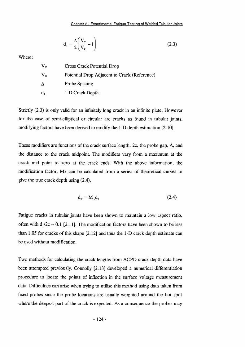
Chapter 2 - Experimental Fatigue Testing of W elded Tubular Joints
‘i . = f[ H
(Z3)
Where:
Vc Cross Crack Potential Drop
V r Potential Drop Adjacent to Crack (Reference)
A Probe Spacing
di 1-D Crack Depth.
Strictly (2.3) is only valid for an infinitely long crack in an infinite plate. However
for the case of semi-elliptical or circular arc cracks as found in tubular joints,
modifying factors have been derived to modify the 1-D depth estimation [2.10].
These modifiers are functions of the crack surface length, 2c, the probe gap. A, and
the distance to the crack midpoint. The modifiers vary from a maximum at the
crack mid point to zero at the crack ends. With the above information, the
modification factor, Mx can be calculated from a series of theoretical curves to
give the true crack depth using (2.4).
d = M ,d , (2.4)
Fatigue cracks in tubular joints have been shown to maintain a low aspect ratio,
often with di/2c = 0.1 [2.11]. The modification factors have been shown to be less
than 1.05 for cracks of this shape [2.12] and thus the 1-D crack depth estimate can
be used without modification.
Two methods for calculating the crack lengths from ACPD crack depth data have
been attempted previously. Connolly [2.13] developed a numerical differentiation
procedure to locate the points of inflection in the surface voltage measurement
data. Difficulties can arise when trying to utilise this method using data taken from
fixed probes since the probe locations are usually weighted around the hot spot
where the deepest part of the crack is expected. As a consequence the probes may
124
Chapter 2 - Experimental Fatigue Testing of W elded Tubular Joints
be 15 - 20 mm apart in the region where the crack ends would be expected to be in
the later stages of life.
A simpler alternative involves truncating the crack depth readings near the crack
ends. Crack lengths produced using this technique have been shown to lie within a
15% error band on optically measured crack lengths.[2.12]. This technique was
adopted here.
Siting of the fixed ACPD Probes requires careful consideration in order to
maximise the usefulness of the data. Crack growth is expected to initiate at the hot
spot site and the deepest point of the crack is expected to remain in this region. In
addition for a balanced axially loaded T joint, two potential crack sites exist, one at
each saddle.
ACPD measurements were performed using a UlO Crack Microguage with an
integral 128 channel multiplexer unit [2.14]. A single ACPD site requires two
channels, one each for the crack and reference readings resulting in a total capacity
of 64 fixed ACPD sites. The 64 ACPD sites were divided equally between each
saddle since both are potential crack locations. The probe sites were weighted
towards the hot spot region where the fatigue cracks were expected to initiate. The
locations of the fixed probes relative to the saddle position are detailed in Table
2.10. The UlO supports the use of 4 sets of field injection points. Two fields were
used for each saddle. Each field therefore covers 16 ACPD sites to one side of the
saddle.
The durability of the ACPD probes is an important consideration. The probes can
be submerged in a corrosive sea water environment for anything up to six months.
It is essential that the probes do not degrade due to this environment as valuable
data would be lost. It is difficult if not impossible to replace or repair probes once
the test is underway.
125 -
Chapter 2 - Experimental Fatigue Testing of W elded Tubular Joints
Preliminary investigations were performed to identify the most durable probe set
up. The outcome of this investigation resulted in a set up that proved highly
reliable with very few failures occurring during testing. The surface of the tubular
was cleaned down to shiny bare metal as this gives the best surface for the
attachment of the probes by spot welding. Several grades of steel wire were
examined and the one resulting in the strongest weld to SE702 was selected. This
was a steel wire of approximately 0.6mm diameter. Once welded to the specimen
surface the probes were cut to a height of 3 to 4mm. Bootlace ferrules (0.5mm^)
were placed over these pins and filled with solder to ensure a low resistance
connection. Electrical connection to the UlO was made by twisted pair multiplexer
ribbon which was terminated in the solder filled ferrule. For the sea water test each
of the 272 individual probes and earth connections were encapsulated in bitumen to
prevent environmental attack. This is an extremely time consuming and repetitive
task but the result is a highly reliable electrical connection that will allow
automated crack depth measurements to be taken underwater, day and night for
many months.
The raw data collected from a typical Test ( ‘T l ’) is shown in Figure 2.7. This data
is completely unmodified and illustrates the repeatability and accuracy of the
ACPD technique for capturing ‘snapshots’ of the crack growth process.
Techniques have been developed to remove some of the ‘peaks’ found in the raw
data. These techniques and the underlying causes are discussed later in this Section.
These anomalies are obviously not representative of the actual crack shape which
are known to have smooth semi-elliptical profiles from post failure sectioning of
cracked members.
The 1-D crack depth equation (2.3) was derived using the assumption that the
cross crack probe gap and the reference probe gap were the same. This is the case
with a standard hand held probe. However inaccuracies in siting the spot welded
fixed probes means that it can no longer be assumed that the probe gaps are equal.
- 126
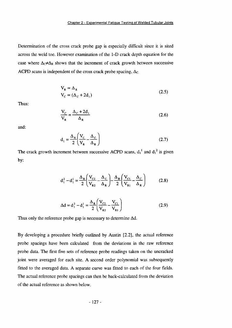
Chapter 2 - Experimental Fatigue Testing of W elded Tubular Joints
Determination of the cross crack probe gap is especially difficult since it is sited
across the weld toe. However examination of the 1-D crack depth equation for the
case where Ac Ar shows that the increment of crack growth between successive
ACPD scans is independent of the cross crack probe spacing, Ac.
Thus:
V R - A ,
Vc «^(Ac + ld j )
Vc Ac+2di
(2.5)
(2.6)
and:
d.= — Vcv V r ^ r y
(2.7)
The crack growth increment between successive ACPD scans, d / and di is given
by:
d f - d l = ^ Vc2R y
Vci ^c
R y(2.8)
A d = d ? - d ; = - ^ Vc2 Vc,V,Vr2 V,Ri y
Thus only the reference probe gap is necessary to determine Ad.
(2.9)
By developing a procedure briefly outlined by Austin [2.2], the actual reference
probe spacings have been calculated from the deviations in the raw reference
probe data. The first five sets of reference probe readings taken on the uncracked
joint were averaged for each site. A second order polynomial was subsequently
fitted to the averaged data. A separate curve was fitted to each of the four fields.
The actual reference probe spacings can then be back-calculated from the deviation
of the actual reference as shown below.
- 127 -

Chapter 2 - Experimental Fatigue Testing of W elded Tubular Joints
VocA
Therefore assuming the actual reference is Ar, and the nominal spacing is 10.
V r= kAR
Vio = klO
Thus;
Ar = 10(Vr / V io) (2.10)
Non zero crack depth readings are expected at some sites even before fatigue
testing has commenced. This is due to errors in the placement of the fixed probes
and some non uniformity of the field. In an attempt to maintain field uniformity two
AC field injection points are employed on each side of the joint each serving 16
ACPD sites. Subtraction of the initial ACPD crack depth readings on the
uncracked joint from all subsequent ACPD scans should give an accurate measure
of crack development. The modified ACPD crack development plot for a typical
test is shown in Figure 2.8. Two inspection intervals were used during the test. The
shorter inspection interval can clearly be seen from the spacing of the crack profile
lines earlier in the test.
2.3.3 Environment Chamber
For the corrosion fatigue tests, the welded intersection where the fatigue crack is
expected to grow must be immersed in sea water. This is achieved via an
environment chamber that bolts around the chord / brace intersection. A water
tight seal was achieved using ribbed rubber strips and silicon sealant. The weight of
the water filled chamber was supported using steel bands around the brace and
chord. Artificial sea water made to ASTM D1141 [2.15] is pumped from a
reservoir through a closed loop passing through the environment chamber. The
fully aerated sea water is maintained between temperature limits of 8-10°C via an
external chiller and between pH 7.8-8.2.
The cathodic protection (CP) system consists of two W ENKING MP81
potentiostats, two platinum coated anodes and two Ag/AgCl reference electrodes.
- 128 -
Chapter 2 - Experimental Fatigue Testing of W elded Tubular Joints
The top and bottom saddle CP systems were independent. A submersible reference
electrode was used for the lower saddle.
Prior to application of fatigue loading, each joint was subjected to a ‘soak time’
where the joint was submerged in sea water with the CP switched on at the
appropriate level. A soak time of two weeks was implemented to achieve
polarisation of the specimen and allow hydrogen to diffuse through the steel.
The time required to achieve a uniform through thickness hydrogen concentration
is dependant on the diffusion coefficient for the material. Unfortunately such data
in the literature is scarce and the values that are quoted can vary by orders of
magnitude or more [2.16]. The soak time for tubular joints is considered less
important than that for simple specimen tests that may only last a day or two. For
the simple specimen case, if the hydrogen has not permeated through the steel
before the crack growth commences it is possible that the crack may grow faster
than the hydrogen diffuses through the metal. This may mask the effect of the
environment on the crack growth rate. For tubular joints however the tests may
last for several months making the through thickness hydrogen concentration
gradient at the commencement of loading less critical.
2.3.4 Test Control and Data Acquisition
Previous tubular joint fatigue tests at UCL have been controlled using the
proprietary FLAPS software [2.17]. FLAPS controls the waveform generation and
ACPD data capture and storage tasks automatically. The particular strength of this
software is its ability to ‘replay’ complex variable amplitude, variable frequency
load sequences such as WASH [2.18]. It does however have certain drawbacks.
The communication protocol used by the software does not allow it to
communicate directly with the UlO crack microguage. Thus during ACPD data
capture the internal UlO switching unit must be replaced by an external switching
unit. It also has more subtle practical implications regarding the test set up and data
storage. Additionally an INSTRON Harrier interface is required to complete the
129
Chapter 2 - Experimental Fatigue Testing of W elded Tubular Joints
waveform generation task. Practical constraints and reliability considerations
dictated that an alternative computer control routine be sought.
As a result a PASCAL test control routine originally written at UCL [2.19] for
controlling simple specimen tests has been modified for this investigation.
Interfacing with a data acquisition board, this program eliminates the need for the
Harrier interface and auxiliary switching unit for the UlO. This flexible routine
allows the user to control the waveform generation by supplying the amphtude and
the frequency for the sinusoidal waveform. ACPD crack depth scans can be
performed automatically at user defined intervals or on demand. ACPD crack
depth and voltage data is stored electronically in a spreadsheet readable format. A
hard copy of the results can also be obtained.
A schematic of the complete experimental test set up showing all aspects of test
control, data acquisition and environmental control is shown in Figure 2.9.
2.4 Experimental Stress Analysis
The hot spot stress concentration factor was measured experimentally using strain
gauges. The steep stress gradient close to the intersection combined with the fact
that a strain gauge averages out the distribution of strains over which they are
located and the anticipated hi-axial stress state resulted in a requirement for small
rosette gauges to achieve maximum accuracy. Three element, 45° rosettes with
over-layed gauge lengths of 2mm were selected and used for all the tubular joints
tested in this study.
A balanced axially loaded T-joint should yield similar hot spot stress concentration
factors for both saddle regions. This of course assumes identical weld profiles at
both hot spot sites and a high level of precision in fabrication in order that the mid
planes of both brace and chord are co-incident to minimise bending effects.
However in reality manufacturing tolerances can result in some variation in hot
- 130 -

Chapter 2 - Experimental Fatigue Testing of W elded Tubular Joints
spot SCF’s at opposing saddles in an axially loaded T- joint. Examination of
previous test results show differences of 10% to 15% to be typical. Experimental
SCF results from a previous test program using a similar geometry [2.2] are shown
in Table 2.11.
The percentage difference is calculated as shown in (2.11 )
MaxSCF - MinSCF Ï S S S ? — >“ «>
The fatigue test rig is designed in such a way as to allow limited adjustment to be
made to the chord position in the vertical plane. This is to allow the alignment of
the T joint mid-plane and the mid-plane of the loading actuator. Mis-alignment
would result in an out of plane bending component being introduced since the
chord ends are fixed. This would affect the experimental stress concentration
factors accordingly.
As a result it was necessary to repeat the experimental stress analysis a number of
times at different chord heights prior to the first fatigue test. The chord height was
subsequently fixed at the position that resulted in the least discrepancy in the
experimental stress concentration factors between the two saddle regions. This was
assumed to indicate joint alignment with the actuator loading axis.
The first fatigue test resulted in a fatigue crack at only one saddle point (the one
with the highest SCF). Although this is reasonably common for such tests, it was
decided that a more scientific approach should be taken to the alignment of the
joint and actuator mid planes.
In consultation with the Department of Photogrammetry and Surveying [2.20] a
procedure was developed to adjust the height of the chord ends to ensure that the
centre lines of the actuator and brace were co-incident. This also ensured that the
131 -
Chapter 2 - Experimental Fatigue Testing of W elded Tubular Joints
chord lay level. A tripod mounted Sokkia Automatic Level was used to determine
the height of collimation of two points known to lie along the centre plane of the
actuator. By measuring the distance between these two points the slope of the
actuator could be determined. It was found that the actuator lay on a slope of 3mm
/ m. Extrapolating this to the chord centre line gave the required height of the
chord. The Sokkia Level was then used to set three points along the chord at the
appropriate height. Hand operated hydraulic jacks were used to move the chord
ends. This process is illustrated in Figure 2.10.
A further factor produces a discrepancy between the SCF results between the two
saddles. This is the bending load due to the self weight of the brace and the swivel
head adapter that forms part of the load train. Therefore it is necessary to zero the
strain gauges under a small tensile load. This has the effect of straightening the
brace and thus reducing the effect of the bending load. This effect was also
identified by Austin [2.2].
The loads applied to the T-Joint during the stress analysis were always significantly
less than the load to be used during the subsequent fatigue test. Strain readings
were taken from each gauge at four increments during both loading and unloading.
The slope of the best fit line to this data was then used to recalculate the strains for
each gauge.
2.4.1 Strain Gauge Siting
For each joint the SCF was determined at up to five sites around each saddle as
shown in Figure 2.11. Only the chord side were investigated as the SCF’s are
known to be higher around the chord than the brace for this particular joint /
loading mode configuration. The strain gauges were located symmetrically about
the saddle and identical locations used for both saddles. Two rosettes were placed
in diametrically opposite positions on the brace remote from the intersection to
measure the nominal strains. It is essential that the hot spot SCF is determined for
each individual joint as this is used to calibrate the loads applied to the joint during
132 -
Chapter 2 - Experimental Fatigue Testinq of W elded Tubular Joints
the fatigue test. The remaining sites on each side were placed at different angular
locations for each test. As the tubular specimens are nominally identical the SCF
results for each joint can then be compiled to allow a more complete assessment of
the SCF distribution without excessive strain gauging of a single joint.
The principal strains, stresses, and the principal angle (j) can be determined from the
strains indicated by each of the three gauges in the rosette, Ea £b & £c as shown in
[2.21].
The UKORSP definition of stress concentration factor was used to determine the
hot spot SCF utilising the maximum principal stress from each rosette. All rosettes
were aligned so that Ea is the component of strain perpendicular to the weld toe.
The angle ({) thus represents the angle with which the direction of the maximum
principal stress deviated from the perpendicular to the weld toe. This angle will
vary around the intersection.
2.4.2 Determination of SCF*s
All SCF’s were determined in accordance with the UKOSRP guidelines as outlined
in Chapter One. For the current joint geometry the guidance on the regions of
strain linearity stipulates that at each position at which the SCF is to be determined,
one gauge is to be placed 10mm from the weld toe and a second 20mm from the
toe in line with the first. Extrapolating the maximum principal stresses calculated
from the strain readings of each gauge, to the weld toe gives the stress level to be
used in the calculation of the SCF.
Since the strains should be fully elastic under the loads being applied during the
stress analysis it is expected that the strains will be a linear function of the applied
load. In practice however slight differences exist between the loading and
unloading traces due to zeroing errors and hysteresis effects. The average gradient
of the strain-load line was determined for each gauge using a least squares linear
regression on the loading and unloading data. This gradient was used to modify the
133 -
Chapter 2 - Experimental Fatigue Testinq of W elded Tubular Joints
strains to account for any non linearity that may occur. Failure to modify the strains
in this manner can result in varying SCF values for each load increment during
loading and unloading. Theoretically the SCF at each site should be constant for
any load level. In practice however the steep stress gradient near the weld toe and
the small spacing of the gauges at each site results in large changes in weld toe
stress levels for small variations in measured stresses due to the magnification
effect of the extrapolation procedure. Using modified strains ensures that the SCFs
at a particular load level are the same for loading and unloading since the stresses
used in the extrapolation procedure are equal.
2.4.3 Experimental SCF Resuits
The choice of SCF to use in the calculation of load in the subsequent fatigue tests
is not as straightforward as may first be thought. Although the SCF should be
independent of applied load the actual experimental results exhibit some scatter.
Each analysis is repeated twice and there are of course two saddle positions to
consider.
The question arises as to exactly which component of the results are chosen as the
definitive SCF for each joint. Several different SCF’s are plausible choices, some of
the factors are detailed below:
1. Which load level to choose? Average across loads or highest SCF
2. Which saddle to consider? Absolute highest SCF or average of each saddle.
3. Which repetition of the stress analysis to choose? Average or highest
4. Use theoretical or measured brace nominal stresses?
The SCF used here for the calibration of the applied load is the average of the
SCF’s recorded at both saddles during each repetition. The exception to this rule is
for the final test, T6. The experimental SCF was determined four times. After the
first two experimental SCF investigations the joint was removed and replaced and
the SCF investigation performed a further two times. The agreement between these
- 134 -

Chapter 2 - Experimental Fatigue Testing of W elded Tubular Joints
four results was excellent and showed that the SCF at the upper saddle was
significantly and repeatedly lower than that at the bottom saddle. No errors in the
positioning of the strain gauges was found. For these reasons the SCF used during
the calibration of the applied loads for T6 was the average of the measured SCF at
the bottom saddle only. The SCF is determined using the measured brace nominal
stress. The measured brace nominal stresses showed good agreement with the
theoretical nominal in all cases. The SCF’s are shown in Table 2.12. Included in
this Table are the maximum and minimum SCF recorded during the investigation of
each joint.
It is noted that the scatter in the experimentally measured SCF’s is quite
considerable. Across the nominally identical joints SCF the minimum SCF can
represent as little as 75% of the maximum recorded SCF. The scatter in the
average SCF’s used to calculate the applied load is somewhat less, with the
difference between the maximum and the minimum SCF representing 16% of the
peak average SCF. This uncertainty in the actual SCF is the reason why the SCF’s
are measured experimentally for each joint rather than solely relying on parametric
SCF predictions or experimentally measured SCF’s on similar joint shapes. The
degree of scatter is typical for specimens of this type.
Experimental stress analysis results for each test are shown in Figure 2.12 together
with the HCD SCF distribution prediction. Austin [2.2] performed similar
experimental SCF investigation on specimens of nominally identical shape. A
Sin(20) function was proposed as a best fit to his experimental data normalised to
the peak SCF. This normalised distribution has been converted into SCF using the
average saddle SCF from the current investigation. This curve has also been
included in Figure 2.12.
- 135 -

Chapter 2 - Experimental Fatigue Testing of W elded Tubular Joints
2.5 Fatigue Test Programme
The two major variables in the current test program are the hot spot stress used
and the apphed levels of cathodic protection. The necessary background required
to make an informed decision on the appropriate levels of each variable is
presented.
It has been stated that basic design curves for welded tubulars and plates should
not be applied to tubulars of yield stress greater than 400MPa.[2.22], until
experimental verification from programmes such as this can be obtained. It is
important therefore that the hot spot stress levels for the six tests in this
programme be chosen with care. In terms of fracture mechanics data some of the
most useful results can be obtained from long life tests operating close to
threshold. However in this region the risk of the test becoming a run out is real.
Guidance on the use of cathodic protection offshore states that the question of the
effect of cathodic protection on the hydrogen embrittlement is mainly relevant to
high strength materials. Thus a greater effect on the corrosion fatigue behaviour of
cathodic protection can perhaps be anticipated in the current programme than
previous programmes utilising lower strength steels such as BS4360;50D.
A review of UK and other design guidance suggests that potentials more negative
than minus 900mV (Ag/AgCl) may be detrimental to steels with strength levels
above 700MPa and even -800mV may be harmful to steels with strength levels
above 800MPa.[2.23]
A total of five corrosion fatigue tests were performed in this programme to
investigate the effect of the impressed current cathodic protection level. Tests have
been undertaken at a C.P. levels of -800mV and -lOOOmV (overprotection) both vs
Ag/AgCl. From the above it could even be argued that for SE702 with a measured
yield strength of approaching 750 MPa that -800mV could be classed as
- 136
Chapter 2 - Experimental Fatigue Testing of W elded Tubular Joints
overprotection. However the utilisation of lower levels is not thought to be
representative.
The air tests were run at close to the machine limitation of IHz. The corrosion
fatigue tests however had to be run at a representative frequency since the crack
growth mechanism is time dependant. Thus a frequency of 0.2Hz was adopted for
the 5 sea water tests. The frequency of 0.2 Hz is slightly higher than the 0.167 Hz
previously used in tubular joint corrosion fatigue tests. This is the frequency at
which most of the energy of the loading spectrum is concentrated in the variable
amplitude load sequence JOSH [2.24]. JOSH (Jack Up Offshore Standardised
Load History) is a pseudo random variable amplitude load sequence based on the
WASH framework. JOSH was based on the results of an extensive analysis of the
differing dynamic behaviour of jack up structures compared to fixed jacket
structures. JOSH has been validated using actual service data from jack ups in the
North Sea. JOSH has been used in the parallel fatigue test programme using
tubular welded Y joints fabricated from the same steel [2.25]. The results of this
parallel programme will be presented here in S-N format only.
2.5.1 Test Parameters
The parameters for the six tests must be chosen with care due to the limited
number of specimens. The original test programme was designed to cover a wide
range of hot spot stress levels from 400 down to 180MPa. This represents
approximately 60% to 25% of the material yield stress. The air tests were to be
performed at the higher stress levels of 400MPa and 300MPa with two corrosion
fatigue tests at 225MPa and two at ISOMPa. For each stress level in the corrosion
fatigue tests, one test was performed using cathodic protection levels of -lOOOmV
and the other at -800mV (both vs. Ag/AgCl).
The unexpected occurrence of a ‘run-out’ during Test T5 (see Section 2.6.1)
required the test program to be modified for the final two tests. The fifth test
specimen was re-tested at a higher hot spot stress level of 300MPa with the same
- 137
Chapter 2 - Experimental Fatigue Testing of W elded Tubular Joints
CP level of -lOOOmV. The sixth and final test was also performed at 300MPa but
with a CP level of -800mV.
The original and modified test program is outlined in Table 2.13. The results of the
re-tested T5 will not be presented here in any great detail as the effect of the
previous testing at the lower stress levels cannot be quantified.
2.5.2 ACPD Data Analysis
The raw data from the fatigue tests is in the form of discrete crack depth
measurements at 64 sites around the brace chord intersection. The computer
control routine monitors the development of the crack by taking a crack depth
measurement at each of the ACPD sites in turn at the required inspection interval.
The inspection interval can be pre-set to any required level prior to commencement
of the test. In addition, supplementary inspections can be performed on demand
during the test. As a result the amount of data collected can be sizeable and a
procedure for analysis of this data to extract the relevant sections must be
implemented.
The raw data file is stored in a spreadsheet readable from by the control routine.
The ACPD reference and cross crack probe potentials are logged in addition to the
measured crack depth at each site. A Microsoft Excel spreadsheet template has
been created to analyse the raw ACPD crack depth data. The spreadsheet
automatically completes the following tasks.
a) Modification of the calculated crack depths using the back calculated reference
probe spacing rather than the nominal 10mm with which the control routine
calculates crack depths.
b) Extraction of crack depth data, leaving the cross crack and reference voltages
behind.
c) Subtraction of initial crack depths measured on the uncracked joint at each site
from all subsequent measurements at that site. This resets all ACPD sites to a
- 138

Chapter 2 - Experimental Fatigue Testing of W elded Tubular Joints
S ta rtin g c ra c k d e p th o f 0.0mm a nd re m o ve s e r ro rs d u e to p ro b e p o s it io n in g and
f ie ld n o n u n ifo rm ity . T h e d a ta is f i l te re d to re m o v e c ra c k in d ic a t io n s o f less
th a n 0.05mm (n o is e ).
d) Extract the deepest recorded crack depth from each inspection.
e) Smooth the deepest point data using the Seven Point Incremental Polynomial
Technique (see below).
f) Calculation of crack growth rates, stress intensity factors and Y factors (the
SIF and Y Factors will be presented in Chapter 5).
The fatigue crack growth rate, experimental SIF and hence the experimental Y
solution are determined from the deepest point of the dominant crack in the tubular
joint over successive inspections. The position of the deepest point may change
between inspection intervals but is not expected to move far from the hot spot. The
filtered crack depth data is scanned and the magnitude and position of the deepest
crack indication is logged. The position of the deepest point is checked to ensure it
is within close proximity to the hot spot. If the deepest point of the crack occurs
away from the saddle then this suggests an erroneous ACPD crack measurement
and is investigated further.
If the raw filtered data is used the scatter in the calculated fatigue crack growth
rate increases with increasing crack depth. This scatter makes subsequent analysis
of the data more difficult. A data reduction technique has thus been implemented to
smooth the data relating to the deepest crack depth. The Seven Point Incremental
Polynomial Technique [2.26] was used. A second order polynomial (a parabola) is
fitted to the three data points from the inspections either side of every data point
except for the first and last three inspections intervals. The crack depth at each site
was then recalculated using the polynomial fitted to the adjacent points and the
fatigue crack growth rate determined from the first derivative of this polynomial.
This parabola was fitted using a least squares method and solving the resulting
linear system using a pivoted gaussian elimination.
139

Chapter 2 - Experimental Fatigue Testing of W elded Tubular Joints
Since this process is computationally intensive and must be repeated for all but six
of the inspections completed during the test, the spreadsheet template has been
designed to perform this task automatically.
2.5.3 Crack Shape
The ratio of the surface length of the fatigue crack to its depth at the deepest point
changes as the crack propagates through the chord wall The crack shape changes
can reveal information, such as the coalescence of adjacent defects, that can help
explain features of the crack growth process.
The Excel spreadsheet used to perform the basic analysis of the ACPD data
(Section 2.5.2) also provides the input data for a FORTRAN routine that calculates
the crack shape. The spreadsheet filters through the crack depth data for each
inspection at each probe site and returns a T ’ if a crack deeper than 0.1mm is
present and a ‘0’ otherwise. The FORTRAN routine scans through this data and
picks up the end positions and maximum depth of up to 5 defects for each
inspection and each saddle. The positions of each probe are known and therefore
the routine can automatically calculate the surface length of each defect. The
length, depth, and shape of each defect is output in spreadsheet readable form. The
defect with the longest surface length is extracted in each case. It is this defect that
is presented in the next Section.
2.6 Fatigue Test Results
The raw ACPD data has been analysed as outlined earlier in this Chapter. The
results of this analysis are presented here. This will include the fatigue life of each
specimen presented in S-N format, crack growth curves and crack growth rates for
each defect, a study of the initiation behaviour of each specimen and the crack
shape results.
- 140

Chapter 2 - Experimental Fatigue Testing of W elded Tubular Joints
2.6.1 S-N Data
The end of each test is defined as the attainment of a through wall fatigue crack.
This is marked by a sudden increase in the indicated ACPD crack depth and a loss
of sea water in the corrosion fatigue tests. The experimental fatigue life ( N 3 ) of
each specimen is detailed in Table 2.14. Also included is the predicted fatigue life
utilising the mean of the 16mm tubular joint data used during the development of
the guidance for lower strength 50D steels (Nap) and the ratio between the two
(Na/Nsp) known as the ‘Reduction Factor’. The fatigue lives predicted by the T
Design Curve for Air and Sea Water environments together with the mean of the
16mm 50D joint data used during the formulation of the fatigue design guidance is
included in an adjacent Table for comparison.
The results are shown graphically in Figure 2.13 together with the design S-N
curves for Air and Sea Water & CP. The mean of the 16mm 50D joint data is also
included for comparison. Error bands have been included on the stress axis for
each test result. These correspond to the stresses that would have resulted had the
maximum or minimum SCF recorded during the stress analysis of each joint had
been used in the calibration of applied loads.
The two air tests (T l & T2) and the -lOOOmV test at 225MPa (T3) all lie on
approximately the same straight line. This is shown by the fact that each of these
tests displays a similar ‘reduction factor’ in Table 2.14. All lives exceed the T ’ Air
Design Curve but fall short of the mean line.
Reducing the applied CP level to -800mV for the fourth test (T4) but leaving the
hot spot stress level unchanged at 225 MPa resulted in an increase in life of almost
40% over the third test.
The fifth test was declared a run-out after completing over 2.25 million cycles
without any crack initiation taking place. This number of cycles equates to almost 6
months of continuous, 24 hour testing. This represents an excellent result for the
- 141 -
Chapter 2 - Experimental Fatigue Testing of W elded Tubular Joints
Steel as the mean of the 50D data suggests a life of 1.5 million cycles. All the
previous tests had fallen short of the mean 50D line. A closer look at the fatigue
life data contained in the Background to New Fatigue Design Guidance [2.22] for
50D tubular joints tested in sea water under cathodic protection shows that only
eight specimens had fatigue lives approaching or exceeding 2 million cycles. Only
constant amplitude loading has been considered here as the ‘peaks’ in variable
amplitude loading can initiate fatigue cracks in tests where the equivalent stress
range may lie below the fatigue limit for constant amplitude tests. By far the
longest of these tests was 2.7 million cycles at a hot spot stress level of only
82MPa [2.27]. However this was performed using a sea water temperature of 20°C
under free corrosion conditions. Such conditions are likely to favour early fatigue
crack initiation. The remaining tests were performed at hot spot stress levels of
between 81 MPa (19% of yield) and 150 MPa (38% of yield) with resulting lives of
between 1.74 and 2.3 million cycles.
Considering air tests only, 15 had initiation lives exceeding 2 million cycles. Of
these 5 were axially loaded T joints. The hot spot stress levels for these tests
ranged between 105 and 135 MPa. The lack of any other tubular joint data
showing similar initiation lives at such stress levels makes the declaration of this
test a run-out a reasonable one.
The specimen was re-tested at 300MPa and failed after 130,(KK) cycles. The results
of this re-test on specimen T5 will not be considered in any subsequent fracture
mechanics analysis as the effect of the earlier testing is unknown. The two sea
water tests (T5 Re-test and T6) both resulted in similar fatigue lives of 130,000
and 138,000 cycles respectively. The test with the lower CP level of -800mV (T6)
gave the longest life in agreement with Test T3 and T4. However in view of the
small difference in life and the fact that T5 Retest had previously been subjected to
2.25 million cycles at 180 MPa, caution should be exercised when drawing
conclusions from these results.
- 142

Chapter 2 - Experimental Fatigue Testinq of W elded Tubular Joints
2.6.2 Crack Growth Curves
Figures 2.14 to 2.18 show the crack growth curves for Tests T l to T4 and Test
T6. Test T5 (re test) is included in Figure 2.19. Included in each of these Figures is
the raw ACPD depth data and the ‘smoothed’ data using the Seven Point
Incremental Polynomial Technique. In each case it can be seen that very little
smoothing was necessary due to the accuracy and repeatability of the crack depth
data. For the Test where a fatigue crack developed at each saddle, both crack
growth curves have been presented on the same axis. The fatigue crack that first
penetrates the chord wall is labelled as the Primary Crack. In each case it can be
seen that large amounts of high quality data has been collected.
The classic tubular joint crack growth curve in air is shown in Figure 2.14 for Test
T l. This shows the defect initiating and propagating through the chord wall
(16mm). It can clearly be seen that after the crack attains a depth of about 4 mm
the slope of the crack growth curve is constant. At lower crack depths the slope of
the curve gradually increases and much important data has been collected in this
region. Although this region accounts for only one quarter of the wall thickness it
occupies approximately half of the total life. This explains the importance of the
data collected in this region when it comes to developing fracture mechanics
models for the prediction of crack growth.
The second and final Air Test ‘T2’ is shown in Figure 2.15. In this case two defects
initiated at approximately the same time, however the low slope of the Secondary
defect crack growth curve meant that it was ‘overtaken’ by the defect that went on
to penetrate the chord wall first. The characteristics of the classic crack growth
curve described above are again found in the Primary crack. The Secondary defect
attained a depth of approximately 12mm at the end of the Test.
The situations becomes somewhat more complex with the introduction of the sea
water environment with cathodic protection. This is demonstrated by Test T3
(Figure 2.16) where it can be seen the crack growth curve found in the two air
- 143

Chapter 2 - Experimental Fatigue Testing of W elded Tubular Joints
tests is no longer applicable. Instead, there are several distinct regions where the
crack growth curves take on different linear slopes. This behaviour is found in the
other corrosion fatigue tests in this study.
Plotting all the crack growth curves on the same axis in Figure 2.19 shows some
interesting points. Tests T3 and T4 were performed at the same hot spot stress
level of 225MPa but with the lower CP level (-800mV) being used in the latter.
Looking at the crack growth for the first 2mm the two tests appear to be behaving
identically. They initiate at approximately the same time and follow the same curve.
However after attaining a depth of approximately 2mm the slope of the curve for
the Primary defect in T4 suddenly falls. In the time it takes the fatigue crack in Test
3 to penetrate the chord wall, the crack in T4 has only grown a further 2mm. One
possible explanation for this sudden change in behaviour of the primary defect in
T4 is the initiation of a second defect at the opposite saddle at approximately the
same time. The initiation behaviour of each of these specimens is dealt with in
Section 2.6.4.
A ll cracks grew on a plane approximately perpendicular to the chord surface
2.6.3 Fatigue Crack Growth Rates
The gradient of the crack growth curves presented in the previous Section gives
the crack growth rate. This data is presented in Figures 2.20 to 2.24.
The feature of crack growth particular to welded tubular joints whereby the crack
growth rate is almost constant for most of the crack propagation process is very
clearly shown in Figure 2.20 for T l and to a lesser extent in Figure 2.21 for T2.
The changes in slope of the crack growth curves for Tests T3 and T4 reported
previously are clearly seen on Figures 2.22 and 2.23 as large fluctuations in the
crack growth rate.
144 -

Chapter 2 - Experimental Fatigue Testing of W elded Tubular Joints
As would be expected the crack growth rate is generally highest for the tests
employing the highest stress levels. This is clearly shown in Figure 2.25 where the
crack growth rates for each of the dominant defects is shown.
2.6.4 Fatigue Crack Initiation
Inspection of the ACPD data collected during the early portion of each test has
shown the ACPD technique to be capable of detecting crack growth increments of
less than 0.1mm. Figure 2.26 shows early crack profiles for a test that appears to
have initiated from two separate defects which subsequently coalesce. This
detection capability is important when it comes to determining the point of
initiation of each defect. Early crack growth data from a typical test is shown in
Figure 2.27. Note that the defect has been detected at depths of less then 0.1mm
and is reliably monitored as it begins to propagate. The definition of initiation. Ni
was therefore taken as the attainment of a 0.1mm deep defect indication. The
initiation lives were determined graphically using the smoothed crack growth data.
The results are summarised in Table 2.15.
The Ni/Nt ratio (initiation to total life) gives a measure of the importance of the
initiation period to the overall fatigue life. Welded tubular joints are generally
known for their short initiation and long propagation lives. These have been
calculated and are shown in Table 2.15 and plotted in Figure 2.28. Determination
of an exact initiation life for Test T6 proved difficult due to a hardware problem.
However the indications suggest a short initiation life of 10,000 cycles of less. The
trend noted by Austin [2.2] was for lower Ni/Nt ratios for higher stress levels. This
effect is certainly not so clear in this instance although the limited number of data
points make it difficult to draw firm conclusions.
The relative importance of initiation to total life can be seen in Figure 2.29. In this
figure the initiation (Ni) and propagation (Nt-Ni) are shown normalised to the T air
curve prediction. The two air tests both show broadly similar proportions of the
total fatigue life taken up by the initiation and propagation phases. The lower stress
- 145
Chapter 2 - Experimental Fatigue Testing of W elded Tubular Joints
(300MPa) air tests shows a slightly shorter proportion of the total life spent
initiating a defect and a slightly longer propagation period.
Both sea water tests show delayed initiation over air tests with Ni/NT (where NT
is the life predicted by the T curve) ratios of approximately 0.4. It is clear from this
figure that the longer life found in Test 4 was due to slower crack growth in the
propagation phase as the relative initiation lives are very similar.
The initiation and total fatigue lives for each of the tests are plotted on an S-N
diagram with the design and mean S-N curves superimposed in Figure 2.30. The
initiation lives all fall below the CP Design Curve.
2.6.5 Crack Shape Development
The development of the shape of the fatigue cracks can be found by plotting the
crack aspect ratio (a/c) against the normalised crack depth (a/t). This data is shown
in Figure 2.31 for all the fatigue cracks produced during this investigation. Each
defect is shown to initiate with a very low aspect ratio (a/c<0.05) meaning that the
depth of the defect is very small compared to the length. Whilst there is little doubt
that the defects are in fact very shallow when first detected, the length of these
defects is subject to a little more uncertainty. The finite spacing of the probes at the
initiation site (4 to 6mm) means the determination of accurate length is difficult for
the smaller defects.
2.7 Examination of Fracture Surfaces
Examination of the fracture surfaces can yield important information on the
dominant crack growth mechanisms in operation. In particular the presence of
‘brittle’ fracture facets on the crack surface can give an indication of the
importance of the role played by hydrogen embrittlement mechanisms.
Additionally, comparison of the optically measured crack shape with the ACPD
- 146 -
Chapter 2 - Experimental Fatigue Testing of W elded Tubular Joints
measurement allows the accuracy of the technique to be demonstrated. This has
been demonstrated many times previously however e.g.[2.2].
Unfortunately at the time of writing this thesis, all the cracked tubular joints were
being used for an experimental investigation into the remaining strength of cracked
tubulars. As a result the fracture surfaces are not currently available for destructive
sectioning. However following completion of the remaining strength investigation
the fracture surfaces will be examined at Cranfield University.
2.8 Discussion
The S-N data presented in this Chapter has been derived from tests performed on T
joints fabricated from SE702 and tested under constant amplitude loading. A
parallel experimental investigation has researched the effect of a realistic variable
amplitude loading sequence on the fatigue crack growth behaviour of the same
steel using Y joint specimens tested under OPB loading [2.25]. The test parameters
for this investigation are given in Table 2.16. Included in this table are the
normalised initiation lives and the experimental fatigue life of each specimen. The
S-N data from this parallel investigation is given in Figure 2.32.
It has long been recognised that the loading mode has an effect on the fatigue life
of tubular welded joints. Although a single S-N curve is used for all loading modes,
examination of the data used to derive the curve illustrates the difference between
tubular joints tested at the same hot spot stress level under different loading modes.
S-N data for the 50D type steels [2.22] has been grouped and analysed according
to loading mode. This is illustrated in Figure 2.33 where the results of the axial and
OPB loaded joints used in the derivation of the guidance have been plotted
together with the individual mean life lines. A clear distinction can be seen between
the loading modes with the longest lives resulting from OPB loading. The
difference is greatest for higher hot spot stresses and diminishes at the lower stress
ranges. The mean axial and OPB lines have been used to derive a curve giving the
- 147 -

Chapter 2 - Experimental Fatigue Testing of W elded Tubular Joints
factor on life between the two loading modes in terms of the applied stress range.
This is illustrated in Figure 2.34. These factors have been applied to the axially
loaded test results presented in this Chapter and these are shown together with the
OPB Y joint results in Figure 2.35. The test results now all lie along what appears
to be a single curve.
A useful benchmark for the comparison of the current test results are those of
Austin [2.2] and Vinas-Pich [2.28]. These tests were performed at UCL prior to
the current work. The dimensions of the test specimens employed by Austin were
nominally identical to the T joint test specimens reported here and those of Vinas
Pich were the same as the Y joints reported from the JÎP. Both Austin and Vinas-
Pich used WASH based multi-seastate variable amplitude loading and the
specimens were tested in sea water with cathodic protection. Both sets of test
specimens were fabricated using the lower strength 50D type steels.
The S-N data from Austin and Vinas-Pich is included with the data from the
current test programmes in Figure 2.36 . An immediate observation is that the
lower strength steel data points all lie below the T ’ Air Design Curve whilst the
SE702 data points all lie above this line. The data points from the high strength
steel appear to lie on a line of shallower slope, diverging at lower stresses. There
exists a clear trend for longer lives at lower stress levels for the high strength steel.
Also included in this figure are three test results also from Vinas-Pich but this time
the tubulars were fabricated from 45OF grade steel (yield strength 450 MPa).
It was noted by Austin that no indication of a fatigue limit was found for multi-
seastate (variable amplitude) loading at stress levels as low as 90MPa for the lower
strength 50D steel. However, data from the IIP tests which were also subjected to
multi-seastate loading appear to confirm the divergence of the test results at the
lower stress levels. Together with the constant amplitude ‘run-out’ at ISOMPa
these results offer some evidence of a higher fatigue limit being operational for this
higher strength steel.
148 -

Chapter 2 - Experimental Fatigue Testing of W elded Tubular Joints
A database of tubular joint fatigue tests performed in sea water with CP is included
in the current design guidance [2.22]. This database is not restricted to any
particular joint shape or loading mode. Normalising this database to a wall
thickness of 16mm using the thickness correction factor included in the guidance
enables the comparison of this database with the current test results. This is shown
in Figure 2.37. There exits a tendency for the results from SE702 to lie towards the
upper end of the scatter band of the 50D tubular data. This is especially so for
lower stress ranges.
2.9 Conclusions
Seven constant amplitude fatigue tests on large scale welded tubular joints have
been performed. A further four variable amplitude tests have been conducted in a
parallel study. The joints were fabricated from SE702, a 7(X)MPa yield steel
commonly specified during jack up construction. Tests have been performed in air
and in sea water with cathodic protection levels of -800mV and -lOOOmV (vs.
Ag/AgCl). A wide range of hot spot stresses from 400MPa to ISOMPa have been
used.
Examination of the 50D tubular joint database shows an effect of loading mode on
the subsequent fatigue life. This data has been used to derive life correction factors
as a function of applied stress range. Application of these factors show aU axial and
OPB SE702 fatigue lives to lie on approximately the same straight line which is
coincident with the mean of the 50D data.
The fatigue life results from the current investigation and the parallel variable
amplitude study suggest that tubular joints fabricated from SE702 lie within the
scatter of the 50D tubular data. There is certainly no evidence to suggest that
SE702 tubular joints suffer from inferior fatigue performance in comparison to 50D
type steels. Indeed comparison with results on nominally identical tubular joints
149 -
Chapter 2 - Experimental Fatigue Testing of W elded Tubular Joints
fabricated from 50D and tested at UCL, show SE702 to offer enhanced fatigue
performance across the range of stresses tested. All tests exceeded the design S-N
life.
The occurrence of a run out at a hot spot stress range of 180 MPa at -lOOOmV
Ag/AgCl is very encouraging. Although this is the lowest stress range used in this
test series it represents a moderate stress range for 50D (approx. 50% yield). No
evidence of similarly long lives was found from the 50D database at similar stress
levels. This suggests that the change in slope of the S-N curve may occur at higher
stress levels for high strength steels such as SE702. Further tests on tubular joints
fabricated from SE702 are recommended. These tests should employ hot spot
stress ranges of less than 200MPa.
No evidence has been found to support the abolition of a change in slope for multi-
seastate loading as was found for lower strength steels. However further variable
amplitude tests at lower stress levels will have to be performed to confirm this.
Increasing the cathodic protection level from -SOOmV to -lOOOmV results in a
shorter fatigue life in each case examined here. For hot spot stress levels of around
200-225MPa a factor on life of around 30% appears appropriate. Fears regarding
the susceptibility of high strength steels to enhanced fatigue crack growth rates due
to Hydrogen Embrittlement at high levels of cathodic protection (-lOOOmV) appear
unfounded from the results of this study. However such effects are likely to be very
material dependant and this statement should be considered in the context of the
scope of this investigation.
150 -
Chapter 2 - Experimental Fatigue Testing of W elded Tubular Joints
2.10 References
[2.1] Coudert, E., Private Communication, Creusot Loire Industrie, October
1997
[2.2] Austin, J. A. ''The role of Corrosion Fatigue Crack Growth Mechanisms
in Predicting the Fatigue Life of Offshore Tubular Joints’\ PhD Thesis,
UCL, October 1994
[2.3] Healy, J., Billingham, J., Chubb, J., Jones, R., Galsworthy, J. "Weldable
High Strength Steels fo r Naval Construction \ Proc. Int. Conf. Offshore
Mechanics and Arctic Engineering, v3A, pp 189-198, ASME, 1993
[2.4] Norme Français, NE P 22 471, "Assemblages Soudés. Étendues des
contrôles non destructifs. ”1986
[2.5] Smith, A., "The Effect of Cathodic Overprotection on the Corrosion
Fatigue Behaviour of AP I 5LX85 Grade Welded Tubular Joints'\
AppendixII, PhD Thesis, City University, London, 1995
[2.6] Stanger Science & Environment, Acrewood Way, St. Albans, Herts. AL4
OJY. "Chemical Composition of Steel Sample ED3639453”, 5 November
1997.
[2.7] Baron, G. "Super Elso SE702’\ Creusot Loire Industrie, February 1989
[2.8] Dowling, N.E., "Mechanical Behaviour of Materials: Engineering
Methods fo r Deformation, Fracture and F a t i g u e Prentice HaU
International, 1993
[2.9] Dover, W .D, Collins, R, "Recent Advances in Detection and Sizing of
Cracks using Alternating Current Field Measurement (A C FM )'\ British
Journal of NDT, Nov. 1988, pp 291-295
[2.10] Collins, R, Michael, D.H., "Crack Monitoring using AC Field
Measurements - Multipliers for Semi Elliptical Cracks" Contract Report
No. NCS 362/3007, London Centre for Marine Technology, UCL, (1982)
[2.11] Ma, C.N., Kam, J.C.P., "Crack Shape Evolution in Tubular Welded
Joints"., NDT&E International v24, n6, pp291-302, 1991
[2.12] Kam, J.C.P., "Structural Integrity of Offshore Tubular Joints Subject to
151
Chapter 2 - Experimental Fatigue Testing of W elded Tubular Joints
F a t ig u e PhD Thesis, UCL, 1985
[2.13] Connolly, M.P.M., “A Fracture Mechanics Approach to Fatigue Analysis
of Offshore Tubular Y and K Joints.”, PhD Thesis, UCL, 1985.
[2.14] TSC Ltd., 'A C FM Crack Microguage - Model UIO User Manual.”, April
1991, Milton Keynes
[2.15] American Society for Testing and Materials, "'Specification for Substitute
Ocean Water.”, ASTM D1141, 1980
[2.16] Laws, P.A., "Corrosion Fatigue Performance of Welded High Strength
Low Alloy Steels for Use Offshore”, PhD Thesis, Cranfield University,
1993
[2.17] Technical Software Consultants Ltd., FLAPS Fatigue Test Control
Software, Milton Keynes
[2.18] Pook, L.P., Dover, W.D., "Progress in the Development of Wave Action
Standard History (WASH) for Fatigue Testing Relevant to Tubular
Structures in the North Sea.”, Development of Fatigue Loading Spectra,
Eds. Watanabe, R.T., Potter, J.M., ASTM STP 1006, American Society
for Testing and Materials, pp99-120 (1989)
[2.19] Faulke, D.A., PASCAL Test Control Routine, University College London,
1993
[2.20] Gilman, J., Private Communication, Department of Photogrammetry and
Surveying, UCL.
[2.21] . Dally, J.W., Riley, W.F., "Experimental Stress Analysis”, McGraw-Hill
Inc, 1978, pp321-327
[2.22] UK Department of Energy, "Background to New Fatigue Design Guidance
for Steel Welded Joints in Offshore Structures”, November 1990
[2.23] Marine Technology Directorate Limited, "Design and Operational
Guidance on Cathodic Protection of Offshore Structures, Subsea
Installations and Pipelines.”, MTD Publication 90/102
[2.24] Etube, L., Brennan, F., P., Dover, W. D., "Service Load Simulation for
Fatigue Testing of Jack Up Steels”, Recent Advances in Corrosion
- 152 -
Chapter 2 - Experimental Fatigue Testing of W elded Tubular Joints
Fatigue, Institute of Materials, Sheffield, April 1997
[2.25] Etube, L., "''Variable Amplitude Corrosion Fatigue and Fracture
Mechanics of High Strength Jack Up Steels'\ PhD Thesis, To be submitted
to University of London, 1998
[2.26] American Society for Testing and Materials, “Standcjrd Test Method for
Measurement of Fatigue Crack Growth Rates'\ Appendix: Recommended
Data Reduction Techniques, ASTM E647-88, 1988
[2.27] De Back, J., Vaessen, G.H.G. “Fatigue and Corrosion Fatigue Behaviour
of Offshore Structures’'. Final Report on ECSC Convention 7210-
KB/6/602 (J.7.1F/76) Stichting Materiaalonderzoek in de Zee, April 1981
[2.28] Vinas-Pich, J., “Influence of Environment, Loading and Steel Composition
on Fatigue of Tubular Joints.", PhD Thesis, University College London,
1994
153
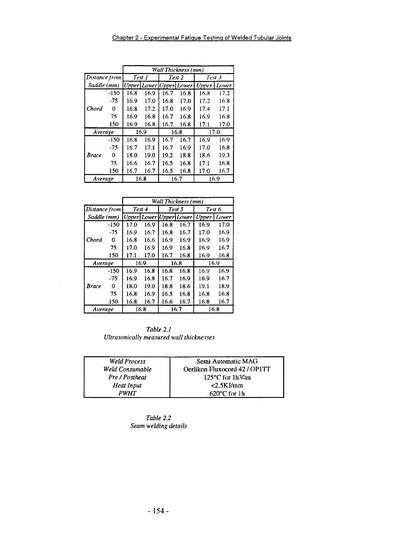
Chapter 2 - Experimental Fatigue Testing of W elded Tubular Joints
Wall Thickne.ss (mm)Distance from Test 1 Te.st 2 Test 3Saddle (mm) Upper Lower Upper Lower Upper Lower
-150 16.8 16.9 16.7 16.8 16.8 17.2-75 16.9 17.0 16.8 17.0 17.2 16.8
Chord 0 16.8 17.2 17.0 16.9 17.4 17.175 16.9 16.8 16.7 16.8 16.9 16.8150 16.9 16.8 16.7 16.8 17.1 17.0
Average 16.9 16.8 17.0-150 16.8 16.9 16.7 16.7 16.9 16.9-75 16.7 17.1 16.7 16.9 17.0 16.8
Brace 0 18.0 19.0 19.2 18.8 18.6 19.375 16.6 16.7 16.5 16.8 17.1 16.8150 16.7 16.7 16.5 16.8 17.0 16.7
Average 16.8 16.7 16.9
Wall Thickness (mm)Distance from Test 4 Te.st 5 Te.st 6Saddle (mm) Upper Lower Upper Lower Upper Lower
-150 17.0 16.9 16.8 16.7 16.9 17.0-75 16.9 16.7 16.8 16.7 17.0 16.9
Chord 0 16.8 16.6 16.9 16.9 16.9 16.975 17.0 16.9 16.9 16.8 16.9 16.7150 17.1 17.0 16.7 16.8 16.9 16.8
Average 16.9 16 8 16 9-150 16.9 16.8 16.8 16.8 16.9 16.9-75 16.9 16.8 16.7 16.9 16.9 16.7
Brace 0 18.0 19.0 18.8 18.6 19.1 18.975 16.8 16.9 16.5 16.8 16.8 16.8150 16.8 16.7 16.6 16.7 16.8 16.7
Average 16 8 16 7 16 8
T a b l e 2 . 1
U l t r a s o n i c a l l y m e a s u r e d w a l l t h i c k n e s s e s
W e l d P r o c e s s Semi Automatic M A GW e l d C o n s u m a b l e Oerlikon Fluxocord 42 / O P IT T
P r e / P o s t h e a t 125°C for lh30mH e a t I n p u t <2.5KJ/mm
P W H T 620°C for Ih
T a b l e 2 . 2
S e a m w e l d i n g d e t a i l s
- 154 -
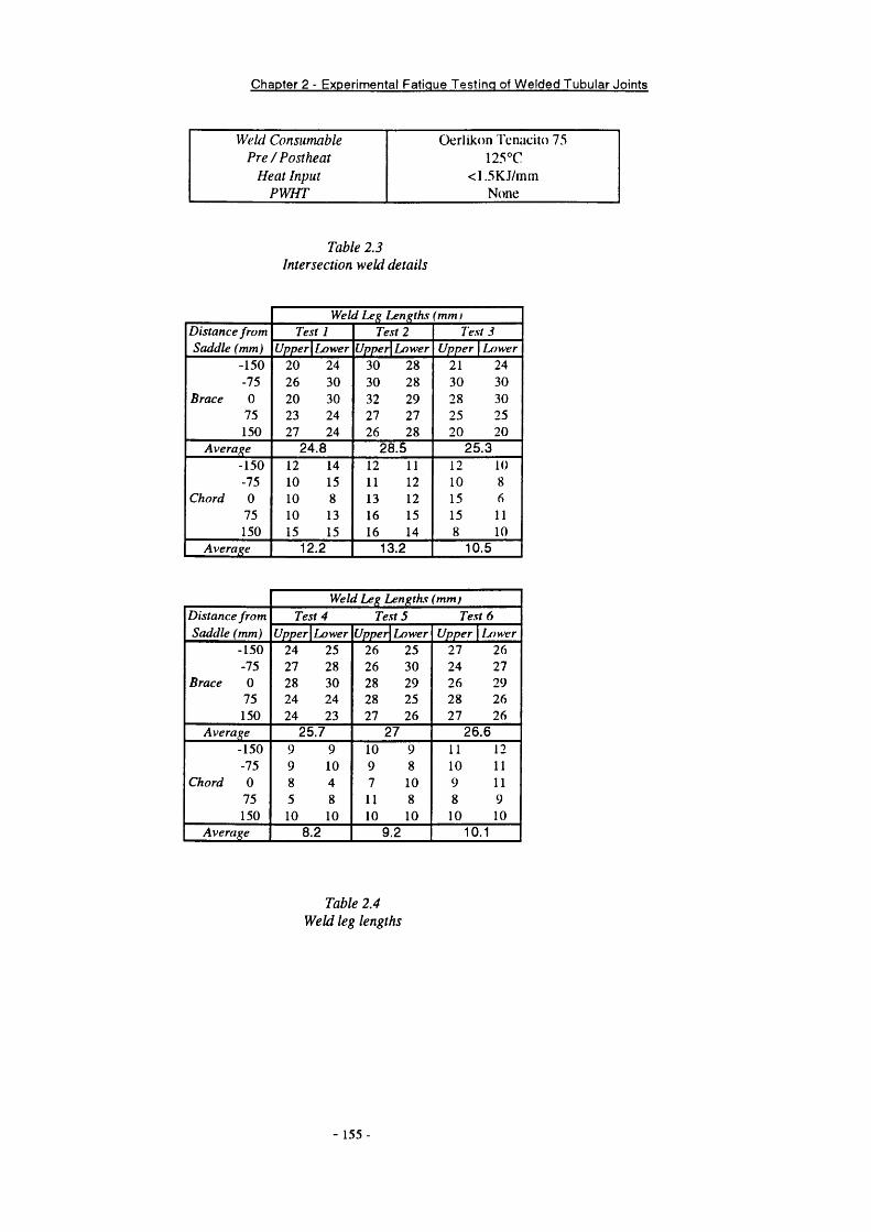
Chapter 2 - Experimental Fatigue Testing of W elded Tubular Joints
W e l d C o n s u m a b l e Oerlikon Tenacito 75P r e / P o s t h e a t 125°C
H e a t I n p u t <1.5KJ/minP W H T None
T a b l e 2 . 3
I n t e r s e c t i o n w e l d d e t a i l s
Weld Leg Lengths (mm iDistance from Test I Te.st 2 Te.st 3Saddle (mm) Upper\Lower Upper Lower Upper Lower
-150 20 24 30 28 21 24-75 26 30 30 28 30 30
Brace 0 20 30 32 29 28 3075 23 24 27 27 25 25150 27 24 26 28 20 20
Average 24.8 28 .5 25 .3-150 12 14 12 11 12 10-75 10 15 11 12 10 8
Chord 0 10 8 13 12 15 675 10 13 16 15 15 11150 15 15 16 14 8 10
Averai^e 12.2 13.2 10.5
Weld Leg Lengths (mm)Distance from Test 4 Te.st 5 Te.st 6Saddle (mm) Upper Lower Upper Lower Upper Lower
-150 24 25 26 25 27 26-75 27 28 26 30 24 27
Brace 0 28 30 28 29 26 2975 24 24 28 25 28 26150 24 23 27 26 27 26
Average 25.7 27 26 .6-150 9 9 10 9 11 12-75 9 10 9 8 10 11
Chord 0 8 4 7 10 9 1175 5 8 11 8 8 9150 10 10 10 10 10 10
Average 8.2 9.2 10.1
T a b l e 2 . 4
W e l d l e g l e n g t h s
- 155 -
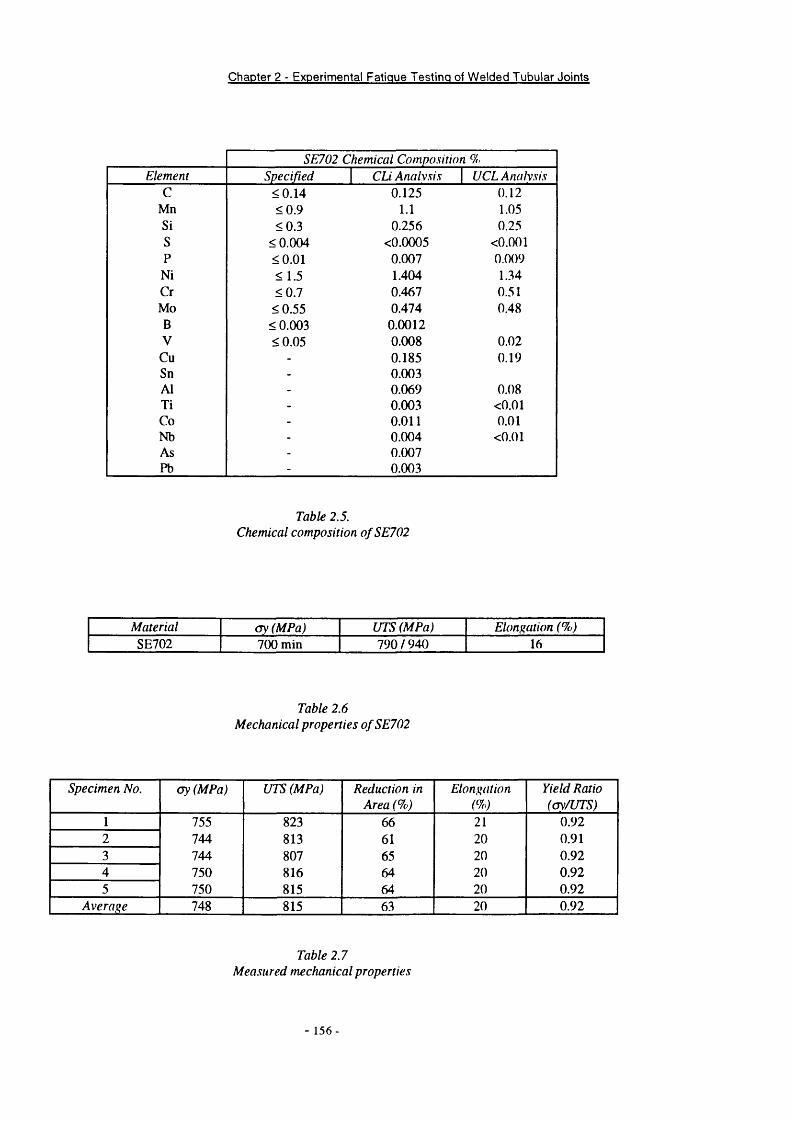
Chapter 2 - Experimental Fatigue Testing of W elded Tubular Joints
S E 7 0 2 C h e m i c a l C o m p o s i t i o n %
E l e m e n t S p e c i f i e d C U A n a l y s i s U C L A n a l y s i s
C <0 .14 0.125 0.12Mn < 0 .9 1.1 1.05Si < 0 .3 0.256 0.25S <0.004 <0.0005 <0.001P <0.01 0.007 0.009
Ni < 1 .5 1.404 1.34Cr < 0 .7 0 . 4 6 1 0.51Mo <0 .55 0.474 0.48B <0.003 0.0012V <0.05 0.008 0.02
Cu - 0.185 0.19Sn - 0.003A1 - 0.069 0.08T i - 0.003 <0.01Co - 0.011 0.01Nb - 0.004 <0.01As - 0.007Pb - 0.003
T a b l e 2 . 5 .
C h e m i c a l c o m p o s i t i o n o f S E 7 0 2
M a t e r i a l a y ( M P a ) U T S ( M P a ) E l o n j ^ a t i o n ( % )
SE702 700 min 790 / 940 16
T a b l e 2 . 6
M e c h a n i c a l p r o p e r t i e s o f S E 7 0 2
S p e c i m e n N o . ( j y ( M P a ) U T S ( M P a ) R e d u c t i o n i n
A r e a ( % )
E l o n } > a t i o n Y i e l d R a t i o
( a y / U T S )
1 755 823 66 21 0.922 744 813 61 20 0.913 744 807 65 20 0.924 750 816 64 20 0.925 750 815 64 20 0.92
A v e r a g e 748 815 63 20 0.92
T a b l e 2 . 7
M e a s u r e d m e c h a n i c a l p r o p e r t i e s
- 156
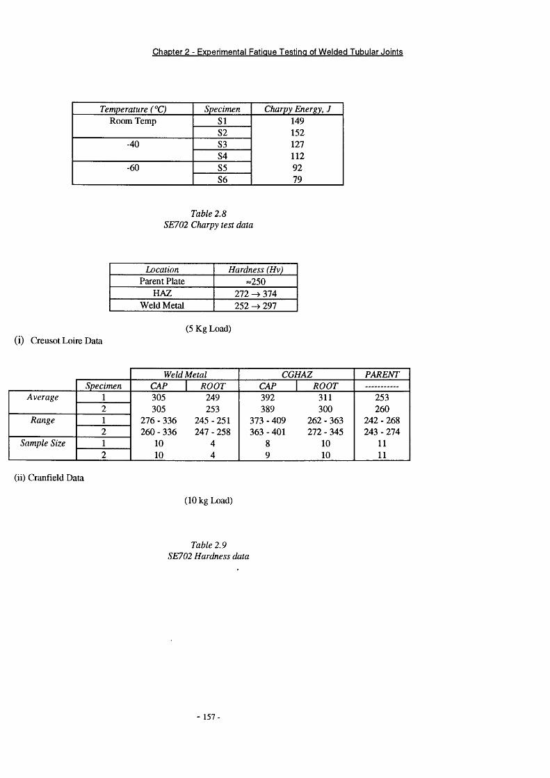
Chapter 2 - Experimental Fatigue Testing of W elded Tubular Joints
T e m p e r a t u r e ( ° C ) S p e c i m e n C h a r p y E n e r g y , J
Room Temp S I 149S2 152
-40 S3 127S4 112
-60 S5 92S6 79
T a b l e 2 . 8
S E 7 0 2 C h a r p y t e s t d a t a
L o c a t i o n H a r d n e s s ( H v )
Parent Plate =250H A Z 272 -> 374
Weld Metal 252 ^ 297
(i) Creusot Loire Data(5 Kg Load)
W e l d M e t a l C G H A Z P A R E N T
S p e c i m e n C A P R O O T C A P R O O T
A v e r a g e 1 305 249 392 311 2532 305 253 389 300 260
R a n g e 1 276 - 336 2 4 5 -2 5 1 373 - 409 262 - 363 242 - 2682 260 - 336 247 - 258 363 - 401 272 - 345 243 - 274
S a m p l e S i z e 1 10 4 8 10 112 10 4 9 10 11
(ii) Cranfield Data
(10 kg Load)
T a b l e 2 . 9
S E 7 0 2 H a r d n e s s d a t a
- 157-

Chapter 2 - Experimental Fatigue Testing of W elded Tubular Joints
P r o b e P o s i t i o n ( m m ) P r o b e P o s i t i o n ( m m )
1 -150 17 22 -135 18 63 -120 19 104 -105 20 155 -91 21 216 -78 22 287 -66 23 368 -55 24 459 -45 25 5510 -36 26 6611 -28 27 7812 -21 28 9113 -15 29 10514 -10 30 12015 -6 31 13516 -2 32 150
T a b l e 2 . 1 0
A C P D p r o b e s i t e l o c a t i o n s
E x p e r i m e n t a l S C F
S p e c i m e n N o . T o p S a d d l e B o t t o m S a d d l e A v e r a g e % D i f f e r e n c e
C l 12.1 13.9 13.0 12.94C2 11.9 12.5 12.2 4.80C3 11.2 13.2 12.2 15.15C4 11.5 11.9 11.7 3.36D1 9.8 10.0 9.9 2.00D2 10.1 9.8 10.0 2.97
T a b l e 2 . 1 1
E x p e r i m e n t a l S C F R e s u l t s f r o m p r e v i o u s t e s t p r o g r a m m e u s i n g . s a m e g e o m e t r y
- 158 -

Chapter 2 - Experimental Fatigue Testing of W elded Tubular Joints
T l T2E x p e r i m e n t a l S C F V a l u e
T3 T4 T5 T6M i n .
M a x .
A v e .
10.92 9.29 11.48 10.96 11.24 10.32
11.49 11.63 10.34 12.13 11.76 12.54 11.16 12.75 11.7 12.3 10.69 12.41
P a r a m e t r i c S C F P r e d i c t i o n s
Efthymiou & Durkin (Fixed) 11.65Efthymiou & Durkin (Pinned) 13.23
Wordsworth & Smedley 13.96UEG 14.16
Hellier, Connolly & Dover 17.85
T a b l e 2 . 1 2
E x p e r i m e n t a l S C F R e s u l t s a n d P a r a m e t r i c P r e d i c t i o n s
O r i g i n a l P r o g r a m m e R e v i s e d P r o g r a m m e
T e s t E n v i r o n m e n t C . P . f ( H z ) ( ^ H S E n v i r o n m e n t C . P . /( M P a ) ( m V ) ( M P a ) ( m V ) ( H z )
T l 400 A ir - 1T2 300 A ir - 1T3 225 Sea Water -1000 0.214 225 Sea Water -800 0.2T5 180 Sea Water -1000 0.2 300 Sea Water -1000 0.2T6 180 Sea Water -800 0.2 300 Sea Water -800 0.2
T a b l e 2 . 1 3
O r i g i n a l a n d R e v i s e d T e s t P r o g r a m m e D e t a i l s
- 159-
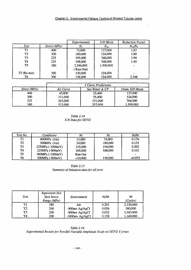
Chapter 2 - Experimental Fatigue Testing of W elded Tubular Joints
E x p e r i m e n t a l 5 0 D M e a n R e d u c t i o n F a c t o r
T e s t S t r e s s ( M P a ) N s N _ i p N M
T l 400 73,000 137,000 1.87T2 300 180,000 324,000 1.80T3 225 395,000 768,000 1.94T4 225 548,000 768,000 1.40T5 180 2,246,000 1,500,000 -
( Run Out)T5 (Re-test) 300 130,000 324,000 -
T6 300 138,000 324,000 2..348
T C u r v e P r e d i c t i o n s
S t r e s s ( M P a ) A i r C u r v e S e a W a t e r & C P 1 6 m m 5 0 D M e a n
400 45,800 23,400 137,000300 111,000 55,400 324,000225 263,000 131,000 768,000180 513,000 257,000 1,500,000
T a b l e 2 . 1 4
S - N D a t a f o r S E 7 0 2
T e s t N o . C o n d i t i o n s N i N t N i / N t
T l 400MPa (A ir) 13,000 74,000 0.176T2 300MPa (A ir) 24,000 180,000 0.133T3 225MPa (-lOOOmV) 115,000 194,000 0.292T4 225MPa (-800m V) 105,000 548,000 0.192T5 180MPa (-lOOOmV) Run Out - -
T6 300MPa (-800m V) <10,000 138,000 <0.072
T a b l e 2 . 1 5
S u m m a r y o f I n i t i a t i o n d a t a f o r a l l t e s t s
T e s t
E q u i v a l e n t H o t
S p o t S t r e s s
R a n g e ( M P a )
E n v i r o n m e n t N i / N t N t
( C y c l e s )
Y1 180 A ir 0.291 2,130,000Y2 260 -800mv Ag/AgCl 0.026 380,000Y3 200 -800mv Ag/AgCl 0.032 1,545,000Y4 200 -lOOOmv Ag/AgCl 0.158 1,140,000
T a b l e 2 . 1 6
E x p e r i m e n t a l R e s u l t s f o r P a r a l l e l V a r i a b l e A m p l i t u d e S t u d y o n S E 7 0 2 Y j o i n t s
- 160-

Chapter 2 - Experimental Fatigue Testing of Welded Tubular Joints
16mm324mm
a = 7 .26 p = 0.71
Y = 14.28
1660mm
0457mm
F i g u r e 2 . 1
N o m i n a l . s p e c i m e n d i m e n s i o n s f o r t u b u l a r w e l d e d T j o i n t
S e a m w elds from Tube fabrication
F i g u r e 2 . 2
P o s i t i o n o f . s e a m w e l d s i n t u b u l a r T j o i n t s
- 161 -
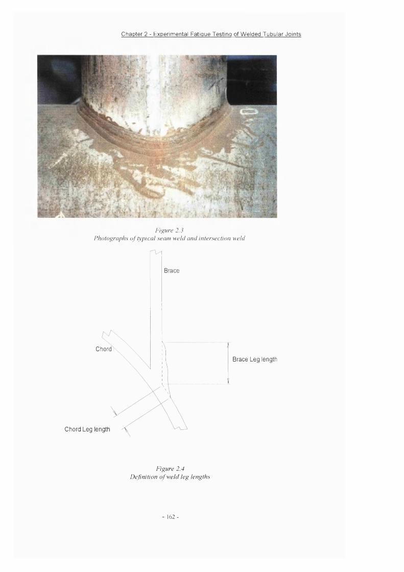
Chapter 2 - Experimental Fatigue Testing of Welded Tubular Joints
F i g u r e 2 . 3
P h o t o g r a p h s o f t y p i c a l s e a m w e l d a n d i n t e r s e c t i o n w e l d
Brace
Chord
Chord Leg length
Brace Leg length
F i g u r e 2 . 4
D e f i n i t i o n o f w e l d l e g l e n g t h s
- 162-
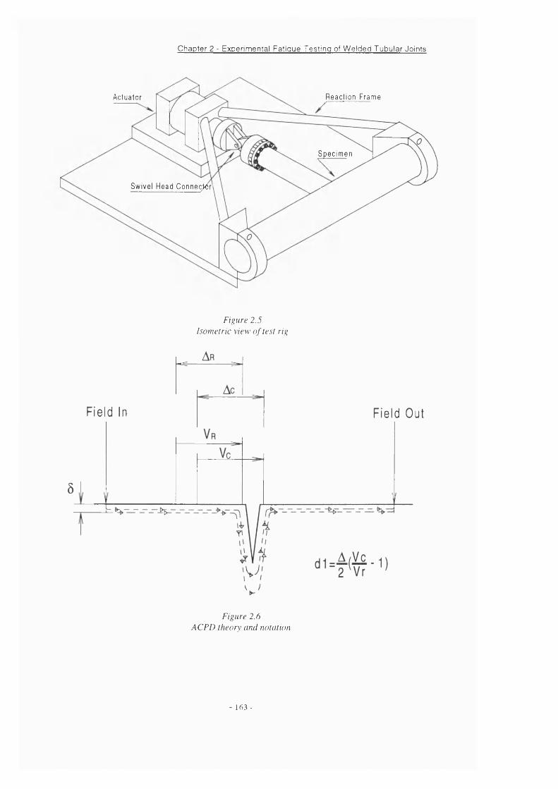
Chapter 2 - Experimental Fatigue Testing of Welded Tubular Joints
R e a c t ion F ra m eActuator
S p e c i m e n
Sw ive l H e a d C o n n e c te r
F i g u r e 2 . 5
I s o m e t r i c v i e w o f t e s t r i g
Field In Field Out
F i g u r e 2 . 6
A C P D t h e o r y a r u l n o t a t i o n
- 163 -
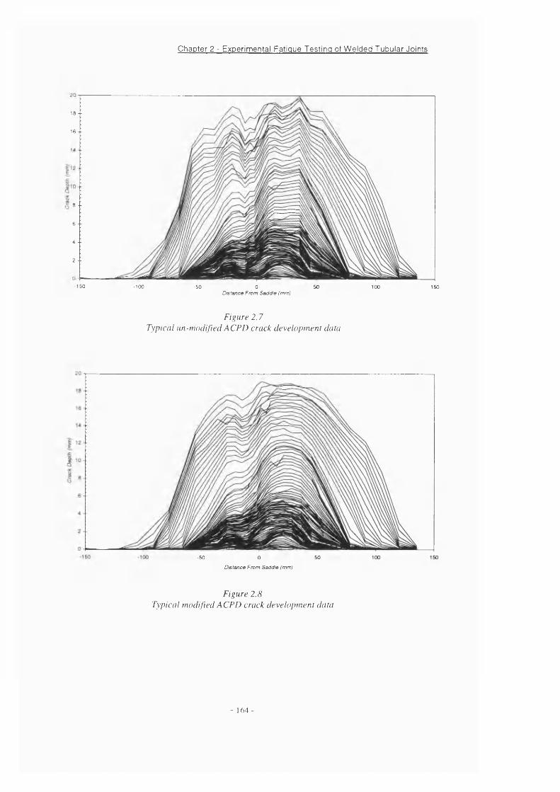
Chapter 2 - Experimental Fatigue Testing of Welded Tubular Joints
18 +
16 +
8 +
6 +
4 +
2 +
■150 -100 ■50 50 100 1500Distance From Saddle (mm)
F i g u r e 2 . 7
T y p i c a l u n - t n o d i f i e d A C P D c r a c k d e v e l o p m e n t d a t a
■50 0 50
Distance From Saddle (mm)
F i g u r e 2 . 8
T y p i c a l m o d i f i e d A C P D c r a c k d e v e l o p m e n t d a t a
- 164-

Chapter 2 - Experimental Fatigue Testing of Welded Tubular Joints
INSTRON Mini Controller
PC Test Control
U10 Crack Microguage
Ctiiller
Poter
Sea Water Resevior
Environment Ctiamber
Sea Water Loop
CP Working ElectrodeCP Counter Electrode CP Reference Electrode Cooling Circuit
ACPD Wiring
Test Control Circuit
F i g u r e 2 . 9
E x p e r i m e n t a l t e s t s e t u p
Actuator Swivel Head Connector Specimen
■i r l - — “ '
F i g u r e 2 . 1 0
T e r m i n o l o g y f o r s p e c i m e n / a c t u a t o r a l i g n m e n t p r o c e d u r e
- 165-
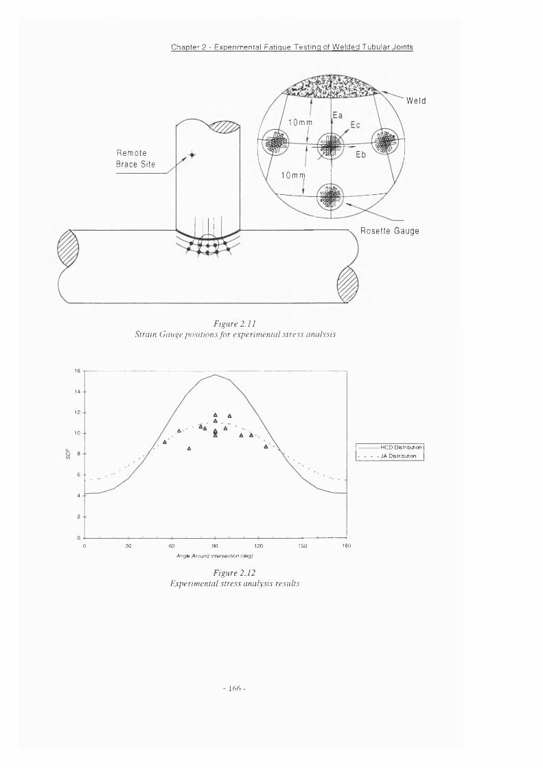
Chapter 2 - Experimental Fatigue Testing of Welded Tubular Joints
W e l d
1 0 m m
R e m o t e Brace Site
1 0 m m
R o s e t t e G a u g e
F i g u r e 2 . 1 1
S t r a i n G a u g e p o s i t i o n s f o r e x p e r i m e n t a l s t r e s s a n a l y s i s
14 --
12 - -
A10 - -
6 - -
4
150 1800 30 GO 90 120Angé Around Intersection (deg)
F i g u r e 2 . 1 2
E x p e r i m e n t a l s t r e s s a n a l y s i s r e s u l t s
------------- HCD Distribution
- - - - JA Distribution
- 1 6 6 -
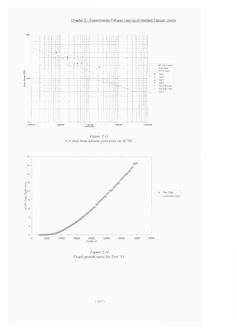
Chapter 2 - Experimental Fatigue Testing of Welded Tubular Joints
Ï
-m -------- 50 0 16mm mean
---------- T A ir Curve
r C P Curve
■ Test1
* Test 2
A Test 3
• Test 4
□ Test 5 (Run-out)
X Test 5 (Re-Test)
Test 6
1 00E«O6 L ie (Cycles)
F i g u r e 2 . 1 3
S - N d a t a f r o m t u b u l a r j o i n t t e s t s o n S E 7 0 2 .
18
cxP0.10
03
L
O Raw Data
Smoottied Data
10000 20000 30000 40000 Cycles. N
50000 60000 70000 80000
Figure 2.14Crack growth cur\>e for Test ‘Tl ’
- 167-
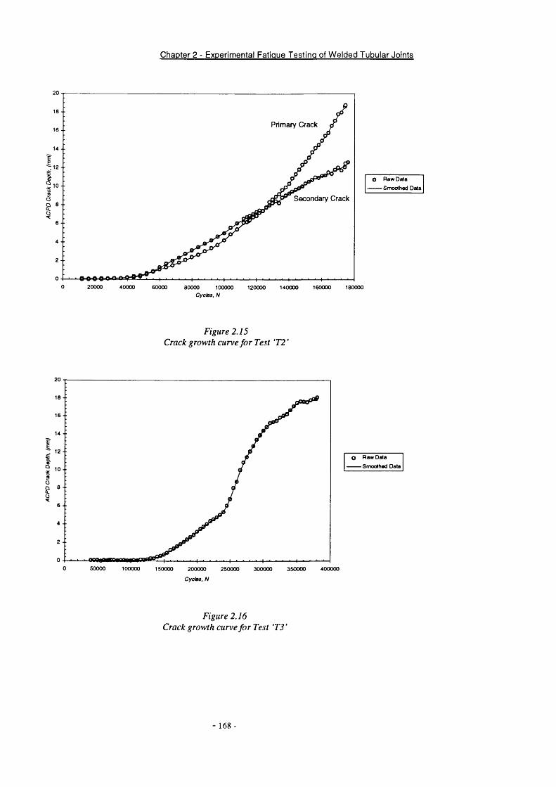
Chapter 2 - Experimental Fatigue Testing of W elded Tubular Joints
20
10 --
Primary Crack16 --
14 --
t:5 Secondary CrackÜ
I6 - •
4 --
2 --
0 20000 40000 60000 160000 18000080000 100000 120000 140000
O Raw Data
Smoothed Data
Cycles, N
F i g u r e 2 . 1 5
C r a c k g r o w t h c u r v e f o r T e s t ‘ T 2 ’
20
18 ■■
16 --
14 -•
r :6 - •
4 --
2 -•
0 100000 150000 250000 350000 400000200000 300000
O Raw Data
Smoothed Data
Cycles. N
Figure 2.16Crack growth curve fo r Test ‘T3 '
- 168 -

Chapter 2 - Experimental Fatigue Testing of W elded Tubular Joints
16 --
14 --
12 - -
Defect 1Defect 2
B --
4 --
2 --
4iunuii[niHinnfl300000
Cycles, N
F i g u r e 2 . 1 7
C r a c k g r o w t h c u r v e s f o r T e s t ‘ T 4 ’
Smoothed DataO Raw Data
20
18 --
16 --
14 --
I 12 --Î
2Or -
6 --
4 --
2 --
0 20000 120000 14000040000 60000 80000 100000
O Raw Data
Smoothed Data
Cycles, N
Figure 2 .18Crack growth curve fo r Test ‘T 6 ‘
169-
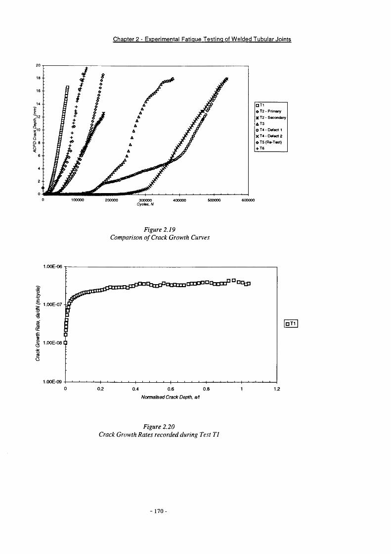
Chapter 2 - Experimental Fatigue Testing of W elded Tubular Joints
20
18 --
14 --
:1 0 --
Q 8 --
6 ■ -
4 --
2
D T I
# T2 - Primary
X T2 - Secondary
AT3O T4 - Defect 1
X T 4 -D e te c t 2
0 T 5 (Re-Test)
+ T6
300000 Cycles, N
F i g u r e 2 . 1 9
C o m p a r i s o n o f C r a c k G r o w t h C u r v e s
1.00E-06
I 1.00E-07-J
I i □ T1
1g 1.00E-08Ü
I1.00E-09
0 0.2 0.8 1 1.20.4 0.6
Normalised Crack Def^h, a/t
Figure 2 .20Crack Growth Rates recorded during Test T l
170-
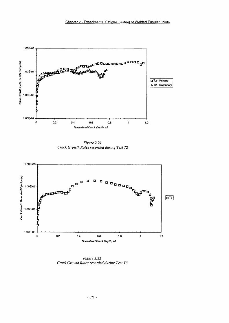
Chapter 2 - Experimental Fatigue Testing of W elded Tubular Joints
1 .OOE-06
□□□□□□□□□□ ° ° ° °
1.00E-07AA
f-R 1.00E-08
.OOE-090 0.2 0.4 0.6 0.8 1 1.2
Normalised Crack Depth, a/t
F i g u r e 2 . 2 1
C r a c k G r o w t h R a t e s r e c o r d e d d u r i n g T e . s t T 2
□ T2 - Primary
A T 2 - Secondary
1.00E-06
1.00E-07 -■
cc
S 1 .00E -08 -
1.00E-09
f
0.2 0.4 0.6 0 .8
Normaised Crack Depth, a/t
□ T3
Figure 2.22Crack Growth Rates recorded during Test T3
- 171 -
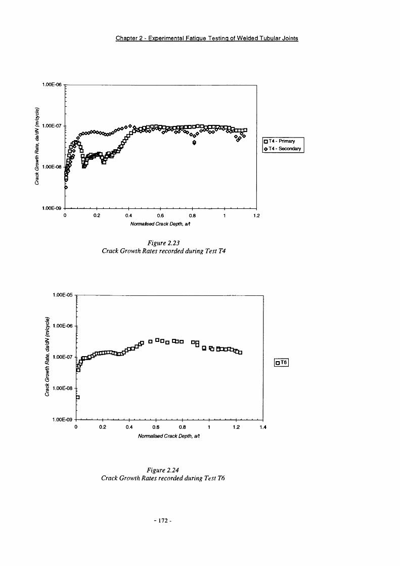
Chapter 2 - Experimental Fatigue Testing of W elded Tubular Joints
1.00E-06
ÎI
1.00E-07 --
1.00E-08
1.00E-09
□ T4 - Pnmary
^ T 4 - Secondary
H—^ —'—'—I—'—'—'—'—I—'—'—'—'—I—'—'— '—'—h 0.2 0.4 0.6 0.8 1
Normalised Crack Depth, a/t
F i g u r e 2 . 2 3
C r a c k G r o w t h R a t e s r e c o r d e d d u r i n g T e s t T 4
1.00E-05
K 1.00E-06
S 1.00E-07
I 1 .0 0 E -0 8 -:
1 .OOE-09
0 0.2 0.4 0.8 1.2 1.40.6 1
Normalised Crack Depth, a/t
Figure 2.24Crack Growth Rates recorded during Test T6
□ T6
172
Chapter 2 - Experimental Fatigue Testing of W elded Tubular Joints
1 .OOE-05
^ 1.00E-06
T l
12 - Primary
13
14 - Primary
T5 (Re-test)
16
& 1.00E-07
so 1.00E-08
1 .OOE-090.4 0.6 0.8 1
NotmaSsed Crack Depth, a/t
F i g u r e 2 . 2 5
C o m p a r i s o n o f C r a c k G r o w t h R a t e
1.4 -■
1.2 -■
II O .S ..
,1
0.4 --
0.2 -■
-50 -40 -30 -20 30 50-10 10 20 400
Distance from Saddle (mm)
F i g u r e 2 . 2 6
E a r l y c r a c k g r o w t h p r o f i l e s s h o w i n g i n i t i a t i o n i n a t y p i c a l T e s t
173
Chapter 2 - Experimental Fatigue Testing of Welded Tubular Joints
0.6
0.5 --
0.4
□ Raw Data
Smoothed Data0.3 - -
Test T1
< 0.2 - -
0 .1mm
0 2000 4000 18000 200006000 8000 10000 12000 14000 16000
Cycles, N
F i g u r e 2 . 2 7
E a r l y c r a c k g r o w t h d a t a s h o w i n g i n i t i a t i o n i n a t y p i c a l T e s t
0 30
0 25 -
0 20
0.15
0 10
005
000150 200 250 300 350 400 450
Hot Spot Stress Range (MPa)
F i g u r e 2 . 2 8
R a t i o o f i n i t i a t i o n t o t o t a l f a t i g u e l i v e s
- 174 -
Chapter 2 - Experimental Fatigue Testing of Welded Tubular Joints
300 (Air)225(-1000mV)
Hot Spot Stress (MPa) 225 (-SOOmV)
Propagation
F i g u r e 2 . 2 9
I n i t i a t i o n t o p r o p a g a t i o n l i v e s n o r m a l i s e d t o t h e T c u r v e
1000
1 OOE+04 1 OOE+05 1 OOE+06 Endurance (Cycles)
1 OOE+07
50D 16mm mean
V Air Curve
V C P Curve
o Initiation Life
o Total Life
1 OOE+08
F i g u r e 2 . 3 0
G r a p h i c a l r e p r e s e n t a t i o n o f t h e r a t i o o f i n i t i a t i o n t o p r o p a g a t i o n l i f e
- 175 -
Chapter 2 - Experimental Fatigue Testing of Welded Tubular Joints
5III
f^>fm/ttiMdCrnck Deiih»
F i g u r e 2 . 3 1
C r a c k s h a p e d a t a
^ T? • Pnmarv
- # • T2 ■ Secrndary
- O -T 4 D * ia c i2
- 1 7 6 -

Chapter 2 - Experimental Fatigue Testing of Welded Tubular Joints
1000
S100
500 16mm mean
T' Air Curve
T 'C .P . Curve
T5 (Run Out) T5 (Re-lest) T6
Y3Y4
1.00E+04 1.00E+05 1.00E+06 Endurance (Cycles)
1.00E+07 1.00E+08
F i g u r e 2 . 3 2
S - N C i i r x ’e . s h o w i n g a l l S E 7 0 2 t u b u l a r j o i n t d a t a
- 177 -
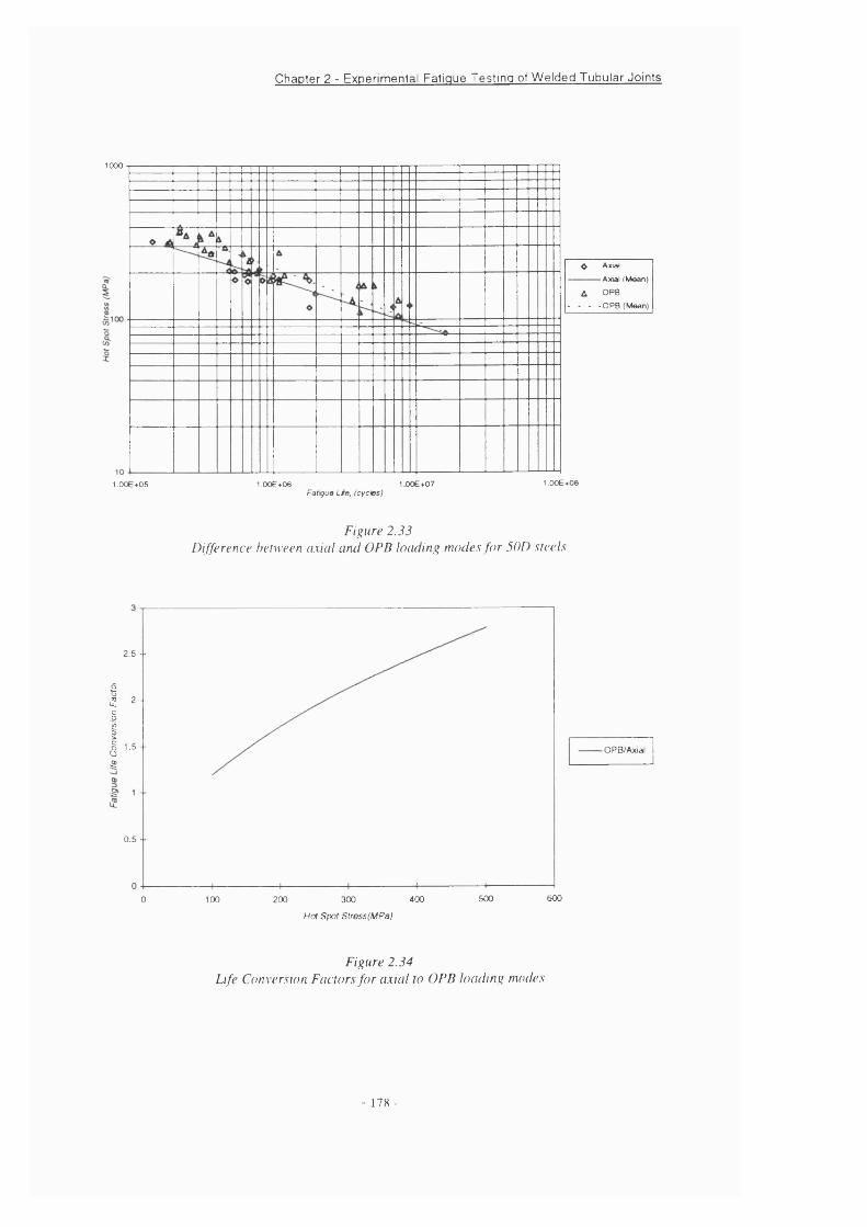
Chapter 2 - Experimental Fatigue Testing of Welded Tubular Joints
1000
O Axial
Axial (Moan)
A OPB
- - - -OPB (Moan)
1.00E+05 1.00e*06 1 OOE+07 1.00E+08Fatigue Life, (cycles)
F i g u r e 2 . 3 3
D i f f e r e n c e b e t w e e n a x i a l a n d O P B l o a d i n g m o d e s f o r 5 0 D s t e e l s
2.5 --
I ...
Io 1.5 ■-U5
0.5 --
500 6000 100 200 300 400
-OPB/Axial
Hot Spot Stress(MPa)
F i g u r e 2 . 3 4
L i f e C o n v e r s i o n F a c t o r s f o r a x i a l t o O P B l o a d i n g m o d e s
- 178 -
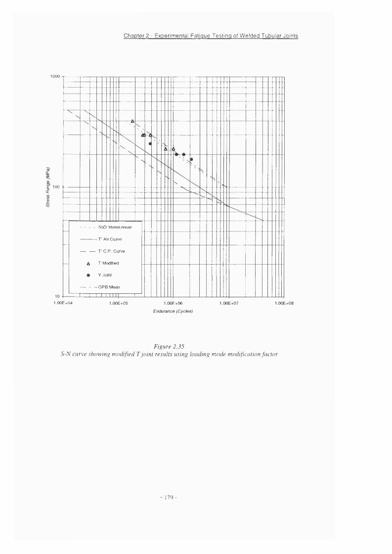
Chapter 2 - Experimental Fatigue Testing of Welded Tubular Joints
1000
§ 100 ct
-
X XX
s -XX s
-X
X\X
X
I'm
«
X ,
X
\ 0X
ss
' N
X»
" N
>
XXX
—
— - - - 50D 16mm mean
T' Air Curve
— — T 'C .P . Curve
A T Modified
# Y Joint
— - -O P B Mean
1 1 I 1 1 M i 1101.00E+04 1.00E+05 1 OOE+06
Endurance (Cycles)
1 OOE+07 1.00E+08
F i g u r e 2 . 3 5
S - N c u r v e . s h o w i n g m o d i f i e d T j o i n t r e s u l t s u . s i n g l o a d i n g m o d e m o d i f i c a t i o n f a c t o r
- 179-
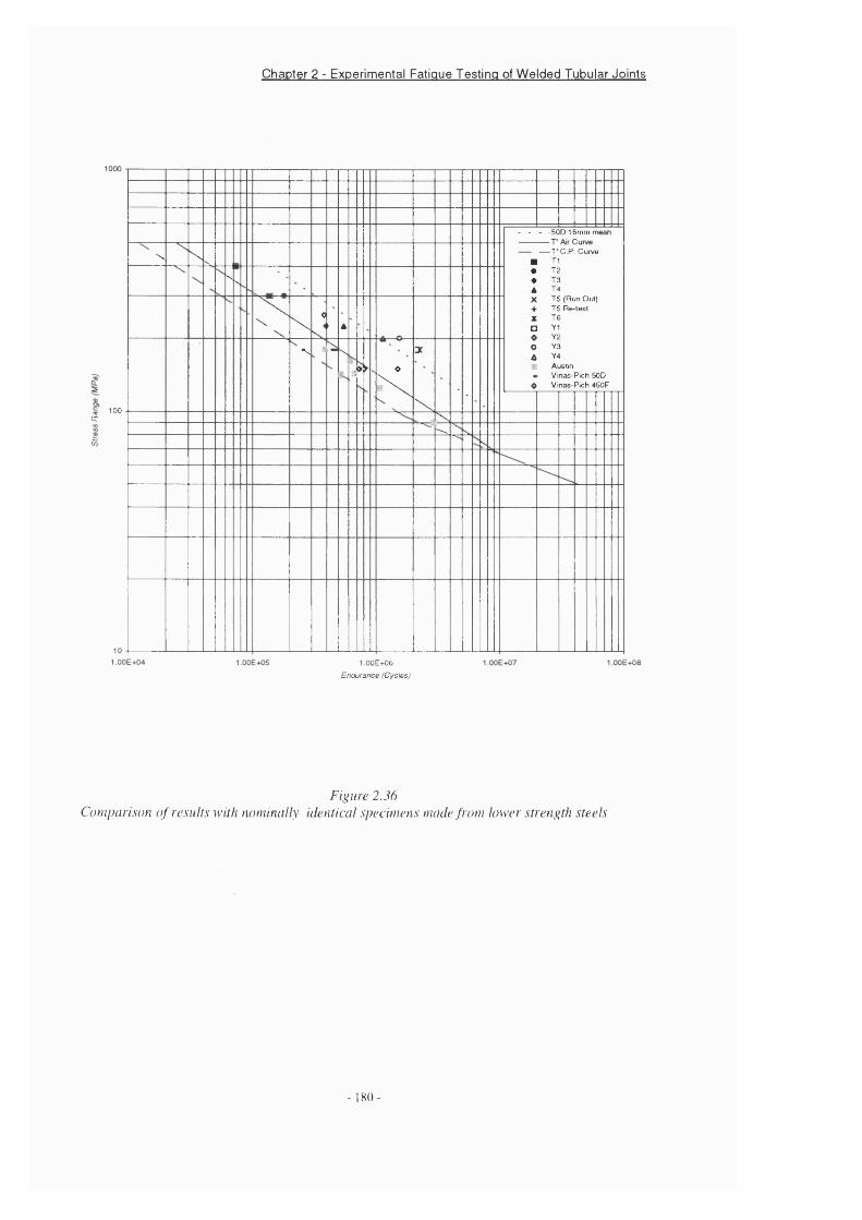
Chapter 2 - Experimental Fatigue Testing of Welded Tubular Joints
« 100 cc
- - - 5CID 115mrn n
N,X
N ■— T' C.P. Curve
1 T1X
- -
•«A
T2T3T4T5 (Run Out)T5 Re-test T6
1 Y1 Y2 Y3 Y4
1 Austin 1 Vinas-Pich SOD
VInas-Pich 4S0F
" XX
XX
c
N,A
X+X0
V * N
à > ►- o
X
X
N
-
oA«
9
X
s
1.00E+06
Endurance (Cycles)
F i g u r e 2 . 3 6
C a m p a r i . w n o f r e s u l t s w i t h n o m i n a l l y i d e n t i c a l . ' s p e c i m e n s m a d e f r o m l o w e r s t r e n g t h . s t e e l s
- 1X0-
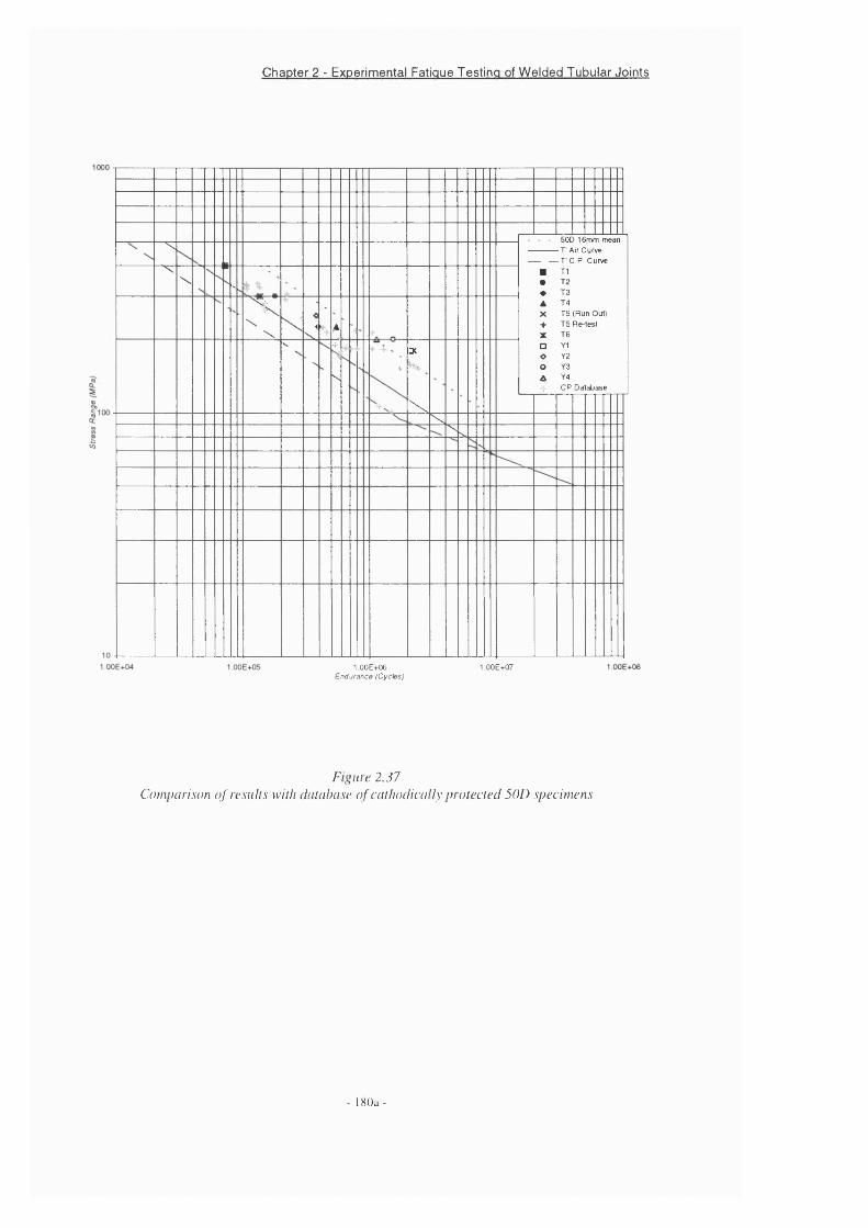
Chapter 2 - Experimental Fatigue Testing of Welded Tubular Joints
- - - SOD 16mm mean----------- T'Air Curve----- — T'C.P. Curve
■ T1• T2♦ 13 A 14X IS (Run Out)+ T5 Re-test X T6 □ Y1 O Y2 O Y3 A Y4+ CP Database
X
XX
s- V
' " xX
X Nci
X ,A
s.s.
4
sV 4
jf.
Ns X
s
1 OOE+06 Endurance (Cycles)
1 OOE+07
F l i r e 2 . 3 7
C o m p a r i s o n o f r e s u l t s w i t h r i o t a b a s e o f c a t h o d i c a i i y p r o t e c t e d 5 0 D s p e c i m e n s
- 180a-
Chapter 3 - Stress Concentrations in Tubular Joints with Rack / Rib Plate
Chapter 3
3. Stress Concentrations in Tubular Joints with Rack / Rib
Plate Stiffened Chord Members Using The Finite Element
Method
3.1 Introduction
It is known that stiffener plates can have a large effect on the stress concentration
factors found at the intersection of welded tubular joints. The strong relationship
between the fatigue life of these tubular joints and the stresses experienced at the
intersection make the accurate knowledge of the SCF’s in this region of crucial
importance. The current investigation aims to quantify the effect of the central
stiffener plate often found in jack up leg chords. The results of almost 400 finite
element models are presented in this Chapter. The common chord configurations
used in jack up leg design were detailed in Chapter One. Due to the variety of
chord configurations it will not be possible to study every case. Instead some of the
most popular chord designs will be studied extensively. Stress analysis work on a
geometry with this kind of stiffener has not previously been published. However
several other stiffener configurations have been investigated and these are
discussed in Section 3.3.
3.2 Scope
Three primary chord designs are to be investigated. The first consists of a tubular
brace to chord connection with a plate stiffener of constant thickness running the
length of the chord as shown in Figure 3.1. This is a first approximation to some
of the most common brace to chord joints found in jack up truss legs. Secondly a
more complex and more realistic chord design containing two distinct stiffener
sections, known as the rack and rib plates will be studied. This design is shown in
181 -
Chapter 3 - Stress Concentrations in Tubular Joints with Rack / Rib Plate
Figure 3.2. The third case represents the extreme of the second design where the
thinner central section of the stiffener is completely removed. This design is shown
in Figure 3.3. Each design will be discussed in more detail in Section 3.7.
Initially a single set of joint parameters will be studied for T and Y shaped joints in
order to reduce the number of variables. Axial, In Plane and Out of Plane Bending
loadcases will be investigated. The chord and brace thickness are both 20mm and
all other dimensions are based on a chord diameter of 0.6m. The joint parameters
are as shown in Table 3.1.
Once the effect of the stiffener is reasonably well understood, an attempt will be
made to quantify it across the range of joint parameters for which the Hellier,
Connolly, Dover parametric equations are valid [3.1].
Finally the mechanism by which the stiffener affects the changes will be
investigated using evidence gained from applying various translational and
rotational restraints to the chord surface of an unstiffened joint along the line where
the central plane of the rack plate would intersect if it were present.
AH the results presented here are from the chord side of the intersection as these
are the highest values, unless stated otherwise.
3.3 Stress Analysis of Stiffened Tubulars
Much effort has been concentrated on determining the SCF formulae for simple
tubular joint configurations subject to different loading conditions. The significant
contributions to this field by Kuang [3.2], Wordsworth and Smedley [3.3],
Efthymiou and Durkin [3.4] and Hellier, Connolly and Dover [3.1] were discussed
in detail in Chapter 1.
182 -
Chapter 3 - Stress Concentrations in Tubular Joints with Rack / Rib Plate
In addition to this work on simple joint configurations, significant research effort
has been focused on the behaviour of tubular joints with ring stiffened chord
members. Such joints are quite common as internal ring stilTeners provide a cheap
and effective solution to punching shear problems in design. A tubular joint
reinforced with ring stiffeners is shown in Figure 3.4.
Amongst the most significant works in this area is that of Dharmavasan and
Aaghaakouchak [3.5] who showed that in the case of axial and OPB loading,
careful positioning of the stiffeners greatly reduces the stress concentrations and
gives a more uniform distribution of the stresses around the intersection. Various
stiffener configurations and stiffener sizes were analysed and recommendations
made on the optimum designs. It was shown that stiffener height has a more
significant effect on SCF than the stiffener thickness leading to the conclusion that
the moment of inertia of the stiffener is the main factor in controlling the SCF’s.
The use of very tall thin stiffeners was warned against as this results in significant
SCF’s in the stiffener. This situation should be avoided since access to the stiffener
for inspection and repair purposes is likely to be difficult if not impossible. A
minimum stiffener thickness equal to the brace thickness was postulated.
The most effective position for ring stiffeners was found to be dependent on the
loading mode. For axial and out of plane bending the middle half' of the plug is the
optimum position. For in plane bending the optimum positions are the outer
quarters of the plug although it is noted that the stiffeners are less effective at
reducing the SCF’s for this load case. The use of a single stiffener at the saddle
position is not recommended since it produces a region of high local stiffness
through which a high proportion of the load is transferred causing high SCF’s on
the chord and brace side.
An attempt is made to predict the SCF’s in the stiffened tubulars using the Ky
correction factor to account for the increased chord inertia when using parametric
- 183 -
Chapter 3 - Stress Concentrations in Tubular Joints with Rack / Rib Plate
equations detailed in [3.6] based on a recommendation by Lloyds Register of
Shipping [3.7]. The modified value of y is given by (3.1).
r =D
2 K J
K^ =(T e \
Axial Loading
OPB Loading
IPB Loading
(3.1)
Using the parametric equations by Wordsworth et al to calculate the SCF for the
chord side and Kuang et al for the brace side, it was found that this method
produced a reasonable estimate of the SCF’s in the ring stiffened tubulars provided
that the stiffeners were located in the optimum positions. It was noted that the
value for Ky for OPB loading should be modified to the same value as for axial
loading for a more accurate representation. In addition, the effect of the stiffeners
for IPB was even less than predicted using the exponent of 0.3.
Further finite element analysis of ring stiffened tubular joints has been undertaken
by Ramachandra et a /.[3.8]. In addition to the numerical analysis, experimental
static and fatigue tests were performed on large scale welded tubular joints. The
conclusions from Dharmavasan et al regarding the optimum size and configuration
for the stiffeners were essentially confirmed. Ramachandra et al have also
produced a set of parametric equations claiming to provide SCF’s for ring stiffened
T and Y joints for both the brace and chord side under each of the three modes of
loading. Concern must be noted about the fact that these parametric equations are
based on the results of only 135 FE models. Closer inspection of these equations
shows that the parameters used do not follow the standard joint parameter
definitions. Indeed it appears that parameters such as the chord length are not even
184
Chapter 3 - Stress Concentrations in Tubular Joints with Rack / Rib Plate
considered. It is suggested that these equations should be treated with some
caution until further validation has been performed.
Seetharaman et al [3.9] have also produced similar Imite element results to
Dharmavasan et al confirming the importance of stiffener position for maximum
benefit.
An alternative and common solution to punching shear problems is the use of
doubler plates. Doubler plates are generally used when the chord diameter is such
that the fabricator is not able to gain access to the interior of the chord to weld the
stiffener plate in position. A tubular joint reinforced with a doubler plate is shown
in Figure 3.5.
Soh and Soh [3.10] have performed important initial work in this area. Doubler
plates have shown their usefulness when dealing with axial compression but little
was known about their response under other loading conditions. Extensive FE
analysis on representative tubular joints with a range of doubler plate sizes led to
the conclusion that joints reinforced with a doubler plate are not subject to more
severe fatigue problems compared to the corresponding unreinforced joints
provided that certain conditions regarding the doubler plate sizes are met. These
criteria essentially govern the doubler plate thickness and state that the doubler
plate thickness should approach that of the chord and should be no more than
approximately 1.4 times the brace thickness.
The only work on stiffener configurations similar to those under investigation here
was concerned with the ultimate strength of these joints rather than the stress
concentration factors experienced at the intersection of the brace and chord. The
study was conducted by Matsuishi et al [3.11]. Despite the differing aims of the
investigations it is worthwhile summarising the salient points of this work as the
geometric similarity mean that some of the conclusions are of direct interest here.
185 -

Chapter 3 - Stress Concentrations in Tubular Joints with Rack / Rib Plate
The leg guides, detailed in Chapter One have been shown to increase the ultimate
strength of unstiffened T joints by 30 to 40 %. Leg guides have not been
incorporated in the current study but this result shows that this is an area of study
that is likely to show a significant effect on the SCF distribution at the intersection.
Furthermore, the addition of a centre plate increased the ultimate strength of a T
joint over an unstiffened joint supported by a leg guide by a further 20%.
Longitudinal chord stiffeners have also been investigated by Choo for X joints
[3.12]. The stiffeners in this case however have more in common with the ring
stiffeners or doubler plate techniques as they are proposed as a solution to
punching shear problems. The stiffeners, although longitudinal are turned through
90° in order to provide a direct load path from brace to brace. In addition the
stiffeners are not continuous along the chord length but instead local to the brace.
3.4 Mesh Generation for Tubular Joints with Longitudinal Stiffeners
The large number of possible variables (e.g. joint and stiffener dimensions,
boundary conditions etc.) necessitate the creation and solution of a large number of
finite element models. Two finite element packages, IDEAS and ABAQUS were
evaluated for this work. IDEAS (Integrated Design Engineering Analysis
Software) [3.13] is an integrated package of mechanical engineering software
tools, including finite element modelling application. ABAQUS [3.14] is a well
established dedicated finite element analysis package. ABAQUS operates in a
‘batch’ mode and does not therefore have the interactive interface offered by
IDEAS. All model information, including nodal and element definitions are
included in an input data file which is generated ‘off-line’. The criteria used for the
selection of the package to be used during this study were based around the degree
of automation that it is possible to introduce to the mesh generation, model
- 186
Chapter 3 - Stress Concentrations in Tubular Joints with Rack / Rib Plate
solution and results extraction and evaluation phases. This was necessary to ensure
the maximum amount of information was obtained from the limited time available.
It was discovered that the ABAQUS batch mode of operation lent itself more
readily to automation of the process. ABAQUS and a similar package PAFEC have
been used extensively in the past within the Department of Mechanical Engineering
at UCL. As a result FORTRAN programs existed to produce ABAQUS model
input files for a tubular joint. In addition it is possible to request a text file
containing the results at the nodes of interest. This avoids the need of manually
extracting the results using a post processor. It was concluded that ABAQUS was
the most the appropriate package for the current study.
The mesh generator was originally written by Dharmavasan [3.15] for the study of
simple T and Y joints. Modifications were subsequently made to the program by
Chang [3.16]. The program allows the user to input the joint dimensions and the
number of elements to be formed around the chord - brace intersection. The degree
of mesh refinement is controlled by the number of elements at the intersection.
Although the framework of the mesh generator was available, several major
modifications were needed. Firstly, subroutines were added to generate the nodes
and elements on the chord stiffener. Secondly it was discovered that the program
did not work for certain joint shapes, namely all joints with an angle between the
brace and chord of less than 89°. Modifications to the way the program used
triangular elements around the intersection solved this and the program now
reliably handles all T and Y tubular joint shapes. The tinal major modification
involved the addition of subroutines to transform the model from S4R5 f ABAQUS
4 noded thin shell elements) to S8R5 fABAQUS 8 noded thin shell elements).
Geometry considerations required the use of a small number of 6 noded triangular
elements, known as STRI65, primarily in and around the plug region. The ability to
replace some or all of the S8R5 thin shell elements with S8R thick shell elements
was also included in the program. Further smaller additions were made enabling the
- 187 -
Chapter 3 - Stress Concentrations in Tubular Joints with Rack / Rib Plate
program to output a complete ABAQUS input file with no further user editing.
This included the assignment of material properties and thickness to the elements,
application of all loading and boundary restraint conditions and specification of all
output variables.
The loads are automatically scaled by the program to give a unit nominal stress for
all load cases. This enables the stress concentration factors to be read directly from
the output file. This saves significant time in the processing of the results.
A simple FORTRAN program was written to extract the principal stresses for the
inner and outer surfaces at the points of interest from the ABAQUS results file.
Specifically this means all nodes along the intersection for the chord and brace side.
The data for these nodes are then automatically written into a much smaller and
more manageable text file in a spreadsheet readable format to facilitate the later
analysis of the results.
Chang [3.16] noted an effect of brace length during his study of SCFs’ in X and
DT joints. He noted that there exists a critical ratio of brace length to brace
diameter, beyond which the brace length has little effect. He recommends the use
of brace lengths which are at least 0.4 times the chord length. All brace lengths
used in the current study comfortably meet this criteria.
The eight noded thin shell elements, S8R5 are reduced integration, doubly curved
shells with 5 degrees of freedom, three translational motions, x, y, and z, and two
in surface rotations. The 8 noded thick shell elements are also reduced integration,
doubly curved shells but with 6 degrees of freedom, three translational motions and
three rotational degrees of freedom, (j) , ({)y, and (|)z.
Shell elements are recommended for use when the shell thickness is less than 10%
of the main global dimension, typically the diameter or radius of curvature. Based
on shell theory they approximate the three dimensional continuum to two
188 -
Chapter 3 - Stress Concentrations in Tubular Joints with Rack / Rib Plate
dimensional theory and have been widely used for analysis of tubular joints. There
are two types of shell elements, known as thick and thin. The choice of which
element type to utilise depends on the importance of shear deformation in the
structure under investigation. The importance of shear deformation generally
increases with increasing ratio of wall thickness to chord diameter Prior to
commencing this investigation many of the models were solved using both thick
and thin shell elements. In each case the difference was less than 1%. For this
reason thin shell elements have been used in this investigation.
An often noted drawback of using thin shell elements to model tubular joints is the
lack of any weld detail. In addition, as shell elements are essentially two
dimensional, possessing thickness in a mathematical sense only, we are effectively
modelling the mid-planes of each tubular. This fact becomes significant at the
intersection of brace and chord resulting in the stresses being calculated at a point
which is not coincident with the weld toe. This error has been found to be quite
small for the chord side but can be significant on the brace side of the intersection.
This point was discussed in some detail in Chapter 1.
A sample mesh is shown in Figure 3.6. Note the refinement of elements around the
stiffener where the stress gradients are greatest and the gradual coarsening of the
mesh remote from this region where the stresses become more uniform. Careful
positioning of the nodes allows the stretch and distortion of the elements to be
reduced to a minimum. Since triangular shell elements are less accurate than
quadrilateral shell elements, their use has been kept to a complete minimum.
Triangular elements are only used where necessary due to reasons of geometric
compatibility around but some distance from the intersection and within the plug
region. Generation of a typical mesh takes just a few seconds and a complete
solution for an average model containing 858 elements can be obtained in 45
seconds of CPU time. AH analysis was performed on a DEC Alphastation
255/233MHZ.
189 -

Chapter 3 - Stress Concentrations in Tubular Joints with Rack / Rib Plate
3.5 Boundary Conditions
Symmetry of the model in the X Y plane allows a half model analysis to be
performed providing the correct boundary conditions are applied to the nodes on
the plane of symmetry. Reducing the size of the model in this manner saves
significant CPU time and disk storage space. ABAQUS provides a ZSYMM
function to allow the automatic application of the appropriate translational and
rotational restraints to simulate symmetry in the Z direction. The constraints
imposed on aU nodes on the plane of symmetry are zero displacement in the z
direction and aU rotations associated with the thin shell elements are fixed at zero.
For chord designs containing a stiffener that passes through the whole of the chord
diameter, the same symmetry boundary conditions are applied to the stiffener.
Stiffener designs where the plate is not continuous through the chord (see Figure
3.3)have no symmetry boundary conditions applied at the free edge.
The symmetry conditions are violated for the Out of Plane Bending loading
condition, but Hellier et al [3.1] discovered that it is still possible to use half joint
meshes with acceptable accuracy by restraining in plane displacements.
The chord ends are modelled as ‘built-in’ with all degrees of freedom being
restrained. No boundary conditions are applied to the brace end other than the
distributed external loads applied at each node.
3.6 Convergence and Model Verification
Prior to any comprehensive investigation of any particular geometry, care must be
taken that the model is behaving as would be anticipated. Primarily this involves a
convergence study to ensure that the mesh density is sufficient to accurately predict
the stresses at the points of interest. In the case of a tubular joint, this region is
usually the intersection of the brace and chord. A steep stress gradient exists within
this region and the stresses can be erroneously predicted if the mesh is too coarse.
- 190 -

Chapter 3 - Stress Concentrations in Tubular Joints with Rack / Rib Plate
On the other hand, too tine a mesh will waste computational effort and therefore,
time and money. A preliminary study was implemented to ensure that mesh density
at the intersection was sufficiently fine. Models with 12, 16, 20 and 24 elements
around the intersection were solved. The results are shown in Table 3.2.
3.7 Finite Element Investigation
3.7.1 Effect of Rack Plate Thickness on SCF Distribution
Several stiffener plate thicknesses of up to 1/3 of the chord diameter have been
investigated and the SCF results around the intersection on the chord side are
presented here. Each of the stiffeners had a constant thickness and was continuous
through the chord diameter. The investigation covered both T and Y joints under
Axial, IPB and OPB loading modes. This stiffener type is illustrated in Figure 3.1
3.7.1.1 ResultsThe SCF distribution around the intersection for axially loaded T and Y joints are
shown in Figures 3.7 and 3.8 respectively. It is noted that the shape of the SCF
distribution around the intersection remains essentially unchanged by the presence
of a stiffener except for the case of a Y joint under axial loading. In this instance
the distribution becomes slightly skewed as the hot spot stress site moves away
from the saddle with the introduction of thicker stiffeners. Even the thinnest
stiffeners produce very significant reductions in peak SCF for both joint shapes.
For comparison purposes. Figures 3.9 and 3.10 present the SCF distribution as the
SCF found in the stiffened joint, normalised against the SCF at the corresponding
angular position around the intersection in the unstiffened joint. It can be seen that
hot spot SCF, i.e. highest SCF around the intersection, for each stiffener thickness
is significantly lower than that of the unstiffened joint. The SCF at the crown is
however greater than that found in the unstiffened joint for both joint shapes. This
increase is not significant in terms of fatigue design as it is considerably lower than
the hot spot SCF. The SCF at the crown appears to be almost independent of
- 191
Chapter 3 - Stress Concentrations in Tubular Joints with Rack / Rib Plate
Stiffener thickness except for the very thickest stiffener. In this instance there is
some evidence of a flattening of the SCF distribution with the SCF at the crown
decreasing and interestingly a slight increase in the SCF at the saddle. This
phenomenon is seen in both joint shapes.
When the same T and Y Joints are subjected to IPB loading the stiffener appears to
have little or no effect. Figures 3.11 and 3.12 illustrate the insensitivity of the
intersection SCF’s to the thickness of the rack plate. In the light of this discovery,
IPB loadcases will not be considered any further in this section.
Out of plane bending is more interesting. Figures 3.13 and 3.14 show the
distribution of SCF around the intersection for the T and Y joints respectively.
Again the SCF distribution for the unstiffened joint is included for comparison. As
would be expected, the SCF at the crown position approaches zero and is
independent of the thickness of the stiffener. For this reason, discussion will be
centred around the saddle region where the effect of the stiffener is greatest and the
SCF highest. The SCF values normalised to the unstiffened joint SCF’s are shown
in Figures 3.15 and 3.16. Out of plane bending does not show the same tendency
towards a flatter SCF distribution for the thicker stiffeners. The SCF at the saddle
decreases with increasing stiffener thickness for all stiffener thicknesses. The
apparent large variations in the normalised SCF values at the crown positions (0°
and 180°) in Figures 3.15 and 3.16 at first appear to contradict the earlier
observation that SCF at the crown is independent of stiffener thickness for OPB
loading. However as the SCF value at the crown of the unstilïened joint is very
close to zero any small change in SCF for the stiffened joint will appear relatively
large when normalised to the unstiffened result.
The SCF data from the saddle position for T and Y joints under Axial and OPB
loading is shown in Figure 3.17. The SCF data is normalised to the peak SCF
found in the corresponding unstiffened geometry. This clearly shows the extra
effectiveness of the stiffener at reducing SCF’s under axial loading than OPB
- 192 -
Chapter 3 - Stress Concentrations in Tubular Joints with Rack / Rib Plate
loading conditions. Additionally it can be seen that the percentage reductions are
very insensitive to joint shape. Reductions of the order of 20% for OPB loading
and 40 to 50% of the unstiffened SCF for axial loading modes have been achieved.
The effect of increasing stiffener thickness rapidly converges for axial loading but
OPB loading shows a rapid initial reduction in SCF followed by a slower but linear
reduction for the three thickest stiffeners.
3.7.2 Effect of Rack and Rib Plate Geometry on the SCF
Some jack up chord designs employ stiffener plates that do not have a constant
cross section through the chord diameter. Examples of this were given in Chapter
One. The behaviour of such chords designs will be investigated here. A typical
chord design of this type is shown in Figure 3.18 detailing the notation and
terminology that will be employed to describe the variations in geometry between
individual finite element models.
The relative thickness ( tl/t2 ) and the depth, z of the rack plate (see Figure 3.18)
will be varied. The variation in the relative thickness of the two plates will be
continued up to the extreme where the thinner rib plate tends to a thickness of
zero. Although this situation is not commonly found in practice it forms a useful
extreme case as it eliminates the possibility of direct load transfer resulting from the
deformation of diametrically opposing chord surfaces. Any resistance to chord
wall deformation must then be provided by some form of bending mechanism
similar to the ring stiffeners presented in Section 3.3. This should allow an insight
into the predominant mechanisms by which the stiffener affects the changes in SCF
at the brace chord intersection.
The forces exerted on the rack plate are considerable and arise from the static
weight of the jack up barge and clamping forces within the jackhouse. This
necessitates a thick solid rack plate. By comparing the SCF’s with those of the
designs utilising a constant thickness rack plate it should be possible to evaluate the
potential for weight saving in the leg section by utilising thinner sections across
193 -

Chapter 3 - Stress Concentrations in Tubular Joints with Rack / Rib Plate
part of the chord diameter. The lack of any compressive clamping forces acting on
the rack plate in this investigation may be significant. Phenomena such as the
buckling of the thinner rib plate under the compressive clamping load are not
considered here but must of course be considered in design.
3.7.2.1 ResultsThe three major variables in this section of the investigation are the thickness of the
rack plate, t l, the thickness of the rib plate, t2 and the depth of the rack plate, z.
Each of the variables will be presented normalised to the diameter of the chord, D.
The SCF presented is the highest around the intersection. In each case the peak
SCF occurred on the chord side. The SCF is presented normalised to the SCF
found in the equivalent unstiffened tubular. This facilitates the quantification of the
relative effect of the presence of a stiffener.
Figures 3.19, 3.20 and 3.21 display the primary results illustrating the effect of a
dual thickness stiffener under axial loading. Each of the three plots represents a
different relative rack plate thickness namely tl/D ratios of 0.08, 0.17 and 0.33
respectively. Each has been plotted on the same scale for ease of comparison. Also
included on each plot is a line indicating the reduction of the peak SCF by the
presence of a stiffener of constant thickness equivalent to that of the rack plate, t l.
This enables an easy visual measure to be formed of how closely the effect of the
presence of the thinner rib plate converges towards that of the heavier continuous
rack plate.
Several trends can be identified from the normalised data. Firstly the rack plate
thickness, t l is seen to be of secondary importance. The maximum difference in
SCF between the thickest and the thinnest rack plate for any given geometry is less
than 1 % of the corresponding unstiffened SCF.
Three normalised rib plate depths of 0.2, 0.4 and 0.6 times the chord radius were
examined. The results show a reduction in SCF with increasing depth, z. The SCF
- 194

Chapter 3 - Stress Concentrations in Tubular Joints with Rack / Rib Plate
was reduced across the range of the rack and rib plate thicknesses tested here.
Again the effect is small, although noticeable and consistent. The maximum
difference in SCF between the most shallow and deep rib plates was less than 4%
of the unstiffened SCF.
The effect of the thickness of the rib plate was shown by examining four different
plate thicknesses for each combination of rack plate thickness and depth. The
normalised rib plate thicknesses of 0.002, 0.008, 0.017 and 0.033 were significantly
thinner than the rack plates. The effect of the rib plate thickness is seen to converge
rapidly in each case.
Figures 3.22, 3.23, 3.24 illustrate the same data for the OPB loadcase. Again all
plots utilise the same scale for ease of comparison. The first observation is that the
effectiveness of the stiffener in reducing the peak SCF around the intersection is
significantly reduced in comparison with the axial loadcase. The maximum
reduction is less than 20% with some stiffener configurations producing reductions
of less than 2%. The effect of the rack plate thickness is again seen to be of
secondary importance. Increasing the rack plate thickness four-fold reduces the
SCF by just a few percent.
The same range of rack plate depths and rib plate thicknesses were examined for
the OPB loadcase as the Axial loadcase. Once again, increasing the depth of the
rack plate reduces the SCF across the range of rib plate thicknesses tested. The
average reduction obtained by increasing the normalised rack plate depth from 0.1
to 0.3 is between 4% and 5% of the unstiffened SCF.
Increasing the rib plate thickness results in an almost linear decay in peak
intersection SCF. The same pattern is found across the range of rack plate depths
and thicknesses tested. This is in contrast with the axial loadcase where the effect
of the plate thickness converged rapidly. This suggests that the mechanism by
which the plate affects the changes is different for axial and OPB loadcases.
- 195 -
Chapter 3 - Stress Concentrations in Tubular Joints with Rack / Rib Plate
For both axial and OPB loadcases the results tend towards those of the continuous
thickness stiffener but do not reach it, the difference however is usually only a few
percent.
Reducing the rib plate thickness to zero represents the extreme case for this chord
design. By removing the possibility of direct load transfer between the deformed
chord walls any change in SCF must be due to the added chord wall stiffness
provided by the rack plate. The two variables in this instance are the rack plate
depth, z and thickness, tl.
The effect of the non continuous rack plate is evaluated by varying the thickness tl
and the depth z. Normalised stiffener depths , z/D of 0.1, 0.2, 0.3, 0.4, and 0.5 and
normalised thicknesses, tl/D of 0.017, 0.033, 0.083, 0.167 and 0.333 have been
investigated.
The results for the hot spot SCF are shown in Figures 3.25, 3.26. Significant
reductions in the peak SCF are achievable using this chord design. However the
reductions are not as significant as those achieved using a continuous rack / rib
plate design. The reduction in SCF with increasing rack plate thickness does not
show the very rapid convergence found in the chord designs with continuous
stiffener plates. In fact the results for the OPB loadcase do not show any sign of
convergence even with the thickest rack plates. The peak reductions of around
30% for the axial loadcase are approximately double that of the OPB loadcase.
The effect of stiffener depth z is illustrated in Figures 3.27, 3.28. For both
loadcases the SCF decreases almost linearly with increasing z. The rate of SCF
reduction with depth appears to be almost independent of the rack plate thickness,
tl.
- 196 -
Chapter 3 - Stress Concentrations in Tubular Joints with Rack / Rib Plate
3.7.3 Investigation of Mechanisms Using Boundary Conditions
In an attempt to understand the mechanism by which the presence of a rack or rib
plate affects the stress distribution in tubular joints, a number of additional models
have been analysed. These models are based on an unstiffened tubular joint but
with additional boundary conditions applied to the chord surface where the
stiffener would intersect the chord. Seven different combinations of boundary
conditions were selected and T and Y joints were modelled under axial and out of
plane bending loading conditions. The seven boundary condition cases are detailed
in Table 3.3 together with references to the figures illustrating the constraints
schematically. It is hoped that this will allow an insight in to the behaviour of the
stiffeners by mimicking their effect using applied boundary conditions.
3.7.3.1 ResuitsIt has been possible to simulate the effect of the stiffener plate by applying specific
rotational and translational restraints on the chord surface. Figures 3.36 to 3.39
illustrates the results for a T joint under axial loading. The same behaviour was
found for a Y joint under axial loading and the discussion below applies equally to
both joint shapes.
It might be expected that the effect of the thicker rack plates would converge
towards the situation where the chord surface is restrained in all degrees of
freedom ( ‘built in’) along the line of intersection with the stiffener. It can be seen
from Figure 3.36 that this is quite clearly not the case. The built in model (Case I)
results in SCF’s which are significantly greater at the saddle position and lower at
the crown compared to the results for one of the thicker stiffeners (100mm).
Restraining only rotation about the x axis (Case 6) is shown to have no effect on
the SCF results with the results closely mimicking the ‘no stiffener’ case.
It is immediately obvious and intuitive that the most important factor is the
restraint of deformation in the z direction. This is the mode of deformation that
would produce compressive stresses in the stiffener plate. Cases 3 and 5 very
- 197 -
Chapter 3 - Stress Concentrations in Tubular Joints with Rack / Rib Plate
closely mimic the behaviour of the 100mm stiffener as shown in Figure 3.37. The
difference between these two cases is the addition of a restraint on (f>y in Case 5
suggesting that this mode of deformation has little effect at reducing the SCF. The
same conclusion can be drawn by comparing the results from Cases 2 and 4 in
Figure 3.38. These two Cases result in the same crown SCF as the models
containing stiffeners and a saddle SCF that lies between the thickest and thinnest
stiffeners. The rotational displacement 0y seems therefore to have very little
relevance to the behaviour of these stiffeners.
Returning to the ‘built-in’ Case 1 it appears that the reasons for the poor modelling
of the stiffener effect is due to the additional restraint of the translational
deformation in the y direction. This is shown by adding restraint in Y to Case 3
forming Case 7. Case 7 closely mimics the built in Case 1 as illustrated in Figure
3.39. Deformation in the x direction (along the chord length) is minimal and the
effect of restraining (py has been shown to have little effect
For axial loading some evidence has already been obtained that there exists an
optimum stiffener thickness beyond which the SCF at the saddle increases and that
at crown decreases. This is the same situation as found with the ‘built in’ Case 1.
This suggests that there are essentially two effects of a rack plate. Firstly even
relatively thin rack plates are effective at restraining chord deformation in the z
direction. This has the immediate effect of reducing the SCF at the intersection. As
the stiffener becomes thicker the restraint to deformation in Y (i.e. direction of
brace loading) becomes more significant. Restraining deformation on Y results in a
tendency towards higher saddle SCF and lower crown SCFs as seen in the built in
case.
This is not thought to be too significant a problem as it only affects axial loading
and the size of the stiffener required to produce significant Y restraint would not be
encountered in practice. In any case even the built in situation produces SCF values
significantly lower than the unstiffened joint.
- 198
Chapter 3 - Stress Concentrations in Tubular Joints with Rack / Rib Plate
For OPB loading a similar pattern emerges for both T and Y joints. Cases 3 and 5
produce SCF which approach those of the thicker stiffeners. The major difference
however is the fact that the built-in case (Case 1) provides a lower bound to all the
results. This suggests that increasing restraint in the Y direction does not have the
detrimental effect on peak SCF for OPB loading as found for axial loading. The
crown position SCF’s are all very similar for all cases and close to zero.
3.7.4 Effect of a Continuous Thickness Rack Plate Across a Range
of Joint Parameters
The investigation thus far has centred around a single set of joint parameters with
two different brace angles. In order to be able to form an idea of the effect of a
stiffener in different joints a single constant thickness stiffener has been inserted
into joints covering the range of parameters for which the Hellier, Connolly, Dover
parametric equations [3.1] are vahd. The parameter ranges covered are given
below:
6.21 < a < 13.1
0.2 < p <0.8
7 .6 < y < 3 2
0.2 < T < 1
35° < 0 < 90°
The geometric parameters were varied one at a time across the validity ranges
given above. All other parameters were constant at the values given in Table 3.1.
The joint dimensions were calculated using a chord diameter of 0.6m and a chord
thickness of 0.02m. The stiffener thickness was the same as the chord thickness.
This was chosen as an intermediate thickness stiffener which is well suited to being
modelled using thin shell elements and which showed a significant effect on the
SCF for both loadcases.
199 -
Chapter 3 - Stress Concentrations in Tubular Joints with Rack / Rib Plate
For each set of joint parameters investigated two models were produced, one with
and one without a stiffener. This is to ensure that the differences in SCF obtained
are due to the presence of the stiffener rather than any errors introduced from
calculating the unstiffened SCF using parametric equations.
The variation of the absolute value of the hot spot SCF will be presented for
stiffened and unstiffened models across the range of each parameter for axial and
OPB loadcases.
3.7.4.1 ResultsIn each of the figures in this Section, the annotation adjacent to each stiffened data
point represents the normalised SCF (SCF in stiffened joint / SCF in unstiffened
joint).
The variation of hot spot SCF with increasing alpha (i.e. increasing chord length) is
illustrated in Figures 3.40 and 3.41 for axial and OPB loadcases respectively.
Immediately noticeable is the insensitivity of the stiffened model to the increase in
chord length. This is in contrast to the unstiffened model which displays a strong
relationship with alpha, showing an increasing in peak SCF of approximately 30%
across the range of alpha. This results in the situation where the greatest benefit
from the rib plate can be obtained for greater alpha ratios. By contrast, the peak
SCF in the stiffened joint under OPB loading shows the same dependency on alpha
as the unstiffened joint resulting in nested curves in Figure 3.41. Table 3.4 gives the
ratio of the stiffened SCF / unstiffened SCF for each value of alpha tested for both
loadcases.
Both the stiffened and unstiffened geometries show similar responses to an
increasing Beta ratio (i.e. increasing brace radius). For the axial loadcase there
appears to be an intermediate value of Beta (around 0.4) which produces the
highest SCF values with and without a stiffener as illustrated in Figure 3.42. The
stiffener results in a continuously decreasing relative SCF with increasing Beta
- 2 00 -
Chapter 3 - Stress Concentrations in Tubular Joints with Rack / Rib Plate
ratio. This is illustrated in Table 3.5. For OPB loading the stiiïener has almost no
effect at the lowest Beta values as shown in Figure 3.43. However the difference
between the stiffened and unstiffened SCF increases continuously with increasing
Beta.
Both stiffened and unstiffened joints under axial and OPB loading display a very
strong relationship with Gamma (Le. decreasing chord thickness). This is as would
be expected since decreasing the relative chord thickness will increase the
deformation of the chord due to its reduced stiffness. Under axial loading the
greatest relative benefits in terms of SCF are obtained at the lower values of
gamma. For OPB loading the effect of the stiffener remains essentially constant
across the range of gamma values investigated. This is illustrated in Figures 3.44
and 3.45 and Table 3.6.
The ratio of the brace to chord thickness, t, does not alter the beneficial effect of
adding a stiffener. This is true for both loadcases. Table 3.7 gives the ratio of the
stiffened to unstiffened SCF for each Tau ratio which are shown to be consistent.
The results are illustrated in Figures 3.46 and 3.47.
Finally the brace angle is shown to have little effect for brace angles greater than
approximately 60° for axial loading and no effect for OPB loading. This is
illustrated in Table 3.8 and Figures 3.48 and 3.49.
3.8 Conclusions and Recommendations
A comprehensive finite element stress analysis study has been completed, covering
a variety of chord rack configurations commonly found in leg structures of jack up
platforms. The effect of the various rack plates on the SCF distribution and in
particular the hot spot SCF at the chord brace intersection has been quantified.
Axial, IPB and OPB loading modes have been considered.
-201 -

Chapter 3 - Stress Concentrations in Tubular Joints with Rack / Rib Plate
For every rack plate configuration considered the hot spot SCF was found to be
reduced compared to the corresponding unstiffened joint. In general stilfeners that
are continuous through the chord diameter are the most effective at reducing the
SCF. For axial loading reduction of 50% of the unstiffened joint hot spot SCF were
approached. The reduction under OPB loading was shown to he less but still
significant at around 20%. In each case, even the thinnest stiffeners had a
significant effect which converges rapidly, especially for axial loading.
The SCF was unaffected under IPB loading as would be expected from the
different positions of chord wall deformation.
The mechanism by which the changes in SCF are achieved have been investigated
by restraining displacements and rotations on the chord surface. This has showed
that there are essentially two separate effects of a rack plate. The first and most
significant is the restraint of chord wall radial deformation. This is the mechanism
that caused the large reductions in intersection SCF. Additionally, thicker rack
plates also provide restraint to the chord deformation in the direction of the brace
axis. This mode of restraint decreases the SCF at the crown positions but increases
the hot spot SCF at the saddle. These two competing mechanisms suggest that
there exists an optimum ratio of rack plate thickness to chord diameter ratio.
The effect of a continuous thickness stiffener has been evaluated across a wide
range of joint parameters for axial and OPB loading. In general the effects
geometry are strongest for axial loading.
Additional restraint provided by leg guides at the hull - leg intersection have been
noted as potentially significant in terms of the SCF at the intersection of the chord
and brace. Leg guides have not been modelled in the current investigation but it is
recommended that their potential effect be evaluated.
-202
Chapter 3 - Stress Concentrations in Tubular Joints with Rack / Rib Plate
3.9 References
[3.1] Hellier, A.K., Connolly, M.P., and Dover, W.D. ''Stress Concentration Factors
for Tubular Y and T Joints'' Int. J. Fatigue, v l2 (l) , 13-23 (1990)
[3.2] Kuang, J.G., Potvin, A.B. and Leick, R.D. "Stress Concentration in Tubular
Joints" Proceedings of the Seventh Annual Offshore Technology Conference,
OTC 2205, Houston. (1975) pp.594 - 612
[3.3] Wordsworth, A C., Smedley, G.P. "Stress Concentrations at Unstiffened Tubular
Joints" European Offshore Steels Research Seminar, Cambridge, (1978) Paper 31
[3.4] Efthymiou, M, Durkin, S. "Stress Concentrations in T/Y and Gap / Overlap K
Joints. ” Behaviour of Offshore Structures, Amsterdam (1985), pp.429-440
[3.5] Dharmavasan, S., Aaghaakouchak, A.A. "Stress Concentrations in Tubular
Joints Stiffened by Internal Ring Stiffeners", Seventh International Conference
on Offshore Mechanics and Arctic Engineering, Houston (1988), pp. 141-148
[3.6] UEG / CIRIA, "Design of Tubular Joints fo r Offshore Structures", Part F5, Vol.
3,1985
[3.7] Lloyds Register of Shipping, "Complex Tubular Joints: Assessment of Stress
Concentration Factors for Fatigue Analysis" HMSO, 1985
[3.8] Ramachandra Murthy,D.S., Madhava Rao, A.G., Ghandi, P. Pant, P.K.
"Structural Efficiency of Internally Ring-Stiffened Steel Tubular Joints", Journal
of Structural Engineering, v l l8 ,n i l , Nov., 1992.
[3.9] Seetharaman, S, Sreedhar, D.S., Madhava Rao, A.G. "Effect of Internal Ring
Stiffeners on the Stress Distribution in Tubular T-Joints", International Offshore
and Polar Engineering Conference”, 14-19 June 1992, pp394-399
[3.10] Soh, A.K., Soh, C.K. "Stress Analysis of Axially Loaded T Tubular joints
Reinforced with Doubler Plates", Computers & Structures (1995), v55, nl,
pp.141-149.
[3.11] Matsuishi, M., Ishihama, T., Iwata, S, Ueda, Y., Nakacho, K. "Ultimate Strength
of Legs fo r Jack-Up Rigs (First Report) - Local Strength of Tubular Joints” ,
203 -
Chapter 3 - Stress Concentrations in Tubular Joints with Rack / Rib Plate
Hitachi Zosen Technical Review, 1984, v45, pp31-37.
[3.12] Choo, Y.S. “Strength Evaluation of X Joints Internally Stiffened with
Longitudinal Diaphragms”, Fourth International Offshore and Polar Engineering
Conference, Osaka, Japan. pp21-29, 1994
[3.13] Structural Dynamics Research Corporation, IDEAS Master Series, vl.3
[3.14] Hibbitt, Karlsson & Sorenson (HKS) Inc., ABAQUS v5-5.1.
[3.15] Dharmavasan, S. “Fatigue Fracture Mechanics Analysis of Tubular Welded Y
Joints”, Ph.D. Thesis, University College London, 1983
[3.16] Chang, E., Dover, W.D. “Stress Concentration Factor Parametric Equations for
Tubular X andD T Joints”, Int. J. Fatigue, vl8, n6, pp363-387,1996
2 0 4 -
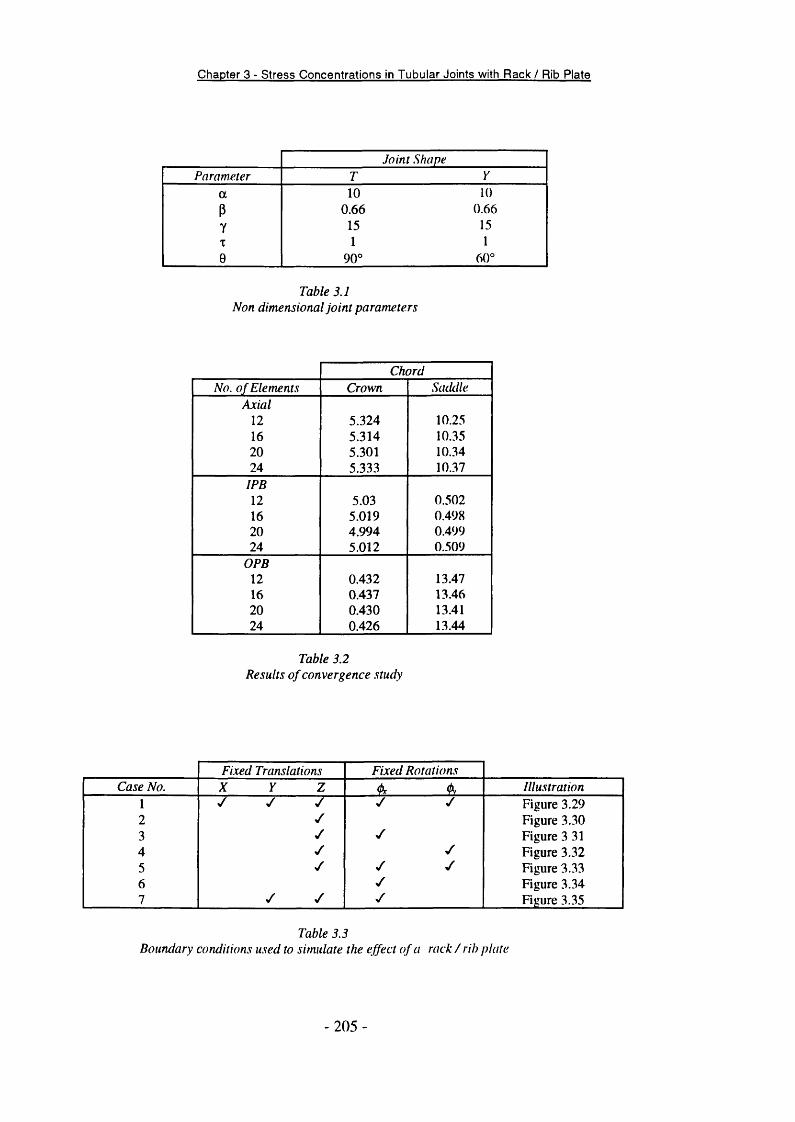
Chapter 3 - Stress Concentrations in Tubular Joints with Rack / Rib Plate
J o i n t . S h a p e
P a r a m e t e r T Y
a 10 10
P 0.66 0.66
Y 15 15T 1 10 90° 60°
T a b l e 3 . 1
N o n d i m e n s i o n a l j o i n t p a r a m e t e r s
C h o r d
N o . o f E l e m e n t s C r o w n S a d d l e
A x i a l
12 5.324 10.2516 5.314 10.3520 5.301 10.3424 5.333 10.37
I P B
12 5.03 0.50216 5.019 0.49820 4.994 0.49924 5.012 0.509
O P B
12 0.432 13.4716 0.437 13.4620 0.430 13.4124 0.426 13.44
T a b l e 3 . 2
R e s u l t s o f c o n v e r g e n c e . s t u d y
F i x e d T r a n s l a t i o n s F i x e d R o t a t i o n s
C a s e N o . X Y Z 4 ^ I l l u s t r a t i o n
1 y / / y y Figure 3.292 y Figure 3.303 y y Figure 3 314 y y Figure 3.325 y y y Figure 3.336 y Figure 3.347 y y y Figure 3.35
T a b l e 3 . 3
B o u n d a r y c o n d i t i o n s u s e d t o s i m u l a t e t h e e f f e c t o f a r a c k / r i b p l a t e
- 2 0 5 -

Chapter 3 - Stress Concentrations in Tubular Joints with Rack / Rib Plate
S C F R a t i o
A l p h a A x i a l O P B
6.21 0.69 0.908 0.59 0.9010 0.54 0.9012 0.52 0.89
13.1 0.52 0.89
T a b l e 3 . 4
E f f e c t o f A l p h a o n r e l a t i v e S C F
S C F R a t i o
B e t a A x i a l O P B
0.2 0.88 0.990.4 0.76 0.970.6 0.6 0.920.7 0.51 0.89
T a b l e 3 . 5
E f f e c t o f B e t a o n r e l a t i v e S C F
S C F R a t i o
G a m m a A x i a l O P B
7.6 0.58 0.9116 0.55 0.9024 0.61 0.9032 0.69 0.89
T a b l e 3 . 6
E f f e c t o f G a m m a o n r e l a t i v e S C F
S C F R a t i o
T a u A x i a l O P B
0.2 0.55 0.870.4 0.54 0.880.6 0.54 0.880.8 0.54 0.891.0 0.54 0.89
T a b l e 3 . 7
E f f e c t o f T a u o n r e l a t i v e S C F
-206

Chapter 3 - Stress Concentrations in Tubular Joints with Rack / Rib Plate
S C F R a t i o
T h e t a A x i a l O P B
35 0.74 0.8960 0.55 0.8970 0.54 0.8990 0.54 0.89
T a b l e 3 . 8
E f f e c t o f T h e t a o n r e l a t i v e S C F
- 2 07 -
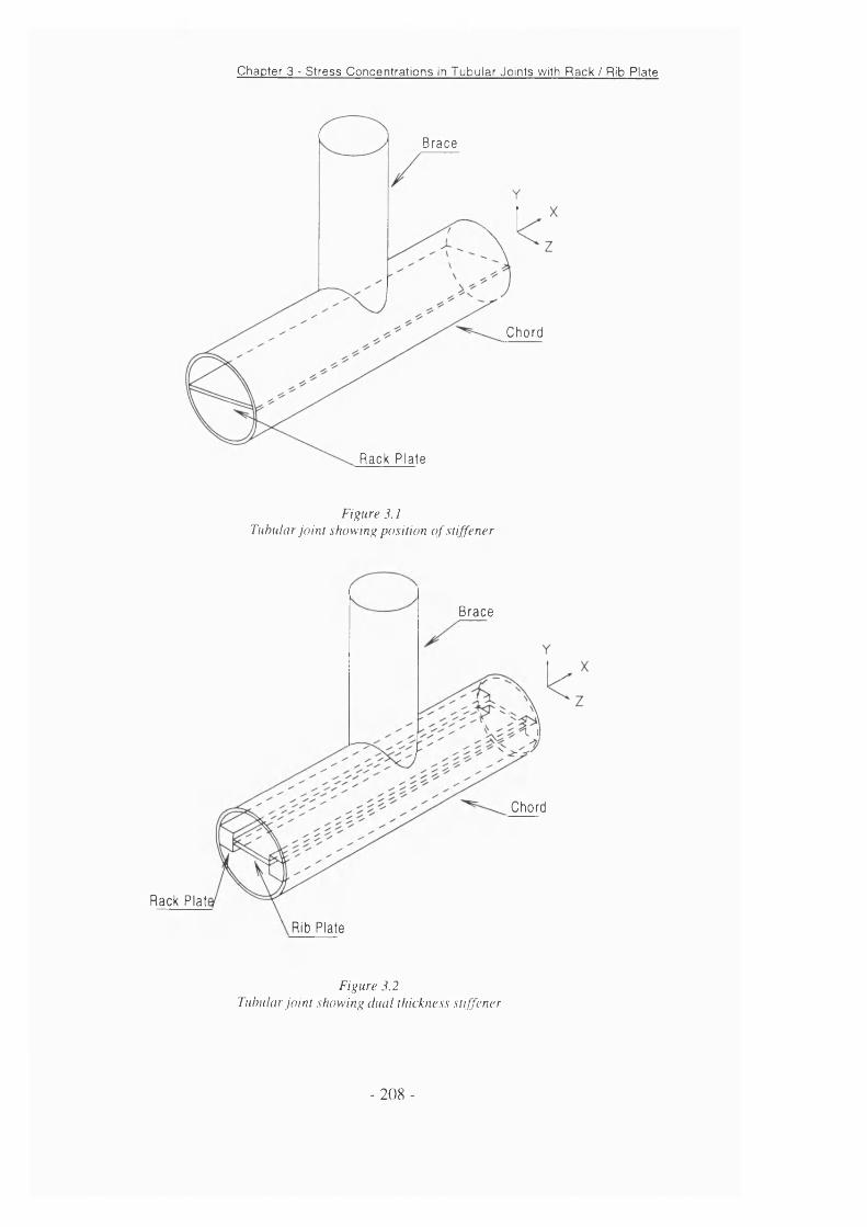
Chapter 3 - Stress Concentrations in Tubular Joints with Rack / Rib Plate
Br ace
Ch or d
Ra c k P lat e
F i g u r e 3 . 1
T u b u l a r j o i n t s h o w i n g p o s i t i o n o f s t i f f e n e r
Brace
Chord
Rack Plati
Rib Plate
F i g u r e 3 . 2
T u b u l a r J o i n t s h o w i n g d u a l t h i c k n e s s . s t i f f e n e r
- 208 -

Chapter 3 - Stress Concentrations in Tubular Joints with Rack / Rib Plate
Br a c e
C h o r d
Ra ck Pl ate
F i g u r e 3 . 3
T u b u l a r j o i n t s h o w i n g n o n c o n t i n u o u s . s t i f f e n e r
Ring St i f f ene
F i g u r e 3 . 4
T u b u l a r j o i n t w i t h i n t e r n a l r i n g . s t i f f e n e r s
- 209 -
Chapter 3 - Stress Concentrations in Tubular Joints with Rack / Rib Plate
I
F i g u r e 3 . 5
T u b u l a r j o i n t w i t h d o u b l e r p l a t e
F i g u r e 3 . 6
S a m p l e T . J o i n t f i n i t e e l e m e n t m e s h
- 2 1 0 -

Chapter 3 - Stress Concentrations in Tubular Joints with Rack / Rib Plate
O 10 --
t l / D
No Stiffener
O 0.0033
A 0.0167
X 0.0333
X 0.0833
O 0.1667
60 90 120
Angle Around inlerseclion
150 180
F i g u r e 3 . 7
E f f e c t o f n o r m i i l i s e d s t i f f e n e r t h i c k n e s s o n S C F d i . s t r i h u t i o n i n a n a x i a l l y l o a d e d T J o i n t
No Sm ener
0.0033
0.0167
0.0333
0.0833
0.1667
60 90 120
Angle Around Inlerseclion
150
Figure 3.8E ffect o f normalised stiffener thickness on SCF di.strihution fo r a.xially loaded Y jo in t
- 2 1 1 -
Chapter 3 - Stress Concentrations in Tubular Joints with Rack / Rib Plate
1.40
1.20
11/D1.000.0033ÜL0.0167
0.80 --0.0333
0.08333 0.16670.60 - -ll
0.3333
0.40 --
0.20 --
0.000 30 60 90 120 150 180
Angle Around Intersection
F i g u r e 3 . 9
E f f e c t o f p l a t e t h i c k n e . s s o n N o r m a l i s e d S C F d i s t r i b u t i o n f o r a . x i a l l y l o a d e d T j o i n t
1.2 --
t l /D
0.0033■o 0 . 8 - -
0.0167
0.0333
0.6 -- 0.0833
0.1667
0.33330.4 --
0.2 --
0 15030 60 90 120 180
Angle Around Intersection
Figure 3.10E ffect o f plate thickness on normalised SCF distribution fo r a.xially loaded Y jo in t
- 2 1 2 -
Chapter 3 - Stress Concentrations in Tubular Joints with Rack / Rib Plate
R a c k P l a t '
2 --
O 0
-2 -■
-4 --
0 20 40 60 to o 120 140 160 18080
t l / D
- No Stiffener
o 0.0033
A 0.0167
X 0.0333
X 0.0833
o 0.1667
Angle Around Intersection
F i g u r e 3 . 1 1
E f f e c t o f p l a t e t h i c k n e s s o n S C F f o r I P B l o a d e d T j o i n t
60 90 120
Angle A round Intersection
150
t l / D
- No Stiflener
O 0.0033
A 0.0167
X 0.0333
X 0.0833
o 0.1677
Figure 3.12Effect o f plate thickness on SC F fo r IP B loaded Y joint
- 2 1 3 -
Chapter 3 - Stress Concentrations in Tubu'ar Joints with Rack / Rib Plate
14 --
10 --
6 --
Y2 --
0 20 40 60 80 100 140 160 180120
t l / D
■ No Stiffener
0.0033
0.0167
0.0333
0.0833 0.1677
Angle Around Intersection
F i g u r e 3 . 1 3
E f f e c t o f p l a t e t h i c k n e s s o n S C F d i s t r i b u t i o n f o r O P B l o a d e d T j o i n t
t l / D
• Unstiffened
0.0033
0.0167
0.0333
0.0833
0.1677
60 80 100 120
Angle Around Intersection
180
Figure 3.14E ffect o f plate thickness on S C F di.strihution fo r OPB loaded Y jo in t
- 2 1 4 -
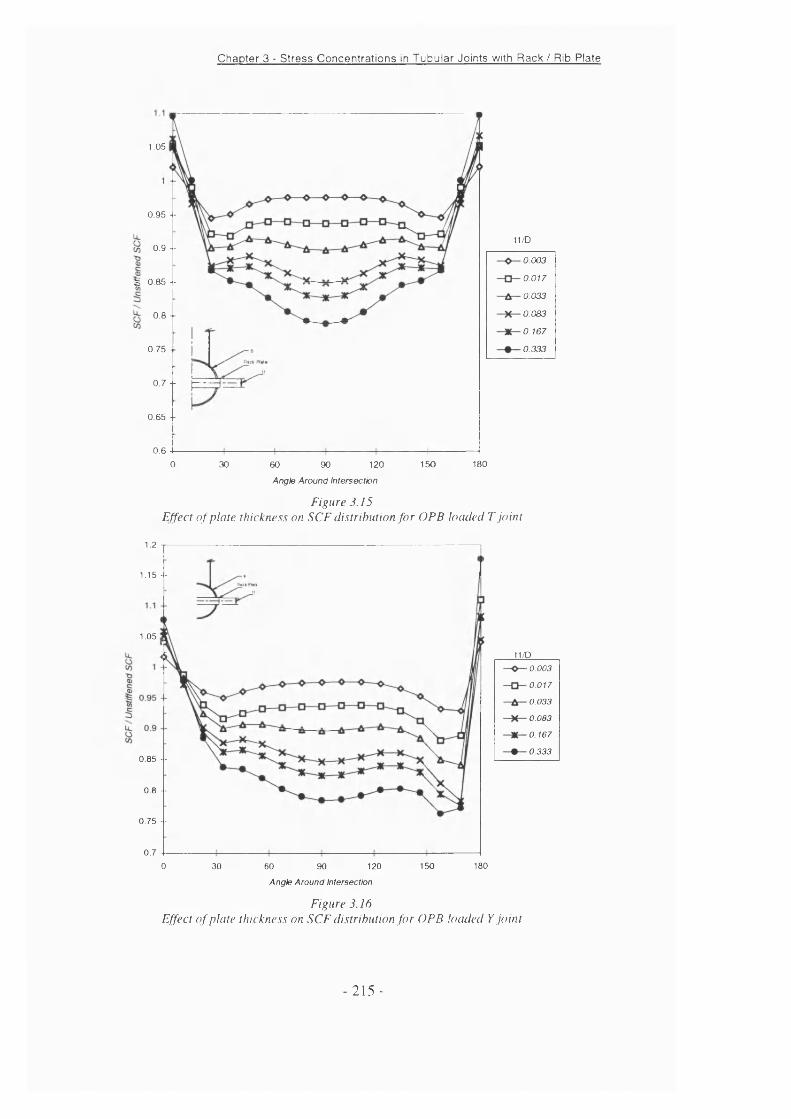
Chapter 3 - Stress Concentrations in Tubular Joints with Rack / Rib Plate
1.05
0.95 --
11/D0.9 --
0.003
0.017§ 0.85 --
0.033
0.0830.8 --0.167
0.75 -- 0.333
0.7 -■ j-----
0.65 --
0.60 150 18030 60 90 120
Angle Around Intersection
F i g u r e 3 . 1 5
E f f e c t o f p l a t e t h i c k n e s s o n S C F d i s t r i b u t i o n f o r O P B l o a d e d T j o i n t
1.2
1.15 --
1.05
0.85 --
0 .8 - -
0.75 --
0.7150 1800 30 60 90 120
tl/D• 0.003
■0.017
0.033
0.083
0 .167
0 .333
Angle Around Intersection
Figure 3.16E ffect o f plate thickness on SC F di.strihution fo r OPB loaded Y jo in t
- 2 1 5 -
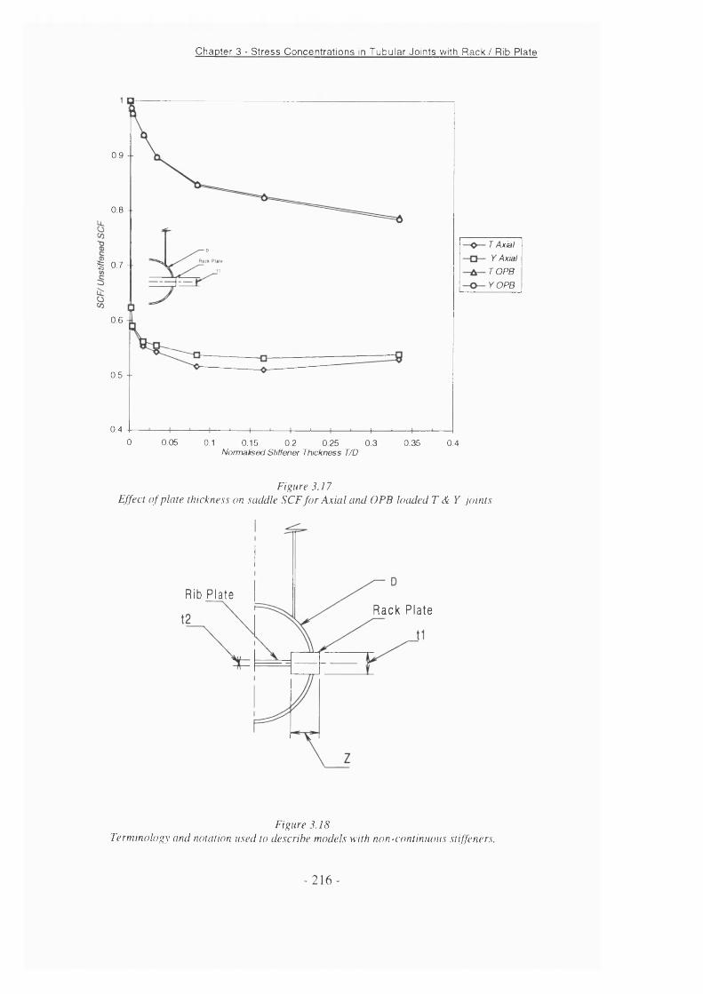
Chapter 3 - Stress Concentrations in Tubular Joints with Rack / Rib Plate
0.9 --
0.8 -■
T Axial
Y Axial
TO PB
Y OPB
% 0 .7 -
0.6
0.5 --
0.40 0.05 0.1 0.15 0.2 0.25 0.3 0.35 0.4
Normalised Stiffener Thickness T/D
F i g u r e 3 . 1 7
E f f e c t o f p l a t e t h i c k n e s s o n s a d d l e S C F f o r A x i a l a m i O P B l o a d e d T & Y j o i n t s
Rib Pla teR a c k P la te
Figure 3.18Terminology and notation used to describe models with non-contmuous stiffeners.
- 2 1 6 -

Chapter 3 - Stress Concentrations in Tubular Joints with Rack / Rib Plate
t1/D = 0.080.620
0.610 --
0 .600 --
0.590 --
0 .580 - -
•o 0.570 --
I 0.560 --
\ 0 .550 --
& 0.540 --
0 .530 --
0.520 --
0.510 --
0.500
0.00 0.01 0.01 0.02 0 .02 0.03
Rib Plate Thickness / Chord D iam eter (t2 /D )
0.03
Continuous
0.04
0.500
0.00
F i g u r e 3 . 1 9 .
E f f e c t o f r i b p l a t e o n a x i a l l y l o a d e d T j o i n t
t1/D = 0.170.620
0 .610 --
0.600 --
0 .590 - -
LL 0 .580 +
■O 0 .570 +
g 0 .560 -- Continuous
0.550 --
0 .540 --
0 .530 --
0 .520 - -
0 .510 --
0.01 0.01 0.02 0 .02 0.03
R t Plate Thickness / Chord Diameter (t2/D)
0.03 0.04
F i g u r e 3 . 2 0
E f f e c t o f r i b p l a t e o n a x i a l l y l o a d e d T j o i n t
- 2 1 7 -
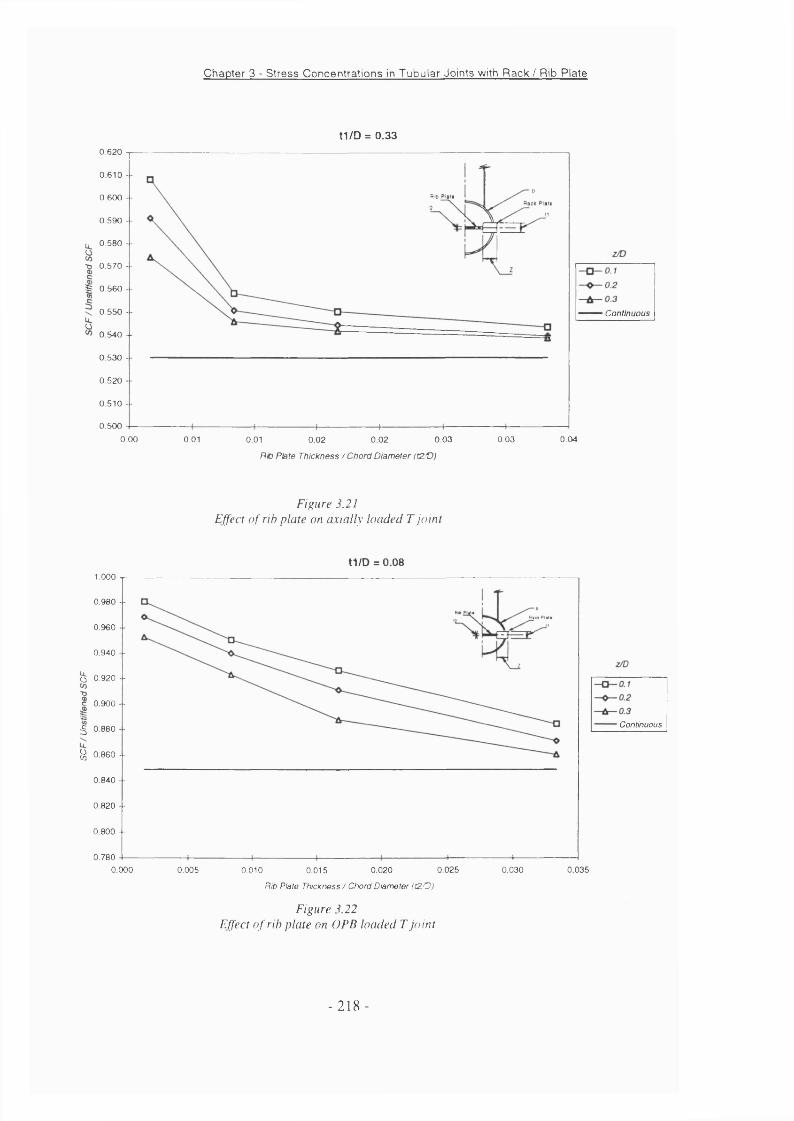
Chapter 3 - Stress Concentrations in Tubular Joints with Rack / Rib Plate
t l /D = 0.33
fe 0 .560 -- tn
0 .550 --
O0 .540 4-
0 .530 - -
0 .520 --
0 .510 --
0 .500
0.00 0.01 0.01 0 .02 0 .02 0.03
Rib Plate Thickness / Chord Diameter (tZID)
0.620
0 .610 --
0 .600 --
0 .590 --
0 .580 - -
t j 0 .570 --
Continuous
0.03 0.04
F i g u r e 3 . 2 1
E f f e c t o f r i b p l a t e o n a j c i a l l y l o a d e d T j o i n t
t1/D = 0.081.000
0.980 --
0.960 --
0.940 - -
U 0.920 --
c 0.900 --
■Ç 0.880 --
Ü 0 .8 6 0 - -
0.840 --
0.820 - -
0.800 - -
0.780
0.000 0.005 0.010 0.015 0.020 0.025
Rib Plate Thickness / Chord D iam eter ( t2 0 )
F i g u r e 3 . 2 2
E f f e c t o f r i b p l a t e o n O P B l o a d e d T j o i n t
0.030
Continuous
0.035
- 2 1 8 -
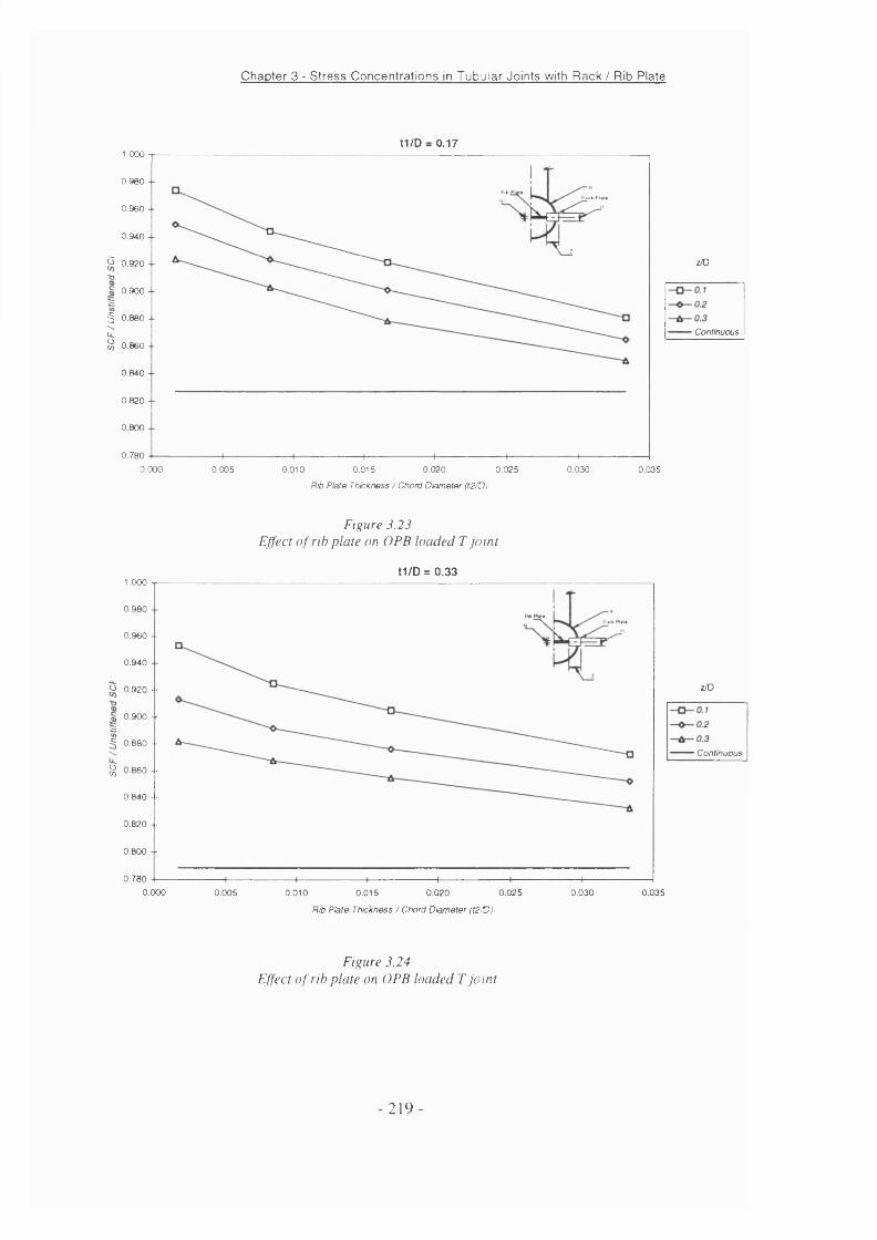
Chapter 3 - Stress Concentrations in Tubular Joints with Rack / Rib Plate
0.000
tl/D = 0.171,000
0.960 - -
0.960 - ■
0.940 - -
Ù 0.920 -.
0.900 --
:§ 0.880 - -
bS 0.860 - -
0.840 - -
0.820 --
0.800 --
0.7800.005 0.010 0.015 0.020 0.025
Rib Plate Thickness / Chord Diameter (t2/D)
0.030
z/D
Continuous
0.035
0.000
F i g u r e 3 . 2 3
E f f e c t o f r i b p l a t e o n O P B l o a d e d T j o i n t
0.005
t l/D = 0.331.0000.980
0.960 --
0.940
O 0.920 --
0.900 -■
0.880 - -
0 .860--
0.840 - ■
0.820 - ■
0.800 - -
0,7800.010 0.015 0.020 0.025
Rib Plate Thickness / Chord Diameter (t2,V)
0.030
z/D
Continuous
0.035
F i g u r e 3 . 2 4
E f f e c t o f r i b p l a t e o n O P B l o a d e d T j o i n t
- 2 1 9 -
Chapter 3 - Stress Concentrations in Tubular Joints with Rack / Rib Plate
0.000 0.050
0.95 -■
0.9 -■
0.85 --
CO 0.8 -■
LL 0.7 - -
0.65 --
0.6 -■
0.55 -■
0.5
0.100 0.150 0.200 0.250Norm alised Rack Plate Thickness, t l / D
0.300 0.350
f i g u r e 3 . 2 5
E f f e c t o f r a c k p l a t e t h i c k n e s s f o r a x i a l l y l o a d e d j o i n t
Norm alised Rack Plate Thickness, t1/D
F i g u r e 3 . 2 6
E f f e c t o f r a c k p l a t e t h i c k n e s s f o r O P B l o a d e d j o i n t
0.98
0.96
Ll% 0.94T3
Z/D
?^ 0.92
I0.20.3
0.4
0.5
0.88
0.86
0.84
0.000 0.050 0.100 0.250 0.300 0.3500.150 0.200
- 2 2 0 -
Chapter 3 - Stress Concentrations in Tubular Joints with Rack / Rib Plate
Normalised Stiffener Deptti (z/D)
F i g u r e 3 . 2 7
E ffe c t o f r o c k p l a t e d e p t h f o r a x i a l l y l o a d e d j o i n t
Normalised Stiffener Depth (z/D)
F i g u r e 3 . 2 8
E f f e c t o f r a c k p l a t e d e p t h f o r O P B l o a d e d j o i n t
0.95
0.9
O 0.85
^ 0.75
0.7
0.65
0.60.1 0.15 0.450.2 0.25 0.3 0.35 0.4 0.5
t l /D■0.017
■0.033
■0 083
■ 0 .167
■0.333
0.98
0.96
0.94
OCO-o 0.92
I%[Z 0.88OCO
0.86
0.84
0.82
0.80.1 0.15 0.2 0.4 0.45 0.50.25 0.3 0.35
tl/D
■0.017
■ 0.033
■ 0.083
■0.167
■ 0.333
- 2 2 1 -
Chapter 3 - Stress Concentrations in Tubular Joints with Rack / Rib Plate
R o t a t i o n a l R e s t r a i n t
T r a n s l a t i o n a l R e s t r a i n t
F i g u r e 3 . 2 9
C a . s e 1 - C h o r d d e f o r m a t i o n r e s t r a i n e d i n a l l d e g r e e s o f f r e e d o m a l o n g l i n e . s h o w n
T r a n s l a t i o n a l R e s t r a i n t
Figure 3.30Case 2 - Chord deformation restrained in Z direction along line shown.
- 222 -
Chapter 3 - Stress Concentrations in Tubular Joints with Rack / Rib Plate
Rota t ion a l R e s tra in t
Translational R e s tra in t
F i g u r e 3 . 3 1
C a s e 3 - C h o r d d e f o r m a t i o n r e s t r a i n e d i n Z d i r e c t i o n a n d r o t a t i o n a b o u t X a x i s a l o n g l i n e
s h o w n
R o ta t iona l R e s tra in t
T ranslational R e s tra in t
Figure 3.32Case 4 - Chord deformation restrained in Z direction arui rotation about V axis along line
shown.
- 223 -
Chapter 3 - Stress Concentrations in Tubular Joints with Rack / Rib Plate
R o t a t i o n a l R e s t r a i n t
T r a n s l a t i o n a l R e s t r a i n t
F i g u r e 3 . 3 3
C a s e 5 - C h o r d d e f o r m a t i o n r e s t r a i n e d i n Z d i r e c t i o n a n d r o t a t i o n s a b o u t X a n d Y a x e s a l o n g
l i n e s h o w n .
R o t a t i o n a l R e s t r a i n t
Figure 3.34Ca.se 6 - Chord deformation restrained in rotations about X axis along line .shown.
- 2 2 4 -

Chapter 3 - Stress Concentrations in Tubular Joints with Rack / Rib Plate
R o t a t i o n a l R e s t r a i n t
T r a n s l a t i o n a l R e s t r a i n t
F i g u r e 3 . 3 5
C a s e 7 - C h o r d d e f o r m a t i o n r e s t r a i n e d i n Y a n d Z d i r e c t i o n a n d r o t a t i o n s a b o u t X a x i s a l o n g
l i n e s h o w n .
16 - -
14 --
No Stiffener
12 --
100mmu 10 --Case 1 (Built In)
8 --
Case 6
6 --
2 -
0 20 40 140 160 18060 80 100 120Angle Around Intersection
F i g u r e 3 . 3 6
S i m u l a t i o n o f t h e e ffe c t o f a s t i f f e n e r u s i n g b o t t m i a r y c o n d i t i o n s
- 225 -

Chapter 3 - Stress Concentrations in Tubular Joints with Rack / Rib Plate
20
16 - ■
14 - -
No Stiffener
12 --1mm
100mmo lO --
Case 38 -■
6 --h—
4 - -
160 1801400 20 40 60 80 100 120Angle Around Intersection
F i g u r e . 3 . 2 7
S i m u l a t i o n o f t h e e ffe c t o f a s t i f f e n e r u s i n g b o u n d a r y c o n d i t i o n s
20
16 - -
14 - -
-O-O 10 --
6 - -
4 - -
160 1801400 60 100 12020 40 80
Angle A round Intersection
F i g u r e 3 . 3 8
S i m u l a t i o n o f t h e e f f e c t o f a s t i f f e n e r u s i n g b o u n d a r y c o n d i t i o n s
No Stiffener
- 1mm
- - - 100mm
Case 2
o Case 4
- 226 -

Chapter 3 - Stress Concentrations in Tubular Joints with Rack / Rib Plate
16 --
No Stiffener
12 -■
- 100mm
Case 1 (Built In)B --
Case 7
4 --
2 -■
0 140 160 18020 40 60 80 100 120^ngie Around intersection
F i g u r e 3 . 3 9
S i m u l a t i o n o f t h e e ffe c t o f a s t i f f e n e r u s i n g b o u n d a r y c o r u i i t i o n s
20
19 --
18 --
17 --
16 --
15 --
Unstiffened
StiffenedO 14 --
13 --
12 --
0.69 0.59 0.54 0.52 0.52
10 --
9 --
6 7 8 12 13 149 10 11Alpha
Figure 3.40E ffect o f Alpha on an axially loaded T jo in t
- 2 2 1 -
Chapter 3 - Stress Concentrations in Tubular Joints with Rack / Rib Plate
15 --
14 --
0.89
Unstiffened
Stiffened
0.9U 13 --
0.9
1 2 - -
105 76 14a 9 10 11 12 13
A p h a
F i g u r e 3 . 4 1
E f f e c t o f A l p h a o n a n O P B l o a d e d T j o i n t
21 - -
20 - -
19 - -
17 - -
16 - -
O 15 - - 0 .760.88
14 - -
13 - -
12 - -0.6
10 - -
0.519 - -
0 0.1 0.2 0 .3 0 .4 0.5 0.6 0 .7 0.8
Beta
Figure 3.42Effect o f Beta on an axia lly loaded T jo in t
■ Unstiffened■ Stiffened
- 228 -
Chapter 3 - Stress Concentrations in Tubular Joints with Rack / Rib Plate
15 --
14 --
0.9213 --
12 - -
1.97
O 1 0 - -
9 --
8 - -
7 --
6 - -
0.99
5 --
0 0.1 0.2 0.5 0.6 0.7 0.80.3 0.4
Unstiffened
- Stiffened
Beta
F i g u r e 3 . 4 3
E f f e c t o f B e t a o n a n O P B l o a d e d T j o i n t
30 - -
25 --
1.69
20 - -
0.6115 --
[5510 - -
5 --
5 350 2510 15 20 30
■ Unstiffened • Stiffened
Gamma
Figure 3.44Effect o f Gamma on an axia lly loaded T jo in t
- 2 2 9 -
Chapter 3 - Stress Concentrations in Tubular Joints with Rack / Rib Plate
30 --
25 -- t).88
20 - -
0.9
15 --
10 - -
0.915 --
350 305 2510 15 20
• Unstiffened• Stiffened
Gamma
F i g u r e 3 . 4 5
E ffe c t o f G a m m a o n a n O P B l o a d e d T j o i n t
20
18 --
16 - '
14 --
12 - -
O 1 0 - -
0.548 - -
0.546 - -
0.544 --
0.54
0.55
0.2 0.90.3 0.4 0.8 10.5 0.6 0.7
-Unstiffened
■ Stiffened
Tau
F i g u r e 3 . 4 6
E ffe c t o f T a u o n a n a x i a l l y l o a d e d T J o i n t
230
Chapter 3 - Stress Concentrations in Tubular Joints with Rack / Rib Plate
14 --
12 - - 1.89
10 - - 0.89
0.886 - -
4 -- 0.88
2 - -
0.87
0 0.2 0.4 0.6 0.8 1Tau
F i g u r e 3 . 4 7
E f f e c t o f T a u o n a n O P B l o a d e d T j o i n t
■ Unstiffened■ Stiffened
20
18 --
16 --
14 --
12 - -
O 1 0 - -0.54
8 - -
1.55
6 - -
0.744 --
2 - -
30 40 50 70 80 9060
■Unstiffened
■ Stiffened
Theta
F i g u r e 3 . 4 8
E f f e c t o f T h e t a o n a n a x i a l l y l o a d e d T j o i n t
-231 -

Chapter 3 - Stress Concentrations in Tubular Joints with Rack / Rib Plate
1 4 . .
13 --0 .54
12 - -
0.54
11 - -
10 - - 0.55
9 --
8 - -
7 -■
6 - -
5 --
0.744 --
3 --
30 40 50 60 70 9060Theta
-Unstiffened
-stiffened
F i g u r e 3 . 4 9
E f f e c t o f T h e t a o n a n O P B l o a d e d T j o i n t
- 2 32 -

Chapter 4- The Effect of a Rack / Rib Plate on the Degree of Through Thickness Bending
Chapter 4
4. The Effect of a Rack / Rib Plate on the Degree of Through
Thickness Bending in Jack Up Chords
4.1 Introduction
It was shown in Chapter 3 that the presence of a Rack or Rib plate as commonly
found in jack up chords can have a significant effect on the SCF’s found at the
intersection between the brace and the chord. Accurate knowledge of the SCF
distribution, and in particular the peak SCF is important for the prediction of
fatigue lives at the design stage using the S-N approach.
For the assessment of defects discovered in service however the S-N approach is
no longer appropriate. For such an analysis the science of fracture mechanics must
be implemented. Any detailed fracture mechanics analysis requires the prior
knowledge of the stress distribution along the anticipated crack path. For tubular
joints this means an accurate knowledge of the proportion of through thickness
bending, commonly called the Degree of Bending (DoB) together with a model of
the load redistribution or ‘load shedding’ that is known to occur.
The results of approximately 500 finite element models will be presented in this
Chapter in an attempt to quantify the effect of a central longitudinal chord stiffener
on the through thickness stress distribution.
4.2 Scope
Three distinct chord designs used in jack up construction were identified and
described in detail in Chapter 3. These three designs are shown schematically in
Figures 4.1 to 4.3. The same three chord designs wiU be investigated here across
- 233 -
Chapter 4- The Effect of a Rack / Rib Plate on the Degree of Through Thickness Bending
the same range of parameters. In the interest of brevity the chord designs will not
be presented again here, instead reference is made to Section 3.3.
Each of the three chord designs will be investigated under axial, in-plane bending
and out of plane bending. As in Chapter 3, initially a single set of joint parameters
will be investigated. The joint parameters are detailed in Table 4.1 and were chosen
as being representative values which results in a high quality finite element mesh
with little element distortion.
The sensitivity of the through thickness stress distribution to the joint parameters
will then be investigated across the range of joint parameters for which the
parametric equations by Connolly et al are valid. [4.1]. This set of parametric
equations will form the basis for comparison during this study and will be discussed
in detail in the next section.
All results presented here are from the chord side as this was shown in Chapter 3
as having the highest stress concentration factors.
4.3 Through Thickness Stress Distributions in Tubular Joints
Conventional fatigue design uses the peak surface SCF to determine the fatigue life
of a tubular joint utilising experimentally derived S-N curves. However
examination of the experimental database used during the derivation of the S-N
Curves [4.2] shows that the ‘hot spot stress’ alone is insufficient to completely
describe the crack growth behaviour in tubular joints. This conclusion was reached
when it became clear that tubular joints with similar hot spot stress levels but
different loading modes often resulted in different fatigue lives. The effect of
loading mode is shown in Figure 4.4 where the axial and OPB loading mode
database has been plotted. Also included in this figure are the mean fatigue life
lines for each loading mode. It can be seen that these mean lines converge at lower
stress levels as change in slope of the design S-N curve is approached. However at
- 234-

Chapter 4- The Effect of a Rack / Rib Plate on the Degree of Through Thickness Bending
the higher stress levels, out of plane bending produces fatigue lives approximately
2.5 times longer than an axially loaded joint at the same stress level.
Holdbrook [4.3] suggests that these differences are due to differences in crack
growth which in turn must depend on the through thickness stress distribution as
well as the hot spot stress level.
The through thickness stress distribution is most commonly described by a simple
linear interpolation between the maximum and minimum principal stresses found on
the inner and outer tubular surfaces respectively as illustrated in Figure 4.5. The
stress concentrating effect of the notch (weld toe) is omitted as it is in the
determination of surface stress concentration factor (SCF). The degree of bending
(DoB) is defined as shown in Eqn (4.1)
DoB = (Ji, /(<T, +cr^) (4.1)
where the subscript represents the bending (b) or the membrane (m) component. A
graphical representation of the make up of different DoB values is given in Figure
4.6
4.3.1 The Importance of Through Thickness Stress Distribution
Several researchers have attempted to account for the through thickness stress
distribution in fracture mechanics models. Most of the models implement some
form of ‘load shedding’ mechanism whereby the bending component of the through
thickness stress distribution is redistributed through alternative load-paths within
the statically indeterminate structure of the tubular joint. The first and most widely
recognised of these models is that of Aaghaakouchak et a! [4.4] who investigated
the discrepancy between the flat plate SIF solution of Newman and Raju [4.5] and
the weight function of Oore and Bums [4.6] with the experimentally derived stress
intensity factors from tubular joint fatigue tests. Noting that both methods
significantly over predicted the stress intensity factors in tubular joints it was
- 235 -
Chapter 4- The Effect of a Rack / Rib Plate on the Degree of Through Thickness Bending
postulated that this was due to incomplete modelling of the phenomenon called
‘load shedding’ caused by the complex boundary conditions found in tubulars. A
finite element study [4.7] of flat plates and rings with edge cracks was analysed
under different boundary conditions. It was found that the statically indeterminate
models (models containing degrees of redundancy) resulted in significantly lower Y
Factors than the statically determinate models. Examination of the reactions at the
supports as the crack depth increased showed that as the crack length increased,
the behaviour of the cracked section approached that of a hinge . A Linear Moment
Release model was proposed whereby the membrane stress remains constant but
the bending stress at the cracked section is continuously and linearly released with
increasing crack depth according to Eqn. (4.2)
— '^boI tj(4.2)
where Sb is the bending stress at the crack tip and Sbo is the surface bending stress
at the surface. It was reported that in conjunction with the Newman - Raju
equations that this model produced Y Factors within the scatter band of
experimentally derived Y Factors for crack depths of between 0.1 < a/T <0.8 for a
range of loading modes and joint shapes.
Forbes et al [4.8] carried out a series of tests on large scale tubular joints and wide
plates to experimentally measure the magnitude of load shedding that occurs in
tubular joints. The data from these tests was used to essentially confirm the initial
postulation of Aaghaakouchak et al with regard to the presence of a load shedding
mechanism. The experimentally derived membrane and bending stresses at the
cracked section were used in conjunction with the SIF solutions of Newman and
Raju [4.5] and the weight function of Oore and Bums [4.6]. It was noted that
improved agreement was found regardless of which analytical technique was used.
It is important to note that Forbes et al did not assume a constant membrane stress
at the cracked section as suggested by Aaghaakouchak et al and the membrane
- 236-

Chapter 4- The Effect of a Rack / Rib Plate on the Degree of Through Thickness Bending
stress used in the calculation of SIF was adjusted with crack depth in line with
experimental measurements. Forbes et al present the variation in experimental
stress measurements with normalised crack depth for the inner and outer surfaces
of a tubular joint under axial brace loading. The information is presented
graphically in terms of the stress normal to the crack surface. The stresses are
normalised to that found on the outer surface of the uncracked joint. The fact that
the stress presented is the stress normal to the crack surface rather than the
maximum principal stress is not thought to be significant as the maximum principal
stress has been shown from the FE analysis to be approximately perpendicular to
the weld toe at the saddle of an uncracked joint. The normalised stresses found on
the inner and outer surfaces of the tubular specimen have been extracted from the
figure and decomposed into normalised bending and membrane components for
normalised crack depths of 0 < a/T < 0.8. The stress measurements were taken a
distance of approximately twice the chord wall thickness from the crack plane. It
was assumed that this would be sufficient to detect changes in the chord wall stress
but sufficiently far away from the crack so as not to be affected by the local stress
relief caused by the crack itself. This information is presented in Figure 4.7. The
stresses are presented normalised to the peak normal surface stress in the
uncracked joint. It is clear from this figure that the hypothesis of Aaghaakouchak et
al that the membrane stress component remains unchanged by the presence of a
fatigue crack is not supported by this experimental evidence. However the bending
component appears to quite closely follow the Linear Moment Release theory,
tending to zero as the crack approaches through wall thickness. The importance of
the positioning of the experimental measurements is unclear but the assumption
made by Forbes et al seems reasonable.
Berge et al [4.9] present the variation of experimentally measured bending and
membrane stresses with increasing crack depth. The stresses were measured a
distance of 24mm from the weld toe. The Linear Moment Release model (4.2) is
shown to under-predict the degree of moment release. The results also show that
the membrane component tends to zero at a/T values of approximately 0.5.
- 237-

Chapter 4- The Effect of a Rack / Rib Plate on the Degree of Through Thickness Bending
Unfortunately the experimental results are only shown for the normalised crack
depth range 0<a/T<0.6 so it is not possible to confirm whether the membrane
stresses become compressive at deeper depths as noted earlier using the data
presented by Forbes et al.
Berge et al have conducted a fracture mechanics study of tubular joints in an
attempt to explain the reasons why the results of a series of tubular joint fatigue
tests fell below the S-N Design curve for 32mm tubular welded joints. The
specimens in question consisted of a single chord with two perpendicular braces
lying in the same plane, acting as a self reacting frame. It was postulated that this
loading arrangement results in a lower degree of bending (DoB) due to an
increased membrane component. The investigation aimed to asses whether this
increased membrane component could be used to explain the short lives found in
the tubular joint fatigue tests.
The fracture mechanics model used by Berge et al is outlined in detail by Haswell
[4.10]. The Y Factors were calculated using thin sheU FE techniques containing
line spring elements to model the crack. Using the Reference State Solution a
weight function was derived using the Y Factors from the FE modelling. A
constant aspect ratio of a/2c=0.1 for cracks deeper than 4mm was assumed. This
fracture mechanics model will be assessed in detail in Chapter 5. FE models of the
uncracked joints show the DoB to decrease from 0.73 to 0.62 with the addition of
the extra brace to form the self reacting frame. This difference in DoB, which was
implicitly included in the line spring FE models resulted in fatigue lives that were
shorter by a factor of two for the double braced model and agreed closely with the
experimental results. The investigation concluded that DoB can significantly affect
the fatigue life of a tubular joint, and in some cases where the DoB is low, the Hot
Spot stress approach can be unconservative.
A simpler fracture mechanics model based on the Linear Moment Release model of
Aaghaakouchak et al and the Shen - Glinka weight function [4.11] was also used.
- 238-

Chapter 4- The Effect of a Rack / Rib Plate on the Degree of Through Thickness Bending
Increasing the DoB from an unrealisticaUy low 0.45 to 0.9 increased the predicted
life by a factor of 2.25. It was stated that the simple model gave results in good
agreement with the 3-D analysis.
4.3.2 Determination of Through Thickness Stress Distribution
By far the most comprehensive investigation into the through thickness stress
distributions have been performed by Connolly et al [4.1] for Y and T Joints and
more recently by Chang for X and DT joint shapes [4.12]. Both investigations
produced parametric equations describing the variation of degree of bending in
terms of the joint parameters.
Connolly et al produced the DoB parametric equations using results from the same
finite element study that Hellier at al [4.13] used to derive SCF parametric
equations for the same joint shapes. Based on a thin shell finite element model, a
database of almost 900 joint shapes under each of axial, IPB and OPB loading was
developed. The weld was not modelled and advantage was taken of symmetry
during the generation of the finite element meshes. The chord ends were
constrained in all degrees of freedom and all loads were applied as uniformly
distributed loads along the brace ends. Verification of the model was achieved by
comparison with experimental results from strain gauged acrylic models.
Several other investigators quote DoB results for single geometries, either from
finite element investigations of individual joint shapes [4.14] or from experimental
results from large scale welded tubular joints e.g.[4.15]. Some such results will be
used for validation of the current finite element model.
4.4 Mesh Generation and Boundary Conditions
The results presented in this Chapter are derived from models sharing a common
heritage with those presented in Chapter 3. In the interests of brevity only a
239-
Chapter 4- The Effect of a Rack / Rib Plate on the Degree of Through Thickness Bending
summary of the mesh generation and boundary condition detail will be presented
here. For full details reference is made to Section 3.4.
The general purpose finite element package ABAQUS [4.16] was used throughout
this investigation. Finite element models were generated using a modification of a
FORTRAN program previously used to analyse simple planar tubular joints (see
Section 3.4 for full details). The mesh generator reliably handles a wide range of
joint shapes and sizes. Mesh refinement is controlled by specifying the number of
elements around the intersection of brace and chord. AU loads are automaticaUy
scaled to give unit nominal stress at the intersection. This enables SCF’s to be read
directly from the output files without further processing. FORTRAN routines have
been developed to automaticaUy open the ABAQUS results files and extract the
relevant information from the nodes of interest. This information is then written
into a file in a spreadsheet readable format.
SheU elements were used throughout this investigation. For models utilising thin
sheU elements these were S8R5 (8 noded quadrilateral) elements with a smaU
number of STRI65 (6 noded triangular) elements for geometric compatibUity in
and around the plug region. A number of models using thick sheU elements have
also been solved. These models used S8R (8 noded quadrilateral) elements. Models
employing thick shell elements will be clearly indicated.
The eight noded thin sheU elements, S8R5 are reduced integration, doubly curved
shells with 5 degrees of freedom, three translational motions, x, y, and z, and two
in surface rotations. The 8 noded thick sheU elements are also reduced integration,
doubly curved shells but with 6 degrees of freedom, three translational motions and
three rotational degrees of freedom, <j)x, (j)y, and (|)z.
A sample mesh is shown in Figure 4.8. Note the refinement of elements around the
intersection where the stress gradients are greatest and the gradual coarsening of
the mesh remote from this region where the stresses become more uniform. Careful
- 240-
Chapter 4- The Effect of a Rack / Rib Plate on the Degree of Through Thickness Bending
positioning of the nodes allows the stretch and distortion of the elements to a
minimum. Since triangular shell elements are less accurate than quadrilateral shell
elements, their use has been kept to a minimum. Triangular elements are only used
where necessary due to reasons of geometric compatibility around but some
distance from the intersection and within the plug region. Generation of a typical
mesh takes just a few seconds and a complete solution for an average model
containing 858 elements can be obtained in 45 seconds of CPU time. AU analysis
was performed on a DEC Alphastation 255/233MHz.
Symmetry of the model in the X Y plane aUows a half model analysis to be
performed providing the correct boundary conditions are applied to the nodes on
the plane of symmetry. Reducing the size of the model in this manner saves
significant CPU time and disk storage space. ABAQUS provides a ZSYMM
function to aUow the automatic application of the appropriate translational and
rotational restraints to simulate symmetry in the Z direction. The constraints
imposed on aU nodes on the plane of symmetry are zero displacement in the z
direction and aU rotations associated with the thin shell elements are fixed at zero.
For chord designs containing a stiffener that passes through the whole of the chord
diameter, the same symmetry boundary conditions are applied to the stiffener.
Stiffener designs where the plate is not continuous through the chord (see Figure
4.3) have no symmetry boundary conditions applied at the free edge.
The symmetry conditions are violated for the Out of Plane Bending loading
condition, but ConnoUy et al [4.1] discovered that it is stiU possible to use half joint
meshes with acceptable accuracy by restraining in plane displacements.
The chord ends are modeUed as ‘built-in’ with aU degrees of freedom being
restrained. No boundary conditions are applied to the brace end other than the
uniformly distributed external loads applied at each node.
- 241-
Chapter 4- The Effect of a Rack / Rib Plate on the Degree of Through Thickness Bending
4.5 Convergence and Model Verification
Convergence of the models was demonstrated in Section 3.6 by comparing the
SCF at the crown and saddle for models with 12, 16, 20 and 24 elements around
the intersection. It was noted that 16 elements around the intersection forms a
reasonable compromise between accuracy and computational cost.
Connolly et al [4.1] presented a comparison of the bending to total stress ratio
from an acrylic model under axial and IPB loading with the results from the finite
element study. A model with the same geometric parameters has been produced
here for comparison with the result from Connolly et al and the acrylic model. The
results are presented in Table 4.2.
Bending to Total stress ratio results from around the intersection of the acrylic
model are shown in Figure 4.9. Axial and IPB loading modes are shown. Also
presented are the results from the current finite element study for a model with the
same geometric parameters as the acrylic model. The IPB results are only shown
between 0° and 60° as past this point it becomes difficult (and irrelevant) to
determine the appropriate principal stresses as the neutral axis is approached.
In general the results agree well and closely follow the same trends. A tendency for
the FE model to over predict the degree of bending at the hot spot for each loading
mode has been identified. Furthermore the degree of bending is under predicted
compared to the acrylic model 90° away from the hot spot. Connolly et al reported
the same trends and the results of the two finite element based investigations agree
closely.
Several models were created and solved using thick shell elements. Thick shell
elements are different to thin shell elements in that they are capable of transmitting
shear forces. The results have shown that there is little difference between the thick
242 -
Chapter 4- The Effect of a Rack / Rib Plate on the Degree of Through Thickness Bending
and thin shell elements. This was found across a range of joint shapes, stiffener
thicknesses and loading mode. The case of an axially loaded T joint is typical and is
illustrated in Figure 4.10. In this figure it is demonstrated that the difference
between the DoB predicted by the thick and thin shell models is of the order of 1%
across the complete range of stiffener thicknesses examined here. For this reason
all further results presented in this Chapter were generated using thin shell
elements.
4.6 Finite Element Investigation
The results and discussion presented here are limited to the DoB found at the hot
spot stress site as this is where the deepest point of the fatigue crack is known to
occur. It is the crack growth at this point that fracture mechanics models strive to
simulate. The DoB at other points around the intersection is largely irrelevant as
the surface crack growth is controlled by the surface stress distribution and fatigue
cracks in tubular joints are known to be approximately semi-elliptical in nature.
4.6.1 Effect of Rack Plate Thickness on Through Thickness Stress
Distributions
Several stiffener plate thicknesses of up to 1/3 of the chord diameter have been
investigated and the SCF results around the intersection on the chord side are
presented here. Each of the stiffeners had a constant thickness and was continuous
through the chord diameter. The investigation covered both T and Y joints under
Axial, IPB and OPB loading modes.
4.6.1.1 ResuitsThe results will first be examined in terms of the absolute DoB found across the
range of stiffener thicknesses for T and Y joints under each loading mode. The
same results will then be presented normalised to the DoB predicted by the
parametric equations of Connolly et al at the hot spot. Presenting the results in this
way will give a measure of the potential for the parametric equations to predict the
DoB in joints of this type.
- 243 -
Chapter 4- The Effect of a Rack / Rib Plate on the Degree of Through Thickness Bending
The absolute DoB values for each of Axial, OPB and IPB are illustrated in Figures
4.11 to 4.13. For the axial and OPB loading modes the introduction of a stiffener
reduces the DoB , i.e. increases the membrane component. For the axial loadcase
this change is approximately 6% and for OPB 2%. For IPB the bending component
is increased by approximately 2%. It is observed that in each case the behaviour is
independent of brace angle and the effect of the brace angle on the actual DoB
measured is minimal, especially for IPB loading. As with the SCF, the effect of the
stiffener converges very quickly with the greatest changes occurring with the
thinnest stiffeners.
The results normalised to the DoB at the hot spot predicted by the parametric
equation of Connolly et al are shown in Figures 4.14 to 4.16. As would be
expected the greatest errors in the predicted to actual DoB ratio are found for the
axial loadcase as this produced the greatest effect on DoB. The errors in this case
are approximately 9% for the thickest rack plate. Such a discrepancy is likely to
adversely affect the accuracy of any fracture mechanics crack growth prediction of
a tubular joint with a thick rack plate using DoB based on the parametric equations
for unstiffened joints.
For OPB loading the basic effect of the stiffener is less for this loading mode, thus
the parametric prediction is within 4% of the actual DoB. For OPB loaded T joints
the parametric equation actually under predicts the DoB and over predicts for Y
joints. For IPB loading the parametric equations over predict the DoB for each
joint shape with the biggest over prediction being for Y joints. Increasing the
stiffener thickness actually improves the accuracy of the parametric prediction for
this loadcase highlighting a possible deficiency in the parametric equations. A
summary of the normalised DoB data for each of the cases presented above is
given in Figure 4.17.
244-

Chapter 4- The Effect of a Rack / Rib Plate on the Degree of Through Thickness Bending
4.6.2 Effect of Rack and Rib Plate Geometry on Througfi Thickness
Stress Distributions
Some jack up chord designs employ stiffener plates that do not have a constant
cross section through the chord diameter. Examples of this were given in Chapter
One. The behaviour of such chord designs will be investigated in this section. A
typical chord design of this type is shown in Figure 4.18 detailing the notation and
terminology that will be employed to describe the variations in geometry between
individual finite element models.
The relative thickness ( tl/t2 ) and the depth, z of the rack plate will be varied. The
variation in the relative thickness of the two plates will be continued up to the
extreme where the thinner rib plate tends to a thickness of zero. Although this
situation is not commonly found in practice it forms a useful extreme case as it
eliminates the possibility of direct load transfer resulting from the deformation of
diametrically opposing chord surfaces. Any resistance to chord wall deformation
must then be provided by some form of bending mechanism similar to the ring
stiffeners presented in Section 3.3. This should allow an insight into the
predominant mechanisms by which the stiffener affects the changes in DoB at the
hot spot.
4.6.2.1 ResultsThe three major variables in this section of the investigation are the thickness of the
rack plate, t l, the thickness of the rib plate, t2 and the depth of the rack plate, z.
Each of the variables will be presented normalised to the diameter of the chord, D.
The DoB presented is that found at the hot spot. In each case the DoB is presented
for the chord side.
Figures 4.19 to 4.21 display the primary results illustrating the effect of a dual
thickness stiffener under axial loading. Each of the three plots represents a different
relative rack plate thickness namely tl/D ratios of 0.08, 0.17 and 0.33 respectively.
Each has been plotted on the same scale for ease of comparison. Also included on
- 245 -

Chapter 4- The Effect of a Rack / Rib Plate on the Degree of Through Thickness Bending
each plot is a line indicating the DoB found in the FE model with a stiffener of
constant thickness equivalent to that of the rack plate, tl. This enables an easy
visual measure to be formed of how closely the effect of the presence of the thinner
rib plate converges towards that of the heavier continuous rack plate.
Several trends can be identified from the DoB data. Firstly the rack plate thickness,
t l is seen to be of secondary importance. The maximum difference in DoB between
the thickest and the thinnest rack plate for any given geometry is very much less
than 1%.
Three normalised rib plate depths of 0.2, 0.4 and 0.6 times the chord radius were
examined. The results show a reduction in DoB with increasing depth, z. The DoB
was reduced across the range of the rack and rib plate thicknesses tested here.
Again the effect is small, although noticeable and consistent. The maximum
difference in DoB between the most shallow and deep rib plates was less than 2%.
The effect of the thickness of the rib plate was shown by examining four différent
plate thicknesses for each combination of rack plate thickness and depth. The
normalised rib plate thicknesses of 0.002, 0.008, 0.017 and 0.033 were significantly
thinner than the rib plates. The effect of the rib plate thickness is seen to converge
rapidly in each case.
Figures 4.22 to 4.24 illustrate the same data for the OPB loadcase. Again all plots
utilise the same scale for ease of comparison. The first observation is that the
effectiveness of the stiffener in reducing the peak DoB around the intersection is
significantly reduced in comparison with the axial loadcase. The effect of the rack
plate thickness, tl, is again seen to be of secondary importance.
The same range of rack plate depths and rib plate thicknesses were examined for
the OPB loadcase as the Axial loadcase. Once again, increasing the depth of the
rack plate reduces the DoB across the range of rib plate thicknesses tested. The
- 246-
Chapter 4- The Effect of a Rack / Rib Plate on the Degree of Through Thickness Bending
average reduction obtained by increasing the normalised rack plate depth from 0.1
to 0.3 is less than 1%.
Increasing the rib plate thickness results in an almost linear decay in DoB. The
same pattern is found across the range of rack plate depths and thicknesses tested.
This is in contrast with the axial loadcase where the effect of the plate thickness
converged rapidly. This suggests that the mechanism by which the plate affects the
changes is different for axial and OPB loadcases. The same observation was
observed for SCF’s in Chapter 3.
For both axial and OPB loadcases the results tend towards those of the continuous
thickness stiffener but do not reach it. The degree of convergence decreases
slightly with increasing rack plate thickness, tl. However in each case it is a small
fraction of 1% DoB.
For IPB the pattern of behaviour is different in that the degree of bending increases
with both rib plate thickness and rack plate depth. This behaviour is illustrated in
Figures 4.25 to 4.27. The maximum change in DoB across the range of geometries
tested under IPB loading is less than 1% DoB.
The preceding commentary describes detailed changes that occur in the measured
DoB for a variety of models with dual thickness stiffeners. It should be borne in
mind however that the maximum change in DoB is less than 2% regardless of
loading mode and stiffener geometry. The small size of these changes largely
makes the detailed changes in the DoB described in this section of little
importance. The errors involved in the calculation of DoB using thin shell elements
are likely to be of similar order of magnitude. In any case the fracture mechanics
models in which this DoB information will ultimately be used have not been
developed to such an extent that warrants DoB details to such accuracy. The errors
involved in each of the available fracture mechanics models, or even in the choice
- 247-

Chapter 4- The Effect of a Rack / Rib Plate on the Degree of Through Thickness Bending
of crack growth law is likely to be many times greater than the changes in
predicted fatigue life produced by more accurate DoB data.
4.6.3 Effect of Continuous Thickness Rack on Through Thickness
Stress Distributions Across a Range of Joint Parameters
Previous discussions have been limited to a single joint geometry with different
stiffener plate configurations. However this gives little information as to whether
the existing DoB parametric equations can be used to predict DoB across a range
of joint geometries.
The applicability of the DoB parametric equations of ConnoUy et al to tubular
joints with a longitudinal chord stiffener will be assessed in this section. For the
purposes of this assessment a single thickness, continuous stiffener has been used.
The thickness of the stiffener is equal to the chord wall thickness in every case. The
dimensions of the tubular joint have been altered in a systematic manner to examine
the effect of the stiffener across the complete range of parameters for which the
parametric equations are valid as shown below.
6.21 < a < 13.1
0.2 < p < 0.8
7 . 6 < y < 3 2
0.2 < X < 1
35° < 0 < 90°
The geometric parameters were varied one at a time across the validity ranges
given above. All other parameters were constant at the values given in Table 4.1.
The joint dimensions were calculated using a chord diameter of 0.6m and a chord
thickness of 0.02m. The stiffener thickness was the same as the chord thickness.
This was chosen as an intermediate thickness stiffener which is weU suited to being
modelled using thin shell elements and which showed a significant effect on the
SCF for axial and out of plane bending loadcases in Chapter 3.
- 248-

Chapter 4- The Effect of a Rack / Rib Plate on the Degree of Through Thickness Bending
For each set of joint parameters investigated two models were produced, one with
and one without a stiffener. This is to ensure that the differences in DoB obtained
are due to the presence of the stiffener rather than any errors introduced from
calculating the DoB using parametric equations. This also allows judgement on the
applicability of the parametric equations for joints of this type to be made in the
light of the errors involved in the prediction of DoB for unstiffened joints of the
type for which the equations were developed.
The variation of the absolute value of the hot spot DoB will be presented for
stiffened and unstiffened models across the range of each parameter for axial, OPB
and IPB loadcases. This will be compared directly with the parametric DoB
predictions for the hot spot and the saddle / crown as appropriate depending on
loading mode.
4.6.3.1 ResultsThe variation of DoB with alpha (D/2T) is shown in Figure 4.28. It can be seen
that the DoB is relatively independent of alpha for both the stil'fened and
unstiffened joints. For axial and OPB loading the stiffened model gives a DoB
which is less than the unstiffened. For axial loading this difference is about 4%
DoB and approximately 1% DoB for OPB loading. In each case the difference is
independent of alpha. IPB loading also displays a difference between the stiffened
and unstiffened variants which is independent of alpha. However in this case the
DoB is higher in the stiffened model (reduced membrane component).
Under axial loading the DoB reaches a peak at intermediate values of Beta (d/D) as
shown in Figure 4.29. For both OPB and IPB the membrane component increases
with increasing Beta i.e. lower DoB. The DoB for the stiffened model is reduced
in comparison with the unstiffened model for Axial and OPB loading whereas the
opposite is true for IPB loading.
- 249-
Chapter 4- The Effect of a Rack / Rib Plate on the Degree of Through Thickness Bending
Increasing Gamma (D/2T) shows a strong effect for the stiffened model under axial
loading. The DoB is reduced by approximately 10% at low gamma values as
shown in Figure 4.30. The effect of the stiffener diminishes with increasing
Gamma. For OPB and IPB loading the effect of the stiffener is less pronounced but
is again the effect diminishes with increasing Gamma. Again only under IPB
loading is the beneficial effect of higher DoB found.
The dependency of DoB on Tau (t/T) and brace angle, Theta is illustrated in
Figures 4.31 and 4.32 respectively. The strongest effect on DoB is found for
axially loaded joints with small brace angle. In this case the DoB was reduced by
approximately 15%. Reductions of this magnitude have significant effect on the
fatigue life of tubular joints. Berge et al [4.9] demonstrated that a reduction of
DoB of 11% accounted for a factor of two on life. The factor on life will of course
be material dependant as it will depend on the Paris constants used in the crack
growth integration.
4.7 Discussion
It has been shown that the presence of a stiffener can in some instances
significantly affect the DoB by as much as 15%. However in many cases the
difference in DoB between the stiffened and unstiffened models is minimal. A
general trend has emerged from the analysis showing the presence of a stiffener
resulting in lower DoB values for axial and OPB loading and higher DoB values
for IPB loading although the increases for IPB loading are generally modest. The
implications of this are that the presence of a stiffener (rack plate) will result in
shorter fatigue lives for Axial and OPB loading but longer fatigue lives for IPB
loading.
In order to accurately predict the crack growth behaviour in tubular joints with
rack plates using fracture mechanics, an accurate measure of DoB is needed for the
geometry under consideration. At present no parametric equations exist that will
predict the DoB specifically for tubular joints with rack plates. However DoB
- 250 -

Chapter 4- The Effect of a Rack / Rib Plate on the Degree of Through Thickness Bending
parametric equations do exist for simple T and Y joints and the suitability of these
equations has been assessed here. Two parametric equations exist for each loading
mode, one for the ‘hot spot’ position and one for the saddle or crown position
depending on the loading mode. These have been included in Figures 4.28 to 4.32.
The applicability of these equations to the current geometry has been assessed by
comparing the DoB from the finite element model to the DoB predicted by the
parametric equations. This has been done for the stiffened and unstiffened models
presented in Section 4.6.3. The saddle / crown DoB parametric equation is
considered in Figure 4.33 and the hot spot equation in Figure 4.34. Also included
in these Figures are error bands showing +/- 5% DoB. Any point above the line on
the diagram indicates an under prediction of the finite element DoB by the
parametric equation and vice versa. Under prediction of the DoB would result in
desirable conservatism in the results of the fracture mechanics models that would
use this data.
It is clear from Figure 4.33 that the parametric equations are able to accurately and
conservatively predict the DoB in unstiffened joints. Almost all the points lie above
the line and most below the 5% over prediction line. However a number of the
stiffened joint results are shown to be unconservatively predicted by the parametric
equations although never by more than 5% DoB.
The ‘hot spot’ parametric equation (Figure 4.34) is clearly shown to be less
accurate by the increased degree of scatter in the results. This applies equally to the
stiffened and unstiffened models.
4.8 Conclusions and Recommendations
An extensive thin shell finite element study has been performed. This has given an
insight into the effect of a central longitudinal stiffener (similar to a rack plate in a
jack up chord) on the through thickness stress distribution in chord wall of tubular
-251

Chapter 4- The Effect of a Rack / Rib Plate on the Degree of Through Thickness Bending
joints. The through thickness stress distribution has been represented by the Degree
of Bending (DoB) parameter.
In general the presence of a rack plate decreases the DoB in all tubular joint
geometries under Axial and OPB loading and increases under IPB loading. Higher
DoB can be translated as slower crack growth and longer fatigue hves. However in
most cases the changes were modest. The behaviour of several types of rack plates
have been investigated and quantified.
The apphcabihty of existing parametric equations has been assessed and it has been
shown that the DoB parameter can in most cases be predicted within +/-5% DoB
for stiffened joints via the use of the appropriate parametric equation. However a
tendency for the parametric equations to return unconservative DoB values has
been identified.
Experimental crack growth data from unstiffened welded tubular joints was
presented in Chapter Two. The similarity of the DoB results from unstiffened and
stiffened models allows greater confidence to be placed in the direct apphcabihty of
these results to the stiffened geometries found in jack ups.
- 252 -
Chapter 4- The Effect of a Rack / Rib Plate on the Degree of Through Thickness Bending
4.9 References
[4.1] Connolly, M.P., Hellier, A.K., Dover, W.D. and Sumo to, J. “A Parametric
Study of the Ratio of Bending / Membrane Stress in Tubular Y and T JointsT
Int. J. Fatigue. v l2 , n l, pp 3-11., 1990
[4.2] UK Department of Energy, 'Background to New Fatigue Design Guidance for
Steel Welded Joints in Offshore Structures”, November 1990
[4.3] Holdbrook, S.J. "The Application of Linear Elastic Fracture Mechanics to
Fatigue Crack Growth in Tubular Welded Y and K Joints”, PhD Thesis,
University College London, 1980
[4.4] Aaghaakouchak, A., Glinka, G., Dharmavasan, S., "A Load Shedding Model
fo r Fracture Mechanics Analysis of Fatigue Cracks in Tubular Joints”, Proc.
8® Int. OMAE, 1989, ppl59-165
[4.5] Newman, J. C. and Raju, I. S., "An Empirical Stress Intensity Factor Equation
for the Surface Crack.”, Engineering Fracture Mechanics, v l5, n2, 1981,
ppl85-192
[4.6] Gore, M. and Burns, D. J. "Estimation of Stress Intensity Factors fo r Irregular
Cracks Subjected to Arbitrary Normal Stress Fields”, Proc. 4^ Int. Conf. On
Pressure Vessel Technology, London, IMechE, 1980, vl,ppl39-147
[4.7] Aaghaakouchak, A., Dharmavasan, S., Glinka, G., "Stress Intensity Factors for
Cracks Under Different Boundary Conditions.”, Eng. Frac. Mech., v37, n5,
p p l125-1137, 1990
[4.8] Forbes, J., Glinka, G., Burns, D.J., "Fracture Mechanics Analysis of Fatigue
Cracks and Load Shedding in Tubular Welded Joints”, Proc. Int. Conf.
Offshore Mechanics and Arctic Engineering, v3, pp307-313, 1992
[4.9] Berge, S., HasweU, J., Engesvik, K., "Fracture Mechanics Analysis of Tubular
Joints Tests Degree of Bending Effects”, Proc. Int. Conf. Offshore Mechanics
and Arctic Engineering, v3, ppl89-194, 1994
[4.10] HasweU, J. "A methodology fo r assessing cracks in complex tubular Joints
- 253-
Chapter 4- The Effect of a Rack / Rib Plate on the Degree of Through Thickness Bending
subject to complex loading''. Integrity of Offshore Structures Symposium,
Glasgow, 1990.
[4.11] Shen, G., Glinka, G., “Weight functions for a surface semi-elliptical crack in a
finite thickness plate". Theoretical and Applied Mechanics, v l5 , ppl47-155,
1991.
[4.12] Chang, E., “Parametric Study of Non Destructive Fatigue Strength Evaluation
of Offshore Tubular Welded Joints", PhD Thesis, October 1997
[4.13] Hellier, A.K., ConnoUy, M.P., Dover, W.D. “Stress Concentration Factors for
Tubular Y and T Joints", Int. J. Fatigue, v l2 (l), 13-23 (1990)
[4.14] Bowness, D, Lee, M.M.K. “Stress Fields and Stress Intensity Factors in
Tubular Joints", Proc. Int. Conf. Offshore Mechanics and Arctic Engineering,
v3, pp839-846, 1993
[4.15] Tubby, P.J., Eide, 0.1., SkaUerud, B., Berge, S. “Variable Amplitude Fatigue
of Steel Tubular Join ts in Sea Water with Cathodic Protection", Proc. Int. Conf
Offshore Mechanics and Arctic Engineering, v3, ppl81-187, 1994
[4.16] Hibbitt, Karlsson & Sorenson (HKS) Inc., ABAQUS v5-5.1.
[4.17] Chang, E., Dover, W.D., “Stress Concentration Factor Parametric Equations
for Tubular X and ST Joints", Int. J. Fatigue, vl8, n6, pp363-387,1996
- 254-
Chapter 4- The Effect of a Rack / Rib Plate on the Degree of Through Thickness Bending
Joint ShapeParameter T Y
a 10 10P 0.66 0.66Y 15 15T 1 1e 90° 60°
T a b l e 4 . 1
F i n i t e E l e m e n t M o d e l J o i n t P a r a m e t e r s
Bending / Total Stres s
Location Loading Mode Acrylic Connolly et at CurrentChord Saddle Axial 0.82 0.83 0.85Chord Crown IPB 0.75 0.77 0.78
T a b l e 4 . 2
V a l i d a t i o n o f F E M o d e l R e s u l t s
- 255-
Chapter 4- The Effect of a Rack / Rib Plate on the Degree of Through Thickness Bending
Brace
Chord
Rack Plate
F i g u r e 4 . 1
T u b u l a r T j o i n t s h o w i n g p o s i t i o n o f c o n s t a n t t h i c k n e s s s t i f f e n e r
Brace
C h or d
Ra c k Plati
Rib Plate
Figure 4.2Tubular jo in t showing dual thickness stiffener
- 256 -
Chapter 4- The Effect of a Rack / Rib Plate on the Degree of Through Thickness Bending
Brace
Chord
Rack Plate
F i g u r e 4 . 3
T u b u l a r j o i n t s h o w i n g n o n c o n t i n u o u s s t i f f e n e r
1000
> Axial
Axial (Mean)
k OPB
- . OPB (Mean)100
101.00E+05 1.00E+06 1.00E+07
Fatigue Life, (cycés)
1.00E+08
F i g u r e 4 . 4
E ffe c t o f l o a d i n g m o d e u s i n g e x p e r i m e n t a l d a t a b a s e r e s u l t s
- 257 -
Chapter 4- The Effect of a Rack / Rib Plate on the Degree of Through Thickness Bending
Th r o u g h T h i c k ne s s St res s Dist r ibut ion
Notch Re g i on O m m i t ed
F i g u r e 4 . 5
T h r o u g h t h i c k n e s s s t r e s s d i s t r i b u t i o n
+
+
+
4-
DoB < 1
DoB = 1
DoB > 1
F i g u r e 4 . 6
E x a m p l e s o f v a r i o u s v a l u e s o f t h e D o B P a r a m e t e r
- 258-
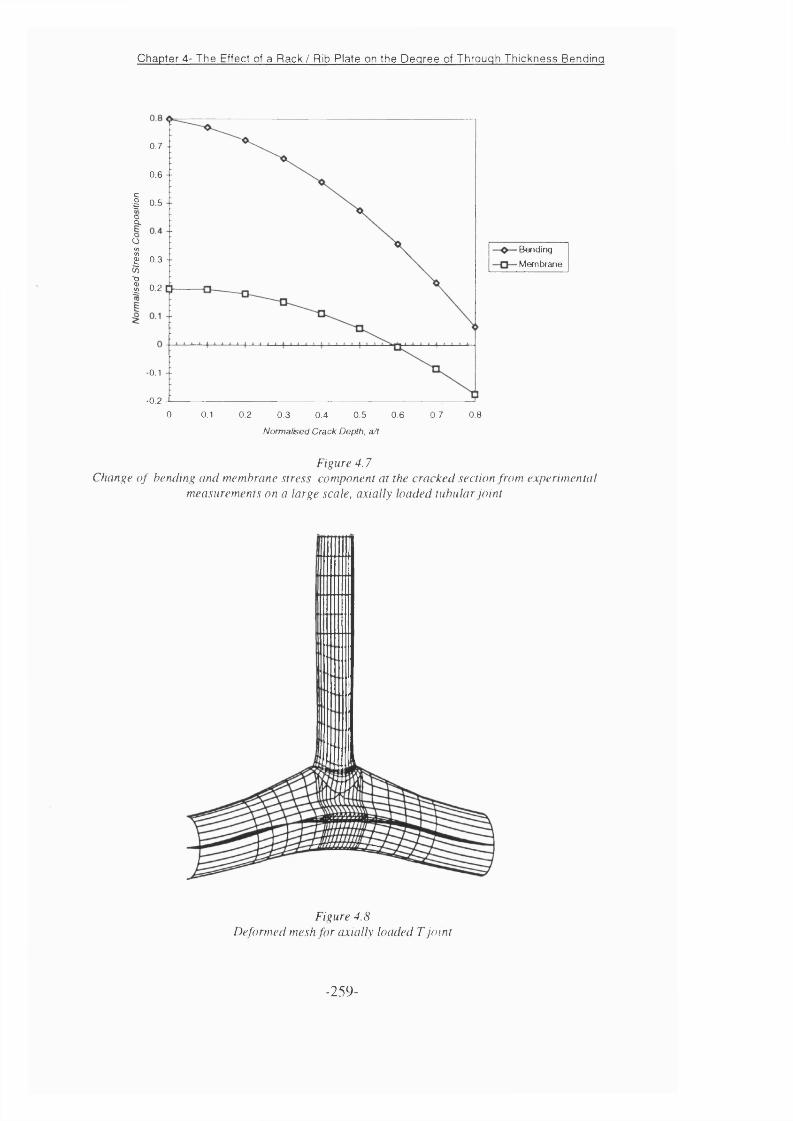
Chapter 4- The Effect of a Rack / Rib Plate on the Degree of Through Thickness Bending
0.7 --
0.6 --
I 0 5a01 0.3 -- CÔI 0.2
-0.1 --
-0.20 0.1 0.2 0.3 0.5 0.7 0.80.4 0.6
■Bending
-Membrane
Normalsed Crack Depth, a/t
F i g u r e 4 .7C h a n g e o f b e n d i n g a n d m e m b r a n e s t r e s s c o m p o n e n t a t t h e c r a c k e d s e c t i o n f r o m e x p e r i m e n t a l
m e a s u r e m e n t s o n a l a r g e s c a l e , a x i a l l y l o a d e d t u b u l a r j o i n t
Figure 4.8Deformed mesh fo r axially loaded T jo in t
-2 5 9 -
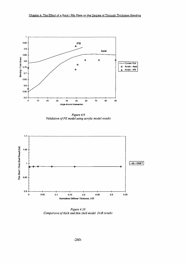
Chapter 4- The Effect of a Rack / Rib Plate on the Degree of Through Thickness Bending
0.95 -- IPB
Axial
0.85 --
0.8 -■
0.75
0.65 - ■
0.6 - -
0.55
0.50 10 7020 80 9030 40 50 60
Ang\e Around Intersection
Current FEAO Acrylic - Axial
A Acrylic - IPB
F i g u r e 4 . 9
V a l i d a t i o n o f F E m o d e l u s i n g a c r y l i c m o d e l r e s u l t s
0.1 0.15 0.2 0.25
NormaSsed Stiffener Tfiickness, tl/D
- Axial T
0.35
Figure 4.10Comparison o f thick and thin shell model D oB results
- 260 -
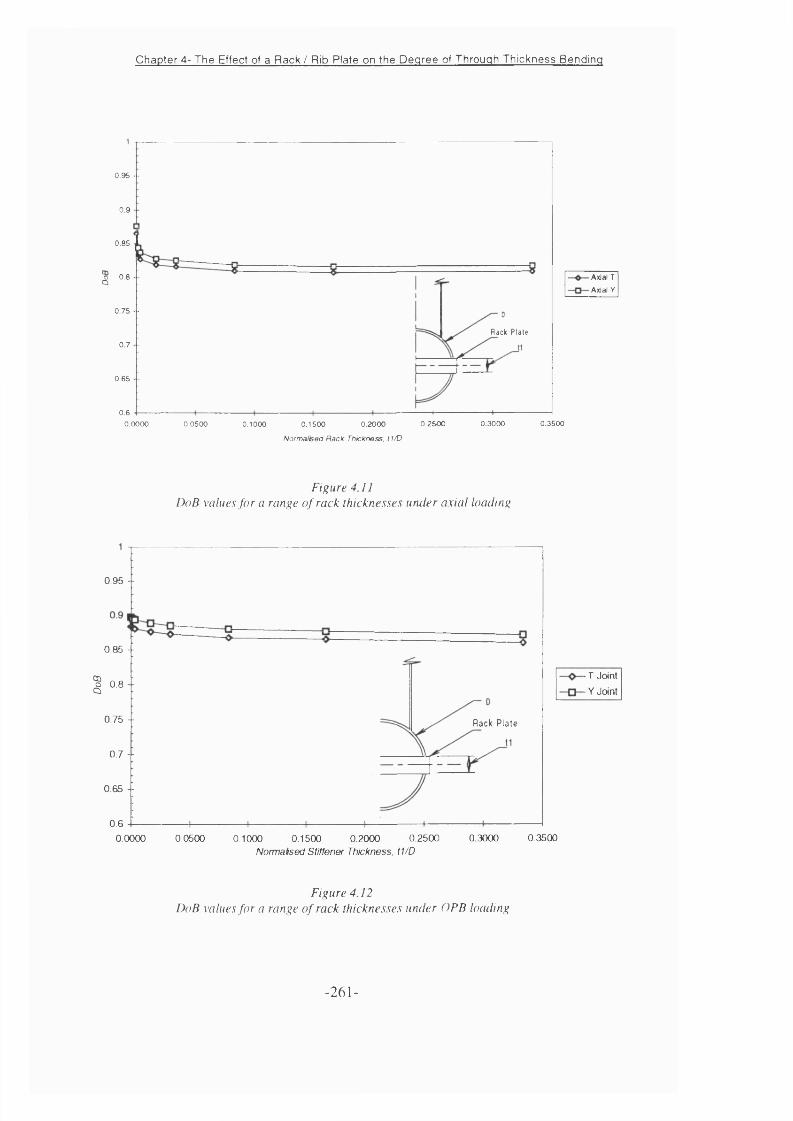
Chapter 4- The Effect of a Rack / Rib Plate on the Degree of Through Thickness Bending
0.95 --
0.9
0.85
Axial T
Axial Y
0.8a
0.75 - ■
Rack Plate
0.7
0.65
0.60.2500 0.3000 0.35000.0000 0.0500 0.1500 0.20000.1000
Normalsed Rack Thickness. 11/D
F i g u r e 4 . 1 1
D o B v a l u e s f o r a r a n g e o f r a c k t h i c k n e s s e s u n d e r a x i a l l o a d i n g
0,0000 0.0500
0.95 --
0.85 --
1 0.8
0.75 -- Rack Plate
0.7 -■
0.65 --
0.60.1000 0.1500 0.2000 0.2500 0 3000 0.3500
Normaised Stiffener Thickness, t1/D
■T Joint
- Y Joint
Figure 4.12DoB values fo r a range o f rack thicknesses under OPB loading
- 261 -
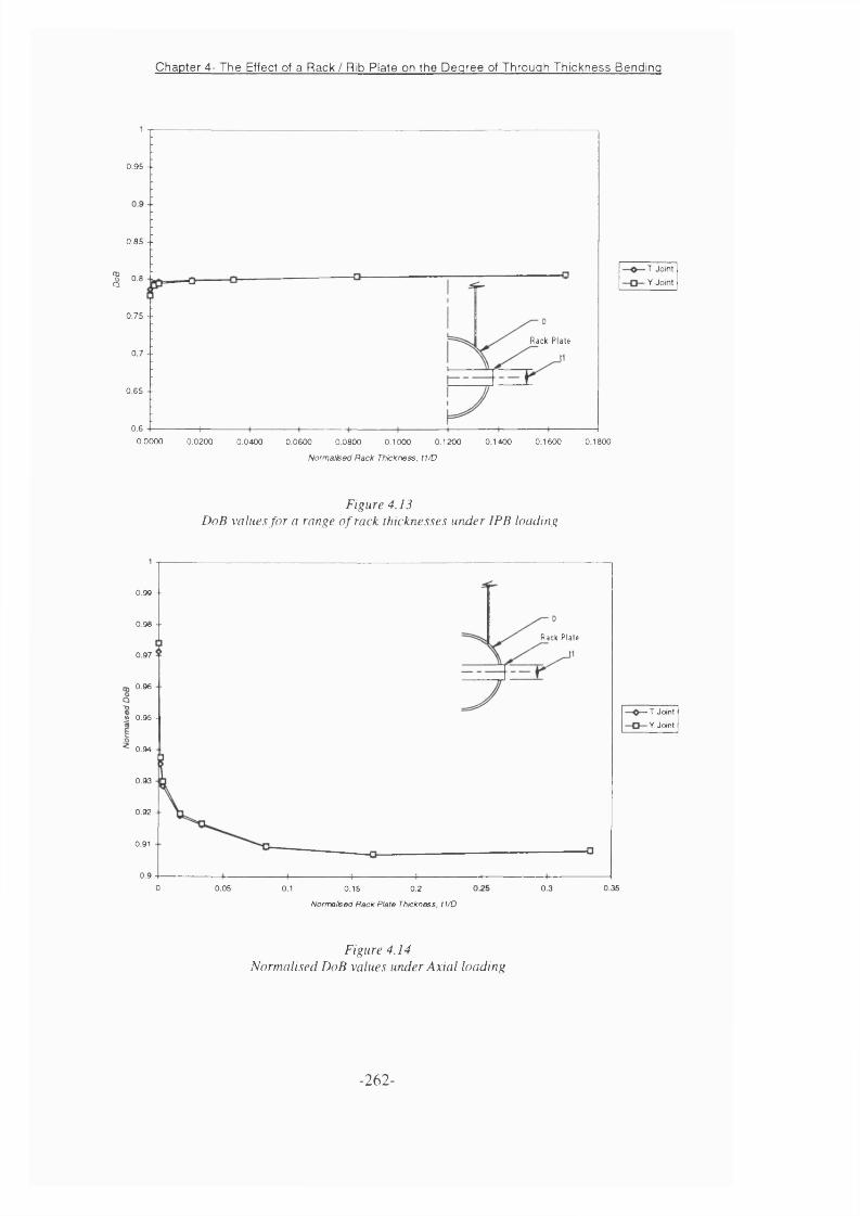
Chapter 4- The Effect of a Rack / Rib Plate on the Degree of Through Thickness Bending
0.95 -
0.85 - •
m 0.8a
0.75 - -
Rack Plate0.7 -
0.65 - -
0.6----0.0000 0.0200 0.1400 0.1600 0.18000.0400 0.0600 0.0800 0.1000 0.1200
-T Joint
- Y Joint
Normaléed Rack Thickness, t l/D
Figure 4.13DoB values fo r a range o f rack thicknesses under IP B loading
0.99 -■
0.98 --
Rack Plate
0.97
0.96
^ 0.95 -
0.94 -
0.93
0.92 -
0.91
0.90 0.05 0.350.1 0.15 0.2 0.3
N orm aisod Rack Plata Thickness, t l /D
Figure 4.14Normalised DoB values under A xia l loading
-T Joint
- Y Joint
- 262-

Chapter 4- The Effect of a Rack / Rib Plate on the Degree of Through Thickness Bending
1.08 ■ -
1.06
1.04 - -
® 1.02 - -
^ 0.98 - -
0 .96 - -
0 .94 ■ -
0 .92 - -
0 .9
0 0.05 0 .2 5 0.3 0.350.1 0.15 0.2
-T Joint
- Y Joint
Normalised Rack Thickness, t l/D
F i g u r e 4 . 1 5
N o r m a l i s e d D o B v a l u e s u n d e r O P B l o a d i n g
0.99
0.98
0.97 ■ -
m 0.96
0.95
0.94
Rack Plate0.93
0.92
0.91 --
0 .9
0 0.16 0.180.02 0.04 0.12 0.140.06 0.08 0.1
- T Joint
-V Joint
Normalised Rack Thickness, tl/D
Figure 4.16Normalised DoB values under IPB loading
- 263-
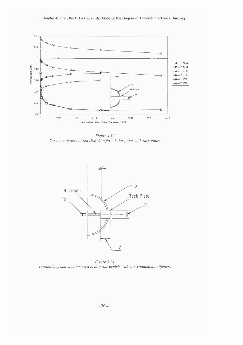
Chapter 4- The Effect of a Rack / Rib Plate on the Degree of Through Thickness Bending
1.04
1.02 - -
0.98 - -
5 0.96
0.94
0.92 --
0 0.05 0.1 0.25 0.3 0.350.15 0.2Normalised Rack Plate Thickness, t1/D
•T Axial
- Y Axial
-T O P S
-Y O P B
■T IPB
Y IPB
F i g u r e 4 . 1 7
S u m m a r y o f n o r m a l i s e d D o B d a t a f o r t u b u l a r j o i n t s w i t h r a c k p l a t e s
Rib Pla teR a c k P la te
F i g u r e 4 . 1 8
T e r m i n o l o g y a n d n o t a t i o n u s e d t o d e s c r i b e m o d e l s w i t h n o n - c o n t i n u o u s s t i f f e n e r s
- 264 -
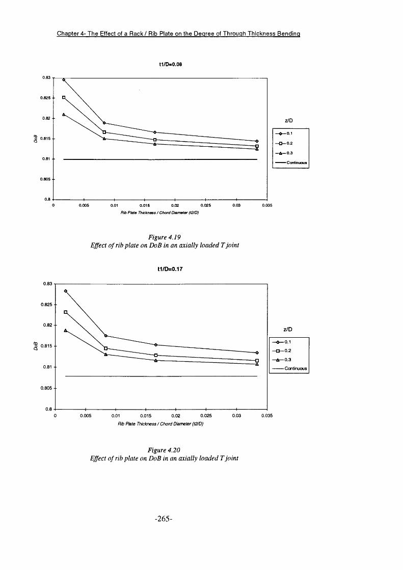
Chapter 4- The Effect of a Rack / Rib Plate on the Degree of Through Thickness Bending
ti/D=o.oa
fl/b Plato Thicknoss / Chord Diarr^ter (t2/D)
F i g u r e 4 . 1 9
E jfe c t o f r i b p l a t e o n D o B i n a n a x i a l l y l o a d e d T j o i n t
t1/D=0.17
0.83
0.825 --
0.82 -- z/D
0.1000.815 --
0.2
0.30.81 -■
Continuous
0.805 ■ -
0.80 0.025 0.03 0.0350.005 0.01 0.015 0.02
0.83
0.825 - -
0.82 - -
o 0.815 --
0.81 --
0.805 ■ -
0.80.005 0.01 0.015 0.02 0.025
Rib Plate Thickness / Chord Diameter (t2/D)
Continuous
0.03 0.035
Figure 4 .20Ejfect o f rib p late on D oB in an ax ially loaded T joint
- 265 -
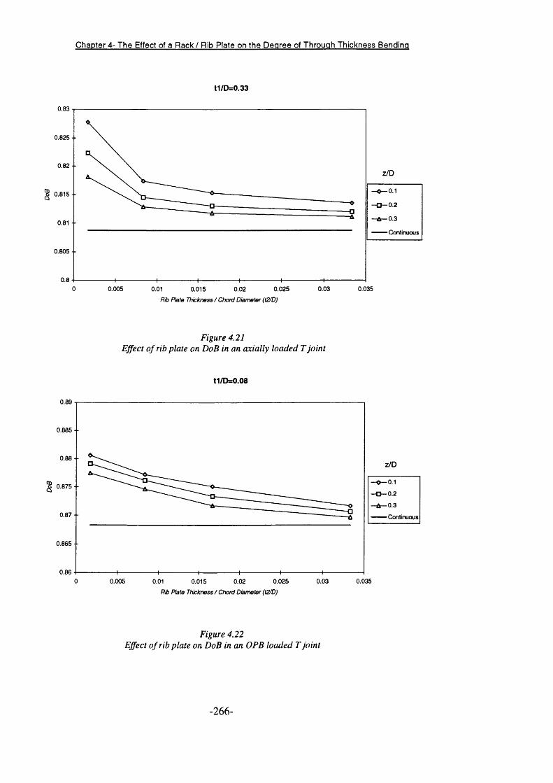
Chapter 4- The Effect of a Rack / Rib Plate on the Degree of Through Thickness Bending
t1/D=0,33
0.83
0.825 --
0.82 --Z/D
0.1o 0.815 "
0.20.3
0.81 --Continuous
0.805 --
0.80.0350 0.005 0.025 0.030.01 0.015 0.02
Rib Plate Thickness / Chord Diameter (t2/D)
F i g u r e 4 . 2 1
E f f e c t o f r i b p l a t e o n D o B i n a n a x i a l l y l o a d e d T j o i n t
t1/D=0.08
Rib Plate Thickness / Chord Diameter (t2/D)
Figure 4.22Effect o f rib p late on DoB in an O PB loaded T Joint
0.89
0.885 ■-
0.8a--Z/D
0.1o 0.875 - -
0.20.3
0.87 - - — ■ " Continuous
0.865 ■ -
0.860.0350 0.005 0.0250.01 0.030.015 0.02
- 266-

Chapter 4- The Effect of a Rack / Rib Plate on the Degree of Through Thickness Bending
t1/D=0.17
Rib Plate Thickness / Chord Diameter (t2/D)
F i g u r e 4 . 2 3
E f f e c t o f r i b p l a t e o n D o B i n a n O P B l o a d e d T j o i n t
t1/D=0.33
Rib Plate Thickness / Chord Dmmeter (t2/D)
Figure 4.24Effect o f rib plate on DoB in an O PB loaded T Joint
0.89
0.885 --
0.88 - -
Z/D
g 0 .875-- 0.20.3
0.87 - - ' Continuous
0.865 - ■
0.860.03 0.0350 0.0250.005 0.01 0.015 0.02
0.89
0.885 --
0.88 --2/00.1
o 0.875 --0.20.3
' Continuous
0.865 --
0.860.0350.025 0.030 0.005 0.020.01 0.015
- 267-
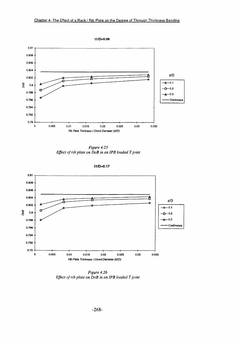
Chapter 4- The Effect of a Rack / Rib Plate on the Degree of Through Thickness Bending
t1/D=0.08
0.810.808 -■
0.806 - -
0.804 --
0.802 -- -O
1 0.8 --
0.798 - ■
0.796 - ■
0.794 - ■
0.792 --
0.790 0.005 0.0250.01 0.015 0.02 0.03 0.035
Z/D
0.10.20.3
— Continuous
Rib Plate Thickness / Chord Diameter (t2/D)
F i g u r e 4 . 2 5
E jfe c t o f r i b p l a t e o n D o B i n a n I P B l o a d e d T J o i n t
t1/D=0.17
0.81
0.808 -■
0.806 --
0.804 - ■Z/D
0.802 -- 0.1S 0.8- 0.2
0.30.798 --
Continuous0.796 --
0.794 - -
0.792 -■
0.790 0.005 0.025 0.030.01 0.015 0.02 0.035
Rb Plate Thickness /Chord Diameter (t2/D)
Figure 4.26Ejfect o f rib p late on DoB in an IP B loaded T jo in t
- 268 -
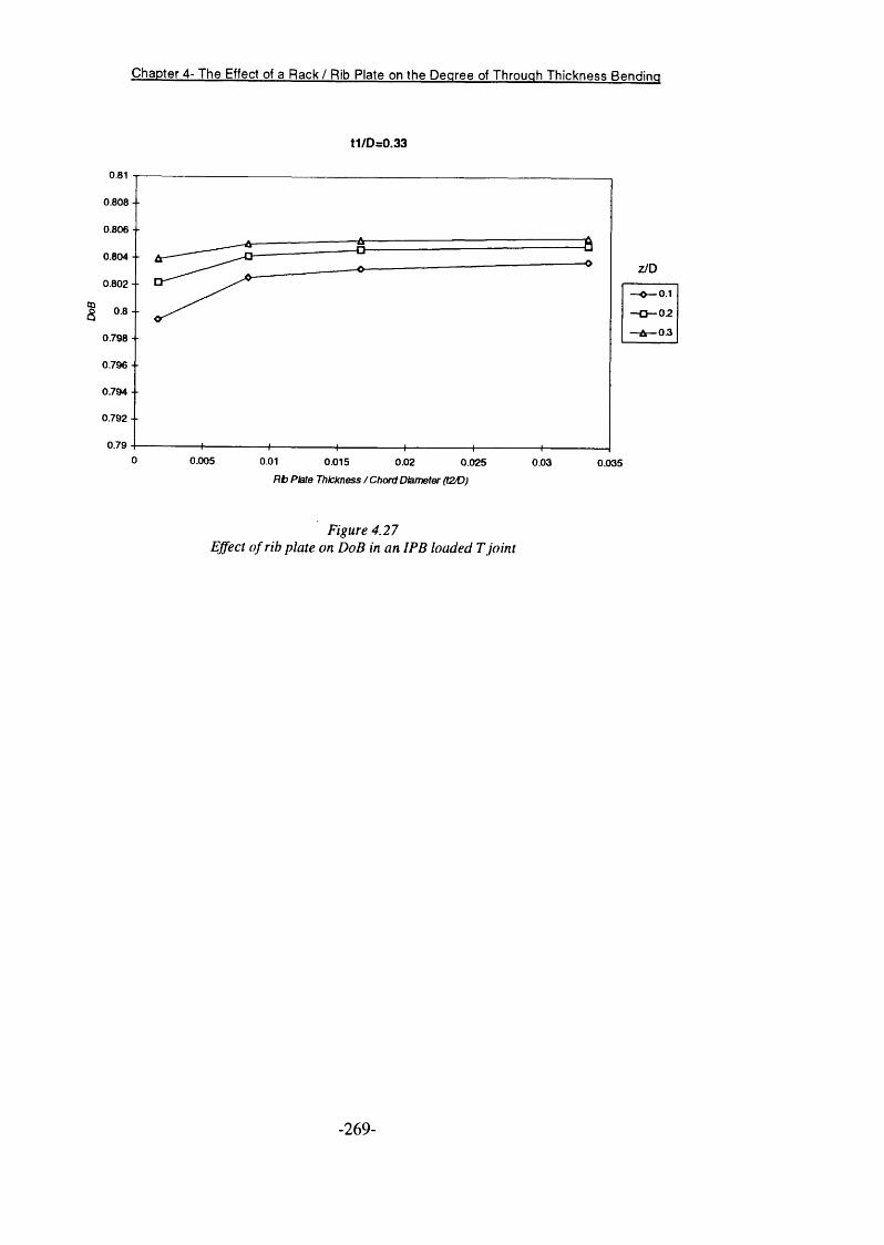
Chapter 4- The Effect of a Rack / Rib Plate on the Degree of Through Thickness Bending
t1/D=0.33
0.81
0.808 - -
0.806 - -
0.804 --Z/D
0.802 -- 0.1020.30.798 - -
0.796 - ■
0.794 - -
0.792 - -
0.790 0.005 0.01 0.015 0.02 0.025 0.03 0.035
R t Plate Thickness / Chord Diameter (t2/D)
F i g u r e 4 . 2 7
E f f e c t o f r i b p l a t e o n D o B i n a n I P B l o a d e d T j o i n t
- 269-
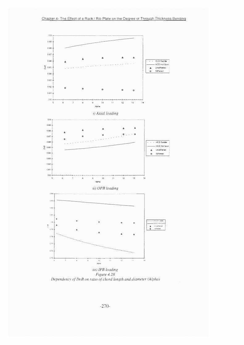
Chapter 4- The Effect of a Rack / Rib Plate on the Degree of Through Thickness Bending
0 87 -
0 8 5Q
0 83 --
0.82
0 81
0 65 6 7 8 9 10 11 12 13 14
Alph*
i ) A x i a l l o a d i n g
0 8 2
0 8 1
5 6 7 14a 9 10 11 12
Alphm
i i ) O P B l o a d i n g
- - - HCO Saddle------------HCO Hot Spot
A UnstifteoedO StiHened
- - - HCO Saddte
-----------HCO Hot Spot
6 Unsltfenad
O Stillaned
s-H(.0 HU
UnshMwiM
H i ) I P B l o a d i n g
F i g u r e 4 . 2 8
D e p e n d e n c y o f D o B o n r a t i o o f c h o r d l e n g t h a n d d i a m e t e r ( A l p h a )
- 270 -

Chapter 4- The Effect of a Rack / Rib Plate on the Degree of Through Thickness Bending
. - -
---------- H(DHrtA IJrml0wiwl O StiMMNNi
i ) A x i a l l o a d i n g
S«la
i i ) O P B l o a d i n g
09 2
0 89
- - - HCO S«ddl»
-------------- HCO Ho( Spot0 88
?
08 5
0 83080 8 0,70 0 1 0 2 0 3 0 4 0 5
0 9
0 8 2
Q
0 7 2
0 80 70 0.1 0 2 0 3 0 4 0 5 0 6
- - - HCOSadde-----------HCO Hot Spot
A UnstxMened O Sifferwd
H i ) I P B l o a d i n g
F i g u r e 4 . 2 9
D e p e n d e n c y o f D o B o n r a t i o o f b r a c e a r u l c h o r d d i a m e t e r s ( B e t a )
- 271 -
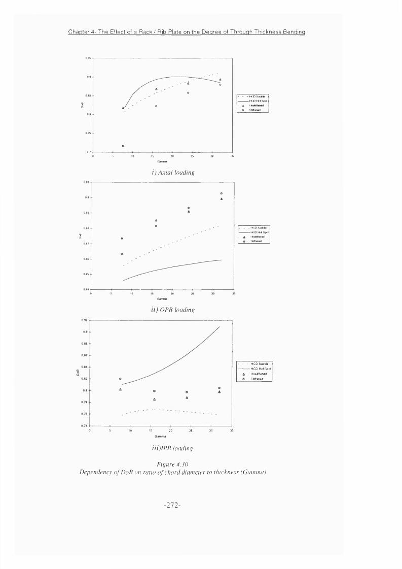
Chapter 4- The Effect of a Rack / Rib Plate on the Degree of Through Thickness Bending
0.75 30 362S
- -
A I
i ) A x i a l l o a d i n g
§
i i ) O P B l o a d i n g
0 92
0 5 10 IS 20 25 30 35
- - - HCO SmddI#
--------------HCO Hot Spot
A Un»tiM#n*d
O SlffiOAd
i i i ) I P B l o a d i n g
F i g u r e 4 . 3 0
D e p e n d e n c y o f D o B o n r a t i o o f c h o r d d i a m e t e r t o t h i c k n e s s ( G a m n u i )
- 272 -
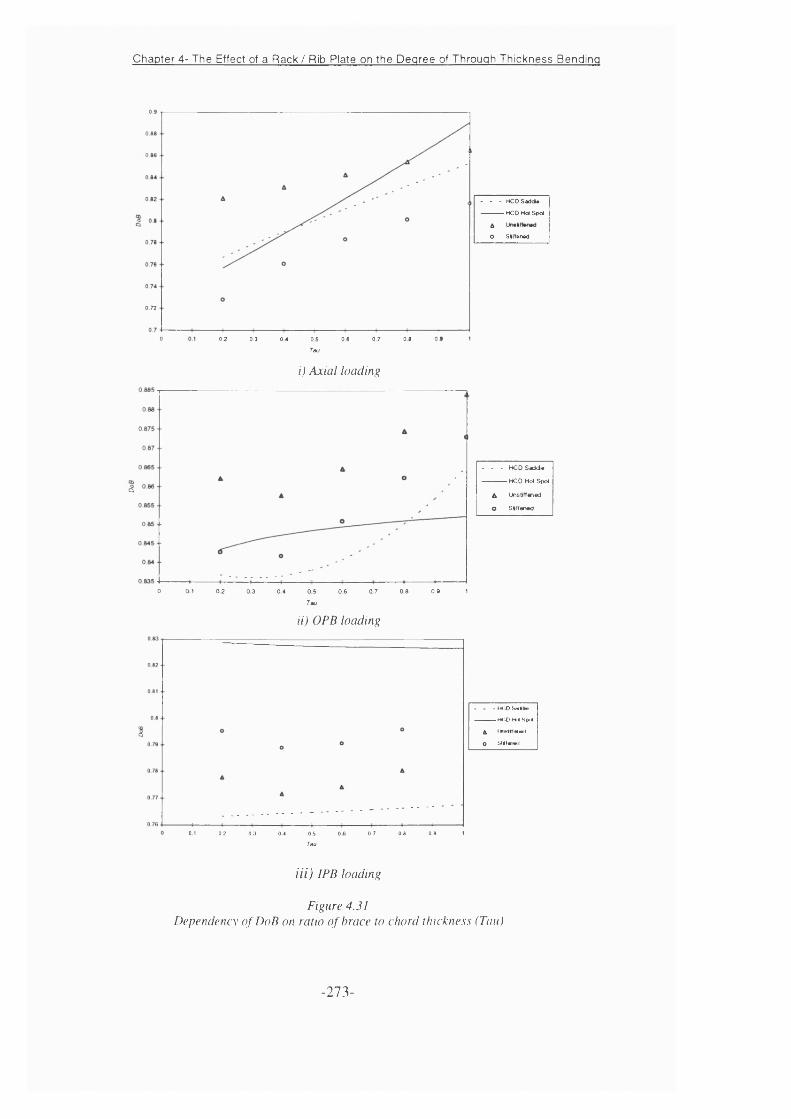
Chapter 4- The Effect of a Rack / Rib Plate on the Degree of Through Thickness Bending
0 7 2
0 0,2 0,3 0 4 0.5 0 6 0 7 0 8
Tau
i ) A x i a l l o a d i n g
Tau
i i ) O P B l o a d i n g
- - - HCO SaddI#
------------- H C O H o*S oo(
AO Siffanad
Q
0 0 1 0 2 0 3 0 4 0 5 0 7 0 8 0 9 10 6
- - - H C O S a d d a
----------- HCO Hotspot
A Unsortened
O S#Maned
. - - HCOSwhk,------------HCX) Hi SjMl
A llimttlMMii
O SI4t«fHNl
0 1 0.2 0.3 0 4 0.5 0 6 0,7 0,6 0 « 1
Tau
H i ) I P B l o a d i n g
F i g u r e 4 . 3 1
D e p e n d e n c y o f D o B o n r a t i o o f b r a c e t o c h o r d t h i c k n e . s . K ( T a u )
- 273-
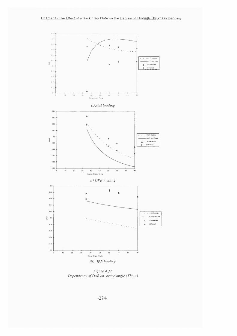
Chapter 4- The Effect of a Rack / Rib Plate on the Degree of Through Thickness Bending
<s
Bm ctA ng tt Thsts
i ) A x i a l l o a d i n g
B itc e Angle. Thetm
i t ) O P B l o a d i n g
0,91
0.87
0,8520 30 50 60
. . -
-------------- H (T > H nl SfMi
4 U iiMrfffV im i
0 78
0.74
0,72
0.720 50
- - HCO
----------HCO Hi4 Spi4
A UriMWIWMMl
o
B rx 0 Angt0. Th»m
H i ) I P B l o a d i n g
F i g u r e 4 . 3 2
D e p e n d e n c y o f D o B o n b r a c e a n g l e ( T h e t a )
- 274 -
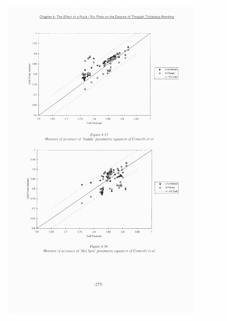
Chapter 4- The Effect of a Rack / Rib Plate on the Degree of Through Thickness Bending
0.95 --
^ 0.85 --I.2 0.8 - -
i !CD
•0
g 0.75 --
0.7 --
0.65 - -
0.60.6 0.65 0.7 0.75 0.85 0.9 0.950.8 1
DoB Predicted
# Unstiffened
O Stiffened
- - - - +/- 5% DoB
F i g u r e 4 . 3 3
M e a s u r e o f a c c u r a c y o f ‘S a d d l e ’ p a r a m e t r i c e q u a t i o n o f C o n n o l l y e t a l
0.95 - -
0.9 --
c 0 .8 5 --
0.65 ■ -
0.65 0.7 0.75 0.8 0.85
DoB Predicted
0.9
* Unstiffened
O Stiffened
- - - - +/- 5% DoB
0.95 1
F i g u r e 4 . 3 4
M e a s u r e o f a c c u r a c y o f ‘ H o t S p o t ’ p a r a m e t r i c e q u a t i o n o f C o n n o l l y e t a l
- 275 -
Chapter 5 - Fracture Mechanics Modelling of Jack Up Chord Defects
Chapter 5
5. Fracture Mechanics Modelling o f Jack Up Chord Defects
5.1 Introduction
Accurate predictions of fatigue crack growth in tubular joints are required for
defects discovered in service. Fatigue cracks found during periodic inspections
must be assessed in order to ensure the structural integrity of the installation is not
compromised. Depending on the outcome of the investigation, remedial action
such as repair grinding, clamping of the joint or simply monitoring of the defect via
more frequent inspections can be implemented.
A number of fracture mechanics models for predicting fatigue crack growth in
tubular welded joints have been published in the literature. A selection of these
models will be presented and assessed here. These will include adapted flat plate,
empirical and analytical (PEA) derived models. The basis and background to each
model will be presented before assessing the accuracy of the models by comparing
the SIP predictions with those derived from the experimental fatigue tests
presented in Chapter Two. Additionally the PEA derived solution of Chong Rhee
et al [5.1] will be evaluated. This model is singled out for separate inspection since
it is to be incorporated as the recommended fracture mechanics solution for welded
tubular T joints in the forthcoming revision of PD6493 [5.2] and the new ISO code
on the Design of Offshore Structures [5.2].
The influence of a rack plate on the stress distribution in jack up chords has been
quantified in Chapters Three and Pour. This information will be integrated into the
models shown to most accurately model the crack growth behaviour from the
experimental study. This should allow an insight in to the manner in which a rack
plate will change the fatigue crack growth behaviour in jack up chords.
276 -
Chapter 5 - Fracture Mechanics Modelling of Jack Up Chord Defects
5.2 Stress Intensity Factors in Tubular Joints
The concept of Stress Intensity Factors being used to characterise the crack tip
stress field and thus fatigue crack growth behaviour was discussed in Section 1.9.
Analytical solutions exist for certain idealised situations. The SIP for an infinite
centre cracked plate under uniform tension as shown in Figure 5.1, is given by
(5.1).
K = a 4 m (5.1)
This is obviously far removed from a semi-elliptical surface crack, in a complex
stress field as found in welded tubular joints. The SIF Modification Factor Y, was
also introduced in Section 1.9 as a means of accounting for effects of geometry
and loading conditions. Additionally Y often varies with crack size.
The Y Factor can be thought of as being the product of several individual factors
each accounting for specific effects. For the case of a tubular joint, the following
corrections are thought to be necessary (5.2).
Y = (5.2)
where
Ys Free surface correction
Yg Non-uniform through thickness stress distribution
Yw Finite plate width correction
Yk Correction for geometrical discontinuity at weld
Yc Crack shape correction factor
Ym Correction for changes in structural restraint
The above breakdown is especially helpful when attempting to adapt Hat plate
based models for cracks in simple stress fields. For empirically derived models.
- 277 -
Chapter 5 - Fracture Mechanics Modelling of Jack Up Chord Defects
each of the above effects is of course, implicitly included via the experimental data
used in the derivation of the model
5.3 Y Factor Predictions Using Empirical Models
A number of models have been developed using Y Factor information derived from
crack growth data generated from fatigue tests on large scale welded tubular joints.
The ability to capture accurate crack depth and shape data using the Alternating
Current Potential Drop Method (ACPD) was demonstrated in Chapter Two. This
information can be manipulated to yield Y Factor information provided that the
da/dN - AK relationship (i.e. C and m Paris Law data) is known for the material to
be tested. Prior to presentation of the development of the empirical models derived
to date, the extraction of Y Factors from crack growth data will be outlined. This
procedure has been applied to the data derived from the expeiimental test
programme presented in Chapter Two and will serve as the basis for the
comparison of the accuracy of each of the models presented in this Chapter.
5.3.1 Extraction of V Factors from Crack Growth Data
By monitoring the crack depth at discrete points along the crack front, the
development of the defect from initiation to through wall penetration can be
captured. The deepest point along the crack front can be determined for each
inspection and this data used to determine the crack growth curve (a versus N).
Using the procedure described in Chapter Two, the experimental crack growth
rates can be determined from the first differential of second order polynomials
fitted around each data point.
With knowledge of the hot spot stress range, Ac, the Paris constants C and m, the
instantaneous crack depth, a, and the experimental crack growth rate (da/dN^xp) at
that point, the experimental Y factor, Ycxp can be determined using (5.3)
- 278 -
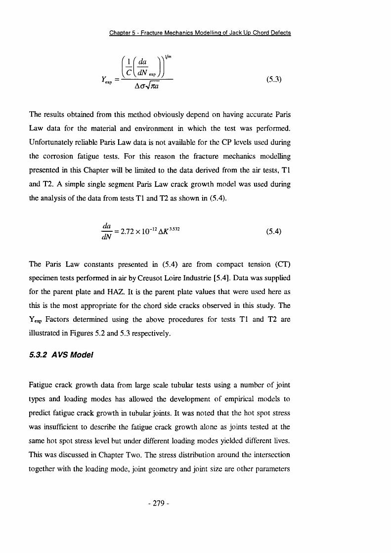
Chapter 5 - Fracture Mechanics Modelling of Jack Up Chord Defects
da
V y j
l/m
n .p = — ^ r - (5 3)
The results obtained from this method obviously depend on having accurate Paris
Law data for the material and environment in which the test was performed.
Unfortunately reliable Paris Law data is not available for the CP levels used during
the corrosion fatigue tests. For this reason the fracture mechanics modelling
presented in this Chapter will be limited to the data derived from the air tests, T1
and T2. A simple single segment Paris Law crack growth model was used during
the analysis of the data from tests T1 and T2 as shown in (5.4).
- ^ = 2.72x 10-‘^AA:” ” (5.4)dN
The Paris Law constants presented in (5.4) are from compact tension (CT)
specimen tests performed in air by Creusot Loire Industrie [5.4]. Data was supplied
for the parent plate and HAZ. It is the parent plate values that were used here as
this is the most appropriate for the chord side cracks observed in this study. The
Ycxp Factors determined using the above procedures for tests T1 and T2 are
illustrated in Figures 5.2 and 5.3 respectively.
5.3.2 AVS Model
Fatigue crack growth data from large scale tubular tests using a number of joint
types and loading modes has allowed the development of empirical models to
predict fatigue crack growth in tubular joints. It was noted that the hot spot stress
was insufficient to describe the fatigue crack growth alone as joints tested at the
same hot spot stress level but under different loading modes yielded different lives.
This was discussed in Chapter Two. The stress distribution around the intersection
together with the loading mode, joint geometry and joint size are other parameters
- 2 79 -

Chapter 5 - Fracture Mechanics Modelling of Jack Up Chord Defects
that also have an effect on joint endurance. The first of these, the stress distribution
around the intersection was considered the most important during the development
of the Average Stress Model (AVS) [5.5]. Central to this model is the average
stress parameter,ASP (5.5).
where
ASP=SCFh /SCFav
SCFh Hot Spot Stress
SCFav Average Stress
(5.5)
and SCFav is given by (5.6) for in plane bending and (5.7) for out of plane bending
and axial loading.
k / 2
SCF^ = - \SCF{<}>)cl(l>^ - f f / 2
(5.6)
where
1 *(5.7)
(j) Angle around intersection
(tc/2 is the saddle position)
Specimen geometry / loading mode combinations resulting in average stress
parameters between 1.18 and 2.22 were used during the development of the model.
The Y factor is given by (5.8).
Y = A
where
A = 0.73-0.18ASP
(5.8)
(5.9)
- 2 8 0 -
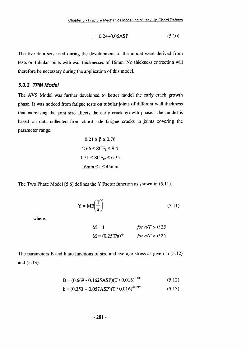
Chapter 5 - Fracture Mechanics Modelling of Jack Up Chord Defects
j=0.24+0.06ASP (5.10)
The five data sets used during the development of the model were derived from
tests on tubular joints with wall thicknesses of 16mm. No thickness correction will
therefore be necessary during the application of this model.
5.3.3 TPM Model
The AVS Model was further developed to better model the early crack growth
phase. It was noticed from fatigue tests on tubular joints of different wall thickness
that increasing the joint size affects the early crack growth phase. The model is
based on data collected from chord side fatigue cracks in joints covering the
parameter range:
0.21 <P <0.76
2.66 < SCFh < 9.4
1.51 < SCFav <6.35
16mm < t < 45mm
The Two Phase Model [5.6] defines the Y Factor function as shown in (5.11).
Y = MBrji Me
(5.11)
where;
M = 1 for a/T > 0.25
M = (0.25T/a)-^ for aTT < 0.25.
The parameters B and k are functions of size and average stress as given in (5.12)
and (5.13).
B = (0.669 - 0.1625ASPKT/0,016)""" (5.12)
k = (0.353 + 0.057ASP)(T / 0.016)’"''” (5.13)
281
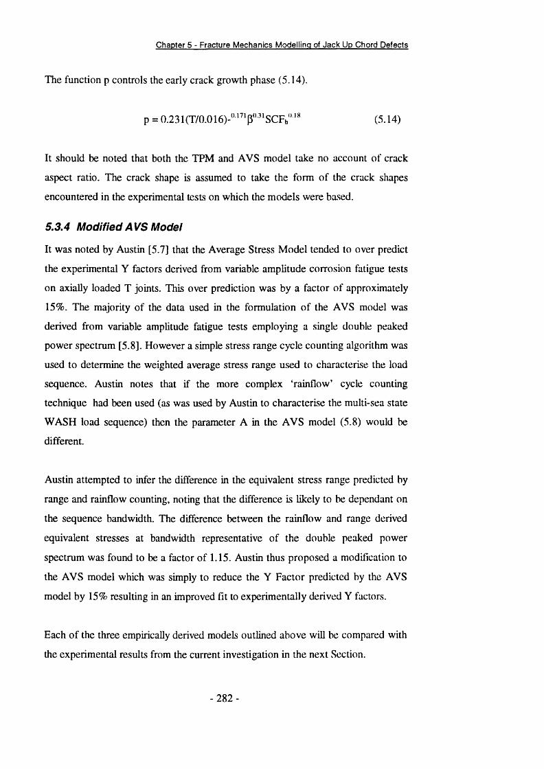
Chapter 5 - Fracture Mechanics Modelling of Jack Up Chord Defects
The function p controls the early crack growth phase (5.14).
p = 0.231(1/0.016)-'’ ‘’ 'P“ ‘SCFb‘” * (5.14)
It should be noted that both the TPM and AVS model take no account of crack
aspect ratio. The crack shape is assumed to take the form of the crack shapes
encountered in the experimental tests on which the models were based.
5 .3.4 Modified A VS Model
It was noted by Austin [5.7] that the Average Stress Model tended to over predict
the experimental Y factors derived from variable amplitude corrosion fatigue tests
on axially loaded T joints. This over prediction was by a factor of approximately
15%. The majority of the data used in the formulation of the AVS model was
derived from variable amplitude fatigue tests employing a single double peaked
power spectrum [5.8]. However a simple stress range cycle counting algorithm was
used to determine the weighted average stress range used to characterise the load
sequence. Austin notes that if the more complex ‘rainflow’ cycle counting
technique had been used (as was used by Austin to characterise the multi-sea state
WASH load sequence) then the parameter A in the AVS model (5.8) would be
different.
Austin attempted to infer the difference in the equivalent stress range predicted by
range and rainflow counting, noting that the difference is likely to be dependant on
the sequence bandwidth. The difference between the rainflow and range derived
equivalent stresses at bandwidth representative of the double peaked power
spectrum was found to be a factor of 1.15. Austin thus proposed a modification to
the AVS model which was simply to reduce the Y Factor predicted by the AVS
model by 15% resulting in an improved fit to experimentally derived Y factors.
Each of the three empirically derived models outlined above will be compared with
the experimental results from the current investigation in the next Section.
2 8 2 -

Chapter 5 - Fracture Mechanics Modelling of Jack Up Chord Defects
5.3.5 Evaluation of Experimentally Derived Models
The AVS, TPM and modified AVS models are plotted in Figures 5.4 and 5.5
where they are compared with the experimentally derived Y Factors from Tests T1
and T2. Although the TPM is the most sophisticated of the empirical models it is
clearly seen to poorly model the early crack growth region (a/t <0.25), under
predicting the Y Factors significantly. This is perhaps surprising as this was the
region where the TPM model was supposed to offer improved modelling of the
thickness effect. Both of the AVS models offer improved correlation with the
experimental results, predicting the shape of the curve very well. In particular the
Modified AVS model is seen to perform particularly well providing an excellent fit
to Ycxp for both tests at all crack depths.
This suggests that the difference between the AVS model and the experimental
results of Austin [5.7] was a geometry effect rather than an artefact of cycle
counting method. The geometry tested by Austin was identical to that used during
this investigation however constant amplitude loading was used in this case. This
discounts the possibility of using variable amplitude based arguments to explain the
difference. It is therefore suggested that the argument used by Austin to justify the
factor applied to the AVS model, whilst valid, is not the sole or even dominant
source of the error. However regardless of the source of the error the quality of the
fit appears to provide a good basis for accurate fracture mechanics crack growth
predictions for the test geometry. However this observation is specific to the
geometry under consideration here.
The second comment that arises from the close agreement of the model and the
experimental based results concerns the Paris Law data used in the derivation of
the Yexp factors from the crack depth information. Greater confidence can now be
placed in these values which were derived from simple specimen tests. This crack
growth model was used for all fatigue crack growth modelling presented in this
Chapter.
- 283 -

Chapter 5 - Fracture Mechanics Modelling of Jack Up Chord Defects
5.3.6 Fatigue Crack Growth Predictions
The AVS models have been shown to provide an excellent fit to the experimental
data. Thus the AVS and Modified AVS models have been chosen as the basis for
the fatigue crack growth predictions presented in this Section.
The procedure used for the crack growth predictions was as follows:
1) The crack depth range under consideration was divided into 250 linear
intervals. Logarithmic intervals were also used initially for comparison
purposes, however the differences in resulting lifetimes was negligible.
2) The value of AK at the beginning and end of each interval was calculated and
the average was used as the representative SIF for the interval. The SIF values
were calculated using the appropriate Y Factor Model.
3) The average crack growth rate for the interval was calculated from the
representative SIF range according to (5.4)
4) The number of cycles required to propagate the crack across the interval, from
ai-i to ai was calculated according to (5.15)
5) The total number of cycles required to propagate a crack to a given depth a,
from an initial depth ao is given by (5.16).
TV, = %ATV, (5.16)
- 2 8 4 -
Chapter 5 - Fracture Mechanics Modelling of Jack U p Chord Defects
The initial crack size used in these calculations was 0.1mm. A survey of the
hterature reveals much attention has been placed on the initial crack size to be used
in fracture mechanics models. Such judgements are usually based on the sizes of
the weld toe defects inherent to untreated welded joints. However in this instance
the procedure is simple as the intention is to model the crack propagation period
found in the tubular joint tests. The ACPD results presented in Chapter two
showed the technique to be able to reliably detect and size defects smaller than
0.1mm. A depth of 0.1mm was set as the criteria for determining the initiation life
for each test. For this reason the summation of the number of cycles used during
each crack growth interval was commenced at the measured initiation life (Ni)
rather than zero. The initial crack depth was set as 0.1mm.
The results of the crack growth modelling using the AVS and modified AVS
models are shown in Figures 5.6 and 5.7. Despite the excellent fit of the models to
the experimentally derived Y Factors, both models under predict fatigue crack
growth hves. The improved fit of the modified AVS over the AVS model results in
more accurate predictions, however they are still a significant underestimation of
the experimental lives. The above applies equally well to both tests T1 and T2.
A simple power law was fitted to the Yexp results from both tests. The equation
was of the form used by the AVS model (5.8) as shown in Figures 5.8 and 5.9.
Although the co-efficients A and j are only slightly different to those predicted by
the AVS model the resulting crack growth predictions are much improved as
shown in Figures 5.6 and 5.7.
5.4 Finite Element Based Models
The finite element based SIF solution of Chong Rhee et al [5.1] provides a fracture
mechanics model for tubular T joints under axial, IPB and OPB loads. The solution
was based on 40 finite element models of cracked tubular T joints. The intersection
between the brace and chord was modelled using 20 node isoparametric elements
285 -
Chapter 5 - Fracture Mechanics Modelling of Jack Up Chord Defects
and 8 noded thick shell elements formed the remainder of the joint. The crack was
modelled using collapsed quarter point elements. The model has been
recommended for inclusion in the revised BS PD6493 [5.9] and for the new ISO
code for fixed steel offshore structures [5.10]. The model is said to be valid over
the following range of joint size and crack shape parameters.
a=12
0.40< P < 0.80
1 0 . 0 < y < 2 0 . 0
0 .3 < t< 1.0
0.05 < a/t < 0.80
0.5 <3c/d< 1.20
where a is the crack depth, c is the crack half length and d is the brace
diameter
The chord length parameter (a) was set at 12 which was assumed sufficient to
neglect the boundary effect of the chord. Apart from the chord length / diameter
ratio (a), all other criteria are met by the tubular T joint fatigue tests described in
Chapter Two. This makes the Yexp factors derived from these tests ideal for
assessing the accuracy of this model.
The stress intensity factors for the deepest point along the crack front for a tubular
T joint under axial loading is given by (5.17)
(5.17)
where
Yg is the joint geometry factor
Yi is a crack size factor
Ys is a joint and crack coupling factor
- 2 8 6 -
Chapter 5 - Fracture Mechanics Modelling of Jack Up Chord Defects
On is the brace nominal stress
The stress intensity factors are given as equivalent SIF’s, where K<; is defmed as
(5.18)
and Y — Q 2 *7 ^ Ç ^ “®-^225-1.26851n/î^ 1.3191-0.1661 In T ^ l .6621+0.37041n ^
_ j^0.3562M-0.0956C^0.0983A+0.2298C+0.0817C^ ^-0.0762i4
y, = (a / tYi'ic I d)'
p = -0.8669 - 0.2198A - 0.0162A^ - 0.4750C^ - 0.1667C’ - 0.01930"
r = 0.0777+1.0531A + 0i820A^ + 0.0810A’ - 0.7001C-0.0604C^ +0.0060C’
A = ln
C = In
{ - K t)
Using the crack shape data measured in Tests T1 and T2, Y Factors have been
calculated using this solution and are compared to the Yexp factors in Figures 5.10
and 5.11. The Stress Intensity Factors predicted by this model are clearly over
conservative in both cases. The sensitivity of the fatigue life predictions to SIF
input data has been demonstrated by performing fatigue crack life integrations
based on the AVS model in the previous section. Even the excellent fit of the AVS
model produced crack propagation lives shorter than the experimental life by a
factor of two or more. It seems unlikely therefore that this model will help produce
accurate predictions of fatigue crack growth in cracked tubular T joints.
-287 -
Chapter 5 - Fracture Mechanics Modelling of Jack Up Chord Defects
Furthermore it can be seen that the vahdity range of the model in terms of crack
depth is severely restricted in Test T2. This is due to the fact that the crack shape
development was different in the second test, with the crack surface length tending
to be slightly longer. This results in the situation where the restriction on the
surface crack length parameter (3c/d) is violated for crack depths deeper than
approximately 10mm.
From this limited investigation into the capability of these equations to accurately
model the crack growth behaviour in tubular T joints, it seems difficult to
understand the reasons for their future inclusion in influential standards. From the
evidence presented here they are unlikely to provide more than a very conservative
estimate of the crack growth behaviour across a limited range of crack depths. It is
suggested that such a function could be equally well performed by a fiat plate based
model such as Newman Raju as presented in the next Section.
5.5 Flat Plate Derived Models
Models have been developed to calculate the SIF for semi-elliptical surface cracks
in flat plates under tension and bending loads. The most widely used of these
models include the equations derived by Holdbrook and Dover [5.11] and Newman
and Raju [5.17]. The Newman-Raju equations were utilised by Monahan [5.12] to
develop a fracture mechanics model to predict the early fatigue crack growth
behaviour in tubular X and more complex multi-brace tubular joints. The Newman
Raju equations and the modifications implemented by Monahan will be presented,
assessed, and modified here.
5.5.1 Newman-Raju Equations
The Newman-Raju equations were developed using the results of a 3-D finite
element analysis of semi-elliptical cracks in an elastic fiat plate. For cracks with
very low aspect ratios, edge cracked plate FEA data were also included during the
development of the equations. The resulting equation takes the form of Eqn (5.19)
and accounts for both tensile and bending loads.
288

Chapter 5 - Fracture Mechanics Modelling of Jack Up Chord Defects
(5.19)
The equations are valid in the range
0<a/c< 1.0
c/b < 0.5
0<(j)<7:
where (|) is the parametric angle around the crack front as illustrated in Figure 5.12.
In this instance, only the SIF at the deepest point of the defect is of interest (i.e. (j)
= 7c/2). The SIF at this point is given by (5.20)
CD(5.20)
where F™ is the boundary correction factor for membrane (tension) loading, as
given by (5.21)
where
= / .
M , =1.13-0.093
0.89M ,- - 0 .5 4 + o 2 + ( « / c)
M , = 0 .5 -1.0
0.65 + [a! c)
and/w is a finite width correction factor
+ 14V c j
(5.21)
(5.22)
(5.23)
(5.24)
289

Chapter 5 - Fracture Mechanics Modelling of Jack Up Chord Defects
/w = secnc a2b \7
1/2
(5.25)
In this case the plate half width was assumed to be one half of the brace diameter.
In all cases yw was less than 1.25. The boundary correction factor for bending is
given by (5.26)
where
H = l + G , - + G J -t j
G, = -1 .22 -0 .21
G2 = 0 .5 5 -1 .0 5 |-
VC
+ 0.47<c
(5.26)
(5.27)
(5.28)
(5.29)
The shape factor >, is a complete elliptical integral of the second kind, an
approximation to which is given by (5.30).
0 = J l+ 1.464\ c j
(5.30)
The Y Factor given by the Newman Raju equation is therefore given by (5.31)
F^{\ — DoB) + FfjDoB 0 (5.31)
where DoB is the degree of through thickness bending (Le. bending to total stress
ratio).
The Y Factors (Y n & r ) predicted using this model are shown in Figures 5.13 and
5.14 for tests T1 and T2. The experimentally measured crack shape (a/c) was used
-290
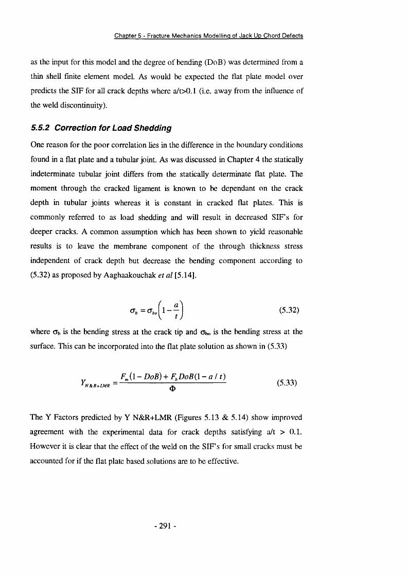
Chapter 5 - Fracture Mechanics Modelling of Jack Up Chord Defects
as the input for this model and the degree of bending (DoB) was determined from a
thin shell finite element model. As would be expected the flat plate model over
predicts the SIF for all crack depths where a/t>0.1 (i.e. away from the influence of
the weld discontinuity).
5.5.2 Correction for Load Shedding
One reason for the poor correlation lies in the difference in the boundary conditions
found in a flat plate and a tubular joint. As was discussed in Chapter 4 the statically
indeterminate tubular joint differs from the statically determinate flat plate. The
moment through the cracked ligament is known to be dependant on the crack
depth in tubular joints whereas it is constant in cracked flat plates. This is
commonly referred to as load shedding and will result in decreased SIF’s for
deeper cracks. A common assumption which has been shown to yield reasonable
results is to leave the membrane component of the through thickness stress
independent of crack depth but decrease the bending component according to
(5.32) as proposed by Aaghaakouchak et a/ [5.14].
Cr. =<T;bo 1-----tJ
(5.32)
where Ch is the bending stress at the crack tip and Cho is the bending stress at the
surface. This can be incorporated into the flat plate solution as shown in (5.33)
F ^ ( l-D o B )+ F i^ D o B il-a / t)^ N & R +IM R ~ 0
The Y Factors predicted by Y N&R+LMR (Figures 5.13 & 5.14) show improved
agreement with the experimental data for crack depths satisfying a/t > 0.1.
However it is clear that the effect of the weld on the SIF’s for small cracks must be
accounted for if the flat plate based solutions are to be effective.
291
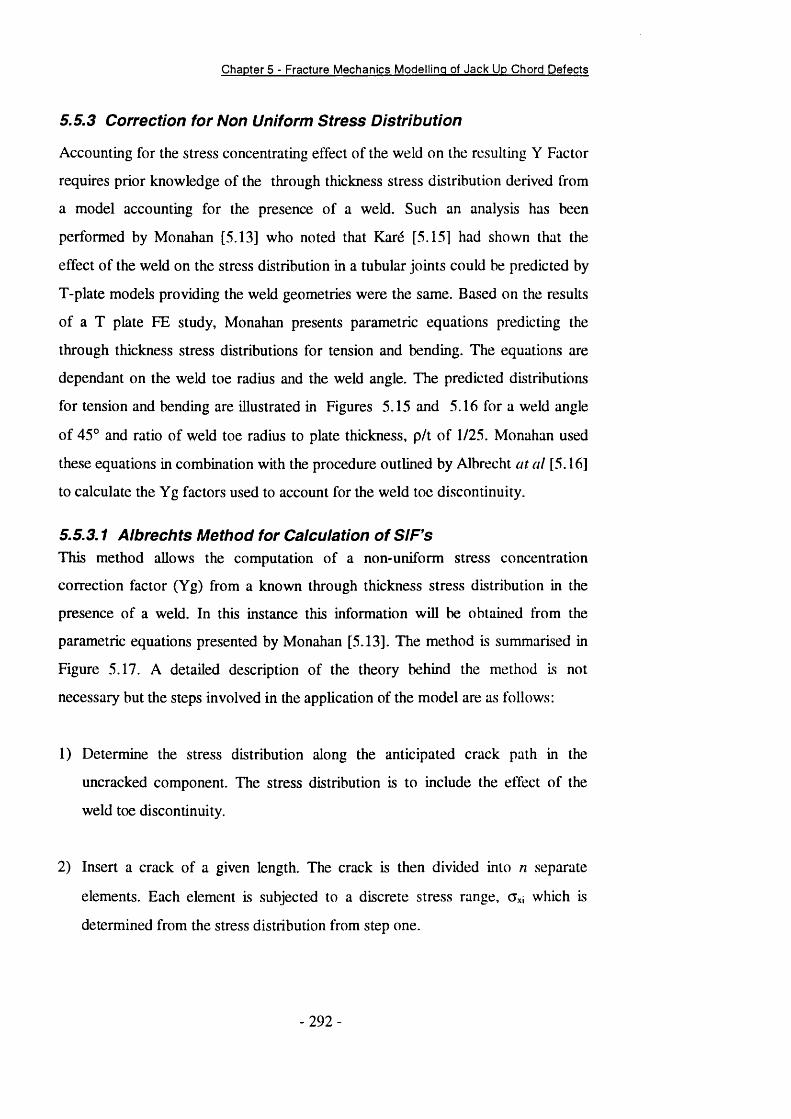
Chapter 5 - Fracture Mechanics Modelling of Jack Up Chord Defects
5.5.3 Correction for Non Uniform Stress Distribution
Accounting for the stress concentrating effect of the weld on the resulting Y Factor
requires prior knowledge of the through thickness stress distribution derived from
a model accounting for the presence of a weld. Such an analysis has been
performed by Monahan [5.13] who noted that Karé [5.15] had shown that the
effect of the weld on the stress distribution in a tubular joints could be predicted by
T-plate models providing the weld geometries were the same. Based on the results
of a T plate FE study, Monahan presents parametric equations predicting the
through thickness stress distributions for tension and bending. The equations are
dependant on the weld toe radius and the weld angle. The predicted distributions
for tension and bending are illustrated in Figures 5.15 and 5.16 for a weld angle
of 45° and ratio of weld toe radius to plate thickness, p/t of 1/25. Monahan used
these equations in combination with the procedure outlined by Albrecht at a I [5.16]
to calculate the Yg factors used to account for the weld toe discontinuity.
5.5.3.1 Aibrectits Method for Calculation of SIF'sThis method allows the computation of a non-uniform stress concentration
correction factor (Yg) from a known through thickness stress distribution in the
presence of a weld. In this instance this information will be obtained from the
parametric equations presented by Monahan [5.13]. The method is summarised in
Figure 5.17. A detailed description of the theory behind the method is not
necessary but the steps involved in the application of the model are as follows:
1) Determine the stress distribution along the anticipated crack path in the
uncracked component. The stress distribution is to include the effect of the
weld toe discontinuity.
2) Insert a crack of a given length. The crack is then divided into n separate
elements. Each element is subjected to a discrete stress range, Gxi which is
determined from the stress distribution from step one.
292 -
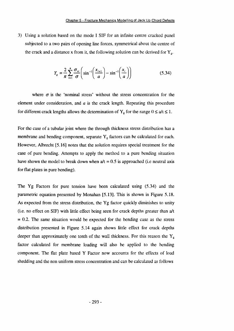
Chapter 5 - Fracture Mechanics Modelling of Jack Up Chord Defects
3) Using a solution based on the mode I SIF for an infinite centre cracked panel
subjected to a two pairs of opening line forces, symmetrical about the centre of
the crack and a distance x from it, the following solution can be derived for Yg.
• -1 SinX
'■+1 -1- smX :
(5.34)
where cr is the ‘nominal stress’ without the stress concentration for the
element under consideration, and a is the crack length. Repeating this procedure
for different crack lengths allows the determination of Yg for the range 0 < a/t < 1.
For the case of a tubular joint where the through thickness stress distribution has a
membrane and bending component, separate Yg factors can be calculated for each.
However, Albrecht [5.16] notes that the solution requires special treatment for the
case of pure bending. Attempts to apply the method to a pure bending situation
have shown the model to break down when a/t = 0.5 is approached (i.e neutral axis
for flat plates in pure bending).
The Yg Factors for pure tension have been calculated using (5.34) and the
parametric equation presented by Monahan [5.13]. This is shown in Figure 5.18.
As expected from the stress distribution, the Yg factor quickly diminishes to unity
(i.e. no effect on SIF) with little effect being seen for crack depths greater than a/t
= 0.2. The same situation would be expected for the bending case as the stress
distribution presented in Figure 5.14 again shows little effect for crack depths
deeper than approximately one tenth of the wall thickness. For this reason the Yg
factor calculated for membrane loading will also be applied to the bending
component. The flat plate based Y Factor now accounts for the effects of load
shedding and the non uniform stress concentration and can be calculated as follows
- 293 -

Chapter 5 - Fracture Mechanics Modelling of Jack Up Chord Defects
„ F j J \ - D o B ) + F J ^ „ D o B ( \ - a l t )^ N & R + L M R + N S C ~ ^ ( j . O j )
where Ygm is the Yg factor for membrane loading as shown in Figure 5.15.
The above assumption appears reasonable as the agreement with experimental Y
Factors is now much improved in the early crack growth region (a/t < 0.2) and
models the shape of the Y Factor curve for Tests T1 and T2 well.
5.5.4 Crack Shape Correction
Monahan [5.13] suggests the use of one final correction factor to account for
differences in crack shape. The suggested form of the correction factor is
Y = — ------- (5.36)^ N A R + N S C + I M R
Plotting Y against the crack shape (a/c) for Tests T1 and T2 in Figure 5.19 shows
some correlation. The approximation to this behaviour derived by Monahan has
been modified to better suit the current data set and is included in Figure 5.19. The
Shape Correction Factor is given by
y/ = 0.9 for a/2c < 0.05 (5.37)
¥ = l + 0.7(fl/2c-0.04) 0.4 - 0.1 for a/2c>0.05 (5.38)
The flat plate based Y Factor accounting for the non linear stress distribution,
linear moment release and crack shape is given by
(1 - DoB) + FJ^„DoB(\
0y — ____________ _^ N & .R + L M R + N S C + C S C ~ ^
294
Chapter 5 - Fracture Mechanics Modelling of Jack Up Chord Defects
This model is shown to accurately predict the Y factors determined experimentally.
It offers advantages over the empirically derived models in that it allows more
control over the input parameters than the AVS based models. This includes the
degree of through thickness bending, crack shape, effect of the weld and moment
redistribution. This flexibihty is important when attempting to model jack up chord
cracks where the stress distribution is known to be different and thus factors such
as crack shape may well be altered compared to unstiffened tubular joints.
5.6 Effect of Rack Plate on Fatigue Crack Growth Predictions
The rack plate has been shown in Chapter 3 and 4 to alter the stress distribution in
two ways for axially loaded T joints. Firstly, a significantly flatter stress distribution
around the outside surface of the intersection results in lower hot spot SCF’s. The
magnitude of the reduction depends on the joint geometry but can be of the order
of 50%. Secondly, a smaller effect on the degree of through thickness bending
(DoB) has been identified. The tendency is for a shght decrease in DoB (i.e.
increased membrane component) although the change is limited to a few percent.
The effect of the changed surface stress distribution on the resulting crack
propagation life can be investigated using the AVS model and its derivative. This
model cannot however take any account of the altered through thickness stress
distribution or any resulting change in crack shape. The AVS model has been
applied to an axially loaded T joint with a number of different stiffener thicknesses.
The tubular joint geometry investigated is that presented in Figure 3.17 of Chapter
3. Rack plate thicknesses of 1, 2, 10 , 20 , and 50mm were examined. Using the
intersection stress distribution determined from the finite element model results the
Average Stress Parameter (5.5) for each stiffener thickness was calculated. The
calculated ASP values for each stiffener are given in Table 5.1. Using these, the
fatigue propagation lives for each of the joints has been calculated using the AVS
and modified AVS models. A hot spot stress range of 400MPa was applied to the
unstiffened joint. The hot spot stress concentration factor was used to calculate the
nominal stress. This nominal stress was then apphed to each of the stiffened models
- 295 -
Chapter 5 - Fracture Mechanics Modelling of Jack Up Chord Defects
and the hot spot stress calculated accordingly. The crack growth results are
illustrated in Figure 5.20 for the AVS model and Figure 5.21 for the modified AVS
model. The results show the logarithmic dependency on hot spot stress as would be
expected. The factor by which the crack propagation lives are changed due to the
rack plate is shown in Figure 5.22. The propagation lives are shown normalised to
the life for the unstiffened joint. This curve is obviously independent of whether the
AVS or modified AVS models are used in its formulation. This analysis of course
takes no account of changes in initiation life due to the lower intersection stresses
and assumes the crack shape found in the experimental data on which it is based.
The Newman Raju based model of Monahan was described in Section 5.5. This
Model was adapted to better model the experimental data from the current test
series. The flexibility of this model in terms of control over the input data makes it
ideal for modelling defects in jack up chords. Factors such as crack shape
development and load shedding characteristics of cracks in jack up chords are
likely to be different to unstiffened tubulars. Unfortunately experimental data
covering the above areas is not currently available for input into the model. In the
absence of this the effects of the known variations in stress distribution were tested
using crack shape and load shedding data derived from unstiffened tubulars. The
Linear Moment Release method described in Section 5.5.2 was used to account for
load shedding. Crack shape development was assumed to be the same as the
experimental investigation presented in Chapter 2. Figure 5.23 shows the fatigue
crack half length c, plotted against the crack depth at the deepest point, a, from
tests T1 and T2. A third order polynomial has been fitted to this data as shown on
the chart. Crack shape development will follow this trend in all Newman Raju
based modelling presented here. The uncertainties discussed above combined with
the demonstrated sensitivity of fatigue life predictions to SIF accuracy combine to
dictate that the results of any analysis presented here are subject to significant
error. However the model can still be utilised to demonstrate the relative
importance of the beneficial surface SCF changes and the onerous reduction in
DoB for tubulars with rack plates.
-296

Chapter 5 - Fracture Mechanics Modelling of Jack Up Chord Defects
Firstly, the analysis presented above using the AVS models has been repeated using
the Newman Raju based model ( Y n & r + l m r + n s c 4C s c ) . The degree of bending
remained unchanged for each stiffener thickness and was equal to that of the
unstiffened model This was done since the DoB cannot be controlled in the AVS
models and since the model was based on the experimental results of unstilïened
joints the unstiffened DoB is most appropriate. The absolute values of the
normalised propagation lives will not be identical due to inherent differences in the
models. However the trends should be similar and we would expect both models to
predict propagation increased by an order of magnitude over their unstiffened
counterparts. This can be seen in Figure 5.24 where the Newman Raju model
predicts an even greater increase in life for the stiffened tubulars over the
unstiffened variety.
One would expect this increase in life to be tempered somewhat by the decrease in
DoB which would be expected to adversely affect propagation lives. The analysis
was therefore repeated but this time the decrease in DoB was implemented in the
model. The values of hot spot SCF and DoB used in this analysis are detailed in
Table 5.2. Accounting for the change in DoB is seen to reduce the propagation
lives (Figure 5.24) for the stiffened tubulars although the reduction in peak SCF
(and therefore hot spot stress range) is clearly the dominant factor.
5.7 Conclusions
Several tubular joint fracture mechanics models from the literature have been
presented. Models based on experimental tubular joint data, finite element data and
solutions for semi elliptical cracks in fiat plates have been included. Each has been
compared against the experimental results derived from the test series presented in
Chapter Two. It appears that all models lack ‘portability’ to a greater or lesser
extent. That is to say that the most accurate models are likely to be specific to
certain joint shapes and sizes and the more general models tend to be subject to
- 297 -
Chapter 5 - Fracture Mechanics Modelling of Jack Up Chord Defects
significant errors. The sensitivity of fatigue crack propagation lifetime predictions
compared to accurate SIF data was demonstrated. This sensitivity was magnified
by the high stress level (300 to 400MPa) used during the modelling.
A model based on the flat plate solution of Newman Raju (developed by Monahan)
was presented as a general fracture mechanics model shown to be able to predict
the shape of the Y Factor curve in tubular joints well. The advantage of this model
is the control the user has over the input parameters such as crack shape, weld
profile, load shedding characteristics etc. which is not available with the other
models. This model has been used to perform some preliminary analysis of crack
growth in jack up chord members using stress distribution information obtained
from the finite element analysis presented in Chapters 3 and 4.
Finally the SIF solution of Chong Rhee [5.1] was assessed against the fracture
mechanics information obtained from the experimental fatigue test on tubular T
joints. The model appears to be extremely over conservative and in some cases of
limited apphcability due to restrictions on allowable crack shapes. However the
solution is conservative over the entire range of crack depths whereas others may
model crack growth better but display unconservative behaviour at different stages
of crack development.
- 298 -
Chapter 5 - Fracture Mechanics Modelling of Jack Up Chord Defects
5.8 References
[5.1] Chong Rhee, H., Han, S., Gibson, G., "'Reliability of Solution Method
and Empirical Formulas of Stress Intensity Factors for Weld Toe Cracks
of Tubular Joints’\ Proc. Tenth Offshore Mechanics and Arctic
Engineering Conference, ASME, v3-B, pp441-452, 1991
[5.2] BS PD 6493:1991 "Guidance on Methods fo r Assessing the
Acceptability of Flaws in Welded Structures’', British Standards
Institution, London, 1991
[5.3] ISO 13819-2, "Petroleum and Natural Gas Industries - Offshore
Structures, Part 2: Fixed Steel Structures", To be published
[5.4] Balladon, P., Coudert, E., ‘TPG 500 Structural Assessment”, Rapport
Technique 95072 C, September 1995
[5.5] Dover, W.D., Dharmavasan, S., "Fatigue Fracture Mechanics Analysis
of Tubular T and Y Joints", Proc. Int. Offshore Technology Conference,
Houston, 1982, Paper OTC 4404
[5.6] Kam, J.C.P., Topp, D.A., Dover, W.D., "Fracture Mechanics Modelling
and Structural Integrity of Welded Tubular Joints in Fatigue", Proc. 6 '
Int. Offshore Mechanics and Arctic Engineering Symposium, ASME, v3,
pp395-402, 1987
[5.7] Austin, J.A., "The Role of Corrosion Fatigue Crack Growth Mechanisms
in Predicting the Fatigue Life of Offshore Tubular Joints.", PhD Thesis,
UCL, October 1994
[5.8] Dover, W.D., "Variable Amplitude Fatigue of Welded Structures.",
Fracture Mechanics: Current Status, Future Prospects, Cambridge, UK,
1979
[5.9] Stacey, A., Burdekin, P.M., and Maddox, S.J., "The Revised BS PD6493
Assessment Procedure - Application to Offshore Structures.", Int. Conf.
Offshore Mechanics and Arctic Engineering, v3, p i3-33, 1996
[5.10] Baerheim, M ., Stacey, A., Nichols, N., "Proposed Fatigue Provisions in
- 2 9 9 -
Chapter 5 - Fracture Mechanics Modelling of Jack Up Chord Defects
the New ISO Code for Offshore Structures'', Int. Conf. Offshore
Mechanics and Arctic Engineering, v3, p513-519, 1996
[5.11] Holdbrook , S.J., Dover, W.D., ''The Stress Intensity Factor for a Deep
Surface Crack in a Finite Plate.", Engineering Fracture Mechanics, vl2,
pp347-364, 1979
[5.12] Newman, J.C., Raju, I.S., “An Empirical Stress Intensity Factor Equation
for the Surface Crack.”, Engineering Fracture Mechanics, vl5, nl-2,
ppl85-192, 1981
[5.13] Monahan, C.C., "Early fatigue Crack Growth in Offshore Structures.",
PhD Thesis, UCL, 1994
[5.14] Aaghaakouchak, A., Glinka, G., Dharmavasan, S., "A Load Shedding
Model fo r Fracture Mechanics Analysis of Fatigue Cracks in Tubular
Joints", Proc. 8 Int. Conf. Offshore Mechanics and Arctic Engineering,
ppl59-165, 1989.
[5.15] Kare, R.F., "Influence of Weld Profde on Fatigue Crack Growth in
Tubular Welded Joints.", PhD Thesis, City University, London, 1989
[5.16] Albrecht, P., Yamada, K., "Rapid Calculation of Stress Intensity
Factors.", Journal of the Structural Division, ASCE, pp377-389, 1977.
300 -
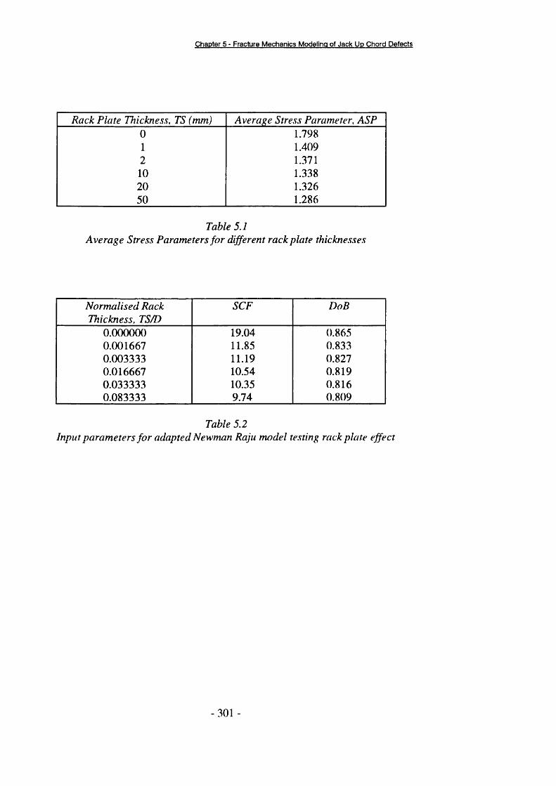
Chapter 5 - Fracture Mechanics Modeling of Jack U p Chord Defects
Rack Plate Thickness, TS (mm) Average Stress Parameter, ASP0 1.7981 1.4092 1.37110 1.33820 1.32650 1.286
Table 5.1Average Stress Parameters for different rack plate thicknesses
Normalised Rack Thickness, TS/D
SCF DoB
0.000000 19.04 0.8650.001667 11.85 0.8330.003333 11.19 0.8270.016667 10.54 0.8190.033333 10.35 0.8160.083333 9.74 0.809
Table 5.2Input parameters for adapted Newman Raju model testing rack plate effect
301 -
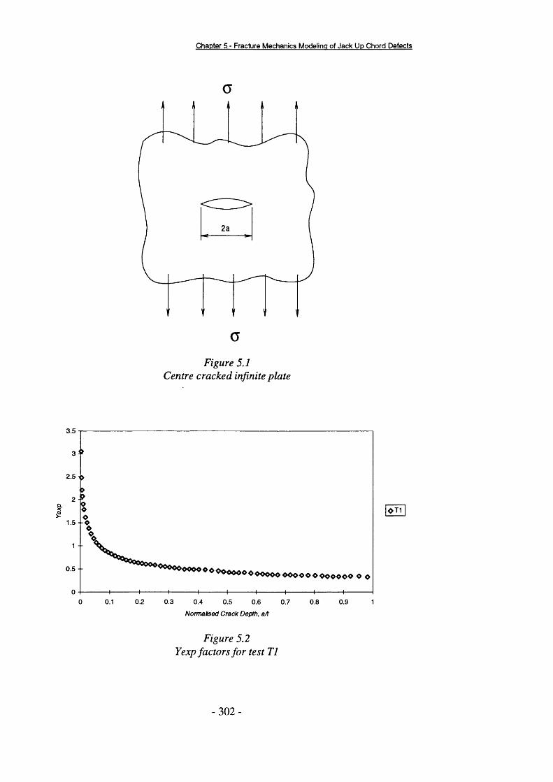
Chapter 5 - Fracture Mechanics Modeling of Jack U p Chord Defects
a
Figure 5.1 Centre cracked infinite plate
3.5
I1.5 - - 0
0 .5 --0 ^0 0 ^ 0 0 ^0 0 ^ 0 0 ^ 0 0 0 ^ 0 0 0 0 O o
0.2 0.30 0.1 0.4 0.5 0.6 0.7 0.8 0.9 1
O T 1
Normalised Crack Depth, aA
Figure 5.2Y exp factors fo r test T I
302 -

Chapter 5 - Fracture Mechanics Modeling of Jack Up Chord Defects
2,5
t ^
0.5 -- OOOOOOO o o o oo OOOOOOO <
0.1 0.2 0.3 0.4 0.5 0.6 0.7 0.8 0.9 10
0 T 2
Normaised Crack Depth, aA
Figure 5.3 Yexp factors for test T2
3 5
2 5 >
o
g
0,5 -- ooooooooooooo ooooo o oooooo O O
0 7 0.90 5 0 6 0.8 10 0 1 02 0 3 0 4
O Yexp
McxJ AVS
Normalised C rack Depth. aA
Figure 5.4Comparison of empirical SIF models with Yexp results from Test Tl
- 303 -

Chapter 5 - Fracture Mechanics Modeling of Jack Up Chord Defects
2.5
2 - ;
&15 --
'Ooo o o0 5 00&0000 0000000 o o Ô
H-------- h0 0 1 0 2 0 3 0 4 0.5 0 6 0 7
Normalised Crack Depth. aA0.8 0 9 1
O Yexp AVSMod AVS
TPM
Figure 5.5Comparison of empirical SIF models with Yexp results from Test T2
1
0.9
0.8
% 0.7
tg 0.6
^ 0.5
•S2 0.4
0.2
0.1
070000 8000030000 40000 50000 6000010000 20000
Cycles, N
Figure 5.6Fracture mechanics crack growth results for Test Tl
-T1
AVS
Mod. AVS
Best Fit Y
- 304 -

Chapter 5 - Fracture Mechanics Modeling of Jack Up Chord Defects
0.9
0.7
0.6
2 0.3
0.2
80000 100000 120000 140000 160000 180000600000 20000 40000
T2AVSMod. AVS
Best Fit Y
Cycles. N
Figure 5.7Fracture mechanics crack growth results for Test T2
y = 0 .3 3 8 1 x ° ^ ^ ® ® r2 = 0.9944
2.5
I
0.5
- t-—
0.2 0.7 0.8 0.9 10.4 0.5 0.60.1 0.3
O T lBest Fit Y
NormaSsed Crack Depth, aA
Figure 5.8Power Law F it fo r Yexp data from Test T l
- 305 -
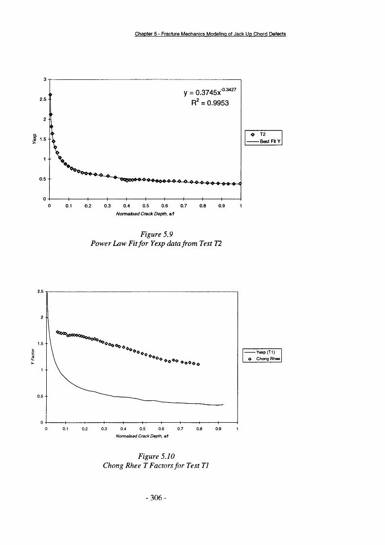
Chapter 5 - Fracture Mechanics Modeling of Jack Up Chord Defects
2.5
I
0.5 --
0 0.5 0.70.1 0.2 0.3 0.4 0.6 0.8 0.9 1
O T2 Best Fit Y
Normalised Crack Depth, aA
Figure 5.9Power Law Fit for Yexp data from Test T2
2.5
0.5 -■
0.5 0.70 0.1 0.2 0.3 0.4 0.6 0.8 0.9 1
Yexp (T1 )O Chong Rhee
NormaHsed Crack Depth, aA
Figure 5.10Chong Rhee T Factors fo r Test TI
3 0 6 -
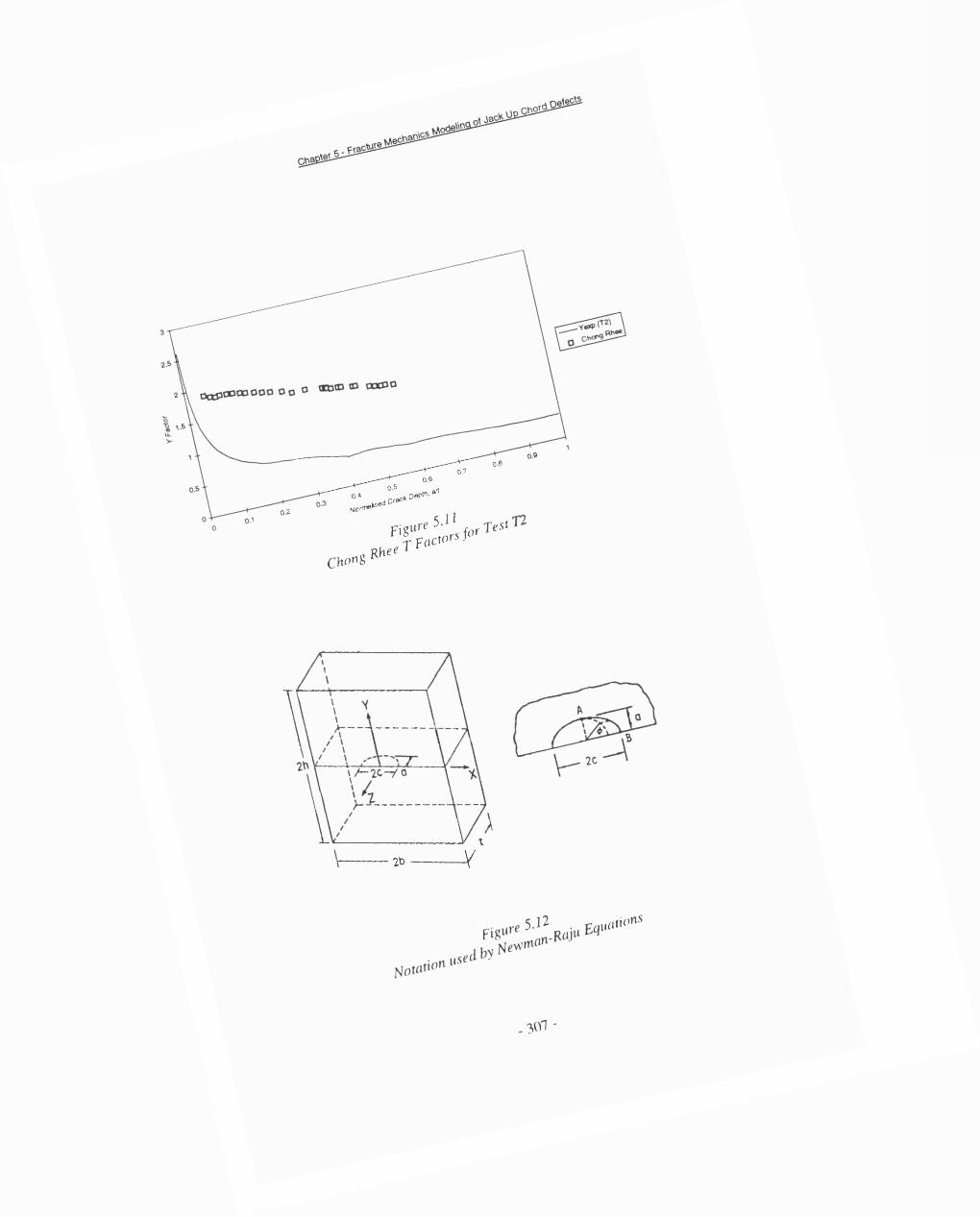
1 ( 1-------1—0.4 0.5 0 ,6 0 .7 0.8
Normatsed Crack Depth, a /t
Figure 5.11 Chong Rhee T Factors fo r Test
02
2t) Y
.................................... ..
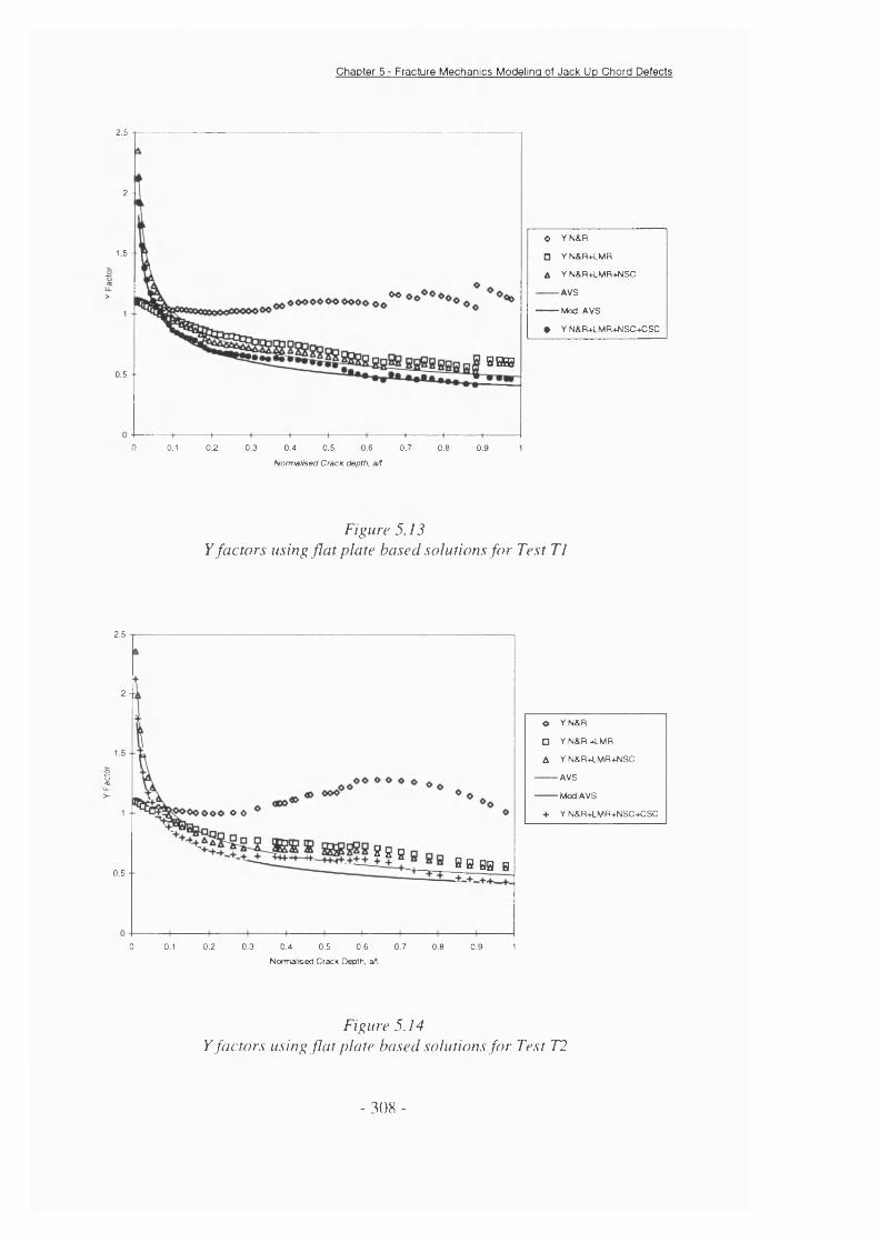
Chapter 5 - Fracture Mechanics Modeling of Jack Up Chord Defects
2.5
2 -■
1.5 -
OO>-
BBS0.5 -■
0 0.1 0.2 0.3 0.4 0.5 0.6 0.7 0.8 0.9 1
O YN&R
□ Y N&R+LMR
A Y N&R+LMR+NSC
AVS
Mod. AVS
# Y N&R+LMR+NSC+CSC
Normalised Crack depth, a/t
Figure 5.13Y factors using flat plate based solutions for Test Tl
2.5
2 --J
IO O
g g g
HB BH H0.5 -
0 0.2 0.3 0.50.1 0.4 0.6 0.7 0.8 0.9 1
o YN&R
□ Y N & R 4 IM R
A Y N&R+LMR+NSC
AVS
---------Mod AVS
+ Y N&R+LMR+NSC+CSC
Normalised Crack Depth, art
Figure 5.14y factors using flat plate based solutions for Test T2
- 308 -
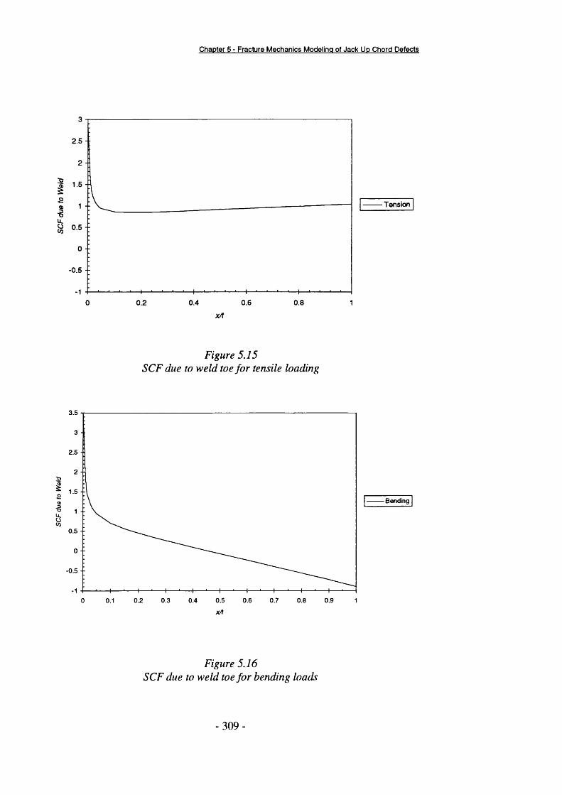
Chapter 5 - Fracture Mechanics Modeling of Jack Up Chord Defects
2.5 -
2 -
I
0 --
-0.5 --
0.4 0.6 0.80 0.2 1xA
Figure 5.15 SCF due to weld toe for tensile loading
3.5
3 -
2.5 -
£
0.5 --
0 --
-0.5 --
0.5 0.70.2 0.3 0.4 0.6 0.8 0.9 10 0.1
x A
Figure 5.16 SCF due to weld toe for bending loads
■Tension
• Bending
-309
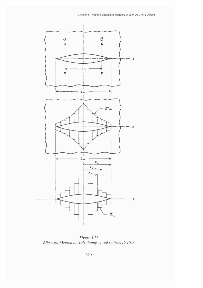
Chapter 5 • Fracture Mechanics Modeling of Jack Up Chord Defects
i L
2 x
2a
— X
A
\ /
2 a
X
X
Figure 5.17Albrechts Method for calculating Yf, (taken from [5.10])
- 3 1 0 -

Chapter 5 - Fracture Mechanics Modeling of Jack Up Chord Defects
2.5
1.5 --
0.5 --
0 0.1 0.2 0.3 0.4 0.5 0.6 0.7 0.8 0.9 1
■ Membrane
aA
Figure 5.18Correction Factors (Yg) for non-uniform stress distribution
0.7 --
0.6 - -Test T l
Test T2
- CSC0.5 -
0.4 --
0.3 --
0.2 - -
0 0.01 0.02 0.03 0.04 0.05 0.06 0.07 0.08 0.09 0.1
a/2c
Figure 5.19Crack shape correction factors
- 311 -
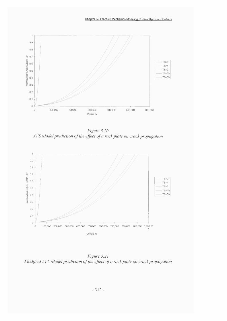
Chapter 5 - Fracture Mechanics Modeling of Jack Up Chord Defects
0 9 -■
0 6 - -
0 4 -■
2 0.3
0 2 -■
0 100,000 200,000 300,000 400,000 500,000 600,000
TS=20TS=50
Cycles N
F i^ re 5.20A l S Model prediction of the e ffect of a rack plate on crack propagation
0 9
IQI 0 5O
I
02
0 100,000 200,000 300,000 400,000 500,000 600,000 700,000 800,000 900,000 1,000,00
TS=0
TS=20TS=50
Cycles. N
Figure 5.21Modified AVS Model prediction of the effect of a rack plate on crack propagation
- j 12 -
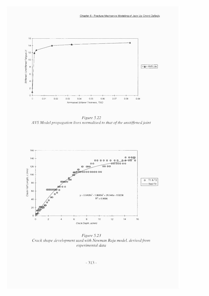
Chapter 5 - Fracture Mechanics Modeling of Jack Up Chord Defects
12
Ü: 10--
8 -■
6 -■
2 -
0 0.01 0.02 0.03 0.04 0.05 0.06 0.07 0.08 0.09
■AVS Ufe
Normalised Stiffener Thickness, TS/D
Figure 5.22AVS Model propagation lives normalised to that of the unstiffened Joint
160
140
O O o o o o oo o o o120 - -
1 ,00- S 80 -
I■g 60
40 -
<D OOOCD
lO O O O O O O OO
O T 1 & T 2
Best FitO O
= 0.0499x - 1 S689x^ + 26.046X - 0.9238 = 0.9686OO
20
0 2 4 6 8 10 12 14 16
C rack Depth, a(m m )
Figure 5.23Crack shape development used with Newman Raju model, derived from
experimental data
- 3 1 3 -
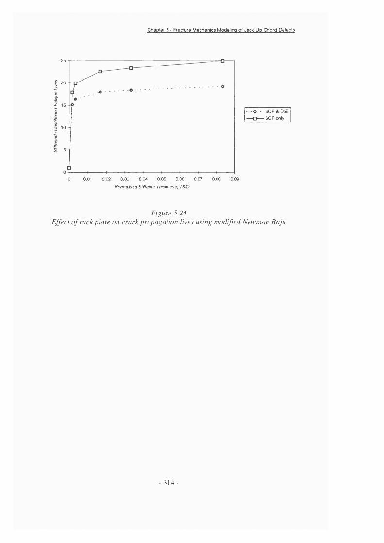
Chapter 5 - Fracture Mechanics Modeling of Jack Up Chord Defects
25
® 20 - -
10 -
5 -
0.05 0.06 0.07 0.090 0.01 0.02 0.03 0.04 0.08
- - O - SCF & DoB
— □ SCF only
Normalised Stiffener Thickness, TS/D
Figure 5.24Effect of rack plate on crack propagation lives using modified Newman Raju
- 3 1 4 -
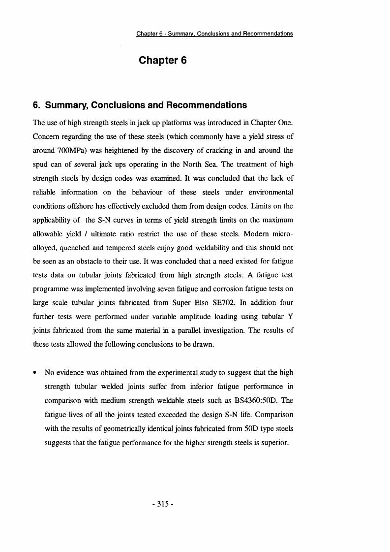
Chapter 6 - Summary. Conclusions and Recommendations
Chapter 6
6. Summary, Conclusions and Recommendations
The use of high strength steels in jack up platforms was introduced in Chapter One.
Concern regarding the use of these steels (which commonly have a yield stress of
around 700MPa) was heightened by the discovery of cracking in and around the
spud can of several jack ups operating in the North Sea. The treatment of high
strength steels by design codes was examined. It was concluded that the lack of
reliable information on the behaviour of these steels under environmental
conditions offshore has effectively excluded them from design codes. Limits on the
applicability of the S-N curves in terms of yield strength limits on the maximum
allowable yield / ultimate ratio restrict the use of these steels. Modern micro
alloyed, quenched and tempered steels enjoy good weldability and this should not
be seen as an obstacle to their use. It was concluded that a need existed for fatigue
tests data on tubular joints fabricated from high strength steels. A fatigue test
programme was implemented involving seven fatigue and corrosion fatigue tests on
large scale tubular joints fabricated from Super Elso SE702. In addition four
further tests were performed under variable amplitude loading using tubular Y
joints fabricated from the same material in a parallel investigation. The results of
these tests allowed the following conclusions to be drawn.
• No evidence was obtained from the experimental study to suggest that the high
strength tubular welded joints suffer from inferior fatigue performance in
comparison with medium strength weldable steels such as BS4360:50D. The
fatigue lives of all the joints tested exceeded the design S-N life. Comparison
with the results of geometrically identical joints fabricated from 50D type steels
suggests that the fatigue performance for the higher strength steels is superior.
- 3 1 5 -

Chapter 5 - Fracture Mechanics Modelling of Jack Up Chord Defects
Some evidence was obtained suggesting that the change of slope of the S-N
curve for tubular joints fabricated from this steel occurs at higher stress ranges
than for the 50D type steels. It is recommended that further fatigue tests be
performed on similar high strength tubular joints to confirm this. Hot spot
stress ranges of 200MPa or less should be used.
Increased crack growth rates were noted for tests under cathodic protection at
CP levels of -800 and -lOOOmV (Ag/AgCl) however these increases were
modest. The feared susceptibility of these steels to large increases in crack
growth rates due to hydrogen embrittlement mechanisms was not found.
However this is likely to be material specific and should be taken in context. The
role played by hydrogen embrittlement in these tests can be assessed from the
proportion of brittle fracture modes on the fracture surface. It has not been
possible to destructively section the crack sites although this will be performed
and reported at a later date.
A review of the typical chord shapes and dimensions for the leg structures was also
presented. The use of a thick longitudinal stiffener, the rack plate was noted. It was
concluded from this review that the stress distribution at the brace-chord
intersection was likely to be significantly different to that in unstiffened tubulars.
An extensive finite element investigation has shown that the presence of a rack
plate can significantly affect the surface SCF distribution at the intersection of the
brace and chord. Several different chord-rack configurations were examined
including designs employing a thinner central section known as a rib plate and
designs where the rack is not continuous through the chord diameter. The effect
has been quantified for a wide range of joint shapes covering the validity range of
common parametric equations. Peak chord SCF’s can be reduced by up to 50% in
comparison with unstiffened joints for axial loading. For OPB loading the
reduction was around 20%. No affect was found for IPB loading. The mechanism
by which the rack brings about these changes was investigated using boundary
- 3 1 6 -
Chapter 6 - Summary. Conclusions and Recommendations
condition sets applied to the chord surface, Thetestriction of chord wall radial
deformation has been shown be the dominant mechanism.
Further work is recommended to quantify the effect of the leg guides commonly
found at the leg-huU intersection. These have been shown elsewhere to have a
significant effect on the ultimate strength of jack up geometries. The significance of
the rack plate has now been demonstrated. It is suggested that more detailed work
on representative joint shapes be performed. This could include modelling the
thicker rack plates using brick rather than thin shell elements. Examining
overlapped bracing and other complicating factors often found in jack up leg
design is also recommended.
The through thickness stress distribution is also altered by the rack plate. This has
again been quantified for a wide range of rack designs and joint geometries. In
general the presence of a rack plate decreases the DoB in all tubular joint shapes
under axial and OPB loading and increases under IPB loading. Higher DoB can be
translated as slower crack growth and longer fatigue crack propagation lives. It
was shown that existing parametric equations for unstiffened joints could predict
the DoB to within +1-5% DoB for the geometries under consideration here.
However a tendency to return unconservative DoB values has been identiifed.
Several contemporary fracture mechanics models have been evaluated against
fracture mechanics data derived from the tubular joint tests mentioned earlier. Of
these the empirically based AVS models performed the best providing an excellent
fit to the experimental Y Factor curve. However attempts to use these models to
predict the observed crack growth in the tubular joint test showed the results to be
subject to large errors. However it should be noted that the stress levels used in the
analysis were extremely high (400MPa and 300MPa) which would of course
amplify any small error in the predicted stress intensity factor.
- 3 1 7 -

Chapter 6 - Summary. Conclusions and Recommendations
A fracture mechanics model based on the flat plate solution of Newman-Raju was
presented as being suitable for the analysis of chord side defects in jack up legs.
The flat plate model was corrected for the effect of the weld toe, load shedding and
crack shape. This model was shown to accurately predict the experimentally
derived Y Factors. The usefulness of this model is its flexibility in terms of input
parameters. The model allows user defined DoB, weld shape and crack shape, all
of which may be important when modelling jack up chord defects. This model was
used to predict fatigue crack propagation lifetimes using the stress distributions
found from the finite element analysis. The model correctly predicted a large
increase in fatigue crack propagation lifetime due to the reduction in peak SCF and
a smaller but significant deleterious effect of the decreased DoB for an axially
loaded T joint.
- 318 -