NARROW»*iBAND IMAGING AND DOPPLER IMAGING OF NATURAL AND

ARTIFICIAL GAS AND PLASMA CLOUDS IN THE INTERPLANETARY

MEDIUM AND IN THE EARTH'S MAGNETOSPHERE

NIGEL PETER MEREDITH

DEPARTMENT OF PHYSICS AND ASTRONOMY

UNIVERSITY COLLEGE LONDON

THESIS PRESENTED FOR THE DEGREE OF

DOCTOR OF PHILOSOPHY

OF THE UNIVERSITY OF LONDON

July 1990

ProQuest Number: 10631079

All rights reserved

INFORMATION TO ALL USERS The quality of this reproduction is dependent upon the quality of the copy submitted.

In the unlikely event that the author did not send a com p le te manuscript and there are missing pages, these will be noted. Also, if material had to be removed,

a note will indicate the deletion.

uestProQuest 10631079

Published by ProQuest LLC(2017). Copyright of the Dissertation is held by the Author.

All rights reserved.This work is protected against unauthorized copying under Title 17, United States C ode

Microform Edition © ProQuest LLC.

ProQuest LLC.789 East Eisenhower Parkway

P.O. Box 1346 Ann Arbor, Ml 48106- 1346

"The known is finite, the unknown infinite; intellectually we stand on an islet in the midst of an illimitable ocean of inexplicability. Our business in every generation is to reclaim a little more land.”

T . H . Huxley

3

ABSTRACT

The properties and dynamics of gas and plasma clouds within the solar wind and in the magnetosphere may be determined by studying the motion and evolution of these clouds in the appropriate region. These clouds may occur naturally, as in the case of cometary atmospheres, or they may be generated by injection of suitable tracer materials from rockets or satellites.

Optical observations of the resulting distributions of ions and neutrals, under all of the above conditions, have been performed using an Imaging Photon Detector, in conjunction with a set of narrow-band interference filters. Line of sight velocity maps of the ions and neutrals have been obtained using a Doppler Imaging System, consisting fundamentally of a Fabry-Perot etalon coupled to an Imaging Photon Detector.

The spatial distributions of the neutral cometary species CN and C2

have been monitored over a wide range of heliocentric distances to yield important information on possible production and destruction mechanisms.

The study of cometary plasmas is characterized by the fact that cometary ions, in particular C0+ and H20+ , can be used as tracers for the dynamical processes taking place. The large-scale and near­nucleus images of the ion coma and tail of the comets Giacobini- Zinner and Hailey are compared and contrasted with each other and with the spacecraft results.

Imaging and Doppler Imaging Systems have been used to observe several artificially injected plasma clouds in both the magnetosphere and the near space environment. When released in the magnetosphere, the migrating ions trace out the distant field and provide direct evidence of the topology of the field. In the near space environment, the interaction of the plasma with the solar wind resembles in many respects the processes occurring in the plasma tails of comets.

4

LIST OF CONTENTS

Abstract ..............................................................3

List of Acronyms ....................................................14

List of Tables ......................................................16

List of Figures .....................................................18

CHAPTER 1 INTRODUCTION TO THE STUDY OF NATURAL AND ARTIFICIAL GAS AND PLASMA CLOUDS WITH IMAGING AND DOPPLER IMAGING SYSTEMS ..........................................33

1.1 Introduction ...................................................33

1.2 The Comets Observed with VHSIS and DIS Systems .............. 351.2.1 Observations of Comet Giacobini-Zinner ............... 351.2.2 Observations of Comet Hailey ..........................361.2.3 Observations of Other Comets ..........................37

1.3 The Spacecraft Missions ....................................... 401.3.1 The ICE Encounter with Comet Giacobini-Zinner .........401.3.2 The Spacecraft Encounters with Comet Hailey ...........40

1.4 Observations of Artificial Ion Clouds ........................ 421.4.1 Observations of the Barium Shaped-Charge Releases .... 42

1.4.1.1 The 1984 Releases Over Alaska ................ 431.4.1.2 The 1986 Releases Over Alaska ................ 431.4.1.3 The 1987 Releases Over Greenland ............. 431.4.1.4 The 1989 Releases Over Northern Canada ........44

1.4.2 Observations of the AMPTE Releases ................... 441.4.3 Observations of Two Rocket Releases Designed to Test

the Critical Ionization Velocity Mechanism ........... 441.4.4 Observations of the Pegsat Releases .................. 44

1.5 Synopsis ....................................................... 45

5

CHAPTER 2 INSTRUMENTATION ..........................................49

2.1 Introduction ...................................................49

2.2 The Imaging Photon Detector ................................... 502.2.1 Brief History of the IPD .............................. 512.2.2 Theory of Operation of the IPD ........................ 522.2.3 The Spectral Response of the IPD ...................... 53

2.2.3.1 The S20 Photocathode ......................... 542.2.3.2 The S25 Photocathode ......................... 542.2.3.3 The GaAs Photocathode ........................ 54

2.2.4 Set-up of the IPD ...................................... 552.2.5 Image Collection and Storage .......................... 562.2.6 Comparison of the IPD with the CCD .................... 57

2.3 The VHSIS Systems used to Observe the Natural and Artificial Gas and Plasma Clouds ..........................................582.3.1 The Optical Bench ...................................... 592.3.2 The Narrow-Band Interference Filters .................. 592.3.3 Instrument Set-up on the Telescope .................... 622.3.4 Observing a Cometary Target ............................632.3.5 Calibration of the VHSIS ............................... 64

2.3.5.1 Thermionic Emission Calibration .............. 642. 3.5.2 Flat Field Calibration........................642. 3.5.3 Sky Background Calibration ................... 64

2.4 Principles of Operation of the Doppler Imaging System ........652.4.1 Theory of the Fabry-Perot Etalon ...................... 662.4.2 Construction of the Fabry-Perot Etalon ................ 682.4.3 The Doppler Imaging System.............................70

2.4.3.1 Set-up of the Doppler Imaging System .........702.4.3.2 Calibration of the Doppler Imaging System ....71

2.5 The DIS Systems used to Observe the Natural and Artificial Gasand Plasma Clouds .............................................. 712.5.1 The DIS used to Observe the Artificial Gas and PlasmaClouds ..........................................................72

6

2.5.2 The DIS Designed for use with the 24" Telescope toObserve Line of Sight Velocities in the Cometary Ion Coma and Tail ...........................................732.5.2.1 Determination of the Focal Length, f^, of the

Negative Lens ................................. 732.5.2.2 Determination of the Etalon Gap .............. 742.5.2.3 Determination of the Focal Length, f2 » of the

Positive Lens ................................. 75

2.6 The Sites and Instruments used to Observe the Cometary Targets ........................................................ 762.6.1 The Sites used to Observe the Cometary Targets ........ 77

2.6.1.1 The Observatorio del Roque de los Muchachos ..772.6.1.2 The Table Mountain Facility ...................77

2.6.2 The Instruments used to Observe the Cometary Targets ..772.6.2.1 The Jacobus Kapteyn Telescope............ 772. 6. 2.2 The 24" Telescope at TMF ...................... 782.6.2. 3 The 16" Telescope at TMF ...................... 782.6.2.4 The 8" Meade Portable Telescope ...............782.6.2.5 The Nikon Camera Lenses ....................... 80

2.7 The Sites and Instruments used to Observe the ArtificialGas and Plasma Clouds ......................................... 802.7.1 The NASA Convair 990 Airborne Observatory ..............802.7.2 Poker Flats Research Range .............................802.7.3 Wallops Island ......................................... 812.7.4 Sondrestrom Incoherent Scatter Radar Facility .........812.7.5 Observatorio del Roque de Los Muchachos ................822.7.6 Churchill Research Range ...............................832.7.7 Table Mountain Facility ................................83

CHAPTER 3 DATA REDUCTION ...........................................93

3.1 Introduction ...................................................93

3.2 Image Transfer from the Field PC to the APL DEC Microvax ..... 94

3.3 Correction of the Raw Images Collected with the VHSIS ........ 953.3.1 Initial Procedures ......................................95

7

3.3.2 Correction for the Thermionic Emission and FlatField Response of the IPD .............................. 963.3.2.1 Correction for Thermionic Emission ..........963.3.2.2 Correction for Flat Field .................... 97

3.3.3 Correction for Sky Background ......................... 973.3.4 Smoothing Routines .....................................98

3.3.4.1 Smoothing using Spline Interpolations ........ 993.3.4.2 Smoothing using Fourier Transforms .......... 100

3.4 Data Reduction ............................................... 1003.4.1 Reduction of the Imaging Data to Line Profiles .1003.4.2 Reduction of the Imaging Data to Circular Profiles ...1013.4.3 Verification of the Routine to Generate the

Circular Profiles ..................................... 1023.4.4 Reduction of the Imaging Data to Sector Profiles ..... 104

3.5 Analysis of the Doppler Imaging Data.......................... 1043.5.1 Determination of the Centre of the Fabry-Perot Ring

System ................................................. 1053.5.2 Reduction of an Image to Radius-Squared Profile ..... 1063.5.3 Determination of Peak Positions ...................... 1073.5.4 Calculation of the Relative Line of Sight

Velocities .............................................107

CHAPTER 4 INTRODUCTION TO COMETS ................................. 119

4.1 Introduction ..................................................119

4.2 Brief Historical Perspective .................................120

4.3 Brief Overview of Cometary Physics up to the Time of theRecent Spacecraft Encounters ................................. 1224.3.1 The Cometary Nucleus .................................. 122

4.3.1.1 Structure of the Cometary Nucleus .......... 1224.3.1.2 Size of the Cometary Nucleus ................123

4.3.2 The Dust Coma/Tail ....................................1234. 3.2.1 Morphology of the Dust Coma/Tail ........... 1234.3.2.2 Composition of the Dust Particles .......... 124

8

4.3.3 The Gaseous Coma ...................................... 1244.3.3.1 Morphology of the Gaseous Coma .............. 1254.3.3.2 Composition of the Gaseous Coma ............. 1254.3.3.3 Excitation Mechanisms ........................126

4.3.4 The Plasma Tail ........................................1264.3.4.1 Morphology of the Plasma Tail ............... 1274.3.4.2 Composition of the Plasma Tail .............. 1274.3.4.3 The Comet-Solar Wind Interaction ............ 128

4.4 The Cometary Nucleus ......................................... 1294.4.1 The Physical Nature of the Nucleus of Comet Hailey ...1304.4.2 The Rotational Period of Comet Hailey ................ 131

4.5 Cometary Dust .................................................1324.5.1 The Chemical Composition of the Dust Particles at

Comet Hailey ...........................................1334.5.1.1 Results from the Spacecraft Encounters ......1334.5.1.2 Results from Earth-Based Infrared

Observations ................................. 1344.5.2 The Spatial and Mass Distributions of the Dust

Particles at Comet Hailey ............................. 1354.5.2.1 Results from the Spacecraft Encounters ......1354.5.2.2 Results from Earth-Based Infrared

Observations ................................. 136

4.6 The Gaseous Cometary Coma - Neutrals and Ions ............... 1364.6.1 Results from the Spacecraft Encounters ................1364.6.2 Results from Earth-Based Observations ................ 1384.6.3 Results from the Dynamics Explorer-1 Satellite ....... 1404.6.4 Results from the Pioneer Venus Orbiter ................1404.6.5 Results from Two Sounding Rockets ..................... 1404.6.6 Results from the International Ultraviolet Explorer

Satellite ..............................................141

4.7 The Plasma Tail ............................................... 1424.7.1 Morphology of the Plasma Tail .........................1424.7.2 The Comet-Solar Wind Interaction ..................... 142

9

CHAPTER 5 THE NEUTRAL COMETARY ENVIRONMENT I - THE DISTRIBUTIONOF CN AND Co ............................................146

5.1 Introduction ................................................. 146

5.2 Models of the Neutral Cometary Environment ...................1475.2.1 Intensity Distribution Caused by Stable Molecules

Expanding Isotropically into Volume ................... 1485.2.2 Intensity Distribution Caused by Exponentially

Decaying Molecules Expanding Isotropically intoVolume ................................................. 149

5.2.3 Intensity Distribution Caused by Exponentially Decaying Daughter Molecules Expanding Isotropicallyinto Volume ............................................150

5.2.4 Limitations of the Haser Model ...................... 1525.2.5 Derivation of Scale Lengths .......................... 153

5.3 Calculation of the CN Parent and Daughter Scale Lengths andtheir Variation with Heliocentric Distance .................. 1545.3.1 Calculation of the CN Daughter Scale Lengths .......1545.3.2 Calculation of the CN Parent Scale Lengths .............156

5.4 Calculation of the C2 Parent Scale Length and its Variationwith Heliocentric Distance ................................... 158

5.5 Discussion of the Errors in the Derived Scale Lengths .......1605.5.1 Estimation of the Errors Caused by Dust

Contamination ......................................... 1615.5.2 Estimation of the Errors Caused by Uncertainties

in the Sky Background ................................. 1625.5.3 Estimation of the Errors Caused by an Inaccurate

Centre Determination .................................. 1635.5.4 Estimation of the Errors in the Derived Parent Scale

Length Caused by Uncertainties in the Daughter Scale Length .................................................164

5.6 Scale Lengths Found by Other Investigators .................. 1665.6.1 CN Parent and Daughter Scale Lengths Found by Other

Investigators ......................................... 166

10

5.6.2 C2 Parent Scale Lengths Found by Other Investigators ......................................... 167

5.6.3 Methods Used by the Other Investigators ............. 1685.6.3.1 Cochran ...................................... 1695.6.3.2 Combi & Delsemme .............................1695.6.3.3 Delsemme & Moreau ............................1695.6.3.4 Newburn & Spinrad ............................1695.6. 3.5 Prieto et al.................................. 170

5.7 Comparison of the Scale Lengths Inferred from the VHSIS Datawith those Calculated by the Other Investigators ............ 1715.7.1 The CN Daughter Scale Length ......................... 1715.7.2 The CN Parent Scale Length ........................... 1725.7.3 The C2 Parent Scale Length ........................... 1725.7.4 Discussion of the Derived Scaling Laws ...............173

5.8 The Anomalous C2 Coma of Comet Borrelly ..................... 174

CHAPTER 6 THE NEUTRAL COMETARY ENVIRONMENT II - THEDETERMINATION OF THE HnO PRODUCTION SCALE LENGTHIN COMET GIACOBINI-ZINNER AND THE SEARCH FOR JETS INTHE NEUTRAL COMA OF COMET HALLEY ...................... 187

6.1 Introduction .................................................. 187

6.2 The Determination of the H 2 O Production Scale Length inComet Giacobini-Zinner at r — 1.03 AU ........................1886.2.1 Introduction .......................................... 1886.2.2 Calculation of the Intensity Distribution Caused by

Exponentially Decaying Grand-Daughter Molecules Expanding Isotropically into Volume... ................ 189

6.2.3 Estimation of the NH2 Component ...................... 1936.2.4 Determination of the H 2 O Production Scale Length ..... 194

6. 2.4.1 Case 1 ........................................ 1956.2.4.2 Case 2 ........................................ 197

6.2.5 Discussion ............................................ 199

6.3 The Search for "Jet-Like" Structures in the Neutral Atmosphere of Comet Hailey Around the Time of the Spacecraft Encounters in March 1986 ............... 200

11

6.3.1 Introduction .......................................... 2006.3.2 Comparison of the Instruments used by the Various

Investigators .......................................... 2016.3.3 The Ring-Masking Technique ........................... 2026.3.4 Critical Examination of the Ring-Masking Technique ...2036.3.5 Results of Applying the Ring Masking Technique to

a Selection of Near-Nucleus VHSIS Images ............. 2066.3.6 Discussion ............................................ 208

CHAPTER 7 THE COMET-SOLAR WIND INTERACTION - ION TAILSTRUCTURES IN COMETS GIACOBINI-ZINNER AND H ALLEY.......224

7.1 Introduction .................................................. 224

7.2 The ICE Intercept of Comet Giacobini-Zinner ............. 226

7.3 The Spacecraft Encounters with Comet Hailey ............. 2277.3.1 The Vega Spacecraft ................................... 2287.3.2 Suisei .................................................2287.3.3 Giotto .................................................229

7.4 VHSIS Observations of the Ion Coma and Tail of CometGiacobini-Zinner .............................................. 2307.4.1 Near-Nucleus Structure of the Ion Coma of Comet

Giacobini-Zinner .......................................2317.4.2 Large-Scale Structure of the Ion Tail of Comet

Giacobini-Zinner .......................................2327.4.3 Comparison of the VHSIS Images with the ICE D a t a .... 233

7.5 VHSIS Observations of the Ion Coma and Tail of CometHailey .........................................................2347.5.1 Near-Nucleus Structure of the Ion Coma of Comet

Hailey ................................................. 2357.5.2 Large-Scale Structure of the Ion Tail of Comet

Hailey ................................................. 236

7.6 A Quantitative Study of the Variation of the Ion Coma ofComet Hailey .................................................. 237

12

7.7 Tail Disconnection Events ......................................239

7.8 Comparison of Ion Tail Structures in Comets Giacobini-Zinnerand Hailey .................................................... 241

CHAPTER 8 PLASMA PROCESSES IN THE MAGNETOSPHERE AND IN THESOLAR WIND............................................... 255

8.1 Introduction ................................................. 255

8.2 The 27 December 1984 AMPTE "Artificial Comet" Experiment ....257

8.3 The 21 March 1985 AMPTE Barium Magnetotail Release ..........260

8.4 Search for Auroral Belt E„ Fields with High-Velocity BariumIon Injections ............................................... 2638.4.1 The April 1984 Experiments ............................ 2648.4.2 Recent Modifications to the VHSIS/DIS used to Observe

the Barium Shaped-Charge Releases .................... 266

8.5 Recent Free Space Experiments Designed to Test the Critical Ionization Velocity Mechanism .................................2688.5.1 The CRIT I Experiment ................................. 2698.5.2 The SR90 Experiment ................................... 271

CHAPTER 9 SUMMARY AND CONCLUSIONS .................................284

9.1 Introduction ..................................................284

9.2 Principal Results from the Cometary Observations ............ 2859.2.1 Observations of the Neutral Cometary Coma ............ 2859.2.2 Observations of the Ion Coma and Tail .................287

9.3 Principal Results from the Observations of SeveralArtificial Chemical Releases ................................. 2889.3.1 Observations of the Barium Shaped-Charge Releases ....2889.3.2 Observations of the AMPTE Releases ....................2889.3.3 Observations of Two Rocket Releases Over Wallops

Island in May 1986 .................................... 289

13

9.4 Future Work with VHSIS/DIS Systems ........................... 2899.4.1 Future Cometary Observations .......................... 2909.4.2 Observations of the Releases to be Associated with

the Combined Radiation Release Effects Satellite Program ................................................ 290

9.4.3 The Doppler Wind Sensor ................................291

9.5 Future Missions to Comets ..................................... 2919.5.1 An Extended Giotto Mission ............................ 2929.5.2 The Comet Rendezvous Asteroid Flyby Mission .......... 2929.5.3 The Comet Nucleus Sample Return Mission.............293

Acknowledgements ................................................... 294References ......................................................... 295

14

LIST OF ACRONYMS

AMPTE Active Magnetospheric Particle Tracer ExplorerAPL Atmospheric Physics LaboratoryCCD Charge Coupled DeviceCHUKCC Comet Hailey UK Coordinating CommitteeCNSR Comet Nucleus Sample Return mission (named Rosetta)CRAF Comet Rendezvous Asteroid Flyby missionCRRES Combined Radiation Release Experimental SatelliteDE Disconnection EventDE-1 Dynamics Explorer 1 satelliteDec DeclinationDIDSY Dust Impact Detection System Experiment (on board Giotto)DIS Doppler Imaging SystemDQE Detective Quantum EfficiencyDUCMA Dust Counter and Mass Analyzer (on board the Vega spacecraft)DWS Doppler Wind SensorEHT Extra High TensionESA European Space AgencyESOC European Space Operations CentreFES Fine Error Sensor (on board IUE)FPI Fabry-Perot InterferometerFSR Free Spectral RangeFWHM Full Width Half MaximumGSFC Goddard Space Flight CenterHERS High Energy Resolution Spectrometer (on board Giotto)HIS High Intensity Spectrometer (on board Giotto)HMC Hailey Multicolour Camera (on board Giotto)IAU International Astronomical UnionICE International Cometary ExplorerIHW International Hailey WatchIKS Infrared Instrument (on board the Vega spacecraft)IMF Interplanetary Magnetic FieldIMS Ion Mass Spectrometer (on board Giotto)IPD Imaging Photon DetectorIR InfraredIRM Ion Release Module (part of AMPTE program)IRTF Infrared Telescope Facility (NASA)

ISIT Intensified Silicon Intensified TargetIUE International Ultraviolet ExplorerJKT Jacobus Kapteyn TelescopeJPL Jet Propulsion LaboratoryKAO Kuiper Airborne Observatory (NASA)MCP MicroChannel PlateNASA National Aeronautics and Space AdministrationNMS Neutral Mass Spectrometer (on board Giotto)NRAO National Radio Astronomy Observatory (NASA)PC Personal ComputerPICCA Positive Ion Cluster Composition Analyzer (on board Giotto)PPT Planetary Patrol Telescope (Perth Observatory)RA Right AscensionRMS Root Mean SquareRS Radiant SensitivitySPU Signal Processing UnitTKS Three Channel Spectrometer (on board the Vega spacecraft)TMF Table Mountain FacilityTVS Television System (on the Vega spacecraft)UAF University of Alaska at FairbanksUCL University College LondonUKS United Kingdom Satellite (as part of AMPTE program)UV UltravioletUVI Ultraviolet Imager (on board IUE)VHSIS Very High Sensitivity Imaging System

16

LIST OF TABLES

CHAPTER 1

Table 1.1 Log of the Cometary Observations ...................... 39Table 1.2 Summary of the Spacecraft Encounters .................. 41Table 1.3 Log of the Observations of the Artificial Chemical

Release Experiments ..................................... 45

CHAPTER 2

Table 2.1 Procedure used for Naming the Files on the Field PC ...56Table 2.2 List of the Narrow-Band Interference Filters

used with the VHSIS and DIS .............................61Table 2.3 The Free Spectral Range Obtained with Different

Etalons .................................................. 74Table 2.4 Angular Separations Between the Fourth Fringe and

the Central Fringe ...................................... 75Table 2.5 Summary of the Instruments used to Observe the

Cometary Targets ........................................ 76Table 2.6 Log of the Cometary Observations, together with the

Instruments used ........................................ 79Table 2.7 Log of the VHSIS/DIS Systems used to Observe the

Artificial Chemical Release Experiments ................ 82

CHAPTER 3

Table 3.1 Additional Information Added to the Filename at UCL ....95

CHAPTER 4

Table 4.1 Chemical Species Identified in Cometary SpectraPrior to the Spacecraft Encounters .................... 125

Table 4.2 Chemical Composition of the Dust in Comet Hailey ......133

17

CHAPTER 5

Table 5.1 CN Daughter Scale Lengths Inferred from the Large-ScaleVHSIS CN Images .........................................156

Table 5.2 CN Parent Scale Lengths Inferred from the Near-NucleusVHSIS CN Images .........................................157

Table 5.3 C2 Parent Scale Lengths Inferred from the Near-NucleusVHSIS C2 Images .........................................159

Table 5.4 Errors on a Typical CN Parent Scale Length Caused byUncertainties in the Sky Background ................... 163

Table 5.5 Errors on a Typical CN Parent Scale Length Caused byan Inaccurate Centre Determination.................... 164

Table 5.6 Errors on Three Typical CN Parent Scale Lengths Causedby Uncertainties in the Daughter Scale Length .........165

Table 5.7 CN Parent and Daughter Scale Lengths Published in theLiterature .............................................. 166

Table 5.8 C2 Parent and Daughter Scale Lengths Published in theLiterature .............................................. 168

CHAPTER 6

Table 6.1 Parameter Set 1 ......................................... 195Table 6.2 Best Fits to the Outer Region of the 0(^D) Profile

using Parameter Set 1 ..................................196Table 6.3 Best Fits to the Inner Region of the 0(^D) Profile

using Parameter Set 1 ..................................196Table 6.4 Parameter Set 2 ......................................... 197Table 6.5 Best Fits to the Outer Region of the 0(^D) Profile

using Parameter Set 2 ..................................198Table 6.6 Best Fits to the Inner Region of the 0(^D) Profile

using Parameter Set 2 ..................................198Table 6.7 Comparison of the Instruments used by the Various

Investigators in their Search for Neutral ComaFeatures ................................................ 202

CHAPTER 7

Table 7.1 Variation of the Line of Sight Sunward and TailwardIon Sector Profiles in Comet Hailey ................... 238

18

LIST OF FIGURES

CHAPTER 2

Figure 2.1 A photograph of the head unit of an Imaging PhotonDetector taken from the front of the device, showing the photocathode window.

Figure 2.2 A schematic diagram of the Imaging Photon Detector headunit, showing the photocathode, the microchannel plates and the resistive anode position sensitive encoder.

Figure 2.3 Graph plotting typical radiant sensitivities againstwavelength for S20, S25 and GaAs devices.

Figure 2.4 The optical bench for the Very High Sensitivity ImagingSystem on the 24" telescope.

Figure 2.5 Graph showing the characteristic curves for two-,three- and four-cavity interference filters.

Figure 2.6 A schematic diagram of the instrument layout.

Figure 2.7 A selection of the Fabry-Perot etalons used by theAtmospheric Physics Laboratory.

Figure 2.8 The design of a Doppler Imaging System for the24" telescope at TMF.

Figure 2.9 The 1 m Jacobus Kapteyn Telescope at the Observatoriodel Roque de los Muchachos, La Palma.

Figure 2.10 The Meade 8" portable telescope on the roof of theaccomodation block, the "Residencia", at the Observatorio del Roque de los Muchachos, La Palma.

Figure 2.11 The 24" telescope at TMF.

19

Figure

Figure

Figure

Figure

Figure

Figure

Figure

Figure

Figure

.12 The inside of the dome of the 24" telescope at TMF, showing the control console and the IPD hardware.

CHAPTER 3

.la Raw image of comet Brorsen-Metcalf taken with the24" telescope at TMF on 9 August 1989 at 11:45 UT, in the light of the molecule.

.lb Thermionic emission file associated with the image in figure 3.1a. The detector photocathode was insulated from light and a 60 minute integration taken.

,1c The flat field file associated with the image in figure3.1a. This is a 5 minute exposure of the twilight sky taken through the 24" telescope at TMF with the C2

filter.

.Id The sky background image associated with the image infigure 3.1a. This is a 5 minute exposure of the night sky taken approximately 5° of arc from the comet, shortly after the comet integration.

.2 The corrected image of comet Brorsen-Metcalf taken withthe 24" telescope at TMF on 9 August 1989 at 11:45 UT, in the light of the C2 molecule.

.3 An aid to understand the reduction of the imagingdata to circular profiles. The basic problem is the conversion of a rectangular grid to a circular grid.

1.4 The reduction to radius of the 1/R test profile image, without the geometric correction.

1.5 The reduction to radius of the 1/R test profile image, with the geometric correction.

20

Figure

Figure

Figure

Figure

Figure

Figure

Figure

Figure

.6 The Fabry-Perot fringes from a barium calibration lamp. This image was taken on 13 April 1986 at Poker Flats Research Range, Alaska with a DIS set up to observe a barium shaped-charge release.

.7 Four 45° sector profiles taken outwards from the centreof the Fabry-Perot ring system shown in figure 3.6.

.8 The 24 equal-angle radius-squared profiles of theFabry-Perot ring system shown in figure 3.6.

.9 An example data file from the 13 April 1986 rocketexperiment. This file was taken with the DIS at 09:21 UT in the light of the 455.4 nm emission of sunlit barium ions.

.10 The 24 equal-angle radius-squared profiles of theDIS data shown in figure 3.9.

CHAPTER 4

.1 Average of several spectra of comet Kohoutek 1973 XIIat 1 AU post-perihelion (from A'Hearn, [1975]).

.2 The nucleus of comet Hailey as seen from a distance of18,270 km by the HMC on board Giotto, taken from Keller et al. [1986]. The frame size is 30 km.

CHAPTER 5

.la This image shows the appearance of the CN coma of cometHailey, pre-perihelion, on 8 December 1985 at 03:26 UT. This image was taken with the 300 mm Nikon camera lens from TMF. The comet was 1.38 AU from the Sun and 0.70 AU from the Earth.

21

Figure 5.1b This image shows the appearance of the CN coma of comet Hailey, post-perihelion, on 2 May 1986 at 21:39 UT.This image was taken with the 300 mm Nikon camera lens from La Palma. The comet was 1.65 AU from the Sun and 0.83 AU from the Earth.

Figure 5.lc This image shows the appearance of the CN coma of comet Bradfield, post-perihelion, on 22 December 1987 at 02:37 UT. This image was taken with the 300 mm Nikon camera lens from TMF. The comet was 1.19 AU from the Sun and 0.86 AU from the Earth.

Figure 5.Id This image shows the appearance of the CN coma of comet Borrelly, close to perihelion, on 22 December 1987 at 07:28 UT. This image was taken with the 300 mm Nikon camera lens from TMF. The comet was 1.36 AU from the Sun and 0.52 AU from the Earth.

Figure 5.2a The large-scale CN profile of comet Hailey taken with the 300 mm Nikon camera lens from TMF on 8 December 1985 at 03:26 UT. A daughter scale length of 1.25 x 10^ km is deduced from this profile.

Figure 5.2b The large-scale CN profile of comet Hailey taken with the 300 mm Nikon camera lens from La Palma on 2 May 1986 at 21:39 UT. A daughter scale length of1.3 x 10^ km is deduced from this profile.

Figure 5.2c The large-scale CN profile of comet Bradfield taken with the 300 mm Nikon camera lens from TMF on 22 December 1987 at 02:37 UT. A daughter scale length of 0.7 x 10^ km is deduced from this profile.

Figure 5.2d The large-scale CN profile of comet Borrelly taken with the 300 mm Nikon camera lens from the TMF on 22 December 1987 at 07:28 UT. A daughter scale length

Cof 0.75 x 10 km is deduced from this profile.

22

Figure 5.3a This image shows the near-nucleus appearance of the CN coma of comet Hailey, post-perihelion, on 22 March 1986 at 11:48 UT. This image was taken with the 16" telescope at TMF. The comet was 1.02 AU from the Sun and 0.76 AU from the Earth.

Figure 5.3b This image shows the inner CN coma of comet Wilson, pre-perihelion, on 4 November 1986 at 02:33 UT. This image was taken on the 24" telescope at TMF. The comet was 2.66 AU from the Sun and 2.64 AU from the Earth.

Figure 5.3c This image shows the inner CN coma of comet Bradfield, post-perihelion, on 19 December 1987 at 02:18 UT. This image was taken on the 24" telescope at TMF. The comet was 1.16 AU from the Sun and 0.85 AU from the Earth.

Figure 5.3d This image shows the inner CN coma of comet Borrelly, close to perihelion, on 19 December 1987 at 05:43 UT. This image was taken with the 24" telescope at TMF.The comet was 1.36 AU from the Sun and 0.51 AU from the Earth.

Figure 5.4a The near-nucleus CN profile of comet Hailey taken withthe 24" telescope at TMF on 22 March 1986 at 11:48 UT.A parent scale length of 22,000 km is deduced from this profile.

Figure 5.4b The near-nucleus CN profile of comet Wilson taken withthe 24" telescope at TMF on 4 November 1986at 02:33 UT. A parent scale length of 95,000 km is deduced from this profile.

Figure 5.4c The near-nucleus CN profile of comet Bradfield taken with the 24" telescope at TMF on 19 December 1987 at 02:18 UT. A parent scale length of 42,000 km is deduced from this profile.

23

Figure

Figure

Figure

Figure

Figure

Figure

Figure

.4d The near-nucleus CN profile of comet Borrelly taken with the 24" telescope at TMF on 19 December 1987 at 05:43 UT. A parent scale length of 55,000 km is deduced from this profile.

.5a This image shows the near-nucleus appearance of the C2

coma of comet Hailey, post-perihelion, on 18 March 1986 at 12:00 UT. This image was taken with the 24" telescope at TMF. The comet was 0.96 AU from the Sun and 0.86 AU from the Earth.

.5b This image shows the inner C2 coma of comet Hailey,post-perihelion, on 6 May 1986 at 00:00 UT. This image was taken with the JKT at La Palma. The comet was 1.70 AU from the Sun and 0.95 AU from the Earth.

.5c This image shows the inner C2 coma of comet Bradfield, post-perihelion, on 21 December 1987 at 02:19 UT. This image was taken with the 24" telescope at TMF. The comet was 1.18 AU from the Sun and 0.86 AU from the Earth.

.5d This image shows the inner C2 coma of comet Borrelly, close to perihelion, on 21 December 1987 at 06: 10 UT. This image was taken with the 24" telescope at TMF.The comet was 1.32 AU from the Sun and 0.52 AU from the Earth.

,6a The near-nucleus C2 profile of comet Hailey taken with the 24" telescope at TMF on 18 March 1986 at 12:00 UT.A parent scale length of 46,000 km is deduced from this profile.

.6b The near-nucleus C2 profile of comet Hailey taken with the 1 m JKT at La Palma on 6 May 1986 at 00:00 UT.A parent scale length of 35,000 km is deduced from this profile.

24

Figure 5.6c

Figure 5.6d

Figure 5.7

Figure 5.8

Figure 5.9

Figure 5.10

Figure 6.1

Figure 6.2

Figure 6.3

The near-nucleus C2 profile of comet Bradfield taken with the 24" telescope at TMF on 21 December 1987at 02:19 UT. A parent scale length of 20,000 km isdeduced from this profile.

The near-nucleus C2 profile of comet Borrelly taken with the 24" telescope at TMF on 21 December 1987at 06:10 UT. This profile is anomalous in that no fitis obtained.

The heliocentric variation of the CN daughter scale length as found by all authors.

The heliocentric variation of the CN parent scale length as found by all authors.

The heliocentric variation of the C2 parent scale length as found by all authors.

C2 profiles of the comets Hailey, Bradfield and Borrelly scaled to R = 1 AU and delta = 1 AU to highlight the anomalous behaviour of C2 in Borrelly.

CHAPTER 6

The near-nucleus image of comet Giacobini-Zinner in the emission of 0(^D) at 630.0 nm, taken with the JKT at La Palma on 1 September 1985 at 03:38 UT.

The near-nucleus 0(^D) Doppler image of comet Giacobini-Zinner taken with the JKT at La Palma on 2 September 1985 at 03:37 UT. The comet was 1.03 AU from the Sun and 0.47 AU from the Earth.

Two 45° sector profiles through the Doppler image shown in Figure 6.2. The red trace is the profile through the comet signal and the green trace is the profile in the opposite direction (used to estimate the sky background).

25

Figure 6

Figure 6

Figure 6

Figure 6

Figure

Figure

Figure

Figure

Figure

Figure

.4 Two 45° sector profiles through the Doppler imageof Figure 6.2 after correction for sky background. The magenta trace is the 0(^D) profile and the cyan trace is the NH2 contamination.

.5 An example fit to the 0(^D) profile of figure 6.1using the parameter set 1.

.6 An example fit to the 0(^D) profile of figure 6.1using the parameter set 2.

.7a Computer generated test comet image having a profile varying inversely with projected distance (count - 5,000/R).

>.7b Computer generated test spiral at 10% main signal of figure 6.7a.

>.7c Computer generated test comet image with test spiral,formed by adding the images in figures 6.7a and 6.7b.

5.7d The result of applying the ring-masking technique tothe image of figure 6.7c. The global radial profile has been removed and the spiral recovered.

5.8a The test comet with spiral of figure 6.7c with Poisson noise added. The spiral is still just visible in the image.

5.8b The result of applying the ring-masking technique tothe image of figure 6.8a. The spiral is again recovered although not as dramatically as in figure 6.7d.

6.8c A test comet with profile varying as 500/R and spiral at 10% with Poisson noise. The spiral is now not visible. It has been drowned in the noise.

26

Figure

Figure

Figure

Figure

Figure

Figure

Figure

Figure

Figure

.8d The result of applying the ring masking technique to the image of figure 6.8c. The spiral is clearly not recovered.

.9a The test comet of figure 6.6c smoothed three times with a five-point spline.

,9b The result of applying the ring-masking technique to figure 6.9a. The spiral has still not been recovered.

.9c The test comet of figure 6.8c smoothed with a heavy Fourier filter.

.9d The result of applying the ring-masking technique tofigure 6.9c. The spiral has just been recovered though other spurious features are also apparent.

.10 The results of applying the ring-masking technique tofour different, near-nucleus, CN images of comet Hailey taken with the VHSIS in March 1986.

».ll The results of applying the ring-masking technique totwo different, near-nucleus, C2 images and two different, near-nucleus, C0+ images of comet Hailey taken with the VHSIS in March 1986.

i.12 The results of applying the ring-masking technique to four different, near-nucleus, H 2 0 + images of comet Hailey taken with the VHSIS in March 1986.

>.13 The results of applying the ring-masking technique to four different, near-nucleus, dust images of comet Hailey taken with the VHSIS in March 1986.

27

Figure 7

Figure 7

Figure 7

Figure 7

Figure 7

Figure

Figure

Figure

CHAPTER 7

.1 Schematic of the ICE encounter with comet Giacobini-Zinner, taken from von Rosenvinge et al. [1986], indicating the times different regions were crossed.

.2 Flyby geometry of the six Hailey spacecraft atencounter, taken from Reinhardt [1987a] and showing the flyby dates, phase angles and speeds.

.3 Schematic of the Vega encounters with comet Hailey,taken from Gringauz et al. [1986], showing the plasma environment.

.4 The plasma flow vectors obtained during the encounterof Suisei with comet Hailey, taken from Mukai et al. [1986].

.5 Schematic of the Giotto encounter with comet Hailey,taken from Neubauer et al. [1986] and showing the cometary plasma environment.

'.6 Schematic representation of the global morphology ofthe solar wind interaction with a well-developed cometary atmosphere, taken from Mendis [1987].

r.7a A near-nucleus image of comet Giacobini-Zinner takennear to perihelion in the light of the H 2 0 + molecule at 580 nm. This image was taken with the JKT at La Palma on 30 August 1985 at 05:17 UT. The comet was 1.03 AU from the Sun and 0.47 AU from the Earth.

1.7b A near-nucleus image of comet Giacobini-Zinner takennear to perihelion in the light of the H 2 0 + molecule at 700 nm. This image was taken with the JKT at La Palma on 31 August 1985 at 03:36 UT. The comet was 1.03 AU from the Sun and 0.47 AU from the Earth.

28

Figure 7.7c A near-nucleus image of comet Giacobini-Zinner takennear to perihelion in the light of the C0+ molecule at 426 nm. This image was taken with the JKT at La Palma on 3 September 1985 at 05:46 UT. The comet was 1.03 AU from the Sun and 0.47 AU from the Earth.

Figure 1.76. A large-scale image of comet Giacobini-Zinner takennear to perihelion in the light of the molecule at700 nm. This image was taken with the Meade 8" portable telescope at La Palma on 11 September 1985 at 05:15 UT. The comet was 1.03 AU from the Sun and 0.47 AU from the Earth.

Figure 7.8 A line profile of the image shown in figure 7.7aalong the sun-comet vector and passing through the centre of the comet.

Figure 7.9 Maximum and minimum sunward profiles taken from the image of figure 7.7a with power law fits.

Figure 7.10 Maximum and minimum tailward profiles taken from the image of figure 7.7a with power law fits.

Figure 7.11a A near-nucleus image of comet Hailey taken post­perihelion in the light of the C0+ molecule at 402 nm. This image was taken with the 24" telescope at TMF on 5 March 1986 at 13:04 UT. The comet was 0.77 AU from the Sun and 1.18 AU from the Earth.

Figure 7.11b A near-nucleus image of comet Hailey taken post­perihelion in the light of the C0+ molecule at 402 nm. This image was taken with the 24" telescope at TMF on 6 March 1986 at 12:39 UT. The comet was 0.77 AU from the Sun and 1.18 AU from the Earth.

29

Figure

Figure

Figure

Figure

Figure

Figure

Figure

.11c A near-nucleus image of comet Hailey taken post­perihelion in the light of the C0+ molecule at 402 nm. This image was taken with the 24" telescope at TMF on 6 March 1986 at 13:01 UT. The comet was 0.77 AU from the Sun and 1.18 AU from the Earth. The comet head has been offset to show the tail rays.

.lid A near-nucleus image of comet Hailey taken post­perihelion in the light of the ^ 0 * molecule at 580 nm. This image was taken with the 24" telescope at TMF on 13 March 1986 at 12:36 UT. The comet was 0.88 AU from the Sun and 0.99 AU from the Earth.

.12 A line profile of the 0"*" image shown in figure 7. lid along the sun-comet vector and passing through the centre of the comet.

.13 Maximum and minimum sunward profiles taken from the image of figure 7.lid with power law fits.

.14 Maximum and minimum tailward profiles taken from the image of figure 7.lid with power law fits.

.15a A large-scale image of comet Hailey taken pre-perihelion in the light of the C0+ molecule at 402 nm. This image was taken with a 300 mm Nikon camera lens from TMF on 13 December 1985 at 04:09 UT. The comet was 1.30 AU from the Sun and 0.79 AU from the Earth.

r.15b A large-scale image of comet Hailey taken post­perihelion in the light of the C0+ molecule at 402 nm. This image was taken with a 180 mm Nikon camera lens from TMF on 9 March 1986 at 12:22 UT. The comet was 0.84 AU from the Sun and 1.08 AU from the Earth.

30

Figure 7.15c A large-scale image of comet Hailey taken post­perihelion in the light of the ^ 0 * molecule at 620 nm.This image was taken with a 300 mm Nikon camera lens from TMF on 13 March 1986 at 12:33 UT. The comet was 0.89 AU from the Sun and 0.98 AU from the Earth.

Figure 7.15d A large-scale image of comet Hailey taken post­perihelion in the light of the C0+ molecule at 402 nm.This image was taken with a 180 mm Nikon camera lens from TMF on 20 March 1986 at 11:59 UT. The comet was1.00 AU from the Sun and 0.80 AU from the Earth. A dramatic tail disconnection event can be seen to be in progress.

A 3-dimensional representation of the image shown in figure 7.15d, illustrating the extent of the two tails.

CHAPTER 8

The appearance of the 27 December 1984 AMPTE "artificial comet" through the DIS on board the Convair 990 aircraft at 12:33:55 UT.

The appearance of the 27 December 1984 AMPTE "artificial comet" through the DIS on board the Convair 990 aircraft at 12:34:46 UT.

The appearance of the 27 December 1984 AMPTE "artificial comet" through the DIS on board the Convair 990 aircraft at 12:35:41 UT.

The appearance of the 27 December 1984 AMPTE "artificial comet" through the DIS on board the Convair 990 aircraft at 12:36:37 UT.

The appearance of the 21 March 1985 AMPTE magnetotail release at 09:29:58 UT taken with a 180 mm Nikon camera lens from the Convair 990 aircraft.

Figure 7.16

Figure 8 .la

Figure 8 .lb

Figure 8 .lc

Figure 8 .Id

Figure 8.2a

31

Figure 8

Figure

Figure

Figure

Figure

Figure

Figure

Figure

Figure

Figure

Figure

.2b The appearance of the 21 March 1985 AMPTE magnetotail release at 09:39:28 UT, taken with a 180 mm Nikon camera lens from the Convair 990 aircraft.

.2c The appearance of the 21 March 1985 AMPTE magnetotail release at 09:44:23 UT, taken with a 180 mm Nikon camera lens from the Convair 990 aircraft.

. 2d A Doppler image of the 21 March 1985 AMPTE magnetotailrelease at 09:32:28 UT through the DIS on board the Convair 990 aircraft.

.3 A Doppler image of a barium jet taken on 30 March 1984at 11:07 UT from Poker Flats Research Range.

i.4 The line of sight ion velocities determined fromfigure 8.3.

:.5a An image of a barium jet (ray A) taken from Poker Flatson 3 April 1986 at 10:44:04 UT.

!.5b An image of two barium jets (ray A through centre,ray B entering from top right) taken from Poker Flats on 3 April 1986 at 10:44:42 UT.

5.5c An image of two barium jets (ray A through centre,ray B fading to the lower right) taken from Poker Flats on 3 April 1986 at 10:46:37 UT.

3.5d An image of a barium jet (ray A) taken from Poker Flatson 3 April 1986 at 10:50:44 UT.

8 .6 a A Doppler image of a barium jet (ray A) taken fromPoker Flats on 3 April 1986 at 10:43:49 UT.

8 .6b A Doppler image of two barium jets (ray through centre,ray B entering from top right) taken from Poker Flats on 3 April 1986 at 10:44:26 UT.

Figure

Figure

Figure

Figure

Figure

Figure

.6 c A Doppler image of two barium jets (ray A throughcentre, ray B fading to the lower right) taken from Poker Flats on 3 April 1986 at 10:46:18 UT.

.6 d A Doppler image of a barium jet (ray A) taken fromPoker Flats on 3 April 1986 at 10:50:08 UT.

.7 Schematic representation of the line of sightvelocities measured in the developed jet (ray A) in figure 8 .6b.

.8 Schematic representation of the line of sightvelocities measured in the developing jet (ray B) in figure 8 .6b.

.9 A 5 s integration showing the appearance of thefirst barium release of the CRIT I experiment 7.5 s after the Release (taken from Stenbaek-Nielsen et al. [1990]).

1.10 A computer simulation of Figure 8.9 (taken from Stenbaek-Nielsen et al., [1990]).

33

CHAPTER 1

INTRODUCTION TO THE STUDY OF NATURAL AND ARTIFICIAL GAS AND PLASMA CLOUDS WITH IMAGING AND DOPPLER IMAGING SYSTEMS

1.1 Introduction

Although the structure of the Solar System may appear to be dominated by the "solid objects" which it contains, such as the planets and their satellites, much of the interesting physics is related to more or less tenuous gases in a neutral, partly ionized or fully ionized state. Since 99% of the visible material in the universe is probably made up of matter in the plasma state, the great importance of studying the processes occurring within plasmas of both terrestrial and stellar origin becomes apparent. Furthermore, in addition to the significant part it plays in stellar, planetary and cometary atmospheres and in the interplanetary and interstellar medium, plasma physics has numerous important applications in the fields of gas electronics, controlled nuclear fusion and space research.

The properties and dynamics of gas and plasma clouds within the solar wind and in the magnetosphere may be determined by studying the motion and evolution of these clouds in the appropriate region. These clouds may occur naturally, as in the case of cometary atmospheres, or they may be generated by injection of suitable materials from rockets or satellites. Examples of the latter include the releases associated with the Active Magnetospheric Particle Tracer Explorer (AMPTE) project [Krimigis et al., 1982] and the barium shaped-charge releases from rockets used to search for auroral belt E„ fields (see, for example, Heppner et al. [1989]). Comets are also interesting objects in their own right, in that they are expected to be remnants left over from the formation of the Solar System which have preserved the chemical and physical characteristics of the condensing matter. They also provide a direct insight into important photochemical reactions not readily observable in the laboratory or in the terrestrial atmosphere.

34

The resulting distributions of ion and neutral species under theabove conditions have been observed using a Very High Sensitivity Imaging System (VHSIS) consisting of an Imaging Photon Detector (IPD) [McWhirter et al., 1982] in conjunction with a set of narrow-band interference filters, to isolate the specific important emission lines and bands of the natural and man-made gas and plasma clouds. Two-dimensional line of sight velocity maps of the ion and neutral species have been obtained under some of the above conditions with a Doppler Imaging System (DIS), consisting essentially of a Fabry-Perot etalon coupled to an IPD.

Over the past five years several comets have been observed with VHSIS and DIS systems (section 1.2). 1 m and 24" class telescopes have been used for near-nucleus studies and a selection of wide-angle Nikon camera lenses, mounted piggy-back on the larger telescopes, have been used to study large-scale structures.

The past decade has been an exciting period in cometary physics, highlighted by the sending of one spacecraft to comet Giacobini-Zinner and an international armada of five spacecraft to comet Hailey (section 1.3). On 11 September 1985 the International Cometary Explorer (ICE) became the first spacecraft to encounter a comet when it successfully passed through the plasma tail of comet Giacobini- Zinner. In March 1986 five spacecraft encountered comet Hailey. These spacecraft, which included two Russian probes, two Japanese probes and one European probe, all made their closest approach to the comet during the period from 6 March 1986 to 14 March 1986.

Over the past six years several artificial chemical releases, both in the magnetosphere and in the near space environment, have beenobserved with VHSIS and DIS systems (section 1.4). Both instrumentshave employed a fairly large field of view (greater than 3° of arc) to track the resulting distributions and line of sight velocities of ions and neutrals.

The VHSIS and DIS systems employed to observe the natural and man- made gas and plasma clouds are discussed in chapter 2 , and the basic methods employed to analyze the data are presented in chapter 3. The subject of cometary physics is introduced in chapter 4. The next two

35

chapters present the results from the study of the neutral comas of the observed comets. The plasma tail of comets Giacobini-Zinner and Hailey are compared and contrasted in chapter 7. The results from the observations of the artificial chemical release experiments are discussed in chapter 8 . The results from the present study are summarized in the final chapter. A more detailed synopsis of this thesis is presented in section 1.5.

1.2 The Comets Observed with VHSIS and DIS Systems

Comet Giacobini-Zinner was the first cometary target to be studied with VHSIS and DIS systems (section 1.2.1). Comet Hailey, the main target, was observed during its recent apparition in three separate observing periods (section 1.2.2). Several additional cometary targets of opportunity have since been observed (section 1.2.3). A detailed log of all the cometary campaigns to date is given in table 1 .1 .

1.2.1 Observations of Comet Giacobini-Zinner

Comet Giacobini-Zinner was observed for a three week period from 25 August 1985 to 13 September 1985 from the Observatorio del Roque de los Muchachos, La Palma. The goals of these observations were twofold: to monitor the comet around the time of the ICE intercept and to evaluate the system for the forthcoming, important apparition of comet Hailey.

An 8 " Meade portable telescope was used from 25 August 1985 to 27 August 1985 to study large-scale phenomena. The 1 m Jacobus Kapteyn Telescope (JKT) was used from 28 August 1985 to 3 September 1985 to study the near-nucleus region. The 8 " Meade was again used from 4 September 1985 to 13 September 1985, primarily to monitor the progress of the comet up to and around the time of the encounter by the ICE spacecraft.

The neutral coma in CN was observed to extend to a radius of at least400.000 km, which was far beyond the "bow wave" identified by the ICE spacecraft. The ion coma was detected to a sunward distance of about50.000 km and an ion tail fan was recorded to a maximum length of

36

500,000 km. An extended type I tail central condensation was not observed. The maximum observed extent of the "ionospheric tail" was about 50,000 km, 5 hours prior to the encounter with the ICE spacecraft. This ionospheric tail rapidly diffused into a broad tail fan. These initial results are discussed in more detail in Rees et al. [1986b].

1.2.2 Observations of Comet Hailey

Observations of this comet were made over three separate observing periods.

Pre-perihelion observations were made from 30 November 1985 to 14 December 1985 from the Table Mountain Facility (TMF) of the Jet Propulsion Laboratory (JPL), situated near Wrightwood, California. The 24" telescope was used for near-nucleus studies and a 300 mmNikon camera lens, mounted piggy-back on the telescope, was used tostudy large-scale phenomena.

The first observations post-perihelion were made at the end of February 1986 from TMF with the Meade 8 " portable telescope. The 24" telescope and a selection of Nikon camera lenses were used from 5 March 1986 to 18 March 1986, and the 16" telescope and the Nikon camera lenses were used from 19 March 1986 until 24 March 1986.

These initial post-perihelion observations were very important, due to their coincidence with the five spacecraft encounters. Comets may show rapid evolution and unpredictable changes in their structure and brightness, particularly when they are in the inner Solar System. Therefore, up to date information on the development of the neutral, ion and dust comas of comet Hailey was essential for the scientists involved in the spacecraft missions. It was obvious that images from the 1910 apparition, from the pre-perihelion period, or, indeed, even from one week prior to encounter would be unrepresentative of the structure and activity during the encounter. For this reason, considerable time and effort was spent to set up a means oftransmitting the VHSIS images in near real time to the European SpaceOperations Centre (ESOC) at Darmstadt [Rees et al., 1986d]. Many images of the comet obtained with the VHSIS were transmitted to ESOC

37

during the encounter period, where they provided information to the Giotto scientists on the comets activity.

A third set of observations of comet Hailey were made from 29 April 1986 to 5 May 1986 from La Palma. The JKT was used to study near­nucleus phenomena and a 300 mm Nikon camera lens, mounted piggy-back on the JKT, was used for large-scale studies.

A final attempt was made to observe comet Hailey from TMF in early October 1986, when the comet was 3.9 AU from the Sun. Due to the faintness of the object (magnitude 14) and the poor observing geometry (the comet was only observable for a short period before dawn), however, no useful results were obtained.

Sodium emission was detected from comet Hailey when the comet was at a heliocentric distance of 1.4 AU in December 1985, an observation confirmed by the Doppler Imaging System (DIS). The CN coma could be detected to an outer radius of more than 2 x 10^ km in December 1985 and to 3 x 10^ km in early March 1986. The comet developed a traditional type I tail in December 1985, which was to persist until late April 1986. In the third observing period in early May 1986 an ion tail was not observed. Observations of the cometary ion coma showed considerable variations from day to day, particularly during the period of the spacecraft encounters. Tail disconnection events were also observed on several occasions, particularly between the Vega-2 and Giotto encounters. A highly spectacular tail disconnection event was observed on 20 March 1986. These initial results are discussed in more detail in Rees et al. [1986c].

1.2.3 Observations of Other Comets

After having made many important and successful observations of the comets Giacobini-Zinner and Hailey, it was decided to maintain an operating system at TMF to allow a quick response to new targets of opportunity.

Comet Wilson, the first such target of opportunity, was observed from TMF over two separate observing periods. Pre-perihelion observations were made from 30 October 1986 to 6 November 1986 when the comet was

38

at a heliocentric distance of approximately 2.7 AU. The near-nucleus CN coma was monitored and seen to extend beyond the field of view of the 24" telescope, to a distance of greater than 400,000 km. Post­perihelion observations were made from 19 May 1987 to 30 May 1987, when it was at a heliocentric distance of approximately 1.3 AU. Unfortunately, during this period, the comet was never very well placed in the evening sky to allow much data to be obtained. However, a number of near-nucleus images were taken of comet Sorrells, which was then approximately 2.0 AU from the Sun, post-perihelion. The near-nucleus CN coma of comet Sorrells was monitored and seen to extend beyond the field of view of the 24" telescope to a distance in excess of 300,000 km.

Comet Bradfield, the second target of opportunity, was observed from TMF from 14 December 1987 to 22 December 1987. Comet Bradfield was then about 1.2 AU from the Sun, post-perihelion. The CN coma of comet Bradfield had a strong tear drop shape, extending to 1.2 x 10^ km in the sunward direction and to more than 3.0 x 10 km in the tailward direction. The plasma tail of comet Bradfield was seen to extend beyond 1.5°, to a distance of more than 4 x 10^ km. Comet Borrelly was also observed during this period, at its perihelion distance of 1.36 AU. The CN coma of comet Borrelly extended to 800,000 km in the sunward direction and to 1.75 x 10^ km in the tailward direction.

Comet Brorsen-Metcalf, the third object of opportunity, was observed from TMF from 9 August 1989 to 23 August 1989. Comet Brorsen-Metcalf was then about 0.8 AU from the Sun, pre-perihelion. The CN coma extended to a radius of approximately 1 . 0 x 1 0 km and a weak ion tail was seen to extend beyond 1.5°, to a distance of more than 2.75 x 106 km.

Comet Austin 1989cl, the fourth target of opportunity, was observed for a four week period from TMF from 28 April 1990 to 28 May 1990. This particular comet had been predicted to be a good second/third magnitude object during this period (see, for example, IAU Circular No. 4972) but unfortunately it did not brighten as anticipated. In fact, the magnitude of the comet peaked at around magnitude 4.5 in mid-April 1990 (IAU Circulars Nos. 4993, 4997, 4999). The cometbecame a fifth magnitude object in May 1990 (IAU Circulars Nos. 5009,

39

5022) and was, therefore, too faint for Doppler imaging. However, the comet was extensively imaged in the light of the CN and C2 molecules and the C0+ and ^ 0 * ions, both with the 24" telescope and with the 300 mm Nikon camera lens. A straight, narrow cometary ion tail was observed in early May 1990. On 5 May 1990, when the comet was at a heliocentric distance of 0.77 AU, the plasma tail extended beyond 5°, to a distance in excess of 6 x 10^ km. The cometary ion tail had completely disappeared by the end of May. In mid-May the CN coma was observed to extend approximately 400,000 km in the sunward direction and 750,000 km in the tailward direction.

Table 1.1 Log of the Cometary Observations

Comet Dates Site Observers

P/G-Z 1984e 25/08/85 - 13/08/85 La Palma Rees, Meredith

P/Halley 1982i 30/11/8528/02/8629/04/8630/10/86

14/12/85 TMF 23/03/86 TMF

Rees, Meredith Rees, Meredith

- 05/05/86 La Palma Meredith, McWhirter- 06/11/86 TMF

Wilson 19861 30/10/86 - 06/11/86 TMF19/05/87 - 30/05/87 TMF

Sorrells 1986n 19/05/87 - 30/05/87 TMF

Bradfield 1987s 14/12/87 - 22/12/87 TMF

P/Borrelly 1987p 14/12/87 - 22/12/87 TMF

B-M 1989o 09/08/89 - 23/08/89 TMF

Austin 1989cl 28/04/90 - 28/05/90 TMF

Meredith

MeredithMeredith

Meredith

Meredith, Rees

Meredith, Rees

Meredith, Rees

Meredith, Rees

40

1.3 The Spacecraft Missions

The International Cometary Explorer (ICE) became the first spacecraft to encounter a comet on 11 September 1985 when it passed through the ion tail of comet Giacobini-Zinner (section 1.3.1). Five spacecraft intercepted comet Hailey in early March 1986 (section 1.3.2). A summary of the spacecraft encounters is given in table 1 .2 .

1.3.1 The ICE Encounter with Comet Giacobini-Zinner

The International Cometary Explorer (ICE) spacecraft encountered comet Giacobini-Zinner at a closest approach of 7,800 km down tail at11:02 UT on 11 September 1985. The spacecraft was instrumentedprimarily to measure charged particles and electromagnetic fields [Brandt et al., 1987]. Only rudimentary measurements were possible of the dust environment of the comet, and no measurements were made of the neutral gas.

1.3.2 The Spacecraft Encounters with Comet Hailey

The first spacecraft to encounter comet Hailey was the Russian probe, Vega-1, which reached a closest approach of 8,890 km on the sunward side at 07:20 UT on 6 March 1986. The spacecraft carried 14 experiments, among them a TV system for imaging the inner coma and nucleus, and instruments to measure the properties of the neutral gas, ions and dust [Sagdeev, 1987].

Two days later the Japanese probe, Suisei, encountered the comet at a closest approach of 151,000 km on the sunward side at 13:06 UT. Suisei carried two scientific instruments, one to study the hydrogen coma, the other to study the interaction between the solar wind and the cometary plasma [Hirao & Itoh, 1987].

The second Russian probe, Vega-2, identical to the first to increasethe overall reliability of the mission, encountered the comet the next day at 07:20 UT at a closest approach of 8,030 km [Sagdeev, 1987].

41

The Japanese spacecraft, Sakigake, passed through a region of the hydrogen coma of comet Hailey on the sunward side at a closest approach of 6.99 x 10^ km at 04:17 UT on 11 March 1986. Sakigake was launched to verify technical subjects such as communication in deep space, manoeuvering of the spacecraft and orbit determination of the spacecraft. In addition, Sakigake carried three scientific experiments to study, in particular, the interactions between the solar wind and the comet [Hirao & Itoh, 1987].

Finally, on 14 March 1986, the European probe, Giotto, encountered the comet at 00:03 UT at a closest approach of 596 km on the sunward side. The scientific payload of Giotto comprised 10 hardware experiments, including a camera for inner coma and nucleus imaging, and instruments to measure properties of the neutral gas, ions and dust [jReinhardt, 1987a] .

Table 1.2 Summary of the Spacecraft Encounters

Comet Spacecraft UT Date and Time Closest Approach

G-Z ICE 11/09/85 1 1 : 0 2 7,800 km (tailward)Hailey Vega-1 06/03/86 07:20 8,890 km (sunward)Hailey Suisei 08/03/86 13:06 151,000 km (sunward)Hailey Vega-2 09/03/86 07:20 8,030 km (sunward)Hailey Sakigake 11/03/86 04:18 6,900,000 km (sunward)Hailey Giotto 14/03/86 00:03 596 km (sunward)

In addition to the five main spacecraft encounters, the ICE spacecraft, which had survived the encounter with comet Giacobini- Zinner relatively unscathed, passed approximately 0.2 AU upstream of comet Hailey in late March 1986, closest approach occurring on the 25 March 1986 [Brandt et al., 1987].

Comet Hailey was observed from Earth orbit by the International Ultraviolet Explorer (IUE) satellite [Feldman et al., 1987] and by the Dynamics Explorer 1 (DE-1) satellite [Craven & Frank, 1987].Comet Hailey was also observed from Venus orbit by the Pioneer-Venus

42

Orbiter spacecraft, which was well placed to observe the comet near perihelion, when observations were difficult from Earth [Stewart, 1987].

Comet Hailey was also monitored extensively from numerous ground- based locations, coordinated on a global scale by the International Hailey Watch (IHW) [Edberg et al., 1987]. In the UK, the Comet Hailey UK Coordinating Committee (CHUKCC) was formed to stimulate cooperative observing programmes from ground-based sites, to support the UK involvement in the Giotto spacecraft, and to encourage submission of the data to the IHW archive [Williams et al., 1989].

1.4 Observations of Artificial Ion Clouds

VHSIS and DIS systems have been employed to observe several artificially injected plasma clouds in both the magnetosphere and in interplanetary space. When released in the magnetosphere, the migrating ions trace out the distant field and provide direct evidence of the topology of the field. In the near space environment the interaction of the plasma with the solar wind resembles in many respects the processes occurring in the plasma tails of comets.

Over the past few years VHSIS/DIS systems have been used to observe several high-velocity barium shaped-charge releases (section 1.4.1). Similar systems were used aboard the NASA Convair 990 aircraft to make observations of some of the AMPTE releases (section 1.4.2). In addition, two VHSIS systems were used to observe two rocket releases designed to test the Critical Ionization Velocity (CIV) mechanism (section 1.4.3) and a VHSIS/DIS system was used to observe the Pegsat barium releases (section 1.4.4). A comprehensive log of the artificial chemical release experiments observed with VHSIS and DIS systems to date is given in table 1.3.

1.4.1 Observations of the Barium Shaped-Charge Releases

Several high-velocity barium shaped-charge releases at collision-free altitudes above the ionosphere have been observed with co-aligned VHSIS and DIS systems from one or more of the ground-based optical sites. The first such releases to be observed with a co-aligned

43

VHSIS/DIS took place over Alaska in 1984. Since then similar systems have been used to observe releases over Alaska (April 1986), releases over Greenland (February/March 1987), and releases over Northern Canada (April 1989). A VHSIS/DIS system was set up in Sondrestrom to observe a release over Norway in December 1988. However, this release was not observed due to bad weather over Sondrestrom at the time of the release.

1.4.1.1 The 1984 Releases Over Alaska

Two rockets were launched from Poker Flats Research Range, near Fairbanks, Alaska in April 1984. These experiments were run by NASA and the Principal Investigator (PI) was Jim Heppner from Goddard Space Flight Center (GSFC). The VHSIS/DIS observations were made from the optical site at the range.

1.4.1.2 The 1986 Releases Over Alaska

Three rockets were launched from Poker Flats Research Range in April 1986. Two of these experiments were run by NASA, the PI being Jim Heppner (GSFC). The other experiment was run by the University of Alaska, the PI being Gene Wescott from the University of Alaska at Fairbanks (UAF). The VHSIS/DIS observations were again made from the optical site at the range.

1.4.1.3 The 1987 Releases Over Greenland

Two rockets were launched from Sondrestrom Air Force Base, Greenland in February/March 1987. These experiments were run by the University of Alaska, the PI being Gene Wescott (UAF). Two VHSIS/DIS systems were employed to observe these releases. One of these was stationed at Sondrestrom, and the other was stationed at La Palma. Both of the releases were observed from Greenland, but only the first could be observed from La Palma. The second release was not observed from La Palma because this occurred right at the end of the campaign when the La Palma window had closed, due to twilight conditions.

44

1.4.1.4 The 1989 Releases Over Northern Canada

Two rockets were launched from Churchill Rocket Range, Manitoba, Canada in April 1989. These experiments were run by NASA, the PI being Bob Hoffman (GSFC). The VHSIS/DIS observations were made from the optical site at the range.

1.4.2 Observations of the AMPTE Releases

The 27 December 1984 AMPTE "artificial" comet and the 21 March 1985 AMPTE magnetotail release were both observed with VHSIS and DIS systems from on board the NASA Convair 990 airborne observatory.

Attempts to observe the 18 July 1985 "artificial" comet with similar systems aboard the Convair 990 were brought to an abrupt halt when the aircraft developed undercarriage problems on take-off. The aircraft caught fire while aborting the take-off and was destroyed, along with all the on-board instrumentation, in the subsequent fire. Fortunately, however, a speedy evacuation allowed all of the crew, support staff and scientists to escape without any injuries.

1.4.3 Observations of Two Rocket Releases Designed to Test the Critical Ionization Velocity Mechanism

Two VHSIS systems were used to observe two rocket release experiments carried out from Wallops Island in May 1986. These experiments were designed to try to understand the apparent failure to observe excess ionization caused by the Alfven Critical Ionization Velocity mechanism in some earlier rocket release experiments from Peru.

1.4.4 Observations of the Pegsat Releases

A co-aligned VHSIS/DIS system was set up at Table Mountain Facility to observe the two Pegsat releases. The first release took place on 16 April 1990 and could not be observed from Table Mountain due to 100% cloud cover at the Facility at the time of the release. However, the conditions were much more favourable at Table Mountain for the second release which occurred on 25 April 1990.

45

Table 1.3 Log of the Observations of Artificial Chemical Release Experiments

Site Dates

Poker Flats 30 March 1984Poker Flats 0 1 April 1984Convair 990 27 Dec. 1984Convair 990 2 1 March 1985Convair 990* 18 July 1985Poker Flats 0 1 April 1986Poker Flats 03 April 1986Poker Flats 13 April 1986Wallops Island 13 May 1986La Palma 26 Feb. 1987Sondrestrom 26 Feb. 1987

icitSondrestrom 05 March 1987S ondre s trom*** 19 Dec. 1988Churchill 09 April 1989Churchill 1 1 April 1989TMF*** 16 April 1990TMF 25 April 1990

PI Observers

Heppner ReesHeppner ReesAMPTE ReesAMPTE Rees, McWhirterAMPTE Rees, MeredithHeppner Rees, MeredithWescott Rees, MeredithHeppner Rees, MeredithWescott ReesWescott Rees.MeredithWescott Stenbaek-NielsenWescott Stenbaek-NielsenWescott MeredithHoffman Rees, MeredithHoffman MeredithHoffman MeredithHoffman Meredith

* No data obtained because of aircraft fire.** This instrument was operated for UCL by Hans Stenbaek-Nielsen from the Geophysical Institute, University of Alaska at Fairbanks.*** No data obtained due to 100% cloud cover at the time of the release.

1.5 Synopsis

The instrumentation deployed to measure the resulting distributions of the ion and neutral species from the various cometary targets and artificial chemical release experiments is examined in detail in chapter 2. The history, theory, set-up and calibration of the VHSIS and DIS are described. The DIS has been successfully deployed to measure thermospheric winds [Rees et al. , 1984; Batten et al. , 1988]

46

and to measure line of sight ion velocities from the artificial releases [.Rees et al., 1986a; 1987a], However, the DIS has not yet successfully observed the line of sight velocities of cometary ions. The design of a suitable DIS for observations of the cometary ion tail with the 24” telescope is also described in this chapter.

The raw data collected in the field has to be initially corrected for instrumental effects and sky background. The two-dimensional corrected data is then reduced to various profiles depending on the analysis required. The data reduction methods employed in the analysis of the VHSIS and DIS images are reviewed in chapter 3.

The subject of cometary physics is introduced in chapter 4, beginning with a brief historical perspective and general overview. The four major parts of a comet, the nucleus, the dust, the gaseous coma and the plasma tail are then discussed in more detail, taking into account the most recent ground-based and spacecraft results.

The next two chapters are concerned with the study of the neutral cometary atmosphere. The spatial distribution of the neutral cometary species CN and C2 can be monitored over a wide range of heliocentric distances to yield important information on possible production and destruction mechanisms. These two species are chemically reactive but physically stable daughter products. A simple radial outflow model with decay has been used to produce characteristic scale lengths for production and decay of these two species. The model, the results from the analysis of the VHSIS images and a comparison with the scale lengths found by other authors are discussed in chapter 5. The VHSIS results are combined with all the other results to study the scaling laws with heliocentric distance for these two species. The CN and C2

distributions were generally found to fit the model within the expected errors, but the C2 distribution in comet Borrelly was discovered to be anomalous in that a good fit by the model was not possible in this case [Meredith et al., 1989]. This anomaly is discussed and possible causes evaluated in section 5.8.

The 0(^D) 630 nm images are potentially very interesting, as they may be used to derive the H2 O production scale length [Wallis et al., 1987b] . The analysis of the 0(^D) data is complicated by the fact

47

that it has more than one parent and also that there is some contamination through the filter from the neighbouring (0 ,8 ,0 ) NH2

band. The analysis of one such image of comet Giacobini-Zinner, taken on 1 September 1985 when the comet was at a heliocentric distance of1.03 AU, is discussed in section 6.2.

Several authors have reported low contrast "jet-like" features in the neutral emissions of comet Hailey [A'Hearn et al. , 1986a; Larson et al., 1986; Cosmovici et al., 1987]. No such features were immediately apparent in any of the corrected near-nucleus VHSIS images of comet Hailey. However, these jets are not normally visible in the raw data, since coma feature contrast is typically much less than 2 0 % at ground-based resolution, and so some form of computer enhancement is necessary to overcome the strong radial gradient. The VHSIS near­nucleus images are potentially very interesting because they were obtained at a higher spectral resolution than most previous or contemporary studies and consequently are less prone to contamination from the cometary continuum or from any neighbouring species. Hence these images should help to resolve the question as to whether these jets are due to the neutral species or dust. A more rigorous search has been made for these features by applying image enhancement techniques, and the results of this analysis are presented in section 6.3.

The study of cometary plasmas is characterized by the fact that cometary ions, in particular C0+ and ^0*, can be used as tracers for the dynamical processes taking place. The VHSIS images of the ion coma and tail of the comets Giacobini-Zinner and Hailey are compared and contrasted with each other and with the spacecraft results in chapter 7.

The results from the two AMPTE experiments, the April 1984 rocket releases and the Critical Ionization Velocity experiments are presented in chapter 8 . The full analysis of the data from the more recent barium shaped-charge release experiments is still in progress and is not discussed. However, the VHSIS/DIS system has undergone considerable modification since the first observed releases and these improvements are discussed in detail in this chapter, with reference to the results from the more recent experiments.

48

The results obtained from the present study are summarized in chapter 9. Future observational programs, such as observations of new cometary targets of opportunity and observations of the releases associated with the Combined Radiation Release Experimental Satellite (CRRES) program, are discussed. The proposed Doppler Wind Sensor (DWS), consisting essentially of a triple etalon FPI coupled to a multi-ring anode IPD, is introduced. In addition, future possible missions to comets, such as the Comet Rendezvous Asteroid Flyby (CRAF) mission and the Comet Nucleus Sample Return (CNSR) mission are reviewed.

49

CHAPTER 2

INSTRUMENTATION

2.1 Introduction

This chapter describes the instrumentation deployed in the observations of the natural and man-made gas and plasma clouds in the interplanetary medium and in the Earth's magnetosphere.

The device used in the focal plane to record the images is the Imaging Photon Detector (IPD). This device is a compact, high- sensitivity, two-dimensional image encoding system, designed for use in low-light level applications, and it is discussed in detail in section 2.2. The IPD is employed as the imaging device in both imaging and Doppler imaging applications.

In imaging applications, it is used in conjunction with narrow-band interference filters to isolate specific important emission lines and bands from the target of interest. In this mode the entire system is referred to as a Very High Sensitivity Imaging System (VHSIS). In the cometary work, the VHSIS has been used with moderate sized telescopes to study the near-nucleus region and with Nikon camera lenses to study the full extent of the coma and tail. For the observations of the artificial chemical releases the VHSIS has been used with a selection of Nikon camera lenses to monitor the evolution of the resulting distributions of ions and neutrals. The operation and calibration of the VHSIS are described in section 2.3.

In Doppler imaging applications, the IPD is used to record the image of several Fabry-Perot fringes from a Fabry-Perot etalon. In this mode the entire system is referred to as a Doppler Imaging System (DIS). This technique yields the spatial morphologies observable by any imaging system and also details the velocity distribution of the emitting gas. The principles of operation of the DIS are outlined in section 2.4.

50

In the cometary work DIS systems have been used with moderate sized telescopes to obtain two-dimensional line of sight velocity maps of the inner coma. For the artificial chemical releases DIS systems have been used to determine the line of sight velocity distributions of the ions in the resulting fast moving ion jets. Both of these systems are discussed in section 2.5.

Over the past six years a number of different cometary targets and artificial chemical releases have been observed with a variety of VHSIS and DIS systems. The separate systems employed are discussed in section 2.6 and 2.7 respectively.

2.2 The Imaging Photon Detector

The Imaging Photon Detector (IPD) is a two-dimensional image encoding system, intended for use in low-light level applications where the available signal is photon limited. A detailed description of the early design and development of the IPD in the Atmospheric Physics Laboratory (APL) at University College London (UCL) may be found in the literature [Rees et al. , 1980; 1981a; McWhirter et al. , 1982]. A similar device, using discrete anode elements, is described by Killeen et al. [1983]. The vacuum device is manufactured by Instrument Technology Limited (ITL) in the United Kingdom and by International Telephone and Telegraph (ITT) in the United States. The electronics and system design, together with the associated software, have been developed within the APL.

The IPD has been used by the APL as the imaging device in a variety of applications since the early 1980s, the most important of which are summarized in section 2.2.1. The theory of the operation of the IPD is discussed in section 2.2.2. Three different types of photocathode have been used and the spectral responses of these three devices are examined in section 2.2.3. The set-up of the IPD and the image collection and storage are discussed in sections 2.2.4 and2.2.5 respectively. Finally, in section 2.2.6, the IPD is compared with the Charge Coupled Device (CCD).

51

2.2.1 Brief History of the Imaging Photon Detector

Over the past decade the APL has employed the IPD as the imaging device in a variety of instruments, primarily to measure atmospheric phenomena.

One of the first IPDs was successfully deployed on the UCL balloon- borne triple Fabry-Perot Interferometer, flown from Palestine, Texas in May 1980 [i?ees et al., 1981c]. This instrument made the first demonstration of a new remote sensing technique for observing stratospheric winds, by using high-resolution spectroscopy to measure the Doppler shift of atmospheric absorption lines from a space-borne platform.

Imaging Fabry-Perot Interferometers (IFPIs) incorporating IPDs havebeen used since the early 1980s to measure thermospheric winds fromthe line of sight Doppler shift of the forbidden oxygen emission line 3 1( ?2 ~ ^2^ at 11131 * Several IFPIs are presently stationed

permanently at sites in Northern Scandinavia, where they are used to make routine observations of thermospheric winds within the auroral oval [i?ees et al., 1982a; 1990; Smith R. W. et al., 1986;Winser et al., 1988;].

The IFPIs discussed above observe only a small region of the sky (1° of arc, full angle) and employ a scanning mirror to look at different areas of the sky. More recently, a DIS has been developed for measuring the thermospheric wind field over a much larger region of the sky. This instrument is basically a field-widened IFPI. A wide- angle system, placed ahead of the Fabry-Perot etalon, matches a wide field of view (some 1 2 0 ° arc, full angle) to the field of view of the Fabry-Perot fringes (about 2.5° arc, full angle). Individual sectors of individual fringes correspond to quite widely separated regions of the sky, so that the DIS line of sight velocity data can be related to independent and spatially resolved measurements of the (basically) horizontal wind field [Rees et al., 1984; Batten et al., 1988].

52

2.2.2 Theory of Operation of the Imaging Photon Detector

The IPD. is a compact, high-sensitivity, twa-dimensional photon counting device. The "X", "Y" position coordinates of each photonevent are output in digital and analogue form, enabling the image to be viewed in real time on an oscilloscope and/or to be sent to a micro-computer for collection, integration, storage and subsequent analysis.

The IPD employs a proximity-focused transparent photocathode, threemicrochannel plates (MCPs) in a "Z" configuration and a proximity-focused "linear" resistive anode all contained in a vacuum tube

- 8(typically 10 torr). The detector head is shown in figure 2.1 and schematically in figure 2.2. A device with a 1.0 mm photocathode to MCP gap and a potential difference of about 250 V across this gap shows a point spread function of 8 6 microns [McWhirter et al., 1982].

The "Z" configuration minimizes ion feedback, which is further reduced by a thin (about 7 nm) film of AI2 O3 on the first of the three MCPs [Csorba, 1979]. A liberated photoelectron has a 70% chance of entering an open channel of the first MCP. Within the first MCP all the electrons are contained within a single channel (diameter about 12 microns). However, on both the successive MCP interfaces a certain amount of spreading occurs so that an electron cloud of some 10^ electrons emerges from 25 to 80 channels of the final MCP. Thischarge cloud is proximity focused on to a position sensitiveresistive anode encoder. The large number of electrons in the cloud and the smoothness of its profile allow the centroid to be determinedto less than the width of two channels.

The position sensitive encoder is in the form of a resistive anode sheet [Lampton & Carlson, 1979] . This resistive anode is a uniform, nearly square, resistive layer terminated by four electrodes in the form of circular arc linear resistors. It has borders shaped and edged so that its electrical properties mimic those of an infinite sheet with the same four contacts. The position of the charge cloud centroid is determined from the ratios of the pulse amplitudes so that a continuous read-out of location in two orthogonal axes is obtained. This operation is performed in the Signal Processing Unit

53

(SPU) . Analogue "X" and "Y" outputs (0 to 10 V) are available to drive an oscilloscope for real time display of the data as a series of dots. The persistence of the screen and the eye enables an image to be seen. Analogue to digital converters provide a convenient parallel output for collection and storage by micro-computer over a suitable integration period.

The diameter of the photocathode of the IPDs used in the VHSIS and DIS systems is 18 mm. The image is processed so that it is stored in a 256 x 256, integer x 2 array, so that each pixel in the image array maps on to approximately 70 microns on the image plane at the detective surface. The typical point spread function of the photocathode is about 8 6 microns [McWhirter et al., 1982], so that the image is under sampled by the Nyquist criterion. However, thespatial resolution achieved with 256 x 256 pixels is quite adequate for most applications, and an image of this dimension is a convenient size for use with a micro-computer.

IPDs have a saturation limit set by the dead-time of the system, which is of the order of 7 microseconds. The maximum observableintensity across the whole photocathode is the reciprocal of thedead-time and is thus of the order 150,000 counts per second. Theincident fluxes from the various isolated cometary emissions and from the isolated emissions from the artificial chemical releases are much less than this value.

2.2.3 The Spectral Response of the Imaging Photon Detector

The spectral response of an IPD depends on the material from which the photocathode is constructed. There are currently three types of photocathode used in the APL, namely the S20, the S25 and more recently a gallium arsenide (GaAs) photocathode. Typical radiant sensitivities for these three types of photocathode are plotted against the wavelength of the incident light in figure 2.3. The Detective Quantum Efficiency (DQE) of a particular photocathode at a particular wavelength ( A ) may be calculated from the Radiant Sensitivity (RS) by the conversion equation:-

DQE (%) 124RSA

2.1

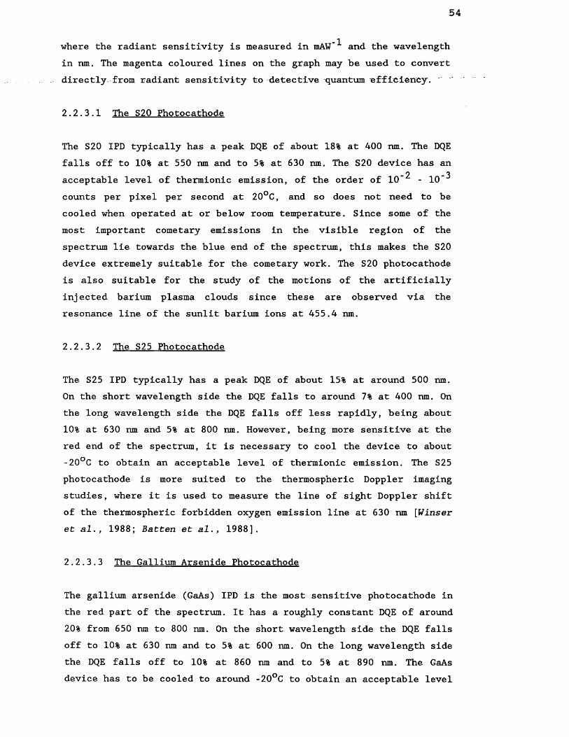
54

where the radiant sensitivity is measured in mAW"^ and the wavelength in run. The magenta coloured lines on the graph may be used to convert directly from radiant sensitivity to detective quantum efficiency:

2.2.3.1 The S20 Photocathode

The S20 IPD typically has a peak DQE of about 18% at 400 ran. The DQEfalls off to 10% at 550 nm and to 5% at 630 ran. The S20 device has an

-2 -3acceptable level of thermionic emission, of the order of 1 0 - 1 0

counts per pixel per second at 20°C, and so does not need to be cooled when operated at or below room temperature. Since some of the most important cometary emissions in the visible region of the spectrum lie towards the blue end of the spectrum, this makes the S20 device extremely suitable for the cometary work. The S20 photocathode is also suitable for the study of the motions of the artificially injected barium plasma clouds since these are observed via the resonance line of the sunlit barium ions at 455.4 nm.

2.2.3.2 The S25 Photocathode

The S25 IPD typically has a peak DQE of about 15% at around 500 nm. On the short wavelength side the DQE falls to around 7% at 400 nm. On the long wavelength side the DQE falls off less rapidly, being about 10% at 630 nm and 5% at 800 nm. However, being more sensitive at the red end of the spectrum, it is necessary to cool the device to about -20°C to obtain an acceptable level of thermionic emission. The S25 photocathode is more suited to the thermospheric Doppler imaging studies, where it is used to measure the line of sight Doppler shift of the thermospheric forbidden oxygen emission line at 630 nm [Winser et al. , 1988; Batten et al., 1988].

2.2.3.3 The Gallium Arsenide Photocathode

The gallium arsenide (GaAs) IPD is the most sensitive photocathode in the red part of the spectrum. It has a roughly constant DQE of around 20% from 650 nm to 800 nm. On the short wavelength side the DQE falls off to 10% at 630 nm and to 5% at 600 nm. On the long wavelength side the DQE falls off to 10% at 860 nm and to 5% at 890 nm. The GaAs device has to be cooled to around -20°C to obtain an acceptable level

55

of thermionic emission. The APL operates one GaAs IPD, currently located at Utah State University, where it is used to derive mesospheric winds by measuring bhe emissions from OH at 843 rtin.

2.2.4 Set-up of the Imaging Photon Detector

Low voltage power for the IPD charge amplifiers and the high voltage unit is supplied from the SPU via a 6 -way lemo plug. The four output signals from the charge amplifier outputs, taken from the electrodes in quadrature from the resistive anode, are taken from the detector to the SPU via four BNC cables. The SPU itself is powered by the 240 V mains, modifiable internally to 115 V. The analogue output is available at two BNC sockets where the "X" and "Y" coordinates of each photon event are output as a voltage from 0 to 1 0 volts. Connection to an oscilloscope in "XY" mode results in an image being seen as a series of dots. The digital output is taken via a 40-way ribbon cable to the Tecmar base board interface of a suitable Personal Computer (PC) .

Before supplying power to the IPD it is essential to ensure that the photocathode is seeing only extremely low light levels because the photocathode can be permanently damaged by sudden exposure to bright light. A useful rule of thumb is that if the light is visible to the dark adapted human eye it is too bright for the IPD.

The image size is normally adjusted so that the circular area of the photocathode extends just beyond the electronic "X-Y" field. If the circular area of the photocathode falls completely within the "X-Y” field then this will be at the expense of resolution. This adjustment is best done on an oscilloscope with the detector exposed to enough light so that the entire area of the photocathode is illuminated.

The charge pulses collected from the IPD anode do not all have the same amplitude. The pulse height spectrum is a function of channel plate saturation, and is normally well defined. The upper and lower threshold controls set a pulse height window which rejects noise and pulses which are too large or too small for the processing electronics to handle. The lower threshold is set at around -0.25 V and the upper threshold to approximately -3.0 V. The position of the

56

lower threshold is fairly critical and is set just above the noise level. MCP noise occasionally gives rise to low-level pulses which appear as "hot-spots" on the image. These can often be removed by adjusting the lower threshold, though sometimes at the expense of genuine photon counts. The purpose of the upper threshold is to block the large pulses caused by a combination of pulse overlap, internal discharge and cosmic rays, which do not represent real data.

2.2.5 Image Collection and Storage

The IPD is controlled by a micro-computer such as an IBM PC or IBM compatible machine such as the Compaq-286. The run program is used to collect, display and store images of the desired integration time. Each image is stored as a 256 x 256, integer x 2 file with the first row being used as a header and storing information appropriate to the image. Each image, therefore, occupies 131 kbytes of memory.

Table 2.1 Procedure used for Naming the Files on the Field PC

Month Code Date Code Date Code Date Code

J anuary A 1 1 13 D 25 PFebruary B 2 2 14 E 26 QMarch C 3 3 15 F 27 RApril D 4 4 16 G 28 SMay E 5 5 17 H 29 TJune F 6 6 18 I 30 UJuly G 7 7 19 J 31 VAugust H 8 8 2 0 KSeptember I 9 9 2 1 LOctober J 1 0 A 2 2 MNovember K 1 1 B 23 NDecember L 1 2 C 24 0

The file is named automatically according to the UT date and time. The method adopted for naming files is best described by referring to

57

an example filename:-

. . . - Example of P.C. filename: E32115.D31

The first label (E) represents the month, and the second label (3) the date. These labels are assigned according to the notation described in table 2.1. The remaining six digits refer to the UT time at the end of the integration and the D stands for data file. Thus the example filename was recorded on 3 May at 21:15:31 UT.

2.2.6 Comparison of the Imaging Photon Detector with the Charge Coupled Device

The most popular detector in optical astronomy is undoubtedly the Charge Coupled Device (CCD). The reasons for using the IPD, therefore, need to be discussed. More detailed comparisons between the performances of IPDs and CCDs may be found in the literature [Ailington-Smith & Schwarz, 1984; Abreu & Skinner, 1988].

For integration times less than 1,000 s the IPD has been found to have a proportionally higher signal-to-noise ratio in cases where the sources were photon limited [.Rees et al., 1984], This is due to the fact that CCDs have a time-independent noise associated with the readout of the charge accumulated during an integration of the order of 40 equivalent photon events per pixel per readout. The IPD has no readout noise [Rees et al., 1984] and is only affected by the thermionic emission of electrons, which may be reduced by cooling if necessary.

CCDs have a very high quantum efficiency in the red part of the spectrum which reach as much as 80%. The quantum efficiency of IPDs, which is set by the photocathode, rarely exceeds 2 0 % even at the peak which is in the blue for S20 devices, green for S25 devices and in the red for GaAs devices (see section 2.2.3).

IPDs have a saturation limit of the order 150,000 counts per second as discussed in section 2.2.2. CCDs are only limited by the total number of counts in each pixel (1 0 per pixel).

58

CCDs are small devices (about 10 mm) with pixels of fixed size (about 30 microns) set by the manufacture of the device. IPDs can be made larger (> 40 mm) and have a pixel size that can be suited to a particular observation.

CCDs need to be cooled to liquid nitrogen temperatures in order to reduce the thermal noise to a negligible level, whereas many IPDs can be operated at room temperature without significant thermal noise. However, IPDs with very high red sensitivity photocathodes, ie S25 and GaAs devices, should be cooled to about -20°C to optimize their performance.

Although CCDs generally have much higher peak quantum efficiency, the differing noise characteristics and spectral range favour the use of IPDs for applications which require high time resolution. This is especially the case in the observations of the artificial chemical releases, where only short integrations, of the order 30 s , are appropriate, due to the rapid evolution of the resulting ion clouds.

2.3 The Very High Sensitivity Imaging Systems used to Observe the Natural and Artificial Gas and Plasma Clouds

The Very High Sensitivity Imaging System (VHSIS) consists basically of an IPD and a narrow-band interference filter. When the VHSIS is used at the Cassegrain focus of a telescope it is set up on an optical bench as described in section 2.3.1. When the VHSIS is used with a Nikon camera lens, the lens is simply mounted onto the IPD via a Nikon camera lens mount and a filter holder. The narrow-band interference filters used with the VHSIS systems are discussed in section 2.3.2. A description of the set-up of the VHSIS on a telescope is given in section 2.3.3. The method of observing a cometary target is described in section 2.3.4. Finally, the important calibrations necessary for the correct interpretation of the VHSIS data files are discussed in section 2.3.5.

59

2.3.1 The Optical Bench

When used with a moderate sized telescope the imaging system is mounted on an optical bench consisting of four steel rods and four mounting plates as shown in figure 2.4. The light from the telescope enters the system through a large aperture in the first plate which also functions as a support and mounting plate. This plate contains four screw threads enabling it to be attached to the telescope mounting plate. The second plate holds the filter wheel which can hold up to three 2" diameter filters. The detector is mounted on the third plate. The fourth plate is the other end plate. The power and signal leads to/from the detector pass through a small light-tight aperture in this plate. The entire optical bench is enclosed in a light-tight cover. The VHSIS is then fastened to the telescope mounting plate and finally attached to the telescope. Figure 2.10 shows the 24" telescope at the Table Mountain Facility (TMF) of the Jet Propulsion Laboratory (JPL), with the VHSIS in position.

2.3.2 The Narrow-Band Interference Filters

The relevant emissions are isolated by state-of-the-art, three- cavity, anti-reflectance coated, narrow-band interference filters.

The heart of a narrow-band interference filter is a series of thin film, partially-reflecting layers arranged as a single or multiple Fabry-Perot interferometer. The spacing between the layers is chosen so that the beams produced by multiple reflections from the layers are in phase with the transmitted beam for the desired wavelength thus enhancing the transmittance of the filter at that wavelength. Other wavelengths are rejected because these multiple beams interfere destructively. A wide variety of band widths and beam shapes are obtainable by varying the reflectivities, the number of layers and the number of Fabry-Perot cavities. The basic series of films deposited on a substrate forms a simple unblocked interference filter which, depending on its design, will have side-bands on both sides of the desired passband. These side-bands are eliminated by blocking filters. Coloured glass absorption filters are also used to provide further blocking.

60

Figure 2.5 gives an indication of the approximate shapes and nearband rejection that can be expected in two-, three- and four-cavity filters. The APL narrow-band interference filters all have three cavities. The Full Width Half Maximum (FWHM) of the majority of these filters is 1 nm. Thus the transmittance is approximately constant within 0.1 nm of the central wavelength, falling to 90% of the peak transmittance 0.25 nm from the central wavelength and to 50% of the peak transmittance 0.5 nm from the central wavelength. The transmittance becomes 1 % of the peak transmittance 1 nm from the central wavelength and below 0.01% of the peak transmittance 2.5 nm from central wavelength.

Transmission characteristics of interference filters change with temperature, due to the contraction and expansion of the spacers and coatings. Interference filters shift to longer wavelengths with increasing temperature and to shorter wavelengths with decreasing temperature. In the visible region, the temperature dependence of the central wavelength is approximately 0.015 nm per degree centigrade change. The interference filter is not temperature controlled so that the peak transmission will vary by a small amount depending on the temperature in the dome. However, since relative intensities only are recorded, this small effect may be completely ignored.

Filters are usually designed for use at normal incidence. However, they may be designed for specific non-normal applications. Non-normal incidence results in a shift of the passband toward shorter wavelengths. The amount of shift depends on the angle of incidence, the effective index of refraction of the filter, and the plane of polarization of the light. Increasing the angle of incidence for unpolarized light not only shifts the band to shorter wavelengths but broadens and for very large angles causes it to become misshapen or even split. For visible wavelengths the approximate amount of shift can be determined from the equation:-

Av/(n^ - sin^i)

n2 . 2

61

where i is the angle of incidence of the radiation, A is the central wavelength at the angle of incidence and n is the effective index of the filter. The value of n typically lies in the range 1.5 to 2.0. Ideally an interference filter should be placed in a parallel beam of light. However, both in the VHSIS and DIS the filter is placed in the converging beam in front of the detector. For the 1 nm FWHM filters, this is certainly justified for instruments with focal lengths down to 180 mm.

Table 2.2 List of the Narrow-Band Interference Filters used with theVHSIS and DIS

Filter (nm) FWHM (nm) Species Isolated

387.1 5 CN388.2 1 CN402.0 1 co+

406.0 (IHW) 7 C3426.0 (IHW) 6.5 C0+455.4 3 Ba+ , C0+471.6 1 c2514.0 (IHW) 9 c2

524.2 0.3 continuum557.2 1 0 1

580.0 1 h2o+589.0 1 Na630.5 1 0 1 , nh2

700.0 (IHW) 17.5 h2 o+

A complete list of the narrow-band filters used in the cometary campaigns is given in table 2.2. These filters belong to the APL unless otherwise stated. The International Hailey Watch (IHW) filter set was used, in addition to the APL filter set, for some observations of the comets Giacobini-Zinner and Hailey. The IHW filters have much larger passbands than the APL filters and experience has shown that much better results are obtained with the IPD when the APL filters are used. This is due to the smaller FWHM of the APL filters which reduces the night sky background level, the

62

contamination from the continuum (dust) and the contamination from any neighbouring cometary lines.

2.3.3 Instrument set-up on the Telescope

The IPD is initially adjusted as described in section 2.2.3 and theoptical components are set up on the optical bench as described insection 2.3.1. The imaging box is then fastened to the telescope.

A schematic diagram showing the complete system layout, as set up for use with a telescope, is given in figure 2.6. This may be compared with the actual instrument set-up as shown in the photograph of the 24" telescope at TMF (figure 2.11). A photograph of the control console for the 24" telescope is shown in figure 2.12.

Once the VHSIS is in place on the telescope it is essential to ensure that the instrument is correctly aligned and focused prior to attempting to view any cometary object. Since comets usually appear as a fuzzy patch they cannot be used to ascertain whether or not the instrument is correctly focused. Therefore, prior to any cometary observations, the telescope is focused by obtaining the sharpest possible image of a star. The best targets are stars of third or fourth magnitude. Second magnitude and brighter stars usuallyoverload the detector, even through the narrow-band filter, and fifth magnitude or fainter stars produce too few photons for real-time focusing. The instrument is coarsely focused by repeatedlyapproaching the focus from both sides until the sharpest stellar image is obtained on the oscilloscope. Fine tuning of the focus is achieved by examining the profile of the stellar image collected by the PC and changing the focus until the sharpest profile is obtained.

The conventional way of displaying astronomical objects is such that the image orientation on the screen corresponds to the image as seen on the sky. Since the position of a particular photon event is determined by the ratio of the charges collected at the four corners of the resistive anode sheet (section 2 .2 .2 ), the four signal leads from the IPD can be arranged so that the image recorded by the computer has the correct orientation, with north at the top of the image and east to the left of the image.

63

2.3.4 Observing a Cometary Target

Comets move fast relative to the stars, especially when in the innerSolar System. It is, therefore, important to know the position of thecomet at regular intervals throughout any observing session to aid inits location, especially if it is faint. Up-to-date orbital parameters of any comet are published in the circulars of the International Astronomical Union (IAU). The JPL ephemeris program, modified for use on STARLINK by Simon Green (University of Kent at Canterbury) , can be used with these parameters to work out cometary positions and movements as a function of time.

The large telescopes can be precisely pointed and require the cometary coordinates in right ascension (RA) and declination (dec), which are taken from the appropriate ephemeris. The 1 m Jacobus Kapteyn Telescope (JKT) at La Palma can be used to offset track on the cometary target by entering the appropriate offset rates in seconds of arc per second. The 24" telescope at TMF can also be used to offset track. There is a linear relationship between the offset rates at the telescope control console and the comet offset rates, enabling the telescope to track on the comet. However, the pointing system is not as sophisticated as on the JKT and the effects of refraction are not taken into account. The 16" telescope at TMF has no offset capabilities and so, to avoid blurring, series of short integrations, of the order 1 - 2 minutes, are taken.

The Meade 8 " portable telescope is set up by the observer in the field. The IPD is mounted directly onto the telescope via a filter holder. No offset tacking on the comet is possible with this instrument and so, as with the 16" telescope at TMF, series of short integrations are used.

Any Nikon camera lens used with the VHSIS is mounted via a Nikon camera mount and a filter holder onto the IPD. For the cometary imaging the IPD is mounted piggy-back onto the large telescope being used, so that the telescope is used to locate and track on the comet. For the artificial chemical releases the IPD is mounted piggy-back onto the DIS being used.

64

2.3.5 Calibration of the Very High Sensitivity Imaging System

The following three calibrations are absolutely essential for the correct interpretation of the raw imaging data.

2.3.5.1 Thermionic Emission Calibration

Thermal electrons emitted from the photocathode cannot bediscriminated from photoelectrons and are a source of noise. However,the rate of thermionic emission for a given IPD can be removed byperforming a thermionic emission calibration. Since the thermionicemission is a function of temperature, this calibration is performedat the temperature at which the detector is to be operated. Thephotocathode is light-sealed and a long integration (about 1 hour)performed. This is the thermionic emission data file. The longintegration time is required to allow a useful signal-to-noise ratioto be obtained, since the thermionic emission rate is normally very

- 2 - 3low, of the order 1 0 - 1 0 counts per pixel per second.

2.3.5.2 Flat Field Calibration

The detector does not respond uniformly to an even source of light. However, the IPD is a photometrically and geometrically stable device, so that the flat field response depends mainly on the wavelength of the incoming light. The flat field response of the imaging system being used is obtained by observing the twilight sky through the complete optical system, independently, with each filter used. The flat field image for each filter is then used to correct all images taken with that filter.

2.3.5.3 Skv Background Calibration

Sky background calibrations are necessary for images in which the observed signal extends beyond the field of view of the detector. This is particularly true of the near-nucleus comet images obtained with the VHSIS on moderate sized telescopes. In this case it is essential to have a knowledge of the sky background level if the cometary component is to be determined with any accuracy.

65

The radiation which contributes to the brightness of the night sky can be separated into atmospheric and extra-terrestrial components. The contribution from the former comes from a mixture of airglow, auroral emission and artificial and natural light scattered by aerosols. The contribution from the latter comes from sunlight scattered from the Moon and interplanetary dust (zodiacal light and gegenschein) and starlight scattered by interstellar dust grains. The relative importance of each component varies both with position and time on the night sky making the sky background level a complicated function of position and time. Sky background images are, therefore, taken immediately before and after a series of cometary integrations with a given filter, and are taken from a region of the sky close to the comet but also far enough removed to ensure no cometary contamination (typically 5° of arc from the comet). The integration time for the sky background image is similar to that used to record the sequence of raw comet images (typically 5 - 1 0 minutes).

2.4 Principles of Operation of the Doppler Imaging System

The Doppler Imaging System (DIS) is basically an Imaging Fabry-Perot Interferometer of high spectroscopic resolution. The DIS consists, essentially, of a Fabry-Perot spectrometer coupled to an IPD. Several fringes from a Fabry-Perot etalon are imaged onto the IPD enabling the detector to record the Doppler shift in a particular part of the two-dimensional field of view as a distortion of the Fabry-Perot ring in that region. This technique yields the spatial morphologies observable by any imaging system and also details the velocity distribution of the emitting gas.

In order to describe the DIS in more detail it is first necessary to discuss the Fabry-Perot etalon. The principles of operation of the Fabry-Perot etalon are outlined in section 2.4.1 and the construction of the Fabry-Perot etalons used by the APL are described in section 2.4.2. The DIS itself is introduced in section 2.4.3. The set up of the DIS is discussed in section 2.4.4 and the instrument calibrations are discussed in section 2.4.5.

66

2.4.1 Theory of the Fabrv-Perot Etalon

In principle, the Fabry-Perot etalon consists of two plane, parallel, highly reflecting surfaces separated by a distance, t. Its operation is based on the multiple interference of a single beam. When the etalon is illuminated by a broad source of monochromatic light the different angles of incidence produce various path differencesbetween reflections from the upper and lower plate. The pathdifference between adjacent transmitted rays for a given angle of incidence 9 is 2tcos 9 , and the condition for constructiveinterference is:-

nA 2tcos0 2.3

2t 2.4

for small 9 . If the focal length of the positive lens used to focus the fringes is L and the distance of a peak from the centre of the

2.5

fringe system is r then:-

rtan 9 = — 9 for

Land the condition for peaks becomes -

1 ~r 2 1nA - 2t 1 --- — + ...

2 L2 . 6

The Fabry-Perot fringes are thus narrow concentric rings, corresponding to the multiple-beam transmission pattern. An example Fabry-Perot fringe pattern is shown in figure 3.6.

The central fringe has an order given by:-

2tn = - 2.7

A

Thus the order of the first fringe is inversely proportional to the wavelength. As the wavelength of light is increased the order of the first fringe decreases so that fringe pattern contracts. Conversely if the wavelength of light is decreased the fringe pattern expands.

67

It can be shown, by summing the amplitudes of the light rays emerging from the etalon (see any standard text book on optics eg B o m & Wolf; Hecht & Zajac), that the transmitted intensity, It, is:-

10 2.8

1 +4Rsin2(5/2)

(1 -R )2

where:-

RSlo

is the reflectance of the coated surfaces of the etalon, is the phase difference between adjacent transmitted rays and is the maximum intensity.

This may be rewritten:-

where:

io 2.9

1 + Fsin2(6/2)

4R 2.10(1-R)

Peaks, thus, occur at specific values of the phase difference given by 27rn. The intensity will drop to half its maximum value whenever:-

1

1 + Fsin (6/2)2.11

2sin-11

V'F2.12

F is generally large so that sin~^(l^/F) — 1//F and, therefore, the half width is:-

4

\/F2.13

An important quantity is the Free Spectral Range (FSR) of an etalon which is the particular wavelength difference at which the n th order

68

fringe for one wavelength, ^ 1 , overlaps with the (n+1 ) th order of some other wavelength, A2 . We may write:-

nAj 2t 2.14

(n+l)A2 2t 2.15

2.16=» FSR

2t

The ratio of the Free Spectral Range (FSR) to the Full Width Half Maximum (FWHM) of the Fabry-Perot fringe is an important quantity known as the finesse and is given by:-

Over the visible range the finesse of most Fabry-Perot etalons is about 30. The finesse is physically limited by deviations in the plates from plane parallelism and by surface defects.

2.4.2 Construction of the Fabry-Perot Etalon

The design and fabrication of the Fabry-Perot etalons used by the APLhave been discussed in detail in the literature [Rees et al., 1981b; 1982b; Killeen et al., 1982]. The optical components of the etalons are manufactured by I.C. Optical Systems.

Any etalon will have limitations due to the intrinsic thermal andmechanical stability of its components. For example, small dimensional changes in the etalon gap of the order of a small fraction of the wavelength of light can cause intolerable drift, producing deleterious effects on the instrument calibration. By careful selection of the component materials, the design of the etalon housing and the etalon mount, the APL, in collaboration with the University of Michigan, were able to develop a very stable rugged etalon for the Fabry-Perot interferometer flown on the NASA Dynamics Explorer satellite mission [Rees et al., 1982b; Killeen et al., 1982]. The majority of etalons built for the APL since then have been designed along similar lines.

2irfinesse 2.17

7 2

69

Basically the etalons are constructed from two plates of fused silica (Spectrosil B) separated by three spacers made of Zerodur. Zerodur is a trade name of Schott optical glass and is a polycrystalline glass ceramic of low expansion coefficient. The two inner surfaces are polished flat to better than 3 nm rms. They are coated with a multilayer dielectric coating to give a peak reflectivity of about 90% over a specified wavelength range. This corresponds to a theoretical finesse of about 30, although the actual finesse obtained is less than this. The disagreement between the calculated and the measured finesse can be attributed to the broadening of the spectral line by the fringe profile and the blurring effects of plate and coating distortions on the interference pattern [Killeen et al., 1981].

The two outer surfaces are flat to 300 nm and are normally set with a wedge angle to the inner etalon surfaces of about 45 arc minutes. This offsets the parasitic fringes caused by interference between the inner and outer surfaces. The parasitic fringes are further decreased by anti-reflectance coating the outer surfaces to give a low reflectivity over the wavelength range at which the etalon is to be used.

The etalon is housed in a mount made of Invar which is used to mechanically hold the etalon and to allow adjustment of the etalon space by three cantilever springs. The mathematical principles of the design are described in detail in Killeen et al. [1982].

The etalon plates can be adjusted to ensure that they are parallel by careful adjustment of the three springs holding the etalon. This is best done by observing the fringes from a diffused He/Ne laser source with the eye. The pupil of the eye may be considered as a small elemental area and as it is moved over the surface of the etalon the fringes will be seen to expand and/or contract if the plates are not exactly parallel or are distorted from flatness. Only when the plates are precisely aligned will the size of the fringe pattern remain constant. This is because the etalon surface may be regarded as being made up of smaller elemental areas each being its own independent etalon. If the etalon plates are not parallel each elemental etalon will be slightly different from its neighbour resulting in a slightly

70

different fringe pattern as seen by the eye. If an instrument is operated with an etalon whose plates are not correctly adjusted, the fringe pattern will be degraded and the fringes broadened.

Once the etalon plates have been adjusted correctly, the etalon is sealed in an air-tight container and evacuated to about 1-10 mm Hg. This prevents atmospheric pressure changes from altering the refractive index of the air in the gap. It also minimizes the effects of any lack of temperature stability.

A selection of the Fabry-Perot etalons that have been used by the APL are shown in figure 2.7. On the left is a 13.2 cm aperture, capacitance-stabilized etalon [2?ees et al., 1981b]. The etalon in the middle has an aperture of 5 cm and is similar to the etalon flown on the Dynamics Explorer-2 satellite. The etalon on the right is another capacitance-stabilized etalon.

2.4.3 The Doppler Imaging System

The Doppler Imaging System (DIS) consists of a Fabry-Perot etalon, a narrow-band interference filter, a positive lens, and an IPD all mounted on an optical bench, similar to that described for the VHSIS in section 2.2.1. The DIS may or may not have optical components in front of the Fabry-Perot etalon.

2.4.3.1 Set-up of the Doppler Imaging System

The IPD is initially adjusted as described in section 2.2.3 and the Fabry-Perot etalon is adjusted for plate parallelism as discussed in section 2.4.2. The components are then set up on the optical bench.

The instrument is coarsely focused by illuminating the front of the etalon with diffused light from an appropriate calibration lamp and observing the fringe profile obtained with the detector in real-time on an oscilloscope. The detector can be moved back and forth on the optical bench until the sharpest fringes are obtained. Fine tuning of the focus is achieved by examining the fringe profile of the calibration image collected on the PC and adjusting the detector until the sharpest fringe profiles are obtained.

71

The etalon is normally adjusted so that the Fabry-Perot fringes are centred on the pho to cathode. This is done by means of three offset screws and three locking screws at the front of the etalon can. The etalon is illuminated as described above and the screws adjusted until the fringes are centred.

2.4.3.2 Calibration of the Donnler Imaging System

The thermionic emission calibration of the IPD in the DIS is performed in exactly the same manner as described for the VHSIS (section 2.3.5).

The instrumental flat field response is measured by observing the twilight sky through the DIS, in much the same way as described for the VHSIS (section 2.3.5).

A full-field spectrometric calibration is achieved by recording the fringes obtained from an appropriate calibration lamp. This calibration provides a reference level from which the relative line of sight velocities are determined.

The full-field spectrometric calibration is performed before and after any given experiment. A typical Fabry-Perot ring system, obtained from a barium calibration lamp, is shown in figure 3.6.

2.5 The Doppler Imaging Systems used to Observe the Natural and Artificial Gas and Plasma Clouds

Over the past six years several different Doppler Imaging Systems have been used to observe the artificial chemical releases and the cometary targets. The DIS systems used to observe the artificial chemical releases generally have no optical components in front of the etalon, and the DIS currently employed for the artificial chemical releases is discussed in section 2.5.1. The DIS systems used with moderate sized telescopes employ a negative lens in front of the etalon to illuminate the etalon with parallel light from a range of angles. The design of the DIS for the cometary work depends on the goals of the experiment. At present the DIS has been successfully deployed with moderate sized telescopes to reveal velocity structures

72

in the inner neutral coma but has not yet succeeded with the cometary ions. The DIS currently used with the 24" telescope at TMF has been designed to achieve this elusive goal and is described in section 2.5.2.

2.5.1 The Doppler Imaging System used to Observe the Artificial Gas and Plasma Clouds

The DIS used to observe the artificial chemical releases consists of a Fabry-Perot etalon, lens, filter and IPD, mounted on an optical bench. The optical bench consists of four steel rods and five mounting plates. These plates are firmly locked into position by grub screws once the instrument is correctly set up. The whole instrument, when assembled, is extremely stable, which is absolutely essential, since accurate positioning of the fringe pattern on the detector must be maintained at all times.

The Fabry-Perot etalon is mounted on the first plate at the front of the instrument. This first plate doubles up as an end plate. A positive lens is mounted on the second plate, immediately behind the etalon. The IPD is mounted on the fourth plate in the focal plane of the positive lens. The interference filter is mounted on the third plate, immediately in front of the detector. The fifth plate is theother end plate. The entire optical bench is enclosed in a light­tight cover.

The Fabry-Perot etalon currently used in this DIS to observe the artificial chemical releases has a working diameter of 80 mm and a fixed gap of 3 mm, corresponding to a free spectral range of 22.8 kms“^ at 455.4 nm. A positive lens, which has a diameter of 80 mm and a focal length of 400 mm, is used to focus the Fabry-Perot fringe pattern onto the front of the detector. The interferencefilter is centred at 455.4 nm and has a FWHM of 1 nm and so passesthe 455.4 nm emission line of sunlit barium ions. Since the diameter of the photocathode is 18 mm, the instrument field of view is of the order 2.5° of arc. Approximately 3 Fabry-Perot fringes are imaged onto the photocathode with this arrangement.

73

2.5.2 The Doppler Imaging System Designed for use with the 24" Telescope to Observe Line of Sight Velocities in the Cometary Ion Coma and Tall

The aim of this investigation is to reveal the line of sight velocities of the ions in the cometary coma and tail. The design of such an instrument depends on several instrumental parameters and the anticipated average line of sight velocities.

For the present study the fixed instrumental parameters are the diameter of the primary mirror (60 cm), the effective focal length of the primary mirror (900 cm), the usable diameter of the etalon plates (18 mm) and the diameter of the photocathode (18 mm).

The parameters to be determined are the focal length of the negative lens, f-p the etalon gap, t, and the focal length of the positive lens, f2 - The diameter of the two lenses should be slightly larger than the diameter of the etalon plates.

2.5,2.1 Determination of the Focal Length, f^ . of the Negative Lens

The focal length, f^, of the negative lens determines the diameter ofthe beam of light illuminating the etalon.

The radius of the primary mirror is 30 cm and its effective focal length is 900 cm. The radius of the etalon is 9 mm. Therefore, by similar triangles, as shown in the diagram (figure 2 .8 ):-

fi 0.91 2.18

900 30

2.19=► f j = 27 cm

The focal length of the negative lens should, therefore, be of theorder of 27 cm.

74

2.5.2.2 Determination of the Etalon Gap ft")

The etalon gap depends on the free spectral range required and the wavelength (A) being examined, according to the relationship:-

cAt = 2.20

2FSR(v)

where FSR(v) is the Free Spectral Range in velocity units.

The two ion species of particular interest for these studies are C0+X J.and H2 O . The CO molecule is observed in resonance fluorescence at

402.0 nm and the ^ 0 * molecule is observed in resonance fluorescence at 580.0 nm.

No single fixed etalon is capable of measuring the range of line of sight velocities expected in the ion coma. The velocity of the solar wind is typically 400 kms"^ and this is the velocity that is eventually attained by the ions. However, the velocity of the ions in the head of the comet will be less than this. A good survey of the ion velocities would be possible with a set of etalons having free spectral ranges of the order 50 kms'^, 100 kms”\ 200 kms’^ and 400 kms"^.

Consider a wavelength of 490.0 nm, intermediate between the two emissions to be studied. The etalon gaps required become 1.5 mm, 0.75 mm, 0.37 mm, and 0.18 mm as tabulated in figure 2.8. The free spectral ranges in units of velocity for the two wavelengths of interest for each etalon gap are given in table 2.3.

Table 2.3 The Free Spectral Range Obtained with Different Etalons

Etalon Gap FSR(v) at 402 nm FSR(v) at 580 nm1 1(mm) (kms ) (kms )

1.5 40 580.75 80 1160.37 160 2320.18 320 464

75

A study of the line of sight velocities of the ions in the head of a comet is possible with the four etalon gaps tabulated in table 2.3.

2•5.2.3 Determination of the Focal Length, fo. of the Positive Lens

The focal length, f2 , of the positive lens is an important parameter as it determines how many fringes fall onto the surface of the photocathode for a given wavelength. Three or four fringes should be mapped onto the detector to obtain a good velocity map. The focal length f£ may be calculated with a knowledge of the angular separation between the central fringe and the fourth fringe from the centre.

The angular separation may be computed as follows. The order, n, of the central fringe is given by equation 2.7. Therefore, the angular separation, 9 , between the central fringe and the fourth fringe from the centre is given by:-

cos-1(n - 4)A

2 t2.21

cos-12A

1 - 2 . 22

This angle depends on both the wavelength of light and the plate separation. It is tabulated in table 2.4 for each etalon gap at the two wavelengths.

Table 2.4 Angular Separations Between the Fourth Fringe and the Central Fringe

Etalon gap Q at 402 nm G at 580 run(mm) (radians) (radians)

1.5 0.033 0.0390.75 0.046 0.0560.37 0.065 0.0790.18 0.095 0.114

76

Thus the smallest angle to the optic axis subtended by the fourth fringe is 0.33 radians produced with a 1.5 mm gap etalon at 402 nm. The focal length, f£, would be 27 cm in this case. The largest angle subtended by the fourth fringe is 0.114 radians produced with the 0.18 mm gap etalon at 580 nm. The required focal length would be 7.9 cm.

The entire system, consisting of negative lens, Fabry-Perot etalon, narrow-band filters, positive lens and IPD is mounted on an optical bench, similar to that described for the VHSIS in section 2.3.1.

2 .6 The Sites and Instruments used to Observe the Cometarv Targets

Two principal sites have been used in the cometary program, the Observatorio del Roque de los Muchachos, La Palma, Canary Islands and the Table Mountain Facility, California, USA (section 2.6.1). A number of different instruments have been used to observe the cometary targets from these two sites and these are described in section 2.6.2. Some important instrumental parameters are tabulated in table 2.5 and the sites used and the instruments deployed are summarized in table 2 .6 .

Table 2.5 Summary of the Instruments used to Observe the Cometary Targets

Instrument Effective Field of view Pixel sizefocal length (arc minutes) (arc seconds)

1 m JKT 15 m 4.13 0.9724" Telescope 9 m 6.87 1.6116" Telescope 6 m 10.3 2.418 " Telescope 2 m 30.9 7.24

300 mm Nikon 0.3 m 206.4 48.4180 mm Nikon 0.18 m 343.2 80.4

77

2.6.1 The Sites used to Observe the Cometary Targets

2.6 .1.1 The Observatorio del Roque de los Muchachos

The Observatorio del Roque de los Muchachos is situated on the island of La Palma which lies in the northwest of the Canarian archipelago. The observatory is at an elevation of 2,369 m, longitude 17° 52’ 34" W, latitude 28° 45' 34" N. The site houses the4.2 m William Herschel Telescope, the 2.5 m Isaac Newton Telescope and the 1 m Jacobus Kapteyn Telescope. All three are operated by the Royal Greenwich Observatory. Also on the mountain are the recently dedicated 2.5 m Nordic Optical Telescope, a solar telescope, a 61 cm reflector and the Carlsberg Automatic Meridian Circle. The observatory is owned by Spain and administered by the Canary Island Institute of Astrophysics.

2.6 .1.2 The Table Mountain Facility

The Table Mountain Facility (TMF) is situated in the San Gabriel Mountains in California near the village of Wrightwood. The observatory is at an elevation of 2,287 m, longitude 117° 40' 48" W, latitude 34° 22' 54" N. It is equipped with a 24" telescope, a 16" telescope, a Schmidt camera and a solar observing facility. A 48" telescope is currently under construction. It is owned and operated by the Jet Propulsion Laboratory, California Institute of Technology.

2.6.2 The Instruments used to Observe the Cometary Targets

The JKT, the 24" telescope and the 16" telescope have been used for near-nucleus studies. An 8 " portable Meade telescope and 300 mm and 180 mm Nikon camera lenses have been used for large-scale imaging.

2.6 .2.1 The Jacobus Kaptevn Telescope

The 1 m Jacobus Kapteyn Telescope (JKT) (figure 2.9) is an ideal telescope for monitoring near-nucleus phenomena. The IPD is employed at the f/15 Cassegrain focus, producing a field of view of 4.13 arc minutes across the 18 mm diameter photocathode. The telescope is fully computer controlled. At the start of any observing session the

78

telescope is calibrated in right ascension (RA) and declination (dec)by centering a known star in the field of view of the detector. Thecoordinates of the comet are then entered and the telescope is driven to the target. Differential offset rates may be entered enabling the telescope to track the comet.

2.6 .2.2 The 24" Telescope at TMF

A picture of the 24" telescope is shown in figure 2.11. The VHSIS canbe seen bolted on to the telescope. The IPD is employed at the f/15 Cassegrain focus, producing a field of view of 6.87 arc minutes across the detective surface. Hence, the 24" telescope is a good instrument for monitoring near-nucleus activity. Figure 2.12 shows the operating console together with the equipment for controlling the detectors. The telescope position is read from clocks registering the RA and dec. The telescope is driven manually to its target by using a joy stick, which drives the telescope in RA and dec. The telescope is capable of offset tracking, there being a linear relationship between the offset rates at the console and the cometary offset rates.

2.6 .2.3 The 16" Telescope at TMF

The 16" telescope was used to study near-nucleus structures of comet Hailey when the 24" telescope was not available. On the 16" telescope, the IPD is used at the f/15 Cassegrain focus producing a field of view of 10 arc minutes. Like the 24" telescope it is controlled manually but unlike the 24" telescope it is not capable of offset tracking. Therefore, series of short integrations are taken to avoid blurring of the cometary target.

2.6 .2.4 The 8 " Meade Portable Telescope

An 8 " Meade portable telescope has been used to study large-scale phenomena from both observatory sites. Figure 2.10 shows the operational set-up at the La Palma Observatory when the Meade was used from the roof of the "Residencia", the accommodation block at the observatory. This telescope has a 2 m focal length which results in a field of view of 31 arc minutes. The Meade has no offset tracking capabilities and so series of short integrations are taken.

79

Table 2 .6 Log of the Cometarv Observations. together with the Instruments used

Comet Site Instruments Dates

P/G-Z 1984e LPO 8 ” Meade 1 m JKT 8 " Meade

25/08/85 - 27/08/85 28/08/85 - 03/09/85 04/08/85 - 13/08/85

P/Halley 1982i TMF 24" telescope & 300 mm Nikon

30/11/85 - 14/12/85

TMF 8 " Meade 24" telescope & Nikon lenses 16" telescope & Nikon lenses

28/02/86 - 04/03/86 05/02/86 - 18/03/86

19/03/86 - 23/03/86

LPO 1 m JKT 29/04/86 - 05/05/86& 300 mm Nikon

Wilson 19861 TMF 24" telescope 30/10/86 - 06/11/86

Sorrells 1986n TMF 24" telescope 19/05/87 - 30/05/87

Bradfield 1987s TMF 24" telescope 14/12/87 - 22/12/87& 300 mm Nikon

P/Borrelly 1987p TMF 24" telescope & 300 mm Nikon

14/12/87 - 22/12/87

B-M 1989o TMF 24" telescope & 300 mm Nikon

09/08/89 - 23/08/89

Austin 1989cl TMF 24" telescope & 300 mm Nikon

28/04/90 - 28/05/90

80

2.6 .2.5 The Nikon Camera Lenses

Two Nikon camera lenses, a 300 mm and a 180 mm, have been used to map large-scale structures. These lenses have corresponding fields of view of 3.4° of arc and 5.6° of arc respectively. These lenses are attached to an IPD, which is itself mounted piggy-back on the larger telescope (see, for example, figure 2 .1 1 ), enabling the long integrations necessary to determine the full extent of the cometary coma in the light of the various species.

2.7 The Sites and Instruments Used to Observe the Artificial Gas and Plasma Clouds

The majority of the artificial chemical release experiments to be monitored with VHSIS/DIS systems have been observed from ground-based sites. The exceptions being the AMPTE releases which were observed with a VHSIS/DIS system aboard the NASA Convair 990 airborne observatory. The sites used and the instruments deployed arediscussed in this section and are summarized in table 2.7.

2.7.1 The NASA Convair 990 Airborne Observatory

A VHSIS and DIS were used from aboard the NASA Convair 990"Galileo II" airborne observatory flown out of NASA Ames Research Center to observe the 27 December 1984 AMPTE "artificial comet"experiment (section 8.2) and the 21 March 1985 AMPTE magnetotail release (section 8.3). The VHSIS and DIS used in both of these experiments were identical. The VHSIS employed a 180 mm Nikon camera lens giving a field of view of 5.7°. The DIS employed a fixed gap etalon with a plate separation of 2 mm and a working diameter of 100 mm. The positive lens used to focus the Fabry-Perot fringes had a focal length of 200 mm. Attempts to observe the 18 July 1985 AMPTE "artificial comet" had to be aborted when the aircraft caught fire on the runway.

2.7.2 Poker Flats Research Range

A co-aligned VHSIS/DIS system was used from the optical site at Poker Flats Research Range, near Fairbanks, Alaska to observe two barium

81

shaped-charge releases from each of two rockets launched from the Range in March/April 1984 (section 8.4). The VHSIS employed a 180 mm Nikon camera lens, giving a field of view of 5.7°. The DIS employed a fixed gap, 80 mm working diameter, etalon with a plate separation of 2 mm. The positive lens used to focus the Fabry-Perot fringes had a focal length of 180 mm.

A co-aligned VHSIS/DIS system was used from the optical site at Poker Flats Research Range to observe two barium shaped-charge releases from each of three rockets launched from the Range in April 1986. The VHSIS employed a 300 mm Nikon camera lens to give a field of view of 3.4°. The DIS employed a fixed gap etalon with a plate separation of 2 mm and a working diameter of 80 mm. The positive lens used to focus the Fabry-Perot fringes had a focal length of 400 mm.

2.7.3 Wallops Island

Two VHSIS systems were used from the optical site at Wallops Island Rocket Range in May 1986 to observe releases from two rockets launched from the Range (section 8.5). Both of these systems employed 85 mm Nikon camera lenses to give a field of view of 12.1°.

2.7.4 Sondrestrom Incoherent Scatter Radar Facility

A co-aligned VHSIS/DIS system was used from the Sondrestrom Incoherent Radar Scatter Facility to observe two barium shaped-charge releases from each of two rockets launched from Sondrestrom Air Force Base in February/March 1987. The VHSIS employed a 180 mm Nikon camera lens to give a field of view of 5.7°. The DIS employed a fixed gap etalon with a plate separation of 3 mm and a working diameter of 80 mm. The positive lens used to focus the Fabry-Perot fringes had a focal length of 400 mm.

A co-aligned VHSIS/DIS was set up at the Sondrestrom Incoherent Radar Scatter Facility to observe two barium shaped-charge releases from a rocket launched from Andoya Rocket Range, Norway in December 1988. The VHSIS employed an 85 mm Nikon camera lens and the DIS was identical to that used from Sondrestrom in February 1987.

82

Unfortunately no observations were made of these releases due to bad weather over Sondrestrom at the time of the release.

Table 2.7 Log of the VHSIS/DIS Systems used to Observe the Artificial Chemical Release Experiments

Site Date PI VHSIS EtalonLens Gap

Poker Flats 30/03/84 Heppner 180 mm 2 mmPoker Flats 01/04/84 Heppner 180 mm 2 mmConvair 990 27/12/84 AMPTE 180 mm 2 mmConvair 990 21/03/85 AMPTE 180 mm 2 mmConvair 990* 18/07/85 AMPTE 180 mm 2 mmPoker Flats 01/04/86 Heppner 300 mm 2 mmPoker Flats 03/04/86 Wescott 300 mm 2 mmPoker Flats 13/04/86 Heppner 300 mm 2 mmSondrestrom 26/02/87 Wescott 180 mm 3 mmSondrestrom 05/03/87 Wescott 180 mm 3 mmLa Palma 26/02/87 Wescott 180 mm 3 mm

'k'kSondrestrom 19/12/88 Wescott 85 mm 3 mmChurchill 09/04/89 Hoffman 50 mm 3 mmChurchill 11/04/89 Hoffman 50 mm 3 mm_,'k'kTMF 16/05/90 Hoffman 85 mm 3 mmTMF 25/05/90 Hoffman 85 mm 3 mm

* No data obtained due to aircraft fire.** No data obtained due to 100% cloud cover at time of release.

2.7.5 Observatorio del Roque de los Muchachos. La Palma

A co-aligned VHSIS/DIS system was used from outside the basement of the 1 m Jacobus Kapteyn Telescope to observe two barium shaped-charge releases from a rocket launched from Sondrestrom Air Force Base in February 1987. The VHSIS/DIS system employed to monitor these releases was identical to that operated to observe the same releases from Sondrestrom.

83

2.7.6 Churchill Research Range

A co-aligned VHSIS/DIS system was used from the optical site at Churchill Rocket Range, near Churchill, Manitoba, Canada in April 1989 to observe two barium shaped-charge releases from each of two rockets launched from the Range. The VHSIS employed a 50 mm Nikon camera lens, giving a field of view of 20.4°. The DIS used to observe these releases was identical to that used to observe the releases from Sondrestrom in February 1987.

2.7.7 Table Mountain Facility

A co-aligned VHSIS/DIS system was used from the heliport at Table Mountain Facility in April 1990 to observe the two Pegsat bariumthermite releases. The VHSIS employed an 85 mm Nikon camera lens,giving a field of view of 12.1°. The DIS used to observe thesereleases was identical to that used to observe the releases fromSondrestrom in February 1987.

Figure 2.184

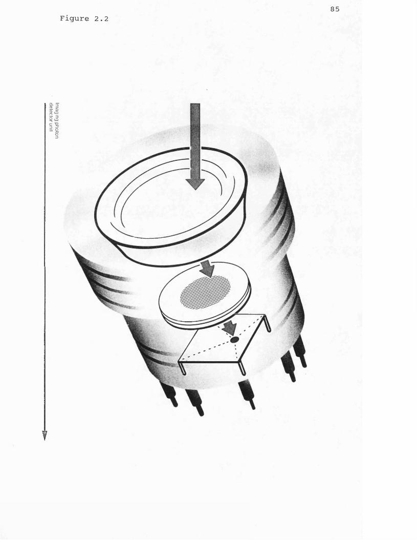
Imaging

photon detector unit

Figure 2.285

V

86Figure 2.3

RADIANT SENSITTUITY, S, CmA/U)

CD CD

rucs — ru<J1 CD CD

cn— ■- m

CD CD CD

mrJ1 E l E lCD CD CD

X>

r~m

33

$Dmiirum>/33•>_'/—*. 3I>\£=

CO p n -

ix V'l

CD \x \

CD -\

CD 111

‘l 1V

u i (S i -

11 1

1 i VICD I

1 1CO(T—| _

11 / I

1L i

CD J +

-J CD - 1 / j 'HLCD

fJ

J/

s

00m \

> 1 .

■ T 1

CD 1i /

(JD CD -

■- -- ~~

-

CD 1 I1

CDCDCD

l l 1CDCD

ru 1CDCD J

CD CD CD CD CD CD —*■ ru u~iCD CD CD ru <_n— *■ ru cn

CD CD

QUANTUM EFFICIENCY, QE

£T> 01 COx> rum i> <ncDco

r a

■TOor o

COr oo

c or oo r

o

o

p ^C O

fc*d< 3

Ofc=jCO

H

o

t- 1

r o

o

COM2 3CO

h-3

t*jc o

Figure 2.487

F i g u r e 2 . 5

05NORMAL BANDWIDTH

(AT 0.5 PEAK \ TRANSMISSION)

5ASS BAND SHAPE FACTOR OF I

(I CAVITY)

0.0PASS BAND SHAPE

FACTOR OF 2 (2 CAVITIES)

PASS BAND SHAPE FACTOR OF 3

i (3 CAVITIES)

0001

0.00014

BANDWIDTH IN MULTIPLES OF NOMINAL BANDWIDTH

Keyboard |

Figure 2.688

!?for-t,£

ft

fc*£ce<74.

0 rvft1&r4-iO,O

gooe

ot

Figure 2.789

90Figure 2.8

TOcc01

3Q3

TO"5H*Q 3

CQ ►—-* CD o-i

OJCD

O3

30 crn

4— ►

03CDCD

O3

1 cm

o O T3 73 ►——* CD

3QCQCQ

03CQ01C+-CD3o3TO3 "CD

ru•A30 3 "

TOCD1CD01 Oo73CD

TO.ru

s - Ȥ 7 01 CD

5 sru

TO3T0

ono3

TO3 "0TOQ

O0TO0333QTOH-O3

OTOro

-t*- ru k (j-iCD CD CD CD CD CD

r\3 ^ = 03a ™'.j*

CD CD CD

cu 03 ru01 CD CD ^

t

(mm

)

CD CD CD CD

CD CD CD CD CD O l -P COru cd cn ru

the

ta

(r

ad

)

TOo3

m E c1"a i0 §3 'o

CQ Q TO 5

=*■ § ° *0S wru33

Figure 2.991

Figure 2.1192

93

CHAPTER 3

DATA REDUCTION

3.1 Introduction

This chapter discusses the data reduction techniques employed in the analysis of the images collected with the Very High Sensitivity Imaging System (VHSIS) and with the Doppler Imaging System (DIS).

The raw data and calibration images collected on the hard disk of the Personal Computer (PC) used in the field are brought back to the UK via a back-up onto tape cartridges and/or floppy disks. These images are then transferred on to the hard disk of a suitable local PC within the Atmospheric Physics Laboratory (APL) at UCL, from where they are transferred to the APL DEC microvax for subsequent reduction, analysis and permanent storage (section 3.2).

All of the raw VHSIS data files collected in the field are initially corrected for the thermionic emission and flat field response of the detector and the sky background. These correction procedures are discussed in section 3.3.

The two-dimensional corrected VHSIS images are converted to a variety of one-dimensional profiles to facilitate comparison with cometary models and with data collected by other observers. These data reduction procedures are discussed in section 3.4.

All of the raw DIS image files collected in the field are initially corrected for the thermionic emission and flat field response of the detector. The corrected DIS data files are then reduced to 24 equal angular sectors in radius-squared space about the centre of the Fabry-Perot ring system. The fringe peak positions in these 24 sectors are determined and compared with the peak positions obtained with a calibration lamp to yield relative line of sight velocities as a function of position across the two-dimensional field of view. The procedures employed in the complete analysis of the DIS data are described in section 3.5.

94

3.2 Image Transfer from the Field PC to the APL DEC Microvax

The images which are collected in the field are initially stored on the hard disk of the field PC. Each image is a 256 x 256, integer x 2 array and occupies approximately 131 kbytes of memory. These images are backed up onto floppy disks and/or tape streamers during the course of any given campaign.

The tape streamers, which have been used in the field to date, have a storage capacity of 10 Mbytes and can, therefore, store up to 76 images. This is an extremely convenient method of backing up the data. However, not all PCs operated in the field possess tape drives. When there is no tape drive on a field PC, floppy disks are used as the backup media. High density disks have a storage capacity of1.2 Mbytes and can store up to 9 images per disk. Double density disks have a storage capacity of 362 kbytes and so may only store a maximum of 2 images per disk.

Once back at the APL, all of the images from a campaign are transferred from tape streamers/floppy disks onto the hard disk of a suitable local PC. Since the majority of the analysis and plotting packages used within the APL are written in Fortran on the microvax, the images need first to be transferred to the microvax. This is done using a program called DTRAN, written by D. Wade of the APL, which allows bulk transfer of images from PC to microvax. Each image on the microvax occupies 258 Vax blocks of memory (1 vax block is equivalent to 512 bytes).

The PC filenames are labelled according to the UT date and time as described in section 2.2.5. However, the year of observation is not included in the filename. It is, therefore, necessary to rename the files once they have been transferred to the microvax so that the year is included. This is essential to prevent the confusion of files from different years. Additional information on the type of file and the location of the instrument is also added to the filename. This additional labelling is best explained by means of an example

95

filename:-

Example of Vax filename: I86E32115.P31

The first character refers to the type of file according to the scheme outlined in table 3.1. The next two digits refer to the year of observation. The character after the dot refers to the location (see table 3.1.). Thus, the above filename describes the raw VHSIS image recorded at La Palma on 3 May 1986 at 21:15:31 UT.

Table 3.1 Additional Information Added to the Filename at UCL

Type of File Code Location Code

Raw data (VHSIS) I Alaska ACorrected data (VHSIS) J California CRaw data (DIS) D Churchill HCorrected data (DIS) E La Palma PFlat field F Sondrestrom SThermionic emission T Wallops Island WSky background S

3.3 Correction of the Raw Images Collected with the Very High Sensitivity Imaging System

Any "hot spots"/"hot lines" are first removed from the raw VHSIS images as described in section 3.3.1. The images are then corrected for thermionic emission and flat field (section 3.3.2) and sky background (section 3.3.3). The corrected images may be smoothed by a variety of methods and these are reviewed in section 3.3.4.

3.3.1 Initial Procedures

After any campaign the raw VHSIS images are first plotted out and studied so that the promising data can be selected for further

96

analysis. The images are displayed on a Tektronix 4113 colour graphics terminal and plotted on a Tektronix 4691 ink jet plotter.

Sometimes data collected in the field contains "hot spots" and/or "hot lines". These are associated with the detector electronics and can be corrected by the software. A "hot spot" is a pixel that contains a very large number of counts above its neighbours. A "hot line" is a horizontal or vertical line of "hot spots". A "hot spot" is removed by replacing it with the average value from the four adjacent pixels. A "hot line" is removed by replacing each value in the line by the average value of its two adjacent pixels perpendicular to the line.

3.3.2 Correction for the Thermionic Emission and Flat Field Response of the IPD

Thermionic emission and flat field files are recorded regularly throughout the course of any given campaign as described insection 2.3.5.

The steps necessary in the correction of a raw image are summarized below. Each image is 256 x 256 pixels and the operations involving image arrays are carried out on a pixel to pixel basis. The raw images and raw flat field images are first corrected for the thermionic emission of the detector (section 3.3.2.1). The images are then corrected for flat field (section 3.3.2.2).

3.3.2.1 Correction for Thermionic Emission

All of the raw images and raw flat field images from any givencampaign are corrected for the detector thermionic emission. Thethermionic emission image, normalized to the integration time of the image to be corrected, is subtracted from the image to be corrected.

Let tt, and tr be the integration times of the thermionic emission image and the image to be corrected respectively, and T and Ir be the thermionic emission image and the image to be corrected. The

97

correction for thermionic emission, then, proceeds as follows

trCl =

k

Ic(256,256) = Ir(256,256) - C!T(256,256)

where C- is the normalizing factor and Ic the resulting image, corrected for thermionic emission.

3.3.2.2 Correction for Flat Field

All of the images, which have been corrected for thermionic emission, are then corrected for the flat field response of the detector by multiplication with the associated flat field correcting factor file (formed for each pixel in the flat field image by dividing the average value in the flat field image by the value in each pixel).

Let Fc be the flat field image corrected for thermionic emission as outlined in section 3.3.2.1 and FaVg be the average value of the photon counts in the flat field. Then the correction of an image for flat field proceeds as follows

FavgFf(256,256) = -------- 3.3

Fc(256,256)

J(256,256) = ^(256,256) x Ff(256,256) 3 ’4

where Ff is the flat field correction image and J is the image corrected for flat field and thermionic emission.

The flat field operation can result in over correction at the edge of the image. This can be removed by applying a circular mask which sets the values in the relevant outer region to zero.

3.3.3 Correction for Sky Background

Finally the processed raw image is corrected for sky background. The raw sky background image is first corrected for the detector thermionic emission and flat field as outlined above. The corrected sky background image, normalized to the integration time of the data,

3.1

3.2

98

is subtracted from the data image. This final step is summarized below, where the notation is similar to that used above. J and S are the corrected image and sky background files respectively, tg is the integration time of the sky background file, and Jc is the final fully corrected image:-

C 2 = - 3.5

Jc(256,256) = J(256,256) - C2S(256,256) 3.6

The sky background image may contain unwanted stellar objects which would introduce errors in certain regions. When this happens the average value of the corrected sky image (excluding the areas occupied by stellar objects) is subtracted from every pixel rather than subtraction on a one to one basis.

A raw image and its associated thermionic emission, flat field and sky background files are shown in figure 3.1. The raw image (figure 3.1a) is a 10 minute exposure of comet Brorsen-Metcalf taken with the 24" telescope at the Table Mountain Facility (TMF) on 9 August 1989 in the light of the C2 molecule. The thermionic emission file (figure 3.1b) is a 60 minute integration taken with the photocathode light sealed. The flat field (figure 3.1c) is a 5 minute integration of the twilight sky taken through the C2 filter. The sky background image (figure 3.Id) is a 5 minute integration of the night sky taken approximately 5° of arc from the comet shortly after the raw image shown in figure 3.1a. The fully corrected image is shown in figure 3.2.

Once the images have been fully corrected they are transferred to magnetic tape, which provides permanent storage of the data. At any one time a small number of fully corrected images are stored on the hard disk of the microvax, from where they are immediately available for analysis.

3.3.4 Smoothing Routines

The random fluctuation in the photon flux can be described by a Poisson distribution. This distribution has the important property

99

that the root mean square fluctuation in the average flux N is simply:-

rms noise a 3 *7

signal/noise = ^/N 3 ' 8

Thus, the signal-to-noise ratio is proportional to the square root of the photon count. The signal-to-noise ratio is, thus, increased by taking longer integrations or by adding a sequence of shorter integrations. The latter method is the only option for telescopes such as the 16” telescope at TMF or the 8 " Meade portable telescope which do not possess any offset tracking capabilities. The integration times are limited to a maximum of about 2 minutes in these cases to avoid blurring the comet.

The pixel to pixel variations in the photon count may originally be large due to the errors inherent in photon counting. However, these variations may be reduced by appropriately smoothing the data. A variety of smoothing routines are available and these may be conveniently divided into two categories, one using spline interpolations the other using Fourier transforms.

3.3.4.1 Smoothing using Spline Interpolations

The spline method involves replacing each pixel value with an average computed from the pixel itself and certain specified neighbouring pixels. For example a five point spline calculates an average for each pixel from the pixel itself and its four adjacent pixels. A nine point spline also includes the additional four pixels in contact with the corners of the central pixel. The amount of smoothing may be increased by involving more pixels in the smooth or by repeating a given spline. Trial and error has shown that a good smoothing process for the VHSIS and DIS images uses the five point spline which is repeated three times.

100

3.3.4.2 Smoothing using Fourier Transforms

An alternative approach to smoothing the images involves Fourier techniques. It can be shown that in the Fourier domain any smoothly varying image will be limited to the lower frequencies, whereas the noise is spread over all frequencies. Thus, an image may be smoothed by the application of a suitable low-pass filter in the Fourier domain.

After a certain amount of experimentation with a variety of filter shapes in the Fourier domain, the Kaiser bell (cosine bell) was found to be the most suitable, the degree of smoothing being controlled by the width of the bell.

3.4 Data Reduction

The data are to be eventually compared with models of the cometary atmosphere and with the results of other observers. In order to achieve this end it is first necessary to reduce the data to a variety of one dimensional profiles. Reduction to line profiles, circular profiles and sector profiles are discussed insections 3.4.1, 3.4.2 and 3.4.4 respectively.

3.4.1 Reduction of the Imaging Data to Line Profiles

Profiles may be taken through an image along any line of any givenwidth. The begin and end points of the upper line together with therequired width of the integration are used to specify the line.

The equation of the line joining the upper begin and end point is first determined. If the gradient of the line is less than one the program will step along the line in units of x, at each pointcalculating the corresponding value of y and storing the value at that pixel as a function of x. The lower begin and end points are calculated and the equation of the line joining the upper begin point to the lower begin point is determined. The program then steps from the upper begin point to the lower begin point in steps of unit y calculating the corresponding x start point at each stage. An integration along the line with the same gradient and length as the

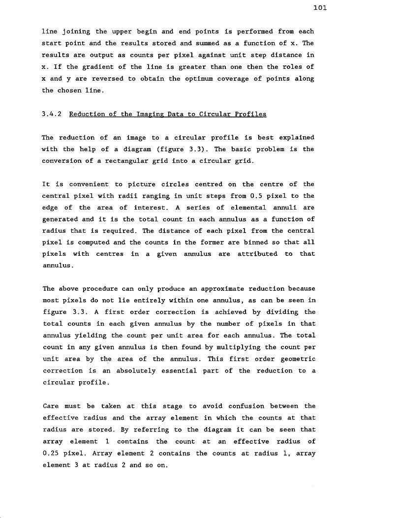
101

line joining the upper begin and end points is performed from each start point and the results stored and summed as a function of x. The results are output as counts per pixel against unit step distance inx. If the gradient of the line is greater than one then the roles ofx and y are reversed to obtain the optimum coverage of points along the chosen line.

3.4.2 Reduction of the Imaging Data to Circular Profiles

The reduction of an image to a circular profile is best explained with the help of a diagram (figure 3.3). The basic problem is the conversion of a rectangular grid into a circular grid.

It is convenient to picture circles centred on the centre of the central pixel with radii ranging in unit steps from 0.5 pixel to theedge of the area of interest. A series of elemental annuli aregenerated and it is the total count in each annulus as a function of radius that is required. The distance of each pixel from the central pixel is computed and the counts in the former are binned so that all pixels with centres in a given annulus are attributed to that annulus.

The above procedure can only produce an approximate reduction because most pixels do not lie entirely within one annulus, as can be seen in figure 3.3. A first order correction is achieved by dividing the total counts in each given annulus by the number of pixels in that annulus yielding the count per unit area for each annulus. The total count in any given annulus is then found by multiplying the count per unit area by the area of the annulus. This first order geometric correction is an absolutely essential part of the reduction to a circular profile.

Care must be taken at this stage to avoid confusion between the effective radius and the array element in which the counts at that radius are stored. By referring to the diagram it can be seen that array element 1 contains the count at an effective radius of 0.25 pixel. Array element 2 contains the counts at radius 1, array element 3 at radius 2 and so on.

102

3.4.3 Verification of the Routine to Generate the Circular Profiles

The reduction of an image to a circular profile forms an important part of much of the analysis referred to in subsequent chapters. It is, therefore, prudent to validate the technique on a test image. For this purpose a two-dimensional image is computer generated to have counts varying exactly inversely with distance from the centre. The centre is chosen to be at pixel 128,128. The method used to generate this image is described below.

Let the distance, in pixel units, of a given pixel from the centre of2 2the test image be given by R, equal to \/(x + Y )» where x is the

distance along the x-axis of the pixel from the central pixel and y the distance along the y-axis of the pixel from the central pixel. The count in that pixel will be given by:-

count(x,y)V2

yi J

x2 1

X] v/(x2 + y2)dxdy 3.9

where:-

*1 x - 0.5*2 x + 0.5yi y - 0.5Y2 y + 0.5

From a table of standard integrals

1sinh~*

X- o dx = —

. \/(x2 + y2) _ y .

>2sinh~*

X

=*> count(x,y) = A —yi _ y _

x2dy 3.11

X 1

A>2

sinh" *~ x2 "

dy*yi _ y _

>2sinh"*

" X1 ‘dy 3Jyi _ y _

103

Consider the following integral I(y):*

sinh-*X

Ky) = —* _ y _

dy 3.13

Let y = —u

The integral becomes:-

I(u) = - X

dy

du

sinh"*udu

From a table of standard integrals:-

sinh”*usinh"*u

-x

du - sinh"*u

so that:-

1

u

sinh” *X

dy = ysinh”*” x "

+ xsinh"*" y "

J _ y _ . y _ _ X

3.14

3.15

3.16

3.17

count(x,y) y2 Sinh-1

- yjsinh-1

+ X2sinh-1

- xjsinh-1

’ x2- y2sinh” *

' X1

_Y2 _ _y2 _

” x2+ yjsinh"*

" xi

_yi _ _yi _

ii

^• t

oi

- X2sinh”*"yi

L x2 J _ x2 _

"y2+ xisinh"*

"yi

. xi . _ xi _

3.18

In order to test the reduction method an integer x 2 image is computer generated centred on (128,128) by setting the constant A to 7,500. This image is reduced to a circular profile both with and without the geometric correction (figures 3.4 and 3.5 respectively).

104

When no geometric correction is applied the errors are of the order ±5% for most annuli (figure 3.4). However, once the geometric correction is applied, the annulus counts become effectively constant after 3 pixels from the centre (figure 3.5). Thus, providing the geometric correction is applied, the method described in section 3.4.2 produces a reliable reduction.

3.4.4 Reduction of the Imaging Data to Sector Profiles

The reduction of an image to sector profiles proceeds along similar lines to that described in section 3.4.2 for the reduction to circular profiles. However, only those points that lie within the specified sector are summed. As with the reduction to circular profiles this method can only produce an approximate reduction because most pixels do not lie entirely in one annular sector. The correction proceeds in a similar manner to that described in section 3.4.2, by dividing the total counts in each given annular sector by the number of pixels in that annular sector to yield the count per unit area for each annular sector. As with the reduction to circular profiles the errors inherent in this reduction become negligible beyond 3 pixels of the centre.

3.5 Analysis of the Doppler Imaging Data

After any campaign, all of the raw Doppler images are first plotted out. The promising images are selected and any "hot spots"/"hot lines" are removed from these images as discussed previously in section 3.3.1. The next step is the correction for the thermionic emission and flat field response of the detector, and these corrections are performed in a similar manner to that described for the raw VHSIS images in section 3.3.2.

The first stage in the analysis of the corrected Doppler imaging data is its reduction to 24 equal angular sectors in radius-squared space about the centre of the Fabry-Perot fringe system. It is important to have an accurate value of this centre prior to reducing the images. The method used to determine the centre of the fringe system is described in section 3.5.1, and the subsequent reduction to radius- squared space is discussed in section 3.5.2. These reduced images are

105

processed to provide fringe peak positions (section 3.5.3). This information is used to provide estimates of the Doppler shifts and thus, the line of sight wind velocities as a function of position across the field of view (section 3.5.4).

3.5.1 Determination of the Centre of the Fabrv-Perot Ring System

The corrected Doppler images are to be dissected into 24 equal angular sectors centred on the centre of the Fabry-Perot fringepattern. Therefore, the coordinates of the centre of the fringepattern have to be determined accurately before proceeding with the reduction of the data. The accuracy of the centre coordinates influences the overall instrumental finesse. If the centre coordinates are off by several pixels then the resulting radialprofiles are blurred. The sharpest radial profiles are obtained when the centre coordinates are known to the nearest pixel.

The centre of the Fabry-Perot fringe pattern is determined byanalyzing the set of Fabry-Perot rings obtained from a calibration lamp (see, for example, figure 3.6). This image is known as the full- field spectrometrie calibration file (section 2.4.3.2). The following method is used to determine the centre of the fringe pattern to the nearest pixel.

a) An initial estimate of the centre is obtained by inspecting the calibration image.

b) This centre is used to obtain 45° sector plots going from the estimated centre to the right-hand edge of the image and from the estimated centre to the left-hand edge of the image. The two sets of fringes are brought into coincidence by changing the x value of the centre.

c) The new x value and the first estimate of the y value are used to obtain 45° sector plots going from the new estimated centre to the top edge of the image and from the new estimated centre to the bottom edge of the image. These fringes are brought into coincidence by changing the y value of the centre.

106

d) The new centre is used to obtain a plot of all four sectors. This procedure should yield the centre of the fringe system to within one pixel.

A typical Fabry-Perot fringe system obtained with the DIS from a barium calibration lamp is shown in figure 3.6. The four sector profiles obtained from the centre of the fringe system are shown in figure 3.7. Moving off the centre by one pixel or more causes the fringe peaks to become misaligned. The method outlined above is, thus, a valid method for determining the centre of the fringe system.

3.5.2 Reduction of an Imaee to Radius-Squared Profile

The theory of the Fabry-Perot etalon (see section 2.4.1) indicates that for a uniform, extended monochromatic source the fringe separation and width decrease with radius. However, transforming from a radial coordinate system to a radius-squared coordinate system produces a fringe pattern where all the fringes have equal width and separation. This also has the advantage that the radius-squared axis is proportional to the relative wavelength change. Thus, when a Doppler image is reduced to a one-dimensional profile it is reduced to a radius-squared coordinate system rather than a simple radial profile.

The reduction to radius-squared profile proceeds as follows. The first step is basically a transformation from a Cartesian coordinate system to a polar coordinate system about the centre of the fringe pattern. Once the polar coordinates (r,0) of each pixel in the image array have been determined, the radial axis is divided into 256 equal radius-squared bins and the polar angle is divided into 24 equal angular sectors. The value in each pixel is then binned according to this system.

As with the reduction of an image to radius (section 3.3.2), the above procedure will only produce an approximate reduction, because individual pixels may not lie entirely within a single annular sector. A first order geometric correction is achieved by dividing the total counts in each given annular sector by the number of pixels in that annular sector yielding the count per unit area for each

107

annular sector. The total counts in a given annular sector are then calculated by multiplying by the area of the annular sector.

3.5.3 Determination of the Peak Positions

A discussion of the method adopted for the determination of the peak positions can be found in Batten et al. [1988], Basically a smoothed fit to the reduced data is obtained by applying a low-pass filter in the Fourier domain. The smoothed fit is examined for turning points which are then subjected to certain tests to determine whether they are due to real peaks, troughs or noise. The troughs are removed by noting the manner in which the gradient changes through the turning point. The majority of the noise peaks are removed by insisting that the peak is higher than a certain threshold value and also a certain proportion higher than the background level. These two parameters depend on the data being analyzed and can be set by the user. Accurate peak positions are found by a Newton-Raphson iteration along the analytical curve.

The peaks are fitted in each angular sector and written to an indexed file. The peak positions can also be plotted graphically, with all 24 angles being shown on one sheet, as shown in figure 3.8, for the calibration file of figure 3.6. A typical data file from a barium release experiment is shown in figure 3.9, together with its reduced profiles in figure 3.10.

The experimentally observed Fabry-Perot fringes obtained with the DIS vary enormously in signal amplitude and modulation, as figure 3.9 and 3.10 show. It is impossible to write a program to uniquely identify every valid peak and ignore every noise peak over such a range. The search parameters are chosen so that all obvious data peaks are recovered. This may result in spurious peaks being found from time to time. These spurious peaks may be removed by detailed examination of the data.

3.5.4 Calculation of the Relative Line of Sight Velocities

If a source and a receiver are in relative motion, the observed frequency is changed compared to that in which there is no motion.

108

This is the well known Doppler effect. It can be shown (see, for example, Hecht & Zajac, [1982]) that the line of sight velocity v is related to the wavelength change> by:-

6X

A

so that:-

cA (cal - dat)

2t FSR

where:-c is the speed of light in vacuum,cal is the calibration lamp peak position,dat is the data peak position,FSR is the free spectral range,A is the rest wavelength of the emission andt is the etalon gap.

The line of sight velocities can only be determined at the fringe peaks and are best represented on a Dopplergram (see, for example, figure 8.4), which is basically a two-dimensional representation of the line of sight velocities as a function of position across the field. The Dopplergram is plotted in radius space and so the positional information in the original Doppler image is maintained.

3.19

109Figure 3.1

sis

M B ^O lllM X I TTTTTlT 1 i ill!-»■ ru— - ru u) i -m ru o w o a c n - i o c u n t n c s

1I8IIK1III:— — ro LOcu <r> cs> cn -i is is ■si ro acn tn ®

M Q ErnnSriTvZZIOEZ

i mcan x j

ru o i. ru cotCO -1 vD TO —1 *U

— rum u i -j m Q w r o i a i n ^ G n s i n y i o ru aru Luoj m C3 ui -1 is Iv --Jis m ui o

|RAU IMA6E

DF B RORS EN-M

ETCALF FILE

; I89H

91145.C46|TH

ERM

I0IHIC

EM

ISSION FILE

FILE ;

T89HH

0955.C00

110Figure 3.2

I—I i >

m m

m l j zz o oid to ru es

ru m u lu r < ji -j o ru cn cs ru CO CT) cxj Q ru CJ1 0: j (J1 Q CJI CD C3 CJ1 CD U1 GD CD

H DD HS3men n “0H Xm m0 70

Figure 3.3111

112Figure 3.4

TOTAL COUNTS IN ANNULAR ELEMENT

©©

©© ©

_i_

ro©

©© ©

<J1©

— L -

"U70OL_m © o •H romooMcn ^ ?

m70O3 CD o •m ©

70ro\

T5t— -

XCD

C(i

m

©00

x cxi©

ru

X

©

—> H-o N— 1 1Stftdo < nt*j<=} >-3o cr*raK Mm 7 0 h-3Htd0 3 >-dM Wo o>— 3

—1o t-HPdfcdP O

• -3

r> cn ~n m ~n m 7x i—i iz i—i z - < r t n r — \ —i —I mto rn m to

ii ii ii n ii

ruoo©■

-*©ro©co

1 'piCOH"0

113Figure 3.5

TOTAL COUNTS IN ANNULAR ELEMENT

m ©

oMco^ ©om70o3 (S o ■ m © zz — !70m

©oo

x ©© ru

d > i— kH—Nt d t do

dt d r a

C O7 0 d

d d7 0 t dO O^=j i— 3►— it dt d

O O l ' H H ' nm 7\ H ZZ Hz-crtnr-1 —I —1 mto mm to

ii n ii ii ii

Fu ' FlC O © ©>. ■ —i- * © •ru© "OCO r~—1

53*1

114Figure 3.6

o m m i—i <C r~i—i —Io m m to

CPQ-JX>.nui33

1—1 © x> ~nzz <£l ~D i—iH 70 r~mi 00

©© 1 “

ru cn —i mDOc 00 ©

© - i © o

115Figure 3.7

TOTAL COUNTS IN SECTOR ELEMENT

^ CD CD

bd

TOO CD

or o

bdso!*►h-3

r or ooo

r oG Oo

m cd zz. ■ —| oo70m

CD

rocnCD

m m m mw o nQ H 00

00 Ui Ocd cn e? cn csQDJl _L.oo

CD

CO CO 00 CO

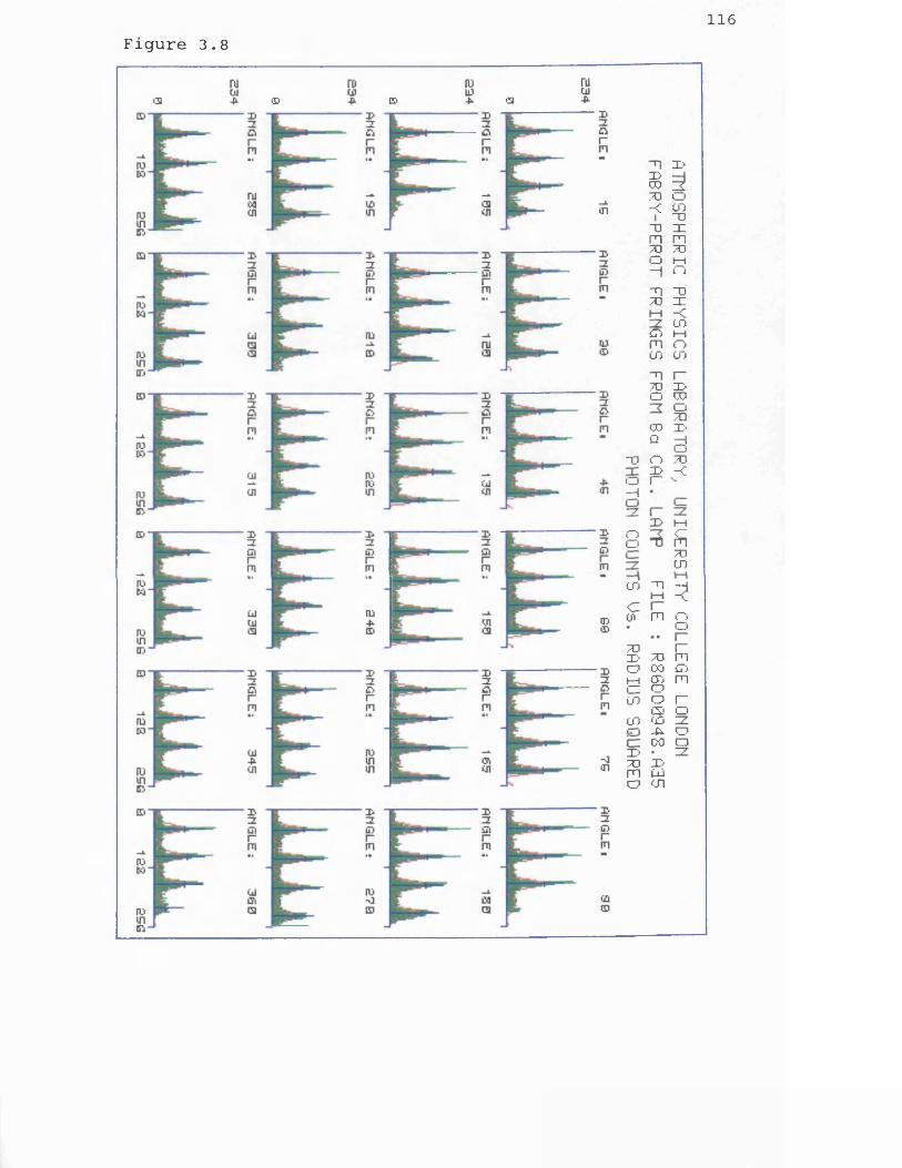
116Figure 3.8

■3 © © a

hi

Xroi

"0

x>XI o-< COnoXn mX 70 O n-I r*X x 70 X

CO£T>mco co70 Xa ro o x x

aX O X X

oo

roQ

o r~ — Ix

CO

-c

ftXCOCO X —1c m o ox r~ x to mo 00 ij) h o ') n r~ o o r~ cs o co ( oX 00 I> •X X m cu o ro

oa

117Figure 3.9

o x m I—I <= r~ •—i —I O IX IX 70IO H—ICO

IroD-ISroro33

— I

l—l CD Xzz ro X—1 ru X1

CO COIS) ro roCl) i COCD H CD

118Figure 3.10

x Xr~ HXCO o

00x XXm

—* XCO i—iDO nCO•w X

Xo -co oo"0 i—iX} or * 00m70 r~

Xi—i X3 o

X£0 X1—1 ZZ

“0 CO XIE •<O O N.—1 Xo —1 XX X ZZ

t—1oo fic= Xx X—1 >—tCO x

i—ic r~(Si m o• o

•• r~70 r~X> 70 mO DO COI—I CO mcz OCO O r~

C3 ooo CO Xo ro oc : □x * X70 Xm too cn

119

CHAPTER 4

INTRODUCTION TO COMETS

4.1 Introduction

The origins of cometary astronomy are lost in the mists of time. However, it is clear that comets have played an important part in the beliefs and social habits of civilization from very early times. Early man would have regarded the sudden appearance of a bright comet in the night sky as an omen for whatever important event occurred while it was visible. In fact, when the history of man's views on nature are considered, comets have always been surrounded with awe and mystery. Many people shared Aristotle's views that the appearance of a comet signalled disaster or drought. Indeed, in the Middle Ages, a comet was regarded as one of the most splendid and ominous of celestial portents. The appearance of a bright comet struck fear into the hearts of its viewers, and with this fear came considerable interest.

During early times, comets were studied more from a point of view of their dynamics. With the passage of time, cometary research hasevolved from a study of dynamics to a study of these objectsthemselves. A brief account of the history of the progress of cometary astronomy up to the beginning of the 20 th Century is presented in section 4.2.

Comets are now generally thought to have formed from the sameinterstellar gas and dust cloud of which the primitive solar nebulawas a part. Many processes have changed the interiors and exteriors

oof the planets and their satellites over the past 4.5 x 10 years and most information about the accumulation process as well as the original state of the material has been erased. Comets, on the other hand, are expected to be remnants left over from the formation of the Solar System which have preserved the chemical and physical characteristics of the condensing matter. They probably solidified at temperatures well below 150 K and are thought to be stored essentially unchanged at the outer edge of the Solar System in the

120

Oort cloud which extends some tens of thousands of AU from the Sun. While the cometary nucleus is a unique witness of the remote past when it accumulated in the interstellar cloud of which the solar nebula was a part, the changing appearance of the coma and tail yields information about the present conditions of the interplanetary space with which the comet interacts.

A brief overview of our knowledge of cometary physics, prior to the spacecraft encounters, is summarized in section 4.3. The following sections then present the most recent findings in the light of the spacecraft encounters and the complementary Earth-based observations. The cometary nucleus (section 4.4), the dust coma (section 4.5), the gaseous coma (section 4.6) and the plasma tail (section 4.7) are discussed in turn.

4.2 Brief Historical Perspective

The history of cometary science may be thought to have began almost entirely as a debate over whether comets were a celestial or an atmospheric phenomena. As early as the 4th century BC Appolonius Myndus regarded comets as heavenly bodies, essentially akin to planets. However, the accepted view for almost two millenia was that put forward by Aristotle (384 - 322 BC), who believed comets to be fiery meteorological phenomena produced by violent winds at the top of the atmosphere.

It was not until the 16th century that comets were first demonstrated to be celestial objects. This came from the work of Tycho Brahe who determined by parallax that the bright comet of 1577 had to be at least four times further away from Earth than the Moon. Thus Tycho concluded that the comet lay between the Moon and Venus. He even attempted to calculate an orbit for the comet. His result was a circular orbit around the Sun, outside the orbit of Venus. However, he could not represent the observed motion of the comet, and he was obliged to assume an irregular motion or to admit that the orbit was not exactly circular but somewhat oblong. This was probably the first time an astronomer had suggested that a celestial body might move in an orbit differing from a circle, without saying distinctly that the curve was the resultant of several circular motions. Later Johannes

121

Kepler postulated that comets move along straight lines but with irregular speed, which was rather surprising considering he had discovered elliptical orbits for the planets.

The problem of cometary orbits began to be resolved in 1665 when Giovanni Borelli (1608-1679) and Hevelius (1611-1687) both, independently, suggested that the path of the bright comet seen in 1664 was parabolic. Newton's laws of motion and gravitation established the basis for calculating cometary motion. Edmund Hailey determined the orbits of 2 0 or so comets for which there were sufficient observations and found them to be very elongated ellipses. He noted that the orbital elements for the comet of 1682 showed close correspondence with the comets of 1607, 1531, and 1456, concludedthat these observations referred to the same comet and predicted that it would return in 1758. The comet did indeed return and is the comet that bears his name today.

Efforts to understand the physical nature of comets began with the research of F. W. Bessel (1784-1846) who observed Hailey's comet in its 1835 apparition. His drawings of the comet show jets, rays, fans, cones and other features that appear to be leaving the nucleus in the direction of the Sun. He developed a theory of cometary forms for particles leaving the head of a comet while subjected to different repulsive forces and solar gravity. This approach was also taken by F. A. Bredichin (1831-1904) who was able to extend the theory.Bredichin classified comet tails into three types. Type I tails are narrow and nearly straight and often show considerable fine structure. Type II tails are curved and relatively lacking in finestructure. Type III tails are strongly curved.

Initial progress in the physics of comets depended upon the spectroscopic identification of the chemical constituents involved. The first spectroscopic observations of a comet were made in 1864 by Giovanni Donati (1828-73) who observed comet Tempel (1864 II). He saw three faint bands of emission as well as the reflected solar continuum. These bands were subsequently shown to be the C2 Swanbands. Photographic records of cometary spectra were first made in 1881. The early photographic results also showed a strong group of

122

emission bands in the ultraviolet (UV) , later to be identified as due to the CN radical.

At the beginning of the 20th century many species had been identified in the head of comets. However, the mechanism of emission was still unknown. Schwarzschild & Kron [1911] suggested that comets shine by the absorption and re-emission of solar radiation. Although there was some debate over the years, Zanstra [1929] demonstrated that fluorescence (and resonance fluorescence) could account for most of the line and band spectra of comets.

4.3 Brief Overview of Cometary Physics up to the Time of the Recent Spacecraft Encounters

The major results of cometary observations prior to the recent spacecraft encounters are reviewed in this section. The nucleus, dust, coma and plasma tail are described in turn.

4.3.1 The Cometary Nucleus

4.3.1.1 Structure of the Cometary Nucleus

The view of a discrete, cohesive nucleus bearing essentially all the mass of the comet can be traced back to Laplace [1813] and Bessel [1836]. Later, however, the association of meteor streams with individual comets had such an impact that comets themselves began to be regarded as the densest part of such streams [Lyttleton, 1953; 1972]. Whipple [1950] returned to the idea of a discretenucleus with his "icy conglomerate model". This model considers the nucleus to be an aggregate of ices (e.g. ^0, CO2 , CO, CH^, NH3

etc.), and meteoric dust. Whipple modified Laplace's early idea and quantified it so that it explained the essential features of cometary observations.

Prior to the spacecraft encoumters the observational evidence clearly favoured the solid nucleus model with the probable modification that the nucleus is a water cLathrate which contains other trapped compounds [Delsemme & Swings, 1952]. Since at most one guest molecule can be trapped for every six molecules of H 2 O, this model

123

predicts the production rate of all other species to be < 1 / 6 that ofh 2 o.

4.3.1.2 Size of the Cometary Nucleus

The direct observation of a bare comet nucleus using conventional ground-based telescopes is extremely difficult due to the small size of the nucleus and to the presence of highly volatile ices which vaporize under the influence of solar radiation at heliocentric distances as large as 10 AU. Prior to the spacecraft encounters, possibly the only direct observation of a comet nucleus had come using radar echoes of comet Encke during its perihelion passage in 1980. These observations indicated a radius in the range 0.4 - 4.0 km [Kamoun et al., 1981].

4.3.2 The Dust Coma/Tail

Dust has long been known to be an important constituent in comets, primarily due to the extensive type II tails developed particularly by bright comets near perihelion.

4.3.2.1 Morphology of the Dust Coma/Tail

Bessel [1836] developed a mechanical theory for dust particle motion in an attempt to explain the dust tail of comet Hailey in its 1835 apparition. He required that in addition to solar gravity a repulsive force acting on the dust particles was necessary to explain the anti- sunward tail. The physical nature of this force was only later recognized to be solar radiation pressure.

The action of two forces, gravity (dependent on particle mass) and radiation pressure (dependent on particle cross-section) results in a mass spectrometric effect which spatially separates particles of different masses in the tails of comets. A quantitative description of this effect is given by Finson & Probstein [1968].

124

4.3.2.2 Composition of the Dust Particles

Before the spacecraft encounters with comet Hailey information about the chemical composition of the dust came mainly from broad emission bands in the infrared (IR) around 10 and 20 microns, which were attributed to silicate grains, perhaps in the form of amorphous olivine [Hanner, 1980], although Vanysek & Wickramasinghe [1975] and Mendis & Wickramasinghe [1975] had attributed these to organics such as polymerized formaldehyde grains. The coexistence of an absorbing graphite component (e.g. magnetite) had also been invoked (e.g. Divine et al. [1986]) to explain the thermal radiation. Greenberg [1982] proposed that cometary grains might have a composite core mantle structure with a silicate core and an organic mantle.

4.3.3 The Gaseous Coma

At large heliocentric distances, a comet generally shows only a continuous spectrum, resulting from reflected sunlight. As it approaches the Sun, gas and dust are released from the nucleus due to solar heating. This then expands outwards into vacuum at about 1 kms"^ giving rise to the observed coma. As the gas expands it is subjected to various physical processes such as dissociation, ionization and gas-phase reactions. The complex molecules released by the nucleus, generally known as parent molecules, are broken down and ultimately give rise to simpler molecules and radicals such as CN, C2, OH, CH, NH2, etc. which are seen in the comet's emission spectra.

Although it is impossible to predict when a particular species will become apparent in the spectra of a comet, the following scenario may be regarded as fairly typical. The first species to become visible as the comet approaches the Sun is CN at around 3 AU. C-j and NH2 appear at around 2 AU. As the comet continues on its inbound leg C2 , CH, OH and NH appear at about 1.5 AU. These emissions grow stronger as the comet moves inside 1.5 AU and the spectra of C0+ , H 2 0+ , N2+ and CH+ appear in the tail. The lines of Na appear near 0.8 AU and, if the comets perihelion distance is very small (about 0.1 AU), lines of Fe, Cr and Ni appear.

125

4.3.3.1 Morphology of the Gaseous Coma

The coma of an average comet appears, generally, spherically symmetric on direct, blue sensitive photographs, and typically has a

gsize of the order 10 km at a heliocentric distance of 1 AU.

The spatial distribution of a neutral cometary species may be modelled by the radial outflow model with decay, [Haser, 1957]. This model considers the observed (daughter) species to be produced from a source of exponentially decaying parent molecules streaming radially with uniform speed, at a constant rate, from a point source nucleus. The daughter molecules continue to move radially with uniform speeds and decay exponentially themselves. Despite its many limitations, this model is readily computable and yields parent and daughter scale lengths for comparison between the data sets (see chapter 5).

4.3.3.2 Composition of the Gaseous Coma

A summary of the atomic and molecular species identified in the spectra of comets prior to the spacecraft encounters with comet Hailey is given in table 4.1.

Table 4.1 Chemical Species Identified in Cometary Spectra Prior to the Spacecraft Encounters (tentative identifications in brackets)

Atoms: H ,0 ,C ,S,Na,K ,Ca,V ,Mn,Fe,Co,Ni,Cu

Molecules: c2 ,ch,cn,co,cs,nh,oh,c3 ,nh2 ,(h2 o>,hcn,ch3 cn,s2 ,hco,nh3 ,(h2 co),(nh4)

Ions: C+ , Ca+ , C0+ , CH+ , CN+ , N2+ , CC>2+ , H 2 0+ , H 2 S+

Most of the observed species are chemically reactive photo­destruction fragments of presumably more stable molecules housed in the nucleus. The cosmically abundant elements H, C, N, 0 and S are well represented in this table, as are the most abundant metals. However, the latter had only been observed in emission in sun-grazing

126

3comets where radiation temperatures in excess of 10 K can vaporize the refractory component of the dust [Preston, 1967].

The optical spectra of comets are dominated by the neutral radicals CN and C2 . A spectrogram, taken from A ’H e a m [1975], is shown in figure 4.1 to illustrate the dominance of the CN and C2 emission features. NH, C3 and NH2 are also frequently prominent.

4.3.3.3 Excitation Mechanisms

The vast majority of the species observed in the UV and visible spectra of comets are excited by resonance fluorescence in the solar radiation field [Swings, 1941; Arpigny, 1965]. However, a small number of forbidden lines have been observed in cometary spectra. These forbidden transitions cannot be attributed to resonance fluorescence, and must be due to some other process producing the observed species in an excited state. For example, the forbidden 0(^D) 630.0 nm line is excited as a result of the photodissociation of H 2 O and OH (see section 6.1), and the metastable C(^D) line is thought to arise from dissociative recombination of CO+ [Feldman, 1978].

4.3.4 The Plasma Tail

Comets have long been observed to have two types of tails extending from the coma. The type I (ion or plasma) tails are aligned morenearly with the radius vector of the cometary orbit than are the typeII dust tails, the lag angles measuring about 5° and < 60°,respectively. Prior to 1951 ion tails of comets were known not to be explicable by effects of either solar radiation or gravitation. From motions of features in comet plasma tails Biermann [1951; 1957]inferred the existence of the solar wind and Alfv6n [1957] suggested that a magnetic field dragged by the solar wind wraps field lines around the comet ionosphere and is pulled into the ion tail byinteraction with the comet ions.

127

4.3.4.1 Morphology of the Plasma Tall

Photographs of cometary plasma tails reveal a constantly changing array of structural features such as rays, streamers, knots, kinks, helices, condensations and disconnection events. Rays are thin rectilinear features which are most easily seen when inclined at a large angle to the tail axis. The rays merge to form large bundles or streamers forming the main tail. Knots are small regions of enhanced brightness observed in almost all comet tails. Kinks are seen as sharp bends, usually in streamers, and helices are wavy corkscrew­like features also observed in the streamers. Condensations are large cloud-like regions of enhanced brightness. A tail disconnection event is a major condensation that has become detached from the region of the comet's head. The total length of typical plasma tails are in the range 1 0 km - 1 0 km.

One of the most prominent morphological phenomenon observed to be associated with plasma tails is the ray structure. Narrow (< 1 , 0 0 0 km), straight tail rays are sometimes seen to extend from 10^ km - 107 km from the coma in an anti-sunward direction. Near the nucleus these rays make angles up to 60° with the tail axis. They are then observed to turn toward the tail axis, coalescing with it on time scales of 20 hours [Wurm, 1968].

Another feature characteristic of the plasma tails is the tail disconnection event (TDE). These events appear to be a cycloidal process involving the abrupt disconnection of the plasma tail in the coma, followed by a reforming of the tail.

4.3.4.2 Composition of the Plasma Tail

The plasma tail is dominated by the emission spectra of C0+ and The C0+ emissions dominate the 380 ran to 480 nm region and the emissions dominate the 560 nm to 700 nm region. Several other ions, both diatomic and triatomic have been observed in the plasma tail of comets and are included in table 4.1. The spectra of these ions are not as extensive (in wavelength) nor as strong as are those of C0+ and H2 0+ .

128

4.3.4.3 The Comet-Solar Wind Interaction

The solar wind and its magnetic field both flow towards the comet at typical speeds of 400 kms"^. After release from the comet nucleus, dissociation and ionization, the newly created cometary ions travel towards the Sun at perhaps 1 kms"^. Charged particles cannot freely cross a magnetic field, but instead perform helical orbits along its line of force. When ions from the outer regions of the atmosphere are deposited into the solar wind, they are captured on the solar wind's magnetic lines of force and consequently travel back toward the comet in the same direction as the solar wind. Because the solar wind has had mass added to it in the form of cometary ions, it must slow down to conserve momentum. This deceleration process continues as progressively more ions are captured during the solar wind's flight toward the inner atmosphere. Eventually a point is reached where so many ions have been captured, and the flow has been so decelerated, that the outward pressure from the ions and other gases are balanced by the inward pressures exerted by the solar wind carrying the captured ions. At this point the solar wind stops; it is said to stagnate. The magnetic field it carries, which have been continuously compressed, form a magnetic barrier which is also at rest.

To form an ionopause (separating the mass-loaded solar-wind flow from the pure cometary ions by a tangential discontinuity) requires sufficient momentum in the cometary outflow, which is generally supplied by the neutrals where they are collisionally coupled to the ions. This occurs at about 2.5 AU for comet Hailey. When the ionopause is developed and stable, a visible tail is formed and is subject to evolution caused by the solar wind magnetic sector structure.

The interaction of the solar wind with a comet near to the Sun occurs over huge regions of space. Neutral atoms and radicals drift away from the nucleus unconstrained by the comet's own gravitational field. When ionization of the neutrals occurs, the resultant ions and electrons are subject to the electromagnetic forces in the solar wind. They are initially accelerated in the electric field, the ions gaining momentum at the expense of the solar wind. The latter is slowed by this process and it has been shown [Biermann et al., 1967]

129

that if the rate of mass loading causes the mass flux to exceed a critical value, a bow shock must form at the critical point upstream of the comet. The theoretical studies of solar wind flow near comets were carried out mainly in the framework of the hydrodynamical description of a plasma [Wallis, 1973; Schmidt & Wegman, 1982]. The main result of these studies was the determination of the positions of the cometary bow shock and the region of solar wind stagnation in the process of loading behind the shock.

The incorporation of collisions of plasma particles with atoms and molecules from the cometary atmosphere and the influence of magnetic stresses on plasma flow in theoretical models has led to the prediction of two other boundaries, the collisionpause and the contact surface that are closer to the nucleus of a comet. The ion neutral friction heavily breaks the loaded solar wind at the collisionpause [Biermann, 1974]. On the other hand, the magnetic field line tension stops the cometary photoplasma collisionally coupled to the expanding cometary gas [Ip & Axford, 1982].

4.4 The Cometary Nucleus

Cometary nuclei are too small to be studied from the Earth and, until the spacecraft missions to comet Hailey in March 1986, all the information with regard to their possible nature, structure and composition had to come from indirect means. However, the in situ measurements by the Vega and Giotto spacecraft have led to a much greater understanding of the cometary nucleus.

One of the main objectives of the missions to comet Hailey was to find out more about the nature of the cometary nucleus. Whipple's model of a discrete nucleus was essentially confirmed by the images taken by the Television System (TVS) on board the Vega spacecraft and by the Hailey Multicolour Camera (HMC) on Giotto (section 4.4.1).

The rotational period of comet Hailey is still a moot point with some observers postulating a rotational period of 2 . 2 days and others favouring a period of 7.4 days. It is possible to reconcile these two different periods by regarding the nucleus of comet Hailey as a rigid, asymmetric top in Eulerian free precession (section 4.4.2).

130

4.4.1 The Physical Nature of the Nucleus of Comet Hailey

The TVS on the Russian spacecraft observed comet Hailey from 4 March 1986 to 11 March 1986, and transmitted 1,500 images to Earth. The best images of the comet nucleus were obtained from distances of8,000 to 9,000 km. These images revealed the nucleus to be anirregular potato-shaped body with a long axis measuring 14 ± 1 km and two short axes of 7.5 ± 1 km [Sagdeev et al., 1986b].

The HMC, on board the Giotto spacecraft, observed the nucleus and its environment and returned more than 2 , 0 0 0 images, including the mostdetailed images ever obtained of a cometary nucleus. The profile ofthe nucleus was determined to be approximately 14.9 km long by up to 10 km wide [Keller et al., 1986]. An image of the nucleus of comet Hailey as seen by the HMC at a distance of 18,270 km is shown in figure 4.2.

A very low geometric albedo of about 4% was inferred from both the TVS and HMC measurements which makes comet Hailey one of the darkest objects in the solar system. Only a few outer Solar System objects, such as Jupiter's satellite Almathea, the dark side of Saturn's satellite Iapetus and the ring particles of Uranus are as black.

The mass of comet Hailey, based on non-gravitational effects of its orbit, is believed to lie in the range of 5 x 1 0 ^ - 1 0 ^ g [Rickman,1986]. This relatively small mass despite its large size, would make

_ 3its inferred bulk density between 0 . 1 and 0 . 2 gem much smaller than_ 3generally assumed (e.g. 1 gem , Divine et al. [1986]). This inferred

low density implies that cometary nuclei are extremely fragile and are the lowest density bodies in the Solar System. This is consistent with the very low tensile strength determined from the splitting of comets - in particular comet West 1976VI [Sekanina & Farrell, 1978]. However, the estimate of the mass is based on the rather uncertain radial non-gravitational parameter and so the implied low values for the bulk density must be treated with some caution.

The Infrared Instrument (IKS) carried by the Vega-1 spacecraft performed IR sounding of the nuclear region of comet Hailey. An

131

emissive centre, a few km in size, was detected with a temperature in the range of 300 - 400 K [Combes et al. , 1986a] - much greater than predicted by ice models of the nucleus (180 - 200 K) see, forexample, Sagdeev et al. [1983]. However, ices must be present in the nucleus to provide the gas in the coma. These conflicting observations of a high surface temperature and the presence of ice may be reconciled if the surface of the nucleus is covered by a thin, insulating layer of a black, porous refractory substance [Sagdeev et al., 1986a]. There can be ice on the lower boundary of this layer, at a temperature of about 200 K, while the external boundary is 100 - 150 K warmer.

The activity of gas production was strongly oriented to the Sun, coming from isolated areas of the nucleus. Thomas & Keller [1987] have classified the emission features streaming from the nucleus at the time of the Giotto closest approach and have identified 17 fine dust structures, more than doubling the number presented earlier [teller et al., 1986]. The surface has to be widely covered by a crust or mantle that prevents free sublimation of the icy conglomerate.

4.4.2 The Rotational Period of Comet Hailey

The Ultraviolet Imager (UVI), on board the Suisei spacecraft, observed strong breathing of the hydrogen coma from the end of November 1985 to the middle of December 1985 [Kaneda et al., 1986]. This phenomenon was interpreted in terms of the outburst of some snow from its source on the surface correlated to the rotation of the cometary nucleus. At a start of the active phase a strong flash was detected at the position of the cometary nucleus and the rotational period was well determined from the interval between the flashes to be 2.2 ± 0.1 days. This rotational period is in good agreement with that determined previously by Sekanina & Larson [1984], T — 52 hours, from the morphology of spiral dust jets in their processed images of comet Hailey taken at its 1910 apparition. This period was also supported by ground-based observations of the brightness variations of comet Hailey, during its recent apparition [Belton et al., 1986].

132

It was, therefore, somewhat surprising when Millis & Schleicher [1986] reported a significantly different value of 7.4 days, based on analysis of their sequential ground-based photometry of comet Hailey during March/April 1986. In addition, the brightness fluctuations detected by Neckel & Mtinch [1987], from their photometric observations of comet Hailey, also indicated a period of 7.3 days, and Samaras inha et al. [1986] reported a period of 7.37 days from their analysis of CN jets in comet Hailey. More support for this rotational period came from the H measurements from the Pioneer Venus Orbiter Ultraviolet Spectrometer which showed a periodic behaviour implying variations in the water production rate having structure within a 7.4 day sidereal period [Stewart, 1987].

Julian [1987] has attempted to explain these different rotational periods of the nucleus of comet Hailey by regarding it as a rigid, homogeneous asymmetric top, in Eulerian free precession. Two qualitatively distinct free precessional modes are allowed for torque free rotation about its centre of mass, each exhibiting the 2 . 2 day and 7.4 day periodicities. This model is obviously still an oversimplification as the shape of the nucleus is markedly different from an ellipsoid and the asymmetric jet activity would lead to substantial torques about the centre of mass. However, this model may represent a reasonable approximation to the actual rotation of the nucleus.

4.5 Cometary Dust

The two basic questions about the cometary dust concern the chemical structure (section 4.5.1) and the physical structure (section 4.5.2). The spacecraft observations of the dust particles have been complemented by Earth-based observations, particularly in the IR part of the spectrum. IR observations are useful for studying dust properties and detecting possible features due to ices and parent molecules. Indeed, in contrast to the UV and visible ranges which show most of the emissions due to cometary radicals and ions, the IR range is especially favourable for the detection of molecular vibrational bands.

133

4.5.1 The Chemical Composition of the Dust Particles at Comet Hallev

4.5.1.1 Results from the Spacecraft Encounters

The PUMA results of the Vega-1 flyby of comet Hailey [Kissel, 1986] essentially confirmed Greenberg's [1982] idea. Although the individual dust grains were found to vary very much in mass and composition, a chondritic silicate fraction seemed to form the main core which was itself embedded in a more or less organic material. Their chemistry is summarized in table 4.2.

The average analysis of about 80 particles yielded an organic fraction of 33% in mass and an inorganic fraction of 67%. [Krueger & Kissel, 1987]. There was 20% carbon in mass in the organic fraction, plus 3% reduced carbon, presumably graphite, in the inorganic fraction. 1 1 % water seemed to be equally distributed in the two fractions. In the inorganic fraction there was a 51.5% by mass of silicates, mainly a silicate of iron and magnesium, the rest being 6 % FeS (triolite), and 1% free sulphur.

Table 4.2 Chemical Composition of the Dust in Comet Hallev - taken from Krueger & Kissel, f19871

Organic 33 % Inorganic 67 %

Unsat. HC. 16.0 % Silicates 51.5 %Water 5.5 % FeS (triolite) 6.0 %H, C+0 5.2 % Water 5.5 %H, C+N 4.5 % C (Graphite) 3 %H, C+S 1 . 8 % Sulphur 1 %

A number of particle classifications have been designated based on chemical signatures measured by the PIA experiment during the Giotto flyby of comet Hailey [Clark et al., 1987]. In addition to silicate like grains and particles of mixed (cosmic) composition there appeared to be several light-element rich populations including the CHON, (H,C), (H,C,0) and (H,C,N) particle types. The relativeabundance of particle types was a function of location within the

134

coma. Certain classes, notably that of the (H,C,0) particles, were found at much lower frequencies outside the inner coma, possibly as a result of destruction by sublimation of the particles during their outbound movement. Other changes in particle relative frequency appear to be evidence for significant compositional heterogeneity in the particle source regions, a fact that could have major implications for theories of the origin of comets.

4.5.1.2 Results from Earth-Based Infrared Observations

Knacke et al. [1987] have reported ground-based spectroscopic observations of emission features near 3.3 microns in comet Hailey. The emission consisted of several components between 3.2 microns and3.6 microns, probably superpositions of C-H group bands. Emission at 3.52 ± 0.2 microns could be evidence for oxygen containing compounds, probably formaldehyde.

Spectrophotometry of P/Halley was obtained from 5 - 1 3 microns in December 1985 and twice from 5 - 1 0 microns in April 1986 from the NASA Kuiper Airborne Observatory (KAO) [Bregman et al., 1987]. Astrong silicate emission band extending from 8 - 1 3 microns, which varied in strength relative to the 5 - 8 micron continuum, was observed and seems indicative of at least two physically separate dust components. The brightness towards the Sun was observed to be higher than in the anti-Sun direction, consistent with dust ejection from the nucleus in the sunward direction.

The linear polarization and colour of the light scattered by the dust grains in comets depend, in general, on the composition, size, and structure of the grains. The linear polarization of comet Hailey at near IR wavelengths was measured over a wide range of phase angles and heliocentric distances to help determine these properties [Brooke et al., 1987]. Mie theory calculations of the polarization from a grain size distribution based on measurements by the Giotto spacecraft indicate that no single component fits the data; a two component model is needed. The two components that give the best fit correspond loosely to a "dirty" silicate and a moderately absorbing material. The average albedo of the grains in the model is 2%.

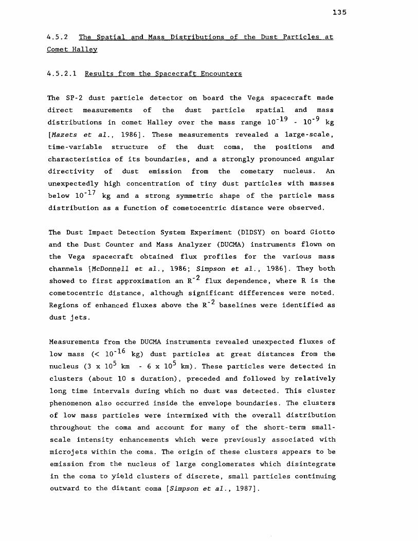
135

4.5.2 The Spatial and Mass Distributions of the Dust Particles at Comet Hailey

4.5.2.1 Results from the Spacecraft Encounters

The SP-2 dust particle detector on board the Vega spacecraft madedirect measurements of the dust particle spatial and mass

-19 - 9distributions in comet Hailey over the mass range 10 - 10 kg[Mazets et al., 1986]. These measurements revealed a large-scale,time-variable structure of the dust coma, the positions andcharacteristics of its boundaries, and a strongly pronounced angulardirectivity of dust emission from the cometary nucleus. Anunexpectedly high concentration of tiny dust particles with masses

-17below 1 0 kg and a strong symmetric shape of the particle mass distribution as a function of cometocentric distance were observed.

The Dust Impact Detection System Experiment (DIDSY) on board Giottoand the Dust Counter and Mass Analyzer (DUCMA) instruments flown onthe Vega spacecraft obtained flux profiles for the various masschannels [McDonnell et al., 1986; Simpson et al., 1986]. They both

- 2showed to first approximation an R flux dependence, where R is thecometocentric distance, although significant differences were noted.

_ oRegions of enhanced fluxes above the R baselines were identified as dust jets.

Measurements from the DUCMA instruments revealed unexpected fluxes of 1 c.low mass (< 1 0 kg) dust particles at great distances from the

nucleus (3 x 10“* km - 6 x 10^ km) . These particles were detected in clusters (about 1 0 s duration), preceded and followed by relatively long time intervals during which no dust was detected. This cluster phenomenon also occurred inside the envelope boundaries. The clusters of low mass particles were intermixed with the overall distribution throughout the coma and account for many of the short-term small- scale intensity enhancements which were previously associated with microjets within the coma. The origin of these clusters appears to be emission from the nucleus of large conglomerates which disintegrate in the coma to yield clusters of discrete, small particles continuing outward to the distant coma [Simpson et al., 1987].

136

4.5.2.2 Results from Earth-Based Infrared Observations

Near IR observations of comet Hailey yielded results which were consistent with a space density distribution of dust in the coma varying as the inverse square of the cometocentric distance [Lorenzetti et al., 1987; Lazaro et al., 1987].

Ground-based evidence of spatial structure indicative of dust ejection occurring mainly on the sunward side of the nucleus has come from a preliminary analysis of the thermal IR images obtained from the NASA-MSFC 20 pixel bolometer array at the NASA Infrared Telescope Facility (IRTF) [Campins et al., 1987].

The IR emission from the dust coma of comet Hailey was monitored throughout the recent apparition with the NASA 3.0 m IRTF at Mauna Kea [Hanner et al., 1987]. The dust coma was never in a steady state during March 1986. Because the dust emission varied strongly with time, the size distribution of the particles varied both with time and position in the coma, as documented by the in situ dust measurements. The IR brightness varied in phase with the optical brightness and the production rates of CS and C2 , and the 10 micron silicate feature correlated with the level of jet activity.

4 .6 The Gaseous Cometary Coma - Neutrals and Ions

4.6.1 Results from the Spacecraft Encounters

All the atmospheric/ionospheric models in recent times had predicted that the stable ion ^ 0 "*" would be the dominant ion in the inner coma. One of the major discoveries of the ion mass spectrometers on board the International Cometary Explorer (ICE) spacecraft to comet Giacobini-Zinner [Ogilvie et al., 1986] and the Vega and Giotto spacecraft to comet Hailey (e.g. Gringauz et al. [1986]; Balsiger et al. [1986]; Korth et al. [1986]) was the detection of this ion.

The neutral and ion mass spectrometers on board Giotto and Vega spacecraft, as well as the 3 channel and IR remote sensing photon spectrometers aboard the Vega spacecraft, detected most of the species in table 4.1 and a few new species. A total neutral

137

30 -1production rate of 10 s was inferred from the Neutral GasExperiment (NGE) on board the Vega-1 spacecraft during the hours prior to the encounter. The total neutral gas density profile along the spacecraft trajectory was determined and shown to vary as the inverse square of the radial distance.

The v vibrational band of ^ 0 at 2.7 microns was revealed by the2.5 - 5.0 micron spectra obtained from the IKS flown on the Vegaspacecraft [Combes et al., 1986b]. In addition the 1.38 micron bandof H 2 O was observed by the three channel spectrometer (TKS) aboardthe Vega-2 spacecraft [Krasnopolsky et al., 1986]. The H2 O productionrate at the time of the Vega-1 flyby was estimated at approximately

30 - 110 s [Combes et al. , 1986b], an observation which confirms that water is the dominant volatile in comet Hailey.

The 2.5 - 5.0 micron spectrum from the IKS instrument revealedseveral other new cometary signatures in addition to the H2 O signal at 2.7 microns. The band of CO2 was observed for the first time at4.7 microns and a broad signal, present in the 3.3 - 3.7 micron region, has been attributed to CH-bearing molecules [Combes et al., 1986b]. In addition, a marginal emission feature at 2.8 microns might be due to the OH (1-0) band, and absorption around 2.9 microns might be attributed to ice. Weak emission features at 3.6 microns and4.7 microns could correspond to the v^ band of H2 CO and the (1-0) band of CO, but they might be spurious since they do not show the expected variation with distance [Combes et al., 1986b].

The RPA2 Positive Ion Cluster Composition Analyzer (PICCA) detected 5 mass peaks with regular spacing of 15 amu up to 120 amu. Starting at 45 amu these peaks decrease in intensity with increasing mass. Within their half-width they are in good agreement with dissociation products of a polyoxymethylene [(H2 C0 )n ] chain [Huebner et al.,

1987] . If this identification is correct, this would be the first polymer identified in space, although earlier Vanysek & Wickramasinghe [1975] and Mendis & Wickramasinghe [1975] had used IR data and inferred physical data from earlier comets to propose that cometary dust was composed mainly of [(H2 C0 )n ].

138

Methane and ammonia abundances in the coma of comet Hailey have been derived from Giotto Ion Mass Spectrometer (IMS) data using a Eulerian model of chemical and physical processes inside the contact surface to simulate the Giotto High Intensity Spectrometer (HIS) ion mass spectral data for mass-to-charge ratios (m/q) from 15 to 19. Theratio m/q = 19/18 as a function of distance from the nucleus is not reproduced by a model for a pure water coma. It is necessary to include the presence of NH^ in coma gases to explain the data. Methane is identified as the most probable source at the distinct peak m/q = 15 [Allen et al., 1987].

4.6.2 Results From Earth-Based Observations

Gaseous neutral water was detected in the coma of comet Hailey duringIR observations from the NASA KAO [Weaver et al., 1987]. The absolutewater production rates measured were large, being of the order

29 30 -110 - 10 s . These measurements, together with the spacecraftresults, basically confirmed the supposition that ^ 0 is the dominant volatile constituent of the nucleus of comet Hailey.

The rotational transition of HCN at 3.4 mm wavelength was observed by Schloerb et al. [1987] using the US National Radio Astronomy Observatory (NRAO) . The data were obtained during a total of 56 individual observing sessions between November 1985 and May 1986. The HCN production rate was well correlated to the total visual magnitude of the comet, suggesting that HCN production follows the overall gas and dust production of the comet. Comparison of the HCN production to the total production of the comet indicates that it is a minor constituent with 0.1% the abundance of ^0. Comparison of HCN and CN production suggests that HCN is a major parent molecule of CN, but probably not the sole parent.

The 1667 MHz and 1665 MHz transitions of the OH radical were detectedand monitored nearly daily from the Nan^ay Radio Telescope [GSrard et al., 1987]. The observations cover the period from July 1985 to July 1986 and provide a unique test for the excitation mechanisms of the OH molecule and the kinematic models of the OH coma. The OH line was unambiguously detected for the first time in late August 1985 when the comet was at a heliocentric distance of 2.8 AU [BockelSe-Morvan

139

29 -1et al. , 1985b]. The OH production rate reached a peak of 3 x 10 s in early 1986. The production rates derived are smaller than those derived from UV observations [Feldman et al., 1986].

Schloerb et al. [1987] observed the 18 cm OH transitions from cometHailey with the US NRAO 4.3 m telescope. The OH production rate

_ oderived from these data follow an r law for heliocentric distances in the range r < 2 AU. Comparison of the radio OH production rates to those estimated by UV techniques continues to show that the radio technique finds systematically lower production rates.

High resolution IR spectra of ^ 0 in comet Hailey were used to characterize the velocity field in the neutral gas outflow from the cometary nucleus. The outflow was predominantly into the Sun facing hemisphere. The measured expansion velocities were 0.9 ± 0.2 kms"^ and 1.4 ± 0 . 2 kms~^ pre- and post-perihelion respectively [Larson et al., 1987].

Ground-based narrow-band imaging of the neutral coma of comets Giacobini-Zinner and Hailey with a Very High Sensitivity Imaging System (VHSIS) used on 1 m and 24" class telescopes and with a selection of wide-angle lenses has enabled an extensive study of the neutral comas of these comets. Characteristic scale lengths for the CN parent and daughter molecules and the C2 parent molecule have been determined for these two important comets at a variety of heliocentric distances. Several additional comets have been studied in a similar manner, allowing a better insight into the variation of these parameters with heliocentric distance (see chapter 5). In addition, the near-nucleus 630.0 nm VHSIS images of comet Giacobini- Zinner have been carefully analyzed to yield the H 2 O production scale length in this comet at 1 AU (section 6.2).

Several authors have recently reported finding low contrast "jet- like" features in the neutral emissions of comet Hailey [A'Hearn et al., 1986a; Cosmovici et al., 1987], an observation which has important implications for the formation of these radicals. No such features are immediately apparent in any of the near-nucleus VHSIS images of the coma of comet Hailey, and a more rigorous search for

140

these features has consequently been made, by applying imageenhancing techniques (section 6.3).

4.6.3 Results from the Dynamics Explorer-1 Satellite

The distribution of atomic hydrogen surrounding comet Hailey wasobserved in resonantly scattered solar Lyman alpha radiation with the imaging photometer for vacuum wavelengths on the Earth orbiting spacecraft Dynamics Explorer-1 (DE-1) [Craven & Frank, 1987],Measurements were made of the total Lyman alpha flux at the Earth due to cometary neutral hydrogen distribution and the hydrogen production rate determined as a function of heliocentric distance. For distances 1.50 to 0.68 AU before perihelion passage the hydrogen production rate varied as Q x r11 where Q = 9.1 x 1 0 ^ s"^ and n - -2.30. Using the same functional dependence in the post-perihelion period atdistances 0.63 to 1.20 AU, preliminary values based on a limited data set are Q = 1.1 x 10^® s“^ and n — -1.62.

4.6.4 Results from the Pioneer-Venus Orbiter

The Pioneer Venus Orbiter Ultraviolet Spectrometer measured theproduction of H, 0, and C in comet Hailey from late December 1985 toearly March 1986 [Stewart, 1987]. The comet passed within 0.27 AU ofVenus on 3 February 1986, and was 0.4 AU from Venus at perihelion on9 February 1986. The Pioneer Venus Orbiter was thus well placed toobserve the comet during its perihelion passage, when observationfrom Earth was difficult. Water production rates from the H data rosefrom 3.3 x 1 0 ^ s”^ at 1 AU inbound to 1.2 x 1 0 ^ s"^ at perihelion.

30 -1There was a further increase to 1 .6 x 10 s , followed by a slow30 -1decline to 1.4 x 10 s at the time of the Vega-1 encounter.

4.6.5 Results from Two Sounding Rockets

A sounding rocket payload to obtain far UV spectral images of comet Hailey was launched on 24 February 1986 and again on 13 March 1986. The payload included an objective grating spectrograph. High quality images of the oxygen coma at 130.4 nm, the carbon coma at 156.1 nmand 165.7 nm, and the sulphur coma at 181.4 nm were obtained [Opal et

al., 1987].

141

The radial distributions of CO, 01, Cl, and CII emissions in the coma of comet Hailey were measured by a long slit far UV spectrograph aboard the two sounding rockets. While radial outflow models of CO can match the observed profiles at cometocentric distances > lO^- km, the observed carbon distribution is not consistent with the model, suggesting an additional source of atomic carbon in the inner coma [Woods et al., 1987]. The analysis of the UV spectra of several comets has shown that the atomic carbon abundance in the inner coma cannot be accounted for by the photodissociation of carbon bearing molecules such as CO, CO2 , and CH^ [Festou, 1984].

4.6.6 Results from the International Ultraviolet Explorer Satellite

The UV spectrum of comet Hailey was monitored by the International Ultraviolet Explorer (IUE) satellite observatory between 12 September 1985 and 8 July 1986, at regular intervals, except for a two month period around perihelion [Feldman et al., 1987]. A partial characterization of the UV spectrum was obtained enabling derivation of coma abundances and a study of the light emission mechanisms of the observed species. The Fine Error Sensor (FES) camera was used to photometrically investigate the coma brightness variation on the time scale of the order of hours. Spectroscopic observations as well as FES measurements show the activity of the nucleus to be highlyvariable, particularly at the end of December 1985 and duringMarch/April 1986. These variations are attributed to a combination of nucleus rotation and outburst of individual jet or active areas of the nucleus.

A large but gradual increase in the brightness of the emission bands of comet Hailey, and thus in the coma abundance of OH, CS, C0 2 + and dust, was observed by the IUE satellite from 23 - 25 March 1986[McFadden et al., 1987]. This activity is different from the smaller and more rapid increase in brightness observed on 18 - 19 March 1986 also with the IUE [Feldman et al. , 1987]. The 18 - 19 March outburst showed a major increase in the abundance of ions without acorresponding increase in the neutrals and could be explained by the sudden release of a pocket of CO2 which was then rapidly ionized. The variation of 23 - 25 March is correlated with the periodic variations

142

observed by Millis & Schleicher [1986] and is most probably explained as a gradual increase in outgassing as an active area rotates into sunlight.

4.7 The Plasma Tail

4.7.1 Morphology of the Plasma Tail

Plasma tail activity for comet Hailey was observed to commence in mid-November 1985, at a heliocentric distance of 1.8 AU. The plasma tail was fully developed by early December 1985, as can be seen from the wide-angle VHSIS image shown in figure 7.15a, and the first dramatic disconnection event was centred on 10 January 1986. The post-perihelion images from the wide-angle VHSIS were spectacular. A disconnection event was clearly seen on 10 March 1986 (figure 7.15c), and an even more dramatic disconnection event was observed on 20 March 1986 (figure 7.15d). A good example of tail ray structure is shown in figure 7.11c. Plasma tail activity continued until late April 1986. The narrow-band ion images of comets Hailey and Giacobini-Zinner, collected with the VHSIS, are discussed in detail in chapter 7.

4.7.2 The Comet-Solar Wind Interaction

Direct exploration of comets began with the ICE interception of cometGiacobini-Zinner on 11 September 1985. Draping of the field lines wasobserved, confirming Alfven's basic picture, and the current sheet inthe centre of the tail was clearly detected. Extensive plasma waveactivity was recorded. The composition of the plasma was dominated bywater group ions. As the spacecraft traversed the comet, the flowspeed of the plasma decreased from solar wind values to low speeds ofthe order of a few tens of kms~^, while the density increased to a

_ 3maximum of approximately 600 cm in the centre of the tail. ICE discovered large fluxes of energetic water group ions over a region several million km in extent surrounding the comet [Hynds et al., 1986; Ipavich et al., 1986]. For a summary of the ICE results see section 7.2. A more detailed description of the ICE results may be found in the March 1986 and April 1986 issues of Geophysical Research Letters, and the 18 April 1986 issue of Science.

143

The particles and fields environment of comet Hailey encountered by Giotto displayed a very complex structure [Balsiger et al., 1986; Johnstone et al., 1986; R&me et al., 1986; Neubauer et al., 1986]. In the midst of rapid fluctuations, well defined regions separated by sharp transitions were distinguished. A summary of the spacecraft observations relating to the comet-solar wind interaction are presented in section 7.3.

144Figure 4.1

VOo £Lr> q^ 3

oo ' *> « <

— e go v> 2trt e ,=63 J L o

CJ O con- O* CDO co <3 o n

M 1-1CO < PO •—C L C/3

S'. «P o

o<o3r+O*oeeraor3O

Po>-•»no3o

p1-1«T3MOIAo3

3 g-co O% Ci «I *** I—*p VOt/9

3 £» w^ « X5*. ? H'"o p

opo 'VIo1-1

*3<-♦•o ’3

op

c►1o

3 >o? d 8 ’or+ O►—• Vi £ • «“► s *°<5 oCO 1-1Q 3*w* rt

3CL

2 .o '3

90pac ’COO►o»

OtO

P3CL

53toOp>iop

3*O

3

ts*^ ST=rS§ S ’a eA w o MCO t;° *s3 o

CO5 wCL co o ' OVCO •W' o

ta p O 3 O' CL coCD 3* *5 «< p CD CLcl 5r

>•

o.pPT3

®8o

-Jooo

“ 7 ne>ooo

Vooo

Aooo

6 ® .

Figure 4.2145

Composite image o f the nucleus o f comet Hallev. North is up and the sun is to the left and 155 below the image plane. This photograph is a composite o f 60 H M C images and has resolution varying from 800 m in the lower right to 100 m in the vicinity o f the northern tip. Image processing steps required to achieve this composite include subtraction o f thermal background charge. Fourier filtering o f coherent noise, detector responsivity correction, geometric rectification, and image registration. (Reitsema et al., 1986)

HALLEY PROFILE

C H A IN OF HILLS —

BH IG H T SOURCE

CRATER

MOUNTAIN

C EN TR A L D E PR E SSIO N REGION

BRIGHT

ROTATION AXIS ORIENTATION Schematic drawing o f major nuclear features as seen by the HM C

146

CHAPTER 5

THE NEUTRAL COMETARY ENVIRONMENT I - THE DISTRIBUTION OF CN AND C2

5.1 Introduction

As a comet approaches the Sun the first spectral feature to appear is generally the brightest CN band, the (0-0) vibrational band system at 388 nm, which is usually first detected at heliocentric distances of the order 3 AU. The C2 Swan band at 472 nm is one of the most prominent emissions in the visible and normally becomes detectable at about 2 AU from the Sun. Thus, the spatial distributions of CN and C2

can be monitored over a wide range of heliocentric distances, yielding important information on the production and destruction mechanisms of these two cometary species.

Since comets are viewed with differing observing geometries and with a variety of instruments, some form of model is required to compare and contrast the gas distributions derived from these disparate data sets. Some simple models of the neutral atmosphere are discussed in section 5.2 leading to the radial outflow model with decay. This model considers the observed (daughter) species to be produced at a constant rate from a source of exponentially decaying parentmolecules streaming radially with uniform speed from a point source nucleus. The daughter molecules continue to move radially withuniform speeds and decay exponentially themselves. The characteristic scale length of a given parent or daughter species is equal to the product of its life-time and velocity.

The narrow-band near-nucleus and large-scale CN images, obtained with the Very High Sensitivity Imaging System (VHSIS), of the observed comets can be used to derive characteristic scale lengths for the CN parent and CN radical (the daughter species) respectively (section 5.3). Since a number of comets have been observed at avariety of heliocentric distances, these results can be used toderive heliocentric scaling laws for the CN parent and the CN

147

radical, and thus provide an insight into the production and destruction mechanisms of the CN radical.

The narrow-band near-nucleus VHSIS C2 images of the observed comets can be used in a similar manner to derive the characteristic scale length of the C2 radical and its variation with heliocentric distance (section 5.4).

There are three sources of error in the derivation of a daughter scale length, namely uncertainties in the amount of dust contamination, uncertainties in the sky background and errors in the centre location. There is an additional source of error in the derivation of a parent scale length caused by uncertainties in the daughter scale length. The relative importance of these sources of error are discussed in section 5.5.

The cometary CN and C2 scale lengths found by other investigators are presented in section 5.6. The methods used by each different observer are critically examined and those methods likely to produce the most accurate results are identified.

The scale lengths calculated by the other observers are compared with those derived from the VHSIS images in section 5.7. More accurate scaling laws are obtained for the scale lengths by combining the VHSIS results with the reliable data points outlined in section 5.6.

The inner C2 coma of comet Borrelly in mid-December 1987 was found to be anomalous, in that the simple radial outflow model could not represent the data. This anomaly is discussed in section 5.8.

5.2 Models of the Neutral Cometary Environment

The first model calculates the expected intensity distribution when stable molecules leave the nucleus and expand isotropically into volume (section 5.2.1). This is not a very realistic model because the solar radiation generally dissociates the cometary molecules. The second model calculates the intensity distribution for molecules leaving the nucleus isotropically but decaying with a time constant t

(section 5.2.2). However, most of the molecules emitting in the

148

visible region are not produced at the nucleus but are themselves dissociation products. The third model (Haser model), calculates the intensity distribution for such daughter molecules which also are dissociated by the solar radiation (section 5.2.3). The limitations of the Haser model are discussed in section 5.2.4. The application of this model to the neutral comet images obtained with the VHSIS is described in section 5.2.5.

5.2.1 Intensity Distribution Caused by Stable Molecules Expanding Isotropically into Volume

This model assumes an isotropic ejection of molecules from the cometary nucleus with velocity, v, and production rate, Q.

Consider an elemental spherical shell at cometocentric distance R. The number density, n(R), is:-

n(R) =number in volume element

volume of element5.1

Qdt

47rR2dR5.2

4ttR 2v5.3

In the case of an optically thin atmosphere, the observed intensity at projected distance, s, is proportional to the column density along the line of sight at that distance. The column density at projected distance, s, is given by:-

N(s) =+oo

n(R) dz-oo

5.4

47TV

+00

2 2 -oo s + zdz 5.5

47TV

1— tan s

-1 +oo

-oo 5.6

149

47TVS 5.7

In this, the simplest of cases, the column density and, therefore, the intensity distribution varies inversely with the projected distance.

5.2.2 Intensity Distribution Caused by Exponentially Decaying Molecules Expanding Isotropically into Volume

As the molecules move outwards they are generally dissociated by the solar radiation. If the time constant for decay is t , the density distribution becomes:-

n(R) =4ttvR'

4ttvR 2

exp-

exp-

t

T

R

L RdJ

5.8

5.9

wheie R^ - . Setting C = , the density distribution becomes47TV

n(R) = —R 2

exp-R

LRdJThe column density is given by:-

5.10

’+oo 1 " R "N(s) = C — ~ exp-

-oo R 2 _R d_dz 5.11

Let X =1— , then R d

2Coo ]

0 s2 + z2 exp-V (s2 + z2)

R ddz 5.12

N(X)

dN(X)

dX

OO 12C

- 2C

-= r exp-[ Xy/ (s2 + z2) ] dz0 s + z2OO 1

o « P - [ X V ( s 2 + z2), dz

5.13

5.14

150

- 2CK0(sX) 5.15

where is the modified Bessel function of the second order.

N(X) - N(0) = - 2C

Let y = sX

rx

oK 0(sX) dX

dy

dX

5.16

5.17

N(X) = N(0) - 2CfsX

0K 0(y) dy

but N(0) is just the integral from model 1 so that:

2CN(s) =

7T 'sX— - K 0(y) dy

_ 2 0

5.18

5.19

5.2.3 Intensity Distribution Caused bv Exponentially Decaying Daughter Molecules Expanding Isotronicallv into Volume

This model is based on the parent-daughter hypothesis in which the parent molecules released by the nucleus decay with a time constant rp corresponding to a distance Lp = vp rp- daughter products thendecay with a time constant corresponding to a scale length

The parent molecules emanate radially with uniform speed from a point source nucleus. The daughter molecules continue to move radially with uniform speeds.

Let the production rate of the parent molecules at the nucleus be Q molecules per second. Then the total number of parent molecules crossing a sphere of radius z per second will be given by:-

Nr Qexp-(Xpz) 5.20

where:-

X rvPfP

5.21

The production rate of the daughter molecules is thus given by:- -dNp dNd

dz dzQXpexp-(Xpz) 5.22

The number of daughter molecules in an elemental spherical shell of radius z and width dz is thus:-

dNd = Q X pexp-(Xpz) dz 5.23

Now consider these specific daughter molecules. When they are a distance R (R > z) from the nucleus their number will be decreased by the factor exp(-X^(R-z)), so that the total number of daughter molecules at a distance, R, from the nucleus due to disintegrations of parent molecules in the given elemental shell becomes

dNd(R) Q X pexp-(Xpz)exp-(Xd[R-z]) dz 5.24

The total number of daughter molecules arriving per cm at a distance R per second becomes

QX.

4?rR'

QX.

4?rR^

R

0 R

_ 0

Qxp

exp-(Xpz)exp-(Xd[R-z]) dz

exp([Xd - X p]z)exp-(XdR) dz

4ttR (Xd - X p)exp([Xd - Xp]z)exp-(XdR)

R

5.25

5.26

5.27

QX.[ exp-(XpR) - exp-(XdR) ] 5.28

47rR (Xd - X p)

The number density at distance R from the nucleus becomes

Q X Pn(R) = [ exp-(XpR) - exp-(XdR) ] 5.29

47rvdR (Xd - X p)

This equation can be broken down into two expressions of the form given in model 2 above, so that the resulting column density is of

152

the form:-

N(s) =Q X p fsXj

47TVds(Xd - Xp) sXdKo(y) dy 5.30

Hence the intensity distribution is of the form:

I(s)fsX.

sXdK 0(y)dy 5.31

This model had been formulated earlier by Mokhnach [1938;1956] and independently by Wallace & Miller [1958], but, it was Haser [1957] who first derived the finite integral given above. This simple radial outflow model with decay is referred to as the Haser model.

5.2.4 Limitations of the Haser Model

The model is still an over-simplification as it assumes spherical symmetry and does not take into account effects such as non-radial flight paths, solar radiation repulsion, the velocity distribution of the emitters (Greenstein effect) or time dependent production. Despite these limitations, the model is readily computable and yields parameters for comparison between the data sets. The analysis of the VHSIS images presented here proceeds via integration over circular annuli to compensate asymmetries due to radiative repulsion and Greenstein effects. It has been used by several authors, see for example Combi & Delsemme [1986], and references therein.

Some attempts at improving the model have been made. Combi & Delsemme [1980] have developed an average random walk model to interpret the intensity distributions of neutral cometary species. This model employs the "Monte Carlo" method [Cashwell & Everett, 1959]. Theactual trajectories of many individual radicals are computed over a time period long enough to achieve a steady-state. Column densities are then obtained by counting the numbers of molecules in a given volume. An isotropic point source of parent molecules is assumed, which are themselves photodissociated to produce the daughter molecules as one of the by-products. The daughters are ejected isotropically from the centre of mass of the parent molecules and are accelerated away from the Sun by solar radiation pressure. Delsemme & Combi [1980] use this method to show that out to the limit of the

153

sunward envelope the zero-acceleration profile coincides with the simple brightness average of the sunward and tailward profiles. Therefore, the distortion due to solar radiation repulsion can be removed by adding the sunward and tailward profiles. They then go on to demonstrate that the Haser scale lengths can be used to interpret observed cometary brightness profiles but that the scale lengths found are not the true space scale lengths but only their radial projections.

5.2.5 Derivation of Scale Lengths

The raw comet images along with their associated sky background images are initially corrected for the thermionic emission and flat field response of the detector as discussed in section 3.3.2. The processed comet images are then corrected for night sky contamination by subtracting the relevant processed and normalized sky background files, as described in section 3.3.3.

The data are to be fitted to a formula of the type:-

fsXsl(s) PK 0(y)dy 5 -32

sXd

where Ig is the surface brightness at projected distance s from the centre of the comet, A is a normalizing parameter related to the production rate, Xp is the reciprocal of the parent scale length, is the reciprocal of the daughter scale length and K q ( x ) is the modified Bessel function of the second order.

It should, therefore, be possible to derive the production rate and the two scale lengths corresponding to the parent and dissociated product from a fit of the expected surface brightness distribution with the observed distribution. However, the images obtained with the VHSIS are not flux calibrated and so production rates cannot be derived. Cochran [1982;1985] has shown that unless there is an a priori method of fixing one of these parameters, the model can fit the data with a whole variety of parameters. Therefore, the data has to be fitted to a formula with two unknowns, the normalizing parameter, A, and the unknown scale length.

154

The corrected data is initially reduced to a radial profile about the comet nucleus as described in section 3.4.2, the counts in any given annulus being stored as a function of radius. For any given value of A and the unknown scale, a relative test of the goodness of the fit may be obtained by comparing the data with the model predictions at each radius. A convenient measure of the goodness of the fit is the sum of the squares of the differences between the data and the model. By varying A and the unknown scale in continuous increments over a suitable range the best fit is obtained by minimizing the sum of the squares of the differences.

5.3 Calculation of the CN Parent and Daughter Scale Lengths and their Variation with Heliocentric Distance

As a comet approaches the Sun, the first spectral feature to appear is generally the brightest CN band, the (0-0) vibrational band system at 388.3 nm, which is usually first detected at heliocentric distances of the order of 3 AU [Swings & Haser, 1956].

The CN daughter scale lengths, determined from the large-angle CN images taken with the VHSIS, are presented in section 5.3.1. The variation of the CN daughter scale length with heliocentric distance, as determined from these results, is also discussed.

The CN parent scale lengths, determined from the near-nucleus CN images taken with the VHSIS, are presented in section 5.3.2. The variation of the CN parent scale length with heliocentric distance, as determined from these results, is also discussed.

5.3.1 Calculation of the CN Daughter Scale Lengths

CN daughter scale lengths can be inferred from the large-scale VHSIS images of the CN coma. Figure 5.1 shows four such large-scale CN images. The characteristic "teardrop" shape of the outer CN coma, caused by the action of solar radiation pressure accelerating the gas molecules in an anti-sunward direction, is readily apparent.

Figure 5.1a shows the large-scale appearance of the CN coma of comet Hailey, pre-perihelion, on 8 December 1985 at 03:26 UT. This image

155

was taken with the 300 mm Nikon camera lens from TMF. The comet was 1.38 AU from the Sun and 0.70 AU from the Earth.

Figure 5.1b shows the large-scale appearance of CN coma of comet Hailey, post-perihelion, on 2 May 1986 at 21:39 UT. This image was taken with the 300 mm Nikon camera lens from La Palma. The comet was 1.65 AU from the Sun and 0.83 AU from the Earth.

Figure 5.1c shows the outer CN coma of comet Bradfield, post­perihelion, on 22 December 1987 at 02:37 UT. This image was taken with the 300 mm Nikon camera lens from TMF. The comet was 1.19 AUfrom the Sun and 0.86 AU from the Earth.

Figure 5. Id shows the outer CN coma of comet Borrelly, close to perihelion, on 22 December 1987 at 07:28 UT. This image was taken with the 300 mm Nikon camera lens from TMF. The comet was 1.36 AU from the Sun and 0.52 AU from the Earth.

The parent scale length in any large-scale image taken in the light of the CN molecules is typically of the order of one or two pixels. This gives a convenient method for determining the daughter scale length by assuming a negligible parent scale and fitting to that part of the profile not affected by the parent scale length. Thus, the first five pixels are ignored in the fit. Figure 5.2 shows the four corresponding best model fits to the radial profiles of the images shown in figure 5.1.

The derived daughter scale lengths from the large-scale images are tabulated in table 5.1. When these daughter scale lengths are plotted against the heliocentric distance of the comet on a log-log graph (dark blue points in figure 5.7), the slope of the best fit to the data is found to be 2.1 ± 0.6. This results is consistent with the daughter scale length varying in direct proportion with the square of the heliocentric distance, and thus confirms the usual assumption that the destruction of the CN radical is controlled by the solar flux of radiation. These results give a value of (5.0 ± 1.1) x 10 km for the daughter scale length at unit heliocentric distance.

156

Table 5.1 CN Daughter Scale Lengths Inferred from the Large-Scale VHSIS CN Images

Comet UT date Exp Delta r Skv id(min) (AU) (AU) (cts/pix) (xlO^ km)

Hailey 85 Dec 8.14 10 0.70 1.38 3.0(3.0) 12.5(4.5)Hailey 85 Dec 12.25 10 0.77 1.32 14.5(0.5) 9.0(1.0)Hailey 86 May 2.94 15 0.83 1.65 1.0(1.0) 13.0(2.0)Hailey 86 May 3.87 15 0.86 1.66 0.5(0.5) 15.0(5.0)Bradfield 87 Dec 22.11 60 0.86 1.19 30.9(0.4) 7.0(1.5)Borrelly 87 Dec 22.31 60 0.52 1.36 19.9(0.9) 7.5(2.0)

5.3.2 Calculation of the CN Parent Scale Lengths

CN parent scale lengths can be inferred from the near-nucleus VHSIS images of the CN coma. Four such near-nucleus CN images are displayed in figure 5.3.

Figure 5.3a shows the near-nucleus appearance of the CN coma of comet Hailey, post-perihelion, on 22 March 1986 at 11:48 UT. This image was taken with the 16" telescope at TMF. The comet was 1.02 AU from the Sun and 0.76 AU from the Earth.

Figure 5.3b shows the inner CN coma of comet Wilson, pre-perihelion, on 4 November 1986 at 02:33 UT. This image was taken with the 24" telescope at TMF. The comet was 2.66 AU from the Sun and 2.64 AU from the Earth.

Figure 5.3c shows the inner CN coma of comet Bradfield, post­perihelion, on 19 December 1987 at 02:18 UT. This image was taken on the 24" telescope at TMF. The comet was 1.16 AU from the Sun and 0.85 AU from the Earth.

Figure 5.3d shows the inner CN coma of comet Borrelly, close to perihelion on 19 December 1987 at 05:43 UT. This image was taken with

157

the 24" telescope at TMF. The comet was 1.36 AU from the Sun and 0.51 AU from the Earth.

The parent scale length may be determined from the near-nucleus images by using the CN daughter scale length found from the large- scale images, scaled to the appropriate heliocentric distance. Figure 5.4 shows the four corresponding best fits to the radial profiles of the images shown in figure 5.3. The parent scale lengths determined from the near-nucleus images are given in table 5.2.

Table 5.2 CN Parent Scale Lengths Inferred from the Near-Nucleus VHSIS CN Images

Comet UT date Exp Delta r Skv(min) (AU) (AU) (cts/pix

h

G-Z 85 Sep 12. 11 10 0.47 1.03 1.0(1. 0) 2. 2(0. 4)Hailey 85 Dec 10. 10 4 0. 73 1. 35 10. 0(10 .0) 4. 0(1. 0)Hailey 86 Mar 5. 53 1 1. 18 0. 77 5.0(5. 0) 2. 1(0. 2)Hailey 86 Mar 6. 55 1 1. 16 0. 79 7. 5(7. 5) 3.0(1. 5)Hailey 86 Mar 15 55 5 0 96 0 90 5 0(5. 0) 4 0(0. 9)Hailey 86 Mar 22 49 2 0 76 1 02 1 0(1. 0) 2 2(0. 3)Wilson 86 Nov 2 12 60 2 62 2 68 6 5(0. 5) 10 1(0. 6)Wilson 86 Nov 4 11 60 2 64 2 66 5 5(0. 5) 9 5(0. 5)Wilson 86 Nov 5 17 60 2 65 2 65 6 0(0. 5) 10 8(0. 7)Sorrells 87 May 28 40 30 1 96 2 01 0 5(0. 5) 5 5(1. 0)Bradfield 87 Nov 26 13 5 0 89 0 94 0 5(0. 5) 3 3(0 1)Bradfield 87 Dec 3 11 20 0 85 1 00 15 0(15.0) 2 1(1 0)Bradfield 87 Dec 14 21 5 0 84 1 10 0 1(0. 1) 3 6(0 3)Borrelly 87 Dec 15 27 10 0 .49 1 36 1 5(0. 5) 3 9(0 5)Bradfield 87 Dec 19 10 10 0 .85 1 16 1 5(0. 5) 4 2(0 1)B-M 89 Aug 9 39 10 0 .63 0 .89 0 .3(0. 3) 1 .1(0 05)B-M 89 Aug 11 .47 10 0 .63 0 .87 0 .5(0. 5) 0 .98(0.02)B-M 89 Aug 12 41 10 0 .63 0 .85 0 .4(0. 4) 1 .08(0.01)B-M 89 Aug 13 .48 10 0 .64 0 .83 0 .2(0. 2) 1 .35(0.02)B-M 89 Aug 21 .44 10 0 .72 0 .70 4 .5(0 5) 0 .89(0.02)B-M 89 Aug 22 .45 5 0 .73 0 .68 1 .5(1 5) 0 .69(0.05)

(xlO km)

158

When a log-log graph is drawn plotting the parent scale length against the heliocentric distance of the comet (dark blue points in figure 5.8), the slope of the best fit to the data is calculated to be 1.6 ± 0.2. This is not consistent with the CN parent scale varying as the square of the heliocentric distance. These results give a value of (2.1 ± 0.2) x 10^ km for the parent scale length at unit heliocentric distance.

5.4 Calculation of the Cn Parent Scale Length and its Variation with Heliocentric Distance

At heliocentric distances less than about 2.0 AU, the visual spectra of most comets is dominated by the Swan bands of C2 , with 5 band sequences measured (delta(v) = -2 to + 2). Although chemical models of the coma suggest that C2 is formed primarily by chemical reactions and that its density distribution differs considerably from a Haser model [Huebner, 1981], it is still common practise to use Haser model parameters to empirically describe the distribution.

The C2 parent scale lengths, determined from the near-nucleus C2

images taken with the VHSIS, are presented in section 5.4.1. The variation of the C2 parent scale length with heliocentric distance, as determined from these results, is also discussed.

Many near-nucleus images of the C2 coma have been taken by the VHSIS for a variety of comets but no large-scale images of the C2

distribution have been taken. The daughter scale length cannot, therefore, be found from the VHSIS data. Consequently a daughter scale length has to be assumed in order to determine the parent scale length from the near-nucleus images. The daughter scale length for C2

is taken to be 1.2 x 10^ km [Combi & Delsemme, 1986], scaling as the square of the heliocentric distance, as expected for decay processes induced by the solar flux of radiation.

C2 parent scale lengths can be inferred from the near-nucleus images of the C2 coma, taken with the VHSIS. Four such near-nucleus C2

images are displayed in figure 5.5.

159

Figure 5.5a shows the near-nucleus appearance of the C2 coma of comet Hailey, post-perihelion, on 18 March 1986 at 12:00 UT. This image was taken with the 24" telescope at TMF. The comet was 0.96 AU from the Sun and 0.86 AU from the Earth.

Figure 5.5b shows the inner C2 coma of comet Hailey, post-perihelion, on 6 May 1986 at 00:00 UT. This image was taken with the JKT. The comet was 1.70 AU from the Sun and 0.95 AU from the Earth.

Figure 5.5c shows the inner C2 coma of comet Bradfield, post­perihelion, on 21 December 1987 at 02:19 UT. This image was taken with the 24" telescope at TMF. The comet was 1.18 AU from the Sun and 0.86 AU from the Earth.

Figure 5.5d shows the inner C2 coma of comet Borrelly, close to perihelion, on 21 December 1987 at 06:10 UT. This image was taken with the 24" telescope at TMF. The comet was 1.32 AU from the Sun and 0.52 AU from the Earth.

Table 5.3 C2 Parent Scale Lengths Inferred from the Hear-NucleusVHSIS Cn Images

Comet UT date Exp Delta r Sky(min) (AU) (AU) (cts/pix) (xlO km)

G-Z 85 Aug 31.11 10 0.47 1.03 126 (2) 2.0(0.3)Hailey 85 Dec 10.15 10 0.73 1.35 15 (15) 4.4(1.2)Hailey 86 Mar 18.50 5 0.86 0.96 7.5(7.5) 4.6(1.7)Hailey 86 May 6.00 10 0.95 1.70 10 (10) 3.5(3.0)Bradfield 87 Nov 26.14 5 0.89 0.94 4.5(0.5) 2.2(0.2)Borrelly 87 Dec 14.37 10 0.49 1.36 2.0(0.5) no fitBorrelly 87 Dec 15.30 10 0.49 1.36 1.5(0.5) no fitBradfield 87 Dec 21.10 10 0.86 1.18 1.0(0.5) 2.0(0.1)Borrelly 87 Dec 21.26 20 0.52 1.36 1.5(0.5) no fitB-M 89 Aug 9.49 10 0.63 0.89 1.8(0.5) 1.2(0.1)B-M 89 Aug 11.49 10 0.63 0.87 1.2(0.5) 1.1(0.1)B-M 89 Aug 23.49 5 0.75 0.68 2.5(0.5) 0.9(0.1)

160

Figure 5.6 shows the corresponding fits to the data shown in figure 5.5. The parent scale lengths determined from the near­nucleus images are given in table 5.3. The near-nucleus C2 images of comet Borrelly cannot be fitted to the Haser model and consequently no parent scale lengths can be derived for this comet. This anomaly is discussed in section 5.8. However, good fits are obtained for all the other comets observed.

When the C2 parent scale length is plotted against the heliocentric distance of the comet on a log-log plot (dark blue points in figure 5.9), the slope of the best fit to the data is calculated to be 1.6 ± 0.6. These results give a value of (1.75 ± 0.25) x 10^ km for the parent scale length at unit heliocentric distance. It is difficult to make any firm conclusions from these VHSIS results. The ten data points range from 0.68 to 1.70 AU and show a good deal of spread which is reflected in the large errors on the gradient and the parent scale at 1 AU. A better estimate of these parameters can only be found by combining the VHSIS C2 results with those found by other investigators (section 5.7.3).

5.5 Discussion of the Errors in the Derived Scale Lengths

The following discussion assumes that there are a sufficient number of photons at each point in the radial profile so that the errors introduced by the statistics of photon counting are small. This criterion is certainly valid in the analyzed VHSIS images, because, at large cometocentric distances, where the counts per pixel are low (of the order 0 - 1 0 per pixel), the integration is performed over a large number of pixels.

In addition, the discussion also assumes that the scale of any VHSIS image is such as to allow a meaningful determination of the derived scale length. This basically means performing a Haser fit from the nucleus, or near the nucleus, out to a radius of the order of 1 - 5 scale lengths. This criterion is also valid in all of the analyzed VHSIS images.

When the above two conditions are satisfied there remain three sources of error in the derivation of a scale length, namely

uncertainties in the amount of dust contamination, uncertainties in the sky background and errors in the centre location. There is an additional source of error in the derivation of a parent scale length caused by uncertainties in the daughter scale length. The relative importance of these sources of error are now discussed in turn.

5.5.1 Estimation of the Errors Caused bv Dust Contamination

In addition to the chosen signal isolated through a given interference filter there will also be present a certain amount of contamination from the cometary continuum. This continuum is caused by scattering of the solar spectrum by the cometary dust particles. The amount of continuum contamination would ideally be monitored by observing the comet with two filters for each line or band observed. One filter would be used to observe the line or band and the other would be offset slightly in a region of pure continuum. However, the Atmospheric Physics Laboratory (APL) filter set includes only one dust filter at 524.2 nm, with a full width half maximum of 0.3 nm. This filter was used consistently only in the observations of comet Hailey, where the signals were strong through all of the other filters employed. Few continuum images have been taken of the comets observed since comet Hailey due to the fact that very weak signals were obtained through other filters, and, consequently, these have been used as upper limits on the dust contamination by assuming no gas emission through the filter.

The amount of dust contamination varies from comet to comet and needs to be estimated in each case. When the signal through any APL filter is particularly weak this may be used as an upper limit on possible dust contamination at that wavelength. The amount of contamination at another wavelength may then be estimated by assuming a solar type spectrum. This technique was successfully applied to show that the C2

profiles of comets Bradfield and Borrelly were not significantly changed by dust contamination. In this particular case 630.5 nm images of the two comets were used to obtain upper limits on the dust* contamination (Meredith et al., 1989). Since the dust contamination is stronger at 471 nm than 388 nm, the CN profiles of these two comets will also not be significantly changed by dust contamination.

162

The C0+ signal at 402 nm was extremely weak in comet Brorsen-Metcalf, being of the order of 2 - .4 counts per pixel per 10 minuteintegration in the near-nucleus region. This compared with a maximum CN signal at 388 nm of the order 1,000 counts per pixel per 10 minute integration, and a maximum C2 signal of the order 500 counts per pixel per 10 minute integration. Thus, the dust contamination is negligible and does not affect the scale lengths derived from the CN and C2 images in this comet. The same was true for comets Wilson and Sorrells.

There was only a small contribution from dust at 388 nm in comet Giacobini-Zinner, estimated from photometry with a 5 nm filter as being a maximum of 3% of the main signal [Williams et al., 1986]. Thus the amount of contamination through the APL 1 nm filter would be a maximum of 0.6% and would not affect the derived scale length appreciably.

A small number of dust images were taken of comet Hailey, through the524.2 nm filter. The dust contamination in comet Hailey, at a given wavelength, was estimated from the images taken with this filter, and corrected for a solar type spectrum. Three near-nucleus CN images of comet Hailey were reanalyzed after correction for dust and it wasfound that the derived parent scale length lay within the errorscaused by uncertainties in the sky background.

Therefore, although there will inevitably be a small amount of dust contamination through the APL CN and C2 filters, it has been shown that this has a negligible effect on the derived scale lengths for the comets that have been observed with the VHSIS to date.

5.5.2 Estimation of the Errors Caused bv Uncertainties in the SkvBackground

It has long been common practise to obtain sky background images both immediately prior and after a series of exposures with a given filter, and this results in a good determination of the sky background. However, the paramount importance of this calibration was not appreciated for some of the early work and so it is necessary to examine the effect of uncertainty in this important parameter.

163

For example, the images of comet Hailey in March 1986 were taken in a very short observing window before dawn, when the sky background was changing rapidly with time. Due to the shortage of observing time, few background images were recorded and so the scale lengths derived from these images have relatively large errors associated with them. The sensitivity of the derived scale length to uncertainties in sky background may be demonstrated by studying an image of comet Hailey, taken in the light of the CN molecule, on 5 March 1986. The sky background is uncertain but must be less than 10 photons per pixel, the average of the values towards the edge of the field of view. The variation of the derived scale length with sky background is tabulated in table 5.4.

Table 5.4 Errors on a Typical CN Parent Scale Length Caused bv Uncertainties in the Skv Background

Skv Background Parent Scale Leneth(photons) (x 10^ km)

0.0 1.552.0 1.364.0 1.216.0 1.098.0 0.95

10.0 0.86

This analysis illustrates the high sensitivity of the result to uncertainties in the sky background.

5.5.3 Estimation of the Errors Caused by an Inaccurate Centre Determination

The centre of the comet is computed as that pixel about which a 5 x 5 pixel grid is the brightest. It was decided to test the sensitivity of the method to inaccuracies in the determined centre. A typical CN image of Brorsen-Metcalf, taken on 13 August 1989, was selected for

164

this purpose. The results of moving off from the true centre are tabulated below.

Table 5.5 Errors on a Typical CN Parent Scale Length Caused by an Inaccurate Centre Determination

Distance off centre Computed Scale Leneth % Error(pixels) (x 104 km)

0 1.35s

1 1.35 0.02 1.35 0.03 1.37 1.54 1.38 2.25 1.39 3.06 1.42 5.27 1.43 5.98 1.47 8.99 1.50 11.1

10 1.54 14.1

The method of finding the centre of the comet should normally result in determining this parameter to the nearest pixel. If, for some reason, the centre is out by one or two pixels the above table indicates that the error on the derived scale length will be small (actually zero in the above case). The computer technique could not result in being off centre by more than this unless a star or image artifact were polluting the image. However, the images are always initially inspected by eye to prevent this possibility. The errors on the derived scale lengths, introduced by this method of centring may, therefore, be assumed to be negligible.

5.5.4 Estimation of the Errors in the Derived Parent Scale Lengths Caused by Uncertainties in the Daughter Scale Length

The CN daughter scale length is computed to be (4.9 ± 0.5) x 10^ kmat 1 AU, its variation with heliocentric distance not being

oinconsistent with r (see section 5.7.1). In order to estimate the

sensitivity of the method to uncertainties in the daughter scale length, three near-nucleus CN images were selected at random. The Haser fits were then performed using maximum and minimum values for the CN daughter scale length. The results are tabulated below.

Table 5.6 Errors on Three Typical CN Parent Scale Lengths Caused bv Uncertainties in the Daughter Scale Length

Daughter Scale Parent Scale (x 104 km)at 1 AU Bradfield Borrelly Brorsen-Metcalf(x 105 km) 87 Dec 14.21 87 Dec 15.27 89 Aug 13.48

4.5 5.05.5

3.673.593.50

3.973.903.82

1.441.401.35

Thus a 10% error in the CN daughter scale length will produce a smaller percentage error in the calculated CN parent scale length of the order 2-3%.

Discussion

The above study has shown that the errors on the derived scale lengths caused by uncertainties in the dust contamination and inaccurate centering is very small. The error on a derived daughter scale length, being independent of the parent scale length, depends largely on the uncertainty in the sky background, and the errors quoted in table 5.1 are the errors caused by this uncertainty. The error on a derived parent scale length depends mainly on the uncertainty in the sky background. There is an additional error of the order of 2-3% caused by uncertainties in the daughter scale length. The errors on the computed CN scale length quoted in tables5.2 and 5.3 are the errors caused by uncertainties in the sky background.

166

5.6 Scale Lengths Found bv Other Investigators

The CN parent and daughter scale lengths found by other investigators are presented in section 5.6.1 and their C2 parent scale lengths are presented in section 5.6.2. The methods used by the other observers are described in section 5.6.3. The relative merits of the various techniques are discussed.

5.6.1 CN Parent and Daughter Scale Lengths Found bv Other Investigators

The CN parent and daughter scale lengths published by otherinvestigators are summarized in table

Table 5.7 CN Parent and Daughter

5.7.

Scale Lengths Published in theLiterature

Observer Comet r(AU) (x 104 km) (xlO5 km)

Delsemme & Bennett 0.60 2.19 ± 0.31 0.55 ± 0.05Moreau ..... Bennett 0.71 1.99 ± 0.51 0.63 ± 0.09(1973) Bennett 0.83 3.16 ± 0.39 1.00 ± 0.12

Bennett 0.84 4.47 ± 0.90 1.12 ± 0.13Bennett 1.12 4.47 ± 0.90 1.78 ± 0.10

Combi & Bennett 0.73 1.15 ± 0.30 > 17.78Delsemme .. .. Bennett 0.83 1.20 ± 0.11 1.17 ± 0.15(1980) Bennett 0.84 1.23 ± 0.21 3.16 ± 0.82

Bennett 0.97 0.89 ± 0.36 > 5.75Bennett 0.99 4.79 ± 3.72 4.68Bennett 1.12 0.93 ± 0.40 > 12.595West 0.44 0.41 ± 0.12 1.74 ± 0.34West, 0.46 0.53 ± 0.04 2.09 ± 0.15West 0.54 1.23 ± 0.06 1.41 ± 0.10West 0.65 1.05 ± 0.07 2.63 ± 0.38West 0.70 0.66 ± 0.03 > 3.55

167

Observer Comet r td(AU) (x 104 km) (xlO^ km)

West 0.84 1.20 ± 0.31 1.95 ± 0.34West 1.01 2.45 ± 0.71 5.25 ± 2.34West 1.14 3.55 ± 1.45 > 1.99West 1.18 2.09 ± 0.54 5.13 ± 2.11West 1.21 3.71 ± 0.96 9.54 ± 5.59

Newburn & Encke 0.78 0.76 ± 0.16 \Spinrad .... Encke 0.84 0.73 ± 0.14(1984) Encke 1.69 2.57 ± 0.93

Tuttle 1.17 2.52 ± 0.58Stephan-Oterma 1.62 2.01Bradfield 1.75 3.60Swift-Gehrels 1.36 3.40Swift-Gehrels 1.53 5.45

Prieto et al. Hailey 1.52 3.7(1987) Hailey 1.92 13.9

Hailey 2.41 13.3

5.6.2 Co Parent Scale Lengths Found by Other Investigators

The C2 parent scale lengths published by other investigators are summarized in table 5.8.

168

Table 5.8 Co Parent Scale Lengths Published in the Literature

Observer Comet r Lp(AU) (xlO4 km)

Tuttle 1.02 1.78Stephan-Oterma 1.58 4.17Meier 1.76 5.25

0.491.121.201.70

1.41 ± 0.171.41 ± 0.211.41 ± 0.14 2.24 ± 0.21

Newburn & Encke 0.78 2.95 ± 0.95Spinrad .. Encke 0.84 max 3.60(1984) Encke 1.69 6.95 ± 2.35

Tuttle 1.17 6.05 ± 1.55Tuttle 1.18 4.00 ± 1.60Stephan-Oterma 1.62 4.37Swift-Gehrels 1.36 3.50Swift-Gehrels 1.53 5.70

5.6.3 Methods Used by the Other Authors

Delsemme & Bennet 0.71Moreau Bennet 0.83(1973) Bennet 0.84

Bennet 1.12

Combi & Kohoutek 0.46Delsemme .... Bennet 0.84(1986) Bennet 0.97

Bennet 0.99

Cochran(1985)

This section outlines the methods used by the other authors in the determination of their published scale lengths. The methods most likely to produce reliable results are identified.

169

5.6.3.1 Cochran

These results were obtained from an intensified dissector scanner spectrograph on the 2.7 m telescope at the Macdonald Observatory [Cochran, 1985]. Spectra were taken of the apparent centralcondensation and of discrete locations throughout the coma. The aperture projected to 4 x 4 arc seconds on the coma.

5.6.1.2 Combi & Delsemme

These results were obtained from spectrograms taken with the medium dispersion spectrograph at the Cassegrain focus of the 1 m telescope at the Ritter Astrophysical Research Center at the University of Toledo [Combi & Delsemme, 1980]. The plates were taken with the photometric nucleus guided on the centre of the spectrograph slit, whose entire length was exposed and which was aligned along theradius vector. This yields the sunward and tailward spatial distribution of the spectrum of the comet along the direction perpendicular to the spectral dispersion. By taking averages of the sunward and tailward profiles, useful scale lengths should bederivable by this method.

5.6.2.3 Delsemme & Moreau

These results were obtained from spectrograms taken with the Cassegrain spectrograph of the 1 m telescope at the Ritter Astrophysical Research Center at the University of Toledo [Delsemme & Moreau, 1973]. These plates were taken in a similar manner to that described for Combi and Delsemme above.

5.6.2.4 Newburn & Sp inrad

This data was collected with the Image Dissector Scanner (IDS) coupled to the 3 m Shane reflector at the Lick Observatory during a2.5 year period from early 1980 to mid 1982 [Newburn & Spinrad, 1984]. The IDS is used with a 4 arc second circular aperture and chops between two points separated by 35 arc seconds in an E-Wdirection. Each observation results in two independent data sets,commonly one on the nucleus and one 35 arc seconds from the nucleus.

170

Some data sets straddle the nucleus, 17.5 arc seconds on either side generally along an E-W line. Parent scale lengths are calculated from any two column densities.

5.6.2.5 Prieto et al.

These results were obtained from multipositional long-slit absolute spectrophotometry of the inner region of the coma of comet Hailey with the 2.5 m Isaac Newton Telescope at La Palma. [Prieto et al. , 1987].

Discussion

The methods outlined above rely on either one-dimensional spectroscopy or a few observations (dotted strategically at various locations across the coma) obtained through a small circular aperture to generate radial profiles. In this analysis the radial profiles are generated from full two-dimensional VHSIS images. This has the great advantage of summing over a much larger number of pixels. This is especially important at large cometocentric distances where the count per pixel may be small.

Any sunward-tailward anisotropies in the two-dimensional VHSIS images are removed to first order by integrating around circular annuli. The sunward-tailward anisotropies are also removed to first order in the analysis of Combi & Delsemme [1980] who average their sunward/tailward profiles. The C2 data of Cochran [1985] was reanalyzed by Combi & Delsemme [1986] to produce C2 parent scale lengths. These scale lengths should also be reliable due to the averaging of sunward/tailward profiles.

However, the results obtained by Delsemme & Moreau [1973] should be regarded with a degree of caution because these authors underestimated the amount of vignetting in their spectrograph optics [Combi & Delsemme, 1980]. Also, the method adopted by Newburn & Spinrad [1984] is questionable as it can only fit to two points which are close together (at minimum of the order of 0.25 Lp and at maximum1.3 I O and takes no account of possible radial asymmetry. Similar

171

arguments may be used to question the validity of the scale lengths calculated by Prieto et al. [1987].

Therefore, in the following section, the scale lengths found by all of the observers are plotted against heliocentric distance for each scale length considered. However, the best straight line fits to the data are calculated without taking into account the results of Delsemme & Moreau [1973], Newburn & Spinrad [1984] and Prieto et al.[1987].

5.7 Comparison of the Scale Lengths Inferred from the Very High Sensitivity Imaging System Data with those Calculated bv the Other Investigators

5.7.1 The CN Daughter Scale Length

Combi & Delsemme [1980] supply nine data points, with heliocentric distances ranging from 0.44 AU to 1.21 AU and the VHSIS results extend the coverage by supplying five data points, ranging from 1.19 AU to 1.65 AU. Delsemme & Moreau [1973] supply five data points, ranging from 0.60 AU to 1.12 AU.

A log-log graph is drawn plotting the CN daughter scale lengths found by these three authors against heliocentric distance (figure 5.7). The CN daughter scale lengths supplied by Delsemme & Moreau [1973] are seen to be consistently low.

A least squares straight line best fit to the VHSIS results and the data of Combi & Delsemme [1980] yields a slope of 1.74 ± 0.24. A value of (4.87 ± 0.48) x 10^ km is determined for the daughter scale length at unit heliocentric distance.

It is difficult to be precise about the variation with heliocentricdistance due to the large amount of scatter on the data. In

ofigure 5.7 the dashed line represents a variation as r and thedotted line represents an dependence. The data are, therefore,

2not inconsistent with an r dependence, although this analysis cannot1 5 2rule out any dependence between r * and r .

172

5.7.2 The CN Parent Scale Length

The majority of the CN parent scale lengths come from Combi & Delsemme [1980] who supply seventeen data points, with heliocentric distances ranging from 0.44 AU to 1.21 AU and from the VHSIS results with twenty one data points, ranging from 0.68 AU to 2.68 AU. Newburn Sc Spinrad [1984] supply eight data points, ranging from 0.78 AU to 1.75 AU, Delsemme Sc Moreau [1973] five, ranging from 0.60 AU to 1.12 AU and Prieto et al. [1986] three, ranging from 1.52 AU to 2.41 AU. The CN parent scale length has thus been monitored over a range of heliocentric distances from 0.44 AU to 2.68 AU.

A log-log graph is drawn plotting the CN parent scale lengths found by all the authors against heliocentric distance (figure 5.8). The CN parent scale lengths supplied by Delsemme Sc Moreau [1973] are seen to be consistently high and those supplied by Newburn Sc Spinrad [1984] are consistently low. The data of Prieto et al. [1987] and the VHSIS results take the data points out beyond 2.0 AU for the first time, although the distant values supplied by Prieto et al. [1987] seem rather high.

A least squares best fit to the VHSIS results and the data of Combi Sc

Delsemme [1980] yields a slope of 1.7 ± 0.2. These results give a value of (2.1 ± 0.2) x 10^ km for the parent scale length at unit heliocentric distance.

It is again difficult to be precise about the variation withheliocentric distance due to the large amount of scatter on the data.

oIn figure 5.8 the dashed line represents a variation as r and the dotted line represents an dependence. The best fit to the dataimplies an dependence, although this analysis cannot rule out

1 5 2any dependence between r and r .

5.7.3 The C2 Parent Scale Length

Newburn Sc Spinrad [1984] supply eight data points, with heliocentric distances ranging 0.78 AU to 1.75 AU, the VHSIS results supply ten, ranging from 0.67 AU to 1.70 AU, Combi Sc Delsemme [1980] four, ranging from from 0.46 AU to 0.99 AU, Delsemme Sc Moreau [1973] four,

173

ranging from 0.71 AU to 1.12 AU and Cochran [1985] three, ranging from 1.02 AU to 1.76 AU.

A log-log graph is drawn plotting the C2 parent scale lengths found by these authors against heliocentric distance (figure 5.9). The C2

parent scale lengths supplied by Delsemme & Moreau [1973] are in good agreement with the results of the other observers but those supplied by Newburn & Spinrad [1984] are consistently high.

A least squares best fit to the VHSIS results and the data of Cochran [1985] and Combi & Delsemme [1980] yields a slope of 1.7 ± 0.3. These results give a value of (1.8 ± 0.2) x 10^ km for the daughter scale length at unit heliocentric distance.

As with the CN parent and daughter scale lengths it is againdifficult to be precise about the variation with heliocentricdistance due to the large amount of scatter on the data. In

ofigure 5.9 the dashed line represents a variation as r and thedotted line represents an r *'* dependence. The best fit to the dataimplies an dependence, although this analysis cannot rule out

1 5 2any dependence between r * and r .

5.7.4 Discussion of the Derived Scaling Laws

The inclusion of the scale lengths found by other investigators has more than doubled the number of reliable data points, and hence improved the significance of the results. The new scaling laws all fall within the range of those predicted from the VHSIS results alone and should be regarded as the best fits to the data available.

The dashed lines on the three graphs (figures 5.7, 5.8, 5.9)represent a variation as the square of the heliocentric distance. In

2all three cases a variation as r can certainly not be ruled out.This would imply decay processes induced by the solar flux ofradiation. However, the scatter of the data in each case is such as

1 5 2to allow any scaling law between r ' and r .

The errors quoted on the heliocentric dependencies and on the scale lengths at 1 AU are the 1 sigma errors associated with the best fit.

174

As can be seen from the large amount of scatter the value of any one particular scale length may well lie well outside the region predicted by these errors.

It is, perhaps, not surprising to find such a scatter on the data points. The scale lengths have been calculated by different authors applying different methods to observe a variety of comets at different observing geometries.

In addition, the Haser model assumes continuous emission from a steady source. However, from the spacecraft observations of comet Hailey, it is now known that gas production is strongly directed towards the Sun and comes from isolated areas of the nucleus. If it is assumed that comet Hailey is a fairly typical comet then additional errors on the parent scale lengths may be caused by time dependent and irregular outbursts.

The derived scale lengths may also be affected by fluctuations in the UV flux of the solar corona. This could be the reason for the widely differing parent scale lengths derived for CN and C2 in comets Bradfield and Brorsen-Metcalf. For example, the derived CN and C2

parent scale lengths for comet Bradfield at 0.94 AU were 3.3 x 10^ km and 2 . 2 x 1 0 ^ km respectively, much larger than anticipated by the derived best fit to the data. Those for comet Brorsen-Metcalf at 0.89 AU were 1.10 x 10^ and 1.24 x 10^ km respectively, much lower than the derived best fit to the data. The observations of comet Bradfield were made in December 1987 during approximate solar minimum conditions. The observations of comet Brorsen-Metcalf were made in August 1989 during more active solar conditions, which could explain the disparity.

5 . 8 The Anomalous Co Coma of Comet Borrelly

The inner C2 coma of comet Borrelly is irregular in that the simple Haser formulation, so successfully applied to the neutral coma in all the other cases, no longer yields a good fit to the data. An image of the inner C2 coma of comet Borrelly, taken with the VHSIS, is shown in figure 5.5d. The anomalous inner C2 profile of comet Borrelly is plotted in figure 5.6d. In order to facilitate comparison with other

175

"normal,f Images figure 5.10 shows a plot of profiles for theocomets Bradfield, Borrelly and Hailey scaled as r /delta. This figure

serves to illustrate the unusual behaviour of C2 in comet Borrelly. The inner profiles of C2 in comet Borrelly reveal production processes with unusual space dependence, varying between the dates. In contrast, the CN profiles of comet Borrelly can be modelled well by the simple Haser model.

The profile of comet Borrelly (figure 5.6d) departs significantly from that anticipated by the Haser model in two important ways. Firstly, the C2 profile of comet Borrelly shows a centrally condensed source. Secondly, the positive gradient of the profile implies that additional C2 is being produced right out to the edge of the field of view.

The images of the comets Bradfield and Borrelly were taken with the same detector and filter set. The sky background is well determined for the images of interest, increasing the confidence in the results. However, the dust contamination is uncertain. The dust pollution does not pose a problem with the CN images, but is more significant for the C2 images. The 630.5 nm images of both Bradfield and Borrelly are centrally condensed and may contain some [0 1 ] , but can be used as an upper limit on the dust pollution at that wavelength. The dust contamination at 471.6 nm may be estimated by correcting for the change in detector sensitivity and by assuming a solar type spectrum. Subtracting such an estimate for the dust image from the corresponding C2 images does not, however, significantly change the shape of the C2 profiles.

The anomalous behaviour of C2 in comet Borrelly would appear, therefore, to be real. Other near-nucleus VHSIS C2 images of comet Borrelly taken on 14 December 1987 and 15 December 1987 also possess a similarly anomalous profile, showing that it does not arise from time dependent emission. Though comet Borrelly was brightening during early December, peaking at magnitude 7.8 around 21 December 1987 (J.D.Shanklin private communication), no special outburst was reported by observers (IAU Circulars nos. 4501, 4512, 4527). In this apparition, as with earlier ones, comet Borrelly appeared to have a

176

diffuse central region as opposed to a central condensation, indicative of a halo of grains.

An alternative explanation for the anomalous profile of C£ is an extended source of this gas. However, the comparison with comet Hailey at the same heliocentric distance shows that the character of this source is not universal.

The source of C2 in comets has long been a puzzle. Organic molecules in the gas phase might be a source, but not linear hydrocarbons [Shul'man, 1987]. The observed C3 and its behaviour with heliocentric distance is even more unlikely to be explained by a gas phase source. "CHON" grains composed primarily of light elements [Clark et al., 1987] and grains with a very high C content [Sagdeev et al.t 1986c] were discovered in comet Hailey. The concept that sub-micron sized grains are superheated and become partially carbonized in the solar radiation has also been discussed [Wallis et al., 1987a]. It is, therefore, very probable that the grain coma could be a ready source of C2 .

Parent scale lengths for CN and C2 of around 2 x 10^ km at 1 AU suggest possible emission from freshly ejected sub-micron grains. This would be true too of the CN and perhaps some of the C2 in Borrelly. However, the second source of C2 at 1.36 AU cannot be a central source and may arise from the coma of long-lived dust grains that give the comet its diffuse appearance. Such grains must be larger, perhaps 0.1 - 1.0 mm, so would not be superheated. Theircarbonization and C2 release is due perhaps to space radiation, via "sputtering" by ultraviolet photons and by protons [Combi, 1987]. Long-lived grain comas have previously been hypothesized as the source of coma gases, specifically of the abundant OH comas at 3 - 4 AU in comets Cernis and Bowell, where the attachment energy of the H 2 O or OH is close to that in ice [Hoyle et al., 1985].

Figure 5.1177

o n 1-- H O :•m iit— io

r~ m3

t 1!*3 —*-m x 3 -

3 •30 - iCO "D 3 Co l£i*3* 2 X 3i3

COCv■>u

D x* r«d

K •x aI? 2

3

-n

ZJ diC .

rv- m

i -] ro

CO 3

jx CT,— ro -t- -j cnro cn <3cr> cn>3) 3 <3 CO

' “ “ ' * y - A.i'j^ v

,<•• • y : . ’ . ", •' . » f. ■ • J' *i m

■ * ■ ■■■ m. ’ *V ■

m to 01 LUro ro

in rn rn

l Tj i— i 3 0c r 2 -n m

- 1 • - oru

X i C4 rurn «* rui— i in cn2 CD M x—1 i-Om 2 COX -3 ~ i 'J

IHBllll^

—-j cn i2 ra ra raOl

'

ij i i— i i~Ti n t~ 33 uJ m

m xra Co

=t OGm i u u.

- 1 ru cn rn— ro -1 t_n -3 «s <3-**■ CO Co C-O <2« CO 3 >3 >5 CS>

■

v-1- ’ -J ,* • 1.; '. ,$pS|k.

,5: ■ • ■:■ . * -; • - ,v -

znX

m

coCOru

m

cxir~tjj■3L Uru•3C~i-Oru~D

m

•X*OSru

0 ^ 1 mi—i

HTO

*_u3 us

x ;

3)

—I

^ t- <it—i. i i iri icn 3<3 , .

CO *x«<3 lu cn*3

X- X7T=» 2 2

-i ru x --] co or* cxi 13 3—a <_.j iy> cnlil |3 £l Q 13 13 a a

m

m>T>rnruru

*3cou*3CTl

Figure 5.2

C0LMT5 IN ANNULU3 ><aE a D E

luikOicaaruAfnM J » .1 .. I > J------1— 1 -J > O CP 73

IX) DO -s] -UCOO m

O CO CDro o ru

COUNTS IN ANNULUS ><CD

CQLHT5 IN OHNULUS

CD

n ro

> o *□u. \CO“0 o70o 70~n mJ-H r~r~ r~mv- -<

00 <o-0 00-uom TJo i—i

COru CDru CD

CO 33V-

COUNTS IN AWULU3

a j ro u M H U) -J M \£Ja ca ro ro o □ a a a ci

I I I 1 , 1-- 1--t-

D

ij -m ro

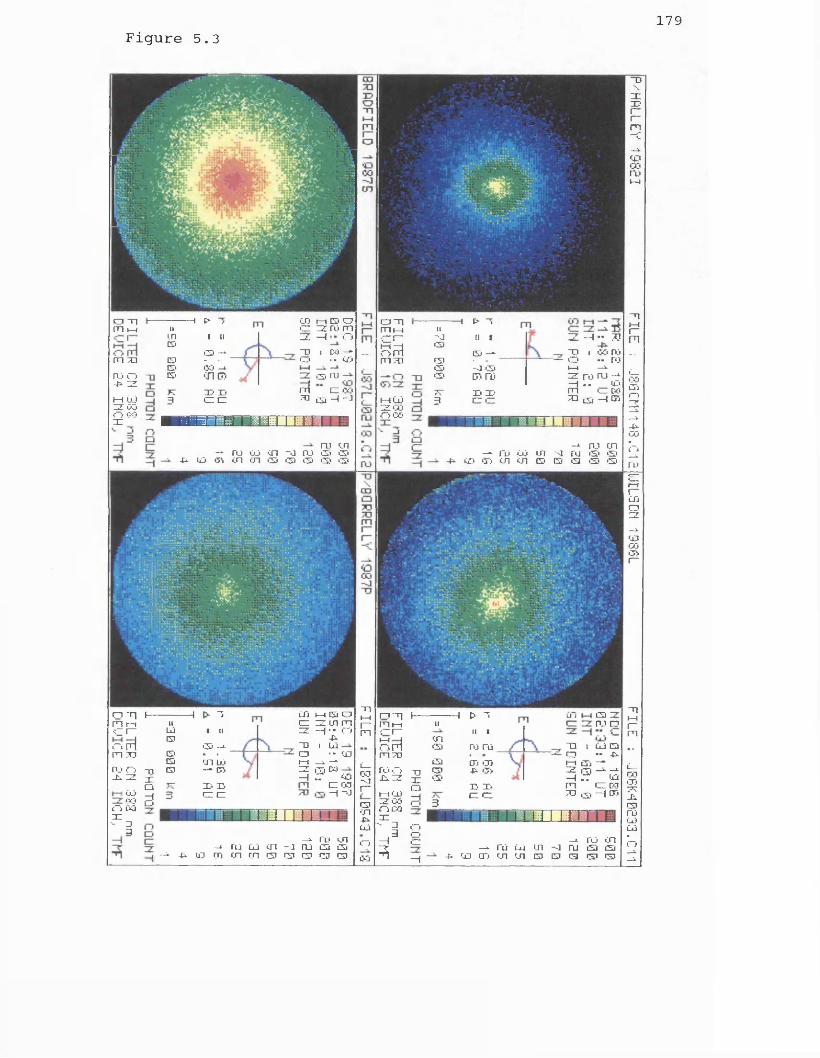
179Figure 5.3

-- —1 O i11-J a i<3 (S3 —C33 -<3 -4 <3<3< cr.ru73 x< zd3 d d

IZ — 4 ■* 713? i cc< ro u «• rot—t —d ro ru —I • • U_'rn ■ 0633 ca —f Gj

-* ru rn — • ro co ui -i ru <S3 <33+ kiD Ix j O l <n D E l Q >33 <33

o nm i—i |

m 33 ru o4a- dl—l 0JIZ 00o <>oX

O -q m i—i<C r- o r !m X3ru oX iz

I CO: co <~j co 313a

f— A 3II

Lu 1 IICD

<33 -j-E< . >CD '33 LO

~n ra — • COXC3 v~ Xa X-1 _• d CD

m m e o d iz cn m IZ —| ■• o -IX33 i Lu O ••C O r—i —a. —- iz ra k<— I .7 cod co

- I ~3

l i m n-a ro cn —*■ m lu >n -3 ru cs d - ^ ■ f r t o c n m c n a o o c u a

CSju Jru o

"Ul—l r o “n 1----r~ m i—im r r

K r lm to•J

S7 ro o

J X Z 33X

i—1—103d O Qrioa

a

•33•33

-11_1

-IX XCu -- 3 o3 1—IO

00

---1

3az

H

II-1 t> 3

II lcn<33 ro ru

i3 i DO <T3<3) -IX eo<3<

X X d d

3

33 I u_j E l O — -ixtU Lji —2 Q - J—4 .7 'Om d c*n 73 i3j —■I CD

JT TT-x ro cn -a ru ui ui ru is a

x u cn cn cn ® 0 q © a

H t> /IIcn 1 IIE< <33 —E< -E< 00 —<•E< •T1CT.JZ ZD X3 d d

<10 m E Od iz ro m _£. —I Cf3D l CO — < < . • CO

rr| cn <v!<3< rucz

33 q -1 -J

■ ^ r m T i i i rrrrrr m m

ru c_n— ro co '33 - j ru cs> <3

-t*- CO <j \ Cn cn <33 <33 <33 <33 <33

o mIT lM■cr~i—i —io m P3 7D

H UZZQj O CO

PHRLLEV

19851 FILE

; J86C

M1148.C12lUILSDM

1986L FILE

: JB

6K4B

233.Cl 1

180Figure 5.4

COUNTS IN ANNULLE *aQ I S K i l S C S - * - - * —* -*■

ed ru -ti. cn m a ru -L*. Qj

O TO X 70

ZD ~0 O 70 T) O I—I~n mn ->■

cnO

n03 DO DO

*\] ■'Jcoom i—io ru

CD

<s>-t*ro

7q tom .. <n-n.cs

counts in annulus

CD — —in cn in

©

R*7im

rocn-4-

rucn-4—

XCDCd W

C9

-4-

ZL

T3

IIroruCS>tso7s3

o XIZ \

X"0 X70 r~O r~X mf—1 -Cr~n —*■CDCOCO ru07 i—i

H i—iZD ru70O =X V

ru Hru• x

i_iCj3

COUNTS IN AmULUS

ca ru UJX—XCDcn w

no\T O

O7070mr~r~-c

0300-0no

ro

cnC9 cn cn

70O cn

h ro

- in> m ZZ. •Q 07

~C370 GjS «n

Gi©

ro

o £1X i—ir~X COX ooX

XHH —r~ CDm 0000

07r~

07 mruX a

o —c

—I

—*• i—i

CQLMTB IN ANNULUS x

"0ahnaoawcnHT>ZZR7] CSD9

7468^802766848027468

181Figure 5.5

O E l— I f> 1.m i— i i ir~ cn 1 IIE'

•S i —-m x i Q -E> •10 —tru o X E< iji Ctt-e r o X

D JT ZD X*l—I -E —I 3 Cl CZ12 J do ru~r~ "‘-w

n3 tZ i=3 C .*h —f -*■ -E CO c\

m CO m E Orzromx> i w mi i ■. x_i JZCO CD XFrl “ COO XI lu -i -J

. - "

m m m m w

-»• ru cn ro co cn -j ru cs> co cn cn co co co co co

■ : w r ■.: > v ••

/••••; MfflhfaBggwtBSlffiiM s3Vi.it*.

T?t * • "V

(— 1 T)rn r-iCl-Sriru <r:■ _t. roi—i -E

c~j roX

m

o

ocz

Lu EJcs>EiCDx3

cn L»j ru ro3> r. cr n

Cn l—l E l EDd 12 cn m 12 —f o■q i ismrn . . _ ii i r o -r*12 C3 E-^ —I .. ^m cz coXI i3> —f ~o

III I I Hru cn—«• ro co cn - j ro lIi tilin cri cn cn a o o m o

Fimxiro o xi4-ru

n m

H t> iIIcn ii :CO E« coCD ■•S' Ei Cl'•s* cr- coX X3 CZ d

m u ■ H U

m x

I L JCO r-t — kxi — x ru ]4IZ —4 * “

CDn

~U i 'S'—*••_J . . L*.*i—i —i.zz ■cn cn —1

Fi iU_>DC*

X I . S - H O l

ru cnuj cn cn ED -i ru

no t—i cn uCO n

•— •: > ~n — ru ± —Ir~-jDTa P

LU a i zzl — -eru •S'E>^ f \ TD i CO Elcn • • — rn — cniSi 10-0 V . l- l - i. coCD cn *s« 21* -3 . . Ei7T X ZD m cz ro3 cz cz X) rz “11 05HB 1:11 1M lr m r u me h

? 335 — ru lu in -e co on cn cn CD E?

ro cn ru is ca 0 0 0

P/HftLLEV 19821

FILE ;

J86CE1200.C

15IP'HPLLEY

19321 FILE

; .JB6E6B000. P01

182Figure 5.6

ra -a coTO •a vihn .Pi raa 2 I?*X CO

ru<n

RX CD UJ X -

CO

U JRX" -E'■ cnX

3 -n

cn

COUNTS IN ANNULUS

cn

CO

X7Qa _n corlaa ru w • cn cn •H z>

R CD*n CO X9n mx| m\ VIK CO 3

XcnE

oru “0\ ro13 O 70 X) O 70

m

DO CD - J 00 “•J O “□mO

-E

cn

rurucn

ru-E

-A.CS 'V

o ro ru 3D x>T3 O

to “nO I—Ix m

nCD

DO DO-o -o

CDOm r—io ru-Ero =

o Xru \X“0 XX r~o r~"n mi—ir~ -Cn -«*

CD00

DO ruon i—i12 i—iX no70 -Eo —X

-1DO =2• XCJ1CD

i—i

C0LHT5 IN ANNULUS

§ ® 3 cn

R*7ii inm ® \ M773

- * ro CD -E in

cn m cn cn cn

COUNTS IN AWULUS

CO CO - l _t ru ro COcn VI cn cn cs Ul m

COUNTS IN hWULUS

c s i w u + i n u i ' j o o cs m cn cn cs m tn cn cn

X\XT>

rn-c

CDDOru

7

Xo

??????@@@@@@@!>>>>>>? ?????@@"

22658888^92245158822

3102313232323284303131313131

5

183Figure 5.7

DAUGHTER SCALE LENGTH (km )ruX -*■ CO 00 X

LU cn cn - j cn X<£i —*■ CO CO X

CD

CD

cnx

oO CD m • ZZ (£) H CS 70 hHo

oI—ILTD — 1 X

O .m co

-uxc

ro

CDCD

LU

cscs

oXL0Xmo

m

COXOE=L0"5ru

CX70l—tX — Il—lo

oo

mo

m

coxCD£=CO

cnCX70

\\\\

\

\\\ \ w w \\

w

\

w- A S :\ \\ \

\

omc~com

70mmcofp

oi_inCP

t=j- 1

SP 70n2 doXm xX

IP

omr~com

m

3 x r

ii n

-J 00 X -J

+ +\ \ I Ics csro x

co

r~ CPQ_ m

COII H

X Xl—lX HX

X X<n hX X

” 5 I-u X

e :7P3

\ \

xcscn

XXo

Xmmco

CPm01H

X l—l

C° H

Xmo

xcso

<=Xr~xIXCOo

Xo

X

I

COIXIX

IXoooX X X

mX

ooIZCP

\\

ipomxCOrn

IX

2 !

C lOmht=jw

coo

t Hm

r - 1

t=d2!OHm

wwr-1oo

w

H

s a

tdH

2o

HtZ3

Figure 5.8

PARENT SCALE LENGTH (km ) xS iS (S ru X to_i. m Ai cs Ul csCS •HJ -U ru -*■ CD

CD

XCOX

XIXr~hhOC l (SIX •X CD—1 CDXHHC l

oHH01—1XX VC l .IX CO

-UXcz

ruxx

uiXX

oXLGXmo

m

coxoe:to"5ru<ZXXHHXH

oo= 1mom01xX£=CO"5—1

cncX X HH X — IhHo

T

A _ AW .

\ \\ \• s -fr-

\ ■

\ \\x

- V \" l u

w

V.

■ w

T

•A4A\

X X X o ClX IX m IX oHH IX £1 l~ ZZm 01 CP to CP

cz m HHd CP X 3

X 3 CPm —13 CP

mo

X CP IXX IX to f“r~ o X =2 to

HH M Q IXX X X

X X IX 2X X m

r or or o

o cz

3 X 1 CPX IX01

II II II H1—1 ru x»

1X

• . HHH Q X —1CD 01— i X+ + CD IS

h' ' X XS Sa a * r~_i. P X-o to £1

7\3

\

0 CPmx 01 m H

m01 x CP H

3 3X XIX ZZo oI—IH XX X

o C 12 X

m xco ci o oX C lr_ -j-.

l X>-CO

IX c i IX o

ZZ —| CPIX hHXHIP

01IX

m

\

<TOZ•T O

W

r ozH

C Or o

r or o

r or oZror o

«r or o

oo

r oZr or o

r o

r op^

r o

pt-r o

oZo

r o

r or or o

Figure 5.9185

PARENT SCALE LENGTH (km ) X-»• rs<s cs cs — UJ cs 4i

m cn cn 03 CSCSQ Ul UJ 00 00 CS

o ro70 UJ

n cs

m m

rn uj m o

ruCDcs

LU

CSCS

7 0 2 0 0 On n m o o m e m o u j ro cn ro x cz m i—i toPP X H X

ZZ n fP IZ

3 *pm oXI cp mm UJ r~o “0 3 Uji—il—lo mX X -7x!XIm <X X mo cz

UJ

X I- roX mn ii

UJH

X1m• i—ico x —Iru

X+ cs CD

> - SX 70r~_i. 3 X00 eX3

U jmm

WITOr-1oor o

r or o

r o

r o

or o

or o

rororo

18 5Figure 5.10

COUNTS IN ANNULUS NORMALISED TD MAXIMUM xcs

cscs

cs(3

csro

csro

cs

no70CD CS t •m cnortoO CS I—I -cn oo —I t>IZom70 csCDnornIZ

\7\3

cn

Xcs

CS _I_

CSO’)

_ i_

cs00_ 1_

CU

cs. 1.

TiroOO ID w LI.)AJ 70 TO/□ HH 70 TDm m m m m mr o r r o Cl<. < -c CD

r u r o - * - * r o - * o ~o—*■—*• cn -fi- im cs x> n\ \ \ \ \ \ —I o—2. —a. —i. ---2. —S. —i. mro ru ru ru ru\ \ \ \ \ \ ,__.OO 00 CO CXI 00 00 0-o -o - j -0 - j cn

- i . - i _ i _ li cs - 1 70

co — UJ co co co cn. ixi on cn i i cn

>30 cs cs cs cs csCT1 00 DO -Jru cn cd co co co

om

II

c d

«t r - 1

II

>-

r o

‘mWot— ir aMC Or s

t— 'r ao•-ao

187

CHAPTER 6

THE NEUTRAL COMETARY ENVIRONMENT II - THE DETERMINATION OF THE HnO PRODUCTION SCALE LENGTH

IN COMET GIACOBINI-ZINNER AND THE SEARCH FOR JETS IN THE NEUTRAL COMA OF COMET HALLEY

6 .1 Introduction

The near-nucleus images of comet Giacobini-Zinner in the emission of O(^D) at 630.0 nm show isophotes close to circular symmetry. The integral profiles reveal a central source region. The OH contribution and the NH2 contamination can be modelled to reveal this source scale (section 6.2). The parent of oxygen, presumed to be ^ 0 , is being released from grains on this scale and proceeding in free molecular flight to populate the sunward and tailward comas uniformly [Wallis et al., 1990].

Jets, spirals and other detailed features in cometary comas have long been thought to be visible only in the continuum reflected by the dust particles or in the emission bands of ions. It was generally thought that these features could not be seen in the emission bands of the neutral species. However, several authors have recently reported "jet-like" features in the neutral emissions (CN and C2 ) of comet Hailey, an observation which has important implications for theformation of these neutral radicals. These coma features were foundclose to the nucleus, extending to cometocentric distances of the order of 60,000 km. These neutral jets should, therefore, also be observable in the near-nucleus images taken with the Very High Sensitivity Imaging System (VHSIS) around the time of the spacecraft encounters with comet Hailey in March 1986. No jet structures were immediately visible in any of the corrected near-nucleus VHSIS images taken during this period. A more rigorous search for such features inthese images was performed by applying extensive image enhancementtechniques (section 6.3).

6 .2 The Determination of the HoO Production Scale Length In Comet Giacobini-Zinner at a Heliocentric Distance of 1.03 AU

6.2.1 Introduction

Swings & Greenstein [1958] were the first to report a bright cometary emission at 630.0 nm in their analysis of comet Mrkos. Due to the brightness of the emission, Biermann & Trefftz [1964] concluded that the emission could not be due to fluorescence, and that a large population of metastable OC^D) was being created by photodissociation of a parent molecule. Later Festou & Feldman [1981] were able to show that fluorescent scattering could be completely neglected in any discussion of the 0(^D) emissions.

Since an 0(^D) atom is produced with an excess velocity of about 1 kms"^ and has a radiative lifetime of about 150 s, its mean displacement from the source molecule before decaying to the 0( P) ground state is approximately 150 km, which is small compared to the scale of the observations. Therefore, the spatial distribution of 0(^D) emissions is an accurate map of the source molecule distributions.

Fink & Johnson [1984] have come to the conclusion that there are two major production mechanisms of metastable 0(^D). One of these, first proposed by Biermann & Trefftz [1964], is the photodissociation of H 2 O molecules directly to the 0(^D) state

uvH20 -+ H2 + O^D) 6-1

and the other, studied by Dishoeck & Dalgarno [1984], from the photodissociation of OH, itself a photodissociation product of H 2 0:-

OH + H 6.2

H + 0{lD) 6.3

The 0(^D) profile may, therefore, be written in terms of the H20

uvh 2o

uvOH

profile (Njj2q(s)) an<* th® profile ( N q ^ ( s ) ) as:-

Nq i(s) aNH20(s) bN0H (s) 6.4

where a is the fraction of ^ 0 that yields 0(^D) directly and b is the fraction of H2 O that eventually produces 0(^D) from OH.

H2 O is a daughter species and so its profile may be modelled by the simple radial outflow decay model as discussed in chapter 5 and attributed to Haser [1957]. Hence, the profile of the 0(^D) produced directly from H2 O is of the form:-

n H20(s) =47rvd (X d - X p) s .

SXf

sXdK 0(y) dy 6.5

where:-

QPvds

x px dK0(y)

is the production rate of the H2O parent, is the average velocity of the H2O molecules, is the projected distance from the cometary nucleus, is the reciprocal of the parent scale length, is the reciprocal of the daughter scale length and is the modified Bessel function of the second order.

The OH distribution, however, is not quite as straightforward. The OH molecule is a grand-daughter species. It is, therefore, necessary to compute the distribution expected for such a tertiary product.

6.2.2 Calculation of the Intensity Distribution Caused bvExponentially Decaying Grand-Daughter Molecules ExpandingIsotropicallv into Volume

The method adopted is an extension of the method adopted by Haser [1957] to determine the daughter profile (see section 5.2.3). The following additional assumptions are made:1) . On production, the grand-daughter molecules move purely radially with uniform speed, and2). the grand-daughter molecules then decay exponentially with scale length Lgd.

190

Let the production rate of the parent molecules at the nucleus be Qp molecules per second. Then the total number of daughter molecules, Nd , crossing a sphere of radius z per second will be given by:-

Nd A [ exp-(Xpz) - exp-(Xdz) ] 6.6

where:-

Qpx pA = 6.7

x d - x pThe production rate of the grand-daughter molecules is, therefore, given by:-

-dNd dNgd= “ A [ Xpexp-(Xpz) - Xdexp-CXdz) ] 6,8

dz dz

The number of grand-daughter molecules in an elemental spherical shell of radius z and width dz is, thus:-

dNgd = A [ X pexp-(Xpz) - X dexp-(Xdz) ] dz 6.9

These specific grand-daughter molecules should now be considered. When they are a distance R (R > z) from the nucleus their number will be decreased by the factor exp(-Xg^R-z)), where Xg^ is the reciprocal of the grand-daughter scale length. The total number of grand-daughter molecules at a distance R from the nucleus due to disintegrations of daughter molecules in the given elemental shell becomes:-

dNgd(R) = A [ X pexp-(Xpz) - X dexp-(Xdz) ] exp-(Xgd[R-z]) dz 6 . 1 0

oThe total number of grand-daughter molecules arriving per cm at a distance R per second becomes:-

Ngd(R)=

[ X pexp-([Xp-X gd]z)exp-(XgdR) -

X dexp-([Xd-Xgd]z)exp-(XgdR) ] dz 6,12

A *R

4 a K-[

0

A *R

4ttR2 0

191

X r

4*RZ (X gd - X p)

A X d

[ exp-(XpR) - exp-(XgdR) ] -

[ exp-(XdR) - exp-(XgdR) ] 6.134?rR (X gd - X d)

The number density at distance R from the nucleus becomes:

n(R) =47rvgdRz (X d - X p) (X gd - X p)

[ exp-(XpR) - exp-(XgdR) ] -

Qp X p X d----------- r [ exp-(XdR) - exp-(XgdR) ]47rvgdR (X d - X p) (X gd - X d) 6.14

This equation can be broken down into four expressions of the form given in model 2 above so that the resulting grand-daughter profile is of the form:-

Ngd(s) =

N q i(s) = a

Qp x p X p 1

4jrvgd (X d - Xp) (Xgd - X p) s

Qp Xp X d 1

4irvgd (X d - Xp) (X gd - X d) s

tion, thus, becomes:-

Qp Xp 1 [sXpK 0(y)

sXd47TVd (X d - Xp) S

Qp Xp X p 1

4irvgd (X d - Xp) (Xgd - Xp) s

Qp Xp X d 1

SXr

sXdKo(y) dy -

rsx dK 0(y) dy

sXgd

sXTKo(y) dy -

47Tvgd (X d - X p) (X gd - X d) s

sX gd

[sXdK 0(y) dy

sXgd

6.15

6.16

This may be rewritten in terms of two integrals:-

X,N0 l(s) =

Q p

4tts (Xd - X p)

X r

L vd

X T

Aics vgd (Xd - X p)

so that:-

X r

vgd (Xgd - Xp)

Xd

r sXfK q(y) dy +

sXd

L (Xgd - Xp) (Xgd - X d) _

sXdK0(y) dy

sXgd6.17

N0 l(s) =

where:

A

B

sXp BXo(y) dy + —

sXd s

a b— + —

fsX,

sXdK0(y) dy

- vd vgd (Xgd _ Xp) _Xr xd

_ (Xgd ~ Xp) (Xgd - X d) _

6.18

6.19

and with the approximation » X d , this simplifies to:

A

B

" X d - x gd- " a Vgd "

- x gd _ _ b vd6.20

In terms of the daughter and grand-daughter scale length we obtain:-

A

BLgd " Ld " a vgd "

i t-1 o. i - b vd6.21

The 0(D) function can, therefore, be rewritten in terms of one unknown constant B, as:-

B A sXp [*sXd 1— Ko(y) dy + K0(y) dys _ B sXd sXgd6.22

The 630 nm image of comet Giacobini-Zinner to be analyzed here was taken on 1 September 1985 at 03:38 UT with the 1 m Jacobus Kapteyn Telescope (JKT) and is shown in figure 6.1. The scale of this near­nucleus image is such as to enable a more accurate determination of

193

the H 2 O production scale. If the filter isolated pure 0(^D) the calculation of the scale length would now be straightforward. However, the 0(^D) emission is blended with cometary emissions from the (0,8,0) NH2 band.

6.2.3 Estimation of the NH2 Component

The NH2 contribution to the total signal may be estimated from the Doppler images taken on 2 September 1985, with the Doppler Imaging System (DIS), on the JKT, through the 630 nm filter. A composite of four such images is shown in figure 6.2. The 0(^D) sky signal shows up as a ring with the cometary component superimposed in the upper right. The NH2 features which contaminate the 0(^D) are on the short wavelength side of the 0(^D) signal, so that the 0(^D) ring is distorted on the outer edge.

An estimate of the NH2 contamination is obtained as follows. A 45° sector profile is taken from the centre of the fringe through the comet (red profile in figure 6.3) and plotted against radius-squared. A second similar 45° sector profile is taken from the centre out in the opposite direction, to obtain the sky contribution (green line in figure 6.3). This profile is then subtracted from the former to obtain the cometary signal. The peak position of the cometary signal is estimated, by examining the upper portion of the plot. The NH2

peak is small and it may be assumed that no cometary NH2 appears to the left of the 0(^D) peak. The 0(^D) profile can then be estimated by assuming symmetry about the peak position (magenta profile in figure 6.4). The NH2 component (cyan profile in figure 6.4) is then determined by subtracting the cometary 0(^D) profile from the cometary 630 nm profile. The amount of each component is proportional to the area under each curve. The NH2 contribution is found to be of the order 17% of the main signal.

The NH2 profile may be modelled by the simple radial outflow model with decay [Haser, 1957]. The NH2 profile will, therefore, be of the form given by equation (6.5). However, since the creation and destruction scales are of the same order (10,000 km, [Fink & Johnson, 1984]), equation (6.5) cannot be evaluated as it stands. The limit as

tends to Xp needs to be considered.

194

As tends to Xp, the integral in equation (6.5) tends to:-

’sXPK 0(y)dy (sXp - sXd)K0(sXp)

JsXd6.23

so that, the functional form for the NH2 profile reduces to:-

n NH2(s) D K q(sX n h 2) 6.24

where D is a constant and X^ 2 is t ie reciprocal of the NH2 scale length.

6.2.4 Determination of the Production Scale Length

The profile recorded through the 630 nm filter is, therefore, of the form:-

The above function can be fitted to the outer 630 nm profile (from 40 to 90 pixels) where the H2 O production scale no longer plays a significant role. The functions may then be extrapolated back to the origin in order to calculate their resulting contributions to the total. There is some degree of uncertainty in the sky background but this may be overcome by varying it so that the NH2 component falls in its anticipated range (ie less than 20% total contribution). The NH2

contribution and the 0(^D) contribution from OH for a given background is subtracted and a Haser function of the form (6.5) is fitted to the resulting profile, by varying the H2 O production scale and the multiplicative constant.

Early comprehensive models of water photodissociation in cometary conditions put the mean OH ejection velocity at about 1.3 kms"^ [Festou, 1978; 1981b]. However, on the basis of laboratorymeasurements available at that time [Welge & Stuhl, 1967], Festou assumed that most of the excess energy of photodissociation was converted to translational energy of H and OH, the conversion to vibrational and rotational energy of OH being negligible. It is now known, from recent laboratory and theoretical work, that, following

I630(s) BO(*D)func + B)Kq(sX jsjh2) 6.25

195

water dissociation, the OH radical is created in excited states of rotation or vibration. When this is taken into account the mean ejection velocity of OH is found to be 1.05 kms"^ [Crovisier, 1988].

The lifetime of OH at 1 AU, for a heliocentric velocity of -1.5 kms’ under solar minimum conditions, is taken to be 1.2 x 10^ s [van Dishoeck & Dalgamo, 1984] . The OH scale length at 1 AU is, therefore, approximately 130,000 km. This is in agreement with the value of (130,000 ± 20,000) km calculated for comet Hailey at 1 AU [Fitzsimmons et al., 1986].

Two sets of input parameters are now considered. The first uses theoretical data on the dissociation of ^ 0 [Festou, 1981b] . Thesecond adopts a higher dissociation rate to fit the 40,000 km scale measured by Giotto [Krankowsky et al., 1986].

6.2.4.1 Case 1

The total lifetime of ^ 0 molecules at 1 AU from the Sun is taken to be 7.6 x 10^ s [Festou, 1981]. If an outflow velocity of 0.9 kms"^ is assumed [Krankowsky et al., 1986], the ^ 0 scale length at 1 AU becomes 6.8 x 10^ km. The theoretical data of Festou [1981] show that, under conditions of quiet Sun appropriate for the VHSIS measurements presented here, 6% of the ^ 0 produces 0(^D) directly and 85% of the ^ 0 produces OH of which 4% produces 0(^D) . The parameters used in this case are summarized in table 6.1.

Table 6.1 Parameter Set 1

b = 0.85 x 0.04 = 0.034 a =0.06 v^ = 0.9 kms "^ v ^ = 1.05 kms"^Ld = 68,000 kmLg^ = 130,000 km

= = » A = 0.96 B

196

The 630 run profile takes the form:-B sXp fsXd

J630(s) = — 0.96 K.()(y) dy + Ko(y) dys _ sXd J sXgd

+ DK q(sX N H 2) 6 .26

The sky background lies in the range 3.6 ± 0.3 counts per pixel. The sky background is varied within this range and the above function is fitted to the outer portion of the profile by letting the parent scale approach zero. The best least squares fits obtained are given in table 6.2.

Table 6.2 Best Fits to the Outer Region of the O( D') Profile Using Parameter Set 1

Background B D % NH0(cts/pix)

3.5 0.94 0.0 0.03.6 0.88 3.4 3.03.7 0.80 9.9 9.23.8 0.72 16.3 15.33.9 0.65 21.4 21.3

The H2 O production scale lengths calculated from these parameters aregiven in table 6.3.

Table 6.3 Best Fits to the Inner Region of the O^D) Profile UsingParameter Set 1

Background B* * ,(cts/pix) (pixels) (xlO km)

3.5 0.92 7.7 2.453.6 0.85 7.4 2.383.7 0.78 7.0 2.253.8 0.70 6.7 2.163.9 0.63 6.4 2.06

A value of (2,200 ± 250) km is thus determined from this parameter set for the ^ 0 production scale length. Figure 6.5 shows a typical fit for these parameters.

6.2.4.2 Case 2

More recently, the mass spectrometer on board the Giotto spacecraftmeasured the H^O scale length to be 40,000 km at 0.89 AU [Krankowsky

oet al., 1986], If an r scaling law is assumed then the ^ 0 scale length at 1 AU would be 50,500 km. 4.4% of the ^ 0 produces 0(^D) and 90% produces OH of which 4% produces 0(^D). The parameters used in this case are summarized in table 6.4.

Table 6.4 Parameter Set 2

b - 0.90 x 0.04 - 0.036a - 0.044v^ “ 0.9 kms’^Vgd =1.05 kms"^

= 50,500 km Lg^ = 130,000 km

= = » A - 0.67 B

The 630 nm profile takes the form:-B sXp *sxd 1= — 0.67 Ko(y) dy + Ko(y) dys — « sXd s gd + D K q(sX n h 2) 6-27

The sky background is again varied within its acceptable limits and function of the above form is fitted to the outer portion of the profile. The fits obtained are tabulated in table 6.5.

198

Table 6.5 Best Fits to the 1Outer Region of the 0(D) Profile UsingParameter Set 2

Background B D % n h2(cts/pix)

3.3 1.2 0.0 0.03.4 1.23 0.7 0.43.5 1.13 6.9 6.03.6 1.04 12.1 11.23.7 0.95 17.3 16.03.8 0.86 22.4 20.9

The H 2O production scale lengths calculated from these parameters are given in table 6.6.

Table 6.6 Best Fits to the Inner Region of the 0(^D) Profile Using Parameter Set 2

Background B** ,(cts/pix) (pixels) (xlO km)

3.3 1.26 7.3 2.353.4 1.22 7.0 2.253.5 1.12 6.7 2.163.6 1.02 6.4 2.063.7 0.93 6.1 1.963.8 0.83 5.7 1.83

This parameter set yields a value of (2,100 ± 250) km for the 1^0 production scale length. A typical fit with these parameters is shown in figure 6.6. When the results from cases 1 and 2 are combined, the final result, for the H2O parent scale length becomes (2,150 ± 300) km. It is important to examine other possiblecontributors to the 630 nm profile neglected in (6.25).

The dust contribution is neglected. However, the central hole is deep implying that the dust level is very low, less than a few per cent. At this level dust scattered light is indistinguishable above other modelling uncertainties.

The H2 O production scale should be compared with the scale for collisional quenching:-

O^D) + M* _> 0(3P) + M g 28

The coefficient, kq for the quenching of the 0(3D) state by ^ 0 is2 x 10~10 cm3s“^ [Streit et al. , 1976]. Even with production rates

30 -1for H2 O as high as 10 s this mechanism will not be an efficient deactivation process beyond the first few hundred km of the nucleus surface [Festou & Feldman, 1981]. Consequently most of the excited oxygen atoms will freely radiate so that the scale length calculated above is a real source scale.

It remains to discuss possible sources of 0(^D) not considered above. Roesler et al. [1987] considered CO and CO2 as potential sources of 0(3D). They concluded that the contribution from these two molecules was negligible for comet Hailey at cometocentric distances less than 10^ km. If the relative abundances of CO and CO2 are similar for comet Giacobini-Zinner then their contributions should also be negligible here.

Electronic collisional excitation of atomic oxygen with cross-section (1.5 - 3.0) x IQ'17 cm^ for 5 - 20 eV electrons [Shyn & Sharp, 1986]

_ O 1 _ 1would give some 2 x 10 0( D) s , some 1% - 2% of the H 2 O source.This source may, therefore, also be neglected here.

6.2.5 Discussion

The analysis presented here has included the NH2 contamination and the separate ^ 0 and OH sources. The central deficit is confirmed as not due to collisional quenching but indicates a source scale for much of the presumed ^ 0 parent of (2,150 ± 300) km. Delsemme & Combi [1979] gave production and destruction scales of the 0-parent in comet Bennet at 0.84 AU both at about 10,000 km. However, they did

not allow for NH2 contamination, nor for a secondary (OH) source. While comparable 01 data for comet Hailey has been p>resented [Itoesler et al., 1986], the spatial resolution is lower ;and the apparent central hole is probably dominated by collisional quienching. With the quenching scale some 10 times larger, the H2 O source scale is probably concealed in that case.

The 01 distribution observed in the APL images is close to radially symmetric and this is a commonly observed characteristic. However, it is also puzzling, given that the Hailey probes have clearly established that gas and dust is emitted almost entirely on thesunward side. It was also found that the spatial density of H 2O at

2comet Hailey varied as r [Krankowsky et al., 1986; Hsieh et al., 1987] .

The explanation for this and the 01 symmetry is probably that the H2 O sublimes largely from micron-sized grains, on a few times 1,000 km scale, rather than from the nucleus itself [Wallis: et al., 1990]. Some sublimes within 1,000 km, where collisions ensure residual sunward bias as evident in UV maps of the OH emission.

6.3 The Search for "Jet-Like” Structures in the Neutral Atmosphere of Comet Hallev Around the Time of the Spacecraft Encounters in March 1986

6.3.1 Introduction

Jets, spirals and other detailed features in cometary connas were long thought to be visible only in the continuum reflected by the dust particles or in the emission bands of ions. It was generally thought that these features could not be seen in the emission bands of the neutral species, at least in part because the neutral gas expands rapidly, perpendicular to any linear feature and consequently the daughter species normally seen in the visible region are produced by dissociations that take place far from the point of origin of the gas. However, several authors have recently reportedl "jet-like" features in the neutral emissions (CN and C2 ) of c-omet Hailey [A'Hearn et al., 1986a; 1986b; Cosmovici et al., 1987; 1988], an

201

observation which has important implications for the formation of these neutral radicals.

A 1 Hearn et al. [1986] made observations of comet Hailey in April 1986 and reported coma features in their neutral images extending to more than 60,000 km from the nucleus. Cosmovici et al. [1987] observed comet Hailey in March 1986 and found neutral jet structures within a field of view of 70,000 km. Therefore, these neutral jets should also be observable in the near-nucleus images taken with the VHSIS(section 6.3.2). However, no jet structures are immediately visible in any of the corrected near-nucleus images. It was, therefore,decided to make a more rigorous search for such features in theseimages. A "ring-masking11 technique was chosen to help to elucidate the features. This method of image enhancement is discussed in detail in section 6.3.3. The method was thoroughly tested before applying it to the real data (section 6.3.4). The results of applying thistechnique to a selection of near-nucleus VHSIS images are discussed in section 6.3.5. The implications of these results are then discussed in section 6.3.6.

6.3.2 Comparison of the Instruments used bv the Various Investigators

A'Hearn et al. [1986] made their observations of comet Hailey in April 1986 on the 24" Planetary Patrol Telescope at Perth Observatory with a Charge Couple Device (CCD) camera system and the International Hailey Watch (IHW) filter set. The chip had an array of 320 x 512 pixels, each 30 microns square. The net scale at the chip was roughly 1.8 arc seconds per pixel. The total field of view in the original images was roughly 9.5 x 15 arc minutes, although the image enhancement technique was applied only to a circular area of radius roughly 2.5 arc minutes.

Cosmovici et al. [1986] made their observations of comet Hailey in March 1986 at the 192 cm South African Astronomical Observatory telescope with a CCD and the IHW filters for near-nucleus studies. An image area of 318 x 510 pixels was used corresponding to an average at the comet of (120 x 190) x 10 km. They have analyzed 135 absolute

202

calibrated images of comet Hailey obtained with 23 different filtersinside a circle of 70,000 km diameter around the nucleus.

The VHSIS images of comet Hailey taken in March 1986 on the24” telescope had an average field of view of 250,000 km,corresponding to approximately 1,000 km per pixel. The images takenon the 16" telescope had a field of view of 365,000 km correspondingto 1,425 km per pixel.

A summary of the instruments used is given in table 6.7. The VHSIS images, therefore, have a similar resolution to the CCD images of A'Hearn et al. [1986] and so should contain detectable jet features. However, no neutral jet features were immediately visible in any of the VHSIS images taken around the period of the spacecraft encounters with comet Hailey in March 1986. It was, therefore, decided to applyimage enhancement techniques to attempt to elucidate the comafeatures.

Table 6.7 Comparison of the Instruments used bv Various Investigators in their Search for Neutral Coma Features

Observer Instrument FOV Pixel size Ring radius(arc min) (arc sec) (arc min)

A'Hearn 24" PPT 9.5 x 15 1.8 2.50Cosmovici 1.92 m 2.97 x 4.76 0.56 0.86Rees 24" TMF 6.34 (diam) 1.48 0.74

1.00 m 4.13 (diam) 0.97 0.48

6.3.3 The Ring-Masking Technique

Since the amplitude variations caused by the jets are in the range of a few per cent with respect to their surrounding signal level, their dynamic range must be increased to make them visible. This can be obtained by dividing each pixel element by the mean value of a sufficiently large area around each pixel. This method yields reliable results when the neighbouring data from which the mean is computed have no trend among themselves. Images of the inner cometary

203

coma have more or less equal amplitudes in concentric annuli around the nucleus. Therefore, the pixels located on concentric rings are used to compute mean values to be used in the division process. A pixel is then divided by the mean value of its neighbours on a ring annulus. This procedure tends to remove global radial profiles. Irregular radial profiles are then recovered by applying a radial mask. This technique was also used by Cosmovici et al. [1987] in their search for coma features.

It is convenient to transform the image to be examined into polar coordinates about the comet centre. This has the advantage that the transformed image contains pixels with equal projected distance from the nucleus and with equal azimuthal position around the nucleus in rows and columns.

The ring-masking technique can only work for radially symmetricprofiles and so the mask should be applied only in the inner regions where this approximation applies. After some initial experimentation with the size of the radial mask it was decided to go out to a radius of 30 pixels. The results obtained with larger radial masks become corrupted by the departure from radial symmetry introduced byradiation pressure effects. This is also a convenient number ofpixels as it allows the image under examination to be expanded four times. This corresponds to a radius of about 35,000 km on the 24" telescope and 50,000 km on the 16" telescope.

6.3.4 Critical Examination of the Ring-Masking Technique

Before applying this technique to any real data it was first necessary to test the feasibility of the technique on known data. The computer generated 1/R profile image discussed in section 3.4 andshown in figure 6.7a was employed for this purpose. A simple test spiral image at 10% of the radial component was computer generated (figure 6.7b) and added to the test comet (figure 6.7c). The ringmasking technique was then applied to this composite image. Theresult of this procedure is shown in figure 6.7d. The method can beseen to have worked well in that the global radial profile has beenremoved and the spiral recovered.

However, the above example is an idealized case, only recognized whenthe errors due to photon counting are negligible. A more realisticmodel should, therefore, include photon noise. The random fluctuation in the photon flux emitted by a steady thermal source can be described by a Poisson distribution. If the probability of n photons from the source crossing a given area in t seconds is p(n,t) then:-

(Nt)nexp-(Nt)p(n,t) = 6.29

n!

where N photons per second is the average flux from the source across the same area. This distribution has the important property that the root mean square (r.m.s.) fluctuation in the average flux N is simply:-

rms noise = a y/N 6.30

The VHSIS images may be thought of as a square array of 256 x 256 discrete individual photon counting elements (pixels). The photon count in each pixel will have an r.m.s. error equal to its square root. The smaller the number of counts in a given pixel the greater will be the relative error. Thus, there is a danger of weak features being drowned in the noise at low photon counts.

Assume that the photon counts in a given pixel due to the 1/R distribution are N and that the contribution from the spiral is N/10. Then: -

counts in pixel = 1.1N 6.31

error in counts = %/1-lN 6.32

As a criterion let us postulate that to be discernable the counts in the spiral must be at least 50% of the noise. Then:-

0.1N > 0.5 V 'l.lN 6 -33

N > 50 6.34

205

According to this criterion a feature at the 10% level will be visible only when the counts are greater than 50 per pixel. This would suggest taking the ring mask out from the centre until the counts drop below 50.

To test this out Poisson noise was added to the computer generated test image. The major contribution was chosen to vary as 5,000/R with the spiral at 10% of the radial component. In this case the counts at the edge of the image are of the order 50 per pixel. The spiral was discernible in the raw image (figure 6.8a) and the ring/radial masking technique worked well, the spiral being visible without any smoothing of the original image (figure 6.8b). The major contribution was next lowered to 500/R with the spiral again at 10% of the radial component. In this case the counts at the edge of the image are of the order 5 per pixel. The spiral was not detectable in the raw image (figure 6.8c), and the ring-masking was not able to bring out the spiral either (figure 6.8d).

The pixel to pixel variations are proportionally higher in the 500/R image as compared with the 5,000/R image and this can be reduced to a certain extent by smoothing. A three point spline was applied three times. The spiral was still not apparent in the raw image (figure 6.9a) and was also not picked out by the ring-masking technique (figure 6.9b). Finally a heavy Fourier smooth, using a Kaiser bell in Fourier space with a FWHM of 20 pixels (see section 3.3.4), was applied (figure 6.9c). The spiral was now just visible in the output although weak additional and spurious structures also have started to appear (figure 6.9d).

Therefore, in order to detect structure at the 10% level, the cometary counts at the edge of the area of the ring mask should not fall much below 50 counts per pixel. The more counts the better the chance of resolving coma features.

The above analysis is still somewhat idealistic in that errors are also introduced when images are corrected for flat field, thermionic emission and sky background, although these will be small in comparison. The purely radial approximation is also an oversimplification. Radiation pressure will distort the images and

206

this will introduce errors. The radial mask should not venture into regions dominated by radiation pressure as this will overshadow any structure in the middle.

6.3.5 Results of Applying the Ring-Masking Technique to a Selection of Near-Nucleus VHSIS Images

This section presents the results of applying the ring-masking technique to a selection of some of the near-nucleus VHSIS images of comet Hailey collected from TMF in March 1986.

The images were initially corrected for flat field and thermionic emission in the normal manner as described in section 3.3.2. Where more than one image existed in a sequence the images were addedtogether to improve the signal to noise ratio. The corrected images were then smoothed by applying a Fourier filter. It was found by trial and error that a good filter in the Fourier domain was a Kaiser bell of full width half maximum of 20 pixels. The inner regions of diameter 30 pixels were then expanded by a factor of 4 before applying the ring-masking technique.

The APL CN filter, centred at 388.2 nm, was used for near-nucleus analysis on six days during the March 1986 observations. Afterprocessing there was evidence of coma features in all of these CN images. Four of the processed images are shown in figure 6.10. Figure 6.10a shows the processed image taken from a series of near­nucleus CN images on 5 March 1986 at around 12:43 UT. There is a strong jet at 5% above the average (at the 5% level) to the north­west and a smaller weaker feature, at the 1% level to the south-east. Figure 6.10b shows the processed image from a series of near-nucleus CN images on 13 March 1986 at around 12:17 UT. A strong northward jet at the 5% level is visible in this image. Figure 6.10c shows theprocessed image taken from a series of near-nucleus CN images on14 March 1986 at around 13:07 UT. There is a broad jet to the north­east at the 2% level and two smaller weaker features at the 1% level, one to the south-east and one to the west. Figure 6.10d shows theprocessed image taken from a series of near-nucleus CN images on22 March 1986 at around 11:48 UT. There are two strong jets, one tothe east at the 3% level and one to the west at the 5% level.

207

The APL C2 filter, centred at 471.6 nm, was used for near-nucleus analysis on three days during the March 1986 observations. After processing there was evidence of coma features in all of these C2

images. Two of the processed images are shown in figure 6.11. Figure 6.11a shows the processed image taken from a series of near­nucleus C2 images on 5 March 1986 at around 12:50 UT. There are two strong jets, one to the north-east at the 8% level and one to the south-west at the 5% level. Figure 6.11b shows the processed image taken from a series of near-nucleus C2 images on 18 March 1986 at around 12:00 UT. There is one broad jet to the east at the 3% level.

The APL C0+ filter, centred at 455.4 nm, was used for near-nucleus analysis on four days during the March 1986 observations. Once again coma features were revealed in the processed images. Two of the processed images are shown in figure 6.11. Figure 6.11c shows the processed image taken from a series of near-nucleus C0+ images on 18 March 1986 at around 12:30 UT. There is one prominent jet feature at the 8% level to the west. Figure 6.lid shows the processed image taken from a series of near-nucleus C0+ images on 20 March 1986 at around 12:21 UT. There is one strong, broad jet to the east at the 5% level.

The APL H20+ filter, centred at 580.0 nm, was used for near-nucleus analysis on six days during the March 1986 observations. Afterprocessing there was evidence of coma features in all of these I^O* images. Four of the processed images are shown in figure 6.12.Figure 6.12a shows the processed image taken from a series of near­nucleus 1^0* images on 13 March 1986 at around 12:36 UT. There is a strong jet at the 3% level to the north-east and a smaller feature at the 3% level to the south-west. Figure 6.12b shows the processedimage taken from a series of near-nucleus H20+ images on 14 March 1986 at around 12:38 UT. A westward jet at the 10% level is visible in this image. Figure 6.12c shows the processed image taken from a series of near-nucleus H20+ images on 22 March 1986 at around 12:32 UT. There is a strong jet at the 8% level to the east.Figure 6.12d shows the processed image taken from a series of near­nucleus J O"*" images on 23 March 1986 at around 12:29 UT. There is one strong jet at the 10% level visible to the north-east.

208

The APL dust filter, centred at 524.3 nm, was used for near-nucleus analysis on five days during the March 1986 observations. After processing there was evidence of coma features in all of these dust images. Four of the processed images are shown in figure 6.13. Figure 6.13a shows the processed image taken from a series of near­nucleus dust images on 14 March 1986 at around 12:14 UT. There is a strong jet at the 10% level to the south-west. Figure 6.13b shows the processed image taken from a series of near-nucleus dust images on 18 March 1986 at around 12:23 UT. A westward jet at the 10% level is visible in this image. Figure 6.13c shows the processed image taken from a series of near-nucleus dust images on 19 March 1986 at around 12:28 UT. There is a strong jet at the 10% level to the east and a smaller feature to the west. Figure 6.13d shows the processed image taken from a series of near-nucleus dust images on 23 March 1986 at around 12:14 UT. There is one strong jet at the 10% level visible to the north-east and a smaller feature to the south-west.

6.3.6 Discussion

Although no coma features are immediately apparent in any of the near-nucleus VHSIS images, the ring masking technique does seem to have revealed possible "jet-like" features in the inner coma of comet Hailey, not just in the continuum and ion emission images, but, more significantly, in the CN and C2 emission images as well. This result, first discovered by A'Heam et al. [1986], has important implications for the formation of the neutral radicals. As pointed out by A'Heam et al. [1986] these jets are much to narrow for the parent to be a neutral gaseous species released from the nucleus. A'Heam et al. [1986] have concluded that these jets are composed of dust grains and that the CN is either dissociated directly from the molecules on the surface of the grains or it is dissociated from parent molecules which vaporize from the grains and which have a very short lifetime against photodissociation. Since estimates of the dissociation lifetimes of a variety of plausible parents for CN are greater than 10^ s [Bockelee-Morvan et al., 1985a], it would seem likely that the CN is being dissociated directly from the grains.

209

The coma features found in the processed dust images show remarkable similarity with those found in the processed ion images. For example, both the processed dust image and the processed ^ 0 * image taken on 14 March 1986 show a major jet to the south-west (compare figures 6.13a and 6.12b). In addition the processed dust and ^0"*" images taken on 23 March 1986 both show strong jets to the north-east (compare figures 6.13d and 6.12d). A correlation is also apparentbetween the dust image taken on 18 March and the C0+ processed image of the same date. In this case a strong south-westward jet is visible in both processed images (compare figures 6.13b and 6.11c).

No such comparison is possible between the dust features and thefeatures in the neutral coma. For example, the processed dust image of 14 March 1986 shows a prominent westward jet (figure 6.13a), whereas the processed CN image of the same date shows a strong jet in the opposite direction (figure 6.9c). In addition the processed dust image of 18 March 1986 shows a prominent westward jet (figure 6.13b), whereas the C2 image of the same date shows a very prominent eastward jet (figure 6.11b).

From the present analysis it would, therefore, seem that whereas the C0+ and H20+ jets resemble the dust jets quite closely, the CN and C2

jets have shapes and directions which are completely different from the visible dust jets. This result for CN is in complete agreement with the findings of A'Heam et al. [1986] and Cosmovici et al. [1987]. Moreover A'Heam et al. [1986] also report that themorphology of CN and C2 is identical and suggest that comparable fractions of the two species are being produced in the jets. However, Cosmovici et al. [1987] disagree. They claim that the C2 morphology is strongly determined by the continuum contribution. This apparent discrepancy may be due to the fact that the field of view examined by A'Heam et al. [1986] is approximately 3 times that examined byCosmovici et al. [1987], so that C2 images taken by Cosmovici et al. [1987] may have significant dust contamination.

It is difficult to come to a firm conclusion from the results presented here as to whether the CN and C2 jets are identical. Only on one date, 5 March 1986, were VHSIS images taken with both the CN filter and the C2 filter, and on this occasion the processed images

210

were similar but not identical (figures 6.8a and 6.9a respectively).However, it is possible to come to a firmer conclusion on thequestion of whether the C2 jets resemble the visible dust jets. Even though the analysis presented here looks at a similar region to that analyzed by Cosmovici et al. [1987], the VHSIS results would favour the hypothesis that the C2 jets are not related to the visible dust jets. The reason for the discrepancy here would be due to the differing filter passbands. Cosmovici et al. [1987] use the IHW C2

filter (513.9 nm peak; FWHM 9 nm) , whereas the VHSIS images were taken with the APL C2 filter (471.6nm peak; FWHM 1 nm). Therefore, a much larger fraction of dust continuum would be passed by the IHW filter.

The results presented here would, therefore, support the idea that both the CN and C2 coma features are unrelated to the continuumfeatures in the visible region. The grains responsible for theproduction of CN and C2 must, therefore, be small, probably no more than 0.1 micron, and so would not be seen in the continuum, since the reflected cometary continuum is dominated by much larger grains. A'Heam et al. [1986] suggest that the CN and C 2 radicals come directly form the "CHON" particles detected by the Vega and Giotto spacecraft.

211Figure 6.1

* -,+l? -; *.*r *

■*” ■ < 't■ *_j £ (s."« pi>• '■ ,, ’\ •£,* v : j*n*

. tt Jb jr Sf !* VT ’» ■ ‘I *"* - >, V' *'1 in K « 1 ■. »*> ,■’■ : v*. ■ - _ ■■■■_:, , ■, . . - - - .- :..v. ' :■' r / if. jr. i _~f * j_M .-. I f i -•*%* »VnL>iL-r T( - 1 > ■* .-) 15. L »Jwt-: < ^ >.u J K W u L % bw A ^ c u: 11' <. b' ■<.:.

;vs3fflllP?,;«S ^ H H H S p ® - * ‘m a s k * ■y/JIXf 1 ••*, - v • . • f.."- ffflir “y * <■ >■ * ?♦ygtjBsBFi JBT ' 3 ? ^ B F p S j r Si ?■?>. * ,<,> - ./

**' i ’* " * ’-~: / •-•- :>• ..*& ft •*.-

- : ,.r. •: ■£■

o m m to

L_ O

m

X>c=

1—1 o CDX o mH OJ "0I 00 o■ ■ —i._*. oO 00 —*•

iOo 00o H cn70

X CD DTI O X aimI—H X

-<

m o

ro fjj - t on o - j w o r n—^ - ^ —^ r u r o r o n j r u c o c o - t * .Ji IJ) 00 Q ru 4i |J) CO Q <J1 O

212Figure 6.2

X o-j O “0o xcp m 70

H D

m Mxi o

cox-C CPm o

m m

cd o o om ro m ru qj Qj cd co o oj cd o no -j ru -j(Jl CD oo o o ru

213Figure 6.3

COUNTS PER PT/EL IN ANNULAR SECTOR

CDCD

CDCD

S CD2 ruczCOCOaczT> CD 70 •mo

mr~co

CDco

COoczs p3 00

xCD

CD

COMO £7

1—HOtdooTf w7 0 1— 1o 2!1— 1

1t“ 1 [S3t=j i— <

GO z;zfcdT O

C OCO4s-

ii ii

co ~n i—i “n 7\ i— t zz l—Ix r~ c o n — I H rn m70

ii ii ii ii

T O O ID CD 012 77 n O-H XI d lczzzo

, o o mCD I— II— I 00cocnCD C5V- i—lCD LJ ru CD C_ CD 7\0J

□ —|UD3 -J

~0CD CD

214Figure 6.4

COUNTS PER PI><EL IN ANNULAR SECTORCD

ruro o oo

oiS3 h— IT> CD 70 •

oio

o i ~n i—i “ n7 \ h-H IZ h—1-C r * o ir ~ —I —I rn m70

CD

3 0 o o rn-T- I | CD n I—1 00

' 01 (J11 u -n CD d -- i—i - o ^ c d q j . GJ 70 Oo~n

2 !ta mto

215Figure 6.5

COUNTS IN ANNULAR ELEMlNT

i

Ul O'

m ru

o ‘-Tdh-H

erah d i— iWo

o►— i t dET* i— it=j 2 3

1— H

r-1IICO

K

■H•H

2 D I 1 D x i r o H i i ru _ O H - jO Xo o o —|□ 2 u d =Z HIZ

I—I TO I—I — |roc= ro xC H C — I I—I —I I—I D l—I□ 2 0

X 7v7\CDX X XruZZru—i. X ru X oo X r~ o ruXr~ ru o_r~ oTj CL

ii ii ii II ii II ii IIx runoro CD—*•01— - i CDX -■* CD_i.

x no 01CDCD CDCDCD 01 CD 00 CDCD 01 CD

m ro i—i “nl—I DZ l—I< r~cnr~ H H m m70n ii ii n0-^c_1— I 00oo 2 on• ■ m t—i■D 01 —j —

CD 00 70 CD0 m oo01 llu\ <— 00 — 7*1 . CD — IT) ' CD 00

Xt=j

CS3

z ;S25w5 0

C OCO

t*J

216Figure 6.6

COUNTS IN ANNULAR ELEMENT

o

\

01

o m ru

C— '

II

C Oa *

>— 1

xruoClX7c!l—lTO

D Xxru□nD Ox a —I x2 ^ TO »—l CTO — 1 CZ i—i H □ i—i X O

oX

oX

X 7 O X X Xru x ru —* xru X oo X n o ru Xr~ ru cl r~ oT j CL

II ii ii II ii ii II II

x -*_i. _ i. O -J

01 CD -J CD -fc- o -=■■_ i D 0J <D D O a i oO LUO LU D O -o o

0J-JO

O l—I01CO001\O

<__r-1-1 n

1—Hwo oo— i w

IT* 1— Ht=j 1—1

Ul TO I— I TO 7\ I—I X I—I-cr-cnr" hsH —I —| m tr'J m70ii ii ii ii

t=j

00017D© m oj Cu(— co7. —I TO O00

CS3

z:wr o

C OCO4^

217Figure 6.7

~ni—i” —Mill I llllil ..

SIMULATIO

N COMET

FILE ;

TESTCOM

ET.DftTlSEMJLRTIQ

N SPIRAL

FILE ;

T5PIR

AL.D

AT

218Figure 6.8

m u.rri IX15rc .. m in

-»■ r-n ru co cs >S‘03 PJ CO ‘S' <31‘ GB <S‘ o

13 1—(

ft Mi l LU(— 00 F3 [*> 03 OD <S‘ CS‘ ‘33 Pjd ^ Ji. M ru di (Si Jtt CO ni Oj lSi ^ 0 0 1 3 1 3 1 3 0 1 3 1 3 ( 3 3 1 1 3

3(—lt~FI

131—1 13cn t—1COo FI-y r-p j _o %r> r~—I t

rn

— 111111111 i n 11 u rm- i >in—1 —*■ ru cu cs> C5J

Ciu -t- *:n J vD PD 03 CD >3 ‘S' 'S'*S< 'S' GD 'S' ‘S' 'S' £3' CD ‘3 'S' 'S'

m m

ni— ir~m

r JC3i— i F3CO t—lCOd3 ftr~ro __d> hr> r~i_m

'S i iS

1V3 ivt 1V3 (£) k o *S‘ is is -t i. m(Si Jti. CO IU dl CD Ji M Til ffi Qi S r S C S C S C S C S D Q i S S G J

'TESTIMftQE

1 WITH

ADDED NOISE

FILE ;

POISSON.DAT [PROCESSED

IMAGE FILE

; Z0E5SD

N.D

AT

219Figure 6.9

M I U I X

-»■ ui-• -* (U 'ij + OS 'S»io <_n --1 >a ru cr> <s> cs <s> cs <3

11 ) D T I

~o1— 4

MM B 1TT r H 111

[SPLINE SMOOTHED

TE5TIMA8E

£ FILE

; P0I5S0NE.SM

3 IPROCESSED

IMAGE FILE

; 2DESSDN

2.5M3

220Figure 6.10

raster

CD EiinCSJE>m /□ m mkO uocnru o

3run-fc-3

CZ 00M UJ3 CO 3 COO CO ooo l & S H B

E> E>

O 0 O O C3 C3 -ico © — ru -*>• cn ®CS) 0 (S Q C9 CQ O—J O ID C D C O IO C S J E ) ZJ CS> 4>. CD CO <D (Ei — q S O O C S C S C S E i

c»-n ru nm >—iM ru Ei cam tj m7D

-o E>cn ro ID oo 00 kDruncr oo cz w

UJ 3 00 r-joo3 COn co

J 11.1 1 LI.IP1 LI-1.1 111( i D I O I i D i a O O O O O Q - iE D D Q E E E Q a r a r a

( O i O t O i O i O O I S D Q Q - i IS ^ f f i M I I I Q J ru A CTj Q 0 0 0 0 0 0 0 0 1 3 0 1 3

PROCESSED IMAGE

OF P'HALLEY

FILE ;

286C51243.C12 [PROCESSED

IMAGE OF

P/HALLEV FILE

: Z86C

D1217.C

18

221Figure 6.11

CS ISCS ISm to ru DOO UDcn-jru o r u niz oo cz Mx* x -l cn,2Z -fio cn z: cn r>ro

Em m LUILiJ.lJ.f.1 IU t D U ( 0 D S C 3 C 3 C 3 Ocs-p.mcocD<s—-ru-fc-crjcsCS IS IS CS OS G) O CD O CD (S

I CO CP CD CD Cl_> <33 CJ CJ^ o -k d c o c o o -* ro cn oq S O C S C S O O E I S

0^1PJ X ru x

n mm^pcs is is csm td CP KI CD W CDun -oro o -uruin o c ro cz PUgr n u i

n cn l~j ro

O Ijj Ijj O O © O Q O O csA®o<iC(DiSi-i.ru_b.crj£s O D E S ® CS C3 CSD CD O 0O o o o o f f l E E )is -L. in oo cd cs -i m□ Q C S O O O C S J E J E

03 OS13 0 0

IPRDCESSED IMAGE

OF P/HALLEY

FILE ;

286C51250.C21 (PROCESSED

IMAGE OF

P/HALLEY FILE

: Z86C

I1200.C15

222Figure 6.12

w- III IE 3ID CO W COx X-

1 pj l4— -• TJ

cu”n ■n —Q *• LOi—i ru"7 3

F lID

cr M—1 Ej

illi:

'Im i—ic rm tonjzx moi— i +

ocnr w■x*

IIT K ■

— i. II 1_i.cn E 33 • •3 ID COcn7\~3 X X

cz cz

ri iS X iTi M ISD 13 CP CP 13 gi 13

mnw-J- Tu A iTj Q B 0 0 0 0

U ' I rn r—i

drlrn ?o

x in ru ocn cn x ro •s

-j Eru cnx x cz cz

3 — — I I I I

ru x> •• X ro id ru • - ruto —*■CDcz cc -M X

11m i—id p1m to— Xcr> ro a *~i +

; cn x<>o •S

ii

n k . '

_ I IIL0CM 3 —ra ~E -J E

Cf1 LOTT3 X X

•x c rcz CO-f in

oc< E-t-ID a ro Q a 13 a 13 CP cx) ij_* <3 -» PJ>

i— i '3 E E '3 ‘3 '3 '3 <3 <3 '3 *3*

' J Um

m mruroai—i +

xooa ■nX _ i _ L _ J . _ L _ i . _ i .I ro ‘■O rO ru r D 13 E E E 13<3* CD 00 CO «3> -*• Pj -P- >Tf >3

q *3 3 3 3 3 3 E E *3 <3 «3

0 1 zz —1

223Figure 6.13

CHAPTER 7

THE COMET-SOLAR WIND INTERACTION - ION TAIL STRUCTURES IN COMETS GIACOBINI-ZINNER AND HALLEY

7.1 Introduction

The study of cometary plasmas is characterized by the fact that cometary ions, in particular CO+ and ^O"1", can be used as tracers for the dynamical processes taking place. Comets with ionized tails may be used as natural probes for the investigation of the solar wind. Information about the direction, the velocity, and other kinematic properties of the solar wind can be inferred. These natural probes are particularly important for investigating those regions that cannot yet be reached by space vehicles, namely regions far out from the ecliptic or generally far away from the Earth's orbit. Comet ion tails can also be used when there are no space vehicles in orbit.

The recent spacecraft missions to the comets Giacobini-Zinner and Hailey have greatly improved our knowledge of the comet-solar wind interaction. The International Cometary Explorer (ICE) spacecraft encountered comet Giacobini-Zinner on 11 September 1985. The instruments on board this spacecraft enabled it to study the comet- solar wind interaction and the most important novel results from this encounter are summarized in sections 7.2. Six spacecraft encountered comet Hailey in March 1986. The most important results concerning the comet-solar wind interaction are summarized in section 7.3.

Comet Giacobini-Zinner was observed with the Very High Sensitivity Imaging System (VHSIS) for a three week period in August/September 1985, a period chosen specifically to coincide with the ICE intercept. The images obtained from this period have been used to examine the ionosphere and near-tail structures and have revealed the wide outer fan of pick-up ions surrounding the plasma tail, which is below the threshold of conventional cometary photography (section 7.4). The wide-angle VHSIS images of the ion emissions from comet Giacobini-Zinner close to the ICE intercept revealed a diffuse fan some 2 x 10^ km long with scale width 25,000 km in the near tail.

225

The higher resolution near-nucleus VHSIS images in ^ 0 * revealed a short tail core within the fan structure. At times the tail fan was forked, while the core was relatively short and ephemeral.

Comet Hailey was observed" with the VHSIS for a three week period in March 1986, this period being chosen to coincide with the spacecraft encounters. The near-nucleus ion images of comet Hailey revealed smooth, parabolic contours on the sunward side, with the sunward envelope extending as far as 150,000 km. On the tailward side the contours generally appeared smooth and symmetric, although tail rays were occasionally visible (section 7.5.1). The wide-angle ion images showed that the ion tail clearly extended beyond 7.5 x 10^ km. On most days the large-scale tail structure was relatively simple with minor knots and condensations moving along the tail, but on other occasions major tail disconnection events were observed to be in progress (section 7.5.2).

The set of near-nucleus ion images of comet Hailey taken in March 1986 form an instructive data base from which the quantitative behaviour of the ion coma, over this important period, has been studied (section 7.6).

For more than a century cometary plasma tails have been known to exhibit a variety of phenomenon, including tail disconnection events, helical structures, ray folding, side rays and kinks. The most impressive of these is the tail disconnection event, in which the plasma tail is uprooted from the head and recedes from the head approximately along the Sun-comet line. Two such events were observed with the wide-angle VHSIS during the March 1986 period. Tail disconnection events are discussed in more detail in section 7.7.

Comet Giacobini-Zinner never developed a conventional, long, structured ion tail as in comet Hailey in December 1985 and later. The criticality criterion is most likely related to a difference of a factor of about 3 - 5 in gas production and indicates an MHDstability criterion (section 7.8).

226

7.2 The ICE Intercept of Comet Giacobini-Zinner

The International Cometary Explorer (ICE) spacecraft passed through the tail of comet Giacobini-Zinner on 11 September 1985 and made in situ measurements of particles, waves, and fields [Brandt et al., 1987]. The encounter is shown schematically in figure 7.1 indicating the times that the ICE spacecraft crossed the different regions.

The first indications of cometary activity came from the plasma wave instrument, which started to detect mid-frequency electric field turbulence at a distance of 2.3 x 10^ km from the nucleus [Scarf et al., 1986]. This turbulence was ascribed to the pick-up of cometary ions.

Energetic ions produced by the interaction between comet Giacobini- Zinner and the solar wind were first observed at a distance of about 1.8 x 10^ km from the comet [Hynds et al., 1986].

Nearer the comet, at a distance of 127,000 km, the average values of electron density and temperature began to increase as the probe entered a region (transition region) of strong interaction between the solar wind and cometary plasma. Before this region was entered the bulk flow speed began to decrease, probably because of the increased number of cometary pick-up ions mass-loading the solar wind. Closer to the time of closest approach another plasma region was found in which the bulk flow speed continued to decrease, while the electron density and temperature began to decrease from their elevated values. This region in which the cometary plasma becomes increasingly important is termed a sheath because it surrounds a cold intermediate coma closer to the comet [Bame et al., 1986].

Centred on the time of closest approach, a well defined, narrow, central region with very high density was observed. The tailward flow speed in the central region of the tail, within the accuracy of the experiment, was no greater than 30 kms"^. It is expected, on the basis of optical observations, that farther downstream in the fully developed tail the plasma flow speed must reach hundreds of kms"^ [Bame et al., 1986].

227

Heavy (> 12 amu), energetic (35 keV - 150 keV) , singly chargedcometary ions were observed within 1.5 x 10^ km of the nucleus of comet Giacobini-Zinner [Ipavich et al., 1986]. The observed angular distributions over the entire energy range in the turbulent region some 50,000 km from the nucleus became isotropic when transformed with approximately the local solar wind speed, implying that the particle pitch angles were strongly scattered after ionization. Particle energies in the rest frame extended to substantially higher values than would be expected if these ions were locally ionized and then picked up by the solar wind, implying a few ions were accelerated or heated.

The magnetometer experiment observed the solar wind magnetic fields distorted by the interaction with comet Giacobini-Zinner [Smith E.J. et al., 1986]. A magnetic tail was penetrated about 7,800 km downstream from the comet and was found to be 10^ km wide. It consisted of two lobes, containing oppositely directed fields with strengths up to 60 nT, separated by a plasma sheet about 10 km thick containing a thin current sheet. The magnetotail was enclosed in an extended ionosheath characterized by intense hydromagnetic turbulence and interplanetary magnetic fields draped around the comet. Hence, Alfvdn's topology [Alfv6n, 1957] was basically confirmed.

The ion composition experiment obtained direct measurements of the composition of the comet [Ogilvie et al., 1986]. Water group ions (H0+ , H20+ , ^0*) were the dominant component, and there was probably C0+ , or HC0+ or both. These measurements confirmed that the major volatile constituent of the "icy conglomerate" model [Whipple, 1950] is water ice.

7.3 The Spacecraft Encounters with Comet Hallev

Six spacecraft intercepted comet Hailey in early March 1986. The flyby geometry of these six spacecraft at encounter is shown in figure 7.2. The major results from the encounters regarding the comet-solar wind interaction are summarized below.

228

7.3.1 The Vega Spacecraft

Figure 7.3 shows a schematic of the various plasma regions observed during the Vega-1 and Vega-2 encounters.

As the spacecraft approached the bow shock, disturbances started to appear in the solar wind plasma distributions. At a distance of about1.2 x 10^ km from the nucleus both Vega spacecraft encountered a broad (10^ km), heavily structured bow shock region and then entered a region of decelerated plasma, the cometosheath. At about100,000 km, the spacecraft entered the cold, almost stagnant or only very slowly moving cometary ion region, which was characterized by increasing ion fluxes in the 300 - 3,000 eV/q range [Gringauz et al., 1986].

Both Vega spacecraft observed draping of the magnetic field lines around the cometary obstacle [Riedler et al., 1986]. Peak field strengths of 70 - 80 nT were observed.

7.3.2 Suisei

During the encounter, Suisei passed through a strong interaction region, where the solar wind flow was severely perturbed by picked-up ions of cometary origin [Mukai et al., 1986]. Figure 7.4 shows the result of the plasma flow observations during Suisei's encounter with comet Hailey. A minimum flow velocity of 54 ± 10 kms”^ was observed when the probe was in the sub solar direction from the cometary nucleus. The flow direction inside the ionosheath was roughly symmetric with respect to the direction 4° - 6° from the solardirection (since the velocity of the comet with respect to the sun was (-24,37,-12) kms” , the flow direction of the solar wind with velocity 400 - 500 kms"^ is expected to incline by 4° - 6° from the solar direction in the comet frame). The plasma parameters changed dramatically at a distance of 4.5 x 10^ km outbound. The flow velocity increased from 240 kms”^ to 440 kms"^’ and the flow direction changed by 16°. This change in flow is interpreted to be due to an outbound crossing of the cometary bow shock. Shell structures in the velocity space of cometary protons and water group ions were clearly seen within 2.3 x 10^ km of the nucleus.

229

7.3.3 Giotto

Figure 7.5 shows a schematic of the encounter geometry. Giotto passed the nucleus at a distance of 600 km on the sunward side.

For several days before closest approach the solar wind was relatively quiet. Its flow speed was about 350 kms~^ and its density

_3between 5 and 8 cm . The first hydrogen ions of cometary origin were detected by the Johnstone Plasma Analyzer (JPA) instrument at a distance of 7.8 x 10 km [Johnstone et al., 1986].

The Ion Mass Spectrometer (IMS) aboard Giotto measured the composition and velocity distributions of cometary ions at distances of 7.5 x 10^ km to 1,300 km from the nucleus [Balsiger et al., 1986]. Well outside the bow shock, pick-up cometary protons were found in a diffuse shell-like distribution. Heavier ions (C+ , H20+ - group, C0+ , and S+) with similar distributions were identified at < 300,000 km from the nucleus.

As Giotto approached the comet, the solar wind became slower, denser and hotter, as expected from the mass loading of the solar wind. A weak bow shock like transition was observed approximately 1.15 x 10^ km from the nucleus. The bulk speed decreased, number density and thermal speed increased and the flow angle changed by 10° rotating away from the Sun-comet line. After the shock there was a roughly steady decrease in speed and in apparent elevation angle. The plasma speed decreased rather steadily from 300 kms"^ at 1.1 x 10^ km to < 100 kms"^ at 1.2 x 10^ km while the flow direction varied between 20° and 40° away from the Sun-comet line. At a distance of 16,400 km from the nucleus the magnetic field strength reached a maximum of 57 nT. Inside the contact surface, which was crossed at a distance of 4,700 km before closest approach, the magnetic field dropped essentially to zero. This had been theoretically predicted and was expected by analogy with Venus and the "artificial comet" of the Active Magnetospheric Particle Tracer Explorer (AMPTE) experiment [Valenzuela et al., 1986].

230

Examination of the three-dimensional data obtained over the 360° x 60° field of view of the High Energy Resolution Spectrometer (HERS) instrument on board Giotto, revealed that pick-up protons were distributed over a spherical shell in phase space; this shell was centred on the solar wind bulk velocity and had a radius equal to the solar wind speed. Such a distribution function is consistent with rapid pitch angle scattering of newly ionized hydrogen out of the expected initial cycloidal trajectories.

The interaction between the solar wind plasma and the cometaryionosphere can be characterized by two distinct boundaries - the bow shock and the contact surface - and several additional broadtransitions, giving the impression of a multi-layered interaction region. A schematic representation of the global morphology of the comet-solar wind interaction is given in figure 7.6.

7.4 VHSIS Observations of the Ion Coma and Tail of Comet Giacobini- Zinner

The ion coma and tail of comet Giacobini-Zinner were monitored for a three week period from 25 August 1985 to 13 September 1985 from La Palma, a period chosen to lead up to and coincide with the ICE intercept. The 1 m Jacobus Kapteyn Telescope (JKT) was used from 28 August 1985 to 3 September 1985 to study the near-nucleus region, and an 8" Meade portable telescope was used from 25 August 1985 to27 August 1985 and from 4 September 1985 to 13 September 1985 tostudy large scale phenomena.

The large-scale images of comet Giacobini-Zinner close to the ICE encounter revealed a diffuse fan some 2 x 10^ km in length with scale width 25,000 km in the near tail (section 7.4.2). The high resolution VHSIS images of comet Giacobini-Zinner in ^ 0 * and C0+ emissions revealed a short tail core within this fan structure. An ionosphere, a steep ionosheath and an ion pick-up region could be distinguished sunward of the nucleus. The tail fan was forked at times, while the core was relatively short and ephemeral (section 7.4.1). A comparison of the results obtained from the VHSIS images and the ICE data is made in section 7.4.3.

231

7.4.1 Near-Nucleus Structure of the Ion Coma of Comet Giacobini- Zinner

The field of view of the VHSIS at the f/15 Cassegrain focus of the JKT is 4.13 arc minutes. Comet Giacobini-Zinner was at a geocentric distance of approximately 0.47 AU during the JKT observations and so the field of view at the comet was approximately 85,000 km. The ion images obtained with the JKT could, therefore, be used to study near­nucleus ion structures.

An image of Giacobini-Zinner in the light of the ^ 0 * molecule at 580 nm, taken with the JKT on 30 August 1985 at 05:17 UT is shown in figure 7.7a. The very broad, near-parabolic, ion coma extends sunward about 10,000 km, laterally about 20,000 km. It merges into the surrounding pick-up region which completely fills the field of view [Bame et al., 1986]. The tail is some 30,000 km in width,appears quite straight, and with relatively uniform brightness across its width. The diminishing intensity down the tail reflects lateral fanning of the tail and continuing anti-sunward acceleration from the magnetized solar wind* s interaction with the cometary ions. The narrow ion tail core observed in the 1959 photographs is not evident, although a short ionospheric tail, extending to a length of less than20,000 km, is resolvable in some of the images taken from this period. A line profile through the centre of the comet along the Sun- comet vector is shown in figure 7.8. The cometary ionosphere appears to occupy a region of some 4 - 5 pixels, or 1,200 - 1,500 km radius, where the density distribution in H 2 0 + is relatively flat (cf models of Ip, 1980). On the sunward side, the ionosheath transition to the decelerated solar wind is very steep (figure 7.8). On the tailward side there is a more gradual drop of ion density into the tail (figure 7.8).

Figure 7.7b shows an image of comet Giacobini-Zinner in the light of the ^ 0 * molecule at 700 nm. This image was taken with the JKT on 31 August 1985 at 03:36 UT. It shows a seeing-limited, centrally- condensed, region 2 arc seconds in diameter, with a coma like structure, similar to that in figure 7.7a, extending to a distance of the order of 10,000 km from the central condensation. The International Hailey Watch (IHW) filter used in this case has a

232

bandpass of 17 nm so there will be a significant dust contribution to the central condensation. The appearance in the tail is distinctly different from that shown in figure 7.7a. The tail appears to have two quite distinct, broad, ray-like features in the tail which maintain their identity anti-sunward at least to the edge of the field of view, a distance of 50,000 km from the nucleus. Both tail rays are embedded within a broad fan or cone of diffuse ions, extending throughout the field of view.

Figure 7.7c shows an image of Giacobini-Zinner in the light of the C0+ molecule at 426 nm, taken with the JKT on 3 September 1985 at 05:46 UT. This image is similar in appearance to that taken with the JKT in the light of the ^0"*" ion 4 days earlier (figure 7.7a). The differences between figures 7.7a and 7.7c, and figure 7.7b reflect real night-to-night variations of the plasma tail. However, the fully diffuse tail of figures 7.7a and 7.7c was more typical of the ion tail during the entire 1985 apparition.

7.4.2 Large-Scale Structure of the Ion Tail of Comet Giacobini- Zinner

The field of view of the VHSIS on the 8" Meade portable telescope is 30.9 arc minutes. Since the comet was at a geocentric distance of 0.47 AU in early September 1985, the field of view was approximately650,000 km at the comet. The ion images obtained with the Meade could, therefore, be used to study the full extent of the ion tail.

The large-scale images of comet Giacobini-Zinner close to the ICE encounter revealed a diffuse fan, lacking the extended higher density core photographed at the 1959 apparition of comet Giacobini-Zinner. One such wide-angle image is shown in figure 7.7d. It shows the image obtained by combining several wide-angle images taken with the Meade telescope in the light of the ^0"*" molecule at 700 nm on 11 September 1985 around 05:15 UT. It shows the appearance of the ion tail approximately 6 hours prior to the ICE encounter. The diffuse fan is some 2 x 10^ km in length with scale width 25,000 km in the near tail. The tail core merges into the tail fan within 135,000 km of the nucleus.

233

The wide-angle image of figure 7.7d shows a simple ion tail structure (similar to figures 7.7a and 7.7c, rather than figure 7.7b). Many other images suggest that the dense ionospheric tail was ephemeral, and was always less than 50,000 km in length. The fully diffuse fan of figures 7.7a and 7.7c was more typical of the ion tail during the entire apparition and was detectable in C0+ or H20+ to a length of500,000 km.

7.4.3 Comparison of the VHSIS Images with the ICE Data

The variation of the ion intensity in the sunward and tailwarddirections may be studied by examining a fairly typical ion image of comet Giacobini-Zinner (figure 7.7a). A complete description of the method used can be found in section 7.6. On the sunward side the ionosheath transition to the incoming solar wind is found to vary as

“ 0*15) along sight lines (figure 7.9). This reflects a region of strong cooling of the plasma via interactions with theneutral coma [Wallis & Ong, 1976]. The steep profile corresponds to a limiting quasi-parabolic sunward envelope which has sometimes been identified with the cometary shock. In fact the ICE data [Jones et al., 1986] show that the bow wave lies far further out, beyond the sunward edge of the image. In the tailward direction there is a more gradual drop in ion density, varying as ~ 0*^9) aiong sightlines (figure 7.10). This corresponds to the flow of ionospheric ions and thermalized pick-up ions into the inner tail.

At the intercept distance of ICE these images indicated that the full cone of the tail was about 30,000 km wide, with a sharp centralstructure perhaps 2,000 - 3,000 km wide [Rees et al. , 1986b]. Nostructures corresponding to the extended neutral sheet (1,000 kmwide, more than 100,000 km long, as inferred from the ICE observations) were observed in any of the high resolution JKT images obtained 10 days before the ICE encounter. These images showed ahigher density core, of similar breadth but less dense than thatprobed by ICE. Unseen H O"*" ions may be a major component. Slavin et

al. [1986] explain it as a thin neutral sheet whose orientation would vary in response to the Interplanetary Magnetic Field (IMF). At the time of the ICE encounter, the neutral sheet orientation as viewed from the Earth would be about 45° to the line of sight. A plasma

234

sheet, viewed obliquely, would have appeared as a diffuse, 7,000 km wide, flat topped peak of relatively low enhancement above the background. The VHSIS images do not support this interpretation, but are consistent with a cylindrically symmetric 1,200 km radius core [Rees et al. , 1986b]. However, the VHSIS data would be compatible with the plasma sheet structure inferred from the ICE encounter if, at the time of the JKT imaging at the end of August 1985, the IMF was so aligned that a thin plasma sheet was aligned within about 10° of the line of sight of Giacobini-Zinner. There was evidence of a short central region of relatively dense plasma in the wide-angle VHSIS ion images taken 5 hours before and 16 hours after the ICE interception. If this was the plasma sheet found by the ICE encounter, its length was probably under 50,000 km maximum, and even that length seems exceptional at this particular apparition of comet Giacobini-Zinner.

7.5 VHSIS Observations of the Ion Coma and Tail of Comet Hallev

The ion coma and tail of comet Hailey were monitored for a 2 week period in December 1985 and again for a 3 week period in March 1986, both sets of observations being made from the Table Mountain Facility (TMF) of the Jet Propulsion Laboratory. The latter important observations were timed to cover the period of the spacecraft encounters. In December 1985 the ion coma was studied with the 24" telescope and the ion tail with a 300 mm Nikon camera lens. In the March 1986 period, the ion coma was studied with the 24" telescope from 5 March to 18 March and then with the 16" telescope from 19 March to 24 March. The ion tail was studied throughout this period with 180 mm and 300 mm Nikon camera lenses.

The near-nucleus ion images of comet Hailey revealed smooth, parabolic, contours on the sunward side. On the tailward side the contours appeared smooth and symmetric on most days, but on others, notably 6 March 1986 and 22, 23 March 1986 tail rays were clearly visible. The near-nucleus ion images are discussed in section 7.5.1. The large-scale tail structure was relatively simple on most days, with minor knots and condensations moving along the tail. On other occasions, for example 12 hours prior to the Giotto encounter and on 20 March 1986, major tail disconnection events were in progress. The

235

results of the large-scale imaging of the ion tail of comet Hailey are presented in section 7.5.2.

7.5.1 Near-Nucleus Structure of the Ion Coma of Comet Hailey

The field of view of the VHSIS at the f/15 Cassegrain focus of the 24" telescope at TMF is 6.87 arc minutes. The geocentric distance of comet Hailey varied from 1.18 AU to 0.76 AU during the course of the March observations. Hence the field of view at the comet varied from350,000 km to 225,000 km. The ion images obtained with the 24" telescope could, therefore, be used to study near-nucleus ion structures.

The ion coma immediately prior to the Vega-1 encounter is shown in figure 7.11a. This image was taken with the 24" telescope and a C0+ filter at 402 nm on 5 March 1986 at 13:04 UT. The intensity contours on the sunward side are smooth and parabolic with apex towards the Sun. The ion tail near to the comet is closely symmetric about the Sun-comet vector. The ion coma extends sunward about 130,000 km and laterally about 150,000 km. It merges into the surrounding pick-up region which completely fills the field of view.

Figure 7.11b shows the ion coma of Hailey in the light of the C0+ molecule at 402 nm taken with the 24" telescope on 6 March 1986 at 12:39 UT. The intensity contours on the sunward side are once again smooth and parabolic, with apex towards the Sun. The sunward apex of the parabolic envelope of the ion coma lies beyond the field of view. Laterally, the ion coma extends beyond 100,000 km. There is evidence of some tail ray structure in this image. This was noted at the time of observation and the telescope was offset from the comet head to study the tail rays in more detail. Figure 7.11c shows one such image. Three major tail rays can be seen extending beyond the field of view to a distance of more than 150,000 km. Prominent tail rays were also visible in the near-nucleus VHSIS ion images taken with a ^0"*" filter on 22 and 23 March 1986.

The ion coma 12 hours ahead of the Giotto encounter is shown in figure 7. lid. This image was taken with the 24" telescope in the light of the H20+ molecule at 580 nm on 13 March 1986 at

236

12:36 UT. The ion coma extends sunward about 70,000 km and laterally about 90,000 km, before merging into the surrounding pick-up region which completely fills the field of view. A line profile through the centre of the comet along the Sun-comet vector is shown in figure 7.12. The cometary ionosphere appears to occupy a region of some 8 pixels, or approximately 4,500 km radius, where the density distribution in C0+ is relatively flat (cf models of Ip, 1980). This is in excellent agreement with the Giotto studies which discovered the contact surface 4,700 km from the nucleus. A more detailed survey of the behaviour of the ion coma of comet Hailey throughout the March period is presented in section 7.6.

7.5.2 Large-Scale Structure of the Ion Tail of Comet Hailey

The field of view of the VHSIS when used with a 300 mm Nikon camera lens is 3.4° and when used with a 180 mm Nikon camera lens is 5.7°. Since the geocentric distance of comet Hailey varied from 1.18 AU to0.76 AU during the course of the March 1986 observations the field of

6 6 view at the comet varied from 10.6 x 10 km to 6.8 x 10 km for the6 6 300 mm Nikon camera lens and from 17.6 x 10 km to 11.4 x 10 km for

the 180 mm Nikon camera lens. The VHSIS ion images obtained with the300 mm Nikon camera lens and with the 180 mm Nikon camera lens are,therefore, ideal for studying the large-scale structure of the iontail of comet Hailey.

A large-scale image of comet Hailey taken with the 300 mm Nikon camera lens in the light of the C0+ ion at 402 nm on 13 December 1985 at 04:09 UT is shown in figure 7.15a. The central ion tail is well developed and is visible to the edge of the image, a distance of7.5 x 10 km from the nucleus of the comet. The central ion tail is embedded within a broad and much fainter fan of pick-up ions.

Figure 7.15b is a composite of four images taken with the 180 mm Nikon camera lens and a C0+ filter at 402 nm on 9 March 1986. This image shows the "normal" structure of the ion tail of comet Hailey in early March 1986. The tail clearly extends well beyond the edge of

gthe field of view, to a distance of more than 8.5 x 10 km.

237

Figure 7.15c shows the ion tail in the light of the H20+ ion on13 March 1986 at 12:33:15 UT, 12 hours prior to the Giotto closestapproach. The ion tail shows a distinct break which is due to a taildisconnection event (see section 7.8) which started 1 day earlier. In

cthis image the new ion tail has propagated some 3.5 x 10 km anti- sunward, while the old, disconnected, ion tail is fading rapidly, while moving anti-sunward at lower declination.

Figure 7.15d shows the ion tail in the light of the C0+ molecule on 20 March 1986 at 11:59:13 UT. The ion tail shows a dramatic tail disconnection event (see section 7.8). The forked tail indicates that the head of the old tail is still moving relatively slowly anti- sunward. A sequence of scans across the tail of figure 7.15d is presented in figure 7.16. The new tail clearly already extends beyond the field of view, to a distance in excess of 10^ km.

7.6 A Quantitative Study of the Variation of the Ion Coma of Comet Hallev

Sunward and tailward sector profiles from around the time of the spacecraft encounters are examined to study the behaviour of the ion coma through this important period.

Each ion image is reduced to two 45° sector profiles about the comet nucleus, one sunward the other tailward. As a power law fit is required the results are plotted in logarithmic space. A straight line fit is then performed on the data to obtain the power dependence.

The cometary ionosphere may be identified as the inner flat region on the graphs and it extends to distances of the order 2 to 5 pixels from the nucleus, corresponding to cometocentric distances of the order 2,000 to 5,000 km. The extent of the ionosphere appears to show day-to-day variations of the order of 2,000 km. The inner 5 pixels are, therefore, ignored in all of the fits.

These images of comet Hailey were taken in a short observing period just before dawn and the sky background level is always uncertain. The errors quoted on the results correspond to the fits obtained by

238

assuming first a minimum background taken as zero photons per pixel and then a maximum value obtained from the perimeter of the image in the sunward direction.

The sunward and tailward sector profiles from the image of comet Hailey taken on 13 March 1986 at 12:36 UT with the 24" telescope in the light of the H20+ molecule at 580 nm (figure 7.lid) are shown in figures 7.13 and 7.14 respectively. The maximum and minimum slopes are plotted together with their corresponding fits in both cases.

The results from the investigation are tabulated in table 7.1.

Table 7.1 Variation of the Line of Sight Sunward and Tailward Ion Sector Profiles in Comet Hailey

UT date and time Ion Sunward Tailward- ve gradient - ve gradient

86 March 05.544 h 2o+ 580 nm 1.47 ± 0.35 0.82 + 0.0286 March 06.529 C0+ 402 nm 1.85 ± 0.42 0.86 + 0.1586 March 07.547 h 2o+ 580 nm 1.78 ± 0.51 0.90 ± 0.1686 March 13.525 h 2o+ 580 nm 0.95 + 0.30 0.56 ± 0.1086 March 14.542 co+ 455 nm 1.36 ± 0.16 0.78 ± 0.1086 March 18.521 h 2o+ 580 nm 1.83 ± 0.53 0.74 + 0.0286 March 19.533 h 2o+ 580 nm 1.39 + 0.63 0.63 + 0.2186 March 20.515 co+ 455 nm 1.80 + 0.52 0.85 ± 0.0686 March 21.480 co+ 455 nm 1.23 + 0.36 0.67 + 0.1086 March 22.522 h 2o+ 620 nm 1.42 + 0.35 0.64 ± 0.0886 March 23.520 h 2o+ 620 nm 1.20 + 0.25 0.54 ± 0.06

Average 1.48 + 0.40 0.72 ± 0.20

The transition to the incoming solar wind is seen to be very steep varying on average as along sight lines. This corresponds to aregion of strong cooling of the plasma via interactions with the neutral coma [Wallis & Ong, 1976] and has been detected by the Giotto

239

ion experiments [Johnstone et al., 1986; Balsiger et al., 1986]. The steep profile corresponds to a limiting quasi-parabolic sunward envelope, which has sometimes been identified with the cometary shock. The Giotto data shows that the bow shock must lie much further out at a distance of 1.4 x 10^ km.

There is a more gradual drop of ion density into the tail, varying on the average as r"^*^. This corresponds to the flow of ionospheric ions and thermalized pick-up ions into the inner tail.

The fits are more sensitive to the sky background in the sunward direction because the counts become of the order of the uncertainty in the background towards the edge of the field. This is reflected in the larger errors quoted for the sunward gradients. Day-to-day variations in the gradient are very apparent particularly in the tailward direction where the confidence in the results is correspondingly greater.

The sunward and tailward gradients appear much steeper just prior to the Giotto encounter on 13 March 1985 than before the Vega encounter on 5 March 1985. This could correspond to greater solar activity during the Giotto encounter.

7.7 Tail Disconnection Events

A major cometary phenomenon is the so-called Tail Disconnection Event (TDE), in which the plasma tail is uprooted from the head and recedes from the head approximately along the Sun-comet line. Indeed, two separate, distinct TDEs were observed with the wide-angle VHSIS during the March 1986 observing period from TMF. The first of these was observed on 13 March 1986 at 12:33 UT, 12 hours before the closest approach of the Giotto spacecraft (figure 7.15c) and the second, a more dramatic event, was observed 1 week later on 20 March 1986 at 11:59 UT (figure 7.15d). The short observing window and the limited field of view of the wide-angle imagers make it difficult to examine the propagation of TDEs from the VHSIS data alone. It is, therefore, necessary to combine these wide-angle images with those of other investigators to obtain the full picture of the development and motions of these TDEs.

240

This has in fact been done by Brosius et al. [1987] for the TDE of 20 - 22 March 1986. They used the wide-angle VHSIS image taken on 20 March 1986 (figure 7.15d), in conjunction with four other good quality images supplied to the International Hailey Watch (IHW), to study that particular TDE. The measured average speeds of tail recession determined from pairs of successive images were found to vary between 40 and 90 kms"\ and the average acceleration determined from successive pairs of average velocity measurements was quite variable. The observed variability in acceleration may be due to the fact that different forces (eg Lorentz force and solar wind dynamic pressure force) dominate the disconnected tail motions at different distances from the nucleus and that these individual forces vary with position and/or time.

Several theories have been put forward to explain these TDEs, but essentially the rival theories may be put into two categories:1) those that explain TDEs in terms of the interaction of the comet and the heliospheric current sheet [Nledner & Brandt, 1978;Lundstedt, 1983] and2) those that explain TDEs in terms of the interaction between the comet and high speed solar wind streams [Jp & Mendis, 1978; Jockers, 1985; Russell et al., 1986].

By examining the ICE magnetometer and electron plasma data taken at a time when the comet and the spacecraft were relatively closetogether, Brosius et al. [1987] concluded that the TDE of20 - 22 March 1986 occurred at a time of sector boundary crossing and uncharacteristically low proton densities. In addition, they also examined the TDE of 11 - 12 April 1986. This particular event was associated both with magnetic reversals in the interplanetarymagnetic field and with compression regions in the solar wind plasma. Their results are, therefore, consistent with the sector boundary model [Niedner & Brandt, 1978] of TDEs, although compression effects and tailside reconnection [Ip & Mendis, 1978; Jockers, 1985; Russell et al., 1986] cannot be completely ruled out for the 11 - 12 April event.

241

7.8 Comparison of Ion Tail Structures in Comets Giacobini-Zinner and Hallev

The wide-angle VHSIS images of both comets show that the traditional visible ion tails are embedded in wide fans of hot thermal ions outside which are extended regions of supra-thermal pick-up ions. These fans of hot thermal ions and extended regions of supra-thermal ions, confirmed by the spacecraft probes, had not previously been successfully imaged.

Comet Hailey displayed an ordered type I plasma tail from November1985 to May 1986. However, comet Giacobini-Zinner, even atperihelion, showed only a short ionospheric tail, and a broadextended ion tail fan. One important question, therefore, is whatunderlies the differences between the two types of ion tail observed?- what distinguishes the diffuse fan with a short, weak, core fromthat with a long and persistent core, as possessed by Hailey fromNovember 1985 to April 1986 and by Giacobini-Zinner itself in the1959 apparition? The difference is undoubtedly related to outgassingstrength [Rees et al., 1987b], although that was only three timeshigher for Hailey (judged by IUE data on OH). It seems that there is

29 -1a critical transition at the level of about 1 x 10 molecules s , evident also from Hailey's development of a structured tail at the end of November 1985. The establishment of a cool ionosphere and ionospheric tail is a necessary but evidently not sufficient condition for the generation of an extended, classical, ion tail structure. Perhaps the ionospheric tail width has to exceed the ion gyroradius - but the wide range of gyroradii found by ICE implies that such a mechanism is unlikely to distinguish tail types so critically. The establishment of MHD stability is a more probable explanation, particularly stability to Kelvin-Helmholtz modes in a magnetized fluid [Ershkovich, 1980].

Figure 7.1242

SHEATH

1 2:10 UT

'B O W S H O C K "OR TR AN S IT IO N REGION

1 0 .0 0 0 k m.DUST-

SOLAR W IN D CURRENT SH EEfUT

7.800 km COLD, DENSE PLASM ANUCLEUS

9 50 UT

DRAPED M AGNETIC FIELD LINE

ICETRAJECTORY

Summary schematic o f results for comet G iacobini-Zinner. Times (UT) along the trajectory refer to the date o f the encounter, September 11. 1985

Figure 7.2

79.2 Km/s/64.9 Km/s

ionopause

bowHailey

nucleus

(25 Mar.’86)'

Sakigake (11 Mar.’86)

Suisei. (8 Mar.’86)-

(6; Mar.'86) LVega 2

(9 * M a r . '8 6 )

Flyby geometry o f the six Hailey spacecraft at encounter. The Sun is to the left: the distance scale is logarithmic. For each mission the flyby dates are given at the bottom, flyby phase angles in the centre and flyby speeds at the top

Figure 7.3

1 3 :00

Bow shock region

/ / / - - 1

Co metosheath

0 9 : 0 0

C o m e tary plasma regionx

om etopause

H eavy ion m antle

0 5 : 0 0D is tu rb e d solar

wind region /

1 - -

,V2

The plasma environment of comet Hailey, as observed by Vega 1 and Vega 2, projected on the spacecraft orbital plane. The x-axis points from the comet nucleus to the Sun. Features of the PLASM A G -1 data are marked with symbols along the spacecraft trajectories (V I, V2), which are marked at 1-h intervals of Universal Time. Wavy lines, region of disturbances in the solar-wind plasma distribution; open rectangles, heavily structured bow shock region;

solid rectangles, heavy-ion mantle

Figure 7.4

(KM/SEC1 x

200--

400 - -

10* KM

Plasma flow vectors obtained during Suisei’s encounter with comet Hailey. The flow vectors and angles are represented in

the rest frame of the comet.

Figure 7.5Earth

Gio tto

C o m e t H a iley •

T ra je c t o ry

B o u n d a ry of c o m e ta ryi o n o s p h e r e /a tm o s p h e r e

The geometry of Giotto's Hailey encounter on 13-14 March 1986. The cometary electron content represents the integrated electron density of Hailey’s ionosphere along the ray path C -A , the cometary mass fluence being accumulated from atmospheric

drag along the trajectory C-B.

Figure 7.6

STRONG PLASMA WAVES

SOLAR WIND v r-j 400 km/# n . N 5 cm*8

FIELD-ALIGNED ELECTRON BEAM

B ~ 5 nT IONOPAUSEC 0 M E T 0 -PAUSE

INNER SHOCK

NEUTRAL SHEET AND CROSS-TAIL CURR EN T

ENHANCED MASS

V LOADINGMASS LOADING

MAGNETIC BARRIER B ~ 3 0 - 50 nT \

UPSTREAM PLASMA WAVES

BI-DIRECTIONAL \ ELECTRON \ STREAMING

Schematic representation of the global morphology of the solarwind interaction with a well developed cometary atmosphere

245Figure 7.7

I m . -

s , m x* co co + mV -nJ

e r~ ® ~oCj 33

V; '*232*

CO T | H m i—i

s co m m xic_ oTv O —I +

4 ir- ro -o iT> O

33

toCD

K3

l> 3

I II

CD —-*• CO-JLOX Xc: cr

m

■ e

cocr=Z

I E< 00: in m I - "0-P-~D I 0> CD O ■. OJ

i-i in 3 tnno-^H .. tom c co TD CEI —I <n

-»■ - * w — ro co -p. od e tn e w t n r n t n m o o c D c s4 £ v .

’3 S » i' i t t - r t L.

v - y”'4

.; -:•_ . v% ' . :::

: f$!„t ■:'■J *

V irt

c nrn t—i C rorlm 70

mII_l ■ iiEE <XEE -t* EE -0 LJ

3C X X3 c c

m cn E Idc= in m3 ■ • -o

_LX in -»■□ ■ • —i-1-1 E3 E -a-1 tom C 0070 - i

i r ^ t waw n r n n o:

-=■• -p. to tn

m

m

c rorrlm TG

c _ x -□7=1 ro -T-—|C=1

r-c n"000O Q

33

o

iiH > T

—» II 1COE E — _§ -C. iE

-JClITT3 X X

C C

y It?■ m

m

e

cr 3 m

c& “ J—I . . IDrn c; do to jTj —i in

— ro co -f. co -n. to in cn cn m e

- * — COa cn o3 E ffl

v i # t*.........•$ ;

o xrni-ic ro n lm x

Tvro- i o■- tr"-o”O Eo e

I Mii_a. ii iCO<E E - i

• •E E

- 3 CO773 X X

C 3

m cn i—I E 33 C 2 C O C 3 —I CD

CO_ * a i E i L0

“ 3 □ . . _ i .h-i 0J

—I •• com c w to Qj —i in■ E l m i n i fa

—*• ro co a Cj o in e — + w tn t/i in i/i o s o s

m

COcn3CEcn-oXcn-oX\ C> t—i XooCDM

ir-j

m70

CODOm

m

DOinxcECOCOE l

XtoCO

246Figure 7.8

COUNTS PER PI^EL

E E E E El EE CD DO EE

I—I Oo zz7\

TJ

OODO

□ZZoCO

no aocn"D

EO Enmzz ozz

oo ^ tn is

om m70o

orn 70nm"0

C OCo

M

E—s .^ E

£1 m gc 00 11-I h z f i ^ h zO OCl-CI COid

E ~nd7Z.

m e <o no oo e ro o ~t cnryE — E —| CZco co e cn m e CSl ca E 70 cn EE"0

247Figure 7.9

COUNTS / (PHOTONS PER PIXEL)

oo

cdCOCjO

CDCDX

CD CD CD D ro X

L . m X CO CDl XCD —*■ CD -o 00 X

Oom

oI—ICOid ro

^ tm\

-ocn

CO X ro—*■ -DCD

uJ

XCD

-H-

3 Xo

"■J 00 00 X COro -ti­ er

XzzCD CDCD CD

CDCD

+

Hf

x- m on ~n i-i ~n: : ® h - 3 h .CQ o ro i—■ cn •—■r— r~~ C*~ C *' 111CD 3 0 3II II II II II II

ro —*• x —* c_ X- cd co ro co cncDcn o ncn + m x

x cn pix x cn m d CD CD 00 X) cn id i_ -o33 7C-

-\~0cn-o

t=J

248Figure 7.10

COUNTS / (PHOTONS PER PIXEL)CD D iD D -*■ COL. m X bo -u CDD —i ro CD X] X

Xcs

o ru

n <-n

X CDCD 0iD 01

CD CO ft- (-t- CD COCxj CO cr* ro

CD CD CD CDco ro co ro

t=jr m w T i H ' n 3 3 0 — 3CD CUCQ — 0 —r— r— r>- C+- 00 3 03II II II II II II

Xx cn cd ru oo cn cd cd cd n cn ^ "• + rn x

x x cn F i cdCD CD 00 70 cn CDC_-vJ3 3

7\ ■ -\~0

cn-j

C O

249Figure 7.11

o m m 7uT O Ox o

250Figure 7.12

COUNTS PER PIXEL

>o roo <JI

SZJw

T JT OO>TC3

tr-*fc*d

E m w u r n n ' nH z n i 7 \ H 2 H0 O £J) l~ CO I-1 3 fI Hrn70II II II II IIII II

ro i r o Lro ro — ro coCD CH CO CD CJ CTj

S. 'u ■ + H O3 0•J1CDCD U1cn ru CO i r u

CD COCTi

D •3 o

roCD

tatr-1t - 1r a- <

<iOCor o

251Figure 7.13

COUNTS / (PHOTONS PER PIXEL)© © © - U j -o

m © © LU co

© ° 00 00 ru ©©

o P .§ ®—I o o mH ps ®o ~-J0I—I01I> CD =2m <*->\

©©

x ru-»• ru © <n

X©

-H-

*T3t dO*=j

tr-1M

o©©-T o o ^Q X rt- li-

4- Qo

=>CD CO 01 — CT

© © ©O©©ro © ro ©

m w n H"n 3 3 CD *-*- 3© £2_© •—■ ai <—>r— i— r*~ tr inCD 3 CD3II II II II II II

m ro c_ x m co ro co <ji cn s*. o ©

^ + H O—i zz. o-i 4 01 O -*■4 ^0 1 00 3 ir o

©N. 00©3 3 —I •

^Iro©

wM*-<

252Figure 7.14

COUNTS / (PHOTONS PER PIXEL) XCD CD CD — OJ CO

CD

ro LD 01 CO -o© Q 01 ro cd CO OJ

1 , .... . l,„. 1 1 -•-H—->

o o H m — I o o m70 i—io0I—I01

CD

©©Oj

CD

CD-0

CD

m

X CDC3CD

<n

-H-

•—a— tat-* t-1tr-150 M

r a

i-3Ot d

s ootr-1w

nQii ii 1 X" n o

• r — U 3CD> -P1- (-t- c• ■ Q 3cd roCD CD 01

77+ + CC\ \1 1 II

© © ©

© © ©ro -j ©

+~7OII II 1

-no Ol1 Q 77

© OJ f+ (-i- CC• • Q-fc. 01 0-J © ccr+ + o\ \ ”51 1 Qnp-

© © »—■-□

© ro 13© 00

ID+

OST)"5

i d m w -n M ^ n3 3 (J h O h . UD CUCQ — 0 *—r- <— r*- r1- Lli0 D 0

1

II II II II II IInj —>■ x ro c_ m o j ru oooic d-c o CD +1—10 -* IZO CD -fi 'Tl n co 01 co x ru CD- 0J CD 13 H*3 Tiro

CD

Z£>

COr o

wt=j

253Figure 7.15

'/• ' •- T> r

„■ . •

m Elm 70CO MCO 10©ro© L_1

s m n i i f r 5 B i r

-*■ ru—- - * fU OJ + 0 o o D i R a c n - i O o o o G i

o*nor! m xi. oOQ Q © +4a. Elru

g -

II~x

-1 T i ii

CO© © -*■s© ro © © ©©X X X

© ©3nDc

UlH-12 © zz -*• X-3 —1 '■ XLH~d i co ru o •• ©i-i ru —m era70 © H CD

lllllill Jill!-i ro

-a - i ru lu i . (Ti Q l2 t n a t n ^ o o a c s G )

'V ,

. •* r v

zz o in-H . . COrn © ooX m -I iTl

o~nH hC[-r>rr]mxcoo©o© 4

4x © roli

iiCO©©©"O g

X 131

§ ?

II IE ' —

- J CO 10 G)© © C C

m

# ■

CO t—I © o C 2 + m 2 —i •• n ©X I <0 — O ■■ lOnjtsX © 4x -*■ H . . IDm c mx Qj-iin

^ ::: Wlll i l lOOcco cr> © cn ro to 4x -x © ©

-*• ru<Tl © © <3 © ©

‘- ■* . • * •

< * ■ - . .J ; ■ * ■ •■■ > - ■ -■ r • • „ ' -'fl• - ■ A-

■ ill' "■ *.»••• ■

if: •• ^ V r •

rnxcoo© 4

ii—1 t> .

ru II 1ro© _ l ©© ■ s© © CO© do -rx©

X XX © X3■ n IflHH

rnA .

ro — 3© ru xX *■ XruX ru ©o •• to1-1 ©X © -i—1 COm © ©70 — 1 co

;r r i r b r r r ;

- i -x ru i i - t ffiTO CD © CH -^ © © El

-x ro © © © ©

~D

rncocoro

m

cocnr*O©©©r-j©\xXmcocoru

m

COCDr>co

rororon©©

254Figure 7.16

~n o oX yU O HH O £100—»■ IZ 2 -1eg I I>cry2 H Z

C 30 0 o i—i mr~ r-mw cr01

~n o oyO D I—I O EZ 01

CZT> O o i—i m

X X El m <x> ui -q n H H H Z n ^ H Z Hz z o o f K r w ro n i 3 yO

noi o o o oo eg oi u rn <n + eg oi0Q -fc.3 7T

cn oo eg eg 3CD CD ru-- 011 "n non cs

CHAPTER 8

PLASMA PROCESSES IN THE MAGNETOSPHERE AND IN THE SOLAR WIND

8.1 Introduction

Experiments with visible artificial ion clouds in interplanetary space provide a means of studying the processes involved in the interactions between the interplanetary plasma and artificially injected ions, and thus help improve our understanding of the physics of ionized comet tails and of the interplanetary plasma itself.

Injections of suitable chemicals into the magnetosphere from rocket and satellite payloads have been used to study the elusive physical processes taking place in these regions. For example, visible artificial ion clouds have been used to search for quite weak but highly significant electric field components aligned parallel to the magnetic field. Such measurements, particularly over extended regions of the magnetosphere, are difficult by any other technique.

The AMPTE (Active Magnetospheric Particle Tracer Explorer) mission "artificial comet" experiments on 27 December 1984 and 18 July 1985 provided an opportunity to study in detail a class of plasma interactions which occurs frequently in the universe and finds its most striking visible expression in the formation of the plasma tails of comets. The general situation is the interaction of a highly supersonic, dilute, magnetized plasma with a dense, stagnant, unmagnetized cloud. The observations of the 27 December 1984 "artificial comet" experiment to be discussed here were made with a Doppler Imaging System (DIS) on board the NASA Convair 990 aircraft, flown out of NASA Ames Research Center, Moffett Field, CA (section 8.2). In many respects the interaction between the solar wind and the artificially injected plasma cloud exhibited many comet­like features. A head and a tail were clearly discernible. The Doppler imaging results showed that while the head was composed of a central core of cold ions, the extended coma and tail were formed by more energetic ions.

The Ion Release Module (IRM) of the three satellite AMPTE project made a barium thermite release at a geocentric distance of 70,000 km, within the Earth's magnetotail, on 21 March 1985 at 09:21 UT. This experiment was designed to study the interaction of the ions with the ambient field and particle environment in the Earth's magnetotail. The results to be presented here were made with a Very High Sensitivity Imaging System (VHSIS) and a DIS operated from the NASA Convair 990 aircraft, flown from NASA Ames Research Center, Moffett Field, CA (section 8.3). The VHSIS results showed that the ions initially expanded to form a spherical shell which later partially collapsed to form an intense field-aligned ion core, and the DIS results revealed a consistent pattern of line of sight velocities.

Over the past few years several experiments have been conducted with high-velocity barium shaped-charge injections, at collision-free altitudes above the ionosphere, to search for auroral belt electric fields aligned parallel to the magnetic field. The resulting Ba+ jets are optically tracked from a network of wide-spread ground-based stations to detect deviations from the predictable motion that results from the initial ion velocities, the gravitational force and the magnetic mirror force. In each of these experiments the subsequent motions of the Ba+ jets have been monitored with a co­aligned VHSIS/DIS from one or more suitable ground-based stations (section 8.4).

In May 1986 two rocket experiments were carried out from Wallops Island to try to understand the apparent failure to observe excess ionization, due to the Alfven Critical Ionization Velocity (CIV) mechanism in some earlier experiments from Peru. The first rocket carried two barium conical shaped-charges which were detonated below the solar UV cut-off. The second rocket carried a high explosive conical shaped-charge with a strontium metal liner which was detonated in full solar UV radiation. The results to be discussed here were obtained with two VHSIS systems stationed at the Wallops V25 site (section 8.5). In the first experiment, the field-aligned streak expected to be produced by the CIV mechanism was not observed. However, an unexpected faint ion cloud of non-solar UV produced ions was detected. The most likely explanation for this ion cloud was collisions of the neutral barium with the ambient atmosphere. No CIV

257

ions were detected with the VHSIS in the second experiment, anobservation setting the maximum number of CIV ions which could have

21been produced, but not detected, at less than 2 x 10

8.2 The 27 December 1984 AMPTE "Artificial Comet” Experiment

The AMPTE "artificial comet" experiments were designed to investigate the acceleration mechanisms for an ion cloud introduced into the solar wind. This experiment had been planned with the expectation that the dense plasma core would start to move slowly in the direction of the streaming solar wind, eventually reaching a speed comparable to that of the solar wind within a time period of 30 - 45 minutes [Haerendel, 1983].

In situ measurements were made with plasma and field diagnostic instruments installed on the German Ion Release Module (IRM), which carried the barium release containers [Haiisler et al., 1985]. In addition, a sub-satellite, UKS, developed in the UK, was injected into nearly the same orbit as the IRM to provide a second probe for plasma and field diagnostics [Ward et al., 1985]. Earth-based optical observations were made from the NASA Convair 990 aircraft flown from NASA Ames Research Center, Moffett Field, CA [Rees et al., 1986a], an Argentine Boeing 707 aircraft flown from Tahiti [Valenzuela et al., 1986] and from one ground-based site near Boulder, Colorado [Rees et al. , 1986a]. Observations had been scheduled from a wide-spreadnetwork of ground-based sites, but poor weather prevented ground- based monitoring from all but this one site. Therefore, the success of the experiment depended to a great extent on the aircraft observations.

The observations to be discussed here were made with a DIS from on board the NASA Convair 990 airborne observatory, flown out of NASA Ames Research Center, Moffett Field, CA. This instrument used anarrow-band, Full Width Half Maximum (FWHM) 3 run, interference filter centred at 455.4 nm to record the 455.4 nm resonance line emission of sunlit barium ions. The DIS employed a fixed gap Fabry-Perot etalon with a plate separation of 2 mm and a working diameter of 100 mm. Thefree spectral range of this etalon at 455.4 nm is, thus, 0.052 nm,equivalent to a line of sight velocity of 34 kms’ . The positive lens

258

used to focus the Fabry-Perot fringes had a focal length of 180 mm, so that the field of view of the DIS was 5.7°, corresponding to a distance of approximately 10,000 km at the height of the release. The theoretical maximum achievable velocity resolution of this DIS is 0.1 kms"^ .

The barium release on 27 December 1984 occurred outside the Earth's magnetopause at a distance of 17.2 Rg, low geographic latitude, at 12:32 UT. Photoionization by the Sun converted the neutral barium vapour on a time scale of about 30 s, as expected from theoretical calculations [Carlsten, 1975]. Contrary to planning, however, the release location turned out to be in front of the Earth's bow shock, due to an increase in the solar wind pressure approximately 30 minutes before the experiment [Liihr et al., 1986].

During the first 30 s of expansion an ion cloud formed, with an intense central core [Rees et al., 1986a]. The expansion of this plasma, the establishment of dynamical equilibrium with the solar wind, and the formation of a diamagnetic cavity were measured in situ by the IRM and the UKS [Lutir et al., 1986]. The imaging results showed that at about 90 s after the release, when the photoionization was essentially complete, the intense core of the ion cloud reached a maximum size of 160 x 100 km. During the first 2 minutes the expanding spherical neutral cloud was essentially coincident with the plasma cloud. A faint, curved, ion tail at least 3,000 km long was observed to develop within the first 90 s [Rees et al., 1986a],

An unexpected motion of the ion cloud core with respect to the neutrals was observed between 12:34 UT and 12:36 UT, 2 - 4 minutes after the release [Rees et al., 1986a; Valenzuela et al., 1986]. Rather than moving anti-sunward, the ion cloud core accelerated southwards with respect to the neutrals, reaching a constant velocityof 5 - 6 kms"^ by 12:35 UT. After about 12:36 UT, there was a

\

noticeable acceleration of the depleted core in the direction of the solar wind. The onset of the anti-sunward acceleration of the core coincided with a rapid decrease in the brightness of the comet as the plasma was withdrawn from the head. The disintegration of the head and final demise of the comet occurred during the fifth minute of observations.

259

A sequence of four images of the "artificial comet" obtained by the DIS are shown in figure 8.1. The diffuse coma and tail regions do not show any fringe structures. This implies that within these regions the barium ions have a line of sight velocity dispersion of > 34 kms"^. An ion temperature of > 10^ K is required to account for this Doppler broadening by a thermal velocity distribution. Part of this velocity dispersion could have been caused by initial heating of the ions by plasma wave turbulence, followed by acceleration of the ions by the broadly northward electric field [Rees et al., 1986a].

The central ion core, however, only stands out in the last three images (figure 8.1), when the core overlies the central "rest fringe" of the Fabry-Perot ring system [Rees et al., 1986a], The core, thus, consists predominantly of cold ions and its shape, location and orientation coincide with the intense gibbous and elliptical features noted by other observers. The temperature of the core ions may be estimated from these fringes at < 5,000 K, in marked contrast to the strongly heated and accelerated plasma in the extended regions of the diffuse coma and tail [Rees et al., 1986a].

Contrary to expectations, the plasma cloud introduced into the solar wind was surprisingly short-lived (about 5 minutes) . This was due to the unexpected efficient and rapid extraction of barium ions by the electric field induced by the solar wind and Interplanetary Magnetic Field (IMF). The Doppler imaging results showed that while the head was composed of a central core of cold ions, the extended coma and tail were formed by more energetic ions. The absence of an initial acceleration of the core in the anti-sunward direction, coupled with an observed drift transverse to the solar wind, point to electrodynamical processes not considered previously. Momentum balance with the extracted ions caused the southward acceleration, while the tailward acceleration appeared to be concentrated in a small part of the ion cloud on the anti-sunward side of the head, rather than causing a bulk anti-sunward acceleration of the entire head and core [Haerendel et al., 1986].

The second "artificial comet" was created on 18 July 1985 at the evening flank of the magnetosphere, this time behind the bow shock as

intended. Attempts to observe this release with a VHSIS and a DIS from the Convair 990 aircraft were curtailed when the aircraft developed problems on take-off from March Air Force Base, near Riverside, CA and burst into flames on the runway. The four man crew and 15 scientists on board, D. Rees and the author included, all managed to escape uninjured via the emergency shutes. However, the aircraft and all the scientific equipment on board was completely destroyed by the ensuing fire, which continued to burn for more than 2 hours after the incident. The fire was caused by a punctured fuel tank in the right hand wing that occurred when a tyre blew out on the right landing gear just before take-off.

8.3 The 21 March 1985 AMPTE Barium Magnetotail Release

The Ion Release Module (IRM) of the three-satellite AMPTE project [Krimigis et al., 1982] made a barium thermite release at a geocentric distance of 70,000 km within the Earth's magnetotail on 21 March 1985 at 09:21 UT. The goals of this release centred on the interaction of the ions with the ambient field and particles in the Earth's magnetotail.

In situ measurements were made with plasma and field diagnostic instruments installed on the German Ion Release Module (IRM) [HaUsler et al., 1985] and on the sub-satellite UKS [Ward et al., 1985]. Earth-based observations were made from several favourable wide­spread ground-based locations in the northern hemisphere and also from two airborne observatories, one over the northern pacific, the other over the southern pacific.

The observations to be reported in this section were made with a VHSIS and a DIS from aboard the NASA Convair 990 aircraft flown from NASA Ames Research Center, Moffett Field, CA. The aircraft was located at approximately 40.4° N, 123.6° W at the time of the release. The VHSIS employed a 180 mm Nikon camera lens, giving a field of view of 5.7°, corresponding to a distance of about 7,000 km at the height of the release. This instrument isolated the 455.4 nm resonance line emission of sunlit barium ions with a narrow-band, FWHM 3 nm, interference filter, centred at 455.4 nm. The DIS employed to observe this release was the same instrument as that used in the

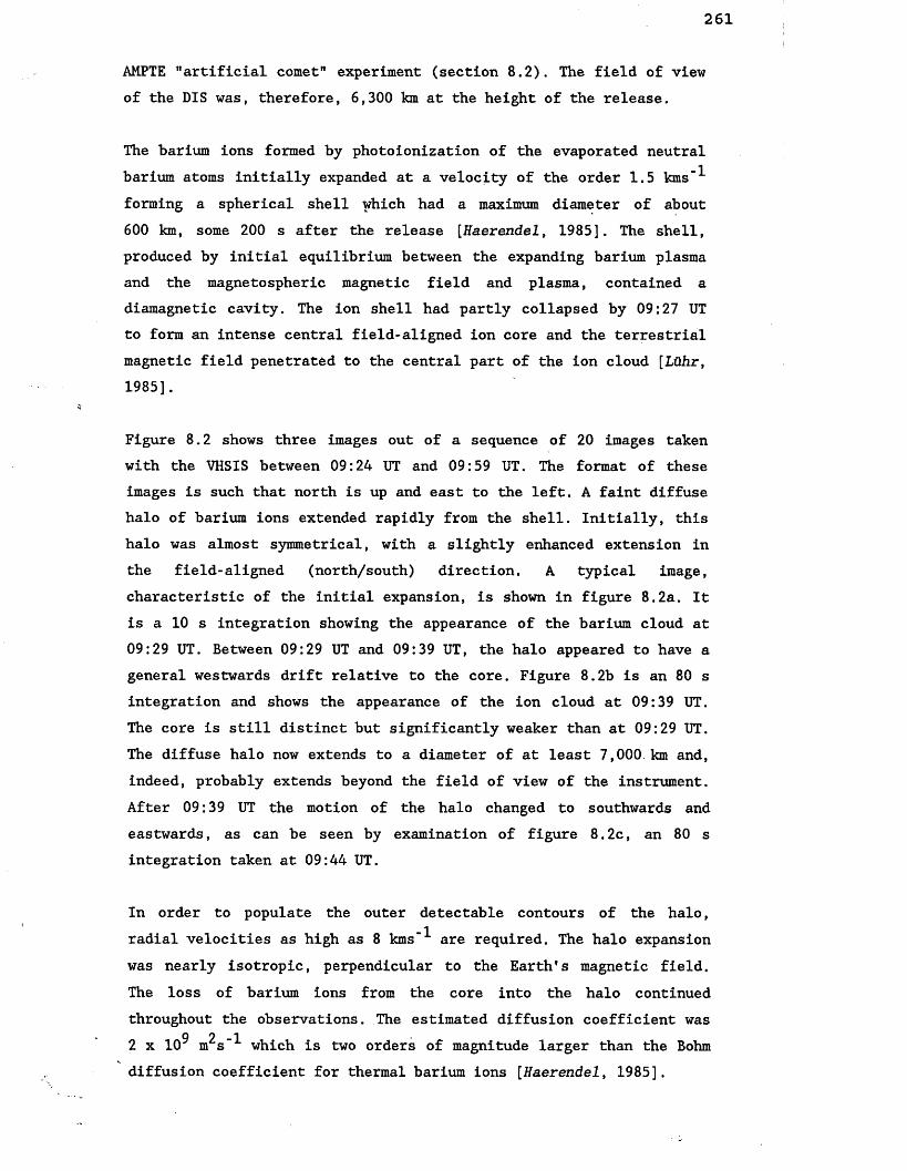
261

AMPTE "artificial comet" experiment (section 8.2). The field of view of the DIS was, therefore, 6,300 km at the height of the release.

The barium ions formed by photoionization of the evaporated neutral barium atoms initially expanded at a velocity of the order 1.5 kms"^ forming a spherical shell which had a maximum diameter of about 600 km, some 200 s after the release [Haerendel, 1985]. The shell, produced by initial equilibrium between the expanding barium plasma and the magnetospheric magnetic field and plasma, contained a diamagnetic cavity. The ion shell had partly collapsed by 09:27 UT to form an intense central field-aligned ion core and the terrestrial magnetic field penetrated to the central part of the ion cloud [LCthr, 1985].

Figure 8.2 shows three images out of a sequence of 20 images taken with the VHSIS between 09:24 UT and 09:59 UT. The format of these images is such that north is up and east to the left. A faint diffuse halo of barium ions extended rapidly from the shell. Initially, this halo was almost symmetrical, with a slightly enhanced extension in the field-aligned (north/south) direction. A typical image, characteristic of the initial expansion, is shown in figure 8.2a. It is a 10 s integration showing the appearance of the barium cloud at 09:29 UT. Between 09:29 UT and 09:39 UT, the halo appeared to have a general westwards drift relative to the core. Figure 8.2b is an 80 s integration and shows the appearance of the ion cloud at 09:39 UT. The core is still distinct but significantly weaker than at 09:29 UT. The diffuse halo now extends to a diameter of at least 7,000 km and, indeed, probably extends beyond the field of view of the instrument. After 09:39 UT the motion of the halo changed to southwards and eastwards, as can be seen by examination of figure 8.2c, an 80 s integration taken at 09:44 UT.

In order to populate the outer detectable contours of the halo,_ 1radial velocities as high as 8 kms are required. The halo expansion

was nearly isotropic, perpendicular to the Earth's magnetic field.The loss of barium ions from the core into the halo continuedthroughout the observations. The estimated diffusion coefficient was

9 2-12 x 10 m s which is two orders of magnitude larger than the Bohm diffusion coefficient for thermal barium ions [Haerendel, 1985],

Once outside the initial diamagnetic cavity individual barium ionsgyrate within the terrestrial magnetic field. Their mean velocity hadto be significantly larger than the 8 kms” radially outwarddiffusion velocity of individual ions. An estimate of the mean

-1 - 1velocity of the halo ions would be about 2 x rr x 8 kms or 50 kms . The gyroradius of 1.5 kms"^ barium ions in the observed terrestrial field of 8 nT was about 260 km, with a gyroperiod of about 200 s [Haerendel, 1985], At 50 kms’ , a barium ion has a gyroradius of about 3,000 km, a value that is comparable with the observed size of the halo.

It is possible that a very small fraction of the initially producedions had velocities of the order 50 kms’ . However, to explain thecontinuous loss of barium ions from the core of the halo, all thebarium ions initially created by photoionization had to eventuallyreach velocities of this order. Within 40 minutes a total of at least3.75 x 10 J of energy was coupled into the ion cloud. A range of lowfrequency electrostatic and electromagnetic waves are endemic withinthe magnetosphere [.Rees et al., 1986]. Assuming a source dimension of6,000 km, comparable with the instrument field of view, the meanenergy density extracted from the background wave field by the barium

8 2ions would be about 5 x 10 Wm . Photoionization of Ba II to Ba III with a time constant of the order of 30 minutes could be a contributing loss mechanism, but seems unlikely in view of the 10 eV ionization potential of Ba II.

A typical Doppler image, from the sequence of 20 Doppler images taken with the DIS, is shown in figure 8.2d. The fringes are obtained from the core of the cloud. These fringes contrast sharply with the lack of such patterns in the images obtained with the same instrument used to observe the 27 December 1984 "artificial comet" (section 8.2).

The DIS observations of the core yielded a consistent pattern of line of sight velocities. A persistent north-south shear of the order of 2 kms"^ was detected, with the line of sight velocity of the south part being more eastward than that of the north part. As time progressed the initial mean line of sight component of about 2 kms"^ directed away from the Earth, changed to a mean earthward component

263

of the same order (a more detailed description is given in Rees, [1987a]).

The DIS observations of the ions in the halo revealed a large line of sight velocity dispersion. The range of toward and away velocities should have exceeded 10 kms“ . Such a velocity range would have been consistent with the velocities of barium ions diffusing to populate the extreme regions of the diffuse and rapidly expanding halo.

8.4 Search for Auroral Belt E.. Fields with High-Velocitv Barium Ion Injections

Measurements of the distributions of electric fields aligned parallel to the magnetic field have been an elusive goal of space plasma physics. The most feasible, currently operational technique for approaching this goal depends on optical tracking of the field- aligned motion of luminous barium ion tracers to detect deviations from the predictable motion that results from the initial ion velocities, the gravitational force, and the jugradB magnetic mirror force. In typical high latitude experiments using high-velocity injections at collision-free altitudes above the ionosphere, the barium ions are propelled to magnetospheric distances of several or more Earth radii with optical tracking suitable for triangulations extending into the 1 - 4 Rg range.

Two techniques for high-velocity Ba+ injections have been employed:1) High velocity shaped-charge injections from rockets usually with a large velocity component parallel to the local magnetic field that dominates the subsequent motion [Wescott et al., 1975; 1976; 1978; Haerendel et al., 1976; Stenbaeck-Nielsen et al., 1984] and2) Low velocity thermite releases from an orbiting vehicle that gives a high velocity component perpendicualr to the local magnetic field, and thus a dominating /igradB force to propel the ions into the magnetosphere [Heppner et al., 1981],

Over the past few years there have been several successful barium shaped-charge releases. These experiments have been conducted independently by NASA and by the University of Alaska. A full

264

description of the experiments observed to date is given in section 2.7. Each of these releases was observed with a co-aligned VHSIS/DIS from one or more suitable ground-based sites.

The first releases to be observed with a co-aligned VHSIS/DIS, took place over Alaska in April 1984. The major goal of the APL observations at this stage was to demonstrate the validity of the Doppler imaging technique in this sort of application (section 8.4.1). The DIS results showed good agreement with the bulk velocities but the peak velocities were not observed with sufficient accuracy to check the velocities from upper tip triangulations. The DIS has since been modified to produce a higher velocity resolution (section 8.4.2).

The analysis of the data from the April 1984 experiments is now complete and the main results are summarized, after the discussion of the DIS results, in section 8.4.1. The full analysis of the data from more recent experiments is still in progress and will, therefore, not be presented here.

8.4.1 The April 1984 Experiments

Four barium shaped-charge releases were detonated from two rockets launched from Poker Flats Research Range, near Fairbanks, Alaska in April 1984. These two experiments were part of the NASA programme to study processes taking place in the magnetosphere. The Principal Investigator (PI) for these two experiments was Jim Heppner from NASA Goddard Space Flight Center.

The first rocket, Black Brant-10 35.007 was launched from Poker Flats Research Range on 30 March 1984 at 11:00:00 UT. The first release occurred at 11:05:40 UT at an altitude of 770 km. The second release occurred at 11:11:25 UT at an altitude of 886 km. The second rocket, Black Brant-10 35.008 was launched from Poker Flats on 1 April 1984 at 07:19:00 UT. The first release occurred at 07:24:40 UT at an altitude of 774 km. The second release occurred at 07:30:25 UT at an altitude of 975 km. Both flights took place under active magnetic conditions.

265

The observations were made with low-light level systems from 7 principal observing sites dotted over the North American continent (see 'Heppner et al. [1989] for a more detailed description of the sites and the instruments used).

The APL observations were made with a co-aligned VHSIS/DIS from the optical site at Poker Flats. The VHSIS employed a 180 mm Nikon camera lens, giving a field of view of 5.7°, corresponding to a distance of about 75 km at the height of the release. The DIS employed a fixed gap Fabry-Perot etalon with a plate separation of 2 mm and a working diameter of 100 mm. The free spectral range of this etalon at455.4 nm is, thus, 0.052 nm, equivalent to a line of sight velocity of 34 kms"^. The positive lens used to focus the Fabry-Perot fringes had a focal length of 180 mm, so that the field of view of the DIS was also 5.7°. The theoretical maximum achievable velocity resolution of this DIS is 0.2 kms"^. Both these optical systems recorded the455.4 nm resonance line emission of sunlit barium ions throughnarrow-band, FWHM 3 nm, interference filters, centred at 455.4 nm. Since this was the first time that such a system had been used inthis kind of experiment, the objective was primarily to test theapplicability of the DIS.

Figure 8.3 shows the appearance of the first barium jet from the first rocket experiment through the DIS at 11:07 UT. Relativevelocities only can be deduced from this image as it stands. By assuming a zero line of sight velocity at the base of the jet, at the right hand edge of the image, line of sight velocities of the order of 15 kms"^ are observed towards the tip of the jet which is just off the field of view of the DIS to the left. The line of sight velocities determined from this Doppler image are shown in figure 8.4. The actual velocity resolution obtained from the peak

_ ipositions in this Doppler image is of the order 1 - 2 kms , caused primarily by the low photon flux detected in the fringes.

Many other Doppler images were taken of the four barium jets associated with the two experiments and they basically showed good agreement with the bulk velocities, but the peak velocities that determine the motion of the upper tips of the rays were not determined with sufficient accuracy to check velocities from upper

266

tip triangulations. Some of the VHSIS images were triangulated with data from other stations to infer motions of the upper and lower tips of the barium jets.

A detailed description of the principal findings from these experiments can be found in Heppner et al. [1989] and will be summarized here. The observations were in agreement with the theoretical time constant of 28 s for photoionization of barium [Carlsten, 1975] and illustrated the lack of any anomalous ionization that might have been expected from Critical Ionization Velocity (CIV) effects. Transient accelerations and/or decelerations were encountered by each of the seven principle Ba+ rays tracked to high altitudes. These E„ perturbations are likely to be associated with suprathermal electron bursts, both upward and downward.

8.4.2 Recent Modifications to the VHSIS/DIS used to Observe the Barium Shaped-Charge Releases

The DIS used in the April 1984 experiments (section 8.4.1) employed a positive lens with a focal length of 180 mm which mapped 10 fringes onto the field of view of the detector. It was, therefore, decided to increase the velocity resolution by changing to a 400 mm focal length lens. This lens maps 4 fringes onto the detector surface, and, therefore, increases the velocity resolution of the instrument by more than a factor of two.

The images obtained with the VHSIS and DIS in the April 1984 experiments were processed and stored as 128 x 128 arrays on a PDP 11/23 computer. After this experiment the PDP 11/23 computer was replaced with an IBM PC. The software was modified to run on the new system and the image format was changed to a 256 x 256 array, doubling the resolution of the instruments. In addition, the dead time of the system was significantly improved by making modifications to the detector electronics.

The result of these changes was that the Doppler imaging system used in the April 1986 experiments had a velocity resolution more than four times greater than its 1984 counterpart. The maximum theoretical velocity resolution achievable with this DIS is 0.05 kms” .

267

The improved VHSIS/DIS was first used to observe a series of barium shaped-charge releases in a set of experiments over Alaska in April 1986. Although the full analysis of the data from these releases is still in progress a selection of the VHSIS/DIS results are presented here to illustrate the improvements in the system. These results were obtained from a rocket experiment conducted by the University of Alaska, PI Gene Wescott, on 3 April 1986. The rocket made two barium shaped-charge releases.

The VHSIS employed a 300 mm Nikon camera lens, corresponding to a field of view of 3.4°. The sequence of images presented here focuses on the passage of a barium jet through the field of view of the two systems. This jet was first acquired at around 10:43:12 UT and was tracked until 10:46:55 UT. Figure 8.5a is a 10 s integration showing the appearance of the first jet at 10:44:04 UT. The corresponding Doppler image is shown in figure 8.6a. By assuming a zero line of sight velocity in the debris cloud, the line of sight velocities in this image vary fairly uniformly from 2 kms"^ near the base to 7 kms” towards the tip. Figure 8.5b is a 10 s integration showing the image obtained at 10:44:42 UT. A second jet has entered the field of view from the left. This jet was released at a different height and is travelling along a different field line. The corresponding Doppler image (figure 8.6b) is able to resolve the two jets by virtue of their different line of sight velocities. The line of sight velocities in the first jet vary from 3 kms"^ to 6 kms’^ (figure 8.7). The line of sight velocities at the tip of the second jet are of the order 12-13 kms"^ (figure 8.8). Figure 8.5c is a 10 s integration showing the appearance of the first jet at 10:46:37 UT, after the passage of the second jet. The corresponding Doppler image is displayed in figure 8.6c. The line of sight velocities derived from this image are of the order 2 kms’ . Figure 8.5d is a 10 s integration showing the appearance of a weak jet at 10:50:44 UT. The corresponding Doppler image is shown in figure 8.6d. There are too few photons in this image for any satisfactory analysis.

The Fabry-Perot fringes obtained from this experiment are clearly a great improvement on those collected in the April 1984 campaign, (compare figures 8.4 and 8.6). The maximum achievable velocity

268

accuracy of the old instrument was 0.2 kms"^. However, the low flux of photons observed with the DIS in the 1984 releases decreased this resolution to the order of 1 - 2 kms~^. The maximum achievablevelocity resolution of the new instrument is 0.05 kms'^, and this was certainly achieved in some of the high photon flux peaks obtained in the April 1986 experiments. The combination of faster electronics, increased number of pixels and fewer fringes at the detector has, thus, increased the velocity accuracy of the DIS by more than a factor of four.

The DIS used in the April 1984 and April 1986 experiments employed an etalon with a fixed gap of 2 mm (equivalent to a free spectral range of 34 kms'^"). Since the largest line of sight velocity anticipated does not exceed 20 kms"^ it is possible to achieve an even higher velocity resolution by using a larger gap etalon. It was, therefore, decided to employ a fixed gap etalon with a plate separation of 3 mm, equivalent to a free spectral range of 22.8 kms"^, in future experiments.

In the first group of experiments observed, the VHSIS employed a 300 mm Nikon camera lens. This lens produces a field of view of about 3.4° at the detector and is able to yield detailed information on jet structures. However, due to the short integration times used in these experiments, few, if any stars are apparent in the images and so these images cannot be used for triangulation. The VHSIS used in these experiments now uses a smaller focal length lens (50 mm or 85 mm) and this produces a much larger field of view (20.4° or 12.1°). These images contain more stars and are more reliable for triangulation.

8.5 Recent Free Space Experiments Designed to Test the Critical Ionization Velocity Mechanism

Over the past few years several free space experiments have been made to test the Critical Ionization Velocity (CIV) effect first proposed by AlfvSn [1954] and Alfv6n & Arrhenius [1975] as part of a theory for the formation of planetary systems. The ionization takes place through collective plasma processes with the energy provided by the neutrals moving across a magnetic field embedded in the background

269

plasma. For the ionization process to take place the velocity of the neutrals must exceed the critical ionization velocity determined by the kinetic energy in the velocity component perpendicular to the magnetic field being equal to the ionization potential of the neutrals.

In project Porcupine, Haerendel [1982] observed 16% - 18% ionization of those neutrals that exceeded the critical velocity from a conical shaped-charge detonated 30° to B well below the UV horizon. Deehr et al. [1982] detected strontium ions in the sunlit detonation of a radial barium shaped-charge. The strontium was present as a 1% impurity and the analysis revealed that about 50% of the strontiumionized - at a time when less than 1% ionization would be produced bysolar UV. Two further CIV experiments were carried out from the magnetic equator in Peru in 1983. However, all of the barium ionsproduced in the Star of Lima experiment [Wescott et al., 1986] couldbe accounted for by solar UV ionization, and the strontium ions produced in the Star of Condor experiment [Wescott et al. , 1986]could also be explained without invoking the CIV mechanism.Therefore, three additional CIV experiments were carried out in May 1986 from Wallops Island to try to understand the apparent failure to observe excess ionization due to the Alfven mechanism in the Peru experiments. CRIT I (section 8.5.1) used two barium conical shaped- charges detonated below the solar UV cut-off altitude at 48° to B. The third experiment, called SR90 (section 8.5.2), consisted of a high-explosive conical shaped-charge with a strontium metal liner detonated in full solar UV radiation. Optical observations of these three releases were made with low-light level imagers from three primary optical sights at Wallops V25, Duck, NC and at Cape May, NJ(for a more detailed description of the sites and the instrumentsused see Stenbaek-Nlelsen et al. [1990]; Wescott et al. [1990]). Two VHSIS systems were operated at the Wallops V25 site and it is the relevant observations and results from these two systems that are presented in this section.

8.5.1 The CRIT I Experiment

A CIV experiment was carried out with a heavily instrumented rocket launched from Wallops Island on 13 May 1986. Two neutral barium beams

270

were created by explosive shaped-charges released from the rocket and detonated at 48° to B at altitudes near 400 km and below the solar UV cut-off. The first detonation occurred at 07:46:00 UT at an altitude of 399 km, 37.60° N and -73.21° E. The second detonation occurred at 07:47:25 UT at an altitude of 373 km, 37.5° N and -72.55° E.

Observations were made with two VHSIS systems from the Wallops V25 site in the launch complex. Both of these systems employed 85 mm Nikon camera lenses, giving a field of view of 12.1°, corresponding to a distance of approximately 80 km at the height of the releases. One of these optical systems recorded the 455.4 nm resonance line emission of sunlit barium ions through a narrow-band, FWHM 3 nm, interference filter, centred at 455.4 nm. The other recorded the553.5 nm resonance line emission of sunlit neutral barium through a narrow-band, FWHM 3 nm, interference filter centred at 553.5 nm. These lines are the dominant barium ion and neutral emission lines excited by fluorescence in sunlight.

This experiment was designed with the expectation that ions would be created near the release by a relatively short lived CIV process to produce a field-aligned jet along the release field line. It was intended to position the VHSIS systems for optimum view of the release field line above the terminator. However, contrary to planning, no real time update information about the trajectory was received after the launch. The bright ion cloud, created by photoionization when the neutral jet came up over the UV terminator, appeared in the field of view. Two 5 s integrations were obtained before the detector turned off, due to overloading. However, this pointing direction turned out to be almost perfect for the unexpected non-solar UV produced ion cloud that appeared. The second release monitored from Wallops was observed to take place along the line of sight of the large diffuse cloud produced by the first release which prevented any useful VHSIS observations.

The first relevant VHSIS image was taken in the light of the Ba+ ion at 455.4 nm and covered a time period from 2 s before detonation to 4 s after detonation. No ions were observed in this image. The second relevant VHSIS image was taken in the light of the Ba+ ion emission at 455.4 nm and covered the time period from 5 to 10 s after the

271

release (figure 8.9). No field aligned streak can be seen in this image. Instead, an ion cloud of relatively uniform and low brightness can be seen in the region above the solar terminator and between the release field line and the barium jet. Several lines have been inserted to help in the interpretation [after Stenbaek-Nielsen et al. , 1990]. The release location is identified by the cross at the far right of the image. The magnetic field line extends up to the left from the release point while the direction of the neutral jet is to the bottom left. The crosses are marked every 10 km. The ion cloud should be observable above a screening height of 19 km which is inserted (row of dots to the right). The row of dots to the left is the maximum distance a neutral or ion at 13.5 kms"^, the maximum velocity in the jet, can reach in 10 s. The ions are in two parts. The very bright circular cloud to the lower left of the image is the cloud produced by photoionization. The second part is the faint cloud of fairly uniform intensity in the centre of the image and between the shown delimiters. These ions were produced below the solar terminator and, therefore, must have resulted from an ionization process other than direct photoionization by solar UV radiation. The process must have been present continuously from the time of release.

A computer simulation of this image (figure 8.10) has shown that the efficiency must be nearly constant in time and equivalent to an ionization time constant of about 1800 s [Stenbaek-Nielsen et al., 1990]. Various sources for these ions have been considered. Although the cross-sections for ionization between the neutral barium and the ambient atmosphere are highly uncertain, this appears to be the most likely process, rather than a CIV process [Stenbaek-Nielsen et al., 1990]. A CIV process may have been present at early times, but its efficiency cannot have exceeded an equivalent ionization time constant of 1800 s. Assuming that the source of the ionization is collisions with the ambient atmosphere, it is clear that this constitutes an important source that must be taken into account in future release experiments.

8.5.2 The SR90 Experiment

This experiment consisted of a high explosive conical shaped-charge with a strontium metal liner on the Taurus-Nike-Tomahawk rocket,

272

38.008 UE, launched from Wallops Island on 13 May 1986 at07:56:00 UT, 9 minutes after the launch of the barium experimentrocket (section 8.5.1). The release was made at 08:01:29 UT, at analtitude of 539.6 km, 37.72° N and -74.72° E, in dawn twilight andwas aimed at 48.2° with respect to B. The background electron density

/was 1.5 x 10 cm" .

Observations were made with two Very High Sensitivity Imaging Systems from the Wallops V25 site in the launch complex. Both of thesesystems employed 85 mm Nikon camera lenses, giving a field of view of 12.1°, corresponding to a distance of about 115 km at the height of the release. One of these optical systems recorded the resonance line emission of sunlit strontium ions and the other recorded the resonance line emission of sunlit neutral strontium.

The neutral strontium cloud was very bright. About 15 s after therelease the detector lens was stopped down to avoid damage to thedetector. Unfortunately both the neutral and ion detector were stopped down and as a consequence the later ion images are verynoisy. No prompt ions were detected. However, a faint trail ofstrontium ions was detected along B above the release over a period 2 - 3 minutes following the release. The apparent velocity of the tip of this field aligned Sr+ jet was determined, from the Duck ISIT data, to be about about 2.6 kms"^.

The differential velocity function of the neutral jet was determinedfrom a white light image taken with the ISIT TV at Dack, 11.5 s afterdetonation. The apparent tip velocity was slightly over 13 kms"'*' anda low velocity peak in the differential velocity function occurred atabout 2.6 kms"^ [Wescott et al., 1990]. This agrees well with thevelocity of the tip of the observed Sr+ jet. This jet is from theportion of the neutral jet with velocity perpendicular to B which isbelow the Alfven critical velocity. The detectable portion of the ion

21streak was found to contain about 10 ions, which can be fully accounted for by solar UV ionization [Wescott et al., 1990].

Although no high-velocity ion jet was observed, tie VHSIS images, combined with model calculations have been used to estimate the maximum number of CIV ions that could have been prssent. The high-

273

21velocity portion of the jet should have produced about 2 x 10 solarUV ions. Computer simulations have since shown this to be morediffuse and just below the threshold of the VHSIS [Wescott et al.,

1990]. Therefore, if there were CIV produced ions present in numberscomparable to the solar UV produced ions they should have beendetected. This sets the maximum number of CIV ions which could have

21been produced, but not detected, at less than 2 x 10

21Thus, any prompt CIV ionization must be less than 2 x 10 ions, orless than 0.18% yield of the vaporized Sr. Since this maximumpossible CIV yield is a factor of 100 less than the Porcupine

5 - 3experiment in which the ambient plasma density was 6 x 10 cm , or30 times greater, Wescott et al. [1990] conclude that future CIV

5 - 3experiments should have the plasma background near 6 x 10 cm

274Figure 8.1

— o ru mnCDeuro -]cn cn ID CZ M —I -ti­

ro min rum to m?D

□ wCZ 00

LUL1i l i s a i

— • — ru cd -p. cn (£i ru |T> cs ro © ro -*■ -* ro co -p. cn C D C n - J i D r 0 C 5 > E i C 3 O < SLO

ru rn ru mm ru _ rom to m 7D

□ ro □ CPCZ wcz ro

zi m i i jru id Ji cn

d ru (D O O O Qro coEJ (3 Xi cn ro row cn cd cn co ru u?

275Figure 8.2

o~nm i—i§5

a 'i rn f-to Sm too co a cn -£<■

(Jlcn33

I—I LU , 210 1 —I “ 70 LOt rururo

_ i. M £Z COCD ~1 G"!

i — i i " i 111

-i -i m ru ru u LOLn-jconjcnra-^conj

lj nmt—icr on1mTDoroI Qcni-) -f*cnoitn23 J W 3 -i-imA-jaiiSEi - n j m o u i y i B i s i a s o

I—I LU2 ^ D —1“ 50GJ I GO mruoo

rucs>

276Figure 8.3

o mm i—i<= r~i—i —1o mm 73o cni—i Qon

Si.cncnZ33

------1 -* 3n o 73_i. -si 03cn o O7C o — *■3 CDcz 00H

ro uj -o cn C) -j oo cd o m - - - m m qj -t iji -o cd -OCn O O O C n O C S O Q C S

CP IDX>HS 3CZ01i_nmIE 73 D h "DOm o m

ieo -cxcoZDH 73 0o c nm i- 73 ZDm cn m om73 ID ZD UOHm o73-c

Figure 8.4277

oxxCOm

xXa=ZnXr~

x i- to x H h D H

X-i m i—i o ocn•• O 3 “0o x x-o Lom •• CO X X CD I—I X I—l ( S u i n nx m o h o x x—| I—I O -C• OI(Jl

X X hO X O X <1 O C 0

m mL0 I I- CD O X I X\ o n r ol—l I CDoj —i m x \ t-l x x — rn lo —i o co m o00 70x o I <• to

CO Xm • x x h x C • HH m co i_m

1—I 70 X IS CO X M O X H

X x o 0 X 0 7s m r m x r x m

£7)x m

co

xcoxx

oxooX

cnox3\CJ1 3\ ex IX CO cn CO 00 o ru cntn’ • • • • ■ • • ■ • • •IX IX o o Q o o o o o o

278Figure 8.5

ZL E>— IAI CO. CD OjLuCD-'J't .. CO_i cz oo

IHBli-* -* ru ru ro co

lo cn -j c ro d) cs ^ co ro

o nrn wcro FtIrunIff ?

I—( -*■ 15 2C3T) —I 70-*•I -*■ El LJca

CD -Ja- —1 (O_i C M iTi —I Oj: !::S

o -n ru i—i c r<~> rrj m mC roX Qcnm Acn cn cn

3 3

O X X (—1c rnrlFI 73

TOa cni—i -p*-cn cn cn

1—t —t OD* ZZ E> 73 -I** 73inI El CD.. Cl)

?*«> _l C 00©Hoi

- ^ m ru ru u i w ^ - ' j o m c n o + Kiro

o x i-i -»■ x5 F H ® 3nnl i £ tDrun " locco -□ o XO t- ..COcn q a c wi—i -t*- —i is —I mcncn 3

“ ; M M ; 1 I liil IBTI I I aa o§ —*■—*■ ru ru ro co_ ) -i cijin-o!£irocDE -p- co ru

279Figure 8.6

SM> T'

o~nFli-ic rorlrnTDo-^ ■ cn cnin

“DxCl3

l-l X X CD "0 -1“ 70I X El

. . UJruw C WCO — I co

11rn

m 7aC? cs wcncn cn

O -nE ) TJm t—tc r

O -fi ipcn icn cn Cjj tl cwo CO ~I UJ

i—j 'Im

mTCC4Xcnoi

XIo

_Z CD U

CO E

CD X)CjJLSJ

IBAREUM SHAPED-CHARGE

RELEASE FILE

; E86D

31043. A 49 (BARIUM

SHAPED-CHARGE RELEASE

FILE :

EB

6D31044.A

26

Figure 8.7280

mm

o~n~ncnm

70a

nX

o i> “n — Icn-*■ i—i

CS £> X —1

■■ I— Iro o cn. xc= c• m H r-• o

nO (-1

Cjj cn\ □to\ CO m CD 70 00 C cr. m • o~n70o

~UO7Tm70

TO X*X H X I — I i o CO 21]

X L0P1 X 70 X l—I J Om o x

r>5xcoXhHx o£0 COm

iX X m to r~o m to x xLO — |m o

70 I <

cm toxcom u

LO On o o r H r H m

o m

cn

xcoxx

oxoO

cocs

773\CJl 773\ui CD

CS

-tiCS

cncs

cocs

-J

cs

CO

csCD■cs

cs

cs cs

rocs

CO

cs

94

Figure 8.8281

m i—iH xmro

o x x —Icn-* i—i CS O X H H•• I— Iro o co zzx c • m

to x x hsrx cn

Lornx xX ux o m o x

XO H X 01 X l—I X O OO'Jrn

oxxcnIX

xx□HoX

• O X X O IX TO □ HTQX h X X

HH X Xm lo­co cn x o\ Xo I -cTO\ CO X

x • cCD X H :oo c • ►O X <o on

X Xx xcnX X Ho —13X L O OO OO77 o xx h xX HXoX XxX X—I oCO zzoX oX 2XCO c=77 77X

COcs

773\Ul

X3\Ul1

'

CD 4*. X <y> H 00CS CS cs cs cs cs

CDcs

cs

cs cs

rocs

COcs

Figure 8.9282

Figure 8.10283

284

CHAPTER 9

THE PRINCIPAL RESULTS FROM THIS STUDY OF NATURAL AND ARTIFICIAL GAS AND PLASMA CLOUDS WITH IMAGING AND DOPPLER IMAGING SYSTEMS

9.1 Introduction

The properties and dynamics of natural and man-made gas and plasma clouds in the solar wind and in the magnetosphere have been studied by monitoring the motion and evolution of these clouds in the appropriate region. The resulting distributions of ions and neutrals under the above conditions have been obtained with a Very High Sensitivity Imaging System (VHSIS). Two-dimensional line of sight velocity maps of the ion and neutral species have been obtained with a Doppler Imaging System (DIS). Both of these devices were discussed in some detail in chapter 2.

Over the past five years a number of cometary targets have been observed with VHSIS and DIS systems. The inner coma has been studied with 1 m and 24" class telescopes, and the outer coma and tail has been studied with a selection of wide-angle Nikon camera lenses. Theprinciple results that have been obtained from these studies aresummarized in section 9.2.

Over the past six years several artificial chemical releases in themagnetosphere and the near-space environment have been observed withVHSIS and DIS systems. The principle results from these experiments are summarized in section 9.3.

VHSIS and DIS systems will continue to be used to make cometary observations and, indeed, a VHSIS is now permanently stationed at the Table Mountain Facility (TMF) to enable a swift response to new cometary targets of opportunity. VHSIS/DIS systems will also continue to be used to observe future artificial chemical releases. The Atmospheric Physics Laboratory (APL) at University College London (UCL) is currently involved in a proposal for an instrument for the European Space Agency's (ESA's) Polar Platform. The proposed future

285

work with low-light level imaging systems within the APL at UCL is discussed in more detail in section 9.4.

The recent missions to the comets Giacobini-Zinner and Hailey and the associated extensive Earth-based observations have greatly improved our knowledge of comets. However, many questions still remain unanswered and a number of future missions ito comets are currently under active consideration (section 9.5).

9.2 Principal Results from the Cometary Observations

The principal results from the narrow-band imaging of the neutral and plasma cometary components are discussed in sections 9.2.1 and 9.2.2 respectively.

9.2.1 Observations of the Neutral Cometary Coma

Ground-based narrow-band imaging of a number of comets has been carried out with a VHSIS on 1 m and 24" telescopes and with aselection of Nikon camera lenses. This has enabled an extensive study of the CN and C2 comas of these comets. The resulting CN and C2

distributions have been modelled by the simple radial outflow model with decay (section 5.2.3), to reveal characteristic scale lengths for production and decay of these daughter products (section 5.3 and 5.4). The derived scale lengths have been compared with those found by other authors (section 5.6) and more accurate scaling laws have been derived (section 5.7).

The CN parent scale lengths obtained from the near-nucleus CN images from the VHSIS were used, together with those obtained by Combi & Delsemme [1980], to obtain a CN parent scale length of(2.0 ± 0.2) x 10^ km at unit heliocentric distance scaling asr(1.7±0.2) The CN daughter scale lengths from the large-scale CNimages from the VHSIS were used, together with those obtained byCombi & Delsemme [1980] , to obtain a daughter scale length of(4.9 ± 0.5) x 10^ km at 1 AU, varying as r(l»75±0.25^ parentscale lengths obtained from the near-nucleus C2 images from the VHSIS were used, with those obtained by other authors [Combi 6c Delsemme, 1980; Cochran, 1985], to obtain a value of (1.8 ± 0.2) x 10^ km for

the C2 parent scale length at 1 AU, scaling as r(l*7±0.3)^ parentscale lengths for both CN and C2 of around 2 x 10^ km, at 1 AU, suggest possible emission from freshly ejected sub-micron grains, rather than direct sublimation from the nucleus.

The inner C2 coma of comet Borrelly was found to be anomalous in that the simple radial outflow model with decay could no longer be used to fit the data (section 5.8). In addition to a centrally condensed source, there was evidence for a second, non-central source, possibly due to the coma of long-lived dust grains that give this comet a diffuse appearance. These grains would be larger, perhaps 0.1 mm - 1.0 mm and would not be superheated. It was postulated that their carbonization and C2 release could be due to space radiation, via "sputtering" by UV photons and by protons.

1The integral profiles of the 0( D) 630 nm near-nucleus images of comet Giacobini-Zinner, taken with the 1 m Jacobus Kapteyn Telescope (JKT) on 1 September 1985, revealed a central source region. A model was developed in section 6.2 to include the H2O and OH sources and the NH2 contamination. The central deficit was confirmed as not due to collisional quenching but is indicative of a source scale for much of the presumed H2O parent of (2,150 ± 300) km. The 0(^D)distribution was found to be close to radially symmetric, a puzzling observation considering that the Hailey probes had clearly established that gas and dust was emitted almost entirely from the sunward side. The explanation for this is probably that H2O sublimes largely from micron-sized grains on a few times 1,000 km scale, rather than from the nucleus itself [Wallis et al., 1990]. Some sublimes within 1,000 km, where collisions ensure sunward bias as evident in UV maps of the OH emission.

Several authors reported low contrast "jet-like" features in the neutral emissions of comet Hailey [A'Hearn et al., 1986; Larson et al., 1986; Cosmovici et al., 1987], an observation that has important implications for the formation of these neutral radicals. Although no coma features were immediately apparent in any of the near-nucleus VHSIS images of comet Hailey from the March 1986 period, a ring- masking technique was able to reveal possible "jet-like" features in the inner coma in all of the continuum, ion and neutral images taken

287

over this period (section 6.3). The CN and C2 jets had shapes and directions that were completely different from the visible dust jets, an observation in agreement with the findings of A'Hearn et al.

[1986]. These results would, therefore, support the hypothesis that some of the CN and C2 radicals come from small sub-micron grains, which would not be seen in the continuum.

9.2.2 Observations of the Ion Coma and Tail

The structural profile of the ion coma of comet Giacobini-Zinner wasdetermined for comparison with the data collected \ by theInternational Cometary Explorer (ICE) probe. The large-scale VHSIS images of comet Giacobini-Zinner close to the ICE encounter revealed a diffuse fan some 2 x 10 km in length with scale width 25,000 km in the near tail. The near-nucleus VHSIS Images of this comet revealed a short tail core within this fan structure (section 7.4).

The structure of the ion coma of comet Hailey was determined at times close to the spacecraft encounters (section 7.5). The near-nucleus images revealed smooth, parabolic contours on the sunward side. On the tailward side the contours appeared smooth and symmetric on most days, but on others, notably 6 March 1986 and 22, 23 March 1986prominent tail rays could be seen. The large-scale tail structure was relatively simple on most days, with minor knots and condensations moving along the tail. On other occasions, for example 12 hours prior to the Giotto encounter and on 20 March 1986, major tail disconnection events were in progress (section 7.7).

The transition to the incoming solar wind, both in comets Giacobini-Zinner and Hailey, was seen to be very steep, varying on average as -1 5r along sight lines, although considerable day-to-day variations

were much in evidence. This corresponds to a region of strong cooling of the plasma via interactions with the neutral coma [Wallis & Ong, 1976] and was also detected by the Giotto ion experiments [Johnstone et al., 1986; Balsiger et al., 1986]. There was a much more gradual tailward decrease of ion intensity for these two comets, varying on average as r’® * ^ along sight lines, corresponding to the flow of ionospheric ions and thermalized pick-up ions into the tail -(section 7.6).

288

Comet Hailey displayed an ordered type I plasma tail from early December 1985 to late April 1986. However, comet Giacobini-Zinner, even at perihelion, showed only a short ionospheric tail, and a broad extended ion tail fan. The difference in appearance of these two tails is undoubtedly related to outgassing strength (section 7.8).

9.3 Principal Results from the Observations of Several Artificial Chemical Releases

The VHSIS/DIS observations of the barium shaped-charge releases are discussed in section 9.3.1, and the principal VHSIS/DIS results from the AMPTE missions and the two rocket releases over Wallops Island in May 1986 are summarized in sections 9.3.2 and 9.3.3 respectively.

9.3.1 Observations of the Barium Shaped-Charge Releases

The first barium shaped-charge releases to be observed with a VHSIS/DIS system took place over Alaska in April 1984 (section 8.4.1) The objective of the APL observations at this stage was primarily to test the feasibility of the DIS. The line of sight velocities calculated from the Doppler images showed good agreement with bulk velocities, but the peak velocities that determine the motion of the upper tips of the rays were not determined with sufficient accuracy to check velocities from upper tip triangulations [Heppner et al., 1989].

Several additional barium shaped-charge releases have since been observed with an improved VHSIS/DIS system (section 8.4.2). However, the full analysis of the data from these campaigns is still in progress and is, therefore, not discussed here.

9.3.2 Observations of the AMPTE Releases

Two of the AMPTE releases were observed with VHSIS/DIS systems from on board the NASA Convair 990 airborne observatory.

The observations of the 27 December 1984 "artificial comet" experiment revealed that the plasma cloud introduced into the solar

289

wind was short lived (about 5 minutes) as a result of rapid extraction of barium ions induced by the solar wind and Interplanetary Magnetic Field [Rees et al., 1986a]. The DIS results showed that while the head was composed of a central core of cold ions, the extended coma and tail were formed by more energetic ions (section 8.2).

The VHSIS observations of the 21 March 1985 AMPTE barium thermite release in the Earth's magnetotail showed that the ions initially expanded to form a spherical shell which later partially collapsed to form an intense field-aligned ion core [Eees et al., 1987a]. The DIS results revealed a consistent pattern of line of sight velocities (section 8.3).

9.3.3 Observations of Two Rocket Releases Over Wallops Island in May 1986

Two rocket experiments were carried out from Wallops Island in May1986 to try to understand the apparent failure of the Alfven CriticalIonization Velocity (CIV) mechanism in some earlier experiments fromPeru [Wescott et al., 1990]. In the first experiment the field-aligned streak expected by the CIV mechanism was not observed, butthe VHSIS images did reveal an unexpected faint cloud of non-solar UVproduced ions (section 8.5.1). The most likely explanation putforward for this ion cloud was collisions of the neutral barium withthe ambient atmosphere [Stenbaek-Nielsen et al., 1990]. In the secondexperiment no CIV ions were detected by the VHSIS, a null observationwhich was used to set the maximum number of CIV ions which could have

21been produced, but not detected, at less than 2 x 10 (section 8.5.2).

9.4 Future Work with VHSIS/DIS Systems

VHSIS/DIS observations will be made of future interesting cometary targets (section 9.4.1) and of future artificial chemical releases (section 9.4.2). In addition, the feasibility and accomodation requirements of a satellite instrument, employing a triple-etalon Fabry-Perot interferometer and a multi-ring anode IPD, is currently being assessed (section 9.4.3). If flown, this instrument, known as

290

the Doppler Wind Sensor (DWS), would measure the circulation in the troposphere and stratosphere.

9.4.1 Future Cometary Observations

A VHSIS is now permanently stationed at the Table Mountain Facility (TMF) to allow a swift response whenever a new bright comet enters the inner Solar System. Indeed, since the observations of comet Hailey in March 1986, four additional cometary targets of opportunity have been observed from this site. The system is also occasionally used by the resident astronomer, Jim Young, to make routine cometary observations.

The DIS has been used with a high degree of success in the observations of the artificial chemical releases (chapter 7). It has also been used to observe Doppler shifts in some neutral cometary species (section 6.2). However, the technique has not yet produced any useful results with cometary ions. The main reason for this is most likely due to the weak ion signal obtained with even the comets of moderate brightness which have appeared since 1985. A good test would be to use the system to observe a really bright comet.

9.4.2 Observations of the Releases to be Associated with the Combined Radiation Release Experimental Satellite Program

The APL is planning to observe the releases to be associated with the Combined Radiation Release Experimental Satellite (CRRES) program, with a co-aligned VHSIS/DIS system. The CRRES program will combine various chemical releases with studies of the effects of energetic magnetospheric radiation, electrons and ions on various types of electronic devices, to try to understand single event upsets, and the general slow and final catastrophic degeneration of the electronic systems currently used in spacecraft.

Over the years, since the proposal evaluations were completed in 1984, some of the experiments and perhaps some of the objectives have changed. At present, there are 24 canisters with various investigators in charge of the objectives for the releases of the various chemicals. Initially there were to be some releases from low

291

Earth orbit, after which the satellite would be placed in an elliptical orbit for experiments at altitudes from 400 km to33,000 km. The proposed low Earth orbit experiments have been replaced with 5 rocket launches to take place from Arecibo, Puerto Rico and two rocket launches from Kwajalein. The satellite will be launched aboard an Atlas Centaur in July 1990 and placed into an elliptical orbit. The launch date is uncertain, due to recent damage to the Centaur, but is slated to be no earlier than 9 July 1990.

9.4.3 The Donnler Wind Sensor

The APL, in collaboration with the Centre National de la Recherche Scientifique (CNRS), the Rutherford Appleton Laboratory (RAL), the British Antarctic Survey (BAS) and the Universities of Cambridge and Sheffield, has proposed an instrument for the European Space Agency's Polar Platform. The primary scientific purpose of the instrument, known as the Doppler Wind Sensor (DWS), will be to study the climatology and meteorology of winds and circulation of the upper troposphere and stratosphere, exploring the detailed coupling of atmospheric chemistry and dynamics. The proposed instrument is a triple-etalon Fabry-Perot interferometer of approximately 10 cm working aperture, with a multi-ring anode IPD with a gallium arsenide photocathode in the focal plane. The instrument is designed to measure the bulk flow of the atmosphere by observations in the visible and near IR spectrum, viewing the atmosphere at the limb of the Earth. The Doppler shift of the individual absorbtion and emission lines will be sensed, to obtain wind and temperature data with height resolution of half a scale height, and a typical horizontal resolution of 100 km - 200 km.

9.5 Future Missions to Comets

Although our knowledge of comets has been greatly improved by the recent spacecraft and Earth-based observations of the comets Giacobini-Zinner and Hailey, many important questions remain to be solved, such as:

1) What is the bulk density of cometary material ?2) Are comets aggregates of kilometre sized and smaller bodies or is their irregular shape caused by the fragmentation of larger bodies ?3) What is the chemical composition of the organic material in comets ?4) Under what conditions does a cometopause form in the region of interaction between the cometary plasma and the solar wind and what are its essential properties ?

A number of future cometary missions have been proposed to answer some of these remaining questions: The Giotto mission could beextended to encounter a second comet (section 9.5.1); a comet rendezvous mission is being planned for launch in early 1993 (section 9.5.2); and a mission to bring back some cometary material is under consideration (section 9.5.3).

9.5.1 An Extended Giotto mission

About one week after the Hailey flyby, Giotto's orbit was changed so that it could return to the Earth. Indeed, the geocentric distance of the spacecraft became less than 1 AU for the first time since the Hailey encounter earlier this year. Giotto was reactivated and the subsequent engineering check-out revealed that the optical system had been severly damaged by the passage through the coma of comet Hailey in 1986. All the other systems, however, appeared to be operating normally. Giotto is currently en route to comet Grigg-Skjellerup, although the mission still needs a financial commitment by the European Space Agency. The encounter would occur on 10 July 1992, 12 days before its perihelion passage [Farquhar et al., 1987].

9.5.2 The Comet Rendezvous Asteroid Flvbv Mission

A Comet Rendezvous Asteroid Flyby (CRAF) mission is planned to be launched in February 1993 [Neugebauer, 1987; 1989]. After gravityassists from Venus and Earth, the spacecraft will flyby the asteroid 46 Hestia en route to a rendezvous with P/Tempel 2 in November 1996.

The scientific objectives of CRAF are to obtain qualitatively new data on the nature of the nucleus, the dust and the gas comas and the

293

solar wind interaction of a short-period comet, over a range of levels of cometary activity, together with close range observations of a main belt asteroid.

9.5.3 The Comet Nucleus Sample Return Mission

A joint ESA/NASA Scientific Definition Team (SDT) was organized in 1985 to consider a Comet Nucleus Sample Return mission (CNSR). By this time ESA had established its mandatory long term science program which includes four main cornerstone missions to be executed by or soon after the year 2,000. One of these cornerstones has been identified as a "mission to primordial bodies including return of pristine material". The projected CNSR mission has been given the name Rosetta, after the Rosetta stone discovered in Egypt in 1799.

Rosetta will be a very challenging and difficult mission, and this inevitably translates into cost. International cost sharing would make the enterprise more affordable. However, Rosetta's ranking is very different in the flight programs of ESA and NASA. Rosetta has been designated a cornerstone mission by ESA with nominal launch date about the end of the century; but in the case of NASA the mission has to join a queue behind other missions that have been planned and in some cases funded and built [l7ood, 1987].

294

ACKNOWLEDGEMENTS

I would like to express my deep gratitude to Dr David Rees for providing me with the opportunity to take part in the many and varied observing projects described in this thesis and also for his considerable help and encouragement throughout the work. I am also deeply grateful to Dr Max Wallis, Honorary Research Fellow at University College Cardiff, for many useful discussions.

I would like to thank all the people who have assisted me in the field. In particular I would like to express my appreciation to Jim Young and Roy Wallis, the resident astronomers at the Table Mountain Facility and at the Observatorio del Roque de los Muchachos respectively. I would also like to thank the staff at both observatories for their help and support during the observational campaigns conducted from their respective sites. In addition I would like to thank the staff at NASA Ames Research Center, at Poker Flats Research Range, at Sondrestrom Incoherent Radar Scatter Facility and at Churchill Research Range for their help and support during the observational campaigns conducted from their respective sites.

Last but not least I would like to express my appreciation to all of the members of the Atmospheric Physics Laboratory who have helped me. In particular I would like to mention Ian McWhirter for his help providing working detectors for use in the field; Keith Smith, Jim Percival and the team in the workshop for their help building and assembling the various imaging systems described in this work; John Harmer, Daniel Wade and Kevin Lea for software support; and Shirley Huang for her help arranging the shipping of the equipment to and from the various field sites. I would also like to thank Simon Mugleston for proof reading this thesis.

The observational programmes and analysis at University College London were supported by grants from the UK Science and Engineering Research Council.

REFERENCES

Abreu V. J. & W. R. Skinner, The CCD as an imaging device for a Fabry-Perot interferometer: Feasibility study and systemoptimisation, Space Physics Research Laboratory, Department of Atmospheric, Oceanic and Space Sciences, The University of Michigan

(1988).

A'Hearn M. F., Spectrophotometry of comet Kohoutek 1973f=1973XII, Astron. J. 80, 861-875 (1975).

A'Hearn M. F., S. Hoban, P. V. Birch, C. Bowers, R. Martin &D. A. Klinglesmith, CN jets in comet P/Halley, Nature 324, 649-651(1986a).

A'Hearn M. F. , S. Hoban, P. V. Birch, C. Bowers, R. Martin &D. A. Klinglesmith, Gaseous jets in comet P/Halley, ESA SP-250 1, 483-486 (1986b).

Alfven H. , On the origin of the Solar System, Oxford University Press, New York (1954).

Alfven H., On the theory of comet tails, Tellus 9, 92-96 (1957).

Alfven H. & G. Arrhenius, Structure and evolution history of the Solar System, D Reidel Publ. Co., Amsterdam (1975).

Allen M. , M. Delitsky, W. Huntress, Y. Yung, W. -H. Ip, R. Schwenn,H. Rosenbauer, E. Shelley, H. Balsiger & J. Geiss, Evidence for methane and ammonia in the coma of comet P/Halley, Astron. Astrophys. 187, 502-512 (1987).

Allington-Smith J. R. & H. E. Schwarz, Imaging photon detectors for optical astronomy, Q. JL. R. Ast. Soc. 25, 268-289 (1984).

Arpigny C., Spectra of comets and their interpretation, Ann. Rev. Astron. Astrophys. 3, 351-376 (1965).

296

Balsiger H., K. Altwegg, F. Biihler, J. Geiss, A. G. Ghielmetti,B. E. Goldstein, R. Goldstein, W. T. Huntress, W.-H. Ip,A. J. Lazarus, A. Meier, M. Neugebauer, U. Rettenmund, H. Rosenbauer, R. Schwenn, R. D. Sharp, E. G. Shelley, E. Ungstrup & D. T. Young, Ion compsition and dynamics at comet Hailey, Nature 321, 330-334(1986).

Bame S. J., R. C. Anderson, R. J. Asbridge, D. N. Baker, W. C. Feldman, S. A. Fuselier, J. T. Gosling, D. J. McComas, M. F. Thomsen, D. T. Young & R. D. Zwickl, Comet Giacobini-Zinner: Plasma description, Science 232, 356-361 (1986).

Batten S., D. Rees, D. Wade & A. Steen, Observations of thermospheric neutral winds by the UCL Doppler Imaging System at Kiruna in Northern Scandinavia, J.A.T.P. 50, 861-888 (1988).

Belton M. J. S., P. Wehinger, H. Spinrad & S. Wyckoff, A precise spin period for P/Halley, ESA SP-250 1, 599-603 (1986).

Bessel F. W., Beobachtungen iiber die physiche beschaffenheit des Hailey'schen kometen und dadurch veranlafite bemerkungen, Astron. Nachr. 13, 185-232 (1836).

Biermann L., Kometenschweife und solare Korpuskular Strahlung, Zs. f. Astrophys. 29, 274-286 (1951).

Biermann L. , Solar corpuscular tadiation and the interstellar gas, Observatory 77, 109-110 (1957).

Biermann L. & E. Trefftz, Uber die mechanism der ionisation und der anregung in kometenatmospheren, Z. Astrophys. 59, 1-28 (1964).

Biermann L. , B. Brosowski & H. U. Schmidt, The interaction of the solar wind with a comet, Solar Phys. 1, 254-283 (1967).

Biermann L. , Rh Liist & R Wegmann, Some new results on the plasma- dynamical processes near comets, Astronautica Acta 18 (Suppl.), 113- 118 (1974).

297

Bockelee-Morvan D. & J. Crovisier, Possible parents for the cometary CN radical: Photochemistry and excitation conditions, Astron.

Astrophys. 151, 90-100 (1985a).

Bockelde-Morvan D., J. Crovisier, E. Gerard, C. Henkel,' P. R. Jewell,L. E. Snyder, C. A. Clemens, A. R. Molloy, F.P. Schloerb, RadioObservations of OH in comet Crommelin 1983n, Astron. J. 90, 2586-2590 (1985b).

Born M. & E. Wolf, Principles of Optics, Pergamnon Press, Oxford, 6 th ed. (1985).

Brandt J. C., R. W. Farquhar, S. P. Maran, M. B. Niedner Jr. &T. T. von Rosenvinge, The International Cometary Explorer, Astron. Astrophys. 187, 969-980 (1987).

Bregman J. D., H. Campins, F. C. Witteborn, D. H. Wooden, D. M. Rank, L. J. Allamandola, M. Cohen & A. G. G. M. Tielens, Airborne and ground-based spectrophotometry of comet P/Halley from 5 - 1 3 microns, Astron. Astrophys. 187, 616-620 (1987).

Brooke T. Y. , R. F. Knacke & R. R. Joyce, The near-infrared polarisation and colour of comet P/Halley, Astron. Astrophys. 187,621-624 (1987).

Brosius J. W., G. D. Holman, M. B. Niedner, J. C. Brandt,J. A. Slavin, E. J. Smith, R. D. Zwickl & S. J. Bame, The cause oftwo plasma-tail disconnection events in comet P/Halley during the ICE-Halley radial period, Astron. Astrophys. 187, 267-275 (1987).

Campins H., C. M. Telesco, R. Decher & B. D. Ramsey, Thermal infrared imaging of comet P/Halley, Astron. Astrophys. 187, 601-604 (1987).

QCarlsten J. L. , Photoionization of barium clouds via the Dmetastable levels, Planet. Space Sci. 23, 53-60 (1975).

Cashwell L. D. & C. J.Everett, The Monte Carlo method for random walk problems, New York Pergammon Press, 28 (1959).

298

Clark B. C., L. W. Mason & J. Kissel, Systematics of the "CHON" and other light element particle populations in comet P/Halley, Astron. Astrophys. 187, 779-784 (1987).

Cochran A. L., PhD thesis, The University of Texas at Austin (1982).

Cochran A. L., A re-evaluation of the Haser model scale lengths for comets, Astr. J. 90 (12), 2609-2614 (1985).

Cochran A. L. , Another look at abundance correlations among comets, Astron. J. 93, 231-238 (1987).

Cochran A. L. , J. R. Green & E. S. Barker, The relationship between low activity comets and more active comets, ESA-SP 278, 151-156(1987).

Combes M., V. I. Moroz, J. F. Crifo, J. M. Lamarre, J. Charra, N. F. Sanko, A. Soufflot, J. P. Bibring, S. Cazes, N. Coron, J. Crovisier, C. Emerich, T. Encrenaz, R. Gispert, A. V. Grigoryev,G. Guyot, V. A. Krasnopolsky, Yu. V. Nikolsky & F. Rocard, Infrared sounding of comet Hailey from Vega 1, Nature 321, 266-268 (1986a).

Combes M. , V. I. Moroz, J. F. Crifo, J. P. Bibring, N. Coron, J. Crovisier, T. Encrenaz, N. Sanko, A. Grigoriev, D. Bockelee- Morvan, R. Gispert, C. Emerich, J. M. Lamarre, F. Rocard, V. Krasnopolsky & T. Owen, Detection of parent molecules in comet Hailey from the IKS-Vega experiment, ESA-SP 250 1, 353-358 (1986b).

Combi M. R. & A. H. Delsemme, Neutral cometary atmospheres II: The production of CN in comets, Astrophys. J. 237, 641-645 (1980).

Combi M. R. & A. H. Delsemme, Neutral cometary atmospheres. V. 0^ and CN in comets, Astrophys. J. 308, 472-484 (1986).

Combi M. R. , Sources of cometary radicals and their jets: Gases or grains, Icarus 71, 178-191 (1987).

299

Cosmovici C. B., S. F. Green, D. W. Hughes, H. U. Keller, P. Mack,F. Moreno-Insertis & H. U. Schmidt, Groundbased CCD observations of comet Hailey with the Giotto HMC filters, ESA SP 250 2, 375-379(1986).

Cosmovici C. B., P. Mack, G. Schwarz, A. Craubner, W. -H. Ip, CCD observations of gas and dust jets in the coma of comet Hailey, ESA SP-278, 195-207 (1987).

Cosmovici C. B., G. Schwarz, W. -H. Ip & P. Mack, Gas and dust jets in the inner coma of comet Hailey, Nature 332, 705-709 (1988).

Craven J. D. & L. A. Frank, Atomic hydrogen production rates for comet P/Halley from observations with Dynamics Explorer-1, Astron. Astrophys. 187, 351-356 (1987).

Crovisier J., The photodissociation of water in cometary atmospheres, Astron. Astrophys. 213, 459-464 (1989).

Csorba I.P., Recent advancements in the field of image intensification: the generation 3 wafer tube, Applied Optics 18,2440-2444 (1979).

Deehr C. S., E. M. Wescott, H. C. Stenbaek-Nielsen, G. J. Romick, T. J. Hallinan & H Foppl, A critical velocity interaction between fast barium and strontium atoms and the ionospheric plasma, Geophys. Res. Lett. 9(3), 195-198 (1982).

Delsemme A. H. & M. R. Combi, 0(^D) and ^ 0 * in comet Bennet 1970 II, Astrophys. J. 228, 330-337 (1979).

Delsemme A. H. & P. Swings, Hydrates de gaz dans les noyeaux cometaires et les grains interstellaires, Ann. d'Ap. 15, 1-6 (1952).

Delsemme A. H. & J. L. Moreau, Brightness profiles in the neutral coma of comet Bennet (1970 II), Astrophys. Lett. 14, 181-185 (1973).

Dishoek E. F. van & A. Delgarno, The dissociation of OH and OD in comets by solar radiation, Icarus 59, 305-313 (1984).

Divine N., H. Fechtig, T. I. Gombosi, M. S. Hanner, H. U. Keller, S. M. Larson, D. A. Mendis, R. L. Newburn, R. Reinhard.., Z. Sekanina,D. K. Yeomans, The comet Hailey dust and gas environment, Space Sci. Rev. 43, 1-104 (1986).

Edberg S. J., R. L. Newburn Jr. & J. Rahe, The International Hailey Watch, Astron. Astrophys. 187, 981-984 (1987).

Ershkovich A. I., Kelvin-Helmholtz instability in type-I comet tails and associated phenomena, Space Science Rev. 25, 3-34 (1980).

Farquhar R., D. W. Dunham & S. C. Hsu, Alternative cometary targets for the Giotto extended mission, ESA SP-278, 727-732 (1987).

Feldman P.D., A model of carbon production in a cometary coma, Astron. Astrophys. 70, 547-553 (1978).

Feldman P.D. , M. F. A'Hearn, M. C. Festou L. A. McFadden,H. A. Weaver, T. N. Woods, Is CO2 responsible for the outbursts of comet Hailey?, Nature 324, 433-436 (1986).

Feldman P. D., M. C. Festou, M. F. A'Hearn, C. Arpigny,P. S. Butterworth, C. B. Cosmovici, A. C. Danks, R. Gilmozzi, W. M. Jackson, L. A. McFadden, P. Patriarch!, D. G. Schleicher,G. P. Tozzi, M. K. Wallis, H. A. Weaver & T. N. Woods, IUEobservations of comet P/Halley: evolution of the ultraviolet spectrum between September 1985 and July 1986, Astron. Astrophys. 187, 325-328 (1987).

Festou M.C., Th&se de Doctorat d'Etat. Univ. Paris VI, 1978

Festou M. C., The density distribution of neutral compounds in cometary atmospheres, Astron. Astrophys. 95, 69-79 (1981a).

Festou M.C., The density distribution of neutral compounds in cometary atmospheres, Astron. Astrophys. 96, 52-57 (1981b).

Festou M. C. & P. D. Feldman, The forbidden oxygen line in comets, Astron. Astrophys. 103, 154-159 (1981).

Finson M. L. & R. F. Probstein, A theory of dust comets. I. Model and equations, Astrophys. J. 154, 353-380 (1968).

Fink U. & J. R. Johnson, Luminosity and spatial distribution of the 01 6300 A emission in comets, Astron. J. 89 (10), 1565-1572 (1984).

Fitzsimmons A., D. J. Adams & I. P. Williams, Narrow-band photometric observations of OH, ions and dust in comet P/Halley, ESA SP-250 3, 63-66, (1986).

Gerard E., D. Bockelee-Morvan, G. Bourgois, P. Colom & J. Crovisier, 18-cm wavelength radio monitoring of the OH radical in comet P/Halley 1982i, Astron. Astrophys. 187, 455-461 (1987).

Greenberg J. M., What are comets made of? A model based on interstellar dust, in Comets, ed. L. L. Wilkeening, University of Arizona Press, Tucson, Arizona, 131-162 (1982).

Gringauz K. I., T. I. Gombosi, A. P. Remizov, I. Apathy, I. Szemerey,M. I. Verigin, L. I. Denchikova, A. V. Dyachkov, E. Keppler,I. N. Klimenko, A. K. Richter, A. J. Somogyi, K. Szegd, S. Szendr6, M. Tatrallyay, A. Varga & G. A. Vladimirova, First in situ plasma and neutral gas measurements at comet Hailey, Nature 321, 282-285 (1986).

Haerendel G., E. Rieger, A. Valenzuela, H. Foppl, H. C. Stenbaek-Nielsen & E. M. Wescott, First observation of electroststic acceleration of barium ions into the magnetosphere, European Programmes on Sounding Rocket and Balloon Research in the Auroral Zone, ESA SP-115, 203 (1976).

Haerendel G., Alfven1s critical velocity effect tested in space, Z. Naturforsch A. 37, 728-735 (1982).

Haerendel G., Towards an artificial comet, Eur. Space Ag. J. 7, 135- 144 (1983).

302

Haerendel G., Optical data from the AMPTE geomagnetic tail releases, Minutes of the AMPTE Joint Science Working Group, 18-20 June 1985, eds. D. A. Bryant & R. Blake, Rutherford Appleton Laboratory (1985).

Haerendel G., G. Paschmann, W. Baumjohann & C. W. Carlson, Dynamics of the AMPTE artificial comet, Nature 320, 720-723 (1986).

Hanner M., in Solid particles in the Solar System, eds. I. Halliday,B. M. McIntosh, Reidel, Dordrecht, 223-236 (1980).

Hanner M. S., A. T. Tokunaga, W. F. Golisch, D. M. Griep &C. D. Kaminski, Infrared emission from P/Halley's dust coma during March 1986, Astron. Astrophys. 187, 653-660 (1987).

Haser L. , La distribution d'intensite dans la tete d'une comdte, Bull. Acad. R. Soc. Belg. 43, 740-750 (1957).

Hdusler B. , F. Melzner, J. Stocker, A. Valenzuela, 0. H. Bauer,P. Parigger, K. Sigritz, R. Schoning, E. Seidenschwang, F. Eberl, K.-H. Kaiser, W. Lieb, B. Merz, U. Pagel, E. Wiezorrek &J. P. Genzel, The AMPTE IRM spacecraft, IEEE Trans. Geosci. Remote Sensing GE-23, 192-201 (1985).

Hecht E. & A. Zajac, Optics, Addison-Wesley publishing company, 7 th ed. (1982).

Heppner J. P., M. L. Miller, M. B. Pongratz, G. M. Smith,L. L. Smith, S. B. Mende & N. R. Nath, The Cameo barium releases: E,t fileds over the polar cap, J. Geophys. Res. 86, 3519-3542 (1981).

Heppner J. P., B. G. Ledley, M. L. Miller, P. A. Marionni,M. B. Pongratz, D. W. Slater, T. J. Hallinan & D. Rees, Search for auroral belt E« fields with high-velocity barium ion injections, J. Geophys. Res. 94, 393-425 (1989).

Hirao K. & T. Itoh, The Sakigake/Suisei missions to Hailey's comet, Astron. Astrophys. 187, 965-968 (1987).

Hoyle F., N. C. Wickramasinghe & M. K. Wallis, in Earth Moon & Planets 33, 179 (1985).

Hsieh K. C., C. C. Curtis, C. Y. Fan, D. M. Hunten, W. -H. Ip,E. Keppler, A. K. Richter, G. Umlauft, V. V. Afonin, J. Ero Jr &A. J. Somogyi, Anisotropy of the neutral gas distribution of comet P/Halley deduced from the NGE/Vega-1 measurements, Astron. Astrophys. 187, 375-379 (1987).

Huebner W.F., Chemical kinetics in the coma. In Comets and the Origin of Life, ed. C. Ponnamperuma, Dordrecht, Holland: D. Reidel, 99-103 (1981).

Huebner W. F., D. C. Boice, C. M. Sharp, A. Korth, R. P. Lin, D. L. Mitchell & H. Rfeme, Evidence for first polymer in comet Hailey: Polyoxymethylene, ESA SP-278, 163-167 (1987).

Hynds R. J., S. W. Cowley, T. R. Sanderson, K. -P. Wenzel & J. J. Van Rooijen, Observations of energetic ions from comet Giacobini-Zinner, Science 232, 361-365 (1986).

Ip W. -H. & D. A. Mendis, The flute instability as the triggermechanism for disruption of cometary plasma tails, Astrophys. J. 223, 671-675 (1978).

Ip W. -H. & W. I. Axford, Theories of physical processes in the cometary comae and ion tails, in Comets, ed. L. L. Wilkeening, University of Arizona Press, Tucson, Arizona, 588-634 (1982).

Ipavich F. M., A. B. Galvin, G. Gloeckler, D. Hovestadt, B. Klecker & M. Schloer, Comet Giacobini-Zinner: In situ observations of energetic heavy ions, Science 232, 366-369 (1986).

Jockers K., The ion tail of comet Kohoutek 1973 XII during 17 days of solar wind gusts, Astron. Astrophys. 62, 791-838 (1985).

304

Johnstone A., A. Coates, S. Kellock, B. Wilken, K. Jockers,H. Rosenbauer, W. Studemann, W. Weiss, V. Formisano, E. Amata,R. Cerulli-Irelli, M. Dobrowolny, R. Terenzi, A. Egidi, H. Borg,B. Hultquist, T. Edwards, W. Feldman, M. Thomsen, M. K. Wallis, L. Biermann, H. Schmidt, R. Lust, G. Haerendel & G. Paschmann, Ion flow at comet Hailey, Nature 321, 344-347 (1986).

Jones D. E., E. J. Smith, J. A. Slavin, B. T. Tsurutani, G. L. Siscoe& D. A. Mendis, The bow wave of comet Giacobini-Zinner: ICE magneticfield observations, Geophys. Res. Lett. 13 (3), 243-246 (1986).

Julian W.H., Free precession of the comet Hailey nucleus, Nature 326, 57-58 (1987).

Kamoun P.G., D. B. Campbell, S. J. Ostro, G. H. Pettengill &I.1. Shapiro, Comet Encke, radar detection of its nucleus, Science 216, 293-295 (1982).

Kaneda E., K. Hirao, M. Takagi, 0. Ashihara, T. Itoh & M. Shimizu, Strong breathing of the hydrogen coma of comet Hailey, Nature 320, 140-141 (1986).

Keller H. U., C. Arpigny, C. Barbieri, R. M. Bonnet, S. Cazes, M. Coradini, C. B. Cosmovici, W. A. Delamere, W. F. Huebner, D. W. Hughes, C. Jamar, D. Malaise, H. J. Reitsema, H. U. Schmidt, W. K. H. Schmidt, P. Seige, F. L. Whipple & K. Wilhelm, First Hailey Multicolour camera imaging results from Giotto, Nature 321, 320-326(1986).

Killeen T. L., P. B. Hays & J. DeVos, Parallelism maps for optically contacted etalons, Applied Optics 20, 2616-2619 (1981).

Killeen T.L., P. B. Hays, B. C. Kennedy & D. Rees, Stable and rugged etalon for the Dynamics Explorer Fabry-Perot interferometer. 2: Performance, Applied Optics 21, 3903-3912 (1982).

Killeen T. L. , B. C. Kennedy, P. B. Hays, D. A. Symanow &D. H. Ceckowski, Image plane detector for the Dynamics Explorer Fabry-Perot interferometer, Applied Optics 22, 3503-3513 (1983).

305

Kissel J., R. Z. Sagdeev, J. L. Bertaux, V. N. Angarov, J. Audouze, J. E. Blamont, K. Biichler, E. N. Evlanov, H. Fechtig, M. N. Fomenkova, H. von Hoerner, N. A. Inogamov, V. N. Khromov,W. Knabe, F. R. Krueger, Y. Langevin, V. B. Leonas, A. V. Levasseur- Regourd, G. G. Managadze, S. N. Podkolzin, V. D. Shapiro,S. R. Tabaldyev & B. V. Zubkov, Composition of comet Hailey dust particles from Vega Observations, Nature 326, 280-282 (1986).

Knacke R. F. , T. Y. Brooke & R. R. Joyce, The 3.2 - 3.6 micronemission features in comet P/Halley: Spectral identifications andsimilarities, Astron. Astrophys. 187, 625-628 (1987).

Korth A., A. K. Richter, A. Loidl, K. A. Anderson, C. W. Carlson,D. W. Curtis, R. P. Lin, H. R6me, J. A. Sauvaud, C. d'Uston,F. Cotin, A. Cros & D. A. Mendis, Mass spectra of heavy ions nearcomet Hailey, Nature 321, 335-336 (1986).

Krankowsky D., P. L&mmerzahl, I. Herrwerth, J. Woweries, P. Eberhardt, U. Dolder, U. Herrmann, W. Schulte, J. J. Berthelier,J. M. Illiano, R. R. Hodges, & J. H. Hoffman, In situ gas and ionmeasurements at comet Hailey, Nature 321, 326-330 (1986).

Krasnopolsky V. A., M. Gogoshev, G. Moreels, V. I. Moroz,A. A. Krysko, T. Gogosheva, K. Palazov, S. Sargoichev, J. Clairemidi, M. Vincent, J. L. Bertaux, J. E. Blamont, V. S. Troshin &B. Valnicek, Spectroscopic study of comet Hailey by the Vega-2 three channel spectrometer, Nature 321, 269-271 (1986).

Krimigis S.M., G. Haerendel, R. W. McEntire, G. Paschmann &D. A. Bryant, The Active Magnetospheric Particle Tracer Explorers program, EOS 63(45), 843-850 (1982).

Krueger F. R. & J. Kissel (1987) taken from Delsemme A. H. , Diversityand similarity of comets, ESA SP-278, 19-30 (1987).

Lampton M. & C. W. Carlson, Low distortion resistive anodes for two- dimensional, position-sensitive MCP systems, Rev. Sci. Instrum. 50, 1093-1097 (1979).

306

Laplace P. S., in Exposition du syst&me du monde (4 th edition), Paris, 130 (1813).

Larson S., Z. Sekanina, D. Levy, S. Tapia & M. Senay, Comet Hailey near-nucleus phenomena in 1986, ESA SP-250 2, 145-150 (1986).

Larson H. P., M. J. Mumma & H. A. Weaver, Kinematic properties of the neutral gas outflow from comet P/Halley, Astron. Astrophys. 187, 391- 397 (1987).

Lazaro C., F. Garz6n & M. J. Arevalo, Low-resolution mapping of comet P/Halley in the near-infrared, Astron. Astrophys. 187, 605-608(1987).

Lorenzetti D., A. Moneti, R. Stanga 6c F. Strafella, Infrared monitoring of comet P/Halley, Astron. Astrophys. 187, 609-615 (1987).

Liihr H., IRM magnetic field observations during the AMPTE geomagnetic tail releases, Minutes of the AMPTE Joint Science Working Group, 18- 20 June 1985, eds. D. A. Bryant 6e R. Blake, Rutherford Appleton Laboratory (1985).

Ltihr H. , D. J. Southwood, N. Klocker, M. W. Dunlop, W. A. C. Mier- Jedrzejowicz, R. P. Rijinbeek, M. Six, B. H&usler 6e M. Acuna, In situ magnetic field observations of the AMPTE artificial comet, Nature 320, 708-711 (1986).

Lundstedt H., in Asteroids Comets and Meteors eds. C. -I. Lagerkvist 6c H. Rickmann, Uppsala, (1983).

Lyttleton R. A., The comets and their origin, Cambridge University Press, (1953).

Lyttleton R. A., Does a continuous solid nucleus exist in comets?, Astrophys. Space Sci. 15, 175-184 (1972).

307

Mazets E. P., R. L. Aptekar, S. V. Golenetskii, Yu. A. Gutyan,A. V. Dyachkov, V. N. Ilyinskii, V. N. Panov, G. G. Petrov,A. V. Sawin, R. Z. Sagdeev, I. A. Sokolov, N. G. Khavenson,V. D. Shapiro & V. I. Shevchenko, Comet Hailey dust environment from SP-2 detector measurements, Nature 321, 276-278 (1986).

McDonnell J. A. M. , W. M. Alexander, W. M. Burton, E. Bussoletti,D. H. Clark, R. J. L. Grard, E. Grim, M. S. Hanner, D. W. Hughes,E. Igenbergs, H. Kuczera, B. A. Lindblad, J.-C. Mandeville,A. Minafra, G. H. Schwehm, Z. Sekanina, M. K. Wallis, J. C. Zarnecki, S. C. Chakaveh, G. C. Evans, S. T. Evans, J. G. Firth, A. N. Littler, L. Masonne, R. E. Olearczyk, G. S. Pankiewicz, T. J. Stevenson &R. F. Turner, Dust density and mass distribution near comet Haileyfrom Giotto observations, Nature 321, 338-341 (1986).

McFadden L. A. , M. F. A'Hearn, P. D. Feldman, E. E. Roettger,D. M. Edsall & P. S. Butterworth, Activity of comet P/Halley 23-25March, 1986: IUE observations, Astron. Astrophys. 187, 333-338(1987).

McWhirter I., D. Rees & A. H. Greenaway, Miniature Imaging Photon Detectors III. An assessment of the performance of the resistiveanode IPD, J. Phys. E: Sci. Instrum. 15, 145-150 (1982).

Mendis D. A. & N. C. Wickramasinghe, Composition of cometary dust:The case against silicates, Astrophys. and Space Sci. 37, L13-L16(1975).

Mendis D. A., Exploration of Hailey's comet: Symposium summary,Astron. Astrophys. 187, 939-947 (1987).

Meredith N. P., M. K. Wallis & D. Rees, The anomalous behaviour of C2 in P/Borrelly 1987p, Mon. Not. R. astr. Soc. 240(3), 647-655 (1989).

Millis R. L. & D. G. Schleicher, Rotational period of comet Hailey, Nature 324, 646-649 (1986).

Mokhnach D. 0., Lenningrad State Univ. Annals Astr. Series, Issue 4 (1938).

308

Mokhnach D. 0., Bull. Inst. Astr. Theor. USSR 6, 269 (1956).

Mukai T. , W. Miyake, T. Terasawa, M. Kitayama & K. Hirao, Plasma observation by Suisei of solar-wind interaction with- comet Hailey, Nature 321, 299-303 (1986).

Neckel T. & G. Munch, Photometry of comet P/Halley at near post­perihelion phases, Astron. Astrophys. 187, 581-584 (1987).

Neubauer F. M. , K. H. Glassmeier, M. Pohl, J. Raeder, M. H. Acuna, L. F. Burlaga, N. F. NeSs, G. Musmann, F. Mariani, M. K. Wallis,E. Ungstrup & H. U. Schmidt, First results from the Giotto magnetometer experiment at comet Hailey, Nature 321, 352-355 (1986).

Neugebauer M. , The Comet Rendezvous Asteroid Flyby mission, ESA SP- 278, 517-522 (1987).

Neugebauer M. 6e P. R. Weissman, CRAF mission, EOS 70(23), 623 & 646(1989).

Newburn R. L. & H. Spinrad, Spectrophotometry of 17 comets. I. The emission features, Astr. J. 89(2), 289-309 (1984).

Niedner M. B. & J. C. Brandt, Interplanetary gas. XXIII, Plasma tail disconnection events in comets: Evidence for magnetic field linereconnection at interplanetary sector boundaries?, Astrophys. J. 223, 655-670 (1978).

Ogilvie K. W., M. A. Coplan, P. Bochsler & J. Geiss, Ion composition results during the International Cometary Explorer encounter with Giacobini-Zinner, Science 232, 374-377 (1986).

Opal C. B., R. P. McCoy & G. R. Carruthers, Far-ultraviolet objective spectra of comet P/Halley from sounding rockets, Astron. Astrophys. 187, 320-324 (1987).

Preston G., The spectrum of comet Ikeya Seki, Astrophys. J. 34, 718- 742 (1967).

309

Prieto M. , G. Garcia, F. Garz6n & M. Kidger, The evolution of CN emission in Hailey's comet with heliocentric distance, ESA SP-278, 561-565 (1987).

Rees D., I. McWhirter, P. A. Rounce & S. J. Kellock, Miniature imaging photon detectors, J. Phys. E: Sci. Instrum. 13, 763-770(1980).

Rees D., I. McWhirter, P. A. Rounce & F. E. Barlow, Miniature imaging photon detectors II. Devices with transparent photocathodes, J. Phys. E: Sci. Instrum. 14, 229-233 (1981a).

Rees D., I. McWhirter, P. B. Hayes & T. Dines, A stable, rugged capacitance-stabilized piezoelectric scanned Fabry-Perot etalon, J. Phys. E: Sci. Instrum. 14, 1320-1325 (1981b).

Rees D., P. A. Rounce, I. McWhirter, A. F. D. Scott, A. H. Greenaway & W. Towlson, Observations of atmospheric absorption lines from a stabilised balloon platform and measurements of stratospheric winds, J. Phys. E: Sci. Instrum. 15, 191-206 (1981c).

Rees D. , P. A. Rounce, P. Charleton, T. J. Fuller-Rowell,I. McWhirter & K. Smith, Ground-based Fabry-Perot observations supported by dynamical simulations with a three-dimensional, time- dependent thermospheric model, J Geophys. 50, 202-211 (1982a).

Rees D. , T. J. Fuller-Rowell, A. Lyons, T. L. Killeen & P. B. Hays, Stable and rugged etalon for the Dynamics Explorer Fabry-Perot interferometer. 1: Design and construction, Applied Optics 21, 3896- 3902 (1982b).

Rees D., A. H. Greenaway, R. Gordon, I. McWhirter, P. J. Charleton 6c A. Steen, The Doppler Imaging System: Initial observations of theauroral thermosphere, Planet. Space Sci. 32(3), 273-285 (1984).

310

Rees D., T. J. Hallinan, H. C. Steribaek-Nielsen, M. Mendillo,J. Baumgardner & P. A. Barnard, Optical observations of the AMPTE "artificial comet" release from the northern hemisphere stations, Nature 320, 740-708 (1986a).

Rees D., N. P. Meredith & M. K. Wallis, Optical observations of ion tail structures and velocity fields in comet Giacobini-Zinner near the time of the ICE encounter, Adv. Space Res. 5 (12), 267-273(1986b).

Rees D. , N. P. Meredith & M. K. Wallis, Optical observations of ion tail structures and velocity flows in comet Hailey during the period of the five spacecraft encounters Adv. Space Res. 5 (12), 255-261 (1986c).

Rees D., I. Perla, N. P. Meredith, J. P. Green & N. van der Heijden, Networking ground-based images of comet Hailey during the Giotto encounter, EOS 67 (50), 1385-1387 (1986d).

Rees D., N. P. Meredith & M. K. Wallis, Optical observations of the neutral and ion coma of comet Hailey, ESA SP-250 1, 493-498 (1986e).

Rees D., N. P. Meredith & M. K. Wallis, Narrow-band spectral imaging observations of comet Hailey between November 1985 and June 1986,Proceedings of the fourteenth annual optical meeting, ed.M. J. Rycroft, 279-295 (1986f).

Rees D., The March 21, 1985 AMPTE barium magnetotail release: Imaging and Doppler imaging observations from the NASA Airborne Observatory, Magnetotail Physics, ed. Anthony T.Y. Lui, Baltimore: John Hopkins University Press, 353-361 (1987a).

Rees D., N. P. Meredith & M. K. Wallis, Comparison of ion structures in comets Hailey and Giacobini-Zinner, Planet. Space Sci. 35 (3), 299-311 (1987b).

Rees D., I. McWhirter, A. Aruliah & S. Batten, Upper atmospheric wind and temperature measurements using Fabry-Perot Interferometers, in press.

311

Reinhard R. , The Giotto mission to Hailey's comet, Astron. Astrophys. 187, 949-958 (1987a).

Reinhard R., The Giotto extended mission, ESA SP-278, 523-529(1987b).

R&me H., J. A. Sauvaud, C. d'Uston, F. Cotin, A. Cros, K. A. Anderson, C. W. Carlson, D. W. Curtis, R. P. Lin, D. A. Mendis, A. Korth & A. R. Richter, Comet Hailey-solar wind interaction from electron measurements aboard Giotto, Nature 321, 349-352 (1986).

Rickman H. , Masses and densities of comets Hailey and Kopf, ESA SP- 249, 195-205 (1986)

Riedler W. A., K. Schwingenschuh, Ye. G. Yeroshenko, V. A. Styashkin & C. T. Russell, Magnetic field observations in comet Hailey's coma, Nature 321, 288-289 (1986).

Roesler F. L. , F. Scherb, K. Magee-Sauer, J. Harlander, R. J. Reynolds, R. J. Oliversen, R. V. Yelle & A. L Broadfoot, Spatial distribution of [01] 6300 A emission determined from narrow­band images of Hailey's comet, ESA SP-250 1, 413-415 (1986).

Russell C. T. , M. A. Saunders, J. L. Phillips & J. A. Fedder, Near­tail reconnection as the cause of cometary tail disconnections, J. Geophys. Res. 91, 1417-1423 (1986).

Sagdeev R. Z., I. S. Anisimov, A. A. Galeev, V. D. Shapiro & V. I. Shevchenko, Dust hazard near Hailey's comet in case of the Vega project, Adv. Space Res. 2, 133-143 (1983).

Sagdeev R. Z., J. Blamont, A. A. Galeev, V. I. Moroz, V. D. Shapiro, V. I. Shevchenko & K. Szegd, Vega spacecraft encounters with comet Hailey, Nature 321, 259-262 (1986a).

312

Sagdeev R.Z., F. Szabo, G. A. Avanesov, P.Cruvellier, L. Szabd, K. Szegd, A. Abergel, A. Balazs, I. V. Barinov, J. -L. Bertaux, J. Blamont, M. Detaille, E. Demarelis, G. N. Dul'nev, G. Endroczy, M. Gardos, M. Kanyo, V. I. Kostenko, V. A. Krasikov, T. Nguyen-Trong, Z. Nyitrai, I. Reny, P. Rusznyak, V. A. Shamis, B. Smith, K. G. Sukhanov, F. Szabd, S. Szalai, V. I. Tarnopolsky, I. Toth,G. Tsukanova, B. I. Valnicek, L. Varhalmi, Yu. K. Zaiko, S. I. Zatsepin, Ya. L. Ziman, M. Zsenei & B. S. Zhukov, Television observations of comet Hailey from Vega spacecraft, Nature 321, 262- 266 (1986b).

Sagdeev R. Z., J. Kissel, E. N. Evlanov, L. M. Mukhin, B. V. Zubkov, 0. F. Prilutskii & M. N. Fomenkova, Elemental composition of the dust component of Hailey's comet: preliminary analysis, ESA SP-250 3, 349- 352 (1986c).

Sagdeev R. Z., The Vega mission to Hailey’s comet, Astron. Astrophys. 187, 959-964 (1987).

Samarasinha N. H. , M. F. A'Hearn, S. Hoban & D. A. Klinglesmith, CN jets of comet P/Halley - rotational properties, ESA SP-250 1, 487-491(1986) .

Scarf F. L., F. V. Coroniti, C. K. Kennel, D. A. Gurnett, W.-H. Ip &E. J. Smith, Plasma wave observations at comet Giacobini-Zinner, Science 232, 377-381 (1986).

Schloerb F. P., W. M. Kinzel, D. A. Swade & W. M. Irvine, Observations of HCN in comet Hailey, Astron. Astrophys. 187, 475-480(1987).

Schmidt H. U. & R. Wegmann, Plasma flow and magnetic fields in comets, in Comets, ed. L. L. Wilkeening, University of Arizona Press, Tucson, Arizona, 538-560 (1982).

Schwarzschild K. & E. Kron, On the distribution of brightness in the tail of Hailey's comet, Astrophys. J. 34, 342-352 (1911).

313

Sekanina Z. & J. A. Farrell, Comet West 1976 VI: Discrete bursts of dust, split nucleus, flare ups and particle evaporation, Astron. J. 83, 1675-1680 (1978).

Sekanina Z. & S. M. Larson, Coma morphology and dust emission pattern of comet Hailey: II Nucleus spin vector and modeling of major dustfeatures in 1910, A. J. 89 (9), 1408-1425 (1984).

Shul'man L. M., Yadra comet, chap. 3, Nauka, Moscow (1987).

Shyn T. W. & W. E. Sharp, Differential excitation cross section of3 1atomic oxygen by electron impact: ( P- D transition), J. Geophys.

Res. 91, 1691-1697 (1986).

Simpson J. A., R. Z. Sagdeev, A. J. Tuzzolino, M. A. Perkins,L. V. Ksanfomality, D. Rabinowitz, G. A. Lentz, V. V. Afonin, J. Ero,E. Keppler, J. Kosorokov, E. Petrova, L. Szabd & G. Umlauft, Dustcounter and mass analyser (DUCMA) measurements of comet Hailey's coma from Vega spacecraft, Nature 321, 278-280 (1986).

Simpson J. A., D. Rabinowitz, A. J. Tuzzolino, L. V. Ksanfomality & R. Z. Sagdeev, The origin of low mass particles within and beyond the dust coma envelopes of comet Hailey, ESA SP-278, 391-397 (1987).

Slavin J. A., E. J. Smith, B. T. Tsurutani, G. L. Siscoe, D. E. Jones & D. A. Mendis, Giacobini-Zinner magnetotail: ICE magnetic fieldobservations, Geophys. Res. Lett. 13, 283-286 (1986).

Smith E. J., B. T. Tsurutani, J. A. Slavin, D. E. Jones, G. L. Siscoe & D. A. Mendis, International Cometary Explorer encounter withGiacobini-Zinner: Magnetic field observations, Science 232, 382-385 (1986).

Smith R.W., D. Rees, F. G. McCormac & P. Charleton, Two-station observations of thermospheric winds in the auroral zone and the polar cap, J.A.T.P. 48(1), 97-105 (1986).

Stenbaek-Nielsen H. C. , T. J. Hallinan, E. M. Wescott & H. Foppl, Acceleration of barium ions near 8,000 km above an aurora, J. Geophys. Res. 89, 10,788-10,800 (1984).

Stenbaek-Nielsen H. C., E. M. Wescott, D. Rees & A. Valenzuela, Non- Solar UV produced ions observed optically from the "CRIT I" Critical Velocity Ionization Experiment, in press.

Stewart A. I. F. , Pioneer Venus measurements of H, 0, and C production in comet P/Halley near perihelion, Astron. Astrophys. 187, 369-374 (1987).

Streit G. E. , C. J. Howard, A. L. Schmeltekopf, J. A. Davidson &H. I. Schiff, Temperature dependance of 0(^D) rate constants for reactions with O2, N2, C02, O3 and H2O, J. Chem. Phys. 65, 4761-4764(1976).

Swings P. & L. Haser, Atlas of representative cometary spectra, Li&ge Inst, d'As trophysique, (1956).

Swings P. , Considerations regarding cometary and interstellar molecules, Astrophys. J. 95, 270-280 (1941).

Swings P. & J. L. Greenstein, Presence des raiers interdites de l'oxygene dans les spectres com&taires, Comptes Rendus Acad. Sci., Paris, 246, 511-513 (1958).

Thomas N. & H. U. Keller, Comet P/Halley's near nucleus jet activity, ESA SP-278, 337-342 (1987).

Valenzuela A., G. Haerendel, H. Foppl, F. Melzner, H. Neuss,E. Rieger, J. Stocker, 0. Bauer, H. Hofner, & J. Loidl, The AMPTE artificial comet experiments, Nature 320, 700-703 (1986).

Vanysek V. & N. C. Wickramasinghe, Formaldehyde polymers in comets, Astrophys. Space Sci. 33, L19-L28 (1975).

315

Von Rosenvinge T. T., J. C. Brandt & R. W. Farquhar, TheInternational Cometary Explorer mission to comet Giacobini-Zinner, Science 232, 353-356 (1986).

Wallace L. V. & F. D. Miller, Isophote configurations for modelcomets, Astr. J. 63, 213-219 (1958).

Wallis M. K., Weakly-shocked flows of the solar wind plasma through atmospheres of comets and planets, Planet. Space Sci. 21, 1647-1660 (1973).

Wallis M. K. & R. S. B. Ong, Cooling and recombination processes in cometary plasma in "Study of Comets", NASA SP-393, 856-875 (1976).

Wallis M. K., R. Rabilizirov & N. C. Wickramasinghe, Evaporating grains in P/Halley's coma, Astr. Astrophys. 187, 801-806 (1987a).

Wallis M. K., N. P. Meredith & D. Rees, Gas coma of comet Giacobini-Zinner: Emission from grains, ESA SP-278, 283-287 (1987b).

Wallis M. K. , N. P. Meredith, D. Rees, I. P. Williams & K. S. Krishna-Swamy, Gas coma of comet Giacobini-Zinner: Emissionfrom grains, in press.

Ward A. K., D. A. Bryant, T. Edward, D. J. Parker, A. O'Hea, T. J. Patrick, P. H. Sheather, K. P. Barnsdale & A. M. Cruise, The AMPTE UKS spacecraft, IEEE Trans. Geosci. Remote Sensing GE-23, 202- 211 (1985).

Weaver H. A., M. J. Mumma & H. P. Larson, Infrared investigation of water in comet P/Halley, Astron. Astrophys. 187, 411-418 (1987).

Welge K. H. & F. Stuhl, Energy distribution in the photodissociation H20 -> H(12S) + 0H(X2II), J. Chem. Phys. 46, 2440 (1967).

Wescott E. M. , H. C. Stenbaek-Nielsen, T. N. Davis, W. B. Murcray,H. M. Peek & P. J. Bottoms, The L = 6.6 Oosik barium plasma injection experiment and magnetic storm of March 7, 1972, J. Geophys. Res. 80, 951-967 (1975).

316

Wescott E. M., H. C. Stenbaek-Nielsen, T. N. Davis & H. M. Peek, The Skylab barium plasma injection experiments, 2, Evidence for a double layer, J. Geophys. Res. 81, 4495-4500, (1976).

Wescott E. M., H. C. Stenbaek-Nielsen, T. N. Davis, R. A. Jeffries & W. H. Roach, The Toredo 1 polar cusp barium plasma injection experiment, J. Geophys. Res. 83, 1565-1575, (1978).

Wescott E. M., H. C. Stenbaek-Nielsen, T. Hallinan, H. Fdppl & A. Valenzuela, Star of Condor: A strontium critical velocityexperiment, Peru, 1983, J. Geophys. Res. 91 (A9), 9933-9938 (1986).

Wescott E. M., H. C. Stenbaek-Nielsen, D. W. Swift, A. Valenzuela &D. Rees, SR90, Strontium shaped-charge critical ionization velocity experiment, in press.

Whipple F. L., A comet model: The acceleration of comet Encke,Astrophys. J. Ill, 375-394 (1950).

Williams I.P., G. P. Williams, P. J. Andrews & A. J. Meadows, Observations of comet Giacobini-Zinner from La Palma, ESA SP-250, 3, 51-55 (1986).

Williams I. P., S. F. Green, P. J. Andrews, S. W. H. Cowley, M. J. Hendrie, D. W. Hughes, A. D. Johnstone, J. A. M. McDonnell,J. D. Shanklin, M. K. Wallis & J. C. Zarnecki, The UK contribution toobservations of comet Hailey, Q. Jl. R. Astr. Soc. 30, 3-32 (1989).

Winser K.J., A. D. Farmer, D. Rees & A. L. Aruliah, Ion-neutral dynamics in the high latitude ionosphere: First results from the INDI experiment, J.A.T.P. 50, 369-377 (1988).

Woods T. N. , P. D. Feldman & K. F. Dymond, The atomic carbondistribution in the coma of comet P/Halley, Astron. Astrophys. 187, 380-384 (1987).

Wood J. A., Rosetta: A mission to sample the nucleus of a comet, ESA SP-278, 531-537 (1987).

317

Wurm K, Structure and kinematics of cometary type I tails, Icarus 8, 287-300 (1968).

Zanstra H., The excitation of line- and band-spectra in comets by sunlight, Mon. Not. R. Astr. Soc. 89, 178-197 (1929).