Physicochemical_descriptors_fo.pdf - UCL Discovery
346
PHYSICOCHEMICAL DESCRIPTORS FOR ORGANIC COMPOUNDS OF ENVIRONMENTAL IMPORTANCE A Thesis presented to the University of London in partial requirements for the degree of Doctor of Philosophy in the Faculty of Science by Amal J. M. Al-Hussaini Chemistry Department University College London June 2002
-
Upload
khangminh22 -
Category
Documents
-
view
1 -
download
0
Transcript of Physicochemical_descriptors_fo.pdf - UCL Discovery

PHYSICOCHEMICAL DESCRIPTORS FOR ORGANIC
COMPOUNDS OF ENVIRONMENTAL IMPORTANCE
A Thesis presented to the University of London in partial requirements for the
degree of Doctor of Philosophy in the Faculty of Science
by
Amal J. M. Al-Hussaini
Chemistry Department
University College London June 2002
ProQuest Number: U 643760
All rights reserved
INFORMATION TO ALL USERS The quality of this reproduction is dependent upon the quality of the copy submitted.
In the unlikely event that the author did not send a com plete manuscript and there are missing pages, th ese will be noted. Also, if material had to be removed,
a note will indicate the deletion.
uest.
ProQuest U643760
Published by ProQuest LLC(2016). Copyright of the Dissertation is held by the Author.
All rights reserved.This work is protected against unauthorized copying under Title 17, United States Code.
Microform Edition © ProQuest LLC.
ProQuest LLC 789 East Eisenhower Parkway
P.O. Box 1346 Ann Arbor, Ml 48106-1346

Abstract
The work presented may be divided into three sections;
In the first section the solvation descriptors for the 209 polychlorobiphenyls
(PCBs) have been determined, from data on gas-liquid chromatographic (GLC)
experiments, together with more limited data from high-performance liquid
chromatography (HPLC) experiments and on octanol-water partition coefficients (log
Poet). The descriptors are the excess molar refraction (R2), the
dipolarity/polarizability the overall hydrogen bond basicity the
logarithm of gas- hexadecane partition coefficient (log and the McGowan volume
(Vx). The calculated descriptors for the PCBs were linearly related to the number of
chlorine atoms, with due regard to the position of the chlorine atoms. The effect for
ortho-substitution was noted, so that the sets of the descriptors for the PCBs were
divided into three groups. From the obtained equations, descriptors for any of the 209
PCBs could be calculated by fitting a given PCBs to a specific group. Using the
calculated descriptors, values of log Poet were predicted for all the PCBs. Good
agreement with experimentally obtained log Poet values was found where the latter
were available. The aqueous solubility, as log Sw, was also calculated and compared
with experimental values. As future work, more properties could be calculated using
these descriptors, and possibly other descriptors related to solute shape.
In the second section, the same descriptors were determined for the 75
polchloronaphthalenes (PCNs) using literature data on various properties. Using these
descriptors, it was possible to estimate for all 75 (PCNs) values of log Poet, log Sw,
the gas-water partition coefficient, as log K^, and the gas-dry octanol partition
coefficient, as log
In the third section literature data on various physicochemical properties of N-
nitrosodialkylamines were similarly analyzed to yield descriptors for these
compounds. From these descriptors, a number of important properties have been
estimated, including the gas-water and water-octanol partition coefficients.
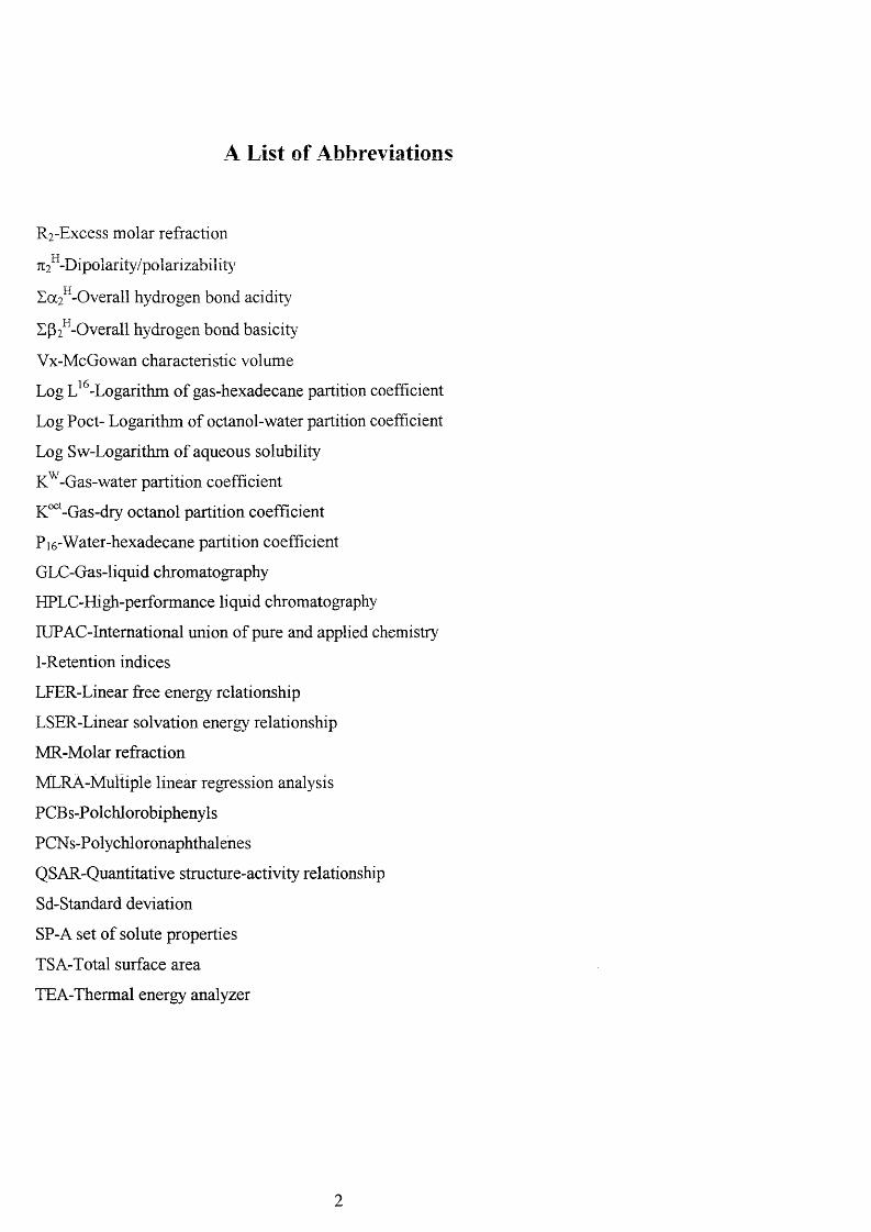
A List of Abbreviations
R2-Excess molar refraction
Tî2^-Dipolarity/polarizabilit>'
Sai^-Overall hydrogen bond acidity
I p 2^-0 verall hydrogen bond basicity
Vx-McGowan characteristic volume
Log ^-Logarithm of gas-hexadecane partition coefficient
Log Poet- Logarithm of octanol-water partition coefficient
Log Sw-Logarithm of aqueous solubility
-Gas-water partition coefficient
K°^ -Gas-dry octanol partition coefficient
P]6-Water-hexadecane partition coefficient
GLC-Gas-liquid chromatography
HPLC-High-performance liquid chromatography
lUPAC-Intemational union of pure and applied chemistry
1-Retention indices
LFER-Linear free energy relationship
LSER-Linear solvation energy relationship
MR-Molar refraction
MLRÀ-Muîtiple linear regression analysis
PCBs-Polchlorobiphenyls
PCNs-Polychloronaphthalenes
QSAR-Quantitative structure-activity relationship
Sd-Standard deviation
SP-A set of solute properties
TSA-Total surface area
TEA-Thermal energy analyzer
Table of Contents
Page no.
Abstract 1
Table of Contents 3
List of Tables 8
Ackn 0 wledgements 14
Introduction 15
Chapter 1 Introduction to Linear Free Energy Relationships
1.0 Introduction 24
1.1 The Solvation Process 27
1.2 The Solute 1:1 Hydrogen-Bond Scales, and 29
1.3 The Polarisability 31
1.4 Solute Dipolarity,/Polarisability Scale, 712^ 32
1.5 References 33
Chapter 2 Calculation of Descriptors by the Method of Abraham
2.0 Introduction 35
2.1 The Abraham Solvation Equation 35
2.1.1 The McGowan Characteristic Volume, Vx 38
2.1.2 The Excess Molar refraction, R2 39
2.1.3 The Solute Dipolarity/Polarisability, 712^ 40
3
2.1.4 The Solute Overall Hydrogen-Bond Scales, and E[32 42
2.2 Appiicati on of Abraham Solvation Equation 46
2.3 References 49
Chapter 3 Correlation Method
3.0 Correlation and Regression Analysis 52
3.1 Information Provided by Regression output 55
3.2 Conclusion 58
3.3 References 59
Chapter 4 Introduction to Polychlorobiphenyls (PCBs) and to Gas
Liquid Chromatography
4.0 Introduction 60
4.1 Chromatography 70
4.1.1 Introduction 70
4.1.2 Concepts of Reversed-Phase HPLC 71
4.1.3 The Retention Volume 73
4.2 Method for the Calculation of the Descriptors for PCBs 79
4.3 The Determination of Descriptors 80
4.4 Techniques Used to Calculate Partition Coefficients 81
4.5 References 83
Chapter 5 The First Calculation of the Descriptors for PCBs
5.0 Introduction 85
5.1 Estimation of the Excess Molar Refraction, R% 95
5.2 Estimation of Overall Hydrogen-Bond Basicity, for PCBs 101
4
5.3 The Calculation of log
5.4 The Calculation of the Solute Dipolarity/Polarisability Parameter, 712^
102
117
Chapter 6 The Second Calculation of Descriptor for PCBs
6.0 Introduction 133
6.1 The Calculation of Tp2^ values from Water-Octanol Partition Coefficients, 133
as log Poet
6.2 Adjustment of the Estimated Values 142
6.3 Individual Calculations for the PCBs 143
6.4 Re-examination of the Polar GLC Phases 145
6.5 References 146
Chapter 7 The Final (Third ) Calculation of Descriptors for PCBs
7.0 Introduction 147
7.1 Using Solver Program to get Final Values for (712^ , Sp2^ , log L ) 147
7.2 Re-calculation of the log Poet Equation from Data in Opperhuizen’s and
Sablijic’s Papers 154
7.3 Calculation of the Descriptors for the rest of the PCBs 159
7.4 Testing the Final Set of the Calculated Descriptors 171
7.5 Conclusions 187
7.6 References 188
Chapter 8 Comparison of Calculated and Observed Partition
PCBs
Coefficients for
8.0 Introduction 189
8.1 Theoretical Background 190
8.2 The Techniques Used to Measure log Poet 191
8.3 Results 192
8.3.1 The Fugacitymeter 193
8.4 Discussion of the Lqa Values 194
8.5 The Final Comparison for Water-Octanol Partition of PCBs 198
8.6 Discussion 204
8.7 References 205
Chapter 9 Calculation and Comparison of Aqueous Solubility for PCBs Using
the Obtained Descriptors
9.0 Introduction 209
9.1 Results 210
9.2 Discussion 229
9.3 References 231
Chapter 10 Discussion of the PCBs
10.0 The conformations of the PCBs 234
10.1 References 243
Chapter 11 Calculation of Descriptors for the Polychloronaphtbalene
11.0 Introduction 244
11.1 Methodolog)^ 246
11.2 Calculation of the Descriptors 248
11.3 Discussion 284
11.4 References 288
Chapter 12 Estimation of Some Physicochemical Properties for the
Polychloronaphthalenes
12.0 Methodology 291
12.1 References 298
Chapter 13 Calculation of the Descriptors for N-Nitrosodialkylamines
13.0 Introduction 299
13.1 Using the LFER to Calculate the Descriptors for
N-Nitrosodialkylamines 301
13.2 Methods for Characterization of Water-Solvent Systems 303
13.3 Characterization of Some New-Water-Solvent Systems 304
13.3.1 The Water-Tributylphosphate System 304
13.3.2 The Water-Bromobenzene System 308
13.3.3 The Water-Iodobenzene System 312
13.3.4 The Fourth System (Water-Diisopropylether) 316
13.4 The Calculation of Parameters for N-Nitrosodialkylamines 319
13.6 Conclusion 326
13.5 References 328
7

List of Tables
Chapter 2 Calculation of Descriptors by the Method of Abraham
Page no.
Table 2 .1. Atom contributions for calculation of Vx (in cm moT^) 39
Table 2.2. A comparison of and for some solutes 43
Table 2.3. A comparison of (3i and Z{32 values 44
Chapter 3 Correlation Method
Table 3.1. The regression output for tributylphosphate 56
Chapter 4 Introduction to polychlorobiphenyls (PCBs) and to gas
liquid chromatography
Table 4.1. Names of PCBs and alkanes, CAS No., lUPAC No. 62
and the PCBs No.
Chapter 5 The first calculation of the descriptors for PCBs
Table 5.1. Names of PCBs with retention indices of PCBs, on various 89
liquid phases in packed columns, at 200 c
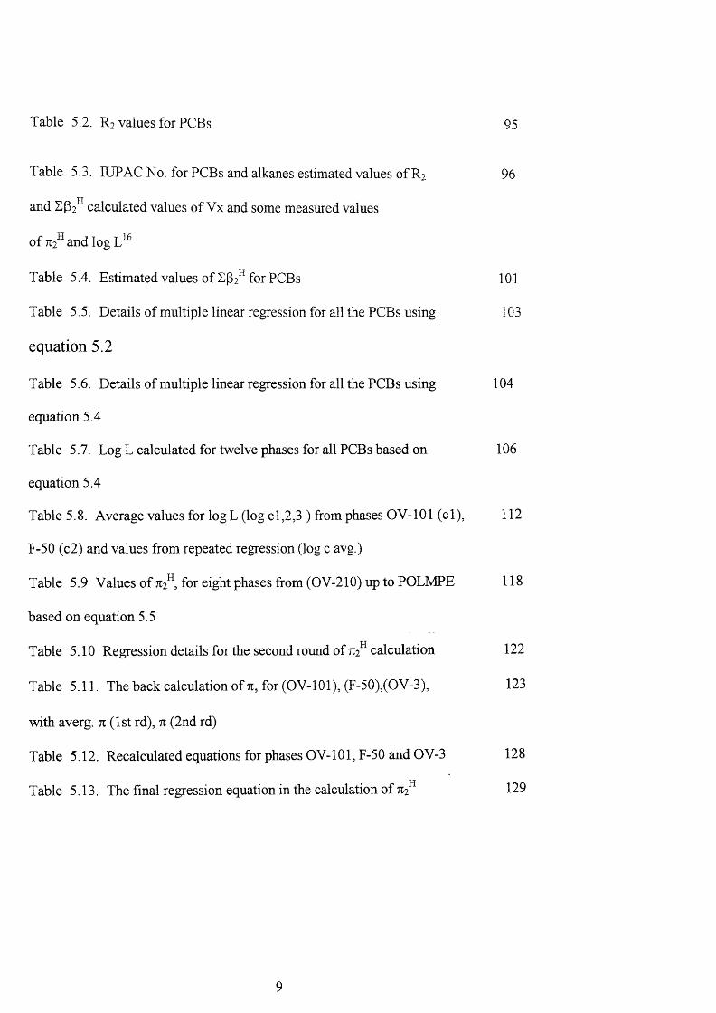
Table 5.2. R2 values for PCBs 9 5
Table 5.3. lUPAC No. for PCBs and alkanes estimated values of R2 96
and Z(32 calculated values of Vx and some measured values
of 712 and logL^^
Table 5.4. Estimated values of 1 (3 2^ for PCBs 101
Table 5.5. Details of multiple linear regression for all the PCBs using 103
equation 5.2
Table 5.6. Details of multiple linear regression for all the PCBs using 104
equation 5.4
Table 5.7. Log L calculated for twelve phases for all PCBs based on 106
equation 5.4
Table 5.8. Average values for log L (log cl,2,3 ) from phases OV-101 (cl), 112
F-50 (c2) and values from repeated regression (log c avg.)
Table 5.9 Values of 712^, for eight phases from (OV-210) up to POLMPE 118
based on equation 5.5
Table 5.10 Regression details for the second round of 712^ calculation 122
Table 5.11. The back calculation of 71, for (OV-101), (F-50),(OV-3), 123
with averg. 71 (1st rd), n (2nd rd)
Table 5.12. Recalculated equations for phases OV-101, F-50 and OV-3 128
Table 5.13. The final regression equation in the calculation of 712^ 129
Chapter 6 The second calculation of descriptors for PCBS
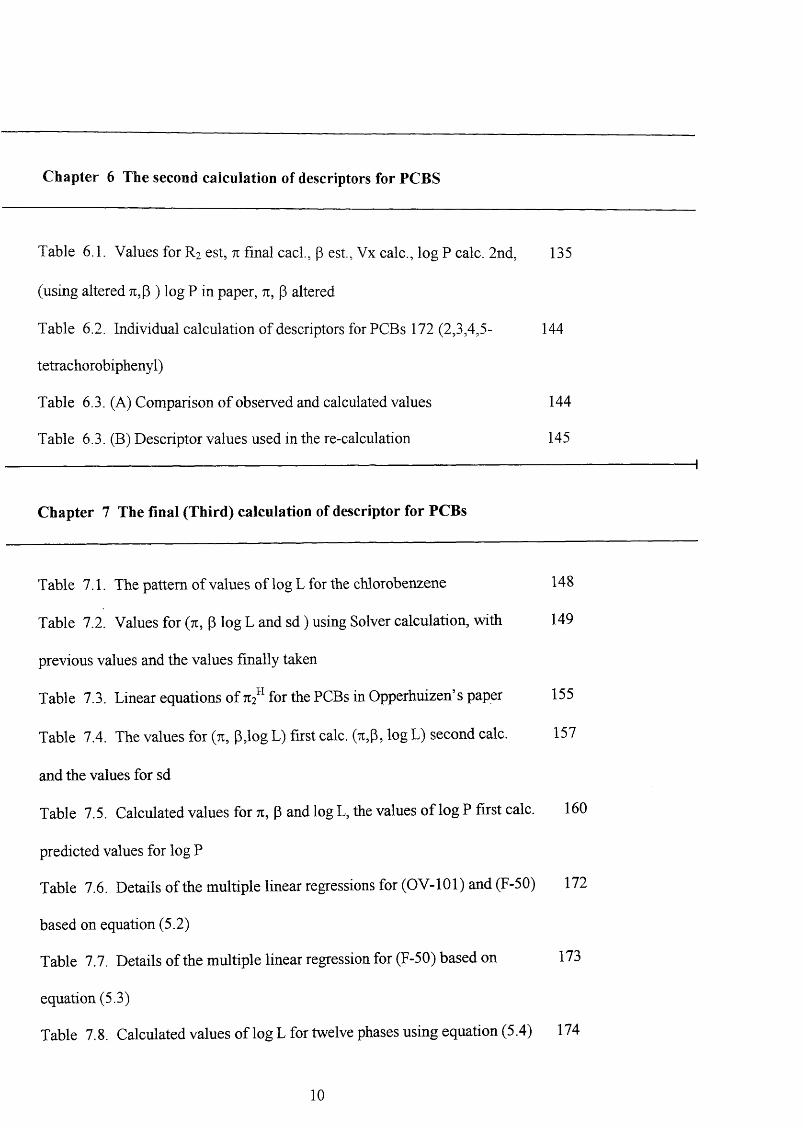
Table 6.1. Values for R2 est, n final cacL, p est., Vx calc., log P calc. 2nd, 135
(using altered 7i,P ) log P in paper, 71, p altered
Table 6.2. Individual calculation of descriptors for PCBs 172 (2,3,4,5- 144
tetrachorobiphenyl)
Table 6.3. (A) Comparison of observed and calculated values 144
Table 6.3. (B) Descriptor values used in the re-calculation 145- - I
Chapter 7 The final (Third) calculation of descriptor for PCBs
Table 7.1. The pattern of values of log L for the chlorobenzene 148
Table 7.2. Values for (%, p log L and sd ) using Solver calculation, with 149
previous values and the values finally taken
Table 7.3. Linear equations of7i2^ for the PCBs in Opperhuizen’s paper 155
Table 7.4. The values for (7 1 , P,log L) first calc. (7 1 ,P, log L) second calc. 157
and the values for sd
Table 7.5. Calculated values for tt, P and log L, the values of log P first calc. 160
predicted values for log P
Table 7.6. Details of the multiple linear regressions for (OV-101) and (F-50) 172
based on equation (5.2)
Table 7.7. Details of the multiple linear regression for (F-50) based on 173
equation (5.3)
Table 7.8. Calculated values of log L for twelve phases using equation (5.4) 174
10

Table 7.9. Details of the multiple linear regressions for all twelve phases 181
based on equation (5.4)
Table 7.10. lUPAC No. log L calc. For (OV-lOl, F-50, APLEZON) with
their average
182
Chapter 8 Comparison of calculated and observed partition coefficients
for PCBs
Table 8.1. PCBs their lUPAC no. log L exp and calc. Log L 192
Table 8.2. lUPAC no. exp. Log L calc. Log L and 196
our calc.log L
Table 8.3. Our calc. Values, with exp. and theoretical one 199
Table 8.4. lUPAC no., calc. Log Poet values from this work, and 200
observed log Poet values from the MedChem data base
Chapter 9 Calculation and Comparison of Aqueous Solubility for
PCBs Using the Obtained Descriptors
Table 9.1. Comparison of our calc. Log S (a), predicted log S (b ), with 216
exp. log S (c) and the values of the sd.
Table 9.2. Comparison of our calc, log S (a), predicted log S(b), 223
exp. log S(c) and the values of the sd.
Table 9. 3. Hydrogen-bond effects on solubility, as log Sw 229
11
Chapter 10 The Conformation of the PCBs
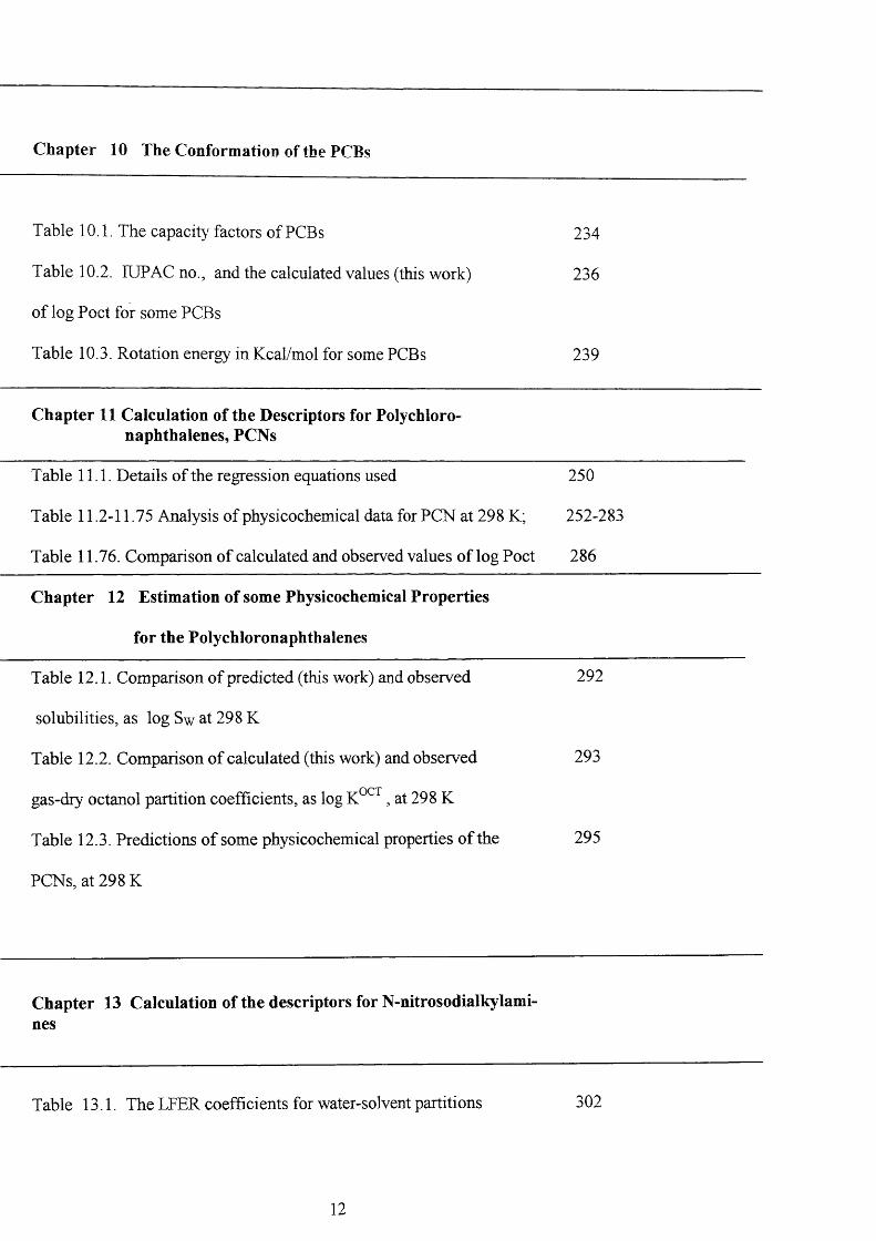
Table 10.1. The capacity factors of PCBs 234
Table 10.2. lUPAC no., and the calculated values (this work) 236
of log Poet for some PCBs
Table 10.3. Rotation energy in Kcal/mol for some PCBs 239
Chapter 11 Calculation of the Descriptors for Polychloronaphthalenes, PCNs
Table 11.1. Details of the regression equations used 250
Table 11.2-11.75 Analysis of physicochemical data for PCN at 298 K; 252-283
Table 11.76. Comparison of calculated and observed values of log Poet 286
Chapter 12 Estimation of some Physicochemical Properties
for the Polychloronaphthalenes
Table 12.1. Comparison of predicted (this work) and observed 292
solubilities, as log Sw at 298 K
Table 12.2. Comparison of calculated (this work) and observed 293
gas-dry octanol partition coefficients, as log , at 298 K
Table 12.3. Predictions of some physicochemical properties of the 295
PCNs, at 298 K
Chapter 13 Calculation of the descriptors for N-nitrosodialkylami- nes
Table 13.1. The LFER coefficients for water-solvent partitions
12
302
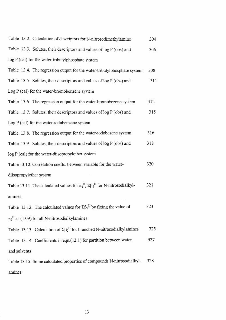
Table 13.2. Calculation of descriptors for N-nitrosodimeth^damine 304
Table 13.3. Solutes, their descriptors and values of log P (obs) and 306
log P (cal) for the water-tributylphosphate system
Table 13.4. The regression output for the water-tributylphosphate system 308
Table 13.5. Solutes, their descriptors and values of log P (obs) and 311
Log P (cal) for the water-bromobenzene system
Table 13.6. The regression output for the water-bromobezene system 312
Table 13.7. Solutes, their descriptors and values of log P (obs) and 315
Log P (cal) for the water-iodobenzene system
Table 13.8. The regression output for the water-iodobezene system 316
Table 13.9. Solutes, their descriptors and values of log P (obs) and 318
log P (cal) for the water-diisopropylether system
Table 13.10. Correlation coeffs. between variable for the water- 320
diisopropylether system
Table 13.11. The calculated values for 7i2 , for N-nitrosodialkyl- 321
amines
Table 13.12. The calculated values for E[32 by fixing the value of 323
712^ as (1.09) for all N-nitrosodialkylamines
Table 13.13. Calculation of 1(32 for branched N-nitrosodialkylamines 325
Table 13.14. Coefficients in eqn.( 13.1) for partition between water 327
and solvents
Table 13.15. Some calculated properties of compounds N-nitrosodialkyl- 328
amines
13
Acknowledgements
My deepest gratitude goes to my supemsor Dr. Michael H. Abraham whose
knowledge, wisdom, patience and kindness have been invaluable during my
postgraduate years and whose constant unequivocal guidance has allowed me to
complete this thesis. With utmost sincerity, I thank Dr. Michael Abraham.
I would also like to thank Professor Ridd for spending his valuable time to look
though my work.
It must be emphasized that the work presented in Chapter 9 had been developed from
Dr. Joell Le Prvease’s work. I am indebted to Joell for her selfless sharing.
I would also like to thank the teams of the past and present; Dr. Caroline Green, for
her advice when I was new to the area and for many other discussions on various
matters. Also, Dr. Julian Dixon for repairing my computer.
I would like to express my appreciation for all the staff in the Chemistry Department,
particularly Dr. Ian Cooper and Dr. Gordon Beck.
Finally, I acknowledge the invaluable contribution of my family, to whom this thesis
dedicated. I think my family for all the sacrifices, patience and encouragement which
have made university and ultimately the completion of this PhD possible.
14

Introduction
There are currently about 70000 organic compounds in commercial production, with
approximately 1000 being added every year. Roughly one third of all organic
compounds produced end up in the environment due to misuse, carelessness and
leaching, which in turn, can lead to environmental contamination. The presence of
pollutants in human beings, animals and plants, is causing a great deal of global
concern. Polychlorinated biphenyls (PCBs), polycyclic aromatic hydrocarbons
(PAHs), naphthalene, phenols and N-nitrosodialkylamines (NOCs) are among some
of the most hazardous and toxic of organic pollutants to enter the environment.^’"’
Figure 1. shows the structures of some common pollutants.
15

PCBs 54 PCBs 80
Cl Cl
V\
Cl Cl
Cl\
Cl
Cly
\Cl
PCBs 152 PCBs 65
Cl Cl Cl
HCl Cl
PCNs
Cl\ Cl
v\ /
\
Cl Clwf C v V / ^
Cl Cl
PCNs
Cl/
CH.
O N - N
CHs
Dimethylnitrosoamine
CH2-CH3
O N - N
CH2-CH3
Diethylnitrosoamine
Figure 1. The structure of some (PCBs), (PCNs) and (NOCs)
16

The polychlorinated biphenyls (PCBs) are a group of xenobiotic chemicals first
manufactured commercially in about 1930 and which were widely used as
transformer coolants, dielectric fluids, solvents, and flame retardants until restriction
on their use were introduced in the early 1970s. Some of the PCBs were thought to
be mobile in the environment and some were in landfill or equipment dumps. There
are 209 possible chlorinated biphenyls ranging from the monochlorobiphenyls to
decachlorobiphenyl. It is only recently that all 209 congeners have been individually
synthesized and characterized. ^
The polychloronaphthalenes (PCNs), of which most are toxic,^’ ’ have been
manufactured in the USA and in several other countries since the 1920s for use as
dielectric fluids and insulators. In addition, they are formed during the combustion
process in waste incineration. The characteristic properties of PCBs and PCNs are
hydrophobicity or low aqueous solubility, relatively low vapour pressure and
resistance to chemical reaction.^’ ’ ’ These properties result in persistence in the
environment and accumulation in soil, sediments, plankton, marine animals and all
the way through the food chain to humans.
The third type of toxic compound to be studied is the N-nitrosodialkylamines
which form a large class of genotoxic chemical carcinogens which occur in the human
diet and in foods and consumer products such as meat, " beer,^ cosm etics,infant
pacifiers,^^ and drug formulation.’ They can also formed endogenously in the human
body, especially tragastrically. Much interest is therefore directed toward quantitation
of various N-nitroso organic compounds (NOC) that occur in different matrices. Their
widespread prevalence can be attributed to the relative ease of formation and to the
abundance of their amine precursors in the environment. The occurrence of N-nitroso
17
compounds in the above products is of great concern, o\^nng to the carcinogenic
properties that many of them exhibit."
In order to evaluate the potential environmental behavior of the PCBs and other
compounds, a knowledge of their physicochemical characteristics is essential. A key
parameter in assessing the potential environmental behavior of such lipophilic
chemicals is the octanol-water partition coefficient, Poct.^° The determination of Poet
is recommended in the OECD chemical hazard evaluation program^ and it has been
used vdth considerable success in estimating bioconcentration factors, soil and
sediment uptake, toxicities and aqueous solubilities.^ ' A number of techniques have
been used to measure Poet values. The first was the shake-flask method. The second
were the measurements and estimates based upon reverse-phase high-performance
liquid chromatography (RP-HPLC) and thin-layer chromatography ( RP-TLC). These
have achieved moderate success for various groups of lipophilic compounds but
require the use of empirical correction factors in the case of PCBs. ' " Also reliable
and consistent Poet values for a number of PCB congeners have been obtained by the
generator column t e c h n iq u e .S om e success has been recently achieved in relating
log Poet to calculated molar volumes. The total surface area (TSA), which is a
function of molar volume, has been found to have linear relationship with log Poet for
compounds such as polyaromatic hydrocarbons, alkyl and halobenzenes.^^*^^
For a number of polychloronaphthalenes (PCNs) a few physicochemical
properties have been reported, including normal phase HPLC capacity factors," ’ RP-
HPLC capacity factors" and gas liquid chromatographic (GLC) retention data.
6,10,43.44.45 Water-octanol partition coefficients, as log Poet, have been determined for
a number of PCNs and values of log Poet can be estimated for all the 75 PNCs
through the CLOG P program."^^
18

For the detection of N-nitroso compounds the majority/ of the anal3^ical methods
had employed gas chromatography (GC) or liquid chromatography (LG) in
conjunction with a thermal energy analyzer (TEA)/^ which relies on the pyrolytic
breakdown of N-NO moieties to release the nitrosyl radical. The disadvantage of
these techniques, however, is that a subsequent confirmation is needed to ensure that
the method does not give rise to a false-positive response." A combination of LC and
mass spectrometry (LC-MS) offers significant anal}^ical advantages over the
aforementioned techniques. The two most coimnon ionization techniques available to
LC-MS, thermo spray (TSP) and electro spray ionization (ESI), yield primarily
molecular weight information, that is little fragmentation is observed to confirm the
structure of the analyze. Alternatively, on-line photolysis can be used to induce
photolytic dissociation of varying types of c o m p o u n d s . T h e s e techniques,
however, are often unreliable and can suffer from a significant loss in sensitivity,^^
and also there are many practical difficulties in the experimental determination of
these quantities for veiy lipophilic compounds. So resort is often had to some form of
estimation. It is the aim of this work to obtain from the available physicochemical
data, solvation descriptors for the PCBs, the PCNs and the NOCS that can then be
used to estimate all kinds of other physicochemical data and which will be of
considerable use in environmental analyses.
19
References
1. D. Macky, W. Shiu and K. Ma, Illustrated handbook of Physical-Chemical
Properties and Enviromnental Fat Organic Chemical-Pesticide Chemical,
1997, Vol. 5. Boca Raton; CRC Press.
2. C. D. S. Tomlin (ed). The Pesticide Manual, British Crop Protection Council,
Famham, 11^ edn., 1997.
3. E. Halfon, S. Galassi, R. Br uggemannn and A. Provini, Chemosphere, 1996,
Vol. 33, 1543.
4. Polychlorinated Biphenyls (National Academy of Sciences-National Research
Council, Washington, DC, 1979).
5. M. D. Mullin, C. M. Pochini, S. McCrindle, M. Romkes, S. Safe, and L. M.
Safe, Environ. Sci. Technol, 1984, Vol. 18,468.
6. K. Kannan, T. Imagaa, A. L. Blankenship and J. P. Giesy, Environ. Sci.
Technol., 1998, Vol. 32, 2507.
7. D. L. Villeneuve, K. Kannan, J. S. Khim, J. Falandysz, V. A. Nikiforov, A.
L.Blankenship and J. P. Giesy, Arch. Environ. Contam. Toxicol., 2000, Vol.
39, 273.
8. A. L. Blankenship, K. Kannan, S. A. Villalobos, D. L. Villleneuve, J.
Falandysz, T. Imagawa, E. Jakobsson and C. Rappe., Environ. Sci. Technol.,
2000, Vol. 35,3153.
9. H. Tausch and G. Stehlik, J. High Res. Chromatogr., 1985, Vol. 8, 524.
10. M. Schneider, L.Stieglitz, R. Will and G. Zwich, Chemosphere, 1998, Vol.
37, 2055.
11. M. Biziuk, A. Przyjazny, J. Czerwinski and M. Wiergo^vski, J. Chromatogr.
A., 1996, Vol. 754,103.
20
12. W. Y. Shiu and D. Mackay, J. Phys. Chem. Réf. Data, 1986, Vol. 15, 911.
13. G. S. Hartley and I. J. Graham-Bryce, Physical Principles of Pesticide
Behaviour, Academic Press, 1980, Vol. 2.
14. B. J. Canas, D. C. Havery, F. J. Jr. Joe, T. J. Fazio, Assoc. Off Anal. Chem.
1986, Vol. 69. 1020.
15. S. M. Billedeau, B. M. Miller, H. C. Thompson, J. Food Sci., 1988, Vol. 53,
1696.
16. S. M. Billedeau, T. M. Heinze, J. G. Wilkes, H. C. Thompson, J. Chromatogr.
A. 1994, Vol. 688, 55.
17. S. M. Billedeau, H. C. Thompson, B. M. Miller, M. I. Wind, J. Assoc. Off
Anal. Chem., 1986, Vol. 69, 31.
18. B. A. Dawson, R. C. Lawrence, J. Assoc. Off Anal. Chem. 1987, Vol. 70.
554.
19. P.N. Magee, R. Montesano, R. Preussman, In Chemical Carcinogens. Searle.
C.W.Ed. ACS Monograph Series 173. American Chemical Society
Washington. DC. 1976, Chapter 11.
20. D. W. Connell, G. Miller, J. Chemistry and Ecotoxicology of Pollution, Wiley
New York, 1984.
21. H. Watarai, M. Tanaka, N. Suzuki, Anal. Chem., 1982, Vol. 54, 702.
22. D. Mackay, Environ. Sci. Technol., 1982, Vol. 16, 274.
23. W. B. Neely, D. R. Bransin, G. E. Blau, Environ. Sci. Technol., 1974,Vol. 8,
1113.
24. S. W. Karickhoff, D. S. Brown, T. A. Scott, Water Res., 1979, Vol. 13, 241.
25. E. E. Kenaga, Ecotoxicol. Environ. Saf., 1980, Vol. 4, 26.
26. H. Konemann, Toxicolog, 1981, Vol. 19, 209.
21

27. C. T. Chiou, V. H. Freed, D. W. Schmedding, R. L. Kohnert, Environ. Sci.
Technol, 1977, Vol. 11,475.
28. C. T. Chiou, D. W. Schmedding, M. Mânes, Environ. Sci. Technol, 1982,
Vol. 16, 4.
29. R. A. Rapaport, S. Eisenreich, J. Environ. Sci. Technol, 1984,Vol. 18, 163.
30. M. T. Tulp, O. Hutzinger, Chemoshere, 1978, Vol. 10, 849.
31. G. D. Veith, N. M. Austin, R. T. Morris, Water Res., 1979, Vol. 13, 43.
32. H. Ellgehausen, C. D’Hondt, R. Fuerer, Pestic. Sci., 1981, Vol. 12, 219.
33. M. L. Coates, D. W. Connell, D. M. Barron, Environ. Sci. Technol, 1985,
Vol. 19, 628.
34. W. A. Bruggeman, J. Van der Steen, O. Hutzinger, J. Chromatogr., 1982, Vol.
238, 335.
35. M. M. Miller, S. Ghodbane, S. P. Wasik, Y. B. Tewari, D. E. Martire. J.
Chem. Eng. Data, 1984, Vol. 29,184.
36. K. B. Woodbum, W. J. Doucette, A. W. Andren, Environ. Sci. Technol, 1984,
Vol. 18,457.
37. L. B. Kier, In Physical Chemical Properties of Drugs, S. H. Yalkowsky, A. A.
Sinkula, S. C. Valvani,Eds, Medicinal Research Series, Dekker, New York,
1980, Vol. 10.
38. S. H. Yalkowsky, S. C. Valvani, J. Chem. Eng. Data., 1979, Vol. 24. 127.
39. S. H. Yalkowsky, R. J. Orr, S. C. Valvani, Ind. Eng. Chem. Fundam., 1979,
Vol. 18,351.
40. S. H. Yalkowsky, S. C. Valvani, J. Med. Chem., 1976, Vol. 19, 727.
41. U. A. Th Brinkman and G. de Vries, J. Chromatogr., 1979, Vol. 169,167.
42. A. Opperhuizen, Toxical. Environ. Chem., 1987, Vol. 15, 249.
22
43. J. Falandysz and C. Rappe, Chemosphere, 1997, Vol. 35, 1737.
44. J. Falandysz, M. Kawano, M. Uatsuda, K. Kannan, J. P. Giesy and T.
Wakimoto, J. Environ. Sci. Health, 2000, Vol A35, 281.
45. J. Olivero and K. Kannan, J. Chromatogr. A. 1999, Vol. 849, 621.
46. Y. D. Lei, F. Wania, W. Y. Shiu and D. G. B. Boocock, J. Chem. Eng. Data,
2000, Vol. 45,738.
47. A. J. Leo, MedChem 2000, The Medicinal Chemistry Project, Pomona
College, Claremont, CA 9171.
48. R. C. Massey, Nitrosoamines, 1988, 16.
49. J. M. Ballard, N. Grinberg, Proceedings of the 40 th ASMS Conference on
Mass Spectrometry and Allied Topics, American Society for Mass
Spectrometry , East Lansing , MI, 1992, 1256.
50. J. D. Laycock, R. A. Yost, Proceedings of the 41 1st ASMA Conference on
Mass Spectrometry and Allied Topics, American Society for Mass
Spectrometry, East Lansing, MI, 1993, 55.
51. K. G. Asano, G. J. Van Berkel, Proceedings of the 41 1st ASMA Conference
on Mass Spectrometry and Allied Topics, American Society for Mass
Spectrometry, East Lansing, Ml, 1993,1068a.
52. W. M. A. Niessen, Van der Greef, J. Liquid Chromatography-Mass
Spectrometry, Marcell-Dekker, Inc, New York, 1992, chapter 17.
23
Chapter 1 Introduction to Linear Free Energy Relationships
1.0 Introduction
Around 1900, Overton put forward his lipoid theory of aqueous anesthesia and
showed tliat the potency of compounds was related to their partition between water and
lipid-like phases such as olive oil. Overton and Meyer ' also showed for numerous series
of compound that the narcotic concentration, C, of aqueous solutes toward the tadpole
was related to their water- olive oil partition coefficient (P) with the latter defined as
P = (concentration in organic phase ) / ( concentration in water ) (1.1)
In 1920, K. H. Meyer and Gottlieb-Billroth expressed the Overton relationship in the
quantitative form,
C . P = constant (1-2)
This work represents the first quantitative structure-activity relationship ever reported.
Some years later, Meyer and Hemmi showed that water-oleyl alcohol partition
coefficients could be used in equation (1.2), again with narcotic concentrations of
aqueous solutes towards the tadpole. It is useful to examine equation (1.2) more closely.
The chemical potential of a species can be expressed as:
24
}i = }io + R T l n a (1.3)
Where p^is tlie chemical potential under a standard set of conditions and a is the acti\nt)
of the solute in solution; a is taken as C.f, where C is the concentration and f is the
activity coefficient. The latter approaches unity as C approaches zero. Thus through
equation (1.3), the concentration can be seen to be a free energy (in this context a Gibbs
free energy) quantity. A partition coefficient defined as in equation (1.1) is simply an
equilibrium constant, related to the standard Gibbs free energy change through,
AG°=-RTlnP° (1.4)
Hence equation (1.2) is an example of a linear fi-ee energy relationship, or LFER, and the
work of Meyer in the 1920s’ and 1930s’ represents some of the first examples of such a
relationship. Equation (1.2) can be expressed in logarithmic form as equation (1.5) or
more generally as equation (1.6) where SP can be a biological property such as 1/C for
tadpole narcosis, or can be a physicochemical property, such as another partition
coefficient.
Log (1/C) = log P + constant (1.5)
Log SP = a. logP + c (1.6)
25
Equation (1.6) was applied by Collander to the correlation of different types of partition
coefficients.
Log P2 = a. log P] + c (1.7)
He was very careful to point out that equation (1.7) applied only to partitions in similar
solvent systems, otherwise equation (1.7) was restricted to homologous series.
Equation (1.6) has been applied to numerous series of biological activities in aqueous
solution and is now referred to as the Overton-Meyer relationship, or sometimes the
Overton rule. Also the first quantitative analysis of gaseous narcosis was carried out by
K.H. Meyer in the same paper in which aqueous narcosis was discussed. A similar
relationship to equation (1.2) was found,
C . L = constant (1.8)
Here C, is the gaseous concentration of the narcotic, and L is the Ostwald solubility
coefficient of the narcotic in some particular solvent,
L = (concentration in solvent ) / (concentration in gas phase) (1.9)
This type of analysis is nowadays referred to as the Ferguson rule or relationship. It
should be pointed out that the Overton rule and the Ferguson rule apply only to non
26
reactive compounds. Another set of quantitative structure-activity relationsliips (QSARs)
has been constructed using the Hansch equation.
Log RBR = - a ( log Poct) + b log Poet + cE + d S + e (1.10)
Here RBR is a relative biological response of a series of substrates, or solutes, in a given
system. The descriptors are log Poet where Poet is the water /1-octanol partition coefficient,
E is an electronic parameter such as Hammets’ a value, and S is a steric term. Even today
equation (1.10) is still used to interpret and predict biological activities^ especially for a
series of structurally related compounds. There is however an insuperable difficulty in
the application of equation (1.10) when the substrate series includes quite different
structures, for example, aliphatic ketones, esters and alcohols, yet there are numerous
very important areas in which substrates of all kinds of structure are involved. This
problem can only be solved by the construction of other types of LFERs and QSARs.
1.1 The Solvation Process
To obtain other types of LFERs and QSARs, it seemed essential to start by devising
new solute descriptors. Since processes such as partitions, above, involve the solvation of
a compound in two phases, some model of the solvation process itself is needed. A
simple solvation model was used by Abraham, Kamlet and Taft (AKT).^’ The solvation
of a gaseous molecule was broken down into stages as follows.
27
Solute
Solvent
o <
o
Solute s
Solvent oo O Oo oo o o
Solute-solventcomplex
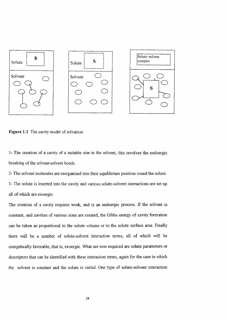
Figure 1.1 The cavity model of solvation
1- The creation of a cavity of a suitable size in the solvent, this involves the endoergic
breaking of the solvent-solvent bonds.
2- The solvent molecules are reorganized into their equilibrium position round the solute.
3- The solute is inserted into the cavity and various solute-solvent interactions are set up
all of which are exoergic.
The creation of a cavity requires work, and is an endoergic process. If the solvent is
constant, and cavities of various sizes are created, the Gibbs energy of cavity formation
can be taken as proportional to the solute volume or to the solute surface area. Finally
there will be a number of solute-solvent interaction terms, all of which will be
energetically favorable, that is, exoergic. What are now required are solute parameters or
descriptors that can be identified with these interaction terms, again for tlie case in which
the solvent is constant and the solute is varied. One type of solute-solvent interaction
28
which is important involves hydrogen-bonding of the type solute acid-solvent base,
and solute base-solvent acid.
1.2 The solute 1:1 hydrogen-bond scales, and
The original solute hydrogen - bond acidity scale, and basicity scale, Pi, of AKT
were not very rigorously def ined,^and other such scales were therefore constructed.
The 1:1 hydrogen bond acidity scale of Abraliam^ was formulated from log K where K
is the equilibrium constant for 1 ; 1 complexion of a series of monomeric acids against a
given reference base in an inert solvent, tetrachloromethane. Both the acid and the base
must be present at low concentration in order for both to be in solution as monomeric and
unassociated forms.
A-H + B = A-H— B
A scale of hydrogen-bond acidity was set up by plotting a series of log K values (against
a given reference base) vs log K values (against another reference base). The various
plots could be generalized through equation 1.11, where log Ka is an ‘average’
hydrogen-bond acidity constant. Plots according to equation 1.11 yielded straight lines,
with an intersection point at log K = -1.1 when K, is expressed on the molar
concentration scale.
Log K ( series of acids against base B ) = Lb .log K a + L>b (1.11)
29
In a similar way, a scale of 1:1 hydrogen-bond basicity, p2 , was established by Abraham
et al., with equation 1 . 1 2 taking tlie place of equation 1 .1 1 ,
Log K (series of bases against acid A) = La .log Kb + Da (1.12)
Tlie 1:1 hydrogen-bond basicit)/ scale was set up by plotting log K values of a series of
bases (against a given reference acid ) versus a series of bases (against another reference
acid ). These plots gave straight lines passing through the same magic point, log K = -1.1,
and enabled the average hydrogen-bond basicity, log Kb for solutes in CCI4 to be
obtained.
The log Ka and log Kb scales were transformed into more useful scales through the
simple equations,
tt2^ = (log Ka^+1.1) 74.636 (1.13)
P2^ = (log Kb^+1.1) 74.636 (1.14)
The factor 4.636 has no physical significance other than to serve as a convenient working
range of 2^ and a 2^ values.
30

1.3 The polarisabilt>'
The polarisability-coirection parameter, 8 2 , in the LFERs of AKT is only an
empirical factor, limited to one of three values; 1 . 0 for aromatic compounds, 0 . 5 for
halogenated aliphatic and 0.0 for all other compounds. A number of possible
replacements for 6 2 , were considered. The molar refraction (MR)^ was a possibility
because it is often used to measure polarisability; it can be defined in terms of the
McGowan volume as;
M R x = 1 0 [ ( n V i ) / ( n " + 2 ) ] V, (1.15)
Where n is the refractive index taken at 293 K with the sodium-D line, and is the
McGowan characteristic volume in ( cm mol ’ ) /lOO . Because of the volume term in
the molar refraction, equation (1.15), tliere is a strong connection between MR^ and V ,
so that it is not possible to incorporate MRx into a hnear equation together with Vx. The
refractive index function itself is an indication of the polarisable electrons in a molecule
that is either aromatic or a halogenated aliphatic compounds, and so some sort of molar
refraction would be a useful parameter. Abraham et al. therefore defined an ‘excess
molar refraction, as molar refraction in excess of the molar refraction^^ of an alkane of
the same characteristic volume as the solute in question,
R2 = MRx (obseiwed ) - MRx ( for alkane of the same V%) (116)
31

By definition R] = 0, for all alkanes, and by calculation R2 is also zero for branched chain
alkanes and for the rare gases as well. Like MR2 , R2 , is almost an additive quantity, and
can reasonably easily be estimated for solid compounds.
1.4 Solute dipolarity / polarisability scale, 71:2^
In the AKT system, 71*2 was taken to be identical to the Kamlet and Taft
solvatochromie parameter 7 1* 1 , for non-associated liquids. As 7t*i, can only be
experimentally obtained for compounds that are liquid at 298.15 K, values of 71*2 , had to
be estimated for all associated compounds (including acids, alcohol, phenols and amides)
as well as solids and gases. So, once again, it was necessary to set up a new scale instead
of the old AKT scale of solute dipolarity-polaiisability. Abraham et al. constructed the
new dipolarity-polaiisability parameter, 712^ for use in LSER from the extensive sets of
retention GLC data of McReynolds and Patte et al. ’
32
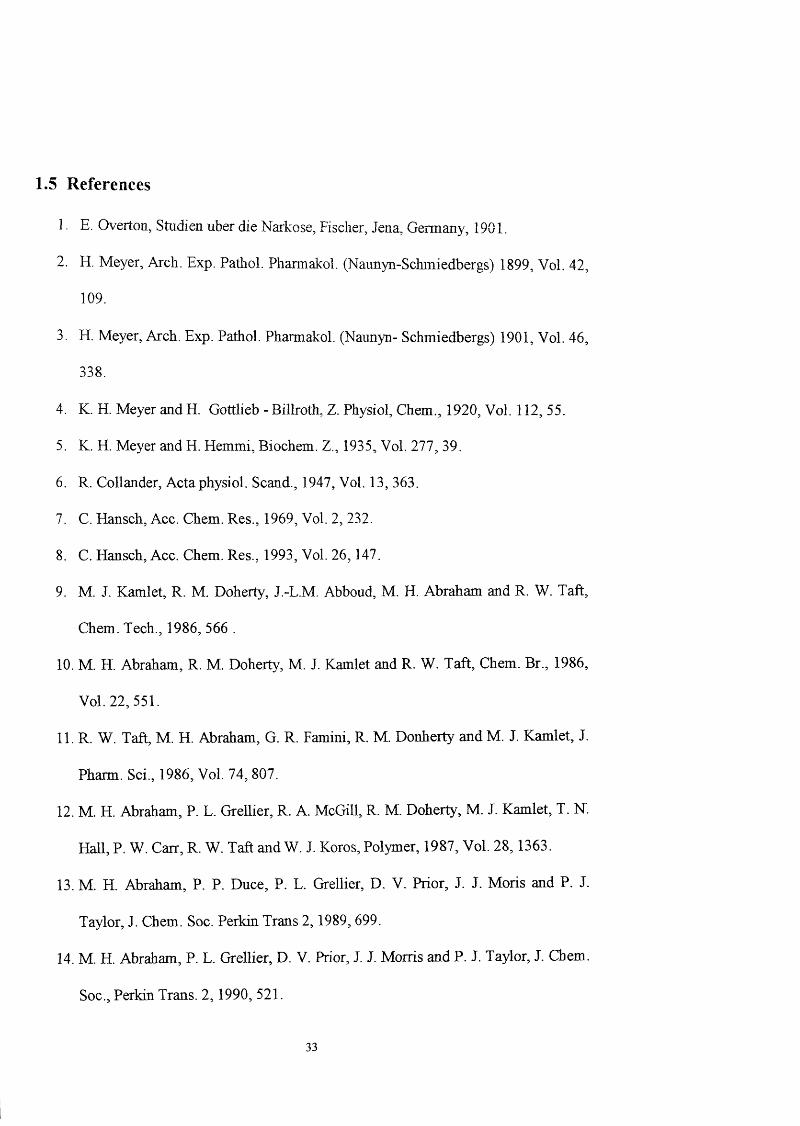
1.5 R eferen ce s
1. E. Overton, Studien uber die Narkose, Fischer, Jena, Germany, 1901.
2. H. Meyer, Aixh. Exp. Pathol. Phannakol. (Naimyn-Schmiedbergs) 1899, Vol. 42,
109.
3. H. Meyer, Arch. Exp. Pathol. Pharmakol. (Naunyn- Schmiedbergs) 1901, Vol. 46,
338.
4. K. H. Meyer and H. Gottlieb - Billroth, Z. Physiol, Chem., 1920, Vol. 112,55.
5. K. H. Meyer and H. Hemmi, Biochem. Z., 1935, Vol. 277, 39.
6 . R. Collander, Acta physiol. Scand., 1947, Vol. 13, 363.
7. C. Hansch, Ace. Chem. Res., 1969, Vol. 2, 232.
8 . C. Hansch, Acc. Chem. Res., 1993, Vol. 26,147.
9. M. J. Kamlet, R. M. Doherty, J.-L.M. Abboud, M. H. Abraham and R. W. Taft,
Chem. Tech., 1986, 566 .
10. M. H. Abraham, R. M. Doherty, M. J. Kamlet and R. W. Taft, Chem. Br., 1986,
Vol. 22, 551.
11. R. W. Taft, M. H. Abraham, G. R. Famini, R. M. Donlierty and M. J. Kamlet, J.
Pharm. Soi., 1986, Vol. 74,807.
12. M. H. Abraham, P. L. Grellier, R. A. McGill, R. M. Doherty, M. J. Kamlet, T. N.
Hall, P. W. Carr, R. W. Taft and W. J. Koros, Polymer, 1987, Vol. 28,1363.
13. M. H. Abraham, P. P. Duce, P. L. Grellier, D. V. Prior, J. J. Moris and P. J.
Taylor, J. Chem. Soc. Perkin Trans 2,1989,699.
14. M. H. Abraham, P. L. Grellier, D. V. Prior, J. J. Morris and P. J. Taylor, J. Chem.
Soc., Perkin Trans. 2,1990, 521.
33
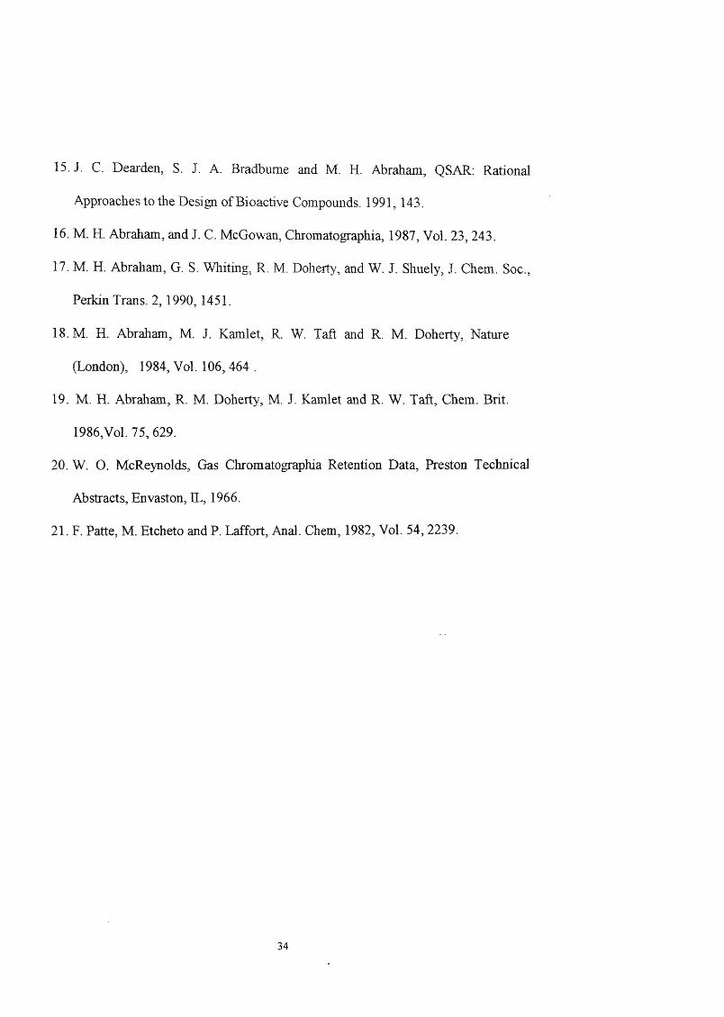
15. J. C. Dearden, S. J. A. Bradbume and M. H. Abraham, QSAR: Rational
Approaches to the Design of Bioactive Compounds. 1991, 143.
16. M. H. Abraham, and J. C. McGowan, Chromatographia, 1987, Vol. 23, 243.
17. M. H. Abraham, G. S. Whiting, R, M. Dohert , and W. J. Shuely, J. Chem. Soc.,
Perkin Trans. 2, 1990, 1451.
18. M. H. Abraliam, M. J. Kamlet, R. W. Taft and R. M. Doherty, Nature
(London), 1984, Vol. 106, 464 .
19. M. H. Abraham, R. M. Doherty, M. J. Kamlet and R. W. Taft, Chem. Brit.
1986,Vol. 75,629.
20. W. O. McReynolds, Gas Chromatographia Retention Data, Preston Technical
Abstracts, Envaston, DL, 1966.
21. F. Patte, M. Etcheto and P. Laffort, Anal. Chem, 1982, Vol. 54, 2239.
34

Chapter 2 Calculation of Descriptors by the Method of
Abraham
2.0 Introduction
Many studies have been carried out on relationships between chemical equilibrium
and rate constants for chemical reactions. Studies show that if a series of changes in
conditions or reactant structure affects the rate or equilibrium of the second reaction in
exactly the way it affected the first, there exists a linear free - energy relationship (LFER)
between the two set of data. These relationships are called linear free - energy because at
constant temperature the rate of reaction is related to the free energy of activation and the
equilibrium is related to the standard free energy change. If such relationships exist they
can be very useful in explaining the mechanism, and in the prediction of reaction rates
and chemical equilibria.’
As was noted in Chapter 1 the Hansch equation is one of the best known examples
of a LFER, and his work has formed a sound basis for many other studies to be carried
out involving LFERs. When applied to solvation processes, LFERs are sometimes
denoted as linear solvation energy relationships (LSERs).
2.1 The Abraham solvation equationThe Abraham solvation equation is based on a simple solvation model used by
Abraham, Kamlet and Tafr, ' (see Figure 1.1). As was outlined in the previous chapter,
both the cavity term and the solute-solvent interaction term will depend on the properties
35

of the solute and the solvent under consideration. Hence to describe these effects for the
general case of a number of solutes in a number of solvents, it is necessary to construct
an equation that includes the relevant properties of both the solutes and the solvents.
In die first case, a single solute undergoes dissolution into a series of solvents. In this
case the solute properties remain constant, and only the varying properties of the solvents
need to be considered. Abraham, Kamlet and Taft suggested that the solvent property
that could be related to the cavity effect was Hildebrands cohesive energy density 5
The solvent properties that describe the interaction term were polarisability, 7t*i, the
solvent hydrogen-bond acidity,a i and the solvent hydrogen-bond basicty, |3], where
subscript 1 denotes a solvent property. The various solvent properties or descriptors were
combined into a solvatochromatic equation;
SP = SPo + d. 5] + s. 7Ci + a. Oil + b. Pi + h.( Ô h ) i (2T)
Where SP is some property of a given solute in a series of solvents, and SPo is a constant.
The term d. 5] was introduced as a polarisability correction term.
In the second case, a series of solutes is investigated in a given solvent (or solvent
system) so that the solvent properties are constant, and it is now the solute properties that
vary. Abraham, Kamlet and Taft found that a similar equation to equation (2.1) could be
used,
SP - SPo + d. Ô2 + s.7t*2 + a. tt2 + b. p2 + m. V2 (2.2)
36
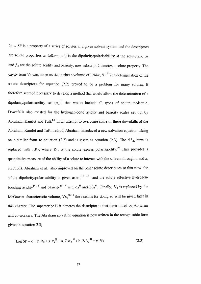
Now SP IS a propert}' of a series of solutes in a given solvent system and the descriptors
are solute properties as follows; 71*2 is the dipolarity/polarisability of the solute and Œ2
and p2 are the solute acidily and basicity; now subscript 2 denotes a solute property. The
cavity' tenn V2 was taken as the intrinsic volume of Leahy, Vi. The determination of the
solute descriptors for equation (2.2) proved to be a problem for many solutes. It
therefore seemed necessary' to develop a method that would allow the determination of a
dipolarity/polarisability scale,^^, that would include all types of solute molecule.
Downfalls also existed for tlie hydrogen-bond acidity and basicity scales set out by
Abraham, Kamlet and Taft.^’ In an attempt to overcome some of these downfalls of the
Abraham, Kamlet and Taft method, Abraham introduced a new solvation equation taking
on a similar form to equation (2.2) and is given as equation (2.3). The d.8 2 , term is
replaced with r.R2 , where R2 , is the solute excess polarisability.This provides a
quantitative measure of the ability of a solute to interact with the solvent through n and 71,
electrons. Abraham et al. also improved on the other solute descriptors so that now the
solute dipolarity/polarisability is given as 712^ and the solute effective hydrogen-
bonding ac id i t y^and basicity as E a 2^ and E{52 - Finally, V2 is replaced by the
McGowan characteristic volume, the reasons for doing so will be given later in
this chapter. The superscript H it denotes the descriptor is that determined by Abraham
and co-workers. The Abraham solvation equation is now written in the recognisable form
given in equation 2.3;
Log SP = c + r. R2 + s. 712 + a. I tt2 b. E P2 ^ + v. Vx (2.3)
37

This equation can be applied to the transport of solutes from one phase in to another,
where tlie equation coefficients c, r, s, a, b, and v describe the twm-phase system. The
new solute descriptors were determined by Abraliam et ah, using various experimental
and empirical metliods. Details of how they v/ere obtained are given below.
2.1.1 The McGowan characteristic volume, Vx
Leaiiy’s computer calculated intrinsic volume, Vi, was ratlier complicated to
evaluate, and so Abraham chose a more straight forward measure Vx (in cm mol ' V
1 0 0 ) 18,19 calculation of Vx, atom contributions are summed, and a ‘bond’ term is
then subtracted. All bonds are considered equal, so that a double bond such as C=C or
C= O or triple bond such as C = C is regarded as one bond. An algorithm proposed by
Abraham, allows the number of bonds in a molecule to be obtained simply.
B = N-1 + R (2.4)
Here B is the number of bonds, N is the total number of atoms and R is the total number
of ring structures. Therefore;
Vx = ( S atom contributions - ( 6.56 * B )) /100 (2.5)
Some typical values for atom contributions required for the calculation of Vx are given in
Table (2.1). The Vx descriptor models the (endoergic) cavity effect that arises through
38
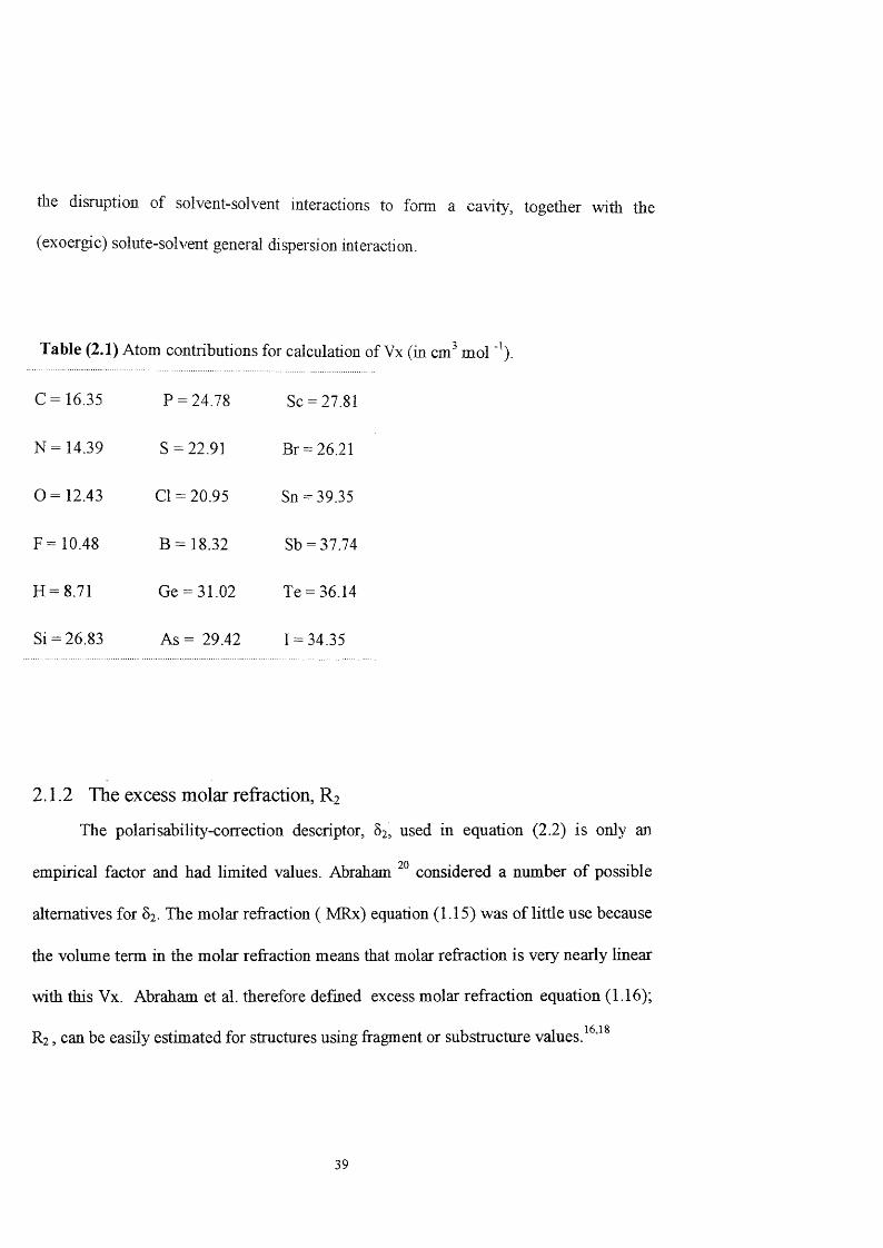
the disruption of solvent-solvent interactions to form a cavity, together with the
(exoergic) solute-solvent general dispersion interaction.
Table (2.1) Atom contributions for calculation of Vx (in cm mol
C= 16.35 P = 24.78 Sc = 27.81
N= 14.39 S = 22.91 Br = 26.21
0=12.43 01 = 20.95 Sn = 39.35
F = 10.48 B = 18.32 Sb = 37.74
H = 8.71 Ge = 31.02 Te = 36.14
Si = 26.83 As = 29.42 1 = 34.35
2.1.2 The excess molar refraction, R2
The polarisabilit)^-correction descriptor, 8 %, used in equation (2.2) is only an
empirical factor and had limited values. Abraham considered a number of possible
alternatives for 8 %. The molar refraction ( MRx) equation (1.15) was of little use because
the volume term in the molar refraction means that molar refraction is very nearly linear
with this Vx. Abraham et al. therefore defined excess molar refraction equation (1.16);
R2 , can be easily estimated for structures using fragment or substructure values.
39

2.1.3 The solute dipolarity/polarisability;
In order to obtain the new 712 parameter, use was made of gas chromatographic
specific retention volumes, Vg , that had been measured for several hundred solutes on
75 stationary' phases.^ The 75 phases contained no hydrogen bonding acidic groups, so a
simplified set of LEERs was used;
Log Vg = c + r.Ri + s. 7:2 * + a. E + 1. logL’ (2.6)
Here is the Oswald solubility coefficient, L on n-hexadecane at 298 K. Log L’ is
used instead of Vx as a cavity size descriptor for the dissolution of a gaseous solute into a
solvent. The solute parameters R2 , Ea2^, log L' and % were used in correlations to give
equation coefficients c, r, s, a and 1, for the 75 phases. The equation took the generalised
form;
Log Vg =Cn+ rn. R2 + s . + a . Sa2^ + In. log L (2.7)
The constant c was then subsumed into the dependent variable to give 75 equations;
Vn-] = rn-i .R i + Sn-1 .%* + Un-i .Ea2^ + L-i -log L (2.8)
Vn-75 = T^n-75 R z + 5 ^ - 7 5 ■' 2* + ^ 7 5 •2^ 2^ + In-75-log L (2.9)
Where
Vn=l0gV(M-Cn (2.10)
40
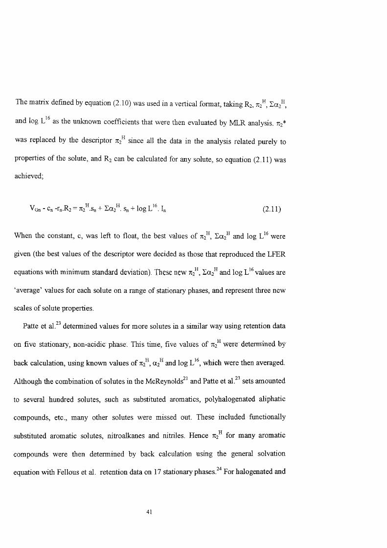
The matrix defined by equation (2.10) was used in a vertical format, taking R%, 712^, Za2 ,
and log as the unknown coefficients that were then evaluated by MLR analysis.
was replaced by the descriptor 712" since all the data in the analysis related purely to
properties of the solute, and R2 can be calculated for any solute, so equation (2.11) was
achieved;
Vgh - Cn -r .R] = 7T2 .Sd + Sn + log In (2.11)
When the constant, c, was left to float, tlie best values of 7 2^, Ea2^ and log were
given (the best values of the descriptor were decided as those that reproduced the LFER
equations with minimum standard deviation). These new 712^, Ea2^ and log L values are
‘average’ values for each solute on a range of stationary phases, and represent three new
scales of solute properties.
Patte et al. determined values for more solutes in a similar way using retention data
on five stationary, non-acidic phase. This time, five values of 7:2^ were determined by
back calculation, using known values of 7C2, and log which were then averaged.
Although the combination of solutes in the McReynolds^’ and Patte et al. sets amounted
to several hundred solutes, such as substituted aromatics, polyhalogenated aliphatic
compounds, etc., many other solutes were missed out. These included functionally
substituted aromatic solutes, nitroalkanes and nitriles. Hence 7:2^ for many aromatic
compounds were then determined by back calculation using the general solvation
equation with Fellous et al. retention data on 17 stationary phases. '’ For halogenated and
41
polyhalogenated aromatic solutes, 712^ values were obtained by Abraham et al/ ^ using
hie same method.
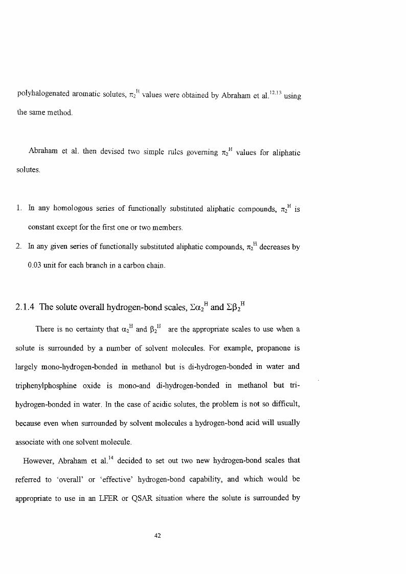
Abraham et al. then devised two simple rules governing 712^ values for aliphatic
solutes.
1. In any homologous series of functionally substituted aliphatic compounds, 712^ is
constant except for the first one or two members.
2. In any given series of functionally substituted aliphatic compounds, 712^ decreases by
0.03 unit for each branch in a carbon chain.
2.1.4 The solute overall hydrogen-bond scales, I a 2 and Ep2^
There is no certainty that and ^2^ are the appropriate scales to use when a
solute is surrounded by a number of solvent molecules. For example, propanone is
largely mono-hydrogen-bonded in mehianol but is di-hydrogen-bonded in water and
triphenylphosphine oxide is mono-and di-hydrogen-bonded in methanol but tri-
hydrogen-bonded in water. In the case of acidic solutes, the problem is not so difficult,
because even when surrounded by solvent molecules a hydrogen-bond acid will usually
associate with one solvent molecule.
However, Abraham et al. " decided to set out two new hydrogen-bond scales that
referred to 'overall’ or ‘effective’ hydrogen-bond capability, and which would be
appropriate to use in an LFER or QSAR situation where the solute is surrounded by
42
solvent molecules. These overall scales were labeled Ta2^ and They were both
derived from various equilibrium processes such as gas liquid cliromatography and
water-solvent partition. To obtain Ta2^ values a preliminary version of equation (2.3)
was set up using a 2^ as the hydrogen-bond acid descriptor and was applied to various
water-solvent paititions (SP in log SP is then the water-solvent partition coefficient).
The descriptor was then modified where necessary, in order to obtain the effective
value, Zcc2^. A new set of equations was then constructed, and the same process repeated
until a self-consistent set of equations and values was given. Since the solutes in the
water-solvent partitions are surrounded by solvent molecules, the overall hydrogen-bond
acidity scale is the actual scale required. It was observed that values of were
constant along any homologous series, except perhaps for the first one or two members,
so once a few values are established, values for the rest of the homologous series can be
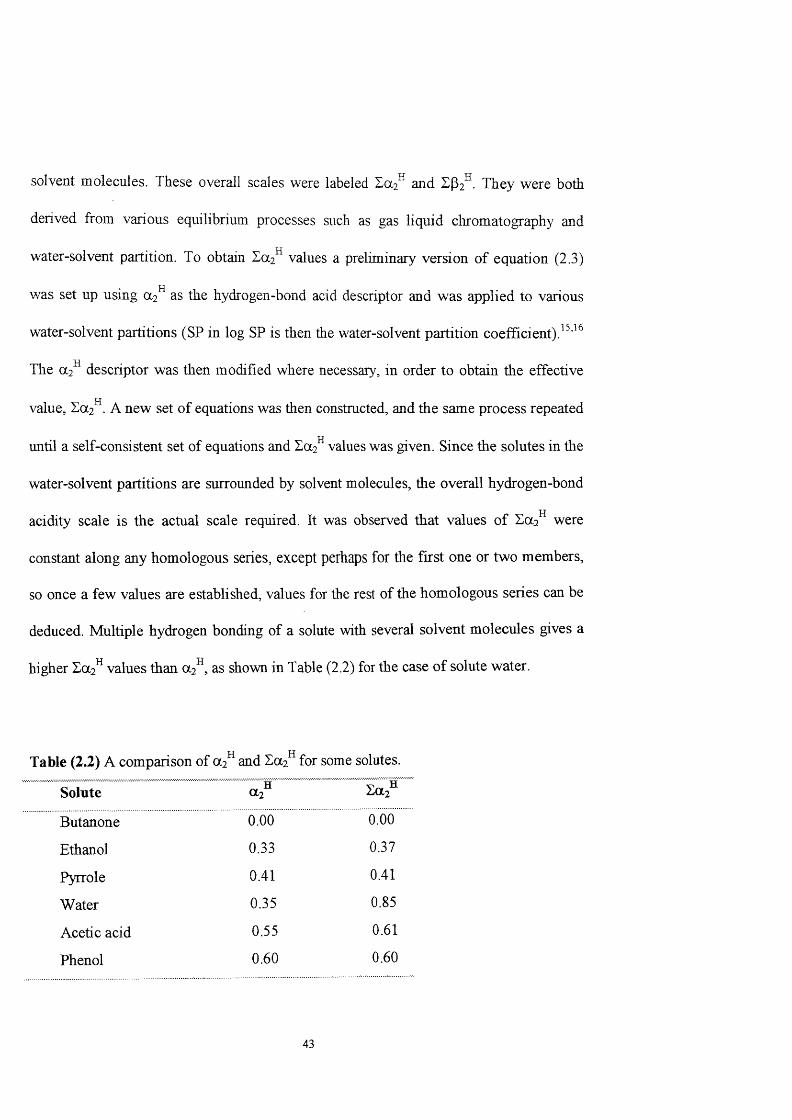
deduced. Multiple hydrogen bonding of a solute with several solvent molecules gives a
higlier values than as shown in Table (2.2) for the case of solute water.
Table (2.2) A comparison of and Sa2^ for some solutes.
Solute «2°
Butanone 0.00 0.00
Ethanol 0.33 0.37
Pyrrole 0.41 0.41
Water 0.35 0.85
Acetic acid 0.55 0.61
Phenol 0.60 0.60
43
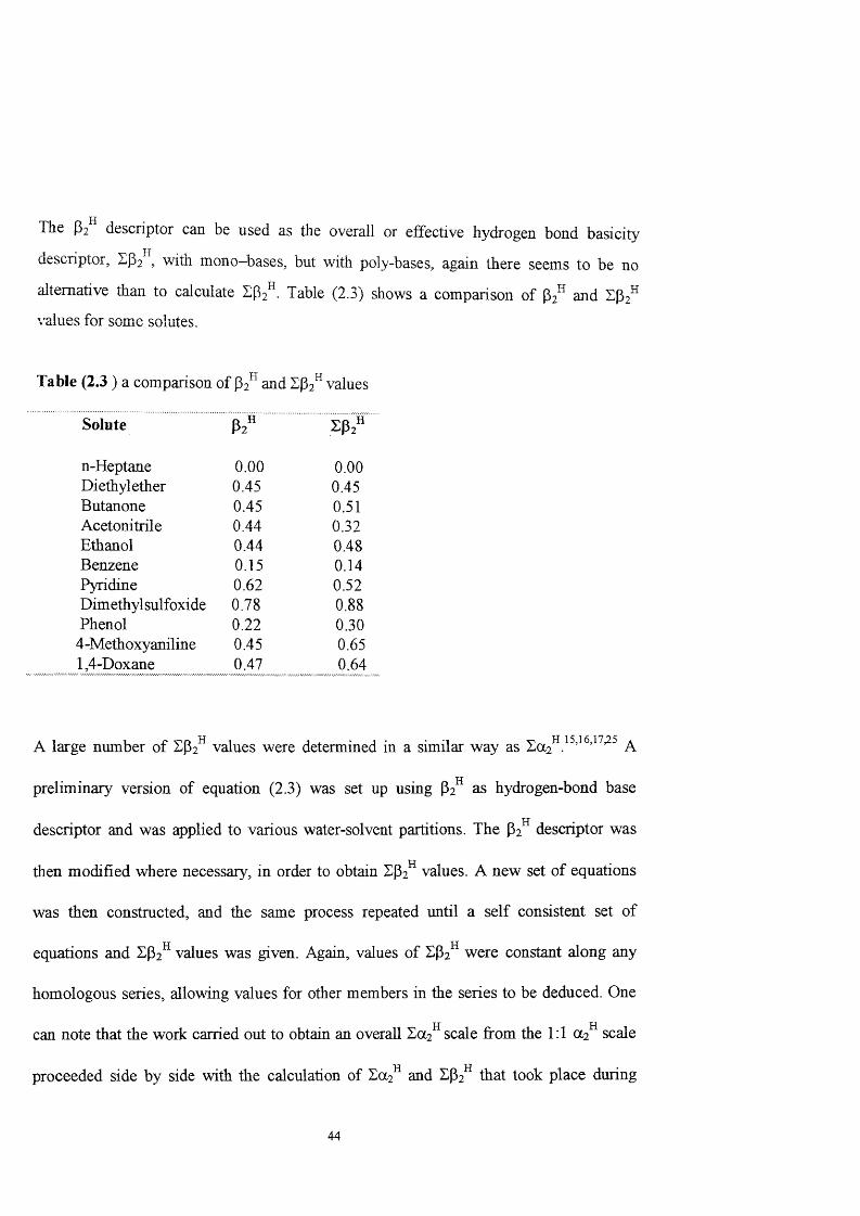
The p2 descriptor can be used as the overall or effective hydrogen bond basicity
aescriptor, z p2 , with mono—bases, but with poly-bases, again there seems to be no
alternative than to calculate Ep2 . Table (2.3) shows a comparison of and Sp2^ values for some solutes.
Table (2.3 ) a comparison of 2^ and ZP2" values
Solute
n-Heptane 0.00 0.00Diethyl ether 0.45 0.45Butanone 0.45 0.51Acetonitrile 0.44 0.32Ethanol 0.44 0.48Benzene 0.15 0.14Pyridine 0.62 0.52Dim ethyl sulfoxi de 0.78 0.88Phenol 0.22 0.304 -Methoxyanil ine 0.45 0.651,4-Doxane 0.47 0.64
A large number of IP 2 values were determined in a similar way as A
preliminary version of equation (2.3) was set up using p2^ as hydrogen-bond base
descriptor and was applied to various water-solvent partitions. The ^2^ descriptor was
then modified where necessary, in order to obtain Tp2^ values. A new set of equations
was then constructed, and the same process repeated until a self consistent set of
equations and ZP2^ values was given. Again, values of were constant along any
homologous series, allowing values for other members in the series to be deduced. One
can note that the work carried out to obtain an overall Za2^ scale from the 1:1 a 2^ scale
proceeded side by side with the calculation of Za2^ and Zp2^ that took place during
44
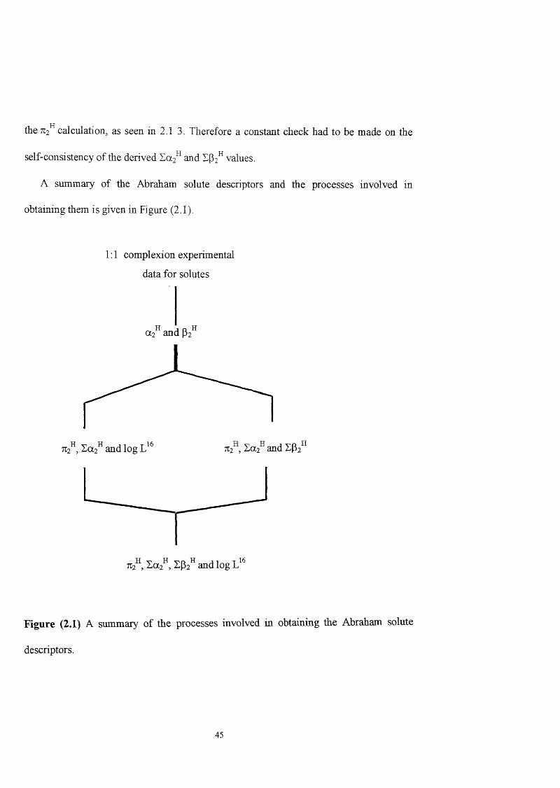
the 712 calculation, as seen in 2.1 3. Therefore a constant check had to be made on the
self-consistency of the derived and values.
A summary of the Abraham solute descriptors and the processes involved in
obtaining them is given in Figure (2.1).
1:1 complexion experimental
data for solutes
tt2^ and ^2^
1:2®, Sal'*, and log
Figure (2.1) A summary of the processes involved in obtaining the Abraham solute
descriptors.
45
Step 1 Equilibrium constants for 1:1 complexation of a series of acids (against a
reference base) and a series of bases (against a reference acid) used to set up new
hydrogen-bond acidity and basicity scales.
Step 2 Gas-liquid chromatography data used to develop a new dipolarity/polarisability
scale, log values and overall hydrogen-bond acidity scales, developed adjacently with
work carried out in step 3.
Step 3 Effective hydrogen-bond acidity and basicity scales developed form water-
solvent partition solvation equation; these values were constantly checked for consistency
with those obtained in step 2.
Step 4 The %2 , Ea2^, E(32 and log scales for solute are all checked for self-
consistency to confirm that solute descriptors can be obtained using either method (step 2
and 3).
2.2 Applications of Abraham Solvation Equation
The Abraham general solvation equation is summarized as follows;
Log SP = c + r. R2 + s. 712 + a. Ea2^ + b. 2^2^ + v. Vx (2.12)
Here SP is a property of a series of solutes in a given system, and the independent
variables are solute descriptors as follows: R2, is an excess molar refraction, 7T2 , is the
dipolarity/polarizability, and 1 ^2^ are tlie solute overall hydrogen-bond acidity and
basicity, Vx is the McGowan characteristic v o l u m e . O n e example of LFER is the
46
Abraham solvation equation which correlates a physical, chemical or biological property
(log SP) for a set of solutes wtli a corresponding set of solute physico-chemical property
descriptors (R2 , '^^2 and Vx). The equation coefficients (c, r, s, a, b and v)
obtained are dependent on the two-phase system under investigation and can be used to
predict or estimate further values of the independent variable for a completely new solute
providing the descriptors are known. In addition, the equation coefficients provide
information on the phase system. In case of the partition between two phases, they will
refer to differences in physico-chemical properties of the two phases. The r-coefbcient is
a measure of difference in phase polarisability and the s-coefficient is a measure of phase
dipolarity/polarisability difference. The a-coefficient measures the difference in the two
phases hydrogen-bond basicity (because an acidic solute will interact with a basic phase)
and the b-coefficient is a measure of how the phases differ in hydrogen-bond acidity. The
v-coefficient is a measure of how the hydrophobicity of the two phases differs.
The generality of the solvation equation is highlighted by the fact that it has been
applied to a very diverse range of processes. This equation has been employed for
processes that take place in condensed phases, such as water-solvent partition, * water-
micelle partition,^^ high performance liquid chromatography (HPLC),^* normal phase
hquid chromatography/^ microemulsion^^ and micellar^ electro-kinetic chromatography,
thin-layer chromatography,^^ solid phase extraction,^ blood-brain distribution, '^’ brain
perfusion, water -skin permeation and tadpole narcosis.A modified form of the
Abraham solvation equation can be used to calculate and predict the solubility of solids
and liquids in waterBecause the solvation equation is going to be used through this
47
work so it was necessary to discuss the general method behind the development of the
Abraham solvation equation in detail.
48
2.3 References
1. N. S. Isaacs, Physical Organic Chemistry - 2nd ed. Logman Scientific and Technical,
Harlow, 1995.
2. L. P. Hammett, J. Chem. Soc., 1937, Vol. 59, 96.
3. M. J. Hamlet, R. M. Doherty, J.-L.M. Abboud, M. H. Abraham and R. W. Taft, Chem.
Tech., 1986, 566.
4. M. H. Abraliam, R. M. Dohert} , M. J. Kami et and R. W. Taft, Chem. Br., 1986, Vol.
22,551.
5. M. J. Kamlet, R. M. Doherty, J-L. M. Abboud, M. H. Abraham and R. W. Taft, J.
Pharm. Sci., 1986, Vol. 75, 338.
6. M. J. Kamlet, R. M. Doherty, M. H. Abraham, P. W. Carr, R. F. Doherty and R. W.
Taft, J. Phys. Chem., 1987, Vol. 91,1996.
7. J. H. Hildebrand and R. L. Scott, The solubility of non-electrolytes, Dover Pub., New
York, 1964.
8. M. J. Kamlet, R. M. Doherty, M. H. Abraham and R. W. Taft, Quant. Struct. Act.
Relat., 1988,71.
9. D. E. Leahy, J. Pharm. Sci., 1986, Vol. 75, 629.
10. M. H. Abraham, G. S. Whiting, R. M. Doherty and W. J. Shuely, J. Chem. Soc.,
Perkin Trans 2, 1990,1451.
11. M. H. Abraham, G. S. Whiting, R. M. Doherty and W. J. Shuely, J. Chromatogr.,
1991, Vol. 587,213.
12. M. H. Abraham and G. S. Whiting, J. Chromatogr., 1992, Vol. 594, 229.
13. M. H. Abraham, J. Chromatogr., 1993, Vol. 644,95.
49

14. M. H. Abraham, P. L. Grellier, D. V. Prior, P. P. Duce, J. J. Morris and P. J. Taylor,
J. Chem. Soc. Perkin Trans. 2, 1989, 699.
15. M. H. Abraham and H. S. Chadha, Applications of a solvation equation to drug
transport properties, in Lipophilicity in Drug Action and Toxicolog}\ Ed. By V.
Pliska, B. Testa and H. van de Waterbeemd, VCH, Weinheim, Germany, 1996.
16. M. H. Abraham, Chem. Soc. Revs., 1993, Vol.22, 73.
17. M. H. Abraham, P. L. Grellier, D. V. Prior, J. Morris and P. J. Taylor, J. Chem. Soc.
Perkin Trans. 2,1990, 521.
18. J. C. McGowan, J. Appl. Chem. Biotechnol., 1984, Vol. 34A, 38.
19. M. H. Abraham and J. C. McGowan, Cbromatographia., 1987, Vol. 23, 243.
20. J. C. Dearden, S. J. A. Bradbume and M. H. Abraham, QSAR: Rational Approaches
to the Design of Bioactive Compounds, 1991,143.
21. W. O. McReynolds, Gas Chromatographic Retention Data, Preston Technical
Abstracts, Evanston, IE, 1966.
22. M. H. Abraham, P. L. Grellier and R. A. McGill, J. Chem. Soc. Perkin Trans 2,1987,
797.
23. F. Patte, M. Etcheto and P. Laffort, Anal. Chem., 1982, Vol. 54, 2239.
24. R. Fellous, L. Lizzani- Cuvelier and R. Luft, Anal. Chem. Acta., 1985, Vol. 174, 53.
25. M. H. Abraham, J. Phys. Org. Chem., 1993, Vol. 6, 660.
26. M. H. Abraham, H. S, Chadha, G. S. VTiiting and R. C. hhtchell, J. Pharm. Sci.,
1994, Vol. 83,1085.
27. M. H. Abraham, H. S. Chadha, J. P. Dixon, C. Treiner, J. Chem. Soc. Perkin Trans.
2, 1995,887.
50
28. M. H. Abraliam andM. Roses, J. Phys. Org., 1994.Vol. 7, 672.
29. F. Z. Oumada, M. Roses, E. Bosch and M. H. Abraliam, Anal. Chim. Acta., 1999,
382.301.
30. M. H. Abraham, C. Treiner, M. Roses, C. Rafols and Y. Ishihama, J. Chromatogr. A,
1996, AAd. 752,243.
31. S. K. Poole and C. F. Poole, Analyst., 1997, Vol 122, 267.
32. M. Fî. Abraham, C. F. Poole and S. K. Poole, J. Chromatogr. A, 1996, Vol. 749, 201.
33. D. S. Siebert, C. F. Poole andM. H. Abraham, Analyst., 1996, Vol. 121, 511.
34. M. H. Abraham, H. S. Chadha, and R. C. Mitchell, J. Phann. Sci., 1994, Vol. 83,
1257.
35. M. H. Abraham, H. S. Chadha, F. Martina, R. C. Mitchell, M. W. Bradbury and J. A.
Gratton, Pestic. Sci., 1999, Vol. 55, 78.
36. J. A. Gratton, M. H. Abraham, M. W. Bradbury and H. S. Chadha, J. Pharm.
Pharmacol., 1997, Vol. 49,1211.
37. M. H. Abraham, H. S. Chadha and R. C. Mitchell, J. Pharmacol., 1995, Vol. 47, 8.
38. M. H. Abraham and C. Rafols, J. Chem. Soc. Perkin Trans. 2, 1995,1843.
39. M. H. Abraham and J. Le, J. Pharm. Sci., 1999, Vol. 88, 868.
51
Chapter 3 Correlation Method
3.0 Correlation and regression analysis
The correlation method used in this work is that of multiple linear regression
analysis, MLRA. This is a common technique in statistics, and is an extension of the
simple regression of y against x. A set of y-values, the dependent variable, may be
linearly related to the independent variable x. A relationship between two variables is
shown, and if it is linear when y values are plotted against x values, then a straight
line can be drawn through the points, and the equation can be written as,
y = mx + c (3.1)
Here c - is the intercept on the y -axis and m - is the slope of the line. The x-variable
is the explanatory or independent variable. If there are scattered points in the plot,
then drawing a straight line may not be too obvious, and any line chosen will affect
the prediction of y values. In such a case, a method called least squares is often used
to decide the best straight line to choose. This is done by taking into account all the
deviations between observed and estimated values of the variable from the line,
squaring them and adding them up. The criterion of least squares is that the best line
is the one with the least sum of squared deviations. This can be drawn when one
variable is present, but starts to be complicated when the number of variables
increases, as in the case of the general solvation equation. In this case the calculation
is done by the use of computer.^
52
Correlation gives the association between the variables, but it is the regression that
uses the variables to help explain the variation in the dependent variable and thus
estimates the parameters of the model, provides a test of the validity of the model, and
the calculation of the confidence limits of the parameter. Since the correlation alone
can not measure the success of the relationship between the variables, other statistical
methods can be used, such as the standard deviation of the estimate, sd, the
correlation coefficient, r, and the F-statistic. Standard deviation is the square root of
the quantity (sum of squares of deviations of individual results from the mean, divided
by one less than the number of results in the set) and is given by:
Sd=[X(x,~x) V ( n - 1)]’' (3.2)
Standard deviation has the same units as the property being measured. It becomes a
more reliable expression of precision as (n) gets larger, so sd is a means of assessing
the reliability of an equation, and is also used in considering the significance of
deviant points. The sd measures the spread of a distribution around the mean. A low
sd value indicates a low spread, i.e. a good relationship, and a high sd value indicates
that the data set contains a high distribution of points from the mean, which is
unfavourable in MLRA. The correlation coefficient gives the measure of success of
the correlation of the dependent variable (y) against the independent variable (x). The
equation for the correlation coefficient which take into account the standard deviation
is:
r= [ l - sd^ (n -2) / yn]'^ (3.3)
53

Here y = 1, ( y -y ) /n and y is the mean, I y /n. The quantity is the variance
of the sample values of y. From this equation it can seen that as the sd-> 0, r ^ 1, ie.
The correlation get nearer to perfection, r is a measure of how closely the data set fits
the relationship given by the MLRA and can range from -1 through to 1. A value o f -1
or 1 indicates that the data set is explained by the correlation equation perfectly,
while a value of zero means there is no relationship between the data set and the
MLRA. A negative value of r - may be interpreted as a poor correlation by an
inexperienced eye so more often than not it is r - that is quoted in relation to multiple
linear regression, r has values of zero through to one and is basically an indicator of
how well the regression analysis explains the relationship among the variables. Now
though the correlation r, is often used, it is r , that is meaningful because it gives the
fraction of the variance of y which is explained by the regression equation. It is more
convenient to convert it to a percentage. Thus when r = 0.90 the regression equation
explains about 90 % of the variance. It is very important that the correlation
coefficient should be considered in relation to the number of data sets correlated.
Students’ t-test can be used to investigate the significance of the coefficient, and
assumes normal distribution of the errors. The t-test is set as a confidence limit,
usually at 90 % but can go up to 99 % depending on the accuracy of the test required.
In MLR analysis, the t-test is performed on each individual variable to test their
significance. Sometimes not all the variables are necessary and this would be
indicated by the level of significance. Another significant test, which is used in
MLRA is the F-statistic or the Fisher statistic. This test accounts for the number of
variables, v , present and the number of data point ( n). The value of the F-statistic
gives an indication of the quality of the regression, to determine whether the observed
54

relationship between the dependent and independent variables occurs by chance the
higher the value of F, the better is the regression.
L yii — V l j / ( 1 --r- )) / (3.4)
Here r, is the correlation coefficient, n, is the number of data points and v is the
degrees of freedom, which is (v -1), where v, is the number of variables. From the
equation, it can be seen that the main factors that contribute to the improvement of the
regression are n, and r, because as these two parameters increase, F increases. Once a
MLRA output has been obtained it is essential to measure how reliable the
relationship is, i.e. it is necessary to validate the model so any predicted values can be
obtained with accuracy and confidence. The main problem with MLR is its sensitivity
to collinearities among the independent variables. Collinearities occur when there is a
high degree of linear correlation between two or more of the independent variables. It
is therefore very important to make sure the variables used in MLR, i.e. the solute
descriptors in the case of the Abraham Solvation Equation, are well defined and
independent. To use MLRA the number of data points is important, as this improves
the reliability of the correlation. It has been suggested that at least five data points are
required per variable, but this seems to be the very minimum that should be used.
3.1 Information provided by the regression output
The significance of an interaction tenn can be identified by the magnitude of the
coefficients and also by the Students’ t-test at 95%. As an example is given the output
for the solvation equation of water-tributylphosphate which was obtained from the
55
value of the partition coefficient for a series of compounds. Log P ^ alues for a series
of 50 solutes were obtained from the Med Chem data base (Table 3.1)
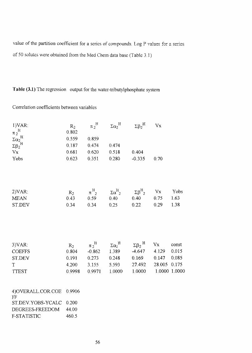
Table (3.1) The regression output for the water-tributylphosphate system
Correlation coefficients between variables
1)VAR: R2 Hn2 Vx
0.8020.559 0.8590.187 0.474 0.474
Vx 0.681 0.620 0.518 0.404Yobs 0.623 0.351 0.280 -0.335 0.70
2)VAR: R2 H2 Za^2 z A Vx Yobs
MEAN 0.43 0.59 0.40 0.40 0.75 1.63ST.DEV 0.34 0.34 0.25 0.22 0.29 1.38
3)VAR: R2 H712 Vx const
COEFFS 0.804 -0.862 1.389 -4.647 4.129 0.015ST.DEV 0.191 0.273 0.248 0.169 0.147 0.085T 4.200 3.155 5.593 27.492 28.005 0.175TTEST 0.9998 0.9971 1.0000 1.0000 1.0000 1.0000
4)0VERALL.C0R.C0E 0.9906 FFST.DEV.YOBS-YCALC 0.200 DEGREES-FREEDOM 44.00 F-STATISTIC 460.5
56
The infoniiation can be divided in to four sections.
1- The first infonnation given is the correlation coefficient between variables, this
shows how the variable is correlated due to the importance of multicollinearity. If
there is a high correlation then a high coefficient between the variables is shown.
The correlation of Yobs against each solute descriptors is also shown.
2 - The next section gives information of the set of solute descriptor itself, in terms of
the mean of the parameter coefficients and the spread of the parameters. For a set of
solutes a large standard deviation is favourable as this shows a diversity of the
descriptor, thus a more general equation is obtained.
3 - Section 3 shows the coefficients of the solvent system, the constants c, r, s, a, b
and V . Also the standard deviation of these coefficients are given, this is important
when back calculation of the descriptors are called for. If the values of the t-tests are
above 0.95 this means that the coefficients are statistically significant.
4 - The last section gives the overall view of the regression output. The quality of the
regression is indicated by the correlation coefficient, r; this depends somewhat on the
type of the system studied, (for example in solid adsorbent, r = 0.95 is generally
accepted). The best regression is indicated by the smallest value of the standard
deviation (Yobs -Ycalc). The F-statistic indicates the quality of the correlation and
thus shows a goodness of fit, F-statistic improves as the number of the data set
increases and the sd decreases.
57
3.2 Conclusion
According to the infonnation in these two chapters (2, 3), one could say it has
been possible to devise a set of solute descriptors. These descriptors, particularly the
effective or overall hydrogen-bond acidity and basicity, can be used to construct
LFERs and QSARs. Also two general equations have been formulated, one that is
more useful for gas-condensed phase processes, and one that is better for processes
within condensed phases. Comparing the two equations the descriptors in both are the
same, except for the size parameter log and . The two equations (LFERs and
QSARs) have been applied to a wide variety of solubility-related processes, and
generally give good results. The r-coefficient shows the tendency of the phase to
interact with solutes through n- and n-electron pairs. Usually the r-constant is
positive, but for phases that contain fluorine atoms, the r-constant can be negative.
The s-coefficient gives the tendency of the phase to interact with dipolar/polarizable
solutes, the a-coefficient denotes the hydrogen-bond basicity of the phase (because
acidic solutes will interact with a basic phase), and the b-coefficient is a measure of
the hydrogen-bond acidity of the phase (because basic solutes will interact with acidic
phase). It is important to note that for gas - phase processes, the s, a, and b-constants
must always be positive (or zero), because interaction between the phase and a solute
will increase the solubility of a gaseous solute. Equation (2.12) provides a new
method for the characterization of GLC stationary phases. There is a need for much
more work to be done to improve and increase the applicability of the two general
equations because in both equations there is no descriptor related to solute shape.
58

3.3 References1. D. L. Massait, B. G. M. Vandeginste, S. N. Deming, Y. Michotte and L.
Kaufman, Chemometrics text book, 1988, Elsevier, Amsterdam.
2. B. F. Ryan, B. L. Joiner, T. A. Ryan Jr., Minitab Handbook, 2nd Edition 1985.
59
Chapter 4 Introduction to Polychlorobiphenyls (PCBs) and to Gas Liquid Chromatography
4.0 Introduction
Technical polychlorobiphenyls (PCBs) constitute a group of chlorin-substituted
biphenyl compounds; each commercial product is assigned a code number indicating the
chlorine content or number of substituted chlorine atoms of the predominant PCBs
present. Moreover, highly toxic by products (such as polychlorinated dibenzofurans)
coexist in technical products and the content of such byproducts may vary according to
the mode of synthesis.
The polychlorinated biphenyls, or PCBs, are a group of xenobiotic chemicals first
manufactured commercially in the 1930’s and which were widely used as transformer
coolants, dielectric fluids, solvents, and flame retardant until restrictions on their use
were introduced in the early 1970’s.' Of the approximately 570 000 000 Kg sold in the U.
S as of 1975, some 68 000 000 Kg were estimated to be mobile in the environment and
some 130 000 000 Kg were in landfills or some equipment dumps. There are 209
possible chlorinated biphenyls ranging from the three monochlorobiphenyls to
decachlorobiphenyl. It is only recently^ that all 209 congers have been individually
synthesized and characterized. The characteristic properties of the PCBs are
hydrophobicity or lipophilicity (i e. large octanol-water partition coefficient and low
aqueous solubility), relatively low vapour pressure, and extreme resistance to chemical
60

reactions/ These properties result in persistence in the environment, a tendency to
accumulate in biota and in sediments, and the ability to be transported tlirougli tlie
atmosphere to regions remote from source discharges/ for example, appreciable
concentrations are found in the soils, sediments, waters, biota atmosphere, and
precipitation in the Great Lakes Basin/ The biological and human health effects of
PCBs, have been reviewed recently/ PCBs, and various chlorinated organic pesticides
are known to induce drug- metabolizing enzymes in the liver, and potent inducers such as
DDT, dieldrin heptachlor, etc. are known to act additively with PCBs. Present levels of
these compounds in human adipose tissues vary widely from locality to locality, and at
worst surpass the 20 ppm level. The possibility exists therefore that such levels could
lead to abnormal enzyme introduction in the liver resulting in accelerated breakdown of
essential hormones and other important biological substances. Indeed, the reduction in
population of certain fish-eating species has been attributed to this cause.
However, in man, it has yet to be established that such effects could result from
present environmental contamination. Another possible effect of environmental PCBs, is
liver damage. In certain parts of Japan, U.S.A. and W. Germany, mothers’ milk has been
shown to contain more than 0.06 ppm PCBs, which gives rise to considerable concern.
PCBs have similar structural functionalities, and so gas- liquid cliromatography (GLC) is
often be used to separated them. The tt 2^ parameter could possibly be obtained from gas-
liquid chromatographic measurements, so it was useful to give some detail about
chromatography, in this chapter.
In Table (4.1) are listed all 209 PCBs together with their CAS numbers, their lUPAC
number (the individual polychlorinated are identified by numbers according to tlie
61

International Union of Pure and Applied Chemistry (lUPAC))/ and the substitution in
tlie two rings. These are referred to as ring A and ring B.
Table (4.1) Names of PCBs and alkanes, CAS No., lUPAC No. and the PCB No.
CAS Name lUPAC
Ring A Ring B PCI
92-52-42051-60-7
Biphenyl2-Monochloro 1 2
NONENONE
12
13029-08-8 2,2’-Dichloro 4 2 2 3
2051-61-8 3-Monochloro 2 3 NONE 4
25569-80-6 2,3'-Dichloro 6 3 2 5
2050-67-1 3,3'-Dichloro 11 3 3 6
2051-62-9 4-Monochloro 3 4 NONE 7
34883-43-7 2,4'-Dichloro 8 4 2 8
2974-90-5 3,4-Dichloro 13 4 3 9
2050-68-2 4,4-Diehl oro 15 4 4 10
33146-45-1 2,6-Dichloro 10 2,6 NONE 11
38444-73-4 2,2’,6-Trichloro 19 2,6 2 12
38444-76-7 2,3'6-Trichloro 27 2,6 3 13
38444-77-8 2,4’,6-Trichloro 32 2,6 4 14
15968-05-5 2,2’,6,6'-Tetrachloro 54 2,6 2,6 15
34883-39-1 2,5-Diehl oro 9 2,5 NONE 16
37680-65-2 2,2',5-Triehloro 18 2,5 2 17
38444-81-4 2,3',5-Triehloro 26 2,5 3 18
16606-02-3 2,4',5-Triehloro 31 2,5 4 19
41454-41-9 2,2',5,6'-T etraehloro 53 2,5 2,6 20
35693-99-3 2,2’,5,5’-Tetraehloro 52 2,5 2,5 21
33284-50-3 2,4-Diehloro 7 2,4 NONE 22
62
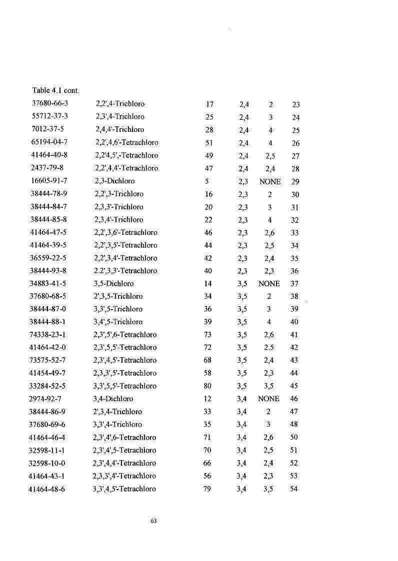
Table 4.1 cont. 37680-66-3 2,2',4-Trichloro 17 2,4 2 2355712-37-3 2,3',4-Trichloro 25 2,4 3 247012-37-5 2,4,4'-Trichloro 28 2,4 4 2565194-04-7 2,2',4,6'-T etrachl oro 51 2,4 4 2641464-40-8 2,2 '4,5',-T etrachl oro 49 2,4 2,5 272437-79-8 2,2',4,4'-Tetracliloro 47 2,4 2,4 2816605-91-7 2,3-Dichloro 5 2,3 NONE 2938444-78-9 2,2',3-Trichloro 16 2,3 2 3038444-84-7 2,3,3'-Trichloro 20 2,3 3 3138444-85-8 2,3,4'-Trichloro 22 2,3 4 3241464-47-5 2,2',3,6'-Tetrachloro 46 2,3 2,6 3341464-39-5 2,2’,3,5'-Tetrachloro 44 2,3 2,5 3436559-22-5 2,2’,3,4'-Tetrachloro 42 2,3 2,4 3538444-93-8 2.2’,3,3'-Tetrachloro 40 2,3 2,3 3634883-41-5 3,5-Dichloro 14 3,5 NONE 3737680-68-5 2',3,5-Trichloro 34 3,5 2 3838444-87-0 3,3',5-Trichloro 36 3,5 3 3938444-88-1 3,4’,5-Trichloro 39 3,5 4 4074338-23-1 2,3',5',6-Tetrachloro 73 3,5 2,6 4141464-42-0 2,3’,5,5’-Tetracliloro 72 3,5 2.5 4273575-52-7 2,3',4,5'-Tetrachloro 68 3,5 2,4 4341454-49-7 2,3,3\5'-Tetrachloro 58 3,5 2,3 44
33284-52-5 3,3',5,5'-Tetrachloro 80 3,5 3,5 452974-92-7 3,4-Dichloro 12 3,4 NONE 46
38444-86-9 2',3,4-Trichloro 33 3,4 2 47
37680-69-6 3,3’,4-Trichloro 35 3,4 3 48
41464-46-4 2,3’,4',6-Tetrachloro 71 3,4 2,6 50
32598-11-1 2,3',4',5-Tetracliloro 70 3,4 2,5 51
32598-10-0 2,3',4,4-Tetrachloro 66 3,4 2,4 52
41464-43-1 2,3,3’,4'-T etracliloro 56 3,4 2,3 53
41464-48-6 3,3',4,5-Tetrachloro 79 3,4 3,5 54
63
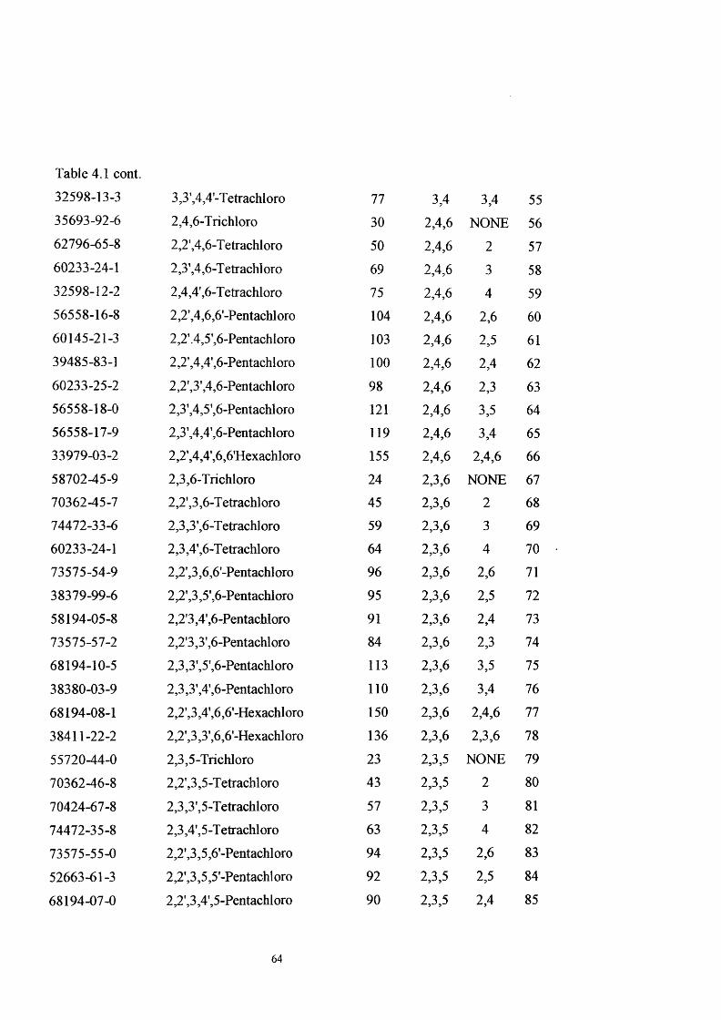
Table 4.1 cont. 32598-13-3 3,3 ',4,4'-T etraehloro 77 3,4 3,4 5535693-92-6 2,4,6-Trichloro 30 2,4,6 NONE 5662796-65-8 2,2',4,6-Tetrachloro 50 2,4,6 2 5760233-24-1 2,3',4,6-Tetrachloro 69 2,4,6 3 5832598-12-2 2,4,4',6-T etraehloro 75 2,4,6 4 5956558-16-8 2,2’,4,6,6'-Pentaehloro 104 2,4,6 2,6 6060145-21-3 2,2’.4,5',6-Pentaehloro 103 2,4,6 2,5 6139485-83-1 2,2’,4,4',6-Pentaehloro 100 2,4,6 2,4 6260233-25-2 2,2',3',4,6-Pentaehloro 98 2,4,6 2,3 6356558-18-0 2,3’,4,5',6-Pentaehloro 121 2,4,6 3,5 6456558-17-9 2,3',4,4',6-Pentaehloro 119 2,4,6 3,4 6533979-03-2 2,2’,4,4’,6,6’Hexaehloro 155 2,4,6 2,4,6 6658702-45-9 2,3,6-Triehloro 24 2,3,6 NONE 6770362-45-7 2,2',3,6-Tetraehloro 45 2,3,6 2 6874472-33-6 2,3,3',6-Tetraehloro 59 2,3,6 3 6960233-24-1 2,3,4’,6-T etraehloro 64 2,3,6 4 7073575-54-9 2,2',3,6,6'-Pentachl oro 96 2,3,6 2,6 7138379-99-6 2,2',3,5',6-Pentaehloro 95 2,3,6 2,5 7258194-05-8 2,2'3,4',6-Pentaehloro 91 2,3,6 2,4 7373575-57-2 2,2'3,3',6-Pentaehloro 84 2,3,6 2,3 7468194-10-5 2,3,3',5’,6-Pentaehloro 113 2,3,6 3,5 7538380-03-9 2,3,3',4',6-Pentaehloro 110 2,3,6 3,4 76
68194-08-1 2,2',3,4',6,6'-Hexaehloro 150 2,3,6 2,4,6 77
38411-22-2 2,2’,3,3',6,6'-Hexaehloro 136 2,3,6 2,3,6 78
55720-44-0 2,3,5-Triehloro 23 2,3,5 NONE 79
70362-46-8 2,2',3,5 -T etraehloro 43 2,3,5 2 80
70424-67-8 2,3,3',5-Tetraehloro 57 2,3,5 3 81
74472-35-8 2,3,4',5-Tetraehloro 63 2,3,5 4 82
73575-55-0 2,2’,3,5,6’-Pentaehloro 94 2,3,5 2,6 83
52663-61-3 2,2’,3,5,5'-Pentaehloro 92 2,3,5 2,5 84
68194-07-0 2,2',3,4',5-Pentaehloro 90 2,3,5 2,4 85
64

Table 4.1 cont. 60145-20-2 2,2',3,3',5-Pentachloro 83 2,3,5 2,3 8639635-32-0 2,3,3 ’,5,5 '-Pentaclil oro 111 2,3,5 3,5 8770424-68-9 2,3,3 ',4', 5 -Pentachl oro 107 2,3,5 3,4 8874472-42-7 2,2',3,4',5,6'-Hexachloro 148 2,3,5 2,4,6 8952744-13-5 2,2',3,3',5,6'-Hexachloro 135 2,3,5 2,3,6 9035694-04-3 2,2',3,3',5,5',-Hexachoro 133 2,3,5 2,3,5 9115862-07-4 2,4,5,-Trichloro 29 2,4,5 NONE 9270362-47-9 2,2’,4,5-T etraehloro 48 2,4,5 2 9373575-53-8 2,3',4,5-Tetrachloro 67 2,4,5 3 9432690-93-0 2,4,4',5-T etrachl oro 74 2,4,5 4 9568194-06-9 2,2',4,5,6'-Pentachloro 102 2,4,5 2,6 9637680-73-2 2,2’,4,5,5'-Pentachl oro 101 2,4,5 2,5 9738380-01-7 2,2',4,4',5-Pentachloro 99 2,4,5 2,4 9841464-51-1 2,2',3',4,5-Pentachloro 97 2,4,5 2,3 9968194-12-7 2,3',4,5,5'-Pentachloro 120 2,4,5 3,5 10031508-00-6 2,3',4,4',5-Pentachloro 118 2,4,5 3,4 10160145-22-4 2,2',4,4',5,6'-Hexachloro 154 2,4,5 2,4,6 102038380-04-0 2,2',3,4',5’,6-Hexachloro 149 2,4,5 2,3,6 10351908-16-8 2,2',3,4'.5,5'-Hexachloro 146 2,4,5 2,3,5 104
35065-27-1 2,2 ’ ,4,4 ’ ,5,5-Hexachl oro 153 2,4,5 2,4,5 10552663-59-9 2,2’,3,4-T etraehloro 41 2,3,4 2 107
74338-24-2 2,3,3',4-T etraehloro 55 2,3,4 3 108
33025-41-1 2,3,4,4'-T etraehloro 60 2,3,4 4 109
73575-57-2 2,2’,3,4,6'-Pentaehloro 89 2,3,4 2,6 110
38380-02-8 2,2',3,4,5'-Pentaehloro 87 2,3,4 2,5 11165510-45-4 2,2'3,4,4'-Pentaehloro 85 2,3,4 2,4 112
52663-62-4 2,2',3,3’,4-Pentaehloro 82 2,3,4 2,3 113
70362-41-3 2,3,3',4,5'-Pentaehloro 108 2,3,4 3,5 114
32598-14-4 2,3,3',4,4'-Pentaehloro 105 2,3,4 3,4 115
59291-64-4 2,2’,3,4,4',6'-Hexaehl oro 140 2,3,4 2,4,6 116
65
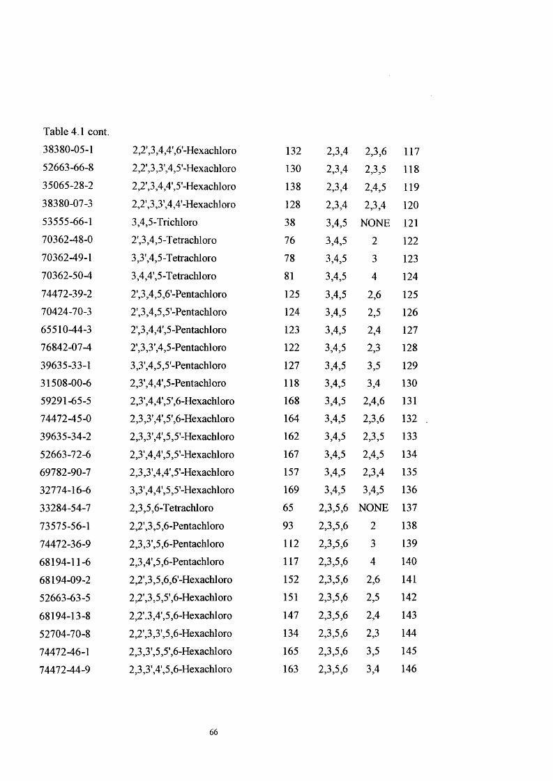
Table 4.1 cont. 38380-05-1 2,2',3,4,4',6'-Hexachloro 132 2,3,4 2,3,6 11752663-66-8 2,2',3,3',4,5'-Hexachloro 130 2,3,4 2,3,5 11835065-28-2 2,2', 3,4,4', 5 -Hexachl oro 138 2,3,4 2,4,5 11938380-07-3 2,2',3,3',4,4'-Hexachloro 128 2,3,4 2,3,4 12053555-66-1 3,4,5-Trichloro 38 3,4,5 NONE 12170362-48-0 2',3,4,5-Tetrachloro 76 3,4,5 2 12270362-49-1 3,3 ’,4,5 -Tetrachl oro 78 3,4,5 3 12370362-50-4 3,4,4',5-Tetrachloro 81 3,4,5 4 12474472-39-2 2',3,4,5,6'-Pentachloro 125 3,4,5 2,6 12570424-70-3 2',3,4,5,5'-Pentachl oro 124 3,4,5 2,5 12665510-44-3 2',3,4,4',5-Pentachloro 123 3,4,5 2,4 12776842-07-4 2’,3,3',4,5-Pentachloro 122 3,4,5 2,3 12839635-33-1 3,3',4,5,5'-Pentachloro 127 3,4,5 3,5 12931508-00-6 2,3',4,4',5-Pentachloro 118 3,4,5 3,4 13059291-65-5 2,3',4,4',5',6-Hexachloro 168 3,4,5 2,4,6 13174472^5-0 2,3,3',4',5',6-Hexachloro 164 3,4,5 2,3,6 13239635-34-2 2,3,3',4',5,5'-Hexachloro 162 3,4,5 2,3,5 13352663-72-6 2,3’,4,4',5,5'-Hexachloro 167 3,4,5 2,4,5 13469782-90-7 2,3,3 ',4,4',5'-Hexachloro 157 3,4,5 2,3,4 13532774-16-6 3,3',4,4',5,5'-Hexachloro 169 3,4,5 3,4,5 136
33284-54-7 2,3,5,6-Tetrachloro 65 2,3,5,6 NONE 137
73575-56-1 2,2',3,5,6-Pentachloro 93 2,3,5,6 2 138
74472-36-9 2,3,3',5,6-Pentachloro 112 2,3,5,6 3 139
68194-11-6 2,3,4',5,6-Pentachl oro 117 2,3,5,6 4 140
68194-09-2 2,2',3,5,6,6'-Hexachloro 152 2,3,5,6 2,6 141
52663-63-5 2,2',3,5,5’,6-Hexachloro 151 2,3,5,6 2,5 142
68194-13-8 2,2'.3,4',5,6-Hexachloro 147 2,3,5,6 2,4 143
52704-70-8 2,2',3,3',5,6-Hexachloro 134 2,3,5,6 2,3 144
74472-46-1 2,3,3',5,5’,6-Hexachloro 165 2,3,5,6 3,5 145
74472-44-9 2,3,3',4',5,6-Hexachl oro 163 2,3,5,6 3,4 146
66
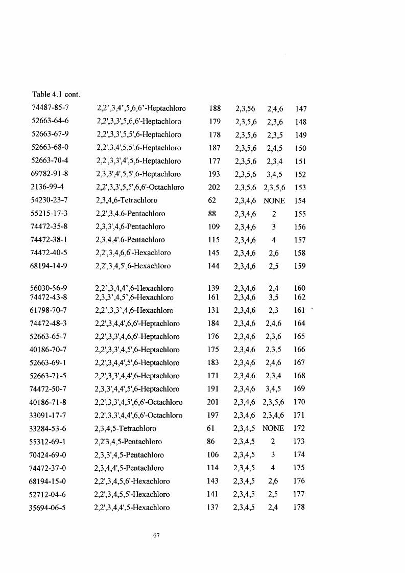
Table 4.1 cont. 74487-85-7 2,2 ’ ,3,4 ’ ,5,6,6 ’ -Heptachloro 188 2,3,56 2,4,6 14752663-64-6 2,2',3,3',5,6,6'-Heptachloro 179 2,3,5,6 2,3,6 14852663-67-9 2,2',3,3',5,5',6-Heptachloro 178 2,3,5,6 2,3,5 14952663-68-0 2,2',3,4',5,5',6-Heptachloro 187 2,3,5,6 2,4,5 15052663-70-4 2,2',3,3',4',5,6-Heptachloro 177 2,3,5,6 2,3,4 15169782-91-8 2,3,3',4',5,5',6-Heptachloro 193 2,3,5,6 3,4,5 1522136-99-4 2,2',3,3’,5,5',6,6'-Octachloro 202 2,3,5,6 2,3,5,6 15354230-23-7 2,3,4,6-Tetrachloro 62 2,3,4,6 NONE 15455215-17-3 2,2’,3,4.6-Pentachloro 88 2,3,4,6 2 15574472-35-8 2,3,3',4,6-Pentachloro 109 2,3,4,6 3 15674472-38-1 2,3,4,4' .6-Pentachloro 115 2,3,4,6 4 15774472^0-5 2,2',3,4,6,6'-Hexachloro 145 2,3,4,6 2,6 15868194-14-9 2,2',3,4,5',6-Hexachloro 144 2,3,4,6 2,5 159
56030-56-9 2,2 ’ ,3,4,4’ ,6-Hexachloro 139 2,3,4,6 2,4 16074472-43-8 2,3,3’,4,5’,6-Hexachl oro 161 2,3,4,6 3,5 16261798-70-7 2,2 ’ ,3,3 ’ ,4,6-Hexacliloro 131 2,3,4,6 2,3 16174472-48-3 2,2',3,4,4',6,6-Heptachloro 184 2,3,4,6 2,4,6 16452663-65-7 2,2',3,3',4,6,6-Heptachloro 176 2,3,4,6 2,3,6 16540186-70-7 2,2',3,3',4,5’,6-Heptachloro 175 2,3,4,6 2,3,5 16652663-69-1 2,2',3,4,4’,5',6-Heptacliloro 183 2,3,4,6 2,4,6 16752663-71-5 2,2',3,3',4,4',6-Heptachloro 171 2,3,4,6 2,3,4 16874472-50-7 2,3,3',4,4’,5',6-Heptachloro 191 2,3,4,6 3,4,5 169
40186-71-8 2,2’,3,3',4,5’,6,6'-Octacliloro 201 2,3,4,6 2,3,5,6 17033091-17-7 2,2',3,3',4,4',6,6’-Octachloro 197 2,3,4,6 2,3,4,6 171
33284-53-6 2,3,4,5-Tetrachloro 61 2,3,4,5 NONE 172
55312-69-1 2,2’3,4,5-Pentachloro 86 2,3,4,5 2 173
70424-69-0 2,3,3’,4,5-Pentachloro 106 2,3,4,5 3 174
74472-37-0 2,3,4,4',5-Pentacliloro 114 2,3,4,5 4 175
68194-15-0 2,2',3,4,5,6’-Hexachloro 143 2,3,4,5 2,6 176
52712-04-6 2,2',3,4,5,5'-Hexachloro 141 2,3,4,5 2,5 177
35694-06-5 2,2 ',3,4,4',5 -Hexachloro 137 2,3,4,5 2,4 178
67

Table 4.1 cont. 55215-18-14 2,2’,3,3’,4,5,-Hexachloro 129 2,3,4,5, 2,3 17939635-35-3 2,3,3',4,5,5'-Hexachloro 159 2,3,4,5 3,5 18038380-08-4 2,3,3 ',4,4’, 5 -Hexachloro 156 2,3,4,5 3,4 18160145-23-5 2,2’,3,4,4',5,6'-Heptachloro 182 2,3,4,5 2,4,6 18238411-25-5 2,2',3,3',4,5,6'-Heptachloro 174 2,3,4,5 2,3,6 18352663-74-8 2,2',3,3',4,5,5'-Heptachloro 172 2,3,4,5 2,3,5 18435065-29-3 2,2’,3,4,4',5,5'-Heptachloro 180 2,3,4,5 2,4,5 18535065-30-6 2,2’,3,3',4,4',5-Heptachloro 170 2,3,4,5 2,3,4 18639635-31-9 2,3,3',4,4',5,5'-Heptachloro 189 2,3,4,5 3,4,5 18752663-75-9 2,2',3,3',4,5,5',6'-Octachloro 199 2,3,4,5 2,3,5,6 18842740-50-1 2,2 ',3,3 ',4,4',5,6'-Octachloro 196 2,3,4,5 2,3,4,6 18935694-08-7 2,2',3,3',4,4’,5,5’-Octachloro 194 2,3,4,5 2,3,4,5 19018259-05-7 2,3,4,5,6-Pentachloro 116 2,3,4,5,6 NONE 19141411-61-4 2,2’,3,4,5,6-Hexachloro 142 2,3,4,5,6 2 19241411-62-5 2,3,3’,4,5,6-Hexachloro 160 2,3,4,5,6 3 19341411-63-6 2,3,4,4’,5,6-Hexachloro 166 2,3,4,5,6 4 19474472-49-4 2,2',3,4,5,6,6'-Heptachloro 186 2,3,4,5,6 2,6 19552712-05-7 2,2’,3,4,5,5’,6-Heptachloro 185 2,3,4,5,6 2,5 19674472-47-2 2,2',3,4,4',5,6-Heptachloro 181 2,3,4,5,6 2,4 19768194-16-1 2,2’,3,3',4,5,6-Heptachloro 173 2,3,4,5,6 2,3 19874472-51-8 2,3,3’,4,5,5’,6-Heptachloro 192 2,3,4,5,6 3,5 19941411-64-7 2,3,3',4,4',5,6-Heptachloro 190 2,3,4,5,6 3,4 20074472-52-9 2,2',3,4,4',5,6,6'-Octachloro 204 2,3,4,5,6 2,4,6 20152663-73-7 2,2’,3,3’,4,5,6,6’-Octachloro 200 2,3,4,5,6 2,3,6 202
68194-17-2 2,2’,3,3’,4,5,5’,6-Octachloro 198 2,3,4,5,6 2,3,5 20352663-76-0 2,2’,3,4,4’,5,5',6-Octachloro 203 2,3,4,5,6 2,4,5 204
52663-78-2 2,2',3,3',4,4’,5,6-Octachloro 195 2,3,4,5,6 2,3,4 20574472-53-0 2,3,3',4,4',5,5',6-Octacliloro 205 2,3,4,5,6 3,4,5 206
52663-77-1 2,2',3,3',4,5,5',6,6'-Nonachloro 208 2,3,4,5,6 2,3,5,6 207
52663-79-3 2,2',3,3',4,4',5,6,6'-Nonachloro 207 2,3,4,5,6 2,3,4,6 208
40186-72-9 2,2',3,3',4,4',5,5',6-Nonachloro 206 2,3,4,5,6 2,3,4,5 209
68

Table 4.1 cont. 2051-24-3 2,2%3,3%4,4%5,5%6,6'-Decachloro 209 2,3,4,5,6, 2,3,4,5,6 210
Dodecane 266Teradecane 268Hexadecane 270Octadecane 272Eicosane 274
Docosane 276
Tetracosane 278
Hexacosane 280
Octacosane 282
Triacosane 284
Dotriacontane 286
Pentatriacontane 289
69
4.1 Chromatography
4.1.1 Introduction
One of the notable scientific achievements of this century is the discovery and
application of chromatography. Chromatography was discovered around the turn of the
century by a Russian botanist named Mikhail S. Tswett who separated green leaf
pigments, namely the chlorophylls into a series of coloured bands using powdered
calcium carbonate tamped firmly into a glass tube. The coloured bands shown on the
column of the adsorbent bed evoked the term chromatography for this kind of separation.
Although colour has little to do with modem chromatography the name has persisted and
despite its irrelevance is still used for all separation techniques that involve a mobile and
a stationary phase.
The theory of partition chromatography were developed by Martin and Synge; they
used mathematics to describe the separation process which result from the use of a liquid
- coated solid phase and a moving liquid phase. Although the historical start of liquid
chromatography (LC) was earlier than gas chromatography (GC), GC grew more rapidly.
As a result, many fundamental studies worked toward the optimization of high- speed gas
separations, and the speed of LC was increased. All these advances contributed to advent
of high performance liquid chromatography (HPLC).
There are three types of chromatographic development:
Elution development. This is best described as a series of absorption-extraction
processes which are continuous from the time a small volume of the sample is
70
injected into the chromatographic system, until the various sample components
exit the column in the form of concentration bands separated in time.
a. Frontal analysis. In frontal analysis the sample is fed continuously into the column,
either as a pure sample or as a solution in the mobile phase. Only part of the first
compound is eluted in a relatively pure state, each subsequent component being
mixed with those previously eluted.
Hi. Displacement development. This is a version of elution chromatography, which
depends on the competition between solutes for the active sites of the absorbent
and is applicable to strongly retained solutes, which cannot be eluted by the mobile
phase alone. It is assumed that the sample components distribute themselves on the
column in zones according to their adsorption strength. To develop the separation,
a substance (the displacer) that is even more strongly held on the stationary phase
than any of the solutes is introduced into the mobile phase.
4.1.2 Concepts of reversed-phase HPLC
Liquid chromatography is a separation method in which a mixture of components is
resolved into its constituent parts by passage through a chromatograpliic column. It is
carried out by passing the mobile phase, containing the mixture of the components,
through tlie stationary phase, which consists of a colunm packed witli solid particles.
Physical and chemical forces acting between the solutes and the two phases are
responsible for the retention of solutes on the chromatographic column. It is the
differences in the magnitude of these forces that determine the resolution and hence
71
separation of the individual solutes. The term reversed-phase liquid chromatography
derived from the fact tiiat the mobile phase is more polar than the stationary phase, which
is the opposite of normal-phase chromatography. The reversed phase method is popular
because of numerous advantages it has for tlie potential chromatographer. The inertness
of the stationary phase allows the exploitation of a wide range of solvent effects through
variation of the mobile phase composition. Analyses with a wide range of polarity can be
separated by this technique. Also, the fact that it requires aqueous mobile phases means
that reversed-phase liquid chromatography is generally compatible with most aqueous
samples which can be directly injected onto the column without the need for pre
treatment.
When a sample is injected onto a column, the compounds that do not interact with the
stationary phase will be eluted at time t o in tlie void volume Vq. The retention time of the
sample (tj is the time from injection to the time of maximum concentration in the eluted
peak. Quite simply, in order for any two solutes to be separated, they must be retained to
a different extent during their passage through the column so that different volumes of
solvent are required to elute each solute Figure (4.1).
72
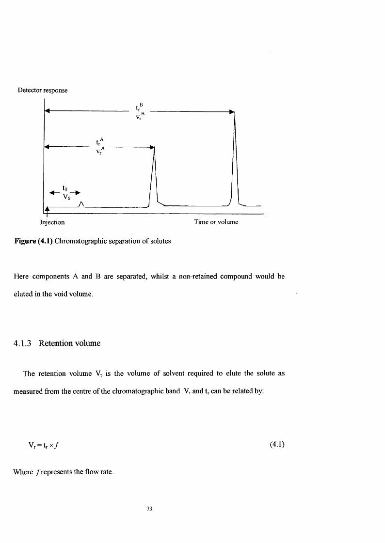
D etector response
Time or volumeInjection
Figure (4.1) Chromatographic separation of solutes
Here components A and B are separated, whilst a non-retained compound would be
eluted in the void volume.
4.1.3 Retention volume
The retention volume Vr is the volume of solvent required to elute the solute as
measured from the centre of the chromatographic band. Vr and tr can be related by;
Vr = t r X /
Wliere /represents the flow rate.
(4.1)
73
In chromatographic separations, the ratio of the time spent by the solute in the
stationary phase to the time it spends in the mobile phase must be optimised. Tliis ratio is
called the solute capacity factor and is given by:
h — (tr — to)/to — (Vr - Vo)/Vo (4.2)
where k is the number of column volumes required to elute a particular solute, tr is the
time taken for a specific solute to reach the detector (retention time) and to is the time
taken for a non-retained species to reach the detector (hold up time). The same value of
k’ is obtained if volumes are used instead of times. The capacity factor of a column is
mostly a function of the packing material but can be manipulated to a degree by varying
the solvent strengtli. Often, only arougli estimation of k’ is required, in which case k’ can
be determined by simple inspection of the chromatogram without exact calculation. From
its capacity factor, the retention time of any solute can be calculated from equation (4.3)
tr = t^(l+k’) = (L/u)(l+k’) (4.3)
where L is the column length and u the average mobile phase velocity.
It is generally assumed that, initially, injection volumes will spread to give a Poisson
distribution and then to a Gaussian distribution. A typical Gaussian peak is shown in
Figure (4.2)
74
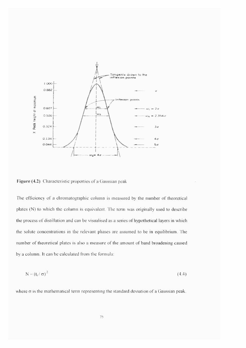
T o n g en ta d raw n to îtîe mfl«K(on p o in t*
! OOO
§E I n A e x w r , po<ttt&
sE Wi -> 2<ro!£.f
0 500 i*!* » 2 3S4(f
0 324
X
0.134
Figure (4.2) Characteristic properties of a Gaussian peak
The efficiency of a chromatogiaphic column is measured by the number of theoretical
plates (N) to which the column is equivalent. The term was originally used to describe
the process of distillation and can be visualised as a series of hypothetical layers in which
the solute concentrations in the relevant phases are assumed to be in equilibrium. The
number of theoretical plates is also a measure of the amount of band broadening caused
by a column. It can be calculated from the formula:
N=(t,/cj)^ (4.4)
where a is the mathematical tenu representing the standard deviation of a Gaussian peak.
75
Assuming that peak shapes are Gaussian, various peak width measurements can be
employed to calculate N. The most commonly used method is the tangent method where
tangents to the curve at the point of inflexion intercept the baseline at a distance of 4a
apart. Equation (4. 4) can then be written as;
N = 16 X (tr/wb)^ (4.5)
Alternatively, the peak width can be measured at the inflexion point (wi) or at half heiglit
(wh), giving rise to equations (4.6) and (4.7) respectively.
N = 4 X (tr / Wi) (4.6)
N = 5 .5 4 x ( t r /W h ) (4.7)
N is often quoted as a measure of the colmnn performance and the larger the number, the
better the column. In general, N increases for smaller stationary phase particle diameters,
low mobile phase flow rates, higher separation temperatures, less viscous solvents, and
smaller solute molecules. The value of N is independent of the retention time of a solute
but is proportional to column lengtli. To enable a direct comparison to be made between
different columns, it is more useful to use the height equivalent to a theoretical plate, H
(also referred to as the plate height), wliich is given by the ratio of the column length (L)
to the column plate number, equation (4.8)
H = L/N (4.8)
76
The selectivity of the chromatographic system is a measure of the difference in retention
times (or volumes) between two given peaks and describes how effectively a
chromatographic system can separate two compounds. Selectivity is defined in terms of
a, which is simply the ratio of capacity factors:
a = k2lkx (4.9)
Tlie value for a can range from unity when tlie retention times of the two components are
identical, to infinity if the first component of interest is eluted in the void volume.
Resolution is defined as the degree of separation between two peaks and is related to
tlie chromatographic variables of selectivity, efficiency and time.
Rs = [N''"/2][(a-l)(/ a +l)[k W (1+k’Av)] (4.10)
where k \v = (k \ + k’2)/2 ; ki and are the capacity factors of the two peaks. The
retention volume may be related to a physicochemical property of the solute-solvent
system, the partition coefficient, K. This is defined as;
K or L = Concentration of the solute in stationary phase
Concentration of tlie solute in mobile phase
The gas-liquid partition coefficient is related to the capacity factor by equation (4.11)
K = p k ’ (4.11)
77

Where (3 is the phase ratio and is equal to the ratio of the volume of the gas (Vg) and
liquid (Vi) phase in the column. For gas-solid cliromatography the phase ratio is given by
the volume of the gas phase divided by the surface area of the stationary phase. The
partition coefficient, K or L, is dimensionless. The gas-liquid partition coefficient is
evaluated from the specific retention volume using the equation below.
K = Vg / P i (4.12)
Vo=t r [Fc* / /W, ]
or Vo = t r * [ F w ( P o - P w ) T c * J ^ / P o T „ W , ] (4.13)
The variable Fw is the gas flow rate at the column outlet, Po is the outlet pressure. Pi is the
pressure inlet, Pw is the vapour of the water at the temperature of the soap-bubble flow,
Tw, Tc is the column, temperature, Wi, is the weight of the stationary phase on the
column, and tr is the retention time. And substituting equation 4.13 into equation 4.12
KorL = t r * [ F w ( P o - P w ) T , * j " / PoTwWi p, ] (4.14)
Where p i is the liquid phase density at the column temperature, and K is the gas-liquid
partition coefficient.
78

4.2 Method for the calculation of the descriptors for PCBs
The original work of Kamlet and Taft, and co-workers showed that it was
indeed possible to define a rather small set of descriptors that could be combined in a
linear way for the correlation of solute properties. After considerable preliminary
work,’" ’ Abraham and co-workers eventually succeeded in constructing a new and more
rigorous set of five solute descriptors, ' as shown in Chapter 2.
Various experimental methods such as HPLC or GLC are used regularly to
determine the descriptors. For volatile compounds they could be obtained fi*om a
combination of experimental data including gas chromatographic and FIPLC retention
data, water-solvent partitions, and Ostwald solubility coefficients (Henry’s constants).
For compounds that are solid at room temperature, use can be made of solubilities in
water and organic solvents, especially if the vapour pressures are k n ow nI n some cases
it was possible to select the most self-consistent vapour pressure for a particular
compound from a possibly variable set of literature data, or in extreme cases, such as that
of Bukminsterfiillerene,^"' to predict the vapour pressure. But all these methods can be
time consuming and very difficult to produce reliable data.
Recently it has been shown that the descriptors can be calculated just from the
structure of a compound, using a group contribution approach, very rapidly indeed (about
700 compounds per min).^ This then opens the way for combinatorial libraries or virtual
libraries to be scanned or screened for relevant transport-related properties. However, the
reliability of such calculations depends on a knowledge of the descriptors for a wide
range of compounds that include different functional groups and different heterocyclic
79

moieties. ’ No PCBs were used in the training set for the calculation of descriptors,
and so it is necessary to determine these from experiment.
The solvation equations to be used are those described in Chapter 2,
Log SP = c + r. R2 + s. " + a. Z Œ] ^ + b. L (3 2^ + v. Vx (4.15)
or
Log SP = c + r. R2 + STT2 ^ + a. I a 2^ + b. I (3 2 ^ + log l ’ (4.16)
4.3 The determination of descriptors
The determination of descriptors is based on equation (4.15) and equation (4.16).
Consider a property of a given compound for a process that is correlated by equation
(4.15), such as water-solvent partition. If the values of log SP (where log SP is now log P)
for several water-solvent systems are known, a series of equations for which we know the
coefficients and the values of log P can be set up, and where the descriptors for the
compomid in equation (4.15) are the unknowns. Now the McGowan characteristic
volume Vx (10'^ cm mol ' ) can be calculated simply from a table of atomic constants
and the number of bonds,^’ especially if the algorithm of Abraham et al for the number
of bonds in any molecule is used. For compounds that are liquid at 293 K, the R2
descriptor (lO ’ cm mol ’) can be obtained from the refractive i n d e x I n case of solids,
either the hypothetical refractive index can be calculated, or R2 can be obtained through
the addition of values for fragments or sub-structures. This leaves only three descriptors
(712 , Za2^ and IP 2^ ) as the unknowns in the set of partition equation. Values of the
80
descriptors can be assigned as those that yield the calculated values of log P that best
reproduce the observed log P values. It is not necessary to restrict the set of equations to
partition equations. Any property can be introduced, such as an equation for a
characterized HPLC system.
If the log descriptor is required, then processes correlated through equation (4.16)
have to be considered. One such process is that of the solubility of gases and vapours in
organic solvents, expressed as log L (equivalent to the gas solvent partition coefficient).
If values of log L are known for the given compound in several solvents, the
corresponding equations can be solved for the four unknown descriptors (712^,
Ea2^, Zp2 ^ and log L ). However, it is then more convenient to combine the log P and
log L sets into one entire set of equations that can be solved for the four unknown
descriptors.
4.4 Techniques use to calculated partition coefficients
A nmnber of teclmiques have been used to measure partition coefficients, P,
especially water-octanol partition coefficients, (Poet). The original method was the
shake-flask method in wliich the concentrations of the compound are measured in
octanol and water, shaken together until equilibrium is attained. However, the water
concentrations may be inaccurate due to fonnation of molecular aggregates and tliere are
analytical difficulties inherent in the measurement of extremely low aqueous equilibrium
concentrations.^^
81
Measurement and estimates based upon reverse-pliase HPLC and thin-layer
chromatography have achieved moderate success for other groups of lipophilic
compounds but require the use of empirical correction factors in the case of FCBs. ' "
Some success has been recently achieved in relating log Poet to calculated molar
volumes/^ Also total surface area (TSA), which is a function of molar volume, has been
found to have a linear relationship with log Poet for compounds such as polyaromatic
hydrocarbons and halobenzenes/^^^ Reliable and consistent (P) values for a number of
PCBs congeners have been obtained by the generator column technique, which obviates
problem such as colloidal suspensions, absorption, and volatilization of the solute.
82
4 .5 R eferen ces
1. Polychlorinated Biphenyls (National Academy of Sciences-National Research
Council, Washington, 1979, DC.
2. M. D. Mullin, C. M. P Dichinio, S. McCrindle, M. Romkes, S. Safe, and L. M
Safe , Environ. Sci. Technol. 1984, Vol. 18, 468.
3. O. Hutzinger, S. Safe, and V. Zitko. The chemistry of PCBs (Boca, Raton, FL,
1974)
4. I. C. T. Nisbet and A. F. Sarofim, Environ Health Perspect. 1972, Vol. 1, 21.
5. D. Mackay, W. Y. Shiu, D. W. Billington, and G. L. Haung; in Physical
Behaviour of PCBs in the Great Lakes, edited by D. Mackay, S. Paterson, S. J.
Eisenreich, and M. S. Simmons. Ann Arbor Scientific, 1983, 59.
6. S. J. Eisenreich, B. B. Looney, and G. J. Hollod; in Physical Behaviour of PCBs in
the Great Lakes, edited by D. Mackay, S. Paterson, S. J. Eisenreich and M. S.
Simmons Ann Arbor Scientific, 1983, 115.
7. S. Safe, in Halogenated Biphenyls. Terphenyls, Naphthalenes, Dibenzodioxins
and Related Products edited by R. D. Kimbrough Elsevier Amsterdam, 1990,
chap. 4.
8. Kiichi UEDA, PCB Poisoning ,1969, chap. 3 , 39 .
9. K. Ballschmiter, A. Mennel, and J. Buyten, Fresenius J. Anal. Chem., 1993, Vol.
346, 396.
10. M. Tswett, Ber. Deut. Botaan. Ges., 1906, 316.
11. T. Synge and A. J. P. Martinn, Biochem. J., 1941, Vol. 35,1358.
83

12. M. J. Kamlet, R. M. Doherty, J. LM. Abboud, M. H. Abraham and R. W. Taft,
Chem., 1986, Vol. 16, 566.
13. M. H. Abraham, R. M. Doherty, M. J. Kamlet, and R. W. Taft, Chem. Brit, 1986,
Vol. 22, 551.
14. M. H. Abraham, G. S. Wliiting, R. M. Doherty and W. J. Shuely, J. Chem. Soc.
Perkin Trans 2,1986,1451.
15. H. Abraham, G. C. Whiting, R. M. Doherty, and W. J. Shuely, J. Chem. Soc.
Perkin Trans 2,1986, 1851.
16. H. Abraham, G. S. Whiting, R. M. Donerty, and W. J. Shuely, J. Chromatogr.,
1991, Vol. 587,213.
17. H. Abraham, J. Phys. Org. Chem., 1993, Vol. 6, 660.
18. H. Abraham, Pure App. Chem., 1993, Vol. 65, 2503.
19. M. H. Abraham, Chem. Soc. Revs., 1993, Vol. 22, 73.
20. M. H. Abraham, and H. S. Chadha., Drug Action and Toxicology, Ed. By V.
Pliska, b. Testa and H. Van de Waterbeemd, VCH. Weinheim, Germany, 1996,
311.
21. M. H. Abraliam, and J. C. McGowan, Chromatographia., 1987, Vol. 23, 243.
22. M. H. Abraham, R. Kumarsingh, J. E. Cometto-Muniz, W. S. Cain, M. Roses, E.
Bosch, and M. L. Diaz., J. Chem. Soc. Perkin Trans. 2,1998,2405.
23. M. H. Abraham, C. E. Green, W. E. Acree, C. E. Hernandez, and L. E. Roy, J.
Chem. Soc. Perkin Trans. 2, 1998, 2677.
24. M. H. Abraham, C. E. Green, and W. E. Acree, J. Chem. Soc. Perkin Trans. 2,
2000, 281.
84

25. J. A. Platts, D. Butina, M. H. Abraliam and A. Hersey, J. Chem. Inf. Comput. Sci.,
1999, Vol. 39, 835.
26. J. A. Platts, M. H. Abraham, D. Butina and A. Hersey, J. Chem. Inf. Comput Sci.,
2000, Vol. 40, 71.
27. M. H. Abraliam, H. S. Chadhd, F. Mitchell, M. W. Bradury, and J. A. Gratton,
Pestic. Sci., 1999, Vol. 55, 78.
28. M H. Abraham, G. S.Whiting, R. M. Doherty, and W. J. Shuely, J. Chem. Soc.
Perkin Trans. 2,1990,1451.
29. R. A. Rapaport, S. Eisenreich, J. Environ. Sci. Technol., 1984, Vol. 18,163.
30. M. T. M. Tulp, O. Hutzinger, Chemosphere. , 1978, Vol. 10, 849.
31. G. D. Veith, N. M. Austin, Morris, R. T. Water Res. 1979, Vol. 13,43.
32. H. Ellgehausen, D. Hondt, R. Fuerer, Pestic. Sci., 1981, Vol. 12,219.
33. M. L. Coates, D. W. Connell, D. M. Barron, Environ. Sci. Technol., 1985, Vol.
19,628.
34. W. A. Bruggeman, J. Van der Steen, O. Hutzinger, J. Chromatogr., 1982, Vol.
238,335.
35. S. H. Yalkowsky, S. C. Valvani, J. Chem. Eng. Data, 1979, Vol. 24,127.
36. L. B. Kier, hi Physical Chemical Properties of Drugs; S. H. Yalkowsky, A. A.
Sinkula, S. C. Valvani, S. C. Eds; Medicinal Research Series; Dekker; New york,
1980, Vol. 10.
37. S. H. Yalkowsky, S. C. Valvani, J. Med. Chem. 1976, Vol. 19, 727.
38. M. M. Miller, S. Ghodbane, S. P. Wasik, Y. B. Tewari, D. E. Martire, J. Chem.
Eng. Data, 1984, Vol. 29,184.
85
39. K. B. Woodburn, W. J. Doucette, A. W. Andren, Environ. Sci. Technol. 1984,
Vol. 18,457.
86

Chapter 5 The First Calculation of the descriptors for PCBs
5.0 Introduction
The solvation equations have been described previously (in chapters land 2). Both
equations have terms in five descriptors. However the PCBs have no hydrogen bond
acidity and hence the term a.Za^ 2 will be redundant. Tlie modified solvation equations
are tlierefore.
Log SP = c + r. R2 + s. 71 2+ b. Z p 2 + V. Vx (5.1)
Log SP = c + r. R2 + s. .71 2 + b. Z P 2 + log L’ (5.2)
Hence a total of five descriptors (over the two equations) are needed to characterise any
PCB. Now the McGowan characteristic volume, Vx, can be calculated simply firom the
structure of the molecule, using a table of atomic and bond contributions. A simple
computer program was available for tlie calculation. Therefore only four descriptors
remained to be determined for each PCB, that is, R2,7c 2 , ^ p \ and log L* .
One of the main sets of physicochemical data on PCBs is that of GLC retention
indices, I , defined by equation 5.3
87

1=100 log X - log (z ) + zlo g x { z + l) - lo g x (z )
(5.3)
Here x is a retention parameter such as adjusted retention time or retention volume, and x
(z+1) and X (z) are the corresponding quantities for an alkane with z+1 and z carbon
atoms; the retention parameter for the compound in equation (5.3) should be between x
(z+1) and X (z).
Fortunately, the retention indices of PCBs on various liquid-phases in packed columns
have been measured before and values were kindly supplied by Dr. Albro (personal
communication) These values were scanned on to a disc, then put in a spreadsheet in
twelve columns starting from non-polar and going on to polar stationary phases, as shown
in Table 5.1.
88
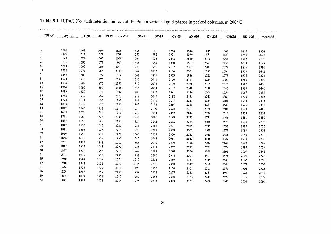
Table 5.1. lUPAC No. with retention indices of PCBs, on various liquid-phases in packed columns, at 200* C
pV-101 F-50 APLEZON GV-210 pV-3 OV-17 OV-2S AN-600 OV-225 CHOM HK- 325 POLMPE
- 1396 1408 1494 1660 1466 1656 1754 1740 1832 2000 1466 19541 1509 1518 1578 1780 1585 1792 1901 1869 1971 2127 1589 20724 1622 1628 1662 1900 1704 1928 2048 2010 2110 2254 1712 21902 1575 1592 1679 1997 1654 1954 1960 1965 2062 2252 1603 21986 1688 1702 1763 2017 1773 1990 2107 2103 2201 2379 1806 231611 1754 1776 1964 2134 1842 2052 2166 2205 2292 2504 1900 24423 1585 1600 1692 1914 1661 1875 1973 1986 2085 2273 1695 22228 1698 1710 1776 2034 1780 2011 2120 2117 2224 2400 1818 234013 1764 1784 1877 2151 1849 2073 2179 2220 2315 2525 1912 246615 1774 1792 1890 2168 1856 2094 2192 2248 2338 2546 1924 249010 1619 1627 1678 1902 1700 1913 2041 1994 2104 2254 1697 219719 1732 1737 1762 2022 1819 2049 2188 2135 2243 2381 1820 231527 1798 1811 1863 2139 1888 2111 2247 2228 2334 2506 1914 244132 1808 1819 1876 2156 1895 2132 2260 2248 2357 2527 1926 246554 1842 1846 1862 2144 1934 2170 2328 2263 2376 2508 1928 24409 1658 1674 1744 1969 1736 1944 2052 2044 2136 2319 1758 226218 1771 1784 1828 2089 1855 2080 2199 2172 2275 2446 1881 238026 1837 1858 1929 2206 1924 2142 2258 2274 2366 2571 1975 250631 1847 1966 1942 2223 1931 2163 2271 2287 2399 2592 1987 253053 1881 1893 1928 2211 1970 2201 2339 2302 2408 2573 1989 250552 1920 1940 1994 2278 2006 2232 2350 2352 2440 2638 2050 25707 1668 1679 1758 1965 1747 1943 2061 2042 2145 2322 1770 228017 1781 1788 1842 2085 1866 2079 2209 2176 2284 2449 1893 239825 1847 1862 1943 2202 1935 2141 2267 2273 2375 2574 1987 252428 1857 1870 1956 2219 1942 2162 2280 2290 2398 2595 1999 254851 1891 1897 1942 2207 1991 2200 2348 2301 2417 2576 2001 252349 1930 1944 2008 2274 2017 2231 2359 2347 2449 2641 2062 259847 1940 1948 2022 2270 2028 2230 2368 2349 2458 2644 2074 26065 1696 1703 1773 2010 1779 1995 2130 2101 2215 2370 1802 232816 1809 1813 1857 2130 1898 2131 2277 2235 2354 2497 1925 244620 1875 1887 1958 2247 1967 2193 2336 2332 2445 2622 2019 257222 1885 1895 1971 2264 1974 2214 2349 2352 2468 2643 2031 2596
89

Table 5,1 cont. 46 1919 1922 1957 2252 2013 2252 2417 2360 2487 2624 2033 257144 1958 1969 2023 2319 2049 2283 2428 2406 2519 2689 2094 263642 1968 1973 2037 2315 2060 2282 2437 2405 2528 2692 2106 265440 1996 1998 2052 2360 2092 2334 2506 2465 2598 2740 2138 270214 1721 1730 1843 2053 1793 1982 2081 2119 2208 2424 1842 238134 1834 1840 1927 2173 1912 2118 2228 2252 2347 2551 1965 249936 1900 1914 2028 2290 1981 2180 2287 2349 2438 2676 2059 262539 1910 1922 2041 2307 1988 2201 2300 2369 2461 2697 2071 264973 1944 1949 2027 2295 2027 2239 2368 2377 2490 2678 2073 262472 1983 1996 2093 2362 2063 2270 2379 2423 2512 2743 2134 268968 1993 2000 2107 2358 2074 2269 2388 2422 2521 2746 2746 270758 2021 2025 2122 2403 2106 2321 2475 2481 2591 2749 2178 275580 2046 2052 2192 2446 2120 2308 2408 2498 2584 2848 2218 280812 1770 1779 1985 2139 1859 2081 2187 2214 2317 2525 1902 247133 1883 1889 1969 2259 1978 2217 2334 2347 2456 2652 2025 258935 1949 1963 2070 2376 2047 2279 2393 2444 2547 2777 2119 271537 1959 1971 2083 2393 2054 2300 2406 2464 2570 2798 2131 273971 1993 1998 2069 2381 2093 2338 2474 2472 2589 2779 2133 271470 2032 2045 2135 2448 2129 2369 2458 2518 2621 2844 2194 277966 2042 2049 2149 2444 2140 2368 2494 2517 2630 2487 2206 279756 2070 2074 2164 2489 2172 2420 2563 2576 2700 2895 2238 284579 2095 2101 2234 2532 2186 2407 2514 2593 2693 2949 2278 289877 2144 2150 2276 2618 2252 2506 2620 2699 2802 3050 2338 298830 1734 1741 1823 2009 1803 2004 2127 2075 2175 2363 1842 232850 1847 1851 1907 2129 1922 2140 2744 2208 2314 2490 1965 244669 1913 1925 2008 2246 1991 2202 2333 2305 2305 2405 2059 257275 1923 1933 2021 2263 1998 2223 2346 2325 2428 2636 2071 2596104 1961 1960 2007 2251 2037 2261 2414 2333 2447 2617 2073 2571103 1996 2007 2073 2318 2073 2292 2425 2379 2479 2682 2134 2636100 2006 2011 2087 2314 2084 2291 2434 2378 2488 2685 2146 265498 2034 2036 2102 2359 2116 2343 2503 2437 2558 2733 2178 2702121 2060 2063 2172 2402 2130 2330 2454 2454 2551 2787 2218 2755119 2108 2112 2214 2488 2196 2429 2560 2549 2660 2888 2278 2845155 2072 2074 2152 2358 2140 2352 2500 2410 2518 2726 2218 270224 1786 1772 1832 2087 1845 2074 2204 2179 2276 2438 1873 2378
45 1899 1882 1916 2207 1964 2210 2351 2312 2415 2565 1996 249659 1965 1956 2017 2324 2033 2272 2410 2409 2506 2690 2090 2622
90
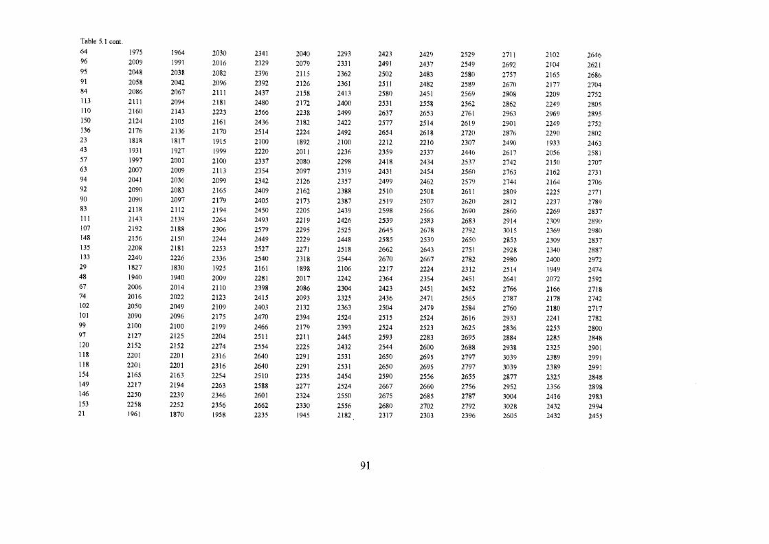
Table 5,1 cont.64 1975 1964 2030 2341 2040 2293 2423 2429 2529 2711 2102 264696 2009 1991 2016 2329 2079 2331 2491 2437 2549 2692 2104 262195 2048 2038 2082 2396 2115 2362 2502 2483 2580 2757 2165 268691 2058 2042 2096 2392 2126 2361 2511 2482 2589 2670 2177 270484 2086 2067 2111 2437 2158 2413 2580 2451 2569 2808 2209 2752113 2111 2094 2181 2480 2172 2400 2531 2558 2562 2862 2249 2805110 2160 2143 2223 2566 2238 2499 2637 2653 2761 2963 2969 2895150 2124 2105 2161 2436 2182 2422 2577 2514 2619 2901 2249 2752136 2176 2136 2170 2514 2224 2492 2654 2618 2720 2876 2290 280223 1818 1817 1915 2100 1892 2100 2212 2210 2307 2490 1933 246343 1931 1927 1999 2220 2011 2236 2359 2337 2446 2617 2056 258157 1997 2001 2100 2337 2080 2298 2418 2434 2537 2742 2150 270763 2007 2009 2113 2354 2097 2319 2431 2454 2560 2763 2162 273194 204] 2036 2099 2342 2126 2357 2499 2462 2579 2744 2164 270692 2090 2083 2165 2409 2162 2388 2510 2508 2611 2809 2225 277190 2090 2097 2179 2405 2173 2387 2519 2507 2620 2812 2237 278983 2118 2112 2194 2450 2205 2439 2598 2566 2690 2860 2269 2837111 2143 2139 2264 2493 2219 2426 2539 2583 2683 2914 2309 2890107 2192 2188 2306 2579 2295 2525 2645 2678 2792 3015 2369 2980148 2156 2150 2244 2449 2229 2448 2585 2539 2650 2853 2309 2837135 2208 2181 2253 2527 2271 2518 2662 2643 2751 2928 2340 2887133 2240 2226 2336 2540 2318 2544 2670 2667 2782 2980 2400 297229 1827 1830 1925 2161 1898 2106 2217 2224 2312 2514 1949 247448 1940 1940 2009 2281 2017 2242 2364 2354 2451 2641 2072 259267 2006 2014 2110 2398 2086 2304 2423 2451 2452 2766 2166 271874 2016 2022 2123 2415 2093 2325 2436 2471 2565 2787 2178 2742102 2050 2049 2109 2403 2132 2363 2504 2479 2584 2760 2180 2717101 2090 2096 2175 2470 2394 2524 2515 2524 2616 2933 2241 278299 2100 2100 2199 2466 2179 2393 2524 2523 2625 2836 2253 280097 2127 2125 2204 2511 2211 2445 2593 2283 2695 2884 2285 2848120 2152 2152 2274 2554 2225 2432 2544 2600 2688 2938 2325 2901118 2201 2201 2316 2640 2291 2531 2650 2695 2797 3039 2389 2991118 2201 2201 2316 2640 2291 2531 2650 2695 2797 3039 2389 2991154 2165 2163 2254 2510 2235 2454 2590 2556 2655 2877 2325 2848149 2217 2194 2263 2588 2277 2524 2667 2660 2756 2952 2356 2898146 2250 2239 2346 2601 2324 2550 2675 2685 2787 3004 2416 2983153 2258 2252 2356 2662 2330 2556 2680 2702 2792 3028 2432 299421 1961 1870 1958 2235 1945 2182 2317 2303 2396 2605 2432 2455
91
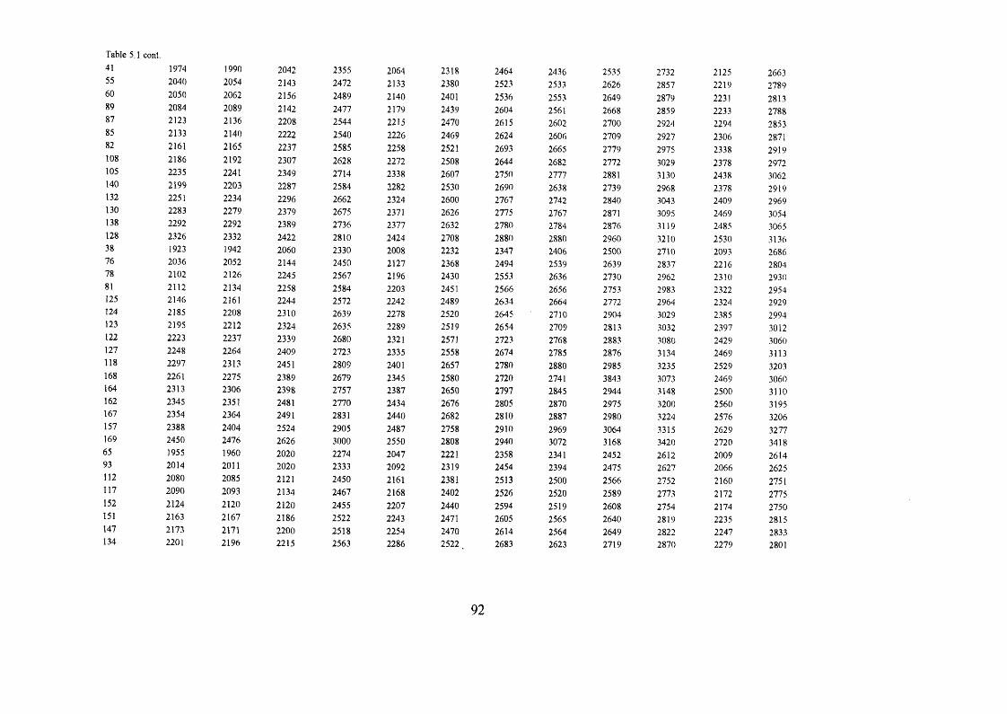
Table 5.1 cont.41 1974 1990 2042 2355 2064 2318 2464 2436 2535 2732 2125 266355 2040 2054 2143 2472 2133 2380 2523 2533 2626 2857 2219 278960 2050 2062 2156 2489 2140 2401 2536 2553 2649 2879 2231 281389 2084 2089 2142 2477 2179 2439 2604 2561 2668 2859 2233 278887 2123 2136 2208 2544 2215 2470 2615 2602 2700 2924 2294 285385 2133 2140 2222 2540 2226 2469 2624 2606 2709 2927 2306 287182 2161 2165 2237 2585 2258 2521 2693 2665 2779 2975 2338 2919108 2186 2192 2307 2628 2272 2508 2644 2682 2772 3029 2378 2972105 2235 2241 2349 2714 2338 2607 2750 2777 2881 3130 2438 3062140 2199 2203 2287 2584 2282 2530 2690 2638 2739 2968 2378 2919132 2251 2234 2296 2662 2324 2600 2767 2742 2840 3043 2409 2969130 2283 2279 2379 2675 2371 2626 2775 2767 2871 3095 2469 3054138 2292 2292 2389 2736 2377 2632 2780 2784 2876 3119 2485 3065128 2326 2332 2422 2810 2424 2708 2880 2880 2960 3210 2530 313638 1923 1942 2060 2330 2008 2232 2347 2406 2500 2710 2093 268676 2036 2052 2144 2450 2127 2368 2494 2539 2639 2837 2216 280478 2102 2126 2245 2567 2196 2430 2553 2636 2730 2962 2310 293081 2112 2134 2258 2584 2203 2451 2566 2656 2753 2983 2322 2954125 2146 2161 2244 2572 2242 2489 2634 2664 2772 2964 2324 2929124 2185 2208 2310 2639 2278 2520 2645 2710 2904 3029 2385 2994123 2195 2212 2324 2635 2289 2519 2654 2709 2813 3032 2397 3012122 2223 2237 2339 2680 2321 2571 2723 2768 2883 3080 2429 3060127 2248 2264 2409 2723 2335 2558 2674 2785 2876 3134 2469 3113118 2297 2313 2451 2809 2401 2657 2780 2880 2985 3235 2529 3203168 2261 2275 2389 2679 2345 2580 2720 2741 3843 3073 2469 3060164 2313 2306 2398 2757 2387 2650 2797 2845 2944 3148 2500 3110162 2345 2351 2481 2770 2434 2676 2805 2870 2975 3200 2560 3195167 2354 2364 2491 2831 2440 2682 2810 2887 2980 3224 2576 3206157 2388 2404 2524 2905 2487 2758 2910 2969 3064 3315 2629 3277169 2450 2476 2626 3000 2550 2808 2940 3072 3168 3420 2720 341865 1955 1960 2020 2274 2047 2221 2358 2341 2452 2612 2009 261493 2014 2011 2020 2333 2092 2319 2454 2394 2475 2627 2066 2625112 2080 2085 2121 2450 2161 2381 2513 2500 2566 2752 2160 2751117 2090 2093 2134 2467 2168 2402 2526 2520 2589 2773 2172 2775152 2124 2120 2120 2455 2207 2440 2594 2519 2608 2754 2174 2750151 2163 2167 2186 2522 2243 2471 2605 2565 2640 2819 2235 2815147 2173 2171 2200 2518 2254 2470 2614 2564 2649 2822 2247 2833134 2201 2196 2215 2563 2286 2522 , 2683 2623 2719 2870 2279 2801
92
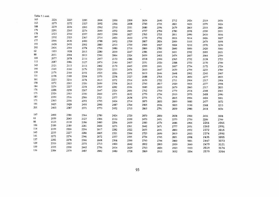
Table 5.1 cont. 165 2226 2223 2285 2606 2300 2509 2634 2640 2712 2924 2319 2934163 2275 2272 2327 2692 2366 2608 2740 2735 2821 3025 2379 3024188 2239 2234 2265 2562 2310 2531 2680 2596 2679 2863 2319 2881179 2291 2265 2274 2640 2352 2601 2757 2700 2780 2938 2350 2931178 2323 2310 2357 2653 2399 2627 2765 2725 2811 2990 2410 3016187 2332 2323 2367 2714 2405 2633 2770 2742 2816 3014 2426 3027177 2366 2636 2400 2788 2452 2709 2807 2824 2900 3105 2479 3098193 2428 2435 2502 2883 2515 2759 2900 2927 3004 3210 2570 3239202 2406 2394 2378 2766 2480 2710 2860 2783 2840 3000 2420 306062 1953 1938 2015 2280 2019 2247 2386 2343 2451 2592 2095 262188 2011 2004 2013 2340 2064 2324 2459 2403 2474 2607 2064 2599109 2077 2078 2114 2457 2133 2386 2518 2500 2565 2732 2158 2725115 2087 2086 2127 2474 2140 2407 2531 2520 2588 2753 2170 2749145 2121 2113 2113 2462 2179 2445 2599 2601 2607 2734 2172 2724144 2160 2160 2179 2529 2215 2476 2610 2647 2639 2799 2233 2789139 2170 2164 2193 2525 2226 2475 2619 2646 2648 2902 2245 2907131 2198 2189 2208 2570 2258 2527 2688 2705 2718 2850 2277 2855161 2223 2216 2278 2613 2272 2514 2639 2722 2711 2904 2317 2908158 2272 2265 2320 2699 2338 2613 2745 2817 2920 3005 2377 2998184 2236 2227 2258 2569 2282 2536 2685 2605 2679 2843 2317 2855176 2288 2258 2267 2647 2324 2606 2762 2709 2779 2918 2348 2905175 2320 2303 2350 2660 2371 2632 2770 2734 2910 2970 2408 2990183 2330 2316 2360 2721 2377 2638 2775 2751 2815 2994 2424 3001171 2363 2356 2393 2795 2424 2714 2875 2833 2899 3085 2477 3072191 2425 2428 2495 2990 2487 2764 2905 2936 3003 3190 2568 3213201 2403 2387 2371 2773 2452 2715 2865 2791 2839 2980 2418 3034
197 2400 2380 2364 2780 2424 2720 2870 2800 2838 2960 2416 300861 2039 2043 2127 2306 2110 2330 2470 2451 2570 2750 2200 274986 2123 2118 2180 2483 2206 2439 2583 2574 2686 2906 2 2 6 6 2 0 6 5106 2189 2189 2281 2600 2275 2501 2642 2671 2777 2931 2 3 6 0 2 991114 2199 2200 2294 2617 2282 2522 2655 2691 2800 2952 2 3 7 2 3 0 1 5143 2233 2227 2280 2605 2321 2560 2723 2699 2819 2933 2 374 2 9 9 0141 2272 2274 2346 2672 2357 2591 2734 2745 2851 2998 2 4 3 5 3 0 5 5137 2282 2278 2360 2668 2368 2590 2743 2744 2860 3001 2 447 3 0 7 3129 2310 2303 2375 2713 2400 2642 2812 2803 2930 3049 2 4 7 9 3 1 2 1159 2335 2330 2445 2756 2414 2629 2763 2820 2923 3103 2 5 1 9 3 1 7 4156 2384 2379 2487 2842 2480 2728 2869 2915 3032 3204 2 5 7 9 3 2 6 4
93
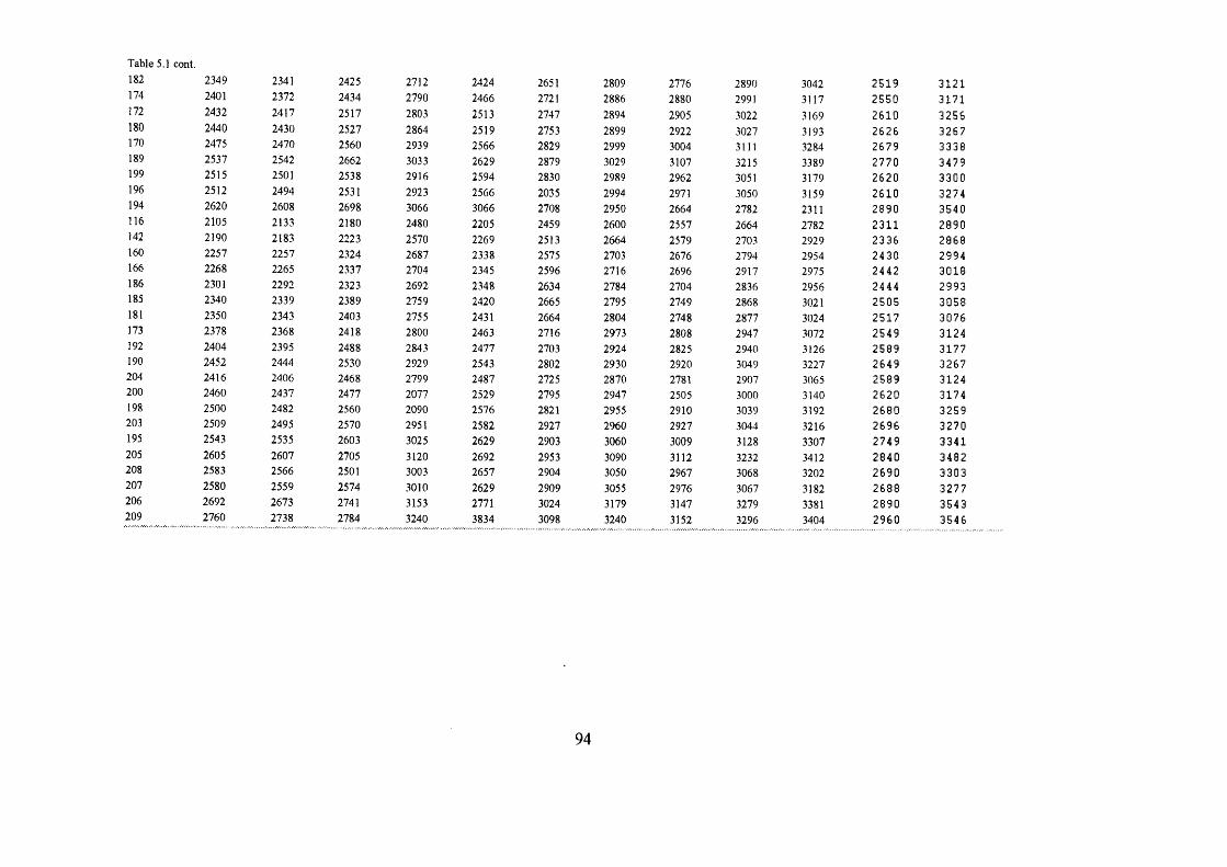
Table 5.1 cont. 182 2349 2341 2425 2712 2424 2651 2809 2776 2890 3042 2519 3 121174 2401 2372 2434 2790 2466 2721 2886 2880 2991 3117 2 550 3171172 2432 2417 2517 2803 2513 2747 2894 2905 3022 3169 261 0 3 2 5 6180 2440 2430 2527 2864 2519 2753 2899 2922 3027 3193 262 6 3267170 2475 2470 2560 2939 2566 2829 2999 3004 3111 3284 267 9 3 338189 2537 2542 2662 3033 2629 2879 3029 3107 3215 3389 2 7 7 0 3479199 2515 2501 2538 2916 2594 2830 2989 2962 3051 3179 2 6 2 0 3300196 2512 2494 2531 2923 2566 2035 2994 2971 3050 3159 2 6 1 0 3274194 2620 2608 2698 3066 3066 2708 2950 2664 2782 2311 2 8 9 0 354 0116 2105 2133 2180 2480 2205 2459 2600 2557 2664 2782 231 1 289 0142 2190 2183 2223 2570 2269 2513 2664 2579 2703 2929 2 3 3 6 286 8160 2257 2257 2324 2687 2338 2575 2703 2676 2794 2954 2 4 3 0 299 4166 2268 2265 2337 2704 2345 2596 2716 2696 2917 2975 2 442 3 0 1 8186 2301 2292 2323 2692 2348 2634 2784 2704 2836 2956 2 4 4 4 2 993185 2340 2339 2389 2759 2420 2665 2795 2749 2868 3021 2 5 0 5 3 058181 2350 2343 2403 2755 2431 2664 2804 2748 2877 3024 2 517 3 076173 2378 2368 2418 2800 2463 2716 2973 2808 2947 3072 2 549 3 124192 2404 2395 2488 2843 2477 2703 2924 2825 2940 3126 2 5 8 9 3 177190 2452 2444 2530 2929 2543 2802 2930 2920 3049 3227 2 6 4 9 3 267204 2416 2406 2468 2799 2487 2725 2870 2781 2907 3065 2 589 3124200 2460 2437 2477 2077 2529 2795 2947 2505 3000 3140 2 620 3174198 2500 2482 2560 2090 2576 2821 2955 2910 3039 3192 2 6 8 0 3 259203 2509 2495 2570 2951 2582 2927 2960 2927 3044 3216 2 6 9 6 3 2 7 0195 2543 2535 2603 3025 2629 2903 3060 3009 3128 3307 2 749 3 341205 2605 2607 2705 3120 2692 2953 3090 3112 3232 3412 2 8 4 0 3 4 8 2208 2583 2566 2501 3003 2657 2904 3050 2967 3068 3202 2 6 9 0 3 3 0 3207 2580 2559 2574 3010 2629 2909 3055 2976 3067 3182 2 6 0 8 3 2 7 7206 2692 2673 2741 3153 2771 3024 3179 3147 3279 3381 2 8 9 0 3 543209 2760 2738 2784 3240 3834 3098 3240 3152 3296 3404 2 9 6 0 3 5 4 6
94
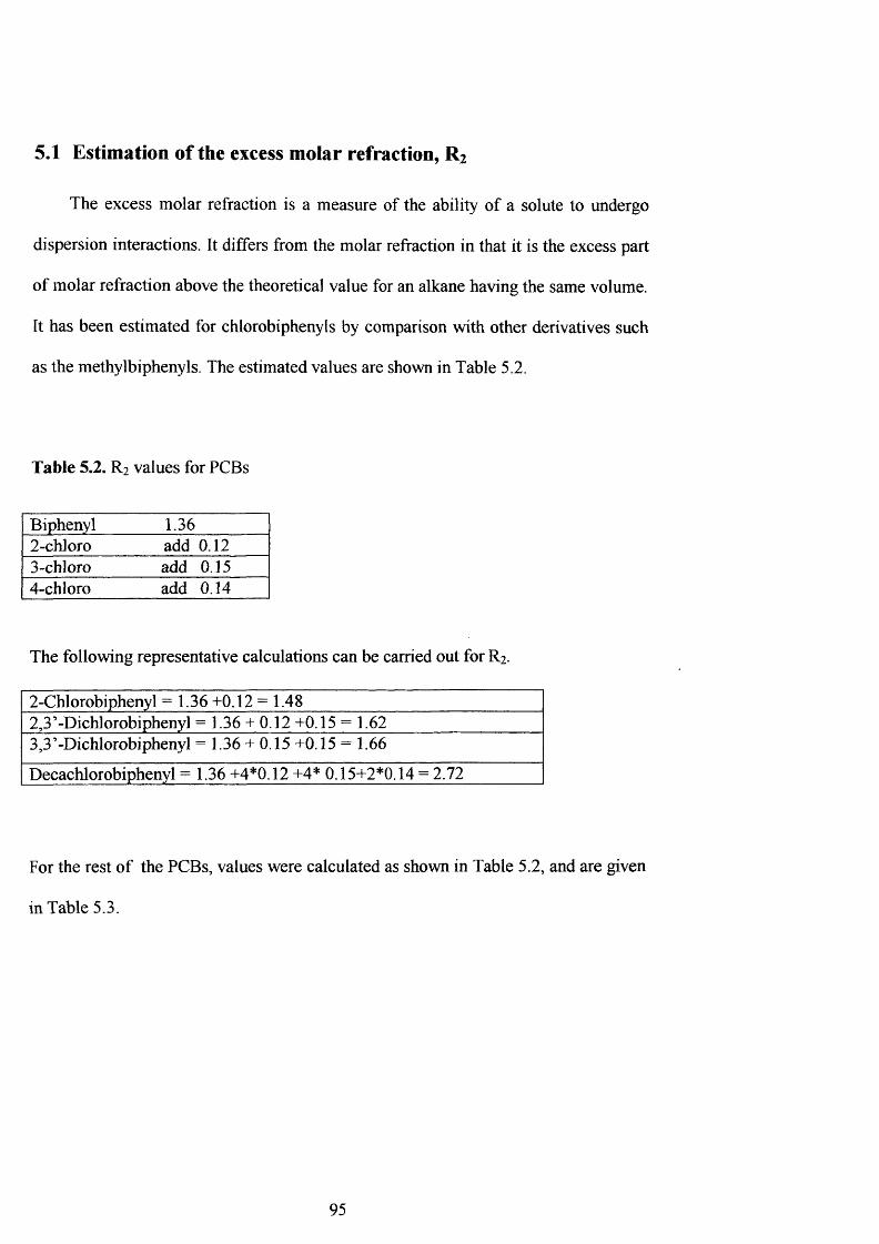
5.1 Estimation of the excess molar refraction, R%
The excess molar refraction is a measure of the ability of a solute to undergo
dispersion interactions. It differs from the molar refraction in that it is the excess part
of molar refraction above the theoretical value for an alkane having the same volume.
It has been estimated for chlorobiphenyls by comparison with other derivatives such
as the methylbiphenyls. The estimated values are shown in Table 5.2.
Table 5.2. R2 values for PCBs
Biphenyl 1.362-chloro add 0.123-chloro add 0.154-chIoro add 0.14
The following representative calculations can be carried out for R2 .
2-Chlorobiphenyl - 1.36 +0.12 = 1.482,3’-Dichiorobiphenyl = 1.36 + 0.12 +0.15 - 1.623,3’-Dichlorobiphenyl = 1.36 + 0.15 +0.15 = 1.66
Decachlorobiphenyl = 1.36 +4*0.12 +4* 0.15+2*0.14 = 2.72
For the rest of the PCBs, values were calculated as shown in Table 5.2, and are given
in Table 5.3.
95

Table 5.3. lUPAC No. for PCBs, and alkanes, estimated values of R2 and S|3 2, calculated values of and some estimated (a) values of tt 2 and log .
lUPAC R2 V. Log
1.36 0.990 0.26 1.324 6.0141 1.48 1.120 0.19 1.447 6.6502 1.51 0.20 1.4473 1.50 1.090 0.20 1.447 6.4804 1.60 0.14 1.5695 1.63 0.16 1.5696 1.63 0.14 1.5697 1.62 0.16 1.5698 1.62 0.14 1.5699 1.63 0.16 1.56910 1.66 0.16 1.56911 1.66 0.14 1.56912 1.65 0.16 1.56913 1.65 0.14 1.56914 1.65 0.16 1.56915 1.64 1.200 0.13 1.569 7.92016 1.75 0.10 1.69117 1.74 0.10 1.69118 1.75 0.10 1.69119 1.72 0.10 1.69120 1.78 0.10 1.69121 1.77 0.13 1.69122 1.77 0.10 1.69123 1.78 0.13 1.69124 1.75 0.13 1.69125 1.77 0.10 1.69126 1.78 0.10 1.69127 1.76 0.10 1.69128 1.76 0.10 1.69129 1.77 0.13 1.69130 1.74 0.13 1.69131 1.77 0.10 1.69132 1.74 0.10 1.69133 1.77 0.01 1.69134 1.78 0.01 1.69135 1.80 0.01 1.69136 1.79 0.01 1.69137 1.79 0.01 1.69138 1.80 0.13 1.69139 1.80 0.01 1.69140 1.90 0.06 1.81441 1.89 0.07 1.81442 1.89 0.07 1.814
16
96
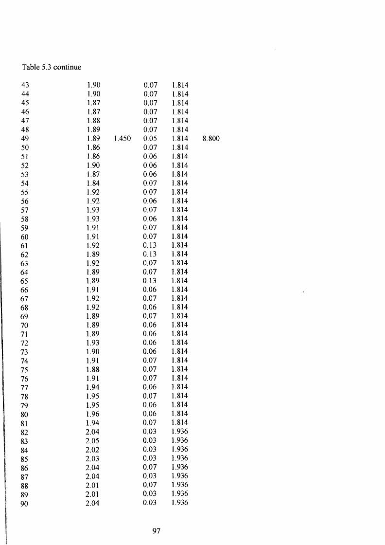
Table 5.3 continue
43 1.90 0.07 1.81444 1.90 0.07 1.81445 1.87 0.07 1.81446 1.87 0.07 1.81447 1.88 0.07 1.81448 1.89 0.07 1.81449 1.89 1.450 0.05 1.81450 1.86 0.07 1.81451 1.86 0.06 1.81452 1.90 0.06 1.81453 1.87 0.06 1.81454 1.84 0.07 1.81455 1.92 0.07 1.81456 1.92 0.06 1.81457 1.93 0.07 1.81458 1.93 0.06 1.81459 1.91 0.07 1.81460 1.91 0.07 1.81461 1.92 0.13 1.81462 1.89 0.13 1.81463 1.92 0.07 1.81464 1.89 0.07 1.81465 1.89 0.13 1.81466 1.91 0.06 1.81467 1.92 0.07 1.81468 1.92 0.06 1.81469 1.89 0.07 1.81470 1.89 0.06 1.81471 1.89 0.06 1.81472 1.93 0.06 1.81473 1.90 0.06 1.81474 1.91 0.07 1.81475 1.88 0.07 1.81476 1.91 0.07 1.81477 1.94 0.06 1.81478 1.95 0.07 1.81479 1.95 0.06 1.81480 1.96 0.06 1.81481 1.94 0.07 1.81482 2.04 0.03 1.93683 2.05 0.03 1.93684 2.02 0.03 1.93685 2.03 0.03 1.93686 2.04 0.07 1.93687 2.04 0.03 1.93688 2.01 0.07 1.93689 2.01 0.03 1.93690 2.04 0.03 1.936
8.800
97
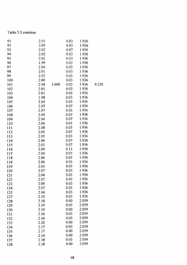
Table 5.3 continue
91 2.01 0.03 1.93692 2.05 0.03 1.93693 2 .02 0 .07 1.93694 2 .02 0.03 1.93695 2 .02 0.03 1.93696 1.99 0.03 1.93697 2 .04 0.03 1.93698 2.01 0.03 1.93699 2.03 0.03 1.936100 2 .00 0.03 1.936101 2 .04 1.600 0.02 1.936102 2.01 0.03 1.936103 2.01 0.03 1.936104 1.98 0.03 1.936105 2 .04 0.03 1.936106 2 .07 0.07 1.936107 2 .07 0.03 1.936108 2 .04 0.03 1.936109 2 .04 0 .07 1.936110 2 .04 0.03 1.936111 2 .08 0.03 1.936112 2.05 0.07 1.936113 2.05 0.03 1.936114 2 .06 0.07 1.936115 2.03 0.07 1.936116 2 .04 0.13 1.936117 2 .04 0.07 1.936118 2.06 0.03 1.936118 2 .06 0.03 1.936119 2.03 0.03 1.936120 2 .07 0.03 1.936121 2 .04 0.03 1.936122 2 .07 0.03 1.936123 2 .09 0.03 1.936124 2 .07 0.03 1.936125 2.04 0.03 1.936127 2 .10 0.03 1.936128 2.18 0.00 2 .059129 2 .19 0.03 2 .059130 2 .19 0.00 2 .059131 2 .16 0.03 2 .059
132 2 .16 0.03 2 .059133 2 .20 0 .00 2 .059
134 2 .17 0.03 2 .059
135 2 .17 0 .00 2 .059
136 2.14 0 .00 2 .059
137 2.18 0.03 2 .059
138 2.18 0 .00 2 .059
98

Table 5.3 continue
139 2.15 0.03 2.059140 2 18 0.00 2.059141 2.19 0.03 2.059142 2.16 0.07 2.059143 2.16 0.03 2.059144 2.16 0.03 2.059145 2.13 0.03 2.059146 2.19 0.00 2.059147 2.16 0.03 2.059148 2.16 0.00 20^9149 2.16 0.00 2.059150 2.13 0.03 2.059151 2.17 0.03 2.059152 2.14 0.03 2.059153 2.18 1.630 0.00 2.059154 2.15 0.00 2.059155 2.12 0.00 2.059156 2.21 0.03 2.059157 2.21 0.00 2.059158 2.18 0.03 2.059159 2.20 0.03 2.059160 2.19 0.07 2.059161 2.19 0.03 2.059162 2.20 0.00 2.059163 2.19 0.03 2.059164 2.19 0.00 2.059165 2.20 0.03 2.059166 2.18 0.07 2.059167 2.21 0.00 2.059168 2.18 0.00 2.059169 2.21 0.00 2.059170 Z33 0.00 2.181171 2.30 0.00 2.181172 2.34 0.00 2.181173 2.31 0.03 2.181174 2.31 0.00 2.181175 2.31 0.00 2.181176 2.31 0.00 2.181177 :L28 0.00 2.181178 2.31 0.00 2.181179 :132 0.00 2.181180 2.29 0.00 2.181181 2.30 0.03 2.181182 2.30 0.00 2.181183 2.30 0.00 2.181184 2.27 0.00 2.181185 2.31 0.03 2.181186 :L28 0.03 2.181
9.890
99
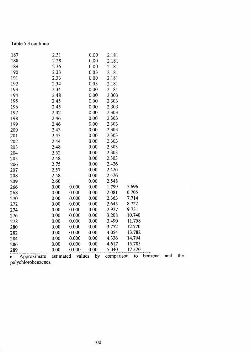
Table 5.3 continue
187 2.31 0.00 2.181188 128 0.00 2.181189 136 0.00 1181190 133 0.03 1181191 133 0.00 1181192 2.34 0.03 2.181193 2.34 0.00 2.181194 2.48 0.00 2.303195 2.45 0.00 1303196 2.45 0.00 1303197 2.42 0.00 1303198 2.46 0.00 1303199 2.46 0.00 1303200 2.43 0.00 2.303201 2.43 0.00 1303202 2.44 0.00 2.303203 2.48 0.00 1303204 152 0.00 2.303205 2.48 0.00 2.303206 2.75 0.00 2.426207 2.57 0.00 2.426208 158 0.00 2.426209 2.60 0.00 2.548266 0.00 0.000 0.00 1.799 5.696268 0.00 0.000 0.00 2.081 6.705270 0.00 0.000 0.00 2.363 7.714272 0.00 0.000 0.00 2.645 8.722274 0.00 0.000 0.00 2.927 9.731276 0.00 0.000 0.00 3.208 10.740278 0.00 0.000 0.00 3.490 11.758280 0.00 0.000 0.00 3.772 12.770282 0.00 0.000 0.00 4.054 13.782284 0.00 0.000 0.00 4.336 14.794286 0.00 0.000 0.00 4.61,7 15.785289 0.00 0.000 0.00 5.040 17.320a- Approximate estimated values by comparison topolychlorobenzenes.
benzene and the
100

5.2 Estimation of overall hydrogen-bond basicity for PCBs.
As a first step, a rough estimate of was made by comparison to values for the
polychlorobenzenes. Since only estimates were needed to start the analysis, it was felt that
values just based on the number of clilorine atoms in each PCBs ring would suffice. Tlie
values of 2 were calculated as shown in Table 5.4.
Ring A Ring B
Table 5.4. Estimated values of zp^ 2 for PCBs
ims in ring TotalA B A+B1 0 1 0.201 1 2 0.142 0 2 0.162 1 3 0.102 2 4 0.063 0 3 0.133 1 4 0.073 2 5 0.033 3 6 0.004 0 4 0.13
101
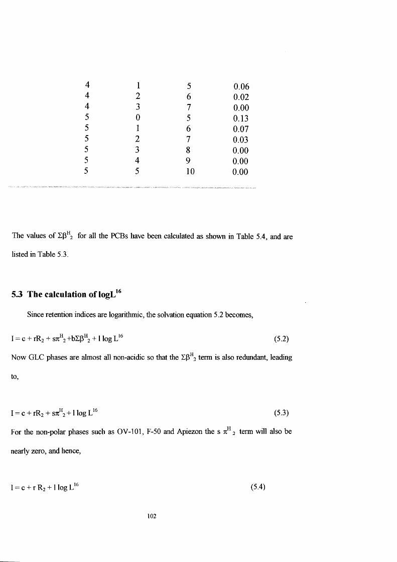
4 1 5 0.064 2 6 0.024 3 7 0.005 0 5 0.135 1 6 0.075 2 7 0.035 3 8 0.005 4 9 0.005 5 10 0.00
Tlie values of S(3 2 for all the PCBs have been calculated as shown in Table 5.4, and are
hsted in Table 5.3.
5.3 The calculation of logL ^
Since retention indices are logaritlimic, tlie solvation equation 5.2 becomes,
I = c + rR2 + S7t +bZp^ 2 +1 log (5.2)
Now GLC phases are almost all non-acidic so that tlie term is also redundant, leading
to,
I = c + rR2 + S7c“2 + HogL'^ (5.3)
For the non-polar phases such as OV-101, F-50 and Apiezon the s tc 2 term will also be
nearly zero, and hence,
1 = c + r R2 + 1 logL^ (5.4)
102

In order to obtain a linear regression to get the values of log for all PCBs using equation
(5.2) or equation (5.3), a number of n " 2 and log L' values for PCBs are necessary to start
witli (approximate estimated values by comparison to benzene and the polychlorobenzenes)
note that 2 and log are known for the alkanes. Table 5.3. The first step was to carry
out hnear regressions using tlie software system Smart for I-values on 12 stationary phases
using equation (5.2). Details of the regressions are given in Table (5.5); results were not very
satisfactory because many regression coefficients were negative, even though the equations
are statistically good.
Table 5.5 Details of multiple linear regression for all the PCBs using equation 5.2.
Phase — - Coefficients — Statistics —Name No. C r s b 1 F n
OV-101 I 72.50 535.32 -583.12 119.93 197.98 2987 0.999 221F-50 2 72.65 457.71 -480.40 198.45 197.96 3009 0.999 221APIEZ 3 71.86 482.97 -■459.72 304.29 198.04 1514 0.997 221OV-210 4 71.12 282.68 -120.61 423.66 198.11 2276 0.996 221OV-3 5 74.50 -97.48 340.32 -40.25 197.75 490 0.995 221OV-17 6 73.26 -130.47 347.91 462.66 197.89 939 0.995 221OV-25 7 72.40 333.82 -56.12 698.48 197.99 2971 0.998 221AN-600 8 71.32 148.07 -193.83 696.64 198.09 1025 0.996 221n v-995 Q 71 51 15A 76 91Q 69 -RRQ4 lOROS R114 0.99.9L ??1THOMS 10 71.63 -127.75 770.8 907.1 198.06 6664 0.997 2213HK-325 1 ] 71.70 444.92 -364.7 96.33 198.12 1477 0.997 221POLMPE12 70.75 224.62 -264.11 871.49 198.11 708 0.996 221
103
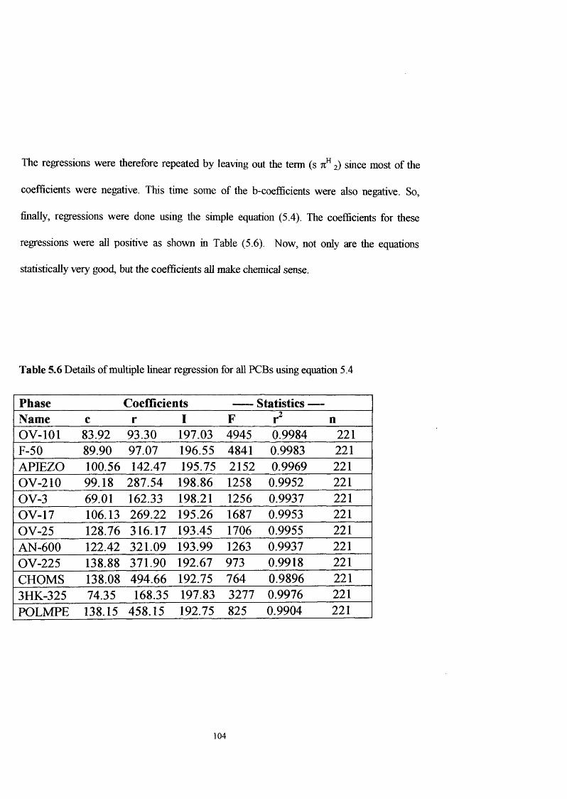
The regressions were therefore repeated by leaving out the term (s 71^ 2) since most of the
coefficients were negative. This time some of the b-coefBcients were also negative. So,
finally, regressions were done using tlie simple equation (5.4). The coefficients for these
regressions were all positive as shown in Table (5.6). Now, not only are the equations
statistically very good, but the coefficients all make chemical sense.
Table 5.6 Details of multiple linear regression for all PCBs using equation 5 .4
Phase Coefficients — — Statistics —Name c r 1 F nOV-101 83.92 93.30 197.03 4945 0.9984 221F-50 89.90 97.07 196.55 4841 0.9983 221APIEZO 100.56 142.47 195.75 2152 0.9969 221OV-210 99.18 287.54 198.86 1258 0.9952 221OV-3 69.01 162.33 198.21 1256 0.9937 221OV-17 106.13 269.22 195.26 1687 0.9953 221OV-25 128.76 316.17 193.45 1706 0.9955 221AN-600 122.42 321.09 193.99 1263 0.9937 221OV-225 138.88 371.90 192.67 973 0.9918 221CHOMS 138.08 494.66 192.75 764 0.9896 2213HK-325 74.35 168.35 197.83 3277 0.9976 221POLMPE 138.15 458.15 192.75 825 0.9904 221
104
Since tlie regression coefficients in Table 5.6 were all positive it was possible to calculate log
for all 209 PCBs; values are given in Table 5.7. The nomenclature is as follows. Results
of calculations of log from the first phase are denoted as log cl and from the second
phase, log c2 , and so on up to, log cl 2 , for POLMPE. The values of loge for the first tliree
non polar phases were in good agreement because the equation which had been used, tliat is
equation 5.4, was suitable for non polar phases. But for the other phases the equations were
not so good because the phases started to be polar.
105

Table 5.7 log L calculated for twelve phases for all PCBs based on equation 5.4.
lUPAC Log cl Logc2 Logc3 Logc4 LogcS Logc6 Loge? LogeS Logc9 LogclO Log e l l Log cl2 OV-101 F-50 APIEZO OV-210 OV-3 OV-17 OV-25 AN-600 OV-225 CHOM HK-325 POLMP
N E
6.015 6.035 6.130 5.973 5.934 6.062 6.179 6.087 6.163 6.170 5.877 6.189I 6.532 6.535 6.472 6.409 6.436 6.594 6.742 6.554 6.652 6.521 6.397 6.5164 7.049 7.035 6.814 6.846 6.939 7.125 7.306 7.082 7.142 6.872 6.917 6.8432 6.853 6.897 6.966 7.473 6.760 7.382 6.998 6.999 7.067 7.092 6.442 7.0986 7.370 7.397 7.308 7.399 7.262 7.401 7.562 7.512 7.557 7.443 7.366 7.42511 7.690 7.759 8.313 7.953 7.586 7.677 7.818 7.988 7.971 8.015 7.816 8.0083 6.908 6.942 7.040 7.064 6.803 6.991 7.082 7.124 7.205 7.227 6.916 7.2478 7.425 7.443 7.382 7.501 7.306 7.522 7.646 7.600 7.695 7.578 7.435 7.57413 7.746 7.804 7.876 8.054 7.629 7.798 7.902 8.082 8.110 8.149 7.885 8.15615 7.872 7.924 8.059 8.376 7.795 8.126 8.230 8.491 8.538 8.669 8.082 8.66110 7.005 7.001 6.852 6.768 6.869 6.965 7.172 6.900 6.995 6.718 6.790 6.73719 7.550 7.531 7.238 7.293 7.420 7.579 7.834 7.528 7.601 7.222 7.360 7.20627 7.866 7.887 7.725 7.831 7.736 7.841 8.073 7.941 7.996 7.768 7.802 7.76532 7.927 7.938 7.805 7.948 7,788 7.976 8.173 8.077 8.154 7.929 7.879 7.93754 8.052 8.026 7.661 7.739 7.902 8.033 8.361 7.989 8.060 7.573 7.804 7.5709 7.217 7.255 7.211 7.154 7,075 7.165 7.278 7.207 7.219 7.132 7.124 7.14518 7.734 7.755 7.553 7.591 7.578 7.696 7.841 7.669 7.709 7.483 7.643 7.47226 8.055 8.117 8.047 8.144 7.901 7.972 8.097 8.145 8.123 8.054 8.093 8.05531 8.110 8.671 8.121 8.246 7.945 8.094 8.181 8.228 8.314 8.189 8.162 8.20353 8.236 8.250 7.977 8.038 8.059 8.150 8.369 8.140 8.168 7.834 8.087 7.83552 8.419 8.475 8.292 8.336 8.217 8.268 8.377 8.348 8.276 8.094 8.370 8.1017 7.273 7.285 7.290 7.148 7.139 7.174 7.341 7.214 7.285 7.173 7.193 7.26217 7.790 7.780 7.632 7.585 7.641 7.705 7.910 7.706 7.775 7.524 7.712 7.58925 8.110 8.142 8.126 8.138 7.965 7.981 8.160 8.156 8.189 8.095 8.162 8.17228 8.166 8.188 8.200 8.240 8.008 8.102 8.244 8.260 8.328 8.230 8.231 8.32051 8.291 8.276 8.055 8.032 8.174 8.159 8.432 8.152 8.234 7.875 8.156 7.95349 8.475 8.500 8.371 8.330 8.280 8.276 8.440 8.339 8.342 8.135 8.439 8.27047 8.530 8.525 8.450 8.324 8.344 8.285 8.503 8.366 8.408 8.176 8.508 8.3365 7.410 7.402 7.359 7.364 7.292 7.426 7.681 7.501 7.629 7.396 7.346 7.48816 7.927 7.903 7.701 7.800 7.794 7.957 8.245 7.993 8.119 7.747 7.866 7.81520 8.248 8.264 8.195 8.353 8.118 8.234 8.501 8.444 8.533 8.319 8.315 8.39722 8.303 8.310 8.269 8.455 8.162 8,355 8.584 8.563 8.672 8.453 8.384 8.54546 8.428 8.398 8.125 8.247 8.276 8.412 8.772 8.439 8.578 8.098 8.309 8.17844 8.612 8.622 8.440 8.545 8.433 8.529 8.780 8.627 8.686 8.359 8.592 8.44442 8.668 8.647 8.519 8.539 8.497 8.538 8.843 8.638 8.752 8.400 8.661 8.56140 8.805 8.770 8.588 8.754 8.650 8.790 9.183 8.931 9.096 8.623 8.815 8.78614 7.528 7.530 7.702 7.554 7.347 7.332 7.395 7.561 7.554 7.625 7.531 7.71534 8.040 8.025 8.037 7.976 7.841 7.849 7.942 8.031 8.025 7.951 8.042 8.01836 8.370 8.397 8.546 8.558 8.180 8.153 8.231 8.515 8.478 8.573 8.509 8.64839 8.416 8.432 8.605 8.630 8.208 8.247 8.282 8.601 8.578 8.657 8.561 8.749
106
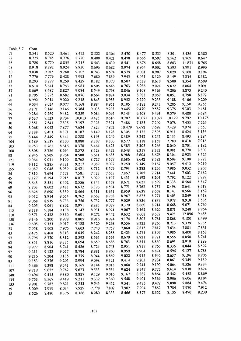
Table 5.7 73
Cont.8.541 8.520 8.461 8.422 8.322 8.304 8.470 8.477 8.535 8.301 8.486 8.382
72 8.725 8.745 8.776 8.720 8.480 8.421 8.478 8.665 8.592 8.562 8.769 8.64768 8.780 8.770 8.855 8.715 8.543 8.430 8.541 8.676 8.658 8.603 11.871 8.76558 8.918 8.892 8.924 8.930 8.696 8.682 8.974 8.964 9.002 8.593 8.991 8.99080 9.030 9.015 9.260 9.105 8.743 8.574 8.579 9.001 8.907 9.029 9.168 9.19412 7.776 7.779 8.428 7.993 7.680 7.839 7.943 8.051 8.120 8.149 7.834 8.18233 8.293 8.279 8.259 8.429 8.182 8.370 8.507 8.538 8.610 8.500 8.354 8.50935 8.614 8.641 8.753 8.983 8.505 8.646 8.763 8.988 9.024 9.072 8.804 9.09137 8.669 8.687 8.827 9.084 8.549 8.768 8.846 9.108 9.163 9.206 8.873 9.24071 8.795 8.775 8.682 8.876 8.664 8.824 9.034 8.983 9.069 8.851 8.798 8.87270 8.992 9.014 9.020 9.218 8.845 8.983 8.952 9.220 9.235 9.188 9.106 9.20966 9.034 9.024 9.077 9.168 8.884 8.951 9.105 9.182 9.243 7.285 9.150 9.25556 9.171 9.146 9.146 9.384 9.038 9.203 9.445 9.470 9.587 9.376 9.303 9.48179 9.284 9.269 9.482 9.559 9.084 9.095 9.143 9.508 9.493 9.579 9.480 9.68477 9.537 9.523 9.704 10.013 9.425 9.616 9.707 10.071 10.078 10.129 9.792 10.17530 7.551 7.541 7.535 7.197 7.323 7.321 7.486 7.185 7.209 7.078 7.455 7.22650 8.068 8.042 7.877 7.634 7.825 7.852 10.479 7.672 7.699 7.429 7.974 7.55364 8.388 8.403 8.371 8.187 8.149 8.128 8.305 8.122 7.595 6.911 8.424 8.13675 8.444 8.449 8.444 8.288 8.193 8.249 8.389 8.242 8.252 8.135 8.493 8.284104 8.589 8.537 8.300 8.080 8.307 8.306 8.577 8.118 8.158 7.780 8.418 7.916103 8.753 8.761 8.616 8.378 8.464 8.423 8.585 8.305 8.266 8.040 8.701 8.182100 8.808 8.786 8.694 8.373 8.528 8.432 8.648 8.317 8.332 8.081 8.770 8.30098 8.946 8.909 8.764 8.588 8.681 8.685 8.988 8.604 8.676 8.304 8.923 8.525121 9.064 9.031 9.100 8.763 8.727 8.577 8.686 8.642 8.582 8.508 9.100 8.728119 9.312 9.285 9.321 9.217 9.069 9.097 9.250 9.149 9.167 9.057 9.412 9.219155 9.087 9.048 8.939 8,421 8,712 8 579 8.793 8.283 8.256 7.986 9.032 8.26324 7.810 7.694 7.573 7.581 7.527 7.665 7.867 7.705 7.714 7.441 7.603 7.46245 8.327 8.194 7.915 8.017 8.029 8.197 8.431 8.192 8.204 7.792 8.122 7.78959 8.643 8.551 8.402 8.556 8.345 8.459 8.671 8.625 8.599 8.338 8.564 8.34769 8.703 8.602 8.483 8.672 8.396 8.594 8.771 8.762 8.757 8.498 8.641 8.51996 8.828 8.690 8.339 8.464 8.511 8.651 8.959 8.637 8.668 8.143 8.566 8.15295 9.012 8.914 8.654 8.762 8.668 8.768 8.967 8.825 8.771 8.403 8.849 8.41891 9.068 8.939 8.733 8.756 8.732 8.777 9.029 8.836 8.837 7.978 8.918 8.53584 9.205 9.061 8.802 8.971 8.885 9.029 9.370 8.660 8.714 8.668 9.071 8.760113 9.318 9.184 9.138 9.147 8.931 8.921 9.067 9.162 8.620 8.871 9.248 8.964110 9.571 9.438 9.360 9.601 9.272 9.442 9.632 9.668 9.672 9.421 12.896 9.455150 9.346 9.200 8.978 8.805 8.916 8.924 9.174 8.803 8.761 8.868 9.180 8.499136 9.605 9.353 9.017 9.188 9.120 9.268 9.556 9.322 9.266 8.713 9.379 8.73523 7.958 7.908 7.976 7.603 7.740 7.757 7.860 7.815 7.817 7.634 7.881 7.83143 8.475 8.408 8.318 8.039 8.242 8.288 8.423 8.271 8.307 7.985 8.400 8.15857 8.796 8.770 8.812 8.593 8.565 8.564 8.679 8.721 8.721 8.556 8.850 8.74163 8.851 8.816 8.885 8.694 8.659 8.686 8.763 8.841 8.860 8.691 8.919 8.88994 8.977 8.904 8.741 8.486 8.724 8.743 8.951 8.717 8.766 8.336 8.844 8.52292 9.211 9.128 9.057 8.784 8.881 8.860 8.959 8.904 8.874 8.596 9.127 8.78890 9.216 9.204 9.135 8.779 8.944 8.869 9.022 8.915 8.940 8.637 9.196 8.90583 9.353 9.276 9.205 8.994 9.098 9.121 9.414 9.203 9.284 8.861 9.349 9.130111 9.466 9.398 9.541 9.169 9.144 9.013 9.060 9.241 9.190 9.064 9.526 9.334107 9.719 9.652 9.762 9.623 9.535 9.534 9.624 9.747 9.775 9.614 9.838 9.824148 9.494 9.415 9.380 8.827 9.129 9.016 9.167 8.882 8.864 8.542 9.458 8.869135 9.753 9.567 9.419 9.211 9.332 9.360 9.548 9.401 9.369 8.906 9.606 9.104133 9.901 9.782 9.821 9.233 9.545 9.452 9.541 9.475 9.472 9.098 9.884 9.47429 8.009 7.979 8.034 7.929 7.778 7.802 7.902 7.904 7.862 7.784 7.970 7.91248 8.526 8.480 8.376 8.366 8.280 8.333 8.466 8.375 8.352 8.135 8.490 8.239
107
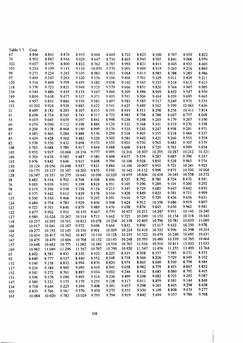
Table 5.7 67
Cont.8.846 8.841 8.870 8.919 8.604 8.609 8.722 8.825 8.300 8.707 8.939 8.822
74 8.902 8.887 8.944 9.020 8.647 8.730 8.805 8.945 8.905 8.841 9.008 8.970102 9.027 8.975 8.800 8.812 8.762 8.787 8.993 8.821 8.811 8.445 8.933 8.603101 9.216 9.199 9.115 9.110 10.059 9.570 9.001 9.003 8.919 9.265 9.216 8.86999 9.271 9.224 9.245 9.105 8.983 8.913 9.064 9.015 8.985 8.788 9.285 8.98697 9.404 9.347 9.263 9.320 9.136 9.166 9.404 7.761 9.329 9.011 9.439 9.211120 9.516 9.469 9.599 9.495 9.182 9.058 9.102 9.345 9.235 9.214 9.615 9.415118 9.770 9.723 9.821 9.949 9.523 9.579 9.666 9.851 9.820 9.764 9.947 9.905154 9.544 9.486 9.439 9.153 9.167 9.060 9.209 8.986 8.909 8.692 9.547 8.950149 9.804 9.638 9.477 9.537 9.371 9.405 9.591 9.506 9.414 8.039 9.695 9.465146 9.957 9.853 9.880 9.559 9.583 9.497 9.583 9.585 9.517 9.249 9.973 9.555153 10.002 9.924 9.938 9.885 9.622 9.541 9.625 9.689 9.562 9.399 10.063 9.63621 8.689 8.183 8.203 8.307 8.015 8.191 8.419 8.311 8.298 8.256 10.411 7.81441 8.698 8.734 8.545 8.743 8.517 8.722 8.983 8.798 8.788 8.607 8.757 8.60855 9.019 9.045 9.039 9.297 8.841 8.998 9.238 9.248 9.203 9.179 9.207 9.19060 9.074 9.090 9.112 9.398 8.884 9.120 9.322 9.368 9.341 9.319 9.276 9.33889 9.200 9.178 8.968 9.190 8.999 9.176 9.510 9.243 9.247 8.958 9.201 8.97187 9.383 9.403 9.284 9.488 9.156 9.294 9.518 9.405 9.355 9.218 9.484 9.23785 9.439 9.428 9.362 9.482 9.220 9.302 9.581 9.442 9.421 9.260 9.553 9.35482 9.576 9.550 9.432 9.698 9.373 9.555 9.921 9.730 9.765 9.483 9.707 9.579108 9.703 9.688 9.789 9.917 9.444 9.488 9.668 9.818 9.729 9.763 9.909 9.854105 9.952 9.937 10.004 10.356 9.777 9.995 10.216 10.307 10.295 10.287 10.212 10.321140 9.703 9.674 9.585 9.487 9.380 9.408 9.677 9.359 9.287 9.087 9.790 9.247132 9.976 9.842 9.646 9.915 9.608 9.794 10.108 9.928 9.850 9.528 9.963 9.554130 10.124 10.056 10.048 9.937 9.821 9.886 10.100 10.007 9.953 9.721 10.241 9.923138 10.175 10.127 10.107 10.263 9.859 9.930 10.142 10.112 9.998 9.871 10.330 10.004128 10.347 10.331 10.275 10.641 10.096 10.320 10.659 10.606 10.434 10.343 10.558 10.37238 8.482 8.534 8.702 8.748 8.308 8.406 8.525 8.792 8.780 8.724 8.672 8.94176 9.003 9.039 9.051 9.199 8.819 8.951 9.105 9.296 9.289 9.101 9.200 9.29278 9.319 9.396 9.538 9.738 9.134 9.213 9.345 9.729 9.685 9.647 9.642 9.85081 9.375 9.442 9.612 9.839 9.178 9.334 9.428 9.849 9.823 9.781 9.711 9.999125 9.500 9.530 9.468 9.631 9.293 9.391 9.616 9.725 9.729 9.426 9.636 9.631124 9.684 9.754 9.783 9.929 9.450 9.508 9.624 9.912 10.356 9.686 9.919 9.897123 9.725 9.765 9.840 9.879 9.489 9.476 9.638 9.874 9.845 9.650 9.962 9.943122 9.877 9.902 9.931 10.139 9.667 9.770 10.027 10.211 10.247 9.951 10.141 10.240127 9.989 10.024 10.267 10.314 9.713 9.662 9.725 10.249 10.153 10.154 10.318 10.443118 10.257 10.293 10.511 10.812 10.078 10.224 10.338 10.805 10.796 10.781 10.655 11.005168 10.017 10.041 10.107 9.972 9.698 9.664 9.832 9.890 15.017 9.632 10.250 9.978164 10.277 10.193 10.145 10.356 9.901 10.009 10.214 10.410 10.332 9.996 10.398 10.214162 10.434 10.417 10.562 10.407 10.130 10.128 10.239 10.522 10.474 10.240 10.693 10.631167 10.475 10.479 10.606 10.704 10.152 10.145 10.248 10.593 10.480 10.339 10.765 10.664157 10.648 10.682 10.775 11.082 10.389 10.534 10.765 11.016 10.916 10.811 11.033 11.033169 10.962 11.049 11.296 11.567 10.707 10.790 10.920 11.547 11.456 11.355 11.493 11.76465 8.602 8.581 8.432 8.330 8.432 8.225 8.435 8.308 8.357 7.985 8.171 8.35393 8.840 8.777 8.337 8.440 8.552 8.548 8.718 8.366 8.226 7.729 8.349 8.102112 9.160 9.138 8.832 8.994 8.876 8.824 8.974 8.863 8.640 8.300 8.798 8.684117 9.216 9.184 8.905 9.095 8.919 8.945 9.058 8.982 8.779 8.435 8.867 8.832152 9.341 9.272 8.761 8.887 9.034 9.002 9.246 8.812 8.685 8.080 8.792 8.465151 9.596 9.570 9.186 9.405 9.314 9.326 9.499 9.248 9.082 8.725 9.203 9.087147 9.580 9.521 9.155 9.179 9.255 9.128 9.317 9.011 8.859 8.381 9.144 8.848134 9.718 9.644 9.225 9.394 9.408 9.381 9.657 9.298 9.203 8.605 9.298 8.658165 9.830 9.766 9.561 9.570 9.454 9.273 9.355 9.336 9.109 8.808 9.474 9.277163 10.084 10.020 9.782 10.024 9.795 9.794 9.919 9.842 9.694 9.357 9.786 9.768
108
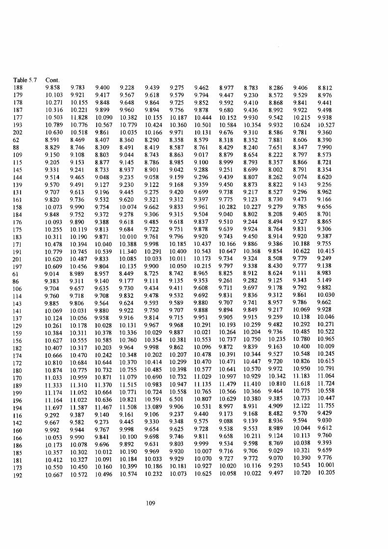
Table 5.7 188
Cont.9.858 9.783 9.400 9.228 9.439 9.275 9.462 8.977 8.783 8.286 9.406 8.812
179 10.103 9.921 9.417 9.567 9.618 9.579 9.794 9.447 9.230 8.572 9.529 8.976178 10.271 10.155 9.848 9.648 9.864 9.725 9.852 9.592 9.410 8.868 9.841 9.441187 10.316 10.221 9.899 9.960 9.894 9.756 9.878 9.680 9.436 8.992 9.922 9.498177 10.503 11.828 10.090 10.382 10.155 10.187 10.444 10.152 9.930 9.542 10.215 9.938193 10.789 10.776 10.567 10.779 10.424 10.360 10.501 10.584 10.354 9.932 10.624 10.527202 10.630 10.518 9.861 10.035 10.166 9.971 10.131 9.676 9.310 8.586 9.781 9.36062 8.591 8.469 8.407 8.360 8.290 8.358 8.579 8.318 8.352 7.881 8.606 8.39088 8.829 8.746 8.309 8.491 8.419 8.587 8.761 8.429 8.240 7.651 8.347 7.990109 9.150 9.108 8.803 9.044 8.743 8.863 9.017 8.879 8.654 8.222 8.797 8.573115 9.205 9.153 8.877 9.145 8.786 8.985 9.100 8.999 8.793 8.357 8.866 8.721145 9.331 9.241 8.733 8.937 8.901 9.042 9.288 9.251 8.699 8.002 8.791 8.354144 9.514 9.465 9.048 9.235 9.058 9.159 9.296 9.439 8.807 8.262 9.074 8.620139 9.570 9.491 9.127 9.230 9.122 9.168 9.359 9.450 8.873 8.822 9.143 9.256131 9.707 9.613 9.196 9.445 9.275 9.420 9.699 9.738 9.217 8.527 9.296 8.962161 9.820 9.736 9.532 9.620 9.321 9.312 9.397 9.775 9.123 8.730 9.473 9.166158 10.073 9.990 9.754 10.074 9.662 9.833 9.961 10.282 10.227 9.279 9.785 9.656184 9.848 9.752 9.372 9.278 9.306 9.315 9.504 9.040 8.802 8.208 9.405 8.701176 10.093 9.890 9.388 9.618 9.485 9.618 9.837 9.510 9.244 8.494 9.527 8.865175 10.255 10.119 9.813 9.684 9.722 9.751 9.878 9.639 9.924 8.764 9.831 9.306183 10.311 10.190 9.871 10.010 9.761 9.796 9.920 9.743 9.450 8.914 9.920 9.387171 10.478 10.394 10.040 10.388 9.998 10.185 10.437 10.166 9.886 9.386 10.188 9.755191 10.779 10.745 10.539 11.340 10.291 10.400 10.543 10.647 10.368 9.854 10.622 10.415201 10.620 10.487 9.833 10.085 10.033 10.011 10.173 9.734 9.324 8.508 9.779 9.249197 10.609 10.456 9.804 10.135 9.900 10.050 10.215 9.797 9.338 8.430 9.777 9.13861 9.014 8.989 8.957 8.449 8.725 8.742 8.965 8.825 8.912 8.624 9.111 8.98386 9.383 9.311 9.140 9.177 9.111 9.135 9.353 9.261 9.282 9.125 9.343 5.149106 9.704 9.657 9.635 9.730 9.434 9.411 9.608 9.711 9.697 9.178 9.792 9.882114 9.760 9.718 9.708 9.832 9.478 9.532 9.692 9.831 9.836 9.312 9.861 10.030143 9.885 9.806 9.564 9.624 9.593 9.589 9.880 9.707 9.741 8.957 9.786 9.662141 10.069 10.031 9.880 9.922 9.750 9.707 9.888 9.894 9.849 9.217 10.069 9.928137 10.124 10.056 9.958 9.916 9.814 9.715 9.951 9.905 9.915 9.259 10.138 10.046129 10.261 10.178 10.028 10.131 9.967 9.968 10.291 10.193 10.259 9.482 10.292 10.271159 10.384 10.311 10.378 10.336 10.029 9.887 10.021 10.264 10.204 9.736 10.485 10.522156 10.627 10.555 10.585 10.760 10.354 10.381 10.553 10.737 10.750 10.235 10.780 10.965182 10.407 10.317 10.203 9.964 9.998 9.862 10.096 9.872 9.839 9.163 10.400 10.009174 10.666 10.470 10.242 10.348 10.202 10.207 10.478 10.391 10.344 9.527 10.548 10.245172 10.810 10.684 10.644 10.370 10.414 10.299 10.470 10.471 10.447 9.720 10.826 10.615180 10.874 10.775 10.732 10.755 10.485 10.398 10.577 10.641 10.570 9.972 10.950 10.791170 11.033 10.959 10.871 11.079 10.690 10.732 11.029 10.997 10.929 10.342 11.183 11.064189 11.333 11.310 11.370 11.515 10.983 10.947 11.135 11.479 11.410 10.810 11.618 11.724199 11.174 11.052 10.664 10.771 10.724 10.558 10.765 10.566 10.366 9.464 10.775 10.558196 11.164 11.022 10.636 10.821 10.591 6.501 10.807 10.629 10.380 9.385 10.733 10.447194 11.697 11.587 11.467 11.508 13.089 9.906 10.531 8.997 8.931 4.909 12.122 11.755116 9.292 9.387 9.140 9.161 9.106 9.237 9.440 9.173 9.168 8.482 9.570 9.429142 9.667 9.582 9.273 9.445 9.330 9.348 9.575 9.088 9.139 8.936 9.594 9.030160 9.992 9.944 9.767 9.998 9.654 9.625 9.728 9.538 9.553 8.989 10.044 9.612166 10.053 9.990 9.841 10.100 9.698 9.746 9.811 9.658 10.211 9.124 10.113 9.760186 10.173 10.078 9.696 9.892 9.631 9.803 9.999 9.534 9.598 8.769 10.038 9.393185 10.357 10.302 10.012 10.190 9.969 9.920 10.007 9.716 9.706 9.029 10.321 9.659181 10.412 10.327 10.091 10.184 10.033 9.929 10.070 9.727 9.772 9.070 10.390 9.776173 10.550 10.450 10.160 10.399 10.186 10.181 10.927 10.020 10.116 9.293 10.543 10.001192 10.667 10.572 10.496 10.574 10.232 10.073 10.625 10.058 10.022 9.497 10.720 10.205
109
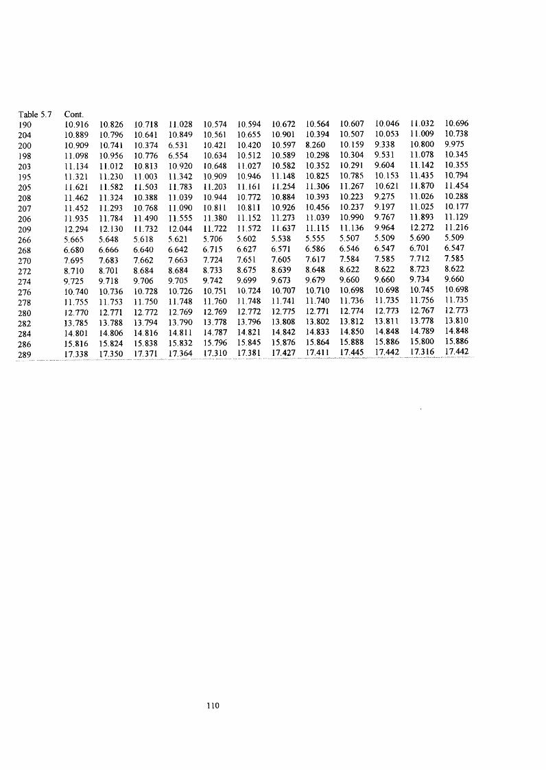
Table 5.7 190
Cont.10.916 10.826 10.718 11.028 10.574 10.594 10.672 10.564 10.607 10.046 11.032 10.696
204 10.889 10.796 10.641 10.849 10.561 10.655 10.901 10.394 10.507 10.053 11.009 10.738200 10.909 10.741 10.374 6.531 10.421 10.420 10.597 8.260 10.159 9.338 10.800 9.975198 11.098 10.956 10.776 6.554 10.634 10.512 10.589 10.298 10.304 9.531 11.078 10.345203 11.134 11.012 10.813 10.920 10.648 11.027 10.582 10.352 10.291 9.604 11.142 10.355195 11.321 11.230 11.003 11.342 10.909 10.946 11.148 10.825 10.785 10.153 11.435 10.794205 11.621 11.582 11.503 11.783 11.203 11.161 11.254 11.306 11.267 10.621 11.870 11.454208 11.462 11.324 10.388 11.039 10.944 10.772 10.884 10.393 10.223 9.275 11.026 10.288207 11.452 11.293 10.768 11.090 10.811 10.811 10.926 10.456 10.237 9.197 11.025 10.177206 11.935 11.784 11.490 11.555 11.380 11.152 11.273 11.039 10.990 9.767 11.893 11.129209 12.294 12.130 11.732 12.044 11.722 11.572 11.637 11.115 11.136 9.964 12.272 11.216266 5.665 5.648 5.618 5.621 5.706 5.602 5.538 5.555 5.507 5.509 5.690 5.509268 6.680 6.666 6.640 6.642 6.715 6.627 6.571 6.586 6.546 6.547 6.701 6.547270 7.695 7.683 7.662 7.663 7.724 7.651 7.605 7.617 7.584 7.585 7.712 7.585272 8.710 8.701 8.684 8.684 8.733 8.675 8.639 8.648 8.622 8.622 8.723 8.622274 9.725 9.718 9.706 9.705 9.742 9.699 9.673 9.679 9.660 9.660 9.734 9.660276 10.740 10.736 10.728 10.726 10.751 10.724 10.707 10.710 10.698 10.698 10.745 10.698278 11.755 11.753 11.750 11.748 11.760 11.748 11.741 11.740 11.736 11.735 11.756 11.735280 12.770 12.771 12.772 12.769 12.769 12.772 12.775 12.771 12.774 12.773 12.767 12.773282 13.785 13.788 13.794 13.790 13.778 13.796 13.808 13.802 13.812 13.811 13.778 13.810284 14.801 14.806 14.816 14.811 14.787 14.821 14.842 14.833 14.850 14.848 14.789 14.848286 15.816 15.824 15.838 15.832 15.796 15.845 15.876 15.864 15.888 15.886 15.800 15.886289 17.338 17.350 17.371 17.364 17.310 17.381 17.427 17.411 17.445 17.442 17.316 17.442
n o

The second step was to take the average of the first tliree phases, i e. log L (cl+c2+c3).
The average values were taken again to do the regression for the first three phases, OV-101,
F-50, APIEZON. Then the values for these three phases were averaged again, and
these values were taken along with the few original ones in order to get the best values for
log c avg., (log L best), as shown in Table 5.8.
I l l
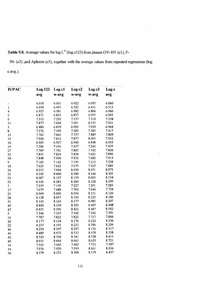
Table 5.8. Average values for log (log cl23) from phases OV-101 (cl), F-
50- (c2) ,and Apiezon (c3), together with tlie average values from repeated regressions (log
c avg.).
lUPAC Log 123 Log cl Log c2 Log c3 Logoavg w-avg w-avg w-avg avg
6.010 6.001 6.022 6.095 6.0601 6.650 6.491 6.502 6.451 6.5134 6.923 6.981 6.982 6.806 6.9662 6.871 6.803 6.857 6.955 6.9056 7.313 7.293 7.337 7.310 7.35811 7.877 7.604 7.691 8.335 7.9213 6.480 6.859 6.903 7.030 6.9648 7.372 7.349 7.383 7.385 7.41713 7.763 7.661 7.737 7.889 7.80915 7.920 7.813 7.877 8.065 7.95210 6.905 6.927 6.940 6.848 6.95319 7.386 7.456 7.457 7.244 7.43927 7.769 7.761 7.805 7.742 7.82632 7.835 7.824 7.858 7.823 7.89054 7.848 7.930 7.932 7.682 7.9139 7.183 7.142 7.195 7.212 7.22818 7.625 7.632 7.675 7.567 7.68126 8.015 7.944 8.030 8.071 8.07331 8.242 8.000 8.580 8.146 8.30153 8.087 8.107 8.150 8.005 8.15452 8.326 8.283 8.369 8.328 8.3957 7.239 7.199 7.227 7.291 7.28317 7.679 7.688 7.702 7.646 7.73425 8.069 8.000 8.056 8.151 8.12628 8.128 8.057 8.103 8.225 8.18451 8.142 8.163 8.177 8.085 8.20749 8.800 8.339 8.395 8.407 8.44847 8.435 8.396 8.421 8.487 8.5025 7.346 7.333 7.342 7.362 7.39116 7.787 7.822 7.822 7.717 7.84420 8.177 8.134 8.176 8.222 8.23622 8.237 8.191 8.223 8.296 8.29446 8.250 8.297 8.297 8.156 8.31744 8.489 8.473 8.515 8.478 8.55842 8.543 8.530 8.541 8.558 8.61140 8.651 8.664 8.661 8.629 8.72114 7.541 7.445 7.465 7.713 7.58734 7.976 7.929 7.939 8.061 8.03436 8.379 8.253 8.306 8.579 8.437
112
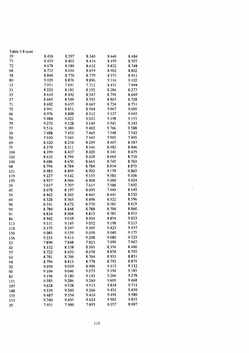
Table 5.8 cont. 39 8.426 8.297 8.340 8.640 8.48473 8.439 8.403 8.414 8.499 8.50772 8.678 8.580 8.632 8.822 8.74868 8.732 8.636 8.659 8.902 8.80258 8.840 8.770 8.779 8.973 8.91180 9.029 8.876 8.896 9.316 9.10212 7.951 7.691 7.712 8.451 7.99433 8.220 8.181 8.192 8.286 8.27735 8.610 8.492 8.547 8.791 8.66937 8.669 8.549 8.593 8.865 8.72871 8.682 8.655 8.667 8.724 8.75170 8.941 8.851 8.904 9.067 9.00966 8.976 8.888 8.912 9.127 9.04556 9.084 9.022 9.032 9.198 9.15579 9.273 9.128 9.149 9.541 9.34577 9.516 9.380 9.402 9.766 9.58830 7.488 7.453 7.465 7.548 7.54250 7.930 7.943 7.945 7.903 7.99569 8.320 8.254 8.299 8.407 8.38775 8.379 8.311 8.346 8.482 8.446104 8.399 8.437 8.420 8.341 8.475103 8.632 8.594 8.638 8.664 8.710100 8.686 8.650 8.665 8.743 8.76398 8.794 8.784 8.784 8.814 8.873121 8.985 8.895 8.902 9.158 9.065119 9.227 9.142 9.155 9.383 9.306155 8.937 8.904 8.908 9.000 9.02424 7.637 7.707 7.615 7.588 7.69245 8.078 8.197 8.095 7.943 8.14559 8.462 8.502 8.443 8.441 8.53269 8.528 8.565 8.496 8.522 8.59696 8.541 8.672 8.570 8.381 8.61995 8.780 8.848 8.788 8.704 8.86091 8.834 8.904 8.815 8.783 8.91384 8.942 9.038 8.934 8.854 9.023113 9.131 9.145 9.052 9.198 9.213110 9.375 9.397 9.305 9.423 9.457150 9.085 9.159 9.058 9.040 9.175136 9.233 9.413 9.208 9.080 9.32523 7.890 7.848 7.823 7.999 7.94743 8.332 8.338 8.303 8.354 8.40057 8.722 8.650 8.658 8.858 8.79363 8.781 8.706 8.704 8.933 8.85194 8.794 8.813 8.778 8.792 8.87492 9.050 9.039 8.996 9.115 9.13290 9.104 9.046 9.073 9.194 9.18583 9.196 9.180 9.143 9.266 9.278111 9.385 9.286 9.260 9.609 9.468107 9.628 9.538 9.513 9.834 9.711148 9.339 9.300 9.266 9.451 9.430135 9.487 9.554 9.416 9.491 9.580133 9.740 9.695 9.624 9.902 9.83529 7.951 7.900 7.895 8.057 8.007
113
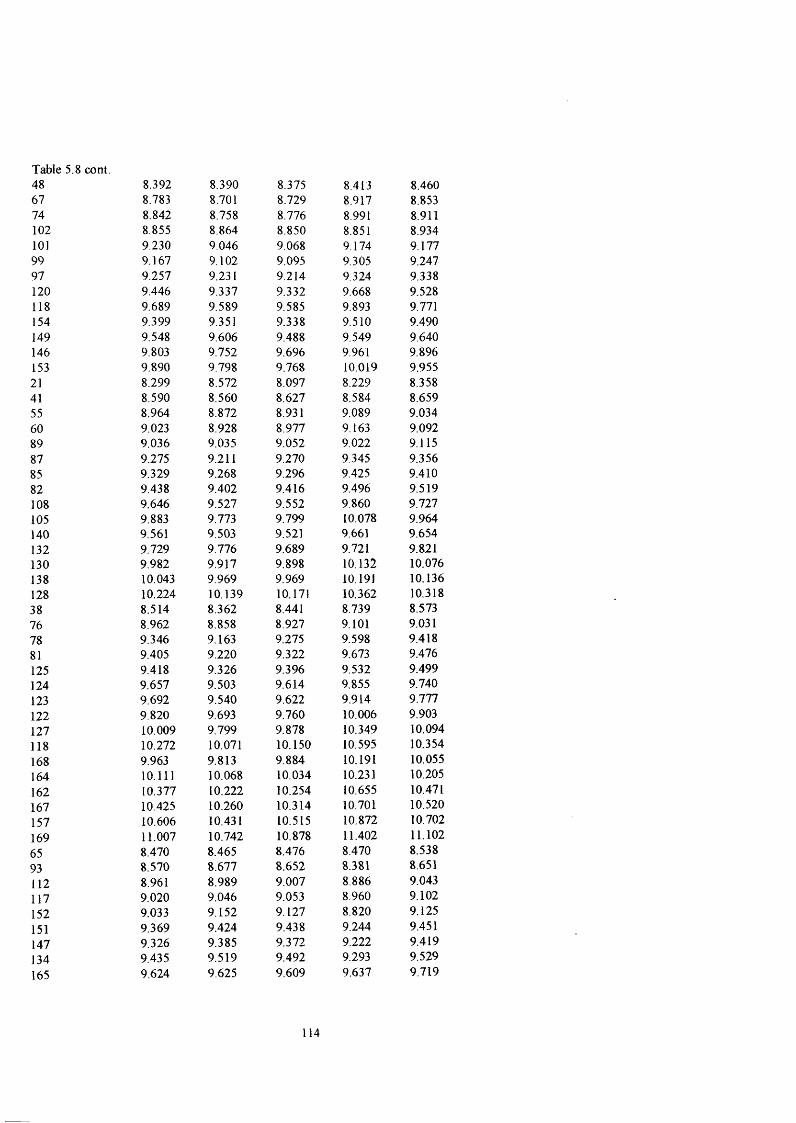
Table 5.8 cont. 48 8.392 8.390 8.375 8.413 8.46067 8.783 8.701 8.729 8.917 8.85374 8.842 8.758 8.776 8.991 8.911102 8.855 8.864 8.850 8.851 8.934101 9.230 9.046 9.068 9.174 9.17799 9.167 9.102 9.095 9.305 9.24797 9.257 9.231 9.214 9.324 9.338120 9.446 9.337 9.332 9.668 9.528118 9.689 9.589 9.585 9.893 9.771154 9.399 9.351 9.338 9.510 9.490149 9.548 9.606 9.488 9.549 9.640146 9.803 9.752 9.696 9.961 9.896153 9.890 9.798 9.768 10.019 9.95521 8.299 8.572 8.097 8.229 8.35841 8.590 8.560 8.627 8.584 8.65955 8.964 8.872 8.931 9.089 9.03460 9.023 8.928 8.977 9.163 9.09289 9.036 9.035 9.052 9.022 9.11587 9.275 9.211 9.270 9.345 9.35685 9.329 9.268 9.296 9.425 9.41082 9.438 9.402 9.416 9.496 9.519108 9.646 9.527 9.552 9.860 9.727105 9.883 9.773 9.799 10.078 9.964140 9.561 9.503 9.521 9.661 9.654132 9.729 9.776 9.689 9.721 9.821130 9.982 9.917 9.898 10.132 10.076138 10.043 9.969 9.969 10.191 10.136128 10.224 10.139 10.171 10.362 10.31838 8.514 8.362 8.441 8.739 8.57376 8.962 8.858 8.927 9.101 9.03178 9.346 9.163 9.275 9.598 9.41881 9.405 9.220 9.322 9.673 9.476125 9.418 9.326 9.396 9.532 9.499124 9.657 9.503 9.614 9.855 9.740123 9.692 9.540 9.622 9.914 9.777122 9.820 9.693 9.760 10.006 9.903127 10.009 9.799 9.878 10.349 10.094118 10.272 10.071 10.150 10.595 10.354168 9.963 9.813 9.884 10.191 10.055164 10.111 10.068 10.034 10.231 10.205162 10.377 10.222 10.254 10.655 10.471167 10.425 10.260 10.314 10.701 10.520157 10.606 10.431 10.515 10.872 10.702169 11.007 10.742 10.878 11.402 11.10265 8.470 8.465 8.476 8.470 8.53893 8.570 8.677 8.652 8.381 8.651112 8.961 8.989 9.007 8.886 9.043117 9.020 9.046 9.053 8.960 9.102152 9.033 9.152 9.127 8.820 9.125151 9.369 9.424 9.438 9.244 9.451147 9.326 9.385 9.372 9.222 9.419134 9.435 9.519 9.492 9.293 9.529165 9.624 9.625 9.609 9.637 9.719
114

Table 5.8 cont. 163 9.867 9.877 9.862 9.862 9.962188 9.577 9.639 9.615 9.478 9.680179 9.706 9.874 9.746 9.498 9.814178 9.986 10.041 9.979 9.936 10.091187 10.040 10.086 10.045 9.988 10.145177 10.699 10.276 11.641 10.180 10.807193 10.603 10.548 10.591 10.670 10.711202 10.218 10.374 10.322 9.957 10.33662 8.421 8.455 8.365 8.444 8.48988 8.548 8.669 8.623 8.352 8.628109 8.938 8.980 8.977 8.856 9.020115 8.997 9.037 9.024 8.931 9.078145 9.011 9.143 9.098 8.790 9.101144 9.250 9.320 9.316 9.113 9.343139 9.304 9.376 9.343 9.192 9.396131 9.412 9.510 9.463 9.264 9.505161 9.601 9.616 9.580 9.607 9.696158 9.845 9.869 9.833 , 9.832 9.939184 9.555 9.630 9.586 9.449 9.657176 9.684 9.866 9.717 9.468 9.790175 9.957 10.026 9.944 9.900 10.062183 10.019 10.083 10.016 9.959 10.124171 10.199 10.248 10.217 10.130 10.304191 10.580 10.540 10.562 10.640 10.688201 10.195 10.365 10.293 9.928 10.313197 10.173 10.357 10.264 9.898 10.29061 8.916 8.867 8.876 9.005 8.98786 9.197 9.211 9.179 9.200 9.278106 9.582 9.523 9.518 9.704 9.665114 9.646 9.579 9.580 9.778 9.729143 9.659 9.686 9.654 9.638 9.752141 9.898 9.862 9.872 9.961 9.993137 9.953 9.919 9.899 10.040 10.046129 10.061 10.053 10.019 10.111 10.156159 10.263 10.172 10.148 10.468 10.357156 10.493 10.411 10.389 10.680 10.589182 10.205 10.178 10.142 10.297 10.309174 10.354 10.432 10.292 10.337 10.459172 10.605 10.568 10.500 10.748 10.713180 10.690 10.640 10.597 10.833 10.793170 10.847 10.790 10.773 10.978 10.954189 11.229 11.082 11.118 11.488 11.338199 10.844 10.908 10.849 10.775 10.963196 10.822 10.899 10.820 10.746 10.940194 11.464 11.421 11.376 11.593 11.584116 9.192 9.121 9.255 9.200 9.273142 9.415 9.470 9.432 9.342 9.507160 9.807 9.787 9.787 9.846 9.901166 9.867 9.848 9.833 9.921 9.961186 9.879 9.950 9.907 9.780 9.982185 10.118 10.126 10.126 10.103 10.224181 10.172 10.183 10.152 10.182 10.277173 10.281 10.317 10.272 10.253 10.386
115

Table 5.8 cont. 192 10.471 10.428 10.389 10.597 10.579190 10.713 10.675 10.642 10.822 10.820204 10.695 10.706 10.656 10.724 10.776200 10.558 10.651 10.545 10.479 10.675198 10.825 10.832 10.753 10.890 10.943203 10.866 10.865 10.806 10.928 10.986195 11.067 11.054 11.027 11.120 11.185205 11.449 11.346 11.371 11.630 11.569208 10.925 11.172 11.102 10.502 11.058207 11.041 11.163 11.073 10.888 11.171206 11.593 11.610 11.536 11.634 11.736209 11.910 11.970 11.882 11.877 12.052266 5.700 5.889 5.817 5.490 5.644268 6.710 6.892 6.826 6.530 6.662270 7.710 7.894 7.834 7.569 7.680272 8.720 8.897 8.842 8.609 8.698274 9.730 9.900 9.850 9.648 9.716276 10.740 10.902 10.858 10.688 10.735278 11.760 11.905 11.866 11.728 11.753280 12.770 12.908 12.874 12.767 12.771282 13.780 13.911 13.883 13.807 13.789284 14.790 14.913 14.891 14.846 14.807286 15.790 15.916 15.899 15.886 15.826289 17.320 17.420 17.411 17.445 17.353
116

5.4 The calculation of the solute dipolarity/polarisability parameter- n *^2
In order to find the best values for similar calculations were started using the fourth
and subsequent phases, which are all somewhat polar. Then equation 5.3, recast as equation
5.5, could be used to find
7T^=[I-c-rR2 -llogL'" ]/s (5.5)
For eight phases from OV-210, up to POLMPE, multiple linear regressions were carried
out, and used to back-calculate n ^ 2 values tlirough equation 5.5. The obtained 7t 2 values are
given in Table 5.9. Unfortunately, the % ^ 2 values were not constant across the phases. For
example, values for PCB 66 range form 1.403 to -0.138, the latter negative value being quite
unrealistic. The most consistent values were obtained from phases 4,5,7 and 11, and
tlierefore n " 2 values were averaged from these four phases only. These values are denoted as
K 1st - rd .
117
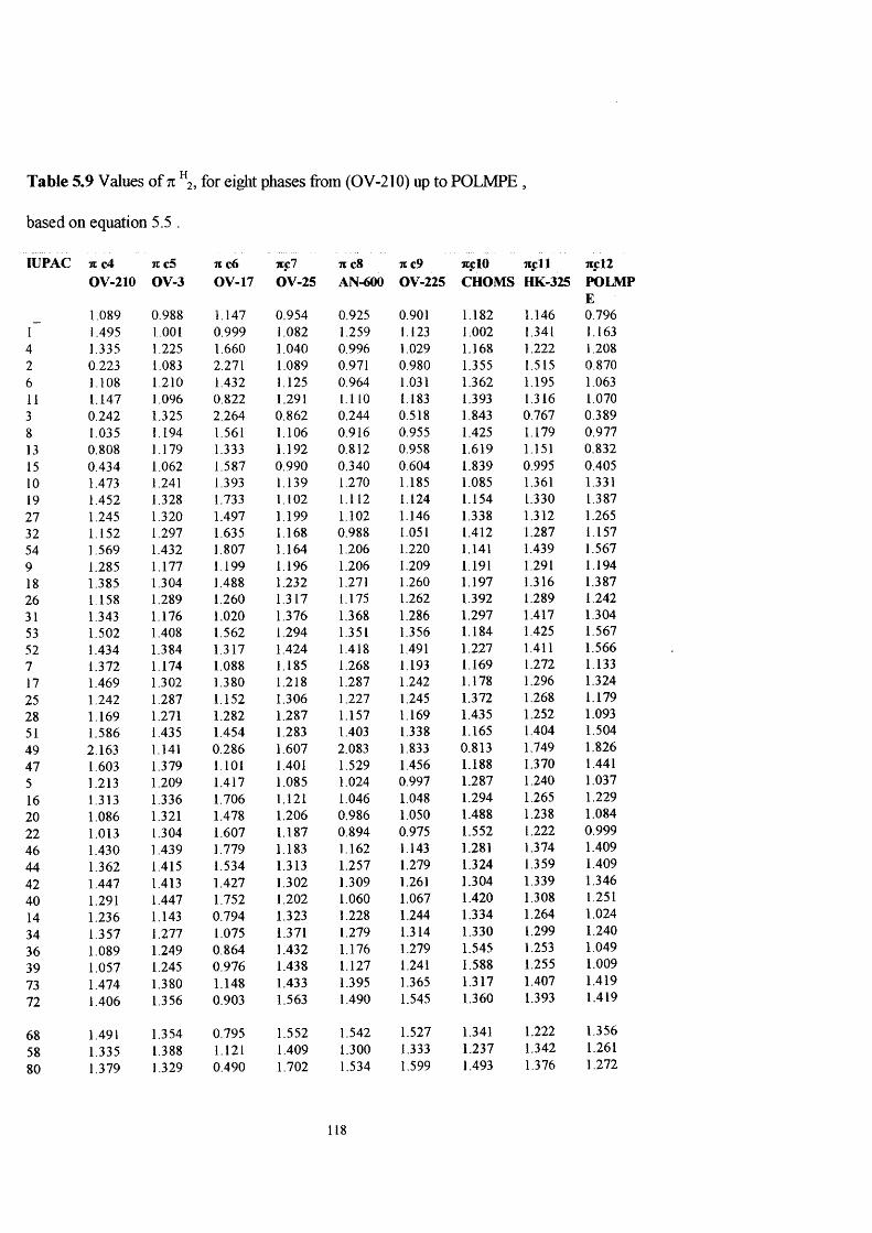
Table 5.9 Values of n for eiglit phases from (OV-210) up to POLMPE
based on equation 5.5 .
l U P A C n c4 71 c5 7C c6 jcc7 7C c8 7C c9 TCClO Ticll i t c l2
O V -2 1 0 O V -3 O V -1 7 O V -2 5 A N -6 0 0 O V -2 2 5 C H O M S H K -325 P O O1?
1.089 0 .988 1.147 0 .9 5 4 0.925 0.901 1.182 1.146mL
0 .796r 1.495 1.001 0 .9 9 9 1.082 1.259 1.123 1.002 1.341 1.1634 1.335 1.225 1.660 1.040 0.996 1.029 1.168 1.222 1.2082 0 .223 1.083 2.271 1.089 0.971 0.980 1.355 1.515 0 .8706 1.108 1.210 1.432 1.125 0 .964 1.031 1.362 1.195 1.06311 1.147 1.096 0 .822 1.291 1.110 1.183 1.393 1.316 1.0703 0 .2 4 2 1.325 2 .2 6 4 0 .8 6 2 0 .244 0.518 1.843 0 .767 0 .3898 1.035 1.194 1.561 1.106 0 .916 0.955 1.425 1.179 0 .9 7 713 0 .8 0 8 1.179 1.333 1.192 0 .812 0.958 1.619 1.151 0 .8 3 2
15 0 .4 3 4 1.062 1.587 0 .9 9 0 0 .340 0.604 1.839 0.995 0 .40510 1.473 1.241 1.393 1.139 1.270 1.185 1.085 1.361 1.33119 1.452 1.328 1.733 1.102 1.112 1.124 1.154 1.330 1.387
2 7 1.245 1.320 1.497 1 .199 1.102 1.146 1.338 1.312 1.265
32 1.152 1.297 1.635 1.168 0 .988 1.051 1.412 1.287 1.157
54 1 .569 1.432 1.807 1.164 1.206 1.220 1.141 1.439 1.567
9 1.285 1.177 1.199 1.196 1.206 1.209 1.191 1.291 1.194
18 1.385 1.304 1.488 1.232 1.271 1.260 1 .197 1.316 1.387
26 1.158 1.289 1.260 1 .317 1.175 1.262 1.392 1.289 1.242
31 1.343 1.176 1.020 1 .376 1.368 1.286 1.297 1.417 1.304
53 1 .502 1.408 1.562 1.294 1.351 1.356 1.184 1.425 1.567
52 1.434 1.384 1.317 1 .424 1.418 1.491 1.227 1.411 1.566
7 1.372 1.174 1.088 1.185 1.268 1.193 1.169 1.272 1.133
17 1 .469 1.302 1.380 1 .218 1.287 1.242 1.178 1.296 1.324
25 1 .242 1.287 1.152 1.306 1.227 1.245 1.372 1.268 1.179
28 1 .169 1.271 1.282 1 .287 1.157 1.169 1.435 1.252 1.093
51 1.586 1.435 1.454 1.283 1.403 1.338 1.165 1.404 1.504
49 2 .163 1.141 0 .2 8 6 1.607 2.083 1.833 0 .813 1.749 1.826
4 7 1.603 1.379 1.101 1.401 1.529 1.456 1.188 1.370 1.441
5 1.213 1.209 1.417 1 .085 1.024 0.997 1.287 1.240 1.037
16 1.313 1.336 1.706 1.121 1.046 1.048 1.294 1.265 1.229
20 1.086 1.321 1.478 1 .206 0 .986 1.050 1.488 1.238 1.084
22 1.013 1.304 1.607 1.187 0 .8 9 4 0.975 1.552 1.222 0 .9 9 9
46 1.430 1.439 1.779 1.183 1.162 1.143 1.281 1.374 1.409
4 4 1.362 1.415 1.534 1.313 1.257 1.279 1.324 1.359 1.409
42 1 .447 1.413 1 .427 1.302 1.309 1.261 1.304 1.339 1.346
40 1.291 1.447 1.752 1.202 1.060 1.067 1.420 1.308 1.251
14 1.236 1.143 0 .7 9 4 1.323 1.228 1.244 1.334 1.264 1.024
34 1 .357 1.277 1.075 1.371 1.279 1.314 1.330 1.299 1.240
3 6 1.089 1.249 0 .8 6 4 1.432 1.176 1.279 1.545 1.253 1.049
39 1 .057 1.245 0 .9 7 6 1.438 1.127 1.241 1.588 1.255 1.009
73 1 .474 1.380 1.148 1.433 1.395 1.365 1.317 1.407 1.419
72 1.406 1.356 0 .903 1.563 1.490 1.545 1.360 1.393 1.419
68 1.491 1.354 0 .795 1.552 1.542 1.527 1.341 1.222 1.356
58 1.335 1.388 1.121 1.409 1.300 1.333 1.237 1.342 1.261
80 1.379 1.329 0 .4 9 0 1.702 1.534 1.599 1.493 1.376 1.272
118

Table 5 .9 12
Cont.1.193 1.099 1.008 1.260 1.118 1111 1.442 1.356 0.975
33 1.026 1.326 1.678 1.215 0.906 1.014 1.612 1.233 1.01635 0.799 1.311 1.450 1.301 0.846 1.016 1.806 1.206 0.87137 0.727 1.294 1.580 1.282 0.754 0.940 1.869 1.190 0.78571 1.143 1.429 1.752 1.278 1.022 1.109 1.598 1.342 1.19570 1.015 1.385 1.532 1.436 1.052 1.189 1.673 1.299 1.12666 1.160 1.403 1.399 1.396 1.169 1.227 -0.138 1.307 1.13256 1.004 1.436 1.724 1.297 0.927 1.033 1.738 1.276 1.03779 1.048 1.377 1.093 1.547 1.161 1.299 1.774 1.310 1.04777 0.718 1.426 1.697 1.391 0.709 0.998 2.056 1.244 0.82330 1.772 1.229 0.954 1.325 1.747 1.564 0.936 1.353 1.47650 1.873 1.356 1.243 0.239 1.776 1.615 0.943 1.379 1.66869 1.645 1.341 1.015 1.447 1.716 2.062 0.111 1.351 1.52375 1.573 1.324 1.144 1.428 1.624 1.542 1.201 1.335 1.437104 2.000 1.455 1.301 1.427 1.901 1.716 0.924 1.493 1.854103 1.922 1.435 1.071 1.554 1.987 1.846 0.973 1.473 1.847100 2.007 1.433 0.963 1.542 2.039 1.828 0.953 1.453 1.78598 1.850 1.467 1.289 1.443 1.797 1.634 1.070 1.422 1.690121 1.897 1.407 0.654 1.694 2.033 1.901 1.104 1.457 1.702119 1.564 1.456 1.261 1.537 1.658 1.600 1.387 1.390 1.476155 2.410 1.486 0.826 1.683 2.528 2.201 0.719 1.536 2.12924 1.419 1.269 1.394 1.225 1.238 1.266 1.147 1.361 1.40745 1.519 1.396 1.683 1.261 1.267 1.316 1.154 1.387 1.59959 1.312 1.387 1.447 1.359 1.228 1.338 1.338 1.369 1.47769 1.219 1.364 1.585 1.328 1.115 1.243 1.412 1.343 1.36996 1.636 1.499 1.757 1.323 1.383 1.408 1.141 1.495 1.77995 1.568 1.475 1.512 1.454 1.478 1.548 1.184 1.481 1.77991 1.653 1.473 1.404 1.442 1.530 1.530 0.724 1.460 1.71684 1.496 1.506 1.730 1.343 1.934 1.736 1.280 1.430 1.621113 1.540 1.447 1.098 1.593 1.522 2.002 1.317 1.464 1.631110 1.210 1.496 1.702 1.437 1.148 1.301 1.598 1.457 1.407150 2.056 1.526 1.266 1.583 2.018 1.902 1.418 1.543 2.060136 1.702 1.566 1.707 1.483 1.509 1.604 1.140 1.508 1.99123 1.797 1.268 1.061 1.369 1.460 1.418 1.113 1.364 1.32843 1.897 1.395 1.350 1.405 1.533 1.469 1.120 1.389 1.52157 1.670 1.380 1.122 1.491 1.472 1.471 1.314 1.362 1.37663 1.597 1.393 1.252 1.472 1.381 1.396 1.378 1.346 1.29094 2.014 1.498 1.424 1.467 1.649 1.564 1.107 1.498 1.70092 1.972 1.465 1.142 1.605 1.767 1.714 1.134 1.498 1.71590 2.057 1.463 1.034 1.594 1.819 1.697 1.114 1.477 1.65283 1.875 1.506 1.397 1.463 1.554 1.488 1.246 1.432 1.542111 1.919 1.447 0.765 1.737 1.787 1.754 1.283 1.466 1.553107 1.588 1.525 1.369 1.581 1.414 1.454 1.564 1.400 1.328148 2.435 1.526 0.933 1.727 2.284 2.055 0.895 1.546 1.981135 2.081 1.566 1.374 1.627 1.775 1.757 1.106 1.554 1.912133 2.459 1.565 1.041 1.771 2.048 1.909 1.072 1.556 1.83429 1.382 1.248 1.018 1.370 1.414 1.423 1.190 1.331 1.30348 1.482 1.375 1.307 1.406 1.465 1.474 1.197 1.357 1.49667 1.255 1.360 1.079 1.492 1.404 1.878 1.391 1.330 1.35074 1.182 1.343 1.209 1.473 1.313 1.401 1.454 1.313 1.265102 1.599 1.478 1.381 1.468 1.581 1.570 1.144 1.465 1.675101 1.740 2.032 2.303 1.661 1.872 1.822 1.588 1.568 1.79499 1.645 1.441 0.986 1.596 1.761 1.704 1.189 1.447 1.628
119
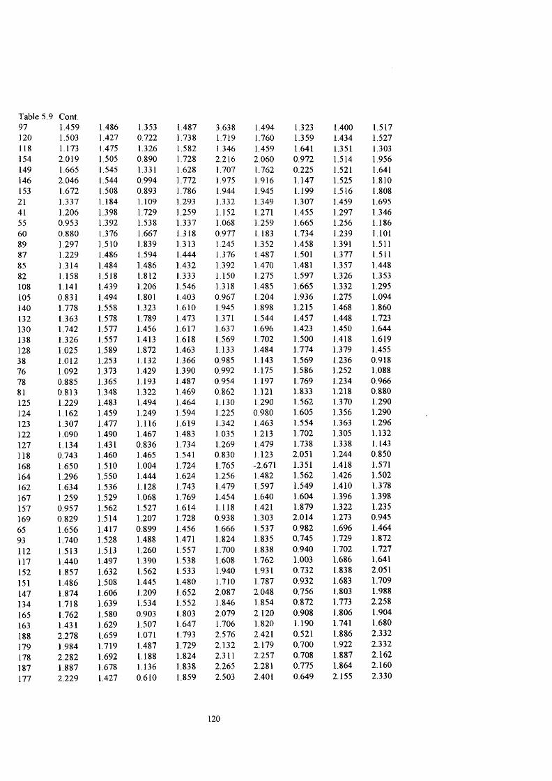
Table 5 .9 97
Cont.1.459 1.486 1.353 1.487 3.638 1.494 1.323 1.400 1.517
120 1.503 1.427 0.722 1.738 1.719 1.760 1.359 1.434 1.527118 1.173 1.475 1.326 1.582 1.346 1.459 1.641 1.351 1.303154 2.019 1.505 0.890 1.728 2.216 2.060 0.972 1.514 1.956149 1.665 1.545 1.331 1.628 1.707 1.762 0.225 1.521 1.641146 2.046 1.544 0.994 1.772 1.975 1.916 1.147 1.525 1.810153 1.672 1.508 0.893 1.786 1.944 1.945 1.199 1.516 1.80821 1.337 1.184 1.109 1.293 1.332 1.349 1.307 1.459 1.69541 1.206 1.398 1.729 1.259 1.152 1.271 1.455 1.297 1.34655 0.953 1.392 1.538 1.337 1.068 1.259 1.665 1.256 1.18660 0.880 1.376 1.667 1.318 0.977 1.183 1.734 1.239 1.10189 1.297 1.510 1.839 1.313 1.245 1.352 1.458 1.391 1.51187 1.229 1.486 1.594 1.444 1.376 1.487 1.501 1.377 1.51185 1.314 1.484 1.486 1.432 1.392 1.470 1.481 1.357 1.44882 1.158 1.518 1.812 1.333 1.150 1.275 1.597 1.326 1.353108 1.141 1.439 1.206 1.546 1.318 1.485 1.665 1.332 1.295105 0.831 1.494 1.801 1.403 0.967 1.204 1.936 1.275 1.094140 1.778 1.558 1.323 1.610 1.945 1.898 1.215 1.468 1.860132 1.363 1.578 1.789 1.473 1.371 1.544 1.457 1.448 1.723130 1.742 1.577 1.456 1.617 1.637 1.696 1.423 1.450 1.644138 1.326 1.557 1.413 1.618 1.569 1.702 1.500 1.418 1.619128 1.025 1.589 1.872 1.463 1.133 1.484 1.774 1.379 1.45538 1.012 1.253 1.132 1.366 0.985 1.143 1.569 1.236 0.91876 1.092 1.373 1.429 1.390 0.992 1.175 1.586 1.252 1.08878 0.885 1.365 1.193 1.487 0.954 1.197 1.769 1.234 0.96681 0.813 1.348 1.322 1.469 0.862 1.121 1.833 1.218 0.880125 1.229 1.483 1.494 1.464 1.130 1.290 1.562 1.370 1.290124 1.162 1.459 1.249 1.594 1.225 0.980 1.605 1.356 1.290123 1.307 1.477 1.116 1.619 1.342 1.463 1.554 1.363 1.296122 1.090 1.490 1.467 1.483 1.035 1.213 1.702 1.305 1.132127 1.134 1.431 0.836 1.734 1.269 1.479 1.738 1.338 1.143118 0.743 1.460 1.465 1.541 0.830 1.123 2.051 1.244 0.850168 1.650 1.510 1.004 1.724 1.765 -2.671 1.351 1.418 1.571164 1.296 1.550 1.444 1.624 1.256 1.482 1.562 1.426 1.502162 1.634 1.536 1.128 1.743 1.479 1.597 1.549 1.410 1.378167 1.259 1.529 1.068 1.769 1.454 1.640 1.604 1.396 1.398157 0.957 1.562 1.527 1.614 1.118 1.421 1.879 1.322 1.235169 0.829 1.514 1.207 1.728 0.938 1.303 2.014 1.273 0.94565 1.656 1.417 0.899 1.456 1.666 1.537 0.982 1.696 1.46493 1.740 1.528 1.488 1.471 1.824 1.835 0.745 1.729 1.872112 1.513 1.513 1.260 1.557 1.700 1.838 0.940 1.702 1.727117 1.440 1.497 1.390 1.538 1.608 1.762 1.003 1.686 1.641152 1.857 1.632 1.562 1.533 1.940 1.931 0.732 1.838 2.051151 1.486 1.508 1.445 1.480 1.710 1.787 0.932 1.683 1.709147 1.874 1.606 1.209 1.652 2.087 2.048 0.756 1.803 1.988134 1.718 1.639 1.534 1.552 1.846 1.854 0.872 1.773 2.258165 1.762 1.580 0.903 1.803 2.079 2.120 0.908 1.806 1.904163 1.431 1.629 1.507 1.647 1.706 1.820 1.190 1.741 1.680188 2.278 1.659 1.071 1.793 2.576 2.421 0.521 1.886 2.332179 1.984 1.719 1.487 1.729 2.132 2.179 0.700 1.922 2.332178 2.282 1.692 1.188 1.824 2.311 2.257 0.708 1.887 2.162187 1.887 1.678 1.136 1.838 2.265 2.281 0.775 1.864 2.160177 2.229 1.427 0.610 1.859 2.503 2.401 0.649 2.155 2.330
120
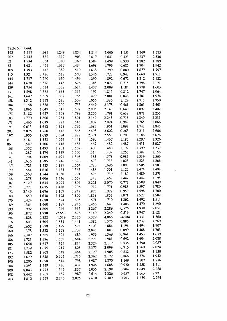
Table 5.9 193
Cont.1.517 1.683 1.249 1.834 1.814 2.000 1.153 1.769 1.775
202 2.145 1.832 1.317 1.903 2.617 2.641 0.323 2.237 2.53662 1.534 1.364 1.300 1.367 1.584 1.499 0.930 1.282 1.38988 1.621 1.457 1.617 1.434 1.698 1.796 0.685 1.704 1.942109 1.393 1.442 1.389 1.519 1.638 1.799 0.880 1.677 1.797115 1.321 1.426 1.518 1.500 1.546 1.723 0.943 1.660 1.711145 1.737 1.560 1.690 1.496 1.290 1.892 0.672 1.812 2.122144 1.670 1.536 1.445 1.626 1.385 2.027 0.715 1.798 2.121139 1.754 1.534 1.338 1.614 1.437 2.009 1.184 1.778 1.603131 1.598 1.568 1.663 1.515 1.195 1.815 0.812 1.747 1.964161 1.642 1.509 1.032 1.765 1.429 2.081 0.848 1.781 1.974158 1.312 1.558 1.636 1.609 1.056 1.336 1.129 1.715 1.750184 2.158 1.588 1.200 1.755 2.449 2.378 0.461 1.861 2.403176 1.865 1.647 1.615 1.692 2.005 2.140 0.640 1.897 2.402175 2.182 1.627 1.308 1.799 2.206 1.791 0.638 1.871 2.255183 1.770 1.606 1.261 1.801 2.140 2.243 0.713 1.840 2.231171 1.465 1.639 1.723 1.645 1.802 2.024 0.989 1.765 2.066191 0.613 1.612 1.378 1.796 1.687 1.961 1.093 1.743 1.845201 2.025 1.760 1.446 1.865 2.498 2.602 0.263 2.211 2.606197 1.906 1.689 1.574 1.828 2.371 2.563 0.203 2.186 2.67661 2.181 1.353 1.079 1.441 1.590 1.467 1.187 1.297 1.32686 1.587 1.506 1.418 1.483 1.467 1.482 1.487 1.431 5.027106 1.352 1.493 1.201 1.567 1.400 1.480 1.197 1.399 1.237114 1.287 1.474 1.319 1.550 1.315 1.409 1.256 1.387 1.156143 1.704 1.609 1.491 1.546 1.583 1.578 0.985 1.539 1.566141 1.636 1.585 1.246 1.676 1.678 1.713 1.028 1.525 1.566137 1.721 1.583 1.139 1.664 1.730 1.696 1.008 1.505 1.503129 1.564 1.616 1.464 1.565 1.488 1.501 1.125 1.474 1.408159 1.568 1.544 0.850 1.791 1.678 1.730 1.182 1.489 1.373156 1.278 1.606 1.436 1.659 1.348 1.467 1.442 1.442 1.195182 2.127 1.635 0.997 1.806 2.221 2.070 0.772 1.589 1.849174 1.773 1.675 1.438 1.706 1.712 1.771 0.983 1.597 1.780172 2.149 1.676 1.109 1.849 1.975 1.922 0.950 1.598 1.700180 1.650 1.630 1.103 1.800 1.818 1.852 1.071 1.527 1.582170 1.424 1.688 1.524 1.695 1.571 1.710 1.302 1.492 1.511189 1.364 1.660 1.179 1.846 1.456 1.647 1.406 1.470 1.290199 1.992 1.809 1.246 1.915 2.267 2.289 0.576 1.938 2.051196 1.872 1.738 -7.650 1.878 2.140 2.249 0.516 1.947 2.121194 1.828 2.828 -1.539 2.326 5.329 4.066 -4.284 1.331 1.560116 1.603 1.505 1.654 1.441 1.582 1.576 0.885 1.232 1.269142 1.602 1.598 1.499 1.573 2.103 1.884 1.196 1.494 1.907160 1.378 1.582 1.268 1.707 2.045 1.888 0.899 1.468 1.763166 1.307 1.565 1.394 1.689 1.956 1.369 0.961 1.453 1.679186 1.721 1.596 1.569 1.684 2.221 1.981 0.692 1.604 2.088185 1.654 1.677 1.324 1.814 2.324 2.117 0.735 1.590 2.087181 1.739 1.675 1.217 1.803 2.375 2.099 0.715 1.569 2.024173 1.582 1.708 1.542 1.464 2.127 1.905 0.832 1.539 1.930192 1.629 1.648 0.907 1.715 2.362 2.172 0.866 1.574 1.942190 1.296 1.698 1.514 1.798 1.987 1.870 1.149 1.507 1.716204 1.291 1.449 1.436 1.431 1.946 1.688 0.920 1.258 1.411200 8.043 1.775 1.549 1.837 5.055 2.198 0.704 1.649 2.288198 8.442 1.767 1.187 1.987 2.614 2.326 0.657 1.663 2.221203 1.812 1.767 2.246 2.025 2.610 2.387 0.703 1.659 2.264
121

Table 5.9 195
Cont.1.449 1.779 1.602 1.834 2.210 2.113 1.009 1.556 2.032
205 1.382 1.752 1.257 1.984 2.095 2.051 1.113 1.535 1.811208 1.796 1.980 1.630 1.989 2.712 2.573 0.414 1.884 2.451207 1.890 1.829 1.453 2.016 2.779 2.653 0.223 1.977 2.642206 2.160 1.977 1.126 2.249 2.873 2.619 0.379 1.845 2.429209 1.874 1.970 1.332 2.204 3.186 2.742 0.243 1.769 2.608266 0.114 -0.004 -0.222 0.068 0.194 0.157 -0.187 0.001 0.081268 0.098 -0.003 -0.189 0.058 0.167 0.135 -0.159 0.001 0.058270 0.067 0.003 -0.135 0.043 0.125 0.103 -0.123 -0.007 0.026272 0.051 0.004 -0.102 0.034 0.097 0.080 -0.095 -0.007 0.003274 0.035 0.005 -0.070 0.024 0.069 0.058 -0.068 -0.006 -0.020276 0.019 0.005 -0.037 0.014 0.041 0.035 -0.041 -0.006 -0.043278 0.019 0.000 -0.026 0.009 0.027 0.021 -0.023 0.003 -0.057280 0.003 0.001 0.006 -0.001 -0.001 -0.002 0.004 0.004 -0.080282 -0.013 0.001 0.039 -0.011 -0.029 -0.025 0.031 0.004 -0.103284 -0.029 0.002 0.071 -0.021 -0.057 -0.048 0.059 0.005 -0.126286 -0.060 0.008 0.126 -0.035 -0.098 -0.079 0.095 -0.004 -0.158289 -0.061 0.001 0.142 -0.043 -0.119 -0.100 0.122 0.010 -0.179
122
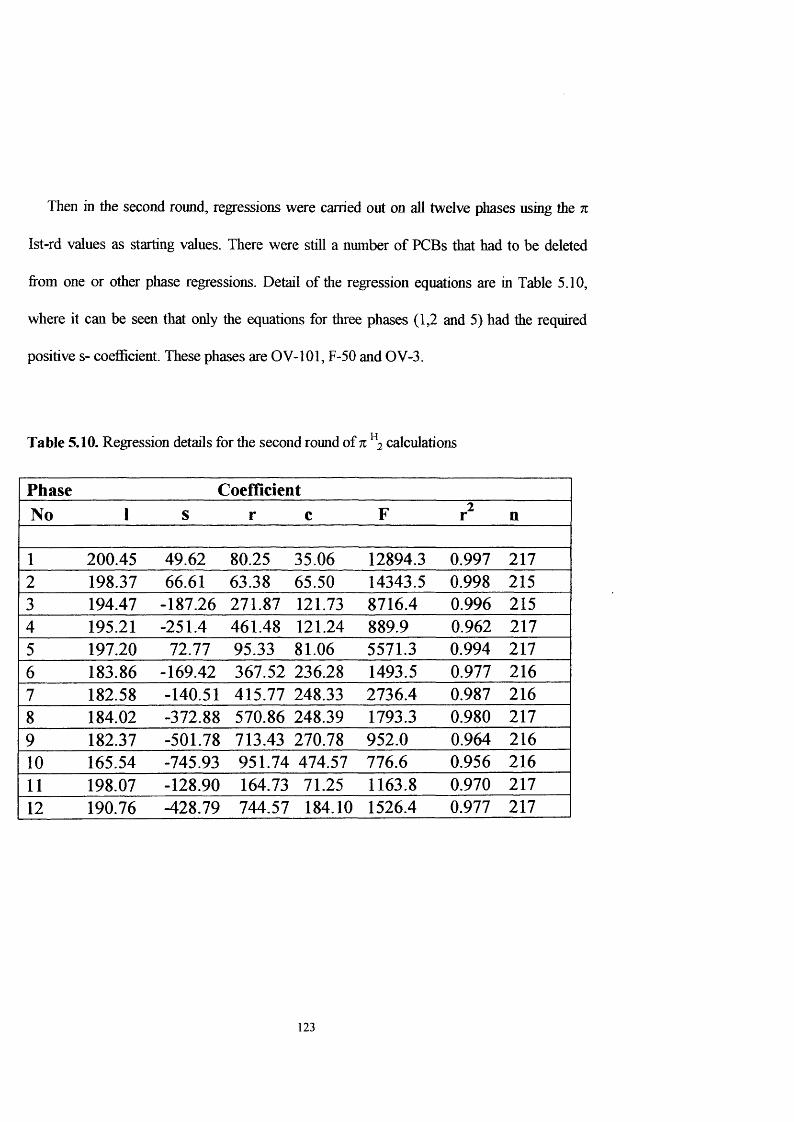
Then in the second round, regressions were carried out on all twelve pliases using the 7t
Ist-rd values as starting values. There were still a number of PCBs that had to be deleted
from one or other phase regressions. Detail of tlie regression equations are in Table 5.10,
where it can be seen that only tlie equations for tliree phases (1,2 and 5) had the required
positive s- coefficient. Tliese phases are OV-101, F-50 and OV-3.
Table 5.10. Regression details for tlie second round of tz ^ 2 calculations
Phase CoefficientNo 1 s r c F n
1 200.45 49.62 80.25 35.06 12894.3 0.997 2172 198.37 66.61 63.38 65.50 14343.5 0.998 2153 194.47 -187.26 271.87 121.73 8716.4 0.996 2154 195.21 -251.4 461.48 121.24 889.9 0.962 2175 197.20 72.77 95.33 81.06 5571.3 0.994 2176 183.86 -169.42 367.52 236.28 1493.5 0.977 2167 182.58 -140.51 415.77 248.33 2736.4 0.987 2168 184.02 -372.88 570.86 248.39 1793.3 0.980 2179 182.37 -501.78 713.43 270.78 952.0 0.964 21610 165.54 -745.93 951.74 474.57 776.6 0.956 21611 198.07 -128.90 164.73 71.25 1163.8 0.970 21712 190.76 -428.79 744.57 184.10 1526.4 0.977 217
123

The next step was to average tlie back-calculated tc ^^2 values from the three selected
phases as shown in Table 5.11, with the average values now denoted as tc 2nd -rd . It can be
seen that there are some considerable changes on going from tc 1st - rd to tc 2nd - rd .
Table 5.11 The back-calculation of Tc for (OV-101), (F-50), (OV-3),with average, t c (1st- rd), TC (2nd - rd).
lUPAC TC calc. TC calc. TC calc. TC avg. TC TC TCOV-101 F -50 OV-3 101,50,3 Sd 1st - rd 2nd
0.994 0.993 0.963 0.983 0.017 1.04 0.981 0.767 0.489 0.707 0.654 0.146 1.22 1.124 1.196 1.179 1.289 1.221 0.059 1.21 1.426 1.215 1.372 1.353 1.313 0.086 1.16 1.2911 1.234 1.565 1.417 1.406 0.166 1.21 0.673 1.919 2.712 2.187 2.273 0.403 0.81 1.098 1.205 1.324 1.309 1.279 0.064 1.13 1.2113 1.225 1.517 1.373 1.372 0.146 1.08 11115 0.861 0.903 0.976 0.913 0.059 1.02 1.2010 1.247 1.279 1.300 1.275 0.027 1.30 1.3419 1.288 1.294 1.425 1.336 0.078 1.30 1.5927 1.315 1.497 1.494 1.435 0.104 1.27 1.4732 1.297 1.439 1.446 1.394 0.084 1.23 1.4154 1.380 1.408 1.562 1.450 0.098 1.40 1.769 1.218 1.408 1.252 1.293 0.101 1.24 1.1418 1.310 1.484 1.403 1.399 0.087 1.31 1.4226 1.329 1.677 1.467 1.491 0.175 1.26 1.2231 1.319 3.575 1.423 2.106 1.273 1.33 1.3253 1.401 1.599 1.54 1.513 0.101 1.04 1.5652 1.423 1.789 1.517 1.577 0.190 1.41 1.377 1.208 1.301 1.263 1.258 0.047 1.25 1.1417 1.300 1.358 1.414 1.357 0.057 1.27 1.3625 1.319 1.551 1.478 1.450 0.119 1.28 1.2928 1.310 1.503 1.434 1.416 0.098 1.24 1.2351 1.392 1.473 1.688 1.518 0.153 1.43 1.4949 1.436 1.114 1.279 1.276 0.161 1.44 1.4547 1.404 1.537 1.539 1.494 0.077 1.38 1.385 1.214 1.237 1.327 1.259 0.060 1.22 1.2216 1.306 1.313 1.478 1.365 0.097 1.26 1.4120 1.325 1.506 1.542 1.458 0.116 1.23 1.28
124

Table 5.11 Cont. 22 1.316 1.458 1.498 1.424 0.096 1.21 1.2446 1.398 1.428 1.614 1.480 0.117 1.37 1.5544 1.42 1.618 1.592 1.543 0.108 1.34 1.5542 1.41 1.492 1.603 1.502 0.097 1.37 1.4140 1.416 1.447 1.667 1.510 0.137 1.27 1.4614 1.229 1.299 1.188 1.238 0.056 1.24 0.9634 1.329 1.385 1.343 1.352 0.029 1.32 1.2136 1.331 1.558 1.399 1.429 0.116 1.26 1.0739 1.339 1.530 1.363 1.411 0.104 1.25 1.0473 1.421 1.500 1.480 1.467 0.041 1.40 1.3772 1.443 1.690 1.457 1.530 0.139 1.39 1.2768 1.433 1.564 1.468 1.489 0.068 1.42 1.2158 1.439 1.519 1.532 1.497 0.050 1.37 1.3080 1.462 1.591 1.397 1.484 0.099 1.36 1.0712 1.224 1.304 1.429 1.319 0.103 1.22 0.7033 1.316 1.380 1.580 1.425 0.138 1.20 1.2335 1.335 1.573 1.644 1.518 0.162 1.27 1.2337 1.326 1.525 1.600 1.484 0.142 1.25 1.1471 1.408 1.495 1.717 1.540 0.159 1.25 1.3770 1.404 1.654 1.682 1.580 0.153 1.28 1.3166 1.420 1.559 1.705 1.562 0.143 1.32 1.3156 1.426 1.514 1.769 1.57 0.178 1.29 1.2979 1.449 1.586 1.634 1.557 0.096 1.34 1.1977 1.436 1.581 1.872 1.629 0.222 1.31 1.3230 1.305 1.353 1.187 1.281 0.086 1.30 1.2350 1.396 1.429 1.338 1.388 0.046 1.37 1.4269 1.415 1.623 1.402 1.480 0.124 1.35 1.3375 1.406 1.574 1.358 1.446 0.114 1.33 1.29104 1.488 1.467 1.420 1.458 0.035 1.46 1.55103 1.510 1.735 1.452 1.565 0.149 1.45 1.45100 1.500 1.609 1.463 1.524 0.076 1.44 1.4598 1.506 1.563 1.527 1.532 0.029 1.44 1.49121 1.529 1.616 1.378 1.508 0.120 1.43 1.32119 1.516 1.631 1.629 1.592 0.066 1.55 1.37155 1.597 1.680 1.386 1.554 0.151 1.51 1.5324 1.308 0.960 1.061 1.110 0.179 1.25 1.2445 1.400 1.036 1.212 1.216 0.182 1.39 1.3659 1.427 1.240 1.281 1.316 0.099 1.36 1.3969 1.409 1.182 1.233 1.275 0.120 1.34 1.3396 1.492 1.151 1.349 1.331 0.171 1.50 1.6895 1.513 1.342 1.327 1.394 0.104 1.47 1.5991 1.504 1.216 1.338 1.352 0.145 1.46 1.5684 1.510 1.171 1.401 1.361 0.173 1.42 1.64113 1.533 1.243 1.267 1.347 0.161 1.46 1.56
125
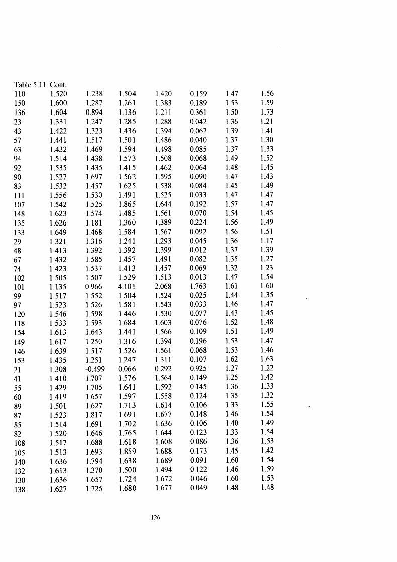
Table 5.11 Cont. 110 1.520 1.238 1.504 1.420 0.159 1.47 1.56150 1.600 1.287 1.261 1.383 0.189 1.53 1.59136 1.604 0.894 1.136 1.211 0.361 1.50 1.7323 1.331 1.247 1.285 1.288 0.042 1.36 1.2143 1.422 1.323 1.436 1.394 0.062 1.39 1.4157 1.441 1.517 1.501 1.486 0.040 1.37 1.3063 1.432 1.469 1.594 1.498 0.085 1.37 1.3394 1.514 1.438 1.573 1.508 0.068 1.49 1.5292 1.535 1.435 1.415 1.462 0.064 1.48 1.4590 1.527 1.697 1.562 1.595 0.090 1.47 1.4383 1.532 1.457 1.625 1.538 0.084 1.45 1.49111 1.556 1.530 1.491 1.525 0.033 1.47 1.47107 1.542 1.525 1.865 1.644 0.192 1.57 1.47148 1.623 1.574 1.485 1.561 0.070 1.54 1.45135 1.626 1.181 1.360 1.389 0.224 1.56 1.49133 1.649 1.468 1.584 1.567 0.092 1.56 1.5129 1.321 1.316 1.241 1.293 0.045 1.36 1.1748 1.413 1.392 1.392 1.399 0.012 1.37 1.3967 1.432 1.585 1.457 1.491 0.082 1.35 1.2774 1.423 1.537 1.413 1.457 0.069 1.32 1.23102 1.505 1.507 1.529 1.513 0.013 1.47 1.54101 1.135 0.966 4.101 2.068 1.763 1.61 1.6099 1.517 1.552 1.504 1.524 0.025 1.44 1.3597 1.523 1.526 1.581 1.543 0.033 1.46 1.47120 1.546 1.598 1.446 1.530 0.077 1.43 1.45118 1.533 1.593 1.684 1.603 0.076 1.52 1.48154 1.613 1.643 1.441 1.566 0.109 1.51 1.49149 1.617 1.250 1.316 1.394 0.196 1.53 1.47146 1.639 1.517 1.526 1.561 0.068 1.53 1.46153 1.435 1.251 1.247 1.311 0.107 1.62 1.6321 1.308 -0.499 0.066 0.292 0.925 1.27 1.2241 1.410 1.707 1.576 1.564 0.149 1.25 1.4255 1.429 1.705 1.641 1.592 0.145 1.36 1.3360 1.419 1.657 1.597 1.558 0.124 1.35 1.3289 1.501 1.627 1.713 1.614 0.106 1.33 1.5587 1.523 1.817 1.691 1.677 0.148 1.46 1.5485 1.514 1.691 1.702 1.636 0.106 1.40 1.4982 1.520 1.646 1.765 1.644 0.123 1.33 1.54108 1.517 1.688 1.618 1.608 0.086 1.36 1.53105 1.513 1.693 1.859 1.688 0.173 1.45 1.42140 1.636 1.794 1.638 1.689 0.091 1.60 1.54132 1.613 1.370 1.500 1.494 0.122 1.46 1.59130 1.636 1.657 1.724 1.672 0.046 1.60 1.53138 1.627 1.725 1.680 1.677 0.049 1.48 1.48
126

Table 5.11 Cont. 128 1.623 1.846 1.864 1.778 0.134 1.42 1.4838 1.338 1.668 1.462 1.489 0.167 1.24 1.0776 1.421 1.734 1.608 1.588 0.158 1.38 1.3378 1.448 1.937 1.677 1.687 0.245 1.43 1.2181 1.439 1.889 1.633 1.654 0.226 1.40 1.60125 1.521 1.859 1.749 1.710 0.172 1.47 1.50124 1.543 2.049 1.727 1.773 0.256 1.39 1.38123 1.559 1.954 1.750 1.755 0.197 1.33 1.35122 1.539 1.878 1.801 1.740 0.178 1.49 1.43127 1.563 1.950 1.667 1.726 0.201 1.41 1.13118 1.524 1.914 1.891 1.776 0.219 1.50 1.37168 1.630 1.995 1.661 1.762 0.202 1.56 1.37164 1.633 1.602 1.536 1.59 0.049 1.47 1.47162 1.639 1.868 1.752 1.753 0.115 1.58 1.30167 1.646 1.957 1.716 1.773 0.163 1.49 1.30157 1.643 2.077 1.900 1.873 0.218 1.50 1.41169 1.637 2.278 1.923 1.946 0.321 1.62 1.2465 1.411 1.491 1.601 1.501 0.095 1.56 1.4993 1.517 1.474 1.473 1.488 0.025 1.62 1.75112 1.536 1.668 1.537 1.580 0.076 1.54 1.61117 1.527 1.619 1.493 1.546 0.066 1.47 1.57152 1.609 1.589 1.609 1.602 0.011 1.71 1.90151 1.502 1.626 1.523 1.551 0.066 1.48 1.64147 1.621 1.654 1.598 1.624 0.028 1.73 1.75134 1.627 1.608 1.662 1.632 0.027 1.76 1.85165 1.650 1.681 1.527 1.619 0.081 1.80 1.67163 1.637 1.675 1.764 1.692 0.065 1.64 1.68188 1.717 1.725 1.521 1.655 0.115 1.78 1.83179 1.746 1.363 1.409 1.506 0.209 1.84 1.93178 1.735 1.609 1.616 1.653 0.071 1.80 1.81187 1.734 1.688 1.576 1.666 0.081 1.82 1.80177 1.705 7.089 1.748 3.514 3.096 1.92 1.75193 1.750 2.040 1.796 1.862 0.155 1.71 1.70202 1.838 1.770 1.656 1.755 0.092 1.87 2.1362 1.412 1.101 1.243 1.252 0.155 1.36 1.3688 1.508 1.386 1.124 1.340 0.196 1.44 1.60109 1.528 1.579 1.188 1.432 0.212 1.51 1.55115 1.518 1.531 1.144 1.398 0.220 1.48 1.64145 1.600 1.501 1.261 1.454 0.175 1.65 1.75144 1.622 1.691 1.238 1.517 0.244 1.65 1.72139 1.613 1.565 1.249 1.476 0.198 1.67 1.68131 1.619 1.520 1.313 1.484 0.156 1.61 1.70161 1.642 1.592 1.178 1.471 0.255 1.67 1.66158 1.629 1.587 1.415 1.544 0.113 1.55 1.68
127
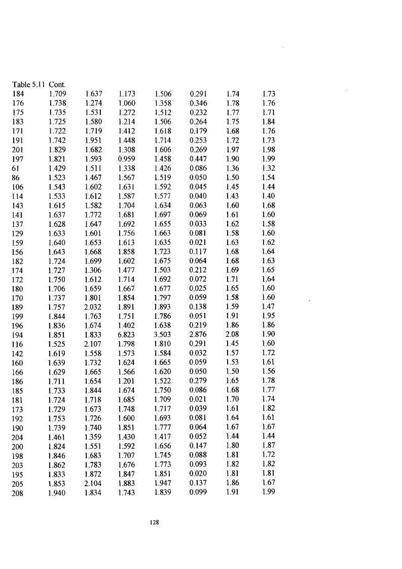
Table 5.11 184
Cont.1.709 1.637 1.173 1.506 0.291 1.74 1.73
176 1.738 1.274 1.060 1.358 0.346 1.78 1.76175 1.735 1.531 1.272 1.512 0.232 1.77 1.71183 1.725 1.580 1.214 1.506 0.264 1.75 1.84171 1.722 1.719 1.412 1.618 0.179 1.68 1.76191 1.742 1.951 1.448 1.714 0.253 1.72 1.73201 1.829 1.682 1.308 1.606 0.269 1.97 1.98197 1.821 1.593 0.959 1.458 0.447 1.90 1.9961 1.429 1.511 1.338 1.426 0.086 1.36 1.3286 1.523 1.467 1.567 1.519 0.050 1.50 1.54106 1.543 1.602 1.631 1.592 0.045 1.45 1.44114 1.533 1.612 1.587 1.577 0.040 1.43 1.40143 1.615 1.582 1.704 1.634 0.063 1.60 1.68141 1.637 1.772 1.681 1.697 0.069 1.61 1.60137 1.628 1.647 1.692 1.655 0.033 1.62 1.58129 1.633 1.601 1.756 1.663 0.081 1.58 1.60159 1.640 1.653 1.613 1.635 0.021 1.63 1.62156 1.643 1.668 1.858 1.723 0.117 1.68 1.64182 1.724 1.699 1.602 1.675 0.064 1.68 1.63174 1.727 1.306 1.477 1.503 0.212 1.69 1.65172 1.750 1.612 1.714 1.692 0.072 1.71 1.64180 1.706 1.659 1.667 1.677 0.025 1.65 1.60170 1.737 1.801 1.854 1.797 0.059 1.58 1.60189 1.757 2.032 1.891 1.893 0.138 1.59 1.47199 1.844 1.763 1.751 1.786 0.051 1.91 1.95196 1.836 1.674 1.402 1.638 0.219 1.86 1.86194 1.851 1.833 6.823 3.503 2.876 2.08 1.90116 1.525 2.107 1.798 1.810 0.291 1.45 1.60142 1.619 1.558 1.573 1.584 0.032 1.57 1.72160 1.639 1.732 1.624 1.665 0.059 1.53 1.61166 1.629 1.665 1.566 1.620 0.050 1.50 1.56186 1.711 1.654 1.201 1.522 0.279 1.65 1.78185 1.733 1.844 1.674 1.750 0.086 1.68 1.77181 1.724 1.718 1.685 1.709 0.021 1.70 1.74173 1.729 1.673 1.748 1.717 0.039 1.61 1.82192 1.753 1.726 1.600 1.693 0.081 1.64 1.61190 1.739 1.740 1.851 1.777 0.064 1.67 1.67204 1.461 1.359 1.430 1.417 0.052 1.44 1.44200 1.824 1.551 1.592 1.656 0.147 1.80 1.87198 1.846 1.683 1.707 1.745 0.088 1.81 1.72203 1.862 1.783 1.676 1.773 0.093 1.82 1.82195 1.833 1.872 1.847 1.851 0.020 1.81 1.81205 1.853 2.104 1.883 1.947 0.137 1.86 1.67208 1.940 1.834 1.743 1.839 0.099 1.91 1.99
128

Table 5.11 207
Cont.1.932 1.746 1.395 1.691 0.273 1.93 1.96
206 2.075 1.981 1.901 1.986 0.087 2.06 2.03209 2.043 1.899 1.830 1.924 0.109 2.02 2.05266 0.270 0.109 -0.070 0.103 0.170 0 0268 0.236 0.101 -0.059 0.093 0.147 0 0270 0.222 0.133 -0.020 0.111 0.123 0 0272 0.187 0.125 -0.009 0.101 0.100 0 0274 0.153 0.118 0.002 0.091 0.079 0 0276 0.118 0.111 0.014 0.081 0.058 0 0278 0.062 0.065 -0.002 0.041 0.038 0 0280 0.027 0.057 0.009 0.031 0.024 0 0282 -0.008 0.050 0.021 0.021 0.029 0 0284 -0.042 0.042 0.032 0.011 0.046 0 0286 -0.056 0.074 0.070 0.029 0.074 0 0289 -0.140 0.005 0.047 -0.029 0.098 0 0
129
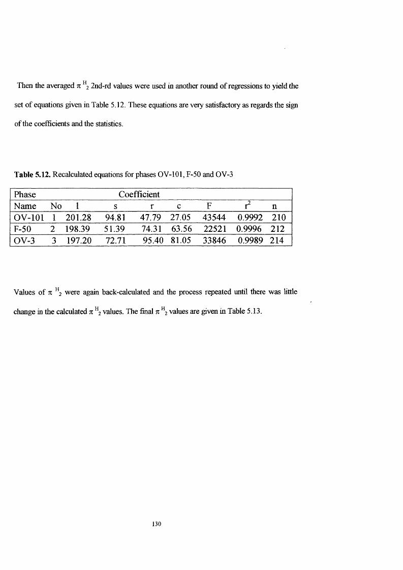
Then the averaged k ^ 2 2nd-rd values were used in another round of regressions to yield the
set of equations given in Table 5.12. Tliese equations are very satisfactory as regards the sign
of the coefficients and the statistics.
Table 5.12. Recalculated equations for phases OV-101, F-50 and OV-3
Phase CoefficientName No I s r c F nOV-101 1 201.28 94.81 47.79 27.05 43544 0.9992 210F-50 2 198.39 51.39 74.31 63.56 22521 0.9996 212OV-3 3 197.20 72.71 95.40 81.05 33846 0.9989 214
Values of n ^ 2 were again back-calculated and the process repeated until there was httle
change in the calculated % \ values. The final tc ^2 values are given in Table 5.13.
130
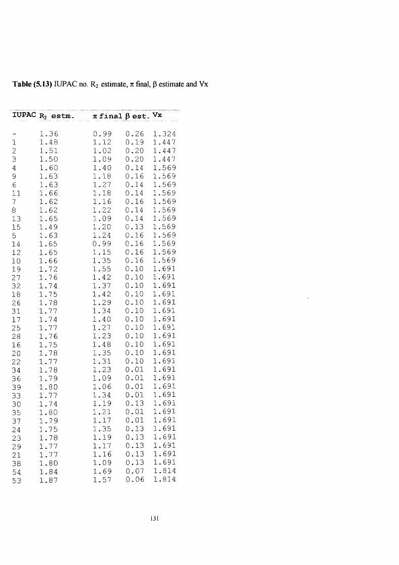
Table (5.13) lUPAC no. R2 estimate, n final, p estimate and Vx
lUPAC R2 e s t m . 7Z f i n a l p © S t. Vx
_ 1 . 3 6 0 . 9 9 0 . 2 6 1 . 3 2 41 1 . 4 8 1 . 1 2 0 . 1 9 1 .4 4 72 1 . 5 1 1 . 0 2 0 . 2 0 1 .4 4 73 1 . 5 0 1 . 0 9 0 . 2 0 1 .4 4 74 1 . 6 0 1 . 4 0 0 .1 4 1 . 5 6 99 1 . 6 3 1 . 1 8 0 . 1 6 1 . 5 6 96 1 . 6 3 1 .2 7 0 .1 4 1 . 5 6 911 1 . 6 6 1 . 1 8 0 .1 4 1 . 5 6 97 1 . 6 2 1 . 1 6 0 . 1 6 1 . 5 6 98 1 . 6 2 1 . 2 2 0 .1 4 1 . 5 6 913 1 . 6 5 1 . 0 9 0 . 1 4 1 . 5 6 915 1 . 4 9 1 . 2 0 0 . 1 3 1 . 5 6 95 1 . 6 3 1 . 2 4 0 . 1 6 1 . 5 6 914 1 . 6 5 0 . 9 9 0 . 1 6 1 . 5 6 912 1 . 6 5 1 . 1 5 0 . 1 6 1 . 5 6 910 1 . 6 6 1 . 3 5 0 . 1 6 1 . 5 6 919 1 . 7 2 1 . 5 5 0 . 1 0 1 . 6 9 127 1 . 7 6 1 . 4 2 0 . 1 0 1 .6 9 132 1 . 7 4 1 . 3 7 0 . 1 0 1 . 6 9 118 1 . 7 5 1 . 4 2 0 . 1 0 1 .6 9 126 1 . 7 8 1 . 2 9 0 . 1 0 1 . 6 9 131 1 .7 7 1 . 3 4 0 . 1 0 1 .6 9 117 1 . 7 4 1 . 4 0 0 . 1 0 1 . 6 9 125 1 . 7 7 1 .2 7 0 . 1 0 1 . 6 9 128 1 . 7 6 1 . 2 3 0 . 1 0 1 .6 9 116 1 . 7 5 1 . 4 8 0 . 1 0 1 . 6 9 120 1 . 7 8 1 . 3 5 0 . 1 0 1 . 6 9 122 1 . 7 7 1 . 3 1 0 . 1 0 1 . 6 9 134 1 . 7 8 1 . 2 3 0 . 0 1 1 .6 9 136 1 . 7 9 1 . 0 9 0 . 0 1 1 .6 9 139 1 . 8 0 1 . 0 6 0 . 0 1 1 . 6 9 133 1 .7 7 1 . 3 4 0 . 0 1 1 . 6 9 130 1 . 7 4 1 . 1 9 0 . 1 3 1 . 6 9 135 1 . 8 0 1 . 2 1 0 . 0 1 1 . 6 9 137 1 . 7 9 1 .1 7 0 . 0 1 1 . 6 9 124 1 . 7 5 1 . 3 5 0 . 1 3 1 .6 9 123 1 . 7 8 1 . 1 9 0 . 1 3 1 . 6 9 129 1 . 7 7 1 .1 7 0 . 1 3 1 . 6 9 121 1 . 7 7 1 . 1 6 0 . 1 3 1 . 6 9 138 1 . 8 0 1 . 0 9 0 . 1 3 1 .6 9 154 1 . 8 4 1 . 6 9 0 . 0 7 1 .8 1 453 1 . 8 7 1 . 5 7 0 . 0 6 1 .8 1 4
131

kOK O H-‘ 1—»K O h-' en en en 00 enen -j en en en enen --0enen -0 -j en en -j 'J 00 en en -o -j i4i=. vtv. v is . vis.. en en Hcn (T> h-'
K OK) t—'
00 Oo
oCj O
O t-» K) en M 00 e n o en 1— ' 00 eo - J eo k O k O enenkOo kOen eno M o 00 00 h O eo o ro v is . en - J KO NOP
C T
h -
NJ1—' ro h O M h J h-' h -* t-"M t—' I— ^ M M t—' I—>1— ' M f—' 1—' 1— ‘ h - ' h-' I—> MM t-J h-' MH-' H-» t—' t—CDen
o KO o O O o o ( O KO 00 00 KO LOK O KO eo 00 KO KO 00 kO KO kO 00 k o 00 œ 00 00 k O k O k O k O 00 CDKO kO kO kO k O kO 00 kO 00 00 00 00 'X?1—'MK O LO t-' o 00 MK O KO un1—>1-' ro e o Mk o N) eo o k O h -' 00 k o en en hJ1—' k O kO en eo w eo o o kO o -J 00 kOen o eo
oopr t
h-> t—' h-' 1—' h-‘ M h - ' t—' M 1—' 1—' [—' M M 1—' t-^ t—' M t—' h->M M M 1—' h-' h - ‘ h-' h-' M M h-'en - 0 eo hOen vis» vis» eneo eo en 1—' K ) eo eo eo vis. hOK ) vis. eo eo vis. vis. vis. en no eo vis. no vis. eo eo no o eo no no eo en vt. en en vis. vis. en vt^o M0 0 -0 ro eo en 0 0 o 00 vfc. M1- en 0 0 vis. 0 0 o o vis. O en -J en o eo kO 0 0 eo vis. en kO-o no vis. en 00 00 eo O eno en
o o o o o o o o o o o o O o o o o o O O o o o O o o o o o o o o o o o o o O o o o o o o O o o oo o o o o o o o t-' o O o o o o o o O o o o O o o o o o o o o o o o o o O o o o o o o o o o oeo eo eo eo eo eo eo eo eo eo eo - J -0 - J - 0 - J - J ~o - J - J - J - J ~o - J ' J -0 - J enen en en en en enen en en en en -o -J enen en
H' M h-' 1—> M Mh-' M h-J I—' t—' M 1—' t-j M M h-»MM1—' h-' Mh-» t—t—' h-' t—' h-' t—' t—' t—' 1—>w u D k O U ^ i o k O k O w c o o D œ œ œ œ œ o o c o o o o o o o œ c o œ œ œ œ œ o o c o œ o o œ œ c o œ œ œ o o c o c o œ o o œ c o c o c o c o c oU ) U ) Ü J U ) U ) ü O ü O ( j O l - ^ l —‘ h - ' l —' I —' I —' 1 —‘ 1—' 1 — ' I —' 1 — ' f —' I —‘ I—‘ I—‘ h - ' l —' f —' t —' I —‘ I—' t —' I —' h - ' h - ' t —' I —‘ f—' I —' I —‘ 1—' h - ^1—'

vo VO KO UO CD KO KO KO CD CD CD CD CD CD CD CD CD CD CD CD CD CD ‘>D CD CD CD CD CD CD CD CD CD CD CD CD CD CD CD en en en en en en en en en enoo OO oo oo 00 CO OO CO 00 OO 00 00 00 oo OO OO 00 00 OO OO 00 00 00 00 OO OO 00 00 00 00 00 OO 00 OO 00 00 00 00 lO LO LO LO LO LO LO LO LO LOm en en enen enen en en enen en enen en en en enen en en enen en en en en en en enen en enen en en en eno o o o o o O o o o
tH v-H s—1\—1M M rH I—1rH \—1M 1—11—1r H 1—1I—1I—11—11—1(—1 r H 5-1r—1 I—1r—1I—11—1\—1 I—1t—1 r H r H r H r—1 r H r H 1—1CO CO eo CO eo CO CO CO CO CO
en 00 CO oo oo CO OO OO oo OO oo CO oo 00 oo oo oo oo oo 00 oo OO OO OO oo OO oo oo IH IH O' IH r~ O' r- r- r- oo oo o o o o o o o o oO o O o o O O O o O o O o o O o o o o o o O o O o o o o O O o O o O o o o r—1o o o o o o o o o oo o O o o o o O o O o O o o o o o o o o o O o o o o o o O O o O o o o o o O o o o o o o o o o o
00 vo I—1CM 00 01 CO r- 00 01 o CD en LO 00 rH CD r- en (—1CD LO 00 o LO o r- 00 enoo 00 en \—1o CD LO O' r~ I—100 r- LO 00lD KO 01 oi 01 CO 01 CD 00 C-J 00 CD LO cO eo 00 00 t—1CO 00 CD CD CD LO LO LO CD lO 0~ CD LO ■O’ CD
-M
rH rH ;—1 \—1\—11—1rH 1—1(—1rH I—1î-\ \—1r H I—1ï—1 vH T-1(—1rH \—1\—1<—1r H I—1r H I—1\—1 r H \—1I—1r— 1 \—1\—1ï—1r H !-11—1(— 1 1—1I—1r H 1—11—1\—1\—1I—1I—1
Oü00 X-1CM uO CO 01 01 00 r~- ï—1 00 r- CD rH 00 0- en r- o CD CO LO \—1 00 r- CO 00 CO CD O' o lO CD en COI—1o O O O o o O o o o o O o o o o O o o o o o O o o o rH O O O O O o o O o o O 1—1 <—1 ;—1r—1 1—1CO r—1 \—1I—1 1—1
LOCD
C\1 CO ( N CO CO CO CO CO CO CO CO CO CO CO CO CO CO CO CO CO CO CO CO CO CO CO CO CO CO CO CO CO CO CO CO CO CO CO CO CO CO CO eo CO CO Cn] CO CO
1—10) o \—1 CO ï—i o 00 00 01 Ol oo CO r- CO CO 0 - en LO CD CD o CD LO œ LO oo en CD oo
r H î—1 I— 1 ■= CO o oo t—1o o o en CO rH en 0- lO CO o o CO CO CO CO CO r H 00 r H r H œ o r H CD O 1—1r— 1 lO oo LO oo oo lO 'lT' LOH CT) 00 I—1 rH enenen 00 J—1\—1r H rH en en t—1r H oo 00 00 00 1— 1 r H r H T-1;—1 r H r— 1 I—1en 1—1 t—1 00 ï— 1 r H 00 r—1 r— 1 I—1 I— 1 r H I—1 r H \—1 T-1 r—1\—1 r H \—1
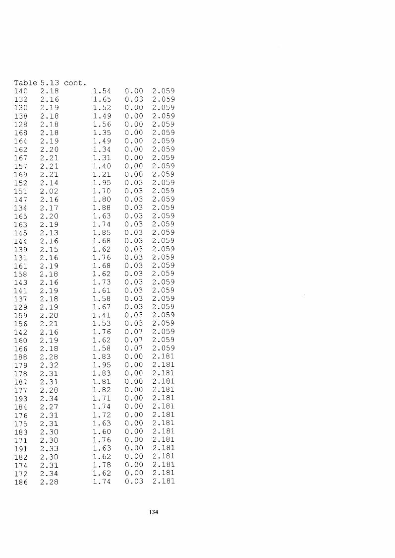
T a b l e 5 . 1 3 c o n t .140 2 . 1 8 1 .5 4 0 . 0 0 2 . 0 5 9132 2 . 1 6 1 . 6 5 0 . 0 3 2 . 0 5 9130 2 . 1 9 1 . 5 2 0 . 0 0 2 . 0 5 9138 2 . 1 8 1 . 4 9 0 . 0 0 2 . 0 5 9128 2 . 1 8 1 . 5 6 0 . 0 0 2 . 0 5 9168 2 . 1 8 1 . 3 5 0 . 0 0 2 . 0 5 9164 2 . 1 9 1 . 4 9 0 . 0 0 2 . 0 5 9162 2 . 2 0 1 . 3 4 0 . 0 0 2 . 0 5 9167 2 . 2 1 1 . 3 1 0 . 0 0 2 . 0 5 9157 2 . 2 1 1 .4 0 0 . 0 0 2 . 0 5 9169 2 . 2 1 1 . 2 1 0 . 0 0 2 . 0 5 9152 2 . 1 4 1 . 9 5 0 . 0 3 2 . 0 5 9151 2 . 0 2 1 . 7 0 0 . 0 3 2 . 0 5 9147 2 . 1 6 1 . 8 0 0 . 0 3 2 . 0 5 9134 2 . 1 7 1 . 8 8 0 . 0 3 2 . 0 5 9165 2 . 2 0 1 . 6 3 0 . 0 3 2 . 0 5 9163 2 . 1 9 1 .7 4 0 . 0 3 2 . 0 5 9145 2 . 1 3 1 .8 5 0 . 0 3 2 . 0 5 9144 2 . 1 6 1 . 6 8 0 . 0 3 2 . 0 5 9139 2 . 1 5 1 . 6 2 0 . 0 3 2 . 0 5 9131 2 . 1 6 1 . 7 6 0 . 0 3 2 . 0 5 9161 2 . 1 9 1 . 6 8 0 . 0 3 2 . 0 5 9158 2 . 1 8 1 . 6 2 0 . 0 3 2 . 0 5 9143 2 . 1 6 1 . 7 3 0 . 0 3 2 . 0 5 9141 2 . 1 9 1 . 6 1 0 . 0 3 2 . 0 5 9137 2 . 1 8 1 .5 8 0 . 0 3 2 . 0 5 9129 2 . 1 9 1 . 6 7 0 . 0 3 2 . 0 5 9159 2 . 2 0 1 . 4 1 0 . 0 3 2 . 0 5 9156 2 . 2 1 1 . 5 3 0 . 0 3 2 . 0 5 9142 2 . 1 6 1 . 7 6 0 . 0 7 2 . 0 5 9160 2 . 1 9 1 . 6 2 0 . 0 7 2 . 0 5 9166 2 . 1 8 1 . 5 8 0 . 0 7 2 . 0 5 9188 2 . 2 8 1 . 8 3 0 . 0 0 2 . 1 8 1179 2 . 3 2 1 . 9 5 0 . 0 0 2 . 1 8 1178 2 . 3 1 1 . 8 3 0 . 0 0 2 . 1 8 1187 2 . 3 1 1 . 8 1 0 . 0 0 2 . 1 8 1177 2 . 2 8 1 . 8 2 0 . 0 0 2 . 1 8 1193 2 . 3 4 1 . 7 1 0 . 0 0 2 . 1 8 1184 2 . 2 7 1 .7 4 0 . 0 0 2 . 1 8 1176 2 . 3 1 1 . 7 2 0 . 0 0 2 . 1 8 1175 2 . 3 1 1 . 6 3 0 . 0 0 2 . 1 8 1183 2 . 3 0 1 . 6 0 0 . 0 0 2 . 1 8 1171 2 . 3 0 1 . 7 6 0 . 0 0 2 . 1 8 1191 2 . 3 3 1 . 6 3 0 . 0 0 2 . 1 8 1182 2 . 3 0 1 . 6 2 0 . 0 0 2 . 1 8 1174 2 . 3 1 1 . 7 8 0 . 0 0 2 . 1 8 1172 2 . 3 4 1 . 6 2 0 . 0 0 2 . 1 8 1186 2 . 2 8 1 .7 4 0 . 0 3 2 . 1 8 1
134
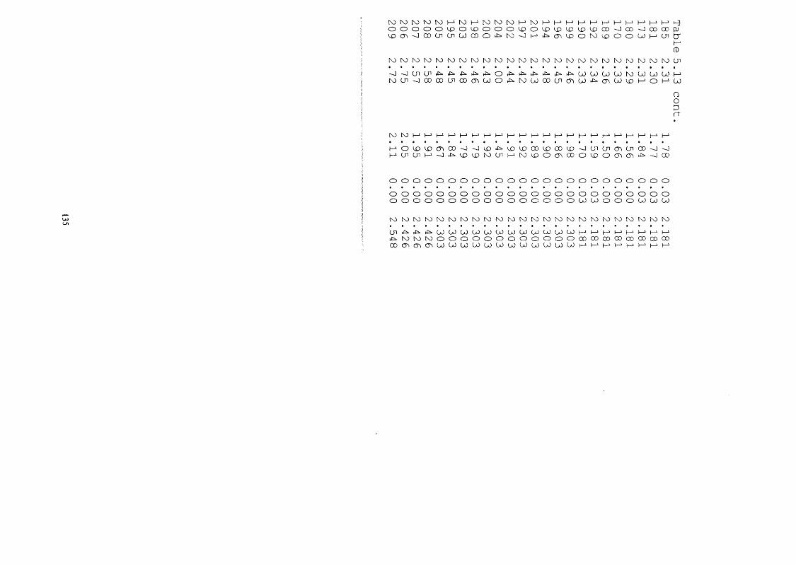
ro ro ro ro ro M ro ro ro ro ro M 1—' t—' 1—>o o o o o LO o LOo o o LOo LOLOLOLOLO00 -J 00 -J 00 00 fuLO CTi <1 00 en en ÜO 00 o ro enLOO to LOO O w en cr
(D
- J - ~ J a ^ < J 1 ^ c ^ t f c . ^ t > ^ x s > ^ ^ ^ o ^ t ï = ■ ^ I i = ■ J i ^ ^ C i . ^ t = > ^ c ^ C J O U ) ( J J ü o ^ o ü O L o ^ J O l —' K)(_n'^œœuioom(jüOW::^r\)(juoouicri i jL)tJ:^(T,(jOLOk-'OH-'UJ
Go;3rt
lo to M M M M t—' t—' h-' t—' t—»h- h-' I—‘ t—' h-' 1—' t-j h-‘ 1—'M o LOLOen 00 -0 ~o LOJi. LOLO00 LO00 LO en en (T, en 00 -J[->enen -J t=. LOLOto en 1—' hOLOo (Ti 00 o LOo (Ti en 'J 00
o o o o o o o o o o o o o o o o o o o o o o o oo o o o o o o o o o o o o o o o o o o o o o o oo o o o o o o o o o o o o o o o eo eo o o o eo eo eo
WN)[ \Jt Vi K) rcW( \ )K)W^JK) l \ ) K) [ \ ) WWK) hJK) hJWt \ ) K)eriJi.ttijr^CjOOOGJüOOOUJCjOUJüJCjOüOCjOh-'t—'Mh- 'Mh-'M l—* hr^t Ot Xi MOOOOOOOOOOOOOOOOOOCDCDCOCOCO C O C r i O ^ O ^ L O O J U > L O L O U ) U ) U ) U > U ) L O U > M l - ^ H ^ I - ^ l - ^ l - ^ l —‘ 1-^
Chapter 6 The Second Calculation of Descriptors for PCBs
6.0 Introduction
In the previous chapter the first estimation of the descriptors was given. In this
chapter the calculation of the descriptors is continued in more specific ways in order to
obtain better estimates. Octanol-water partition coefficients (Poet) of many PCBs
congeners have been determined, either by direct measurement’ or indirectly by reverse-
phase high-performance liquid chromatography. In addition predictions of log Poet can
be made^ by the use of models based on chemical structure.^ From tlie point of view of
the general solvation equation one could say that the use of log Poet would be a very
good way to obtain estimates of descriptors, and would be a complimentary method to
the GLC procedure.
6.1 The calculation of Ep ^ 2 values from water-octanol partition coefficients, as log Poet
Because the GLC phases are all non-acidic, the b.E(3 2 term is redundant. This
means that it is not possible to obtain 2 values for the PCBs from the GLC data. Tlie
other main source of data that could be used for the calculation of 2 values is that of
water-octanol partition coefficients, as log Poet values, for which the solvation equation
is known ;
log Poet = 0.088 + 0.562 R2 - 1.054 A + 0.034 Sa^ 2 - 3.460 Zp”.+ 3.814 Vx (6.1)
136
Values of log Poet for the PCBs were obtained from a number of sources, the main ones
being the Med Chem’ listed values , and those listed by Sangster in the LOGKOW data
base. For the PCBs, Za^ 2 is zero and the truncated solvation equation can be used,
log Poet = 0.088 +0.562 R2 - 1.054 A - 3.460 Zp^ 2 + 3.814 (6.2)
Hence for any PCB, if log Poet is known, and if R2 , 2 and Vx are available, then
1(3 2 can be calculated tlirough equation (6.2). However, as a start, Zp^ 2 was first roughly
estimated as shown in Table (5.3), see column (3 est. Then not only Zp^ 2 but also
sometimes 7 ^ 2 was altered in order to reproduce the correct values of log Poet. Results
are in the last two columns of Table 6.1.
137
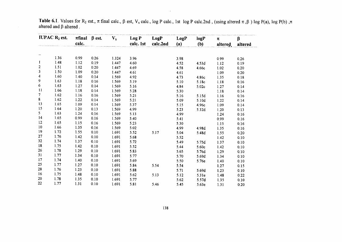
Table 6.1. Values for R2 est., n final calc., p est, Vx cale., log P calc., 1st log P calc.2nd , (using altered tt ,p ) log P(a), log P(b) ,71 altered and P altered .
lUPAC R2 est. Tufinalcalc.
P est. Vx Log? calc. 1st
LogPca!c.2nd
LogP(a)
logP(b)
K
altéré^Paltered
-1.36 0.99 0.26 1.324 3.96 3.98 0.99 0.26
1 1.48 1.12 0.19 1.447 4.60 4.52 4.53d 1.12 0.192 1.51 1.02 0.20 1.447 4.69 4.58 4.66c 1.02 0.203 1.50 1.09 0.20 1.447 4.61 4.61 1.09 0.204 1.60 1.40 0.14 1.569 4.92 4.73 4.86c 1.35 0.189 1.63 1.18 0.16 1.569 5.19 5.10 5.18c 1.18 0.166 1.63 1.27 0.14 1.569 5.16 4.84 5.02c 1.27 0.1411 1.66 1.18 0.14 1.569 5.28 5.30 1.18 0.147 1.62 1.16 0.16 1.569 5.21 5.16 5.15d 1.16 0.168 1.62 1.22 0.14 1.569 5.21 5.09 5.10d 1.22 0.1413 1.65 1.09 0.14 1.569 5.37 5.15 4.96c 1.09 0.1415 1.64 1.20 0.13 1.569 4.99 5.23 5.32d 1.20 0.135 1.63 1.24 0.16 1.569 5.13 4.99 1.24 0.1614 1.65 0.99 0.16 1.569 5.40 5.41 0.99 0.1612 1.65 1.15 0.16 1.569 5.23 5.30 1.15 0.1610 1.66 1.35 0.16 1.569 5.02 4.99 4.98d 1.35 0.1619 1.72 1.55 0.10 1.691 5.52 5.17 5.04 5.48d 1.55 0.2027 1.76 1.42 0.10 1.691 5.68 5.52 1.42 0.1032 1.74 1.37 0.10 1.691 5.72 5.49 5.75d 1.37 0.1018 1.75 1.42 0.10 1.691 5.52 5.44 5.60c 1.42 0.1026 1.78 1.29 0.10 1.691 5.83 5.65 5.76d 1.29 0.1031 1.77 1.34 0.10 1.691 5.77 5.70 5.69d 1.34 0.1017 1.74 1.40 0.10 1.691 5.69 5.50 5.76e 1.40 0.1025 1.77 1.27 0.10 1.691 5.84 5.54 5.54 1.27 0.1528 1.76 1.23 0.10 1.691 5.88 5.71 5.69d 1.23 0.1016 1.75 1.48 0.10 1.691 5.62 5.13 5.12 5.31e 1.48 0.2220 1.78 1.35 0.10 1.691 5.77 5.62 5.57d 1.35 0.1022 1.77 1.31 0.10 1.691 5.81 5.46 5.45 5.63e 1.31 0.20
138
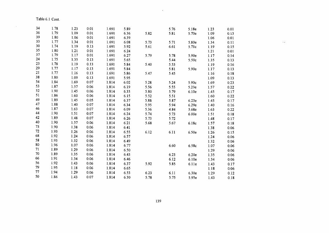
Table 6,1 Cont.
34 1.78 1.23 0.01 1.691 5.89 5.76 5.18e 1.23 0.0136 1.79 1.09 0.01 1.691 6.36 5.82 5.81 5.70e 1.09 0.1339 1.80 1.06 0.01 1.691 6.39 1.06 0.0133 1.77 1.34 0.01 1.691 6.08 5.73 5.71 5.80e 1.34 0.1130 1.74 1.19 0.13 1.691 5.92 5.61 6.61 5.71c 1.19 0.1535 1.80 1.21 0.01 1.691 6.24 1.21 0.0137 1.79 1.17 0.01 1.691 6.27 5.79 5.78 5.90e 1.17 0.1424 1.75 1.35 0.13 1.691 5.65 5.44 5.50c 1.35 0.1323 1.78 1.19 0.13 1.691 5.84 5.40 5.53 1.19 0.1629 1.77 1.17 0.13 1.691 5.84 5.81 5.90e 1.17 0.1321 1.77 1.16 0.13 1.691 5.86 5.47 5.45 1.16 0.1838 1.80 1.09 0.13 1.691 5.95 1.09 0.1354 1.84 1.69 0.07 1.814 6.02 5.28 5.24 5.90c 1.69 0.2353 1.87 1.57 0.06 1.814 6.19 5.56 5.55 5.23e 1.57 0.2252 1.90 1.45 0.06 1.814 6.33 5.80 5.79 6.10e 1.45 0.1751 1.86 1.60 0.06 1.814 6.15 5.52 5.51 1.60 0.2249 1.89 1.45 0.05 1.814 6.37 5.88 5.87 6.23e 1.45 0.1747 1.88 1.40 0.07 1.814 6.34 5.95 5.94 6.29e 1,40 0.1646 1.87 1.63 0.07 1.814 6.09 5.36 4.84 5.68e 1.63 0.2244 1.90 1.51 0.07 1.814 6.24 5.74 5.73 6.00e 1.51 0.1842 1.89 1.48 0.07 1.814 6.26 5.73 5.72 1.48 0.1740 1.90 1.57 0.06 1.814 6.21 5.68 5.67 6.18c 1.57 0.1873 1.90 1.38 0.06 1.814 6.41 1.38 0.0672 1.93 1.26 0.06 1.814 6.55 6.12 6.11 6.50e 1.26 0.1568 1.92 1.24 0.06 1.814 6.57 1.24 0.0658 1.93 1.32 0.06 1.814 6.49 1.32 0.0680 1.96 1.07 0.06 1.814 6.77 6.60 6.58c 1.07 0.0671 1.89 1.29 0.06 1.814 6.50 1.29 0.0670 1.89 1.35 0.06 1.814 6.43 6.23 6.20e 1.35 0.0666 1.91 1.34 0.06 1.814 6.46 6.12 6.10e 1.34 0.0656 1.92 1.43 0.06 1.814 6.37 5.92 5.85 6.11e 1.43 0.1779 1.95 1.18 0.06 1.814 6.65 1.18 0.0677 1.94 1.29 0.06 1.814 6.53 6.23 6.11 6.30e 1.29 0.1250 1.86 1.43 0.07 1.814 6.30 5.78 5.75 5.95e 1.43 0.18
139

Table 6.1 Cont.
69 1.89 1.30 0.07 1.814 6.45 6.04 6.03 5.89e 1.30 0.1575 1.88 1.26 0.07 1.814 6.49 6.05 6.03 5.94e 1.26 0.1445 1.87 1.57 0.07 1.814 6.16 5.48 4.84 1.57 0.2559 1.91 1.45 0.07 1.814 6.31 1.45 0.0769 1.89 1.40 0.07 1.814 6.35 5.77 5.76 6.35c 1.40 0.1943 1.90 1.44 0.07 1.814 6.31 1.44 0.0757 1.93 1.30 0.07 1.814 6.48 1.30 0.0763 1.92 1.30 0.07 1.814 6.47 6.12 6.10 1.30 0.1448 1.89 1.41 0.07 1.814 6.34 5.99 5.99 5.69c 1.41 0.1467 1.92 1.28 0.07 1.814 6.49 6.32 1.28 0.0774 1.91 1.24 0.07 1.814 6.53 6.10 6.10 6.67e 1.24 0.1641 1.89 1.48 0.07 1.814 6.21 6.11 5.79e 1.48 0.0755 1.92 1.35 0.07 1.814 6.42 1.35 0.0760 1.91 1.31 0.07 1.814 6.45 6.06 6.01 5.95e 1.31 0.1476 1.91 1.31 0.07 1.814 6.45 1.31 0.0778 1.95 1.21 0.07 1.814 6.58 1.21 0.0781 1.94 1.14 0.07 1.814 6.65 1.14 0.0765 1.89 1.51 0.13 1.814 5.96 5.96 5.94e 1.51 0.1362 1.89 1.38 0.13 1.814 6.63 1.38 0.1361 1.92 1.30 0.13 1.814 6.30 6.40 1.30 0.13104 1.98 1.58 0.03 1.936 6.86 1.58 0.03103 2.01 1.46 0.03 1.936 6.95 6.12 6.11 1.46 0.2100 2.00 1.43 0.03 1.936 6.98 6.23 6.23 1.43 0.1898 2.01 1.52 0.03 1.936 6.89 1.52 0.03121 2.04 1.27 0.03 1.936 7.17 6.43 6.43 1.27 0.16119 2.03 1.38 0.03 1.936 7.05 6.42 6.4 0.1696 1.99 1.72 0.03 1.936 6.67 0.0395 2.02 1.60 0.03 1.936 6.81 5.99 5.92 0.291 2.01 1.58 0.03 1.936 6.83 6.32 6.31 5.87c 0.1584 2.02 1.66 0.03 1.936 6.75 6.25 6.24 5.96e 0.15113 2.05 1.41 0.03 1.936 7.01 6.45 6.45 0.15110 2.04 1.52 0.03 1.936 6.91 6.45 6.22 0.1594 2.02 1.58 0.03 1.936 6.83 0.0392 2.05 1.45 0.03 1.936 6.99 6.32 6.32 6.05e 0.17
140

Table 6.1 Cont.
90 2.04 1.44 0.03 1.936 6.99 6.32 6.32 0.1783 2.05 1.52 0.03 1.936 6.92 6.52 6.51 0.12111 2.08 1.27 0.03 1.936 7.19 6.33 6.32 6.11 0.19107 2.07 1.43 0.03 1.936 7.02 0.03102 2.01 1.55 0.03 1.936 6.86 0.03101 2.04 1.60 0.02 1.936 6.82 6.51 6.50 6.16e 0.1299 2.03 1.36 0.03 1.936 7.07 6.42 6.41 7.21c 0.1697 2.04 1.49 0.03 1.936 6.94 6.34 6.31 6.67e 0.17120 2.07 1.24 0.03 1.936 7.22 5.68 5.68 0.26118 2.06 1.35 0.03 1.936 7.10 6.58 6.57 6.24e 0.1489 2.01 1.63 0.03 1.936 6.78 0.0387 2.04 1.51 0.03 1.936 6.92 6.24 6.23 6.80e 0.2085 2.03 1.48 0.03 1.936 6.94 6.63 6.61e 0.0382 2.04 1.57 0.03 1.936 6.86 0.03108 2.04 1.29 0.03 1.936 7.16 0.03105 2.04 1.41 0.03 1.936 7.02 6.79 6.79 0.09125 2.04 1.46 0.03 1.936 6.97 0.03124 2.07 1.35 0.03 1.936 7.11 0.03123 2.09 1.33 0.03 1.936 7.14 0.03122 2.07 1.40 0.03 1.936 7.06 0.03127 2.10 1.15 0.03 1.936 7.34 0.03118 2.06 1.24 0.03 1.936 7.21 6.59 6.57 6.24c 0.1893 2.02 1.80 0.07 1.936 6.47 6.58 6.06e 0.07112 2.05 1.67 0.07 1.936 6.62 6.41 0.07117 2.04 1.63 0.07 1.936 6.65 6.40 0.0788 2.01 1.69 0.07 1.936 6.57 0.07109 2.04 1.53 0.07 1.936 6.76 0.07115 2.03 1.53 0.07 1.936 6.75 6.45 0.0786 2.04 1.59 0.07 1.936 6.70 0.07106 2.07 1.44 0.07 1.936 6.87 0.07114 2.06 1.41 0.07 1.936 6.90 6.72 0.07116 2.04 1.60 0.13 1.936 6.48 6.30 6.14c 0.13150 2.13 1.56 0.03 2.059 7.39 6.65 6.64 6.31e 0.20136 2.14 1.75 0.00 2.059 7.30 6.67 6.45 7.14c 0.18
141
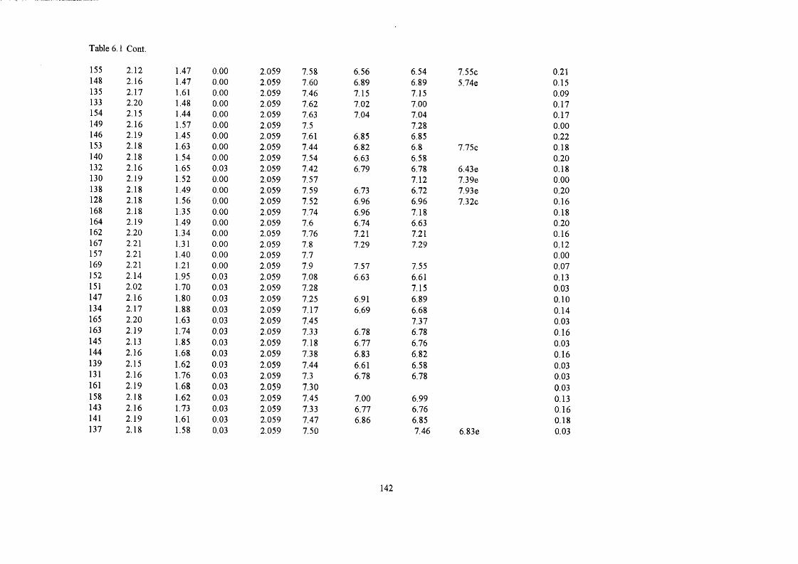
Table 6.1 Cont.
155 2.12 1.47 0.00 2.059 7.58148 2.16 1.47 0.00 2.059 7.60135 2.17 1.61 0.00 2.059 7.46133 2.20 1.48 0.00 2.059 7.62154 2.15 1.44 0.00 2.059 7.63149 2.16 1.57 0.00 2.059 7.5146 2.19 1.45 0.00 2.059 7.61153 2.18 1.63 0.00 2.059 7.44140 2.18 1.54 0.00 2.059 7.54132 2.16 1.65 0.03 2.059 7.42130 2.19 1.52 0.00 2.059 7.57138 2.18 1.49 0.00 2.059 7.59128 2.18 1.56 0.00 2.059 7,52168 2.18 1.35 0.00 2.059 7.74164 2.19 1.49 0.00 2.059 7.6162 2.20 1.34 0.00 2.059 7.76167 2.21 1.31 0.00 2.059 7.8157 2.21 1.40 0.00 2.059 7.7169 2.21 1.21 0.00 2.059 7.9152 2.14 1.95 0.03 2.059 7.08151 2.02 1.70 0.03 2.059 7.28147 2.16 1.80 0.03 2.059 7.25134 2.17 1.88 0.03 2.059 7.17165 2.20 1.63 0.03 2.059 7.45163 2.19 1.74 0.03 2.059 7.33145 2.13 1.85 0.03 2.059 7.18144 2.16 1.68 0.03 2.059 7.38139 2.15 1.62 0.03 2.059 7.44131 2.16 1.76 0.03 2.059 7.3161 2.19 1.68 0.03 2.059 7.30158 2.18 1.62 0.03 2.059 7.45143 2.16 1.73 0.03 2.059 7.33141 2.19 1.61 0.03 2.059 7.47137 2.18 1.58 0.03 2.059 7.50
6.56 6.54 7.55c 0.216.89 6.89 5.74e 0.157.15 7.15 0.097.02 7.00 0.177.04 7.04 0.17
7.28 0.006.85 6.85 0.226.82 6.8 7.75c 0.186.63 6.58 0.206.79 6.78 6.43e 0.18
7.12 7.39e 0.006.73 6.72 7.93e 0.206.96 6.96 7.32c 0.166.96 7.18 0.186.74 6.63 0.207.21 7.21 0.167.29 7.29 0.12
0.007.57 7.55 0.076.63 6.61 0.13
7.15 0.036.91 6.89 0.106.69 6.68 0.14
7.37 0.036.78 6.78 0.166.77 6.76 0.036.83 6.82 0.166.61 6.58 0.036.78 6.78 0.03
0.037.00 6.99 0.136.77 6.76 0.166.86 6.85 0.18
7.46 6.83e 0.03
142
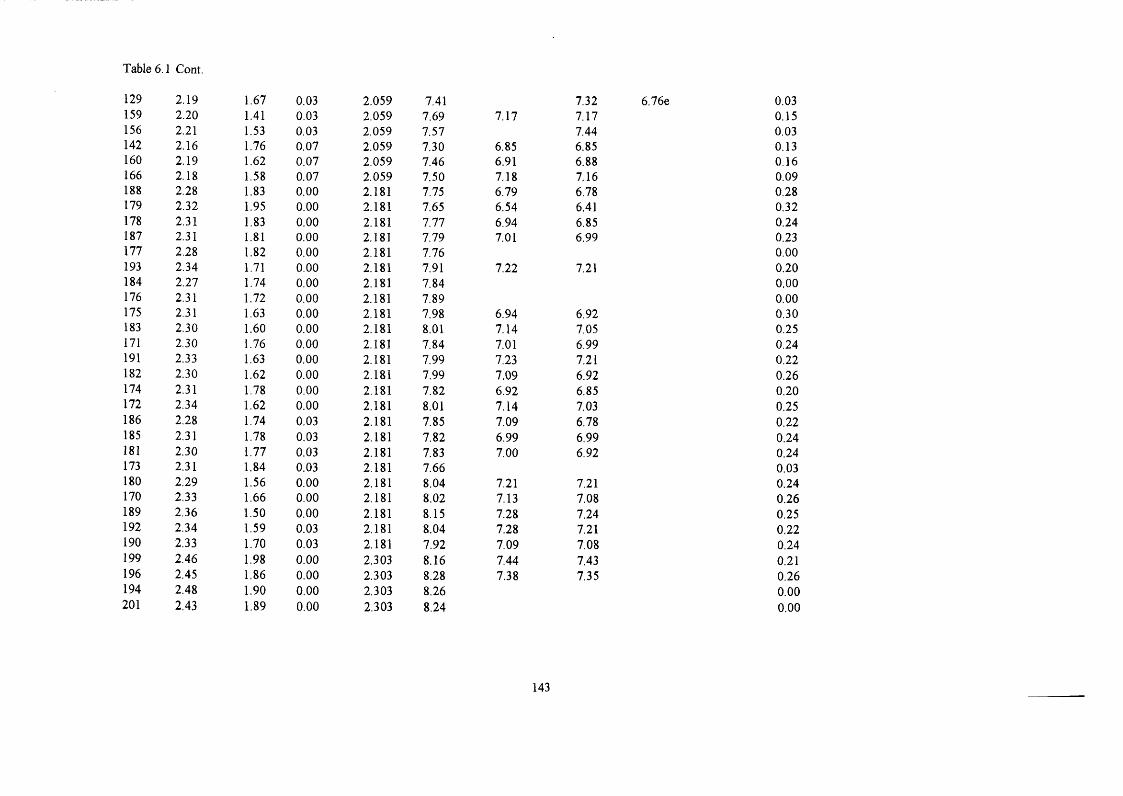
Table 6.1 Cont.
129 2.19 1.67 0.03 2.059 7.41 7.32 6.76e 0.03159 2.20 1.41 0.03 2.059 7.69 7.17 7.17 0.15156 2.21 1.53 0.03 2.059 7.57 7.44 0.03142 2.16 1.76 0.07 2.059 7.30 6.85 6.85 0.13160 2.19 1.62 0.07 2.059 7.46 6.91 6.88 0,16166 2.18 1.58 0.07 2.059 7.50 7.18 7.16 0.09188 2.28 1.83 0.00 2.181 7.75 6.79 6.78 0.28179 2.32 1,95 0.00 2.181 7.65 6.54 6,41 0.32178 2.31 1.83 0.00 2.181 7.77 6.94 6.85 0.24187 2.31 1.81 0.00 2.181 7.79 7.01 6.99 0.23177 2.28 1.82 0.00 2.181 7.76 0.00193 2.34 1.71 0.00 2.181 7.91 7.22 7.21 0.20184 2.27 1.74 0,00 2.181 7.84 0.00176 2.31 1.72 0.00 2.181 7.89 0.00175 2.31 1.63 0.00 2.181 7.98 6.94 6.92 0.30183 2.30 1.60 0.00 2.181 8.01 7.14 7.05 0.25171 2.30 1.76 0.00 2.181 7.84 7.01 6.99 0.24191 2.33 1.63 0.00 2.181 7.99 7.23 7.21 0.22182 2.30 1.62 0.00 2.181 7.99 7.09 6.92 0.26174 2.31 1.78 0.00 2.181 7.82 6.92 6.85 0.20172 2.34 1,62 0.00 2,181 8.01 7.14 7,03 0.25186 2.28 1.74 0.03 2.181 7.85 7.09 6.78 0.22185 2,31 1.78 0.03 2.181 7.82 6.99 6.99 0.24181 2.30 1.77 0.03 2.181 7.83 7.00 6.92 0.24173 2.31 1.84 0.03 2.181 7.66 0.03180 2.29 1.56 0.00 2.181 8.04 7.21 7.21 0.24170 2.33 1.66 0.00 2.181 8.02 7.13 7.08 0.26189 2.36 1.50 0.00 2.181 8.15 7.28 7.24 0.25192 2.34 1.59 0.03 2.181 8.04 7.28 7.21 0.22190 2.33 1.70 0.03 2.181 7.92 7.09 7.08 0.24199 2.46 1.98 0.00 2.303 8.16 7.44 7.43 0.21196 2.45 1.86 0.00 2.303 8.28 7.38 7.35 0.26194 2.48 1.90 0.00 2.303 8.26 0.00201 2.43 1.89 0.00 2.303 8.24 0.00
143

Table 6.1 Cont.
197 2.42 1.92 0.00 2.303 8.21 0.00202 2.44 1.91 0.00 2.303 8.23 0.00204 2.38 1.85 0.00 2.303 8.50 7.60 7.48 0.26200 2.43 1.92 0.00 2.303 8.21 7.31 7,21 7.11c 0.26198 2.46 1.79 0.00 2.303 8.36 7.46 7.43 0.26203 2.48 1.79 0.00 2.303 8.37 7.51 7.49 0.25195 2.45 1.84 0.00 2.303 8.30 7.41 7.35 0.26205 2.48 1.67 0.00 2.303 8.50 7.64 7.62 0.25208 2.58 1.91 0.00 2.426 8.77 0.00207 2.57 1.95 0.00 2.426 8.73 0.00206 2.60 2.05 0.00 2.426 8.25 8.16 0.00209 2.72 2.11 0.00 2.548 8.18 8.26 7.73c 0.00
a- Log P listed by Sangster as log KOW
b- Values of log P from ref. paper ( c- from Opperhuizen e- from Rapaport d- from Sabiljic )
144
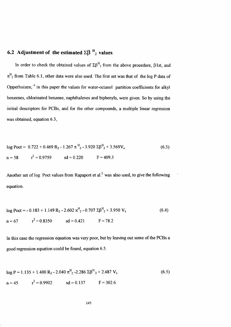
6.2 Adjustment of the estimated E|3 ” 2 values
In order to check the obtained values of from the above procedure, plst, and
7 ^ 2 from Table 6.1, other data were also used. The first set was that of the log P data of
Opperhuizen; in this paper tlie values for water-octanol partition coefficients for alkyl
benzenes, chlorinated benzene, naphthalenes and biphenyls, were given. So by using the
initial descriptors for PCBs, and for the other compounds, a multiple linear regression
was obtained, equation 6.3,
log Poet = 0.722 + 0.469 R2 - 1.267 t c " 2 - 3.920 + 3.569Vx (6.3)
n = 58 = 0.9759 sd = 0.220 F = 409.3
Another set of log Poet values from Rapaport et al. was also used, to give the following
equation.
log Poet = - 0.183 + 1.149 R2 - 2.602 71^2 - 0.707 Sp^ + 3.950 (6.4)
n = 67 r = 0.8350 sd = 0.421 F = 78.2
In this case tlie regression equation was very poor, but by leaving out some of the PCBs a
good regression equation could be found, equation 6.5.
log P = 1.135 + 1.400 R2 - 2.040 tc^ -2.286 Sp^ 2 + 2.487 (6.5)
n = 45 r = 0.9902 sd = 0.137 F = 302.6
145
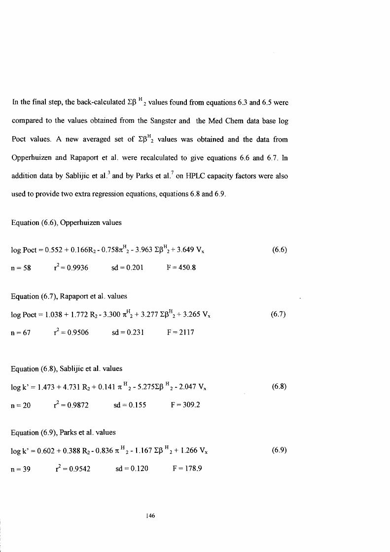
In the final step, the back-calculated ^ 2 values found from equations 6.3 and 6.5 were
compared to the values obtained from the Sangster and the Med Chem data base log
Poet values. A new averaged set of values was obtained and the data from
Opperhuizen and Rapaport et al. were recalculated to give equations 6.6 and 6.7. In
addition data by Sablijic et al. and by Parks et al. on HPLC capacity factors were also
used to provide two extra regression equations, equations 6.8 and 6.9.
Equation (6.6), Opperhuizen values
log Poet = 0.552 + 0.166R: - 0.758A - 3.963 +3.649 (6.6)
n = 58 r = 0.9936 sd = 0.201 F = 450.8
Equation (6.7), Rapaport et al. values
log Poet = 1.038 + 1.772 Rj - 3.300 + 3.277 + 3.265 V* (6.7)
n = 67 = 0.9506 sd = 0.231 F = 2117
Equation (6.8), Sablijic et al. values
log k’ = 1.473 + 4.731 Rj + 0.141 it “ 2 - 5.275ZP " 2 - 2.047 V, (6.8)
n = 20 = 0.9872 sd = 0.155 F = 309.2
Equation (6.9), Parks et al. values
log k’ = 0.602 + 0.388 R2 - 0.836 tc " 2 - 1 167 ZP “ 2 + 1.266 V, (6.9)
n = 39 = 0.9542 sd = 0.120 F =178.9
146

6.3 Individual calculations for the PCBs
The regression equations obtained to data are summarized in Table 5.6 [This will
give the GLC, log P, log k’ etc. equations]. Then for each PCB, the values of the
dependent variable, I , log Poet, or log k’ were back-calculated from the equations. If the
back-calculated values did not entirely agree with the observed values, then the
descriptor values were adjusted accordingly. As found before, imsatisfactory results were
obtained with the more polar GLC phases, so most recalculations were carried out with
the non-polar GLC phases and tlie various phases used in the calculation of As an
example, the individual calculation for PCB 172 (2,3,4,5- tetrachlorobiphenyl) is given in
Table 6.2.
Table 6.2. Individual calculation of descriptors for PCB 172 (2,3,4,5-
tetrachlorobiphenyl).
6.2 (A) Comparison of observed and calculated values
System
log Poet
log k’(3) '
Obs. Values C a lc .\
6.450 6.3936.406 6.586
2.039 1.8982 2.043 1.9083 2.127 1.9984 2.306 2.2775 2.110 2.02611 2.000 2.200
147

sd: 0.118
a Reference number, b For the GLC phases I/IOOO is entered.
6.3 (B) Descriptor values used in the recalculation
Descriptor Original values Recalculatedvalues
R2 1.92 1.9271 2 1.30 1.31
0.09 0.09Log 8.30 8.28V. 1.814 1.814
6.4 Re-examination of the polar GLC phases
Because a number of polar GLC phases had not yielded satisfactory results, new
regression equations were obtained with the descriptors found in 6.4. An example is
phase 8 (An-600).
I =324.626 + 363.005R2 + 421.229ji”2 + 157.589logL'^ (6.10)
n = 49 = 0.963 sd = 0.203 F = 209.7
This is still not satisfactory, and so most of the polar GLC phases were not further used.
148

6.5 References
1. A. J. Leo, The Medicinal Chemistry Project, Pomona College, Claremont, CA
9171.
2. R. A. Rapaport and S. J. Eisenreich, Environ. Sci. Technol., 1984, Vol. 18,163.
3. A. Sablijic, H. Gusten, J. Hennens and A. Opperhuizen. Environ. Sci. Technol.
1993, Vol. 27, 1394.
4. M. H. Abraham, H. S. Chadha, G. S. Whiting and R. C. Mitchell, J. Pharm . Sci.,
1994, Vol., 83, 1085.
5. J. Sangster., J. Phys. Chem. Ref. Data., 1989, Vol. 18,1111.
6. A. Opperhuizen, Toxico. and Environ. Chem., 1987, Vol. 15,249.
7. J. H. Park, P. W. Carr, M. H. Abraham, R.W. Taft, R. M. Doherty and M. J.
Kami et. Adv. Technol. and Res. 1987, Vol. 25, 30.
149
Chapter 7 The Final (Third) Calculation of Descriptors for PCBs
7.0 Introduction
This chapter is a continuation of the work which was described in the previous two
chapters (Chapters 5 and 6). In this chapter most of the calculations will be done by using
Solver, the Microsoft Excel computer program which is fast and easy to use. In the first
part of the Chapter, the PCBs studied by Opperhuizen' will be dealt witli, and in the
second part all the 209 PCBs will be considered.
7.1 Using Solver program to get the final values for (tu®2 , and lo g L '^ )
The Solver program is a program in Excel that automatically carries out the
procedure for the calculation of descriptors that was done by hand previously.
Regression coefficients for all systems examined were entered into the Excel
spreadsheet. Then for any given PCB, the dependent variables were entered. The
descriptors and were taken as fixed values, and Solver then calculates the values of
71 2 , ZP^ 2 and log L'^ that give the best fit of observed and calculated dependent
variables. It is possible to over-ride the Solver calculations, and fix descriptors either
within a range or as a definite value. For example, from tlie previous work, it was clear
that for all the dichlorobiphenyls was within the range O i l to 0.19, and so this
range for dichlorobiphenyls was fixed in Solver.
150

The range for values of log for the PCBs was estimated using data on the
polychlorobenzenes, (see Table 7.1 ). The log values fall into a definite pattern. This
a pattern was used to estimate log values for the PCBs as a first assessment, in the
Solver program. The PCBs listed in die paper of Opperhuizen paper and studied using
Solver are given in Table (7.2 ).
Table (7.1) The pattern of values of log for the chlorobenzenes
Name logL'^ Difference Est log
Benzene 2.79Chlorobenzene 3.63 0.87 3.661,2-Di chlorobenzene 4.47 0.98 4.441,2,3-Trichlorobenzene 5.31 0.81 5.251,2,3,5-Tetrachlorobenzene 6.15 0.75 6.00Pentachl orobenzene 6.99 0.72 6.72Hexachlorobenzene 7.83 0.90 7.62
In Table 7.2 are given a number of different sets of values for the descriptors for the
PCBs listed in the paper of Opperhuizen.^ The first set of results (I) was by use of the
Solver program, which had to be done two or tliree times in order to get the best set
according to the limitation of the values of Sp2 . The second sets (2) were by hand
calculation using an in-house method (LPCALC). The third set was the one that was
chosen to give the ‘best’ values for all the descriptors. There is not much difference
151

between the values, and the set with the smallest sd value (in Solver) was taken as the
final set of values (shown as ‘3’ in the Table 7.2 ).
Table (7.2) Values for ( tt 2 , , log and sd ) using Solver calculations, with
previous values and the values finally taken .
Name R 2 V x LogL“ Sd
Biphenyl 1.36 1.32 0.87 0.32 4.62 0.281 0.94 0.25 5.19 0.19
0.98 0.25 5.44 0.150.98 0.24 5.44 0.16
2 0.98 0.25 5.40 0.163 0.98 0.25 5.44 0.15
2-Monochlorobiphenyl 1.48 1.45 0.94 0.26 6.36 0.051 1.08 0.20 6.44 0.04
1.08 0.18 6.44 0.071.08 0.18 6.35 0.09
2 1.11 0.19 6.30 0.663 1.08 0.20 6.35 0.04
3 -Mo nochloro biphenyl 1.51 1.45 0.62 0.38 6.62 0.131 1.06 0.17 6.35 0.18
1.06 0.20 6.35 0.181.06 0.18 6.35 0.18
2 1.02 0.20 6.40 0.173 1.06 0.18 6.35 0.18
4-Monochlorobiphenyl 1.50 1.45 1.08 0.28 6.67 0.171 0.64 0.38 6.72 0.09
1.01 0.20 6.57 0.131.01 0.18 6.57 0.15
2 1.09 0.17 6.48 0.153 1.01 0.20 6.57 0.13
2,2'-Dichlorobiphenyl 1.60 1.57 1.29 0.22 4.80 0.47I 1.34 0.15 6.79 0.06
1.34 0.14 6.79 0.072 1.46 0.10 6.66 0.863 1.29 0.15 6.79 0.06
152
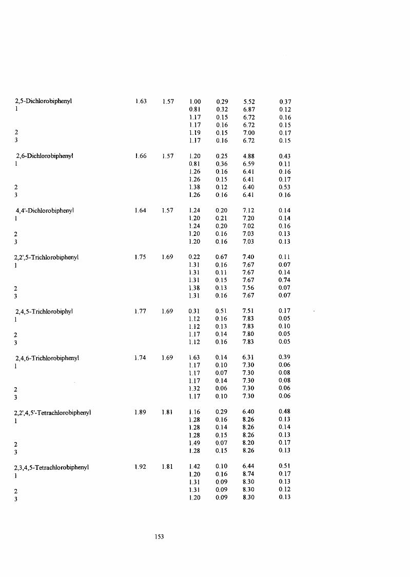
2,5 -Dichloro biphenyl 1.63 1.57 1.00 0.29 5.52 0.371 0.81 0.32 6.87 0.12
1.17 0.15 6.72 0.161.17 0.16 6.72 0.15
2 1.19 0.15 7.00 0.173 1.17 0.16 6.72 0.15
2,6-Dichlo ro biphenyl 1.66 1.57 1.20 0.25 4.88 0.431 0.81 0.36 6.59 0.11
1.26 0.16 6.41 0.161.26 0.15 6.41 0.17
2 1.38 0.12 6.40 0.533 1.26 0.16 6.41 0.16
4,4'-Dichlorobiphenyl 1.64 1.57 1.24 0.20 7.12 0.14I 1.20 0.21 7.20 0.14
1.24 0.20 7.02 0.162 1.20 0.16 7.03 0.133 1.20 0.16 7.03 0.13
2,2', 5 -T richlo robiphenyl 1.75 1.69 0.22 0.67 7.40 0.111 1.31 0.16 7.67 0.07
1.31 0.11 7.67 0.141.31 0.15 7.67 0.74
2 1.38 0.13 7.56 0.073 1.31 0.16 7.67 0.07
2,4,5-T richlo robiphyl 1.77 1.69 0.31 0.51 7.51 0.17I 1.12 0.16 7.83 0.05
1.12 0.13 7.83 0.102 1.17 0.14 7.80 0.053 1.12 0.16 7.83 0.05
2,4,6-Trichlorobiphenyl 1.74 1.69 1.63 0.14 6.31 0.391 1.17 0.10 7.30 0.06
1.17 0.07 7.30 0.081.17 0.14 7.30 0.08
2 1.32 0.06 7.30 0.063 1.17 0.10 7.30 0.06
2,2',4,5'-T etrachlorobiphenyl 1.89 1.81 1.16 0.29 6.40 0.481 1.28 0.16 8.26 0.13
1.28 0.14 8.26 0.141.28 0.15 8.26 0.13
2 1.49 0.07 8.20 0.173 1.28 0.15 8.26 0.13
2,3,4,5-T etrachlorobiphenyl 1.92 1.81 1.42 0.10 6.44 0.511 1.20 0.16 8.74 0.17
1.31 0.09 8.30 0.132 1.31 0.09 8.30 0.123 1.20 0.09 8.30 0.13
153
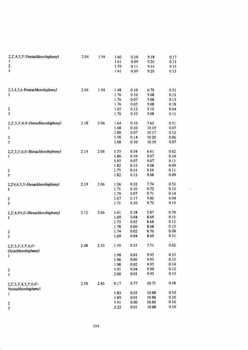
2,2 ',4,5,5 '-Pentachlorobiphenyl 1 2 3
2,3,4,5,6-Pentachlorobiphenyl 1
2,2',3,3',4,4'-Hexachlorobiphenyl1
2,2',3,3',6,6'-Hexachlorobiphenyl1
2,2'4,4,5,5 '-Hexachlorobiphenyl 1
2,2',4,4'6,6'-Hexachlorobiphenyl 1
23
2,2',3,3',5,5',6,6'- Octachlo robiphenyl I
23
2,2',3,3’,4,5,5',6,6'-Nonachlorobiphenyl1
23
2.04 1.94
2.04 1.94
2.18 2.06
2.14 2.06
2.19 2.06
2.12 2.06
2.48 2.30
2.58 2.43
1.60 0.10 9.18 0.171.61 0.09 9.20 0.131.59 0.11 9.14 0.151.61 0.09 9.20 0.13
1.48 0.10 6.70 0.511.76 0.10 9.08 0.111.76 0.07 9.08 0.151.76 0.05 9.08 0.181.65 0.12 9.10 0.041.76 0.10 9.08 0.11
1.64 0.10 7.62 0.511.68 0.10 10.19 0.071.88 0.07 10.17 0.121.58 0.14 10.20 0.061.68 0.10 10.19 0.07
1.53 0.34 6.61 0.621.86 0.10 9.07 0.101.93 0.07 9.07 0.111.82 0.12 9.08 0.091.75 0.14 9.10 0.111.82 0.12 9.08 0.09
1.26 0.32 7.74 0.521.71 0.10 9.72 0.131.79 0.07 9.71 0.141.67 0.17 9.80 0.041.71 0.10 9.72 0.13
1.61 0.18 5.87 0.701.69 0.04 8.69 0.111.73 0.02 8.68 0.121.78 0.00 8.68 0.131.74 0.02 8.70 0.081.69 0.04 8.69 0.11
1.39 0.35 7.51 0.62
1.98 0.01 9.95 0.131.98 0.00 9.95 0.131.98 0.02 9.95 0.141.91 0.04 9.90 0.122.00 0.01 9.95 0.13
0.17 0.77 10.71 0.38
1.83 0.03 10.88 0.101.89 0.01 10.88 0.101.91 0.00 10.80 0.102.22 0.01 10.88 0.10
154
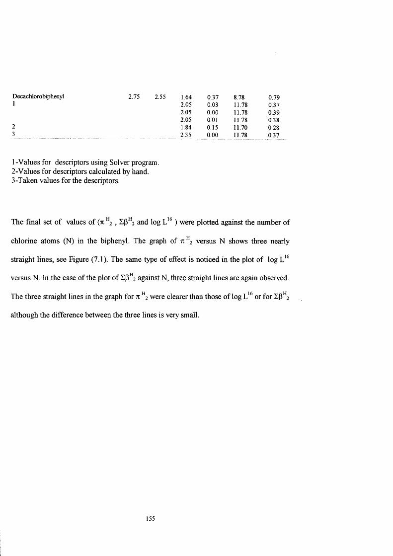
D ecachlorobiphenyl 2 .75 2 .55 1.64 0 .3 7 8.78 0 .7 91 2 .05 0.03 11.78 0 .3 7
2.05 0 .0 0 11.78 0 .3 92.05 0.01 11.78 0 .38
2 1.84 0.15 11.70 0 .283 2.35 0 .00 11.78 0 .3 7
1 - Values for descriptors using Solver program.2-Values for descriptors calculated by hand.3-Taken values for the descriptors.
The final set of values of (tc ^ 2 , Zp^ 2 and log ) were plotted against the number of
chlorine atoms (N) in the biphenyl. The graph of 7 1 ^ 2 versus N shows three nearly
straight lines, see Figure (7.1). The same type of effect is noticed in the plot of log
versus N. In the case of the plot of Z(3 2 against N, three straight lines are again observed.
The three straight lines in the graph for n ^ 2 were clearer than those of log or for Zp^ 2
although the difference between the three lines is very small.
155

2.50
2 00
1 50
1.00
0.50
0 0 0 4- -
0 00
I
2 00
♦%
ift
tit
4 00 6 .00 8.00
Chlorine number10.00
Figure (7.1) Plot of tt vs chlorine number.
For ortho-substituted congeners ( ♦ ) 2,2’,6,6’-substituted congeners, ( H ) 2,2’-
substituted congeners, ( ^ ) 2- substituted congeners and ( X ) non-substituted .
156
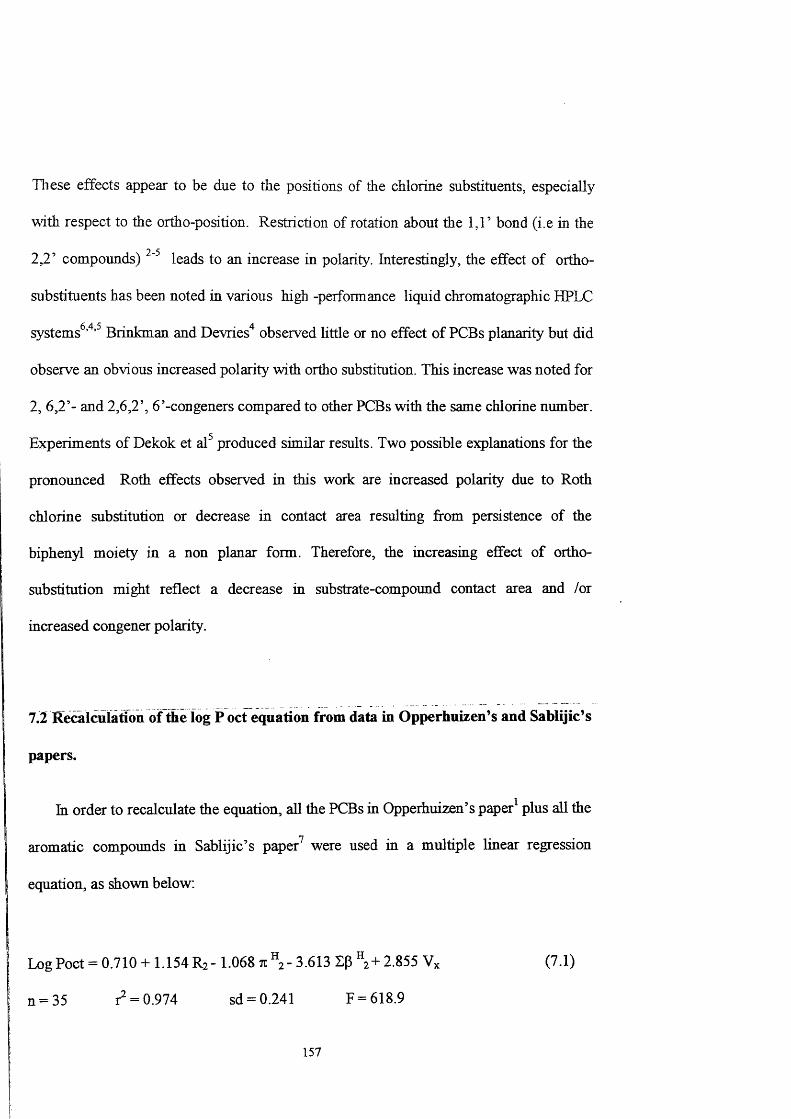
Tliese effects appear to be due to the positions of the chlorine substituents, especially
w th respect to the ortho-position. Restriction of rotation about the 1,1’ bond (i.e in the
2,2’ compounds) leads to an increase in polarity. Interestingly, the effect of ortho
substituents has been noted in various high -performance liquid chromatographic HPLC
systems^’"’ Brinkman and Devries' observed httle or no effect of PCBs planarity but did
observe an obvious increased polarity with ortho substitution. This increase was noted for
2, 6,2’- and 2,6,2’, 6’-congeners compared to other PCBs with the same chlorine number.
Experiments of Dekok et al produced similar results. Two possible explanations for the
pronounced Roth effects observed in this work are increased polarity due to Roth
chlorine substitution or decrease in contact area resulting from persistence of the
biphenyl moiety in a non planar form. Therefore, the increasing effect of ortho-
substitution might reflect a decrease in substrate-compound contact area and /or
increased congener polarity.
7.2 R ecalculatioii o f the log P oct equation from data in O pperhuizen s and Sablijic’s
papers.
In order to recalculate the equation, all the PCBs in Opperhuizen’s paper^ plus all the
aromatic compounds in Sablijic’s paper^ were used in a multiple linear regression
equation, as shown below;
Log Poet = 0.710 +1.154 R2 -1.068 Tt “2 - 3.613 Sp "2 + 2.855 V, (7.1)
n = 35 1 = 0.974 sd = 0.241 F = 618.9
157

This equation was then used as a reference equation in the Solver program, together with
previous equations. New values for the descriptors for compounds in Opperhuizen's
paper were then calculated. A new graph for each descriptor verses the number of
chlorine atoms, N, was drawn. Using the linear regression the equation for each line was
found. The first one represented the (2,2’,6,6’) ortho-substituted PCBs, the second line
represented the 2,2’ substituted PCBs, and the last line was for one substituted or non -
substituted, as shown in Table (7.3). From tlie equations for the line, new calculated
values for ( tt % aud log ) were obtained.
Table (7.3)
Linear equations of ti 2 , log L for the PCBs in Opperhuizen’s paper^
Linear equations of 7i ^ 2
g + N, where g is a constant and N is the number of chlorine atoms in the PCB
0.98 + 0.13 N, for (2,2’,6,6’) ortho-substituted PCBs
n = 9 r = 1.00 sd = 0.01 F = 1691.5
0.96 + 0.13 N, for ( 2,2’) ortho-substituted PCBs
n = 6 r = 1.00 sd = 0.01 F = 1106.5
0.96 + 0.11 N, for one substituted or, non substituted
n = 7 r^= 1.00 sd = 0.01 F= 1053.4
Linear equations for |3 ^ 2
158
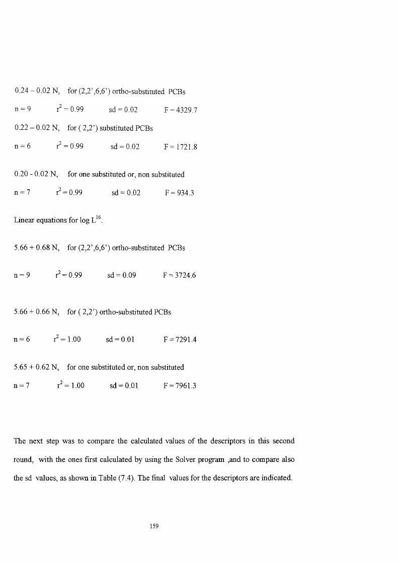
0.24-0.02 N, for (2,2’,6,6’) ortho-substitiited PCBs
n = 9 r^-0.99 sd = 0.02 F = 4329.7
0.22 - 0.02 N, for ( 2,2’) substituted PCBs
n = 6 r = 0.99 sd = 0.02 F= 1721.8
0.20 - 0.02 N, for one substituted or, non substituted
n = 7 r = 0.99 sd = 0.02 F = 934.3
Linear equations for log
5.66 + 0.68 N, for (2,2’,6,6’) ortho-substituted PCBs
n = 9 r = 0.99 sd = 0.09 F = 3724.6
5.66 + 0.66 N, for ( 2,2’) ortho-substituted PCBs
n = 6 r^=1.00 sd = 0.01 F = 7291.4
5.65 + 0.62 N, for one substituted or, non substituted
n = 7 r = 1.00 sd = 0.01 F = 7961.3
The next step was to compare the calculated values of the descriptors in this second
round, with the ones first calculated by using the Solver program ,and to compare also
the sd values, as shown in Table (7.4). The final values for the descriptors are indicated.
159

Table (7.4) The values for (n 2 , ^2 , log ) first calc., ( t c ^2, ^ 2, log ) second calc. and the values for sd .
Name N ^ " 2 ZP^2 logL '' Sd Z P ''] logL'" sd
2nd 2nd 2nd 2nd 1st 1st 1st 1stBiphenyl 0.00 0.97 0.24 5.530 0.106 0.98 0.25 5.444 0.0972-Monochlorobiphenyl 1.00 1.13 0.22 6.320 0.096 1.10 0.22 6.340 0.0943 -Mono chlorobi phenyl 1.00 1.11 0.22 6.230 0,130 1.01 0.22 6.440 0.1174-Monochlorobiphenyl 1.00 1.10 0.22 6.320 0.125 1.00 0.21 6.400 0.0972,2 '-Di chl orobiphenyl 2.00 1.24 0.17 6.980 0.086 1.20 0.18 6.800 0.0702,5 -Di chl orobiph enyl 2.00 1.18 0.20 7.220 0.096 1.25 0.19 6.900 0.0942,6 -Di chl orobiphenyl 2.00 1.23 0.20 7.220 0.121 1.25 0.19 6.746 0.120
4,4 ’ -Di chl orobiph enyl 2.00 1.06 0.19 7.220 0.117 1.07 0.19 6.900 0.116
2,2',5-Trichlorobiphenyl 3.00 1.34 0.15 7.640 0.074 1.30 0.16 7.500 0.063
2,4,5-Trichlorobiphenyl 3.00 1.27 0.18 7.720 0.093 1.28 0.16 7.500 0.0822,4,6-T richl orobipheny 3.00 1.36 0.17 7.720 0.152 1.35 0.17 7.400 0.127
2,2',4,5'-Tetrachlorobipheny 4.00 1.47 0.14 8.300 0.124 1.48 0.13 8.251 0.0982,3,4,5-T etiachlorobiphen 4.00 1.39 0.15 8.330 0.103 1.53 0.15 8.300 0.098
2,2',3,4,5'Pentachlorobipheny 5.00 1.64 0.11 8.960 0.142 1.62 0.11 9.160 0.101
2,3,4,5,6-Pentachlorobiphenyl 5.00 1.59 0.13 9.030 0.101 1.55 0.12 9.090 0.084
2,2',3,3',4,4'-Hexachlorobiphenyl 6.00 1.65 0.09 9.620 0.143 1.75 0.08 9.900 0.095
160
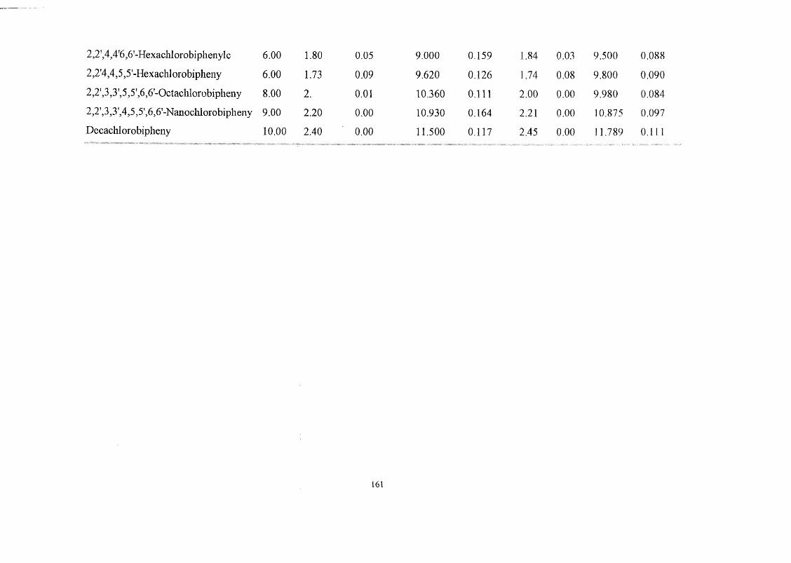
2,2 ',4,4 '6,6 '-Hexachl orobiphenyl c 6.00 1.80 0.05 9.000 0.159 1.84 0.03 9.500 0.0882,2 '4,4,5,5 '-Hexachl orobipheny 6.00 1.73 0.09 9.620 0.126 1.74 0.08 9.800 0.0902,2',3,3',5,5',6,6'-Octachlorobipheny 8.00 2. 0.01 10.360 0.111 2.00 0.00 9.980 0.0842,2',3,3',4,5,5',6,6'-Nanochlorobipheny 9.00 2.20 0.00 10.930 0.164 2.21 0.00 10,875 0.097Decachlorobipheny 10.00 2.40 0.00 11.500 0,117 2.45 0.00 11.789 0.111
161
7. 3 Calculation of the descriptors for the rest of the PCBs.
Once the best values of the descriptors for the compounds in Opperhuizen’s paper
were found, plots against N were again carried out. The various equations from linear
regressions were found in the same way as before. Using these equations, calculated
values for the descriptors for the rest of the PCBs could be obtained. Values for all 209
PCBs are shown in Table (7.5).
Using these calculated descriptors, it was possible to predict values for the water-
octanol partition coefficients for all the PCBs, through equation (5.2). Results are also
shown in Table (7.5). Comparison of the calculated logPoct values with those observed
(Table 6.1, log P calculated using the altered n , [3 values) gave a standard deviation in
observed- predicted values of only 0.122, which is a very acceptable value.
162

Table (7.5 ) Calculated values for ( t c 2^, ZP 2^ and log ) the values of log P first calc, Predicted values for log P16
Name lUPAC Log cal Log P cal(a) Log P prd(b) 7t 2 cal ZP2" cal Log P
Biphenyl 5.660 3.890 4.06 0.98 0.24 0.172-Monochloro 1 6.430 4.600 4.54 1.11 0.22 -0.063-Monochloro 2 6.430 4.690 4.60 1.00 0.20 -0.094-Monochloro 3 6.340 4.610 4.58 1.00 0.20 -0.032,2'-Dichloro 4 7.020 5.060 5.07 1.28 0.22 0.012,3-Dichloro 5 6.980 5.130 5.08 1.20 0.18 -0.052,3'-Dichloro 6 6.980 5.165 5.08 1.20 0.18 -0.082,4-Dichloro 7 6.980 5.010 5.06 1.20 0.18 0.052,4'-Dichloro 8 6.980 5.130 5.06 1.20 0.18 0.072,5-Dichloro 9 6.980 5.150 5.08 1.20 0.18 0.072,6-Dichloro 10 6.980 5.090 5.14 1.20 0.18 0.053,3’-Dichloro 11 6.880 5.280 5.30 1.18 0.16 -0.023,4-Dichloro 12 6.880 5.230 5.30 1.18 0.16 0.073,4'-Dichloro 13 6.880 5.250 5.18 1.18 0.16 -0.073,5-Dichloro 14 6.880 5.320 5.37 1.18 0.16 0.054,4'-Dichloro 15 6.880 5.300 5.35 1.18 0.16 0.052,2',3-Trichloro 16 7.640 5.620 5.62 1.33 0.15 0.002,2',4-Trichloro 17 7.640 5.620 5.60 1.33 0.15 -0.022,2',5-Trichloro 18 7.640 5.527 5.62 1.33 0.15 0.092,2',6-Trichloro 19 7.640 5.550 5.62 1.33 0.15 0.072,3,3-Trichloro 20 7.510 5.590 5.57 1.29 0.14 0.022,3,4-Trichloro 21 7.510 5.670 5.61 1.29 0.14 0.042,3,4-Trichloro 22 7.510 5.590 5.61 1.29 0.14 -0.022,3,5-Trichloro 23 7.510 5.690 5.61 1.29 0.14 -0.08
163
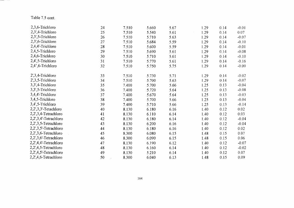
Table 7,5 cont.
2,3,6-Tricliloro 24 7.510 5.660 5.67 ].29 0.14 -0.012,3',4-Tricliloro 25 7.510 5.540 5.61 1.29 0.14 0.072,3',5-Tricliloro 26 7.510 5.710 5.63 1.29 0.14 -0.072,3',6-Trichloro 27 7.510 5.684 5.59 1.29 0.14 -0.102,4,4'-Tricliloro 28 7.510 5.600 5.59 1.29 0.14 -0.012,4,5-Trichloro 29 7.510 5.690 5.61 1.29 0.14 -0.082,4,6-Trichloro 30 7.510 5.710 5.61 1.29 0.14 -0.102,4',5-Trichloro 31 7.510 5.770 5.61 1.29 0.14 -0.162,4’,6-Trichloro 32 7.510 5.750 5.75 1.29 0.14 -0.00
2',3,4-Trichloro 33 7.510 5.730 5.71 1.29 0.14 -0.022',3,5-Trichloro 34 7.510 5.700 5.63 1.29 0.14 -0.073,3',4-Trichloro 35 7.400 5.700 5.66 1.25 0.13 -0.043,3',5-Trichloro 36 7.400 5.720 5.64 1.25 0.13 -0.083,4,4'-Tricli]oro 37 7.400 5.670 5.64 1.25 0.13 -0.033,4,5-Tricliloro 38 7.400 5.700 5.66 1.25 0.13 -0.043,4',5-Tricliloro 39 7.400 5.710 5.66 1.25 0.13 -0.142,2',3,3'-Tetachloro 40 8.130 6.180 6.16 1.40 0.12 0.022,2',3,4-Tetrachloro 41 8.130 6.110 6.14 1.40 0.12 0.032,23,4'-Tetrachl oro 42 8.130 6.180 6.14 1.40 0.12 -0.042,2',3,5-Tetracliloro 43 8.130 6.200 6.16 1.40 0.12 -0.042,2',3,5'-TetrachIoro 44 8.130 6.180 6.16 1.40 0.12 0.022,2',3,6-TetrachIoro 45 8.300 6.080 6.15 1.48 0.15 0.072,2 3,6 '"T etr achi oro 46 8.300 6.090 6.15 1.48 0.15 0.062,2',4,4'-Tetracliloro 47 8.130 6.190 6.12 1.40 0.12 -0.072,2',4,5-TetracliIoro 48 8.130 6.160 6.14 1.40 0.12 -0.022,2',4,5'-Tetrachloro 49 8.130 5.210 6.14 1.40 0.12 0.072,2',4,6-Tetrachloro 50 8.300 6.040 6.13 1.48 0.15 0.09
164
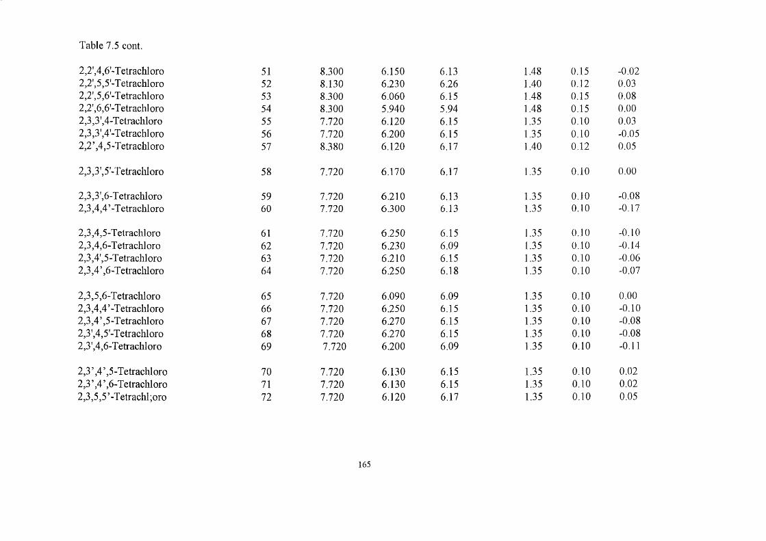
Table 7.5 cont.
2,2',4,6-Tetrachloro 51 8.300 6.150 6.13 1.48 0.15 -0.022,2',5,5'-Tetrachloro 52 8.130 6.230 6.26 1.40 0.12 0.032,2',5,6'-Tetrachloro 53 8.300 6.060 6.15 1.48 0.15 0.082,2',6,6'-Tetracliloro 54 8.300 5.940 5.94 1.48 0.15 0.002,3,3',4-T etracliloro 55 7.720 6.120 6.15 1.35 0.10 0.032,3,3',4'-Tetrachloro 56 7.720 6.200 6.15 1.35 0.10 -0.052,2 ’ ,4,5 -T etracliloro 57 8.380 6.120 6.17 1.40 0.12 0.05
2,3,3',5'-T etracliloro 58 7.720 6.170 6.17 1.35 0.10 0.00
2,3,3',6-Tetracliloro 59 7.720 6.210 6.13 1.35 0.10 -0.082,3,4,4 ’ -T etr aclil oro 60 7.720 6.300 6.13 1.35 0.10 -0.17
2,3,4,5-Tetrachloro 61 7.720 6.250 6.15 1.35 0.10 -0.102,3,4,6-Tetracliloro 62 7.720 6.230 6.09 1.35 0.10 -0.142,3,4',5-Tetracliloro 63 7.720 6.210 6.15 1.35 0.10 -0.062,3,4’,6-Tetrachloro 64 7.720 6.250 6.18 1.35 0.10 -0.07
2,3,5,6-Tetrachloro 65 7.720 6.090 6.09 1.35 0.10 0.002,3,4,4 ’ -T etr aclil oro 66 7.720 6.250 6.15 1.35 0.10 -0.102,3,4’,5-Tetrachloro 67 7.720 6.270 6.15 1.35 0.10 -0.082,3',4,5'-Tetrachloro 68 7.720 6.270 6.15 1.35 0.10 -0.082,3',4,6-Tetrachloro 69 7.720 6.200 6.09 1.35 0.10 -0.11
2,3’,4’,5-Tetrachloro 70 7.720 6.130 6.15 1.35 0.10 0.022,3 ’ ,4 ’ ,6-T etracliloro 71 7.720 6.130 6.15 1.35 0.10 0.022,3,5,5 ’ -T etr aclil ;oro 72 7.720 6.120 6.17 1.35 0.10 0.05
165
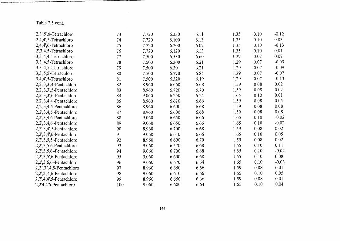
Table 7.5 cont.
2,3',5',6-Tetracliloro 73 7.720 6.230 6.11 ].35 0.10 -0.122,4,4',5-Tetrachloro 74 7.720 6.100 6.13 1.35 0.10 0.032,4,4',6-Tetracliloro 75 7.720 6.200 6.07 1.35 0.10 -0.132',3,4,5-Teti-achloro 76 7.720 6.120 6.13 1.35 0.10 0.013,3',4,4'"Tetraciiloro 77 7.500 6.530 6.60 1.29 0.07 0.073,3 ' ,4,5 -T etr aclil oro 78 7.500 6.300 6.21 1.29 0.07 -0.093,3',4,5'-Tetracliloro 79 7.500 6.30 6.21 1.29 0.07 -0.093,3',5,5'-Tetrachloro 80 7.500 6.770 6.85 1.29 0.07 -0.073,4,4', 5 -T etraclil oro 81 7.500 6.320 6.19 1.29 0.07 -0.132,2',3,3',4-Pentachloro 82 8.960 6.660 6.68 1.59 0.08 0.022,23 ,35-Pentacliloro 83 8.960 6.720 6.70 1.59 0.08 0.022,2',3,3',6-Pentachloro 84 9.060 6.250 6.24 1.65 0.10 0.012,2',3,4,4'-Pentacliloro 85 8.960 6.610 6.66 1.59 0.08 0.052,2', 3,4,5-Pentachl oro 86 8.960 6.600 6.68 1.59 0.08 0.082,2',3,4,5'-Pentachloro 87 8.960 6.600 6.68 1.59 0.08 0.082,2',3,4,6-Pentacliloro 88 9.060 6.650 6.66 1.65 0.10 -0.022,2',3,4,6'-Pentachloro 89 9.060 6.650 6.66 1.65 0.10 -0.022,2',3,4',5-Pentachloro 90 8.960 6.700 6.68 1.59 0.08 0.022,2',3,4',6-Pentachloro 91 9.060 6.610 6.66 1.65 0.10 0.052,2',3,5,5'-Pentachloro 92 8.960 6.690 6.70 1.59 0.08 0.022,2',3,5,6-Pentachloro 93 9.060 6.570 6.68 1.65 0.10 0.112,2 3,5,6 -Pentachl oro 94 9.060 6.700 6.68 1.65 0.10 -0.022,2',3,5',6-Pentachloro 95 9.060 6.600 6.68 1.65 0.10 0.082,2',3,6,6'-Pentachloro 96 9.060 6.670 6.64 1.65 0.10 -0.032,2’,3’,4,5-Pentachloro 97 8.960 6.650 6.66 1.59 0.08 0.012,2',3',4,6-Pentachloro 98 9.060 6.610 6.66 1.65 0.10 0.052,2',4,4',5-Pentachloro 99 8.960 6.650 6.66 1.59 0.08 0.012,2'4,4'6-Pentachloro 100 9.060 6.600 6.64 1.65 0.10 0.04
166
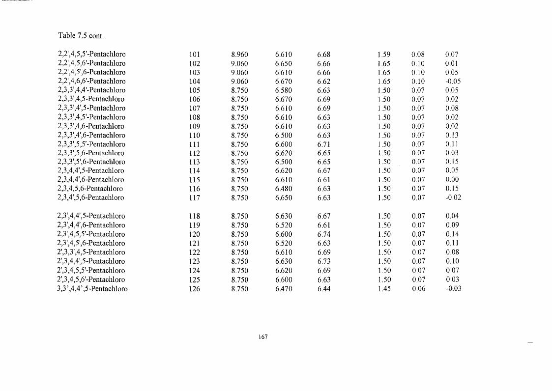
Table 7.5 cont.
2,2',4,5,5'-Pentachloro 101 8.960 6.610 6.68 1.59 0.08 0.072,2',4,5,6'-Pentachloro 102 9.060 6.650 6.66 1.65 0.10 0.012,2’,4,5',6-Pentachloro 103 9.060 6.610 6.66 1.65 0.10 0.052,2',4,6,6'-Pentachloro 104 9.060 6.670 6.62 1.65 0.10 -0.052,3,3',4,4'-Pentacliloro 105 8.750 6.580 6.63 1.50 0.07 0.052,3,3',4,5-Pentacliloro 106 8.750 6.670 6.69 1.50 0.07 0.022,3,3',4',5-Pentachloro 107 8.750 6.610 6.69 1.50 0.07 0.082,3,3 ',4,5 '-Pentacliloro 108 8.750 6.610 6.63 1.50 0.07 0.022,3,3',4,6-Pentacliloro 109 8.750 6.610 6.63 1.50 0.07 0.022,3,3',4',6-Pentacliloro 110 8.750 6.500 6.63 1.50 0.07 0.132,3,3',5,5 '-Pentacliloro 111 8.750 6.600 6.71 1.50 0.07 0.112,3,3 ', 5,6 -Pentachl oro 112 8.750 6.620 6.65 1.50 0.07 0.032,3,3',5',6-Pentachloro 113 8.750 6.500 6.65 1.50 0.07 0.152,3,4,4',5-Pentachl oro 114 8.750 6.620 6.67 1.50 0.07 0.052,3,4,4',6-Pentachloro 115 8.750 6.610 6.61 1.50 0.07 0.002,3,4,5,6-Pentachloro 116 8.750 6.480 6.63 1.50 0.07 0.152,3,4',5,6-Pentachloro 117 8.750 6.650 6.63 1.50 0.07 -0.02
2,3',4,4',5-Pentachloro 118 8.750 6.630 6.67 1.50 0.07 0.042,3',4,4',6-Pentachloro 119 8.750 6.520 6.61 1.50 0.07 0.092,3',4,5,5'-Pentachloro 120 8.750 6.600 6.74 1.50 0.07 0.142,3',4,5',6-Pentachloro 121 8.750 6.520 6.63 1.50 0.07 0.112',3,3',4,5-Pentachloro 122 8.750 6.610 6.69 1.50 0.07 0.082',3,4,4',5-Pentachloro 123 8.750 6.630 6.73 1.50 0.07 0.102',3,4,5,5'-Pentachloro 124 8.750 6.620 6.69 1.50 0.07 0.072',3,4,5,6'-Pentachloro 125 8.750 6.600 6.63 1.50 0.07 0.033,3 ’ ,4,4 ’ ,5 -Pentachl oro 126 8.750 6.470 6.44 1.45 0.06 -0,03
167

Table 7.5 cont.
3,3',4,5,5'-Pentachioro 127 8.750 6.720 6.75 1.45 0.06 0.032,2',3,3 ',4,4'Hexacliloro 128 9.620 7.300 7.20 1.70 0.05 0.102,2',3,3',4,5-Hexachloro 129 9.620 7.310 7.22 1.70 0.05 -0.082,2',3,3',4,5'-Hexachloro 130 9.620 7.170 7.22 1.70 0.05 0.052,2',3,3',4,6-Hexachloro 131 9.740 7.320 7.19 1.75 0.06 -0.132,2',3,3',4,6’-Hexachloro 132 9.740 7.300 7.19 1.75 0.06 -0.112,2',3,3',5,5'Hexachloro 133 9.620 7.090 7.20 1.70 0.05 0.112,2',3,3',5,6-Hexachloro 134 9.740 7.150 7.21 1.75 0.06 0.062,2 ',3,3 ',5,6 ’ -Hexachl oro 135 9.740 7.230 7.21 1.75 0.06 -0.022,2',3,3',6,6'-Hexachloro 136 9.740 7.120 7.16 1.75 0.06 0.042,2',3,4,4',5 -Hexach 1 oro 137 9.620 7.340 7.20 1.70 0.05 -0.142,2',3,4,4',-Hexachloro 138 9.620 7.290 7.20 1.70 0.05 0.092,2',3,4,4',6-Hexachloro 139 9.740 7.290 7.17 1.75 0.06 -0.122,2',3,4,4',6'-Hexachloro 140 9.740 7.320 7.23 1.75 0.06 -0.092,2',3,4,5,5'-Hexachloro 141 9.620 7.190 7.22 1.70 0.05 0.032,2',3,4,5,6-Hexacliloro 142 9.740 7.300 7.19 1.75 0.06 -0.112,2',3,4,5,6'-Hexachloro 143 9.740 7.330 7.19 1.75 0.06 -0.142,2',3,4,5',6-Hexachloro 144 9.740 7.300 7.21 1.75 0.06 -0.092,2',3,4,6,6'-Hexachloro 145 9.740 7.180 7.14 1.75 0.06 -0.042,2’,3,4’,5,5’-Hexchloro 146 9.620 7.200 7.20 1.70 0.05 0.002,2',3,4',5,6-Hexachloro 147 9.740 7.200 7.19 1.75 0.06 -0.012,2',3,4',5,6’-Hexachloro 148 9.740 7.250 7.19 1.75 0.06 -0.062,2',3,4',5',6-Hexacliloro 149 9.740 7.320 7.19 1.75 0.06 -0.132,2',3,4',6,6'-Hexachloro 150 9.740 7.200 7.14 1.75 0.06 -0.062,2',3,5,5',6-Hexachloro 151 9.740 7.850 6.92 1.75 0.06 -0.072,2’,3,5,6,6'-Hexachloro 152 9.740 7.080 7.16 1.75 0.06 0.082,2'4,4,5,5 '-Hexachl oro 153 9.620 6.300 7.22 1.70 0.05 0.082,2',4,4',5,6'-Hexachloro 154 9.740 7.170 7.17 1.75 0.06 0.00
168
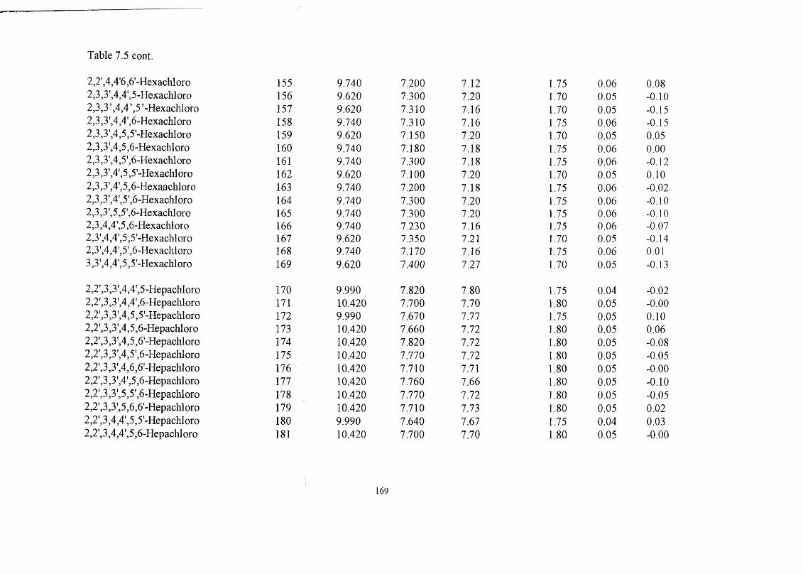
Table 7,5 cont.
2,2',4,4'6,6'-Hexachloro 155 9.740 7.200 7.12 1.75 0.06 0.082,3,3',4,4',5-Hexachloro 156 9.620 7.300 7.20 1.70 0.05 -0.102,3,3’,4,4’,5’>Hexacliloro 157 9.620 7,310 7.16 1.70 0.05 -0.152,3,3',4,4',6-Hexachloro 158 9.740 7.310 7.16 1.75 0.06 -0.152,3,3',4,5,5'-Hexachloro 159 9.620 7.150 7.20 1.70 0.05 0.052,3,3',4,5,6-Hexachloro 160 9.740 7.180 7.18 1.75 0.06 0.002,3,3',4,5',6-Hexachloro 161 9.740 7.300 7.18 1.75 0.06 -0.122,3,3',4',5,5'-Hexacliloro 162 9.620 7.100 7.20 1.70 0.05 0.102,3,3',4’,5,6-Hexaachloro 163 9.740 7.200 7.18 1.75 0.06 -0.022,3,3',4',5',6-Hexachloro 164 9.740 7.300 7.20 1.75 0.06 -0.102,3,3',5,5',6-Hexachloro 165 9.740 7.300 7.20 1.75 0.06 -0.102,3,4,4',5,6-HexachIoro 166 9.740 7.230 7.16 1.75 0.06 -0.072,3',4,4',5,5'-Hexachloro 167 9.620 7.350 7.21 1.70 0.05 -0.142,3',4,4',5',6-Hexacliloro 168 9.740 7.170 7.16 1.75 0.06 0.013,3',4,4',5,5'~HexachIoro 169 9.620 7.400 7.27 1.70 0.05 -0.13
2,2',3,3',4,4',5-Hepachloro 170 9.990 7.820 7.80 1.75 0.04 -0.022,2',3,3',4,4',6-Hepacliloro 171 10.420 7.700 7.70 1.80 0.05 -0.002,2',3,3',4,5,5'-Hepacliloro 172 9.990 7.670 7.77 1.75 0.05 0.102,2',3,3',4,5,6-Hepachloro 173 10.420 7.660 7.72 1.80 0.05 0.062,2',3,3',4,5,6’-Hepachloro 174 10.420 7.820 7.72 1.80 0.05 -0.082,2',3,3',4,5',6-Hepacliloro 175 10.420 7.770 7.72 1.80 0.05 -0.052,2',3,3',4,6,6'-Hepacliloro 176 10.420 7.710 7.71 1.80 0.05 -0.002,2',3,3',4',5,6-Hepachloro 177 10.420 7.760 7.66 1.80 0.05 -0.102,2',3,3',5,5',6-Hepachloro 178 10.420 7.770 7.72 1.80 0.05 -0.052,2',3,3',5,6,6'-Hepachloro 179 10.420 7.710 7.73 1.80 0.05 0.022,2',3,4,4',5,5'-Hepacliloro 180 9.990 7.640 7.67 1.75 0.04 0.032,2',3,4,4',5,6-Hepachloro 181 10.420 7.700 7.70 1.80 0.05 -0.00
169

o oo o o
-o — o o m 8 3o o9 9 9 9 o 9 9 o
r"i mo o o o 9 9 o o'9 9 9 9 9
noo
IT) vn vn o o o o o o
o o o o o o o o o o o o o o o o o o o o o o o oo o o o o o o o o o o o o o o o o o o o o o o o
o o o oooo»nin*n>ov^or^r-r^r''t>r^r^r^t>-r^i>-ooooooooo oooocsooor r' r-c r r oooooooooooooooqooooocrNjfNfN
o or- r-- \D C-- o
rN io rNi vo 'OO or \ i ( NO N»n mto >o mr ' - r ' - ' 00 ‘/^t>-vo‘o ' 0vo 'O t - c~ c\i cN cN ?—i cni i—i «—i i—i (N| r—i oj t—i i—it ^ c ^ c ^ c ^ t ^ c ^ c ^ i 9 t > ' o d o d o d o 6 o d o d o d o 6 o d o d o d o d o 6 o o o d
o o o o o o o o o o o o o o o o o o o o o o o o o o o oo v o m ( N > / ^ oo (N '0 'O O o o ' o vo o o r —i r n O ’—i r ^ m v n o o v ^ m mc ^ ' C ) r ^ O : 0 ; v p o r - ; \ q ( N ' - 4 r s r \ ) r 4 r - 4 r s ^ r < r 4 r S ( N ( N T f T - ^r - r - t 9 r - r - r - r - oo oo oo o6 oo od oo oo oo oo oo oo oo od od
o o oCN CN CSTf Tf- Tj-o o o
o o o o o o o(NCNCNCnJ O O O O O ' ^ ' ^ ' ^Tj-Tj-T]-Tj-T|-T^Tj-Tj-TfvcOOO\0^0\00\0\0\Gr\0\ • • _ • ■ v_r\ L n vri vm _• _■ _■ _ • _ • _ • _• _ •o o o o ' 9 ' 9 ' 9 ' 9 < > o o
T—I r—I 1—4 O s O s O S O s 0 \ r-4 1—4
o o o o o o o o o o o oTj-
o o o o o o o o o o
rsi m "TT i T S ' O i > - c i o o s o ^ r N i m ' ^ » r > s o i ^ o o o s 0 4 - 4 r N m T i - m s o t ^ o ooooooo OOOOOOOOOOOsOsOsOsOsOsOsOsOSOSOOOOOOOOOT—I 1—4 1—I r —I 1—1 1—1 1—1 1—I 1—4 1—4 1— 1 1— 1 1—1 1—I 1—1 1— 1 1—( 1—I cs) fN) (N) (~sj (N) fNj (N| fNl
Itrst9o
H
ë 0 g*0 'ü ^ cü cdAAA
Ô Ô,« 9 Cn scT _ ^
'9 ^ ^ rrf r9 c9?9 f9 cnT (9 c9
fÎ9irT
(tT
«N
IVO
ro ro fN <N(9 (9
Si1 1IIo OoO VO
9
fN ro(9 f9
i
IVO VO
0 5 .ro ro^ (9 r9 (9 (9
lit.VO ^ VO
9i
"9ro ro ro ro 9,(9 (9 (9
nIIn ^ VO
:9 :
§ IB B O O_« so
iÎOB
O
§
ÎBO
§
iO
oo
Î
roro
ro
/'O<N CNj(9 c9
s o s o
9 " VO
ro ro ro r 9
VO
«I VO VO
5 < <O m m ^ ro" ro"
rN (N <N <N <N(9 rsf (9 (9 (9
s o s o : o
^ '9VO VO VO
9 % 9 ;ro Tf ro ro" ro" (N fN <N(9 (9 c9
l!Avo]:VO vo"
II"9iro(N CN
iiIIso so so" so"O o
VO
ro^ ro ro" ro" rs CNc9 (9

Table 7.5 cont.
209 11.600 8.340 8.28 2.30 0.00 0.06
a- Log P cal. using the altered n ,(3 , (Table 6.1)
b- Log P predicted using the last cal. values (Table 7.5)
171

The plots of (71 ^2 , and log L"' ) versus the chlorine num ber for all 209 PCBs are
shown in figures (7.2). (7.3) and (7 4). the effect of the ortho-substituents being ver\
clear.
2.00
1.50 -
1.00
0.50 -
0.000.00 2.00 4.00 6.00 8.00 10.00 12.00
C hlorine Num ber
Figure (7.2) Plot of vs chlorine number.
For ortho-substituted congeners ( ♦ ) 2,2’,6,6’-subsrituted congeners, ( I ) 2,2'-
substituted congeners, ( A ,) 2- substituted congeners and ( X ) non -substituted .
172
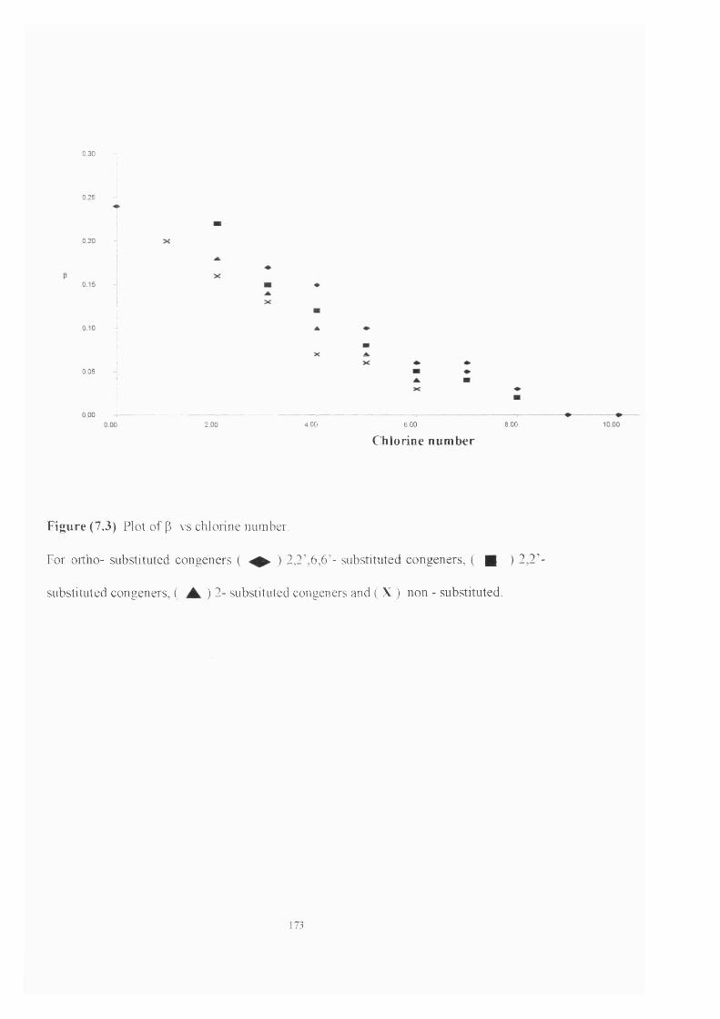
0.05
4.00 6.00 8.00
Chlorine number
Figure (7.3) Plot of p vs chlonne number.
For ortho- substituted congeners ( ) 2,2’,6,6’- substituted congeners, ( ■ ) 2,2'-
substituted congeners, ( ) 2- substituted congeners and ( X ) non - substituted.
173
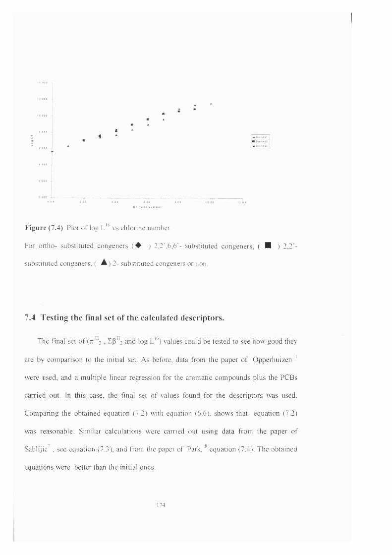
ài
Figure (7.4) Plot of log L'^’ v s chlorine number.
For ortho- substituted congeners ( ♦ ) 2,2 ',6 ,6’- substituted congeners, ( I ) 2,2'-
substituted congeners, ( 2- substituted congeners or non.
7.4 Testing the final set of the calculated descriptors.
The final set of and log values could be tested to see how good they
are by comparison to the initial set. As before, data from the paper o f Opperhuizen '
were used, and a m ultiple linear regression for the aromatic compounds plus the PCBs
carried out. In this case, the final set of values found for the descriptors was used.
Comparing the obtained equation (7.2) with equation (6.6), shows that equation (7.2)
was reasonable. Similar calculations were carried out using data from the paper of
Sablijic^ , see equation (7.3), and from the paper of Park, equation (7.4). The obtained
equations were better than the initial ones.
174

Equation (7.2) Opperhuizen values
log P„c, = 0.609 + 0.288 R2 - 0.752 k \ -3.059 Eg"; + 3.445 V,(7.2)
n = 58 = 0.975 sd = 0.239 F = 354.8
Equation (7.3) Sablijic values
log k’ = - 0.110 - 0.265 Rz -1.617 n ^ - 4.455 Ep ^ 2 + 5.360 V,(7.3)
n = 20 = 0.992 sd = 0.122 F = 498.8
Equation (7.4) Park values
log (7.4)log k’ = - 0.603 + 1.650 R2 + 1.211 7 1 ^ 2 + 0.252 Ep ^ 2 + 1.591
n = 39 r = 0.976 sd = 0.103 F = 272.1
The second test for the set of new descriptors involved recalculations for the GLC data on
the twelve phases. As mentioned in section (5.3), applying equation (5.2) for the first
three phases yielded negative b-coefficients, see Table (5.5). This is because these phases
are non-polar and equation 5.2 should not really be applied.
175
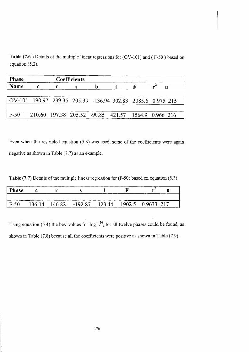
Table (7.6 ) Details of the multiple linear regressions for (OV-101) and ( F-50 ) based on equation (5.2).
Phase CoefficientsName c r s b 1 F n
OV-101 190.97 239.35 205.39 -136.94 302.83 2085 6 0.975 215
F-50 210.60 197.38 205.52 -90.85 421.57 1564.9 0.966 216
Even when the restricted equation (5.3) was used, some of the coefficients were again
negative as shown in Table (7.7) as an example.
Table (7.7) Details of the multiple linear regression for (F-50) based on equation (5.3)
Phase c r s 1 F n
F-50 136.14 146.82 -192.87 123.44 1902.5 0.9633 217
Using equation (5.4) the best values for log for all twelve phases could be found, as
shown in Table (7.8) because all the coefficients were positive as shown in Table (7.9).
176
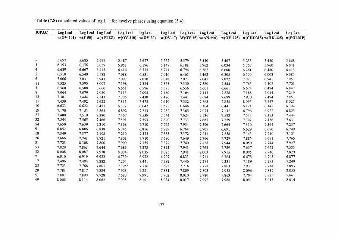
Table (7.8) calculated values of log for twelve phases using equation (5.4).
lyPAC Log Leal Log Leal Log Leal Log Leal logLcal Log Leal Log Leal Log Leal Log Leal Log Leal Log Leal Log Lealw(OV-lOl) w(F-50) w(APTEZ) w(OV-210) w(OV-30).....w(0V-17) W(OV-25) w(AN-600)...w(OV-225)...w(CHOMS) n(llK-325) w(POLMP)
- 5.697 5 685 5.699 5.487 5.677 5.552 5.579 5.430 5.467 5.253 5.440 5 6681 6.193 6.176 6.059 5.951 6.196 6.147 6.188 5.962 6.034 5.767 5 960 6.0414 6.689 6.667 6.418 6.416 6.715 6.741 6.796 6.562 6.600 6.281 6480 6.4132 6.510 6.540 6.582 7.088 6.531 7.016 6.465 6.462 6.505 6 509 6 003 6 6856 7.006 7.031 6.941 7.007 7.050 7.048 7,073 7.045 7.072 7023 6.941 7.05711 7.323 7.395 8.007 7.598 7.384 7.354 7.350 7.580 7.544 7 765 7.402 7.7013 6 568 6 588 6.660 6.651 6 576 6.585 6.556 6.601 6.661 6.674 6A94 6 8478 7.064 7.079 7.020 7.115 7.095 7.180 7.164 7.144 7.228 7.188 7.014 7.21913 7.381 7.444 7.543 7.706 7.430 7.486 7.441 7.684 7.699 7 930 7.474 7 86315 7.439 7.492 7.622 7.815 7.475 7619 7.532 7.863 7 855 8 095 7.547 8 02510 6633 6 622 6.457 6.332 6.642 6.572 6.648 6.364 6.441 6.121 6.341 6 30219 7.170 7.153 6.864 6.892 7.213 7252 7.365 7.071 7.132 6 796 6.922 6 82527 7.480 7.510 7.380 7.467 7.539 7.544 7.624 7.536 7.583 7.511 7.373 744432 7.544 7.565 7.466 7.591 7.593 7.690 7.733 7.687 7.759 7.702 7.456 7.63154 7.650 7.639 7.310 7.368 7.710 7.762 7.934 7.596 7.664 7.310 7.364 7.2379 6.852 6.886 6.838 6.745 6.856 6.789 6.764 6.705 6.691 6 629 6690 6.74918 7.349 7.377 7.198 7.210 7.375 7.383 7.372 7.231 7.258 7.143 7.2)0 7.12126 7.666 7.741 7.721 7.801 7.710 7.690 7.649 7.766 7.729 7.885 7.671 7.76531 7.723 8.308 7.800 7.909 7.755 7.822 7.740 7.858 7.944 8.050 7.744 7.92753 7.829 7.863 7.644 7.686 7.873 7.893 7.941 7.768 7.789 7.657 7.652 7.53352 8.008 8.087 7.978 8.004 8.035 8.025 7.948 8.003 7.915 8.005 7.940 7 8297 6.910 6.919 6.922 6.739' 6.922 6.797 6.833 6.711 6.764 6 675 6.763 6.87717 7.406 7.404 7.282 7.204 7,441 7.392 7.446 7.271 7.331 7.189 7.283 7.24925 7.723 7.768 7.805 7.795 ' 7.776 7.698 7.718 7.778 7.803 7.931 7.744 7 89328 7.781 7.817 7.884 7.903 7.821 7.831 7,809 7.893 7958 8.096 7.817 8 05551 7.887 7.890 7.728 7.680 7.991 7902 8.010 7.780 7863 7.704 7.725 7.66149 8.066 8.114 8.062 7.998 8.101 8.034 8,017 7.992 7.988 8.051 8.013 8.014
177

Table 7.8 47
Cont.8.124 8.142 8.145 7.992 8.167 8.042 8.086 8.021 8 062 8 098 8 086 8 085
5 7.047 7.036 6.996 6 969 7.081 7.076 7.202 7.034 7.154 6.964 6 920 7,12616 7.543 7.527 7.355 7.434 7.600 7.670 7.810 7.594 7.721 7.478 7.440 749820 7.860 7.892 7.878 8.024 7.935 7.977 8.087 8,100 8 193 8 220 7.901 8.14222 7.918 7.940 7.957 8.133 7.980 8.109 8.179 8 233 8.348 8J85 7.974 8.30446 8.024 8.013 7.801 7.909 8.098 8.181 8.379 8.102 8 253 7 993 7 882 7.91044 8.202 8.237 8.135 8.227 8.260 8.312 8.387 8.314 8.378 8 340 8,170 8 20642 8.260 8.265 8.219 8.221, 8.326 8.321 8.455 8.326 8.452 8 386 8 243 8.33440 8.397 8.388 8.292 8.451 8.485 8.599 8.825 8.654 8 842 8.675 8.400 8 58314 7.161 7.163 7.359 7.172 7.137 6 974 6.891 7.102 7.072 7.266 7.109 T37834 7.650 7.648 7.710 7.621 7.647 7.554 7.481 7.639 7.618 7.753 7.619 7 72536 7.981 8.025 8.250 8.243 7.999 7.889 7.794 8.180 8.131 8 549 8.100 8 41939 8.025 8.060 8.312 8.320 8.027 7.993 7.849 8.278 8.245 8 660 8.1 52 8,53173 8.131 8.133 8.157 8.096 8.145 8.065 8.050 8.147 8 208 8 268 8 060 8.13772 8.310 8.357 8.490 8.414 8.307 8.196 8.057 8.359 8 275 8.615 8 349 8 43368 8 368 8.385 8.574 8.408 8.373 8.205 8.126 8.371 8.349 8 661 11.556 8 56158 8.504 8.508 8.647 8.638 8.532 8.483 8.596 8.694 8.738 8.654 8 578 8.81080 8.612 8 628 9.003 8.825 8.579 8.368 8.165 8.738 8 635 &225 &757 9 03712 7.411 7.418 8.128 7.641 7.482 7.531 7.486 7.650 7.711 7930 T422 7 89233 7.907 7.909 7.946 8.106 8.001 8.126 8.094 8.204 8 278 8.444 7.942 8 26435 8.224 8.273 8.469 8 696 8.335 8.432 8.371 8.710 8.750 9 186 8.403 8 90837 8.282 8.321 8.548 8.805 8.381 8.565 8.463 8.843 8 905 9.351 8.476 9 07071 8.388 8.394 8.392 8.581 , 8.498 8.636 8.663 8.712 8.810 8 959 8J84 8 67670 8.588 8.638 8.750 8.947 8 687 8.811 8.573 8.978 8.997 9 386 8.703 9 04866 8.625 8.646 8.810 8.893 8.727 8.776 8.739 8.936 9.009 6 985 8.745 9.10056 8.761 8.769 8.883 9.123 8.886 9.055 9.109 9.259 9399 9.641 8 902 9 34979 8.869 8.889 9238 9.310 8.933 8 939 8.779 9.304 9.295 9 916 9^81 9 57677 9.126 9.150 9.474 9.795 9.287 9.510 9.393 9.933 9 955 10.607 9.404 10.11530 7.166 7.160 7.179 6.789 7.112 6.970 6 986 6.689 6 692 6 624 7.017 6 84950 7.662 7.651 7.538 7.254 7.630 7.564 10.235 7.244 7.259 7.138 7.537 7.22169 7.979 8.016 8.062 7.845 7.965 7.871 7.871 7.750 7.144 6.499 T997 7 86675 8.037 8.064 8.140 7.954 8.011 8.003 7.962 7.883 7.886 8.045 8.070 8.028104 8.163 8.137 7.984 7.730 8.128 8.075 8.163 7.752 7.790 7.653 7.979 7.634103 8.322 8.361 8.318 8.048 ' 8.291 8.206 8.170 7.964 7.916 8.000 8 267 7 929100 8.380 8.389 8.402 8.042 8.357 8.215 8.239 7.976 7989 8.046 8.340 &057
178
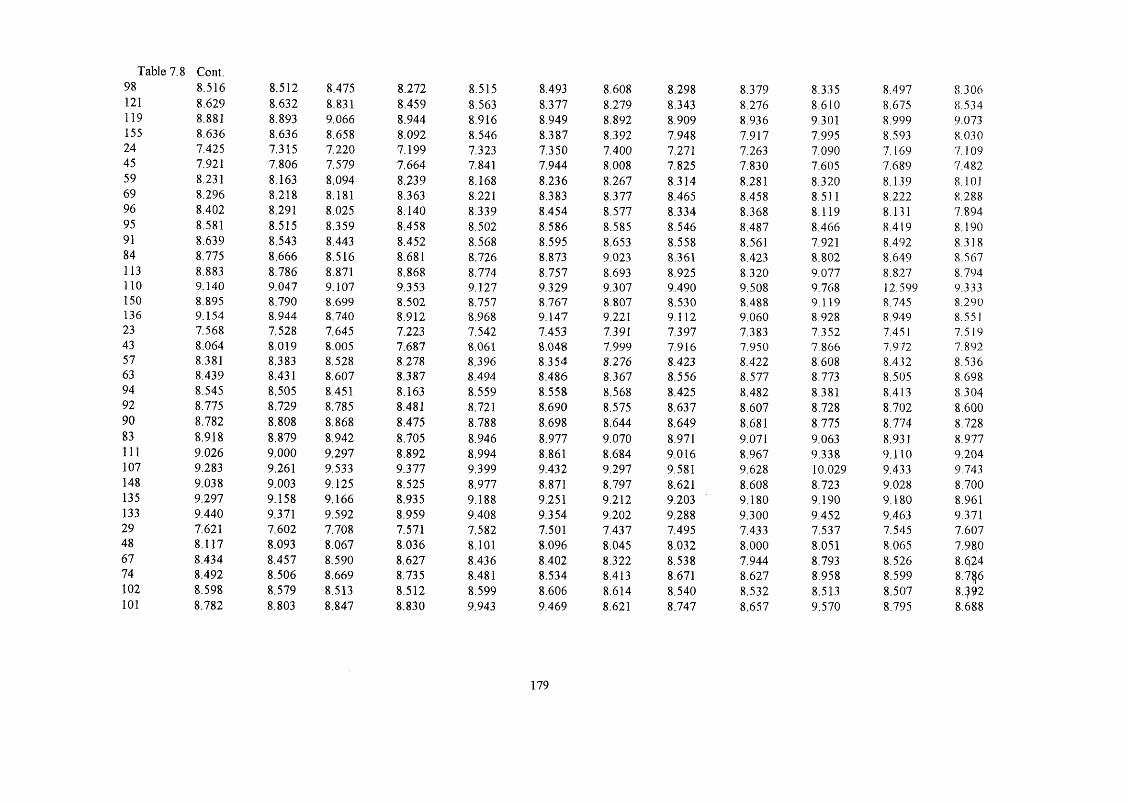
Table 7.898
Cont.8.516 8.512 8.475 8.272 8.515 8.493 8.608 8.298 8 379 8 335 8 497 8 306
121 8.629 8.632 8.831 8.459 8.563 8.377 8.279 8.343 8 276 8 610 8 675 8 534119 8.881 8 893 9.066 8.944 8.916 8.949 8.892 8.909 8 936 9.301 8 999 9 073155 8.636 8.636 8.658 8.092 8.546 8.387 8.392 7948 7.917 7.995 8 593 8 03024 7.425 7.315 7.220 7.199 7.323 7350 7.400 7.271 T263 7.090 7 169 7 10945 7921 7.806 7.579 7.664 7.841 7.944 8.008 7.825 7.830 7.605 7 689 748259 8.231 8.163 8.094 8 239 8.168 8.236 8 267 8.314 8.281 8 320 8.139 8.10169 8 296 8.218 8.181 8 36} 8.221 8.383 8.377 8.465 8.458 8.511 8 222 8 28896 8.402 8.291 8.025 8.140 8.339 8.454 8.577 8.334 8 368 8.119 8.131 7 89495 8.581 8.515 8.359 8.458 8 502 8.586 8.585 8.546 8.487 8.466 8.419 8J:9091 8 639 8.543 8.443 8.452 8 568 8 595 8 653 8.558 8.561 7.921 8.492 8 31884 8.775 8 666 8.516 8.681 8.726 8.873 9.023 8.361 8.423 8 802 8 649 8 567113 8.883 8.786 8.871 8 868 8.774 8.757 8 693 8.925 8.320 9.077 8 827 8 794110 9.140 9.047 9.107 9.353 9.127 9329 9.307 9.490 9 508 9 768 12 599 9 333150 8.895 8.790 8 609 8.502 8.757 8.767 8.807 8.530 8 488 9.119 &745 8 290136 9.154 8.944 8.740 8.912 8968 9.147 9.221 9.112 9.060 8 928 8 949 8.55123 7.568 7.528 7.645 7.223 7.542 7.453 7.391 7.397 7.383 7352 7.451 7.51943 8.064 8.019 8.005 7.687 8.061 8.048 7999 7 916 7950 7 866 7.972 7 89257 8.381 8J83 8 528 8.278 8 396 8 354 8 276 8.423 8.422 8 608 8 432 8 53663 8.439 8.431 8.607 8.387 8.494 8.486 8 367 8.556 8.577 &773 8.505 8 69894 8.545 8.505 8.451 8.163 8.559 8.558 8 568 8.425 8.482 8.381 8.413 8 30492 8.775 8.729 8.785 8.481 8.721 8 690 8.575 8.637 8.607 8 728 8.702 8.60090 8.782 8.808 8.868 8.475 8.788 8 698 8.644 8.649 8.681 8.775 8.774 8 72883 8.918 8.879 8.942 8.705 8.946 8.977 9.070 8.971 9.071 9 063 8.931 8 977111 9 026 9.000 9.297 8.892 8.994 8.861 8.684 9.016 8 967 9 338 9.110 9.204107 9.283 9.261 9.533 9.377 9399 9.432 9 297 9.581 9 628 10.029 9.433 9 743148 9.038 9.003 9.125 8.525 8.977 8.871 8.797 8.621 8.608 8.723 9 028 8.700135 9.297 9.158 9.166 8.935 9.188 9.251 9.212 9.203 9.180 9 190 9 180 8 961133 9.440 9.371 9 592 8.959 9408 9354 9.202 9 288 9J00 9452 9 463 9.37129 7.621 7.602 7.708 7.571 7.582 7.501 7.437 7,495 7433 7.537 7.545 7.60748 8.117 8.093 8.067 8.036 8.101 8.096 8.045 8.032 8 000 8.051 8 065 7 98067 8.434 8.457 8 590 8.627 8.436 8.402 8.322 8.538 7.944 8 793 8 526 8 42474 8.492 8.506 8.669 8.735 8.481 8.534 8.413 8.671 8.627 8 958 8 599 8 7%6102 8 598 8.579 8.513 8.512 8 599 8.606 8.614 8.540 8.532 8.513 &507 8^92101 8.782 8.803 8.847 8.830 9.943 9.469 8.621 8.747 8.657 9.570 8 795 8 688
179

Table 7.899
Cont.8.840 8.831 8 985 8.824 8.828 8.746 8.690 8.759 8.731 8 959 8 868 8 816
97 8.971 8.954 9.004 9.053 8.986 &025 9.060 7.357 9.121 9 248 &025 9 065120 9 079 9.074 9 359 9.240 9.034 8.909 8.730 9.132 9.017 9 523 9 204 9J^2118 9336 9.335 9 595 9.725 9.387 9.480 9.344 9.697 9.678 10.214 9 548 9.831154 9.091 9.078 9.187 8.874 9.017 8.919 8.843 8.737 8 658 8 908 9 122 8 788149 9.350 9.232 9.228 9.284 9.228 9299 9.258 9.318 9 230 8 085 9.274 9 049146 9.498 9.445 9.654 9.307 9.448 9.402 9.248 9.409 9 350 9 636 9.557 9 459153 9.546 9.520 9.716 9.656 9.488 9450 9 295 9.525 9.400 9.821 9 650 9J^721 8.306 7.810 7 886 7.975 7.828 7929 7.999 7.951 7 926 8 135 10.069 7.49941 8.291 8.353 8.246 8.440 8.347 8.523 8.607 8.505 8 493 8 650 8J42 8 38555 8 608 8.665 8 769 9030 8 682 8.830 8.884 9.011 8.964 9 391 &803 9 02960 8 666 8.713 8.848 9.139 8.727 8 962 8.975 9.144 9.120 9 563 8.876 9.19189 8.772 8.787 8.692 8.915 8 845 9 034 9.176 9.013 9 024 9.164 8.784 8 79787 8.951 9.011 9.026 9.233 9.007 9.165 9.183 9.196 9 150 9.511 9 072 9 09385 9.009 9.038 9.109 9.227 9.073 9.174 9.252 9.237 9.223 9 558 9 1 45 9.22182 9.145 9.161 9.183 9.457, 9.232 9.452 9.622 9.560 9 613 9.847 9 302 9.470108 9 273 9.301 9 562 9.691 9.305 9 379 9.346 <7658 9.572 10.202 9.511 9 773105 9 523 9.556 9.790 10.160 9.650 9936 S\942 10.205 10.212 10.866 9 825 10.287140 9.244 9 265 9.342 9.230 9.237 9.304 9.351 9.156 9.089 9 426 9 368 9.1 18132 9.524 9.439 9.407 9.687 9.474 9.726 9.820 9.791 &723 9 973 9.551 9.454130 9 667 9 653 9 833 9.711 9 693 9.830 9.810 9.882 9.842 10.235 9 833 9 864138 9.719 9.727 9 895 10.059 9.733 9.878 9 856 9L998 9 892 10.419 9 927 9.952128 9 893 9.935 10.073 10.463 9.979 10.306 10.418 10.551 10.385 11.018 10.162 10.35738 8.092 8.164 8.415 8.4451 8.132 8.168 8.113 8.491 8.474 8.745 &267 8.74376 8 594 8.661 8.783 8 926 8 659 8.776 8.739 9.063 9.061 9 287 8.797 9.14078 8.905 9.019 9 298 9.501 8.985 9.068 8 998 9.552 9.512 10.002 9 248 9.75981 8 962 9.067 9 376 9.609 9.030 9.201 9.089 9.685 9 668 10.167 9.321 9.921125 9.068 9.140 9.221 9 386 9.148 9.272 9.290 9.554 9.572 9.774 9 229 9 527124 9.247 9.364 9.554 9.704 9.311 9.404 9.297 9.766 10.285 10.121 9.517 9 823123 9.285 9.372 9.614 9.651 9.351 9.370 9.312 9.725 9.709 10.088 9 559 9 875122 9.442 9.515 9.712 9.928 9.535 9.691 9.736 10.100 10.161 10.457 9.747 10.200127 9.549 9.635 10.067 10.115 9 583 9.575 9.406 10.145 10.058 10.732 &925 10.427118 9.827 9.916 10.326 10.647 9 962 10.189 10.074 10.764 10.780 11.503 10.280 11.042168 9.561 9.639 9.895 9.748 9.566 9.585 9.519 9.750 15.565 10.117 9.844 9 923164 9 820 9.793 9.935 10.158 9.777 9.965 9.934 10.332 10.271 10.583 9 995 10.184
180

Table 7.8 162
Cont.9.977 10.020 10.377 10.213 10.014 10.097 9.961 10.458 10.432 10.898 10.299 10.644
167 10.016 10.081 10.423 10.530 10.037 10.117 9.971 10.539 10.440 11.029 10.372 10.682157 10.190 10.288 10.602 10.934 10.283 10.544 10.532 11.011 10.933 11.628 10.649 11.087169 10.507 10.662 11.155 11,452 10.612 10.826 10.701 11.605 11.543 12.318 11.125 11 89265 8.194 8.197 8.127 7.998 8.258 7.978 8.012 7.957 8.006 7 860 7.736 8.10593 8.407 8.375 8.023 8.114 8.381 8.344 8.315 8.033 7.872 7.611 7.901 7.841112 8.724 8.739 8.546 8.705 8.716 8.650 8.592 8.591 8.343 8 353 8 362 8 486117 8.782 8.788 8.625 8.813 8.761 8.783 8.683 8.724 8.499 8.518 8.435 8 648152 8.888 8.861 8.469 8.590 8.879 8.854 8.884 8.541 8 403 8.126 8 343 8.254151 9.169 9.185 8.922 9.145 9.171 9.200 9 163 9.019 8 839 8 874 8.784 8 926147 9.125 9.112 8.886 8.902 9.108 8.995 8.960 8.765 8 602 8.519 8.704 8 677134 9.261 9236 8.960 9.131 9 266 9.273 9.330 9.087 8 992 8 808 8.861 8.470165 9.369 9 356 9.315 9.319 9.314 9.157 9.000 9.132 8 889 9 083 9.040 9.154163 9.626 9.617 9.551 9.803 9.667 9.729 9.614 9 698 9 549 9.774 9 363 9 693188 9.381 9.360 9.143 8.952 9.297 9.167 9.113 8.737 8.530 8 468 8 958 8 650179 9.619 9.494 9 160 9.314 9.482 9.504 9.473 9.266 9 039 8 854 9 079 8 835178 9.790 9.734 9.618 9.401 9.737 9.665 9 536 9.428 9.242 9 223 9 403 9 346187 9.836 9.801 9 672 9.734 9 768 9.698 9.564 9 526 9.271 9.381 9 486 9 408177 10.030 11.446 9 874 10.185 10.039 10.169 5.945 10.052 9 826 10.060 9.794 9 889193 10.306 10.363 10.379 10.608 10.317 10.365 10.240 10.539 10.312 10.590 10.208 10.544202 10.126 10.083 9 628 9.812 10.048 9.947 9 834 9.532 9.143 8.941 9J22 9 27062 8.184 8.083 8.099 8.030 8.112 8.124 8.169 7.969 8.000 7.729 8.186 8.14588 8.399 8.346 7.993 8.168 8.244 8.386 8.361 8.102 7 886 7.507 7.901 7.718109 8.716 8.710 8.516 8.759 8.579 8.693 8.638 8.608 8.358 8.248 8 362 8 362115 8.774 8.758 8.595 8.867 8.624 8.825 8.730 8.741 8.514 8.413 8.435 8.524145 8.879 8.831 8.439 8.644 8.742 8.897 8.930 9.031 8.418 8.021 8.343 8.130144 9.058 9.055 8.773 8.962 8.904 9.028 8.938 9.244 8.544 8 368 8.631 8 426139 9.116 9.083 8.857 8 956 8.970 9.037 9.006 9.255 8.617 9 072 8.704 9.125131 9.253 9.206 8.930 9.185 9.129 9.315 9.376 9.578 9 007 8.704 8.861 8 803161 9 360 9.326 9 285 9.373 9.176 9.200 9 046 9.623 8.904 8 978 9.039 9 030158 9 617 9.587 9 521 9.857 9.530 9.771 9 660 10.188 10.151 9 669 9 363 9 569184 9J72 9.330 9.113 9.006 9.159 9.209 9.159 8.807 8.550 8.363 8 958 8 527176 9.611 9.464 9 130 9.368 9.345 9 546 9.519 9.336 9.054 8.750 9.079 8.712175 9.774 9 698 9 580 9.439 9 590 9.693 9.564 9.480 9 823 9 092 9 392 9.197183 9 832 9.772 9 642 9.788 9 630 9.741 9.611 9.595 9 286 &276 9.486 9 285
181
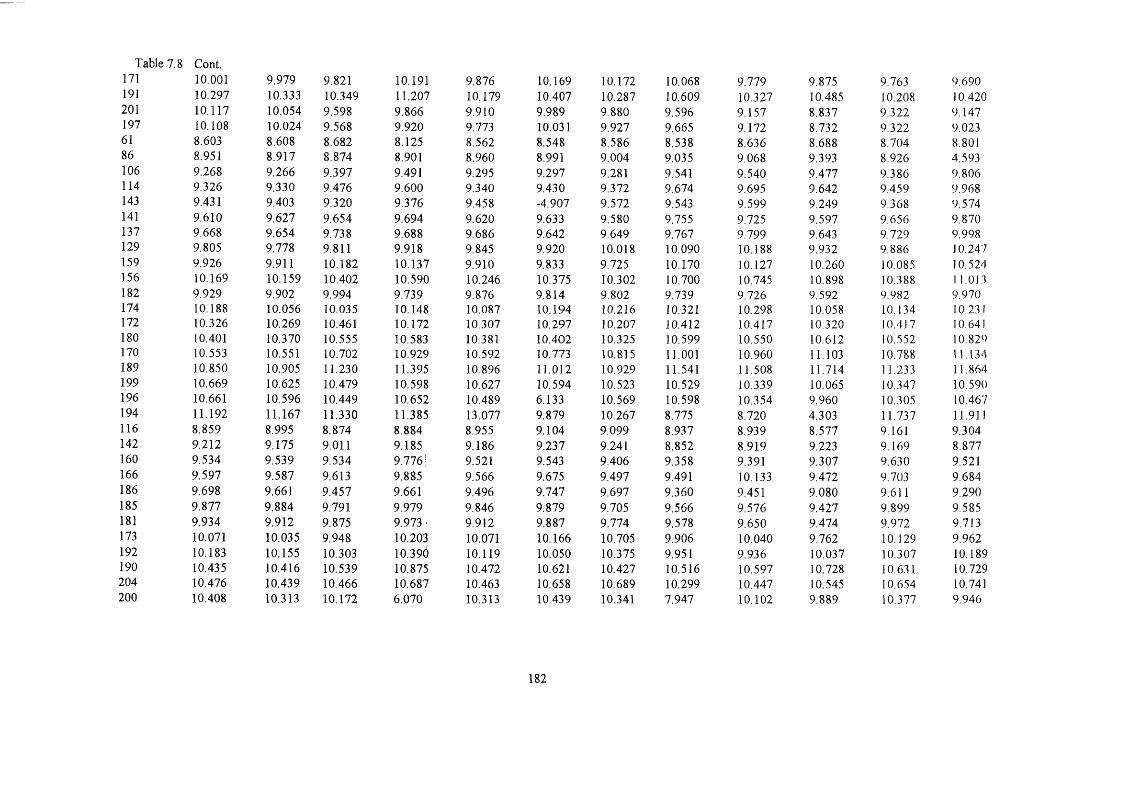
Table 7.8 171
Cont.10.001 9.979 9.821 10.191 &876 10.169 10.172 10.068 9.779 9.875 9 763 9 690
191 10.297 10.333 10.349 11.207 10.179 10.407 10.287 10.609 10.327 10.485 10.208 10.420201 10.117 10.054 9 598 9 866 9 910 9989 9 880 9 596 9.157 8.837 9 322 9.147197 10.108 10.024 9 568 9.920 9.773 10.031 9.927 91665 9.172 8.732 9 322 9 02361 8.603 8.608 8.682 8.125 8.562 8.548 8.586 8.538 8 636 8 688 8.704 8.80186 8.951 8.917 8.874 8.901 8.960 8.991 9.004 9.035 9 068 9 393 8 926 4.593106 9268 &266 9397 9.491 9.295 9.297 9.281 9.541 9.540 9.477 9 386 9 806114 9 326 9 330 9476 9.600 9.340 9.430 9.372 9.674 9 695 9.642 9 459 9 968143 9431 9.403 9.320 9 376 9.458 -4.907 9.572 9.543 9 599 9.249 9 368 9.574141 9.610 9.627 9.654 9,694 9.620 9.633 9.580 9.755 9 725 9.597 9 656 9 870137 9 668 9.654 9.738 9.688 9.686 9.642 9.649 9.767 9 799 9.643 9 729 9 998129 9.805 9.778 9.811 9.918 9.845 9.920 10.018 10.090 10.188 9 932 9 886 10.247159 9 926 9.911 10.182 10.137 9.910 9.833 9.725 10.170 10.127 10.260 10.085 10.524156 10.169 10.159 10.402 10.590 10.246 10.375 10.302 10.700 10.745 10.898 10.388 1 1.01.3182 9 929 9 902 9.994 9.739 9.876 9.814 9 802 9.739 9.726 9.592 9 982 9.970174 10.188 10.056 10.035 10.148 10.087 10.194 10.216 10.321 10.298 10.058 10.134 10.231172 10.326 10.269 10.461 10.172 10.307 10.297 10.207 10.412 10.417 10.320 10.417 10.641180 10.401 10.370 10.555 10.583 10.381 10.402 10.325 10.599 10.550 10.612 10.552 10.820170 10.553 10.551 10.702 10.929 10.592 10.773 10.815 11.001 10.960 11.103 10.788 11.134189 10.850 10.905 11.230 11.395 10.896 11.012 10.929 11.541 11.508 11.714 11.233 11.864199 10.669 10.625 10.479 10.598 10.627 10.594 10.523 10.529 10.339 10.065 10.347 10.590196 10.661 10.596 10.449 10.652 10.489 6.133 10.569 10.598 10.354 9 960 10.305 10.467194 11.192 11.167 11.330 11.385 13.077 9.879 10.267 8.775 8.720 4.303 11.737 11.911116 8.859 8.995 8.874 8.884 8.955 9.104 9.099 8.937 8 939 8.577 9.161 9 304142 9.212 9.175 9.011 9.185 9.186 9.237 9.241 8.852 8.919 9.223 9 169 8.877160 9.534 9.539 9.534 9.776! 9.521 9.543 9.406 9.358 9.391 9.307 9 630 9.521166 9.597 9.587 9.613 9.885 9 566 9.675 9.497 9.491 10.133 9.472 9J03 9 684186 9 698 9.661 9.457 9.661 9.496 9.747 9.697 9360 9.451 9.080 9.611 9 290185 9.877 9.884 9.791 9.979 9.846 9.879 9.705 9 566 9 576 9.427 9 899 9 585181 9.934 9.912 9.875 9.973 ■ 9.912 9.887 9.774 9.578 9 650 9.474 9 972 9.713173 10.071 10.035 9.948 10.203 10.071 10.166 10.705 9.906 10.040 9 762 10.129 9 962192 10.183 10.155 10.303 10.396 10.119 10.050 10.375 9.951 9 936 10.037 10.307 10.189190 10.435 10.416 10.539 10.875 10.472 10.621 10.427 10.516 10.597 10.728 10.631 10.729204 10.476 10.439 10.466 10.687 10.463 10.658 10.689 10.299 10.447 10.545 10.654 10.741200 10.408 10.313 10.172 6.070 10.313 10.439 10.341 7.947 10.102 9 889 10.377 9 946
182
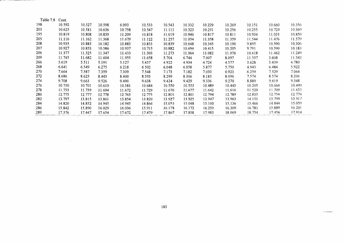
Table 7.8 198
Cont.10.592 10.527 10.598 &093 10.533 10.543 10.332 10.229 10.269 10.151 10.660 10.356
203 10.625 10.581 10.636 10.758 10.547 11.111 10.323 10.291 10.256 10.255 10.724 10.369195 10.819 10.808 10.839 11.209 10.818 11.019 10.940 10.817 10.811 10.934 11.031 10.850205 11.116 11.162 11.368 11.679 11.122 11.257 11.054 11.358 11.359 11.544 11.476 11.579208 10.935 10.883 10.182 10.883 10.853 10.839 10.648 10.345 10.190 9 895 10.590 10.306207 10.927 10.853 10.586 10.937 10.715 10.882 10.694 10.415 10.205 9.791 10.590 10.183206 11.377 11.325 11.347 11.433 11.303 11.273 11.064 11.082 11.076 10.618 11.462 1 1.249209 11.745 11.682 11.604 11.955 11.658 5.704 6.744 7.007 8.097 11.537 3 608 Il 342266 5.619 5.511 5.191 5.127 5.457 4.922 4.934 4.724 4.577 3 628 5.439 4.780268 6.641 6.549 6.275 6.218 6,502 6.048 6.058 5.877 5.750 4.943 6 484 5^22270 7.664 7.587 7.359 7.309 7.548 7.173 7.182 7.030 6923 6 259 7 529 7.064272 8 686 &625 8.443 8.400 8.593 8.299 8.306 8.183 8 096 7.574 8.574 &206274 9.708 9.663 9.526 9.490 9 638 9.424 9.429 9 336 9.270 8 889 9 619 9 348276 10.730 10.701 10.610 10.581 10.684 10.550 10.553 10.489 10.443 10.205 10.664 10.490278 11.753 11.739 11.694 11.672 11.729 11.676 11.677 11.642 11.616 11.520 11.709 11.632280 12.775 12.777 12.778 12.763 12.775 12.801 12.801 12.794 12.789 12.835 12.754 12.774282 13.797 13.815 13.861 13.854 13.820 13.927 13.925 13.947 13 963 14.151 13.799 13.917284 14.820 14.852 14.945 14.945 14.866 15.053 15.048 15.100 15.136 15.466 14.844 15.059286 15.842 15.890 16.029 16.036 15.911 16.178 16.172 16.253 16.309 16.781 15 889 16.201289 17.376 17.447 17.654 17.672 17.479 17.867 17.858 17.983 18.069 18.754 17.456 17.914
183

Finally, the very restricted equation (5.4) was applied to all the twelve phases. It would
not be expected tliat this equation would apply to the polar-phases, but the statistics
obtained can be used to identify the polar and nonpolar phases. In Table (7.9) are details
of multiple linear regressions for the twelve phases based on equation (5.4).
Table (7.9) Details of the multiple linear regressions for all twelve phases based on equation (5.4).
Phase Coefficients
Name c r 1 F n
OV-101 100.74 132.93 195.64 3926.8 0.9726 216F-50 138.10 128.26 192.69 2866.1 0.9632 217APIEZON 241.96 147.26 184.56 1353.1 0.9245 215OV-210 259.96 289.77 183.35 692.4 0.8663 214OV-3 156.05 164.60 191.31 2237.5 0.9533 215OV-17 325.49 252.95 177.68 1176.5 0.9156 216OV-25 321.81 322.94 177.97 1915.7 0.9459 215AN-600 380.55 306.94 173.45 876.8 0.9221 213OV -225 419.80 353.14 170.47 632.7 0.8517 216CHOMS 648.31 406.60 152.06 473.57 0.8129 216HK-325 159.12 195.38 191.39 1776.2 0.9223 214POLMPE 362.90 440.04 175.12 798.87 0.8784 217
The same facts were noticed as mentioned before, that the best values of logL were for
the first three phases (OV-IOl, F-50, Aplezon). The average of the back-calculated log
values were found as shown in Table (7.10). A plot of the final calculated log
values versus N is shown in Figure (7.5 ).
184

Table (7.10) lUPAC No. log L'*” cal. from (OV-101, F-50, APLEZON ) with Üieir
averages.
lUPAC Log Leal Log Leal Log Leal Logw(OV-lOl) w(F-50) w(APLEZON) Avg
5.697 5 685 5.699 5 694T 6 193 6.176 6059 6.1434 6.689 6.667 6.418 6.5912 6.510 6.540 6 582 6.5446 7.006 7.031 6.941 6 99311 7.323 7 395 8.007 7.5753 6 568 6 588 6.660 6.6068 7.064 7.079 1U020 7.05413 7.381 7.444 7.543 7.45615 7.439 7.492 7.622 7.51710 6 633 6.622 6.457 6.57119 7.170 7.153 6.864 7.06227 7.480 7.510 7.380 7.45732 7.544 7\565 7.466 7.52554 7.650 7,639 7.310 7.5339 6.852 6.886 6.838 6 85918 7.349 7.377 7.198 7.30826 7.666 7.741 7.721 7.70931 7.723 8.308 7.800 7.94453 7.829 7.863 7.644 7.77952 8.008 8.087 7.978 8.0247 6.910 6.919 6.922 6.91717 7.406 7.404 7.282 7.36425 7.723 7.768 7.805 7.76628 7.781 7.817 7.884 7.82751 7.887 7.890 7.728 7.83549 8.066 8.114 &062 8.08147 8.124 8.142 8.145 8.1375 7.047 7.036 6 996 7.02616 7.543 7.527 7.355 7.47520 7.860 T892 7.878 7.87722 7.918 7.940 7.957 7.93846 8.024 8.013 7.801 7.94644 8.202 8.237 8.135 8.19242 8 260 8.265 8.219 8.24840 8.397 8.388 8 292 8.35914 7.161 7.163 7.359 7.22834 7.650 7.648 7.710 7.66936 7.981 8.025 8.250 8.08539 8.025 8.060 8.312 8.13273 8.131 8.133 8.157 8.14072 8.310 8.357 8.490 8 38668 8^68 8J85 8.574 8.44258 8.504 8.508 8.647 8 55380 8.612 8.628 9.003 8.74712 7.411 7.418 8.128 7652
185

Table 7.10 cont.
33 7.907 7909 7.946 7.92135 8.224 8.273 8.469 8.32237 8 282 8.321 8.548 8 38471 8388 8 394 8.392 8.39270 8 588 8 638 &750 8.65966 8 625 8.646 8.810 8.69356 8.761 8.769 8 883 8.80479 8 869 8 889 9.238 8.99977 9 126 9.150 9.474 9.25030 7.166 7.160 7.179 7.16850 7.662 7.651 7.538 7.61769 7.979 8.016 8.062 8.01975 8.037 8.064 8.140 8.080104 8.163 8.137 7.984 8 095103 8 322 8.361 8.318 8.334100 8.380 8 389 8.402 8.39098 8.516 8.512 8.475 8.501121 8.629 8.632 8.831 8.697119 8.881 8 893 9 066 8.947155 8 636 8.636 8.658 8.64324 7.425 7.315 7.220 7.32045 7.921 7.806 7.579 7.76959 8.231 8.163 8.094 8.16369 8.296 8.218 8.181 8.23296 8.402 8.291 8.025 8.24095 8.581 8.515 8 359 8.48591 8 639 8.543 8.443 8.54184 8.775 8.666 8.516 8.652113 8 883 8.786 8.871 8.847110 9.140 9.047 9.107 9 098150 8 895 8.790 8.699 8.795136 9.154 8.944 8.740 8 94623 7.568 7.528 7.645 7.58143 8.064 8.019 8.005 8.03057 8.381 8.383 8.528 8.43163 8.439 8.431 8.607 8.49294 8.545 8.505 8.451 8.50092 8.775 8.729 8.785 8.76390 8.782 8.808 8 868 8.82083 8.918 8.879 8.942 8.913111 9.026 9.000 9.297 9.108107 9.283 9.261 9^33 9 359148 9.038 9.003 9.125 9.055135 9.297 9.158 9.166 9.207133 9.440 9.371 9J92 9.46829 7.621 7.602 7.708 7.64448 8.117 8.093 8.067 8.09367 8.434 8.457 8 590 8.49474 8.492 8.506 8 669 8.555102 8.598 8.579 8.513 &563101 8.782 8.803 8.847 8.81199 8.840 8.831 8 985 8 885
186

Table 7.10 cont.
97 8.971 8.954 9.004 8 976120 9.079 &074 9359 9.171118 9.336 9335 ST595 9.422154 9.091 9078 91187 9.118149 9.350 9.232 9.228 9 270146 9.498 9.445 9».654 9.532153 9.546 9320 9.716 9.59421 8.306 7.810 "7886 8.00141 8.291 8 353 8.246 8.29755 8.608 8365 8.769 8.68160 8.666 8.713 8.848 8.74289 8.772 8.787 8.692 8.75087 8.951 9011 9.026 8 99685 9009 9 038 97109 9.05282 9.145 9.161 97183 9.163108 9.273 9.301 97562 9379105 9 523 9 556 9.790 97623140 9.244 9 265 97342 9.284132 9.524 9.439 9.407 9457130 9.667 9.653 97833 9.717138 9.719 9.727 97895 9.780128 9 893 9.935 10.073 9.96738 8.092 8.164 8.415 8.22376 8.594 8.661 8.783 8.67978 8 905 9.019 97298 9.07481 8.962 9.067 9.376 9.135125 9.068 9.140 9.221 9.143124 9.247 9364 9.554 9389123 9.285 9372 9.614 9.424122 9.442 9.515 9.712 9.556127 9.549 9.635 10.067 9.750118 9.827 9.916 10.326 10.023168 9.561 9.639 9395 9.698164 9 820 9.793 97935 9.850162 9.977 10.020 10.377 10.125167 10.016 10.081 10.423 10.173157 10.190 10.288 10.602 10.360169 10.507 10.662 11.155 10.77565 8.194 8.197 8.127 8.17393 8.407 8.375 8.023 8.268112 8.724 8.739 8.546 8.670117 8.782 8.788 8.625 8.731152 8.888 8.861 8.469 8.739151 9169 9.185 8 922 9.092147 9.125 9.112 8.886 9.041134 9.261 9.236 8 960 9.152165 9369 9.356 9.315 9.346163 9 626 9.617 9.551 9 598188 9.381 9360 9.143 9.294179 9.619 9.494 9.160 9.424178 9.790 9.734 9.618 9.714187 9.836 9.801 9.672 9.770
187
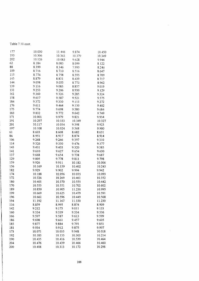
Table 7.10 cont.
177 10.030 11.446 9.874 10.450193 10 306 1&363 1CX379 10.349202 10.126 10 083 St628 9.94662 8.184 8.083 8.099 8.12288 8.399 8346 ir.993 8.246109 8.716 8.710 8.516 8.647115 8.774 8.758 EL595 8.709145 8.879 8.831 8.439 8.717144 9.058 &055 8.773 8.962139 9.116 9 083 8 857 9.019131 9 253 9206 8.930 9.129161 9360 9326 (\285 9.324158 9 617 9 587 9.521 9.575184 9J72 9330 9.113 9.272176 9.611 9.464 9.130 9.402175 9.774 9 698 9 580 9 684183 9.832 9.772 9.642 9.749171 10.001 9979 9.821 9.934191 10.297 10.333 10.349 10.327201 10.117 10.054 9 598 9.923197 10.108 10.024 9368 9.90061 8.603 8.608 8 682 8.63186 8.951 8.917 8.874 8.914106 9 268 9 266 9397 9.310114 9326 9.330 9.476 9.377143 9.431 9.403 9320 91.385141 9.610 9.627 9.654 9.630137 9.668 9.654 9 738 9.687129 9 805 9.778 9.811 9.798159 9 926 9.911 10.182 10.006156 10.169 10.159 10.402 10.243182 9929 9 902 9.994 9.942174 10.188 10.056 10.035 10.093172 10.326 10.269 10.461 10.352180 10.401 10.370 10.555 10.442170 10.553 10.551 10.702 10.602189 10.850 10 905 11.230 10.995199 10.669 10.625 10.479 10.591196 10.661 10 596 10.449 10.568194 11.192 11.167 11.330 11.230116 8.859 8.995 8.874 8.909142 9.212 9.175 9.011 9.133160 9.534 9 539 9.534 9.536166 &597 9.587 9.613 9.599186 9 698 9.661 9.457 9U605185 9.877 9 884 9.791 9.851181 9.934 9.912 9.875 9.907173 10.071 10.035 9.948 10.018192 10.183 10.155 10.303 10.214190 10.435 10.416 10.539 10.464204 10.476 10.439 10.466 10.460200 10.408 10.313 10.172 10.298
188

Table 7.10 cont.
198 10.592 10.527 1(1598 10.572203 10 625 10.581 1(1636 1(1614195 10.819 10.808 1(1839 10 822205 11.116 11.162 11.368 11.215208 10.935 10 883 10.182 10.667207 10.927 10.853 10.586 10.789206 11.377 11.325 11.347 11.350209 11.745 11.682 11.604 11.677266 5 619 5.511 5.191 5.440268 6.641 6 549 &275 6.488270 7.664 7.587 7J59 7.536272 8 686 8 625 8.443 8 584274 9 708 9 663 9 526 9.632276 10.730 10.701 10.610 10.680278 11.753 11.739 11.694 11.728280 12.775 12.777 12.778 12.776282 13.797 13.815 13.861 13.824284 14.820 14.852 14.945 14.872286 15.842 15.890 16.029 15.920289 17.376 17.447 17.654 17.492
189
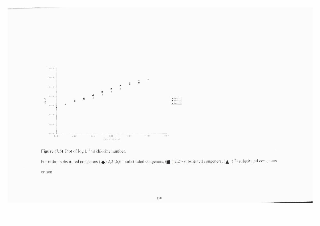
: h l o r l n e n u m b #
Figure (7.5) Plot o f log L' vs chlorine number.
For ortho- substituted congeners ( 2 ,2’,6,6’- substituted congeners, ( | | ) 2,2’- substituted congeners, ) 2- substituted congeners
or non.
190
7.5 Conclusions
The solvation descriptors for the 209 PCBs have been determined, using data on the
209 compounds from GLC experiments, togetlier with more limited data from HPLC
experiments, and on log Poet values. The calculated descriptors for a number of PCBs
were linearly related to the number of chlorine atoms, N, with due regard to the position
of the chlorine atom. The effect for ortfio- substitution was noted, so that the sets of the
descriptors for the PCBs were divided into four groups. These groups were as follows:
PCBs, 2,2’6-substituted, 2,2’,6,6’-substituted PCBs, 2,2’-ortho-substituted PCBs, 2-
ortho-subsituted and non substituted. From the obtained equations, descriptors for any of
the 209 PCBs could be calculated by fitting a given PCB to a specific group. Using the
calculated descriptors, values of log Poet were predicted for all the PCBs. Good
agreement with experimentally obtained logPoct values was found. In the next Chapter,
other properties of PCBs will be calculated from the descriptors, and, again, compared to
experiment.
191
7 .6 R e fe r e n c e s
1. A. Opperhuizen, Toxicol, and Environ. Cliem., 1987,Vol. 15, 249.
2. D. Sissons and D. Welti, J. Cliromatogr, 1971, Vol.60, 15.
3. G. W. Whelan, Advanced Organic Chemistry, Wiley New York, 1960.
4. U. A. Th. Brinkman and G. Devries, J. Chromatogr. 1979, Vol. 169, 167.
5. J. J. Dekok, A. Dekok, U. A. Th. Brinkman and R. M. Kok, J. Chromatogr. 1977,
Vol.142, 367.
6. E. Sholkovitz,and D. Copland, Geochim. Cosmochim, Acta. 1981, Vol. 45,1411.
7. A. Sablijic, H. Gusten, J. Hermens and A. Opperhuizen. Environ. Sci. Technol. 1993,
Vol. 27, 1394.
8. J. H. Park, P. W. Carr, M. H. Abraham, R.W. Taft, R. M. Doherty and M. J. Kamlet.
Adv. Technol. and Res ,1987, Vol.25, 30.
192
Chapter 8 Comparison of Calculated and Observed Partition Coefficients for PCBs
8.0 Introduction
The environmental fate of organic chemicals is largely determined by their
partitioning tendencies between aqueous, atmospheric and organic phases. The key
parameter for assessing and describing the partitioning behaviour of organic
chemicals between aqueous and organic phases is the water-octanol partition
coefficient (Poet). For example, log Poet has been found to be highly correlated with
the soil sorption and bioconcentration factor of aquatic organisms such as fish,
daphnids and molluscs, for a diverse range of chemicals. In addition, log Poet has
been correlated to biomagnification in beef cattle and swine^’ and to aqueous
solubility. This has resulted in the extensive use of log Poet in the development of
Quantitative-Structure and Property Relationships (QSPRs). The importance of highly
specific QSPRs becomes obvious when the fate and transport of structurally similar
compounds are considered especially in the case of polychlorinated biphenyls (PCBs).
PCBs were released into the environment in the form of multicongener mixtures
referred to as Aroclors. Not all PCBs are Aroclors, but most Aroclors are mixtures of
PCBs. Each Aroclor (e.g. 1016, 1221, 1232, ect.) contains a general mixture and the
major congener composition has been used to estimate the type of Aroclor (s) present
in the environmental sam ples.H ow ever, it has been shown that Aroclors extracted
from environmental samples show significantly different congener compositions than
those present in the original Aroclor (s). ' It is likely that there is a selective
microbial degradation/dechlorination,^^’ chemical/physical partitioning process
193

and reactions of congeners. Thus to effectively evaluate the relative importance of
congener-specific partitioning processes, accurate values of water-octanol partition
coefficients must be measured or predicted for each congener.
8.1 Theoretical background
The Poet value is defined as the ratio of the equilibrium of concentration of a
dissolved substance in a two-phase system consisting of the two largely immiscible
solvents, octanol and water. Mallhot and Peters studied the empirical relationships
between water-octanol partition coefficient and nine physicochemical properties.
They found that the property that predicts the partition coefficient most precisely is
aqueous solubility. Recently, Isnard and Lambert^ discussed the eighteen aqueous
solubility and water-octanol partition coefficient correlations available in the
literature. They concluded that there is a need to re-examine the theoretical approach.
In part, published values of water solubility can vary greatly for the same compound
and relatively little experimental data exists for many of the PCBs, an important class
of organic chemicals. Estimating log Poet from aqueous solubility introduces an
additional error into any correlation equation. Therefore, it is highly desirable to have
a reliable method to calculate water-octanol partition coefficients only from
information already present in the structural fonnulas of the compounds. Predicting
log Poet from chemical structure has advantages over methods based on aqueous
solubility. Wame et al. " predicted aqueous solubility and water-octanol partition
coefficient for lipophilic compounds using molecular descriptors and physicochemical
properties. The best simple linear regressions they incorporated are with either
connectivity indices or some measure of molecular surface area or volume. The
molecular surface area has been previously shown to be highly correlated with
194
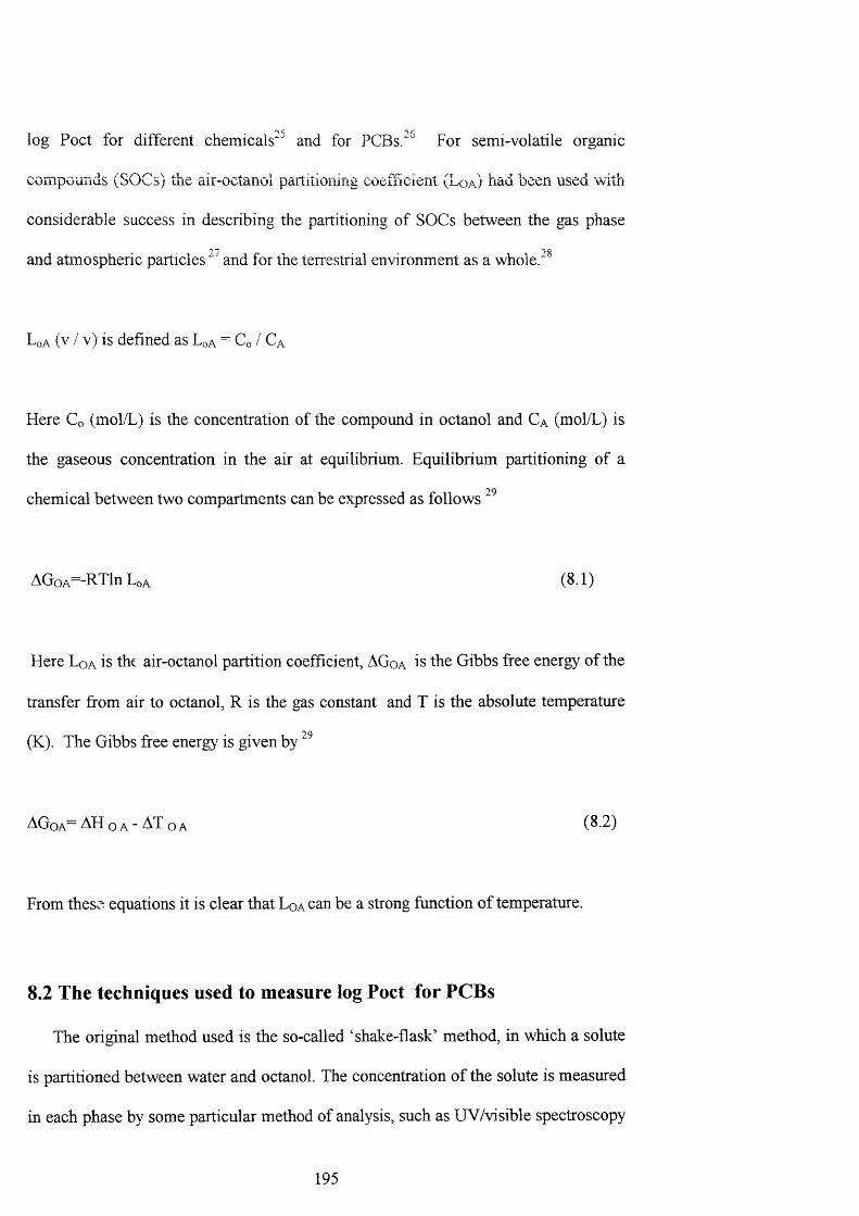
log Poet for different chemicals"" and for PCBs."*" For semi-volatile organic
compounds (SOCs) the air-octanol partitioning coefficient (Lqa) had been used with
considerable success in describing the partitioning of SOCs between the gas phase
and atmospheric particles and for the terrestrial environment as a whole.
Loa (v / v) is defined as Loa = Co / Ca
Here Co (mol/L) is the concentration of the compound in octanol and Ca (mol/L) is
the gaseous concentration in the air at equilibrium. Equilibrium partitioning of a
chemical between two compartments can be expressed as follows
A G oA =-R T ln Loa (8 .1)
Here L qa is the air-octanol partition coefficient, AGoa is the Gibbs free energy of the
transfer fi’om air to octanol, R is the gas constant and T is the absolute temperature
(K). The Gibbs free energy is given by
AGoA=AHoA-AToA (8.2)
From these equations it is clear that L qa can be a strong function of temperature.
8.2 The techniques used to measure log Poet for PCBs
The original method used is the so-called ‘shake-flask’ method, in which a solute
is partitioned between water and octanol. The concentration of the solute is measured
in each phase by some particular method of analysis, such as UV/visible spectroscopy
195
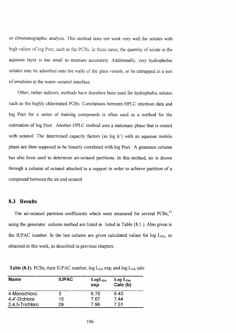
or chromatographic analysis. This method does not work very well for solutes with
high values of log Poet, such as the PCBs. In these cases, the quantity' of solute in the
aqueous layer is too small to measure accurately. Additionally, very hydrophobic
solutes may be adsorbed onto the walls of the glass vessels, or be entrapped in a sort
of emulsion at the water- octanol interface.
Other, rather indirect, methods have therefore been used for hydrophobic solutes
such as the highly chlorinated PCBs. Correlations between HPLC retention data and
log Poet for a series of training compounds is often used as a method for the
estimation of log Poet. Another HPLC method uses a stationary phase that is coated
with octanol. The determined capacity factors (as log k’) with an aqueous mobile
phase are then supposed to be linearly correlated with log Poet. A generator column
has also been used to determine air-octanol partitions. In this method, air is drawn
through a column of octanol attached to a support in order to achieve partition of a
compound between the air and octanol.
8.3 Results
The air-octanol partition coefficients which were measured for several PCBs/^
using the generator column method are listed in listed in Table (8.1 ). Also given is
the ILPAC number. In the last column are given calculated values for log Lqa, as
obtained in this work, as described in previous chapters.
Table (8.1) PCBs, their TUPAC number, log L qa exp, and log Lqa calc
Name lUPAC LogLoAexp
Log Loa Calc (b)
4-Monochloro 3 6.78 6.434,4'-Dichloro 15 7.67 7.442,4,5-Trich loro 29 7.96 7.51
196

2,3.4,5-Tetrachloro 612,2',4,4',6,6'- 155Hexachioro
8.748.99
8.318.84
b Calculated \’alues, this work.
Plots of log Lqa exp and log Loa calc (b ) versus the number of chlorine atoms in the
PCB are shown in Figure (8.1 ).
C hlorine Number
Figure (8.1) Plots of log L vs chlorine number
calculated
) log L measured and
8.3.1 The fugacit) meter
Measurements of the partitioning of polychlorinated biphenyls between air and
octanol have also been made using a fugacity met er . Ai r was passed through a
column packed with glass wool coated with an octanol solution of PCBs of known
concentration. The PCBs in the air were allowed to come into equilibrium with the
PCBs in the octanol. Upon leaving the column the PCBs in air were trapped on a
Florisil cartridge. The extraction and analysis of this cartridge allowed the
197
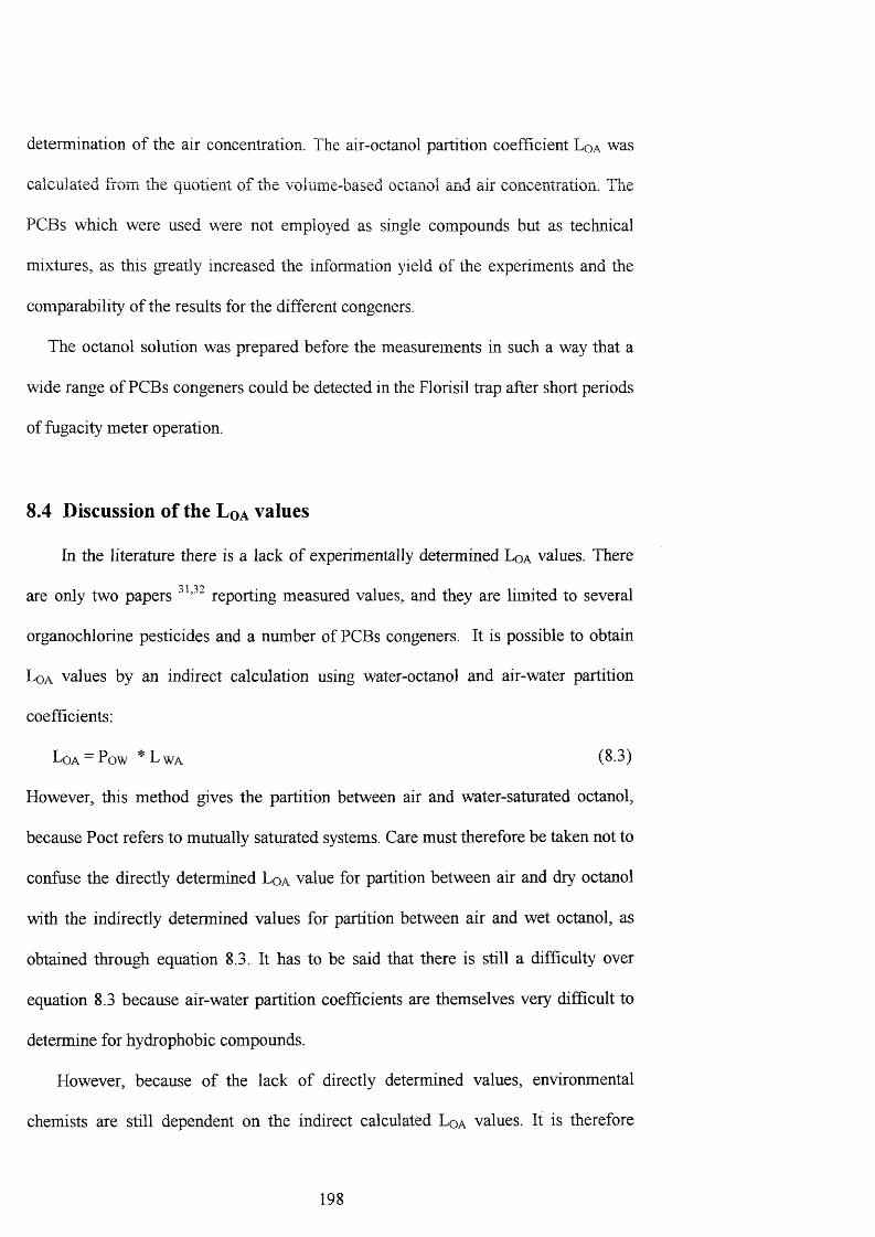
determination of the air concentration. The air-octanol partition coefficient Lqa was
calculated from the quotient of the volume-based octanol and air concentration. The
PCBs which were used were not employed as single compounds but as technical
mixtures, as this greatly increased the infonnation yield of the experiments and the
comparability of the results for the different congeners.
The octanol solution was prepared before the measurements in such a way that a
wide range of PCBs congeners could be detected in the Florisil trap after short periods
of fugacity meter operation.
8.4 Discussion of the L q a values
In the literature there is a lack of experimentally determined Lqa values. There
are only two papers reporting measured values, and they are limited to several
organochlorine pesticides and a number of PCBs congeners. It is possible to obtain
Loa values by an indirect calculation using water-octanol and air-water partition
coefficients:
L o a ~ P o w * L w a (^ 3 )
However, this method gives the partition between air and water-saturated octanol,
because Poet refers to mutually saturated systems. Care must therefore be taken not to
confuse the directly determined Lqa value for partition between air and dry octanol
with the indirectly determined values for partition between air and wet octanol, as
obtained through equation 8.3. It has to be said that there is still a difficulty over
equation 8.3 because air-water partition coefficients are themselves very difficult to
determine for hydrophobic compounds.
However, because of the lack of directly determined values, environmental
chemists are still dependent on the indirect calculated Lqa values. It is therefore
198
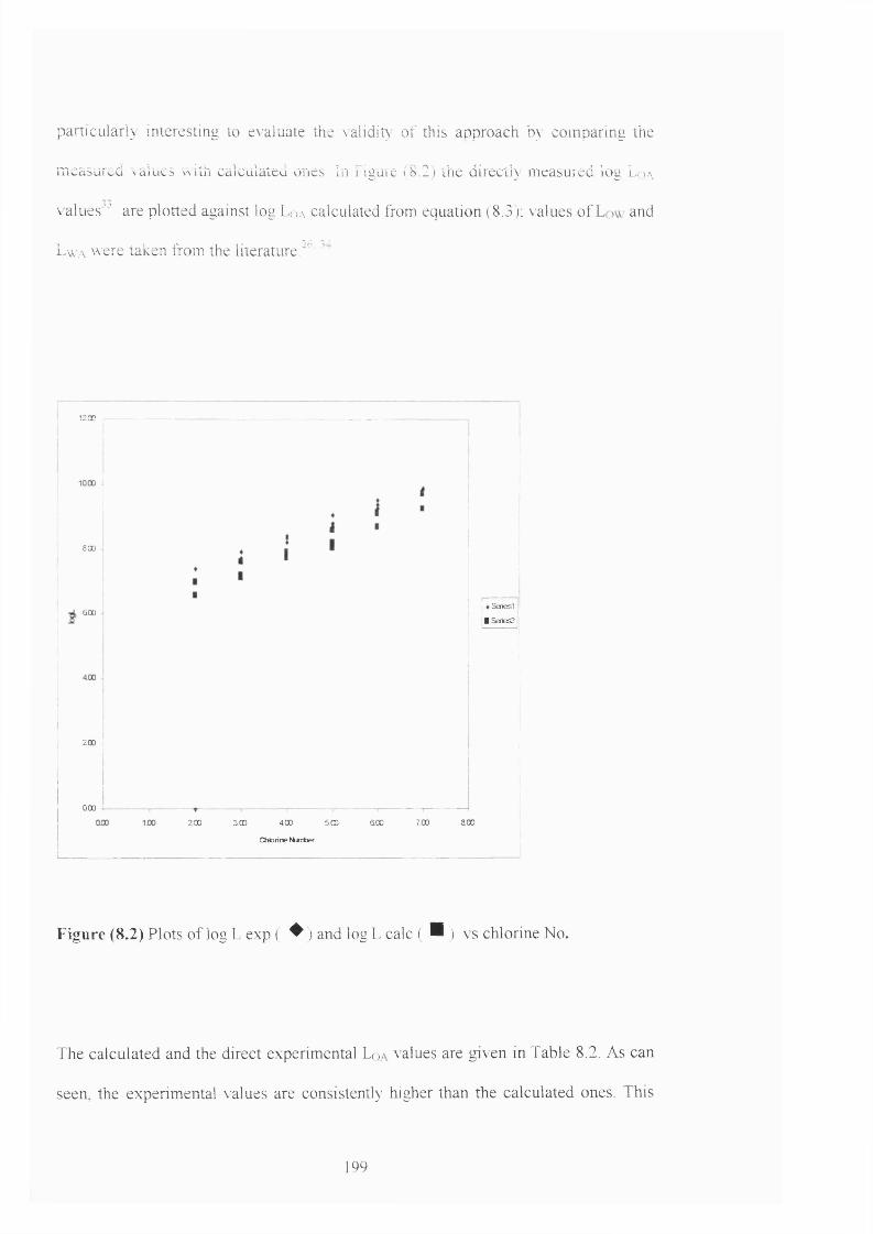
particularly interesting to e\'a)uate the validity o f this approach by com paring the
m easured values with calculated ones. In Figure (8.2) the direcllx m easured log Lqa
\ alLies'' are plotted against log Loa calculated from equation (8.3 ): values o f and
LwA ^vere taken from the literature.'^'
1200
aoo
aoo
200 i
QQO
I ♦Seriesl
|lSeries2
2.00 3.00 400 5.00 600 7.00 600
Chlorine fO rtief
Figure (8.2) Plots o f log L exp ( ^ ) and log L calc ( B ) vs chlorine No.
The calculated and the direct experim ental Lq.a values are given in Table 8.2. As can
seen, the experim ental values are consistently higher than the calculated ones. This
199

indicates that the calculated Loa system atically under predicts the true value. H am er
and M ackay ' ' suggested that th is may be because the Low value represents the
chem icals’ partitioning betw een octanol saturated with w ater and w ater saturated with
octanol, no t betw een pure octanol and pure water. There is very good agreem ent,
how ever, betw een the directly determ ined experim ental values and those calculated
in this w ork, from the descriptors that have been obtained.
Table (8.2) lU PA C No. exp. Log calc. Log L qa^^^\ and our calc.
LogLoA^^^
PCS S u b s t i t u t i o n lUPAC(D)
LogL ex p A
LogL c a l c B
LogL c a l c C
( 2 ,2 ' ) ; ( 2 , 6 ) 4 + 10 7 . 1 8 6. 56 6. 95
( 2 , 4 ' ) ( 2 , 3 ) 8+5 7. 40 6. 98 6. 98
( 2 , 2 ' , 5 ) 18 7. 60 7 . 12 7. 58
( 2 , 2 ' , 3 ) ; ( 2 , 4 ' , 6 ) 16+32 7. 72 7 . 1 8 7 . 5 7
( 2 , 4 ' 5 ) ; ( 2 , 4 , 4 ' ) 31+28 7. 92 7 . 61 7 . 6 1
( 2 , 2 ' , 5 , 5 ' ) 52 8.22 7 . 73 8 .2 2
( 2 , 2 ' , 3 , 5 ' ) 44 8. 36 7 . 78 8 .2 2
( 2 , 3 , 4 ' , 6 ) 64 8. 41 7 . 91 8. 32
( 2 , 2 ' , 3 , 5 ' , 6 ) 95 8 . 7 1 8. 04 8. 64
( 2 , 2 ' , 3 , 3 ' , 6 ) ; 84+101 8. 80 8 .2 0 8 . 75
( 2 , 2 ' , 4 , 5 , 5 ' )
( 2 , 3 , 3 ' , 4 ' , 6 ) 110 9. 06 8. 58 8. 98
( 2 , 2 ' , 3 , 4 ' , 5 ' , 6 ) 149 9.27 8 .6 8 9. 25
( 2 , 2 ' , 4 , 4 ' , 5 , 5 ' ) 153 9.37 9 . 09 9. 52
( 2 , 2 ' , 3 , 4 , 4 ' , 5 ' ) ;
(2, 3, 3 ' , 4 , 4 ' , 6 ) 138+158 9.51 9 . 12 9. 58
(2, 2 ' , 3 , 4 ' , 5 , 5 ' , 6 ) 187 9.87 9 . 25 9. 85
( 2 , 2 ' , 3 , 4 , 4 ' , 5 , 5 ' ) 180 9.88 9 . 72 1 0 . 1 7
200
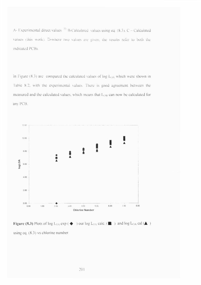
A- Experim ental direct values. " B-Calculated \ alues using eq. (8.3). C - Calculated
values (this work). D-\vhere two values are given, the results lefei to both the
indicated PCBs.
In Figure (8.3) are com pared the calculated \ alues o f log Loa which were showm in
Table 8.2, w ith the experimental values. There is good agreem ent betw een the
m easured and the calculated values, which means that Low can now be calculated for
anv PCB.
12.00
2.00 3.00 4.00 5.00
Chlorine Num ber
7.00
Figure (8.3) Plots o f log L q a exp ( ♦ ) our log Loa calc. ( ■ ) and log Lo.v cal (▲ )
using eq. (8.3) vs chlorine number.
201

8.5 The Final Comparison for Octanol/Water Partitioning of
PCBs
Because the PCBs are quite hydrophobic compounds, with large values of logPoct,
it is veiy difficult to obtain directly measured values. Thus, most quoted values are
those that have been predicted by some calculation method, and only few measured
values are known.
One of the most useful studies is that of Hawker^^ who measured 13 PCB
congeners by the generator column method. The series of 13 PCBs was selected so as
to contain a great deal of structural variation and cover a wide rang of lipophilicity. It
included seven terachlorobiphenyls with from zero (3,3’,4,4’-) to four (2,2’,6,6’-)
ortho-substitued chlorine atoms, two congeners substituted on one ring only, and
others with five, six, eight, and nine chlorine substituents. The determined log Poet
values had been used by Hansen^^ to compare his calculated log Poet for the same
PCBs, as shown in Table (8.3). Another well known program for the calculation of
log Poet values is the Clog P program of Leo. Values of Clog P are also given in
Table (8.3). The most recent and accurate measured values for log P were the ones
listed in MedChem program; in this program more than one value for each PCBs
may be found, the most reliable one is log P*. In Table (8.3) the calculated values
(this work) were compared with the experimental and other calculated ones.
202

Table (8.3) Comparison of calculated values, this work, with experimental and other
calculated values of log Poet for PCBs
C a l l o g P o e t E x p l o g P o e t
Name lUPAC This Hansen ClogP Log P* MedChem Hawkework
2,2',3,3'-Tetachiorobiphenyl 40 6.18 5.71 6.26 6 .1 8 5.15 5.552,2',5,6'-Tetrachlorobiphenyl 53 6 .0 6 5.67 6.13 5.54 5.462,2',6,6'-T etrachlorobiphenyl 54 5 .9 6 5 .32 5 .9 4 5.94 5.482,3,4,5 -T etrachlorobiphenyl 61 6.34 5 .87 6.51 6.41 6.182,3,5,6-T etrachlorobiphenyl 65 5 .9 6 5.71 6 .3 8 5 .9 4 5.942,3 ',4,4'-T etrachlorobiphenyl 66 6 .2 5 6.31 6.313,3’,4,4'-Tetrach]orobiphenyl 77 6 .6 3 6.14 6 .1 9 6 .6 3 6 .1 0 6.212 ,2 ',4 ,6 ,6 '- 104 5.93 5.83 5.81 5.81 5.37 5.37Pentachlorobiphenyl2 ,3 ,3 ',4 ,4 '- 105 6 .6 8 6 .3 9 7.10 6 .2 3 5.82Pentachlorobiphenyl2 ,2 ',3 ,3 ',6 ,6 '. 136 7.16 6.19 5.92 7.12 6.44 5.76Hexacchlorobiphenyl2 ,2 '3 ,3 ',4 ,4 ,5 ,5 '. 194 8.61 7.55 8 .9 9 8 .6 8 8 .2 7 7.67Octachl orobiphenyl2 ,2 ',3 ,3 ',4 ,5 ',6 ,6 '- 201 8.17 7.03 7.24 7.21Octachlorobiphenyl2 ,2 ',3 ,3 ',4 ,4 ',5 ,6 ,6 '- 207 8 .3 4 7.49 9 .45 7.63 7.52Nonchlorobipheny]
The last comparison for the calculated log Poet values in this work for all 209
PCBs, was obtained by comparing 209 PCBs with values from the MedChem data
base. As mentioned before, in this data base there may be more than one value for any
PCB. The average of the given values was taken and also the minimum and maximum
for each PCB. For some of the PCBs, a value of log P* was given; this indicates the
most reliable value. All these details are shown in Table (8.4) with the lUPAC
number for each one. From these Table (8.4) it is clear that the calculated log Poet
values in this work are in excellent agreement with observed values. Therefore, where
there are no observed values, the calculated ones obtained in this work could be used
quite reliably.
203
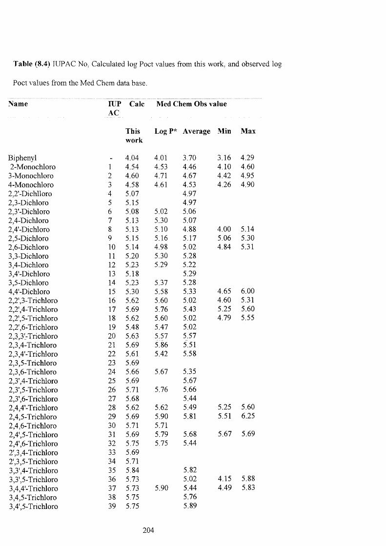
Table (8,4) IIJPA C No, Calculated log Poet values from this work, and observed log
P oet values from the M ed Chem data base.
Name rupAC
Calc Med Chem Obs value
This Log P* Average Min Maxwork
Biphenyl - 4.04 4.01 3.70 3.16 4.292-Monochloro 1 4.54 4.53 4.46 4.10 4.60
3-Monochloro 2 4.60 4.71 4.67 4.42 4.954-Monochloro 3 4.58 4.61 4.53 4.26 4.902,2'-Dichlloro 4 5.07 4.972,3-Dichloro 5 5.15 4.972,3'-Dichloro 6 5.08 5.02 5.062,4-Dichloro 7 5.13 5.30 5.072,4'-Dichloro 8 5.13 5.10 4.88 4.00 5.142,5-Dichloro 9 5.15 5.16 5.17 5.06 5.302,6-Dichloro 1 0 5.14 4.98 5.02 4.84 5.313,3-Dichloro 1 1 5.20 5.30 5.283,4-Dichloro 1 2 5.23 5.29 5.223,4’-Dichloro 13 5.18 5.293,5-Dichloro 14 5.23 5.37 5.284,4'-Dichloro 15 5.30 5.58 5.33 4.65 6 . 0 0
2,2',3-Trichloro 16 5.62 5.60 5.02 4.60 5.312,2',4-Trichloro 17 5.69 5.76 5.43 5.25 5.602,2',5-Trichloro 18 5.62 5.60 5.02 4.79 5.552,2',6-Trichloro 19 5.48 5.47 5.022,3,3-Trichloro 2 0 5.63 5.57 5.572,3,4-Trichloro 2 1 5 .ë 5 86 5.512,3,4'-Trichloro 2 2 5.61 5.42 5.582,3,5-Trichloro 23 5.692,3,6-Trichloro 24 5.66 5.67 5.352,3',4-Trichloro 25 5.69 5.672,3',5-Trichloro 26 5.71 5.76 5.662,3',6-Trichloro 27 5.68 5.442,4,4'-Trichloro 28 5.62 5.62 5.49 5.25 5.602,4,5-Trichloro 29 5.69 5.90 5.81 5.51 6.252,4,6-Trichloro 30 5.71 5.712,4',5-Trichloro 31 5.69 5.79 5.68 5.67 5.692,4',6-Trichloro 32 5.75 5.75 5.442',3,4-Trichloro 33 5.692',3,5-Trichloro 34 5.713,3',4-Trichloro 35 5.84 5.823,3',5-Trichloro 36 5.73 5.02 4.15 5.883,4,4'-Trichloro 37 5.73 5.90 5.44 4.49 5.833,4,5-Trichloro 38 5.75 5.763,4',5-Trichloro 39 5.75 5.89
204
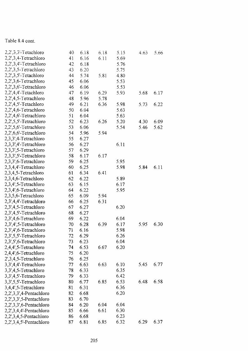
Table 8.4 cont.
2,2:3 J'-T etachloro 40 6.18 6.18 5.15 4.65 5.662,2',3,4-T etrachloro 41 6.16 6 . 1 1 5.692,2',3,4’-T etrachloro 42 6.18 5.762,2',3,5-Tetrachloro 43 6 . 2 0 5.752,2',3,5'-T etachloro 44 5.74 5.81 4.802,2',3,6-Tetrachloro 45 6.06 5.532,2',3,6'-Tetrachloro 46 6.06 5.532,2',4,4'-T etachloro 47 6.19 6.29 5.93 5.68 6.172,2',4,5-Tetrachloro 48 5.96 5.782,2',4,5'-Tetachloro 49 6 . 2 1 6.36 5.98 5.73 6 . 2 2
2,2',4,6-Tetrachloro 50 6.04 5.632,2',4,6’-T etrachloro 51 6.04 5.632,2',5,5'-Tetrachloro 52 6.23 6.26 5.20 4.30 6.092,2',5,6’-Tetrachloro 53 6.06 5.54 5.46 5.622 ,2 ',6 ,6 '-Tetrachloro 54 5.96 5.942,3,3’,4-Tetrachloro 55 6.272,3,3 ',4'-T etrachloro 56 6.27 6 . 1 1
2,3,3',5-T etrachloro 57 6.292,3,3',5'-Tetrachloro 58 6.17 6.172,3,3’,6-T etrachloro 59 6.25 5.952,3,4,4'-Tetrachloro 60 6.25 5.98 5.84 6 . 1 1
2,3,4,5-Tetrachloro 61 6.34 6.412,3,4,6-Tetrachloro 62 6 . 2 2 5.892,3,4',5-T etrachloro 63 6.15 6.172,3,4',6-Tetrachloro 64 6 . 2 2 5.952,3,5,6-T etrachloro 65 6.09 5.942,3',4,4'-Tetrachloro 6 6 6.25 6.312,3',4,5-T etrachloro 67 6.27 6 . 2 0
2,3',4,5'-Tetrachloro 6 8 6.272,3',4,6-Tetrachloro 69 6 . 2 2 6.042,3',4',5-Tetrachloro 70 6.28 6.39 6.17 5.95 6.302,3',4',6-Tetrachloro 71 6.16 5.982,3',5,5'-Tetrachloro 72 6.29 6.262,3',5',6-Tetrachloro 73 6.23 6.042,4,4',5-Tetrachloro 74 6.53 6.67 6 . 2 0
2,4,4',6-T etrachloro 75 6 . 2 0
2',3,4,5-Tetrachloro 76 6.253,3',4,4'-Tetrachloro 77 6.63 6.63 6 . 1 0 5.45 6.773,3',4,5-Tetrachloro 78 6.33 6.353,3',4,5'-Tetrachloro 79 6.33 6.423,3',5,5'-Tetrachloro 80 6.77 6.85 6.53 6.48 6.583,4,4',5-T etrachloro 81 6.31 6.362,2',3,3',4-Pentachloro 82 6 . 6 8 6 . 2 0
2,2',3,3',5-Pentachloro 83 6.702,2',3,3',6-Pentachloro 84 6 . 2 0 6.04 6.042,2',3,4,4'-Pentachloro 85 6 . 6 6 6.61 6.302,2',3,4,5-Pentachloro 8 6 6 . 6 8 6.232,2',3,4,5'-Pentachloro 87 6.81 6.85 6.32 6.29 6.37
205

Table 8.4 cont.
2 ,2 ',3,4,6-Pentachloro 8 8 6.56 6.072,2',3,4,6'-Pentachloro 89 6.56 6.072,2',3,4',5-Pentachloro 90 6.73 6.362,2',3,4’,6-Pentach] oro 91 6.25 6.312,2',3,5,5'-Pentachloro 92 6 . 8 6 6.97 6.352,2',3,5,6-Pentachloro 93 6.582,2',3,5,6'-Pentachloro 94 6.58 6.132,2’,3,5',6-Pentachloro 95 6.58 6.552,2',3,6 ,6 '-Pentachloro 96 6.65 5.712,2',3',4,5-Pentachloro 97 6 . 6 6 6.67 6.292,2',3 ',4,6-Pentachloro 98 6.56 6.072,2',4,4',5-Pentachloro 99 6.79 7.21 6.392,2'4,4'6-Pentachloro 1 0 0 6.54 6.232,2',4,5,5'-Pentachloro 1 0 1 6.81 6.85 6.51 5.92 7.072,2',4,5,6'-Pentachloro 1 0 2 6.56 6.162,2',4,5',6-Pentachloro 103 6.56 6 . 2 2
2,2',4,6,6'-Pentachloro 104 5.93 5.81 5.372,3,3',4,4’-Pentachloro 105 6 . 6 8 6.23 5.82 6.652,3,3',4,5-Pentachloro 106 6.742,3,3',4',5-Pentachloro 107 6.74 6.712,3,3',4,5'-Pentachloro 108 6 . 6 8 6.712,3,3',4,6-Pentachloro 109 6 . 6 8 6.482,3,3',4',6-Pentachloro 1 1 0 6 . 6 8 6.482,3,3',5,5’-Pentachloro 1 1 1 6.762,3,3 ',5,6 -Pentachloro 1 1 2 6.72 6.452,3,3',5',6-Pentachloro 113 6.70 6.542,3,4,4',5-Pentachloro 114 6.72 6.652,3,4,4',6-Pentachloro 115 6 . 6 6 6.492,3,4,5,6-Pentachloro 116 6.72 6.74 6.49 6.30 6.852,3,4',5,6-Pentachloro 117 6 . 6 8 6.462,3',4,4',5-Pentachloro 118 7.10 7.12 6.652,3',4,4',6-Pentachloro 119 6 . 6 6 6.582,3',4,5,5'-PentachIoro 1 2 0 6.74 6.24 5.68 6.792,3’,4,5',6-Pentachloro 1 2 1 6 . 6 8 6.642',3,3',4,5-Pentachloro 1 2 2 6.74 6.642',3,4,4',5-Pentachloro 123 6.78 6.742',3,4,5,5'-Pentachloro 124 6.742',3,4,5,6'-Pentachloro 125 6 . 6 8
3,3',4,5,5'-Pentachloro 127 6.48 6.963,3’,4,5,5'-Pentachloro 127 6.80 6.952,2',3,3',4,4'-Hexachloro 128 7.29 7.32 7.09 6.74 7.442,2',3,3’,4,5-Hexachloro 129 7.31 7.32 6.98 6.73 7.222,2',3,3',4,5'-Hexachloro 130 7.31 7.39 7.00 6.80 7.202,2',3,3',4,6-HexachIoro 131 6.93 6.82 6.582,2',3,3',5,5'-Hexachloro 133 7.09 7.07 6 . 8 6
2,2',3,3 ',5,6 -Hexachloro 134 6.91 6.81 6.552,2’,3,3',5,6-Hexachloro 134 6.95 6.812,2',3,3',6,6'-Hexachloro 136 7.16 7.12 6.44 5.76 6.81
206

Table 8.4 cont.
2,2',3,4,4',5-Hexachloro 137 7.33 7.43 7.242,2',3,4,4',5'-Hexachloro 138 7.29 7.25 7.372,2',3,4,4',6-Hexachloro 139 6.97 6.932,2',3,4,4',6'-Hexachloro 140 6.96 6.97 6.672,2',3,4,5,5'-Hexachloro 141 7.24 7.19 6.822,2 ' ,3,4,5,6 -Hexachloro 142 6.99 6.97 6.512,2',3,4,56'-Hexachloro 143 6.99 6.92 6.602,2’,3,4,5',6-Hexachloro 144 6.95 6.79 6.672,2',3,4,6,6'-Hexachloro 145 6 . 8 8 6.75 6.252,2',3,4',5,6 '-Hexachloro 148 6.93 6.87 6.732,2',3,4',5,6'-Hexachloro 148 6.93 6.87 6.732,2',3,4',5',6-Hexachloro 149 6.93 6 . 8 6 6.692,2',3,4',6,6'-Hexachloro 150 6 . 8 8 6.75 6.322,2',3,5,5',6-Hexachloro 151 6.77 6.85 6.642,2',3,5,6,6'-Hexachloro 152 6.63 6.51 6 . 2 2
2,2'4,4,5,5'-Hexachloro 153 7.35 7.44 7.102,2',4,4',5,6'-Hexachloro 154 6.91 6.89 6.762,2',4,4'6,6'-Hexachloro 155 7.12 7.29 6.992,3,3',4,4',5-Hexacchloro 156 7.50 7.57 7.182,3,3',4,4',6-Hexachloro 158 7.23 7.25 7.022,3,3',4,5,5'-Hexachloro 159 7.32 7.47 7.262,3,3',4,5,6-Hexachloro 160 7.30 7.30 6.932,3,3',4,5',6-Hexachloro 161 7.18 7.10 7.082,3,3',4',5,5'-Hexachloro 162 7.32 7.47 7.242,3,3',4',5,6 -Hexachloro 163 7.27 7.25 6.992,3,3',4',5',6-Hexachloro 164 7.22 7.20 7.022,3,3',5,5',6-Hexachloro 165 7.32 7.37 7.082,3,4,4',5,6-Hexachloro 166 7.28 7.31 6.932,3',4,4',5,5'-Hexachloro 167 7.34 7.50 7.272,3',4,4',5',6-Hexachloro 168 7.18 7.17 7T13,3',4,4',5,5'-Hexachloro 169 7.34 7.41 7.642,2',3,3',4,4',5-Hetachloro 170 7.78 7.272,2',3,3',4,4',6-Hetachloro 171 7.70 6.902,2',3,3',4,5,5'-Hetachloro 172 7.74 7.332,2',3,3',4,5,6-Heptachloro 173 7.72 7.022,2',3,3',4,5,6'-Heptachloro 174 7.72 7.112,2',3,3',4,5',6-Heptachloro 175 7.72 7.172,2',3,3',4,6,6'-Heptachloro 176 7.71 6.762,2’,3,3',4',5,6-Heptachloro 177 7.662,2’,3,3',5,5’,6-Heptachloro 178 7.72 7.142,2',3,3',5,6,6'-Heptachloro 179 7.73 7.432,2',3,4,4',5,5'-Hetachloro 180 7.64 7.362,2',3,4,4',5,6-Heptachloro 181 7.70 7.112,2',3,4,4',5,6'-Heptachloro 182 7.70 7.022,2',3,4,4',5',6-Heptachloro 183 7.70 7.202,2',3,4,4',6,6'-Heptachloro 184 7.64 6 . 8 6
2,2',3,4,5,5',6-Heptachloro 185 7.72 7.93 7.112,2',3,4,5,6,6-Heptachloro 186 7.66 6.69
6.83 7.466.83 7.90
6.67 6.70
6.34 7.75
6.41 7.55
7.05 7.11
7.42 7.87
6 . 6 8 7.11
6.73 8.13
207
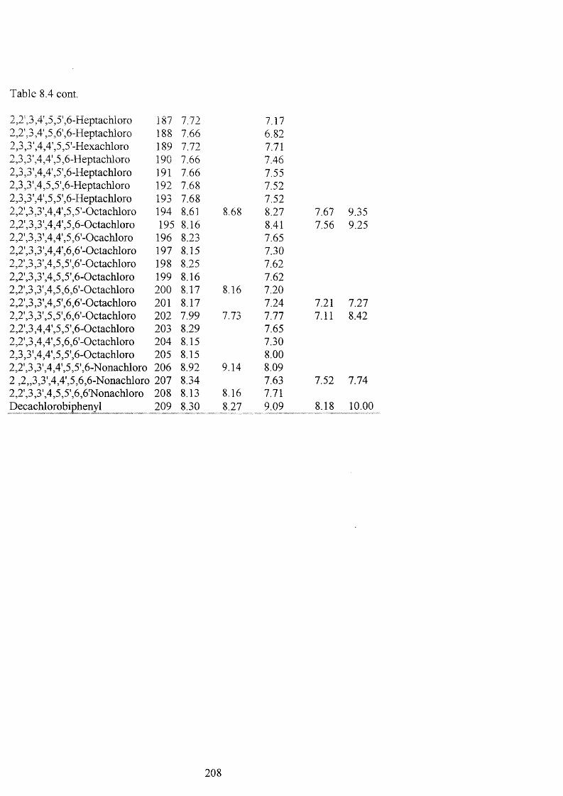
Table 8.4 cont.
2,2’,3,4',5,5',6-Heptachloro 187 7.72 7.172,2’,3,4',5,6',6-Heptachloro 188 7.66 6.822,3,3 ',4,4',5,5'-Hexachloro 189 7.72 7.712,3,3',4,4',5,6-Heptachloro 190 7.66 7.462,3,3 ’,4,4',5',6-Heptachloro 191 7.66 7.552,3,3',4,5,5',6-Heptachloro 192 7.68 7.522,3,3',4',5,5',6-Heptachloro 193 7.68 7.522,2',3,3',4,4',5,5'-Octachloro 194 8.61 8 . 6 8 8.27 7.67 9.352,2',3,3 ',4,4',5,6 -Octachloro 195 8.16 8.41 7.56 9.252,2',3,3',4,4',5,6'-Ocachloro 196 8.23 7.652,2',3,3',4,4',6,6'-Octachloro 197 8.15 7.302,2',3,3',4,5,5',6'-Octachloro 198 8.25 7.622,2',3,3',4,5,5',6-Octachloro 199 8.16 7.622,2',3,3',4,5,6,6'-Octachloro 2 0 0 8.17 8.16 7.202,2',3,3',4,5',6,6'-Octachloro 2 0 1 8.17 7.24 7.21 7.272,2',3,3',5,5',6,6'-Octachloro 2 0 2 7.99 7.73 7.77 7.11 8.422,2',3,4,4',5,5',6-Octachloro 203 8.29 7.652,2',3,4,4',5,6,6'-Octachloro 204 8.15 7.302,3,3',4,4',5,5',6-Octachloro 205 8.15 8 . 0 0
2,2',3,3',4,4',5,5',6-Nonachloro 206 8.92 9.14 8.092 ,2,,3,3',4,4',5,6,6-Nonachloro 207 8.34 7.63 7.52 7.742,2',3,3',4,5,5',6,6'Nonachloro 208 8.13 8.16 7.71Decachlorobiphenyl 209 8.30 8.27 9.09 8.18 1 0 . 0 0
208

8.6 Discussion
Many of the persistent, semi-volatile hydrophobic organic chemicals that are of
interest are difficult to handle experimentally because they sorbs strongly to surfaces,
especially from aqueous solution. Measurements of L a w and Poet are thus difficult to
make, and are subject to error, and the reported values often vary considerably, as is
apparent from examination of compilations of data. ' ^
Calculation of L q a from Poet and L a w thus combines these errors and introduces
considerable uncertainty. It is also possible that the presence of octanol in the water
layer, and, especially, water in the octanol layer, leads to the indirect value of L a w
being not the same as the direct value using dry octanol. The possibility of calculating
Law for partition from air to dry octanol is therefore of considerable importance. In
this work, such a calculation for all 209 PCBs has been achieved for the first time.
The calculation of log Poet for all 209 PCBs in this work, is not the first such
calculation at all, but does seem to be more reliable than any other calculation of log
Poet.
209
8.7 References
1. G.G. Briggs, Nature (London) 1969, Vol. 223,1288
2. C. T. Chiou, L. T. Peters and V. H. Freed, Science, 1979, Vol. 206, 831.
3. S. W. Karichhoff, D. S. Brown and T. A. Scott, Water Res., 1979, Vol. 13,
241.
4. R. P. Schwarzenbach, J. Westall, Environ. Sci. Technol., 1981, Vol. 15,
1360.
5. C. T. Chiou, P. E. Porter, D. W. Schemedding, Environ. Sci. Technol.,
1983, Vol. 17,227.
6 . W. B. Neely, D. R. Bronson, G. E. Blau, Environ Sci. Technol., 1974, Vol.
8 , 1113.
7. D. Mackay, Environ. Sci. Technol., 1982, Vol. 16, 274.
8 . C. T. Chiou, Environ. Sci. Technol., 1985, Vol. 19, 57.
9. K. Suqiura, N. Ito, N. Matsumoto, Y. Mihara, K. Murata, Y. Tsukakoshi,
M. Goto, Chemosphere, 1978, Vol. 9, 731.
10. H. Konemann, K. Van Leeuwen, Chemosphere, 1980, Vol. 9, 3.
11. E. E. Kenaga, Sci. Technol., 1980, Vol. 14, 553.
12. D. Mackay, A. Bobra, W. Y. Shiu, S.H. Yalkowsky, Chemosphere, 1980,
Vol. 9,701.
13. C. T. Chiou, V. H. Freed D. W. Schmedding, R. L. Kohnert, Enviro. Sci.
Technol., 1977, Vol. 11,475.
14. M. M. Miller, S. P. Wasik, G. L. Huang, W.Y. Shiu, D. Mackay, Environ.
Sci. Technol., 1985, Vol. 9, 522.
210

15. W. A. Bruggeman, J. Van der Steen, O. Hutziger, J. Chromatogr., 1982,
Vol. 238, 335.
16. P. W. Albro, C. E. Parker, J. Chromatogr., 1979, Vol. 169, 161.
17. P. W. Albro, F. J. Corbett, J. L. Schroeder, J. Chromatogr., 1981, Vol.
205, 103.
18. R. F. Bopp, H. J. Simpson, C. R. Olsen, N. Kostyk, Environ. Sci.
Technol., 1981, Vol. 15,210.
19. B. Bush, L. A. Shere, M. Wahlen, Chemosphere., 1987, Vol. 16, 733.
20. J. F. Brown, D. L. Bedard, M. J. Brennan, J. C. Camalan, H. Feng, R. E.
Wagner, Science, 1987, Vol. 236, 709.
21. J. F. Quensen, J. M. Tiedje, S. A. Boys, Science, 1988, Vol. 242, 752.
22. H. Mallhot, R. H. Peters, Environ. Sci. Technol., 1988, Vol. 22, 1479.
23. P. Isard, S. Lambert, Chemosphere, 1989, Vol. 18, 1837.
24. M. St. J. Wame, D. W. Connell, D. W. Hawker, G. Schurmann,
Chemosphere., 1990, Vol. 21 , 877.
25. S. H. Yalkowsky, S. C. Valvani, J. Chem. Eng. Data., 1979, Vol. 24, 127.
26. D. W. Hawker, D. W. Connell, Environ. Sci. Technol., 1988, Vol. 22,
382.
27. A. Finizio, D. Mackay, T. Bidleman, and T. Hamer, Atmos. Environ.,
1997, Vol. 33, 2289.
28. M. S. McLachlan, Environ. Sci. Technol. 1996, Vol. 30, 252.
29. A. Opperhuizen, P. Seme, and J. M. D. Van der Steen. Environ. Sci.
Technol., 1988, Vol. 22, 286.
30. M. Horstmann, M. S. McLachlan, Environ. Sci. Technol., 1992, Vol. 26,
1643.
211
31. T. Hamer, D, Mackay, Environ Sci. Techno]., 1995, Vol. 29, 1599.
32. T. Hamer, T. F. Bidleman, J. Chem. Eng. Data. 1996, Vol. 41, 895.
33. P. Komp, and M. S. Mclachlan, Environ. Toxic. And Chem., 1997, Vol.
16, 2433.
34. F. M. Dunnivant, A. W. Elzennan, P. C. Jurs and M. N. Hasan, Environ.
Sci. Technol. , 1992, Vol. 26, 1567.
35. B. J. Hansen, A. B. Paya- Perez, M. Rahaman, and B. R. Larsen.,
Chemosphere., 1999, Vol. 39, 2209.
36. A. J. Léo. Medchem. The Medicinal Chemistry Project, Pomona College,
Claremont, C A 9171.
37. D. Mackay, W. Y. Shiu, K. C. Ma, Illustrated Handbook of Physical-
Chemical Properties and Environmental Fate for Organic Chemicals.
Lewis Publishing Co., Chelsea, MI, Vol. 1, 1991.
38. J. Sangster, J. Phys. Chem. Ref. Data., 1989, Vol. 18,1111.
212
Chapter 9 Calculation and Comparison of Aqueous Solubility
for PCBs Using the Obtained Descriptors
9.0 Introduction
Aqueous solubility is a very important molecular property which plays an integral
role in many different biological and physical processes. As a property involving water as
the solvent, it is important in a diverse array of situations including pharmaceutical,
environmental, and industrial applications. The rate and extent of biodégradation are also
affected by the aqueous solubility of organic compounds in the environment.Obtaining
experimental values of aqueous solubility is not a difficult task for compounds that are
reasonably soluble, but determination of very low solubilities can be very difficult
indeed. There is therefore sample justification for creating methods that can predict this
property. Being able to predict the aqueous solubility of compound would greatly assist
drug development, because a solubility could be estimated before the compound was
synthesized, which would eliminate the need to synthesize many unsuitable compounds.
The ability to predict aqueous solubility would also be useful in environmental impact
studies, because the solubility could be estimated without handling compounds that are
highly toxic, carcinogenic, or undesirable for some other reason. There is no question
that the ability to predict the aqueous solubility of compounds is useful. Many different
methods have been developed for the estimation of aqueous solubility with varying
success and applicability. Some recent developments include a neural network model
relating aqueous solubility to topological descriptors, the use of mobile order solubility
213

models a clustering approach, group contribution approaches and linear and
neural network models based on semi-empirical quantum chemical descriptors.
There is not only a correlation of aqueous solubility (Sw) with n-octanol/water
partition coefficients (Kow) " but also with bioconcentration factors (BCF).’" Therefore,
a prediction of Sw is also useful as regards the prediction of bioconcentration, and also
otlier enviromnental processes. Prediction of Sw or of log Sw for polychorinated
biphenyl (PCBs) would be important, because these compounds have serious ecologically
harmful effects and are implicated as carcinogens.^ For the aqueous solubility of PCBs
congeners, it has been found that there is high correlation with various physiochemical
properties, including total surface area, molecular volume,^ boiling point,^ melting
point , th i rd shadow area,’ polarizability parameter,^^ mobile order of PCBs,^
connectivity indexes and the degree of ortho-chlorine substitution in the biphenyl
skeleton. Especially, linear solvation energy relationships (LSER), are regarded as
being useful in the prediction of partitioning and solubility. In addition, the substitution
constant (tt) derived from partition coefficients of compounds has also been reported as a
useful descriptor to predict log Sw.
9.1 Results
This method starts with the general solvation equation,
log SP = c + r R2 + s + a I + b XP2^ + v Vx (9.1)
Here, the dependent variable, log SP, is a property of a series of solutes in a given system,
such as log Poet or log Sw, and the independent variables are solute descriptors as
214
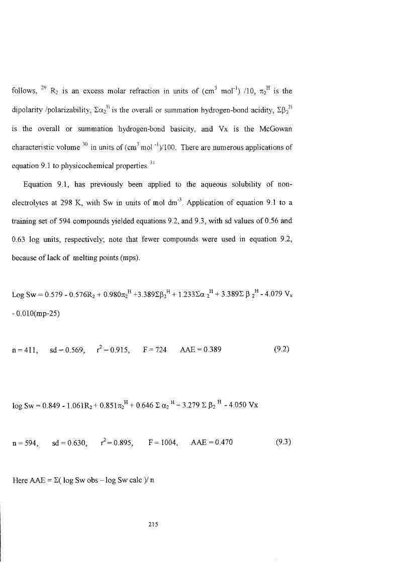
follows, " R] is an excess molar refraction in units of (cm mol’ ) /lO, :i2^ is tlie
dipolarity /polarizability, is the overall or summation hydrogen-bond acidity,
is the overall or summation hydrogen-bond basicity, and Vx is the McGowan
characteristic volume in units of (cm mol ' ’)/100. There aie numerous applications of
equation 9.1 to physicochemical properties.
Equation 9.1, has previously been applied to the aqueous solubility of non
electrolytes at 298 K, with Sw in units of mol dm'\ Application of equation 9.1 to a
training set of 594 compounds yielded equations 9.2, and 9.3, with sd values of 0.56 and
0.63 log units, respectively; note that fewer compounds were used in equation 9.2,
because of lack of melting points (mps).
Log Sw = 0.579 - O.5 7 6 R2 + 0.980%" +3.389%" + 1.2331a 2" + 3.389E |3 2" - 4.079 Vx
- 0.010(mp-25)
n = 411, sd = 0.569, r = 0.915, F = 724 AAE = 0.389 (9.2)
log Sw = 0.849 - I.O6 IR2 + 0.851 + 0.646 + 3.279 £ P2 “ - 4.050 Vx
n= 594, sd = 0.630, r^=0.895, F= 1004, AAE = 0.470 (9.3)
Here AAE = Z( log Sw obs - log Sw calc )/ n
215
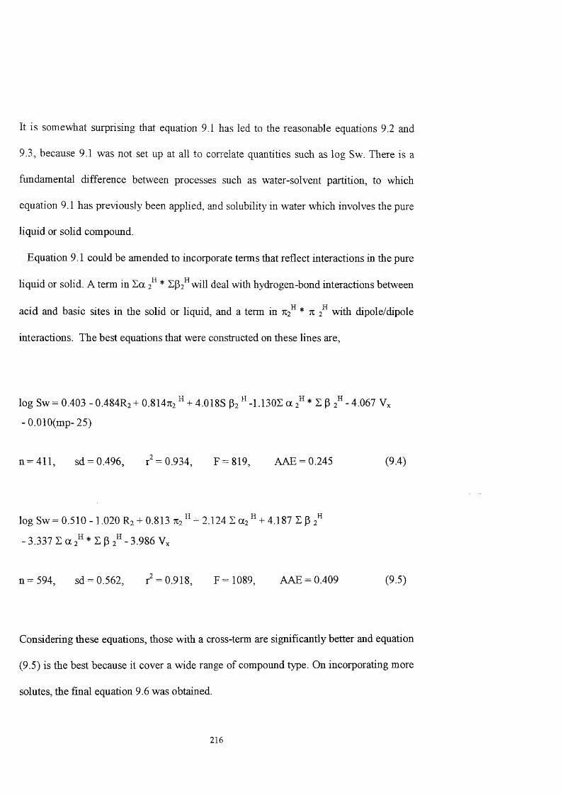
It is somewhat surprising that equation 9.1 has led to the reasonable equations 9.2 and
9.3, because 9.1 was not set up at all to correlate quantities such as log Sw. There is a
fundamental difference between processes such as water-solvent partition, to which
equation 9.1 has previously been applied, and solubility in water which involves the pure
liquid or solid compound.
Equation 9.1 could be amended to incorporate terms that reflect interactions in the pure
liquid or solid. A term in Sa * Sj^i^will deal with hydrogen-bond interactions between
acid and basic sites in the solid or liquid, and a term in 712^ * % 2^ with dipole/dipole
interactions. The best equations that were constructed on tliese lines are.
log Sw= 0.403 -0.484R2+0.814tc2^ + 4.018S P2 "-1.130Sa 2^* ZP 2^-4.067 V,
- 0.010(mp-25)
n = 411, sd = 0.496, r = 0.934, F = 819, AAE = 0.245 (9.4)
log Sw = 0.510 - 1.020 R2 + 0.813 % ^ + 2.124 S a 2 ^ + 4.187 Sp 2 ^
- 3.337 S a 2 * S P 2 - 3.986 Vx
n = 594, sd = 0.562, r = 0.918, F = 1089, AAE = 0.409 (9.5)
Considering these equations, those with a cross-term are significantly better and equation
(9.5) is the best because it cover a wide range of compound type. On incorporating more
solutes, the final equation 9.6 was obtained.
216
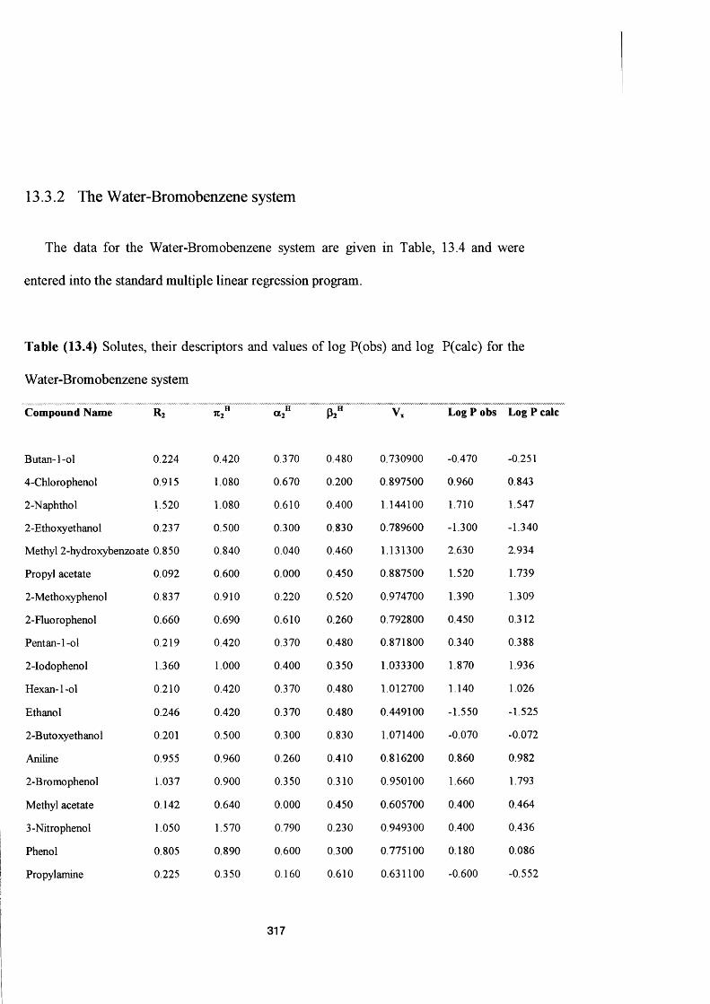
13.3.2 The Water-Bromobenzene system
The data for the Water-Bromobenzene system are given in Table, 13.4 and were
entered into the standard multiple linear regression program.
Table (13.4) Solutes, their descriptors and values of log P(obs) and log P(calc) for the
Water-Bromobenzene system
Compound Name «2® V, Log P obs Log P
Butan-]-ol 0.224 0.420 0.370 0.480 0.730900 -0.470 -0.251
4-Chlorophenol 0.915 1.080 0.670 0.200 0.897500 0.960 0.843
2-Naphthol 1.520 1.080 0.610 0.400 1.144100 1.710 1.547
2-Ethoxy ethanol 0.237 0.500 0.300 0.830 0.789600 -1.300 -1.340
Methyl 2-hydroxybenzoate 0.850 0.840 0.040 0.460 1.131300 2.630 2.934
Propyl acetate 0.092 0.600 0.000 0.450 0.887500 1.520 1.739
2-Methoxyphenol 0.837 0.910 0.220 0.520 0.974700 1.390 1.309
2-Fluorophenol 0.660 0.690 0.610 0.260 0.792800 0.450 0.312
Pentan-l-ol 0.219 0.420 0.370 0.480 0.871800 0.340 0.388
2-Iodophenol 1.360 1.000 0.400 0.350 1.033300 1.870 1.936
Hexan-l-ol 0.210 0.420 0.370 0.480 1.012700 1.140 1.026
Ethanol 0.246 0.420 0.370 0.480 0.449100 -1.550 -1.525
2-Butoxyethanol 0.201 0.500 0.300 0.830 1.071400 -0.070 -0.072
Aniline 0.955 0.960 0.260 0.410 0.816200 0.860 0.982
2-Bromophenol 1.037 0.900 0.350 0.310 0.950100 1.660 1.793
Methyl acetate 0.142 0.640 0.000 0.450 0.605700 0.400 0.464
3-Nitro phenol 1.050 1.570 0.790 0.230 0.949300 0.400 0.436
Phenol 0.805 0.890 0.600 0.300 0.775100 0.180 0.086
Propylamine 0.225 0.350 0.160 0.610 0.631100 -0.600 -0.552
317
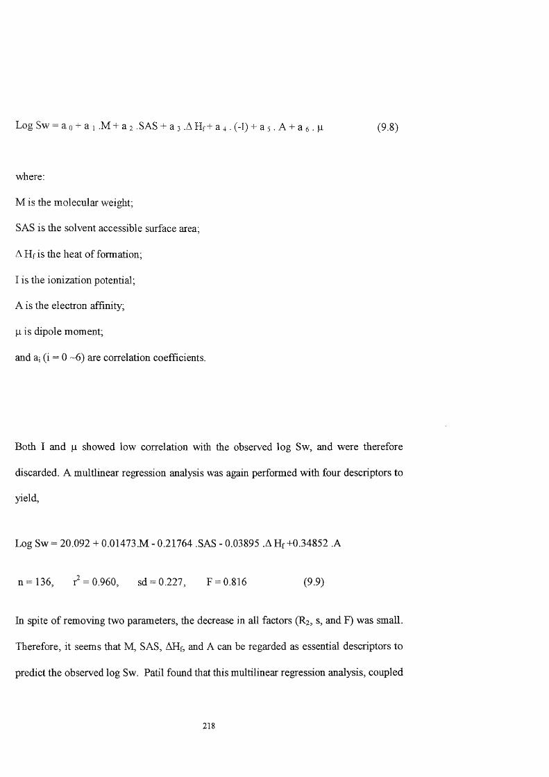
Log Sw - a 0 + a 1 .M + a 2 .SAS + a 3 .A Hf + a 4 . (-1) + a 5 . A + a 6 . M- (9.8)
where;
M is the molecular w eight;
SAS is tlie solvent accessible surface area;
A H f is the heat of formation;
I is the ionization potential;
A is the electron affinity;
p. is dipole moment;
and ai (i = 0 ~6) are correlation coefficients.
Both I and p showed low correlation with the observed log Sw, and were therefore
discarded. A multlinear regression analysis was again performed with four descriptors to
yield.
Log Sw= 20.092 + 0.01473.M - 0.21764 .SAS - 0.03895 .AHf+0.34852 .A
n = 136, r = 0.960, sd = 0.227, F = 0.816 (9.9)
In spite of removing two parameters, the decrease in all factors (R2 , s, and F) was small.
Therefore, it seems that M, SAS, AHf, and A can be regarded as essential descriptors to
predict the observed log Sw. Patil found that this multilinear regression analysis, coupled
218

with the descriptors of M, SAS, AHf and A, was an excellent way to predict the log Sw of
136 PCBs congeners. However, it should be noted that equation 9.9 is not a prediction at
all, but is a correlation of already known log Sw values.
A comparison of the calculated values in this work using equation 9.7, with the
experimental data obtained from the literature by Patil , and the correlated values based
on equation 9.9 was therefore made. The sd between our values and the experimental
values is 0.173 and between our values and the conelated ones is 0.171, which are more
or less the same, as shown in Table 9.1.
219

Table 9.1. Comparison of our calc. Log S (a), predicted log S (b ), with exp. log S (c) and the values of the sd.
Nam e lU P A C R2 Vx CalcJog S(a) C alc.log S(b) O bs.log S(c) Sd (a-c) Scl(h7ç)
3 -Monochlorobiphenyl 2 1.51 1.00 0.21 1.447 -5.10625 -5.0762 -5.39 0.080515 0.0984704-Monochloro 3 1.50 1.00 0.20 1.447 -5.13859 -5.0361 -5.33 0.036638 0.0863772,2'-Dichloro 4 1.60 1.24 0.19 1.569 -5.58274 -5.5390 -5.72 0.018839 0.0327612,3-Dichloro 5 1.63 1.25 0.22 1.569 -5.47801 -5.5645 -5.35 0.016387 0.0460102,3'-Dichloro 6 1.63 1.25 0.22 1.569 -5.47801 -5.6937 -5.26 0.047530 0.1880962,4-Dichloro 7 1.62 1.15 0.18 1.569 -5.71459 -5.7971 -5.56 0.023899 0.0562162,4'-Dichloro 8 1.62 1.18 0.19 1.569 -5.64908 -5.6393 -5.46 0.035752 0.0321483,3'-Diehl oro 11 1.66 1.13 0.17 1.569 -5.81255 -5.7762 -6.45 0.406339 0.4540063,4-Dichloro 12 1.65 1.00 0.17 1.569 -5.90274 -5.6095 -6.39 0.237419 0.6091803,4'-Dichloro 13 1.65 1.00 0.17 1.569 -5.90274 -5.7354 -6.40 0.247265 0.4416934,4'-DichIoro 15 1.64 1.00 0.14 1.569 -6.01984 -5.7021 -6.37 0.122610 0.4460902,2',3-Trichloro 16 1.75 1.31 0.17 1.691 -6.25055 -6.1252 -6.10 0.022664 0.0006352,2',4-Trichloro 17 1.74 1.28 0.15 1.691 -6.34840 -6.3661 -6.49 0.020051 0.0153512,2',5-Trichloro 18 1.75 1.31 0.16 1.691 -6.29293 -6.3321 -6.35 0.003257 0.0003202,2',6-Trichloro 19 1.72 1.37 0.17 1.691 -6.17417 -5.9300 -5.90 0.075168 0.0009002,3,4-Trichloro 21 1.77 1.32 0.17 1.691 -6.26292 -6.2698 -6.18 0.006875 0.0080642,3,4'-Tirchloro 22 1.77 1.33 0.17 1.691 -6.25521 -6.1968 -5.80 0.207213 0.1574502,3,6-Tirchloro 24 1.75 1.30 0.14 1.691 -6.38540 -6.4478 -6.49 0.010942 0.0017812,3',4-Tirchloro 25 1.77 1.33 0.16 1.691 -6.29759 -6.4900 -6.11 0.035189 0.1444002,3',5-Tirchloro 26 1.78 1.33 0.16 1.691 -6.30763 -6.4648 -6.14 0.028099 0.1054952,4,4'-Tirchloro 28 1.76 1.32 0.15 1.691 -6.33764 -6.4256 -6.22 0.013838 0.0422712,4',5-Tirchloro 31 1.77 1.32 0.16 1.691 -6.30530 -6.4316 -6.18 0.015699 0.0633032,4',6-Tirchloro 32 1.74 1.32 0.16 1.691 -6.27518 -6.2607 -6.21 0.004248 0.002570
220
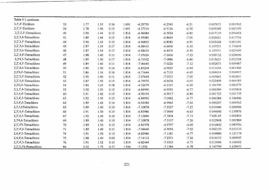
Table 9.1 continues 2,3',4'-Tirchloro 33 1.77 1.33 0.16 1.691 -6.29759 -6.2543 -6.21 0.007671 0.0019622,3',5'-Tirchloro 34 1.78 1.30 0.15 1.691 -6.37314 -6.5126 -6.30 0.005349 0.0451992,2',3,3'-Tetrachloro 40 1.90 1.44 0.13 1.814 -6.96084 -6.5924 -6.83 0.0171 19 0.056454
2,2',3,4-Tetrachloro 41 1.89 1.44 0.13 1.814 -6.95080 -6.8669 -7.00 0.002421 0.0177162,2',3,5'-Tetracliloro 44 1.90 1.43 0.13 1.814 -6.96855 -6.8383 -6.91 0.003428 0.0051412,2',3,6-Tetrachloro 45 1.87 1.54 0.17 1.814 -6.68410 -6.6696 -6.30 0.147531 0.1366042,2',3,6-Tetrachloro 46 1.87 1.54 0.17 1.814 -6.68410 -6.4470 -6.30 0.147531 0.0216092,2',4,4'-Tetrachloro 47 1.88 1.40 0.11 1.814 -7.05636 -7.0606 -7.23 0.030152 0.0286962,2'4,5-T etrachloro 48 1.89 1.50 0.17 1.814 -6.73502 -7.0886 -6.86 0.015621 0.052258
2,2',4,5'-Tetrachloro 49 1.89 1.40 0.11 1.814 -7.06640 -7.0226 -7.12 0.002873 0.0094872,2',4,6-Tetrachloro 50 1.86 1.50 0.14 1.814 -6.83204 -6.9025 -6.94 0.011656 0.0014062,2'4,6'-Tetrachloro 51 1.86 1.54 0.16 1.814 -6.71644 -6.7133 -6.65 0.004414 0.0040072,2', 5,5'-Tetrachloro 52 1.90 1.40 0.11 1.814 -7.07644 -7.0533 -7.00 0.005843 0.0028412,2', 5,6'-T etrachloro 53 1.87 1.50 0.15 1.814 -6.79970 -6.6636 -6.65 0.022409 0.0001852,2'6,6'-Tetrachloro 54 1.84 1.65 0.18 1.814 -6.52679 -6.2167 -6.20 0.106790 0.0002792,3,3',4-Tetrachloro 55 1.92 1.50 0.15 1.814 -6.84990 -6.9593 -6.77 0.006384 0.0358342,3,4,4'-Tetrachloro 60 1.91 1.42 0.15 1.814 -6.90154 -6.9017 -6.86 0.001725 0.0017392,3,4', 5-Tetrachloro 63 1.92 1.50 0.15 1.814 -6.84990 -7.0962 -6.77 0.006384 0.1064062,3,4',6-Tetachloro 64 1.89 1.42 0.14 1.814 -6.92384 -6.9963 -7.02 0.009247 0.0005622,3,5,6Tetrachloro 65 1.89 1.40 0.10 1.814 -7.10878 -7.2527 -7.25 0.019944 0.0000062,3',4,4'-Tetrachloro 66 1.91 1.50 0.15 1.814 -6.83986 -7.0040 -6.63 0.044040 0.1398762,3',4,5-Tetrachloto 67 1.92 1.40 0.10 1.814 -7.13890 -7.1838 -7.13 7.92E-05 0.0028942,3'4,6-Tetrachloro 69 1.89 1.40 0.10 1.814 -7.10878 -7.3137 -7.26 0.022868 0.0028842,3',4'5-Tetrachloro 70 1.89 1.50 0.15 1.814 -6.81978 -6.9797 -6.69 0.016842 0.0839262,3',4',6-T etrachloro 71 1.89 1.40 0.11 1.814 -7.06640 -6.9054 -7.02 0.002153 0.0131332,4,4', 5-Tetrachloro 74 1.91 1.50 0.15 1.814 -6.83986 -7.1181 -6.77 0.004880 0.1211742,4,4',6-Tetrachloro 75 1.88 1.40 0.09 1.814 -7.14112 -7.2531 -7.26 0.014133 0.0000452,3',4',5-Tetrachloro 76 1.91 1.52 0.15 1.814 -6.82444 -7.0365 -6.71 0.013096 0.1066022,2',3,3 '6-Pentachloro 84 2.02 1.75 0.17 1.936 -7.1592 -7.1384 -6.78 0.143794 0.128451
221
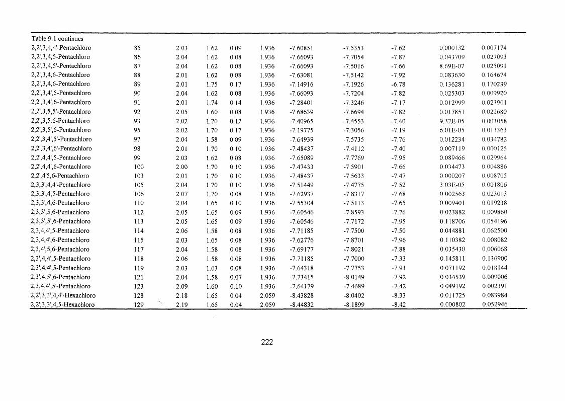
Table 9.1 continues 2,2',3,4,4'-Pentachloro 85 2.03 1.62 0.09 1.936 -7.60851 -7.5353 -7.62 0.000132 0.0071742,2',3,4,5-Pentachloro 86 2.04 1.62 0.08 1.936 -7.66093 -7.7054 -7.87 0.043709 0.0270932,2',3,4,5'-Pentachloro 87 2.04 1.62 0.08 1.936 -7.66093 -7.5016 -7.66 8.69E-07 0.0250912,2',3,4,6-Pentachloro 88 2.01 1.62 0.08 1.936 -7.63081 -7.5142 -7.92 0.083630 0.1646742,2',3,4,6-Pentachloro 89 2.01 1.75 0.17 1.936 -7,14916 -7.1926 -6.78 0,136281 0.1702392,2',3,4',5-Pentachloro 90 2.04 1.62 0.08 1.936 -7.66093 -7.7204 -7,82 0.025303 0.0099202,2',3,4',6-Pentachloro 91 2.01 1.74 0.14 1.936 -7.28401 -7.3246 -7,17 0.012999 0.0239012,2',3,5,5'-Pentachloro 92 2.05 1.60 0.08 1.936 -7.68639 -7.6694 -7,82 0.017851 0.0226802,2',3,5.6-Pentachloro 93 2.02 1.70 0.12 1.936 -7.40965 -7.4553 -7,40 9.32E-05 0.0030582,2',3,5',6-Pentachloro 95 2.02 1.70 0.17 1.936 -7.19775 -7.3056 -7,19 6.01E-05 0.0133632,2', 3,4', 5 '-Pentachloro 97 2.04 1.58 0.09 1.936 -7.64939 -7.5735 -7,76 0.012234 0.0347822,2',3,4',6'-Pentachloro 98 2.01 1.70 0.10 1.936 -7.48437 -7.4112 -7,40 0,0071 19 0.0001252,2',4,4',5-Pentachloro 99 2.03 1.62 0.08 1.936 -7.65089 -7.7769 -7.95 0.089466 0.0299642,2',4,4',6-Pentachloro 100 2.00 1.70 0.10 1.936 -7.47433 -7.5901 -7.66 0,034473 0.0048862,2',4'5,6-Pentachloro 103 2.01 1.70 0.10 1.936 -7.48437 -7.5633 -7.47 0.000207 0.0087052,3,3 ',4,4 '-Pentachloro 105 2.04 1.70 0.10 1.936 -7.51449 -7.4775 -7.52 3.03E-05 0.0018062,3,3',4,5-Pentachloro 106 2.07 1.70 0.08 1.936 -7.62937 -7,8317 -7.68 0.002563 0.0230132,3,3',4,6-Pentachloro 110 2.04 1.65 0.10 1.936 -7.55304 -7.5113 -7.65 0.009401 0.0192382,3,3',5,6-Pentachloro 112 2.05 1.65 0.09 1.936 -7,60546 -7.8593 -7.76 0.023882 0.0098602,3,3', 5',6-Pentachloro 113 2.05 1.65 0.09 1.936 -7.60546 -7.7172 -7.95 0.1 18706 0.0541962,3,4,4',5-Pentachloro 114 2.06 1.58 0.08 1.936 -7.71185 -7.7500 -7,50 0.044881 0.0625002,3,4,4', 6-Pentachloro 115 2.03 1.65 0.08 1.936 -7.62776 -7.8701 -7,96 0.110382 0.0080822,3,4', 5,6-Pentachloro 117 2.04 1.58 0.08 1.936 -7.69177 -7.8021 -7.88 0.035430 0.0060682,3',4,4',5-Pentachloro 118 2.06 1.58 0.08 1.936 -7.71185 -7.7000 -7.33 0.145811 0.1369002,3',4,4',5-Pentachloro 119 2.03 1.63 0.08 1.936 -7.64318 -7,7753 -7.91 0,071192 0.0181442,3',4,5',6-Pentachloro 121 2.04 1.58 0.07 1.936 -7.73415 -8.0149 -7.92 0.034539 0.0090062,3,4,4', 5'-Pentachloro 123 2.09 1.60 0.10 1.936 -7.64179 -7.4689 -7.42 0.049192 0.0023912,2', 3,3 ',4,4'-Hexachloro 128 2.18 1.65 0.04 2.059 -8.43828 -8.0402 -8.33 0.011725 0.0839842,2',3,3',4,5-Hexachloro 129 2.19 1.65 0.04 2.059 -8.44832 -8.1899 -8.42 0.000802 0.052946
222

Table 9.1 continues 2,2',3,3',4,6-Hexachloro 131 2,16 1.77 0.13 2.059 -7.94426 -8.0103 -8.48 0.287014 0.2206182,2',3,3',4,6'-Hexachloro 132 2.16 1.77 0.13 2.059 -7.94426 -7.7413 -7.65 0.086591 0.0083362,2',3,3',5,6-Hexachloro 134 2.17 1.78 0.13 2.059 -7.94659 -7.9141 -7.65 0.087967 0.0697492,2',3,3'5,6'-Hexacliloro 135 2.17 1.78 0.13 2.059 -7.94659 -7.9431 -7.82 0.015523 0.0146652,2,3,4,4',5-Hexachloro 137 2.18 1.60 0.04 2.059 -8.47683 -8.4062 -8.52 0.001863 0.0129502,2,3,4,4',5'-Hexachloro 138 2.18 1.65 0.06 2.059 -8.35352 -8.1728 -8.38 0.000701 0.0429322,2,3,4,4',6'-Hexachloro 140 2.18 1.76 0.10 2.059 -8.09919 -8.0438 -8.24 0.019827 0.0384942,2', 3,4,5,5 '-Hexachloro 141 2.19 1.68 0.08 2.059 -8.25567 -8.3499 -8.42 0.027003 0.0049142,2', 3,4,5,6'-Hexachloro 143 2.16 1.75 0.11 2.059 -8.04444 -8.0651 -8.13 0.007320 0.0042122,2,3,4,5',6-Hexachloro 144 2.16 1.78 0.13 2.059 -7.93655 -8.1667 -8.01 0.005394 0.0245552,2',3,4', 5,5'-Hexachloro 146 2.19 1.65 0.04 2.059 -8.44832 -8.3538 -8.58 0.017339 0.0511662,2',3,4',5',6-Hexachloro 149 2.16 1.80 0.12 2.059 -7.96351 -8.0144 -7.94 0.000553 0.0055352,2',3,5,5',6-Hexachloro 151 2.17 1.78 0.13 2.059 -7.94659 -8.1229 -7.93 0.000275 0.0372102,2',4,4',5,5'-Hexachloro 153 2.18 1.60 0.04 2.059 -8.47683 -8.4047 -8.49 0.000173 0.0072762,2',4,4', 5,5'-Hexachloro 154 2.15 1.77 0.12 2.059 -7.9766 -8.2354 -8.12 0.020563 0.0133172,2',4,4',6,6'-Hexachloro 155 2.12 1.65 0.05 2.059 -8.33566 -8.1089 -8.12 0.046511 0.0001232,3,3',4,4',5 -Hexachloro 156 2.21 1.60 0.06 2.059 -8.42219 -8.3394 -8.31 0.012587 0.0008642,3,3',4,4', 6-Hexachloro 158 2.18 1.65 0.05 2.059 -8.3959 -8.4114 -8.48 0.007072 0.0047062,3,3 ', 4'5, ôHexachloro 163 2.19 1.65 0.05 2.059 -8.40594 -8.3483 -8.48 0.005484 0.0173452,3,3',4',5',6-Hexachloro 164 2.19 1.67 0.06 2.059 -8.34814 -8.2239 -8.27 0.006106 0.0021252,3',4,4',5,5'-Hexacliloro 167 2.21 1.65 0.06 2.059 -8.38364 -8.4216 -8.21 0.030152 0.0447753,3',4,4',5,5'-Hexachloro 169 2.21 1.60 0.04 2.059 -8.50695 -8.3802 -8.85 0.117681 0.2207122,2',3,3'4,4',5 -Hexachloro 170 2.33 1.87 0.00 2.181 -9.07520 -8.8439 -8.90 0.030694 0.0031472,2',3,3',4,5,5'-Heptachloro 172 2.34 1.85 0.00 2.181 -9.10066 -8.9644 -9.10 4.32E-07 0.0183872,2',3,3',4,5,6'-Hexachloro 174 2.31 1.90 0.06 2.181 -8.77771 -8.6284 -8.59 0.035234 0.0014752,2',3,3',4,5',6-Hexachloro 175 2.31 1.90 0.06 2.181 -8.77771 -8.7943 -8.68 0.009547 0.0130642,2', 3,3 ', 4,6,6'-Hexachloro 176 2.31 1.95 0.12 2.181 -8.48488 -8.2893 -8.15 0.112143 0.0194042,2',3,3 ',4,5',6'-Hexachloro 177 2.28 1.90 0.12 2.181 -8.49331 -8.5210 -8.42 0.005374 0.0102012,2'3,3',5,5',6-Hexachloro 178 2.31 1.90 0.12 2.181 -8.52343 -8.6962 -8.59 0.004432 0.011278
223

Table 9.1 continues 2,2',3,3',5,6,6'-Hexachloro 179 2 .3 2 1.95 0.12 2.181 -8.49492 -8.2248 -7.94 0.307933 0.0811112,2',3,4,4',5,5'-Hexachloro 180 2 .2 9 1.84 0.00 2.181 -9.05817 -8.9934 -9.10 0.001750 0.0113642,2',3,4,4',5,6-Hexachloro 181 2 .3 0 1.90 0.04 2.181 -8.85243 -8.8593 -8.97 0.013823 0.0122542,2',3,4,4',5,6'-Ilexachloro 182 2 .3 0 1.90 0 .0 6 2.181 -8.76767 -8 .8 6 7 2 -8.68 0.007686 0.0350442,2',3,44',5',6-Heptachloro 183 2 .3 0 1.90 0.04 2.181 -8.85243 -8.8050 -8 .8 5 0.000106 0.0020252,2',3,4,5,5',6-Heptachloro 185 2.31 1.90 0.04 2.181 -8.86247 -8.8208 -8.75 0.012649 0.0050132,2',3,4',5,6,6'-Heptachloro 188 2 .2 8 1.95 0.12 2.181 -8.45476 -8.4765 -8.49 0.001242 0.0001822,3,3',4,4',5,5'-Heptachloro 189 2 .3 6 1.87 0 2.181 -9.10532 -9.1040 -8.72 0.148469 0.1474562,3,3',4,4',5,6-Heptacliloro 190 2 .3 3 1.89 0 2.181 -9.05978 -9.0829 -8.9.0 0 .0 1 2 3 0 6 0.0012382,3,3',4,4',5',6-I[ep1:acliloro 191 2 .3 3 1.85 0 2.181 -9.09062 -9.0920 -9.10 0.000005 6.0000502,3,3',4,5,5',6-Tleptachloro 192 2.34 1.85 0 2.181 -9.10066 -9.3078 -9.10 0.000100 0.0431812,3,3',4',5,5',6-Heplachloro 193 2.34 1.85 0 2.181 -9 .1 0 0 6 6 -9.0200 -9.10 0.000040 0.0064002,2',3,3',4,4',5,5'-Octachloro 194 2 .4 8 1.75 0 2.303 -9.80473 -9.5810 -9.70 0 .0 1 0 9 6 9 0.0141612,2',3,3','1,4',5,6-Octachloro 195 2.45 1.99 0 2 .3 0 3 -9.58957 -9 .3 4 5 9 -9 .2 9 0.089743 0.0031252,2',3,3',4,4',5,6'-Octachloro 196 2.45 1.99 0 2 .3 0 3 -9.58957 -9 .4 2 2 6 -9.42 0.028754 0.0000762,2', 3,3',4,4'6,6'-OGtachloro 197 2.42 2.11 0 2 .3 0 3 -9 .4 6 6 9 3 -9.1058 -9.10 0.134638 0.0000302,2',3,3',4,5,5',6-Octachioro 198 2.46 1.99 0 2 .3 0 3 -9.59961 -9.4485 -9.42 0.032260 0.0008122,2',3,3',4,5,6,6'-Octachloro 199 2 .4 6 2 .2 0 0 2 .3 0 3 -9.43770 -8.9608 -9.10 0.114042 0.0193772,2',3,3',4,5',6,6'-Octachloro 200 2.43 2 .2 0 0 2.303 -9.40758 -8.9550 -9.20 0.04309 0.0600252,2', 3,3',4,5,5',6-Octachloro 201 2.43 1.99 0 2.303 -9.56949 -9.2900 -9 .2 9 0.078115 02,2',3,4,4',5,5',6-Octachloro 203 2.48 2.00 0 2.303 -9.61198 -9.4739 -9.5 0.01254 0.0006812,2'3,4,4',5,6,6'-Octachloro 204 2 .5 2 2.10 0 2 .3 0 3 -9.57504 -9.2492 -9.48 0.009033 0.0532692,3,3',4,4',5,5',6-Octachloro 2 0 5 2 .4 8 1.99 0 2.303 -9.61969 -9.7792 -9.70 0.00645 0.0062732,2',3,3',4,4',5,5',6-Nanochloro 2 0 6 2 .6 0 2.11 0 2.426 -10.1381 -10.0286 -10.18 0.00176 0.022922
2 ,2 ',3 ,3 ',4 ,4 ',5 ,6 ,6 '-Nanochlorobiphenyi 207 2.57 2.13 0 2.426 -10.0925 -9.7531 -10.07 0.000507 0.100426
3.999493 3.899574
224
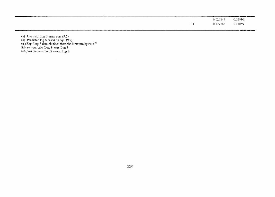
SD:0.0298470.172763
0.0291010.17059
(a) Our calc. Log S using eqn. (9.7)(b) Predicted log S based on eqn. (9.9)(c ) Exp. Log S data obtained from the literature by Patil Sd (a-c) our calc. Log S- exp. Log S Sd (b-c) predicted log S - exp. Log S
225

The next step was to calculate log Sw for the rest of the 209 PCBs, but the sd between
our values and those calculated by Patil, was about the same as that obtained before.
Hence equation 9.7 is a good equation for the prediction of log Sw for the PCBs, possibly
because the term is zero .
The second calculation that was carried out, uses equation 9.4 to calculate log Sw. Since
the term in is zero, equation 9.4 becomes
log Sw = 0.403 - 0.484 Rj + 4.018 ZPz" - 4.067 Vx- 0.010 (mp -25) (9.10)
Where mp is the melting point for PCBs. Values calculated through equation 9.10
were compared with the experimental and correlated values, as shown in Table 9.2. The
sd value between those calculated through equation 9.10 and the experimental ones is
0.159 and between our calculated and PatiTs correlated values is 0.171, which are nearly
the same. Thus equation 9.10 seems a little better than equation 9.7 in that the sd
between calculated and experimental is a little less. However, equation 9.10 requires the
use of an experimental mp for the PCBs.
226
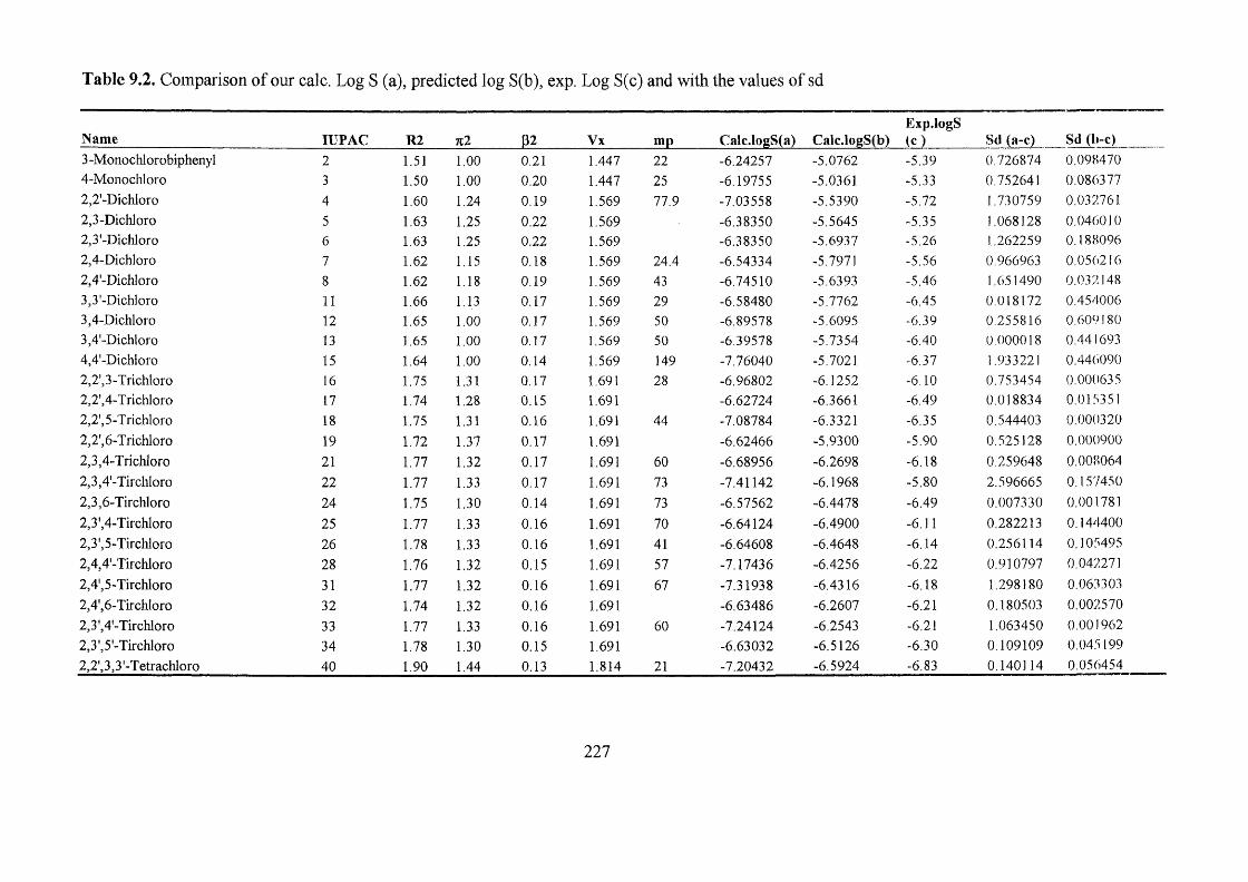
Table 9.2. Comparison of our calc. Log S (a), predicted log S(b), exp. Log S(c) and with the values of sd
Exp.logSName lUPAC R2 n2 32 Vx mp Calc.logS(a) Calc.logS(b) (c) Sd (a-c) Sd (b-c)3 -Monochlorobiphenyl 2 1.51 1.00 0.21 1.447 22 -6.24257 -5.0762 -5.39 0.726874 0.0984704-Monochloro 3 1.50 1.00 0.20 1.447 25 -6.19755 -5.0361 -5.33 0.752641 0.0863772,2'-Dichloro 4 1.60 1.24 0.19 1.569 77.9 -7.03558 -5.5390 -5.72 1.730759 0.0327612,3-Dichloro 5 1.63 1.25 0.22 1.569 -6.38350 -5.5645 -5.35 1.068128 0.0460102,3'-Dichloro 6 1.63 1.25 0.22 1.569 -6.38350 -5.6937 -5.26 1.262259 0.1880962,4-Dichloro 7 1.62 1.15 0.18 1.569 24.4 -6.54334 -5.7971 -5.56 0.966963 0.0562162,4'-Dichloro 8 1.62 1.18 0.19 1.569 43 -6.74510 -5.6393 -5.46 1.651490 0.0321483,3'-Dichloro 11 1.66 1.13 0.17 1.569 29 -6.58480 -5.7762 -6.45 0.018172 0.4540063,4-Dichloro 12 1.65 1.00 0.17 1.569 50 -6.89578 -5.6095 -6.39 0.255816 0.6091803,4'-Dichloro 13 1.65 1.00 0.17 1.569 50 -6.39578 -5.7354 -6.40 0.000018 0.4416934,4'-Dichloro 15 1.64 1.00 0.14 1.569 149 -7.76040 -5.7021 -6.37 1.933221 0.4460902,2',3-Trichloro 16 1.75 1.31 0.17 1.691 28 -6.96802 -6.1252 -6.10 0.753454 0.0006352,2',4-Trichloro 17 1.74 1.28 0.15 1.691 -6.62724 -6.3661 -6.49 0.018834 0.0153512,2',5-Trichloro 18 1.75 1.31 0.16 1.691 44 -7.08784 -6.3321 -6.35 0.544403 0.0003202,2',6-Trichloro 19 1.72 1.37 0.17 1.691 -6.62466 -5.9300 -5.90 0.525128 0.0009002,3,4-Trichloro 21 1.77 1.32 0.17 1.691 60 -6.68956 -6.2698 -6.18 0.259648 0.0080642,3,4'-Tirchloro 22 1.77 1.33 0.17 1.691 73 -7.41142 -6.1968 -5.80 2.596665 0.1574502,3,6-Tirchloro 24 1.75 1.30 0.14 1.691 73 -6.57562 -6.4478 -6.49 0.007330 0.0017812,3',4-Tirchloro 25 1.77 1.33 0.16 1.691 70 -6.64124 -6.4900 -6.11 0.282213 0.1444002,3',5-Tirchloro 26 1.78 1.33 0.16 1.691 41 -6.64608 -6.4648 -6.14 0.256114 0.1054952,4,4'-Tirchloro 28 1.76 1.32 0.15 1.691 57 -7.17436 -6.4256 -6.22 0.910797 0.0422712,4',5-Tirchloro 31 1.77 1.32 0.16 1.691 67 -7.31938 -6.4316 -6.18 1.298180 0.0633032,4',6-Tirchloro 32 1.74 1.32 0.16 1.691 -6.63486 -6.2607 -6.21 0.180503 0.0025702,3',4'-Tirchloro 33 1.77 1.33 0.16 1.691 60 -7.24124 -6.2543 -6.21 1.063450 0.0019622,3',5'-Tirchloro 34 1.78 1.30 0.15 1.691 -6.63032 -6.5126 -6.30 0.109109 0.045 1992,2',3,3'-Tetrachloro 40 1.90 1.44 0.13 1.814 21 -7.20432 -6.5924 -6.83 0.140114 0.056454
227
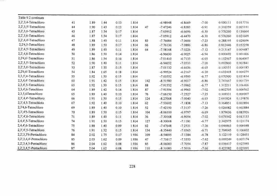
Table 9.2 continues 2,2',3,4-Tetrachloro 41 1,89 1,44 0,13 1,814 -6,98948 -6,8669 -7,00 0.00011J 0,0177162,2',3,5'-Tetrachloro 44 1,90 1,43 0,13 1,814 47 -7,47246 -6.8383 -6,91 0,316359 0,0051412,2',3,6-Tetrachloro 45 1,87 1,54 0,17 1,814 -7,05912 -6,6696 -6,30 0,576260 0,1366042,2',3,6-Tetrachloro 46 1,87 1,54 0,17 1,814 -7,05912 -6,4470 -6,30 0,576260 0.0216092,2',4,4'-T etrachloro 47 1.88 1,40 0,11 1,814 83 -7,76684 -7.0606 -7,23 0,288195 0,0286962,2'4,5-Tetrachloro 48 1,89 1,50 0,17 1,814 66 -7,76136 -7,0886 -6,86 0,812446 0,052258
2,2',4,5'-Tetrachloro 49 1,89 1,40 0,11 1,814 64 -7,58168 -7.0226 -7,12 0,213147 0,0094872,2',4,6-Tetrachloro 50 1,86 1,50 0,14 1,814 -6,96630 -6,9025 -6,94 0,000692 0,0014062,2'4,6'-Tetrachioro 51 1,86 1,54 0,16 1,814 -7,01410 -6,7133 -6,65 0,132567 0,0040072,2',5,5'-Tetrachioro 52 1,90 1,40 0,11 1,814 -6,94652 -7,0533 -7.00 0,002860 0,0028412,2',5,6'-Tetrachloro 53 1,87 1,50 0,15 1,814 -7,01132 -6,6636 -6,65 0,130551 0,0001852,2'6,6'-Tetrachloro 54 1,84 1,65 0,18 1,814 -6,99524 -6,2167 -6,20 0,632403 0,0002792,3,3',4-Tetrachloro 55 1,92 1,50 0,15 1,814 -7,03552 -6,9593 -6.77 0,070500 0,0358342,3,4,4'-Tetrachloro 60 1,91 1,42 0,15 1,814 142 -8,51580 -6,9017 -6,86 2,741667 0,0017392,3,4', 5 -T etrachloro 63 1,92 1,50 0,15 1,814 88 -7,91552 -7,0962 -6,77 1,312211 0,1064062,3,4',6-Tetacliloro 64 1,89 1,42 0,14 1,814 87 -7,91594 -6,9963 -7,02 0.802705 0,0005622,3,5,6Tetrachloro 65 1,89 1,40 0,10 1,814 76 -7,66150 -7,2527 -7,25 0,169331 0,0000072,3',4,4'-Tetrachloro 66 1,91 1,50 0,15 1,814 124 -8,27068 -7,0040 -6.63 2,691824 0,1398762,3',4,5-Tetrachloto 67 1,92 1,40 0,10 1,814 62 -7,53602 -7,1838 -7,13 0,164851 0,0028942,3 '4,6-T etrachloro 69 1,89 1,40 0,10 1,814 52 -7,42150 -7,3137 -7,26 0.026082 0,0028842,3',4'5-Tetrachloro 70 1,89 1,50 0,15 1,814 104 -8,06100 -6,9797 -6,69 1.879636 0,0839262,3',4',6-Tetrachloro 71 1,89 1,40 0,11 1,814 36 -7,30168 -6,9054 -7,02 0,079342 0,0131332,4,4', 5-Tetrachloro 74 1,91 1,50 0,15 1,814 127 -8.30068 -7,1181 -6.77 2,342975 0,121 1742,4,4',6-Tetrachloro 75 1,88 1,40 0,09 1,814 62 -7,47648 -7,2531 -7.26 0,046863 0,0000482,3',4',5-T etrachloro 76 1,91 1,52 0,15 1,814 134 -8,35440 -7,0365 -6.71 2,704045 0,1066022,2', 3,3 '6-Pentachloro 84 2,02 1,75 0,17 1,936 109 -8.54695 -7,1384 -6,78 3.122119 0,1284512,2',3,4,4'-Pentachloro 85 2,03 1,62 0,09 1,936 47 -7,71617 -7.5353 -7,62 0.009249 0,0071742,2',3,4,5-Pentachloro 86 2,04 1,62 0,08 1,936 85 -8,06083 -7,7054 -7,87 0.036417 0.0270932,2',3,4,5'-Pentachloro 87 2,04 1,62 0,08 1,936 110 -8,31083 -7,5016 -7,66 0.423582 0,025091
228

Table 9.2 continues
2,2',3,4,6-Pentachloro 88 2.01 1.62 0.08 1.936 66 -7.85631 -7.5142 -7.92 0.004056 0.1646742,2',3,4,6-Pentachloro 89 2.01 1.75 0.17 1.936 85 -8.30211 -7.1926 -6.78 2.316825 0.1702392,2',3,4',5-Pentachloro 90 2.04 1.62 0.08 1.936 51 -7.72083 -7.7204 -7.82 0.009834 0.0099202,2',3,4',6-Pentachloro 91 2.01 1.74 0.14 1.936 62 -7.95971 -7.3246 -7.17 0.623645 0.0239012,2', 3,5,5'-Pentachloro 92 2.05 1.60 0.08 1.936 60 -7.83195 -7.6694 -7.82 0.000143 0.0226802,2',3,5.6-Pentachloro 93 2,02 1.70 0.12 1.936 96 -8.25675 -7.4553 -7.40 0.734024 0.0030582,2',3,5',6-Pentachioro 95 2.02 1.70 0.17 1.936 93 -8.42765 -7.3056 -7.19 1.531782 0.0133632,2', 3,4', 5'-Pentachloro 97 2.04 1.58 0.09 1.936 78 -8.06357 -7.5735 -7.76 0.092156 0.0347822,2', 3,4', 6'-Pentachloro 98 2.01 1.70 0,10 1.936 94 -8.15155 -7.4112 -7.40 0.564830 0.0001252,2',4,4',5-PentachIoro 99 2.03 1.62 0.08 1.936 59 -7.79599 -7.7769 -7.95 0.023718 0.0299642,2',4,4',6-Pentachloro 100 2.00 1.70 0.10 1.936 -7.20671 -7.5901 -7.66 0.205470 0.0048862,2',4'5,6-Pentachloro 103 2.01 1.70 0.10 1.936 69 -7.90155 -7.5633 -7.47 0.186237 0.0087052,3,3',4,4'-Pentachloro 105 2.04 1.70 0,10 1.936 116 -8.38607 -7.4775 -7.52 0.750081 0.0018062,3,3',4,5-Pentachloro 106 2.07 1.70 0.08 1.936 85 -8.01023 -7.8317 -7.68 0.109053 0.02.10132,3,3',4,6-Pentachloro 110 2.04 1.65 0.10 1.936 53 -7.79677 -7.5113 -7.65 0.021542 0.0192382,3,3',5,6-Pentachloro 112 2.05 1.65 0.09 1.936 91 -8.14143 -7.8593 -7.76 0.145490 0.0098602,3,3',5',6-PentachIoro 113 2.05 1.65 0.09 1.936 56 -7.79143 -7.7172 -7.95 0.025144 0.0541962,3,4,4',5-Pentachloro 114 2.06 1.58 0.08 1.936 98 -8.23307 -7.7500 -7.50 0.537395 0.0625002,3,4,4',6-Pentachloro 115 2.03 1.65 0.08 1.936 65 -7.83157 -7.8701 -7.96 0.016494 0.0080822,3,4',5,6-Pentachloro 117 2.04 1.58 0.08 1.936 167 -8.91339 -7.8021 -7.88 1.067899 0.0060682,3',4,4',5-Pentachloro 118 2.06 1.58 0.08 1.936 111 -8.36307 -7.7000 -7.33 1.067238 0.1369002,3',4,4',5-PentachIoro 119 2.03 1.63 0.08 1.936 75 -7.94785 -7.7753 -7.91 0.001433 0.0181442,3',4,5',6-Pentachloro 121 2.04 1.58 0.07 1.936 93 -8.13321 -8.0149 -7.92 0.045459 0.0090062,3,4,4',5'-Pentachloro 123 2.09 1.60 0.10 1.936 134 -8.67167 -7.4689 -7.42 1.566683 0.0023912,2',3,3',4,4'-Hexachloro 128 2.18 1.65 0.04 2.059 150 -9.09369 -8.0402 -8.33 0.583227 0.0839842,2',3,3',4,5-Hexachloro 129 2.19 1.65 0.04 2.059 102 -8.61853 -8.1899 -8.42 0.039415 0.0529462,2',3,3',4,6-Hexachloro 131 2.16 1.77 0.13 2.059 135 -9.19795 -8.0103 -8.48 0.515457 0.2206182,2', 3,3 ', 4,6'-Hexachloro 132 2.16 1.77 0.13 2.059 116 -9.00795 -7.7413 -7.65 1.844036 0.008336
229
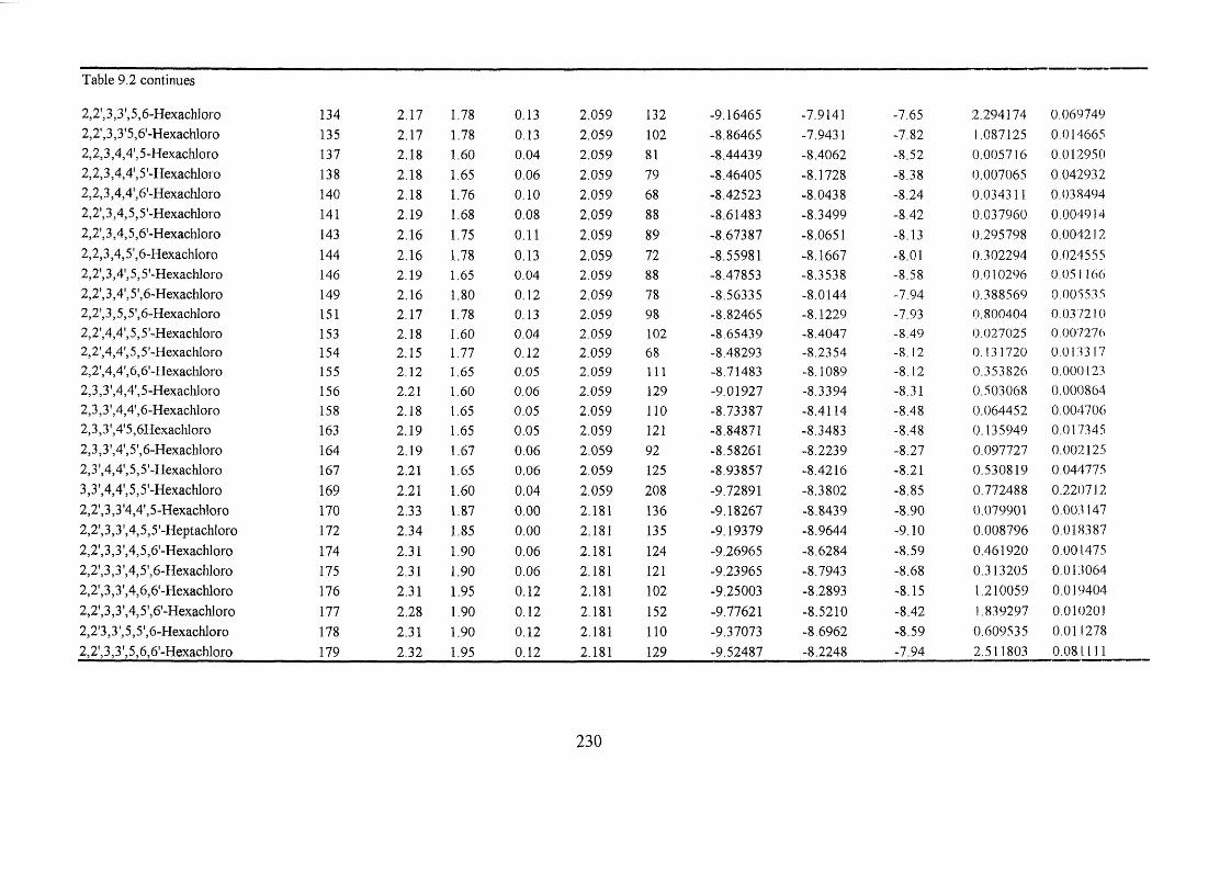
Table 9.2 continues
2,2', 3,3 5,6-Hexachloro 134 2.17 1.78 0.13 2.059 132 -9.16465 -7.9141 -7.65 2.294174 0.0697492,2', 3,3 ' 5,6’ -Hexachlor 0 135 2.17 1.78 0.13 2.059 102 -8.86465 -7.9431 -7.82 1.087125 0.0146652,2,3,4,4',5-Hexachloro 137 2.18 1.60 0.04 2.059 81 -8.44439 -8.4062 -8.52 0.005716 0.0129502,2,3,4,4',5'-Hexachloro 138 2.18 1.65 0.06 2.059 79 -8.46405 -8.1728 -8.38 0,007065 0.0429322,2,3,4,4',6'-Hexachloro 140 2.18 1.76 0.10 2.059 68 -8.42523 -8.0438 -8.24 0.034311 0.0384942,2',3,4,5,5'-Hexachloro 141 2.19 1.68 0.08 2.059 88 -8.61483 -8.3499 -8.42 0.037960 0.0049142,2',3,4,5,6'-Hexachloro 143 2.16 1.75 0.11 2.059 89 -8.67387 -8.0651 -8.13 0.295798 0.0042122,2,3,4,5',6-Hexachloro 144 2.16 1.78 0.13 2.059 72 -8.55981 -8.1667 -8.01 0.302294 0.0245552,2', 3,4', 5,5 '-Hexachloro 146 2.19 1.65 0.04 2.059 88 -8.47853 -8.3538 -8.58 0.010296 0.0511662,2', 3,4', 5 6-Hexachloro 149 2.16 1.80 0.12 2.059 78 -8.56335 -8.0144 -7.94 0.388569 0.0055352,2',3,5,5',6-Hexachloro 151 2.17 1.78 0.13 2.059 98 -8.82465 -8.1229 -7.93 0.800404 0.0372102,2',4,4', 5,5'-Hexachloro 153 2.18 1.60 0.04 2.059 102 -8.65439 -8.4047 -8.49 0.027025 0.0072762,2',4,4',5,5'-Hexachloro 154 2.15 1.77 0.12 2.059 68 -8.48293 -8.2354 -8.12 0.131720 0.0133 172,2',4,4',6,6'-Hexachloro 155 2.12 1.65 0.05 2.059 111 -8.71483 -8.1089 -8.1.2 0.353826 0.0001232,3,3',4,4',5-Hexachloro 156 2.21 1.60 0.06 2.059 129 -9.01927 -8.3394 -8.31 0.503068 0.0008642,3,3',4,4',6-Hexachloro 158 2.18 1.65 0.05 2.059 110 -8.73387 -8.4114 -8.48 0.064452 0.0047062,3,3',4'5,6Hexachloro 163 2.19 1,65 0.05 2.059 121 -8.84871 -8.3483 -8.48 0.135949 0.0173452,3,3',4',5', 6-Hexachloro 164 2.19 1.67 0.06 2.059 92 -8.58261 -8.2239 -8.27 0.097727 0.0021252,3',4,4',5,5'-Hexachloro 167 2.21 1.65 0.06 2.059 125 -8.93857 -8.4216 -8.21 0.530819 0.0447753,3',4,4', 5,5 '-Hexachloro 169 2.21 1.60 0.04 2.059 208 -9.72891 -8.3802 -8.85 0.772488 0.2207122,2',3,3 '4,4', 5-Hexachloro 170 2.33 1.87 0.00 2.181 136 -9.18267 -8.8439 -8.90 0.079901 0.0031472,2',3,3',4,5,5'-Heptachloro 172 2.34 1.85 0.00 2.181 135 -9.19379 -8.9644 -9.10 0.008796 0.0183872,2',3,3',4,5,6'-Hexachloro 174 2.31 1.90 0.06 2.181 124 -9.26965 -8.6284 -8.59 0.461920 0.0014752,2',3,3',4,5',6-Hexachloro 175 2.31 1.90 0.06 2.181 121 -9.23965 -8.7943 -8.68 0.313205 0.0130642,2',3,3',4,6,6'-Hexachloro 176 2.31 1.95 0.12 2.181 102 -9.25003 -8.2893 -8.15 1.210059 0.0194042,2',3,3',4,5',6'-Hexachloro 177 2.28 1.90 0.12 2.181 152 -9.77621 -8.5210 -8.42 1.839297 0.0102012,2'3,3 ', 5,5 ', 6-Hexachloro 178 2.31 1.90 0.12 2.181 110 -9.37073 -8.6962 -8.59 0.609535 0.0112782,2',3,3',5,6,6'-Hexachloro 179 2.32 1.95 0.12 2.181 129 -9.52487 -8.2248 -7.94 2.511803 0.08 1111
230
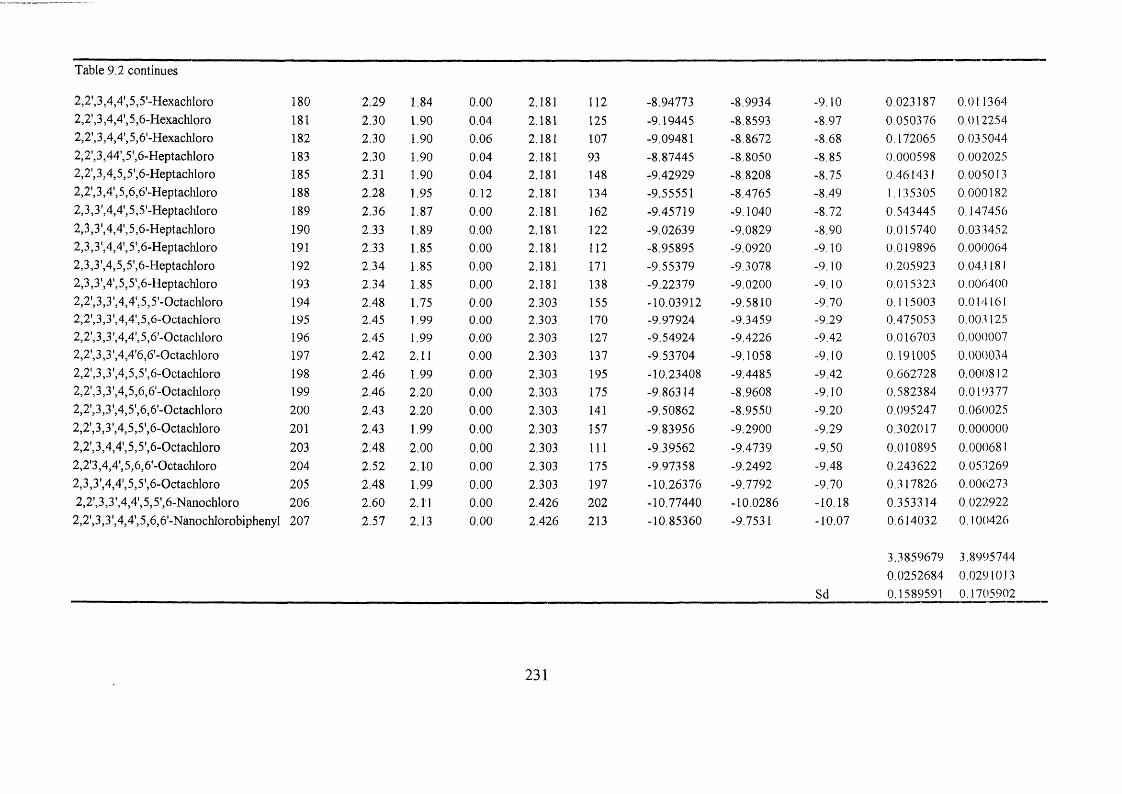
Table 9.2 continues
2,2',3,4,4',5,5'-Hexachloro 180 2.29 1.84 0.00 2.181 112 -8.94773 -8.9934 -9.10 0.023187 0.0113642,2',3,4,4', 5,6-Hexachloro 181 2.30 1.90 0.04 2.181 125 -9.19445 -8.8593 -8.97 0.050376 0.0122542,2', 3,4,4', 5,6'-Hexachloro 182 2.30 1.90 0.06 2.181 107 -9.09481 -8.8672 -8.68 0.172065 0.0350442,2',3,44',5',6-Heptachloro 183 2.30 1.90 0.04 2.181 93 -8.87445 -8.8050 -8.85 0.000598 0.0020252,2',3,4,5,5',6-Heptacliloro 185 2.31 1.90 0.04 2.181 148 -9.42929 -8.8208 -8.75 0.46143) 0.0050132,2',3,4',5,6,6'-Heptachloro 188 2.28 1.95 0.12 2.181 134 -9.55551 -8.4765 -8.49 1.135305 0.0001822,3,3',4,4', 5,5'-Heptachloro 189 2.36 1.87 0.00 2.181 162 -9.45719 -9.1040 -8.72 0.543445 0.1474562,3,3',4,4',5,6-Heptachloro 190 2.33 1.89 0.00 2.181 122 -9.02639 -9.0829 -8.90 0.015740 0.0334522,3,3',4,4',5',6-Heptachloro 191 2.33 1.85 0.00 2.181 112 -8.95895 -9.0920 -9.10 0.019896 0.0000642,3,3',4,5,5',6-Heptachloro 192 2.34 1.85 0.00 2.181 171 -9.55379 -9.3078 -9.10 0.205923 0.0431812,3,3',4',5,5',6-Heptachloro 193 2.34 1.85 0.00 2.181 138 -9.22379 -9.0200 -9.10 0.015323 0.0064002,2',3,3',4,4',5,5'-Octachloro 194 2.48 1.75 0.00 2.303 155 -10.03912 -9.5810 -9.70 0.115003 0.0141612,2',3,3',4,4',5,6-Octachloro 195 2.45 1.99 0.00 2.303 170 -9.97924 -9.3459 -9.29 0.475053 0.0031252,2',3,3',4,4',5,6'-Octachloro 196 2.45 1.99 0.00 2.303 127 -9.54924 -9.4226 -9.42 0.016703 0.0000072,2',3,3',4,4'6,6'-Octachloro 197 2.42 2.11 0.00 2.303 137 -9.53704 -9.1058 -9.10 0.191005 0.0000342,2',3,3',4,5,5',6-Octachloro 198 2.46 1.99 0.00 2.303 195 -10.23408 -9.4485 -9.42 0.662728 0.0008)22,2',3,3',4,5,6,6'-Octachlorp 199 2.46 2.20 0.00 2.303 175 -9.86314 -8.9608 -9.10 0.582384 0.0193772,2',3,3',4,5',6,6'-Octachloro 200 2.43 2.20 0.00 2.303 141 -9.50862 -8.9550 -9.20 0.095247 0.0600252,2',3,3',4,5,5',6-Octachloro 201 2.43 1.99 0.00 2.303 157 -9.83956 -9.2900 -9.29 0.302017 0.0000002,2',3,4,4',5,5',6-Octachloro 203 2.48 2.00 0.00 2.303 111 -9.39562 -9.4739 -9.50 0.010895 0.00068)2,2'3,4,4',5,6,6'-Octachloro 204 2.52 2.10 0.00 2.303 175 -9.97358 -9.2492 -9.48 0.243622 0.0532692,3,3',4,4',5,5',6-Octachloro 205 2.48 1.99 0.00 2.303 197 -10.26376 -9.7792 -9.70 0.317826 0.0062732,2',3,3',4,4',5,5',6-Nanochloro 206 2.60 2.11 0.00 2.426 202 -10.77440 -10.0286 -10.18 0.353314 0.0229222,2',3,3',4,4',5,6,6'-Nanochlorobiphenyl 207 2.57 2.13 0.00 2.426 213 -10.85360 -9.7531 -10.07 0.614032 0.100426
Sd
3.3859679 3.89957440.0252684 0.02910)3G. 1589591 0.1705902
231

(a) Our cacl. LogS using eqn, (9,10)(b) Predicted log S based on eqn. (9.9)(c) Exp. Log S data obtained from the literature by Patil Sd (a - c) our cacl. Log S- exp. Log SSd (b- c) predicted log S - exp log S
232
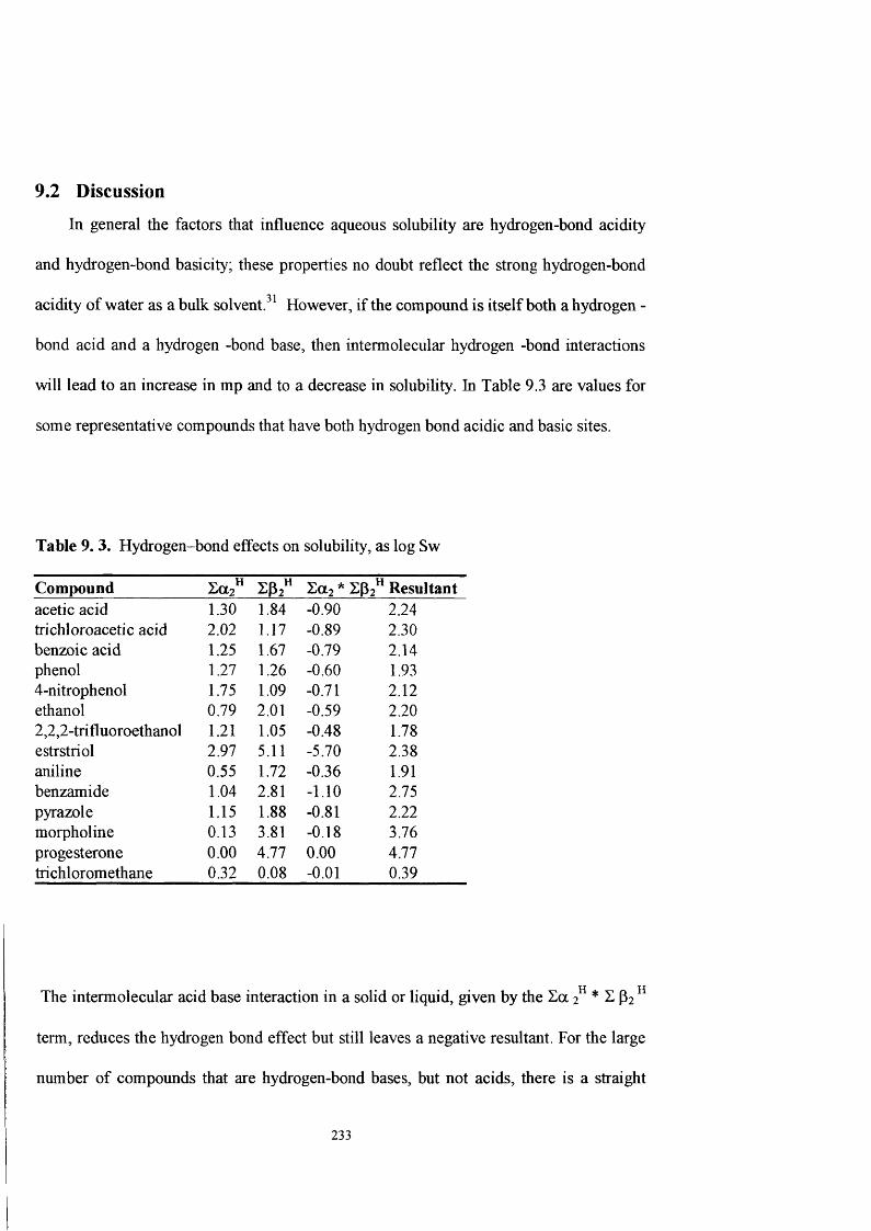
9.2 Discussion
In general the factors that influence aqueous solubility are hydrogen-bond acidity
and hydrogen-bond basicity; these properties no doubt reflect the strong hydrogen-bond
acidity of water as a bulk solvent.^ However, if the compound is itself both a hydrogen -
bond acid and a hydrogen -bond base, then intermolecular hydrogen -bond interactions
will lead to an increase in mp and to a decrease in solubility. In Table 9.3 are values for
some representative compounds that have both hydrogen bond acidic and basic sites.
Table 9. 3. Hydrogen-bond effects on solubility, as log Sw
Compound ZP2" Za2* 2P2^ Resultantacetic acid 1.30 1.84 -0.90 2.24trichloroacetic acid 2.02 1.17 -0.89 2.30benzoic acid 1.25 1.67 -0.79 2.14phenol 1.27 1.26 -0.60 1.934-nitrophenol 1.75 1.09 -0.71 2.12ethanol 0.79 2.01 -0.59 2.202,2,2-trifluoroethanol 1.21 1.05 -0.48 1.78estrstriol 2.97 5.11 -5.70 2.38aniline 0.55 1.72 -0.36 1.91benzamide 1.04 2.81 -1.10 2.75pyrazole 1.15 1.88 -0.81 2.22morpholine 0.13 3.81 -0.18 3.76progesterone 0.00 4.77 0.00 4.77trichloromethane 0.32 0.08 -0.01 0.39
The intermolecular acid base interaction in a solid or liquid, given by the 2a 2^ * ^ P2
term, reduces the hydrogen bond effect but still leaves a negative resultant. For the large
number of compounds that are hydrogen-bond bases, but not acids, there is a straight
233
forward effect of increased solubility (also shown in Table 9.3).There are but few
compounds that are hydrogen-bond acids and yet have no or veiy little hydrogen bond
basicity. The term in s. ti 2^ leads also to an increase in solubility. The two other terms in
equation 9.5, that affect the solubility are r.R] and v.Vx both of which result in a decrease
in solubility; the r - and v- coefficients in equation 9.5, are markedly more negative than
in the solvation equation for gaseous solubility. The R2 descriptor refers to the propensity
of solute to interact with surrounding a and tc electrons, the negative r-coefflcient
suggesting that such interaction within the solid or liquid is much larger than the
corresponding interaction between the solute and bulk water.
234
9 .3 R eferen ce s
1. G. Klopman, S. Wang, and D. M. Balthasar. J. Chem. Inf. Comput. Sci., 1992, Vol.
32,474.
2. G. S. Patil, J. Hazard. Mater., 1994, Vol. 36, 35.
3. J. Huuskonen, J. Salo, J. Taskinen. J. Pharm. Sci., 1997, Vol.86, 450.
4. T.M. Nelson, P C. Jurs. J. Chem. Inf. Comput Sci., 1994, Vol. 34, 601.
5. P. Ruelle, U. W. Kesselring. J. Pharm. Sci., 1997, Vol. 86,197.
6. P. Ruelle, U. W. Kesselring. J. Chem. Soc., Faraday Trans., 1997, Vol. 93, 2049.
7. J. Nouwen, B. Hansen. Act. Relat. 1996, Vol. 15,17.
8. T. Suzuki. J. Comput. Aided Mol. Design, 1991, Vol. 5, 149.
9. A. Li, W. J. Doucette, A. W. Andren. Cheraosphere., 1994, Vol 29, 657.
10. P. B. Myrdal, A. M. Manka, S. H. Yalkowsky, Chemosphere., 1995, Vol. 30, 1619.
11. N. Bodor, M. Huang. J. Pharm. Sci., 1992, Vol. 81, 954.
12. N. Bodor, M. Huang, A. Harget,. Neural Network Studies. 4. International Journal of
Quantum Chemistry, 1992, Vol. 26, 853.
13. S. Banerjee, Ph. H. Howard, Environ. Sci. Technol., 1988, Vol. 22, 839.
14. W.B. Neely, D R. Branson, G. F. Blau. Environ. Sci. Technol., 1974, Vol. 8,1113.
15. J. H. Robertson, W. F. Cowen, Y.J. Longfield. Chem. Eng. 1980, Vol. 87,102.
16. A. Opperhulzen, F.A.P.C. Gobas, M. D. Van der Steen, O. Hutzinger,. Environ. Sci.
Technol. 1988, Vol. 22, 638.
17. M. M. Miller, S. Ghodbane, S.P. Wasik, Y. B. Tewari, D.E. Martire. J. Chem. Eng.
Data 1984, Vol. 29,184.
235
18. S. H. Yalkowsky, S. C. Valvani,. J. Pharm. Sci. 1981, Vol. 70, 1177.
19. P. M. Dunnlvant, A. W. Elzerman, P. C. Jurs, M. N. Hasan. Enwon. Sci. Technol.
1992, Vol. 26, 1567.
20. N. N. Nirmalakhandan, R. E. Speece, Environ. Sci. Technol. 1989, Vol. 23, 708.
21. P. Ruelle, M. Buchmann, H. Nam-Tran, W. Kesselring. Environ. Sci. Technol. 1993,
Vol. 27, 266.
22. L. B. Kier, L. H. Hall, W. J. Murray, M. Landic. J. Pharm. Sci., 1975,Vol. 64, 1971.
23. J. H. Robertson, W. F. Cowen, Y. J. Longfield. Chem. Eng. 1980, Vol. 87,102.
24. C. S. Hong, H. Qiao. Chemosphere., 1995, Vol. 31, 4249.
25. M. J. Kami et, R. M. Doherty, P. W. Carr, D. Mackay, M. H. Abraham, R. W. Taft.
Environ. Sci. Technol., 1988, Vol. 22, 503.
26. C. Hansch, A. Leo, Substitution constant for correlation analysis in chemistry and
biology. New York, NY: Wiley; 1979.
27. T. Fujita, T. Nishioka, M. Nakajima. J. Med . Chem . 1977, Vol. 20,1071.
28. H. M. Abraham, LE. Joelle. J. Phama. Sci., 1999, Vol. 88, 868.
29. M. H. Abraham. Chem. Soc. Rev., 1993, Vol. 22, 73.
30. M. H. Abraham, J. C. McGowan. Chromatographia., 1987, Vol. 23, 243.
31. M. H. Abraham, H. S. Chadha, G. S. Whiting, R. C. Mitchell. J. Pharm. Sci., 1994,
Vol. 83, 1085.
32. G. S. Patil. Chemosphere., 1991, Vol. 22,723.
33. M. Bolgar, J. Cunningham, R. Cooper, R. Kozloski, J. Hubball, Chemosphere.,
1995, Vol. 31, 2687.
236
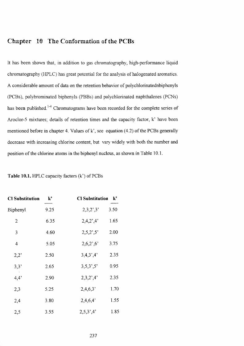
Chapter 10 The Conformation of the PCBs
It has been show that, in addition to gas chromatography, high-performance liquid
chromatography (HPLC) has great potential for the analysis of halogenated aromatics.
A considerable amount of data on the retention behavior of polychlorinatednhiphenyls
(PCBs), polybrominated biphenyls (PBBs) and polychlorinated naphthalenes (PCNs)
has been published. Chromatograms have been recorded for the complete series of
Aroclor-5 mixtures; details of retention times and the capacity factor, k’ have been
mentioned before in chapter 4. Values of k’, see equation (4.2) of the PCBs generally
decrease with increasing chlorine content, but vary widely with both the number and
position of the chlorine atoms in the biphenyl nucleus, as shown in Table 10.1.
Table 10.1. HPLC capacity factors (k’) of PCBs
Cl Substitution k’ Cl Substitution k’
Biphenyl 9.25 2,3,2’,3’ 3.50
2 6.35 2,4,2’,4’ 1.65
3 4.60 2,5,2’,5’ 2.00
4 5.05 2,6,2’,6’ 3.75
2,2' 2.50 3,4,3’,4’ 2.35
3,3’ 2.65 3,5,3’,5’ 0.95
4,4’ 2.90 2,3,2’,4’ 2.35
2,3 5.25 2,4,6,3’ 1.70
2,4 3.80 2,4,6,4’ 1.55
2,5 3.55 2,5,3’,4’ 1.85
237

2.6 5.40 2,3,4,2-,3-,4- 2.15
3,4 4.00 2,3,6,2-,3-,6- 2.25
3,5 2.60 2,4,5,2-,4-,5- 1,15
2,5,2- 3.20 2,4,6,2-,4-,6- 0.75
2,5,3- 2.15 3,4,5,3-,4-,5- 1.50
2,5,4- 2.05 Deca 0.45
From the results in Table 10.1 and from other previously published compilations of
retention time data on PCBs/'^ several conclusions can be drawn;
1- Although, in general, retention decreases when an increasing number of
chlorine atoms are introduced into the biphenyl nucleus, the introduction of
chlorine atoms ortho to the phenyl-phenyl bond (2-and 6- positions) increases
retention.
2- The order of elution of homogenate biphenyls bearing one to four halogen
atoms in a single ring as a rule is the same as that of the symmetrically
substituted compounds having from two to eight constituents.
3- Although there is a general tendency for the k’ values to decrease with
increase in the number of substitutions, the positions of the halogen atoms are
seen to exert a marked influence. For instance, the chlorobiphenyls, having
substituents ortho to the phenyl-phenyl bond, display markedly lower k’
values than do their non-ortho-substituted isomers. For the remainder,
substitution meta to the central C-C bond affects retention only slightly,
whereas substituted para to this bond strongly promotes retention, as shown
238
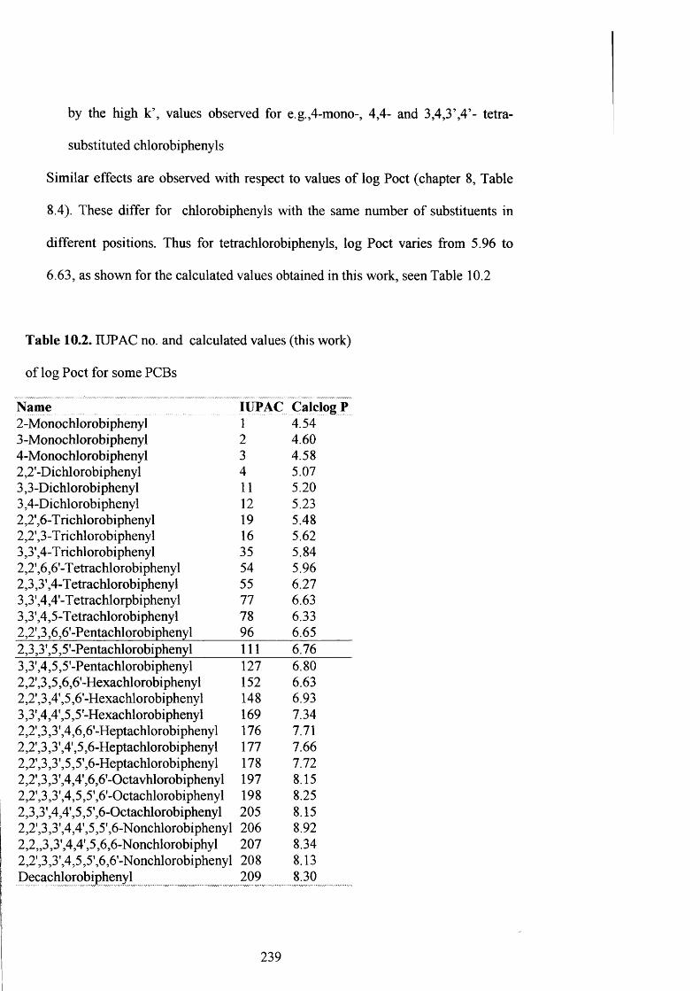
by the high k% values observed for e.g.,4-mono-, 4,4- and 3,4,3’,4’- tetra-
substituted chlorobiphenyls
Similar effects are observed with respect to values of log Poet (chapter 8, Table
8.4). These differ for chlorobiphenyls with the same number of substituents in
different positions. Thus for tetrachlorobiphenyls, log Poet varies from 5.96 to
6.63, as shown for the calculated values obtained in this work, seen Table 10.2
Table 10.2. lUPAC no. and calculated values (this work)
of log Poet for some PCBs
Name lUPAC Calelog P2-Monochlorobiphenyl 1 4.543 -Monochlorobiphenyl 2 4.604-Monochlorobiphenyl 3 4.582,2'-Dichlorobiphenyl 4 5.073,3-Dichlorobiphenyl 11 5.203,4-Dichlorobiphenyl 12 5.232,2',6-T richlorobiphenyl 19 5.482,2',3-T richlorobiphenyl 16 5.623,3',4-T richlorobiphenyl 35 5.842,2',6,6’-T etrachlorobiphenyl 54 5.962,3,3',4-T etrachlorobiphenyl 55 6.273,3',4,4'-Tetrachlorpbiphenyl 77 6.633,3',4,5-Tetrachlorobiphenyl 78 6.332,2',3,6,6'-Pentachlorobiphenyl 96 6.652,3,3',5,5'-Pentachlorobiphenyl 111 6.763,3',4,5,5'-Pentachlorobiphenyl 127 6.802,2',3,5,6,6'-Hexachlorobiphenyl 152 6.632,2',3,4',5,6'-Hexachlorobiphenyl 148 6.933,3',4,4*,5,5'-Hexachlorobiphenyl 169 7.342,2',3,3',4,6,6'-Heptachlorobiphenyl 176 7.712,2',3,3',4',5,6-Heptachlorobiphenyl 177 7.662,2',3,3',5,5’,6-Heptachlorobiphenyl 178 7.722,2',3,3',4,4',6,6’-Octavhlorobiphenyl 197 8.152,2',3,3',4,5,5',6'-Octachlorobiphenyl 198 8.252,3,3',4,4',5,5',6-Octachlorobiphenyl 205 8.152,2',3,3',4,4',5,5',6-Nonchlorobiphenyl 206 8.922,2,,3,3',4,4',5,6,6-Nonchlorobiphyl 207 8.342,2',3,3',4,5,5’,6,6’-Nonchlorobiphenyl 208 8.13Decachlorobiphenyl 209 8.30
239

Looking closely at Table 10.2 there are differences between log Poet values for each
groups of PCBs, as regards the number of substituents. With few substituents, the
differences are greater, and as the molecule becomes bigger (ie with more
substituents), the differences become smaller. The PCBs with 2,6 or 2,2’,6,6’-
substution always have smallest values of log Poet, as mentioned before in chapter
(7). The ortho-substitution effect which increases the polarity of the PCB was noted
especially for the 2,2’,6 and 2,2’,6,6’-congeners as compared to other PCBs, with the
same chlorine number.
All these results on HPLC capacity factors and log Poet values, suggests that the
rotational energy in the PCBs could be important, and so a study was made to obtain
the energy barrier to rotation about the C-C bond for a number of ortho-substituted
PCBs. The modeling software program PC Model was used to construct the PCBs
and to obtain the rotational energy as function of rotational angle (in Figure 10.1, the
rotational angle is defined, looking down the molecule along the C-C central bond).
This work started with biphenyl, then with the ortho substituted PCBs with 2,2’-, 3,3’-
, 4,4’- and 2, 2’, 6, 6’- substituents as shown in Table 10.3; graphs of the rotational
energy are shown below in Figures 10.3 and 10.4 as two examples. From the PC
Model results, the rotational energy maximum for all the PCBs studied were more or
less the same, except for the 2,2’, 6,6’-PCB where the energy maximum was much
larger. This helps to explain the substitutent effect on descriptors. For example the
value of 712 for the 2,2’,6,6’-substituted tetrachlorobiphenyl was larger than those of
the other tetrachlorobiphenyls. This can be seen also in Figure (7.2) chapter 7. The
presence of ortho-substitution increases the polarity, decreases the contact area and
makes the molecules non-planar. These conclusions agree with those of Brinkman et
al. ^
240

CD>
a b
Q180*
Figure. 10.1. The rotation angle about the central C-C bond
241
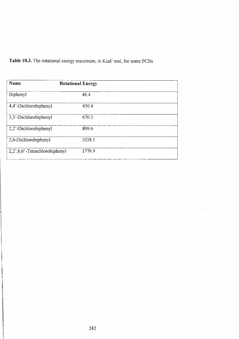
Table 10.3. The rotational energy maximum, in Kcal/ mol, for some PCBs
Name Rotational Energy
Biphenyl 46.4
4,4’ -Di chlorobiphenyl 450.4
3,3’ -Dichlorobiphenyl 670.3
2,2 ’ -Dichlorobiphenyl 809.6
2,6-Dichlorobiphenyl 1038.5
2,2 ’ ,6,6 ’ -T etrachl orobiphenyl 1776.9
242
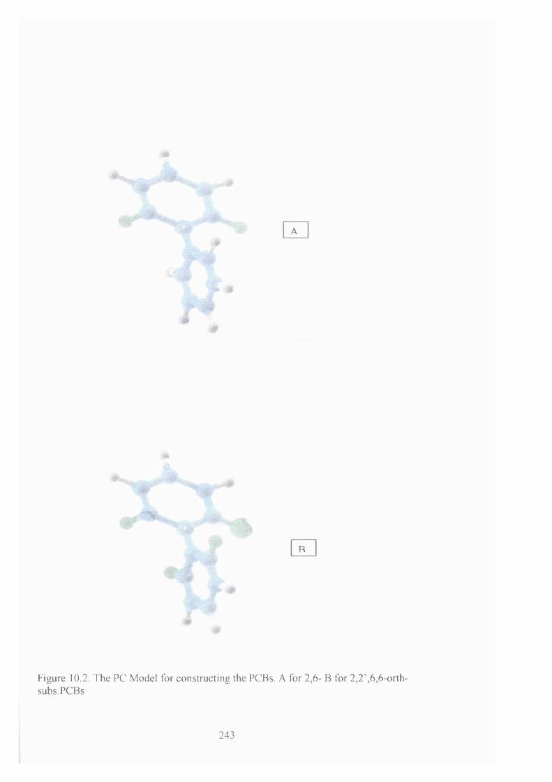
#
#
#
R
Figure 10.2. The PC Model for constructing the PCBs. A for 2,6- B for 2,2’,6,6-orth- subs.PCBs
243

1 0 3 8 . 4 6 1
9 6 4 . 2 8 i
8 9 0 . 1 1
8 1 5 . 9 3 4
' 4 1 . 7 5
UC
\ /
Figure 10.3. Rotation energy about the c-c bond for 2,6-ortho-substituted PCBs,
244
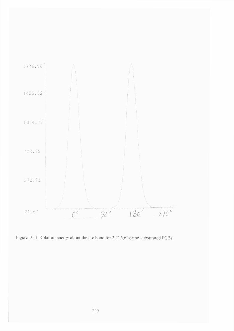
1176 .86 A/ \
1425.821I i
1074.78
723 .75 ^
372 .71
21 .67— T - r r ; r r r - r r r '— r ■ I r - r r - ; ; n ' r - r
c: . . C
Figure 10.4. Rotation energy about the c-c bond for 2,2’,6,6’-ortho-substituted PCBs
245

R e fe r e n c e s
1. U. A. Th. Brinkman, J. W. F. L. Seetz and H. G. M. Reyem, J. Chromatogr.,
1976, Vol. 116,353.
2. U. A. Th. Brinkman, A. de Kok, G.de Vries and H. G. M. Reymer, J.
Chromatogr., 1976, Vol. 128, 101.
3. J. J. de Kok, A. de Kok, U. A. Th. Brinkman and R. M. Kok. J. Chromatogr.,
1977, Vol. 142, 367.
4. U. A. Th. Brinkman, A. de Kok, H. G. M. Reymer and G. de Vries, J.
Chromatogr., 1976, Vol. 129, 193.
5. U. A. Th. Brinkman and G. De. Vries, J. Chromatogr., 1970, Vol. 169, 167.
246
Chapter 11 Calculation of the Descriptors for Polychloro-
naphthalenes, PCNs
11.0 Introduction
Polychlorinated naphthalenes (PCNs), written as CioHg-xClx, are a group of compounds
composed of two fused benzene rings (naphthalene) with one to eight chlorine substitutions
(Figure 1 ). There are a total of 75 possible PCN congeners. In general, they are hydrophobic
waxy solids with thermal stability and inertness. PCNs are structurally similar to PCBs and
exhibit similar physical and chemical properties. * Technical mixtures of the 75 possible PCN
congeners have been used in dielectric fluids, engine oil additives, electroplating masking
compounds, wood preservatives, lubricants and dye production.’’ Technical PCN mixtures with
chlorine contents ranging from 22 to 70 wt %, known as Halowaxes, have been produced by
Koppers Company in the United States since the 1920s. PCNs have also been manufactured in
other countries as Nibren waxes (Bayer Germany), Seekay waxes (ICI, U.K.) and Cerifal
materials (Caffaro, Italy). The exact amount of production of technical PCN mixtures is not
known, but it has been estimated to be approximately 150 000 tons, which is 10 % of the total
global production of PCBs. Although the industrial production of technical PCN formulations
has declined in the United States since the early 1980s, products containing these formulations
are still present in the environment. Furthermore, the secondary formation of PCNs in thermal
processing such as municipal solid waste incineration (MWI) suggests sustaining environmental
sources of PCNs. Similar to PCBs, PCNs are persistent and lipophilic compounds that tend to
bioaccumulate. PCNs are wide spread in the biosphere on global scale.^’ PCNs have been found
in a wide variety of environmental matrices including Arctic and urban air, wildlife,
247
and human tissues including breast milk. Consumption of contaminated fish is considered
to be an important route of exposure of humans lo PCNs. High concentrations of penta-and
hexachloronaphthalenes in human blood plasma have been correlated with fish consumption.^^
Distribution, bioaccumulation, and fate of PCBs, polychlorinated dibenzo-p-dioxins (PCDDs),
and polychlorinated dibenzofurans (PCDFs) in various environmental media near a chlor-alkali
plant have been described. Little is know about the fate, transport, and biological effects of
individual PCN congeners. This is due in part, to a deficiency of standards of individual
congeners and a lack of sensitive, congener specific analytical methods. Now that many
standards have been developed, such as capillary gas chromatography and high-resolution mass
spectrometry (HRGC/HRMS), PCN congeners have been detected in environmental samples.
10, i L 19, 2 0 , 2 1 the composition of PCN congeners in technical Halowax mixtures has
been reported.^ The characteristic properties of PCNs are hydrophobicity or lipophilicity,
relatively low vapour pressure and extreme resistance to chemical reaction, and high chemical
and thermal stability. Many of the PCNs are toxic and in view of their tendency to
bioaccumulate and their widespread distribution^^’ are now acknowledged to be important
environmental contaminants.^
Polychloronaphthlenes (PCNs) have similar structural functionalities, but a number of
analytical methods have been used to separate the congeners. The corresponding data can then be
used to obtain physicochemical properties of PCNs. Such analytical methods include normal
phase HPLC capacity factors, reversed-phase HPLC capacity factors and gas liquid
chromatographic (GLC) retention data onDB-5, Rtx-5 and TC-1701/OV-1701. ’ Water-
octanol partition coefficients, as log Poet, have been determined for a number of PCNs ^ and
values of log Poet can be estimated for all the 75 PCNs through the CLOGP program. Gas-dry
248

octanol partition coefficients for 24 PCNs have been determined at several temperatures.^"
However, key environmental quantities such as gas-water partition coefficients and aqueous
solubilities are unknown, except for a few aqueous solubilities.^ There are enonnous practical
difficulties in the experimental determination of these quantities for very lipophilic compounds,
and so resort is often had to some fonn of estimation. It is the aim of this work to obtain from the
available physicochemical data, solvation descriptors that can then be used to estimate all kinds
of other physicochemical data, and especially those of use in environmental analyses.
Although there is a numbering scheme for the 75 PCNs we prefer to use abbreviations that
relate to the PCN structure. We therefore denote 1,2-dichloronaphthalene as PCN12, and
I,2,3,5-tetrachloronaphthalene as PCN 1235, etc.
II.1 Methodology
We start with two general solvation equations:
Log SP = c + r. R2 + s. 712 a. Z a 2 ^ + b. I p 2^ + V. Vx (H I)
LogSP = c + r.R2 + s. 7t2^+a. Z a 2^ + b. Z P 2 ^ + H g ( 1 L 2 )
The dependent variable, SP, is a set of solute properties in a given system. Eqn.(ll. 1) is used for
processes in condensed systems; for example SP might then be log Poet where Poet is the water-
octanol partition coefficient for a series of compounds. Eqn.(11.2) is used for gas-condensed
phase processes, such as gas liquid chromatography where SP can be a relative retention time, as
log t, or the Kovats retention index. I, can be used instead of log SP. The independent variables in
249
eqn.(ll.l) and eqn.(11.2) are solute descriptors as fo llow s.R 2 is the solute excess molar
reffactivity, in uniis of (mol dm ()/10, defined as the solute molar remactivity less the molar
reffactivity of an alkane of the same McGowan volume. R? represents the tendency of a solute to
take part in intermolecular interactions through a and n electrons. The reason why an ‘excess’
molar refraction is used instead of the molar refraction itself is that the latter is too closely
related to solute volume to be incorporated in the any linear equation that includes volume as a
descriptor. 712^ is the solute dipolarity/polarizability and and Sp2^ are the overall or
summation hydrogen bond acidity and basicity. Vx is the McGowan characteristic volume in
units of (mol dm'^)/100. This volume is calculated through addition of atomic fragments, and can
very simply be calculated just from the solute molecular formula and the number of rings in the
molecule, using the algorithm of Abraham. Log is the logarithm of the gas-hexadecane
partition coefficient at 298 K. Both Vx and logf’ encode two particular types of interaction,
that may be explained as follows. The dissolution of a gaseous solute in a solvent can
conceptually take place in two stages, (a) a hole or cavity has to be formed in the solvent, and (b)
the solute is then inserted into the cavity and then takes part in various solute/solvent interactions.
The work required to form a cavity is roughly proportional to the size of the cavity, and since
both Vx and log are related to size, this cavity work will depend on Vx or log The
solute/solvent interactions can mostly be modeled by the descriptors R2 , Za2^, and SP2^, but
there will be interactions of the London dispersion force type that are not thus modeled. These
interactions depend also on solute size, and so the Vx and logL descriptors include not only the
cavity size effect, but also the propensity of a solute to undergo London dispersion interactions.
Thus the descriptors in eqn.(ll.l) and eqn.(11.2) all refer to how a solute might interact with a
solvent phase, and the Vx and logL descriptors also include the cavity effect. Although the
250

processes listed in Table 11.1 appear to be quite different, they have in common the various
solute/' solvent interactions to which our descriptors refer. This is why the R2 -descriptor, for
example, seems relevant in all sorts of different processes.
The coefficients in eqn. (11.1) and eqn. (11.2) are evaluated through multiple linear regression
analysis, MLRA, using standard mathematical software packages or our own in-house software.
Some examples of eqn. (11.1) and eqn. (11.2) are in Table 11.1, where the obtained coefficients
and statistics are summarized.
The general method for the detennination of solute descriptors has been given previously.
We start with values of SP for a given compound in a number of systems that have been
characterized through eqn. (11.1) or eqn. (11.2). The R2 descriptor can be obtained from the
liquid refractive index at 293K, or can easily be estimated, Vx can readily be calculated from
structure, ' and so we have four descriptors tc2^, and log that remain to be
evaluated. Various combinations of E(32^ and log are used to calculate the known
SP values, and the combination that best reproduces the observed values is then selected. It is
important to note that Sa2^ and Zj32^ refer to hydrogen bond acidity and basicity, and not to
proton acidity and basicity. The PCNs have no hydrogen bond acidity (a 2^ = 0), but they are
potentially hydrogen bond bases, and so there are the three descriptors, 712^, SP2^ and log to
be evaluated. In tihis respect, the PCNs resemble the chlorobenzenes that have zero hydrogen
bond acidity, but some hydrogen bond basicity. "
11.2 Calculation of the descriptors
Preliminary estimates of descriptors are used to start with, as follows. The R2 descriptor can
easily be estimated by analogy with previous work on the polychlorinated benzenes. We started
251
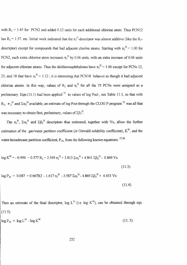
with R2 = 1.45 for PCN2 and added 0.12 units for each additional chlorine atom. Thus PCN 12
has R] = 1.57, ere. Initial work indicated that the Tti^-descriptor was almost additive (like the R?-
descriptor) except for compounds that had adjacent chorine atoms. Starting with 712^= 1.00 for
PCN2, each extra chlorine atom increases 712^ by 0.06 units, with an extra increase of 0.06 units
for adjacent chlorine atoms. Thus the dichloronaphthalenes have 712^ =1.06 except for PCNs 12,
23, and 18 that have 712^ = 1.12 ; it is interesting that PCN 18 behaves as though it had adjacent
chlorine atoms. In this way, values of R2 and 712^ for all the 75 PCNs were assigned as a
preliminary. Eqn. (11.1) had been applied to values of log Poet, see Table 11.1, so that with
R2, 712^ and Xa2^ available, an estimate of log Poet through the CLOG P program was all that
was necessary to obtain first, preliminary, values of 1(32 .
The 712 , Za2^ and E(32 descriptors thus estimated, together with Vx, allow the further
estimation of the gas/water partition coefficient (or Ostw'ald solubility coefficient), K^, and the
water-hexadecane partition coefiticient, P]6, from the following known equations;
l o g 0.994 + 0.577 R2 + 2.549 712 + 3.813 Ea2^ + 4.841 S132 - 0.869 Vx
(11.3)
logP]6 = 0.087 +0.667R2 -1.617712^ -3.587Za2^ - 4.869 4.433 Vx
(11.4)
Then an estimate of the final descriptor, log (i.e. log K’ ), can be obtained through eqn.
(11.5):
logP]6 = log -logK^ (11 ■5)
252

Once the initial estimates of all four descriptors had been accomplished, it was then possible to
characterize the various sets of GLC retention data through eqn.(11.2). The resulting equations
were then used to adjust the initial estimates to give a second set of 712^, Zp2^ and log
descriptors; use was also made of known gas-dr ' octanol partition coefficients, as log
because the correlation equation for log involves the logL^^-descriptor. The second set of
log values were again used to characterize the sets of GLC retention data that were then used
to obtain a third (final) set of descriptors. The final GLC equations are summarized in Table 11.1,
together with details of the other equations that were have used. The statistics of the GLC
equations are only notional, because the equations are a result of an iterative procedure. In order
to weight the equations satisfactorily, Kovats retention indices were correlated as I/lOO, and t
and log t were correlated as lOt and lOlog t so that the equation coefficients were then of the
same order as those for the log P equations. The following statistics of the regressions are in
Table 11.1: n is the number of data points (compounds), sd is the standard deviation, and is the
variance. Note that for the retention data of Falandysz et al. the given relative retention times, t,
were used, that gave a better regression than the normally-used log t values.
Table 11.1. Details of the regression equations used
System c e s a b v/1 n sd 2r
Water/wet octanol 0.088 0.562 -1.054 0.034 -3.460 3.814 613 0.12 0.995
Water/CHiCli 0.314 0.001 0.022 -3.328 -4.137 4.259 38 0.14 0.991
Water/CHCls 0.327 0.157 -0.391 -3.191 -3.437 4.191 335 0.25 0.971
Water/CCU 0.260 0.573 -1.254 -3.558 4.588 4.589 210 0.11 0.996
253
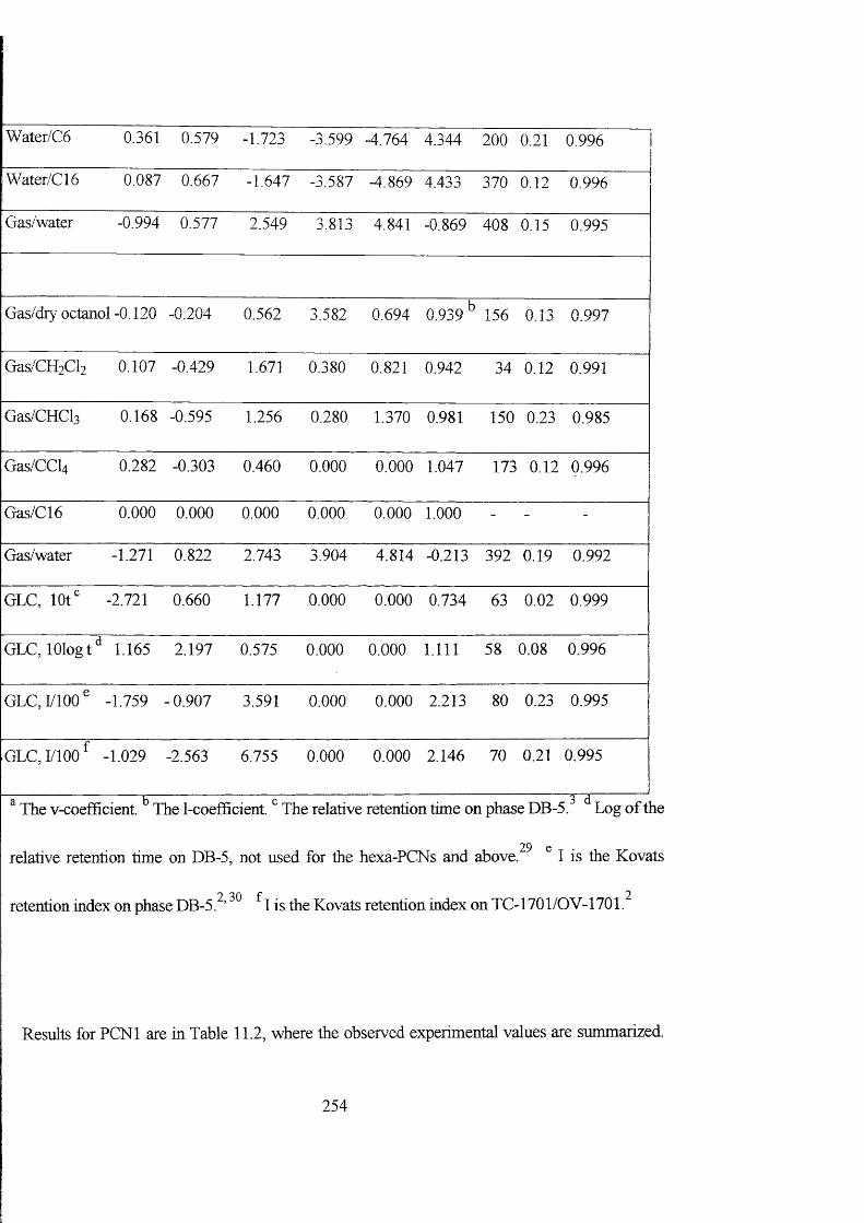
Water/C6 0.361 0.579 -1.723 -3.599 -4.764 4.344 200 0.21 0.996
Water/C 16 0.087 0.667 -1.647 -3.587 -4.869 4.433 370 0.12 0.996
; Gas/water -0.994 0.577 2.549 3.813 4.841 -0.869 408 0.15 0.995
Gas/dry octanol -0.120 -0.204 0.562 3.582 0.694 0.939 ^ 156 0.13 0.997
Gas/CH2Cl2 0.107 -0.429 1.671 0.380 0.821 0.942 34 0.12 0.991
Gas/CHCl] 0.168 -0.595 1.256 0.280 1.370 0.981 150 0.23 0.985
Gas/CCl4 0.282 -0.303 0.460 0.000 0.000 1.047 173 0.12 0.996
Gas/C16 0.000 0.000 0.000 0.000 0.000 1.000 - - -
Gas/water -1.271 0.822 2.743 3.904 4.814 -0.213 392 0.19 0.992
GLC, lOt" ■2.721 0.660 1.177 0.000 0.000 0.734 63 0.02 0.999
GLC, lOlogt^ 1.165 2.197 0.575 0.000 0.000 1.111 58 0.08 0.996
GLC, moo^ -1.759 - 0.907 3.591 0.000 0.000 2.213 80 0.23 0.995
GLC, LlOO -1.029 -2.563 6.755 0.000 0.000 2.146 70 0.21 0.995
The v-coefiGcient. The l-coefficient. The relative retention time on phase DB-5.^ Log of the
29 erelative retention time on DB-5, not used for the hexa-PCNs and above. I is the Kovats
retention index on phase DB-5.^’ is the Kovats retention index on TC-1701/OV-1701.^
Results for PCNl are in Table 11.2, where the observed experimental values are summarized.
254
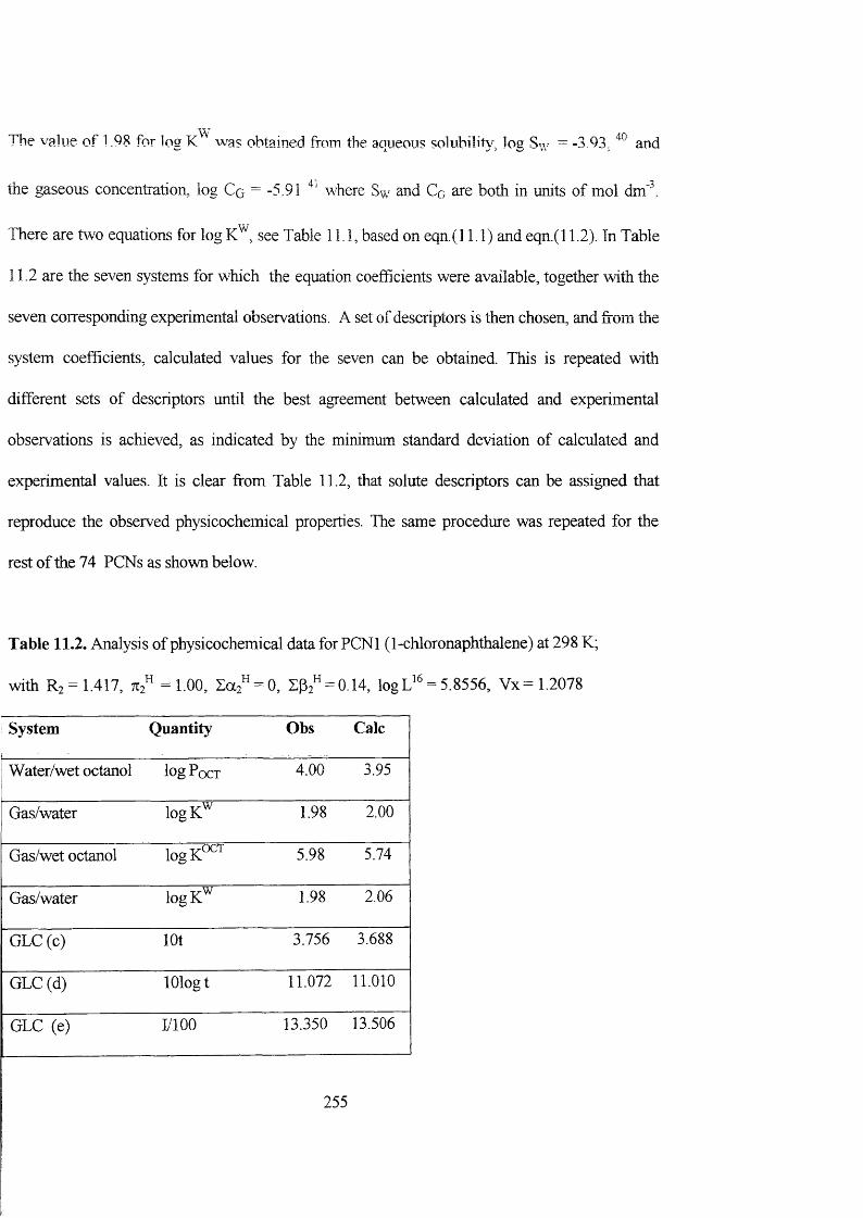
The value of 1.98 for log was obtained from the aqueous solubility, log S\y = -3 93. and
the gaseous concentration, log Cg = -5.91 where Sw and Co are both in units of mol dm’\
There are two equations for log K^, see Table 11.1, based on eqn.(l 1.1) and eqn.(l 1.2). In Table
11.2 are the seven systems for which the equation coefficients were available, together with the
seven corresponding experimental observations. A set of descriptors is then chosen, and fi'om the
system coefficients, calculated values for the seven can be obtained. This is repeated with
different sets of descriptors until the best agreement between calculated and experimental
observations is achieved, as indicated by the minimum standard deviation of calculated and
experimental values. It is clear from Table 11.2, that solute descriptors can be assigned that
reproduce the observed physicochemical properties. The same procedure was repeated for the
rest of the 74 PCNs as shown below.
Table 11.2. Analysis of physicochemical data for PCNl (1-chloronaphthalene) at 298 K;
with R2 = 1.417, =1,00, Za2^ = 0. % " = 0.14. l o g = 5.8556, Vx=1.2078
System Quantity Obs Calc
Water/wet octanol log Pqct 4.00 3.95
Gas/water logK"^ 1.98 2.00
Gas/wet octanol logK^'^ 5.98 5.74
Gas/water logK"^ 1.98 2.06
GLC (c) lot 3.756 3.688
GLC (d) lOlog t 11.072 11.010
GLC (e) I/lOO 13.350 13.506
255
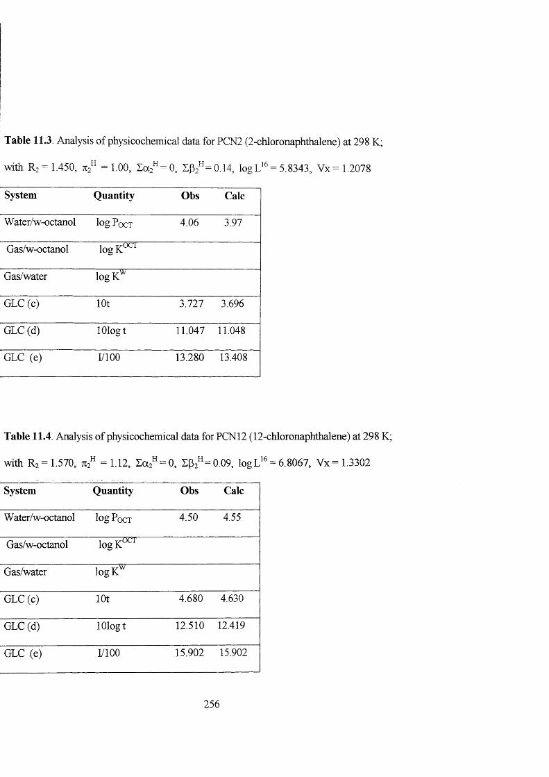
Table 11.3. Analysis of physicochemical data for PCN2 (2-chloronaphthalene) at 298 K;
with R2 = 1.450, =1.00, = 0, logL“ = 5.8343, Vx=1.2078
System Quantity Obs Calc
Water/w-octanol log PoCT 4.06 3.97
Gas/w-octanol logK^^
Gas/water logK"^
GLC (c) lOt 3.727 3.696
GLC (d) lOlogt 11.047 11.048
GLC (e) I/lOO 13.280 13.408
Table 11.4 Analysis of physicochemical data for PCN12 (12-chloronaphthalene) at 298 K;
with R; = 1.570, =1.12, Za2^ = 0, XP2” =0.09, logL'^ = 6.8067, Vx= 1.3302
System Quantity Obs Calc
Water/w-octanol logPoCT 4.50 4.55
Gas/w-octanol logK °^
Gas/water logK"^
GLC (c) lot 4.680 4.630
GLC(d) lOlogt 12.510 12.419
GLC (e) I/lOO 15.902 15.902
256

Table 11.5. Analysis of physicochemical data for PCN 13 (13-chloronaphthalene) at 298 K;
with R ] = 1.570, 712 = 1.06, Za2^ = 0 , 0.08, logL
System Quantity Obs Calc
Water/w-octanol lo g P qct 4.65 4.65
Gas/w-octanol logK°^
Gas/water logK"^
GLC (c) lOt 4.506 4.462
GLC (d) lOlogt 12.235 12.235
GLC (e) I/lOO 15.380 15.395
Table 11.6. Analysis of physicochemical data for PCNl 4 (N
with R% = 1.570, 712 =1.06, Sa 2^ = 0, L(32^ = 0 .0 9 , logL
System Quantity Obs Calc
Water/w-octanol lo g P qct 4.66 4.62
Gas/w-octanol logK°^
1 Gas/water logK"^
I GLC (c) lOt 4.572 4.522
GLC (d) lOlogt 12.345 12.325
j GLC (e) I/lOO 15.560 15.576
16
16
257
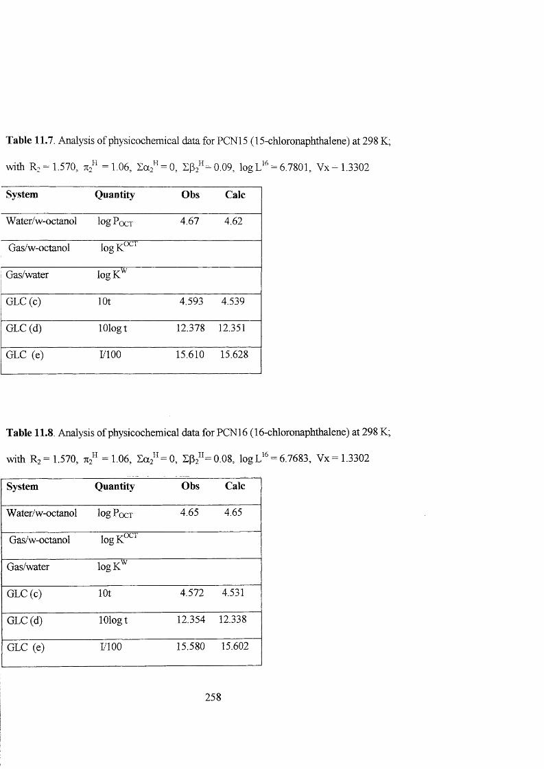
Table 11.7. Analysis of physicochemical data for PCNl 5 (15-chloronaphthalene) at 298 K;
with R: = 1.570. it,” =1.06, Sa,“ = 0, % "=0.09. logL“ = 6.7801, Vx= 1.3302
System Quantity Obs Calc
Water/w-octanol lo g Pqct 4.67 4.62
Gas/w-octanol logK°^^
Gas/water logK^^
GLC (c) lOt 4.593 4.539
GLC (d) lOlogt 12.378 12.351
GLC (e) I/lOO 15.610 15.628
Table 11.8. Analysis of physicochemical data for PCN16 (16-chloronaphthalene) at 298 K;
with Rz= 1.570, 712“ = 1.06, Ea2“ = 0, % "= 0 .0S . l o g = 6.7683, Vx= 1.3302
System Quantity Obs Calc
Water/w-octanol log Pqct 4.65 4.65
Gas/w-octanol logK°^^
Gas/water logK"^
GLC(c) lot 4.572 4.531
GLC (d) lOlogt 12.354 12.338
GLC (e) I/lOO 15.580 15.602
258
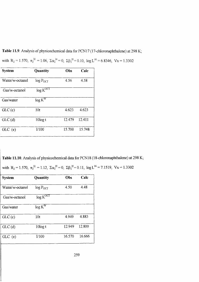
Table 11.9. Analysis of physicochemical data for PCNl 7 (17-chloronaphthalene) at 298 K;
with R2 = 1.570, 712 =1.06, Za2^ = 0 . % " = 0.10, logL
System Quantity Obs Calc
Water/w-octanol lo g Pqct 4.56 4.58
Gas/w-octanol logK°^^
Gas/water logK"^
GLC (c) lOt 4.623 4.623
GLC (d) lOlogt 12.479 12.411
GLC (e) I/lOO 15.700 15.748
16
Table 11.10. Analysis of physicochemical data for PCNl 8 (18-chloronaphthalene) at 298 K;
with R2 = 1.570, Ttj” =1.12, Za;" = 0, % "=0.11. logL'* = 7.1519, Vx=1.3302
System Quantity Obs Calc
Water/w-octanol log P q c t 4.50 4.48
Gas/w-octanol logK ^'
Gas/water logK"^
GLC (c) lot 4.949 4.883
1 GLC (d) lOlogt 12.949 12.800
GLC (e) I/lOO 16.570 16.666
259

Table 11.11. Analysis of physicochemical data for PCN23 (23-chloronaphthalene) at 298 K;
with R ] = 1.570, 71;^ = 1.12, = 0, 0.09, logL
System Quantity Obs Calc
Water/w-octanol lo g P qct 4.51 4.55
Gas/w-octanol logK°^^
Gas/water logK"^
GLC (c) lOt
GLC (d) lOlog t 12.558 12.557
GLC (e) I/lOO
Table 11.12 Analysis of physicochemical data for PCN26 (]
with Rî = 1.570, =1.12, Za2* = 0, % "=0.08 , logL
System Quantity Obs Calc
Water/w-octanol lo g P qct 4.60 4.59
Gas/w-octanol logK°^
Gas/water logK"^
GLC (c) lot 4.623 4.581
GLC (d) lOlogt 12.428 12.346
:GLC (e) PI 00 15.700 15.755
260
16
16
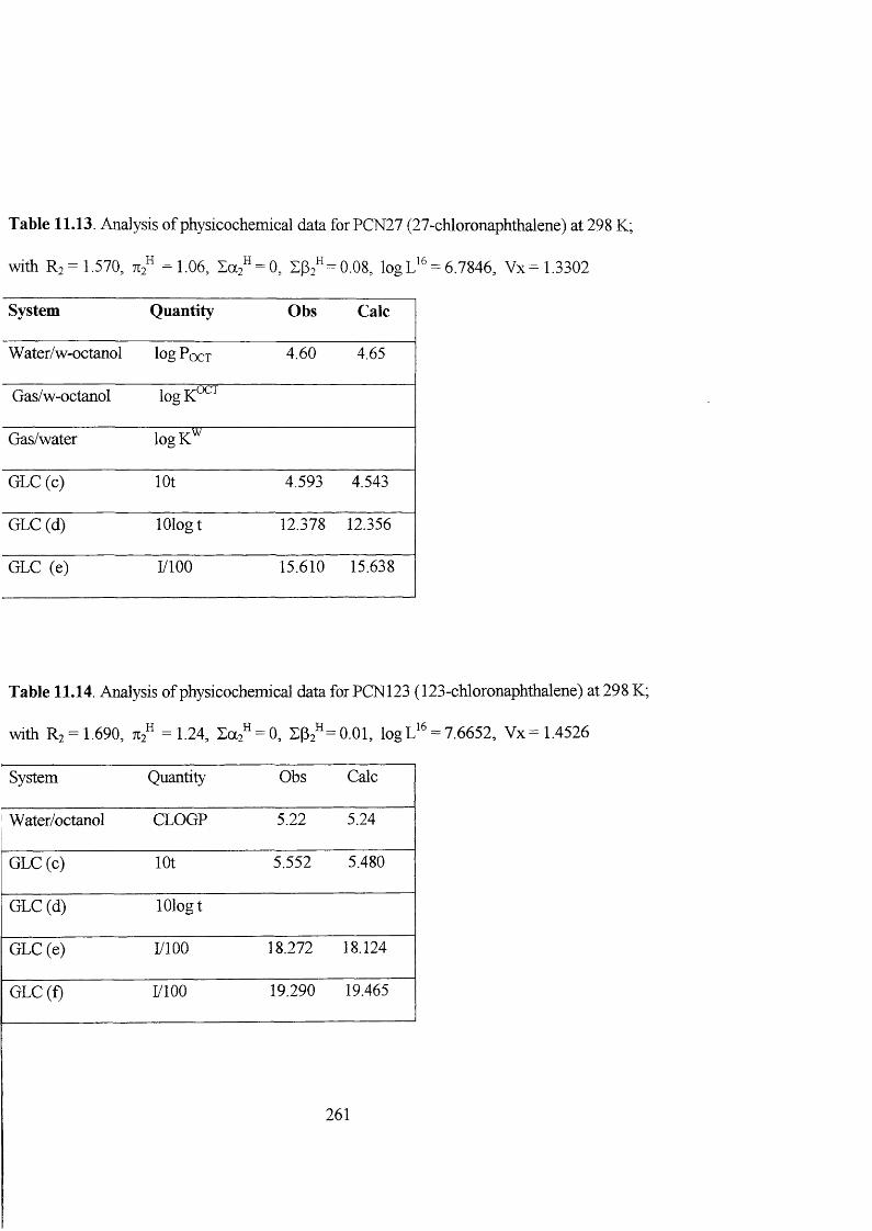
Table 11.13. Analysis of physicochemical data for PCN27 (27-chloronaphthalene) at 298 K;
with R] = 1.570, 712 = 1.06, = 0, spT-= 0.08, logL
System Quantity Obs Calc
Water/w-octanol log P OCT 4.60 4.65
Gas/w-octanol logK°^^
Gas/water logK^^
GLC (c) lot 4.593 4.543
GLC (d) lOlogt 12.378 12.356
GLC (e) I/lOO 15.610 15.638
Table 11.14. Analysis of physicochemical data for PCN 123
with R: = 1.690, =1.24, Ea,“ = 0, Ek"=0.01, logL
System Quantity Obs Calc
Water/octanol CLOGP 5.22 5.24
GLC (c) lot 5.552 5.480
GLC (d) lOlogt
GLC (e) 1/100 18.272 18.124
GLC(f) I/lOO 19.290 19.465
16
16
261
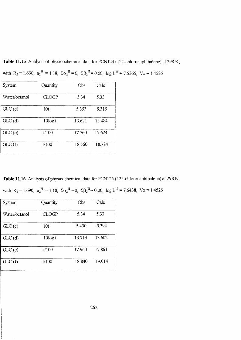
Table 11.15. Analysis of physicochemical data for PCN124 (124-chloronaphthalene) at 298 K;
with R, = 1.690, =1.18, la]" = 0, Zfe“ = 0.00, logL‘ = 7.5365, Vx= 1.4526
System Quantity Obs Calc
Water/octanol CLOGP 5.34 5.33
GLC (c) lot 5.353 5.315
GLC(d) lOlogt 13.621 13.484
GLC (e) LlOO 17.760 17.624
GLC(f) LlOO 18.560 18.784
Table 11.16. Amalysis of physicochemical data for PCN 125
with R2 = 1.690, 712 =1.18, Sa2^ = 0, L(32 == 0.00, logL
System Quantity Obs Calc
Water/octanol CLOGP 5.34 5.33
GLC(c) lot 5.430 5.394
GLC (d) lOlogt 13.719 13.602
GLC(e) I/lOO 17.960 17.861
GLC(f) LlOO 18.840 19.014
16
262
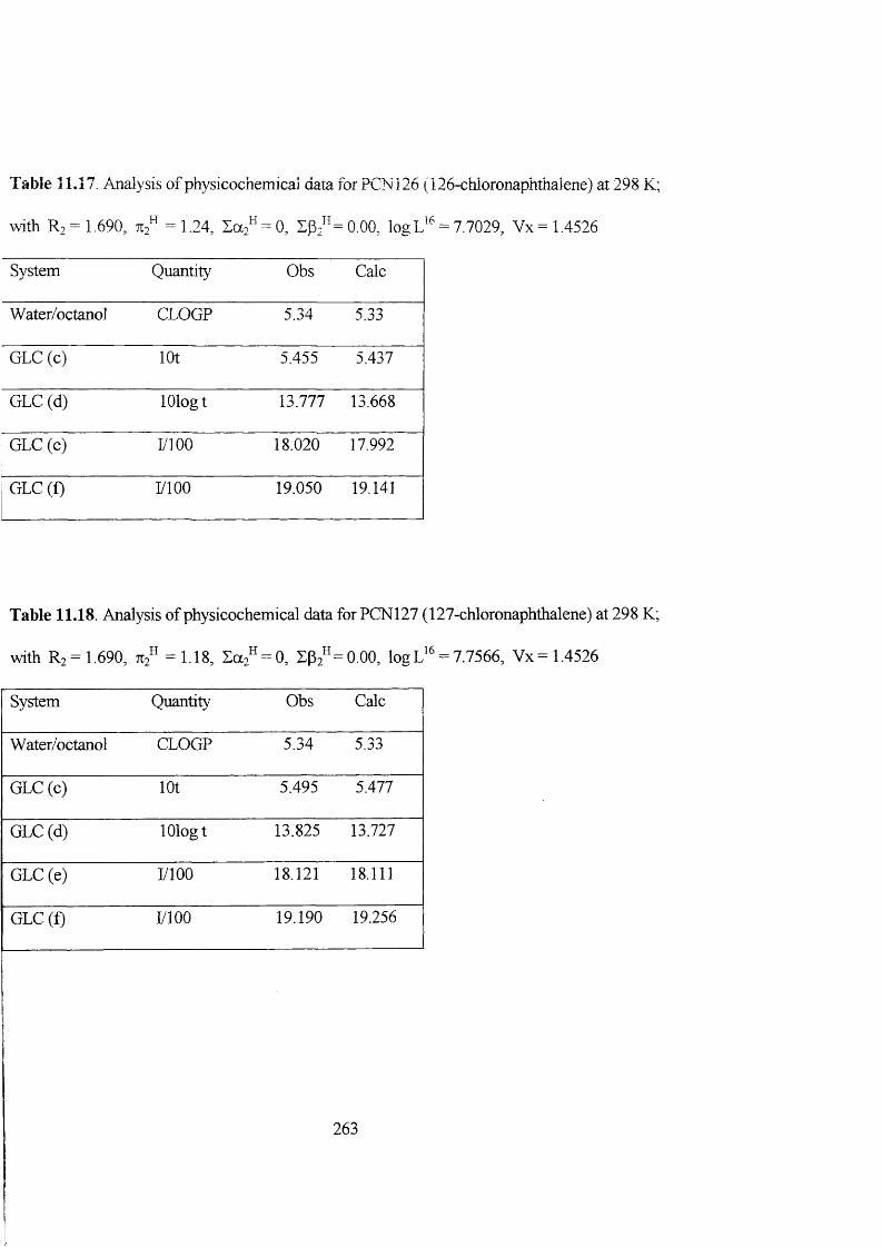
Table 11.17 Analysis of physicochemical daia for PCNl 26 (126-chloronaphthalene) at 298 K;
^vith R? = 1.690, 71,” =1.24, = 0, Zpn" = 0.00, logL
System Quantity Obs Calc
Water/octanol CLOGP 5.34 5.33
GLC (c) lot 5.455 5.437
GLC (d) lOlogt 13.777 13.668
GLC(e) LlOO 18.020 17.992
GLC(f) LlOO 19.050 19.141
Table 11.18. Analysis of physicochemical data for PCN 127
with Rj = 1.690, = 1.18, = 0.00, logL
System Quantity Obs Calc
Water/octanol CLOGP 5.34 5.33
GLC (c) lOt 5.495 5.477
GLC (d) lOlogt 13.825 13.727
GLC (e) LlOO 18.121 18.111
GLC(f) LlOO 19.190 19.256
16
16
263

Table 11.19. Analysis of physicochemical data for PCNl 28 (128-chloronaphthalene) at 298 K;
16 _ O \ 1with Ri = 1.690, 712 =1.18, = 0, XP2'' = 0.00, logL
System Quantity Obs Calc
Water/octanol CLOGP 5.34 5.33
GLC (c) lOt 5.836 5.807
GLC (d) lOlogt 14.344 14.223
GLC (e) LlOO 18.960 18.106
GLC(f) LlOO 20.300 20.221
Table 11.20. Analysis of physicochemical data for PCN 135
with Rz = 1.690, =1.12, Eaz" = 0, Sp2“ = 0,00, logL
System Quantity Obs Calc
Water/octanol CLOGP 5.46 5.40
GLC(c) lot 5.283 5.280
GLC(d) lOlogt 13.510 13.499
GLC (e) LlOO 17.610 17.516
GLC(f) LlOO 18.380 18.483
16
264
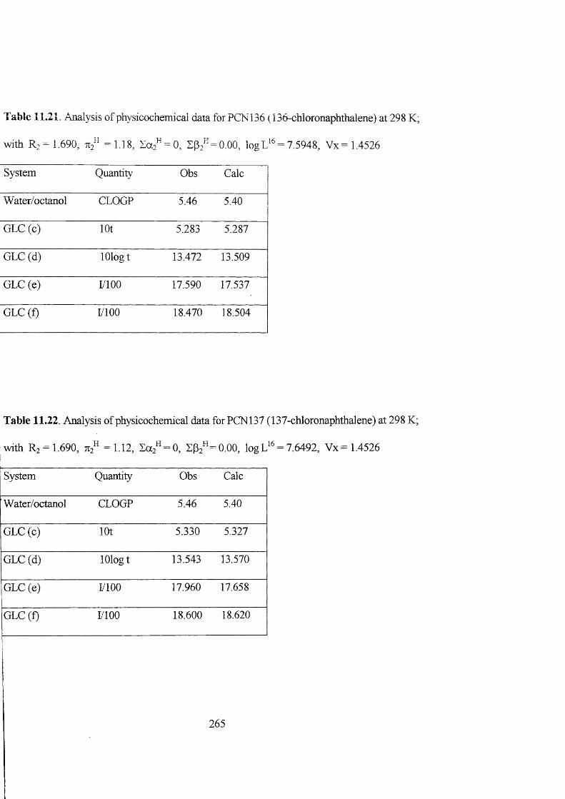
Table 11.21. Analysis of physicochemical data for PCN 136 (136-chloronaphthalene) at 298 K;
with R2 = 1.690, 712 =1.18, = 0 , = 0.00, logL
System Quantity Obs Calc
Water/octanol CLOGP 5.46 5.40
GLC (c) lOt 5.283 5.287
GLC (d) lOlogt 13.472 13.509
GLC (e) LlOO 17.590 17.537
GLC(f) LlOO 18.470 18.504
16
Table 11.22. Analysis of physicochemical data for PCNl 37 (137-chloronaphthalene) at 298 K;
7-___1with R2 = 1.690, 712 =1.12, Za2^ = 0 , I|32” = 0.00, logL
System Quantity Obs Calc
Water/octanol CLOGP 5.46 5.40
GLC (c) lOt 5.330 5.327
GLC(d) lOlogt 13.543 13.570
GLC (e) LlOO 17.960 17.658
GLC (f) LlOO 18.600 18.620
265
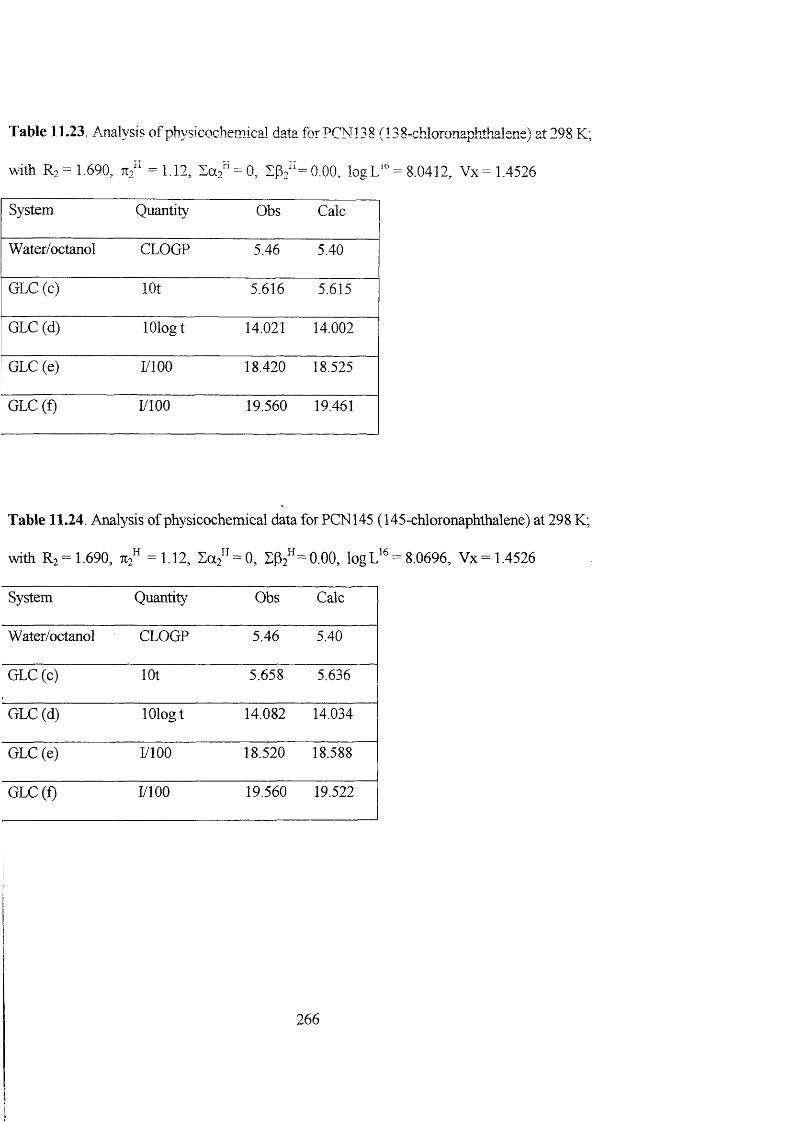
Table 11.23, Analysis of physicochemical data for PCNl 3 8 (138-chloronaphthalene) at 298 K;
with R? = 1.690, 712" =1.12, E a / = 0, 0.00, logL
System Quantity Obs Calc
Water/octanol CLOGP 5.46 5.40
GLC (c) lût 5.616 5.615
GLC (d) lOlogt 14.021 14.002
GLC (e) LlOO 18.420 18.525
GLC(f) LlOO 19.560 19.461
Table 11.24. Analysis of physicochemical data for PCN 145
with Rz = 1.690, =1.12, Za2" = 0, ZP:"= 0.00, logL
System Quantity Obs Calc
Water/octanol CLOGP 5.46 5.40
GLC (c) lot 5.658 5.636
GLC(d) lOlogt 14.082 14.034
GLC (e) LlOO 18.520 18.588
GLC(f) LlOO 19.560 19.522
16
266
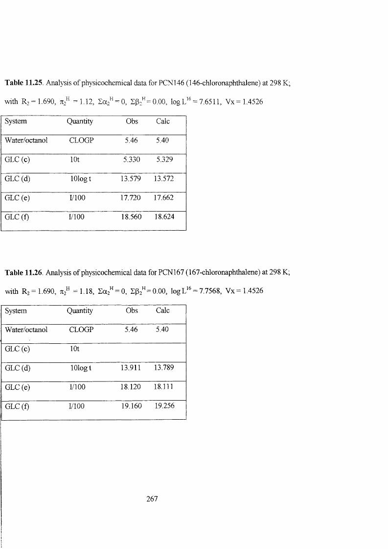
Table 11.25. Analysis of physicochemical data for PCNl 46 (146-chloronaphthalene) at 298 K;
with = 1.690, 712 =1.12, = 0, S |5 / = 0.00, logL
System Quantity Obs Calc
Water/octanol CLOGP 5.46 5.40
GLC (c) lot 5.330 5.329
GLC (d) lOlogt 13.579 13.572
GLC (e) I/lOO 17.720 17.662
GLC (f) I/lOO 18.560 18.624
Table 11.26 Analysis of physicochemical data for PCNl 67
with R2 = 1.690, 7T2 =1.18, Za2^ = 0, XP2 = 0.00, logL
System Quantity Obs Calc
Water/octanol CLOGP 5.46 5.40
GLC (c) lot
GLC (d) lOlogt 13.911 13.789
GLC (e) I/lOO 18.120 18.111
GLC (f) I/lOO 19.160 19.256
16
16 _
267
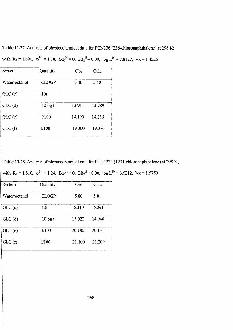
Table 11.27. Analysis of physicochemical data for PCN236 (236-chloronaphthalene) at 298 K;
with Rj = 1.690, =1.18, Sa2“ = 0, Zk^^O.OO, logL'^ = 7.8127, Vx= 1.4526
System Quantity Obs Calc
Water/octanol CLOGP 5.46 5.40
GLC (c) lot
GLC (d) lOlog t 13.911 13.789
GLC (e) LlOO 18.190 18.235
GLC (f) LlOO 19.360 19.376
Table 11.28. Analysis of physicochemical data for PCN 1234 (1234-chloronaphthalene) at 298 K;
with Rj= 1.810, =1.24, Sa2^ = 0, ZPz^^O.OO, log L" = 8.6212, Vx= 1.5750
System Quantity Obs Calc
Water/octanol CLOGP 5.80 5.81
GLC (c) lOt 6.310 6.261
GLC (d) lOlogt 15.022 14.940
GLC(e) LlOO 20.180 20.131
GLC (f) LlOO 21.100 21.209
268

Table 11.29 Analysis of physicochemical data for PCN 1235 (1235-chloronaphthalene) at 298 K;
with R] = 1.810, Tr:"" = 1.24, Ea:"" = 0, = 0.00, logL
System Quantity Obs Calc
Water/octanol CLOGP 5.91 5.81
GLC(c) lOt 6.239 6.202
GLC (d) lOlogt 14.958 14.851
GLC (e) LlOO 20.000 19.953
GLC(f) LlOO 20.920 21.036
Table 11.30. Analysis of physicochemical data for PCN1236 (1236-chloronaphthalene) at 298 K;
with R2 = 1.810, =1.24, Za2^ = 0, % "= 0 .00 . logL'’ = 8.5913, Vx=1.5750
System Quantity Obs Calc
Water/octanol CLOGP 6.05 5.81
GLC (c) lot
GLC (d) lOlogt
GLC(e) LlOO 20.060 20.065
GLC(f) LlOO 21.150 21.145
269
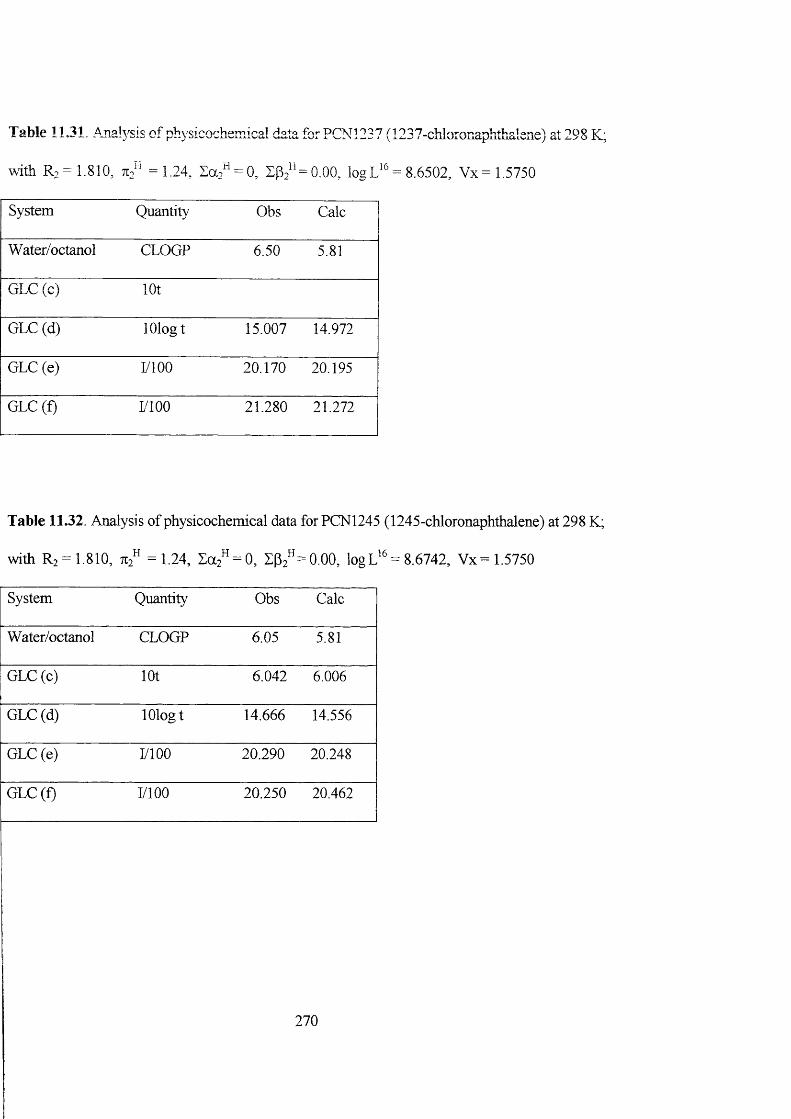
Table 1131. Analysis of physicochemical data for PCNl 237 (1237-cMoronaphthalene) at 298 K;
with R2 = 1.810, 712" =1.24, Eao^^O, % " = 0.00, logL^ = 8.6502, Vx= 1.5750
System Quantity Obs Calc
Water/octanol CLOGP 6.50 5.81
GLC (c) lot
GLC (d) 1 Olog t 15.007 14.972
GLC (e) I/lOO 20.170 20.195
GLC(f) LlOO 21.280 21.272
Table 1132. Analysis of physicochemical data for PCN1245 (1245-chloronaphthalene) at 298 K;
with R2 = 1.810, Ttj" =1.24, r a 2” = 0, ^"^O .OO. logL" = 8.6742, Vx=l,5750
System Quantity Obs Calc
Water/octanol CLOGP 6.05 5.81
GLC (c) lOt 6.042 6.006
GLC (d) lOlogt 14.666 14.556
GLC(e) LlOO 20.290 20.248
GLC(f) LlOO 20.250 20.462
270

Table 11.33. Analysis of physicochemical data for PCNl 246 ( 1246-chloronaphthalene) at 298 K;
with R2 = 1.810, 712 =1.24, Eoi2 = 0, ZP2^=0.00, logL^ = 8.2732, Vx= 1.5750
System Quantity Obs Calc
Water/octanol CLOGP 5.91 5.81
GLC(c) lot 6.042 6.006
GLC (d) lOlogt 14.666 14.556
GLC (e) LlOO 19.500 19.361
GLC(f) LlOO 20.250 20.462
Table 11.34. Analysis of physicochemical data for PCNl 247 (1247-chloronaphthalene) at 298 K;
with R2 = 1.810, 7t2 =1.24, I a 2^ = 0, 2^2^= 0.00, l o g = 8.2732, Vx= 1.5750
System Quantity Obs Calc
Water/octanol CLOGP 5.91 5.81
GLC (c) lot 6.042 6.006
GLC(d) lOlogt 14.666 14.556
GLC (e) LlOO 19.500 19.361
GLC(f) LlOO 20.250 20.462
271

Table 11.35. Analysis of physicochemical data for PCN1248 ( 1248-chloronaphthalene) at 298 K;
with R2 = 1.810, 712" =1.24, Z»]" = 0, Z&" = 0.00, logL“ = 8.7362, Vx= 1.5750
System Quantity Obs Calc
Water/octanol CLOGP 5.91 5.81
GLC (c) lot 6.383 6.345
GLC (d) lOlogt 15.143 15.067
GLC (e) LlOO 20.380 20.385
GLC (f) LlOO 21.410 21.456
Table 11.36. Analysis of physicochemical data for PCNl 256 (1256-chloronaphthalene) at 298 K;
16 _ o CO 1 C \ r „ _ i C 7 C Awith R2 = 1.810, 7T2 = 1.24, Za2^ = 0, Z k"= 0.00, logL
System Quantity Obs Calc
Water/octanol CLOGP 5.91 5.81
GLC (c) lot 6.213 6.188
GLC (d) lOlogt 14.921 14.830
GLC(e) LlOO 19.930 19.910
GLC (f) LlOO 20.920 20.995
272
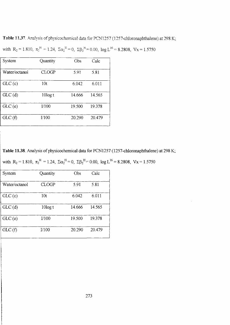
Table 11.37. Analysis of physicochemical data for PCNl 257 (1257-chioronaphthalene) at 298 K;
with Rn = 1.810, 71;” =1.24, Ia.2“ = 0, logL“ = 8.2808, Vx= 1.5750
System Quantit} Obs Calc
Water/octanol CLOGP 5.91 5.81
GLC (c) lOt 6.042 6.011
GLC (d) lOlogt 14.666 14.565
GLC (e) I/lOO 19.500 19.378
GLC(f) I/lOO 20.290 20.479
Table 11.38. Analysis of physicochemical data for PCNl 257
with R2 = 1.810, 712 =1.24, Za2^ = 0, Zp2^^ 0.00, logL
System Quantity Obs Calc
Water/octanol CLOGP 5.91 5.81
GLC(c) lot 6.042 6.011
GLC (d) lOlogt 14.666 14.565
GLC (e) moo 19.500 19.378
GLC(f) I/lOO 20.290 20.479
273
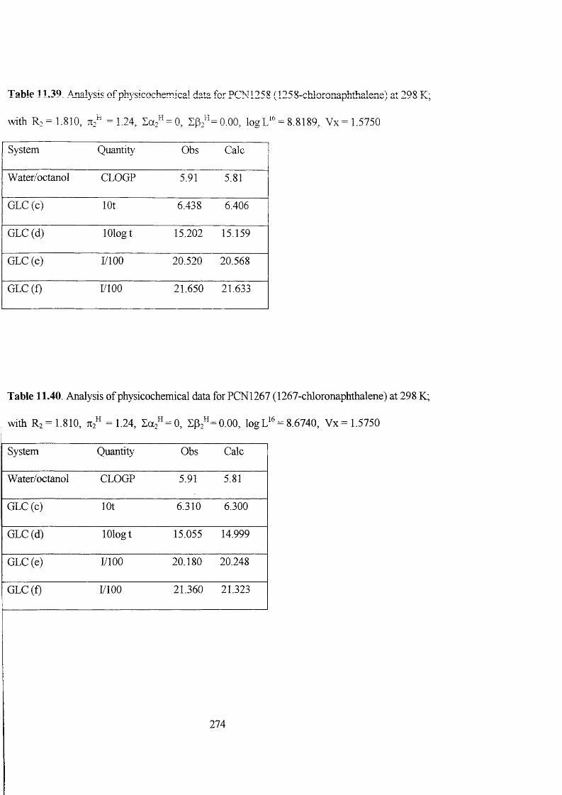
Table 11.39. Analysis of physicochemical data for PCN1258 (1258-chloronaphthalene) at 298 K;
with Ro = 1.810, Ti." = 1.24, = 0 , 1 0 2 '^= 0.00, logL
System Quantit}: Obs Calc
Water/octanoi CLOGP 5.91 5.81
GLC(c) lot 6.438 6.406
GLC(d) lOlogt 15.202 15.159
GLC(e) moo 20.520 20.568
GLC(f) moo 21.650 21.633
Table 11.40. Analysis of physicochemical data for PCN1267 (1267-chloronaphthalene) at 298 K;
with Rî = 1.810, = 1.24, Za2" = 0, % "= 0.00 , log O'* = 8.6740, Vx= 1.5750
System Quantity Obs Calc
Water/octanol CLOGP 5.91 5.81
GLC(c) lOt 6.310 6.300
GLC(d) lOlogt 15.055 14.999
GLC (e) I/lOO 20.180 20.248
GLC(f) I/lOO 21.360 21.323
274

Table 11.41. . jialysis of physicochemical data for PCN1268 (1268-chJoronaphthalene) at 298 K;
Vvdth R] = 1.810, 712' = 1.24, 0.00, logL
System Quantit}' Obs Calc
Water/octanol CLOGP 5.91 5.81
GLC (c) lot 6.438 6.433
GLC (d) lOlogt 15.240 15.198
GLC(e) I/lOO 20.520 20.648
GLC (f) LlOO 21.820 21.711
16
Table 11.42. Analysis of physicochemical data for PCN1278 (1278-chloronaphthalene) at 298 K;
16 _ o T r „ _ i c ^ c Awith R2 = 1.810, 712 =1.24, La2^ = 0, = 0.00, logL
System Quantity Obs Calc
Water/octanol CLOGP 6.05 5.74
GLC (c) lot 6.670 6.650
GLC (d) lOlogt 15.540 15.471
GLC (e) LlOO 21.140 21.361
GLC(f) I/lOO 22.680 22.539
275
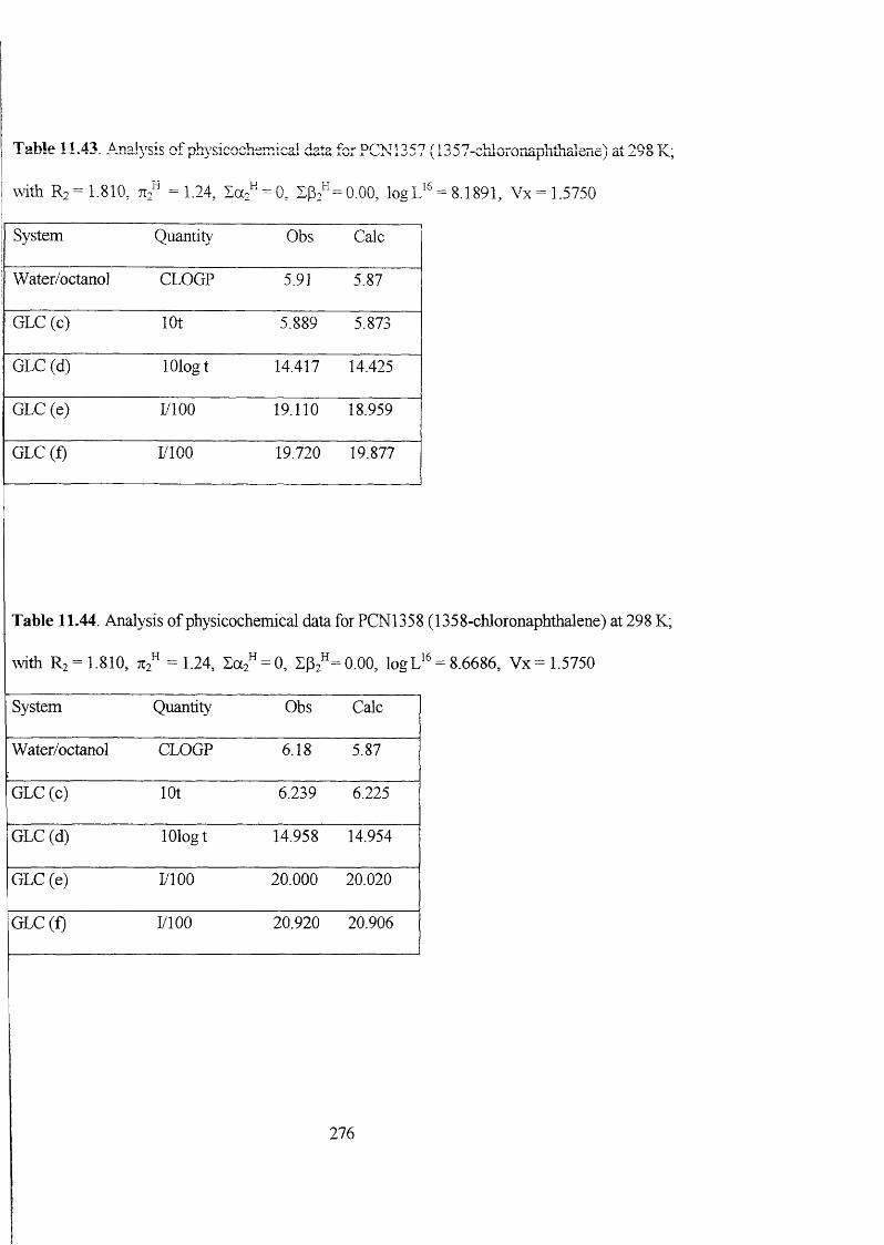
Table 11.43. Amalysis of physicochca-|-v»l/p1 /ipfp JLOX J. Xw'w' /
\Adth Ro = 1.810, TT?" = 1.24, = 0, ZP:" = 0.00, logL'
System Quantity Obs Calc
1 Water/octanol CLOGP 5.91 5.87
1 GLC(c) lot 5.889 5.873
GLC (d) lOlogt 14.417 14.425
GLC (e) LlOO 19.110 18.959
GLC (f) LlOO 19.720 19.877
16
Table 11.44. Analysis of physicochemical data for PCN1358 (1358-chloronaphthalene) at 298 K;
with Rz = 1.810, 7t2 = 1.24, I a 2^ = 0, ^^2»= 0.00, logL
System Quantity Obs Calc
Water/octanol CLOGP 6.18 5.87
GLC(c) lot 6.239 6.225
GLC (d) lOlogt 14.958 14.954
GLC (e) LlOO 20.000 20.020
GLC (f) LlOO 20.920 20.906
16
276

Table 11.45. Analysis of physicochemical data for PCN1367 (1367-chloronaphthalene) at 298 K;
R:= 1.810, =1.24, Zoc2 = 0, % ^=0.00, logL'' = 8.5446, Vx= 1.5750
System Quantity Obs Calc
Water/octanol CLOGP 6.05 5.87
GLC (c) lot
GLC (d) lOlogt 14.812 14.817
GLC (e) LlOO 19.700 19.746
GLC(f) LlOO 20.690 20.640
Table 11.46. Analysis of physicochemical data for PCN1368 (1368-chloronaphthalene) at 298 K;
16 _ o o 1 c t c awith R2 = 1.810, = 1.24, Za2^ = 0. 0.00, logL
System Quantity Obs Calc
Water/octanol CLOGP 6.05 5.87
GLC(c) lOt
GLC (d) lOlogt 14.983 14.947
GLC (e) LlOO 19.930 20.005
GLC(f) LlOO 20.950 20.891
277

Table 11.47. Analysis of physicochemical data for PCN1458 (1458-chloronaphthalene) at 298 K;
with R? = 1.810, 712" = 1.24, = 0, ZP2" = 0.00, logL
System Quantity Obs Calc
Water/octanol CLOGP 6.05 5.87
GLC (c) lOt 6.571 6.568
GLC (d) lOlogt 15.441 15.469
GLC(e) LlOO 20.860 21.053
GLC(f) 1/100 22.120 21.907
16
Table 11.48. Analysis of physicochemical data for PCN1467 (1467-chloronaphthalene) at 298 K;
16 _ o 1 c n c nwith R2 = 1.810, 712” = 1.24, Za;" = 0 , 0.00, logL
System Quantity Obs Calc
Water/octanol CLOGP 5.93 5.87
GLC(c) lOt 6.138 6.126
GLC (d) lOlogt 14.803 14.804
GLC(e) LlOO 19.740 19.720
GLC (f) LlOO 20.590 20.614
278
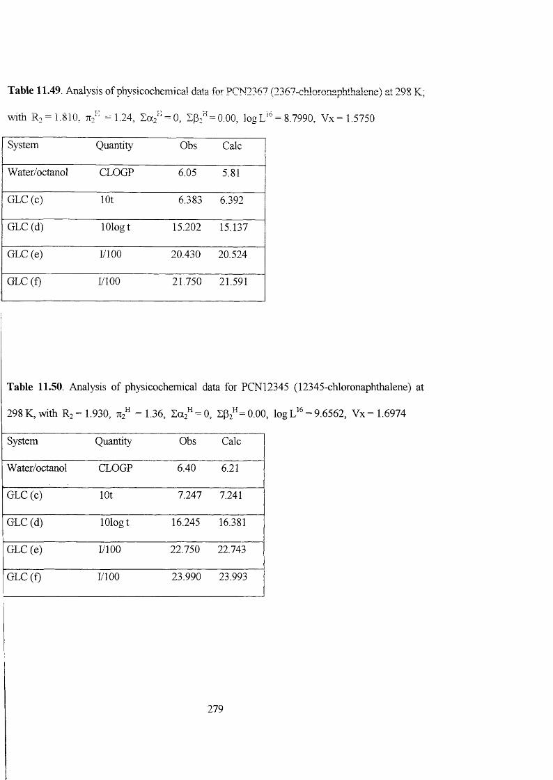
Table 11.49. Analysis of physicochemical data forPCN2367 (2367-chioronaphthalene) at 298 K;
with R] = 1.810, Til" = 1.24, E a /' = 0, = 0.00, logL
System Quantity Obs Calc
Water/octanol CLOGP 6.05 5.81
GLC(c) lOt 6.383 6.392
GLC (d) lOlogt 15.202 15.137
GLC (e) LlOO 20.430 20.524
GLC (f) LlOO 21.750 21.591
Table 11.50. Analysis of physicochemical data for PCN12345 (12345-chloronaphthalene) at
298K, with Rz= 1.930, =1.36. 2a2“ = 0, % "=0.00, logL'^ = 9.6562, Vx= 1.6974
System Quantity Obs Calc
Water/octanol CLOGP 6.40 6.21
GLC(c) lot 7.247 7.241
GLC (d) lOlogt 16.245 16.381
GLC (e) LlOO 22.750 22.743
GLC(f) LlOO 23.990 23.993
279
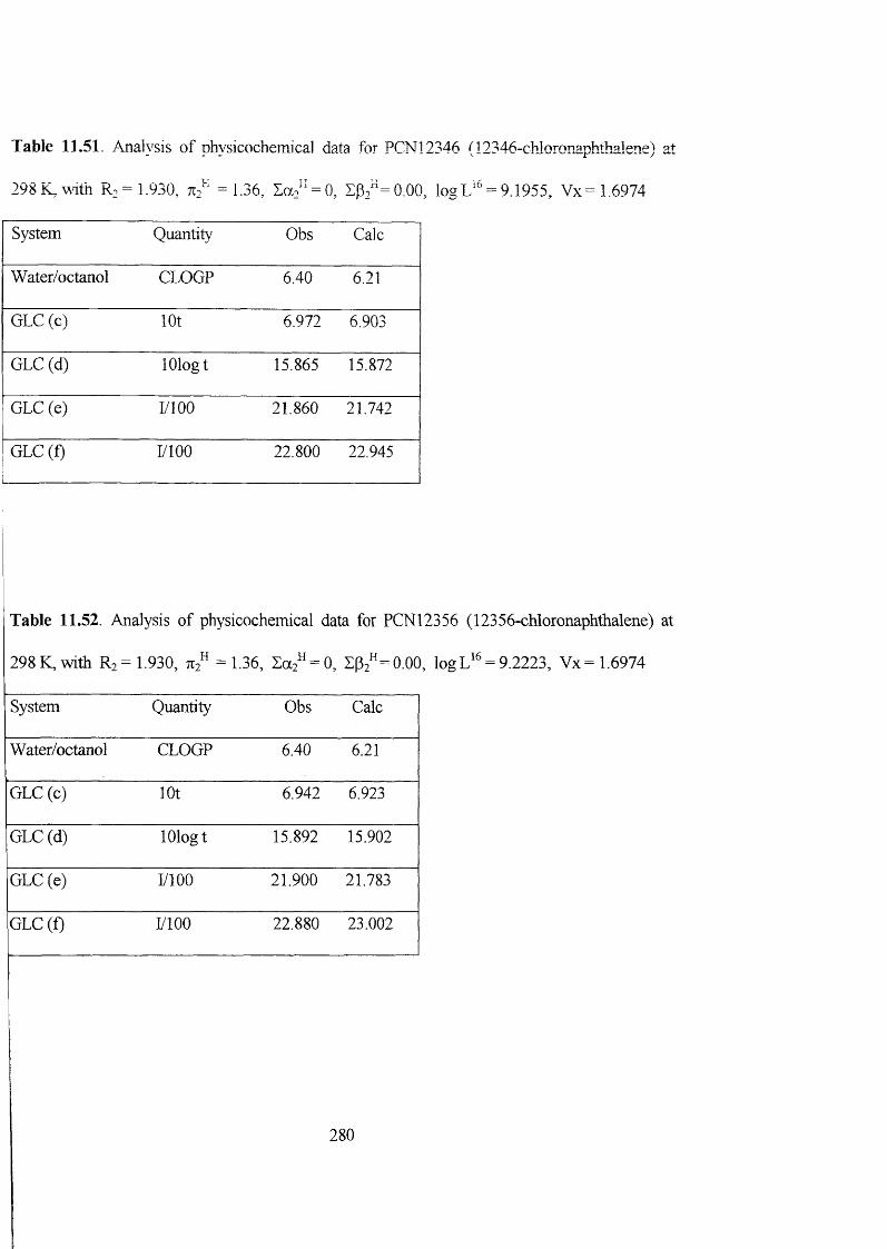
Table 11.51. Analysis of Dhvsicochemical data for PCN12346 (12346-chloronaphthalene) at
298K,with R: = 1.930, 712" =1.36, Za2" = 0, % "=0.00, logL'^ = 9.1955, Vx= 1.6974
System Quantitv' Obs Calc
Water/octanol CLOGP 6.40 6 . 2 1
GLC(c) lot 6.972 6.903
GLC(d) lOlogt 15.865 15.872
GLC (e) I/lOO 21.860 21.742
GLC(f) r/ 1 0 0 22.800 22.945
Table 11.52. Analysis of physicochemical data for PCN12356 (12356-chloronaphthalene) at
298 K, with R2 = 1.930, 712^ = 1.36, Za2^ = 0, % ^=0.00, log L = 9.2223, Vx= 1.6974
System Quantity Obs Calc
Water/octanol CLOGP 6.40 6 . 2 1
GLC (c) lot 6.942 6.923
GLC (d) lOlogt 15.892 15.902
GLC (e) I/lOO 21.900 21.783
GLC(f) I/lOO 22.880 23.002
280
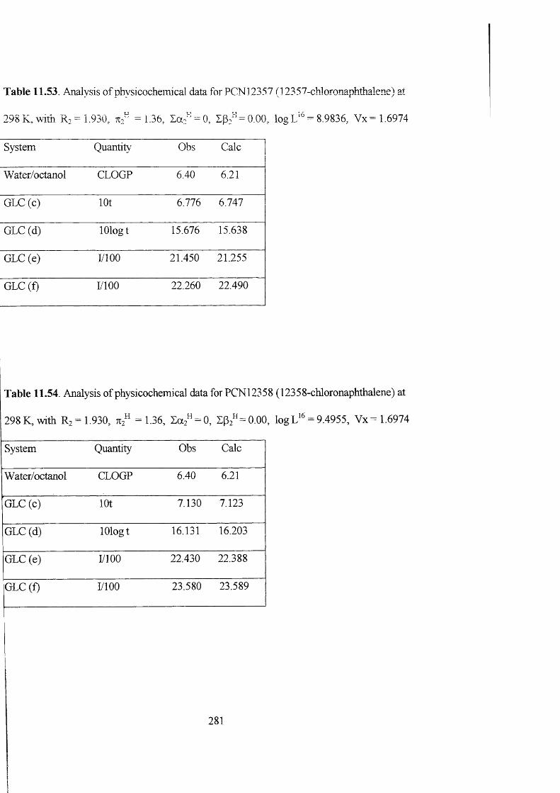
Table 11.53. Analysis of physicochemical data for PCNl 2357 (] 2357-chloronaphthalene) at
298 K, with = 1.930, =1.36, E ar = 0, EP:"=0.00, logL'° = 8.9836, Vx= 1.6974
System Quantity Obs Calc
Water/octanol CLOGP 6.40 6.21
GLC(c) lot 6.776 6.747
GLC (d) lOlogt 15.676 15.638
GLC (e) LlOO 21.450 21.255
GLC (f) LlOO 22.260 22.490
Table 11.54. Analysis of physicochemical data for PCNl 2358 (1235 8-chloronaphthalene) at
1 6 _ n298 K, with 1.930, = 1.36, Za;" = 0, ZP2" = 0.00
System Quantity Obs Calc
Water/octanol CLOGP 6.40 6.21
GLC (c) lot 7.130 7.123
GLC (d) lOlogt 16.131 16.203
GLC (e) LlOO 22.430 22.388
GLC(f) LlOO 23.580 23.589
281

Table 11.55. Analysis of physicochemical data for PCNl 2367 (12367-chloronaphthalene) at
298 K, with R? 1.930, 712- = 1.36, Ea:" = 0, % "=0.00
System Quantity Obs Calc
Water/octanol CLOGP 6.40 6.21
GLC(c) lOt 7.033 7.056
GLC (d) lOlogt 16.033 16.102
GLC (e) LlOO 22.170 22.185
GLC(f) LlOO 23.450 23.391
Table 11.56 Analysis of physicochemical data for PCN12368 (12368-chloronaphthalene) at
298K,with R ,= 1.930, =1.36, Ea2" = 0, SP2" = 0.00, logL" = 9.5432. Vx= 1.697416
System Quantity Obs Calc
Water/octanol CLOGP 6.40 6.21
GLC (c) lOt 7.130 7.158
GLC (d) lOlogt 16.131 16.256
GLC(e) LlOO 22.430 22.493
GLC(f) LlOO 23.830 23.691
282

Table 11.57. Analysis of physicochemical data for PCNl 2378 (12378-chloronaphthalene) at
298fLwith 1.930, Ti," =1.36, Za2" = 0, EP:"=0.00, logL'^ = 9.7920, Vx= 1.6974
System Quantity Obs Calc
Water/octanol CLOGP 6.40 6.21
GLC(c) lot 7.367 7.414
GLC(d) lOlogt 16.421 16.641
GLC (e) I/lOO 23.090 23.265
GLC (f) I/lOO 24.750 24.440
Table 11.58. Analysis of physicochemical data for PCNl 2456 (12456-chloronaphthalene) at
] 6 _ n 11 _ 1298 K, with R2 = 1.930, 712 ~ 1.36, Sa2* = 0, ZP2"=0.0C
System Quantity Obs Calc
Water/octanol CLOGP 6.40 6.21
GLC (c) lot 7.071 7.061
GLC (d) lOlogt 16.058 16.110
GLC (e) I/lOO 22.270 22.201
GLC(f) LlOO 23.360 23.408
283
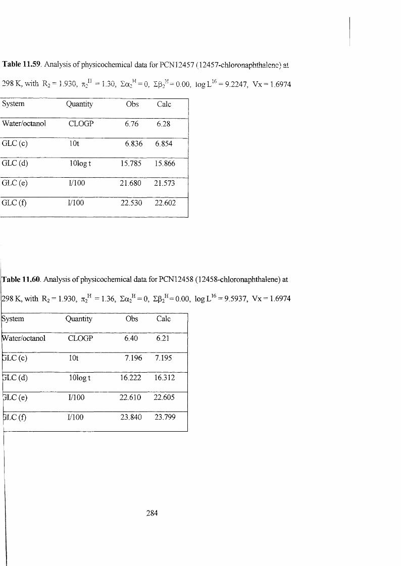
Table 11.59. Analysis of physicochemical data for PCNl 2457 (12457-ch.loronaphthalene) at
298K, Vvith R2 = 1.930, 71,” = 1.30, Eo,” = 0, %"=0.0G
System Qnantit}' Obs Calc
Water/octanol CLOGP 6.76 6.28
GLC(c) lot 6.836 6.854
GLC(d) lOlogt 15.785 15.866
GLC(e) LlOO 21.680 21.573
GLC(f) LlOO 22.530 22.602
Table 11.60. Analysis of physicochemical data for PCNl 2458 (12458-chloronaphthalene) at
298K,with R2 = 1.930, =1.36, Za2" = 0, % "= 0.00 , logL‘° = 9.5937, Vx= 1.697416
System Quantity Obs Calc
Water/octanol CLOGP 6.40 6.21
SLC (c) lot 7.196 7.195
3LC (d) lOlogt 16.222 16.312
j LC (e) LlOO 22.610 22.605
jLC(f) LlOO 23.840 23.799
284
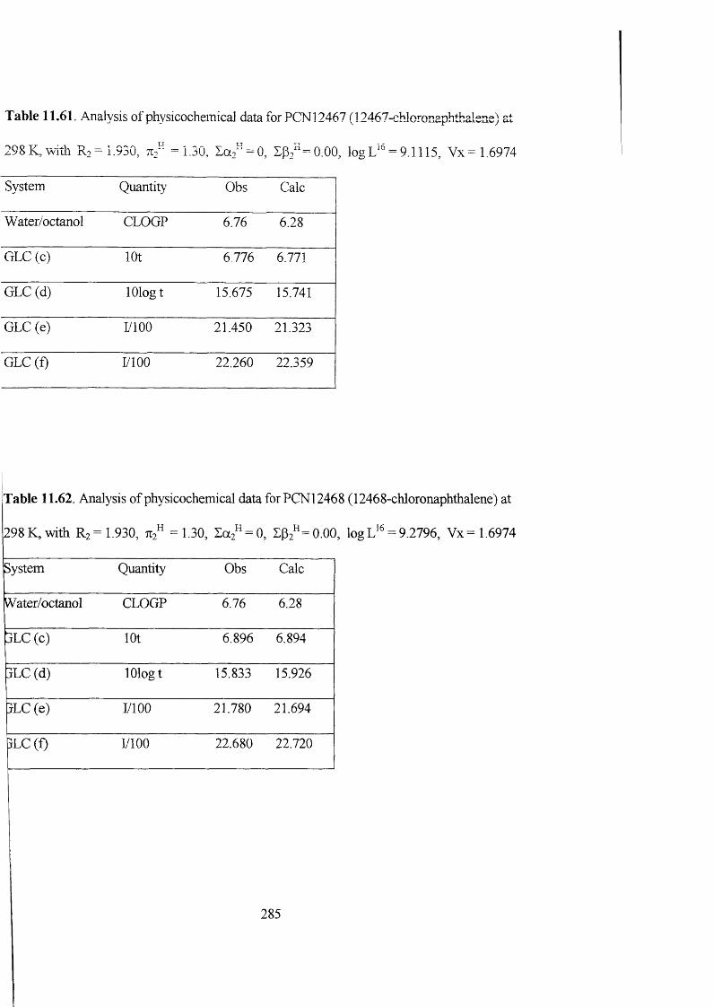
Table 11.61. Analysis of physicochemical data for PCNl 2467 (12467-cbJoronaphthalene) at
298K,with R2 = 1.930, Tii" =1.30, Za2" = 0, Ep2"=0.00, logL'^ = 9.1115, Vx=1.6974
System Quantity Obs Calc
Water/octanol CLOGP 6.76 6.28
GLC (c) lOt 6.776 6.771
GLC (d) lOlogt 15.675 15.741
GLC (e) I/lOO 21.450 21.323
GLC(f) I/lOO 22.260 22.359
Table 11.62. Analysis of physicochemical data for PCNl 2468 (12468-chloronaphthalene) at
298 K, with R2 = 1.930, = 1.30, Dx;" = 0, Ip 2“ = 0.00, log = 9.2796, Vx = 1.6974
System Quantity Obs Calc
Water/octanol CLOGP 6.76 6.28
jLC (c) lot 6.896 6.894
jLC (d) lOlogt 15.833 15.926
3LC(e) I/lOO 21.780 21.694
jLC(f) I/lOO 22.680 22.720
285

Table 11.63. Analysis of physicochemical data for PCNl 2478 (12478-chloronaphthalene) at
298K, with R2 = 1.930, =1.36, Za;" = 0, % "=0.00, logL'^ = 9.4620, Vx= 1.6974
System Quantity Obs Calc
Water/octanol CLOGP 6.64 6.21
GLC (c) lot 7.106 7.099
GLC (d) lOlogt 16.101 16.166
GLC (e) I/lOO 22.350 22.314
GLC(f) 1/100 23.510 23.517
Table 11.64. Analysis of physicochemical data for PCN123456 (123456-chloronaphthalene) at
298 K, with R: = 2.050, =1.42, 1 0 2 “ = 0, ZPz^^O.OO, log L'*= 10.5365, Vx= 1.8198
System Quantity Obs Calc
Water/octanol CLOGP 7.23 6.68
GLC (c) lot 7.952 8.037
GLC (d) lOlogt
GLC (e) I/lOO 24.720 24.798
GLC(f) I/lOO 26.030 25.920
286

Table 11.65. Analysis of physicocheiuical data for PCN123457 (123457-cliloronaplithalene) at
298K ,wth R, = 2.050, =1.42, = i p ” =0.00, logL“ = 10.1808, Vx= 1.8198
System Quantity Obs Calc
Water/octanol CLOGP 7.23 6.68
GLC (c) lot 7.708 7.776
GLC (d) lOlogt
GLC (e) LlOO 24.050 24.011
GLC(f) LlOO 25.140 25.157
Table 11.66. Analysis of physicochemical data for PCNl 2345 8 (12345 8-chloronaphthalene) at
298 K, with R: = 2.050, =1.42, 2 )0 2 ” = 0, 1 ^2“ = 0.00, l o g = 10.6570, Vx= 1.8198
System Quantity Obs Calc
Water/octanol CLOGP 7.23 6.68
GLC (c) lot 8.032 8.126
GLC (d) lOlogt
GLC(e) LlOO 24.930 25.065
GLC(f) LlOO 26.350 25.179
287
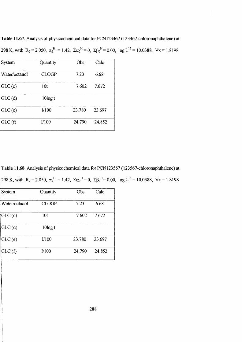
Table 11.67. Analysis of physicochemical data for PCNl23467 (123467-chloronaphthalene) at
298 K, with R2 = 2.050, =1.42, Z%" = 0, Zk"=0.00, log L"^= 10.0388, Vx= 1.8198
System Quantity Obs Calc
Water/octanol CLOGP 7.23 6.68
GLC (c) lOt 7.602 7.672
GLC (d) lOlogt
GLC (e) I/lOO 23.780 23.697
GLC(f) LlOO 24.790 24.852
Table 11.68. Analysis of physicochemical data for PCNl 23567 (123567-chloronaphthalene) at
298 K, with R; = 2.050, =1.42, Za^^^O, SP2“ =0.00, logL"^ = 10.0388, Vx= 1.8198
System Quantity Obs Calc
Water/octanol CLOGP 7.23 6.68
GLC (c) lot 7.602 7.672
GLC (d) lOlogt
GLC (e) I/lOO 23.780 23.697
GLC (f) LlOO 24.790 24.852
288
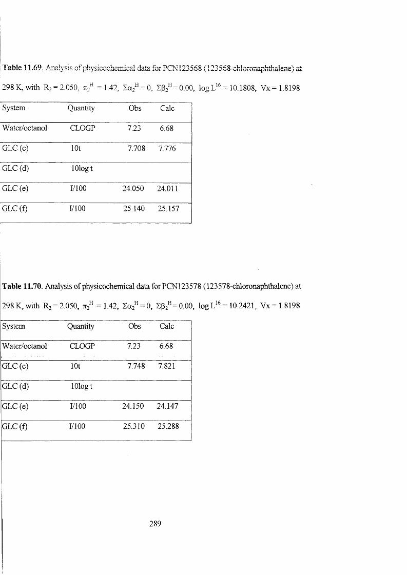
Table 11.69. Analysis of physicochemical data for PCN123568 (123568-chloronaphthalene) at
298K,with = 2.050, ti,” =1.42, 2%" = 0. Zp_” =0.00, logL'*’= 10.1808, Vx=1.8198
System Quantity Obs Calc
Water/octanol CLOGP 7.23 6 . 6 8
GLC (c) lot 7.708 7.776
GLC (d) lOlogt
GLC (e) LlOO 24.050 24.011
GLC(f) LlOO 25.140 25.157
Table 11.70. Analysis of physicochemical data for PCNf123578 (123578-chloronaphthalene) at
298 K, with R2 = 2.050, =1.42, Sa2* = 0, SP2" = 0 .0 0 , logL" =10.2421, Vx= 1.819816
System Quantity Obs Calc
Water/octanol CLOGP 7.23 6 . 6 8
GLC(c) lot 7.748 7.821
GLC (d) lOlogt
GLC(e) LlOO 24.150 24.147
GLC(f) LlOO 25.310 25.288
289
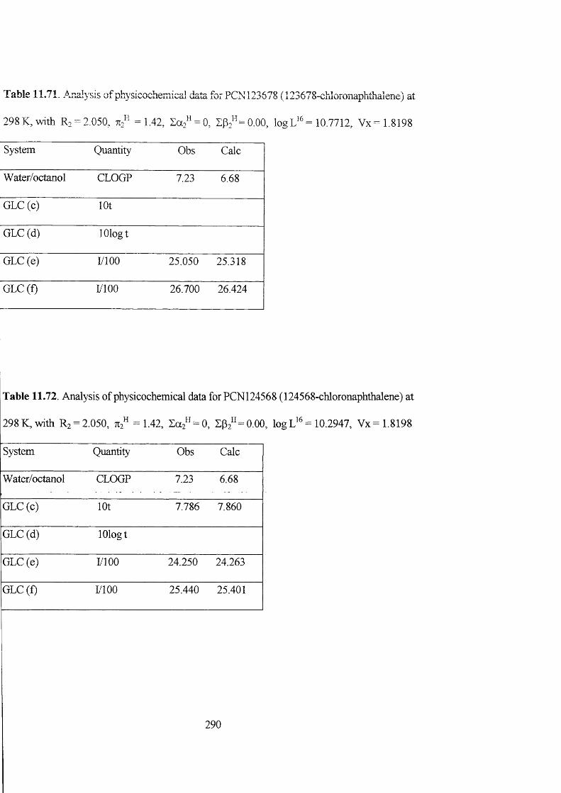
Table 11.71. .Ajialysis of physicochemical data for PCNl23678 (123678-chloronaphthalene) at
298K .with R, = 2.050. %" =1.42, = 0. Zp,” =0.00, logL“ = 10.7712, Vx= 1.8198
System Quantity Obs Cale
Water/octanol CLOGP 7.23 6 . 6 8
GLC (c) lOt
GLC (d) lOlogt
GLC (e) LlOO 25.050 25.318
GLC(f) LlOO 26.700 26.424
Table 11.72. Analysis of physicochemical data for PCNl 24568 (124568-chloronaphthalene) at
298 K, with R; = 2.050, %" =1.42, 1 0 2 ^ = 0, ZP2“ = 0 .0 0 , logL'*= 10.2947, Vx= 1.8198
System Quantity Obs Cale
Water/octanol CLOGP 7.23 6 . 6 8
GLC(c) lOt 7.786 7.860
GLC(d) lOlogt
GLC(e) LlOO 24.250 24.263
GLC(f) LlOO 25.440 25.401
290
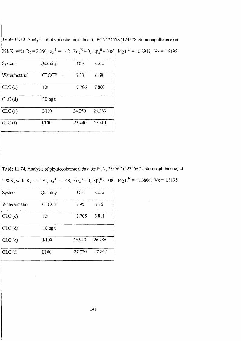
Table 11.73. Analysis of physicochemical data for PCNl 24578 (124578-chloronaphthalene) at
298K,with R2 = 2.050, =1.42, % " = 0.00, logL'^= 10.2947, Vx= 1.8198
System Quantity Obs Calc
Water/octanol CLOGP 7.23 6 . 6 8
GLC (c) lot 7.786 7.860
GLC (d) lOlogt
GLC (e) LlOO 24.250 24.263
GLC(f) LlOO 25.440 25.401
Table 11.74 Analysis of physicochemical data for PCNl 234567 (1234567-chloronaphthalene) at
298K, with 2.170, =1.48, Sa2“ = 0, ZPz^^O.OO, logL'^ = 11.3866, Vx= 1.8198
System Quantity Obs Calc
Water/octanol CLOGP 7.95 7.16
GLC (c) lOt 8.705 8.811
GLC (d) lOlogt
GLC (e) LlOO 26.940 26.786
GLC(f) LlOO 27.720 27.842
291
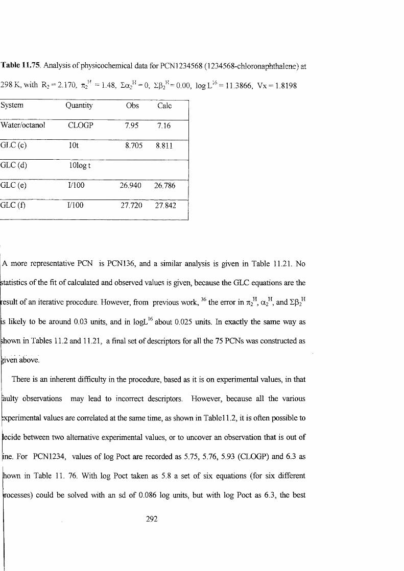
Table 11.75. Analysis of physicochemical data for PCNl 234568 (1234568-chJoronaphthalene) at
298K,^\4th R2 = 2.170, 7:2" =1.48, ^«2 = 0, %"' = 0.00, logU^= 11.3866, Vx= 1.8198
System Quantity Obs Calc
Water/octanol CLOGP 7.95 7.16
GLC (c) lOt 8.705 8.811
GLC (d) lOlogt
GLC (e) LlOO 26.940 26.786
GLC(f) LlOO 27.720 27.842
A more representative PCN is PCNl36, and a similar analysis is given in Table 11.21. No
statistics of the fit of calculated and observed values is given, because the GLC equations are the
result of an iterative procedure. However, from previous work, the error in 712^, ql , and L(32^
is likely to be around 0.03 units, and in logL'^ about 0.025 units. In exactly the same way as
ïhown in Tables 11.2 and 11.21, a final set of descriptors for all the 75 PCNs was constructed as
îiven above.
There is an inherent difficulty in the procedure, based as it is on experimental values, in that
aulty observations may lead to incorrect descriptors. However, because all the various
experimental values are correlated at the same time, as shown in Tablet 1.2, it is often possible to
lecide between two alternative experimental values, or to uncover an observation that is out of
ine. For PCN1234, values of log Poet are recorded as 5.75, 5.76, 5.93 (CLOGP) and 6.3 as
hown in Table 11. 76. With log Poet taken as 5.8 a set of six equations (for six different
irocesses) could be solved with an sd of 0.086 log units, but with log Poet as 6.3, the best
292

solution led to an sd of no less than 0.231 log units. Ver>’ clearly, the smaller log Poet value of 5.8
is more compatible with the other five experimental values.
11.3 Discussion
Although the descriptors change reasonably regularly with the number of chlorine atoms,
there are a number of exceptions. PCNs with chlorine atoms in the 1,8-positions nearly always
have larger log descriptors than the corresponding PCNs without the 8-substituent. In
addition, the increase of 0.06 in 712^ for adjacent chlorine atoms is never more than 0.12, no
matter if there are more than two adjacent interactions. Structure-retention relationships have
been developed for retention indices. I, of 62 PCNs on the DB-5 phase.^ A four-parameter
equation gave r = 0.995 and sd = 17 I; the PCN descriptors were (1) the number of chlorine
atoms, (2) a quantum chemical index obtained by subtracting the atomic heats of formation from
the binding energy, (3) the spatial electronic distribution in a particular carbon atom, and (4) the
minimum electronic orbital population. The correlation equation. Table 1.11 (e), gives r = 0.995
and sd = 23 I using the standard descriptors in eqn. (11.2); note that n = 80 for the equation
because values for the alkanes are included as well as the PCNs
What is more important is to compare physicochemical properties calculated from the
solvation descriptors with what is known in the literature. In Table 11.76 is given a comparison
of calculated log Poet values with the observed values that are available. Lei et al. gave two
sets of log Poet values, both obtained by an HPLC method. In the first procedure, the solute
1,3,5-trichlorobenzene was used as a reference, and the obtained log Poet values were denoted as
‘experimentaP; these are in Table 11.76 under heading (d). In the second procedure, the
Experimental’ log Poet values were regressed against values for standard compounds and a set of
293
log Poet values, referred to as ‘calibrated’ values, were deduced from the regression equation;
log Poet‘calibrated’ = - 1.115 + 1.294 log Poet‘experimental’ (11-6)
These ‘calibrated’ values are in Table 11.76, under heading (e). Unfortunately, as was pointed
out,^’ the fit to the regression line, eqn. (11.6) is very poor for ‘experimental’ values above about
4.5 (corresponding to ‘calibrated’ values above 4.7). Furthermore, eqn. ((11.6) has a very large
intercept-if the regression line was forced through the origin, then the “calibrated’ values would
be very close to the ‘experimental’ ones at high log Poet values. Interestingly, the calculated
values are extraordinarily close to the ‘experimental’ ones. The calculated values using mobile
order theory, MOD, are also very close to the ‘experimental’ values, see Table 11.76. This
difficulty over the ‘calibrated’ and ‘experimental’ values applies only tto the more lipophilic
PCNs. Up to and including the pentachloronaphthalenes, there is general agreement between all
the log Poet values shown in Table 11.76.
There is also a recorded value for the water-hexane partition coeffi cient for PCNl2345678,
6.00 as log P6, but this seems far too small to be realistic. The MOD method also leads to a
low value of 6.70 which is much lower than the predicted MOD value o f 7.35 for log Poet. On
the other hand, the descriptors for PCN12345678 can be used, together with the regression
coefficients in Table 11.1, to predict a value of 8.00 for log P . This value is quite compatible
Mth the value of 7.63 for log Poet.
294
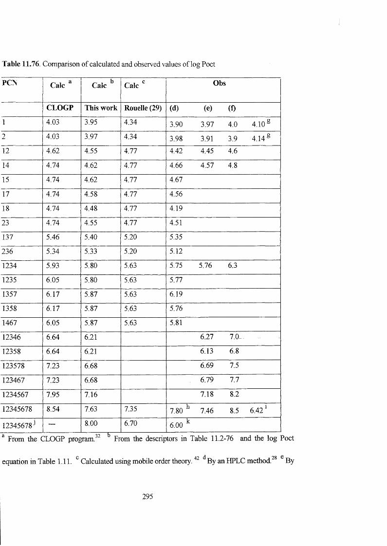
Table 11.76. Comparison of calculated and observed values of log Poet
PCN Calc ^ Calc ^ Calc Obs
CLOGP This work Rouelle (29) (d) (e) (f)
1 4.03 3.95 4.34 3.90 3.97 4.0 4.10^2 4.03 3.97 4.34 3.98 3.91 3.9 4.14^12 4.62 4.55 4.77 4.42 4.45 4.6
14 4.74 4.62 4.77 4.66 4.57 4.8
15 4.74 4.62 4.77 4.67
17 4.74 4.58 4.77 4.56
18 4.74 4.48 4.77 4.19
23 4.74 4.55 4.77 4.51
137 5.46 5.40 5.20 5.35
236 5.34 5.33 5.20 5.12
1234 5.93 5.80 5.63 5.75 5.76 6.3
1235 6.05 5.80 5.63 5.77
1357 6.17 5.87 5.63 6.19
1358 6.17 5.87 5.63 5.76
1467 6.05 5.87 5.63 5.81
12346 6.64 6.21 6.27 7.0--
12358 6.64 6.21 6.13 6.8
123578 7.23 6.68 6.69 7.5
123467 7.23 6.68 6.79 7.7
1234567 7.95 7.16 7.18 8.2
12345678 8.54 7.63 7.35 7.80 ^ 7.46 8.5 6.42 '
12345678^ — 8.00 6.70 6.00 ^
From the CLOGP program. From the descriptors in Table 11.2-76 and the log Poet
42 d 28 eequation in Table 1.11. Calculated using mobile order theory. By an HPLC method. By
295

an HPLC method.^ ‘Calibrated values’ by the HPLC met hod. ^ Recommended va lues . ^ A
value derived from the given HPLC data in ref c. A ‘shake-flask’ va l ue . ^ Values in this row
for water-hexane partitions. Observed ‘shake-flask’ value." ^
296
11.4 References
I. F. Kover, Environmental Hazard Assessment Report: Chlorinated naphthlenes. EPA 560/8-75-
001, Us Environmental Protection Agency, Washington, DC.
2 K. Kannan, T. Imagawa, A. L .Blankenship and J P. Giesy, Environ. Sci.Technol., 1998,Vol.
. 32,2507.
3. J. Falandysz, M. Kawano, M. Ueda, M. Matsuda, K. Kannan, J. P. Giesy and T. Wakimoto,
J. Environ. Sci. Health, 2000, Vol. A35,281.
4. F. A. Beland, R. D. Greer. J. Chromatogr., 1973, Vol. 84, 59.
5. J. Falandysz, Environ. Pollution, 1998, Vol. 101,77.
6. M. J. Crookes, P. D. Howe, Environmental Hazard Assessment: Halogenated Naphthalenes;
Report TSD/13 ; Department of the Environment: London, 1993.
7. U. Jamberg, L. Aplund, C. de Wit, A. K. Grafstrom, P. Haglund, B. Jansson, K. Lexen, M.
Strandell, M. Olsson, B. Jonsson, Environ. Sci. Technol., 1993, Vol. 27,1364.
8. B. Jansson, R. Andersson, L. Asplund, K. Litzen,, K. Nylund, U. Sellstrom, U.-B. Uvemo,
C. Wahlberg, U. Wideqvist, T. Odsjo, M. Olsson, Environ. Toxicol. Chem., 1993, Vol.
12,1163.
9. T. Hamer, T. F. Bidleman, Atoms. Environ. 1997, Vol. 31,4009.
10. T. Hamer, H. Kylin, T. F. Bidleman, C. Halsall, W. M. J. Strachan, L. A. Barrie, Felin,
Environ. Sci. Technol., 1998, Vol. 32,3257.
II. J.Falandysz, C. Rappe, Environ. Sci. Technol. 1996. Vol. 30,3362.
12. U. Jamberg, L. Asplund, C. de Wit, A-L. Egeback, U. Wideqvist, E. Jakobsson, Arch.
Environ. Contam. Toxicol. 1997, Vol. 32,232.
13. D. T. Williams, B. Kennedy, G. L. LeBel, Chemosphere., 1993, Vol. 27,795.
297

14. C. Weistrand, K. Noren, A. Nilsson, Environ. Sci. Pollut. Res. 1997, Vol. 4,2.
15. A. Lunden, K. Noren, Arch. Environ. Contam. Toxicol. 1998, Vol. 34,414.
16. L. Asplund, Ph.D Thesis, Department of Environmental Chemistry Stockholm University
Sweden, 1994.
17. K. Kannan, K. A. Maruya, S.Tanabe., Environ. Sci. Technol. 1997, Vol. 31,1483.
18. K. Kannan, H. Nakata, R. Stafford, G. R. Masson, S. Tanabe, Giesy, J. P. Environ. Sci.
Technol. 1998, Vol. 32,1214.
19. E. T. Furlong, D. S. Carter, R. A. Hites, J. Great Lakes RES., 1988, Vol. 14,489.
20. D. T. Williams, B. Kennedy, G. L. LeBel, Chemosphere 1993, Vol. 27,795.
21. K. Kannan, N. Yamashita, T. Imagawa, W. DeCoen, S. J. Kim, R. M. Day, C. L. Summer,
Giesy, J. P. Environ. Sci. Technol. 2000, Vol. 34, 566.
22. D. L. Villeneuve, K. Kannan, J. S. Khim, J. Falandysz, V. A. Nikiforov, A. L. Blankenship
and J. P. Giesy, Arch. Environ. Contam. Toxicol., 2000, Vol. 39,273.
23. A. L Blankenship, K. Kannan, S. A. Villalobos, D. L. Villeneuve, J. Falandysz,
T. Imagawa, E. Jakobsson and J.P. Giesy, Environ. Sci. Technol., 2000, Vol. 34,3153.
24. J. Falandysz and C. Rappe,. Chemosphere, 1997, Vol.35,1737.
25. B. Gevao, T. Hamer and K.C Jones, Environ. Sci. Technol., 2000, Vol. 34, 33; T.
Hamer, R. G. M.Jones andK. C. Jones, Environ. Sci. Technol., 2000, Vol. 34,3137
26. N. Yamashita, K. Kannan, T.Imagawa, D. L.Villeneuve, S.Hashimoto, AMiyazaki and
J. P. Giesy, Environ. Sci. Technol., 2000, Vol.34,3560.
27. U. A. Th. Brinkman and G. de Vries,. J. Chromatogr., 1979, Vol. 169,167.
28. A. Opperhuizen, Toxicol. Environ. Chem., 1987, Vol. 15,249.
29. M. Schneider, L. Stieglitz, R.Will and G.Zwick, Chemosphere, 1998, Vol.37,2055.
298
30. J. Olivero andK. Kannan, J. Chromatogr. A, 1999, Vol. 849, 621.
31. Y. D. Lei, F. Wania, W. Y. Shiu andD. G. B. Boocock, J. Chem. Eng. Data, 2000, Yol.45,
738.
32. A. J. Leo, Med Chem 2000, The Medicinal Chemistry Project, Pomona College, Claremont,
CA91711.
33. T .Hamer and T. F. Bidleman, J. Chem. Eng. Data, 1998, Vol. 43,40.
34. M. H. Abraham, Chem. Soc.Rev., 1993, Vol.22, 73.
35. M. H. Abraham, P. L. Grellier and 35 R. A. McGill, J. Chem. Soc., Perkin Trans.2, 1987,
797
36. M. H, Abraham, R. Kumarsingh, J. E. Cometto-Muniz, W. S. Cain, M. Roses, E. Bosch and
M. L. Diaz, J. Chem. Soc., Perkin Trans.2, 1998, 2405.
37. M. H. Abraham, H. S. Chadha, G. S. Whiting and R. C. Mitchell, J. Pharm. Sci., 1994, Vol.
& 1085.
38. M. H. Abraham, J. Andonian-Haftvan, G. S. Whiting, A. Leo and R. W. Taft, J. Chem. Soc.,
Perkin Trans.2, 1994,1777.
39. C. E. Green, M. H. Abraham, W. E. Acree, Jr., K. M. De Fina, and T L. Sharp, Pest Manag.
. Sci. 2000, Vol. 56,1043.
40. M. H. Abraham and J. .Le, J. Pharm. Sci., 1999, Vol. 88, 868.
41. R. M. Stevenson and S. Malinowski, Handbook of the themodynamics of organic
compounds, Elsevier, New York, 1987.
42. P. Ruelle, Chemosphere, 2000, Vol. 40,457.
43. F. A. P. C. Gobas, J. M Lahittete, G. Garofalo, W. Y. Shiu and D. Mackay, J. Pharm. Sci.,
1988,Vol. 77,265.
299
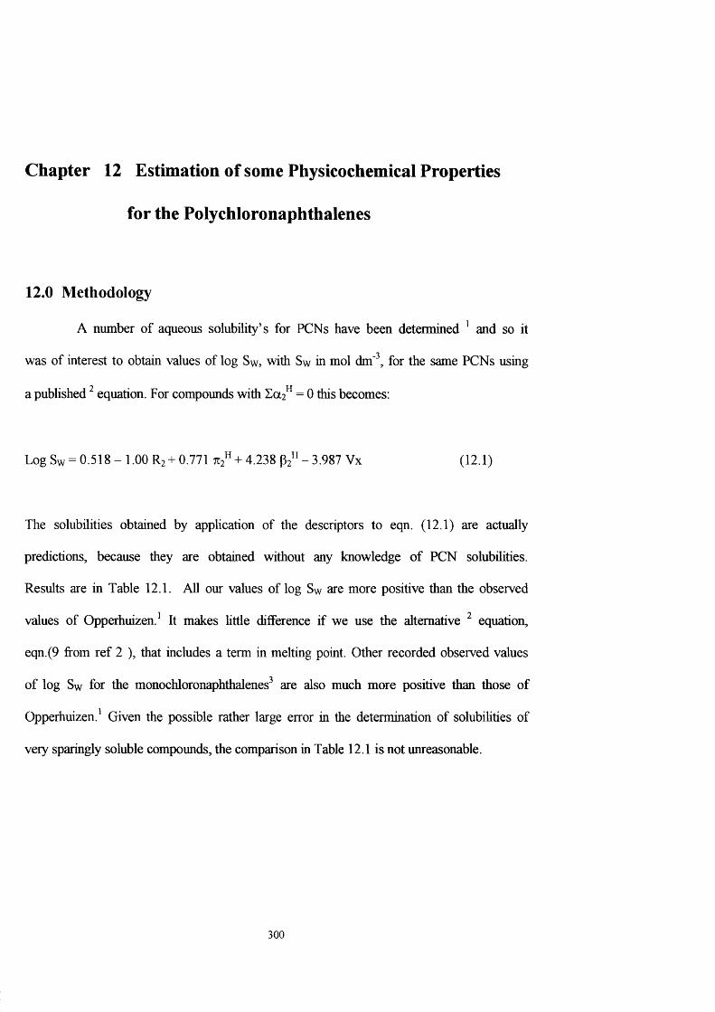
Chapter 12 Estimation of some Physicochemical Properties
for the Polychloronaphthalenes
12.0 Methodology
A number of aqueous solubility’s for PCNs have been determined ’ and so it
was of interest to obtain values of log Sw, with Sw in mol dm' , for the same PCNs using
a published equation. For compounds with = 0 this becomes:
Log Sw = 0.518 - 1.00 R2 + 0.771 + 4.238 P2" - 3.987 Vx (12.1)
The solubilities obtained by application of the descriptors to eqn. (12.1) are actually
predictions, because they are obtained without any knowledge of PCN solubilities.
Results are in Table 12.1. All our values of log Sw are more positive than the observed
values of Opperhuizen.’ It makes httle difference if we use the alternative equation,
eqn.(9 from ref 2 ), that includes a term in melting point. Other recorded observed values
of log Sw for the monochloronaphthalenes are also much more positive than those of
Opperhuizen.’ Given the possible rather large error in the determination of solubihties of
very sparingly soluble compounds, the comparison in Table 12.1 is not unreasonable.
300

Table 12.1. Comparison of predicted (this298 K
work) and observed solubilities, as log Sw at
PCN Fred " Obs "1 -4.35 -4.75 (-3.93)"
2 -4.39 -5.25 (-4.14) "
12 -5.12 -6.16
14 -5.16 -5.80
15 -5.16 -5.70
17 -5.12 -5.92
18 -5.03 -5.52
23 -5.12 -5.36
137 -6.11 -6.55
236 -6.06 -7.14
1234 -6.63 -7.80
1235 -6.63 -7.86
1357 -6.67 -7.82
1358 -6.67 -7.51
1467 -6.67 -7.52
12345678 -8.83 -9.70
^Predicted values from PCN descriptors and eqn.(12.1). Observed values. Observed values.^
It is also of interest to see if the descriptors in eqn. (11.2) that reproduce the various
GLC retention data do also reproduce the observed gas-dry octanol partition coefficients.
Details are in Table 12.2; the agreement is excellent. Although this does not verify either
our calculations or the accuracy of the data, it certainly indicates that there is an
extraordinary self-consistency in the observed values."
301
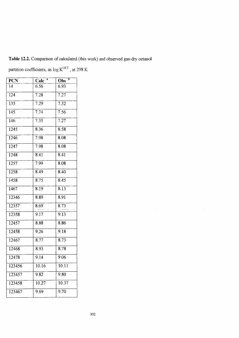
Table 12.2. Comparison of calculated (this work) and observed gas-dry octanol
partition coefficients, as log , at 298 K
PCN Calc ' Obs "14 6.56 6.93
124 7.28 7.27
135 7.29 7.32
145 7.74 7.56
146 7.35 7.27
1245 8.36 8.58
1246 7.98 8.08
1247 7.98 8.08
1248 8.41 8.41
1257 7.99 8.08
1258 8.49 8.40
1458 8.75 8.45
1467 8.19 8.13
12346 8.89 8.91
12357 8.69 8.73
12358 9.17 9.13
12457 8.88 8.86
12458 9.26 9.18
12467 8.77 8.73
12468 8.93 8.78
12478 9.14 9.06
123456 10.16 10.11
123457 9.82 9.80
123458 10.27 10.37
123467 9.69 9.70
302
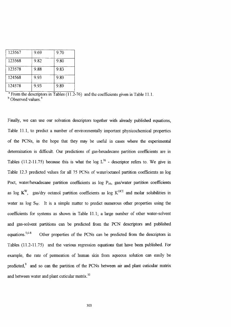
123567 9.69 9.70
123568 9.82 9.80
123578 9.88 9.83
124568 9.93 9.89
124578 9.93 9.89
From the descriptors in Observed values/
ables (11.2-76) and the coefficients given in Table 11.1.
Finally, we can use our solvation descriptors together with already published equations.
Table 11.1, to predict a number of environmentally important physicochemical properties
of the PCNs, in the hope that they may be usefiil in cases where the experimental
determination is difBcult. Our predictions of gas-hexadecane partition coefficients are in
Tables (11.2-11.75) because this is what the log - descriptor refers to. We give in
Table 12.3 predicted values for all 75 PCNs of water/octanol partition coefficients as log
Poet, water/hexadecane partition coefficients as log Pi6, gas/water partition coefficients
as log K^, gas/dry octanol partition coefficients as log and molar solubihties in
water as log Sw- It is a simple matter to predict numerous other properties using the
coefficients for systems as shown in Table 11.1; a large number of other water-solvent
and gas-solvent partitions can be predicted fi*om the PCN descriptors and published
e q u a t i o n s . O t h e r properties of the PCNs can be predicted fi'om the descriptors in
Tables (11.2-11.75) and the various regression equations that have been pubhshed. For
example, the rate of permeation of human skin from aqueous solution can easily be
predicted,^ and so can the partition of the PCNs between air and plant cuticular matrix
and between water and plant cuticular matrix.
303
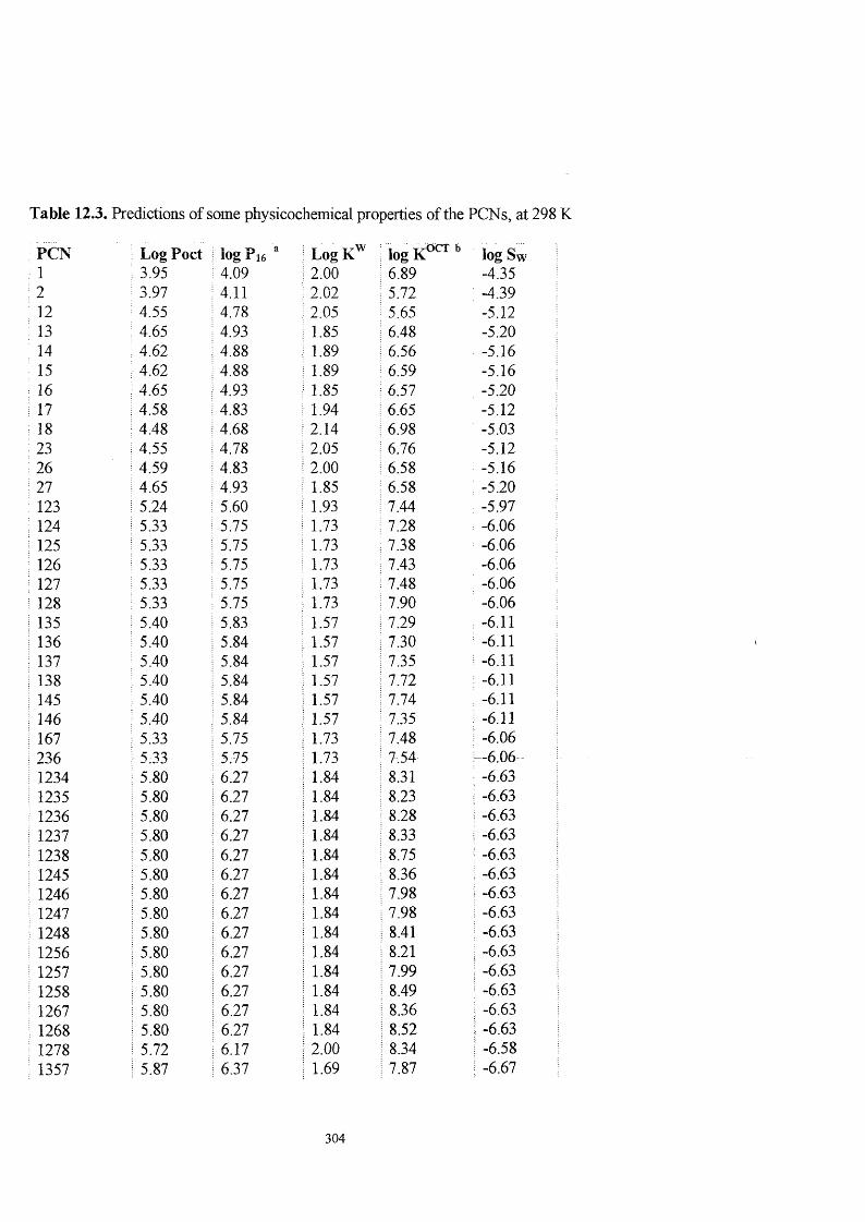
Table 12.3. Predictions of some physicochemical properties of the PCNs, at 298 K
PCN Log Poet iogPi6 ^ LogK^ log ^ log Sw! 1 3.95 4.09 2.00 6.89 -4.35: 2 3.97 4.11 2.02 5.72 -4.39: 12 4.55 4.78 2.05 5.65 -5.12: 13 4.65 4.93 1.85 6.48 -5.20: 14 4.62 4.88 1.89 6.56 -5.16
15 4.62 4.88 1.89 6.59 -5.1616 4.65 4.93 1.85 6.57 -5.20
; 17 4.58 4.83 1.94 6.65 -5.12; 18 4.48 4.68 2.14 6.98 -5.03: 23 4.55 4.78 2.05 6.76 -5.12: 26 4.59 4.83 2.00 6.58 -5.16; 27 4.65 4.93 1.85 6.58 : -5.20: 123 5.24 5.60 1.93 7.44 -5.97: 124 5.33 5.75 1.73 7.28 -6.06i 125 5.33 5.75 1.73 7.38 -6.06; 126 5.33 5.75 1.73 7.43 -6.06; 127 5.33 5.75 1.73 7.48 -6.06; 128 5.33 5.75 1.73 7.90 -6.06; 135 5.40 5.83 1.57 7.29 : -6.11; 136 5.40 5.84 1.57 7.30 -6.11: 137 5.40 5.84 1.57 7.35 : -6.11; 138 5.40 5.84 1.57 7.72 : -6.11; 145 5.40 5.84 1.57 7.74 ; -6.11! 146 5.40 5.84 1.57 7.35 ; -6.11: 167 5.33 5.75 1.73 7.48 -6.061 236 5:33 5.75 1.73 7.54 :—6.06: 1234 5.80 6.27 1.84 8.31 -6.63; 1235 5.80 6.27 1.84 8.23 : -6.63; 1236 5.80 6.27 1.84 8.28 i -6.63; 1237 5.80 6.27 1.84 8.33 : -6.63; 1238 5.80 6.27 1.84 8.75 ! -6.63i 1245 5.80 6.27 1.84 8.36 : -6.63: 1246 5.80 6.27 1.84 7.98 ; -6.63I 1247 5.80 6.27 1.84 7.98 ! -6.63: 1248 5.80 6.27 1.84 8.41 ! -6.63: 1256 5.80 6.27 1.84 8.21 i -6.63; 1257 5.80 6.27 1.84 7.99 ! -6.63: 1258 5.80 6.27 1.84 8.49 -6.63i 1267 5.80 6.27 1.84 8.36 I -6.63! 1268 5.80 6.27 1.84 8.52 ! -6.63i 1278 5.72 6.17 2.00 8.34 ! -6.58I 1357 5.87 6.37 1.69 7.87 ; -6.67
304
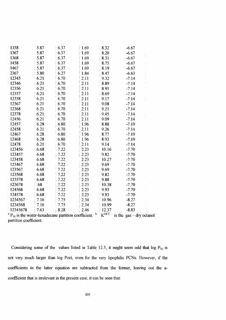
1358 5.87 6.37 1.69 : 8.32 -6.67: 1367 5.87 6.37 1.69 8.20 -6.67; 1368 5.87 6.37 1.69 : 8.31 -6.67: 1458 5.87 6.37 1.69 : 8.75 -6.67: 1467 5.87 6.37 1.69 ; 8.19 -6.672367 5.80 6.27 1.84 ; 8.47 -6.63
: 12345 6.21 6.70 2.11 9.32 -7.14: 12346 6.21 6.70 2.11 ! 8.89 -7.14
12356 6.21 6.70 2.11 8.91 -7.1412357 6.21 6.70 2.11 i 8.69 -7.1412358 6.21 6.70 2.11 9.17 -7.1412367 6.21 6.70 2.11 9.08 -7.1412368 6.21 6.70 2.11 9.21 -7.1412378 6.21 6.70 2.11 9.45 -7.1412456 6.21 6.70 2.11 9.09 -7.1412457 6.28 6.80 1.96 8.88 -7.1912458 6.21 6.70 2.11 9.26 -7.1412467 6.28 6.80 1.96 8.77 -7.1912468 6.28 6.80 1.96 8.93 -7.1912478 6.21 6.70 2.11 9.14 -7.14123456 6.68 7.22 2.23 10.16 -7.70123457 6.68 7.22 2.23 9.82 -7.70123458 6.68 7.22 2.23 10.27 -7.70123467 6.68 7.22 2.23 9.69 -7.70123567 6.68 7.22 2.23 9.69 -7.70123568 6.68 7.22 2.23 9.82 -7.70
: 123578 6.68 7.22 2.23 9.88 -7.70123678 .68 7.22 2.23 10.38 -7.70124568 6.68 7.22 2.23 9.93 -7.70124578 6.68 7.22 2.23 9.93 -7.70
: 1234567 7.16 7.75 2.34 : 10.96 -8.271234568 7.16 7.75 2.34 ; 10.99 -8.2712345678 7.63 8.28 2.46 : 12.37 -8.83
Pi6 is the water-hexadecane partition coefficient. partition coefficient.
^OCT is the gas-
Considering some of the values listed in Table 12.3, it might seem odd that log Pi6 is
not very much larger tlian log Poet, even for the very lipophihc PCNs. However, if the
coefficients in the latter equation are subtracted from the former, leaving out the a-
coefficient that is irrelevant in the present case, it can be seen that;
305
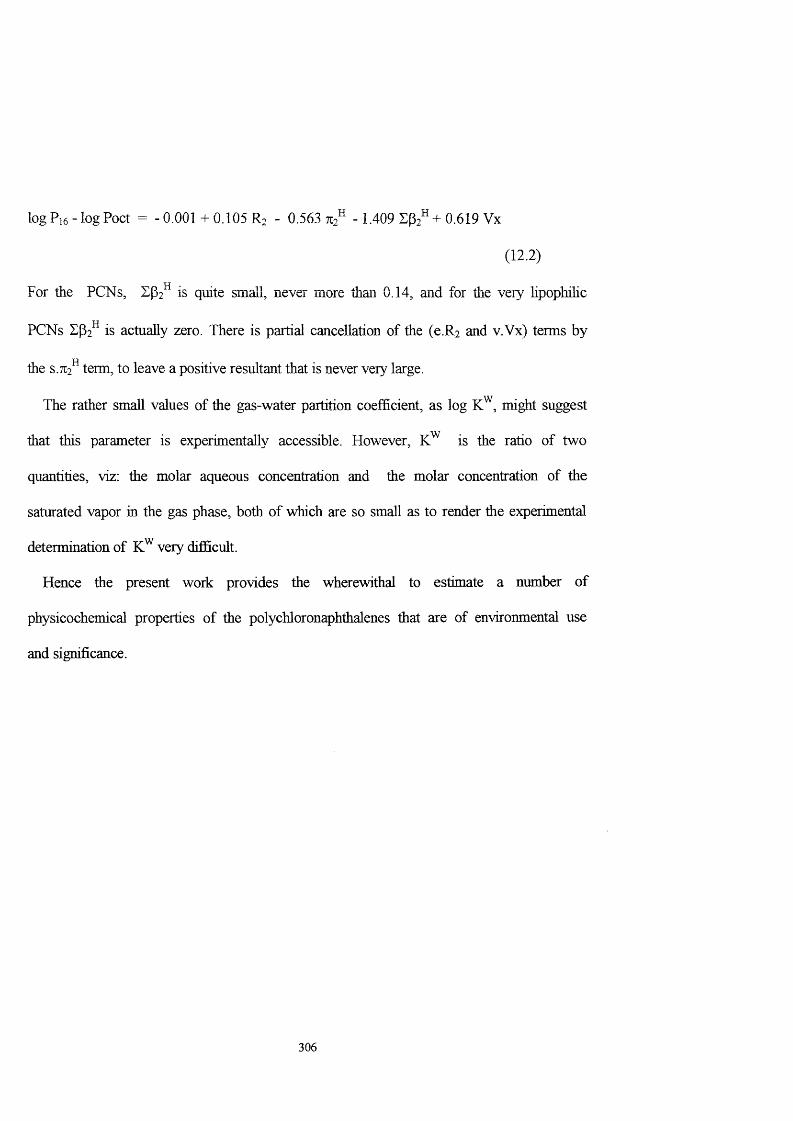
log Pi6-log Poet = -0.001 +0.105 R. - 0.563 7T2 - 1.409 + 0.619 Vx
(12.2)
For the PCNs, is quite small, never more than 0.14, and for the veiy lipophihc
PCNs Zp2^ is actually zero. There is partial cancellation of the (e.R2 and v.Vx) terms by
the s.712 term, to leave a positive resultant that is never very large.
The rather small values of the gas-water partition coefficient, as log K^, might suggest
that this parameter is experimentally accessible. However, is the ratio of two
quantities, viz; the molar aqueous concentration and the molar concentration of the
saturated vapor in the gas phase, botli of which are so small as to render the experimental
determination of very difficult.
Hence the present work provides the wherewithal to estimate a number of
physicochemical properties of the polychloronaphthalenes that are of environmental use
and significance.
306

12.1 R eferen ces
1. A. Opperhuizen, Toxicol. Environ. Chem., 1987, Vol. 15, 249.
2. M. H. Abraham and J. Le, J. Pharm. Sci., 1999, Vol. 88, 868.
3. J. Huuskonen, J. Chem. Inf. Comp. Sci., 2000, Vol. 40, 773.
4. T. Hamer and T.F. Bidleman, J. Chem. Eng. Data, 1998, Vol. 43, 40
5. M. H. Abraham, H. S. Chadha, G. S. Whiting and R.C. Mitchell, J. Pharm. Sci.,
1994, Vol. 83,1085
6. M. H. Abraham, J. A. Platts, A. Hersey, A. J. Leo and R. W. Taft, J. Pharm. Sci.,
1999, Vol. 88,670.
7. M. H. Abraham, J. Le and W. E. Acree, Jr. Coll. Czech. Chem. Comm., 1999,
Vol. 64, 1748.
8. C. E. Green, M. H. Abraham, W. E. Acree, Jr., K.M. De Fina, and T. L. Sharp,
Pest. Manag. Sci., 2000, Vol.56, 1043.
9. M. H. Abraham, F. Martins and R. C. Mitchell, J. Pharm. Pharmacol., 1997, Vol.
49, 858.
10. J. A. Platts andM. H. Abraham, Environ. Sci. Technol., 2000, Vol. 34, 318.
307
Chapter 13 Calculation of the Descriptors for N- Nitrosodialky lamines
13.0 Introduction
N-Nitrosodialkylamines form a large class of genotoxic chemical carcinogens
which occur in the human diet and environment. They can be also formed endogenously
in human body, especially in-tragastrically. Much interest is therefore directed toward
quantitation of the various N-nitroso-organic compounds (NOC) that occur in different
matrices. Twenty-five years after the carcinogenicity of N-nitrosodimethylamine
(NDMA) was first demonstrated/ scientific research in tlie field of N-nitroso
compounds has virtually exploded. More than 1400 papers have been published annually
on the analysis, formation, chemistry, biochemistry, metabolism and biological effects of
N-nitroso compounds. There are many reasons for this development, the potent
carcinogenicity of many N-nitroso compounds, the organ-specificity of this group of
chemical carcinogens, the occurrence of certain N-nitroso compounds in the human
environment and the possibility of an in vivo formation of such potent carcinogens from
precursor amines and nitrosating agents.
Although N-nitroso compounds have mutagenic, and teratogenic activity,
carcinogenicity clearly is the most important biological activity of this group of
compounds. Data on carcinogenicity in experimental animals showed that about 300
different N-nitroso compounds have been tested for carcinogenicity, and about 90% of
these compounds have shown carcinogenic activity.
308
N-nitroso compounds are important because they are often found in a large variety of
food and consumer products such as meat, beer, cosmetics/^ infant pacifiers, and
drug formulations. Their widespread prevalence can be attributed to the relative ease
of formation and the abundance of their amine precursors in the environment. The
occurrence of N-nitroso compounds in these products is of great concern, owing to the
carcinogenic properties that many of them exhibit.
As was shown in the first chapter the term "correlation analysis” was first introduced
in 1966. Since then, interest in this type of study has grown remarkably among both
basic and applied researchers. Today, research on quantitative structure-activity
relationships (QSARs) is given priority by regulatory agencies and industry so that
valuable and cost-effective predictions and environmental chemical.N-nitroso
compounds, in general, and nitrosoamines, in particular, attract a great deal of interest
with regard to QSAR studies for several reasons. (1) They have carcinogenic,’
mutagenic,’* and teratogenic potential in numerous animal species, including
primates. (2) It is well-known that the incidence of cancer in humans is associated
not so much with direct contact with these chemical species as with the formation
mechanisms that occur prior to their action (therefore, this is a subject of utmost
importance in food science and technology As a consequence, in addition to interest
in kinetics, research on the mechanisms of formation of nitroso compounds and their
biochemical decomposition is increasing. (3) It is a proven fact that nitosoamines are
well suited as a subject for free energy correlations.
A number of physicochemical properties of N-nitrosodialkylamines have been
reported. The evaluation of the carcinogenicity of a large number of NOCs towards the
309
liver of the rat/^ also the determination of aqueous solubility, and water-hexane partition
coefficients. Mirvish et al measured water-ether and air-water partition coefficients,
and showed that many N-nitrosodialkylamines were volatilized from aqueous solution.
The water-solvent partition coefficients for fourteen alpihatic N-nitrosodialklamines in
six systems have been detennined;^^ these values were given in tenns of mol fi*action,
but were later converted to the more usual standard state of mol dm' . It is the aim of
this work to obtain, from the available physicochemical data, chemical properties or
‘ descriptors’ that can then be used to estimate all kinds of other physicochemical data,
and especially those employed in environmental analyses.
13.1 Using LFER to calculated the descriptors for N-Nitroso dialkylamines
The majority of the analytical methods for detection of N-nitrosodialkylamines,
have employed gas chromatography (GC) or liquid chromatography (LC) in conjunction
with detectors based on a thermal energy analyzer (TEA), " which relies on the pyrolytic
break down of N-NO moieties to release the nitrosyl radical. The disadvantage of these
techniques, however, is that a subsequent confirmation is needed to ensure that the
method does not give rise to false-positive response. These techniques however, are
often unreliable and can suffer from a significant loss in sensitivity, however, they do
furnish quantitative data that can be used.
The LFER that will be used is the same as that previously introduced in chapter two:
Log SP= c + r. R2 + s.tü2^+ ot. E0 C2 ^ + b.S(32^+v. Vx (13.1)
310
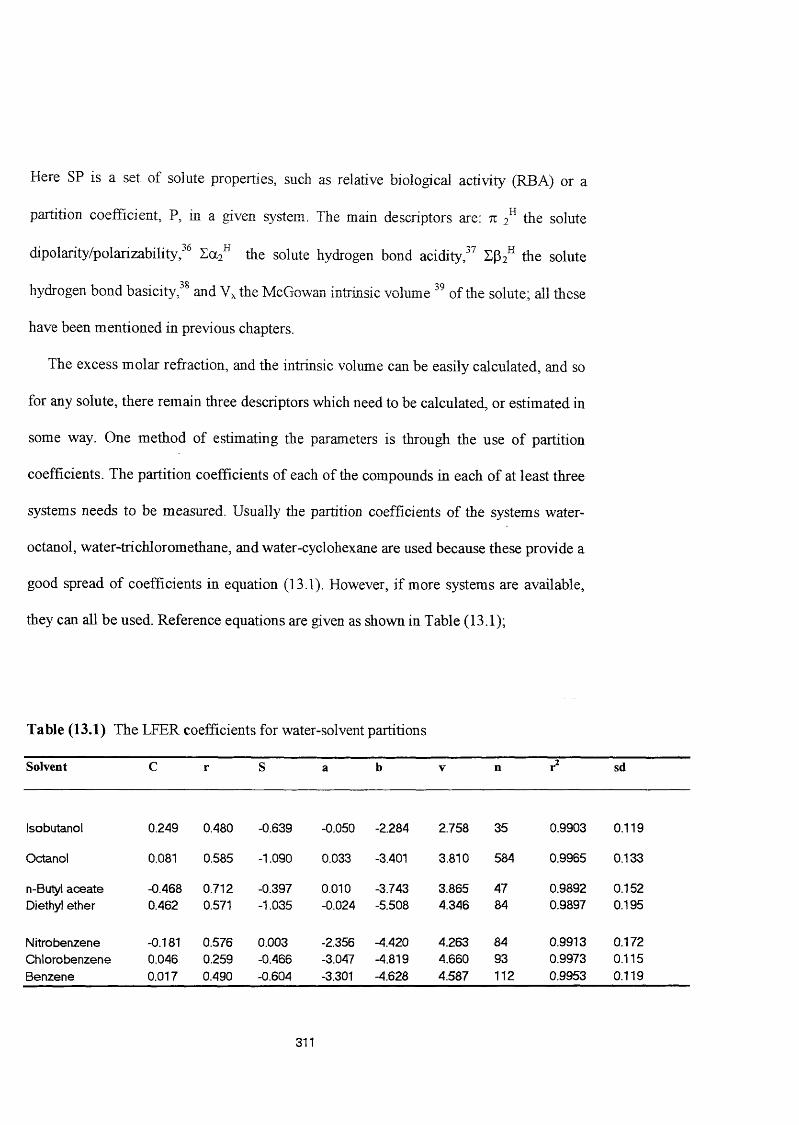
Here SP is a set of solute properties, such as relative biological activity (RBA) or a
partition coefficient, P, in a given system. The main descriptors are; n 2 ^ the solute
dipolarity/polarizability/^ the solute hydrogen bond acidity/^ the solute
hydrogen bond basicity/^ and Vx the McGowan intrinsic volume of the solute; all these
have been mentioned in previous chapters.
The excess molar refraction, and the intrinsic volume can be easily calculated, and so
for any solute, there remain three descriptors which need to be calculated, or estimated in
some way. One method of estimating the parameters is through the use of partition
coefficients. The partition coefficients of each of the compounds in each of at least three
systems needs to be measured. Usually the partition coefficients of the systems water-
octanol, water-trichloromethane, and water-cyclohexane are used because these provide a
good spread of coefficients in equation (13.1). However, if more systems are available,
they can all be used. Reference equations are given as shown in Table (13.1);
Table (13.1) The LFER coefficients for water-solvent partitions
Solvent C r S a b V n sd
Isobutanol 0.249 0.480 -0.639 -0.050 -2.284 2.758 35 0.9903 0.119
Octanol 0.081 0.585 -1.090 0.033 -3.401 3.810 584 0.9965 0.133
n-Bulyl aceate -0.468 0.712 -0.397 0.010 -3.743 3.865 47 0.9892 0.152Diethyl ether 0.462 0.571 -1.035 -0.024 -5.508 4.346 84 0.9897 0.195
Nitrobenzene -0.181 0.576 0.003 -2.356 -4.420 4.263 84 0.9913 0.172Chlorobenzene 0.046 0.259 -0.466 -3.047 -4.819 4.660 93 0.9973 0.115Benzene 0.017 0.490 -0.604 -3.301 -4.628 4.587 112 0.9953 0.119
311
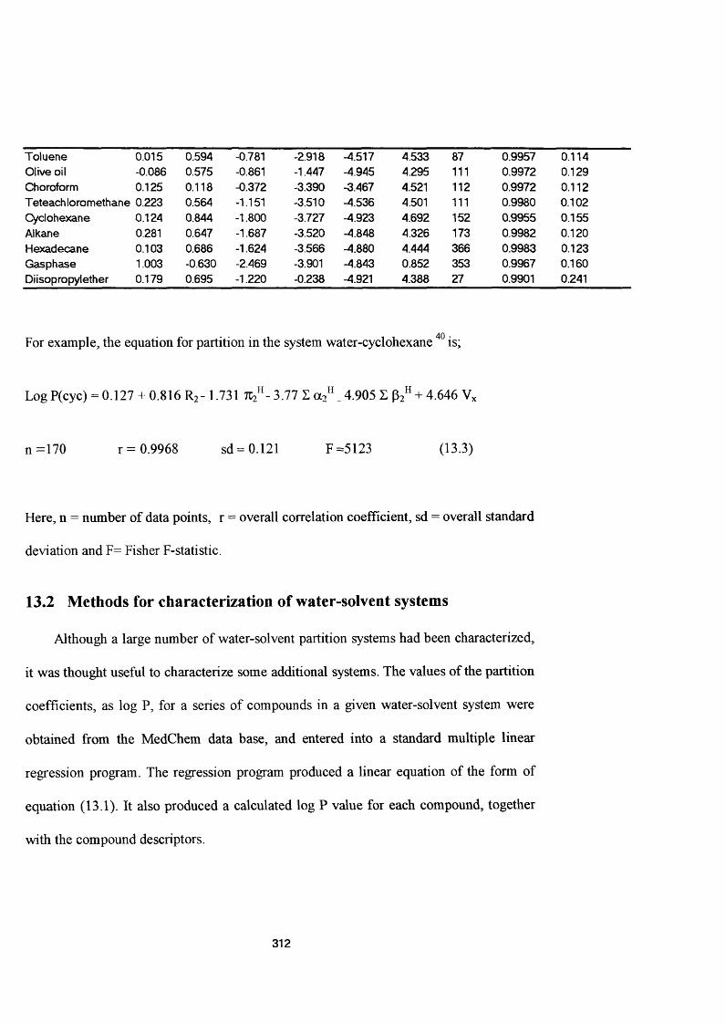
Toluene 0.015 0.594 -0.781 -2.918 -4.517 4.533 87 0.9957 0.114Olive oil -0.086 0.575 -0.861 -1.447 -4.945 4.295 111 0.9972 0.129Choroform 0.125 0.118 -0.372 -3.390 -3.467 4.521 112 0.9972 0.112Teteachloromethane 0.223 0.564 -1.151 -3.510 -4.536 4.501 111 0.9980 0.102Cyclohexane 0.124 0.844 -1.800 -3.727 -4.923 4.692 152 0.9955 0.155Alkane 0.281 0.647 -1.687 -3.520 -4.848 4.326 173 0.9982 0.120Hexadecane 0.103 0.686 -1.624 -3.566 -4.880 4.444 366 0.9983 0.123Gasphase 1.003 -0.630 -2.469 -3.901 -4.843 0.852 353 0.9967 0.160Diisopropylether 0.179 0.695 -1.220 -0.238 -4.921 4.388 27 0.9901 0.241
For example, the equation for partition in the system water-cyclohexane is;
Log P(cyc) = 0.127 + 0.816 R ,- 1.731 It;" -3.77 Z a;" _ 4.905 Z P;" + 4.646 V,
n=170 r = 0.9968 sd = 0.121 F =5123 (13.3)
Here, n = number of data points, r = overall correlation coefficient, sd = overall standard
deviation and F= Fisher F-statistic.
13.2 Methods for characterization of water-solvent systems
Although a large number of water-solvent partition systems had been characterized,
it was thought useful to characterize some additional systems. The values of the partition
coefficients, as log P, for a series of compounds in a given water-solvent system were
obtained from the MedChem data base, and entered into a standard multiple linear
regression program. The regression program produced a linear equation of the form of
equation (13.1). It also produced a calculated log P value for each compound, together
with the compound descriptors.
312
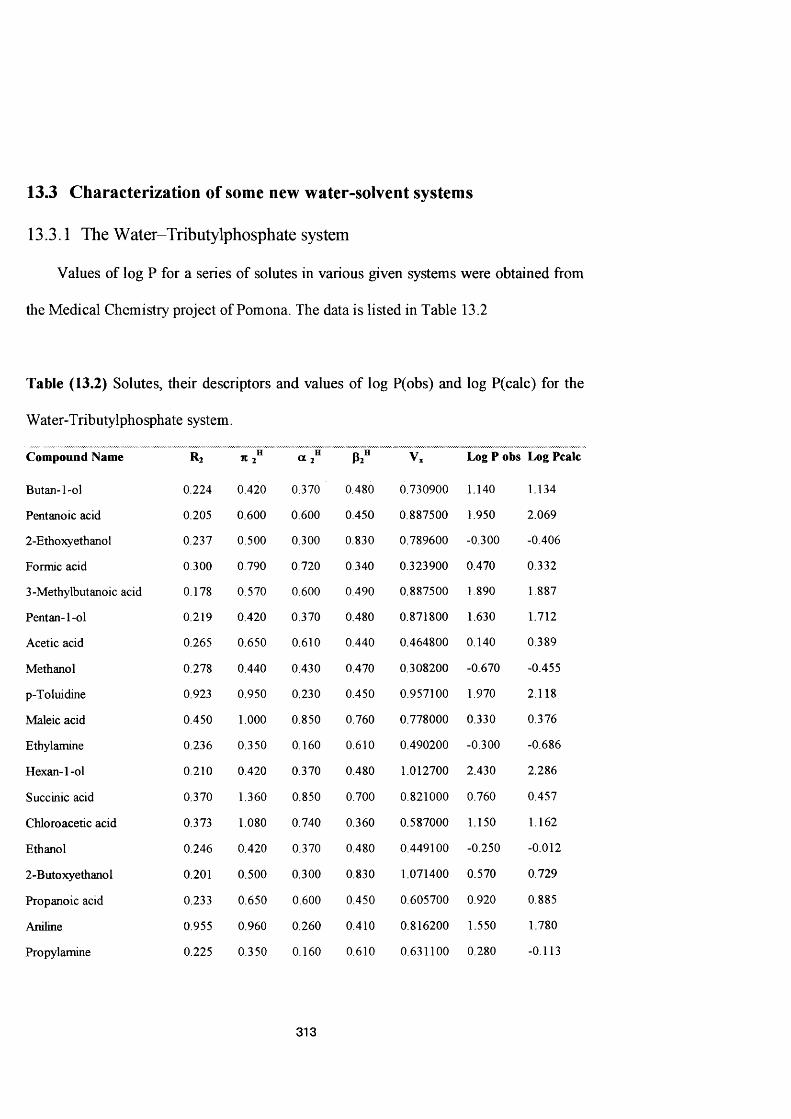
13.3 Characterization of some new water-solvent systems
13.3.1 The Water-Tributylphosphate system
Values of log P for a series of solutes in various given systems were obtained from
the Medical Chemistry project of Pomona. The data is listed in Table 13.2
Table (13.2) Solutes, their descriptors and values of log P(obs) and log P(calc) for the
Water-Tributylphosphate system.
Compound Name R2 it 2 a 2 ** V.
Butan-l-ol 0.224 0.420 0.370 0.480 0.730900
Pentanoic acid 0.205 0.600 0.600 0.450 0.887500
2-Ethoxyethanol 0.237 0.500 0.300 0.830 0.789600
Formic acid 0.300 0.790 0.720 0.340 0.323900
3-Methylbutanoic acid 0.178 0.570 0.600 0.490 0.887500
Pentan-l-ol 0.219 0.420 0.370 0.480 0.871800
Acetic acid 0.265 0.650 0.610 0.440 0.464800
Methanol 0.278 0.440 0.430 0.470 0.308200
p-ToIuidine 0.923 0.950 0.230 0.450 0.957100
Maleic acid 0.450 1.000 0.850 0.760 0.778000
Ethylamine 0.236 0.350 0.160 0.610 0.490200
Hexan-l-ol 0.210 0.420 0.370 0.480 1.012700
Succinic acid 0.370 1.360 0.850 0.700 0.821000
Chloroacetic acid 0.373 1.080 0.740 0.360 0.587000
Ethanol 0.246 0.420 0.370 0.480 0.449100
2-Butoxyethanol 0.201 0.500 0.300 0.830 1.071400
Propanoic acid 0.233 0.650 0.600 0.450 0.605700
Aniline 0.955 0.960 0.260 0.410 0.816200
Propylamine 0.225 0.350 0.160 0.610 0.631100
Log P obs Log Pcalc
1.140
1.950
-0.300
0.470
1.890
1.630
0.140
-0.670
1.970
0.330
-0.300
2.430
0.760
1.150
-0.250
0.570
0.920
1.550
0.280
1.134
2.069
-0.406
0.332
1.887
1.712
0.389
-0.455
2.118
0.376
- 0.686
2.286
0.457
1.162
- 0.012
0.729
0.885
1.780
-0.113
313

Heptan-l-ol 0.211 0.420 0.370 0.480 1.153600 2.740 2.869
Propan-l-ol 0.236 0.420 0.370 0.480 0.590000 0.430 0.562
Butanoic acid 0.210 0.620 0.600 0.450 0.746600 1.410 1.474
2-Aininophenol 1.110 1.100 0.600 0.660 0.874900 1.530 1.337
Oxygen 0.000 0.000 0.000 0.000 0.183000 0.400 0.771
Butyl amine 0.224 0.350 0.160 0.610 0.772000 0.580 0.468
2-Propoxyethanol 0.212 0.500 0.300 0.830 0.930500 0.000 0.156
Argon 0.000 0.000 0.000 0.000 0.190000 0.756 0.799
Carbon dioxide 0.000 0.280 0.050 0.100 0.280900 0.578 0.538
Methane 0.000 0.000 0.000 0.000 0.249500 1.096 1.045
Ethane 0.000 0.000 0.000 0.000 0.390400 1.740 1.627
Propane 0.000 0.000 0.000 0.000 0.531300 2.398 2.209
Butane 0.000 0.000 0.000 0.000 0.672200 2.935 2.790
Ethene 0.107 0.100 0.000 0.070 0.347400 1.317 1.124
Buta-l,3-diene 0.320 0.230 0.000 0.100 0.586200 2.132 2.029
Ammonia 0.139 0.350 0.140 0.620 0.208400 -2.297 -2.001
Phenol 0.805 0.890 0.600 0.300 0.775100 2.650 2.534
2-Methylphenol 0.840 0.860 0.520 0.300 0.916000 3.060 3.059
3-Methylphenol 0.822 0.880 0.570 0.340 0.916000 3.020 2.911
4-Methylphenol 0.820 0.870 0.570 0.310 0.916000 3.000 3.057
2,3 -Dimethylphenol 0.850 0.810 0.530 0.360 1.056900 3.360 3.427
2,4-Dimethylphenol 0.843 0.800 0.530 0.390 1.056900 3.230 3.290
2,5 -Dimethylphenol 0.840 0.790 0.540 0.370 1.056900 3.300 3.403
2,6-Dimethylphenol 0.860 0.790 0.390 0.390 1.056900 3.410 3.118
3,4-DimethylphenoI 0.830 0.860 0.560 0.390 1.056900 3.040 3.270
3,5 -Dimethylphenol 0.820 0.840 0.570 0.360 1.056900 3.220 3.432
2-Ethylphenol 0.831 0.840 0.520 0.370 1.056900 3.450 3.325
3-Ethylphenol 0.810 0.910 0.550 0.370 1.056900 3.380 3.290
4-Ethylphenol 0.800 0.900 0.550 0.360 1.056900 3.200 3.337
4-Propylphenol 0.793 0.880 0.550 0.370 1.197800 3.600 3.884
4-Hydroxybenzoic acid 0.930 0.920 0.870 0.530 0.990400 3.260 2.804
314

The regression for the Water-Tributylphosphate system produced the following equation.
Log P = 0.015 +0.804 R2 -0.862712^+1.389 I - 4.647E ^ 2^+4.129 V,
n = 50 r = 0.9906 sd = 0.200 F = 460.5 (13.4)
For this regression, seven compound data sets were deleted. The compounds that were
deleted were those whose standard deviations of log P calc-log P obs. were greater than
two regression standard deviations. An output for the values of log P obs, log Pcalc, the
coefficients and the statistics are shown in Tables (13.2) and (13.3). The values of the T-
Test for all coefficients were between (0.99-1.0). It therefore seemed that the overall
parameter relationship produced a good linear relationship.
Table (13.3) The regression output for the water-tributylphosphate system
VARr R2 «2^ P2"' Vx
«2^Pi""Vxlog Pobs
0.8020.5590.1870.6810.623
0.8590.4740.6200.351
0.4740.5180.280
0.404-0.335 0.704
VAR: R2 Pi"" Vx CONSTCOEFFS 0.804 -0.862 1.389 -4.647 4.129 0.015ST.DEV 0.191 0.273 0.248 0.169 0.147 0.085T 4.200 3.155 5.593 27.492 28.005 0.175TTEST 0.99987 0.99711 1.00000 1.00000 1.00000 0.82600
315
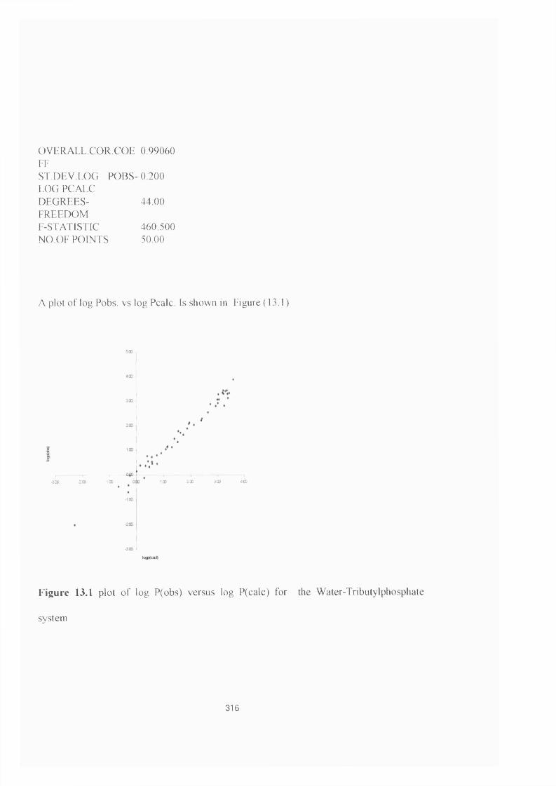
OVERALL.COR.COE 0.99060 FFST.DEV.LOG PO B S-0.200 LOG PCALCDEGREES- 44.00FREEDOMF-STATISTIC 460.500NO OF POINTS 50.00
A plot o f log Pobs. vs log Pcalc. Is shown in Figure (13.1)
.300 -200 -10O 0,10 100 200 300 400
Figure 13.1 plot o f log P(obs) versus log P(calc) for the W ater-Tributylphosphate
svstein
316

log Sw = 0.518 - 1.004 R2 + 0.771 Jt 2” + 2.168 Z a; " + 4.238 I P 2"
-3.362 Za2"* Zp 2" -3.987 V,
a = 659, sd = 0.557, = 0.920, F =1256, AAN = 0.408 (9.6)
Abraham and Le considered that equation 9.6 was the best equation that had been
constructed from the general solvation descriptors. They concluded that equation 9.6
which contains the extra Z a 2^ * Z p 2^ term, can correlate and predict log Sw values to
0.561 log units.
In the present calculations for log Sw, equation 9.6 will be used. However, since PCBs
have no hydrogen bond acidity the two terms containing Za2^ will be redundant. Then
equation 9.6 becomes.
Log Sw = 0 .5 18 - 1 .004 R2 + 0.771%" + 4.238Z P 2" - 3.987 Vx (9.7)
The log Sw values for the 136 PCBs, were first calculated using the descriptors
calculated in this work, and are compared with the experimental data obtained from the
literature by Patil,^ and with the predicted values also obtained by Patil. The latter were
based on a multilinear regression analysis that was carried out on the observed log Sw
values for 136 PCBs congeners.^^ The regression analysis gave the following equation.
217

4-Hydroxy-3-methoxybenzaldehyd
1.040 1.040 0.320 0.670 1.131300 0.810 1.057
Heptan-l-ol 0.211 0.420 0.370 0.480 1.153600 1.790 1.668
Propan-l-ol 0.236 0.420 0.370 0.480 0.590000 -0.800 -0.888
4-Nitro aniline 1.220 1.910 0.420 0.380 0.990400 1.510 1.175
2-Hydroxybenzoic acid 0.890 0.700 0.720 0.410 0.990400 0.100 0.264
4-Ethylphenol 0.800 0.900 0.550 0.360 1.056900 1.240 1.265
3-Chlorophenol 0.909 1.060 0.690 0.150 0.897500 0.930 1.003
4-Iodophenol 1.380 1.220 0.680 0.200 1.033300 1.550 1.593
Pentan-2,4-dione 0.412 0.560 0.000 0.790 0.844500 0.790 0.172
2-Fur aldehyde 0.690 1.200 0.000 0.440 0.692900 0.770 0.973
5-Methyl furfural 0.744 1.100 0.000 0.550 0.833900 1.200 1.178
3,4-Dimethylphenol 0.830 0.860 0.560 0.390 1.056900 1.120 1.123
2,4 -Dimethylphenol 0.843 0.800 0.530 0.390 1.056900 1.160 1.251
2,5 -Dimethylphenol 0.840 0.790 0.540 0.370 1.056900 1.330 1.308
3,5 -Dimethylphenol 0.820 0.840 0.570 0.360 1.056900 1.170 1.226
Ethyl acetate 0.106 0.620 0.000 0.450 0.746600 1.080 1.097
1-Naphthol 1.520 1.050 0.600 0.370 1.144100 1.800 1.725
Pentyl acetate 0.067 0.600 0.000 0.450 1.169300 2.860 3.011
2,4-Dichlorophenoi 0.960 0.840 0.530 0.190 1.019900 1.900 2.022
Helium 0.000 0.000 0.000 0.000 0.068000 0.118 0.183
Neon 0.000 0.000 0.000 0.000 0.085000 0.218 0.261
Argon 0.000 0.000 0.000 0.000 0.190000 0.665 0.739
Krypton 0.000 0.000 0.000 0.000 0.246000 0.937 0.994
Xenon 0.000 0.000 0.000 0.000 0.329000 1.372 1.373
Hydrogen 0.000 0.000 0.000 0.000 0.108600 0.415 0.368
Deuterium 0.000 0.000 0.000 0.000 0.110000 0.442 0.375
Oxygen 0.000 0.000 0.000 0.000 0.183000 0.661 0.707
Nitrogen 0.000 0.000 0.000 0.000 0.222200 0.665 0.886
Carbon dioxide 0.000 0.280 0.050 0.100 0.280900 0.343 0.442
Methane 0.000 0.000 0.000 0.000 0.249500 1.035 1.010
Ethane 0.000 0.000 0.000 0.000 0.390400 1.788 1.652
Propane 0.000 0.000 0.000 0.000 0.531300 2.482 2.294
318

Octane 0.000 0.000 0.000 0.000 1.235800 5.846 5.504
Ethene 0.107 0.100 0.000 0.070 0.347400 1.318 1.158
T etrafiuoro methane -0.280 -0.200 0.000 0.000 0.320300 1.141 1.271
ChJoromethane 0.249 0.430 0.000 0.080 0.371900 1.187 1.181
lodoethane 0.640 0.400 0.000 0.150 0.648600 2.551 2.314
Dimethyl ether 0.000 0.270 0.000 0.410 0.449100 0.138 -0.013
1,4-Dioxane 0.329 0.750 0.000 0.640 0.681000 0.122 0.002
Butanone 0.166 0.700 0.000 0.510 0.687900 0.498 0.560
Triethylamine 0.101 0.150 0.000 0.790 1.053800 0.902 1.119
Nitromethane 0.313 0.950 0.060 0.310 0.423700 0.089 0.037
Ethanol 0.246 0.420 0.370 0.480 0.449100 -1.434 -1.525
Sulfur hexafluoride -0.600 -0.200 0.000 0.000 0.464300 1.741 1.782
Toluene 0.601 0.520 0.000 0.140 0.857300 3.136 3.253
For this system, the following equation was obtained.
LogP = - 0.126 + 0.455 R 2 - 0.327 712” - 3.407S az" - 4.497% ^ + 4.556 V>
n = 64 r = 0.9906 sd-0.161 F=611 (13.5)
Five data points were deleted form the regression to get a good value for correlation
coefficient as shown in Table (13.5); the compounds that were deleted were those that
had standard deviations greater than twice those of the regression equation. An output
for the values of log Pobs, log Pcalc is shown in Table 13.4 and statistics are given in
Table 13.5. A plot of log Pobs vs. log Pcalc. was made; see Figure (13.2).
319
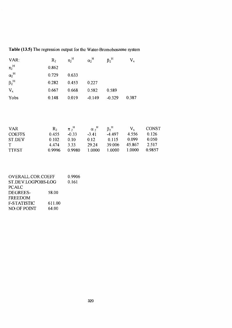
Table (13.5) The regression output for the Water-Bromobenzene system
VAR: Ri 712 «2^ P2" Vx0.8620.729 0.633
Pi" 0.282 0.453 0.227
Vx 0.667 0.668 0.582 0.589Yobs 0.148 0.019 -0.149 -0.329 0.387
VAR Ri a 2" P2" Vx CONSTCOEFFS 0.455 -0.33 -3.41 -4.497 4.556 0.126ST.DEV 0.102 0.10 0.12 0.115 0.099 0.050T 4.474 3.33 29.24 39.006 45.867 2.517TTEST 0.9996 0.9980 1.0000 1.0000 1.0000 0.9857
OVERALL.COR.COEFF 0.9906ST. DEV.LOGPOBS-LOG 0.161PCALCDEGREES- 58.00FREEDOMF-STATISTIC 611.00NO.OF POINT 64.00
320

000^-200 -100 * 0.(0 100 2 (0 300 400 500 600 700
Figure 13.2 A plot o f log P(obs) vs log P(calc) for the W ater-Bromobenzene system
13.3.3 ITie Water-]odobenzene system
The third regression was for the W ater-Iodobenzene system. The data are in Table
13.6, where log P values were again from the MedChem data base
Table (13.6) Solutes, their descriptors and the values o f log Pobs and log Pcalc for the
W ater-Iodobenzene system
Compound Name R% tc 2 ” a. 2 " P;" V, Log P obs log P calc
Butan-l-ol
4-Chlorophenol
0.224 0.420 0.370 0.480 0.730900 -0.490 -0.335
0.915 1.080 0.670 0.200 0.897500 0.900 0.783
321

2-Naphthol 1.520 1.080 0.610 0.400 1.144100 1.510 1.451
Methyl 2-hydroxybenzoate 0.850 0.840 0.040 0.460 1.131300 2.690 2.776
5-Methylfurfliral 0.744 1.100 0.000 0.550 0.833900 1.090 1.037
2-Methylphenol 0.840 0.860 0.520 0.300 0.916000 0.930 0.946
1-Naphthol 1.520 1.050 0.600 0.370 1.144100 1.730 1.630
3-Methylphenol 0.822 0.880 0.570 0.340 0.916000 0.400 0.585
2-Furaldehyde 0.690 1.200 0.000 0.440 0.692900 0.690 0.847
2-Fluorophenol 0.660 0.690 0.610 0.260 0.792800 0.400 0.255
Pentan-l-ol 0.219 0.420 0.370 0.480 0.871800 0.400 0.293
Ethyl 2-hydroxybenzoate 0.802 0.990 0.120 0.350 1.272200 3.400 3.569
2-Chlorophenol 0.853 0.880 0.320 0.310 0.897500 1.320 1.477
3,5 -Dimethylphenol 0.820 0.840 0.570 0.360 1.056900 1.080 1.137
Buty lamine 0.224 0.350 0.160 0.610 0.772000 -0.120 -0.025
Methanol 0.278 0.440 0.430 0.470 0.308200 -2.150 -2.359
4-Bro mo phenol 1.080 1.170 0.670 0.200 0.950100 0.970 1.063
2-Nitro aniline 1.180 1.370 0.300 0.360 0.990400 1.780 1.716
Ethylamine 0.236 0.350 0.160 0.610 0.490200 -1.300 -1.279
2-lodophenol 1.360 1.000 0.400 0.350 1.033300 1.840 1.828
Hexan-l-ol 0.210 0.420 0.370 0.480 1.012700 0.990 0.918
Propyl 2-hydroxybenzoate 0.793 0.900 0.140 0.350 1.413100 4.100 4.159
2,4-Dichlorophenol 0.960 0.840 0.530 0.190 1.019900 1.830 1.937
2-Bromophenol 1.037 0.900 0.350 0.310 0.950100 1.640 1.689
3-Nitro phenol 1.050 1.570 0.790 0.230 0.949300 0.220 0.382
Phenol 0.805 0.890 0.600 0.300 0.775100 0.100 0.027
Propylamine 0.225 0.350 0.160 0.610 0.631100 -0.620 -0.654
Heptan-l-ol 0.211 0.420 0.370 0.480 1.153600 1.680 1.548
Propan-l-ol 0.236 0.420 0.370 0.480 0.590000 -0.960 -0.959
4-Nilro aniline 1.220 1.910 0.420 0.380 0.990400 1.350 1.069
3-Chloro phenol 0.909 1.060 0.690 0.150 0.897500 0.860 0.948
4-Iodophenol 1.380 1.220 0.680 0.200 1.033300 1.500 1.521
Butylamine 0.224 0.350 0.160 0.610 0.772000 -0.120 -0.025
3,5 -Dimethylphenol 0.820 0.840 0.570 0.360 1.056900 1.080 1.137
322
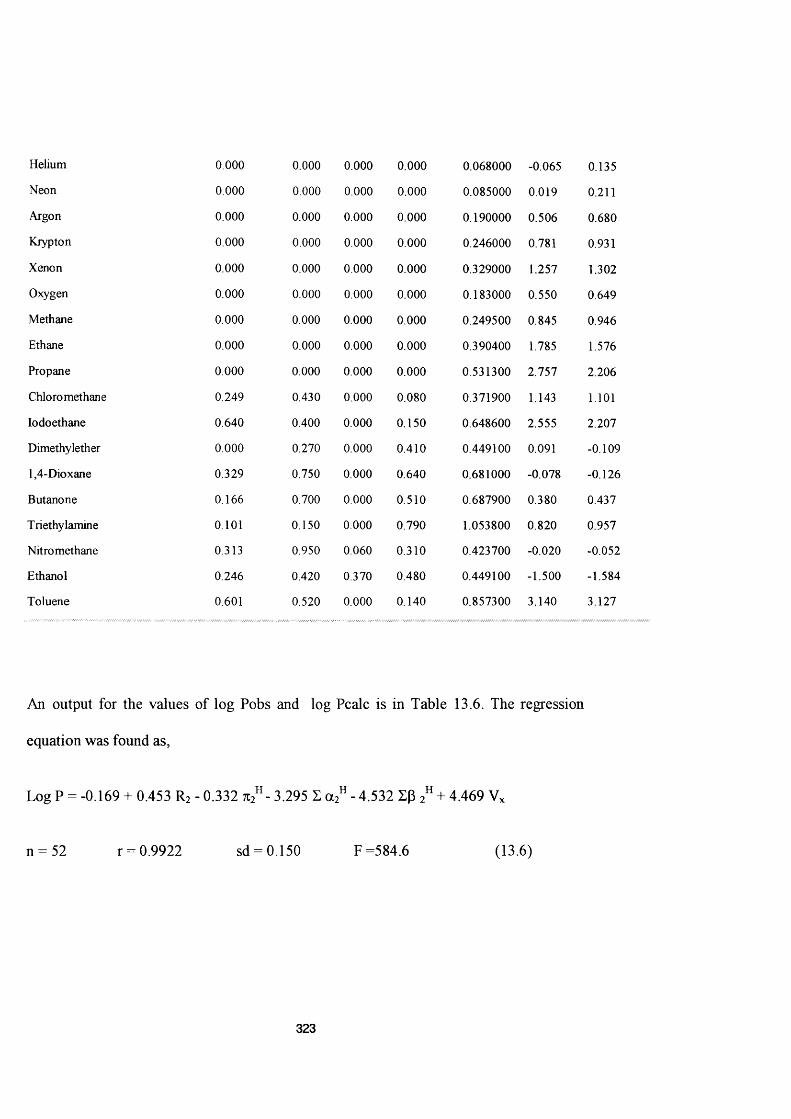
Helium 0.000 0.000 0.000 0.000 0.068000 -0.065 0.135
Neon 0.000 0.000 0.000 0.000 0.085000 0.019 0.211
Argon 0.000 0.000 0.000 0.000 0.190000 0.506 0.680
Krypton 0.000 0.000 0.000 0.000 0.246000 0.781 0.931
Xenon 0.000 0.000 0.000 0.000 0.329000 1.257 1.302
Oxygen 0.000 0.000 0.000 0.000 0.183000 0.550 0.649
Methane 0.000 0.000 0.000 0.000 0.249500 0.845 0.946
Ethane 0.000 0.000 0.000 0.000 0.390400 1.785 1.576
Propane 0.000 0.000 0.000 0.000 0.531300 2.757 2.206
Chloro methane 0.249 0.430 0.000 0.080 0.371900 1.143 1.101
lodoethane 0.640 0.400 0.000 0.150 0.648600 2.555 2.207
Dimethylether 0.000 0.270 0.000 0.410 0.449100 0.091 -0.109
1,4-Dioxane 0.329 0.750 0.000 0.640 0.681000 -0.078 -0.126
Butanone 0.166 0.700 0.000 0.510 0.687900 0.380 0.437
Triethylamine 0.101 0.150 0.000 0.790 1.053800 0.820 0.957
Nitromethane 0.313 0.950 0.060 0.310 0.423700 -0.020 -0.052
Ethanol 0.246 0.420 0.370 0.480 0.449100 -1.500 -1.584
Toluene 0.601 0.520 0.000 0.140 0.857300 3.140 3.127
An output for the values of log Pobs and log Pcalc is in Table 13.6. The regression
equation was found as.
Log P = -0.169 + 0.453 - 0.332 3.295 S - 4.532 Zp 2“ + 4.469 V,
n = 52 r = 0.9922 sd = 0.150 F =584.6 (13.6)
323

For this regression, five compound data sets needed to be deleted to get a good value for
the correlation coefficient, as shown in Table (13.7). From the value of the T-Test, all
five descriptors were significant; it therefore seemed that the overall parameter
relationship produced a good linear relationship. The statistics are in Table 13.7, and a
plot of log Fobs, vs log Pcalc. Is shown in Figure (13.3).
Table (13.7) Regression output for the Water-lodobenzene system
VAR; R2 71:2” a:" P2" Vx7: 2" 0.871a / 0.681 0.606P 2 ” 0.099 0.250 0.098Vxx 0.734 0.684 0.534 0.452Yobs 0.397 0.235 -0.094 -0.304 0.530
VAR: R2 a 2" P2" Vx CONSTCOEFFS 0.453 -0.332 -3 295 -4.532 4.469 -0.169ST DEV 0.127 0.105 0.117 0.138 0.121 0.059T 3.561 3.165 28.229 32.755 37.083 Z883TTEST 0.99913 0.99725 1.00000 1.00000 1.00000 0.99403
OVERALL.COR.COEFF 0.9922 ST.DEV.LOGPOBS-LOG 0.158
PCALCDEGREES- 46.00 FREE
F- STATISTIC 584.60 NO.OF POINTS 52
324

/ f - '-
200 -100 ♦ Ci 0 1 00 2 00 3 00 4 00 5 00 600 700
Figure 13.3 A plot of log P(obs) versus log P(calc) for the Water-Iodobezene system
13.3.4 The Water-Diisopropylelher system
The last regression was for the Water-Di isopropyl ether system using data for 82
compounds as shown in Table 13.8
325

Table (13.8) solutes, their descriptors and values of log P(obs) and log P(calc) for the
Water-Diisopropylether system
Compound Name Rz V, LogPobs
Log P calc
Catechol 0.970 1.0700 0.8500 0.5200 0.8338 0.6500 0.4642-Naphthylamine 1.670 1.2800 0.2200 0.5500 1.1850 2.1500 2.238Pentanoic acid 0.205 0.6000 0.6000 0.4500 0.8875 1.0500 1.1455-MethylfurfuraI 0.744 1.1000 0.0000 0.5500 0.8339 0.6300 0.3252-Fur aldehyde 0.690 1.2000 0.0000 0.4400 0.6929 0.3000 0.088Pyridine 0.631 0.8400 0.0000 0.5200 0.6753 0.1300 0.015Diethylamine 0.154 0.3000 0.0800 0.6900 0.7720 -0.2100 -0.089Formaldehyde 0.220 0.7000 0.0000 0.3300 0.2652 -1.2600 -0.964Butyl amine 0.224 0.3500 0.1600 0.6100 0.7720 -0.0400 0.2731-Naphthylamine 1.670 1.2600 0.2000 0.5700 1.1850 2.1500 2.168Formic acid 0.300 0.7900 0.7200 0.3400 0.3239 -0.8100 -0.9811 -Naphthol 1.520 1.0500 0.6000 0.3700 1.1441 3.3800 3.0304-Hydroxy benzaldehyde 1.010 1.5400 0.7900 0.4000 0.9317 0.8400 0.952Butanoic acid 0.210 0.6200 0.6000 0.4500 0.7466 0.3900 0.506Hexanoic acid 0.174 0.6000 0.6000 0.4500 1.0284 1.4800 1.742Hydroquinone 1.000 1.0000 1.1600 0.6000 0.8338 0.0700 0.1035-Ethyl-5-(2- pentyl) barbital
1.030 1.1100 0.4700 1.2300 1.7966 1.6900 1.278
Naphthalene 1.340 0.9200 0.0000 0.2000 1.0854 3.5500 3.785Acetic acid 0.265 0.6500 0.6100 0.4400 0.4648 -0.6100 -0.683Trimethylamine 0.140 0.2000 0.0000 0.6700 0.6311 -0.3600 -0.477Estrone 1.730 3.1000 0.5600 0.9100 2.1558 2.3000 2.466Phenol 0.805 0.8900 0.6000 0.3000 0.7751 1.3200 1.453Propanoic acid 0.233 0.6500 0.6000 0.4500 0.6057 -0.0600 -0.133Cocaine 1.355 1.9200 0.0000 1.5000 2.2977 1.1900 1.498Estradiol 1.800 3.3000 0.8800 0.9500 2.1988 2.3000 2.187Aniline 0.955 0.9600 0.2600 0.4100 0.8162 0.8600 1.192Caffeine 1.500 1.6000 0.0000 1.3300 1.3632 -1.1900 -1.275Octane 0.000 0.0000 0.0000 0.0000 1.2358 5.9520 5.6201,4-Dioxane 0.329 0.7500 0.0000 0.6400 0.6810 -0.4960 -0.651Butanone 0.166 0.7000 0.0000 0.5100 0.6879 0.1230 -0.033Nitro methane 0.313 0.9500 0.0600 0.3100 0.4237 -0.1440 -0.425Ethanol 0.246 0.4200 0.3700 0.4800 0.4491 -0.9980 -0.624Toluene 0.601 0.5200 0.0000 0.1400 0.8573 2.9170 3.053
The following equation was produced. An output for the values of log P obs. and
log Pcalc. is in Table 13.8, above.
326
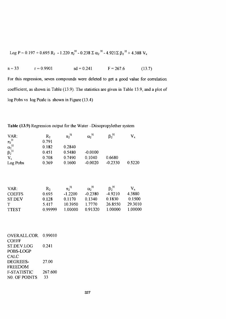
Log P = 0.197 + 0.695 R2 - 1.220 n2 - 0.238 Z a 2 - 4.9212 ^2 “ + 4.388 Vx
n = 33 r = 0.9901 sd = 0.241 F = 267.6 (13.7)
For this regression, seven compounds were deleted to get a good value for correlation
coefficient, as shown in Table (13.9). The statistics are given in Table 13.9, and a plot of
log Fobs vs log Pcalc is shown in Figure (13.4)
Table (13.9) Regression output for the Water -Diisopropylether system
VAR: R 2 712^ P 2 " Vx712” 0.791
0.182 0.28400.451 0.5480 -0.0100
Vx 0.708 0.7490 0.1040 0.6680Log Fobs 0.369 0.1600 -0.0020 -0.2330 0.5220
VAR: R2 7C2^ P2" VxCOEFFS 0.695 -1.2200 -0.2380 -4.9210 4.3880ST.DEV 0.128 0.1170 0.1340 0.1830 0.1500T 5.417 10.3950 1.7770 26.8550 29.3010TTEST 0.99999 1.00000 0.91320 1.00000 1.00000
OVERALL.COR. 0.99010 COEFFST.DEV.LOG 0.241POBS-LOGPCALCDEGREES- 27.00FREEDOMF-STATISTIC 267.600NO. OF POINTS 33
327

10 0 2 00 3 0 0 4 00 5 00 600
Figure 13. 4 A plot of log P(obs) versus log P(calc) for the W ater - Diisopropylether system
13.4 The calculation of parameters (7c,p), for N-Nitrosodialkylamines
A spreadsheet was set up which contained the coefficients (c, r, s, a, b) for a large
number o f systems see Table (13.1) . As noted before, the parameters R2 and Vx can
always be obtained and so only 712", Z a 2^ and are unknown. For the N-
nitrosodialkylamines, (R1 R2 N-NO ) Z a 2^ is zero because they have no hydrogen - bond
acidity ,and so only 712 and I p 2 ** need to be detennined. In Table (13.10) is an example
of the calculation for N-nitrosodimethylamine. Values o f log P are known for eight
systems, and the iz 2" and i p 2" values that best reproduced these eight log P values were
328
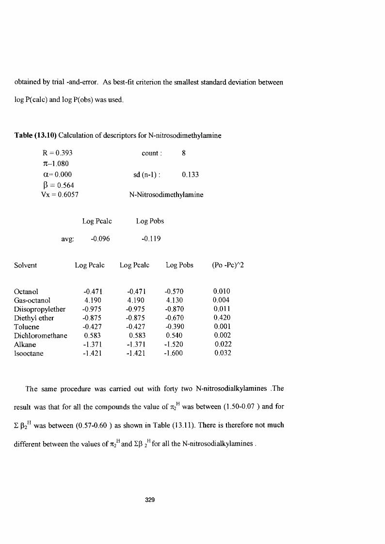
obtained by trial -and-error. As best-fit criterion the smallest standard deviation between
log P(calc) and log P(obs) was used.
Table (13.10) Calculation of descriptors for N-nitrosodimethylamine
count : 8R = 0.393 71=1.080 a= 0.000 (3 = 0.564
Vx = 0.6057
sd(n-l): 0.133
N-Nitrosodimethylamine
Log Pcalc
avg; -0.096
Log Pobs
-0.119
Solvent Log Pcalc Log Pcalc Log Pobs (Po -Pc)^2
Octanol -0.471 -0.471 -0.570 0.010Gas-octanol 4.190 4.190 4.130 0.004Diisopropylether -0.975 -0.975 -0.870 0.011Diethyl ether -0.875 -0.875 -0.670 0.420Toluene -0.427 -0.427 -0.390 0.001Dichloromethane 0.583 0.583 0.540 0.002Alkane -1.371 -1.371 -1.520 0.022Isooctane -1.421 -1.421 -1.600 0.032
The same procedure was carried out with forty two N-nitrosodialkylamines
result was that for all the compounds the value of was between (1.50-0.07 ) and for
E was between (0.57-0.60 ) as shown in Table (13.11). There is therefore not much
different between the values of 7:2^ and E{3 2^ for all the N-nitrosodialkylamines .
329

Table (13.11) calculated values of 712^ and Zp 2^ for N-nitroso dialkyla mines
Name R2 P2” Vx n sd
N-Nitrosodimethylamine 0.393 1.190 0.564 0.6057 16 0.056
N-Nitrosomethylethylamine 0.374 1.100 0.585 0.7466 14 0.059
N-Nitrosodiethylamine 0.345 1.084 0.582 0.8875 17 0.052
N-Nitrosoethylpropylamine 0.340 1.050 0.610 1.0284 6 0.010
N-Nitrosomethylpropylamine 0.360 1.050 0.583 0.8875 14 0.050
N-Nitro somethylbutyl ami n e 0.340 1.070 0.600 1.0284 14 0.043
N-Nitrosomtehylpentylamine 0.320 1.050 0.590 1.1693 6 0.016
N-Nitrosomethylhexyl am i ne 0.300 1.094 0.600 1.3102 4 0.067
N-Nitrosomethylheptylamine 0.310 1.080 0.600 1.4511 4 0.067
N-Nitrosoethylhexyl amine 0.300 1.092 0.600 1.4511 6 0.041
N-Nitrosoethylpentylamine 0.310 1.094 0.600 1.3102 1 0.055
N-Nitrosoethylbutylamine 0.320 1.000 0.620 1.1693 14 0.055
N-Nitrosodipropylamine 0.318 l.OlO 0.630 1.1693 14 0.066
N-Nitrosopropylbutylamine 0.310 0.990 0.640 1.3102 16 0.097
N-Nitrosodibutylamine 0.300 0.980 0.650 1.4511 17 0.097
N-Nitrosobutylpentyl amine 0.290 0.980 0.650 1.5920 4 0.041
N-N itrosodipentylamine 0.280 0.980 0.660 1.7329 5 0.036
N-Nitrosodiisobutylamine 0.300 0.780 0.750 1.4511 13 0.011
N-Nitrosodiisopropylamine 0.300 0.950 0.670 1.1693 17 0.078
N-Nitrosomethylisopropylamin 0.360 1.200 0.633 0.8875 4 0.009
330
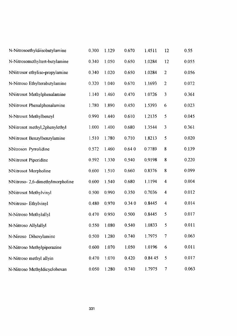
N-Ni trosoethyldii sobutyl amine 0.300 1.129 0.670 1.4511 12 0.55
N-Nitrosomethyltert-butylamine 0.340 1.050 0.650 1.0284 12 0.055
NNitrosor ethyliso-propylamine 0.340 1.020 0.650 1.0284 2 0.056
N-Nitroso Ethylterabutylamine 0.320 1.040 0.670 1.1693 2 0.072
NNitrosot Methylphenalamine 1.140 1.460 0.470 1.0726 3 0.361
NNitrosot Phenalphenalamine 1.780 1.890 0.450 1.5393 6 0.023
N-Ntrosot Methylbenzyl 0.990 1.440 0.610 1.2135 5 0.045
NNitrosot methyl,2phenylethyl 1.000 1.400 0.680 1.3544 3 0.361
NNitrosot Benzylbenzylamine 1.510 1.780 0.710 1.8213 5 0.020
NNtroson Pyrrolidine 0.572 1.460 0.64 0 0.7789 8 0.139
NNitrosot Piperidine 0.592 1.330 0.540 0.9198 8 0.220
NNitrosot Morpholine 0.600 1.510 0.660 0.8376 8 0.099
NNitroso- 2,6-dimethylmorpholine 0.600 1.540 0.680 1.1194 4 0.004
NNitrosot Methyl vinyl 0.500 0.990 0.350 0.7036 4 0.012
NNitroso- Ethylvinyl 0.480 0.970 0.34 0 0.8445 4 0.014
N-Nitroso Methylallyl 0.470 0.950 0.500 0.8445 5 0.017
N-Nitroso Allylallyl 0.550 1.080 0.540 1.0833 5 0.011
N-Niroso Diliexylamine 0.500 1.280 0.740 1.7975 7 0.063
N-Nitroso Methylpiperazine 0.600 1.070 1.050 1.0196 6 0.011
N-Nitroso methyl allyin 0.470 1.070 0.420 0.84 45 5 0.017
N-Nitroso Methyldicyclohexan 0.050 1.280 0.740 1.7975 7 0.063
331

In a second step, the value for was taken as an average of 1.09 for the straight chain
aliphatic compounds, and then the value of E(3 2^ was calculated by getting the smallest
standard deviation as before. The values of Zp 2 ^ were hardly changed as shown in Table
(13.12) except for branched-nitroso compound like N-nitrosodiisopropylamine.
332

Table 13.12 calc. Sp by fixing n as 1.09
Name Rz TCz” Pz” Vx n sd
N-Nitrosodimethylamine 0.393 1.090 0.562 0.6057 16 0.078
N-Nitrosomethylethylamine 0.374 1.090 0.581 0.7466 14 0.055
N-Nitrosodiethylamine 0.345 1.090 0.582 0.8875 17 0.096
N-Nitrosoethylpropylamine 0.340 1.090 0.602 1.0284 6 0.041
N-Nitrosomethylpropylamine 0.360 1.090 0.583 0.8875 14 0.099
N-Nitrosomethylbutylamine 0.340 1.090 0.580 1.0284 14 0.129
N-Nitrosomethylpentyl amine 0.320 1.090 0.579 1.1693 6 0.070
N-Nitrosomethylhexylamine 0.300 1.090 0.600 1.3102 4 0.069
N-Nitrosomethylheptylamine 0.310 1.090 0.579 1.4511 4 0.056
N-Nitrosoethylhexylamine 0.300 1.090 0.614 1.4511 6 0.053
N-Nitrosoethylpentylamine 0.310 1.090 0.601 1.3102 1 0.069
N-Nitrosoethylbutylamine 0.320 1.090 0.588 1.1693 14 0.067
N-Nitrosodipropylamine 0.318 1.090 0.593 1.1693 14 0.079
N-Nitrosopropylbutylamine 0.310 1.090 0.614 1.3102 16 0.067
N-Nitrosodibutylamine 0.300 1.090 0.610 1.4511 17 0.097
N-Nitrosobutylpentylamine 0.290 1.090 0.593 1.5920 4 0.043
N-Mitrosodipentylamine 0.280 1.090 0.629 1.7329 5 0.046
N-Nitrosodiisobutylamine 0.300 1.090 0.700 1.4511 13 0.100
N-Nitrosodiisopropylamine 0.300 1.090 0.636 1.1693 17 0.071
333

N-Nitrosomethylisopropylamine 0.360 1.090 0.670 0.8875 4 0.067
N-Nitrosoethyldiisobutylamine 0.300 1.090 0.670 1.4511 12 0.55
N-Nitrosomethyltert-butylamine 0.340 1.090 0.658 1.0284 12 0.055
N-Nitroso ethyli sopropyl am in e 0.340 1.090 0.630 1.0284 2 0.041
N-Nitroso ethyl-t-butylamine 0.320 1.090 0.630 1.1693 2 0.048
N-Nitroso dihexylamine 0.500 1.090 0.700 1.7975 7 0.120
There are five branched-chain nitroso compounds, and the 71:2^ values for the branched-
chain compounds were adjusted as recommended before, that is 1.09 with 0.03 units
subtracted for each branch. Results are in Table (13.13).
Table (13.13) calculation of Sp 2 for branched-chain N-nitrosodialkylamines
C om pound N am e R 2 ^ 2“ ZP2'' V . n sd
N-Nitrosodiisobutylamine 0.300 1.03 0.760 1.4511 13 0.118
N-Nitrosodiisopropylamine 0.320 1.03 0.636 1.1693 17 0.227
N -Nitrosom ethyli sopr opyl amine 0.360 1.06 0.583 0.8875 4 0.067
N-Nitrosomethyl-t-butylamine 0.340 1.03 0.660 1.0284 12 0.055
N-Nitrosoethylisopropylamine 0.340 1.06 0.600 1.1692 2 0.048
These results are then consistent with the two rules of Abraham el al. for aliphatic
solutes, as was mentioned in chapter 2.
334

13.5 Conclusion
The solvation equations for four water-solute system were obtained from the values
of partition coefficients for a series of compounds. These partition coelficients were all
obtained from the MedChem data base. For all four system the values of the overall
regression standard deviation were less than 0.24, although a few compounds had to be
eliminated in the regressions. The values for the correlation coefficient were all very
good, and plots of log Pcalc. vs log Pobs showed good straight lines for all the systems.
According to these results one could say that the equations extend the data set of
equations, and could provide a useful tool for the prediction of further data for
compounds in these systems.
The equations obtained can then be used to describe the systems in terms of its
coefficients, althougli none of the four systems are in any way unusual. The water-
diisopropylether system was useful in the calculation of descriptors for N-
nitrosodialkylamines.
The values of and for the N-nitrosodialkylamines are also very useful,
because they allow the calculation of numerous other partition coefficients without the
necessity of direct working with these carcinogenic substances.
More importantly, we can now use the descriptors collected in Table 13.11, together
with the coefficients of the two solvation equations to calculate a number of properties
of environmental interest. As part of our method of determining descriptors, we have had
to estimate the gas-water partition coefficient, K^, which is equivalent to the Henry’s
335
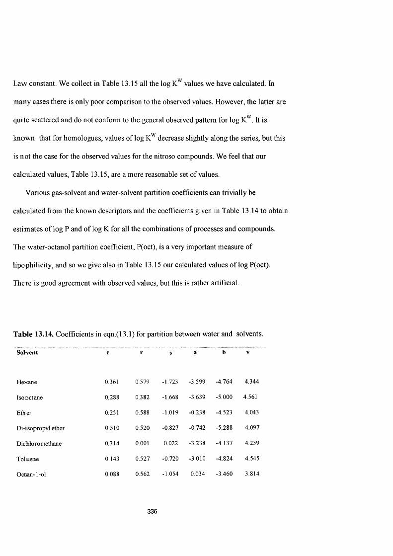
Law constant. We collect in Table 13.15 all the log values we have calculated. In
many cases there is only poor comparison to the observed values. However, the latter are
quite scattered and do not conform to the general observed pattern for log K^. It is
known that for homologues, values of log decrease slightly along the series, but this
is not the case for the observed values for the nitroso compounds. We feel that our
calculated values. Table 13.15, are a more reasonable set of values.
Various gas-solvent and water-solvent partition coefficients can trivially be
calculated from the known descriptors and the coefficients given in Table 13.14 to obtain
estimates of log P and of log K for all the combinations of processes and compounds.
The water-octanol partition coefficient, P(oct), is a very important measure of
lipo'philicity, and so we give also in Table 13.15 our calculated values of log P(oct).
There is good agreement with observed values, but this is rather artificial.
Table 13.14. Coefficients in eqn.(I3.I) for partition between water and solvents.
S o K e n t c r s a b V
H ex a n e 0.361 0.579 -1.723 -3 .5 9 9 -4 .7 6 4 4 .3 4 4
Iso o c ta n e 0 .288 0.382 -1 .668 -3 .639 -5 .0 0 0 4.561
Ethter 0.251 0.588 -1 .019 -0 .2 3 8 -4 .523 4.043
D i-iisopropyl ether 0 .510 0 .520 -0 .8 2 7 -0 .742 -5 .2 8 8 4 .0 9 7
D ich lorom ethan e 0 .314 0.001 0.022 -3 .238 -4 .1 3 7 4 .2 5 9
T ohaene 0.143 0 .527 -0 .720 -3 .0 1 0 -4 .8 2 4 4 .545
O c ta n - l-o l 0 .088 0 .562 -1 .054 0 .0 3 4 -3 .4 6 0 3 .814
336
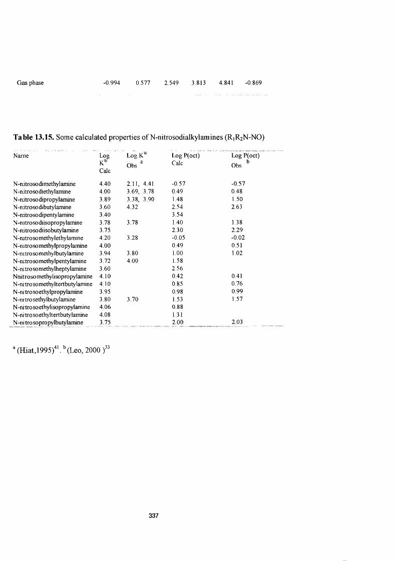
Gas phase -0.994 0.577 2.549 3.813 4.841 -0.869
Table 13.15. Some calculated properties of N-nitrosodialkylamines (R1R2N-NO)
(Hiat,1995)'". ’’(Leo, 2000
N am e L og LogK'"' L og P (oct) L og P (oct)r W
O bs ^ Calc Obs ^Calc
N -nitrosodim ethylam ine 4 .4 0 2 .11 , 4.41 -0 .5 7 -0 .5 7N -n itro so diethylamin e 4 .00 3 .6 9 , 3 .78 0 .49 0.48N-rutro so dipropylamine 3 .89 3 .38 , 3 .90 1.48 1.50N -nntro so dibutylamine 3 .60 4 .3 2 2 .54 2.63N -n itro so dipenty lamine 3.40 3.54N-natro so diisopropy lamin e 3.78 3 .78 1.40 1.38N -natrosodiisobuty lamine 3.75 2.30 2 .29N-natro so m ethylethy lamin e 4 .20 3 .28 -0 .05 -0 .0 2N -natroso m ethylpropy lamine 4 .0 0 0 .49 0.51N -n itro so methyl buty lamin e 3.94 3 .8 0 1.00 1.02N -nitro som ethylpentylam ine 3 .72 4 .0 0 1.58N -nitro so m ethylhepty lamine 3 .60 2.56N nitrosom ethylisopropylam ine 4 .1 0 0 .42 0.41N -n itro som ethyltertbuty lamine 4 .1 0 0 .85 0 .76
N -m tro so ethylpropy lamine 3 .95 0 .98 0 .99N -m tro sethylbutylam ine 3 .80 3 .70 1.53 1.57N -n itro soethylisopropylam ine 4 .0 6 0 .88N -niIro so ethylt ertbuty lamine 4 .08 1.31N -n itro so propylbuty lamine 3 .75 2 .00 2.03
337
13.6 References
1. P. H. Magee, J. M. Bames, Br. J. Cancer, 1956, Vol. 10,114.
2. S. Neale, Mutat. Res., 1976, Vol. 32, 229.
3. R. Montesano, H. Bartsch, Mutat. Res., 1976, Vol. 32, 179.
4. W. Lijinsky, A. W. Andrews, Mutat. Res., 1979, Vol. 68,1.
5. A. W. Andrews, W. Lijinsky, Mutagenesis, 1980, Vol. 1, 295.
6. T. Kreybig, Aulendorf, Editio Cancer, 1968.
7. W. Wechsler, Lyon, International Agency for Research on Cancer. 1973, 127.
8. B. J. Canas, D. C. Havery, F. J. Joe, Jr. T. Fazio., J. Assoc. Anal.
Chem., 1986, Vol. 69, 1020 .
9. S. M. Billedeau, B. M. Miller, H. C. Thompson, J. Food Sci., 1988,Vol. 53,
1696.
10. S. M. Billedeau, T. M. Heinze, J. G. Wilkes, H. C. Thompson, J.
Chromatogro A., 1994, Vol. 688, 55.
11. S. M. Billedeau, H. C. Thompson, B. M. Miller, M. L. Wind., J. Assoc. Anal.
Chem, 1986, Vol. 69,31.
12. B. A. Dawson, R. C. Lawrence, J. Assoc. Anal. Chem., 1987, Vol. 70, 554.
13. P. N. Magee, R. Montesano, R. Preussman., In Chemical Carcinogens, Searie
C. W., Ed. Monograph series 173. American Chemical Society Washinton, DC,
1976 Chapter 11.
14. Y. U. Zhdanov, A. Minkin, V. I. Korrelyatsionnyi Analiz Organ-icheskoi
Khimil Izdatelstvo Universiteta; Rotovon-Don, 1966.
338

15. S. Borman, Chem. Eng. News 1990, Vol. 68, 20.
16. B. Pignatelli, G. Descortes, H. Bartsch, Actual. Chim., 1985, Vol. 10, 33.
17. R. Preussmann, B. W. Stewart, In Chemical Carcinogens, 2nd ed. Searie, C.
E. Ed., Americal Chemical Society Washington, D. C., 1985, 643.
18. F. K. Zimmermann, Biochem. Pharmacol., 1971, Vol. 20, 985.
19. H. Druckrey, Xenobiotica, 1973, Vol. 3,271.
20. T. J. Coomes, ACTA Cient. Comp., 1982, Vol. 19, 9.
21. F. Ender, G. Havre, A. Helgebostad, N. Koppang, R. Masden, L. Ceh,
Naturwissenschaften, 1964, Vol. 51, 637.
22. C. L. Walters, S. 1. West, In Recent Advances in the Chemistry of Meat, A. J.
Bailey, Ed, Royal Society of Chemistry: London, 1984, 178.
23. J. Casado, A. Castro, M. A. Lopez Quintela, M. F. Z. Rodriguez Prieto, Phy.
Chem. Neue Folge, 1979, Vol. 118, 43.
24. J. Casado, M. A. Mosquera, M. Rodriguez Prieto, M. F. Vazquez Tato, J.
Phy. Chem., 1983, Vol. 87, 1208.
25. J. Casado, A. Castro, R. Leis, M. Mosquera, M. E. Pena, J. Chem. Soc.,
Perkin Trans. 2 1985, 1859.
26. J. Casado, Acastro, M. A. Lopez Quintela, B. Lorenzo, Soc. Chim. Fr. 1987,
401.
27. J. Casado, A. Arco del, C. Izuierdo, P. Motilva, J. L. Usero, Studia Chemica,
1986, Vol. 11,351.
28. P. Motilva, A. Arco del, J. L. Usero, C. Izquierdo, J. Casado, Int. J. Biochem.,
1988, Vol. 20, 41.
339
29. M. Montes, J. L. Usero, A. Arco del, C. Izquierrdo, J. Casado, J.
Chromatogr., 1989, Vol. 20,197.
30. H. Druckrey, R. Preussmann, S. Ivanovic, D. Schmaehl, Organtrope
Carcinogene Wirkungen bei verschieden N-nitroso- verbindungen an BD- ratten,
Z. Kerbsforsch., 1967, Vol. 69, 103.
31. S. S. Mirvish, P. Issenberg, H. C. Somsen, J. Natl. Cancer Inst., 1976, Vol. 56,
1125.
32. A. Vera, M. Montes, J. L. Usero, J. Casado, J. Pharm. Sci., 1992, Vol. 81, 791.
33. A. J. Léo, The Medicinal Chemistry Project, Pomona, College, Claremont, CA
9171.
34. R. C. Massey, Nitrosamines, 1988,16.
35. N. M. A. Niessen, van der Greef, J. Liquid Chromatography-Mass
Spectrometry, Marcell-Dekker, Inc. New York, 1992, Chapter 17.
36. M. H. Abraham, G. S. Whiting, R. M. Doherty, W. J. Shuely, J.
Chromatogro., 1991, Vol. 587, 213.
37. M. H. Abraliam, P. P. Duce, P. L. Grellier, D. V. Prior, J. J. Morris, P. J.
Taylor, Tetrahedron Lett., 1989, Vol. 29,1587.
38. M. H. Abraham, P. P. Duce, P. L. Grellier, D. V. Prior, J. J. Morris, P. J.
Taylor, Tetrahedron Lett., 1989, Vol. 30, 2571.
39. M. H. Abraham, J. C. McGowen, Chromatographia, 1987, Vol. 23, 243.
40. M. H. Abraham, H. S. Chadha, G. S. Whiting and R. C. Mitchell, J. Pharm.
Sci. in press.
41. M. H. Hiatt, Anal. Chem., 1995, Vol. 67, 4044.
340
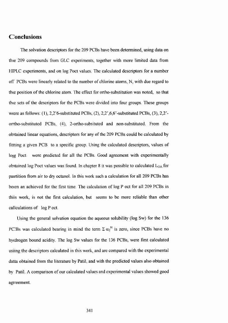
Conclusions
The solvation descriptors for the 209 PCBs have been determined, using data on
thie 209 compounds from GLC experiments, together with more limited data from
HtPLC experiments, and on log Poet values. The calculated descriptors for a number
ofT PCBs were linearly related to the number of chlorine atoms, N, with due regard to
thte position of the chlorine atom. The effect for ortho-substitution was noted, so that
thte sets of the descriptors for the PCBs were divided into four groups. These groups
weere as follows: (1), 2,2’6-substituted PCBs, (2), 2,2’,6,6’-substituted PCBs, (3), 2,2’-
orrtho-substituted PCBs, (4), 2-ortho-subsituted and non-substituted. From the
obitained linear equations, descriptors for any of the 209 PCBs could be calculated by
fittting a given PCB to a specific group. Using the calculated descriptors, values of
lojg Poet were predicted for all the PCBs. Good agreement with experimentally
obtained log Poet values was found. In chapter 8 it was possible to calculated Lqa for
pairtition from air to dry octanol. In this work such a calculation for all 209 PCBs has
beeen an achieved for the first time. The calculation of log P oct for all 209 PCBs in
thiis work, is not the first calculation, but seems to be more reliable than other
callculations of log P oct.
Using the general solvation equation the aqueous solubility (log Sw) for the 136
PC>Bs was calculated bearing in mind the term D a'P is zero, since PCBs have no
hycdrogen bound acidity. The log Sw values for the 136 PCBs, were first calculated
usiing the descriptors calculated in this work, and are compared with the experimental
datta obtained from the literature by Patil, and with the predicted values also obtained
by Patil. A comparison of our calculated values and experimental values showed good
agrreement.
341

It has been shown that, in addition to GLC, HPLC has great potential for the
analysis of halogenated aromatics. All the results on HPLC capacity factors and
log Poet values, suggested that the rotation energy in the PCBs could be important,
and so a study was made to obtain the energy barriers to the rotation about the C-C
bond for a number of ortho-substituted PCBs. The results of this wok was that the
rotational energy maximum for all the PCBs studied were more or less the same,
except for 2, 2% 6, 6’-PCB where the energy maximum was much larger. This helps
to explain the effect of substituents on descriptors.
Similar to PCBs, PCN are persistent and lipophilic compounds. Therefore in
chapter 11, the solvation descriptors for the 75 polychloronaphthalenes have been
derived from literature data on various properties. These descriptors were the usual
ones, (R], 7i2 \ log Vx ). The initial work indicated that the descriptor is
almost additive (like the R% descriptor) except for compounds that have adjacent
chlorine atoms. Also the ^ 2 descriptor was quite small, never more than 0.14, and for
the very lipophilic PCNs ^2^ is actually zero. Once the descriptors were obtained, it
was possible to predict values for water-octanol partition coefficients, as log P oct,
the aqueous solubility as log Sw, the gas-water partition coefficient as log K^, and the
gas-dry octanol partition coefficient as log
Finally, the carcinogenic compounds, the N-nitrosodialkylamines were studied.
Firstly, the solvation equations for four water-solute systems were obtained from the
values of partition coefficients for a series of compounds. These partition coefficients
weire all obtained from the Med Chem database. Using some of these water-solvent
systems the values of 712^ and p2^ for forty two N-nitrosodialklyamines could be
calculated. From the results obtained the values for 712^ and ^ 2^ hardly changed for
straiight chain compounds, but values for branched-chain nitroso compounds were a
342
little different. The solvation descriptors were then used to calculated the gas-water
partition coefficient, which is equivalent to Henry’s law constant. Various gas-
solvent and water-solvent partitions can trivially be calculated from the known
descriptors and the coefficients could be used to obtain estimates of log P for all the
combinations of processes and compounds. There was good agreement between the
calculated values and observed values, where the latter was available.
Finally, it can be concluded that the two general solvation equations provided a
very good way to obtain descriptors. These descriptors together with the already
published equations could be used to predict a number of environmentally important
physicochemical properties of PCBs, PCNs, and the N-notrosocompounds, in the
hope that they may be useful in cases where the experimental determination is
difficult. Since some of them are carcinogenic and thus not easily handled, the ability
to predict a large number of properties should be of considerable use.
As future wok other properties of the PCNs can be predicted from the descriptors
and the various regression equations that have been published. Examples are the rate
of permeation of human skin from aqueous solution, and the partition of PCNs
betw een air and plant cuticular matrix and between water and plant cuticular matrix.
Also there are a number of other important biological and environmental properties of
the N-nitrosodialkylamines that can also be predicted using the descriptors. These
include human intestinal adsorption, blood-brain distribution, skin permeation, as well
as adsorption from air or water by plant cell matrix. In the present study, there were
eight of the most common N-nitrosodialkylamines found in foods, these are N-
nitroso-dimethyl, methylethyl, diethyl, dipropyl, dibutyl-amines as well as N-
nitrosomorphloine, N-nitrosopiperdine and N-nitrosopyrollidine, and so estimation of
343
biological and environmental properties for these particular compounds would be of
considerable value.
344