BEYOND THE STANDARD MODEL: COMPOSITEHIGGS AND DARK MATTER

A Dissertation

Presented to the Faculty of the Graduate School

of Cornell University

in Partial Fulfillment of the Requirements for the Degree of

Doctor of Philosophy

by

Ofri Telem

August 2019

c© 2019 Ofri Telem

ALL RIGHTS RESERVED

BEYOND THE STANDARD MODEL: COMPOSITE HIGGS AND DARK

MATTER

Ofri Telem, Ph.D.

Cornell University 2019

The Standard Model (SM) of particles and interactions provides some of the

most extensively tested predictions in science. However, it does not adequately

describe quantum gravity, and does not contain a suitable candidate for Dark

Matter. Furthermore, the UV sensitivity of the SM Higgs sector suggests that

new states beyond the SM might exist at energies not far above the weak scale.

This dissertation explores potential scenarios for physics beyond the SM, either

in a dark sector or linked to the Higgs sector of the SM.

The first part of this work includes two novel classes of composite Higgs

models, with far reaching phenomenological consequences. In the first of these,

an adjustable tree-level Higgs quartic coupling, allows for a significant reduc-

tion in the tuning of the Higgs potential. The quartic in this model originates

from the dimensional reduction of a 6D theory, and is the first example of a holo-

graphic composite Higgs model with a tree-level quartic. In the second novel

class of composite Higgs models, the top and gauge partners responsible for cut-

ting off the Higgs quadratic divergences form a continuum. A concrete example

is presented, based on a warped extra dimension with a linear dilaton, where

this finite gap appears naturally. Spectral densities are derived for this model,

as well as the full Higgs potential for a phenomenologically viable benchmark

point, with percent level tuning. The continuum top and gauge partners in this

model evade all resonance searches at the LHC and yield qualitatively different

collider signals.

The second part of this work features two different classes of models for an

extended dark sector that undergoes either confinement or bound states forma-

tion. It is shown how each of these mechanisms could lead to vast modifications

of early universe dynamics, as well as unique signals today. In the first of these,

the relic abundance of heavy stable particles charged under a confining gauge

group is depleted by a second stage of annihilations near the deconfinement

temperature. This mechanism can be used to construct ultra-heavy dark-matter

models with masses above the naive unitarity bound. The second contribution

is Self-Destructing Dark Matter (SDDM), a new class of dark matter models

which are detectable in large neutrino detectors. In this class of models, a com-

ponent of dark matter can transition from a long-lived state to a short-lived one

by scattering off of a nucleus or an electron in the Earth. The short-lived state

then decays to SM particles, generating a dark matter signal with a visible en-

ergy of order the dark matter mass rather than just its recoil.

BIOGRAPHICAL SKETCH

Ofri Telem was born in Israel on July 20th, 1989, and grew up in the town

of Modi’in. At age 15, he attended the Israel Art and Science Academy in

Jerusalem, where he majored in Physics, Mathematics, Computer Science and

Philosophy. At age 18, he enlisted in the Israel Defense Forces (IDF), serving in

Talpiot, the IDF’s elite technological training program. As part of the training,

he completed a bachelor’s degree in Physics and Mathematics at the Hebrew

University, Jerusalem.

Towards the end of his military training in 2010, Ofri met Laura, the love of

his life, on a “Birthright Israel” trip, and the two lived together in Israel until

moving to the US in 2016. Ofri and Laura were married in 2015, and are expect-

ing their first child.

In the years 2010-2016, Ofri served as an R&D officer in the IDF, and was

granted the rank of Major. During his service, Ofri completed a Master’s degree

in Physics at the Technion - Israel Institute of Technology, under the supervi-

sion and mentorship of Professor Yael Shadmi. Ofri is particularly indebted to

Professor Shadmi for introducing him to the world of High Energy Physics. To-

gether with his close friend and collaborator Dr. Michael Geller, Ofri published

the first Composite Higgs UV completion of the Twin Higgs model, which was

the first in a wave of renewed interest in the Twin Higgs model.

In the fall of 2016, Ofri started his graduate studies at Cornell University, un-

der the supervision and mentorship of Professor Csaba Csaki. Professor Csaki

provided Ofri with endless support, ideas, care and guidance, and Ofri con-

siders him a lifelong mentor. In the fall, after the birth of his first child, Ofri

will continue his work in theoretical High Energy Physics as a postdoctoral re-

searcher at the University of California, Berkeley.

iii

To my loved ones, and the one to come.

iv

ACKNOWLEDGEMENTS

Before jumping into the physics, I would like to thank my parents, Tali and

Itiel, and my sister Liri. Moving to a different country to pursue your dream is

an extremely hard thing, especially for a tight-knit family like ours. Ima, Aba

and Liri, I love you and miss you every day.

Laura, my love and my soulmate. Having you by my side makes everything

better. Thank you for listening to me talk about dark matter before we’ve even

had coffee.

And now to physics. Throughout my short career so far in High Energy

Physics, I’ve had the immense luck and pleasure to have three extraordinary

particle physicists guide my path.

The first is Michael Geller, my first (and hopefully lifelong) collaborator.

From Michael I learned that ideas need to be sharp and crystal clear, and that

good physicists are ones who are brutally honest with themselves. Another

thing that I learned from Michael is that you need to know what to expect from

a calculation ahead of time - otherwise the result is just some random output

from a black box. I thank Michael for being my scientific older brother, with

whom I can share any idea that I have, and get laser focused feedback.

The second particle physicist who guides my path is Yael Shadmi. I did my

Master’s degree under her supervision at the Technion in the years 2012-2015,

and enjoyed her wisdom. I learned from Yael how to write physics papers, and

especially how to galvanize a physics idea and attack it from every possible

angle, until it reaches maturity. Several times I rushed ahead in my eagerness to

push a project forward, only to come full circle to Yael’s original understanding

of the physics. I thank Yael for helping me become a more mature physicist.

Last, but not least, I would like to thank Csaba Csaki, my mentor. In Csaba I

v

found a deep thinker, who is on the path to a better understanding of Quantum

Field Theory. It’s hard to summarize everything that I learned from Csaba, but if

I have to name one thing, it would be to dare to ask the big questions. It’s very

tempting to get carried away by scientific fads, or to get lost in some techno-

cratic number crunching. Csaba reminds me time and again that there are still

so many wonderful things to understand better - be it instantons, monopoles,

dualities or any other mind blowing concept, and that even people like me, who

are no Ken Wilson, can maybe one day discover something truly deep. I am in-

debted to Csaba for bringing me to Cornell and giving me all the support in the

world. I couldn’t have asked for a better advisor.

I have many other thanks to give, so from now on I will have to make it

shorter...

I thank Julia Thom-Levy and Maxim Perelstein for being on my committee,

and also thank Maxim for many interesting physics discussions. Yuval, toda for

all the fun ideas that we had together and for being there when I need a little

bit of home away from home. Thank you to my dear collaborators Csaba Csaki,

Yael Shadmi, Michael Geller, Sal Lombardo, Gabe Lee, Sho Iwamoto, Seung Lee,

Roni Harnik, Yue Zhang, and Andi Weiler. I am also grateful to a host of other

particle physicist with whom I’ve had the pleasure to talk physics. The list is far

from exhaustive, and I am sorry if I forgot anyone: Nima Arkani-Hamed, John

Terning, Yuri Shirman, Jay Hubisz, Liam McAllister, Tom Hartman, Eric Kuflic,

Yonit Hochberg, Tomer Volansky, Gilad Perez, Yevgeny Kats, Nathaniel Craig,

David Curtin, Jonathan Feng, Jeff Dror, Jack Collins, Hari Ramani, Oren Slone,

Gustavo Marques-Tavares, Yushin Tsai, Kim Berghaus, Shaouly Bar-Shalom,

Gad Eilam, Yaniv Weiss, Eitan Gozani, Yoav Afik, and many more.

I would like to express my gratitude to the UMD physics department for

vi

their hospitality and their support. I was honored and grateful for the opportu-

nity to talk to Raman Sundrum, Zackaria Chacko, Kaustubh Agashe, and Anson

Hook.

To the physics department at UC Berkeley - I am eager and excited to start

working together. I thank Hitoshi Murayama, Lawrence Hall, Zoltan Ligeti,

Yasunori Nomura and Christian Bauer for the opportunity. See you soon!

Thank you to the power trio - Jeff Dror, Sal Lombardo, and Jack Collins.

You guys are the best. Thank you to all the friends that I’ve had at Cornell

- on the the post-doc side, Sungwoo Hong, Matt Klimek, Edgar Shagoulian,

and Kartik Prabhu. On the student side, thank you to Ibrahim Shehzad, Gowri

Kurup, Mehmet Demirtas, Amir Tajdini, Nima Afkhami-Jeddi, Wee-Hao Ng,

Yu-Dai Tsai, Mijo Ghosh, Dnyanesh Kulkarni, Gebreile Rigo and Cem Eroncel. It

was a pleasure to rant to you about American idiosyncrasies in our little model

UN. Not that I managed to keep the rants to myself when around my other

friends - ma man Cody Duell, Naomi Gendler, Dante Iozzo (ok Canadian), Mike

Matty, Eamonn O’Shea (ok Irish), and Geoff Fatin. A special thanks to Katerina

Malysheva and Kacey Bray Acquilano for their support along the way.

Many thanks to the organizers of TASI 2016, GGI 2017, Pheno 2017-2018,

MITP 2017, JHU workshop Budapest 2017, and for the hospitality of the Tech-

nion - Israel Institute of Technology, the Weizmann Institute, and the University

of Toronto.

vii

TABLE OF CONTENTS

Biographical Sketch . . . . . . . . . . . . . . . . . . . . . . . . . . . . . . iiiDedication . . . . . . . . . . . . . . . . . . . . . . . . . . . . . . . . . . . ivAcknowledgements . . . . . . . . . . . . . . . . . . . . . . . . . . . . . . vTable of Contents . . . . . . . . . . . . . . . . . . . . . . . . . . . . . . . viiiList of Tables . . . . . . . . . . . . . . . . . . . . . . . . . . . . . . . . . . xiList of Figures . . . . . . . . . . . . . . . . . . . . . . . . . . . . . . . . . xii

1 Introduction 11.1 The Higgs Hierarchy Problem . . . . . . . . . . . . . . . . . . . . . 21.2 Models Motivated by Higgs Naturalness . . . . . . . . . . . . . . 31.3 Dark Matter . . . . . . . . . . . . . . . . . . . . . . . . . . . . . . . 51.4 Reader’s Guide . . . . . . . . . . . . . . . . . . . . . . . . . . . . . 7

2 Review of Composite Higgs 82.1 The Electroweak Gauge Boson sector . . . . . . . . . . . . . . . . . 92.2 Partial Compositeness . . . . . . . . . . . . . . . . . . . . . . . . . 112.3 The Top Sector . . . . . . . . . . . . . . . . . . . . . . . . . . . . . . 132.4 5D Realization . . . . . . . . . . . . . . . . . . . . . . . . . . . . . . 14

2.4.1 4D Interpretation . . . . . . . . . . . . . . . . . . . . . . . . 202.4.2 Gauge-Higgs Unification . . . . . . . . . . . . . . . . . . . 20

2.5 The Higgs Potential . . . . . . . . . . . . . . . . . . . . . . . . . . . 242.6 Phenomenology . . . . . . . . . . . . . . . . . . . . . . . . . . . . . 25

3 A Tree Level Quartic from 6D Composite Higgs 283.1 Introduction . . . . . . . . . . . . . . . . . . . . . . . . . . . . . . . 293.2 Motivations for a Quartic from 6D . . . . . . . . . . . . . . . . . . 313.3 The 6D Composite Higgs Model . . . . . . . . . . . . . . . . . . . 333.4 A 5D Model Holographic Composite Higgs Model with a Tree-

level Quartic . . . . . . . . . . . . . . . . . . . . . . . . . . . . . . . 373.4.1 The tree-level quartic . . . . . . . . . . . . . . . . . . . . . 403.4.2 The 4D interpretation . . . . . . . . . . . . . . . . . . . . . 41

3.5 The SM field content . . . . . . . . . . . . . . . . . . . . . . . . . . 433.5.1 The top sector . . . . . . . . . . . . . . . . . . . . . . . . . . 443.5.2 The top contribution to the Higgs potential . . . . . . . . . 473.5.3 Lifting the flat direction . . . . . . . . . . . . . . . . . . . . 47

3.6 The 2HDM Potential . . . . . . . . . . . . . . . . . . . . . . . . . . 503.6.1 Mass terms and quartic . . . . . . . . . . . . . . . . . . . . 513.6.2 Matching to the general 2HDM potential . . . . . . . . . . 52

3.7 Phenomenological Consequences . . . . . . . . . . . . . . . . . . . 533.8 Conclusions . . . . . . . . . . . . . . . . . . . . . . . . . . . . . . . 55

viii

4 Continuum Naturalness 574.1 Introduction . . . . . . . . . . . . . . . . . . . . . . . . . . . . . . . 574.2 Effective Action for Continuum States . . . . . . . . . . . . . . . . 614.3 Modeling the Continuum Dynamics with Linear Dilaton Geometry 634.4 A Realistic Continuum Composite Higgs Model . . . . . . . . . . 684.5 Summary of Results . . . . . . . . . . . . . . . . . . . . . . . . . . . 714.6 Calculating Spectral Densities . . . . . . . . . . . . . . . . . . . . . 75

4.6.1 Fermion Spectral Densities . . . . . . . . . . . . . . . . . . 784.7 The Higgs Potential . . . . . . . . . . . . . . . . . . . . . . . . . . . 854.8 Comments on Phenomenology . . . . . . . . . . . . . . . . . . . . 864.9 Conclusions . . . . . . . . . . . . . . . . . . . . . . . . . . . . . . . 88

Appendix 894.A Gauge Boson Green’s Functions . . . . . . . . . . . . . . . . . . . . 894.B Fermion Green’s Functions . . . . . . . . . . . . . . . . . . . . . . 95

5 Review of Dark Matter 1005.1 Observations of Dark Matter . . . . . . . . . . . . . . . . . . . . . . 100

5.1.1 Rotation Curves . . . . . . . . . . . . . . . . . . . . . . . . . 1005.1.2 Galaxy Clusters . . . . . . . . . . . . . . . . . . . . . . . . . 1015.1.3 Cosmological Scales . . . . . . . . . . . . . . . . . . . . . . 101

5.2 Early Universe Dynamics . . . . . . . . . . . . . . . . . . . . . . . 1055.3 Dark Matter Searches . . . . . . . . . . . . . . . . . . . . . . . . . . 107

5.3.1 Direct Detection . . . . . . . . . . . . . . . . . . . . . . . . . 1075.3.2 Indirect Detection . . . . . . . . . . . . . . . . . . . . . . . . 1105.3.3 Collider Searches . . . . . . . . . . . . . . . . . . . . . . . . 111

5.4 Generic Dark Sectors . . . . . . . . . . . . . . . . . . . . . . . . . . 114

6 Dark Quarkonium Formation in the Early Universe 1176.1 Introduction . . . . . . . . . . . . . . . . . . . . . . . . . . . . . . . 1186.2 Description of the Toy Model . . . . . . . . . . . . . . . . . . . . . 1226.3 The Rearrangement Process . . . . . . . . . . . . . . . . . . . . . . 124

6.3.1 Setup . . . . . . . . . . . . . . . . . . . . . . . . . . . . . . . 1256.3.2 The incoming and outgoing wavefunctions . . . . . . . . . 1276.3.3 The matrix element for rearrangement . . . . . . . . . . . . 1306.3.4 Rearrangement results . . . . . . . . . . . . . . . . . . . . . 132

6.4 The Radiation Process: Spectator Brown Muck . . . . . . . . . . . 1356.4.1 Radiation results . . . . . . . . . . . . . . . . . . . . . . . . 138

6.5 Implications for Cosmology . . . . . . . . . . . . . . . . . . . . . . 1396.6 Conclusions . . . . . . . . . . . . . . . . . . . . . . . . . . . . . . . 141

ix

Appendix 1466.A Cross Section for Bound-State Formation in the Radiation Process 146

6.A.1 Eigenstates of the Cornell potential . . . . . . . . . . . . . . 1466.A.2 Bound-state formation cross section in the dipole approx-

imation . . . . . . . . . . . . . . . . . . . . . . . . . . . . . . 1506.A.3 Thermally-averaged cross section . . . . . . . . . . . . . . 154

7 Self-Destructing Dark Matter 1567.1 Introduction . . . . . . . . . . . . . . . . . . . . . . . . . . . . . . . 1577.2 Survival of SDDM from the early universe . . . . . . . . . . . . . . 1617.3 High angular momentum stabilization . . . . . . . . . . . . . . . . 162

7.3.1 Bound state lifetimes . . . . . . . . . . . . . . . . . . . . . . 1657.3.2 Bound state scattering . . . . . . . . . . . . . . . . . . . . . 1687.3.3 Signal Rates in Neutrino Detectors . . . . . . . . . . . . . . 1697.3.4 Challenges in SDDM production in early universe . . . . . 1757.3.5 Scenarios for late time SDDM production . . . . . . . . . . 178

7.4 Tunneling stabilization . . . . . . . . . . . . . . . . . . . . . . . . . 1847.5 Symmetry stabilization . . . . . . . . . . . . . . . . . . . . . . . . . 1877.6 Experimental signatures and Model independent searches . . . . 1907.7 Conclusions . . . . . . . . . . . . . . . . . . . . . . . . . . . . . . . 196

Appendix 1987.A Estimation of Rates in the Tunneling Model . . . . . . . . . . . . . 198

Bibliography 202

x

LIST OF TABLES

3.1 Representations of the 5D Model Top Sector . . . . . . . . . . . . 45

xi

LIST OF FIGURES

1.1 The one loop corrections to the Higgs mass parameter in the SM.All three diagrams are quadratically divergent, leading to thehierarchy problem. . . . . . . . . . . . . . . . . . . . . . . . . . . 2

2.1 A sketch of the Randall-Sundrum geometry. The expanding linesfrom the UV brane to the IR brane are just an illustration of the zdependent factor a(z) which scales all distances as we move fromthe UV to the IR. Reproduced from [30]. . . . . . . . . . . . . . . . 15

2.2 Localizations of first few fermion KK modes in RS, for c = 0.1and Dirichlet boundary conditions for ψ on both branes. Toppanel: f n

χ (z). Bottom panel: f nψ (z). The number of zeros for each

profile is exactly n. . . . . . . . . . . . . . . . . . . . . . . . . . . . 182.3 The localization of the zero mode for c > 0 (blue) and c < 0 (red).

These correspond to a mostly composite or mostly elementaryLH fermion in the 4D EFT, respectively. Reproduced from [30]. . 19

2.4 The 5D setup for SO(5)/SO(4) composite Higgs. Reproducedfrom [30]. . . . . . . . . . . . . . . . . . . . . . . . . . . . . . . . . 22

3.1 A sketch of the layout of the 6D model. The rectangle representsthe two extra dimensions, the horizontal corresponding to thewarped extra dimension, the vertical to the extra flat segmentof the 6th dimension. The 3-branes in the 3 corners representthe symmetry breaking pattern at those locations, necessary toobtain the appropriate pattern of Higgs fields and couplings. . . 34

3.2 Slices of the 6D zero modes. (a): z-slice at y = R6/2 as a functionof z, illustrating that both are IR localized. (b) y-slice of the IR 4-brane z = R′. Here the modes differ: mode A is localized close tothe IR-Down corner, while mode B is localized close to the IR-Upcorner. . . . . . . . . . . . . . . . . . . . . . . . . . . . . . . . . . . 36

3.3 A sketch of the main elements of our deconstructed 5d model.The two sites in the bulk represent the S O(5)u × S O(5)d, bro-ken on the IR into S O(4)u × S O(4)d and on the UV into S O(5)u ×

[S U(2)L × U(1)Y]dS M. The bulk link corresponds to the breaking of

S O(5)u × S O(5)d into the diagonal S O(5)V with a constant VEV inthe bulk. . . . . . . . . . . . . . . . . . . . . . . . . . . . . . . . . 38

3.4 The top partner spectrum in our model. . . . . . . . . . . . . . . 49

4.1 A cartoon of a typical fermionic spectral density. The delta func-tion corresponds to a massive particle in the spectrum, while thecontinuous part indicates a fermion continuum. . . . . . . . . . . 62

4.2 A cartoon of a typical fermionic spectral density in the case of aninfinite tower of massive fermions (KK modes). . . . . . . . . . . 62

xii

4.3 The spectral density for a continuum Weyl fermion modeled ina linear dilaton background. The anomalous dimension dχ islinked to the bulk mass by the relation dχ = 2 − c. The darkblack line is the spectral function for a single, massless particleLH fermion. . . . . . . . . . . . . . . . . . . . . . . . . . . . . . . . 66

4.4 The spectral density for a continuum gauge boson in a lineardilaton background. . . . . . . . . . . . . . . . . . . . . . . . . . . 67

4.5 A sketch of our geometry in the string frame. The IR brane car-ries local fields that result in jump conditions for the bulk fields. 69

4.6 Top, bottom and b′ spectral densities for v/ f = 0.3 and parametervalues from the BP in Eq. 4.21. The spectral function featuresbroad peaks that could be probed at a future 100 TeV collider. . . 73

4.7 Gauge spectral density for v/ f = 0.3 and parameter values fromthe BP in Eq. 4.21. . . . . . . . . . . . . . . . . . . . . . . . . . . . . 73

4.8 The Coleman-Weinberg potential in our model. The minimum isat v/ f = sin (〈h〉 / f ) = 0.3 and the Higgs mass is reproduced. . . . 74

4.9 The partonic cross section σ (qq→ G∗ → tRtR) in three simplifiedmodels: only SM gluon, with KK gluons, and with continuumgluons. While the presence of KK gluons leads to resonances inthe partonic cross section, the continuum only leads to a smoothrise above the SM background. . . . . . . . . . . . . . . . . . . . . 75

4.10 Inverse Green’s function for the gauge bosons for v/ f = 0.3. Thezero modes are at mW and mZ. . . . . . . . . . . . . . . . . . . . . . 79

4.11 Spectral densities for additional exotic top partners. . . . . . . . . 824.12 Spectral densities for the remaining top partner quantum num-

bers. The figure contains ten overlapping spectral densities cor-responding to components that are continuous across the IR brane. 83

4.13 Top, bottom and b′ inverse Green’s functions. The zero modes oft and b are lifted in the presence of the Higgs VEV. . . . . . . . . 84

4.14 The effect of the IR mass on the width of a fermionic peak in atoy model with a single bulk fermion. By varying the IR mass,the peak could be made as wide as 2 TeV. . . . . . . . . . . . . . . 84

4.15 Bound from running αs from the gluon continuum scale µg toQ = 1.42 TeV. . . . . . . . . . . . . . . . . . . . . . . . . . . . . . . 87

4.16 Spectral density for W/W ′ mix with µ = 1 TeV, 1/R′ = 4 TeV. . . . 914.17 Inverse Green’s function for W/W ′ mix with µ = 1 TeV, 1/R′ =

4 TeV. . . . . . . . . . . . . . . . . . . . . . . . . . . . . . . . . . . . 924.18 Spectral density for cL = 0.3, cR = −0.1, M1 = 0.3, M2 = 0. . . . . . 974.19 Inverse Green’s function for cL = 0.3, cR = −0.1, M1 = 0.3, M2 =

0. The inverse Green’s function gets a non-trivial zero for v/ f = 0.3. 98

xiii

5.1 ΛCDM model 68% and 95% constraint contours on the matter-density parameter Ωm and fluctuation amplitudeσ8. The boundsfrom DES lensing, Planck CMB lensing, and the joint lensingconstraint are shown in green, grey, and red, respectively. Theblue filled contour shows the independent constraint from thePlanck CMB power spectra. Reproduced from [143]. . . . . . . . 102

5.2 TT power spectrum as measured by the Plank Collaboration.The red dots are the measured spectrum and the blue line is theΛCDM best fit prediction. Reproduced from [143]. . . . . . . . . 103

5.3 Mass ranges for different DM Models. Reproduced from [164] . . 1065.4 The current experimental parameter space for spin-independent

WIMP- nucleon cross sections. Only some of the bounds areshown. The space above the lines is excluded at a 90% confi-dence level. The dashed line limiting the parameter space frombelow represents the neutrino floor from the irreducible back-ground from coherent neutrino-nucleus scattering (CNNS). Thisplot is reproduced from [166] . . . . . . . . . . . . . . . . . . . . . 109

5.5 95% C.L. upper limits on the dark matter annihilation cross-section as a function of the dark matter mass for the processDM DM → V V , with V decaying into uu, bb, tt for MDM MV,with the V mass being just sufficiently heavier than the decaysmodes. Reproduced from [174]. . . . . . . . . . . . . . . . . . . . 111

5.6 Regions in a (mediator-mass, DM-mass) plane excluded at 95%CL by visible and invisible searches, for leptophobic axial-vectormediator simplified model. Reproduced from [175]. . . . . . . . 112

5.7 95% CL observed and expected exclusion regions in mMed − mDM

plane for di-jet searches and different MET based DM searchesfrom CMS in the leptophobic Vector model. The exclusions arecomputed for a universal quark coupling of gq = 0.25 and for aDM coupling of gDM = 1.0. Reproduced from [176]. . . . . . . . . 113

5.8 A comparison of direct detection SI bounds with the ATLASbounds on the V/AV simplified model. Reproduced from [175]. . 114

5.9 Collected constraints on a kinetically mixed vector with mass mV

and kinetic mixing parameter κ of the dark and visible photons.Reproduced from [163]. . . . . . . . . . . . . . . . . . . . . . . . . 116

6.1 Coordinate system used in the calculation of the rearrangementprocess. . . . . . . . . . . . . . . . . . . . . . . . . . . . . . . . . . 127

6.2 The incoming effective potential Vin in units of α2Dmq for the X–

X system in the Born-Oppenheimer approximation (blue solid),as a function of X–X separation in units of the Bohr radiusaq = 1/(αDmq). Also shown is the Coulomb potential for the (XX)quarkonium (red dashed). . . . . . . . . . . . . . . . . . . . . . . 129

xiv

6.3 Examples of incoming wavefunctions with various mX, Ei, l (top)and a comparison of an incoming and outgoing wavefunction(bottom). mX is given in units of the inverse Bohr radius αDmq

and Eb = 12 α

2Dmq is the HX binding energy. . . . . . . . . . . . . . 130

6.4 The rearrangement cross section for each partial wave l, for twodifferent values of mX, with Ei = 0.6Eb. All partial waves in theincoming state contribute up to a maximal l ≡ lmax ∼ kiaq. . . . . 133

6.5 The branching fraction σnl/σl for some initial partial waves toform an (XX) quarkonium of definite n, l (uniquely defined bythe x-axis). The results are presented for mX = 3 × 104αDmq andseveral values of Ei and l. Left panel: The branching fraction as afunction of the kinetic energy in the final state. Right panel: Thebranching fraction as a function of RXX, the mean radius of thefinal state. . . . . . . . . . . . . . . . . . . . . . . . . . . . . . . . . 143

6.6 The rearrangement cross section. The blue line is the total crosssection for an incoming energy Ei = 0.6Eb, and is geometric. Sev-eral individual partial-wave contributionsσl/(2l + 1) are given ingreen, together with the unitarity bound 4π/k2

i (red dashed line)for l < lmax ∼ kiaq. . . . . . . . . . . . . . . . . . . . . . . . . . . . . 144

6.7 Jk,ln as a function of εln for xc = 15 and εk = 0.25. The lines corre-spond to different values of l. . . . . . . . . . . . . . . . . . . . . 144

6.8 Results of thermally-averaged radiative quarkonium productioncross section 〈σv〉 (top panel) and 〈σ〉 (bottom panel) as a func-tion of temperature for different values of mX/ΛD. . . . . . . . . . 145

6.9 The effective potential Veff(x) with xc = 15 (mX ' 125ΛD), for threevalues of l. In the left panel, aD = 7, which corresponds to αD =

0.3, while aD = 0 in the right panel. The largest l in each panelcorresponds to the upper-bound on l of the bound states. Notethat the plots for l = 0 correspond to V(x) in Eq. (6.52). . . . . . . 148

6.10 The energy spectrum of bound states. Left panel: aD = 7, rightpanel: aD = 0 (linear). We also show, for the linear potential, thesemiclassical results in Eq. (6.55) as the small dots. . . . . . . . . 148

6.11 Wavefunctions obtained from solving Eqs. (6.51–6.52) with xc =

15, aD = 0. Top: χln(x) for bound states. The left panel containssmaller l (0,1) while the right panel has intermediate and highl (5, 18, 19 = lmax), where (l, n) = (5, 10) is the highest-energybound state. Bottom: χkl(x) for scattering states. The left paneldisplays the partial waves of the scattering states with ε = 0.25(Ek = 0.05ΛD), while the right panel shows those with ε = 7.5(Ek = 1.5ΛD). . . . . . . . . . . . . . . . . . . . . . . . . . . . . . . 149

7.1 A schematic picture of self-destructing DM, where DM denotesthe cosmologically long-lived state and DM’ denotes the veryshort-lived one. . . . . . . . . . . . . . . . . . . . . . . . . . . . . . 158

xv

7.2 Contours that give 100 DM self-destruction events per year inthe ε − mχ parameter space of the angular momentum model.The other parameters are chosen to be mV = 2mχ/3, αV = 0.01,αφ = 0.001. The colorful thick curves correspond to Super-Kamiokande (red), and DUNE (dark green). Contours for SNO+(light green), Borexino (orange) are shown as arrows in order toreduce the number of curves with the understanding that theyrun parallel to that of Super-K. The solid, dashed and dottedcurves assume the initial DM bound state is Ψ10,9 and comprises10−9, 10−5 and 10−2 of the total DM relic density, respectively.The gray curves correspond to constant decay length contoursof the dark photon V (see Section 7.6 for their effect on the sig-nal characteristics). The light red and blue shaded regions showthe existing experimental constraints from searching for visibly-decaying dark photons and DM direct detection (assuming χ tobe the dominant DM), respectively. . . . . . . . . . . . . . . . . . 173

7.3 An illustration of a two minima potential as described in Sec-tion 7.4. . . . . . . . . . . . . . . . . . . . . . . . . . . . . . . . . . 186

7.4 Left: Feynman diagram for the scattering process (χχ)+n→ (χχ)+η in the model described in Section 7.5. Right: A possible way ofdestructing the (χχ) bound state after the scattering. . . . . . . . . 188

7.5 A schematic illustration of the expected signals for various de-cay lengths of the mediator V . In the case of Ψ′ → 2V decay, eachblack arrow represents a pair of SM particles with a total energyof mΨ′/2, an invariant mass of mV , and a total momentum point-ing in the arrow direction. A double arrow represents two suchpairs back-to-back. . . . . . . . . . . . . . . . . . . . . . . . . . . 194

7.6 An illustration of tunneling Stabilization. Left: The potential andenergy eigenvalues. Right: Sample wavefunctions. The coordi-nate r is in unit of m−1

χ , the potential energy V is in unit of mχ andthe bound state wavefunctions are in unit of m3/2

χ . . . . . . . . . . 1997.7 Lifetimes for states in the two minima potential as function of

the barrier width, for mχ = 0.5GeV, αV = 10−2. . . . . . . . . . . . 200

xvi

CHAPTER 1

INTRODUCTION

The Standard Model (SM) of particles and interactions provides some of the

most extensively tested predictions in science. As of the end of 2018, the LHC

has collected close to 70 fb−1 of data at 13 TeV. The analysis of close to 40 fb−1 of

this data by the ATLAS and CMS collaborations yielded no apparent significant

deviation from the Standard Model [1]. Similarly, experiments at the intensity

frontier such as LHCb [2], Belle II [3] and BaBar [4] provide extremely high-

precision tests of the SM and its parameters, the most recent being the measure-

ment of CP violation in the charm system [5] which is consistent with the SM

value.

In spite of the tremendous success of the SM, it is not viewed as a complete

theory of Nature, but rather as an Effective Field Theory (EFT). This is because

it does not provide a quantum description of gravity. By naive dimensional

analysis, gravity is expected to start exhibiting its quantum nature at energies

no higher than the Planck scale MP ∼ 1019 GeV. This means that the cutoff Λ of

the SM is smaller than the Planck scale Λ ≤ MP. Since this upper bound is much

higher than any terrestrial scattering experiment one could imagine, it is useful

to ask if there are any hints that physics beyond the SM might exist at energies

hierarchically lower than the Planck scale. The answer to that is that we cannot

know for sure, but there are good reasons to believe that this is the case.

1

= + +

Figure 1.1: The one loop corrections to the Higgs mass parameter in theSM. All three diagrams are quadratically divergent, leading tothe hierarchy problem.

1.1 The Higgs Hierarchy Problem

The first hint that new physics might be linked to the TeV scale comes from

the Higgs sector of the SM. This is the famous “Higgs Hierarchy Problem” (for

excellent reviews, see [6, 7]). It stems from the UV sensitivity of the effective

potential for the SM Higgs boson. This potential is given by

Veff (H) = − µ2 H2 + λH4 , (1.1)

where µ is the Higgs quadratic coupling and λ is the Higgs quartic coupling.

One way to see the UV sensitivity of the Higgs potential is in old fashioned renor-

malization, i.e. by calculating the one loop radiative corrections to the Higgs

potential due to top quark and gauge boson loops (see Fig. 1.1).

The SM 1-loop renormalized quadratic is quadratically divergent:

µ2|ren. = µ2|bare +Λ2

32π2

[−6y2

t +14

(9g2 + 3g′2

)+ 6λ

], (1.2)

where g, g′ are the SU(2) and U(1) gauge couplings and yt is the top Yukawa

coupling. Note that Λ in this calculation is just a stand-in for the energy scale

of some unknown new physics states that cuts off the quadratic divergence.

The measured Higgs mass mH = 125 GeV and Higgs VEV v = 246 GeV fix the

renormalized values to be µ2|ren. = 87 GeV, λ|ren. = 1/8, and so to have Λ TeV,

the bare value and the cutoff have to be extremely fine-tuned.

2

A more modern formulation of the UV sensitivity of the SM Higgs potential

is in terms of Wilsonian renormalization. In this language, the parameters of

the Higgs potential are energy dependent, and their values at the cutoff Λ are

fixed by coarse graining over some underlying UV theory. Below Λ, the values

of µ(E), λ(E) flow according to the SM Renormalization group equations (RGE),

and the quadratic divergence Eq. 1.2 manifests itself as extreme sensitivity of

the resulting µ(TeV) to the RGE boundary conditions at Λ. The higher Λ is, the

higher the sensitivity, such that if Λ ∼ MP, we need µ(Λ) to be tuned to an accu-

racy of 10−18 to reproduce the observed µ(TeV). From an RGE perspective, this is

because the Higgs quadratic is a relevant parameter, unlike all other parameters

in the SM which are either marginal or irrelevant.

1.2 Models Motivated by Higgs Naturalness

One way out of the Hierarchy problem is if the cutoff Λ for the SM is low, and if

there’s an underlying symmetry which protects the Higgs potential from UV

sensitivity above Λ. This class of models is often called “natural solutions”

to the Hierarchy problem, since they seek to minimize the tuning of parame-

ters in the Higgs potential. Most of these models involve new states at Λ that

contribute radiative corrections to the Higgs potential which exactly cancel the

quadratic divergences due to the SM top quark and gauge bosons. The cancel-

lation is exact by virtue of the imposed UV symmetry.

There are currently two classes of natural solutions to the Hierarchy prob-

lem:

• Supersymmetry

3

In Supersymmetry (SUSY)1 the SM is embedded in a UV theory with

fermion ↔ boson symmetry. In an exactly supersymmetric theory, every

particle has a supersymmetric partner of opposite spin, and scalars like

the Higgs are protected from quadratic divergences by the chiral symme-

try that they inherit from their supersymmetric partner. In particular, the

top quark quadratic correction to the Higgs potential is exactly canceled by

the contribution of the stop, the scalar supersymmetric partner of the top.

An analogous cancellation happens for the gauge quadratic correction. To

accommodate the SM as a low energy EFT, SUSY has to be explicitly bro-

ken by giving >∼ TeV masses to all of the superpartners. This means that

the SM Higgs potential is sensitive to the physics at the scale of the SUSY

breaking masses, but not to higher scales where the superpartners enter.

• Composite Higgs

In composite Higgs (CH) models [9–15], the Higgs is not a fundamental

particle, but is rather a composite particle of some strong dynamics, which

confines at a scale Λ above the TeV scale. This mechanism is inspired by

the hadrons in QCD, which are insensitive to UV physics above the con-

finement scale Λ, simply because at high energies they separate into their

constituents. In most realistic composite Higgs models, the Higgs is not

just a composite, but is also a pseudo-Nambu-Goldstone boson (pNGB) of

some global UV symmetry, which is broken by the confining dynamics. In

the QCD analogy, this would make the Higgs similar to pions, which are

the pNGBs of chiral symmetry breaking. As a pNGB, the effective cutoff

in the Higgs potential is suppressed by an O(10) with respect to the con-

finement scale Λ, allowing for a natural parametric separation between

the mass of the Higgs and the strong dynamics at Λ. This is crucial for1See [8] for a classic review of Supersymmetry.

4

realistic models, as the strong dynamics scale Λ is severely constrained by

flavor and electroweak constraints.

In addition to natural models, there is a growing interest in recent years in

Anthropic and dynamical solutions to the Higgs Hierarchy problem, among

them relaxion-type models [16] and N-naturalness [17], as well as some initial

ideas concerning UV-IR mixing [18].

1.3 Dark Matter

Dark Matter (DM) is our first and foremost indication for physics beyond the

Standard Model. In the past decade, there has been an overwhelming accumu-

lation of evidence for the existence of DM from galaxy rotation curves, weak

lensing of clusters, the bullet cluster, and signals from the early universe. These

early universe signals, such as the Cosmic Microwave Background radiation

(CMB), Baryon Acoustic Oscillations (BAO), cosmic shear, and type Ia super-

novae, allow for precision measurements of DM properties. For example, both

late time and early universe signals allow us to establish that dark matter is

a gravitationally interacting, cold matter, which interacts at most weakly with

itself and with the SM.

The above properties are reflected in the standard cosmological model,

ΛCDM, which describes the entire cosmological history of the universe based on

the dynamics of DM, baryonic matter, and the cosmological constant. The aver-

age matter density in the universe Ωm, a key parameter in ΛCDM, is extremely

well measured by the CMB data from the Planck collaboration, consistently with

BAO and cosmic shear data. This a triumph to the cold DM paradigm and its

5

experimental observation. However, there are some cosmological indications

that ΛCDM is incomplete, most notably in the tension between the value of the

Hubble constant measured from supernova data and from the CMB [19]. Addi-

tionally, data at the galactic scale hints at some level of self-interaction among

DM particles. This collection of observations is known collectively as “small

scale problems” [20].

From the particle physics side, the challenge that DM poses is clear. The SM

has no DM candidate, and so there is a world encompassing effort to probe the

possible particle nature of DM. Since DM is by definition weakly interacting

with the SM, this means that the scarcity of DM interactions has to be overcome

with large and/or extremely sensitive detectors, long detection timescales, and

good background rejection. As we currently have almost no priors for what the

mass of DM might be1, the searches for DM are extremely diverse, ranging from

tabletop precision experiments, through electron/nuclear recoil experiments,

and all the way to collider searches and indirect detection in telescopes.

Finally, there is a growing interest in recent years in generic dark sectors

that contain more than just one DM particle. This a-priori reasonable possibility

gives rise to very rich early universe dynamics and novel detection possibili-

ties. This work focuses on two such scenarios, both involving the possibility of

bound state formation in the dark sector.1There are some general bounds like the the Tremaine-Gunn [21] bound on fermionic DM or

the fuzzy DM bound [22] on ultralight bosons. However the leave a good 90 orders of magni-tude leeway for what the mass of DM might be.

6

1.4 Reader’s Guide

This work comprises of two parts: one dedicated to novel classes of compos-

ite Higgs models (chapters 2-4), and one dedicated to DM and the surprising

implications of bound state formation in the dark sector (chapters 5-7).

Chapter 2 provides an introduction to composite Higgs model building and

phenomenology. In chapter 3 we present a novel class of composite Higgs mod-

els with a tree-level Higgs quartic coupling, originating from a 6D geometry.

This chapter is based on the work done in [23], in collaboration with Csaba

Csaki and Michael Geller. Chapter 4 demonstrates a unique class of composite

Higgs models that lack any new particles beyond the SM, and instead predict

the existence of continuum states that don’t show up as resonances. This chap-

ter is based on [24], which was done in collaboration with Csaba Csaki, Gabriel

Lee, Seung Lee, and Salvator Lombardo.

Part 2 starts with an introduction to DM physics in chapter 5, followed by

a study of Quarkonium formation in a strongly interacting dark sector in chap-

ter 6. This is based on work done in [25], in collaboration with Michael Geller,

Sho Iwamoto, Gabriel Lee, and Yael Shadmi. Finally, in chapter 7 we present an

outside-the-box idea for how DM could “self-destruct” in detectors, leading to

very unusual signals in neutrino detectors. This is based on work done in [26],

in collaboration with Yuval Grossman, Roni Harnik, and Yue Zhang.

7

CHAPTER 2

REVIEW OF COMPOSITE HIGGS

In the upcoming chapters we will focus on novel variants of (pNGB-) compos-

ite Higgs models with non-standard phenomenology. To this end, we review

standard composite Higgs models with a pNGB Higgs2.

In composite Higgs models, the UV theory consists of some particles charged

under an asymptotically free gauge theory, for example SU(N). At a scale

Λ ∼ 10 TeV the strong dynamics confines, generating composite fermions and

vectors. Additionally, the UV theory respects a global symmetry G, which is

broken by the strong dynamics to a subgroup H. The scale associated with

this breaking is f ∼ Λ/4π. By Goldstone’s theorem, the effective theory be-

low Λ must contain massless (in our case composite) “pions” transforming non-

linearly in the coset G/H, similarly to the chiral Lagrangian in QCD. To identify

these pions with the SM Higgs, we embed the SM SU(2)I ×U(1)Y gauge symme-

try in G, such that the pions are in the complex 21/2 doublet of SU(2)I ×U(1)Y .

The gauging of only SU(2)I × U(1)Y explicitly breaks the original G global

symmetry, and so the Higgs is no longer an exact NGB but rather a pseudo-

NGB. In particular, it gets a 1-loop potential (also called a Coleman-Weinberg

potential [31]) from radiative corrections of the SU(2)I × U(1)Y gauge bosons.

In addition to the SM gauge bosons, we also have a whole G-adjoint worth of

massive composite vectors. As we will see later, the strong dynamics tends

to generate a whole infinite tower of such composite vectors, whose mass gap

is ∼ f , the scale of G/H breaking. This tower of composite vectors plays an

important role in keeping the Higgs potential insensitive to UV physics above

2For reviews of composite Higgs, see [27–30].

8

the scale ∼ f .

To demonstrate the above construction, let us focus on a concrete model -

the classic CH model of [32]. In this model G = SO(5) × U(1)X, while H =

SO(4) × U(1)X. The number of generators of SO(5) is 5·42 = 10, while the SO(4)

has 4·32 = 6 generators. This leaves 4 pNGBs in the coset SO(5)/SO(4). Gauging

SU(2)I ×U(1)Y ⊂ SO(5) ×U(1)X, it’s easy to check that these pNGBs indeed form

the complex 21/2 doublet of SU(2)I ×U(1)Y : the composite Higgs doublet.

Consequently, the spectrum of scalars/vectors before electroweak symme-

try breaking (EWSB) comprises the four massless SM gauge bosons in SU(2)I ×

U(1)Y , a (massless at tree level) Higgs doublet, and a tower of SO(5)×U(1)X com-

posite vectors whose masses start at ∼ f . The potential for the pNGB Higgs is

zero at tree level, but arises radiatively from loops of the gauge bosons, which

are cut at the scale ∼ f by the radiative contribution of the massive vector tow-

ers.

Finally, we have not addressed the SM SU(3)C gauge symmetry, since it is

implicitly assumed to exist in both the elementary and the composite sectors. In

particular, the composite quarks transform in the fundamental of this SU(3)C,

and there is a tower of composite gluons in the spectrum.

2.1 The Electroweak Gauge Boson sector

Here we describe the gauge sector of composite Higgs models using the classi-

cal SO(5)/SO(4) composite Higgs as a prototype. First, we make the choice of

global symmetry in the strong sector to be SO(5)×U(1)X, which is broken by the

9

confining dynamics to SO(4)×UX. The pNGB Higgs is in the coset SO(5)/SO(4),

and transforms as (2, 2) under SU(2)L × SU(2)R = SO(4).

Once the symmetry breaking pattern SO(5)/SO(4) is fixed, the form of the

effective gauge boson action below the scale ∼ f is uniquely fixed by the

Coleman-Callan-Wess-Zumino formalism (CCWZ) [33]. This formalism dic-

tates the unique way to write an effective action which realizes the SO(4)×U(1)X

symmetry linearly, and the full SO(5) × U(1)X non-linearly. To do this we define

the pNGB matrix

U = ei√

2f haT a

, (2.1)

where Ta are the generators in SO(5)/SO(4), as well as the SO(5) vector

Σ = U (0, 0, 0, 0, f )T =sin h

f

f

(h1, h2, h3, h4, h cot

hf

)T

, (2.2)

where h ≡√

haha. The effective action for the SM gauge bosons is then given by

Lgauge =12

(Dµ Σ

)† (Dµ

1 Σ), (2.3)

where Dµ is the SU(2)I×U(1)Y gauge covariant derivative, including momentum

dependent form factors that represent the integrated out tower of composite

vectors.

Expanding Eq. 2.3 in the SM gauge fields and the complex Higgs doublet H

we arrive at

Lgauge =12

PµνT

ΠX

0

(p2

)+ Π0

(p2

)+

sin2 hf

4Π1

(p2

) BµBν+

+

Π0

(p2

)+

sin2 hf

4Π1

(p2

) WaµWa

ν + 2 sin2 hfΠ1

(p2

)H†T a

LYHWaµBν

,(2.4)

10

where PµνT =

(ηµν −

pµpν

p2

)is the transverse projection operator, and

Π0,1

(p2

), ΠX

0

(p2

)are momentum dependent form factors from integrating out

the tower of composite vectors at ∼ f such that [27],

Π0 (0) = 0 = ΠX0 (0) , Π1 (0) = f

1g2 = − Π′0 (0) ,

1g′2

= −[Π′0 (0) + ΠX′

0 (0)]. (2.5)

Note that the form factors Π0,1

(p2

), ΠX

0

(p2

)encode the details confining dynamics

and so cannot be determined by the group theoretical considerations that we

applied so far. In Sec. 2.4 we will show how to generate them from a warped 5D

model of the confining dynamics.

From the effective gauge Lagrangian Eq. 2.4 we can calculate the 1-loop po-

tential of the pNGB Higgs, using the Coleman-Weinberg formula:

Vgauge(h) =92

∫d4 p

(2π)4 log

1 +14

Π1

(p2

)Π0

(p2) sin2 h

f

. (2.6)

The momentum integral is damped for p2>∼ f 2 due to the confining dynamics en-

coded in the form factors Π0,1

(p2

). Interestingly, the potential generated by the

gauge bosons is always positive, and so we always need a negative contribution

from the fermions to trigger EWSB.

2.2 Partial Compositeness

To incorporate the SM fermions into composite Higgs models, we need a way

to make them couple to the composite Higgs. For that, the fermion multiplets

have to “feel” the G/H breaking, and so naturally they must be linked to the

composite fermions generated below Λ. This seems problematic, since the SM

11

fermions are chiral while the composite fermions are vectorlike. Moreover, the

SM fermions don’t come in full G multiplets.

The solution is to consider partially-composite fermions. In this scenario, the

composite fermions come in complete vectorlike G multiplets QL,R, TL,R, BL,R.

While the strong dynamics generates entire towers of these multiplets, in this

part we will only keep the lightest state in each tower, whose mass is at ∼ f .

In addition, we introduce an elementary sector with the SM gauge symmetry

SU(2)I×U(1)Y and fermions qL, tR, bR in the usual SM representations 2 16, 1 2

3, 1− 1

3.

We implicitly take these quarks to be in the fundamental of SU(3)C.

The essence of the partial compositeness mechanism [34–37] is the introduc-

tion of linear mixing between the elementary and composite sectors:

fλq qLQR + fλt tRTL + fλb bRBL , (2.7)

where QR, TL, BL are the parts of QR, TL, BL that have the same quantum num-

bers as qL, tR, bR. Since the elementary quarks are chiral, in the mass basis we get

chiral fermions with SM quantum numbers, which are a mixture of elementary

and composite fermions. These are the partially composite SM quarks, and they

have and a Yukawa coupling to the Higgs through their composite components.

Since the mixing terms in Eq. 2.7 only involves parts of the G multiplets,

they constitute a source of explicit breaking of G, which provides an additional

radiative contribution to the Higgs potential. This time, the contribution is from

the quarks, and most importantly the top, which has the largest elementary-

composite mixing. The top radiative contribution is cut at the scale ∼ f by the

contribution of the tower of vectorlike composite fermions in full G-multiplets.

This the pNGB composite-Higgs model at work: both the radiative corrections

of the top and the gauge bosons are cut at ∼ f by the corresponding tower of

12

composite fermions and vectors.

Finally, note that in this part we’ve only talked about partially composite

quarks, but an analogous construction can be made for the SM leptons.

2.3 The Top Sector

To get the low energy effective action for the top sector below the scale ∼ f ,

we first need to choose SO(5)×U(1)X representations for the composite fermion

towers QL, TR, BR1. In the classic CH4 [32], the fermion representations were

QL(4) 13, TR(4) 1

3, BR(4) 1

3, while in the more realistic models [38, 39], the fermion

multiplets were QL(5)− 23, TR(5)− 2

3, BR(10)− 2

3. For simplicity, we will focus on the

former, following [27].

As in the gauge sector, the effective action is completely determined by the

CCWZ formalism up to form factors that encode the confining dynamics:

Ltop =∑

Ψ=QL,TR, BR

Ψ/p[ΠΨ

0 (p) + ΠΨ1 (p) ΓiΣi

]Ψ + QL

[MT

0 (p) + MT1 (p) ΓiΣi

]TR +

QL

[MB

0 (p) + MB1 (p) ΓiΣi

]BR , (2.8)

where Γi are the gamma matrices for SO(5) and ΠQ,T,B0,1 (p), MQ,T,B

0,1 (p) are form fac-

tors that encode the composite dynamics and cannot be determined by group

theory alone. Expanding Σ and keeping only the SM fermions qL, tR2 we arrive

at

L = qL /p(Π

Q0 (p) + Π

Q1 (p) cos

hf

)qL + tR /p

(ΠT

0 (p) − ΠT1 (p) cos

hf

)tR +

+ sinhf

MT1 (p) qLHctR + h.c. (2.9)

1QR, TL, BL will be in the conjugate representations to allow for vectorlike masses.2we neglect the bottom quark for the purpose of calculating the Higgs potential

13

We can now calculate the Coleman-Weinberg potential for the pNGB Higgs that

arises from the top quark:

Vtop(h) ≈ 6∫

d4 p(2π)4

F1

(p2

)cos

hf− F2

(p2

)sin2 h

f

(2.10)

where

F1

(p2

)≡

ΠT1

ΠT0

− 2Π

Q1

ΠQ0

F2

(p2

)≡

(MT

1

)2

(−p2) (ΠQ

0 + ΠQ1

) (ΠT

0 − ΠT1

) . (2.11)

Similarly to the integral in the gauge sector, F1,2

(p2

)are also damped at p >∼ f ,

yielding a Higgs potential which is insensitive to UV physics above this scale.

2.4 5D Realization

As mentioned above, the Coleman-Weinberg potential of pNGB Higgs is gener-

ated at the 1-loop level from the radiative corrections of the SM top quark and

gauge bosons. These corrections are cut at the G/H breaking scale by the towers

of massive vectors and vectorlike quarks. The cancellation at ∼ f makes sense

from a symmetry perspective, since the Higgs is a pNGB of G/H. However, to

demonstrate the finiteness of the Higgs potential explicitly and calculate it, we

need some way to model this infinite tower of composite states. One way is to

use Weinberg sum rules [40, 41] to demonstrate the finiteness of the potential,

and then approximate the Coleman-Weinberg potential by truncating the tower

of composites.

An alternative way, inspired by the AdS/CFT correspondence [42], is to

14

Figure 2.1: A sketch of the Randall-Sundrum geometry. The expandinglines from the UV brane to the IR brane are just an illustrationof the z dependent factor a(z) which scales all distances as wemove from the UV to the IR. Reproduced from [30].

model the confining dynamics in a warped 5D geometry1. Consider a slice

of AdS 5 space, parametrized by the Poincare coordinates x1,2,3,4 ∈ [−∞,∞) and

x5 ≡ z ∈ [R,R′], and the metric

ds2 = a(z)2[dxµdxµ − dz2

], (2.12)

where a(z) ≡(

Rz

), and R ∼ M−1

P , R′ ∼ TeV−1. In the full AdS 5 we have z ∈ [0,∞),

while here we only consider a slice, bound between a 3-brane at z = R (UV brane)

and a 3-brane at z = R′ (IR brane). This is the famous Randall-Sundrum geom-

etry [44], whose stabilization was considered in [45]. A sketch of this geometry

is shown in Fig. 2.4

To model the confining dynamics in our composite Higgs model, we will

consider bulk fields in this geometry [36,46], and extract their Green’s functions

by solving their bulk Equations of Motion (EOM), subject to boundary condi-

1For applications for QCD, see [43]

15

tions on the UV and IR branes. These Green’s functions serve to construct a 4D

effective action involving the partially composite SM fields below the confine-

ment scale.

For example, let us model the interaction of a single elementary Weyl

fermion with a confining strong sector that gives rise to a tower of composite

vectorlike fermions [47]. The 5D action for a bulk fermion in RS is [48]:

S 5 =

∫d5x a(z)4

−iχσµ∂µχ − iψσµ∂µψ +

12

(ψ←→∂z χ − χ

←→∂z ψ

)+

cz

(ψχ + χψ),

(2.13)

where χ, ψ are the left and right chiralities of the bulk Dirac fermion, and c is the

bulk mass. The bulk solutions for χ, ψ are χ = χ(x) fχ(z), ψ = ψ(x) fψ(z), where

fχ,ψ(z) satisfy the EOM:

f ′χ(z) −2 − c

zfχ(z) = p fψ(z)

f ′ψ(z) −2 + c

zfψ(z) = − p fχ(z) , (2.14)

subject to the IR Dirichlet boundary condition fψ(R′) = 0. To model the strong

dynamics coupling to an elementary left handed Weyl fermion, we demand

fχ(R) = 1, (left-handed source). The Green’s function for the CFT operator mix-

ing with the elementary fermion is given by

〈OROR〉 = ¯limR→0fψ(R)

p, (2.15)

while the Green’s function for the left handed fermion after integrating out the

strong sector is

G(p2

)= ¯limR→0

1p fψ(R)

≈4c(

p2)c+ 12

Γ(

12 + c

)Γ(

12 − c

) Jc− 12(pR′)

J 12−c(pR′)

. (2.16)

The 4D effective action for the LH Weyl fermion is then

S 4D eff. = − iχ /p Π(p2

)χ , (2.17)

16

with Π(p2

)≡

[p2G

(p2

)]−1. This is the 4D action describing a single Weyl

fermion, whose 2-point function encodes an entire tower of composite vector-

like fermions that were integrated out below the confinement scale Λ ∼ R′−1.

The Green’s function G(p2) has poles at discrete values of the four momentum p,

corresponding to the tower of composite vectorlike fermions that we integrated

out. There is also a pole at p = 0 corresponding to the partially composite chiral

“zero mode” χ.

It is useful to plot fχ,ψ(z) for p = mn where the mn are the poles of G(p2).

The functions f nχ,ψ(z) ≡ fχ,ψ(z)|p=mn are called Kaluza-Klein (KK) profiles, and they

form the eigenbasis of solutions to the bulk Dirac operator subject to the bound-

ary conditions fψ(R) = fψ(R′) = 0. In fact, we could have gotten a 4D effective

action by expanding the bulk fields in the action Eq. 2.13 in this eigenbasis and

then integrating over z ∈ [R,R′]. This is called a KK expansion, and it is use-

ful when calculating the production and decay rates of composite particles, as

well as their contribution to flavor violation. For the purpose of calculating the

Higgs potential, we prefer the use of Green’s functions, since they make the UV

finiteness of the potential more apparent.

17

0.0 0.2 0.4 0.6 0.8 1.00

1

2

3

4

5

z [1/TeV]

f χ(z)/

10

19

LH KK Localizations, c=0.1

ψ(R)=ψ(R')=0

n=1

n=2

n=3

n=4

0.0 0.2 0.4 0.6 0.8 1.00

1

2

3

4

5

z [1/TeV]

f ψ(z)/

10

19

RH KK Localizations, c=0.1

ψ(R)=ψ(R')=0

n=1

n=2

n=3

n=4

Figure 2.2: Localizations of first few fermion KK modes in RS, for c = 0.1and Dirichlet boundary conditions for ψ on both branes. Toppanel: f n

χ (z). Bottom panel: f nψ (z). The number of zeros for each

profile is exactly n.

In Fig. 2.2 we plot the localization[(

Rz

)2f nχ (z)

]2for the first few KK profiles, for

c = 0.1. Note that the number of zeros for each mode is exactly its index n - this

is equivalent to potential-well eigenfunctions in QM. Finally, we comment on

the KK profile for the zero mode m0 = 0. Going back to Eq. 2.14 and solving for

18

UVElementary

IR

Composite

Figure 2.3: The localization of the zero mode for c > 0 (blue) and c < 0(red). These correspond to a mostly composite or mostly ele-mentary LH fermion in the 4D EFT, respectively. Reproducedfrom [30].

fχ,ψ(z) with fψ(R) = fψ(R′) = 0, we see that the solution has to be of the form

fχ(z) ∼( zR

)2−c, fψ(z) = 0 . (2.18)

this is a reflection of the fact that the zero mode is chiral - and exists only for

the left handed chirality as anticipated. Interestingly, the zero mode localization

depends on the sign of c: for c > 0, the localization grows in the IR (z → R′),

and we say that the zero mode is IR localized - which correspond to a “mostly

composite” partially composite fermion in the 4D EFT. Conversely, for c < 0,

the localization grows in the UV (z → R), and we say that the zero mode is

UV localized - which correspond to a “mostly elementary” partially composite

fermion in the 4D EFT. This is illustrated in Fig. 2.4.

19

2.4.1 4D Interpretation

Analogously to the AdS/CFT correspondence, the z coordinate in the RS geom-

etry represents RGE flow, where the UV brane corresponds to E ∼ MP and the

IR brane to E ∼ O(TeV). The asymptotically free strong sector is approximately

conformal and thus is well captured by the bulk of AdS 5. However, the theory

ultimately breaks conformal invariance in the IR and flows to a gapped theory

with a tower of composite excitations. This is captured by the IR brane cutting

off the z coordinate at R′ ∼ TeV−1, ultimately giving rise to a tower of massive

particles in the 4D effective action for every bulk field the theory. The UV brane,

on the other hand, represents external deformations to the strong sector, sup-

pressed by powers of the Planck scale. These deformations are the sources for

the explicit breaking of the global symmetry G of the strong sector, which even-

tually lead to the SM gauge group and partially composite fermions below the

confinement scale Λ ∼ R′−1. The deformations a for LH source are relevant for

c < 12 , since the anomalous dimension of the RH operator coupling to the source

is dOR = 2 + c (see [47]).

2.4.2 Gauge-Higgs Unification

So far we’ve shown how to model the confining dynamics by considering bulk

fields in the RS geometry and extracting Green’s functions. However, we have

not yet shown how to model the breaking of the global symmetry G into H by

this confining dynamics. This is a crucial ingredient if we want the Higgs to

be a pNGB. The way to model this breaking in called Gauge-Higgs Unification

20

(GHU)1.

In GHU, we consider a gauge symmetry G in the bulk of our RS geometry.

This is dual to the global symmetry G in the 4D picture. The G gauge bosons

propagate in the bulk, and are given boundary conditions on the UV and IR

branes. Each bulk gauge boson has a 4D component Aµ with µ = 1, 2, 3, 4 and an

extra component A5, which gets opposite boundary conditions to Aµ due to orb-

ifold parity. The A5 for the generators in the G/H coset plays a very important

role in our mechanism - it’s what gives rise to the pNGB Higgs in the effective

4D action.

On the IR brane, the G symmetry is broken to the H subgroup by giving

Dirichlet boundary conditions to the Aµ in the G/H coset. Similarly, the sym-

metry is reduced on the UV brane to the SM gauge symmetry SU(2)I × U(1)Y.

The 4D effective spectrum only has massless modes for fields that have Neu-

mann boundary conditions on both branes. Here, as before, we’ve neglected to

mention to mention SU(3)C, which exists both in the bulk and on the two branes.

We will demonstrate this construction in the classic SO(5)/SO(4) model of

[32]. In this model, there is a total of 11 bulk gauge bosons in SO(5) ×U(1)X. To

account for the symmetry breaking on the two branes we give the gauge bosons

1Originally introduced in [49, 50]. For more recent incarnations, see [51–57]

21

Figure 2.4: The 5D setup for SO(5)/SO(4) composite Higgs. Reproducedfrom [30].

the following boundary conditions1:

On the UV brane

Gauge bosons in SU(2)I ×U(1)Y : Aµ (+) , A5 (−)

Gauge bosons inSO(5) ×U(1)X

SU(2)I ×U(1)Y: Aµ (−) , A5 (+)

On the IR brane

Gauge bosons in SO(4) ×U(1)X : Aµ (+) , A5 (−)

Gauge bosons inSO(5)SO(4)

: Aµ (−) , A5 (+) (2.19)

The above symmetry assignments and boundary conditions are depicted in

Fig. 2.4.2.

The only thing that remains is to connect the UV and IR brane boundary

conditions, i.e. determine the misalignment of the SU(2)I×U(1)Y and the SO(4)×

U(1)X within SO(5) × U(1)X. This relative misalignment is determined by the

1“+” means Neumann and “-” means Dirichlet.

22

Wilson line [9, 32, 58, 59]:

U = eig5∫ R′

R 〈Aa5〉T

a dz , (2.20)

where g5 is the 5D gauge coupling, T a are the four generators in SO(5)/SO(4)

and⟨Aa

5

⟩is the VEV. Note that the Wilson line is nothing but the 5D realization

of the pNGB matrix Eq. 2.1.

If⟨Aa

5

⟩= 0 there is no misalignment and SU(2)I ×U(1)Y ⊂ SO(4) ×U(1)X, and

so the boundary conditions are given as follows:

• 4 gauge bosons in SU(2)I ×U(1)Y: Aµ (++) , A5 (−−)

• 4 gauge bosons in SO(5)/SO(4): Aµ (−−) , A5 (++)

• 3 gauge bosons in SO(4)×U(1)XSU(2)I×U(1)Y

: Aµ (−+) , A5 (+−)

This means that the 4D effective theory has 4 massless SU(2)I × U(1)Y gauge

bosons and a complex Higgs doublet from the A5 of G/H.

If⟨Aa

5

⟩, 0, SU(2)I × U(1)Y is no longer contained in SO(4) × U(1)X, and we

need to apply the boundary conditions Eq. 2.19 for the fields Aµ,5 on the UV

brane and for the fields U Aµ,5 U−1 on the IR brane. In this case we have

• SM photon in [SU(2)I ×U(1)Y] ∩ [SO(4) ×U(1)X]: Aµ (++) , A5 (−−)

• SM W±, Z in [SU(2)I ×U(1)Y] ∩[

SO(5)SO(4)

]: Aµ (+−) , A5 (−+)

• 1 gauge boson in[

SO(5)×U(1)XSU(2)I×U(1)Y

]∩

[SO(5)SO(4)

]: Aµ (−−) , A5 (++)

• 6 gauge bosons in[

SO(5)×U(1)XSU(2)I×U(1)Y

]∩ [SO(4) ×U(1)X]: Aµ (−+) , A5 (+−)

Consequently, the 4D effective theory has 1 massless photon, 3 massive SM vec-

tors W±, Z, and a single real scalar - the physical Higgs. This is the 5D manifes-

tation of the Higgs mechanism [32, 50, 58].

23

The form factors in Eq. 2.4 are extracted from our 5D model by applying

the BC Eq. 2.19 for the VEV-rotated fields U Aµ,5 U−1, and extracting the Green’s

functions in a similar way to Sec. 2.4. To extract the form factors in the top sector,

we can introduce bulk fermions and apply UV and IR BC for their Higgs-rotated

fields as well. We will not dwell into the details of this calculation, as it was

covered many times in the literature [32, 38, 39, 59–62].

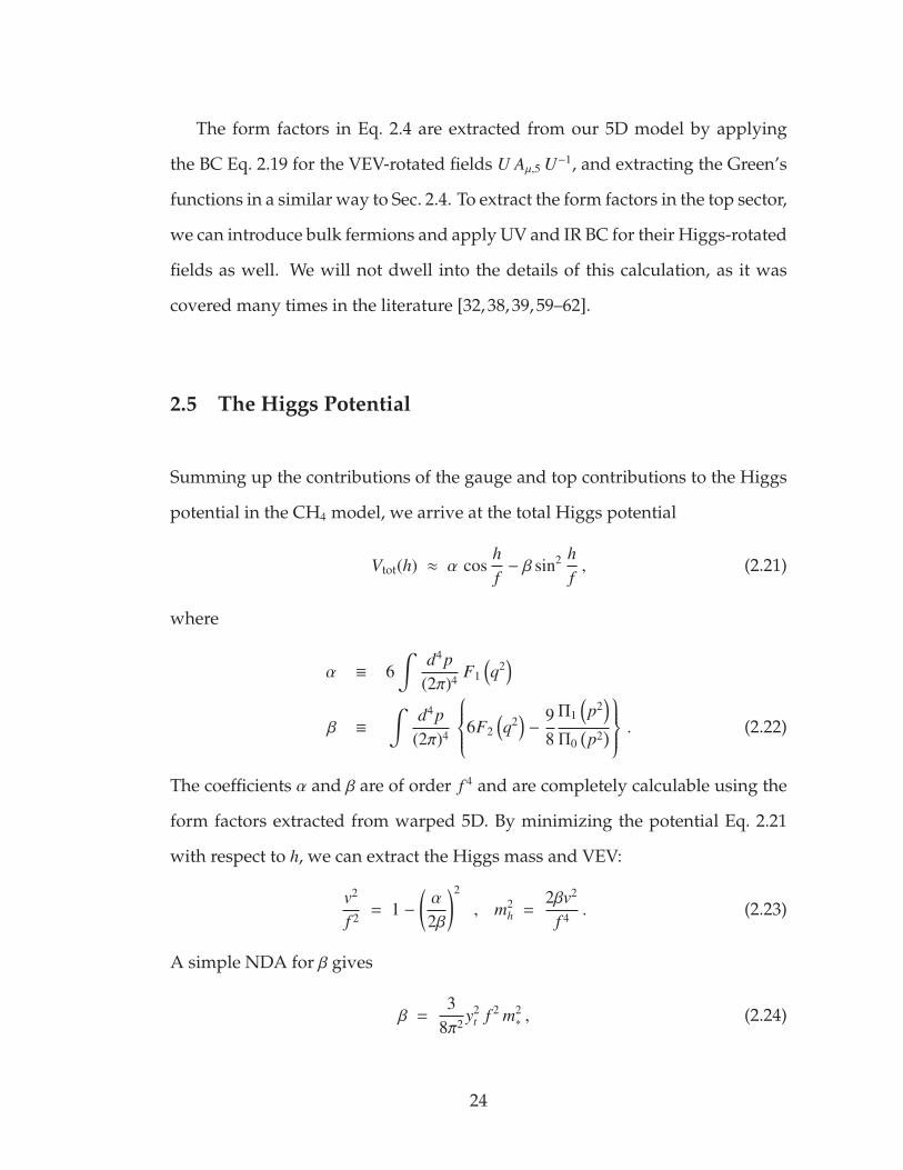
2.5 The Higgs Potential

Summing up the contributions of the gauge and top contributions to the Higgs

potential in the CH4 model, we arrive at the total Higgs potential

Vtot(h) ≈ α coshf− β sin2 h

f, (2.21)

where

α ≡ 6∫

d4 p(2π)4 F1

(q2

)β ≡

∫d4 p

(2π)4

6F2

(q2

)−

98

Π1

(p2

)Π0

(p2)

. (2.22)

The coefficients α and β are of order f 4 and are completely calculable using the

form factors extracted from warped 5D. By minimizing the potential Eq. 2.21

with respect to h, we can extract the Higgs mass and VEV:

v2

f 2 = 1 −(α

2β

)2

, m2h =

2βv2

f 4 . (2.23)

A simple NDA for β gives

β =3

8π2 y2t f 2 m2

∗ , (2.24)

24

where m∗ is an effective O( f ) mass scale that is directly calculable from Eq. 2.22

using the 5D form factors. This gives

m2h =

3y2t

4π2 ξm2∗ , (2.25)

where ξ ≡ v2

f 2 . Electroweak precision constraints require ξ <∼ 0.1, and so we can

accommodate a 125 GeV Higgs if m∗ >∼ 2 TeV.

The fine tuning required in this model was estimated in [63] to be m2t

m2∗

∼ 1%,

characteristic of what they define as “double-tuned models”. Other CH models

of this category are the CH5 and CH10 [64], while the tuning in CH14 [41, 65] is

only ∼ ξ ∼ 10%.

2.6 Phenomenology

Here we briefly review the current and future bounds on CH models. These

involve:

• Higgs couplings:

In SO(5)/SO(4) CH, the Higgs-gauge boson term in the effective La-

grangian is given by

LhVV = PµνT

M2V

v2 f 2 sin2(

hf

)VµVν , (2.26)

where V = W,Z and v2 ≡ f 2 sin2(〈h〉/ f ), as can be seen by expanding Eq. 2.4.

Expanding around h = 〈h〉, we have

LhVV = PµνT

M2V

v2

[v2 + 2v

√1 − ξh + (1 − 2ξ)h2 + . . .

]VµVν . (2.27)

25

Consequently, the hVV and hhVV couplings in CH models deviate from

their SM values by

ghVV = gSMhVV

√1 − ξ , ghhVV = gSM

hhVV (1 − 2ξ) , (2.28)

with similar representation dependent deviations for ghtt. The projected

bounds on ghZZ and ghtt from future lepton colliders (CPEC, FCC-ee, ILC)

is of order 0.8% and 5%, respectively, providing projected bounds [66] of

ξ . 3 · 10−3, which could imply extensive tuning.

• Electroweak precision:

Electroweak precision bounds from LEP are usually formulated in terms

of the Peskin-Takeuchi parameters S and T [67]. In CH models with cus-

todial symmetry in the Higgs sector (for example all SO(5)/SO(4) mod-

els), there is no tree level deviation in the T parameter due to the ex-

change of composite vector resonances. The S parameter gets a contri-

bution [32, 64, 68]

S = 4π (2.08)(

vmρ

)2

, (2.29)

where mρ is the effective mass gap of the composite vector tower. An ad-

ditional correction to the S and T parameters comes from the deviation in

the Higgs-gauge boson couplings [69]:

∆S =1

12πξ log

(4π fmh

)∆T = −

3 sec2 θW

16πξ log

(4π fmh

). (2.30)

The LEP bounds on S , T then imply that mρ > 3 TeV and that ξ ≤ 0.1 for

mρ ∼ 3.5 [27].

• Flavor:

The flavor bounds on models with partial compositeness (and no flavor

26

symmetry) were studied in [39, 70]. The leading bound was from the con-

tribution of the tower of composite gluons to tree level Flavor Changing

Neutral Currents (FCNCs), and specifically the C4K operator. Interestingly,

models with partial compositeness enjoy some level of protection from

FCNCs due to an alignment mechanism called RS-GIM [37], which lowers

the bound on heavy vector resonances from ΛGUT to mρ ∼ O(30 TeV). This

is still and order of magnitude above the TeV scale, and so natural CH

models with mρ ∼ 3.5 TeV require flavor symmetry.

• Direct top and gauge partner searches:

Finally, the LHC has put direct lower bounds on the masses of heavy vec-

tor resonances and vectorlike top partners. The current bounds on vector-

like top partners are of order 1.2 TeV @ 36 fb−1, where the exact limits de-

pend on the charge of the top partner and its branching ratios [71–75].

The combined ATLAS bounds on heavy vector resonances are of order

3 − 4 TeV @ 36 fb−1, depending on the channel [76–79], comparable to the

bound from electroweak precision.

27

CHAPTER 3

A TREE LEVEL QUARTIC FROM 6D COMPOSITE HIGGS

BEYOND THE STANDARD MODEL: COMPOSITE HIGGS AND DARK

MATTER

Ofri Telem, Ph.D.

Cornell University 2019

We present a new class of composite Higgs models where an adjustable tree-

level Higgs quartic coupling allows for a significant reduction in the tuning of

the Higgs potential. Our 5D warped space implementation is the first exam-

ple of a holographic composite Higgs model with a tree-level quartic. It is in-

spired by a 6D model where the quartic originates from the Tr[A5, A6]2 term of

the gauge field strength, the same model that led to the original little Higgs con-

struction of Arkani-Hamed, Cohen, and Georgi. Beyond the reduction of the

tuning and the standard composite Higgs signatures, the model predicts a dou-

bling of the KK states with relatively small splittings as well as a Higgs sector

with two doublets in the decoupling limit.

3.1 Introduction

The origin of the Higgs potential and its stabilization is one of the key mysteries

posed by the standard model (SM) of particle physics. An exciting possibility

for explaining the dynamics behind electroweak symmetry breaking (EWSB) is

that the Higgs boson itself is composite [9, 13, 14], due to an additional strong

interaction at scales about a decade or two above the weak scale. While this idea

is intriguing, it does not work without additional structure: in order to reduce

the scale of the Higgs mass well below the new strong coupling scale, one also

needs to assume that the Higgs is a pseudo-Nambu-Goldstone boson (pNGB)

of a global symmetry broken at a scale f , giving rise to pNGB composite Higgs

models. There are two basic types of these: little Higgs (LH) models [80, 81]

which were very popular in the early 2000s and (holographic) composite Higgs

(CH) models [32,58,64,82], the simplest of which is the so called Minimal Com-

posite Higgs Model (MCHM). For reviews see [27–30]. In both cases the essen-

tial ingredient for the 1-loop cancellation of the quadratic divergences is collec-

tive symmetry breaking [81], in which no single explicit breaking term breaks

the global symmetry completely, and the divergences in the Higgs potential are

softened. Most LH models contain a tree-level collective quartic (and a loop-

induced finite or at most log divergent quadratic term), resulting in completely

natural EWSB with no tuning. However, since the size of the quartic is deter-

mined by the same parameters as the quadratic, these models predict a heavy

Higgs boson well above the observed 125 GeV mass. Holographic composite

Higgs models have a loop-induced quartic and therefore predict the correct size

of the Higgs mass. This, however, comes at a cost of a (v/ f )2 tuning [39] in the

Higgs potential. Additionally, the top partners in these models tend to be at

29

least as heavy as 1.5− 2 TeV and thus not immediately discoverable at the LHC.

The tuning in holographic composite Higgs models could clearly be reduced

if a tree-level but adjustable quartic were present.1 This realization has inspired

us to revisit the original little Higgs model [80], formulated as a 6D gauge theory

where two Higgses correspond to two Wilson loops going around the fifth and

sixth dimensions and the collective quartic arises from the field strength term

Tr[A5, A6]2.

The aim of this work is to implement the ideas of [80] within the holographic

approach where the extra dimension is warped. For this purpose, we construct

a 6D model on an AdS 5 × S 1 background where the quartic is generated simi-

larly to [80] and the Higgs can be interpreted as a composite pNGB. We discuss

the essential aspects of the 6D model and then quickly zoom in on a simple

and transparent formulation in terms of a warped 5D model, where only the

sixth dimension has been deconstructed. The resulting Higgs sector is a CP-

conserving two Higgs doublet model (2HDM) in the decoupling limit with a

tree-level, MSSM-like quartic. As we will see, this quartic can be adjusted to fit

the observed value without extra tuning.

In its warped 5D version it provides the first example of a composite Higgs

model with a tree-level Higgs quartic coupling in which the only source of tun-

ing is related to the reduction of the Higgs mass parameter. Moreover, the top

partners in this model can be light and discoverable at the LHC. It turns out to

be a relatively simple model which captures almost all the essential elements of

the 6D theory (as well as the original model of [80]).

1For an alternative recent approach towards reducing the tuning in the Higgs potential forCH models see [83].

30

The chapter is organized as follows: Sec. 3.2 contains an explanation of the

reduction of the tuning in the Higgs potential due to the presence of the ad-

justable Higgs quartic. In Sec. 3.3 we present the essential ingredients of the 6D

theory and the structure of the zero modes. Sec. 3.4 contains the warped 5D

model, which is the main new result of this work. We provide the matter con-

tent along with the structure of the Higgs potential and a mechanism for lifting

the flat direction in the tree-level potential in Sec. 3.5. The matching onto generic

2HDM models is contained in Sec. 3.6, and the basic elements of the expected

phenomenology in Sec. 3.7. We conclude in Sec. 3.8.

3.2 Motivations for a Quartic from 6D

The first implementation of the little Higgs idea [80] was based on a decon-

structed [84] 6D gauge theory. The aim was to construct a composite Higgs

model where a large tree-level quartic could result in a fully natural electroweak

symmetry breaking (EWSB) Higgs potential. The extra dimensional compo-

nents A5, A6 of the gauge field can have the right quantum numbers to be identi-

fied with the Higgs. Compactification of the extra dimension can provide physi-

cal irreducible Wilson lines in the extra dimension which have all the properties

of a pNGB in 4D (see also [85]). The quartic arises from the field strength term:

Tr[A5, A6]2 ∈ F56F56. (3.1)

In the deconstructed version, this corresponds to a plaquette operator.

Before explaining the details of the full 6D construction (as well as the simple

warped 5D version), we would like to explain how the presence of such a tree-

31

level quartic could help alleviate the tuning in composite Higgs models1. The

Higgs potential in CH models with a loop-induced quartic is parametrized as

V(h) =3g2

t M2Ψ

16π2

(−ah2 +

b2

h4

f 2

)(3.2)

where gt is the SM coupling, MΨ = gΨ f is the top partner mass, and a and b

are (at most) O(1) numbers. The coefficients a and b can be smaller than 1 (at

the price of tuning various terms against each other) but can not be bigger than

O(1). The tuning is then quantified by

∆ =1

ab. (3.3)

The origin of the v2/ f 2 tuning is easy to see: since both the quadratic and quartic

terms are loop-induced by the same dynamics, the minimum of the potential is

when v2

f 2 = ab , which for b ∼ 1 gives the “irreducible” tuning of composite Higgs

models ∆ = 1ab =

f 2

v2>∼9. The lower bound on this tuning follows from electroweak

precision and Higgs coupling constraints, which imply that that fv>∼ 3. A more

detailed analysis of the tuning yields

∆ ' 8 yt

( gΨ

1.8

)2(

f /v3

)2>∼ 8 yt , (3.4)

since gΨ > 1.8 is required to get a large enough loop-induced quartic.

An additional (adjustable) tree-level quartic significantly changes the pic-

ture, reducing the previously “irreducible” fv tuning. The reason is that the cou-

pling gΨ setting overall magnitude of the loop-induced Higgs potential can be

taken smaller, while the adjustable contribution ensures that λ = 0.13. In this

case the dominant bound on the tuning is no longer the indirect bound Eq. (3.4)

but rather the direct bound on the top partner mass from direct searches at the

LHC,

∆ ' 5.5 yt

( MΨ

1100 GeV

)2>∼ 5.5 yt . (3.5)

1For a detailed analysis of the tuning in CH models, see [63].

32

This is parametrically weaker than the bound in the conventional CH. More-

over, Eq. 3.5 implies that top partners should lie just around the corner, well

within the reach of the LHC.

The reduction of the bounds on tuning in twin Higgs type models [61, 62,

86–93] is even more impressive. One can show that twin Higgs models with an

additional source of quartic will remain natural (no tuning required) even after

the end of the high luminosity 13 TeV run of the LHC. Similar ideas have been

discussed in [94, 95].

3.3 The 6D Composite Higgs Model

In the following section we present a warped model with a collective tree-level

quartic for the pNGB Higgs. This model can either be written in six dimen-

sions or deconstructed into lower dimensional models. As we will see in the

next section, the simplest and most useful representation of this model is as a

warped 5D model with two sites in the bulk representing the sixth dimension.

To motivate this construction, we first review the essential features of the full

6D theory.

The 6D model is defined on an interval of AdS 5 × S 1/Z2 × Z2 with metric

ds2 =

(Rz

)2

(dx2 − dz2) − dy2 (3.6)

where the R < z < R′ coordinate parametrizes the warped direction of AdS 5 and

0 < y < Ry parametrizes the S 1 direction. The geometry along with the boundary

conditions is illustrated in Fig. 3.1. At z = R and z = R′ there are UV and IR 4-

branes, and at y = 0 and y = Ry there are other 4-branes, denoted Down and Up.

33

G

H

H

UV

Up

Down

IR

SM

Figure 3.1: A sketch of the layout of the 6D model. The rectangle repre-sents the two extra dimensions, the horizontal correspondingto the warped extra dimension, the vertical to the extra flat seg-ment of the 6th dimension. The 3-branes in the 3 corners rep-resent the symmetry breaking pattern at those locations, neces-sary to obtain the appropriate pattern of Higgs fields and cou-plings.

Furthermore, there are 3-branes at the four ‘corners’ UV-Down, UV-Up, IR-Up,

and IR-Down.

The bulk gauge symmetry of the model is G (usually chosen to be S O(5) to

incorporate custodial symmetry), broken to an H subgroup (S O(4) in the sim-

plest model) on the IR-Up, and IR-Down 3+1 branes. This setting is a direct

extension of the standard CH construction of a bulk G in AdS 5 broken to H on

the IR brane. The two IR symmetry breaking points in our case correspond to

two sets of G/H pNGBs instead of just a single one in the standard CH. Addi-

tionally, the bulk symmetry on the UV-Down corner to the SM S U(2) × U(1).

This is analogous to the UV breaking in the standard CH, which ensures that

only the SM gauge bosons remain light.

In a similar way to 5D gauge-Higgs unification, the Higgses in our setting

34

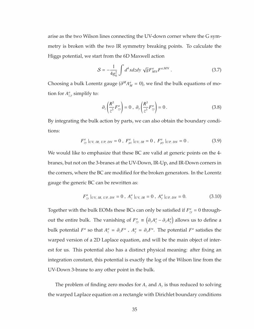
arise as the two Wilson lines connecting the UV-down corner where the G sym-

metry is broken with the two IR symmetry breaking points. To calculate the

Higgs potential, we start from the 6D Maxwell action

S = −1

4g26

∫d4xdzdy

√gFa

MN Fa;MN . (3.7)

Choosing a bulk Lorentz gauge (∂MAaM = 0), we find the bulk equations of mo-

tion for Aaz,y simplify to:

∂z

(R3

z3 Fazy

)= 0 , ∂y

(R3

z3 Fazy

)= 0 . (3.8)

By integrating the bulk action by parts, we can also obtain the boundary condi-

tions:

Fazy |UV, IR, UP, DN = 0 , Fa

µz |UV, IR = 0 , Faµy |UP, DN = 0 . (3.9)

We would like to emphasize that these BC are valid at generic points on the 4-

branes, but not on the 3-branes at the UV-Down, IR-Up, and IR-Down corners in

the corners, where the BC are modified for the broken generators. In the Lorentz

gauge the generic BC can be rewritten as:

Fazy |UV, IR, UP, DN = 0 , Aa

z |UV, IR = 0 , Aay |UP, DN = 0. (3.10)

Together with the bulk EOMs these BCs can only be satisfied if Fazy = 0 through-

out the entire bulk. The vanishing of Fazy ≡

(∂yAa

z − ∂zAay

)allows us to define a

bulk potential Fa so that Aaz = ∂zFa , Aa

y = ∂yFa. The potential Fa satisfies the

warped version of a 2D Laplace equation, and will be the main object of inter-

est for us. This potential also has a distinct physical meaning: after fixing an

integration constant, this potential is exactly the log of the Wilson line from the

UV-Down 3-brane to any other point in the bulk.

The problem of finding zero modes for Az and Ay is thus reduced to solving

the warped Laplace equation on a rectangle with Dirichlet boundary conditions

35

0 10 20 30 40

-80

-60

-40

-20

0

z

Lo

gF(z

,R6/2)/

R' A and B modes

0.0 0.2 0.4 0.6 0.8 1.0

-1.0

-0.5

0.0

0.5

1.0

y

Lo

gF(R

',y)/

R'

A mode B mode

IR brane

Figure 3.2: Slices of the 6D zero modes. (a): z-slice at y = R6/2 as a functionof z, illustrating that both are IR localized. (b) y-slice of the IR4-brane z = R′. Here the modes differ: mode A is localized closeto the IR-Down corner, while mode B is localized close to theIR-Up corner.

everywhere but the three gauge symmetry breaking points on the UV-Down, IR-

Up, and IR-Down corners. We have obtained the full solution to this problem

via Fourier transforms. The solution is a linear combination of two zero modes

A, B = 1, 2:

F i(z, y, x) = FA(z, y) hiA(x) + FB(z, y) hi

B(x), (3.11)

where FA are the extra dimensional wave functions and hiA are two 4D doublet

modes. Both of these are IR localized, FA is localized in the IR-Up corner and

FB is localized in the IR-Down corner. The index i above stands for the S U(2)L

doublet embedded in the adjoint of S O(5) as usual, and will be suppressed in

the following. We present slices of the zero modes obtained from solving the 2D

Laplace equation in Fig. 3.2. We can see that indeed both modes are IR localized,

and peak at two different corners on the IR brane.

36

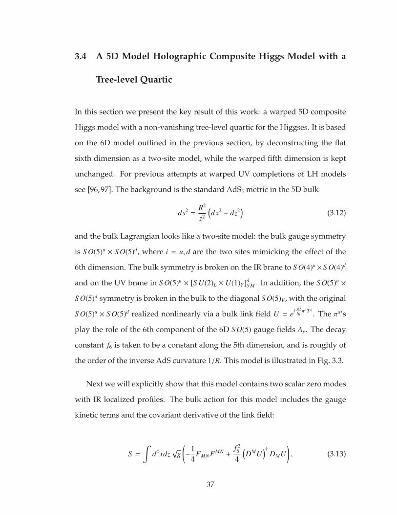
3.4 A 5D Model Holographic Composite Higgs Model with a

Tree-level Quartic

In this section we present the key result of this work: a warped 5D composite

Higgs model with a non-vanishing tree-level quartic for the Higgses. It is based

on the 6D model outlined in the previous section, by deconstructing the flat

sixth dimension as a two-site model, while the warped fifth dimension is kept

unchanged. For previous attempts at warped UV completions of LH models

see [96, 97]. The background is the standard AdS5 metric in the 5D bulk

ds2 =R2

z2

(dx2 − dz2

)(3.12)

and the bulk Lagrangian looks like a two-site model: the bulk gauge symmetry

is S O(5)u × S O(5)d, where i = u, d are the two sites mimicking the effect of the

6th dimension. The bulk symmetry is broken on the IR brane to S O(4)u × S O(4)d

and on the UV brane in S O(5)u × [S U(2)L × U(1)Y]dS M. In addition, the S O(5)u ×

S O(5)d symmetry is broken in the bulk to the diagonal S O(5)V , with the original

S O(5)u × S O(5)d realized nonlinearly via a bulk link field U = ei√

2f6πaT a

. The πa’s

play the role of the 6th component of the 6D S O(5) gauge fields Ay. The decay

constant f6 is taken to be a constant along the 5th dimension, and is roughly of

the order of the inverse AdS curvature 1/R. This model is illustrated in Fig. 3.3.

Next we will explicitly show that this model contains two scalar zero modes

with IR localized profiles. The bulk action for this model includes the gauge

kinetic terms and the covariant derivative of the link field:

S =

∫d4xdz

√g(−

14

FMN FMN +f 26

4

(DMU

)†DMU

), (3.13)

37

Figure 3.3: A sketch of the main elements of our deconstructed 5d model.The two sites in the bulk represent the S O(5)u × S O(5)d, brokenon the IR into S O(4)u × S O(4)d and on the UV into S O(5)u ×

[S U(2)L × U(1)Y]dS M. The bulk link corresponds to the breaking

of S O(5)u×S O(5)d into the diagonal S O(5)V with a constant VEVin the bulk.

where the covariant derivatives are

DµU =

√2f6∂µπ − g5A(A)

µ

+ ..., DzU = −

√2f6∂zπ − g5A(A)

z − i

√2g5

f6

[Au

z , π] + ...

(3.14)

and A(A)µ,z ≡ Au

µ,z − Adµ,z , A(V)

µ,z ≡ Auµ,z + Ad

µ,z, while the ellipses stand for higher order

commutator terms and terms negligible in the limit R R′. The scalar zero

modes live in a linear combination of π and Au,dz . We will use the Lorentz gauge

∂µAµ = 0, with the additional gauge fixing A(A)0 = 0. The vector combination AV

z

corresponds to an unbroken bulk symmetry, and so the part of the zero mode

contained in the corresponding fifth component must be of the usual form AVz ∼

z. Substituting the π variation in the axial part of the A0 variation, we obtain the

equation for the zero mode as well as the relation between Az and π components

38

of the zero mode:

z3

R3∂z

[Rz∂zπ

]− g2

5 f 26 π = 0

∂zπ −g5 f6√

2A(A)

z = 0 . (3.15)

We choose the UV boundary condition to be Auz |UV = 0. We do not need to

specify an IR boundary condition for the Azs: the reason is that in the gauge we

chose there is no boundary localized term involving Az, thus one does not need

to consider the boundary variation of these fields. This is in accordance with

our expectations from the fact that the Az equations of motion are effectively

first order, hence one BC should be sufficient. The space of zero mode solutions

is two dimensional, spanned by modes A and B satisfying:

A mode : Adz |IR = 0

B mode : Auz |IR = 0 . (3.16)

The two solutions to the EOM are:

π(z, x)A/B =g5 f6

2√

2

[±

11 + α

( RR′

)α ( zR

)1+α

+1

1 − α

( RR′

) ( zR

)1−α]

hA/B(x)

Auz (z, x)A/B =

12R

zR′

+

[±

( RR′

)α ( zR

)α+

( RR′

) ( zR

)−α]hA/B(x)

Adz (z, x)A/B =

12R

zR′−

[±

( RR′

)α ( zR

)α+

( RR′

) ( zR

)−α]hA/B(x) , (3.17)

where α =

√1 + g2

5 f 26 R2 and hA(x) and hB(x) are the two canonically normalized

4D modes. The ±mean a ”+” for the A mode and a ”−” for the B mode.

In the g5 f6R = g∗ f6R3/2 ≡ θ6 1 limit, which is necessary to obtain a quartic

smaller than O(1) (see Sec. 3.4.1), the profiles far from the UV brane (z R) are:

A Mode : Auz (z) =

1R

zR′

hA(x) , Adz (z) = O(θ2

6) hA(x) , π(z) = O(θ6) hA(x)

B Mode : Auz (z) = O(θ2

6) hB(x) , Adz (z) =

1R

zR′

hB(x) , π(z) = O(θ6) hB(x) (3.18)

39

This can be understood as the limit of no bulk breaking, in which the two modes

simply correspond to the pNGBs of the two separate SO(5)/SO(4) cosets. It is

then sensible to define the pNGB matrices:

Σu = exp(ig6

∫ R′

RAu

z dz)≡ eihu/ f , Σd = exp

(ig6

∫ R′

RAd

z dz)≡ eihd/ f (3.19)

These matrices restore the two S O(5) symmetries by rotating the IR vacua that

break S O(5) into S O(4). In the limit θ6 1:

hu ≈ hA , hd ≈ hB . (3.20)

Since we need to work in this limit for any realistic model building, from now

on we identify hA,B with hu,d.

3.4.1 The tree-level quartic

We can now evaluate the quartic scalar coupling by substituting the zero modes

in the commutator term of Eq. (3.14):

Lλ = λTr [hA, hB]2≈ λTr [hu, hd]2 (3.21)

with

λ = g25

∫dz

(Rz

)3 [πA AV

z,B − πB AVz,A

]2. (3.22)

Plugging in the profiles and working in the limit R′/R→ ∞, we get:

λ = g25

g25 f 2

6 R

4(1 + α)3 ∼14

g2∗ θ

26 . (3.23)

where the last result is in the limit that the scale of the bulk breaking is small,

i.e. θ6 1. This choice is necessary to get a quartic which is smaller than O(1),

and as promised, also justifies the identification Eq. (3.20).

40

The quartic has the following structure:

λ [hu, hd]2 = λ(h†1h1 − h†2h2

)2+ λ tr

(h1h†1 − h2h†2

)2, (3.24)

where we have adopted the definitions of [80]:

h1 =1√

2(hu + ihd) , h2 =

1√

2(hu − ihd) . (3.25)

This quartic has a flat direction for hu or hd, which corresponds to h1 = ±h2.

In Sec. 3.5.3 we will discuss how these flat directions are lifted radiatively by the

SM top and its partners.

3.4.2 The 4D interpretation

The warped 5D picture makes it easier to identify the 4D dual to our model

based on the rules of the AdS/CFT correspondence [42, 98, 99]. As in the stan-

dard CH, this dual is a strongly interacting theory which is close to conformal

in the UV but confines in the IR. Above the confinement scale there is a global

symmetry G × G (the bulk symmetry in the 5D picture), and the IR condensate

breaks it to H × H with two sets of G/H pNGBs.

To better understand the CFT dual to the G ×G → G breaking in the bulk we

have to specify the origin of this breaking. We take this origin to be a scalar in

the bi-fundamental of G × G which gets a bulk VEV. The generic profile of this

scalar is:

U(z) = f6

[( zR

)−ε+ b

( zR′

)4+ε], (3.26)

with ε =√

4 + m2/k2 − 2. The coefficient b is determined by the IR boundary

conditions and is generically ∼ O(

RεR′ε

). By choosing the bulk mass of the scalar

41

to be small, we can have ε ≈ 0 and b ∼ O (1), so that

U(z) ≈ f6

[1 + b

( zR′

)4], (3.27)

Which is well approximated by a constant VEV f6 in the bulk and slightly larger

VEV f ′6 = f6 (1 + b) on the IR brane. The presence of G×G → G breaking on the

IR brane does not spoil the collective breaking in our scenario, as we elaborate

towards the end of this section.

Using the AdS/CFT dictionary, this configuration corresponds to a source

JG×G coupled to an operator OG×G that transforms as a bi-fundamental of the

global G ×G:

∆L = JG×G OG×G . (3.28)

The magnitude of the source is f6, while its dimension is −ε ≈ 0 and the di-

mension of the operator is 4 + ε ≈ 4. The source explicitly breaks G × G to the

diagonal, and also triggers a VEV for the operator [99]:

〈OG×G〉 = (4 + 2ε)b f6

R′4+ε, (3.29)

Due to the explicit G × G → G breaking from the source, the G × G/H × H

pNGBs get a tree-level potential. Remarkably, this tree-level potential consists

only of a commutator-squared term, and in particular does not include tree-

level masses for the pNGBs. This is a demonstration of the ’collective’ nature of

our potential.

In addition to the effect of the explicit G ×G breaking, one might worry that

the VEV 〈OG×G〉 (dual to the G×G breaking on the IR brane) could generate a tree

level mass to the axial PNGB, spoiling our collective breaking. This is indeed

true, but is an artifact of representing the six dimension with only two sites

42

in the bulk. Indeed, in the full 6D model the two G/H breakings are physically

separated along the 6th dimension, and the tree level mass for the axial PNGB is

exponentially suppresses. This effect would have been captured in a 5D model

with more sites in the bulk. For that reason, we did not include any G × G

breaking on the IR brane in our 5D model from section 3.4.

3.5 The SM field content

So far we have only considered the scalar modes and their tree-level quartic

(while also introducing the SM gauge fields). In this picture, the 4D gauge fields

correspond to the zero modes of the surviving diagonal subgroup of the bulk

gauge symmetry:

AS Mµ = Au

µ + Adµ. (3.30)

These are the S U(3) × S U(2) × U(1)Y gauge fields, which have Neumann BC on

both branes and no bulk mass.

The scalar sector consists of two pNGB Higgs scalars which in the θ6 1

limit are the hu,d of S O(5)u,d/S O(4)u,d. However, the hu,d basis is not the physical

basis for our Higgses, as we will see from the radiatively generated contribu-

tion. Instead, we work in the h1,2 basis of Eq. (3.24), with the quartic given by

Eq. (3.25).

Next we introduce the SM fermion matter content into this theory. Presently

we do not specify the light fermion representations, as there are many different

possibilities. The exact choice will definitely be relevant for flavor physics, but

its effect on the Higgs potential is negligible. In the following we will only focus

on the top sector and its contribution to the Higgs potential. To be consistent

43

with the LHC results on Higgs couplings, we require one Higgs to be SM-like,

while the other one should be heavy. We achieve this by arranging for the top

to couple only to h1 so that the top loop gives a negative mass term for h1, while

h2 is lifted by the other members of the top’s S O(5) multiplet.

3.5.1 The top sector

The simplest choice for the top sector is to embed tL in a multiplet TL transform-

ing as a (5, 1) + (1, 5) of S O(5) × S O(5), while tR is a singlet localized on the IR

brane. This is summarized in Tab. 3.1. In terms of two component spinors, the

bulk fermion TL can be written as

TL =

χuL χd

L

ψuL ψd

L

, (3.31)

where χu,d, ψu,d are 2-component Weyl spinors. We impose a Z4 symmetry on the

fermion sector in the bulk and on the U field:

Z4 : T uL → −T d

L T dL → T u

L

U → U† (π→ −π) . (3.32)

As we will see, this Z4 symmetry ensures that the top couples only to h1, which

is important for a realistic Higgs potential. The 5D Lagrangian for TL can be

written as

LTL =

[iχLσ

µDµχL + iψLσµDµψL +

12

(ψL←→DzχL − χL

←→Dz ψL

)+

cL

z(ψLχL + χLψL

)]u,d

+

y6θ6

2z

(iψd

L U† χuL − iψu

L UχdL + iχd

L U† ψuL − iχu

L U ψdL

), (3.33)

where y6 is a O(1) coupling of the link field. The first line is just the standard 5D

warped fermion Lagrangian, while the second line includes the fermion cou-

44

plings to the link field which stand for their coupling to A6 in the full 6D La-

grangian. The bulk masses for both multiplets are assumed to be equal. This

arises naturally in the 6D picture and can be thought of as a u↔ d Z2 symmetry

that is preserved in the bulk and on the IR brane (while broken in the UV).

Field SO(5)u SO(5)d

(χL, ψL

)u 1(

χL, ψL)d 1

tR 1 1

U

Table 3.1: Representations of the 5D Model Top Sector

The Az VEV is set to zero by a gauge rotation [59], with the Az Wilson line

entering in the IR boundary condition. Rotating to the bulk mass basis, we have

LTL =

[iχLσ

µ∂µχL + iψLσµ∂µψL +

12

(ψL←→∂z χL

)+

cL ± y6θ6

zψLχL

]0,1

, (3.34)

where ψ0,1L = 1

√2

(ψu

L ± iψdL

), χ0,1

L = 1√

2

(χu

L ± iχdL

).

We see that the full TL bulk multiplet splits into two bulk fermions with

masses cL ± y6θ6. On the IR brane we will always take the same BC for the up

and down fermions, while on the UV the BC may be different. To understand

how this works, take for example the following BC for a bulk fermion:

χuL : (−,+) , χd

L : (+,+) , (3.35)

where the tilde serves to remind us that the boundary conditions are for the

Wilson line rotated fields

χuL = χu

L Σu , χdL = χd

L Σd , (3.36)

45

and Σu,d are the usual pNGB matrices given by Eq. (3.19). In terms of the two

combinations in the bulk mass basis ψ0,1l this corresponds to:

ψ0L(R) = ψ1

L(R) , χ0L(R) = −χ1

L(R)

ψ0L(R′) = 0 , ψ1

L(R′) = 0 . (3.37)

These boundary conditions result in a single zero mode that lives both in the 0

and 1 parts of the multiplet:

χ0,1L (z, x) ∼

( zR

)cL±y6θ6

tL (x) . (3.38)

Note that the combination χ0 with the higher bulk mass rises faster towards the

IR, and so the dominant contribution to the Higgs potential comes from that

combination. In the following calculation of the Higgs potential we will neglect

the χ1 contribution, and comment on it in the end of section 3.6.

On the IR brane, the singlets of S O(4) × S O(4) in the TL multiplet can couple

to tR. Formally, these couplings can be written in terms of the spurions that

break the S O(5)s into S O(4)s, denoted as S u,d = (0, 0, 0, 0, 1). The IR Lagrangian

is given by:

LIR = µχuLΣuS utR + µχd

LΣdS dtR + h.c. (3.39)

with the projections of the pNGB matrices written explicitly as

Σu,dS u,d =sin

(hu,d

f

)hu,d

[hu,d

1 , hu,d2 , hu,d

3 , hu,d4 , hu,d cot

(hu,d

f

)]T

, hu,d =

√hu,d

a hu,da . (3.40)

We have also assumed that the IR masses respect the u↔ d symmetry (similarly

to the bulk masses).

46

3.5.2 The top contribution to the Higgs potential

The 4D effective Lagrangian for the top zero mode can be obtained from

Eq. (3.39) by inserting the bulk profile of Eq. (3.38) evaluated on the IR brane.

The profile on the IR brane is dominated by the combination T 0L = 1

√2

(T u

L + iT dL

)of the two bulk multiplets, and so on the IR brane

χdL ' iχ0

L , χuL ' χ

0L (3.41)

The 4D Lagrangian for the top is then:

Ltop =yt f√

2χ0

L

(ΣuS u + iΣdS d

)tR (3.42)

where

χ0L =

1√

2

(−ibL, bL, itL, tL, 0

). (3.43)

Substituting these definitions and expanding to second order in the Higgs dou-

blets h1,2, where

h1,2 =12

ihu3 + hu

4 ± i(

ihd3 + hd

4

)−ihu

1 + hu2 ± i

(−ihd

1 + hd2

) , (3.44)

we get the effective Yukawa coupling of the top:

Leff = yt h1 tLtR. (3.45)

We see that the top couples only to h1, so that it contributes a −3y2t M2

KK16π2 h1h†1 to the

2HDM potential, generating a negative quadratic term in the h1 direction.

3.5.3 Lifting the flat direction

To lift the flat direction we must have a sizable positive mass term of h2. To do

that, we break down the contribution of the top partners to the Higgs potential.

47

The top partners populate the TL multiplet, which is the (5, 1) + (1, 5) of S O(5) ×

S O(5). As before, we separate TL into the linear combinations:

T 0,1L =

1√

2

(T u

L ± iT dL

), (3.46)

These multiplets couple to tR through the pNGB matrices:

Ltop+topKK =yt f√

2χ0,1

(ΣuS u ± iΣdS d

)tR + h.c. (3.47)

where χ0,1 are the left handed Weyl fermions in the Dirac fermions T 0,1L .

The total contribution to the Higgs potential from complete multiplets T 0L

and T 1L has to be zero, because their linear combinations T u

L, T dL form complete

S O(5) × S O(5) multiplets. Furthermore, even the individual contributions of

complete multiplets T 0L and T 1

L are separately zero. Indeed, the Coleman Wein-

berg potential depends on T 0,1L through∣∣∣∣∣∣yt f√

2

(ΣuS u ± iΣdS d

)∣∣∣∣∣∣2 = y2t f 2 , (3.48)

which is independent of h1,2. Since our zero modes live mostly in T 0L and all the

other modes are at MKK , we can now ignore the complete multiplet T 1L and focus

only on the T 0L contribution, which is cut at MKK .

The top partners in T 0L are:

T 0L =

1√

2

(0, 0,−it0

d, t0d, t

0s

). (3.49)

Here t0d is part of an electroweak doublet and t0

s is an electroweak singlet. Their

couplings to the Higgs in Eq. (3.47) can be explicitly written as:

Ltop partners = yt t0dLh†2tR + yt t0

sL

(f −

h21

2 f−

h22

2 f

)tR + Md t0

dLt0dR + Mst0

sLt0sR , (3.50)

while the Higgs potential contribution of this sector is

V(h1, h2) = −3y2

t M2s

16π2 h1h†1 +3y2

t

(M2

d − M2s

)16π2 h2h†2 . (3.51)

48

TL0 TL

1

t

ts

td t1,ts1,td

1MKK

mt

Ms

Figure 3.4: The top partner spectrum in our model.

The top partner spectrum of our model is shown in Fig. 3.4. We see that Ms

acts effectively as a cutoff for the h1 mass term, while both the doublet and the

singlet contribute to h2 with opposite signs. For Md > Ms, we get a positive mass

for h2, lifting the flat direction as required. A simple way to achieve this is to

take t0sL as a zero mode as well, and marry it in the bulk and on the IR to a similar

right handed fermion in a new multiplet. The b.c. for the top multiplet are thus

taken as:

(tL, bL) : χuL : (−,+) , χd

L : (+,+)

(tdL, bdL) : χuL : (−,+) , χd

L : (−,+)

sL : χuL : (−,+) , χd

L : (+,+), (3.52)

where the b.c. are given for the left-handed Weyl fermion and the b.c. are

flipped for the opposite chirality. The new multiplet S R is also in a (5, 1) + (1, 5)

of S O(5)× S O(5). Its boundary conditions are different from those of TL, as only

49

the singlets of S O(4) × S O(4) have BC similar to the top

χuS : (−,+) , χd

S : (+,+) , (3.53)

while the rest have (−,+) BC for both up and down components. This means

that the zero mode, which we denote s0R, exactly mirrors t0

sL and can marry it in

the bulk and on the IR. The bulk mass of the multiplet is chosen such that zero

mode is localized sufficiently far from the UV so that Ms<∼ Mkk. We also choose

the mixing of the two multiplets to obey the full S O(5)×S O(5) symmetry so that

a new contribution to the Higgs potential is not generated. The 4D Lagrangian

is then exactly Eq. (3.50) with Ms being a free parameter. With our choice of

Ms < Md ∼ MKK , the total radiative Higgs potential is

V(h1, h2) = −3y2

t M2s

16π2 h1h†1 +3y2

t M2KK

16π2 h2h†2 . (3.54)

This potential lifts the h2 mass to the KK scale, so that:

mh2 =MKK

Msmh1 ≈

MKK√

2Ms

mh (3.55)

where mh is the measured mass of the SM Higgs (which corresponds to h1 in our

scenario).

3.6 The 2HDM Potential

In this section we present the Higgs potential in our model. As we will see, this

is a 2HDM potential in the decoupling limit1. The h1 doublet will serve as the

SM Higgs, coupling with approximately SM magnitudes to the W and Z gauge

bosons and to the top and bottom sector, while h2 will be heavy.

1For another example of a CH model with a 2HDM scalar sector, see [100].

50

3.6.1 Mass terms and quartic

The SM-like h1 gets a negative quadratic term via top loops

m2h1∼ −

3y2t M2

s

16π2 , (3.56)

while the positive quadratic term of the second Higgs is

mh2 ∼MKK

Msmh1 , (3.57)

as explained above. Additionally, there is a small h1h2 mixing from the sub-

dominant mode with bulk mass c − ∆c, which we have neglected previously.

Including this mode, we get a fermion Lagrangian of the form of Eq. (3.50) with

the following corrections:

h1 → h1 + εh2 , h2 → h2 + εh1 , (3.58)

where ε ∼(

RR′

)2∆c∼ 1

40 is the mixing angle of the subdominant combination in the

top zero mode. The resulting correction to the 2HDM potential is subdominant

except for a possibly important mixing term −m212 h1h2 which was neglected in

Eq. (3.54). We estimate this term to be

m212 ∼ εm

2h2. (3.59)

The only tree-level part of the 2HDM potential is the quartic term

λ(h†1h1 − h†2h2

)2+ λ tr

(h1h†1 − h2h†2

)2, (3.60)

with λ given by Eq. (3.23).

51

3.6.2 Matching to the general 2HDM potential

The general 2HDM Lagrangian [101, 102] is

Lh12 = m2h1

h†1h1 + m2h2

h†2h2 − m212

(h†1h2 + h.c.

)+

+12λ1

(h†1h1

)2+

12λ2

(h†2h2

)2+ λ3

(h†1h1

)(h†2h2

)+ λ4

(h†1h2

)(h†2h1

)+ other CP violating quartics . (3.61)

Matching this to our case, we have λ1 = λ2 = −2λ3 = −2λ4 = 4λ, while the other

CP violating quartics are zero - exactly the same as in the Higgs sector of the

MSSM. Since |m212| < |m

2h1| < |m2

h2|, we are in the decoupling limit with small tan β.

Indeed, minimizing the potential we get:

tan β ∼ ε ∼1

40, (3.62)

so that m2A = m2

H± = m2h2

. In the decoupling limit, we can just fit the quartic to its

experimental value12

g2∗θ

26 = 2λ ≈ 0.13 . (3.63)

For g∗ >∼ 3 we get that the bulk S O(5)× S O(5) breaking parameter is θ6 ∼ 0.1. The

physical Higgs masses in the decoupling limit are just:

mh ' mh1 , mH ' mh2 , (3.64)

while the alignment angle is

cos (α − β) = tan βmh√

m2H − m2

h

. (3.65)

Since our cos (α − β) is small, our decoupling limit leads to alignment: the vector

bosons couple to h with SM-like magnitudes, while their coupling to H is sup-

pressed. In other words, h is almost completely SM-like, while H is both heavy

and inert up to O( 140 ).

52

3.7 Phenomenological Consequences

The BSM phenomenology of our model can be largely divided into standard

composite Higgs phenomenology, which implies all the generic features of com-

posite Higgs models, and additional features which are specific to our model.

The standard composite Higgs phenomenology has been covered extensively in

the literature (see [27–30]), and here we only briefly summarize the main pre-

dictions:

• Fermionic top partners: New vector-like quarks that would appear in di-

rect searches. In our model there is a light top partner - t0s with SM quan-

tum numbers (3, 1, 2/3), which is lighter than the rest of the KK states. This

state cancels the top loop and so its mass is directly connected to the tun-

ing. Current constraints are Ms>∼ 1.1 TeV [103, 104], which corresponds to

a tuning of O(20%). We assume the rest of the top KK modes are much

heavier: MKK > 3 TeV.

• Gauge partners: Heavy new EW vectors that would appear as resonances

at the LHC. The gauge partners also directly contribute to the tuning, and

their mass has to be MV>∼ 2.5 TeV. In this model we assume that the neces-

sary O(20%) tuning in the Higgs sector is obtained via the cancellation of

the top and gauge loops.

• Higgs data: Due to the pNGB nature of the Higgs, the coupling of the

Higgs differ from the SM expectation by O(

v2

f 2

). This is also the main devi-

ation in the Higgs signals in our model.

• EW precision data: In composite Higgs models with custodial protection,

the dominant effect is on the S parameter due to tree-level mixing with the

53

gauge partners. At the loop level, the change in the Higgs coupling and

the new top partners also have a measurable effect. This is true for our

model as well.

• Flavor: The new composite states can mediate FCNC. These are sup-

pressed if the SM fermions are partially composite, but the suppression

is usually not sufficient for the composite Higgs to be the solution of the

hierarchy problem. To avoid these constraints, CH models with various

flavor symmetries have been considered [105–108]. Addressing these con-

straints is beyond the scope of this work, but it is plausible that similar

symmetries can be implemented in our model for the same purpose.

The main non-standard features of our model are the doubled KK spectrum

and the extended Higgs sector.

Double KK spectrum. All the KK modes in our model appear in both the up

and down sites. The splitting between two such modes is O(θ6MKK) ∼ 300 GeV

for fermion KK modes and O(θ26 MKK) ∼ 30 GeV for vector KK modes. To obtain

the measured quartic we require θ6 ∼ 0.1. The small splitting between the modes

is a clear prediction of our model.

Extended Higgs sector. The Higgs sector of our model is a 2HDM where the

second doublet is almost inert. The mass of the second doublet depends on the

ratio between the light top partner and the KK scale:

mh2 ∼MKK√

2MS

mh (3.66)

For reasonable choice of parameters, we get mh2 ∼ 300 − 500 GeV. The phe-

nomenology of the states in this doublet depends on the embedding of the

quarks in our model. If we assume that all the quarks couple to h1 similarly

54

to the top, then the coupling to the second doublet are suppressed by the mix-

ing which is O( 140 ). This suppresses all single production processes for the scalar

states in the second doublet. The charged Higgs can additionally be produced

in pairs via an unsuppressed Drell-Yan process. Further analysis is required to

obtain precise bounds and discovery potential for these states.

3.8 Conclusions

Composite Higgs models are among the most exciting viable extensions of the

SM. One of the long-standing issues with such models is the tuning necessary

to obtain a realistic Higgs potential with a 125 GeV Higgs mass. In this work

we presented a novel class of models where this tuning can be reduced in the

presence of a tree-level quartic for the Higgs. The model originates from a 6D

orbifold producing two pNGB Higgs doublets which naturally obtain a collec-

tive quartic due to the 6D gauge interactions. The simplest and most useful

implementation is based on its 5D two-site deconstructed version, where the

bulk gauge group for the minimal model is S O(5)× S O(5), with a bulk link field

breaking the group to the diagonal, in addition to boundary breakings ensur-

ing the presence of the two light Higgs doublets. This is the first example of

a holographic composite Higgs model with a tree-level quartic for the Higgs.

Importantly, the magnitude of the quartic can be adjusted by dialing the param-

eters of the theory which can result in the SM quartic dominantly arising from

the tree-level contribution. This in turn allows us to suppress all loop effects,

leading to the reduction of the tuning. The main experimental consequence of

such models (beyond the standard signals of composite Higgs models such as

colored top partners, gauge partners, etc) is the doubling of the KK spectrum.

55

The splitting among the KK modes is related to the same parameters setting the

magnitude of the quartic. We find that for a realistic model with reduced tuning,

the splitting among the doubled KK states has to be relatively small (of order

tens of GeV for the vector KK modes and hundreds of GeV for the fermionic

KK modes). In addition, the Higgs sector has to contain two Higgs doublets,

which must be in the decoupling limit in order to correctly reproduce the mea-

sured Higgs phenomenology. Finally, unlike the CH case, direct searches for

fermionic top partners provide the most stringent bounds on naturalness in our

model, and so we expect them to lie just around the corner within the LHC

reach.

56

CHAPTER 4

CONTINUUM NATURALNESS

BEYOND THE STANDARD MODEL: COMPOSITE HIGGS AND DARK

MATTER

Ofri Telem, Ph.D.

Cornell University 2019

We present a novel class of composite Higgs models in which the top and gauge

partners responsible for cutting off the Higgs quadratic divergences form a con-

tinuum. The continuum states are characterized by their spectral densities,

which should have a finite gap for realistic models. We present a concrete ex-

ample based on a warped extra dimension with a linear dilaton, where this

finite gap appears naturally. We derive the spectral densities in this model and

calculate the full Higgs potential for a phenomenologically viable benchmark

point, with percent level tuning. The continuum top and gauge partners in this

model evade all resonance searches at the LHC and yield qualitatively different

collider signals.

4.1 Introduction

The cornerstone of conventional solutions to the hierarchy problem, e.g. super-

symmetry and composite Higgs (CH) [13,27–30,32,80,109,110], is the existence

of new states around the TeV scale. The role of these top and gauge partners

is to cut off the quadratically divergent radiative corrections to the Higgs po-

tential from the top quark and gauge bosons. In recent years, searches at the

LHC have placed the naturalness paradigm under pressure by setting signif-

icant lower bounds on the masses of top and gauge partners of about 1.2–1.4

TeV [71, 72, 111–114] and 2.2–2.5 TeV [78, 115, 116], respectively.

However, many of these searches assume that the top and gauge partners are

particles that can be produced on-shell. In this work we introduce a new class

of models in which the top and gauge partners are gapped continuum states

[117–120], rather than ordinary particles.

The simplest example of a spectrum with gapped continuum modes is that

obtained from the finite potential well in standard quantum mechanics (QM).

While the bound states inside the well form a discrete set, the scattering states

form a continuum with energies above the well. Another example is a strongly-

interacting theory with a critical behavior in the IR that gives rise to a gapped

continuum1. For example, it is believed that at the bottom of the conformal

window of supersymmetric QCD, a gapped continuum can be generated by

turning on a squark mass [119].

In this work we present a CH model in which continuum top and gauge

partners arise as the composites of a strong sector with critical behavior in the

IR. Inspired by the AdS/CFT correspondence [42] and holographic realizations

of CH models [32, 58], our gapped continuum arises from a warped 5D geom-

etry [44] with a linear dilaton [125–127]. The resulting Green’s functions have

a branch cut starting at a finite gap µ corresponding to the slope of the linear

dilaton, indicating the emergence of a continuum.

Based on this linear dilaton geometry, we construct a fully realistic CH model

1For example, see [121–124].

with partial compositeness [34–37, 46] and gauge-Higgs unification [49–53, 57].

Similar to the standard warped 5D realizations of CH, our setting involves AdS5

with a UV brane and an IR brane. However, in our case, the fifth dimension

continues beyond the IR brane to infinity, with a dilaton rising in the deep

IR [128–130]. The other ingredients of the model are identical to standard CH

models: a bulk gauge symmetry S O(5) × U(1) broken to S O(4) × U(1) on the IR

brane and to S U(2)L ×U(1)Y on the UV brane; the A5 of S O(5)/S O(4) playing the

role of the pseudo-Nambu-Goldstone (pNGB) Higgs; and the Standard Model

(SM) fermions and their partners embedded in bulk S O(5) representations.

The result is a realistic CH model in which the top and gauge partners are all

continua, with no BSM resonances within the reach of the LHC. We demonstrate

this by focusing on one point in our parameter space, for which we get a realistic

Higgs potential (with 1% tuning) with gaps of about 1–2 TeV.

The chapter is structured as follows. In Section 4.2 we present the effective

action for continuum states, and how the properties of the continua are encoded

in their spectral densities. In Section 4.3 we show how to model gauge and

fermion continua in a warped 5D geometry with a linear dilaton. We give an in-

tuitive argument for the emergence of a gapped continuum from this geometry,

based on an effective Schrodinger equation, and then calculate the continuum

spectral densities in a procedure inspired by AdS/CFT. Using linear dilaton ge-

ometry, we construct a realistic CH model with gauge-Higgs unification and

continuum top and gauge partners in Section 4.4. For the purpose of breaking

the bulk S O(5) symmetry, we introduce an IR brane. However, the fifth dimen-

sion continues beyond the IR brane to a region where the linear dilaton dom-

inates and leads to the gapped continuum. The role of the Higgs is played as

usual by the A5 of the S O(5)/S O(4) generators, while the SM Yukawa couplings

originate from the jump conditions for the bulk fields on the IR brane.

Our results are summarized in Section 4.5, while the detailed calculation

of the gauge and fermion spectral densities is given in Section 4.6 (and in the

appendices). To extract the fermion spectral densities, we solve the 5D inhomo-

geneous equations of motion (EOM) subject to the UV boundary conditions and

the IR jump conditions. We account for the bulk VEV of the Higgs–A5 by rotat-

ing it into the IR jump conditions as usual [59]. We diagonalize the resulting

20 × 20 fermionic Green’s function matrix to obtain all of the fermionic spectral

densities in our model. The gauge spectral densities are calculated in a similar

manner.

In Section 4.7 we calculate the Coleman-Weinberg potential for the Higgs

from the spectral densities of our benchmark point in parameter space. We

obtain a fully realistic Higgs potential, consistent with electroweak precision

bounds on v/ f and with a tuning of 1%, compared to per mille level tuning in a

corresponding composite Higgs model with the same IR scale R′ and the same

choice of bulk representations [63]. Finally, we comment on the phenomenol-

ogy of continuum partners: the lack of resonances within the reach of the LHC,

bounds from the running of αs, and the way to calculate the pair-production

cross section for continuum fermions. The phenomenology of continuum part-

ners will be explored further in an upcoming work [131].

4.2 Effective Action for Continuum States

The essential ingredients of CH models are the tower of composite top and

gauge partners. These states cancel the one-loop SM top and gauge contribu-

tions to the Higgs potential below the confinement scale of Λ, which we take to

be about 2–3 TeV. The main new aspect of the model we present in this work

is that the critical IR dynamics give rise to a continuum of top and gauge part-

ners rather than a tower of ordinary particles. To study the phenomenology of

such continuum top and gauge partners we need to first explain how to write

an effective action for these states.

We will illustrate this by presenting the general effective action for a contin-

uum Weyl fermion. We start with the Lagrangian for an ordinary massless Weyl

fermion χ:

Lχ = − iχσµpµχ . (4.1)

The two-point function in momentum space is simply the inverse of the bilinear

term in Eq. 4.1,

〈χχ〉 =i

σµpµ=

iσµpµp2 . (4.2)

The Lagrangian for a continuum Weyl fermion generalizes Eq. 4.1 by including

a momentum-dependent form factor G(p2):

Lcont.χ = − iχ

σµpµp2G(p2)

χ , (4.3)

from which we can extract the two point function

〈χχ〉cont = iσµpµG(p2) . (4.4)

Clearly, in the limit G(p2) → ip−2, the continuum fermion just reduces to the

massless particle limit. In general, G(p2) is a complex function whose poles

sρχ(s)

mparticle

μcontinuum

2 2

Figure 4.1: A cartoon of a typical fermionic spectral density. The deltafunction corresponds to a massive particle in the spectrum,while the continuous part indicates a fermion continuum.

s

ρχ(s)

m1

2 m2

2 m3

2 m4

2 m5

2

...

Figure 4.2: A cartoon of a typical fermionic spectral density in the case ofan infinite tower of massive fermions (KK modes).

correspond to massive particles and whose branch cut corresponds to a contin-

uum. This complex structure is easily captured by introducing the (real-valued)

spectral density function ρ(s), such that

G(p2) =

∫ ∞

0

ρ(s)s − p2 + iε

ds , ρ(s) =1π

ImG(s) . (4.5)

The spectral density contains all the relevant spectral information for the

fermion χ, and is essentially the famous Kallen-Lehmann spectral density

[132, 133]. Its typical form is illustrated in Fig. 4.1, with the delta functions cor-

responding to massive particles and the continuous part encoding the fermion

continuum. For comparison, in Fig. 4.2, we show the spectral density for a tower

of massive fermions, which, in the narrow width approximation, is just a se-

quence of delta functions. This is the typical KK spectrum obtained by putting

a Weyl fermion in the bulk of 5D Randall-Sundrum geometry [44]. One can in-

deed think of the continuum as the merging of the spectral density of the KK

modes as their separation goes to zero while their width remains finite.

4.3 Modeling the Continuum Dynamics with Linear Dilaton

Geometry

The effective action presented in the previous section was completely generic

in the sense that it did not assume a specific functional form for the spectral

density ρ(s). However, to say something meaningful about the continuum dy-

namics, we would like to find a model of the strong dynamics responsible for

the emergence of continuum modes that allows us to calculate quantities below

the strong scale. Inspired by the AdS/CFT duality, we seek to model the con-

tinuum dynamics in some weakly coupled, warped 5D geometry. We build on

past work on how to model continuum dynamics. The authors of [120] showed,

among other things, how a bulk Dirac fermion in AdS5 is dual to a gapless Weyl

fermion continuum, while in [134], a gapped supersymmetic continuum arose

from a chiral superfield in AdS5 with a bulk dependent mass. We will use a

setup similar to the latter, albeit in a non-supersymmetric setting.

To correctly model the continuum dynamics, we consider Weyl fermions in a

dilaton background1. In this background the 5D Lagrangian in the string frame

1For the stabilization of linear dilaton backgrounds, see [135] and references therein. As

is then

LS = e−2Φ(z)a5S (z)

[a−1

S (z)Lkin +1R

(c + y Φ(z))(ψχ + χψ

)], (4.6)

where z ∈ [0,∞) is the coordinate of the fifth dimension, aS (z) = Rz is the AdS

scale factor, Φ(z) is the dilaton profile, and y is a bulk Yukawa coupling between

the dilaton and the bulk fermion. Later we will introduce a UV brane and cut

off the space at z = R. The kinetic term is the standard kinetic term for a 5D

Dirac fermion:

Lkin = − iχσµpµχ − iψσµpµψ +12

(ψ←→∂ 5χ − χ

←→∂ 5ψ

). (4.7)

To conveniently extract the fermion EOM, we first move to the Einstein frame

through the rescaling of the coordinates leading to a(z) = aS (z) e−23 Φ(z), followed

by a canonical renormalization of the fermions. The resulting Einstein frame

Lagrangian is then

LE = a4(z)Lkin + a5(z)c(z)R

(ψχ + χψ

), (4.8)

where c(z) ≡ (c + yΦ(z))e23 Φ(z). The fermion bulk EOM’s are conveniently pre-

sented in a Schrodinger form [122]:

−χ′′(z) + Veff(z) χ(z) = p2χ(z) , (4.9)

where χ(z) =(

Rz

)2χ(z) and the effective Schrodinger potential is

Veff(z) =c(c + 1) + yΦ(z)(2c + yΦ(z) + 1) − yzΦ′(z)

z2 . (4.10)

This equation has gapped continuum solutions (similar to scattering solutions

in standard QM) when Veff(z → ∞) = const > 0. That clearly indicates that

we will elaborate below, our realistic model involves an IR brane stabilized by the usualGoldberger-Wise [45] mechanism, which in turn can set the boundary conditions for the lin-ear dilaton, generating the IR scale µ.

Φ(z) has to be linear in z in the deep IR—a linear dilaton. For the linear dilaton

Φ(z) = µ(z − R) with µ ∼ 1 TeV, Veff(z → ∞) = y2µ2, and we expect a continuum

beyond the gap yµ. Indeed, the IR regular1 bulk solutions are

χ(z) = A a−2(z) W(−

cµy∆, c +

12, 2∆z

),

ψ(z) = A a−2(z) W(−

cµy∆, c −

12, 2∆z

)µy − ∆

p,

(4.11)

where ∆ =√

y2µ2 − p2 and W(a, b, z) is a Whittaker function. From these bulk

solutions we can extract the left-handed (LH) source Green’s function as

〈OROR〉 = −(2π)−2c−1 (µy − ∆)

2(c + 1

2

)p2

Γ(1 − 2c)Γ(1 + 2c)

Γ(1 + c µy+∆

∆

)Γ(1 + cµy−∆

∆

) (2∆)2c , (4.12)

while the Green’s function for χ is its (almost) inverse

G(p2) = −(2π)2c−1

2(c − 1

2

)(µy − ∆)

Γ(1 + 2c)Γ(1 − 2c)

Γ(1 + c µy−∆

∆

)Γ(1 + cµy+∆

∆

) (2∆)−2c . (4.13)

The notation lim indicates a regulated limit, i.e., the leading term regulated by

powers of z. We’ve normalized our Green’s function such that at p µ it is

identical with the Green’s function for an ungapped fermionic unparticle [120].

For a right-handed (RH) source, we replace χ(z)↔ ψ(z) and y↔ −y. The Green’s

function, extracted from 5D, now serves as the momentum-dependent form fac-

tor of Eq. 4.3. It has a pole at p2 = 0, indicating a massless zero mode. For p ≥ yµ,

∆ goes imaginary and G(p2) has a branch cut corresponding to the continuum.

The exact form of the spectral density depends on the bulk mass c, which we

take in the range 0 ≤ c < 12 to avoid poles from the gamma functions. The result-

ing spectral densities for select values in this range are shown in Fig. 4.3. Note

also that following the case of pure AdS5 [120], we can assign the LH source an

1As in standard AdS/CFT, we define the ”IR regular” solution for Lorentzian AdS as the ana-lytic continuation of the corresponding IR regular solution for Euclidean AdS. This is equivalentto choosing an outgoing wave boundary condition in Lorentzian AdS.

0 2 4 6 8 100.000

0.005

0.010

0.015

0.020

0.025

p

ρ(p

2)

Fermion spectral function

Linear Dilaton

dχ=1.55

dχ=1.65

dχ=1.75

dχ=1.85

dχ=1.95

Figure 4.3: The spectral density for a continuum Weyl fermion modeled ina linear dilaton background. The anomalous dimension dχ islinked to the bulk mass by the relation dχ = 2 − c. The darkblack line is the spectral function for a single, massless particleLH fermion.

anomalous dimension dOR = 2 + c in the range 2 ≤ dOR ≤52

1. This anomalous

dimension governs the UV behavior of our spectral function, where it goes over

to the fermionic unparticle spectral function. The corresponding anomalous di-

mension for the LH fermion is given by dχ = 4 − dOR = 2 − c.

We model the gauge continuum in a similar way to the fermion continuum,

by considering gauge modes in the bulk of a linear dilaton geometry with Φ(z) =

µ(z − R). The Einstein frame Lagrangian is

LE = a(z) e−43µ(z−R)

[14

FMN FMN

], (4.14)

while the effective Schrodinger equation is

−A′′(z) + Veff(z)A(z) = p2A(z) , (4.15)1For a RH source, the identification becomes dOL = 2 − c and 3/2 ≤ dOR ≤ 2.

0 2 4 6 8 100.00

0.01

0.02

0.03

0.04

p

ρ(p

2)

Gauge spectral function

Linear Dilatonμ = 1 TeV

Figure 4.4: The spectral density for a continuum gauge boson in a lineardilaton background.

where A(z) =

√Rz e−µ(z−R) A(z) and the effective Schrodinger potential is

Veff(z) = µ2 +µ

z+

34z2 . (4.16)

As in the fermion case, the potential in the deep IR goes to a constant, Veff(z →

∞) = µ2. Hence we expect a gauge continuum with a gap of µ. Indeed, the IR

regular bulk solutions are

A(z) = A√

zR

eµ(z−R) W(−µ

2∆, 1; 2∆z

), (4.17)

with ∆ =√µ2 − p2, and the Neumann Green’s function has a pole at p2 = 0 and

a branch cut for p2 > µ2 with the spectral density

ρ(s) =1π

limz→0

ImA(z)A′(z)

=12s

[π + iψ

(12

+µ

2∆

)− iψ

(12−

µ

2∆

)], (4.18)

where ψ(x) is the digamma function. The gauge spectral density is depicted in

Fig. 4.4.

4.4 A Realistic Continuum Composite Higgs Model

In the two previous sections, we have shown how to model the fermion and

gauge continua in a linear dilaton geometry. Here, we use them as building

blocks in a full CH model, in which the continuum fermion and gauge modes

play the role of top and gauge partners. In fact, our construction mirrors the

existing CH models in its group theory, choice of representations, etc. The only

modification is in the introduction of a linear dilaton geometry instead of the

standard RS one.

Our extra dimensional geometry is depicted in Fig. 4.5. We consider AdS5

regulated by a UV brane at z = R. In addition we introduce an IR brane at

z = R′ ∼ 1/TeV, which is stabilized as usual by the Goldberger-Wise mechanism.

The fifth dimension continues beyond the IR brane to z → ∞. The IR brane has

a double role in our model:

1. It provides the location for the breaking of the bulk gauge symmetry.

2. It is responsible for the generation of the IR scale µ ∼ TeV, which is the

slope of the linear dilaton. The dilaton profile is basically negligible up to

distances close to the IR brane, where it has a boundary condition involv-

ing the IR scale µ. After the IR brane, the dilaton grows linearly with a

slope µ. We are agnostic about the exact mechanism stabilizing the dila-

ton beyond the IR brane (see [135] and references therein for possibilities),

but note that there is no tuning involved because the slope of the dilaton

is related to its boundary condition on the IR brane. In other words, the

solution to the hierarchy problem in our case is the usual Goldberger-Wise

mechanism, or dimensional transmutation. The linear dilaton is merely a

z

UV

z = R

IR

z = R′

Φ(z) = µ(z − R)

aS (z) = Rz

Figure 4.5: A sketch of our geometry in the string frame. The IR branecarries local fields that result in jump conditions for the bulkfields.

way to model a different confining dynamics which gives rise to compos-

ite continua.

The remaining details of our model are very similar to standard CH mod-

els [32, 38, 39, 58]. We consider a G = S O(5) × U(1)X gauge symmetry in the bulk

of our geometry. This gauge symmetry is reduced to S O(4) × U(1)X on the IR

brane, by giving Dirichlet boundary conditions (B.C.) to the gauge fields corre-

sponding to broken generators. On the UV brane, we break S O(5) × U(1)X to

the SM electroweak gauge symmetry S U(2)L ×U(1)Y , such that Y = T 3R + X. This

choice of boundary conditions leads to a zero mode in the fifth component of

the bulk gauge field, Aa5, with a denoting the generators in the coset G/H. The

role of the pNGB Higgs boson is then played by the Wilson line from the UV to

the IR brane, ig5

∫ R′

RA5 dz. It is interesting to note that this Wilson line between

the two branes is the only gauge invariant Wilson line we can write, so there

is no physical meaning to the A5 profile beyond the IR brane. We can always

account for the effect of the A5 vacuum expectation value (VEV) by rotating it

into the matching conditions on the IR brane.

In addition to the bulk gauge symmetry, we embed the SM fermions qL, tR, bR

in the bulk multiplets QL, TR, BR, transforming in the 5 23, 5 2

3, 10 2

3representations

of S O(5) × U(1)X, respectively. This is the same choice of bulk representations

as [38, 39]. Under the subgroup S U(2)L × U(1)Y , the bulk multiplets decompose

as:

QL(5) 23→ qL(2) 1

6+ qL(2) 7

6+ yL(1) 2

3,

TR(5) 23→ qR(2) 1

6+ qR(2) 7

6+ tR(1) 2

3, (4.19)

BR(10) 23→ q′R(2) 1

6+ q′R(2) 7

6+ xR(3) 2

3+ yR(1) 7

6+ yR(1) 1

6+ bR(1)− 1

3.

Let χ and ψ be the LH and RH components of the bulk Dirac fermion appearing

in Eq. (4.7). On the UV brane, the states χqL , ψtR and ψbR get Neumann B.C., while

all other states in χQL , ψTR and ψBR get Dirichlet B.C. On the IR brane, all of the

states in χQL , ψTR and ψBR get Neumann B.C. Consequently, we have zero modes

only for the SM states qL, tR and bR. On the IR brane with induced metric gind,

we can write the S O(4) × U(1)X invariant mass terms:

S IR =

∫d4x√

gind[

M1 yLtR + M4(qLqR + ¯qLqR

)+ Mb

(qLq′R + ¯qLq′R

) ]. (4.20)

These terms give rise to the SM Yukawa coupling in the 4D effective action.

From the 5D point of view, these IR brane-localized terms provide the disconti-

nuity (jump B.C.) resulting in quasi-IR brane-localized wave function profiles

for the fermionic fields (albeit with support in the deep IR), but with large

enough wave function overlap with the physical A5 below the IR brane to obtain

the correct top mass.

4.5 Summary of Results

In this section we present a concise summary of the results in our model. The

details are fleshed out in the next sections and the appendices.

• Overview: We constructed a realistic CH model with continuum top part-

ners. There are no fermionic KK resonances in the model. The contin-

uum generically does contain broad peaks (of width ∼ TeV) that could be

probed with non-resonant high pT dilepton searches at a future 100 TeV

collider. The only gauge particle resonances occur at energies well outside

the reach of the LHC.

• Model parameters: We have only two additional parameters to the standard

parameters of CH models: the dilaton slope µ and the fermion-dilaton

Yukawa y. The other standard CH parameters are R and R′, as well as

the gauge parameters θ, r (see Sec. 4.6) and the fermion bulk and IR brane

mass parameters cQ, cT , cB,M1,M4 and Mb. We demonstrate a realistic SM

spectrum and Higgs potential for the following benchmark point (BP) in

parameter space:

R/R′ = 10−16, 1/R′ = 2.81 TeV, µ = 1 TeV, y = 1.75,

r = 0.975, sin θ = 0.39,

cQ = 0.2, cT = − 0.22, cB = −0.03,

M1 = 1.2, M4 = 0, Mb = 0.017 .

(4.21)

For this particular point in parameter space, all of the SM variables are

correctly reproduced, except for the mass of the top quark, which is a

bit too light (125 GeV instead of 140 GeV at 2 TeV). This is an artifact of

our particular bulk fermion representations that also exists in standard

CH models [38, 39], and can be overcome by either changing to different

bulk representations or choosing a slightly more tuned point in parameter

space.

• Continua: In our specific point in parameter space, the gauge continuum

starts at µ = 1 TeV, while the fermion continuum starts at yµ = 1.75 TeV. It

is of course possible to find other points with larger gaps for the continua,

at the cost of more tuning in the Higgs potential. The existence of the rela-

tively low gauge continuum is phenomenologically viable due to the lack

of s-channel resonances in our model, but the fermion continuum taken to

be higher to avoid tension with LHC bounds. The spectral densities of the

top and bottom are depicted in Fig. 4.6 and those of the W and Z in Fig. 4.7.

The broad peaks in the fermion spectral densities at 5 TeV and 9 TeV orig-

inate in their IR brane masses (see Sec. 4.6.1). These broad peaks, of width

∼ 1 TeV, could be probed at a future 100 TeV collider.

• Higgs Potential: As in standard CH models, the potential for the pNGB

Higgs is radiatively generated. The radiative contributions of the top, W

and Z in our model are balanced by the contribution of the fermion and

gauge continua, which also couple to the pNGB Higgs. We get the correct

Higgs potential at the cost of a standard 1% tuning, with v/ f = 0.3, consis-

tent with electroweak precision bounds [136]. This is to be compared with

per mille level tuning in a corresponding composite Higgs model with the

same IR scale R′ and the same choice of bulk representations [63]. The

Higgs potential in our model is depicted in Fig. 4.8.

• Phenomenology: Since there are practically no s-channel resonances in our

model, the regular bounds on KK gauge bosons do not apply. This is the

main feature of the continuum naturalness, which is illustrated in Fig. 4.9,

0 2 4 6 8 10

-100000

0

100000

200000

300000

400000

500000

600000

p [TeV]

ρ(p)

μ = 1 TeV

1/R' = 2.81 TeV

v/f = 0.3

y = 1.75

ρb'(p)

ρb(p) ρt(p)

yμ

Figure 4.6: Top, bottom and b′ spectral densities for v/ f = 0.3 and param-eter values from the BP in Eq. 4.21. The spectral function fea-tures broad peaks that could be probed at a future 100 TeV col-lider.

0 5 10 15 20

0

5.0×1010

1.0×1011

1.5×1011

2.0×1011

p [TeV]

ρ(p)

μ = 1 TeV

1/R' = 2.81 TeV

v/f = 0.3

r = 0.975

sθ = 0.39

ρW (p), ρZ (p)

ρA(p)

μ

Figure 4.7: Gauge spectral density for v/ f = 0.3 and parameter values fromthe BP in Eq. 4.21.

0.20 0.25 0.30 0.35 0.40-2

0

2

4

6

8

10

v/f [1]

V(v/f)[G

eV

2]

mh = 125 GeV

v/f = 1/3

Figure 4.8: The Coleman-Weinberg potential in our model. The minimumis at v/ f = sin (〈h〉 / f ) = 0.3 and the Higgs mass is reproduced.

where the partonic cross-section for σ (qq→ G∗ → tRtR) in our model is

compared to models with gauge KK resonances. We use G∗ to denote the

overall sum of the SM gluon, the tower of KK gluons in the RS case, and

the gluon spectral density in the continuum case. Compared to the KK

case, in the continuum case the spectral density tends to push the effect of

new physics to the higher invariant mass regions where there is a larger

PDF suppression, resulting in an overall suppression of the total cross sec-

tion. To simplify the calculation we assume an IR brane localized tR, which

is in general a very good approximation in CH models.

A lower bound on the gap of the gauge continuum is obtained from the

running of αs in Sec. 7.6: the bound is µ & 600 GeV. To correctly infer the

LHC bounds on continuum top partners, we have to calculate their pair

production cross-section, which we do in an upcoming work [131].

5 10 15 20

0.01

0.10

1

10

100

s [TeV]

σ(s)[

pb]

σ(qq → G*→ tRtR)

SM Gluon

Continuum Gluon

KK Gluon

Figure 4.9: The partonic cross section σ (qq→ G∗ → tRtR) in three simpli-fied models: only SM gluon, with KK gluons, and with contin-uum gluons. While the presence of KK gluons leads to reso-nances in the partonic cross section, the continuum only leadsto a smooth rise above the SM background.

4.6 Calculating Spectral Densities

In the following sections we give an overview of the calculations that lead to

the results in Sec. 4.5. Some of the details are presented in the appendices. This

section explains the basic ingredients used for obtaining the various spectral

densities for the gauge and fermion states in our model, using methods similar

to Sec. 4.3. The 4D Green’s function is extracted as the UV limit of the 5D Green’s

function as

G(p2) = limz,z′→R

G(z, z′; p2) , (4.22)

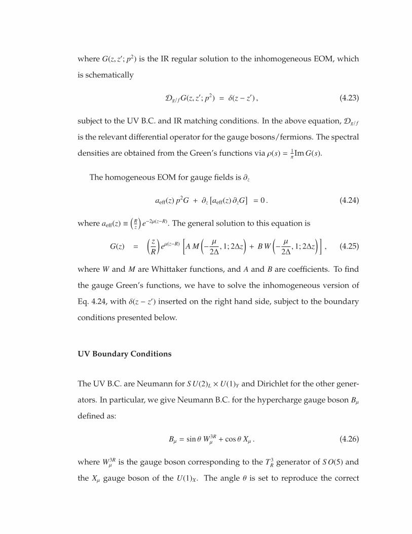
where G(z, z′; p2) is the IR regular solution to the inhomogeneous EOM, which

is schematically

Dg/ f G(z, z′; p2) = δ(z − z′) , (4.23)

subject to the UV B.C. and IR matching conditions. In the above equation, Dg/ f

is the relevant differential operator for the gauge bosons/fermions. The spectral

densities are obtained from the Green’s functions via ρ(s) = 1πIm G(s).

The homogeneous EOM for gauge fields is ∂z

aeff(z) p2G + ∂z[aeff(z) ∂zG

]= 0 . (4.24)

where aeff(z) ≡(

Rz

)e−2µ(z−R). The general solution to this equation is

G(z) =

( zR

)eµ(z−R)

[A M

(−µ

2∆, 1; 2∆z

)+ B W

(−µ

2∆, 1; 2∆z

) ], (4.25)

where W and M are Whittaker functions, and A and B are coefficients. To find

the gauge Green’s functions, we have to solve the inhomogeneous version of

Eq. 4.24, with δ(z − z′) inserted on the right hand side, subject to the boundary

conditions presented below.

UV Boundary Conditions

The UV B.C. are Neumann for S U(2)L ×U(1)Y and Dirichlet for the other gener-

ators. In particular, we give Neumann B.C. for the hypercharge gauge boson Bµ

defined as:

Bµ = sin θ W3Rµ + cos θ Xµ . (4.26)

where W3Rµ is the gauge boson corresponding to the T 3

R generator of S O(5) and

the Xµ gauge boson of the U(1)X. The angle θ is set to reproduce the correct

Weinberg angle θW . Similarly to [39], we also include a UV brane localized ki-

netic term for the S U(2)L gauge bosons, which changes their UV B.C. to

∂zGS U(2)L + CBKT GS U(2)L |z=R = 0 (4.27)

where CBKT = r2 p2R log R′/R and r is an O(1) parameter adjusted to reproduce

the correct right W mass for any value of g5.

IR Matching Conditions

On the IR brane we have matching conditions, which are either

∆G|z=R′ = ∆∂zG|z=R′ = 0 (4.28)

for the generators of S O(4) × U(1)X or

G|z=R′− = G|z=R′+ = 0 (4.29)

for the generators of S O(5)/S O(4). Here and below, we use G|z=R′+ ,G|z=R′− to de-

note the Green’s function evaluated at z → R′ from the right and left, respec-

tively, and ∆G ≡ G|z=R′+−G|z=R′− . We only select Green’s functions that are regular

in the deep IR, as described in Sec. 4.3.

Accounting for the VEV of the Higgs–A5

As a final complication, note that we are generically looking for the Green’s

functions in the presence of a VEV for the Higgs–A5. To account for the VEV, we

use the well known technique of rotating the 〈A5〉 into the IR boundary condi-

tions. We do this by the bulk gauge transformation Aµ → eig∫ z

R 〈A5〉dz′Aµe−ig∫ z

R 〈A5〉dz′

to the left of the IR brane and Aµ → eig5∫ z

R′ 〈A5〉dz′Aµe−ig5∫ z

R′ 〈A5〉dz′ to the right of the IR

brane. This eliminates the bulk 〈A5〉, but changes the IR matching conditions for

the S O(4) × U(1)X fields to

G|z=R′+ = U(h) G|z=R′− U(h)−1 ∂zG|z=R′+ = U(h) ∂zG|z=R′− U(h)−1 . (4.30)

where U(h) ≡ eig5∫ R′

R 〈A5〉dz′ ≡ eig5hf . Note that the rotation to the right of the IR

does not have any impact on the boundary conditions because the A5 is pure

gauge in this region.

Results

In Fig. 4.7 we present the gauge spectral density, for a Higgs VEV ratio v/ f = 0.3.

The spectral density is nonzero above the gap µ. Note the poles on top of

the continuum at 11 TeV: these are the result of the IR brane Dirichlet B.C. for

the generators of S O(5)/S O(4), and are the only BSM poles that appear in our

model. Since these are well beyond the reach of the LHC, we will not study them

further in this work. In addition to the gauge boson continuum, our gauge bo-

son Green’s functions reproduce the SM W and Z masses and a massless photon:

in Fig. 4.10, we show the inverse of the gauge boson Green’s functions, which

intersect zero exactly at the SM values.

4.6.1 Fermion Spectral Densities

The quadratic fermion Lagrangian is the one from Eq. 4.8, where each one of the

bulk multiplets QL, TR and BR has a different bulk mass cQ, cT or cB. The three

multiplets have dilaton Yukawa couplings y,−y,−y. Note the flip in the sign of

the dilaton Yukawa, required to get a zero mode in the ψ component of TR, BR.

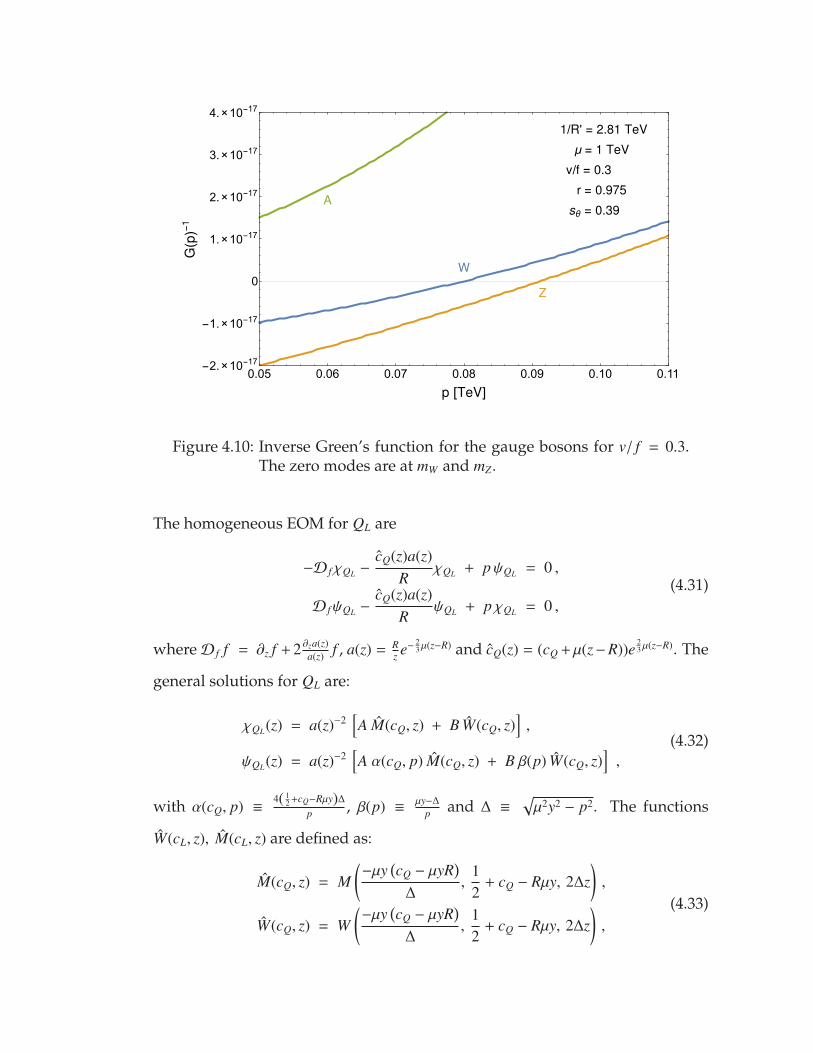
0.05 0.06 0.07 0.08 0.09 0.10 0.11-2.×10-17

-1.×10-17

0

1.×10-17

2.×10-17

3.×10-17

4.×10-17

p [TeV]

G(p)-

1

μ = 1 TeV

1/R' = 2.81 TeV

v/f = 0.3

r = 0.975

sθ = 0.39

W

Z

A

Figure 4.10: Inverse Green’s function for the gauge bosons for v/ f = 0.3.The zero modes are at mW and mZ.

The homogeneous EOM for QL are

−D fχQL −cQ(z)a(z)

RχQL + pψQL = 0 ,

D fψQL −cQ(z)a(z)

RψQL + p χQL = 0 ,

(4.31)

whereD f f = ∂z f + 2∂za(z)a(z) f , a(z) = R

z e−23µ(z−R) and cQ(z) = (cQ +µ(z−R))e

23µ(z−R). The

general solutions for QL are:

χQL(z) = a(z)−2[A M(cQ, z) + B W(cQ, z)

],

ψQL(z) = a(z)−2[A α(cQ, p) M(cQ, z) + B β(p) W(cQ, z)

],

(4.32)

with α(cQ, p) ≡ 4( 12 +cQ−Rµy)∆

p , β(p) ≡ µy−∆

p and ∆ ≡√µ2y2 − p2. The functions

W(cL, z), M(cL, z) are defined as:

M(cQ, z) = M(−µy

(cQ − µyR

)∆

,12

+ cQ − Rµy, 2∆z),

W(cQ, z) = W(−µy

(cQ − µyR

)∆

,12

+ cQ − Rµy, 2∆z),

(4.33)

where M(a, b, z),W(a, b, z) are Whittaker functions. The homogeneous solution

for TR (BR) is the same as the one for QL under cQ → −cT (B) and χQL , ψQL →

ψTR(BR), χTR(BR).

To find the Green’s functions, we have to solve the inhomogeneous version

of Eq. 4.31, inserting δ(z − z′) on the right side of the first or second of these

equation, depending on the Green’s function. The full details of the calculation

are presented in Appendix 4.B.

The fermionic Green’s functions are subject to the boundary conditions

given below.

UV Boundary Conditions

We assign UV brane Dirichlet B.C. to the following states:

QL : ψqL , χqL , χyL ,

TR : ψqR , ψqR , χtR , (4.34)

BR : ψq′R , ψq′R , ψxR , ψyR , ψyR , χbR .

These boundary conditions reflect the fact that only qL, qR and bR are partially

composite and should have the SM fermions as zero modes.

IR Matching Conditions

Due to the masses M1,4,b on the IR brane (Eq. 4.20), we have the jump conditions

relating G± = G|z=R′+ ±G|z=R′− for the different multiplets.

G−tR = κM1 G+sL, G−yL

= κM1 G+tR ,

G−aR= κM4 G+

aL, G−aL

= κM4 G+aR

+ κMb G+a′R, (4.35)

G−a′R = κMb G+aL,

where a = q, q and the κ = ∓1 is for the χ/ψ Green’s function. We only select

Green’s functions that are regular in the deep IR, as described in Sec. 4.3.

Accounting for the VEV of the Higgs–A5

Similarly to the gauge case, we can account for the VEV of the Higgs–A5 by

acting on the fermion with the Wilson line U(h). The IR matching conditions

remain the same as long as we modify the definition of G± to be

G± = G|z=R′+ ± Gh|z=R′− , (4.36)

where Gh = U(h)G for QL, TR in the 5 of S O(5) and Gh = U(h) G U(h)−1 for BR

in the 10 of S O(5).

Results

Here we show the final results for the fermionic spectral densities for the pa-

rameter choices in Eq. 4.21. Since the bulk matter content of the full model is

given by the representations 5 + 5 + 10, we will end up with a 20 × 20 matrix for

the Green’s functions. Each entry of the matrix is a two-point function between

0 2 4 6 8 10

-1.×10-7

0

1.×10-7

2.×10-7

3.×10-7

4.×10-7

5.×10-7

6.×10-7

p [TeV]

ρ(p)

μ = 1 TeV

1/R' = 2.81 TeV

v/f = 0.3

y = 1.75

yμ

Figure 4.11: Spectral densities for additional exotic top partners.

a pair of fermions, and diagonalizing this yields the 20 fermionic spectral den-

sities of our model. In Fig. 4.6 we can see the spectral densities for t, b and an

exotic b′. All other spectral densities corresponding to states with other quan-

tum numbers in the decomposition Eq. 4.19 are shown in Figs. 4.6, 4.11, and 4.12.

Note that the difference in normalization between the different spectral densi-

ties stems from the difference in bulk mass between the three bulk multiplets,

which leads to factors of(

RR′

)∆cbetween the spectral densities depicted in the

figures.

As stated before, some of the spectral functions feature broad peaks that can

be probed at future colliders. The width of these peaks is a model dependent

parameter which depends on the magnitude of the IR mass M1. By choosing

a slightly different point in parameter space with M1 = 2, we can make these

peaks as wide as 2 TeV. This effect is depicted in Fig 4.14 in a toy model with a

single bulk fermion.

0 2 4 6 8 10

0.00

0.01

0.02

0.03

0.04

p [TeV]

ρ(p)

μ = 1 TeV

1/R' = 2.81 TeV

v/f = 0.3

y = 1.75

yμ

Figure 4.12: Spectral densities for the remaining top partner quantumnumbers. The figure contains ten overlapping spectral densi-ties corresponding to components that are continuous acrossthe IR brane.

Without a Higgs VEV, four of the 20 fermions, tL,R and bL,R, would have zero

modes. The Higgs VEV lifts these to mt and mb, as shown in the inverse Green’s

functions for t, b and b′ in Fig. 4.13.

0.00 0.05 0.10 0.15 0.20

-5.×10-9

0

5.×10-9

1.×10-8

1.5×10-8

p [TeV]

G(p)-

1

μ = 1 TeV

1/R' = 2.81 TeV

v/f = 0.3

y = 1.75

b'

b

t

Figure 4.13: Top, bottom and b′ inverse Green’s functions. The zero modesof t and b are lifted in the presence of the Higgs VEV.

0 2 4 6 8 10

0

500000

1×106

p [TeV]

ρ(p)

cQ = 0.202

cT = -0.22

M = 1.2

M = 2

yμ

Figure 4.14: The effect of the IR mass on the width of a fermionic peak in atoy model with a single bulk fermion. By varying the IR mass,the peak could be made as wide as 2 TeV.

4.7 The Higgs Potential

Given all of the gauge and fermion Green’s functions that we have calcu-

lated, it is straightforward to compute the Coleman-Weinberg potential for the

Higgs using the formula [39]:

V(h) =3

16π2

∫dp p3

−420∑j=1

log G f j(ip) +

4∑k=1

log Ggk(ip)

, (4.37)

where G f j(p) and G fk(p) are the eigenvalues of the fermion and gauge Green’s

function matrices, respectively. Note that these Green’s functions are Higgs-

dependent, hence their contribution to the Coleman-Weinberg potential. In

Fig. 4.8 we plot the Coleman-Weinberg potential as a function of sin 〈h〉 / f ≡ v/ f .

There is a minimum at v/ f = 0.3, and so the right Higgs VEV is obtained for

f = 820 GeV, which is consistent with electroweak precision bounds. By differ-

entiating this twice, one can show that indeed mh = 125 GeV.

By varying the parameters of our model, we can estimate the tuning for the

BP. We use the Barbieri-Giudice measure to quantify the tuning:

tuning =

[maxi

d log vd log pi

]−1

, (4.38)

where pi ∈R,R′, µ, r, θ, y, cQ, cT , cB,M1,m4,Mb

are the fundamental parameters

of the model. We obtain a tuning of 1% for the BP, with the strongest dependence

being on cQ and cT as expected.

4.8 Comments on Phenomenology

The detailed study of continuum partner phenomenology will appear in a sep-

arate work [131]. Here, we will merely point out some of the main points re-

garding the phenomenology of continuum partners.

1. No s-channel resonances at the LHC: The unique feature of our contin-

uum CH model is the lack of particle resonances within the reach of the

LHC. This leads to vastly different phenomenology, in which the tradi-

tional searches for KK gauge bosons no longer apply, as well as all of

the resonance-based top partner searches. To demonstrate this point, we

present the partonic cross-section σ (qq→ G∗ → tRtR), in three simplified

models: only SM gluon, KK gluons, and continuum gluons. This cross

section is given by

σ(s) = σ(s)SM × s2 |G(R,R′; s)|2 , (4.39)

where G(R,R′; s) is the UV to IR Green’s function, calculated in a similar

manner to Sec. 4.6. The results are depicted in Fig. 4.9.

2. Bounds from the running of αS : The running of αs in the presence of a colored

gauge boson continuum provides an interesting bound on µ, the starting

point of the gapped continuum. The running of the 4D gauge coupling is

given by [39, 98, 137]

1g2(Q)

=1g2

5

∫ 1/Q

Rdz a(z) +

1g2

UV

−bUV

8π2 log(

1RQ

), (4.40)

where g25 = g2

∗R, gUV is the UV brane coupling, and bUV is the one-loop beta

function including effects for the zero modes on the UV brane. In our case,

we localize all fields except for tR on the UV brane, so bUV = 22/3.

There are determinations of αs up to Q ∼ 1.42 TeV from measurements of

jets by CMS using√

s = 7 TeV LHC data [138–141]. For a given value of µg,

we choose the SM value for αs(µg). Evaluating Eq. (4.40) at two different

scales Q = µg, 1.42 TeV and taking the difference, we can determine the

effect of the continuum on the running of αs. Results with different UV-

brane localized values of αUV are shown in Fig. 4.15: gluon continuum

scales above µ = 600–700 GeV are generically safe from the 1σ-high value

of αs(1.42 TeV). The value of αUV = 0.025 corresponds to the limit g2∗ < (4π)2

from requiring perturbativity in the bulk.

0.4 0.6 0.8 1.0 1.2

0.086

0.087

0.088

0.089

0.090

0.091

0.092

0.093

Figure 4.15: Bound from running αs from the gluon continuum scale µg toQ = 1.42 TeV.

3. Pair production of continuum top partners: We expect the continuum top pair-

production cross section to be parametrically smaller than the one for par-

ticle top partners. This is due to the smearing of the spectral density to

higher energies, where PDF suppression dominates. This is also the case

in the result of [120] for colored fermionic unparticles.

The full calculation of the pair-production cross section for continuum top

partners is far from trivial, as it is unclear how to calculate the phase space

factor for a pair of final-state continuum fermions. Inspired by the work

of [119, 120], we can use the optical theorem to relate the pair-production

cross section to the imaginary part of the diagram of the vacuum polariza-

tion with a continuum fermion loop, which we can calculate using disper-

sion relations. We leave the full calculation of the top partner pair produc-

tion for future work [131].

Since we are not calculating the full cross section in this work, we chose

a conservative point in parameter space with a continuum fermion gap of

1.75 TeV, with 1% tuning.

4.9 Conclusions

We presented a novel type of composite Higgs model, where all top and gauge

partners form continua rather than being ordinary particles. Such top and gauge

partners will evade all s-channel resonance searches and are expected to lead to

unique experimental signatures. We showed how to obtain a realistic model of

this sort from a warped extra dimension, where space continues beyond the IR

brane. A linear dilaton dominates the deep IR region, corresponding to critical

IR dynamics that produces a gapped continuum. We have shown how to cal-

culate the full set of spectral densities for the fermion and gauge partners. Fur-

thermore, we established a phenomenologically viable benchmark point, tuned

at the percent level, with a realistic radiatively generated Higgs potential. The

phenomenology of continuum partners, as well as the existing collider bounds

on this model, will appear in an upcoming publication.

APPENDIX

4.A Gauge Boson Green’s Functions

In this appendix we present the details necessary for evaluating the gauge bo-

son spectral densities. We demonstrate our calculation in a simple toy model

with a bulk U(1) × U(1) broken to U(1) on the IR brane, where the role of

the Higgs is played by the A5 of the broken U(1). In the bulk we have two

gauge bosons, Wµ and W ′µ. Wµ corresponds to an unbroken direction (before

the Higgs VEV) with the boundary conditions (+,+) on the UV and IR branes,

while W ′µ corresponds to a broken direction (−,−). The Higgs VEV will mix

these two fields. There are now four different Green’s functions to solve for:

〈W(z)W(z′)〉 , 〈W ′(z)W(z′)〉 , 〈W(z)W ′(z′)〉 and 〈W ′(z)W ′(z′)〉, which we denote col-

lectively by G(z, z′; p2)i j, i, j ∈ W,W ′.

To get each spectral density we need to first specify whether the source (the

delta function) is in the W or the W ′ equation. This depends if we’re looking for

W(z′) or W ′(z′) in the correlation function. In a shorthand notation, we will write

Dg G(z, z′; p2)i j = δi j δ(z − z′) . (4.41)

The gauge EOM is Eq. 4.24, with a general solution of the form Eq. 4.25. To

solve for the Green’s function, we divide our space into the domains R ≤ z ≤

z′, z′ ≤ z ≤ R′ and R′ ≤ z, where the coefficients are denoted←−A ,←−B ,−→A ,−→B and

A∞, B∞, respectively. Our goal is then to find these coefficients, subject to the

following jump/boundary conditions:

89

• UV BC:

∂zGW j|z=R = GW′ j|z=R = 0 . (4.42)

• Jump conditions at z = z′:

∆GW j|z=z′ = ∆GW′ j|z=z′ = 0 ,

∆∂zGi j|z=z′ = a(z)−1δi j .

(4.43)

• Jump conditions at z = R′:

∆GW j|z=R′ = ∆∂zGW j|z=R′ = 0 ,

GW′ j|z=R′− = GW′ j|z=R′+ = 0 .(4.44)

• Regularity of G(z, z, p2) at z→ ∞:

A∞W j = A∞W′ j = 0 . (4.45)

From these linear conditions we arrive at the Green’s function matrix

G(z, z′; p2)i j. We can of course diagonalize this matrix and define two spectral

densities:

ρ(s)1,2 ≡ limz,z′→R

1π

Im G(z, z′; s)1,2 . (4.46)

corresponding to the two eigenvalues of Gi j. Note, however, that in the present

case GW′W = GW′W′ = 0 by virtue of the UV Dirichlet BC, and also that GWW′ = 0

because the W and W ′ IR BC are completely decoupled. The situation is different

once we consider a bulk 〈A5〉 VEV rotating the two multiplets. In this case the

IR BC is modified to:

∆GW j|z=R′ = ∆∂zGW j|z=R′ = 0 ,

GW′ j|z=R′− = GW′ j|z=R′+ = 0 ,(4.47)

0 5 10 15 20

-2000

0

2000

4000

6000

8000

10000

12000

p [TeV]

ρ(p)

μ = 1 TeV

1/R' = 4 TeV

v/f = 0

v/f = 0.3

μ

Figure 4.16: Spectral density for W/W ′ mix with µ = 1 TeV, 1/R′ = 4 TeV.

with

GW j = ch GW j + sh GW′ j ,

GW′ j = − sh GW j + ch GW′ j ,

(4.48)

and ch = cos (〈h〉 / f ) , sh = sin (〈h〉 / f ) ≡ v/ f . The resulting spectral density ρ1(p)

is depicted in Fig. 4.16 (ρ2(p) is still zero by virtue of the Dirichlet BC for W ′).

Note that for v/ f , 0, ρ1(p) acquired a pole on top of the branch cut. This is as

expected: the pole originates from the W ′ component of the eigenstate 1, and

W ′ has a Dirichlet BC at R′. We also note that the zero mode of eigenstate 1

is no longer massless since it acquires a mass from the Higgs. This is seen by

determining where 1/G1(p) vanishes, as shown in Fig. 4.17.

We are now ready to present the spectral densities for the gauge bosons of

the realistic model. As previously explained, the bulk gauge symmetry S O(5) ×

U(1)X is broken on the IR brane to S O(4) × U(1)X. We choose the following

0.0 0.1 0.2 0.3 0.4-1.×10-8

-5.×10-9

0

5.×10-9

1.×10-8

1.5×10-8

2.×10-8

p [TeV]

G(p) 1

-1

μ = 1 TeV

1/R' = 4 TeV

v/f = 0

v/f = 0.3

gauge mass

Figure 4.17: Inverse Green’s function for W/W ′ mix with µ = 1 TeV, 1/R′ =

4 TeV.

generators as a basis of S O(5):(T a

L,R

)i j

= −i2

[εabcδb

i δcj ±

(δa

i δ4j − δ

4i δ

aj

) ],(

T aC

)i j

= −i√

2

[ (δa

i δ5j − δ

5i δ

aj

) ],

(4.49)

with a ∈ 1, 2, 3 and a ∈ 1, 2, 3, 4. The gauge bosons corresponding to the

generators T aL,R are continuous across the IR brane, while the ones corresponding

to T aC get a Dirichlet BC. The Higgs emerges as the 4D component of ACa

5 . To

solve for the bulk profiles in the presence of a Higgs VEV, we use the trick of

solving for v = 0 but with the IR BC rotated by the Higgs matrix:

Uh = ei g5∫ R′

R A5(z)TCa ha(x) dz . (4.50)

The profile A5(z) is given by solving the bulk EOM:

∂z [a(z)A5(z)] = 0 . (4.51)

and so A5(z) = N5 a−1(z), with N5 =

[∫ R′

Ra−1(z)dz

]−1/2. We only integrate A5 up to

the IR brane because it is pure gauge beyond it. In other words, the only gauge

invariant Wilson line for the A5 is between the UV and IR branes.

Due to the SM gauge freedom, we are allowed to choose the Higgs VEV 〈h〉

to be in the a = 4 direction. We then have:

Uh = ei TC4 〈h〉/ f , (4.52)

where f = g−15

[∫ R′

Ra−1(z)dz

]−1/2. Substituting the expression for TC4, we get

Uh =

0 0 0 0 0

0 0 0 0 0

0 0 0 0 0

0 0 0 cos (〈h〉 / f ) sin (〈h〉 / f )

0 0 0 − sin (〈h〉 / f ) cos (〈h〉 / f )

. (4.53)

The components of the bulk S O(5) gauge field are:

Wµ = W±,3;Lµ T±,3L + W±,3;R

µ T±,3R + W±,±µ T±± , (4.54)

where

T±L,R =1√

2

(T 1

L,R ± iT 2L,R

),

T±∓ =1√

2

(T 3

C ± iT 4C

),

T±± =1√

2

(T 1

C ± iT 2C

).

(4.55)

There is an additional bulk U(1)X field that we denote by Xµ. The extra U(1)X

is required to reproduce the correct hypercharge assignments for the SM fields

[32].

The UV boundary conditions are then

W±;Rµ |z=R = W±,±

µ |z=R = 0 ,

∂z W±,3;Lµ + Ck W±,3;L

µ |z=R = 0 ,

cθ W3;Rµ − sθ Xµ |z=R = 0 ,

∂z

[sθ W3;R

µ + cθ Xµ

]|z=R = 0 .

(4.56)

Note that the above boundary conditions mix the gauge fields W3;Rµ and Xµ with

an angle θ as a result of a UV boundary kinetic term. A similar boundary kinetic

term Ck ≡ Rp2r2 log R′/R is responsible for the mixed boundary conditions for

W±,3;Lµ . This term is necessary to get the right S U(2)L gauge coupling for every

value of the bulk coupling g5. To account for the VEV of the Higgs–A5, we rotate

its effect into the IR jump conditions, which are now given are given in terms of

the Higgs-rotated gauge fields:

Wµ = Uh Wµ U−1h . (4.57)

This multiplet is decomposed similarly to Eq. 4.54:

Wµ = W±,3;Lµ T±,3L + W±,3;R

µ T±,3R + W±,±µ T±± . (4.58)

The IR BC are then

∆W±,3;Lµ |z=R′ = ∆W±,3;R

µ |z=R′ = 0 ,

W±,±µ |z=R′ = 0 .

(4.59)

The resulting gauge boson spectral densities and inverse Green’s functions are

presented in the main text in Figs. 4.7 and 4.10.

4.B Fermion Green’s Functions

Next we explain how an A5 (Higgs) VEV can give mass to two fermion zero

modes. This is a standard result in Gauge-Higgs unification, and we demon-

strate it here explicitly in the context of continuum CH. As a starting point, we

take two bulk fermions Q1,2L with equal bulk masses and dilaton Yukawas cL, y

and opposite UV boundary conditions, and two bulk fermions Q1,2R with equal

bulk masses and dilaton Yukawas cR,−y and opposite UV boundary conditions.

In the context of warped CH models, Q1,2L will represent two different quan-

tum numbers within the same QL bulk multiplet that is in a large representation

of the bulk gauge group, and likewise for Q1,2R . However, in this toy example

we will not be concerned with the group theory aspects of the model. The UV

boundary conditions are:

ψ1L|z=R = χ2

L|z=R = ψ1R|z=R = χ2

R|z=R = 0 , (4.60)

where Q1,2L =

(χ1,2

L , ψ1,2L

)and Q1,2

L =(χ1,2

R , ψ1,2R

). These boundary conditions, to-

gether with the assignment of ±y dilaton Yukawas and the demand for a regular

solution in the deep IR, implies zero modes for χ1L and ψ2

R. As IR mass terms only

couple (Q1L,Q

1R), (Q2

L,Q2R), they won’t be enough to lift the zero modes χ1

L and ψ2R.

As we will see below, only a non-zero VEV for the A5-Higgs can rotate the mul-

tiplets and lift the two zero modes. To obtain the matrix of Green’s functions we

divide the problem into the same domains as in the gauge case, and solve for←−A j,←−B j,−→A j,−→B j, A∞j , B

∞j , where this time i, j are joint indices in 1L, 2L, 1R, 2R.

The boundary and jump conditions in this case are:

• UV BC:

GψL1; j|z=R = Gχ

L2; j|z=R = GψR1; j|z=R = Gχ

R2; j|z=R = 0 . (4.61)

• Jump conditions at z = z′:

∆Gψi j|z=z′ = − ∆Gχ

i j|z=z′ = Di j a(z′)−4 . (4.62)

• Jump conditions at z = R′: On the IR brane we turn on the masses M1 Q1L Q1

R

and M2 Q2L Q2

R, which give us the jump condition:

∆Gχak; j|z=R′ = − Mk

⟨Gχ

ak; j

⟩|z=R′

∆Gψak; j|z=R′ = Mk

⟨Gψ

ak; j

⟩|z=R′ ,

(4.63)

where j ∈ 1L, 2L, 1R, 2R, a ∈ L,R, and k ∈ 1, 2.

• Regularity of G(z, z; p2) at z→ ∞: as before, A∞i j = 0.

Note that we have yet to turn on a Higgs VEV mixing the 1 and 2 states.

At this stage there are zero modes in χ1L and in ψ2

R. The IR masses M1,2 cannot

change this fact, we can only lift the two zero modes with a mass that connects

them to each other. This is impossible as long as the 1 and 2 BC are completely

decoupled. This is not the case when a Higgs VEV is turned on. As usual, this

VEV appears as a rotation of the IR jump conditions:

Ga1; j|z=R′ = ch Ga1; j + sh Ga2; j ,

Ga2; j|z=R′ = − sh Ga1; j + ch Ga2; j .

(4.64)

The rotation is the same for Gχi j and Gψ

i j. We now write the IR BC in Eq. 4.63 in

terms of the Higgs-rotated Green’s functions Gi j.

Solving these conditions, we obtain the Green function Ghi j with Ga1; j =

Gχa1; j , Ga2; j = Gψ

a2; j. This matrix now has four eigenvalues Gh(z, z′; p)1,2,3,4 with

appropriate spectral densities ρh(p)1,2,3,4. The label h is an explicit reminder that

they depend on the Higgs VEV. In Fig. 4.18 we plot the spectral densities for

R′ = (4 TeV)−1, M1 = 0.3, M2 = 0, cL = 0.3 and cR = −0.1, for v/ f = 0.3. In Fig. 4.19

0 2 4 6 8 10

0.0

0.5

1.0

1.5

p [TeV]

ρ(p)

v/f=0.3 10-9*ρ1(p)

10-3*ρ2(p)

109*ρ3(p)

103*ρ4(p)

yμ

Figure 4.18: Spectral density for cL = 0.3, cR = −0.1, M1 = 0.3, M2 = 0.

we plot the inverse Green’s functions for v/ f = 0, 0.3, and show that there are

non-trivial zeros for v/ f = 0.3.

We are now ready to present the spectral densities for the top/bottom sector

for the realistic model. We will choose the fermions to be embedded in the bulk

multiplets QL, TR and BR in the 5 23, 5 2

3and 10 2

3of S O(5) × U(1)X. The SM gauge

group S U(2)L is a subgroup of S O(5), and the hypercharge is a combination of

U(1)R ⊂ S O(5) and U(1)X defined by Y = T 3R + X. Under the subgroup S U(2)L ×

U(1)Y , the bulk multiplets decompose as:

QL(5) 23→ qL(2) 1

6+ qL(2) 7

6+ yL(1) 2

3,

TR(5) 23→ qR(2) 1

6+ qR(2) 7

6+ tR(1) 2

3,

BR(10) 23→ q′R(2) 1

6+ q′R(2) 7

6+ xR(3) 2

3+ yR(1) 7

6+ yR(1) 1

6+ bR(1)− 1

3.

(4.65)

We choose the UV BC such that only qL, tR and bR have zero modes by assigning

Neumann BC for GχqL , Gψ

qR and GψBR

, and Dirichlet BC for all the other GχQL, Gψ

TR

0.00 0.05 0.10 0.15 0.20 0.25 0.30-4.×10-11

-2.×10-11

0

2.×10-11

4.×10-11

6.×10-11

8.×10-11

p [TeV]

[G(p) 1]-

1v/f = 0

v/f = 0.3

zero mode mass

Figure 4.19: Inverse Green’s function for cL = 0.3, cR = −0.1, M1 =

0.3, M2 = 0. The inverse Green’s function gets a non-trivialzero for v/ f = 0.3.

and GψBR

. The S O(4) × U(1)X symmetry on the IR brane allows for three mass

terms:

S IR =

∫dx4 √gind

[M1 yLtR + M4

(qLqR + ¯qLqR

)+ Mb

(q′LqR + ¯q′LqR

) ]. (4.66)

These mass terms lead as usual to IR jump conditions which are for QL:

∆GχqL,qL; j|z=R′ = − M4

⟨Gχ

qR,qR; j

⟩− Mb

⟨Gχ

q′R,q′R; j

⟩|z=R′ ,

∆GψqL,qL; j|z=R′ = M4

⟨Gψ

qR,qR; j

⟩− Mb

⟨Gψ

q′R,q′R; j

⟩|z=R′ ,

∆GχyL; j|z=R′ = − M1

⟨Gχ

tR; j

⟩|z=R′ ,

∆GψyL; j|z=R′ = M1

⟨Gψ

tR; j

⟩|z=R′ .

(4.67)

For TR they are:

∆GχqR,qR; j|z=R′ = − M4

⟨Gχ

qL,qL; j

⟩|z=R′ ,

∆GψqR,qR; j|z=R′ = M4

⟨Gψ

qL,qL; j

⟩|z=R′ ,

∆GχtR; j|z=R′ = − M1

⟨Gχ

sL; j

⟩|z=R′ ,

∆GψtR; j|z=R′ = M1

⟨Gψ

sL; j

⟩|z=R′ ,

(4.68)

and for BR they are:

∆Gχ

q′R,q′R; j|z=R′ = − Mb

⟨Gχ

qL,qL; j

⟩|z=R′ ,

∆Gψ

q′R,q′R; j|z=R′ = Mb

⟨Gψ

qL,qL; j

⟩|z=R′ ,

∆GχxR,yR,yR,bR; j|z=R′ = 0 ,

∆GψxR,yR,yR,bR; j|z=R′ = 0 .

(4.69)

As usual, in the IR jump conditions, the fields to the left of the IR brane are

really the Higgs-rotated fields:

GQL = Uh GQL , GTR = Uh GTR , GBR = Uh GBR U−1h , (4.70)

decomposed into their different components. The jump discontinuity due to IR

localized mass terms results in quasi-IR brane-localized wave function profiles

for the fermionic fields as noted at the end of Sec. 4.4.

CHAPTER 5

REVIEW OF DARK MATTER

5.1 Observations of Dark Matter

Dark Matter (DM) is our first and foremost indication for physics beyond the

Standard Model. Though not yet observed in the lab, there is a plethora of

observational evidence for the existence of DM, which we shall briefly review

here, following [142] and [143]. This brief review is by no means exhaustive.

5.1.1 Rotation Curves

A Galactic rotation curve is a measurement of the radial rotation speed of viri-

alized matter as a function of its distance from the center of the galaxy. The

velocity is measured by spectrometry of atomic hydrogen, which extends well

beyond the galaxy’s stellar component. Current compendia of galactic rotation

curves are given in [144, 145]. While the theoretical rotation curves due to bary-

onic matter only tend to decay as v(r) ∼ r−12 , observational data indicates flat

v(r) ∼ r0 rotation curves up to radii well beyond the maximal radius of the stel-

lar component. This constituted the original observational evidence for the ex-

istence of a DM galactic halo [146]. In a DM halo with ρDM(r) ∼ r−2, the rotation

curve goes as

v(r) ∼

√4πG

∫ r

0ρ(r) r2 dr

r∼ r0 , (5.1)

as indicated by data.

100

5.1.2 Galaxy Clusters

The most striking evidence for DM at the cluster level is from the bullet cluster

(1E 0657-56) [147–149]. This is a groundbreaking observation of two clusters

colliding. While the DM components of these two clusters already crossed each

other, the X-ray emitting baryonic plasma in them lags, due to dissipation. This

results in an 8σ spatial offset between the center of mass of each cluster (as

observed by weak lensing), and the observed location of the plasma in each

cluster. Further indications for DM at the cluster level involve weak lensing

studies of DM sub-halos in the Coma cluster using the Subaru telescope [150],

as well as extensive weak lensing surveys using the Subaru Telescope and the

Canada-France-Hawaii telescope (see [151] and references therein). Baryonic

counterparts to weak lensing (showing that the baryonic mass is smaller than

the total cluster mass) were presented in [152] as a direct indication of DM.

5.1.3 Cosmological Scales

Observations from the early universe allow us to put very stringent bounds

on the parameters of the ΛCDM model, including Ωm, the average comoving

matter density in the universe (including DM), and σ8, the present RMS matter

fluctuation averaged over a sphere of radius 8h−1 Mpc. A summary plot of these

stringent bounds in the Ωm−σ8 plane is shown in Fig. 5.1, reproduced from [143].

The bounds originate from cosmological-scale observations of the Cosmic Mi-

crowave Background Radiation (CMB), Baryonic Acoustic oscillations (BAO),

and bounds from Large Scale Structure as observed by the Dark Energy Survey

(DES).

Figure 5.1: ΛCDM model 68% and 95% constraint contours on the matter-density parameter Ωm and fluctuation amplitude σ8. Thebounds from DES lensing, Planck CMB lensing, and the jointlensing constraint are shown in green, grey, and red, respec-tively. The blue filled contour shows the independent con-straint from the Planck CMB power spectra. Reproduced from[143].

Cosmic Microwave Background Radiation

The CMB is the approximately isotropic photon radiation from the early uni-

verse. CMB photons decoupled from matter following Hydrogen recombina-

tion, at a redshift of z ∼ 1100. On average, the CMB fits very well to a blackbody

spectrum with T = 2.762 K. However, the CMB has 10−5 anisotropies in the

temperature, which can be expanded as

δTT

(θ, φ) =

+∞∑`=2

+∑m=−`

a`mY`m(θ, φ) , (5.2)

Figure 5.2: TT power spectrum as measured by the Plank Collaboration.The red dots are the measured spectrum and the blue line isthe ΛCDM best fit prediction. Reproduced from [143].

where the Y`m(θ, φ) are spherical harmonics. The TT power spectrum D` is then

defined as

D` ≡1

2π

∑m=−`

|a`m|2 . (5.3)

The power spectrum has peaks due to DM-baryonic matter acoustic oscilla-

tions, whose position, height, and spacing of the peaks are extremely sensi-

tive to cosmological parameters. Peaks with a similar sensitivity exist in the

temperature-polarization (TE) and polarization-polarization (EE) power spec-

tra. The Planck space observatory [143,153,154] provided the most precise mea-

surement of the CMB power spectrum, which can be seen in Fig. 5.2.

Baryon Acoustic Oscillations

Baryon Acoustic Oscillations (BAO) are are peaks in the matter power spectrum

inferred from galaxy surveys such as the Sloan Digital Sky Survey III [155] and

the 6dF Galaxy Survey [156]. More specifically, BAO surveys measure the dis-

tance ratioDV(z)

rs

(zdrag

) , (5.4)

at reshifts 0.1 ≤ z ≤ 0.7. In the equation above, rs

(zdrag

)is the comoving sound

horizon at the baryon drag epoch (when baryons became dynamically decou-

pled from the photons) and DV(z) is a combination of the angular-diameter dis-

tance, DA(z), and the Hubble parameter, H(z). As for the CMB peaks, the height

and position of BAO peaks are sensitive to cosmological parameters such as

Ωm [157], and so they provide a complimentary bound to the CMB, as can be

seen in Fig. 5.1.

Dark Energy Survey

The Dark Energy survey [158,159] provides complimentary bounds on Ωm from

two types of measurements: cosmic shear and type Ia supernovae. Cosmic

shear measures the correlated distortion of the light emitted from distant galax-

ies due to weak gravitational lensing by Large Scale Structure. The amplitude

of the lensing signal is primarily sensitive to the normalization of the matter

fluctuations, σ8, and to the matter density Ωm. Another very recent constraint

on Ωm comes from the DES-SN survey [160], measuring the luminosity distance

vs redshift of type Ia supernovae for z < 1. This allows for complementary

constraints on Ωm through its impact on H(z).

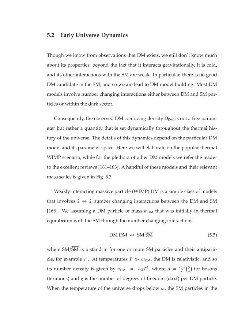
5.2 Early Universe Dynamics

Though we know from observations that DM exists, we still don’t know much

about its properties, beyond the fact that it interacts gravitationally, it is cold,

and its other interactions with the SM are weak. In particular, there is no good

DM candidate in the SM, and so we are lead to DM model building. Most DM

models involve number changing interactions either between DM and SM par-

ticles or within the dark sector.

Consequently, the observed DM comoving density ΩDM is not a free param-

eter but rather a quantity that is set dynamically throughout the thermal his-

tory of the universe. The details of this dynamics depend on the particular DM

model and its parameter space. Here we will elaborate on the popular thermal

WIMP scenario, while for the plethora of other DM models we refer the reader

to the excellent reviews [161–163]. A handful of these models and their relevant

mass scales is given in Fig. 5.3.

Weakly interacting massive particle (WIMP) DM is a simple class of models

that involves 2 ↔ 2 number changing interactions between the DM and SM

[165]. We assuming a DM particle of mass mDM that was initially in thermal

equilibrium with the SM through the number changing interactions

DM DM ↔ SM SM , (5.5)

where SM/SM is a stand in for one or more SM particles and their antiparti-

cle, for example e±. At temperatures T mDM, the DM is relativistic, and so

its number density is given by nDM = AgT 3, where A =ζ(3)π2

(34

)for bosons

(fermions) and g is the number of degrees of freedom (d.o.f) per DM particle.

When the temperature of the universe drops below m, the SM particles in the

Figure 5.3: Mass ranges for different DM Models. Reproduced from [164]

plasma no longer have enough energy to pair produce DM, and so the process

SM SM → DM DM stops. Now, the DM number density drops like that of a

non-relativistic particle:

nDM ≈ neq(T ) = g(mDMT

2π

)3/2

e−mDM/T . (5.6)

The depletion in the number density of DM does not continue indefinitely, since

at some temperature T ∗ ≈ mDM/10, the rate for the process DM DM → SM SM

becomes smaller than the expansion rate of the universe given by the Hubble

parameter H(T ). This happens when

nDM 〈σ vDM〉 = H(T ∗) , (5.7)

where σ is the cross section for DM DM → SM SM and 〈σ vDM〉 ia a thermal

average at temperature T ∗. Below this temperature, the comoving number den-

sity is constant, and we say that the DM is “frozen-out”. The observed ΩDM to

day is then

ΩDM h2 = h2 mDM stoday

ρcrit s(T ∗)n∗DM =

10−9 GeV−2

〈σ vDM〉, (5.8)

and so to get the correct DM relic abundance we need

〈σ vDM〉 ≈ 10−9 GeV−2= 10−26 cm3/s , (5.9)

which is a typical thermally averaged 2 ↔ 2 cross section for a 1 TeV weakly

coupled DM particle. This coincidence was dubbed “the WIMP miracle”, and

was the driving force behind an extensive DM search program in the past two

decades.

5.3 Dark Matter Searches

5.3.1 Direct Detection

Direct detection is the effort to probe DM by searching for DM-SM elastic scat-

tering events in dedicated DM detectors. The signal in these scattering events is

the recoil of a nucleus or an electron within the detector. The predicted differ-

ential rate for nuclear recoils is given by

dRdEnr

= R0 exp(−

Enr

E0

4mDMmN

(mDM + mN)2

)F2 (Enr) , (5.10)

where mN is the mass of the nucleus, E0 ∼12mDM v2 (with v ∼ 230 km/s) is the

mean kinetic energy of the DM particle, F2 (Enr) is the nuclear form factor. The

nominal rate R0 for is given by

R0 =2√π

ndetρDM

mDMσ v . (5.11)

where ndet is the nucleon number density in the detector and σ is either the

spin independent or spin dependent cross section for DM-nucleon scattering.

Note that due to the small momentum transfer, the DM interacts with the entire

nucleus coherently. From the above functional form we learn a few things:

• The total rate decreases exponentially when increasing the detector thresh-

old energy Eminnr , which is typically O(keV).

• The total rate decreases exponentially when decreasing mDM for mDM < mN .

• The total rate increases linearly when increasing mDM for mDM mN .

In practice, this means we can only use nuclear recoils to probe DM heav-

ier than ∼ 5 GeV, and also that direct detection bounds weaken linearly for

mDM>∼ 100 GeV, as can been in Fig 5.4. Above WIMP masses of ∼ 5 GeV, the

strongest limits are placed by the the liquid xenon (LXe) Time Projection Cham-

bers (TPC) XENON1T, LUX, and PandaX-II. The experiment with the best sen-

sitivity to WIMPs in this mass-range is XENON1T, a LXe TPC with a 2.0 ton

target. It excluded the spin-independent DM- nucleon interactions with cross

sections above 4.1 × 1047cm2 @ 30 GeV and 90% confidence level in a run with a

1 ton × year exposure [167]. This is much smaller than the cross-section needed

to get the right ΩDM in the early universe, and so it is in major tension with the

vanilla WIMP scenario.

In the DM mass range 1.8 GeV <∼ mDM

<∼ 5GeV, the most competitive

bounds are given by electron recoil experiments such as the Liquid-Argon based

DarkSide-50, whose electron recoil threshold was as low as 0.1 keV. The limits

are weaker than in the nuclear recoil regime due to enhanced background.

Lastly, there has been an extensive effort in the past 5 years to probe light

Figure 5.4: The current experimental parameter space for spin-independent WIMP- nucleon cross sections. Only someof the bounds are shown. The space above the lines is ex-cluded at a 90% confidence level. The dashed line limiting theparameter space from below represents the neutrino floor fromthe irreducible background from coherent neutrino-nucleusscattering (CNNS). This plot is reproduced from [166]

(1 meV <∼ mDM

<∼ 1 GeV) and ultralight (10−22 eV <

∼ mDM<∼ 1 meV). A partial list of

detection concepts for light DM involves DM induced chemical bond breaking,

superfluid helium, magnetic bubble chambers, semiconductors and supercon-

ductors. Ultra-light scalar DM has a macroscopic Compton wavelength, and so

it interacts coherently like a wave. Consequently, the search for ultralight DM

focuses on precision tabletop experiments such as atom interferometry, NMR,

X-ray, and torsion balance experiments. For excellent reviews of the different

detection concepts and their implementations, see [163, 164, 168].

5.3.2 Indirect Detection

Indirect detection is the astrophysical search for DM decay/annihilation signals

in the present and in the early universe. Given that the lifetime of DM has to

be longer than the age of the universe, and that DM interacts at most weakly

with the SM, we expect these decay/annihilation events to be rare, though po-

tentially striking and with low SM backgrounds.

For example, the rate of expected gamma rays from DM annihilation in our

galaxy (neglecting redshifting, absorption, etc) is given by (see the review by

[169]):1A

dNγ

dEdt=〈σvrel〉

m2DM

(dNγ

dE

)0

Jann , (5.12)

where A is the effective area of the observing telescope,( dNγ

dE

)0

is the spectrum of

gamma rays obtained for each annihilation event, and 〈σvrel〉 is the cross section

for DM annihilation. The factor

Jann ≡1

8π

∫dr dΩ ρDM(~r)2 (5.13)

is an astrophysical factor which accounts for the integral of line-of-sight DM

density to the source.

Measurements of the CMB provide additional indirect bounds on DM anni-

hilation through the latter’s effect on the ionization history of the universe [170].

In Fig. 5.5 we present the current indirect detection bounds from the CMB, the

Fermi-LAT [171] observation of the Milky-way dwarf spheroidal galaxies, and

the H.E.S.S. Imaging Atmospheric Cherenkov Telescope [172] observation of the

Galactic center. Other sources of indirect bounds are from cosmic ray measure-

ment using the AMS-02 detector [173] on the international space station.

Figure 5.5: 95% C.L. upper limits on the dark matter annihilation cross-section as a function of the dark matter mass for the processDM DM → V V , with V decaying into uu, bb, tt for MDM MV,with the V mass being just sufficiently heavier than the decaysmodes. Reproduced from [174].

5.3.3 Collider Searches

Collider searches look for potential DM particles generated in collider exper-

iments. The modern approach to DM searches at the LHC is using simpli-

fied models, most notably the V/AV simplified model in which DM is pro-

duced through a vector/axial vector mediator, and the S/PS simplified model,

in which the mediator is a scalar/pseudoscalar. The bounds on these simpli-

fied models are from several complementary channels, namely the EmissT + X,

dijet, di-b-jets, dilepton, and tt resonance channels [175]. LHC bounds on the

leptophobic V/AV simplified model are shown, from ATLAS (Fig 5.6) and CMS

(Fig 5.7). In Fig 5.8, these bounds are shown in comparison to the bounds from

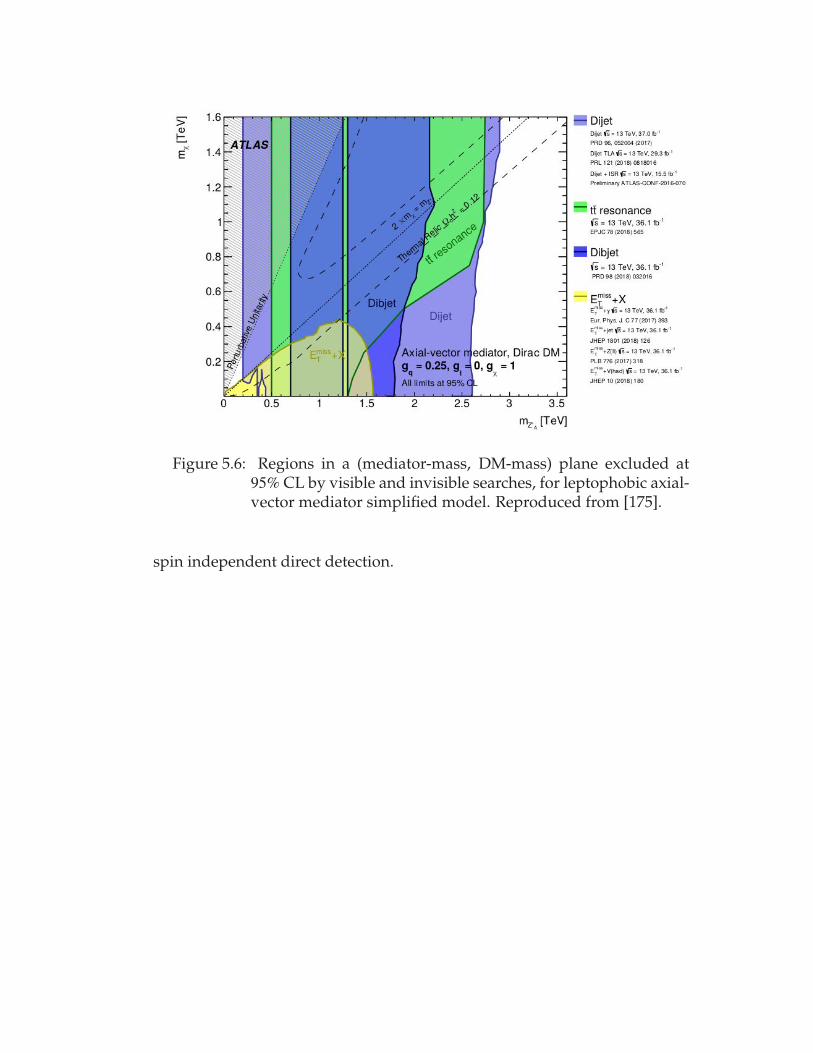
Figure 5.6: Regions in a (mediator-mass, DM-mass) plane excluded at95% CL by visible and invisible searches, for leptophobic axial-vector mediator simplified model. Reproduced from [175].

spin independent direct detection.

Figure 5.7: 95% CL observed and expected exclusion regions in mMed−mDM

plane for di-jet searches and different MET based DM searchesfrom CMS in the leptophobic Vector model. The exclusions arecomputed for a universal quark coupling of gq = 0.25 and for aDM coupling of gDM = 1.0. Reproduced from [176].

Figure 5.8: A comparison of direct detection SI bounds with the ATLASbounds on the V/AV simplified model. Reproduced from[175].

5.4 Generic Dark Sectors

In the past 20 years, most of the theoretical and experimental effort has focused

on minimal dark sectors. This was in part due to the popularity of the WIMP

paradigm, which tied the relic abundance Ωm to a single weakly interacting par-

ticle. However, following the strong direct detection bounds on WIMP DM,

there is a resurgence of models involving richer physics in the dark sector. In-

deed, given the rich physics observed in the SM, there is no a-priori reason for

the dark sector not to have its own gauge symmetry (abelian or non-abelian), or

even a Higgs mechanism.

The consideration of more generic dark sectors could lead to early universe

dynamics which is very different from that of a single, weakly interacting par-

ticle, and could have a major impact on the relic density. This goes back to the

idea of number changing processes in the dark sector [177], and its modern in-

carnation as the SIMP [178–181] and ELDER [182] models. Two other popular

scenarios are asymmetric DM [183–185], in which the relic density in the dark

sector is set by a primordial matter-antimatter asymmetry (with or without a

link to SM baryogenesis), and freeze-in DM [186], in which an initially empty

dark sector is populated by SM decays. Additionally, bound state formation /

confinement in the dark sector could have an impact on the relic density of dark

matter, [187–196], as is demonstrated in this work.

Searches for generic dark sector physics often involves a mediator - a new

particle that couples the dark sector to the SM. Typical mediators are a dark pho-

ton which mixes with the SM photon, dark scalar mixing with the SM Higgs, or

a dark axion-like particle coupling to the SM. Dark matter coupled to a dark

vector or scalar mediator can either annihilate in the early universe to the me-

diator or directly to the SM, depending on the DM/mediator mass ratio. The

parameter space for dark photons is constrained by a combination of collider

searches (both LHC and fixed target experiments), astrophysical bounds such

as the 1987A supernova bound, and other bounds from 5th force experiments,

CMB, late decays. The current bounds are depicted in Figure 5.9.

Finally, a generic dark sector with some self interaction could influence

galactic dynamics [197] and even address small scale problems [198–200].

Figure 5.9: Collected constraints on a kinetically mixed vector with massmV and kinetic mixing parameter κ of the dark and visible pho-tons. Reproduced from [163].

CHAPTER 6

DARK QUARKONIUM FORMATION IN THE EARLY UNIVERSE

BEYOND THE STANDARD MODEL: COMPOSITE HIGGS AND DARK

MATTER

Ofri Telem, Ph.D.

Cornell University 2019

The relic abundance of heavy stable particles charged under a confining gauge

group can be depleted by a second stage of annihilations near the deconfine-

ment temperature. This proceeds via the formation of quarkonia-like states, in

which the heavy pair subsequently annihilates. The size of the quarkonium

formation cross section was the subject of some debate. We estimate this cross

section in a simple toy model. The dominant process can be viewed as a rear-

rangement of the heavy and light quarks, leading to a geometric cross section

of hadronic size. In contrast, processes in which only the heavy constituents

are involved lead to mass-suppressed cross sections. These results apply to any

scenario with bound states of sizes much larger than their inverse mass, such as

U(1) models with charged particles of different masses, and can be used to con-

struct ultra-heavy dark-matter models with masses above the naive unitarity

bound. They are also relevant for the cosmology of any stable colored relic.

6.1 Introduction

Stable “colored” particles, charged under QCD or a hidden confining gauge

group, have been proposed as dark matter (DM) candidates [187, 189, 192,

194, 196, 201–217], and are predicted in various extensions of the Standard

Model [218–220]. Even in the simplest models, the cosmological history of col-

ored relics is intriguing, and their present-day abundances have been the subject

of some debate. The relic abundance of a heavy colored particle X is sensitive to

the two inherent scales in the problem: its mass mX, and the confinement scale

ΛD. If mX ΛD, the freeze-out of X proceeds via standard perturbative annihi-

lations at temperatures T ∼ mX/30. However, at temperatures T ∼ ΛD, long after

the perturbative X–X annihilations have shut off, the X relic abundance may be

further reduced by interactions of hadronized Xs, whose size is set by 1/ΛD.

The annihilation process at T . ΛD was described in a semiclassical approx-

imation in Ref. [219]. At T ∼ ΛD, most of the Xs are in color-singlet heavy-light

hadrons, which we label by HX. An X-hadron HX and an X-hadron HX experi-

ence a residual strong interaction whose effective range is ∼ 1/ΛD, much larger

than the Compton wavelength ∼ 1/mX, but much smaller than the mean distance

between X-hadrons at T ∼ ΛD. X–X annihilation then proceeds via the forma-

tion of X–X “quarkonia”, which subsequently de-excite to the ground state. In

the ground state, the X–X distance is of order the Compton wavelength, and the

pair annihilates into light mesons, (dark) photons, or glueballs. In the follow-

ing, we use parentheses to denote quarkonium-like states, and refer to the (XX)

states as quarkonia.

The cross section for quarkonia formation was argued in Ref. [219] to be

purely geometric. This certainly holds for the scattering cross section of two HX

hadrons; however, it is less clear that it holds for the quarkonium production

cross section, which requires a significant modification of the trajectories of the

heavy particles. One semiclassical argument for a mass-suppressed cross sec-

tion was described in Ref. [220]. To form a bound state, the X and X must lose

energy and angular momentum. Classically, one can estimate the cross section

by modeling the energy loss as Larmor radiation. This is proportional to the

acceleration-squared, which scales as Λ4D/m

2X. At T ∼ ΛD, the Xs are very slow,

with speed v ∼√

ΛD/mX. Thus it takes a long time for the hadrons to cross a

distance 1/ΛD; however, the total amount of radiation still scales as m−3/2X and is

suppressed by the large X mass.

Our goal in this work is to quantify the cross section for dark quarkonia

formation. This is, of course, a strong-coupling problem, so we will employ

two simple toy models in which the calculation is tractable. As we will see, the

results can be readily interpreted to infer the behavior of the cross section in the

case of interest.

We consider a dark SU(N) with two Dirac fermions X and q in the funda-

mental representation. We denote the SU(N) confinement scale by ΛD, although

much of our discussion applies to real QCD as well. X is heavy, with mass

mX ΛD, while q is light, with mq . ΛD. We denote the color-singlet heavy-light

mesons by HX ≡ Xq and HX ≡ Xq. The X and X, as well as their hadrons, are

stable by virtue of a flavor symmetry.

We examine two prototypical contributions to quarkonia production in HX–

HX collisions. The first is a radiation process, in which the “brown muck” is

merely a spectator. To isolate the contribution of the heavy Xs, we invoke a

dark U(1), under which X is charged while q is neutral. The heavy fermions X

and X emit radiation in order to bind, and the relevant process is

HX + HX → (XX) + ϕ [radiation by the Xs]. (6.1)

Here ϕ is the dark photon. Since the photon is emitted by the heavy X, the cross

section for this process can be calculated using non-relativistic QCD (NRQCD)

with a simple potential modeling the SU(N) interaction. We use the Cornell

potential, with a cutoff at a distance of order 1/ΛD to simulate the screening by

the brown muck. The resulting cross section is not geometric, but rather mX-

suppressed, in accordance with the simple semiclassical estimate above.

In the second process, the brown muck plays a key role in the interaction,

leading to a geometric cross section for quarkonium formation. This happens,

for example, when the radiation is emitted by the brown muck itself, which, as a

result, exerts a force on the heavy X. While we cannot reliably calculate the cross

section in this case, we can nonetheless capture the brown muck dynamics by

considering the limit mq > ΛD, in which quarkonium formation can be thought

of as a rearrangement of the heavy and light quarks,

HX + HX → (XX) + (qq) [rearrangement]. (6.2)

The cross section for this process can be calculated in analogy with hydrogen-

antihydrogen rearrangement into protonium and positronium. As we will see,

for mq > ΛD, only the Coulombic states contribute. The result is a geometric

cross section, which scales as the square of the Bohr radius aq = 1/(αDmq). Thus,

quarkonium production is effective at low temperatures not because of confine-

ment per se, but because of the large hierarchy between aq (the size of HX) and

1/mX (the Compton wavelength). We expect this result to persist as mq is dialed

back below ΛD: the quarkonium cross section will continue to scale as the size

of HX, which, in this case, is 1/Λ2D.

As we will see, the geometric cross section arises from summing the contri-

butions of many large (i.e., ∼ aq-sized) X–X bound states, for which the process is

exothermic. These states cannot be dissociated, and will de-excite to the ground

state, in which the X and X annihilate. We will not discuss the cosmology of a

specific model in detail, but merely sketch the essentials, following Ref. [219].

Prior to the formation of the HX and HX mesons, the X particles annihilate and

freeze out in the early universe with the standard relic density

ΩannX h2 ∼

10−9 GeV−2⟨σann

X v⟩ ∼

( mX

104 GeV

)2 1α2

D(mX). (6.3)

Following the second stage of annihilations, the HX relic abundance is given by

ΩfHX∼

√ΛD

mX

( mX

30 TeV

)2. (6.4)

Some fraction of Xs remain in hadrons containing multiple Xs, such as baryons.

The various final abundances are model dependent and we do not explore them

in detail here. Still, the late re-annihilations give a new mechanism for generat-

ing the relic abundance of dark matter, which is now a function of the two scales

mX and ΛD. This opens up many interesting directions to explore. We discuss

some of the implications for cosmology in Sec. 6.5. In particular, the models can

lead to a long era of matter domination between mX and ΛD.

Note that the Xs can hadronize with light quarks q, and the potential be-

tween them is screened at large distances. The cosmology of these models is

thus somewhat different from quirky models. The presence of light quarks is

important for yet another reason: even if there are no photons in the theory, en-

ergy loss can proceed via the emission of light pions. In contrast, in models with

a pure SU(N) at low energies, the lightest particles are glueballs, whose mass is

∼ 7ΛD.

The formalism and the results in this work can be applied more broadly. For

example, it is applicable to any confined heavy relic—be it all the dark matter

or a component thereof, such as gluinos in split supersymmetry, messengers in

gauge-mediated supersymmetry breaking, and so on.

This chapter is structured as follows. The toy model is described in Sec. 6.2.

The rearrangement calculation and its results are presented in Sec. 6.3. Sec-

tion 6.4 focuses on the radiation process from the Xs in which the brown muck

is a spectator. In Sec. 6.5 we consider the dynamics of the X–X bound states

generated by these processes and further implications for cosmology. In the

Appendix, we collect some useful results on the properties of the Cornell and

linear potentials and their wavefunctions, and discuss the details of the deriva-

tion of the cross section used in Sec. 6.4.

6.2 Description of the Toy Model

The minimal particle content in our models consists of two Dirac fermions, (q, q)

and (X, X), in the fundamental representation of a dark SU(N). In Sec. 6.4, we

will assume that X and X are also charged under a U(1) gauge symmetry. To

describe the X–X interaction, we turn to models of quarkonium [221, 222]. The

Cornell potential interpolates between the Coulombic QCD potential at small

distances and the confining linear potential with string tension ΛD at large dis-

tances:

VCornell(R) = −CαD

R+ Λ2

DR , (6.5)

where R is the distance between X and X, C = (C1+C2−C12)/2, and Ci (C12) are the

quadratic Casimirs of the constituents (bound state). Since X is a fundamental of

SU(N) and we require a color-singlet bound state, C = C1 = C2 = (N2 − 1)/(2N).

The deep bound states of the system are then Coulombic, while the shallow

states are controlled by the linear potential.

At large distances, the attractive potential is screened by the brown muck

surrounding X and X. In QCD, for example, this distance is roughly the inverse

of the string tension ≈ 400 MeV (see, e.g., Refs. [223, 224]). In order to capture

this screening, the potential is cut off at a distance Rc,1

V(R) =

−αD

(1R −

1Rc

)+ Λ2

D (R − Rc) + V0 for R < Rc ,

V0 for R ≥ Rc ,

(6.6)

where αD = CαD, and V0 is a constant.2 The cutoff behavior will naturally

emerge in the rearrangement calculation of Sec. 6.3, where we work in the cal-

culable limit mq & ΛD. For mq & ΛD, the attractive potential is cut off at distances

of order the Bohr radius of the heavy-light meson,3

aq =1

αDmq. (6.7)

Thus, for mq sufficiently large, the problem reduces to a purely Coulombic

potential, and we can calculate the cross section in analogy with hydrogen-

antihydrogen rearrangement into protonium and positronium.

In Sec. 6.4 we will calculate quarkonia formation via radiation by the Xs.

Here the linear part of the potential is important, and the cutoff Rc is introduced1While this option is not pursued here, it may be interesting to use a temperature-dependent

cutoff to qualitatively capture the screening effects of the quark-gluon plasma. These cause largeX–X bound states to “dissolve” at finite temperatures [224–226].

2The choice of the constant V0 is of course a matter of convenience, and we will in fact choosedifferent constants in the rearrangement and radiation calculations.

3In this expression, αD should be evaluated at the energy scale of the inverse Bohr radius.

by hand. As we will describe, the choice of Rc will be motivated by a comparison

with the masses of B and D mesons in the Standard Model.

We note that, in QCD, the string tension in the confined phase and the di-

mensional transmutation scale from the running of the QCD gauge coupling are

approximately the same [141,224,227], whereas the deconfinement temperature

is about a factor of two lower [228]. We will not be concerned with the lightest

glueball state because its mass is a factor of about seven larger than the string

tension [229].

6.3 The Rearrangement Process

At temperatures below ΛD, the heavy Xs are mostly found in HX (Xq) and HX

(Xq) mesons. These mesons can further deplete through HX–HX scattering into

(XX) quarkonia plus light hadrons. For mq < ΛD, the calculation of the cross

section for this process requires the full machinery of perturbative NRQCD [230]

and is extremely difficult; we will limit ourselves to the case mq & ΛD. This puts

us firmly in the non-relativistic limit, in which quarkonium production can be

thought of as rearrangement of the four partons,

HX + HX → (XX) + (qq). (6.8)

For mX mq, the wavefunctions of the system can be calculated in the Born-

Oppenheimer approximation, as in hydrogen-antihydrogen rearrangement into

protonium and positronium [231–233]. We will closely follow this calculation,

applying it to the near-threshold energies of interest.

If the semiclassical arguments in Ref. [219] are correct, the cross section is

expected to be geometric when the temperature is comparable to the binding

energy of HX, with no mX suppression. We verify this in the following calcula-

tion.

6.3.1 Setup

As discussed above, for mq sufficiently larger than ΛD, only the Coulombic (XX)

states contribute. We will later comment on the validity of this approach as mq

is taken below ΛD.

The full interacting Hamiltonian of our system is written as the sum

Htot = Hfree +Hint , (6.9)

where

Hfree = −1

mX∇2

R −1

2mq∇2

rq−

12mq∇2

rq,

Hint = VXX (R) + Vqq

(|rq − rq|

)+Htr , (6.10)

Htr = VqX

(|rq + R/2|

)+ VqX

(|rq − R/2|

)− VqX

(|rq + R/2|

)− VqX

(|rq − R/2|

).

Here R is the vector from X to X and rq, rq are the positions of q, q relative to the

X–X center-of-mass (CM), respectively, as shown in Fig. 6.1. The potentials VqX,

VqX, VqX, VqX, Vqq, and VXX are the usual Coulomb potentials (with the relevant

sign for same/opposite color quarks taken into account in Eq. (6.10)):

V(r) = −αD

r. (6.11)

Since we assume that X–X are in a color-singlet configuration, this factor is the

same for the six potentials.

The calculation of the rearrangement cross section involves a subtlety well

known to nuclear physicists: the asymptotic in and out states are not eigenstates

of the same free Hamiltonian, but rather eigenstates of two different interact-

ing Hamiltonians. This is different from conventional non-relativistic scattering

where limt→±∞Htot = Hfree. In our case, the infinite past Hamiltonian is

Hin ≡ limt→−∞

Htot = Hfree + VqX

(|rq + R/2|

)+ VqX

(|rq − R/2|

), (6.12)

while the infinite future Hamiltonian is

Hout ≡ limt→∞Htot = Hfree + VXX (R) + Vqq

(|rq − rq|

). (6.13)

The scattering cross section is then calculated in the multi-channel formalism.

By solving the Lippmann-Schwinger equation for multi-channel scattering (see,

e.g., Ref. [234]), we get the simple formula for the cross section:

dσdΩ

= (2π)2 k f

kimXmq|M|

2 , (6.14)

where k f and ki are the momenta of the final and initial states in the CM frame

(see below) and the transition matrix element is

M = 2π⟨Ψ f (R, rq, rq)

∣∣∣Htr

∣∣∣ Ψi(R, rq, rq)⟩, (6.15)

where Ψ f ,Ψi are the final- and initial-state wavefunctions andHtr = Htot −Hout,

as can be seen from Eqs. (6.10) and (6.13). Note that in this representation of the

cross section, the outgoing states Ψ f are eigenstates ofHout, while the incoming

states Ψi are eigenstates of the full Hamiltonian Htot. Below, we discuss these

states in more detail.

q

q

X

XR

rq

rq

Figure 6.1: Coordinate system used in the calculation of the rearrangementprocess.

6.3.2 The incoming and outgoing wavefunctions

We wish to express our incoming and outgoing wavefunctions in the factorized

form

Ψ(R, rq, rq) = ψXX(R)ψqq(R; rq, rq) . (6.16)

In the final state this factorization is exact, since the outgoing X-onium and q-

onium are asymptotically non-interacting. In other words:

Hout = HXX +Hqq , (6.17)

with

HXX = −1

mX∇2

R + VXX (R) ,

Hqq = −1

2mq∇2

rq−

12mq∇2

rq+ Vqq

(|rq − rq|

). (6.18)

The final state therefore trivially factorizes as the product of a plane wave for

the outgoing (qq) and the Coulomb bound states ψXXnlm(R) (an eigenstate of HXX)

and ψqq100(rq, rq) (an eigenstate ofHqq). For concreteness, we assume that the final-

state q-onium is in its ground state and the (XX) is static.

In contrast with the outgoing state, the incoming state is an eigenstate of the

full HamiltonianHtot, so we naively do not expect it to factorize as in Eq. (6.16).

However, we can use the Born-Oppenheimer approximation to express it in this

factorized form,

Ψi(R, rq, rq) = ψXXi (R)ψqq

i (R; rq, rq) . (6.19)

Since we are in the limit mX mq, this is a very good approximation: at any

given X–X distance R, q and q will quickly adjust their configuration, and their

wavefunction ψqqi can therefore be calculated by integrating out X and X and

treating them as sources for the light quarks. This gives the energy and wave-

function of the light quarks for a fixed separation R between the heavy Xs as

solutions to the eigenvalue problem

[Htot −HXX

]ψ

qqi = VBO(R)ψqq

i . (6.20)

Substituting this back into the full Schrodinger equation and neglecting deriva-

tives of ψqqi with respect to the X–X coordinates, one obtains the equation for the

X–X wavefunction,[−

12mX∇2

R + VXX(R) + VBO(R)]ψXX

i = Ei ψXXi . (6.21)

The effective potential for the X–X system is then

Vin(R) = VXX(R) + VBO(R) (6.22)

with

VBO(R) =⟨ψ

qqi

∣∣∣Htot −HXX

∣∣∣ψqqi

⟩. (6.23)

VBO(R) should interpolate between twice the binding energy of HX, 2Eb ≡ α2Dmq,

at large R, and the q-onium binding energy, −α2Dmq/4, at small R. Unlike in

molecules, for which the Coulombic repulsion of the nuclei must be overcome,

here the two heavy particles attract each other, so we do not expect a significant

potential barrier. These naive expectations are borne out in the calculation of

Ref. [235]. Since VBO(R) does not depend on the initial energy of the system or

1 2 3 4 5-1.6

-1.4

-1.2

-1.0

-0.8

-0.6

-0.4

R/aq

Vin[αD2mq]

Vin(R)

-αD/R-1/4 αD2 mq

Figure 6.2: The incoming effective potential Vin in units of α2Dmq for the X–

X system in the Born-Oppenheimer approximation (blue solid),as a function of X–X separation in units of the Bohr radius aq =

1/(αDmq). Also shown is the Coulomb potential for the (XX)quarkonium (red dashed).

on the mass mX, we can extract VBO(R) from Ref. [235]. We plot Vin in Fig. 6.2: as

expected, the effects of the light quarks captured in VBO(R) set in for R of order

aq. Their main effect is to screen the X–X interaction at large R; in practice, this

happens for R ∼ 2aq.

Since Vin(R) approaches a constant at large R, the X–X wavefunction at large

distances (R ≥ 4aq) is the standard free-particle solution,

Ψi(R, rq, rq)R≥4aq−−−−→

∑l

il√

2l + 1 eiδl[cos δl jl(kiR) − sin δl nl(kiR)

]Yl0(θR)ψqq

i (R; rq, rq) .

(6.24)

The wavefunctions for R ≤ 4aq are found numerically, while their normalization

is fixed by matching to Eq. (6.24) at R = 4aq. Some examples for the incoming

and outgoing wavefunctions are given in Fig. 6.3.

mX =104 , ℓ=0 , Ei=0.2Eb

mX =105, ℓ=0, Ei=0.2Eb

mX =105, ℓ=25 , Ei=0.2Eb

mX =105, ℓ=0 , Ei=2×10-8Eb

0 1 2 3 4

-1.0

-0.5

0.0

0.5

R/aq

ψX_X

Incoming: mX =105, ℓ=0 , Ei=0.2Eb

Outgoing: mX =105, ℓ=0, n=24

0 1 2 3 4-1.5

-1.0

-0.5

0.0

0.5

1.0

R/aq

ψX_X

Figure 6.3: Examples of incoming wavefunctions with various mX, Ei, l(top) and a comparison of an incoming and outgoing wave-function (bottom). mX is given in units of the inverse Bohr ra-dius αDmq and Eb = 1

2 α2Dmq is the HX binding energy.

6.3.3 The matrix element for rearrangement

Using the factorized incoming and outgoing wavefunctions, the transition ma-

trix element Eq. (6.15) can be written in position space as

M =

∫d3RψXX∗

f (R)ψXXi (R) T (R) , (6.25)

where

T (R) =

∫d3rq d3rq ψ

qq∗f (rq, rq)Htr ψ

qqi (R; rq, rq) . (6.26)

We will assume that the angular part of T (R) is constant. This is justified when

the (qq) is in the ground state, and in the short-distance approximation for the

plane wave of the (qq) relative to the (XX). The second condition is broken

when k2f becomes large enough, where we expect an O(1) correction. We neglect

this correction in this work, since we are mostly interested in the parametric

behavior of this process.

It is easy to see that T (R) is appreciable only for R of order aq. For R aq,

this can be seen by substitutingHtr = VBO(R) −Hqq in Eq. (6.26). ψqqf is an eigen-

function ofHqq, so one is left with the overlap integral of ψqqf and the asymptotic

ψqqi at large R. These solve the same Hamiltonian with different eigenvalues:

the former is a bound state and the latter is a continuum state. For small R, the

initial- and final-state wavefunctions in the integrand do overlap, butHtr tends

to zero.

The full calculation of T (R) is complicated. In fact, the Born-Oppenheimer

approximation breaks down for R . 0.74aq, where the q and q are no longer

bound to their respective X (see, e.g., Ref. [233]). Still, we can use this approx-

imation to get a rough estimate of the cross section. In particular, T (R) is in-

dependent of the mass mX in the Born-Oppenheimer approximation, so we can

extract T (R) from Ref. [233].1 The result in the relevant range (R ∼ aq) can be

1The mX dependence will enter through higher-order corrections in the effective theory, andwill be suppressed by some fractional power of mX . Here we are only interested in the leadingresult.

parametrized as

T (R) =

β[E f + 1

4 α2Dmq − VBO(R)

]for R > 0.74aq ,

0 for R ≤ 0.74aq ,

(6.27)

where E f is the kinetic energy in the final state and β is anO(1) factor determined

by matching to the hydrogen-antihydrogen results. Evidently, T (R) depends on

the binding energy of the (XX) quarkonium, EXXb , since E f = Ei + EXX

b −34 α

2Dmq.

6.3.4 Rearrangement results

We calculate the cross section of Eq. (6.14) for different masses mX and incoming

kinetic energies Ei, keeping aq fixed. In the approximation we use (see Sec. 6.3.3),

the angular part of the overlap integral is translated into a selection rule lXX =

li ≡ l. The breakdown of the cross section into partial waves—or (XX) angular

momenta—is given in Fig. 6.4 for high incoming kinetic energy Ei = 0.6Eb and

αD = 1/137. We see that it vanishes above some maximal l, which corresponds

to the classical angular momentum

lmax ∼ kiaq =√

EimXaq ∼√

EimX/mq . (6.28)

It is also interesting to examine the branching fraction σnl/σl for some initial

partial wave to form an (XX) quarkonium of definite binding energy. In Fig. 6.5

(left panel), we show this branching fraction for l = 0, 14, as a function of the

final kinetic energy for two values of the initial kinetic energy Ei/Eb = 0.6, 0.06.

We see that quarkonium formation by rearrangement is an exothermic pro-

cess: the kinetic energy in the final state does not vanish even when the initial

0 10 20 30 40

5.×10-40.001

0.0050.010

0.0500.100

ℓ

σl×(α

Dmq)2

mX

α_D mq

=105

mXα_D mq

=106

Figure 6.4: The rearrangement cross section for each partial wave l, for twodifferent values of mX, with Ei = 0.6Eb. All partial waves in theincoming state contribute up to a maximal l ≡ lmax ∼ kiaq.

momentum is taken to zero. Therefore the inverse process shuts off at low en-

ergies . Eb. Furthermore, only quarkonia with binding energies around Eb are

produced at T ∼ Eb. The cross sections drop to zero for large final-state energies

corresponding to (XX) binding energies above Eb. Thus, deep Coulombic bound

states with binding energies EXXb ∼ α2

D mX are not formed in the rearrangement

process. Correspondingly, the bound states produced are large, with size ∼ aq.

This behavior is clearly exhibited in Fig. 6.5 (right panel), where we show the

cross section as a function of the mean quarkonium radius RXX.

The total cross section for an initial energy of order the HX binding energy

is plotted in Fig. 6.6 (blue line) as a function of mX. Indeed, the cross section is

geometric, σ ∼ a2q, and is independent of mX to a very good approximation. It is

interesting to compare the partial-wave contributions with the unitarity bound,

σl ≤ (2l + 1)4πk2

i

. (6.29)

We therefore also plot in this figure several individual partial-wave contribu-

tions normalized by 2l + 1 (green lines), compared to 4π/k2i (red dashed line).

Clearly, for initial-state energies close to the binding energy of HX, the cross sec-

tion for each partial wave lies close to the unitarity bound. Summing over all

the partial waves up to lmax,

σ =

lmax∑l=1

σl ∼4πk2

i

lmax∑l=1

(2l + 1) ∼4πk2

i

l2max ∼ 4πa2

q . (6.30)

Thus the total cross section is geometric, and scales with the area of the HX

bound state. In the low-temperature limit, we have checked that only s-wave

processes are non-vanishing and the cross section scales as

σ ∼1ki

aq , (6.31)

as demonstrated in Refs. [231, 233].

The above results apply to pure U(1) models. In the context of an SU(N),

we have explicitly seen that for mq above ΛD, the light quarks truncate the X–X

attraction for R & aq via VBO, long before the linear potential sets in. This justifies

neglecting the linear potential in the rearrangement calculation.

We can now turn to the limit of interest, mq below ΛD. As we have seen

above, the cross section scales with the size of the HX bound state, aq 1/mX,

thanks to the large number of partial waves contributing. This behavior is not

special to the purely Coulombic case. In fact, the Coulombic contribution gives

a conservative estimate of the cross section generated by the Cornell potential.

Thus we expect a geometric cross section for mq below ΛD, with the Bohr radius

aq replaced by 1/ΛD.

The X–X bound states produced via rearrangement at T ∼ Eb are of size ∼ aq,

much larger than the Compton wavelength of X. However, since the process

is exothermic, these X–X bound states cannot be dissociated at T . Eb. In the

case at hand, since there are light pions (or mesons) in the theory, nothing im-

pedes the relaxation of these states to the ground state, in which the X–X pair

annihilates.

6.4 The Radiation Process: Spectator Brown Muck

In the rearrangement process described above, the brown muck plays a central

role. It is instructive to contrast this with a process in which the brown muck is

merely a spectator. As we will see, in this case, the cross section scales with mX.

To isolate the dynamics of the heavy quarks, we take X to be charged un-

der a dark U(1), while the light quarks are neutral. The relevant bound states

are large, of size ∼ 1/ΛD, and are described by the linear part of the Cornell

potential. To calculate (XX) quarkonium production for T . ΛD, we can there-

fore neglect the Coulombic part of the potential. This is also consistent with

previous studies showing that, for pure U(1) models with no light charged par-

ticles, (XX) bound-state formation gives only mild modifications of the X relic

abundance [188,190]. For bound-state formation to deplete the X abundance by

orders of magnitude, a new scale is required. In the radiation process consid-

ered here, the new scale is ΛD.

The radiative quarkonium production process is then

HX + HX → (XX) + ϕ , (6.32)

where ϕ is a (dark) photon that couples only to X; however, our results below

apply more generally to other light particles which can be emitted by X. Unlike

in the previous section, here the light quarks q are relativistic.

We will follow the field-theoretic formalism for computing bound-state for-

mation cross sections with long-range interactions detailed in Ref. [191]. Alter-

natively, these results can be obtained using the standard non-relativistic QM

approach for calculating transition amplitudes, treating the photon as a classi-

cal field [193, 236].

The first step is to derive the spectrum and two-particle wavefunctions that

describe the bound and scattering states of the X–X system. While the light

quarks do not actively participate in the radiation process, they screen the heavy

Xs at large distances. This is captured by the cutoff Rc in the potential of Eq. (6.6),

and leads to a continuum of HX–HX states with energies above the open HX–HX-

production threshold. Roughly speaking, the hadron mass is given by the sum

of the heavy constituent masses, with each light quark or gluon contributing

about ΛD to the mass. More precisely,

mHX = mX + κΛDΛD + O(Λ2D/m

2X) , (6.33)

where κΛD is an O(1) constant [237]. The spectrum of bottom and charm mesons

in QCD suggests κΛDΛD ∼ 600 MeV, with ΛD ∼ 400 MeV, so in the following,

we set κΛD = 1.5. To estimate the cutoff Rc, we use the fact that the maximal HX

binding energy, Emaxb , coincides with the onset of the continuum,

2mX + Emaxb = 2mHX . (6.34)

Since the maximal bound state energy of the linear potential is

Emaxb = Λ2

DRc +l(l + 1)mXR2

c∼ Λ2

DRc , (6.35)

we set the cutoff to

Rc =2κΛD

ΛD=

3ΛD

. (6.36)

In summary, the potential we consider is

V(R) =

Λ2

D (R − Rc) for R < Rc ,

0 for R ≥ Rc ,

(6.37)

with Rc given by Eq. (6.36) and V0 of Eq. (6.6) chosen as zero for convenience.

Defining

R0 ≡

(ΛD

mX

)1/3 1ΛD

, E0 ≡

(ΛD

mX

)1/3

ΛD , (6.38)

which are the characteristic splittings in energy and size between successive

states, the radial part of the wavefunction, χln, solves

−χ′′ln(x) + V leff(x) χln(x) = εlnχln(x) , (6.39)

where x = R/R0, εln = Eln/E0, and

V leff(x) =

l(l + 1)x2 + x − xc (6.40)

with xc = Rc/R0.

Using the semiclassical approximation, we can estimate the maximal angular

momentum lmax of the bound states and the energy εmin of the lowest bound state

with a given l. The lowest energy bound state for each l classically corresponds

to a minimum of the effective potential; the position xlmin and the energy V l

eff(xl

min)

of the minimum must satisfy xlmin < xc and V l

eff(xl

min) < 0, which result in

lmax '

√4x3

c

27, εmin ' 3

(l2

)2/3

− xc . (6.41)

In Appendix 6.A.1, we collect some results for the effective potential and radial

wavefunctions for various choices of the parameters.

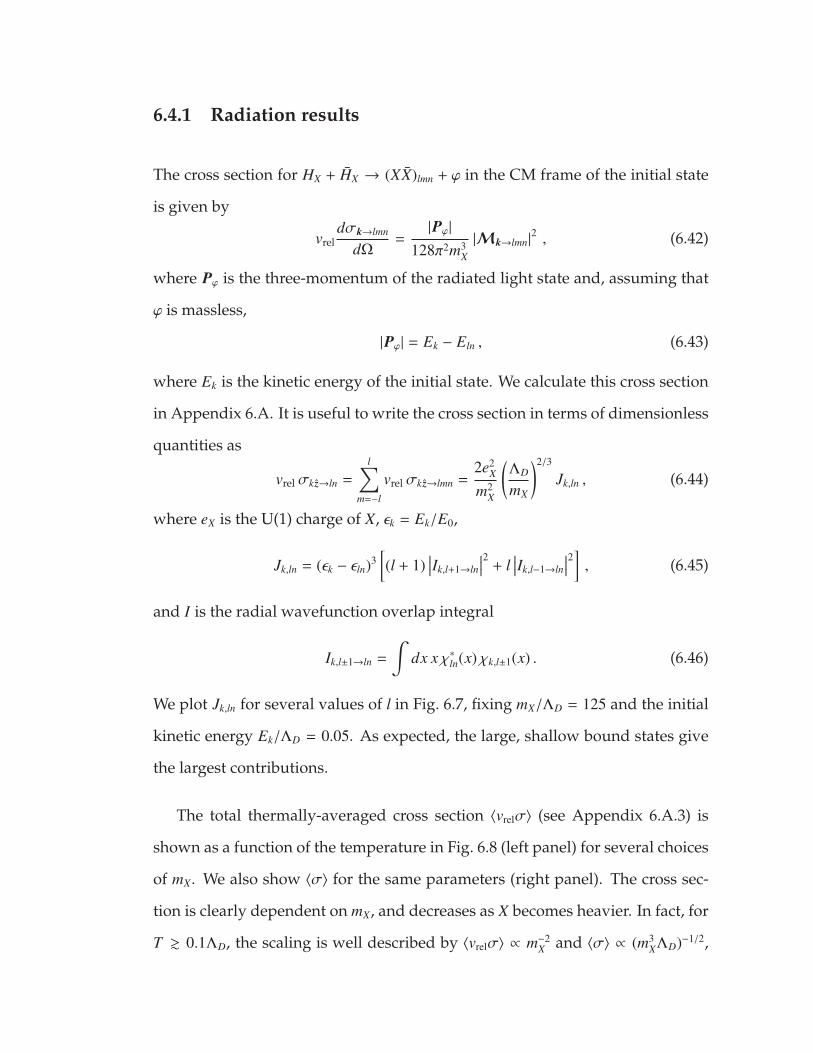
6.4.1 Radiation results

The cross section for HX + HX → (XX)lmn + ϕ in the CM frame of the initial state

is given by

vreldσk→lmn

dΩ=

|Pϕ|

128π2m3X

|Mk→lmn|2 , (6.42)

where Pϕ is the three-momentum of the radiated light state and, assuming that

ϕ is massless,

|Pϕ| = Ek − Eln , (6.43)

where Ek is the kinetic energy of the initial state. We calculate this cross section

in Appendix 6.A. It is useful to write the cross section in terms of dimensionless

quantities as

vrel σk z→ln =

l∑m=−l

vrel σk z→lmn =2e2

X

m2X

(ΛD

mX

)2/3

Jk,ln , (6.44)

where eX is the U(1) charge of X, εk = Ek/E0,

Jk,ln = (εk − εln)3[(l + 1)

∣∣∣Ik,l+1→ln

∣∣∣2 + l∣∣∣Ik,l−1→ln

∣∣∣2] , (6.45)

and I is the radial wavefunction overlap integral

Ik,l±1→ln =

∫dx x χ∗ln(x) χk,l±1(x) . (6.46)

We plot Jk,ln for several values of l in Fig. 6.7, fixing mX/ΛD = 125 and the initial

kinetic energy Ek/ΛD = 0.05. As expected, the large, shallow bound states give

the largest contributions.

The total thermally-averaged cross section 〈vrelσ〉 (see Appendix 6.A.3) is

shown as a function of the temperature in Fig. 6.8 (left panel) for several choices

of mX. We also show 〈σ〉 for the same parameters (right panel). The cross sec-

tion is clearly dependent on mX, and decreases as X becomes heavier. In fact, for

T & 0.1ΛD, the scaling is well described by 〈vrelσ〉 ∝ m−2X and 〈σ〉 ∝ (m3

XΛD)−1/2,

which agrees with the semiclassical estimate in Sec. 6.1. Thus, for the high mass

region of interest, mX ΛD, this contribution is negligible compared to pro-

cesses mediated by the brown muck, such as the rearrangement process. We

expect this qualitative behavior to persist regardless of the spin of the radiated

particles.

6.5 Implications for Cosmology

We have found that, at temperatures below the confinement scale ΛD, (XX)

bound states are formed with a geometric cross section with no mX suppression.

These bound states are of size ∼ 1/ΛD, but since the process is exothermic, they

cannot be dissociated, and eventually de-excite to the ground state, in which the

X–X pair annihilates. The rate for this de-excitation process depends mainly on

the light degrees of freedom. For the large (XX) bound states produced, the level

splittings are of order (ΛD/mX)1/3ΛD, so we need massless photons or light pions

in order to have allowed transitions (as in the models we considered here). In

the case where the DM is charged under real QCD, the rate should be sizable,

so we expect any (XX) bound states to quickly decay to light particles.1

As a result, the abundance of HX hadrons is depleted by this second stage of

annihilations, down to [219]

ΩfHX∼

√ΛD

mX

( mX

30 TeV

)2, (6.47)

which can be much smaller than the relic density from perturbative X–X anni-

hilations earlier in the thermal history.1In models with no light degrees of freedom, as in the case of an adjoint X with no light

quarks [205], the lightest degrees of freedom are glueballs of mass ∼ 7ΛD, and this rate is sup-pressed by powers of αl

D.

There are, however, various different hadronic states (in addition to HX) in

which X can survive [201]. These include other types of single-X hadrons such

as baryonic XqN−1 hadrons, double-X states such as baryonic XXqN−2, and up to

purely heavy baryons XN . Thus, in general, our simple toy model can produce

multi-component DM with different masses and relic abundances.

We leave a detailed investigation of the parameter space of the models for

future study, but note a few qualitative features.1 The cross section for produc-

ing double-X states should be comparable to the quarkonium cross section we

calculated, albeit smaller by O(1) factors because of the smaller binding ener-

gies in this case. However, for N > 2, the double-X hadrons contain some light

quark(s), so their size is 1/ΛD. They can therefore interact quite efficiently with

hadrons containing X to form bound states containing both X and X, where X–X

pairs can quickly annihilate. Meanwhile, they can also interact with HX hadrons

and form triple-X hadrons, and this chain may go on until pure-X (or pure-X)

baryons are formed. All these processes should have geometric cross sections.

The pure-X baryons eventually de-excite to the ground state, the size of which

is much smaller than 1/ΛD. Their interactions with other hadrons therefore shut

off. As a result, the Xs inside the baryons remain as stable relics, while the other

Xs may effectively be annihilated. A systematic analysis necessitates solving

the Boltzmann equation with these dynamics, which is beyond the scope of this

work. However, it is safe to assume that a sizable fraction of the original Xs can

be preserved in a variety of stable hadronic relics.

For DM charged under real QCD, heavy-light hadrons, with size 1/ΛD, are

subject to stringent constraints, but they are efficiently depleted at T . ΛD as

we have shown. In contrast, the relic abundance of X3 baryons may be just

1Many of the relevant processes were described in Ref. [201] for TeV-mass colored relics.

somewhat smaller than the original X relic abundance. Thus the fundamental

Xs we considered here may give a different realization of colored DM [196],

but whether the models are viable requires a more detailed analysis. Note that

the scenario considered in Ref. [196], namely a heavy Dirac adjoint X, is non-

generic, in that two Xs can form a stable singlet with no additional light quarks.

In summary, the simple models considered here typically give rise to several

components of DM composites of different masses. For certain choices of mX

and ΛD, these can exhibit self-interactions, transitions between different excited

states, and, depending on the coupling to the Standard Model, modified direct

and indirect detection cross sections. In some variants of these models, the DM

abundance can be significantly depleted at ΛD, leading to a long era of matter

domination between mX and ΛD.

6.6 Conclusions

In this work we have considered the cosmological dynamics of bound states that

are much larger than their inverse mass, taking as an example Xq mesons in a

confining theory where X is much heavier than q and the confinement scale. We

calculated the cross section for quarkonium production from heavy-light meson

scattering. The cross section is geometric, and scales with the area of the inci-

dent heavy-light mesons. The relic density of heavy-light X-mesons is therefore

efficiently diluted with rates much higher than the s-wave unitarity bound due

to the participation of many partial waves in the process. We also find that the

process is mainly mediated by the effective interaction of the light quarks. In

contrast, processes in which only the heavy constituents participate have mass-

suppressed rates. It is amusing to note that if the lifetime of B-mesons were

longer, such processes could be experimentally measured.

0.0 0.5 1.0 1.5 2.010-5

10-4

0.001

0.010

0.100

1

Ef /Eb

BranchingRatio

σnl/σl Ei=0.06Eb , ℓ=0 Ei=0.6Eb , ℓ=0

Ei=0.6Eb , ℓ=14

1.0 1.5 2.010-4

0.001

0.010

0.100

RX X_ /aq

BranchingRatio

σnl/σl

Ei=0.06Eb , ℓ=0

Ei=0.6Eb , ℓ=0

Ei=0.6Eb , ℓ=14

Figure 6.5: The branching fraction σnl/σl for some initial partial waves toform an (XX) quarkonium of definite n, l (uniquely defined bythe x-axis). The results are presented for mX = 3 × 104αDmq andseveral values of Ei and l. Left panel: The branching fraction asa function of the kinetic energy in the final state. Right panel:The branching fraction as a function of RXX, the mean radius ofthe final state.

5 ×104 1 ×105 5 ×105 1 ×106

10-4

0.001

0.010

0.100

1

10

mX [αD mq]

σ×(α

Dmq)2 Total Cross section

ℓ=0

ℓ=10

ℓ=15

Unitarity Bound

Figure 6.6: The rearrangement cross section. The blue line is the total crosssection for an incoming energy Ei = 0.6Eb, and is geomet-ric. Several individual partial-wave contributions σl/(2l + 1)are given in green, together with the unitarity bound 4π/k2

i (reddashed line) for l < lmax ∼ kiaq.

-15 -10 -5 0

10-4

10-2

1

100

Figure 6.7: Jk,ln as a function of εln for xc = 15 and εk = 0.25. The linescorrespond to different values of l.

10-2 0.05 0.1 0.5 1 5 1010-5

10-4

10-3

10-2

0.1

10-2 0.05 0.1 0.5 1 5 1010-3

10-2

0.1

1

10

Figure 6.8: Results of thermally-averaged radiative quarkonium produc-tion cross section 〈σv〉 (top panel) and 〈σ〉 (bottom panel) as afunction of temperature for different values of mX/ΛD.

APPENDIX

6.A Cross Section for Bound-State Formation in the Radiation

Process

In this section we summarize the calculation of the bound-state formation cross

section via radiation discussed in Sec. 6.4. We also collect here some useful

results on the spectrum and wavefunctions of the Cornell and linear potential.

6.A.1 Eigenstates of the Cornell potential

We model the X–X attractive interaction by the cutoff Cornell potential of

Eq. (6.6), with the cutoff given in Eq. (6.36) and V0 = 0.

The bound states (XX) are characterized by three integers (l,m, n), where l

labels the angular momentum, m labels the angular momentum along the z-

axis, and n ≥ 1. An HX–HX scattering state is approximated by an X–X unbound

state, which is characterized by the X–X relative momentum k, with energy Ek ≈

k2/mX, where k = |k|. The reduced mass of both the bound and scattering states

is approximately mX/2.

The bound-state wavefunctions can be written as

ψlm,n(R0x) =1

R3/20

χln(x)x

Ylm(Ωx) , (6.48)

where the dimensionless coordinate x is defined below Eq. (6.39). The

146

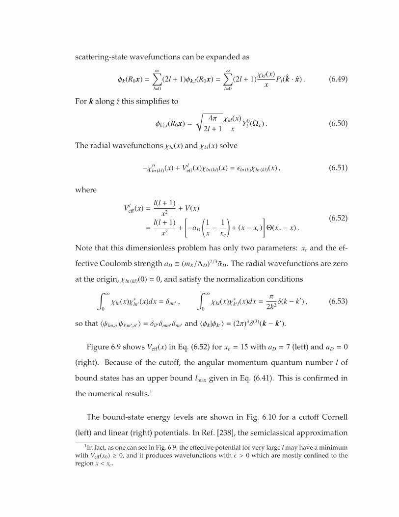
scattering-state wavefunctions can be expanded as

φk(R0x) =

∞∑l=0

(2l + 1)φk,l(R0x) =

∞∑l=0

(2l + 1)χkl(x)

xPl(k · x) . (6.49)

For k along z this simplifies to

φk z,l(R0x) =

√4π

2l + 1χkl(x)

xY0

l (Ωx) . (6.50)

The radial wavefunctions χln(x) and χkl(x) solve

−χ′′ln (kl)(x) + V leff(x)χln (kl)(x) = εln (k)χln (kl)(x) , (6.51)

where

V leff(x) =

l(l + 1)x2 + V(x)

=l(l + 1)

x2 +

[−aD

(1x−

1xc

)+ (x − xc)

]Θ(xc − x) .

(6.52)

Note that this dimensionless problem has only two parameters: xc and the ef-

fective Coulomb strength aD ≡ (mX/ΛD)2/3αD. The radial wavefunctions are zero

at the origin, χln (kl)(0) = 0, and satisfy the normalization conditions∫ ∞

0χln(x)χ∗ln′(x)dx = δnn′ ,

∫ ∞

0χkl(x)χ∗k′l(x)dx =

π

2k2 δ(k − k′) , (6.53)

so that 〈ψlm,n|ψl′m′,n′〉 = δll′δmm′δnn′ and 〈φk|φk′〉 = (2π)3δ(3)(k − k′).

Figure 6.9 shows Veff(x) in Eq. (6.52) for xc = 15 with aD = 7 (left) and aD = 0

(right). Because of the cutoff, the angular momentum quantum number l of

bound states has an upper bound lmax given in Eq. (6.41). This is confirmed in

the numerical results.1

The bound-state energy levels are shown in Fig. 6.10 for a cutoff Cornell

(left) and linear (right) potentials. In Ref. [238], the semiclassical approximation

1In fact, as one can see in Fig. 6.9, the effective potential for very large l may have a minimumwith Veff(x0) ≥ 0, and it produces wavefunctions with ε > 0 which are mostly confined to theregion x < xc.

0 5 10 15 20

-20

-10

0

10

0 5 10 15 20

-20

-10

0

10

Figure 6.9: The effective potential Veff(x) with xc = 15 (mX ' 125ΛD), forthree values of l. In the left panel, aD = 7, which corresponds toαD = 0.3, while aD = 0 in the right panel. The largest l in eachpanel corresponds to the upper-bound on l of the bound states.Note that the plots for l = 0 correspond to V(x) in Eq. (6.52).

continuum

Coulomb

linear

0 1 2 3 19 20 21

-25

-20

-15

-10

-5

0continuum

linear

0 1 2 3 18 19 20

-15

-10

-5

0

Figure 6.10: The energy spectrum of bound states. Left panel: aD = 7, rightpanel: aD = 0 (linear). We also show, for the linear potential,the semiclassical results in Eq. (6.55) as the small dots.

is used to obtain the energy levels of the eigenstates of central potentials. Fol-

lowing their discussion, the energy levels under the linear potential are given

by

Eln − V(0) ≈[32π

(n +

l2−

14

)]2/3

E0 , (6.54)

or in our notation, since V(0) = −RcΛ2D = −xcE0,

εln ≈

[32π

(n +

l2−

14

)]2/3

− xc . (6.55)

We reproduce this result in Fig. 6.10(b). For a Cornell potential (Fig. 6.10(a)),

0 5 10 15 20

-0.5

0.0

0.5

1.0

0 5 10 15 20

-0.5

0.0

0.5

1.0

0 5 10 15 20

-2

-1

0

1

2

3

4

0 5 10 15 20-0.4

-0.2

0.0

0.2

0.4

0.6

0.8

Figure 6.11: Wavefunctions obtained from solving Eqs. (6.51–6.52) withxc = 15, aD = 0. Top: χln(x) for bound states. The left panelcontains smaller l (0,1) while the right panel has intermediateand high l (5, 18, 19 = lmax), where (l, n) = (5, 10) is the highest-energy bound state. Bottom: χkl(x) for scattering states. Theleft panel displays the partial waves of the scattering stateswith ε = 0.25 (Ek = 0.05ΛD), while the right panel shows thosewith ε = 7.5 (Ek = 1.5ΛD).

deep states are governed by the Coulomb force and therefore obey the well-

known Coulombic energy levels

εln ≈ −a2

D

4N2 − xc , (6.56)

where the principal quantum number N is given by n + l. For shallower states,

the Coulomb force is negligible and the linear potential governs the spectrum.1

We show some examples of bound-state and scattering-state wavefunctions

1The average size 〈x〉 of bound states is given by the virial theorem as ε + xc = −aD/(2 〈x〉) fora Coulombic bound states, i.e., if the effect of the linear term is negligible, and ε + xc = 3 〈x〉 /2for bound states in the linear regime.

that solve Eq. (6.51) with the cutoff linear potential (Eq. (6.52) with aD = 0) in

the top and bottom rows of Fig. 6.11, respectively. The bound state with (l, n) =

(5, 10) is found to be the shallowest bound state, but it should be emphasized

that this is an accident due to the cutoff being just above the energy of this

state. In general, shallower states with smaller l have wavefunctions that tend

to penetrate beyond x > xc. For the scattering states, wavefunctions of states

with larger ε and smaller l have penetrate further into the region x < xc.

6.A.2 Bound-state formation cross section in the dipole approx-

imation

We calculate the matrix element for the bound-state formation by a vector-

mediated interaction,

HX + HX → (XX)lm,n + ϕ (6.57)

with the X–ϕ interaction given by

L 3

∣∣∣∣(∂µ − ieXϕµ)

X∣∣∣∣2 . (6.58)

We follow the approach and notation in Refs. [191, 195]. From now on, we fo-

cus on the linear potential and set aD = 0 because, as we will see, the radia-

tive bound-state formation process favors shallow bound states, for which the

Coulomb force is negligible.

The bound-state formation cross section is given by [191]

(vrelσ)BSFk =

∑l,m,n

(vrelσ)BSFk→lm,n =

∑l,m,n

∫ dΩPϕ

4π|Pϕ|

32 πm3X

∑pol.

∣∣∣ε ·Mk→lm,n

∣∣∣2 (6.59)

in the CM frame, where k, Pϕ, and ε are the relative momentum of the initial

state, the momentum of the radiated light state ϕ, and its polarization vector,

respectively, and

vrel '|k|

mX/2, |Pϕ| = Ek − Eln ; (6.60)

Ek is kinetic energy of the initial scattering state. The matrix element is

Mjk→lm,n = −4eX

√mX

∫d3 p

(2π)3 p jψ∗lm,n(p)[φk

(p +

Pϕ

2

)+ φk

(p−

Pϕ

2

)], (6.61)

where φk(p) and ψlm,n(p) are the momentum-space equivalents of Eqs. (6.48)–

(6.49).

It is convenient to expand the matrix element in partial waves (cf. Eq. (6.49)):

Mjk→lm,n =

∞∑l′=0

(2l′ + 1)M jk,l′→lm,n ,

Mjk,l′→lm,n = −4eX

√mX

∫d3 p

(2π)3 p jψ∗lm,n(p)[φk,l′

(p +

Pϕ

2

)+ φk,l′

(p−

Pϕ

2

)]= 8ieX

√mX

∫d3r d3r′ ψ∗lm,n(r)φk,l′(r′) cos

(Pϕ

2· r′

)∂

∂r j δ(3)(r − r′) .

After partial integration, the derivative acts on ψ∗lm,n(r), and the integral over

d3r′ is trivial using the delta function. Dotting with the polarization vector and

performing another partial integration (the derivative of the cosine is zero as

ε · Pϕ = 0) yields

ε ·Mk,l′→lm,n = 4ieX√

mX

∫d3r cos

(Pϕ

2· r

)ε ·

[ψ∗lm,n∇φk,l′ − φk,l′∇ψ

∗lm,n

], (6.62)

where ψ∗lm,n and φk,l′ are functions of r. The quantity in brackets above appears in

the difference of the Schrodinger equations for the scattering- and bound-state

wavefunctions,

−1

mX∇ · (ψ∗lm,n∇φk,l′ − φk,l′∇ψ

∗lm,n) = (Ek − Enl)ψ∗lm,nφk,l′ . (6.63)

Using the identity1∫d3r (∇ · F) r = −

∫d3r F (∇ · r) = −

∫d3r F (6.64)

1By assumption, F satisfies appropriate fall-off behavior at large |r| so the boundary term isnegligible.

with F = ψ∗lm,n∇φk,l′ − φk,l′∇ψ∗lm,n and substituting into Eq. (6.62), we obtain1

ε ·Mk,l′→lm,n = 4ieX√

mX

∫d3r (ε · r)

[mX(Ek − Eln)ψ∗lm,nφk,l′ cos

(Pϕ

2· r

)+

Pϕ

2· (ψ∗lm,n∇φk,l′ − φk,l′∇ψ

∗lm,n) sin

(Pϕ

2· r

) ].

(6.65)

We are interested in temperatures T . ΛD for which Pϕ mX, and thus

ε ·Mk,l′→lm,n ' 4ieX

√m3

X(Ek − Eln)∫

d3r (ε · r)ψ∗lm,nφk,l′ cos(

Pϕ

2· r

). (6.66)

Also, we can evaluate Pϕ · r/2 as

Pϕ

2· r ≤

|Pϕ|r2

=|Ek − Eln|r

2= κΛD

|Ek − Eln|

ΛD

rRc. (6.67)

Note that as the integrand contains a bound-state wavefunction, the integral

has support only for r . Rc. Also, for T ΛD, the overlaps of the bound

and scattering states are larger for shallower bound states. Combining these,

we can approximate Pϕ · r/2 1 in order to employ the dipole approximation

cos(Pϕ · r/2)→ 1, which simplifies the cross section to

(vrelσ)BSFk →

∑l,m,n

∫ dΩPϕ

4π|Pϕ|

32 πm3X

∑pol.

∣∣∣∣∣∣∣∑l′(2l′ + 1)4ieX

√m3

X(Ek − Eln)ε · I k,l′→lm,n

∣∣∣∣∣∣∣2

=∑l,m,n

∫ dΩPϕ

4πe2

X(Ek − Eln)3

2π

∑pol.

∣∣∣∣∣∣∣∑l′(2l′ + 1)ε · I k,l′→lm,n

∣∣∣∣∣∣∣2

, (6.68)

where the integral of the wavefunctions is defined as

Ijk,l′→lm,n =

∫d3r r j ψ∗lm,n φk,l′ . (6.69)

Next, we express the integral in the basis ra = (r+, r0, r−) defined by

r± =−1√

2

(±r1 + ir2

)= r

√4π3

Y±11 (Ωr) , r0 = r

√4π3

Y01 (Ωr) . (6.70)

1This is the form of the matrix element in Refs. [193, 236]; both employ the dipole approxi-mation and the Hamiltonian formulation.

Taking the z-axis parallel to k, substituting Eq. (6.48) and Eq. (6.50) for the wave-

functions in Eq. (6.69), we obtain

Iak,l′→lm,n =

4πR5/20

√3(2l′ + 1)

Ikl′→ln

∫dΩxY0

l′(Ωx)Ya1 (Ωx)Ym∗

l (Ωx)

= (−1)m√

4π(2l + 1) R5/20 Ikl′→ln

l′ 1 l

0 0 0

l′ 1 l

0 a −m

, (6.71)

Ikl′→ln =

∫dx x χ∗ln(x) χkl′(x) , (6.72)

where we have expressed the integral over solid angle of three spherical har-

monics in terms of Wigner 3 j-symbols

∫dΩ Ym1

l1Ym2

l2Ym3

l3=

[(2l1 + 1)(2l2 + 1)(2l3 + 1)

4π

]1/2l1 l2 l3

0 0 0

l1 l2 l3

m1 m2 m3

. (6.73)

These symbols give the selection rules l′ = |l ± 1| and m = a, so that |m| ≤ 1.

With these results, the sum over m, l′, and polarizations in Eq. (6.68) evalu-

ates to1

l∑m=−l

∑pol.

∣∣∣∣∣∣∣∑l′(2l′ + 1)ε · I k,l′→lm,n

∣∣∣∣∣∣∣2

=

l∑m=−l

1∑a=−1

∣∣∣(2l + 3)Imk,l+1→lm,n + (2l − 1)Im

k,l−1→lm,n

∣∣∣2 δam

=

1∑m=−1

∣∣∣(2l + 3)Imk,l+1→lm,n + (2l − 1)Im

k,l−1→lm,n

∣∣∣2= 4πR5

0

[(l + 1)

∣∣∣Ik,l+1→ln

∣∣∣2 + l∣∣∣Ik,l−1→ln

∣∣∣2] . (6.74)

Inserting this into the cross section in Eq. (6.68) and trivially performing the

1Note that Iak z,l−1→lm,n is always zero if l = 0.

dΩPϕ yields

(vrelσ)BSFk = 2e2

XR50

∑l,n

(Ek − Eln)3[(l + 1)

∣∣∣Ik,l+1→ln

∣∣∣2 + l∣∣∣Ik,l−1→ln

∣∣∣2]=

2e2X

m2X

(ΛD

mX

)2/3 ∑l,n

Jk,ln , (6.75)

with Jk,ln defined in Eq. (6.45).

6.A.3 Thermally-averaged cross section

Here we briefly describe the procedure to calculate the thermally-averaged cross

section, 〈vrelσ〉 (β), as a function of the inverse temperature β = T−1. As in the

previous discussion, we denote the momenta of the initial particles as k1, k2.

As we are interested in T mX, the kinetic distributions of HX and HX are

given by the Maxwell-Boltzmann distribution,

fMB(p) =

(2πβm

)3/2

exp(−β|p|2

2mX

), (6.76)

which is normalized so that∫

d3 p(2π)3 fMB(p) = 1. With this distribution, the

thermally-averaged cross section is given by

〈vrelσ〉 (β) =

∫d3 k1

(2π)3

d3 k2

(2π)3 fMB(k1) fMB(k2)(vrelσ)BSFk

=

(2πβmX

)3 ∫d3K(2π)3

d3 k(2π)3 exp

(−β(|K/2|2 + |k|2)

mX

)(vrelσ)BSF

k

=

√16β3

πm3X

∫dk k2 e−βk2/mX (vrelσ)BSF

k , (6.77)

where, as before, K = k1 + k2 and k = (k1 − k2)/2. We have neglected the depen-

dence of the (non-relativistic) cross section (vrelσ)BSFk on K since |K| |k|.

Combining the previous result and also including the final-state effect of ϕ,

we obtain

〈vrelσ〉 (β) =2e2

X

m2X

(ΛD

mX

)2/3 ∫dk w(k; β)

∑l,n

Jk,ln

1 − exp[−β(Ek − Eln)

] , (6.78)

where we define

w(k; β) =

√16β3

πm3X

k2 e−βk2/mX ,

∫w(k; β)dk = 1 . (6.79)

CHAPTER 7

SELF-DESTRUCTING DARK MATTER

BEYOND THE STANDARD MODEL: COMPOSITE HIGGS AND DARK

MATTER

Ofri Telem, Ph.D.

Cornell University 2019

We present Self-Destructing Dark Matter (SDDM), a new class of dark matter

models which are detectable in large neutrino detectors. In this class of models,

a component of dark matter can transition from a long-lived state to a short-

lived one by scattering off of a nucleus or an electron in the Earth. The short-

lived state then decays to Standard Model particles, generating a dark matter

signal with a visible energy of order the dark matter mass rather than just its

recoil. This leads to striking signals in large detectors with high energy thresh-

olds. We present a few examples of models which exhibit self destruction, all

inspired by bound state dynamics in the Standard Model. The models under

consideration exhibit a rich phenomenology, possibly featuring events with one,

two, or even three lepton pairs, each with a fixed invariant mass and a fixed en-

ergy, as well as non-trivial directional distributions. This motivates dedicated

searches for dark matter in large underground detectors such as Super-K, Borex-

ino, SNO+, and DUNE.

7.1 Introduction

Our knowledge of the nature of dark matter (DM) is very limited. Though it

accounts for over 80% of the matter in the universe, it is often assumed that the

dark sector is minimal, consisting of a single particle that interacts only feebly

with the Standard Model (SM). This assumption, which is the most sensible first

guess, motivates a set of strategies in our search for DM. In particular, when

searching for DM directly, we try to detect the low energy recoil of a nucleus

which was struck by a slowly moving DM particle [239]. DM direct detection

thus focuses on detectors with thresholds between sub keV and tens of keV.

The current search program is undoubtedly important and must be pursued

further. However, we should not let minimality be our only guide. Indeed,

considering even slightly non-minimal DM models has led to significant vari-

ations in direct detection phenomenology [240–254], including changes in the

predicted recoil spectrum, annual modulation, and in the manner in which the

DM deposits energy in the detector. These interesting models, however, keep

direct detection phenomenology within the purview of low threshold detectors.

The reason for this is that the available energy in the problem is at most the ki-

netic energy in the DM-nucleus or DM-electron system. This energy is of order

µv2, where v ∼ 10−3c is the DM velocity, and µ is the reduced mass of the system.

In this work, we consider a drastic departure from this picture and discuss

the possibility that DM is capable of leaving not just kinetic energy in the de-

tector, but rather all of its mass. This can lead to DM direct detection signals

above MeV, allowing to extend the search for DM to detectors with much higher

thresholds. In particular, large existing neutrino experiments such as Borex-

1

Figure 7.1: A schematic picture of self-destructing DM, where DM denotesthe cosmologically long-lived state and DM’ denotes the veryshort-lived one.

ino and Super-Kamiokande, as well as future experiments such as SNO+ and

DUNE, can probe self destructing DM models.

A naıve idea to convert the DM rest mass to detectable signal is to consider

its down-scattering to a nearly massless state, with the difference in mass con-

verted to recoil energy. This is however unfeasible since it leads to a DM par-

ticle that is cosmologically unstable by decaying to this nearly massless state.

Instead, we must consider a non-minimal setup in which an interaction of DM

with a nucleus triggers a transition from a state that is stable on cosmological

timescales to one which is very short-lived. The signal is then not a recoil sig-

nal, but rather a subsequent decay of the short-lived state to SM particles. A

sketch of this is depicted in Figure 7.1. The crucial ingredients in the story are a

cosmologically long lived state and a short lived state, with a possible transition

between the two which is induced by the interaction with the Earth. We call this

class of DM models self-destructing DM (SDDM for short).

SDDM is not the first class of DM models in which the measured energy

is more than just the DM recoil energy. In [245], for example, the DM down-

scatters and converts part of its rest mass to recoil energy. However, in that

model the mass splittings considered were still of the same order as the ki-

netic energy. In [253] the possibility of releasing more than the recoil energy

was considered, but with signals still in the domain of low threshold detectors.

Other DM models [204, 255–261], are similar to our scenario in that they can

be probed at neutrino detectors [262]. Yet, in these models, the dynamics that

lead to signals at neutrino detector (a “removal” of a baryon from the detector

or a boosted population of DM) is different than the case of SDDM. Lastly, we

mention that the axion and other ultralight bosons that can be fully absorbed

by a detector may be considered a fully SDDM candidate, but their lightness

leads to much lower energy deposition, and thus to very different experimental

signatures [263–265].

In the upcoming sections, we present three models which realize the idea of

SDDM. These ideas are intended as a proof of principle rather than as complete,

well motivated models. In each case, DM is stabilized by a different princi-

ple that can be un-done by interactions in the Earth. None of these models is

minimal by any means. They are, however, inspired by phenomena that are

observed in the visible sector. Particles in the Standard Model find themselves

to be either short-lived or meta-stable for a variety of reasons. In many cases

different effects, forces, or interactions come into play, balancing one against the

other to produce a long- or short-lived state. We are therefore quite liberal in

allowing for several particles and interactions. Furthermore, like the visible sec-

tor which contains several populations of cosmic relics, we will be open to the

possibility that only a subcomponent of DM is self-destructing.

The model building challenge for SDDM is to have a dark matter compo-

nent that is very long-lived, yet capable self-annihilating once it interacts with a

nucleus in the Earth. In its long-lived state, this component needs to have a life-

time for more than about 1028 sec to satisfy observational constraints [266–268],

if it makes up all of DM. Even if we consider only a small sub-component of DM

to relax this bound, the state needs to live for more than the age of the universe.

In contrast, the short-lived state of our DM component has to decay in much

less than 10 seconds, its Earth-crossing time.

The chapter is organized as follows: In Section 7.2 we discuss the cosmolog-

ical challenges in realizing SDDM, and arrive at an upper bound on the temper-

ature in which it is produced. In Section 7.3 we review the first in our class of

SDDM models. In this model, some of the DM consists of excited positronium-

like bound states which are stable due to a large angular momentum barrier.

Interaction with the matter in the Earth can change the angular momentum of

the bound state, rendering it unstable. We then estimate the signal rate of this

model in large neutrino detectors and discuss possibilities for its early Universe

history. In the second model, presented in Section 7.4, the DM is in a metastable

minimum far away from the origin of a bound-state potential. Interaction with

the Earth can shake the internal structure and move the system to the global

minimum where annihilation is very fast. In our last example, Section 7.5, DM

consists of dark baryons. A baryon number violating interaction with matter

causes a transition from a dark baryon to a dark meson which can now decay

in a detector. In Section 7.6, we discuss the phenomenological signals of our

framework in large detectors further in order to motivate more detailed studies.

We conclude and provide some further directions for exploration in Section 7.7.

7.2 Survival of SDDM from the early universe

The self-destructing scenario is possible thanks to the high density of matter in

the Earth, one which is unprecedented from the perspective of an incoming DM

particle. The expected number of DM interactions off of a target with number

density n is roughly

〈N〉 ∼ n〈σv〉∆t , (7.1)

where v is the typical relative velocity, σ is the interaction cross section, and

∆t is the amount of time spent in this environment. A DM particle with v ∼

10−3c crosses the Earth in about 10 seconds. However, before its short traversal

through Earth, it had spent about 1016 more time in the low density environment

of the galaxy. On the other hand, the number density of atoms in the Earth is

about 1023 larger than that in the galaxy. As a result, it is reasonable for the

expected rate of transitions to an unstable state to be much larger in one Earth-

crossing than it is in the preceding Hubble time.

Of course, one should not forget that in the early universe the DM candi-

date was immersed in a dense thermal bath. Because the density of targets for

self-destruction increases early on, there is an upper bound on the tempera-

ture above which all SDDM will be destroyed. The probability of destruction is

given by p = nσv∆t. For the case of Super-K, n is the number density of targets

in water and ∆t is the time interval of dark matter passing through the detector.

Assuming that we could observe 100 events in the Super-K detector per year,

we could derive the probability of its self-destruction,

p ' 10−20( mχ

10 MeV

)(7.2)

based on the local dark matter density. We could repeat the calculation for early

universe, where the number density of SM particles is given by n ∼ T 3, and the

Hubble time ∆t = H−2 ' Mplanck/T 2. The destruction of SDDM will be significant

at temperatures above

Tsurvival ∼ 10 MeV ×(10 MeV

mχ

)(7.3)

This implies an upper limit on the temperature for SDDM to be produced in the

early universe.

7.3 High angular momentum stabilization

In this model, a component of the DM is a positronium-like bound state

which is stabilized by angular momentum conservation. In particular, the self-

annihilation of this “dark positronium” is suppressed due to a large angular

momentum barrier. An interaction with the Earth allows the dark matter to

transition to a lower angular momentum state that has a lifetime which is expo-

nentially shorter.

The dark sector contains light fermions χ and χ which are charged under

two broken abelian gauge groups U(1)φ and U(1)V . The Lagrangian for this

sector takes the form

L = χi /Dχ − mχχχ −14φµνφµν +

12

m2φφµφ

µ −14

VµνVµν +12

m2VVµVµ −

ε

2VµνFµν , (7.4)

where

Dµχ = (∂µ + igφφµ + igVVµ)χ , (7.5)

and φµν, Vµν, and Fµν are the field strengths for φ, V and the standard model

photon respectively. For simplicity, we assume no kinetic mixing of φ to any

of the other gauge bosons. We further define the fine-structure constants, αV =

g2V/(4π) and αφ = g2

φ/(4π), and the usual αEM = e2/(4π).

We will consider two benchmark models for the lighter of the two gauge

bosons, φ. One benchmark that is weakly coupled and one that exhibits strong

coupling an confinement. Both models will share the same phenomenology of

self destruction, but can have difference cosmological histories as discussed in

Section 7.3.5.

Weakly coupled model: In this case φ is assumed to be a weakly coupled U(1)

gauge boson. This field is φ is assumed to be light enough to mediate a long

range force which leads to χχ positronium-like bound states with n∗ ∼ 10 energy

levels. On the other hand, φ is taken to be too heavy to be emitted on-shell in

transitions among energy levels. These constraints give

14α2φmχ < mφ <

12n∗

αφmχ . (7.6)

We further assume that V is too heavy to play a role in the bound state dy-

namics, but is light enough to be emitted in the self-annihilation of the χχ state,

thus12αφmχ < mV . mχ . (7.7)

We assume that αV & αφ so that on-shell Vs are produced in a sizable fraction of

the annihilation processes. Our last assumption is

mV > 2me , (7.8)

so V could decay into e+e− and can be detected easily.

Before proceeding, we comment on some possible alternative weakly cou-

pled models. For example, one could consider a model with a single vector

boson from the dark sector playing the roles of both φ and V . However, in this

case, Eq. (7.8) with αφ . 10−2 and n∗ ∼ 10, and the upper bound in Eq. (7.10)

can only be reconciled when mχ 1 GeV. As we are interested in a wide

range of mχ, as low as the MeV scale, see Section 7.3.2, we keep both φ and V

in the following discussion. Another possibility is to allow φ to also mix with

the SM photon, a possibility which, for the most part, affect the signal rate es-

timated in Section 7.3.2. In addition, there may be other variants of this model

where either or both V and φ are replaced by light scalars or pseudoscalars or

when additional particles are introduced. We focus here on the gauge case for

concreteness but other options are considered when the phenomenology is dis-

cussed in Section 7.6.

Strongly coupled model: In this case φ is assumed to a non-abelian gauge bo-

son which is massless mφ = 0. In the UV, φ is weakly coupled and runs to

become strong at some scale Λφ at which point the theory becomes confining.

We will assume that the confinement scale is lower than the mass of χ or any

other φ-colored state,

Λφ < mχ (7.9)

Once produced (at zero temperature), a χχ bound state will exhibit quirky dy-

namics [219]. The χχ pair remains bound by a string and will loose energy by

emitting glueballs with mass ∼ Λ. Such a bound state will settle in a Coulombic

bound state with a Bohr radius of rB ∼ αφ(mχ)mχ/2, where αφ(mχ) is the coupling

evaluated at the scale mχ which is perturbative. The typical energy splittings

in this atom-like system are of order α2φ(mχ)mχ/4. We will assume that the gap

in the theory, given by the glueball mass Λφ is such that an on-shell glueball

is too heavy to be radiated in transitions among these states. Combining these

requirements, we will consider the region of parameter space

14α2φmχ < Λφ < mχ . (7.10)

The restrictions on the mass of V will be the same in the weakly coupled model,

Equations (7.7) and (7.8).

Though both of these frameworks are quite different in the UV, the bound

state dynamics and lifetimes of the various states will be similar. In the next

subsection we estimate the various relevant lifetimes using the language of the

weakly couple model, though the results apply to both.

7.3.1 Bound state lifetimes

We now consider the lifetimes of the χχ bound states. As we show below, states

with ` & 10 have lifetimes much longer than the cosmological bound on DM

lifetime, while S -wave states annihilate very quickly, within the time it traverses

the Earth.

In the vacuum, bound states could be destroyed either by direct χχ annihi-

lation or by de-excitation to a lower-` state. We begin with an estimate of direct

annihilation to Vs. (In the following we also refer to V as the dark photon.) The

number of Vs in the final state is denoted by NV . This number is 2 for bound

states that are even under charge conjugation and 3 for odd ones. The leading

decay to consider is thus Ψn,` → VV or Ψn,` → VVV . The amplitude for anni-

hilation into dark photons for the Ψn,` state is proportional to the `th derivative

of the wave function at the origin. Roughly speaking every derivative result in

an extra power of αφ in the amplitude. Assuming no significant phase space

suppression, these decay rates can be estimated by [193],

Γn,`→V′s ∼

(αφn

)2`+3αNV

V mχ , (7.11)

Annihilation into φφ or into φV have a similar power counting. With mχ ∼ 1 GeV,

and αV ∼ αφ ∼ 10−2 we find that, for example, the inverse width of annihilation

of the Ψn=10,`=9 state is about 1042 seconds, while Ψn=7,`=6 lives for about 1022 sec.

The latter is too short to evade bounds on the lifetime of all of DM, but is safe if

that state is a small fraction of the DM.

Next, we consider de-excitation. Since mV ,mφ > α2φmχ/4, the de-excitation

of Ψn,` to lower states cannot happen via on-shell φs or Vs. Rather the leading

decay is to three photons through an off shell V or an off shell φ, if it couples

to the SM. The binding energy difference, of order ∼ α2φmχ, is assumed to be

too small to emit a pair of e+e− for all the parameter space under consideration.

There is also the possibility for the off-shell V∗ to turn into two neutrinos via its

kinetic mixing with the SM Z-boson. The partial rate, in this case, is even more

suppressed than the two or three photon final states we are considering.

The de-excitation rate of Ψn,` → Ψn−1,`−1 via off-shell V is approximately

Γn,`→n−1,`−1 ∼

(αφn2

)2 αVε2αEM

m4V

α3EM

m8e

α2φmχ

n3

13

, (7.12)

where the term in the first parentheses αφ/n2 is the matrix element for dark pho-

ton radiation from the bound states, and the term in the last parentheses α2φmχ/n3

stands for the difference in binding energy. This dimensionful quantity is raised

to the thirteenth power in order to make up the dimension of the rate. For exam-

ple, with mχ ∼ mV ∼ 1 GeV, ε ∼ 10−2, and αV ∼ αφ ∼ 10−2 we find that the lifetime

of the Ψn=10,`=9 state is about 1041 seconds, making it cosmologically stable. The

lifetime is even longer for smaller values of mχ, or for transitions with ∆` > 1.

If φ also mixes with the photon, the bound state de-excitation rate via off-

shell φ can be estimated in a similar way, with the V kinetic mixing parameter

and the dark photon mass replaced by those of φ. If φ is a scalar particle and

does not mix with the SM Higgs boson, the de-excitation is even slower because

it requires at least three loops and two powers of the kinetic mixing parameter

ε for it to decay into two SM photons.

We have thus shown that high-` excitations of the χχ bound state are cos-

mologically stable and are a viable candidate to be at least a portion of DM.

On the other hand, the bound states with small n and ` quantum numbers can

decay much faster, into 2V or 3V , depending on its charge-conjugation parity

(C = (−1)L+S ) as discussed above. The amplitude for an S -wave χχ bound state

to annihilate into 2V is proportional to its wave function at the origin, and, ne-

glecting phase space effects, the decay rate is

ΓΨ

(+)n,0→2V =

α3φα

2Vmχ

2n3 ,

ΓΨ

(−)n,0→3V =

2(π2 − 9)α3φα

3Vmχ

9πn3 .

(7.13)

Setting mχ = 1 GeV, αV = αφ = 0.01, and a DM speed of v ∼ 10−3 we find the decay

length of the ground state to be, vτΨ

(+)1,0→2V ∼ 4×10−7 cm, or vτ

Ψ(−)1,0→3V ∼ 3×10−4 cm,

which is a prompt decay. For an S-wave state with n ≤ 10 the decay is prompt

in view of DM or neutrino detectors.

In conclusion, the model has the two desirable ingredients: a cosmologically

long lived state and a short lived one that can generate a signal in the detector.

The next task is to estimate the rate for transitioning from the long to the short

lived states.

7.3.2 Bound state scattering

In this subsection, we demonstrate how collisions of a high-`, long-lived bound

state Ψ with a nucleus can induce a transition to a lower ` state Ψ′ that decays

quickly into SM particles. The amplitude for the leading non-relativistic inelas-

tic scattering of a proton with a bound state

Ψ(~p1) + p(~p2)→ Ψ′(~p3) + p(~p4), (7.14)

occurs via t-channel dark photon (V) exchange and it takes the form

MΨ+p→Ψ′+p = 4mχFD(|~q |)gVεe|~q| 2 + m2

V

up(~p4)γ0up(~p2) . (7.15)

Here up is the proton spinor, and FD(|~q |) is the form factor for the Ψ→ Ψ′ transi-

tion in the presence of a three-momentum ~q = ~p3 − ~p1 injection,

FD(|~q |) =

∫d3~x Ψ′∗(~x)Ψ(~x)

[ei~q·~x/2 − e−i~q·~x/2

]. (7.16)

In the following we estimate FD(|~q |) by making the approximation that Ψ and

Ψ′ are Coulomb-like wave functions. Parity invariance implies that the orbital

angular quantum numbers of the initial and final states in Eq. (7.16) must differ

by an odd integer.

The differential scattering cross section off a nucleus (with atomic and mass

numbers Z, A) takes the approximate form

dσscatter

d|~q |2'

g2Vε

2e2

4πv2(|~q| 2 + m2V)2×

∣∣∣FD(|~q |)∣∣∣2 × Z2F2(|~q|) , (7.17)

where v ' 10−3 is the incoming DM bound state velocity. For F(|~q|), the nuclear

form factor, we use the Woods-Saxon form given in [269]. Note that when Ψ′ is

a deeper bound state than Ψ, both the binding energy difference and the initial

kinetic energy contribute to the momentum transfer, ~q. In the small v limit, the

upper and lower limit of |~q|2 take the form

(|~q|2

)max

min= 2µΨ′A(mΨ − mΨ′) ± µΨ′Av

(mΨ

mΨ′

) √8µΨ′A(mΨ − mΨ′) + O(v2) , (7.18)

where the reduced mass µΨ′A is defined as µΨ′A = mΨ′mA/(mΨ′ + mA). For weakly

bounded states, we have mΨ ∼ mΨ′ ' 2mχ and mΨ − mΨ′ ∼ mχα2φ. The above

expansion converges for αφ & v, i.e., when the binding energy release, mΨ−mΨ′ ∼

mχα2φ, dominates over the DM kinetic energy, ∼ mχv2. To further simplify the

result, we consider the limit |~q2| m2V and mΨ mA, which is the region of

interest for this study. In this case, the scattering cross section is approximately,

σscatter '64πε2αEMαVαφm2

χ

πvm4V

×∣∣∣FD(|~q |)

∣∣∣2 × Z2F2(|~q|) , (7.19)

with FD(|~q |) and F(|~q |) evaluated at the typical momentum transfer, |~q| ∼ mχαφ.

Numerically, F(|~q|) ' 1 and the typical value of FD(|~q |) is around 10−2 for αφ =

10−3 − 10−2.

Before proceeding to estimate a signal rate, we note that if the lighter vector

boson φ were allowed to have a kinetic mixing εφφµνFµν, the scattering rate in

Equation (7.19) would have an additional contribution with mV andε replaced

by mφ andεφ. This contribution can potentially be larger because φ is lighter.

In this sense the rate estimate in the next subsection, where εφ is set to zero, is

conservative.

7.3.3 Signal Rates in Neutrino Detectors

Once a high-` state hits the Earth, it scatters and transitions to a low-` state

which is short-lived. Generically, the short-lived state decays promptly to two

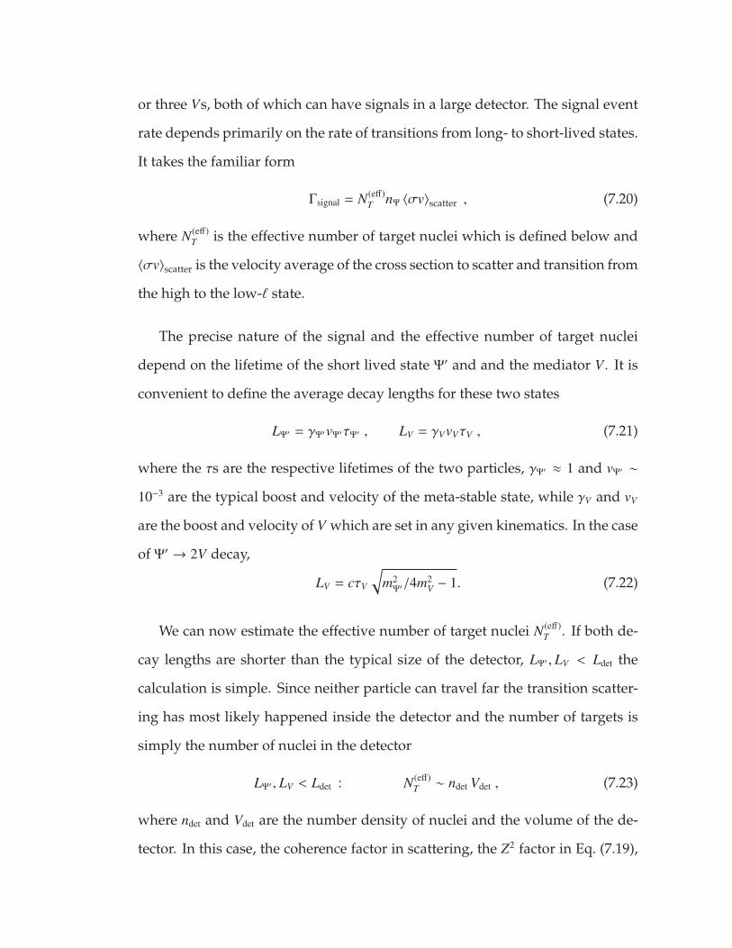
or three Vs, both of which can have signals in a large detector. The signal event

rate depends primarily on the rate of transitions from long- to short-lived states.

It takes the familiar form

Γsignal = N(eff)T nΨ 〈σv〉scatter , (7.20)

where N(eff)T is the effective number of target nuclei which is defined below and

〈σv〉scatter is the velocity average of the cross section to scatter and transition from

the high to the low-` state.

The precise nature of the signal and the effective number of target nuclei

depend on the lifetime of the short lived state Ψ′ and and the mediator V . It is

convenient to define the average decay lengths for these two states

LΨ′ = γΨ′vΨ′τΨ′ , LV = γVvVτV , (7.21)

where the τs are the respective lifetimes of the two particles, γΨ′ ≈ 1 and vΨ′ ∼

10−3 are the typical boost and velocity of the meta-stable state, while γV and vV

are the boost and velocity of V which are set in any given kinematics. In the case

of Ψ′ → 2V decay,

LV = cτV

√m2

Ψ′/4m2

V − 1. (7.22)

We can now estimate the effective number of target nuclei N(eff)T . If both de-

cay lengths are shorter than the typical size of the detector, LΨ′ , LV < Ldet the

calculation is simple. Since neither particle can travel far the transition scatter-

ing has most likely happened inside the detector and the number of targets is

simply the number of nuclei in the detector

LΨ′ , LV < Ldet : N(eff)T ∼ ndet Vdet , (7.23)

where ndet and Vdet are the number density of nuclei and the volume of the de-

tector. In this case, the coherence factor in scattering, the Z2 factor in Eq. (7.19),

should be taken as that of the detector material, be it water, liquid argonne, etc.

In the case that either of the decay lengths is larger than the typical detector

size, LΨ′ > Ldet or LV > Ldet, the production of Vs is likely to occur elsewhere in

the Earth. It is interesting that even in this case, the effective number of target

nuclei is parametrically the same as in the short lifetime case. Consider, for

example, the case where LV is much longer than the detector but shorter than

the size of the earth, while LΨ′ is short. In this case, we can assume the decay

of Ψ′ to Vs occurred at the scatter site. The effective number of targets is a

sum over Earth nuclei, weighted by the probability that a V decays inside the

detector given that is originated near the nucleus in question

Ldet < LV . R⊕ : N(eff)T ∼ n⊕

∫⊕∩LV

d3~rTL2

det

4π|~rdet − ~rT |2

Ldet

LV∼ n⊕ Vdet , (7.24)

where the integration limits are

|~rT | < R⊕ and 0 < |~rdet − ~rT | < LV (7.25)

in a coordinate system in which the origin is at the center of the Earth. Here

we have treated the earth as a sphere of constant density n⊕. The fraction in the

integrand is the suppression due to the small solid angle that the detector sub-

tends, as seen from the scatter site. In the last step, we have used the fact this

suppression factor is undone by the fact that the number of target nuclei grows

like |~rdet − ~rT |2 (which will show up as a Jacobian). This effect is similar to the

signal rate in [246]. Note that here we do not account for an O(1) geometrical

factor, which, for example, comes from the fact that there is more Earth below

the detector than above it. The case in which both LV and LΨ′ are larger than

the detector is slightly more convoluted but parametrically similar. Note, that

in cases of long lived V and/or Ψ′ the coherence factor of Z2 would be the aver-

aged over the rock, perhaps dominated by iron, but may get contributions from

heavier elements such as lead. In practice, we use a more realistic earth density

profile [270] to derive the upper bounds on ε.

Though the signal rate does not depend strongly on LV , the character of the

signal does. In the case of a short lived V , LV < Ldet, both Vs can decay inside

the detector and will result in two back-to-back or three e+e− (or µ+µ−, if kinemat-

ically allowed) pairs. In the case where LV > Ldet it is more likely that just one

such pair will be in the detector. In the case where LV is much longer than the

underground depth of the laboratory, there will be more events coming from

below than from above. These, and other signal characteristics are discussed in

more detail in Section 7.6.

The reach of a particular experiment depends on the detector-specific back-

ground rate for the signal in question. Though we expect very little background

that mimics our particular signals, we did not delve into these detector-specific

details. Instead, we simply estimate the event rates in several detectors as a

function of the model parameters. In Fig. 7.2, we show the parameters that lead

to 100 events per year in the ε − mχ plane. For a weakly-coupled bound state as

the SDDM, its mass is related to that of χ, mΨ ' 2mχ.

0.01 0.1 1 10 100 1000

10-11

10-9

10-7

10-5

10-3

10-1

Super K DUNE SNO+ Borexino

Xenon,1TCDMSLite

CRESST-II

Xenon,10

(elec.)

Babar

ae

BeamDump

Supernova

Na48

CMS8h→Zγ

CMS7

DY

EWPT LHC8

10m

Rmoho

R⊕

Figure 7.2: Contours that give 100 DM self-destruction events per year inthe ε − mχ parameter space of the angular momentum model.The other parameters are chosen to be mV = 2mχ/3, αV = 0.01,αφ = 0.001. The colorful thick curves correspond to Super-Kamiokande (red), and DUNE (dark green). Contours forSNO+ (light green), Borexino (orange) are shown as arrowsin order to reduce the number of curves with the understand-ing that they run parallel to that of Super-K. The solid, dashedand dotted curves assume the initial DM bound state is Ψ10,9

and comprises 10−9, 10−5 and 10−2 of the total DM relic den-sity, respectively. The gray curves correspond to constant de-cay length contours of the dark photon V (see Section 7.6for their effect on the signal characteristics). The light redand blue shaded regions show the existing experimental con-straints from searching for visibly-decaying dark photons andDM direct detection (assuming χ to be the dominant DM), re-spectively.

The colorful thick curves correspond to the observation of this rate of Ψ′ de-

cay events in various neutrino experiments: Super-Kamiokande, SNO+, Borex-

ino and DUNE.1 In order to reduce the clutter in the plot, we have denoted

the limits on the smaller two experiments with arrows, with the understanding

that their rate contours run parallel to those of Super-K. The 100-event-per-year

contour for ε is given by:

ε2100 =

100 events

Tyear × nV × nχχ 〈σv〉(ε=1)scatter × Br (V → l+l−)

, (7.26)

where nV is the effective number of targets, defined by the terms in parentheses

in Eqs. (7.23) and (7.24) for LV < Ldet and LV > Ldet respectively. Our result is

a rough estimate as we have omitted the O(1) geometry-dependent factor for

LV > Ldet and we neglected the density variations in the Earth. The curves in

Fig. 7.2 are derived assuming that the initial DM bound state is Ψ10,9 and com-

prises 10−9, 10−5 or 10−2 of the total DM relic density. For the final state Ψ′, we

consider all possible S -wave bound states with n = 1, . . . , 9. (Note that this is a

conservative assumption as we did not consider the effect of any non-S -wave

states.) The model parameters in the plot are set to: mV = (2/3) mχ, αV = 0.01 and

αφ = 0.001. Since we have used αφ αV the resulting unstable bound state an-

nihilates predominantly into two Vs (and then into SM particles). In the shaded

regions, we also show the existing experimental constraints from searching for

visibly-decaying dark photons [271–273] as well as direct detection (assuming χ

to be the dominant DM). Interestingly, the signals can help to probe a large por-

tion of the parameter space that is not yet accessible otherwise with the existing

dark photon searches. This gives a strong motivation for exploring the neutrino

experimental data and looking for the existence of DM bound states in nature.

Although the current neutrino detectors focus on energy ranges relevant for in-

coming neutrinos [274–277], they are also sensitive to higher energy ranges and

might be used to probe SDDM up to higher masses. We will return to a more1Our signal could also be constrained by the IceCUBE experiment which due to its higher

threshold will cover the mass window above tens of GeV.

detailed discussion of the phenomenology of SDDM and some search strategies

in Section 7.6.

7.3.4 Challenges in SDDM production in early universe

In Section 7.2 we derived an upper limit on the temperature in which SDDM is

produced:

Tsurvival ∼ 10 MeV ×(10 MeV

mχ

), (7.27)

this leaves two possibilities for the production of SDDM: early universe pro-

duction below Tsurvival or late time production in our galaxy. Here we explore

the challenges in realizing the first option, while in the next section we ex-

plore mechanisms for late time production. As we will see, the cosmology of

early universe production in this model is challenging and might involve a non-

thermal production or other mechanisms.

The difficulty arises from the constraint Eq. (7.10), which implies that the

mediator φ is heavier than the Rydberg energy, mφ > (α2φmχ)/4. This implies that

even at zero temperature, an incoming mediator has the potential to dissociate

the χχ bound states. This fact strongly restricts the production mechanisms of

χ, χ bound states in the early universe. We now discuss several possible pro-

duction mechanisms. We leave a more dedicated study of these possibilities for

a future work.

Thermal freeze out. Consider the case where χ, χ, and φ are in thermal equilib-

rium with each other in the early universe. For simplicity, we assume that the

dark sector has the same temperature as the SM sector. Around T ∼ mχ/25, the χ

and χ particles freeze out by annihilating into φs and/or Vs. Assuming αφ ∼ αV ,

their relic abundances satisfy

Ωχ = Ωχ ∼ 10−4( αφ0.01

)−2 ( mχ

1 GeV

),

nφnχ∼ 1014

( αφ0.01

)2 ( mχ

1 GeV

)−1. (7.28)

After freeze out, χ, χ bound states could be formed through the process χ + χ→

(χχ) + φ, where (χχ) is a χχ bound state. Since the formation rate is smaller than

the Hubble expansion, the resulting bound state relic abundance is given by

ΩBS = Ωχ

RBS F

H, RBS F = nχσBS F , (7.29)

where σBS F is the bound state formation cross section. On the other hand, a

bound state could be dissociated by encountering a φ particle, (χχ) + φ→ χ + χ.

The dissociation cross section σDIS is related to σBS F via crossing symmetry. For

T & mφ, the two are related by σDIS ∼ (mχ/T )3/2σBS F [236]. Note that because the

φ mass is greater than the binding energies, see Eq. (7.10), we must rely on the

kinetic energies of χ, χ, dictated by the temperature T , for bound state formation

to occur. The dissociation rate for each bound state is then

RDIS = nφσvDIS ∼

(nφnχ

) (mχ

T

) 32

RBS F . (7.30)

From Eqs. (7.28) and (7.29), we learn that the probability for a bound state to

dissociate satisfies,

PDIS =RDIS

H& 108

(mχ

T

) 32( αφ0.01

)4 ( mχ

1 GeV

)−2. (7.31)

The above result implies that all bound states are quickly destroyed within a

Hubble time as soon as they are produced.

This is a problem since we would like ΩBS > 10−10 for the SDDM to be of

experimental interest (see Fig. 7.2). This problem could be cured if we further

extend the dark sector with light states which φ can annihilate or decay into.

The coupling of these light states to φ has to be large enough to deplete the φ

population and prevent bound-state dissociation. Its coupling to the χ, has to

be small enough to not dissociate the bound states themselves.

χ as asymmetric DM. Since χ is much lighter than the weak scale, the ther-

mal production scenario cannot accommodate a situation where χ comprises all

the DM relic abundance. It is then tempting to consider the production of χ

in an asymmetric scenario. Additionally, in such a scenario one can avoid cos-

mological constraints on DM annihilation such as the CMB [278]. The problem

with this scenario is that the number of χ is exponentially suppressed at late

time [279, 280] because the χχ annihilation cross section is very large. The ex-

ponential suppression of χ would make it even harder to form any χχ bound

states in the early universe.

Non-thermal history. The thermal freeze out picture we discussed above does

not work in its minimal form mainly because it produces many more φ particles

than χ and χ. This problem could be alleviated if the dark sector particles are

produced non-thermally, with a suppressed nφ/nχ ratio compared to Eq. (7.28).

Non-thermal production mechanisms include the freeze-in of χ and χ through a

small kinetic mixing between V and/or φ and the SM photon, or the late decay

of some heavier dark sector states. The relic abundance of high-` bound states

in these cases is model dependent but it seems plausible that they can still be

probed in neutrino detectors.

Additional confining dark force. Another way of efficiently producing the high-

` bound states is to replace φ by a confining dark force. This implies that χ is

colored under a non-abelian dark gauge interaction. In this case, there are no

free χ and χ particles at distances larger than the inverse of the dark confinement

scale. In that case, it is likely for the high-` χχ states to form efficiently [219].

If the dark confinement scale of this gauge interaction is very small, the low-

level states are to a good approximation given by a 1/r potential. Then, the

self-destructing DM scattering, which involves short-distance physics, and the

experimental detection discussions in section 7.3.2 still remain valid.

7.3.5 Scenarios for late time SDDM production

We present three possible scenarios for the late time production of SDDM be-

low Tsurvival. This list is by no means exhaustive. These scenarios are: (a) a late

time decay of a heavy scalar Φ (b) late time binding in neutron stars (c) dark

hydrogen collisions. Below we provide heuristic descriptions of these late time

binding scenarios.

Late time decay

In this scenario, we focus on the strongly coupled benchmark presented earlier

in Section 7.3. The dark sector contains a confining gauge group (e.g., S U(N))

and the elementary particle χ belongs to the fundamental representation of it.

For χ production, we introduce a heavy scalar Φ with a Yukawa coupling to

χ, yχχΦ. We assume that Φ obtains a small primordial relic abundance in the

early universe, making up a subdominant portion of the dark matter energy

density. The Yukawa coupling y is taken to be small enough so that the de-

cay of Φ into χ, χ only occurs at temperatures below Tsurvival, defined in subsec-

tion 7.2. This provides a non-thermal production mechanism with a naturally

suppressed population of the dark force carriers (the gluons of the dark S U(N)

gauge symmetry, or dark glueballs at low energies), which is favored based on

the discussions in the previous subsection. After the decay of Φ, the χ, χ parti-

cles will eventually form bound states when their number density drops below

the Λ−3, where Λ is the energy scale for S U(N) confinement. For mχ Λ, this

corresponds to the quirky picture [219], and the (χχ) bound states are expect to

first form in the excited states, with large orbital angular momentum, `. These

excited states could de-excite by radiating the dark gluons, with ∆` = 1 after

each radiation. Eventually, after the de-excitations are completed, the resulting

(χχ) bound states will have a wide range of `. As discussed in subsection 7.3.1,

the low ` states are unstable and will decay away quickly, whereas the high `

states are cosmologically long lived and could serve as the SDDM candidate

if there exist a dark photon to mediate the interaction between χ and our sec-

tor. The states with intermediate values of ` could be still decaying today and

provide additional indirect detection signals for testing this scenario.

Dark Hydrogen Collisions

In this section, we present a potentially working and calculable model of late

time production of SDDM in the galaxy. The starting point is the weakly cou-

pled model presented earlier, in which φ is a U(1) gauge boson. To enhance

late time production we will make use of the Fermi and Teller mechanism [281]

for low energy protonium production. We will sketch the basic picture here,

while a more systematic use of the Fermi-Teller mechanism in the dark sector

will appear in [282].

In [281], the following protonium production process was considered,

H + p → (pp) + e . (7.32)

It was concluded that its cross section is at least geometric (σFT ' πr2b where

rb = (αme)−1 is the Bohr radius of the hydrogen atom), in particular when the

incoming antiproton is slow, i.e., EK → 0. The reason is that for impact parame-

ters ∼ rb, the pp system can no longer support an e bound state, and the electron

is ionized. The condition for generating a bound state is EK < −EB, the bind-

ing energy of the electron. In this case there is a high probability for the pp to

bind into protonium. As we will see, because the size of the incoming hydrogen

(dictating the impact parameter) is much larger than that of the ground state

protonium, the generated protonium tends to have high-n and high-l.

We will consider dark matter bound state formation by making analogy to

this elegant binding mechanism. We introduce a dark sector containing a dark

proton χ and dark electron ψ (much lighter than χ) having opposite charges

under a dark U(1) gauge symmetry. In analogy to baryon number, we assume

that there is a global symmetry that prevent the decay χ→ ψ+ φ/V to occur. We

assume the dark photon φ is massive, but its mass is small enough for the χ − ψ

to bind efficiently. To prevent the dissociation of dark hydrogen in the presence

of the relic φ, we assume:

mφ <12

EB . (7.33)

where EB = 12α

2φmψ is the χ − ψ binding energy. In particular, that means that

mφ <14α2φmχ , (7.34)

in contrast with Eq. 7.10. This means that in this variant of our model the SDDM

will be able to transition to lower ` states and eventually self-annihilate. How-

ever, by choosing mφ to be larger than several energy splittings in (χχ) state, we

can make its decay length long enough to observe significant flux on Earth.

In the early universe, the relic abundance of ψ is set by a primordial asym-

metry. The ψψ annihilation cross section is sufficiently large so that all the ψ

particles have been annihilated away and only ψ particles are around. On the

other hand, the relic abundance of χ is symmetric. As the temperature of the

dark sector cools below EB, the dark recombination will occur allowing χ and ψ

to capture each other and form hydrogen-like bound states. After the dark re-

combination, the universe contains a relic abundance of the dark hydrogen and

free χ particles.

This is exactly the composition that allows for the Fermi-Teller process to

take place in the following evolution of the universe. In particular, we consider

the following process to occur in the galaxy today

(χψ) + χ → (χχ)nl + ψ . (7.35)

The cross section for such a process is

σFT = π

(f

αφmψ

)2

, (7.36)

where the factor f was calculated by Bracci et al. [283] for the original Fermi-

Teller process and was found to be in the range 2−10, depending on the collision

energy. To be conservative we will assume here that f ∼ 2.

By energy conservation (assuming zero kinetic energy of the outgoing ψ) it

is straightforward to derive that the principle quantum number of the final (χχ)

bound state is

n ∼1√

2(mψ

mχ− v2

α2φ

), (7.37)

where v = 10−3 is the average DM velocity in the galaxy. For example, with the

following set of parameters mχ/mψ ∼ 50, αφ = 7.5 × 10−3, we can get n ∼ 15. The

maximal angular momentum of the final (χχ) bound state can be estimated as

`max = mχvbcrit ∼ fmχ

mψ

vαφ

. (7.38)

With the same set of parameters, we find that `max ∼ 13 so that the high-n, high-

` (χχ) bound states can be efficiently formed through this process. These are

nothing but our desired SDDM candidates.

Due to the Fermi-Teller process, every point in the galaxy has an average

SDDM production rate per volume of

dΓSDDM

dV= f(χψ) fχ

(ρDM

mχ

)2

rSDDM σFT v , (7.39)

where rSDDM is the O(1) fraction of high-l states produced in the rearrangement

process, and where f(χψ), fχ are the fractions of (χψ) and χ states in the total

DM relic density. Assuming the formed SDDM has a mean free path d(χχ) (the

shortest of its decay length and mean free path for dissociation), most of the

SDDM that could reach the earth are formed within a sphere with radius d(χχ)

around the Earth. More precisely, the flux of SDDM coming from all over the

galaxy is then

Φ⊕SDDM =

∫d3r

dΓSDDM

dV1

4πr2 e−r/d(χχ) , (7.40)

where r is the distance to the earth. Assuming that d(χχ) is smaller than the

distance to the end of the Milky-way halo, and that the DM density is a constant

ρDM ∼ 0.3 GeV/cm3, we could expect a flux of SDDM

Φ⊕SDDM ∼ 104 cm−2 sec−1rSDDM f(χψ) fχ

(10 GeV

mχ

)2(100 MeVmψ

)2 (0.01αφ

)2 (d(χχ)

1 kpc

). (7.41)

For the model parameters selected above, mφ can be taken heavy enough such

that the SDDM can only de-excite through a forbidden ∆` = 5 transition, and

so the decay length is much longer than 1 kpc. We still take 1 kpc as our refer-

ence value to account for effects that could destroy the SDDM like premature

self-destruction, dissociation and inverse rearrangement. The resulting flux is

significant, and is comparable to the flux of 1 TeV WIMPs. As we have shown

in Fig. 7.2, our model yields detectable signals even for fluxes a factor of 10−7

smaller. The attractive feature of this picture is that the SDDM does not have

to be produced in the early universe but rather produced more recently in our

galaxy. Therefore, the constraint on its lifetime could be relaxed compared to

that estimated in section 7.3.1.

One by product of this late time production mechanism is that the Fermi-

Teller process could also generate short lifetime (χχ) states that potentially lead

to indirect detection signals.

Binding in neutron stars

In addition to the production in the early universe, we can consider the more

recent production of χχ bound states by a late time binding process of relic χ and

χ. The φ particles are sufficiently diluted in the universe today so they no longer

play a role in dissociation. Because mφ is larger than the Rydberg energy, the χ

and χ in the initial state must have large enough velocities. One might imagine

more efficient bound state formation inside neutron stars where χ and χ are

gravitationally accelerated. The formed bound states could be liberated if the

neutron star belongs to a binary system which inspirals and finally merges [284].

This picture then ties the bound state formation rate to the neutron star merger

rate.

7.4 Tunneling stabilization

We now consider a different mechanism to generate the meta-stable state of

DM required for the self-destructing phenomenology. The idea is that the long-

lived DM state is protected by a potential barrier which keeps the constituents

apart, requiring exponentially suppressed tunneling to self annihilate. The same

bound state can scatter into a short-lived bound state, where the constituents

are localized closer together. This transition can happen through excitation to a

de-localized state and a decay to the localized state near the origin.

A key ingredient in this tunneling stabilization mechanism is the existence

of a metastable minimum far from the origin, so that the tunneling probabil-

ity is exponentially small. This happens in nature usually due to an interplay

between several forces, both attractive and repulsive. Consider for example

the states that can be made of two deuterium atoms. The two atoms can be

assembled into a di-deuterium molecule, D2. The two nuclei of D2 can, with

a very long lifetime, tunnel through the Coulomb barrier to form a Helium-4

atom. Similarly, some common isotopes of table salt, NaCl, can tunnel to be-

come a Nickel atom since they have the same number of protons, neutrons, and

electrons. Though these examples are inspiring, they do not quite fulfill our re-

quirements since excited molecular states of D2 are still very unlikely to fuse into

helium. Perhaps real-world examples which are closer to what self-destructing

DM requires are super cooled systems in crystals and liquids [285].

To illustrate the main features of tunneling stabilization, we consider a dif-

ferent kind of χχ bound state, one which is bounded not by a Coulomb mediator

but by a potential V(r) such that r is the relative distance between the χ and χ.

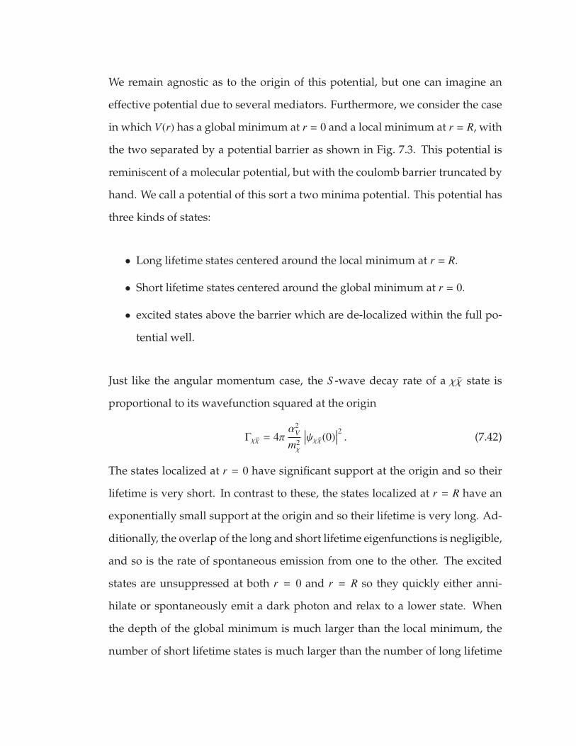
We remain agnostic as to the origin of this potential, but one can imagine an

effective potential due to several mediators. Furthermore, we consider the case

in which V(r) has a global minimum at r = 0 and a local minimum at r = R, with

the two separated by a potential barrier as shown in Fig. 7.3. This potential is

reminiscent of a molecular potential, but with the coulomb barrier truncated by

hand. We call a potential of this sort a two minima potential. This potential has

three kinds of states:

• Long lifetime states centered around the local minimum at r = R.

• Short lifetime states centered around the global minimum at r = 0.

• excited states above the barrier which are de-localized within the full po-

tential well.

Just like the angular momentum case, the S -wave decay rate of a χχ state is

proportional to its wavefunction squared at the origin

Γχχ = 4πα2

V

m2χ

∣∣∣ψχχ(0)∣∣∣2 . (7.42)

The states localized at r = 0 have significant support at the origin and so their

lifetime is very short. In contrast to these, the states localized at r = R have an

exponentially small support at the origin and so their lifetime is very long. Ad-

ditionally, the overlap of the long and short lifetime eigenfunctions is negligible,

and so is the rate of spontaneous emission from one to the other. The excited

states are unsuppressed at both r = 0 and r = R so they quickly either anni-

hilate or spontaneously emit a dark photon and relax to a lower state. When

the depth of the global minimum is much larger than the local minimum, the

number of short lifetime states is much larger than the number of long lifetime

V(r)

rexcited

long lifetime

short lifetime

R

hb

w0

Figure 7.3: An illustration of a two minima potential as described in Sec-tion 7.4.

states (NShort NLong). In that limit, the excited state decays predominantly to

short lifetime states, which annihilate instantaneously.

For our SDDM scenario, we envision a fraction of DM is made up of the long-

lived state with 〈r〉 ∼ R. An interaction of this state with a nucleus on Earth can

excite it to the delocalized state, which then proceeds to decay and annihilate as

discussed above. The annihilation products, assumed to be dark photons, can

then decay in a detector leading to a signal. In the Appendix, we show a toy

example which we used to estimate the various rates more quantitatively. We

find that the lifetimes of the long, short and excited states scale as

τShort

τLong∼τexcited

τLong∼ e−2

√mχhbR , (7.43)

where hb is the height of the potential barrier.

In this work, we do not construct a full model which yields a potential simi-

lar to the one in Fig. 7.3. A working model, however, would need to have both

a significant barrier, say with√

hbR ∼ 20, and excited bound states that can live

classically above the barrier. Molecules found in nature have the former, but not

the latter.

While we were unable to construct a full model, we do not see any fun-

damental reason that we will not be able to. We can speculate about ways to

modify the molecular picture to make it viable to our model. One way is to add

a confining potential that will make the probability to decay into the short lived

state significantly. Another idea is to have droplets of a super-cooled dark fluid

which make up a part of DM.

7.5 Symmetry stabilization

As a third class of models, we consider bound states in an asymmetric DM sce-

nario, with the DM charged under baryon number. The self-destructing DM

picture can be realized when the bound state interacts with SM nuclei.

More specifically, consider a Dirac fermion χ which carries the baryon num-

ber q, with q , ±1,±1/2. The exchange of a scalar dark force carrier φ (with zero

baryon number) allows both χ, χ and χ, χ to form bound states. Because the (χχ)

bound state is stable, we can assume it comprises a significant fraction or even

makes up all of the total DM relic abundance today.1 We also introduce another

fermion η which carries non-zero baryon number 1 + 2q. The assigned baryon

quantum numbers above allow a dimension 6 effective interaction between χ, η

1With a scalar dark force, it is possible for a large number of χ particles to form stable boundstates (also called nuggets) [236, 286–290]. In principle, a similar phenomenon as discussedbelow could also apply to nuggets. For simplicity, we only consider two-body bound stateshere.

Figure 7.4: Left: Feynman diagram for the scattering process (χχ) + n →(χχ) + η in the model described in Section 7.5. Right: A possibleway of destructing the (χχ) bound state after the scattering.

and the neutron n,

Lint =(χcχ)(ηn)

Λ2 + h.c. . (7.44)

If 2mχ < mη + mp, the (χχ) bound state is stable. However, when it reaches the

detector, the above interaction triggers the following reaction,

(χχ) + n→ (χχ) + η , (7.45)

as shown by the Feynman diagram in Fig. 7.4 (left). At the “partonic level” in

the dark sector, one of the χs participates in the reaction χ+ n→ χ+ η. The other

χ is a spectator, and it becomes bounded with the χ in the final state into a (χχ)

bound state. After this reaction, a neutron is removed from the target and the

final state particle η can escape away without further interaction. We consider

mη ≈ mn, and then the cross section for the scattering of a (χχ) ground state into

a (χχ) ground state is,

σ(χχ)+n→(χχ)+η 'µ2χn

πΛ4 , (7.46)

where µχn = mχmn/(mχ + mn), and we make the approximation that the dark form

factor, in analogy to Eq. (7.16), is of order 1, when both (χχ) and (χχ) are in the

ground states.

Like the other two scenarios we discuss before, the most striking signal is

generated due to the destruction of the unstable (χχ) state. It can self-annihilate

into SM particles via mediators (e.g., a pair of dark photons, see Fig. 7.4 (right))

between the two sectors. The present data from neutrino and DM experiments

can be interpreted as constraints on the cutoff scale Λ. As an estimate, if the

(χχ) bound state comprises all the DM relic abundance, having 100 events per

year from (χχ) → (χχ) scattering and the (χχ) destruction inside the Super-K or

DUNE detectors corresponds to a cutoff scale

Λ ' 50 TeV( mχ

1 GeV

)1/4. (7.47)

An additional signature predicted in this model besides DM self destruction

is the removal of a neutron from a target nucleus. The resulting nucleus is often

unstable which leads to additional hadronic activities inside the detectors.

As a necessary condition for this scenario to work, the η particle mass must

lie in the following window,

mn − 2mχ + BE(χχ) < mη < mn + KE + BE(χχ) − BE(χχ) , (7.48)

where mn is the effective neutron mass inside the nucleus, BE(χχ),(χχ) is the bind-

ing energy for the (χχ), (χχ) bound states, respectively, and KE is the kinetic

energy of the incoming (χχ) bound state that enters the detector. The upper

bound of the above window is derived for the process (χχ) + n → (χχ) + η to be

kinematically allowed, and the lower bound is from the requirement of neutron

stability against the decay n → η + (χχ). In addition, if mη mn, the final state

χ, χ particles would carry too large a relative momentum for them to remain

bounded together. This limitation could be relaxed if the dark force for binding

the (χχ) and (χχ) states is not from the exchange of a scalar φ but a confining

non-abelian (S U(2)) dark gauge interaction. In this case, there are no free χ, χ

particles and bound states of them always form.

In this model, the new η particle is nearly degenerate in mass with the neu-

tron. There is a potential constraint from neutron star stability as recently no-

ticed in [291]. It is worth noting that here, instead of mixing with the neutron,

the η particle couples to the neutron in together with two dark matter parti-

cles via a higher dimensional operator. Therefore, as long as the dark matter is

heavier than 0.1 GeV, the neutron star bound will not apply.

The idea of DM eliminating a neutron and rendering a nucleon unstable has

been discussed previously in [204, 255, 256]. However, in those models, the en-

ergy release is completely due to the destruction of a nucleon, yielding a signal

very similar to the usual nucleon decay. In contrast, in the model discussed here,

as well as the two SDDM models presented in the previous sections, the visible

energy is released from χχ annihilation into mediators and then into pairs of

e+e− or µ+µ−. These striking signals are not currently looked at. Furthermore,

in these scenarios, it is possible to reconstruct the masses of the DM particle as

well as the mediator from the self destruction final states.

7.6 Experimental signatures and Model independent searches

Each one of the different SDDM scenarios presented above has its own unique

signature. Still, these different experimental signatures share certain broad

brush features. Some of the phenomenology was discussed in the context of

the angular momentum model in Section 7.3.3. In this section, we discuss the

signal characteristics more broadly. Our aim is not to perform a detailed study

of a specific model but rather, to discuss the general properties of the possible

signals and suggest a set of relatively model-independent searches that an ex-

periment can perform.

We assume that the couplings between the two sectors are very small. In that

limit, the DM annihilates into mediators that eventually decay to SM particles

rather than into the Standard Model directly. The signal characteristics depend

on several parameters of the model, and we discuss a few of them below.

Event Rate: The rate of events in a detector is discussed in detailed for a spe-

cific model in Section 7.3.3 but will be repeated here for completeness. The rate

depends on the scattering cross section σscatter which induces the transition from

a long-lived state, Ψ, to a short-lived one, Ψ′. As discussed previously, the rate

does not depend strongly on the mediator decay length LV ≡ γVvVτV , with τV the

mediator lifetime. If the mediator is short-lived, LV < Ldet the scattering takes

place inside the detector, but if it is long-lived it can also happen in the Earth,

outside the detector. However, as long as the mediator decay length is within

the size of the Earth, the signal rate is largely independent of the mediator life-

time. This is because the 1/r2 fall-off in the flux emanating from a particular

scatter site is compensated by the r2 growth in the amount of volume to scatter

on. As a result, up to order one geometric factors

Rate ∼ nVdet nΨ〈σv〉scatter , (7.49)

where Vdet is the volume of the detector, n is the nuclear number density either

in the detector or in Earth, depending on whether the mediator is long or short

lived. Also, nχχ is the number density of long-lived bound states, 〈σv〉scatter is the

velocity averaged cross section to transition from the long lived DM state to its

short lived counterpart. Note that the atomic number of the scattering nucleus

may be different for LV larger or smaller than the detector size, which may affect

the coherence factor in the cross section.

Particle ID: The mass, spin, and couplings of the mediator determine its de-

cay branching fractions. A well motivated mediator is a dark photon which

couples to the SM via kinetic mixing. In this case, the mediator has a sizable

branching fraction to decay to electrons as well as to muons, charged pions or

heavy flavor (whenever the mediator is above the relevant thresholds). A scalar

or pseudo-scalar mediator could have a sizable branching fraction to the heavi-

est particle to which it is kinematically allowed. Di-photons are also an interest-

ing final state, particularly for light (pseudo)scalars.

Event Multiplicity: The decay length of the mediators in the lab frame is

LV = cτV

√E2

V

m2V

− 1 . (7.50)

For Ψ′ → 2V decay, EV = mΨ′/2 while for Ψ′ → 3V decay, there is a spectrum

for EV between 0 and mΨ′/2. If this decay length is shorter than the size of the

detector, there can be a sizable fraction of the events in which both mediators de-

cay inside the detector. The signature, in this case, is two simultaneous pairs of

leptons with opposite reconstructed velocities (since the decaying bound state

is non-relativistic), consistent with a single vertex where the bound state decay

took place. This is schematically shown in the left panel of Figure 7.5. Such

events are expected to have an extremely low background.

Event Kinematics: Each event consists of decays of on-shell mediators pro-

duced via the annihilation χχ→ 2V or 3V inside the short-lived bound state Ψ′.

Consequently, we expect a double or triple lepton pair-production. In the case

of Ψ′ → 2V decay, each pair has energy which is half of the dark bound state

mass and an invariant mass of mV ,

Epair =mΨ′

2and mpair = mV . (7.51)

Opening Angle: As the mediators in all of our scenarios are produced

boosted, their decay products can’t be back-to-back. When the decay products

are relativistic, the typical opening angle between the, say, `+ and `− in each pair

roughly satisfies

cos θ`+`− ∼ 1 −8m2

V

m2Ψ′

, (7.52)

in the case of Ψ′ → 2V decay. As long as mV is not too small, detectors with good

angular resolution will be able to distinguish the pair from a single energetic

particle. On the other hand, as long as the mediator is not too close to half the

bound state mass, the pairs will not be back-to-back and the detector will be

able to reconstruct the direction of the mediator velocity.

Event Directionality: When the decay length of the mediator is much larger

than the detector, each event will only consist of a single pair. This region of

parameter space can be further categorized based on the directional distribu-

tion of the mediator velocity. If the decay length is shorter than the depth of

the underground laboratory, the events will be isotropic. If on the other hand,

the decay length is larger than the laboratory depth, the reconstructed velocities

would be primarily coming from below. These two possibilities are also shown

Ldecay . 10 m 10 m . Ldecay . 1 km 1 km . Ldecay . R

2 pairs per event. Single pair per event. Single pair per event.

Isotropic.Isotropic. Pointing up.

Figure 7.5: A schematic illustration of the expected signals for various de-cay lengths of the mediator V . In the case of Ψ′ → 2V decay,each black arrow represents a pair of SM particles with a totalenergy of mΨ′/2, an invariant mass of mV , and a total momen-tum pointing in the arrow direction. A double arrow representstwo such pairs back-to-back.

schematically in Figure 7.5.

Associated Signals: The transition from the long-lived to the short-lived

state could also lead to a visible signal. In this case, if LV is smaller than the

detector size, both the transition and the decay of the mediator(s) can be visible.

For example, in the model described in section 7.5, the transition from the long-

lived to the short-lived state was associated with the removal of a neutron from

a target nucleus which would lead to an additional energy deposit. So long as

this process, as well as the decay time of the short live state, are prompt, the

mediator velocity would then point back to the transition point. This class of

events can also have very low backgrounds.

Simplified Model Searches: Having discussed the signal characteristics, we

finally suggest simplified model searches that large detectors can perform. Of

course, picking a model and presenting limits in the spirit of Figure 7.2 can cer-

tainly be useful, in the sense that a comparison to other searches can be made.

However, a more model independent presentation of the limits, which can then

be translated to any model, may also be useful. This is common practice in col-

lider searches, where a limit on a particular final state, say a di-lepton resonance,

is presented as a limit on a cross section times a branching fraction rather as a

limit on couplings. Other examples are searches for simplified models of, say,

supersymmetry, where results are shown as limits on the cross section in the

stop-neutralino mass plane using a contour or a color scale.

In the case of SDDM, the signal consists of one or two lepton pairs. The

invariant mass of the pairs is set by mV and the energy is set by mΨ′ , see equa-

tion (7.51). A useful way to present results is thus to show the limit on the

event rate per unit volume in the mV-mΨ′ plane. To further sophisticate the anal-

ysis, this should be repeated for three different assumptions about the decay

length LV which correspond to different angular distributions and multiplicities

as shown in Figure 7.5, since each of these options can have a different back-

ground rate. In the same way that LHC resonances are searched for in a variety

of final states, here too, searches can be carried out for pairs of electrons, muons,

photons, pions, etc.

We conclude that the framework of self-destructing DM has a rich phe-

nomenology. The predicted events can have very particular characteristics

which in many cases have very low backgrounds. The background rates and

rejection efficiencies can be studied systematically for current and future detec-

tors on a phenomenological basis, varying the model parameters mΨ′ , mV and τV

as well as the decay products (electrons, muons, etc).

7.7 Conclusions

The search for DM is currently at the frontiers of high energy physics. In recent

years, great efforts have been made in the direct detection of dark matter, aim-

ing at recoil energies around the keV scale or even lower. This is based on the

assumption that the available energy in each dark matter scattering is no larger

than its kinetic energy. In this work, we have proposed a novel class of DM mod-

els called self-destructing Dark Matter (SDDM), in which the scattering of a DM

with the detector (or the Earth) induces its decay to SM particles. The striking

new feature of this class of models is the conversion of the entire rest mass of the

SDDM to a detectable signal, rather than just its recoil energy. We have demon-

strated how large neutrino detectors such as Super-K and DUNE could be at

the frontier of the search for SDDM. Additionally, we presented three concrete

realizations of SDDM, all of which are based on the DM being a bound state

of some dark interaction, with qualitatively different stabilization mechanisms.

Finally, we briefly described the broad brush features of the expected detector

signals in the SDDM scenario.

There are several directions for further study. More detailed studies of the

background to SDDM in large neutrino detectors are required, as well as a closer

look at its production in the early universe. Though outside the scope of the cur-

rent work, SDDM also has potentially interesting indirect signatures. The most

striking one is DM decay in the Sun or in Jupiter. In traditional DM models,

the DM may be captured in the core of the Sun, yielding an annihilation sig-

nal. In our model, however, the DM can simply “self-destruct” in the Sun in a

similar manner to Earth. This could yield, e.g., gamma ray or e+e− signals for

indirect detection experiments [292, 293]. Additional model dependent indirect

signals could arise from DM self destruction induced by DM-DM scattering in

the galactic center or in extragalactic sources.

APPENDIX

7.A Estimation of Rates in the Tunneling Model

To estimate the relevant rates in the tunneling stabilization model discussed in

section 7.4, we focus on an idealized potential model

V(r) =

−h0 r < w0

−hR + hb w0 < r < w0 + R

−hR w0 + R < r < w0 + R + wR

(7.53)

The results derived in this section, however are quite generic for more realistic

two minima potentials with a wide barrier. The potential Eq. (7.53) is depicted

in Fig. 7.6 (left) for h0 = 50, hR = 15,w0 = wR = 1 and hb = 8,R = 30, where

h0, hR, hb are in units of mχ and w0,wR,R are in units of m−1χ .

We denote the height and width of the barrier by hb and R, respectively. The

height and width of the potential wells are denoted h0,w0 and hR,wR for the r = 0

and r = R minima. The typical wavefunctions of the relevant states are shown

in Fig. 7.6 (right), and their values near the origin are then,∣∣∣ΨLong(0)∣∣∣2 ∼ 1

wRe−2

√hbR , |ΨShort(0)|2 ∼

1w0

, |Ψexcited(0)|2 ∼1R. (7.54)

As a result, we have

τShort

τLong∼τexcited

τLong∼ e−2

√hbR . (7.55)

For 2√

hbR ∼ 40, the long lifetime states could be cosmologically stable while

the short lifetime ones decay in a second. The rate for spontaneous emission

ΨLong → ΨShort is

ΓS EL→S =

4αV(∆E)3

3

∣∣∣∣∣∫ d3r Ψ∗Short(r)~r ΨLong(r)∣∣∣∣∣2 ∼ e−2

√hbR , (7.56)

198

0 10 20 30 40 50

-50

-40

-30

-20

-10

0

10

Long Lifetime

Excited States

Short Lifetimeh0

hb hRR

w0

wR

0 10 20 30 40 50-0.10

-0.05

0.00

0.05

0.10

Long Lifetime

Excited State

Short Lifetime

Figure 7.6: An illustration of tunneling Stabilization. Left: The potentialand energy eigenvalues. Right: Sample wavefunctions. Thecoordinate r is in unit of m−1

χ , the potential energy V is in unitof mχ and the bound state wavefunctions are in unit of m3/2

χ .

and so the long lifetime states are cosmologically stable. In the above estimate,

we assume the energy difference ∆E is large enough for a dark photon to be

radiated on-shell in this model.

The cross section for a long lifetime state to hit the Earth and up scatter to

an excited state is given by Eqs. (7.16)-(7.17). The form factor FD(|~q |) is given

6 8 10 12 14-20

-10

0

10

20

30

τLg→Sh

τLg,ann

τEx→ShτEx→Lg

τEx,ann

τSh,ann

of the universe

Travel time through earth

Figure 7.7: Lifetimes for states in the two minima potential as function ofthe barrier width, for mχ = 0.5GeV, αV = 10−2.

by integral between ΨLong and Ψexcited which, given a large enough momentum

transfer, is not exponentially suppressed. Once in the excited state, the total rate

for spontaneous emission to short lifetime states is

ΓS EE→S =

∑i

4αV(∆Ei)3

3

∣∣∣∣∣∫ d3r Ψ∗Short,i(r)~r Ψexcited(r)∣∣∣∣∣2 , (7.57)

which is also free from the exponential suppression. For NShort NLong, the ex-

cited states transit exclusively to short lifetime states. A quantitative analysis of

the rates in this model is given in Fig. 7.7 for the simple two minima potential

Eq. (7.53), with mχ = 0.5GeV, αV = 10−2. As we can see in the plot, the only life-

times that depend significantly on R are the lifetimes of the long lifetime states

to annihilate or spontaneously emit a dark photon and transfer to a short life-

time state. This is because the tunneling suppression for these states depends

exponentially on R. For R & 12 m−1χ , the long lifetime states are cosmologically

stable, while the short lifetime states annihilate in roughly a picosecond. In-

terestingly, for this particular configuration, the excited states tend to annihilate

rather than spontaneously emit to either the short or long lifetime states. This is,

of course, a completely viable option from the point of view of self-destructing

phenomenology.

BIBLIOGRAPHY

[1] S. Rahatlou, 54th Rencontres de Moriond on Electroweak Interactions andUnified Theories: Experimental Summary. Mar, 2019.

[2] LHCB collaboration, A. A. Alves, Jr. et al., The LHCb Detector at the LHC,JINST 3 (2008) S08005.

[3] BELLE-II collaboration, T. Abe et al., Belle II Technical Design Report,1011.0352.

[4] BABAR collaboration, B. Aubert et al., The BaBar detector, Nucl. Instrum.Meth. A479 (2002) 1–116, [hep-ex/0105044].

[5] LHCB collaboration, R. Aaij et al., Observation of CP violation in charmdecays, 1903.08726.

[6] G. F. Giudice, The Dawn of the Post-Naturalness Era, in From My VastRepertoire ...: Guido Altarelli’s Legacy (A. Levy, S. Forte and G. Ridolfi,eds.), pp. 267–292. 2019. 1710.07663. DOI.

[7] N. Craig, PiTP2017 - Naturalness and New Approaches to the HierarchyProblem. July, 2017.

[8] S. P. Martin, A Supersymmetry primer, hep-ph/9709356.

[9] D. B. Kaplan and H. Georgi, SU(2) x U(1) Breaking by VacuumMisalignment, Phys. Lett. 136B (1984) 183–186.

[10] D. B. Kaplan, H. Georgi and S. Dimopoulos, Composite Higgs Scalars,Phys. Lett. 136B (1984) 187–190.

[11] H. Georgi, D. B. Kaplan and P. Galison, Calculation of the Composite HiggsMass, Phys. Lett. 143B (1984) 152–154.

[12] T. Banks, CONSTRAINTS ON SU(2) x U(1) BREAKING BY VACUUMMISALIGNMENT, Nucl. Phys. B243 (1984) 125–130.

[13] H. Georgi and D. B. Kaplan, Composite Higgs and Custodial SU(2), Phys.Lett. 145B (1984) 216–220.

202

[14] M. J. Dugan, H. Georgi and D. B. Kaplan, Anatomy of a Composite HiggsModel, Nucl. Phys. B254 (1985) 299–326.

[15] H. Georgi, A Tool Kit for Builders of Composite Models, Nucl. Phys. B266(1986) 274–284.

[16] P. W. Graham, D. E. Kaplan and S. Rajendran, Cosmological Relaxation ofthe Electroweak Scale, Phys. Rev. Lett. 115 (2015) 221801, [1504.07551].

[17] N. Arkani-Hamed, T. Cohen, R. T. D’Agnolo, A. Hook, H. D. Kim andD. Pinner, Solving the Hierarchy Problem at Reheating with a Large Number ofDegrees of Freedom, Phys. Rev. Lett. 117 (2016) 251801, [1607.06821].

[18] N. Craig, CosmoGrav2018 - 21 Increasingly Crazy Approaches to theHierarchy Problem. June, 2018.

[19] J. L. Bernal, L. Verde and A. G. Riess, The trouble with H0, JCAP 1610(2016) 019, [1607.05617].

[20] J. S. Bullock and M. Boylan-Kolchin, Small-Scale Challenges to the ΛCDMParadigm, Ann. Rev. Astron. Astrophys. 55 (2017) 343–387, [1707.04256].

[21] S. Tremaine and J. E. Gunn, Dynamical Role of Light Neutral Leptons inCosmology, Phys. Rev. Lett. 42 (1979) 407–410.

[22] W. Hu, R. Barkana and A. Gruzinov, Cold and fuzzy dark matter, Phys. Rev.Lett. 85 (2000) 1158–1161, [astro-ph/0003365].

[23] C. Csaki, M. Geller and O. Telem, Tree-level Quartic for a HolographicComposite Higgs, JHEP 05 (2018) 134, [1710.08921].

[24] C. Csaki, G. Lee, S. J. Lee, S. Lombardo and O. Telem, ContinuumNaturalness, JHEP 03 (2019) 142, [1811.06019].

[25] M. Geller, S. Iwamoto, G. Lee, Y. Shadmi and O. Telem, Dark quarkoniumformation in the early universe, JHEP 06 (2018) 135, [1802.07720].

[26] Y. Grossman, R. Harnik, O. Telem and Y. Zhang, Self-Destructing DarkMatter, 1712.00455.

[27] R. Contino, The Higgs as a Composite Nambu-Goldstone Boson, in Physics ofthe large and the small, TASI 09, proceedings of the Theoretical Advanced Study

Institute in Elementary Particle Physics, Boulder, Colorado, USA, 1-26 June2009, pp. 235–306, 2011. 1005.4269. DOI.

[28] B. Bellazzini, C. Csaki and J. Serra, Composite Higgses, Eur. Phys. J. C74(2014) 2766, [1401.2457].

[29] G. Panico and A. Wulzer, The Composite Nambu-Goldstone Higgs, Lect.Notes Phys. 913 (2016) pp.1–316, [1506.01961].

[30] C. Csaki, S. Lombardo and O. Telem, TASI Lectures on Non-supersymmetricBSM Models, in Proceedings, Theoretical Advanced Study Institute inElementary Particle Physics : Anticipating the Next Discoveries in ParticlePhysics (TASI 2016): Boulder, CO, USA, June 6-July 1, 2016, pp. 501–570,WSP, WSP, 2018. 1811.04279. DOI.

[31] S. R. Coleman and E. J. Weinberg, Radiative Corrections as the Origin ofSpontaneous Symmetry Breaking, Phys. Rev. D7 (1973) 1888–1910.

[32] K. Agashe, R. Contino and A. Pomarol, The Minimal composite Higgsmodel, Nucl. Phys. B719 (2005) 165–187, [hep-ph/0412089].

[33] C. G. Callan, Jr., S. R. Coleman, J. Wess and B. Zumino, Structure ofphenomenological Lagrangians. 2., Phys. Rev. 177 (1969) 2247–2250.

[34] D. B. Kaplan, Flavor at SSC energies: A New mechanism for dynamicallygenerated fermion masses, Nucl. Phys. B365 (1991) 259–278.

[35] N. Arkani-Hamed and M. Schmaltz, Hierarchies without symmetries fromextra dimensions, Phys. Rev. D61 (2000) 033005, [hep-ph/9903417].

[36] Y. Grossman and M. Neubert, Neutrino masses and mixings innonfactorizable geometry, Phys. Lett. B474 (2000) 361–371,[hep-ph/9912408].

[37] K. Agashe, G. Perez and A. Soni, Flavor structure of warped extra dimensionmodels, Phys. Rev. D71 (2005) 016002, [hep-ph/0408134].

[38] A. D. Medina, N. R. Shah and C. E. M. Wagner, Gauge-Higgs Unificationand Radiative Electroweak Symmetry Breaking in Warped Extra Dimensions,Phys. Rev. D76 (2007) 095010, [0706.1281].

[39] C. Csaki, A. Falkowski and A. Weiler, The Flavor of the CompositePseudo-Goldstone Higgs, JHEP 09 (2008) 008, [0804.1954].

[40] S. Weinberg, Precise relations between the spectra of vector and axial vectormesons, Phys. Rev. Lett. 18 (1967) 507–509.

[41] A. Pomarol and F. Riva, The Composite Higgs and Light ResonanceConnection, JHEP 08 (2012) 135, [1205.6434].

[42] J. M. Maldacena, The Large N limit of superconformal field theories andsupergravity, Int. J. Theor. Phys. 38 (1999) 1113–1133, [hep-th/9711200].

[43] A. Karch, E. Katz, D. T. Son and M. A. Stephanov, Linear confinement andAdS/QCD, Phys. Rev. D74 (2006) 015005, [hep-ph/0602229].

[44] L. Randall and R. Sundrum, A Large mass hierarchy from a small extradimension, Phys. Rev. Lett. 83 (1999) 3370–3373, [hep-ph/9905221].

[45] W. D. Goldberger and M. B. Wise, Modulus stabilization with bulk fields,Phys. Rev. Lett. 83 (1999) 4922–4925, [hep-ph/9907447].

[46] T. Gherghetta and A. Pomarol, Bulk fields and supersymmetry in a slice ofAdS, Nucl. Phys. B586 (2000) 141–162, [hep-ph/0003129].

[47] R. Contino and A. Pomarol, Holography for fermions, JHEP 11 (2004) 058,[hep-th/0406257].

[48] C. Csaki, J. Hubisz and P. Meade, TASI lectures on electroweak symmetrybreaking from extra dimensions, in Physics in D ¿= 4. Proceedings, TheoreticalAdvanced Study Institute in elementary particle physics, TASI 2004, Boulder,USA, June 6-July 2, 2004, pp. 703–776, 2005. hep-ph/0510275.

[49] N. S. Manton, A New Six-Dimensional Approach to the Weinberg-SalamModel, Nucl. Phys. B158 (1979) 141–153.

[50] Y. Hosotani, Dynamical Mass Generation by Compact Extra Dimensions,Phys. Lett. 126B (1983) 309–313.

[51] I. Antoniadis, K. Benakli and M. Quiros, Finite Higgs mass withoutsupersymmetry, New J. Phys. 3 (2001) 20, [hep-th/0108005].

[52] M. Kubo, C. S. Lim and H. Yamashita, The Hosotani mechanism in bulkgauge theories with an orbifold extra space S**1 / Z(2), Mod. Phys. Lett. A17(2002) 2249–2264, [hep-ph/0111327].

[53] G. von Gersdorff, N. Irges and M. Quiros, Finite mass corrections in orbifoldgauge theories, in Proceedings, 37th Rencontres de Moriond on ElectroweakInteractions and Unified Theories: Les Arcs, France, March 9-16, 2002,pp. 169–176, 2002. hep-ph/0206029.

[54] C. Csaki, C. Grojean and H. Murayama, Standard model Higgs from higherdimensional gauge fields, Phys. Rev. D67 (2003) 085012,[hep-ph/0210133].

[55] C. A. Scrucca, M. Serone and L. Silvestrini, Electroweak symmetry breakingand fermion masses from extra dimensions, Nucl. Phys. B669 (2003) 128–158,[hep-ph/0304220].

[56] C. A. Scrucca, M. Serone, L. Silvestrini and A. Wulzer, Gauge Higgsunification in orbifold models, JHEP 02 (2004) 049, [hep-th/0312267].

[57] G. Cacciapaglia, C. Csaki and S. C. Park, Fully radiative electroweaksymmetry breaking, JHEP 03 (2006) 099, [hep-ph/0510366].

[58] R. Contino, Y. Nomura and A. Pomarol, Higgs as a holographicpseudoGoldstone boson, Nucl. Phys. B671 (2003) 148–174,[hep-ph/0306259].

[59] A. Falkowski, About the holographic pseudo-Goldstone boson, Phys. Rev. D75(2007) 025017, [hep-ph/0610336].

[60] A. Falkowski, Pseudo-goldstone higgs from five dimensions, in SUSY 2007Proceedings, 15th International Conference on Supersymmetry and Unificationof Fundamental Interactions, July 26 - August 1, 2007, Karlsruhe, Germany,pp. 658–661, 2007. 0710.4050.

[61] M. Geller and O. Telem, Holographic Twin Higgs Model, Phys. Rev. Lett. 114(2015) 191801, [1411.2974].

[62] C. Csaki, M. Geller, O. Telem and A. Weiler, The Flavor of the CompositeTwin Higgs, JHEP 09 (2016) 146, [1512.03427].

[63] G. Panico, M. Redi, A. Tesi and A. Wulzer, On the Tuning and the Mass ofthe Composite Higgs, JHEP 03 (2013) 051, [1210.7114].

[64] R. Contino, L. Da Rold and A. Pomarol, Light custodians in naturalcomposite Higgs models, Phys. Rev. D75 (2007) 055014,[hep-ph/0612048].

[65] D. Pappadopulo, A. Thamm and R. Torre, A minimally tuned compositeHiggs model from an extra dimension, JHEP 07 (2013) 058, [1303.3062].

[66] J. Gu, H. Li, Z. Liu, S. Su and W. Su, Learning from Higgs Physics at FutureHiggs Factories, JHEP 12 (2017) 153, [1709.06103].

[67] M. E. Peskin and T. Takeuchi, Estimation of oblique electroweak corrections,Phys. Rev. D46 (1992) 381–409.

[68] K. Agashe, R. Contino, L. Da Rold and A. Pomarol, A Custodial symmetryfor Zbb, Phys. Lett. B641 (2006) 62–66, [hep-ph/0605341].

[69] R. Barbieri, B. Bellazzini, V. S. Rychkov and A. Varagnolo, The Higgs bosonfrom an extended symmetry, Phys. Rev. D76 (2007) 115008, [0706.0432].

[70] B. Keren-Zur, P. Lodone, M. Nardecchia, D. Pappadopulo, R. Rattazziand L. Vecchi, On Partial Compositeness and the CP asymmetry in charmdecays, Nucl. Phys. B867 (2013) 394–428, [1205.5803].

[71] ATLAS collaboration, M. Aaboud et al., Combination of the searches forpair-produced vector-like partners of the third-generation quarks at

√s = 13

TeV with the ATLAS detector, 1808.02343.

[72] ATLAS collaboration, M. Aaboud et al., Search for new phenomena inevents with same-charge leptons and b-jets in pp collisions at

√s = 13 TeV with

the ATLAS detector, 1807.11883.

[73] CMS collaboration, A. M. Sirunyan et al., Search for vector-like quarks inevents with two oppositely charged leptons and jets in proton-proton collisionsat√

s = 13 TeV, Submitted to: Eur. Phys. J. (2018) , [1812.09768].

[74] CMS collaboration, C. Collaboration, Search for vector-like T or B quarkpairs in leptonic final states in 36 fb−1 of proton-proton collisions at

√s = 13

TeV, .

[75] CMS collaboration, A. M. Sirunyan et al., Search for single production ofvector-like quarks decaying to a top quark and a W boson in proton-protoncollisions at

√s = 13 TeV, Eur. Phys. J. C79 (2019) 90, [1809.08597].

[76] CMS collaboration, A. M. Sirunyan et al., Search for heavy resonancesdecaying into two Higgs bosons or into a Higgs boson and a W or Z boson inproton-proton collisions at 13 TeV, JHEP 01 (2019) 051, [1808.01365].

[77] CMS collaboration, A. M. Sirunyan et al., Search for heavy resonancesdecaying into a vector boson and a Higgs boson in final states with chargedleptons, neutrinos and b quarks at

√s = 13 TeV, JHEP 11 (2018) 172,

[1807.02826].

[78] CMS collaboration, A. M. Sirunyan et al., Search for a heavy resonancedecaying into a Z boson and a Z or W boson in 2l2q final states at

√s = 13 TeV,

JHEP 09 (2018) 101, [1803.10093].

[79] ATLAS collaboration, M. Aaboud et al., Search for heavy resonancesdecaying into a W or Z boson and a Higgs boson in final states with leptons andb-jets in 36 fb−1 of

√s = 13 TeV pp collisions with the ATLAS detector, JHEP

03 (2018) 174, [1712.06518].

[80] N. Arkani-Hamed, A. G. Cohen and H. Georgi, Electroweak symmetrybreaking from dimensional deconstruction, Phys. Lett. B513 (2001) 232–240,[hep-ph/0105239].

[81] N. Arkani-Hamed, A. G. Cohen, E. Katz and A. E. Nelson, The LittlestHiggs, JHEP 07 (2002) 034, [hep-ph/0206021].

[82] G. F. Giudice, C. Grojean, A. Pomarol and R. Rattazzi, TheStrongly-Interacting Light Higgs, JHEP 06 (2007) 045, [hep-ph/0703164].

[83] C. Csaki, T. Ma and J. Shu, Maximally Symmetric Composite Higgs Models,Phys. Rev. Lett. 119 (2017) 131803, [1702.00405].

[84] N. Arkani-Hamed, A. G. Cohen and H. Georgi, (De)constructingdimensions, Phys. Rev. Lett. 86 (2001) 4757–4761, [hep-th/0104005].

[85] T. Gregoire and J. G. Wacker, Mooses, topology and Higgs, JHEP 08 (2002)019, [hep-ph/0206023].

[86] Z. Chacko, H.-S. Goh and R. Harnik, The Twin Higgs: Natural electroweak

breaking from mirror symmetry, Phys. Rev. Lett. 96 (2006) 231802,[hep-ph/0506256].

[87] Z. Chacko, H.-S. Goh and R. Harnik, A Twin Higgs model from left-rightsymmetry, JHEP 01 (2006) 108, [hep-ph/0512088].

[88] G. Burdman, Z. Chacko, H.-S. Goh and R. Harnik, Folded supersymmetryand the LEP paradox, JHEP 02 (2007) 009, [hep-ph/0609152].

[89] N. Craig, S. Knapen and P. Longhi, Neutral Naturalness from OrbifoldHiggs Models, Phys. Rev. Lett. 114 (2015) 061803, [1410.6808].

[90] M. Low, A. Tesi and L.-T. Wang, Twin Higgs mechanism and a compositeHiggs boson, Phys. Rev. D91 (2015) 095012, [1501.07890].

[91] R. Barbieri, D. Greco, R. Rattazzi and A. Wulzer, The Composite TwinHiggs scenario, JHEP 08 (2015) 161, [1501.07803].

[92] J. Serra and R. Torre, Neutral naturalness from the brother-Higgs model, Phys.Rev. D97 (2018) 035017, [1709.05399].

[93] N. Craig, A. Katz, M. Strassler and R. Sundrum, Naturalness in the Dark atthe LHC, JHEP 07 (2015) 105, [1501.05310].

[94] R. Harnik, K. Howe and J. Kearney, Tadpole-Induced Electroweak SymmetryBreaking and pNGB Higgs Models, JHEP 03 (2017) 111, [1603.03772].

[95] A. Katz, A. Mariotti, S. Pokorski, D. Redigolo and R. Ziegler, SUSY MeetsHer Twin, JHEP 01 (2017) 142, [1611.08615].

[96] J. Thaler and I. Yavin, The Littlest Higgs in Anti-de Sitter space, JHEP 08(2005) 022, [hep-ph/0501036].

[97] C. Csaki, J. Heinonen, M. Perelstein and C. Spethmann, A Weakly CoupledUltraviolet Completion of the Littlest Higgs with T-parity, Phys. Rev. D79(2009) 035014, [0804.0622].

[98] N. Arkani-Hamed, M. Porrati and L. Randall, Holography andphenomenology, JHEP 08 (2001) 017, [hep-th/0012148].

[99] R. Rattazzi and A. Zaffaroni, Comments on the holographic picture of theRandall-Sundrum model, JHEP 04 (2001) 021, [hep-th/0012248].

[100] J. Mrazek, A. Pomarol, R. Rattazzi, M. Redi, J. Serra and A. Wulzer, TheOther Natural Two Higgs Doublet Model, Nucl. Phys. B853 (2011) 1–48,[1105.5403].

[101] J. F. Gunion and H. E. Haber, The CP conserving two Higgs doublet model:The Approach to the decoupling limit, Phys. Rev. D67 (2003) 075019,[hep-ph/0207010].

[102] J. Bernon, J. F. Gunion, H. E. Haber, Y. Jiang and S. Kraml, Scrutinizing thealignment limit in two-Higgs-doublet models: mh=125 GeV, Phys. Rev. D92(2015) 075004, [1507.00933].

[103] ATLAS collaboration, M. Aaboud et al., Search for pair production of heavyvector-like quarks decaying to high-pT W bosons and b quarks in thelepton-plus-jets final state in pp collisions at

√s = 13 TeV with the ATLAS

detector, JHEP 10 (2017) 141, [1707.03347].

[104] CMS collaboration, A. M. Sirunyan et al., Search for pair production ofvector-like quarks in the bWbW channel from proton-proton collisions at

√s =

13 TeV, Phys. Lett. B779 (2018) 82–106, [1710.01539].

[105] G. Cacciapaglia, C. Csaki, J. Galloway, G. Marandella, J. Terning andA. Weiler, A GIM Mechanism from Extra Dimensions, JHEP 04 (2008) 006,[0709.1714].

[106] C. Csaki, A. Falkowski and A. Weiler, A Simple Flavor Protection for RS,Phys. Rev. D80 (2009) 016001, [0806.3757].

[107] M. Redi and A. Weiler, Flavor and CP Invariant Composite Higgs Models,JHEP 11 (2011) 108, [1106.6357].

[108] R. Barbieri, D. Buttazzo, F. Sala and D. M. Straub, Flavour physics from anapproximate U(2)3 symmetry, JHEP 07 (2012) 181, [1203.4218].

[109] C. Csaki, C. Grojean and J. Terning, Alternatives to an Elementary Higgs,Rev. Mod. Phys. 88 (2016) 045001, [1512.00468].

[110] C. Csaki and P. Tanedo, Beyond the Standard Model, in Proceedings, 2013European School of High-Energy Physics (ESHEP 2013): Paradfurdo,Hungary, June 5-18, 2013, pp. 169–268, 2015. 1602.04228. DOI.

[111] CMS collaboration, A. M. Sirunyan et al., Search for top quark partners with

charge 5/3 in the same-sign dilepton and single-lepton final states inproton-proton collisions at

√s = 13 TeV, Submitted to: JHEP (2018) ,

[1810.03188].

[112] CMS collaboration, A. M. Sirunyan et al., Search for single production ofvector-like quarks decaying to a top quark and a W boson in proton-protoncollisions at

√s = 13 TeV, 1809.08597.

[113] CMS collaboration, A. M. Sirunyan et al., Search for vector-like T and Bquark pairs in final states with leptons at

√s = 13 TeV, JHEP 08 (2018) 177,

[1805.04758].

[114] ATLAS collaboration, M. Aaboud et al., Search for pair production of heavyvector-like quarks decaying into hadronic final states in pp collisions at

√s = 13

TeV with the ATLAS detector, Phys. Rev. D98 (2018) 092005, [1808.01771].

[115] CMS collaboration, A. M. Sirunyan et al., Search for a heavy resonancedecaying to a pair of vector bosons in the lepton plus merged jet final state at√

s = 13 TeV, JHEP 05 (2018) 088, [1802.09407].

[116] ATLAS collaboration, M. Aaboud et al., Search for resonant WZ productionin the fully leptonic final state in proton-proton collisions at

√s = 13 TeV with

the ATLAS detector, Phys. Lett. B787 (2018) 68–88, [1806.01532].

[117] H. Georgi, Unparticle physics, Phys. Rev. Lett. 98 (2007) 221601,[hep-ph/0703260].

[118] H. Georgi, Another odd thing about unparticle physics, Phys. Lett. B650(2007) 275–278, [0704.2457].

[119] G. Cacciapaglia, G. Marandella and J. Terning, Colored Unparticles, JHEP01 (2008) 070, [0708.0005].

[120] G. Cacciapaglia, G. Marandella and J. Terning, The AdS/CFT/UnparticleCorrespondence, JHEP 02 (2009) 049, [0804.0424].

[121] D. Stancato and J. Terning, The Unhiggs, JHEP 11 (2009) 101,[0807.3961].

[122] A. Falkowski and M. Perez-Victoria, Electroweak Breaking on a Soft Wall,JHEP 12 (2008) 107, [0806.1737].

[123] A. Falkowski and M. Perez-Victoria, Holographic Unhiggs, Phys. Rev. D79(2009) 035005, [0810.4940].

[124] B. Bellazzini, C. Csaki, J. Hubisz, S. J. Lee, J. Serra and J. Terning,Quantum Critical Higgs, Phys. Rev. X6 (2016) 041050, [1511.08218].

[125] O. Aharony, M. Berkooz, D. Kutasov and N. Seiberg, Linear dilatons, NSfive-branes and holography, JHEP 10 (1998) 004, [hep-th/9808149].

[126] A. Giveon and D. Kutasov, Little string theory in a double scaling limit,JHEP 10 (1999) 034, [hep-th/9909110].

[127] I. Antoniadis, S. Dimopoulos and A. Giveon, Little string theory at a TeV,JHEP 05 (2001) 055, [hep-th/0103033].

[128] B. Batell, T. Gherghetta and D. Sword, The Soft-Wall Standard Model, Phys.Rev. D78 (2008) 116011, [0808.3977].

[129] B. Batell and T. Gherghetta, Dynamical Soft-Wall AdS/QCD, Phys. Rev. D78(2008) 026002, [0801.4383].

[130] J. A. Cabrer, G. von Gersdorff and M. Quiros, Soft-Wall Stabilization, NewJ. Phys. 12 (2010) 075012, [0907.5361].

[131] C. Csaki, G. Lee, S. J. Lee and O. Telem, Phenomenology of ContinuumPartners, to appear (2018) .

[132] G. Kallen, On the definition of the Renormalization Constants in QuantumElectrodynamics, Helv. Phys. Acta 25 (1952) 417.

[133] H. Lehmann, On the Properties of propagation functions and renormalizationcontants of quantized fields, Nuovo Cim. 11 (1954) 342–357.

[134] H. Cai, H.-C. Cheng, A. D. Medina and J. Terning, ContinuumSuperpartners from Supersymmetric Unparticles, Phys. Rev. D80 (2009)115009, [0910.3925].

[135] G. F. Giudice, Y. Kats, M. McCullough, R. Torre and A. Urbano,Clockwork/linear dilaton: structure and phenomenology, JHEP 06 (2018) 009,[1711.08437].

[136] K. Agashe and R. Contino, The Minimal composite Higgs model andelectroweak precision tests, Nucl. Phys. B742 (2006) 59–85,[hep-ph/0510164].

[137] R. Contino, P. Creminelli and E. Trincherini, Holographic evolution of gaugecouplings, JHEP 10 (2002) 029, [hep-th/0208002].

[138] CMS collaboration, S. Chatrchyan et al., Measurement of the ratio of theinclusive 3-jet cross section to the inclusive 2-jet cross section in pp collisions at√

s = 7 TeV and first determination of the strong coupling constant in the TeVrange, Eur. Phys. J. C73 (2013) 2604, [1304.7498].

[139] CMS collaboration, V. Khachatryan et al., Measurement of the inclusive3-jet production differential cross section in proton–proton collisions at 7 TeVand determination of the strong coupling constant in the TeV range, Eur. Phys.J. C75 (2015) 186, [1412.1633].

[140] CMS collaboration, V. Khachatryan et al., Constraints on partondistribution functions and extraction of the strong coupling constant from theinclusive jet cross section in pp collisions at

√s = 7 TeV, Eur. Phys. J. C75

(2015) 288, [1410.6765].

[141] PARTICLE DATA GROUP collaboration, C. Patrignani et al., Review ofParticle Physics, Chin. Phys. C40 (2016) 100001.

[142] G. Bertone, D. Hooper and J. Silk, Particle dark matter: Evidence, candidatesand constraints, Phys. Rept. 405 (2005) 279–390, [hep-ph/0404175].

[143] PLANCK collaboration, N. Aghanim et al., Planck 2018 results. VI.Cosmological parameters, 1807.06209.

[144] F. Walter, E. Brinks, W. J. G. de Blok, F. Bigiel, R. C. Kennicutt, Jr. et al.,THINGS: The HI Nearby Galaxy Survey, Astron. J. 136 (1985) 2563–2647,[0810.2125].

[145] F. Lelli, S. S. McGaugh and J. M. Schombert, SPARC: Mass Models for 175Disk Galaxies with Spitzer Photometry and Accurate Rotation Curves, Astron.J. 152 (2016) 157, [1606.09251].

[146] V. C. Rubin and W. K. Ford, Jr., Rotation of the Andromeda Nebula from aSpectroscopic Survey of Emission Regions, Astrophys. J. 159 (1970) 379–403.

[147] M. Markevitch, A. H. Gonzalez, L. David, A. Vikhlinin, S. Murray,W. Forman et al., A Textbook example of a bow shock in the merging galaxycluster 1E0657-56, Astrophys. J. 567 (2002) L27, [astro-ph/0110468].

[148] D. Clowe, A. Gonzalez and M. Markevitch, Weak lensing massreconstruction of the interacting cluster 1E0657-558: Direct evidence for theexistence of dark matter, Astrophys. J. 604 (2004) 596–603,[astro-ph/0312273].

[149] D. Clowe, M. Bradac, A. H. Gonzalez, M. Markevitch, S. W. Randall,C. Jones et al., A direct empirical proof of the existence of dark matter,Astrophys. J. 648 (2006) L109–L113, [astro-ph/0608407].

[150] N. Okabe, T. Futamase, M. Kajisawa and R. Kuroshima, SubaruWeak-lensing Survey of Dark Matter Subhalos in the Coma Cluster: SubhaloMass Function and Statistical Properties, Astrophys. J. 784 (2014) 90,[1304.2399].

[151] R. Massey, T. Kitching and J. Richard, The dark matter of gravitationallensing, Rept. Prog. Phys. 73 (2010) 086901, [1001.1739].

[152] J. M. Kubo, H. Khiabanian, I. P. Dell’Antonio, D. Wittman and J. A.Tyson, Dark Matter Structures In The Deep Lens Survey, Astrophys. J. 702(2009) 980–988, [0809.5072].

[153] PLANCK collaboration, P. A. R. Ade et al., Planck 2013 results. XVI.Cosmological parameters, Astron. Astrophys. 571 (2014) A16, [1303.5076].

[154] PLANCK collaboration, P. A. R. Ade et al., Planck 2015 results. XIII.Cosmological parameters, Astron. Astrophys. 594 (2016) A13, [1502.01589].

[155] BOSS collaboration, S. Alam et al., The clustering of galaxies in thecompleted SDSS-III Baryon Oscillation Spectroscopic Survey: cosmologicalanalysis of the DR12 galaxy sample, Mon. Not. Roy. Astron. Soc. 470 (2017)2617–2652, [1607.03155].

[156] P. Carter, F. Beutler, W. J. Percival, C. Blake, J. Koda and A. J. Ross, LowRedshift Baryon Acoustic Oscillation Measurement from the Reconstructed6-degree Field Galaxy Survey, 1803.01746.

[157] D. H. Weinberg, M. J. Mortonson, D. J. Eisenstein, C. Hirata, A. G. Riess

and E. Rozo, Observational probes of cosmic acceleration, Physics Reports 530(2013) 87 – 255.

[158] DES collaboration, T. M. C. Abbott et al., Dark Energy Survey year 1results: Cosmological constraints from galaxy clustering and weak lensing,Phys. Rev. D98 (2018) 043526, [1708.01530].

[159] DES collaboration, M. A. Troxel et al., Dark Energy Survey Year 1 results:Cosmological constraints from cosmic shear, Phys. Rev. D98 (2018) 043528,[1708.01538].

[160] DES collaboration, T. M. C. Abbott et al., First Cosmology Results usingType Ia Supernovae from the Dark Energy Survey: Constraints on CosmologicalParameters, Astrophys. J. 872 (2019) L30, [1811.02374].

[161] D. Hooper, Particle Dark Matter, in Proceedings of Theoretical AdvancedStudy Institute in Elementary Particle Physics on The dawn of the LHC era(TASI 2008): Boulder, USA, June 2-27, 2008, pp. 709–764, 2010.0901.4090. DOI.

[162] M. Bauer and T. Plehn, Yet Another Introduction to Dark Matter,1705.01987.

[163] T. Lin, TASI lectures on dark matter models and direct detection,1904.07915.

[164] M. Battaglieri et al., US Cosmic Visions: New Ideas in Dark Matter 2017:Community Report, in U.S. Cosmic Visions: New Ideas in Dark Matter CollegePark, MD, USA, March 23-25, 2017, 2017. 1707.04591.

[165] E. W. Kolb and M. S. Turner, The Early Universe, Front. Phys. 69 (1990)1–547.

[166] M. Schumann, Direct Detection of WIMP Dark Matter: Concepts and Status,1903.03026.

[167] XENON collaboration, E. Aprile et al., Dark Matter Search Results from aOne Ton-Year Exposure of XENON1T, Phys. Rev. Lett. 121 (2018) 111302,[1805.12562].

[168] S. Knapen, T. Lin and K. M. Zurek, Light Dark Matter: Models andConstraints, Phys. Rev. D96 (2017) 115021, [1709.07882].

[169] T. R. Slatyer, Indirect Detection of Dark Matter, in Proceedings, TheoreticalAdvanced Study Institute in Elementary Particle Physics : Anticipating theNext Discoveries in Particle Physics (TASI 2016): Boulder, CO, USA, June6-July 1, 2016, pp. 297–353, 2018. 1710.05137. DOI.

[170] D. P. Finkbeiner, S. Galli, T. Lin and T. R. Slatyer, Searching for Dark Matterin the CMB: A Compact Parameterization of Energy Injection from NewPhysics, Phys. Rev. D85 (2012) 043522, [1109.6322].

[171] FERMI-LAT collaboration, W. B. Atwood et al., The Large Area Telescope onthe Fermi Gamma-ray Space Telescope Mission, Astrophys. J. 697 (2009)1071–1102, [0902.1089].

[172] H.E.S.S. collaboration, F. Aharonian et al., The h.e.s.s. survey of the innergalaxy in very high-energy gamma-rays, Astrophys. J. 636 (2006) 777–797,[astro-ph/0510397].

[173] AMS collaboration, M. Aguilar et al., First Result from the Alpha MagneticSpectrometer on the International Space Station: Precision Measurement of thePositron Fraction in Primary Cosmic Rays of 0.5350 GeV, Phys. Rev. Lett. 110(2013) 141102.

[174] S. Profumo, F. S. Queiroz, J. Silk and C. Siqueira, Searching for SecludedDark Matter with H.E.S.S., Fermi-LAT, and Planck, JCAP 1803 (2018) 010,[1711.03133].

[175] ATLAS collaboration, M. Aaboud et al., Constraints on mediator-based darkmatter and scalar dark energy models using

√s = 13 TeV pp collision data

collected by the ATLAS detector, 1903.01400.

[176] A. Albert, ICHEP2018 - Dark Matter searches at CMS. July, 2018.

[177] E. D. Carlson, M. E. Machacek and L. J. Hall, Self-interacting dark matter,Astrophys. J. 398 (1992) 43–52.

[178] Y. Hochberg, E. Kuflik, H. Murayama, T. Volansky and J. G. Wacker,Model for Thermal Relic Dark Matter of Strongly Interacting Massive Particles,Phys. Rev. Lett. 115 (2015) 021301, [1411.3727].

[179] Y. Hochberg, E. Kuflik, T. Volansky and J. G. Wacker, Mechanism forThermal Relic Dark Matter of Strongly Interacting Massive Particles, Phys.Rev. Lett. 113 (2014) 171301, [1402.5143].

[180] S.-M. Choi, Y. Hochberg, E. Kuflik, H. M. Lee, Y. Mambrini,H. Murayama et al., Vector SIMP dark matter, JHEP 10 (2017) 162,[1707.01434].

[181] Y. Hochberg, E. Kuflik and H. Murayama, Twin Higgs model with stronglyinteracting massive particle dark matter, Phys. Rev. D99 (2019) 015005,[1805.09345].

[182] E. Kuflik, M. Perelstein, N. R.-L. Lorier and Y.-D. Tsai, Phenomenology ofELDER Dark Matter, JHEP 08 (2017) 078, [1706.05381].

[183] D. E. Kaplan, M. A. Luty and K. M. Zurek, Asymmetric Dark Matter, Phys.Rev. D79 (2009) 115016, [0901.4117].

[184] K. M. Zurek, Asymmetric Dark Matter: Theories, Signatures, and Constraints,Phys. Rept. 537 (2014) 91–121, [1308.0338].

[185] K. Petraki and R. R. Volkas, Review of asymmetric dark matter, Int. J. Mod.Phys. A28 (2013) 1330028, [1305.4939].

[186] L. J. Hall, K. Jedamzik, J. March-Russell and S. M. West, Freeze-InProduction of FIMP Dark Matter, JHEP 03 (2010) 080, [0911.1120].

[187] F. Chen, J. M. Cline and A. R. Frey, Nonabelian dark matter: Models andconstraints, Phys. Rev. D80 (2009) 083516, [0907.4746].

[188] J. L. Feng, M. Kaplinghat, H. Tu and H.-B. Yu, Hidden Charged DarkMatter, JCAP 0907 (2009) 004, [0905.3039].

[189] J. M. Cline, Z. Liu, G. Moore and W. Xue, Composite strongly interactingdark matter, Phys. Rev. D90 (2014) 015023, [1312.3325].

[190] B. von Harling and K. Petraki, Bound-state formation for thermal relic darkmatter and unitarity, JCAP 1412 (2014) 033, [1407.7874].

[191] K. Petraki, M. Postma and M. Wiechers, Dark-matter bound states fromFeynman diagrams, JHEP 06 (2015) 128, [1505.00109].

[192] M. Cirelli, P. Panci, K. Petraki, F. Sala and M. Taoso, Dark Matter’s secretliaisons: phenomenology of a dark U(1) sector with bound states, JCAP 1705(2017) 036, [1612.07295].

[193] H. An, M. B. Wise and Y. Zhang, Effects of Bound States on Dark MatterAnnihilation, Phys. Rev. D93 (2016) 115020, [1604.01776].

[194] K. Harigaya, M. Ibe, K. Kaneta, W. Nakano and M. Suzuki, Thermal RelicDark Matter Beyond the Unitarity Limit, JHEP 08 (2016) 151,[1606.00159].

[195] K. Petraki, M. Postma and J. de Vries, Radiative bound-state-formationcross-sections for dark matter interacting via a Yukawa potential, JHEP 04(2017) 077, [1611.01394].

[196] V. De Luca, A. Mitridate, M. Redi, J. Smirnov and A. Strumia, ColoredDark Matter, 1801.01135.

[197] J. Fan, A. Katz, L. Randall and M. Reece, Double-Disk Dark Matter, Phys.Dark Univ. 2 (2013) 139–156, [1303.1521].

[198] M. Rocha, A. H. G. Peter, J. S. Bullock, M. Kaplinghat,S. Garrison-Kimmel, J. Onorbe et al., Cosmological Simulations withSelf-Interacting Dark Matter I: Constant Density Cores and Substructure,Mon. Not. Roy. Astron. Soc. 430 (2013) 81–104, [1208.3025].

[199] A. Kamada, M. Kaplinghat, A. B. Pace and H.-B. Yu, How theSelf-Interacting Dark Matter Model Explains the Diverse Galactic RotationCurves, Phys. Rev. Lett. 119 (2017) 111102, [1611.02716].

[200] K. K. Boddy, M. Kaplinghat, A. Kwa and A. H. G. Peter, Hidden SectorHydrogen as Dark Matter: Small-scale Structure Formation Predictions and theImportance of Hyperfine Interactions, Phys. Rev. D94 (2016) 123017,[1609.03592].

[201] C. Jacoby and S. Nussinov, The Relic Abundance of Massive Colored Particlesafter a Late Hadronic Annihilation Stage, 0712.2681.

[202] C. F. Berger, L. Covi, S. Kraml and F. Palorini, The Number density of acharged relic, JCAP 0810 (2008) 005, [0807.0211].

[203] K. Cheung, W.-Y. Keung and T.-C. Yuan, Phenomenology of iquarkonium,Nucl. Phys. B811 (2009) 274–287, [0810.1524].

[204] H. Davoudiasl, D. E. Morrissey, K. Sigurdson and S. Tulin, Hylogenesis: A

Unified Origin for Baryonic Visible Matter and Antibaryonic Dark Matter,Phys. Rev. Lett. 105 (2010) 211304, [1008.2399].

[205] J. L. Feng and Y. Shadmi, WIMPless Dark Matter from Non-Abelian HiddenSectors with Anomaly-Mediated Supersymmetry Breaking, Phys. Rev. D83(2011) 095011, [1102.0282].

[206] N. Blinov, D. E. Morrissey, K. Sigurdson and S. Tulin, Dark MatterAntibaryons from a Supersymmetric Hidden Sector, Phys. Rev. D86 (2012)095021, [1206.3304].

[207] Y. Bai and P. Schwaller, Scale of dark QCD, Phys. Rev. D89 (2014) 063522,[1306.4676].

[208] K. K. Boddy, J. L. Feng, M. Kaplinghat and T. M. P. Tait, Self-InteractingDark Matter from a Non-Abelian Hidden Sector, Phys. Rev. D89 (2014)115017, [1402.3629].

[209] J. M. Cline and A. R. Frey, Nonabelian dark matter models for 3.5 keV X-rays,JCAP 1410 (2014) 013, [1408.0233].

[210] K. K. Boddy, J. L. Feng, M. Kaplinghat, Y. Shadmi and T. M. P. Tait,Strongly interacting dark matter: Self-interactions and keV lines, Phys. Rev.D90 (2014) 095016, [1408.6532].

[211] L. Forestell, D. E. Morrissey and K. Sigurdson, Non-Abelian Dark Forcesand the Relic Densities of Dark Glueballs, Phys. Rev. D95 (2017) 015032,[1605.08048].

[212] J. M. Cline, W. Huang and G. D. Moore, Challenges for models withcomposite states, Phys. Rev. D94 (2016) 055029, [1607.07865].

[213] P. Asadi, M. Baumgart, P. J. Fitzpatrick, E. Krupczak and T. R. Slatyer,Capture and Decay of Electroweak WIMPonium, JCAP 1702 (2017) 005,[1610.07617].

[214] S. P. Liew and F. Luo, Effects of QCD bound states on dark matter relicabundance, JHEP 02 (2017) 091, [1611.08133].

[215] J. M. Cline, H. Liu, T. Slatyer and W. Xue, Enabling Forbidden Dark Matter,Phys. Rev. D96 (2017) 083521, [1702.07716].

[216] L. Forestell, D. E. Morrissey and K. Sigurdson, Cosmological Bounds onNon-Abelian Dark Forces, 1710.06447.

[217] A. Berlin, N. Blinov, S. Gori, P. Schuster and N. Toro, Cosmology andAccelerator Tests of Strongly Interacting Dark Matter, 1801.05805.

[218] H. Baer, K.-m. Cheung and J. F. Gunion, A Heavy gluino as the lightestsupersymmetric particle, Phys. Rev. D59 (1999) 075002,[hep-ph/9806361].

[219] J. Kang, M. A. Luty and S. Nasri, The Relic abundance of long-lived heavycolored particles, JHEP 09 (2008) 086, [hep-ph/0611322].

[220] A. Arvanitaki, C. Davis, P. W. Graham, A. Pierce and J. G. Wacker, Limitson split supersymmetry from gluino cosmology, Phys. Rev. D72 (2005) 075011,[hep-ph/0504210].

[221] V. A. Novikov, L. B. Okun, M. A. Shifman, A. I. Vainshtein, M. B.Voloshin and V. I. Zakharov, Charmonium and Gluons: Basic ExperimentalFacts and Theoretical Introduction, Phys. Rept. 41 (1978) 1–133.

[222] E. Eichten, K. Gottfried, T. Kinoshita, K. D. Lane and T.-M. Yan,Charmonium: The Model, Phys. Rev. D17 (1978) 3090.

[223] QUARKONIUM WORKING GROUP collaboration, N. Brambilla et al.,Heavy quarkonium physics, hep-ph/0412158.

[224] N. Brambilla et al., Heavy quarkonium: progress, puzzles, and opportunities,Eur. Phys. J. C71 (2011) 1534, [1010.5827].

[225] N. Brambilla, M. A. Escobedo, J. Ghiglieri and A. Vairo, Thermal widthand gluo-dissociation of quarkonium in pNRQCD, JHEP 12 (2011) 116,[1109.5826].

[226] N. Brambilla, M. A. Escobedo, J. Ghiglieri and A. Vairo, Thermal widthand quarkonium dissociation by inelastic parton scattering, JHEP 05 (2013)130, [1303.6097].

[227] C. Simolo, Extraction of characteristic constants in QCD with perturbativeand nonperturbative methods. PhD thesis, Milan U., 2006. 0807.1501.

[228] M. Teper, Large N, PoS LATTICE2008 (2008) 022, [0812.0085].

[229] C. J. Morningstar and M. J. Peardon, The Glueball spectrum from ananisotropic lattice study, Phys. Rev. D60 (1999) 034509,[hep-lat/9901004].

[230] N. Brambilla, A. Pineda, J. Soto and A. Vairo, Effective field theories forheavy quarkonium, Rev. Mod. Phys. 77 (2005) 1423, [hep-ph/0410047].

[231] P. Froelich, S. Jonsell, A. Saenz, B. Zygelman and A. Dalgarno,Hydrogen-antihydrogen collisions, Phys. Rev. Lett. 84 (May, 2000) 4577–4580.

[232] S. Jonsell, A. Saenz, P. Froelich, B. Zygelman and A. Dalgarno, Stability ofhydrogen-antihydrogen mixtures at low energies, Phys. Rev. A 64 (Oct., 2001)052712.

[233] S. Jonsell, A. Saenz, P. Froelich, B. Zygelman and A. Dalgarno,Hydrogen–antihydrogen scattering in the born–oppenheimer approximation, J.Phys. B 37 (2004) 1195.

[234] J. R. Taylor, Scattering Theory: The Quantum Theory on NonrelativisticCollisions. John Wiley & Sons, Inc., June, 1972.

[235] K. Strasburger, Accurate born–oppenheimer potential energy curve for thehydrogen–antihydrogen system, J. Phys. B 35 (2002) L435.

[236] M. B. Wise and Y. Zhang, Stable Bound States of Asymmetric Dark Matter,Phys. Rev. D90 (2014) 055030, [1407.4121].

[237] A. V. Manohar and M. B. Wise, Heavy quark physics, vol. 10 of CambridgeMonographs on Particle Physics, Nuclear Physics and Cosmology. CambridgeUniversity Press, Mar., 2000.

[238] C. Quigg and J. L. Rosner, Quantum Mechanics with Applications toQuarkonium, Phys. Rept. 56 (1979) 167–235.

[239] M. W. Goodman and E. Witten, Detectability of Certain Dark MatterCandidates, Phys. Rev. D31 (1985) 3059.

[240] D. Tucker-Smith and N. Weiner, Inelastic dark matter, Phys. Rev. D64 (2001)043502, [hep-ph/0101138].

[241] D. P. Finkbeiner and N. Weiner, Exciting Dark Matter and the

INTEGRAL/SPI 511 keV signal, Phys. Rev. D76 (2007) 083519,[astro-ph/0702587].

[242] S. Chang, G. D. Kribs, D. Tucker-Smith and N. Weiner, Inelastic DarkMatter in Light of DAMA/LIBRA, Phys. Rev. D79 (2009) 043513,[0807.2250].

[243] J. Bramante, P. J. Fox, G. D. Kribs and A. Martin, Inelastic frontier:Discovering dark matter at high recoil energy, Phys. Rev. D94 (2016) 115026,[1608.02662].

[244] S. Chang, A. Pierce and N. Weiner, Using the Energy Spectrum atDAMA/LIBRA to Probe Light Dark Matter, Phys. Rev. D79 (2009) 115011,[0808.0196].

[245] P. W. Graham, R. Harnik, S. Rajendran and P. Saraswat, Exothermic DarkMatter, Phys. Rev. D82 (2010) 063512, [1004.0937].

[246] B. Feldstein, P. W. Graham and S. Rajendran, Luminous Dark Matter, Phys.Rev. D82 (2010) 075019, [1008.1988].

[247] R. Essig, J. Kaplan, P. Schuster and N. Toro, On the Origin of Light DarkMatter Species, Submitted to: Physical Review D (2010) , [1004.0691].

[248] Y. Bai and P. J. Fox, Resonant Dark Matter, JHEP 11 (2009) 052,[0909.2900].

[249] M. Pospelov and A. Ritz, Resonant scattering and recombination ofpseudo-degenerate WIMPs, Phys. Rev. D78 (2008) 055003, [0803.2251].

[250] H. An, M. Pospelov and J. Pradler, Direct constraints on charged excitationsof dark matter, Phys. Rev. Lett. 109 (2012) 251302, [1209.6358].

[251] S. Chang, A. Pierce and N. Weiner, Momentum Dependent Dark MatterScattering, JCAP 1001 (2010) 006, [0908.3192].

[252] S. Chang, N. Weiner and I. Yavin, Magnetic Inelastic Dark Matter, Phys.Rev. D82 (2010) 125011, [1007.4200].

[253] M. Pospelov, N. Weiner and I. Yavin, Dark matter detection in two easysteps, Phys. Rev. D89 (2014) 055008, [1312.1363].

[254] K. Kumar, A. Menon and T. M. P. Tait, Magnetic Fluffy Dark Matter, JHEP02 (2012) 131, [1111.2336].

[255] H. Davoudiasl, D. E. Morrissey, K. Sigurdson and S. Tulin, BaryonDestruction by Asymmetric Dark Matter, Phys. Rev. D84 (2011) 096008,[1106.4320].

[256] J. Huang and Y. Zhao, Dark Matter Induced Nucleon Decay: Model andSignatures, JHEP 02 (2014) 077, [1312.0011].

[257] K. Agashe, Y. Cui, L. Necib and J. Thaler, (In)direct Detection of BoostedDark Matter, JCAP 1410 (2014) 062, [1405.7370].

[258] J. Berger, Y. Cui and Y. Zhao, Detecting Boosted Dark Matter from the Sunwith Large Volume Neutrino Detectors, JCAP 1502 (2015) 005, [1410.2246].

[259] K. Kong, G. Mohlabeng and J.-C. Park, Boosted dark matter signals upliftedwith self-interaction, Phys. Lett. B743 (2015) 256–266, [1411.6632].

[260] H. Alhazmi, K. Kong, G. Mohlabeng and J.-C. Park, Boosted Dark Matterat the Deep Underground Neutrino Experiment, JHEP 04 (2017) 158,[1611.09866].

[261] D. Kim, J.-C. Park and S. Shin, Dark Matter Collider from Inelastic BoostedDark Matter, Phys. Rev. Lett. 119 (2017) 161801, [1612.06867].

[262] SUPER-KAMIOKANDE collaboration, C. Kachulis et al., Search for BoostedDark Matter Interacting With Electrons in Super-Kamiokande, Phys. Rev. Lett.120 (2018) 221301, [1711.05278].

[263] P. Sikivie, Experimental Tests of the Invisible Axion, Phys. Rev. Lett. 51 (1983)1415–1417.

[264] S. Chaudhuri, P. W. Graham, K. Irwin, J. Mardon, S. Rajendran andY. Zhao, Radio for hidden-photon dark matter detection, Phys. Rev. D92 (2015)075012, [1411.7382].

[265] Y. Hochberg, T. Lin and K. M. Zurek, Absorption of light dark matter insemiconductors, Phys. Rev. D95 (2017) 023013, [1608.01994].

[266] A. Arvanitaki, S. Dimopoulos, S. Dubovsky, P. W. Graham, R. Harnik and

S. Rajendran, Astrophysical Probes of Unification, Phys. Rev. D79 (2009)105022, [0812.2075].

[267] A. Arvanitaki, S. Dimopoulos, S. Dubovsky, P. W. Graham, R. Harnik andS. Rajendran, Decaying Dark Matter as a Probe of Unification and TeVSpectroscopy, Phys. Rev. D80 (2009) 055011, [0904.2789].

[268] R. Essig, E. Kuflik, S. D. McDermott, T. Volansky and K. M. Zurek,Constraining Light Dark Matter with Diffuse X-Ray and Gamma-RayObservations, JHEP 11 (2013) 193, [1309.4091].

[269] G. Jungman, M. Kamionkowski and K. Griest, Supersymmetric darkmatter, Phys. Rept. 267 (1996) 195–373, [hep-ph/9506380].

[270] C. M. Jarchow and G. A. Thompson, The nature of the mohorovicicdiscontinuity, Annual Review of Earth and Planetary Sciences 17 (1989)475–506,[https://doi.org/10.1146/annurev.ea.17.050189.002355].

[271] J. Alexander et al., Dark sectors 2016 workshop: Community report, 2016.1608.08632.

[272] LHCB collaboration, R. Aaij et al., Search for Dark Photons Produced in 13TeV pp Collisions, Phys. Rev. Lett. 120 (2018) 061801, [1710.02867].

[273] J. H. Chang, R. Essig and S. D. McDermott, Revisiting Supernova 1987AConstraints on Dark Photons, JHEP 01 (2017) 107, [1611.03864].

[274] SUPER-KAMIOKANDE collaboration, E. Richard et al., Measurements of theatmospheric neutrino flux by Super-Kamiokande: energy spectra, geomagneticeffects, and solar modulation, Phys. Rev. D94 (2016) 052001, [1510.08127].

[275] SNO+ collaboration, S. Andringa et al., Current Status and FutureProspects of the SNO+ Experiment, Adv. High Energy Phys. 2016 (2016)6194250, [1508.05759].

[276] BOREXINO collaboration, G. Bellini et al., Measurement of the solar 8Bneutrino rate with a liquid scintillator target and 3 MeV energy threshold in theBorexino detector, Phys. Rev. D82 (2010) 033006, [0808.2868].

[277] DUNE collaboration, R. Acciarri et al., Long-Baseline Neutrino Facility

(LBNF) and Deep Underground Neutrino Experiment (DUNE),1512.06148.

[278] M. S. Madhavacheril, N. Sehgal and T. R. Slatyer, Current Dark MatterAnnihilation Constraints from CMB and Low-Redshift Data, Phys. Rev. D89(2014) 103508, [1310.3815].

[279] M. L. Graesser, I. M. Shoemaker and L. Vecchi, Asymmetric WIMP darkmatter, JHEP 10 (2011) 110, [1103.2771].

[280] G. B. Gelmini, J.-H. Huh and T. Rehagen, Asymmetric dark matterannihilation as a test of non-standard cosmologies, JCAP 1308 (2013) 003,[1304.3679].

[281] E. Fermi and E. Teller, The capture of negative mesotrons in matter, Phys. Rev.72 (1947) 399–408.

[282] I. S. L. G. S. Y. T. O. Feng J., Geller M., To appear, .

[283] L. Bracci, G. Fiorentini and O. Pitzurra, PROTONIUM FORMATION INFLIGHT, Phys. Lett. 85B (1979) 280–284.

[284] LIGO SCIENTIFIC, VIRGO collaboration, B. P. Abbott et al., GW170817:Observation of Gravitational Waves from a Binary Neutron Star Inspiral, Phys.Rev. Lett. 119 (2017) 161101, [1710.05832].

[285] F. H. Stillinger, A topographic view of supercooled liquids and glass formation,Science 267 (1995) 1935–1939,[https://science.sciencemag.org/content/267/5206/1935.full.pdf].

[286] M. B. Wise and Y. Zhang, Yukawa Bound States of a Large Number ofFermions, JHEP 02 (2015) 023, [1411.1772].

[287] E. Hardy, R. Lasenby, J. March-Russell and S. M. West, Big Bang Synthesisof Nuclear Dark Matter, JHEP 06 (2015) 011, [1411.3739].

[288] E. Hardy, R. Lasenby, J. March-Russell and S. M. West, Signatures of LargeComposite Dark Matter States, JHEP 07 (2015) 133, [1504.05419].

[289] M. I. Gresham, H. K. Lou and K. M. Zurek, Nuclear Structure of BoundStates of Asymmetric Dark Matter, Phys. Rev. D96 (2017) 096012,[1707.02313].

[290] M. I. Gresham, H. K. Lou and K. M. Zurek, Early Universe synthesis ofasymmetric dark matter nuggets, Phys. Rev. D97 (2018) 036003,[1707.02316].

[291] D. McKeen, A. E. Nelson, S. Reddy and D. Zhou, Neutron stars excludelight dark baryons, Phys. Rev. Lett. 121 (2018) 061802, [1802.08244].

[292] P. Schuster, N. Toro, N. Weiner and I. Yavin, High Energy Electron Signalsfrom Dark Matter Annihilation in the Sun, Phys. Rev. D82 (2010) 115012,[0910.1839].

[293] J. L. Feng, J. Smolinsky and P. Tanedo, Detecting dark matter through darkphotons from the Sun: Charged particle signatures, Phys. Rev. D93 (2016)115036, [1602.01465].