arX

iv:h

ep-p

h/05

0617

5v2

16

Nov

200

5The large mass of the littlest Higgs

F. Bazzocchi and M. Fabbrichesi

INFN, Sezione di Trieste and

Scuola Internazionale Superiore di Studi Avanzati

via Beirut 4, I-34014 Trieste, Italy

M. Piai

Department of Physics,

Sloane Physics Laboratory

University of Yale, 217 Prospect Street

New Haven CT 06520-8120, USA

(Dated: May 17, 2013)

1

Abstract

We study the exact (one-loop) effective potential of the littlest Higgs model and determine the

dependence of physical quantities, such as the vacuum expectation value vW and mass mh of the

Higgs boson, on the fundamental parameters of the Lagrangian—masses, couplings of new states,

the fundamental scale f of the sigma model, and the coefficients of operators quadratically sensitive

to the cutoff of the theory. On the one hand, we show that it is possible to have the electroweak

ground state and a relatively large cutoff Λ = 4πf with f in the 2 TeV range without requir-

ing unnaturally small coefficients for quadratically divergent quantities, and with only moderate

cancellations between the contribution of different sectors to the effective potential of the Higgs.

On the other hand, this cannot be achieved while at the same time keeping mh close to its cur-

rent lower bound of 114.4 GeV. The natural expectation for mh is O(f), mainly because of large

logarithmically divergent contributions to the effective potential of the top-quark sector. Even a

fine-tuning at the level of O(10−2) in the coefficients of the quadratic divergences is not enough

to produce small physical Higgs masses, and the natural expectation is in the 800 GeV range for

f ∼ 2 TeV. We conclude that the littlest Higgs model is a solution of the little hierarchy problem,

in the sense that it stabilizes the electroweak symmetry breaking scale to be a factor of 100 less

than the cutoff of the theory, but this requires a quite large physical mass for the Higgs, and hence

precision electroweak studies should be redone accordingly. We also study finite temperature cor-

rections. The first order electroweak phase transition is no stronger than in the standard model.

A second phase transition (non-restoration of symmetry at high temperature) depends strongly on

the logarithmic terms in the potential.

PACS numbers: 12.60.Fr, 11.30.Qc

2

I. MOTIVATIONS

The littlest Higgs model [1] has been introduced to address the little hierarchy problem

which arises because of the quadratically divergent one-loop corrections to the quadratic

term µ2hh

2 in the standard model Higgs boson potential. Given a cutoff of the theory at Λ,

these corrections are of order Λ2/16π2. For a Higgs boson mass mh around or just above

the current bound of 114.4 GeV [2], the cutoff must be around 1 TeV to be natural. This is

in (mild) contrast with respect to current bounds on new physics coming from electroweak

precision measurements [2] which suggest the absence of new physics up to 10 TeV. The

same problem arises if we consider the electroweak vacuum vW and wish to stabilize its

value in the presence of a 10 TeV cutoff.

In the littlest Higgs model (and in similar models built according to the same idea [3,

4, 5]) this problem is solved by making the Higgs boson into a pseudo-Goldstone mode of

a global symmetry SU(5) (containing two copies of the electroweak groups SU(2) × U(1))

spontaneously broken at the scale f . The model is thus defined up to a cutoff Λ = 4πf .

The scalar sector of the theory is protected by two copies of a global SU(3) symmetry which

are only broken collectively by two or more terms in the lagrangian so that at one-loop the

Higgs boson mass only receives logarithmically divergent contributions and vW is much less

than f .

While it is clear that this idea works qualitatively, there are two tests that the model

must pass to be also quantitatively successful. First of all, because of the enlarged symmetry,

the littlest Higgs model contains more states (heavy gauge bosons, a scalar SU(2) triplet

and at least one heavy quark) than the standard model and their effect on electroweak

precision measurements constrains the possible values of the symmetry breaking scale f .

For the model to work, these constraints must not be too strong and therefore still allow

a value of f around 2 TeV. This seems to be the case in the most recent fit in which loop

corrections and the effect of the scalar triplet are properly included [6] (for previous, and

more pessimistic, analyses see [7]).

The second test has to do with the fine-tuning in the Coleman-Weinberg (CW) effective

potential [8] for the Higgs boson (and the closely related isospin triplet). The CW poten-

tial contains both quadratically and logarithmically divergent terms. These divergent terms

are controlled by (unknown) coefficients, the determination of which would require the ul-

3

traviolet completion of the theory [9]. For all practical purposes, they can be considered

additional parameters of the model, and of them, only those in the quadratically divergent

terms are relevant since the others can only weakly affect the potential. The meaning of

these coefficients is the amount of symmetry breaking we allow into the model from oper-

ators induced by states living below (which are known) and just above the cutoff (which

are instead unknown). For the model to be natural, these coefficients cannot be very small

because this would be equivalent to suppressing by hand the symmetry breaking operators.

To address the question of how much more natural is the littlest Higgs model with respect

to the standard model, we study the exact potential, rather than its truncation to terms

quartic in the fields, and include all logarithmic terms—which are usually neglected in all

analysis [6, 7]. These logarithmic terms are important and cannot be neglected; for the

model to be successful they must be numerically small enough to give the Higgs boson the

desired mass without further fine tuning.

In reporting on our results, we first illustrate the main results with an approximate

analysis, in which we neglect the existence of the triplet field, and expand the resulting

potential for the Higgs field in powers of h/f . The numerical study however is performed

using the complete 1-loop potential, with inclusion of the triplet field, and without expanding

in h/f in looking for the minima for the vacuum expectation values of the scalar doublet

and triplet.

After fixing three combinations of gauge and Yukawa couplings to reproduce the standard

model couplings g, g′ and λt (that is, the mass mt of the top quark), the littlest Higgs model

is controlled by six parameters: 2 gauge and 1 Yukawa couplings, the two coefficients c1 and

c2, of the quadratically divergent terms, one for the bosonic and one for the fermionic loops

and the symmetry breaking scale f . At the same time, we have six constraints given by the

vanishing of the first derivatives in the doublet and triplet directions, the value vW of the

electroweak vacuum (that is, the value of the Higgs field in the minimum of the potential)

and that of the triplet field, the mass mh of the Higgs boson and of the triplet (the second

derivatives of the potential at the minimum).

We therefore have an effective theory in which all parameters and coefficients are con-

strained and the model completely determined. We can study it as a function of the physi-

cally significant parameters vW , mh and f ; in particular, what are the values of the coeffi-

cients c1 and c2? Are there any choices which allow for vW at its physical value, the mass of

4

the Higgs to be, say, around 115 GeV and f around 2 TeV, as suggested by the electroweak

data? While the answer seems to be positive for the value of vW (and in this respect the

model is successful), it is negative for mh, in the sense that there are no solutions, as we

vary the gauge couplings and the coefficients, leading to mh and f in the desired range. The

main reason for this failure lays in the logarithmic contributions to the Higgs boson mass

which are O(f) rather than O(mh) thus leading to a littlest Higgs with a mass around 800

GeV. Larger masses are also possible (and natural) but would lead the theory outside its

perturbative definition.

At first, this negative result does not seem too troublesome since we know that the

inclusion of the next-order (two-loop) corrections is crucial in the precise determination of

mh. What is surprising is the large size of these logarithmic terms which force us to introduce

a proportionally large two-loop correction thus rising some doubts on the entire perturbative

expansion. Even after the two-loop corrections have been included, the possible choices in

which the model gives mh and f in the desired range lead to very unnatural values of the

coefficients—at least one of the coefficients ci must be unreasonably small—which defy the

very purpose of introducing the model. In fact, as we already pointed out, these coefficients

control the symmetry breaking operators, and if we were allowed to suppress them by fine

tuning we could have done it directly in the standard model without having to resort to the

littlest Higgs model in the first place.

This problem seems to be more serious for the model than the amount of fine-tuning in the

parameters imposed by electroweak precision measurements. Moreover, our analysis shows

that the recent fit within the littlest Higgs model of the electroweak radiative corrections [6]

falls in a region of the parameter space that is excluded by the requirement of having the

ground state near zero rather than fπ/2.

We consider next an improved version of the littlest Higgs model in which the top

fermionic sector is completed to make its contribution to the CW one-loop potential fi-

nite [9]. We study this model and show that, even though (marginally) better than the

littlest Higgs model, again the requirement of a light Higgs boson mass and f around 2 TeV

would lead to unreasonable values of the parameters and excessive fine tuning.

Having computed the exact potential, it is interesting to also study physics at finite

temperature T . There are two issues. The first is about the electroweak transition and

whether is of the first order and any stronger than in the standard model for values of the

5

Higgs mass around the current bound. This question has a negative answer. The second is

about the symmetry non-restoration which many models based on pseudo Goldstone bosons

present. The details of the high-T phase transition is very sensitive to the values of the

coefficients of the divergent terms. We show that it is also sensitive to the logarithmically

divergent terms which therefore cannot be neglected.

II. THE EXACT POTENTIAL

The littlest Higgs model is based on an approximate SU(5) global symmetry sponta-

neously broken to SO(5). The symmetry breaking gives rise to 14 Goldstone bosons. Four

of them are eaten by the heavy gauge bosons that acquire a mass when [SU(2) × U(1)]2 is

broken to the diagonal [SU(2) × U(1)], which is then identified with the electroweak gauge

group. The other 10 degrees of freedom with respect to the diagonal [SU(2) × U(1)]W give

rise to two complex fields: a SU(2) triplet φ and doublet ϕ.

When the [SU(2) × U(1)]W gauge group is broken to the U(1)Q electric charge gauge

group, other 3 degrees of freedom are eaten by the standard model gauge bosons, and the

remaining physical fields are a double charged complex scalar φ++, a single charged complex

scalar φ+, one neutral pseudoscalar, φ0, and two neutral scalars, t and h, the Higgs boson.

The two neutral scalars arise from the mixing between the neutral components of Im φ and

Re ϕ, which are the components that acquire a vacuum expectation value and break the

electroweak gauge group into U(1)Q.

In the following we will consider only the part of the effective potential involving the

scalar components responsible of the electroweak gauge group spontaneous breaking. We

will come back to the complete spectrum when we will discuss the littlest Higgs at finite

temperature.

The lagrangian for the Goldstone bosons Σ is given by

LΣ = LK + Lt , (1)

where LK is the kinetic term

LK =f 2

8Tr (DµΣ)(DµΣ∗) , (2)

6

f is the SU(5) spontaneous breaking scale and

Dµ = ∂µ −∑

i

{igiW aiµ

(QaiΣ + ΣQa T

i ) + ig′iBi(YiΣ + ΣY T

i )} , (3)

where gi and g′i , i = 1, 2, are the gauge couplings of the two copies of [SU(2)×U(1)]i gauge

groups.

Lt is the top quark Yukawa lagrangian

Lt =√

2λ1 f ǫijkǫxy χi Σjx Σkyu′c

3 +√

2λ2 f t̃t̃c + h.c. , (4)

where χi is a triplet of one of the two SU(3) groups in SU(5) and t̃ a vector-like quark [1].

The effective potential of the Higgs boson in the littlest Higgs model is found by comput-

ing the CW potential [8] generated by the gauge boson and fermion loops. At the one-loop,

it can be written as

V1[ci, gi, g′i, λi; Σ] = 3

c1Λ2

32π2Tr M2

B(Σ) − 12c2Λ

2

32π2Tr M2

F (Σ) + 31

64π2TrM4

B(Σ) log c3M2

B(Σ)/Λ2

−121

64π2Tr M4

F (Σ) log c4M2

F (Σ)/Λ2 , (5)

where the factors 3 and 12 in front of the operators count the degrees of freedom of, respec-

tively, bosons and colored fermions. The coefficients ci are unknown constants, the values of

which come (presumably) from the ultraviolet completion of the theory [9]. They are there

because these terms are divergent and UV physics cannot be safely decoupled. Additional

states may contribute to the relevant operators and their effect cannot be computed. From

the effective theory point of view, these coefficients are arbitrary numbers to be determined.

In what follows, we take c3,4 equal to 1 since they appear in the logarithmic contributions

and their contribution cannot be crucial 1.

As we shall see, it is also important to include terms that may arise from two-loop

quadratic divergent contributions. They can be of various (and complicated) forms, and we

1 The presence of a divergence signals the necessity to add a counterterm in the theory, and hence, as for

quadratic divergences, one should allow for the coefficient of this term to vary. On the other hand, the

divergent part is local in Σ, while we find that the most significant contribution to the potential comes

from the (finite) non-local part, which does not depend on the arbitrary coefficients ci. This fact will be

exemplified in a cleaner way when we discuss the modification of the top sector which removes 1-loop

divergences completely. Modifying the coefficients c3 and c4 certainly affects the potential, but does not

change significantly our results, unless extremely big or extremely small choices are made, which would

imply very big fine-tuning.

7

indicate it by a generic operator of canonical dimension two:

V2[c5; Σ] =c5Λ

2

(4π)4O2−loop(Σ) . (6)

We are not going to compute these terms and, as discussed below, just take c5 to be the

coefficient of a term of order f 2/16π2, which controls the size of the two-loop quadratically

divergent contributions.

The traces in eq. (5) over the effective (squared) masses are the one-loop quadratically

divergent contribution of, respectively, bosonic and fermionic degrees of freedom in the CW

potential:

Tr M2

B(Σ) =f 2

4

(

g2

i

∑

a

Tr [(QqiΣ)(Qq

iΣ)∗] + g′iTr [(YiΣ)(YiΣ)∗]

)

Tr M2

F (Σ) = −2 λ2

1 f 2ǫwxǫyzǫijkǫkmnΣiwΣjxΣ

∗myΣ∗nz (7)

These terms depend on the model coupling constants gi, g′i and λ1,2. The gauge couplings

can be rewritten as functions of the SU(2) and U(1) electroweak g, g′ gauge couplings and

of two new parameters G, G′ defined by

G2 = g2

1 + g2

2

G′2 = g′2

1 + g′2

2 . (8)

Since

g2 =g21g

22

g21 + g2

2

g′2 =g′2

1g′22

g′21 + g′2

2

, (9)

we have

g21,2 =

G2

2± G

2

√

G2 − 4g2 , (10)

and similar expressions for the U(1) g′i couplings. The standard model gauge couplings are

given by g =√

4πα/ sin θW and g′ = g tan θW in terms of the fine structure constant α and

the Weinberg angle θW .

In a similar way, by imposing that the top-quark Yukawa coupling λt gives the experi-

mental mass mt, λ2 can be expressed in terms of λt and λ1 which we rename xL. From

λt =2λ1λ2

√

λ21 + λ2

2

xL = λ1 , (11)

8

we have

λ2 =xLλt

√

4x2L − λ2

t

. (12)

Together, eqs. (10)–(11) fix the range of the parameter G,G′ and xL. By imposing the

reality of gi, g′i and λt we have

G ≥ 2g(mW ) G′ ≥ 2g′(mW ) xL ≥ λt(mW )

2. (13)

The value G = 2g corresponds to the maximally symmetrical case where g1 = g2 and the

heavy bosons are decoupled from their lighter copies. The actual value is usually chosen so

as to minimize the overall electroweak corrections [6, 7].

By combining eq. (7) with eqs. (10)–(11), the part of the CW potential proportional only

to the Higgs boson field h is

Tr M2B =

3f 2

4G2 +

f 2

20G′2 +

f 2

16(G2 + G′2) sin4 h/f

Tr M2F =

8f 2x4L

4x2L − λ2

t

− 2f 2x2L sin4 h/f , (14)

where h = Reϕ0, with ϕ0 the neutral components of the complex SU(2) doublet ϕ. Notice

the cancellation of terms proportional to sin2 h.

The complete expression inclusive of the triplet field is too complicated to be reported

here. We only write the contribution to the triplet mass

3f 2

4

[

c1(G2 + G′2) + 64c2x

2

L

]

(15)

because it will be important in discussing the relevance of the logarithmic corrections.

Once these coupling constants have been fixed together with the coefficients ci’s, the

model is completely determined and, after requiring the potential (5) to have a minimum

in 〈h〉 = vW/√

2, we can study the values of f and mh which are possible within the littlest

Higgs model. Vice versa, by imposing the desired values for f and mh, we can find what are

the required values for these coefficients.

The terms in (5) proportional to logarithms of the cutoff give rise to the Higgs boson mass

but also contribute to the other terms in the potential. The latters are usually neglected [6,

7]. As it turns out, they are important and, as we shall show, crucial in determining the

properties of the model. Their main contribution is to the quadratic terms of the potential

which we write as

Llog = µ2

hh2 + µ2

t t2 , (16)

9

where h and t are defined as 〈Reϕ0〉 and 〈Im φ0〉 respectively and where we have neglected

the subleading term µthhth.

Taking only the leading order of each term of eq. (16), we have

µ2h

f 2= − 9

256π2g2G2 log

G2

64π2− 3

1280π2q2G′2 log

G′2

320π2

+3

π2

λ2tx

4L

4x2L − λ2

t

log4x4

L

8π2(4x2L − λ2

t )

µ2t

f 2=

3

128π2

[

G2

2(G2 − 8g2) log

G2

64π2+

G′2

10(G′2 − 4g′2) log

G′2

320π2

]

+24

π2

x6L

4x2L − λ2

t

log4x4

L

8π2(4x2L − λ2

t ). (17)

We have written eq. (17) as function of the electroweak parameters g, g′ and λt, and of

the free parameters, G, G′ and xL, only for convenience and used Λ = 4πf . Usually [6, 7],

the terms in the potential are reported as functions of the heavy gauge bosons and of the

heavy top-like quark masses, which by eqs. (10)–(11) are given by

M2

W ′ =1

4G2f 2 M2

B′ =1

20G′2f 2 M2

t̃ =8x4

L

4x2L − λ2

t

f 2 . (18)

A. Approximate analysis

Before embarking in the analysis of the complete model, it is useful to examine quali-

tatively its main features. This will help in elucidating the numerical analysis in the next

section. In particular, there are two conditions we would like to satisfy: for f ≃ 2 TeV and

vW at the electroweak scale we must have

v2W

f 2= −2µ2

h

λf 2≃ 10−2, (19)

while, at the same time, in order to have a light mh

µ2h

f 2≃ 10−3 . (20)

For simplicity, we ignore the U(1) groups and therefore take g′1,2 = 0. We expand eq. (5)

up to the fourth and second order in the doublet and triplet field components respectively,

so that the potential is given by

V [h, t] = µ2

hh2 + λ3 hth + λ4h

4 + λφt2 . (21)

10

If in eq. (21) we neglect the logarithmic contributions (except in µ2h), the coefficients λ3, λ4

and λφ are easily obtained from eq. (7) and they are given by

λφ/4 = λ4 =3

16(c1G

2 + 64c2x2

L)

λ3 =3

4(c1G

2(s2

g − c2

g) + 64c2x2

L) , (22)

where G and xL have been defined in the previous section and

cg = g1/G sg = g2/G . (23)

By imposing the conditions for the existence of a minimum in the potential,

∂V [h, t]

∂h= 0 ,

∂V [h, t]

∂t= 0 , (24)

we find that the vacuum expectation values are given by

〈t〉 = − λ3

2λφ

〈h〉2f

〈h〉2 = −µ2h

λ̃, (25)

where

λ̃ = 2λ4 −λ2

3

2λφ

=3

2

c1G2c2g(c1G

2s2g + 64c2x

2L)

c1G2 + 64c2x2L

. (26)

Assuming c1 = c2 = 1, and hence no fine-tuning between UV and low energy sources of

symmetry breaking, this reduces to:

λ̃ =3

2

G2c2g(G

2s2g + 64x2

L)

G2 + 64x2L

. (27)

In order to make contact with electroweak physics we have to impose 〈h〉 = vw/√

2, where

vW is 246 GeV. The mass of the physical Higgs boson, H , and of the physical scalar are

therefore

m2

h = −2µ2

h = λ̃v2

w ,

m2φ = λφf

2 . (28)

11

Finally, let us give an estimate of µ2h, which is determined by the logarithmically divergent

part of the CW potential plus finite terms. At leading order, eq. (17) yields

µ2h

f 2= − 9

256π2g2G2 log

G2

64π2+

3

π2

λ2tx

4L

4x2L − λ2

t

log4x4

L

8π2(4x2L − λ2

t ), (29)

and using the constraints, on mt and the gauge couplings,

xL > λt/2

G2 > 4g2 , (30)

we find that, for instance by taking xL ≃ 1 and G ≃ 2g, we have

µ2

h ≃(

0.01g2G2 − x4L

4x2L − 1

)

f 2 ≃ −0.3f 2 . (31)

With these, one gets for the Higgs mass:

m2

h ≃ 0.6f 2 . (32)

If we want f ≃ 2 TeV, then

λ̃ = −2µ2h

v2w

=0.6f 2

v2w

≃ 40 , (33)

which is at the limit of validity of the perturbative expansion (the expansion parameter

being roughly given by λ̃/16π2). The mass of the triplet would be mφ ≃ few TeV. This

scenario would correspond to a cutoff of the theory Λ ≃ 25 TeV, which is what we wanted,

but requires a mass for the physical Higgs mh ≃ 1 TeV.

On the contrary, if we also demand that the Higgs boson mass be close to 115 GeV (from

LEP lower bound) when f ≃ 2 TeV we must have m2h/f

2 ≃ 3 × 10−3. At the same time,

the triplet must be a heavy state with mφ ≃ f . We therefore need

µ2

h ≃ 3 × 10−3f 2

λ̃ ≃ 0.2

λφ ≃ O(1) . (34)

The condition λφ ≃ O(1) yields

3

4(c1G

2 + 64c2x2L) ≃ O(1) . (35)

12

On the other hand, the requirement (obtained by using (35) in (26))

λ̃ ≃ 3

2c1G

2c2

g(c1G2s2

g + 64c2x2

L) ≃ 0.2 , (36)

implies that at least one of the ci coefficients must be fine-tuned to small values. Hence,

the requirement of small values for the Higgs mass, close to the experimental bound, would

reintroduce the problem of fine-tuning that the little Higgs wanted to alleviate.

Finally, the ratio µ2h/f

2 is dominated by the top sector and is far from being of the desired

order O(10−3). We see by eq. (31) that the problem can be ameliorated only by allowing

the coupling G to assume large values, and hence a very large fine tuning between different

sectors of the model (gauge and top loops) in order to cancel the top contribution to µ2h.

Large values of G2 would also require even smaller values for the ci coefficients, in order to

adequately suppress λ̃.

These are all features that are confirmed by the more complete numerical analysis, to

which we now turn, in which all the logarithmically divergent contributions are properly

taken into account. As discussed in the next section, the presence of the logarithmic contri-

butions to the mass of the triplet will further constrain the region of the allowed coefficients.

III. NUMERICAL ANALYSIS

Most electroweak precision data analyses and the fine tuning estimates in the littlest

Higgs model present in literature [6, 7] have been done expanding the CW potential up

to the fourth and second order in the Higgs and triplet field respectively. In [16] the full

potential is studied, but the logarithmic contributions are neglected. In [10] the full potential

inclusive of the logarithms is discussed.

We study the full one-loop CW potential, with no approximations both in the Higgs

and in the triplet field, in order to perform a detailed analysis of the parameter space. As

already discussed, the CW effective potential is controlled by six parameters and coefficients

(c1, c2, G, G′, xL, f) which are fixed by the six constraints provided by

• the existence (vanishing of first derivatives in the h and t directions),

• the value (to be vW and v′ for, respectively, the h and t fields) and

• the stability (m2h and m2

t both larger than zero)

13

of the ground states in the Higgs and triplet directions. In addition, we can add a new

coefficients c5 (of the two-loop correction) in order to bring mh closer to the desired value.

Since we study the potential numerically, we reverse the problem and instead of solving to

find the values of these parameters and coefficients we generate possible sets of their values

and check what mh and f (as well as the corresponding quantities for the triplet field) are

thus obtained.

We proceed in three steps by imposing the constraints which the potential must satisfy.

As we shall see, these constraints greatly reduce the allowed values of the coefficients c1, c2

and c5.

-2 -1 0 1 2Log10 c1

-2

-1

0

1

2

Log

10c 2

-2 -1 0 1 2Log10 c1

-2

-1

0

1

2

Log

10c 2

FIG. 1: Possible values (on a logarithmic scale) of the coefficients c1 and c2. The two figures

correspond to G′ = 0.72, xL = 0.56 and, respectively, two choices of G = 3 and G = 8. Each

point in the light-gray region is a possible potential with a maximum at h/f = π/2, which means

a possible minimum around h = vW /√

2. The darker region, where both ci are small, corresponds

to potentials with a minimum in h/f = π/2 which are not allowed.

A. First step: making vW (and v′) the ground state

A first constraint arises from the requirement of having the correct electroweak ground

state for both the Higgs boson and the triplet fields. Here correct means for small values

of the fields as opposed to larger values around πf/2. This is most easily implemented

by studying the properties of the potential along one of its direction, for instance at large

values of Higgs field h. The complete potential at one-loop V1[ci, G, G′, xL, h/f, t/f, f ] is a

periodic function in h/f in the plane where the triplet t = 0. In order to have the ground

14

state at the electroweak vacuum vW around the origin, V1 must be positive for h/f = π/2.

This condition is sufficient to guarantee the existence of the correct ground state because

the complete potential for the Higgs field h is given by (defining V1[0] = 0)

V1[h/f ] = A sin2 h/f + B sin4 h/f + C sin6 h/f + D sin8 h/f (37)

with A, B, C and D complicated functions of the coefficients and parameters and such as

the first derivative of the potential with respect to h does not change sign between zero

and π/2 when V1[h/f = π/2] < 0. Another way to understand the same feature is that

if V1[h/f = π/2] is not positive, the mass squared of either h or t is negative and the

electroweak ground state is unstable.

-0.3 -0.2 -0.1 0 0.1 0.2 0.3log10 c2

-1.1

-1

-0.9

-0.8

-0.7

log 1

0v W��!!! 2

f

FIG. 2: Dependence (on a logarithmic scale) of the minimum on one of the coefficients after having

fixed the other (c1 = 1) and all parameters (G = 3, G′ = 0.75 and xL = 0.56). The physical region,

where f ≃ 2 TeV, corresponds to the line log vW /√

2f = −1.1 (lower right hand corner in the

figure).

This requirement makes possible to fix a region

V1[ci, G, G′, xL, h/f = π/2, t = 0, f ] > 0 (38)

of allowed values in the six-dimensional parameter space (c1, c2, G, G′, xL, f) (no two-loop

contributions are for the moment included and therefore there is no parameter c5). The

potential V1 is given by

1

f 4V1[ci, G, G′, xL, h/f = π/2, t = 0] =

3

16c1

(

G2 + G′2)

+ 12c2x2

L +(

α − β G2)

logG2

64π2

15

+(

γ − δ G′2 +15

4096π2G′4

)

logG′2

64π2

+3x4

L

4π2(4x2L − 1)

(

1 + 4x2L

)

logx4L

2π2(4x2L − 1)

, (39)

where α = 6.3 × 10−4, β = 1.8 × 10−3, γ = 2.0 × 10−5, δ = 2.3 × 10−4. The numerical

coefficients in eq. (39) are obtained by giving their experimental values to the gauge and

Yukawa couplings of the standard model.

Fig. 1 shows the values of c1 and c2 which satisfy the condition above for two choices of

the gauge coupling G (the dependence on G′ is weaker). A similar plot could be shown by

varying xL. In general, for given G, G′, xL, this condition forbids the configurations with

both c1 and c2 of O(10−2) and it is even more restrictive for larger values of the gauge

coupling G (see plot on the right side of Fig. 1).

Therefore, the very requirement of having the electroweak vacuum as the ground state of

the littlest Higgs model is far from obvious for arbitrary coefficients ci. As we shall see, this

is important for fits to the electroweak data.

We can plot this ground state as a function of one of these coefficients after the other one—

and all the other parameters—have been fixed to some values. As shown in Fig. 2, in the

physical region, where f ≃ 2 TeV—which corresponds to the line log10 vW/√

2f = −1.1—we

obtain the desired ratio vW/f ∼ 1/10 for c1 = 1 and c2 ≃ 1.2 and, therefore, with a natural

choice of the coefficients. In addition, we would also like to find vW ≪ f for a large range

of values of these coefficients, that is, the logarithmic derivative should not be too large:

d log(vW/√

2f)

d log ci< 10 . (40)

The result in Fig. 2 is a variation that is close to 1 for most values of c2. In this respect, the

model is therefore working well and it stabilizes the electroweak symmetry breaking scale to

be a factor of one hundred less than the cutoff of the theory.

B. Second step: possible values of mh and f in the one-loop CW potential

In the second step of our study—given the set of parameters (c1, c2, G, G′, xL) for which

the scalar potential has the right behavior at large h and therefore h = vW/√

2 is its ground

state—we look (see Fig. 3) at the possible values of mh and f for a large range of parameters

and coefficients. We take ci between 0.01 and 100, and consider four different values of G,

16

0 2000 4000 6000f

0

1000

2000

3000

4000

mh

FIG. 3: mh vs. f for c1,2 between 0.01 and 100 Each point represent a choice of c1 and c2. Four

different values of G, G′ and xL (G = 1.3, 3, 8, 10, G′ = 0.72, 0.75, 2, 4 and xL = 0.52, 0.56, 1.2) are

shown in different colors. No 2-loop contribution is included. The little red box (rather squeezed

by the axis scales) indicates the preferred values f = 2000 ± 200 GeV and mh = 110 ± 20 GeV.

G′ and xL to show the dependence on the gauge and Yukawa parameters. Values of ci not

allowed (see Fig. 1) are automatically excluded.

No choice of values gives a light mass for the Higgs boson if f is larger than 1 TeV.

Roughly speaking, the mass of the Higgs boson is a linear function of the scale f as we vary

c1 and c2. The bigger the gauge coupling G (or the Yukawa xL), the slower the raising of mh

with f . Notice, however, that by increasing the value of G we increase the difference in the

values of the couplings g1 and g2 of the original gauge groups, and, for instance, at G = 10

we find g1 ≃ 10 and g2 ≃ 0.65. The same features are also shown in Figs. 4 and 5, where

the ratio mh/f is plotted against f for different choices of G and xL. The natural values

all lay on line at values of mh of the same order as f and even stretching the parameters

does not bring the ratio mh/f near the desired values (for instance, 0.1 for f ≃ 2 TeV). The

dependence on G′ is instead rather weak.

Even for very small ci’s, the logarithmic contributions make mh of the order of f so that

if we want the mass of the Higgs boson to be small, we find that f is small as well. Even

though it is not surprising that mh does not come out right—after all the (unknown and

uncomputed) two-loop contributions have been usually introduced in the literature [7] to

argue that the µ2 term in the potential eq. (16) is essentially a free parameter to be adjusted

17

0 2000 4000 6000 8000f

0

0.2

0.4

0.6

0.8

mH�f

FIG. 4: mh/f vs. f for c1,2 between 0.01 and 100 Each point represents a choice of c1 and c2 with

c1 increasing from the bottom to the top and c2 from left to right. Holes in the dots distributions

are an artifact of the numerical simulation mash. Four different values of G = 1.3, 3, 8, 12 (at fixed

xL = 0.55 and G′ = 0.72) are shown in different colors with smaller values toward the bottom of

the figure. No 2-loop contribution is included. No choice of values of these coefficients gives a light

mh and f around 2 TeV at the same time.

in order to have the desired mass for the Higgs bosons—what is worrisome is that we find

that the logarithmic terms are rather large and the coefficients of the two-loop corrections

would have to be accordingly large to compensate them and fine-tuned to give a net mass

one order of magnitude smaller.

C. Third step: including the two-loop term

We therefore proceed to the third and final step in our analysis and include a (quadrati-

cally divergent) two-loop contribution to the term quadratic in h in the scalar potential:

V ′[c5; h] =c5f

4

16π2

(

h

f

)2

. (41)

This is a somewhat ad hoc (and minimal) choice to simulate the actual 2-loop computation

which is vastly more complicated and the result of which would presumably be a series of

operators similar to those we have included. Other terms proportional to φ2 or hφh could

be added (and if added would completely change the analysis) but they would correspond

18

1000 2000 3000 4000 5000 6000f

0.2

0.4

0.6

0.8

1

1.2

mH�f

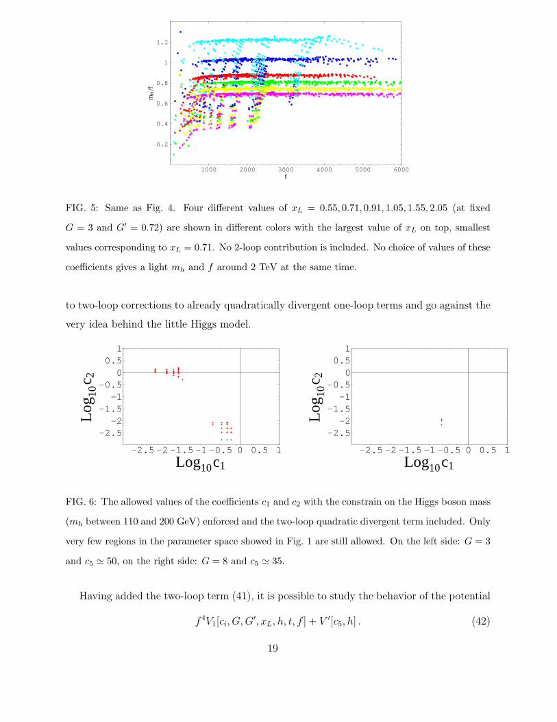
FIG. 5: Same as Fig. 4. Four different values of xL = 0.55, 0.71, 0.91, 1.05, 1.55, 2.05 (at fixed

G = 3 and G′ = 0.72) are shown in different colors with the largest value of xL on top, smallest

values corresponding to xL = 0.71. No 2-loop contribution is included. No choice of values of these

coefficients gives a light mh and f around 2 TeV at the same time.

to two-loop corrections to already quadratically divergent one-loop terms and go against the

very idea behind the little Higgs model.

-2.5 -2 -1.5 -1 -0.5 0 0.5 1

Log10c1

-2.5-2

-1.5-1

-0.50

0.51

Log

10c 2

-2.5 -2 -1.5 -1 -0.5 0 0.5 1

Log10c1

-2.5-2

-1.5-1

-0.50

0.51

Log

10c 2

FIG. 6: The allowed values of the coefficients c1 and c2 with the constrain on the Higgs boson mass

(mh between 110 and 200 GeV) enforced and the two-loop quadratic divergent term included. Only

very few regions in the parameter space showed in Fig. 1 are still allowed. On the left side: G = 3

and c5 ≃ 50, on the right side: G = 8 and c5 ≃ 35.

Having added the two-loop term (41), it is possible to study the behavior of the potential

f 4V1[ci, G, G′, xL, h, t, f ] + V ′[c5, h] . (42)

19

around the origin. For each choice of (G, G′, xL), by imposing the four constrains arising

from the two first derivatives (to have a minimum and it to be at the correct value) and

from the value of mh and mt, the three coefficients, c1, c2 and c5, are fixed.

The study we performed shows that the new constraint of having a Higgs boson mass

close to the current bound [2] drastically reduces the allowed region in the parameter space of

(c1, c2, G, G′, xL, f) and given G, G′ and xL the allowed regions are characterized by having

either c1 of O(1) and c2 of O(10−2) or the opposite, as shown in Fig. 6. For each of these

choices of coefficients c1 and c2, a value of c5 must be chosen so as to obtain the desired

mass mh. This is only possible for rather large values of the coefficient c5. If we are willing

to allow larger Higgs boson masses (that is, mh > 300 GeV), c5 will turn proportionally

smaller but we will still have similar severe constraints on c1 and c2.

1600 1800 2000 2200 2400

f HGeVL

100

120

140

160

180

200

220

mHHG

eVL

FIG. 7: mh vs. f . Each point corresponds to a choice of all coefficients and parameters in the

range discussed in the text (c1 = O(10−2), c2 = O(1), c5 ≃ 50) and varied in discrete steps; G = 3,

G′ = 0.75 and xL = 0.56 are fixed.

D. Conclusions

Fig. 7 shows the possible values of mh and f close to the desired values for a range of the

coefficients c1, c2 and c5 in the allowed regions. These values are now possible but we pay a

rather high price for it. The two main problems are that

• the natural case in which all the coefficients ci are O(1) seems to be ruled out. Values

20

for f and mh in the desired range are only obtained by taking c1 of O(10−2) and

c2 O(1) or vice versa. A coefficient of order O(10−2) clearly goes against the very

rationale of introducing the littlest Higgs model in the first place because we have to

make small by hand one of the symmetry breaking terms;

• the phenomenological two-loop term must have rather large coefficients (c5 =45-55).

This already anticipated feature reminds us of the importance of these terms in com-

pensating the logarithmic contribution to the Higgs boson mass, which are therefore

rather larger than one would wish and usually assume in the little-Higgs framework.

Roughly speaking, these logarithmic terms are O(f) whereas we expected them to

be of O(mh). This is unfortunate since the naturalness of a scale f around 2 TeV is

questionable once such a large two-loop term is included in order to bring mh around

its current bound. Moreover, given the size of our example of two-loop contribution,

there is no way to argue that these two-loop contributions can be neglected in any

other part of the potential and the entire approach at one-loop seems to break down.

A similar conclusion was reached in a recent work were the fine-tuning of the littlest

Higgs is discussed [10].

The analysis above shows that once the scale f is required to be larger than 1 TeV, after

all coefficients have been fixed, the value of the Higgs boson mass—which is linked to that

of the neutral component of the triplet—cannot be made as small as desired. In particular,

it is not possible to have it close to the current experimental lower bound unless some the

coefficients of the quadratically divergent terms are made unrealistically small while at the

same time the two-loop correction is made rather large. The necessary smallness of some

of the coefficients defeats the purpose of introducing the collective breaking mechanism to

make the mass terms small and the littlest Higgs model stable against one-loop radiative

corrections. Moreover, the mass of the Higgs boson itself comes out in a very unnatural way

from the cancellation of terms one order of magnitude larger than its value.

This result seems to be a more serious problem for the model than that of the fine

tuning required in order to be consistent with electroweak precision measurements. The

problem has been so far ignored in the literature because it has been assumed that it was

always possible to add to the logarithmically divergent part of the potential the two-loop

quadratically divergent contribution so as to obtain the desired Higgs boson mass. This is

21

however only possible at the price of introducing an unreasonable large coefficient in this

term and even then at the price of having at least one of the other two coefficients very

small.

On the other hand, if we let instead the model to decide what value the mass of the Higgs

boson should be, we find that it comes out close to the scale f and therefore, for f in the

1-2 TeV range, the Higgs is accordingly heavier than expected. A similar result (but for

different reasons) was recently obtained in a little-Higgs-like unified model of electroweak

and flavor physics [12]. This result is not necessarily in contradiction with the electroweak

precision measurements [13] because the fit should now be redone after including the heavy

Higgs boson as well as the new states introduced by the littlest Higgs model (see, however,

[11]).

E. Comparison with other studies

There are many discussions in the literature about the littlest Higgs model and elec-

troweak precision constraints [6, 7]. In all these papers, however, the values of the coefficients

of the divergent terms are assumed to be of O(1) or, at most O(0.1) and the logarithmic

terms not included. Moreover in [7] only the parameters relevant to the effective operators in

the gauge boson sector are discussed and the coefficients of the divergent terms are assumed

of the desired order and not studied. The only reference in which the scalar potential is

actually constrained is [6]. In order to show that our conclusions agree with what found in

this reference, let us, following their notation, fix the coupling g and g′ in terms of the fine-

structure constant α and the Weinberg angle, vW and v′—the vacuum expectation values

of the isospin triplet t—by means of the Fermi constant and reparametrize the top Yukawa

couplings λ1 and λ2 in terms of

xL =λ2

1

λ21 + λ2

2

mt

vW=

λ1λ2√

λ21 + λ2

2

[

1 +v2

2f 2xL(1 + xL)

]

(43)

we are thus left with a model that, after assigning a value to mt and mH , only depends on

f , xL, s and s′ (as defined in Ref. [6]) and the counterterms a and a′ (which correspond

to 3c1/2 and 6c2). These two can be found for each choice of the first four parameters by

22

solving

a

2

[

g2

s2c2+

g′2

s′2c′2

]

+ 8a′λ2

1 = 2m2H

v2W

1

1 − (4v′f/v2W )

2

−a

4

[

g2(c2 − s2)

s2c2+

g′2(c′2 − s′2)

s′2c′2

]

+ 4a′λ2

1 = 2m2Hv′f

v4W

1

1 − (4v′f/v2W )

2(44)

We thus find that in order to have, for instance, f = 2 TeV while mH = 115 GeV (and

v′ = 3.54 GeV, xL = 0.4, s = 0.22 and s′ = 0.66, as discussed in [6]) we must take the

coefficients a and a′ of order 1/100 (more precisely, a = 0.036 and a′ = 0.063 in this case;

small coefficients are found also for other allowed choices of f and v′), a choice that clearly

defeats the very rationale for introducing the littlest Higgs model in the first place.

This result is consistent with our analysis as presented in the previous section in the case

in which the logarithmic contributions are neglected and the 2-loop terms included. However,

as soon as the logarithmic contributions are not neglected (and we have shown that they

cannot be neglected), the solution above does not exist because it would correspond to a

negative value of the triplet mass and an unstable electroweak ground state. Going back to

Fig. 1, the solutions studied in [6] is in the region ruled out where both coefficients ci are

very small.

IV. A MODIFIED TOP SECTOR

In the previous sections we have seen that the littlest Higgs model, given a cutoff Λ = 4πf

around 10 TeV, predicts a large Higgs mass around 500 GeV. Introducing a 2-loop effective

quadratic term allows to bring this mass to a value smaller than 200 GeV but the 2-loop

term coefficient must then be very large. Because the problem is largely due to the fermionic

sector of the model, in this section we discuss a possible modification of the fermion content

of the model, as proposed in [14], to see if it helps. We neglect in the following the triplet

and focus on the Higgs doublet.

We anticipate that, with these modifications, the fermion contribution to the potential is

finite, and hence no ambiguity (or freedom) is left in the choice of the coefficients of this part

of the potential, which are fixed by the choice of (physical) masses and couplings. Here we

report only on the approximate analysis of the model, which is confirmed by the numerical

study we performed, since the results are not significantly different from the model discussed

previously.

23

A. The model

The lagrangian of the model we consider differs from that of the littlest Higgs model

only by the fermionic contributions Lψ. The fermionic content is given by an electroweak

doublet QL = (t0, b0)L, an electroweak singlet tcgLand by two colored SU(5) quintuplets, X

and X̄. The Yukawa lagrangian is given by an SU(5) invariant term, and by two explicit

breaking terms of the SU(5) global symmetry, both of them preserves enough symmetry to

prevent the Higgs to gain a mass. Only the loops contributions that involves both of them

can produce a mass for the Higgs. The Yukawa lagrangian is given by

LY =√

2λ1f X̄ Σ X +√

2λ2f (ac1Lb0L

+ ac2Lt0L

) +√

2λ3f tcgLtdL

, (45)

where

X =

p1L

p2L

tdL

r1L

r2L

X̄ =

ac1L

ac2L

tctL

bc1L

bc2L

. (46)

By eq. (45) we obtain the fermion mass matrix given by

MfRL= f

−√

2λ1 sin2 hf

i λ1 sin 2hf

√2 λ2

√2 λ1 cos2 h

f√2λ1 cos2 h

fi λ1 sin 2h

f0 −

√2 λ1 sin2 h

f

0√

2λ3 0 0

i λ1 sin 2hf

i√

2λ1 cos 2hf

0 i λ1 sin 2hf

, (47)

where in eq. (47) we have put t = 0. By eq. (47) we see that

Tr M †fRL

MfRL= 2(L2

1 + L22 + λ2

1) f 2

Tr (M †fRL

MfRL)2 = 4(L4

1 + L4

2 + λ4

1) f 4 , (48)

where

L21 = λ2

1 + λ22

L2

2 = λ2

1 + λ2

3 . (49)

24

Eq. (48) indicates that there are no one-loop fermionic divergent contributions to the mass

of the Higgs. The only one-loop fermionic contributions are finite and therefore calculable.

From now on we take L1 = L2.

One of the eigenvalues does not depend on h, and is given by:

m23 = 2λ2

1f2 . (50)

The lightest mass is to be interpreted as that of the standard top quark, with mass approx-

imated by

m2

t = λ2

tf2 sin2 h

f+

(

−λ2

t +λ4t

L21

)

sin4 h

f, (51)

where

λt = 2λ1λ2λ3

√

λ21 + λ2

2

√

λ21 + λ2

3

. (52)

It gives a negligible contribution to the effective potential. The two relevant eigenvalues can

be expanded in powers of sin h/f obtaining:

m2

1/f2 = 2L2

1 +√

2L1λt sinh

f− λ2

t

2sin2 h

f−(

L1λt√2

− 5λ3t

8√

2L1

)

sin3 h

f

+1

2

(

λ2t −

λ4t

L21

)

sin4h

f+ O(sin5

h

f) ,

m2

2/f2 = 2L2

1 −√

2L1λt sinh

f− λ2

t

2sin2 h

f+

(

L1λt√2

− 5λ3t

8√

2L1

)

sin3 h

f

+1

2

(

λ2

t −λ4t

L21

)

sin4 h

f+ O(sin5 h

f) . (53)

The fermionic contribution to the potential for the Higgs field obtained when L1 = L2

(which is the most favorable case) is therefore

Vtnf 4

= −3λ2tL

21

4π2sin2 h

f+

λ4t

16π2

(

−4 +12L2

1

λ2t

− 3 lnλ2t

2L21

)

sin4 h

f. (54)

B. Approximate analysis

The bosonic sector of the model has not been modified, hence we can write (see eq. (21))

the (approximate) expressions:

µ2h

f 2= − 9

256π2g2G2 log

G2

64π2− 3λ2

tL21

4π2,

λ4 =3c1G

2

16+

λ2tL

21

4π2+

λ4t

16π2

(

−4 +12L2

1

λ2t

− 3 lnλ2t

2L21

)

. (55)

25

Choosing L1 ∼√

2 (that is, a value close to the smallest possible after λt = 1), one obtains

(taking the bosonic part from eq. (31))

µ2h

f 2≃ 0.01G2g2 − 0.15 ,

λ4 ≃ 3c1G2

16+ 0.2 . (56)

The finite contributions to µ2h in this variation of the model are comparable in size to

the original logarithmically divergent ones. Further, the quartic coupling is now dominated

by the gauge boson sector, since the top sector gives only a small contribution. From this,

comparing with the original littlest Higgs model, we conclude that there is no substantial

improvement: the cancellation of logarithmic divergences is not enough to reduce the large

top contribution to the sin2 h/f term in the potential. For this reason we leave out a more

general numerical analysis of this modified model.

V. THE LITTLEST HIGGS MODEL AT FINITE TEMPERATURE

We now turn to the study of the littlest Higgs model at finite temperature to determine

the existence and nature of its phase transitions. We do it by assuming that the Higgs mass

is in the light, notwithstanding our argument against this choice, because it is the scenario

more often discussed in the literature and also because the phase transition can only become

weaker for a heavier Higgs mass.

The finite temperature effective potential is given by

V [ci, Σ, T ] = V1[ci, Σ] + VT [ci, Σ] (57)

where V1[ci, Σ] is the potential of eq. (5) and VT [ci, Σ] is the temperature dependent contri-

bution

VT [ci, Σ] = ∓gfT 4

2π2

∫ ∞

0

dx x2 ln[

1 ± exp−√

x2 + M2(Σ)/T 2

]

, (58)

where the sign of the exponential term depends on the statistics of the particles and gf is

the number of degrees of freedom. In the limit mi/T ≪ 1 , with mi the mass of a generic

boson or fermion, eq. (58) simplifies and we obtain

VT [ci, Σ] ≃ T 2

24

[

Tr M2B(Σ) +

1

2Tr M2

F (Σ)]

− T

12πTr M3

B(Σ)

+1

64π

[

Tr M4

B(Σ)( logcBT 2

Λ2) − Tr M4

F (Σ)( logcFT 2

Λ2)]

, (59)

26

where B, F denote, respectively, the bosonic and fermionic degrees of freedom.

Because the potential is very different, at least at large h, with respect to that of the

standard model, one may wonder whether the electroweak phase transition is any stronger

for values of the Higgs boson mass close to the current bounds than in the standard model.

This is an important problem in the study of baryogenesis.

We study the potential with the restrictions on the coefficients and parameters we have

discussed so far (that is, the coefficients ci in the range of Fig. 7). Fig. 8 shows the potential

of the littlest Higgs model and compares it to that of the standard model at three different

T close to T = Tc, where Tc is the temperature of the electroweak phase transition. A small

improvement is present in going from the standard model to the littlest Higgs but it is not

significant. The crucial term linear in T is not large enough to strengthen the transition

and, as in the standard model, only for small values of the Higgs boson mass the phase

transition can be strong enough to sustain electroweak baryogenesis.

0.1 0.2 0.3 0.4

h�T

-0.75

-0.5

-0.25

0

0.25

0.5

0.75

1

108�

VHh�TL

FIG. 8: A comparison of the potential V [h] in the standard model and in the littlest Higgs model

(G = 1.3, G′ = 0.72, and xL = 0.56) at three different T close to Tc. The coefficients c1, c2 and

c5 of the CW potential are those yielding a small Higgs mass. Red dots represent the standard

model, black dots the littlest Higgs model behavior. The transition is weakly of the first order for

mh = 120 GeV for both models.

Models based on pseudo-Goldstone bosons may present an interesting phenomenon of

symmetry non-restoration at high T (see [15], and more recently [16] in the little-Higgs con-

text). The littlest Higgs model is case in point. Because the potential is a periodic function

27

of the pseudo-Goldstone fields, and of the Higgs field h in particular, as the temperature

increases, the maximum in the potential at h/f = π/2 turns into a minimum with an energy

lower than in h = 0. Accordingly, the symmetric ground state in zero becomes unstable and

there is no restoration of the symmetry at higher temperatures.

00.5

11.5

h0

0.5

1

1.5

T

-0.20

0.2

00.5

11.5

h

00.5

11.5

h0

0.5

1

1.5

T

-0.20

0.2

00.5

11.5

h

FIG. 9: Comparison between the potential as a function of h and T in the littlest Higgs model

without and with the logarithmically divergent terms (G = 3, G′ = 0.75, and xL = 0.56). The value

of Tc where V [hmin, Tc] = 0 changes by 20% (from Tc ≃ f to 0.7f) after including the logarithmic

terms.

When we study the high temperature behavior, we can approximate eq. (59) by

VT [ci, Σ] ≃ T 2

24

(

Tr M2

B(Σ) +1

2Tr M2

F (Σ))

(60)

Keeping into account for the generic M2B,F (Σ) only the 1-loop quadratically divergent con-

tributions, we have:

∑

d.o.f.

Tr M2

V =9

4G2 +

3G′2

20+

3

16(G2 + G′2) sin4 h/f

∑

d.o.f.

Tr M2

S,PS =3

2

[

c1(G2 + G′2) + 64c2x

2

L

]

(1 − 2 sin4 h/f)

∑

d.o.f.

Tr M2

SC =3

2

[

c1(G2 + G′2) + 64c2x

2

L

]

(1 − sin4 h/f)

∑

d.o.f.

Tr M2

DC =3

2

[

c1(G2 + G′2) + 64c2x

2

L

]

(1 − sin4 h/f)

∑

d.o.f.

Tr M2

F =8x4

L

4x2L − λ2

t

− x2

L sin4 h/f , (61)

28

where V , S, PS, SC, DC denote respectively the gauge bosons contributions, the scalar and

pseudoscalar contributions and the single and double charged ones.

We therefore have the potential

V [ci, h, T ] ≃{

3

16c1(G

2 + G′2) + 12c2x2L + T 2

[

− 3

16c1(G

2 + G′2)

− 16c2x2

L +1

192(3G2 + 3G′2 − 32x2

L)]}

sin4 h/f , (62)

which is a good approximation at high temperature.

The potential in (62) clearly depends on the coefficients ci and the very presence or not of

a phase transition depends on their values. For arbitrary choices the phase transition can be

anywhere and even not exist at all. However, we find that for values of these coefficients in the

allowed range—where not both coefficients are small—we identified in the previous sections,

the phase transition is always present and for values of the temperature T < Λ/π ≃ 4f for

which we trust the potential.

The potential (62) only includes the quadratically divergent terms. As discussed in the

previous sections, we must add to it the logarithmically divergent terms as well in order to

obtain a reliable result.

Fig. 9 shows the behavior of the potential for different T and h and compares the case

without the logarithmic terms with that in which all terms in the potential are retained.

The phase transition is always present but the value of Tc is moved by a substantial amount

(20%) so that it is necessary to keep the full potential if we want to discuss the temperature

dependence of the potential. In particular, Tc tends to be smaller than f after including

the logarithmic terms and this means that the potential in eq. (62) is not correct because

some of the heavy states may now live above the critical temperature obtained within the

approximated potential, and the exact form based on eq. (58) should be used instead.

Acknowledgments

MP acknowledges SISSA and INFN, Trieste, for hospitality during the completion of this

research. This work is partially supported by the European TMR Networks HPRN-CT-

2000-00148 and HPRN-CT-2000-00152. The work of MP is supported in part by the US

29

Department of Energy under contract DE-FG02-92ER-40704.

[1] N. Arkani-Hamed, A. G. Cohen, E. Katz and A. E. Nelson, JHEP 0207, 034 (2002)

[arXiv:hep-ph/0206021].

[2] S. Eidelman et al., Phys. Lett. B592 (2004) 1.

[3] N. Arkani-Hamed, A. G. Cohen and H. Georgi, Phys. Lett. B 513, 232 (2001)

[arXiv:hep-ph/0105239];

N. Arkani-Hamed, A. G. Cohen, E. Katz, A. E. Nelson, T. Gregoire and J. G. Wacker, JHEP

0208, 021 (2002) [arXiv:hep-ph/0206020];

I. Low, W. Skiba and D. Smith, Phys. Rev. D 66, 072001 (2002) [arXiv:hep-ph/0207243];

M. Schmaltz, Nucl. Phys. Proc. Suppl. 117, 40 (2003) [arXiv:hep-ph/0210415];

D. E. Kaplan and M. Schmaltz, JHEP 0310, 039 (2003) [arXiv:hep-ph/0302049];

W. Skiba and J. Terning, Phys. Rev. D 68, 075001 (2003) [arXiv:hep-ph/0305302];

M. Schmaltz, JHEP 0408, 056 (2004) [arXiv:hep-ph/0407143].

[4] S. Chang and J. G. Wacker, Phys. Rev. D 69, 035002 (2004) [arXiv:hep-ph/0303001];

S. Chang, JHEP 0312, 057 (2003) [arXiv:hep-ph/0306034];

H. C. Cheng and I. Low, JHEP 0309, 051 (2003) [arXiv:hep-ph/0308199];

H. C. Cheng and I. Low, JHEP 0408, 061 (2004) [arXiv:hep-ph/0405243].

[5] F. Bazzocchi, S. Bertolini, M. Fabbrichesi and M. Piai, Phys. Rev. D 68, 096007 (2003)

[arXiv:hep-ph/0306184]; Phys. Rev. D 69, 036002 (2004) [arXiv:hep-ph/0309182];

F. Bazzocchi, Phys. Rev. D 70, 013002 (2004) [arXiv:hep-ph/0401105];

[6] M. C. Chen and S. Dawson, Phys. Rev. D 70, 015003 (2004) [arXiv:hep-ph/0311032].

[7] C. Csaki, J. Hubisz, G. D. Kribs, P. Meade and J. Terning, Phys. Rev. D 67, 115002 (2003)

[arXiv:hep-ph/0211124];

J. L. Hewett, F. J. Petriello and T. G. Rizzo, JHEP 0310, 062 (2003) [arXiv:hep-ph/0211218];

T. Han, H. E. Logan, B. McElrath and L. T. Wang, Phys. Rev. D 67, 095004 (2003)

[arXiv:hep-ph/0301040];

C. Csaki, J. Hubisz, G. D. Kribs, P. Meade and J. Terning, Phys. Rev. D 68, 035009 (2003)

[arXiv:hep-ph/0303236];

R. Casalbuoni, A. Deandrea and M. Oertel, JHEP 0402, 032 (2004) [arXiv:hep-ph/0311038];

30

W. Kilian and J. Reuter, Phys. Rev. D 70, 015004 (2004) [arXiv:hep-ph/0311095].

[8] S. R. Coleman and E. Weinberg, Phys. Rev. D 7, 1888 (1973).

[9] A. E. Nelson, arXiv:hep-ph/0304036;

E. Katz, J. y. Lee, A. E. Nelson and D. G. E. Walker, arXiv:hep-ph/0312287;

R. Contino, Y. Nomura and A. Pomarol, Nucl. Phys. B 671, 148 (2003)

[arXiv:hep-ph/0306259];

S. Chang and H. J. He, Phys. Lett. B 586, 95 (2004) [arXiv:hep-ph/0311177].

K. Agashe, R. Contino and A. Pomarol, arXiv:hep-ph/0412089;

M. Piai, A. Pierce and J. Wacker, arXiv:hep-ph/0405242;

J. Thaler and I. Yavin, arXiv:hep-ph/0501036;

J. Thaler, arXiv:hep-ph/0502175.

[10] J. A. Casas, J. R. Espinosa and I. Hidalgo, JHEP 0411, 057 (2004) [arXiv:hep-ph/0410298];

arXiv:hep-ph/0502066.

[11] G. Marandella, C. Schappacher and A. Strumia, arXiv:hep-ph/0502096.

[12] F. Bazzocchi and M. Fabbrichesi, Phys. Rev. D 70, 115008 (2004) [arXiv:hep-ph/0407358];

Nucl. Phys. B 715, 372 (2005) [arXiv:hep-ph/0410107].

[13] M. E. Peskin and J. D. Wells, Phys. Rev. D 64, 093003 (2001) [arXiv:hep-ph/0101342];

J. Hubisz, P. Meade, A. Noble and M. Perelstein, arXiv:hep-ph/0506042.

[14] See, for instance, the first reference in Ref. [9].

[15] A. K. Gupta, C. T. Hill, R. Holman and E. W. Kolb, Phys. Rev. D 45, 441 (1992).

[16] J. R. Espinosa, M. Losada and A. Riotto, arXiv:hep-ph/0409070.

31