arX

iv:1

211.

1549

v2 [

hep-

ph]

7 F

eb 2

013

Implication of Higgs at 125 GeV within stochastic superspace

framework

Manimala Chakrabortia1, Utpal Chattopadhyaya2 and Rohini M. Godboleb3

a Department of Theoretical Physics, Indian Association for the Cultivation of Science,

2A & B Raja S.C. Mullick Road, Jadavpur, Kolkata 700 032, Indiab Centre for High Energy Physics, Indian Institute of Science, Bangalore 560 012, India

Abstract

We revisit the issue of considering stochasticity of Grassmannian coordinates in

N = 1 superspace, which was analyzed previously by Kobakhidze et al. In this stochas-

tic supersymmetry(SUSY) framework, the soft SUSY breaking terms of the minimal

supersymmetric Standard Model(MSSM) such as the bilinear Higgs mixing, trilinear

coupling as well as the gaugino mass parameters are all proportional to a single mass

parameter ξ, a measure of supersymmetry breaking arising out of stochasticity. While

a nonvanishing trilinear coupling at the high scale is a natural outcome of the frame-

work, a favorable signature for obtaining the lighter Higgs boson mass mh at 125 GeV,

the model produces tachyonic sleptons or staus turning to be too light. The previous

analyses took Λ, the scale at which input parameters are given, to be larger than the

gauge coupling unification scale MG in order to generate acceptable scalar masses ra-

diatively at the electroweak scale. Still this was inadequate for obtaining mh at 125

GeV. We find that Higgs at 125 GeV is highly achievable provided we are ready to

accommodate a nonvanishing scalar mass soft SUSY breaking term similar to what

is done in minimal anomaly mediated SUSY breaking (AMSB) in contrast to a pure

AMSB setup. Thus, the model can easily accommodate Higgs data, LHC limits of

squark masses, WMAP data for dark matter relic density, flavor physics constraints

and XENON100 data. In contrast to the previous analyses we consider Λ = MG, thus

avoiding any ambiguities of a post-grand unified theory physics. The idea of stochastic

superspace can easily be generalized to various scenarios beyond the MSSM .

PACS Nos: 12.60.Jv, 04.65.+e, 95.30.Cq, 95.35.+d

1tpmc@iacs.res.in2tpuc@iacs.res.in3rohini@cts.iisc.ernet.in

1

1 Introduction

Low energy supersymmetry (SUSY) [1–4] has been one of the most promising candidates for

a theory of fundamental particles and interactions going beyond the Standard Model (SM);

the so-called BSM physics. The minimal extension of the SM including SUSY, namely, the

minimal supersymmetric Standard Model (MSSM), extends the particle spectrum of the SM

by one additional Higgs doublet and the supersymmetric partners of all the SM particles

- the sparticles. The Supersymmetric extension of the SM provides a particularly elegant

solution to the problem of stabilizing the electroweak (EW) symmetry breaking scale against

large radiative correction and keeps the Higgs ”naturally” light. In fact, a very robust upper

limit on the mass of the lightest Higgs boson is perhaps one of the important predictions

of this theory. Further, this upper limit is linked in an essential way to the values of some

of the SUSY breaking parameters in the theory. In addition, in R–parity conserving SUSY,

the lightest supersymmetric particle (LSP) emerges as the natural candidate for the dark

matter (DM),the existence of which has been proved beyond any doubt in astrophysical

experiments. The search for evidence of the realization of this symmetry in nature(in the

context of high energy collider experiments, precision measurements at the high intensity

B–factories and in the DM detection experiments) has therefore received enormous attention

of particle physicists, perhaps only next to the Higgs boson. The recent observation of a

boson with mass around ∼ 125 GeV at the Large Hadron Collider (LHC) [5] and the rather

strong lower limits on the masses of sparticles that possess strong interactions that the

LHC searches have yielded [6], necessitates careful studies of the MSSM in the context of

all the recent low energy data. In these studies, it is also very important to seek suitable

guiding principles which could possibly reduce the associated large number of SUSY breaking

parameters of MSSM. Thus, looking for modes of specific SUSY breaking mechanisms that

involve only a few input quantities given at a relevant scale can be useful. Here, the soft

SUSY breaking parameters at the electroweak scale are found via renormalization group (RG)

analyses. Apart from the simplicity of having a few parameters as input, such schemes create

challenging balancing acts. On the one hand, various soft breaking masses and couplings

become correlated with one another in such schemes. On the other hand, overall one has to

accommodate a large number of very stringent low energy constraints in a comprehensive

model consisting of only a few parameters. A simple and well-motivated example of a SUSY

model is the minimal supergravity (mSUGRA) [7]. Here, SUSY is broken spontaneously in

2

a hidden sector and the breaking is communicated to the observable sector where MSSM

resides via Planck mass suppressed supergravity interactions. The model involves soft-SUSY

breaking parameters like (i) universal gaugino mass parameter m 1

2

, (ii) the universal scalar

mass parameter m0 , (iii) the universal trilinear coupling A0, (iv) the universal bilinear

coupling B0, all given at the gauge coupling unification scale. In addition to it, one has

the superpotential related Higgsino mixing parameter µ0 with its associated sign parameter.

The two radiative electroweak symmetry breaking (REWSB) conditions may then be used

so as to replace B0 and µ0 with the Z-boson mass MZ and tan β, the ratio of Higgs vacuum

expectation values. Similar to mSUGRA, one has other SUSY breaking scenarios like the

gauge mediated SUSY breaking and models with anomaly mediated SUSY breaking (AMSB)

etc [2, 3]. Apart from direct collider physics data, one has to satisfy constraints from flavor

changing neutral current (FCNC) as well as flavor conserving phenomena like the anomalous

magnetic moment of muon, constraints like electric dipole moments associated with CP

violations or to check whether there is a proper amount of dark matter content in an R-

parity conserving scenarios or proper neutrino masses in R-parity violating scenarios [1–3].

A single model is yet to be found that can adequately explain various stringent experimental

results and at the same time possesses a sufficient degree of predictiveness. Howevr, it is

always important to continue the quest of a simple model and check the degree of agreement

with low energy constraints.

In this work, we pursue a predictive theory of SUSY breaking by considering a field theory

on a superspace where the Grassmannian coordinates are essentially fluctuating/stochastic

[8–10]. We note that in a given SUSY breaking scenario, our limitation of knowing the

actual mechanism of breaking SUSY is manifested in the soft parameters. Here, in stochastic

superspace framework we assume that a manifestation of an unknown but a fundamental

mechanism of SUSY breaking may effectively lead to stochasticity in the Grassmannian

parameters of the superspace. With a suitably chosen probability distribution, this causes

a given Kahler potential and a superpotential to lead to soft breaking terms that carry

signatures of the stochasticity. As we will see, the SUSY breaking is parametrized by ξ which

is nothing but 1/< θθ >, where the symbol <> refers to averaging over the Grassmannian

coordinates. The other scale that is involved is Λ. Values of various soft parameters at this

scale are the input parameters of the scheme. The values of the same at the electroweak

scale are then obtained from these input values by using the renormalization group evolution.

3

Considering the superpotential of MSSM, the soft terms obtained are readily recognized as

the ones supplied by the externally added soft SUSY breaking terms of constrained MSSM

(CMSSM) [3], except that the model is unable to produce a scalar mass soft term [8].

Reference [8] used Λ and ξ as free parameters while analyzing the low energy signatures

within MSSM. Λ was chosen between MG to MP , the scale of gauge coupling unification

and the Planck mass scale respectively. The model as given in Ref. [8] is called as stochastic

supersymmetric model (SSM) and it is characterized by universal gaugino mass parameter

m 1

2

, universal trilinear soft SUSY breaking parameter A0, and universal bilinear soft SUSY

breaking parameter B0, all being related to ξ, the parameter related to SUSY breaking.

We note that with the bilinear soft SUSY parameter being given, tan β, becomes a derived

quantity.

However, as already mentioned, in spite of the fact that the SSM generates soft SUSY

breaking terms, it produces no scalar mass soft term. Scalar masses start from zero at

the scale Λ and renormalization group evolution is used to generate scalar masses at the

electroweak scale MZ . Scalar masses at MZ severely constrain the model because typically

scalars are very light. In particular, quite often sleptons turn to be the lightest supersym-

metric particles or even become tachyonic over a large part of the parameter space. This

is partially ameliorated when one takes the high scale Λ to be larger than the gauge cou-

pling unification scale MG ∼ 2 × 1016 GeV. However, in spite of obtaining valid parameter

space that would provide us with a lightest neutralino as a possible dark matter candidate

in R-parity preserving framework, we must note that the low values that one obtains for

the masses of the first two generation of squarks are hardly something of an advantage in

view of the constraints coming from FCNC as well as those from the LHC data [6]. On the

other hand, SSM has a natural advantage of being associated with a nonvanishing trilinear

coupling that is favorable to produce a relatively light spectra for a given value of Higgs

boson mass mh. The recent announcement from the CMS and ATLAS Collaborations of the

LHC experiment about the discovery of a Higgs-like boson at ∼ 125 GeV [5] thus makes this

model potentially attractive. However, as explored in Ref. [10], SSM as such is unable to

accommodate such a large mh in spite of having a built-in feature of having a nonvanishing

A0. It could at most reach 116 GeV for mh [9,10] and the constraint due to Br(Bs → µ+µ−)

as used in Ref. [10] was much less stringent in comparison to the same of present day [11].

Furthermore, it is also important to investigate the effect of the direct detection rate of dark

4

matter as constrained by the recent XENON100 data [12].

In this analysis, we would like to give all the input parameters at the grand unification

scaleMG, the scale at which the Standard Model gauge group, namely, SU(3)×SU(2)×U(1),comes into existence. Any evolution above MG would obviously demand choosing a suitable

gauge group; a question that is not going to be addressed in this work. In this way we

would like to avoid unknown issues arising out of a post-grand unified theory(GUT) [13]

physics. However, we would rather try to meet the phenomenological demand of confronting

the issue of sleptons becoming tachyonic or avoiding scalar masses to become light in general

in a minimal modification by considering an externally given scalar mass soft parameter m0

as a manifestation of an additional origin of SUSY breaking. It would be useful to have the

first two generations of scalar masses adequately heavy so as to overcome the FCNC related

constraints and LHC data [6] on squark masses. Additionally this will also be consistent

with having the lighter Higgs boson mass (mh) to be in the vicinity of 125 GeV. We will

henceforth denote the model as Mod-SSM.

We may note that traditionally minimal versions of models of SUSY breaking have been

extended for phenomenological reasons. It is also true that extending a minimal model often

lowers predictiveness and may even cause partial dilution of the main motivations associated

with the building of the model. For example, considering nonuniversal gaugino or scalar

mass scenarios may be more suitable than CMSSM or mSUGRA so as to obtain a relatively

lighter spectra in the context feasibility of exploring via LHC. Another example may be

given in the context of the minimal AMSB model. As we know, a pure AMSB scenario [14]

is associated with form invariance of the renormalization group equations (RGE) of scalar

masses and absence of flavor violation. However, it produces tachyonic sleptons. In the

minimal AMSB model [3, 15] one introduces an additional common mass parameter m0 for

all the scalars of the theory. This ameliorates the tachyonic slepton problem but it is true

that we sacrifice the much cherished feature of form invariance and accept some degree of

flavor violations at the end. We would like to explore a non-minimal scenario of stochastic

supersymmetry model, namely, Mod-SSM in this spirit. We particularly keep in mind that

the stochastic supersymmetry formalism may be used not only within the MSSM framework

but it may be extended to superpotentials beyond that of the MSSM [9]. The fact that the

model with a minimal modification can easily accommodate the recent Higgs boson mass

range by its generic feature of having a nonvanishing trilinear coupling parameter makes it

5

further attractive. We believe that our approach of considering an additional SUSY breaking

scalar mass term is justified for phenomenological reasons.

Thus, in Mod-SSM we consider the input of soft term parameters m 1

2

, B0 and A0 (all are

either proportional to |ξ| or ξ∗ ) and a universal scalar mass soft parameter m0, all being

given at a suitable scale which we simply choose as the gauge coupling unification scale

MG considering the LEP data on gauge couplings could be a hint of the existence of grand

unification. As in Ref. [8] we would also restrict ξ to be real, either positive or negative.

We clearly like to emphasize that the SSM framework produces no scalar mass soft term

at a scale Λ. With Λ set to the gauge coupling unification scale MG, SSM is plagued with

tachyonic sleptons. With Λ > MG one can avoid tachyonic scalar but there is no scope

of obtaining the currently accepted Higgs boson mass. In Mod-SSM we consider Λ = MG

and add the extra scalar mass term for an additional SUSY breaking effect. With the

trilinear coupling parameter A0 and the bilinear coupling parameter B0 becoming correlated

with m 1

2

, Mod-SSM parameter space is essentially a subset of the one for the constrained

MSSM (CMSSM). In Mod-SSM, the SSM inspired nonvanishing A0 parameter is suitable

for producing an appropriately large loop correction to the lighter Higgs boson mass while

keeping the overall sparticle spectra relatively at a lower range. CMSSM, on the other hand

, does not pinpoint with any fundamental physical distinction/motivation for such a zone of

parameter space that is capable of producing the correct Higgs mass with similarly smaller

sparticle mass scale. Even if we consider the stochastic superspace model in its original

form as only a toy idea, we believe that it may be worthwhile to explore it with minimal

modifications in regard to the current Higgs boson mass, as well as other phenomenological

constraints.

2 Stochastic Grassmannian coordinates and SUSY break-

ing

As seen in Ref. [8] we consider an N = 1 superspace where the Grassmannian coordinates θ

and θ are taken to be stochastic in nature. One starts with identifying the terms involving

superfields in the superpotential and the kinetic energy terms that could be used to construct

the SUSY invariant Lagrangian density for a given model. Each term is then multiplied with

a probability distribution function P(θ, θ) and integrated over the Grassmannian coordinates

6

appropriately. P(θ, θ) can be expanded into terms involving θ and θ which obviously has a

finite number of terms because of the Grassmannian nature of θ and θ. One then imposes the

normalization condition∫d2θd2θP(θ, θ) = 1 and vanishing of Lorentz nonscalar moments

like < θ >,< θ >,< θθ >,< θ2θ > and < θθ2 >. The stochasticity parameter ξ is defined

as < θθ >= 1/ξ∗. Here, ξ is a complex parameter with mass dimension unity. As computed

in Ref. [8], and as worked out in this analysis explicitly in the Appendix, the above leads to

the following Hermitian probability distribution.

P(θ, θ)|ξ|2 = P(θ, θ) = 1 + ξ∗(θθ) + ξ(θθ) + |ξ|2(θθ)(θθ). (1)

For the simple case of a Wess-Zumino type of scenario [3] where the kinetic term is obtained

from Φ†Φ and the superpotential is given as W =1

2mΦ2 +

1

3hΦ3, where Φ is a chiral su-

perfield, one finds that the effect of stochasticity as described above leads to the following

SUSY breaking term:

−Lsoft =1

2ξ∗mφ2 +

2

3ξ∗hφ3 +H.c.. (2)

Applying the stochasticity idea to the superpotential of MSSM, along with considering the

effect on the gauge kinetic energy function, the above formalism leads to the following tree

level soft SUSY breaking parameters to be given at the high scale Λ:

a. universal gaugino mass parameter m 1

2

= 12|ξ|,

b. universal trilinear soft parameter A0 = 2ξ∗,

c. universal bilinear Higgs soft parameter B0 = ξ∗.

Recall that there is no scalar mass soft SUSY breaking term in SSM.

For convenience we take ξ to be a real positive number with an additional input sign(ξ). If

we count the universal gaugino mass parameter m 1

2

as the independent parameter, we have,

A0 = sign(ξ).4m 1

2

, B0 = sign(ξ).2m 1

2

. (3)

As has already been discussed before, we introduce a nonvanishing scalar mass parameter

m0 and fix Λ at MG.4 Thus with the above extension, the input quantities for the stochastic

SUSY model are:

m 1

2

, m0, sign(µ) and sign(ξ).

4We note that a vanishing scalar mass parameter at a post-GUT scale, with RG evolution corresponding

to an appropriate gauge group, would indeed generate nonvanishing scalar mass terms at the unification

scale MG [13].

7

We note that the model quite naturally is associated with nonvanishing trilinear soft breaking

terms. As we will see, this is quite interesting in view of the recent LHC announcement for

the Higgs mass range centering around 125 GeV [5]. In this analysis, we will discuss only

the case of ξ < 0 because the other sign of ξ does not produce a spectra compatible with

the dark matter relic density constraint.

The requirement of the REWSB then results in the following relations at the electroweak

scale:

µ2 = −1

2M2

Z +m2

HD−m2

HUtan2 β

tan2 β − 1+

Σ1 − Σ2 tan2 β

tan2 β − 1, (4)

and,

sin 2β = 2Bµ/(m2HD

+m2HU

+ 2µ2 + Σ1 + Σ2) , (5)

where Σi denote the one-loop corrections [16, 17]. Here, B refers to the value of bilinear

Higgs coupling at the electroweak scale which has to be consistent with its given value B0 at

MG. B0 is determined via m 1

2

apart from a sign of the stochasticity parameter as mentioned

before. Consequently, tanβ is a derived quantity in the model. B0 at the scale MG and B

at the electroweak scale are connected via the following RGE written here at the one-loop

level:dB

dt= (3α2m2 +

3

5α1m1) + (3YtAt + 3YbAb + YτAτ ) , (6)

where t = ln(M2G/Q

2) with Q being the renormalization scale. αi = αi/(4π) for i = 1, 2, 3

refer to scaled gauge coupling constants (with α1 = 53αY ) and mi for i = 1, 2, 3 are the

running gaugino masses. Yi are the squared Yukawa couplings, e.g, Yt ≡ y2t /(4π)2 where yt

is the top Yukawa coupling. In this analysis, the value of tan β is determined via Eqs.4-6

along with B0 = sign(ξ)2m 1

2

at the scale MG. We use SuSpect [18] for solving the RGEs

and obtaining the spectra. The code takes tan β as an input quantity. Hence, we implement

a self-consistent method of solution that starts from a guess value of tanβ resulting into a

B(MG) that in general would not agree with the input of B0. Use of a Newton-Raphson root

finding scheme ensures a fast convergence toward the correct value of tan β when B(MG)

matches with the input of B0. Here we stress that we do not encounter any parameter point

with multiple values of tanβ in our analysis.5

5See Ref. [19] for such a general possibility in REWSB where B0 is given as an input.

8

3 Results

The fact that the model has tanβ as a derived quantity necessitates studying the behavior

of the evolution of the bilinear Higgs parameter B. Figure1 shows the evolution of a few

relevant couplings for a specimen input of m1/2 = 600 GeV, m0 = 2 TeV and µ > 0 in Mod-

SSM. For ξ < 0, both B0 as well as A0 are negative, namely, B0 = −2m1/2 and A0 = −4m1/2.

For a valid parameter point within the model with µ > 0 , we require B = B(Mz) > 0, a

necessity in order to have a positive sin 2β from Eq.(5).6 We note that the denominator

in the right-hand side of Eq.(5) is the square of pseudoscalar Higgs mass which needs to

be positive. The fact that B is originally negative at MG and has to change to a positive

value at MZ puts a strong constraint on the parameter space of the model. Numerically,

this results in tanβ assuming large values. In regard to the evolution of A parameters we

defer our discussion until Fig.3.

Figure 2 shows a scatter plot of parameter points in the tan β −m 1

2

plane that satisfy the

REWSB constraints of Eqs.(4) and (5). As m0 is varied up to 7 TeV and m 1

2

up to 2 TeV,

tanβ is seen to have a range of 32 to 48. The spread of tan β for a given m 1

2

arises from

variation ofm0. For smaller values ofm 1

2

, there is a larger dependence ofm0 on tan β. Hence,

there is a larger spread of tan β when m0 is varied. For larger m 1

2

, the valid solution of tan β

has a lesser dependence on m0. Hence, for larger m 1

2

values the spread in values of tan β

decreases. The white region embedded within the blue-green area corresponds to parameter

points with no valid solution satisfying REWSB. Typically, the two REWSB conditions are

nonlinear in nature with respect to m 1

2

and m0. The code unsuccessfully tries with a large

number of iterations to find consistent µ2 and m2A solutions for parameter points within the

white region (for all m0). Thus a lack of a valid tan β for any value of m0 results in the above

white region. It is worth mentioning that the range of valid tanβ is much larger for the case

of ξ > 0 where B stays positive throughout the range from MG to MZ . This is unlike the

case of ξ < 0 under discussion, where B is negative at MG and necessarily has to become

positive at the electroweak scale, thus adding stringency to tan β in its range. However, as

already mentioned, we will not discuss the case of ξ > 0 further because of the resulting

overabundance of dark matter for the entire parameter space for this sign of ξ.

6tanβ , which is the ratio of two vacuum expectation values, is positive. Hence, sin 2β = 2 tan β

(1+tan2 β) is also

positive.

9

100

104

108

1012

1016

Scale Q (GeV)

-3000

-2000

-1000

0

1000

2000

Cou

plin

gs (

GeV

)

B

At

Ab

Ατ

µξ < 0m

1/2=600 GeV, m

0=2 TeV

m1

m2

Figure 1: Evolution of a few relevant couplings for a specimen input of m1/2 = 600 GeV, m0 =

2 TeV and µ > 0. With ξ < 0, one has B0 = −2m1/2 and A0 = −4m1/2. For a valid parameter

point within the model with µ > 0 we require B = B(MZ) > 0, a necessity in order to have a

positive sin 2β from Eq.(5).

We will study now the effect of low energy constraints particularly in the context of the

recent discovery of the Higgs-like boson [5]. Figure .3 shows the result in the m 1

2

−m0 plane

for ξ < 0. A sufficiently nonvanishing At (see, for example, Figure 1) helps in producing

a large loop correction to the lighter CP-even Higgs boson h. This can be understood by

looking at the expression for the dominant part of loop correction to the Higgs boson mass

coming from the top-stop sector [20–22]

∆m2h =

3mt4

2π2v2 sin2 β

[log

M2S

mt2+

X2t

2M2S

(1− X2

t

6M2S

)]. (7)

Here, MS =√mt1mt2 , Xt = At − µ cotβ, v = 246 GeV and mt is the running top-quark

mass that also takes into account QCD and electroweak corrections. The loop correction is

maximized if Xt =√6MS. Clearly, a nonvanishing A0 can be useful to increase ∆m2

h so that

mh reaches the LHC specified zone without a need to push up the average sparticle mass scale

10

200 400 600 800 1000 1200 1400 1600 1800 2000m

1/2 (GeV)

5

10

15

20

25

30

35

40

45

50

55

60

tanβ

ξ < 0

Figure 2: Scatter plot of parameter points in the m 1

2

− tan β plane when m0 and m 1

2

are scanned

up to 7 TeV and 2 TeV, respectively. Here we only consider the validity of REWSB constraints of

Eqs.(4) and (5). The values of tan β that satisfy the REWSB constraint vary from 32 to 48. The

white region inside the shaded (blue-green) region corresponds to invalid parameter points where

no consistent solution satisfying REWSB could be found even after trying with a large number of

iterations. The spread of tan β for a given m 1

2

arises from variation of m0. This spread decreases

as m 1

2

becomes larger because of decreased sensitivity on m0 while satisfying REWSB.

by a large amount. As particularly mentioned in Ref [8], the SSM is additionally attractive in

this context since it naturally possesses a nonvanishing and large |A0|. We further note that

in this model, the lighter Higgs boson h has couplings similar to those in the Standard Model

because the CP-odd Higgs boson mass (mA) is in the decoupling zone [23]. The ATLAS and

CMS results for the possible Higgs boson masses are 126.0± 0.4 (stat)± 0.4(syst) GeV and

125.3 ± 0.4 (stat)± 0.5(syst) GeV , respectively [5]. In regard to MSSM light Higgs boson

mass, we note that there is about a 3 GeV uncertainty arising out of uncertainties in the

top-quark mass, renormalization scheme, as well as scale dependence and uncertainties in

higher order loop corrections up to three loop [24–28]. Hence, in this analysis we consider

11

the following limits for mh:

122 GeV < mh < 128 GeV. (8)

We will outline the other relevant limits used in this analysis. A SUSY model parameter

500 1000 1500 2000m1/2 (GeV)

0

1000

2000

3000

4000

5000

6000

7000

m0 (

GeV

)

Bs --> µ+µ-

mh = 122 GeV

mh = 128 GeV

III

III

b --> s+γ

ξ < 0

Figure 3: Constraints shown in the m 1

2

−m0 plane for µ > 0 and ξ < 0 for Mod-SSM. A0 and B0 in

the model satisfy A0 = sign(ξ).4m 1

2

and B0 = sign(ξ).2m 1

2

. tan β becomes a derived quantity that

varies between 32 and 48. The Higgs boson limits are shown as two solid blue lines. Br(b → sγ)

limit is shown as a maroon dot-dashed line. The lower part corresponds to discarded region via

Eq.(9) where the branching ratio goes below the lower limit of the constraint. Br(Bs → µ+µ−)

limit is shown as a brown solid line of which the lower region exceeds the upper limit of Eq.(10). The

top green region (I) corresponds to discarded zone via REWSB. The bottom blue-green region (III)

refers to the zone where stau becomes LSP or tachyonic. The gray region (II) has discontinuous

patches of valid parameter zones, the details of which are mentioned in the text. Red points/areas

falling in region-II satisfy the WMAP-7 data only for the upper limit of Eq.12. Typically, the red

points bordering region-III and some part of the extreme left red points (for very small m 1

2

) satisfy

both the upper and the lower limits of Eq.(12).

12

space finds a strong constraint from Br(b → sγ). In SM, the principal contribution that

almost saturates the experimental value comes from the loop comprising of top-quark and

W-boson [29]. In MSSM, principal contributions arise from loops containing top quark

and charged Higgs bosons, and the same containing top squarks and charginos [30]. The

chargino loop contributions are proportional to Atµ and this may cause cancellations or

enhancements between the principal terms of the MSSM contribution depending on the

sign of Atµ. Similar to mSUGRA, both the SSM and Mod-SSM with ξ < 0 also typically

have At < 0. With µ > 0, this primarily means cancellation between the chargino and

the charged Higgs contributions. This leads to a valid region for Br(b → sγ) for a larger

sparticle mass scale compared to the case of µ < 0. Br(b → sγ) constraint thus favors the

positive sign of µ by allowing larger areas of parameter space. We consider the experimental

value Br(b → sγ) = (355 ± 24 ± 9)× 10−6 [31]. This results in the following 3σ level zone

as used in this analysis.

2.78× 10−4 < Br(b→ sγ) < 4.32× 10−4. (9)

The above constraint is displayed as a maroon dot-dashed line. The left region of this

line would be a discarded zone. Next, the fact that the stochastic model with ξ < 0 selects

appreciably large values for tan β necessitates checking the Bs → µ+µ− limit. This is required

because Bs → µ+µ− increases with tan β as tan6 β and decreases with increase in mA, the

mass of pseudoscalar Higgs boson as m−4A [32]. We use the recent experimental limit from

LHCb [11]: Br(Bs → µ+µ−)exp = (3.2+1.4−1.2(stat.)

+0.5−0.3(syst.))× 10−9. This is contrasted with

the SM evaluation Br(Bs → µ+µ−)SM = (3.23±0.27)×10−9 [33]. As in Ref. [34], combining

the errors of the LHCb data along with that of the SM result one finds the following:

0.67× 10−9 < Br(Bs → µ+µ−) < 6.22× 10−9. (10)

The upper limit of Br(Bs → µ+µ−) is shown as a brown solid line going across Fig.3.

Parameter values in the region below this curve lead to values of Br(Bs → µ+µ−) higher

than the above limit.

We also compute Br(B → τντ ) in this analysis. The SUSY contribution to Br(B → τντ )

is typically effective for large tanβ and small charged Higgs boson mass scenarios [35].

The experimental data from BABAR [36] reads Br(B+ → τ+ντ ) = (1.83+0.53−0.49(stat.) ±

0.24(syst.))× 10−4. The recent result from Belle [37] for B− → τ−ντ that used the hadronic

13

tagging method is given by Br(B− → τ−ντ ) = (0.72+0.27−0.25(stat.) ± 0.11(syst.)) × 10−4.

The same branching ratio from Belle extracted by using a semileptonic tagging method

is (1.54+0.38−0.37(stat.)

+0.29−0.31(syst.))× 10−4 [38]. We use Ref. [39] for the result of averaging of all

the recent Belle and BABAR data which is Br(B → τν)exp = (1.16± 0.22)× 10−4. The SM

result strongly depends on the CKM element |Vub| and the B-meson decay constant. We use

Br(B → τν)SM = (0.97 ± 0.22) × 10−4 [39]. Using the above theoretical and experimental

errors appropriately, we obtain the following:

R(B→τντ ) =Br(B → τντ )SUSY

Br(B → τντ )SM= 1.21± 0.30. (11)

This translates into 0.31 < R(B→τντ ) < 2.10 at 3σ. Here Br(B → τντ )SUSY denotes the

branching ratio in a SUSY framework, of course including the SM contribution. In general,

we find that the model parameter space of Mod-SSM is not constrained by B → τντ since

charged Higgs bosons are sufficiently heavy.

We have not, however, included the constraint from muon g−2 in this analysis considering the

tension arising out of large deviation from the SM value, uncertainty in hadronic contribution

evaluations and accommodating SUSY models in view of the LHC sparticle mass lower

limits [40].

We now explore the cosmological constraint for neutralino dark matter relic density [41]. At

3σ, the WMAP-7 data [42] are considered as shown below:

0.094 < Ωχ0

1

h2 < 0.128. (12)

The conclusions in regard to the relic density constraint is additionally found to be sensitive

on the top-quark mass in this model. We divide the dark matter analysis into two parts

depending on (a) the top-quark pole mass set at 173.3 GeV and (b) using a spread of top-

quark pole mass within its range mt = 173.3 ± 2.8 GeV following the result of the recent

analysis performed in Ref. [43]. In this context, we note that the experimental value as

measured by the CDF and D0 Collaborations of Tevatron is: mexpt = 173.2±0.9 GeV [44]. 7

3.1 Analysis with mt = 173.3 GeV: Underabundant LSP

The lightest neutralino, the LSP of the model is typically highly bino dominated except in

a few regions where the Higgsino mixing parameter µ turns out to be small. The parameter

7For bottom quark mass we have used mbMS(mb) = 4.19 GeV.

14

points within all of the white region in Figure 3 have bino-dominated LSP. At this point we

note that the implementation of the REWSB conditions as manifest in Eqs.(4) and (5) has

to be done by keeping in mind (i) positivity of sin 2β and (ii) positivity of µ2 and and (iii)

the requirement of B0, A0 being related to m 1

2

as given by Eq. (3), as well as requiring that

the lighter chargino mass lower limit is respected. All these requirements lead the top green

shaded region (labeled as I) to be a discarded zone. On the other hand, the gray shaded

region (II) has discontinuous zones of valid parameter points, shown in red. The red points

have considerably small values of µ, thus giving the LSP a large degree of Higgsino mixing.

Apart from the red points, there are no solutions in the gray areas of region II. The need to

satisfy the point (i) as explained above along with the requirement to satisfy the condition

(iii) (implemented via a Newton-Raphson method of finding the correct tanβ) stringently

negates the existence of solution zones within region II. As a result, either there are solutions

with appreciably small µ or no solution at all within this region. This on the other hand

leads to a large amount of χ01 − χ±

1 coannihilation. Such degrees of coannihilations indeed

cause the LSP to be only a subdominant component of DM. Thus, in this part of the analysis

we consider the possibility of an underabundant dark matter candidate and ignore the lower

limit of the WMAP-7 data. Typically we see that the relic density falls below the lower limit

of Eq.(12) in region II by an order of magnitude. Such underabundant LSP scenarios have

been discussed in several works [45].

The lower shaded region III is disallowed as the mass of the stau (τ1) turns negative or it is

the LSP. Typically the red strip near region III refers to the LSP-stau coannihilation8 zone

where the relic density can be consistent with both the upper and lower limits of Eq.(12).

Quite naturally, the coannihilation may be stronger and this would additionally produce

some underabundant DM points for this zone. Finally, the leftmost red region (with very

small m 1

2

) satisfying WMAP-7 data is discarded by all other constraints. We note that

only a small region satisfying the Higgs mass bound is discarded via Br(b → sγ). On the

other hand, the Higgs mass bound line of 122 GeV supersedes the constraint imposed by

the recent data on inclusive search for SUSY by the ATLAS experiment [6]. The most

potent constraint to eliminate a large region of parameter space with m0 up to 1.5 TeV or

so is due to Br(Bs → µ+µ−) data (Eq.(10)). The constraint is effective simply because of

8See, for example, works in Ref. [46] for various annihilation processes in relation to SUSY parameter

space in general.

15

the large values of tan β involved in the model. The discarded part of parameter space via

the above constraint includes a large zone that satisfies the dark matter limit via LSP-stau

coannihilation.

We will now describe the spin-independent direct detection scattering cross section for

scattering of the LSP with proton. The scalar cross section depends on t-channel Higgs

exchange diagrams and s-channel squark diagrams. Unless the squark masses are close to

that of the LSP, the Higgs exchange diagrams dominate [47]. We note that for the cases of

parameter points with Ωχh2 < (ΩCDMh

2)min, where (ΩCDMh2)min refers to the lower limit

of Eq.(12), one must appropriately include the fraction of local DM density contributed by

the specific candidate of DM under discussion while evaluating the event rate.

0 200 400 600 800 1000mχ1

0 (GeV)10

-12

10-11

10-10

10-9

10-8

10-7

ζσSI

(p-χ

) (pb)

XENON100

Figure 4: Scaled spin-independent χ01 − p scattering cross section vs LSP mass. The scaling factor

is given as ζ = Ωχh2/(ΩCDMh2)min, where (ΩCDMh2)min refers to the lower limit of Eq.(12).

This translates into multiplying σSIpχ0

1

for such underabundant scenarios by ρχ/ρ0. Here, ρχ is

the actual DM density contributed by the specific DM candidate contributing to ρ0 where the

latter is the local dark matter density. We thus use ρχ = ρ0ζ where ζ = Ωχh2/(ΩCDMh

2)min.

16

On the other hand, ζ is simply 1 for abundant or overabundant dark matter cases. Thus,

we conveniently define ζ = min1,Ωχh2/(ΩCDMh

2)min [48]. Figure4 shows the rescaled

cross section as computed via micrOMEGAs version 2.4 [49]. We wish to emphasize that

while some region of parameter space where the LSP typically has a large degree of Higgsino

component is eliminated via XENON100 data as announced in the summer of 2012 [12], a

large section of parameter space remains to be explored via future direct detection of DM

experiments. This consists of both types of coannihilation zones, namely, the chargino as

well as the stau coannihilation zones. We must also keep in mind the issue of theoretical

uncertainties, particularly the hadronic uncertainties in evaluating σSIpχ0

1

. The strangeness

content of nucleon finds a large reduction in the evaluation of relevant couplings via lattice

calculations [50]. This is not incorporated in our computation while using micrOMEGAs to

calculate the cross section. Thus, the above itself will cause a reduction of σSIpχ0

1

by almost

an order of magnitude. There is also an appreciable amount of uncertainty of the local dark

matter density [51]. All these points need to be kept in mind while evaluating the implica-

tions of Fig. 4 for SUSY models.

3.2 Analysis with mt = 173.3± 2.8 GeV: LSP of right abundance

It is to be noted that in the gray area (shown as region II) of Fig.3 the existence of a valid

solution depends very critically on the parameters of the model. It was found that either (i)

we obtain a very small µ (barely satisfying the lighter chargino mass lower limit) in the gray

area that would only provide us with extreme coannihilation between lighter chargino and

LSP leading to underabundance of DM, or (ii) we find no valid solution at all. The sensitivity

arises from the stringency of satisfying REWSB on the parameter space for this region. In

other words, for a given m 1

2

, a small change in assumed m0 for a valid parameter point

would produce a small change in tanβ in the white region producing most probably another

valid parameter point. However, the change may not be allowed via REWSB, particularly

Eq.(5) if the parameter point is considered in the gray region. Eq.(5) means sin 2β needs

to be a positive quantity less than unity. This typically becomes a severe constraint even

if condition of satisfying the lighter chargino mass lower limit is met. With the top-quark

mass having a strong influence on REWSB , it may be useful to investigate whether varying

mt may extract newer valid points within the gray region that would have a suitable µ so

17

as to satisfy a well-tempered [52] LSP situation. This will then have the right abundance of

dark matter satisfying both the lower and the upper limit of DM of Eq.(12).

The present experimental data on top-quark mass read: mexpt = 173.2 ± 0.9 GeV [44].

Recently Ref. [43] predicted the pole mass of top-quark to be mpolet = 173.3 ± 2.8 GeV.

The analysis used the next-to-next-to-leading order (NNLO) in the QCD prediction of the

inclusive pp → tt +X cross section and the Tevatron and LHC data of the the same cross

section. The comparison between the experimental and theoretical results helped extracting

the top-quark mass in the modified minimal subtraction (MS) scheme. This was then used

to compute the pole mass mpolet . We now extend our analysis by investigating the effect

of varying top-quark pole mass within the above range (mpolet = 173.3 ± 2.8 GeV) on the

solution space of the model. Indeed, we will see that even with a variation of 0.9 GeV, the

range of experimental error would be enough to have a substantial effect on the conclusions.

Figure 5 shows the scattered points that satisfy the WMAP-7 given range of relic density

for the aforesaid variation of mt ≡ mpolet . Here, m 1

2

and m0 are varied up to 2 TeV and

7 TeV, respectively. We see from this figure that the central value of mt (=173.3) GeV as

considered in Figure 3 is indeed the one which has the least amount of possibility to satisfy

the WMAP-7 data. The occurrence of points which satisfies WMAP-7 data is particularly

rare around this value of mt, near the lower part of the limit of relic density. We already

found that the gray region (region II) of Figure 3 is a sensitive zone because of REWSB,

where µ can be quite small. For such small values of µ, one can only expect a large degree

of χ01 − χ±

1 coannihilation which results into very small relic density. The latter goes below

the lower limit of Eq.(12). Hence no red point exists near the bottom blue line of Figure 5

for this value of mt. On the contrary, a value of mt less than 1 GeV from the central value,

which is only within the experimental error ofmexpt , would cause to have an LSP with correct

abundance for DM. The most favored zone for mt, however, would be from 171 to 172 GeV

for satisfying the relic density limits. In fact, a reduced degree of sensitivity for satisfying

REWSB is the reason for obtaining a well-tempered LSP while considering a top-quark mass

little away from the central value.

Figure 6 shows the effect of scanning the top-quark mass on the m 1

2

−m0 plane. Region I

shown in green is a disallowed area of parameter space via REWSB similar to Fig.3, except

18

170 171 172 173 174 175 176m

t (GeV)

0.095

0.1

0.105

0.11

0.115

0.12

0.125

0.13

Ωχh2

ξ<0

(m1/2

< 2 TeV, m0 < 7 TeV)

Figure 5: Relic density satisfied points shown in red that fall within the lower and upper limits of

WMAP-7 data for the neutralino relic density, when mt is varied by 2.8 GeV on either side of 173.3

GeV. Here m 1

2

and m0 are scanned up to 2 TeV and 7 TeV, respectively, for µ > 0 and ξ < 0. The

two blue lines are the WMAP-7 limits of Eq.(12). The value of mt = 173.3 GeV as used in Figure

3 visibly falls in a disfavored zone in the context of obtaining the correct relic density, particularly

toward the lower limit of of Eq.(12).

that it is now an invalid region for all values of mt within its limit. Thus, this region is

smaller in extension than the corresponding region of Figure 3. The region II is disallowed

because of stau turning tachyonic or the least massive. The constraints from Br(b → sγ)

and Br(Bs → µ+µ−) are as shown. The lines denote the boundary of purely discarded zones

irrespective of variation of mt within its range. The blue line for mh = 124 GeV means that

mh < 124 GeV for all the region left of the line irrespective of the value of mt within the

range. The ATLAS specified limit [6] for squarks also falls well within this left zone. The

neutralino relic density satisfied areas are below region I and above region II. The red points

satisfy both the limits of the WMAP-7 data, and thus correspond to having the right degree

of abundance of DM. On the other hand, we have also shown blue-green points that only

satisfy the upper limit of the WMAP-7 data. In this part of the analysis, we consider the

19

500 1000 1500 2000m

1/2 (GeV)

0

1000

2000

3000

4000

5000

6000

7000

m0 (

GeV

)

I

II

mtop

scanned

(ξ<0)

mh=124 GeV

b-->sγ Bs-->µ+µ−

A

B

C

Figure 6: Scattered points in the m 1

2

−m0 plane for µ > 0 and ξ < 0 when top-quark mass is varied

by 2.8 GeV on either side of 173.3 GeV. Region I is the same as that in Fig.3 except that it is now

a discarded zone for all values of mt within its limit. The region II is discarded via stau turning the

LSP or turning itself tachyonic for all mt. The constraints from Br(b → sγ) and Br(Bs → µ+µ−)

are as shown. The lines show the boundary of purely discarded zones irrespective of variation of

mt within its range. There is no region toward the left of the blue line labeled as mh = 124 GeV for

which mh may become larger than 124 GeV irrespective of values of mt. Three benchmark points

A,B and C are shown corresponding to Table 1.

LSP to have the correct abundance so as to be a unique candidate for DM.

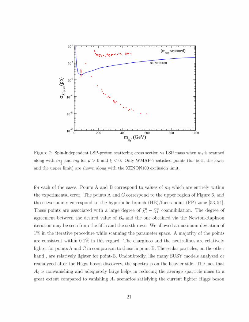
Finally we show the effect of varyingmt on the spin-independent LSP-proton scattering cross

section in Figure 7. Only the WMAP-7 satisfied points are shown (in red). Considering an

order of magnitude of uncertainty (reduction), primarily because of the issue of strangeness

content of nucleon as well as astrophysical uncertainties as mentioned before, we believe

that the recent XENON100 data still can accommodate Mod-SSM even while considering

the LSP as a unique candidate of DM.

Table 1 shows three benchmark points of the model. The top-quark mass mt is as shown

20

0 200 400 600 800 1000mχ1

0 (GeV)10

-12

10-11

10-10

10-9

10-8

10-7

σ SI(p

-χ) (p

b)

(mtop

scanned)

XENON100

Figure 7: Spin-independent LSP-proton scattering cross section vs LSP mass when mt is scanned

along with m 1

2

and m0 for µ > 0 and ξ < 0. Only WMAP-7 satisfied points (for both the lower

and the upper limit) are shown along with the XENON100 exclusion limit.

for each of the cases. Points A and B correspond to values of mt which are entirely within

the experimental error. The points A and C correspond to the upper region of Figure 6, and

these two points correspond to the hyperbolic branch (HB)/focus point (FP) zone [53, 54].

These points are associated with a large degree of χ01 − χ±

1 coannihilation. The degree of

agreement between the desired value of B0 and the one obtained via the Newton-Raphson

iteration may be seen from the fifth and the sixth rows. We allowed a maximum deviation of

1% in the iterative procedure while scanning the parameter space. A majority of the points

are consistent within 0.1% in this regard. The charginos and the neutralinos are relatively

lighter for points A and C in comparison to those in point B. The scalar particles, on the other

hand , are relatively lighter for point-B. Undoubtedly, like many SUSY models analyzed or

reanalyzed after the Higgs boson discovery, the spectra is on the heavier side. The fact that

A0 is nonvanishing and adequately large helps in reducing the average sparticle mass to a

great extent compared to vanishing A0 scenarios satisfying the current lighter Higgs boson

21

limit. The mh for point-C, however, goes below the assumed limit of Eq.(8). However ,

we, still believe that it is within an acceptable zone considering the various uncertainties to

compute mh as mentioned before. Points A and C have larger spin-independent scattering

cross section σSIpχ than the XENON100 limit. But, we believe this is within acceptable

limit considering the existing uncertainties arising out of strangeness content of nucleon as

well as those from astrophysical origins, particularly from local DM density. Finally, it is

also possible to satisfy all the limits in full subject to a 5% − 10% heavier spectra and/or

considering a multicomponent DM scenario.

22

Parameter A B C

mt 173.10 173.87 171.58

m1/2 838.78 1239.16 579.69

m0 6123.75 1817.69 4200.55

(A0 = −4m1/2) -3355.13 -4956.64 -2318.75

(B0 = −2m1/2) -1677.56 -2478.32 -1159.37

B0 (as output) -1683.56 -2478.32 -1160.27

tanβ (as output) 45.86 40.92 45.11

sgn(µ) 1 1 1

µ 403.86 2508.85 310.43

mg 2145.53 2727.64 1525.80

muL6247.84 2994.87 4292.70

mt1 , mt2 3758.76, 4376.60 1333.10, 2078.60 2587.56, 3026.20

mb1, mb2

4397.10, 4886.58 2054.58, 2339.25 3037.22, 3381.67

meL, mνe 6119.53, 6119.05 1983.72, 1982.21 4197.61, 4196.89

mτ1 , mντ 4750.43, 5482.91 549.62, 1536.41 3281.31, 3770.25

mχ±

1

, mχ±

2

406.25, 741.03 1038.00, 2491.42 304.84, 518.70

mχ0

1, mχ0

2356.62, 417.02 548.95, 1038.00 241.80, 316.70

mχ0

3, mχ0

4424.40, 741.06 2489.56, 2491.14 322.35, 518.80

mA, mH± 2573.69, 2573.69 1967.83, 1967.50 1846.04, 1846.04

mh 124.42 126.55 121 .57

Ωχ1h2 0.1105 0.1002 0.1106

BF (b→ sγ) 3.23× 10−4 2.96× 10−4 3.15× 10−4

BF (Bs → µ+µ−) 2.98× 10−9 5.23× 10−9 2.89× 10−9

R(B→τν) 0.98 0.98 0.97

∆aµ 5.78× 10−11 1.65× 10−10 1.22× 10−10

σSIpχ 3 .05 × 10−8 1.04× 10−11 2 .64 × 10−8

Table 1: Spectra of three specimen parameter points A, B and C as shown in Fig.6. Results

with marginal deviation from the assumed limits are shown in italics (red). Muon g − 2 is

not imposed as a constraint in this analysis. B0 = B(MG) has two entries. The first one is

the desired value while the second one is the value obtained with a suitable tanβ as found

from the Newton-Raphson root finding scheme. See text for further details.23

4 Conclusion

In the SSM [8], one assumes that a manifestation of an unknown but a fundamental mech-

anism of SUSY breaking may effectively lead to stochasticity in the Grassmannian param-

eters of the superspace. With a suitable probability distribution decided out of physical

requirements, stochasticity in Grassmannian coordinates for a given Kahler potential and a

superpotential may lead to well-known soft breaking terms. When applied to the superpo-

tential of the MSSM, the model leads to soft breaking terms like the bilinear Higgs coupling

term, a trilinear soft term as well as a gaugino mass term, all related to a parameter ξ,

the scale of SUSY breaking. The other scale considered in the model of Ref. [8] at which

the input quantities are given is Λ, where the latter can assume a value between the gauge

coupling unification scaleMG and the Planck mass scale MP . There is an absence of a scalar

mass soft term at Λ in the original model that leads to stau turning to be the LSP or even

turning itself tachyonic if Λ is chosen as MG. This is only partially ameliorated when Λ is

aboveMG. However, the model because of its nonvanishing trilinear parameter is potentially

accommodative to have a larger lighter Higgs boson mass via large stop scalar mixing. As

recently shown in Ref. [10] the model in spite of its nice feature of bringing out the desired

soft breaking terms of MSSM is not able to produce mh above 116 GeV, and it has an LSP

which is only a subdominant component of DM.

In this work, a minimal modification (referred as Mod-SSM) is made by allowing a

nonvanishing single scalar mass parameter m0 as an explicit soft breaking term. Phe-

nomenologically the above addition is similar to what was considered in minimal AMSB

while confronting the issue of sleptons turning tachyonic in a pure AMSB framework. The

modified model successfully accommodates the lighter Higgs boson mass near 125 GeV. Ad-

ditionally, it can accommodate the stringent constraints from the dark matter relic density,

Br(Bs → µ+µ−), Br(b → sγ) and XENON100 data on direct detection of dark matter. A

variation of top-quark mass within its allowed range is included in the analysis and this shows

the LSP to be a suitable candidate for dark matter satisfying both the limits of WMAP-7

data. Finally, we remind that the idea of stochastic superspace can easily be generalized to

various scenarios beyond the MSSM .

Acknowledgments

M.C. would like to thank the Council of Scientific and Industrial Research, Government of

India for support. U.C. and R.M.G are thankful to the CERN THPH division (where the

24

work was initiated) for its hospitality . R.M.G. wishes to acknowledge the Department of

Science and Technology of India, for financial support under Grant no. SR/S2/JCB-64/2007.

We would like to thank B. Mukhopadhyaya, S. Kraml, P. Majumdar, K. Ray, S. Roy and

S. SenGupta for valuable discussions.

5 Appendix

Using Ref. [8], we consider the following Hermitian probability distribution :

P(θ, θ) = A+ θαΨα + θαΞα + θαθαB + θαθ

αC + θασµαβ θ

βVµ

+θαθαθαΛα + θαθ

αθαΣα + θαθαθαθαD (13)

Here, A, B, C, D and Vµ are complex numbers. Ψ, Ξ, Λ, and Σ are Grassmann numbers.

In order to arrive at the results of Ref. [8], we use the following [3]: d2θ = −14dθαdθα,

d2θ = −14dθαdθ

α, d4θ = d2θd2θ,∫d2θ (θθ) = 1,

∫d2θ (θθ) = 1,

∫d2θ =

∫d2θ = 0 and

∫d2θ θα =

∫d2θ θα = 0.

Normalization:

First, P(θ, θ) should satisfy the normalization condition∫d2θd2θ P(θ, θ) = 1. All the terms

except the one with the coefficient D vanishes in∫d2θd2θ P(θ, θ). Thus D = 1.

Vanishing fermionic moments:

Next, we require vanishing of moments of fermionic type because of the requirement of

Lorentz invariance. The fact that < θβ >=∫d2θd2θ θβP(θ, θ) = 0 means Σα = 0. Similarly,

< θβ >= 0 means Λα = 0, and < θβ θγ >= 0 leads to Vµ = 0. Finally, < θ2θβ >= 0 gives

Ξα = 0 and < θβ θ2 >= 0 gives Ψα = 0.

Bosonic moments:

We now compute the bosonic moments.

< θθ >=∫d2θd2θ θβθβP(θ, θ) =

∫d2θd2θ (θθ)(θθ)C = C.

Similarly, < θθ >= B. Calling B = 1/ξ, one has B = C∗ = 1/ξ.

Furthermore,< θθθθ >= A. The fact that < θθθθ >=< θθ >< θθ > leads to A = 1/|ξ|2.Thus we find the following Hermitian probability measure for the stochastic Grassmann

variables:

P(θ, θ)|ξ|2 = P(θ, θ) = 1 + ξ∗(θθ) + ξ(θθ) + |ξ|2(θθ)(θθ). (14)

25

We consider the Wess-Zumino model with a single chiral superfield Φ. Φ has the following

expansion [3] :

Φ = φ(x)− iθσµθ∂µφ(x)−1

4θ2θ2∂µ∂

µφ(x) +√2θψ(x)

+i√2θ2∂µψ(x)σ

µθ + θ2F (x). (15)

Correspondingly, for Φ† we have:

Φ† = φ∗(x) + iθσµθ∂µφ∗(x)− 1

4θ2θ2∂µ∂

µφ∗(x) +√2θψ(x)

− i√2θ2θσµ∂µψ(x) + θ2F ∗(x). (16)

The kinetic term of the Lagrangian L is[Φ†Φ

]

D. One finds,

Φ†Φ = |φ|2 +√2θψφ∗ +

√2θψφ+ θ2φ∗F + θ2F ∗φ+ 2θψθψ

+i√2θ2θσµψ[∂µ]φ

∗ +√2θ2θψF − 2iθσµθφ∗[∂µ]φ

+i√2θ2θσµψ[∂µ]φ+

√2θ2θψF ∗

+θ2θ2(F ∗F +

1

2∂µφ

∗[∂µ]φ− 1

2φ∗[∂µ]∂

µφ+ iψσµ[∂µ]ψ). (17)

Here, X [∂µ]Y = 12(X∂µY − Y ∂µX). Upon vanishing the appropriate surface terms, the D

term in particular reads:

[Φ†Φ

]

D= F ∗F + ∂µφ

∗∂µφ+i

2

(ψσµ∂µψ − ∂µψσ

µψ). (18)

Next, we consider the superpotential W given by W = 12mΦ2 + 1

3hΦ3. One has:

Φ2 = φ2 + 2√2θψφ+ θ2(2φF − ψψ), and

Φ3 = φ3 + 3√2θψφ2 + 3θ2(Fφ2 − ψψφ). (19)

Thus,

W =(1

2mφ2 +

1

3hφ3

)+√2θψ(mφ++hφ2) + θ2

(mφF − 1

2mψψ + hFφ2 − hψψφ

). (20)

The potential energy density term will be as follows:

[W +H.c.]F =(mφF − 1

2mψψ + hFφ2 − hψψφ

)+H.c. (21)

26

Kinetic and potential terms averaged over θ and θ and emergence of soft SUSY

breaking terms:

Averaging over the Grassmannian coordinates, we compute L =< L >=∫d2θd2θP(θ, θ)L.

Here L is the usual super-Lagrangian density: L = Φ†Φ+Wδ(2)(θ)+W †δ(2)(θ). Then, using

Eq.(17) and Eq.(14) < Lkinetic >, namely, the kintetic part of L is found as,

< Lkinetic >=[Φ†Φ

]

D+

SUSY︷ ︸︸ ︷

|ξ|2|φ|2 + ξ∗φF ∗ + ξφ∗F . (22)

Similarly, the potential energy density averaged over θ and θ is given by,

< W +H.c >=∫d2θd2θP(θ, θ)

(Wδ(2)(θ) +W †δ(2)(θ)

). (23)

Using Eq.(20) and Eq.(14) we find,

< W +H.c. >=

SUSY︷ ︸︸ ︷

ξ∗(1

2mφ2 +

1

3hφ3

)+(mφF − 1

2mψψ + hFφ2 − hψψφ

)+H.c. (24)

Total Lagrangian is then:

L =< L >=< Lkinetic > + < W +H.c. > . (25)

Using Eqs.(21), (22) and (24) we break L into SUSY invariant and SUSY breaking parts as

follows:

L = < L >SUSY +< L >SUSY , (26)

where

< L >SUSY =[Φ†Φ

]

D+ [W + h.c.]F , (27)

and

< L >SUSY = |ξ|2|φ|2 + ξ∗φF ∗ + ξφ∗F +

[ξ∗(1

2mφ2 +

1

3hφ3

)+ h.c.

]. (28)

The equations of motion of auxiliary fields are then

F = −(ξ∗φ+mφ∗ + hφ∗2), and

F ∗ = −(ξφ∗ +mφ+ hφ2). (29)

Substituting F and F ∗ in L, one finds,

L = LOn−shell−SUSY + Lsoft, (30)

27

where LOn−shell−SUSY is the usual on shell SUSY invariant Lagrangian for interacting Wess-

Zumino model and is given by,

LOn−shell−SUSY = ∂µφ∗∂µφ+

i

2

(ψσµ∂µψ − ∂µψσ

µψ)−m2|φ|2 − h2(|φ|2)2

−[(mh|φ|2φ+

1

2mψψ + hψψφ

)+H.c.

], (31)

and Lsoft is given by,

−Lsoft =[(

1

2ξ∗mφ2 +

2

3hξ∗φ3

)+H.c.

]. (32)

We remind that a negative sign in the left-hand side of Eq.32 appears simply because of con-

sidering a positive sign before < W +H.c. > in Eq.(25) while writing the total Lagrangian.

We note that it is only the superpotential term in the original theory that leads to soft

breaking terms in the resulting Lagrangian (m→ ξ∗m and h→ 2ξ∗h going fromW to Lsoft).

Thep presence of a vector field will not lead to any soft SUSY breaking term. This can easily

be seen by considering a vector superfield in Wess-Zumino gauge.

MSSM:

In the MSSM, as mentioned in Ref. [8], the superpotential term µHuHd will lead to ξ∗µHuHd

and terms like yupQU cHu will lead to 2ξ∗yupQUcHu as soft SUSY breaking terms. Here,

fields with tildes denote the scalar component of the corresponding chiral superfields. One

further obtains a gaugino mass term ξ∗

2Σiλ

(i)λ(i). Thus, one finds a universal gaugino mass

m1/2 =12|ξ|, a bilinear Higgs soft parameter Bµ = ξ∗ and a universal trilinear soft parameter

A0 = 2ξ∗. With no resulting scalar mass term, one has the universal scalar mass parameter

m0 = 0. These are the input quantities to be given at a scale Λ. Low energy spectra are

then found via RG evolutions. Reference [8] considered ξ and Λ as the input quantities and

considered MG < Λ < MP .

28

References

[1] For reviews on supersymmetry, see, e.g., H. P. Nilles, Phys. Rep. 110, 1 ( 1984);

J. D. Lykken, hep-th/9612114; J. Wess and J. Bagger, Supersymmetry and Supergrav-

ity, 2nd ed., (Princeton, 1991).

[2] D. J. H. Chung, L. L. Everett, G. L. Kane, S. F. King, J. D. Lykken and L. T. Wang,

Phys. Rept. 407, 1 (2005); H. E. Haber and G. Kane, Phys. Rep. 117, 75 ( 1985) ;

S. P. Martin, arXiv:hep-ph/9709356.

[3] M. Drees, P. Roy and R. M. Godbole, Theory and Phenomenology of Sparticles, (World

Scientific, Singapore, 2005).

[4] H. Baer and X. Tata, Weak scale supersymmetry: From superfields to scattering events,

Cambridge, UK: Univ. Pr. (2006) 537 p.

[5] G. Aad et al. [ATLAS Collaboration], Phys. Lett. B 716, 1 (2012) [arXiv:1207.7214

[hep-ex]];

S. Chatrchyan et al. [CMS Collaboration], Phys. Lett. B 716, 30 (2012)

[arXiv:1207.7235 [hep-ex]].

[6] G. Aad et al. [ATLAS Collaboration], Phys. Rev. D 86, 092002 (2012); arXiv:1208.4688

[hep-ex]; G. Aad et al. [ATLAS Collaboration],

Phys. Lett. B 710, 67 (2012) [arXiv:1109.6572 [hep-ex]]; S. Chatrchyan et al. [CMS

Collaboration], Phys. Rev. Lett. 107, 221804 (2011).

[7] A. H. Chamseddine, R. Arnowitt and P. Nath, Phys. Rev. Lett. 49, 970 (1982);

R. Barbieri, S. Ferrara and C. A. Savoy, Phys. Lett. B 119, 343 (1982); L. J. Hall,

J. Lykken and S. Weinberg, Phys. Rev. D 27, 2359 (1983); P. Nath, R. Arnowitt and

A. H. Chamseddine, Nucl. Phys. B 227, 121 (1983); N. Ohta, Prog. Theor. Phys. 70,

542 (1983); P. Nath, R. Arnowitt and A.H. Chamseddine, Applied N =1 Supergravity

(World Scientific, Singapore, 1984).

[8] A. Kobakhidze, N. Pesor and R. R. Volkas, Phys. Rev. D 79, 075022 (2009)

[arXiv:0809.2426 [hep-ph]].

29

[9] A. Kobakhidze, N. Pesor and R. R. Volkas, Phys. Rev. D 81, 095019 (2010)

[arXiv:1003.4782 [hep-ph]].

[10] A. Kobakhidze, N. Pesor, R. R. Volkas and M. J. White, Phys. Rev. D 85, 075023

(2012) [arXiv:1201.1624 [hep-ph]].

[11] R. Aaij et al. [LHCb Collaboration], Phys. Rev. Lett. 110, 021801 (2013)

arXiv:1211.2674.

[12] E. Aprile et al. [XENON100 Collaboration], arXiv:1207.5988 [astro-ph.CO].

[13] R. L. Arnowitt and P. Nath, Phys. Rev. D 56, 2833 (1997) [hep-ph/9701325].

[14] G. F. Giudice, M. A. Luty, H. Murayama, and R. Rattazzi, J. High Energy Phys. 12,

027 (1998); L. Randall and R. Sundrum, Nucl. Phys. B557, 79 (1999); J. Bagger, T.

Moroi, and E. Poppitz, J. High Energy Phys. 04, 009 (2000).

[15] T. Gherghetta, G. F. Giudice, and J. D. Wells, Nucl. Phys. B559, 27 (1999); J. L. Feng,

T. Moroi, L. Randall, M. Strassler, and S. Su, Phys. Rev. Lett. 83, 1731 (1999); J. L.

Feng and T. Moroi, Phys. Rev. D61, 095004 (2000); U. Chattopadhyay, D. K. Ghosh

and S. Roy, Phys. Rev. D 62, 115001 (2000).

[16] R. Arnowitt and P. Nath, Phys. Rev. D 46, 3981 (1992).

[17] G. Gamberini, G. Ridolfi and F. Zwirner, Nucl. Phys. B 331, 331 (1990); V. D. Barger,

M. S. Berger and P. Ohmann, Phys. Rev. D 49, 4908 (1994); S. P. Martin, Phys. Rev.

D 66, 096001 (2002).

[18] A. Djouadi, J. -L. Kneur and G. Moultaka, Comput. Phys. Commun. 176, 426 (2007)

[hep-ph/0211331].

[19] M. Drees and M. M. Nojiri, Nucl. Phys. B 369, 54 (1992).

[20] A. Djouadi, Phys. Rept. 459, 1 (2008) [hep-ph/0503173].

[21] H.E. Haber, R. Hempfling, A.H. Hoang, Z. Phys. C75, 539 (1997).

30

[22] H.E. Haber and R. Hempfling, Phys. Rev. Lett. 66, 1815 (1991); Y. Okada, M. Ya-

maguchi and T. Yanagida, Prog. Theor. Phys. 85, 1 (1991), Phys. Lett. B 262, 54

(1991); J. Ellis, G. Ridolfi and F. Zwirner, Phys. Lett. B 257, 83 (1991), Phys. Lett.

B 262, 477 (1991).

[23] H.E. Haber and Y. Nir, Phys. Lett. B306 327 (1993); H.E. Haber, hep-ph/9505240; A.

Dobado, M.J. Herrero and S. Penaranda, Eur. Phys. J. C17 487 (2000) ; J.F. Gunion

and H.E. Haber, Phys. Rev. D67 075019 (2003); A. Djouadi and R. M. Godbole,

arXiv:0901.2030 [hep-ph].

[24] A. Arbey, M. Battaglia, A. Djouadi and F. Mahmoudi, JHEP 1209, 107 (2012)

[arXiv:1207.1348 [hep-ph]].

[25] S. Heinemeyer, O. Stal and G.Weiglein, Phys. Lett. B 710, 201 (2012) [arXiv:1112.3026

[hep-ph]].

[26] B. C. Allanach, A. Djouadi, J. L. Kneur, W. Porod and P. Slavich, JHEP 0409, 044

(2004) [hep-ph/0406166].

[27] G. Degrassi, S. Heinemeyer, W. Hollik, P. Slavich and G. Weiglein, Eur. Phys. J. C

28, 133 (2003) [hep-ph/0212020].

[28] R. V. Harlander, P. Kant, L. Mihaila and M. Steinhauser, Phys. Rev. Lett. 100, 191602

(2008) [Phys. Rev. Lett. 101, 039901 (2008)] [arXiv:0803.0672 [hep-ph]].

S. P. Martin, Phys. Rev. D 75, 055005 (2007) [hep-ph/0701051];

[29] S. Bertolini, F. Borzumati and A. Masiero, Phys. Rev. Lett. 59, 180 (1987); N. G. Desh-

pande, P. Lo, J. Trampetic, G. Eilam and P. Singer, Phys. Rev. Lett. 59, 183

(1987); B. Grinstein and M. B. Wise, Phys. Lett. B 201, 274 (1988); B. Grin-

stein, R. P. Springer and M. B. Wise, Phys. Lett. B 202, 138 (1988); W. -S. Hou

and R. S. Willey, Phys. Lett. B 202, 591 (1988); B. Grinstein, R. P. Springer and

M. B. Wise, Nucl. Phys. B 339, 269 (1990).

[30] S. Bertolini, F. Borzumati, A. Masiero and G. Ridolfi, Nucl. Phys. B 353, 591 (1991);

R. Barbieri and G. F. Giudice, Phys. Lett. B 309, 86 (1993) [hep-ph/9303270];

R. Garisto and J. N. Ng, Phys. Lett. B 315, 372 (1993) [hep-ph/9307301]; P. Nath and

31

R. L. Arnowitt, Phys. Lett. B 336, 395 (1994) [hep-ph/9406389]; M. Ciuchini, G. De-

grassi, P. Gambino and G. F. Giudice, Nucl. Phys. B 534, 3 (1998) [hep-ph/9806308].

[31] D. Asner et al. [Heavy Flavor Averaging Group Collaboration], arXiv:1010.1589 [hep-

ex].

[32] S. R. Choudhury and N. Gaur, Phys. Lett. B 451, 86 (1999); K. S. Babu and C. Kolda,

Phys. Rev. Lett. 84, 228 (2000); A. Dedes, H. K. Dreiner, and U. Nierste Phys. Rev.

Lett. 87, 251804 (2001); P. H. Chankowski and L. Slawianowska, Phys. Rev. D 63,

054012 (2001) [hep-ph/0008046]; R. Arnowitt, B. Dutta, T. Kamon and M. Tanaka,

Phys. Lett. B 538 (2002) 121; J. K. Mizukoshi, X. Tata and Y. Wang, Phys. Rev. D 66,

115003 (2002); S. Baek, P. Ko, and W. Y. Song, JHEP 0303, 054 (2003); G. L. Kane,

C. Kolda and J. E. Lennon, hep-ph/0310042; T. Ibrahim and P. Nath, Phys. Rev.

D 67, 016005 (2003); J.R. Ellis, K.A. Olive and V.C. Spanos, Phys. Lett. B 624, 47

(2005); S. Akula, D. Feldman, P. Nath and G. Peim, Phys. Rev. D 84, 115011 (2011)

[arXiv:1107.3535 [hep-ph]]; A. J. Buras, J. Girrbach, D. Guadagnoli and G. Isidori,

arXiv:1208.0934 [hep-ph].

[33] A. J. Buras, J. Girrbach, D. Guadagnoli and G. Isidori, Eur. Phys. J. C 72, 2172

(2012) [arXiv:1208.0934 [hep-ph]].

[34] L. Roszkowski, S. Trojanowski, K. Turzynski and K. Jedamzik, arXiv:1212.5587 [hep-

ph].

[35] G. Isidori and P. Paradisi, Phys. Lett. B 639, 499 (2006) [hep-ph/0605012]; B. Bhat-

tacherjee, A. Dighe, D. Ghosh and S. Raychaudhuri, Phys. Rev. D 83, 094026 (2011)

[arXiv:1012.1052 [hep-ph]].

[36] J. P. Lees et al. [BABARCollaboration], arXiv:1207.0698 [hep-ex].

[37] I. Adachi et al. [Belle Collaboration], arXiv:1208.4678 [hep-ex].

[38] K. Hara et al. [Belle Collaboration], Phys. Rev. D 82, 071101 (2010) [arXiv:1006.4201

[hep-ex]].

[39] W. Altmannshofer, M. Carena, N. Shah and F. Yu, arXiv:1211.1976 [hep-ph].

32

[40] S. Bodenstein, C. A. Dominguez and K. Schilcher, Phys. Rev. D 85, 014029 (2012)

[arXiv:1106.0427 [hep-ph]]; G. -C. Cho, K. Hagiwara, Y. Matsumoto and D. Nomura,

JHEP 1111, 068 (2011) [arXiv:1104.1769 [hep-ph]]; D. Ghosh, M. Guchait, S. Ray-

chaudhuri and D. Sengupta, Phys. Rev. D 86, 055007 (2012) [arXiv:1205.2283 [hep-

ph]]; S. Akula, P. Nath and G. Peim, Phys. Lett. B 717, 188 (2012) arXiv:1207.1839

[hep-ph].

[41] G. Bertone, D. Hooper and J. Silk, Phys. Rept. 405, 279 (2005) [hep-ph/0404175];

G. Jungman, M. Kamionkowski and K. Griest, Phys. Rept. 267, 195 (1996) [hep-

ph/9506380].

[42] E. Komatsu et al. [WMAP Collaboration], Astrophys. J. Suppl. 192, 18 (2011)

[arXiv:1001.4538 [astro-ph.CO]].

[43] S. Alekhin, A. Djouadi and S. Moch, Phys. Lett. B 716, 214 (2012) [arXiv:1207.0980

[hep-ph]].

[44] [Tevatron Electroweak Working Group and CDF and D0 Collaborations],

arXiv:1107.5255 [hep-ex].

[45] F. Boudjema and G. D. La Rochelle, Phys. Rev. D 86, 115007 (2012)

arXiv:1208.1952 [hep-ph]. S. Caron, J. Laamanen, I. Niessen and A. Strubig, JHEP

1206, 008 (2012) [arXiv:1202.5288 [hep-ph]]; U. Chattopadhyay and D. P. Roy, Phys.

Rev. D 68, 033010 (2003) [hep-ph/0304108].

[46] S. Mohanty, S. Rao and D. P. Roy, J. High Energy Phys.11 (2012) 175

arXiv:1208.0894 [hep-ph]; M. A. Ajaib, T. Li and Q. Shafi, Phys. Rev. D 85, 055021

(2012) [arXiv:1111.4467 [hep-ph]]; D. Feldman, Z. Liu, P. Nath and B. D. Nelson,

Phys. Rev. D 80, 075001 (2009) [arXiv:0907.5392 [hep-ph]]; U. Chattopadhyay, D. Das,

D. K. Ghosh and M. Maity, Phys. Rev. D 82, 075013 (2010) [arXiv:1006.3045 [hep-ph]];

D. Feldman, Z. Liu and P. Nath, Phys. Rev. D 80, 015007 (2009) [arXiv:0905.1148

[hep-ph]]; U. Chattopadhyay, D. Das and D. P. Roy, Phys. Rev. D 79, 095013 (2009)

[arXiv:0902.4568 [hep-ph]]; U. Chattopadhyay and D. Das, Phys. Rev. D 79, 035007

(2009) [arXiv:0809.4065 [hep-ph]]; R. M. Godbole, M. Guchait and D. P. Roy, Phys.

Rev. D 79, 095015 (2009) [arXiv:0807.2390 [hep-ph]]; U. Chattopadhyay, D. Das,

33

P. Konar and D. P. Roy, Phys. Rev. D 75, 073014 (2007) [hep-ph/0610077]; U. Chat-

topadhyay, D. Das, A. Datta and S. Poddar, Phys. Rev. D 76, 055008 (2007)

[arXiv:0705.0921 [hep-ph]]; G. Belanger, F. Boudjema, A. Cottrant, R. M. Godbole

and A. Semenov, Phys. Lett. B 519, 93 (2001) [hep-ph/0106275].

[47] M. Drees and M.M. Nojiri, Phys. Rev. D 48, 3483 (1993) [hep-ph/9307208].

[48] N. Fornengo, S. Scopel and A. Bottino, Phys. Rev. D 83, 015001 (2011)

[arXiv:1011.4743 [hep-ph]]; A. Bottino, F. Donato, N. Fornengo and S. Scopel, Phys.

Rev. D 81, 107302 (2010) [arXiv:0912.4025 [hep-ph]]; A. Bottino, V. de Alfaro, N. For-

nengo, S. Mignola and S. Scopel, Astropart. Phys. 2, 77 (1994) [hep-ph/9309219];

T. K. Gaisser, G. Steigman and S. Tilav, Phys. Rev. D 34, 2206 (1986).

[49] G. Belanger, F. Boudjema, A. Pukhov and A. Semenov, Comput. Phys. Commun.

180, 747 (2009) [arXiv:0803.2360 [hep-ph]].

[50] M. Perelstein and B. Shakya, arXiv:1208.0833 [hep-ph]; C. Beskidt, W. de Boer,

D. I. Kazakov and F. Ratnikov, JHEP 1205, 094 (2012) [arXiv:1202.3366 [hep-ph]];

J. Giedt, A. W. Thomas and R. D. Young, Phys. Rev. Lett. 103, 201802 (2009)

[arXiv:0907.4177 [hep-ph]]; H. Ohki, H. Fukaya, S. Hashimoto, T. Kaneko, H. Mat-

sufuru, J. Noaki, T. Onogi and E. Shintani et al., Phys. Rev. D 78, 054502 (2008)

[arXiv:0806.4744 [hep-lat]]. J. R. Ellis, K. A. Olive and C. Savage, Phys. Rev. D 77,

065026 (2008) [arXiv:0801.3656 [hep-ph]].

[51] See for example the second reference of Ref. [50]

[52] N. Arkani-Hamed, A. Delgado and G. F. Giudice, Nucl. Phys. B 741, 108 (2006),

[arXiv:hep-ph/0601041].

[53] K. L. Chan, U. Chattopadhyay and P. Nath, Phys. Rev. D 58, 096004 (1998);

[arXiv:hep-ph/9710473]; U. Chattopadhyay, A. Corsetti and P. Nath, Phys. Rev. D

68, 035005 (2003) [arXiv:hep-ph/0303201]; S. Akula, M. Liu, P. Nath and G. Peim,

Phys. Lett. B 709, 192 (2012) [arXiv:1111.4589 [hep-ph]].

[54] J. L. Feng, K. T. Matchev and T. Moroi, Phys. Rev. D 61, 075005 (2000); Phys. Rev.

Lett. 84, 2322 (2000); J. L. Feng, K. T. Matchev and F. Wilczek, Phys. Lett. B 482,

34

388 (2000); J. L. Feng and F. Wilczek, Phys. Lett. B 631, 170 (2005); U. Chattopad-

hyay, T. Ibrahim and D. P. Roy, Phys. Rev. D 64, 013004 (2001); U. Chattopadhyay,

A. Datta, A. Datta, A. Datta and D. P. Roy, Phys. Lett. B 493, 127 (2000); S. P. Das,

A. Datta, M. Guchait, M. Maity and S. Mukherjee, Eur. Phys. J. C 54, 645 (2008),

[arXiv:0708.2048 [hep-ph]].

35