arX

iv:0

711.

0382

v1 [

hep-

th]

4 N

ov 2

007

An extension of the Linear Delta Expansion to Superspace

M. C. B. Abdalla∗, J. A. Helayel-Neto†, Daniel L. Nedel‡ and Carlos R. Senise Jr.§

Instituto de Fısica Teorica, UNESP, Rua Pamplona 145,

Bela Vista, Sao Paulo, SP, 01405-900, Brazil

Centro Brasileiro de Pesquisas Fısicas,

Rua Dr. Xavier Sigaud 150, Urca,

Rio de Janeiro, RJ, 22290-180, Brazil and

Universidade Federal do Pampa, Rua Carlos Barbosa S/N,

Bairro Getulio Vargas, 96412-420, Bage, RS, Brazil

Abstract

We introduce and discuss the method of Linear Delta Expansion for the calculation of effective

potentials in superspace, by adopting the improved version of the super-Feynman rules. Calcu-

lations are carried out up to two-loops and an expression for the optimized Kahler potential is

worked out.

∗ mabdalla@ift.unesp.br† helayel@cbpf.br‡ dnedel.unipampa@ufpel.tche.br§ senise@ift.unesp.br

1

From among the most important tools of Quantum Field Theory (QFT) one selects the

study of the effective action and the effective potential. They have been used as a device to

study important quantum properties of field theory, such as vacuum energy and symmetry

breaking patterns.

There are well-known methods to compute effective actions and effective potentials to all

finite orders in perturbation theory [1]. Specially, the issue of effective potential calculations

has been discussed in a wide variety of models, due to the relevance of the problem in

proposing unified models for the fundamental interactions [2, 3, 4]. Also, the important

discussion of the gauge-(in)dependence of the effective potential in the framework of Yang-

Mills theories has received a great deal of attention in connection with the calculation of

physical quantities in the Electroweak Theory [5, 6, 7].

In the case of supersymmetric theories, a very powerful method to compute quantum cor-

rections to the effective action is to use super-Feynman rules and then apply perturbation

theory directly in superspace [8, 9, 10, 11]. In general, the super-effective action is described

by two functions of the chiral and the antichiral superfields; one is required to be a holomor-

phic function and the other one, called Kahler potential, less constrained, is required to be

just a real function. The superspace techniques allow us to use various non-renormalization

theorems, which constrain the perturbative quantum corrections to the holomorphic part of

the effective action and lead to all orders results [13, 17]. On the other hand, the Kahler

potential encodes the wave function renormalization for the chiral superfields and receives

corrections to all orders in perturbation theory.

In general, the outstanding problems of QFT are typically non-perturbative. In this case

it is necessary to develop a method to make possible a ressumation of Feynman diagrams

and derive a result which has all orders of the coupling constant. Those methods sum

infinite Feynman diagrams that belong to a specific set. The more traditional ressumation

result is the Coleman-Weinberg potential [18]. It is the sum of all one-loop diagrams. There

are many ways to derive the Coleman-Weinberg potential, the two traditional ones are the

diagrammatic calculation and the functional calculation [18, 19]. If the fields are defined

in a N-dimensional representation of any group, the Coleman-Weinberg potential can also

be derived from a 1/N expansion in the large N limit. If we are interested in finite N

results, which means to make a ressumation that involves more than one-loop diagrams,

both the diagrammatic and the functional methods are very difficult to use. Mainly because

2

it is necessary to work with infinite diagrams, which turns the renormalization procedure a

difficult task.

Over the past years, an alternative ressumation method has been developed, namely

the Linear Delta Expansion (LDE) [20]. This method can easily reproduce the Coleman-

Weinberg potential, and the use of the LDE in various QFT models has proved to be a

powerful tool to derive finite N results [21]. The main characteristic of the method is to use

a traditional perturbative approach together with an optimization procedure. So, in order

to derive a non-perturbative result, it is just necessary to work with a few diagrams and use

perturbative renormalization techniques.

The main goal of this paper is to show that the LDE can be also a powerful method

to derive non-perturbative results in supersymmetric theories. To this end, in Section I,

we present the main steps of the method based on the LDE, in Section II, we further

develop the method to be applied directly in superspace and, in Section III, we derive the

Coleman-Weinberg potential plus two-loop corrections for the Wess-Zumino (WZ) model.

Our Concluding Remarks are finally cast in Section IV.

I. THE LINEAR DELTA EXPANSION

In this section we are going to make a brief review of the LDE. Starting with a Lagrangian

L, let us define the following Lδ interpolated Lagrangian:

Lδ = δL(µ) + (1 − δ)L0(µ) , (1)

where δ is an arbitrary parameter, L0(µ) is the free Lagrangian and µ is a mass parameter.

Note that when δ = 1 the original theory is retrieved, so δ is just a bookkeeping parameter.

The δ parameter labels interactions and it is used as a perturbative coupling instead of

the original coupling. The mass parameter appears in L0 and δL0. In fact, we are using

the traditional trick consisting of adding and subtrac- ting a mass term in the original

Lagrangian. The µ dependence of L0 is absorbed in the propagators, whereas δL0 is regarded

as a quadratic interaction.

Let us now define the strategy of the method. We apply usual perturbation theory in δ

and at the end we put δ = 1. Up to this stage traditional perturbation theory was applied,

working with finite Feynman diagrams, and the results are purely perturbative. However,

3

quantities evaluated at finite order in δ depend explicitly on µ. So, it is necessary to fix the

µ parameter. There are two ways of doing it. The first one is to use the Principle of Minimal

Sensitivity (PMS) [23]. Since µ does not belong to the original theory, we may require that a

physical quantity, such as the effective potential V (k)(µ), calculated perturbatively to order

δk, must be evaluated at a point where it is less sensitive to the parameter µ. According to

the PMS µ = µ0 is the solution of the equation

∂V (k)(µ)

∂µ

∣

∣

∣

∣

µ=µ0,δ=1

= 0. (2)

After this procedure, the optimum value µ0 will be a function of the original coupling and

the fields. Then we replace µ0 into the effective potential V (k) and obtain a non-perturbative

result, since the propagator depends on µ.

The second way to fix µ is known as the Fastest Apparent Convergence (FAC) criterion

[23]. It requires that from any k coefficient of the perturbative expansion

V (k)(µ) =k

∑

i=0

ci(µ)δi , (3)

the following relation is fulfilled:

[

V k(µ) − V k−1(µ)]∣

∣

δ=1= 0. (4)

Again, the µ0 solution of the above equation will be a function of the original couplings

and the fields, and when we replace µ = µ0 into V (µ) we obtain a non-perturbative result.

The equation (4) is equivalent to taking the k-th coefficient of equation (3) equals to zero

(ck = 0). If we are interested in an order δk result ( V (k)(µ)) using the FAC criterion, it is

just necessary to find the solution of the equation ck+1(µ)|µ=µ0= 0 and put it in V (k)(µ).

The reference [21] provides an extensive list of successful applications of the method.

To exemplify the above results, we calculate the effective potential for the Gross-Neveu

model [22] at order δ. This is a model consisting in N fermions with quartic interaction,

in (1 + 1)-dimension, and it is interesting for the study of some important subjects in

field theory, such as discrete chiral symmetry breaking, dimensional transmutation and

assymtoptic freedom. It was first analyzed with LDE in [24] ,where the large N result was

reproduced. Important finite N results was derived in [25, 26], where the emergence of a

tricritical point was discovered.

4

The original Lagrangian of the model is

L = iψa∂mγmψa +

g

2N(ψaψa)2 , (5)

with a = 1, 2, ..., N . We now introduce the auxiliary field σ in the form

L→L−N

2g

(

σ −g

Nψaψa

)2

, (6)

which allows us to make a 1/N expansion. Solving the Euler-Lagrange equations, we have

σ =g

Nψaψa , (7)

which is a constraint equation. Thus, the new Lagrangian is

L → L + µψaψa − µψaψa

= iψa∂mγmψa −

N

2gσ2 + σψaψa + µψaψa − µψaψa

= L0(µ) + Lint(µ) , (8)

with

L0(µ) = iψa∂mγmψa −

N

2gσ2 − µψaψa ,

Lint(µ) = σψaψa + µψaψa . (9)

The interpolated Lagrangian is

Lδ = δL(µ) + (1 − δ)L0(µ)

= iψa∂mγmψa −

N

2gσ2 − µψaψa + δσψaψa + δµψaψa . (10)

In this expression, the −µψaψa term is a mass term appearing in the propagator and the

term δµψaψa represents an interaction with weight δ. Note that the σ-propagator carries

the 1/N -factor and each fermion-loop contains a N factor.

In general, when the effective potential is calculated in QFT we do not worry about

vacuum diagrams, since they do not depend on fields. However, the vacuum diagrams

depend on µ and are important in the LDE, since the arbitrary mass parameter will depend

on fields after the optimization procedure. So, in the LDE, it is necessary to calculate the

vacuum diagrams order by order.

5

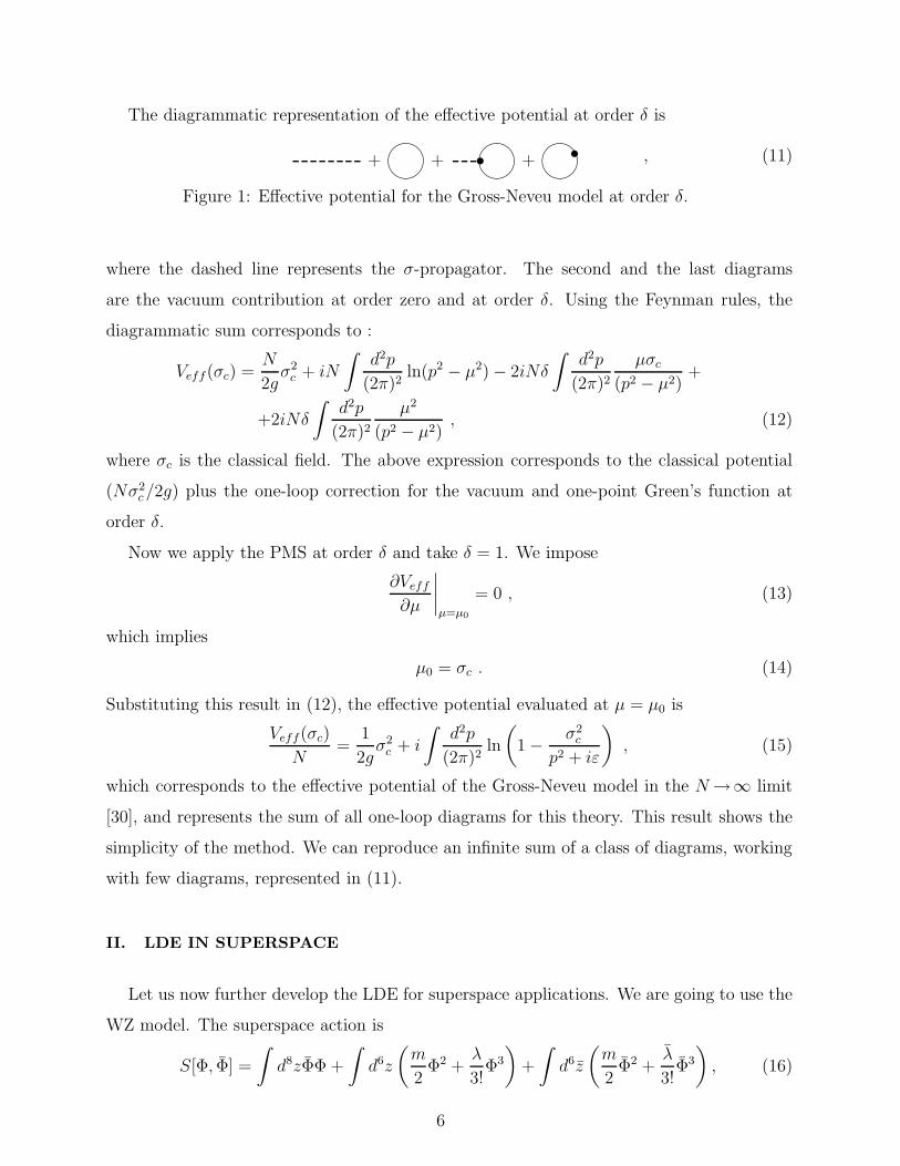
The diagrammatic representation of the effective potential at order δ is

+ ����

+ •����

+ ����

• , (11)

Figure 1: Effective potential for the Gross-Neveu model at order δ.

where the dashed line represents the σ-propagator. The second and the last diagrams

are the vacuum contribution at order zero and at order δ. Using the Feynman rules, the

diagrammatic sum corresponds to :

Veff(σc) =N

2gσ2

c + iN

∫

d2p

(2π)2ln(p2 − µ2) − 2iNδ

∫

d2p

(2π)2

µσc

(p2 − µ2)+

+2iNδ

∫

d2p

(2π)2

µ2

(p2 − µ2), (12)

where σc is the classical field. The above expression corresponds to the classical potential

(Nσ2c/2g) plus the one-loop correction for the vacuum and one-point Green’s function at

order δ.

Now we apply the PMS at order δ and take δ = 1. We impose

∂Veff

∂µ

∣

∣

∣

∣

µ=µ0

= 0 , (13)

which implies

µ0 = σc . (14)

Substituting this result in (12), the effective potential evaluated at µ = µ0 is

Veff(σc)

N=

1

2gσ2

c + i

∫

d2p

(2π)2ln

(

1 −σ2

c

p2 + iε

)

, (15)

which corresponds to the effective potential of the Gross-Neveu model in the N→∞ limit

[30], and represents the sum of all one-loop diagrams for this theory. This result shows the

simplicity of the method. We can reproduce an infinite sum of a class of diagrams, working

with few diagrams, represented in (11).

II. LDE IN SUPERSPACE

Let us now further develop the LDE for superspace applications. We are going to use the

WZ model. The superspace action is

S[Φ, Φ] =

∫

d8zΦΦ +

∫

d6z

(

m

2Φ2 +

λ

3!Φ3

)

+

∫

d6z

(

m

2Φ2 +

λ

3!Φ3

)

, (16)

6

where we have the notation d8z = d4xd2θd2θ, d6z = d4xd2θ, d6z = d4xd2θ. Using the non-

renormalization theorems, the more general effective action for the WZ model is written

as

Γ[Φ, Φ] =

∫

d8z[

K(Φ,Φ) + ...]

(17)

where the first term is the Kahler Potential and the other terms involve derivatives of the

fields. The effective action can be calculated perturbatively directly in superspace using

superspace Feynman rules. Here we use the improved Feynman rules defined originally in

[27].

Let us start to apply the LDE in the WZ model. The first modification is to implement

two mass parameters, µ and µ, instead of just one. In order to fix these parameters we use

two optimization equations. In particular we use the FAC criterion, so that we have one

equation similar to (4) for µ and other for µ. Using two mass parameters the Lagrangian

Lδ can be written as

Lδ = δL + (1 − δ)L0

=

∫

d4θΦΦ +

∫

d2θ

(

M

2Φ2 +

δλ

3!Φ3 −

δµ

2Φ2

)

+

+

∫

d2θ

(

M

2Φ2 +

δλ

3!Φ3 −

δµ

2Φ2

)

, (18)

where M = m+µ and M = m+ µ. The action Sδ can be written using the matrix notation

as [28]

Sδ[Φ, Φ] =1

2

∫

dz dz′(

Φ(z) Φ(z))

H(M,M)

Φ(z′)

Φ(z′)

+

∫

d6z

(

δλ

3!Φ3 −

δµ

2Φ2

)

+

∫

d6z

(

δλ

3!Φ3 −

δµ

2Φ2

)

, (19)

where

H(M,M) =

M −14D2

−14D2 M

δ+(z, z′) 0

0 δ−(z, z′)

. (20)

Now one has a new chiral and antichiral quadratic interaction proportional to δµ and δµ.

Also, the superpropagator GM,M , defined in terms of the chiral and antichiral delta functions

(δ+(z, z′), δ−(z, z′)) by the equation

G(M,M)H(M,M) =

δ+(z, z′) 0

0 δ−(z, z′)

, (21)

7

has shifted mass terms M = m + µ and M = m + µ. The new Feynman rules can now be

written as:

• 1. Propagators:

ΦΦ : −i

k2 +MMδ4(θ − θ′) ,

ΦΦ :iM

k2(k2 +MM )

1

4D2(k)δ4(θ − θ′) , (22)

ΦΦ :iM

k2(k2 +MM )

1

4D2(k)δ4(θ − θ′) ;

• 2. Vertices:

• = iδλ

∫

d8z , ◦ = iδλ

∫

d8z ,

× = −iδ

∫

µd8z , (23)

⊗ = −iδ

∫

µd8z .

The perturbative effective Kahler potential can be calculated in powers of δ using the

OPI functions. It is well-known that, in superspace, vacuum superdiagrams are identically

zero, owing to Berezin integrals. To avoid this, we have to consider, from the very beginning,

the parameters µ, µ as superfields and keep the vacuum supergraphs until the optimization

procedure. From the supergenerator functional in the presence of the chiral (J) and antichiral

(J) sources:

Z[J, J ] = exp

[

iSINT

(

1

i

δ

δJ,1

i

δ

δJ

)]

exp

i

2(J, J)G(M,M)

J

J

, (24)

we can write the super-effective action:

Γ[Φ, Φ] = −i

2ln[sDet

(

G(M,M))

] − i ln Z[J, J ] −

∫

d6zJ(z)Φ(z) −

∫

d6zJ(z)Φ(z), (25)

where sDet(

G(M,M))

is the superdeterminant of the matrix propagator, which in general is

equal to one, but here we keep it because G(M,M) depends on µ and µ. Also, due to the

µ and µ dependence, the vacuum diagrams supergenerator Z[0, 0] is not identically equal

8

to one. We can define the normalized functional generator as ZN = Z[J,J]

Z[0,0]and write the

effective action as

Γ[Φ, Φ] = −i

2ln[sDet(G)] − i ln Z[J0, J0] + ΓN [Φ, Φ] , (26)

where the sources J0 and J0 are defined by the equations

δW [J, J ]

δJ(z)|J=J0

=δW [J, J ]

δJ(z)|J=J0

=δZ[J, J ]

δJ(z)|J=J0

=δZ[J, J ]

δJ(z)|J=J0

= 0 . (27)

In equation (26) the first two terms represent the vacuum diagrams (which are usually zero)

and ΓN [Φ, Φ] is the usual contribution to the effective action.

III. KAHLER POTENTIAL IN THE LDE USING THE FAC CRITERION

Let us now calculate the Kahler potential using the LDE up to the order δ2. We are going

to show that this corresponds to the Coleman-Weinberg potential plus a sum of infinite two-

loop supergraphs.

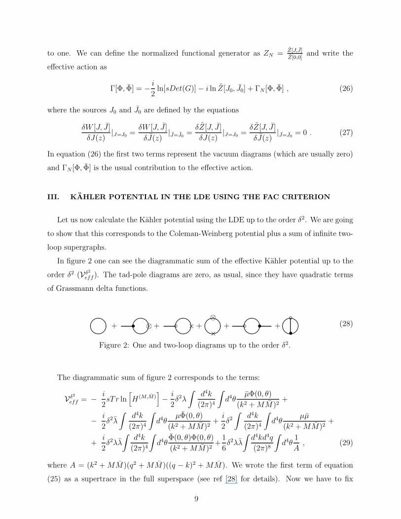
In figure 2 one can see the diagrammatic sum of the effective Kahler potential up to the

order δ2 (Vδ2

eff). The tad-pole diagrams are zero, as usual, since they have quadratic terms

of Grassmann delta functions.

����

+ •����

⊗ + ◦����

× + ����⊗

×+ ◦��

��• + ��

��◦

•(28)

Figure 2: One and two-loop diagrams up to the order δ2.

The diagrammatic sum of figure 2 corresponds to the terms:

Vδ2

eff = −i

2sTr ln

[

H(M,M)]

−i

2δ2λ

∫

d4k

(2π)4

∫

d4θµΦ(0, θ)

(k2 +MM )2+

−i

2δ2λ

∫

d4k

(2π)4

∫

d4θµΦ(0, θ)

(k2 +MM)2+i

2δ2

∫

d4k

(2π)4

∫

d4θµµ

(k2 +MM)2+

+i

2δ2λλ

∫

d4k

(2π)4

∫

d4θΦ(0, θ)Φ(0, θ)

(k2 +MM )2+

1

6δ2λλ

∫

d4kd4q

(2π)8

∫

d4θ1

A, (29)

where A = (k2 + MM )(q2 + MM )((q − k)2 + MM ). We wrote the first term of equation

(25) as a supertrace in the full superspace (see ref [28] for details). Now we have to fix

9

the mass parameters and write the Kahler potential of equation (28) at δ = 1 in terms of

the optimized parameters µ0 and µ0. The FAC criterion is employed as an optimization

procedure. In order to calculate the Kahler effective potential up to order 2 in δ (Vδ2

eff) we

have to solve for µ0 and µ0 the equation

c3(µ, µ) = 0 , (30)

at δ = 1, where c3(µ, µ) corresponds to the δ3 coefficients in the perturbative expansion of

the Kahler potential.

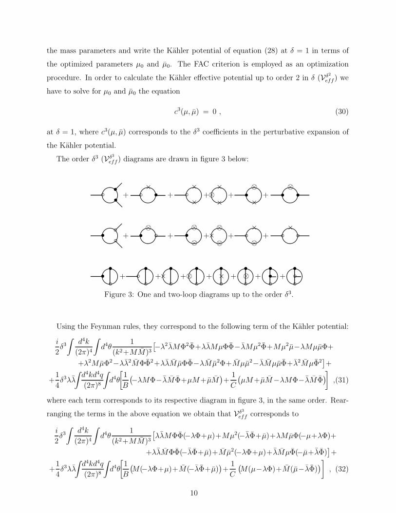
The order δ3 (Vδ3

eff) diagrams are drawn in figure 3 below:

����◦

•

•

@

�+ ◦��

��ו + ��

��◦×

×+ ��

��⊗

×

×+ ��

��•⊗

×+ ��

��• •⊗

����•

◦

◦

@

�+ •��

��⊗◦ + ��

��•⊗

⊗+ ��

��×

⊗

⊗+ ��

��◦×

⊗+ ��

��◦ ◦×

����•◦

•+ ��

��◦◦

•+ ��

��×

◦

•+ ��

��⊗

◦

•+��

��×◦

•+��

��⊗◦

•+��

��•◦

•+��

��◦◦

•

Figure 3: One and two-loop diagrams up to the order δ3.

Using the Feynman rules, they correspond to the following term of the Kahler potential:

i

2δ3

∫

d4k

(2π)4

∫

d4θ1

(k2+MM)3

[

−λ2λMΦ2Φ+λλMµΦΦ−λMµ2Φ+Mµ2µ−λMµµΦ+

+λ2MµΦ2−λλ2MΦΦ2+λλMµΦΦ−λMµ2Φ+Mµµ2−λMµµΦ+λ2MµΦ2]

+

+1

4δ3λλ

∫

d4kd4q

(2π)8

∫

d4θ

[

1

B

(

−λMΦ−λM Φ+µM+µM)

+1

C

(

µM+µM−λMΦ−λM Φ)

]

,(31)

where each term corresponds to its respective diagram in figure 3, in the same order. Rear-

ranging the terms in the above equation we obtain that Vδ3

eff corresponds to

i

2δ3

∫

d4k

(2π)4

∫

d4θ1

(k2+MM)3

[

λλMΦΦ(−λΦ+µ)+Mµ2(−λΦ+µ)+λMµΦ(−µ+λΦ)+

+λλMΦΦ(−λΦ+µ)+Mµ2(−λΦ+µ)+λMµΦ(−µ+λΦ)]

+

+1

4δ3λλ

∫

d4kd4q

(2π)8

∫

d4θ

[

1

B

(

M(−λΦ+µ)+M(−λΦ+µ))

+1

C

(

M(µ−λΦ)+M(µ−λΦ))

]

, (32)

10

where C = (k2+MM)(q2+MM)((q−k)2+MM)2 and B = (k2+MM)2(q2+MM)((q−k)2+

MM ). From the above equation we can derive the following simple solution for equation

(30), before calculating the integrals:

µ0 = λΦ ,

µ0 = λΦ . (33)

Finally, substituting this solution into equation (29) at δ = 1 we have only two terms for

the optimized Kahler potential:

Veff = −i

2sTr ln

[

H(M0,M0)]

+

+1

6λλ

∫

d4kd4q

(2π)8

∫

d4θ1

(k2 +M0M0)(q2 +M0M0)((q − k)2 +M0M0), (34)

where H(M0,M0) is the same as H(M,M) defined in (20) replacing M by M0 = m + λΦ and

M by M0 = m + λΦ. The first one corresponds to the Coleman-Weinberg potential and

it represents the sum of all one-loop supergraphs. The second corresponds to a sum of

infinite Feynman diagrams that belong to a special set of two-loop diagrams. We can now

regularize the integrals and go ahead by adopting renormalization approaches compatible

with supersymmetry [31].

IV. CONCLUDING REMARKS

We have applied superspace and supergraph techniques to carry out the LDE for the WZ

model. We understand that this is a first step towards a more substantial programme of

applications of the efficacy of supergraph methods to compute quantum corrections in the

framework of supersymmetric field theories.

The next natural systems to probe the method are the O’Raifeartaigh [32] and Fayet-

Iliopoulos [33] models, which realise the spontaneous breaking of supersymmetry. We have

interesting non-renormalisation theorems [31] to be satisfied and these calculations may be

a good test for the LDE in the situation of spontaneous breaking of supersymmetry.

More relevant for phenomenology are the models in which the soft explicitly breaking

terms are introduced. The latter have been carefully classified and studied by Girardello

and Grisaru, in the work of reference [34]. With those (phenomenologically interesting)

terms, supergraph techniques become less obvious, but they have anyhow been extended to

11

include the effect of the supersymmetry breaking parameters to all orders [9]. We believe that

the application of the LDE to such a class of models may be relevant for the understanding

of the method and also for the sake of application in phenomenologically realistic models

based on supersymmetry. We shall be reporting on these results in a forthcoming work.

Finally, we point out that it would be of interest to investigate the control of the con-

vergence of the LDE in superspace. This question has not yet been adressed to, but its

development could bring a new insight and new elements in the extension of the LDE to

superspace.

[1] I. L. Buchbinder, S. D. Odintsov and I. L. Shapiro, “Effective Action in Quantum Gravity”,

Taylor and Francis Group.

[2] A. Salam and J. J. Strathdee, Phys. Rev. D 9 (1974) 1129.

[3] S. Y. Lee and Alain M. Sciaccaluga, Nucl. Phys. B 96 (1975) 435.

[4] S. Weinberg, Phys. Rev. D 7 (1973) 2887.

[5] T. Hagiwara and Burt A. Ovrut, Phys. Rev. D 20 (1979) 1988.

[6] Burt A. Ovrut, Phys. Rev. D 20 (1979) 1446.

[7] I. J. R. Aitchison and C. M. Fraser, Annals Phys. 156 (1984) 1.

[8] R. D. C. Miller, Phys. Lett. 124 B (1983) 59.

[9] J. A. Helayel-Neto, Phys. Lett. 135 (1984) 78-84.

[10] F. Feruglio, J. A. Helayel-Neto and F. Legovini, Nucl. Phys. B 249 (1985) 533-556.

[11] P. P. Srivastava, Phys. Lett. 132 B (1983) 83.

[12] S. J. Gates, M. T. Grisaru, M. Rocek and W. Siegel, Front. Phys. 58 (1983) 1

[arXiv:hep-th/0108200].

[13] V. A. Novikov, M. A. Shifman, A. I. Vainshtein and V. I. Zakharov, Nucl. Phys. B 223 (1983)

445.

[14] M. A. Shifman and A. I. Vainshtein, Nucl. Phys. B 277 (1986) 456 [Sov. Phys. JETP 64 (1986

ZETFA,91,723-744.1986) 428].

[15] N. Seiberg, Phys. Lett. B 318 (1993) 469 [arXiv:hep-ph/9309335].

[16] N. Seiberg, Phys. Rev. D 49 (1994) 6857 [arXiv:hep-th/9402044].

[17] K. A. Intriligator, R. G. Leigh and N. Seiberg, Phys. Rev. D 50 (1994) 1092

12

[arXiv:hep-th/9403198].

[18] S. Coleman and E. Weyberg, Phys. Rev. D7, 1973, 1888.

[19] R. Jackiw, Phys. Rev. D 9 (1974) 1686.

[20] A. Okopinska, Phys. Rev. D 35 (1987) 1835.

A. Duncan and M. Moshe, Phys. Lett. B 215 (1988) 352.

[21] J. L. Kneur, M. B. Pinto and R. O. Ramos, Phys. Rev. A 68 (2003) 043615

[arXiv:cond-mat/0207295].

[22] David J. Gross and Andre Neveu, Phys. Rev. D 10 (1974) 3235-3253.

[23] P. M. Stevenson, Phys. Rev. D 23 (1981) 2916.

[24] S. K. Gandhi, H. F. Jones and M. B. Pinto, Nucl. Phys. B 359 (1991) 429.

[25] J. L. Kneur, M. B. Pinto, R. O. Ramos and E. Staudt, Phys. Rev. D 76 (2007) 045020

[arXiv:0705.0676 [hep-th]].

[26] J. L. Kneur, M. B. Pinto and R. O. Ramos, Phys. Rev. D 74 (2006) 125020

[arXiv:hep-th/0610201].

[27] M. T. Grisaru, W. Siegel and M. Rocek, Nucl. Phys. B 159 (1979) 429.

[28] Ioseph L. Buchbinder and Sergei M. Kuzenko, “Ideas and methods of supersymmetry and

supergravity, or a walk through superspace”, revised edition, Institute of Physics Publishing.

[29] Sidney Coleman, “Aspects of Symmetry”, Selected Erice Lectures, Cambridge University

Press.

[30] Sidney Coleman, R. Jackiw and H. D. Politzer, Phys. Rev. D10 (1974) 2491-2499.

[31] S. J. Gates, Jr. , M. T. Grisaru, M. Rocek and W. Siegel, “Superspace, or a thousand and

one lessons in supersymmetry”, The Benjamin/Cummings Publishing Company, Inc.

[32] L. O’Raifeartaigh, Nucl. Phys. B 96 (1975) 331.

[33] P. Fayet and J. Iliopoulos, Phys. Lett. 51 B (1974) 461.

[34] L. Girardello and M. T. Grisaru, Nucl. Phys. B 194 (1982) 65.

13