Preprint typeset in JHEP style - HYPER VERSION CERN-PH-TH/2009-036

Strong Double Higgs Production at the LHC

Roberto Contino

Dipartimento di Fisica, Universita di Roma “La Sapienza”

INFN, Sezione di Roma, Italy

CERN, Physics Department, Theory Unit, Geneva, Switzerland

Christophe Grojean

CERN, Physics Department, Theory Unit, Geneva, Switzerland

Institut de Physique Theorique, CEA Saclay, France

Mauro Moretti

Dipartimento di Fisica, Universita di Ferrara, and INFN, Sezione di Ferrara, Italy

Fulvio Piccinini

INFN, Sezione di Pavia, Italy

Riccardo Rattazzi

Institut de Theorie des Phenomenes Physiques, EPFL, Lausanne, Switzerland

Abstract: The hierarchy problem and the electroweak data, together, provide a plausible

motivation for considering a light Higgs emerging as a pseudo-Goldstone boson from a

strongly-coupled sector. In that scenario, the rates for Higgs production and decay differ

significantly from those in the Standard Model. However, one genuine strong coupling

signature is the growth with energy of the scattering amplitudes among the Goldstone

bosons, the longitudinally polarized vector bosons as well as the Higgs boson itself. The

rate for double Higgs production in vector boson fusion is thus enhanced with respect to

its negligible rate in the SM. We study that reaction in pp collisions, where the production

of two Higgs bosons at high pT is associated with the emission of two forward jets. We

concentrate on the decay mode hh → WW (∗)WW (∗) and study the semi-leptonic decay

chains of the W ’s with 2, 3 or 4 leptons in the final states. While the 3 lepton final states

are the most relevant and can lead to a 3σ signal significance with 300 fb−1 collected at a

14 TeV LHC, the two same-sign lepton final states provide complementary information. We

also comment on the prospects for improving the detectability of double Higgs production

at the foreseen LHC energy and luminosity upgrades.

Keywords: Higgs, Electroweak symmetry breaking, Composite models.

arX

iv:1

002.

1011

v2 [

hep-

ph]

24

May

201

0

Contents

1. Introduction 1

2. General parametrization of Higgs couplings 3

3. Anatomy of V V → V V and V V → hh scatterings 7

3.1 V V → V V scattering 7

3.2 V V → hh scattering 13

4. The analysis 15

4.1 Channel S3: three leptons plus one hadronically-decaying W 16

4.1.1 Estimate of showering effects 23

4.1.2 Additional backgrounds from fake leptons 24

4.2 Channel S2: two same-sign leptons plus two hadronically-decaying W ’s 25

4.2.1 Estimate of showering effects 30

4.2.2 Fake leptons and lepton charge misidentification 31

4.3 Channel S4: four leptons 33

4.4 Results 35

5. Features of strong double Higgs production 37

6. Higgs mass dependence 38

7. Luminosity vs energy upgrade 40

8. Conclusions and outlook 47

A. Model parameters 50

B. Montecarlo generation 50

1. Introduction

It is clear that, in addition to the four known fundamental forces (gravity, electromag-

netism, the weak and the strong interactions), new dynamics must exist in order to account

for the observed phenomenon of electroweak symmetry breaking (EWSB). Luckily the state

of our knowledge is about to change as the Large Hadron Collider (LHC) is set to directly

explore, for the first time in history, the nature of this dynamics. A basic question the

LHC will address concerns the strength of the new dynamics: is the force behind EWSB

a weak or a strong one? In most regards this question is equivalent to asking whether a

1

light Higgs boson exists or not. This is because in the absence of new states (in particular

the Higgs boson) the strength of the interaction among the longitudinally polarized vector

bosons grows with energy becoming strong at around 1 or 2 TeV’s. The Standard Model

(SM) Higgs boson plays instead the role of ‘moderator’ of the strength of interactions,

and allows the model to be extrapolated at weak coupling down to very short distances,

possibly down to the Unification or Planck scale [1]. In order to achieve this amazing goal

the couplings of the SM Higgs are extremely constrained and predicted in terms of just

one new parameter, the mass of the Higgs itself. In such situation, the SM Higgs is for

all practical purposes an elementary particle. However it is also possible, and plausible in

some respects, that a light and narrow Higgs-like scalar does exist, but that this particle

is a bound state from some strong dynamics not much above the weak scale. In such a

situation the couplings of the Higgs to fermions and vector bosons are expected to deviate

in a significant way from those in the SM, thus indicating the presence of an underlying

strong dynamics. Provided such deviations are discovered, the issue will be to understand

the nature of the strong dynamics. In that perspective the importance of having a well

founded, but simple, theoretical picture to study the Higgs couplings at the LHC cannot

be overemphasized.

The hierarchy problem and electroweak data, together, provide a plausible motivation

for considering a light composite Higgs. It is well known that the absence of an elementary

Higgs scalar nullifies the hierarchy problem. Until recently the idea of Higgs composite-

ness was basically seen as coinciding with the so called Higgsless limit, where there exists

no narrow light scalar resonance. The standard realization of this scenario is given by

Technicolor models [2]. However, another possibility, which is now more seriously con-

sidered, is that the Higgs, and not just the eaten Goldstone bosons, arises as a naturally

light pseudo-Goldstone boson from strong dynamics just above the weak scale [3, 4, 5, 6].

This possibility is preferable over standard Technicolor in view of electroweak precision

constraints. The reason is that the electroweak breaking scale v is not fixed to coincide

exactly with the strong dynamics scale f , like it was for Technicolor. Indeed v is now

determined by additional parameters (in explicit models these can be the top Yukawa and

the SM gauge couplings) and it is conceivable to have a situation where there is a small

separation of scales. As a matter of fact v ∼< 0.3f is enough to largely eliminate all tension

with the data. The pseudo-Goldstone Higgs is therefore a plausible scenario at the LHC. In

that respect one should mention another possibility that was considered recently where the

role of the Higgs is partially played by a composite dilaton, that is the pseudo-Goldstone

boson of spontaneously broken scale invariance [7]. This second possibility is less moti-

vated than the previous one as regards electroweak data, in that, like in Technicolor, no

parameter exists to adjust the size of S (and T ). However it makes definite predictions

for the structure of the couplings, that are distinguished from the pseudo-Goldstone case.

The existence of the dilaton example suggests that it may be useful to keep a more ample

perspective on “Higgs” physics.

The effective Lagrangian for a composite light Higgs was characterized in Ref. [6], also

focussing on the pseudo-Goldstone scenario. It was shown that the Lagrangian is described

at lowest order by a very few parameters, and, in particular, in the pseudo-Goldstone case,

2

only two parameters cH and cy are relevant at the LHC. Both parameters modify in a

rather restricted way the Higgs production rate and branching ratios. In particular, the

parameter cH , that corresponds to the leading non-linearity in the σ-model kinetic term,

gives a genuine “strong coupling” signature by determining a growing amplitude for the

scattering among longitudinal vector bosons. As seen in the unitary gauge, because of

its modified coupling to vectors, the Higgs fails to completely unitarize the scattering

amplitude. This is the same σ-model signature one has in Technicolor. The novelty is

that the Higgs is also composite belonging to the σ-model, and thus the same growth with

energy is found in the amplitude for VLVL → hh (V = W,Z). One signature of this class

of models at hadron collider is therefore a significant enhancement over the (negligible)

SM rate for the production of two Higgs bosons at high pT along with two forward jets

associated with the two primary partons that radiated the VLVL pair. The goal of the

present paper is to study the detectability of this process at the LHC and at its foreseen

energy and luminosity upgrades.

2. General parametrization of Higgs couplings

In this section we will introduce a general parametrization of the Higgs couplings to vectors

and fermions. The goal is to describe deviations from the SM in Higgs production and

decay.

We are interested in the general situation in which a light scalar h exists in addition

to the vectors and the eaten Goldstones associated to the breaking SU(2) × U(1)Y →U(1)Q. By the request of custodial symmetry, the Goldstone bosons describe the coset

SO(4)/SO(3) and can be fit into the 2× 2 matrix

Σ = eiσaπa/v v = 246 GeV . (2.1)

By working at sufficiently low energy with respect to any possible strong scale, we can

perform a derivative expansion. The leading effects growing with energy arise at the 2-

derivative level, and so we truncate our Lagrangian at this order. Moreover we assume

that the gauge fields are coupled to the strong sector via weak gauging: the operators

involving the field strengths Wµν and Bµν will appear with loop suppressed coefficients,

and we neglect them. Similarly, we assume that the elementary fermions are coupled to

the strong sector only via the (proto)-Yukawa interactions, so that the leading effects will

not involve derivatives (e.g. operators involving the product of a fermionic and σ-model

current will be suppressed).

Under these assumptions the most general Lagrangian is 1

L =1

2(∂µh)2 − V (h) +

v2

4Tr(DµΣ†DµΣ

)[1 + 2a

h

v+ b

h2

v2+ . . .

]−mi ψLi Σ

(1 + c

h

v+ . . .

)ψRi + h.c. ,

(2.2)

1In general c can be a matrix in flavor space, but in the following we will assume for simplicity that it

is proportional to unity in the basis in which the mass matrix is diagonal. In this way no flavor-changing

neutral current effects originate from the tree-level exchange of h.

3

where V (h) denotes the potential for h

V (h) =1

2m2hh

2 + d31

6

(3m2

h

v

)h3 + d4

1

24

(3m2

h

v2

)h4 + . . . (2.3)

and a, b, c, d3, d4 are arbitrary numerical parameters. We have neglected terms of higher

order in h (denoted by the dots) as they do not affect the leading 2 → 2 processes. For

a = b = c = d3 = d4 = 1 and vanishing higher order terms, the scalar h can be embedded

into a linear multiplet

U ≡(

1 +h

v

)Σ , (2.4)

and one obtains the SM Higgs doublet Lagrangian. The role of a, b and c in 2→ 2 processes

is easily seen by working in the equivalent Goldstone boson approximation [8], according to

which longitudinal vector bosons can be replaced by the corresponding Goldstone bosons

at high energy, V iL ↔ πi. The parameter a controls the strength of the VLVL → VLVL

scattering (V = W,Z), see Fig. 1 (upper row). At the two derivative level the Goldstone

scattering amplitude is

A(πiπj → πkπl) = δijδklA(s) + δikδjlA(t) + δilδjkA(u) (2.5)

with

A(s) ' s

v2(1− a2) (2.6)

where subleading terms in (M2W /s) have been omitted. Perturbative unitarity is thus

satisfied for a = 1. The parameter b instead controls the process VLVL → hh, see Fig. 1

(lower row),

A(πiπj → hh) ' δijs

v2(b− a2) . (2.7)

In this case perturbative unitarity is satisfied for b = a2. Notice that an additional contri-

bution from the s-channel Higgs exchange via the trilinear coupling d3 has been omitted

because subleading at high energy. In fact, as it will be shown in the following sections,

in a realistic analysis of double Higgs production at the LHC such contribution can be

numerically important and lead to a significant model dependency. Finally the parameter

c controls the VLVL → ψψ amplitude

A(πiπj → ψψ) = δijmψ√s

v2(1− ac) , (2.8)

which is weak for ac = 1. Hence, as well known, only for the SM choice of parameters

a = b = c = 1 the theory is weakly coupled at all scales.

From the above general perspective, the study of V V → V V , V V → hh and V V → ψψ

tests three different parameters. However, in specific models a, b and c can be related

to each other. For instance in the pseudo-Goldstone Higgs models based on the coset

SO(5)/SO(4) [4, 5], indicating by f the decay constant of the σ-model and defining ξ ≡v2/f2, one has

a =√

1− ξ b = 1− 2ξ . (2.9)

4

+ crossed

+ crossed

Figure 1: Leading diagrams for the VLVL → VLVL (upper row) and VLVL → hh (lower row)

scatterings at high energies.

The parameter c, on the other hand, depends on which SO(5) representation the SM

fermions belong to. For examples, fermions in spinorial and fundamental representations

of SO(5) imply:

c =√

1− ξ spinorial representation (4 of SO(5)) (2.10)

c =1− 2ξ√

1− ξfundamental representation (5 of SO(5)) . (2.11)

By expanding the above equations at small ξ, the result matches the general expressions

obtained by using the Strongly Interacting Light Higgs (SILH) Lagrangian in the notation

of Ref. [6]

a = 1− cH2ξ b = 1− 2cHξ c = 1−

(cH2

+ cy

)ξ . (2.12)

In particular, fermions in the spinorial (fundamental) representations of SO(5) correspond

to cy = 0 (cy = 1). Notice however that the general SILH parametrization applies more

generally to a light composite SU(2)L Higgs doublet, regardless of whether it has a pseudo-

Goldstone boson interpretation. The prediction for d3 and d4 is more model dependent, as

it relies on the way the Higgs potential is generated. As benchmark values for the trilinear

coupling d3 we consider those predicted in the SO(5)/SO(4) minimal models of Ref. [4]

(MCHM4) and Ref. [5] (MCHM5), respectively with spinorial and fundamental fermion

representations, where the Higgs potential is entirely generated by loops of SM fields: 2

d3 =√

1− ξ MCHM4 with spinorial representations of SO(5) (2.13)

d3 =1− 2ξ√

1− ξMCHM5 with vector representations of SO(5) . (2.14)

2The singularity for ξ → 1 in Eqs. (2.11) and (2.14) appears because this limit is approached by keeping

the mass of the Higgs and of the fermions fixed.

5

Another, distinct example arises when h represents the dilaton from spontaneously

broken scale invariance. There one obtains a different relation among a, b and c. Indeed

the dilaton case corresponds to the choice a2 = b = c2 with the derivative terms in the

Lagrangian exactly truncated at quadratic order in h. For this choice one can define the

dilaton decay constant by v/a ≡ fD, the dilaton field as

eφ/fD = 1 +h

fD(2.15)

and the Lagrangian can be rewritten as [7]

L = e2φ/fD

[1

2(∂µφ)2 +

v2

4Tr(DµΣ†DµΣ

)]−(mi e

φ/fD ψLiΣψRi + h.c.)

(2.16)

as dictated by invariance under dilatations

φ(x)→ φ(xeλ) + λfD πa(x)→ πa(xeλ) ψ(x)→ e3λ/2 ψ(xeλ) . (2.17)

Notice that in the case of a SILH all the amplitudes of the three processes discussed above

grow with the energy. On the other hand, in the dilaton case the relation a2 = b ensures

that the amplitude for V V → hh does not feature the leading growth ∝ s. The wildly

different behaviour of the process V V → hh is what distinguishes the case of a genuine,

but otherwise composite Higgs, from a light scalar, the dilaton, which is not directly linked

to the breakdown of the electroweak symmetry. Another difference which is worth pointing

out between the specific case of a pseudo–Goldstone Higgs and a dilaton or a composite

non-Goldstone Higgs has to do with the range of a, b, c. In the case of a pseudo-Goldstone

Higgs one can prove in general that a, b < 1 [9], while all known models also satisfy c < 1.

Instead one easily sees that in the dilaton case depending on fD > v or fD < v one

respectively has a, b, c < 1 or a, b, c > 1.

In general the couplings a, b, c also parametrize deviations from the SM in the Higgs

branching ratios. However, for the specific case of the dilaton the relative branching ratios

into vectors and fermions are not affected. Instead, for loop induced processes like h→ γγ

or gg → h, deviations of order 1 with respect to the Standard Higgs occur due to the trace

anomaly contribution [10]. Similarly, in the pseudo-Goldstone Higgs case with matter in

the spinorial representation, the dominant branching ratios to fermions and vectors are not

affected. On the other hand, in the case with matter in the fundamental representation the

phenomenology can be dramatically changed when ξ ∼ O(1). From Eqs. (2.9) and (2.11)

we haveΓ(h→ ψψ)

Γ(h→ V V )=

(1− 2ξ

1− ξ

)2 Γ(h→ ψψ)

Γ(h→ V V )

∣∣∣SM

, (2.18)

so that around ξ ∼ 1/2 the width into fermions is suppressed. In this case, even for mh

significantly below the 2W threshold the dominant decay channel could be the one to

WW ∗. In Fig. 2 we show the Higgs branching ratios as a function of ξ in this particular

model. The possibility to have a moderately light Higgs decaying predominantly to vectors

is relevant to our study of double Higgs production. It turns out that only when such decay

channel dominates do we have a chance to spot the signal over the SM backgrounds.

6

0.2 0.4 0.6 0.8 10.0001

0.001

0.01

0.1

1

bbWWττZZγγ

ξ

Higg

s BR

smH=120 GeV

0 0.2 0.4 0.6 0.8 10.00001

0.0001

0.001

0.01

0.1

1

WWZZbbττγγ

ξ

Higg

s BR

s

mH=180 GeV

Figure 2: Higgs decay branching ratios as a function of ξ for SM fermions embedded into

fundamental representations of SO(5) for two benchmark Higgs masses: mh = 120 GeV (left plot)

and mh = 180 GeV (right plot). For ξ = 0.5, the Higgs is fermiophobic, while in the Technicolor

limit, ξ → 1, the Higgs becomes gaugephobic.

One final remark must be made concerning the indirect constraints that exist on a, b, c.

As stressed by the authors of Ref. [11], the parameter a is constrained by the LEP precision

data: modifying the Higgs coupling to the SM vectors changes the one-loop infrared con-

tribution to the electroweak parameters ε1,3 by an amount ∆ε1,3 = c1,3(1−a2) log(Λ2/m2h),

where c1 = −3α(MZ)/16π cos2 θW , c3 = α(MZ)/48π sin2 θW and Λ denotes the mass

scale of the resonances of the strong sector. For example, assuming no additional correc-

tions to the precision observables and setting mh = 120 GeV, Λ = 2.5 TeV, one obtains

0.8 . a2 . 1.5 at 99% CL. However, such constraint can become weaker (or stronger) in

presence of additional contributions to ε1,3. For that reason in our analysis of double Higgs

production we will keep an open mind on the possible values of a. On the other hand, no

indirect constraint exists on the parameters b, c, thus leaving open the possibility of large

deviations from perturbative unitarity in the V V → hh and V V → ψψ scatterings.

3. Anatomy of V V → V V and V V → hh scatterings

3.1 V V → V V scattering

The key feature of strong electroweak symmetry breaking is the occurrence of scattering

amplitudes that grow with the energy above the weak scale. We thus expect them to

dominate over the background at high enough energy. Indeed, with no Higgs to unitarize

the amplitudes, on dimensional grounds, and by direct inspection of the relevant Feynman

diagrams, one estimates [12]

A(VTVT → VTVT ) ∼ g2f(t/s) and A(VLVL → VLVL) ∼ s

v2(3.1)

with f(t/s) a rational function which is O(1), at least formally, in the central region

7

Figure 3: The full set of diagrams for qq → WWqq at order g4W . The blob indicates the sum of

all possible WW →WW subdiagrams. It is understood that the bremsstrahlung diagrams (second

and third diagrams) correspond to all possible ways to attach an outgoing W to the quark lines.

−t = O(s). Then, according to the above estimates, in the central region we have

dσLL→LL/dt

dσTT→TT /dt

∣∣∣t∼−s/2

= Nhs2

M4W

, (3.2)

where Nh is a numerical factor expected to be of order 1. On the other hand, f(t/s) has

simple Coulomb poles in the forward region, due to t- and u-channel vector exchange. Then,

after imposing a cut 3 −s + Q2min < t < −Q2

min, with M2W � Q2

min � s, the expectation

for the integrated cross sections is

σLL→LL(Qmin)

σTT→TT (Qmin)= Ns

sQ2min

M4W

. (3.3)

Here again Ns is a numerical factor expected to be of order 1. By the above estimates,

we expect the longitudinal cross section, both the hard one and the more inclusive one, to

become larger than the transverse cross section right above the vector boson mass scale.

In reality the situation is more complicated because, since we do not posses on-shell

vector boson beams, the V ’s have first to be radiated from the colliding protons. Then

the physics of vector boson scattering is the more accurately reproduced the closer to

on-shell the internal vector boson lines are, see Fig. 3. This is the limit in which the

process factorizes into the collinear (slow) emission of virtual vector bosons a la Weizsacker–

Williams and their subsequent hard (fast) scattering [13, 14]. As evident from the collision

kinematics, the virtuality of the vector bosons is of the order of the pT of the outgoing

quarks. Thus the interesting limit is the one where the transverse momentum of the two

spectator jets is much smaller than the other relevant scales. In particular when

pTjet � pTW MW � pTW (3.4)

where pTW and pTjet respectively represent the transverse momenta of the outgoing vector

bosons and jets. In this kinematical region, the virtuality of the incoming vector bosons can

be neglected with respect to the virtuality that characterizes the hard scattering subdia-

grams. Then the cross section can be written as a convolution of vector boson distribution

3The offshellness of the W ’s radiated by the quarks in fact provides a natural cut on |t| and |u| of the

order of p4Tjet/s. Nevertheless, the total inclusive cross section is dominated by soft physics and does not

probe the dynamics of EW symmetry breaking.

8

functions with the hard vector cross section. It turns out that the densities for respec-

tively transverse and longitudinal polarizations have different sizes, and this adds an extra

relative factor in the comparison schematized above. In particular, the emission of trans-

verse vectors is logarithmically distributed in pT , like for the Weizsacker–Williams photon

spectrum. Thus we have that the transverse parton splitting function is [13]

P T (z) =g2A + g2

V

4π2

1 + (1− z)2

2zln

[p2T

(1− z)M2W

], (3.5)

where z indicates the fraction of energy carried by the vector boson and pT is the largest

value allowed for pT . On the other hand, the emission of longitudinal vectors is peaked at

pT ∼MW and shows no logarithmic enhancement when allowing large pT [13]

PL(z) =g2A + g2

V

4π2

1− zz

. (3.6)

Hence, by choosing a cut pTjet < pT with pT �MW the cross section for transverse vectors

is enhanced due to their luminosity by a factor (ln pT /MW )2. For reasonable cuts this is not

a very important effect though. At least, it is less important than the numerical factors Nh

and Ns that come out from the explicit computation of the hard cross section, and which

we shall analyze in a moment.

One last comment concerns the subleading corrections to the effective vector boson

approximation (EWA). On general grounds, we expect the corrections to be controlled by

the ratio p2Tjet/p

2TW , that is the ratio between the virtuality of the incoming vector lines

and the virtuality of the hard V V → V V subprocess 4. In particular, both in the fully

hard region pTjet ∼ pTW ∼√s and in the forward region pTjet, pTW ∼< mW we expect

the approximation to break down. In these other kinematic regions, the contribution of

the other diagrams in Fig. 3 is not only important but essential to obtain a physically

meaningful gauge independent result [14]. For the process qq → qqVTVT , when the cross

section is integrated over pTjet up to pT the subleading corrections to EWA become only

suppressed by 1/(ln pT /MW ). This is the same log that appears in P T (z). The process

qq → qqVTVT is not significantly affected by a strongly coupled Higgs sector. On the other

hand, in the presence of a strongly coupled Higgs sector, for qq → qqVLVL the EWA is

further enhanced with respect to subleading effects because of the underlying VLVL → VLVLstrong subprocess. Indeed, by applying the axial gauge analysis of Ref. [15], one finds that,

independent of the cut on pTjet, the subleading effects to the EWA are suppressed by at

least M2W /p

2TW .

Having made the above comments on vector boson scattering in hadron collisions, let

us now concentrate on the partonic process. We will illustrate our point with the example

of the W+W+ →W+W+ process (similar results can be obtained for the other processes)

in the case of the composite pseudo-Goldstone Higgs, where for a 6= 1 the longitudinal scat-

tering is dominated at large energies by the (energy-growing) contact interaction. Let us

4In fact, another kinematic parameter controlling the approximation is given by the invariant mass of

the W + jet subsystem m2JW = (pW + pjet)

2. In the region m2JW � s the bremsstrahlung diagrams are

enhanced by a collinear singularity. In a realistic experimental situation this region is practically eliminated

by a cut on the relative angle between the jet and the (boosted) decay products of the W ’s.

9

channel weight Atγ AtZ Auγ AuZ Areg. As

LL→ LL 1/2 2e2 g2(1−2c2W )2

2c2W2e2 g2(1−2c2W )2

2c2W

2(M2W−c

2Wm2

h)

c2W v2a2 − 1

LL→ TTLL→ ++ 1 0 0 0 0 g2(1− a2)/2 0

LL→ +− 1 0 0 0 0 g2(a2 − 1)/2 0

LT → LT L+→ L+ 4 2e2 −g2(1− 2c2W ) 0 0 g2(a2 − 1)/2 0

TT → TT++→ ++ 1 2e2 2g2c2

W 2e2 2g2c2W 0 0

+− → +− 2 2e2 2g2c2W 0 0 2g2 0

Table 1: W+W+ → W+W+ scattering: coefficients for the decomposition of the amplitude

according to Eq. (3.7). Of the 13 independent polarization channels those not shown above can be

obtained by either crossing or complex conjugation due to Bose symmetry. Cross sections can be

computed by weighting each channel in the table by the corresponding multiplicity factor reported

in the third column. Only channels with non-vanishing coefficients in the decomposition of Eq. (3.7)

are shown. Terms proportional to (1 − a2) have been omitted for simplicity in the expression of

Areg. in the LL→ LL channel.

then compare the semihard and hard cross sections for different polarizations as prospected

in Eqs. (3.2) and (3.3). Considering first the case s � M2W with fixed t and u, for each

polarization channel we can write the amplitude as 5

A 'Atγ s

t+

AtZ s

t−M2Z

+Auγ s

u+

AuZ s

u−M2Z

+Areg. +Ass

v2, (3.7)

where the A’s are numerical constants which take different values for the different polar-

ization channels (see Table 1). The coefficients At,u are easily computed in the eikonal

approximation and are directly related to the electric- and SU(2)L- charges of the W ’s:

Aγ = 2× (electric charge of W+)2 and AZ = 2× (“SU(2)L charge” of W+)2 . (3.8)

Since U(1)em is unbroken, the longitudinal and transverse W ’s have the same electric

charge e, but their SU(2)L charges are different: the charge of the transverse W ’s, gcW ,

is directly obtained from the triple point interaction W+W−Z, whereas the charge of the

longitudinal W , g(c2W − s2

W )/(2cW ), can be deduced from the coupling of the Z to the

Goldstones π± of the Higgs doublet.

The energy-growing term in Eq. (3.7) has a non-vanishing coefficient As only for the

scattering of longitudinal modes (and a 6= 1), in which case it dominates the differential

cross section. At large s and for |t|, |u| > Q2min �M2

W (s� Q2min) one has:

σLL→LL(Qmin) ' (1− a2)2 s

32π v4. (3.9)

5Here and in the following equations the high-energy approximation consists in neglecting terms of

order (M2W /s).

10

500 1000 1500 2000 2500 3000

1x105

1x106

1x107 LL → LLTT →TTLT → LT

√s [GeV]

σ tot (

W+ W

+ →W

+ W+ )

[fb]

a2=0.5

a2=0

a2=1

500 1000 1500 2000 2500 3000

1x103

1x104

1x105

1x106

1x107LL → LLTT →TTLT → LT

√s [GeV]

σ tot (W

+ W+ →

W+ W

+ ) [fb

]

a2=0.5

a2=0

a2=1

t-cut

-3/4 < t/s < -1/4

Figure 4: Cross section for the hard scattering W+W+ → W+W+ as a function of the center

of mass energy for two different cuts on t and mh = 180 GeV. The left plot shows the almost

inclusive cross section with −s + 4M2W < t < −M2

W . The right plot shows the hard cross section

with −3/4 < t/s < −1/4.

On the other hand, the scattering of transverse modes is dominated by the forward t- and

u-poles

σTT→TT (Qmin) ' g4

π

(s4W

Q2min

+c4W

Q2min +M2

Z

)∼ g4

π

s4W + c4

W

Q2min

, (3.10)

and the ratio of the longitudinal to transverse cross section is

σLL→LL(Qmin)

σTT→TT (Qmin)' (1− a2)2

512

Q2min

s4W + c4

W

s

M4W

(3.11)

corresponding to a numerical factor Ns ∼ 1/500 ! By using Table 1 one can directly

check that this factor simply originates from a pile up of trivial effects (factors of 2) in

the amplitudes. Interestingly, this numerical enhancement occurs for the TT → TT and

LT → LT scattering channels, as clearly displayed by the left plot of Fig. 4, while it is

absent in TT → LL (this latter channel is not shown in Fig. 4 because its cross section is

much smaller than the others).

Of course the best way to test hard vector boson scattering is to go to the central

region where the ‘background’ from the Coulomb singularity of Z and γ exchange is absent.

Figure 5 reports the ratio of the differential cross sections as a function of t both for a = 0

(left plot) and a = 1 (right plot). It is shown that even for exactly central W ’s (t = −s/2)

the ratio is still smaller than its naive estimate, the suppression factor being Nh ∼ 4×10−4

for a = 0. The origin of this numerical (as opposed to parametric) suppression is in the

value of the coefficients Ai entering the various scattering channels. Indeed, for t = −s/2Eq. (3.7) simplifies to

A ' −2(Atγ +AtZ +Auγ +AuZ

)+Areg. +As

s

v2, (3.12)

11

-1 -0.8 -0.6 -0.4 -0.2 0

1x10-4

2x10-4

3x10-4

4x10-4 W+W+→W+W+

a=0

t/s

(dσ L

L→LL

/dt)/

(dσ T

T→TT/dt)

x M

W/s

24

-1 -0.8 -0.6 -0.4 -0.2 0

0.05

0.1

0.15

0.2

0.25

t/s

(dσ L

L→LL/dt)/(dσ T

T→TT/dt)

W+W+→W+W+

a=1

Figure 5: Differential cross section for longitudinal versus transverse polarizations for a = 0

(left plot) and in the Standard Model (a = 1, right plot). The different normalization reflects the

different naive expectation in the two cases: in the SM, both differential cross sections scale like

1/s2 at large energy, whereas for a = 0 the longitudinal differential cross section stays constant, see

Eq. (3.13).

which leads to the differential cross sections (for t = −s/2):

dσLL→LLdt

∣∣∣a6=1' (1− a2)2

32π v4,

dσLL→LLdt

∣∣∣a=1'g4(c2Wm

2h + 3M2

W

)2128πc4

WM4W s2

dσTT→TTdt

' g4 (64 + 2× 4)

16π s2=

72 g4

16π s2.

(3.13)

HencedσLL→LL/dt

dσTT→TT /dt

∣∣∣t∼−s/2

=(1− a2)2

2304

s2

M4W

for a 6= 1 , (3.14)

corresponding to an amazingly small numerical factor Nh = 1/2304 again resulting from

a pile up of ‘factors of 2’. In Eq. (3.13) we detailed the contribution of the non-vanishing

polarization channels to the transverse scattering cross section (the dominant channels are

++ → ++ and its complex conjugate). The result of our analysis is synthesized in the

plots of Fig. 4. For the hard cross section (right plot, with −3/4 < t/s < −1/4) the signal

wins over the SM background at√s ∼ 600 GeV (a = 0), while for the inclusive cross

section (left plot, with −s + 4M2W < t < −M2

W ) one must even go above 1 TeV. This is

consistent with the different s dependence displayed in Eqs. (3.3) and (3.2). These scales

are both well above MW due to the big numerical factors Nh,s. Of course the interesting

physical phenomenon, hard scattering of two longitudinal vector bosons, is better isolated

in the hard cross section, but at the price of an overall reduction of the rate.

It is this numerical accident that makes the study of strong vector boson scattering

difficult at the LHC. The center of mass energy mWW of the vector boson system must

be ∼> 1 TeV in order to have a significant enhancement over the TT → TT background.

But, taking into account the αW price to radiate a W , mWW ∼ 1 TeV is precisely where

12

0 500 1000 1500 2000 2500

1

MWW [GeV]

dσ(p

p → W

±W

± j j)

/dM

WW

[ fb

/GeV

]

10-3

10-2

10-1

a=1

a=0

LLTTLT

Figure 6: The differential cross section for pp → W±W±jj as a function of the invariant mass

of the WW pair, for different choices of the outgoing W helicities. All curves have been obtained

by using Madgraph and imposing the following cuts: Mjj > 500 GeV, pTj < 120 GeV, pTW > 300

GeV. The cut on pTj exploits the forward jets always present in the signal. The cut on pTWeliminates the forward region where the cross section is (trivially) dominated by the Z and γ

t-channel exchange.

the W luminosity runs out of steam. This situation is depicted in Fig. 6. The case a = 0

corresponds to the Higgsless case already studied in Ref. [16, 17, 18, 19]. Our result, in

spite of the different cuts, basically agrees with them: the cut in energy necessary to win

over the TT background reduces the cross section down to σ(pp → jjW±LW±L ) ∼ 2.5 fb 6.

Remarkably, a collider with a center of mass energy increased by about a factor of 2 would

do much better than the LHC. But this is an old story.

3.2 V V → hh scattering

As illustrated by Fig. 7, the situation is quite different for the WW → hh scattering. Here

there is no equivalent of a fully transverse scattering channel, as the Higgs itself can be

considered as a ‘longitudinal’ mode, being the fourth Goldstone from the strong dynamics.

The scatterings WTWT → hh and WLWT → hh never dominate over WLWL → hh. As

previously, at large energy (s � M2W with fixed t and u) the amplitude for the various

polarization channels can be decomposed as:

A 'AtW s

t−M2W

+AuW s

u−M2W

+Areg. +Ass

v2, (3.15)

where the numerical constants A’s are given in Table 2. The only scattering channel

which can have in principle a Coulomb enhancement is also the one with the energy-

growing interaction, i.e. the longitudinal to Higgs channel. Furthermore, after deriving

the differential cross sections for s� v2

dσLL→hhdt

' (b− a2)2

32π v4,

dσTT→hhdt

' g4(a4 + (b− a2)2)

64π s2, (3.16)

6This corresponds to ∼ O(10) events with 100 fb−1 in the fully leptonic final state W±W± → l±νl±ν.

13

500 1000 1500 2000 2500 30001

1x101

1x102

1x103

1x104

1x105

1x106

1x107

LL → hh (MHCM5)LL → hh (MHCM4)TT → hhLT → hh

√s [GeV]

σ tot (

W+ W

- →hh

) [fb

]a2-b=0.5

a2-b=1

SM

500 1000 1500 2000 2500 3000

1x10-1

1

1x101

1x102

1x103

1x104

1x105

1x106

LL → hh (MCHM5)LL → hh (MCHM4)TL → hhTT → hh

√s [GeV]

σ tot (W

+ W- →

hh) [

fb]

a2-b=0.5a2-b=1

SM

t-cut

Figure 7: Cross section for the hard scattering W+W− → hh with mh = 180 GeV. The left

plot shows the inclusive cross section with no cut on t. The right plot shows the hard scattering

cross section with a cut −s + 2m2h + 2M2

W + Q2min < t < −Q2

min, with Q2min = s/2 − m2

h −M2W − (s/4)

√(1− 4m2

h/s)(1− 4M2W /s). This choice of Q2

min is compatible with the kinematical

constraint close to threshold energies and coincides with the cut applied in the right plot of Fig. 4

for s � m2h (as Q2

min → s/4). Notice that differently from WW → WW , the ratio of longitudinal

over transverse scattering is not particularly enhanced by the cut. The behavior of the amplitudes

near threshold is sensitive to the cubic self-coupling d3 controlling the s-channel Higgs exchange.

The continuous and dotted LL→ hh curves respectively correspond to the MHCM4 and MCHM5

models with ξ = (a2 − b) and d3 as given in Eqs. (2.13) and (2.14).

channel weight AtW AuW Areg. As

LL→ hh 1/2 a2g2/2 a2g2/2g2((4a2−2b)M2

W +(3ad3−2a2)m2h)

4M2W

b− a2

TT → hh++→ hh 1 0 0 (b− a2)g2/2 0

+− → hh 1 0 0 −a2g2/2 0

Table 2: W+W− → hh scattering: coefficients for the decomposition of the amplitude according

to Eq. (3.15). By crossing and complex conjugation there are only 4 independent polarization

channels, one of which has vanishing coefficients and is not shown. When computing the cross

section each channel has to be weighted by the corresponding multiplicity factor reported in the

third column.

one finds that in this case the naive estimate works well, and the onset of strong scattering

is at energies√s ≈ gv. Notice that the differential cross sections in Eq. (3.16) are almost

independent of t, except in the very forward/backward regions where the longitudinal

channels can be further enhanced by the W exchange.

A final remark concerns the behavior of the WLWL → hh cross section close to thresh-

old energies. While at s � v2 the cross section only depends on (a2 − b), as expected

from the estimate performed in the previous section using the Goldstone boson approxi-

mation, at smaller energies there is a significant dependence on the value of the trilinear

coupling d3. This is clearly shown in Fig. 7, where the continuous and dotted curves re-

14

spectively correspond to the MHCM4 and MCHM5 models with ξ = (a2 − b) and d3 as

given in Eqs. (2.13) and (2.14). As we will see in the next sections, such model dependency

is amplified by the effect of the parton distribution functions and significantly affects the

total rate of signal events at the LHC, unless specific cuts are performed to select events

with a large Mhh invariant mass.

4. The analysis

In this section we discuss the prospects to detect the production of a pair of Higgs bosons

associated with two jets at the LHC. If the Higgs decays predominantly to bb, we have

verified that the most important signal channel, hhjj → bbbbjj, is completely hidden by

the huge QCD background. We thus concentrate on the case in which the decay mode

h → WW (∗) is large, and consider the final state hhjj → WW (∗)WW (∗)jj. As shown

in Section 2, see Fig. 2, if the Higgs couplings to fermions are suppressed compared to

the SM prediction, the rate to WW (∗) can dominate over bb even for light Higgses. In our

analysis we have set mh = 180 GeV and considered as benchmark models the SO(5)/SO(4)

MCHM4 and MCHM5 discussed in the previous sections. All the values of the Higgs

couplings are thus controlled by the ratio of the electroweak and strong scales ξ = (v/f)2,

see Eqs. (2.9), (2.10), (2.11), (2.13) and (2.14). As anticipated, the two different models do

not simply lead to different predictions for the Higgs decay fractions, but also to different

pp→ hhjj production rates as a consequence of the distinct predictions for the Higgs cubic

self-coupling d3. For example, for mh = 180 GeV one has

σ(pp→ hhjj) [fb] MCHM4 MCHM5

ξ = 1 9.3 14.0

ξ = 0.8 6.3 9.5

ξ = 0.5 2.9 4.2

ξ = 0 (SM) 0.5 0.5

where the acceptance cuts of Eq. (4.2) have been imposed on the two jets. Values of the

signal cross section for the various final state channels will be reported in the following

subsections for ξ = 1, 0.8, 0.5 in the MCHM4 and ξ = 0.8, 0.5 in the MCHM5. We do

not consider ξ = 1 in the MCHM5 because the branching ratio h → WW (∗) vanishes in

this limit. Notice that the coupling hWW formally vanishes for ξ → 1 in both models,

but in the MCHM4 all couplings are rescaled in the same way, so that the branching ratio

h → WW (∗) stays constant to its SM value. Cross sections for the SM backgrounds will

be reported assuming SM values for the Higgs couplings and detailing possible (resonant)

Higgs contributions as separate background processes whenever sizable. A final prediction

for the total SM background in each model will be presented at the end of the analysis in

Section 4.4 by properly rescaling the Higgs contributions to account for the modified Higgs

couplings.

Throughout our analysis we have considered double Higgs production from vector

boson fusion only, neglecting the one-loop QCD contribution from gluon fusion in associ-

ation with two jets. The latter is expected to have larger cross section than vector boson

15

fusion [20], but it is insensitive to non-standard Higgs couplings to vector bosons. As dis-

cussed in the literature for single Higgs production with two jets [21, 22], event selections

involving a cut on the dijet invariant mass and η separation, as the ones we are considering,

strongly suppress the gluon fusion contribution. We expect the same argument applies also

to double Higgs production.

We concentrate on the three possible decay chains that seem to be the most promising

ones to isolate the signal from the background:

S4 = pp→ hhjj → l+l+l−l− 6ET + 2j

S3 = pp→ hhjj → l+l−l± 6ET + 4j

S2 = pp→ hhjj → l+(−)l+(−) 6ET + 5j (6j) ,

(4.1)

where l± = e±/µ±, 6ET denotes missing transverse energy due to the neutrinos and j

stands for a final-state jet. A fully realistic analysis, including showering, hadronization

and detector simulation is beyond the scope of the present paper. We will stick to the

partonic level as far as possible, including showering effects only to provide a rough account

of the jet-veto benefit for this search. We perform a simple Gaussian smearing on the jets

as a crude way to simulate detector effects. 7 Signal events have been generated using

MADGRAPH [23], while both ALPGEN [24] and MADGRAPH have been used for the background. A

summary with information about the simulation of each process, including the Montecarlo

used, the choice of factorization scale and specific cuts applied at the generation level can

be found in the Appendix B.

Our event selection will be driven by simplicity as much as possible: we design a

cut-based strategy by analyzing signal and background distributions, cutting over the ob-

servable which provides the best signal significance, and reiterating the procedure until

no further substantial improvement is achievable. As our starting point, we define the

following set of acceptance cuts

pTj > 30 GeV |ηj | < 5 ∆Rjj′ > 0.7

pT l > 20 GeV |ηl| < 2.4 ∆Rjl > 0.4 ∆Rll′ > 0.2 ,(4.2)

where pTj (pT l) and ηj (ηl) are respectively the jet (lepton) transverse momentum and

pseudorapidity, and ∆Rjj′ , ∆Rjl, ∆Rll′ denote the jet-jet, jet-lepton and lepton-lepton

separations.

In the next sections we will present our analysis for each of the three channels of

Eq. (4.1) assuming a value mh = 180 GeV for the Higgs mass. A qualitative discussion on

the dependence of our results on the Higgs mass will be given in Section 6.

4.1 Channel S3: three leptons plus one hadronically-decaying W

Perhaps the most promising final state channel is that with three leptons. The signal is

characterized by two widely separated jets (at least one in the forward region) and up to

7We have smeared both the jet energy and momentum absolute value by ∆E/E = 100%/√E/GeV, and

the jet momentum direction using an angle resolution ∆φ = 0.05 radians and ∆η = 0.04.

16

0 50 100 150 2000

0.5

1.0

1.5

2.0

2.5

3.0

3.5

pT [GeV]

(dσ/

dpT)

[ab/GeV]

0 50 100 150 2000

1

2

3

4

pT [GeV]

(dσ/

dpT)

[ab/GeV]

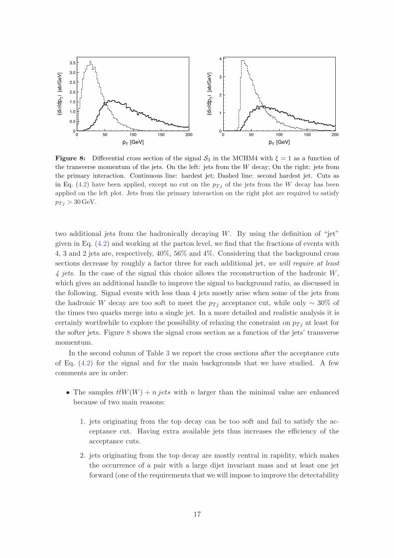
Figure 8: Differential cross section of the signal S3 in the MCHM4 with ξ = 1 as a function of

the transverse momentum of the jets. On the left: jets from the W decay; On the right: jets from

the primary interaction. Continuous line: hardest jet; Dashed line: second hardest jet. Cuts as

in Eq. (4.2) have been applied, except no cut on the pTj of the jets from the W decay has been

applied on the left plot. Jets from the primary interaction on the right plot are required to satisfy

pTj > 30 GeV.

two additional jets from the hadronically decaying W . By using the definition of “jet”

given in Eq. (4.2) and working at the parton level, we find that the fractions of events with

4, 3 and 2 jets are, respectively, 40%, 56% and 4%. Considering that the background cross

sections decrease by roughly a factor three for each additional jet, we will require at least

4 jets. In the case of the signal this choice allows the reconstruction of the hadronic W ,

which gives an additional handle to improve the signal to background ratio, as discussed in

the following. Signal events with less than 4 jets mostly arise when some of the jets from

the hadronic W decay are too soft to meet the pTj acceptance cut, while only ∼ 30% of

the times two quarks merge into a single jet. In a more detailed and realistic analysis it is

certainly worthwhile to explore the possibility of relaxing the constraint on pTj at least for

the softer jets. Figure 8 shows the signal cross section as a function of the jets’ transverse

momentum.

In the second column of Table 3 we report the cross sections after the acceptance cuts

of Eq. (4.2) for the signal and for the main backgrounds that we have studied. A few

comments are in order:

• The samples ttW (W ) + n jets with n larger than the minimal value are enhanced

because of two main reasons:

1. jets originating from the top decay can be too soft and fail to satisfy the ac-

ceptance cut. Having extra available jets thus increases the efficiency of the

acceptance cuts.

2. jets originating from the top decay are mostly central in rapidity, which makes

the occurrence of a pair with a large dijet invariant mass and at least one jet

forward (one of the requirements that we will impose to improve the detectability

17

Channel σ1 σ2 σ3 σCMS4 σATLAS4

S3 (MCHM4− ξ = 1) 30.4 27.7 16.8 16.7 16.4

S3 (MCHM4− ξ = 0.8) 20.4 18.7 11.2 11.2 11.0

S3 (MCHM4− ξ = 0.5) 9.45 8.64 5.26 5.24 5.14

S3 (MCHM5− ξ = 0.8) 29.4 26.7 15.4 15.4 15.1

S3 (MCHM5− ξ = 0.5) 14.8 13.6 7.88 7.85 7.71

S3 (SM− ξ = 0) 1.73 1.34 0.75 0.75 0.73

Wl+l−4j 12.0 ×103 658 4.07 3.35 2.47

Wl+l−5j 3.83 ×103 16.6 0.13 0.08 0.00

hl+l−jj →WWl+l−jj 102 29.7 0.50 0.50 0.49

WWW4j 86.2 3.47 0.35 0.28 0.23

ttWjj 408 11.3 0.66 0.55 0.37

ttWjjj 287 2.40 0.15 0.12 0.09

ttWW 315 4.48 0.02 0.02 0.02

ttWWj 817 28.1 1.40 1.16 0.89

tthjj → ttWWjj 610 8.89 0.65 0.52 0.38

tthjjj → ttWWjjj 329 0.84 0.05 0.04 0.03

Wτ+τ−4j 206 11.5 1.26 1.05 0.68

Total background 18.9 ×103 775 9.23 7.66 5.65

Table 3: Cross sections, in ab, for the signal S3 (see Eq. (4.1)) and for the main backgrounds

after imposing the cuts of Eq. (4.2) (σ1); of Eqs. (4.2) and (4.3) (σ2); of Eqs. (4.2)–(4.4) (σ3); of

Eqs. (4.2)–(4.5) (σCMS4 ); of Eqs. (4.2)–(4.4) and (4.6) (σATLAS4 ). For each channel, the proper

branching fraction to a three-lepton final state (via W → lν, qq and τ → lνντ ) has been included.

of our signal) quite rare. Additional jets from initial state radiation are instead

more likely to emerge with large rapidity.

Notice that including all the samples ttW (W ) +n jets at the partonic level is redun-

dant and in principle introduces a problem of double counting. A correct procedure

would be resumming soft and collinear emissions by means of a parton shower, which

effectively accounts for Sudakov form factors, and matching with the hard matrix

element calculation by means of some procedure to avoid double counting of jet

emissions. Here we retain all the ttW (W ) +n jets contributions, as the cuts that we

will impose on extra hadronic activity make the events with additional jets almost

completely negligible, solving in this way the problem of double counting.

• Events with additional jets are much less important for the Wll backgrounds, where

already at leading order the jets can originate from a QCD interaction. This is clearly

illustrated in Table 3 by the small cross section of Wll5j after the cuts.

• For mh = 180 GeV the bulk of the contribution to ttWW + n jets is via Higgs

production and decay: tth + n jets → ttWW (∗) + n jets. Given the complexity of

18

the final state, for n = 2, 3 we have computed this latter simpler signal as a good

approximation of ttWW + n jets.

• There is no overlap between ttWW and ttWjj, since the latter has been computed

at order O(αEW ) and as such it does not include contributions from intermediate

W ∗ → jj.

• The process WWW4j includes the resonant contributions WWWWjj →WWW4j,

hW4j → WWW4j and hWWjj → WWWWjj → WWW4j. For simplicity, since

WWW4j represents only a small fraction of the total background at the end of the

analysis, the Higgs resonant contributions have not been separately reported in this

case.

• The process Wl+l−4j includes the Higgs resonant contribution hWjj → ZZWjj

with ZZ → l+l−jj. This accounts for less than 7% of the total Wl+l−4j, and has

not been reported separately for simplicity.

• The process Wτ+τ−4j leads to a three-lepton final state provided both τ ’s decay

leptonically. It is clearly subdominant compared to Wl+l−4j, but it is at the same

time much less reduced by the cut on the dilepton invariant mass mSF -OS which we

impose in the following (see Eq. (4.4)). For this reason it must be included in the list

of relevant backgrounds.

As clearly seen from Table 3, after the acceptance cuts the background is still by far

dominating over the signal. We therefore try to exploit the peculiar kinematics of the

signal, which is distinctive of vector boson fusion events: two widely separated jets with

a least one at large rapidity. We will refer to these two jets as “reference” jets in the

following. To identify them we first select the jet with the largest absolute rapidity, and

we then compute the dijet invariant mass it forms with each one of the remaining jets: the

two reference jets will be those forming the largest dijet invariant mass. 8 Figure 9 shows

the rapidity of the most forward jet (first reference jet), ηrefJ1 , the invariant mass of the two

reference jets, mrefJJ , and their separation, ∆ηrefJJ = |ηrefJ1 − η

refJ2 |. In the case of the signal,

the remaining jets will reconstruct a W boson. In Fig. 10 we plot the invariant mass of all

the jets other than the reference ones, mWJJ , for both the signal 9 and the background.

A second crucial feature of the signal is that there are two Higgs bosons in the final

state: one decaying fully leptonically, the other semileptonically. The two leptons from

the leptonically-decaying Higgs can be identified as those forming the opposite-charge pair

8In the case of the signal this procedures selects, at the partonic level, the two jets which are not produced

in the W decay with an efficiency of ∼ 0.97 (∼ 0.90) for ξ ≥ 0.5 (ξ = 0). A similar result is obtained using

∆ηJJ to select the reference jets. At the partonic level mJJ looks slightly better, although this has to be

confirmed by a more detailed analysis.9Obviously, the distribution for the signal has a Breit-Wigner peak with a small continuous tail due to

events where jets from the decay of the W have been chosen as reference jets. The experimental resolution

on the dijet mass is much larger than the W width, and this has to be properly taken into account if we

wish to use this observable to improve the significance of the signal. At the rough level of our analysis, this

will be taken into account by selecting an appropriate mass window around the W mass.

19

0 1 2 3 4 5 60

0.01

0.02

0.03

0.04

ηJ1ref0 2 4 6 8 10

0

0.01

0.02

0.03

0.04

ΔηJJref

0 500 1000 1500 2000 25000

0.01

0.02

0.03

0.04

0.05

0.06

mJJ [GeV]ref

Figure 9: Differential cross sections after the acceptance cuts of Eq. (4.2) for the signal S3 in the

MCHM4 at ξ = 1 (continuous line) and the background (dashed line). Upper left plot: rapidity of

the most forward jet (in absolute value); Upper right plot: separation between the two reference

jets; Lower plot: invariant mass of the two reference jets. All curves have been normalized to unit

area.

with the smallest relative angle. Both lepton spin correlations and the boost of the Higgs

in the laboratory frame favour this configuration. For example, for a final state e+µ+e−X,

we compute cos θe+e− and cos θµ+e− and we pick up the pair with the largest cosine. 10

Figure 11 shows the mass of this lepton pair, mhll, for both the signal and the background.

The other Higgs boson candidate is reconstructed as the sum of the remaining lepton plus

all the jets different from the reference ones; its mass, mhJJl, is also shown in Fig. 11.

As a first set of cuts, we use the observables discussed above and require that each

individual cut reduces the signal by no more than ∼ 2%. We demand:

|ηrefJ1 | ≥ 1.8 mrefJJ ≥ 320 GeV ∆ηrefJJ ≥ 2.9

|mWJJ −mW | ≤ 40 GeV mh

ll ≤ 110 GeV mhJJl ≤ 210 GeV

(4.3)

Signal and background cross sections after this set of cuts are reported as σ2 in Table 3.

We first notice that all the backgrounds with a number of jets larger than four have been

strongly reduced: this is mostly due to the cuts on mWJJ and on mh

JJl, that heavily penalize

10Here θij is defined as the angle between the directions of particle i and particle j.

20

0 50 100 150 200 250 300 3500

0.02

0.04

0.06

0.08

0.10

0.12

0.14

Signal x 50

mJJ [GeV]W

( dσ/

dmJJ

) [fb

/GeV

]W

Figure 10: Differential cross section as a function of the invariant mass of all the non-reference

jets for the signal S3 in the MCHM4 at ξ = 1 (continuous line) and the background (dashed line)

after the acceptance cuts of Eq. (4.2).

0 20 40 60 80 100 120 140 160

1

10

mll [GeV]h

( dσ/

dmll )

[fb/G

eV]

h

10-1

10-2

10-3

10-4

0 100 200 300 400 500 600 7000

0.05

0.10

0.15

0.20

Signal x 50

mJJl [GeV]

( dσ/

dmJJl )

[fb/G

eV]

h

h

Figure 11: Differential cross sections after the acceptance cuts of Eq. (4.2) for the signal S3 in

the MCHM4 at ξ = 1 (continuous line) and the background (dashed line). Left plot: invariant mass

of the two leptons forming the first Higgs candidate; Right plot: invariant mass of the lepton plus

jets forming the second Higgs candidate.

events with a large available jet energy. This is the reason why we can neglect the problem

of double counting introduced by including samples with arbitrary number of jets: after

the cuts of Eq. (4.3) are imposed, the events with a too large number of jets are essentially

rejected.

We now proceed to identify the cuts which are most effective for improving the signifi-

cance of our signal. We first notice that the largest background, Wl+l−4j, has a dominant

contribution from the Z resonance. In Fig. 12 we plot the invariant mass, mSF -OS , of the

e+e− or µ+µ− pair found in the event. If two such pairings are possible (this is the case

when the three leptons in the final state all have the same flavor), the invariant mass closer

to MZ is selected. It is clear that the significance of the signal can be largely improved by

excluding values of mSF -OS that are in a window around the Z pole or close to the photon

pole.

We searched for the optimal set of cuts on mSF -OS and other possible distributions

21

0 20 40 60 80 100 120 140 160

1

10

mSF-OS [GeV]

( dσ/

dmSF

-OS )

[fb/G

eV]

10-1

10-2

10-3

10-4

Figure 12: Differential cross section after the acceptance cuts of Eq. (4.2) as a function of the

invariant mass, mSF -OS , of the e+e− or µ+µ− pair. Whenever two such pairings are possible the

mass closer to MZ is selected. Continuous line: signal S3 in the MCHM4 at ξ = 1; Dashed line:

background.

(including all those mentioned above and shown in Figs. 9–12 by following an iterative

procedure: at each step we cut over the observable which provides the largest enhancement

of the signal significance, until no further improvement is possible. The significance has

been computed performing a goodness-of-fit test of the background-only hypothesis with

Poisson statistics. 11 We assumed 300 fb−1 (3000 fb−1) of integrated luminosity at the

LHC (at the LHC luminosity upgrade). We end up with the following set of additional

cuts:mSF -OS ≥ 20 GeV |mSF -OS −MZ | ≥ 7 ΓZ

∆ηrefJJ ≥ 4.5 mrefJJ ≥ 700 GeV mh

JJl ≤ 160 GeV ,(4.4)

MZ and ΓZ being respectively the Z boson mass and width. The cross sections for signal

and backgrounds after these cuts are reported as σ3 in Table 3.

As a final set of cuts, we consider a further restriction on mWJJ around the W pole:

|mWJJ −MW | < 30 GeV (4.5)

|mWJJ −MW | < 20 GeV (4.6)

The cuts in Eqs. (4.5)-(4.6) correspond to twice the expected invariant dijet mass resolution

respectively for the CMS and ATLAS detector resolution. The corresponding final cross

sections are denoted as σCMS4 and σATLAS4 in Table 3. An additional veto on b-jets has a

relatively small impact, since it would reduce the ttW (W ) + jets backgrounds which are

however already subdominant. Assuming for example a b-jet tagging efficiency of εb = 0.55

for ηb < 2.5, the signal significances increase by approximately 10%.

11 Given the number of signal and background events a p-value is computed using the Poisson distribution.

The significance is defined as the number of standard deviations that a Gaussian variable would fluctuate

in one direction to give the same p-value. For example, a p-value = 2.85 × 10−7 corresponds to a 5σ

significance.

22

1 2 3 4 5 6 7 8 90

0.2

0.4

0.6

0.8

1

Number of jets

Frac

tion

of e

vent

s

Figure 13: Number of jets after showering with PYTHIA and imposing the acceptance cuts of

Eq. (4.2). Continuous line: signal S3 in the MCHM4 with ξ = 1; Dashed line: background. Jets

are reconstructed using the cone algorithm implemented in the GETJET routine.

4.1.1 Estimate of showering effects

There is still one feature of the signal which has not been exploited yet. A unique signature

of vector boson fusion events is a very small hadronic activity in the central region (rapidi-

ties between the first and second reference jet) [25]. This is not the case for the backgrounds,

especially after imposing the cuts on ∆ηrefJJ and mrefJJ in Eq. (4.4), which imply a large total

invariant mass√s for the event and therefore a stronger radiation probability (the radia-

tion probability is proportional to log2(s/λ2), where λ is the infrared/collinear cut-off). By

vetoing this activity in the central region, one can then obtain an additional suppression

of the background without affecting much the signal. For our event selection, the effect of

the showering on the background is twofold: a large number of jets appears in the final

state and, as a consequence, both mWJJ and mh

JJl are shifted towards larger values. 12 In

order to assess the relative impact of these effects, we have processed both the signal and

the most relevant background, Wl+l−4j, through the parton shower PYTHIA [26], and we

have reconstructed the final-state jets using a cone algorithm a la UA1, as implemented in

the GETJET [27] routine. To avoid mixing different and unrelated effects, we have studied

only the relative efficiencies of the various cuts compared to the partonic level analysis.

Figure 13 shows the distribution of the number of jets for both the signal and the

Wl+l−4j background after showering and imposing the acceptance cuts of Eq. (4.2). A

comparison between the mWJJ and mh

JJl background distributions, as reconstructed at the

parton and shower level after imposing the cuts on ∆ηrefJJ and mrefJJ of Eq. (4.4), is shown in

Fig. 14. Notice that these observables, as well as the jet multiplicity, are strongly correlated,

so that applying a cut on any one of them strongly diminishes the efficiency on the others.

A rough estimate of the effect of the showering can be obtained by monitoring the

collective efficiency of the cuts on mWJJ (Eq. (4.3)) and on ∆ηrefJJ , mref

JJ , mhJJl (Eq. (4.4)).

12Let us denote as X the system of final state jets other than the reference jets. If the additional radiation

is from the X system, MX will be unaffected, if instead it is from initial state or from the reference jets the

momentum of the radiation will add to that of the X system increasing its mass.

23

0 200 400 600 8000

0.02

0.04

0.06

0.08

mJJ [GeV]W0 200 400 600 800 1000

0

0.01

0.02

0.03

0.04

0.05

0.06

0.07

mJJl [GeV]h

Figure 14: Differential cross section for the background Wl+l−4j after the showering (continuous

line) and at the parton level (dashed line) as as a function of mWJJ (left plot) and mh

JJl (right plot).

Only events which pass the acceptance cuts of Eq. (4.2) and those on ∆ηrefJJ and mrefJJ of Eq. (4.4)

have been included.

After showering, we find the following additional reduction on the signal and background

rates compared to the partonic level:

S3 (ξ = 1, 0.8, 0.5) Wl+l−4j

εshower/εparton 0.8 0.6

A further veto on events with more than 5 jets has a negligible impact, both for the signal

and the background, as the cuts on mWJJ and mh

JJl effectively act like a veto on extra

hadronic activity. Although a full inclusion of showering effects can only be obtained by

using matched samples, yet we expect that our rough estimate captures the bulk of the

effect.

4.1.2 Additional backgrounds from fake leptons

Since the number of signal events at the end of our analysis is very small, it is important to

check if there are additional potential sources of reducible backgrounds. Here we consider

the possibility that a jet is occasionally identified as a lepton, in which case we speak of

a “fake” lepton from a jet. We find that the effect of such jet mistagging is likely to be

negligible in the three lepton case as follows.

As shown in Table 3, the dominant background in this case is Wll4j. After the

acceptance cuts we have σpp→Wl+l−4j = 12 fb. A first possibility is that a fake lepton

(most likely an electron) originates from the misidentification of a “light jet” (originated

either from gluons or from a light quark). In this case the most serious potential source

of background is ll + 5j. Since the relative cross section after the acceptance cuts is

σpp→l+l−+5j ' 2.8 pb, even a modest mistagging probability . 10−3 (according to both

CMS and ATLAS collaborations [28, 29], rejection factors as small as 10−5 can be achieved

by making the jet reconstruction algorithm tight enough) is sufficient to suppress this

source of background.

A second possibility is that a heavy quark (b or c) decays semileptonically and the

resulting lepton is isolated. Backgrounds of this type are l+l−bb + 3j and l+l−cc + 3j,

24

which have similar cross sections. To estimate the first process we have computed the cross

section for pp → l+l−bb + 3j where one of the two b’s is randomly chosen and assumed

to be mistagged as a lepton. After applying the cuts of Eqs. (4.2)–(4.5) we obtain a cross

section of 1.2 fb. A b mistagging probability ∼ 10−3 is therefore sufficient to keep this

background below the irreducible background. This level of rejection seems feasible at the

LHC: in Ref. [30] a mistagging probability of 7×10−3 is estimated for a lepton with pT > 10

GeV, rapidly decreasing (by a factor 10 to 30 for pT > 20 GeV) with increasing pT . A

potentially more problematic contribution is tt + 3j, whose cross section after acceptance

cuts is σpp→tt+3j = 770 fb. A b mistagging probability . 10−3 makes this background

at most as important as the other tt channels in Table 3, which however turn out to be

subdominant at the end of the analysis.

We thus conclude that the effect of fake leptons is expected to be negligible in the

three lepton case.

4.2 Channel S2: two same-sign leptons plus two hadronically-decaying W ’s

In the case of a two-lepton final state, in order to keep the background at a manageable

level, and avoid the otherwise overwhelming tt background, we are forced to select only

events with two leptons with the same charge.

Along with the two leptons, the signal is characterized by two widely separated jets

and up to four additional jets from the two hadronically-decaying W ’s. Using the definition

of “jet” given in Eq. (4.2) and working at the parton level, we find that in the majority of

the events at least one quark from a W decay is either too soft to form a jet or it merges

with another quark to form one single jet. The fractions of signal events with 6, 5, 4 and

3 jets are respectively 0.16, 0.43, 0.37 and 0.04. We choose to retain events with at least

5 jets. Including events with a lower jet multiplicity is not convenient, as the background

increases by a factor ∼ 3 for each jet less, and the identification of the Higgs daughters in

the signal becomes less effective.

In order to suppress the otherwise overwhelming Wl+l−+ jets background, we forbid

the presence of extra hard isolated leptons: we require to have

exactly two leptons (with the same charge) satisfying the acceptance cuts of Eq. (4.2).

In this way the resonant contribution WZ + jets → Wl+l−+ jets is strongly suppressed.

Other backgrounds that can have 3 leptons in their final state at the partonic level are also

reduced. 13

In the second column of Table 4, we report the cross sections after the acceptance

cuts of Eq. (4.2) for the signal S2 and for the main backgrounds we have studied. A few

comments are in order (comments made for Table 3 also apply and will not be repeated

here):

• While the cross section for WW production is obviously much larger than the cross

section for WWW production, those for WWW and W+(−)W+(−) (equal sign) are

comparable, so that both these latter backgrounds must be included.

13These backgrounds are: ttWjjj, ttWWj, tthjj → ttWWjj, tthjjj → ttWWjjj and Wτ+τ−5j.

25

Channel σ1 σ2 σ3 σCMS4 σATLAS4

S2 (MCHM4− ξ = 1) 69.4 62.8 51.8 51.3 49.9

S2 (MCHM4− ξ = 0.8) 47.0 42.6 34.9 34.6 33.7

S2 (MCHM4− ξ = 0.5) 22.2 20.1 16.9 16.7 16.2

S2 (MCHM5− ξ = 0.8) 68.5 61.8 50.0 49.4 47.8

S2 (MCHM5− ξ = 0.5) 35.5 32.2 26.4 26.1 25.3

S2 (SM− ξ = 0) 4.51 3.52 2.87 2.84 2.76

Wl+l−5j 2.23 ×103 200 61.8 55.1 42.1

W+(−)W+(−)5j 700 53.3 13.8 11.7 8.91

WWWjjj 194 29.5 8.65 8.49 8.18

hWjjj 97.0 29.2 12.5 12.4 12.1

WWWWj 5.94 0.63 0.11 0.11 0.11

WWWWjj 10.9 1.40 0.52 0.52 0.49

ttWj 929 89.0 13.4 12.9 12.0

ttWjj 1.64 ×103 134 25.7 23.2 19.6

ttWjjj 1.18 ×103 44.6 8.52 7.48 6.04

ttWW 886 24.1 1.27 1.24 1.15

ttWWj 1.65 ×103 173 28.4 26.6 23.2

tthjj → ttWWjj 1.27 ×103 98.6 18.7 17.2 14.5

tthjjj → ttWWjjj 732 21.3 3.99 3.64 3.07

Wτ+τ−4j 655 78.2 22.8 20.0 15.9

Wτ+τ−5j 463 31.7 8.77 7.88 6.19

Total Background 12.7 ×103 1.01 ×103 229 209 174

Table 4: Cross sections, in ab, for the signal S2 (see Eq. (4.1)) and for the main backgrounds

after imposing the cuts of Eq. (4.2) (σ1); of Eqs. (4.2) and (4.7) (σ2); of Eqs. (4.2) and (4.7)-(4.8)

(σ3); of Eqs. (4.2) and (4.7)–(4.9) (σCMS4 ); of Eqs. (4.2), (4.7), (4.8) and (4.10) (σATLAS4 ). For

each channel the proper branching fraction to a same-sign dilepton final state (via W → lν, qq

and τ → lνντ , qqντ ) has been included. For the decay modes of the taus, see text. In the case of

the background Wl+l−5j, the lepton with different sign is required to fail the acceptance cuts of

Eq. (4.2), see text.

• The backgroundWWWWj includes the resonant contributionWWhj →WWWWj.

For simplicity, since WWWWj represents only a small fraction of the total back-

ground at the end of the analysis, the Higgs resonant contribution has not been

reported separately. There is no overlap between WWWWj and WWWjjj, since

the latter has been generated at order O(α3EW ) and as such it does not include con-

tributions from intermediate W ∗ → jj.

• The process Wτ+τ−4j leads to a dilepton final state if one τ decays leptonically and

the other is mistagged as a QCD jet. 14 We have conservatively assumed that the

14We thank James Wells for pointing out to us the importance of the processes Wτ+τ−4j and Wτ+τ−5j

26

momentum of the mistagged jet is equal to that of the parent τ , and we have included

a mistagging probability at the end of our analysis.

• The process Wτ+τ−5j leads to a dilepton final state if one τ decays leptonically

and the other is either not detected (independently of its decay mode), or it decays

hadronically and it is mistagged as a QCD jet. We include the mistagging probability

at the end of our analysis, when we impose a veto on hadronic taus in the event. The

momentum of the mistagged jet has been assumed to be equal to that of the parent τ .

• Included in the cross sections of the processes ttWWj, tthjj, tthjjj and ttWjjj is

the contribution of the three leptons final state where both tops decay leptonically

and the wrong-sign lepton fails the acceptance cut. The analog contribution from

ttW4j has been computed and found to be very small, and for simplicity is not

reported here.

• If required for trigger issues, the cut on the hardest lepton can be increased to pT >

30 GeV at basically no cost for the signal (the efficiency relative to the acceptance

cuts of Eq. (4.2) is 97%). This should be sufficient to pass the high-level trigger at

CMS and ATLAS even during the high-luminosity phase of the LHC. Furthermore,

the presence of a huge amount of hadronic energy in the signal might help to reduce

the trigger requirements on the pT of the leptons.

As one can see from Table 4, after the acceptance cuts the background dominates by

far over the signal. In order to select our first set of additional cuts we proceed in close

analogy to the three-lepton case. We first identify the two “reference” jets as described in

Section 4.1. The distributions of the rapidity of the first reference jet, ηrefJ1 , the invariant

mass of the two reference jets, mrefJJ , and their separation, ∆ηrefJJ , are quite similar to those

of Fig. 9 and are thus not reported here. Next, we reconstruct one hadronic W as follows:

using all the non-reference jets, we select the pair with invariant mass mWJJ closer to the

W mass. If |mWJJ −MW | < 40 GeV we label these two jets as jW1

1 and jW12 , otherwise the

event is rejected. All the remaining jets will be labelled as belonging to the other hadronic

W , jW2k . We then proceed to identify the decay products of the two Higgs bosons. As

a criterion to select the lepton and the W from the same Higgs, we use the separation

∆R between them, as they will tend to emerge collimated due to the Higgs boost. More

explicitly, by defining

pWi =∑n

pjWin,

we compute ∆Rl1W1 and ∆Rl2W1 . If ∆Rl1W1 < ∆Rl2W1 , we assign l1 and jW1k to the first

Higgs and the remaining jets and lepton to the second one; otherwise we form the first

Higgs boson candidate with l2 and jW1k and the other one with the remaining jets and

lepton. We denote by mhlW1

and mhlW2

the invariant mass of the Higgs system containing

respectively the jet jW1k and jW2

k . They are plotted in Fig. 15 for both the signal and the

background.

as potential backgrounds.

27

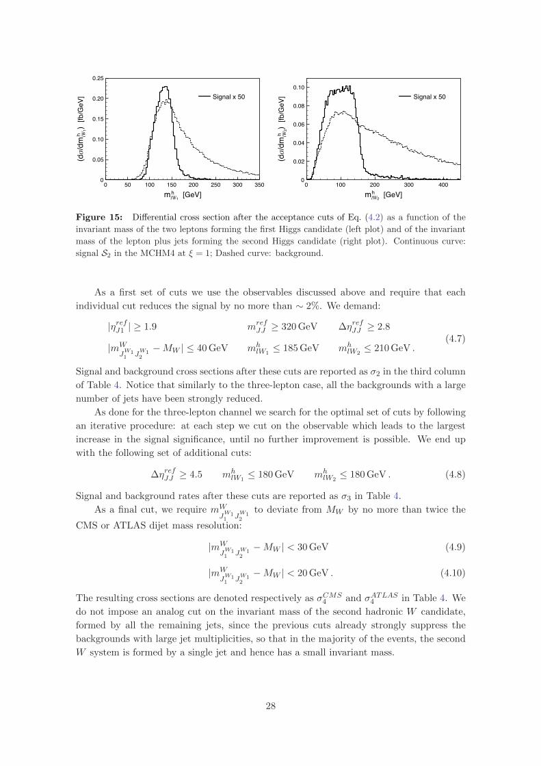
0 50 100 150 200 250 300 3500

0.05

0.10

0.15

0.20

0.25

Signal x 50

mlW1 [GeV]h

(dσ/

dmlW

1) [f

b/G

eV]

h

0 100 200 300 4000

0.02

0.04

0.06

0.08

0.10Signal x 50

mlW2 [GeV]

(dσ/

dmlW

2) [f

b/G

eV]

h

h

Figure 15: Differential cross section after the acceptance cuts of Eq. (4.2) as a function of the

invariant mass of the two leptons forming the first Higgs candidate (left plot) and of the invariant

mass of the lepton plus jets forming the second Higgs candidate (right plot). Continuous curve:

signal S2 in the MCHM4 at ξ = 1; Dashed curve: background.

As a first set of cuts we use the observables discussed above and require that each

individual cut reduces the signal by no more than ∼ 2%. We demand:

|ηrefJ1 | ≥ 1.9 mrefJJ ≥ 320 GeV ∆ηrefJJ ≥ 2.8

|mW

JW11 J

W12

−MW | ≤ 40 GeV mhlW1≤ 185 GeV mh

lW2≤ 210 GeV .

(4.7)

Signal and background cross sections after these cuts are reported as σ2 in the third column

of Table 4. Notice that similarly to the three-lepton case, all the backgrounds with a large

number of jets have been strongly reduced.

As done for the three-lepton channel we search for the optimal set of cuts by following

an iterative procedure: at each step we cut on the observable which leads to the largest

increase in the signal significance, until no further improvement is possible. We end up

with the following set of additional cuts:

∆ηrefJJ ≥ 4.5 mhlW1≤ 180 GeV mh

lW2≤ 180 GeV . (4.8)

Signal and background rates after these cuts are reported as σ3 in Table 4.

As a final cut, we require mW

JW11 J

W12

to deviate from MW by no more than twice the

CMS or ATLAS dijet mass resolution:

|mW

JW11 J

W12

−MW | < 30 GeV (4.9)

|mW

JW11 J

W12

−MW | < 20 GeV . (4.10)

The resulting cross sections are denoted respectively as σCMS4 and σATLAS4 in Table 4. We

do not impose an analog cut on the invariant mass of the second hadronic W candidate,

formed by all the remaining jets, since the previous cuts already strongly suppress the

backgrounds with large jet multiplicities, so that in the majority of the events, the second

W system is formed by a single jet and hence has a small invariant mass.

28

Channel σCMS5 σCMS

6 σATLAS5 σATLAS6

S2 (MCHM4− ξ = 1) 51.3 51.3 49.9 49.9

S2 (MCHM4− ξ = 0.8) 34.6 34.6 33.7 33.7

S2 (MCHM4− ξ = 0.5) 16.7 16.7 16.2 16.2

S2 (MCHM5− ξ = 0.8) 49.4 49.4 47.8 47.8

S2 (MCHM5− ξ = 0.5) 26.2 26.2 25.3 25.3

S2 (SM− ξ = 0) 2.84 2.84 2.76 2.76

Wl+l−5j 21.8 21.8 16.3 16.3

W+(−)W+(−)5j 11.7 11.7 8.91 8.91

WWWjjj 8.49 8.49 8.18 8.18

hWjjj 12.4 12.4 12.1 12.1

WWWWj 0.11 0.11 0.11 0.11

WWWWjj 0.52 0.52 0.49 0.49

ttWj 12.9 3.65 12.0 3.43

ttWjj 23.2 8.47 19.6 7.34

ttWjjj 7.10 3.23 5.77 2.62

ttWW 1.24 0.51 1.15 0.49

ttWWj 25.6 10.2 22.2 8.91

tthjj → ttWWjj 15.4 7.39 13.0 6.22

tthjjj → ttWWjjj 3.11 1.70 2.65 1.44

Wτ+τ−4j 20.0 5.24 15.9 4.19

Wτ+τ−5j 6.28 4.86 5.02 3.79

Total Background 170 100 144 84.6

Table 5: Cross sections, in ab, for the signal S2 and for the main backgrounds after the cuts of

Eqs. (4.2) and (4.7)–(4.9) plus a veto on soft leptons (σCMS5 ) or a veto on soft leptons, taus and

b-jets (σCMS6 ); of Eqs. (4.2), (4.7), (4.8) and (4.10) plus a veto on soft leptons (σATLAS5 ) or a veto

on soft leptons, taus and b-jets (σATLAS6 ).

A further reduction of the Wl+l−5j background can be achieved by vetoing events

which contain soft leptons (1 GeV ≤ pT l ≤ 20 GeV) that are isolated from any jet (∆Rjl >

0.4) and form a same-flavor opposite-sign pair with at least one of the two hard leptons. In

order to estimate the efficiency of such veto on the signal, we showered and hadronized the

events with PYTHIA. We find that the majority of the additional leptons originates from

the decay of the final-state hadrons, especially from the leptonic decay of charmed mesons.

The fraction of signal events rejected is quite small, less than 4%, and we will neglect it.

For simplicity, the effect of the veto on all the backgrounds with exactly two leptons at

the parton level 15 will also be neglected. The cross sections after this veto are reported in

Table 5 as σCMS5 and σATLAS5 , respectively after the cut of Eq. (4.9) and Eq. (4.10).

15These backgrounds are: W+(−)W+(−)5j, WWWjjj, hWjjj, WWWWj, WWWWjj, ttWj, ttWjj,

ttWW and Wτ+τ−4j.

29

0 200 400 600 8000

0.02

0.04

0.06

0.08

0.10

mlW2 [GeV]h

Figure 16: Differential cross section as a function of mhlW2

after the showering (continuous line)

and at the parton level (dashed line) of the sum of the backgrounds Wl+l−5j, WWWjjj, hWjjj,

ttWjj and ttWWj. Only events which pass the acceptance cuts and those on mrefJJ (Eq. (4.7)) and

on ∆ηrefJJ (Eq. (4.8)) have been included.

A final reduction of the background can be obtained by resorting to b-jet and tau

tagging and vetoing these particles in the final state. We assume a b-tagging efficiency

εb = 0.55 within ηb < 2.5 (εb = 0 otherwise), and a τ veto efficiency of 80% within ητ < 2.5

(zero otherwise). The resulting cross sections after vetoing both taus and b-jets are reported

as σCMS6 and σATLAS6 in Table 5, respectively after the cut of Eq. (4.9) and Eq. (4.10).

4.2.1 Estimate of showering effects

As for the three leptons channel, background events have generically a larger hadronic

activity in the central region, compared to the signal, once the showering is turned on. In

this case, the main effect is that of shifting the mhlW2

distribution towards larger values.

This is clearly illustrated by Fig. 16, which reports the sum of the cross sections of the

main backgrounds, Wl+l−5j, WWWjjj, hWjjj, ttWjj and ttWWj, as a function of

mhlW2

after imposing the acceptance cuts, ∆ηrefJJ > 4.5 and mrefJJ > 320 GeV.

We derive a rough estimate of the effect of the showering by monitoring the collective

efficiency of the cuts on mrefJJ (Eq. (4.7)) and on ∆ηrefJJ , mh

lW2(Eq. (4.8)). After the

showering, we find the following additional reduction on the rates of the signal and of the

main backgrounds:

S2 (ξ = 1, 0.8, 0.5) Wl+l−5j WWWjjj hWjjj ttWjj ttWWj

εshower/εparton 0.86 0.34 0.32 0.80 0.55 0.95

A further veto on events with 7 or more jets has a negligible impact, both for the signal and

the background, as the cut on mhlW2

effectively acts like a veto on extra hadronic activity.

In the case of events with 6 jets one could think of keeping only those where the two jets

associated with the second Higgs candidate reconstruct an hadronic W : |mW

JW21 J

W22

−MW | <40 GeV. We find, however, that even this additional constraint has little impact on the

background, as mW

JW21 J

W22

is already forced to be small after the cut on mhlW2

is met. As for

30

Channel σCMS6 σATLAS6

W + 6j 3.8× 104 3.0× 104

Channel σCMS6 σATLAS6

ttjj 46.0× 104 44.3× 104

tt3j 17.9× 104 15.8× 104

Table 6: Cross sections, in ab, for the most important backgrounds with fake leptons from light

jets (table on the left) and from heavy jets (table on the right). In both tables, σCMS6 and σATLAS6

indicate the cross section after respectively the cuts of Eqs. (4.2) and (4.7)–(4.9) plus a veto on

b-jets, and Eqs. (4.2), (4.7), (4.8) and (4.10) plus a veto on b-jets.

the three-lepton case, it is worth stressing that these results should be confirmed by a full

treatment of showering effects using matched samples.

4.2.2 Fake leptons and lepton charge misidentification

Differently from the three lepton case, we expect the effect of fake leptons from jet misiden-

tification to be much more relevant for same-sign dilepton events. The reason is that the

cross section for the production of two same-sign W ’s is about two orders of magnitude

smaller than that for W+W−. It might then turn out to be more convenient to produce

one W and pay the misidentification probability factor for a fake lepton from an extra jet

than having a second leptonically-decaying W with the same sign. Moreover, an additional

source of background comes in this case from events where the charge of a primary lepton

is misidentified. A precise estimate of all these effects is beyond the scope of the present

paper, since it would require a full detector simulation as well as a dedicated strategy de-

signed to minimize the effect while keeping the lepton reconstruction efficiency as high as

possible. We will limit ourselves to performing a crude estimate and quoting the rejection

factors required to make such backgrounds negligible.

The most serious potential source of background with fake leptons from light jets is

W + 6j. Table 6 reports the relative cross section after all the cuts imposed in our analysis

(without including any mistagging probability factor). The quoted number is obtained by

computing the cross section for pp→ W + 6j, picking up randomly one jet and assuming

it is mistagged as a lepton, and multiplying by a factor 6 to account for the six different

possibilities to mistag a jet. A rejection factor of ∼ 10−5, quoted as achievable by both

collaborations [28, 29], is sufficient to reduce this background down to a manageable level. A

dedicated experimental study is however required to establish whether this can be obtained

without reducing too much the lepton identification efficiency. The largest background with

fake leptons from heavy quarks is ttjj, with one b from a top decay tagged as a lepton.

Table 6 reports the cross sections for ttjj and tt3j after all the cuts plus a b-jet veto. For

simplicity, we have approximated the “fake” lepton momentum to be equal to that of its

parent b quark. This is a conservative, reasonable assumption as the requirement of having

a hard, isolated lepton forces the remaining hadronic activity from the b decay to be quite

soft to escape detection [30]. As Table 6 shows, our rough estimate seems to indicate that

rejection factors as small as 10−4 are required to make this background comparable to

those studied in the previous sections.

31

Channel σCMS6 σATLAS6 σATLAS6 × εCH × ε 6ET>25 GeV

ξ = 1 51.3 49.9 45.1

tt3j 11.9× 103 9.2× 103 11.1

tt4j 4.0× 103 3.2× 103 3.96

l+l−5j 112.4× 103 88.4× 103 11.5

Table 7: Cross sections, in ab, for the most important backgrounds where the charge of a primary

lepton is misidentified. The first two columns show the cross sections after the cuts of respectively

Eqs. (4.2) and (4.7)–(4.9) plus a veto on b-jets (σCMS6 ) and Eqs. (4.2), (4.7), (4.8) and (4.10)

plus a veto on b-jets (σATLAS6 ), without including any charge misidentification efficiency. The last

column reports the cross section σATLAS6 multiplied by the efficiency of a cut 6ET > 25 GeV and a

charge misidentification probability equal to 10−3 for electrons and 3×10−4 for muons (collectively

indicated as εCH). For convenience, values of the cross section for the signal S2 in the MCHM4 at

ξ = 1 are also shown.

0 20 40 60 80 100 120 140 1600

0.05

0.10

0.15

0.20

ET [GeV]∕

Figure 17: 6ET distribution for the signal S2 in the MCHM4 at ξ = 1 (continuous curve) and

the l+l−5j background (dashed curve) after the cuts of Eqs. (4.2) and (4.7)–(4.10). The missing

transverse energy is computed including a Gaussian resolution σ( 6ET ) = 0.55 ·√∑

ET /GeV, see

text. The curves have been normalized to unit area.

Finally, we consider the most dangerous backgrounds where the charge of a primary

lepton is not correctly measured. The size of this effect strongly depends on the algorithm

used to reconstruct the leptons, and it is in general larger for electrons than for muons.

Table 7 reports the cross sections for tt3j, tt4j and l+l−5j after all the cuts imposed in our

analysis plus a b-jet veto, assuming that the charge of one lepton has not been correctly

measured. Even after applying a charge misidentification probability 10−3 for electrons and

a few×10−4 for muons as quoted in the ATLAS TDR [29] for leptons with pT ∼ 100 GeV,

the l+l−5j background is still sizable, while the tt+jets channels are smaller. Since however

l+l−5j has no neutrinos, while the signal has two of them, 6ET provides an important

handle to reduce this background. In Fig. 17 we plot 6ET for both the signal S2 in the

MCHM4 at ξ = 1 and l+l−5j. We have computed 6ET by including a Gaussian resolution

σ( 6ET ) = a ·√∑

ET /GeV, where∑ET is the total transverse energy deposited in the

calorimeters (from electrons and jets). We chose a = 0.55, which is expected to be a good

32

fit for the ATLAS detector [29]. Assuming a charge misidentification probability equal to

10−3 for electrons and 3 × 10−4 for muons, we find that a cut 6ET > 25 GeV provides the

best sensitivity, the efficiency on the signal being ' 0.9. The corresponding cross sections

after this cut (including the charge misidentification probabilities) are reported in the last

column of Table 7, which shows that the background has been reduced to a manageable

level although it remains non-negligible.

To summarize, our estimates show that both backgrounds with fake leptons from jets

and those with misidentification of the charge of a primary lepton are expected to have

an important impact on the same-sign dilepton channel. A detailed experimental study is

therefore needed to determine the precise relevance of these backgrounds and fully assess

the signal significance in this case.

4.3 Channel S4: four leptons

The last channel we have considered is the one with four leptons. In this case, the signal

is characterized by two widely separated jets with no further hadronic activity in between,

four hard leptons from the decay of the two Higgses and missing energy. The second column

of Table 8 reports the cross sections (σ1) for the signal S4 and for the main backgrounds

we have studied after the acceptance cuts of Eq. (4.2). We notice that (comments made

for Tables 3 and 4 also apply and will not be repeated here):

• The Higgs resonant contributions hl+l−jj → WWl+l−jj and hjj → τ+τ−l+l−jj

are separately reported and are thus not included in the backgrounds τ+τ−l+l−jj

and WWl+l−jj.

• The background l+l−l+l−jj includes the Higgs resonant contribution hjj → l+l−l+l−jj.

The latter has not been separately reported in this case since the entire background

is negligible at the end of the analysis.

• The backgroundWWWWjj is largely dominated by its resonant subprocess hWWjj →WWWWjj. The non-resonant contribution is negligible and it has not been reported

in the table.

As for the three- and two-lepton case, the two reference jets have been identified as

the pair with the largest invariant mass containing the most forward jet. We identify the

pair of leptons coming from the first Higgs, (l+1 l−1 ), and that from the second Higgs, (l+2 l

−2 ),

by using the angular separation as a criterion: there are two ways of combining the initial

four leptons in two opposite-sign pairs, and we choose the combination which maximizes

cos θl+1 l−1

+ cos θl+2 l−2

, as leptons from the same Higgs tend to emerge collimated due to both

the Higgs boost and the spin correlations. We will refer to (l+1 l−1 ) and (l+2 l

−2 ) defined in

this way as our two Higgs candidates.

As a first set of cuts, we use the invariant mass and rapidities of the two reference jets as

well as the invariant masses of the two Higgs candidates. The corresponding distributions

for the signal have the same shape as those in Figs. 9 and 11 (left plot). Similarly to the

33

Channel σ1 σ2 σ3 σ4 σ5

S4 (MCHM4− ξ = 1) 6.64 6.16 5.10 4.33 4.33

S4 (MCHM4− ξ = 0.8) 4.40 4.10 3.38 2.86 2.86

S4 (MCHM4− ξ = 0.5) 1.99 1.86 1.52 1.30 1.30

S4 (MCHM5− ξ = 0.8) 6.06 5.59 4.52 3.76 3.76

S4 (MCHM5− ξ = 0.5) 3.00 2.79 2.26 1.90 1.90

S4 (SM− ξ = 0) 0.32 0.24 0.19 0.15 0.15

l+l−l+l−jj 1.73 ×103 171 0.04 0.00 0.00

l+l−τ+τ−jj 44.6 4.28 0.55 0.11 0.11

hjj → l+l−τ+τ−jj 1.03 0.57 0.12 0.06 0.06

WWl+l−jj 105 0.78 0.10 0.03 0.03

hl+l−jj →WWl+l−jj 41.4 11.2 1.30 0.75 0.75

hWWjj →WWWWjj 0.79 0.07 0.06 0.04 0.04

ttl+l− 558 6.15 0.90 0.02 0.01

ttl+l−j 624 57.3 1.26 0.24 0.13

ttWW 67.5 0.48 0.34 0.02 0.01

ttWWj 83.3 6.58 0.84 0.14 0.08

tthjj → ttWWjj 46.0 8.19 0.08 0.02 0.02

tthjjj → ttWWjjj 22.9 6.15 0.00 0.00 0.00

Total background 3.32 ×103 272 5.59 1.44 1.25

Table 8: Cross sections, in ab, for the signal S4 (see Eq. (4.1)) and for the main backgrounds

after imposing the cuts of Eq. (4.2) (σ1); of Eqs. (4.2) and (4.11) (σ2); of Eqs. (4.2), (4.11), (4.12)

plus a veto on extra jets, (σ3); of Eqs. (4.2), (4.11), (4.12), (4.13) plus a veto on extra jets (σ4);

of Eqs. (4.2), (4.11), (4.12), (4.13) plus a veto on extra jets and on b-jets (σ5). For each channel

the proper branching fraction to a four-lepton final state (via W → lν and τ → lνντ ) has been

included.

previous two analyses, we require that each individual cut reduces the signal by no more

than ∼ 2%. We demand:

|ηrefJ1 | ≥ 1.8 mrefJJ ≥ 320 GeV |∆ηrefJJ | ≥ 2.9

mhl1l1 ≤ 110 GeV mh

l2l2 ≤ 110 GeV .(4.11)

Signal and background cross sections after this set of cuts are reported in Table 8 as σ2.

At this level, the l+l−l+l−jj background is much larger than the signal. It can be

drastically reduced, however, by exploiting the fact that the signal has four neutrinos,

hence a substantial amount of missing energy, while l+l−l+l−jj has none, see Fig. 18. Here

as before, the missing energy of each event has been computed by including a Gaussian

resolution σ(6ET ) = 0.55 ·√∑

ET /GeV to account for calorimeter effects, where∑ET is

the total transverse energy of jets and electrons. A further reduction is obtained by cutting

on the invariant mass of same-flavor opposite-sign lepton pairs, mSF -OS , excluding values

34

0 50 100 150 200

∕ET miss [GeV]

10-3

10

10

-2

-1

Figure 18: 6ET distribution for the signal S4 in the MCHM4 at ξ = 1 (continuous curve) and

the l+l−l+l−jj background (dashed curve) after the cuts of Eqs. (4.2) and (4.11). The missing

transverse energy is computed including a Gaussian resolution σ( 6ET ) = 0.55 ·√∑

ET /GeV, see

text. The curves have been normalized to unit area.

around MZ . This clearly suppresses l+l−l+l−jj, as well as all the processes with resonant

Z contributions. We find that optimized values for these cuts, which almost completely

eliminate the l+l−l+l−jj background, are as follows:

6ET ≥ 40 GeV |mSF -OS −MZ | ≥ 2 ΓZ . (4.12)

The individual efficiencies on l+l−l+l−jj are of ∼ 5 × 10−3 for the cut on 6ET and ∼ 0.05

for that on mSF -OS . The other feature of the signal that can be exploited to further reduce

the background is its small hadronic activity in the central region. We have thus imposed

a

veto on any extra hard and isolated jet (in addition to the two reference jets)

satisfying the acceptance cuts of Eq. (4.2). Signal and background cross sections after this

veto and the cuts in Eq. (4.12) are reported in Table 8 as σ3.

Next, as for the other channels, we have monitored the observables of Eqs. (4.11) and

(4.12) in search for the optimal set of cuts. We find that the best improvement in the signal

efficiency is obtained by strengthening the cut on the separation between the reference jets

as follows:

|∆ηrefJJ | > 4.5 . (4.13)

Signal and background cross sections after this cut are reported in Table 8 as σ4.

A final reduction of the background is obtained by imposing a veto on b-jets in the

central region ηb < 2.5. Assuming a b-tagging efficiency εb = 0.55 we find the signal and

background cross sections reported in Table 8 as σ5.

4.4 Results

We collect here our final results for the three channels and the statistical significance of the

signal in each case. Table 9 reports the final number of events with 300 fb−1 of integrated

35

3 leptons 2 leptons 4 leptons

# Events with 300 fb−1 signal bckg. signal bckg. signal bckg.

MCHM4

ξ = 1 4.9 1.1 15.0 16.6 1.3 0.08

ξ = 0.8 3.3 1.2 10.1 18.3 0.9 0.14

ξ = 0.5 1.5 1.4 4.9 21.0 0.4 0.23

MCHM5ξ = 0.8 4.5 1.8 14.3 26.0 1.1 0.19

ξ = 0.5 2.3 1.2 7.6 18.4 0.6 0.21

SM ξ = 0 0.2 1.7 0.8 25.4 0.05 0.37

Table 9: Number of events with 300 fb−1 of integrated luminosity based on the cross sections

predicted in each channel at the end of the analysis (σATLAS4 , σATLAS6 and σ5 for the channels

with respectively three, two and four leptons). Values for the background have been obtained by

properly rescaling the Higgs contributions to account for its modified couplings in each model.

SM hypothesis CHM hypothesis

Significance S3 S2 S4 S3 S2 S4

MCHM4

ξ = 1 2.7 (9.0) 2.7 (8.6) 1.3 (4.8) 3.1 (10.3) 3.2 (10.3) 2.0 (7.1)

ξ = 0.8 1.9 (6.4) 1.8 (6.0) 0.8 (3.5) 2.1 (7.2) 2.1 (6.9) 1.2 (4.7)

ξ = 0.5 0.8 (3.2) 0.9 (3.0) 0.0 (1.7) 0.9 (3.4) 1.0 (3.2) 0.0 (2.0)

MCHM5ξ = 0.8 2.5 (8.3) 2.6 (8.3) 1.1 (4.2) 2.5 (8.2) 2.5 (8.2) 1.3 (5.1)

ξ = 0.5 1.3 (4.7) 1.4 (4.5) 0.0 (2.5) 1.5 (5.3) 1.6 (5.2) 0.0 (3.0)

Table 10: Signal significance with 300 fb−1 in the channels with three (S3), two (S2) and four

(S4) leptons assuming two statistical hypotheses: Higgs with SM couplings (SM hypothesis) and

Higgs with modified couplings (CHM hypothesis), see text. Numbers in parenthesis correspond to

the significance with 3 ab−1.

luminosity based on the cross sections predicted in each channel at the end of the analysis

(σATLAS4 , σATLAS6 and σ5 for the channels with respectively three, two and four leptons).

Values for the background have been obtained by properly rescaling the Higgs contributions

to account for its modified couplings in each model (see Eqs. (2.9)–(2.11)). The Higgs decay

branching fractions that have been used in the case of the MCHM5 are those shown in the

right plot of Fig. 2. Backgrounds from fake leptons and charge misidentification, for which

we provided an estimate in Sections 4.1.2 and 4.2.2, have not been included. In the case of

the same-sign dilepton channel their inclusion is likely to decrease the signal significance.

36

The signal significance is shown in Table 10 for two statistical hypotheses: 16 in the

first hypothesis (dubbed as SM in the Table), we assume the Standard Model and compute

the significance of the observed excess of events compared to its expectation. This means

in particular that the number of background events assumed in this case is that for the

SM, ie, ξ = 0. In the second hypothesis (dubbed as CHM in the Table), we assume that

the Higgs couplings have been already measured by means of single production processes,

and that the underlying model has been identified. In this case the assumed number of

background events is that predicted by taking into account the modified Higgs couplings.

5. Features of strong double Higgs production

The discussion insofar focused on the possibility to detect the signal over a relatively large

background. This was done as a counting experiment. The very limited number of events

left no other possibility open. Assuming a much larger statistics one can try to establish

the distinguished features of strong double Higgs production. These are basically two. The

first and most important one is the hardness of the WLWL → hh subprocess in the SILH

scenario, corresponding to an s-wave dominated cross section growing with the invariant

mass squared m2hh = (p

(1)h +p

(2)h )2 of the two Higgs system: σ(WW → hh) ≈ m2

hh/(32πf4).

In spite of this obvious property of the signal, as we will discuss below, a harder cut on mhh

would not help our analysis. A second feature is the presence of two energetic forward jets

with a transverse momentum pT peaked at pT ∼ mW , independently of the jet energy. The

absence of a typical scale in the collinear momentum of the virtual WL emitted from the

quark lines implies that also the partonic cross section σ(qq′ → hhjj) grows with the square

of the center of mass energy s of the hhjj system. For the same reason, the quantities

mhh, HT (where HT is defined as the scalar sum of the transverse momenta of all the jets

and charged leptons forming the two Higgs candidates) and mrefJJ will all be distributed, for

fixed s, with a typical value of order√s. Given that the partonic cross section of the signal

grows with s, one would naively expect the distribution of these variables to be harder

for the signal than for the background. Similarly, the rapidity separation of the reference

jets ∆ηrefJJ , which for the signal is directly correlated with lnmrefJJ (given that the pT of

the jets is peaked at ∼ mW ) is expected to have a more significant tail at large values

than for the background. In practice things are however more complicated. First of all, in

order to realize the above expectations it is essential to identify the Higgs decay products

and to impose the optimized cuts of Eq. (4.4). The results are shown in Fig. 19, where

we plot the distributions for mvishh (the visible mhh, defined as the invariant mass of the

system of the two Higgs candidates, i.e., excluding the neutrinos), HT , mrefJJ and ∆ηrefJJ

for the three-lepton channel after imposing all the optimized cuts of Eqs. (4.2)–(4.4) and

(4.6). Before the optimized cuts, the background distributions are actually harder than the

signal ones, and this is more so for mhh and HT . Secondly when devising optimized cuts

not all variables work equally well. In particular the signal significance is better enhanced

by cutting on ∆ηJJ as shown in the analysis. This is largely due to complex features

16The way in which the significance has been computed from the number of events is explained in

footnote 11.

37

of the background that are not immediately described analytically. There are however

features of the signal than can be easily understood analytically. In particular the relative

hardness in the distributions of mJJ and mhh is one such feature. Indeed, working in

first approximation with√s�,mW ,mh and using σ(WW → hh) ∝ m2

hh and the splitting

quark function Pq→WLq(x) ∝ (1−x)/x, we find the following partonic distributions at fixed

s:

dσξ=1

d(m2hh/s)

∝ s

v4

[(1 +

m2hh

s

)ln

(s

m2hh

)− 2

(1−

m2hh

s

)](5.1)

dσξ=1

d(mref 2JJ /s)

∝ s

v4

mref 2JJ

sln

(s

mref 2JJ

). (5.2)

This result shows that, for the signal, mhh is distributed with lower values than mrefJJ . This

is a consequence of the soft 1/x singularity in the splitting function that favors softer hh

invariant masses. This property is clearly shown by Fig. 19: One can see that mrefJJ has a

significant tail up to 3.5 TeV while mvishh dies off already above 1 TeV (the total mhh dies off

above 1.5 TeV). Notice that, after optimized cuts, also for the background the distribution

of mJJ is harder than that of mhh.

We already explained that at the stage of optimization cuts ∆ηrefJJ is the best variable

to cut on. On observing Fig. 19, one may wonder if additional cuts on any of the above

observables could further enhance the signal. In practice we have checked that below the

already optimistic luminosity of 3 ab−1 this is not the case, due to the loss of statistics.

This is, for example, illustrated by Fig. 20, where we show the number of three-lepton

events at the end of the analysis (i.e., after the optimized cuts) as a function of mvishh and

HT . Additional cuts on mvishh or HT would always further reduce the significance. The only

possible and marginal improvement would be obtained by a further cut on ∆ηrefJJ in the

case ξ = 0.5. Of course, if an excess were to be discovered, the study of the distributions

in the above variables would provide an essential handle to attribute the excess to strong

double Higgs production. It turns out that the scalar pT sum, HT , seems overall the best

variable in this regard: its shape is distinguished from both the SM background and from

the ξ = 0 limit of pp → hhjj, and this is a simple consequence of the signal consisting

of a pure s-wave amplitude. Notice that the normalized distributions in mvishh , mref

JJ and

∆ηrefJJ ,while they significantly differ from the background, surprisingly depend very little

on ξ. In particular they are basically the same as for ξ = 0, where σ(WW → hh) is

dominated by the forward t−channel vector boson exchange and goes to a constant ∝ m2W ,

rather than growing, at large energy. This flattening in the ξ dependence is due to the

rapidly decreasing quark PDFs that makes the cross section dominated by events close

to threshold, that is with m2hh/s fixed. On the other hand, even close to threshold the

distribution in HT of the signal stands out, on both QCD background and on ξ = 0.

6. Higgs mass dependence

All the results presented so far were obtained by setting the Higgs mass to 180 GeV.

This choice was made to enhance the decay branching fraction to two W ’s. Varying the

38

0 200 400 600 800 10000

0.02

0.04

0.06

0.08

0.10

0.12

0.14

0.16

0.18

mhh [GeV]vis0 200 400 600 800

0

0.05

0.10

0.15

0.20

0.25

HT [GeV]

ξ = 0

0 1000 2000 3000 40000

0.02

0.04

0.06

0.08

0.10

0.12

0.14

0.16

mJJ [GeV]ref3 4 5 6 7 8 9 10

0

0.02

0.04

0.06

0.08

0.1

ΔηJJref

Figure 19: Differential cross sections for the three-lepton channel after imposing the optimized

cuts of Eqs. (4.2)–(4.4) and (4.6). From up left to down right: invariant mass of the system of the

two Higgs candidates, excluding the neutrinos, mvishh ; scalar sum of the pT ’s of the jets and leptons

forming the two Higgs candidates, HT ; invariant mass, mrefJJ , and separation, ∆ηrefJJ , of the two

reference jets. Continuous curves: signal S3 in the MCHM4 for ξ = 1, 0.5, 0. Dashed curve: total

background. All curves have been normalized to unit area.

Higgs mass affects the decay branching ratios and the signal cross section, as well as the

kinematics of the events. For example, Fig. 21 shows how the value of the cross section of

the three-lepton channel changes after the acceptance cuts when varying the Higgs mass.

In order to extract the different effects, we have set the BR(h→WW ) to one.

The overall decrease of the signal for lighter Higgs masses is the result of two competing

effects. On one hand, due to the fast decrease of the quark PDFs at large energies, the cross

section is dominated by events close to threshold, i.e., corresponding to quarks carrying

away a fraction of the proton’s momentum of order x1x2 ∼ 4m2h/s. The cross section is thus

expected to increase for lighter Higgs masses, as smaller values of x1,2 are probed. This is

indeed the case before the acceptance cuts, as shown for the MCHM4 and the MCHM5 by

Table 11. On the other hand, the lighter the Higgs is, the softer its decay products, and

the less effective the acceptance cuts. In fact, this second effect dominates and leads to

the overall decrease of the signal cross section when the Higgs mass diminishes. We have

checked that, as expected, the bulk of the reduction comes from the pT cut on the softest

jet and lepton.

As already noticed, the value of the Higgs mass also affects the final number of signal

39

0 200 400 600 800 10000

0.1

0.2

0.3

0.4

mhh [GeV]vis

Num

ber o

f Eve

nts/

40 G

eV L = 300 fb-1ξ = 1

ξ = 0.5ξ = 0

0 200 400 600 8000

0.1

0.2

0.3

0.4

0.5

0.6

HT [GeV]

Num

ber o

f Eve

nts/

40 G

eV

ξ = 1

ξ = 0.5ξ = 0

L = 300 fb-1

Figure 20: Number of three-lepton events with 300 fb−1 after imposing the optimized cuts

of Eqs. (4.2)–(4.4) and (4.6) as a function of the invariant mass of the system of the two Higgs

candidates, excluding the neutrinos, mvishh (left plot), and the scalar sum of the pT ’s of the jets and

leptons forming the two Higgs candidates, HT (right plot). Continuous curves: signal S3 in the

MCHM4 for ξ = 1, 0.5, 0. Dashed curve: total background.

120 130 140 150 160 170 180 190 2001

10

100

mh [GeV]

σ [a

b]

Figure 21: Cross section (in ab) for the signal S3 after the acceptance cuts of Eq. (4.2) as a

function of the Higgs mass. The BR(h → WW ) has been set to 1 (see text). Filled (empty)

squares and circles correspond to the MCHM5 (MCHM4) with respectively ξ = 1 and ξ = 0.5.

events through the decay branching ratios. In models like the MCHM4, where the Higgs

couplings are shifted by a common factor, the branching ratio to two W ’s is the same as

in the SM, and thus rapidly falls to zero below the WW threshold. In general, however,

the branching ratios can be significantly modified compared to the SM prediction, and the

branching ratio BR(h→ WW ) can be still sizable even for very light Higgses. This is for

example the case of the MCHM5 with ξ ∼ 0.5, as illustrated by Fig. 2.

7. Luminosity vs energy upgrade

The key feature of the composite Higgs scenario is the partonic cross section growing

with s. This behaviour persists until the strong coupling scale is reached where new states

40

mh [GeV]

σ(pp→ hhjj) [fb] 120 140 160 170 180 190

ξ = 1MCHM4 12.4 11.3 10.3 9.77 9.31 8.88

MCHM5 17.4 16.3 15.3 14.6 14.2 13.8

ξ = 0.5MCHM4 4.31 3.75 3.29 3.07 2.87 2.70

MCHM5 5.75 5.17 4.69 4.40 4.25 4.03

Table 11: Values of the pp → hhjj cross sections for undecayed Higgses with acceptance cuts

applied only on the jets.

are expected to come in and the growth in the cross section saturates. Of course, with a

sufficiently high beam energy, it is the direct study of the new, possibly narrow, resonances

that conveys most information on the compositeness dynamics. 17 Still, it is fair to ask

how better a higher beam energy would allow one to ascertain the growth in the partonic

cross section below the resonance threshold. Unfortunately, since after the acceptance

cuts the signal is still largely dominated by the background, it turns out that it is not

possible to properly answer that question without a dedicated study, in particular without

cut optimization, a task that exceeds the purpose of this paper. Here we limit ourselves

to a qualitative discussion based on “standard” (at the LHC) acceptance cuts and on a

few additional cuts which seem the most obvious to enhance the signal to background

ratio. Since the most promising channel is the one with three leptons and the respective

background is dominantly Wl+l−4j, we restrict our discussion to this channel and we

examine the behaviour of this background only.

A reasonable expectation is that, as the centre of mass energy grows, the signal features

become more prominent over the background. In the upper panel of Table 12, we report

the cross section, with the same acceptance cuts as for 14 TeV, as a function of the collider

energy√s for both the signal and the background. It is manifest that contrary to naive

expectations the signal to background ratio is insensitive (if not degrading) to the rising

collider energy. As a matter of fact, this result is easily understood as follows.

In general, at fixed s the differential cross section to some final state X can be written

as the product of a partonic cross section σ(qAqB → X) times a partonic luminosity

factor ρAB:

dσ

ds=

1

sσ(qAqB → X) ρAB(s/s,Q2)

ρAB(τ,Q2) = τ

∫ 1

0dx1

∫ 1

0dx2 fqA(x1, Q

2)fqB (x2, Q2) δ(x1x2 − τ) ,

(7.1)

17In the simplest models based on 5-dimensional constructions there exists no spin-0 resonance that

could provide an s-channel enhancement of WW → hh. Such a resonance instead exists in a 4-dimensional

example based on a linear SO(5)/SO(4) σ-model [11]. For recent studies on the detection of vector and

scalar heavy resonances at the LHC see for example [31].

41

10 TeV 14 TeV 20 TeV 28 TeV 40 TeV

S3 (MCHM4 – ξ = 1) 12.1 30.4 70.0 135 252

S3 (SM – ξ = 0) 0.77 1.73 3.69 6.53 10.9

Wl+l−4j 4.75×103 12.0×103 28.6×103 59.7×103 122×103

S3 (MCHM4 – ξ = 1) 11.1 24.5 45.4 66.3 81.0

S3 (SM – ξ = 0) 0.59 1.17 1.99 2.62 2.88

Wl+l−4j 3.44×103 6.54×103 10.9×103 15.0×103 17.2×103

Table 12: Cross sections, in ab, as a function of the collider energy√s, for signal and main

background in the three-lepton channel. Upper panel: values after imposing the acceptance cuts of

Eq. (4.2); Lower panel: values after imposing the acceptance cuts and the rescaled cut s > 0.01 s.

0.1 1

1

10

10

10

10

10

10

2

3

-1

-2

-3

10 10 10-3-4 -2

Q = 80 GeV

τ

Figure 22: Partonic luminosities ρAB(τ,Q2) as a function of τ for partons qAqB = ud (black

continuous curve); gg (red dotted curve); ug (blue dashed curve); uu (green dot-dashed curve). The

factorization scale has been set to Q = 80 GeV.

where fq(x,Q2) denotes the PDF for the parton q, and Q is the factorization scale. An

implicit sum over all possible partons qA, qB is understood. The dependence on the collider

energy s only enters through the luminosity factors ρAB(s/s,Q2), which rapidly fall off

when s/s increases, see Fig. 22. In fact, as a consequence of the luminosity fall off, at the

LHC with√s = 14 TeV both the signal and background cross section are saturated near

threshold, see Fig. 23. The total cross section can be written as

σ = σ(s0)× F (s, s0), with F (s, s0) ≡∫s0

ds

s

σ(s)

σ(s0)ρ(s/s) (7.2)

where s0 denotes the minimum value of s implied by the threshold constraint or by the cuts

imposed. F (s, s0) is an effective luminosity function depending on the form of ρ and σ.

When the collider energy s is increased, the growth of the total cross section is controlled

by the factor F (s, s0), as a result of the change in the parton luminosities. Consider for

42

0 1000 2000 3000 4000 5000 60000

0.02

0.04

0.06

0.08

ŝ [GeV]√

0 1000 2000 3000 4000 5000 60000

0.04

0.08

0.12

0.16

ŝ [GeV]√

Figure 23: Differential cross section for three-lepton events as a function of the total invariant

mass√s (including the neutrinos) after the acceptance cuts of Eq. (4.2) (left plot) and the optimized

cuts of Eqs. (4.2)–(4.4) and (4.6) (right plot). Continuous curve: signal S3 in the MCHM4 at ξ = 1;

Dashed curve: total background. All curves have been normalized to unit area.

instance a simple form ρ(τ,Q2) = 1/τ q, which gives a good fit of the ud (gg) parton

luminosity for τ . 0.01 with q ' 0.5 (q ' 1.35), see Fig. 22. With that simple scaling,

for all processes where the integral defining F is saturated at the lower end (s ∼ s0) one

has that under s → α · s the integrated cross sections rescale universally as σ → αq · σ.

Even though this idealized situation is not exactly realized for our processes, we believe

it largely explains the ‘universal’ growth in the cross sections shown in Table 12. That

is a simple reflection of the growth of the PDFs at small x. This phenomenon is typical

when considering rather inclusive quantities, as it is the case for the total cross section

after simple acceptance cuts. To the extreme case, with suitable hard and exclusive cuts,

one should be able to contrast the ∝ s growth of the partonic signal cross section on the

∝ 1/s decay of the background.

The first obvious thing to do in order to put the underlying partonic dynamics in

evidence is to rescale the lower cut as s0 = y s, with fixed y. Doing so, it is easy to see

that, independent of the form of ρ, for a partonic cross section scaling like σ ∝ sp one

finds an integrated hadronic cross section scaling in the same way: σ ∝ sp. The lower

panel in Table 12 shows the signal and background cross sections as a function of√s after

imposing s > 0.01 s in addition to the acceptance cuts. One notices immediately that the

background cross section still grows with√s, although with a much slower rate. In fact,

this is not surprising, since in absence of more exclusive cuts the t-channel singularities

of the background Wl+l−+ jets imply a constant cross section even at the partonic level,

σ ∝ 1/M2W , with a possible residual logarithmic growth due to the soft and collinear

singularities. Imposing more aggressive cuts can further uncover the 1/s behavior of the

background at high energies, but the efficiency on the signal would likely be too small,

and assessing the effectiveness of this strategy to enhance the signal significance requires a

dedicated study.

A more surprising result is the behavior of the signal in Table 12: after the rescaled

cut, one would expect the signal cross section at ξ = 1 to grow like s, modulo a mild

43

0 1 2 3 4 5 6 70

0.01

0.02

0.03

0.04

ηJmax

Figure 24: Rapidity of the most forward jet (in absolute value) in the signal S3 at ξ = 1 for√s = 40 TeV (continuous curve) and

√s = 28 TeV (dashed curve). The curves have been normalized

to unit area.

logarithmic evolution of the PDFs. We do observe such a growth between 10 and 20 TeV,

but the growth saturates towards 40 TeV. On inspection, this is a simple consequence of the

acceptance cut we have imposed. A first effect comes from the constraint on the rapidity of

the forward jets: |ηj | < 5. Since the pT of the forward jets is ∼ mW , their rapidity will scale

like ln√s/mW . Our Montecarlo simulation shows that above 40 TeV the ηj distribution

peaks above 4.5, and thus the apparently reasonable acceptance cut eliminates a significant

portion of the signal (approximately 20% at 40 TeV, which increases when selecting events

at large s, or large mhh), see Fig. 24. We do not know how realistic is to consider detectors

with larger rapidity acceptance, but it seems that one lesson to be drawn is that forward

jet tagging is a potential obstacle towards the exploitation of very high beam energies.

A second and more dramatic effect comes from our request of having highly separated

jets and leptons. Quite intuitively, the more energetic the event is, the more boosted the

Higgses, and the more collimated their decay products. This implies that the efficiency of

the “standard” isolation cuts in Eq. (4.2) drastically decreases at large energies. Rather

than s, the best variable to look at in this case is mhh, which is the real indicator of the

strength of the hard scattering in the signal and consequently of the boost of the Higgs

decay products. At 14 TeV, in the MCHM4 at ξ = 1, the total fraction of three-lepton

events where the two quarks from the decay of the hadronic W are reconstructed as a single

jet, so that the event has three hard and isolated jets, is 0.17. This has to be confronted

with the fraction of events with four hard isolated jets, i.e., those selected for the analysis

of Section 4.1, which is equal to 0.4. If one requires mhh > 750 GeV, the fraction of events

where the hadronicW is reconstructed as a single ‘fat’ jet grows to 0.32, while the fraction of

four jet events decreases to 0.36. For mhh > 1500 GeV, these fractions become respectively

0.59 and 0.18. It is thus clear that a different cut and event selection strategy has to be

searched for if one wants to study the signal at very large energies. Certainly, events with

three jets will have to be included in the analysis, and jet substructure techniques [32] can

prove extremely useful to beat the larger background. Ultimately, the very identification

44

500 1000 1500 2000 25000

50

100

150

200

mhh [GeV]500 1000 1500 2000 2500

0.2

0.4

0.6

0.8

1.0

1.2

mhh [GeV]

Figure 25: Left plot: ratio of the differential cross sections for pp → hhjj in the MCHM4

and in the SM as a function of mhh, (dσ/dmhh)|MCHM4/(dσ/dmhh)|SM. Right plot: ratio of the

differential cross sections for pp→ hhjj in the MCHM4 and in the MCHM5 as a function of mhh,

(dσ/dmhh)|MCHM4/(dσ/dmhh)|MCHM5. Red squares, yellow diamonds and blue circles correspond

respectively to ξ = 1, 0.8, 0.5. The vertical bars report the statistical error on the ratio.

and reconstruction of the signal events will probably have to be reconsidered, trying to

better exploit the peculiar topology of the signal events at large energy, a limit in which

the two Higgses and the two reference jets form four collimated and energetic clusters.

Other than to beat the background, studying the signal at large energies is crucial

to disentangle its model dependency and extract (a2 − b). If the subdominant ZZ → hh

contribution is neglected, the signal cross section at fixed mhh can be written as the product

of a WW → hh hard cross section times a W luminosity factor ρW :

dσ

dm2hh

=1

m2hh

σ(WiWj → hh) ρijW (m2hh/s,Q

2)

ρijW (τ,Q2) = τ

∫ 1

0dx1

∫ 1

0dx2 fqA(x1, Q

2)fqB (x2, Q2)

∫ 1

0dz1

∫ 1

0dz2 P

iA(z1)P jB(z2) δ(x1x2z1z2 − τ) .

(7.3)

An implicit sum over all partons qA, qB and over transverse and longitudinal W polariza-

tions i, j = T, L is understood. P T,LA,B(z) are the W splitting functions given in Eqs. (3.5)

and (3.6), which depend upon the parton flavor A,B through the vectorial and axial cou-

plings. Unless a cut on the rapidity of the final Higgses is imposed (see Section 3.2), the

contribution of the longitudinal W ’s is by far dominating both at ξ 6= 0 and at ξ = 0.

Hence, by taking the ratio of the observed number of signal events over the SM expecta-

tion at ξ = 0, the W luminosity factors drop out, and the quadratic growth in mhh can

be extracted. The left plot of Fig. 25 shows such ratio for events with no cuts imposed.

After the cuts, one obtains a similar plot, although the range of accessible values of mhh

is reduced as the consequence of the smaller efficiency at large mhh discussed above. The

plot on the right in Fig. 25 reports, instead, the ratio of the number of signal events pre-

dicted in two different models, respectively the MCHM4 and MCHM5, with BR(h→WW )

set to one. As expected, at large mhh the universal ∝ m2hh behavior dominates over the

45

0 500 1000 1500 2000 25000

10

20

30

40

mhh [GeV]

40 TeV

28 TeV

Figure 26: Increase in the number of signal events at a given mhh when upgrading to 28 TeV

(filled histogram) and 40 TeV (empty histogram). The two continuous blue curves correspond to

the ratio of W luminosities r(m2hh/s) = ρLLW (m2

hh/s,Q2)/ρLLW ((mhh/14 TeV)2, Q2) respectively for√

s = 28 TeV and√s = 40 TeV.

model-dependent threshold effects controlled by the Higgs trilinear coupling, and the ratio

tends to 1. These two plots show that the strong scattering growth of the signal could be

established, and (a2 − b) be extracted, if one were able to study events with mhh up to

1.0− 1.5 TeV, corresponding to mvishh up to ∼ 0.7− 1.0 TeV. As Fig. 20 clearly illustrates,

at 14 TeV with 300 fb−1 there are too few events at large mhh to perform such study. It

is thus necessary to have either a luminosity or an energy upgrade of the LHC.

With 3 ab−1 of integrated luminosity our analysis predicts approximately 50 three-

lepton events and 150 two same-sign lepton events in the MCHM4 at ξ = 1, see Table 9.

Although these are still small numbers, this shows that even following a standard strategy

a tenfold luminosity upgrade of the LHC should be sufficient to extract the energy growing

behavior of the signal. The advantage of a higher-energy collider compared to a luminosity

upgrade is that, for the same integrated luminosity, one can probe larger values of mhh.

According to Eq. (7.3), when the collider energy is increased the differential cross section

gets rescaled due to the modified luminosity factor ρW . The plot of Fig. 26 shows the

increase in the number of signal events at a given mhh. This is well approximated by

the ratio of luminosity factors r(m2hh/s) = ρLLW (m2

hh/s,Q2)/ρLLW ((mhh/14 TeV)2, Q2) and

is thus independent of the imposed cuts. One can see that at 28 TeV the increase is larger

than 10 only for events with mhh & 1.6 TeV. This suggests that in order to study the signal

up to mhh ∼ 1.5 TeV a tenfold luminosity upgrade of the LHC would be as effective as,

if not better than, a 28 TeV collider. Of course a definitive conclusion on which of the

two facilities is the most effective, whether a luminosity or an energy upgrade, requires a

precise estimate of the background, which scales differently in the two cases, and a more

precise knowledge of how the various reconstruction efficiencies are modified at the higher

luminosity phase. We leave this to a future study.

46

8. Conclusions and outlook

In this paper we have considered the general scenario where a light composite CP even

scalar h with couplings similar, but different, to those of the Standard Model Higgs arises

from the electroweak symmetry breaking dynamics. We have simply called h ‘the Higgs’,

although our parametrization also applies to situations where h is quite distinguished from a

Higgs, like for instance the case of a light dilaton. We have noticed that besides deviations

from the SM in single Higgs production and decay rates, this scenario is characterized

by the growth with the energy of the amplitudes for the processes WLWL → WLWL,

WLWL → hh and WLWL → tt. In particular, the reaction of double Higgs production in

vector boson fusion WLWL → hh emerges, along with the well studied process of vector

boson scattering WLWL → WLWL, as a potentially interesting probe of strongly coupled

electroweak dynamics. Specifically, the amplitude for WLWL → hh is predicted to grow

with energy at the same rate as WLWL →WLWL in models where h is a pseudo-Goldstone

boson, like those based on the SO(5)/SO(4) coset of Refs. [4, 5]. On the other hand, when

h represents a dilaton, the amplitude for WLWL → hh does not grow at the leading linear

order in the center of mass energy s.

Motivated by the above, we have performed a detailed analysis of the detectability of

the process WLWL → hh at the LHC, more precisely pp→ hhjj. Our analysis focussed for

concreteness on the pseudo-Goldstone Higgs scenario, but our results have clearly a broader

validity. Theoretically the physics of strong WLWL → hh in hadron collisions resembles

quite closely that of WLWL → WLWL. In practice there are important differences due to

the different decay channels of the final states and due to the different SM backgrounds.

For instance, it is a known fact, which we reviewed in Section 3, that the cross section

for the scattering of transversely polarized vector bosons WTWT →WTWT is numerically

large in the SM, to the point that even in maximally coupled Higgsless models one must

go to a center of mass energy around 700 GeV in order for the signal WLWL →WLWL to

win over. This ‘difficulty’ is compensated by the availability of rather clean final states,

in particular the purely leptonic gold-plated modes WLWL → ``+ 6ET . The end result

is that, at 14 TeV with 300 fb−1, strong vector boson scattering should be detectable

in Higgsless models and in pseudo-Goldstone Higgs models with v2/f2 & 0.5 [6]. In the

case of WLWL → hh the situation is somewhat reversed. In realistic composite Higgs

models the rate for WLWL → hh is significantly bigger than the one in the SM, already

close to threshold. However, the final states from the decay of the Higgs pair most of the

time involve QCD jets, thus making it more difficult to distinguish the signal from the

background created by other SM processes.

We performed a partonic analysis of pp → hhjj using ‘standard’ cuts as shown in

Eq. (4.2) to define jets. With that method we found that for the final state hh→ bbbb the

pure QCD background from pp → bbbbjj makes the signal undetectable. We have then

focussed on the case where the Higgs decays dominantly toW ’s, i.e., hh→W+W−W+W−.

While in the SM this requires mh ∼> 150 GeV, it should be remarked that in the case of a

composite Higgs the range can in principle extend to lower values of mh as the single Higgs

couplings are also modified. For example, in some interesting models like those based

47

on the SO(5)/SO(4) coset with matter transforming as the fundamental representation

of SO(5), the Higgs coupling to fermions is suppressed over a significant range of the

parameter space, thus enhancing the relevance of the channel h → WW ∗ over h → bb.

We have made a detailed study of the detectability of the final states involving at least

2 leptons shown in Eq. (4.1). One basic feature of the signal events that plays a crucial

role in our analysis is the presence of two very energetic forward jets with large rapidity

separation, large relative invariant mass and pT ∼< mW . Like in WW -scattering, these jets

originate from the collinear splitting q → qW ∗L, where W ∗L is a longitudinally polarized

W with virtuality ∼ pT ∼ mW . For each of the final states we have devised the optimal

cuts by proceeding with a 3-step analysis. First we have performed standard acceptance

cuts (Eq. (4.2)). In our simple partonic analysis those also provide our crude definition of

jets. Secondly we have identified the relevant set of kinematical variables that characterize

the signal against the background. These are the rapidity separation and invariant mass

of the suitably identified forward jets ∆ηrefJJ , mrefJJ , and the mass shell conditions of the

reconstructed candidate h’s and W ’s. On those variables we then performed a set of master

cuts defined in such way that cutting on each variable would not decrease the signal by

more than 2%. As a third final step we searched for the optimal set of cuts on the relevant

kinematical variables by following an iterative procedure: at each step we cut over the

observable providing the largest enhancement of the signal significance, until no further

improvement is possible. For instance, for the three lepton final state S3 the optimized

cuts are shown in Eqs. (4.4), (4.5) and (4.6), where in the latter two equations we specialize

the cut on the invariant mass on the candidate hadronic W ’s to the energy resolution of

respectively CMS and ATLAS. In the case of two and four-lepton events we proceeded in

a similar way.

The final results for the cross section of the signal and of the various backgrounds at

different stages of the cut procedure are shown in Tables (3), (4) and (8), respectively for

S3, S2 and S4. Some of the background processes needed in our study were not available

in the literature, and we computed them by writing new routines in ALPGEN. We believe

that the results of our simple partonic analysis are robust, and should remain stable when

performing a more proper treatment of initial and final state radiation. We have not done

a complete analysis, but only considered showering for the signal and the leading sources of

background. We found that the inclusion of showering enhances the efficiency of our cuts.

This is not surprising: while the energy scale in the signal is large, colored particles have

a virtuality ∼< mW and little QCD radiation is associated with them. This is not the case

for the background: extra radiation in this case increases the invariant masses of the Higgs

and W candidates and makes it more difficult for the background to pass our on-shell cuts.

The outcome of our analysis is synthesized in Tables (9) and (10). With 300 fb−1 only

for very low compositeness scale ξ = 1, basically the Technicolor limit, can one barely see

the signal. A realistic viewpoint is therefore that the LHC luminosity upgrade of 3 ab−1

will be needed to study strong double Higgs production. The three lepton final state would

then provide a rather clean signal for ξ > 0.5. The two same-sign lepton final state is

not as free from background, but yields a predicted number of events a factor 3 larger.

Both channels would independently give a 9σ signal in the limiting case ξ = 1. It should

48

be emphasized that for the case of the two lepton signal a more careful estimate of the

background, including correcting for detector efficiency, will be needed to reach the above

mentioned significance, given that the background is more important for that channel. One

should compare our results for strong double Higgs production to those of the more studied

WW scattering. In that case the final numbers are significantly better. For instance,

according to Ref. [16], the reaction W+W+ → W+W+ in the purely leptonic final state

would yield approximately 40 events of signal at ξ = 1 with 300 fb−1, with a background

of about 10 events (mostly due to the scattering of transversely polarized W ’s). It should

however be emphasized that the hh final state gives access to additional information on

the independent parameters b and d3. At large mhh the effect of b dominates as it controls

the energy growing part of the amplitude. In our analysis, we did not impose a lower cut

on mhh and we thus collected also the events close to threshold, which depend also on

the Higgs cubic d3. This parameter has a significant impact on the total cross section.

For instance, this can be seen in Table 9 by inspecting the two lepton channel in the two

different models MCHM4 and MCHM5 for the same value ξ = 0.8, that is for coinciding

a and b: the 40% mismatch in the number of events is a measure of the relevance of the

cubic coupling d3. In principle a scan of the dependence of the signal events on mhh should

allow the extraction of both b and d3. By putting together the information contained in

Figs. 20 and 25 one can deduce that with a tenfold luminosity upgrade of the LHC it

would be realistic to perform such a study, at least for models that deviate sizably from

the SM (i.e., with (a2 − b) = O(1)). We have not attempted to estimate how well we

could extract b and d3, because in order to do so in a general model-independent way, we

would also need to study in more detail how accurately a and c can be extracted from

single Higgs production. This is because these two parameters affect both the signal and

the background cross sections. On the other hand, if an excess in the total cross section

is found, it should be possible to decide whether it was a pseudo-Goldstone Higgs or a

dilaton by considering the energy distribution of the events. In the case of a dilaton the

dependence on mhh would be the same as in the SM, while for the pseudo-Goldstone Higgs

a characteristic growth ∝ m2hh as well as a harder distribution in HT would appear.

Our detailed study of the background was done assuming 14 TeV collisions. We have

not attempted such an analysis at higher energies. We have however tried to assess how

better an energy upgrade, as opposed to a luminosity upgrade, would improve things. We

believe that the answer to the above dilemma is somewhat answered by Fig. 26, where we

show how the differential signal cross section rescales with the beam energy in the relevant

region of mhh. Assuming the same luminosity as the LHC, it seems that an energy upgrade

to 28 TeV would not do better than a tenfold luminosity upgrade at 14 TeV. Of course

there are many other variables in such extrapolation, like for instance the issue of pile-up,

which we cannot control. Our result should thus be taken as a hint. It should also not be

forgotten that an increase in beam energy would increase the sensitivity to resonances. In

particular a scalar resonance in the s-channel could clearly enhance our signal.

There are a few directions along which our analysis can be extended or improved. One

source of limitation in our study was the small branching ratio to leptonic final states. A

possible improvement could come from considering W decays to τ . By a simple estimate,

49

one concludes that by including events with three leptons of which one is a tau, the yield

of this channel is almost doubled. A careful study of background, including consideration

of the efficiency of τ tagging and τ/jet mistagging, would however be in order. Another

limitation of our analysis is due to our ‘conservative’ choice of acceptance cuts. The parton

isolation criterion corresponding to these cuts clearly disfavors the signal in the interesting

energy range where the center of mass energy of the two Higgs system is large and the

final decay products are boosted. It would be interesting to explore another cut strategy

where the jets and leptons from each decaying Higgs are allowed to merge, and where the

features of the signal are contrasted to those of the background by using jet substructure

observables. On one hand this direction seems to make things worse by increasing the

relevance of background events with fewer jets. On the other hand, it would allow a

more efficient collection of signal events in the region of large invariant mhh where the

signal cross section becomes larger. Indeed with that more aggressive strategy one could in

principle consider the possible relevance of the one lepton channel, where only one W decays

leptonically. One advantage of that channel is that one can reconstruct the momentum of

the neutrino and close the kinematics. To the extreme one could even reconsider the 4b’s

final state, which could well be the dominant one if the Higgs is light.

Appendix

A. Model parameters

For convenience, we report here the values of the Lagrangian parameters for the two min-

imal SO(5)/SO(4) models of Refs. [4, 5], MCHM4 and MCHM5, with SM fermions trans-

forming respectively as spinorial and fundamental representations of SO(5) (the Higgs field

is canonically normalized and ξ = v2/f2):

Coupling MCHM4 MCHM5

gξhWW = a · gSMhWW a =√

1− ξ a =√

1− ξ

gξhhWW = b · gSMhhWW b = 1− 2ξ b = 1− 2ξ

gξhff = c · gSMhff c =√

1− ξ c =1− 2ξ√

1− ξ

gξhhh = d3 · gSMhhh d3 =√

1− ξ d3 =1− 2ξ√

1− ξ

B. Montecarlo generation

We report here the details about the Montecarlo generation of background and signal. In

all the simulations we have used the CTEQ6l1 PDF set. All the signal samples have been

generated with MADGRAPH, setting the factorization and normalization scale to Q = mW .

For the simulation of the background samples we have used both MADGRAPH and ALPGEN.

50

The following tables report the choice of the factorization and renormalization scale Q

chosen for each sample (where mh = 180 GeV, mt = 171 GeV):

Backgrounds generated

with ALPGEN

Sample Q

Wl+l−4j√m2W +M2

ll

Wl+l−5j√m2W +M2

ll

Wτ+τ−4j√m2W +M2

ττ

Wτ+τ−5j√m2W +M2

ττ

W+(−)W+(−)5j 2mW

WWWjjj 3mW

WWW4j 3mW

hWjjj mh +mW

WWWWj 4mW

WWWWjj 4mW

tthjjj 2mt +mh

ttjj√

2m2t +

∑i=t,j(pT i)

2

tt3j 2mt

tt4j 2mt

W6j√M2lν +

∑j(pTj)

2

l+l−5j Mll

l+l−l+l−jj M4l

l+l−τ+τ−jj Mllττ

hjj mh

WWl+l−jj√M2ll + 2m2

W

WWhjj 2mW +mh

Backgrounds generated

with MADGRAPH

Sample Q

ttWjj 2mt +mW

ttWjjj 2mt +mW

ttWW 2mt +mh

ttWWj 2mt +mh

tthjj 2mt +mh

ttl+l− 2mt +mZ

ttl+l−j 2mt +mZ

hl+l−jj mh +mZ

Acknowledgments

We would like to thank M. Chanowitz, R. Franceschini, S. Frixione, A. Giammanco, G. Giu-

dice, B. Grinstein, Z. Kunszt, T. Lari, M. Mangano, C. Mariotti, B. Mele, M. Pierini,

S. Pokorski, V. Rychkov, G. Salam, R. Tenchini, J. Wells and A. Wulzer for useful discus-

sions and comments. We would also like to thank the Galileo Galilei Institute for Theoret-

ical Physics and the CERN TH Unit for hospitality and support during various stages of

this work. The work of C.G. has been partly supported by European Commission under the

contract ERC advanced grant 226371 ‘MassTeV’ and the contract PITN-GA-2009-237920

51

‘UNILHC’. The work of R.R. is supported by the Swiss National Science Foundation under

contracts No. 200021-116372 and No. 200022-126941.

References

[1] D. A. Dicus and V. S. Mathur, Phys. Rev. D 7 (1973) 3111. C. H. Llewellyn Smith, Phys.

Lett. B 46 (1973) 233. J. M. Cornwall, D. N. Levin and G. Tiktopoulos, Phys. Rev. Lett. 30

(1973) 1268 [Erratum-ibid. 31 (1973) 572]. J. M. Cornwall, D. N. Levin and G. Tiktopoulos,

Phys. Rev. D 10 (1974) 1145 [Erratum-ibid. D 11 (1975) 972]. B. W. Lee, C. Quigg and

H. B. Thacker, Phys. Rev. Lett. 38 (1977) 883. B. W. Lee, C. Quigg and H. B. Thacker,

Phys. Rev. D 16 (1977) 1519.

[2] S. Weinberg, Phys. Rev. D 13 (1976) 974. L. Susskind, Phys. Rev. D 20 (1979) 2619.

[3] D. B. Kaplan and H. Georgi, Phys. Lett. B 136 (1984) 183. S. Dimopoulos and J. Preskill,

Nucl. Phys. B 199, 206 (1982). T. Banks, Nucl. Phys. B 243, 125 (1984). D. B. Kaplan,

H. Georgi and S. Dimopoulos, Phys. Lett. B 136, 187 (1984). H. Georgi, D. B. Kaplan and

P. Galison, Phys. Lett. B 143, 152 (1984). H. Georgi and D. B. Kaplan, Phys. Lett. B 145,

216 (1984). M. J. Dugan, H. Georgi and D. B. Kaplan, Nucl. Phys. B 254, 299 (1985).

[4] K. Agashe, R. Contino and A. Pomarol, Nucl. Phys. B 719 (2005) 165

[arXiv:hep-ph/0412089].

[5] R. Contino, L. Da Rold and A. Pomarol, Phys. Rev. D 75 (2007) 055014

[arXiv:hep-ph/0612048].

[6] G. F. Giudice, C. Grojean, A. Pomarol and R. Rattazzi, JHEP 0706 (2007) 045

[arXiv:hep-ph/0703164].

[7] E. Halyo, Mod. Phys. Lett. A 8 (1993) 275. W. D. Goldberger, B. Grinstein and W. Skiba,

Phys. Rev. Lett. 100 (2008) 111802 [arXiv:0708.1463 [hep-ph]].

[8] M. S. Chanowitz and M. K. Gaillard, Nucl. Phys. B 261 (1985) 379.

[9] I. Low, R. Rattazzi and A. Vichi, arXiv:0907.5413 [hep-ph].

[10] G. F. Giudice, R. Rattazzi and J. D. Wells, Nucl. Phys. B 595, 250 (2001)

[arXiv:hep-ph/0002178].

[11] R. Barbieri, B. Bellazzini, V. S. Rychkov and A. Varagnolo Phys. Rev. D 76, 115008 (2007)

[arXiv:0706.0432 [hep-ph]].

[12] M. S. Chanowitz, M. Golden and H. Georgi, Phys. Rev. Lett. 57 (1986) 2344.

M. S. Chanowitz, M. Golden and H. Georgi, Phys. Rev. D 36 (1987) 1490.

[13] R. N. Cahn and S. Dawson, Phys. Lett. B 136 (1984) 196 [Erratum-ibid. B 138 (1984) 464].

S. Dawson, Nucl. Phys. B 249 (1985) 42. M. S. Chanowitz and M. K. Gaillard, Phys. Lett. B

142 (1984) 85. G. L. Kane, W. W. Repko and W. B. Rolnick, Phys. Lett. B 148 (1984) 367.

[14] E. Accomando, A. Ballestrero, A. Belhouari and E. Maina, Phys. Rev. D 74 (2006) 073010

[arXiv:hep-ph/0608019].

[15] Z. Kunszt and D. E. Soper, Nucl. Phys. B 296 (1988) 253.

[16] J. Bagger et al., Phys. Rev. D 49 (1994) 1246 [arXiv:hep-ph/9306256]; J. Bagger et al., Phys.

Rev. D 52 (1995) 3878 [arXiv:hep-ph/9504426].

52

[17] A. Ballestrero, G. Bevilacqua, D. B. Franzosi and E. Maina, JHEP 0911 (2009) 126

[arXiv:0909.3838 [hep-ph]]. A. Ballestrero, G. Bevilacqua and E. Maina, JHEP 0905 (2009)

015 [arXiv:0812.5084 [hep-ph]]. N.Amapane et al. “Study of VV-scattering processes as a

probe of electroweak symmetry breaking”, CMS note CERN-CMS-NOTE-2007-005.

E. Accomando, A. Ballestrero, A. Belhouari and E. Maina, Phys. Rev. D 75 (2007) 113006

[arXiv:hep-ph/0603167].

[18] J. M. Butterworth, B. E. Cox and J. R. Forshaw, Phys. Rev. D 65 (2002) 096014

[arXiv:hep-ph/0201098].

[19] For recent progress see: T. Han, D. Krohn, L. T. Wang and W. Zhu, arXiv:0911.3656

[hep-ph].

[20] E. W. N. Glover and J. J. van der Bij, Nucl. Phys. B 309, 282 (1988).

[21] V. Del Duca, W. Kilgore, C. Oleari, C. Schmidt and D. Zeppenfeld, Phys. Rev. Lett. 87,

122001 (2001) [arXiv:hep-ph/0105129].

[22] V. Del Duca, W. Kilgore, C. Oleari, C. Schmidt and D. Zeppenfeld, Nucl. Phys. B 616, 367

(2001) [arXiv:hep-ph/0108030].

[23] J. Alwall et al., JHEP 0709 (2007) 028 [arXiv:0706.2334 [hep-ph]]; F. Maltoni and

T. Stelzer, JHEP 0302 (2003) 027 [arXiv:hep-ph/0208156]; T. Stelzer and W. F. Long,

Comput. Phys. Commun. 81 (1994) 357 [arXiv:hep-ph/9401258].

[24] M. L. Mangano, M. Moretti, F. Piccinini, R. Pittau and A. D. Polosa, JHEP 0307, 001

(2003) [arXiv:hep-ph/0206293].

[25] Y. L. Dokshitzer, V. A. Khoze and S. Troyan, in Proceedings of the 6th International Con-

ference on Physics in Collisions, (1986) ed. M. Derrick (World Scientific, Singapore, 1987)

p.365; Sov. J. Nucl. Phys. 46 (1987) 712 [Yad. Fiz. 46 (1987) 1220]; Y. L. Dokshitzer, V. A.

Khoze and T. Sjostrand, Phys. Lett. B274 (1992) 116; J. D. Bjorken, Int. J. Mod. Phys. A7,

4189 (1992); Phys. Rev. D47, 101 (1993); preprint SLAC-PUB-5823 (1992); R. S. Fletcher

and T. Stelzer, Phys. Rev. D48, 5162 (1993).

[26] T. Sjostrand, S. Mrenna and P. Skands, JHEP 0605 (2006) 026 [arXiv:hep-ph/0603175].

[27] F.E. Paige and S.D. Protopopescu, in Physics of the SSC, Snowmass, 1986, Colorado, edited

by R. Donaldson and J. Marx.

[28] CMS physics: Technical Design Report, Volume I: Detector Performance and Software,

CERN-LHCC-2006-001, February 2006; Section 9.1.

[29] G. Aad et al. [The ATLAS Collaboration], “Expected Performance of the ATLAS Experiment

- Detector, Trigger and Physics”, CERN-OPEN-2008-020, arXiv:0901.0512 [hep-ex].

[30] See for example: E. Berger and Z. Sullivan, Z. Sullivan and E. L. Berger, Phys. Rev. D 74

(2006) 033008 [arXiv:hep-ph/0606271]; Phys. Rev. D 78 (2008) 034030 [arXiv:0805.3720

[hep-ph]].

[31] A. Birkedal, K. Matchev and M. Perelstein, Phys. Rev. Lett. 94 (2005) 191803

[arXiv:hep-ph/0412278]. H. J. He et al., Phys. Rev. D 78 (2008) 031701 [arXiv:0708.2588

[hep-ph]]. K. Agashe et al., Phys. Rev. D 76 (2007) 115015 [arXiv:0709.0007 [hep-ph]].

E. Accomando, S. De Curtis, D. Dominici and L. Fedeli, Phys. Rev. D 79 (2009) 055020

[arXiv:0807.5051 [hep-ph]]; Nuovo Cim. 123B (2008) 809 [arXiv:0807.2951 [hep-ph]].

C. Englert, B. Jager, M. Worek and D. Zeppenfeld, Phys. Rev. D 80 (2009) 035027

53

[arXiv:0810.4861 [hep-ph]]. R. Barbieri, G. Isidori, V. S. Rychkov and E. Trincherini, Phys.

Rev. D 78 (2008) 036012 [arXiv:0806.1624 [hep-ph]]. A. Belyaev, R. Foadi, M. T. Frandsen,

M. Jarvinen, F. Sannino and A. Pukhov, Phys. Rev. D 79 (2009) 035006 [arXiv:0809.0793

[hep-ph]]. K. Agashe, S. Gopalakrishna, T. Han, G. Y. Huang and A. Soni, Phys. Rev. D 80

(2009) 075007 [arXiv:0810.1497 [hep-ph]]. O. Cata, G. Isidori and J. F. Kamenik, Nucl. Phys.

B 822 (2009) 230 [arXiv:0905.0490 [hep-ph]]. K. Agashe, A. Azatov, T. Han, Y. Li, Z. G. Si

and L. Zhu, arXiv:0911.0059 [hep-ph].

[32] J. M. Butterworth, A. R. Davison, M. Rubin and G. P. Salam, Phys. Rev. Lett. 100 (2008)

242001 [arXiv:0802.2470 [hep-ph]]. T. Plehn, G. P. Salam and M. Spannowsky,

arXiv:0910.5472 [hep-ph]. T. Han, D. Krohn, L. T. Wang and W. Zhu, arXiv:0911.3656

[hep-ph]. G. D. Kribs, A. Martin, T. S. Roy and M. Spannowsky, arXiv:0912.4731 [hep-ph].

54