HAL Id: tel-00924105https://tel.archives-ouvertes.fr/tel-00924105

Submitted on 6 Jan 2014

HAL is a multi-disciplinary open accessarchive for the deposit and dissemination of sci-entific research documents, whether they are pub-lished or not. The documents may come fromteaching and research institutions in France orabroad, or from public or private research centers.

L’archive ouverte pluridisciplinaire HAL, estdestinée au dépôt et à la diffusion de documentsscientifiques de niveau recherche, publiés ou non,émanant des établissements d’enseignement et derecherche français ou étrangers, des laboratoirespublics ou privés.

Observation of a Higgs boson and measurement of itsmass in the diphoton decay channel with the ATLAS

detector at the LHCNarei Lorenzo Martinez

To cite this version:Narei Lorenzo Martinez. Observation of a Higgs boson and measurement of its mass in the diphotondecay channel with the ATLAS detector at the LHC. Other [cond-mat.other]. Université Paris Sud -Paris XI, 2013. English. �NNT : 2013PA112139�. �tel-00924105�

LAL 13-288Septembre 2013

THESE DE DOCTORAT

soutenue le 10 septembre 2013 par

Narei Lorenzo Martinez

pour obtenir le grade de

Docteur en Sciencesde l’Universite Paris-Sud XI, Orsay

Observation of a Higgs boson and measurement of its mass in the

diphoton decay channel with the ATLAS detector at the LHC.

devant la commission d’examen composee de

Maarten BOONEKAMP Examinateur

Lance DIXON Examinateur

Marumi KADO Directeur de these

Markus SCHUMACHER Rapporteur

Christopher SEEZ Rapporteur

Achille STOCCHI President du jury

2

Abstract

The Standard Model of particle physics predicts the existence of a massive scalar boson, referredto as the Higgs boson, resulting from the introduction of a doublet of complex scalar fields and theSpontaneous Symmetry Breaking mechanism, needed to generate the mass of the particles. TheHiggs boson, whose mass is theoretically undetermined, has been searched for experimentally5

since almost half a century by various experiments. The search for the Higgs boson is oneof the goals of the LHC physics program. One of the most important decay channels at theLHC is the diphoton channel, because the final state can be completely reconstructed with highprecision. In this thesis, a detailed study of the photon energy response, using the ATLASelectromagnetic calorimeter has been performed. In particular, the stability and uniformity10

of the energy response has been tested. This study has provided a better understanding ofthe photon energy resolution and scale, which are very important for the determination of thesystematic uncertainties on the mass and production rate in the diphoton channel. This channelhad a prominent role in the discovery of a new particle compatible with the Standard ModelHiggs boson by the ATLAS and CMS experiments. Using this channel as well as the improved15

understanding of the photon energy response, a measurement of the mass of this particle isproposed in this thesis, with the data collected in 2011 and 2012 at a center-of-mass energy of 7TeV and 8 TeV. A mass of 126.8 ± 0.2 (stat) ± 0.7 (syst) GeV/c2 is found. The calibrationof the photon energy measurement with the calorimeter is the source of the largest systematicuncertainty on this measurement. Strategies to reduce this systematic error are discussed.20

Among them, a method to measure the amount of material upstream of the calorimeter, whichprovides the largest contribution to the uncertainty on the energy scale, has been developed.The energy scale measurement of the different layers of the electromagnetic calorimeter, that isalso a source of uncertainty for the global energy scale, is presented.

Resume25

Le Modele Standard de la physique des particules predit l’existence d’un boson scalaire mas-sif, appele boson de Higgs, comme resultant de l’introduction d’un doublet de champs scalairescomplexes et d’un mecanisme de brisure spontanee de symetrie, qui permet de generer la massedes particules. Le boson de Higgs, dont la masse est inconnue theoriquement, est rechercheexperimentalement depuis plusieurs decennies par plusieurs experiences. La recherche du bo-30

son de Higgs est un des objectifs du programme de physique du collisionneur LHC. Un descanaux de desintegration les plus interessants a etudier au LHC est le canal en deux pho-tons, car l’etat final peut etre integralement reconstruit avec une grande precision. Dans cettethese une etude approfondie de la reponse en energie des photons en utilisant le calorimetreelectromagnetique d’ATLAS a ete faite. En particulier, la stabilite et l’uniformite de la reponse35

en energie ont ete testees. Ces etudes ont permis de mieux comprendre la resolution et l’echelled’energie des photons, qui sont des parametres importants dans la determination des incer-titudes systematiques sur la masse et le nombre de signal dans le canal en deux photons.Ce canal a eu un role preponderant dans la decouverte d’une nouvelle particule compatibleavec le boson de Higgs en Juillet 2012 par les experiences ATLAS et CMS. En utilisant ce40

canal ainsi que la meilleure comprehension de la reponse en energie acquise au cours de cettethese, une mesure de la masse du boson est proposee avec les donnees collectees durant lesannees 2011 et 2012 avec une energie de centre de masse de 7 TeV et 8 TeV. Une masse de126.8 ± 0.2 (stat) ± 0.7 (syst) GeV/c2 a ete trouvee. L’etalonnage de la mesure de l’energiedes photons avec le calorimetre electromagnetique est la plus grande source d’incertitude sur45

3

cette mesure. Une strategie pour reduire cette erreur systematique sur la masse est egalementdetaillee. Une methode de mesure de la quantite de matiere an amont du calorimetre a no-tamment ete developpee. L’echelle d’energie des differentes couches du calorimetre a aussi eteetudiee. Ces deux points constituent une grande source d’incertitude sur l’echelle d’energieglobale des photons.50

4

Synopsis of personal contribution

The work presented in this thesis has been made in collaboration with and is based on previouswork of a large number of collaborators in ATLAS. To avoid ambiguities, I summarize belowwhich parts of the analyses presented in this thesis are pertaining to my own work and where Ihad a significant contribution.55

Chapter 4 is dedicated to the discussion of the ATLAS data quality criteria. In particular, anew procedure to assign a noise burst to a calorimeter partition in order to reduce the fractionof data losses in Section 4.2.2, and of an algorithm to discriminate misidentified photons comingfrom calorimeter noises from real photon candidates in Section 4.3, which corresponds to my60

contributions, are reported. The performance of additional discriminative variables has alsobeen compared and their dependence to the photon transverse momentum investigated.

Chapter 5 corresponds to the core of the thesis where the calibration of the electron and photonenergy is described. The following studies that I have completed are described:65

• Study of the calorimeter barrel-endcap transition region calibration in Section 5.2.3.

• Estimation of the energy scale systematic uncertainty: contribution from the presamplerscale and the material mismodeling. Extrapolation to different energy ranges and tophotons (Sections 5.3.5.3 and 5.3.5.4).

• Measurement of the stability of the electron energy response with respect to time, pileup70

and location in the bunch train. Study of the uniformity of the energy response as a func-tion of the azimuthal angle and pseudorapidity. Correction of periodic non-uniformities(Section 5.4).

• Check of the energy calibration path with an alternative method based on the Jacobianpeak. Estimation of all the related systematic uncertainties, Section 5.5.75

• Study of the Z → ee lineshape in Section 5.6.

• Measurement of the presampler energy scale and of the strip and middle relative energyscale using the Z → ee invariant mass. Definition of the method, estimation of thesystematics and comparison with alternative methods. Section 5.7.

• Impact of the layer calibration on the Z → ee lineshape, in Section 5.8.80

Chapter 6 is dedicated to an overview of the measurement of the material in the ATLAS detec-tor. Different methods are described including the shower shape method that I used to probematerial upstream of the calorimeter. With this method, various small simulation problemswere solved as described in Section 6.4.

85

5

The H → γγ analysis is presented in Chapter 7 in its most recent form. My contribution to thisanalysis are reported below:

• Study of the effect of the interference between the gluon fusion signal and the backgroundon the H → γγ signal rate in Section 7.4.3.

• Estimation of various systematic uncertainties, related to the mass resolution or signal90

yield in Sections 7.8.1 and 7.8.3.

• Estimation of the systematic uncertainties on the peak position in Section 7.8.4, andbuilding of a model to take into account the correlations.

Finally, a measurement of the Higgs boson mass is proposed in Chapter 8, using the H → γγdecay channel. In this chapter:95

• I provide a full validation of the method chosen for the measurement in Section 8.3,

• I test the robustness of the measurement as a function of various variables in Section 8.5,

• I investigate the effects of the signal resolution on the mass and signal strength measure-ments in Section 8.6,

• I finally estimate the contribution of the different sources of systematic uncertainties to100

the total error on the mass in Section 8.8.

6

Introduction

The spontaneous symmetry breaking and the presence of a scalar boson have been predicted forhalf a century [1,2,3,4,5,6] as the most compelling mechanism to allow the fermions and bosonsto have masses in the Standard Model [7, 8, 9].105

After an unsuccessful search for this boson, referred to as the Higgs boson, at the LEP collider,the LHC machine at CERN, whose construction started in 2000 and ended in 2008, was designedto provide energy in the center of mass of 14 TeV and high luminosity of 1.1034cm−2s−1. Twoof the experiments of the LHC collider, ATLAS and CMS, were designed in part for the search110

for the Higgs boson. In particular, the electromagnetic calorimeter of ATLAS was designed tooptimize the sensitivity to the H → γγ channel which was expected to take a important role inthis hunt.

The proton-proton collisions at LHC, with half the design beam energy and a luminosity con-115

siderably lowered due to an interconnection problem, started in 2010. The luminosity wascontinuously increased during this year and the following ones. In December 2011, the ATLASand CMS experiments reported an excess of events over the background expectation in thediphoton and four-leptons decay channels with a combined local significance of 3.6σ and 2.6σrespectively for a mass around 125 GeV. These two channels both benefit from the complete final120

state reconstruction and from a high mass resolution resulting from the excellent performanceof the electromagnetic calorimeter, tracker and muon spectrometer in these two experiments.The excesses in these two channels have continued to grow with more data recorded. In July2012 both experiments announced the observation of a new boson, with a significance close to5σ, again combining these two channels [10, 11].125

Using the various decay channels available in the low mass region, and the dedicated categoriessensitive to the different production modes, the couplings of the neutral boson to gauge bosonsand fermions have been measured in ATLAS in September 2012. No deviations with respectto the Standard Model expectation were found [12, 13, 14]. In December 2012, a preliminary130

combined measurement of the Higgs boson mass in the H → γγ and H → 4l channels was pro-vided. A difference in mass between these two channels was found with a statistical significanceof about 2.5σ [15] [16]. This has been investigated and has led to a large number of checks andsystematic studies. In July 2013, one year after the discovery, an evidence for the spin-0 natureof the new boson was reported by ATLAS, using the three decay channels H → γγ, H → 4l135

and H →WW → lνlν [17].

I had the privilege to work from 2011 to 2013 in ATLAS on the H → γγ analysis. The sensitivityof the analysis depends mostly on the rejection of the background events and on the photonenergy resolution, as the signal would appear as a narrow peak over a large background in the140

7

diphoton invariant mass. The knowledge of the amount of material upstream of the calorimeteris for example an important ingredient, as mismodeling of this material would deteriorate theenergy resolution. Local or longer-range non-uniformities in the calorimeter also have an impacton the constant term of the energy resolution. Studies have been carried out in this thesis inorder to better understand the photon energy response.145

Most of the properties of the Higgs boson have been measured and found to be in agreementwith the Standard Model. However, other models provide a similar phenomenology so thatmuch refined studies are still needed to confirm if this is the Higgs boson. The measurement ofthe mass of the Higgs boson is of crucial importance: it is the unique parameter of the Stan-150

dard Model not yet determined, and once accurately measured, precise predictions can be madeabout the couplings of the Higgs boson to other particles. Hence, the measurement of the Higgsboson mass is a first step toward the validation of the Standard Model spontaneous symmetrybreaking sector.

155

A first measurement of the mass of the Higgs boson in the H → γγ channel is proposed in thisthesis. This measurement is based on the knowledge acquired on the photon energy reconstruc-tion with the ATLAS calorimeter.

8

Contents

1 The Standard Model and Spontaneous Symmetry Breaking 15160

1.1 Spontaneous Symmetry Breaking and the generation of mass . . . . . . . . . . . 151.1.1 Symmetries . . . . . . . . . . . . . . . . . . . . . . . . . . . . . . . . . . . 151.1.2 U(1) symmetry . . . . . . . . . . . . . . . . . . . . . . . . . . . . . . . . . 161.1.3 The electroweak sector and the SSB . . . . . . . . . . . . . . . . . . . . . 19

1.1.3.1 The Electroweak sector . . . . . . . . . . . . . . . . . . . . . . . 19165

1.1.3.2 The SSB in the Electroweak sector . . . . . . . . . . . . . . . . . 201.1.3.3 Masses of the fermions . . . . . . . . . . . . . . . . . . . . . . . 23

1.2 The constraints on the Higgs boson mass . . . . . . . . . . . . . . . . . . . . . . 231.2.1 Unitarity of scattering amplitudes . . . . . . . . . . . . . . . . . . . . . . 241.2.2 Triviality of the Higgs boson self-coupling . . . . . . . . . . . . . . . . . . 24170

1.2.3 Vacuum stability . . . . . . . . . . . . . . . . . . . . . . . . . . . . . . . . 261.2.4 Fine tuning: radiative correction to mH . . . . . . . . . . . . . . . . . . . 27

1.3 Consequence of a 125 GeV Higgs boson in the Electroweak fit . . . . . . . . . . 281.3.1 Electroweak precision data . . . . . . . . . . . . . . . . . . . . . . . . . . 281.3.2 Introducing the Higgs boson mass . . . . . . . . . . . . . . . . . . . . . . 30175

2 The phenomenology of the Standard Model Higgs Boson at LHC 332.1 Cross sections . . . . . . . . . . . . . . . . . . . . . . . . . . . . . . . . . . . . . . 33

2.1.1 The production modes . . . . . . . . . . . . . . . . . . . . . . . . . . . . . 332.1.2 Theoretical uncertainties . . . . . . . . . . . . . . . . . . . . . . . . . . . . 36

2.1.2.1 PDFs . . . . . . . . . . . . . . . . . . . . . . . . . . . . . . . . . 36180

2.1.2.2 PDF4LHC recommendations . . . . . . . . . . . . . . . . . . . . 372.1.2.3 Scale dependence . . . . . . . . . . . . . . . . . . . . . . . . . . 38

2.2 The decays of the Higgs boson . . . . . . . . . . . . . . . . . . . . . . . . . . . . 382.2.1 Partial Widths . . . . . . . . . . . . . . . . . . . . . . . . . . . . . . . . . 39

2.2.1.1 Decay to two photons . . . . . . . . . . . . . . . . . . . . . . . . 40185

2.2.1.2 Other decays . . . . . . . . . . . . . . . . . . . . . . . . . . . . . 422.2.2 Total width and Branching Ratios . . . . . . . . . . . . . . . . . . . . . . 43

3 The LHC and the ATLAS Detector 463.1 The LHC machine . . . . . . . . . . . . . . . . . . . . . . . . . . . . . . . . . . . 46

3.1.1 Description . . . . . . . . . . . . . . . . . . . . . . . . . . . . . . . . . . . 46190

3.1.1.1 LHC Layout . . . . . . . . . . . . . . . . . . . . . . . . . . . . . 463.1.1.2 Main components of the LHC machine . . . . . . . . . . . . . . 473.1.1.3 The LHC injector Complex . . . . . . . . . . . . . . . . . . . . . 483.1.1.4 Beam Structure . . . . . . . . . . . . . . . . . . . . . . . . . . . 48

3.1.2 Performance . . . . . . . . . . . . . . . . . . . . . . . . . . . . . . . . . . 49195

9

3.2 The ATLAS detector . . . . . . . . . . . . . . . . . . . . . . . . . . . . . . . . . . 523.2.1 Overview of the ATLAS detector . . . . . . . . . . . . . . . . . . . . . . . 53

3.2.1.1 Coordinate System . . . . . . . . . . . . . . . . . . . . . . . . . . 543.2.1.2 Tracking . . . . . . . . . . . . . . . . . . . . . . . . . . . . . . . 543.2.1.3 Calorimetry . . . . . . . . . . . . . . . . . . . . . . . . . . . . . 57200

3.2.1.4 Magnets . . . . . . . . . . . . . . . . . . . . . . . . . . . . . . . 593.2.1.5 Muon Systems . . . . . . . . . . . . . . . . . . . . . . . . . . . . 593.2.1.6 Forward detector . . . . . . . . . . . . . . . . . . . . . . . . . . . 603.2.1.7 Trigger system and data acquisition . . . . . . . . . . . . . . . . 60

3.2.2 The LAr electromagnetic calorimeter . . . . . . . . . . . . . . . . . . . . 61205

3.2.2.1 Barrel . . . . . . . . . . . . . . . . . . . . . . . . . . . . . . . . . 613.2.2.2 Endcap . . . . . . . . . . . . . . . . . . . . . . . . . . . . . . . . 633.2.2.3 Presampler . . . . . . . . . . . . . . . . . . . . . . . . . . . . . . 643.2.2.4 The High Voltage settings . . . . . . . . . . . . . . . . . . . . . . 653.2.2.5 The energy reconstruction . . . . . . . . . . . . . . . . . . . . . 66210

3.2.3 Material Distribution . . . . . . . . . . . . . . . . . . . . . . . . . . . . . 70

4 The ATLAS Data and their Quality 734.1 ATLAS Data . . . . . . . . . . . . . . . . . . . . . . . . . . . . . . . . . . . . . . 73

4.1.1 Distribution of the data . . . . . . . . . . . . . . . . . . . . . . . . . . . . 734.1.2 Organization of the data . . . . . . . . . . . . . . . . . . . . . . . . . . . . 74215

4.2 The Quality of Data . . . . . . . . . . . . . . . . . . . . . . . . . . . . . . . . . . 744.2.1 High voltage power supply trip . . . . . . . . . . . . . . . . . . . . . . . . 754.2.2 Burst of coherent noise . . . . . . . . . . . . . . . . . . . . . . . . . . . . 75

4.2.2.1 Assignation of a noise burst to a partition . . . . . . . . . . . . . 774.2.2.2 Time window veto . . . . . . . . . . . . . . . . . . . . . . . . . . 78220

4.2.3 Problematic channels . . . . . . . . . . . . . . . . . . . . . . . . . . . . . . 784.2.3.1 The Good Run List . . . . . . . . . . . . . . . . . . . . . . . . . 79

4.3 Complementing the offline data quality . . . . . . . . . . . . . . . . . . . . . . . . 814.3.1 Impact of a noisy channels on the physics . . . . . . . . . . . . . . . . . . 814.3.2 The LAr cleaning variable and the photon cleaning . . . . . . . . . . . . . 82225

4.3.2.1 LAr Cleaning . . . . . . . . . . . . . . . . . . . . . . . . . . . . . 824.3.2.2 Photon Cleaning . . . . . . . . . . . . . . . . . . . . . . . . . . . 83

4.3.3 Other variables of interest . . . . . . . . . . . . . . . . . . . . . . . . . . . 874.3.3.1 Cell-based variables . . . . . . . . . . . . . . . . . . . . . . . . . 87

5 The calibration of the electron and photon energy 90230

5.1 Electron and photon energy reconstruction . . . . . . . . . . . . . . . . . . . . . 905.1.1 Clustering algorithm . . . . . . . . . . . . . . . . . . . . . . . . . . . . . . 905.1.2 Electron and Photon Reconstruction . . . . . . . . . . . . . . . . . . . . . 915.1.3 Electron and Photon Identification . . . . . . . . . . . . . . . . . . . . . . 915.1.4 Electron and Photon Energy Calibration . . . . . . . . . . . . . . . . . . . 92235

5.2 The cluster-based energy calibration using MCs . . . . . . . . . . . . . . . . . . . 945.2.1 Method . . . . . . . . . . . . . . . . . . . . . . . . . . . . . . . . . . . . . 945.2.2 Performance . . . . . . . . . . . . . . . . . . . . . . . . . . . . . . . . . . 965.2.3 Transition Region . . . . . . . . . . . . . . . . . . . . . . . . . . . . . . . 96

5.3 The in situ energy calibration . . . . . . . . . . . . . . . . . . . . . . . . . . . . . 98240

5.3.1 Samples and Event Selection . . . . . . . . . . . . . . . . . . . . . . . . . 995.3.2 Background . . . . . . . . . . . . . . . . . . . . . . . . . . . . . . . . . . . 100

10

5.3.3 Method . . . . . . . . . . . . . . . . . . . . . . . . . . . . . . . . . . . . . 1005.3.4 Results . . . . . . . . . . . . . . . . . . . . . . . . . . . . . . . . . . . . . 1015.3.5 Systematic uncertainties . . . . . . . . . . . . . . . . . . . . . . . . . . . . 101245

5.3.5.1 Theoretical uncertainties . . . . . . . . . . . . . . . . . . . . . . 1015.3.5.2 Experimental uncertainties . . . . . . . . . . . . . . . . . . . . . 1025.3.5.3 The energy scale uncertainty for different pT regimes . . . . . . 1035.3.5.4 The energy scale uncertainty for photons . . . . . . . . . . . . . 104

5.3.6 Resolution extraction . . . . . . . . . . . . . . . . . . . . . . . . . . . . . 109250

5.3.7 Systematics uncertainties and Results . . . . . . . . . . . . . . . . . . . . 1105.4 Uniformity and stability of the energy response . . . . . . . . . . . . . . . . . . . 111

5.4.1 The Z → ee Method . . . . . . . . . . . . . . . . . . . . . . . . . . . . . 1115.4.2 The E/p Method . . . . . . . . . . . . . . . . . . . . . . . . . . . . . . . . 1125.4.3 Stability of energy response versus time and pile-up . . . . . . . . . . . . 112255

5.4.4 Effect of the location in the bunch train . . . . . . . . . . . . . . . . . . . 1145.4.5 Uniformity along η . . . . . . . . . . . . . . . . . . . . . . . . . . . . . . . 1155.4.6 Comparing Z → ee and W → eν in narrow φ bins . . . . . . . . . . . . 1175.4.7 Intermodule widening effect . . . . . . . . . . . . . . . . . . . . . . . . . . 1175.4.8 Summary . . . . . . . . . . . . . . . . . . . . . . . . . . . . . . . . . . . . 123260

5.5 Response uniformity using the Jacobian peak . . . . . . . . . . . . . . . . . . . . 1245.5.1 Method . . . . . . . . . . . . . . . . . . . . . . . . . . . . . . . . . . . . . 1245.5.2 Results . . . . . . . . . . . . . . . . . . . . . . . . . . . . . . . . . . . . . 1265.5.3 Cross checks . . . . . . . . . . . . . . . . . . . . . . . . . . . . . . . . . . 130

5.6 The Z → ee lineshape . . . . . . . . . . . . . . . . . . . . . . . . . . . . . . . . . 131265

5.6.1 Multiple scattering modeling . . . . . . . . . . . . . . . . . . . . . . . . . 1355.6.2 Other effects . . . . . . . . . . . . . . . . . . . . . . . . . . . . . . . . . . 136

5.7 The layer inter-calibration . . . . . . . . . . . . . . . . . . . . . . . . . . . . . . . 1375.7.1 The presampler calibration . . . . . . . . . . . . . . . . . . . . . . . . . . 137

5.7.1.1 E0 and E1/E2 correlation . . . . . . . . . . . . . . . . . . . . . . 138270

5.7.1.2 The E1/E2 modeling . . . . . . . . . . . . . . . . . . . . . . . . 1415.7.1.3 Uncertainties on E1/E2 modeling . . . . . . . . . . . . . . . . . 1415.7.1.4 Presampler energy scale . . . . . . . . . . . . . . . . . . . . . . . 143

5.7.2 The strip/middle inter-calibration . . . . . . . . . . . . . . . . . . . . . . 1435.7.2.1 Invariant mass method . . . . . . . . . . . . . . . . . . . . . . . 144275

5.7.2.2 Comparison of the results . . . . . . . . . . . . . . . . . . . . . . 1475.8 Z → ee lineshape after layer inter-calibration . . . . . . . . . . . . . . . . . . . . 148

6 Probing the material budget upstream of the calorimeter with shower shapes1516.1 Interaction of particles with matter . . . . . . . . . . . . . . . . . . . . . . . . . . 151

6.1.1 Electron interactions . . . . . . . . . . . . . . . . . . . . . . . . . . . . . . 151280

6.1.2 Photons interactions . . . . . . . . . . . . . . . . . . . . . . . . . . . . . . 1526.1.3 Radiation length . . . . . . . . . . . . . . . . . . . . . . . . . . . . . . . . 1526.1.4 Electromagnetic shower development . . . . . . . . . . . . . . . . . . . . . 153

6.1.4.1 Definition . . . . . . . . . . . . . . . . . . . . . . . . . . . . . . . 1536.1.4.2 Modeling . . . . . . . . . . . . . . . . . . . . . . . . . . . . . . . 155285

6.2 Estimating the material upstream of the calorimeter . . . . . . . . . . . . . . . . 1556.2.1 Secondary Hadronic interactions . . . . . . . . . . . . . . . . . . . . . . . 1556.2.2 SCT extensions . . . . . . . . . . . . . . . . . . . . . . . . . . . . . . . . . 1566.2.3 Conversions . . . . . . . . . . . . . . . . . . . . . . . . . . . . . . . . . . . 157

11

6.2.4 K0s mass . . . . . . . . . . . . . . . . . . . . . . . . . . . . . . . . . . . . . 157290

6.2.5 Energy flow studies . . . . . . . . . . . . . . . . . . . . . . . . . . . . . . . 1586.3 Electromagnetic shower shapes in simulation . . . . . . . . . . . . . . . . . . . . 159

6.3.1 Variable of interest . . . . . . . . . . . . . . . . . . . . . . . . . . . . . . . 1606.3.2 Geometries . . . . . . . . . . . . . . . . . . . . . . . . . . . . . . . . . . . 1616.3.3 Quantifying the sensitivity . . . . . . . . . . . . . . . . . . . . . . . . . . 161295

6.3.4 Analysis . . . . . . . . . . . . . . . . . . . . . . . . . . . . . . . . . . . . . 1616.4 Shower shapes studies with data . . . . . . . . . . . . . . . . . . . . . . . . . . . 163

6.4.1 Probing the material vs φ . . . . . . . . . . . . . . . . . . . . . . . . . . . 1636.4.2 Probing the material vs η . . . . . . . . . . . . . . . . . . . . . . . . . . . 165

6.4.2.1 Calibration coefficients in presampler energy . . . . . . . . . . . 166300

6.4.2.2 The back energy . . . . . . . . . . . . . . . . . . . . . . . . . . . 1676.4.2.3 f0 and f1 . . . . . . . . . . . . . . . . . . . . . . . . . . . . . . . 1716.4.2.4 The region η ∼ 1.7 . . . . . . . . . . . . . . . . . . . . . . . . . . 172

6.4.3 Quantification of material . . . . . . . . . . . . . . . . . . . . . . . . . . . 178

7 The H → γγ analysis 180305

7.1 Event selection . . . . . . . . . . . . . . . . . . . . . . . . . . . . . . . . . . . . . 1807.1.1 Diphoton events selection . . . . . . . . . . . . . . . . . . . . . . . . . . . 1807.1.2 Object selection . . . . . . . . . . . . . . . . . . . . . . . . . . . . . . . . 182

7.2 Invariant mass reconstruction . . . . . . . . . . . . . . . . . . . . . . . . . . . . . 1837.3 Event categorization . . . . . . . . . . . . . . . . . . . . . . . . . . . . . . . . . . 184310

7.3.1 2011 data taking . . . . . . . . . . . . . . . . . . . . . . . . . . . . . . . . 1857.3.2 2012 data taking . . . . . . . . . . . . . . . . . . . . . . . . . . . . . . . . 186

7.4 Signal Model Specific Corrections . . . . . . . . . . . . . . . . . . . . . . . . . . . 1887.4.1 Signal MC description . . . . . . . . . . . . . . . . . . . . . . . . . . . . . 1887.4.2 General corrections . . . . . . . . . . . . . . . . . . . . . . . . . . . . . . . 189315

7.4.3 Interference correction . . . . . . . . . . . . . . . . . . . . . . . . . . . . . 1897.4.3.1 Definition . . . . . . . . . . . . . . . . . . . . . . . . . . . . . . . 1897.4.3.2 Application to the analysis . . . . . . . . . . . . . . . . . . . . . 192

7.5 Signal modeling . . . . . . . . . . . . . . . . . . . . . . . . . . . . . . . . . . . . . 1957.5.1 Signal shape . . . . . . . . . . . . . . . . . . . . . . . . . . . . . . . . . . 195320

7.5.2 Signal yield . . . . . . . . . . . . . . . . . . . . . . . . . . . . . . . . . . . 1967.6 Background modeling . . . . . . . . . . . . . . . . . . . . . . . . . . . . . . . . . 197

7.6.1 Background composition . . . . . . . . . . . . . . . . . . . . . . . . . . . . 1977.6.1.1 Reducible and Irreducible background . . . . . . . . . . . . . . . 1977.6.1.2 Data driven background composition . . . . . . . . . . . . . . . 198325

7.6.2 MC samples . . . . . . . . . . . . . . . . . . . . . . . . . . . . . . . . . . . 1997.6.3 Background modeling . . . . . . . . . . . . . . . . . . . . . . . . . . . . . 199

7.7 Summary . . . . . . . . . . . . . . . . . . . . . . . . . . . . . . . . . . . . . . . . 2007.8 Systematic uncertainties . . . . . . . . . . . . . . . . . . . . . . . . . . . . . . . . 201

7.8.1 Uncertainty on signal yield . . . . . . . . . . . . . . . . . . . . . . . . . . 201330

7.8.1.1 Experimental sources of uncertainties . . . . . . . . . . . . . . . 2017.8.1.2 Theoretical sources of uncertainties . . . . . . . . . . . . . . . . 2037.8.1.3 Summary . . . . . . . . . . . . . . . . . . . . . . . . . . . . . . . 203

7.8.2 Migration uncertainties . . . . . . . . . . . . . . . . . . . . . . . . . . . . 2037.8.3 Uncertainty on signal resolution . . . . . . . . . . . . . . . . . . . . . . . 206335

7.8.4 Uncertainties on signal peak position . . . . . . . . . . . . . . . . . . . . . 209

12

7.8.4.1 The impact of the energy scale systematic on the peak position . 2107.9 Statistics Intermezzo . . . . . . . . . . . . . . . . . . . . . . . . . . . . . . . . . . 212

7.9.1 Description of the statistical procedure . . . . . . . . . . . . . . . . . . . . 2127.9.2 Treatment of systematic uncertainties . . . . . . . . . . . . . . . . . . . . 216340

7.10 Results . . . . . . . . . . . . . . . . . . . . . . . . . . . . . . . . . . . . . . . . . . 2197.10.1 Comparison to background-only hypothesis . . . . . . . . . . . . . . . . . 2197.10.2 Signal strength . . . . . . . . . . . . . . . . . . . . . . . . . . . . . . . . . 2207.10.3 Couplings and production modes . . . . . . . . . . . . . . . . . . . . . . . 220

7.10.3.1 Signal strength per production mode . . . . . . . . . . . . . . . 220345

7.10.3.2 Couplings . . . . . . . . . . . . . . . . . . . . . . . . . . . . . . . 2217.10.4 Fiducial cross section . . . . . . . . . . . . . . . . . . . . . . . . . . . . . 223

8 Measurement of the Higgs boson mass 2248.1 Method . . . . . . . . . . . . . . . . . . . . . . . . . . . . . . . . . . . . . . . . . 2248.2 Results . . . . . . . . . . . . . . . . . . . . . . . . . . . . . . . . . . . . . . . . . . 225350

8.3 Validation of the method . . . . . . . . . . . . . . . . . . . . . . . . . . . . . . . 2288.3.1 Validation of the mass measurement . . . . . . . . . . . . . . . . . . . . . 2288.3.2 Validation of the strength parameter measurement . . . . . . . . . . . . . 2298.3.3 Coverage of the error . . . . . . . . . . . . . . . . . . . . . . . . . . . . . . 231

8.3.3.1 Coverage for a given µ . . . . . . . . . . . . . . . . . . . . . . . . 231355

8.3.3.2 Dependence of the statistical mass uncertainty on µ . . . . . . . 2318.3.3.3 Dependence of the coverage on µ . . . . . . . . . . . . . . . . . . 2328.3.3.4 Calibration of the statistical uncertainty . . . . . . . . . . . . . 2338.3.3.5 Checks of the error calibration chain . . . . . . . . . . . . . . . . 234

8.4 Checks on the diphoton invariant mass . . . . . . . . . . . . . . . . . . . . . . . . 234360

8.4.1 Electronic calibration: LAr cell miscalibration . . . . . . . . . . . . . . . . 2348.4.2 Calibration of converted photons . . . . . . . . . . . . . . . . . . . . . . . 2358.4.3 Conversion fraction . . . . . . . . . . . . . . . . . . . . . . . . . . . . . . . 2368.4.4 Presampler scale . . . . . . . . . . . . . . . . . . . . . . . . . . . . . . . . 2368.4.5 Relative calibration of layer 1 and 2 . . . . . . . . . . . . . . . . . . . . . 236365

8.4.6 Angle reconstruction . . . . . . . . . . . . . . . . . . . . . . . . . . . . . . 2378.5 Consistency checks for the mass measurement . . . . . . . . . . . . . . . . . . . . 238

8.5.1 Influence of the Background Models and Fit Ranges . . . . . . . . . . . . 2388.5.1.1 Influence of the Background Model choice . . . . . . . . . . . . . 2388.5.1.2 Dependence to the fit range . . . . . . . . . . . . . . . . . . . . . 239370

8.5.2 Signal model choice . . . . . . . . . . . . . . . . . . . . . . . . . . . . . . 2408.5.3 Categorized vs. inclusive analysis . . . . . . . . . . . . . . . . . . . . . . . 2408.5.4 Consistency checks inside the categories of the analysis . . . . . . . . . . . 2418.5.5 Excluding events around the transition region . . . . . . . . . . . . . . . . 2428.5.6 Production process strength parameters . . . . . . . . . . . . . . . . . . . 243375

8.5.7 Further consistency checks for converted photons . . . . . . . . . . . . . . 2438.5.8 Stability with time . . . . . . . . . . . . . . . . . . . . . . . . . . . . . . . 2448.5.9 Dependence on the pileup . . . . . . . . . . . . . . . . . . . . . . . . . . . 2478.5.10 Dependence on the choice of the primary vertex . . . . . . . . . . . . . . 2478.5.11 Dependence on the cos(θ∗) angle . . . . . . . . . . . . . . . . . . . . . . . 247380

8.6 Signal resolution effects . . . . . . . . . . . . . . . . . . . . . . . . . . . . . . . . 2498.6.1 Impact on the peak position . . . . . . . . . . . . . . . . . . . . . . . . . . 2498.6.2 Impact on the strength parameter . . . . . . . . . . . . . . . . . . . . . . 250

13

8.6.3 Impact on the nuisance parameter related to the resolution . . . . . . . . 2518.6.4 Validation of the mass resolution . . . . . . . . . . . . . . . . . . . . . . . 254385

8.6.4.1 Validation for the inclusive analysis . . . . . . . . . . . . . . . . 2548.6.4.2 Validation in separated categories . . . . . . . . . . . . . . . . . 255

8.7 Summary of the checks and validations . . . . . . . . . . . . . . . . . . . . . . . . 2568.8 Impact of the final mass scale uncertainties . . . . . . . . . . . . . . . . . . . . . 257

Bibliography 264390

14

Chapter 1

The Standard Model andSpontaneous Symmetry Breaking

1.1 Spontaneous Symmetry Breaking and the generation of mass

The Standard Model of particle physics is governed by symmetry principles, some of which are395

first described below.

1.1.1 Symmetries

The Noether theorem [18] states that to each continuous symmetry is associated a conservedquantity. For example, the invariance under space translation indicates momentum conservation,the invariance under time translation corresponds to energy conservation, and the invarianceunder rotations signals angular momentum conservation.There are global and local symmetries. The first, also referred to as internal symmetry, standsfor symmetries that leave the space-time point invariant. One example is the ensemble of wavefunction phase transformations

{

φ → eiαφφ∗ → e−iαφ∗

where α is constant. These transformations form an unitary Abelian group (i.e where themultiplicative operations commute), called U(1). The Dirac equation

γµ∂µψ = mψ, (1.1)

for example is invariant under global transformations. It is obtained by varying the Lagrangianof a free fermion:

L = iψγµ∂µψ −mψψ,

where γµ corresponds to the Dirac matrices and where mψψ represents the self interaction ofthe vectorial field of mass m, in the equation of motion

∂

∂xµ(

∂L

∂( ∂ψ∂xµ )) − ∂L

∂ψ= 0.

According to the Noether theorem, this indicates the conservation of a quantity:

Jµ = ψγµψ,

15

which corresponds to the electromagnetic current. The charge of the fermion is written:

Q =

∫

d3 × J0.

The local symmetries corresponds to transformations where the parameters are functions ofthe space-time point: in the previous equation this consists in replacing α by α(x). This kindof transformation are generally improperly referred to as gauge transformations [19].400

The Lagrangian described above is not invariant under a local symmetry. To re-establishthis invariance, the covariant derivative

Dµ = ∂µ − ieAµ (1.2)

has to be introduced in Equation 1.1 in place of ∂µ. Aµ is a vectorial gauge field that coupleswith the Dirac particle.

The kinetic term for the field Aµ should also be introduced by hand in the Lagrangian, andhas to be invariant under a transformation of Aµ. This is the case for the expression

1

4FµνF

µν (1.3)

with Fµν = ∂µAν − ∂νAµ.However, a mass term for the field Aµ cannot be added to this Lagrangian as it would break

the gauge invariance.405

A symmetry can be broken explicitly or spontaneously. In the example given above, theintroduction ”by hand” of a mass term in the Lagrangian would break explicitly the symmetry.The spontaneous breaking of a symmetry is a concept that is derived from the phase transitionphenomenon observed in solid physics. Indeed, it was noticed by Heisenberg in 1928 [20] thatferro-magnets at a temperature below a critical threshold TC are in an ordered state where410

the dipoles are aligned in arbitrary directions. This state spontaneously breaks the rotationalsymmetry of the system. The term of ”Spontaneous Symmetry Breaking” (SSB) in particlephysics was first introduced by Baker and Glashow [21] and the transposition of the SSB fromcondensed matter to particle physics was done by Nambu and Jona-Lasinio [22,23,24,25].

415

The origin of the mass of particles in the Standard Model is based on symmetry consider-ations. It will be shown in the following that to introduce mass terms in the Standard ModelLagrangian, one should break spontaneously the gauge symmetry. This is first described in asimple U(1) Abelian symmetry.

1.1.2 U(1) symmetry420

Global invariance The Lagrangian for a complex scalar field can be expressed as:

L = (∂µφ)∗(∂µφ) − V (φφ∗) (1.4)

withV (φφ∗) = +µ2φ∗φ+ λ(φ∗φ)2

corresponding to the potential and where µ and λ are constant parameters, with λ positive tohave a potential bounded from below. The (φ∗φ)2 term symbolises a four-vertex configurationfor the self interaction of the field φ, with a coupling of size λ. The complex scalar field φ iswritten as

φ = (φ1 + iφ2√

2).

16

The Lagrangian is invariant under the transformation φ → eiαφ, which is a U(1) global gaugesymmetry.

If the sign of µ2 sign is positive, one gets one minimum for the potential V (φφ∗), by askingdV (φφ∗) = 0. If the sign of µ2 is negative, one gets instead one maximum at φ = 0 which is anunstable solution, and a continuous family

φ21 + φ2

2 = v2, (1.5)

which are stable solutions with

v2 =−µ2

λ. (1.6)

This ensemble of solutions corresponds to the equation of a circle of centre 0 and radius v inthe (φ1,φ2) frame. The potential in the case µ2 < 0 is illustrated in Figure 1.1 in the (φ1,φ2)frame.425

One can choose arbitrarily the solution

(

v0

)

, that fulfils the requirement given in Equa-

R=v

V(φ) 

Re(φ) 

Im(φ) 

Figure 1.1: Complex Scalar Potential.

tion 1.5. Choosing this specific solution spontaneously breaks the U(1) symmetry.

The Lagrangian is expanded near this stable minimum to find the spectrum of the theory,using the following expression for the complex scalar field:

φ(x) =1√2[v + η(x) + iξ(x)] (1.7)

with η(x) and ξ(x) corresponding to quantum fluctuations around the minimum.Replacing this expression in the Lagrangian, one gets a new expression:

L′ =1

2(∂µξ)

2 +1

2(∂µη)

2 + µ2η2 +A+ O(η3) + O(ξ3) + O(η4) + O(ξ4)

where A is a constant. The term µ2η2 corresponds to a mass term for the field η: mη =√

−2µ2 =430 √2λv2 using Equation 1.6. The field ξ does not get a mass term in this new Lagrangian.

This is an illustration of the Goldstone theorem: in 1960, Goldstone showed that masslessscalar bosons appear when a continuous global symmetry is spontaneously broken [26,27]. Thenumber of Goldstone bosons is equal to the number of broken generators. In the above example,the field ξ corresponds to the massless Goldstone boson expected from this theorem.435

17

Local gauge invariance The Lagrangian given in Equation 1.4 is not invariant under a localtransformation like

φ→ eiα(x)φ.

The covariant derivative defined in Equation 1.2 is used to restore the invariance, and the self-interaction of the field φ, with the form given in Equation 1.3, is introduced in the Lagrangian,which is written as

L = (Dµφ)∗(Dµφ) − µ2φ∗φ− λ(φ∗φ)2 − 1

4FµνF

µν ,

with λ > 0 and µ2 < 0. The minima of the potential are the same as the ones detailed previously,and the complex scalar field φ is rewritten as in Equation 1.7. Using this new expression of φ,the Lagrangian becomes:

L′ =1

2(∂µξ)

2 +1

2(∂µη)

2 − v2λη2 +1

2e2v2AµA

µ − evAµ∂µξ − 1

4FµνF

µν + ...

The remaining terms not included here correspond to interaction terms. The inspection of thisnew Lagrangian leads to the following statement:

• A massive scalar particle η appears with a mass mη =√

2λv2

• A massive gauge boson Aµ is produced, whose mass is mAµ = ev

• A massless Goldstone boson ξ is generated, mξ = 0440

The number of initial degrees of freedom in term of field content is two (for the complexscalar field φ) whereas the final number is three, one for the massless Goldstone boson, one forthe massive scalar and one for extra longitudinal mode of the massive gauge boson. However,the spontaneous symmetry breaking should not create additional degrees of freedom.

The extra degree of freedom in reality corresponds to the freedom of making a gauge trans-formation [28]. Hence one should find a particular gauge transformation that allows to eliminatethis extra degree of freedom: from Equation 1.7 one can write

φ(x) =1√2[v + η(x) + iξ(x)] ∼ 1√

2[v + η(x)]ei

ξv

and choose the particular transformation:

φ→ 1√2[v + h(x)]ei

θ(x)v (1.8)

If θ(x) is fixed, h(x) is real and then the theory is independent of θ.445

Repeating the procedure described above using this transformation, the Lagrangian becomes:

L′′ =1

2(∂µh)

2 − v2λh2 +1

2e2v2AµA

µ − λvh3 − 1

4λh4 + ve2AµA

µh+1

2e2AµA

µh2 − 1

4FµνF

µν

The conclusions stated before are modified:

• A scalar massive particle h appears with the mass mh =√

2λv2

• A massive vector Aµ is produced, whose mass is mAµ = ev

• The massless Goldstone boson has disappeared

18

When a Spontaneous Symmetry Breaking (SSB) occurs with a local gauge invariance, there450

is an exception to the Goldstone theorem: the Goldstone boson is not produced, it is insteadabsorbed by the longitudinal polarization of the gauge vector. This mechanism corresponds tothe so-called ”Higgs mechanism” and the scalar massive particle h is referred to as the Higgsboson. The mass of this scalar particle is not determined, as the constant λ is unknown. Thenthe Higgs boson mass cannot be determined except by measuring it experimentally.455

One can notice the presence of interaction terms in h3, h4, hAµAµ, h2AµA

µ with the corre-sponding strengths λv, 1

4λ, ve2, 12e

2 which correspond to the self-couplings of the scalar massiveboson and its couplings to the gauge boson Aµ. The self-couplings strength are unknown dueto the presence of the constant λ but the couplings to the gauge bosons can be determined.

460

The constant v has been evaluated experimentally from the measurement of the W massand the constant g or from the measurement of the Fermi constant GF : v = 246 GeV. Themass of a Higgs-like boson has been measured recently at LHC (see Chapter 8). Consideringthe value mH = 126 GeV, one gets

λ =m2H

2v2∼ 0.13.

This means that the theory can be calculated in a perturbative regime.

1.1.3 The electroweak sector and the SSB

1.1.3.1 The Electroweak sector

The Lagrangian of the Electroweak interactions is invariant under SU(2)L×U(1)Y transforma-tions, where L corresponds to the left-handed components and Y to the weak hyper-charge.465

This can be written:−igJµ.Wµ = −igχLγµτ.WµχL

and

−ig′

2jYµ .B

µ = −ig′ψγµY

2.ψBµ

where:

• Jµ (jYµ ) is an isotriplet of weak current (weak hyper-charge current) of the SU(2)L (U(1)Y )group of transformation

• Wµ and Bµ are vector bosons

• g (g′

2 ) is the strength of the coupling to Wµ (Bµ)470

• χL is an isospin doublet used for left-handed fermions.

• τ (Y ) are the generators of the SU(2)L (U(1)Y ) group

The generator τ are linear independent traceless matrices 3× 3 with τ = σ2 where σ are the

Pauli matrices:475

σ1 =

(

0 11 0

)

, σ2 =

(

0 −ii 0

)

, σ3 =

(

1 00 −1

)

19

To complete the electroweak theory, one has also to consider the U(1)em group correspondingto the electromagnetic interactions:

−iejemµ Aµ = ie(ψγµQψ)Aµ

where similarly:

• jemµ is the electromagnetic current of the U(1)em group of transformations

• Q are the generators of this group480

• Aµ corresponds to the associated vector boson

• e is the strength of the coupling to this vector

The generators for these three groups follow the relation:

Q = τ3 +Y

2(1.9)

and then :

jemµ = J3µ +

1

2jYµ (1.10)

This means that the electromagnetic current is a linear combination of the neutral currents485

J3µ and jYµ and therefore that the gauge fields associated to these currents W 3

µ and Bµ areorthogonal linear combination of the physical neutral gauge fields Aµ and Zµ. This is describedin more detail below.

1.1.3.2 The SSB in the Electroweak sector

Four fields are needed to describe the Spontaneous Symmetry Breaking in the Electroweaksector. These fields should belong to the SU(2) × U(1) multiplet in order to keep the gaugeinvariance of the Lagrangian. The choice historically made by Weinberg in 1967 [7], is to putthem in an isospin doublet, with weak hyper-charge equal to 1:

φ =

(

φ+

φ0

)

with{

φ+ = φ1+iφ2√2

φ0 = φ3+iφ4√2

The Electroweak Lagrangian, invariant under a local U(1) × SU(2) transformation, can bewritten as 1

L = (Dµφ)†(Dµφ) − V (φ†φ) (1.11)

withV (φ†φ) = µ2φ†φ+ λ(φ†φ)2

where λ > 0 and µ2 < 0 and with

Dµ = ∂µ − igσ

2· Wµ − ig′

Y

2Bµ

1Setting aside the gauge kinematic terms.

20

The gauge vector fields Wµ and Bµ have then been introduced to re-establish the invariance490

of the Lagrangian.The stable minima of the potential are solutions of:

1

2(φ2

1 + φ22 + φ2

3 + φ24) =

−µ2

2λ(1.12)

which is the equation of a sphere in a 4-dimensional space.

The choice φ1 = φ2 = φ4 = 0 and φ23 = −µ2

2λ = v2 is one particular solution of Equation 1.12,

leading to φ0 =

(

0v

)

. This choice hides the symmetry that resided in the φi fields.

Each choice of φ0 that breaks a symmetry generates a mass for the corresponding gaugeboson. Therefore, if φ0 is left invariant under a group of gauge transformation, the gauge bosonassociated to this group will be massless. The choice of this solution is then not fortuitous: itshould break both SU(2)L and U(1)Y and should be invariant under the U(1)em transformationgroup in order to let the photon massless. If φ0 is neutral, the U(1)em symmetry is not broken.Indeed, the transformation

φ0 → φ′0 = eiα(x)Qφ0

leads to φ′0 = φ0, whatever the value of α(x). The vacuum is therefore invariant under U(1)em,495

and the photon remains massless. The generator of U(1)em is related to the generators of SU(2)Land U(1)Y following the relation 1.9. Then the choice Y = 1, T 3 = −1

2 and T = 12 both satisfy

this relation and breaks at the same time SU(2)L and U(1)Y .

The Lagrangian is expanded near this particular minimum:

φ(x) =1√2

(

0v + η(x) + iξ(x)

)

with η(x) and ξ(x) corresponding to quantum fluctuations around the minimum.500

As described in Section 1.1.2, for the local transformations, there is an extra degree offreedom in the Lagrangian, corresponding to the freedom of making a gauge transformation.Similarly to Equation 1.8, one can choose the transformation:

φ(x) → eiσ·θ(x)/v

√2

(

0v + h(x)

)

and substituting this expression into the Lagrangian it is again seen that it becomes independentof θ. The fields θ corresponds to three massless Goldstone bosons that are absorbed by thistransformation.

In the Lagrangian defined in Equation 1.11, the part that will provide the mass term for thefields Wµ and Bµ corresponds to:

| (−igσ

2· Wµ − ig′

Y

2Bµ)φ |2

with the symbol | |2 representing the product ( )†( )This leads to

1

2| −i

2

(

gW 3µ + g′Bµ g(W 1

µ − iW 2µ)

g(W 1µ + iW 2

µ) −gW 3µ + g′Bµ

)(

0v

)

|2

21

that can be re-written as:

1

4v2g2W+

µ W−µ +

1

8v2(W 3

µ , Bµ)

(

g2 −gg′−gg′ g′2

)(

Wµ3

Bµ

)

(1.13)

with

W±µ =

W 1µ ∓ iW 2

µ√2

.

This provides a mass term for the gauge boson W :

MW =1

2gv

The matrix

(

g2 −gg′−gg′ g′2

)

mixes explicitly the states Wµ3 and Bµ. This matrix is diagonal-505

isable, and the eigenvalues corresponds to 0 and g2+g′2. There are then two linearly independentvectors associated to these eigenvalues which corresponds to

a =

(

g′

g

)

; z =

(

g−g′

)

respectively for the eigenvalues 0 and g2 + g′2. Aµ and Zµ diagonalizes the matrix and corre-sponds respectively to the photon and Z bosons physical states. After normalization of these510

eigenvectors, one gets the relation

(

ZµAµ

)

=

(

cos θW − sin θWsin θW cos θW

)(

W 3µ

Bµ

)

with

sin θW =g′

√

g2 + g′2; cos θW =

g√

g2 + g′2(1.14)

where θW is the mixing angle introduced by Weinberg in 1967 [7].From the eigenvalues and from Equation 1.13, one can then deduce the mass terms for these

two bosons:

MA = 0 ; MZ =1

2v√

g2 + g′2

The Lagrangian describes then two massive gauge fields with a mass MW = 12gv, one massive

gauge field with a mass MZ = 12v√

g2 + g′2, one massless gauge field and one scalar h with the

mass mh =√

2λv2 (see Section 1.1.2). The massless Goldstone bosons have disappeared, the515

gauge fields became massive by ”eating” them.

From Equation 1.14, one can deduce the relation between the W and Z mass:

MW

MZ= cos(θW ) (1.15)

which is a prediction of the Standard Model with a Higgs boson doublet. The W and Z massesare different due to the mixing between W 3

µ and Bµ. The parameter ρ is defined as:

ρ =M2W

M2Z cos2(θW )

= 1.

22

This parameter is equal to 1, due to the global (or custodial) SU(2)R symmetry of the HiggsLagrangian.

This model, also called the Weinberg-Salam model, corresponds to the minimal model of the520

electroweak interactions.Developing the full Lagrangian, one can find terms that represent the interaction between

the gauge massive bosons and the Higgs boson. These terms are in the form:

gHV V ∝ m2V

v(1.16)

with mV the gauge boson mass.

1.1.3.3 Masses of the fermions

A mass term for the fermions mψψ breaks explicitly the symmetry of the Electroweak La-grangian. The Higgs mechanism allows to generate the lepton and quark masses using the same525

Higgs doublet as the one previously described for the generation of the gauge boson masses.To generate the fermions masses, a Yukawa term invariant under SU(2) × U(1) is added to

the initial Lagrangian. For example for the quarks, this term is written as:

Lquarks = −Gi,jd (ui, d′i)L

(

φ+

φ0

)

djR −Gi,ju (ui, d′i)L

(

−φ0

φ−

)

ujR + h.c.

with φL =

(

φ+

φ0

)

and φR =

(

−φ0

φ−

)

corresponding respectively to the left-handed and

right-handed doublets and where i, j = 1, ..., N with N the number of quark doublets and where530

the primed states are the linear combination of the flavour eigenstates.

When substituting φL by

(

0v + h(x)

)

and φR by

(

v + h(x)0

)

the Lagrangian transforms

as:

Lquarks = −middidi(1 +

h

v) −mi

uuiui(1 +h

v)

where mid and mi

u depend on Gijd and Giju which are arbitrary couplings of the theory. Thereforethe quark masses are also not predicted by the theory.

Looking at the term that couples the Higgs boson with the quarks, it can be noticed thatthis coupling is proportional to the quark mass. The same conclusion also apply to leptons, sothat:

gHff ∝ mf

v(1.17)

with mf the fermion mass. This property can be checked experimentally.

1.2 The constraints on the Higgs boson mass535

The Higgs boson mass is not predicted in the theory, its value depends on two constants, λ andv (see Equation 1.1.2). However this mass has been measured recently at LHC and is about126 GeV (see Chapter 8). In the following it will be shown in more detail that with this mass,the unitarity of the theory is ensured, but that an uncertainty on the stability of the potentialarises. See for more details [29] for example.540

23

1.2.1 Unitarity of scattering amplitudes

In the scattering process W+W− → W+W−, if one does not consider the presence of a Higgsboson particle in the intermediate loop, the amplitude of the process scales quadratically withthe energy. When the Higgs boson is introduced (see Figure 1.2), the amplitude, in the limit ofcenter of mass energies well beyond the W mass, is modified as follows

A(W+W− →W+W−) −→ 1

v2

[

s+ t− s2

s−m2H

− t2

t−m2H

]

,

with s = (pi + pf )2 and t = (pi − pf )

2, pi and pf being the initial and final momentum.

Figure 1.2: Feynman diagrams for the WW scattering, with a Higgs boson exchange.

Requiring that the unitarity conditions are met [30] [31], this gives an approximative con-dition on the Higgs boson mass: mH < 870 GeV and mH < 710 GeV when including thescattering processes ZZ, HH and ZH [32]. Therefore with a mass mH ∼ 126 GeV, and since545

the couplings of the Higgs-like boson measured are in agreement with the Standard Model ex-pectations [12, 13, 14], the unitarity constraint do not seems to be an issue anymore. However,it is still important to test the couplings with higher precision to check the unitarization.

1.2.2 Triviality of the Higgs boson self-coupling

The evolution of the quartic coupling of the Higgs boson λ with the energy scale is described bythe Renormalization Group Equations (RGE) [33]. Taking into account the first loop correctionsfor the Higgs boson self-interaction (see Figure 1.3 for loops of Higgs bosons and Figure 1.4 forloops of fermions and vector bosons), the evolution of λ with the energy scale Q can then bewritten as:

dλ

d logQ2∼ 1

16π2

[

12λ2 + 6λλ2t − 3λ4

t −3

2λ(3g2 + g′2) +

3

16(2g4 + (g2 + g′2)2)

]

(1.18)

with λt the top Yukawa coupling (λt =√

2mt

v ) and g, g′ the couplings in the electroweak sector.550

Only the dominant quark and vector boson loops are kept here.For large values of the Higgs boson mass, the first term dominates in the expression 1.18,

corresponding to the case where only Higgs bosons enter in the loops.

Figure 1.3: Feynman diagrams for Higgs boson self-coupling and 1-loop Higgs boson corrections.

24

Figure 1.4: Feynman diagrams for Higgs boson self-coupling and 1-loop vector bosons andfermions corrections.

In this case, the solution is:

1

λ(Q2)=

1

λ(Q20)

− 3

4π2log(

Q2

Q20

).

The quartic coupling of the Higgs boson varies logarithmically with the energy scale in thisapproximation. The pole of this equation, referred to as the Landau pole, is written as

QLandau = v exp(4π2v2

3m2H

)

To avoid this pole, one should ask Q < QLandau. To have a theory perturbative at all scales, thequartic coupling should vanish, thus rendering the theory non-interacting, i.e trivial [34]. From555

this equation, one can notice that the smaller the Higgs boson mass, the larger the energy scaleuntil which the theory is valid. In Figure 1.5(a), this bound which is called the ”Perturbativitybound” is shown in blue lines. Typically, for a Higgs boson mass mH < 170 GeV, the presenceof physics Beyond the Standard Model is not necessary up to the Planck scale [35]. Given theHiggs boson mass of around 126 GeV, the theory does not reach the triviality bound.560

(a) (b)

Figure 1.5: Perturbativity and Stability bounds as a function of the Higgs boson mass andcut-off (a) and enlarging of the curves illustrating the stability bounds (b). Taken from thereference [35].

25

1.2.3 Vacuum stability

For low Higgs boson mass, the contribution of the Higgs boson to the loops for the Higgs self-coupling becomes sub-dominant with respect to the contribution of the top quark and vectorbosons. Neglecting this contribution in the RGE equations and replacing the top Yukawa cou-pling by its expression as a function of the top mass, Equation 1.18 can be then rewrittenas [33]

dλ

d logQ2∼ 1

16π2

[

−12m4t

v4+

3

16(2g4 + (g2 + g′2)2)

]

,

where only the dominant contributions of the top quark and of the gauge bosons W,Z are kept.The solution of this equation is

λ(Q2) = λ(v2) +1

16π2[−12

m4t

v4+

3

16(2g4 + (g2 + g′2)2))] log(

Q2

v2)

A negative value of the quartic coupling at the scale Q can be reached, due to the negative signin front of the dominant top quark term leading to a vacuum which not anymore bounded frombelow and then to an unstable vacuum. The transition between a negative and positive λ(Q2)value depends on the top mass. The stability argument consists in requiring that the quartic565

coupling at the scale Q is always larger than 0 [36, 37]. Figure 1.5 shows the stability bound,in yellow curve. On this figure, the mass measured at LHC implies a theory valid up to about109 − 1010 GeV.

The case where the vacuum is metastable has also been considered. See for more details570

the references [38, 39, 40]. This configuration relaxes the condition on the mass as seen inFigure 1.5(b) where the blue and red curves show two different models for the metastability [35].With the Higgs boson mass measured at LHC, there is a preference for a meta-stability of thevacuum for an energy scale above 1010 GeV, as seen in Figure 1.6, even if the stability scenariois not excluded [41].575

From this figure, one can see that both the precise measurement of the Higgs boson massand top quark masses are necessary to know the fate of the universe, if the Standard Model isvalid up to high energies.

Figure 1.6: Stability, metastability and instability regions as a function of the Higgs boson andtop masses [41].

26

1.2.4 Fine tuning: radiative correction to mH

Radiative corrections to the Higgs boson mass arise from loop corrections to the Higgs boson580

propagator. In the loops, fermions, vector bosons and Higgs boson can circulate (see Figure 1.7).

Figure 1.7: Feynman diagrams for the radiative corrections to the Higgs boson propagator, dueto fermions, gauge vectors and Higgs bosons.

The physical mass, when keeping only the dominant contribution and cutting off the loopintegral at the scale Λ (scale where the new physics is supposed to occur) can be written as:

m2H = (m0

H)2 +3Λ2

8π2v2[m2

H + 2m2W +m2

Z − 4m2t ]

As can be seen in this expression, the physical mass has a quadratic divergence with the cut-off. In order to suppress this divergence, a compensation between the bare mass m0

H and theradiative corrections is needed. If the theory is valid up to the Planck scale, a control of these585

parameters along 16 orders of magnitude is required. This procedure, called the fine-tuning, isusually considered as inelegant.

Another way to eliminate the divergences would be to have vanishing radiative correctionsleading to the relation m2

H + 2m2W + m2

Z − 4m2t = 0. This is referred to as the Veltman

condition [42]. Given the W, Z and top mass values, this gives a prediction on the Higgs boson590

mass: mH ∼ 320 GeV.Only the first order has been added above. Including higher orders one can generally rewrite

the previous expression as [43]

m2H = (m0

H)2 + Λ2∑

n

cn(λi) logn(Λ

Q), (1.19)

where λi represents the coupling constants.To eliminate the divergences, the Veltman condition must be fulfilled at all orders, that is

normally impossible given that at each orders the expressions are independent. In reality, onedoes not need to have the radiative corrections perfectly equal to zero, some fine-tuning is stillpossible if it is enough small. The amount of fine-tuning which is acceptable is defined as [44]

∆FT = |∆m2W

m2W

| = |∆m2H

m2H

|. (1.20)

The larger ∆FT is, the more fine-tuning is needed. ∆FT ≤ 1 means that there is no fine-tuning.Using the expressions 1.20 and 1.19, the amount of fine-tuning translates:

∆FT =2Λ2

m2H

∑

n

cn(λi) logn(Λ

mH)

27

It can be noticed that the fine-tuning increases when Λ increases or mH decreases.This sets a lower bound on the value of mH , in order to have small enough fine tuning up

to large scales. This is illustrated in Figure 1.8 where the boundaries for two different allowed595

amount of fine-tuning 1/∆FT (10% or 1%) are depicted. This figure summarizes also the pre-vious constraints derived from stability and triviality arguments. A tiny region at large scales

Figure 1.8: Bounds from fine-tuning as a function of the Higgs boson mass and cut-off. Takenfrom reference [44].

is still allowed around mH = 200 GeV. This region is called the ”Veltman throat”. ConsideringmH = 125 GeV, a small tuning of 10 (100) is possible until a scale of around 2 TeV (8 TeV).

600

This fine-tuning problem raises the question of naturalness: this argument require that theparameters of any physical theory should take reasonable values of order 1. This principle isbroken when trying to compensate the divergent radiative corrections of the Higgs boson massby a fine-tuned value of the bare mass.

1.3 Consequence of a 125 GeV Higgs boson in the Electroweak605

fit

1.3.1 Electroweak precision data

The Standard Model contains 19 free parameters that are necessary to describe the masses ofthe particles, the Higgs boson mass and its self-coupling, and the different couplings betweenthe particles.610

All the parameters of the Standard Model, even until very recently the Higgs boson mass,have been determined from direct measurements. The Higgs boson mass can also be determinedindirectly through radiative corrections to electroweak observables and precision measurementof them.

28

Indeed, looking at the Fermi constant for example, at leading order it can be written:

GLOF =πα√

2m2W sin2(θW )

=πα√

2m2W (1 −m2

W /m2Z)

(1.21)

using Equation 1.15. In addition, there are radiative corrections to the W propagator, due to615

top and Higgs boson loops (see Figure 1.9).

(a) (b)

Figure 1.9: Feynman diagrams for the radiative corrections to the W and Z propagators, due tofermions (a) and Higgs boson (b) loops.

These loops introduce a correction to the Fermi constant which is then modified as:

GNLOF = GLOF · (1 + ∆r) (1.22)

The correction ∆r is proportional to the squared top mass for top contributions in the loopand to the logarithm of mH/mW for Higgs boson contribution in the loop:

∆r ∼ c1m2t

m2W

+ c2 log(mH

mW) (1.23)

with c1 and c2 two constants. The weakness of the dependence of the radiative corrections onthe Higgs boson mass is explained by the so-called ”Veltman screening theorem”. The radiativecorrections involving a Higgs boson appear only logarithmically and are suppressed due to the620

small value of the electroweak coupling.

The expression 1.23 describes the correlation between the top, W, Z and Higgs boson masses,the fine structure constant, the Weinberg angle θW and the Fermi constant.

Many observables of the electroweak sector have been precisely measured from electron-625

positron colliders (LEP, SLC) or proton colliders (Tevatron).Among them, some observables are sensitive to the Higgs boson mass through Equations 1.21,

1.22 and 1.23. These parameters, beside the W mass, are the leptonic left-right asymmetry ledby the longitudinal asymmetry ALR (that can be derived for polarized electron beams) and thehadronic asymmetry led by the forward-backward asymmetry for the b quarks AbFB. There isanother parameter which is the ratio of partial widths for Z decay to fermions over the one fordecay to hadrons:

Rf =Γ(Z → ff)

Γ(Z → hadrons)(1.24)

From all these sensitive parameters, the Higgs boson mass can then be predicted [45, 46,47]. This can be done with a likelihood fit on the mass, given that the other parameters are

29

measured elsewhere. The prediction on the Higgs boson mass is then, with the most up-to-datemeasurements of the electroweak parameters [48],

mH = 94 ±2522 GeV (1.25)

(see Figure 1.11(a), grey band). For the Higgs boson-like resonance observed at LHC, ATLASand CMS have respectively measured a mass of 126.0 ± 0.4 (stat) ± 0.4 (syst) GeV and 125.3± 0.4 (stat) ± 0.5 (syst) GeV. The values are (unofficially) combined assuming uncorrelated630

uncertainties yielding the combined mass 125.7 ± 0.4 GeV.This value is consistent with the one given in Equation 1.25 at 1.3σ.The main part of the uncertainty on the Higgs boson mass prediction comes from the uncer-

tainty on the ∆α(5)had(m

2Z) parameter [48]. This parameter is involved when running the value

of α (the coupling constant for electromagnetism, normally measured at low energy) to the635

electroweak mass scale.In this case the electromagnetic constant is modified as:

α(m2Z) =

α(0)

1 − ∆αl(m2Z) − ∆α

(5)had(m

2Z) − ∆αtop(m2

Z)

where α(0) corresponds to the value of α at low energy, and (5) means that only the 5 less massivequarks enter in the loop. The top quark is considered apart, through αtop. The contributionfrom the top is very small (∼ 10−5).

The contribution from leptons amounts to around 0.0315 and the contributions from the 5lightest quarks is of order 0.02761. The world average value of α at the electroweak scale is:

α(m2Z) =

1

128.951 ± 0.027

1.3.2 Introducing the Higgs boson mass640

Once the mass of the Higgs boson is measured, all the fundamental parameters of the StandardModel are known. This allows to perform a test of the internal consistency of the StandardModel.

The GFitter group has made such studies [48]. The full electroweak fit gives a χ2min = 21.8

for 14 free parameters. This translates into a p-value of 0.07 (1.8σ). This result shows a rather645

good internal consistency of the Standard Model when adding the Higgs boson mass.In addition, the pulls of the comparison of the fitted values of the electroweak parameters to

their direct measurement are always below 3σ. Small tensions of 2.5 σ and 2.4 σ are observed forthe forward-backward asymmetry and the ratio of partial width of Z decay into b quarks overthe total width for Z boson decay into hadrons Rb (see expression 1.24). These tensions are not650

due to the introduction of the Higgs boson mass in the fit, but instead observed since a long time.

As seen in Figure 1.10, the ALR (=Al(SLD) on plot) measurement favours light Higgs bosonmass (as the W mass does) whereas the AbFB measurement prefers a heavy Higgs boson.

The noteworthy result is that the introduction of the measurement of the Higgs boson mass655

dramatically improves the prediction of the top and W masses as well as the prediction ofthe effective weak mixing angle (see Figure 1.11). Indeed, the precision on these parametersrespectively goes from 6.2 GeV to 2.5 GeV, 28 MeV to 11 MeV and from 2.3 · 10−3 to 1.0 · 10−5,while staying in good agreement with the direct measurements. Except for the top mass, thesepredictions have even a smaller uncertainty than the ones reached by the direct measurements.660

30

[GeV]HM

6 10 20 210 210×23

10

LHC average

HFit w/o M

WM

0,b

FBA

(SLD) lA

(LEP) lA

0.4±125.7

-22 +25

94

-19

+56 60

-169

+585387

-15 +47 27

-66

+248109G fitter SM

Se

p 1

2

Figure 1.10: Higgs boson mass prediction from leptonic and hadronic asymmetries and compar-ison to direct measurements [48].

The biggest uncertainty on the prediction of the W mass and on the effective weak mixingangle comes from the uncertainty on the top mass. The uncertainty coming from the unknownhigher electroweak corrections contributes around 50%. The uncertainty on the Higgs bosonmass contributes very little to the total uncertainty, due to the logarithmic dependence of theseparameters on the Higgs boson mass already discussed (Equation 1.23).665

The 68% and 95% Confidence Level (CL) for the (mW ,mt) contour has also been computed,as shown in Figure 1.12. The contours when the Higgs boson mass value is introduced arecompared to the direct measurement of these two parameters, as well with the Higgs bosonmass prediction. This result demonstrates again a good internal consistency of the StandardModel. It can be noticed from this plot that the uncertainty on the W mass contributes more670

than the top mass one on the Higgs boson mass uncertainty.

31

[GeV]HM

60 70 80 90 100 110 120 130 140

2χ

∆

0

0.5

1

1.5

2

2.5

3

3.5

4

4.5

5

σ1

σ2

SM fit

measurementH

SM fit w/o M

ATLAS measurement [arXiv:1207.7214]

CMS measurement [arXiv:1207.7235]

G fitter SM

Se

p 1

2

(a)

[GeV]WM

80.32 80.33 80.34 80.35 80.36 80.37 80.38 80.39 80.4 80.41

2χ

∆

0

1

2

3

4

5

6

7

8

9

10

σ1

σ2

σ3 measurementW

SM fit w/o M

measurementsH

and MW

SM fit w/o M

SM fit with minimal input

world average [arXiv:1204.0042]WM

G fitter SM

Se

p 1

2

(b)

[GeV]tm

160 165 170 175 180 185 190

2χ

∆

0

1

2

3

4

5

6

7

8

9

10

σ1

σ2

σ3 measurementt

SM fit w/o m

measurementsH

and Mt

SM fit w/o m

ATLAS measurement [arXiv:1203:5755]tkinm

CMS measurement [arXiv:1209:2319]tkinm

Tevatron average [arXiv:1207.1069]tkinm

[arXiv:1207.0980]tt

σ obtained from Tevatron tpolem

G fitter SM

Se

p 1

2

(c)

)leff

θ(2sin

0.231 0.2312 0.2314 0.2316 0.2318

2χ

∆

0

1

2

3

4

5

6

7

8

9

10

σ1

σ2

σ3)l

effθ(2SM fit w/o meas. sensitive to sin

meas.H

) and Ml

effθ(2SM fit w/o meas. sensitive to sin

SM fit with minimal input

LEP/SLD average [arXiv:0509008]

G fitter SM

Se

p 1

2

(d)

Figure 1.11: ∆χ2 for the electroweak fit as a function of mH (a), mW (b), mt (c) and sin2(θeff )(d) [48].

[GeV]tm

140 150 160 170 180 190 200

[G

eV

]W

M

80.25

80.3

80.35

80.4

80.45

80.5

=50 GeV

HM=125.7

HM=300 G

eV

HM=600 G

eV

HM

σ 1± Tevatron average kint

m

σ 1± world average WM

=50 GeV

HM=125.7

HM=300 G

eV

HM=600 G

eV

HM

68% and 95% CL fit contours measurements

t and m

Ww/o M

68% and 95% CL fit contours

measurementsH

and Mt

, mW

w/o M

G fitter SM

Sep 1

2

Figure 1.12: (mW ,mt) contour [48].

32

Chapter 2

The phenomenology of the StandardModel Higgs Boson at LHC

2.1 Cross sections675

2.1.1 The production modes

Gluon Fusion At hadron colliders, the main Higgs boson production process in the StandardModel is the fusion of gluons via a loop of heavy quarks (top, bottom) [49]. Figure 2.1 showsthe Feynman diagram for this process. The main contribution comes from the top, because ofits large Yukawa couplings to the Higgs boson.

Figure 2.1: Feynman diagram for the Higgs boson production through gluon-gluon fusion.

680

The gluon fusion cross section has been calculated at next-to-leading order (NLO) [50,51,52]and can be calculated up to the next-to-next-to-leading order (NNLO) in QCD [53,54,55].

At next-to-leading order (NLO), the QCD correction reaches 80 to 100% of the cross section,and at the next-to-next leading order (NNLO), an additional 25% correction of the cross sectionarises, both computed in the limit of large top mass mt. At NLO, the cross section was also685

computed exactly (see [50]). This approximation has been shown to describe well the exactcalculation at better than 1% for low Higgs boson masses (mH <300 GeV) [56, 57, 58]. Theadditional re-summation of soft gluons at next-to-next-leading-logarithm (NNLL) has also beencomputed. This allows to improve the precision of the cross section [59] and adds an extra 7-9%QCD correction to the cross section.690

The electroweak (EW) corrections have also been calculated up to the next-to-leading order[60, 61, 62]. These corrections strongly depend on the Higgs boson mass, going from 5% formH = 120 GeV to −2% for mH = 300 GeV.

33

See Table 2.1 for the values of the cross section for this production mode, for√s = 7, 8 TeV695

and for a Higgs boson mass of 125 GeV. The evolution of the cross section with the Higgs bosonmass is shown in Figure 2.8.

Vector Boson Fusion process The signature of this process corresponds to the productionof two forward jets with a large rapidity gap. In addition, there is no colour exchange betweenthe quarks lines, and a very low hadronic radiation activity is therefore expected in the central700

region of the detector. This process offers thus a possibility of a good background suppression,as the usual QCD background does not produce such a configuration. A set of cuts, like onthe jet transverse momentum, on the rapidity gap between the jets or on the jet rapidity aresufficient to obtain a good purity. This production mode is an order of magnitude lower thangluon fusion because this is an electroweak process.705

Three channels are available as shown in Figure 2.2, but only the two first, where the Higgsboson is coupled to weak bosons themselves linked to quarks, correspond to the genuine VBFmodes. The third channel, the s-channel, is suppressed is suppressed when using the cutsmentioned above. This is why the total production cross section can be generally approximatedby the contribution of the t- and u-channels alone [63].710

Figure 2.2: Feynman diagrams for the Higgs boson production by Vector Boson Fusion.

In the approximation where only the channels t and u are included, the QCD corrections tothe cross section have been fully calculated up to NLO and are of order of 5-10% at NLO [64,65].Approximate corrections up to NNLO have been also computed [66].

The electroweak corrections to the cross section include contributions with a photon in theinitial state. They have been fully computed up to NLO and are of order of -5%, almost as large715

as the QCD corrections [64,65].The values of the cross section for a Higgs boson mass of 125 GeV can be found in Table 2.1.

The evolution of the cross section with the Higgs boson mass is shown in Figure 2.8.

The production of a Higgs boson in association with 2 jets, could also come from the gluon720

fusion process. The cross section for such configuration has been computed theoretically [67]but suffers from quite large uncertainty at NLO [68,69].

Such QCD production corresponds to a background for the VBF signal. But after applyingthe VBF-type cuts, they contribute to only ∼ 25% of the Higgs boson + 2 jets production for aHiggs boson mass of 120 GeV (see for example Figure 7.5). The other backgrounds for the VBF725

process for Higgs decays to τ pairs consist for example in the Z + 2 jets production, where thethe Z boson decays to τ pairs.

Associated production WH/ZH This is usually referred to as the ”Higgs-strahlung” pro-cess. It is characterized at leading-order by the production of an off-shell vector boson via theDrell-Yan process and then by the radiation of a Higgs boson by this produced boson. Fig-730

ure 2.3 shows this process for the W (a) and Z (b) bosons. For the production of a Higgs boson

34

in association with a Z boson, a third contribution arises at next-to-leading-order. The Higgsboson and Z bosons are produced through a top quark loop from the fusion of two gluons. Thisis shown in Figure 2.3 (c). This process is involved in 2-6% of the cases for ZH production, for√s = 7 TeV in the center of mass [63].735

For the first two contributions, the inclusive partonic cross section of the ZH process roughlycorresponds to the Drell-Yan cross-section multiplied by the probability that the virtual bosondecay into a Higgs boson boson and another vector boson. The hadronic cross section is obtainedby convolving the partonic cross section with the parton distribution functions.

Figure 2.3: Feynman diagram for associated production of a Higgs boson with a boson W,Z

At NLO as well as NNLO, the QCD corrections solely come from the corrections to the Drell-740

Yan process. The full QCD corrections have been calculated at NLO [70] and at NNLO [71].The electroweak correction are also derived for this process. Unlike the QCD corrections,

there is no factorization of the corrections concerning the Drell-Yan process. The full calculationup to NLO of the EW corrections has been completed [72].

The combination of the electroweak and QCD corrections to the cross section can be treatedin different ways. The method adopted for the VH production process is the full factorizationof the two effects [73]. This leads to the inclusive cross section at NNLO:

σWH = σNNLOWH × (1 + δWH,EW ),

σZH = σNNLOZH × (1 + δZH,EW ) + σgg→ZH ,

where745

• σNNLOWH (σNNLOZH ) is the WH (ZH) cross section including QCD corrections calculated upto NNLO without including the third process gg → ZH.

• σgg→ZH is the cross section for the process gg → ZH

• δWH,EW (δZH,EW ) is the relative electroweak correction to the WH (ZH) cross section.

The cross sections for the WH and ZH processes are given in Table 2.1. The evolution of750

the cross section with the Higgs boson mass is shown in Figure 2.8.

ttH production mode This process corresponds to the production of a Higgs boson in asso-ciation with a top quark pair, as illustrated in Figure 2.4. This production mode has the smallestcross section which is for example around 100 times smaller than the gluon-gluon fusion one.Moreover the background for this process is large: the dominant ones are for example the ttbb,755

ttγγ, and ttW+W− processes. In addition it will be seen in Section 2.1.2 that this process suffersfrom large uncertainties even at LO.

The measurement of the ttH production cross section is however useful to provide directinformation on the Yukawa top-Higgs boson coupling.

35

Figure 2.4: Feynman diagram for associated production of a Higgs boson with top quarks.

Only QCD corrections are computed for this process. This has been done up to NLO760

[74, 75,76,77].The central values and error on the cross section can be found in Table 2.1. The evolution

of the cross section with the Higgs boson mass is shown in Figure 2.8.

2.1.2 Theoretical uncertainties

2.1.2.1 PDFs765

One of the most important theoretical uncertainties comes from the limited knowledge of theParton Distribution Functions (PDFs). The PDFs describe the momentum distribution of thepartons inside the protons. They are essential in order to predict the production cross sectionfor any process at LHC. The PDFs are obtained from the fit of deep inelastic scattering, jetproduction or Drell-Yan data, recorded in various experiments like HERA (e-p collider) or Teva-770

tron (hadron collider). Various sets of PDFs are provided by different groups. These functionshave differences that come from many sources: the choice of the datasets used, the statisticaltreatment of the data (experimental uncertainties), the PDF parametrization , the choice of thevalue of the strong coupling constant αs and its uncertainty (theoretical uncertainty). Indeed,the PDFs are sensitive to αs mainly through the gluon distribution.775

The LHC experiments use mostly the three sets of PDFs referred to as Cteq6 [78], Mstw

[79] and Nnpdf [80].Their differences are numerous. Among others, mention may be made of [63]:

• The statistical treatment: Cteq6 and Mstw use Hessian method whereas Nnpdf use aMonte Carlo approach.780

• The number of functions and free parameters used: Cteq6 group uses 6 independentPDFs (two to parametrize the lightest flavours and corresponding anti-flavours, one forthe total strangeness and the latest models the gluon) and introduces 22 free parameters.Instead, the Mstw group used 7 independent PDFS (three for the lightest favours andcorresponding anti-flavours, and one for the gluon) with a total of 28 free parameters.785

Finally the Nnpdf use the same 7 independent PDFs as Mstw, the difference is that ituses 259 free parameters, 37 for each of the PDFs.

• The value of αs at next-to-leading-order used : 0.118 for Cteq6, 0.120 for Mstw, and0.119 for Nnpdf.

• The treatment of αs: Cteq6 and Nnpdf introduce the value of αs(MZ) as an external790

parameter, whereas Mstw group considers the value of αs(MZ) as a parameter in the fit.

36

As seen in Figure 2.5, the relative parton-parton luminosities at NLO are in good agreementfor Mstw, Nnpdf and Cteq6 in the low Higgs boson mass region. For other sets of PDFs likeHeraPdf1.0, the agreement is less good especially at low and high x. This can be explained bythe fact that some of these PDFs do not use the data from Tevatron for the production of jets795

and W bosons that however allow to constrain respectively the gluon (low x) and light-quarks(high x) distributions. The differences observed between the different sets of PDFs remain whengoing to next-to-next-to-leading-order calculations, demonstrating that the difference comeseither from experimental choices or from the different treatment of charm mass in ep collisionsat HERA.800

Figure 2.5: Relative gluon-gluon luminosity for different sets of PDFs [81].

2.1.2.2 PDF4LHC recommendations

The predictions can be quite different depending on the set of PDFs used. The full differencebetween the various PDFs cannot be taken as the total uncertainty because very different inputsenter in these PDFs. This is why a standard procedure for the evaluation of the uncertaintycoming from the PDFs has been defined. The PDF4LHC recommendations [82] consist on using805

the predictions from the three sets of PDFs Mstw, Nnpdf and Cteq6. These PDFs can becompared as they all use data from hadron colliders (Tevatron), fixed target experiments ande-p colliders (HERA). More precisely, the PDF versions that are compared are Mstw2008,Nnpdf2.0 and Cteq6.6. These versions are used because they are the most commonly usedby the LHC experiments.810

The uncertainty coming from the coupling constant αs has a strong impact on the PDFsuncertainties as this constant is used in the fits, especially for the gluon-gluon process whichstarts at the level of α2

s. An evaluation of the combined PDF + αs uncertainties has beenperformed [83,84].815

Figure 2.6, shows the uncertainty band for the total Higgs boson production cross sectionvia gluon fusion at NLO for the three sets of PDFs, normalized to the central Mstw result.At NLO, the central value is taken as the middle point of the envelope provided by the centralvalues and the PDF + αs errors from these three sets. The error is taken as the full envelope820

37

itself.At NNLO, the central value is directly given by the prediction from the Mstw2008 PDF setbecause it includes a larger variety of data from hadron colliders. The error is derived in thesame way as described for the NLO prescriptions.

Figure 2.6: Uncertainty band for the total Higgs boson production cross section via gluon fusionat NLO [63].

2.1.2.3 Scale dependence825

Another large source of uncertainty comes from the scale dependence. This uncertainty corre-sponds to the fact that the cross section evaluated at a given order of the QCD perturbativeseries depends on the factorization and renormalization scales µR and µF . This variation is notphysical, it only reflects the arbitrary truncation in the perturbative series. In most of the cases,going to higher orders allows to decrease this uncertainty. This uncertainty mainly impacts the830

gluon-gluon fusion process, whereas it is small for the other processes (see Table 2.1).The uncertainty is estimated by varying the renormalization and factorization scales in an

arbitrary window. An example of this scale dependence is that the NLO total cross section forthe Higgs boson production is a factor two higher than the LO cross section, and the NNLOcross section is 20% larger than the NLO one [63]. This is illustrated in Figure 2.7. At NLO, the835

scale dependence is about 15 %, leading to a quite good control of the theoretical uncertainties.

2.2 The decays of the Higgs boson

As seen in Equations 1.17 and 1.16, the couplings of the Higgs boson to fermions are proportionalto their masses and the couplings to bosons are proportional to their squared masses. The840

consequence is that the Higgs boson will preferentially decay into the heaviest particles, giventhe available phase space. Most of the particle masses are very well known, allowing a preciseprediction of the various branching ratios for the decay of the Higgs boson. For Higgs bosonsearch studies and the measurement of the Higgs boson properties, a precise knowledge of thekinematic properties of the final states is needed.845

38

Figure 2.7: Total cross section for Higgs boson production at LHC with√s = 14 TeV [63].

Table 2.1: Cross section for the different production modes, at a center-of-mass energy√s = 7, 8

TeV at LHC, for a Higgs boson mass of 125 GeV. The highest order reached in the calculationfor QCD and EW corrections are given, as well as the uncertainty on these cross sections comingfrom the scale dependence and from the PDFs following the PDF4LHC recommendation. Thetotal uncertainty corresponds to the linear combination of the QCD and PDF4LHC uncertainties.

Production QCD EW√s σ [pb] Scale (%) PDF4LHC (%)

ggH NNLO NLO 7 TeV 15.32 +7.1−7.8

+7.6−7.1

+ NNLL 8 TeV 19.52 +7.2−7.8

+7.5−6.9

VBF NNLO NLO 7 TeV 1.22 ±0.3 +2.5−2.1

8 TeV 1.58 ±0.2 +2.6−2.8

WH NNLO NLO 7 TeV 0.57 +0.2−0.8 ±3.5

8 TeV 0.70 +0.2−0.6 ±3.5

ZH NNLO NLO 7 TeV 0.32 +1.4−1.6 ±3.5

8 TeV 0.39 +1.6−1.5 ±3.5

ttH NLO - 7 TeV 0.09 +3.3−9.3 ±8.5

8 TeV 0.13 +3.8−9.3 ±7.8

2.2.1 Partial Widths

The Branching Ratios for the various decay modes of the Higgs boson have been calculated.This calculation starts from the derivation of all the partial widths. The branching ratio for theith mode is defined by:

BRi =Γi

Γtot(2.1)

with Γi corresponding to the partial width and Γtot the total width for the Higgs boson.

The uncertainties on the partial width come from QCD and Electroweak corrections. ForQCD, the calculation is up to NLO. The uncertainty coming from missing higher order correc-850

tions has been estimated by varying the scale and by looking the impact on the width.The partial width for the decay into different types of particles and their radiative corrections

are detailed below. More attention will be given to the decay into two photons which is the

39

[GeV] HM

100 150 200 250 300

H+

X)

[pb

]

→(p

p

σ

-210

-110

1

10= 7 TeVs

LH

C H

IGG

S X

S W

G 2

01

0

H (NNLO+NNLL QCD + NLO EW)

→pp

qqH (NNLO QCD + NLO EW)

→pp

WH (NNLO QCD + NLO EW)

→pp

ZH (NNLO QCD +NLO EW)

→pp

ttH (NLO QCD)

→pp

Figure 2.8: Evolution of the cross sections for the different Higgs boson production mode withthe Higgs boson mass for a center-of-mass energy

√s = 7 TeV [63].

channel studied in this thesis.

2.2.1.1 Decay to two photons855

The decay into massless photons is made possible thanks to intermediate loops. The particlesinvolved in these loops are either fermions or W vector bosons. This channel provides a cleansignature at LHC with two isolated photons with a high transverse momentum.

Massive Beyond Standard Model particles could circulate in the intermediate loop. The testof the effective coupling of the Higgs boson to the photons provides a test of such models and860

could put constraints on the mass of the unexpected particle circulating in the loops.

The partial width for the decay into photons is [85].

Γ[H → γγ] =GFα

2m3H

128√

2π3

∣

∣

∣

∣

∣

∣

∑

f

NcQ2fF

H1/2(τf ) + FH1 (τW )

∣

∣

∣

∣

∣

∣

2

(2.2)

where Qf is the charge of the fermion. The squared term corresponds to form factors thatdepends on the spin of the particle in the loop:

• FH1/2(τf ) for spin 1/2 (fermions, mainly the top quark)865

• FH1 (τW ) for spin 1 (W boson)

These form factors are functions of τi with τi = m2H/4m

2i and i = f,W . They are expressed as:

FH1/2(τ) = 2[τ + (τ − 1)f(τ)]τ−2

40

FH1 (τ) = −[2τ2 + 3τ + 3(2τ − 1)f(τ)]τ−2

with the function f(τ) defined as:

f(τ) =

{

arcsin2 √τ τ ≤ 1

−14

[

log 1+√

1−τ−1

1−√

1−τ−1− iπ

]2τ > 1

The W and top one-loop contributions interfere destructively. This provides a sensitivity tothe relative sign between the W and top coupling to the Higgs boson [86]. The Standard Modelpredicts the same sign for both couplings, a deviation from this could be interpreted as due to870

beyond standard model contributions.

The evolution of the real and complex parts of the partial width as a function of the Higgsboson mass has been studied. When the Higgs boson boson mass is lower than 2mi, the am-plitudes are real as illustrated in Figure 2.9. For low mass Higgs boson (mH <160 GeV), the875

dominant amplitude for this decay is then always real [29].

Figure 2.9: Imaginary and real parts of the W boson (left) and heavy fermion (right) amplitudesin the H → γγ decay as a function of the variable τi = m2

H/4m2i . Taken from reference [29].

The partial width ΓH→γγ evolves rapidly with the Higgs boson mass due to the cubic depen-dence on mH seen in Equation 2.2, going from a few keV to ∼ 100 keV, when the Higgs bosonmass vary from 100 to 300 GeV.

880

For the H → γγ decay, the NLO QCD corrections consist uniquely in virtual corrections asseen in Figure 2.10. Indeed, the real corrections are forbidden due to color conservation. Thecorrection factor δ to the LO partial width such that Γγγ = ΓLOγγ (1 + δ) is quite small for lowmasses [29]. These NLO QCD corrections are calculated in references [50,87, 88,89].

885

Two-loop electroweak corrections also arise for this decay. These corrections have beenextensively studied in references [60,90,91].

41

Figure 2.10: Feynman diagrams for Higgs boson decay to photons, and QCD corrections.

2.2.1.2 Other decays

Decay to fermions The study of the Higgs boson decay into fermions is needed to test theHiggs boson couplings to fermions. However in the LHC environment these final states are not890

easy to detect.The partial width for decay into fermions at leading order in the Born approximation can

be written as [85,92]

ΓBorn[H → ff ] =GµNc

4√

2πmHm

2fβ

3f =

g2Nc

32πm2W

mHm2fβ

3f (2.3)

with β = (1 − 4m2f/m

2H)1/2, and Nc the color factor (1 for leptons and 3 for quarks).

The partial width increases linearly with the Higgs boson mass mH and increases quadrat-ically with the fermion mass mf . Then, below the tt threshold, the bb channel will be the895

dominant one.For the decay into quarks, the QCD NLO corrections are important and have to be taken into

account. Figure 2.11 shows these corrections at the first order, which include gluon exchangesand gluon emissions in the final state. With respect to the tree level, in the limit where thequark masses are small compared to the Higgs boson one, at NLO the width is multiplied by acorrection factor that depends logarithmically on the ratio between the quark and Higgs bosonmass [93,94,95,96]

Γ[H → qq] =3Gµ

4√

2πmHm

2q [1 +

4

3

αsπ

(9

4+

3

2log(

m2q

m2H

))].

The EW corrections for the decay into bottom and charm quarks are calculated in theapproximation of small Higgs boson mass up to NLO [97,98,99,100] (valid with ∼ 1% accuracyfor mH < 135 GeV).

Figure 2.11: Feynman diagram for Higgs boson decay to fermions, and QCD corrections.

Decay to vector bosons The Higgs boson decay to vector boson pairs is expected to have900

a very clear signature at LHC especially in the decay into two Z bosons decaying consecutivelyin two leptons each.

42

The partial width for the decay into electroweak gauge bosons can be written as [101,92]

Γ[H → V V ] =Gµm

3H

16√

2πδV

√1 − 4x(1 − 4x+ 12x2), (2.4)

with x =m2

V

m2H

, V = W,Z and δW = 2 ; δZ = 1.

From this equation, one can notice that the partial width grows as m3H . This is expected to

have an important impact on the total Higgs boson width at high masses.905

The difference in the dependence with mH for the decay into fermions and into vector bosons(mH vs m3

H) comes from the fact that the vector boson gets a longitudinal polarization for largeHiggs boson mass that grows with the energy [29].

The ZZ and WW channels are open for low Higgs boson mass, even below the mass thresholds2mZ or 2mW , because one of the bosons can be off-shell. However this process is strongly910

reduced [102,103,104].In addition, when the Higgs boson mass is below the ZZ threshold, the interference for final

states with identical fermions becomes important. For a Higgs boson mass of 120 GeV, this in-terference increases by about 10% the H → eeee and H → µµµµ branching ratios and decreaseby about 5% the H → eνeeνe and H → µνµµνµ processes.915

The complete QCD and EW NLO corrections for the decay into a pair of vector bosons,with either a 4-leptons final state [105] or a semileptonic and hadronic final state [106] havebeen computed.

2.2.2 Total width and Branching Ratios920

The total width of the Higgs boson is computed as the sum of all the partial widths. Figure 2.12shows the evolution of the total width as a function of the Higgs boson mass hypothesis. Theshoulder observed around mH = 160 GeV corresponds to the vector boson threshold. At mH =125 GeV, the total width amounts to 4.03 MeV. The mass peak resolution is therefore completelydominated by detector effects.925

Figure 2.12: Evolution of the total width of the Higgs boson as a function of its mass. Takenfrom reference [63].

43

The value of the branching ratios are derived from Equation 2.1 which uses the computationof the partial widths described previously and of the total width.

Figure 2.13 shows the evolution of the branching ratios as a function of the Higgs bosonmass for various decay modes.

[GeV]HM

100 200 300 1000

Bra

nchin

g r

atios

-310

-210

-110

1

500

bb

ττ

cc

ttgg

γγ γZ

WW

ZZ

LH

C H

IGG

S X

S W

G 2

010

Figure 2.13: Dependence of the Branching Ratios for the different Higgs boson decay modes onthe Higgs boson mass. Taken from reference [63].

The branching ratios change rapidly with the Higgs boson mass. Their values for a Higgs930

boson mass of 125 GeV are summarized in Table 2.2. The QCD and electroweak uncertaintiescoming from missing higher order terms are also summarized in this table.

Following the mass window which is considered, more or fewer channels are exploitable atLHC. Three windows can be considered: the low mass range 110 < mH < 160 GeV, the inter-mediate mass range 160 < mH < 250 GeV and the high mass range 250 < mH < 1000 GeV.935

Table 2.2: Main branching ratios for a standard model Higgs boson at mH = 125 GeV infermionic and bosonic final states and the associated systematic uncertainties coming from miss-ing higher orders QCD and EW terms [63]. The highest orders reached for the partial width areindicated.

Decay Branching ratio QCD (%) EW (%)

H → tt < 5 · 10−8 ∼ 5% (NLO) < 2 − 5% (NLO)

H → bb 5.78 ·10−1 0.1-0.2% (NNNLO) 1-2% (NLO)

H → cc 2.68 ·10−2 0.1-0.2% (NNNLO) 1-2% (NLO)

H → ττ 6.37 ·10−2 - 1-2% (NLO)

H → gg 8.6 ·10−2 10% (NNLO) 1% (NLO)

H → γγ 2.30 ·10−3 < 1% (NLO) < 1% (NLO)

H →WW 2.16 ·10−1 < 0.5% (NLO) ∼ 0.5% (NLO)

H → ZZ 2.67 ·10−2 < 0.5% (NLO) ∼ 0.5% (NLO)

44

Low mass region In this region, most of the decay channels are accessible. An hypotheticalHiggs boson at 125 GeV is then an ideal scenario for studying its couplings to other particles.Typically, the branching ratio for low mass range mH < 135 GeV amounts to around:

• H → bb ∼ 40 − 80%

• H →WW ∼ 0 − 40%940

• H → ττ ∼ 4 − 8%

• H → gg ∼ 6 − 7%

• H → ZZ ∼ 0 − 5%

• H → cc ∼ 2 − 4%

The other are below the percent level in this mass window. The H → bb channel is the dominant945

one below 130 GeV, and is sensitive only below this mass threshold.

Intermediate mass region In the intermediate mass range, there are only three survivingdecay modes: ZZ, WW , and bb at the level of a few percent.

High mass region Finally, in the high mass range, the two remaining decay channels areWWand ZZ, that share respectively approximately 2/3 and 1/3 of the total Higgs boson width. The950

top quark is the heaviest particle, but this channel is not open for Higgs boson masses belowaround 260 GeV.

At high mass, the tt channel does not contribute so much compared to WW and ZZ, becauseits partial width grows as mH whereas the WW and ZZ partial widths grows more rapidly, asm3H (see Equations 2.3 and 2.4).955

45

Chapter 3

The LHC and the ATLAS Detector

3.1 The LHC machine

3.1.1 Description

The Large Hadron Collider is a hadron accelerator and collider machine based at CERN near960

Geneva. This machine uses the 27 km tunnel, located underground between 50 m and 175m depth, that was built between 1984 and 1989 for the LEP machine. In 2000, LEP stoppedoperations to give way to the LHC. The approval of the LHC project has been given in December1994, by the CERN Council [107].

The LHC started its operation on September 10, 2008. It was obliged to stop soon after965

for more than one year due to serious damages on accelerator components caused by faultyelectrical connections, which led to an important helium leakage in the tunnel [108]. The LHCrestarted on November 20, 2009 with a center of mass energy well below the nominal 14 TeV.The instantaneous luminosity was also well below the nominal target, but it has increasedcontinuously since. In 2012, the beam energies increased, reaching 4 TeV each.970

In February 2013, the LHC stopped again its operation for an expected long period of twoyears. This long shutdown (LS) is necessary to prepare the machine for going to higher energy,close to the 14 TeV initially targeted.

3.1.1.1 LHC Layout

The tunnel geometry was designed for electron-positron collisions for LEP: it consists of eight975

long arcs (2.45 km each) and eight insertions also denoted Points. The arcs contain the dipolebending magnets (154 in each arc). An insertion is made of one long straight section (approx-imately 528 m) plus two transition regions, one at each end. The layout of a straight sectionis not constant, it depends on the objective of the insertion: it can be for physics, or for beaminjection, extraction and cleaning. An octant starts from the middle of an arc and ends in the980

middle of the following arc, and therefore covers a full insertion, as illustrated in Figure 3.1.The LHC experiment hosts four experiments: ATLAS [110], CMS [111], LHCb [112] and

ALICE [113]. The ATLAS and CMS experiments are located respectively at Points 1 and 5(diametrically opposite straight sections). These two insertions are identical in term of hardwareand optics. However the crossing angles are different: it is in the vertical plane in Point 1 and in985

the horizontal plane in Point 5. ALICE and LHCb are located at Points 2 and 8 respectively. TheBeam 1 going clockwise is injected at Point 2 whereas the Beam 2 going anti-clockwise is injectedat Point 8. The four remaining interaction points are not used for physics experiments: thestraight section at Point 6 contains the beam extraction system, the one at Point 4 contains two

46

Figure 3.1: LHC layout [109].

Radio-Frequency systems, one for each LHC beam, that allow to compensate for the synchrotron990

radiation losses, and at Points 3 and 7, collimation systems are installed. The collimation andextraction system are not detailed here. See for example the references [109,114].

3.1.1.2 Main components of the LHC machine

The Radio-Frequency (RF) cavities consist in an important element of the LHC machine, as theyare at the source of the gain of energy of the particles. Indeed, this energy gain is proportional to995

the delivered voltage, which is a sinusoidal function of the RF. For hadron beams, low frequencyRF cavities are used.

The acceleration of bunches of charged particles requires a synchronization, which is achievedby matching the RF with the particle’s velocity. The LHC uses eight cavities per beam, eachdelivering 2 MV at 400 MHz.1000

Another important element of the LHC machine is the magnet system. Different types ofmagnets are used [115]. The dipole magnets are used to control the beam orbit, by guidingthe charged particle along the desired orbit. Each dipole is 15 m long and weighs around 35 t.There are 1232 units of such magnets in the LHC tunnel. In addition 392 quadrupole magnets1005

are used to control the beam size. In particular, the beam size is required to be very smallnear the interaction point, to maximize the average number of interactions per bunch crossing.Finally, sextupole and higher order magnets are used to control the chromatic and geometricaberrations.

47

The peak energy is directly proportional to the strength of the dipole field given a specific1010

acceleration circumference. To reach the high energy target needed at LHC, superconductingtechnology has been used. The peak dipole field is 8.33 T for a beam energy of 7 TeV in theLHC machine.

3.1.1.3 The LHC injector Complex

The LHC Injector Complex is made of several stages [116, 117]. The protons are initially ex-1015

tracted by stripping electrons from hydrogen atoms. These protons are first accelerated in theLinac2 accelerator, which is 30 meters long, until reaching the energy of 50 MeV. They are theninjected into the Proton Synchrotron Booster (PSB), which accelerates them to 1.4 GeV. ThePSB is made of four superposed rings, and has a circumference of 157 meters. The protons arethen injected into the Proton Synchrotron (PS) where they are accelerated to 26 GeV. The PS1020

has a circumference of 628 meters (this corresponds to four times the PSB circumference), andit forms the bunches spaced by 25 or 50 ns necessary for LHC operation. The protons are thensent to the Super Proton Synchrotron (SPS) that has a circumference of 6911 meters, wherethey are accelerated to 450 GeV. They are finally transferred to the LHC, through two transferlines, the TI2 and TI8 lines corresponding to the clockwise and anti-clockwise injections as seen1025

previously. The filling of the LHC ring takes about 4 min.The protons are finally acceleratedfor about 20 minutes to their nominal energy.

Figure 3.2 summarizes the characteristic of the LHC Injector Complex.

Figure 3.2: LHC Injector Complex.

3.1.1.4 Beam Structure

The LHC 400 MHz Radio-Frequency system provides 35640 possible bunch positions every 2.51030

ns (0.75 m) along the LHC circumference. The smallest bunch-to-bunch distance was fixed to 25ns, that corresponds to a maximal number of bunches of 3564, from which has to be subtractedsome dead-time for the beam extraction system (dump kickers). In the nominal LHC pattern,

48

the beam is composed of 2808 proton bunches, organized into 39 groups of 72 bunches spacedby 25 ns. Between each group there are variable spacings, requested by the different injection1035

and extraction systems.This bunch organisation inside the LHC ring actually comes from the different steps of

injection from the PSB to the LHC. As seen in Section 3.1.1.3, in the PSB two to four bunchesare formed and injected into the PS, twice, for a total of 6 booster bunches injected into thePS. Each injection into the PS takes 1.2 s. In the PS, each of the 6 bunches are split into 121040

smaller bunches, yielding a total of 72 bunches injected into the SPS. This is repeated two tofour times, yielding a total of 144 to 288 bunches injected into the SPS, each injection taking3.6 s. Finally, these groups of bunches are extracted from the SPS and injected into the LHC.To fill the LHC, 12 cycles of SPS synchrotron are needed, providing at the end the 39 groups of72 bunches mentioned above. Each SPS cycle takes 21.6 s.1045

Figure 3.3 summarizes the beam structure.

Figure 3.3: Bunch Structure of the LHC. Over a total of 3564 possible bunch positions, 2808 arereally filled for a 25 ns beam structure, whereas 756 are free due to the SPS injection kicker risetime (which typically covers 8 positions), the LHC Injection kicker rise time (which typicallycovers 38-39 positions) and the LHC dump kicker rise time (which typically covers 119 positions).Taken from [109].

In reality, as seen in Table 3.1 which summarizes the evolution of the LHC parameters, for2011 and 2012 the LHC has operated with a 50 ns bunch spacing, which corresponds to a finalnumber of bunches of 1380. The 50 ns beam structure provides a higher peak luminosity, at theprice of a higher pile-up.1050

3.1.2 Performance

The luminosity is related to the number of events of a given type produced each second at theLHC:

Nevent = Lσevent

49

where σevent corresponds to the cross section of the event under study and L is the machineluminosity. The luminosity only depends on the machine characteristics:

L =N2b nbfrev

4πσ∗xσ∗yF =

N2b nbfrevγr4πǫnβ∗

F (3.1)

where

• Nb is the number of particles per bunch

• nb is the number of bunches

• frev is the frequency of revolution. The nominal value is 11.25 kHz.1055

• σ∗x and σ∗y are respectively the horizontal and vertical beam size at the collision point.Their value are typically 16 µm.

• γr is the relativistic gamma factor (γr = 1√1−β2

, and β = vc with v the particle velocity

and c the light speed)

• ǫn is the normalized transverse beam emittance which corresponds to the phase space1060

volume occupied by the beam. The transverse emittance of a beam corresponds to theaverage spread of a particle’s coordinates in position and momentum phase space, in theperpendicular plane of the particle’s motion. A low emittance means that the particlesare confined to a small distance and that they have nearly the same momentum. Theinteraction with a particle in the opposite bunch will be then more probable, increasing1065

consequently the luminosity.

• β∗ is the beta function at the collision point:

β∗ =σ2γrǫn

This beta function relates the beam size σ to the emittance, it corresponds to the beamenvelope.

• F is the geometric luminosity reduction factor due to the crossing angle at the InteractionPoint (IP):

F =

(

1 + (θcσz2σ∗

)2)−1/2

with θc the crossing angle at the IP, σz the RMS bunch length, and σ∗ the transverse RMSbeam size at the IP. This angle is not null in order to avoid unwanted collisions near the1070

interaction points. The angle is typically about 150-200 µrad.

Table 3.1 summarizes the value of these parameters and show their evolution with time [118].Figure 3.4 shows the peak luminosity in cm−2s−1 as a function of the time in 2012, for the

ATLAS detector [119]. The peak luminosity has been regularly increased between 2010 and2012, reaching finally a value close to the one expected at nominal design, as seen in Table 3.1.1075

The integrated luminosity corresponds to the integral of the instantaneous luminosity over agiven time period. For the 2012 data taking period the integrated luminosity expressed in fb−1

is shown in Figure 3.5.

50

Table 3.1: Evolution of the LHC parameters.

Parameter 2010 2011 2012 Nominal

Energy (TeV) 3.5 3.5 4.0 7.0

Number of protons per bunch N (1011) 1.2 1.45 1.58 1.15

Number of bunches nb 368 1380 1374/1380 2808

Bunch spacing (ns) 150 75/50 50 25

Emittance ǫ (µm rad) 2.4-4 1.9-2.4 2.2-2.5 3.75

Betatron function β∗ (m) 3.5 1.5→1 0.6 0.55

Luminosity L (cm−2s−1) 2 · 1032 3.5 · 1033 7.6 · 1033 1 · 1034

Between 2010 and 2012 a total of about 27 fb−1 has been recorded by the ATLAS experimentcorresponding to about 0.05 fb−1 in 2010, 5.25 fb−1 in 2011 and 21.74 fb−1 for 2012. However1080

not all these data can be used for physics analyses: as will be seen in Chapter 4, the quality ofthe data is first scrutinized. The data affected by quality problems are removed, correspondingto a fraction of around 8% in 2011 and 5% in 2012.

The final dataset used in physics analyses like Higgs boson searches corresponds then to 4.9fb−1 collected in 2011 and 20.7 fb−1 collected in 2012. This dataset corresponds to the so-called1085

Run I dataset.

Month in 2010 Month in 2011 Month in 2012Jan Apr Jul

Oct Jan Apr JulOct Jan Apr Jul

Oct

]-1

s-2

cm

33

Peak L

um

inosity [10

0

2

4

6

8

10 = 7 TeVs = 7 TeVs = 8 TeVs

ATLASOnline Luminosity

Figure 3.4: Peak Luminosity as a function of time [119].

In order to enhance the number of interesting events produced at the LHC in a given timeperiod, for a fixed bunch spacing of 50 ns like in 2011 and 2012 LHC operation, the numberof protons per bunch is increased. One can notice from Table 3.1 that this number was larger1090

than the nominal one for these two years. This led to an average number of collisions per bunchcrossing (referred to as 〈µ〉) of about 9 in 2011 and 21 in 2012 (see Figure 3.6). The largedifference between 2011 and 2012 is in part explained by the lowering of the β∗ function in 2012,that is also a factor playing in the luminosity as seen in formula 3.1. The number of collisionsper bunch crossing can be approximately measured by counting the number of reconstructed1095

primary vertices. Figure 3.7 shows an illustration of a collision that occurred in 2012 where a Zboson decaying to a pair of muons has been produced. The vertex has to be reconstructed fromamong 25 other vertices.

In the following, the term ”pileup” will refer to the effect of having more than one event ata time interacting within the detector.1100

51

Day in 2012

26/03 31/05 06/08 11/10 17/12

]-1

To

tal In

tegra

ted L

um

inosity [fb

0

5

10

15

20

25

30 = 8 TeVs ATLAS Online Luminosity

LHC Delivered

ATLAS Recorded

-1Total Delivered: 23.3 fb-1Total Recorded: 21.7 fb

Figure 3.5: Integrated Luminosity for 2012 data taking [119].

Mean Number of Interactions per Crossing

0 5 10 15 20 25 30 35 40 45

/0.1

]-1

Record

ed L

um

inosity [pb

0

20

40

60

80

100

120

140

160

180Online LuminosityATLAS

> = 20.7µ, <-1Ldt = 20.8 fb! = 8 TeV, s

> = 9.1µ, <-1Ldt = 5.2 fb! = 7 TeV, s

Figure 3.6: Distribution of the mean number of interactions per bunch crossing in 2011 and2012 data taking [119].

3.2 The ATLAS detector

ATLAS (A Toroidal LHC ApparatuS) is an experiment located at Point 1 in the LHC ring, atCERN near Geneva. It is 25 meters in height, 44 meters in length and weighs about 7000 tons.ATLAS is a forward/backward symmetric detector with respect to the interaction point.

The design of the ATLAS detector was mostly dictated by physics requirements: the search1105

for the Standard Model Higgs boson was used as one of the benchmarks to establish the per-formance of many of the ATLAS sub-systems. For example, for low masses of the Higgs boson,the natural width is of order of few MeV so that the observed width is dominated by the instru-mental resolution. Thus, an excellent resolution has to be reached in the detectors measuring

52

Figure 3.7: Z candidate decaying in two muons, recorded in 2012, inside an environment of 25other reconstructed vertices.

the energy, in order to provide a good discrimination between the signal and the background.1110

At design luminosity, 40 million bunch crossings are expected to occur per second. With aninelastic proton-proton cross-section of 80 mb, this leads to 109 inelastic collisions per second.This can cause radiation damages in the detectors. Fast and robust electronics are required. Inaddition, an efficient trigger system is needed, as not all the events can be recorded.

The ATLAS detector includes sub-detectors with a high granularity, especially in the central1115

region. It has a large acceptance in pseudorapidity and an almost full coverage for the azimuthalangle.

The ATLAS design is described in more detail below.

3.2.1 Overview of the ATLAS detector

The ATLAS detector geometry follows classical rules for the high energy physics experiments:1120

it is made of various sub-detectors, each having its particular role, in a concentric design: theinnermost detector is the tracker for the measurement of particle momentum and charge, thencome the calorimeters that measure particle energy and finally the muon system, providing ameasurement of the momentum and charge of muons.

It is composed of a barrel section (concentric around the beam axis) and two endcaps (per-1125

pendicular to the beam-axis). These sub-detectors are described in more detail in the following.

53

3.2.1.1 Coordinate System

The origin of the coordinate system used by ATLAS corresponds to the nominal interactionpoint. The beam direction defines the z-axis, which is used to determine the so called side-A(positive z) and side-C (negative z) of the detector. The transverse plane, perpendicular to thebeam axis, is delimited by the (x,y) axis. The positive x coordinate points to the centre of theLHC ring while the positive y coordinate points upward. The pseudorapidity η is defined as

η = − log tan(θ

2),

with θ the polar angle.Figure 3.8 shows the overall ATLAS detector with the various sub-detectors and its coordi-

nate system.

Figure 3.8: The different components of the ATLAS detector and the coordinate system. Mod-ified from [110].

1130

3.2.1.2 Tracking

Within |η| < 2.5, around 1000 particles emerge from the collision point every 25 ns at designluminosity. This creates a very large density of tracks in the detector. A fine detector granularityhas been designed to overcome this difficulty.

The tracker system is made of three sub-detectors: the silicon-pixel detector, the Semicon-1135

ductor Tracker (SCT) and the Transition Radiation Tracker (TRT) [120, 121]. The full innerdetector (ID) is immersed in a 2 T solenoid field, generated by the central solenoid, which ex-tends over a length of 5.3 m with a diameter of 2.5 m (see Section 3.2.1.4). Figures 3.9 and 3.10show the tracker system structure in barrel and endcap respectively. The intrinsic accuraciesof individual hit measurements in the three sub-detectors are given in Table 3.2. The average1140

momentum resolution provided by this tracker system is σpT/pT ∼ 0.05% pT (GeV) ⊕ 1%.

54

Pixels The silicon-pixel detector covers the region |η| < 2.5. This detector is made of 3concentric cylindrical silicon-pixel layers in the barrel and of 3 silicon-pixel disks perpendicularto the beam axis in the endcap [122]. The layers are segmented in R-φ and in the z directionin 1744 identical sensors (also referred to as modules) [123]. The majority of the sensors have a1145

size of 50×400 µm2 and the remaining ones (mainly in the module’s front-end) have a larger sizeof 50×600 µm2. Each sensor is made of 47232 pixels. This leads to a total of about 80 millionreadout channels for the pixel detector. This detector has the highest granularity, especiallyaround the vertex region. It has been designed to enhance the secondary vertex measurement.

Semiconductor Tracker The Semiconductor Tracker (SCT) also covers the region |η| < 2.5.1150

The barrel of this detector consists of 4 concentric cylindrical silicon microstrip double-layers.One of the layers of each sensor plane is axial (parallel to the beam axis, to measure the R-φcoordinate) and the other one has a stereo angle of 40 µrad. This stereo angle enables a completemeasurement of the particle coordinates. In the endcap (EC) region, the SCT is made of 9 disksperpendicular to the beam axis, with a set of strips running radially, and a set of stereo strips1155

at an angle of 40 µrad. The SCT detector is segmented into 4088 modules distributed in 2112modules in the barrel and 1976 modules in the endcap [124, 125]. In the barrel, the siliconmicrostrip sensors have a typical pitch of 80 µm [126]. The total number of readout channels isapproximately 6 million.All the silicon sensors (from both the pixel and SCT detectors) are maintained at a temperature1160

of about -5o C to -10o C, in order to limit radiation damage effects. A coolant liquid at atemperature of -25o C is then routed up to these sensors through copper cooling pipes runningalong the cryostat. The cryostat is a thermally insulating vessel used to contain cryogenicdetectors and magnets [110].

Transition Radiation Tracker The Transition Radiation Tracker (TRT) has been designed1165

to provide a large number of measured space-points and to enhance the electron identificationcapabilities up to |η| = 2. It is made of straw tubes of about 4 mm diameter, that providea large number of measured points, typically, 36 per track. In the barrel region, there are 73straw layers, that are parallel to the beam axis; each straw is 144 cm long. In the EC region,there are 160 planes of 768 straws that are arranged radially in wheels; each straw is 37 cm1170

long. The straw tubes are filled with a Xenon-based gas mixture (70% Xe, 27% CO2, 3% O2).When an electron crosses the straws, transition radiation is emitted and absorbed in the gasmixture. The amplitude of the signal detected is larger than for other charged particles. Twoelectronic thresholds exist (low and high) that allow to distinguish between tracking signals andtransition radiation [127]. The total number of readout channels for the TRT is approximately1175

351 000. This detector is much less precise than the pixel or SCT detector (it provides onlythe R-φ information), but this feature is compensated by a larger number of hits, that facilitatepattern recognition.

The TRT detector has been designed to operate at room temperature.

Mechanical structure and Services Carbon-fibre rails, fastened in the barrel cryostat inner1180

wall, have been designed to support the detector and to allow an easy access to sub-detectors.The pixel detector is housed in a octagonal pixel support tube (PST), as shown in Figure 3.11.The PST inner radius is about 230 mm.The pixel services (cooling services, power cables, monitoring) are routed to the end of the PST,and included inside this structure. The power lines of this detector are connected to four Patch1185

Panels. The Patch Panels 0 and 1 (PP0 and PP1) are located in the cryostat wall in the ID

55

Table 3.2: Intrinsic accuracy of the different Inner Detector sub-detectors.

Detector Intrinsic accuracy (µm)

Pixel Barrel 10 (R− φ) 115 (z)Pixel Disks 10 (R− φ) 115 (R)

SCT barrel 17 (R− φ) 580 (z)SCT disks 17 (R− φ) 580 (R)

TRT 130

Figure 3.9: Illustration of the Inner Detector, for the barrel part [110].

Figure 3.10: Illustration of the Inner Detector, for the EC part [110].

volume, whereas the Patch Panels 2 and 3 (PP2 and PP3) are located outside the ID volume.Figure 3.12 shows a picture of the PP0 region. This region is very complex to simulate becauseof the high concentration of cables and electronics.

The ID volume is sealed at each end by two large aluminium end-plates. These plates have1190

two skins and the ID services (TRT,SCT) are inserted between these two skins.

56

Figure 3.11: Schematic view of the pixel detector surrounded by its octagonal supports [128].

Figure 3.12: Picture of the PP0 region.

3.2.1.3 Calorimetry

The calorimetry system of ATLAS is made of three sampling calorimeters. This kind of detectorconsist in a succession of active medium and absorber plates. The interaction of the initialparticle with the absorbers creates daughter particles that ionize the active medium. The energy1195

of the initial particle is reconstructed from the signal collected from this ionization. Liquid argonhas been chosen for most of the ATLAS calorimeters for its intrinsic linear behaviour, its stabilityof response over time and its intrinsic radiation-hardness.

The first liquid argon calorimeter for the detection of electromagnetic showers in high energyexperiments was introduced in 1974 by Willis and Radeka [129]. Their primary detector was1200

composed of a stack of steel plates immersed in a liquid argon medium. A voltage was appliedbetween the steel plates to allow the drift of the electrons. The ATLAS liquid argon calorimeterdesign is based on a similar concept.

The three different calorimeters correspond to the electromagnetic calorimeter (EM) which isused for the detection and reconstruction of the electrons and photons, the hadronic calorimeter1205

(H) which is dedicated to detecting jets arising from the hadronization of quarks or gluons, andfinally the forward calorimeter (FCAL) that both provides the electromagnetic and hadronicmeasurements in the forward region (see Figure 3.13). The liquid argon technology is used inthe EM calorimeters, in the FCAL and in the endcaps of the hadronic calorimeter. The barrelsection of the latter uses scintillating tiles, as described in more detail below.1210

There are in total 182468 readout channels for the liquid argon: 60% and 35% are dedicatedto the barrel and endcap electromagnetic calorimeters, 3% to the hadronic endcap and finally2% to the forward calorimeter. These channels represent 97.2% of the full ATLAS calorimeter

57

readout system, the remaining 2.8% belong to the scintillating tile hadronic barrel.

(E MB)

Figure 3.13: Localization of the three calorimeters in ATLAS [110].

For the measurement of the Higgs boson mass in the di-photon channel, the electromagnetic1215

calorimeter plays an important role. It is described in detail in Section 3.2.2, after a quick reviewof the other calorimeter systems below.

Hadronic calorimeter This detector is a sampling calorimeter made of a large barrel covering|η| < 1.0, plus two extended barrel cylinders covering 0.8 < |η| < 1.7. The EC region coversthe range 1.5 < |η| < 3.2. Two different technologies are used for the barrels and endcaps.1220

In the barrels, the steel is used as absorber and scintillating tiles as active material. They areazimuthally divided into 64 modules, and in depth in three layers. The total thickness of this tiledetector in hadronic interaction length is 9.7 λ at η = 0. Each endcap is made of two independentwheels, each of them made of 32 identical wedge-shaped modules, and divided in depth into twosections, for a total of 4 layers per endcap. The wheels the closest (the furthest) to the interaction1225

point are built from parallel copper plates of 50 mm (25 mm) thickness interleaved with 8.5 mmLAr gaps as active medium. The endcap wheels are placed immediately behind the EM ECcalorimeters, and share the same cryostat. The energy resolution provided by this calorimeteris σE/E ∼ 50%/

√E ⊕ 3%.

LAr forward calorimeter The LAr forward detector is a sampling calorimeter that provides1230

both electromagnetic and hadronic energy measurement up to |η| = 4.9. It is made of twoparts, housed in the same cryostats as the ones used for the EC hadronic and EM calorimeters,providing a good uniformity along the coverage of the calorimeter. This detector is exposedto high particle flux as it is located at a high pseudorapidity and at a distance of roughly 4.7m from the interaction point. It is about 10 interaction lengths in depth. Each calorimeter1235

is segmented in 3 modules: the first (FCal1) is composed of copper for the absorbers, and isdedicated to electromagnetic energy measurement, whereas the two other (FCal2 and FCal3)are mainly composed of tungsten for the absorbers and are optimized for hadronic energy mea-surement. Figure 3.14 shows a schematic view of their location along the z axis, as well as the

58

relative location of the electromagnetic and hadronic EC. All the modules use liquid-argon as1240

the sensitive medium. This detector provides an energy resolution of σE/E ∼ 100%/√E⊕10%.

Figure 3.14: Illustration of the structure of the Forward Detector along the z axis [110].

3.2.1.4 Magnets

There are four large magnets in the ATLAS detector. The first one is a thin superconductingsolenoid surrounding the Inner Detector cavity, parallel to the beam axis, that provides a 2 Taxial field, dedicated to the inner detector for the bending of the tracks. It has been designed1245

with a small thickness in order to reduce the material in front of the calorimeter (∼ 0.66 radiationlengths at normal incidence).There are three superconducting air-core toroids. One is dedicated to the barrel and two otherto the endcap regions. The latter are inserted in both ends of the barrel toroid. These magnetsare placed concentrically behind the calorimeter and produce a 0.5 T (1 T) toroid magnetic field1250

in the barrel (EC) dedicated to the detection and momentum measurement of muons. They arecomposed of eight coils, which are arranged radially and symmetrically around the beam axis.In the barrel, the eight coils are each immersed in their own cryostat whereas they are housed alltogether in in a single large cryostat in each endcap. The endcap toroid coil system is rotated by22.5 degrees with respect to the barrel one in order to provide a radial overlap and to optimise1255

the bending power.

3.2.1.5 Muon Systems

The muon spectrometer surrounds the calorimeters. It is designed to detect and measure themomentum of charged particles exiting the calorimeters, in the range |η| < 2.7. It is also designedto trigger on these particles in the region |η| < 2.4. In the region |η| < 1.4, the deflection of the1260

muons is provided by the barrel toroid, whereas in the region 1.6 < |η| < 2.7, they are bent bythe two EC toroids. In the transition region 1.4 < |η| < 1.6, the magnetic bending is provided bya combination of the barrel and EC toroids’ fields. The overall momentum resolution providedby the muon system is σpT

/pT = 4% at 50 GeV and σpT/pT = 11% at 1 TeV.

The spectrometer is made of two different kinds of chambers which are arranged in eight1265

octants with an azimuthal symmetry, each octant being divided in two sectors, one small andone larger, that allow a region of overlap in φ, thus reducing gaps in detector coverage. Thisoverlap also enables a relative alignment of adjacent sectors. In the barrel, the chambers are

59

arranged in three concentric shells whereas in the EC region they are arranged in 4 large parallelwheels, perpendicular to the z axis.1270

The two different muon chambers are the precision tracking chambers which provide a precisemeasurement of the track coordinates and the fast trigger chambers that allows to trigger onmuon tracks by providing information on the track within a few tens of nanoseconds.

The first chambers are located between and on the eight coils of the barrel toroid magnetsor in front of and behind the EC toroid magnet. The precision tracking chambers are of two1275

types:

• the Monitored Drift Tube chambers (MDT’s), that cover the region |η| < 2.7, except inthe innermost endcap layer where they cover the region |η| < 2.0. In each chamber thereare three to eight tube layers, providing a resolution of 35 µm per chamber.

• the Cathode-Strip-Chambers (CSC) are used instead in the innermost layer of the EC. The1280

resolution of a chamber is about 40 µm in the bending plane and 5 mm in the transverseplane.

The fast trigger chambers cover the region |η| < 2.4 and enable the track coordinates mea-surement, in the bending and non bending planes (η and φ). These chambers are composed oftwo systems, the Resistive Plate Chambers (RPC) in the region |η| < 1.05 and the Thin Gap1285

Chambers (TGC) in the region 1.05 < |η| < 2.4.

The muon spectrometer defines the overall size of the ATLAS detector.

3.2.1.6 Forward detector

There are three small detectors in the forward region whose main purpose is to measure the1290

luminosity seen by the ATLAS detector:

• LUCID (LUminosity measurement using Cerenkov Integrating Detector), located at ±17m from the interaction point. This is the main relative luminosity monitor in ATLAS.The measurement of the integrated and instantaneous luminosity is made by detectinginelastic p-p scattering in the forward direction.1295

• ALFA (Absolute Luminosity For ATLAS), located at ±240 m from the interaction point.It estimates the absolute luminosity of ATLAS by measuring the elastic-scattering ampli-tude in the forward direction and by comparing it to the total p-p cross section. Thesemeasurements can only be performed with special beam conditions (high β∗ optics andreduced beam emittance) since very small scattering angles are needed (about 3 µrad),1300

smaller than the nominal beam divergence.

• ZDC (Zero-Degree Calorimeter) located at ±140 m from the interaction point is dedicatedto the measurement of centrality for heavy-ions collisions by the detection of forwardspectator neutrons.

3.2.1.7 Trigger system and data acquisition1305

The proton-proton interaction rate at the design luminosity (1034cm2s−1) amounts to approx-imately 1 GHz, if considering the 40 MHz frequency of collisions of LHC and an average of 25interactions per bunch crossing. Due to a limited capacity for storage of data this rate has tobe lowered to around 200 Hz leading to an overall rejection factor of 5 millions. This rejection

60

has to be done while maintaining high efficiency for recording events from interesting physics1310

processes. There are three levels of triggers:

• the Level 1 trigger (L1) enables the reduction from 40 MHz to 75 kHz, using a subsetof the detector information. It selects mainly high transverse momentum muons (usingtrigger information coming from the muon spectrometer), electrons and photons (usinginformation from the calorimeters with a broader granularity), jets, large missing energy1315

and large transverse energy. In each event, this trigger defines one or more Regions-of-Interest (ROI’s), which corresponds to a (η, φ) region where the interesting event occurred.The L1 decision takes about 2.5 µs.

• the Level 2 trigger (L2) is designed to reduce the rate to 3.5 kHz, within 40 ms. Thisreduction is done using the ROI’s and reconstructing the interesting events around this1320

region with the full granularity and precision using all the available detector information.

• the Event Filter (EF) provides the final necessary reduction to 200 Hz. The selection ismade using offline reconstruction procedure, within 4 s on average.

The latter two triggers together are called the High Level Trigger (HLT).1325

After an event is accepted by the L1 trigger, the interesting data are transferred off the detectorto ROD’s (Readout Drivers), which are elements of the front-end systems. The digitised signalsare converted into raw data and transferred to the Data Acquisition (DAQ) system. This systemtemporally stores the data in local buffers, from which they are solicited by the L2 trigger forthe data associated to ROI’s. The events selected by the L2 trigger are then sent to the event-1330

building system and finally transferred to the Event Filter. The events that are finally selectedby the EF are transferred to the CERN computer center, for permanent storage.

3.2.2 The LAr electromagnetic calorimeter

This detector is a sampling calorimeter which uses lead as absorber and liquid argon as activematerial and which extends up to |η| < 3.2. The incident electron or photon interacts with lead1335

and initiates an electromagnetic shower, whose secondary electrons ionize the active medium.An electrode in the middle of the liquid argon gap is powered on both sides with high voltage.The difference of voltage between the electrode and the rest of the gap creates a current. Thetotal energy of the incident particle is proportional to the total ionization.

The EM calorimeter is divided into a barrel part covering the region |η| < 1.475 and two1340

endcap components covering the region 1.375< |η| <3.2. These three parts are each immersedin their own cryostat, shared with the hadronic and forward calorimeters. The electromagneticcalorimeter provides an energy resolution of: σE/E = 10%/

√E ⊕ 0.7%.

3.2.2.1 Barrel

The barrel calorimeter consists of two identical half-barrels, separated by a small gap of 4 mm1345

at z = 0. Each half barrel is divided into 16 modules, each covering ∆φ = 22.5o. One half-barrelconsists of 1024 accordion shaped lead absorbers interleaved with readout kapton electrodes,which are positioned in the middle of the liquid argon gap by honeycomb spacers. The readoutelectrodes consist of three conductive copper layers separated by insulating polyamide sheets.The two outer layers are at high-voltage potential whereas the inner layer is used for the read-out1350

of the signal via capacitive couplings. Azimuthal segmentation is obtained by ganging togetherthe appropriate number of electrodes. In the region |η| < 0.8 ( |η| > 0.8) the absorbers have a

61

thickness of 1.53 mm (1.13 mm). The change in thickness at |η| = 0.8 was necessary to limitthe decrease of the sampling fraction as |η| increases. As a consequence, there are two differentkind of electrodes, dedicated to these two regions. The size of the drift gaps on each side of1355

the electrodes is 2.1 mm. This leads to a total drift time of 450 ns for an operating voltage of2000 V .

In the barrel the EM calorimeter is divided into three sections in depth. The very finesegmentation in η of the first layer allows a precise measurement of the shower position and agood rejection of π0 decaying to two photons. The second layer is the largest, designed to collect1360

the largest fraction of the energy. The third layer is dedicated to the measurement of the tailsof the shower, to enhance the discrimination between hadronic and electromagnetic showers. Ithas a coarser granularity in η. Figure 3.15 depicts these three layers and their segmentation inη and φ. Table 3.3 gives the granularity of these layers.

Figure 3.16 shows an illustration of a barrel electrode. The three layers in depth are clearly1365

seen, as well as the change of electrodes at |η| = 0.8.The support structure of the barrel is made of seven stainless-steel outer rings that provide

the required rigidity. Each ring is made of 16 pieces corresponding to the 16 modules. Thesepieces are all identical, except for the two pieces at the level of the cryostat rails. Similarly,there are eight inner rings, each being also made of 16 pieces. The absorbers are screwed into1370

these ring-pieces.The total thickness of a barrel module increases from 22 to 30 electromagnetic radiation

length (X0) between η = 0 and |η| = 0.8 and from 24 X0 to 33 X0 between |η| = 0.8 and|η| = 1.3.

There are in total 101760 readout channels for the barrel.1375

= 0.0245

= 0.025

37.5mm/8 = 4.69 mmm= 0.0031

=0.0245x436.8mmx

Trigger Tower

= 0.0982

= 0.1

16X0

4.3X0

2X0

1500

mm

470

mm=0

Strip cel l s in L ayer 1

Square cel l s in

L ayer 2

1.7X0

Cells in Layer 3

× = 0.0245×0.05

Cells in PS

× = 0.025×0.1

TriggerTower

=147.3mm4

Figure 3.15: Longitudinal segmentation of the accordion detector [110].

62

Table 3.3: Granularity ∆η × ∆φ of the electromagnetic calorimeter as a function of η

Barrel endcap

presampler 0.025 × 0.1 (η < 1.52) 0.025 × 0.1 (1.5 < η < 1.8)

Layer 1 0.025/8 × 0.1 (η < 1.40) 0.05 × 0.025 (1.375 < η < 1.425)0.025 × 0.025 (1.40 < η < 1.475) 0.025 × 0.1 (1.425 < η < 1.5)

0.025/8 × 0.1 (1.5 < η < 1.8)0.025/6 × 0.1 (1.8 < η < 2.0)0.025/4 × 0.1 (2.0 < η < 2.4)0.025 × 0.1 (2.4 < η < 2.5)0.1 × 0.1 (2.5 < η < 3.2)

Layer 2 0.025 × 0.025 (η < 1.40) 0.050 × 0.025 (1.375 < η < 1.425)0.075 × 0.025 (1.40 < η < 1.475) 0.025 × 0.025 (1.425 < η < 2.5)

0.1 × 0.1 (2.5 < η < 3.25)

Layer 3 0.050 × 0.025 η < 1.35 0.050 × 0.025 1.5 < η < 2.5

Figure 3.16: Illustration of a barrel electrode [110].

3.2.2.2 Endcap

The EC are divided into two coaxial wheels: an outer wheel covering the region 1.375 < |η| < 2.5and an inner wheel covering the region 2.5 < |η| < 3.2. The boundary between the inner andouter wheel is 3 mm wide, mostly filled with low density material.

The endcap wheels are divided into eight wedge shaped modules. In the outer (inner) wheel1380

of each endcap, there are 768 (256) absorbers, interleaved with readout electrodes similarly tothe barrel. The absorbers have a thickness of 1.7 mm for the precision measurement region(|η| < 2.5) and of 2.2 mm in the region |η| > 2.5. As in the barrel, the electrodes are segmentedin depth in three layers for the precision region |η| < 2.5, but only in two layers for |η| > 2.5.As seen in Table 3.3, the η granularity in front layer varies with η. This is done in order to keep1385

the copper strip width larger than a few millimetres. Indeed, the ∆η =0.025/8 pitch cannot beachieved for |η| > 1.8 because this would give strips below 5 mm, which is too narrow comparedto the shower width and which can induce a too high level of cross talk. As in barrel, the ∆φgranularity is obtained by gathering the signals from adjacent electrodes : for the outer wheel,12 adjacent electrodes are summed for a front cell and 3 for a middle or back cell. An endcap1390

electrode is shown in Figure 3.17.Unlike in the barrel section, the drift gap is not constant, but is a function of the radius (R).

In the outer wheel it decreases from 2.8 mm at R = 200 cm to 0.9 mm at R = 60 cm. In theinner wheel it varies from 3.1 mm at R = 70 cm to 1.8 mm at R = 30 cm.

63

Figure 3.17: Illustration of an endcap electrode [130].

The electromagnetic endcap is supported by six support rings, three in the front and three1395

in the back.The material thickness increases from 24 to 38 X0 as |η| increases from 1.475 to 2.5 and from

26 X0 to 36 X0 as η increases from 2.5 to 3.2.There are in total 62208 readout channels for the EC region.

1400

For both the barrel and the EC, the accordion geometry provides a full φ symmetry withoutazimuthal cracks and a fast extraction of the signal at the rear or at the front of the electrodes.

3.2.2.3 Presampler

In the region |η| < 1.8 a fourth section is present in depth, the presampler (PS) detector, whichis used to correct for the energy losses upstream of the calorimeter. This detector consists of1405

a layer made uniquely of active LAr, for a thickness of 1.1 cm in the barrel and 0.5 in the ECregion [131, 132]. Beyond |η| = 1.8, this layer is no longer necessary given the more limitedamount of dead material in this region (see Section 3.2.3) and the higher energy of particles fora given transverse momentum (E = pT cosh(η)).

In each half-barrel, the presampler is made of 32 identical azimuthal sectors, each of them1410

3.1 m long and 0.28 m wide, thus covering the half-barrel length. Each sector covers the region∆η × ∆φ = 1.52 × 0.2. The sectors are mounted on rails which are fixed on the barrel inter-nal rings. Contiguous sectors are mounted with a nominal gap of 0.4 mm at room temperature,which expand up to 1.1 mm in liquid argon due to the thermal transverse shrinkage of the sectors.These sectors each house eight modules, seven of them covering a region of ∆η×∆φ = 0.2× 0.21415

and the last, located at the edge of the sector, covering a region ∆η × ∆φ = 0.12 × 0.2. Fig-ure 3.18 shows an illustration of a presampler sector. Each module is divided into eight cellsin η and two cells in φ, leading to a total of 16 cells per module, except at the ends of thebarrel where the modules have a reduced size with only ten cells. Therefore the granularityof the barrel presampler is ∆η × ∆φ = 0.025 × 0.1. The required granularity in η is obtained1420

assembling together the appropriate numbers of electrodes. In the φ direction, the electrodesare sub-divided into two compartments by etching. In total 7808 read out channels are thenneeded for the PS.

64

Figure 3.18: Schematic view of a presampler sector [133].

Each endcap has also a PS up to |η| = 1.8 that is made of 32 identical azimuthal sectors.1425

The PS are placed in a 5 mm deep cavity in the back of the endcap cryostat cold wall, in orderto avoid creating a gap in the electromagnetic calorimetry coverage (endcap wheels have to beas close as possible to the barrel modules). The cell granularity is also ∆η × ∆φ = 0.025 × 0.1corresponding to 768 channels per endcap wheel. A module of the endcap presampler is made oftwo active liquid-argon layers, each 2 mm thick. Theses modules are formed by three electrodes,1430

which are made from double-sided printed circuit boards, and are separated by honeycombspaces and glued together with 2 mm thick bars. The bars are used to link the absorbers to thestructure; they are parallel to the accordion waves. A negative high voltage is applied to theexternal electrode, and the signal is read out from the central one as shown in Figure 3.19.

Figure 3.19: Detailed view of a presampler endcap module [133].

3.2.2.4 The High Voltage settings1435

For the electromagnetic barrel, the high voltage is constant with η, and the granularity of thehigh-voltage sectors is ∆η × ∆φ = 0.2 × 0.2. The two sides of the electrodes are poweredseparately at a nominal voltage of 2000 V.

For the endcap calorimeter this is different as the gap thickness varies with η. The collectedsignal is proportional to the sampling fraction fsamp and to the drift velocity vd while it is

65

inversely proportional to the liquid argon gap thickness g:

Etot ∝fsampg

vd

Therefore, a variation of the gap thickness implies a variation of the signal.The gap thickness and sampling fraction variations along the detector radius are correlated1440

and, more precisely, they partially compensate. To keep a signal response constant with η anelectric field strength almost independent of the radius is then needed. This translates into acontinuously decreasing high voltage with respect to η. For technical reasons, a step-varyinghigh voltage has been used instead. The size of the steps is ∆η×∆φ = 0.2×0.2, therefore sevenhigh voltage sectors in the electromagnetic endcap outer wheel and two high voltage sectors for1445

the inner wheel are used. This is shown in Figure 3.20.

Figure 3.20: High Voltage settings as a function of η in the endcaps [130].

If one side of the electrode is not powered, due to a High Voltage problem, only half of thesignal is collected. The total energy can be recovered by applying an offline correction factor.Indeed, the variation of the signal amplitude with the high voltage can be fitted with a functionof type Etot = a.V b with a and b constant and V corresponding to the high voltage. This1450

procedure is efficient and leads to only a small loss of accuracy. Figure 3.21 shows that thevariation of the signal amplitude with the high voltage is limited: for example, when decreasingthe high-voltage to half its nominal value, 77% of the signal is still collected. In the same way,when electrodes encounters problems like a short-circuit, they can be operated with a loweredvoltage. The energy collected is consequently different, but this can again be corrected by the1455

procedure described above.

3.2.2.5 The energy reconstruction

The path from the current created by the ionization of the liquid argon to the final energy isdescribed below.

The raw signals coming from the calorimeters cells are in a first step summed by the Summing1460

Boards. These Summing Boards are placed at the front and back faces of the detector. For thefront layer for example, 16 cells in azimuth are integrated.

66

Figure 3.21: Dependence of the collected energy on the high voltage [110].

Then the signals are transferred by cables to the feedthrougth, via the Motherboards (see3.22). There are 64 feedthroughs each composed of 1920 signal lines. The cryostat feedthroughsallow to transmit the current collected in the electrodes outside the cold vessel to the pre-1465

amplifiers that belong to the Front End Board (FEB) system.

The Front End Boards The Front End Boards (FEBs) read the signal coming from thecells [134]. They are housed inside front-end crates (FEC). There are 1448 FEBs in the electro-magnetic calorimeter each containing 128 channels. The location of the FEBs in the detectoris such that the access is very difficult during the operation of the LHC. This means that these1470

devices need to be very reliable and robust. The role of the FEBs is to perform an analogueprocessing, store all signals and digitize accepted signals. They thus contain all the electronicsnecessary to amplify, shape, sample, and digitize signals. The FEB noise is dominated by thepre-amplifier noise, which reaches 10-50 MeV for one channel. The operation scale of the FEBshould thus extend from this pre-amplifier noise up to around 3 TeV, which corresponds to the1475

largest energy deposit in one channel by an electron coming from the hypothetical Z ′ at 5 TeV.The corresponding scale for the current is then from the nA to the mA (1 GeV ∼ 2-3 µA). Thisis why a pre-amplification is needed. There are 32 pre-amplifiers per FEBs, then one is sharedbetween four channels.

The large scale range of the pre-amplifier cannot be transmitted directly to the digitization1480

step. The amplified signal is directed through three shapers that shapes and amplifies again withthree different linear gains: 1, 10 and 100. These three gains corresponds to different energyranges: the low range is available for energy up to 3 TeV, the medium one for energies up to300 GeV and finally the high gain for energies up to 30 GeV. The difference between the inputand output signal after the signal shaping can be seen in Figure 3.231485

Next the signals emerging from these three channels are sampled following the LHC clock(40 MHz or 25 ns). This is done by the switched capacitor array (SCA). For physics studies,the 5 samples that correspond to the peak rise are stored. The third sample corresponds tothe maximum of the amplitude. Sometimes 32 samples are also recorded for some dedicatedanalyses. Finally the signal is stored there waiting for a decision from the L1 trigger. If the1490

signal is accepted, five samples per channel are read from the SCA and the optimal gain is used.

67

TT

C v

i + T

TC

ex

LTP

CP

U

CP

U

SP

AC

ma

ste

r b

oa

rd

ROD

TB

M b

oa

rd

E= ∑ai S

i

T= ∑bi S

i

CTP

TTC

External triggers

L1

processor

L1

interface Calorimeter

monitoring

Rc

Lc

DAC

Clock

I

∑

∑

Optical link

Controller

Optical

reception

SPAC

slave

Preamplifiers

Buffering

&

ADC

SPAC slaveSPAC slave SPAC slave

Calibration Tower builder

Controller

board

Front-end board

Front-end crate

TTCrx

40 MHz clock

L1A reset

SPAC bus

TTC crate

Readout crate (ROC)

32 bits

40 MHz

US

A1

5O

n d

ete

cto

r

Cryostat

SC

A

La

ye

r S

um

~1

5k

~1

80

k

Mother-board

Electrode

T=90°K

networkDAQ

Sh

ap

ers

∫ ∫ ∫

Cd

Figure 3.22: Illustration of the Liquid Argon Electronic Readout System [110].

The signal is digitised using 12-bits ADC (Analogue to Digital Converter). An op-amp is usedto match between the SCA output and the ADC input. There are 16 ADC devices per FEB,therefore 1 ADC digitizes the signal from 8 channels. A voltage offset is added such that themean value of the sample amplitudes corresponds to about 1000 ADC counts (the ”pedestal”).1495

This allows to measure both the positive and negative part of the pulse. The raw data are alsoformatted before to be sent outside the detector toward the Read Out Driver (ROD) thanks toan optical link. These links are able to transmit around 1.6 GB per second. Figure 3.24 showsthe architecture of a front-end board.

Electronic Calibration The calibration boards allow to monitor the response of the 1824681500

cells of the liquid argon. They are located in the front end crates. Calibrated current pulses areinjected through injection resistors in order to simulate an energy deposition in the calorimeter.The calibration pulse is injected as close as possible to the electrodes, and it is then treatedas an ionization pulse. The resistors are placed on the motherboards and are connected tothe electrodes through the summing boards. The pulse produced is distributed to a group of1505

nearby channels that have little or no cross-talk in the detector. This calibration pulse has

68

Figure 3.23: Ionization pulse before and after shaping.

Figure 3.24: Layout of a Front-End-Board.

an exponential shape, that mimics the ionization triangular shape. The calibration pulse isparametrized with fstep and τcali. These parameters are measured for all the calibration boards,and are routinely extracted.

The electronic calibration system is designed to test the current to ADC value conversion,1510

whereas the current to energy conversion is calculated from first principle or simulations, asexplained below.

The full path for the energy reconstruction from the electrodes to the ROD and the calibra-tion system are shown in Figure 3.22.

Energy reconstruction The reconstruction of the signal amplitude of the cells in the liquidargon used an Optimal Filtering algorithm applied on the samples sj . The amplitude in ADCcounts for the pulse is:

A =

Nsample∑

j=1

aj(sj − p)

69

(a) Gain (b) Pedestal

Figure 3.25: (a) Relative variation of the gain and (b) absolute variation of the pedestal overtime, for the electromagnetic detector with high gain switch and for data collected over the 2012running period [135].

where Nsample is generally equal to 5, p is the ADC pedestal and aj the Optimal Filtering1515

Coefficients (OFC). They are calculated for each cell from two inputs: the predicted ionizationpulse shape and the measure of the autocorrelation noise in order to minimize the contributionof the noise and the pileup on A. The pedestal corresponds to the mean of the signal sample sjin ADC counts.

From the amplitude obtained with this algorithm, the energy can be calculated:

Ecell = FDAC→µA × FµA→MeV × 1

Mphys/Mcal×G×A

where:1520

• FDAC→µA refers to the conversion from DAC (Digital Analogue Converter) to µA.

• FµA→MeV is the function that converts the µA to MeV. It is estimated from simulationsand beam test studies. In case the high voltage setting of the channel is non-nominal, ittakes into account the necessary correction.

• Mphys and Mcal corresponds to the ionization and calibration pulse response. The same1525

current has been used for both pulses.

• G is the cell gain. It is obtained by comparing the amplitude of the pulse to a calibrationpulse with a known amplitude, and increasing this amplitude. If there is a bias due tocross talk, for example in the first calorimeter layer, this is corrected here.

The LAr electronic system in the electromagnetic calorimeter is very stable with time, as1530

seen in Figure 3.25 for the pedestal and gain coefficients.

3.2.3 Material Distribution

The total material budget in the ID should be ideally kept very low to allow a precise measure-ment of the particle tracks. However due to mechanical constraints, the total amount of materialis quite large (the overall weight of the ID detector is 4.5 t). Precise studies have been made1535

in order to precisely model the detector geometry. Figure 3.26 shows the simulated integrated

70

|η|0 0.5 1 1.5 2 2.5 3 3.5 4 4.5 5

)0

Ra

dia

tio

n le

ng

th (

X

0

0.5

1

1.5

2

2.5

|η|0 0.5 1 1.5 2 2.5 3 3.5 4 4.5 5

)0

Ra

dia

tio

n le

ng

th (

X

0

0.5

1

1.5

2

2.5

Services

TRT

SCT

Pixel

Beam-pipe

(a) (b)

Figure 3.26: Material budget in the inner detector in radiation length X0 traversed by a particleexisting the Inner Detector as a function of η and integrated over φ. The contributions of thedifferent sub-detectors as well of the external services are shown in (a). Figure (b) shows thebreakdown of this material budget into ID components [110].

radiation length, X0, traversed by a particle in the inner detector as a function of η. A largeamount of material is present in the barrel endcap transition region. This corresponds mainlyto inactive material like the services. Most of the mechanical supports and services are locatedoutside the ID volume, moderating the impact on the track measurement, but worsening the1540

energy resolution as measured in the calorimeter. See Chapter 6 for an example of validation ofthe material simulation.

The expected integrated amount of material before the calorimeter is also illustrated inFigure 3.27. Locally, the density of material can be important, as for example around thecrack transitions between barrel and endcap parts of the detector |η| ∼ 1.5 (∼ 10X0) or in the1545

transition between the inner wheel of the endcap and the forward detector |η| ∼ 3.5 (∼ 12X0).The amount of material increases continuously from |η|=0 to the end of the barrel, and then it isstable up the end of the electromagnetic calorimeter with an average value of ∼ 3X0. The darkand light blue corresponds respectively to the case where we consider material only before thepresampler layer or before the accordion detector. The difference between the two corresponds1550

to the cabling services located between the presampler and the first layer of the calorimeter. In

|η|0 0.5 1 1.5 2 2.5 3 3.5 4 4.5

]0

Ra

dia

tio

n le

ng

th [

X

0

2

4

6

8

10

12

14 Before EM calorimeter

Before presampler

Extra material

ATLAS Simulation

Figure 3.27: Radiation length (X0) as a function of the pseudorapidity [110].

71

order to optimize the amount of material in front of the calorimeter, the central solenoid andthe LAr calorimeter share a common vacuum vessel. This allows to eliminate two vacuum walls.

The presampler was designed to correct for energy loss in front of the electromagneticcalorimeter, due to interaction with material. Correcting for this effect allows improvement1555

of the energy resolution. See Chapter 6 for a presentation of studies using the presampler toprobe the material budget.

72

Chapter 4

The ATLAS Data and their Quality

The organization and distribution of the data in ATLAS is described below, before presenting1560

details of the quality of the data taken during 2011 and 2012.

4.1 ATLAS Data

4.1.1 Distribution of the data

The rate of data that are stored each second is limited by the storage capacities of the ATLAScomputing system, and is about 200 Hz. Each raw selected event has an approximate size of 1.61565

Mbytes, leading to a total required storage of around 1 Pbytes per year. A reduction of the sizeper event is achieved through different steps [136].

At the trigger level, the data are split into different streams, corresponding to physics ob-jects (presence of an electron, muons, jet, photon, ...). The events selected by the triggersare transferred to the CERN Central Tier0 computing center. A set of files in pool (Pool Of1570

persistent Objects for LHC) format called Event Summary Data (ESD) and containing all thereconstruction information about these events is built. The per event size is typically 700 kbytes.A further reduction of the per event size is achieved by keeping only the information related tothe objects and not anymore to the detectors (for example the details on the calorimeters cellsare removed). This gives again a set of pool files called Analysis Object Data (AOD). This leads1575

to a per event size of around 150 kbytes.These two steps are realized within 24 hours after the data taking and the associated files

are distributed to 10 Tier1 centres. A subsequent distribution of the AODs and a subset of theESD and raw data is done toward Tier2 centres from the Tier1.

An ultimate per event size reduction is achieved using different techniques: the skimming,1580

which does an event selection and reduces the average per event size, and the trimming, thin-ning and slimming that respectively remove all objects, selected objects and some parts of anindividual object of a certain type. These three techniques ,with increasing reduction of the sizeof each event, are very efficient to reach a low dataset size.

Datasets more specific to a sub-detector or to physics objects are built, with files in pool1585

format called Derived Physics Data (DPD). The selection of the objects is done using the filteringalgorithm described above. The DPD size obtained is only 20% of the ESD size.

From one primary DPD many other derived DPDs can be produced thanks to the filteringalgorithm, they are called D2PD, D3PD, following the level of derivation applied.

Two other further processings actually occur: the first one, happening right after the raw1590

data reprocessing, concerns the quality of the data and is described in the following section. The

73

other may happen a few times per year. It is induced by the fact that the ATLAS reconstructionsoftware evolves continuously and gets at some point better performance than the previous one.A new reprocessing of the data is done with the improved software, followed by the productionof new AOD and DPDs, and their distribution to Tier1 and Tier2 centres.1595

4.1.2 Organization of the data

The possibility for ATLAS to record data depends on the LHC beam conditions. For stablebeam conditions, collision data can be recorded. The length of LHC fills varies considerably,it depends on many parameters of the machines such as the ones described in Chapter 3. Theaverage length observed in 2012 was typically 6 hours for each fill, with a record of 23 hours1600

observed the 12th of June 2012 [137].The standard unit of data in ATLAS is the lumi-block (LB). During the data taking, the

events are split into these independent LBs that corresponds to roughly one or two minutesdepending on the conditions. This subdivision is made in order to only reject a short period oftime, corresponding to a few LBs, in case of data taking problem. The final dataset is obtained1605

by merging the remaining LBs.The total integrated luminosity for NLB selected lumiblocks corresponds to:

Ltot =

NLB∑

i=1

∆ti · Li

where Li and ∆ti are the average instantaneous luminosity and duration time of the lumi-blocki.

The data are also split in time periods, that have coherent detector or trigger configurations.They consist of groups of runs, and they are contiguous and non-overlapping. A significant1610

change in the calibration or configuration of the detector or the trigger leads to the definition ofa new period. Tables 4.1 and 4.2 summarize the characteristics of the various periods for 2011and 2012 respectively [137].

Table 4.1: Characteristic of the 2011 data periods

Data Period B C D E F G H I J L M

Start Date 3/21 4/14 4/30 5/15 5/27 6/16 7/13 7/30 8/4 9/7 10/6

Integrated lumi. 0.02 0.18 0.05 0.15 0.56 0.28 0.40 0.23 0.66 1.57 1.17recorded (fb−1)

Peak lumi. 0.2 0.7 0.8 1.1 1.3 1.3 1.9 2.0 2.3 3.3 3.6(1033 cm−2 s−1)

Peak events per 8 7 8 8 8 7 9 10 11 16 32Bunch crossing

LAr EM Fraction 94.7 95.3 98.5 97.7 98.2 96.4 98.7 98.7 98.9 98.0 95.3of good data (%)

4.2 The Quality of Data

A Data Quality assessment system has been introduced in order to identify problems that can1615

occur during the data taking. A first level, which corresponds to the on-line data quality system,

74

allows the stopping of the data taking if a very severe problem occurs. Before restarting therecording of events, the problem should be fixed by the experts present on site. The second levelis a more refined study of the quality of the data, which is done offline (after the data have beentaken).1620

This second level is explained below.

Table 4.2: Characteristic of the 2012 data periods

Data Period A B C D E G H I J L

Start Date 4/4 5/1 7/1 7/24 8/23 9/26 10/13 10/26 11/2 11/30

Integrated lumi. 0.86 5.40 1.57 3.43 2.76 1.33 1.58 1.08 2.77 0.91recorded (fb−1)

Peak lumi. 5.5 6.7 6.2 7.3 7.6 7.3 7.5 7.3 7.4 7.5(1033 cm−2 s−1)

Peak events per 30 32 34 35 36 34 36 35 35 37Bunch crossing

LAr EM Fraction 96.5 99.7 97.8 99.5 99.3 99.7 99.7 99.2 99.5 99.8of good data (%)

Before being used for physics analysis, a processing of the data is made, as explained inSection 4.1.1. At the end of this procedure, a further period of 48 hours is allocated to scrutinizethe quality of the recorded collisions. When the period comes to its end, a second processing,called the ”bulk”, occurs and takes into account changes to be made following data quality1625

arguments, closing the so called ”calibration loop”. Some of the pathologies encountered in thedata are summarized below [138].

4.2.1 High voltage power supply trip

In 2011 and 2012 large high voltage instabilities, causing a sudden drop of the high voltage dueto a current spike (see Figure 4.1), were observed. As the recorded energy strongly depends on1630

the high voltage applied to the electrodes, the affected data normally cannot be used any more,leading to the exclusion of the corresponding LBs.

In reality, the energy can be corrected, when the high voltage is not at its nominal setting,but only if the other side of the electrode is still supplied (see Section 3.2.2.4). However thecorrection is not accurate; measuring the energy with the correct HV settings gives much better1635

precision. This is why a recovering of the nominal HV is needed.Three flags are attributed to the HV status: ”Trip” for the drop in HV, ”Ramp” for the

linearly increase of the HV up to its nominal value, and ”OK” when the nominal setting isreached, as seen in Figure 4.1. Only the period ”Ramp” can be corrected by the proceduredescribed above. A system allowing an automatic recovering of this nominal HV has been1640

designed. This system allows to increases linearly the voltage up to his nominal setting, in avery short time (the period ”Ramp” is strongly reduced).

4.2.2 Burst of coherent noise

With the 40 MHz collision frequency, there is the possibility to place protons bunches every 25ns all along the LHC ring. In reality, there are gaps due to the delays required for injection and1645

extraction (see Section 3.1.1.4). Moreover, in 2011 and 2012 the LHC mostly ran with a bunchspacing of 50 ns.

75

Luminosity block

664 665 666 667 668 669 670 671 672

Vo

lta

ge

[V]

0

500

1000

1500

2000

A]

µC

urr

en

t[

0

2

4

6

Ok

Ramp

Trip

Figure 4.1: Illustration of a high voltage power supply trip [138].

For the data quality assessment, specific triggers are used to select only the collision deadtimes. A special stream is created for such events, called the CosmicCalo stream. The goalis to check the response of the ATLAS electronic during data taking periods, but without any1650

collision in order to spot the problems. Very low activity in the detectors is expected duringthese short time periods, mainly due to cosmic muons.

Large depositions of energy in these non-colliding streams have been observed in the calorime-ter, reaching sometimes a total energy of up to a few TeVs. Such problems pollute significantly1655

the real collision data. An example of such a burst of noise in the calorimeter is shown inFigure 4.2, where the total energy reaches about 5 TeV.

Energ

y[M

eV

]

210

310

410

510

610

x[m]

-2.5 -2 -1.5 -1 -0.5 0 0.5 1 1.5 2 2.5

y[m

]

-2.5

-2

-1.5

-1

-0.5

0

0.5

1

1.5

2

2.5ATLAS Internal

Figure 4.2: Example of a burst of coherent noise in the A side of the electromagnetic calorimeterendcap in the run 205071 [138].

This problem seems to be linked to the high voltage system, as turning-off the power suppliesfor the HV leads to an extinction of these bursts of noise. More precise studies [139] even showthat the noise seems to be radiated by the unshielded high voltage cables inside the cryostat.1660

This noise can be suppressed by requiring that the ionization pulse be similar to the standardpulse for a physical event. If the energy deposit is produced by the electronic system, it isexpected not to have the same shape as a real physics event. The quality of the pulse shape is

76

parametrized with the Quality factor:

Q2 =1

Ndof

∑

j=1

Nsample

(sf −Agphysj )2

σ2noise + (kA)2

(4.1)

where Nsample is the number of pulse samples used (see Chapter 3), sj the amplitude in ADC

counts of each sample, gphysj is the normalized predicted ionization pulse , A is the maximumamplitude in ADC counts, k is a factor that quantifies the relative accuracy of the amplitude,and Ndof is the number of degree of freedom. The k factors are layer dependent and amountto 0.9%, 1.1%, 0.8% and 0.75% [140] for the presampler, layers 1, 2 and 3, respectively. Thiscomplete form is not used, instead, the following one:

Q2 =1

Ndof

∑

j=1

Nsample

(sf −Agphysj )2

σ2noise

(4.2)

where the (kA)2 term is removed, for the analyses presented below.Two different criteria are established to identify a noise event:

• The standard flag: if more than 5 FEBs contain more than 30 channels having a QualityFactor greater than 4000, then the event is considered as noisy. It is efficient for identifyingcoherent noise with a large extension.1665

• The saturated flag: for very different pulses, the Quality Factor can be saturated at 216

(=65536), due to the 16 bits coding of the pulses. If more than 20 channels have a saturatedQuality Factor, then the event is tagged as noisy. This condition is more stringent andallow to identify more localized noises.

The procedure adopted in the beginning of the data taking at the LHC was to reject all the1670

LBs where the coherent noise appeared.

4.2.2.1 Assignation of a noise burst to a partition

Using the standard flag, the presence of a noise burst is detected immediately, as the number ofaffected cells is huge. The problem is then not the detection, but rather the attribution of thisnoise to a detector, because of its extension.1675

Many detectors use liquid argon as the active medium, as seen in Chapter 3. These detectorsare called ”partitions” in the following: the electromagnetic barrel (EMB) and endcaps (EMC),the hadronic endcaps (HEC) and the forward calorimeter (FCAL). These partitions are subdi-vided in two parts, the negative one with respect to the z axis (”B”) and the positive one (”A”).There are thus in total eight partitions.1680

The bursts of coherent noise were generally assigned to all partitions with a significant frac-tion of noise. Unnatural correlations were however observed between partitions that don’t sharethe same cryostat. This kind of correlation is suspicious, as the three cryostats are electronicallyindependent.

A more refined procedure, attributing the coherent noise to the noisiest partition, was in-1685

stead chosen, enabling an important reduction of the correlations. Figure 4.3 illustrates thecorrelations between the two endcaps’ cryostats, and between the barrel and endcaps’ cryostatsobserved with the old and new procedures, for runs in 2011. With the old one, a large fractionof the LBs were assigned at the same time in completely independents partitions. With the newone, this fraction is lowered up to about 10%.1690

77

Runs

179804 180122 180124 180139 180153 180225 180400 180481 180636

% L

Bs

0

10

20

30

40

50

60

  Old assignment 

  New assignment Barrel‐End‐cap 

(a)

Runs

179804 180122 180124 180139 180153 180225 180400 180481 180636

% L

Bs

0

10

20

30

40

50

60

70

80

  Old assignment 

  New assignment End‐cap A‐C 

(b)

Figure 4.3: Percentage of LBs where the noise burst is assigned: both to barrel and endcappartitions (a) or both to the A and C partitions of the endcaps (b) with the old and newattribution procedure, for runs in 2011.

4.2.2.2 Time window veto

A dependence of the rate of bursts of coherent noise with the luminosity has been noticed. Thefraction of Lumiblocks affected by this issue increases linearly with the instantaneous luminosity.With the restart of the LHC at a peak luminosity of around 1 · 1034cm−2s−1, it is expected thatthe totality of the LBs of a given data taking period will be rejected due to this problem.1695

To avoid this strong dependence between the rate of noise and the luminosity, an alternativeprocedure called ”time window veto” is used. This method comes from the observation that thelifetime of a noise burst is well below the LB duration, typically less than 5 µs. A window of250 ms in 2012 and 1 s in 2011 is applied around a group of very noisy events well identifiedwith the standard flag, and this window is rejected. This allow to strongly reduce the rate of1700

data rejected due to noise bursts. For the future data taking with an increased luminosity, thetime window will be tuned in order to better match the noise burst duration and then reduceunnecessary data losses. This time window veto cleaning is applied after the 48 hours of thecalibration loop, during the second reprocessing mentioned above.

4.2.3 Problematic channels1705

Regular calibrations of the full LAr electronic allows to identify problematic channels, or chan-nels starting to deviate from their usual operation. Dedicated runs, launched between physicsruns several times per week, allow to calibrate the pedestals (noise properties of the readoutelectronic), the pulse shapes as a function of the time, and the readout gains. This calibration isdone on randomly triggered events. However, all the faulty channels are not detected, especially1710

when they have non-Gaussian noise. This has been noticed especially in presence of collisions.Three kind of noisy channels have been listed:

• Non-operational cells: these cells do no read out any more or are permanently noisy. Theyare always masked offline during the event reconstruction, and they get their energy fromthe average of neighbouring cells energies.1715

• Noisy cells: they are a source of background especially for unconverted photons. Indeed,such photons are characterized by localized energy deposition without associated track,which can be mimicked by noisy cells. When the Quality Factor of these cells is above4000, they are considered as non-operational and selectively masked as in the previous

78

case. If a given channel is noisy with Q>4000 more than 80 times, it is finally considered1720

as definitively non-operational and is permanently masked.

• Cells for which the calibration constant are not available due to faulty calibration lines:the missing coefficient are recalculated from similar cells.

All these features concern only a low fraction of cells; in total at the beginning of 2012 99.9% ofthe cells in the liquid argon system are operational.1725

The burst of coherent noise studied in the previous paragraph can locally fire many cells,giving the impression that they are noisy by themselves. In order to spot correctly genuineproblematic cells, the noise bursts first have to be removed. However the cleaning of theseevents with the time window veto is done only during the second processing, when this is too1730

late to identify the noise. Therefore, for tracking the noisy channels, the LBs where a burst ofcoherent noise occurred are temporarily rejected, and only the remaining LBs are studied. Themasking of the genuine noisy channels is also done during the second processing.

The Presampler issue These problematic channels are usually well distributed all over theacceptance of the calorimeters so that there are no dead regions, and the impact on the physics1735

is negligible. However there is an exception in the presampler of the electromagnetic calorimeter.Figure 4.4(a) shows the (η, φ) distribution of events with an energy greater than 800 MeV in theelectromagnetic presampler in the CosmicCalo stream. There is a quite dense activity aroundthe region [−0.3, 0]. Now looking at the fraction of these events having a quality factor above4000, in Figure 4.4(c) one can see that almost all this activity comes from noisy channels.1740

The masking procedure explained before is efficient in rejecting such events, as illustrated inFigure 4.4(b) which shows the same events than in Figure 4.4(a) but after the cleaning. Thenumber of events having an energy higher than 800 MeV is significantly reduced.

An energy up to 100 GeV can be recorded in these cells, which can be noisy for only a shorttime and then come back to a nominal operation. From the detector point of view, there is1745

nothing particular in this region that could explain such concentration of noise.

However, a relation with the HV system has been found: when lowering the high voltagelines for some of the presampler cells, the number of noisy channels decreases significantly.

This solution has been used since the data period H (October 2012, from Run 212619). The1750

result is shown in Figure 4.5 where the percentage of selectively masked channels goes from 7%at the beginning of the 2012 data taking to about 1% at the end of the year. In the same timethe number of permanently masked channels did not evolve, it stays around 0.2%.

More precisely, all or some of the lines are progressively lowered from 1600 V to 800 V forthe barrel and from 2000 V to 1200 V in the endcaps.1755

4.2.3.1 The Good Run List

Once the quality of the data for a given period has been assessed and the problems identified,LumiBlocks or even entire runs, that cannot be used for the physics due to a severe problem,are rejected. A list of runs and LBs that are available for physics analysis is established andcalled the Good Run List.1760

In this list, not only the LAr electromagnetic detector defects are taken into account butalso all the defects from the other systems.

Tables 4.1 and 4.2 (last lines) give the fraction of data that are considered as usable forthe physics analysis from the LAr electromagnetic calorimeter point of view. This fraction

79

1

10

210

310

η

-1.5 -1 -0.5 0 0.5 1 1.5

φ

-3

-2

-1

0

1

2

3

ATLAS Internal

(a)

1

10

210

310

η

-1.5 -1 -0.5 0 0.5 1 1.5

φ

-3

-2

-1

0

1

2

3

ATLAS Internal

(b)

0

0.1

0.2

0.3

0.4

0.5

0.6

0.7

0.8

0.9

1

η

-1.5 -1 -0.5 0 0.5 1 1.5

φ

-3

-2

-1

0

1

2

3

ATLAS Internal

(c)

Figure 4.4: Number of events in the run 205071 and in the CosmicCalo stream with an energygreater than 800 MeV in the electromagnetic presampler before (a) and after (b) the offlinecleaning. Fraction of the same events with a quality factor above 4000 (c). Taken from [138].

Data period

A B C D E G H I J L

Fra

ction o

f cells

[%]

0

1

2

3

4

5

6

7

8

Cells selectively masked

Cells permanently masked

ATLAS Internal 2012

Figure 4.5: Evolution of the fraction of selectively and permanently masked channels with thedata period in 2012 [138].

evolves with the time: in 2010, an average of about 9% of data where rejected due to problem1765

in this detector, whereas this quantity amounts to 2% in 2011 and decreases to 1% in 2012.This constant improvement of the quality of the data is due to the huge effort made to betterunderstand the various issues observed and to treat them so that the least amount of data is

80

lost.

4.3 Complementing the offline data quality1770

The masking procedure that allows rejection of the noisy channels may fail. For example, thiscould happen if such cells are noisy during a LB polluted by bursts of coherent noise and rejectedduring the cell masking procedure.

After the second processing, when all the other cells are masked correctly and the timewindow veto has rejected the coherent noise, these cells appear clearly as spots in the Cos-1775

micCalo stream. All the LBs where these cells are noisy are consequently rejected, to avoidtheir misidentification as photons.

An additional offline procedure, to be applied after the second reprocessing at the physicsanalysis level, has been created to solve this issue. It is detailed below.

4.3.1 Impact of a noisy channels on the physics1780

In order to see if sporadic noise can be misidentified as a photon and in which proportion, astudy has been done using non-colliding data samples.

Data samples from the CosmicCalo stream, before and after the second reprocessing are usedin ESD format in order to have access to cell information. They correspond to the run 165956taken in September 2010, with an amount of data of 0.105 pb−1. The sample before the second1785

reprocessing is enriched in problematic channels which provides a sufficient number of eventsneeded for the study.

In these samples, photon candidates with an energy above 10 GeV are selected in the elec-tromagnetic calorimeter acceptance (η < 2.47). A (η, φ) distribution of these photons beforeand after the masking of the noisy channels is given in Figure 4.6(a) and 4.6(c) respectively.1790

Two hot spots are seen in Figure 4.6(a). Their coordinates are: (η, φ)= (0.012, -0.113) and(η, φ)= (-1.521, -1.137). These spots probably correspond to sporadic noisy channels misiden-tified as photons. This seems to be confirmed by Figure 4.6(c) where these red points havedisappeared. For this particular run, the data masking procedure worked perfectly.

One can require some conditions on the photon shower shapes in order to remove noisy1795

channels misidentified as photons. There are two sets of identification criteria for the photons,loose” and ”tight”, following the hardness of the cuts (see Section 5.1.3). The tight identificationis used for example in the H → γγ analysis that looks for very well identified photons (seeChapter 7).

The map in Figure 4.6(b) shows the distribution of photons selected with the loose criteria, in1800

the CosmicCalo sample before masking of the noisy channels. Among all the photon candidatesselected at the beginning, 50% of them pass this criteria. However, the two red spots are stillpresent. Only ∼ 4% of the events belonging to these spots have been removed by this cut. Whenapplying the tight set of cuts instead, the majority of the photon candidates are rejected, andthe two hot spots are not any more seen.1805

For analyses using the loose photon identification set of cuts, the sporadic noise will in certaincases be misidentified as photons. This is the reason why an additional cleaning is needed forthe photons.

81

-3 -2 -1 0 1 2 3-4

-3

-2

-1

0

1

2

3

4

0

50

100

150

200

250

(a) All photons, before masking

-3 -2 -1 0 1 2 3-4

-3

-2

-1

0

1

2

3

4

0

20

40

60

80

100

120

140

160

180

200

220

240

(b) Loose photons, before masking

-3 -2 -1 0 1 2 3-4

-3

-2

-1

0

1

2

3

4

0

2

4

6

8

10

12

(c) All photons, after masking

Figure 4.6: Map (η, φ) for all the photons of the CosmicCalo sample for the run 165956, before (a)and after the bulk processing (c). (b) Same map for photons selected with the loose identification,before masking.

4.3.2 The LAr cleaning variable and the photon cleaning

4.3.2.1 LAr Cleaning1810

The Quality Factor (Q factor) is used to reject the noisy channels (see 4.2.3). These channelsare characterized by large energy deposition in the calorimeter in absence of collisions.

A discriminative variable is built from the Q factor and the cells energies. It is calledLarCleaning referencing the JetCleaning variable used to clean the hadronic calorimeter fromnoise [141]. The difference between the two variables is mainly the size of the clusters used.1815

The LArCleaning is computed as the sum of the energy of the cells with quality factor greaterthan 4000 over the sum of all the cells energies in the photon cluster [142] :

LarCleaning =

∑

cells Ecell(Qcell > 4000)∑

cells Ecell(4.3)

82

4.3.2.2 Photon Cleaning

Additional variables In addition to the LAr Cleaning, three other discriminative variablesare used to form the photon cleaning procedure. This procedure should be applied on eachphysics analysis dealing with photons in order to reject efficiently the noise.

First, the recorded collision time of the cells averaged over the photon cluster, is used. This1820

time is obtained by the study of the cell pulse shape. This forms a good indicator because noisycells are fired sporadically, without any coherence with the collision time.

The other variables used are sensitive to the photon shower development shape. The noisychannels are signified by narrower energy deposition in the calorimeter, compared to the realphotons. The variables rη and rφ, defined as [143]:

rη =Ecell,3×7

Ecell,7×7; rφ =

Ecell,3×3

Ecell,3×7

with Ecell,x×y the energy in a cluster of size x× y in η × φ in cell units, allow to quantify the ηand φ size of the energy deposit.

Physics samples An alternative for the CosmiCalo samples before and after the masking of1825

the noisy channels is the use of physics samples dominated either by real or spurious photons.The samples that are expected to contain mostly real photons events are well balanced γγ andγ-jet samples, where the sum of the transverse momentum vectors is close to zero. The samplethat is expected to be enriched in misidentified photon clusters is the γ-MET sample, wherethere is no visible object balancing the transverse momentum of the photons.1830

In these three samples, the photon candidates are selected in the detector acceptance andexcluding the transition region between the barrel and endcap of the electromagnetic calorimeter:|η| < 1.37 or 1.52 < η < 2.37. The photons are required to have a transverse momentum largerthan 25 GeV (45 GeV) in the γγ and γ-jet samples (γ-MET sample).

The γγ and γ-jet samples have a uniform distribution of the photons candidates along η1835

and φ, unlike the γ-MET sample where some regions are more densely populated. This is morelikely to be noisy channels.

The distribution of the variables defined previously for these three representative samplesare shown in Figure 4.7.

The feature of the γ-MET sample is clearly different from the two other ones for these four1840

discriminative variables, confirming the presence of misidentified photons in this sample. Moreprecisely, the amount of candidates having a LArCleaning bigger than 0.8 is much larger thanin the other samples, the time distribution is more spread out, reaching up to 40-50 ns delaywith respect to the collision, the rη distribution has very large tails above 1, and rφ has alsolarger tails above 1.1845

The photon cleaning cuts These results allow to define a set of cuts efficient in rejectingthe misidentified photon electromagnetic clusters. These cuts are defined as:

1. LArCleaning < 0.8

2. |τcluster| < 10 ns

3. rη < 0.981850

4. rφ < 1

A photon is considered as a good candidate, if it passes the cut 1 and at least one of theconditions 2, 3, or 4.

83

LArCleaning

0 0.2 0.4 0.6 0.8 1

-510

-410

-310

-210

-110

sampleγ γ from L

γ

jet sampleγ from γ

sampleT

E γ from γ

Cluster time [ns]

-50 -40 -30 -20 -10 0 10 20 30 40 500

0.1

0.2

0.3

0.4

0.5

0.6

0.7

sampleγ γ from L

γ

jet sampleγ from γ

sampleT

E γ from γ

φr

0.4 0.5 0.6 0.7 0.8 0.9 1 1.1 1.2

-410

-310

-210

-110

1 sampleγ γ from

Lγ

jet sampleγ from γ

sampleT

E γ from γ

ηr

0.8 0.85 0.9 0.95 1 1.05 1.1 1.15 1.2-710

-610

-510

-410

-310

-210

-110

sampleγ γ from L

γ

jet sampleγ from γ

sampleT

E γ from γ

Figure 4.7: Distribution of discriminative variables for the γγ (green squares), γ-jet (blue trian-gular) and γ-MET (red circles) physics samples [142].

Efficiency and rejection The photon cleaning procedure has a good efficiency and rejectionin eliminating misidentified photon clusters. This is quantified by comparing the number of1855

photon primarily selected Ncandid to the number of events rejected once the photon cleaningprocedure is appliedNreject. This allows to compute the rejection rate: Rreject = Nreject/Ncandid.The results are shown in Table 4.3.

Table 4.3: Rejection due to the photon cleaning procedure for the three different physic samples.

Sample γγ γ-jet γ-MET

Ncandid 237210 3468247 2890Nreject 2 21 1646

Rreject (%) 1.3 · 10−3 0.6 · 10−3 57.0

As foreseen from Figure 4.7, the rejection for the γγ and γ-jet samples is very low. On theother hand, the rejection for the γ-MET sample, which is expected to contain mainly misiden-1860

tified photons due to noise in the calorimeter, reaches almost 60%. Therefore this procedureprovides a good rejection of fake photon clusters.

84

pT dependence Figure 4.8 shows, for the diphoton sample, the rejection Rreject as describedpreviously as a function of the pT of the photon candidate. A quite strong dependence is observedbetween these two variables, both for the LArCleaning variable and for the complete photon1865

cleaning selection.

[GeV]T

p

100 200 300 400 500

Kill

ing

Ra

te (

%)

-410

-310

-210

-110

1

killed by LArCleaning

killed by the PhotonCleaning

Figure 4.8: Correlation between the transverse momentum of the photons and the rejectionachieved either by the LArCleaning variable alone (green triangles) or the photon cleaningprocedure (blue squares) in the γγ sample [142].

This correlation arises from the cell Quality Factor dependence on the cells’ energy. Theformula 4.1 corresponding to the original cell Quality Factor has on average no dependence onthe energy thanks to the term kA in the denominator. Indeed, the precision on the samplesamplitudes increases with the amplitude and so with the energy for a given gain. If the prediction1870

of the LAr ionization pulse is not perfect, the Q factor, similar to a χ2 test will increase with theenergy. The kA factor, that also scales with the energy, allows to compensate this dependence.The formula for the Q-factor actually used is the one given in formula 4.2 where this term isremoved. Therefore the dependence of the Quality Factor with the energy is expected.

This could be an issue, as events could be rejected because they have a large energy, and not1875

because they are noisy.

Impact of the LAr Cleaning variable on noisy channels Coming back to the non-colliding sample studied in Section 4.3.1, the performance of the LArCleaning variable is tested.Two sporadic noisy channels have been spotted in this sample, and are successfully masked inthe second reprocessing.1880

Figure 4.9 shows the distribution of the LArCleaning variable for this sample. It can benoticed that a large fraction of the events peaks at 1. These photon candidates have the majorityof their cells with a quality factor bigger than 4000. A (η, φ) map for the events having aLArCleaning > 0.8 is also shown. In this map, the two spots already mentioned are well seen.

Figure 4.9 shows also the η and φ distribution of the photon candidates in the CosmicCalo1885

stream. The sporadically noisy channels are well visible in these distributions as they form verynarrow peaks around the coordinates (η, φ)= (0.012, -0.113) and (η, φ)= (-1.521, -1.137) as seen

85

previously. When the events having a LArCleaning variable bigger than 0.8 are overlaid, onecan see that they correspond mainly to these two hot spots. More quantitatively, this variablehas been shown to be as efficient as the masking of the noisy channels during the calibration1890

loop: 100% of the events cleaned with this procedure are also removed by the LArCleaning.

The LArCleaning variable and the photon cleaning procedure have been therefore shown tobe efficient in replacing the standard flagging in case it would fail.

LArCleaning0 0.2 0.4 0.6 0.8 1 1.2

Nu

mb

er o

f ev

ents

0

50

100

150

200

250

300

350

(a) Distribution of the LArCleaning

η-3 -2 -1 0 1 2 3

φ

-4

-3

-2

-1

0

1

2

3

4

0

50

100

150

200

250

(b) (η, φ) map for the photons having LC > 0.8

η-3 -2 -1 0 1 2 3

Nu

mb

er o

f ev

ents

0

50

100

150

200

250

AllLC>0.8sporadics

(c) η distribution

φ-3 -2 -1 0 1 2 3

Nu

mb

er o

f ev

ents

0

50

100

150

200

250

All

LC>0.8sporadics

(d) φ distribution

Figure 4.9: Figure 4.9(a) shows the distribution of the new variable LArCleaning for the samplestudied. A cut like LC < 0.8 will remove the peak which seems to correspond to sporadic noise.In Figure 4.9(b), the (η, φ) map for the photons having a LArCleaning bigger than 0.8 is shown:one can notice that the two red spots are seen by this cut.

Burst of coherent noise In the η distribution seen in Figure 4.9(c) there is an additional1895

peak at η ∼ 1.5 that is rejected in part by the LarCleaning variable. This corresponds to the

86

band seen in Figure 4.9(b). These events are noisy and not localized, which is a typical signatureof a noise burst (see Section 4.2.2).

4.3.3 Other variables of interest

4.3.3.1 Cell-based variables1900

The photon cleaning procedure defined previously mainly relies on the Quality Factor of theionization pulse. However an energy dependence is expected from this variable, artificiallyincreasing the rejection of good photon candidates when increasing the energy.

Moreover, the Quality Factor is very dependent on the time of the cell: when the cell isdelayed with respect to collisions, it increases with respect to non-delayed cell. This is an issue1905

when aiming to search for delayed particles coming from long decay chains, as predicted in someBeyond Standard models.

Improvements on the computation of the Q-Factor have been done and are ongoing (seefor example [144]). But other variables could also be investigated to replace this variable andeventually be combined with the LArCleaning.1910

Using information at the cell level, the following variables have been built:

• The maximal cell energy in a cluster. This particular cell is called cmax.

• The maximal ADC value (maxADC) of cmax and the position of this maximum (index) interm of samples. This gives information about the shape of the pulse (ADC counts whereaddressed in Section 3.2.2.5).1915

• The weighted (by the energy) sum of the Q-Factors of the cells in a cluster, called Qmean:Qmean =

∑

i(EiQi)/∑

iEi. With this variable more weight is given to cells having greaterenergies and so decreases the impact of the electronic noise. It avoid the case where acluster would be rejected because of one very noisy cell with low energy, so not contributingso much in the total cluster energy.1920

• The weighted (by the energy) sum of the Q-Factors of the cells in a cluster in the secondsampling of the electromagnetic calorimeter s2 called Qs2: Qs2 =

∑

i(Es2,iQi)/∑

iEs2,i.

• The ratio of a given cell energy by the total cluster energy, called Rcell or Ecell/Etot .

In Figure 4.10 the distribution of these variables for the photon candidates and for the eventsin the two hot spots are depicted. The distribution of events having a LArCleaning above 0.81925

are also overlaid.Looking at these distributions for the the noisy channel, the following points are noticed:

• The Qmean and Qs2 distribution peak at very high values and the pulse shape is verydifferent from the predicted one.

• The MaxADC distribution is centred around high values1930

• There is a non-negligible amount of events having a maximal value of ADC in the fourthposition (this is also illustrated by the pulse shape). However the position of the MaxADChas the same problem than the time variable: a delayed pulse will have its MaxADC athigher value than a ”normal” pulse.

• The Rcell distribution is strongly peaked at 1, meaning that almost all the energy is1935

concentrated is only one cell.

87

# digit1 2 3 4 5

Dig

it

1000

1500

2000

2500

3000

(a) Example of cell pulse shape

Qmean factor0 10000 20000 30000 40000 50000 60000 70000

Nu

mb

er o

f ev

ents

0

10

20

30

40

50

60

70

80 AllLC>0.8sporadics

(b) Qmean distribution of cmax

Qs2 factor0 10000 20000 30000 40000 50000 60000 70000

Nu

mb

er o

f ev

ents

1

10

210

AllLC>0.8sporadics

(c) Qs2 distribution of cmax

Ecell/Etot0 0.2 0.4 0.6 0.8 1 1.2 1.4

Nu

mb

er o

f ev

ents

0

20

40

60

80

100

120

140

160

180

200

220

240

AllLC>0.8sporadics

(d) Rcell distribution of cmax

MaxADC1000 1500 2000 2500 3000 3500 4000

Nu

mb

er o

f ev

ents

0

5

10

15

20

25

30AllLC>0.8sporadics

(e) MaxADC distribution of cmax

indexMaxADC0 0.5 1 1.5 2 2.5 3 3.5 4

Nu

mb

er o

f ev

ents

0

100

200

300

400

500

600

700

800AllLC>0.8sporadics

(f) Index of MaxADC distributionof cmax

Figure 4.10: Distributions of different discriminative variables for the cell of maximal energy ina cluster. A comparison between all the photon candidates (blue histogram), the events locatedin the two hot spots (purple histogram) and the events spotted by the LArCleaning variable(green histogram) is done using the CosmicCalo stream before the second reprocessing. See textfor the definition of the variables. On the top left (a) an example of a cell ionization pulse shapefor a photon candidate and a event belonging to one the two hot spots is also depicted.

The dependence of these variables on the transverse momentum pT or energy is investigated,using collision data, where photons with pT > 10 GeV and in the detector acceptance areselected. The conclusions of this study are:

• The maximal ADC value (MaxADC) scales with the energy for a given gain. Figure 4.11(a)1940

illustrates this dependence for this physics sample. The two branches seen in this figurecorrespond to the two different gains accessible here, i.e high and medium.

• The various Q factors all have a dependence on the energy, even when evaluated in thesecond sampling or doing an energy weighting.

• The variable Rcell has no dependence on energy or transverse momentum as shown in1945

Figure 4.11(b). A cut on this variable such that Rcell > 0.8 is as efficient as the maskingprocedure or the LArCleaning cut to remove the noisy channels as seen in Figure 4.10(d)and has in addition the advantage of not scaling with the photon transverse momentum.

88

MaxADC1000 1500 2000 2500 3000 3500 4000

En

erg

y (G

eV)

0

50

100

150

200

250

1

10

210

310

(a)

[GeV]T

p0 20 40 60 80 100 120 140 160 180 200

tot

/Ecell

E

0.105

0.11

0.115

0.12

0.125

0.13

0.135

(b)

Figure 4.11: Dependence of the variable MaxADC (a) and Ecell/Etot variables with the photonenergy or transverse momentum.

89

Chapter 5

The calibration of the electron and1950

photon energy

In this chapter, the energy response calibration of the electrons and photons is reviewed. Theirreconstruction and identification is first described below.

5.1 Electron and photon energy reconstruction

5.1.1 Clustering algorithm1955

The electrons and photons are reconstructed from a cluster algorithm referred to as the slidingwindow.

The sliding window algorithm starts by defining a fixed size square window, that moves alonga ∆η×∆φ grid in the electromagnetic calorimeter up to |η| = 2.5, with a cell size of 0.025×0.025and a depth corresponding to the three layers of the calorimeter [145]. This fixed size window1960

is optimized to obtain the best efficiency in finding the clusters and highest rejection of fakeclusters arising from noise. It corresponds to ∆η × ∆φ = 5 × 5 in cell units. The position ofthis window is optimized so that it contains the local maximal transverse energy. If this localmaximum is above a given threshold (ET,threshold = 3 GeV), a pre-cluster is formed.

The pre-cluster is used to find the final electromagnetic cluster. The size of the final cluster1965

depends on the particle type (electron, converted or unconverted photon) and on the detectorregion: indeed, it should contain most of the energy of the particle to avoid large lateral leakage,while keeping a small size in order to reduce the noise. The magnetic field, for example, curveselectron trajectories azimuthally, so that a larger cluster size is necessary in this plane. In theendcap, this field being less pronounced, the size of the cluster can be reduced. The physical1970

cell size in the detector should also be taken into account: in the endcap, for example, this sizeis smaller than in the barrel along the pseudorapidity direction, so that the number of cells inthe cluster should be larger to compensate.

Table 5.1 gives the size in ∆η × ∆φ of the final cluster depending on the particle type andon the detector region in cell units.1975

The sum of the individual cell energies in a cluster is used to reconstruct the energy of theelectromagnetic particle. At this step no calibration is done to recover energy loss laterally orin dead material before the calorimeter. This is the topic of Section 5.2.

90

Table 5.1: Electromagnetic cluster size for the sliding window method as a function of theparticle type and detector region, in units of cells of size ∆η × ∆φ = 0.025 × 0.025.

Barrel endcap

Electron 3 × 7 5 × 5Converted photon 3 × 7 5 × 5

Unconverted photon 3 × 5 5 × 5

5.1.2 Electron and Photon Reconstruction

A cluster is reconstructed as an electron if a track with pT > 0.5 GeV is associated to it. The1980

association requires that the extrapolation of the track up to the calorimeter middle layer isclose to the cluster longitudinal barycentre. In case no track matches the cluster, the event iscategorized as an unconverted photon. The cluster is reconstructed as a converted photon if aconversion vertex with a radius lower than 800 mm is associated to it. If such a vertex is found,the event is sub-categorized as a single or double track converted photon if one or two tracks1985

are associated to the cluster.For a transverse energy above 20 GeV, the efficiency of this algorithm is good: only 0.1%

(0.9%) of the photons (electrons) are not reconstructed at all and only 2.1% of the photons orelectrons are mistakenly reconstructed as electrons or photons respectively [146]. The recon-struction of the electrons has been improved in 2012 with respect to 2011 by using Gaussian1990

Sum Filter methods, which better reconstruct the tracks of the charged particle, in particularin case of conversion and bremsstrahlung [147].

Figure 5.1 shows the electron reconstruction efficiency in the data collected in 2011 (4.7 fb−1)and 2012 (0.8 fb−1) and in the simulation, as a function of the electron transverse energy andpseudorapidity.1995

(a) vs ET (b) vs η

Figure 5.1: Electron reconstruction efficiency in the data collected in 2011 (red) and 2012 (blue)and in the simulation, as a function of the electron transverse energy (a) and pseudorapidity(b). Taken from [148].

5.1.3 Electron and Photon Identification

The identification algorithms allow to discriminate prompt electron and photon events frombackground. The main background for the photon is the neutral pion decay into two photons

91

and the main ones for the electron are the QCD jets, the heavy flavour decays leading to non-isolated electrons, and electrons from photon conversion. The discrimination is achieved using2000

information from the calorimeter, the tracker, and also from the quality of the combination ofthese two quantities. For the calorimeter, a set of rectangular cuts on shower shape variablesthat are efficient in rejecting events mimicking the electron and photon responses is used.

Three (two) references sets of cuts are designed for the electrons (photons), loose, mediumand tight (loose and tight):2005

• The loose selection has a common set of cuts for the electrons and the photons. This menuis based mainly on the information on the middle layer, on the hadronic leakage and on theenergy reconstructed in the hadronic calorimeter. In addition, for the electrons, a trackshould be matched to the cluster with a loose quality. For the photon, a requirement onthe energy in the strip layer is made to reject the π0.2010

• In the electron medium menu, a requirement is made on the energy deposited in the striplayer, as well as on the quality of the track and on the track-cluster matching.

• Finally, the tight menu for electrons is used to further reject the background: the qualitycuts on the track-cluster matching are tightened and a cut on the impact parameter isdone. To reject more specifically the charged hadrons the ratio of the energy measured in2015

the cluster over the one measured in the tracker E/p and the fraction of tight thresholdhits in the TRT are used. The photon conversions are rejected by asking at least one hitin the pixel layer and by removing candidates that match a conversion vertex. The tightmenu for photons uses the same variables as defined for the loose one, with tighter cuts.In addition cuts on middle and strips layer variables are made.2020

Table 5.2 summarizes the different variables and cuts used for the different identificationselections for the electrons and photons.

The cuts are optimized in bins of pT and η. Variables like the fraction of energy thatleaks in the hadronic calorimeter are very sensitive to pileup effects. In order to have a pileup-independent identification the cuts on these variables are relaxed and the cuts on pileup insen-2025

sitive variables are tightened (for example the variables related to energy in the strips). Thisimprovement has been achieved in 2012. Figure 5.2 shows the evolution of the identificationefficiency for electrons as a function of the number of reconstructed primary vertices for the2011 and 2012 identifications.

The photon identification efficiency was measured in 2011 with 4.9 fb−1 [149]. For the tight2030

criteria it is typically 85 % at low transverse momentum and reaches a plateau of 95% at aroundET = 100 GeV.

5.1.4 Electron and Photon Energy Calibration

The calibration of the photon and electron energies starts with an electronic calibration, doneat the cell level, which was described in Section 3.2.2.5. This calibration converts the observed2035

signal in ADC counts to a measured energy in GeV.A calibration based on the clusters is made in a second step with the use of single electron

simulation samples. This step allows to correct separately the electrons, converted and uncon-verted photon energies for energy losses in material upstream of the calorimeter or out of thefixed-size cluster. This calibration relies on the actual knowledge of the material and geometry of2040

the ATLAS detector, and on the interaction of the particles with material, through the Geant

4 simulation [150].

92

Table 5.2: Definition of variables used for all electron and photon identification cuts. Takenfrom [146].

Type Description Name

Loose electron and photon cuts

Acceptance of the detector |η| < 2.47 for electrons, |η| < 2.37 for photons (1.37 < |η| < 1.52 excluded) -

Hadronic leakage Ratio of ET in the 1st sampling of the hadronic calorimeter to ET of the Rhad1

EM cluster (used over the range |η| < 0.8 and |η| > 1.37)Ratio of ET in the hadronic calorimeter to ET of the EM cluster Rhad

(used over the range |η| > 0.8 and |η| < 1.37)

Middle layer of the Ratio in η of cell energies in 3 × 7 versus 7 × 7 cells. Rη

EM calorimeter Lateral width of the shower w2

Medium electron cuts (in addition to the loose cuts)

Strip layer of the Total lateral shower width (20 strips) wstot

EM calorimeter Ratio of the energy difference between the largest and second largest Eratio

energy deposits over the sum of these energies

Track quality Number of hits in the pixel detector (at least one) -Number of hits in the pixels and SCT (at least seven) -Transverse impact parameter (<5 mm) d0

Track matching ∆η between the cluster and the track in the strip layer of the EM calorimeter ∆η1

Tight electron cuts (in addition to the medium electron cuts)

B-layer Number of hits in the B-layer (at least one)

Track matching ∆φ between the cluster and the track in the middle layer of the EM calorimeter ∆φ2

Ratio of the cluster energy to the track momentum E/p

TRT Total number of hits in the TRT -(used over the acceptance of the TRT, |η| < 2.0)Ratio of the number of high-threshold hits to the total number of TRT hits -(used over the acceptance of the TRT, |η| < 2.0)

Tight photon cuts (in addition to the loose cuts, applied with stricter thresholds)

Middle layer of the Ratio in φ of cell energies Rφ

EM calorimeter in 3×3 and 3×7 cells

Strip layer of the Shower width for three strips around maximum strip ws3

EM calorimeter Total lateral shower width wstot

Fraction of energy outside core of three central strips but within seven strips Fside

Difference between the energy of the strip with the second largest ∆Eenergy deposit and the energy of the strip with the smallest energy deposit betweenthe two leading stripsRatio of the energy difference associated with the largest and second largest Eratio

energy deposits over the sum of these energies

93

Figure 5.2: Evolution of the identification efficiency for electrons as a function of the numberof reconstructed primary vertices for the 2011 and 2012 identification optimizations, using datacollected in 2011 [148].

Finally, a in situ calibration is performed, coming from the comparison of the Z → eeinvariant mass peak position in the data and the simulation. This last step allows to correct forunexpected features in the data like non-uniformities or material mismodeling .2045

The second and third steps are further detailed below.

5.2 The cluster-based energy calibration using MCs

5.2.1 Method

The total energy of a single particle, can be divided in four contributions [151]: the energydeposited in the calorimeter (Ecalo) which can be inside or outside the cluster (lateral leak-2050

age), behind the calorimeter (longitudinal leakage, Ebehind), or in dead material in front of thecalorimeter (Efront) like in the inner detector, the cryostat, the coils or the material betweenthe presampler and the strips.

The total energy is written [152] :

Etot = [Efront + Ecalo + Ebehind] · F (η, φ)

where F (η, φ) is a correction factor for the energy modulation depending on the impact pointof the particle in the cell [153].2055

The total energy deposited in the accordion calorimeter is written as:

Ecalo = fcalo(η,X) · (1 + fout(η,X))∑

i=1,3

Ei

where

• Ei corresponds to the energy deposited only in the active medium (LAr) in the layer i,with i = 1,2,3 for the strip, middle and back respectively.

• X is the shower depth, i.e the longitudinal barycentre of the shower, expressed as:

X =

∑

i=1,3Ei ·Xi∑

i=1,3Ei·

94

where Xi is the depth in radiation length of each layer, from the interaction point. Thesedepths depend on η, see Figure 5.3.2060

• fcalo is a correction factor to the accordion sampling fraction in the cluster, depending onX and η. The sampling fraction corresponds to the ratio of the energy deposited in theactive (LAr) to the inactive (lead) mediums. Its typical value is around 0.2.

• fout is a correction parameter, depending on X and η, for the energy loss outside thecluster.2065

The energy loss in dead material in front of the calorimeter is expressed as:

{

Efront = a(Ecalo, η) + b(Ecalo, η) · EPS + c(Ecalo, η) · E2PS η < 1.8

Efront = a(Ecalo, η) + b(Ecalo, η) ·X + c(Ecalo, η) ·X2 η > 1.8

where

• EPS is the energy deposited in the presampler

• a, b and c are parameters which depend on Ecalo and η; they parametrize the dependenceof the front energy on the presampler energy when it is present or with the shower depthotherwise. An attempt to parametrize this energy loss in the region without presampler2070

with the front energy was made [152] but it did not show better performance than the useof the shower depth.

Finally, the energy deposited behind the calorimeter is written as:

Ebehind = Ecalo · fleak(η,X)

where fleak is a correction parameter, depending on X and η, for the energy loss longitudinally.

(a) (b)

Figure 5.3: Depth in radiation length of each layer, from the interaction point as a function ofthe probe pseudorapidity in the barrel (a) and the endcap (b). Taken from [110].

An azimuthal symmetry and a positive/negative symmetry in pseudorapidity are assumedin this procedure. The range of energy and pseudorapidity considered are: 10 < E < 1000 GeV2075

for 0 < |η| < 1.425 and 25 < E < 1000 GeV for 1.55 < |η| < 2.5. No coefficients are available inthe region between the two cryostats: 1.425 < |η| < 1.55. All the factors are derived separatelyfor the three kinds of particles (electrons, converted and unconverted photons).

95

5.2.2 Performance

The energy resolution is expressed as:

σEE

=a√E

⊕ b

E⊕ c (5.1)

where E is the energy, a the stochastic (or sampling) term, b the noise term, and c the constant2080

term and where ⊕ corresponds to the quadratic sum.Figure 5.4 shows the resolution measured in the single particles simulations for electrons,

converted (CV) and unconverted (UC) photons as a function of the pseudorapidity of the par-ticles and for different particles energies. The worsening of the relative resolution for electronsand converted photons with respect to unconverted photons especially at low energy is due to2085

bremsstrahlung effects and to the bending of the trajectories in the φ direction. The deterio-ration of the relative resolution in the region 1.5 < |η| < 1.8 is due to a rapid increase of thematerial budget in this region.

From dedicated studies, the main contribution to the resolution for electrons and convertedphotons appears to come from the energy lost in front of the calorimeter, whereas for unconverted2090

photons it appears to come from the sampling fraction [154].For unconverted photons, the constant term is around 0.4% almost everywhere except in theregion between 1.5 < |η| < 1.8 where it increases up to roughly 1%. For converted photons, theconstant term is around 0.6%, and for electrons, the constant term is below 0.4% expect in theregion 1.5 < |η| < 1.8 where it increases up to 1.3%.2095

The comparison of the reconstructed energy, after the calibration described above is appliedto the generated ones in MC samples, Ereco

Etrue, is shown in Figure 5.4 for the three types of particles

as a function of the pseudorapidity and for different energies. A good calibration of the energyis achieved, inside ∼ ±0.5% for electrons and unconverted photons almost everywhere. The per-formance is worst for converted photons at low energy. The same conclusion as draw previously2100

arises here: the performance is better for large particle energy, for unconverted photons andoutside the region 1.5 < |η| < 1.8.

5.2.3 Transition Region

The region 1.425 < |η| < 1.55 corresponds to the transition region between the barrel andendcap calorimeters. This region is not used in the H → γγ analysis, as the performance of the2105

photon reconstruction, identification and calibration is very poor there. It is however describedbelow, for completeness.

The energy in this region is reconstructed differently by using both the energy collected inthe scintillators present in the gaps Escint and in the cluster Ecl. The energy calibration is notcovered by the above procedure; a different method called the Longitudinal Weights Method [154]is used. The total energy is written as the weighted sum of the energies in these two detectors:

Etot = λ(α+ Ecl + βEscint)

where λ, α, and β are parameters determined by a χ2 fit minimizing the ratio (Etot−Etrue)2

σ2 withσ the expected uncertainty on the reconstructed energy.

The performance in the transition region is much worse than the one obtained in other re-2110

gions of the calorimeter, with a constant term of approximately 4% [156].

An improvement of the performance has been achieved, using a slightly different method.The transition region is defined as 1.425 ≤ |η| ≤ 1.55 with η defined in the ATLAS frame

96

(a) Electrons, resolution (b) Electrons, linearity

(c) CV photons, resolution (d) CV photons, linearity

(e) UC photons, resolution (f) UC photons, linearity

Figure 5.4: Resolution and linearity performance of the MC-based calibration, for the electron(a,b), converted (c,d) and unconverted photons (e,f) using single particles simulations, as afunction of the pseudorapidity probe and for different particles energies. Taken from [155].

(which is defined with respect to the nominal vertex (0,0,0)) and calibrated with the longitudinal2115

weights as defined above. The rest of the detector is calibrated with the method described inSection 5.2.1, but using the calorimeter frame to define the pseudorapidity. The pseudorapidityis computed in the second sampling of the accordion: η = ηs2. In the transition region, ηs2cannot be used because it is not well defined due to the small number of middle cells, whereasoutside this region, this definition gives the best accuracy.2120

97

This difference of frame definition for the pseudorapidity definition leads to small incon-sistencies near to the boundaries, when small misalignments between the different detectorsoccur. The consequence is that a small fraction of the clusters are calibrated by none of the twomethods, resulting in uncalibrated energies (called ”raw” energies).

Changing the frame for one of the two calibrations in order to match the pseudorapidity2125

definition would worsen the energy response, due to reason evoked above. It is found better tostay with this small inconsistency.

In the transition region, along the azimuthal direction, 16 scintillators cells have been re-moved to facilitate the routing of cables. This creates a non-uniformity of the energy response2130

in φ. A modified calibration is designed, where the regions with and without scintillator cells areoptimized separately. In addition, the calibration is run in the extended region 1.4 < |η| < 1.6,to avoid boundary problems as the ones mentioned above. This new calibration improves theenergy linearity by a few percent and the resolution by 10% to 30 % [157].

This calibration is extrapolated to photons (using the same weights). This leads to a slight2135

improvement of the energy linearity and resolution, even if the energy tends to be over-estimated.Figure 5.5 shows the invariant mass distribution of Z → ee events, with the nominal and

improved transition region calibration. The resolution of the distribution is improved by 40%and the peak position is increased by 3%, getting closer to the expected Z boson mass.

M(ee) (Gev)50 60 70 80 90 100 110 120 130

Ev

en

ts

0

20

40

60

80

100

120

140

Entries 183038

Mean 0.05236± 86.1

RMS 0.03702± 8.377

Entries 28722

Mean 0.1262± 87.92

RMS 0.08923± 8.162

Entries 28722

Mean 0.1262± 87.92

RMS 0.08923± 8.162

Data 2011 Data 2012

Figure 5.5: Invariant mass distribution for Z → ee events with at least one electron in thetransition region 1.37 < |η| < 1.52, selected in the data collected in 2011 and reconstructed withthe nominal transition region calibration scheme (blue) and collected in 2012 and reconstructedwith the the improved calibration scheme (red). The two histograms are normalized to the samenumber of events. The means and rms values of the distributions in the range [50,130] GeV aregiven for indication.

5.3 The in situ energy calibration2140

The last step of the energy reconstruction and calibration is the comparison of the positionof the Z → ee invariant mass peak between the data and the simulation after the MC-basedcalibration is applied.

98

5.3.1 Samples and Event Selection

The simulation of this process is done using two generators: Pythia 6 [158] mainly in 2010 and2145

2011 or Pythia 8 [159] associated to Powheg that allows to implement NLO calculations [160]with the tune AU2CT10 (mainly in 2012).

Then the events generated are submitted to a full simulation of the ATLAS detector withthe Geant4 program.

The data used corresponds to the full dataset collected in 2011 with√s = 7 TeV corre-2150

sponding to 4.9 fb−1, as well as the dataset collected in 2012 with√s = 8 TeV (20.7 fb−1).

The selection of this process for the data and the simulation is similar:

• the event should be selected by specific triggers, requiring one electron with a mediumidentification criteria, and with transverse momentum larger than at least 20 GeV andup to 45 GeV. A veto in the energy deposited on the hadronic calorimeter can be also2155

done, usually it should be lower than 1 GeV [161]. The trigger used to make the selectionchanges with the time, becoming more stringent when the peak luminosity increases.

• The electrons should be reconstructed in the detector acceptance, i.e. |η| < 2.47

• Exactly two electron candidates with opposite charge reconstructed in the fiducial regionof the calorimeter are required.2160

• The transverse momentum of the electrons should be larger than 27 GeV.

• The ”medium” level of identification selection cuts is used for the two electrons.

• Only the events entering in the window 80 < mee < 100 GeV are selected.

• Finally a cut on the position of the primary vertex is done: |z0| < 150 mm.

The MC is in addition corrected for various imperfect simulations of the data:2165

• The efficiency of the trigger, electron identification and reconstruction are corrected tomatch the ones in data.

• The width of the z distribution of the primary vertices simulated in the MC does notcorrespond to the one actually observed in data (7.5 cm vs 5.6 cm in 2011 and 6.6 cm vs4.8 cm in 2012). The events are reweighted in order to better simulate the data.2170

• The distribution of the average number of interactions per bunch crossing µ in the sim-ulation does not corresponds to the one observed in data. The events are reweighted inorder to better simulate the data.

• The Z boson transverse momentum is not well simulated in the MC used in 2011. ThisMC is based on the Pythia generator with modifications with respect to the 2010 version.2175

The 2011 version fails in simulating the Z pT so that a correction is made to recover theone simulated in the 2010 Pythia version. The 2012 MC which is based on the generatorPowheg+Pythia simulates this variable well, and no correction is made for this MC.

99

5.3.2 Background

The main backgrounds for the Z → ee process are of two types [162]:2180

• The QCD background that consists in jet events, where the jets are misidentified as elec-trons. It gives an uniform dielectron invariant mass falling with the increasing of the mass.This background is extracted with data-driven methods described in references [162,163].A small fraction of such background enters in the Z → ee invariant mass distribution(around 1%).2185

• The electroweak background corresponds to real electrons in the final states, for examplecoming from W , top, τ , or diboson’s (WW , WZ, ZZ) electronic decays. It is simulatedwith MC samples, and extracted with two Gaussian functions having a common mean.There is very small fraction of such events in the Z → ee selection (around 0.1%).

5.3.3 Method2190

Two methods to extract the comparison between the data and the simulation for the peakposition of the dielectron invariant mass for the Z → ee process are designed: the lineshapeor template method. Both methods assume a good uniformity in the azimuthal direction, andmake the comparison only as a function of pseudorapidity in a small numbers of bin:

0, 0.2, 0.4, 0.6, 0.8, 1.0, 1.2, 1.37, 1.47, 1.55, 1.63, 1.74, 1.82, 2.0, 2.1, 2.3, 2.4, 2.47

The binning is dictated by the non-uniformities observed in the data (see Section 5.4) and byhardware and high-voltage structures of the calorimeter. It also follows the boundaries of thetransition region. In addition, the measurement of the angle between the two electrons θ1,2 isassumed to be perfectly modeled.

The lineshape method is described here, see references [164, 165] for a description of the2195

template method.

The energy of the electrons measured in the data is assumed to have a small bias αi withrespect to the true energy of the electrons generated in the simulation:

Emeas = Etrue(1 + αi)

assuming the electron being in a η bin i.The measured invariant mass:

mmeasee =

√

2Emeas1 Emeas2 (1 − cos θ1,2) (5.2)

is rewritten as:

mmeasee ∼ mtrue

ee

(

1 +αi + αj

2

)

when neglecting second order terms.An unbinned likelihood is built:

−Ltot =

Ni,j∑

k=1

−Li,j(

mmeask

1 +αi+αj

2

)

with Ni,j the number of events selected in the regions i, j and Li,j the probability density2200

function (pdf) quantifying the compatibility of an event with the Z lineshape [166]. The pdfs

100

come from simulated samples in the mass range [70,110] GeV, which are expected to contain allknown theoretical and experimental effects.

The minimization of the likelihood Ltot leads to the determination of αi + αj . Repeatingthis procedure in all the regions i and j yields an unique determination of the scale factors in2205

each bin.A small non-closure of the method arises from the different mass ranges for the pdf deter-

mination and the fit. A correction is provided for this effect.

5.3.4 Results

For the 2011 dataset, the data energy scale factor extracted with the two methods as a function of2210

η are compared in Figure 5.6(a). A good agreement is found everywhere except in the transitionregion. The results for the 2011 and 2012 datasets obtained with the template method arecompared in Figure 5.6(b). Sizeable differences are observed between the two years, arisingfrom various sources like a modified electronic calibration, a new electron reconstruction, orchanges in the calorimeter cells high voltage settings.2215

-2.5 -2 -1.5 -1 -0.5 0 0.5 1 1.5 2 2.5-0.05

-0.04

-0.03

-0.02

-0.01

0

0.01

0.02

Z line shape method

Z line shape method, corrected

Template method

(a) Methods comparison

η-2 -1 0 1 2

α

-0.04

-0.02

0

0.02

0.04 , 2012ee from Mα

, 2011ee from Mα

(b) Datasets comparison

Figure 5.6: Comparison of the energy calibration scale factor as a function of η between the twomethods (with and without corrections for the lineshape method) [157] (a) and between the twodatasets collected in 2011 and 2012 (b).

Only statistical errors are indicated in these figures, the systematic ones are discussed below.

5.3.5 Systematic uncertainties

The uncertainty on the energy scale for the data come from various theoretical and experimentalsources. The evaluation of these uncertainties is described in references [156] and [157].

5.3.5.1 Theoretical uncertainties2220

• The simulation of the Z lineshape in the MC relies on various theoretical aspects likethe relativistic Breit Wigner model for the Z decay, the interference with the Drell-Yanprocess γ∗ → ee, the parton distribution function, and the final state radiation (FSR). Allthese aspects are not modeled in the same way in the different generators programs. Thisuncertainty is thus taken as the difference between two typical generators: Pythia 8 and2225

Powheg. This results in an uncertainty of 2.1 × 10−4 independent of η.

101

• The Z transverse momentum model can also affect the computation of the energy scale.The uncertainty coming from this modeling is computed by switching on/off the correctionmade in the MC to better match the data. This leads to an uncertainty of 0.9 × 10−4.

5.3.5.2 Experimental uncertainties2230

There are two kinds of experimental uncertainties: ones are related to the analysis and the otherto the extrapolation of the energy scale to other kinematic ranges and to photons.

Uncertainty related to the analysis

• The use of the medium identification to select the electron leads to a small bias in theextraction of the energy scale. This bias is estimated by using tighter identification cuts,2235

leading to a difference of 0.8 × 10−4 with respect to the standard case.

• The uncertainty on the identification and reconstruction efficiencies is propagated to theuncertainty on the energy scale by varying within one standard deviation these efficienciesand recomputing the scale factors. A η-dependent uncertainty is found varying from0.04×10−4 (0.03×10−4) in the central region and up to 1.4×10−4 (1.4×10−4) in some2240

regions like the barrel-endcap transition for the identification (reconstruction). The triggerefficiency is close to 100% and the related uncertainty is then neglected.

• The uncertainty on the background is evaluated by changing its normalization by ± 10% forthe EW component and ± 40% for the QCD one. This gives a η-dependent uncertainty onthe energy scale going from 0.001×10−4 (0.002×10−4) in the central region up to 5.5×10−4

2245

(4.6×10−4) in the transition regions for the EW (QCD) background.

• The effects of the corrections applied to the MC is estimated by switching on/off thesecorrections. For the pile-up reweighting this leads to an uncertainty of 0.4 × 10−4. The zvertex reweighting is supposed to be sufficiently well known not to give an uncertainty onthe scale extraction.2250

• The uncertainty on the methods used to extract the energy scales is evaluated by varyingthe mass window in which they are extracted, and by comparing the results of the twomethods. This gives respectively the uncertainty on the scale factors of 1.1 × 10−4 and2.7 × 10−4

Uncertainty on the extrapolation to photons and to different pT regimes The energy2255

calibration scale factors are extracted using the Z → ee lineshape and used for a large energyrange and for electrons, converted and unconverted photons. Other methods dedicated to lowerenergies or to photons exist, but they are not yet ready. For the low energy electrons, a methodis investigated to extract the calibration coefficients using the J/Ψ decay into two electronsand using a similar procedure as the one described in Section 5.3.3 [156, 166]. This method2260

encounters some difficulties due to the poor electron reconstruction performance at low energy.For the photons, a method could allow to extract their calibration scale factors using the Z → eeγor Z → µµγ radiative processes. In this method, the scale factors obtained with the proceduredescribed in Section 5.3.3 are applied to the electrons and photons energies coming from thesedecays. Then a template fit is used to extract the best scale factor αγ that provides the best2265

agreement between the MC and the data distributions [157]. This method currently suffers fromlow statistics.

102

Applying the scale factors obtained with the standard method to different energy ranges orto photons could lead to a bias. This bias is estimated below.

5.3.5.3 The energy scale uncertainty for different pT regimes2270

The different sources of systematic uncertainties are given in the following:

• The uncertainty on the linearity of the response of the readout electronics has been es-timated to be 0.1% for the high and medium cell gains [167]. This number is taken asan uncertainty for the energy scale systematic uncertainty extrapolation to different pTregimes.2275

• The comparison between the scale factors extracted with low pT electrons from the J/Ψdecay agrees within 1% with the ones extracted from the Z decay: an uncertainty of ±1%is added for electrons with pT = 10 GeV and a linearly decreasing uncertainty is addedfor larger energies, until reaching pT = 20 GeV where the systematic uncertainty is takenas null [156].2280

• The impact of a material mismodeling varies with the electron energy: low energy electronsloss relatively more energy in material than high energy electrons. This will then inducea bias when extrapolating the standard scale factors to different electron energies. Thisbias is estimated in three steps:

1. The scale factors αmat arising from the comparison between the energy response in2285

a nominal MC simulation and in a MC with a distorted geometry with additionalmaterial in the Inner Detector and in the calorimeter (see also Table 5.6, configurationG’) are first extracted. The configuration G’ represents the current uncertainty onthe material budget in data, even if further studies (see Chapter 6) will show that thisuncertainty is much smaller. The distorted geometry is used as pseudo-data and the2290

scale factors αmat are extracted following the procedure presented in Section 5.3.3.Figure 5.7(a) shows these scale factors as a function of η.

2. Then the electron energies in the distorted MC are corrected with these scale factorsαmat.

3. Finally, the ratio Ereco/Etrue for the nominal and distorted MC are compared along2295

pT . By construction, the two ratios agree well for pT around 40 GeV (the averageelectron pT for the Z → ee decay) but disagree when going to different pT ranges.The discrepancies are taken as an uncertainty (see Table 5.3 and Figure 5.8).

• An uncertainty of ±5% (±10%) in the barrel (endcap) on the presampler energy scalehas been extracted from the comparison of the energy deposited in this layer in data and2300

MC [156]. A more precise measurement of the presampler energy scale is proposed inSection 5.7.1. The fraction of energy deposited in the presampler for the same materialconfiguration varies with the electron energy: it is relatively larger for lower energies.Similarly as in the previous item, this induces a bias on the extrapolation which is evaluatedin three steps:2305

1. The scale factors αPS arising from the comparison between the energy response in anominal MC and in a MC where the presampler energy is biased by 5% in the barreland 10% in the endcap are first extracted. The biased MC is used as pseudo-data andthe scale factors αPS are extracted following the procedure presented in Section 5.3.3.Figure 5.7(b) shows these scale factors as a function of η.2310

103

2. Then the electron energies in the biased MC are corrected with these scale factorsαPS .

3. Finally, the ratio Ereco/Etrue for the nominal and biased MC are compared as afunction of pT . By construction, the two ratios agree well for pT around 40 GeVbut disagree when going to different pT ranges. The discrepancies are taken as an2315

uncertainty (see Table 5.3 and Figure 5.8).

• The different accordion layers can have a different energy scale due to longitudinal crosstalk and imperfect determination of the electronic calibration. The electronic calibrationdifference between the middle and third (first) layer has been measured to be 2% (1%) [168].As the fraction of energy deposited in the different layers depends on the electron energy,2320

this induces a bias on the extrapolation. This bias is estimated using the same three-stepsmethod described above. The back layer contains a tiny fraction of the shower energy,so that the related bias is found to be negligible. For the front layer, the impact on theenergy scale is found to be ±0.1% which is taken as an uncertainty. A measurement ofthe relative layer energy scale is proposed in Section 5.7.2.2325

η-2.5 -2 -1.5 -1 -0.5 0 0.5 1 1.5 2 2.5

Cal

ibra

tio

n C

orr

ecti

on

-0.025

-0.02

-0.015

-0.01

-0.005

0

0.005

(a) αmat

-2 -1 0 1 2

PS

, c

orr

ela

ted

-0.01

-0.005

0

0.005

0.01

0.015

0.02

(b) αPS

Figure 5.7: Calibration coefficients resulting from the comparison between a distorted and anominal MC sample (αmat, (a)), and between a MC where the PS energy scale has been modifiedand a nominal MC sample (αPS , (b)) for Z → ee events.

Table 5.3 summarizes all the uncertainties on the electron energy scale, and Figure 5.8illustrates the evolution of these uncertainties as a function of pT and η.

5.3.5.4 The energy scale uncertainty for photons

Until a sizeable sample of Zγ events is available, especially at a high photon pT , the photonenergy scale must rely on the energy scale measured from electrons, with dedicated systematics2330

estimated from Monte-Carlo.Most of the energy scale uncertainties derived for electrons are identical for photons. This

is the case for the theoretical and experimental uncertainties related to the analysis.In addition, the systematic from the front energy scale is taken as similar for electrons and

photons, due to its small contribution.2335

All these uncertainties are quadratically summed and somewhat misleadingly called ”Uncer-tainties from the method” in the following.

104

Table 5.3: Summary of uncertainty on electron energy scale in %, taken from ATL-COM-PHYS-2011-263.

Statistical η-dependent from 2.6 · 10−4 to 8.4 · 10−4

Background EW η-dependent from 0.001 · 10−4 to 5.5 · 10−4

Background QCD η-dependent from 0.002 · 10−4 to 4.6 · 10−4

ǫ(ID) η-dependent from 0.04 · 10−4 to 1.4 · 10−4

ǫ(reco) η-dependent from 0.03 · 10−4 to 1.4 · 10−4

ID 0.8 · 10−4

Pile-up 0.4 · 10−4

Mass window 1.1 · 10−4

Method Comparison 2.7 · 10−4

Front energy scale ±0.1%Electronic non-linearity ±0.1%Presampler energy scale pT -dependent, from −1% to +1% for η < 1.8

Extra-material pT -dependent, from −1.5% to +2%

The other source of uncertainty, the presampler energy scale or the material mismodeling,are common sources for electrons and photons, but have a different impact on them due to theirdifferent interaction with material and their different longitudinal shower shapes.2340

Impact of material upstream of the calorimeter mismodeling The extrapolation ofthe scale factor to photons, when the discrepancy between the data and MC energy scale arisesfrom material mismodeling is evaluated here.

A sample simulating the Higgs boson decay to two photons is used as a source of high energyand well identified photons. A second sample simulating the same process, and with a distorted2345

geometry where additional material is added in the inner detector and calorimeter, is also used(symmetrical results are obtained if considering a deficit of material instead).

The following procedure is run:

• The ratio Enomreco /Etrue and Edistreco/Etrue are built from the photon sample in the differentη bins of the analysis, and separately for converted and unconverted photons, with Enomreco2350

and Edistreco the energy reconstructed in the nominal and distorted MC samples respectively.

• The energy Edistreco is corrected with the scale factors derived in the previous section (seeFigure 5.7(a)) and is called Edist

′

reco

• The nominal energy and the distorted one after correction are compared through thevariable δMAT :

δMAT =Edist

′

reco /EtrueEnomreco /Etrue

− 1

The results is shown in Figure 5.9 as a function of the photon pseudorapidity, and ofthe conversion status. A large dependence on η is observed, coinciding with the material2355

distribution in the detector. The difference is positive, meaning that the scale factorsfrom electrons over-correct the photon energy (which lose less energy upstream of thecalorimeter), and is larger for unconverted photons than converted ones. The pT depen-dence was checked and found to be small; it is then neglected. These values are taken asan uncertainty on the photon energy scale due to material mismodeling2360

105

[GeV]TE

20 30 40 100 200 300 1000

Energ

y s

cale

uncert

ain

ty

-0.03

-0.02

-0.01

0

0.01

0.02

0.03

Systematic uncertainty

Without material uncertainty|<0.6η0<|

ATLAS =7 TeV,sData 2010, ∫ -140 pb≈tdL

(a)

[GeV]TE

20 30 40 100 200 300 1000

Energ

y s

cale

uncert

ain

ty

-0.03

-0.02

-0.01

0

0.01

0.02

0.03

Systematic uncertainty

Without material uncertainty|<1.0η0.6<|

ATLAS =7 TeV,sData 2010, ∫ -140 pb≈tdL

(b)

[GeV]TE

20 30 40 100 200 300 1000

Energ

y s

cale

uncert

ain

ty

-0.03

-0.02

-0.01

0

0.01

0.02

0.03

Systematic uncertainty

Without material uncertainty|<1.37η1.0<|

ATLAS =7 TeV,sData 2010, ∫ -140 pb≈tdL

(c)

[GeV]TE

20 30 40 100 200 300 1000

Energ

y s

cale

uncert

ain

ty

-0.03

-0.02

-0.01

0

0.01

0.02

0.03

Systematic uncertainty

Without material uncertainty|<1.8η1.52<|

ATLAS =7 TeV,sData 2010, ∫ -140 pb≈tdL

(d)

[GeV]TE

20 30 40 100 200 300 1000

Energ

y s

cale

uncert

ain

ty

-0.03

-0.02

-0.01

0

0.01

0.02

0.03

Systematic uncertainty

Without material uncertainty|<2.5η1.8<|

ATLAS =7 TeV,sData 2010, ∫ -140 pb≈tdL

(e)

Figure 5.8: Uncertainty on the electron energy scale as a function of the electron transversemomentum, for different bins of pseudorapidity. The contribution from the material is drawn inlight blue whereas all the other contributions are drawn in dark blue [166].

Uncertainty from Presampler Energy Scale The extrapolation of the scale factor tophotons, when the discrepancy between the data and MC energy scale arises from a +5%(+10%) mismodeling of the presampler scale in barrel (endcap) is evaluated here (symmetricalresults are obtained for the opposite sign biases).

The samples and the procedure described in the previous paragraph are used. The distorted

106

-2 -1 0 1 2

Mat

-0.002

0

0.002

0.004

0.006

0.008

0.01

0.012

0.014

0.016

0.018

All

UC

CV

Figure 5.9: Residuals difference between reconstructed nominal energy and reconstructed dis-torted energy -corrected by the appropriate scale factors-, for converted (CV), unconverted (UC)and both (All) photons as a function of the pseudorapidity.

MC sample with additional material is replaced by a MC where a bias of 5% (10%) of thepresampler energy in the barrel (endcap) is injected. The resulting reconstructed energy Ebias PSreco

is corrected with the scale factors αPS defined in Section 5.3.5.2. The residual difference betweenthe nominal energy and this corrected energy can be written as:

δPS =Ebias PS

′

reco /EtrueEnomreco /Etrue

− 1

The result is shown in Figure 5.7(b) as a function of η.2365

-2 -1 0 1 2

PS

-0.008

-0.006

-0.004

-0.002

0

0.002

All

UC

CV

Figure 5.10: Residuals difference between reconstructed nominal energy and reconstructed mod-ified energy (by the change of the presampler energy scale) -corrected by the appropriate scalefactors-, for converted, unconverted and both photons, as a function of the pseudorapidity

This difference is negative, meaning that the scale factors from electrons over-correct thephoton energy: the photons deposit less energy in the presampler, and the +5− 10% shift givesthen smaller biases of their energies. As for the material mismodeling, the difference is largerfor unconverted photons than converted ones. A large dependence on the pseudorapidity isobserved, resulting from the different biases applied in the barrel and endcap, but also from the2370

material distribution in the detector.

107

These residual differences are found to be pT -dependant as seen in Figure 5.11, where anadditional binning is pT is done:

[30, 40, 50, 60, 70, 80, 100, 150,∞] GeV

The dependence is observed for both converted and unconverted photons.

η-2 -1.5 -1 -0.5 0 0.5 1 1.5 2

PS

, CV

δ

-0.005

-0.004

-0.003

-0.002

-0.001

0

0.001

0.002

0.003

30<pt<40 GeV40<pt<50 GeV50<pt<60 GeV60<pt<70 GeV70<pt<80 GeV80<pt<100 GeV100<pt<150 GeVpt>150 GeV

(a) Converted photons

η-2 -1.5 -1 -0.5 0 0.5 1 1.5 2

PS

, UC

δ-0.007

-0.006

-0.005

-0.004

-0.003

-0.002

-0.001

0

30<pt<40 GeV40<pt<50 GeV50<pt<60 GeV60<pt<70 GeV70<pt<80 GeV80<pt<100 GeV100<pt<150 GeVpt>150 GeV

(b) Unconverted photons

η-2 -1.5 -1 -0.5 0 0.5 1 1.5 2

PS

, All

δ

-0.005

-0.004

-0.003

-0.002

-0.001

0

30<pt<40 GeV40<pt<50 GeV50<pt<60 GeV60<pt<70 GeV70<pt<80 GeV80<pt<100 GeV100<pt<150 GeVpt>150 GeV

(c) All photons

Figure 5.11: Residuals difference between reconstructed nominal energy and reconstructed mod-ified energy (by the change of the presampler energy scale) -corrected by the appropriate scalefactors-, for converted, unconverted and both photons, as a function of the pseudorapidity andfor different pT bins.

However, as one can see, the shapes of the distributions for converted and unconvertedphotons is very different: for the unconverted case, the difference δPS is always negative forall the pT ranges, whereas for the converted photons this is not always the case. For a given2375

η bin, the difference is positive at low pT and become negative when increasing the transversemomentum. The uncertainty on the photon energy scale due to an uncertainty on the presamplerenergy scale is then pT and η dependent.

108

5.3.6 Resolution extraction

Figure 5.12 shows the Z → ee invariant mass distribution for the data and the MC for the2380

inclusive case and separately for the cases where both electrons are in the barrel or in theendcap. The full calibration of the energy is applied resulting in a good agreement of the peakpositions. However, the widths of the data distribution are larger than the MC one. Morequantitatively, the resolution is extracted with a fit using a relativistic Breit-Wigner convolutedwith a Crystal Ball function [169], [170], [171]. The Crystal Ball function corresponds to a2385

Gaussian core up to a certain threshold after which it is replaced by a power-law function forthe tails. The parameters of the Breit Wigner are fixed to the PDG values, and the resolutioncorresponds to the σ of the Crystal Ball. The values are indicated in the figure and show adiscrepancy of around 10% (20%) in the barrel (endcap) between the data and MC.

[GeV]eem

70 75 80 85 90 95 100 105 110

Events

/ 1

GeV

0

20

40

60

80

100

1203

10×

0.01 GeV±=1.60 data

0.01 GeV± =1.45 MC |<1.37|

-1 = 4.6 fbtdL=7 TeV, sData 2011,

Data

Fit result

MCeeZ

ATLAS Preliminary

(a) Barrel

[GeV]eem

70 75 80 85 90 95 100 105 110

Events

/ 1

GeV

0

2

4

6

8

10

12

14

16

18

20

223

10×

0.02 GeV±=1.99 data

0.01 GeV± =1.68 MC |<2.471.52<|

-1 = 4.6 fbtdL=7 TeV, sData 2011,

Data

Fit result

MCeeZ

ATLAS Preliminary

(b) endcap

[GeV]eem

70 75 80 85 90 95 100 105 110

Events

/ 1

GeV

0

20

40

60

80

100

120

140

160

180

2003

10×

0.01 GeV±=1.76 data

0.01 GeV± =1.59 MC |<2.47|

-1 = 4.6 fbtdL=7 TeV, sData 2011,

Data

Fit result

MCeeZ

ATLAS Preliminary

(c) All

Figure 5.12: Z → ee invariant mass distribution for the data (black points) and the MC (yellowhistogram), separately when both electrons are in the barrel (a) or in the endcap (b) and forthe inclusive case (c). The resolution is extracted with a fit using a relativistic Breit-Wignerconvoluted with a Crystal Ball shown in red line. The fitted resolutions are indicated in thefigures for both data and MC. Taken from [172].

The discrepancy is assumed to come only from different constant terms; the sampling term2390

and noise terms are assumed to be well modeled by the MC (see in Equation 5.1 the expressionfor the resolution ). An additional constant term is thus added to the MC in order to matchthe resolution observed in the data.

The mass resolution measured in the data for electrons in the regions i and j is approximated

109

1 by:

σi,jmee

mi,jee

=1

2{ σiEEi

⊕ σjEEj

}

This can be rewritten as:

σi,jmee

mi,jee

=1

2{ ( [

σiEEi

]MC ⊕ ci) ⊕ ( [σjEEj

]MC ⊕ cj) }

where ci and cj are corrections introduced to the MC resolution. From this one can deduce:

c2i,j = 2 · [(σi,jmi,j

ee

mee)2 − (

σi,jmee

mi,jee

)2MC ] (5.3)

with

c2i,j =1

2(c2i + c2j ) = (c2i,j)data − (c2i,j)MC (5.4)

Two methods exist for the extraction of the additional constant term ci,j :2395

• The subtraction method uses Equations 5.3 and 5.4 and the lineshape method as describedin Section 5.3.3 to extract this correction and the constant term in data.

• The template method uses a nominal template coming from the MC simulation and injectbiases in the constant term, from 0% to 5%. A χ2 minimization is then made on datausing these biased templates and the constant term in data is extracted as the minimum2400

of the χ2.

5.3.7 Systematics uncertainties and Results

The constant term for the data derived from the two methods is shown in Figure 5.13 for the 2011and 2012 data for the lineshape method. The template method gives similar results [157]. Theconstant term in data reaches around 1% almost everywhere, except in the region 1.37 < η < 1.82where it reaches 3%. The two datasets collected in 2011 and 2012 are found to have a similarconstant term for the energy resolution. From the formula 5.3, a smearing factor for the electronenergies in the MC is derived and applied such that:

Eismear = Ei · (1 + ci · Gaus(0, 1))

The correction factor is multiplied by a Gaussian probability function centred in 0 and of unitwidth.

Two main uncertainties come from:2405

• The assumption of a well modeled sampling term: varying this term by ±10% leads to avariation of ±0.006 of the constant term, which is taken as an uncertainty.

• The method comparison: the differences between the two methods is η-dependent andgoes from 0.0006 to 0.0069. This is taken as an uncertainty.

The statistical error is the dominant uncertainty, it is η-dependent and goes from 0.0006 to2410

0.0069.1Assuming that the measurement of the angle is well simulated by the MC and that the resolution is small

compared to the mass

110

2011 dataset !

2012 dataset!

Figure 5.13: Constant term in the data extracted with the subtraction (blue) and template(black) methods (see text).

5.4 Uniformity and stability of the energy response

The mass resolution difference between the data and the MC is assumed to come only from theconstant term. This difference is quite large, especially in the endcap. The non-uniformities ofthe energy response have a direct impact on the constant term. There are local non-uniformities2415

like the gap and absorber structure variations and fine material variation upstream of thecalorimeter, and long-range non-uniformities like calibration issues or cross talk.

Uniformity studies from test beams and cosmic muon data did not show any large effectresponsible for the sizeable difference observed between the MC and the data for the constantterm [173, 174]. The main purpose of the study presented here is to verify a possible impact of2420

the non-uniformities along the η and φ directions measured in the data on the constant term.The stability of the energy response as a function of the time and pileup is also evaluated, asthis could also deteriorate the resolution.

This is investigated in the following using two different methods, based on the distributionof the Z → ee invariant mass and the variable E/p from W → eν events.2425

5.4.1 The Z → ee Method

In this method, one of the electrons is used as a probe. The second electron pseudorapidity iscorrelated with the first one, due to the kinematics, as seen in Figure 5.14. The two electronstend to be both either in positive η region or in negative one. This will lead to a reduction ofthe size of the non-uniformity measured, due to the averaging from the second electron.2430

The events selected for this study follow the baseline cut defined in Section 5.3.1. Addition-ally, the transition region (1.37 < |η| < 1.52) is removed. The peak position of the invariantmass is determined with two methods:

1. The mean value M in the mass range [80− 100 GeV] is taken as the representative for thepeak. This method is quite sensitive to the tails of the distribution.2435

111

leadingη

-2 -1 0 1 2

su

b-l

ead

ing

η

-2

-1

0

1

2

1

10

210

310

Mean 0.04488± 90.16

RMS 0.03174± 3.633

/ ndf 2χ 74.23 / 66

Constant 1.59± 81.24

Mean 0.08± 90.93

Sigma 0.083± 2.641

Zee invariant Mass (GeV)80 82 84 86 88 90 92 94 96 98 100

Nu

mb

er

of

ev

en

ts

0

10

20

30

40

50

60

70

80

90 Mean 0.04488± 90.16

RMS 0.03174± 3.633

/ ndf 2χ 74.23 / 66

Constant 1.59± 81.24

Mean 0.08± 90.93

Sigma 0.083± 2.641

<-1.23η-1.25<

Figure 5.14: The left plot shows the kinematics in η of the two electrons coming from Z → eeevents. The right plot shows an example of a Z → ee distribution and its fit to the peak with aGaussian function in η region: −1.25 < η < −1.23.

2. A Gaussian fit to the peak in a window [M − 0.5 σ,M + 1.5 σ] gives another estimationof the mass peak, less sensitive to the tails. (see Figure 5.14).

The second method is generally used unless otherwise stated.

5.4.2 The E/p Method

In this method all the electrons are used as a probe.2440

Selection of W → eν The selection of the events is as following:

• Same pre-selection as the one used for the Z → ee events (see Section 5.3.1).

• The candidates are required to have pT > 20 GeV

• The missing transverse energy defined as EmissT = −

∑Ni=1 p

iT with N the number of tracks

in the event should be larger than 25 GeV.2445

• A set of tight identification criteria is applied.

• The transverse mass of the W, defined as mT =√

2pTEmiss(1 − cos(φ− φmiss)) whereφmiss corresponds to the azimuthal angle associated to the missing energy, is required tobe larger than 40 GeV.

A Crystal Ball fit is used in the region E/p ∈ [0.9, 2.2] to extract the Most Probable Value2450

(MPV). See Figure 5.4.2 where the MPV is called ”mean” and where ”alpha”, ”n”, and ”sigma”are the other parameters of the Crystal Ball fit).

5.4.3 Stability of energy response versus time and pile-up

The electron energy response using the full 2011 and 2012 datasets, as a function of time and2455

average interaction per bunch crossing is shown in Fig. 5.16. The two methods presented aboveare compared, after the response is normalized to one. Within the uncertainties, the two methodsagree well and the obtained results are stable in a range of ±0.1 %.

112

Figure 5.15: Examples of E/p distribution for e± from W decays and their Crystal Ball fits withtwo different η regions, 0.0 < |η| < 1.37 and 1.52 < |η| < 2.47. Taken from [157].

(a) (b)

Average interactions per bunch crossing

8 10 12 14 16 18 20 22 24 26 28

Rela

tive e

nerg

y s

cale

0.995

0.996

0.997

0.998

0.999

1

1.001

1.002

1.003

1.004

1.005

E/pνe→ Wee inv. mass→ Z

RMS: 0.019%

RMS: 0.015%

ATLAS Preliminary

-1 = 13.0 fbtdL∫=8 TeV, sData 2012,

(c)

Date (Day/Month)

03⁄26 04⁄25 05⁄25 06⁄24 07⁄24 08⁄23 09⁄22

Rela

tive e

nerg

y s

cale

0.995

0.996

0.997

0.998

0.999

1

1.001

1.002

1.003

1.004

1.005

RMS: 0.023%

RMS: 0.033%

E/pνe→ Wee inv. mass→ Z

ATLAS Preliminary

-1 13.0 fb= tdL∫=8 TeV, sData 2012,

(d)

Figure 5.16: Fitted peak value of the Z → ee invariant mass and E/p most probable value forelectrons from W → eν decays, normalized to one, as a function of the average interaction perbunch crossing in 2011 (a) and 2012 (c) and as a function of the time in 2011 (b) and 2012 (d).The quoted RMS are the sum of statistical fluctuations and < µ > (time) dependence, providingan upper bound on the energy response uniformity with < µ > (time).

113

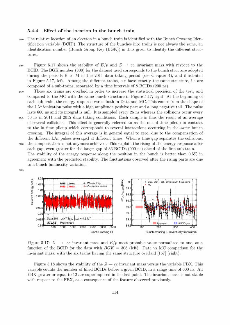
5.4.4 Effect of the location in the bunch train

The relative location of an electron in a bunch train is identified with the Bunch Crossing Iden-2460

tification variable (BCID). The structure of the bunches into trains is not always the same, anidentification number (Bunch Group Key (BGK)) is thus given to identify the different struc-tures.

Figure 5.17 shows the stability of E/p and Z → ee invariant mass with respect to the2465

BCID. The BGK number (308) for the dataset used corresponds to the bunch structure adoptedduring the periods H to M in the 2011 data taking period (see Chapter 4), and illustratedin Figure 5.17, left. Among the different trains, six have exactly the same structure, i.e arecomposed of 4 sub-trains, separated by a time intervals of 8 BCIDs (200 ns).

These six trains are overlaid in order to increase the statistical precision of the test, and2470

compared to the MC with the same bunch structure in Figure 5.17, right. At the beginning ofeach sub-train, the energy response varies both in Data and MC. This comes from the shape ofthe LAr ionization pulse with a high amplitude positive part and a long negative tail. The pulselasts 600 ns and its integral is null. It is sampled every 25 ns whereas the collisions occur every50 ns in 2011 and 2012 data taking conditions. Each sample is thus the result of an average2475

of several collisions. This effect is generally referred to as the out-of-time pileup in contrastto the in-time pileup which corresponds to several interactions occurring in the same bunchcrossing. The integral of this average is in general equal to zero, due to the compensation ofthe different LAr pulses averaged at different times. When a time gap separates the collisions,the compensation is not anymore achieved. This explain the rising of the energy response after2480

each gap, even greater for the larger gap of 36 BCIDs (900 ns) ahead of the first sub-train.The stability of the energy response along the position in the bunch is better than 0.5% inagreement with the predicted stability. The fluctuations observed after the rising parts are dueto a bunch luminosity variation.

2485

Bunch Crossing ID

0 500 1000 1500 2000 2500 3000 3500

Rela

tive e

nerg

y s

cale

0.98

0.985

0.99

0.995

1

1.005

1.01

1.015

1.02

E/pνe→ Wee inv. mass→ Z

RMS: 0.206%

RMS: 0.196%

ATLAS Preliminary

-1 = 4.9 fbtdL∫=7 TeV, sData 2011,

Bunch crossing ID (eventually translated)

100 200 300 400

[G

eV

][8

0,1

00]

>-e

+e

<m

89.3

89.4

89.5

89.6

89.7

89.8

89.9

90 Data, BGK = 308, all trains with 4 sub-trains

MC

Large gap 8 BCID gap

Figure 5.17: Z → ee invariant mass and E/p most probable value normalized to one, as afunction of the BCID for the data with BGK = 308 (left). Data vs MC comparison for theinvariant mass, with the six trains having the same structure overlaid [157] (right).

Figure 5.18 shows the stability of the Z → ee invariant mass versus the variable FBX. Thisvariable counts the number of filled BCIDs before a given BCID, in a range time of 600 ns. AllFBX greater or equal to 12 are superimposed in the last point. The invariant mass is not stablewith respect to the FBX, as a consequence of the feature observed previously.

114

A correction has been designed to handle this effect. It uses the Z → ee invariant mass2490

versus FBX variation, in order to take advantage of the larger statistics offered by this variable.The correction is based on the prediction of the energy from the knowledge of the luminosity

per BCID, and from the prediction of the out-of-time pile up. The corrected energy correspondsto:

EcorrBCID = EmeasBCID − EpredBCID,µ1,µ2,...µN

with EcorrBCID the corrected energy for a given BCID, EmeasBCID the measured energy for a given

BCID, and EpredBCID,µ1,µ2,...µN the predicted additional energy due to out of time pile up for agiven BCID, depending on the luminosity of all BCID before and after the one considered (µiwith i the BCID number).2495

FBX

0 2 4 6 8 10 12

[G

eV

][8

0,1

00]

>-e

+e

<m

89.6

89.8

90

Data, BGK = 308

MC

FBX

0 2 4 6 8 10 12

[G

eV

][8

0,1

00]

>-e

+e

<m

89.6

89.8

90

90.2 Data, period M

Data, period M, corrected

Figure 5.18: Z → ee invariant mass for the data and the MC (left) and for the data only beforeand after the BCID-dependent correction based on the prediction of the additional energy dueto out of time pile up (right) [157].

5.4.5 Uniformity along η

The uniformity along η is measured in narrow bins of size of one cell of the second layer of thecalorimeter (∆η ∼ 0.025), and integrated over φ. The variables αE/p and αZee defined as:

αE/p =MPV DATA

E/p

MPVMCE/p

− 1 (5.5)

αZee =MDATAee

MMCee

− 1 (5.6)

are compared in Figure 5.19.The two methods agree well and see common structures in the following areas:

• |η| ∼ 0.6: an excess is observed in data (∼ 1%)2500

• |η| ∼ 1.52 − 1.55: a negative scale is observed in both methods up to -6%.

• |η| ∼ 1.68: a negative scale is measured with both methods (∼ 3%)

• |η| ∼ 1.8: an excess is observed in data (∼ 2 − 3%)

115

Figure 5.19: Uniformity along η, with a one-cell binning - φ integrated. The overview plot isfollowed by five zooms in different η regions.

• |η| > 2.4: a negative scale is measured with both methods (up to ∼ 3% for the Z methodand ∼ 6% for W one)2505

The overall non-uniformity for this narrow η binning, calculated as the spread of the points(rms) is:

• ∼ 1.9% for E/p from W → eν

• ∼ 0.7% for Z → ee invariant mass

The difference of a factor two between the methods is expected from the averaging effect in the2510

invariant mass method (see above).The binning that was proposed for the in situ calibration 5.3 deals with the non-uniformities

observed here as well with the HV sectors.

116

5.4.6 Comparing Z → ee and W → eν in narrow φ bins

The uniformity in φ is expected to be good from the accordion geometry. This is tested for the2515

2011 and 2012 datasets.Along the pseudorapidity axis, various non-uniformities have been observed. To not bias the

uniformity on the azimuthal axis, the detector is divided in six η bins (excluding the cracks):

[−2.4,−1.6], [−1.3,−0.8], [−0.8, 0], [0, 0.8], [0.8, 1.3], [1.6, 2.4]

A narrow binning in φ is chosen, corresponding to one cell of the second layer of the calorimeter(∆φ = 0.025).

The normalized energy responses in the data for the two methods are compared and shownin Figure 5.20. For this comparison, it should be kept in mind that a factor of about 2 in the2520

measured non-uniformities is expected between the two methods. The comparison of data andMC energy response for both methods, using Equation (5.6) is also shown in Figure 5.21.

This figure shows that the two methods agree very well in the full azimuthal range and in all ηregions. In the region η > 1.6, the E/p method sees however much larger fluctuations, probablydue to the worsening of the tracking performance in this region. The following structures are2525

seen along the φ range for both methods:

• In most of the η regions in the barrel, narrow dips are seen at φ = −π, 0, π. This indicatesan energy loss in the data not well modeled by the MC. This could be produced by amaterial mismodeling. The inner detector rails are good candidates, as they are locatedin these precise regions and extend up to a radius of around 1144-1152 mm. This is more2530

developed in Chapter 6.

• For 0.0 < η < 0.8, and φ ∼ −0.8, a structure is seen. In this region, some Front EndBoards are known to be defective in the back layer of the calorimeter. This issue coversthe region (η, φ) ∼ (0.5,−0.8) and could induce a small loss of energy. In addition, inthis region the High-Voltage settings are problematic.2535

• In the region 1.6 < |η| < 2.4, in the full φ range a large oscillation is seen with a periodicityof ∼ 2π. The effect is more pronounced with the E/p method. A sinusoidal function withthe form A + B · sin(φ) is used to fit this shape with this method, with A and B twoconstants determined in the fit. The result of the fit in the data gives the followingnumbers: A = 1.0002 ± 0.0004 and B = −0.0060 ± 0.0005 for the negative side and2540

A = 1.0001±0.0004 and B = −0.0052±0.0005 for the negative side, where the uncertaintyis statistical only. The fluctuation is then significant and maximal at φ = ±π/2 with asize of ∼ 0.5−0.6%. A mechanical sagging effect of the electrodes and absorbers is a goodcandidate to explain this feature. A gradient of temperature of the liquid argon in theendcap has been also considered, but this temperature is controlled over the time and in2545

different points. This monitoring has shown a good homogeneity of the temperature ofthe liquid argon [175,176].

• Structures with periodicity ∆φ ∼ 0.4 can be seen in the region |η| < 0.8 with both methods.This fine effect is investigated in the next section.

5.4.7 Intermodule widening effect2550

The periodicity of the structure observed with the two methods in the previous section is typicalof the calorimeter modules pattern. The electromagnetic calorimeter is divided in 16 modules in

117

Figure 5.20: Uniformity in data in narrow φ bins and in six η regions, using the Z → ee invariantmass and E/p methods.

the barrel and 8 modules in each endcap. In the barrel each module is subdivided into 16 cells ofsize ∆φ = 0.025. The center of the first module is located at φ = 0 and the two edges at φ = ±0.2.

2555

In Figure 5.22 the most probable value of the variable E/p and the Z → ee invariant mass aredrawn as a function of the azimuth of the electron probe. The modules of the barrel calorimeterare folded to increase the statistical precision. The φ-bin size is 2π/1024, in order to see moreprecisely any cell-structure. The positive and negative azimuths are separated.

The data and MC disagree in the region φ ∼ 0.2, both in positive and negative φ. The size2560

of the discrepancy is different: ∼ 3.5% resp. ∼ 1.5% for φ > 0 resp. φ < 0. The drop in E/pfollows the typical inter-modules localization, and this suggests a loss of energy in the data dueto non-instrumented gaps between the modules.

The gap size uniformity has been probed with the measurement of the electron drift time

118

φ

-3 -2 -1 0 1 2 3

α

-0.1

-0.08

-0.06

-0.04

-0.02

0

0.02

0.04

0.06

0.08

0.1

< -1.6η-2.4 < E/pνe→W

ee inv. mass→Z

ATLAS Preliminary

-1 = 4.9 fbtdL∫=7 TeV, sData 2011,

φ

-3 -2 -1 0 1 2 3

α

-0.1

-0.08

-0.06

-0.04

-0.02

0

0.02

0.04

0.06

0.08

0.1

< -0.8η-1.3 < E/pνe→W

ee inv. mass→Z

ATLAS Preliminary

-1 = 4.9 fbtdL∫=7 TeV, sData 2011,

φ

-3 -2 -1 0 1 2 3

α

-0.1

-0.08

-0.06

-0.04

-0.02

0

0.02

0.04

0.06

0.08

0.1

< 0.0η-0.8 < E/pνe→W

ee inv. mass→Z

ATLAS Preliminary

-1 = 4.9 fbtdL∫=7 TeV, sData 2011,

φ

-3 -2 -1 0 1 2 3

α

-0.1

-0.08

-0.06

-0.04

-0.02

0

0.02

0.04

0.06

0.08

0.1

< 0.8η0.0 < E/pνe→W

ee inv. mass→Z

ATLAS Preliminary

-1 = 4.9 fbtdL∫=7 TeV, sData 2011,

φ

-3 -2 -1 0 1 2 3

α

-0.1

-0.08

-0.06

-0.04

-0.02

0

0.02

0.04

0.06

0.08

0.1

< 1.3η0.8 < E/pνe→W

ee inv. mass→Z

ATLAS Preliminary

-1 = 4.9 fbtdL∫=7 TeV, sData 2011,

φ

-3 -2 -1 0 1 2 3

α

-0.1

-0.08

-0.06

-0.04

-0.02

0

0.02

0.04

0.06

0.08

0.1

< 2.4η1.6 < E/pνe→W

ee inv. mass→Z

ATLAS Preliminary

-1 = 4.9 fbtdL∫=7 TeV, sData 2011,

Figure 5.21: This figure compares MC with Data using the α (Eq. 5.6) parameter.

in the liquid argon from cosmic events and found to be good along pseudorapidity [174]. The2565

uniformity of the drift time along the azimuthal angle has also been checked with cosmic muonsand collision data [177]. A similar periodical φ asymmetry has been found as shown in Fig-ure 5.23(a), for the second sampling of the calorimeter. The dashed lines corresponds to thebarrel inter-modules. The drops in E/p or invariant mass corresponds to peaks in drift time,since an enlargement of the gaps induces a larger drift time and a smaller collection of energy.2570

The φ dependence This effect has a φ-dependence as already observed in Figure 5.22 withE/p. Figure 5.23(b) shows the evolution of the drift time deviations along φ. A sinusoidal shapeis found, that can be fitted to extract a correction. The drift time allow precise measurementof the effect because of the large number of measured events available. //

A check of the φ-dependence is made with E/p, in larger regions. The barrel is divided in2575

four parts each containing four modules: π/4 < φ < 3π/4 (top), −3π/4 < φ < −π/4 (bottom),

119

phi0 0.05 0.1 0.15 0.2 0.25 0.3 0.35 0.4

E/p

pea

k (p

hi>

0)

1

1.01

1.02

1.03

1.04

phi-0.4 -0.35 -0.3 -0.25 -0.2 -0.15 -0.1 -0.05 0

E/p

pea

k (p

hi<

0)

1.02

1.025

1.03

1.035

1.04

1.045

(a) E/p (b) Z → ee invariant mass

Figure 5.22: Evolution of the E/p most probable value - for positive (top) or negative (bottom)azimuths - (a) and of the Z invariant mass (b) for the data (green) and nominal MC (blue) asa function of φ in the barrel calorimeter when the 16 modules are folded.

(a)

(b)

Figure 5.23: Drift time measurement in the second layer of the calorimeter as a function of φusing collision data (a) and evolution of the deviations observed at the inter-module with respectto φ (b). Taken from [177].

−π/4 < φ < π/4 (right) and −3π/4 < φ < 3π/4 (left). The E/p extracted in these four regionsfor the data is shown in Figure 5.24.

The top and bottom parts of the calorimeter have respectively the maximal (∼ 3.5%) andminimal (∼ 1.5%) deviations in the inter-modules, whereas the two sides have intermediate2580

deviations (∼ 2.5%). This confirms the effect seen in the drift time measurement. This is

120

Figure 5.24: Evolution of the most probable value of E/p for the data (blue) as a function of φ inthe barrel calorimeter. The 16 modules are folded and grouped in four regions: π/4 < φ < 3π/4(top left), −3π/4 < φ < −π/4 (bottom left), −π/4 < φ < π/4 (top right) and −3π/4 < φ <3π/4 (bottom right). The black line corresponds to the Double Fermi-Dirac fit of the data (seetext).

interpreted as a widening of the barrel inter-module gaps, modulated by a mechanical saggingeffect. The top part of the calorimeter has larger gaps because the sagging under gravity tendsto widen them.

Correction of the effect Even if very localized, the impact of this fine effect on the total2585

energy and in the constant term is not negligible. Figure 5.22(b) shows that at the inter-module,the mass decreases by around 1%.

Given that this drop concerns around 1 cell in 16, a global effect of around 0.1% is expectedon the total energy in the barrel.

2590

A correction for this effect is derived, using the E/p variable. The holes observed in dataare fitted with a Double Fermi-Dirac (DFD) function:

f(φ) = A−B · 1

1 + e(C·(φ−0.2))· 1

1 + e(D·(φ−0.2))

with A the averaged value on either sides of the hole, B the hole depth and C and D thehole width. This provides four sets of coefficients (A,B,C,D). The result of the fit is seen inFigure 5.24, in black line.

The electron energy is corrected with this function f(φ), and the correction size in GeV asa function of φ is illustrated in Figure 5.25 for electrons with pT = 40 GeV.2595

A tool has been provided that returns automatically the corrected energy, given the φ andη coordinates and the energy of the electrons or photons [178].

The impact of the correction is evaluated at around +0.1% for the mean value of the Z →invariant mass while the rms stays unchanged. The change in the mean value corresponds to

121

Figure 5.25: Size of the correction of the energy in GeV as a function of φ, for an electron withpT = 40 GeV.

the loss of energy expected.2600

The η dependence Inside the barrel, the evolution of the energy loss due to the intermodulewidening along η has been checked. Using the E/p method, it is shown that in the four differentregions: 0 < |η| < 0.34, 0.34 < |η| < 0.68, 0.68 < |η| < 1.03 and 1.03 < |η| < 1.37, integratedover φ, the energy loss in the inter-modules varies. It is respectively 2.45%, 1.94%, 1.92%, 1.87%.A check is done with the drift time variable. Figure 5.26 shows a map (η, φ) of the drift time2605

values in collision data 2. The inter-module effect is clearly seen in this plot, corresponding tothe yellow/red band for φ ∼0.2 3. The increasing of the drift time is larger in the very centralregion of the calorimeter in η, for η < 0.3, as seen from the E/p study. This η-dependence isnot yet taken into account in the correction for the effect.

eta-1 -0.5 0 0.5 1

ph

i

0

0.05

0.1

0.15

0.2

0.25

0.3

0.35

0.4

445

450

455

460

465

470

475

480

485

490

Figure 5.26: Map (η, φ) of the drift time in the second layer of the calorimeter from collisionsdata. The modules are folded along φ.

2The data samples have been kindly provided by the authors cited in reference [177].3The small shift observed between the 2 barrel sides corresponds to one absorber shift simply arising from the

binning.

122

Overview A more accurate correction is planed, using drift time measurements that are more2610

sensitive to the gap size variations and taking into account the η-dependence.The same effect has been investigated in the endcaps (using the appropriate size of the mod-

ules), but nothing similar has been found.

Figure 5.27 shows the variable αE/p, as a function of φ, in the four barrel bins, before and2615

after the correction for the Intermodule Widening Effect is applied. The uniformity and theagreement with the MC is improved with this correction.

Table 5.4 shows the rms in each η bins before and after the correction, for both methods.

η-bin Before Correction [%] After Correction [%]

E/p Z → ee E/p Z → ee−2.4 < η < −1.6 1.04 0.48 1.04 0.50−1.3 < η < −0.8 0.58 0.44 0.57 0.46−0.8 < η < 0 0.51 0.33 0.42 0.290 < η < 0.8 0.54 0.37 0.43 0.34

0.8 < η < 1.3 0.67 0.49 0.67 0.521.6 < η < 2.4 0.88 0.47 0.88 0.49

Table 5.4: This table shows the impact of the Intermodule Widening Effect in narrow φ binning.

As expected, a factor ∼ 2 between the E/p and Z → ee invariant mass non-uniformities arisesand no effect on endcap regions rms is observed after the correction. The average improvement2620

due to the intermodule widening correction is ∼ 12% for the E/p case and ∼ 9% for the Zinvariant mass one.

The final rms are quite small in the barrel regions (below 0.5%), demonstrating that theresidual effects do not contribute much to the large constant term measured in the data. A largepositive/negative asymmetry for the E/p variable is seen in the bin 1.6 < |η| < 2.4: the spread2625

of the points is larger in the negative side. This effect is not yet understood.

5.4.8 Summary

Table 5.5 summarizes the non-uniformities observed in data coming from the time dependenceof the energy response, the stability against pile-up (µ), and the bunch-position dependence ofthe energy response. The numbers quoted corresponds to the sum of statistical fluctuations and2630

non-uniformity, which explain partly the differences between the two methods. They give thenan upper bound on the non-uniformity of the energy response which is in total about 0.1%.

Data (Mee) Data (E/p)

Time 0.052 0.032< µ > 0.058 0.027FBX 0.09 -

Table 5.5: Non-uniformities observed in data as a function of the time, pile-up and bunchposition for the E/p and Z invariant mass methods, extracted from the rms of these profiles.The results are given in percent.

The non-uniformity contribution to the constant term has been also evaluated along φ in η-bins of size ∆η ∼ 0.2. A level of uniformity of typically 0.5% is found. Larger effects occur very

123

φ

-3 -2 -1 0 1 2 3

E/p

α

-0.1

-0.08

-0.06

-0.04

-0.02

0

0.02

0.04

0.06

0.08

0.1

< -0.8η-1.3 < before IMW correctionafter IMW correction

ATLAS Preliminary

-1 = 4.9 fbtdL∫=7 TeV, sData 2011,

φ

-3 -2 -1 0 1 2 3

E/p

α

-0.1

-0.08

-0.06

-0.04

-0.02

0

0.02

0.04

0.06

0.08

0.1

< 0.0η-0.8 < before IMW correctionafter IMW correction

ATLAS Preliminary

-1 = 4.9 fbtdL∫=7 TeV, sData 2011,

φ

-3 -2 -1 0 1 2 3

E/p

α

-0.1

-0.08

-0.06

-0.04

-0.02

0

0.02

0.04

0.06

0.08

0.1

< 0.8η0.0 < before IMW correctionafter IMW correction

ATLAS Preliminary

-1 = 4.9 fbtdL∫=7 TeV, sData 2011,

φ

-3 -2 -1 0 1 2 3

E/p

α

-0.1

-0.08

-0.06

-0.04

-0.02

0

0.02

0.04

0.06

0.08

0.1

< 1.3η0.8 < before IMW correctionafter IMW correction

ATLAS Preliminary

-1 = 4.9 fbtdL∫=7 TeV, sData 2011,

Figure 5.27: αE/p from Eq. 5.6 as a function of φ in the four barrel bins, after the IntermoduleWidening Effect (IMWE) is corrected [157].

locally (as the intermodule widening effect or near the transition regions), but do not contribute2635

significantly to the quality of the intercalibration. Performing an absolute calibration as afunction of pseudorapidity only is then justified.

5.5 Response uniformity using the Jacobian peak

An alternative method is used to probe the electron calibration and is described below. Thismethod relies on the transverse momentum of electrons from Z → ee and W → eν decays. The2640

pT distribution for such electrons forms a Jacobian peak, which is characterized by a sharp edgelocated at half the W or Z mass. Most of the electrons have a pT less than this value, as shownin Figure 5.28 for the W → eν process and in Figure 5.29 for the Z → ee one.

The measurement of the edge position gives access to the relative energy scale. The advantageof this method is that it relies only on the electron pT mainly measured in the calorimeter2645

detector. However, the theoretical uncertainties for the modeling of the Z or W pT distributionare quite large due to emission of additional partons in the final state. This gives on averagean uncertainty on the pT distribution of around 10% corresponding to the size of the strongcoupling constant [179].

5.5.1 Method2650

The method is based on the comparison of the electron pT distribution for the data with a setof MC templates taken from a nominal distribution. The energy in data is not corrected with

124

pT (GeV)30 40 50 60 70 80 90

A.U

0

0.005

0.01

0.015

0.02

0.025

0.03

0.035

(a) W+ → e+ν

pT (GeV)30 40 50 60 70 80 90

A.U

0

0.005

0.01

0.015

0.02

0.025

0.03

0.035

(b) W− → e−ν

Figure 5.28: Electron pT distribution for the W → eν process for the data (black points) andthe nominal MC (blue histogram) for the positrons only (a) and the electrons only (b).

30 35 40 45 50 55 60 65 70

Events

0

5000

10000

15000

20000

25000

30000 +eMC reweighted

Data

pT (GeV)

30 35 40 45 50 55 60 65 70

Data

/MC

0.95

1

1.05

1.1

1.15

1.2

(a) Z → ee, e+

30 35 40 45 50 55 60 65 70

Eve

nts

0

5000

10000

15000

20000

25000

30000 -e

MC reweighted

Data

pT (GeV)30 35 40 45 50 55 60 65 70

Da

ta/M

C

0.95

1

1.05

1.1

1.15

(b) Z → ee, e−

Figure 5.29: Electron pT distribution for the Z → ee process for the data (black points) and thenominal MC (blue histogram) for the positrons only (a) and the electrons only (b).

the scale factors derived from the in situ calibration and the energy in MC is not smeared withthe correction factor derived from the same calibration (see Section 5.3.6).

The electrons from the Z → ee and W → eν processes are selected following the procedure2655

described in Section 5.3.1. All the corrections for the MC listed in Section 5.3.1 are applied,particularly the Z pT reweighting for the 2011 MC.

The MC does not well model the lepton pT distribution for theW → eν process, especially forthe positrons (see Figure 5.28). Such a discrepancy could arise from background contaminationin this channel which is not negligible [180]. As the method is fully based on shape comparisons2660

125

between data and MC, this process cannot be used until the disagreements are better understoodand a deeper study of the background contribution for this process is done.

The Z → ee process is used instead, as it has less background contamination and because theMC better model the lepton pT distribution: as shown in Figure 5.29, the agreement is within±2% up to pT = 60 GeV where it starts to worsen up to 15% at pT = 70 GeV. The range2665

chosen for the study is then [35,55] GeV, so that the discrepancy observed from pT = 60 GeVdoes not affect the comparison.

The Z pT distribution is shown in Figure 5.30 for the data and MC and for the two years2011 and 2012, after reweighting for the 2011 MC sample. The two MC distributions agree well2670

with the observation, except in the low pT range where they both have difficulty to simulate thedata. The discrepancy amounts around 10% for pT,Z < 5 GeV. The effect of this discrepancywill be checked in the following.

0 10 20 30 40 50

Eve

nts

0

5000

10000

15000

20000

25000

30000

35000

MC reweighted

Data

(GeV)Z

pT0 10 20 30 40 50

Da

ta/M

C

0.9

0.95

1

1.05

1.1

1.15

1.2

(a) 2011

[GeV]Z

pT0 10 20 30 40 50

Eve

nts

0

10000

20000

30000

40000

50000 2012

MC

Data

[GeV]Z

pT0 10 20 30 40 50

Dat

a/M

C

0.920.940.960.98

11.021.041.061.08

1.11.12

(b) 2012

Figure 5.30: Z boson pT distribution for the data (black points) and the nominal MC (bluehistogram) for the inclusive dataset collected in 2011 (a), and in 2012 (b).

The MC templates are created by scaling the electron pT by a factor αjac:

pT,bias = pT (1 + αjac)

with αjac taking values between -4% and +4% with a step of 0.2%. Three initial templatesare created, with αjac = −4%, 0,+4%, the others are obtained by linearly interpolating these2675

histograms following a technique described in reference [181]. For illustration, Figure 5.31(a)shows a typical interpolation between -4% and +4% with a step of 2%.

A χ2 minimization is done between the templates and the data distribution, leading to aparabola as a function of the bias injected. The minimum of the parabola gives the scale factorin the data and its width the error on this factor. Figure 5.31(b) shows a typical parabola and2680

the associated fit with a second order polynomial to extract the minimum.

5.5.2 Results

Inter-calibration along η The Jacobian peak method is used to probe the relative inter-calibration along the pseudorapidity. Two different binnings are used in this study: the one

126

pT (GeV)30 40 50 60 70 80

A.U

0

0.005

0.01

0.015

0.02

0.025

0.03

0.035

(a) Interpolation

jac

-0.04 -0.03 -0.02 -0.01 0 0.01 0.02 0.03 0.04

2

0

50

100

150

200

250

300

(b) χ2 minimization

Figure 5.31: (a) Linear interpolation of histograms for αjac between -4% (black line) and 4%(green line) around the nominal template (blue line) with a step of 2% (-2%: red line and +2%pink line). (b) χ2 minimization between the interpolated histograms and the data distribution,as a function of the injected bias (blue empty dots). The black line shows the second orderpolynomial function used to extract the minimum and its error.

defined in Section 5.3 and a narrower binning with ∆η = 0.025. The Jacobian method is run2685

separately for the electrons and positrons, in order to check their compatibility, and the finalresult is given as an average of the two sets of scale factors. The compatibility of the results isfound to be good. In some narrow regions, like near the barrel-endcap transition, or at the endof the endcap, a small difference is observed. This has been understood as coming from the badenergy resolution in these points, which smears out the pT distribution and leads to a loss of2690

sensitivity to the energy scale.The result for a large η binning is shown in Figures 5.32(a) and 5.32(b) for the 2011 and

2012 datasets. The scale factors obtained with the in situ calibration method are overlaid forcomparison. A good agreement of the general shape for the two methods is obtained. A globalshift of the Jacobian scale factors with respect to the reference in the barrel is seen for the 20112695

dataset. The bin-by-bin difference between the two methods is shown in Figure 5.32(d) for thetwo years. The average of the differences for the two years is: 0.0002 ± 0.0002 (0.0000 ± 0.0002in the barrel) in 2012 and −0.0021 ± 0.0002 (−0.0030 ± 0.0002) in 2011. Then a much betteragreement is found in 2012 than in 2011 between the two methods. This could come from variousreasons, both from the detector and simulation side. In Section 5.5.3 the robustness of the result2700

against various parameters is tested.The goodness of the minimization has been also checked. No obvious structure was found,

for both electrons and positrons. The typical value is χ2/NDF ∼ 1, and is no larger than 3,demonstrating the good behaviour of the fit.

2705

The same study has been made with a finer binning, as seen in Figure 5.33. The positiveand negative pseudorapidities are averaged to increase the statistical precision. The scale factorsobtained with the in situ method are overlaid. The structures seen in both methods are in goodagreement and the Jacobian method with its finer binning shows in more details these structures.This study demonstrates the good sensitivity of this method to the relative energy scale, even2710

with a small granularity.

127

η

-2 -1 0 1 2

jac

α

-0.04

-0.03

-0.02

-0.01

0

0.01

0.02

0.03

0.04

2011

Both electrons

ee from Mα

(a) αjac, 2011

η

-2 -1 0 1 2

jac

α

-0.05

-0.04

-0.03

-0.02

-0.01

0

0.01

0.02

0.03

0.04

2012

Both electrons

ee from Mα

(b) αjac, 2012

η-2 -1 0 1 2

jac

α

-0.02

-0.01

0

0.01

0.02

0.03Both electrons 2012

Both electrons 2011

(c) αjac, 2011 vs 2012

η-2 -1 0 1 2

off

α-ja

cα

-0.01

0

0.01

0.02

0.032012

2011

(d) αjac - αoff 2011 vs 2012

Figure 5.32: Inter-calibration scale factors from the Jacobian method compared to the officialscale factors obtained with the in situ method (black line) using the 2011 (a) and 2012 (b)datasets. Comparison of the results for the two years (c) and difference between the two methodsfor the two years (d).

0 0.5 1 1.5 2 2.5

jac

-0.05

-0.04

-0.03

-0.02

-0.01

0

0.01

0.02

Both electrons

ee from M

Figure 5.33: Inter-calibration scale factors for the Jacobian method (blue line) compared to theofficial scale factors obtained with the in situ method (black line). Only the dataset collectedin 2011 is used here.

128

Uniformity vs φ The uniformity along the azimuthal angle is checked with the Jacobianpeak method. The binning used corresponds to ∆φ = 0.1, thus corresponding to four cells ofthe second layer of the calorimeter. The results for the 2011 and 2012 datasets inclusively areshown in Figure 5.34(a).2715

The global inter-calibration scale factors are found to be close to 0, within ±0.5% except insome points:

• At φ = 0, a hole is present for both years. It is more pronounced in the barrel region.This could arise from the ID rail modeling in the MC (see Section 5.4 and Chapter 6).

• A sinusoidal shape of the scale factors, with a maximum and a minimum at φ = −π/22720

and φ = +π/2 respectively is observed. This is more pronounced in the endcap region(see Figure 5.34(b)), in agreement with the effect observed using the E/p method (seeSection 5.4). The regions η < 2 and η > 2 for the endcap have been tested separately, butdid not shown obvious differences. This sinusoidal shapes have been fitted for the Jacobianmethod in 2011 and 2012 in the endcaps with a function of type A + B · sin(φ) with A2725

and B two constants determined in the fit. The result of the fit in the data gives thefollowing numbers: A = 0.0026 ± 0.0003 and B = −0.0040 ± 0.0005 for the 2011 datasetand A = −0.0017 ± 0.0002 and B = −0.0045 ± 0.0005 for the 2012 dataset, where theuncertainty is statistical only. The constants A are significantly different from 0 becauseno energy scale corrections are applied in this study.2730

The amplitudes of the sinusoidal shapes have been compared for the Jacobian methodin 2011 and 2012 and for the E/p method presented in Section 5.4. The constants Ahave been all put to zero and an average of the positive and negative φ sides for theE/p method has been done. Figure 5.35 shows this comparison, without including thestatistical uncertainties. The amplitudes are comparable within these uncertainties.2735

This effect was also observed with drift time measurements in endcaps with a comparableamplitude [182].

φ-3 -2 -1 0 1 2 3

jac

α

-0.01

-0.005

0

0.005

0.01

0.015

0.02v17

Both electrons, 2011

Both electrons, 2012

(a) αjac, 2011 vs 2012

φ

-3 -2 -1 0 1 2 3

jac

α

-0.02

-0.01

0

0.01

0.02

Both electrons, End-Cap Events

2011

2012

(b) αjac, endcap, 2011 vs 2012

Figure 5.34: (a) Inter-calibration scale factors from the Jacobian method as a function of φusing the 2011 (blue dots) and 2012 (red dots) datasets. (b) Same scale factors, selecting eventsin the endcap only.

129

φ

-3 -2 -1 0 1 2 3

Rel

ativ

e en

ergy

sca

le-0.006

-0.004

-0.002

0

0.002

0.004

0.006Both electrons, End-Cap Events

2011, E/p

2011, Jacobian

2012, Jacobian

)φA + B*sin(

Figure 5.35: Sinusoidal functions corresponding to the fit of the scale factors extracted from theE/p method (black line) and the Jacobian method for the 2011 (blue dashed line) and 2012 (reddotted line) datasets.

5.5.3 Cross checks

The robustness of the Jacobian peak method has been tested in various studies. The first checkis the closure of the method: a nominal MC template without bias, is compared to the set2740

of templates used to extract the scale factors in the data. The best scale factor is estimatedwith the same method as described above. Figure 5.36(a) shows the result as a function of thepseudorapidity. It demonstrates a good closure of the method.

The same exercise is done with an injection of a bias of +3% in the initial MC template.Figure 5.36(b) shows the resulting scale factors extracted using the Jacobian peak method.2745

Again, the method shows a good accuracy.

-2 -1 0 1 2

jac

-0.003

-0.002

-0.001

0

0.001

0.002

Both electrons

(a) αjac, closure check

-2 -1 0 1 2

jac

-0.032

-0.031

-0.03

-0.029

-0.028 Both electrons

(b) αjac, injection of a +3% bias

Figure 5.36: Inter-calibration scale factors from the Jacobian method using the nominal MC aspseudo-data (a) and a MC template with +3% bias of the energy scale as pseudo-data (b)

In order to understand the differences between the in situ and Jacobian methods, other testsare done.

130

Impact of the background The background in the Z → ee process can be further rejectedby requiring a tight electron identification criteria. The scale factor obtained with an electron2750

medium (reference case) and tight identification criteria are compared to test the impact of theresidual background on the energy response with the Jacobian method and how the agreementwith the reference results evolves. No sizeable differences are found between the two identifica-tions, showing that the method is quite robust with respect to the background.

Impact of the Z pT modeling As seen in Section 5.5.1, the Z pT is not perfectly modeled2755

in the low pT regime, even after the reweighting for the 2011 MC is applied. The impact ofsuch mismodeling is evaluated by removing all the events having a Z pT lower than 5 GeV. Noobvious differences are seen with this selection.

Impact of the modeling of cos θ∗ The distributions of the Cosine of the angle θ∗ in theCollins-Soper frame for the data and the MC are in good agreement everywhere except in the2760

region cos θ∗ > 0.7 where the MC has some difficulties to model the data. The two regionscos θ∗ > 0.7 and cos θ∗ < 0.7 have very different kinematic characteristics, especially for the pTof the Z. A mismodeling of the region cos θ∗ > 0.7 could then have an impact on the extractionof the Jacobian scale factors. The scale factors are computed by removing the events havingcos θ∗ > 0.7, and compared to the nominal scale factors. A small difference of about 0.1% in2765

average in the barrel is found. This number is then taken as an uncertainty on these scalefactors.

Impact of the MC energy smearing For each η bin, the agreement between the pT distribu-tions in data and MC is checked, after scaling the energies with the best fitted αjac. Figure 5.37shows the ratio of the pT distributions, for the barrel and the endcap, when adding the results2770

of all the bins. A structure around 45 GeV is observed only in the barrel, typical of a resolutioneffect. The resolutions of data and MC do not agree, as expected (no correction was applied)and create this effect. The impact of the smearing correction is tested, by comparing the Jaco-bian scale factor extracted with and without the smearing, and how the agreement between thetwo methods evolves. A small difference of about 0.1% in average in the barrel is found. This2775

number is then taken as an uncertainty on these scale factors.

PDFs The uncertainty on the Z pT modeling, mainly arises from the uncertainty on theparton distribution functions (PDFs). The set of PDFs involved in the MC used for the studycorresponds to the CT10 scheme [183]. The impact of this particular choice on the inter-calibration scale factors is tested rerunning the analysis with a different set of PDFs. The2780

HERAPDF 1.0 [184] set is chosen.Figure 5.38 shows the impact of the change of PDF set on the electron pT distribution. No

obvious difference is observed.Here only two sets of PDF are compared. A more accurate study is needed, to fully under-

stand the effect of the PDFs on the result. One could use additional sets of PDFs like MSTW2785

2008 [79] to pursue the comparison or use the CT10 set alone, playing with the uncertainties onthis specific set.

5.6 The Z → ee lineshape

After the scale factor and smearing correction from the in situ calibration are applied respectivelyto the data and the MC, the final step consists in comparing the Z → ee lineshape itself in the2790

131

pT (GeV)30 40 50 60 70 80

Dat

a/M

C

10

11

12

13

14

15

16

17

18

(a) Barrel

pT (GeV)30 40 50 60 70 80

Data

/MC

8

10

12

14

16

18

20

22

24

26

28

(b) endcap

Figure 5.37: Ratios of the pT distributions in data and MC after scaling the energies with thebest fitted αjac in barrel (a) and endcap (b), and adding the results of all the η bins. The y axisshows the sum of the individual bins ratio, this is why it is far from 1.

[GeV]T

p

30 35 40 45 50 55 60 65 70

Eve

nts

0

10000

20000

30000

40000

50000

60000

70000

80000 ee from Z

-2012, e

Data

MCMC, Reweighting pdfs

[GeV]T

p

30 35 40 45 50 55 60 65 70

Da

ta/M

C

0.92

0.94

0.96

0.98

1

1.02

1.04

1.06

1.08

No reweighting

Pdf Reweighting

Figure 5.38: Distribution of the electron pT for the data (blue histogram) and the MC with theset of PDF CT10 (black points) and HERAPDF10 (pink points). The 2012 dataset is used here.

data and the MC. This lineshape can eventually reveal residual discrepancies not addressed bythe calibration chain. Figure 5.39 shows the data to MC ratio along the Z → ee invariant massafter each step of the calibration for the 2011 and 2012 datasets. The agreement between thefinal lineshapes in data and MC is fairly good in 2011, whereas a 10% discrepancy is seen at lowinvariant mass in 2012.2795

The modification of the low mass tails between the two years is observed only in the MC,the data being stable with time. To understand the origin of this issue, the main modificationsto the MC in 2012 are listed below:

• A new electron reconstruction (seeded track, GSF for electrons, crack calibration).

132

[GeV]-e+em

80 82 84 86 88 90 92 94 96 98 100

Data

/ M

C

0.95

1

1.05

1.1

1.15

1.2

No correction

+ Data correction

+ MC smearing

(a) 2011 (b) 2012

Figure 5.39: Data to MC ratio as a function of the Z → ee invariant mass for the different stepsof the calibration: no correction (blue), after the rescaling of the energies in data (red) and thesmearing of the energies in the MC (black) for the 2011 [157] (a) and 2012 [185] (b) dataset.

• A larger number of interactions per bunch crossing simulated to follow the increasing2800

pileup in data in 2012.

• A change in Geant 4 concerning the multiple scattering modeling. An inconsistency wasfound in the 2011 modeling, leading to unexpected back scattering for high energy electron.The change consisted in removing those unexpected back-scattering events cutting on theangular deflection.2805

Dedicated MC samples have been produced in order to test separately the impact of thesechanges.

Pile up The nominal 2011 MC sample is compared with a sample having identical conditionsexcept the pileup, which is not simulated. This allows to test its impact on the lineshape. Fig-ure 5.40(a) shows the invariant mass distribution for these two samples: no obvious discrepancy2810

is seen in particular in the low mass range. In the following, all the MCs used do not containpileup.

Reconstruction A nominal 2011 MC sample without pileup is compared with a sample havingidentical conditions except the reconstruction, which corresponds to part of the improved 2012one (the seeded tracking is not integrated). Changing the reconstruction leads to a shift of the2815

peak position, by around 100 MeV. As this is not the issue being investigated here, this shift iscorrected so that the two peaks are aligned. After this alignment, no discrepancy is seen betweenthe two lineshapes, especially in the low mass range, as seen in Figure 5.40(b). The sample withpart of the 2012 improved reconstruction is compared with a similar MC where the full 2012reconstruction is applied, in order to test the impact of the seeded tracking. Figure 5.40(c)2820

shows the comparison of the two lineshapes, and again no obvious effect is noticed.

Multiple Scattering The nominal 2011 MC sample with the old multiple scattering mod-eling is compared with an identical sample where the new modeling is implemented. A shiftof the peak position is induced by this modification, which is corrected so that the two peaksare aligned. Figure 5.40(d) shows the comparison of the two lineshapes after this correction. A2825

133

discrepancy of about 10% is seen in the low mass range tails. The 2012 modeling of the multiplescattering yields a reduction of the low mass tails with respect to the 2011 modeling.

[GeV]eeM

80 82 84 86 88 90 92 94 96 98 100

0.01

0.02

0.03

0.04

0.05

0.06

0.07 MC11, reco11, with MSC bug (s1272_r3043)

MC11, reco11, with MSC bug, no pileup (s1576_r4021)

[GeV]eeM

80 82 84 86 88 90 92 94 96 98 100

(s1

57

6_

r40

21

)/(s

12

72

_r3

04

3)

0.9

0.95

1

1.05

1.1

1.15

(a) Pileup

[GeV]eeM

80 82 84 86 88 90 92 94 96 98 100

0.01

0.02

0.03

0.04

0.05

0.06

MC11, reco11, with MSC bug, no pileup (s1576_r4021)

MC11, reco12 (except seed. track.), with MSC bug, no pileup (s1576_r4017)

[GeV]eeM

80 82 84 86 88 90 92 94 96 98 100

(s1

57

6_

r40

17

) /

(s1

57

6_

r40

21

)

0.85

0.9

0.95

1

1.05

1.1

1.15

(b) Reconstruction (without seeded tracking)

[GeV]eeM

80 82 84 86 88 90 92 94 96 98 100

0.01

0.02

0.03

0.04

0.05

0.06

0.07MC11, reco12 (except seed. track.), with MSC bug, no pileup (s1576_r4017)

MC11, full reco12, with MSC bug, no pileup (s1576_r4018)

[GeV]eeM

80 82 84 86 88 90 92 94 96 98 100

(s1576_r4

017)/

(s1576_r4

021)

0.9

0.95

1

1.05

1.1

(c) Reconstruction (with seeded tracking)

[GeV]eeM

80 82 84 86 88 90 92 94 96 98 100

0.01

0.02

0.03

0.04

0.05

0.06MC11, reco11, with MSC bug (s1272_r3043)

MC11, reco11, MSC bug fix (s1535_r3043)

[GeV]eeM

80 82 84 86 88 90 92 94 96 98 100

(s1

53

5_

r30

43

) / (s

12

72

_r3

04

3)

0.8

0.85

0.9

0.95

1

1.05

1.1

1.15

(d) Multiple Scattering

Figure 5.40: Z → ee invariant mass distributions for different configurations of the MC (seetext) and ratio as a function of the invariant mass.

Two possibilities are tested in the following to explain the difference between the 2011 and 2012MC:2830

1 The angular cut introduced in the multiple scattering modeling in 2012 removes artificiallya fraction of the low mass tails and creates a discrepancy of ∼ +10% with respect to thedata in this region.

2 Not introducing this angular cut leads to a wrong modeling of the lineshape, with toomuch low mass tails with respect to the data. However another effect with similar size and2835

opposite sign would have to be present to compensate it and make the agreement good

134

as seen in Figure 5.39(a). For example, a mismodeling of the material could create suchtails. This compensation effect would have to be constant in time.

Figure 5.41 illustrates schematically these two configurations.

[GeV]-e+em

80 82 84 86 88 90 92 94 96 98 100

Da

ta /

MC

0.95

1

1.05

1.1

1.15

1.2

No correction

+ Data correction

+ MC smearing

‐ Mul&ple Sca,ering 

‐ Unknown effect  

1)! 2011!

[GeV]-e+em

80 82 84 86 88 90 92 94 96 98 100

Da

ta /

MC

0.95

1

1.05

1.1

1.15

1.2

No correction

+ Data correction

+ MC smearing

‐ Mul&ple Sca,ering 

‐ Unknown effect 

2012!

[GeV]-e+em

80 82 84 86 88 90 92 94 96 98 100

Da

ta /

MC

0.95

1

1.05

1.1

1.15

1.2

No correction

+ Data correction

+ MC smearing

2011!

‐ Mul&ple Sca,ering 

‐ Unknown effect 

[GeV]-e+em

80 82 84 86 88 90 92 94 96 98 100

Da

ta /

MC

0.95

1

1.05

1.1

1.15

1.2

No correction

+ Data correction

+ MC smearing

‐ Mul&ple Sca,ering 

‐ Unknown effect 

2012!

Figure 5.41: Schematic view of the data over MC ratio for the 2011 (left) and 2012 (right)samples, for the two options (top and bottom) considered in the text to explain the discrepancyin the tails in the low mass range, playing with the multiple scattering effect (pink, plain line)and with another unknown effect (blue dashed line).

5.6.1 Multiple scattering modeling2840

The simulation of the multiple scattering process in 2011 in Geant 4 is covered by the Urban93

framework. In order to understand the origin of the backscattering issue, many checks wereperformed. A numerical instability possibly causing this problem was found and corrected andthe angular cut introduced initially was consequently removed. The checks have highlightedthe existence of another problem: as the step size in gas become smaller, the scattering angle2845

becomes larger, that is an unexpected feature (defect of the model for small steps in gas).Another correction was included, correcting for this effect by introducing a cut on the parameterthat governs the large angular deflection [186].

In order to test the impact of these new fixes on the Z → ee lineshape, and to test therobustness of the multiple scattering modeling, special MC simulations were generated, for the2850

Z → ee process. All these simulations have no pileup, and use the reconstruction designed in2011, but different versions of Geant 4. Two simulations use the nominal Geant4 versionsused in 2011 and 2012 and are called mc11-like and mc12-like.

An alternative multiple scattering model has been also tested, covered by the Urban 95

framework (in the nominal version, the framework used is Urban 93). In addition, a new2855

relativistic modeling for the bremsstrahlung (based on the Seltzer-Berger model [187]) and anew model for the conversion process has been also tested. These two changes are called in

135

the following BremConv95. The old modeling of bremsstrahlung and conversion is calledBremConv93.

The Z → ee invariant mass distribution is built from all the simulations described above,2860

after the usual selection of the events as described in Section 5.3.1. These distributions areshown in Figure 5.42 top. To compare the low mass tails, the ratios of all the lineshapes to themc11-like simulation is done and shown in Figure 5.42 bottom.

These ratios show a discrepancy at low mass for all the simulations with respect to the mc11-

like one, even if attenuated using the Urban 93 model associated with the BremConv95 one.2865

The correction of the numerical instability and of the problematic model for small steps ingas did not modify the lineshape.

[GeV]eeM

80 85 90 95 100

A.U

0

0.02

0.04

0.06

0.08

0.1 mc11-like (s1576_r4018)

mc12-like (s1469_r4075)

Urban93-BremConv93 (s1635)

Urban95-BremConv93 (s1654)

Urban95-BremConv95 (s1657)

Urban93-BremConv95 (s1660)

Aligning the peaks = 90.45 +/- 0.02 GeVeem

= 90.46 +/- 0.02 GeVeem

= 90.53 +/- 0.02 GeVeem = 90.46 +/- 0.02 GeVeem

= 90.45 +/- 0.02 GeVeem = 90.47 +/- 0.02 GeVeem

[GeV]eeM

80 85 90 95 100

fix /

bu

g

0.8

0.85

0.9

0.95

1

1.05

1.1

1.15

1.2mc12-like / mc11-like

Urban93-BremConv93 / mc11-like

Urban95-BremConv93 / mc11-like

Urban95-BremConv95 / mc11-like

Urban93-BremConv95 / mc11-like

Figure 5.42: Z → ee invariant mass for the nominal 2011 (blue line) and 2012 MC (black). Theother distributions corresponds to alternative versions of Geant4 as explained in the text.

This study has demonstrated a good stability of the multiple scattering modeling in term ofits impact on the lineshape.

5.6.2 Other effects2870

In the previous section, the impact of multiple scattering modeling modifications on the line-shape has been shown to be negligible, after the correction of the numerical instability. Thesecond scenario is thus tested in the following.

The impact of a material mismodeling on the lineshape is tested. The lineshapes of a MC with2875

additional material in the inner detector and in the calorimeter (following the G’ configuration,see Table 5.6) and of the nominal MC are compared in Figure 5.43. The MC with the distortedgeometry is treated as pseudo-data and energy scale factor and smearing corrections are derivedfrom the comparison to the nominal MC following the method described in Section 5.3.3. The

136

different steps of the calibrations are shown in this figure. After all the corrections are applied,2880

an effect of around 10% in the low mass tails is visible in the ratio between the distorted andnominal lineshapes.

Figure 5.43: Ratios between a distorted and nominal MC lineshapes from the Z → ee invariantmass, using the 2012 dataset. The different calibrations steps are shown: no correction (bluedots), after applying the energy scale factor in the distorted MC (red dots) and applying alsothe smearing correction in the nominal MC (black dots) [185].

If the data have additional material in some regions one could thus expect an increasing ofthe low mass tails. However the amount of material added in the distorted MC is very large,and many studies have shown the data to be quite similar to the nominal MC except in some2885

localized regions (see Chapter 6). Some other effects are expected to have an impact on thelineshape. Among them, the layer inter-calibration will be tested in Section 5.8, after a fullmeasurement of the relative layers scales which will be discussed in Sections 5.7.1 and 5.7.2.

5.7 The layer inter-calibration

The electromagnetic calorimeter is divided into three layers and a presampler. The inter-2890

calibration of these four layers is necessary before any more global calibration, using the energyfractions in these layers, is done.

5.7.1 The presampler calibration

The presampler layer is a system which is mainly used to recover the energy lost in front of theaccordion and is a separated layer independent of the accordion system. An inter-calibration2895

between this layer and the accordion is needed.The presampler energy scale is defined as the ratio between the data and the MC of the

energy deposited in the presampler layer. However, due to the sensitivity of the presampler tothe material, a bias on this ratio could come from different sources:

• A material mismodeling in the MC2900

• A presampler energy scale difference between data and MC

137

These two effects can be decorrelated using an extra variable, also sensitive to materialmismodeling. The variable chosen is E1/E2, corresponding to the ratio of energy deposited inthe first and second sampling of the accordion. It was shown in Chapter 6 to be very powerful inprobing the material distribution. Figure 5.44 shows the response of the presampler energy and2905

E1/E2 in data compared to the nominal MC, as a function of pseudorapidity. The responsesare clearly correlated. This variable has been also chosen because the E1 and E2 energies havebeen shown to be quite well modeled from tests with cosmic muons [174].

η-2 -1 0 1 2

da

ta /

MC

0.6

0.7

0.8

0.9

1

1.1

1.2

1.3

0E

2/E

1E

Figure 5.44: Comparison between the data over MC ratios for the presampler energy (red line)and for the E1/E2 variable (blue line) as a function of the pseudorapidity for Z → ee events.

5.7.1.1 E0 and E1/E2 correlation

The correlation between the presampler energy E0 and E1/E2 is investigated using simulations2910

with additional material in different places of the detector.Table 5.6 gives the characteristic of these different simulations. Different kind of geometries

are used, with additional material:

1) In the Inner Detector,

2) Just before the calorimeter in the cryostat,2915

3) Between the presampler and the accordion,

4) Just after the calorimeter, in the cryostat.

The energy deposited in the presampler is only sensitive to material added before this detector(categories 1 and 2). The energy deposited in the layers 1 and 2 is only sensitive to materialadded before the accordion (categories 1, 2 and 3). A bias is therefore expected from this2920

method, due to the third geometry category, that is not seen by both variables. An uncertaintywill be derived for this.

The analysis is performed in pseudorapidity bins, as the material distribution varies rapidlywith this variable. The binning used is similar to the one used for the in situ method:

0, 0.2, 0.4, 0.6, 0.7, 0.8, 0.9, 1.0, 1.1, 1.2, 1.3, 1.37, 1.55, 1.63, 1.74, 1.8

excluding the complicated transition region [1.37, 1.55] and averaging the positive and negativesides.

138

Table 5.6: Fraction of radiation lengths (X0) added in various places of the detectors, for thedifferent MC geometries configurations. The different places are in the whole Inner Detector(ID), in the pixel or SCT services (Pixel S, SCT S), at the end of SCT/TRT endcaps (SCT/TRTEC), in the Inner Detector end-plate (ID e.p), in the pixels or SCT only (Pixel, SCT), radiallyin barrel cryostat before the calorimeter (Cryost. 1), radially between the presampler and thestrips in barrel (PS/S1), and radially in the cryostat after the barrel calorimeter (Cryost. 2).

Config. ID Pixel S. SCT S. SCT/TRT EC ID e.p Pixel SCT Cryost. 1 PS/S1 Cryost. 2

A (16-02) 5% - - - - - - - - -B (16-03) 10% - - - - - - - - -C (16-04) - 20% - - - - - - - -D (16-05) - - 20% - - - - - - -E (16-06) - - - 15% - - - - - -F (16-07) - - - - 15% - - - - -G’ (16-11) 5% 20% 20% 15% 15% - - 0.1 0.05 0.1I’ (16-12) 5% 20% 20% 15% - - - - - -J (16-13) - - - - - 5% - - - -K (16-14) - - - - - - 5% - - -L (16-15) - - - - - - - 0.1 - -M (16-16) - - - - - - - - 0.05 -

For each of these bins, for the data and for the different distorted MC geometries, the2925

distribution of the E0 and E1/E2 variables are made, and their means are extracted: Edata0 ,Edist0 , (E1/E2)

data, (E1/E2)dist. The ratios with the mean extracted from the nominal MC

geometry: Enom0 , (E1/E2)nom, are computed. In order not to be influenced by the MC-based

calibration, the uncalibrated (raw) energies, are used.Figure 5.45 shows the ratios, simultaneously for the two variables and for the representative2930

bin 1.0 < |η| < 1.1.In this figure, the geometries belonging to the categories 1 and 2 are depicted with full circles,

whereas the ones belonging to the categories 3 and 4 are depicted with empty circles. The dataare depicted with the green diamond.

A linear correlation is observed between the two variables, for all the geometries used. The2935

slope is the same for the two kind of geometries illustrated, even if the second one is shifted byδ(E1/E2) = 3% along the (E1/E2)/(E1/E2)

nom axis, as expected (the energy in presampler isinsensitive to this kind of material). The same behaviour is observed for all the other bins.

The correlation between the two variables is then expressed as:

E0

Enom0

= 1 +A · ( E1/E2

(E1/E2)nom− 1) (5.7)

for the different geometries, with A the slope fitted through the points representing the geome-tries with material before the presampler.2940

If the presampler energy scale in MC is well simulated, the data point should be aligned withthe other geometries. The difference, illustrated in the figure with the green arrow, is interpretedas coming from a different energy scale in data and MC.

More analytically, the ratio of the presampler energy observed to the one predicted is written:

Edata, obs0

Enom0

=Edata,mat.0

Enom0

· Edata, calib0

Enom0

= αPSmat · αPScalib

139

nom)2

/E1

)/(E2

/E1

(E

0.9 0.95 1 1.05 1.1

nom

0/E0

E

0.9

0.95

1

1.05

1.1

1.15

δ(E1/E2)!

PS

sc

ale!

1

1.05

1.1

1.15

GEO-16-12

GEO-16-02

GEO-16-03

GEO-16-04

GEO-16-05

GEO-16-06

GEO-16-07

GEO-16-13

GEO-16-14

GEO-16-15

GEO-16-16

GEO G’

Data

1.0 < |η| < 1.1!

Figure 5.45: Ratio of the mean of the presampler energy distribution in data or in distorted MCgeometries over the nominal MC as a function of the same ratio for the E1/E2 variable, usingZ → ee events, for the bin 1.0 < η < 1.1.

where αPSmat and αPScalib are the presampler energy response in data only due to material mis-2945

modeling and presampler scale mismodeling respectively.

Similarly, one can write:

(E1/E2)data, obs

(E1/E2)nom=

(E1/E2)data,mat.

(E1/E2)nom· (E1/E2)

data, calib

(E1/E2)nom= αE12

mat · αE12calib

with αE12mat and αE12

calib the E1/E2 energy response in data only due to material mismodelingand to inter-calibration between the first and second layer respectively.

From Equation 5.7, one can write:

αPSmat = 1 +A · (αE12mat − 1)

Given that:

αPScalib =Edata, obs0

Enom0

· 1

αPSmatand that

αE12mat =

(E1/E2)data, obs

(E1/E2)nom· 1

αE12calib

one gets finally:

αPScalib =Edata, obs0

Enom0

· 1

1 +A · ( (E1/E2)data, obs

(E1/E2)nom · 1αE12

calib

− 1)(5.8)

In this equation, all the quantities are measurable directly from Figure ??, except αE12calib which2950

represents the inter-calibration difference between data and MC of the layers 1 and 2. Thisquantity can be determined with an separate study which is presented below.

140

5.7.1.2 The E1/E2 modeling

Despite the good agreement between data and MC of the E1/E2 response found during the testbeams, a study is done to determine more precisely the quantity αE12

calib.2955

In order to test only the relative layer scales and to be insensitive to the material before theaccordion, a sample of radiative unconverted photons is used. The unconverted photon are suchthat the conversion radius is larger than 800 mm, ensuring a non-interaction with the materialup to this radius. In addition the transverse energy deposited in the presampler is requiredto be below 0.5 GeV, reducing strongly the number of events having interacted with material2960

upstream the presampler 4.The fraction E1/E2 for these photons is compared between the data and MC. This ratio

should be only sensitive to the relative layer scale.Figure 5.46 shows this ratio as a function of the pseudorapidity.

Figure 5.46: E1/E2 comparison between data and MC for radiative unconverted photons withlow energy deposited in the PS as a function of the pseudorapidity of the photons for the 2011and 2012 datasets. The red lines corresponds to a linear fit of the points in large η regions andthe red filled regions the uncertainties on this fit.

A relative E1/E2 scale different from 1 for the data to MC comparison is observed everywhere,2965

leading to around -3% in the barrel, +2% in the region 1.55 < |η| < 1.8 and +7% in the end ofthe endcap. There is a point where the data/MC ratio differs from 1 by 17% at |η| ∼ 1.9. Thesenumbers are used for the presampler scale measurement. The uncertainties on these values areestimated below.

5.7.1.3 Uncertainties on E1/E2 modeling2970

Three different sources of uncertainties arise from the measurement of αE12calib:

1) The statistical error.

2) The uncertainty on the purity of the sample used: if converted photons contaminate it,this can leads to a bias on the E1/E2 response due to material effects.

4This selection does not allow to remove events having interacted with material located between the presamplerand the strips

141

3) The uncertainty on the material after the PS.2975

Uncertainty from material before presampler This uncertainty is evaluated using sim-ulated single photon events with additional material only before the presampler, typically theconfiguration L defined in Table 5.6. In this configuration the material is added in the cryostatjust before the PS. The same selection as the one described previously is made, in order to selectonly photons interacting very little with the material. The distorted to nominal MC ratio of the2980

variable E1/E2 is shown in Figure 5.47(a) as a function of the pseudorapidity in three large bins(barrel, 1.55 < |η| < 1.8 and end of the endcap). Two kind of photons are shown: ones havingthe cut on the PS energy EPS,T < 0.5 GeV and the others with this constraint inverted. Thevalue of E1/E2 from a single electrons MC simulation is overlaid as a comparison. No cut on thepresampler energy is done on these electrons, as this removes the majority of the events. This2985

figure shows that the cut on the PS energy for photons is efficient in reducing material effects.A residual effect is however observed for these events, that is interpreted as the impact of thecontamination of converted photons in the sample. The effect is around 0.5% and taken as anuncertainty on the αE12

calib variable.

η

0 0.5 1 1.5 2 2.5

nom

)2

/E 1/(

Ed

ist

)2

/E 1(E

0.98

0.99

1

1.01

1.02

1.03

1.04

GEO-20-13-01 (10% X0, ID-PS)

<0.5 GeVPS, T

UC photons, E

>0.5 GeVPS, T

UC photons, E

Electrons

(a) Material before PS

η

0 0.5 1 1.5 2 2.5

no

m)

2/E 1

/(E

dis

t)

2/E 1

(E

0.99

1

1.01

1.02

1.03

1.04

GEO-20-14-01 (5%X0, PS-strips)

<0.5 GeVPS, T

UC photons, E

>0.5 GeVPS, T

UC photons, E

Electrons

(b) Material between PS and strips

Figure 5.47: Distorted over nominal MC ratio for the variable E1/E2 as a function of the pseu-dorapidity with the distorted geometry corresponding to additional material in cryostat beforethe presampler (a) or between the presampler and the strips (b). Three different populationsare depicted: single unconverted photons with the cut E0,T < 0.5 GeV (black open circles), orE0,T > 0.5 GeV (black full circles) and single electrons (red triangles).

Uncertainty from material between presampler and strips The presence of material2990

just after the presampler could bias the measurement of the layer inter-calibration. For the pre-sampler scale measurement, the dependence of E1/E2 to this late material is already contained

in the ratio (E1/E2)data, obs

(E1/E2)nom as seen in Equation 5.8. The variable αE12calib estimated with the method

presented above, also indirectly measures the contribution of such material. From Equation 5.8,one can thus see that this dependence washes out. In reality, one needs to take into account the2995

difference of response between radiative unconverted photons and electrons from Z → ee.Again this is achieved with a MC with a distorted geometry where material is added only

between the presampler and the strips (see configuration M in Table 5.6).Figure 5.47(b) shows the ratio of the distorted MC response to the nominal one for the

E1/E2 variable for single unconverted photons with a cut on presampler transverse energy. This3000

is compared with the single electrons without cut on the presampler energy. The difference along

142

the pseudorapidity is at worst around 1%. This difference is taken as an uncertainty comingfrom material located after the presampler.

5.7.1.4 Presampler energy scale

All the quantities from Equation 5.8 are now determined. Figure 5.48 shows the variable αPScalib3005

as a function of the pseudorapidity. The binning used correspond to ∆η = 0.05. The uncertain-ties coming from the statistical errors and the uncertainty on the αE12

calib measurement are alsodepicted. Two different results are presented: using a fitted estimation of the variable αE12

calib

as seen in Figure ?? in large η regions or using the values determined in each η-bin. This hasan impact on the presampler scale shape along η, but the results are compatible within the3010

uncertainties. Using the unfitted evaluation, the presampler scale is flattened in the barrel. Thetypical values of this scale are around -2% in the barrel and -14% in the endcap. The uncer-tainty in the barrel and endcap is typically 3%. The presampler is composed of 16 modules (14modules of size ∆η = 0.2 in the barrel and 2 modules of size ∆η = 0.3 in the endcap). Theenergy scale is thus extracted in each modules. Within a presampler module, the energy scales3015

evaluated with a binning of 0.05 well agree each other, except in the endcap.

(a) Fitted αE12calib (b) Unfitted αE12

calib

Figure 5.48: Presampler energy scale in the data, as a function of the pseudorapidity for electronsfrom the Z → ee decay using a fitted (a) or unfitted (b) estimation of the variable αE12

calib. Theblue line corresponds to the fit through presampler modules and the blue band corresponds tothe uncertainty.

Figure 5.49(a) shows the ratiosEdata, obs

0Enom

0and

Edata, calib0Enom

0, corresponding to the data to MC ratio

of the presampler energy before and after the material correction. In this plot, no miscalibrationof the E1/E2 in the data is assumed. The difference between this figure and Figure 5.48 showstherefore the impact of the inter-calibration of the layers 1 and 2 on the measurement of the3020

presampler energy scale. Figure 5.49(b) illustrates the material correction itself, i.eEdata, mat.

0Enom

0.

It is an indirect representation of the mismodeling of the material in the nominal MC.

5.7.2 The strip/middle inter-calibration

The different accordion layers may have different energy scale due to longitudinal cross talk andimperfect determination of the electronic calibration. In Section 5.3.5.2, it has been shown that3025

only the inter-calibration between the first and second layer is relevant.

143

η-2 -1.5 -1 -0.5 0 0.5 1 1.5 2

no

m, m

c11

/E0

data

E0

0.6

0.7

0.8

0.9

1

1.1

1.2

1.3

Before correction

After correction

(a)

η-2 -1 0 1 2

Ma

teria

l C

orre

cti

on

0.8

0.9

1

1.1

1.2

1.3

1.4

(b)

Figure 5.49: (a) Data to MC ratio of the presampler energy before (blue full circles) and after(red empty circles) the material correction, as a function of the pseudorapidity for electronsfrom the Z → ee decay and assuming αE12

calib = 1. (b) Material correction as a function of thepseudorapidity.

This inter-calibration has been already measured in Section 5.7.1.2, using unconverted pho-tons interacting little with the material as it was needed for the presampler calibration. However,this method suffers from the uncertainty on the material located after the presampler. This un-certainty was factorized and eliminated in the presampler scale measurement, but for the layer3030

inter-calibration this cannot be done.Other methods free from such material effects are used to probe this inter-calibration. The

one presented here relies on the dependence of the Z invariant mass to the fraction E1/E2.

5.7.2.1 Invariant mass method

Method The ratio E1/E2 is related to the amount of energy lost upstream of the calorimeter3035

and then to a quantity like the Z → ee invariant mass. A nominal MC simulating the Z → eeprocess and the 2012 datasets are used in this study. The Z candidates are selected as describedin Section 5.3.3.

Figure 5.50(b) shows the correlation between the invariant mass of the events selected andthe variable E1/E2 for the representative bin 0.4 < |η| < 0.6. The analysis is performed in allthe other regions with the binning:

0, 0.2, 0.4, 0.6, 0.8, 1.0, 1.2, 1.37, 1.52, 1.8, 1.9, 2.1, 2.3, 2.47

The data over MC ratio should be stable against the variation of E1/E2, if the MC well simulatesthe data. This is not the case, as seen in Figure 5.50(c), where the ratio decreases as a function3040

of E1/E2.

The origin of this mismodeling may be:

• A material mismodeling: a MC simulating the Z → ee process with additional materialfollowing the configuration G’ (see Table 5.6) is used to test this possibility. The distorted3045

to nominal MC ratio for the invariant mass is shown in Figure ??. It is stable againstE1/E2 so that it cannot be the cause of the effect observed in the data to MC ratio.

144

2/E1

E

0.1 0.2 0.3 0.4 0.5 0.6 0.7 0.8 0.9 1

Events

0

20

40

60

80

100

120

140

310×

Data

Nominal MC

Distorted (G’) MC

|<0.600.40<|

(a)

2/E

1E

0.1 0.2 0.3 0.4 0.5 0.6 0.7 0.8 0.9 1

[G

eV

]e

em

88

88.5

89

89.5

90

90.5

91

91.5

Data

+3%1

Data, bias E

=cst2

+E1

biased, E2

/E1

Data, E

MC, Nominal

MC, Distorted (G’)

|<0.600.40<|

(b)

2/E

1E

0.1 0.2 0.3 0.4 0.5 0.6 0.7 0.8 0.9 1

ee

Ratio m

0.985

0.99

0.995

1

1.005

1.01

1.015

|<0.600.40<|

Data / Nominal MC

+3%) / Nominal MC1

(Data, bias E

=cst) / Nominal MC2+E1

, E2

/E1

(Data, bias E

Distorted (G’) / Nominal MC

(c)

Figure 5.50: (a) E1/E2 distribution for the data (black histogram), the nominal MC (blue opencircles) and the MC with additional geometry following configuration G’ (pink open squares).(b) Z → ee invariant mass as a function of E1/E2 for the data (black points), the nominalMC (blue open circles), the MC with additional geometry following configuration G’ (pink opensquares), the data with a 3% scale of the strips energy keeping (red stars) or not (green triangles)the sum of strips and middle energy constant. (c) Ratios of the previous curves to the nominalMC one. The bin shown is 0.4 < |η| < 0.6.

• A layer 1 and 2 relative miscalibration as seen in Section 5.7.1.2: this is tested by anarbitrary rescaling of the strips energy by +3%. The MC-based calibration described inSection 5.2 is rerun because the scaling of the strip energy changes the repartition of the3050

total energy in the different layers. Only an approximative calibration is performed, usinga dedicated tool (Offline Calibration Tool [188]). The resulting energy is used to computethe invariant mass, which is compared to the one in the nominal MC. As seen in Figure ??,the scaling of the strip layer energy has an impact on the MC description of the evolutionof the invariant mass with E1/E2. Therefore this could be at the origin of the effect seen3055

in the data to MC ratio.

• Cross talk between the strips and middle layers: this can be probed using the proceduredescribed in the previous item, requiring in addition that the sum of the layer 1 and 2energies be constant, to describe a transfer of energy between these two layers. The ratioof the resulting invariant mass, recomputed using the same calibration tool, to the mass3060

145

from the nominal MC is shown in Figure ??. It is not different from the simple data overMC ratio. The discrepancy between data and MC can therefore not be explained by across talk effect.

The method is therefore sensitive to layer inter-calibration, and is free from effects like cross-talk or material mismodeling.3065

The inter-calibration between the two layers is measured by varying the strip energy scale α1

from 0.89 to 1.16 in 0.01 steps, leaving the middle layer energy unchanged. For each variationof α1, the procedure explained above is repeated. A χ2 minimization is done to find the bestvalue of α1 that renders the invariant mass data to MC ratio the most compatible with a flat3070

line. The χ2 as a function of the factor α1 is fitted with a parabola whose minimum and widthgive the best value of α1 and its statistical uncertainty.

The result of this minimization for all the η bins is shown in Figure 5.51(a).

η

0 0.5 1 1.5 2 2.5

1α

0.85

0.9

0.95

1

1.05

1.1 Without PS energy correction

With PS energy correction

With ’flat’ PS energy correction

(a)

η

0 0.5 1 1.5 2 2.5

2χ

best

0

50

100

150

200

250

300

350Without PS energy correction

With PS energy correction

With ’flat’ PS energy correction

(b)

Figure 5.51: Strip/middle inter-calibration (a) and best fitted χ2 associated to this inter-calibration when the presampler scale is not corrected (blue up triangles), when it is correctedusing a fitted (pink down triangles) or unfitted (black dots) estimation of the variable αE12

calib asa function of the pseudorapidity for electrons from the Z → ee decay.

In addition, the impact of the presampler calibration is tested: the two sets of presamplerscale factors derived in the Section 5.7.1.4 are used to correct for the presampler energy. As3075

for the scaling of the strip energy, the approached MC-based calibration tool is used. The fullprocedure presented above is rerun with this correction.

Figure 5.51(a) presents the comparison with the case where no PS correction is made. Thishas a large impact in the endcap, where the presampler scale factor is around 14% and a smalleffect in the barrel up to |η| = 0.8. For |η| > 0.8 the impact is slightly larger.3080

The two different sets of presampler scale give compatible results except in the bin 1.2 <|η| < 1.37.

Figure 5.51(b) shows the best fitted χ2 associated to the strip scale extracted. This showsup pathological regions, where this number is very large, indicating that no appropriate scalefactor for the strips was found to flatten the data to MC ratio. This is the case for the regions3085

1.5 < |η| < 1.8 and 2.3 < |η| < 2.47.

In the barrel, the E1/E2 inter-calibration results are similar to the ones found with theunconverted radiative photons. However the measured inter-calibration from the photons was

146

flat in this region which is not the case with the present method. More particularly, a step at3090

η = 0.8 is seen.In the endcap, the two methods disagree.

Systematic The systematic uncertainties associated with this method are evaluated below.First the robustness of the method is tested by closure. The nominal MC is treated as pseudo-data and the full analysis is rerun with it. The result is shown in Figure 5.52(a). The biggest3095

deviations are around 1%. This number is taken as an uncertainty coming from the method.

η

0 0.5 1 1.5 2 2.5

1α

0.985

0.99

0.995

1

1.005

1.01

1.015

1.02

1.025 MC nominal as data, closure check

(a)

η

0 0.5 1 1.5 2 2.5

1α

0.98

0.99

1

1.01

1.02

1.03

1.04

1.05

1.06MC distorted (G’) as data

(b)

Figure 5.52: (a) Closure check for the method, using a nominal MC as pseudo-data. (b) Evalu-ation of the impact of the material mismodeling in the layer intercalibration, using a distortedgeometry following the configuration G’ as pseudo-data.

The second test concerns the material mismodeling. Even though the method is found tobe insensitive to the presence of extra-material, the full analysis is rerun with the distortedMC geometry following configuration G’ treated as the pseudo-data. The result is shown inFigure 5.52(b). In the barrel and in the endcap with η > 1.8, the closure works well, and the3100

biggest deviations are 1.5% and 2% respectively. In the region 1.52 < η < 1.8, a larger devia-tion of ∼ 4% is found. These three numbers are taken as an uncertainty coming from materialmismodeling.

As seen from Figure 5.51(b), this particular region is complicated, the method fails to find3105

an appropriate scale factor.

5.7.2.2 Comparison of the results

This method is compared with two other procedures:

• The same analysis is rerun, using the variable E/p as a probe instead of the Z → ee invari-ant mass. However this method is effective only in the barrel, as the track measurement3110

is less accurate in the endcap, especially for large E1/E2 fractions.

• The muons traversing the detector are insensitive to the material. The energy loss inthe calorimeter is used as a direct probe of the layer scales. The ratio E1/E2 providesdirectly a measurement of the the layer strip/middle inter-calibration. However, due tovery low fraction of energy loss in the calorimeter, this method is sensitive to cross talk and3115

147

electronic noise. Two different methods to extract the mean of the energy loss distributionare tried: using a convoluted fit of a Landau and a Gaussian function or a truncated meanestimator from 50% to 90%.

The results obtained with all the methods are overlaid and shown in Figure 5.53.

Figure 5.53: Relative layer 1 and 2 calibration as a function of the pseudorapidity of the probe,as measured with different methods. The black horizontal lines and grey filled area correspondto the weighted average with a χ2 penalty of all the methods and the associated uncertainty.

All the methods agree well in the barrel and in the endcap except in the bins 1.2 < |η| < 1.43120

and 1.5 < |η| < 1.8 for the invariant mass method. The structure is the same, especially thestep at η = 0.8. In this figure, all the statistic and systematic errors for the different methodsare shown. The precision on the layer relative scale is around 1-4% depending on the region.The difference between the result found with these methods and the one found with unconvertedradiative photons can be interpreted as an effect of material located after the presampler.3125

5.8 Z → ee lineshape after layer inter-calibration

As discussed in Section 5.6, it has been found that the discrepancy observed in the Z → eelineshape might be due to material mismodeling. However, from the actual knowledge of thematerial distribution in the data (see Chapter 6), this source is not sufficient to explain thefull discrepancy. In this section other possibilities are investigated. In particular, the layer3130

miscalibration that has been measured in Sections 5.7.1 and 5.7.2 is tested.Figure 5.54 shows the impact on the lineshape of rescaling the presampler and strips energy

according to their energy scale measured previously. For the strips rescaling, two options aretested: the sum of of the strip and middle energies are kept constant or not. From this figure,it can be seen that only the modification of the presampler scale has a sizeable impact on the3135

low mass tails: around 5% more tails are expected when applying the scale modification. Thisgoes in the right direction to explain the discrepancy seen in data.

However, the presampler extends only up to |η = 1.8| so that it is not expected to be theonly source. A test has been made to estimate the effect of the strip miscalibration and thematerial mismodeling in the region |η| > 1.8.3140

The discrepancy observed in the lineshape as seen in Figure 5.39 has been derived from aninclusive sample (no η selection). It has been then first checked that selecting exclusively eventsin the region |η| > 1.8 gives a similar effect. A study has shown that 10% more low mass tails

148

[GeV]eem

80 85 90 95 100

A.U

0

0.02

0.04

0.06

0.08

0.1 Aligning the peaks

Nominal MC12

MC12, bias E1 like in data

MC12, bias E1/E2 like in data, E1+E2=cst

MC12, bias E0 follow. PS scale

[GeV]eem

80 85 90 95 100

bia

se

d /

no

min

al

0.9

0.95

1

1.05

1.1

1.15

1.2

1.25MC12: bias E1 like in data / Nominal

MC12: bias E1/E2 like in data (E1+E2)=cst / Nominal

MC12: bias E0 follow. PS scale

Figure 5.54: Z → ee lineshape comparisons for the nominal MC (black line), a MC where thestrips energy has been scaled according to scale measured in data and where the middle energyis kept constant (blue line), a MC where the strips energy has been scaled according to scalemeasured in data and where the middle energy has been modified so that the sum of strip andmiddle energy remain constant (pink line), and a MC where the presampler energy has beenscaled according to scale measured in data (red line). The ratios of each of these configurationsto the nominal MC is shown on the bottom.

are again seen in the data to MC comparison after all corrections, when selecting only electronswith |η| > 1.8 [185].3145

Figure 5.55(a) shows the Z → ee lineshape for both electrons in the region |η| > 1.8 forthe nominal MC and for a MC where the strips energy has been scaled accordingly to the scalemeasurement in data. On can see that even in this region, the strips miscalibration cannotexplain the lineshape discrepancies. In Figure 5.55(b), the nominal MC lineshape is comparedto a MC with additional material in the detector following the configuration G’. In this case,3150

the discrepancy in the low mass tails is still present and amounts to about 15%.The region |η| > 1.8 is precisely where a large discrepancy arises between data and MC in

the longitudinal shower shapes variable E1/E2 used for the measurement of the material bud-get in data (see Figure 6.24). This discrepancy amounted to about 10% in this region. Moreparticularly, it is shown from this Figure 6.24 that in this region, the material budget in data3155

seem to be closer to the G’ configuration than to the nominal one.

All this leads to the conclusion that the lineshape discrepancy observed between the dataand the MC could, at least in the region |η| > 1.8, be explained by a material mismodeling.For the region |η| < 1.8, two sources have been highlighted, the material mismodeling and the3160

presampler scale miscalibration. In reality other effects have also been found to have an impacton the low mass tails, for example the lateral shower shape discrepancies between data and MC,arising from a lateral leakage (out-of cluster energy) mismodeling [189]. The full understanding

149

of the Z → ee lineshape is thus not yet complete, and more studies will be needed to understandall the effects and model them well.3165

[GeV]eem

80 85 90 95 100

A.U

0

0.02

0.04

0.06

0.08

0.1 Aligning the peaks

Nominal MC12

MC12, bias E1 like in data

|>1.8ηBoth electrons with |

[GeV]eem

80 85 90 95 100

bia

se

d /

no

min

al

0.9

0.95

1

1.05

1.1

MC12: bias E1 like in data / Nominal

(a)

[GeV]eem

80 85 90 95 100

A.U

0

0.02

0.04

0.06

0.08

0.1Aligning the peaks

Nominal MC12

MC12, distorted geometry (G’)

|>1.8ηBoth electrons with |

[GeV]eem

80 85 90 95 100b

iase

d /

no

min

al

0.9

0.95

1

1.05

1.1

1.15

1.2

1.25

MC12, distorted geo (G’) / Nominal

(b)

Figure 5.55: Z → ee lineshape comparisons between the nominal MC (black line) and (a) aMC where the strips energy has been scaled according to scale measured in data and where themiddle energy is kept constant (blue line) (b) and a MC with additional material in the detectorfollowing the configuration G’. The ratios of each of this configuration to the nominal MC isshown on the bottom.

150

Chapter 6

Probing the material budgetupstream of the calorimeter withshower shapes3170

From Chapter 3 it has been seen that the amount of material in front of the electromagneticcalorimeter is quite substantial. This may lead to energy losses upstream of the calorimeters.As seen in Chapter 5, such energy losses are corrected for with a MC-based simulation. Thecorrections are valid if the material description in the simulation well corresponds to the one indata.3175

A method developed to compare the material budget in data and MC is described below.

6.1 Interaction of particles with matter

6.1.1 Electron interactions

The electrons or positrons can interact with the detector material through different processes:ionization, Moller scattering (e−e− → e−e−), Bhabha scattering (e+e− → e+e−), positron3180

annihilation, elastic Coulomb scattering, or radiation of a photon in presence of an electric fieldcoming for example from a nucleus. This last process is usually called bremsstrahlung. Theevolution of the energy loss due to these processes as a function of the electron energy is shownin Figure 6.1 [190].

The two dominant processes are the ionization and the photon radiation for low energy 13185

and high electron energy respectively. The electrons from the Z decay that are used to calibratethe energy will then mainly interact by bremsstrahlung. In this process, the energy loss is dueto the emission of a braking photon when the electron passes close to the electric field of theatom. The probability of the photon emission is inversely proportional to the squared mass ofthe particle, meaning that for muons for example, the radiation will be like 40000 less important3190

than for the electrons.A single Coulomb scattering differential cross section is described by the Rutherford formula

[191], which goes in 1/ sin4(θ/2) where θ corresponds to the scattering angle. This implies thatlarge angular deflections of the incident charged particle will be in general suppressed. Successivescatterings (multiple scattering) along the particle path lead to many random small deflections3195

with respect to the initial direction. After several steps, a big deflection can arise from the

1below around 10 MeV.

151

Figure 6.1: Energy loss induced by different processes for electrons in Lead, as a function of itsenergy [190].

cumulation of these small scatterings. A back scattering of the charged particle with respect toits initial direction can happen. This particularity depends on the particle energy (the smallestis this energy the most probable is the phenomenon) and on the atomic number of the materialcrossed (the probability increase with Z). It also depends on the incidence angle of the particle.3200

6.1.2 Photons interactions

Three main processes can affect a photon passing through material: the photoelectric effect, theCompton scattering and the pair production. The photoelectric effect is dominant at low energy,whereas the pair production is the leading process at high energy as seen in Figure 6.2) [190]. Thepair production process, also called the photon conversion corresponds to the transformation of3205

a photon into an electron-positron pair in presence of a nuclear (or electric) field . The conditionfor this pair production is that the photon energy be above the threshold 2 ∗me = 1.022 MeV.

6.1.3 Radiation length

The probability for a particle not suffering an interaction with the medium over a distance xcan be written as P (x) = e−αx where α is the probability to have an interaction between x3210

and x + dx. The mean free path λ can be calculated, it actually corresponds to 1/α. Foran electron interacting by photon radiation, the energy after a distance x can be expressed asE(x) = E0 exp(−x/X0) where E0 is the initial energy. The radiation length X0 is defined asthe distance over which the electron energy is reduced by a factor 1/e with e the Euler number.The radiation lengths have been tabulated for various common material and relevant numbers3215

as the one concerning the lead and liquid argon are given in Table 6.1. The radiation length forthe lead is very small, for comparison, the one in air is X0,air = 300.50 cm = 36.20 g·cm−2 [192].

The mean free path λpair correspond to the average distance travelled by a photon before itconverts into an electron-position pair. This quantity is related to the radiation length becausethese two processes are related by a simple substitution rule. Thus, it can be expressed as:λpair = 9

7X0. In others words, the probability of conversion of a photon in a material of

152

Figure 6.2: Energy loss induced by different processes for photons in Lead, as a function ofits energy. The symbols σp.e designates the photoelectric effect, κnuc and κe represent the pairproduction in a nuclear and electron field respectively and finally σgdr is for the giant dipoleresonance [190].

thickness x by unit of radiation length is expressed as:

P (x,X0) = 1 − exp(7

9

x

X0) (6.1)

Table 6.1: Some atomic and nuclear properties of the liquid argon and lead [193].

Quantity Liquid Argon Lead

Atomic number 18 82

Radiation length (g·cm−2) 19.55 6.37

Radiation length (cm) 14.00 0.56

Critical energy (MeV) 32.84 7.43

Moliere radius (g·cm−2) 12.62 18.18

Moliere radius (cm) 9.04 1.60

6.1.4 Electromagnetic shower development

6.1.4.1 Definition3220

An electromagnetic shower in the EM calorimeter can either be formed from an electron ora photon. The incident particle interacts with the lead absorber as described above (photon

153

radiation or pair production), leading thus either to a photon or to an electron-positron pair.The daughter particles at their turn interact with another lead absorber and creates new photonsand electrons. Figure 6.3 shows a schematic view of an electromagnetic shower development3225

starting from an electron. This process continues until the electrons reach the critical energyEc. The critical energy corresponds to the electron energy for which the loss due to radiation andionization are roughly equivalent. It can be approximated by: Ec = 1600 mec2

Z [194]. Anotherapproximation of the critical energy, more often used, uses the fact that the critical energycorresponds to the point where losses due to ionization per radiation length is equal to the3230

electron energy [195]. The expression of this energy can be approximated by Ec ∼ 610Z+1.24 MeV

for solids. The critical energies for lead and liquid argon are given in Table 6.1. Figure 6.4 showsthe evolution of the critical energy with the atomic number.

1X0 2X0 3X0

Figure 6.3: Electromagnetic shower development.

Beyond the critical energy, the electron interact with the material mainly through ionization.The lead used in the absorbers of the ATLAS electromagnetic calorimeter has a critical energy3235

of around 7 MeV.

Ec (

MeV

)

Z

1 2 5 10 20 50 100 5

10

20

50

100

200

400

610 MeV________ Z + 1.24

710 MeV________ Z + 0.92

SolidsGases

H He Li Be B CNO Ne SnFe

Figure 6.4: Critical energy as a function of the atomic number for electrons [190].

154

6.1.4.2 Modeling

The cascade of electrons, positrons and photons is a process that can be modeled in a simplifiedway assuming that in average, the electron (photon) radiates (converts) over one radiationlength (see Figure 6.3). In this model the energy of the daughter particles is assumed to beE(x) ∼ E0/2

x with 2x corresponding to the number of particles produced at the step x. Fromthis, one can deduces over which number of radiation lengths the shower will stops, given thetransition energy. This is given by

xmax =ln(E0/Ec)

ln 2,

that allows to determine the size of the calorimeter in order to contain the full shower develop-ment.

More realistic modelings are also developed, based on Monte Carlo simulations. The trans-3240

verse development of the electromagnetic shower scales with the Moliere radius RM [196]. Thisquantity is defined such that in average, only 10% (1%) of the total energy of the incident par-ticle goes outside a cylinder of radius RM (3.5·RM ) [190]. Typical values of the Moliere radiusfor liquid argon and lead are given in Table 6.1.

6.2 Estimating the material upstream of the calorimeter3245

Many different methods exist in order to probe the material distribution in the ATLAS detector.These methods are complementary either for the regions they can probe, or for the precisionthey can reach. Combining the information from these methods can be used to test the accuracyof the material simulation in MCs.

Most of the studies use the 2009 or 2010 first data with a center of mass energy of√s = 9003250

GeV and√s = 7 TeV respectively, because of the low amount of pileup events in these early

data. Minimum bias events triggered with the Minimum Bias Trigger Scintillators (MBTS) aremostly used. A transverse momentum larger that about 100 MeV is required in these studies.

6.2.1 Secondary Hadronic interactions

Hadrons also interact with the matter via strong interactions. They have been used to probe3255

the material distribution in the detector. The technique used for this study is based on thereconstruction of the secondary vertices due to interaction of primary hadrons with the detectormaterial. This method allows to probe only the inner detector material. The data describedabove have been used (corresponding to about 0.2 nb−1) and compared to the simulation. Aselection on the quality of the tracks and on the impact parameter allows to reject most of3260

the background. Excellent resolution on the position in R and z is reached, up to 200-300 µmfor low radius (R < 100 mm) and 1 mm for larger ones [197] as seen in Figure 6.5(a) wheredistribution of reconstructed secondary vertices as a function of the transverse position (x,y) isshown. An uncertainty on the amount of material of around 7% arises from the different sourceof systematic uncertainties for this method.3265

From this study, two main issues are highlighted:

• The beam pipe is found to be not centred around the nominal origin (0,0) (the displacementis found to be (x, y) = (0.22 ± 0.04,−2.01 ± 0.04) mm and explained by the mechanicalflexibility of the beam-pipe [197])

155

• Some of the pixel support structures 2 at radius R ∼ 190 mm and R ∼ 235 mm seems3270

to be in wrong place (about 1 cm displacement in opposite directions). This last point isillustrated in the R profile of these secondary vertices in Figure 6.5(b).

(a)

Radius [mm]

0 50 100 150 200 250 300 350N

um

ber

of V

ert

ices / m

m

-210

-110

1

10

210

310

410

510 ATLAS Preliminary = 7 TeVs-1 ~ 0.2 nbintL

Data 2010Non-Diffractive MC

(b)

Figure 6.5: Distribution of the reconstructed secondary vertices as a function of the transversepositions (x, y) for minimum bias events data collected in 2010 [198] (a) and of the radius R forthe same data (black points) compared to the simulation (yellow histogram) [199] (b).

The issues have been taken into account and a newer version of the Monte Carlo contains allthese modifications. Except for these two issues, the material description in the inner detectoris found to be well modeled by the simulation.3275

6.2.2 SCT extensions

This method is based on the rate of tracks of charged pions reconstructed in the pixels, that arematched to hits in the SCT [200] [201]. This method allows to probe material outside the pixelvolumes, especially the inactive material between the pixel and the SCT. The presence of ma-terial in this region deviates the particle trajectory and results in a degraded matching between3280

pixel and SCT hits. Using a similar dataset to the one presented above, material mismodelingsin the regions η ∼ 1.8 and η > 2.2 can be seen in Figure 6.6 which shows the distribution ofthe SCT extension efficiency as a function of the pseudorapidity. This is interpreted as comingfrom the Patch Panel 0 region 3 which appears to suffer from an underestimation of the materialbudget.3285

The material description has been improved by adding an octagonal structure just behindthe pixels endcaps in the simulation. The impact of this modification is shown in Figure 6.6,red line. The agreement between data and MC is improved but the regions η ∼ 1.9 and η > 2.3are still not well described. The MC simulation of this geometry is still being refined in orderto match the data.3290

2See Section 3.2.1.2.3See Chapter 3.

156

Figure 6.6: SCT extension efficiency as a function of η for the data collected in 2010 (blackpoints) and for the MC before (black dotted line) and after (red line) the addition of an octagonalstructure in the PP0 region [201].

6.2.3 Conversions

The photon conversion probability depends on the amount of material traversed (see Equa-tion 6.1). The rate of photon conversions provides a probe of the material distribution.

This method uses photons from π0 decays selected 4 in a dataset similar to the ones describedpreviously. The sample of selected converted photons has a very high purity of about 90% [202]3295

in most of the regions probed. This method is only sensitive to the material in the innerdetector, because the conversion vertices cannot be seen beyond, and has the best accuracy forR < 400mm. The radial resolution for the vertex position is about 4 mm [202].

Figure 6.7(a) shows the distribution of the reconstructed conversions in data as a function ofthe transverse positions (x, y). The three pixel layers, the octagonal shape of the pixel support3300

tubes and the first two SCT layers can be seen clearly. The same material mismodeling ashighlighted in Section 6.2.1 are also seen with this method: the beam pipe position deviationis confirmed and the pixel octagonal supports and pixel support tube are found to be slightlydisplaced. After the modification in the simulation according to these observation mentionedin this section, the data to MC agreement is improved, as seen in Figure 6.7(b), for the region3305

−0.6 < η < −0.1 which shows the distribution of the number of converted photons as a functionof the radius.

6.2.4 K0s mass

The K0s particles are abundantly produced in pp colliders. Their main decay mode is K0

s →π+π−. The charged pions can interact electromagnetically with the material through ionization3310

and multiple scattering. Any unaccounted material would then bias the reconstruction of thetrack momenta and then the K0

s invariant mass. Two oppositely charged tracks coming fromthe same vertex with a transverse momentum of about 100 MeV each are selected, with inaddition requirements on the vertex and track reconstruction quality [204]. The K0

s has a decaylength of about 2.7 cm (5 cm taking into account the relativistic factor), and a selection on the3315

distance between the primary vertex and the decay vertex of the K0s is made. The peak of the

reconstructed mass of the K0s is fitted in order to extract the most probable value. This method

4See reference [202] for a description of this selection.

157

x [mm]

-400-300-200-100 0 100 200 300 400

y [

mm

]

-400

-300

-200

-100

0

100

200

300

400

0

10

20

30

40

50

60

70

80

90

100

Data

ATLAS Preliminary

(a)

R [mm]

0 50 100 150 200 250 300 350 400

En

trie

s /

2 m

m

0

2000

4000

6000

8000

10000

R [mm]

0 50 100 150 200 250 300 350 400

En

trie

s /

2 m

m

0

2000

4000

6000

8000

10000

< -0.100η-0.626 < ATLASPreliminary

Data

MC conversion candidates

MC true conversions

(b)

Figure 6.7: Distribution of the reconstructed photon conversions as a function of the transverseposition (a) for the data and as a function of the radius (b) for the data and the simulation [203].

is sensitive only to pixel material, as the number of K0s decaying outside this detector is too low

to constrain SCT material. The ratio of the extracted mass in the data and in the simulationas a function of the radius is shown in Figure 6.8. No obvious deviations are found along the3320

radius, neither along the azimuth or the pseudorapidity up to η = 2. The sensitivity of themethod is tested by using simulations where the nominal inner detector volume is scaled by 10%or 20%. As seen in Figure 6.8(b), this additional material compared to the nominal simulationinduces significant biases on the K0

s invariant mass especially at low radius.

Radius [mm]10 210

310

fitte

d m

ea

n r

atio

0 SK

0.99

0.992

0.994

0.996

0.998

1

1.002

1.004

1.006

1.008

1.01

Be

am

Pip

e

Pix

el L

aye

r-0

Pix

el L

aye

r-1

Pix

el L

aye

r-2

SC

T L

aye

rs

Data / MC (nominal)

| < 1.5η|

=900 GeV)sMinimum Bias Events (

ATLAS Preliminary

(a)

Radius [mm]10 210

310

fitte

d m

ea

n r

atio

0 SK

0.99

0.992

0.994

0.996

0.998

1

1.002

1.004

1.006

1.008

1.01

Be

am

Pip

e

Pix

el L

aye

r-0

Pix

el L

aye

r-1

Pix

el L

aye

r-2

SC

T L

aye

rsMC (10%) / MC (nominal)MC (20%) / MC (nominal)

| < 1.5η|

=900 GeV)sMinimum Bias Events (

ATLAS Preliminary

(b)

Figure 6.8: Relative variation of the most probable value of the K0s mass in data (a) or in MC

with additional material in the inner detector (b) with respect to the nominal MC as a functionof the radius R [204].

6.2.5 Energy flow studies3325

This method is based on the sensitivity of the electromagnetic calorimeter occupancy to thetotal amount of material in front of the calorimeter. The occupancy is defined as the fraction of

158

events having an energy above five times the electronic noise [205] 5. The presence of materialin front of the calorimeter reduces its occupancy, and this can be tested to probe the materialsimulation. The interest of this method is that it enables a scan of the whole detector up3330

to the electromagnetic detector, thus complementing the methods described in the previoussections which are not sensitive to material beyond the inner detector. Similar data as that usedpreviously are used.

This method has been used to probe the material as a function of the azimuth, as seenin Figure 6.9 that shows the number of measured radiation lengths as a function of φ in the3335

interval −0.1 < φ < 0.1 for the two regions η < 0.6 and 0.6 < η < 1.4. In the first region, theagreement between the simulation and the data is very good, whereas there is a clear lack ofmaterial in the second region, up to 1 X0, affecting the whole interval −0.1 < φ < 0.1. Thisis interpreted as being due to mismodelling of the inner detector rails. They are located in theinner wall of the calorimeter cryostat, at φ = 0, π and extend up to η = 1.7. These rails are3340

very narrow (∆φ = 0.005) and represent about 0.45 (0.7) X0 of material in the region η < 0.6(0.6 < η < 1.4). This discrepancy has been taken into account in the Monte Carlo simulationand the amount of material in this particular regions has been increased.

φ

-0.1 -0.05 0 0.05 0.1

be

fore

pre

sa

mp

ler

0N

um

be

r o

f X

1.6

1.7

1.8

1.9

2

2.1

2.2

2.3

2.4

2.5

2.6ATLAS Preliminary

=7 TeVsData

Monte Carlo

|<0.6η|

(a)

φ

-0.1 -0.05 0 0.05 0.1

be

fore

pre

sa

mp

ler

0N

um

be

r o

f X

3

3.2

3.4

3.6

3.8

4

4.2

4.4

4.6

4.8ATLAS Preliminary

=7 TeVsData

Monte Carlo

|<1.4η0.6<|

(b)

Figure 6.9: Material distribution in radiation length as a function of φ, restricted to −0.1 < φ <0.1, for two regions in pseudorapidity: η < 0.6 (a) and 0.6 < η < 1.4 (b) [205].

6.3 Electromagnetic shower shapes in simulation

The material in the detector has been probed with the previous studies, mainly in the inner3345

detector volume and up to radius not exceeding 400 mm. In the following, the material descrip-tion is tested using shower shape variables that probe the integrated material distribution up tothe electromagnetic calorimeter.

A full MC study has been performed before the first collisions at LHC in order to test thepossibility to detect and quantify biases in material description thanks to high pT electrons [206].3350

More particularly, the sensitivity of various electromagnetic shower shapes variables and trackvariables has been tested. The results of this study are given below, before applying this methodto data recorded in 2010 and 2011.

5The electronic noise is typically 25 MeV for the second sampling [205]

159

6.3.1 Variable of interest

The energy collected in each of the four calorimeter layers will be called E0, E1, E2 and E3 for3355

the presampler, strips, middle and back layers. The total reconstructed energy from these fourlayers is called Etot (see Chapter 5 for the details of the energy reconstruction and calibration).The variables used in this study are:

• The fraction of energy collected in the presampler or in the first layer of the accordiondetector: f0 = E0/Etot and f1 = E1/Etot. As seen in Figure 6.10, the middle layer collects3360

most of the shower, whereas the strips and the back collect respectively the begin and theend of this shower. The presampler collects the energy loss upstream. Additional materialin front of the calorimeter leads to a premature development of the shower that depositsthen more energy in the strips and presampler and less in the middle.

• The shower width along η, w4 strips calculated with the ± 4 strips around the strips con-3365

taining the maximum energy and the relative difference between the amount of energydeposited in ± 3 cells and ± 1 cell around the strip of maximal energy fout 1. When theshower development is early, its width at the level of the strips is larger than expected andthese two variables increase.

• The shower width along φ in the sampling 2, ws2. In case of a bremsstrahlung emission,3370

the electron and the emitted photon are separated in azimuth due to the magnetic field.This leads to an enlarged shower shape in φ and then to the increasing of this variable.

• The comparison E/p between the energy reconstructed in the cluster, E and the mo-mentum reconstructed from the track, p. An electron emitting a photon has its trackmomentum reduced, whereas the full energy of the initial electron is reconstructed in the3375

calorimeter clusters 6, see Figure 6.11. This leads to a ratio E/p larger than 1. The tailsof the distribution of this variable are especially sensitive to material.

Figure 6.10: Illustration of an electromagnetic shower developing in the ATLAS electromagneticcalorimeter, i.e, in the four compartments that are the presampler (red), the strips (green), themiddle (blue) and the back (purple) layers. Dead material is present both before the presampler(yellow) and between the presampler and the strips (brown).

6The cluster size are optimized to contain both the emitted photon and the electron, see Chapter 5.

160

Figure 6.11: The construction of the E/p variable: when an electron radiates a photon, itsmomentum decreases, whereas the total energy of the electron and the photon and electron iscollected in the calorimeter, thus leading to E/p > 1.

6.3.2 Geometries

To quantify the sensitivity of the variables defined above under material variations, differentsimulations are used. One contains the nominal simulation of the material in ATLAS, whereas3380

the others contain extra material at various places of the detector. These distorted MC have:0.05X0 extra material added as a cylinder between the presampler and the strips (referred toas GEO1), 0.10 X0 extra material added as a cylinder in the cryostat (referred to as GEO2) orextra material in the inner detector:

• In the silicon ID (1% and 1 − 3% added as a cylinder in pixel and SCT respectively, for3385

η < 0.6, referred to as GEO3),

• Between the SCT and the TRT (0.025 to 0.05 X0 added as a cylinder, referred to asGEO4),

• Between the barrel and endcap TRT (0.03 X0 added as a disk, to account for the siliconand TRT cables and services, referred to as GEO5),3390

• At the end of the ID, before the cryostat (0.15 X0, referred to as GEO6).

6.3.3 Quantifying the sensitivity

In order to test the sensitivity of the different variables defined above, the quantity Rxgeo isbuilt. It corresponds to the ratio of the averaged value of one of these variables x in a modifiedgeometry geo to the nominal one. The significance Sxgeo of a deviation of Rxgeo is also quantified,3395

it corresponds to Sxgeo =|Rx

geo−1|σstat

R ⊕σsystR

, with σsystR = 0 in simulation.

6.3.4 Analysis

Well identified electrons from the W → eν decay with pT > 15 GeV and η < 2.47 are selectedand used in this study. The number of events in the MC samples corresponds to 250pb−1.

Sensitivity to material added between the presampler and the strips This is tested3400

using the MC sample with the geometry GEO1. As the material is added after the presampler,the variable f0 cannot be used. The ones used in this study are f1 and w4 strips.

161

The ratios RxPS−S1 for these two variables are measured along η with a binning of ∆η = 0.1.Calculating the sensitivity as described in Section 6.3.3, f1 is found to be more sensitive overη than w4 strips. In the particular bin −1 < η < −0.9, Sf1PS−S1 = 5σ and S

w4 strips

PS−S1 = 4σ. The3405

evolution of the ratio RxPS−S1 can be also depicted as a function of the material crossed in

radiation lengths. The response of Rf1PS−S1 is found to be linear with the amount of materialseen, allowing then a quantification of this extra material.

Sensitivity to material added in the cryostat This is done using the geometry GEO2.The variable f0 can be used as the material is placed before the presampler. In addition fout 1,3410

w4 strips and f1 are also tested. The distribution of fout 1 and f0 for the nominal and distortedgeometries can be seen in Figure 6.12.

(a) f0 (b) fout 1

Figure 6.12: Distribution of the two variables f0 (a) and fout 1 (b) for the nominal (green, fullline) and distorted with extra material in the cryostat (red, dashed lines) geometries. See textfor more precise definitions of the variables. Taken from [206].

The ratios R and significances S are calculated for these four variables as a function of ηThey are all found to be very sensitive to an addition of material in this place, with a significancealways larger than 4σ, the most sensitive one being f0.3415

Sensitivity to material added in the inner detector For this study, the geometries GEO3,GE04, GEO5 and GEO6 are used. The longitudinal shower shapes variables f0 and f1 and theshower width along η w4 strips are shown to be less sensitive than the other ones to this kind ofmaterial. The variables related to the tracks or to the shower width in the φ direction are foundto be more sensitive.3420

For the material added only inside the silicon ID (GEO3), the two variables E/p and thews2 are very sensitive. The percentage of events having E/p > 1.2 provides the most sensitivevariable with a significance of about 10 σ for seeing the 1% to 3% X0 added in the silicondetectors. For comparison, the ws2 variable gives a significance of about 7 σ.

3425

When the material is added between the barrel and endcaps of the TRT (GEO5) or betweenthe SCT and TRT (GEO4), the variables described above become less sensitive than variablesbased on the track quality, like the fraction of tracks reconstructed in the silicon detectors thatdo not match TRT hits, or the percentage of outliers 7 in a given ID silicon layer.

7A outlier is a hit that deviates from the fit of the other hits, indicating the place where a photon may havebeen radiated [206].

162

6.4 Shower shapes studies with data3430

The material study with shower shapes was done with different datasets, depending on thespecific analyses. Both data with a center of mass energy

√s = 7 TeV (2010, 2011) and

√s = 8

TeV (2012) were used. High pT electrons coming from the Z → ee or W → eν decays are usedin this analysis. The selection of the events and the MC samples for these two processes havebeen described in Sections 5.3.1 and 5.4.2. In addition, simulations of single electrons will be3435

used. This kind of simulation provides a source of well-known electrons that have interactedwith the material of the detector. Simulations with additional material in some places of thedetector are also used. Some of the geometries used were described in Section 6.3.2, the otherones were detailed in Table 5.6.

The events generated for the MC samples are submitted to a full simulation of the ATLAS3440

detector thanks to the Geant4 program [150]. This program simulates the interaction of theparticles with the detector. This simulation evolves continuously following improvements inthe geometry, as the ones detailed before. A tag is given to the different geometries, that isATLAS-GEO-XX-YY-ZZ. The letters XX indicates the major version number of the ATLASgeometry included in Geant4. It corresponds to important changes in the ATLAS geometry.3445

To give an example, more than 10 official versions have circulated between 2010 and 2013. TheYY letters (also called ”minor version numbers”) are used mainly for the type of geometry used:the nominal description of the detector or the distorted ones with additional material in variousplaces. It can also be used for a change in the detector alignment. Here again up to twentydifferent geometries can be counted for certain versions. Some of them are also denoted with a3450

letter. Finally the ZZ letters are used to designate further sub-releases of a given version.

Sensitive variables The following variables will be used in the studies:

• f0 (see description in Section 6.3)

• f1 the definition is a bit modified with respect to Section 6.3: f1 = E1/E2

• the track-cluster matching variable E/p. Both the peak of this quantity (fitted with3455

different functions) and the tails (generally defined as the percentage of events with E/p >1.4) will be used.

• the shower depth χ defined in Section 5.2. It corresponds to a kind of shower longitudinalbarycentre. A low (large) depth means that the shower starts early (late). Figure 6.13shows its distribution, for the data, the nominal and distorted simulations following the3460

configuration G’ (see Table 5.6), in four pseudorapidity regions.

6.4.1 Probing the material vs φ

For this study, electrons from W → eν events are used. About 760 000 events are selected fromthe 2011 data.

The longitudinal shower shape variable f0 is used to probe the material as a function of3465

φ. The region is decomposed in bins of size ∆φ = 0.025 corresponding to the cell size in themiddle layer. The profile of the f0 variable along the azimuthal position of the electron isshown in Figure 6.14 for the data and the nominal MC, and for two η regions: |η| < 0.8 and0.8 < |η| < 1.4. Common structures are seen in data and MC, for φ = 0,−π,+π interpreted asarising from the ID rails (see Section 6.2.5).3470

163

Figure 6.13: Distribution of the shower depth variable for the data (green), nominal MC (blue)and the distorted geometry (pink), were material is added following configuration G’. Four setsof curves corresponds to the four different η regions, as labelled.

Figure 6.14: Profile of the f0 variable along φ for the data (green) and the nominal Monte-Carlo(blue) and for two η regions: |η| < 0.8 (left) and 0.8 < |η| < 1.4 (right).

Figure 6.15 shows the comparison between the data and the MC. In the region |η| < 0.8,there is a quite good agreement, whereas in the region 0.8 < |η| < 1.4, the structures mentionedearlier are still seen, deviating by 20% with respect to the nominal MC. One interpretation isthat the amount of material added in the MC after the discovery of a problem in this region

164

with the energy flow study (see Section 6.2.5) is not sufficient.3475

Figure 6.15: Profile of the ratio between data and nominal MC of the f0 variable along φ forthe two different η regions: |η| < 0.8 (blue) and 0.8 < |η| < 1.4 (red).

A sinusoidal shape of the f0 response is observed both in the data and MC, being morepronounced in the data. Several possibilities exist to explain such effect: a barrel displacementin the cryostat, a mechanical sagging effect, or a LAr temperature non-uniformity. This shape aswell as the spikes in φ = 0,−π,+π were already observed with the uniformity studies presentedin Chapter 5. The barrel displacement has to be excluded because in the uniformity studies, the3480

shape was also observed in the endcap. Mechanical sagging of the calorimeter is also rejectedas an explanation. The reason of such effect is not yet understood.

The variable f1 has been also looked at and found to give similar results than the f0 one.

6.4.2 Probing the material vs η3485

The shower shape variables f0 and f1 for electrons from the W decay are used to probe thematerial along the pseudorapidity. The same dataset as described previously is used. Theacceptance region [−2.47,+2.47] is decomposed in bins of size ∆η = 0.025 corresponding to thecell size in the middle layer.

The profiles of the variables as a function of the pseudorapidity are shown in Figure 6.16.3490

Large discrepancies arise in the data to MC ratio along η.To understand these discrepancies the variations of the individual energies with η in the

four layers is studied. The energy profiles of these four individual layers as a function of thepseudorapidity obtained using a version of the reconstruction software of early 2011 (Release16) are shown in Figure 6.17. Both data and the nominal MC are shown.3495

The repartition of the total energy into the four different layers is seen from these plots. Afraction of ∼ 60% is collected in the middle layer, ∼ 30% in the first layer and less than 1% in

165

eta-3 -2 -1 0 1 2 3

f0

0.05

0.1

0.15

0.2

0.25

(a)

eta-3 -2 -1 0 1 2 3

E1/

E2

0.2

0.3

0.4

0.5

0.6

0.7

0.8

0.9

1

(b)

eta-3 -2 -1 0 1 2 3

(f0_

dat

a)/(

f0_n

om

)

0.6

0.7

0.8

0.9

1

1.1

(c)

eta-3 -2 -1 0 1 2 3

(E1/

E2_

dat

a)/(

E1/

E2_

no

m)

0.7

0.8

0.9

1

1.1

1.2

(d)

Figure 6.16: Profile of the f0 (a) and f1 (b) variables as a function of η, for the data (green dots)and the MC (blue dots). Data over MC ratio of the f0 (c) and f1 (d) variables as a function ofη.

the back layer. The presampler collects about 10% of the total energy.The change of the absorber widths at η = 0.8 are seen in the first and second layer as small

drops in the energy response. Overall, a good agreement between the data and the simulation3500

is observed in the barrel part for the four layers. In the endcap however, discrepancies are seenin almost all the layers.

6.4.2.1 Calibration coefficients in presampler energy

Looking in more detail at the E0 profile, a discrepancy between the data and the simulationappears at around η = 0.3 (see Figure 6.18). This discrepancy is very localized (about 1 cell),3505

and seems to be a feature in the MC (the energy in this region varies smoothly and there isnothing in the geometry that could explain such a drop). In order to understand this, manychecks have been done, including a test on the calibration coefficients was performed.

From the MC-based calibration described in Chapter 5, two different sets of coefficients, forthe data and the simulation, are attributed to the energies in the different samplings. Comparing3510

the energies before and after this calibration, it was noticed that the discrepancy observed inFigure 6.18 only arises after calibration of the energies. The calibration coefficients in the MChave been checked. The extraction of some coefficients has been found to have failed, creatingwrong calibration coefficients for the MC in this region. This feature has been corrected, and a

166

Figure 6.17: Profile of the energy in the different layers: presampler (top left), strips (top right),middle (bottom left) and back (bottom right) as a function of η, for data (green) and MC (blue).

Figure 6.18: Profile of the energy in presampler layer as a function of η, in the range 0.10 < η <0.55 for the data (green) and the MC (blue).

new set of coefficients produced. After this correction, the discrepancy is no longer seen.3515

6.4.2.2 The back energy

One of the biggest disagreements observed in Figure 6.17 concerns the back layer energy profile,in the endcap regions. In the MC, it can be seen that the value of E3 becomes negative at theends of the pseudorapidity range. This is typical of a cross talk effect, i.e of a signal leakagefrom middle cells to back cells. Cross-talk modifies the signal pulse shape and consequently the3520

167

energy computed using the optimal filtering coefficients (see Chapter 3). The cross talk betweenthe different layers of the LAr calorimeter has been studied [207,208,209].

Three different types of crosstalk are found: the capacitive one which is dominant in stripscells, the resistive one between strips and middle cells, which comes from the ink resistor connect-ing the high voltage between these two layers, and finally the inductive one, which is dominant3525

between the middle and back cells and that comes from a mutual inductance between these cells.Figure 6.19 illustrates schematically a signal pulse accompanied by its related cross talk

signal.

Figure 6.19: Illustration of a physic signal pulse and the resulting cross talk signal pulse magni-fied in ADC counts as a function of the time. The definition of Xmax, Vmax, Tmax and X(Tmax)are drawn in this figure. Taken from [208].

Two definitions of the magnitude of the cross talk are usually derived:

• the peak-to-peak cross talk, which is the ratio between the maximum amplitude of the3530

cross talk and the physics signal amplitude (Xmax/Vmax in Figure 6.19).

• the cross talk under-the-peak which corresponds to the ratio between the cross talkpulse amplitude taken at the signal peak time and the peak amplitude of the signal(X(Tmax)/Vmax in Figure 6.19).

The under-the-peak measure is more relevant because it directly gives the impact of the cross3535

talk on the physics signal peak amplitude. However, this is very sensitive to the shape of thecross talk pulse. The peak-to-peak measure in general overestimates the real effect of the crosstalk on the peak amplitude, but it is a more robust variable. It can be considered as an upperlimit on the cross talk effect.

In previous software releases, the under-the-peak definition was used. The negative values3540

observed in the layer 3 energy profile can be understood from the definition of this crosstalk: ifthe rising of the crosstalk signal is very short, it may happen than the negative part of the crosstalk signal be under the peak of the real signal thus leading to a negative ratio.

From this observation, the definition of the crosstalk has been modified in the software. Athird model has been implemented, which is based on the crosstalk shape after application of3545

the OFC method. In this method, the amplitudes are not anymore used, instead, the energies

168

computed from the OFC algorithm are compared. These energies for the real and cross talksignals are written respectively EV =

∑

aivi and EX =∑

aixi where ai are the coefficientsderived from the OFC method and where vi and xi are the sampling amplitudes for the real andcross talk amplitudes. The cross talk is given by the ratio EX/EV [210].3550

This corresponds then to an effective cross-talk, which will depends on the computation ofthe OFCs.

With the new definition of the cross talk, the profile of the back energy as a function of ηis shown in Figure 6.20. The negative values seen in the nominal MC are no longer present forthe large values of η. However, the agreement with the data is still very poor.3555

Figure 6.20: Profile of the energy in the back layer as a function of η, after the modification ofthe definition of the cross talk, for the W → eν channel.

Background The W → eν decay suffers from quite large QCD background. Figure 6.21 showsa distribution of the transverse momentum of the electron from the W, for the signal and thebackground events [180]. The background contamination is the largest at low pT and becomesinsignificant for large pT .3560

One can see from this figure that increasing the value of the cut on the transverse momentumfrom 20 GeV to 30 GeV would eliminate most of the background contamination. The analysishas been redone using this new selection of the electrons. No difference is found in this layerwith respect to the previous analysis.

W → eν and Z → ee comparison Comparing the back energy profile for the electrons coming3565

from the Z → ee and W → eν processes, no difference in the discrepant points at high η can benoticed.

Pile-up Another potential source of energy bias is the superimposition of signals from multiplecollisions, also called pileup (see Chapter 3). A check is performed to test the dependence ofthe back energy with the pileup. To perform this test, data samples with different values of the3570

pileup have been used. For this study the full 2011 dataset is used and divided in two blocks:one from period B to J where the average measured number of interactions per bunch crossingis 8-10 and the other from period L to M where the average measured number of interactionsper bunch crossing is 15-30 (see Table 4.1). Figure 6.22 shows the profile of the back layerenergy normalized to the total one: E3/Etot, as a function of η for the two different groups3575

of data and for the nominal simulation. The compatibility between the two datasets is very

169

[GeV]TE

20 30 40 50 60 70 80 90 100

Events

/ 2

.5 G

eV

1000

2000

3000

4000

5000

6000

7000

[GeV]TE

20 30 40 50 60 70 80 90 100

Events

/ 2

.5 G

eV

1000

2000

3000

4000

5000

6000

7000 = 7 TeV)sData 2010 (

ν e→W

QCD

ντ →W

-1

L dt = 36 pb∫

-e

ATLAS

Figure 6.21: Distribution of the transverse energy for the W → e−ν process for the 2010 dataset(back dots) and the nominal MC (white histogram). The same distributions for QCD (blue)and W → τν (yellow) backgrounds are also depicted. Taken from [180].

good, demonstrating a good robustness of the energy computation with respect to the pileup,as already shown in Section 5.4.

η-2 -1 0 1 2

E3/

Eto

t

0.004

0.006

0.008

0.01

0.012

0.014

0.016

MCData, Period B-KData, Period L-M

Figure 6.22: Profile of the back layer energy normalized to the total energy as a function of η,for different datasets of 2011 data: period B to J in red and L to M in pink. The nominal MCis also drawn in blue for comparison.

Cross talk Various possibilities have been tested to understand the discrepancies in the backlayer at high η. A material effect could be considered: too much amount of material in the3580

simulation could lead to a shower propagating more deeply in the calorimeter, thus increasingthe back energy. But the effect seen in Figure 6.20 is very large, the discrepancy with respectto the MC is about 170% which cannot be explained by any realistic amount of material

Another possibility is to consider again a cross talk effect between the middle and backlayers. In order to assess this hypothesis, the correlation between the middle and back energy3585

170

is looked at. For a cross-talk between these two layers one would see a correlation between thetwo layers energies different from the natural correlation arising form the shower development.In Figure 6.23(a) the differences observed between the data and MC energies in the back layeris drawn as a function of the energy in the middle layer in data. The energy is proportional tocosh(η) then the x axis can be interpreted also as the pseudorapidity evolution.

(a)

E3 (GeV)0 1 2 3 4 5

E2

(GeV

)20

40

60

80

100

120

140

160

0

5

10

15

20

25

30

35

40

45

(b)

Figure 6.23: Correlation between: the discrepancy of the energy back layer of data with respectto MC and the the energy in second sampling in data (a) ; the energy in back and middle layersin data (b).

3590

The discrepancy between data and MC evolves in two steps: the first step, up to η ∼ 2.3, isa slow variation of the difference with the energy in middle. In the second step, the variation ofthe discrepancy is very fast with respect to the middle energy. For both steps, a linear featurecan be approximatively considered, and the slopes can be compared. This gives a slope for thesecond region which is more than ten times larger that the one for the first region.3595

Figure 6.23(b) shows the variation of the middle energy with respect to the back energyfor the data. Once again, two regimes are highlighted: one where the energy in third layersevolves quite linearly with the second one. This concerns the majority of the events. In theother branch, the correlation between the two is also quite linear but the back energy increasesmuch more rapidly.3600

The presence of these two regimes in both plots, and such sharp variations between thetwo cannot be explained easily for example by longitudinal shower development arguments.Assuming instead that at η ∼ 2.3 a cross talk not accounted for between the two layers arises,could match better with the previous observations. More refined studies on this are needed, forexample by looking at the pulse shapes.3605

6.4.2.3 f0 and f1

The individual layer energy dependence on η are better understood. Returning to the f0 andf1 energy profiles shown in Figure 6.16, various discrepancies between the data and the MC arestill unexplained. Some of these discrepancies are correlated between the two variables.

The common and larger disagreements are found in these regions:3610

171

• η ∼0.6, both variables are larger in data than in MC, which is typical of the presence ofadditional material upstream of the presampler.

• η ∼0.8, both variables are lower in data than MC. This could arise from a small crackbetween two electrodes.

• η ∼1.7, similar effect as for η ∼0.63615

• η ∼1.9 , similar effect as for η ∼0.6

In Figure 6.24 a comparison is made between the two ratios fdata1 /fMC1 and fdist1 /fMC

1 wherefdist1 corresponds to the variable f1 evaluated in a MC with additional material following con-figuration G’ (see Table 5.6). This configuration corresponds to a geometry where the materialbudget of the inner detector and services has been increased by one standard deviation of its3620

uncertainty. The figure shows that the data to MC ratio is close to 1 almost everywhere, and sig-nificantly different from the G’ to nominal configuration ratio. The points where the fdata1 /fMC

1

ratio significantly deviates from 1 are the four mentioned above as well as those in the region|η| > 1.8.

This leads to the conclusion that except from the points raised above, the geometry is quite3625

well simulated in the nominal MC. Taking the G’ geometry as it is done currently in variousanalyses when wanting to estimate the impact of material mismodeling, would provide thenclearly a large overestimation of the real effects. A study is ongoing to build a new geometrywith additional material in the detector, according to the differences observed between the ratiosfdata1 /fMC

1 and fdist1 /fMC1 . This new geometry would better reflect the reduced uncertainty on3630

the material budget resulting from the studies described above.

η

-2 -1 0 1 2

>2

/E1

<E

0.8

0.9

1

1.1

1.2

1.3

1.4Data/(MC Nominal)

(MC Distorted)/(MC Nominal)

Figure 6.24: Profile of the fdata1 /fMC1 (blue line) and fdist1 /fMC

1 (pink line) as a function of η.

6.4.2.4 The region η ∼ 1.7

As seen previously, the agreement between the shower shape response in data and MC is verypoor in the region η ∼ 1.7. This has been already noticed with the uniformity studies presentedin Chapter 5: a 3% drop of the Z → ee invariant mass in data with respect to the MC was seen3635

at η = 1.68. In this region where the material in the tracker and the services have a maximumsome features were noticed like a very large constant term and rapidly varying calibration scalefactors (see Chapter 5).

172

In addition the electron reconstruction efficiency is found to be low in this region, as illus-trated in Figure 6.25, that shows the η distribution for electrons from the Z decay, for the data3640

and the MC, normalized to 1. The fraction of electrons reconstructed in the region η ∼ 1.7 isabout 20% lower in data that in MC. Various tests have been done to understand the origin ofthis efficiency loss in the data.

The variable used for the pseudorapidity can be either calculated from the cluster barycentreor from the track extrapolation to the calorimeter. To possibly obtain a clue to the origin of the3645

effect, the electron pseudorapidity is plotted with the pseudorapidity computed in both ways,and the two distributions are compared. The same efficiency losses are found, as shown inFigure 6.26(a). The dependence on the electronic charge has been also checked and no obviousdifferences between electrons and positron was found from this study.

The stability of the effect as a function of the time was investigated: the η distribution3650

in data is compared between the 2011 and 2012 datasets collected at a center of mass energy√s = 7 TeV and

√s = 8 TeV. The results are shown in Figure 6.26(b). No difference is

observed between these two datasets in the region η ∼ 1.7.The dependence with the electron transverse momentum was also tested. The Figure 6.26(c)

shows that the efficiency loss is quite stable with respect to the electron pT .3655

To localize this effect in the detector, its response along the azimuth was tested. TheFigure 6.26(d) shows that no further structures are seen in φ.

cluster, leadingη

-2 -1 0 1 2

Even

ts

0

1000

2000

3000

4000

5000

6000

7000

Data

MC

Figure 6.25: Normalized distributions of the pseudorapidity as computed from the clusterbarycentre for the data collected in 2011 (green line) and the MC (blue line).

This discrepancy between data and MC could at least be explained by two different possi-bilities: a large material mismodeling in this region, or a MC-based calibration feature.

3660

The first possibility is tested using the shower depth variable. Figure 6.27(a) shows theprofile of this variable as a function of η, with a binning of ∆η = 0.1 for the full datasetcollected in 2012 and for the MC. The shower depth is quite well described by the MC in thebarrel region, however large discrepancies are seen in the endcap parts. Figure 6.27(b) showsmore particularly the region 1.5 < η < 2. Discrepancies arise in three regions: η ∼ 1.68 with3665

about 0.2X0 difference between the data and the MC, η ∼ 1.73 with a difference of about 0.8X0

and η ∼ 1.88 with a difference of about 0.6X0. These three pathological regions were alsospotted by the shower shape variables f0 and f1.

For the region η ∼ 1.7, structures in φ are looked for. To be more sensitive, the four detector

173

η-2 -1 0 1 2

Ev

en

ts

0

2000

4000

6000

8000

10000

12000

14000

clusterη

trackη

(a)

η

1.6 1.8 2 2.2 2.4

A.U

0

0.0002

0.0004

0.0006

0.0008

0.001

0.0012

0.0014

0.0016

0.0018

0.002

Data 2011

Data 2012

(b)

cluster, leadingη

1.6 1.8 2 2.2 2.4 2.6

Even

ts

0.001

0.002

0.003

0.004

0.005

0.006

Data, inclusive

Data, pt<40 GeV

Data, 40<pt<50 GeV

Data, pt>50 GeV

(c)

leadingφ

-3 -2 -1 0 1 2 3

Even

ts

0

20

40

60

80

100

120

140

|<1.8leading

η1.6<|

DataMC

(d)

Figure 6.26: (a) Normalized distributions of the pseudorapidity as computed from the clusterbarycentre (blue line) or from the track extrapolation to the calorimeter (pink line), for thedata collected in 2011. (b) Normalized distributions of the pseudorapidity comparing the datacollected in 2011 (blue line) and in 2012 (red line). (c) Normalized distributions of the pseu-dorapidity for different electrons pT ranges: pT < 40 GeV (red line) 40 < pT < 50 (blue line)and pT > 50 (pink line) compared to the inclusive distribution (black line). (d) Normalizeddistribution of the azimuth in the region 1.6 < |η| < 1.8 for the data (blue line) and the MC(green line).

quarters −π < φ < −π/2, −π/2 < φ < 0, 0 < φ < π/2 and π/2 < φ < π are folded on3670

each others. Small pseudorapidity regions of size ∆η = 0.025 are scanned. Figure 6.29, thedistribution of the shower depth as a function of the folded azimuthal direction, for the bin1.725 < η < 1.750 is shown for the data and the MC. Very different structures are found inthis bin: the MC has a two-holes structure whereas the data shows only small fluctuations andhas a broader distribution of the shower depth. The structures seen in the MC shower-depth at3675

φfolded = 30 and 40, correspond to a quantity of material of about 2X0.The study was repeated in other η bins, and the structures observed in the MC are present

from about η = 1.68 up to η = 1.8. Similar results have been found from an independent studyusing electrons from the W decay [211].

From discussions with inner detector geometry experts [212,213] this problem was interpreted3680

as due to a mismodeling of the SCT endcap cooling pipes running along the cryostat. Indeed,looking at Figure 6.28(a) that shows the material budget for the inner detector services in theregion 1.725 < η < 1.750, four double-spikes can be seen, located in the middle of each detector

174

η

-2.5 -2 -1.5 -1 -0.5 0 0.5 1 1.5 2 2.5

)0

Show

er

Depth

(X

10

11

12

13

14

15

ee→Z

MC

Data

(a)

η

1.6 1.7 1.8 1.9 2

)0

Show

er

Depth

(X

10

11

12

13

14

15

ee→Z

MC

Data

(b)

Figure 6.27: Profile of the shower depth for Z → ee events in data (green up triangles) and MC(blue down triangles) as a function of η in the full acceptance (a) and in the range 1.5 < η < 2(b).

quarter. These structures represent an amount of material of about 2 X0. This well correspondsto the structures observed previously in the Z → ee MC.3685

(a) (b)

Figure 6.28: (a) Simulation of the amount of material in radiation length from the inner detectorservices in the region 1.725 < η < 1.750 as a function of φ. The different colors corresponds tothe different TRT and SCT services as well as the rails supports. The double-spikes in blue colorreferred to as ”SctFwdCryoCooling” corresponds to the SCT endcap cooling pipes running alongthe cryostat [214]. (b) New simulation of the amount of material in the SCT endcap coolingpipes volumes in radiation length in the region 1.6 < η < 1.8 [215].

The simulation of the total material in this region was found to be correct but not its distri-bution [215]. A new model was proposed, where about 40% of the material volume is left at itsinitial position whereas 40% of this material is spread around the initial position within ±49o

around the horizontal plane and 20% is moved radially outside the ID volume in barrel-endcaptransition regions. The new distribution of the material is shown in Figure 6.28(b) for the region3690

1.6 < η < 1.8. A new geometry tag referred to as GEO-21 (with respect to the tag GEO-20 forthe nominal geometry) has been created including this new model.

175

To test the impact of these modifications, MC samples of single electrons have been producedwith this tag. The single electrons have been produced with different pT (20, 40, 90 GeV) and3695

in the region 1.6 < η < 1.8.A comparison between the new and actual geometry is performed using these samples and

a single electron sample with the nominal geometry. In order to be compatible with the resultsobtained with the Z → ee MC, the single electrons are selected in the range 40 < pT < 50 GeV.

The study performed previously for the Z → ee samples is repeated here for these single3700

electrons samples. Figures 6.29(c) and 6.29(d) shows the distribution of the shower depth as afunction of the folded azimuth for the new and nominal geometry.

(folded)cell

φ

0 10 20 30 40 50 60

)0

Sh

ow

er

De

pth

(X

4

6

8

10

12

14

16

18

20

0

2

4

6

8

10

12

14

16

18

20|<1.750η1.725<|

(a) Z → ee events, MC GEO-20

(folded)cell

φ

0 10 20 30 40 50 60

)0

Sh

ow

er

De

pth

(X

4

6

8

10

12

14

16

18

20

0

5

10

15

20

25

30

|<1.750η1.725<|

(b) Z → ee events, Data

(folded)cell

φ

0 10 20 30 40 50 60

)0

Sh

ow

er

De

pth

(X

4

6

8

10

12

14

16

18

20

0

1

2

3

4

5

6

7

8

9|<1.750η1.725<|

(c) Single electrons, GEO-20

(folded)cell

φ

0 10 20 30 40 50 60

)0

Sh

ow

er

De

pth

(X

4

6

8

10

12

14

16

18

20

0

1

2

3

4

5

6

7

|<1.750η1.725<|

(d) Single electrons, GEO-21

Figure 6.29: Distribution of the shower depth for Z → ee events in MC (a) and data (b) as afunction of the folded azimuthal direction, for the bin 1.725 < η < 1.750. Distribution of theshower depth for single electrons with 40 < pT < 50 GeV in the nominal geometry (c) and withthe improved modeling of the SCT services (d) as a function of the folded azimuthal direction,in the region 1.6 < η < 1.8.

The structures seen in the single electron sample with the current geometry are similar tothe ones observed with the Z → ee sample. With the new geometry, the dips in shower depthare almost halved and the distribution of the shower depth has broaden elsewhere. This provides3705

a distribution which is more similar to the data even if the overall agreement is not perfect.The new tag GE0-21 will be used to generate the next generation of Z → ee MC samples.

Once these samples will be ready, it will be possible to test the agreement with the data and toevaluate which impact this modification has on the constant term for example.

176

3710

It is however expected that this effect is not sufficient to explain the poor performance of thisregion. Beside the shower shape study, in order to understand if other material mismodelingcould affect the shower shapes, drawings and mockups of the detector have been studied. Fromdiscussions with experts [210,211], small mismodelings have been found:

• The bolts between the inner warm cylinder and the warm bulkhead are missing in the3715

simulation and the thickness of the flange in this region is underestimated. This concernsa small region around η = 1.7. Steel bolts have been added and the thickness has beenincreased from 35 to 50 mm in the simulation. The result of these modifications can beseen in Figure 6.30 where a Geantino scan 8 is made for the standard geometry and for theimproved one as a function of phi. In this Figure, the structures observed previously are3720

present, because the same region is scanned. The addition of the steel bolts has a visibleimpact, it broadens the distribution of X0 along φ. The small structures that were seen indata (see Figure 6.29(b)) could be due to these bolts and their addition in the MC couldimprove the data to MC agreement.

• Coil supports are misplaced and incorrectly described in the region 1.63 < η < 1.68.3725

There are 24 such pieces along φ for each side of the detector, corresponding to a maximalthickness along the trajectory of about 1 X0. In the standard positioning, these supportsare equidistant, whereas they are in reality grouped by two. The size of these supports isalso mismodeled. The simulation has since been corrected.

Both problems have been noted the problem is noted and will be fixed in future. A test will be3730

performed once simulation samples integrating all these effects will be ready.

97

Figure 6.30: Simulation of the amount of material in radiation length before the presamplerin the region 1.7 < η < 1.73, for the nominal geometry (open circles) and for a new geometrywhere the screw barrel cryostat are added (red points), using a Geantino scan [210].

8Geantino are virtual particles for simulation which do not interact with materials and undertake transportationprocesses only [150].

177

6.4.3 Quantification of material

The shower shape variables f0 and f1 are used to quantify deviations in the material budgetwith respect to the MC. This method is described here but not used due to two issues. First,as seen in Chapter 5, the presampler and strips energy are miscalibrated. The variables f0 and3735

f1 cannot then be used to quantify the amount of material, they should be before corrected forwith the calibration scale factors derived in this chapter. This is an ongoing work. Then, asseen in most of the studies previously, the shower shapes are not only sensitive to the materialmismodeling but also to calibration and simulation problems. All the effects seen in the f0

and f1 should then be first understood, in order to only quantify effects coming from material3740

mismodeling.

This method is based on the linear response of these two variables under a variation of theamount of material, as already noticed in Section 6.3.

Single electrons MC samples have been used in this study. The variation of the amount of3745

material are provided by the use of the geometries described below.

• Configurations A1,2,3: Add 1, 2, 4% extra X0 after the first pixel layer (ATLAS-GEO-06).The energies E=25,50 GeV are simulated with η in [0.65-0.75] and [1.25-1.35],

• Configurations B1,2,3: Add 1 − 3, 2 − 6, 4 − 12% extra X0 in the SCT Layer 1 (ATLAS-GEO-06). The energies E=25,50 GeV are simulated with η in [0.65-0.75],3750

• Configuration C1,2,3: Add 3,6,10 % extra X0 between TRT Barrel and Endcap (ATLAS-GEO-06). The energies E=25,50 GeV are simulated with η in [0.65-0.75],

• Configuration E1,2,3: Add 1,2.5,5,7.5 % extra X0 between SCT Endcap and TRT Endcap(r=60cm) (ATLAS-GEO-06), with η in [1.25-1.35] and [1.9-2.14],

• Configuration F1,2,3. Add 1,3,4 % extra X0 between Pixel Barrel and endcap (ATLAS-3755

GEO-06),

• Configuration G1,2,3: Add 0.6− 1.2, 1.2− 2.4, 2.4− 4.8% extra X0 between pixel forwardservices along z (ATLAS-GEO-06).

These geometries corresponds to the general tag ATLAS-GEO-06 designed in 2010. The singleelectrons are simulated with different energies (25, 50, 100 GeV) and in different η regions3760

(0.65 < η < 0.75,1.25 < η < 1.35 and 1.9 < η < 2.1). There are about 90000 single electronsgenerated by sample.

The variable Rxgeo defined in Section 6.3 and corresponding to the ratio of the averaged valueof one of the variables x in a modified geometry geo to the nominal one is used here.

Figure 6.31 shows the evolution of Rf0b layer and Rf1b layer as a function of the amount of material3765

added in the b-layer (first pixel layer), for electron of 25 GeV and in the regions 0.65 < η < 0.75and 1.25 < η < 1.35.

A dependence is observed with the pseudorapidity region. A difference of response is alsoseen between these two variables. This arises from the calibration of the presampler with respectto the accordion which is not corrected here. The linear behaviour can be fitted for each variable3770

and each region, and the slopes extracted.This study has been repeated for all the different geometries described above, for the three

η regions, and the three energies. A qualitative comparison has been made between the slopesextracted in all these configurations. It has been found that the slopes depends on the η region

178

% X0 added after b-layer0 0.5 1 1.5 2 2.5 3 3.5 4

0.995

1

1.005

1.01

1.015

1.02

1.025

1.03

1.035

1.04

0.65<|η|<0.75!

1.25<|η|<1.35!

•  Rf0!

o  Rf1!

Figure 6.31: Evolution of the ratio Rf0 (full dot) and Rf1 (empty circle) as a function of theamount of material in radiation length added in the b-layer, for electrons of 25 GeV and in theregions 0.65 < η < 0.75 (blue) and 1.25 < η < 1.35 (red).

and on the radius at which the material has been added. More precisely, going from smaller3775

radius (e.g the b-layer) to larger radius (e.g the TRT), the slope extracted from the linear fitsdecrease by about 60%. This is true for different energies and for both variables. The variationof the slope with η is less clear, it depends on the geometry considered. Almost no dependencehas been found with respect to the energy.

To conclude, measuring of the amount of material is really possible but would require to3780

know the location of the material when using the shower shape method. This is an issue whenusing the shower shapes method, were only an integral of all the material crossed is provided.Instead, an upper limit on the amount of material can be putted, by using the largest slopes tomeasure the material budget. At least, it is possible to test if the amount of material seen inthe data is in agreement which what is modeled in the simulation.3785

179

Chapter 7

The H → γγ analysis

The ATLAS collaboration has performed a search for the Higgs boson in the diphoton channel.The evolution of this analysis is described in [216,217,218,219,220,221,222,223].The latest analysis is described here. It uses the full dataset of the ATLAS Run I (see Chapter 3)3790

i.e up to the Long Shut Down 1 (LS1) that started on the 16th of February 2013. This correspondsto 4.8 fb−1 of data recorded by ATLAS at a center of mass energy of

√s =7 TeV in 2011 and

20.7 fb−1 at a center of mass energy of√s =8 TeV in 2012.

7.1 Event selection

7.1.1 Diphoton events selection3795

The candidates are first preselected with the following criteria:

• The run and Luminosity Block need to be contained in the Good Run List (GRL, seeChapter 4) to ensure data of good quality from the inner detector, electromagnetic andhadronic calorimeters.

• The events need to pass specific trigger chains requiring at least two photons with loose3800

identification criteria and with transverse momentum of at least 20 GeV for both photonsin 2011 and at least 35 and 25 GeV for the leading and sub-leading photon in 2012. Thesetriggers are respectively denoted 2g20_loose and g35 loose g25 loose. The efficienciesof these triggers is measured from the data recorded by ATLAS using a bootstrap approachwhere the efficiency of the Event Filter selection with respect to tight photons triggered by3805

the L1 times the efficiency of the L1 selection on tight photons triggered by the MinimumBias triggers is computed [161]. The measured efficiency of these triggers with respect tothe H → γγ selection is 98.9+0.2

−0.3% for early 2011 and 98.8+0.3−0.4% for later 2011 and 99.4%

in 2012 [224,225].

• In order to reject candidates from non-collision backgrounds, the events are required to3810

have at least one reconstructed primary vertex. This selection applies only for low lumi-nosity data samples as the ones recorded in early 2011.

• Photon clusters mistakenly built from LAr noisy channels are removed using the LArCleaning procedure described in Chapter 4 and in reference [142].

• The converted photon candidates reconstructed in a region where the first pixel layer is not3815

working properly are rejected. This strongly decreases the misidentification of electronsas photons.

180

• Photons are considered as candidates only if reconstructed in the fiducial region of thecalorimeter |ηs2| < 1.37 or 1.52 < |ηs2| < 2.37 (where ηs2 corresponds to the photonpseudorapidity in the second sampling of the calorimeter). The barrel to endcap transition3820

region is excluded, as photons in this region suffer from a worse reconstruction due to thelarge amount of material (see Chapter 5).

• At least two reconstructed photons with a tight identification criteria are required.

The candidates are then selected following the signature of a Higgs boson decaying into twophotons:3825

• pT1 > 40 GeV and pT2 > 30 GeV for the leading and sub-leading photons respectively.These values have been tuned in order to yield the highest sensitivity. The energy of thephotons has been calibrated following the procedure reviewed in Chapter 5. In addition,a specific tool for correcting converted photon energy is used. This correction enablesan improvement of the RMS of the diphoton invariant mass using the photon conversion3830

radius that brings an important information about material in the detector. A sizeableimprovement of 6% on the mass resolution is for example achieved when both photons areconverted [226].

• The selection of the primary vertex of the event is crucial as it has an impact on theaccuracy of the invariant diphoton mass and then on the signal resolution. In a high3835

pileup environment (typically an average of 9 and 21 interactions per bunch crossing in2011 and 2012 respectively), a Neural Network algorithm is used to determine the correctprimary vertex. This algorithm combines several quantities:

– The longitudinal segmentation of the calorimeter, that allows to measure the pseu-dorapidity of the photons. This method is called the calorimeter pointing.3840

– The conversion vertex in silicon detectors if available for converted photons

– The scalar or squared sum of transverse momenta which depart from the consideredvertex

– The azimuthal angle difference between the sum of the tracks pT associated to avertex and the diphoton system3845

The two latest variables are related to the kinematic properties of hard scattering eventswhere a non-zero Higgs boson pT and an angular deviation in the transverse plane areexpected, due to gluon production in the initial state. This method has been studied withsimulation samples and compared to other methods. It has been demonstrated to give oneof the best resolutions on the diphoton invariant mass and to be more robust against harsh3850

pileup conditions. The efficiency of choosing a reconstructed vertex, in H → γγ events,that is within 0.3 mm of the true H → γγ vertex position has been evaluated to be 75%using Z → ee events from data and MC where the electrons track have been removed andafter applying the necessary extrapolations to mimic the Higgs boson to diphoton decaysignal [223].3855

• The clusters (and tracks for converted photons) should be isolated in order to remove theindirect or fake photons coming from hadronic decays.

– The track isolation requires that the sum of transverse momentum of the tracks insidea cone of size ∆R =

√

(∆η)2 + (∆φ)2 = 0.2 around the photon is lower than 2.6GeV.3860

181

– The calorimeter isolation then requires that the sum of energy reconstructed in topo-logical clusters with positive energy in a cone of size ∆R = 0.4 around the photonis lower than 6 GeV. This isolation is corrected for underlying event and pileup noiseand is almost pileup-independent [227]. This is illustrated in Figure 7.1 where theisolation is very stable as a function of the bunch position in a train of bunches, which3865

is sensitive to the out-of-time pileup (see Chapter 5).

Figure 7.1: Isolation energy as defined in the text, as a function of the position of the bunchin the train, for Z → ee events selected in a data sample corresponding to 3 fb−1 recorded byATLAS at a center of mass energy

√s =7 TeV in 2011 (black points) and in a MC simulating the

Z → ee process (red triangles). The blue and red bands corresponds respectively to small andlarge gaps without any bunches corresponding to 8 and 36 standard bunch positions (BCID).This is equivalent to 200 ns and 900 ns. Taken from [228].

7.1.2 Object selection

With the relatively large statistics accumulated during the 2011 and 2012 data taking periods,distinguishing between the different production modes for the Higgs boson production becomesachievable. As reviewed in Chapter 2 the five main production processes are the fusion of gluons3870

(ggF), the Vector-Boson-Fusion (VBF), the associated production of a Higgs boson with a W(WH) or a Z (ZH) boson and finally the associated production of a Higgs boson with top quarks(ttH). The specific signatures of these processes are used to build an analysis where at leastthe four main processes are distinguished. The lepton, jet and neutrino selections are describedbelow.3875

Electrons The electrons are reconstructed from clusters in the calorimeter and identified witha set of cuts on shower shapes, track quality, and track-cluster matching variables as reviewedin Chapter 5. The electrons are asked to have pT > 15 GeV and ηcluster < 2.47. As for thephotons, the electrons should be isolated both in the tracking and calorimeter environments.

Muons The muons are reconstructed by combining tracks in the inner detector and either3880

a complete track or a track-segment in the muon spectrometer 1 [229]. The muon candidates

1In the forward region outside the Inner Detector coverage (2.5 < |η| < 2.7), they are reconstructed from themuon spectrometer alone.

182

are required to pass the kinematic cuts: pT > 10 GeV and ηµ < 2.7 and to be isolated. Themuons are selected only if hits could be reconstructed in the three Inner Detector compartments(pixels, SCT, TRT). In addition, the muon vertex should have transverse and longitudinal impactparameters smaller than 1 and 10 mm respectively.3885

Jets The jets are reconstructed from topological clusters in the calorimeters using the anti-kt algorithm with a distance parameter of R = 0.4 [230]. To avoid a dependence of the jetenergy response on pileup, a subtraction scheme based on the jet area algorithm is applied [231].Finally, jets from pileup events are avoided using the fraction of the tracks transverse momentaassociated to a jet of at least 30 GeV coming from the diphoton vertex. This fraction denoted3890

JV F (Jet Vertex Fraction) should be larger than 0.25 (0.50) in 2012 (2011). The reconstructedjet should satisfy the following kinematic cuts: ηjet < 4.5 and pT,jet > 25 GeV (pT,jet > 30 GeV)for ηjet < 2.4 (ηjet > 2.4).

Missing transverse energy EmissT is reconstructed as the complement of the visible trans-

verse energy (i.e the sum of all calibrated objects in the detector) in an event. The performance3895

of the reconstruction and calibration of this quantity for the 2011 and 2012 data taking periodare detailed in references [232, 233, 234]. The measurement of the missing transverse energyis very sensitive to the pileup. Methods have been designed to suppress the pileup contribu-tion [233]. However the resolution of the Emiss

T deteriorates proportionally to the squared totalenergy deposited in the calorimeter. The significance of the missing energy SEmiss

Tdefined as3900

the ratio of the missing transverse energy over its resolution, is used instead.

7.2 Invariant mass reconstruction

The analysis is based on the search for a resonance in the diphoton invariant mass distributionover a large monotonic falling background. The diphoton invariant mass is reconstructed with:

mγγ =√

2ET1ET2(cosh ∆η − cos ∆φ) (7.1)

where ET1 and ET2 are the corrected transverse energies of the leading and subleading photons,∆φ is the difference in azimuthal angle between the two photons as determined from the secondcalorimeter layer and ∆η is the difference in pseudorapidity between the two photons as measured3905

from the extrapolation of the first calorimeter layer position to the primary vertex one.The resolution on the mass depends then on the primary vertex selection efficiency and on

the precision on the photon energy.Both the energy response 2 and the calorimeter pointing method are stable against pileup.

The invariant mass reconstruction is therefore expected to be stable when varying the number3910

of average interactions per bunch crossing. This is illustrated in Figure 7.2.The explored range in invariant mass is [100,150] GeV but events in the range [100,160] GeV

are used in the analysis for background fitting. The presence of a Z → ee background peaking at91 GeV, with electrons misidentified as photons, makes the lower mass range difficult to analyse.With the statistics accumulated in the Run I, the higher mass ranges are not yet usable (see3915

Chapter 2).The number of candidates selected in this mass window with the data sample described

previously is respectively 23788 and 118893 in 2011 and 2012.

2See Section 5.4.

183

Figure 7.2: Diphoton invariant mass distribution for sets of events having different averagenumber of interactions per bunch crossing µ for a MC simulating the H → γγ process at 125GeV [10].

7.3 Event categorization

The events passing the above selections are classified mainly according to:3920

• Their signal over background ratio

• Their resolution

which are two correlated quantities. This classification further increases the sensitivity to apotential signal [235]. As reviewed in Chapter 5, the resolution of the photons is the best inthe central barrel region and the worst around the transition region, and is better for uncon-3925

verted photon than converted ones. Therefore, categories based on the photon pseudorapidityas measured in the second sampling of the calorimeter (ηs2) and conversion status are built.

In addition, the variable pTt is defined. It corresponds to the component of the pT vectortransverse to the improperly called ”thrust axis”. The thrust vector is defined as follows:

px,thrust = px1 − px2, (7.2)

py,thrust = py1 − py2.

pTt = 2 · |px1 · py,thrust − py1 · px,thrust| . (7.3)

with the indices 1 and 2 denoting the leading and sub-leading photons, and pthrust the thrustvector normalized to unit vector. See Fig 7.3.

thrust axis

pT

ggp

Tt

pTl

pT

g1pT

g2

Figure 7.3: Sketch of the pTt definition.

This variable allows classification of the events according to their signal over background, as3930

the signal is expected to have a harder pT distribution, especially in the VBF process, as seen

184

in Figure 7.4.

[GeV]Tt

p0 50 100 150 200 250 300

En

trie

s /

5 G

eV

(n

orm

aliz

ed

to

un

ity)

-510

-410

-310

-210

-110

1 j Background+

Bkgd. Uncertainty

=125 GeVH

ggF m

=125 GeVH

VBF+VH+ttH m

ATLAS Simulation

Preliminary

= 7 TeVs

Figure 7.4: Distribution of the pTt variable for the background (green filled histogram) and forthe signal produced with the gluon-gluon fusion (blue dots) and the Vector Boson Fusion (reddots) processes, in the simulation [10].

Additional categories are created for separating the different production processes. Thisseparation is built from the following topological variables:3935

• the invariant mass of the two leading jets mj1j2

• their pseudorapidity separation ∆ηj1j2

• the azimuthal angle difference between the diphoton and the dijet systems ∆φ(γ1γ2− j1j2),

• the diphoton system pseudorapidity in the frame of the tagging jet pseudorapidity, usuallycalled Zeppenfeld variable [236]: η∗ = |ηγ1γ2 −

ηj1+ηj22 |3940

• the minimal ∆R between one of the photons and one of the two leading jets ∆Rγ1,2j1,2

min .

A more detailed description of the categories for the two analyses performed with the datacollected in 2011 and 2012 respectively is given in the next section.

7.3.1 2011 data taking

The analysis is made of ten categories, with one exclusively dedicated to the VBF process. This3945

category is the first filled, by asking for events with two reconstructed jets in addition to thephotons. The events that fail this condition are then classified in the remaining 9 categories.

• C1: Both photon candidates are unconverted, and have |ηs2| < 0.75; the diphoton systemhas pTt < 60 GeV.

• C2: Both photon candidates are unconverted, and have |ηs2| < 0.75; the diphoton system3950

has pTt > 60 GeV.

• C3: Both photon candidates are unconverted and at least one candidate has |ηs2| > 0.75;the diphoton system has pTt < 60 GeV.

185

• C4: Both photon candidates are unconverted and at least one candidate has |ηs2| > 0.75;the diphoton system has pTt > 60 GeV.3955

• C5: At least one photon candidate is converted and both photon candidates have |ηs2| <0.75; the diphoton system has pTt < 60 GeV.

• C6: At least one photon candidate is converted and both photon candidates have |ηs2| <0.75; the diphoton system has pTt > 60 GeV.

• C7: At least one photon candidate is converted and both photon candidates have |ηs2| <3960

1.3 or |ηs2| > 1.75, but at least one photon candidate has |ηs2| > 0.75. The diphotonsystem has pTt < 60 GeV.

• C8: At least one photon candidate is converted and both photon candidates have |ηs2| <1.3 or |ηs2| > 1.75, but at least one photon candidate has |ηs2| > 0.75. The diphotonsystem has pTt > 60 GeV.3965

• C9: At least one photon candidate is converted and at least one photon candidate is inthe range 1.3 < |ηs2| < 1.37 or 1.52 < |ηs2| < 1.75.

• C10: VBF category. The two leading jets passing the selection cuts must pass in additionthe following cuts: ∆ηj1j2 > 2.8, mj1j2 > 400 GeV and ∆φ(γ1γ2 − j1j2) > 2.6.

7.3.2 2012 data taking3970

For the 2012 dataset, the events selected are classified into 14 categories of which 5 are dedicatedto the VBF and VH processes. The nine others are defined exactly as the 2011 case, exceptfor C9 where the selection in pseudorapidity is slightly different: 1.3 < |ηs2| < 1.37 or 1.56 <|ηs2| < 1.75.

The five categories dedicated to VBF and WH or ZH (VH) production process are further3975

presented below [237]:

• C14: Lepton category (VH). At least one electron or one muon is required. If the invariantmass computed with the electron and one of the two selected photons is contained in thewindow [84,94] GeV, the candidate is removed.

• C13: EmissT category (VH). The candidate should not be selected by the previous category,3980

and should have SEmissT

> 5.

• C12: Low mass 2-jets category (VH). The candidate should not be selected by the previouscategories, and should pass the following criteria: at least two reconstructed jets, such that∆ηj1j2 < 3.5, 60 < mj1j2 < 110 GeV and ∆η(γ1γ2 − j1j2) < 1. The diphoton system shouldhave pTt > 70 GeV.3985

• C11-C10: High mass 2-jets categories (VBF). The candidate should not be selected by theprevious categories and contain at least two reconstructed jets. The C11-C10 separation,corresponding to a loose and tight selection of the VBF candidates is done in two ways:using a cut-based method or a Multi-Variate-Analysis that classify the events accordingto a Boosted-Decision-Tree (BDT) [238].3990

– Cut-based: the two jets should satisfy: ∆ηj1j2 > 2.8,mj1j2 > 400 GeV and ∆φ(γ1γ2−j1j2) > 2.6.

186

∗ C11: a tighter cut is applied on the 2-jets invariant mass mj1j2 > 520 GeV. In

addition, two additional criteria are requested: ∆Rγ1,2j1,2

min > 2 for jets with atransverse momentum above 30 GeV, and η∗ < 2.4.3995

∗ C10: all the preselected events that do not pass the criteria for the C11 category.

– MVA:

Eight discriminating variables are used to build the BDT: the jets pseudorapidityηj1 and ηj2 , mj1j2 , ∆ηj1j2 , the pTt of the diphoton system, ∆φ(γ1γ2 − j1j2), η

∗, and

∆Rγj1min .4000

The two jets are preselected with: ∆ηj1j2 > 2, η∗ < 5 and with the output of theBDT which should be larger than 0.44.

∗ C11: BDT > 0.74

∗ C10: 0.44 < BDT < 0.74

The C10 category in 2011 does not correspond perfectly to the one defined in 2012, neither4005

with the cut-based method nor with the MVA. The MVA is used as the default method, theCut-Based is used only as a cross-check. All the results and numbers given in the following usethe MVA method unless otherwise stated.

The categories dedicated to the VBF and VH production modes have been optimized inorder to get the highest purity and to increase the sensitivity. This optimization is documented4010

in reference [239].Table 7.1 summarizes the repartition of the selected events into the 10 (14) categories of the

analysis performed in 2011 (2012) in the [100,160] GeV mass window.

Table 7.1: Repartition of the selected events into the 10 (14) categories of the analysis performedin 2011 (2012) with 4.9 fb−1 (20.7 fb−1) collected at a center of mass energy

√s = 7 TeV

(√s = 8 TeV) in the mass window [100,160] GeV.

Category 2011 2012

Unconverted central, low pTt 2054 10900Unconverted central, high pTt 97 553

Unconverted rest, low pTt 7129 41236Unconverted rest, high pTt 444 2558Converted central, low pTt 1493 7109Converted central, high pTt 77 363

Converted rest, low pTt 8313 38156Converted rest, high pTt 501 2360

Converted transition 3591 14864VBF 89 -

VBF loose - 276VBF tight - 136VH(had) - 210Emiss

T - 49VH(lep) - 123

Inclusive 32788 118893

Figure 7.5 shows, from a MC study, the signal composition of the categories in terms of thedifferent production processes. A high purity is achieved for the categories dedicated to the VH4015

process with leptonic and missing transverse energy signatures (around 80 − 85%). The VH

187

hadronic category is less efficient and contaminated by gluon fusion production process (almost50%). In the tight (loose) high-mass two-jet category 75% (55%) of the signal is from VBF.

Finally the untagged category has a large fraction of events produced with the gluon fusionprocess as expected.4020

Figure 7.5: Signal decomposition of the different production modes, for the 14 categories builtfor the 2012 analysis, computed from a H → γγ MC sample at the mass mH = 126.5 GeV [223].

7.4 Signal Model Specific Corrections

The H → γγ simulation is mostly used to extract a signal parametrization (which will bepresented in Section 7.5). Its description is given below.

7.4.1 Signal MC description

The production of a Standard Model Higgs boson through the gluon-gluon fusion and the Vector4025

Boson Fusion processes is modeled with the generator Powheg [240,241] interfaced with Pythia

[158] for the generation of the parton showers and their hadronization. The production of theHiggs boson in association with vector bosons or top quark pairs is modeled with the Pythia

generator.The Higgs boson Branching Ratio into two photons and its uncertainty as a function of4030

the Higgs boson mass are calculated using the Hdecay program [242] and are taken fromreferences [63,243].

The sets of parton distribution functions used correspond to Ct10 [183] for the Powheg

generator and to Cteq6l1 [78] or Mrstmcal [244] for the Pythia generator.The pileup is modeled in these simulations following the conditions observed in data by4035

summing up additional simulated inelastic proton-proton collisions. A 50 ns bunch spacing issimulated.

The full simulation of the ATLAS detector is made using the Geant4 [150] program. Anadditional simulation with extra material in the detector for the gluon-gluon fusion process and

188

for a Higgs boson mass of 120 GeV has been also used in order to study the effect of additional4040

material on the yields, resolution and peak position.

7.4.2 General corrections

Some features are not taken into account in the simulation described above and are accountedfor as follows:

• Discrepancies in the distribution of variables describing the lateral electromagnetic shower4045

shape have been observed between data and MC especially for the variables wη2, Rη andfside. These variables are used to perform the photon identification cuts; their definitionis given in Chapter 5. The MC events have been reweighted to simulate the data followinga method described for example in reference [245].

• The photon energy in MC is smeared to account for differences in resolution between data4050

and simulation. This smearing has been derived from the comparison of the width of theZ → ee invariant mass in data and in simulation as described in Chapter 5.

• The beam-spot size in z simulated in the MC does not correspond to the one actuallyobserved in data (7.5 cm vs 5.6 cm in 2011 and 6.6 cm vs 4.8 cm in 2012 [246]). The MCevents have been reweighted to simulate the data.4055

• The distribution of the average number of interactions per bunch crossings µ in the simula-tion does not correspond to the one observed in data. The MC events have been reweightedto simulate the data.

• The Higgs boson pT distribution in the MC simulating the gluon fusion process is correctedto match the one obtained with the Hqt program [247] which gives a more accurate4060

prediction. Indeed Hqt includes QCD soft-gluon re-summations up to NNLL, unlike theMC which contains only LL re-summation.

7.4.3 Interference correction

7.4.3.1 Definition

The two-loops process gg → H → γγ can interfere with the one-loop 3 process gg → γγ that4065

corresponds to the irreducible continuum background for this channel (see Section 7.6.1). Thisis illustrated in Figure 7.6.

This interference was first studied for intermediate Higgs boson masses at leading order. Itseffect on the signal yield was found to be negligible [249]. The effect on the cross section atnext-to-leading order has been also considered in reference [248]. The calculation made in this4070

reference is quickly summarized below as it will be necessary for the following discussion.The amplitude of the gg → γγ process can be written as the sum of the resonance and

continuum amplitudes:

Agg→γγ =−Agg→HAH→γγ

s−m2H + imHΓH

+Acont,

where s corresponds to the gluon-gluon invariant mass andmH and ΓH stand for the Higgs bosonmass and width respectively. The cross section can be computed from the term |Agg→γγ |2. An

3or two-loops if considering the QCD NLO corrections.

189

Figure 7.6: Feynman diagrams of the process contributing to the interference between the con-tinuum and the resonance. Taken from reference [248].

interference term arises in this computation:

σinterfgg→H→γγ = −2(s−m2H)Re(Agg→HAH→γγA

∗cont)

(s−m2H)2 +m2

HΓ2H

− 2mHΓHIm(Agg→HAH→γγA

∗cont)

(s−m2H)2 +m2

HΓ2H

(7.4)

The hadronic cross section is obtained by integrating this partonic cross section over s:

σinterfpp→H→γγ =

∫

ds

sG(s)σinterfgg→H→γγ (7.5)

where G(s) corresponds to the gluon-gluon luminosity function which depends on the gluondistribution functions.

The term (s−m2H) in the real part of the interference term in Equation 7.4 is odd about the4075

Higgs boson peak as illustrated in Figure 7.7, so that it vanishes in the integration. The realpart thus contribute negligibly to the interference yield.

Figure 7.7: Real part of the interference term given in Equation 7.4, as a function of the diphotoninvariant mass (Mγγ =

√s). Taken from [250].

190

For low Higgs boson masses (below the WW threshold) the resonant amplitude is mainly real(see Chapter 2). In addition, the imaginary part of the term Acont vanishes at one loop due tohelicity selection rules and to the quark-mass suppression [249], so that at LO, the interference4080

term of Equation 7.4 is very small.When the computation is done at the two-loop level, the imaginary part of the interference

term arising from the term Acont is not anymore negligible.The fractional interference correction to the resonance can be written as:

δ =σinterfgg→H→γγ

σgg→H→γγ

where σgg→H→γγ is the total cross section. In the case where the photons and gluons areunpolarized, and neglecting some sub-dominant terms (see reference [248] for more details), ananalytical approximate expression for the fractional interference is :

δ ∼2αα2

s(mH)mHΓH∑

q=u,c,d,s e2q

πRe(A(1)gg→H)Re(A

(1)H→γγ)

× (3ImFL−−++(θ) − 1

3ImFSL−−++(θ)) (7.6)

where α and αs correspond to the coupling constants, A(1)gg→H and A

(1)H→γγ correspond to the4085

amplitude terms for the two processes gg → H and H → γγ at the first order (see Chap-ter 1), FL−−++(θ) and FSL−−++(θ) are functions which describe the leading and sub-leading colorcontributions [251] and finally θ designates the angle between one of the photons and the proton-proton beam-line in the Higgs boson Center of Mass frame. In this approximate expression, onlyvirtual corrections such as the one represented in Figure 7.6 are considered. This leads then to4090

the constraint that the Higgs boson is in a small pT regime.This formula has been included in a program built and kindly provided by the authors of

reference [248]. This program uses an energy in the center of mass of√s = 7 TeV. In Figures

7.8(a) and 7.8(b), the evolution of the interference term computed from this program as afunction of the Higgs boson mass and the θ angle are shown.

Higgs Mass (GeV)100 110 120 130 140 150

(%

)

-5

-4.5

-4

-3.5

-3

(a)

(degrees)10 20 30 40 50 60 70 80 90

(%

)

-14

-12

-10

-8

-6

-4

-2

(b)

Figure 7.8: Evolution of the interference term (in %) as a function of mH for θ = 45o (a) andas a function of θ for mH = 120 GeV.

4095

191

The interference is destructive between the two processes for any mass or angle.It is the smallest in the signal region. From Equation 7.6 one can see that the fractional correctiondepends on the Higgs boson width. This explains why the correction increases strongly whenapproaching mH = 160 GeV, which corresponds to the threshold where the WW channel opens.The interference correction is the biggest in the forward region (small values of θ) because the4100

imaginary part of the continuum amplitude gg → γγ at two-loops (whose phase dominates theinterference effect) is peaked forward.

7.4.3.2 Application to the analysis

The impact of the interference on the signal yield has been studied using MC simulations forthe gg → H → γγ process at

√s = 7 TeV, with different Higgs boson masses and using the4105

expression given in Equation 7.6. The selection and categorization performed in 2011 are usedfor this study.

This study is done in the Collins-Soper frame 4 [252]. In this frame, the Y -axis is perpendic-ular to the plane generated by the two photons momenta P1 and P2, the X-axis is contained inthis plane but is perpendicular to the two photons momenta and the Z-axis is such that it cuts4110

in two identical parts the angle between P1 and -P2. Finally, any vector in this frame can belocalized thanks to two angles: φ and θ as shown in Figure 7.9.

Figure 7.9: Illustration of the (X,Y, Z) Collins-Soper frame for the Higgs boson decaying to twophotons of momenta P1 and P2 and definition of the angles φ and θ in this frame. Figure takenfrom reference [253].

In order to see the impact of the destructive interference on the H → γγ search analysis, δis computed for various mass hypotheses (100 to 150 GeV by steps of 5 GeV). For each event,depending on its production angle θ and mass mH , an interference weight is calculated and the4115

final global correction to the signal yield is obtained by doing a simple average of the correctionsobtained for each candidate.

In Figure 7.10(a) the distribution of the angle θ for the simulated events after the full analysisselection is shown for a Higgs boson mass hypothesis of 120 GeV. This distribution peaks ataround θ = 90o.4120

The distribution of the interference term, for a Higgs boson mass of 120 GeV, is shown inFigure 7.10(b). The most probable value of this distribution is δ ∼ −2% as expected fromFigure 7.8(b) and the major part (more than 80%) of the candidates have δ > −5%.

4Choice positively received by the authors of reference [248].

192

(degrees)0 10 20 30 40 50 60 70 80 90

Nu

mb

er

of

ev

en

ts

0

100

200

300

400

500

600

(a)

(%)δ-60 -50 -40 -30 -20 -10 0

Nu

mb

er o

f ev

ents

1

10

210

310

410

(b)

Figure 7.10: Distributions of the angle θ (a) and δ (b) for mH = 120GeV

Inclusive Analysis Table 7.2 gives the fractional interference correction to the resonance forvarious masses hypotheses, for an inclusive gg → H → γγ MC analysis.

Table 7.2: Interference term computed from MCs samples simulating the gg → H → γγ processwith 100 < mH < 150 GeV in %Mass (GeV) 100 105 110 115 120 125 130 135 140 145 150

δ(%) -3.16 -2.84 -2.60 -2.44 -2.34 -2.32 -2.38 -2.57 -2.90 -3.46 -4.41

4125

A term of order [-2.3%,-4.4%], depending on the mass, is considered as a correction to theH → γγ signal for the gluon fusion production. More particularly a value of -2.32% is foundfor mH = 125 GeV which is approximately the mass measured for the Higgs-like particle (seeChapter 8).

Categorization The interference term can also be computed taking into account the specifici-4130

ties of each category. Among the four kinds of categorizations which are performed in the 2011analysis (pseudorapidity, status conversion, Higgs boson pTt and production process), only theone based on the photon localization in the detector is relevant. Indeed, the interference correc-tion is independent of the pTt variable 5 and of the conversion status, so that these categoriescan be merged in this study.4135

The correction δ is given in Table 7.3 for several Higgs boson mass hypotheses and for thethree repartitions of the photons in the detector. The three categories are:

• Central: both photons are required to have |ηs2| < 0.75, corresponding to the categoriesC1, C2, C5, C6.

• Transition: at least one photon is required to have 1.3 < |ηs2| < 1.75: corresponding to4140

the category C9.

5The calculation has been performed in the approximation of small pT regimes, and the events with high pTt

deviates from this approximation. Such events are in the minority (there are typically 15 to 20 times more low-pTt

events) and are then merged with low pTt events.

193

• Rest: at least one photon is required to have |ηs2| > 0.75, (and both have |ηs2| < 1.3 or|ηs2| > 1.75), corresponding to the categories C3, C4, (C7, C8).

Table 7.3: Interference term for 100 < mH < 150 GeV in %η Category 100 105 110 115 120 125 130 135 140 145 150

Central -2.76 -2.44 -2.23 -2.04 -1.94 -1.91 -1.96 -2.09 -2.33 -2.75 -3.50Rest -3.34 -2.98 -2.73 -2.56 -2.45 -2.41 -2.50 -2.69 -3.04 -3.60 -4.59

Transition -3.20 -2.90 -2.68 -2.47 -2.38 -2.38 -2.48 -2.69 -3.04 -3.61 -4.59

The ”central” category has the smallest interference correction whereas the ”rest” categoryhas the biggest one. This is expected as the events with smaller pseudorapidities are in reality4145

events which are produced almost perpendicularly to the beam axis. As an illustration, Fig-ure 7.11 shows the correlation between cos θ∗ and the pseudorapidity of the leading photon fromthe MC sample.

leading

-2.5 -2 -1.5 -1 -0.5 0 0.5 1 1.5 2 2.5

*)cos(

-1

-0.8

-0.6

-0.4

-0.2

0

0.2

0.4

0.6

0.8

1

0

10

20

30

40

50

Figure 7.11: Distribution of the cos θ∗ variable as a function of the pseudorapidity of the leadingphoton, for a MC simulating the H → γγ process at 120 GeV.

Discussion

The calculation is based on the assumption that the system has pT ∼ 0. Using this correction4150

with generators dealing with diagrams having real corrections is not completely obvious.

The calculation was performed with a center of mass energy of√s = 7 TeV. The extrapo-

lation of this study to the analysis made in 2012, with√s = 8 TeV was considered. The only

difference with respect to the 7 TeV analysis is that the beam energy changes. This has an4155

influence on the parton distributions, in particular on the gluon one, g(x) with x the fraction ofproton momentum carried by the gluon. For a higher beam energy, the gluons are expected tobe sampled at a lower value of x for a fixed Higgs boson mass and this could have an influence onthe interference calculation. However, the correction δ is expressed as a fraction of the normalHiggs boson production cross section (see Equation 7.6). The gluon luminosity G(s) function4160

defined in Equation 7.5 enters both at the numerator and at the denominator of the fraction in

194

the same way and therefore is eliminated in the ratio [254]. So the same numbers are taken forthe 8 TeVanalysis, as referenced in Table 7.3.

In reference [250], a shift of the Higgs boson peak with respect to the expected position4165

when the interference is neglected has been reported. The shift arises from the real part of theinterference term given in Equation 7.4 and represented in Figure 7.7, when detector resolutioneffects are considered by smearing out the invariant mass distribution. The shift arises becausethis real part is odd about the Higgs boson mass peak. This effect has been further investigatedin references [255, 256] for example. The size of the shift depends on various parameters like4170

the method used to fit the diphoton invariant mass distribution in the data, and the transversemomentum and the width of the Higgs boson. These dependences could allow to measureindirectly the width of the Higgs boson [255]. The typical size of this shift is about 100 MeV,which is small compared to the size of the current total error for the mass measurement (seeChapter 8), but which could become significant with higher statistics samples, and reduced4175

systematic uncertainties.

7.5 Signal modeling

7.5.1 Signal shape

A model for the signal is needed for the statistical studies, and this model is derived thanks toMC samples where the H → γγ process is simulated at different masses. The full selection and4180

categorization presented above is applied to these MC samples, in order to get similar conditionsthan in the data.

The Higgs boson to diphoton invariant mass peak is described with a composite model ofa Crystal Ball (CB) function for the core of the distribution and a small wide Gaussian (Ga)component, used to model the tails. The analytical form of the Gaussian and Crystal Ball4185

functions respectively are given below:

FGa(tGa, NGa) = NGa · e−t2Ga/2

FCB(tCB, αCB, nCB, NCB) = NCB·{

e−t2CB/2 if tCB > −αCB

( nCB

|αCB |)nCB · e−|αCB |2/2 · ( nCB

|αCB | − |αCB| − tCB)−nCB if tCB ≤ −αCB

with txx =mγγ−µxx

σxxand Nxx the normalization. The variables µxx and σxx correspond respec-

tively to the mean and resolution of the diphoton invariant mass.The composition of these two functions is written as:

C(FCB, FGa, fCB) = fCB · FCB + (1 − fCB) · FGa (7.7)

The following constraints are set in the fit:4190

• µCB = µGa

• nCB is arbitrarily fixed at 10 to help the fit convergence.

• the width of the Gaussian for the non-Gaussian tails is parametrized as σGa = κGa · σCB.

195

Then Equation 7.7 can be expressed in the simpler form:

C(µCB, σCB, αCB, fCB, κGa) = fCB · FCB(mγγ , µCB, σCB, αCB)

+ (1 − fCB) · FGa(mγγ , µCB, κGa · σCB) (7.8)

The MCs simulating the process H → γγ for masses from 100 to 150 GeV with steps of 54195

GeV are fitted simultaneously with this model, for all the categories of the analysis.In order to get a model valid for any mass value (necessary for the statistical studies), the

dependence of the parameters fitted on the mass has been investigated.The parameters µCB, σCB, αCB have a linear dependence on the mass whereas the parameters

fCB, κGa have a only a small dependence on the mass. A linear fit is then performed for thefirst case, providing an interpolation for any mass value, whereas a constant value is consideredfor the second case. The linear relation between the parameters and the mass is expressed as:

µCB(m) = µCB(m = 125 GeV) + sµ · (m− 125) (7.9)

and similarly for the two other parameters, so that three new parameters arise to take intoaccount the mass dependence: sµ, sα, sσ corresponding to the slopes of the linear fits.4200

Therefore, eight parameters are considered for the signal model for each of the categories ofthe analysis: 3 dependent of the mass µCB, σCB, αCB with the 3 associated slopes sµ, sα, sσ and2 independent of the mass fCB, kGa.

Figure 7.12 shows an example of such fit, for two categories, the one with the best resolutionand one with a lower resolution.4205

[GeV]m

105 110 115 120 125 130 135 140 145

/ 0

.5 G

eV

1/N

dN

/dm

0

0.02

0.04

0.06

0.08

0.1

0.12ATLAS Simulation Unconverted central

Tthigh p

Converted rest

Ttlow p

H

= 125 GeVHm

= 8 TeV s

FWHM = 3.2 GeV

FWHM = 4.4 GeV

Figure 7.12: Invariant mass distribution for a simulation of the H → γγ process at 125 GeV.The fit described in the text is superimposed. Taken from [10].

7.5.2 Signal yield

The fit described previously can also be used to extract the selection efficiency 6 of the Higgsboson decaying into two photons, and then predict a signal yield, for a given mass, production

6Here the word ”efficiency” includes the acceptance of the kinematic cuts.

196

Table 7.4: Efficiency (including the acceptance of the kinematic cuts) of the selection andexpected number of signal events for the different production processes at mH = 125 GeV, forthe 2011 (4.9 fb−1) and 2012 (20.7 fb−1) analyses.

√s gg → H VBF WH ZH ttH Total

ǫ(%) Nevt ǫ(%) Nevt ǫ(%) Nevt ǫ(%) Nevt ǫ(%) Nevt Nevt

7 TeV 42.3 71.83 43.18 5.87 37.83 2.43 38.02 1.35 36.69 0.32 81.88 TeV 35.7 352.9 36.3 28.8 30.9 11 32.4 6.29 28.4 1.87 401

process or category. For a given category and production process, the evolution of the yieldextracted from these fits as a function of the Higgs boson mass is well modeled by a 3rd order4210

polynomial. This dependence simply reproduces the H → γγ branching ratio dependence onthe mass already seen in Chapter 2. In Table 7.4 an example of these signal yields and efficiencyis given for the mass mH = 125 GeV for the inclusive case and for the two analyses performedin 2011 and 2012.

7.6 Background modeling4215

Proper understanding of the diphoton background is important to correctly assess its impact onthe analysis.

7.6.1 Background composition

7.6.1.1 Reducible and Irreducible background

After all the selection cuts, the background composition is estimated using MC and data-driven4220

studies [257], [258]. The main background is of two types:

• Irreducible background: it is characterized by two real isolated photons that come fromthe following processes:

– the Born process (see Figure 7.13(a))

– the fragmentation process (see Figure 7.13(b))4225

– the box process (see Figure 7.13(c))

This background is dominant and corresponds to about 80% of the total background forthis channel.

• Reducible background: it is made mainly of jets fragmenting into leading π0 decaying totwo photons. The isolation criteria defined in Section 7.1 rejects most of this background4230

unless the neutral pion carries most of the initial transverse momentum. Further rejec-tion, beyond isolation, is possible thanks to the fine granularity of the first layer of theelectromagnetic calorimeter, which allows to distinguish between two very close clusters(as expected from a neutral pion decay with high transverse momentum) and a uniquecluster. This last type of background is composed of γ-jet, jet-γ and jet-jet events.4235

The Drell-Yan process where the two electrons from the Z boson decay are misidentified asphotons makes a small contribution to the total background at the lower end of the diphotonmass range.

197

(a) Born process (b) Fragmentation process (c) Box process

Figure 7.13: Feynman diagrams for the three main background processes for the H → γγanalysis.

7.6.1.2 Data driven background composition

The different types of backgrounds and their relative weights have been estimated with different4240

data-driven methods [257, 258]. This decomposition is not used in the analysis but it allows tocheck the background shape and magnitude simulated in the MC samples.

Non Drell-Yan background One of these methods, denoted the 4×4 matrix method, relieson the classification of the diphotons candidates according to their isolation (see Section 7.1and reference [227]). Prompt photons are expected to have a smaller isolation energy than jets4245

faking photons. This property allows to distinguish between the four types of backgrounds γγ,γ-jet, jet-γ and jet-jet. The probabilities ǫ (f) that a prompt (fake) photon passes the isolationcriteria is taken into account and calculated either directly from the data or from diphotonMC samples. These probabilities are evaluated using control regions. For example a controlregion is built by selecting all the photons that fail the tight identification criteria but pass a4250

looser identification where the cuts on strip shower shape are not applied. This control region isexpected to be enriched in fake photons. The number of candidates going into each of the fourkinds of background is indicated in Table 7.5. The uncertainties quoted in this table come fromthe definition of the control regions.

Table 7.5: Decomposition of the background for the H → γγ analysis, using the data-driven4 × 4 matrix method. The systematics come from the uncertainties of the number of selectedevents when changing the definition of the control regions.

Yield (± (stat) +syst−syst) Relative yield [%] (± (stat) +syst

−syst)

γγ 97691 ± 379+7211−5021 82.2 ± 0.3+6.1

−4.2

γ-jet 14712 ± 88+2735−4817 12.4 ± 0.1+2.3

−4.1

jet-γ 3714 ± 62+1729−1630 3.1 ± 0.1+1.5

−1.4

jet-jet 2776 ± 21+1289−1473 2.3 ± 0.0+1.1

−1.2

The invariant mass distributions of γ-jet and jet-jet events as well as of the γγ events4255

are illustrated in Figure 7.14(a) for a subset of the 2012 data. Unlike for the invariant massdistribution of the irreducible background component, no peak is observed at mγγ ∼ 125 GeVfor the reducible one. The background coming from the Drell-Yan process is not separated fromthe irreducible γγ one.

Drell-Yan background The number of Drell-Yan events in the final γγ sample is expressed4260

as a function of the rate of mis-identification of Z → ee as diphoton events, ρ12. In the data

198

(a)

[GeV]m70 80 90 100 110 120 130 140 150 160

Events

/ G

eV

1

10

210

310

410

510

ATLAS

-1 L dt=5.9 fb= 8 TeV, s

Data 2012

eeZ

(b)

Figure 7.14: (a) Invariant mass distribution of γ-jet (green) jet-jet (red) and γγ events (blue)for the 2012 data [222]. (b) Decomposition of the background for the H → γγ analysis into theγγ (black) and Z → ee (green) components for the 2012 data, as a function of the diphotoninvariant mass [10].

the Z invariant mass peak is reconstructed for two cases: using two electrons, and using oneelectron and one photon, the photon being either leading or sub-leading. Fitting these distri-butions, the number of Drell-Yan events mis-identified as diphoton events is then estimated tobe 403.4 ± 10.8 (stat) ± 81.1 (syst) in the region 100 < mγγ < 160. The systematics come4265

mainly from the extrapolation of the mγγ ∼ mZ→ee region to higher mγγ regions.Figure 7.14(b) shows the decomposition of the background into the γγ and Z → ee compo-

nents for the 2012 data.

7.6.2 MC samples

Simulations are needed to model the background invariant mass distribution (see Section 7.6.34270

for the description of this modeling).The irreducible background is simulated with the generators Sherpa [259], Diphox [260] and

MadGraph [261]. The generator Sherpa is used for the γ-jet background whereas Pythia [262]models the jet-jet and Drell-Yann backgrounds.

7.6.3 Background modeling4275

In order to accurately extract the number of signal events, the number of background events hasto be known with a good precision. This is achieved by modeling the background shape withan analytic function relating the background in the side bands to that in the signal region. Thechoice of the fit function is made on background MC samples, by minimizing any potential biasintroduced by this function. The bias for a given parametrization is estimated by fitting the MC4280

samples with a function combining the signal and background models. A given parametrizationis kept, if the number of signal events extracted from this fit (called the ”spurious” signal) Nsp

satisfy at least one the two criteria:

• Nsp < 10% NS,exp.

• Nsp < 20% σbackg4285

199

where NS,exp. is the expected number of signal and σbackg is the statistical uncertainty on thenumber of background events. The tightness of the criteria depends on the luminosity, becausethe statistical uncertainty on the number of background events decrease when the luminosityincreases. The choice of the background model has been therefore done separately for the 2011and 2012 datasets.4290

After these criteria are satisfied, a few functions are in general still allowed. The model whichis chosen is the one giving the best expected sensitivity, taking the systematics into account.

Exponential decreasing function, 4th order Bernstein polynomial and exponential of a 2nd

order polynomial functions have been selected for the 2011 and 2012 analyses. See Table 7.6.

Table 7.6: List of the functions chosen to fit the background and the associated systematicuncertainties for the different categories and for the two analyses performed in 2011 and 2012.

Category Year Parametrization Uncertainty [Nevent]2011 2012

Unconverted central, low pTt 2011 & 2012 Exp. of 2nd order pol. 2.1 4.6Unconverted central, high pTt 2011 & 2012 Exponential 0.2 0.8

Unconverted rest, low pTt 2011 & 2012 4th order pol. 2.2 11.4Unconverted rest, high pTt 2011 & 2012 Exponential 0.5 2.0Converted central, low pTt 2011 & 2012 Exp. of 2nd order pol. 1.6 2.4Converted central, high pTt 2011 & 2012 Exponential 0.3 0.8

Converted rest, low pTt 2011 & 2012 4th order pol. 4.6 8.0Converted rest, high pTt 2011 & 2012 Exponential 0.5 1.1

Converted transition 2011 & 2012 Exp. of 2nd order pol. 3.2 9.1VBF 2011 Exponential 0.4 -

VBF loose 2012 Exponential - 1.1VBF tight 2012 Exponential - 0.3VH(had) 2012 Exponential - 0.6Emiss

T 2012 Exponential - 0.1VH(lep) 2012 Exponential - 0.3

Inclusive 2011 & 2012 4th order pol. 7.3 12.0

The systematic uncertainty introduced by the choice of a given function corresponds simply4295

to Nsp. This number is given in Table 7.6. As illustrated in this table, the number of spurioussignal events is larger in 2012, due to the larger statistics gathered by this dataset.

7.7 Summary

Figure 7.15 shows the invariant mass distribution of all the diphoton events selected in themass range [110, 160] GeV for the 2011 and 2012 datasets. A background-only fit as well as4300

the composition of the signal and background fits are overlaid, based on the models defined inSections 7.5 and 7.6.3.

Table 7.7 summarizes the general characteristic of the different categories like their resolutionor their signal over background ratio. The categories that have the better S/B ratio correspondto the VBF categories. This is explained by the clear signature of this process.4305

200

Events

/ 2

GeV

2000

4000

6000

8000

10000

ATLAS Preliminary

H

-1Ldt = 4.8 fb = 7 TeV, s

-1Ldt = 20.7 fb = 8 TeV, s

Selected diphoton sample

Data 2011+2012=126.8 GeV)

HSig+Bkg Fit (m

Bkg (4th order polynomial)

[GeV]m100 110 120 130 140 150 160E

vents

- F

itte

d b

kg

-200

-100

0

100

200

300

400

500

Figure 7.15: Diphoton invariant mass distribution in the range 110 < mγγ < 160 GeV forthe events selected in the data (black points) with the 2011 and 2012 datasets, fitted with abackground-only fit (dashed red line) and a signal+background fit (red line). On the bottom,the difference between the total number of events and the number of events extracted from thebackground only fit as a function of the mass is shown, and fitted with a signal-only model.Taken from reference [223].

7.8 Systematic uncertainties

The systematic uncertainties can be classified into five different types: uncertainty on the signalyield, on the signal yield per category (migrations), on the background estimation, on the signalresolution and on the signal position. The background uncertainty arises from the choice ofthe background model and has been already described in Section 7.6.3. The signal yield and4310

signal yield per category uncertainties are reviewed below. Unlike the uncertainties on the signalresolution and peak position which are also described in the following, they are not expected tohave an impact on the mass measurement.

7.8.1 Uncertainty on signal yield

7.8.1.1 Experimental sources of uncertainties4315

Luminosity The luminosity recorded by the ATLAS detector is extracted from the measure-ment of the inelastic or elastic proton-proton scattering cross section in the forward directionwith the LUCID and ALFA detectors (see Chapter 3). This measurement has an uncertainty of±1.8% in 2011 [263] and ±3.6% in 2012 [264], and has an impact on all the analyses.

Trigger The triggers used to select diphoton events 2g20_loose and g35 loose g25 loose4320

have an efficiency close to 100% (see Section 7.1). The uncertainty on this efficiency estimatedto be ±0.5% [161] directly induces an uncertainty on the signal yield.

Photon identification The efficiency of the photon identification cut was measured withdata-driven techniques and has an uncertainty that depends on the conversion status, the pseu-

201

Table 7.7: Signal resolution fitted from the Crystal Ball function in the MC (σCB), Full Widthat Half the Maximum (FWHM), number of expected signal events (NS), number of backgroundevents (NB) and signal to background ratio (NS/NB) in a mass window aroundmH = 126.5 GeVcontaining 90% of the expected signal events for each of the 14 categories and for the inclusivecase for the 2012 analysis.

√s Category σCB [GeV] FWHM [GeV] Observed NS NB NS/NB

7 TeV Inclusive 1.63 3.84 2653 71.5 2557.6 0.028Unconv. central, low pTt 1.45 3.41 161 9.4 154.9 0.061Unconv. central, high pTt 1.37 3.22 7 1.3 7.2 0.181

Unconv. rest, low pTt 1.57 3.71 700 19.5 669.7 0.029Unconv. rest, high pTt 1.43 3.36 57 2.5 37.7 0.066Conv. central, low pTt 1.63 3.84 166 6 136.4 0.044Conv. central, high pTt 1.48 3.48 2 0.9 6.4 0.141

Conv. rest, low pTt 1.79 4.23 986 18.9 967.3 0.02Conv. rest, high pTt 1.61 3.8 48 2.5 51.2 0.049

Conv. transition 2.27 5.52 709 8.5 703.9 0.012VBF 1.52 3.59 12 2 8.7 0.23

8 TeV Inclusive 1.77 4.23 14025 355.5 13279.8 0.027Unconv. central, low pTt 1.5 3.53 911 46.6 881.2 0.053Unconv. central, high pTt 1.4 3.3 49 7.1 44.1 0.161

Unconv. rest, low pTt 1.74 4.18 4611 97.1 4347.3 0.022Unconv. rest, high pTt 1.69 3.99 292 14.4 247.5 0.058Conv. central, low pTt 1.68 3.96 722 29.8 687 0.043Conv. central, high pTt 1.54 3.64 39 4.6 31.5 0.146

Conv. rest, low pTt 2.01 4.78 4865 88 4657.4 0.019Conv. rest, high pTt 1.87 4.41 276 12.9 266.3 0.048

Conv. transition 2.52 6.04 2554 36.1 2499.1 0.014VBF loose 1.71 4.06 40 4.8 28 0.171VBF tight 1.64 3.89 24 7.3 12.8 0.57VH (had) 1.62 3.83 21 3 21 0.143Emiss

T1.74 4.11 8 1.1 4.6 0.239

VH (lep) 1.75 4.13 19 2.6 12.8 0.203

dorapidity and the transverse momentum of the photons [149]. This uncertainty is propagated4325

to the signal yield by reweighting all the events in a MC signal sample by a Gaussian fluctuationwithin the photon identification uncertainty. The correlations and anti-correlations between thedifferent η and pT regions are taken into account [237]. The resulting spread on the signal yieldis taken as an uncertainty on the Higgs boson signal yield and amounts to ±8.46% in 2011 and±2.4% in 2012.4330

Isolation The uncertainty on the efficiency of the isolation selection is evaluated using Z →ee events, by comparing data and MC results. The photon isolation variables described inSection 7.1, are slightly modified to be applied instead on electrons. The difference on efficiencybetween the data and the simulation, amounting to ±0.4% in 2011 and ±1% in 2012 is taken asan uncertainty.4335

Photon Energy Scale The uncertainty on the energy scale described in Chapter 5 gives anuncertainty on the pT scale used to select the photons.

202

For each category the selection efficiency is evaluated varying the energy scale within theuncertainty

The variation in efficiency can be written as:

δeff =N ′A +N ′

B

NA +NB− 1

with NA and NB being the number of selected events respectively in a category with pTt <4340

60 GeV and pTt > 60 GeV, and N ′A and N ′

B being the number of selected events in the samecategories, when varying the energy scale. These two categories are complementary due to theirdefinition; they share any difference of efficiency due to the energy scale variation.

The inclusive impact of the systematics from energy scale on the total yield was found to be±0.30% in 2011 and ±0.25% in 2012 .4345

7.8.1.2 Theoretical sources of uncertainties

Branching Ratio The branching ratio of Standard Model Higgs boson decaying into twophotons has a theoretical uncertainty of ∼ ±5% for a Higgs boson mass around 126 GeV, and thisuncertainty depends on the mass (from ±5.9% at mH = 110 GeV to ±2.1% at mH = 150 GeV) [265].4350

Scale The Higgs boson production cross sections for the different processes have an uncertaintycoming from the variation of the renormalization and factorization scales (Table 2.1 for thevalues). This uncertainty is the largest for the gluon fusion process and amounts to around±7% both for

√s = 7 TeV and

√s = 8 TeV.

PDF+αs The variation of the set of parton distribution functions chosen to compute the cross4355

section also leads to an uncertainty as already seen in Chapter 2. The uncertainties for eachproduction mode following the PDF4LHC recommendations were given in Table 2.1. It is againthe largest for the gluon fusion production and amounts to around ±7% both for

√s = 7 TeV

and√s = 8 TeV.

Theory Cross section on gluon fusion A Higgs boson resulting from the gluon fusion4360

process can be mis-identified as a VBF-type event, when two jets are produced in the final state.The cross section of this configuration is calculated theoretically but has a large uncertainty atNLO (see Section 2.1.1). This uncertainty leads to migration within the 2-jets categories, namelythe tight and loose high-mass two jets (C10 and C11: ±48% and ±28%) and the low-mass twojets (C12: ±30%) for the 2012 analysis, and the VBF category (C10: ±25%) for the 2011 period.4365

7.8.1.3 Summary

Table 7.8 summarizes all the uncertainties on the signal yield for the 2011 and 2012 analyses.The models chosen to parametrize statistically these uncertainties are given in this table andcommented with more details in Section 7.9. All the uncertainties are correlated between thetwo years except for the luminosity.4370

7.8.2 Migration uncertainties

This systematic impacts the repartition into the different categories of the analysis and comesfrom uncertainties on the variables used to build the categories.

203

Table 7.8: Summary of the impact of systematic uncertainties on the signal yields for the analysisof the 7 TeVand 8 TeV data.

√s Systematic uncertainties Value(%) Constraint

7 TeV Luminosity ±1.8Photon Identification ±8.46 Log-normal

Isolation ±0.4Photon Energy Scale ±0.3

Branching ratio ±5.9% −±2.1% (mH = 110 - 150 GeV) AsymmetricLog-normal

Scale ggF: +7.1−7.8 VBF: +0.2

−0.3 WH: +0.2−0.8 Asymmetric

ZH: +1.4−1.6 ttH: +3.3

−9.3 Log-normal

PDF+αs ggF: +7.6−7.1 VBF: +2.5

−2.1 WH: ±3.5 AsymmetricZH: ±3.6 ttH: ±8.5 Log-normal

Theory cross section on ggF 2-jets category ±25 Log-normal

8 TeV Luminosity ±3.6Trigger ±0.5

Photon Identification ±2.4 Log-normalIsolation ±1.0

Photon Energy Scale ±0.25

Branching ratio ±5.9% −±2.1% (mH = 110 - 150 GeV) AsymmetricLog-normal

Scale ggF: +7.2−7.8 VBF: +0.2

−0.2 WH: +0.2−0.6 Asymmetric

ZH: +1.6−1.5 ttH: +3.8

−9.3 Log-normal

PDF+αs ggF: +7.5−6.9 VBF: +2.6

−2.7 WH: ±3.5 AsymmetricZH: ±3.6 ttH: ±7.8 Log-normal

Theory cross section on ggF Tight VBF ±48 Log-normalLoose VBF ±28

VH (had) ±30

204

Underlying event In some cases underlying events can be misidentified as jets coming fromthe diphoton vertex and contaminate the VBF or hadronic VH categories. A change in the4375

distribution of the underlying events has then an impact on the repartition of the events withinthe three related categories. The uncertainty on the underlying events distribution and kinematicis estimated by comparing simulations where the multi-parton interaction is simulated or not.The subsequent uncertainty on the event yield per category is given in Tables 7.10 and 7.9 fordifferent production processes and for the two years 2011 and 2012.4380

Jet Energy Scale and Resolution Like the electron and photon energy responses, thejet energy scale and resolution are corrected using in situ techniques [266]. These correctionsintroduce a new uncertainty coming from different sources: the comparison between differentmethods, the pileup conditions and the jets topologies (flavour response, close-by jets). Theseuncertainties have an impact on the signal yield per category, depending on the production4385

process, because of the kinematic cut applied on the jets. The overall migration uncertainty forthe different categories and production processes are summarized in Tables 7.10 and 7.9 for thetwo years 2011 and 2012.

η∗ modeling The topological variable η∗ defined in Section 7.3 serves as a tighter cut onthe VBF candidates and then participates in the separation between the loose and tight VBF4390

categories for the Cut-Based method. It is an initial requirement for categorizing the events inone of the VBF categories in the MVA method. An uncertainty on this variable then induces amigration of events, either within these two categories or between these categories and the otherones. This migration has been estimated by varying η∗ within its uncertainty and found to be+7.6% (+6.2%) in the tight (loose) VBF category.4395

Dijet angular modeling The variable ∆φ(γ1γ2 − j1j2) is used in the MVA method as a dis-criminant variable for the VBF process. An uncertainty on its modeling then leads to migrationsbetween these two categories and other categories. The uncertainty on the tight (loose) categoryyield is found to be +7.6% (+6.2%) whereas it is negligible for the other categories.

Higgs boson pT The Higgs boson transverse momentum modeling is important for predicting4400

the numbers of jets produced in the final state as well as for the EmissT . Moreover, it is correlated

with the variable pTt that is used to categorize events. An uncertainty on the Higgs boson pTleads then to migrations between the categories. The uncertainty on the categories yield is givenin Tables 7.10 and 7.9 for the two years 2011 and 2012.

Material Mis-modeling The probability of conversion for a photon interacting with the de-4405

tector depends on the amount of crossed material (see Chapter 6). Consequently, an uncertaintyon the amount of material leads to an uncertainty on the number of converted photons withrespect to the number of unconverted ones and then on the population of the various categories.This has been estimated using a MC with additional material (the G’ geometry). The migrationof events from unconverted to converted categories and vice versa are respectively −4% and4410

+3.5%.

JVF The JVF variable, defined in Section 7.1.2 is used to select the jets objects accompanyingdiphoton events. If no jet pass the criteria on the JVF, the event considered is categorized withinthe η−pTt−conversion categories. Then an uncertainty on the JVF variable leads to migrationswithin the categories. The uncertainty values are given in Table 7.9 for the different production4415

205

process and the 2-jets categories. The uncertainty on the VBF-tight category is negligible (dueto the hardness of the jets) and then neglected here.

EmissT An uncertainty on the missing transverse energy also leads to migrations between cate-

gories, because of the cut on the significance of this variable and of the way events are categorized.The sources of uncertainties on the Emiss

T are numerous, as this variable corresponds to the com-4420

plement to all the objects’ transverse momenta. For example, the uncertainty on the Jet EnergyScale or Resolution leads to an uncertainty on the missing energy. The impact on the yieldof the category tagged with the Emiss

T significance is looked at and the uncertainty due to themigrations is referenced in Table 7.9, for different production processes. The migrations withinthe other categories are found to be negligible.4425

Lepton reconstruction, identification, energy scale and resolution For the leptonicdecay of the VH process, the uncertainties on the variables used to select the lepton could leadto changes in its selection and then cause a migration between this category and the other ones.The uncertainty on the identification, reconstruction, resolution and calibration of the electronand muons are then considered. All these uncertainties lead to migration uncertainties in the4430

lepton category less than 1% and negligible for the other categories.

Photon Energy Scale The uncertainty on the energy scale leads to an uncertainty on theboundary between low and high pTt categories. The systematic on the migration of candidatesbetween these two categories is evaluated as:

δmig =α′

α− 1

with α =NA

NA +NB, α′ =

NA′

NA′ +NB′

and NA, NB, N ′A and N ′

B defined in Section 7.8.1. The

δmig is computed for the different categories and found to be lower than ±0.10%. It is thereforeneglected.

Summary The systematic uncertainties on the per-categories yield for the 2011 and 20124435

analyses are given in Tables 7.10 and 7.9.

7.8.3 Uncertainty on signal resolution

Constant term The diphoton invariant mass in the MC simulation is smeared to take into ac-count discrepancies with the data. This smearing has an uncertainty coming from the parametriza-tion of the constant term in the data (as given in Chapter 5) and mainly relies on the assumption4440

that the sampling term is well modeled in the simulation. In order to test the impact of a wrongmodel of the sampling term, the sampling term is varied within +10% and the propagation ofthe associated variation of the constant term into the width of the H → γγ peak is taken asan uncertainty on the signal resolution. This uncertainty has been derived inclusively in 2011and found to be ±12%, and for each category of the analysis in 2012. The values can be found4445

in Table 7.11. The increasing of the uncertainty in 2012 with respect to 2011 is related to theincrease of the constant term in 2012 (see Chapter 5).

206

Table 7.9: Systematic uncertainties on the signal assignment to categories (migration) for theanalysis of the 8 TeV data.

Systematic uncertainties Category Value(%) ConstraintUnderlying Event Tight high-mass two-jet ggF: ±8.8 VBF: ±2.0 VH, ttH: ±8.8 Log-normal

Loose high-mass two-jet ggF: ±12.8 VBF: ±3.3 VH, ttH: ±12.8Low-mass two-jet ggF: ±12 VBF: ±3.9 VH, ttH: ±12

Jet Energy Scale Low pTt ggF: −0.1 VBF: −1.0 Others: −0.1 GaussianHigh pTt ggF: −0.7 VBF: −1.3 Others: +0.4

Tight high-mass two-jet ggF: +11.8 VBF: +6.7 Others: +20.2Loose high-mass two-jet ggF: +10.7 VBF: +4.0 Others: +5.7

Low-mass two-jet ggF: +4.7 VBF: +2.6 Others: 1.4Emiss

Tsignificance ggF: 0.0 VBF: 0.0 Others: 0.0

one-lepton ggF: 0.0 VBF: 0.0 Others: −0.1

Jet Energy Resolution Low pTt ggF: 0.0 VBF: 0.2 Others: 0.0 GaussianHigh pTt ggF: −0.2 VBF: 0.2 Others: 0.6

Tight high-mass two-jet ggF: 3.8 VBF: −1.3 Others: 7.0Loose high-mass two-jet ggF: 3.4 VBF: −0.7 Others: 1.2

Low-mass two-jet ggF: 0.5 VBF: 3.4 Others: −1.3Emiss

Tsignificance ggF: 0.0 VBF: 0.0 Others: 0.0

one-lepton ggF: −0.9 VBF: −0.5 Others: −0.1

η∗ modeling Tight high-mass two-jet: +7.6 GaussianLoose high-mass two-jet: +6.2

Dijet angular modeling Tight high-mass two-jet: +12.1 GaussianLoose high-mass two-jet: +8.5

Higgs boson pT Low pTt: +1.3 GaussianHigh pTt: −10.2

Tight high-mass two-jet: −10.4Loose high-mass two-jet: −8.5

Low-mass two-jet: −12.5Emiss

Tsignificance: −2.0

one-lepton : −4.0

Material Mismodeling Unconv: −4.0 Conv: +3.5 Gaussian

JVF Loose High-mass two-jet ggF: −1.2 VBF: −0.3 Others: −1.2 GaussianLow-mass two-jet ggF: −2.3 VBF: −2.4 Others: −2.3

Emiss

TEmiss

Tsignificance ggF: +66.4 VBF: +30.7 VH, ttH: +1.2 Gaussian

e reco and identification one-lepton: < 1 Gaussiane Escale and resolution one-lepton: < 1 Gaussianµ reco, ID resolution one-lepton: < 1 Gaussian

µ spectrometer resolution one-lepton: 0 Gaussian

207

Table 7.10: Systematic uncertainties on the signal assignment to categories (migration) for theanalysis of the 7 TeV data.

Systematic uncertainties Category Value(%) ConstraintUnderlying Event VBF-tagged category ggF: ±30.0 VBF: ±6.0 VH, ttH: ±30 Log-normal

Jet Energy Scale Low pTt ggF: −0.1 VBF: −1.0 Others: 0.0 GaussianHigh pTt ggF: −0.4 VBF: −2.5 Others: −0.1

VBF-tagged category ggF: +15.1 VBF: +6.4 Others: +12.1

Higgs boson pT Low pTt: +1.1 GaussianHigh pTt: −12.5

VBF-tagged category: −9.0

Material Mismodeling Unconv: −4.0 Conv: +3.5 Gaussian

Table 7.11: Systematic uncertainty on the signal resolution coming from the uncertainty on theconstant term for each category of the 2012 analysis.

√s Category Systematic [%]

7 TeV Inclusive 12.00

8 TeV Inclusive 20.00Unconv. central, low pTt 17.91Unconv. central, high pTt 20.70

Unconv. rest, low pTt 22.41Unconv. rest, high pTt 22.49Conv. central, low pTt 18.39Conv. central, high pTt 26.48

Conv. rest, low pTt 18.63Conv. rest, high pTt 21.00

Conv. transition 13.08Other categories 20.00

Electron to photon extrapolation The smearing of the MC photon and electron energy ismade on the basis of the comparison of the resolution observed in data and in the simulation.If the source of the largest effective constant term observed in data is specific to the electrons,4450

applying the same correction for photons and electrons could lead to a bias on photon energyin the MC. For example, the presence of extra material in data leads to an increase of theresolution, but this source will have a lower impact on photons (the unconverted photons do notinteract with the material). The uncertainty (coming from this resolution extrapolation fromelectrons to photons) is estimated to be ±6%.4455

Pileup In general the pileup deteriorates the energy resolution. The impact of the pileupon the diphoton invariant mass distributions from MC samples is evaluated by comparing theresolution in the two following cases: µ < 10 and µ > 10 with µ the average number of

208

Table 7.12: Summary of the uncertainties on the mass H → γγ mass resolution for the 2011and 2012 analyses.

Source Systematic Constraint√s = 7 TeV

√s = 8 TeV

Constant term ±12% ±20% -Pileup ±3% ±3% -

e−/γ extrapolation ±6% ±6% -

Total ±14% ±21% Log-normal

interactions per bunch crossing . The average deterioration of the resolution when going fromthe low to the high pileup category is estimated to be ±3%.4460

Primary vertex selection The mass resolution is sensitive to the primary vertex positionmeasurement. The method to select the primary vertex is varied to test the impact on theuncertainty on the vertex position on the mass resolution. No obvious effect is observed andthis source is then neglected.

Summary A summary of the uncertainty on the mass resolution is given in Table 7.12 for the4465

2011 and 2012 analyses.

7.8.4 Uncertainties on signal peak position

The uncertainty on the electron and photon energy scale has been reviewed in Chapter 5.Three main sources of uncertainties have been highlighted, namely the limited knowledge on theamount of material in the detector, the energy scale response of the presampler layer and the4470

method to extract the scale factor for the in situ calibration. These uncertainties depend on theparticle pseudorapidity, on its transverse momentum, on its type (electron or photon) and forthe photon on its conversion status.

These uncertainties induce an error on the position of the H → γγ peak, that has beenevaluated for each category both for the 2011 and 2012 analyses.4475

A model for taking properly into account the possible correlations has been built. Thepossible correlations are:

• between the two photons,

• between the electrons and the photons when considering a combination of the H → γγchannel with H → llll one,4480

• between the three different sources of uncertainties,

• within the categories.

The three sources are un-correlated because they do not have the same origin. The uncer-tainties are chosen to be correlated within the categories. For each of these three sources, theway the two photons are correlated is explained in the following.4485

209

Uncertainty from the Method The ”Method” uncertainty (defined in Chapter 5) is thequadratic sum of small uncertainties that are for most of them common to electrons and photonsand that slightly depend on η. It is then correlated for the two photons and for the photons andelectrons.

Uncertainty from extra-material For the material uncertainty, the treatment is more com-4490

plex because there is a strong η dependence and the effect is not small. Fully correlating thetwo photons would give an estimation too conservative: the geometry chosen for the study isobviously too pessimistic, many studies have already shown this (see Chapter 6). For the com-bination of several channels for the Higgs boson search, a too large systematic on the energyscale could give too much freedom to the peak position in one channel to be aligned with a peak4495

in another one, thus artificially increasing the sensitivity.To be more realistic, the detector is divided into two parts: |η| < 1.8 and |η| > 1.8. This

separation is justified by the distribution of the inactive material of the Inner Detector but notby the distribution of material in cryostat (see Chapter 6). This is a simplified model, notrealistic enough and is only a temporary choice until the amount of material in the detector is4500

better known.These two regions are then taken as uncorrelated: two sub-sources of uncertainties are built

to take into account this decorrelation: one deals with the uncertainty due to extra-material for|η| < 1.8, whereas the other one deals with the uncertainty due to extra-material for |η| > 1.8.

Uncertainty from presampler The systematic coming from the uncertainty on the presam-4505

pler energy scale is also quite important and dependent on η (see Chapter 5). For this reason,the same kind of model as the one addressing the uncertainty from extra-material is used. Thepresampler is composed of three sub-detectors, one for the barrel and two for the endcaps. Thebarrel and the endcaps form three different detectors, and the uncertainty can be taken as decor-related in these three parts. To build a simple model, the two endcaps are assumed to have a4510

correlated uncertainty. Two sub-sources are then considered: the presampler energy scale in thebarrel and the one in the endcaps.

7.8.4.1 The impact of the energy scale systematic on the peak position

A MC sample simulating the gg → H → γγ process at 120 GeV is used, and the candidatesare selected as described in Section 7.1. For this study, the peak position is defined as the4515

mean of the distribution of the invariant mass mγγ in a window [MPV−1.5σ, MPV+2σ], where”MPV” corresponds to the most probable value of the distribution in the initial window [95,145 GeV] and ”σ” corresponds to the RMS of the same distribution in the same window (seeFigure 7.16). Various other methods have been tried (for example fitting the peak with a CrystalBall convoluted with a Gaussian function) but the results have been found to be very similar.4520

The first method has been chosen for its stability especially when there are few events.The impact of the energy scale systematic on the peak position is studied as follow: the energy

of the photon is biased by a factor which corresponds to the energy scale uncertainty, and thisprocedure is applied separately for each of the 5 components of the energy scale systematicfor photons described above (method, material at low and high η, presampler energy scale in4525

barrel and in endcap). The peak positions of the resulting distributions are extracted and calledPmethod, Pmaterial η<1.8, Pmaterial η>1.8, PPS barrel and PPS endcap. The nominal peak position iscalled Pnom. For a given systematic xx, the uncertainty on the peak position due to the energy

scale systematic is computed as : δPxx =Pnom − Pxx

Pnom.

210

Mean 0.01102± 119.3

RMS 0.007793± 2.378

[GeV]γγm114 116 118 120 122 124

Eve

nts

100

200

300

400

500

600

700

800

900

Mean 0.01102± 119.3

RMS 0.007793± 2.378

Figure 7.16: Distribution of the invariant mass for a MC simulation the H → γγ process, afterselection of the events, in the range [MPV−1.5σ, MPV+2σ].

The uncertainty on the peak position can be calculated either for an inclusive analysis (no4530

distinction between the candidates) or for an analysis with categories. This is described in thefollowing sections.

Inclusive analysis In Table 7.13 the values of the uncertainty on peak position δPi (i=1,...,5for the 5 systematics) are given.

The overall inclusive uncertainty on the peak position is simply the quadratic sum of the4535

five numbers in this table, as the five sources are assumed to be un-correlated: δPinclusive =±0.5%. This number is not negligible: for a Higgs boson mass of around 120 GeV, this gives anuncertainty of about 600 MeV on the peak position. The main contributors to this uncertaintyare the systematic from the method and the one from the material in η < 1.8.

Analysis with categories The analysis has been repeated, estimating the uncertainty in4540

each of the categories.The results are summarized in Table 7.13. For each of the five sources, the inclusive result

seen previously can be recovered doing a weighted (by the number of events in the category)sum of the numbers over a column, as the categories are assumed to be correlated.

As expected, the photons that are in the central part of the barrel (η < 0.75, C1, C2, C5,4545

C6) are unaffected by the systematic due to material at high η or by the presampler energyscale uncertainty in endcap. Moreover the uncertainty in converted photons categories (C5, C6,C7, C8) due to material or presampler energy scale is smaller than in the unconverted ones.This is due to the extrapolation if the energy scale from electrons to photons which is moreaccurate for photons (see Chapter 5). For the category C9 where at least one photon is in the4550

transition region (1.3 < η < 1.75 excluding the crack), the systematics are very high due tothe huge amount of material in this region. Only one category has non-zero value coming fromthe presampler energy scale uncertainty in the endcap. The endcap presampler has a smallextension (1.52 < η < 1.8) and thus concerns very few candidates.

211

Table 7.13: 2012 uncertainty on peak position due to energy scale uncertainties, in differentcategories Uncertainty on peak position due to energy scale uncertainties, in different categories

√s Category Method Mat. |η| < 1.8 Mat. |η| > 1.8 PS Barrel PS endcap

7 TeV Inclusive ±0.30% ±0.30% ±0.10% ±0.10% ±0.0%C1 ±0.30% ±0.30% - ±0.10% -C2 ±0.30% ±0.30% - ±0.10% -C3 ±0.30% ±0.50% ±0.10% ±0.20% -C4 ±0.30% ±0.50% ±0.10% ±0.30% -C5 ±0.30% ±0.10% - - -C6 ±0.30% ±0.10% - - -C7 ±0.30% ±0.20% ±0.10% ±0.10% -C8 ±0.30% ±0.20% ±0.10% ±0.10% -C9 ±0.40% ±0.60% - - ±0.10%C10 ±0.30% ±0.30% - ±0.10% -

8 TeV Inclusive ±0.34% ±0.39% ±0.06% ±0.10% ±0.01%C1 ±0.30% ±0.26% - ±0.10% -C2 ±0.31% ±0.26% - ±0.11% -C3 ±0.35% ±0.47% ±0.10% ±0.16% ±0.02%C4 ±0.35% ±0.49% ±0.08% ±0.18% ±0.01%C5 ±0.31% ±0.19% - ±0.03% -C6 ±0.31% ±0.20% - ±0.07% -C7 ±0.35% ±0.31% ±0.09% ±0.05% -C8 ±0.35% ±0.39% ±0.11% ±0.08% -C9 ±0.38% ±0.71% ±0.07% ±0.05% ±0.06%C10 ±0.33% ±0.41% ±0.07% ±0.10% -C11 ±0.33% ±0.38% ±0.03% ±0.13% -C12 ±0.33% ±0.43% ±0.06% ±0.12% -C13 ±0.34% ±0.39% ±0.05% ±0.12% -C14 ±0.34% ±0.40% ±0.07% ±0.10% -

Constraint All Gaussian

7.9 Statistics Intermezzo4555

7.9.1 Description of the statistical procedure

Statistical methods are needed to evaluate the properties of a signal when it is observed, likethe mass mH , the signal strength µ, the couplings to other particles or the spin. The signalstrength corresponds to the ratio of the number of signal events observed to the number of signalpredicted for a Standard Model Higgs boson,

µ =Ns

NSMs

. (7.10)

Likelihood The likelihood contains the parameters of interest, i.e. the variables that aretested (µ, mH ,...). It contains other parameters referred to as nuisance parameters that modelthe impact of the systematic uncertainties of the analysis on the accuracy of the measurement4560

of the parameters of interest. The nuisance parameters are denoted with the vector θ. Thediphoton channel uses a single side-band-type fit with an extended unbinned likelihood. For thesake of clarity, the fit technique will be detailed in a binned fashion.

212

Let us consider a variable xmeasured both in the signal and background samples. From thesemeasurements, one can build an histogram. The probability si (bi) for a signal (background)event to be found in the bin i of the histogram corresponds to

si = stot ·∫

bin ifs(x, θs)dx,

bi = btot ·∫

bin ifb(x, θb)dx,

where stot (btot) represents the total number of signal (background) events, fs (fb) the probabilitydensity function (pdf) of the variable x for the signal (background) and θs (θb) are the parameters4565

that characterize the signal (background) pdf shapes.The mean value νi of the number of events ni in each bin i can simply be written as:

νi ≡ 〈ni〉 = µsi + bi. (7.11)

Then the likelihood corresponds to the product of Poisson probabilities in each bin, and canbe written as [267]

L(µ, θ) =N∏

i=1

(µsi + bi)ni

ni!e−(µsi+bi), (7.12)

where N is the number of bins and θ the set of the nuisance parameters.4570

For an unbinned analysis, the likelihood is instead expressed in term of events

L(µ, θ) =(µNSM

s +Nb)N

N ′!e−(µ·NSM

s +Nb)N ′

∏

k=1

µ ·NSMs

µNSMs +Nb

Ψks +

Nb

µNSMs +Nb

Ψkb , (7.13)

where N ′ is the total number of events, µNSMs and Nb the number of signal and background

observed and Ψks and Ψk

b are the probability density functions for the event k respectively forthe signal and the background.

Profile Likelihood Ratio The unbinned likelihood is used to perform the statistical studies.A statistical test based on the ratio of the profiled likelihood for the variable of interest µ to thelikelihood maximizer λ(µ) is used and defined as:

λ(µ) =L(µ,

ˆθ(µ))

L(µ, θ), (7.14)

where θ and µ are the values of θ and µ that unconditionally maximize the likelihood function:they are called Unconditional Maximal Likelihood Estimators (MLE) of θ and µ; and where4575

ˆθ(µ) corresponds to the value of θ that maximizes the likelihood function for a given value of µ:it is called the Conditional Maximal Likelihood Estimator of θ. The presence of the nuisanceparameters, when they are not fixed, will broaden the profile likelihood ratio, reflecting thesystematic uncertainty on the number of signal events measured. By allowing the nuisanceparameters to vary, the corresponding systematic error is converted into a statistical error. The4580

value of λ(µ) lies between 0 and 1, where 1 signifies a good agreement between the observeddata and the value of µ.

213

Statistical test The statistical test itself is carried out using a statistic expressed as

tµ = −2 log λ(µ), (7.15)

and then takes values from 0 to infinity, with 0 meaning again a good agreement. A highervalue of tµ indicates more incompatibility between the observed data and the value of µ tested.To quantify more accurately this incompatibility, the p-value variable is built as:

pµ =

∫ ∞

tµ,obs

f(tµ|µ)dtµ,

where tµ,obs is the value of tµ observed in the data using the formula 7.15 and f(tµ|µ) is theprobability density function of tµ under the hypothesis of µ.

With this method, the tested hypothesis can be excluded if the measured pµ is below a4585

certain threshold that varies following the level of confidence one wants to set on the result. Forsetting limits, this threshold is generally 0.05, corresponding to providing an exclusion within95% Confidence Level (CL).

Significance This variable can also be converted into a significance Z: the probability thata Gaussian distributed variable be found at Z standard deviations above the Gaussian mean isequal to the upper-tail probability pµ. Analytically, this can be expressed as

Z = Φ−1(1 − pµ), (7.16)

with Φ−1 corresponding to the inverse of the cumulative distribution function (also calledthe quantile function) for the standard Gaussian (with zero mean and unit variance). This4590

corresponds to a one-sided definition.

Discovery The above corresponds to a general case for µ. An particular case is when onewants to test the compatibility of the observed data with the background only hypothesis, thenwith µ = 0. This test is important because when the case µ = 0 is excluded, this corresponds tothe discovery of a new signal. In this particular case, repeating the procedure discussed above,one can build a test statistic: t0 = −2 log λ(0). An issue arises with this test due to the fact thatany large upward or downward fluctuation could reject the µ = 0 hypothesis. When searchingfor a signal from the the Higgs boson decay, having µ < 0 does not mean that a signal has beenfound, but rather that the background largely fluctuated downward. To prevent from excludingthe background-only hypothesis due to background downward fluctuation, the test t0 is slightlymodified and called q0

q0 =

{

−2 log λ(0) µ ≥ 0+2 log λ(0) µ < 0

(7.17)

where the negative fluctuations are conserved but assigned to large values of q0 for large fluctu-ations.

Again, to quantify the level of incompatibility of the data observed with the background-onlyhypothesis, the p0 quantity is built

p0 =

∫ ∞

q0,obs.f(q0|0)dq0, (7.18)

and the significance can be calculated from the formula 7.16.4595

It is customary to claim the discovery of a signal when Z ≥ 5, corresponding then top0 = 2.87 · 10−7.

214

Asymptotic formulae To access this p0 value, one has to know the distribution of the teststatistic q0 under the µ = 0 hypothesis. This distribution can be built from MC pseudo-experiments, by generating a background only dataset. However this procedure is really timeand CPU consuming, as one has to reach p0 values of order of 10−7 to match with the discoverylevel. Approximated methods called ”Asymptotic formulae” have been introduced, that allowsto generate this distribution in a much faster way. These methods are in general exact in thelimit of large sample size, that is the case in the H → γγ analysis. One of these methods isbased on the results of A. Wald [268]: for the general f(qµ|µ′) probability density function ofthe variable qµ under the hypothesis µ′, the test statistic can be approximated by

tµ = −2 log λ(µ) ∼ (µ− µ)2

σ2+ O(

1√N

), (7.19)

whereN corresponds to the sample size and where µ is distributed following a Gaussian function,of mean µ′ and standard deviation σ. If µ is really distributed following a Gaussian functionand the term O( 1√

N) can really be neglected, then this provides a good estimation of the test4600

statistic. In this case, tµ is shown to be distributed following a non-central χ2 function for ddegree of freedom, corresponding to the number of parameters of interest.

The particular case for which the mean µ′ = µ, corresponds to a well known case, alreadydemonstrated by S.S Wilks [269], where the distribution of the test statistic follows a simple χ2

function for d degrees of freedom.4605

Asimov Dataset Another method is useful in order to get the distribution of the test statisticin a very rapid and accurate way. This method allows to replace many sets of simulated eventsobtained with MC techniques by a simple representative set called ”Asimov dataset” by referenceto a short story by Isaac Asimov [270] [267]. This dataset is such that for each parameter of thelikelihood (nuisance parameter or parameter of interest), the Maximum Likelihood Estimator(MLE) defined previously is equal to the true value of the parameter: for example µ = µ or θ = θ.More precisely, to get the MLE, one has to minimize the likelihood defined in Equation 7.12.Using Equations 7.11 and 7.12 the binned likelihood is rewritten as

L(µ, θ) =

N∏

i=1

νni

i

ni!e−νi ,

and then

log[L(µ, θ)] =

N∑

i=1

(

log(νni

i

ni!) − νi

)

∼N∑

i=1

(ni log νi − ni logni − νi) ,

using the Stirling approximation [271].Finally the minimization is expressed as

∂ logL

∂θi= 0 =

∂ logL

∂νi

∂νi∂θi

=

N∑

i=1

(niνi

− 1)∂νi∂θi

,

with θi = (µ, θ)The solutions of this Equation ni,Asimov are

ni,Asimov = νi = µ · si + bi.

The set of the solutions ni,Asimov form the Asimov dataset.

215

p0 and Z0 Using the approximation defined in Equation 7.19 in the case where the backgroundonly hypothesis is tested, one finds from Equation 7.174610

q0 =

{

µ2

σ2 µ ≥ 00 µ < 0

and one can show that the function f(q0|0) can be written as [267]

f(q0|0) =1

2+

1

2· 1√

2π· 1√

q0· e−

√q0

2/2,

where one can recognize the delta function and the χ2 function for one degree of freedom.Following Equation 7.18, one can rewrite:

p0 = 1 −∫ q0,obs.

−∞f(q0|0)dq0 = 1 − Φ(

√q0).

Finally using Equation 7.16, one finds

Z0 = Φ−1(1 − p0) = Φ−1(Φ(√q0)) =

√q0. (7.20)

Combining multiple channels or categories In the H → γγ analysis, categories are madein order to increase the sensitivity (see Section 7.3). Statistically, each category c has its ownlikelihood Li(µ, θc), with the parameter of interest (here µ) common to all the categories, whereas4615

the nuisance parameters θc can be different for each channel. In case of correlated uncertaintieswithin several channels, a common associated nuisance parameter is used.

If all the categories are independent (this is generally the case), the full likelihood is simplythe product of the individual likelihoods over all the categories:

L(µ, θ) =

Nc∏

c=1

Lc(µ, θc)

where θ = ∪ θc = (θ1, θ2, ...) is the complete set of nuisance parameters, and Nc is the totalnumber of categories. Following Equation 7.14, the profile likelihood ratio then corresponds to:

λ(µ) =

∏

c Lc(µ,ˆθc)

∏

c Lc(µ, θc)

The same procedure is applied when combining different channels, like H → γγ and H → llllor different analyses like H → γγ at

√s = 7 TeV and

√s = 8 TeV.

7.9.2 Treatment of systematic uncertainties4620

The systematic uncertainties are taken into account through the use of nuisance parameters inthe likelihood.

216

Signal normalization For the systematic affecting the event yield, the systematic uncertain-ties are carried out by the parameter Kc in the expression [272] [273]

N cs = µNSM,c

s = µ[NggH,c +NV BF,c +NWH,c +NZH,c +N ttH,c] ·Kc + nspurious ·Kspurious,

where N cs is the number of signal observed in the category c.

For example for the√s = 8 TeV analysis:

Kc = KLumi ·KID ·KIso ·KES ·KBR ·Kcσtheor

ggH·Kc

η∗ ·Kc∆φ ·Kc

pT·Kc

mat ·Kce− ·Kc

µ

and

NX,c = NX,SM [KX ,scale ·KX ,PDF ·KcX ,UE ·Kc

X ,JES ·KcX ,JER ·Kc

X ,JV F ·KcX ,Emiss

T]

In these formulae:

• nspurious is the number of signal measured in background-only sample with a signal+background4625

fit (see Section 7.6.3). This is more detailed in next paragraphs.

• NX,SM corresponds to the number of signal expected in the Standard Model for a Higgsboson production via the X process, X = ggH, V BF, WH, V H, ttH

• the terms Kyy correspond to the function that models the systematic uncertainty associ-ated with the source yy (see Tables 7.8, 7.9 and 7.10 and Section 7.8 for the definitions4630

and values of these systematic uncertainties)

• the terms Kcyy have the same definition than the Kyy except that they depend on the

category c.

• the terms KX,yy or KcX,yy have the same definition than the Kyy or Kc

yy except that theydepend on the production process X4635

Signal width and position The signal shape is modeled with a composition of a Crystal Balland a Gaussian functions as detailed in Section 7.5. Taking now the systematic uncertaintiesinto account, Equation 7.8 can be rewritten as:

C = fCB ·FCB(mγγ , µCB ·Kµ, σCB ·Kσ, αCB)+(1−fCB)·FGa(mγγ , µCB ·Kµ, κGa·σCB ·Kσ) (7.21)

where Kµ and Kσ are functions that model the systematic uncertainties on the signal positionand resolution and with Kµ defined as:

Kµ = Kmethod ·Kmat,low η ·Kmat,high η ·KPS,barrel ·KPS,EC (7.22)

following the five uncorrelated sources of uncertainties for the signal position determined in4640

Section 7.8

Background The number of background events, Nb, also has a systematic uncertainty comingfrom the fit model chosen (see 7.6.3). Table 7.6 gives the functional forms chosen for the modelingof the background shape in the various categories and summarizes the uncertainty on the numberof background events referred to as ”spurious signal”. The parameters of the background fit4645

functions are considered as nuisance parameters and determined in the likelihood fit. Thespurious signal is modeled as a real signal, it is fitted with the same function.

217

K modeling and the constraints The functions K defined above have different modeling,depending on the source of uncertainties they represent. Two main cases are:

1.K = 1 + δθ,

2.K = e

√log(1+δ2)θ,

where δ is the value of the uncertainty and θ is the nuisance parameter associated to the4650

uncertainty.

The systematic uncertainty as experimentally or theoretically determined δ is not used directlyas an uncertainty in these models. Instead, the factor θ gives more or less weight to thisuncertainty. This is the frequentist approach for treating the systematic uncertainties. Theθ parameters are directly determined during the fit, so that they minimize the likelihood as4655

already seen previously. Their value is not free to vary. The constraint can take different forms:

a) Gaussian constraint G: G = 1N e

(x−δ)2/2. The fit is allowed to find a value of θ inside aGaussian function having for mean the value of the uncertainty itself δ and a width ofunity. It is then less probable to find a value far from the mean.

b) Bifurcated Gaussian constraint G′:

G′ =

{

1N e

(x−δ)2/2σ2L x < δ

1N e

(x−δ)2/2σ2R x > δ

The parameter θ is constrained by a Gaussian function that has different widths on the4660

left and on the right sides of the mean of the distribution. This allows to take into accountasymmetrical errors.

For example for the uncertainty on the peak position, taking Equation 7.22:

Kµ = (1 + θ1δmethod).(1 + θ2δmat,low η).(1 + θ3δmat,high η).(1 + θ4δPS,barrel).(1 + θ5δPS,EC)

where θ1, θ2, θ3, θ4, θ5 are 5 nuisances parameters constrained with a Gaussian form G andwhere δmethod, δmat,low η, δmat,high η, δPS,barrel, and δPS,EC correspond to the different systematics4665

uncertainties values associated to the peak position.The same form is used for the uncertainty coming from the background model Kspurious

These forms are called Gaussian constraints.Another representative example concerns the uncertainty on the resolution:

Kσ = e√

log(1+δ2σ)θσ

where θσ is constrained with a Gaussian function G. This form is called a lognormal constraint.Finally if the Gaussian function is replaced by a bifurcated one, the form is called an Asym-4670

metric Log-normal constraint.The constraints taken for each source of systematic are reported in the tables of the Sec-

tion 7.8.

218

Nuisance parameters in the framework A total of 119 nuisance parameters are used inthe combined likelihood for the 2011 and 2012 analyses for the modeling of the systematic4675

uncertainties, and for the background parametrization and normalization. Two parameters ofinterest add up, dedicated to the Higgs boson mass and signal strength, leading to 121 parametersto be fitted.

More precisely, 66 parameters are dedicated to the background parametrization and normal-ization (29 for 2011 and 37 for 2012), 14 to the uncertainty on the background parametrization,4680

6 and 10 for the experimental and theoretical uncertainties on the signal yield, 17 for the un-certainty on the signal yield per category, 1 for the uncertainty on the signal resolution and 5for the uncertainty on the signal peak position.

The unconditional ensemble The systematic uncertainties reviewed earlier are mostly mea-sured directly in the data and the statistical procedure used to fit the parameter of interest, in4685

general does not allow to constrain these systematics. Their direct measurement in the datausing the knowledge of the detector performance is called an auxiliary measurement. When gen-erating pseudo-experiments, there is an issue for this kind of systematic, as there is not anymorethe possibility to extract them from the data. For example, for the systematic uncertaintiescoming from the photon energy scale, the associated nuisance parameters are constrained with4690

a Gaussian function of mean δES (the value of the uncertainty itself) and of unit width. For thepseudo-experiments, to mimic a measurement in the data, the mean of the Gaussian functionis not anymore fixed at δES but rather randomized around this value [274]. This procedure isreferred to as the unconditional ensemble.

7.10 Results4695

The RooStat tool [275] is used to compute the statistical results, with the help of the RooFittool for fitting [276, 277]. All the aspects of the H → γγ analysis have been reviewed in theprevious sections. Now the final results obtained using the statistical tools defined previouslyare discussed.

7.10.1 Comparison to background-only hypothesis4700

Figure 7.17 shows the local p0 value for the data as defined in Equation 7.20, then correspondingto a test of the background-only hypothesis. The signal is such that the compatibility with abackground only hypothesis is about 10−13, and the conversion into a significance (Equation 7.16)leads to the value of 7.4σ for a mass of 126.5 GeV.

The expected value, obtained from a MC analysis with µ = 1, shown with dashed lines, is4705

smaller: p0 ∼ 10−4 and leads to the significance 4.1σ at the same mass.The level of significance measured in the data is sufficient to state that a signal of a particle

decaying into two photons is observed. No other significant deviation is seen within the massrange of the analysis.

Looking more precisely at Figure 7.17(a), one can see the difference of expected sensitivity4710

when doing an inclusive (black line) or categorized (red line) analysis.Figure 7.17(b) shows the difference of p0 value for the two analyses performed with the data

collected in 2011 and 2012. The large difference on the statistical size of the dataset (aroundfour times larger for 2012) is one of the reasons explaining the difference in sensitivity. Theminimum of the p0 value peaks at around the same values for the two years, that demonstrates4715

a good stability of the excess observed (this will be studied in more detail in Chapter 8).

219

(a) (b)

Figure 7.17: (a) Observed (full line) and expected (dashed line) p0 value as a function of theHiggs boson mass hypothesis, comparing the analyses with categories (red line) and inclusive(black line) for the full dataset collected in 2011 and 2012. (b) Comparison of the p0 value forthe 2011 (blue line) and 2012 analyses (red line). The black line corresponds to the combinationof the two datasets. Taken from [223].

7.10.2 Signal strength

From the previous discussion, it appears that the size of the excess observed is larger thanthe expectation for a Standard Model Higgs boson. The signal strength µ (Equation 7.10) ismeasured using the profile likelihood ratio defined in Equation 7.14. The statistical test tµdefined in Equation 7.15 is evaluated for different values of µ. The value that minimizes tµ, fora mass of mH = 126.8 GeV is

µ = 1.64+0.34−0.30 = 1.64 ± 0.24 (stat) +0.25

−0.18 (syst),

where ”stat” denotes the statistical uncertainty and ”syst” the systematic one. The errors onthe signal strength are given by the width of tµ: the values of the signal strength for whichtµ = 1 corresponds to two times the total error on the signal strength.4720

This measurement can also be made in individual categories in order to test the compatibilityof the signal strength in the different categories. The evolution of the best fitted signal strengthvalue as a function of the category is shown in Figure 7.18.

The values found in the different categories, inside their uncertainty, are really stable andwell distributed around the combined value. The large errors for the categories dedicated to the4725

VH production process reflect the small number of signal events expected in these categories.More studies on the measurement of the signal strength and its dependence on the signal

resolution can be found in the next chapter.

7.10.3 Couplings and production modes

7.10.3.1 Signal strength per production mode4730

Due to the dedicated categories designed to capture the VBF and VH processes, the signalstrength can also be measured for the different production modes. This measurement is ofcourse approximative as some contamination from other production processes is expected (seeFigure 7.5). Moreover, from the number of signal events observed one cannot disentangle the

220

Figure 7.18: Evolution of the best fitted signal strength value as a function of the category ofthe analysis, for the 2012 dataset. The blue rectangle area shows the combined value with itsuncertainty and the vertical dashed blue line depicts the Standard Model expectation µ = 1.Taken from [223].

production and decay processes. Figure 7.19 illustrates the best fitted signal strength values for4735

the three different processes : µV H× BrBrSM

(categories C12, C13, C14), µV BF × BrBrSM

(categories

C10,C11) and µggH+ttH × BrBrSM

(all the other categories).The values found for these three different signal strengths are

µggF+ttH × Br

BrSM= 1.6 ± 0.3 (stat) +0.3

0.2 (syst),

µV BF × Br

BrSM= 1.7 ± 0.8 (stat) +0.5

0.4 (syst),

µV H × Br

BrSM= 1.8+1.5

−1.3 (stat) ± 0.3 (syst).

These three values show a good compatibility.

7.10.3.2 Couplings

The couplings of the signal observed with the bosons and fermions can be tested. From the decay4740

mode into two photons via fermions and W loops, the Higgs boson couples to both fermionsand bosons in an indirect way. However, the particles circulating in the loops could be BeyondStandard Model particles. From the production mode, more information can be gathered asmost of them do not contain loops. This is the case for example for the VBF, WH and ZHprocesses that are mediated by vector bosons. The ttH process, mediated by quarks, is also4745

unambiguous but it cannot be probed alone yet. The fusion of gluons is mediated by a loop offermions. Therefore the couplings to vector bosons and to fermions can be tested grouping the

221

Figure 7.19: Evolution of the best fitted signal strength value as a function of the productionprocess-tagged categories, for the 2011 and 2012 datasets. The blue, red and black lines cor-responds respectively to the systematic, statistical and total uncertainties. The vertical bluedashed line corresponds to µ = 1. Taken from [223].

signal strength in the following way: µV BF+V H× BrBrSM

and µggH+ttH× BrBrSM

. The simultaneousfit of these two quantities using the 2011 and 2012 datasets is shown in Figure 7.20. The best two-dimensional fit value is slightly larger than the Standard Model point (1,1), which is contained4750

in the 95% CL contour.

Figure 7.20: Best fitted signal strength values µV BF+V H × BrBrSM

and µggH+ttH × BrBrSM

for the2011 and 2012 datasets. The best two-dimensional fit value is shown with the black cross, andthe 68% and 95% CL contours are also shown in plain and dashed lines. Taken from [223].

222

7.10.4 Fiducial cross section

The fiducial cross section corresponds to the cross section measured in a well defined phasespace, determined by the pseudorapidity and transverse momentum of the photons: η < 2.37and pT1 > 40 GeV and pT2 > 30 GeV. No extrapolation to the rest of the acceptance is done.4755

The measurement is performed with the inclusive analysis and with the 2012 dataset at√s = 8 TeV.

The fiducial cross section is measured from the formula:

σfid ×Br =Nsignal

C.L

where L is the integrated luminosity, Nsignal the total number of signal events measured witha signal+background fit on the diphoton invariant mass distribution and C is a factor thatallows to correct for detector effects, like the trigger, reconstruction, identification or isolation4760

efficiencies. It is determined using MC simulations of the H → γγ process, for each productionmode, by comparing the total number of events generated and selected by the analysis to thetotal number of events generated and falling inside the fiducial region.

The fiducial cross section is measured:

σfid ×Br = 56.2 ± 10.5 (stat) ± 6.5 (syst) ± 2.0 (lumi) fb

The main source of systematic uncertainty on the measured number of signal is the photonidentification, the isolation, the trigger and the energy scale (see values in Tables 7.8).4765

223

Chapter 8

Measurement of the Higgs bosonmass

8.1 Method

For the purpose of the mass measurement, the Likelihood L(mH , µ, θ) is built with mH the4770

mass of the Higgs boson as the parameter of interest, µ the signal strength treated as a nui-sance parameter without any constraint and θ the vector of nuisance parameters represents thesystematic uncertainties for this channel as described in Section 7.8.

The profile likelihood ratio as defined in Equation 7.14 is computed

λ(mH) =L(mH , ˆµ,

ˆθ)

L(mH , µ, θ), (8.1)

with ˆµ andˆθ being respectively the values of the strength parameter and of the nuisance pa-

rameters that maximize the likelihood for the mass hypothesis mH , and the denominator corre-4775

sponding to the unconditional maximum of the likelihood.Then the expression

− 2 log λ(mH), (8.2)

is evaluated at each tested mass point: the parameter mH is varied from 110 GeV to 135 GeVin steps of 0.1 GeV.

A mass-dependent signal parametrization is then needed, as the one described in Section7.5, and for example in Equation 7.9. This parametrization is based on a composite model of4780

a Crystal Ball function for the core of the distribution and a small wide Gaussian component,used to model the tails.

Given their small dependence on the mass, the theoretical uncertainties are assumed to beconstant, and their values are taken at the mass 126.5 GeV.

The minimum of the likelihood given in Equation 8.2 gives the central value of the resonance4785

mass and the width defined by the crossing of this curve with the line −2 log λ(mH) = 1 givestwo times the total uncertainty on the mass. This total uncertainty can be decomposed into thestatistical and systematic parts.

In order to test the impact of one or more nuisance parameters on the mass measurement,4790

one can choose to fix these parameters so that they do not contribute to the fit. These parame-ters are not fixed to their nominal value (which is in general 0) but rather to their profiled value

224

i.e θ: this corresponds to the value obtained when doing a fit with all the parameters free. Thisprocedure produces what is called the Maximum Likelihood Estimate (MLE) (see Section 7.9).

4795

8.2 Results

Figure 8.1 shows the likelihood defined in Equation 8.2 as a function of the tested mass. Thetwo curves with the smaller and larger width give a measurement of the mass and respectivelyof the statistical and total uncertainties.

The measured mass and its statistical uncertainty are

mH = 126.8 ± 0.7 GeV = 126.8 ± 0.2(stat) ± 0.7(syst) GeV

where the systematic error is obtained by quadratically subtracting the statistical uncertainty4800

from the total uncertainty.

[GeV]H

m122 124 126 128 130 132

)H

(mλ

-2 ln

0

10

20

30

40

50

60

MVA analysis, 2011 + 2012 data, with mass scale uncertainties

MVA analysis, 2011 + 2012 data, fix mass scale uncertainties

Figure 8.1: Likelihood −2 lnλ(mH) as a function of the Higgs boson mass hypothesis, using thefull 2011 and 2012 datasets and the running the analysis described in Chapter 7. The dashed(full) line corresponds to the likelihood ratio when the systematic uncertainties related to thepeak position are fixed (not fixed) to their profiled value.

To assess the influence of the strength parameter µ on the mass measurement, the correlationbetween these two quantities is tested. The 68% and 95% CL contours of the likelihood versus(mH , µ) are shown in Figure 8.2, this time including µ as a parameter of interest in the profilelikelihood, i.e. using the likelihood

λ(mH , µ) =L(mH , µ,

ˆθ)

L(mH , µ, θ). (8.3)

No obvious correlation is found between the mass and the signal strength.The measurement of the signal strength using the likelihood defined in Equation 8.3 gives

µ = 1.64 ± 0.32.

225

[GeV]Hm

124 125 126 127 128 129 130

µ

0.5

1

1.5

2

2.5

3 All systematics

Without mass scale uncertainties

Without systematic

Best fit

-1 Ldt=4.8 fb=7 TeV, s

-1 Ldt =20.7 fb=8 TeV, s

68% CL

95% CL

ATLAS Preliminary

H

Figure 8.2: The best-fit values of mH and µ, and their 68% (blue) and 95 % (red) CL contourswhen all the systematics are included (full line). Results when all the systematics (tight dottedline) or only the mass scale systematics (loose dotted line) are fixed to their profiled values arealso shown.

This is compatible with the result detailed in the previous chapter.4805

The nuisance parameters introduced in the statistical model are used to model the systematicuncertainties of the analysis and the background fit parameters. There are different kinds ofsystematics as already reported in the previous chapter: theoretical uncertainties, systematicson the yield, migrations, background estimation, signal resolution or peak position. Only onecategory significantly contributes to the mass measurement: the systematic on the peak position.4810

The uncertainty on the signal resolution does not have a sizeable impact on the likelihoodwidth, as illustrated in Figure 8.3(a). In this figure, the likelihood ratio as defined in Equation 8.2is drawn for a dataset of 13 fb−1 recorded at

√s = 8 TeV 1 combined with the full dataset

collected at√s = 7 TeV, following the analysis procedure described in Chapter 7. In these

curves, the nuisance parameter associated to the uncertainty on the signal resolution is fixed4815

(dashed line) or not (full line) to its MLE, all the other parameters being kept free and fitted.No difference is seen between these two curves.

The other nuisance parameters do not have either an effect on the mass uncertainty asdemonstrated in Figure 8.3(b) which shows the difference on the likelihood ratio width when allthe uncertainties of the analysis or only those related to the peak position are fixed (the related4820

nuisance parameters are fixed to their MLE). No difference can be seen between the two curvesup to 2-3 standard deviations illustrating the negligible impact of the other systematic on theuncertainty on the mass in the vicinity of the minimum. At higher masses, the profile whereonly the uncertainty on the peak position are fixed is widening, which reflects the impact of allthe other nuisance parameters in this region.4825

The impact of the systematic uncertainties on the µ and mH measurements was shown inFigure 8.2: fixing the uncertainty from mass scale has a very large impact on the total uncer-tainty on the mass, but no impact on the signal strength uncertainty. On the contrary, fixingall the other systematic uncertainties does not change the uncertainty on the mass, whereas for

1Not the full dataset of 20.7 fb−1 was available when this test was done.

226

[GeV]H

m

122 124 126 128 130 132

)H

(m-2

ln

0

5

10

15

20

25

With Mass Resolution Uncertainty (14%)

Combined, without Mass Resolution Uncertainty

(a)

[GeV]H

m

118 120 122 124 126 128 130 132 134

)H

(m-2

ln

0

5

10

15

20

25

30

Combined, fix all NPs

Combined, fix only ESS

(b)

Figure 8.3: (a) Comparison of the likelihood −2 lnλ when all the nuisance parameters are fixedto their MLE, including (solid line) or excluding (dashed line) the one related to the massresolution for the full 2011 dataset combined with a subset of the 2012 dataset correspondingto 13 fb−1. (b) Comparison of the profile likelihood ratio when all the nuisance parameters(dashed line) or only the ones related to the uncertainty on peak position (solid line) are fixedto their profiled value. The same datasets are used.

the signal strength the impact is significant.4830

The statistical uncertainty is defined as the uncertainty obtained when all the nuisance pa-rameters of the statistical model are fixed to their MLE except the signal strength and thenuisance parameters related to the background fit parameters. Since only the uncertainties re-lated to the peak position have an impact on the likelihood width in the vicinity of the minimum,4835

one can consider that the statistical uncertainty is equivalent to the uncertainty obtained whenonly the parameters related to the peak position are fixed. This approximation will be used inthe following to calculate the statistical uncertainty, unless stated otherwise.

In the ATLAS experiment, the H → llll channel has also observed a resonance in the4840

low mass region [10, 278] and measured its mass. This channel benefits from the high massresolution, even if is suffers from a small number of expected signal events. A comparison withthe measurement made in the H → γγ channel has been done and these two channels have beencombined [16,12]. This comparison is shown in Figure 8.4.

A large discrepancy between these two channels is observed. This has provoked very deep4845

investigations on all the possible aspects of the mass measurement. First a validation of themass measurement method itself has been performed, as described in Section 8.3, then investiga-tions on the reconstruction of the diphoton invariant mass have been performed, as reviewed inSection 8.4, implying the calibration of the photons and the reconstruction of the primary ver-tex. Consistency checks on the mass measurement have been made, as reported in Section 8.5,4850

and finally the impact of the signal resolution on the mass measurement was also checked asdescribed in Section 8.6.

227

[GeV]Hm121 122 123 124 125 126 127 128 129

-2ln

0

1

2

3

4

5

6

7

1

2

PreliminaryATLAS-1Ldt = 4.6-4.8 fb = 7 TeV: s

-1Ldt = 20.7 fb = 8 TeV: s

Combined (stat+sys)

Combined (stat only)

H

l 4 (*)

ZZH

Figure 8.4: Mass measurement in the channelsH → γγ (red line) andH → 4l and combination ofthe two measurements (black line), for the full Run I dataset. The dashed black line correspondsto the likelihood curve with all systematic uncertainties fixed in the fit. Taken from [12].

8.3 Validation of the method

8.3.1 Validation of the mass measurement

The method is validated using pseudo-experiments, generated by randomly drawing the number4855

of background events from a Poisson distribution around the fitted values in the data and thenumber of signal events also from a Poisson distribution around the expected values for a givensignal strength and mass. Different pseudo-datasets are generated, for different hypotheses onthe mass and signal strength of the signal: the two values µ = 1 and µ = 2 and masses inthe [120,130] GeV range with a mass step of 1 GeV are tested. An average of 1000 pseudo-4860

experiments are performed to obtain a good accuracy on this measurement. The number ofevents used for the pseudo-experiments corresponds to 4.9 fb−1 at

√s = 7 TeV in 2011 and

13 fb−1 at√s = 8 TeV in 2012. The resulting mass of the signal generated is measured with the

method described in Section 8.1: the statistical test defined in Equation 8.2 is evaluated for eachmass and signal strength hypothesis and the mass that minimizes the likelihood is extracted.4865

All the parameters are free in this fit.The measured mass is then compared to the injected value in order to test the goodness

of the method closure. In Figure 8.5, the mean value of the distribution of the mass obtainedwith all the pseudo-experiments for each mass hypothesis when considering µ = 2 is drawn asa function of the injected mass value. The agreement is very good: fitting with a first order4870

polynomial gives a slope extremely close to 1. The same result is found for µ = 1. Including ornot the systematic uncertainties of the analysis in the fit leads to the same result.

The procedure described above leads then to an unbiased estimate of the Higgs boson mass.

228

[GeV]Hm120 122 124 126 128 130

measure

d [G

eV

]H

m

120

122

124

126

128

130

p0 = 1.00008 +- 2.8e-08

p1 = 0

Figure 8.5: Average of the measured Higgs boson mass in pseudo-experiments as a function ofthe injected mass mH , for a signal strength of µ = 2. The result of a linear fit is shown in redand the values of the fit parameters (slope p0 and intercept p1) are indicated.

8.3.2 Validation of the strength parameter measurement

The measurement of the mass and signal strength are related because the signal strength corre-4875

sponds to a nuisance parameter in the mass measurement likelihood. The measurement of thesignal strength is then also checked in the following.

The same test as the one described previously for the mass is carried out but this time withthe signal strength as parameter of interest in the fit. This parameter is scanned from µ=0.5to µ=2.5 with a step of 0.5, and the mass value is set to 126 GeV, using a similar number of4880

pseudoexperiments and generated events.

Without systematic uncertainties In a first study, all the systematic uncertainties of theanalysis are fixed to their profiled value, in order to check only the impact of the statisticalfluctuations. The correlation between the best fitted signal strength µ and the injected one isshown in Figure 8.6(a). The method tends to slightly overestimate the value of µ especially for4885

low values. This bias decreases as µ increases. Typically, the bias is about 8 − 10% for µ = 1and falls to ∼ 3% for µ = 2. This is expected from the procedure chosen: when searching asignal over a large background, the tendency is always to fit the largest fluctuation. When thesignificance of the signal increases (or equivalently, for the same dataset, if the signal strengthis higher), there is less probability to find a background fluctuation as big (or bigger) than the4890

one corresponding to the signal and so the real signal is fitted. This explains the trend observedin Figure 8.6(a).

With systematic uncertainties A more realistic study which includes all the systematics ofthe analysis is carried. Figure 8.6(b) shows the resulting correlation between the injected signalstrength and the measured one with the procedure described above, using pseudo-experiments.4895

The general overestimation of the signal strength by the method is not anymore a constantfeature. It appears only for µ below 1, switching on the contrary to an underestimation for µabove 1. This bias slightly decreases when µ increases, and it is typically about −3.5% for µ = 2and ∼ +2% for µ = 1.

This feature is tested with dedicated pseudo-experiments having different nuisance parameter4900

229

(a) Without systematic

injectedµ

0.5 1 1.5 2 2.5

µavera

ged

0.5

1

1.5

2

2.5 = 126 GeVH

Pseudo-experiments with systematics, m

(b) With systematic

Figure 8.6: Average of the measured strength parameter in pseudo-experiments as a function ofthe injected µ, when all the systematic uncertainties of the analysis are fixed to their MLE (a)or freely fitted (b). The result of a linear fit is shown in black solid line (a) and the line x = yis shown in black dashed line (a,b).

settings. As an example, the distribution of the measured signal strength for a set of pseudo-datawith µ = 2 and a mass of 126 GeV for the different settings is shown in Figure 8.7.

µ

-1 0 1 2 3 4 5

Eve

nts

0

100

200

300

400

500

> = 2.06µNo NPs: <> = 1.92µWith NPs, no ESS: <

> = 2.10µWith NPs, no Randomization: <> = 1.93µWith NPs : <

> = 2.00µWith NPs, BifurGaussian->Gaussian : <> = 2.10µWith NPs, BifurGaussian->Gaussian, no logNormal : <

Figure 8.7: Distribution of the best fit of the signal strength for pseudo-experiments generatedwith µ = 2 and mH = 126 GeV. The red and black lines correspond to the case where allthe nuisance parameters are free and fixed respectively. The green line illustrates the casewhere the nuisance parameters related to the peak position are fixed. The blue and yellow linescorrespond to the cases where the bifurcated Gaussian and lognormal functions in the likelihood(see Section 7.9.2) are replaced by simple Gaussian functions. Finally the pink line correspondsto the case where the auxiliary measurement in the pseudo-experiments (see Section 7.9.2) isnot anymore randomized. The mean values of the distributions are given in each case.

230

From the different nuisance parameters settings illustrated in this figure and the resultingmean value for the signal strength measurement, it is noticed that both the randomization of theauxiliary measurement and the presence of bifurcated Gaussian (corresponding to an asymmetric4905

lognormal constraint, see Section 7.9.2) and lognormal functions in the likelihood lead to thenegative bias observed in the measurement of the signal strength. This effect seems then to berelated to the asymmetric functions.

8.3.3 Coverage of the error

The coverage of a statistical measurement is usually defined as the percentage of events for which4910

the measured quantity x is included in the interval [x-δx, x+δx] with δx being the statisticaluncertainty associated to the measurement of x. For a quantity behaving as a Gaussian function,the expected value of this coverage is then 68%. In the studies described below, it is assumedthat the parameter of interest mH has Gaussian properties.

8.3.3.1 Coverage for a given µ4915

The coverage is computed for the mass mH measured following the method described in Sec-tion 8.1. The evolution of the coverage of the error for the mass is tested as a function of themass, for a given µ.

For this study, 1000 pseudo-experiments generated with a fixed signal strength of µ = 2and with masses in the range [120,130] GeV with a 1 GeV step are used. The statistic used4920

corresponds to the full 2011 dataset as well as a subset corresponding to 13fb−1 of the 2012dataset. Two different definitions of the coverage are tested: the fraction of pseudo-experimentsresulting in measured masses within one standard deviation

1- from the average mass (percentage of events in [< mH > - < δmH > , < mH > +< δmH >]),4925

2- from the injected mass (percentage of events such that mH − δmH < mH < mH + δmH).

The evolution of the coverage of the error following these two definitions as a function of thegenerated mass is shown in Figure 8.8(a). The statistical uncertainty on the coverage measure-ment is not indicated in this figure, it corresponds roughly to 1.5% 2. Given this uncertainty,the statistical uncertainty on the mass measurement is close to 68% for both definitions, and for4930

the full mass range, as expected for Gaussian errors.

8.3.3.2 Dependence of the statistical mass uncertainty on µ

Even if it is profiled in the likelihood estimation, the signal strength has an influence on thestatistical uncertainty δmH on the mass since larger signals will result in smaller uncertaintieson the mass. Pseudo-experiments are generated with a fixed mass mH = 126 GeV and for µ4935

taking values in the range [0.5,2.5] with a step of 0.5. In Figure 8.8(b), the correlation betweenthe statistical uncertainty on the mass measurement and the measured signal strength for thedifferent µ hypotheses is shown. The mean values of the distributions of δmH and µ obtainedwith all the pseudo-experiments are shown. The dependence observed between the two quantitiesis the same regardless the true value of µ. This dependence is as expected, δmH decreases when4940

µ increases.

2Calculated from the usual formula for the statistic uncertainty on an efficiency ǫ for N events : δǫN

=q

ǫ(1−ǫ)N

[279].

231

[Gev]Hm120 122 124 126 128 130

%

64

66

68

70

72

74 ]aver

+erraver

, mHhataver

-erraver

% of events in the window [mHhat

< mHhat+err]injected

% of events which have [mHhat-err < mH

(a)

µ 0 0.5 1 1.5 2 2.5 3 3.5 4

]2

[G

eV

/cH

merr

1

10

= 0.5injected

µ

= 1.0injected

µ

= 1.5injected

µ

= 2.0injected

µ

= 2.5injected

µ

(b)

Figure 8.8: (a) Fraction of pseudo-experiments resulting in measured masses within one standarddeviation from the average measured mass (blue) or the injected mass (red). (b) Measureduncertainty on the Higgs boson mass in pseudo-experiments as a function of the measuredsignal strength µ for different injected values of µ.

8.3.3.3 Dependence of the coverage on µ

While keeping the coverage constant, having an higher value of µ leads to a more accuratemeasurement of the mass. The distribution of the measured mass becomes then narrower whileincreasing µ. The coverage as a function of the signal strength is checked using the second4945

definition given in Section 8.3.3.1. For this study, 60000 pseudo-experiments with a mass of 126GeV and signal strengths of 1 and 1.8 are generated, using the full 2011 dataset and a subset ofthe 2012 dataset corresponding to 13 fb−1.

For the injected value µ = 1, Figure 8.9(a) shows the integrated coverage as a function of themean value of the measured µ. The coverage is about 59% for µ = µinjected = 1, which is well4950

under the expected coverage of 68% for Gaussian distributions. The coverage decreases evenmore when going to higher values of µ. Integrating over all µ > 0 leads to a global coverage of63 ± 0.2%.

An under-coverage is then observed for µ = 1, which increases with µ/µinjected, that can be4955

understood as the breaking of the Gaussian feature when large background fluctuations ariseand bias the measurement of the strength parameter. In this case, the statistical uncertainty onthe mass is artificially reduced, while the distribution does not become narrower. The coveragebecomes then insufficient.

The same study is done in bins of µ/µinjected of size 0.1, and for the two values of the strength4960

parameter µ = 1 and µ = 1.8. Figure 8.9(b) illustrates this test. The correlation emphasizedabove is again observed and an under-coverage at µ/µinjected = 1 is also noticed for both valuesof µ, and is worse for the lowest one (64.1 ± 0.4 % and 66.0 ± 0.4 % respectively for µ = 1 andµ = 1.8). Repeating the same study with other values of µ, this appears to be a global feature:the coverage becomes closer to 68% at µ/µinjected = 1 when increasing µ.4965

Assuming the Standard Model, and given the value of the strength parameter measured inthe analysis µ ∼ 1.6, the coverage is found to be only ∼ 55 ± 1 %. Assuming instead a value ofthe strength parameter similar to the one observed, one finds a coverage of about ∼ 66 ± 1 %

232

µ

0 0.2 0.4 0.6 0.8 1 1.2 1.4 1.6 1.8 2 2.2

)]H

m+

err

(H

m),

H

m-e

rr(

Hm

in

[H

% w

ith

m

0.45

0.5

0.55

0.6

0.65

(a)

injectedµ/µ

0.4 0.6 0.8 1 1.2 1.4 1.6 1.8

)]H

m+

err

(H

m),

H

m-e

rr(

Hm

in

[H

% w

ith

m

0.5

0.55

0.6

0.65

0.7

0.75

0.8 = 1injected

µ

= 1.8injected

µ

(b)

Figure 8.9: (a) Integrated coverage as a function of the mean value of the measured µ for pseudo-experiments with µ = 1. (b) Coverage as a function of bins of the mean value of the measuredµ for pseudo-experiments with µ = 1 (blue line) and µ = 1.8 (pink line). The horizontal dashedline corresponds to the coverage of 68%.

8.3.3.4 Calibration of the statistical uncertainty

The coverage observed is far from that expected for a Gaussian error, and has to be corrected,4970

by inflating the statistical uncertainty.A Gaussian function is assumed, with width σ. The integral of the Gaussian function in the

window [−σ, +σ] should give 68% of the full integral. In other words, using the Inverse Erffunction 3, one gets 1√

2× 1

Erf−1(68%)= 1 σ.

The statistical uncertainty for the mass measurement is assumed to be distributed in such a4975

Gaussian function, and the value of σ′ that gives the coverages measured previously is calculatedusing the Inverse Erf function, replacing the value 68% by the coverage really observed. Thisleads for example to the modified widths σ′ = 1.32 σ and σ′ = 1.05 σ for the coverage of 55%and 66% respectively.

Assuming the Standard Model, and Gaussian statistical uncertainties, the width of this4980

Gaussian function should then be inflated by around 1.32 to give the correct coverage of 68%,implying also that the statistical uncertainty on the mass measurement should be inflated by thesame amount. If instead a Higgs-like boson with a cross section times branching ratio similarto the observed one is assumed, then the inflation factor would be much smaller, around 1.05.Figure 8.10(a) shows the correction factor on the statistical uncertainty as a function of the ratio4985

µ/µinjected and for the two different hypotheses of µ.These factors are used to correct the statistical uncertainty of the mass. The study presented

in Section 8.3.3.2 and whose result is illustrated in Figure 8.8(b) is performed again, for the twodifferent µ. The statistical uncertainty on the mass with and without the correction are comparedin Figure 8.10(b).4990

Before the correction, the trend noticed in Figure 8.8(b) is seen again. More precisely, theuncertainty on the mass behaves as a 1/µ function. After the correction, the correlation betweenthe uncertainty and µ is a bit flatter, and the curves for the different hypotheses of µ are notanymore overlaid. This new trend behaves more like a 1/

õ function.

3The function Erf(z) gives the normal probability for an event to be included in the window [−z,+z].

233

injectedµ/µ

0.4 0.6 0.8 1 1.2 1.4 1.6 1.8

Err

or

Ca

libra

tio

n C

oe

ffic

ien

t

0.6

0.7

0.8

0.9

1

1.1

1.2

1.3

1.4

1.5 = 1injected

µ

= 1.8injected

µ

(a)

µ

0.5 1 1.5 2 2.5 3 3.5

) [G

eV

]H

err

(m

0.2

0.4

0.6

0.8

1

1.2

1.4 = 1injected

µ

= 1.8injected

µ

= 1, Correctedinjected

µ

= 1.8, Correctedinjected

µ

fitµ 1/

(b)

Figure 8.10: (a) Correction factor for the statistical uncertainty due to an under-coverage asa function of the ratio µ/µinjected for two different injected signal strength: µ = 1 (blue) andµ = 1.8 (pink). (b) Statistical uncertainty on the mass measurement as a function of themeasured signal strength for two different injected signal strength: µ = 1 (blue) and µ = 1.8(pink); before (full circles) and after (empty circles) the correction of the statistical uncertainty.

8.3.3.5 Checks of the error calibration chain4995

A Neyman construction [280] is made in order to check the full calibration chain of the statisticaluncertainty obtained with the standard fitting procedure.

This frequentist method allows to construct an interval of confidence level α%, such that theprobability this interval contains the true value of the measured quantity is precisely α%. Thiscorresponds then to the coverage probability defined previously.5000

The construction is made using pseudo-experiments generated with µ = 1 and mH =125, 126, 127, 128 GeV. They are then fitted with the standard procedure to obtain the val-ues of µ and mH . Figure 8.11 shows such a construction. The best fitted signal strength isselected in the range 1.1 < µ < 1.3.

The uncertainty on the mass δmH derived from this method and indicated with a red arrow5005

in this figure, amounts to around 800 MeV. From Figure 8.10(b), one can note that the statisticaluncertainty on the mass for µ = 1 and µ ∼ 1.2, before correction, was around 680 MeV whereasit was 800 MeV after correction. The Neyman construction gives then directly the correctedstatistical uncertainty on the mass.

The check has been repeated with various ranges for the mH and the resulting uncertainty on5010

the mass always corresponds to the corrected one in Figure 8.10(b). The Neyman constructiongives then an unbiased measurement of the statistical measurement, assuming Gaussian errors.It validates also the calibration of the uncertainty carried previously.

8.4 Checks on the diphoton invariant mass

8.4.1 Electronic calibration: LAr cell miscalibration5015

For the cells in the electromagnetic calorimeter, the transition between the medium and highgain occurs for cluster transverse energy of around 60 GeV. The proportion of cells with amedium gain in the H → γγ channel is then expected to be higher than in the Z → ee one. Incase of mis-calibration of the medium and/or high gain cells, the inter-calibration coefficientswould correct for such effect. But as they are performed with the Z → ee channel and given the5020

234

[GeV]Hm

124 125 126 127 128 129

[G

eV

]H

, in

jecte

dm

124

124.5

125

125.5

126

126.5

127

127.5

128

128.5

129

<1.3µ1.1<

δmH!

Figure 8.11: Neyman construction for the statistical uncertainty on the mass measurement withpseudo-experiments for µ = 1 and mH = 125, 126, 127, 128 GeV. The result of the fit for agiven mass is depicted by the blue dots and the dashed blue line corresponds to the linear fitof these points. The blue horizontal lines corresponds to the interval around the averaged mH

that contains 68% of the distribution of mH . The uncertainty on the mass δmH is indicatedwith a red arrow.

different proportion of high/medium gain cells, the effect would be not completely corrected bythe in-situ calibration.For a Z → ee sample, the lineshape for the events having all their cells in high gain and the eventshaving at least one cell in the medium gain are compared. A distortion is observed between thetwo lineshapes due to the implicit higher kinetic selection in the second case. When comparing5025

the peak positions between high and medium gains for data and MC samples a difference of0.2% is identified and assumed to fully come from the LAr cell mis-calibration.

As around 2/3 of the cells in the H → γγ channel are in the medium gain, and assumingthat all the cells in the Z → ee channel are in the high gain, the final uncertainty due to cell gaindifference of calibration is simply assumed to be 0.15% (2/3 × 0.2%) on the diphoton invariant5030

mass. This number is taken as an uncertainty on the peak position.

8.4.2 Calibration of converted photons

A further energy calibration for converted photons is applied in the analysis, both in data andin the simulation, depending on the conversion radius (see Section 7.2). The impact of thisadditional calibration on the diphoton invariant mass is investigated.5035

Using simulation samples of the H → γγ process, for a mass of 125 GeV, the peaks of thediphoton invariant mass with and without this dedicated correction are extracted from the signalmodel fit. The fitted values are compared, for each category of the analysis. The main differencearises in the transition region. This is expected as this is where the amount of material is largest5040

and the conversion rate is highest. A weighted average is made of the differences observed ineach category, giving a value of 70 MeV.

A similar test is performed on the data with the diphoton events selected as described inChapter 7. The additional correction for converted photons is not applied in the data, keepingonly the standard calibration described in Chapter 5. The excess in the data is fitted with a5045

235

signal model where this correction is applied. The value extracted from this test differs fromthe nominal result by about 70 MeV (correction applied both in data and MC). This effect,representing the full effect of the correction, is quite small and neglected in the following.

8.4.3 Conversion fraction

The MC-based calibration of the electromagnetic particles is done independently for electrons,5050

converted photons and unconverted photons (see Chapter 5). Reconstructing an unconvertedphoton as a converted one would give a biased energy. The energy would be over-estimated asbigger corrections for energy loss in dead material would be applied. Unconverted photons canbe wrongly reconstructed as converted when for example a random track matches by chance aphoton cluster in the electromagnetic calorimeter.5055

The conversion fraction in the MC and in the data have been compared, as a function ofpT and η. The agreement depends on these two quantities, and is worst for η > 2.3 and forpT < 40 GeV (discrepancy of about 10%) In this region, an unconverted photon mistakenlyreconstructed as a converted one would have its energy biased by about 2.5%. Then an upperbound has been put on the effect on the mass value

δm

m∼ 1

2· δE1

E1· δE2

E2,

giving then:δm ∼ 126.6 × 0.5 × 0.1 × 0.025 GeV = 0.16 GeV.

This study can be refined to take into account the proportion of events in the problematicregions. For the moment a systematic uncertainty of 0.16 GeV is used.

8.4.4 Presampler scale

The uncertainty on the presampler energy scale was estimated in 2010 to be around 5% inthe barrel and 10% in the endcaps, from the data to MC ratio of the presampler energy for5060

electrons coming from the Z → ee decay. These numbers are propagated to an uncertainty onthe peak position in the H → γγ channel (see Chapter 7). In reality, a direct measurement ofthe presampler energy scale presented in Chapter 5 has shown that the discrepancy between thedata and the MC is rather 15% in the endcap region.

This discrepancy is on average corrected with the in situ calibration presented in Chapter 5,5065

which is obtained for electrons with pT = 40 GeV, average pT of the electrons coming from theZ decay. The bias induced by the fact that photons with different pT are used is evaluated, usinga H → γγ simulation at 125 GeV. With respect to the bias induced with the 10% uncertaintyon the presampler scale, a difference of 0.05% is found, which is taken as an uncertainty comingfrom the presampler scale uncertainty.5070

8.4.5 Relative calibration of layer 1 and 2

The relative calibration of the layer 1 and 2 has been shown to be different from what isexpected in MC simulation in Chapter 5. This difference averages -3% in the barrel and +5%in the endcap.

As in the case of the presampler scale, such difference is corrected on average with the in-situ5075

calibration which is obtained for electrons at 40 GeV. The bias induced by the fact that photonswith different pT are used is evaluated, using a H → γγ simulation at 125 GeV.

236

This bias on the diphoton invariant mass for each η-dependent category is shown in Table 8.1.The peak position in each category is estimated with a Crystal Ball fit. The effects in the variouscategories are weighted by the corresponding relative significances, that are given in the last5080

column of the table. The final global effect on the mass amounts to 0.2% using these weights.

Table 8.1: Biases on the diphoton invariant mass due to a bias of −3% (+5%) in the barrel(endcap) for the nine η-dependent categories and the associated significances

Category δmγγ,CB [%] Significance [log(1 + S/B)]

Inclusive 0.12

1 0.31 0.05

2 0.36 0.15

3 0.09 0.02

4 0.11 0.06

5 0.15 0.04

6 0.20 0.15

7 0.04 0.02

8 0.07 0.05

9 -0.02 0.01

8.4.6 Angle reconstruction

A check of the impact of the primary vertex (PV) reconstruction on the peak position is madeby quantifying the variations of the H → γγ peak in MC samples and of the Z → ee peak inMC and data samples for different choices of the PV:5085

• (0,0,0) : the primary vertex is considered to be at the centre of the detector.

• Track: the direction of the electrons tracks from Z → ee events is used to reconstruct theη direction and then the primary vertex.

• Pointing: the direction of the electrons is reconstructed thanks to the longitudinal seg-mentation of the calorimeter (position of the cluster in the first and second layer of the5090

calorimeter).

• PV0: the primary vertex having the highest sum of p2T is selected.

• MLP: MVA method which uses only cluster information. This method takes as input thepointing, the sum of p2

T , the sum of pT and the ∆φ between the diphoton system and thevertex direction.5095

Test on H → γγ MC samples The H → γγ invariant mass in MC samples is computedfollowing the formula given in Equation 7.1, using the different methods described previouslyfor the reconstruction of the primary vertex. The resulting invariant masses are all compatible,although the resolution deteriorates when going from the MVA method to the simple pointingfor example.5100

237

Test on Z → ee MC and data samples To test the impact of the PV reconstruction in thedata, Z → ee events are used. As above, the Z invariant mass is computed using the differentPV reconstruction methods, both in data and MC. As expected from the previous check, theinvariant masses are all compatible in the MC. However, small deviations are observed betweendata and MC for the different methods, as seen in Table 8.2 which gives the ratios between the5105

peaks positions in data and MC. The maximal deviation, amounting to 0.03% (translating into40 MeV uncertainty for a Higgs boson mass of 126 GeV), is taken as an uncertainty comingfrom the reconstruction of the primary vertex.

Table 8.2: Data to MC ratio of the Z → ee invariant mass for various PV reconstructionmethods.

Tracks MLP PV0 Pointing (0,0,0)

mdata/mMC 1.0054 1.0054 1.0052 1.0055 1.0055

Test on pseudo-experiments A test is performed on pseudo-experiments in order to decor-relate systematic and statistical effects when measuring the mass of the resonance with different5110

choices of the primary vertex. Using pseudo-experiments simulating the background and signaldistributions in the H → γγ channel allows to get rid of the systematic effects. The number ofsignal and background events are drawn at random in a Poisson distribution around the numberexpected from the statistical model. Many pseudo-experiments are run, and the mass is fittedwith two definitions of the PV in each of these experiments, and the distribution of the mass5115

difference for these two definitions is built. Two different comparisons are done: between thenominal and the pointing PV choices, and between the nominal and the (0,0,0) PV choices. Inthe two cases, the distribution of the mass difference is centred around 0, demonstrating thatthe choice of the primary vertex does not bias the mass measurement. However the statisticaluncertainties derived from the width of the mass difference distributions are very different: 4005120

and 700 MeV respectively for the first and second case. In the first case, the statistical uncer-tainty is similar to the one expected for a mass measurement with the number of events used.In the second one, the choice of the (0,0,0) largely broadens the invariant mass distribution.The result is a statistical uncertainty with is much larger, coming from background fluctuationsunder the signal peak.5125

8.5 Consistency checks for the mass measurement

8.5.1 Influence of the Background Models and Fit Ranges

8.5.1.1 Influence of the Background Model choice

The background model was described in Section 7.6.3. The model chosen is such that it min-imizes the number of signal extracted from a signal plus background fit on MC samples. The5130

parameters of the models are directly fitted in the data.The influence of a particular background model choice on the value of the fitted mass both

on the data and on pseudo-experiments, and both in inclusive and categorized analysis is tested.This is performed by changing the model and comparing the resulting mass with the one obtainedwith the nominal function.5135

The models tested for the inclusive analysis are:

I1) A 3th order Bernstein polynomial instead of the nominal 4th order,

238

I2) A simple exponential instead of the nominal 4th order Bernstein.

And for the categorized analysis:

C1) Replace the usual functions used for the different categories by less flexible functions:5140

the quadratic exponential used in categories 1,5,9 and the 4th order Bernstein used incategories 3,7 are replaced by a 2nd order Bernstein,

C2) Replace the usual functions used for the different categories by more flexible functions:the quadratic exponential used in categories 1,5,9 and the 4th order Bernstein used incategories 3,7 are replaced by a 5th order Bernstein,5145

C3) The nominal functions are used but the signal region 115 < mγγ < 130 GeV is excluded.

The mass of the resonance observed in data is fitted with the combined signal+backgroundfit, with the background modified as explained before. Modifying this model leads to shifts inthe measured mass that are reported in Table 8.3.

Table 8.3: Shifts of the mass fitted on the data with the different background models, withrespect to the nominal model.

Model Shift (MeV)

I1 +10I2 -10C1 +30C2 -100C3 -6

No large bias is observed in data (the largest is of the order of 100 MeV which is below the5150

statistical uncertainty). No additional systematic is then taken from this test.

The data are not free from fluctuations in the whole mass range, and the results foundpreviously could be sensitive to a particular configuration of the invariant mass distribution fora given dataset.5155

A similar study has been repeated using pseudo-experiments. Background events are drawnat random around one of the models described previously and fitted with the nominal function,to mimic what happens when data are fitted.

No shift of the mass larger than 100 MeV for any of the models is found, confirming theinsensitivity of the mass measurement with respect to the background model. However, an un-5160

certainty of 0.1%, corresponding to the maximal deviation observed in these pseudo-experimentstudies, is conservatively added.

8.5.1.2 Dependence to the fit range

The impact of the fit range on the peak position is also tested using the 2012 dataset, and theinclusive analysis. The nominal range for fitting the signal is 100 < mH < 160 GeV. In this test,5165

two different reduced fit ranges are tested:

• 110 < mH < 150 GeV

• 115 < mH < 135 GeV

239

To improve the fit stability, the strength parameter µ is constrained to positive values.The observed values in the two reduced fit ranges and in the nominal case are the following5170

ones:

• [100, 160] GeV : mH = 126.68 ± 0.66 GeV

• [110, 150] GeV : mH = 126.62 ± 0.58 GeV

• [115, 135] GeV : mH = 126.59 ± 0.68 GeV

Reducing the fit range leads to a variation of the peak position which decreases by 90 MeV5175

at most. This can be explained by statistic fluctuations in the background parametrization.However, this variation is small enough to be neglected.

8.5.2 Signal model choice

In the current analysis a unique signal parametrization is used for all production processes. Theimpact of this choice is studied, comparing the shapes and peak positions of the Higgs boson5180

signal in MC at the mass mH = 125 GeV, for different processes. This is performed by mergingthe categories of the analysis into the four following ones: low pTt Higgs boson, high pTt Higgsboson, central photons and non-central photons. The invariant mass distributions for the maingluon fusion process and for the other ones have quite different shapes coming mainly fromkinetic arguments (the processes other than ggH have a higher Higgs boson pT which improves5185

the resolution a little). From Table 8.4 one can notice that the peak positions between the vectorboson fusion (VBF) and ggH are in good agreement. For the other processes, there are largerdifferences (∼ 100-200 MeV). These sizeable differences do not contribute a lot in the total massmeasurement, because of the low fraction of these events in the data.

Table 8.4: Peak position in GeV of a MC Higgs boson signal at 125 GeV, for different productionprocesses.

Process ggH VBF ttH WH ZH

Central categories 124.66±0.02 124.65±0.02 124.85±0.06 124.79±0.05 124.80±0.06Not central categories 124.63±0.03 124.65±0.02 124.63±0.11 124.81±0.08 124.67±0.09Low pT,t categories 124.61±0.03 124.66±0.02 124.67±0.09 124.72±0.07 124.75±0.07High pT,t categories 124.66±0.03 124.62±0.03 124.86±0.06 124.85±0.06 124.81±0.06

8.5.3 Categorized vs. inclusive analysis5190

The introduction of analysis categories improves the signal significance in the presence of aSM Higgs boson due to the differences in the expected signal-to-background ratios (S/B) and themass resolution between the categories. This argument also translates to the mass measurement.The mass determination in the inclusive dataset, i.e. without categories, is expected to yield aconsistent central value but larger uncertainties. However the categorization could also cause a5195

bias in the mass measurement. This should be verified in case the photon energy scale, S/B orthe mass resolution are not correctly estimated.

Performing the mass measurement in the inclusive analysis and categorized analysis, oneobtains consistent central values, as expected. The total uncertainty on this measurement ishowever 15 to 25 % smaller for the categorized analysis compared to the inclusive one.5200

240

8.5.4 Consistency checks inside the categories of the analysis

Using the various categories, consistency checks can be performed. One can test the dependenceof the mass value with respect to:

• The conversion status of the photons by comparing categories with both unconvertedphotons, UC, (1,2,3,4) vs categories where at least one photon is converted, CV, (5,6,7,8,9).5205

The numbering corresponds to the one defined in Section 7.3.

• The detector region comparing categories where both photons are in the central part ofthe detector (η < 0.8, categories 1, 2, 5, 6) vs categories where at least one photon is notin the central part (3,4,7,8,9)

• The Higgs boson pTt comparing categories where the diphoton system has a low pTt (< 605210

GeV, categories 1,3,5,7) versus categories with high pTt (> 60 GeV, categories 2,4,6,8).

• The production process comparing VBF-tagged categories (2 jets high-mass, categories 10and 11) versus the other categories (1 to 9 and 12, 13, 14). The VH-tagged categories cannot be tested alone due to the small signal.

The results of the mass measurement for these four specific comparisons are found in Table 8.55215

and the corresponding likelihood ratios in Figure 8.12. The profiled values of the signal strengthand of the nuisance parameter related to the resolution, θ are also given with their uncertaintyobtained with the Minuit processor Minos [281]. The value of θ gives an idea of how muchdeviates the fitted resolution with respect to the nominal one. It can be seen as the numberof standard deviations with respect to the nominal value (this can be approximated: σfitted =5220

σnom(1 + δθ), with δ the systematic uncertainty on the resolution).

Table 8.5: Best fitted values of mass mH , strength parameter µ and nuisance parameter relatedto the resolution θ for the different categories.

Categories mH (GeV) µ θ

VBF categories 125.57 ± 0.54 (stat) ± 0.72 (syst) 2.06 ± 0.69 -0.31 ± 0.87ggH + VH categories 127.15 ± 0.25 (stat) ± 0.69 (syst) 1.64 ± 0.34 -1.01 ± 0.71

UC categories 127.03 ± 0.36 (stat) ± 0.81 (syst) 1.66 ± 0.44 -0.76 ± 0.89CV categories 126.89 ± 0.47 (stat) ± 0.67 (syst) 1.75 ± 0.53 -0.56 ± 0.86

Central categories 127.19 ± 0.54 (stat) ± 0.63 (syst) 1.12 ± 0.43 -0.48 ± 0.9Forward categories 126.35 ± 0.32 (stat) ± 0.84 (syst) 2.32 ± 0.52 -0.60 ± 0.76

Low pTt categories 127.29 ± 0.37 (stat) ± 0.69 (syst) 1.76 ± 0.43 -0.42 ± 0.97

High pTt categories 126.29+0.52−0.94 (stat) +0.80

−1.29 (syst) 1.69+0.63−0.55 -0.49 ± 1.12

A 1 σ tension is observed between VBF and other production process categories (the VBF-tagged categories have on average a lower mass). A tension of the same size is also observedbetween low and high pTt categories (the high pTt categories have on average a lower massvalue). These two tensions are probably correlated as the high pTt regime tends to select more5225

VBF events (see Figure 7.5). For all the other categories, a good compatibility of the massmeasurement is observed, suggesting a good understanding of the detector energy response andthe photon energy calibration. As expected, the categories having both photons in the centralpart of the detector or at least one converted photon get the smallest systematic uncertainties.

241

[GeV]H

m123 124 125 126 127 128 129 130

)H

(mλ

-2 ln

0

2

4

6

8

10

12

14

16

18

20

’VBF’ categories, all systematics

’VBF’ categories, without mass scale uncertainties

’ggH/VH’ categories, all systematics

’ggH/VH’ categories, without mass scale uncertainties

-1 Ldt=4.8 fb∫=7 TeV, s

-1 Ldt =20.7 fb∫=8 TeV, s

(a)

[GeV]H

m123 124 125 126 127 128 129 130

)H

(mλ

-2 ln

0

5

10

15

20

’UC’ categories, all systematics

’UC’ categories, without mass scale uncertainties

’CV’ categories, all systematics

’CV’ categories, without mass scale uncertainties

-1 Ldt=4.8 fb∫=7 TeV, s

-1 Ldt =20.7 fb∫=8 TeV, s

(b)

[GeV]H

m123 124 125 126 127 128 129 130

)H

(mλ

-2 ln

0

1

2

3

4

5

6

7

8

9

’Central’ categories, all systematics

’Central’ categories, without mass scale uncertainties

’Rest’ categories, all systematics

’Rest’ categories, without mass scale uncertainties

-1 Ldt=4.8 fb∫=7 TeV, s

-1 Ldt =20.7 fb∫=8 TeV, s

(c)

[GeV]H

m123 124 125 126 127 128 129

)H

(mλ

-2 ln

0

2

4

6

8

10

12

14

’ categories, all systematicsTt

’Low p

’ categories, without mass scale uncertaintiesTt

’Low p

’ categories, all systematicsTt

’High p

’ categories, without mass scale uncertaintiesTt

’High p

-1 Ldt=4.8 fb∫=7 TeV, s

-1 Ldt =20.7 fb∫=8 TeV, s

(d)

Figure 8.12: Evolution of the likelihood −2lnλ for ggH/VH (blue) vs VBF (red) tagged categories(a), Converted (blue) vs Unconverted (red) tagged categories (b), Central (red) vs Rest (blue)tagged categories (c), and Low (red) vs High (blue) pTt tagged categories (d), as a function of theHiggs boson mass hypothesis. The dashed lines show the likelihood ratio when the systematicuncertainties related to the peak position are fixed to their profiled value.

One can notice that the nuisance parameter related to the mass resolution is more pulled in5230

the ggH/VH-tagged categories than in the VBF ones, more in the unconverted than convertedcategories, and more in the forward than central categories.

8.5.5 Excluding events around the transition region

The category with the worst sensitivity and mass resolution is the one where at least one5235

photon is converted and close to the barrel-endcap transition (1.3 < |η| < 1.75, excluding theregion 1.37 < |η| < 1.55, category C9, see Section 7.3). The energy measurement in this regionis affected by the large amount of material in front of the calorimeter which is rapidly varyingas a function of η and could then be largely biased.

A check is performed removing this category from the measurement. No significant difference5240

is observed with respect to the nominal case where these events are included. This is expectedas this category is also the one that has the smallest weight in the combination of the different

242

categories, due to its poor mass resolution.

8.5.6 Production process strength parameters

In the statistical model used in the H → γγ analysis, the signal strength of the five mainproduction processes are parametrized with five parameters µXi

which are all required to beequal to 1

µggH = µttH = µV BF = µZH = µWH = 1.

An additional global signal strength µ is used to test the deviation of the number of signal events5245

observed with respect to the one expected from the Standard Model (see Chapter 7).To test the dependence of the mass measurement to this specific choice, another model is

built where the global signal strength is fixed at 1 while the signal strength per productionprocess are free in the likelihood and fitted. To help the fit convergence, a simplification basedon physical arguments is introduced. Only two signal strengths are kept, one for the Higgs5250

boson coupling to bosons (µbosons = µV BF = µZH = µWH) and one for the coupling to fermions(µfermions = µggH = µttH)

With this new parametrization, the mass measurement is performed and compared to thenominal measurement. This comparison is shown in Figure 8.13, using the full 2011 datasetand a subset of the 2012 dataset corresponding to 13 fb−1. One can see that modifying the5255

parametrization of the signal strength has no impact on the peak position nor on its width.

Figure 8.13: Comparison of the likelihood −2lnλ(mH) for two different models of the signalstrength: µggH = µttH = µV BF = µZH = µWH = 1 and the global parameter µ is fitted (blue)and µggH = µttH ; µV BF = µZH = µWH are fitted and µ = 1 is fixed (red, dashed line).

8.5.7 Further consistency checks for converted photons

The calibration of the electrons and photons has been described in Chapter 5. At the MClevel, three sets of calibration parameters are derived for the electrons and the converted andunconverted photons. In the in-situ calibration, the same corrections are applied to these three5260

types of particles. A small inconsistency in the energy response between the single and doubletrack conversions has been measured in 2012 using radiative Z → µµ decays [157]. To assessthe impact of such a discrepancy in the mass measurement and to test more deeply the validity

243

of the extrapolation of the electron scale factors to converted or unconverted photons, specialcategories 4 have been built with the following criteria:5265

• Both photons are unconverted (UC)

• One photon is unconverted and the other is converted with a single-track (CV 1-track)

• One of the photons is converted with a double-track (CV 2-tracks) and the other is indif-ferent

Additional categories with two single-track conversions or two double-track conversions were5270

also tried, but they appear to be too poorly populated to be statistically significant.With these new categories, the full analysis has to be rerun: introduction of new signal and

background models specific to the categories, and computation of the systematic uncertaintiesfor each of the categories. In reality, only the uncertainty coming from the photon energy scaleare recomputed, because the other systematic have been shown to have a negligible impact on5275

the mass measurement (see Section 8.1).Figure 8.14 shows the profile likelihood ratio for these three categories in the full mass range

and in a smaller region around the signal.The best fitted mass values inside these three new categories are given below:

• Both photons UC: mH = 126.5 ± 0.5 (stat) ± 0.7 (syst) GeV5280

• 1 UC + 1 CV 1-track : mH = 127.1 ± 1.0 (stat) ± 0.4 (syst) GeV

• 1 CV 2-tracks: mH = 127.1 ± 0.8 (stat) ± 0.5 (syst) GeV

These mass values are compatible within one standard deviation. The plot in the full massrange allows to see if spurious structures appear outside the signal region. Quite importantminima for the two categories with at least one converted photon are present at around 1205285

GeV (130 GeV) for the 1 CV 2-tracks (1 UC + 1 CV 1-track) category.This is checked by drawing the variation of the profiled signal strength for these three cat-

egories as a function of the tested mass, illustrated in Figure 8.15. The minimum at 120 GeV(130 GeV) in the 1 CV 2-tracks (1 UC + 1 CV 1-track) category is in reality due to a localdeficit in the distribution of the diphoton invariant mass, fitted as a signal but with a negative5290

signal strength. On the other hand, the minima found around 126 GeV look more consistentwith a real localized excess of events.

The impact of the double-track conversions calibration can also be tested by removing thepathological double-track conversion photons from the selected events. The mass is recomputedwithout these events and found to be in very good agreement with the nominal value.5295

8.5.8 Stability with time

In order to test the evolution of the mass with the time three subsets are built and the massmeasurement with these data are compared. These datasets correspond to the full 2011 datasetand to the 2012 dataset divided in two smaller sets corresponding to approximately the periodsFebruary-June and July-September 2012 with a integrated luminosity of 5.9 fb−1 and 7.1 fb−1

5300

respectively. These two datasets are called in the next figures ”pre-ICHEP” and ”post-ICHEP”respectively The results of the mass measurement from these three datasets are shown in Figure8.16 and given below:

4These categories are not used in the analysis, they were specially built for this check.

244

[GeV]H

m110 115 120 125 130 135

)H

(mλ

-2ln

0

5

10

15

20Both UC, with ESS

Both UC, without ESS

1 UC + 1 CV 1 track, with ESS

1 UC + 1 CV 1 track, without ESS

1 CV 2 tracks, with ESS

1 CV 2 tracks, without ESS

(a)

[GeV]H

m123 124 125 126 127 128 129

)H

(mλ

-2ln

0

2

4

6

8

10

12

14Both UC, with ESS

Both UC, without ESS

1 UC + 1 CV 1 track, with ESS

1 UC + 1 CV 1 track, without ESS

1 CV 2 tracks, with ESS

1 CV 2 tracks, without ESS

(b)

Figure 8.14: Evolution of the likelihood −2lnλ as a function of the Higgs boson mass mH in therange [110, 135] GeV (a) and [123, 130] GeV (b), for three different categories: both photonsunconverted (red), one photon is unconverted and the other is converted with a single-track(blue) and one of the photons converted with a double-track and the other indifferent (green).The dataset used corresponds to a fraction of the full 2012 dataset. The dashed curves refer tothe case where the nuisance parameters related to the energy scale systematics are fixed to theirprofiled value.

[GeV]H

m110 115 120 125 130 135

µ

-3

-2

-1

0

1

2

3

4 -1 Ldt =13 fb∫2012 data,

Both UC, without ESS

1 UC + 1 CV 1 track, without ESS

1 CV 2 tracks, without ESS

Figure 8.15: Profiled signal strength as a function of the tested mass mH for three differentcategories: both photons unconverted (red), one photon is unconverted and the other is convertedwith a single-track (blue) and one of the photons converted with a double-track and the otherindifferent (green). The dataset used corresponds to a fraction of the full 2012 dataset.

• 2011 data: mH = 126.24 ± 0.78 GeV

• 2012 data, Feb. to June: mH = 126.77 ± 0.80 GeV5305

• 2012 data, July to Sep.: mH = 126.64 ± 0.86 GeV

245

In Figure 8.16(a), the profile likelihood is shown in the full mass range in order to checkthe presence of common spurious structures outside the signal regions. No recurrent anomaliescan be seen. Figure 8.16(b) shows a closer view of the previous figure, allowing to check thatfor these three datasets the compatibility of the minima of the profile likelihood is very good,5310

below one standard deviation.

[GeV]H

m110 115 120 125 130 135

)H

(mλ

-2 ln

0

2

4

6

8

10

12

14

16

18)-1Combined 2011 + 2012 data (~ 18 fb

2011 dataset, with ESS2011 dataset, without ESS

), with ESS-12012 pre-ICHEP dataset (~5.9 fb), without ESS-12012 pre-ICHEP dataset (~5.9 fb), with ESS-12012 post-ICHEP dataset (~7.1 fb), without ESS-12012 post-ICHEP dataset (~7.1 fb

(a)

[GeV]H

m123 124 125 126 127 128 129

)H

(mλ

-2 ln

0

2

4

6

8

10

12

14

16)-1Combined 2011 + 2012 data (~ 18 fb

2011 dataset, with ESS2011 dataset, without ESS

), with ESS-12012 pre-ICHEP dataset (~5.9 fb), without ESS-12012 pre-ICHEP dataset (~5.9 fb), with ESS-12012 post-ICHEP dataset (~7.1 fb), without ESS-12012 post-ICHEP dataset (~7.1 fb

(b)

Figure 8.16: Evolution of the likelihood −2lnλ as a function of the Higgs boson mass mH in therange [110, 135] GeV (a) and [123, 130] GeV (b), for the three datasets: full 2011 data (red),2012 data, February to June (blue) and 2012 data, July to September (green). The dashedcurves refer to the case where the nuisance parameters related to the energy scale systematicsare fixed to their profiled value.

A last check consists of looking at the stability of the signal strength with respect to thetime in the signal region. This is shown in Figure 8.17. This plot shows a good stability of thisparameter in time, both in location of the signal and in its size. No other structure with higherstrength is noticed along the mass range and the time.5315

[GeV]H

m110 115 120 125 130 135

µ

-1.5

-1

-0.5

0

0.5

1

1.5

2

2.5

3 2011 dataset, without ESS

), without ESS-12012 pre-ICHEP dataset (~5.9 fb

), without ESS-12012 post-ICHEP dataset (~7.1 fb

Figure 8.17: Profiled signal strength as a function of the tested mass mH for three different dataperiods (see text).

246

8.5.9 Dependence on the pileup

The pileup effect on the mass measurement has been cross-checked as it is a source of potentialbias for the energy scale. For example, it can enhance the wrong matching of a random track toan electromagnetic cluster and lead to a mis-calibration of the unconverted photons as convertedones (see Section 8.4).5320

Four categories of events, based on the average interactions per bunch crossing µ have beenbuilt and the mass was fitted for each of these categories.

No sizeable bias was noticed among the categories within the uncertainties, demonstratingthe good stability of the mass measurement with respect to the pileup.

8.5.10 Dependence on the choice of the primary vertex5325

The impact of the different methods to select the primary vertex on the diphoton invariant masshas been shown in Section 8.4.6. In what follows, the impact of these methods on the resonancemass measurement in data is tested. Three alternative methods are tried, and the comparisonsof the resulting mass measurements to the nominal one are given in Table 8.6 (see Section 8.4.6for the definition of the methods).5330

Table 8.6: Best fitted values of the mass for different PV reconstruction methods.

Nominal Pointing PV0 (0,0,0)mH (GeV) 126.7 ± 0.7 126.6 ± 0.7 126.5 ± 0.8 125.8 ± 0.7

Except for the (0,0,0) method, the mass value is rather stable with respect to the choiceof primary vertex. A shift of the order of 200 MeV is observed for the PV0 method, but thisshift is within the statistical uncertainty. The large shift of around -900 MeV observed in the(0,0,0) method is rather compatible with the statistical uncertainty of 700 MeV expected for suchchoice (see Section 8.4.6). The distribution of the diphoton invariant mass and the associated5335

signal+background fit for the nominal and (0,0,0) case are shown in Figure 8.18. The diphotoncandidates are clearly redistributed with this last choice, modifying the shape and position ofthe peak around 126 GeV. This explains the large shift measured for the mass. Taking thecentre of the detector as the primary vertex is a rather extreme choice and the rather large biasthat this induces is not so large as to imply a problem.5340

8.5.11 Dependence on the cos(θ∗) angle

In Section 7.4.3, an interference effect between the continuum background gg → γγ and theresonance gg → H → γγ has been highlighted. This interference is destructive so that thesignal yield is reduced by 3% in average. In addition a shift of the peak of the resonance dueto this interference was reported as being expected by different authors [250, 255]. The size of5345

the shift depends on the Higgs boson width and is predicted to be around 100-200 MeV for theStandard Model Higgs boson at around 126 GeV.

A test of a possible shift of the peak due to this interference is described here. The interferenceis mainly sensitive to the angle between one of the photons and the proton-proton beam-axis inthe Higgs boson Center of Mass frame, θ∗, in the Collins-Spoper frame. More precisely, at LO,5350

the strength of the interference increases when | cos(θ∗)| approaches 1. Above | cos(θ∗)| = 0.7,the NLO terms have also to be taken into account. This can also be translated into a dependence

247

invMass100 110 120 130 140 150 160

Eve

nts

/ (

1 )

0

500

1000

1500

2000

2500

A RooPlot of "invMass"

(a) Nominal PV

invMass100 110 120 130 140 150 160

Eve

nts

/ (

1 )

0

500

1000

1500

2000

2500

A RooPlot of "invMass"

(b) (0,0,0) PV

Figure 8.18: Distribution of the diphoton invariant mass of the events selected in a subset ofthe 2012 data for two different choices of the primary vertex: the nominal primary vertex (a)and the centre of the detector (0,0,0) (b). The blue line corresponds to the signal+backgroundfit of the mass distribution.

on the photon pseudorapidity as seen in Section 7.4.3: in the central region, the interference isexpected to be smaller than in more forward regions. This study can be then compared to theone presented in Section 8.5.4.5355

The dependence of the fitted mass value with respect to different values of this angle istested. Four categories (C1 to C4) are made on the basis of the value of cos(θ∗): [-1, -0.5, 0,0.5, 1].

The two categories C1 and C4 are the ones expected to be the most sensitive to the inter-ference and then to an hypothetical shift of the peak whereas C2 and C3 are control categories.5360

The fitted mass values found for the four categories are the following ones:

• C1: mH = 126.5 ± 1.5 GeV

• C2: mH = 126.5 ± 0.8 GeV

• C3: mH = 126.9 ± 1.1 GeV

• C4: mH = 127.0 ± 0.9 GeV5365

The distribution of the diphoton invariant mass in the window 100-160 GeV and the sig-nal+background fit are shown in Figure 8.19 for the four categories. There is no obvious de-pendency of the mass value with cos(θ∗) and no obvious difference between the categories C1,C4 and C2, C3. The positive cos(θ∗) have slightly larger values of the mass, by around 400-500MeV. This difference is not significant given the large uncertainties on the mass values.5370

With the data accumulated in 2011 and 2012 and due to the large uncertainties on thephoton energy scale, it seems impossible to see a bias in the peak position as expected from theinterference effect. This test may be repeated with a larger sample of data, when the uncertaintyon the mass measurement will be significantly reduced.

An independent cross-check has however been performed with more categories of cos(θ∗):5375

[−1,−0.85,−0.7,−0.4,−0.1, 0.2, 0.5, 0.8, 1]. This study also showed a stability of the mass mea-surement with the angle, within the uncertainties [185].

248

invMass100 110 120 130 140 150 160

Eve

nts

/ (

1 )

0

100

200

300

400

500

600

700

(a) −1 < cos(θ∗) < −0.5

invMass100 110 120 130 140 150 160

Eve

nts

/ (

1 )

0

100

200

300

400

500

(b) −0.5 < cos(θ∗) < 0

invMass100 110 120 130 140 150 160

Eve

nts

/ (

1 )

0

100

200

300

400

500

600

(c) 0 < cos(θ∗) < 0.5

invMass100 110 120 130 140 150 160

Eve

nts

/ (

1 )

0

100

200

300

400

500

600

700

(d) 0.5 < cos(θ∗) < 1

Figure 8.19: diphoton invariant mass distribution for the events selected in the analysis andcategorized in bins of cos(θ∗).

8.6 Signal resolution effects

The excess observed in the diphoton invariant mass is fitted with a signal model where theresolution is fixed (see Section 7.5). In this model, the resolution comes from the Crystal Ball5380

width and it is fixed to the values fitted in the MC simulating the H → γγ process. In this MCa smearing correction to the photon energy is applied. This smearing correction comes from thecomparison of the Z → ee invariant mass resolution in data and MC samples (see Section 5.3.6).The different constant terms between data and MC arises from various effects: material mis-modeling, multiple scattering modeling, lateral leakage, non-uniformities of the energy response5385

or layer mis-calibration for example. Applying the smearing correction extracted from Z → eeto photons from the Higgs boson decay could lead to a bias in the H → γγ invariant massresolution. Indeed, the electron multiple scattering modeling for example which is at the originof an increase of the constant term in 2012 (see Chapter 5), should not increase the resolutionof the photon energy. Another example is the material mis-modeling which is expected to have5390

a larger effect on the electron than photon resolution.

8.6.1 Impact on the peak position

The impact on the peak position of fitting with a different resolution that the nominal one istested. The study is done with the full 2011+2012 dataset and with the analysis presented inthe previous chapter.5395

249

The width of the Crystal Ball is modified and takes its values in the range [0.8, 1.2] timesthe nominal resolution with steps of 0.05 or 0.1 depending on the study. The signal observedin data is fitted with a signal model where the resolution changes as described above, and theresulting mass measurement is compared to the nominal case.

The result is shown in Figure 8.20(a). The best fitted value of the mass, mH , in data is5400

quite stable when the resolution with which the peak is fitted varies. The error bars shown inthis figure corresponds to the total systematic uncertainty on the mass measurement. Theseuncertainties are correlated between the different points of the figure.

This feature is not stable with respect to the time: taking a subset of the 2012 dataset with13 fb−1, a different result is found, as illustrated in Figure 8.20(b). The best fitted value of the5405

mass, mH , as well as its uncertainty in data increase with the resolution with which the peakis fitted. For 40 % increasing of the resolution, the best mass value and its uncertainty increaseby about 0.5 % and 28 % respectively.

The uncertainty on the resolution is about ±20% (see Chapter 7), leading to an uncertaintyon the peak position of ∼ ±200 MeV ∼ 0.15%. A 0.15% systematic uncertainty on the peak5410

position from the uncertainty on the resolution was initially taken as an additional uncertaintyfor the mass measurement.

However, the observation of the dependence of this effect with the time led to more re-fined studies to understand its origin. Following this, the additional uncertainty on the massmeasurement coming from the uncertainty on the resolution was removed.5415

To assess the effect, two studies are made:

• The first one uses 200 pseudo-experiments, generated with a mass of 126 GeV and withtwo different strength parameters: µ = 1 and µ = 2. The statistic used corresponds tothe full 2011 dataset as well a subset of the 2012 dataset amounting to 13 fb−1. Eachpseudo-experiments is generated with the nominal resolution, and is fitted with a different5420

one as was done for the data. For each resolution tried, the average of the 200 massesextracted from these fits is done. The evolution of the best fit averaged mass as a functionof the resolution used in the fit appears to be very flat.

• The second one uses an Asimov dataset (see Section 7.9) for each strength parameterhypothesis µ = 1 and µ = 2. This pseudo-data corresponds to the same integrated5425

luminosity as the one described above. As in the previous case, these Asimov events aregenerated with the nominal resolution and fitted with a different one. Once again thebest fit mass is constant with respect to the resolution used to perform the fit. This isillustrated in Figures 8.20(c) and 8.20(d)

The best fitted mass, mH , is stable in both studies. This suggests that the specific dataset,5430

with a particular configuration of events, leads to the dependence on resolution observed inFigure 8.20(b).

8.6.2 Impact on the strength parameter

In the likelihood ratio defined in Equation 8.2 the parameter of interest, mH , is replaced bythe signal strength, µ. In this way, the impact of the mis-modeling of the signal resolution on5435

the signal strength can also be checked. The same study as described in the previous section isrepeated. In Figure 8.21(a), one can see that enlargement of the signal resolution increases thebest fit signal strength, µ. The size of the effect is quite large: µ increases by ∼ 10% for a 40%increase of the resolution.

250

CBσfraction of the nominal

0.8 0.85 0.9 0.95 1 1.05 1.1 1.15 1.2

[G

eV

]H

m

126

126.5

127

127.5

128

-1 Ldt=4.8 fb∫=7 TeV, s

-1 Ldt =20.7 fb∫=8 TeV, s

(a) Full dataset

CBσfraction of the nominal

0.8 0.85 0.9 0.95 1 1.05 1.1 1.15 1.2

[G

eV

]m

H

125

125.5

126

126.5

127

127.5

128

128.5

129

(b) Data subset

CBσfraction of the nominal

0.8 0.85 0.9 0.95 1 1.05 1.1 1.15 1.2

[G

eV

]H

m

125

125.5

126

126.5

127

127.5

128 = 1µ=126.5 GeV,

HAsimov Dataset, m

(c) Asimov dataset µ = 1

CBσfraction of the nominal

0.8 0.85 0.9 0.95 1 1.05 1.1 1.15 1.2

[G

eV

]H

m

125

125.5

126

126.5

127

127.5

128 = 2µ=126.5 GeV,

HAsimov Dataset, m

(d) Asimov dataset µ = 2

Figure 8.20: Best fitted value of the peak position when varying the width of the Crystal Ballin the signal parametrisation, using the full data (a), a subset of the data (b), and using toyssimulated with a strength parameter of 1 (c) and 2 (d).

A test is done using Asimov datasets to decorrelate systematic effect and specific configura-5440

tions of the data.As seen in Figures 8.21(b) and 8.21(c), a dependence of the signal strength on the resolution

used for the fit is found for these datasets with µ = 1 and µ = 2. Similar results are found usingpseudo-experiments.

The size of the effect is comparable to what is found in data: for a 40% increase in resolution,5445

an increase of 17% and 10% is measured for µ = 1 and µ = 2 respectively. The data are closerto the µ = 2 hypothesis in term of size of the effect, in agreement with the direct measurementof µ in data which is also closer to 2. As the resolution is fixed during the fit, an increase of itsvalue leads to an increase of the signal integrated. If the resolution chosen to fit the signal istoo large, this leads to an overestimation of the number of events in the peak and then of the5450

the signal strength.

8.6.3 Impact on the nuisance parameter related to the resolution

The systematic uncertainty on the resolution is taken into account through the use of a nui-sance parameter in the likelihood. The systematic uncertainty is implemented in the statisticalframework through the parameter Kσ which takes the form

Kσ = eθ√ln(1+δ2), (8.4)

251

CBσfraction of the nominal

0.8 0.85 0.9 0.95 1 1.05 1.1 1.15 1.2

µ

1.2

1.4

1.6

1.8

2

2.2

-1 Ldt=4.8 fb∫=7 TeV, s

-1 Ldt =20.7 fb∫=8 TeV, s

(a) Data

CBσfraction of the nominal

0.8 0.85 0.9 0.95 1 1.05 1.1 1.15 1.2

µ

0.6

0.8

1

1.2

1.4

1.6 = 1µ=126.5 GeV, H

Asimov Dataset, m

(b) Asimov dataset µ = 1

CBσfraction of the nominal

0.8 0.85 0.9 0.95 1 1.05 1.1 1.15 1.2

µ

1.4

1.6

1.8

2

2.2

2.4

2.6

2.8

= 2µ=126.5 GeV, H

Asimov Dataset, m

(c) Asimov dataset µ = 2

Figure 8.21: Best fit value of the strength parameter when varying the width of the CrystalBall in the signal parametrisation, in data (a) and using an Asimov dataset with µ = 1 (b) andµ = 2 (c).

with δ the uncertainty value on the mass resolution and θ the nuisance parameter related to theresolution, constrained with a Gaussian function of width 1 in the likelihood (see Section 7.8.3).

The resolution is written as

σ = σnom.Kσ = σnomeθ√ln(1+δ2), (8.5)

with σnom the nominal mass resolution.5455

This nuisance parameter is expected to deviate from its nominal value 0 when the resolutionused in the fit is different from that in the data.

The signal model used in the fit is modified as described the previous section, with a varyingresolution. The value of the nuisance parameter related to the resolution is extracted from the5460

fit of the data with the likelihood described in Section 8.1. Its dependence on the resolutionused in the signal model is illustrated in Figure 8.22(a).

A study is done using Asimov datasets generated with the nominal resolution and fittedwith the varying resolution. The statistic used corresponds to the full Run I dataset. The twohypotheses µ = 1 and µ = 2 are tested and the result is shown in Figures 8.22(b) and 8.22(c).5465

252

CBσfraction of the nominal

0.8 0.85 0.9 0.95 1 1.05 1.1 1.15 1.2

res

θ

-2

-1.5

-1

-0.5

0

0.5

-1 Ldt=4.8 fb∫=7 TeV, s

-1 Ldt =20.7 fb∫=8 TeV, s

(a) Data

CBσfraction of the nominal

0.8 0.85 0.9 0.95 1 1.05 1.1 1.15 1.2

res

θ

-1.5

-1

-0.5

0

0.5

1

1.5

2

= 1µ=126.5 GeV, H

Asimov Dataset, m

(b) Asimov dataset µ = 1

CBσfraction of the nominal

0.8 0.85 0.9 0.95 1 1.05 1.1 1.15 1.2

res

θ

-1.5

-1

-0.5

0

0.5

1

1.5

2

= 2µ=126.5 GeV, H

Asimov Dataset, m

(c) Asimov dataset µ = 2

Figure 8.22: Evolution of the central value of the nuisance parameter associated to the resolutionas a function of the Crystal Ball width used to fit the mass. The dataset used are the data (a),an Asimov dataset, with mH = 126.5 GeV and µ = 1 (b) or µ = 2 (c).

The trend observed in the Asimov dataset is as expected for both µ hypotheses: the devia-tion of θres from its nominal value (referred to as the ”pull” in the following) is minimum whenfitting with the nominal resolution and increases when fitting with a different resolution. Fora resolution varying between 0.8 and 1.2 times the nominal one, the nuisance parameter takesvalues within ±0.3 and ±0.6 for µ = 1 and µ = 2 respectively. The larger pull measured in the5470

µ = 2 case can be understood as an effect of the reduction of the statistical error that givesmore penalty when fitting with a wrong resolution. This leads to a higher pull of the nuisanceparameter to correct this.

In the data, the pull of the nuisance parameter associated to the resolution at the nominal5475

resolution is not minimal. The value measured is rather ∼ −1. The points are fitted with afirst order polynomial function, and the minimal deviation of the nuisance parameter is foundfor a resolution of ∼ 0.6 × σnom. This indicates an overestimation of the photon resolution inthe data the investigation of which in more detail is described in Section 8.6.4.

5480

In Figure 8.23, a comparison between the fitted resolution, σ, (derived from Equation 8.4)and the nominal one is made as a function of the resolution used to fit the signal, for the two

253

Asimov datasets. For µ = 2, the resolution fitted is closer to the nominal one than for µ = 1.The fact that the points in this figure depart from the dashed line x = y, is due the uncertaintyon the mass resolution.5485

nomσ /

fitσ

0.8 0.85 0.9 0.95 1 1.05 1.1 1.15 1.2

no

mσ

/

σ

0.7

0.8

0.9

1

1.1

1.2

1.3

1.4

=126.5 GeVH

Asimov Dataset, m

= 1µ

= 2µ

Figure 8.23: Ratio of the fitted resolution over the nominal one as a function of the ratio of theresolution used in the fit over the nominal one, for two Asimov dataset generated with µ = 1(black open circle) and µ = 2 (red dots) and a mass of 126.5 GeV, for a statistic correspondingto the full Run I dataset.

8.6.4 Validation of the mass resolution

With the 2011 and 2012 datasets, there is sufficient data to perform a direct measurement ofthe resolution of the observed resonance, using the formula given in Equation 8.4.In this equation, the nuisance parameter related to the mass resolution θ is normally constrainedwith a Gaussian function. To perform the measurement of the resolution, the Gaussian con-5490

straint is removed.In Table 8.8, the best values of the mass, strength parameter and nuisance parameter θ with

and without the constraint on θ are detailed. The consequences of removing the constraint onthe nuisance parameter θ are:

• A slight increase of the mass value,5495

• An increase of the nuisance parameter related to resolution, θ,

• A decrease by 10-15% of the best fit of µ.

8.6.4.1 Validation for the inclusive analysis

With these numbers, one can measure the resolution using Equation 8.4. The value of theresolution for the inclusive 2012 analysis is

σ = σnom.(0.79+0.21−0.17) = 1.38+0.37

−0.30 GeV,

with σnom corresponding to the nominal resolution given in Table 7.7.The resolution measured in data is around 20 % smaller than the nominal one. Fitting the5500

signal with 20 % over-estimation of the resolution, leads to an over-estimation of the signal

254

Table 8.7: Best fitted values of mass, strength parameter and nuisance parameter related to theresolution, with different configurations.

Configuration Constraint on θ mH µ θ

2011 Inclusive Yes 126.32 ± 1.07 2.16+0.91−0.84 -0.08 ± 1.02

2011 Categorized Yes 126.24 ± 0.89 2.17+0.76−0.68 -0.25 ± 1.01

2012 Inclusive Yes 126.71 ± 0.81 1.91 ± 0.36 -0.52 ± 0.732012 Inclusive No 126.73 ± 0.81 1.77 ± 0.37 -1.14 ± 1.14

2012 Categorized Yes 126.91 ± 0.76 1.59 ± 0.33 -0.86 ± 0.70

2012 Categorized No 126.95 ± 0.74 1.47 ± 0.32 −1.64+0.95−1.03

2011 + 2012 Categorized Yes 126.79 ± 0.72 1.64 ± 0.32 -0.96 ± 0.692011 + 2012 Categorized No 126.85 ± 0.71 1.50 ± 0.21 -1.84 ± 0.96

strength, following studies on data and pseudo-experiments detailed in Section 8.6.2. This over-estimation is expected to be about 5%. In Table 8.8, a reduction of ∼ 7% of the central value ofthe best fit of the signal strength is seen when removing the constraint on θ, in agreement withthe previous statement.5505

8.6.4.2 Validation in separated categories

The measurement of the mass, signal strength and nuisance parameter related to the resolu-tion were given in Table 8.5. The values of these quantities when the nuisance parameter isunconstrained are given in Table 8.8.

Table 8.8: Best fitted values of mass, strength parameter and nuisance parameter related to theresolution θ, for detector and conversion based categories, when the constraint on θ is removed.

mH [GeV] µ θ

UC categories 126.23 ± 0.77 1.34+0.44−0.39 −2.98+1.7

−1.98

CV categories 126.89+0.84−0.79 1.59 ± 0.59 −1.16+2.22

−3.84

Central categories - - -

Rest categories 126.47 ± 0.92 2.07+0.58−0.48 -1.54 ± 1.26

The UC category has a large negative value of θ, implying a large discrepancy of the measured5510

resolution with respect to the nominal one. Photons in this category are most dissimilar toelectrons and the extrapolation of the electron constant term to this category could be theorigin of the disagreement.

For the Central category the fit did not converge properly after the removing of the constraint.The resulting resolutions are:5515

σUC ∼ 0.55 × σnom,UC ; σCV ∼ 0.80 × σnom,CV ; σrest ∼ 0.75 × σnom,rest

There is clearly an inconsistency for the categories of type Unconverted: indeed, the measuredresolution is less than the smallest achievable resolution assuming a perfect detector with a nullconstant term.

255

The observations suggest a combined effect of an overestimation of the resolution due to theextrapolation of the constant term and of an upward fluctuation of the number of events in the5520

signal region.

8.7 Summary of the checks and validations

In the previous sections, sources of potential biases for the mass measurement coming from thestatistical method, the reconstruction of the diphoton invariant mass or the analysis has beendiscussed in detail. Underestimates of the uncertainty on the mass measurement and biases5525

on the signal strength measurement have also been noted. In Chapter 5, sources of potentialbiases for the mass measurement that are not specific to the H → γγ analysis have been alsonoticed. Finally in Chapter 7 a model for the photon energy scale uncertainty depending on thecategories has been established.

5530

The potential biases on the mass measurement have been translated into additional energyscale uncertainties and are summarized in Table 8.9. The previous sections and Chapter 5provides more details.

These additional uncertainties on the peak position complete the model built for the H → γγanalysis.5535

Table 8.9: Additional mass scale uncertainties added to the 2012 uncertainty on peak positiondue to energy scale uncertainties. These uncertainties are common to all categories.

Source of uncertainty Uncertainty on mH

In situ Method ±0.3%Material mismodeling ±0.3%

Presampler energy scale ±0.1%Conversion fraction ±0.13%

Lateral leakage: e→ γ ±0.1%Lateral leakage: energy dependence ±0.02%

LAr cell gain mis-calibration ±0.15%E1/E2 inter-calibration ±0.2%

Primary vertex ±0.03%Background model ±0.1%

Total ±0.54%

All these uncertainties are added quadratically and a new nuisance parameter is built forthis, completely uncorrelated with the five other parameters dedicated to the uncertainty onthe peak position. This new nuisance parameter is also constrained with a Gaussian functionwith unit width. This is a preliminary model, that does not take into account the correlations,and that is not separately defined in the various categories: for most of the uncertainties listed5540

below, a strong dependence to the category is expected. This model is being refined, while thesource of uncertainties are better understood.

The undercoverage of the statistical uncertainty on the mass described in Section 8.3.3 re-quires the inflation of the statistical uncertainty by a factor that depends on the true value of5545

µ. Choosing the observed value of µ the inflation factor is 1.05.

256

8.8 Impact of the final mass scale uncertainties

The uncertainty on the peak position has different sources as described in Section 7.8.4. In addi-tion an extra uncertainty has been added to account for extra biases on the mass measurementdue to other sources. Figure 8.24 shows the breakdown of the four main sources of Mass ScaleSystematic (MSS). From this figure, one can deduce the contribution of each of these sources tothe total mass uncertainty

mH = 126.79 ± 0.24 (stat.) ± 0.41 (mat.) ± 0.41 (meth.) ± 0.15 (PS) ± 0.38 (other MSS) GeV,

where ”stat.” corresponds to the statistical error, and where ”mat”, ”meth.”, ”PS”, and ”otherMSS” correspond to the contribution of the material mis-modeling, the uncertainty on the in-situ5550

calibration procedure, the uncertainty on the presampler scale and the various other uncertaintieson the peak position coming from the sources described in this chapter, respectively.

[GeV]Hm125 125.5 126 126.5 127 127.5 128 128.5

)H

(mλ

-2 ln

0

2

4

6

8

MVA analysis, 2011+2012 data

With all mass scale uncertainties

Fix all mass scale uncertaintiesWith ’METHOD’ uncertainty onlyWith ’MATERIAL’ uncertainty only

With ’PS’ uncertainty only

With ’OTHERS’ uncertainties only

Figure 8.24: Evolution of the likelihood −2lnλ with the Higgs boson mass hypothesis, for themass measurement. The various curves show the contribution of the different sources of uncer-tainty on the peak position to the total width of the likelihood.

The dominant contribution comes from the method used to extract the calibration coefficientsand from the material mis-modeling in the simulation. The uncertainty on presampler scale isat the level of the statistical uncertainty.5555

The measurement of the mass is then systematics-limited, and more precisely limited by theuncertainty on the photon energy scale.

A statistical uncertainty of around 200 MeV is reached, but the control of the photon energyresponse with the electromagnetic calorimeter is not perfect and already limits the accuracy on5560

the measurement of the Higgs boson mass. In the future, efforts will be more concentrated ona better understanding of the calorimeter response to improve this measurement. An overviewof the work achieved toward this direction has been presented in Chapters 5 and 6.

• From what has been studied in Chapter 5, the method contribution is expected to decreaseonce the Z → ee lineshape issue is better understood.5565

257

• Various studies have shown that the amount of material in data is well described by thenominal geometry except in some localized places (see Chapter 6). New simulations havebeen carried with a more reasonable amount of material and will be used to better assessthe uncertainty on the peak position due to material effects.

• The model for the extra uncertainties added within one single nuisance parameter, common5570

to all the categories will be refined. Most of the components of this nuisance parameter arein reality uncorrelated and will be treated in this way in the new model. The dependencewithin the different categories will be checked and taken into account.

• The presampler scale has been measured quite precisely in Chapter 5. Hence the uncer-tainty from this source will decrease.5575

The pull of the different nuisance parameters related to the mass scale systematics has beenchecked at the best fit mass point and their value is given in Table 8.10. No significant deviationat this point is noticed. Their evolution with the Higgs boson mass hypothesis is shown inFigure 8.25: these parameters are not pulled in the signal region, whereas when moving awayfrom this region, they start to be pulled, to allow the fit to catch the signal.5580

[GeV]H

m120 122 124 126 128 130 132 134

Pull

of N

uis

ance P

ara

mete

r

-4

-3

-2

-1

0

1

2

3 ATLAS_EM_ES_Z

ATLAS_EM_MAT1

ATLAS_EM_MAT2

ATLAS_EM_PS1

ATLAS_EM_PS2

ATLAS_EM_OTHERS

-1 Ldt=4.8 fb∫=7 TeV, s

-1 Ldt =20.7 fb∫=8 TeV, s

Figure 8.25: Pull of the nuisance parameters related to the mass scale uncertainties as a functionof the mass. The parameter ATLAS EM ES Z is related to the uncertainty on the methodto extract the calibration coefficients, ATLAS EM MAT1 and ATLAS EM MAT2 are relatedrespectively to the uncertainties coming from material in the region η < 1.8 and η > 1.8,ATLAS EM PS1 and ATLAS EM PS2 are related respectively to the uncertainties coming fromthe presampler scale in barrel and endcap and finally ATLAS EM OTHERS is related to theadditional mass scale uncertainties.

The correlations between the parameters of the likelihood and the variables mH and µhave been also checked and are shown in Tables 8.11 for the nuisance parameters and 8.12for the background parametrization parameters. The biggest correlations for mH are foundfor the nuisance parameter related to the uncertainty on the peak position coming from thescale extraction method (∼ −50%), the one related to the material mis-modeling for η < 1.85585

(∼ −46%), the one related to the additional systematic uncertainties on the peak position

258

Table 8.10: Pull of the various nuisance parameter connected to the mass scale uncertainties atthe best fit point.

Nuisance parameter Value

Method 0.018 ± 0.985Material low η −0.409 ± 0.968Material high η 0.017 ± 0.991

PS barrel −0.329 ± 0.987PS endcap 0.044 ± 0.994

Others MSS 0.002 ± 0.990

(∼ −51%). For µ the biggest correlations are found for the nuisance parameter related to theresolution (∼ +34%), the one related to the Branching ratio and the ggH scale (∼ −29%).

259

Table 8.11: Correlations between the nuisance parameters of the likelihood and the variablesmH and µ.

Parameter Correlation with mH Correlation with µ

mH 1 0.045274µ 0.045274 1

EM ES Z -0.501767 -0.023111EM PS BARR -0.119437 -0.0331385

EM PS EC 0.00765871 0.00340684EM MAT LOW -0.462807 -0.0363392EM MAT HIGH -0.0114053 0.00660754

EM rest -0.5086 -0.023172Resolution -0.0573699 0.339891

Identification -0.0104833 -0.186229Energy scale (yield) -0.000223616 -0.0121445

Material -0.000778814 -0.00130868Isolation 0.000602445 -0.0529663Trigger 0.000615498 -0.0249806

Luminosity 2011 -0.00282827 -0.0131306Luminosity 2012 0.00440558 -0.182847

Pileup -0.00515506 -0.022994JES13 -0.0164092 -0.0532586

MultiJES1 -0.0127557 -0.0415417MultiJES2 -0.00495624 -0.0186752

JES14 -0.00183338 -0.00255528JES4 -0.00487818 -0.0203544JES19 -0.00274189 -0.0111506

MultiJES3 -0.00262524 -0.0115534JER -0.00263841 -0.00958726JVF 0.00024435 0.00612038UE -0.0180568 -0.0840402η∗ -0.00412078 -0.0182896

∆φ model -0.006258 -0.0283686Electron Efficiency 0.000427163 -0.000919293Muon Efficiency 0.000170733 -0.000366595Branching Ratio -0.00179756 -0.290923pT modeling (ggH) 0.0202132 0.112709

scale ggH 0.0139911 -0.291681scale ggH 2jets -0.0155161 -0.0586106scale ggH 3jets -0.0239566 -0.107047

scale ggH VHhad 0.000565484 -0.0309627pdf gg 0.00856474 -0.30383pdf qq -0.00355466 -0.0445858

scale VBF -0.000494949 -0.00230359scale VH 0.000459028 -0.0040114scale ttH 0.00077596 -0.00410074

background bias C1 0.00672798 -0.0474693background bias C2 0.000690657 -0.0217494background bias C3 0.00125244 -0.055687background bias C4 -0.000578584 -0.0339568background bias C5 0.0211511 -0.0267764background bias C6 -0.00876807 -0.0227881background bias C7 -0.0090152 -0.036761background bias C8 -0.00658421 -0.0133684background bias C9 -0.00521445 -0.0278989background bias C10 -0.00583105 -0.0274368background bias C11 -0.0124476 -0.0370241background bias C12 0.000325293 -0.0117947background bias C13 0.00143518 -0.00560626background bias C14 0.00367811 -0.00911533

260

Table 8.12: Correlations between the background parametrization parameters of the likelihood and thevariables mH and µ.

Parameter Correlation with mH Correlation with µ

a1EP C1 2011 0.000402044 -0.0521118a1EP C1 2012 -0.00468192 -0.112054a1EP C5 2011 -0.00661806 -0.0490738a1EP C5 2012 -0.00381515 -0.0934916a1EP C9 2011 0.000536746 -0.032934a1EP C9 2012 0.00140544 -0.0726089

a1 C3 2011 0.00113241 -0.00210247a1 C3 2012 -0.00476096 0.00180574a1 C7 2011 0.00940012 -0.00250387a1 C7 2012 0.00867673 0.00105508

a2EP C1 2011 -0.00109234 0.0499473a2EP C1 2012 0.00279119 0.107179a2EP C5 2011 0.0052222 0.0474035a2EP C5 2012 0.00159532 0.0895985a2EP C9 2011 -0.000312926 0.0334308a2EP C9 2012 -0.000417237 0.0734119

a2 C3 2011 -0.00149769 -0.0425225a2 C3 2012 0.00182871 -0.0933063a2 C7 2011 -0.00801403 -0.0368042a2 C7 2012 -0.0102729 -0.0868604a3 C3 2011 0.000893997 0.0284892a3 C3 2012 -0.000775078 0.0667168a3 C7 2011 0.00443793 0.0259543a3 C7 2012 0.00650089 0.0613763a4 C3 2011 -2.32484e-05 -0.0205293a4 C3 2012 -0.00194846 -0.046772a4 C7 2011 0.00180092 -0.0182893a4 C7 2012 -0.000255743 -0.0435812

Nbkg C10 2011 0.00791652 -0.0391671Nbkg C10 2012 0.00447067 -0.0569992Nbkg C11 2012 0.0148873 -0.0820435Nbkg C12 2012 0.000847427 -0.0334452Nbkg C13 2012 -0.00377426 -0.0390215Nbkg C14 2012 -0.00273105 -0.0568039Nbkg C1 2011 0.000764774 -0.039513Nbkg C1 2012 -0.002594 -0.0921894Nbkg C2 2011 -0.000266008 -0.0177808Nbkg C2 2012 -0.000886396 -0.0498619Nbkg C3 2011 -0.000499798 -0.050013Nbkg C3 2012 -0.00284702 -0.107339Nbkg C4 2011 -0.00024833 -0.0338073Nbkg C4 2012 -0.00222902 -0.0611486Nbkg C5 2011 -0.00398862 -0.0369006Nbkg C5 2012 -0.00144986 -0.0767019Nbkg C6 2011 0.00525127 -0.00582532Nbkg C6 2012 -0.000540647 -0.0434392Nbkg C7 2011 0.00089509 -0.0445949Nbkg C7 2012 -0.00234686 -0.102731Nbkg C8 2011 0.00241504 -0.020083Nbkg C8 2012 -0.00155032 -0.0546482Nbkg C9 2011 8.85475e-05 -0.0306665Nbkg C9 2012 -0.00037041 -0.0673792slope C10 2011 0.00197348 -0.00133026slope C10 2012 -0.00272235 0.00470611slope C11 2012 -0.0034154 0.00362749slope C12 2012 -0.00131703 -0.000474422slope C13 2012 -0.00264708 -0.0139669slope C14 2012 -0.00153896 0.0062155slope C2 2011 -0.00129194 -0.00551558slope C2 2012 -0.00351865 -0.00327659slope C4 2011 -9.0587e-05 0.00023546slope C4 2012 0.00116713 -0.000112801slope C6 2011 0.000370316 -0.00128413slope C6 2012 -0.00403512 -0.00810936slope C8 2011 -0.00178334 -0.000601639slope C8 2012 -0.00058568 0.00046469

261

Conclusion

This thesis presents studies of the energy response of photons and electrons in ATLAS and5590

its impact on the analysis of the H → γγ channel. The reconstruction of the photon energyand subsequently the diphoton mass is one of the critical elements of this analysis which relieslargely on the reconstruction of a narrow resonance on top of a continuously falling background.The diphoton channel has played an instrumental role in the design of the ATLAS calorimeter.This design and the quality of the calorimeter construction has allowed this channel to play a5595

leading role in the discovery of the Higgs boson at a mass of approximately 125.6 GeV. Usingthe diphoton channel and the improved understanding of the photon energy response, the massof the Higgs boson has been measured with a 0.5% precision.

An algorithm to discriminate misidentified photons from calorimeter cells noise from real5600

photons candidates has been designed. This algorithm is efficient in removing residual sporadicnoise, but has a dependence on the photon transverse momentum. Additional variables havebeen investigated and one has been found to be independent of the transverse momentum, whilekeeping a high efficiency.

The electron and photon energy response calibration has been tested using an alternative5605

method based on the Jacobian peak. This test has demonstrated a good understanding of theelectron energy response in the calorimeter. The standard calibration has also been improved,through a new calorimeter layer calibration. This study has shown that the presampler is mis-calibrated by about 15% in the endcaps, and that the strip and middle layers are relativelymis-calibrated by about -3% in the barrel.5610

The uniformity of the energy response along the azimuthal angle has been studied usingelectrons. Structures have been found, understood and corrected. Apart from small residualeffects, the uniformity in this plane has been shown to be good and to have a minor contributionto the total constant term. The stability of the energy response with respect to time and pileuphas also been checked and found to be under control with fluctuations smaller than 0.1%.5615

A study of the Z → ee lineshape that is used to extract the constant term has been done.Small inaccuracies have been found but did not totally solve the disagreement between theobserved and simulated lineshapes. The origin of such discrepancy is imputed to at leasttwo sources: the material mis-modeling upstream of the calorimeter and the presampler mis-calibration. The material budget upstream of the calorimeter has been probed using longitudinal5620

shower shapes methods. This study highlighted various small simulation issues, that have beensubsequently corrected. In addition it has been shown that the primary uncertainty on theamount of material upstream of the calorimeter was largely overestimated. Using this method,new, more realistic uncertainties have been derived.

The H → γγ channel has been used for the search and thereafter the mass measurement of5625

the Higgs boson. The impact of the interference between the signal produced through the gluonfusion mode and background has been evaluated and found to reduce the signal yield by 2.3%

262

on average at the mass of 125 GeV. A model for the energy scale systematic uncertainties, thattakes into account the various correlations, has been designed for this analysis. This leads to anaverage systematic uncertainty on the signal peak position of about 0.5%.5630

Finally, after the validation of the method, the mass has been measured in this channel andfound to be: mH = 126.8 ± 0.2 (stat) ± 0.7 (syst) GeV. The systematic part of the error isalready dominant. From the various validation tests performed, a small underestimation of thestatistical uncertainty has been seen, and a small bias on the signal strength measurement hasbeen noted. A correlation between the signal resolution and the signal strength has been also5635

reported.A combined measurement of the Higgs boson mass in the H → γγ and H → 4l channels givesthe following value: mH = 125.5 ± 0.2 (stat) +0.5

0.6 (sys) GeV which provide a measurement asprecise as 0.5% and compatible with the CMS result [282].

263

Bibliography5640

[1] F. Englert and R. Brout. Broken symmetry and the mass of gauge vector mesons. Phys.

Rev. Lett., 13:321, 1964.

[2] Peter W. Higgs. Broken symmetries, massless particles and gauge fields. Phys. Lett.,12:132, 1964.

[3] Peter W. Higgs. Broken symmetries and the masses of gauge bosons. Phys. Rev. Lett.,5645

13:508, 1964.

[4] Peter W. Higgs. Spontaneous symmetry breakdown without massless bosons. Phys. Rev.,145:1156, 1966.

[5] G. S. Guralnik, C. R. Hagen, and T. W. B. Kibble. Global conservation laws and masslessparticles. Phys. Rev. Lett., 13:585, 1964.5650

[6] T. W. B. Kibble. Symmetry breaking in non-Abelian gauge theories. Phys. Rev., 155:1554,1967.

[7] Steven Weinberg. A model of leptons. Phys. Rev. Lett., 19:1264, 1967.

[8] A. Salam. Elementary Particle Theory. Almqvist and Wiksell, Stockholm, 1968.

[9] S. L. Glashow. Partial symmetries of weak interactions. Nucl. Phys., 22:579, 1961.5655

[10] Georges Aad et al. Observation of a new particle in the search for the Standard ModelHiggs boson with the ATLAS detector at the LHC. Phys.Lett., B716:1–29, 2012.

[11] Serguei Chatrchyan et al. Observation of a new boson at a mass of 125 GeV with theCMS experiment at the LHC. Phys.Lett., B716:30–61, 2012.

[12] Georges Aad et al. Measurements of Higgs boson production and couplings in diboson5660

final states with the ATLAS detector at the LHC. Submitted to Phys.Lett.B, CERN-PH-

EP-2013-103, 2013.

[13] Georges Aad et al. Evidence for the spin-0 nature of the Higgs boson using ATLAS data.Submitted to Phys.Lett.B, CERN-PH-EP-2013-102, 2013.

[14] Serguei Chatrchyan et al. Study of the Mass and Spin-Parity of the Higgs Boson Candidate5665

Via Its Decays to Z Boson Pairs. Phys.Rev.Lett., 110:081803, 2013.

[15] An update of combined measurements of the new Higgs-like boson with high mass resolu-tion channels. ATLAS-CONF-2012-170, Dec 2012.

264

[16] Combined measurements of the mass and signal strength of the higgs-like boson with theatlas detector using up to 25 fb−1 of proton-proton collision data. ATLAS-CONF-2013-5670

014, Mar 2013.

[17] Study of the spin of the new boson with up to 25 fb−1 of ATLAS data. ATLAS-CONF-

2013-040, Apr 2013.

[18] E. Noether. Invariant variation problems. Transport Theory and Statistical Physics, 1:186–207, 1971.5675

[19] Jean Iliopoulos. Introduction to the Standard Model of the Electro-Weak Interactions.2012 CERN Summer School of Particle Physics, Angers, France, 2012.

[20] W. Heisenberg. Zur theorie des ferromagnetismus. Zeitschrift fr Physik, 49(9-10):619–636,1928.

[21] M. Baker and S. L. Glashow. Spontaneous breakdown of elementary particle symmetries.5680

Phys. Rev., 128:2462–2471, Dec 1962.

[22] Yoichiro Nambu. Quasiparticles and Gauge Invariance in the Theory of Superconductivity.Phys.Rev., 117:648–663, 1960.

[23] Yoichiro Nambu. Axial vector current conservation in weak interactions. Phys. Rev. Lett.,4:380–382, Apr 1960.5685

[24] Y. Nambu and G. Jona-Lasinio. Dynamical model of elementary particles based on ananalogy with superconductivity. i. Phys. Rev., 122:345–358, Apr 1961.

[25] Y. Nambu and G. Jona-Lasinio. Dynamical model of elementary particles based on ananalogy with superconductivity. ii. Phys. Rev., 124:246–254, Oct 1961.

[26] J. Goldstone. Field theories with superconductor solutions. Il Nuovo Cimento, 19(1):154–5690

164, 1961.

[27] Jeffrey Goldstone, Abdus Salam, and Steven Weinberg. Broken symmetries. Phys. Rev.,127:965–970, Aug 1962.

[28] F. Halzen and A.D. Martin. Quarks and leptons: an introductory course in modern particle

physics. Wiley, 1984.5695

[29] Abdelhak Djouadi. The anatomy of electro-weak symmetry breaking. I: The Higgs bosonin the Standard Model. Phys. Rept., 457:1, 2008.

[30] Duane A. Dicus and Vishnu S. Mathur. Upper bounds on the values of masses in unifiedgauge theories. Phys. Rev. D, 7:3111–3114, May 1973.

[31] Benjamin W. Lee, C. Quigg, and H. B. Thacker. Weak interactions at very high energies:5700

The role of the higgs-boson mass. Phys. Rev. D, 16:1519–1531, Sep 1977.

[32] William J. Marciano and Scott S.D. Willenbrock. Radiative corrections to heavy Higgsscalar production and decay. Phys.Rev., D37:2509, 1988.

[33] T.P. Cheng, E. Eichten, and Ling-Fong Li. Higgs Phenomena in Asymptotically FreeGauge Theories. Phys.Rev., D9:2259, 1974.5705

265

[34] K.G. Wilson and John B. Kogut. The Renormalization group and the epsilon expansion.Phys.Rept., 12:75–200, 1974.

[35] J. Ellis, J.R. Espinosa, G.F. Giudice, A. Hoecker, and A. Riotto. The Probable Fate ofthe Standard Model. Phys.Lett., B679:369–375, 2009.

[36] Manfred Lindner, Marc Sher, and Helmut W. Zaglauer. Probing Vacuum Stability Bounds5710

at the Fermilab Collider. Phys.Lett., B228:139, 1989.

[37] Gino Isidori, Giovanni Ridolfi, and Alessandro Strumia. On the metastability of thestandard model vacuum. Nucl.Phys., B609:387–409, 2001.

[38] Greg W. Anderson. New cosmological constraints on the Higgs boson and top quarkmasses. Phys.Lett., B243:265–270, 1990.5715

[39] Peter Brockway Arnold and Stamatis Vokos. Instability of hot electroweak theory: boundson mH and mt. Phys.Rev., D44:3620–3627, 1991.

[40] J.R. Espinosa and M. Quiros. Improved metastability bounds on the standard model Higgsmass. Phys.Lett., B353:257–266, 1995.

[41] Giuseppe Degrassi, Stefano Di Vita, Joan Elias-Miro, Jose R. Espinosa, Gian F. Giudice,5720

et al. Higgs mass and vacuum stability in the Standard Model at NNLO. JHEP, 1208:098,2012.

[42] M.J.G. Veltman. The Infrared - Ultraviolet Connection. Acta Phys.Polon., B12:437, 1981.

[43] M.B. Einhorn and D.R.T. Jones. The Effective potential and quadratic divergences.Phys.Rev., D46:5206–5208, 1992.5725

[44] Christopher F. Kolda and Hitoshi Murayama. The Higgs mass and new physics scales inthe minimal standard model. JHEP, 0007:035, 2000.

[45] ALEPH Collaboration et al. Precision Electroweak Measurements and Constraints on theStandard Model. CERN-PH-EP-2010-095, 2010.

[46] J. Alcaraz et al. Precision Electroweak Measurements and Constraints on the Standard5730

Model. CERN-PH-EP-2007-039, 2007.

[47] M. Baak, M. Goebel, J. Haller, A. Hoecker, D. Ludwig, et al. Updated Status of theGlobal Electroweak Fit and Constraints on New Physics. Eur.Phys.J., C72:2003, 2012.

[48] M. Baak, M. Goebel, J. Haller, A. Hoecker, D. Kennedy, et al. The Electroweak Fit of theStandard Model after the Discovery of a New Boson at the LHC. Eur.Phys.J., C72:2205,5735

2012.

[49] H. M. Georgi, S. L. Glashow, M. E. Machacek, and Dimitri V. Nanopoulos. Higgs bosonsfrom two-gluon annihilation in proton-proton collisions. Phys. Rev. Lett., 40:692, 1978.

[50] M. Spira, A. Djouadi, D. Graudenz, and P. M. Zerwas. Higgs boson production at theLHC. Nucl. Phys., B453:17, 1995.5740

[51] S. Dawson. Radiative corrections to Higgs boson production. Nucl.Phys., B359:283–300,1991.

266

[52] A. Djouadi, M. Spira, and P.M. Zerwas. Production of Higgs bosons in proton colliders:QCD corrections. Phys.Lett., B264:440–446, 1991.

[53] Robert V. Harlander and William B. Kilgore. Next-to-Next-to-Leading Order Higgs Pro-5745

duction at Hadron Colliders. Phys. Rev. Lett., 88:201801, 2002.

[54] Charalampos Anastasiou and Kirill Melnikov. Higgs boson production at hadron collidersin NNLO QCD. Nucl. Phys., B646:220, 2002.

[55] V. Ravindran, J. Smith, and W. L. van Neerven. NNLO corrections to the total crosssection for Higgs boson production in hadron-hadron collisions. Nucl. Phys., B665:325,5750

2003.

[56] Robert V. Harlander and Kemal J. Ozeren. Finite top mass effects for hadronic Higgsproduction at next-to-next-to-leading order. JHEP, 11:088, 2009.

[57] Simone Marzani, Richard D. Ball, Vittorio Del Duca, Stefano Forte, and Alessandro Vicini.Higgs production via gluon-gluon fusion with finite top mass beyond next-to-leading order.5755

Nucl.Phys., B800:127–145, 2008.

[58] Alexey Pak, Mikhail Rogal, and Matthias Steinhauser. Finite top quark mass effects inNNLO Higgs boson production at LHC. JHEP, 1002:025, 2010.

[59] Stefano Catani, Daniel de Florian, Massimiliano Grazzini, and Paolo Nason. Soft gluonresummation for Higgs boson production at hadron colliders. JHEP, 0307:028, 2003.5760

[60] U. Aglietti, R. Bonciani, G. Degrassi, and A. Vicini. Two-loop light fermion contributionto Higgs production and decays. Phys. Lett., B 595:432, 2004.

[61] Stefano Actis, Giampiero Passarino, Christian Sturm, and Sandro Uccirati. NLO elec-troweak corrections to Higgs boson production at hadron colliders. Phys. Lett., B 670:12,2008.5765

[62] Charalampos Anastasiou, Radja Boughezal, and Frank Petriello. Mixed QCD-electroweakcorrections to Higgs boson production in gluon fusion. JHEP, 0904:003, 2009.

[63] LHC Higgs Cross Section Working Group. Handbook of LHC Higgs Cross Sections: 1.Inclusive Observables. CERN-2011-002, CERN, Geneva, 2011.

[64] M. Ciccolini, Ansgar Denner, and S. Dittmaier. Strong and electroweak corrections to the5770

production of Higgs + 2jets via weak interactions at the LHC. Phys.Rev.Lett., 99:161803,2007.

[65] Mariano Ciccolini, Ansgar Denner, and Stefan Dittmaier. Electroweak and QCD correc-tions to Higgs production via vector-boson fusion at the LHC. Phys.Rev., D77:013002,2008.5775

[66] Paolo Bolzoni, Fabio Maltoni, Sven-Olaf Moch, and Marco Zaro. Higgs production viavector-boson fusion at NNLO in QCD. Phys.Rev.Lett., 105:011801, 2010.

[67] V. Del Duca, W. Kilgore, C. Oleari, C. Schmidt, and D. Zeppenfeld. Higgs + 2 jets viagluon fusion. Phys.Rev.Lett., 87:122001, 2001.

267

[68] Shireen Gangal and Frank J. Tackmann. NLO Uncertainties in Higgs + 2 jets from Gluon5780

Fusion. Phys.Rev., D87:093008, 2013.

[69] John M. Campbell, R. Keith Ellis, and Ciaran Williams. Hadronic production of a Higgsboson and two jets at next-to-leading order. Phys.Rev., D81:074023, 2010.

[70] Tao Han and S. Willenbrock. QCD correction to the pp → WH and ZH total cross-sections. Phys.Lett., B273:167–172, 1991.5785

[71] Oliver Brein, Abdelhak Djouadi, and Robert Harlander. NNLO QCD corrections to theHiggs-strahlung processes at hadron colliders. Phys.Lett., B579:149–156, 2004.

[72] M.L. Ciccolini, S. Dittmaier, and M. Kramer. Electroweak radiative corrections to associ-ated WH and ZH production at hadron colliders. Phys.Rev., D68:073003, 2003.

[73] O. Brein, M. Ciccolini, S. Dittmaier, A. Djouadi, R. Harlander, et al. Precision calculations5790

for associated WH and ZH production at hadron colliders. Physics at TeV colliders.

Proceedings, Workshop, Les Houches, France, May 26-June 3, 2003, 2004.

[74] W. Beenakker, S. Dittmaier, M. Kramer, B. Plumper, M. Spira, et al. Higgs radiation offtop quarks at the Tevatron and the LHC. Phys.Rev.Lett., 87:201805, 2001.

[75] W. Beenakker, S. Dittmaier, M. Kramer, B. Plumper, M. Spira, et al. NLO QCD correc-5795

tions to t anti-t H production in hadron collisions. Nucl.Phys., B653:151–203, 2003.

[76] S. Dawson, L. H. Orr, L. Reina, and D. Wackeroth. Next-to-leading order qcd correctionsto pp→ tth at the cern large hadron collider. Phys. Rev. D, 67:071503, Apr 2003.

[77] S. Dawson, C. Jackson, L.H. Orr, L. Reina, and D. Wackeroth. Associated Higgs pro-duction with top quarks at the large hadron collider: NLO QCD corrections. Phys.Rev.,5800

D68:034022, 2003.

[78] Pavel M. Nadolsky, Hung-Liang Lai, Qing-Hong Cao, Joey Huston, Jon Pumplin, et al.Implications of CTEQ global analysis for collider observables. Phys.Rev., D78:013004,2008.

[79] A.D. Martin, W.J. Stirling, R.S. Thorne, and G. Watt. Parton distributions for the LHC.5805

Eur.Phys.J., C63:189, 2009.

[80] Richard D. Ball, Luigi Del Debbio, Stefano Forte, Alberto Guffanti, Jose I. Latorre, et al.A first unbiased global NLO determination of parton distributions and their uncertainties.Nucl.Phys., B838:136–206, 2010.

[81] Stefano Forte and Graeme Watt. Progress in the Determination of the Partonic Structure5810

of the Proton. 2013.

[82] Pdf4lhc - recommendation for lhc cross section calculations. http://www.hep.ucl.ac.

uk/pdf4lhc, 2013.

[83] A.D. Martin, W.J. Stirling, R.S. Thorne, and G. Watt. Uncertainties on αS in global PDFanalyses and implications for predicted hadronic cross sections. Eur.Phys.J., C64:653–680,5815

2009.

268

[84] Federico Demartin, Stefano Forte, Elisa Mariani, Juan Rojo, and Alessandro Vicini. Theimpact of PDF and alphas uncertainties on Higgs Production in gluon fusion at hadroncolliders. Phys.Rev., D82:014002, 2010.

[85] John R. Ellis, Mary K. Gaillard, and Dimitri V. Nanopoulos. A Phenomenological profile5820

of the Higgs boson. Nucl. Phys., B106:292, 1976.

[86] LHC Higgs Cross Section Working Group, A. David, A. Denner, M. Duehrssen, M. Grazz-ini, et al. LHC HXSWG interim recommendations to explore the coupling structure of aHiggs-like particle. CERN, LHCHXSWG-2012-001, 2012.

[87] Han-qing Zheng and Dan-di Wu. First-order qcd corrections to the decay of the higgs5825

boson into two photons. Phys. Rev. D, 42:3760–3763, Dec 1990.

[88] A. Djouadi, M. Spira, J.J. van der Bij, and P.M. Zerwas. QCD corrections to γγ decaysof higgs particles in the intermediate mass range. Physics Letters B, 257(12):187 – 190,1991.

[89] S. Dawson and Russel P. Kauffman. QCD corrections to the higgs-boson decay H → γγ.5830

Phys. Rev. D, 47:1264–1267, Feb 1993.

[90] U. Aglietti, R. Bonciani, G. Degrassi, and A. Vicini. Master integrals for the two-looplight fermion contributions to gg → H and H → γγ . Phys. Lett., B 600:57, 2004.

[91] Giuseppe Degrassi and Fabio Maltoni. Two-loop electroweak corrections to the Higgs-boson decay H → γγ. Nucl. Phys., B 724:183, 2005.5835

[92] L. Resnick, M.K. Sundaresan, and P.J.S. Watson. Is there a light scalar boson? Phys.Rev.,D8:172–178, 1973.

[93] E. Braaten and J. P. Leveille. Higgs-boson decay and the running mass. Phys. Rev. D,22:715–721, Aug 1980.

[94] N. Sakai. Perturbative quantum-chromodynamic corrections to the hadronic decay width5840

of the higgs boson. Phys. Rev. D, 22:2220–2223, Nov 1980.

[95] Takeo Inami and Takahiro Kubota. Renormalization group estimate of the hadronic decaywidth of the higgs boson. Nuclear Physics B, 179(1):171 – 188, 1981.

[96] Manuel Drees and Ken-ichi Hikasa. Heavy-quark thresholds in higgs-boson physics. Phys.

Rev. D, 41:1547–1561, Mar 1990.5845

[97] J. Fleischer and F. Jegerlehner. Radiative corrections to higgs-boson decays in theweinberg-salam model. Phys. Rev. D, 23:2001–2026, May 1981.

[98] D. Yu. Bardin, B.M. Vilensky, and P. Kh. Khristova. Calculation of the Higgs boson decaywidth into fermion pairs. Sov.J.Nucl.Phys., 53:152–158, 1991.

[99] A. Dabelstein and W. Hollik. Electroweak corrections to the fermionic decay width of the5850

standard higgs boson. Zeitschrift fr Physik C Particles and Fields, 53(3):507–515, 1992.

[100] Bernd A. Kniehl. Radiative corrections for H → ff(γ) in the standard model. Nuclear

Physics B, 376(1):3 – 28, 1992.

269

[101] Benjamin W. Lee, C. Quigg, and H.B. Thacker. Weak Interactions at Very High-Energies:The Role of the Higgs Boson Mass. Phys.Rev., D16:1519, 1977.5855

[102] Thomas G. Rizzo. Decays of Heavy Higgs Bosons. Phys.Rev., D22:722, 1980.

[103] Wai-Yee Keung and William J. Marciano. HIGGS SCALAR DECAYS: H → W+−X.Phys.Rev., D30:248, 1984.

[104] G. Pocsik and T. Torma. On the Decays of Heavy Higgs Bosons. Z.Phys., C6:1, 1980.

[105] A. Bredenstein, Ansgar Denner, S. Dittmaier, and M.M. Weber. Precise predictions for5860

the Higgs-boson decay H →WW/ZZ → 4leptons. Phys.Rev., D74:013004, 2006.

[106] A. Bredenstein, Ansgar Denner, S. Dittmaier, and M.M. Weber. Radiative corrections tothe semileptonic and hadronic Higgs-boson decays H → WW/ZZ → 4fermions. JHEP,0702:080, 2007.

[107] Oliver Sim Brning, Paul Collier, P Lebrun, Stephen Myers, Ranko Ostojic, John Poole,5865

and Paul Proudlock (Eds.). LHC Design Report. CERN, Geneva, 2004.

[108] M Bajko et al. Report of the task force on the incident of 19th september 2008 at theLHC. Technical Report LHC-PROJECT-Report-1168. CERN-LHC-PROJECT-Report-1168, CERN, Geneva, Mar 2009.

[109] Lyndon Evans and Philip (Eds.) Bryant. LHC machine. JINST, 3(08):S08001, 2008.5870

[110] ATLAS Collaboration. The ATLAS Experiment at the CERN Large Hadron Collider.JINST, 3:S08003, 2008.

[111] The CMS Collaboration. The CMS experiment at the CERN LHC. Journal of Instru-

mentation, 3(08):S08004, 2008.

[112] The LHCb Collaboration. The LHCb detector at the LHC. Journal of Instrumentation,5875

3(08):S08005, 2008.

[113] The ALICE Collaboration. The ALICE experiment at the CERN LHC. Journal of In-

strumentation, 3(08):S08002, 2008.

[114] O. S. Bruning (Ed. ) et al. LHC design report. Vol. I: The LHC main ring. CERN-2004-003-V-1.5880

[115] C. Wyss. The LHC magnet programme: From accelerator physics requirements to pro-duction in industry. CERN-LHC-PROJECT-REPORT-429, pages 207–211, 2000.

[116] K. Schindl. The injector chain for the LHC. CERN-PS-99-018-DI, pages 47–52, 1999.

[117] M. Benedikt, (Ed. ), P. Collier, (Ed. ), V. Mertens, (Ed. ), J. Poole, (Ed. ), and K. Schindl,(Ed. ). LHC Design Report. 3. The LHC injector chain. CERN-2004-003-V-3.5885

[118] Jorg Wenninger. The LHC machine, GIF School, 2012. http://indico.lal.in2p3.fr/

conferenceTimeTable.py?confId=1821.

[119] Luminosity public plots. https://twiki.cern.ch/twiki/bin/view/AtlasPublic/

LuminosityPublicResults, 2012.

270

[120] ATLAS Collaboration. ATLAS Inner Detector: Technical Design Report, 1. Technical5890

Design Report ATLAS. CERN, Geneva, 1997.

[121] ATLAS Collaboration, S Haywood, L Rossi, R Nickerson, and A Romaniouk (Eds.). AT-

LAS Inner Detector: Technical Design Report, 2. Technical Design Report ATLAS. CERN,Geneva, 1997.

[122] ATLAS Collaboration, Norbert Wermes, and G Hallewel (Eds.). ATLAS Pixel Detector:5895

Technical Design Report. Technical Design Report ATLAS. CERN, Geneva, 1998.

[123] ATLAS Collaboration. ATLAS Pixel Detector electronics and sensors. Journal of Instru-

mentation, 3(07):P07007, 2008.

[124] ATLAS Collaboration. The barrel modules of the ATLAS Semiconductor Tracker. Nuclear

Instruments and Methods in Physics Research Section A: Accelerators, Spectrometers,5900

Detectors and Associated Equipment, 568(2):642 – 671, 2006.

[125] ATLAS Collaboration. The ATLAS Semiconductor Tracker End-Cap Module. Nuclear

Instruments and Methods in Physics Research Section A: Accelerators, Spectrometers,

Detectors and Associated Equipment, 575(3):353 – 389, 2007.

[126] ATLAS Collaboration. The Silicon Microstrip sensors of the ATLAS Semiconductor5905

Tracker. Nuclear Instruments and Methods in Physics Research Section A: Accelerators,

Spectrometers, Detectors and Associated Equipment, 578(1):98 – 118, 2007.

[127] The ATLAS TRT collaboration. The ATLAS Transition Radiation Tracker (TRT) pro-portional drift tube: design and performance. Journal of Instrumentation, 3(02):P02013,2008.5910

[128] ATLAS Collaboration. Inner Detector Pictures. http://www.atlas.ch/photos/

inner-detector.html.

[129] V. Radaka and W.J. Willis. Liquid Argon ionization chambers as total absorption detec-tors. Nucl.Instrum.Meth., 120:221–236, 1974.

[130] ATLAS Electromagnetic Liquid Argon Endcap Calorimeter Group. Construction, assem-5915

bly and tests of the atlas electromagnetic end-cap calorimeters. Journal of Instrumenta-

tion, 3(06):P06002, 2008.

[131] Bernard Aubert et al. Performance of the ATLAS electromagnetic calorimeter end-capmodule 0. Nucl.Instrum.Meth., A500:178–201, 2003.

[132] M.L. Andrieux, B. Belhorma, A. Belymam, D. Benchekroun, R. Cherkaoui, et al. Con-5920

struction and test of the first two sectors of the ATLAS barrel liquid argon presampler.Nucl.Instrum.Meth., A479:316–333, 2002.

[133] ATLAS liquid-argon calorimeter: Technical Design Report. Technical Design Report AT-LAS. CERN, Geneva, 1996.

[134] N.J. Buchanan, L. Chen, D.M. Gingrich, S. Liu, H. Chen, et al. Design and implementation5925

of the Front End Board for the readout of the ATLAS liquid argon calorimeters. JINST,3:P03004, 2008.

271

[135] ATLAS Collaboration. https://twiki.cern.ch/twiki/pub/AtlasPublic/

LArCaloPublicResultsDetStatus/Stability 2012 note.pdf, 2013.

[136] Karsten Kneke and the ATLAS collaboration. A new data format for the commissioning5930

phase of the ATLAS detector. Journal of Physics: Conference Series, 219(3):032047, 2010.

[137] Data summary. https://atlas.web.cern.ch/Atlas/GROUPS/DATAPREPARATION/

DataSummary, 2012.

[138] B Trocm, J Levque, M Majewski, R McPherson, and O Simard. The monitoring and dataquality assessment of the ATLAS liquid argon calorimeter. Technical Report ATL-LARG-5935

INT-2013-004, CERN, Geneva, Jul 2013.

[139] E. Laisne. Performances of the electromagnetic calorimeter and search for new gauge

bosons in the dielectron channel with the ATLAS experiment. PhD thesis, 2012.

[140] P Bernat, C Collard, D Fournier, and M Kado. Measurement of the drift time in theATLAS barrel electromagnetic calorimeter using cosmic muon data. Application to the5940

Calorimeter uniformity of response. Technical Report ATL-COM-LARG-2009-024, CERN,Geneva, Jul 2009.

[141] Jet cleaning. https://twiki.cern.ch/twiki/bin/viewauth/AtlasProtected/

HowToCleanJets2011, 2011.

[142] Q Buat, J Leveque, N Lorenzo Martinez, F Polci, and B Trocme. Definition of the photon5945

cleaning procedure for 2011 data. Technical Report ATL-COM-PHYS-2012-134, CERN,Geneva, Feb 2012.

[143] Expected photon performance in the ATLAS experiment. ATL-PHYS-PUB-2011-007,2011.

[144] Huong Lan TRAN. Q-factor studies. https://indico.cern.ch/contributionDisplay.5950

py?contribId=1&confId=240809, 2013.

[145] W Lampl, S Laplace, D Lelas, P Loch, H Ma, S Menke, S Rajagopalan, D Rousseau,S Snyder, and G Unal. Calorimeter clustering algorithms: Description and performance.ATL-LARG-PUB-2008-002, 2008.

[146] ATLAS Collaboration. Electron and photon reconstruction and identification in ATLAS:5955

expected performance at high energy and results at 900 GeV. ATLAS-CONF-2010-005,2010.

[147] ATLAS Collaboration. Improved electron reconstruction in ATLAS using the GaussianSum Filter-based model for bremsstrahlung. ATLAS-CONF-2012-047, 2012.

[148] Electron efficiency measurements, ATLAS public results. https://atlas.web.cern.ch/5960

Atlas/GROUPS/PHYSICS/EGAMMA/PublicPlots/20120611/ElectronEfficiency2012/

ATL-COM-PHYS-2011-783/index.html, 2012.

[149] Measurements of the photon identification efficiency with the ATLAS detector using 4.9fb−1 of pp collision data collected in 2011. ATLAS-CONF-2012-123, 2012.

[150] S. Agostinelli et al. Geant4, a simulation toolkit. Nucl. Instrum. Meth., A506:250, 2003.5965

272

[151] D. Banfi, L. Carminati, and L. Mandelli. Calibration of the ATLAS electromagneticcalorimeter using calibration hits. ATL-LARG-PUB-2007-012, 2007.

[152] E Nebot and J Del Peso. Electron energy reconstruction for the em endcap calorimeterusing calibration hits. Technical Report ATL-LARG-INT-2008-001. ATL-COM-LARG-2008-005, CERN, Geneva, May 2008.5970

[153] G. Aad et al. Expected Performance of the ATLAS Experiment - Detector, Trigger andPhysics. I: Performances. 2009.

[154] D Banfi, L Carminati, J del Peso, N Kerschen, L Mandelli, D Nebot, and E Paganis.The measurement of the energy of electrons and photons in the atlas electromagneticcalorimeters. Technical Report ATL-PHYS-INT-2010-038, CERN, Geneva, Apr 2010.5975

[155] Ruggero Turra, C Meroni, and M Fanti. Energy calibration and observation of the Higgs

boson in the diphoton decay with the ATLAS experiment. PhD thesis, Milano U., Jan 2013.Presented 18 Feb 2013.

[156] Electron energy scale in situ calibration and performances. Technical Report ATL-COM-PHYS-2011-263, 2011.5980

[157] Supporting note for the 2011 EM calibration analysis. Technical Report ATL-COM-PHYS-2012-1473, 2012.

[158] Torbjorn Sjostrand, Stephen Mrenna, and Peter Skands. PYTHIA 6.4 physics and manual.JHEP, 0605:026, 2006.

[159] Torbjorn Sjostrand, Stephen Mrenna, and Peter Z. Skands. A Brief Introduction to5985

PYTHIA 8.1. Comput. Phys. Commun., 178:852, 2008.

[160] S. Alioli, P. Nason, C. Oleari, and E. Re. A general framework for implementing NLOcalculations in shower Monte Carlo programs: the POWHEG BOX. JHEP, 1006:043,2010.

[161] Performance of the ATLAS Electron and Photon Trigger in p-p Collisions at√s = 7 TeV5990

in 2011. ATLAS-CONF-2012-048, 2012.

[162] N Besson, M Boonekamp, G Gaycken, H Martinez-Bruzual, and K Muller. Measurementof the transverse momentum distribution of z/γ∗ bosons in proton-proton collisions at

√s

= 7 tev with the ATLAS detector: Update with 4.7 fb−1 of the previous measurement atthis energy. Technical Report ATL-COM-PHYS-2013-117, CERN, Geneva, Feb 2013.5995

[163] H Bauchemin et al. Measurement of the cross section for jets produced in association withz bosons. Technical Report ATL-COM-PHYS-2011-141, CERN, Geneva, Feb 2011.

[164] N. Besson and M. Boonekamp. Determination of the Absolute Lepton Scale Using Z BosonDecays. ATL-PHYS-PUB-2006-007, 2005.

[165] Nathalie Besson, Maarten Boonekamp, Esben Klinkby, Sascha Mehlhase, and Troels Pe-6000

tersen. Re-evaluation of the LHC potential for the measurement of mW . Eur.Phys.J.,C57:627–651, 2008.

[166] ATLAS Collaboration. Electron performance measurements with the ATLAS detectorusing the 2010 LHC proton-proton collision data. Eur. Phys. J., C72:1909, 2012.

273

[167] ATLAS Collaboration. Performance of the electronic readout of the ATLAS liquid argon6005

calorimeters. Journal of Instrumentation, 5(09):P09003, 2010.

[168] C. Collard, D. Fournier, S. Henrot-Versill, and L. Serin. Prediction of signal amplitudeand shape for the ATLAS electromagnetic calorimeter. ATL-LARG-PUB-2007-010, 2007.

[169] T. Skwarnicki. Ph.d. thesis. DESY-F31-86-02, page Appendix E, 1986.

[170] M. Oreglia. Ph.d. thesis. SLAC-R-0236, page Appendix D, 1980.6010

[171] J. Gaiser. Ph.d. thesis. SLAC-R-0255, page Appendix F, 1982.

[172] Calibrated z → ee mass, atlas public results. https://atlas.web.cern.

ch/Atlas/GROUPS/PHYSICS/EGAMMA/PublicPlots/20110512/CalibratedZee/

ATL-COM-PHYS-2011-1637/index.html, 2011.

[173] Aharrouche et al. Response uniformity of the ATLAS liquid argon electromagnetic6015

calorimeter. Nuclear Instruments and Methods in Physics Research A, 582:429–455,November 2007.

[174] ATLAS Collaboration. Readiness of the ATLAS Liquid Argon Calorimeter for LHC Col-lisions. Eur. Phys. J., C 70:723, 2010.

[175] J-B Blanchard, J Bremer, C Fabre, V Filimonov, P Puzo, L Serin, and A Talyshev.6020

Performance of the cryogenic regulation and the monitoring system of the liquid argoncalorimeter temperature. Technical Report ATL-COM-LARG-2010-003, CERN, Geneva,Jan 2010.

[176] Jean-Baptiste Blanchard and L Serin. Asymetrie de charge et mesures angulaires des

bosons W dans lexperience ATLAS aupres du LHC. PhD thesis, LAL, Orsay, 2011. Pre-6025

sented 12 Sep 2011.

[177] X Ruan, D Fournier, S Jin, and Z Zhang. Drift time measurement in the ATLAS LiquidArgon Barrel Electromagnetic Calorimeter using Collision Events. Technical Report ATL-COM-LARG-2011-039, CERN, Geneva, Oct 2011.

[178] Inter-module correction tool. https://espace.cern.ch/atlas-egamma/egamma-2011/6030

Lists/Calibration/DispForm.aspx?ID=35, 2011.

[179] P. Langacker. Neutrinos in Physics and Astrophysics: From 10−33 to 10+28 cm ; TASI

98, Boulder, Colorado, USA, 1-26 June 1998. World Scientific Publishing Company In-corporated, 2000.

[180] Georges Aad et al. Measurement of the inclusive W± and Z/gamma cross sections in6035

the electron and muon decay channels in pp collisions at√s = 7 TeV with the ATLAS

detector. Phys.Rev., D85:072004, 2012.

[181] Alexander L. Read. Linear interpolation of histograms. Nucl. Instrum. Meth., A 425:357,1999.

[182] V Arnal, D Fournier, L March, J del Peso, J Toth, and JB de Vivie. Measurement of non-6040

uniformity from sagging deformations in the ATLAS electromagnetic end-cap calorimeter.Technical Report ATL-COM-LARG-2011-013, CERN, Geneva, Sep 2011.

274

[183] Marco Guzzi, Pavel Nadolsky, Edmond Berger, Hung-Liang Lai, Fredrick Olness, et al.CT10 parton distributions and other developments in the global QCD analysis. SMU-

HEP-10-11, 2011.6045

[184] F.D. Aaron et al. Combined Measurement and QCD Analysis of the Inclusive e±-p Scat-tering Cross Sections at HERA. JHEP, 1001:109, 2010.

[185] Private communication. Jean-Baptiste de Vivie.

[186] Private communication. V. Ivantchenko and J. Apostolakis.

[187] Seltzer-berger bremsstrahlung model. http://indico.cern.ch/getFile.py/access?6050

contribId=3&sessionId=0&resId=0&materialId=slides&confId=216433, 2012.

[188] Offline calibration tool. https://twiki.cern.ch/twiki/bin/viewauth/

AtlasProtected/CalibrationHitOffline, 2013.

[189] Private communication. Remie Hanna.

[190] Particle Data Group, K. Beringer, et al. Review of particle physics. Phys. Rev.,6055

D86:010001, 2012.

[191] E. Rutherford. The Scattering of α and β Particles by Matter and the Structure of theAtom. Philos. Mag, 6, 1911.

[192] W.R. Leo. Techniques for nuclear and Particle Physics Experiments. Springer-Verlag,Lausanne, 1987.6060

[193] Atomic nuclear properties. http://pdg.lbl.gov/2012/AtomicNuclearProperties,2012.

[194] M.J. Berger and S.M. Seltzer. Tables of Energy Losses and Ranges of Electrons and

Positrons. National Aeronautics and Space Administration Report NASA-SP-3012, Wash-ington, 1964.6065

[195] M.J. Rossi. High Energy Particles. Prentice-Hall, Inc., Englewood Cliffs, NJ, 1952.

[196] Walter R. Nelson, Theodore M. Jenkins, Richard C. McCall, and Joseph K. Cobb.Electron-induced cascade showers in copper and lead at 1 gev. Phys. Rev., 149:201–208,Sep 1966.

[197] ATLAS Collaboration. A study of the material in the ATLAS Inner Detector using sec-6070

ondary hadronic interactions. J. Instrum., 7:P01013. 41 p, Oct 2011.

[198] Atlas public results, hadronic interactions. http://atlas.web.cern.ch/Atlas/GROUPS/

PHYSICS/IDTRACKING/PublicPlots/ATL-COM-PHYS-2013-336, 2013.

[199] Mapping the material in the ATLAS Inner Detector using secondary hadronic interactionsin 7 TeV collisions. ATLAS-CONF-2010-058, 2010.6075

[200] G Aad et al. Track reconstruction efficiency in√s = 7 tev data for tracks with pt > 100

Mev. Technical Report ATL-PHYS-INT-2011-001, CERN, Geneva, Jan 2011.

275

[201] HM Gray, G Gorfine, M Limper, and A Salzburger. Using the SCT Extension Efficiencyto Probe Material between the Pixel Detector and the SCT. Technical Report ATL-COM-PHYS-2010-100, CERN, Geneva, Feb 2010.6080

[202] Photon Conversions at√s = 900 GeV measured with the ATLAS Detector. ATLAS-

CONF-2010-007, (ATLAS-CONF-2010-007, ATLAS-COM-CONF-2010-007), 2010.

[203] Public plots for conversions studies. https://atlas.web.cern.ch/Atlas/GROUPS/

PHYSICS/EGAMMA/PublicPlots/20110216/ATL-COM-PHYS-2011-120/index.html, 2011.

[204] Study of the Material Budget in the ATLAS Inner Detector with K0S decays in collision6085

data at√s=900 GeV. (ATLAS-CONF-2010-019, ATLAS-COM-CONF-2010-019), 2010.

[205] Probing the material in front of the ATLAS electromagnetic calorimeter with energy flowfrom

√s = 7 TeV minimum bias events. ATLAS-CONF-2010-037, 2010.

[206] M Kuna, C Gabaldon, F Hubaut, and P Pralavorio. Study of material in front of theEM calorimeter with high pT electron shower shapes and tracks. Technical Report ATL-6090

PHYS-INT-2008-026. ATL-COM-PHYS-2008-081, CERN, Geneva, Jun 2008.

[207] Jacques Colas, C de La Taille, R. Lafaye, N. Massol, Pascal Pralavorio, et al. Crosstalkin the ATLAS Electromagnetic Calorimeter. 1999.

[208] J Labbe and R Ishmukhametov. Crosstalk Measurements in the Electromagnetic Calorime-ter during ATLAS Final Installation. Technical Report ATL-LARG-INT-2009-004. ATL-6095

COM-LARG-2008-012, CERN, Geneva, Dec 2008.

[209] Fabrice Hubaut, Pascal Pralavorio, Bouchra Dekhissi, Jamal Eddine Derkaoui, Abderrah-man El-Kharrim, et al. Crosstalk in production modules of the Electromagnetic EndcapCalorimeter. ATL-LARG-2003-012, 2003.

[210] Private communication. Guillaume Unal.6100

[211] Private communication. Daniel Fournier.

[212] Private communication. Oleg Fedin.

[213] Private communication. Patricia Ward.

[214] Oleg Fedin. Investigations at η ∼ 1.7. https://indico.cern.ch/getFile.py/access?

contribId=2\&resId=0\&materialId=slides\&confId=199852, 2012.6105

[215] Patricia Ward. Sct forward cryostat cooling. https://indico.cern.ch/

materialDisplay.py?contribId=2\&materialId=slides\&confId=221198, 2012.

[216] ATLAS Collaboration. Search for the Higgs boson in the diphoton final state with 38pb−1 of data recorded by the ATLAS detector in proton-proton collisions at

√s=7 TeV.

ATLAS-CONF-2011-025, 2011.6110

[217] ATLAS Collaboration. Search for the Higgs Boson in the Diphoton Channel with theATLAS Detector using 209 pb−1 of 7 TeV Data taken in 2011. ATLAS-CONF-2011-085,2011.

[218] Georges Aad et al. Search for the Standard Model Higgs boson in the two photon decaychannel with the ATLAS detector at the LHC. Phys.Lett., B705:452–470, 2011.6115

276

[219] ATLAS Collaboration. Search for the Standard Model Higgs boson in the diphoton decaychannel with 4.9 fb−1 of ATLAS data at

√s=7TeV. ATLAS-CONF-2011-161, 2011.

[220] Georges Aad et al. Search for the Standard Model Higgs boson in the diphoton decaychannel with 4.9 fb−1 of pp collisions at

√s = 7 TeV with ATLAS. Phys.Rev.Lett.,

108:111803, 2012.6120

[221] ATLAS Collaboration. Observation of an excess of events in the search for the StandardModel Higgs boson in the gamma-gamma channel with the ATLAS detector. ATLAS-

CONF-2012-091, 2012.

[222] ATLAS Collaboration. Observation and study of the Higgs boson candidate in the twophoton decay channel with the ATLAS detector at the LHC. ATLAS-CONF-2012-168,6125

Dec 2012.

[223] ATLAS Collaboration. Measurements of the properties of the Higgs-like boson in the twophoton decay channel with the ATLAS detector using 25 fb−1 of proton-proton collisiondata. ATLAS-CONF-2012-168, Mar 2013.

[224] HSG1 Working Group. Signal studies in H → γγ search with 4.9 fb−1 of 7 TeV data.6130

Technical Report ATL-COM-PHYS-2012-501, CERN, Geneva, May 2012.

[225] HSG1 Working Group. Signal studies in H → γγ search with 8 TeV data. TechnicalReport ATL-COM-PHYS-2012-755, CERN, Geneva, Jun 2012.

[226] ATLAS Collaboration. Converted photon calibration tool. https://twiki.cern.ch/

twiki/bin/viewauth/AtlasProtected/ConvertedPhotonCalibrationTool, 2011.6135

[227] S Laplace and JB de Vivie. Calorimeter isolation and pile-up. Technical Report ATL-COM-PHYS-2012-467, CERN, Geneva, May 2012.

[228] ATLAS Collaboration. Public results: Calorimeter isolation with topoclusters versuspile-up. https://atlas.web.cern.ch/Atlas/GROUPS/PHYSICS/EGAMMA/PublicPlots/

20120404/TopoIsolation/ATL-COM-PHYS-2012-362/index.html, 2012.6140

[229] Muon reconstruction efficiency in reprocessed 2010 LHC proton-proton collision datarecorded with the ATLAS detector. ATLAS-CONF-2011-063, (ATLAS-CONF-2011-063,ATLAS-COM-CONF-2011-068), 2011.

[230] Matteo Cacciari, Gavin P. Salam, and Gregory Soyez. The Anti-k(t) jet clustering algo-rithm. JHEP, 0804:063, 2008.6145

[231] Matteo Cacciari and Gavin P. Salam. Pileup subtraction using jet areas. Phys.Lett.,B659:119–126, 2008.

[232] Georges Aad et al. Performance of Missing Transverse Momentum Reconstruction inProton-Proton Collisions at 7 TeV with ATLAS. Eur.Phys.J., C72:1844, 2012.

[233] ATLAS Collaboration. Performance of Missing Transverse Momentum Reconstruction in6150

ATLAS with 2011 Proton-Proton Collisions at√s = 7 TeV. ATLAS-CONF-2012-101,

2012.

277

[234] ATLAS Collaboration. Performance of Missing Transverse Momentum Reconstruction inATLAS studied in Proton-Proton Collisions recorded in 2012 at 8 TeV. ATLAS-CONF-

2013-082, Aug 2013.6155

[235] ATLAS Collaboration. Expected performance of the ATLAS experiment: detector, triggerand physics. CERN-OPEN-2008-020, 2008.

[236] David L. Rainwater, R. Szalapski, and D. Zeppenfeld. Probing color singlet exchange inZ + two jet events at the CERN LHC. Phys.Rev., D54:6680–6689, 1996.

[237] HSG1 Working Group. Selection for H → γγ analysis supporting note, for Moriond 2013.6160

Technical Report ATL-COM-PHYS-2013-093, CERN, Geneva, Jan 2013.

[238] Andreas Hoecker, Peter Speckmayer, Joerg Stelzer, Jan Therhaag, Eckhard von Toerne,and Helge Voss. TMVA: Toolkit for Multivariate Data Analysis. PoS, ACAT:040, 2007.

[239] HSG1 Working Group. Supporting note for coupling measurements in diphoton channel,for Moriond 2013. Technical Report ATL-COM-PHYS-2013-094, CERN, Geneva, Jan6165

2013.

[240] Simone Alioli, Paolo Nason, Carlo Oleari, and Emanuele Re. NLO Higgs boson productionvia gluon fusion matched with shower in POWHEG. JHEP, 0904:002, 2009.

[241] Paolo Nason and Carlo Oleari. NLO Higgs boson production via vector-boson fusionmatched with shower in POWHEG. JHEP, 1002:037, 2010.6170

[242] A. Djouadi, J. Kalinowski, and M. Spira. HDECAY: A Program for Higgs boson decays inthe standard model and its supersymmetric extension. Comput.Phys.Commun., 108:56–74,1998.

[243] LHC Higgs Cross Section Working Group, S. Dittmaier, C. Mariotti, G. Passarino, andR. Tanaka (Eds.). Handbook of LHC Higgs Cross Sections: 2. Differential Distributions.6175

CERN-2012-002, 2012.

[244] A. Sherstnev and R. S. Thorne. Parton distributions for LO Generators. Eur. Phys. J,C55:553, 2008.

[245] Nansi Andari and Louis Fayard. Observation of a BEH-like boson decaying into two pho-

tons with the ATLAS detector at the LHC. PhD thesis, Orsay, LAL, Sep 2012. Presented6180

26 Sep 2012.

[246] Beam spot public results. https://twiki.cern.ch/twiki/bin/view/AtlasPublic/

BeamSpotPublicResults#2011 2012 pp Collisions, 2011-2012.

[247] Daniel de Florian, Giancarlo Ferrera, Massimiliano Grazzini, and Damiano Tommasini.Transverse-momentum resummation: Higgs boson production at the Tevatron and the6185

LHC. JHEP, 1111:064, 2011.

[248] Lance J. Dixon and M. Stewart Siu. Resonance continuum interference in the diphotonHiggs signal at the LHC. Phys. Rev. Lett., 90:252001, 2003.

[249] Duane A. Dicus and Scott S. D. Willenbrock. Photon pair production and the intermediate-mass higgs boson. Phys. Rev. D, 37:1801–1809, Apr 1988.6190

278

[250] Stephen P. Martin. Shift in the LHC Higgs diphoton mass peak from interference withbackground. Phys.Rev., D86:073016, 2012.

[251] Z. Bern, A. De Freitas, and Lance J. Dixon. Two loop amplitudes for gluon fusion intotwo photons. JHEP, 0109:037, 2001.

[252] John Collins and Davison Soper. Angular distribution of dileptons in high-energy hadron6195

collisions. Physical Review D, 16:2219–2225, 1977.

[253] R.J. Fries. Angular distribution of Drell-Yan pairs in p + A at LHC. 2002.

[254] Private communication. Lance Dixon.

[255] Lance J. Dixon and Ye Li. Bounding the Higgs Boson Width Through Interferometry.Submitted to Phys. Rev. Lett., 2013.6200

[256] Stephen P. Martin. Interference of Higgs diphoton signal and background in productionwith a jet at the LHC. 2013.

[257] HSG1 Working Group. Background Studies for the Search of Higgs Boson Decaying toTwo Photons with 4.9 fb1 of 7 TeV data with the ATLAS Experiment. Technical ReportATL-COM-PHYS-2012-515, CERN, Geneva, May 2012.6205

[258] HSG1 Working Group. Background Studies for the Search of Higgs Boson Decaying toTwo Photons with 8 TeV data. Technical Report ATL-COM-PHYS-2012-754, CERN,Geneva, Jun 2012.

[259] T. Gleisberg et al. Event generation with SHERPA 1.1. JHEP, 0902:007, 2009.

[260] T. Binoth, J.P. Guillet, E. Pilon, and M. Werlen. A Full next-to-leading order study of6210

direct photon pair production in hadronic collisions. Eur.Phys.J., C16:311–330, 2000.

[261] Johan Alwall, Michel Herquet, Fabio Maltoni, Olivier Mattelaer, and Tim Stelzer. Mad-Graph 5 : Going Beyond. JHEP, 1106:128, 2011.

[262] Torbjorn Sjostrand, Patrik Eden, Christer Friberg, Leif Lonnblad, Gabriela Miu, et al.High-energy physics event generation with PYTHIA 6.1. Comput.Phys.Commun.,6215

135:238–259, 2001.

[263] Georges Aad et al. Improved luminosity determination in pp collisions at√s = 7 TeV using

the ATLAS detector at the LHC. Submitted to Eur. Phys. J. C, CERN-PH-EP-2013-026,2013.

[264] The Luminosity Group. Preliminary Luminosity Determination in pp Collisions at√s =6220

8 TeV using the ATLAS Detector in 2012. Technical Report ATL-COM-LUM-2012-013,CERN, Geneva, Nov 2012.

[265] A. Denner, S. Heinemeyer, I. Puljak, D. Rebuzzi, and M. Spira. Standard Model Higgs-Boson Branching Ratios with Uncertainties. Eur. Phys. J., C71:1753, 2011.

[266] ATLAS Collaboration. Jet energy measurement with the ATLAS detector in proton-proton6225

collisions at√s = 7 TeV. Submitted to Eur. Phys. J. C, 2011.

[267] G. Cowan, K. Cranmer, E. Gross, and O. Vitells. Asymptotic formulae for likelihood-basedtests of new physics. Eur. Phys. J., C71:1554, 2011.

279

[268] Abraham Wald. Tests of Statistical Hypotheses Concerning Several Parameters When theNumber of Observations is Large. Transactions of the American Mathematical Society,6230

54(3):426–482, November 1943.

[269] S. S. Wilks. The Large-Sample Distribution of the Likelihood Ratio for Testing CompositeHypotheses. The Annals of Mathematical Statistics, 9(1):60–62, 1938.

[270] I. Asimov. The Complete Stories:Franchise. Number vol. 1. Doubleday, 1990.

[271] J. Stirling. Methodus differentialis: sive tractatus de summatione et interpolatione se-6235

rierum infinitarum. Typis Gul. Bowyer; impensis G. Strahan, 1730.

[272] HSG1 Working Group. Statistics studies for H → γγ search in the full 2011 dataset.Technical Report ATL-COM-PHYS-2012-732, CERN, Geneva, Jun 2012.

[273] HSG1 Working Group. Statistics studies for H → γγ search with 2012 dataset andcombined results with the full 2011 dataset. Technical Report ATL-COM-PHYS-2012-6240

757, CERN, Geneva, Jun 2012.

[274] The ATLAS Collaboration. Frequentist limit recommendations. https:

//twiki.cern.ch/twiki/pub/AtlasProtected/StatisticsTools/Frequentist

Limit Recommendation.pdf.

[275] Lorenzo Moneta, Kevin Belasco, Kyle S. Cranmer, S. Kreiss, Alfio Lazzaro, et al. The6245

RooStats Project. PoS, ACAT2010:057, 2010.

[276] J. Back et al. A User’s Guide to the RooFit Tools Package for Unbinned MaximumLikelihood Fitting. BaBar Analysis Document N18, Version 12, June 21, 2001.

[277] W Verkerke and D Kirkby. The roofit toolkit for data modeling. Technical Reportphysics/0306116, SLAC, Stanford, CA, Jun 2003.6250

[278] ATLAS Collaboration. Observation of an excess of events in the search for the StandardModel Higgs boson in the H → ZZ(∗) → 4ℓ channel with the ATLAS detector. ATLAS-

CONF-2012-092, Jul 2012.

[279] Marc Paterno. Calculating efficiencies and their uncertainties. FERMILAB-TM-2286-CD,2004.6255

[280] J. Neyman. Outline of a Theory of Statistical Estimation Based on the Classical Theory of

Probability. Philosophical transactions of the Royal Society of London. A. Mathematicaland physical sciences. Royal Society, 1937.

[281] F. James. MINUIT - Function Minimization and Error Analysis - Reference Manual.CERN Program Library Writeup D506, 2000.6260

[282] Serguei Chatrchyan et al. Observation of a new boson with mass near 125 GeV in ppcollisions at sqrt(s) = 7 and 8 TeV. JHEP, 06:081, 2013.

280

Remerciements - Acknowledgements

Tout d’abord, je tiens a remercier Achille Stocchi pour m’avoir accueillie dans le master NPAC,cela a rendu possible cette these et a confirme une passion naissante pour la physique des partic-6265

ules. Je le remercie aussi ainsi que Guy Wormser pour m’avoir ensuite accueillie au Laboratoirede l’Accelerateur Lineaire. Je le remercie finalement de faire partie de mon jury de these.

I would like to warmly thanks Markus Schumacher and Christopher Seez for giving me thehonour of accepting to be my referees. Thanks very much Chris for your very helpful and nu-6270

merous comments.

Je remercie Laurent Serin, Daniel Fournier et Jean-Baptiste de Vivie, avec qui j’ai eul’immense chance de travailler a un moment ou a un autre de la these. Vous m’avez beau-coup apporte, merci d’avoir ete patients avec moi. Je remercie Maarten Boonekamp pour le6275

formidable travail que nous avons pu faire ensemble. J’ai trouve cela tres stimulant de travailleren ta compagnie, merci de m’avoir tant appris. Merci aussi d’avoir accepte de faire partie demon jury.

Je remercie Quentin Buat avec qui j’ai travaille en debut de these. Ton amitie et ton enthou-6280

siasme ont ete tres benefiques pour moi. J’ai adore les moments ou nous refaisions le monde, ala cafeteria du CERN, autour d’une tisane a la menthe. Florian Teischinger, thanks very muchfor your collaboration in the past two years. I have really appreciated working with you.

Je remercie Jessica Leveque, Benjamin Trocme et Isabelle Wingerter pour m’avoir fait6285

decouvrir et aimer le suivi de la qualite de prise de donnees dans le calorimetre a argon liqui-de. Merci beaucoup pour votre aide Jessica et Benjamin pendant ces longues semaines de shiftou vous etiez toujours prets a repondre a n’importe quelle question. Merci a Isabelle pour lescroissants et les cerises le dimanche matin, en salle de shift. Merci pour ta gentillesse.

6290

Je remercie Jean-Baptiste Blanchard, qui loin de m’en vouloir pour une histoire de frigo,m’a techniquement enormement apporte. Merci d’avoir consacre du temps pour ca, je te doisbeaucoup. Je retourne les meme remerciements a Sebastien Binet, pour m’avoir dispense sonaide et m’avoir fait profiter de son impressionnante connaissance du C++. Merci d’avoir et’eun bon professeur.6295

Je remercie chaleureusement Guillaume Unal pour avoir repondu si efficacement a mes nom-breuses questions tout au long de la these. Il semble quil n’y ait pas de limites a ta connaissance,merci pour de m’en avoir fait profite a tout moment.

6300

281

I would like to thanks Lance Dixon for his help about theoretical questions and for the in-teresting discussions. Thanks you so much for having accepted to be part of my thesis committee.

Merci a tous les membres du groupe ATLAS, et notamment Sophie Henrot-Versille, Lau-6305

rent Duflot, RD Schaffer, Marc Escalier, Lydia et Louis Fayard, Jana Schaarschmidt, NikolaMakovec, Patrick Puzo pour votre soutien et vos conseils et pour certains d’entre vous votrerelecture du manuscrit.

Je voudrais remercier Stephane Plaszczynski qui a parraine cette these. Merci pour ton6310

soutien dans les moments difficiles.

Pauline Bernat, merci beaucoup pour ton amitie et ton soutien, ainsi que tous tes conseilsdans ce passage de relais. Je veux remercier Driss Charfeddine, Samah Khalek et Lan Huongmes compagnons de route. Merci Lan pour ta gentillesse et tes bons plats asiatiques, merci Driss6315

pour les longues discussions enrichissantes, merci Samah pour ta generosite et tes bons platslibanais. Il semblerait que je n’ai jamais mange autant de bonnes choses qu’en these. Courage,c’est bientot votre tour ! Merci a Marthe Teinturier, ma collocataire de bureau pendant uneannee, j’ai adore discuter avec toi et tes conseils m’etaient tres precieux. Merci a Nancy Andari,tu m’as prise sous ton aile quand je suis arrivee au labo, je t’en suis tres reconnaissante.6320

Je remercie Genevieve Gilbert, Annie Huguet, Dominique Longieras, Francoise Marechal,Isabelle Vauleon et Cristelle Berezaie pour leur efficacite et leur gentillesse. Merci Genevievepour ta generosite et ta bonne humeur constantes.

6325

J’ai une pensee emue pour une certaine conseillere d’orientation du lycee qui m’assurait sansen demordre que le metier de physicien n’existait pas. Je ne compte plus le nombre d’entre euxque j’ai pu rencontrer durant ma these.

J’aimerais maintenant tout specialement remercier mon directeur de these, Marumi Kado.6330

La quantite de choses que tu m’as apportee ne pourrait se decrire sur une seule page. Merci dem’avoir donne la chance de faire cette these. Merci de m’avoir dedie de ton temps malgre tonemploi du temps extremement charge. Merci pour les discussions, pour tes bonnes idees, pourm’avoir aidee a me faire une place dans la collaboration ATLAS. Merci aussi de m’avoir apprisa etre independente, cela me servira toujours.6335

Et enfin je voudrais remercier du fond du coeur mes proches. Marıa, mi hermanita querida,muchas gracias por todo, te quiero tanto. Gracias por tener siempre fe en mi. Merci a ma merepour m’avoir autrefois encouragee a suivre mes reves et a ma petite soeur Galadriel pour lesbons moments de notre enfance.6340

Merci infiniment a Dominique, Didier, Sylvain, Floor, Fanny, David, Simon, Pauline et Raph-nin. Vous m’avez toujours soutenue et cru en moi, vous etes comme une famille pour moi.

Nicolas, je voudrais te dedier cette these. Tu es ici celui qui a le plus contribue a sonaccomplissement. Ta prevenance, ton soutien, ton ecoute, ta disponibilite, tes conseils, ton6345

humour, tes petits plats, ta complicite, ta generosite, tes sacrifices, ta bienveillance, en un motton amour, m’ont permis de ne jamais flancher meme dans les moments les plus difficiles. Tum’as toujours aidee a garder un equilibre essentiel au bon deroulement de la these. Merci millefois de m’avoir toujours encouragee et fait confiance. Je te dois tout, merci d’etre a mes cotes.

282