arX

iv:h

ep-p

h/03

1219

3v2

19

Jan

2004

SLAC-PUB-10277December 2003

Higgsless Electroweak Symmetry Breaking in Warped

Backgrounds: Constraints and Signatures ∗

H. Davoudiasl1,a, J.L. Hewett2,b, B. Lillie2,c, and T.G. Rizzo2,d†

1School of Natural Sciences, Institute for Advanced Study, Princeton, NJ 08540

2Stanford Linear Accelerator Center, Stanford, CA, 94309

Abstract

We examine the phenomenology of a warped 5-dimensional model based on SU(2)L×SU(2)R× U(1)B−L model which implements electroweak symmetry breaking through

boundary conditions, without the presence of a Higgs boson. We use precision elec-

troweak data to constrain the general parameter space of this model. Our analysis in-

cludes independent L and R gauge couplings, radiatively induced UV boundary gauge

kinetic terms, and all higher order corrections from the curvature of the 5-d space.

We show that this setup can be brought into good agreement with the precision elec-

troweak data for typical values of the parameters. However, we find that the entire

range of model parameters leads to violation of perturbative unitarity in gauge boson

scattering and hence this model is not a reliable perturbative framework. Assuming

that unitarity can be restored in a modified version of this scenario, we consider the

collider signatures. It is found that new spin-1 states will be observed at the LHC and

measurement of their properties would identify this model. However, the spin-2 gravi-

ton Kaluza-Klein resonances, which are a hallmark of the Randall-Sundrum model, are

too weakly coupled to be detected.

∗Work supported in part by the Department of Energy, Contract DE-AC03-76SF00515†e-mails: ahooman@ias.edu, bhewett@slac.stanford.edu, clillieb@slac.stanford.edu, and

drizzo@slac.stanford.edu

1 Introduction

After more than 30 years of experimental investigation, the mechanism for electroweak Sym-

metry Breaking (EWSB) remains unknown. The simplest picture of EWSB employs a scalar

field, the Higgs, whose vacuum expectation value provides masses for the Standard Model

(SM) W±, Z bosons, as well as for the fermions. Experiments have yet to find this particle,

even though generic expectations place it within the reach of recent searches. Direct searches

[1] place the lower limit on the Higgs mass of mh >∼ 114 TeV, whereas a global fit to the

precision electroweak data set [2] places the indirect upper bound of mh < 219 GeV at 95%

CL.

On a more theoretical level, a weak scale Higgs scalar seems unnatural, as its mass is

typically expected to receive large radiative corrections from UV physics. Thus, a hierarchy

problem arises, as there seem to be much higher scales present in Nature, such as the Planck

scale of gravity, MP l ∼ 1018 GeV. This problem may be resolved by the addition of new

physics at the weak scale, such as Higgs compositeness, strong dynamics (technicolor), or

supersymmetry. None of these proposals have been experimentally verified, and they also

suffer from various phenomenological problems.

Over the past few years, the possibility of extra spatial dimensions has been exploited

to address the hierarchy conundrum. In particular, the warped 5-dimensional (5-d) Randall-

Sundrum (RS) model [3], which is based on a truncated AdS5 spacetime, offers a natural

geometric setup for explaining the size of the weak scale. In this model, the weak scale is

generated exponentially from the curvature of the extra dimensional space. The AdS/CFT

conjecture in string theory [4] suggests that the RS model is dual to a 4-d strongly interacting

field theory. The Higgs in the 5-d picture is then identified with a dual 4-d composite scalar.

It has been recently proposed [5] that one could use the boundary conditions of a

5-d flat space SU(2)L× SU(2)R× U(1)B−L theory to generate masses for W± and Z bosons

of the SM, in the absence of a Higgs scalar. This proposal predicted unacceptably large

deviations from precision EW data and seemed to be excluded. However in Ref.[6], this

Higgsless approach to EWSB was studied in the context of the RS geometry, and agreement

with data was much improved. This can be understood from the fact that the model contains

a custodial SU(2) symmetry, as noted in Ref. [7] which is broken only by terms of size of

order the spatial variance of the bulk W and Z wavefunctions. In the warped geometry,

1

these wavefunctions are nearly flat over most of the bulk, as opposed to the O(1) spatial

variance in the case of flat space.

Using the AdS/CFT correspondence [4], one may think of this proposal as a tech-

nicolor model without a Higgs scalar. This duality also addresses the improved agreement

of the warped model with data, since the global SU(2)L× SU(2)R symmetry in the bulk

provides the equivalent of a 4-d custodial symmetry that suppresses corrections to the EW

observables. Here, we note that even though this construct is dual to some strong dynamics,

the warped 5-d geometry could in principle provide a computationally controlled theory,

with quantitative predictions.

In this paper, we study a 5-d Warped Higgsless Model (WHM), employing a set of

parameters that is more general than those used in the original model of Ref.[6]. In particular,

we allow for independent bulk gauge couplings to the L and R gauge sectors, which is crucial

in getting good agreement with the precision EW data. We also include the effects of UV

boundary gauge kinetic terms, assuming that they are radiatively generated [8]. We do not

specify a mechanism for fermion mass generation, but adopt a simple parametrization that

could accommodate a large class of possible scenarios.‡ In addition, our analysis incorporates

all higher order corrections from the curvature of the 5-d space that were ignored in the initial

work[6].

We will demonstrate that with typical values for the model parameters, good agree-

ment with the precision EW data can be achieved. However, we have found that pertur-

bative unitarity in W+L W−

L gauge boson scattering is violated throughout the entire model

parameter space. In particular, for the region where the good agreement with precision

measurements is obtained, we find that unitarity is violated at√

s ≈ 2 TeV, which is below

the mass of the new states studied by Csaki et al. [5]. We thus find that this model is not

reliably predictive in its present form. However, assuming that unitarity can be restored

by an appropriate modification of this scenario, e.g., with the inclusion of additional non-

Higgs states, we then consider the collider signatures which should be present in any generic

WHM. In particular, we find that the gauge boson Kaluza Klein (KK) excitations of the

strong and electroweak sectors are observable at the LHC. However, it is unlikely that the

LHC experiments will be able to detect the spin-2 graviton KK resonances which constitute

the most distinct signature of the conventional RS-based models.

‡We note that a recent paper [9] has proposed a mechanism for generating the fermion masses geometri-cally by also employing boundary conditions from the WHM configuration.

2

In the next section, we introduce our formalism and notation. We then determine

the couplings of the various KK towers to the SM fields in Section 3. Our predictions for

the EW observables and the resulting parameter space constraints are given in Section 4.

Unitarity is examined in Section 5 and the collider signatures of the model are discussed in

section 6. Concluding remarks are given in Section 7.

2 Formalism and Notation

In the analysis that follows, we will, for the most part, follow the notation of Csaki et al.[6]

with some modifications that are necessary to make contact with our previous work [10, 11].

For this reason we now review the RS metric in both notations. In the original RS scheme

(employed in our earlier work), the 5-d metric is given by

ds2 = gMNdxMdxN = e−2σηµνdxµdxν − dy2 , (1)

with uppercase Roman indices extending over 5-dimensional space-time and Greek indices

corresponding to 4-d. Here, σ = k|y| = krc|φ|, with rc being the compactification radius, k

is the curvature scale associated with the 5-d space, and −π ≤ φ ≤ π with φ parameterizing

the 5th coordinate. For numerical purposes we will take krc = 11.27 throughout our analysis.

The geometrical setup contains 2 branes, one residing at φ = 0 (known as the Planck brane)

and one at φ = π (the TeV brane), i.e., the branes are located at the boundaries of the 5-

dimensional Anti-de Sitter space. We define the quantity Λπ ≡ MP le−πkrc, which represents

the scale of physical processes on the TeV brane. In the scheme used in Ref. [6], this metric

is rewritten as

ds2 =

(

R

z

)2

(ηµνdxµdxν − dz2) , (2)

with R ≤ z ≤ R′. Here, we see that the relationships k = R−1, R′ = Reπkrc, and z = eky/k

converts one form of the metric to the other. In this convention, the Planck (TeV) brane

resides at z = R (R′). It is important to note that the range R ≤ z ≤ R′ maps onto only

half of the −π ≤ φ ≤ π interval. When employing the Csaki et al. notation in what follows,

we will normalize our wavefunctions over twice the R ≤ z ≤ R′ interval for consistency with

our earlier work.

In the WHM, the gauge theory in the bulk is SU(3)C× SU(2)L× SU(2)R× U(1)B−L

3

for which the bulk action is given by

S =

∫

d4xdy√−g

∑

i

−1

4g25i

F iABF AB

i , (3)

where we have suppressed the group indices, −g ≡ det(gMN), the sum extends over the four

gauge groups, and g5i are the appropriate 5-d coupling constants. Note that for generality,

we allow for the possibility of g5L 6= g5R in our analysis below. The boundary conditions are

chosen such that the gauge symmetry breaking chain SU(2)R× U(1)B−L → U(1)Y occurs at

the Planck scale and subsequently the gauge symmetry breaking SU(2)L× U(1)Y → U(1)QED

takes place at the TeV scale. This hierarchical two-step breaking scheme is analogous to that

of the usual breaking pattern of the conventional Left-Right Symmetric Model [12]. After the

gauge symmetry is broken at the Planck scale, a global SU(2)R× SU(2)L symmetry remains

in the brane picture. This global symmetry is broken on the TeV brane to a diagonal group,

SU(2)D, which corresponds to the SU(2) custodial symmetry present in the SM. It is the

presence of this custodial symmetry which essentially preserves the tree-level value of unity

for the ρ parameter in this model. Of the 7 generators present in the high-scale electroweak

sector, 3 are broken near MP l, 3 are broken near the TeV scale, leaving one generator for

U(1)QED as in the SM. SU(3)C , of course, remains unbroken and is simply the 5-d analog of

QCD.

In addition to the bulk action above, significant boundary (brane) terms can exist in

this scenario [8] which can be generated via quantum contributions§ [13]. The only sizable

effects arise at y = 0, i.e., on the Planck brane, due to the renormalization group evolution

(RGE) between the physical scales associated with the two branes, ∼ k and ∼ ke−πkrc . Since

the gauge group below the scale k is simply SU(3)C× SU(2)L× U(1)Y , only these gauge fields

will have brane localized kinetic terms, which we may write as

Sbrane =

∫

d4xdy√−g δ(y)

− 1

4g2L

F µνL F L

µν −1

4g2Y

F µνY F Y

µν −1

4g2s

F µνC F C

µν

, (4)

where

1

g2i

=βi

8π2ln(

k

ke−πkrc

) =βi

8π2πkrc , (5)

§There may be other brane terms in the effective theory that can be important on both the IR and UVbranes. In this treatment, we ignore such possible terms.

4

for i = L , Y , s and βi being the appropriate beta function. If only SM fields are present in the

model, then (βL , βY , βs) = (−10/3 , 20/3 ,−7); we will assume these values in our numerical

analysis. Note that due to the large logarithms, these coefficients can be significant, of O(1)

or larger, and will lead to important effects as will be seen below.

In our earlier analysis [11], we introduced the notation

g25i

g2i

≡ rcci ≡ 2δi

k, (i = L , Y , s) (6)

which is useful for quantifying the size of the brane kinetic terms. Given the above relations

for 1/g2i , and the assumption that only SM fields contribute to the beta functions, one can

show that δY is not an independent parameter, but is directly calculable. (We will return to

the case of 5-d QCD later.) From Eq. (5) we have

1

g2Y

= −21

g2L

, (7)

where the factor of −2 arises from the ratio βY /βL. This leads to

g25Y

g2Y

= −2g25Y

g2L

. (8)

Since SU(2)R× U(1)B−L → U(1)Y , we have the relations

1

g25Y

=1

g25R

+1

g25B

, (9)

which we can write as

g25L

g25Y

=1

κ2+

1

λ2, (10)

by introducing the notation

κ ≡ g5R

g5L

, λ ≡ g5B

g5L

. (11)

Solving the above for g25Y , we obtain

g25Y

g2Y

= −2λ2κ2

λ2 + κ2

g25L

g2L

, (12)

5

which yields

δY = −2λ2κ2

λ2 + κ2δL . (13)

As we will see below, the value of λ will be determined by the MW,Z mass relationship while

κ will remain a free parameter confined to a constrained region.

The following set of boundary conditions generate the symmetry breaking pattern

discussed above (note that we suppress the Minkowski indices):

On the TeV brane at z = R′ (y = πrc) one has

∂z(g5RAaL + g5LAa

R) = 0 ; ∂zAaC = 0 ;

g5LAaL − g5RAa

R = 0 ; ∂zB = 0 ; (14)

g5LALa5 + g5RARa

5 = 0 ; B5 = 0 ;

∂z(g5RALa5 − g5LARa

5 ) = 0 ,

with AaL(R) or Aa

C being one of the SU(2)L(R) or SU(3)C fields with gauge index a, and B

being the corresponding U(1)B−L field.

On the Planck brane at z = R (y = 0) the boundary conditions are

∂zAaL = −δLx2

nkǫ2AaL ; ∂zA

aC = −δsx

2nkǫ2Aa

C ;

A1,2R = 0 ; g5BB − g5RA3

R = 0 ; (15)

∂z[g5BA3R + g5RB] = −δY x2

nkǫ2[g5BA3R + g5RB] ;

ALa5 = 0 ; ARa

5 = 0 ; B5 = 0 ,

where ǫ = e−πkrc , and mn = xnkǫ is the mass of the nth gauge KK state. For the remainder

of this paper, we will work in the unitary gauge, where the fifth components of the gauge

fields are zero.

Recalling the breaking pattern for SU(2)R× U(1)B−L → U(1)Y , we introduce the

fields

Y =g5RB + g5BA3

R√

g25R + g2

5B

,

ζ =g5BB − g5RA3

R√

g25R + g2

5B

, (16)

6

and identify Y with the usual hypercharge field. In that case, the boundary condition on

the third line in Eq. (15) can be written more simply as

∂zY = −δY x2nkǫ2Y . (17)

The KK decomposition we use is essentially that of Csaki et al., but allowing for

g5L 6= g5R and is expanded to include the SU(3)C group:

B(x, z) = αBγ(x) +∑

χBk (z)Z(k)(x) ,

A3L(x, z) = αLγ(x) +

∑

χL3

k (z)Z(k)(x) ,

A3R(x, z) = αRγ(x) +

∑

χR3

k (z)Z(k)(x) ,

A±L (x, z) =

∑

χL±

k (z)W (k)±(x) , (18)

A±R(x, z) =

∑

χR±

k (z)W (k)±(x) ,

AC(x, z) = αgg(x) +∑

χgk(z)g(k)(x) ,

where we have again suppressed the Lorentz indices and the sum extends over the KK tower

states, k = 1...∞. Here, γ(g) is the massless photon(gluon) field and αB,L,R,g are numerical

constants which are determined from the boundary conditions. Note that since the photon

and gluon zero-mode states are massless, their wavefunctions are z-independent, i.e., they

are ‘flat’ in z. The wavefunctions χAk (z) take the form

χAk (z) = z(ak

AJ1(mkz) + bkAY1(mkz)) , (19)

with J1 , Y1 being first-order Bessel functions with the coefficients akA , bk

A and the KK masses

mk to be determined by the boundary conditions as we now discuss.

Let us first consider the case of the charged gauge boson sector. We first introduce

the notation,

Ri ≡ Yi(xWn ǫ)/Ji(x

Wn ǫ) ,

Ri ≡ Yi(xWn )/Ji(x

Wn ) , (20)

where xWn kǫ are the masses of the W± KK tower states. Expressions for the coefficients

b±L,R , a±R in terms of a±

L can easily be obtained via the boundary conditions; we find (dropping

7

the KK index for convenience)

b±L = −a±L

R0

XL ,

b±R = −a±R

R1

, (21)

a±R = −κ

(1 − XLR0/R0)

(1 − R0/R1)a±

L ,

where a±L will be determined by the wavefunction normalization and

XL ≡ 1 + δLxWn ǫRW

1 + δLxWn ǫR1RW /R0

, (22)

with RW ≡ J1(xWn ǫ)/J0(x

Wn ǫ). The masses of the KK states can then be determined and are

explicitly given by the root equation

(R1 − R0)(R0 − XLR1) + κ2(R1 − R1)(R0 − XLR0) = 0 . (23)

Note that for g5L = g5R, i.e., κ = 1, and in the absence of boundary terms (δL = 0, XL = 1),

this expression reduces to that obtained by Csaki et al. [6]. We will return to a study of the

roots and corresponding gauge KK masses in the next section.

We now turn to the neutral electroweak sector and first consider the massive tower

states. The boundary conditions yield (where Ri , Ri are defined as above with W → Z)

bL = −aLXL

R0,

bR = −aL(1 − XLR1/R0) + κ2(1 − XLR0/R0)

κ(R0 − R1),

aR = −κaL(1 − XLR0/R0) − bRR0 , (24)

bB = −aB

R0

,

aB = −λaL(XY aR/aL + R0bR/aL)

κ(XY − R0/R0),

8

where now aL is determined via normalization and we have defined

XL,Y ≡ 1 + δL,Y xZn ǫRZ

1 + δL,Y xZn ǫRZR1/R0

, (25)

with RZ ≡ J1(xZn ǫ)/J0(x

Zn ǫ). The root equation for the neutral KK tower masses is then,

−λ2(R0 − R1)

κ2XY (R0 − R1)(R0 − XL − R0) + (R0 − XLR1)(R0 − XY R0)

+ κ2(R0 − XLR0)(R0 − XY R0)

+ κ2(R0 − XY R0)

κ2(R0 − R1)(R0 − XLR0) + (R1 − R0)(R0 − XLR1)

+ κ2(R0 − XLR0)(R1 − R0)

= 0 . (26)

Note that unlike the case where brane terms are neglected, this equation does not factorize

into a pair of KK towers associated with the γ and Z. In fact, as we will see below, the γ

and Z tower states are highly mixed and do not simply appear to be more massive copies of

the SM photon and Z boson.

Turning to the case of the zero-mode photon, the fact that its wavefunction is constant

in z trivializes all but two of the boundary conditions from which the coefficients in Eq. (18)

may be obtained:

αR = αL/κ , αB = αL/λ , (27)

with αL to be determined via normalization of the massless photon field.

For the remaining case of SU(3)C , we see that αg is determined via the normalization

of the massless gluon field and the two boundary conditions lead to the single relation

bs = −asXs

R0, (28)

where Xs is defined from Eq. (22) with xWn → xg

n, δL → δs. The mass spectrum of the gluon

excitations are then given by the simple relation

R0 − XsR0 = 0 . (29)

As before, as will be determined via the normalization conditions in the next section.

9

3 Determination of the KK Mass Spectrum and Cou-

plings

In this section, we solve the various root equations to determine the mass spectrum and

couplings of the KK sector. A priori, it would seem that the parameters κ , λ, and δL

are completely arbitrary, but as we will see, some of them are determined by data. We

first consider the W± KK tower. In this case, the root equation depends on κ and δL, and

although 1/g2L is known, the ratio g2

5L/g2L, which gives δL, is not. However, δL is not arbitrary

and can be determined from the measured value of the Fermi constant in a self-consistent

manner as follows. Our approach is: (i) we choose a value of κ and an input value of

δL(= δinL ) and then calculate the roots xW

n using Eq. (22). Since mW1= MW = xW

1 kǫ is

identified with the physical W± state observed in experiment and is thus known, this fixes

kǫ so that the masses of all the KK excitations mWncan be determined. (ii) Now that the

values of the xWn are known, the coefficients a±

R , b±L,R of the wavefunctions are also calculable;

this allows us to determine the couplings of the KK states to the SM fermions. These are of

the form

g2Wn

= Nng25L

2πrc, (30)

where the coefficients Nn are computed below. (iii) We observe that the above equation

can be rewritten to give g25L provided that g2

W1, which corresponds to the usual W boson

coupling, is known. We find

g25L = 2πrcg

2W1

/N1 , (31)

so that

δoutL = πkrc

g2W1

N1g2L

. (32)

(iv) Next we must examine whether δoutL = δin

L as a test of consistency. We recall from

µ-decay that at tree-level,

8GF√2

=∞

∑

n=1

g2Wn

m2Wn

=g2

W1

M2W

∞∑

n=1

Nn

N1(xWn /xW

1 )2, (33)

10

with all the quantities in this equation being known except g2W1

. Hence solving for g2W1

and

inserting this result into the previous equation, we obtain a calculable expression for δoutL ,

δoutL =

πkrc

N1g2L

8GF M2W√

2

[

∞∑

n=1

Nn

N1(xn/x1)2

]−1

. (34)

If δoutL 6= δin

L for a fixed value of κ, we perform another search until convergence is obtained.

When we have found a consistent solution (i.e., δinL = δout

L ), g2Wn

and g25L are determined

absolutely as a function of κ. We would expect δL to only weakly depend on κ since this

dependence vanishes at zeroth-order in 1/πkrc ≃ 1/35. Here, we emphasize the importance

of the µ-decay constraint in obtaining this result, as GF determines the absolute strength

of the coupling gW1, thus providing a reference to which all others can be scaled. Fig. 1

displays the value of δoutL versus δin

L for κ = 3, for demonstration, and we see that a unique

solution is obtained only when δL ≃ −7.8; we find similar results for other values of κ near

unity.

Figure 1: The value of δL(= δoutL ) calculated via the procedure described in the text as a

function of the input value (red curve). The curve corresponding to δinL = δout

L is also shown(green curve); the solution lies at the intersection of the two curves. Here, κ = 3 is assumed.

The parameter κ is bounded from below as can be seen from Eqs. (10) and (11) of

11

Ref. [8] which apply at lowest order in 1/πkrc,

c−2w =

M2Z

M2W

=κ2λ2(1 + DL) + (κ2 + λ2)(1 + DY )

(κ2 + λ2)(1 + DY ), (35)

where DL,Y = δL,Y /πkrc, and cw = cos θw where θw is the weak mixing angle. Solving for

λ2, using DY = −2DLκ2λ2/(κ2 + λ2), and demanding that λ2 > 0, we obtain the bound

κ2 >c−2w − 1

1 + DL(2c−2w − 1)

. (36)

With δL ≃ −7.8 and c2w ≃ 0.78, this implies the constraint

κ >∼ 0.66 . (37)

Although there will be corrections to this result from terms of order 1/πkrc, we expect these

to be no more than a few percent. To be concrete, we will assume that κ ≥ 0.75 in our

analysis.

It is also possible to obtain an approximate upper bound on κ based on perturbativity

arguments, as the typical 4-d couplings g24R ≡ g2

5R/2πrc cannot become too strong. A short

analysis leads to the constraint that κ <∼ 4. To be specific, we will thus limit ourselves to the

range 0.75 ≤ κ ≤ 4 in our study. This agrees with our expectations that on general grounds,

the values of g5R and g5L should not be too different, implying that κ ∼ 1.

Next, in order to define the KK couplings to SM fields, we need to discuss the local-

ization of the SM fermions. (Note that we define the strength of the ‘weak coupling’ via the

interaction of the SM W± boson and fermions.) In the original analysis of the WHM [5, 8],

the SM fermions were all localized on the Planck brane; for further model-building purposes

this need not be so [9]. However, it is well-known that if the fermions are localized close

to the Planck brane their gauge couplings can be well approximated by the purely Planck

brane values [14, 15]. We have checked that the gauge field wavefunctions are reasonably

flat for fermions localized with ν <∼ −0.6, where the quantity ν is as defined in Ref. [14].

For simplicity, we thus make this assumption below. Under this assumption, the covariant

derivative acting on these fields is given by

Dµ = ∂µ + ig5LTLAµL + ig5RTRAµ

R + ig5BB − L

2Bµ + ig5sTsA

µC . (38)

12

In this case, following Csaki et al. [6] and Nomura [8], the couplings of the Wn KK

states to the SM fermions are given by

g2Wn

= Ω2 g25L|χL±

n (R)|2NWn

, (39)

with

NWn=

∫ R′

R

dzR

z

|χL±

n (z)|2[2 + cLrcδ(z − R)] + 2|χR±

n (z)|2

, (40)

where the relative factors of 2 arise from the interval extension discussed in the previous

section. The coefficient Ω is determined numerically via the self-consistency procedure de-

scribed above, which demands that for n = 1 (i.e.. the SM W boson), we recover the usual

SM coupling g2W1

= g2SM . Thus, the W boson coupling automatically retains its known value

by construction when we identify W±1 ≡ W±

SM as the experimentally observed state (and

correspondingly mW1= MW through the use of GF ). Using MW and g2

SM from experiment,

we thus can determine the masses and couplings of all the higher KK modes. Here, we as-

sume the LEPEWWG [2] central values of the SM gauge boson masses, MW = 80.426 GeV

and MZ = 91.1875 GeV in our analysis.

Figure 2 displays the masses of the first few W KK excitations as a function of κ.

We see that the masses grow reasonably rapidly as κ increases and can be quite heavy. For

example, for κ = 3, the first W± excitation above the SM-like W boson, W±2 , has a mass

of ≃ 2.32 TeV. The masses of the higher KK states are approximately given by the root

relation xWn = xW

2 + (n − 2)π. The coupling strength of the gauge KK excitations are small

relative to those for the W± and decrease rapidly as the KK mode number increases. E.g.,

the first W± KK excitation has a fermionic coupling of only g2W2

≃ 0.0431g2SM . As we will

see below, this will have important implications in the consideration of unitarity violation

in WLWL scattering.

We now turn to the neutral KK states and first discuss their mass spectrum. We

will refer to these states as Zn, but they are KK excitations of both the γ and Z and are

mixtures thereof. In our analysis, we will force the W and Z bosons to have the correct

masses, i.e., those given by experiment, and will also make use of the on-shell definition of

the weak mixing angle.

cos2 θosw ≡ M2

W

M2Z

. (41)

13

Figure 2: Masses of the electroweak gauge KK excitations as a function of κ. The solidcurves correspond to the W± states, while the Z KK excitations correspond to both thesolid and dashed curves as labeled. In the latter case, the solid curves correspond to thealmost doubly degenerate states.

14

W Z

Figure 3: Schematic comparison of the W± and Z KK mass spectra showing that the W±

KK states have masses almost identical to those of the degenerate pair of Z KK excitations.

Thus, determining the roots xW1 (κ) from the analysis discussed above, yields

xZ1 (κ) =

MZ

MWxW

1 (κ) , (42)

with the ratio MZ/MW taken as exactly known. Note that we identify the lightest massive

neutral KK state with the Z boson observed at LEP/SLC. In order to solve the Zn eigenvalue

equation (26), we input our chosen value of κ and our determined value of δL from which we

can obtain δY ; λ remains an independent variable, but we pick its value in order to obtain

the correct root xZ1 above. Once this is accomplished, all of the electroweak parameters in

the model (except κ) are completely determined, in particular, the Zn KK tower masses and

the wavefunction coefficients aR,B and bL,R,B of Eq. (19).

The masses of the Zn KK tower states have an unusual behavior; there is a repeating

pattern of a pair of almost degenerate states, followed by a single state, e.g., the states Z2

and Z3 have a mass splitting of only 1%, Z4 has no other nearby states, Z5,6 are nearly

degenerate, and so forth. In addition, the pair of states become more degenerate as the KK

mode number increases. This KK mass spectrum is more easily understood by examining

Figs. 2 and 3, where the W and Z KK spectra are displayed. Note that the W KK tower has

a conventional mass spectrum, and each W KK mode coincides with the pair of degenerate

Z KK states.

The couplings of the SM fermions to the massive Zn KK tower states can be written

in the suggestive formgZn

cw

(T f3L − s2

nQf) , (43)

15

with cw = cos θosw and T f

3L(Qf) being the usual fermion third-component of weak isospin

(electric charge). Matching with the form of the covariant derivative, the parameter s2n is

found to be given by

s2n =

−λχBn (R)

χLn(R) − λχB

n (R), (44)

with s21 ≡ sin2 θeff , i.e., the value of the weak mixing angle obtained on the Z-pole. The

values for s2n vary significantly, even in sign, as the KK mode number varies. For example,

for κ = 3, s22 = 0.743 , s2

3 = −0.109 , and s24 = 0.218. We note that for the KK levels which

are non-degenerate, the value of s2n is not too far from the on-shell value, sin2 θos

w ≃ 0.22210,

as defined above. This can be understood as being due to the fact that the double states are

mixtures of the γ and Z excitations, while the single states are almost pure Z excitations.

Turning to gZn, we know that in the SM gZ = gW , i.e., gZ1

= gW1and it is traditional to

define an effective ρ parameter [16]

ρZeff =

g2Z1

g2W1

=g2

Z

g2W

, (45)

which can be directly calculated once the gZnare known. Matching with the covariant

derivative, we find that these couplings can be written as

g2Zn

c2w

= Ω2g25L

|χLn(R) − λχB

n (R)|2NZn

, (46)

where Ω is determined numerically as discussed above. The normalization in the absence of

brane kinetic terms is easily obtained,

N0Zn

= 2

∫ R′

R

dzR

z

|χLn(z)|2 + |χR

n (z)|2 + |χBn (z)|2

, (47)

with the factor of 2 being related to the interval of integration as described above. In order

to determine NZnin the more general case we must return to the two actions in Eqns. (3)

and (4). To simplify the discussion, we first rescale each gauge field by its appropriate 5-d

coupling, Ai → g5iAi, and concentrate solely on the action integrands which we can combine

and write symbolically as

−1

4F 2

L − 1

4F 2

R − 1

4F 2

B − 1

4F 2

C − 1

4(cLF 2

L + cY F 2Y + csF

2C)rcδ(y) . (48)

16

From this it is clear how to normalize fields [11] which are purely composed of AL or AC

as in the case of the W± above. The difficulty with the remaining fields is that both the

gauge fields and brane terms are a mixture of the two bulk fields as can be seen from the

definition of Y in Eq. (16). Rewriting the Y fields in terms of A3R and B, substituting

the KK decomposition into the respective field strength tensors for the neutral fields, and

neglecting the QCD terms, we see that symbolically

−1

4F 2

L − 1

4F 2

R − 1

4F 2

B − 1

4(cLF 2

L + cY F 2Y )rcδ(y) →

|χL|2 + |χR|2 + |χB|2 + cLrc|χL|2δ(y) + cY rc

∣

∣

∣

∣

∣

g5RχB + g5BχR√

g25R + g2

5B

∣

∣

∣

∣

∣

2

δ(y) (49)

= |χL|2(1 + cLrcδ(y)) + |χR|2 + |χB|2 + cY rc

∣

∣

∣

∣

κχB + λχR√κ2 + λ2

∣

∣

∣

∣

2

δ(y) .

Allowing for the extension of the integration range, this gives

NZn=

∫ R′

R

dzR

z

|χnL(z)|2(2 + cLrcδ(z − R)) + 2|χn

R(z)|2 + 2|χnB(z)|2

+ cY rc|κχn

B(z) + λχnR(z)|2

κ2 + λ2δ(z − R)

, (50)

which reduces to the result above when the ci are neglected. Note that this expression also

tells us how to normalize the photon field, which is a constant (i.e., z-independent) with the

substitutions χγL = αL , χγ

R = αL/κ , and χγB = αL/λ. We will return to this point below.

Given NZn, the g2

Znare calculable and ρZ

eff can be directly determined; we find that in all

cases |ρZeff − 1| <∼ 10−4. As in the case of the W KK tower, these couplings are observed

to decrease rapidly as the KK mode number increases. For example, if κ = 3, the first KK

excitation above the Z has a coupling strength which is only ∼ 11% of the SM Z boson.

Returning to the case of the photon, we note from the form of the covariant derivative

that it couples as

g5LT f3Lχγ

L + g5RT f3Rχγ

R + g5BB − L

2χγ

B

= g5LαL

(

T f3L + T f

3R +B − L

2

)

≡ g5LαLQf , (51)

17

apart from a normalization factor which can be determined directly from NZnabove, giving

Nγ = 2πrcα2L

(

κ2 + λ2 + κ2λ2

κ2λ2

)

1 +1

πkrc

κ2λ2δL + (κ2 + λ2)δY

κ2 + λ2 + κ2λ2

. (52)

We thus obtain the αL independent quantity

e2 ≡ g25Lα2

L

Nγ, (53)

from which we can define the mixing angle

sin2 θeg ≡ e2

g2W1

, (54)

where g2W1

has been previously defined.

Note that in the above discussion we have introduced three different definitions of

the weak mixing angle: (i) the on-shell value sin2 θosw , (ii) the effective value on the Z-pole,

sin2 θeff , and (iii) sin2 θeg. In the SM, at tree-level, the values of these three definitions are,

of course, equivalent. In the WHM, they need not be in general; however, if the model is to

be consistent with experiment, it is clear that these three quantities must be reasonably close

numerically. Fig. 4 shows these three definitions of sin2 θw as functions of the parameter κ,

where sin2 θosw is, of course, κ independent. As a rough guide, the figure also shows the current

1σ errors on the value of sin2 θosw arising from the measured W and Z mass uncertainties.

From this figure, we see that as κ increases the three values of sin2 θw merge together. This is

due to the KK masses becoming heavier as well as the strengthening of the SU(2)R couplings

associated with the custodial symmetry which forces the WHM to become more like the SM.

Clearly, for values of κ ≃ 3 − 4, the three definitions of the weak mixing angle are quite

close numerically. It is interesting to note that this model predicts sin2 θeff to be somewhat

smaller than the on-shell value, e.g., for κ = 3, sin2 θosw − sin2 θeff ≃ 0.0006. This slightly

lower value of sin2 θeff is suggestive of the low value obtained from LEP and SLD [2] from

measurements of the leptonic couplings of the SM Z.

Before we further discuss the electroweak parameters in the next section, we will

conclude this section by examining the KK tower associated with the gluon. In analogy to

the case of the photon, the massless gluon zero-mode has a flat, z-independent wavefunction.

18

Figure 4: sin2 θ in each of the three definitions as a function of κ. The black (upper),red (middle), and green (lower) curves correspond to the schemes sin2 θos

w , sin2 θeff , andsin2 θeg defined in the text. The dotted curves show the present 1σ errors on sin2θos

w frommeasurements of the Z and W masses.

19

This implies that the conventional strong coupling can be defined directly via the zero-mode

coupling to fermions following from the boundary conditions and the KK decomposition.

We thus can write

g2s =

g25s

2πrcZ0, (55)

where

Z0 = 1 +cs

2π= 1 +

δs

πkrc. (56)

Note that to maintain Z0 > 0, δs ≥ −πkrc is required. Solving for g25s we obtain

g25s =

2πrcg2s

1 − g2s/g

2s

, (57)

so that

δs = πkrcg2

s

g2s − g2

s

. (58)

Since 1/g2s = 1/g2

L · (βs/βL) is known, δs can be directly calculated. Taking αs = 0.118 we

obtain

δs ≃ −29.14 , (59)

independent of κ.

Knowing the value of δs, we can now determine the gluon KK spectrum. Note that

this value of δs is not far away from the critical region of δ = −πkrc ≃ −35.4 discussed above,

where the KK spectrum and couplings become highly perturbed as shown in our earlier work

[11]. In fact, for δs ≤ −πkrc, the system becomes unphysical as ghost states appear. For the

value of δs computed above, the first gluon KK excitation, g1, is pushed upwards in mass

by ≃ 10% in comparison to what would be naively expected for smaller values of the brane

term, and hence mg1is roughly 200 GeV heavier than the first gauge KK excitation. The

mass splitting for the higher gluon KK states are similar to those of the W KK tower.

The couplings of the gluon KK tower states can be directly calculated as in the W

and Z cases above from the covariant derivative,

g2sn

g2s

= 2πrcZ0|χC

n (R)|2Nsn

, (60)

20

where

Nsn=

∫ R′

R

dzR

z|χC

n (z)|2[2 + csrcδ(z − R)] . (61)

Here, we note that g2s0

= g2s , the usual QCD coupling. The coupling of the first gluon KK

state is displayed as a function of the strong brane term in Fig. 5, where we see that the KK

states of the gluon are more strongly coupled, scaled to the zero-mode coupling strength,

as compared to the other KK towers. For the higher KK levels, the ratio g2sn

/g2s does not

decrease as quickly as in, e.g., the case of the corresponding W boson KK tower couplings.

For example, g2s2

/g2s ≃ 0.233, while we previously found g2

W2/g2

W ≃ 0.043. This is due to the

large magnitude of δs.

Figure 5: Behavior of the coupling of the SM quarks to the first gluon KK excitation as afunction of the brane term δs, demonstrating the rapid growth in the coupling as δs → −πkrc.

4 Electroweak Oblique Parameters

As discussed in the previous section, the WHM leads to a complete determination of the

couplings of the W , Z and gluon (as well as their KK towers) as a function of κ. We

21

showed that the gauge boson zero-mode couplings to fermions are slightly different from

their corresponding tree-level values in the SM, resulting in shifts from the SM expectations

for the precision electroweak observables. It has become common practice in the literature

to describe the influence of many classes of new physics on electroweak precision data at

the one loop level through the use of the oblique parameters S , T , U [17]. In the present

model we have observed substantial deviations from SM expectations, e.g., the three distinct

values of sin2θ, already at the tree level. Similar parameter shifts are known to exist in the

case of other sources of new physics, such as in the case of a simple Z ′ model [18]. Though

such corrections are not oblique, it has been shown[18] that the shifts in several electroweak

observables can be parameterized in a manner similar to that of S , T , U . In order to not

confuse any such parameterization with the usual oblique parameters S , T , U,, we will denote

these pseudo-oblique parameters as ∆S , ∆T , and ∆U . We wish to emphasize that these

quantities are being introduced solely as a device to demonstrate the deviations of the present

scenario from SM expectations and they are not to be interpreted as the ordinary oblique

corrections.

We take α, MZ , and GF to be input parameters in performing our fit to the elec-

troweak measurements. Usually, when fitting the electroweak data the most important set

of quantities to examine is MW , sin2θeff and the width for either Z → l+l− or νν, i.e., the

invisible Z width. (Here we will employ the invisible width.) These quantities are either

very precisely measured or are most unambiguously sensitive to new physics. We can then

parameterize any deviations of these quantities away from their SM expectations through

the usual definitions, employing the pseudo-oblique parameters ∆S etc. [17, 19]

sin2 θeff = sin2 θ0 +α∆S

4(c2w − s2

w)− c2

ws2wα∆T

c2w − s2

w

,

M2W = M2

WSM

[

1 − α∆S

2(c2w − s2

w)+

c2wα∆T

c2w − s2

w

+α∆U

4s2w

]

, (62)

Γν = ΓνSM(1 + α∆T ) ,

where α is the fine-structure constant. Note that here, we are simply exchanging the shifts

from the SM predictions for the observables on the left-hand side of this equation for the

pseudo-oblique parameters. We write ∆S(T, U) as shifts in these parameters away from

their exact value at tree-level in the SM, i.e., we recover the SM when the pseudo-oblique

parameters vanish. Since we are comparing with the SM at tree-level we have sin2 θ0 =

22

sin2 θosw . The ratio Γν/ΓνSM

is equal to ρZeff , using the notation of the previous section.

Lastly, we have again imposed the requirement that MW be in agreement with its SM value

as defined by experiment, so that the expression in brackets on the right-hand side of the

equation must vanish, thus forcing a relationship between the pseudo-oblique parameters.

Since for all values of κ, ρZeff is found to differ from unity only at the order of a few ×10−5,

it is clear that ∆T is very small. The expression for MW then yields

∆U ≃ 2s2w

c2w − s2

w

∆S . (63)

Using the values of ρZeff computed above and sin2 θeff from the previous section, we can

determine the pseudo-oblique parameters as a function of κ. This is displayed in Fig. 6.

Here, we see that ∆T is very small as expected, ∆U tracks ∆S, and ∆S falls rapidly in

magnitude as κ increases, as expected. The main point of this figure is to demonstrate

that the pseudo-oblique parameters fall rapidly to zero as the value of κ increases; this is as

expected since this limit approaches the SM.

The most recent fit to the oblique parameters has been performed by Erler [20] using

the data presented at the 2003 summer conferences [2]. The results for this fit are highly

correlated; using mH = 117 GeV, Erler obtains the 1σ constraints S = −0.13 ± 0.10,

T = −0.17 ± 0.12 and U = 0.22 ± 0.13. Slightly negative values of S, T are favored while

the fit prefers slightly positive values of U . While we cannot directly compare to the data it

is clear that the results of Fig 6, as well as Fig. 4, strongly suggest that a reasonably large

value of κ >∼ 3, approximately reproduces the SM at tree-level.

We recall that at loop level, S, T , and U are traditionally determined from the gauge

boson self-energies [17]. Note that we are now working with the formal definitions of S , T

and U from [17]. Loop contributions are of order α, so they may also be important compared

to the tree-level values discussed above. To leading order in 1/(πkrc) the wavefunctions of

the W±1 and Z1 are flat in z, so we can calculate loop contributions in this approximation;

the corrections will be of order α/(kπrc) ≃ 2 × 10−4, and can be safely ignored. For the

photon, of course, the wavefunction is flat to all orders. The coupling of an approximately

flat zero-mode to two excited modes is then given by, e.g.,

g5LΩ

∫ R′

R

dzR

z

χZ1 χW

n χWm [2 + cLrcδ(z − R)]

(NZ1NWn

NWm)1/2

= g5Lδnm (64)

23

Figure 6: Shifts in the values of the pseudo-oblique parameters ∆S, ∆T , and ∆U as afunction of κ from the tree-level analysis discussed in the text.

by the orthonormality condition in Ref. [11]. This means that the couplings of the KK W

modes (which participate in the loop of the γ/Z self-energy diagram) to the exterior Z or

γ are exactly the same as the SM triple gauge couplings in this limit. In particular, the

coupling of an excited W to the hypercharge boson is zero. We can write S as [21]

S = −16π∂ΠZY (q2)

∂q2

∣

∣

∣

∣

q2=0

, (65)

where ΠZY (q2) is the self-energy mixing between the Z and the hypercharge boson (in this

example) through W loops. So we conclude that, at order α, ∆S = 0. We also expect the

contribution to T to be small due to the presence of the custodial symmetry and because

the mass splittings between the excited W and Z bosons are small. Hence the KK loop

contributions to the oblique parameters can be safely ignored.

A more serious problem arises from the fact that the Higgs boson is no longer in the

spectrum, and hence cannot run in loops. To estimate the one loop values of S, T , and U

correctly, one would need a procedure for systematically removing the effects of the Higgs

loops from the precision electroweak observables. It is not clear how this can be accomplished

24

easily, due to the non-gauge invariant nature of the relevant graphs.

It is also possible that there are higher dimension operators localized on the TeV

brane that violate S, since there is no symmetry to prevent them (T is protected by the

custodial SU(2)). The size of these operators will naively be M2Z/Λ2

π ≈ 10−4, leading to

contributions to S of order 1αM2

Z/Λ2π ≈ 10−2.

In Ref. [22], the precision electroweak constraints on the WHM model, within a less

general parameter space, were considered. Qualitatively, we agree with their conclusion that

in the regime where many KK modes lie below the IR cutoff scale ∼ Λπ of the warped space

(corresponding to the regime of weakly interacting distinct states), the WHM is excluded by

precision electroweak data. In our approach, a similar conflict arises between the electroweak

data and unitarity, where the former requires the absolute scale of higher KK modes to lie

above ∼ 2 TeV, and the latter demands the opposite.

5 Perturbative Unitarity in Gauge Boson Scattering

An important function of the Higgs boson in the SM is to insure the perturbative unitarity

of the broken gauge theory. In this Higgsless model, we would like to test the claim in Ref.

[5, 6] that the KK modes will be able to insure the unitarity in place of the Higgs.

The classic test of perturbative unitarity is the elastic scattering of two longitudinally

polarized gauge bosons, W+L W−

L → W+L W−

L [23]. This amplitude receives tree-level contribu-

tions from the four-W vertex, and from the three-boson vertices through exchange of a single

neutral gauge boson in the s- and t-channels, as shown in Fig. 7. The diagram involving

the four-boson vertex contains terms that grow like s2, s and s0, as well as innocuous terms

involving powers of 1/s. For the scattering to respect unitarity, the terms that grow with

s must cancel against those arising from other graphs in the theory. Csaki et al. [5] have

investigated the behavior of these terms at large s. Strictly speaking, the expansion they

performed is only valid at energies ‘above’ all the KK masses. In practice, however, it is a

good approximation to take values of√

s above a sufficiently large number of KK modes.

In that region, as shown in Ref. [5], there are two necessary conditions for the terms which

grow with energy in the 4-point contribution to be cancelled by those from the one-boson

25

WL

WL

WL

WL

A4

γ, ZkWL

WL

WL

WL

A(γ,ZK)s

γ, Zk

WL

WL

WL

WL

A(γ,ZK)t

Figure 7: Feynman diagrams for the tree-level amplitudes contributing to W+L W−

L scattering.

exchange graphs:

g2nnnn =

∑

k

g2nnk ,

4g2nnnnM

2n = 3

∑

k

g2nnkM

2k . (66)

Here g2nnnn is the coupling of four gauge bosons with KK-number n, and gnnk is the three

boson coupling between two states with KK-number n and one with KK-number k. The

first of these conditions insures the cancelling of terms in the amplitude that grow like s2,

and is guaranteed by the original gauge invariance. The second condition is required for the

cancellation of the terms that grow like s, and it is not trivial that it will be satisfied in the

present model. For the case of ordinary W scattering, n = 1.

To test these conditions we have examined numerically the case of W+L W−

L scattering,

since this is an important process, and will be measured at future colliders. The relevant

couplings are given by

g21111 = g2

5LΩ2

∫ R′

R

dzR

z

1

N2W1

(

|χL±

1 |4[2 + cLrcδ(z − R)] + 2κ2|χR±

1 |4)

, (67)

g11k = g5LΩ

∫ R′

R

dzR

z

1

NW1

√

NZk

(

|χL±

1 |2χL0

k [2 + cLrcδ(z − R)] + 2κ|χR±

1 |2χR0

k

)

,

where NW1and NZk

are the normalization factors given above. For the first sum rule we also

need the coupling of two W±1 bosons to the photon, which is just e by gauge invariance.

We have numerically evaluated g21111 and g11k for k extending over the photon, the

Z1, and the first 9 (or more) higher excited states for the entire range of κ. The agreement

26

Figure 8: The residual of the sum rule 1 =∑

k g211k/g

21111 as a function of the highest KK

state included in the sum. This shows that the sum rule is converging, and hence the crosssection will behave like 1/s at asymptotically large

√s. Here we have assumed that κ = 3

for purposes of demonstration.

with the sum rules is quite good, and was observed to rapidly improve as more states were

added. If, e.g., κ = 3, the residuals of these sum rules after including the first 9 excited

states are

1 −10

∑

k=γ,1

g211k

g21111

= 7.85 × 10−8 ,

1 − 3

4

10∑

k=1

g211k

g21111

M2Zk

M2W1

= 1.96 × 10−3. (68)

This shows that the sum rules are being satisfied, and so in the asymptotic region the cross

section will indeed fall like 1/s. The convergence of these sums as more KK states are added

can be seen in Fig. 8.

The sum rules, however, are necessary, but not sufficient conditions for perturbative

unitarity. In particular, the amplitude for W+L W−

L scattering, which grows like s2 near a

few times M2W , could grow too large before sufficiently many KK modes are passed. There

is also a term formally independent of s, the coefficient of which could grow as more and

more KK modes are included. It is possible that this term will also contribute to unitarity

27

violations. To investigate this issue we examine the full amplitude for W+L W−

L scattering.

The amplitudes due to photon and Z exchange have been previously computed. Sim-

ple modifications of the formulae in Ref. [24] gives

Asγ = − 1

16ie2s2β2(3 − β2)2 cos θ ,

AsZk= − 1

16ig2

11k

s3

s − ξZk

β2(3 − β2)2 cos θ ,

Atγ = −ie2s3

32t

[

β2(4 − 2β2 + β4) + β2(4 − 10β2 + β4) cos θ

+(2 − 11β2 + 10β4) cos2 θ + β2 cos3 θ]

, (69)

AtZk= − ig2

11ks3

32(t − ξZk)

[

β2(4 − 2β2 + β4) + β2(4 − 10β2 + β4) cos θ

+(2 − 11β2 + 10β4) cos2 θ + β2 cos3 θ]

,

A4 = − 1

16ig2

1111s2(1 + 2β2 − 6β2 cos θ − cos2 θ) ,

where ξZk= M2

k/M2W , t = −1

2sβ2(1−cos θ), and β =

√

1 − 4/s, and the labels refer to s and

t-channel exchanges. Here s and t have been scaled to M2W . As is well known, in the SM the

sum of these amplitudes grows like s. This growth is cancelled by the Higgs contributions

AsH = − 1

16ig2s2(1 + β2)2 1

s − ξH

,

AtH = − 1

16ig2s2(β2 − cos θ)2 1

t − ξH, (70)

with ξH = m2H/m2

W .

As we have seen, in the present model, the terms growing with s are cancelled at

large s by the sum over the KK modes. For intermediate regions of s we investigate the full

amplitude

A = A4 + Asγ + Atγ +

∞∑

k=1

(AsZk+ AtZk

) . (71)

For reference, the cross section, with a cut on the scattering angle | cos θ| ≤ z0, is

σ =1

16πs2β2

∫ t+

t−

dt |A|2 , (72)

28

Figure 9: The cross section for W+L W−

L → W+L W−

L scattering with the first 10 KK statesincluded. A heavy fake state has also been included with a mass of 14.7 TeV and couplingg = 2.8 × 10−4g1111 to complete the sum rules and show that the cross section falls like 1/sasymptotically. No attempt has been made to smooth the poles at the KK resonances. Herewe have assumed that κ = 3 for purposes of demonstration and have set z0 = 0.98.

with t± = (2− 12s)(1∓z0). This cross section, summed over the first 10 KK modes, is shown

in Fig. 9, taking z0 = 0.98. To demonstrate the asymptotic behavior for the case κ = 3, we

have inserted a heavy fake state with mass mheavy = 14.7 TeV and coupling g = 2.8×10−4g111

chosen to cancel the residuals in Eq. (68). This heavy fake state is intended to numerically

compensate for extending the KK sum out to infinity. When this state is included, the cross

section is seen to fall like as expected. However, it is clear that while including 10 KK states

is enough to flatten the cross section, as seen in the region below the fake state, it is not

enough to make it fall with s.

A good test of the unitarity of this scattering process is that the first partial wave

amplitude should be bounded for all s [23]

|Re (a0)| =

∣

∣

∣

∣

Re

(

1

32π

∫ 1

−1

d cos θ(−iA)

)∣

∣

∣

∣

≤ 1

2. (73)

We have calculated this quantity for the amplitude in Eq. (71), again summing over the

first 10 (or more) KK modes. Our result is shown in Fig 10 for the case κ = 3. Unitarity is

clearly violated at a center of mass energy of√

s ≈ 2.0 TeV, below the mass of the first KK

29

Figure 10: The real part of the zeroth partial wave amplitude for W+L W−

L → W+L W−

L scat-tering as a function of

√s. The first 10 KK states have been included. We have taken κ = 3

and z0 = 0.98. Unitarity is violated if this amplitude exceeds 1/2, which is seen to occur at√s ≈ 2 TeV.

mode. Note that this is only slightly better than the value obtained for the 4-d Standard

Model without a Higgs, where unitarity breaks down at√

s ≈ 1.7 TeV. The problem can be

traced to the fact that the first higher excited modes are too heavy to have much influence

before unitarity is violated. So, while the cross section will behave like 1/s at asymptotically

high energies, unitarity is violated before that regime sets in.

For comparison we have performed the same calculation for the equivalent theory in

flat space (with κ = 1), as presented in Section 6 of Ref. [5]. Our results are shown in Fig.

11. In that case, the first excited mode sits at 240 GeV, and the spacing between successive

modes is 160 GeV. When√

s has reached a few TeV many KK modes have been passed

and both sum rules are nearly saturated, so the terms growing with s are nearly cancelled.

We thus see that the flat space equivalent theory is well-behaved [25].

In order to discern how serious the problem of unitarity violation is in the WHM,

we have repeated the above analysis over the entire allowed range of κ, even in the regimes

where we do not expect the model to agree with the precision measurements. In particular,

one might expect that if unitarity is to be respected it would be in the case when the neutral

KK states are as light as possible and where deviations from SM couplings are also large,

30

Figure 11: The real part of the zeroth partial wave amplitude for W+L W−

L → W+L W−

L scat-tering in the flat space equivalent of the WHM. The first 10 KK states have been includedand we have taken κ = 3 and z0 = 0.98. Unitarity is violated if this amplitude exceeds1/2, which is seen not to occur. In this case the sum rules are almost saturated well before√

s = 1.7 TeV, where the SM without a Higgs boson violates unitarity.

i.e., for small values of κ [22]. However, we find that perturbative unitarity breaks down

for all values of κ, as shown in Fig. 12, although the scale where the violation occurs is

somewhat larger when κ is small. We see that for all values of κ, perturbative unitarity is

violated below any new scale, such as Λπ for k/MP l ≤ 0.1. It is possible that the additional

brane terms mentioned in Section 4 could be adjusted to make the theory both unitary and

consistent with data. Whether this can be achieved with or without fine-tuning is not clear.

We also note that the W+L W−

L scattering process can proceed by KK graviton ex-

change, and that this contribution has the opposite sign in the amplitude, so one might hope

that unitarity could be restored by destructive interference between the gauge and gravity

sectors. However, the ratio of the KK graviton to gauge exchange amplitudes is roughly

M2W /(g2Λ2

π) ≈ 10−4, leading to a strong suppression. Numerically we find this effect to be

insignificant. A similar situation holds for the contribution of the radion scalar, which is

also present in the model. We thus conclude that this model is not a reliable perturbative

framework.

31

Figure 12: The value of√

s at which perturbative unitarity breaks down in W+L W−

L →W+

L W−L scattering as a function of κ, taking z0 = 0.98. The points represent the distinct

cases for which we numerically computed the unitarity violation and the curve extrapolatesbetween the points.

6 Collider Signals

Thus far, we have seen that consistency with precision electroweak data demands that the

ratio κ = g5R/g5L take on larger values, such as κ ∼ 3, which strongly enforces the SM limit.

We have also seen that unitarity in gauge boson scattering is problematic in the WHM for

such values of κ. Although the sum rules in Ref. [5], which are derived from the amplitude

for longitudinal W scattering, are satisfied once enough gauge KK states are included, we

demonstrated that the unitarity condition for the zeroth partial wave amplitude is violated.

Hence the WHM is not a weakly coupled model. In this section, however, we will take the

view that the model may be extended or modified, e.g., with the inclusion of additional

non-Higgs states, in such a way as to restore unitarity. We thus examine the general collider

signatures of the gauge and graviton KK states, as these are most likely a generic feature in

any extended Higgsless model based on a warped geometry.

We first examine the signatures of the neutral gauge KK states, recalling that the

mass spectrum of these states and their couplings to the SM fields are derived in Section 3.

We will take κ = 3 throughout this section, in accordance with the constraints from precision

electroweak measurements. The resulting spectrum and fermionic couplings for the first few

32

mZn(TeV) gZn

/gSM s2n

Z2 2.30 0.106 0.743

Z3 2.31 0.163 -0.109

Z4 3.62 0.065 0.218

Z5 5.24 0.072 0.748

Z6 5.26 0.113 -0.104

Table 1: Mass spectrum and fermionic couplings for the first five excited neutral gauge KKstates above the Z, taking κ = 3. The KK coupling strength is scaled to the SM weakcoupling.

excited neutral gauge KK states above the Z are displayed in Table 1, where the couplings

are written in the formgZn

cw(T f

3L − s2nQ

f) . (74)

We see a general trend of decreasing coupling strength, gZn, with increasing KK mode. These

couplings are roughly 7− 16% (with the exact value depending on the mode number) of the

SM weak coupling strength, and hence we can expect smaller production rates for these

states. In addition, we note that the pair of nearly degenerate states have different fermionic

interactions due to the parameter s2n. Measuring these couplings would separate the two

degenerate states and uniquely identify this model.

The classic mechanism for producing heavy neutral gauge bosons in hadronic collisions

is Drell-Yan production, pp → Zn → ℓ+ℓ−, where the Zn appears as a resonance. The Drell-

Yan lineshape is clearly dependent on the total width of the Zn, which varies in the WHM

depending on the placement of the fermions. We have thus allowed for the total width of

the nth gauge KK state to float,

Γn = c Γ0n , (75)

where Γ0n corresponds to the case where all the SM fermions reside on the Planck brane. We

have taken the range 1 ≤ c ≤ 100, which accomodates for the possibility, e.g., that the third

generation fermions are in the bulk and are localized far from the Planck brane. The resulting

event rate, in the electron channel only, for the nearly degenerate states Z2,3 is displayed in

Fig. 13 for the LHC with an integrated luminosity of 3 ab−1. This high value of integrated

luminosity corresponds to that proposed for the LHC upgrades [26]. The apparently isolated

33

single resonance is, of course, a superposition of the Z2 and Z3 KK states. The effect of

increasing the Zn width is readily visible; the resonance peak becomes flattened if the total

width is too large. However, it is clear that Drell-Yan production provides a clean discovery

channel for the first two excited states in the case Γn <∼ 25Γ0n. For present design luminosities,

∼ 100 fb−1, the event rate is simply scaled by a factor of 30 and the signal remains strong.

The next excitation, Z4, is very weakly coupled, and we have found that the corresponding

peak is too small to be observed above the Drell-Yan SM continuum. The corresponding

event rate for the higher mass KK states, Z5,6, is also shown in Fig. 13, again assuming 3

ab−1 of integrated luminosity. Here, we see that the number of events is small, and even

when the µ channel is also included these resonances are unlikely to be observed. Hence the

LHC is likely to only observe a single resonance peak, corresponding to the superposition of

the first two Z excitations. We also expect that only the first W excitation will be observable

at the LHC. We note that the visible spectrum of the weak gauge KK states in the WHM

at the LHC will appear similar to that from a flat extra dimension with brane terms. The

KK states arising from flat space in the absence of brane terms will have a larger production

rate [27], due to the larger couplings, and will be differentiable from the WHM.

In principle, neutral gauge KK production may be distinguished from that of more

conventional extra gauge bosons arising in, e.g., a GUT model [28]. The presence of the two

nearly degenerate KK states (whether they be the Z2,3 in the WHM, or the photon and Z

KK excitations in flat space) results in a unique resonance shape, which is different from the

case of a single new gauge state. In the present case, the Z2 and Z3 resonances destructively

interfere with the SM background, yielding the dip in the line-shape in the invariant mass

bins just below the heavy resonances. This effect is in principle measurable at the LHC [29],

given enough statistics, and is a means for identifying the production of gauge KK states.

In addition, the indirect exchange of the Zn (for√

s < mZn) in fermion pair production in

e+e− annihilation results in a pattern of deviations in the cross sections and corresponding

asymmetries which allows for the determination of the fermionic couplings of additional Z

bosons [30]. In principle, a TeV class Linear Collider (LC) could thus be able to resolve the

Z2 from the Z3 and separately measure their couplings. This claim should be verified by an

independent study. A multi-TeV LC, such as CLIC, would be able to run on the resonance

peaks, measure the individual line-shapes, and perform detailed studies of the couplings for

each state.

The KK excitations of the gluon may be produced as resonances in dijet distributions

34

Figure 13: Top panel: Event rate for Drell-Yan production of the Z2,3 gauge KK states, in theelectron channel, as a function of the invariant mass of the lepton pair at the LHC with 3 ab−1

of integrated luminosity. The dotted histogram corresponds to the SM background, whilethe histograms from the top down (represented by red, green, blue, magenta, cyan, solid,and dashed) correspond to letting the width float with a value of c = 1 , 2 , 3 , 5 , 10 , 25 , 100.Bottom Panel: Event rate for Drell-Yan production of the Z5,6 gauge KK states as a functionof the invariant mass of the lepton pair at the LHC with 3 ab−1 of integrated luminosity(blue histogram). The bottom solid histogram corresponds to the SM background.

35

at the LHC. The 2 → 2 parton-level subprocesses which contribute to dijet production

are qq → qq , qq → gg , qg → qg , gg → gg , and qq → qq. In principle, the gluon KK

states can contribute via s-channel exchange in the qq and gg initiated processes, and via

t- and u-channel exchange in qg → qg and gg → gg. Here, we are only concerned with

the search for peaks in the dijet invariant mass distribution, and hence neglect the possible

gluon KK t- and u-channel contributions. Such contributions would, however, be revealed

in dijet angular distributions. We are then left with computing the KK s-channel exchange

diagrams, for which we need to first examine the gluon KK couplings to the SM fields. The

expression for the qqgn coupling is given in Eq. (60) and its strength is shown in Fig. 5

for the first excitation as the brane kinetic term is allowed to vary. For the value of the

brane terms present in the WHM, the strength of the square of this coupling is 0.234 (gSMs )2

for the first gluon excitation and 0.143 (gSMs )2 for the second KK mode. These coupling

strengths are a larger fraction of the usual SM value as compared to the corresponding

couplings of the weak boson KK states due to the large negative value of δs. Recalling that

the zero-mode gluon wavefunctions are flat in z, it is easy to see that the g0g0g1 coupling

is forbidden by orthonormality. Hence the gg initiated process does not contribute to the

resonant production of the KK modes and the qq → qq subprocess is the only process we

need to consider here. We also recall that the gluon KK mass spectrum tracks that of the

W boson KK states with mg1= 2.53 TeV and mg2

= 5.51 TeV.

The resulting event rate for the dijet invariant mass distribution is displayed in Fig. 14

for the first and second KK excitations, taking 100 fb−1 and 3 ab−1 of integrated luminosity,

respectively. Here, we have employed the cuts |η| < 1 and |pjet1T | > 800(1500) GeV for the

first (second) excitation. We see that the event rates are enormous and that both excitations

will be observable at the LHC. Varying the width, as done above in the case of Drell-Yan

production, will flatten the peak, but should not affect the visibility of the signal unless the

width grows very large. Observation of the first dijet resonance, in addition to the peak

present in the Drell-Yan distribution, will signal that the full SM gauge sector resides in the

bulk. The slightly different value of the mass for g1, as compared to that for Z2,3, with the

g1 being roughly 200 GeV heavier than the Z KK states, will signal that brane kinetic terms

are present in the model. Given the large event rate for the production of these KK states,

this mass difference should be measurable. Observation of the second gluon KK dijet peak

will reveal the mass gap between the states in the KK tower, and will signal the presence

of a warped, rather than flat, geometry. Hence, observation of the KK dijet resonances is

36

critical to the identification of this model.

We now turn to the production of the graviton KK states and first consider the case

of resonant graviton production. This is well-known to be the main signature of the original

RS model [10]. In principle, resonant graviton production can proceed via qq and gg initiated

subprocesses. However, in the WHM scenario where the fermions are localized on the Planck

brane, the graviton KK tower couples to fermions with M−1

P l strength or smaller since no

warp factor is generated in the coupling. Hence the graviton KK tower decouples from the

fermion sector. Examining the couplings of the graviton excitations to the zero-mode vector

bosons, we see that in the absence of brane terms these are given simply by [14]

g0V0V0Gn

=2

Λππkrc

(

1 − J0(xGn )

(xGn )2|J2(xG

n )|

)

, (76)

where xGn denotes the roots which determine the graviton KK mass spectrum and, for ex-

ample, V0 = g. In the presence of brane kinetic terms, both the V0 wavefunction and the

V0V0Gn interaction are modified; in the case V0 = g,

gV0V0Gn=

NV0(δi = 0)

NV0

g0V0V0Gn

+ · · ·

, (77)

where δi denotes the appropriate brane term. The omitted terms in the bracket are propor-

tional to (xGn )2e−2πkrc for n > 0 and thus are negligible. Note that these terms are essential,

however, to retain the M−1

P l behavior of the zero-mode graviton coupling. For the case of

the graviton KK tower, the only influence of the brane terms on the V0V0Gn coupling arises

from modifications of the vector boson wavefunction.

Resonant graviton KK production thus proceeds through gg → Gn → γγ , gg , ZZ , WW .

Since the Gn coupling is significantly weaker than that for the gluon excitations, we expect

that the gg channel and ZZ, WW decay to hadronic final states will be overwhelmed by the

SM background. Likewise, we expect the rate for the leptonic final states to be small due

to the low ZZ, WW leptonic branching fractions. Thus, we only consider the γγ final state.

The SM diphoton background arises from qq → γγ and gg → γγ, where the latter process

proceeds through a box diagram. We include both of these SM processes in our background

calculation. The event rate at the LHC, with 3 ab−1 of integrated luminosity, is displayed in

Fig. 15 for the first graviton excitation and the SM background as a function of the diphoton

invariant mass. In our numerical calculations, we assume k/MP l = 0.1. We see that the

37

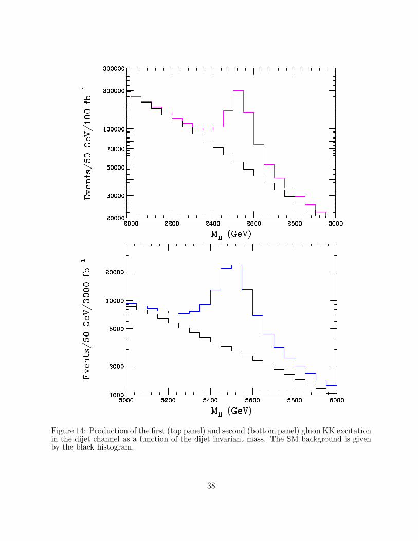
Figure 14: Production of the first (top panel) and second (bottom panel) gluon KK excitationin the dijet channel as a function of the dijet invariant mass. The SM background is givenby the black histogram.

38

G1 production has a very small event rate and is indistinguishable from the background.

Hence, the WHM differs from the usual RS scenario in that graviton resonances will not be

observed.

Figure 15: Production rate for the first graviton excitation at the LHC via the processgg → G1 → γγ as a function of the diphoton invariant mass. The SM diphoton background isalso shown. The two histograms are indistinguishable except for the small blip at Mγγ = mG1

For completeness, we also considered the associated production of KK gravitons via

gg → Gn + g. Appropriately modifying the expressions in Ref. [31] for the WHM we

computed the event rate at the LHC for G1 production as a function of jet energy using an

integrated luminosity of 3 ab−1. We found that for typical jet energies of Ej = 200 GeV the

cross section was of order 0.016 ab, and hence is also too small to be observed, even with

the proposed LHC luminosity upgrades. We thus conclude that in this model, the graviton

KK tower can not be observed at high energy colliders.

Lastly, we note that there exists a radion scalar in this model and that it may have

distinctive collider signatures.

39

7 Conclusions

Various phenomenological aspects of a Higgsless 5-d model [6], based on the RS hierarchy

proposal [3], were studied in this paper. We considered independent left and right bulk gauge

couplings and included the effects of UV brane localized kinetic terms for the gauge fields

[8]. These terms were assumed to be radiatively generated, which is a generic expectation

in orbifold models [13]. Our analysis was not limited to leading order bulk-curvature effects

unlike in Refs. [6, 8], and also allowed for a more general set of parameters than that

discussed in Ref. [22].

We computed the mass spectrum and the relevant couplings of the W± and γ/Z KK

towers, and studied experimental constraints on the model parameters. Our main conclusion

is that in the region of parameter space allowed by precision EW data, this model is not

perturbatively unitary at tree level above√

s ≈ 2 TeV, which is below the scale of the new

KK states. Futhermore, we find that tree-level unitarity is violated over the entire param-

eter space, even in those regions where comparisons with the precision measurements are

anticipated to be quite poor. Thus, to make reliable calculations based on the WHM, one

must extend this model in order to unitarize the amplitudes. Setting the issue of perturba-

tive unitarity aside, it was also observed that quantum contributions to the S, T , U oblique

parameters [17, 19] are expected to be small. However, in the absence of the Higgs, regu-

larization of the relevant loop diagrams may require non-renormalizable TeV brane counter

terms whose coefficients are unknown. This imposes a degree of uncertainty on loop cor-

rections. Further work regarding loop corrections is needed before more precise statements

could be made in this regard.

Finally, we considered the collider signatures of the model, assuming that unitarity

could somehow be restored without significantly modifying our numerical results. These

signatures depend on the 5-d configuration of bulk fermions. We assumed a simple setup,

where all fermions, except perhaps for the third generation, are localized near the Planck

brane. The effect of different localizations of quarks was then taken into account by varying

the widths of the KK resonances. Generically, we found that the low-lying gauge boson KK

modes, including the gluons, would be observable, whereas the most distinct RS signature,

the spin-2 graviton KK resonances, would most likely evade detection at the LHC.

The AdS/CFT correspondence [4] provides a 4-d interpretation of this model in terms

of strong dynamics. Thus, the tools and insights of both five and four dimensional model

40

building can be employed in making this scenario more realistic such that it agrees with the

SM at low energies. This setup provides an entirely higher dimensional explanation of the

observed weak interaction mass scales, directly linking them to the IR scale in the RS model.

Thus, it is worth the effort to find solutions for the problems that plague the present form

of the WHM.

Acknowledgements The work of H.D. was supported by the Department of Energy under

grant DE-FG02-90ER40542. We would like to thank Nima Arkani-Hamed, Tim Barklow,

Graham Kribs, Hitoshi Murayama, and Michael Peskin for discussions related to this work.

References

[1] For a review of Higgs boson searches, see, M. Schmitt, talk given at the XXI Interna-

tional Symposium on Lepton and Photon Interactions at High Energies, Batavia, IL,

August 2003.

[2] The LEP and SLD Electroweak and Heavy Flavor Working Groups,

arXiv:hep-ex/0312023.

[3] L. Randall and R. Sundrum, Phys. Rev. Lett. 83, 3370 (1999) [arXiv:hep-ph/9905221].

[4] J. M. Maldacena, Adv. Theor. Math. Phys. 2, 231 (1998) [Int. J. Theor. Phys. 38, 1113

(1999)] [arXiv:hep-th/9711200].

[5] C. Csaki, C. Grojean, H. Murayama, L. Pilo and J. Terning, “Gauge theories on an

interval: Unitarity without a Higgs,” arXiv:hep-ph/0305237.

[6] C. Csaki, C. Grojean, L. Pilo and J. Terning, “Towards a realistic model of Higgsless

electroweak symmetry breaking,” arXiv:hep-ph/0308038.

[7] K. Agashe, A. Delgado, M. J. May and R. Sundrum, JHEP 0308, 050 (2003)

[arXiv:hep-ph/0308036].

[8] Y. Nomura, “Higgsless theory of electroweak symmetry breaking from warped space,”

arXiv:hep-ph/0309189.

[9] C. Csaki, C. Grojean, J. Hubisz, Y. Shirman and J. Terning, “Fermions on an interval:

Quark and lepton masses without a Higgs,” arXiv:hep-ph/0310355.

41

[10] H. Davoudiasl, J. L. Hewett and T. G. Rizzo, Phys. Rev. Lett. 84, 2080 (2000)

[arXiv:hep-ph/9909255], Phys. Lett. B 473, 43 (2000) [arXiv:hep-ph/9911262]. See also,

A. Pomarol, Phys. Lett. B 486, 153 (2000) [arXiv:hep-ph/9911294].

[11] H. Davoudiasl, J. L. Hewett and T. G. Rizzo, Phys. Rev. D 68, 045002 (2003)

[arXiv:hep-ph/0212279]. See also, M. Carena, E. Ponton, T. M. P. Tait and

C. E. M. Wagner, Phys. Rev. D 67, 096006 (2003) [arXiv:hep-ph/0212307].

[12] For a review and original references, see R.N. Mohapatra, Unification and Supersym-

metry, Springer, New York, (1986).

[13] H. Georgi, A. K. Grant and G. Hailu, Phys. Lett. B 506, 207 (2001)

[arXiv:hep-ph/0012379].

[14] H. Davoudiasl, J. L. Hewett and T. G. Rizzo, Phys. Rev. D 63, 075004 (2001)

[arXiv:hep-ph/0006041].

[15] T. Gherghetta and A. Pomarol, Nucl. Phys. B 586, 141 (2000) [arXiv:hep-ph/0003129].

[16] See, for example, Ref. 2 and references therein.

[17] M. E. Peskin and T. Takeuchi, Phys. Rev. D 46, 381 (1992).

[18] T. G. Rizzo, Phys. Rev. D 50, 2256 (1994) [arXiv:hep-ph/9403241]; G. Altarelli,

R. Casalbuoni, S. De Curtis, N. Di Bartolomeo, R. Gatto and F. Feruglio, Phys. Lett.

B 318, 139 (1993).

[19] C. P. Burgess, S. Godfrey, H. Konig, D. London and I. Maksymyk, Phys. Lett. B 326,

276 (1994) [arXiv:hep-ph/9307337]; I. Maksymyk, C. P. Burgess and D. London, Phys.

Rev. D 50, 529 (1994) [arXiv:hep-ph/9306267].

[20] J. Erler, “Constraining electroweak physics,” arXiv:hep-ph/0310202.

[21] M. A. Luty and R. Sundrum, Phys. Rev. Lett. 70, 529 (1993) [arXiv:hep-ph/9209255].

[22] R. Barbieri, A. Pomarol and R. Rattazzi, “Weakly coupled Higgsless theories and pre-

cision electroweak tests,” arXiv:hep-ph/0310285.

[23] B. W. Lee, C. Quigg and H. B. Thacker, Phys. Rev. D 16, 1519 (1977).

42

[24] M. J. Duncan, G. L. Kane and W. W. Repko, Nucl. Phys. B 272, 517 (1986).

[25] For further considerations of unitarity in gauge boson scattering in flat space, see,

R. S. Chivukula, D. A. Dicus, H. J. He and S. Nandi, Phys. Lett. B 562, 109 (2003)

[arXiv:hep-ph/0302263]; R. Sekhar Chivukula, D. A. Dicus and H. J. He, Phys. Lett. B

525, 175 (2002) [arXiv:hep-ph/0111016].

[26] F. Gianotti et al., “Physics potential and experimental challenges of the LHC luminosity

upgrade,” arXiv:hep-ph/0204087.

[27] T. G. Rizzo and J. D. Wells, Phys. Rev. D 61, 016007 (2000) [arXiv:hep-ph/9906234];

J. Hewett and M. Spiropulu, Ann. Rev. Nucl. Part. Sci. 52, 397 (2002)

[arXiv:hep-ph/0205106].

[28] T. G. Rizzo, JHEP 0306, 021 (2003) [arXiv:hep-ph/0305077]; T. G. Rizzo, in Proc. of

the APS/DPF/DPB Summer Study on the Future of Particle Physics (Snowmass 2001)

ed. N. Graf, eConf C010630, P304 (2001) [arXiv:hep-ph/0109179].

[29] G. Azuelos et al., arXiv:hep-ph/0204031;

[30] T. G. Rizzo, Phys. Rev. D 55, 5483 (1997) [arXiv:hep-ph/9612304]; J. A. Aguilar-

Saavedra et al. [ECFA/DESY LC Physics Working Group Collaboration], “TESLA

Technical Design Report Part III: Physics at an e+e- Linear Collider,”

arXiv:hep-ph/0106315.

[31] G. F. Giudice, R. Rattazzi and J. D. Wells, Nucl. Phys. B 544, 3 (1999)

[arXiv:hep-ph/9811291]. See also, E. A. Mirabelli, M. Perelstein and M. E. Peskin,

Phys. Rev. Lett. 82, 2236 (1999) [arXiv:hep-ph/9811337].

43