arX

iv:h

ep-p

h/01

0530

4v3

15

Jun

2002

DESY 01-067 hep-ph/0105304

May 2001 (rev. February 2002)

MS vs. Pole Masses of Gauge Bosons:Electroweak Bosonic Two-Loop Corrections

F. Jegerlehner1, M. Yu. Kalmykov2 3, O. Veretin4

DESY Zeuthen, Platanenallee 6, D-15738, Zeuthen, Germany

Abstract

The relationship between MS and pole masses of the vector bosons Z and W iscalculated at the two-loop level in the Standard Model. We only consider the purelybosonic contributions which represent a gauge invariant subclass of diagrams. All cal-culations were performed in the linear Rξ gauge with three arbitrary gauge parametersutilizing the method of asymptotic expansions. The results are presented in analyticform as series in the small parameters sin2 θW and the mass ratio m2

Z/m2H . We also

present the corresponding on-shell mass counter-terms for the massive gauge bosons,which will be needed for the calculation of observables at two-loops in the on-shellrenormalization scheme.

1 Introduction

Precision Physics of the electroweak gauge bosons Z and W started about 12 years ago atthe LEP storage ring with the ALEPH, DELPHI, L3 and OPAL experiments and endedjust recently with the dismantling of the LEP installation. In particular the very accuratedetermination of the masses and the couplings to the fermions revealed unexpectedly richinformation about the quantum correction of the Standard Model (SM) [1]. Calculationsof higher order corrections thus gained increasing importance. At the one–loop level thesecalculations for the relevant “2 fermions into 2 fermions” processes were completed beforeLEP started operating in 1989 [2]. These SM predictions enabled an indirect determinationof the top mass which culminated in the top discovery at the Tevatron. Now after the topmass has been fixed with rather good accuracy, the indirect bound to the Higgs mass, the

1 E-mail: fjeger@ifh.de2 E-mail: kalmykov@ifh.de3 On leave of absence from BLTP, JINR, 141980, Dubna (Moscow Region), Russia4 E-mail: veretin@ifh.de

1

last missing SM parameter, is the main goal. The knowledge of the actual value of the Higgsmass is extremely important because it determines how Higgs physics will look like at futurecolliders like the LHC or TESLA [3]. Since the sensitivity of SM predictions on the Higgsmass is weak the precise meaning of the indirect Higgs mass bounds depend crucially on theaccuracy of the theoretical predictions. Fortunately a lot of important theoretical progresshas been made in the last decade with the calculation of leading and some sub-leading two–loop effects [4]-[9]. However, no complete two–loop calculation could be achieved so far,because such calculations are hampered by the dramatic increase in complexity encounteredin such calculations. How important the precise evaluation of radiative corrections is maybe illustrated by the following fact: taking only the leading corrections, the shift ∆αem inthe fine structure constant and the quadratic top mass correction ∆ρtop in the relationshipbetween neutral and charged current effective couplings, predictions are about 10σ off fromthe data for most of the precisely known observables like sin2 θℓ

eff or MW [10, 11]. Thusthe sub-leading effects are huge in relation to current experimental precision. Therefore theissue of sub-leading two–loop corrections has to be taken very seriously. They easily mayobscure the interpretation of the indirect Higgs mass bound obtained from LEP experimentsby using SM predictions which are incomplete at the two–loop level.

Although we are a long way from filling the gap, as a first step we calculate the fullbosonic two-loop electroweak corrections to the on-shell masses of gauge bosons. In otherwords, we evaluate the two-loop renormalization constants, the relations between bare, MSand on-shell masses, which are required as an essential part for the two-loop renormalizationprogram in the on-shell scheme, with the fine structure constant α and the gauge bosonmasses MW and MZ as independent input parameters.

The programs developed for performing the present calculations can be applied withoutmodifications for the calculation of the on-shell wave-function renormalization constants ofthe gauge bosons. Since these quantities are gauge dependent we don’t reproduce corre-sponding results here. As yet we have not calculated any observable quantity. However, thenew set of corrections will be important for future, complete electroweak two-loop calcula-tions of physical observables. Also after the shutdown of LEP it is important to continue suchcalculations because the question how additional corrections affect the Higgs mass boundcan be answered retrospectively, once given the precise LEP/SLC results. Full two-loopcalculations would be indispensable in future in any case if a project like TESLA with theGigaZ option would be realized.

The most recent essential progress here was achieved in the calculation of the top–quarkcontributions to the two-loop electroweak corrections. The corresponding contributions tothe ρ-parameter were considered in [6], the one’s to ∆r, which determines the MW − MZ

relationship, in [7] and to the Z boson partial widths in [8]5. Two different approaches—the asymptotic expansion method [12] and numerical integration[13] —have been used toperform these calculations. One of the important steps when performing these calculationsis the two-loop renormalization of the gauge boson masses, which also is contributing to thesin2 θW renormalization [14]-[16]. In the SM so far no complete analytical calculation of the

5 Another important step forward was the calculation of the two–loop QED correction to the muon decaywidth [9].

2

two-loop renormalized propagator has been carried out [17]. The first available results weregiven for zero external momentum [5], when the original diagrams may be reduced to a set ofbubble-type integrals with different masses [18]. In [19] the two-loop unrenormalized fermioncorrections to the gauge boson propagator have been presented for off-shell momentum inthe general linear Rξ gauge. The results are presented in terms of scalar master integralswith several different mass scales, the masses of fermions and bosons. For the evaluationof these master diagrams analytical results [20, 21] or one-fold integral representations areavailable [22].

The main aim of the present paper is to present a calculation within the Standard Modelof the two-loop bosonic contributions to the relationship between MS and on-shell massesof the gauge bosons (W, Z). This relationship, alternatively, will be represented in terms ofon-shell renormalization constants. We shall discuss in some detail the algorithm used forcalculating two-loop electroweak corrections for on-shell quantities in an arbitrary gauge.

The paper is organized as follows. In Section 2 we briefly reconsider the definition ofthe pole mass of the massive gauge bosons within the Standard Model. The calculationshave been performed with the help of computer programs which will be described in somedetail in Section 3. In Section 4 we discuss the UV renormalization of the pole mass and theinterrelation of our results with the standard renormalization group approach. In particularwe make several cross-checks of the singular 1/ε2- and 1/ε-terms. The numerical resultsfor the finite parts are presented and discussed in Section 5. For further technical detailsand some useful formulae we refer to four appendices. In Appendix A we collect resultsfor the one-loop propagator type diagrams. Special attention is given here to the ε-partsof the corresponding integrals which are needed for the two-loop calculation. Appendix Band C collect one-loop results in d = 4 and d 6= 4, respectively. They are included forcompleteness. In Appendix D we present the analytical coefficients which are the mainresults of our investigation.

2 Pole mass

The position of the pole sP of the propagator of a massive gauge boson in a quantum fieldtheory is a solution for p2 at which the inverse of the connected full propagator equals zero,i.e.,

sP − m2 − Π(sP , m2, · · ·) = 0, (2.1)

where Π(p2, · · ·) is the transversal part of the one-particle irreducible self-energy. The latterdepends on all SM parameters but, in order to the keep notation simple, we have indicatedexplicitly only the dependence on the external momentum p and in some cases also m, wherem is the mass of the particle under consideration. This can be either the bare mass m0 orthe renormalized mass defined in some particular renormalization scheme.

Generally, the pole sP is located in the complex plane of p2 and has a real and animaginary part. We write

sP ≡ M2 − iMΓ. (2.2)

3

The real part of (2.2) defines M which we call the pole mass6, while the imaginary part isrelated to the width Γ of the particle. This is the natural generalization of the physical massof a stable particle, which is defined by the mass of its asymptotic scattering state.

For the remainder of the paper we will adopt the following notation: capital M alwaysdenotes the pole mass; lower case m stands for the renormalized mass in the MS scheme,while m0 denotes the bare mass. In addition we use e and g to denote the U(1)em andSU(2)L couplings of the SM in the MS scheme.

In perturbation theory (2.1) is to be solved order by order. To two loops we have thefollowing solution of (2.1)

sP = m2 + Π(1)(m2, m2, · · ·) + Π(2)(m2, m2, · · ·) + Π(1)(m2, m2, · · ·)Π(1)′(m2, m2, · · ·), (2.3)

which yields the pole mass M2 and the width Γ at this order. Π(L) is the bare (m = m0) orMS -renormalized (m the MS -mass) L-loop contribution to Π, and the prime denotes thederivative with respect to p2. In this way we need to evaluate propagator type diagrams andtheir derivatives at p2 = m2. Diagrammatically the self-energy contributions are shown inFig. 1.

The (on-shell) mass counter terms δM2 for the on-shell renormalization scheme are ob-tained by considering the real part of (2.3) upon identifying the r.h.s with the bare expression,setting m2 ≡ m2

0 = M2 + δM2 and solving for δM2 = (δM2)(1) + (δM2)(2) to two loops.In this paper we show by explicit calculation at the two-loop level that the bosonic

correction to the pole sP (and hence to the on-shell mass counter-term) is a gauge invariantand infrared stable quantity7. The free propagator of a massive vector boson in the linearRξ gauge reads

Dµν(p) =i

p2 − m2

(−gµν + (1 − ξ)

pµpν

p2 − ξm2

), (2.4)

where ξ is a gauge parameter. We decompose the vector boson self-energy Πµν(p2, m2, · · ·)

into a transverse Π(p2) and a longitudinal L(p2) part

Πµν(p2, m2, · · ·) =

(gµν −

pµpν

p2

)Π(p2) +

pµpν

p2L(p2). (2.5)

In (2.3) only the transverse part contributes and the dressed propagator reads

Dµν(p) =−i

p2 − m2 − Π(p2)

(gµν −

pµpν

p2

)+

pµpν

p2· · · (2.6)

The simple relation between the full propagator and the irreducible self-energy only holds ifthere is no mixing, like for the W -boson. In the neutral sector, because of γ −Z mixing, we

6Throughout this paper we identified the terms pole mass and on-shell mass.7From general considerations we know (see [16], for example), that after summing all diagrams, including

the tadpoles, at a given order of perturbation theory the location of the pole of the propagator is a gaugeinvariant quantity. The gauge invariance of the 2-loop massless fermion correction to the pole mass of thegauge bosons was verified in [19].

4

cannot consider the Z and γ propagators separately. They form a 2 × 2 matrix propagator,so that (2.1) is modified into (see details in [16, 23])

sP − m2Z − ΠZZ(sP ) − Π2

γZ(sP )

sP − Πγγ(sP )= 0. (2.7)

We note that the Π2γZ mixing term starts to contribute at the two-loop level. Obviously,

we do not need to compute Πγγ here since it starts to play a role only beyond the two-loopapproximation. In the sequel we will denote the self-energies by ΠV (V = W, Z) with

ΠW (p2, · · ·) = ΠWW (p2, · · ·)

and

ΠZ(p2, · · ·) = ΠZZ(p2, · · ·) +Π2

γZ(p2, · · ·)p2 − Πγγ(p2, · · ·) .

Thus, formally, the form (2.1) applies for both the W and the Z.The non-zero imaginary part (width) (2.2) of the on-shell gauge boson self-energy appears

as soon as the fermions are included. For the bosonic contributions alone the imaginary partof Π(p2) on the mass-shell is zero at the two-loop level (see below).

3 Program part

In order to find the relations between the pole masses M2Z , M2

W and the MS masses m2Z , m2

W

we have to compute the one- and two-loop self-energies for Z- and W -bosons at p2 = m2Z

and p2 = m2W , respectively. The complete set of topologies that occurs in this calculation is

shown in Fig. 1. In order to be able to work with manifestly gauge parameter independentrenormalization constants we have to include the Higgs tadpole diagrams.

While at one-loop order we have about 50 diagrams, in the two-loop approximation thenumber of diagrams is about 1000, which requires an automatized generation and evaluationof diagrams. We use QGRAF [24] to generate the diagrams and then the C-programDIANA [25] to produce for each diagram an input suitable for our FORM [26] packages8.

For two-loop propagator type diagrams with several masses a complete set of recurrencerelations is given in [27]. It allows us to reduce all tensor integrals to a small set of so-calledmaster-integrals. However, the master-integrals which show up in the SM are not expressiblein terms of known functions but may be written e.g. as one-fold integrals [22]. Instead ofusing these explicit formulae we resort to some approximations here, namely, we perform anappropriate series expansion in mass ratios9. Each coefficient of this series can be calculatedanalytically by means of the asymptotic expansion algorithm described in [12].

To keep control of gauge invariance we work in a Rξ gauge with three different gaugeparameters ξW , ξZ and ξγ. The corresponding free vector boson propagators (2.4) thus

8DIANA generates additional information, e.g. identifying symbols for the particles of the diagram andtheir masses, distribution of integration momenta, number of fermion loops etc.

9For diagrams with several different masses, there may exist several small parameters. In this case weapply different asymptotic expansions (see [28]) one after another.

5

Π =(2)

++ HΠ (1) =

+

H H H

+ + +

H

H

H

H +

H

H H

+ +H

H+

H

HH

+ + + +

+

+

+ + +

Figure 1: One- and two-loop contributions to the massive boson self-energies.

exhibit the new masses√

ξWmW and√

ξZmZ in the propagators. This complicates thecalculation enormously both in Tarasov’s algorithm as well as in the asymptotic expansionapproach. With the first method the presence of new masses in both the reduction formulaeand the Gram determinants leads to cumbersome expressions which are difficult to simplify.In the asymptotic expansion approach the unphysical parameters ξWm2

W and ξZm2Z define

two new scales. Of course, in order to keep things manageable, we have to keep the numberof scales as small as possible. This can be done by expanding diagrams about some fixedvalues of the gauge parameters. Three different regimes of expansion are feasible: a) ξ → ∞,b) ξ → 0 and c) ξ → 1. We choose the last possibility expanding the original propagatorsat ξi = 1 in a Taylor series. For the purpose of checking the gauge invariance of our resultsit is sufficient to keep the first three terms of the expansion, so that the propagators of thevector bosons and associated Higgs scalar ghosts look like

DVµν(p) =

i

p2 − m2V

(−gµν + (1 − ξV )

pµpν

p2 − m2V

− (1 − ξV )2 m2V pµpν

(p2 − m2V )2

+ . . .

),

∆V (p) =i

p2 − m2V

1 − (1 − ξV )m2

V

p2 − m2V

+ (1 − ξV )2

(m2

V

p2 − m2V

)2

+ . . .

, (3.8)

where V = W, Z and the dots stand for the terms of higher order in (1 − ξV ), which we

6

don’t take into account. At the same time we do not have any problems with the photonpropagator and use it in its usual form.

One drawback of our choice of the expansion about ξi = 1 is that possible unphysicalthresholds do not show up in our expansion and hence will not produce the correct imaginarypart for a given diagram. Examples are the thresholds p2 = 4ξZM2

Z (Z → φ0φ0 production,φ0 the neutral Higgs ghost) which is below the Z mass-shell p2 = M2

Z when ξZ < 14

orp2 = ξWM2

W (W± → φ±γ production, φ± the charged Higgs ghosts) which is below the Wmass-shell p2 = M2

W when ξW < 1. In such cases, the above expansion does not preserve theanalytical properties of diagrams exhibiting ghost particles. However, in any case unphysicaldegrees of freedom should not contribute to the physical width. While individual diagramsexhibit an imaginary part, in the sum of all diagrams it has to cancel. This cancellationis a consequence of the Slavnov-Taylor identities, which tell us how Higgs ghost, Faddeev-Popov ghosts and scalar components contained in the gauge boson fields decouple fromobservables like the physical width. Therefore, the above expansion indeed reproduces thecorrect gauge invariant result. At the one-loop level one can do an exact analytic calculationfor the Rξ gauge with an arbitrary value of the gauge parameter. This has been done longtime ago [16] and, not surprisingly, the on-shell self-energies of the W - and Z-bosons aregauge invariant and do not exhibit any unphysical threshold (possible problems related tounphysical thresholds in the non-gauge invariant wave-function renormalization factor arealso discussed in [16]). For the two-loop contribution, as we should, we get a gauge invarianton-shell limit which is real. Gauge cancellations are highly non-trivial and only happen ifone is doing a perfectly consistent calculation. We have verified that for gauge parametersξ > 1 the imaginary part of the W and Z self-energies in the bosonic sector up to two-loops is zero, by applying the Cutkowsky rules and inspecting all possible two and threeparticle intermediate states allowed by the SM Lagrangian. While for ξ > 1 the imaginarypart is zero for each individual diagram, for small enough values of the gauge parameters anon-trivial cancellation must take place. An independent direct check of this is possible byconsidering the problem in the limit ξ → 0, for example.

After we have made the expansion (3.8), the bosonic contributions we are consideringonly depend on the three different masses m2

W , m2Z and m2

H . One natural small parameteris the weak mixing parameter sin2 θW = 1 − m2

W /m2Z < 0.25. We expand in this parameter

and get rid in this way of mW (or mZ). For diagrams which contain Higgs boson lines10 weapply an asymptotic expansion with respect to a heavy Higgs mass. Taking into accountthe most recent lower bound on the value of the Higgs boson mass we are dealing with anexpansion parameter m2

Z/m2H<∼0.64. This implies that we have to calculate quite a number of

coefficient in the expansion in order to get a convincing result. We should mention that theseexpansions are well behaved because p2 = M2

V in any case is below the possible thresholds.The convergence of such expansions can be easily checked for the one-loop case where theexact analytic result is available.

In our case we find four different prototype structures with Higgs lines inside of the loops.The large mass expansion has been performed with the help of the packages TLAMM [29]

10We have 280 and 357 two-loop one-particle irreducible diagrams for the Z- and W -boson, respectively.

7

and [30] once for Euclidean [31] and once for Minkowski space-time, respectively. Thecorresponding topologies and set of subgraphs are given in Fig. 2. The diagrams without

Figure 2: The prototype diagrams and their subgraphs contributing to the large massexpansion for two-loop diagrams with heavy propagators. Thick and thin lines correspondto the heavy- and light-mass (massless) particle propagators, respectively. Dotted linesindicate the lines omitted in the subgraph.

Higgs11 are nothing but single scale massive diagrams, when all internal masses are equalto the external momentum or zero. Such diagrams can be calculated analytically. For thispurpose we use the packages ONSHELL2 [32] and another one written by O.V. [33] for thecalculation of the set of the master integrals given in [34]. We find that only the followingfour prototypes are required (in terms of the notation used in [32]): F11111, F11110,F01111 and F01101.

For independent verification of the input, the Feynman rules and the evaluation weperformed calculations independently in Euclidean (M.Yu.K) and Minkowski (O.V.) space-time and got full agreement between them 12.

11At the two-loop level we find 336 one-particle irreducible diagrams without a Higgs line for the Z-bosonand 435 for the W -boson.

12The packages used in the calculations and the results can be found at the following URL addresshttp://www-zeuthen.desy.de/˜kalmykov/pole/pole.html.

8

4 UV renormalization in the MS scheme

Here we describe in more detail the renormalization procedure. It is well known that thepole mass in QED/QCD is a gauge independent and infrared stable quantity to all ordersof the loop expansion [35]. To renormalize the pole mass at the two-loop level requiresto calculate the one-loop renormalization constants for all physical parameters (charge andmasses), and the two-loop renormalization constant only for the mass itself. Not neededare the wave-function renormalizations or ghost (unphysical) sector renormalizations. Theabove mentioned basic properties of the pole mass are valid also in the SM. In order to obtaina gauge invariant result in the SM, however, we have to add in a proper way the tadpolecontributions [16]. The tadpole terms are due to the vacuum expectation value (VEV) ofthe Higgs field, which does not vanish automatically. By a constant shift we can adjust theHiggs field to have vanishing VEV, however. Since here the Higgs field is integrated out inthe path integral the result cannot depend on whether we perform a shift or not. Indeed,after we take into account all diagrams shown in Fig. 1 we find a gauge invariant result forthe pole mass up to two loops in terms of the bare parameters. The tadpole contributioncan be calculated either from tadpole diagrams13 or from Ward identities, which connect thetadpoles with the one-particle irreducible self-energies of the pseudo-Goldstone bosons Πφφ

at zero momentumΠ1PI

φφ (0) + T = 0, (4.1)

where φ = φ+, φ−, φ0. We performed both types of calculations and obtained full agreement.Diagrams contributing to the Z-boson pole mass do not contain infrared singularities at thetwo-loop level. Infrared finiteness of the W -boson mass was proven in [36]. We also give analternative proof of this statement for our case.

In our calculation dimensional regularization [37] is used, which allows one to regularizeboth UV and IR singularities by the same parameter ε related to the dimension of space-timeby d = 4 − 2ε. We first perform the UV-renormalization within the MS scheme in order toobtain finite results. In a next step we find the relation between the pole- and MS parameters.We adopt the convention that the MS-parameters are defined by multiplying each L-loopintegral by the factor (exp(γ)/4π)εL. Each loop picks an additional factor 1/16π2.

4.1 One-loop charge renormalization

The bare charge e0 and the MS charge14 e are related via e0 = µεe(1 + Z

(1)

MS/ε + O(e4)

),

with the appropriate constant Z(1)

MS. At the same time, the relation between the MS and the

on-shell charge readse = eOS

(1 + z

(1)OS + O(e4

OS)),

where eOS is defined by the Thompson limit of Compton scattering. The electromagneticWard–Takahashi identity implies that some of the diagrams cancel, such that z

(1)OS at the

13These are the two-loop bubble diagrams for the process H in terms of QGRAF notation.14 All MS-parameters, like e, g, g′ and all renormalization constants, like ZMS or zOS are µ-dependent

quantities.

9

one-loop level can be written in terms of self-energies only [15]

z(1)OS = −1

2Π(1)

γγ′(0) +

sin θW

cos θW

Π(1)γZ(0)

M2Z

− 1

εZ

(1)

MS. (4.2)

UV-finiteness of z(1)OS implies

e0 = µεe

(1 − 1

ε

7

2

e2

16π2

). (4.3)

This may be confirmed also by using a renormalization group analysis of the SM keepingthe Yang–Mills and the Higgs sector only. From the relation

1

e2=

1

g2+

1

g′2, (4.4)

where g′ and g are the U(1) and the SU(2) gauge coupling constants, respectively, it is easyto deduce that

βe = e3

(βg

g3+

βg′

g′3

)= −7

2

e3

16π2+ O(e5) . (4.5)

The β-functions β(1)g,g′ may be calculated in the unbroken theory. They have been calculated

in [38]. We see that the above result is in agreement with (4.3) if we take into account that(µ2d/dµ2) e = − ε

2e + βe .

4.2 Mass renormalization

We introduce the following notation for the mass renormalization constants

m2V,0 = m2

V (µ)

(1 +

g2(µ)

16π2εZ

(1,1)V +

g4(µ)

(16π2)2εZ

(2,1)V +

g4(µ)

(16π2)2ε2Z

(2,2)V

), (4.6)

where V stands for any of the bosons Z, W or H . In addition to the masses we haveone coupling constant as a free parameter of the SM which we have chosen above to bee = g sin θW . The one-loop mass counter-terms are well known [16]. For the purely bosoniccontributions we have

Z(1,1)H = −3

2− 3

4

m2Z

m2W

+3

4

m2H

m2W

, (4.7)

Z(1,1)W = −3

4

m2H

m2W

− 3m2

W

m2H

− 3

2

m4Z

m2Hm2

W

+3

4

m2Z

m2W

− 17

3, (4.8)

Z(1,1)Z = −3

4

m2H

m2W

− 3m2

W

m2H

− 3

2

m4Z

m2W m2

H

+11

12

m2Z

m2W

− 7m2

W

m2Z

+7

6. (4.9)

All masses here are MS masses and depend on the renormalization scale µ: m2V = m2

V (µ). Itshould be noted that unlike in the case of the couplings the mass renormalization constants

10

cannot be calculated from the unbroken gauge theory. Here in any case the calculation ofthe Feynman diagrams in the Standard Model is required.

Let us comment about the somewhat unusual looking dependence of our MS renormal-ization constants on the particle masses. Since masses are induced by the Higgs mechanismwe have the mass coupling relations

mW = gv

2, mZ =

√g2 + g′2

v

2, mH =

√2λ v

where v is the Higgs VEV and λ the Higgs self-coupling. One peculiarity of the “spontaneoussymmetry breaking” and the related mixing of states, like the γ − Z mixing, leads to thenon-polynomial nature of the perturbation expansion in the SM. Due to the mixing, the

actual Z coupling reads√

g2 + g′2 = g/ cos θW etc. In the dimensionless mass ratios the

factors v2 drop out and we have in fact just ratios of couplings. To a large extent this is atrivial consequence of factorizing out powers of g2 which cancels against such factors whichappear in the denominators of the Z

(1,1)V ’s. However, there are also true inverse powers of

the Higgs self-coupling present. They originate in the tadpoles which we need taking intoaccount for the sake of gauge invariance.

Our results for the two-loop mass renormalization constants are as follows:

Z(2,1)W =

63

64

m4H

m4W

− 3

4

m2H

m2W

− 3

8

m2Hm2

Z

m4W

− 301

192

m4Z

m4W

+17

12

m2Z

m2W

− 53

3

+31

12

m4Z

m2Hm2

W

− 17

2

m2Z

m2H

− 176

3

m2W

m2H

+59

24

m6Z

m2Hm4

W

, (4.10)

Z(2,2)W = − 9

32

m4H

m4W

+43

8

m2H

m2W

+65

32

m4Z

m4W

− 35

8

m2Z

m2W

+334

9+

27

4

m4Z

m2Hm2

W

+6m2

Z

m2H

+ 34m2

W

m2H

− 5

2

m6Z

m2Hm4

W

+ 9m4

W

m4H

+ 9m4

Z

m4H

+9

4

m8Z

m4Hm4

W

, (4.11)

Z(2,1)Z =

63

64

m4H

m4W

− 3

4

m2H

m2W

− 3

8

m2Hm2

Z

m4W

+11

3+

7

6

m2Z

m2W

− 64

3

m2W

m2Z

− 253

192

m4Z

m4W

−176

3

m2W

m2H

− 17

2

m2Z

m2H

+31

12

m4Z

m2Hm2

W

+59

24

m6Z

m2Hm4

W

, (4.12)

Z(2,2)Z = − 9

32

m4H

m4W

+1

4

m2H

m2W

− 1

8

m2Hm2

Z

m4W

+21

4

m2H

m2Z

− 55

6+

11

12

m2Z

m2W

+629

288

m4Z

m4W

+245

6

m2W

m2Z

+27

2

m2W

m2H

+ 16m2

Z

m2H

+ 21m4

W

m2Zm2

H

− 7

2

m4Z

m2Hm2

W

− 11

4

m6Z

m2Hm4

W

+9m4

W

m4H

+ 9m4

Z

m4H

+9

4

m8Z

m4Hm4

W

. (4.13)

Again the higher order pole terms 1/ε2 can be checked by means of the appropriate

renormalization group equation. Let us write the relation m2V,0 = m2

V

(1 +

∑n Z

(n)V /εn

)

11

which connects bare and renormalized masses and introduces the anomalous dimension ofthe mass γV = (µ2 d/dµ2) lnm2

V . Taking into account that (µ2d/dµ2)m2V,0 = 0 and repeating

the calculations given in [39] we find

γV =1

2g

∂

∂gZ

(1)V , (4.14)

(γV + βg

∂

∂g+∑

i

γim2i

∂

∂m2i

)Z

(n)V =

1

2g

∂

∂gZ

(n+1)V . (4.15)

For each function like γV or Z(n)V we may perform a loop expansion γV =

∑∞

k=1(g2/16π2)kγ

(k)V

or Z(n)V =

∑∞

k=n(g2/16π2)kZ(n,k)V and (4.15) can be written for each loop correction separately.

In particular, for n = 1, we have

γ(1)V = Z

(1,1)V ,

γ(2)V = 2Z

(2,1)V ,

such that the coefficient of the n = 2 poles can be checked via

(Z

(1,1)V

)2+

16π2

g22β(1)

g Z(1,1)V

g+∑

i

Z(1,1)mi

m2i

∂

∂m2i

Z(1,1)V = 2Z

(2,2)V . (4.16)

The value of β(1)g = −43

12g3

16π2 may be calculated from the relation

β(1)g sin θW =

1

2gcos2 θW

sin θW

(g2

16π2

)(γ

(1)W − γ

(1)Z

)+ β(1)

e , (4.17)

where β(1)e is given in (4.5), and cos2 θW = m2

W /m2Z .

An independent verification of the 1/ε terms can be obtained from the relationshipe2 = g2 sin2 θW , which is valid for bare and MS renormalized quantities. Differentiatingthe renormalized quantities with respect to ln µ2 we find

e4

(βg

g3+

βg′

g′3

)= gβg sin2 θW − 1

2g2 (γW − γZ) cos2 θW , (4.18)

or for the two-loop case

g2β

(2)g′

g′3sin4 θW − β(2)

g

gsin2 θW cos2 θW = −

(g2

16π2

)2 (Z

(2,1)W − Z

(2,1)Z

)cos2 θW . (4.19)

The two-loop β-functions for g and g′ are given in [40] and read

βg′ =1

12

g′3

16π2+

1

4

g′5

(16π2)2+

3

4

g′3g2

(16π2)2,

βg = −43

12

g3

16π2− 259

12

g5

(16π2)2+

1

4

g3g′2

(16π2)2. (4.20)

12

The fact that after UV renormalization we get a finite result confirms the infrared finite-ness of the bosonic contribution to the pole mass.

Let us write now the RG equation for the effective Fermi constant GF . GF is usuallydefined as a low energy constant in one-to-one correspondence with the muon lifetime. How-ever, if we consider physics at higher energies a parameterization in terms of low energyconstants may lead to large radiative corrections. Much in the same way as the fine struc-ture constant α often is replaced by the effective running fine structure constant α(µ) weexpect that GF should be replaced by an effective version of it at higher energies. Unlike inthe case of α, however, because of the smallness of the light fermion Yukawa couplings, GF

starts to run effectively only at scales beyond the W–pair production threshold (see below).The bare relations are

m2W,0 =

g20v

20

4, (4.21)

1

v20

=√

2 GF,0. (4.22)

Both these relations are valid also for MS renormalized parameters, so that their differenti-ation with respect to ln µ2 gives rise to the relation

γW = 2βg

g− γGF

, (4.23)

where we introduced the anomalous dimension of the Fermi constant γGF= (µ2 d/dµ2) ln GF .

Its loop expansion looks like γGF= γ

(1)GF

+ γ(2)GF

+ · · ·. At the one-loop level we have

γ(1)GF

= 2β(1)

g

g− Z

(1,1)W

=g2

16π2

1

4m2W

{2

m2H

3 (2m4

W + m4Z) + m4

H − 4∑

f

m4f

−3 (2m2

W + m2Z) − m2

H − 2∑

f

m2f

}

(4.24)

and we used the results of Ref. [16] for the fermion contributions. The first term proportional1/m2

H is the contribution from the tadpoles. The appearance of the tadpole terms is some-what mysterious, since we know that in renormalized observables tadpoles drop out. Herethey seem to contribute to the renormalization group evolution of the Fermi constant. Inany case the tadpoles are present in the relationship between the bare and the renormalizedparameters. At the two-loop level, our results allows us to write the bosonic corrections only.They are given by

γ(2),bosonGF

= 2β(2)

g

g− 2Z

(2,1)W

13

= − 2g4

(16π2)2

{63

64

m4H

m4W

− 3

4

m2H

m2W

− 3

8

m2Hm2

Z

m4W

− 301

192

m4Z

m4W

+7

6

m2Z

m2W

+25

6

+31

12

m4Z

m2Hm2

W

− 17

2

m2Z

m2H

− 176

3

m2W

m2H

+59

24

m6Z

m2Hm4

W

}. (4.25)

The equations (4.24) and (4.25) are written in MS scheme. As usual in this scheme, insolving the renormalization group equation

µ2 d

dµ2GF (µ) = GF (µ) γGF

the decoupling of the heavy particles has to be performed “by hand”. This means thatfor low values of the energy scale µ, when µ < mH , mW , mZ , the bosonic terms on ther.h.s. are equal to zero while the light fermion contributions proportional to GF m2

f are tiny.Consequently, below the W mass, the effective Fermi constant does practically not changewith scale. Obviously, the running of GF only starts at about µ ∼ mZ , when the scale of aprocess exceeds the masses of the bosons. Also the top quark will contribute once we havepassed its threshold.

5 Results, discussion and conclusion

After UV renormalization the pole mass (see (2.3))

M2V = m2

V + Π(1)V + Π

(2)V + Π

(1)V Π

(1)V

′ (5.1)

is represented in terms of finite MS renormalized amplitudes

Π(i)V = Π

(i)V (p2, m2

V , · · ·)∣∣∣p2=m2

V, F.P.

.

F.P. denotes the MS finite part prescription. The calculation of the one-loop MS renormal-ized amplitude is well known. We get it by rewriting the bare expression in terms of MSparameters according to (4.6) and (C.1)

Π(1)V ≡ lim

ε→0

(m2

0,V − m2V + m2

0,V

g20

16π2X

(1)0,V

)

= m2V (µ)

e2

16π2 sin2 θW

limε→0

(1

εZ

(1,1)V + X

(1)0,V

)= m2

V (µ)e2

16π2 sin2 θW

X(1)V . (5.2)

We restrict ourselves to a consideration of the bosonic part X(1),boson0,V . The renormaliza-

tion of the off-shell self-energy functions Π(1)0,V

′ and Π(2)0,V is more complicated. Besides the

renormalization of the physical parameters, it would require us to perform order-by-order,the wave-function renormalization as well as the renormalization of the ghost sector, inparticular of the unphysical gauge parameters. However, the MS renormalization of the

14

combination Π(2)0,V + Π

(1)0,V Π

(1)0,V

′ it much simpler. The subtraction of sub-divergencies in thiscase is reduced to the one-loop renormalization of the charge and the physical masses only,while the wave-function renormalization or the renormalization of the unphysical sector isnot needed. Accordingly, as a genuine two-loop counter-term, only the mass renormalizationoccurs.

The full two-loop MS renormalized amplitude can be written in the form

Π(2)V + Π

(1)V Π

(1)V

′ ≡{

Π(2)0,V + Π

(1)0,V Π

(1)0,V

′

}

MS

= limε→0

(Π

(2)0,V + Π

(1)0,V Π

(1)0,V

′

+m2V (µ)

1

ε

(e2

16π2 sin2 θW

)2 [Z

(1,1)V +

[∆g2

g2

]+∑

j

Z(1,1)

m2

j

∂

∂m2j

]X

(1)0,V

+m2V (µ)

(e2

16π2 sin2 θW

)2 [1

εZ

(2,1)V +

1

ε2Z

(2,2)V

])(5.3)

where the sum runs over all species of particles j = Z, W, H and

[∆g2

g2

]=

cos2 θW

sin2 θW

(Z

(1,1)W − Z

(1,1)Z

)− 7 sin2 θW .

The functions Z(i,j)V , X

(1)V and X

(1)0,V are defined in (4.7)-(4.9), (4.10)-(4.13), (B.1) and (C.1),

respectively. Again, throughout, we take into account only the bosonic corrections. Ther.h.s. of (5.3) is given by the bare two-loop contributions, the two-loop contribution ob-tained by expanding the bare parameters in the one-loop amplitude (subtraction of thesub-divergences) and the genuine two-loop subtractions. The second type of contribution

follows from writing Π(1) = m20

(g20

16π2

)X

(1)0 and by utilizing (4.6). We would like to stress,

that each of the one-loop bare amplitudes Π(1)0,V and Π

(1)0,V

′ has to be expanded up to linearterms in ε. Together with the singular 1/ε terms the contributions linear in ε yield additional

finite contributions in the limit ε → 0. In the product Π(1)0,V Π

(1)0,V

′ the parameters may be

identified by the MS renormalized quantities, but all functions, A0 and B0 have to be takenin d = 4 − 2ε dimensions and must be expanded up to terms linear in ε (see Appendix A).

As mentioned earlier, for the purely bosonic contributions alone the imaginary part ofΠ(p2) on the mass-shell is zero at the two-loop level. This is due to the fact that in thebosonic sector we have the physical masses mγ = 0, MZ , MW and MH and by inspection ofthe possible two and three particle intermediate states one observes that all physical thresh-olds lie above the mass shells of the W and Z bosons, i.e., the self-energies of the massivegauge bosons develop an imaginary part only at p2 > M2

V (to two loops in the SM). On kine-matical grounds imaginary parts could show up from the Higgs or Faddeev-Popov ghosts,which have square masses ξV M2

V , for small values of the gauge parameter. However, as wehave verified, the two-loop on-shell self-energies are gauge independent. This implies thatghost contributions have to cancel and hence cannot contribute to the imaginary part. ThussP = M2

V in our case. In higher orders for the Z–propagator one gets an imaginary part assoon as p2 > 0, from diagrams like

15

Z ZW W

γ

...

γ

.

For the W–propagator an imaginary part is only possible for p2 > M2W , because charge

conservation requires at least one W in any physical intermediate state.For the massive gauge bosons Z and W we write

M2V

m2V

= 1 +

(e2

16π2 sin2 θW

)X

(1)V +

(e2

16π2 sin2 θW

)2

X(2)V , (5.4)

where both e and sin θW are to be taken in the MS scheme.The one-loop coefficients X

(1)V for Z, W and H are known of course as exact results.

We write them down for completeness in Appendix B. For the coefficients X(2)V we make an

expansion and perform them as double series: in sin2 θW and in the mass ratio m2V /m2

H .We have calculated the first six terms of the expansion with respect to sin2 θW and the firstsix terms with respect to mass ratio m2

V /m2H . The analytical values of these coefficients are

presented in Appendix D. These represent our main result.Sometimes in massive multi-loop calculations the so-called modified MS scheme (MMS)

is used [41]. The difference between MS and MMS is that in the former scheme each loopis multiplied by (eγ/4π)ε while in the latter the normalization factor is 1/(4π)ε/Γ(1 + ε),which yields a difference at the two-loop level. It has been shown that in QCD both schemesreproduce the same formula for the mass relation analogous to (5.1) [42]. We have checkedthat the same holds true for the pole masses in the Standard Model.

Very often the inverse of (5.1) is required. To that end we have to express all MSparameters in terms of on-shell ones. Thus

m2V = M2

V − Π(1)V −

{Π

(2)0,V + Π

(1)0,V Π

(1)0,V

′

}

MS

−∑

j

(∆m2j )

(1) ∂

∂m2j

Π(1)V − (∆e)(1) ∂

∂eΠ

(1)V

∣∣∣∣∣m2

j=M2

j, e=eOS

, (5.5)

where the sum runs over all species of particles j = Z, W, H and

(∆m2j )

(1) = −ReΠ(1)j

∣∣∣∣∣m2

j=M2

j, e=eOS

≡ −M2V

e2OS

16π2 sin2 θW

X(1)V

∣∣∣∣∣m2

j=M2

j

stands for the self-energy of the jth particle at p2 = m2j in the MS scheme and parameters

replaced by the on-shell ones. Note that in the above relation we had to perform a changefrom the MS to the on-shell scheme also for the electric charge

e(µ2) = eOS

[1 +

e2OS

16π2

(7

2ln

(M2

W

µ2

)− 1

3

)](5.6)

16

with e2OS/4π = α ∼ 1/137. Accordingly, since Π(1) depends on e by an overall factor e2 only,

(∆e)(1) ∂

∂eΠ

(1)V =

e2

16π2

[7 ln

(M2

W

µ2

)− 2

3

]Π

(1)V .

By identifying m2V = m2

V,0 = M2V + δM2

V (5.5) is the relationship appropriate to obtainthe on-shell gauge-boson mass counter-terms δM2

V :

δM2V = −Re

[Π

(1)V,0 + Π

(2)V,0 + Π

(1)V,0Π

(1)V,0

′

+∑

j

(δM2j )(1) ∂

∂m2j,0

Π(1)V,0 + (δe)(1) ∂

∂e0Π

(1)V,0

] ∣∣∣∣∣m2

j,0=M2

j, e0=eOS

=

(ZMS · ZOS − 1

)M2

V (5.7)

in terms of the original bare on-shell amplitudes

Π(i)V,0 = Π

(i)V,0(p

2, m2V,0, · · ·)

∣∣∣p2=M2

V,m2

j,0=M2

j, e0=eOS

and the bare on-shell counter-terms δM2j and δe. The second equality gives δM2

V in termsof the singular factor ZMS = m2

V,0/m2V (µ) given in (4.6) and the finite factor ZOS = m2

V /M2V

given in (5.5). These will be needed in two-loop calculations of observables in the on-shellscheme.

We now turn to a discussion of our results which we obtained for the relationship (5.5).For our numerical analysis we used the following values of the pole masses: MW = 80.419GeV and MZ = 91.188 GeV and α = 1/137.036. We first investigate numerically the re-lationship between the MS–mass mV (µ) and the pole-mass MV . In Figs. 3 and 4 we plot∆Z ≡ m2

Z(MZ)/M2Z −1 as function of the Higgs mass MH for intermediate and heavier Higgs

masses, respectively. For the one-loop corrections the exact analytical functions are evalu-ated while for the two-loop results we utilize all coefficients of our expansion. Analogously,in Figs. 5 and 6 the Higgs mass dependence of ∆W ≡ m2

W (MW )/M2W − 1 is depicted for the

same ranges of the Higgs mass. As we can see, for a “light” Higgs of mass less than about200 GeV the two-loop corrections are small as compared to the one-loop ones. However, ata Higgs mass of about 220 GeV the absolute value of the two-loop correction is of the samesize as the one-loop result, such that the two-loop corrections start to play an essential role.

Our analysis shows (see Figs. 4 and 6) that the perturbative expansion looses its meaningfor large Higgs masses (strong coupling regime). In the relationship between the MS – andthe pole–masses corrections exceed the 50% level around 880 GeV (for µ = MV ). The sizeof the corrections depend on the choice of the renormalization scale µ.

Since our results have been obtained by an expansion in m2V /m2

H (i.e., for a heavy Higgs),one of the main questions which remains to be considered is the validity of our results aswe approach lighter Higgs masses. Note that we are dealing with an asymptotic expansion(which means the radius of convergence is zero) and thus we can answer the question about

17

where the expansion is reliable only empirically; at least as long as an exact result is notavailable for a direct comparison. Since the structure of the one- and two-loop correctionsfor both massive gauge bosons is very similar, we are going to investigate in the followingthe problems of convergence of our results for the Z–boson only. For the W–boson theconvergence is better because of the smaller value of the W–mass. Obviously our series–expansion breaks down for a “light” Higgs, when mH >

→mZ . Unexpectedly, we find that the

two-loop corrections remain numerically small for values of the Higgs mass even down to100 GeV (below about 0.2%). However, we observe a steep raise of the correction whichsignals that the expansion becomes unreliable below about 130 GeV15. We also should keepin mind that, on the level of the size of the two-loop corrections, which are very small in theregion around 150 GeV for µ ∼ mZ , the latter depend substantially on the choice of the MSrenormalization–scale µ, which causes an essentially constant shift in the quantities shownin the Figures which follow.

In Fig. 7 we show the dependences of the two-loop corrections to ∆Z = m2Z(M2

Z)/M2Z −

1 as a function of the Higgs mass and the number of coefficients of the expansion usedfor their evaluation. For a “light” Higgs the difference between the result, including sixcoefficients of the expansion, and the results obtained by including only the first three ofthem (leading, next-to-leading and next-to-next-to-leading) are numerically small. However,the convergence of the series is not satisfactory. The coefficients grow fast beyond the firstfour terms and the correction starts growing fast. For a heavy Higgs with a mass of more than300 GeV the convergence is much better, so that we omit the corresponding plot. We onlymention, that there is no essential differences between the full result and the next-to-leadingone. Similarly, the dependence of the two-loop corrections on the number of coefficients ofthe expansion with respect to sin2 θW for a “light” Higgs is illustrated in Fig. 8. Here unlikein the previous “light” case, the first coefficient is relatively large already, while the higherterms of the expansion do not alter the result in a significant manner. Again, we observethat results become unreliable below about 130 GeV.

Finally we analyze the Higgs mass dependence of sin2 θW . The relation between the MSweak mixing parameter and its version in terms of the pole masses reads

sin2 θW = 1 − m2W

m2Z

= 1 − M2W

M2Z

1 + δ

(1)W + δ

(2)W

1 + δ(1)Z + δ

(2)Z

=

(1 − M2

W

M2Z

)− M2

W

M2Z

[(δ

(1)W − δ

(1)Z )(1 − δ

(1)Z ) + δ

(2)W − δ

(2)Z

](5.8)

where we adopted the notation, m2V /M2

V = 1 + δ(1)V + δ

(2)V . It turns out that in (5.8) all M4

H

terms cancel. The corresponding results are depicted in Figs. 9 and 10. Again for a “light”Higgs the two-loop corrections are small, while for a heavier Higgs particle the correctionsbecome large. Again, below about 120 GeV we cannot trust the series–expansion any longer.

15We have checked the convergence of the corresponding expansion at the one-loop level, where the exactresult is available. Deviations start to show up below about 145 GeV and grow to about 30% at 100 GeV.The best approximation in this case is based on the first 3 or 4 coefficients. In this case, beyond the firstfew terms, the series starts to diverge in a way typical for an asymptotic expansion

18

We would like to mention that the presence of m4H corrections in the relation (5.4)

does not contradict Veltman’s screening theorem [43] which states, that the L-loop Higgsdependence of a physical observable is at most of the form (m2

H)L−1 lnL m2H for large Higgs

masses. This theorem applies to physical observables like cross sections and asymmetries,whereas our formula is nothing but a relation between parameters of two different schemes.

In conclusion, the main results of our paper are the following: (i) we have presentedan independent proof of gauge invariance and infrared stability of the 2-loop electroweakbosonic corrections to the pole of the gauge boson propagators; (ii) analytical results for anumber of coefficients of the expansion in sin2 θW = 1−m2

W /m2Z and m2

V /m2H for the 2-loop

electroweak bosonic corrections are given for the on-shell mass counter-terms (5.7) and therelationship between MS and on-shell masses of the gauge bosons W and Z. All calculationshave been performed in the electroweak Standard Model.

Note added: After completion of our paper we received the preprint [52], which presentsa complete SM calculation of the Higgs mass dependent terms to the observable ∆r whichdetermines the MW − MZ relationship given α, Gµ and MZ as input parameters.

Acknowledgments. We are grateful to D. Bardin, A. Davydychev, J. Fleischer, O.V. Tarasovand G. Weiglein for useful discussions. We thank A. Freitas for pointing out some misprintsin the original version of the preprint and to the referee for valuable comments. We especiallywant to thank M. Tentukov for his help in working with DIANA. We also thank C. Ford forcarefully reading the manuscript. M. K.’s research was supported in part by INTAS-CERNgrant No. 99-0377.

A The one-loop master integral and its ε-expansion

For the two-loop calculation we have to take into account the part proportional to ε of theone-loop propagator type integral16

J =∫

ddq

(q2 − m21 + i0)((k − q)2 − m2

2 + i0), (A.1)

where d = 4− 2ε and “+i0” is the causal prescription for the propagator. Its finite part hasbeen presented in [44], the O(ε)-part in [45], the terms up to order ε3 can be extracted bymeans of Eq. (A.3) of [33] and an all order ε-expansion was obtained in [46]. We write thepart of J linear in ε in a form suitable for the implementation in FORM 17

J = iπ2−ε Γ(1 + ε)

2(1 − 2ε)

{m−2ε

1 +m−2ε2

ε+

m21−m2

2

ε k2

(m−2ε

1 −m−2ε2

)

16In [45] it is denoted as J (2)(4 − 2ε; 1, 1).17The higher order ε terms can be extracted from [46, 47].

19

−2

√−λ(m2

1, m22, k

2)

k2

[arccos

(m2

1 + m22 − k2

2m1m2

)(1 − ε ln

(−λ(m2

1, m22, k

2)

k2

))

+2ε(Cl2 (τ1) − Cl2 (π − τ1) + Cl2 (τ2) − Cl2 (π − τ2)

)]+ O(ε2)

}, (A.2)

where λ(m21, m

22, k

2) = (m41 + m4

2 + k4 − 2m21k

2 − 2m22k

2 − 2m21m

22) and the angles τi are

defined (see [46]) via

cos τ1 =k2 − m2

1 + m22

2m2

√k2

, cos τ2 =k2 + m2

1 − m22

2m1

√k2

. (A.3)

Cl2 (θ) is the Clausen function Cl2 (θ) = 12i

[Li2

(eiθ)− Li2

(e−iθ

)]. The expansion (A.2) is

directly applicable in the region where λ ≤ 0, i.e. when (m1 −m2)2 ≤ k2 ≤ (m1 + m2)

2. Forthe region λ > 0 we need the proper analytic continuation which has been given in [47]. Letus briefly describe it here. First of all, we rewrite (A.2) in the form (see section (2.2) of [47]for details)

J = iπ2−ε Γ(1 + ε)

2(1 − 2ε)

(m−2ε

1 +m−2ε2

ε+

m21−m2

2

εk2

(m−2ε

1 −m−2ε2

)

−i[−λ(m2

1, m22, k

2)]1/2−ε

(k2)1−ε

{2Γ2(1 − ε)

εΓ(1 − 2ε)(1 − ρ1 − ρ2) +

1

ε

2∑

i=1

(ρi(−zi)

−ε − (1 − ρi)(−zi)ε

)

+2ε2∑

i=1

(ρi(−zi)

−εLi2(zi) − (1 − ρi)(−zi)εLi2(1/zi) + O(ε)

)}), (A.4)

where ρ1 and ρ2 are some numbers, which we will define later and

z1 =

[√λ(m2

1, m22, k

2) + m21 − m2

2 − k2]2

4m22k

2, z2 =

[√λ(m2

1, m22, k

2) − m21 + m2

2 − k2]2

4m21k

2.

(A.5)Firstly, we note that the causal prescription amounts to the following rule for λ (λ > 0)

ln(−λ(m21, m

22, k

2)) = ln(λ(m21, m

22, k

2)) − iπ,√−λ(m2

1, m22, k

2) = −i√

λ(m21, m

22, k

2).

The function Li2(z) is real for real z and |z| ≤ 1. For real z and |z| > 1 we change argumentz → 1/z using the relation 18

Li2(z) + Li2

(1

z

)= −1

2ln2(−z) − ζ2,

18For the higher order poly-logarithm the relation is [48]

Lin(z) + (−1)nLin

(1

z

)= − 1

n!lnn(−z) −

[n/2]∑

j=1

lnn−2r(−z)

(n − 2r)!ζ2r.

20

by which an imaginary part shows up. This change of variables can be done from the verybeginning in (A.4) by an appropriate choice of the values of the coefficients ρj :

0 < zj < 1 ⇒ ρj = 1; ln(−zj) = ln(zj) + iπ,

zj > 1 ⇒ ρj = 0; ln(−zj) = ln(zj) − iπ.

Assuming m1 < m2 in the following we have

• for k2 < (m1 − m2)2 ⇒ z1 < 1, z2 > 1

J = iπ2−ε Γ(1 + ε)

2(1 − 2ε)

(m−2ε

1 +m−2ε2

ε+

m21−m2

2

εk2

(m−2ε

1 −m−2ε2

)

+

√λ(m2

1, m22, k

2)

k2

{ln(z1z2) + ε

[2Li2

(1

z2

)− 2Li2(z1) −

1

2ln2 z1 +

1

2ln2 z2

− ln(z1z2) ln

(λ(m2

1, m22, k

2)

k2

)+ O(ε2)

]})(A.6)

• for k2 > (m1 + m2)2 ⇒ z1 < 1, z2 < 1

J = iπ2−ε Γ(1 + ε)

2(1 − 2ε)

(m−2ε

1 +m−2ε2

ε+

m21−m2

2

εk2

(m−2ε

1 −m−2ε2

)

+

√λ(m2

1, m22, k

2)

k2

{ln(z1z2) + ε

[−8ζ2 − 2Li2(z1) − 2Li2(z2)

−1

2ln2 z1 −

1

2ln2 z2 − ln(z1z2) ln

(λ(m2

1, m22, k

2)

k2

)]

+iπ

[2 − 2ε ln

(λ(m2

1, m22, k

2)

k2

)]+ O(ε2)

}). (A.7)

In a similar manner, starting from Eq. (2.17) of [47] and performing an analytical continua-tion, it is possible to obtain the higher order terms of the ε expansion 19. In particular, theimaginary part of J in each order of ε coincides with that obtained from the exact result[21]

ImJ = iπθ(k2 − (m1 + m2)

2)√

λ(m21, m

22, k

2)

k2

(λ(m2

1, m22, k

2)

k2

)−εΓ(1 − ε)

Γ(2 − 2ε).

In the limit, when one of the masses vanishes, the result is [47]

J |m1=0, m2≡m = iπ2−εm−2ε Γ(1 + ε)

(1 − 2ε)

{1

ε−1 − u

2uε

[(1 − u)−2ε − 1

]− (1−u)1−2ε

uεLi2(u)+O(ε2)

},

(A.8)19A collection of useful expressions for the one-loop two-point function is given also in Appendix A of [49].

21

with u = k2/m2.The transition from the bare parameters to the renormalized ones requires differenti-

ations of the one-loop propagators with respect to all parameters, couplings, masses andexternal momentum. The integrals obtained thereby can be reduces again to integrals oftype (A.4) plus simpler bubble integrals. The expansion of the propagators with respect tosmall parameters (ratios of the masses or momenta and masses) can be extracted from theexact analytical results written in terms of hyper-geometric functions (see [50]).

B MS vs. pole masses at one-loop

In this Appendix we present, for completeness, the well know [16] one-loop relations betweenpole and MS masses of gauge bosons. Using the following notation

M2V

m2V

= 1 +

(e2

16π2 sin2 θW

)X

(1)V (B.1)

we have

X(1)H =

1

2− 1

2ln

M2W

µ2− B(m2

W , m2W ; m2

H)

+m2

H

m2W

(−3

2+

9

8

π√3

+3

8ln

M2H

µ2+

1

4B(m2

W , m2W ; m2

H) +1

8B(m2

Z , m2Z ; m2

H)

)

+m2

Z

m2W

(1

4− 1

4ln

M2Z

µ2− 1

2B(m2

Z , mZ ; m2H)

)

+m2

W

m2H

(3 − 3 ln

M2W

µ2+ 3B(m2

W , mW ; m2H)

)

+m4

Z

m2W m2

H

(3

2− 3

2ln

M2Z

µ2+

3

2B(m2

Z , mZ ; m2H)

)(B.2)

X(1)W =

73

9− 3 ln

M2W

µ2+ 2 ln

M2Z

µ2− 17

3B(m2

Z , m2W ; m2

W ) + B(m2H , m2

W ; m2W )

+m4

H

m4W

(1

12− 1

12ln

M2H

µ2+

1

12B(m2

H , m2W ; m2

W )

)

+m2

H

m2W

(7

12+

1

12ln

M2W

µ2− 1

2ln

(M2

H

µ2

)− 1

3B(m2

H , m2W ; m2

W )

)

+m4

Z

m4W

(1

12− 1

12ln

M2Z

µ2+

1

12B(m2

Z , m2W ; m2

W )

)

+m2

Z

m2W

(3

4+

1

12ln

M2W

µ2− 2

3ln

M2Z

µ2+

4

3B(m2

Z , m2W ; m2

W )

)

+m2

W

m2Z

(−8 + 4 ln

M2W

µ2− 4B(m2

Z , m2W , m2

W )

)

22

+m4

Z

m2W m2

H

(1

2− 3

2ln

M2Z

µ2

)+

m2W

m2H

(1 − 3 ln

M2W

µ2

)(B.3)

X(1)Z =

13

18− 1

6ln

M2W

µ2+

4

3B(m2

W , mW ; m2Z)

+m4

H

m2W m2

Z

(1

12− 1

12ln

M2H

µ2+

1

12B(m2

H , m2Z ; m2

Z)

)

+m2

H

m2W

(7

12+

1

12ln

M2Z

µ2− 1

2ln

M2H

µ2− 1

3B(m2

H , m2Z ; m2

Z)

)

+m2

Z

m2W

(2

9− 1

6ln

M2Z

µ2+

1

12B(m2

W , m2W ; m2

Z) + B(m2H , m2

Z ; m2Z)

)

+m2

W

m2Z

(−4

3ln

M2W

µ2− 17

3B(m2

W , m2W ; m2

Z)

)+

m4W

m4Z

(4 ln

M2W

µ2− 4B(m2

W , m2W ; m2

Z)

)

+m2

W

m2H

(1 − 3 ln

M2W

µ2

)+

m4Z

m2W m2

H

(1

2− 3

2ln

M2Z

µ2

). (B.4)

where we have used the following function:

B(m21, m

22; p

2) =

1∫

0

dx ln

(m2

1

µ2x +

m22

µ2(1 − x) − p2

µ2x(1 − x) − i0

).

C Unrenormalized one-loop expressions in d dimension

The computation of higher loop corrections requires a deeper expansion in ε of lower orderterms. In this Appendix we present for completeness the results for unrenormalized one-loopcorrections to the relation between pole and MS masses of the gauge bosons in arbitrarydimension d without expanding it in ε. Using the following notation

M2V

m20,V

= 1 +

(g20

16π2

) [X

(1),boson0,V + X

(1),fermion0,V

], (C.1)

we have

X(1),boson0,W =

1

4(d − 1)

[m4

H

m4W

(−B0(m

2H , m2

W , m2W ) − A0(m

2H))

+m2

H

m2W

(A0(m

2W ) + 4B0(m

2H , m2

W , m2W ))

+m4

Z

m4W

(−B0(m

2Z , m2

W , m2W ) − A0(m

2Z))− 16B0(m

2Z , m2

W , m2W )

+m2

Z

m2W

(A0(m

2W ) + 4A0(m

2Z) + 8B0(m

2Z , m2

W , m2W ))]

23

− m2Z

m2W

(2B0(m

2Z , m2

W , m2W ) + A0(m

2Z))

+ 7B0(m2Z , m2

W , m2W )

+2m2

W

m2Z

(2B0(m

2Z , m2

W , m2W ) + A0(m

2W ))− B0(m

2H , m2

W , m2W )

+(d − 5)A0(m2W ) + (d − 2)A0(m

2Z) − d − 1

2

m4Z

m2Hm2

W

A0(m2Z)

−1

2

m2H

m2W

A0(m2H) − m2

W

m2H

(d − 1)A0(m2W ) − 2

1

d − 3A0(m

2W )

(1 − m2

W

m2Z

), (C.2)

X(1),fermion0,W = −1

2

d − 2

d − 1

∑

lepton

(B0(0, m

2l , m

2W ) +

m2l

m2W

A0(m2l )

)+

∑

lepton

2m4

l

m2W m2

H

A0(m2l )

+1

2

d − 3

d − 1

∑

lepton

m2l

m2W

B0(0, m2l , m

2W )

+1

2

1

d − 1

∑

lepton

m4l

m4W

(B0(0, m

2l , m

2W ) + A0(m

2l ))

− Nc

2(d − 1)

3∑

i,j=1

[(2m2

uim2

dj

m4W

− m4ui

m4W

−m4

dj

m4W

)− (d − 3)

(m2

ui

m2W

+m2

dj

m2W

)

+(d − 2)

]× KijK

∗

ijB0(m2ui

, m2dj

, m2W )

− Nc

2(d − 1)

3∑

i=1

m2ui

m2W

A0(m2ui

)

(3∑

j=1

m2dj

m2W

KijK∗

ij −m2

ui

m2W

+ (d − 2) − 4(d − 1)m2

ui

m2H

)

− Nc

2(d − 1)

3∑

i=1

m2di

m2W

A0(m2di

)

(3∑

j=1

m2uj

m2W

KjiK∗

ji −m2

di

m2W

+ (d − 2) − 4(d − 1)m2

di

m2H

)

(C.3)

X(1),boson0,Z =

1

4(d − 1)

[m4

H

m2W m2

Z

(−B0(m

2H , m2

Z , m2Z) − A0(m

2H))

+m2

H

m2W

(A0(m

2Z) + 4B0(m

2H , m2

Z , m2Z))

− m2Z

m2W

(B0(m

2W , m2

W , m2Z) + 2A0(m

2Z))

+8m2

W

m2Z

(−2B0(m

2W , m2

W , m2Z) + A0(m

2W ))

−2(A0(m

2W ) − 4B0(m

2W , m2

W , m2Z))]

−m2W

m2Z

(2A0(m

2W ) − 7B0(m

2W , m2

W , m2Z))− 1

2

m2H

m2W

A0(m2H)

24

− m2Z

m2W

B0(m2H , m2

Z , m2Z) − 2B0(m

2W , m2

W , m2Z) − d − 1

2

m4Z

m2Wm2

H

A0(m2Z)

+2m4

W

m4Z

((d − 2)A0(m

2W ) + 2B0(m

2W , m2

W , m2Z))− (d − 1)

m2W

m2H

A0(m2W ) (C.4)

X(1),fermion0,Z = −1

4

d − 2

d − 1

∑

lepton

[m2

Z

m2W

B0(0, 0, m2Z) −

(12 − 8

m2W

m2Z

− 5m2

Z

m2W

)B0(m

2l , m

2l , m

2Z)

+

(10

m2l

m2W

+ 16m2

l m2W

m4Z

− 24m2

l

m2Z

)(A0(m

2l ) +

2

d − 2B0(m

2l , m

2l , m

2Z))]

−Nc

36

d − 2

d − 1

∑

up

[−(

40 − 17m2

Z

m2W

− 32m2

W

m2Z

)B0(m

2u, m

2u, m

2Z)

+

(34

m2u

m2W

+ 64m2

um2W

m4Z

− 80m2

u

m2Z

)(A0(m

2u) +

2

d − 2B0(m

2u, m

2u, m

2Z))]

−Nc

36

d − 2

d − 1

∑

down

[−(

4 − 5m2

Z

m2W

− 8m2

W

m2Z

)B0(m

2d, m

2d, m

2Z)

+

(10

m2d

m2W

+ 16m2

dm2W

m4Z

− 8m2

d

m2Z

)(A0(m

2d) +

2

d − 2B0(m

2d, m

2d, m

2Z))]

+∑

lepton

{2

m4l

m2W m2

H

A0(m2l ) +

1

2

m2l

m2W

B0(m2l , m

2l , m

2Z)

}

+Nc

∑

quark

{2

m4q

m2Wm2

H

A0(m2q) +

1

2

m2q

m2W

B0(m2q , m

2q, m

2Z)

}(C.5)

In above formulae we use the following functions

A0(m21) =

1

m21

(µ2eγ

4π

)ε ∫ ddq

iπd/2

1

(q2 − m21)

,

B0(m21, m

22; p

2) =

(µ2eγ

4π

)ε ∫ddq

iπd/2

1

(q2 − m21)((p − q)2 − m2

2). (C.6)

muiand mdi

denote the masses of corresponding up- and down-quarks, Nc is a number ofcolor (Nc = 3) and Kij is the element of the Kobayashi-Maskawa matrix.

D MS vs. pole masses at two-loop

After expansion of the diagrams with respect to sin2 θW we get rid of one of the boson massesand write the functions X

(2)V introduced in (5.4) in the form

X(2)V =

m4H

m4V

5∑

k=0

sin2k θW AVk . (D.7)

In particular for the Z boson propagator we eliminate mW and vice versa. Consequently, thecoefficients AV

i in the above formula are functions of the Higgs mass and one of the boson

25

masses. We expand this function with respect to m2V /m2

H

AVi =

5∑

j=0

AVi,j

(m2

V

m2H

)j

and calculate analytically the first six coefficients. This is not a naive Taylor expansion. Thegeneral rules for asymptotic expansions [12] allow us to extract also logarithmic dependences,or in other words, to preserve all analytical properties of the original diagrams. In the resultof the asymptotic expansion all propagator diagrams are reduced to single scale massivediagrams (including the two-loop bubbles). As a consequence, the finite as well as the ε-part of the corresponding diagrams, are characterized by a restricted set of transcendentalnumbers [51] which may appear in the coefficients Ai,j. We find the following constants:

S0 =π√3∼ 1.813799365..., S1 =

π√3

ln 3 ∼ 1.992662272...,

S2 =4

9

Cl2(

π3

)

√3

∼ 0.260434137632162..., S3 = πCl2(

π3

)∼ 3.188533097... (D.8)

Furthermore, ln(m2H) denotes ln (m2

H/µ2) where µ is the ’t Hooft scale. We also introducethe notation wH = m2

W /m2H and zH = m2

Z/m2H .

D.1 Analytical results for the two-loop finite part of W-boson

AW0 =

[−359

128+ 243

32S2 − 1

24π2 + 33

16ln(m2

H) − 932

(ln(m2

H))2]

+ wH

[2483192

− 23132

S0 + 24332

S2 + 433864

π2 − 16132

ln(wH) + 6916

ln(wH) ln(m2H)

−51932

ln(m2H) + 99

16ln(m2

H)S0 + 438

(ln(m2

H))2]

+ w2H

[831157320736

− 1538

S3 − 2434

S0 − 87651128

S2 − 478933456

π2 + 45916

ζ(3) − 3999431728

ln(wH)

+170516

ln(wH)S0 + 180548

(ln(wH))2 + 195124

ln(wH) ln(m2H) − 356585

1728ln(m2

H)

+159516

ln(m2H)S0 + 10013

288

(ln(m2

H))2]

+ w3H

[10730119

86400− 3451

96S0 − 35739

80S2 + 3167

1080π2 − 1173881

4320ln(wH)

+5178

ln(wH)S0 + 676796

(ln(wH))2 + 174316

ln(wH) ln(m2H) − 30383

192ln(m2

H)

+2978

ln(m2H)S0 + 177

4

(ln(m2

H))2]

+ w4H

[−276774409

1296000+ 86473

3200S0 − 3807

20S2 + 859

80π2 − 168691

1152ln(wH) + 10323

160ln(wH)S0

26

+90121960

(ln(wH))2 + 1872

ln(wH) ln(m2H) + 15733

240ln(m2

H) + 814

(ln(m2

H))2]

+ w5H

[−13424129921

14112000+ 416057

2400S0 − 452727

1120S2 + 1395311

30240π2 − 3016477

10080ln(wH)

+773940

ln(wH)S0 + 1600760

(ln(wH))2 + 1234772

ln(wH) ln(m2H) + 6333137

30240ln(m2

H)

]

AW1 = wH

[7948

+ 7732

S0 + 316

π2 + 2132

ln(wH) − 916

ln(wH) ln(m2H) − 25

32ln(m2

H) − 3316

ln(m2H)S0

]

+ w2H

[−15491

576+ 65

6S3 − 11183

48S0 + 66 S1 − 4239

16S2 + 8837

216π2 − 22

3π2 ln(3) + 67

4ζ3

−149216

ln(wH) − 20912

ln(wH)S0 − 27772

(ln(wH))2 − 54

ln(wH) ln(m2H) + 559

72ln(m2

H)

−47324

ln(m2H)S0 − 5

16

(ln(m2

H))2]

+ w3H

[−14221

216+ 977

72S0 + 8181

64S2 + 5705

1728π2 − 5923

216ln(wH) + 77

3ln(wH)S0

+2801144

(ln(wH))2 + 39716

ln(wH) ln(m2H) − 1361

192ln(m2

H) + 998

ln(m2H)S0 + 12

(ln(m2

H))2]

+ w4H

[−43842631

288000+ 259993

4800S0 + 4329

160S2 + 21149

1440π2 + 26903

1200ln(wH) + 4431

80ln(wH)S0

+40579720

(ln(wH))2 + 4238

ln(wH) ln(m2H) + 635

32ln(m2

H) + 27(ln(m2

H))2]

+ w5H

[−367144853

518400+ 2094431

7200S0 + 29151

320S2 + 210541

2880π2 + 8105093

43200ln(wH)

+28277120

ln(wH)S0 + 120943720

(ln(wH))2 − 538

ln(wH) ln(m2H) − 4829

480ln(m2

H)

]

AW2 = wH

[−29

32+ 35

16S0 + 3

16π2 + 21

32ln(wH) − 9

16ln(wH) ln(m2

H) + 4532

ln(m2H) − 15

8ln(m2

H)S0

]

+ w2H

[4393213456

+ 736

S3 + 18119144

S0 − 44 S1 + 1446964

S2 − 19417576

π2 − 16 π2 ln(2) + 1109

π2 ln(3)

−75124

ζ3 − 973432

ln(wH) − 23312

ln(wH)S0 − 581144

(ln(wH))2

+4516

ln(wH) ln(m2H) + 281

96ln(m2

H) − 714

ln(m2H)S0 + 55

32

(ln(m2

H))2]

+ w3H

[−304691

3456+ 15601

576S0 + 10659

64S2 + 9167

1728π2 + 4267

864ln(wH) + 1073

48ln(wH)S0

+3509144

(ln(wH))2 + 39316

ln(wH) ln(m2H) + 945

64ln(m2

H) + 1418

ln(m2H)S0 + 45

4

(ln(m2

H))2]

27

+ w4H

[−107428459

432000+ 990193

9600S0 + 5103

40S2 + 111

5π2 + 10042841

86400ln(wH) + 10771

160ln(wH)S0

+32969320

(ln(wH))2 + 8018

ln(wH) ln(m2H) + 1881

32ln(m2

H) + 992

(ln(m2

H))2]

+ w5H

[−3726216829

2592000+ 2622653

3600S0 + 98229

320S2 + 1160293

8640π2 + 21966593

43200ln(wH)

+2722160

ln(wH)S0 + 253819720

(ln(wH))2 + 18

ln(wH) ln(m2H) − 199

96ln(m2

H)

]

AW3 = wH

[−2 + 49

18S0 + 3

16π2 + 21

32ln(wH) − 9

16ln(wH) ln(m2

H) + 7532

ln(m2H) − 7

3ln(m2

H)S0

]

+ w2H

[−799

12− 199

54S3 − 26975

144S0 − 5

3S1 + 4745

24S2 + 1669

54π2 + 104

27π2 ln(3) − 425

36ζ(3)

+28427

ln(wH) − 1709108

ln(wH)S0 − 389

(ln(wH))2 + 558

ln(wH) ln(m2H) + 47

4ln(m2

H)

−859108

ln(m2H)S0 + 15

4

(ln(m2

H))2]

+ w3H

[−857575

6912+ 196669

5184S0 + 49193

192S2 + 13715

1728π2 + 26065

576ln(wH) + 2429

432ln(wH)S0

+7795288

(ln(wH))2 + 30916

ln(wH) ln(m2H) + 2169

64ln(m2

H) + 1258

ln(m2H)S0 + 8

(ln(m2

H))2]

+ w4H

[−3314383

9000+ 1531019

10800S0 + 42717

160S2 + 53773

1440π2 + 6187879

21600ln(wH) + 7507

120ln(wH)S0

+19279120

(ln(wH))2 + 13238

ln(wH) ln(m2H) + 3943

32ln(m2

H) + 81(ln(m2

H))2]

+ w5H

[−3404318779

1296000+ 1761697

1296S0 + 288607

480S2 + 1098061

4320π2 + 4020149

3600ln(wH)

+3892954

ln(wH)S0 + 4332572

(ln(wH))2 + 558

ln(wH) ln(m2H) + 2839

480ln(m2

H)

]

AW4 = wH

[−3095

1152+ 2723

864S0 + 3

16π2 + 21

32ln(wH) − 9

16ln(wH) ln(m2

H) + 563192

ln(m2H)

−389144

ln(m2H)S0

]

+ w2H

[−40045

432− 841

216S3 − 747209

5184S0 + 1

9S1 + 125399

384S2 + 660755

31104π2 + 68

27π2 ln(3) − 791

144ζ3

+4151216

ln(wH) − 267231296

ln(wH)S0 − 635144

(ln(wH))2 + 17516

ln(wH) ln(m2H) + 27841

1728ln(m2

H)

28

−71531296

ln(m2H)S0 + 185

32

(ln(m2

H))2]

+ w3H

[−803113

5184+ 323699

7776S0 + 33121

96S2 + 28757

2592π2 + 85597

864ln(wH) − 30247

1296ln(wH)S0

+7933288

(ln(wH))2 + 14516

ln(wH) ln(m2H) + 10643

192ln(m2

H) + 10312

ln(m2H)S0 + 9

4

(ln(m2

H))2]

+ w4H

[−1919013

4000+ 40790531

259200S0 + 869239

1920S2 + 1015361

17280π2 + 16268087

28800ln(wH) + 7991

360ln(wH)S0

+6601512880

(ln(wH))2 + 20258

ln(wH) ln(m2H) + 7121

32ln(m2

H) + 4954

(ln(m2

H))2]

+ w5H

[−305951057

72000+ 414264923

194400S0 + 265819

240S2 + 955459

2160π2 + 11862391

5400ln(wH)

+30224813240

ln(wH)S0 + 4074145

(ln(wH))2 + 1098

ln(wH) ln(m2H) + 6673

480ln(m2

H)

]

AW5 = wH

[−5947

1920+ 2975

864S0 + 3

16π2 + 21

32ln(wH) − 9

16ln(wH) ln(m2

H)

+1051320

ln(m2H) − 425

144ln(m2

H)S0

]

+ w2H

[−942115

5184− 37

9S3 − 3403793

19440S0 − 1

54S1 + 643159

1440S2 + 3758107

116640π2 + 10

9π2 ln(3) + 7

6ζ3

+614812160

ln(wH) − 4435162

ln(wH)S0 − 33172

(ln(wH))2 + 15 ln(wH) ln(m2H) + 3829

180ln(m2

H)

−995216

ln(m2H)S0 + 125

16

(ln(m2

H))2]

+ w3H

[−4522879

25920+ 1329751

38880S0 + 120049

288S2 + 39089

2592π2 + 16039

96ln(wH) − 84613

1296ln(wH)S0

+92936

(ln(wH))2 − 9916

ln(wH) ln(m2H) + 77011

960ln(m2

H) − 359

ln(m2H)S0 − 6

(ln(m2

H))2]

+ w4H

[−239678009

432000+ 15484933

129600S0 + 635063

960S2 + 771181

8640π2 + 42518293

43200ln(wH) − 9928

135ln(wH)S0

+74083240

(ln(wH))2 + 29438

ln(wH) ln(m2H) + 58767

160ln(m2

H) + 180(ln(m2

H))2]

+ w5H

[−16217189681

2592000+ 138228439

48600S0 + 1072891

576S2 + 6308171

8640π2 + 171948913

43200ln(wH)

+604271648

ln(wH)S0 + 895867720

(ln(wH))2 + 1638

ln(wH) ln(m2H) + 10507

480ln(m2

H)

]

29

D.2 Analytical results for the two-loop finite part of Z-boson

AZ0 =

[−359

128+ 243

32S2 − 1

24π2 + 33

16ln(m2

H) − 932

(ln(m2

H))2]

m4Z

m4W

+ zH

[2483192

− 23132

S0 + 24332

S2 + 433864

π2 − 16132

ln(zH) + 6916

ln(zH) ln(m2H)

−51932

ln(m2H) + 99

16ln(m2

H)S0 + 438

(ln(m2

H))2]

+ z2H

[831157320736

− 1538

S3 − 2434

S0 − 87651128

S2 − 478933456

π2 + 45916

ζ(3) − 3999431728

ln(zH)

+170516

ln(zH)S0 + 180548

(ln(zH))2 + 195124

ln(zH) ln(m2H) − 356585

1728ln(m2

H)

+159516

ln(m2H)S0 + 10013

288

(ln(m2

H))2]

+ z3H

[10730119

86400− 3451

96S0 − 35739

80S2 + 3167

1080π2 − 1173881

4320ln(zH) + 517

8ln(zH)S0

+676796

(ln(zH))2 + 174316

ln(zH) ln(m2H) − 30383

192ln(m2

H) + 2978

ln(m2H)S0 + 177

4

(ln(m2

H))2]

+ z4H

[−276774409

1296000+ 86473

3200S0 − 3807

20S2 + 859

80π2 − 168691

1152ln(zH) + 10323

160ln(zH)S0

+90121960

(ln(zH))2 + 1872

ln(zH) ln(m2H) + 15733

240ln(m2

H) + 814

(ln(m2

H))2]

+ z5H

[−13424129921

14112000+ 416057

2400S0 − 452727

1120S2 + 1395311

30240π2 − 3016477

10080ln(zH)

+773940

ln(zH)S0 + 1600760

(ln(zH))2 + 1234772

ln(zH) ln(m2H) + 6333137

30240ln(m2

H)

]

AZ1 = zH

[−2243

288+ 77

8S0 + 243

16S2 + 271

432π2 + 7

6ln(zH) − ln(zH) ln(m2

H)

+9112

ln(m2H) − 33

4ln(m2

H)S0

]

+ z2H

[−4637683

10368+ 589

12S3 − 12295

24S0 + 66 S1 + 157725

64S2 + 99227

1728π2 + 11

3π2 ln(3)

−8538

ζ(3) + 225601864

ln(zH) − 427924

ln(zH)S0 − 73318

(ln(zH))2 − 6329

ln(zH) ln(m2H)

+203531864

ln(m2H) − 3839

24ln(m2

H)S0 − 5119144

(ln(m2

H))2]

+ z3H

[−4480681

43200+ 6445

144S0 + 126999

160S2 − 10643

1440π2 + 694519

2160ln(zH) − 2167

12ln(zH)S0

30

−11395144

(ln(zH))2 − 122 ln(zH) ln(m2H) + 5381

24ln(m2

H) − 99 ln(m2H)S0 − 129

2

(ln(m2

H))2]

+ z4H

[2843928011296000

− 155881960

S0 + 3797140

S2 − 66118

π2 + 612341343200

ln(zH) − 383716

ln(zH)S0

−1112996

(ln(zH))2 − 194

ln(zH) ln(m2H) − 763

240ln(m2

H) − 272

(ln(m2

H))2]

+ z5H

[6259218463

3969000− 1671301

1800S0 + 685701

224S2 − 5834099

30240π2 − 270677

6048ln(zH) − 25747

30ln(zH)S0

−204503360

(ln(zH))2 + 1632

ln(zH) ln(m2H) + 89983

840ln(m2

H)

]

AZ2 = zH

[3307576

− 732

S0 + 72932

S2 + 217288

π2 + 11996

ln(zH) − 1716

ln(zH) ln(m2H) − 383

96ln(m2

H)

+ 316

ln(m2H)S0 − 1

8

(ln(m2

H))2]

+ z2H

[−14576777

20736− 2923

72S3 + 110455

72S0 − 176 S1 − 349773

128S2 − 111577

1152π2 − 121

9π2 ln(3)

+873148

ζ(3) + 25009576

ln(zH) − 8716

ln(zH)S0 + 13

(ln(zH))2 + 119572

ln(zH) ln(m2H)

+1128611728

ln(m2H) − 731

48ln(m2

H)S0 + 23932

(ln(m2

H))2]

+ z3H

[−452509

3200+ 6145

144S0 + 2913

80S2 + 2279

270π2 − 251521

1440ln(zH) + 1943

12ln(zH)S0

+5623288

(ln(zH))2 + 48516

ln(zH) ln(m2H) − 2951

64ln(m2

H) + 7358

ln(m2H)S0 + 37

4

(ln(m2

H))2]

+ z4H

[−106557211

144000+ 3265133

9600S0 + 41949

160S2 + 65291

1440π2 − 16156451

86400ln(zH) + 51121

160ln(zH)S0

+109207960

(ln(zH))2 + 1392

ln(zH) ln(m2H) + 6093

80ln(m2

H) + 634

(ln(m2

H))2]

+ z5H

[−109475704943

25401600+ 15528551

7200S0 + 1335741

1120S2 + 9380087

30240π2 + 34762379

151200ln(zH)

+188237120

ln(zH)S0 + 3653945

(ln(zH))2 + 1002172

ln(zH) ln(m2H) + 5529703

30240ln(m2

H)

]

AZ3 = zH

[5324

+ 77144

S0 + 2438

S2 + 95108

π2 + 2116

ln(zH) − 98

ln(zH) ln(m2H) − 15

16ln(m2

H)

−1124

ln(m2H)S0 −

1

4

(ln(m2

H))2]

31

+ z2H

[6479761

5184+ 365

54S3 − 11525

8S0 + 457

3S1 + 102293

96S2 + 21419

288π2 + 377

27π2 ln(3)

−488936

ζ(3) − 65147432

ln(zH) + 9091108

ln(zH)S0 + 59

(ln(zH))2 + 874

ln(zH) ln(m2H)

−65201432

ln(m2H) + 2339

27ln(m2

H)S0 + 69572

(ln(m2

H))2]

+ z3H

[31526343200

− 1607712592

S0 + 92279480

S2 − 39834320

π2 + 1874332160

ln(zH) − 12461216

ln(zH)S0

−43772

(ln(zH))2 − 998

ln(zH) ln(m2H) + 9839

96ln(m2

H) − 1494

ln(m2H)S0 − 29

2

(ln(m2

H))2]

+ z4H

[2758663311296000

− 350811710800

S0 + 1335320

S2 − 140390

π2 + 120238910800

ln(zH) − 293215

ln(zH)S0

−17940

(ln(zH))2 + 2874

ln(zH) ln(m2H) + 15001

240ln(m2

H) + 9(ln(m2

H))2]

+ z5H

[178942516547

63504000− 871139

324S0 + 8825401

3360S2 − 6422629

30240π2 − 5656397

50400ln(zH)

−162991108

ln(zH)S0 − 1170124

(ln(zH))2 + 708736

ln(zH) ln(m2H) + 3910009

15120ln(m2

H)

]

AZ4 = zH

[79

+ 371864

S0 + 121532

S2 + 869864

π2 + 13396

ln(zH) − 1916

ln(zH) ln(m2H) + 5

16ln(m2

H)

− 53144

ln(m2H)S0 − 3

8

(ln(m2

H))2]

+ z2H

[−12699875

20736+ 793

216S3 + 1537817

2592S0 − 365

9S1 − 22477

128S2 − 1229275

31104π2 − 95

27π2 ln(3)

+3767144

ζ(3) + 285611728

ln(zH) − 181551296

ln(zH)S0 + 79

(ln(zH))2 + 193772

ln(zH) ln(m2H)

+347571728

ln(m2H) − 17485

1296ln(m2

H)S0 + 3409288

(ln(m2

H))2]

+ z3H

[−3647159

25920+ 142763

7776S0 + 23303

96S2 + 4529

2592π2 − 1921

144ln(zH) + 743

324ln(zH)S0

−1775288

(ln(zH))2 − 20916

ln(zH) ln(m2H) + 9841

192ln(m2

H) + 5324

ln(m2H)S0 − 69

4

(ln(m2

H))2]

+ z4H

[−696762899

1296000+ 36167453

259200S0 + 832139

960S2 + 38173

8640π2 − 1862941

17280ln(zH) + 56477

1440ln(zH)S0

+860232880

(ln(zH))2 + 92 ln(zH) ln(m2H) + 21263

240ln(m2

H) + 454

(ln(m2

H))2]

+ z5H

[−430433439517

127008000+ 343121543

194400S0 + 3744143

1120S2 + 49949

672π2 − 54474521

151200ln(zH)

32

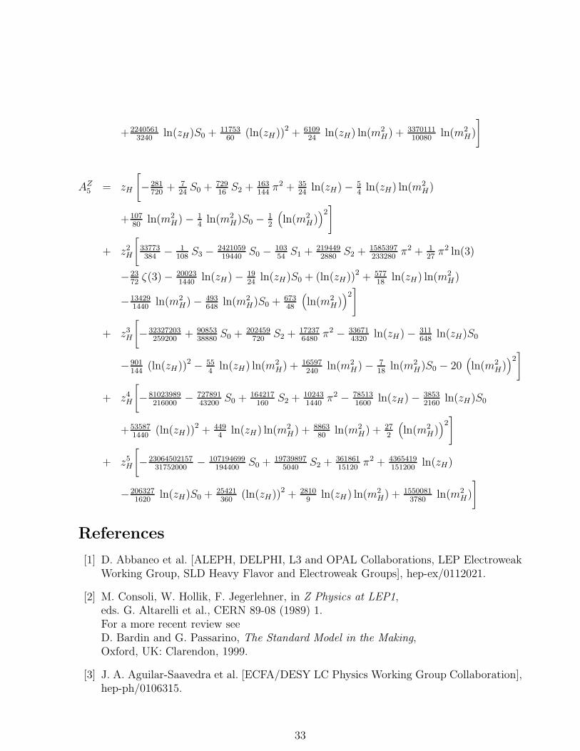
+22405613240

ln(zH)S0 + 1175360

(ln(zH))2 + 610924

ln(zH) ln(m2H) + 3370111

10080ln(m2

H)

]

AZ5 = zH

[−281

720+ 7

24S0 + 729

16S2 + 163

144π2 + 35

24ln(zH) − 5

4ln(zH) ln(m2

H)

+10780

ln(m2H) − 1

4ln(m2

H)S0 − 12

(ln(m2

H))2]

+ z2H

[33773384

− 1108

S3 − 242105919440

S0 − 10354

S1 + 2194492880

S2 + 1585397233280

π2 + 127

π2 ln(3)

−2372

ζ(3) − 200231440

ln(zH) − 1924

ln(zH)S0 + (ln(zH))2 + 57718

ln(zH) ln(m2H)

−134291440

ln(m2H) − 493

648ln(m2

H)S0 + 67348

(ln(m2

H))2]

+ z3H

[−32327203

259200+ 90853

38880S0 + 202459

720S2 + 17237

6480π2 − 33671

4320ln(zH) − 311

648ln(zH)S0

−901144

(ln(zH))2 − 554

ln(zH) ln(m2H) + 16597

240ln(m2

H) − 718

ln(m2H)S0 − 20

(ln(m2

H))2]

+ z4H

[−81023989

216000− 727891

43200S0 + 164217

160S2 + 10243

1440π2 − 78513

1600ln(zH) − 3853

2160ln(zH)S0

+535871440

(ln(zH))2 + 4494

ln(zH) ln(m2H) + 8863

80ln(m2

H) + 272

(ln(m2

H))2]

+ z5H

[−23064502157

31752000− 107194699

194400S0 + 19739897

5040S2 + 361861

15120π2 + 4365419

151200ln(zH)

−2063271620

ln(zH)S0 + 25421360

(ln(zH))2 + 28109

ln(zH) ln(m2H) + 1550081

3780ln(m2

H)

]

References

[1] D. Abbaneo et al. [ALEPH, DELPHI, L3 and OPAL Collaborations, LEP ElectroweakWorking Group, SLD Heavy Flavor and Electroweak Groups], hep-ex/0112021.

[2] M. Consoli, W. Hollik, F. Jegerlehner, in Z Physics at LEP1,eds. G. Altarelli et al., CERN 89-08 (1989) 1.For a more recent review seeD. Bardin and G. Passarino, The Standard Model in the Making,Oxford, UK: Clarendon, 1999.

[3] J. A. Aguilar-Saavedra et al. [ECFA/DESY LC Physics Working Group Collaboration],hep-ph/0106315.

33

[4] S. Eidelman and F. Jegerlehner, Z. Phys. C67 (1995) 585;M. Steinhauser, Phys.Lett. B429 (1998) 158.

[5] J.J. van der Bij and M. Veltman, Nucl. Phys. B231 (1984) 205;J.J. van der Bij, Nucl. Phys. B248 (1984) 141;J.J. van der Bij and F. Hoogeven, Nucl. Phys. B283 (1987) 477;A. Djouadi, Nuovo Cim. A100 (1988) 357;M. Consoli, W. Hollik and F. Jegerlehner, Phys. Lett. B227 (1989) 167;B. A. Kniehl, Nucl. Phys. B347 (1990) 86;F. Halzen and B.A. Kniehl, Nucl. Phys. B353 (1991) 567;J. Fleischer et. al., Phys. Lett. B293 (1992) 437;K. G. Chetyrkin, A. Kwiatkowski and M. Steinhauser, Mod. Phys. Lett. A8 (1993)2785;G. Degrassi, Nucl. Phys. B407 (1993) 271;G. Buchalla and A. J. Buras, Nucl. Phys. B398 (1993) 285;R. Barbieri et al., Phys. Lett. B288 (1992) 95; B312 (1993) 511(E);Nucl. Phys. B409 (1993) 105;J. Fleischer, O.V. Tarasov and F. Jegerlehner, Phys. Lett. B319 (1993) 249;L. Avdeev et al., Phys.Lett. B336 (1994) 560; B349 (1995) 597(E);K. G. Chetyrkin, J.H. Kuhn and M. Steinhauser, Phys. Lett. B351 (1995) 331;K.G. Chetyrkin, J.H. Kuhn and A. Kwiatkowski, Phys. Lett. B282 (1992) 221;Phys. Rept. 277 (1996) 189;A. Czarnecki and J. H. Kuhn, Phys. Rev. Lett. 77 (1996) 395;R. Harlander, T. Seidensticker and M. Steinhauser, Phys. Lett. B426 (1998) 125;J. Fleischer et al., Phys. Lett. B459 (1999) 625;G. Degrassi, S. Fanchiotti and P. Gambino, Int. J. Mod. Phys.A10 (1995) 1377G. Degrassi et al., Phys. Lett. B350 (1995) 75;T. van Ritbergen and R.G. Stuart, Phys. Rev. Lett. 82 (1999) 488;D. Bardin et al., Comput. Phys. Commun. 133 (2001) 229.

[6] G. Degrassi et al., Phys. Lett. B350 (1995) 75.

[7] G. Degrassi, P. Gambino and A. Vicini, Phys. Lett. B383 (1996) 219;G. Degrassi, P. Gambino and A. Sirlin, Phys. Lett. B394 (1997) 188;G. Degrassi et al., Phys. Lett. B418 (1997) 209;S. Bauberger and G. Weiglein, Phys. Lett. B419 (1998) 333;A. Freitas et al., Phys. Lett. B495 (2000) 338.

[8] G. Degrassi and P. Gambino, Nucl. Phys. B567 (2000) 3.

[9] T. van Ritbergen and R.G. Stuart, Phys. Rev. Lett. 82 (1999) 488;Nucl. Phys. B564 (2000) 343;M. Steinhauser and T. Seidensticker, Phys. Lett. B467 (1999) 271.

[10] F. Jegerlehner, Nucl. Phys. Proc. Suppl. 37B (1994) 129.

34

[11] A. Sirlin, in Proc. of the 19th Intl. Symp. on Photon and Lepton Interactions at High

Energy LP99 ed. J.A. Jaros and M.E. Peskin, Int. J. Mod. Phys. A 15S1 (2000) 398.

[12] V.A. Smirnov, Commun. Math. Phys. 134 (1990), 109; Mod. Phys. Lett. A10 (1995)1485; Renormalization and asymptotic expansions (Bikrhauser, Basel, 1991).

[13] P. Gambino, A. Sirlin and G. Weiglein, J.High Energy Phys. 04 (1999) 025.

[14] G. ’t Hooft and M. Veltman, Nucl. Phys. B50 (1972) 318;D.A. Ross and J.C. Taylor, Nucl. Phys. B51 (1973) 125;D.Yu. Bardin, P. Khristova and O.M. Fedorenko, Nucl. Phys. B175 (1980) 435;Nucl. Phys. B197 (1982) 1;S. Sakakibara, Phys. Rev. D24 (1981) 1149;K. Aoki et al., Prog. Theor. Phys. Suppl. 73 (1982) 1;M. Bohm, H. Spiesberger and W. Hollik, Fortsch. Phys. 34 (1986) 687;A. Denner, Fortsch. Phys. 41 (1993) 307.

[15] A. Sirlin, Phys. Rev. D22 (1980) 971.

[16] J. Fleischer and F. Jegerlehner, Phys. Rev. D23 (1981) 2001;F. Jegerlehner, in “Radiative Corrections in SU(2)L × U(1)”,eds. B.W. Lynn, J.F. Wheater, World Scientific Publ., Singapore, 1984.

[17] J. Fleischer, O. V. Tarasov and M. Tentyukov, Nucl. Phys. Proc. Suppl. 89 (2000) 112.

[18] C. Ford, I. Jack and D.R.T. Jones, Nucl. Phys. B387 (1992) 373; B504 (1997) 551(E);A.I. Davydychev and J.B. Tausk, Nucl. Phys. B397 (1993) 123.

[19] G. Weiglein, R. Scharf and M. Bohm, Nucl. Phys. B416 (1994) 606.

[20] D.J. Broadhurst, J. Fleischer and O.V. Tarasov, Z. Phys. C60 (1993) 287;F.A. Berends et. al., Z. Phys. C63 (1994) 227;S. Bauberger, F.A. Berends, M. Bohm and M. Buza, Nucl. Phys. B434 (1995) 383.

[21] R. Scharf and J.B. Tausk, Nucl. Phys. B412 (1994) 523.

[22] F.A. Berends and J.B. Tausk, Nucl. Phys. B421 (1994) 456;A. Ghinculov and J.J. van der Bij, Nucl. Phys. B436 (1995) 30;S. Bauberger and M. Bohm, Nucl. Phys. B445 (1995) 25.

[23] L. Baulieu and R. Coquereaux, Ann. Phys. 140 (1982) 163.

[24] P. Nogueira, J. Comput. Phys. 105 (1993) 279.

[25] J. Fleischer and M.N. Tentyukov, Comp. Phys. Commun. 132 (2000) 124.

[26] J. A. M. Vermaseren, Symbolic manipulation with FORM,Amsterdam, Computer Algebra Nederland, 1991.

35

[27] O.V. Tarasov, Nucl. Phys. B502 (1997) 455; Phys. Rev. D54 (1996) 6479.

[28] J. Fleischer, M.Yu. Kalmykov and O.L. Veretin, Phys. Lett. B427 (1998) 141.

[29] L.V. Avdeev et al., Nucl. Ins. Meth. A389 (1997) 343;Comp. Phys. Commun. 107 (1997) 155.

[30] J. Fleischer et al., Phys. Lett. B459 (1999) 625.

[31] M. Veltman, Diagramatica, Cambridge University Press, 1994.

[32] J. Fleischer and O.V. Tarasov, Comp. Phys. Commun. 71 (1992) 193;J. Fleischer and M. Yu. Kalmykov, Comp. Phys. Commun. 128 (2000) 531.

[33] J. Fleischer et al., Nucl. Phys. B539 (1999) 671; B571 (2000) 511(E).

[34] J. Fleischer, A.V. Kotikov and O.L. Veretin, Nucl. Phys. B547 (1999) 343;J. Fleischer, M.Yu. Kalmykov and A.V. Kotikov, Phys. Lett. B462 (1999) 169;B467 (1999) 310(E);A.I. Davydychev and M.Yu. Kalmykov, Nucl. Phys. B605 (2001) 266 (hep-th/0012189).

[35] R. Tarrach, Nucl. Phys. B183 (1981) 384;A.S. Kronfeld, Phys. Rev. D58 (1998) 051501.

[36] P. Gambino and P.A. Grassi, Phys. Rev. D62 (2000) 076002.

[37] G. ’t Hooft and M. Veltman, Nucl. Phys. B44 (1972) 189;C.G. Bollini and J.J. Giambiagi, Nuovo Cim. B12 (1972) 20;J.F. Ashmore, Lett. Nuovo Cim. 4 (1972) 289;G.M. Cicuta and E. Montaldi, Lett. Nuovo Cim. 4 (1972) 329.

[38] D.J. Gross and F. Wilczek, Phys. Rev. D8 (1973) 3633.

[39] G. ’t Hooft, Nucl. Phys. B61 (1973) 455.

[40] D.R.T. Jones, Nucl. Phys. B87 (1975) 127; Phys. Rev. D25 (1982) 581;M.E. Machacek and M.T. Vaughn, Nucl.Phys. B222 (1983) 83.

[41] D.J. Broadhurst, Z. Phys. C54 (1992) 599.

[42] N. Gray et al., Z. Phys. C48 (1990) 673;L.V. Avdeev and M.Yu. Kalmykov, Nucl. Phys. B502 (1997) 419.

[43] M. Veltman, Acta Phys. Polon. B8 (1977) 475.

[44] G. ’t Hooft and M. Veltman, Nucl. Phys. B153 (1979) 365.

[45] U. Nierste, D. Muller and M. Bohm, Z. Phys. C57 (1993) 605.

36

[46] A.I. Davydychev, Proc. Workshop “AIHENP-99”, Heraklion, Greece, April 1999(Parisianou S.A., Athens, 2000), p. 219 (hep-th/9908032); Phys. Rev. D61 (2000)087701.

[47] A.I. Davydychev and M.Yu. Kalmykov, Nucl. Phys. B (Proc. Suppl.) 89 (2000) 283(hep-th/0005287); Nucl. Phys. B605 (2001) 266 (hep-th/0012189).

[48] L. Lewin, Polylogarithms and associated functions (North-Holland, Amsterdam, 1981).

[49] F. A. Berends, A. I. Davydychev and V. A. Smirnov, Nucl. Phys. B478 (1996) 59.

[50] E.E. Boos and A.I. Davydychev, Theor. Math. Phys. 89 (1991) 1052.

[51] D.J. Broadhurst, hep-th/9604128; Eur. Phys. J. C8 (1999) 311;J. Fleischer and M. Yu. Kalmykov, Phys. Lett. B470 (1999) 168;M.Yu. Kalmykov and O. Veretin, Phys. Lett. B483 (2000) 315.

[52] A. Freitas, W. Hollik, W. Walter, G. Weiglein, “Electroweak two-loop corrections tothe MW − MZ mass correlation in the Standard Model”, hep-ph/0202131.

37

Figure 3: One- and two-loop corrections to the relation ∆Z ≡ m2Z(MZ)/M2

Z−1 as a functionof the Higgs mass MH for intermediate Higgs masses.

Figure 4: One- and two-loop corrections to the relation ∆Z ≡ m2Z(MZ)/M2

Z−1 as a functionof the Higgs mass MH for heavy Higgs masses.

38

Figure 5: One- and two-loop corrections to the relation ∆W ≡ m2W (MW )/M2

W − 1 as afunction of the Higgs mass mH for intermediate Higgs masses.

Figure 6: One- and two-loop corrections to the relation ∆W ≡ m2W (MW )/M2

W − 1 as afunction of the Higgs mass mH for heavy Higgs masses.

39

Figure 7: The dependence on the number of coefficients of the expansion (5.4) used for the

evaluation of the two-loop corrections. We show δ ≡ −(Π

(2)Z + Π

(1)Z Π

(1)Z

′

)/M2

Z (see 5.3) asa function of the Higgs mass. The dotted, dashed, dot-dashed and full lines show resultsobtained with the first one, two, three and all calculated (six) coefficients, respectively.

Figure 8: The dependence on the number of coefficients of the expansion with respect tosin2 θW of the two-loop corrections. We show δ ≡ −

(Π

(2)Z + Π

(1)Z Π

(1)Z

′

)/M2

Z (see 5.3) asa function of the Higgs mass. The dotted, dashed, dot-dashed and full lines show resultsobtained with the first one, two, three and all calculated (six) coefficients, respectively.

40

Figure 9: One- and two-loop corrections to ∆s = sin2 θMSW / sin2 θOS

W − 1 (see (5.8)) as afunction of the Higgs mass mH for intermediate Higgs masses (µ = MZ).

Figure 10: One- and two-loop corrections to ∆s = sin2 θMSW / sin2 θOS

W − 1 (see (5.8)) as afunction of the Higgs mass mH for heavy Higgs masses (µ = MZ).

41