arX

iv:1

011.

6470

v1 [

hep-

ph]

30

Nov

201

0DCP-10-05

A renormalizable fermion mass model with the double

tetrahedral group

Alfredo Aranda,1,2∗ Cesar Bonilla,1† Raymundo Ramos,1‡ and Alma D. Rojas1§

1Facultad de Ciencias, CUICBAS

Universidad de Colima, Colima, Mexico

2Dual C-P Institute of High Energy Physics, Mexico

(Dated: December 1, 2010)

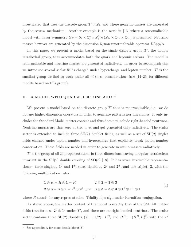
Abstract

We present a renormalizable model for fermion masses based solely on the double tetrahedral

group T ′. It does not include right handed neutrinos and majorana neutrino masses are generated

radiatively. The scalar sector of the model involves three SU(2) doublets and a set of lepton number

violating (charged) scalars needed to give mass to the neutrinos. In the quark sector the model

leads to a Fritzsch type scenario that is consistent with all the existing data. In the lepton sector,

the model leads to tribimaximal (and near tribimaximal) mixing, and an inverted mass hierarchy.

PACS numbers: 11.30.Hv, 12.15.Ff, 14.60.Pq

∗ Electronic address:fefo@ucol.mx† Electronic address:rasec.cmbd@gmail.com‡ Electronic address:raalraan@gmail.com§ Electronic address:alma.drp@gmail.com

1

I. INTRODUCTION

Discrete symmetries have been extensively used in an attempt to describe the observed

patterns in fermion masses and mixing angles (for a thorough list of references see [1–3]).

Typical scenarios include some of the following ingredients:

• Introduction of a flavor symmetry, usually a product between a non-abelian and several

abelian discrete groups. There can be different groups for different sectors (quark or

leptonic) or only for one of the sectors.

• Introduction of heavy right-handed neutrinos. This provides Dirac and Majorana

mass terms for neutrinos and allows one to consider, for example, generation of small

neutrino Majorana masses using some version of the seesaw mechanism [4].

• Introduction of several scalar fields charged under the flavor symmetry that may or not

acquire vacuum expectation values (vevs), thus breaking or not the flavor symmetry.

These scalars may or not be singlets under the Standard Model (SM) gauge group.

Typically there are high energy scales associated to the vevs of these fields (when they

are singlets under the SM gauge group). With a few exceptions, the extended scalar

sector can have collider relevant phenomenology [5, 6].

• Neutrino masses can be generated, in addition to the seesaw mechanism, through

higher order operators that violate lepton number [7] or through quantum (radiative)

corrections [8–10].

It is important to note that the ingredients above can be used in the frameworks (or

combination thereof) of supersymmetric and non-supersymmetric models, Grand Unified

Theories, extra dimensional models, and so on. Also the list is not exhaustive and includes

only some of the most important and general considerations.

Among the possibilities generated by these ingredients, one that has been recently ex-

plored consists of creating renormalizable models [11–13], i.e. models that forbid the inclu-

sion of higher (> 4) dimension operators. There are two main challenges in this approach.

First, it is highly nontrivial to create a model based on a single discrete group that can

accommodate both quarks and leptons. Second, since no higher order operators are allowed,

obtaining small neutrino masses is not trivial. For example in [12] a renormalizable model is

2

investigated that uses the discrete group T ′ ×Z2, and where neutrino masses are generated

by the seesaw mechanism. Another example is the work in [13] where a renormalizable

model with flavor symmetry GF = S4 ×Zq3 ×Z2

2 ⋊ (Z2e ×Z2µ ×Z2τ ) is presented. Neutrino

masses however are generated by the dimension 5, non renormalizable operator LLφφ/Λ.

In this paper we present a model based on the single discrete group T ′, the double

tetrahedral group, that accommodates both the quark and leptonic sectors. The model is

renormalizable and neutrino masses are generated radiatively. In order to accomplish this

we introduce several scalar fields charged under hypercharge and lepton number. T ′ is the

smallest group we find to work under all of these considerations (see [14–26] for different

models based on this group).

II. A MODEL WITH QUARKS, LEPTONS AND T ′

We present a model based on the discrete group T ′ that is renormalizable, i.e. we do

not use higher dimension operators in order to generate patterns nor hierarchies. It only in-

cludes the Standard Model matter content and thus does not include right-handed neutrinos.

Neutrino masses are thus zero at tree level and get generated only radiatively. The scalar

sector is extended to include three SU(2) doublet fields, as well as a set of SU(2) singlet

fields charged under lepton number and hypercharge that explicitly break lepton number

conservation. These fields are needed in order to generate neutrino masses radiatively.

T ′ is the group of all 24 proper rotations in three dimensions leaving a regular tetrahedron

invariant in the SU(2) double covering of SO(3) [18]. It has seven irreducible representa-

tions:1 three singlets, 10 and 1±, three doublets, 20 and 2±, and one triplet, 3, with the

following multiplication rules:

1⊗R = R⊗ 1 = R 2⊗ 2 = 1⊕ 3

2⊗ 3 = 3⊗ 2 = 20 ⊕ 2+ ⊕ 2− 3⊗ 3 = 3⊕ 3⊕ 10 ⊕ 1+ ⊕ 1−(1)

where R stands for any representation. Triality flips sign under Hermitian conjugation.

As stated above, the matter content of the model is exactly that of the SM. All matter

fields transform as 20 ⊕ 10 under T ′, and there are no right-handed neutrinos. The scalar

sector contains three SU(2) doublets (Y = 1/2): HS, and HD = (HD1 , HD

2 ) with the T ′

1 See appendix A for more details about T ′.

3

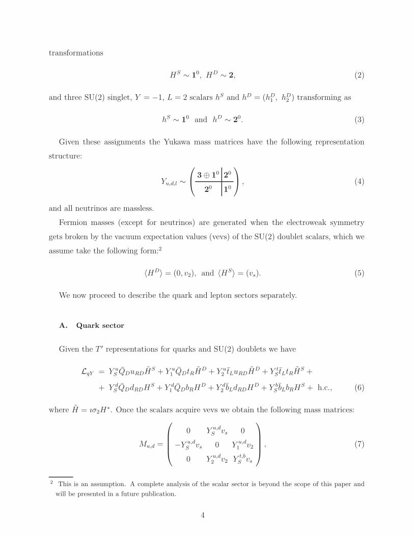
transformations

HS ∼ 10, HD ∼ 2, (2)

and three SU(2) singlet, Y = −1, L = 2 scalars hS and hD = (hD1 , hD

2 ) transforming as

hS ∼ 10 and hD ∼ 20. (3)

Given these assignments the Yukawa mass matrices have the following representation

structure:

Yu,d,l ∼

3⊕ 10 20

20 10

, (4)

and all neutrinos are massless.

Fermion masses (except for neutrinos) are generated when the electroweak symmetry

gets broken by the vacuum expectation values (vevs) of the SU(2) doublet scalars, which we

assume take the following form:2

〈HD〉 = (0, v2), and 〈HS〉 = (vs). (5)

We now proceed to describe the quark and lepton sectors separately.

A. Quark sector

Given the T ′ representations for quarks and SU(2) doublets we have

LqY = Y uS QDuRDH

S + Y u1 QDtRH

D + Y u2 tLuRDH

D + Y tS tLtRH

S +

+ Y dS QDdRDH

S + Y d1 QDbRH

D + Y d2 bLdRDH

D + Y bS bLbRH

S + h.c., (6)

where H = ıσ2H∗. Once the scalars acquire vevs we obtain the following mass matrices:

Mu,d =

0 Y u,dS vs 0

−Y u,dS vs 0 Y u,d

1 v2

0 Y u,d2 v2 Y t,b

S vs

, (7)

2 This is an assumption. A complete analysis of the scalar sector is beyond the scope of this paper and

will be presented in a future publication.

4

where each entry depends on both the values of the vevs and the Yukawa couplings. We see

that these matrices can be parametrized as

Mu,d =

0 Au,d 0

−Au,d 0 Bu,d

0 Du,d Cu,d

. (8)

These matrices are similar to those found by Fritzsch for a three family model [27] (see

also [13]). Following that analysis and taking Cu,d = y2u,dmt,b, we rewrite the mass matrices

above in terms of the quark masses and free parameters yu,d [13, 28],

Mu,d = mt,b

0 qu,d/yu,d 0

−qa,d/yu,d 0 bu,d

0 du,d y2u,d

, (9)

where

q2u,d =mu,dmc,s

m2t,b

, (10)

pu,d =m2

u,d +m2c,s

m2t,b

, (11)

du,d =

√

pu,d + 1− y4u,d +Ru,d

2−

(

qu,dyu,d

)2

, (12)

bu,d =

√

pu,d + 1− y4u,d − Ru,d

2−

(

qu,dyu,d

)2

, (13)

Ru,d = ((1 + pu,d − y4u,d)2 − 4(pu,d + q4u,d) + 8q2u,dy

2u,d)

1/2, (14)

and where Mu,d are matrices with real entries obtained from the phase factorization of

Mu,d [28] through

Mu,d = Pu,dMP ∗u,d (15)

with Pu,d diagonal phase matrices such that P = P †uPd = diag(1, eiβu,d, eiαu,d).

5

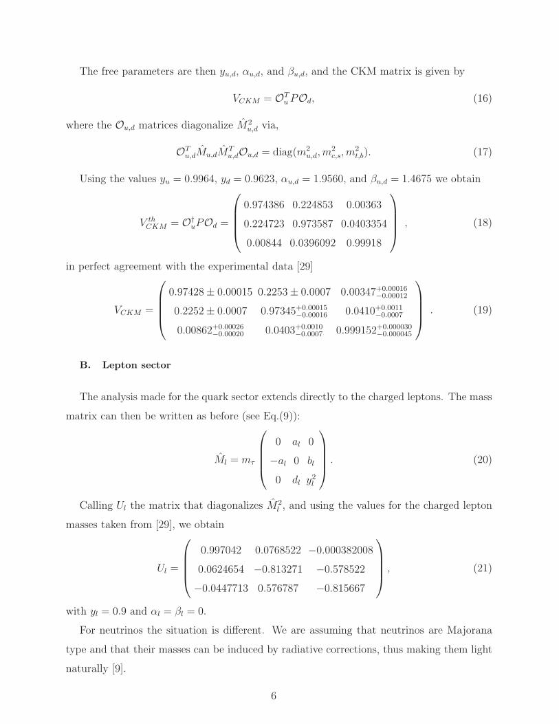
The free parameters are then yu,d, αu,d, and βu,d, and the CKM matrix is given by

VCKM = OTuPOd, (16)

where the Ou,d matrices diagonalize M2u,d via,

OTu,dMu,dM

Tu,dOu,d = diag(m2

u,d, m2c,s, m

2t,b). (17)

Using the values yu = 0.9964, yd = 0.9623, αu,d = 1.9560, and βu,d = 1.4675 we obtain

V thCKM = O†

uPOd =

0.974386 0.224853 0.00363

0.224723 0.973587 0.0403354

0.00844 0.0396092 0.99918

, (18)

in perfect agreement with the experimental data [29]

VCKM =

0.97428± 0.00015 0.2253± 0.0007 0.00347+0.00016−0.00012

0.2252± 0.0007 0.97345+0.00015−0.00016 0.0410+0.0011

−0.0007

0.00862+0.00026−0.00020 0.0403+0.0010

−0.0007 0.999152+0.000030−0.000045

. (19)

B. Lepton sector

The analysis made for the quark sector extends directly to the charged leptons. The mass

matrix can then be written as before (see Eq.(9)):

Ml = mτ

0 al 0

−al 0 bl

0 dl y2l

. (20)

Calling Ul the matrix that diagonalizes M2l , and using the values for the charged lepton

masses taken from [29], we obtain

Ul =

0.997042 0.0768522 −0.000382008

0.0624654 −0.813271 −0.578522

−0.0447713 0.576787 −0.815667

, (21)

with yl = 0.9 and αl = βl = 0.

For neutrinos the situation is different. We are assuming that neutrinos are Majorana

type and that their masses can be induced by radiative corrections, thus making them light

naturally [9].

6

In absence of right-handed neutrinos the only possible mass terms for left-handed neutri-

nos are Majorana mass terms. The simplest mass term in this case, without the introduction

of scalars with non trivial SU(2) representations, is the dimension five operator with form

L ∝ lcLlLHHM

. Although this term is non-renormalizable, it may be induced by radiative

corrections if we introduce a scalar field that breaks lepton number (provided there are at

least two SU(2) Higgs doublets [8]). This is why we have introduced the fields hS and hD

in our renormalizable model.

In order to see how this works, consider the following example: A two Higgs doublet

model with SM fermion content and an additional scalar field h with charges (1,−1) under

SU(2)× U(1)Y and lepton number L = 2 [8, 10]. The Yukawa couplings of h are

Lllh = κabǫij(Lai )

cLbjh

† + h.c. , (22)

where i, j are SU(2) indices, a, b are family indices, κab = −κba from Fermi statistics, and

Li denotes the SU(2) lepton doublets. If there are two (or more) Higgs doublets, there will

be a cubic coupling term like

LHHh = λαβǫijHαi H

βj h+ h.c., (23)

with λαβ = −λβα, and α, β = 1, 2. This term explicitly violates lepton number and allows

the generation of majorana masses for the neutrinos.

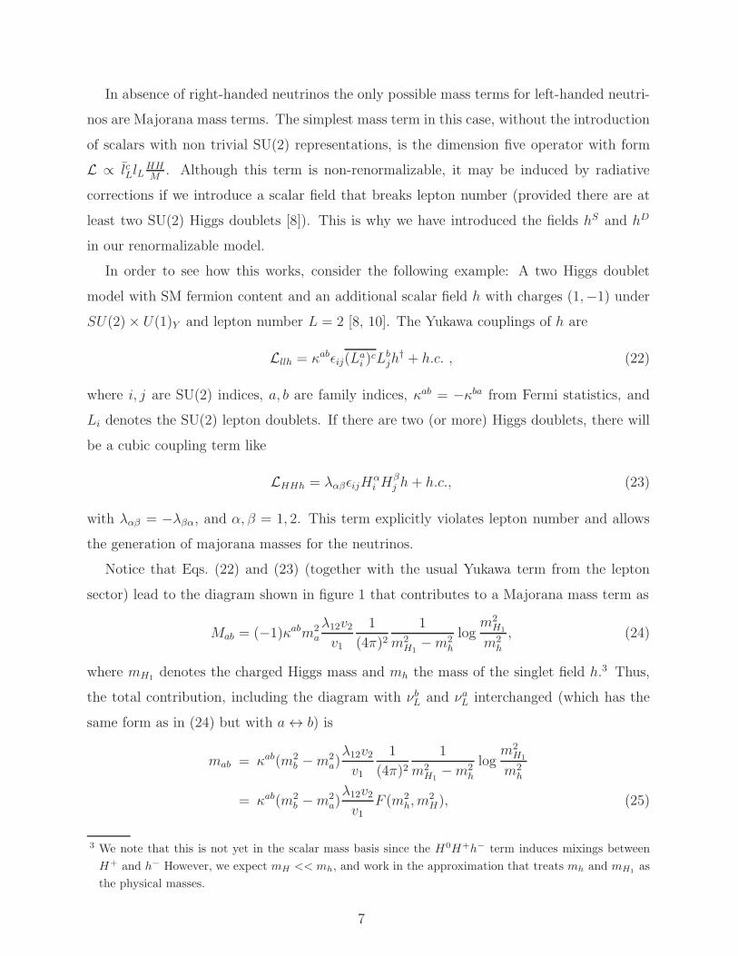
Notice that Eqs. (22) and (23) (together with the usual Yukawa term from the lepton

sector) lead to the diagram shown in figure 1 that contributes to a Majorana mass term as

Mab = (−1)κabm2a

λ12v2v1

1

(4π)21

m2H1

−m2h

logm2

H1

m2h

, (24)

where mH1denotes the charged Higgs mass and mh the mass of the singlet field h.3 Thus,

the total contribution, including the diagram with νbL and νa

L interchanged (which has the

same form as in (24) but with a ↔ b) is

mab = κab(m2b −m2

a)λ12v2v1

1

(4π)21

m2H1

−m2h

logm2

H1

m2h

= κab(m2b −m2

a)λ12v2v1

F (m2h, m

2H), (25)

3 We note that this is not yet in the scalar mass basis since the H0H+h− term induces mixings between

H+ and h− However, we expect mH << mh, and work in the approximation that treats mh and mH1as

the physical masses.

7

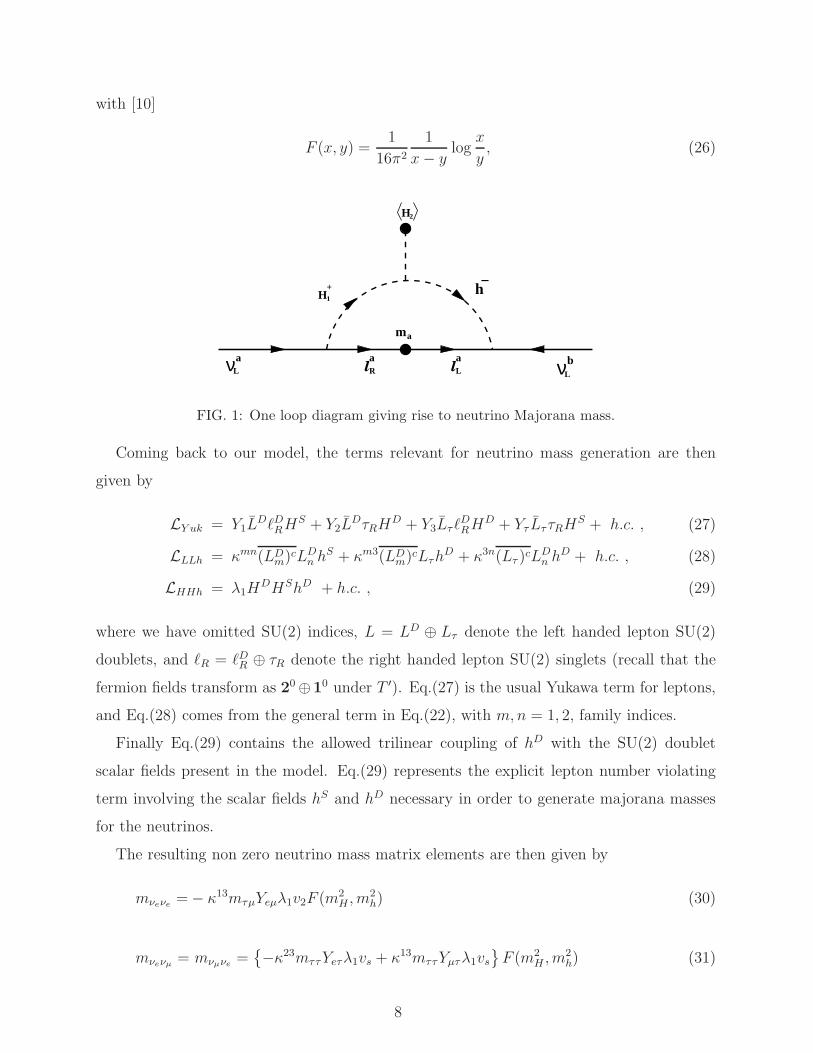
with [10]

F (x, y) =1

16π2

1

x− ylog

x

y, (26)

lR

alL

aνL

bνL

a

ma

H2

h−H+1

FIG. 1: One loop diagram giving rise to neutrino Majorana mass.

Coming back to our model, the terms relevant for neutrino mass generation are then

given by

LY uk = Y1LDℓDRH

S + Y2LDτRH

D + Y3LτℓDRH

D + Yτ LττRHS + h.c. , (27)

LLLh = κmn(LDm)

cLDn h

S + κm3(LDm)

cLτhD + κ3n(Lτ )cL

Dn h

D + h.c. , (28)

LHHh = λ1HDHShD + h.c. , (29)

where we have omitted SU(2) indices, L = LD ⊕ Lτ denote the left handed lepton SU(2)

doublets, and ℓR = ℓDR ⊕ τR denote the right handed lepton SU(2) singlets (recall that the

fermion fields transform as 20⊕10 under T ′). Eq.(27) is the usual Yukawa term for leptons,

and Eq.(28) comes from the general term in Eq.(22), with m,n = 1, 2, family indices.

Finally Eq.(29) contains the allowed trilinear coupling of hD with the SU(2) doublet

scalar fields present in the model. Eq.(29) represents the explicit lepton number violating

term involving the scalar fields hS and hD necessary in order to generate majorana masses

for the neutrinos.

The resulting non zero neutrino mass matrix elements are then given by

mνeνe =− κ13mτµYeµλ1v2F (m2H , m

2h) (30)

mνeνµ = mνµνe ={

−κ23mττYeτλ1vs + κ13mττYµτλ1vs}

F (m2H , m

2h) (31)

8

mνeντ = mντνe ={

κ31meµYeµλ1v2 − κ32mµτYeτλ1vs + κ13mτµYτµλ1vs

+κ13mττYττλ1v2}

F (m2H , m

2h) (32)

mντντ ={

−κ32mµeYτeλ1vs + κ31meµYτµλ1vs}

F (m2H , m

2h) (33)

Assuming that κ ∼ O(1), λ1 ∼ mH ∼ 500 GeV, and noting that Y 〈H〉 must be at the

same scale of ml, then mh ∼ 4× 105 GeV leads to matrix elements of O(eV). The Majorana

neutrino mass matrix then has the texture:

Mν =

a b c

b 0 0

c 0 d

, (34)

where all entries are O(eV).

The neutrino mixing matrix UMNS is obtained by

UMNS = U †l Uν , (35)

where Ul is the unitary matrix that diagonalizes the square of the charged leptons matrix,

and Uν is the unitary matrix that diagonalizes Mν .

In order to perform the numerical analysis we used the following experimental results [29]:

sin2(2θ12) = 0.087± 0.03 (36)

sin2(2θ23) > 0.92 (37)

sin2(2θ13) < 0.15 (38)

and

∆m221 = 7.59+0.19

−0.21 × 10−5 eV2 (39)

∆m232 = 2.43± 0.13× 10−3 eV2 . (40)

Since the absolute mass scale in the neutrino sector is not known, we use the following ratio

0.0338 <

∣

∣

∣

∣

∆m221

∆m232

∣

∣

∣

∣

< 0.0288 . (41)

In order to determine whether the mass matrices in this model can reproduce these results,

we performed a scan of the complete range in all three angles. Then for each case where a

9

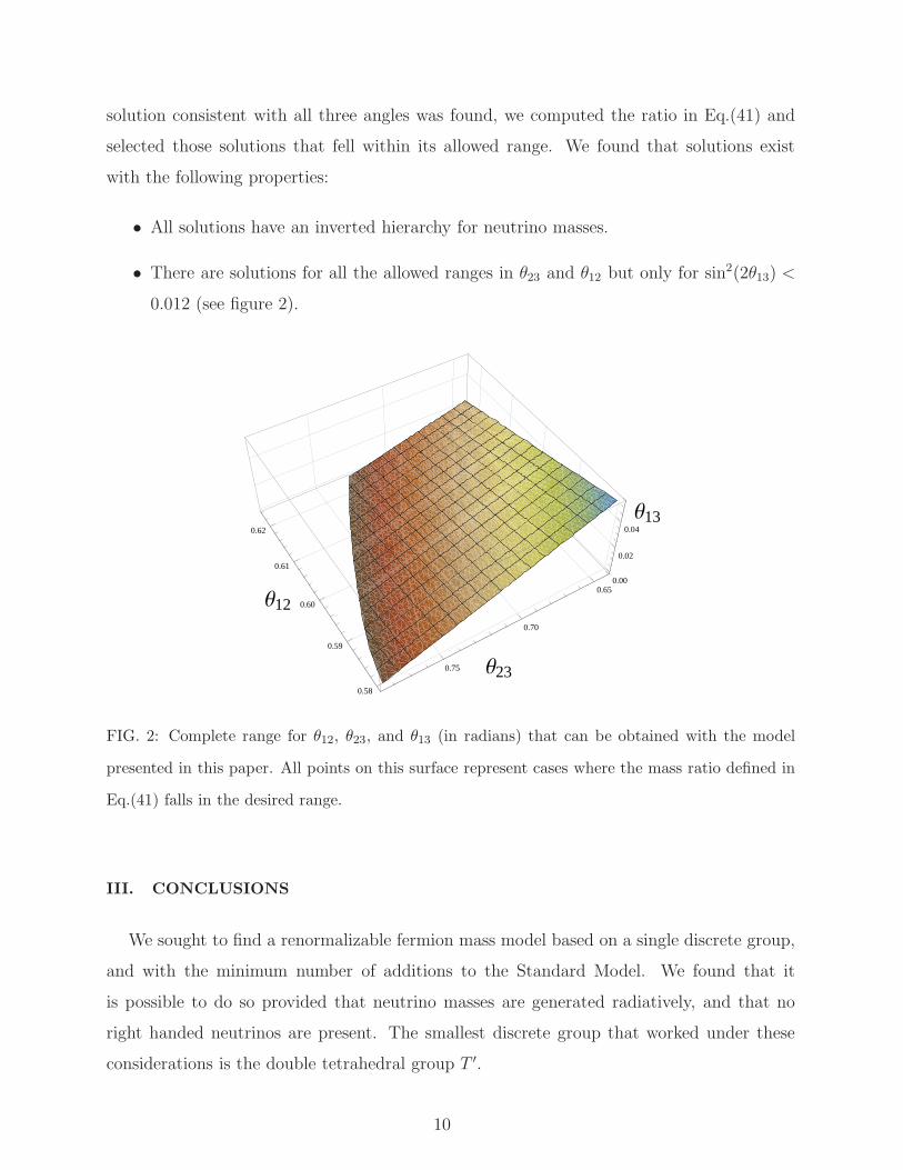
solution consistent with all three angles was found, we computed the ratio in Eq.(41) and

selected those solutions that fell within its allowed range. We found that solutions exist

with the following properties:

• All solutions have an inverted hierarchy for neutrino masses.

• There are solutions for all the allowed ranges in θ23 and θ12 but only for sin2(2θ13) <

0.012 (see figure 2).

0.58

0.59

0.60

0.61

0.62

Θ120.65

0.70

0.75 Θ23

0.00

0.02

0.04

Θ13

FIG. 2: Complete range for θ12, θ23, and θ13 (in radians) that can be obtained with the model

presented in this paper. All points on this surface represent cases where the mass ratio defined in

Eq.(41) falls in the desired range.

III. CONCLUSIONS

We sought to find a renormalizable fermion mass model based on a single discrete group,

and with the minimum number of additions to the Standard Model. We found that it

is possible to do so provided that neutrino masses are generated radiatively, and that no

right handed neutrinos are present. The smallest discrete group that worked under these

considerations is the double tetrahedral group T ′.

10

A specific realization of a model is presented. It contains the Standard Model fermion

content and a scalar sector that involves three SU(2) doublets as well as a set of lepton

number violating (charged) scalars, needed to give mass to the neutrinos.

In the quark sector the model leads to a Fritzsch type scenario that is consistent with

all the existing data. In the lepton sector, the model leads to tribimaximal (and near

tribimaximal) mixing and an inverted mass hierarchy: it accommodates all existing data in

both the quark and lepton sectors with sin2(2θ13) < 0.012. The phenomenology of the scalar

sector is currently being studied and will be presented in a future publication.

Acknowledgments

This work was supported in part by CONACYT.

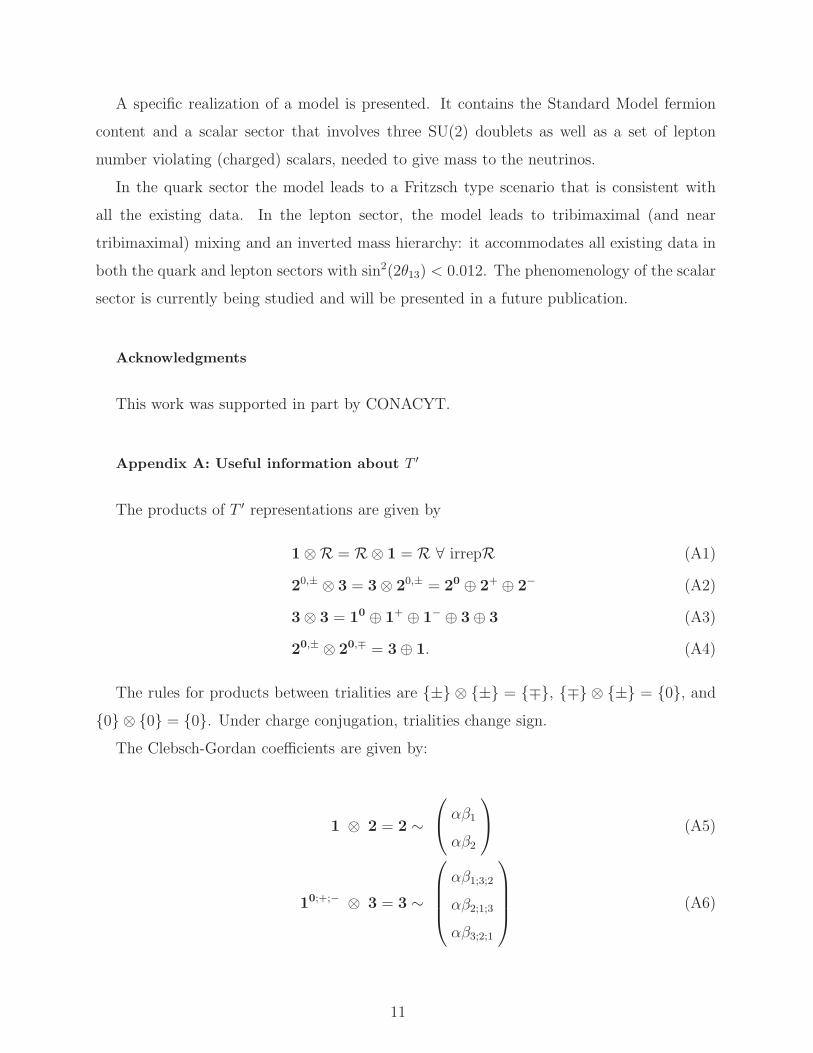
Appendix A: Useful information about T ′

The products of T ′ representations are given by

1⊗R = R⊗ 1 = R ∀ irrepR (A1)

20,± ⊗ 3 = 3⊗ 20,± = 20 ⊕ 2+ ⊕ 2− (A2)

3⊗ 3 = 10 ⊕ 1+ ⊕ 1− ⊕ 3⊕ 3 (A3)

20,± ⊗ 20,∓ = 3⊕ 1. (A4)

The rules for products between trialities are {±} ⊗ {±} = {∓}, {∓} ⊗ {±} = {0}, and

{0} ⊗ {0} = {0}. Under charge conjugation, trialities change sign.

The Clebsch-Gordan coefficients are given by:

1 ⊗ 2 = 2 ∼

αβ1

αβ2

(A5)

10;+;− ⊗ 3 = 3 ∼

αβ1;3;2

αβ2;1;3

αβ3;2;1

(A6)

11

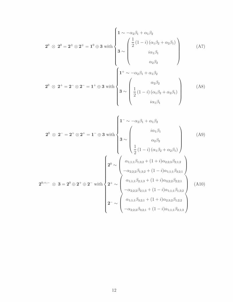
20 ⊗ 20 = 2± ⊗ 2∓ = 10 ⊕ 3 with

1 ∼ −α2β1 + α1β2

3 ∼

1

2(1− i) (α1β2 + α2β1)

iα1β1

α2β2

(A7)

20 ⊗ 2+ = 2− ⊗ 2− = 1+ ⊕ 3 with

1+ ∼ −α2β1 + α1β2

3 ∼

α2β2

1

2(1− i) (α1β2 + α2β1)

iα1β1

(A8)

20 ⊗ 2− = 2+ ⊗ 2+ = 1− ⊕ 3 with

1− ∼ −α2β1 + α1β2

3 ∼

iα1β1

α2β2

1

2(1− i) (α1β2 + α2β1)

(A9)

20;+;− ⊗ 3 = 20 ⊕ 2+ ⊕ 2− with

20 ∼

α1;1;1β1;3;2 + (1 + i)α2;2;3β2;1;2

−α2;2;2β1;3;2 + (1− i)α1;1;1β3;2;1

2+ ∼

α1;1;1β2;1;3 + (1 + i)α3;2;2β2;2;1

−α2;2;2β2;1;3 + (1− i)α1;1;1β1;3;2

2− ∼

α1;1;1β3;2;1 + (1 + i)α2;3;2β1;2;2

−α2;2;2β3;2;1 + (1− i)α1;1;1β2;1;3

(A10)

12

3⊗ 3 = 10 ⊕ 1+ ⊕ 1− ⊕ 3s ⊕ 3a with

10 ∼ α1β1 + α2β3 + α3β2

1+ ∼ α1β2 + α2β1 + α3β3

1− ∼ α1β3 + α2β2 + α3β1

3s ∼

2α1β1 − α3β2 − α2β3

2α3β3 − α1β2 − α2β1

2α2β2 − α1β3 − α3β1

3a ∼

−α2β3 + α3β2

−α1β2 + α2β1

−α1β3 + α3β1

(A11)

where αi and βi denote the entries in the first and second representations respectively.

[1] G. Altarelli, F. Feruglio, [arXiv:1002.0211 [hep-ph]].

[2] H. Ishimori, T. Kobayashi, H. Ohki et al., Prog. Theor. Phys. Suppl. 183, 1-163 (2010).

[arXiv:1003.3552 [hep-th]].

[3] G. Altarelli, arXiv:1011.5342 [hep-ph].

[4] J. Schechter and J. W. F. Valle, Phys. Rev. D 22, 2227 (1980).

[5] K. Tsumura, L. Velasco-Sevilla, Phys. Rev. D81, 036012 (2010). [arXiv:0911.2149 [hep-ph]].

[6] P. H. Frampton, C. M. Ho, T. W. Kephart et al., [arXiv:1009.0307 [hep-ph]].

[7] S. Weinberg, Phys. Rev. Lett. 43, 1566-1570 (1979).

[8] A. Zee, Phys. Lett. B 93, 389 (1980) [Erratum-ibid. B 95, 461 (1980)].

[9] K. S. Babu and V. S. Mathur, Phys. Rev. D 38, 3550 (1988).

[10] M. Fukugita, T. Yanagida, Berlin, Germany: Springer (2003) 593 p.

[11] P. H. Frampton, S. Matsuzaki, [arXiv:0806.4592 [hep-ph]].

[12] P. H. Frampton, T. W. Kephart, S. Matsuzaki, Phys. Rev. D78, 073004 (2008).

[arXiv:0807.4713 [hep-ph]].

[13] S. Morisi and E. Peinado, Phys. Rev. D 81, 085015 (2010) [arXiv:1001.2265 [hep-ph]].

[14] K. M. Case, R. Karplus, C. N. Yang, Phys. Rev. 101, 874-876 (1956).

[15] W. M. Fairbairn, T. Fulton, W. H. Klink, J. Math. Phys. 5, 1038 (1964).

13

[16] P. H. Frampton, T. W. Kephart, Int. J. Mod. Phys. A10, 4689-4704 (1995). [hep-ph/9409330].

[17] A. Aranda, C. D. Carone, R. F. Lebed, Phys. Lett. B474, 170-176 (2000). [hep-ph/9910392].

[18] A. Aranda, C. D. Carone and R. F. Lebed, Phys. Rev. D 62, 016009 (2000)

[arXiv:hep-ph/0002044].

[19] F. Feruglio, C. Hagedorn, Y. Lin et al., Nucl. Phys. B775, 120-142 (2007). [hep-ph/0702194].

[20] M. -C. Chen, K. T. Mahanthappa, Phys. Lett. B652, 34-39 (2007). [arXiv:0705.0714 [hep-ph]].

[21] P. H. Frampton, T. W. Kephart, JHEP 0709, 110 (2007). [arXiv:0706.1186 [hep-ph]].

[22] A. Aranda, Phys. Rev. D76, 111301 (2007). [arXiv:0707.3661 [hep-ph]].

[23] M. -C. Chen, K. T. Mahanthappa, [arXiv:0710.2118 [hep-ph]].

[24] S. Sen, Phys. Rev. D76, 115020 (2007). [arXiv:0710.2734 [hep-ph]].

[25] G. -J. Ding, Phys. Rev. D78, 036011 (2008). [arXiv:0803.2278 [hep-ph]].

[26] M. -C. Chen, K. T. Mahanthappa, F. Yu, Phys. Rev. D81, 036004 (2010). [arXiv:0907.3963

[hep-ph]].

[27] H. Fritzsch, Phys. Lett. B 73, 317 (1978).

[28] K. S. Babu, J. Kubo, Phys. Rev. D71, 056006 (2005). [hep-ph/0411226].

[29] K. Nakamura et al. (Particle Data Group), JPG 37, 075021 (2010) (URL: http://pdg.lbl.gov)

14