Split fermion quasinormal modes
11
arXiv:hep-th/0701193v2 8 Feb 2007 LYCEN 2006-24 RITS-PP-011 Split fermion quasi-normal modes H. T. Cho, 1, * A. S. Cornell, 2, † Jason Doukas, 3, ‡ and Wade Naylor 4, § 1 Department of Physics, Tamkang University, Tamsui, Taipei, Taiwan, Republic of China 2 Universit´ e de Lyon, Villeurbanne, F-69622, France; Universit´ e Lyon 1, Institut de Physique Nucl´ eaire de Lyon 3 School of Physics, University of Melbourne, Parkville, Victoria 3010, Australia. 4 Department of Physics, Ritsumeikan University, Kusatsu, Shiga 525-8577, Japan (Dated: February 2, 2008) In this paper we use the conformal properties of the spinor field to show how we can obtain the fermion quasi-normal modes for a higher dimensional Schwarzschild black hole. These modes are of interest in so called split fermion models, where quarks and leptons are required to exist on different branes in order to keep the proton stable. As has been previously shown, for brane localized fields, the larger the number of dimensions the faster the black hole damping rate. Moreover, we also present the analytic forms of the quasi-normal frequencies in both the large angular momentum and the large mode number limits. PACS numbers: 02.30Gp, 03.65ge I. INTRODUCTION With the advent of theories postulating the existence of additional dimensions, there has been much discussion in the literature related to the quasi-normal modes (QNMs) of black holes (BHs), for example, in the context of the QNMs of higher dimensional BHs see reference [1]. By QNMs we refer to the complex frequency modes of oscillation which arise from perturbations of the BH, where the real part represents the actual frequency of the oscillation and the imaginary part represents the damping due to the emission of gravitational waves. Recent investigations of large extra-dimensional scenarios [3], where the hierarchy problem can be shifted into a problem of the scale of the extra-dimensions, has led to the somewhat striking prediction that BHs may be observed at particle accelerators such as the LHC [4], for an interesting treatment of mini BHs within an effective field theory framework see [5]. However, one poignant problem is that in order to suppress a rapid proton decay we need to physically split the quarks and leptons. Such models are generically called split fermions models, see, for example, reference [6]. In supersymmetric versions of this idea the localizing scalars and bulk gauge fields will have fermionic bulk superpartners. In this respect it is important to consider the properties of bulk fermions. Note that up to now only brane localized QNMs have been calculated [8] (where other BH effects have been considered in reference [7]). That said, the motivations for studying the fermion QNMs from BHs in this paper are two-fold; the first of these being from the theoretical point of view, where the lack of any work done in greater than four dimensions [2] with Dirac fields is an omission in the literature. Our calculations serve to fill this gap. Secondly, having a complete catalog of all QNMs would be a necessary precursor to eventually studying the emission rates of collider produced, or TeV scale, BHs. In a forthcoming work we shall present details of BH absorption cross-sections for bulk Schwarzschild fermions in d-dimensions [9]. See also reference [10] for tense branes in six-dimensions, where bulk fermions on the tense brane background defined there have yet to be obtained. As such, this paper shall be structured as follows: In the next section we shall discuss how a conformal transformation of the metric allows for a convenient separation of the Dirac equation into a time-radial part and a (d − 2)-sphere, in d-dimensions. Such a method has already been applied in reference [11] to the case of low energy s-wave absorption cross-sections (which the authors are currently generalizing to higher energies and quantum numbers). However, this has not been used yet in the context of BH QNMs. After this we shall present our results for the QNMs, along with the analytical forms of the frequencies in both the large angular momentum as well as the large mode number limits. Finally, in the last section, we shall make some concluding statements. * Email: htcho“at”mail.tku.edu.tw † Email: cornell“at”ipnl.in2p3.fr ‡ Email: j.doukas“at”physics.unimelb.edu.au § Email: naylor“at”se.ritsumei.ac.jp
Transcript of Split fermion quasinormal modes

arX
ivh
ep-t
h07
0119
3v2
8 F
eb 2
007
LYCEN 2006-24RITS-PP-011
Split fermion quasi-normal modes
H T Cho1 lowast A S Cornell2 dagger Jason Doukas3 Dagger and Wade Naylor4 sect
1Department of Physics Tamkang University Tamsui Taipei Taiwan Republic of China2Universite de Lyon Villeurbanne F-69622 France Universite Lyon 1 Institut de Physique Nucleaire de Lyon
3School of Physics University of Melbourne Parkville Victoria 3010 Australia4Department of Physics Ritsumeikan University Kusatsu Shiga 525-8577 Japan
(Dated February 2 2008)
In this paper we use the conformal properties of the spinor field to show how we can obtain thefermion quasi-normal modes for a higher dimensional Schwarzschild black hole These modes are ofinterest in so called split fermion models where quarks and leptons are required to exist on differentbranes in order to keep the proton stable As has been previously shown for brane localized fieldsthe larger the number of dimensions the faster the black hole damping rate Moreover we alsopresent the analytic forms of the quasi-normal frequencies in both the large angular momentum andthe large mode number limits
PACS numbers 0230Gp 0365ge
I INTRODUCTION
With the advent of theories postulating the existence of additional dimensions there has been much discussion inthe literature related to the quasi-normal modes (QNMs) of black holes (BHs) for example in the context of theQNMs of higher dimensional BHs see reference [1] By QNMs we refer to the complex frequency modes of oscillationwhich arise from perturbations of the BH where the real part represents the actual frequency of the oscillation andthe imaginary part represents the damping due to the emission of gravitational waves
Recent investigations of large extra-dimensional scenarios [3] where the hierarchy problem can be shifted into aproblem of the scale of the extra-dimensions has led to the somewhat striking prediction that BHs may be observedat particle accelerators such as the LHC [4] for an interesting treatment of mini BHs within an effective field theoryframework see [5] However one poignant problem is that in order to suppress a rapid proton decay we need tophysically split the quarks and leptons Such models are generically called split fermions models see for examplereference [6] In supersymmetric versions of this idea the localizing scalars and bulk gauge fields will have fermionicbulk superpartners In this respect it is important to consider the properties of bulk fermions Note that up to nowonly brane localized QNMs have been calculated [8] (where other BH effects have been considered in reference [7])
That said the motivations for studying the fermion QNMs from BHs in this paper are two-fold the first of thesebeing from the theoretical point of view where the lack of any work done in greater than four dimensions [2] withDirac fields is an omission in the literature Our calculations serve to fill this gap Secondly having a complete catalogof all QNMs would be a necessary precursor to eventually studying the emission rates of collider produced or TeVscale BHs In a forthcoming work we shall present details of BH absorption cross-sections for bulk Schwarzschildfermions in d-dimensions [9] See also reference [10] for tense branes in six-dimensions where bulk fermions on thetense brane background defined there have yet to be obtained
As such this paper shall be structured as follows In the next section we shall discuss how a conformal transformationof the metric allows for a convenient separation of the Dirac equation into a time-radial part and a (dminus 2)-sphere ind-dimensions Such a method has already been applied in reference [11] to the case of low energy s-wave absorptioncross-sections (which the authors are currently generalizing to higher energies and quantum numbers) However thishas not been used yet in the context of BH QNMs After this we shall present our results for the QNMs along withthe analytical forms of the frequencies in both the large angular momentum as well as the large mode number limitsFinally in the last section we shall make some concluding statements
lowastEmail htcholdquoatrdquomailtkuedutwdaggerEmail cornellldquoatrdquoipnlin2p3frDaggerEmail jdoukasldquoatrdquophysicsunimelbeduausectEmail naylorldquoatrdquoseritsumeiacjp
2
II SPINOR RADIAL WAVE EQUATION
We shall begin our analysis by supposing a background metric which is d-dimensional and spherically symmetricas given by
ds2 = minusf(r)dt2 + h(r)dr2 + r2dΩ2dminus2 (1)
where dΩ2dminus2 denotes the metric for the (dminus 2)-dimensional sphere
Under a conformal transformation [11 12]
gmicroν rarr gmicroν = Ω2gmicroν (2)
ψ rarr ψ = Ωminus(dminus1)2ψ (3)
γmicronablamicroψ rarr Ω(d+1)2γmicronablamicroψ (4)
where we shall take Ω = 1r the metric becomes
ds2 = minus f
r2dt2 +
h
r2dr2 + dΩ2
dminus2 where ψ = r(dminus1)2ψ (5)
Since the t minus r part and the (d minus 2)-sphere part of the metric are completely separated one can write the Diracequation in the form
γmicronablamicroψ = 0
rArr[(
γtnablat + γrnablar
)
otimes 1]
ψ +[
γ5 otimes(
γanablaa
)
Sdminus2
]
ψ = 0 (6)
where (γ5)2 = 1 Note that from this point on we shall change our notation by omitting the bars
We shall now let χ(plusmn)l be the eigenspinors for the (dminus 2)-sphere [13] that is
(γanablaa)Sdminus2χ
(plusmn)l = plusmni
(
l+dminus 2
2
)
χ(plusmn)l (7)
where l = 0 1 2 Since the eigenspinors are orthogonal we can expand ψ as
ψ =sum
l
(
φ(+)l χ
(+)l + φ
(minus)l χ
(minus)l
)
(8)
The Dirac equation can thus be written in the form
γtnablat + γrnablar + γ5
[
plusmni(
l +dminus 2
2
)]
φ(plusmn)l = 0 (9)
which is just a 2-dimensional Dirac equation with a γ5 interactionTo solve this equation we make the explicit choice of the Dirac matrices
γt =rradicf
(minusiσ3) γr =rradichσ2 (10)
where the σi are the Pauli matrices
σ1 =
(
0 11 0
)
σ2 =
(
0 minusii 0
)
σ3 =
(
1 00 minus1
)
(11)
Also
γ5 = (minusiσ3)(σ2) = minusσ1 (12)
The spin connections are then found to be
Γt = σ1
(
r2
4radicfh
)
d
dr
(
f
r2
)
Γr = 0 (13)
3
From this point on we shall work with the + sign solution where the minus sign case would work in the same way TheDirac equation can then be written explicitly as
rradicf
(minusiσ3)
[
part
partt+ σ1
(
r2
4radicfh
)
d
dr
(
f
r2
)]
+rradichσ2 part
partr+ (minusσ1)(i)
(
l +dminus 2
2
)
φ(+)l = 0
rArr σ2
(
rradich
)[
part
partr+
r
2radicf
d
dr
(radicf
r
)]
φ(+)l minus iσ1
(
n+dminus 2
2
)
φ(+)l = iσ3
(
rradicf
)
partφ(+)l
partt (14)
We shall now determine solutions of the form
φ(+)l =
(radicf
r
)minus12
eminusiEt
(
iG(r)F (r)
)
(15)
where E is the energy The Dirac equation can then be simplified to
σ2
(
rradich
)(
idGdr
dFdr
)
minus iσ1
(
l +dminus 2
2
)(
iGF
)
= iσ3E
(
rradicf
)(
iGF
)
(16)
orradic
f
h
dG
drminus
radicf
r
(
l +dminus 2
2
)
G = EF (17)
radic
f
h
dF
dr+
radicf
r
(
l +dminus 2
2
)
F = minusEG (18)
It will be convenient to define the tortoise coordinate rlowast and the function W asradic
f
h
d
drequiv d
drlowast W =
radicf
r
(
l+dminus 2
2
)
(19)
In which case our equations can be expressed as(
d
drlowastminusW
)
G = EF
(
d
drlowast+W
)
F = minusEG (20)
The equations can then be separated to give(
minus d
dr2lowast+ V1
)
G = E2G and
(
minus d
dr2lowast+ V2
)
F = E2F (21)
where
V12 = plusmndWdrlowast
+W 2 (22)
Since V1 and V2 are supersymmetric to each other F and G will have the same spectra both for scattering and
quasi-normal Incidentally for φ(minus)n we have these two potentials again
Refining our study now to a d-dimensional Schwarzschild BH where f becomes
f(r) = hminus1(r) = 1 minus(rHr
)dminus3
(23)
and where the horizon is at r = rH with
rdminus3H =
8πMΓ((dminus 1)2)
π(dminus1)2(dminus 2) (24)
In this case the potential V1 can be expressed as
V1(r) = fd
dr
[
radic
f
(
l+ dminus22
r
)]
+ f
(
l+ dminus22
r
)2
=
[
1 minus(rHr
)dminus3]
d
dr
[
radic
1 minus(rHr
)dminus3(
l + dminus22
r
)]
+
[
1 minus(rHr
)dminus3]
(
l+ dminus22
r
)2
(25)
4
TABLE I Massless bulk Dirac QNM frequencies (Re(E) gt 0) for a higher dimensional Schwarzschild BH with l ge n ge 0with d = 5 6 7 8 9 and 10 dimensions Given the accuracy of the 3rd order WKB method results are presented up to threesignificant figures only
(l n) Odd d d = 5 d = 7 d = 9
l=0 n=0 0725 - 0396 i 179 - 0809 i 266 - 0999 i
l=1 n=0 132 - 0384 i 273 - 0807 i 373 - 103 i
l=1 n=1 115 - 122 i 205 - 268 i 230 - 357 i
l=2 n=0 188 - 0384 i 361 - 0817 i 471 - 106 i
l=2 n=1 175 - 118 i 311 - 256 i 365 - 335 i
l=2 n=2 156 - 203 i 227 - 453 i 180 - 623 i
l=3 n=0 243 - 0384 i 446 - 0821 i 564 - 108 i
l=3 n=1 233 - 117 i 408 - 252 i 485 - 329 i
l=3 n=2 217- 199 i 338 - 436 i 330 - 584 i
l=3 n=3 196 - 284 i 246 - 636 i 130 - 887 i
(l n) Even d d = 6 d = 8 d = 10
l=0 n=0 128 - 0639 i 224 - 0924 i 305 - 105 i
l=1 n=0 210 - 0623 i 327 - 0936 i 414 - 110 i
l=1 n=1 171 - 204 i 224 - 318 i 226 - 387 i
l=2 n=0 287- 0631 i 421 - 0956 i 514 - 114 i
l=2 n=1 211 - 342 i 345 - 301 i 375 - 359 i
l=2 n=2 227 - 453 i 215 - 545 i 126 - 695 i
l=3 n=0 361 - 0632 i 511 - 0964 i 608 - 116 i
l=3 n=1 339 - 193 i 454 - 296 i 506 - 354 i
l=3 n=2 300 - 332 i 346 - 518 i 295 - 6340 i
l=3 n=3 249 - 478 i 204 - 769 i 0327 - 100 i
Next we shall define for notational convenience
κ equiv l +dminus 2
2 (26)
∆ equiv rdminus3(rdminus3 minus rdminus3H ) (27)
with κ = d2 minus 1 d
2 d2 + 1 This allows the above potential V1 to be simplified to
V1 =κ∆12
r2(dminus2)
[
κ∆12 minus rdminus3 +
(
dminus 1
2
)
rdminus3H
]
(28)
For the case d = 4 this then becomes
V1 =κ∆12
r4
(
κ∆12 minus r + 3M)
(29)
with ∆ = r(r minus 2M) which is just the radial equation for the Dirac equation in the 4-dimensional Schwarzschild BH[14]
III QNMS USING THE IYER AND WILL METHOD
To evaluate the QNM frequencies we adopt the WKB approximation developed by Iyer and Will [15] also see refer-ences therein Note that this analytic method has been used extensively in various BH cases [16] where comparisonswith other numerical results have been found to be accurate up to around 1 for both the real and the imaginaryparts of the frequencies for low-lying modes with n lt l (where n is the mode number and l is the spinor angularmomentum quantum number) Furthermore we have also included the n = l modes in our results but the inclusion
5
of these modes does depend on the number of the dimensions d The formula for the complex quasi-normal modefrequencies E in the WKB approximation carried to third order beyond the eikonal approximation is given by [15]
E2 = [V0 + (minus2Vprimeprime
0 )12Λ] minus i(n+1
2)(minus2V
primeprime
0 )12(1 + Ω) (30)
where we denote V0 as the maximum of V1 and
Λ =1
(minus2Vprimeprime
0 )12
1
8
(
V(4)0
Vprimeprime
0
)
(
1
4+ α2
)
minus 1
288
(
Vprimeprimeprime
0
Vprimeprime
0
)2
(7 + 60α2)
(31)
Ω =1
(minus2Vprimeprime
0 )
5
6912
(
Vprimeprimeprime
0
Vprimeprime
0
)4
(77 + 188α2) minus 1
384
(
Vprimeprimeprime
0
2V
(4)0
Vprimeprime
03
)
(51 + 100α2)
+1
2304
(
V(4)0
Vprimeprime
0
)2
(67 + 68α2) +1
288
(
Vprimeprimeprime
0 V(5)0
Vprimeprime
02
)
(19 + 28α2) minus 1
288
(
V(6)0
Vprimeprime
0
)
(5 + 4α2)
(32)
Here
α = n+1
2 n =
0 1 2 middot middot middot Re(E) gt 0
minus1minus2minus3 middot middot middot Re(E) lt 0and V
(n)0 =
dnV
drnlowast
∣
∣
∣
∣
rlowast=rlowast(rmax)
(33)
It is worth mentioning that in the spin-12 case it does not seem possible to solve for rmax for an arbitrary valueof d that is to find an analytic solution for the roots (unlike the case for fields of other spins [16]) In the caseof a bulk spin-0 field and the graviton tensor perturbations on a d-dimensional Schwarzschild background a similaranalytic expression can be found for rmax in d dimensions see reference [18] Thus we must find this maximumnumerically using a root finding algorithm Note that for a given d we can solve for the roots analytically using asymbolic computer program although this is not essential it does improve the performance of our code
IV LARGE ANGULAR MOMENTUM
If we now focus on the large angular momentum limit (κrarr infin) we can easily extract an analytic expression for theQNMs to first order
E2 asymp V0 minus i(n+1
2)(minus2V
primeprime
0 )12 + (34)
where V0 is the maximum of the potential V1 see equation (28) In this limit the potential now takes the form
V1
∣
∣
∣
κrarrinfinasymp κ2(rdminus3 minus rdminus3
h )
rdminus1 (35)
The location of the maximum of the potential is at
rmax
∣
∣
∣
κrarrinfinasymp(
dminus 1
2
)1
dminus3
rH (36)
The maximum of the potential in such a limit is then found to be
V0
∣
∣
∣
κrarrinfinasymp κ22
2dminus3 (dminus 3)
(dminus 1)dminus1dminus3 r2H
(37)
In this case we find from the 1st order WKB approximation that
E∣
∣
∣
κrarrinfinasymp 2
1dminus3
radicdminus 3
(dminus 1)dminus1
2(dminus3) rH
[
κminus i(
n+1
2
)radicdminus 3
]
(38)
This result agrees with the standard result in four dimensions d = 4 for example see reference [16] and is similarto the spin-0 result given in reference [17] These limiting values also appear to agree well with the plots made inFigure 1 and 2 We have also plotted the QNM n = l = 0 dependence on dimension d in Figure 3
6
V ASYMPTOTIC QUASINORMAL FREQUENCY
Finally we can also calculate the quasinormal frequency in the limit of large mode number n In this case as wecan see from the results in the previous sections that as n rarr infin the imaginary part of E tends to negative infinityImE rarr minusinfin Hence we are really looking at the large |E| limit here Using the method by Andersson and Howls[19] who have combined the WKB formalism with the monodromy method of Motl and Neitzke [20] we make ourevaluations in this limit Note that in reference [2] this method has been used to obtain the asymptotic quasinormalfrequency for the four-dimensional Dirac field Since we are following the same procedure as in references [2 19]we shall only show the essential steps where one can consult references [2 19] for details To start we return toequation (21)
(
minus d2
dr2lowast+ V1
)
G = E2GrArr d2G
dr2lowast+(
E2 minus V1
)
G = 0 (39)
Defining a new function
Z(r) =∆12
rdminus3G(r) (40)
equation (39) can be rewritten as
d2Z
dr2+R(r)Z = 0 (41)
with
R(r) =r4(dminus3)
∆2
[
E2 minus V1 +(dminus 3)(dminus 2)rdminus3
h
2rdminus1minus (dminus 3)(dminus 1)r
2(dminus3)h
4r2(dminus2)
]
(42)
The WKB solutions to this equation are
f(t)12(r) =
1radic
Q(r)eplusmniint r
t
dξ Q(ξ) (43)
where t is a reference point and
Q2(r) = R(r) minus 1
4r2
=r4(dminus3)
∆2
[
E2 minus V1 minus1
4r2+
(d2 minus 5d+ 7)rdminus3h
2rdminus1minus (dminus 2)2r
2(dminus3)h
4r2(dminus2)
]
(44)
As |E| rarr infin the zeros of Q2(r) or the turning points tn in this WKB approximation are close to the origin in thecomplex r-plane In this limit
Q2(r) sim(
rdminus3
rdminus3h
)2 [
E2 minus (dminus 2)2r2(dminus3)h
4r2(dminus2)
]
(45)
and the turning points are at
Q2(r) = 0 rArr t2(dminus2) sim (dminus 2)2r2(dminus3)h
4E2 (46)
Asymptotically E is very close to the negative imaginary axis that is E sim |E|eminusiπ2 as such the turning points canthen be represented by
tn sim[
(dminus 2)2r2(dminus3)h
4|E|2
]12(dminus2)
ei(2nminus1)π2(dminus2) (47)
7
for n = 1 2 middot middot middot 2(dminus2) Note that the equation giving the asymptotic quasinormal frequency involves two quantitiesthe first being the line integral from one turning point to the other Here we have
γ equiv minusint t2
t1
dξ Q(ξ)
= minusint t2
t1
dξ
(
ξdminus3E
rdminus3h
)[
1 minus (dminus 2)2r2(dminus3)h
4E2ξ2(dminus2)
]12
= minus1
2
int minus1
1
(
1 minus 1
y2
)12
= minusπ2 (48)
where we have made the change of variable y = 2Eξ(dminus2)(d minus 2)r(dminus3)h The other quantity is the closed contour
integration around r = rh
Γ equiv∮
r=rh
dξ Q(ξ) =
∮
r=rh
dξrdminus3E
rdminus3 minus rdminus3h
=2πirhE
dminus 3 (49)
The asymptotic quasinormal frequency is then given by the formula
eminus2iΓ = minus(1 + 2 cos 2γ) rArr e4πrhE(dminus3) = 1
rArr En = minusi(
dminus 3
2rh
)
n (50)
for large n In terms of the corresponding Hawking temperature TH = (dminus 3)4πrh
En = minusi2πTHn (51)
We therefore obtain a vanishing real part for the frequency and find that the spacing of the imaginary part goesto 2πTH regardless of the dimension Note that these results are in accordance with that of integral spin fields inhigher-dimensional Schwarzschild spacetimes [20 21 22]
VI CONCLUDING REMARKS
In this paper we have presented new results for the QNMs of a massless Dirac field on a bulk d-dimensionalbackground see Figure 1 and 2 The results can be compared with the brane-localized results of reference [8]revealing that bulk fermion modes result in much larger damping rates (in both cases larger d results in greaterdamping rates) Some words of caution are necessary as can be seen for example in the d = 10 result which plots thel = 0 1 2 and 3 channels In the next angular momentum channel l = 4 the point n = l crosses the imaginary axisThe presence of a branch cut along this axis would force us to choose the positive imaginary value in accordance withthe constraint equation (33) However this does not signify that there are modes which are unstable but indicatesas can be deduced from our asymptotic large n analysis that the WKB approximation is breaking down
Furthermore if a more detailed analysis such as along the lines of Leaverrsquos approach [23] confirms the result thatsome of the QNMs have real part equal to zero (algebraically special frequencies) as our WKB results imply forn amp l then such modes would be transparent However as mentioned we cannot say too much based upon the WKBapproximation in this vicinity
Also given that the BH damping rate increases with dimension d see Figure 3 we can naively infer that the amountof energy available to be radiated as Hawking radiation will increase with d These issues are left for further study[9]
In section IV we investigated the large angular momentum limit and found an asymptotic result that agrees withthe d = 4 result In section V we discussed the remaining issue of asymptotic quasinormal frequencies The expectedresult in d-dimensions is obtained in such a limit Note that recently Dirac QNMs have been analyzed under theinfluence of Lorentz violation [24] It is of interest that the authors introduce a γ5 term in their equations similar tothe one found in our reduced 2-dimensional Dirac equation (9)
Finally it may be worth mentioning that split fermion theories often have massive fermions in the bulk examples ofthis are the higher order modes of the quarks and leptons which are freed from the localizing potential at high energyOther examples are the bulk Higginos and gauginos in SUSY formulations In addition to our results depending onthe energy scale involved investigations of these massive Dirac QNMs would also be of interest
8
Acknowledgments
HTC was supported in part by the National Science Council of the Republic of China under the Grant NSC 95-2112-M-032-013 JD wishes to thank Dr G C Joshi for his advice and supervision during the production of thiswork The authors would also like to thank Prof Misao Sasaki for the guidance and advice given during the manyfruitful discussions we had with him
[1] R A Konoplya Phys Rev D 68 (2003) 124017 [arXivhep-th0309030] E Berti M Cavaglia and L Gualtieri Phys RevD 69 (2004) 124011 [arXivhep-th0309203] V Cardoso J P S Lemos and S Yoshida Phys Rev D 69 (2004) 044004[arXivgr-qc0309112] V Cardoso J P S Lemos and S Yoshida JHEP 0312 (2003) 041 [arXivhep-th0311260] V Car-doso G Siopsis and S Yoshida Phys Rev D 71 (2005) 024019 [arXivhep-th0412138] D K Park Phys Lett B 633
(2006) 613 [arXivhep-th0511159] A Lopez-Ortega Gen Rel Grav 38 (2006) 1747 [arXivgr-qc0605034] R G DaghighG Kunstatter D Ostapchuk and V Bagnulo Class Quant Grav 23 (2006) 5101 [arXivgr-qc0604073] F W Shu andY G Shen JHEP 0608 (2006) 087 [arXivhep-th0605128] J y Shen B Wang and R K Su Phys Rev D 74 (2006)044036 [arXivhep-th0607034] Sayan K Chakrabarti Kumar S Gupta IntJModPhys A21 (2006) 3565-3574
[2] H T Cho Phys Rev D 73 (2006) 024019 [arXivgr-qc0512052][3] N Arkani-Hamed S Dimopoulos and G R Dvali Phys Lett B 429 263 (1998)[4] P C Argyres S Dimopoulos and J March-Russell Phys Lett B 441 96 (1998) S Dimopoulos and G Landsberg Phys
Rev Lett 87 161602 (2001) S B Giddings and S D Thomas Phys Rev D 65 056010 (2002)[5] S Bilke E Lipartia and M Maul [arXivhep-ph0204040] SR Choudhury AS Cornell GC Joshi and BHJ
McKellar Mod Phys Lett A 19 2331 (2004) [arXivhep-ph0307275] Jason Doukas SR Choudhury and GC JoshiMod Phys Lett A 21 2561 (2006) [arXivhep-ph0604220]
[6] N Arkani-Hamed and M Schmaltz Phys Rev D 61 033005 (2000) N Arkani-Hamed Y Grossman and M SchmaltzPhys Rev D 61 115004 (2000) T Han G D Kribs and B McElrath Phys Rev Lett 90 031601 (2003)
[7] D C Dai G D Starkman and D Stojkovic Phys Rev D 73 104037 (2006) D Stojkovic F C Adams and G D Stark-man Int J Mod Phys D 14 2293 (2005)
[8] P Kanti and R A Konoplya Phys Rev D 73 (2006) 044002 [arXivhep-th0512257] P Kanti R A Konoplya andA Zhidenko Phys Rev D 74 (2006) 064008 [arXivgr-qc0607048]
[9] H T Cho A S Cornell J Doukas W Naylor and M Sasaki work in progress[10] D C Dai N Kaloper G D Starkman and D Stojkovic [arXivhep-th0611184][11] S R Das G W Gibbons and S D Mathur Phys Rev Lett 78 (1997) 417 [arXivhep-th9609052][12] G W Gibbons and A R Steif Phys Lett B 314 (1993) 13 [arXivgr-qc9305018][13] R Camporesi and A Higuchi J Geom Phys 20 (1996) 1 [arXivgr-qc9505009][14] H T Cho Phys Rev D 68 (2003) 024003 [arXivgr-qc0303078][15] S Iyer and C M Will Phys Rev D 35 (1987) 3621[16] S Iyer Phys Rev D 35 (1987) 3632[17] R A Konoplya Phys Rev D 68 (2003) 024018 [arXivgr-qc0303052][18] A S Cornell W Naylor and M Sasaki JHEP 0602 (2006) 012 [arXivhep-th0510009][19] N Andersson and C J Howls Class Quantum Grav 21 (2004) 1623 [arXivgr-qc0307020][20] L Motl and A Neitzke Adv Theor Math Phys 7 (2003) 307 [arXivhep-th0301173][21] S Das and S Shankaranarayanan Class Quantum Grav 22 (2005) L7 [arXivhep-th0410209][22] J Natario and R Schiappa Adv Theor Math Phys 8 (2004) 1001 [arXivhep-th0411267][23] E W Leaver Proc Roy Soc Lond A 402 (1985) 285[24] Songbai Chen Bin Wang Rukeng Su [arXivgr-qc0701089]
9
-3
-25
-2
-15
-1
-05
0
-25 -2 -15 -1 -05 0 05 1 15 2 25
Im(E
)
Re(E)
d = 5
l = 0
l = 1
l = 2
l = 3
l = 1
l = 2
l = 3
l = 4
n = 0 n = 0 n = 0 n = 0n = minus1n = minus1n = minus1n = minus1
1 1 1minus2minus2minus2
2 2minus3minus3
3minus4
-7
-6
-5
-4
-3
-2
-1
0
-5 -4 -3 -2 -1 0 1 2 3 4 5
Im(E
)
Re(E)
d = 7
l = 0
l = 1
l = 2
l = 3
l = 0
l = 1
l = 2
l = 3
n = 0 n = 0 n = 0 n = 0n = minus1n = minus1n = minus1n = minus1
1 1 1minus2minus2minus2
22
minus3minus3
3minus4
-9
-8
-7
-6
-5
-4
-3
-2
-1
0
-6 -4 -2 0 2 4 6
Im(E
)
Re(E)
d = 9
l = 0
l = 1
l = 2
l = 3
l = 1
l = 2
l = 3
l = 4
n = 0 n = 0 n = 0n = 0n = minus1n = minus1n = minus1n = minus1
11 1
minus2minus2minus2
22
minus3minus3
3minus4
FIG 1 Lines of constant l for massless bulk Dirac QNM frequencies for a Schwarzschild BH in odd d-dimensions
10
-5
-45
-4
-35
-3
-25
-2
-15
-1
-05
0
-4 -3 -2 -1 0 1 2 3 4
Im(E
)
Re(E)
d = 6
l = 0
l = 1
l = 2
l = 3
l = 1
l = 2
l = 3
l = 4
n = 0 n = 0 n = 0 n = 0n = minus1n = minus1n = minus1n = minus1
1 1 1minus2minus2minus2
2 2minus3minus3
3minus4
-8
-7
-6
-5
-4
-3
-2
-1
0
-6 -4 -2 0 2 4 6
Im(E
)
Re(E)
d = 8
l = 0
l = 1
l = 2
l = 3
l = 1
l = 2
l = 3
l = 4
n = 0 n = 0 n = 0n = 0n = minus1n = minus1n = minus1n = minus1
11 1
minus2minus2minus2
22
minus3minus3
3minus4
-10
-8
-6
-4
-2
0
-8 -6 -4 -2 0 2 4 6 8
Im(E
)
Re(E)
d = 10
l = 0
l = 1
l = 2
l = 3
l = 1
l = 2
l = 3
l = 4
n = 0 n = 0 n = 0 n = 0n = minus1n = minus1n = minus1n = minus1
1 1 1minus2
minus2minus2
2
2
minus3
minus3
3minus4
FIG 2 Lines of constant l for massless bulk Dirac QNM frequencies for a Schwarzschild BH in even d-dimensions
11
-12
-1
-08
-06
-04
-02
0
05 1 15 2 25 3 35
Im(E
)Re(E)
l = 0 n = 0
d = 5
6
7
8
910
FIG 3 Variation of the QNM frequency with dimension for l = n = 0 Both the frequency of oscillation and the damping rateincrease with the number of dimensions

2
II SPINOR RADIAL WAVE EQUATION
We shall begin our analysis by supposing a background metric which is d-dimensional and spherically symmetricas given by
ds2 = minusf(r)dt2 + h(r)dr2 + r2dΩ2dminus2 (1)
where dΩ2dminus2 denotes the metric for the (dminus 2)-dimensional sphere
Under a conformal transformation [11 12]
gmicroν rarr gmicroν = Ω2gmicroν (2)
ψ rarr ψ = Ωminus(dminus1)2ψ (3)
γmicronablamicroψ rarr Ω(d+1)2γmicronablamicroψ (4)
where we shall take Ω = 1r the metric becomes
ds2 = minus f
r2dt2 +
h
r2dr2 + dΩ2
dminus2 where ψ = r(dminus1)2ψ (5)
Since the t minus r part and the (d minus 2)-sphere part of the metric are completely separated one can write the Diracequation in the form
γmicronablamicroψ = 0
rArr[(
γtnablat + γrnablar
)
otimes 1]
ψ +[
γ5 otimes(
γanablaa
)
Sdminus2
]
ψ = 0 (6)
where (γ5)2 = 1 Note that from this point on we shall change our notation by omitting the bars
We shall now let χ(plusmn)l be the eigenspinors for the (dminus 2)-sphere [13] that is
(γanablaa)Sdminus2χ
(plusmn)l = plusmni
(
l+dminus 2
2
)
χ(plusmn)l (7)
where l = 0 1 2 Since the eigenspinors are orthogonal we can expand ψ as
ψ =sum
l
(
φ(+)l χ
(+)l + φ
(minus)l χ
(minus)l
)
(8)
The Dirac equation can thus be written in the form
γtnablat + γrnablar + γ5
[
plusmni(
l +dminus 2
2
)]
φ(plusmn)l = 0 (9)
which is just a 2-dimensional Dirac equation with a γ5 interactionTo solve this equation we make the explicit choice of the Dirac matrices
γt =rradicf
(minusiσ3) γr =rradichσ2 (10)
where the σi are the Pauli matrices
σ1 =
(
0 11 0
)
σ2 =
(
0 minusii 0
)
σ3 =
(
1 00 minus1
)
(11)
Also
γ5 = (minusiσ3)(σ2) = minusσ1 (12)
The spin connections are then found to be
Γt = σ1
(
r2
4radicfh
)
d
dr
(
f
r2
)
Γr = 0 (13)
3
From this point on we shall work with the + sign solution where the minus sign case would work in the same way TheDirac equation can then be written explicitly as
rradicf
(minusiσ3)
[
part
partt+ σ1
(
r2
4radicfh
)
d
dr
(
f
r2
)]
+rradichσ2 part
partr+ (minusσ1)(i)
(
l +dminus 2
2
)
φ(+)l = 0
rArr σ2
(
rradich
)[
part
partr+
r
2radicf
d
dr
(radicf
r
)]
φ(+)l minus iσ1
(
n+dminus 2
2
)
φ(+)l = iσ3
(
rradicf
)
partφ(+)l
partt (14)
We shall now determine solutions of the form
φ(+)l =
(radicf
r
)minus12
eminusiEt
(
iG(r)F (r)
)
(15)
where E is the energy The Dirac equation can then be simplified to
σ2
(
rradich
)(
idGdr
dFdr
)
minus iσ1
(
l +dminus 2
2
)(
iGF
)
= iσ3E
(
rradicf
)(
iGF
)
(16)
orradic
f
h
dG
drminus
radicf
r
(
l +dminus 2
2
)
G = EF (17)
radic
f
h
dF
dr+
radicf
r
(
l +dminus 2
2
)
F = minusEG (18)
It will be convenient to define the tortoise coordinate rlowast and the function W asradic
f
h
d
drequiv d
drlowast W =
radicf
r
(
l+dminus 2
2
)
(19)
In which case our equations can be expressed as(
d
drlowastminusW
)
G = EF
(
d
drlowast+W
)
F = minusEG (20)
The equations can then be separated to give(
minus d
dr2lowast+ V1
)
G = E2G and
(
minus d
dr2lowast+ V2
)
F = E2F (21)
where
V12 = plusmndWdrlowast
+W 2 (22)
Since V1 and V2 are supersymmetric to each other F and G will have the same spectra both for scattering and
quasi-normal Incidentally for φ(minus)n we have these two potentials again
Refining our study now to a d-dimensional Schwarzschild BH where f becomes
f(r) = hminus1(r) = 1 minus(rHr
)dminus3
(23)
and where the horizon is at r = rH with
rdminus3H =
8πMΓ((dminus 1)2)
π(dminus1)2(dminus 2) (24)
In this case the potential V1 can be expressed as
V1(r) = fd
dr
[
radic
f
(
l+ dminus22
r
)]
+ f
(
l+ dminus22
r
)2
=
[
1 minus(rHr
)dminus3]
d
dr
[
radic
1 minus(rHr
)dminus3(
l + dminus22
r
)]
+
[
1 minus(rHr
)dminus3]
(
l+ dminus22
r
)2
(25)
4
TABLE I Massless bulk Dirac QNM frequencies (Re(E) gt 0) for a higher dimensional Schwarzschild BH with l ge n ge 0with d = 5 6 7 8 9 and 10 dimensions Given the accuracy of the 3rd order WKB method results are presented up to threesignificant figures only
(l n) Odd d d = 5 d = 7 d = 9
l=0 n=0 0725 - 0396 i 179 - 0809 i 266 - 0999 i
l=1 n=0 132 - 0384 i 273 - 0807 i 373 - 103 i
l=1 n=1 115 - 122 i 205 - 268 i 230 - 357 i
l=2 n=0 188 - 0384 i 361 - 0817 i 471 - 106 i
l=2 n=1 175 - 118 i 311 - 256 i 365 - 335 i
l=2 n=2 156 - 203 i 227 - 453 i 180 - 623 i
l=3 n=0 243 - 0384 i 446 - 0821 i 564 - 108 i
l=3 n=1 233 - 117 i 408 - 252 i 485 - 329 i
l=3 n=2 217- 199 i 338 - 436 i 330 - 584 i
l=3 n=3 196 - 284 i 246 - 636 i 130 - 887 i
(l n) Even d d = 6 d = 8 d = 10
l=0 n=0 128 - 0639 i 224 - 0924 i 305 - 105 i
l=1 n=0 210 - 0623 i 327 - 0936 i 414 - 110 i
l=1 n=1 171 - 204 i 224 - 318 i 226 - 387 i
l=2 n=0 287- 0631 i 421 - 0956 i 514 - 114 i
l=2 n=1 211 - 342 i 345 - 301 i 375 - 359 i
l=2 n=2 227 - 453 i 215 - 545 i 126 - 695 i
l=3 n=0 361 - 0632 i 511 - 0964 i 608 - 116 i
l=3 n=1 339 - 193 i 454 - 296 i 506 - 354 i
l=3 n=2 300 - 332 i 346 - 518 i 295 - 6340 i
l=3 n=3 249 - 478 i 204 - 769 i 0327 - 100 i
Next we shall define for notational convenience
κ equiv l +dminus 2
2 (26)
∆ equiv rdminus3(rdminus3 minus rdminus3H ) (27)
with κ = d2 minus 1 d
2 d2 + 1 This allows the above potential V1 to be simplified to
V1 =κ∆12
r2(dminus2)
[
κ∆12 minus rdminus3 +
(
dminus 1
2
)
rdminus3H
]
(28)
For the case d = 4 this then becomes
V1 =κ∆12
r4
(
κ∆12 minus r + 3M)
(29)
with ∆ = r(r minus 2M) which is just the radial equation for the Dirac equation in the 4-dimensional Schwarzschild BH[14]
III QNMS USING THE IYER AND WILL METHOD
To evaluate the QNM frequencies we adopt the WKB approximation developed by Iyer and Will [15] also see refer-ences therein Note that this analytic method has been used extensively in various BH cases [16] where comparisonswith other numerical results have been found to be accurate up to around 1 for both the real and the imaginaryparts of the frequencies for low-lying modes with n lt l (where n is the mode number and l is the spinor angularmomentum quantum number) Furthermore we have also included the n = l modes in our results but the inclusion
5
of these modes does depend on the number of the dimensions d The formula for the complex quasi-normal modefrequencies E in the WKB approximation carried to third order beyond the eikonal approximation is given by [15]
E2 = [V0 + (minus2Vprimeprime
0 )12Λ] minus i(n+1
2)(minus2V
primeprime
0 )12(1 + Ω) (30)
where we denote V0 as the maximum of V1 and
Λ =1
(minus2Vprimeprime
0 )12
1
8
(
V(4)0
Vprimeprime
0
)
(
1
4+ α2
)
minus 1
288
(
Vprimeprimeprime
0
Vprimeprime
0
)2
(7 + 60α2)
(31)
Ω =1
(minus2Vprimeprime
0 )
5
6912
(
Vprimeprimeprime
0
Vprimeprime
0
)4
(77 + 188α2) minus 1
384
(
Vprimeprimeprime
0
2V
(4)0
Vprimeprime
03
)
(51 + 100α2)
+1
2304
(
V(4)0
Vprimeprime
0
)2
(67 + 68α2) +1
288
(
Vprimeprimeprime
0 V(5)0
Vprimeprime
02
)
(19 + 28α2) minus 1
288
(
V(6)0
Vprimeprime
0
)
(5 + 4α2)
(32)
Here
α = n+1
2 n =
0 1 2 middot middot middot Re(E) gt 0
minus1minus2minus3 middot middot middot Re(E) lt 0and V
(n)0 =
dnV
drnlowast
∣
∣
∣
∣
rlowast=rlowast(rmax)
(33)
It is worth mentioning that in the spin-12 case it does not seem possible to solve for rmax for an arbitrary valueof d that is to find an analytic solution for the roots (unlike the case for fields of other spins [16]) In the caseof a bulk spin-0 field and the graviton tensor perturbations on a d-dimensional Schwarzschild background a similaranalytic expression can be found for rmax in d dimensions see reference [18] Thus we must find this maximumnumerically using a root finding algorithm Note that for a given d we can solve for the roots analytically using asymbolic computer program although this is not essential it does improve the performance of our code
IV LARGE ANGULAR MOMENTUM
If we now focus on the large angular momentum limit (κrarr infin) we can easily extract an analytic expression for theQNMs to first order
E2 asymp V0 minus i(n+1
2)(minus2V
primeprime
0 )12 + (34)
where V0 is the maximum of the potential V1 see equation (28) In this limit the potential now takes the form
V1
∣
∣
∣
κrarrinfinasymp κ2(rdminus3 minus rdminus3
h )
rdminus1 (35)
The location of the maximum of the potential is at
rmax
∣
∣
∣
κrarrinfinasymp(
dminus 1
2
)1
dminus3
rH (36)
The maximum of the potential in such a limit is then found to be
V0
∣
∣
∣
κrarrinfinasymp κ22
2dminus3 (dminus 3)
(dminus 1)dminus1dminus3 r2H
(37)
In this case we find from the 1st order WKB approximation that
E∣
∣
∣
κrarrinfinasymp 2
1dminus3
radicdminus 3
(dminus 1)dminus1
2(dminus3) rH
[
κminus i(
n+1
2
)radicdminus 3
]
(38)
This result agrees with the standard result in four dimensions d = 4 for example see reference [16] and is similarto the spin-0 result given in reference [17] These limiting values also appear to agree well with the plots made inFigure 1 and 2 We have also plotted the QNM n = l = 0 dependence on dimension d in Figure 3
6
V ASYMPTOTIC QUASINORMAL FREQUENCY
Finally we can also calculate the quasinormal frequency in the limit of large mode number n In this case as wecan see from the results in the previous sections that as n rarr infin the imaginary part of E tends to negative infinityImE rarr minusinfin Hence we are really looking at the large |E| limit here Using the method by Andersson and Howls[19] who have combined the WKB formalism with the monodromy method of Motl and Neitzke [20] we make ourevaluations in this limit Note that in reference [2] this method has been used to obtain the asymptotic quasinormalfrequency for the four-dimensional Dirac field Since we are following the same procedure as in references [2 19]we shall only show the essential steps where one can consult references [2 19] for details To start we return toequation (21)
(
minus d2
dr2lowast+ V1
)
G = E2GrArr d2G
dr2lowast+(
E2 minus V1
)
G = 0 (39)
Defining a new function
Z(r) =∆12
rdminus3G(r) (40)
equation (39) can be rewritten as
d2Z
dr2+R(r)Z = 0 (41)
with
R(r) =r4(dminus3)
∆2
[
E2 minus V1 +(dminus 3)(dminus 2)rdminus3
h
2rdminus1minus (dminus 3)(dminus 1)r
2(dminus3)h
4r2(dminus2)
]
(42)
The WKB solutions to this equation are
f(t)12(r) =
1radic
Q(r)eplusmniint r
t
dξ Q(ξ) (43)
where t is a reference point and
Q2(r) = R(r) minus 1
4r2
=r4(dminus3)
∆2
[
E2 minus V1 minus1
4r2+
(d2 minus 5d+ 7)rdminus3h
2rdminus1minus (dminus 2)2r
2(dminus3)h
4r2(dminus2)
]
(44)
As |E| rarr infin the zeros of Q2(r) or the turning points tn in this WKB approximation are close to the origin in thecomplex r-plane In this limit
Q2(r) sim(
rdminus3
rdminus3h
)2 [
E2 minus (dminus 2)2r2(dminus3)h
4r2(dminus2)
]
(45)
and the turning points are at
Q2(r) = 0 rArr t2(dminus2) sim (dminus 2)2r2(dminus3)h
4E2 (46)
Asymptotically E is very close to the negative imaginary axis that is E sim |E|eminusiπ2 as such the turning points canthen be represented by
tn sim[
(dminus 2)2r2(dminus3)h
4|E|2
]12(dminus2)
ei(2nminus1)π2(dminus2) (47)
7
for n = 1 2 middot middot middot 2(dminus2) Note that the equation giving the asymptotic quasinormal frequency involves two quantitiesthe first being the line integral from one turning point to the other Here we have
γ equiv minusint t2
t1
dξ Q(ξ)
= minusint t2
t1
dξ
(
ξdminus3E
rdminus3h
)[
1 minus (dminus 2)2r2(dminus3)h
4E2ξ2(dminus2)
]12
= minus1
2
int minus1
1
(
1 minus 1
y2
)12
= minusπ2 (48)
where we have made the change of variable y = 2Eξ(dminus2)(d minus 2)r(dminus3)h The other quantity is the closed contour
integration around r = rh
Γ equiv∮
r=rh
dξ Q(ξ) =
∮
r=rh
dξrdminus3E
rdminus3 minus rdminus3h
=2πirhE
dminus 3 (49)
The asymptotic quasinormal frequency is then given by the formula
eminus2iΓ = minus(1 + 2 cos 2γ) rArr e4πrhE(dminus3) = 1
rArr En = minusi(
dminus 3
2rh
)
n (50)
for large n In terms of the corresponding Hawking temperature TH = (dminus 3)4πrh
En = minusi2πTHn (51)
We therefore obtain a vanishing real part for the frequency and find that the spacing of the imaginary part goesto 2πTH regardless of the dimension Note that these results are in accordance with that of integral spin fields inhigher-dimensional Schwarzschild spacetimes [20 21 22]
VI CONCLUDING REMARKS
In this paper we have presented new results for the QNMs of a massless Dirac field on a bulk d-dimensionalbackground see Figure 1 and 2 The results can be compared with the brane-localized results of reference [8]revealing that bulk fermion modes result in much larger damping rates (in both cases larger d results in greaterdamping rates) Some words of caution are necessary as can be seen for example in the d = 10 result which plots thel = 0 1 2 and 3 channels In the next angular momentum channel l = 4 the point n = l crosses the imaginary axisThe presence of a branch cut along this axis would force us to choose the positive imaginary value in accordance withthe constraint equation (33) However this does not signify that there are modes which are unstable but indicatesas can be deduced from our asymptotic large n analysis that the WKB approximation is breaking down
Furthermore if a more detailed analysis such as along the lines of Leaverrsquos approach [23] confirms the result thatsome of the QNMs have real part equal to zero (algebraically special frequencies) as our WKB results imply forn amp l then such modes would be transparent However as mentioned we cannot say too much based upon the WKBapproximation in this vicinity
Also given that the BH damping rate increases with dimension d see Figure 3 we can naively infer that the amountof energy available to be radiated as Hawking radiation will increase with d These issues are left for further study[9]
In section IV we investigated the large angular momentum limit and found an asymptotic result that agrees withthe d = 4 result In section V we discussed the remaining issue of asymptotic quasinormal frequencies The expectedresult in d-dimensions is obtained in such a limit Note that recently Dirac QNMs have been analyzed under theinfluence of Lorentz violation [24] It is of interest that the authors introduce a γ5 term in their equations similar tothe one found in our reduced 2-dimensional Dirac equation (9)
Finally it may be worth mentioning that split fermion theories often have massive fermions in the bulk examples ofthis are the higher order modes of the quarks and leptons which are freed from the localizing potential at high energyOther examples are the bulk Higginos and gauginos in SUSY formulations In addition to our results depending onthe energy scale involved investigations of these massive Dirac QNMs would also be of interest
8
Acknowledgments
HTC was supported in part by the National Science Council of the Republic of China under the Grant NSC 95-2112-M-032-013 JD wishes to thank Dr G C Joshi for his advice and supervision during the production of thiswork The authors would also like to thank Prof Misao Sasaki for the guidance and advice given during the manyfruitful discussions we had with him
[1] R A Konoplya Phys Rev D 68 (2003) 124017 [arXivhep-th0309030] E Berti M Cavaglia and L Gualtieri Phys RevD 69 (2004) 124011 [arXivhep-th0309203] V Cardoso J P S Lemos and S Yoshida Phys Rev D 69 (2004) 044004[arXivgr-qc0309112] V Cardoso J P S Lemos and S Yoshida JHEP 0312 (2003) 041 [arXivhep-th0311260] V Car-doso G Siopsis and S Yoshida Phys Rev D 71 (2005) 024019 [arXivhep-th0412138] D K Park Phys Lett B 633
(2006) 613 [arXivhep-th0511159] A Lopez-Ortega Gen Rel Grav 38 (2006) 1747 [arXivgr-qc0605034] R G DaghighG Kunstatter D Ostapchuk and V Bagnulo Class Quant Grav 23 (2006) 5101 [arXivgr-qc0604073] F W Shu andY G Shen JHEP 0608 (2006) 087 [arXivhep-th0605128] J y Shen B Wang and R K Su Phys Rev D 74 (2006)044036 [arXivhep-th0607034] Sayan K Chakrabarti Kumar S Gupta IntJModPhys A21 (2006) 3565-3574
[2] H T Cho Phys Rev D 73 (2006) 024019 [arXivgr-qc0512052][3] N Arkani-Hamed S Dimopoulos and G R Dvali Phys Lett B 429 263 (1998)[4] P C Argyres S Dimopoulos and J March-Russell Phys Lett B 441 96 (1998) S Dimopoulos and G Landsberg Phys
Rev Lett 87 161602 (2001) S B Giddings and S D Thomas Phys Rev D 65 056010 (2002)[5] S Bilke E Lipartia and M Maul [arXivhep-ph0204040] SR Choudhury AS Cornell GC Joshi and BHJ
McKellar Mod Phys Lett A 19 2331 (2004) [arXivhep-ph0307275] Jason Doukas SR Choudhury and GC JoshiMod Phys Lett A 21 2561 (2006) [arXivhep-ph0604220]
[6] N Arkani-Hamed and M Schmaltz Phys Rev D 61 033005 (2000) N Arkani-Hamed Y Grossman and M SchmaltzPhys Rev D 61 115004 (2000) T Han G D Kribs and B McElrath Phys Rev Lett 90 031601 (2003)
[7] D C Dai G D Starkman and D Stojkovic Phys Rev D 73 104037 (2006) D Stojkovic F C Adams and G D Stark-man Int J Mod Phys D 14 2293 (2005)
[8] P Kanti and R A Konoplya Phys Rev D 73 (2006) 044002 [arXivhep-th0512257] P Kanti R A Konoplya andA Zhidenko Phys Rev D 74 (2006) 064008 [arXivgr-qc0607048]
[9] H T Cho A S Cornell J Doukas W Naylor and M Sasaki work in progress[10] D C Dai N Kaloper G D Starkman and D Stojkovic [arXivhep-th0611184][11] S R Das G W Gibbons and S D Mathur Phys Rev Lett 78 (1997) 417 [arXivhep-th9609052][12] G W Gibbons and A R Steif Phys Lett B 314 (1993) 13 [arXivgr-qc9305018][13] R Camporesi and A Higuchi J Geom Phys 20 (1996) 1 [arXivgr-qc9505009][14] H T Cho Phys Rev D 68 (2003) 024003 [arXivgr-qc0303078][15] S Iyer and C M Will Phys Rev D 35 (1987) 3621[16] S Iyer Phys Rev D 35 (1987) 3632[17] R A Konoplya Phys Rev D 68 (2003) 024018 [arXivgr-qc0303052][18] A S Cornell W Naylor and M Sasaki JHEP 0602 (2006) 012 [arXivhep-th0510009][19] N Andersson and C J Howls Class Quantum Grav 21 (2004) 1623 [arXivgr-qc0307020][20] L Motl and A Neitzke Adv Theor Math Phys 7 (2003) 307 [arXivhep-th0301173][21] S Das and S Shankaranarayanan Class Quantum Grav 22 (2005) L7 [arXivhep-th0410209][22] J Natario and R Schiappa Adv Theor Math Phys 8 (2004) 1001 [arXivhep-th0411267][23] E W Leaver Proc Roy Soc Lond A 402 (1985) 285[24] Songbai Chen Bin Wang Rukeng Su [arXivgr-qc0701089]
9
-3
-25
-2
-15
-1
-05
0
-25 -2 -15 -1 -05 0 05 1 15 2 25
Im(E
)
Re(E)
d = 5
l = 0
l = 1
l = 2
l = 3
l = 1
l = 2
l = 3
l = 4
n = 0 n = 0 n = 0 n = 0n = minus1n = minus1n = minus1n = minus1
1 1 1minus2minus2minus2
2 2minus3minus3
3minus4
-7
-6
-5
-4
-3
-2
-1
0
-5 -4 -3 -2 -1 0 1 2 3 4 5
Im(E
)
Re(E)
d = 7
l = 0
l = 1
l = 2
l = 3
l = 0
l = 1
l = 2
l = 3
n = 0 n = 0 n = 0 n = 0n = minus1n = minus1n = minus1n = minus1
1 1 1minus2minus2minus2
22
minus3minus3
3minus4
-9
-8
-7
-6
-5
-4
-3
-2
-1
0
-6 -4 -2 0 2 4 6
Im(E
)
Re(E)
d = 9
l = 0
l = 1
l = 2
l = 3
l = 1
l = 2
l = 3
l = 4
n = 0 n = 0 n = 0n = 0n = minus1n = minus1n = minus1n = minus1
11 1
minus2minus2minus2
22
minus3minus3
3minus4
FIG 1 Lines of constant l for massless bulk Dirac QNM frequencies for a Schwarzschild BH in odd d-dimensions
10
-5
-45
-4
-35
-3
-25
-2
-15
-1
-05
0
-4 -3 -2 -1 0 1 2 3 4
Im(E
)
Re(E)
d = 6
l = 0
l = 1
l = 2
l = 3
l = 1
l = 2
l = 3
l = 4
n = 0 n = 0 n = 0 n = 0n = minus1n = minus1n = minus1n = minus1
1 1 1minus2minus2minus2
2 2minus3minus3
3minus4
-8
-7
-6
-5
-4
-3
-2
-1
0
-6 -4 -2 0 2 4 6
Im(E
)
Re(E)
d = 8
l = 0
l = 1
l = 2
l = 3
l = 1
l = 2
l = 3
l = 4
n = 0 n = 0 n = 0n = 0n = minus1n = minus1n = minus1n = minus1
11 1
minus2minus2minus2
22
minus3minus3
3minus4
-10
-8
-6
-4
-2
0
-8 -6 -4 -2 0 2 4 6 8
Im(E
)
Re(E)
d = 10
l = 0
l = 1
l = 2
l = 3
l = 1
l = 2
l = 3
l = 4
n = 0 n = 0 n = 0 n = 0n = minus1n = minus1n = minus1n = minus1
1 1 1minus2
minus2minus2
2
2
minus3
minus3
3minus4
FIG 2 Lines of constant l for massless bulk Dirac QNM frequencies for a Schwarzschild BH in even d-dimensions
11
-12
-1
-08
-06
-04
-02
0
05 1 15 2 25 3 35
Im(E
)Re(E)
l = 0 n = 0
d = 5
6
7
8
910
FIG 3 Variation of the QNM frequency with dimension for l = n = 0 Both the frequency of oscillation and the damping rateincrease with the number of dimensions

5
of these modes does depend on the number of the dimensions d The formula for the complex quasi-normal modefrequencies E in the WKB approximation carried to third order beyond the eikonal approximation is given by [15]
E2 = [V0 + (minus2Vprimeprime
0 )12Λ] minus i(n+1
2)(minus2V
primeprime
0 )12(1 + Ω) (30)
where we denote V0 as the maximum of V1 and
Λ =1
(minus2Vprimeprime
0 )12
1
8
(
V(4)0
Vprimeprime
0
)
(
1
4+ α2
)
minus 1
288
(
Vprimeprimeprime
0
Vprimeprime
0
)2
(7 + 60α2)
(31)
Ω =1
(minus2Vprimeprime
0 )
5
6912
(
Vprimeprimeprime
0
Vprimeprime
0
)4
(77 + 188α2) minus 1
384
(
Vprimeprimeprime
0
2V
(4)0
Vprimeprime
03
)
(51 + 100α2)
+1
2304
(
V(4)0
Vprimeprime
0
)2
(67 + 68α2) +1
288
(
Vprimeprimeprime
0 V(5)0
Vprimeprime
02
)
(19 + 28α2) minus 1
288
(
V(6)0
Vprimeprime
0
)
(5 + 4α2)
(32)
Here
α = n+1
2 n =
0 1 2 middot middot middot Re(E) gt 0
minus1minus2minus3 middot middot middot Re(E) lt 0and V
(n)0 =
dnV
drnlowast
∣
∣
∣
∣
rlowast=rlowast(rmax)
(33)
It is worth mentioning that in the spin-12 case it does not seem possible to solve for rmax for an arbitrary valueof d that is to find an analytic solution for the roots (unlike the case for fields of other spins [16]) In the caseof a bulk spin-0 field and the graviton tensor perturbations on a d-dimensional Schwarzschild background a similaranalytic expression can be found for rmax in d dimensions see reference [18] Thus we must find this maximumnumerically using a root finding algorithm Note that for a given d we can solve for the roots analytically using asymbolic computer program although this is not essential it does improve the performance of our code
IV LARGE ANGULAR MOMENTUM
If we now focus on the large angular momentum limit (κrarr infin) we can easily extract an analytic expression for theQNMs to first order
E2 asymp V0 minus i(n+1
2)(minus2V
primeprime
0 )12 + (34)
where V0 is the maximum of the potential V1 see equation (28) In this limit the potential now takes the form
V1
∣
∣
∣
κrarrinfinasymp κ2(rdminus3 minus rdminus3
h )
rdminus1 (35)
The location of the maximum of the potential is at
rmax
∣
∣
∣
κrarrinfinasymp(
dminus 1
2
)1
dminus3
rH (36)
The maximum of the potential in such a limit is then found to be
V0
∣
∣
∣
κrarrinfinasymp κ22
2dminus3 (dminus 3)
(dminus 1)dminus1dminus3 r2H
(37)
In this case we find from the 1st order WKB approximation that
E∣
∣
∣
κrarrinfinasymp 2
1dminus3
radicdminus 3
(dminus 1)dminus1
2(dminus3) rH
[
κminus i(
n+1
2
)radicdminus 3
]
(38)
This result agrees with the standard result in four dimensions d = 4 for example see reference [16] and is similarto the spin-0 result given in reference [17] These limiting values also appear to agree well with the plots made inFigure 1 and 2 We have also plotted the QNM n = l = 0 dependence on dimension d in Figure 3
6
V ASYMPTOTIC QUASINORMAL FREQUENCY
Finally we can also calculate the quasinormal frequency in the limit of large mode number n In this case as wecan see from the results in the previous sections that as n rarr infin the imaginary part of E tends to negative infinityImE rarr minusinfin Hence we are really looking at the large |E| limit here Using the method by Andersson and Howls[19] who have combined the WKB formalism with the monodromy method of Motl and Neitzke [20] we make ourevaluations in this limit Note that in reference [2] this method has been used to obtain the asymptotic quasinormalfrequency for the four-dimensional Dirac field Since we are following the same procedure as in references [2 19]we shall only show the essential steps where one can consult references [2 19] for details To start we return toequation (21)
(
minus d2
dr2lowast+ V1
)
G = E2GrArr d2G
dr2lowast+(
E2 minus V1
)
G = 0 (39)
Defining a new function
Z(r) =∆12
rdminus3G(r) (40)
equation (39) can be rewritten as
d2Z
dr2+R(r)Z = 0 (41)
with
R(r) =r4(dminus3)
∆2
[
E2 minus V1 +(dminus 3)(dminus 2)rdminus3
h
2rdminus1minus (dminus 3)(dminus 1)r
2(dminus3)h
4r2(dminus2)
]
(42)
The WKB solutions to this equation are
f(t)12(r) =
1radic
Q(r)eplusmniint r
t
dξ Q(ξ) (43)
where t is a reference point and
Q2(r) = R(r) minus 1
4r2
=r4(dminus3)
∆2
[
E2 minus V1 minus1
4r2+
(d2 minus 5d+ 7)rdminus3h
2rdminus1minus (dminus 2)2r
2(dminus3)h
4r2(dminus2)
]
(44)
As |E| rarr infin the zeros of Q2(r) or the turning points tn in this WKB approximation are close to the origin in thecomplex r-plane In this limit
Q2(r) sim(
rdminus3
rdminus3h
)2 [
E2 minus (dminus 2)2r2(dminus3)h
4r2(dminus2)
]
(45)
and the turning points are at
Q2(r) = 0 rArr t2(dminus2) sim (dminus 2)2r2(dminus3)h
4E2 (46)
Asymptotically E is very close to the negative imaginary axis that is E sim |E|eminusiπ2 as such the turning points canthen be represented by
tn sim[
(dminus 2)2r2(dminus3)h
4|E|2
]12(dminus2)
ei(2nminus1)π2(dminus2) (47)
7
for n = 1 2 middot middot middot 2(dminus2) Note that the equation giving the asymptotic quasinormal frequency involves two quantitiesthe first being the line integral from one turning point to the other Here we have
γ equiv minusint t2
t1
dξ Q(ξ)
= minusint t2
t1
dξ
(
ξdminus3E
rdminus3h
)[
1 minus (dminus 2)2r2(dminus3)h
4E2ξ2(dminus2)
]12
= minus1
2
int minus1
1
(
1 minus 1
y2
)12
= minusπ2 (48)
where we have made the change of variable y = 2Eξ(dminus2)(d minus 2)r(dminus3)h The other quantity is the closed contour
integration around r = rh
Γ equiv∮
r=rh
dξ Q(ξ) =
∮
r=rh
dξrdminus3E
rdminus3 minus rdminus3h
=2πirhE
dminus 3 (49)
The asymptotic quasinormal frequency is then given by the formula
eminus2iΓ = minus(1 + 2 cos 2γ) rArr e4πrhE(dminus3) = 1
rArr En = minusi(
dminus 3
2rh
)
n (50)
for large n In terms of the corresponding Hawking temperature TH = (dminus 3)4πrh
En = minusi2πTHn (51)
We therefore obtain a vanishing real part for the frequency and find that the spacing of the imaginary part goesto 2πTH regardless of the dimension Note that these results are in accordance with that of integral spin fields inhigher-dimensional Schwarzschild spacetimes [20 21 22]
VI CONCLUDING REMARKS
In this paper we have presented new results for the QNMs of a massless Dirac field on a bulk d-dimensionalbackground see Figure 1 and 2 The results can be compared with the brane-localized results of reference [8]revealing that bulk fermion modes result in much larger damping rates (in both cases larger d results in greaterdamping rates) Some words of caution are necessary as can be seen for example in the d = 10 result which plots thel = 0 1 2 and 3 channels In the next angular momentum channel l = 4 the point n = l crosses the imaginary axisThe presence of a branch cut along this axis would force us to choose the positive imaginary value in accordance withthe constraint equation (33) However this does not signify that there are modes which are unstable but indicatesas can be deduced from our asymptotic large n analysis that the WKB approximation is breaking down
Furthermore if a more detailed analysis such as along the lines of Leaverrsquos approach [23] confirms the result thatsome of the QNMs have real part equal to zero (algebraically special frequencies) as our WKB results imply forn amp l then such modes would be transparent However as mentioned we cannot say too much based upon the WKBapproximation in this vicinity
Also given that the BH damping rate increases with dimension d see Figure 3 we can naively infer that the amountof energy available to be radiated as Hawking radiation will increase with d These issues are left for further study[9]
In section IV we investigated the large angular momentum limit and found an asymptotic result that agrees withthe d = 4 result In section V we discussed the remaining issue of asymptotic quasinormal frequencies The expectedresult in d-dimensions is obtained in such a limit Note that recently Dirac QNMs have been analyzed under theinfluence of Lorentz violation [24] It is of interest that the authors introduce a γ5 term in their equations similar tothe one found in our reduced 2-dimensional Dirac equation (9)
Finally it may be worth mentioning that split fermion theories often have massive fermions in the bulk examples ofthis are the higher order modes of the quarks and leptons which are freed from the localizing potential at high energyOther examples are the bulk Higginos and gauginos in SUSY formulations In addition to our results depending onthe energy scale involved investigations of these massive Dirac QNMs would also be of interest
8
Acknowledgments
HTC was supported in part by the National Science Council of the Republic of China under the Grant NSC 95-2112-M-032-013 JD wishes to thank Dr G C Joshi for his advice and supervision during the production of thiswork The authors would also like to thank Prof Misao Sasaki for the guidance and advice given during the manyfruitful discussions we had with him
[1] R A Konoplya Phys Rev D 68 (2003) 124017 [arXivhep-th0309030] E Berti M Cavaglia and L Gualtieri Phys RevD 69 (2004) 124011 [arXivhep-th0309203] V Cardoso J P S Lemos and S Yoshida Phys Rev D 69 (2004) 044004[arXivgr-qc0309112] V Cardoso J P S Lemos and S Yoshida JHEP 0312 (2003) 041 [arXivhep-th0311260] V Car-doso G Siopsis and S Yoshida Phys Rev D 71 (2005) 024019 [arXivhep-th0412138] D K Park Phys Lett B 633
(2006) 613 [arXivhep-th0511159] A Lopez-Ortega Gen Rel Grav 38 (2006) 1747 [arXivgr-qc0605034] R G DaghighG Kunstatter D Ostapchuk and V Bagnulo Class Quant Grav 23 (2006) 5101 [arXivgr-qc0604073] F W Shu andY G Shen JHEP 0608 (2006) 087 [arXivhep-th0605128] J y Shen B Wang and R K Su Phys Rev D 74 (2006)044036 [arXivhep-th0607034] Sayan K Chakrabarti Kumar S Gupta IntJModPhys A21 (2006) 3565-3574
[2] H T Cho Phys Rev D 73 (2006) 024019 [arXivgr-qc0512052][3] N Arkani-Hamed S Dimopoulos and G R Dvali Phys Lett B 429 263 (1998)[4] P C Argyres S Dimopoulos and J March-Russell Phys Lett B 441 96 (1998) S Dimopoulos and G Landsberg Phys
Rev Lett 87 161602 (2001) S B Giddings and S D Thomas Phys Rev D 65 056010 (2002)[5] S Bilke E Lipartia and M Maul [arXivhep-ph0204040] SR Choudhury AS Cornell GC Joshi and BHJ
McKellar Mod Phys Lett A 19 2331 (2004) [arXivhep-ph0307275] Jason Doukas SR Choudhury and GC JoshiMod Phys Lett A 21 2561 (2006) [arXivhep-ph0604220]
[6] N Arkani-Hamed and M Schmaltz Phys Rev D 61 033005 (2000) N Arkani-Hamed Y Grossman and M SchmaltzPhys Rev D 61 115004 (2000) T Han G D Kribs and B McElrath Phys Rev Lett 90 031601 (2003)
[7] D C Dai G D Starkman and D Stojkovic Phys Rev D 73 104037 (2006) D Stojkovic F C Adams and G D Stark-man Int J Mod Phys D 14 2293 (2005)
[8] P Kanti and R A Konoplya Phys Rev D 73 (2006) 044002 [arXivhep-th0512257] P Kanti R A Konoplya andA Zhidenko Phys Rev D 74 (2006) 064008 [arXivgr-qc0607048]
[9] H T Cho A S Cornell J Doukas W Naylor and M Sasaki work in progress[10] D C Dai N Kaloper G D Starkman and D Stojkovic [arXivhep-th0611184][11] S R Das G W Gibbons and S D Mathur Phys Rev Lett 78 (1997) 417 [arXivhep-th9609052][12] G W Gibbons and A R Steif Phys Lett B 314 (1993) 13 [arXivgr-qc9305018][13] R Camporesi and A Higuchi J Geom Phys 20 (1996) 1 [arXivgr-qc9505009][14] H T Cho Phys Rev D 68 (2003) 024003 [arXivgr-qc0303078][15] S Iyer and C M Will Phys Rev D 35 (1987) 3621[16] S Iyer Phys Rev D 35 (1987) 3632[17] R A Konoplya Phys Rev D 68 (2003) 024018 [arXivgr-qc0303052][18] A S Cornell W Naylor and M Sasaki JHEP 0602 (2006) 012 [arXivhep-th0510009][19] N Andersson and C J Howls Class Quantum Grav 21 (2004) 1623 [arXivgr-qc0307020][20] L Motl and A Neitzke Adv Theor Math Phys 7 (2003) 307 [arXivhep-th0301173][21] S Das and S Shankaranarayanan Class Quantum Grav 22 (2005) L7 [arXivhep-th0410209][22] J Natario and R Schiappa Adv Theor Math Phys 8 (2004) 1001 [arXivhep-th0411267][23] E W Leaver Proc Roy Soc Lond A 402 (1985) 285[24] Songbai Chen Bin Wang Rukeng Su [arXivgr-qc0701089]
9
-3
-25
-2
-15
-1
-05
0
-25 -2 -15 -1 -05 0 05 1 15 2 25
Im(E
)
Re(E)
d = 5
l = 0
l = 1
l = 2
l = 3
l = 1
l = 2
l = 3
l = 4
n = 0 n = 0 n = 0 n = 0n = minus1n = minus1n = minus1n = minus1
1 1 1minus2minus2minus2
2 2minus3minus3
3minus4
-7
-6
-5
-4
-3
-2
-1
0
-5 -4 -3 -2 -1 0 1 2 3 4 5
Im(E
)
Re(E)
d = 7
l = 0
l = 1
l = 2
l = 3
l = 0
l = 1
l = 2
l = 3
n = 0 n = 0 n = 0 n = 0n = minus1n = minus1n = minus1n = minus1
1 1 1minus2minus2minus2
22
minus3minus3
3minus4
-9
-8
-7
-6
-5
-4
-3
-2
-1
0
-6 -4 -2 0 2 4 6
Im(E
)
Re(E)
d = 9
l = 0
l = 1
l = 2
l = 3
l = 1
l = 2
l = 3
l = 4
n = 0 n = 0 n = 0n = 0n = minus1n = minus1n = minus1n = minus1
11 1
minus2minus2minus2
22
minus3minus3
3minus4
FIG 1 Lines of constant l for massless bulk Dirac QNM frequencies for a Schwarzschild BH in odd d-dimensions
10
-5
-45
-4
-35
-3
-25
-2
-15
-1
-05
0
-4 -3 -2 -1 0 1 2 3 4
Im(E
)
Re(E)
d = 6
l = 0
l = 1
l = 2
l = 3
l = 1
l = 2
l = 3
l = 4
n = 0 n = 0 n = 0 n = 0n = minus1n = minus1n = minus1n = minus1
1 1 1minus2minus2minus2
2 2minus3minus3
3minus4
-8
-7
-6
-5
-4
-3
-2
-1
0
-6 -4 -2 0 2 4 6
Im(E
)
Re(E)
d = 8
l = 0
l = 1
l = 2
l = 3
l = 1
l = 2
l = 3
l = 4
n = 0 n = 0 n = 0n = 0n = minus1n = minus1n = minus1n = minus1
11 1
minus2minus2minus2
22
minus3minus3
3minus4
-10
-8
-6
-4
-2
0
-8 -6 -4 -2 0 2 4 6 8
Im(E
)
Re(E)
d = 10
l = 0
l = 1
l = 2
l = 3
l = 1
l = 2
l = 3
l = 4
n = 0 n = 0 n = 0 n = 0n = minus1n = minus1n = minus1n = minus1
1 1 1minus2
minus2minus2
2
2
minus3
minus3
3minus4
FIG 2 Lines of constant l for massless bulk Dirac QNM frequencies for a Schwarzschild BH in even d-dimensions
11
-12
-1
-08
-06
-04
-02
0
05 1 15 2 25 3 35
Im(E
)Re(E)
l = 0 n = 0
d = 5
6
7
8
910
FIG 3 Variation of the QNM frequency with dimension for l = n = 0 Both the frequency of oscillation and the damping rateincrease with the number of dimensions

6
V ASYMPTOTIC QUASINORMAL FREQUENCY
Finally we can also calculate the quasinormal frequency in the limit of large mode number n In this case as wecan see from the results in the previous sections that as n rarr infin the imaginary part of E tends to negative infinityImE rarr minusinfin Hence we are really looking at the large |E| limit here Using the method by Andersson and Howls[19] who have combined the WKB formalism with the monodromy method of Motl and Neitzke [20] we make ourevaluations in this limit Note that in reference [2] this method has been used to obtain the asymptotic quasinormalfrequency for the four-dimensional Dirac field Since we are following the same procedure as in references [2 19]we shall only show the essential steps where one can consult references [2 19] for details To start we return toequation (21)
(
minus d2
dr2lowast+ V1
)
G = E2GrArr d2G
dr2lowast+(
E2 minus V1
)
G = 0 (39)
Defining a new function
Z(r) =∆12
rdminus3G(r) (40)
equation (39) can be rewritten as
d2Z
dr2+R(r)Z = 0 (41)
with
R(r) =r4(dminus3)
∆2
[
E2 minus V1 +(dminus 3)(dminus 2)rdminus3
h
2rdminus1minus (dminus 3)(dminus 1)r
2(dminus3)h
4r2(dminus2)
]
(42)
The WKB solutions to this equation are
f(t)12(r) =
1radic
Q(r)eplusmniint r
t
dξ Q(ξ) (43)
where t is a reference point and
Q2(r) = R(r) minus 1
4r2
=r4(dminus3)
∆2
[
E2 minus V1 minus1
4r2+
(d2 minus 5d+ 7)rdminus3h
2rdminus1minus (dminus 2)2r
2(dminus3)h
4r2(dminus2)
]
(44)
As |E| rarr infin the zeros of Q2(r) or the turning points tn in this WKB approximation are close to the origin in thecomplex r-plane In this limit
Q2(r) sim(
rdminus3
rdminus3h
)2 [
E2 minus (dminus 2)2r2(dminus3)h
4r2(dminus2)
]
(45)
and the turning points are at
Q2(r) = 0 rArr t2(dminus2) sim (dminus 2)2r2(dminus3)h
4E2 (46)
Asymptotically E is very close to the negative imaginary axis that is E sim |E|eminusiπ2 as such the turning points canthen be represented by
tn sim[
(dminus 2)2r2(dminus3)h
4|E|2
]12(dminus2)
ei(2nminus1)π2(dminus2) (47)
7
for n = 1 2 middot middot middot 2(dminus2) Note that the equation giving the asymptotic quasinormal frequency involves two quantitiesthe first being the line integral from one turning point to the other Here we have
γ equiv minusint t2
t1
dξ Q(ξ)
= minusint t2
t1
dξ
(
ξdminus3E
rdminus3h
)[
1 minus (dminus 2)2r2(dminus3)h
4E2ξ2(dminus2)
]12
= minus1
2
int minus1
1
(
1 minus 1
y2
)12
= minusπ2 (48)
where we have made the change of variable y = 2Eξ(dminus2)(d minus 2)r(dminus3)h The other quantity is the closed contour
integration around r = rh
Γ equiv∮
r=rh
dξ Q(ξ) =
∮
r=rh
dξrdminus3E
rdminus3 minus rdminus3h
=2πirhE
dminus 3 (49)
The asymptotic quasinormal frequency is then given by the formula
eminus2iΓ = minus(1 + 2 cos 2γ) rArr e4πrhE(dminus3) = 1
rArr En = minusi(
dminus 3
2rh
)
n (50)
for large n In terms of the corresponding Hawking temperature TH = (dminus 3)4πrh
En = minusi2πTHn (51)
We therefore obtain a vanishing real part for the frequency and find that the spacing of the imaginary part goesto 2πTH regardless of the dimension Note that these results are in accordance with that of integral spin fields inhigher-dimensional Schwarzschild spacetimes [20 21 22]
VI CONCLUDING REMARKS
In this paper we have presented new results for the QNMs of a massless Dirac field on a bulk d-dimensionalbackground see Figure 1 and 2 The results can be compared with the brane-localized results of reference [8]revealing that bulk fermion modes result in much larger damping rates (in both cases larger d results in greaterdamping rates) Some words of caution are necessary as can be seen for example in the d = 10 result which plots thel = 0 1 2 and 3 channels In the next angular momentum channel l = 4 the point n = l crosses the imaginary axisThe presence of a branch cut along this axis would force us to choose the positive imaginary value in accordance withthe constraint equation (33) However this does not signify that there are modes which are unstable but indicatesas can be deduced from our asymptotic large n analysis that the WKB approximation is breaking down
Furthermore if a more detailed analysis such as along the lines of Leaverrsquos approach [23] confirms the result thatsome of the QNMs have real part equal to zero (algebraically special frequencies) as our WKB results imply forn amp l then such modes would be transparent However as mentioned we cannot say too much based upon the WKBapproximation in this vicinity
Also given that the BH damping rate increases with dimension d see Figure 3 we can naively infer that the amountof energy available to be radiated as Hawking radiation will increase with d These issues are left for further study[9]
In section IV we investigated the large angular momentum limit and found an asymptotic result that agrees withthe d = 4 result In section V we discussed the remaining issue of asymptotic quasinormal frequencies The expectedresult in d-dimensions is obtained in such a limit Note that recently Dirac QNMs have been analyzed under theinfluence of Lorentz violation [24] It is of interest that the authors introduce a γ5 term in their equations similar tothe one found in our reduced 2-dimensional Dirac equation (9)
Finally it may be worth mentioning that split fermion theories often have massive fermions in the bulk examples ofthis are the higher order modes of the quarks and leptons which are freed from the localizing potential at high energyOther examples are the bulk Higginos and gauginos in SUSY formulations In addition to our results depending onthe energy scale involved investigations of these massive Dirac QNMs would also be of interest
8
Acknowledgments
HTC was supported in part by the National Science Council of the Republic of China under the Grant NSC 95-2112-M-032-013 JD wishes to thank Dr G C Joshi for his advice and supervision during the production of thiswork The authors would also like to thank Prof Misao Sasaki for the guidance and advice given during the manyfruitful discussions we had with him
[1] R A Konoplya Phys Rev D 68 (2003) 124017 [arXivhep-th0309030] E Berti M Cavaglia and L Gualtieri Phys RevD 69 (2004) 124011 [arXivhep-th0309203] V Cardoso J P S Lemos and S Yoshida Phys Rev D 69 (2004) 044004[arXivgr-qc0309112] V Cardoso J P S Lemos and S Yoshida JHEP 0312 (2003) 041 [arXivhep-th0311260] V Car-doso G Siopsis and S Yoshida Phys Rev D 71 (2005) 024019 [arXivhep-th0412138] D K Park Phys Lett B 633
(2006) 613 [arXivhep-th0511159] A Lopez-Ortega Gen Rel Grav 38 (2006) 1747 [arXivgr-qc0605034] R G DaghighG Kunstatter D Ostapchuk and V Bagnulo Class Quant Grav 23 (2006) 5101 [arXivgr-qc0604073] F W Shu andY G Shen JHEP 0608 (2006) 087 [arXivhep-th0605128] J y Shen B Wang and R K Su Phys Rev D 74 (2006)044036 [arXivhep-th0607034] Sayan K Chakrabarti Kumar S Gupta IntJModPhys A21 (2006) 3565-3574
[2] H T Cho Phys Rev D 73 (2006) 024019 [arXivgr-qc0512052][3] N Arkani-Hamed S Dimopoulos and G R Dvali Phys Lett B 429 263 (1998)[4] P C Argyres S Dimopoulos and J March-Russell Phys Lett B 441 96 (1998) S Dimopoulos and G Landsberg Phys
Rev Lett 87 161602 (2001) S B Giddings and S D Thomas Phys Rev D 65 056010 (2002)[5] S Bilke E Lipartia and M Maul [arXivhep-ph0204040] SR Choudhury AS Cornell GC Joshi and BHJ
McKellar Mod Phys Lett A 19 2331 (2004) [arXivhep-ph0307275] Jason Doukas SR Choudhury and GC JoshiMod Phys Lett A 21 2561 (2006) [arXivhep-ph0604220]
[6] N Arkani-Hamed and M Schmaltz Phys Rev D 61 033005 (2000) N Arkani-Hamed Y Grossman and M SchmaltzPhys Rev D 61 115004 (2000) T Han G D Kribs and B McElrath Phys Rev Lett 90 031601 (2003)
[7] D C Dai G D Starkman and D Stojkovic Phys Rev D 73 104037 (2006) D Stojkovic F C Adams and G D Stark-man Int J Mod Phys D 14 2293 (2005)
[8] P Kanti and R A Konoplya Phys Rev D 73 (2006) 044002 [arXivhep-th0512257] P Kanti R A Konoplya andA Zhidenko Phys Rev D 74 (2006) 064008 [arXivgr-qc0607048]
[9] H T Cho A S Cornell J Doukas W Naylor and M Sasaki work in progress[10] D C Dai N Kaloper G D Starkman and D Stojkovic [arXivhep-th0611184][11] S R Das G W Gibbons and S D Mathur Phys Rev Lett 78 (1997) 417 [arXivhep-th9609052][12] G W Gibbons and A R Steif Phys Lett B 314 (1993) 13 [arXivgr-qc9305018][13] R Camporesi and A Higuchi J Geom Phys 20 (1996) 1 [arXivgr-qc9505009][14] H T Cho Phys Rev D 68 (2003) 024003 [arXivgr-qc0303078][15] S Iyer and C M Will Phys Rev D 35 (1987) 3621[16] S Iyer Phys Rev D 35 (1987) 3632[17] R A Konoplya Phys Rev D 68 (2003) 024018 [arXivgr-qc0303052][18] A S Cornell W Naylor and M Sasaki JHEP 0602 (2006) 012 [arXivhep-th0510009][19] N Andersson and C J Howls Class Quantum Grav 21 (2004) 1623 [arXivgr-qc0307020][20] L Motl and A Neitzke Adv Theor Math Phys 7 (2003) 307 [arXivhep-th0301173][21] S Das and S Shankaranarayanan Class Quantum Grav 22 (2005) L7 [arXivhep-th0410209][22] J Natario and R Schiappa Adv Theor Math Phys 8 (2004) 1001 [arXivhep-th0411267][23] E W Leaver Proc Roy Soc Lond A 402 (1985) 285[24] Songbai Chen Bin Wang Rukeng Su [arXivgr-qc0701089]
9
-3
-25
-2
-15
-1
-05
0
-25 -2 -15 -1 -05 0 05 1 15 2 25
Im(E
)
Re(E)
d = 5
l = 0
l = 1
l = 2
l = 3
l = 1
l = 2
l = 3
l = 4
n = 0 n = 0 n = 0 n = 0n = minus1n = minus1n = minus1n = minus1
1 1 1minus2minus2minus2
2 2minus3minus3
3minus4
-7
-6
-5
-4
-3
-2
-1
0
-5 -4 -3 -2 -1 0 1 2 3 4 5
Im(E
)
Re(E)
d = 7
l = 0
l = 1
l = 2
l = 3
l = 0
l = 1
l = 2
l = 3
n = 0 n = 0 n = 0 n = 0n = minus1n = minus1n = minus1n = minus1
1 1 1minus2minus2minus2
22
minus3minus3
3minus4
-9
-8
-7
-6
-5
-4
-3
-2
-1
0
-6 -4 -2 0 2 4 6
Im(E
)
Re(E)
d = 9
l = 0
l = 1
l = 2
l = 3
l = 1
l = 2
l = 3
l = 4
n = 0 n = 0 n = 0n = 0n = minus1n = minus1n = minus1n = minus1
11 1
minus2minus2minus2
22
minus3minus3
3minus4
FIG 1 Lines of constant l for massless bulk Dirac QNM frequencies for a Schwarzschild BH in odd d-dimensions
10
-5
-45
-4
-35
-3
-25
-2
-15
-1
-05
0
-4 -3 -2 -1 0 1 2 3 4
Im(E
)
Re(E)
d = 6
l = 0
l = 1
l = 2
l = 3
l = 1
l = 2
l = 3
l = 4
n = 0 n = 0 n = 0 n = 0n = minus1n = minus1n = minus1n = minus1
1 1 1minus2minus2minus2
2 2minus3minus3
3minus4
-8
-7
-6
-5
-4
-3
-2
-1
0
-6 -4 -2 0 2 4 6
Im(E
)
Re(E)
d = 8
l = 0
l = 1
l = 2
l = 3
l = 1
l = 2
l = 3
l = 4
n = 0 n = 0 n = 0n = 0n = minus1n = minus1n = minus1n = minus1
11 1
minus2minus2minus2
22
minus3minus3
3minus4
-10
-8
-6
-4
-2
0
-8 -6 -4 -2 0 2 4 6 8
Im(E
)
Re(E)
d = 10
l = 0
l = 1
l = 2
l = 3
l = 1
l = 2
l = 3
l = 4
n = 0 n = 0 n = 0 n = 0n = minus1n = minus1n = minus1n = minus1
1 1 1minus2
minus2minus2
2
2
minus3
minus3
3minus4
FIG 2 Lines of constant l for massless bulk Dirac QNM frequencies for a Schwarzschild BH in even d-dimensions
11
-12
-1
-08
-06
-04
-02
0
05 1 15 2 25 3 35
Im(E
)Re(E)
l = 0 n = 0
d = 5
6
7
8
910
FIG 3 Variation of the QNM frequency with dimension for l = n = 0 Both the frequency of oscillation and the damping rateincrease with the number of dimensions

7
for n = 1 2 middot middot middot 2(dminus2) Note that the equation giving the asymptotic quasinormal frequency involves two quantitiesthe first being the line integral from one turning point to the other Here we have
γ equiv minusint t2
t1
dξ Q(ξ)
= minusint t2
t1
dξ
(
ξdminus3E
rdminus3h
)[
1 minus (dminus 2)2r2(dminus3)h
4E2ξ2(dminus2)
]12
= minus1
2
int minus1
1
(
1 minus 1
y2
)12
= minusπ2 (48)
where we have made the change of variable y = 2Eξ(dminus2)(d minus 2)r(dminus3)h The other quantity is the closed contour
integration around r = rh
Γ equiv∮
r=rh
dξ Q(ξ) =
∮
r=rh
dξrdminus3E
rdminus3 minus rdminus3h
=2πirhE
dminus 3 (49)
The asymptotic quasinormal frequency is then given by the formula
eminus2iΓ = minus(1 + 2 cos 2γ) rArr e4πrhE(dminus3) = 1
rArr En = minusi(
dminus 3
2rh
)
n (50)
for large n In terms of the corresponding Hawking temperature TH = (dminus 3)4πrh
En = minusi2πTHn (51)
We therefore obtain a vanishing real part for the frequency and find that the spacing of the imaginary part goesto 2πTH regardless of the dimension Note that these results are in accordance with that of integral spin fields inhigher-dimensional Schwarzschild spacetimes [20 21 22]
VI CONCLUDING REMARKS
In this paper we have presented new results for the QNMs of a massless Dirac field on a bulk d-dimensionalbackground see Figure 1 and 2 The results can be compared with the brane-localized results of reference [8]revealing that bulk fermion modes result in much larger damping rates (in both cases larger d results in greaterdamping rates) Some words of caution are necessary as can be seen for example in the d = 10 result which plots thel = 0 1 2 and 3 channels In the next angular momentum channel l = 4 the point n = l crosses the imaginary axisThe presence of a branch cut along this axis would force us to choose the positive imaginary value in accordance withthe constraint equation (33) However this does not signify that there are modes which are unstable but indicatesas can be deduced from our asymptotic large n analysis that the WKB approximation is breaking down
Furthermore if a more detailed analysis such as along the lines of Leaverrsquos approach [23] confirms the result thatsome of the QNMs have real part equal to zero (algebraically special frequencies) as our WKB results imply forn amp l then such modes would be transparent However as mentioned we cannot say too much based upon the WKBapproximation in this vicinity
Also given that the BH damping rate increases with dimension d see Figure 3 we can naively infer that the amountof energy available to be radiated as Hawking radiation will increase with d These issues are left for further study[9]
In section IV we investigated the large angular momentum limit and found an asymptotic result that agrees withthe d = 4 result In section V we discussed the remaining issue of asymptotic quasinormal frequencies The expectedresult in d-dimensions is obtained in such a limit Note that recently Dirac QNMs have been analyzed under theinfluence of Lorentz violation [24] It is of interest that the authors introduce a γ5 term in their equations similar tothe one found in our reduced 2-dimensional Dirac equation (9)
Finally it may be worth mentioning that split fermion theories often have massive fermions in the bulk examples ofthis are the higher order modes of the quarks and leptons which are freed from the localizing potential at high energyOther examples are the bulk Higginos and gauginos in SUSY formulations In addition to our results depending onthe energy scale involved investigations of these massive Dirac QNMs would also be of interest
8
Acknowledgments
HTC was supported in part by the National Science Council of the Republic of China under the Grant NSC 95-2112-M-032-013 JD wishes to thank Dr G C Joshi for his advice and supervision during the production of thiswork The authors would also like to thank Prof Misao Sasaki for the guidance and advice given during the manyfruitful discussions we had with him
[1] R A Konoplya Phys Rev D 68 (2003) 124017 [arXivhep-th0309030] E Berti M Cavaglia and L Gualtieri Phys RevD 69 (2004) 124011 [arXivhep-th0309203] V Cardoso J P S Lemos and S Yoshida Phys Rev D 69 (2004) 044004[arXivgr-qc0309112] V Cardoso J P S Lemos and S Yoshida JHEP 0312 (2003) 041 [arXivhep-th0311260] V Car-doso G Siopsis and S Yoshida Phys Rev D 71 (2005) 024019 [arXivhep-th0412138] D K Park Phys Lett B 633
(2006) 613 [arXivhep-th0511159] A Lopez-Ortega Gen Rel Grav 38 (2006) 1747 [arXivgr-qc0605034] R G DaghighG Kunstatter D Ostapchuk and V Bagnulo Class Quant Grav 23 (2006) 5101 [arXivgr-qc0604073] F W Shu andY G Shen JHEP 0608 (2006) 087 [arXivhep-th0605128] J y Shen B Wang and R K Su Phys Rev D 74 (2006)044036 [arXivhep-th0607034] Sayan K Chakrabarti Kumar S Gupta IntJModPhys A21 (2006) 3565-3574
[2] H T Cho Phys Rev D 73 (2006) 024019 [arXivgr-qc0512052][3] N Arkani-Hamed S Dimopoulos and G R Dvali Phys Lett B 429 263 (1998)[4] P C Argyres S Dimopoulos and J March-Russell Phys Lett B 441 96 (1998) S Dimopoulos and G Landsberg Phys
Rev Lett 87 161602 (2001) S B Giddings and S D Thomas Phys Rev D 65 056010 (2002)[5] S Bilke E Lipartia and M Maul [arXivhep-ph0204040] SR Choudhury AS Cornell GC Joshi and BHJ
McKellar Mod Phys Lett A 19 2331 (2004) [arXivhep-ph0307275] Jason Doukas SR Choudhury and GC JoshiMod Phys Lett A 21 2561 (2006) [arXivhep-ph0604220]
[6] N Arkani-Hamed and M Schmaltz Phys Rev D 61 033005 (2000) N Arkani-Hamed Y Grossman and M SchmaltzPhys Rev D 61 115004 (2000) T Han G D Kribs and B McElrath Phys Rev Lett 90 031601 (2003)
[7] D C Dai G D Starkman and D Stojkovic Phys Rev D 73 104037 (2006) D Stojkovic F C Adams and G D Stark-man Int J Mod Phys D 14 2293 (2005)
[8] P Kanti and R A Konoplya Phys Rev D 73 (2006) 044002 [arXivhep-th0512257] P Kanti R A Konoplya andA Zhidenko Phys Rev D 74 (2006) 064008 [arXivgr-qc0607048]
[9] H T Cho A S Cornell J Doukas W Naylor and M Sasaki work in progress[10] D C Dai N Kaloper G D Starkman and D Stojkovic [arXivhep-th0611184][11] S R Das G W Gibbons and S D Mathur Phys Rev Lett 78 (1997) 417 [arXivhep-th9609052][12] G W Gibbons and A R Steif Phys Lett B 314 (1993) 13 [arXivgr-qc9305018][13] R Camporesi and A Higuchi J Geom Phys 20 (1996) 1 [arXivgr-qc9505009][14] H T Cho Phys Rev D 68 (2003) 024003 [arXivgr-qc0303078][15] S Iyer and C M Will Phys Rev D 35 (1987) 3621[16] S Iyer Phys Rev D 35 (1987) 3632[17] R A Konoplya Phys Rev D 68 (2003) 024018 [arXivgr-qc0303052][18] A S Cornell W Naylor and M Sasaki JHEP 0602 (2006) 012 [arXivhep-th0510009][19] N Andersson and C J Howls Class Quantum Grav 21 (2004) 1623 [arXivgr-qc0307020][20] L Motl and A Neitzke Adv Theor Math Phys 7 (2003) 307 [arXivhep-th0301173][21] S Das and S Shankaranarayanan Class Quantum Grav 22 (2005) L7 [arXivhep-th0410209][22] J Natario and R Schiappa Adv Theor Math Phys 8 (2004) 1001 [arXivhep-th0411267][23] E W Leaver Proc Roy Soc Lond A 402 (1985) 285[24] Songbai Chen Bin Wang Rukeng Su [arXivgr-qc0701089]
9
-3
-25
-2
-15
-1
-05
0
-25 -2 -15 -1 -05 0 05 1 15 2 25
Im(E
)
Re(E)
d = 5
l = 0
l = 1
l = 2
l = 3
l = 1
l = 2
l = 3
l = 4
n = 0 n = 0 n = 0 n = 0n = minus1n = minus1n = minus1n = minus1
1 1 1minus2minus2minus2
2 2minus3minus3
3minus4
-7
-6
-5
-4
-3
-2
-1
0
-5 -4 -3 -2 -1 0 1 2 3 4 5
Im(E
)
Re(E)
d = 7
l = 0
l = 1
l = 2
l = 3
l = 0
l = 1
l = 2
l = 3
n = 0 n = 0 n = 0 n = 0n = minus1n = minus1n = minus1n = minus1
1 1 1minus2minus2minus2
22
minus3minus3
3minus4
-9
-8
-7
-6
-5
-4
-3
-2
-1
0
-6 -4 -2 0 2 4 6
Im(E
)
Re(E)
d = 9
l = 0
l = 1
l = 2
l = 3
l = 1
l = 2
l = 3
l = 4
n = 0 n = 0 n = 0n = 0n = minus1n = minus1n = minus1n = minus1
11 1
minus2minus2minus2
22
minus3minus3
3minus4
FIG 1 Lines of constant l for massless bulk Dirac QNM frequencies for a Schwarzschild BH in odd d-dimensions
10
-5
-45
-4
-35
-3
-25
-2
-15
-1
-05
0
-4 -3 -2 -1 0 1 2 3 4
Im(E
)
Re(E)
d = 6
l = 0
l = 1
l = 2
l = 3
l = 1
l = 2
l = 3
l = 4
n = 0 n = 0 n = 0 n = 0n = minus1n = minus1n = minus1n = minus1
1 1 1minus2minus2minus2
2 2minus3minus3
3minus4
-8
-7
-6
-5
-4
-3
-2
-1
0
-6 -4 -2 0 2 4 6
Im(E
)
Re(E)
d = 8
l = 0
l = 1
l = 2
l = 3
l = 1
l = 2
l = 3
l = 4
n = 0 n = 0 n = 0n = 0n = minus1n = minus1n = minus1n = minus1
11 1
minus2minus2minus2
22
minus3minus3
3minus4
-10
-8
-6
-4
-2
0
-8 -6 -4 -2 0 2 4 6 8
Im(E
)
Re(E)
d = 10
l = 0
l = 1
l = 2
l = 3
l = 1
l = 2
l = 3
l = 4
n = 0 n = 0 n = 0 n = 0n = minus1n = minus1n = minus1n = minus1
1 1 1minus2
minus2minus2
2
2
minus3
minus3
3minus4
FIG 2 Lines of constant l for massless bulk Dirac QNM frequencies for a Schwarzschild BH in even d-dimensions
11
-12
-1
-08
-06
-04
-02
0
05 1 15 2 25 3 35
Im(E
)Re(E)
l = 0 n = 0
d = 5
6
7
8
910
FIG 3 Variation of the QNM frequency with dimension for l = n = 0 Both the frequency of oscillation and the damping rateincrease with the number of dimensions

8
Acknowledgments
HTC was supported in part by the National Science Council of the Republic of China under the Grant NSC 95-2112-M-032-013 JD wishes to thank Dr G C Joshi for his advice and supervision during the production of thiswork The authors would also like to thank Prof Misao Sasaki for the guidance and advice given during the manyfruitful discussions we had with him
[1] R A Konoplya Phys Rev D 68 (2003) 124017 [arXivhep-th0309030] E Berti M Cavaglia and L Gualtieri Phys RevD 69 (2004) 124011 [arXivhep-th0309203] V Cardoso J P S Lemos and S Yoshida Phys Rev D 69 (2004) 044004[arXivgr-qc0309112] V Cardoso J P S Lemos and S Yoshida JHEP 0312 (2003) 041 [arXivhep-th0311260] V Car-doso G Siopsis and S Yoshida Phys Rev D 71 (2005) 024019 [arXivhep-th0412138] D K Park Phys Lett B 633
(2006) 613 [arXivhep-th0511159] A Lopez-Ortega Gen Rel Grav 38 (2006) 1747 [arXivgr-qc0605034] R G DaghighG Kunstatter D Ostapchuk and V Bagnulo Class Quant Grav 23 (2006) 5101 [arXivgr-qc0604073] F W Shu andY G Shen JHEP 0608 (2006) 087 [arXivhep-th0605128] J y Shen B Wang and R K Su Phys Rev D 74 (2006)044036 [arXivhep-th0607034] Sayan K Chakrabarti Kumar S Gupta IntJModPhys A21 (2006) 3565-3574
[2] H T Cho Phys Rev D 73 (2006) 024019 [arXivgr-qc0512052][3] N Arkani-Hamed S Dimopoulos and G R Dvali Phys Lett B 429 263 (1998)[4] P C Argyres S Dimopoulos and J March-Russell Phys Lett B 441 96 (1998) S Dimopoulos and G Landsberg Phys
Rev Lett 87 161602 (2001) S B Giddings and S D Thomas Phys Rev D 65 056010 (2002)[5] S Bilke E Lipartia and M Maul [arXivhep-ph0204040] SR Choudhury AS Cornell GC Joshi and BHJ
McKellar Mod Phys Lett A 19 2331 (2004) [arXivhep-ph0307275] Jason Doukas SR Choudhury and GC JoshiMod Phys Lett A 21 2561 (2006) [arXivhep-ph0604220]
[6] N Arkani-Hamed and M Schmaltz Phys Rev D 61 033005 (2000) N Arkani-Hamed Y Grossman and M SchmaltzPhys Rev D 61 115004 (2000) T Han G D Kribs and B McElrath Phys Rev Lett 90 031601 (2003)
[7] D C Dai G D Starkman and D Stojkovic Phys Rev D 73 104037 (2006) D Stojkovic F C Adams and G D Stark-man Int J Mod Phys D 14 2293 (2005)
[8] P Kanti and R A Konoplya Phys Rev D 73 (2006) 044002 [arXivhep-th0512257] P Kanti R A Konoplya andA Zhidenko Phys Rev D 74 (2006) 064008 [arXivgr-qc0607048]
[9] H T Cho A S Cornell J Doukas W Naylor and M Sasaki work in progress[10] D C Dai N Kaloper G D Starkman and D Stojkovic [arXivhep-th0611184][11] S R Das G W Gibbons and S D Mathur Phys Rev Lett 78 (1997) 417 [arXivhep-th9609052][12] G W Gibbons and A R Steif Phys Lett B 314 (1993) 13 [arXivgr-qc9305018][13] R Camporesi and A Higuchi J Geom Phys 20 (1996) 1 [arXivgr-qc9505009][14] H T Cho Phys Rev D 68 (2003) 024003 [arXivgr-qc0303078][15] S Iyer and C M Will Phys Rev D 35 (1987) 3621[16] S Iyer Phys Rev D 35 (1987) 3632[17] R A Konoplya Phys Rev D 68 (2003) 024018 [arXivgr-qc0303052][18] A S Cornell W Naylor and M Sasaki JHEP 0602 (2006) 012 [arXivhep-th0510009][19] N Andersson and C J Howls Class Quantum Grav 21 (2004) 1623 [arXivgr-qc0307020][20] L Motl and A Neitzke Adv Theor Math Phys 7 (2003) 307 [arXivhep-th0301173][21] S Das and S Shankaranarayanan Class Quantum Grav 22 (2005) L7 [arXivhep-th0410209][22] J Natario and R Schiappa Adv Theor Math Phys 8 (2004) 1001 [arXivhep-th0411267][23] E W Leaver Proc Roy Soc Lond A 402 (1985) 285[24] Songbai Chen Bin Wang Rukeng Su [arXivgr-qc0701089]
9
-3
-25
-2
-15
-1
-05
0
-25 -2 -15 -1 -05 0 05 1 15 2 25
Im(E
)
Re(E)
d = 5
l = 0
l = 1
l = 2
l = 3
l = 1
l = 2
l = 3
l = 4
n = 0 n = 0 n = 0 n = 0n = minus1n = minus1n = minus1n = minus1
1 1 1minus2minus2minus2
2 2minus3minus3
3minus4
-7
-6
-5
-4
-3
-2
-1
0
-5 -4 -3 -2 -1 0 1 2 3 4 5
Im(E
)
Re(E)
d = 7
l = 0
l = 1
l = 2
l = 3
l = 0
l = 1
l = 2
l = 3
n = 0 n = 0 n = 0 n = 0n = minus1n = minus1n = minus1n = minus1
1 1 1minus2minus2minus2
22
minus3minus3
3minus4
-9
-8
-7
-6
-5
-4
-3
-2
-1
0
-6 -4 -2 0 2 4 6
Im(E
)
Re(E)
d = 9
l = 0
l = 1
l = 2
l = 3
l = 1
l = 2
l = 3
l = 4
n = 0 n = 0 n = 0n = 0n = minus1n = minus1n = minus1n = minus1
11 1
minus2minus2minus2
22
minus3minus3
3minus4
FIG 1 Lines of constant l for massless bulk Dirac QNM frequencies for a Schwarzschild BH in odd d-dimensions
10
-5
-45
-4
-35
-3
-25
-2
-15
-1
-05
0
-4 -3 -2 -1 0 1 2 3 4
Im(E
)
Re(E)
d = 6
l = 0
l = 1
l = 2
l = 3
l = 1
l = 2
l = 3
l = 4
n = 0 n = 0 n = 0 n = 0n = minus1n = minus1n = minus1n = minus1
1 1 1minus2minus2minus2
2 2minus3minus3
3minus4
-8
-7
-6
-5
-4
-3
-2
-1
0
-6 -4 -2 0 2 4 6
Im(E
)
Re(E)
d = 8
l = 0
l = 1
l = 2
l = 3
l = 1
l = 2
l = 3
l = 4
n = 0 n = 0 n = 0n = 0n = minus1n = minus1n = minus1n = minus1
11 1
minus2minus2minus2
22
minus3minus3
3minus4
-10
-8
-6
-4
-2
0
-8 -6 -4 -2 0 2 4 6 8
Im(E
)
Re(E)
d = 10
l = 0
l = 1
l = 2
l = 3
l = 1
l = 2
l = 3
l = 4
n = 0 n = 0 n = 0 n = 0n = minus1n = minus1n = minus1n = minus1
1 1 1minus2
minus2minus2
2
2
minus3
minus3
3minus4
FIG 2 Lines of constant l for massless bulk Dirac QNM frequencies for a Schwarzschild BH in even d-dimensions
11
-12
-1
-08
-06
-04
-02
0
05 1 15 2 25 3 35
Im(E
)Re(E)
l = 0 n = 0
d = 5
6
7
8
910
FIG 3 Variation of the QNM frequency with dimension for l = n = 0 Both the frequency of oscillation and the damping rateincrease with the number of dimensions
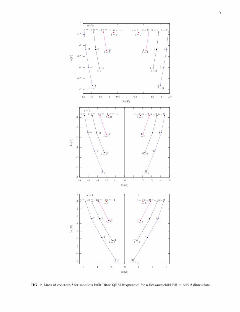

11
-12
-1
-08
-06
-04
-02
0
05 1 15 2 25 3 35
Im(E
)Re(E)
l = 0 n = 0
d = 5
6
7
8
910
FIG 3 Variation of the QNM frequency with dimension for l = n = 0 Both the frequency of oscillation and the damping rateincrease with the number of dimensions