Seediscussions,stats,andauthorprofilesforthispublicationat:https://www.researchgate.net/publication/235595457

Determinationofthelatticesusceptibilitywithinthedualfermionmethod

ArticleinPhysicalReviewB·November2008

DOI:10.1103/PhysRevB.78.195105·Source:arXiv

CITATIONS

13

READS

26

3authors,including:

Someoftheauthorsofthispublicationarealsoworkingontheserelatedprojects:

QuantumSpinHallstatesinhoneycomb-basedmaterialsViewproject

GangLi

TUWien

33PUBLICATIONS198CITATIONS

SEEPROFILE

HartmutMonien

UniversityofBonn

103PUBLICATIONS4,549CITATIONS

SEEPROFILE

AllcontentfollowingthispagewasuploadedbyGangLion03December2016.

Theuserhasrequestedenhancementofthedownloadedfile.

arX

iv:0

804.

3043

v1 [

cond

-mat

.str

-el]

18

Apr

200

8

Lattice susceptibility for 2D Hubbard Model within dual fermion method

Gang Li, Hunpyo Lee, and Hartmut MonienPhysikalisches Insititut, Universitat Bonn, 53115 Bonn, Germany

(Dated: April 18, 2008)

In this paper, we present details of the dual fermion (DF) method to study the non-local correctionto single site DMFT. The DMFT two-particle Green’s function is calculated using continuous timequantum monte carlo (CT-QMC) method. The momentum dependence of the vertex function isanalyzed and its renormalization based on the Bethe-Salpeter equation is performed in particle-holechannel. We found a magnetic instability in both the dual and the lattice fermions. The latticefermion susceptibility is calculated at finite temperature in this method and also in another recentlyproposed method, namely dynamical vertex approximation (DΓA). The comparison between thesetwo methods are presented in both weak and strong coupling region. Compared to the susceptibilityfrom quantum monte carlo (QMC) simulation, both of them gave satisfied results.

PACS numbers: 71.10.Fd

I. INTRODUCTION

Strongly correlated electron systems, such as heavyfermion compounds, high-temperature superconductors,have gained much attention from both theoretical andexperimental point of view. The competition betweenthe kinetic energy and strong Coulomb interaction offermions generates a lot of fascinating phenomena. Vari-ous theoretical approaches have been developed to treatthe regime of intermediate coupling. The widely usedperturbative methods, such as random phase approxi-mation (RPA), fluctuation exchange (FLEX)1,2, and thetwo-particle self-consistent (TPSC)3,4 method are basedon the expansion in the Coulomb interaction which isonly valid in weak-coupling. To go beyond the perturba-tive approximation and to gain insight of the correlationeffects of the fermion systems, new theoretical methodsare needed. Dynamical mean field theory (DMFT)5,6,7 isa big step forward in the understanding Metal-Insulatortransition.

Dynamical mean field theory maps a many-body inter-acting system on a lattice onto a single impurity embed-ded in a non-interacting bath. Such a mapping becomesexact in the limit of infinite coordination number. Alllocal temporal fluctuations are taken into account in thistheory, however spatial fluctuations are treated on themean field level. DMFT has been proven a successfultheory describing the basic physics of the Mott-Hubbardtransition. But the non-local correlation effect can’t al-ways be omitted. Although, straight forward extensionsof DMFT8,9,10,11,12 have captured the influence of short-range correlation, these methods are still not capable ofdescribing the collective behavior, e.g. spin wave excita-tions of many-body system. At the same time, most ofthe numerically exact impurity solvers require a substan-tial amount of time to achieve a desired accuracy even ona small cluster, which makes the investigation of largerlattice to be impossible.

Recently, some efforts have been made to takethe spatial fluctuations into account in differentways13,14,15,16,17. All these methods construct the non-

local contribution of DMFT from the local two-particlevertex. The electron self-energy is expressed as a functionof the two-particle vertex and the single-particle propa-gator. The cluster extention of DMFT considers the cor-relation within the small cluster. Compared to these, thediagrammatic re-summation technique involved in thesenew methods makes them only approximately include thenon-local corrections. While, long range correlations arealso considered in these methods and the computationalburden is not serious.

In this paper we will apply the method of Rubtsov14

to consider the vertex renormalization of the DF throughthe Bethe-Salpeter equation. Lattice susceptibility is cal-culated from the renormalized DF vertex.

The paper is organized as follows: In Sec. II we sum-marize the basic idea of the DF method and give detailsof the calculation. The DMFT two-particle Green’s func-tion and the corresponding vertex calculation are imple-mented in CT-QMC in Sec. III. The frequency depen-dent vertex is modified through the Bethe-Salpeter Equa-tion to obtain the momentum dependence in Sec. IV. InSec. V we present the calculation of the lattice suscep-tibility and compare it with QMC results and also theworks from Toschi13. The conclusions are summarized inSec. VI, where we also present possible application.

II. THE DF METHOD

We study the general one-band Hubbard model at twodimensions

H =∑

k,σ

ǫk,σc†kσckσ + U∑

i

ni↑ni↓ (1)

c†kσ(ckσ) creates (annihilates) an electron with spin-σand momentum k. The dispersion relation is ǫk =

−2t∑N

i=1 cos ki, where N is the number of lattice sites.The basic idea of the DF method14 is to transform thehopping between different sites into coupling to an aux-iliary field f(f †). By doing so, each lattice site can be

2

viewed as an isolated impurity. The interacting latticeproblem is reduced to solving a multi-impurity problemwhich couples to the auxiliary field. This can be doneusing the standard DMFT calculation. After integratingout the lattice fermions c(c†) one can obtain an effectivetheory of the auxiliary field where DMFT serves as anstarting point of the expansion over the coupling betweeneach impurity site with the auxiliary field.

To explicitly demonstrate the above idea we start fromthe action of DMFT which can be written as

S[c+, c] =∑

i

Siimp −

∑

ν,k,σ

(∆ν − ǫkν)c†νkσcνkσ (2)

where ∆ν is the hybridization function of the impurityproblem defined by Si

imp which is the action of an iso-lated impurity at site i with the local Green’s functiongν . Using the Gaussian identity, we decouple the latticesites into many impurities which couple only to the fieldf

S[c†, c; f †, f ] =∑

i

Siimp +

∑

k,ν,σ

[g−1ν (c†kνσfkνσ + h.c.)

+g−2ν (∆ν − ǫk)−1f †

kνσfkνσ] (3)

The equivalence of Eqs. (2) and (3) form an exact rela-tion between the Green’s funtion of the lattice electronsand the DF.

Gν,k = g−2ν (∆ν − ǫk)−2Gd

ν,k + (∆ν − ǫk)−1 (4)

This relation is easily derived by considering the deriva-tive over ǫk in the two actions. Eq. (4) allows now tosolve the many-body “lattice” problem based on DMFTwhich is different from the straight forward cluster exten-sion. The problem is now to solve the Green’s functionof the DF Gd

ν,k. It is determined by integrating Eq. (3)

over c† and c yielding a Taylor expansion series in powersof f † and f . The Grassmann integral ensures that f andf appear only in pairs associated with the lattice fermionn-particle vertex obtained from the single-site DMFT cal-culation. In this paper we restrict our considerations tothe two-particle vertex γ(4).

Expanding the Luttinger-Ward functional in γ4, thefirst two contributions to the self energy function are thediagrams shown in Fig. 1. Diagram (a) vanishes forthe bare DF since this diagram exactly corresponds to

2

1

3

4

(a) (b)

FIG. 1: The first two self-energy diagrams. They are com-posed of the local vertices function and DF propagator.

the DMFT self consistency. Therefore the first non-localcontribution is given by diagram (b). The self-energy forthese two diagrams are

Σ(1)σ (k1) = −

T

N

∑

σ′,k2

Gdσ′ (k2)γ

(4)σσ′ (ν, ν′; ν′, ν) (5a)

Σ(2)σ (k1) = −

T 2

2N2

∑

2,3,4

Gdσ2

(k2)Gdσ3

(k3)Gdσ4

(k4)

γ(4)σ1234

(ν1, ν2; ν3, ν4)γ(4)σ4321

(ν4, ν3; ν2, ν1)

δk1+k2,k3+k4δσ1+σ2,σ3+σ4

(5b)

Here space-time notation is used, k = (~k, ν), q = (~q, ω).Fermionic Matsubara frequency is νn = (2n + 1)π/β,bosonic frequency is ωm = 2mπ/β where β is the inversetemperature. Together with the bare DF Green’s func-tion Gd

0(k) = −g2ν/[(∆ν − ǫk)−1 + gν], the new Green’s

function can be derived from the Dyson equation

[Gd(k)]−1 = [Gd0(k)]−1 − Σd(k) (6)

The algorithm of the whole calculation is:

1. Set initial value of ∆ν for the first DMFT loop.

2. Determine the single-site DMFT Green’s functiongν from the hybridization function ∆ν . The self-consistency condition ensures that the first diagramof the DF self-energy is very small.

3. Go through the DMFT loop once again to calcu-late the two-particle Green’s function and corre-sponding γ-function. The method for determiningthe γ-function is implemented for both strong andweak-coupling CT-QMC in the next section of thispaper.

4. Start an inner loop calculation to determine the DFGreen’s function and in the end the lattice Green’sfunction.

(a) From Eqs. (5a), (5b) and the Dyson equation(6) to calculate the self-energy of the DF.

(b) Repeatly use Eq. (5a), (5b) and Eq. (6) untilthe convergence of the DF Green’s function isachived.

(c) The lattice Green’s function is then given byEq. (4) from that of the DF.

5. Fourier transform the momentum lattice Green’sfunction into real space. And from the on-site com-ponent Gii to determine a new hybridization func-tion ∆ν which is given by Eq. (9).

6. Go back to the Step 3. and iteratively performthe outer loop until the hybridization ∆ν doesn’tchange any more.

3

Although diagram (a) is exactly zero for the bare DFGreen’s function, it gives non-zero contribution from thesecond loop where the DF Green’s function is updatedfrom Eq. (6). As a result, the hybridization functionshould also be updated before the next DMFT loop isperformed . This is simply done by setting the local fullDF Green’s function to zero, together with the conditionthat the old hybrization function forces the bare local DF

Green’s function to be zero (∑

k G0,dν,k = 0), we obtain a

set of equations

1

N

∑

k

[Gν,k − (∆Newν − ǫk)−1]g2

ν(∆Newν − ǫk)2 = 0 (7a)

1

N

∑

k

[G0ν,k − (∆Old

ν − ǫk)−1]g2ν(∆Old

ν − ǫk)2 = 0 (7b)

which yields

∆Newν − ∆Old

ν ≈1

N

∑

k

(Gν,k − G0ν,k)(∆Old

ν − ǫk)2 (8)

This equation finally gives us the relation between thenew and old hybridization function.

∆Newν = ∆Old

ν + g2νGd

loc (9)

In the whole calculation, the DF perturbation calcula-tion converges quickly. The most time consuming part ofthis method is the DMFT calculation of the two particleGreen’s function. There are some useful symmetries toaccelerate the calculation. As already pointed out18,19,it is convenient to take the symmetric form of the inter-action term. The two particle Green’s function is then afully antisymmetric function. Such fully antisymmetricform is very useful to speed up the calculation of the twoparticle Green’s function. One does not need to calculateall the frequency points within the cutoff in Mastsubaraspace, a few special points are calculated and the valuesfor the other points are given by that of those specialpoints through antisymmetric property. In the DF selfenergy calculation, we always have the convolution typeof momentum summation which is very easy to be calcu-lated by fast fourier transform (FFT).

III. CT-QMC AND TWO-PARTICLE VERTEX

From the above analysis, the key idea of the DFmethod is to construct the nonlocal contribution from theauxiliary field and the DMFT two-particle Green’s func-tion. Therefore it is quite important to accurately deter-mine the two-particle vertex. Here we adapt the newlydeveloped CT-QMC method20,21,22 to calculate the twoparticle Green’s function χ.

First we briefly outline the CT-QMC technique. Formore details, we refer the readers to20,21,22. Here we dis-cuss the two-particle Green’s function and some numeri-cal implemetations in more detailed. Two variants of the

CT-QMC methods have been proposed based on the di-agrammatic expansion. Unlike the Hirsch-Fye method,these methods don’t have a Trotter error and can ap-proach the low temperature region easily. In the weak-coupling method20 the non-interacting part of the parti-tion function is kept and expanded the interaction terminto Taylor series. Wick’s theorem ensures that the cor-responding expansion can be written into a determinantat each order

Z =∑

k

(−U)k

k!

∫

dτ1 · · · dτke−S0 det[D↑D↓] (10)

with

D↑D↓ =

(

· · · G↑(τ1 − τk)· · · · · ·

) (

· · · · · ·G↓(τk − τ1) · · ·

)

(11)where S0 is the non-interacting action and G0 is the Weissfield, and the one-particle Green’s function is measusedas

G(ν) = G0(ν) −1

βG0(ν)

∑

i,j

Mi,jeiν(τi−τj)G0(ν) (12)

In the strong coupling method the effective action is ex-panded in the hybridization function by integrating overthe non-interacting bath degrees of freedom. Such anexpansion also yields a determinant.

Z = TrTτe−Sloc

∏

σ

∑

kσ

1

kσ!

∫

dτs1 · · ·dτs

kσ

∫

dτe1 · · · dτe

kσ

Ψσ(τe)

∆(τe1 − τs

1 ) · · · ∆(τe1 − τs

kσ)

· · ·. . . · · ·

∆(τekσ

− τs1 ) · · · ∆(τe

kσ− τs

kσ)

Ψ†

σ(τs) (13)

Here Ψ(τ) = (c1(τ), c2(τ), · · · , ckσ(τ)). The action isevaluated by a Monte Carlo random walk in the spaceof expansion order k. Therefore the corresponding hy-bridization matrix changes in every Monte Carlo step.One particle Green’s function is measured from the ex-pansion of hybridization function as G(τe

j − τsi ) = Mi,j .

M is the inverse matrix of the hybridization function.Apparently one needs to calculate this inverse matrix inevery update step which is time consuming, fortunatelyit can be obtained by the fast-update algorithm20.

At the same time such a relation allows direct mea-surement of the Matsubara Green’s function

G(iνn) =1

β

∑

i,j

e−iνnτsi Mi,je

iνnτej (14)

Compared with the imaginary time measurement, itseems additional computational time is needed for thesum over every matrix elements Mi,j. K. Haule proposedto implement such measurement in every fast update pro-cedure which makes sure that only linear amount of timeis needed23.

4

In our calculation the Green’s function is measuredin the weak-coupling CT-QMC at each accepted up-date which greatly reduces the computational time. Theweak-coupling CT-QMC normally yields a higher per-turbation order k than the strong-coupling CT-QMC. Itseems that the performance of the strong-coupling CT-QMC is better24. Concerning the convergence speed, theweak-coupling CT-QMC is almost same as the strong-coupling one under the above implementation togetherwith a proper choice of α, since in strong-coupling CT-QMC more Monte Carlo steps are needed usually in orderto smooth the noise of Green’s function at imaginary timearound β/2 or at large Matsubara frequency points. Fur-thermore, the weak-coupling CT-QMC is much easier im-plemented for large cluster DMFT calculation, in whichcase the strong-coupling method needs to handle a bigeigenspace. In this paper we mainly use weak-couplingCT-QMC as impurity solver, while all the results canbe obtained in the strong-coupling CT-QMC which wasused as an accuracy check.

Similarly, we adapt K. Haule’s implementation to cal-culate the two-particle Green’s function in frequencyspace. In the weak coupling CT-QMC, the non-interacting action has Gaussian form which ensures theapplicability of Wick’s theorem for measuring the twoparticle Green’s function

χσσ′ (ν1, ν2, ν3, ν4) = T [Gσ(ν1, ν2)Gσ′ (ν3, ν4)

− δσσ′Gσ(ν1, ν4)Gσ(ν3, ν2)] (15)

The over-line indicates the Monte Carlo average. Ineach Monte Carlo measurement, G(ν, ν′) depends on twodifferent argument ν and ν′, only in the average level,G(ν, ν′) = G(ν)δν,ν′ is a function of single frequency.In each fast-update procedure, the new and old G(ν, ν′)have a closed relation which ensures that one can deter-mine the updated Green’s function GNew(ν, ν′) from theold one GOld(ν, ν′). For example, adding pair of kinksand supposing before updating the perturbation order isk, then it is k+1 for the new M-matrix. The new insertedpair is at k + 1 row and k + 1 column.

GNew(ν, ν′) − Gold(ν, ν′)

=MNew

k+1,k+1

βG0(ν)

{

XL · XR − XR · e−iντsk+1

−XL · eiν′τek+1 + e−iντs

k+1+iν′τek+1

}

G0(ν′)(16)

Here, XL =∑k

i=1 e−iντsi Li, XR =

∑kj=1 eiν′τe

j Rj and

Li, Rj have the same definition as in Ref20. In every step,one only needs to calculates the Green’s function whenthe update is accepted and only a few calculations areneeded. A similar procedure for removing pairs, shift-ting end-point operation can be used. Such method isalso applicable in the segment picture of strong-couplingCT-QMC. In the weak-coupling CT-QMC, such an im-plementation greatly improves the calculating speed inlow temperature and strong interaction regime30. Once

one obtains the two frequency dependent Green’s func-tion in every monte carlo step, the two-particle Green’sfunction can be determined easily from Eq. (15). Thetwo-particle vertex is then given from the following equa-tion:

γσσ′

ω (ν, ν′) =β2[χσσ′

ω (ν, ν′) − χ0ω(ν, ν′)]

gσ(ν)gσ(ν + ω)gσ′(ν′ + ω)gσ′(ν′)(17)

where

χ0ω(ν, ν′) = T [δω,0gσ(ν)gσ′ (ν′)− δσσ′δν,ν′gσ(ν)gσ(ν + ω)]

(18)is the bare susceptibility. For the multi-particle Green’sfunction, it still can be constructed from the two fre-quency dependent Green’s function G(ν, ν′), but moreterms appear from Wicks theorem. Simply, when setν = ν′ one can calculate the one-particle Green’s funtioneasily.

IV. MOMENTUM DEPENDECE OF VERTEX

As mentioned earlier diagram (a) in Fig. 1 only givesthe local contribution. The first non-local correction inthe DF method is from diagram (b). Momentum de-pendences comes into this theory through the bubble-like diagram between the two vertices which yields themomentum dependence of the DF vertex. The naturalway to renormalize vertex is through the Bethe-Salpeterequation. Since the DMFT vertex is only a function ofMatsubara frequency, the integral over internal momen-tum k and k′ ensures that the full vertex only dependson the center of mass momentum Q. The Bethe-Salpeterequation in the particle-hole channel18,19 are shown inFig. 2.

From the construction of the DF method, we knowthe interaction of the DF is coming from the two parti-cle vertex of lattice fermion which is obtained throughDMFT calculation. In the Bethe-Salpeter equation, itplays the role of the building-block. The correspondingBethe-Salpeter equation for these two channels are

Γph0,σσ′

Q (ν, ν′) = γσσ′

ω (ν, ν′)−

T

N

∑

k′′σ′′

γσσ′′

ω (ν, ν′′)Gd(k′′)Gd(k′′ + Q)Γph0,σ′′σ′

Q (ν′′, ν′)

(19a)

Γph1,σσQ (ν, ν′) = γσσ

ω (ν, ν′)−

T

N

∑

k′′

γσσω (ν, ν′′)Gd(k′′)Gd(k′′ + Q)Γph1,σσ

Q (ν′′, ν′)

(19b)

Here, the short hand notation of spin configuration isused. γσσ′

represents γσσσ′σ′

, while γσσσσ is denoted byγσσ where σ = −σ. Γph0(ph1) are the full vertices in theSz = 0 and Sz = ±1 channel, respectively. Gd is the fullDF Green’s function obtained from section II which is

5

������������

��������

������������

��������

= +σ

σσ

σ

’

’

σ

σ

σ

σ

σ

σ

σ

σ’

’

’

’ σ

σ

+=σ σ

σσ

σ

σ

σ

σ

σ

σ

σ

σ

σ

σ

_ __

___ _

’’

’’

S

z

z = +_ 1

S = 0

FIG. 2: Sz = 0 (ph0) and Sz = ±1 (ph1) particle-hole chan-nels of the DF vertex, between vertices there are two fullDF Green’s function. The Sz = ±1 component is the tripletchannel, while that for Sz = 0 can be either singlet or triplet.

kept unchanged in the calculation of the Bethe-SalpeterEquation. Different from the work of S. Brener25, wesolve the above equations directly in momentum spacewith the advantage that in this way we can calculate thesusceptibility for any specific center of mass momentumQ and it’s convenient to use FFT for investigating largerlattice.

In Eq. (19) one has to sum over the internal spinindices in the Sz = 0 channel which is not present inSz = ±1 channel. One can decouple the Sz = 0 chan-nel into the charge and spin channels γc(s) = γσσ ± γσσ

which can be solved seperately, and it turns out that thespin channel vertex function is exactly same as the thatin Sz = ±1 channel, see e.g. P. Nozieres19. Such relationis true for the DMFT vertex, and was also verified forthe momentum dependent vertex in the DF method25.In our calculation, we have solved the Sz = 0 channel bydecoupling it to the charge and spin channel, while theph1 channel is not used.

Once the converged momentum dependent DF vertexis obtained, one can determine the corresponding DF sus-ceptibility in the standard way by attaching four Green’sfunctions to the DF vertex.

χσσ′

d (Q) = χ0d(Q)+

T 2

N2

∑

k,k′

Gdσ(k)Gd

σ(k + Q)Γσσ′

(Q)Gdσ′ (k′)Gd

σ′ (k′ + Q)

(20a)

χσσd (Q) = χ0

d(Q)+

T 2

N2

∑

k,k′

Gdσ(k)Gd

σ(k + Q)Γσσ(Q)Gdσ(k′)Gd

σ(k′ + Q)

(20b)

The momentum sum over ~k and ~k′ can be performedindependently by FFT becasue the DF vertx Γσσ′

(Q)only depends on the center of mass momentum Q.

Now the z-component DF spin susceptibility 〈Sz ·Sz〉 =12 (χ↑↑

d − χ↑↓d ) can be determined from the spin channel

component calculated above. In Fig. 3, χzz = χzz − χzz0

is shown for U/t = 4 at temperatures βt = 4.0 (leftpanel) and βt = 1.0 (right panel). With the lowing down

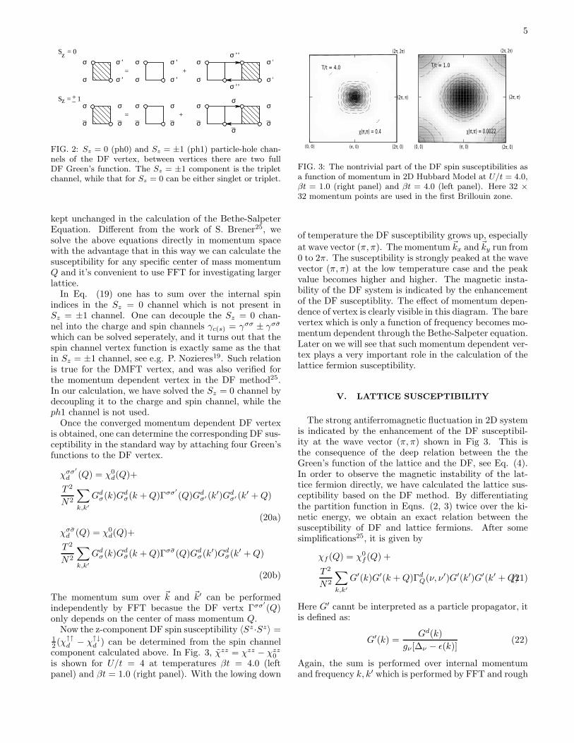
FIG. 3: The nontrivial part of the DF spin susceptibilities asa function of momentum in 2D Hubbard Model at U/t = 4.0,βt = 1.0 (right panel) and βt = 4.0 (left panel). Here 32 ×

32 momentum points are used in the first Brillouin zone.

of temperature the DF susceptibility grows up, especially

at wave vector (π, π). The momentum ~kx and ~ky run from0 to 2π. The susceptibility is strongly peaked at the wavevector (π, π) at the low temperature case and the peakvalue becomes higher and higher. The magnetic insta-bility of the DF system is indicated by the enhancementof the DF susceptiblity. The effect of momentum depen-dence of vertex is clearly visible in this diagram. The barevertex which is only a function of frequency becomes mo-mentum dependent through the Bethe-Salpeter equation.Later on we will see that such momentum dependent ver-tex plays a very important role in the calculation of thelattice fermion susceptibility.

V. LATTICE SUSCEPTIBILITY

The strong antiferromagnetic fluctuation in 2D systemis indicated by the enhancement of the DF susceptibil-ity at the wave vector (π, π) shown in Fig 3. This isthe consequence of the deep relation between the theGreen’s function of the lattice and the DF, see Eq. (4).In order to observe the magnetic instability of the lat-tice fermion directly, we have calculated the lattice sus-ceptibility based on the DF method. By differentiatingthe partition function in Eqns. (2, 3) twice over the ki-netic energy, we obtain an exact relation between thesusceptibility of DF and lattice fermions. After somesimplifications25, it is given by

χf (Q) = χ0f(Q) +

T 2

N2

∑

k,k′

G′(k)G′(k + Q)ΓdQ(ν, ν′)G′(k′)G′(k′ + Q)(21)

Here G′ cannt be interpreted as a particle propagator, itis defined as:

G′(k) =Gd(k)

gν [∆ν − ǫ(k)](22)

Again, the sum is performed over internal momentumand frequency k, k′ which is performed by FFT and rough

6

0.2

0.3

0.4

0.5

0.6

0.7

0.8

0.2 0.4 0.6 0.8 1 1.2 1.4 1.6 1.8 2

χ m(0

,0)

T/t

U/t = 4.0

8 * 8 QMCDF (full vertex)

DF (bare vertex)

FIG. 4: The uniform spin suscetibility of the DF using thebare vertex (only frequency dependent) and the full ver-tex(vertex from the Bethe-Salpeter quqation) for half filled2D Hubbard model at U/t = 4.0 and various temperatures.These results reproduce the similiar solution in comparisonwith the calculation of finite size of QMC.

summing over a few Matsubara points. Again as in Eq.(4), this equation established a connection between thelattice susceptibility and the DF susceptibility. From thispoint of view, it is easy to understand that the instabilityof DFs generates the instability of the lattice fermions.

One can also find relations for the higher order Green’sfunction of the DF and the lattice fermions in the sameway. This emphasizes the similar nature of the DF andlattice fermions except that DF possess only non-local in-formation, since the DMFT self-consistency ensures thatthe local DF Green’s function is exactly zero.

The lattice magnetic susceptibility is calculated usingthe following definition

χm(q) =1

N

∑

i

eiq·ri

∫ β

0

dτe−iωmτχf (i, τ)

= 2(χ↑↑f − χ↑↓

f ) (23)

where χf (i, τ) = 〈[ni,↑(τ)−ni,↓(τ)]× [n0,↑(0)−n0,↓(0)]〉.χf represents the lattice susceptibility in order to distin-guish with that of the DF.

We have used two different ways to calculate the latticesusceptibility. First we have solved the above equationusing the bare vertex Γ(ν, ν′; ω) which is obtained fromthe DMFT calculation. In contrast, the second calcula-tion was performed using the full DF vertex. In bothof these calculations, the full one particle DF Green’sfunction was used. The momentum dependent of the DFvertex is obtained through the calculation of the Bethe-Salpeter equation. The lattice susceptibility is expectedto be improved if we use the momentum dependence DFvertex. In this way, we can understand the effect of mo-mentum dependence in the DF vertex.

In Fig. 4 we plotted the results for the uniform sus-

0

1

2

3

4

5

6

0.2 0.3 0.4 0.5 0.6 0.7 0.8 0.9 1

χ(π,

π)

T/t

U/t = 4.0

4 * 4 QMCDF (full vertex)

DF (bare vertex)

FIG. 5: Uniform spin susceptibility at the wave vector (π, π).The QMC results are obtained from Ref.27.

ceptibility χm=0(0, 0) by using both the bare and full DFvertex. The lattice QMC result26 is shown for compar-ison. The calculation is done for U/t = 4.0 and severalvalues of temperature. The momentum sum is approxi-mated over 32 × 32 points here. Both of these calcula-tions reproduce the well known Curie-Weiss law behavior.Surprisingly enough, the results for the bare vertex fit theQMC results better than that for the momentum depen-dent vertex. We believe that this is the finite size effectof QMC26. A. Moreo showed that χ becomes smallerwhen increasing the cluster size N . The 4 × 4 clustercalculation result at the same temperature located aboveof that from 8 × 8 cluster calculation. Therefore the re-sults obtained from the full vertex is expected to be morereliable.

The importance of the momentum dependence of theDF vertex is more clearly observed in the calculationof χm(π, π), see Fig. 5. Again, in this diagram QMCresults27 are shown for comparison. The same parame-ters are used as in Fig. 4. The result from the DF withbare vertex does not produce the same results comparedwith QMC solution. Evenmore interesting, with decreas-ing temperature the deviation becomes larger. On theother hand, the momentum dependent vertex in the DFmethod gives a satisfactory answer. This shows the im-portance of the momentum dependence in the DF vertexfunction. Fig. 6 shows the evolution of χ against q forfixed transfer frequency ωm = 0. The path in momen-tum space is shown in the inset. From this diagram wecan see that χ(q, 0) reaches its maximum value at wavevector (π, π).

The comparison between the DF and QMC resultsshows the good performance of DF method. The DFcalculation started from a single site DMFT calculationand by introducing an auxiliary field, the non-local in-formation is introduced and nicely reproduces the QMCresults. Our calculation could be done within four hoursfor each value of the temperature on average. In this

7

0.4

0.8

1.2

1.6

2

2.4

(0,0)(π,π)(π,0)(0,0)

χ(p,

0)

p

βt = 2.0, U/t = 4.0

(0,0) (π,0)

(π,π)

FIG. 6: χ(q, 0) vs q at βt = 2.0, U/t = 4.0 for various q whichis along the trajectory shown in the inset.

sense, this method is cheap and reliable compared withthe more computationally intensive lattice QMC calcu-lation.

Similar as the DF method, Dynamical Vertex Approx-imation (DΓA)13 is also based on the two particle localvertex. It deals with the lattice fermion directly, with-out introducing any auxiliary field. The perturbative na-ture of this method ensures its validity at weak-couplingregime. Unlike in the DF method, DΓA takes the irre-ducible two particle local vertex as building blocks.

γ−1c(s)(ν, ν′; ω) = γ−1

c(s),ir(ν, ν′; ω) − χ0(ν; ω)δν,ν′ (24a)

Γ−1c(s)(ν, ν′; Q) = γ−1

c(s),ir(ν, ν′; ω) − χ0(ν; Q)δν,ν′ (24b)

with the spin and charge vertex defined as γc(s) = γ↑↑ ±

γ↑↓. The bare susceptibility is defined as

χ0(ν; ω) = −TGloc(ν)Gloc(ν + ω) (25a)

χ0(ν, Q) = −T

N

∑

~k

G0(~k, ν)G0(~k + ~q, ν + ω) (25b)

And the self-energy is calculated through the standardSchwinger-Dyson equation

Σ(k) = −UT 2

N2

∑

k′,Q

Γf (k, k′; Q)G0(k′)G0(k′+Q)G0(k+Q)

(26)Here, the full vertex Γf (k, k′; Q) is obtained by summingall the channel dependent vertices and subtracting thedouble counted diagrams.

Γf (k, k′; Q) =1

2

{

[3Γc(ν, ν′; Q) − Γs(ν, ν′; Q)]

−[Γc(ν, ν′; ω) − Γs(ν, ν′; ω)]

}

(27)

The one particle propagator is given by the DMFT lat-tice Green’s function where the self energy is purely local

0.4

0.45

0.5

0.55

0.6

0.65

0.7

0.2 0.3 0.4 0.5 0.6 0.7 0.8 0.9 1

χ m(0

,0)

T/t

U/t = 4.0

DF (full vertex)DΓA (G0)DΓA (G)

FIG. 7: Comparison with the DΓA susceptibilities χ(0, 0)which obtained from both the DMFT lattice Green’s func-tion (DΓA (G0)) and the full Green’s function (DΓA (G)),see context for more details.

G0(k) = 1/[iν−ǫ(k)−Σ(ν)], the local Green’s function isGloc(ν) = 1/[iν−∆(ν)−Σ(ν)]. Then the Dyson equationgives the lattice Green’s function from the self-energyfunction G−1 = G−1

0 − Σ.Before presenting the comparison, we take a deeper

look at the analysis of Eq. (24),

Γ−1c(s)(ν, ν′; Q) = γ−1

c(s)(ν, ν′; ω) −

[χ0(ν; Q) − χ0(ν, ω)]δν,ν′ (28)

The second term in the brackets on RHS removes thelocal term from the bare susceptibility. The whole termin the brackets then represents only the non-local baresusceptibility. In order to compare with the DF method,we take the inverse form of Eq. (19)

Γ−1d,cs(ν, ν′; Q) = γ−1

c(s)(ν, ν′, ω) −

T

N

∑

~k

Gd(k)Gd(k + q) (29)

The above two equations are same except for the lastterm. Since the local DF Green’s function Gd

loc is zero,the bare DF susceptibility is purely non-local which coin-cides with the analysis of DΓA Bethe-Salpeter equation.Therefore, it is not surprising that these two methodsgenerate similar results. It is not easy to perform a termto term comparison between the DF method and DΓAalthough the bare susceptibilities have no local term inboth of these method. The one particle Green’s functionshave different meaning in these two methods.

The lattice susceptibility within the DΓA method isobtained by attaching four Green’s functions on the ver-tex obtained in Eq. (27). There are two possible choicesof the lattice Green’s function, one is the DMFT latticeGreen’s function G0, the other one is the Green’s func-tion G constructed by the non-local self-energy from the

8

0

1

2

3

4

5

6

7

0.3 0.4 0.5 0.6 0.7 0.8 0.9 1

χ(π,

π)

T/t

U/t = 4.0

DF (full vertex)DΓA (G0)DΓA (G)

FIG. 8: DΓA susceptibilities χ(π, π) at U/t = 4.0. The sus-ceptibility are determined from both of the DMFT and fulllattice Green’s function together with the vertex obtainedfrom Eq. (27)

.

Dyson equation. In Fig. 7 and 8, we presented the DΓAlattice susceptibility calculated from both the DMFT lat-tice Green’s function labeled as DΓA(G0) and the fullGreen’s function labeled as DΓA(G). The DF result fromthe calculation with the full DF vertex is re-plotted forcomparison. In Fig. 7, the DΓA susceptibility calculatedfrom the DMFT Green’s function (DΓA(G0)) is basicallythe same as the DF susceptibility only with some smalldeviation. The results for T/t > 1.0 which are not shownhere which nicely repeat the DF and QMC results, thedeviation between the DΓA and the DF method becomessmaller with the increasing of temperature. The DΓAsusceptibility is calculated from the full Green’s func-tion (DΓA(G)) shows a different behavior at low tem-perature regime which reached its maximum value atT/t ≈ 0.36. As we know, the Hubbard Model at half fill-ing with strong coupling maps to the Heisenberg model,χ reasches a maximum at T ≈ J where J is the effectivespin coupling constant given as 4t2/U . The calculationuses the parameter U/t = 4.0 which is in the intermedi-ate coupling regime. Therefore we further calculated thelattice susceptibility at U/t = 10.0 which are shown inFig. 9.

When the temperature is greater than 0.4, the DFmethod and DΓA (DΓA(G0)) generate the similar re-sults to the QMC calculation. Reducing the tempera-ture further, the QMC susceptibility greatly drops andshows a peak around 0.4 which coincides with the be-havior of the Heisenberg model. The DF femion andDΓA susceptibility continuously grows up with the de-creasing of temperature. Although the DΓA with thefull Green’s function (DΓA(G)) shows a peak, it locatesat T/t = 0.6667 which is larger than the peak positionof the QMC. And DΓA(G) generated a large deviationfrom that of QMC. In this diagram, we only show the

0.3

0.4

0.5

0.6

0.7

0.8

0.9

1

1.1

1.2

1.3

0.1 0.2 0.3 0.4 0.5 0.6 0.7 0.8 0.9 1

χ m(0

,0)

T/t

U/t = 10.04 * 4 QMC

DF (full vertex)DΓA (G0)DΓA (G)

FIG. 9: The comparison of the DF resulsts and that ofQMC for the uniform susceptibility at U/t = 10. 4×4 QMCresults26 also shows the errorbars.

results of the DF approach for T/t > 0.3 and the DΓAresults for T/t > 0.4. The Bethe-salpeter equation ofthe DΓA have a eigenvalue approaching one when fur-ther lowering the temperature, which makes the accessof lower temperature region impossible.

Fig. 8 shows the results of DΓA susceptibilities atwave vector (π, π). In contrast to the comparison forχ(0, 0) results, the DΓA susceptibility calculated fromthe full Green’s function DΓA (G) yields better resultsthan that from the calculation with the DMFT Green’sfunction DΓA (G0). DΓA (G) results are almost on top ofthe DF results, the results with DMFT Green’s functionDΓA (G0) is large than the DF results. The deviationbecomes larger at lower temperature. Summarizing, theDΓA calculation using the full Green’s function gener-ated the same result as the DF method for χ(π, π) whilefailed to produce χ(0, 0) correctly. In contrast, the cal-culation with the DMFT Green’s function in DΓA nicelyproduced the results calculated with the DF method for

FIG. 10: The evolution of maximum eigenvalue in spin chan-nel against temperature for DF method and DΓA.

9

0.54

0.56

0.58

0.6

0.62

0.64

0.6 0.7 0.8 0.9 1

χ m(0

,0)

<n>

U/t = 4.0

DF (full vertex)DΓA (G0)

0.6

0.65

0.7

0.75

0.8

0.85

0.9

0.95

0.5 0.6 0.7 0.8 0.9 1

<n>

U/t = 10.0

DF (full vertex)DΓA (G0)

FIG. 11: Uniform magentic susceptibility is plotted as a func-tion of dopping at βt = 2.5 and U/t = 4.0, 10.0.

χ(0, 0) while generated larger devivation for χ(π, π) atlower temperature regime compared to that from the DFmethod. Together with Fig. 4 and 5, we can see that theDF fermion calculation with the full DF vertex generatedbasically the same results for both χ(0, 0) and χ(π, π)compared to the results of QMC.

In both the DF method and the DΓA, the operation ofinverting large matrices is required for solving the Bethe-Salpeter equation. Fig. 10 shows the leading eigenvalueof Eqns. (19) and (24). As expected, the leading eigen-value approaches one with decreasing temperature whichdirectly indicates the magnetic instability of 2D system.The eigenvalues corresponding to the DF fermion methodalways lies below of that from DΓA indicating the betterconvergence of the DF method. When the leading eigen-values are closed to one, the matrix inversion in Eqns.(19) and (24) are ill defined, which prevents the investi-gation at very low temperature.

Concerning the performance of the DF method, wealso calculated the uniform susceptibility at away half-filling. In the strong-coupling limit, the Hubbard modelis equivalent to the Heisenberg model with coupling con-stant J = 4t2/U . The consequence of doping is to ef-fectively decrease the coupling J , which yields the in-creasing behavior of χ with doping. The finite size QMCcalulation26,28 observed a slightly increasing χ with verysmall doping at strong interaction or in the low tempera-ture region. Here, we did a similar calculation at βt = 2.5and U/t = 4, 10. Since the DF method and the DΓA donot suffer from the finite size problem. We would ex-

pect to observe results similar to those of QMC26,28. InDΓA the suseceptibility is calculated from the DMFTGreen’s function G0 and the vertex obtained from Eq.(27). As shown in Fig. 11 at U/t = 4.0, the susceptibil-ity χ slightly increases in the weak dopping region whereδ is around 0.05, DF fermion results clearly showed suchbehavior, DΓA also gave a signal of it. Further dopingthe system, both the DΓA and the DF method reproducethe decrease with doping as already seen in the QMC.With the increasing of interaction, we would expect tosee the enhancement of this effect, however our calcu-lation indicates that such increasing-decreasing behavirodissappear. Both the DΓA and the DF method give thesame decreasing curve which contradict to QMC result26.The results will most likely be further improved by in-cluding the higher order vertex or calculating the clusterDMFT plus DF/DΓA29.

VI. CONCLUSION

In this paper, we extended both the DF method andDΓA to calculate the lattice susceptibility. Both of thesemethods gave equally good results compared with QMCcalculation at U/t = 4.0. Although they are supposedto be weak-coupling methods, at U/t = 10.0 these twomethods generated right results at high temperature re-gion. While both of them failed to reproduce the Heisen-berg physics at low temperature. The investigation of thelattice susceptibility suffers from hard determined matrixinversion problem at low temperature regime. The DFmethods always generates smaller eigenvalues comparedto DΓA indicating the better convergence. The imple-mentation of DF method in momentum space greatlyimproves the calculational speed and makes it easier todeal with larger size lattice.

Acknowledgments

We would like to thank the condensed matter group ofA. Lichtenstein at Hamburg University for their hospital-ity in particular for the discussions and open exchange ofdata with H. Hafermann. Gang Li and Hunpyo Lee wouldlike to thank Philipp Werner for his help in implementingthe strong-coupling CT-QMC code.

1 N. E. Bickers, D. J. Scalapino, and S. R. White, Phys. Rev.Lett. 62, 961 (1989).

2 N. E. Bickers and S. R. White, Phys. Rev. B 43, 8044(1991).

3 S. Allen and A.-M. Tremblay, J. Phys. Chem. Solids (UK)56, 1769 (1995).

4 Y. Vilk, L. Chen, and A.-M. Tremblay, Phys. Rev. B 49,13267 (1994).

5 A. George, G. Kotliar, W. Krauth, and M. J. Rozenberg,Rev. Mod. Phys. 68, 13 (1996).

6 W. Metzner and D. Vollhardt, Phys. Rev. Lett. 62, 324(1989).

7 E. M. Hartmann, Z. Phys. B 57, 281 (1984).8 T. Maier, M. Jarrell, T. Pruschke, and M. H. Hettler, Rev.

Mod. Phys. 77, 1027 (2005).9 M. H. Hettler, A. N. Tahvildar-Zaden, M. Jarrell, T. Pr-

10

uschke, and H. R. Krishnamurthy, Phys. Rev. B 58, 7475(1998).

10 G. Kotliar, S. Savrasov, G. Pallson, and G. Biroli, Phys.Rev. Lett. 87, 186401 (2001).

11 S. Okamoto, A. Millis, H. Monien, and A. Fuhrmann, Phys.Rev. B 68, 195121 (2003).

12 M. Potthoff, Eur. Phys. J. B 36, 335 (2003).13 A. Toschi, A. A. Katanin, and K. Held, Phys. Rev. B 75,

045118 (2007).14 A. N. Rubtsov, M. I. Katsnelson, and A. I. Lichtenstein,

cond-mat/0612196.15 H. Kusunose, J. Phys. Soc. Jpn. 75, 054713 (2006).16 V. I. Tokar and R. Monnier, cond-mat/0702011.17 C. Slezak, M. Jarrell, T. Maier, and J. Deisz, cond-

mat/0603421.18 A. Abrikosov, L. Gorkov, and I. Dzyaloshinski, Methods

of quantum field theory in statistical physics (Dover, NewYork, N.Y., 1963).

19 P. Nozieres, Theory of interacting fermi systems (W. A.Benjamin, INC., New York. New York, 1964).

20 A. N. Rubtsov, V. V. Savkin, and A. I. Lichtenstein, Phys.Rev. B 72, 035122 (2005).

21 P. Werner, A. Comanac, L. D. Medici, M. Troyer, and A. J.Millis, Phys. Rev. Lett. 97, 076405 (2006).

22 P. Werner and A. J. Millis, Phys. Rev. B 74, 155107(2006).

23 K. Haule and G. Kotliar, Phys. Rev. B 75, 155113 (2007).24 E. Gull, P. Werner, A. Millis, and M. Troyer, Phys. Rev.

B 76, 235123 (2007).25 S. Brener, H. Hafermann, A. N. Rubtsov, M. I. Katsnelson,

and A. I. Lichtenstein, cond-matt/0711.3647.26 A. Moreo, Phys. Rev. B 48, 3380 (1993).27 N. E. Bickers and S. R. White, Phys. Rev. B 43, 8044

(1991).28 L. Chen and A.-M. S. Tremblay, Phys. Rev. B 49, 4338

(1993).29 H. Hafermann, S. Brener, A. N. Rubtsov, M. I. Katsnelson,

and A. I. Lichtenstein, Pis’ma v ZhETF 86, 769 (2007).30 In fact, the improvement is more obvious for larger M-

matrices. The strong coupling CT-QMC and the weak cou-pling CT-QMC require approximately the same amount ofCPU time although in the weak coupling case the averageperturbation order is higher than in the strong couplingcase