HAL Id: tel-01271042https://tel.archives-ouvertes.fr/tel-01271042

Submitted on 8 Feb 2016

HAL is a multi-disciplinary open accessarchive for the deposit and dissemination of sci-entific research documents, whether they are pub-lished or not. The documents may come fromteaching and research institutions in France orabroad, or from public or private research centers.

L’archive ouverte pluridisciplinaire HAL, estdestinée au dépôt et à la diffusion de documentsscientifiques de niveau recherche, publiés ou non,émanant des établissements d’enseignement et derecherche français ou étrangers, des laboratoirespublics ou privés.

Hunting the charged Higgs boson with lepton signaturesin the ATLAS experiment

Alexander Madsen

To cite this version:Alexander Madsen. Hunting the charged Higgs boson with lepton signatures in the ATLAS experi-ment. High Energy Physics - Experiment [hep-ex]. Université Grenoble Alpes; Uppsala universitet,2015. English. �NNT : 2015GREAY043�. �tel-01271042�

THÈSEPour obtenir le grade de

DOCTEUR DE L’UNIVERSITÉ GRENOBLE ALPES

préparée dans le cadre d’une cotutelle entre l’Université Grenoble Alpes et Uppsala Universitet

Spécialité : Physique Subatomique et Astroparticules

Arrêté ministériel : le 6 janvier 2005 - 7 août 2006

Présentée par

Alexander Kondrup MADSEN

Thèse dirigée par Johann COLLOT et Arnaud FERRARIet co-encadrée par Mattias Ellert

préparée au sein des Laboratoire de Physique Subatomique et de Cosmologie de Grenoble et Ångströmlaboratoriet

dans les Écoles Doctorales de Physique de Grenoble et Uppsala

À la recherche d'un boson de Higgs chargé impliquant des signatures leptoniques à l'aide de l'expérience ATLASThèse soutenue publiquement le 22 Mai 2015,devant le jury composé de:

Mme Susan GASCON-SHOTKINProf. Université de Lyon, Présidente et RapporteureMme Ritva KINNUNENDr. Helsinki Institute of Physics, RapporteureM. Christophe CLÉMENTDr. Stockholm University, MembreM. Oscar STÅLDr. Stockholm University, MembreM. Volker ZIEMANNDr. Uppsala University, MembreM. Johann COLLOTProf. Université Joseph Fourier, Directeur de thèseM. Arnaud FERRARIDr. Uppsala University, Directeur de thèse

Abstract

This thesis presents searches for a charged Higgs boson (H±) in proton-proton col-

lisions with center-of-mass energies of 7 TeV and 8 TeV, using data collected by the

ATLAS experiment at the Large Hadron Collider at CERN. Multiple search channels

are used with the common characteristic of at least one charged lepton (electron or

muon) that effectively reduces the multi-jet background and is used for efficient trig-

gering. Charged Higgs bosons decaying to a tau lepton and a neutrino are searched

for using final states with two charged leptons, or one charged lepton and a hadroni-

cally decaying tau. A significant background originates from quark- or gluon-initiated

jets that may be misidentified as hadronic tau decays. Methods to estimate this back-

ground are presented, including a largely data-driven matrix method. Signal processes

with a charged Higgs boson mass below or above that of the top quark are considered.

With the dataset collected at a center-of-mass energy of 8 TeV, corresponding to an

integrated luminosity of 20.3 fb−1, upper limits at 95% confidence level are placed

on the branching fraction B(t → bH±)×B(H±

→ τν) in the range 1.1–0.3% for

charged Higgs boson masses between 80 GeV and 160 GeV, as well as on the top-

quark associated H± production cross section in the range 0.93–0.03 pb for charged

Higgs boson masses between 180 GeV and 1 TeV.

Résumé

Cette thèse présente la recherche d’un boson de Higgs chargé (H±) qui serait produit

dans les collisions proton-proton à des énergies de 7 TeV et 8 TeV, en utilisant les don-

nées recueillies par l’expérience ATLAS au LHC (Large Hadron Collider). Plusieurs

canaux de recherche sont utilisés, présentant la caractéristique commune de contenir

au moins un lepton chargé (électron ou muon) énergétique, ce qui réduit efficacement

le bruit de fond contenant des jets, tout en permettant un déclenchement efficace du

détecteur. Ici, le boson de Higgs chargé se désintègre en un lepton tau et un neutrino,

ce qui conduit à des états finaux avec deux leptons chargés, ou bien un lepton chargé et

un tau hadronique. Une source importante de taus mal identifiés provient de quarks et

de gluons, par l’intermédiaire des jets hadroniques qu’ils initient. Plusieurs méthodes

ont été développées pour estimer ce bruit de fond, l’une d’elles étant basée directement

sur les données. Des processus avec des bosons de Higgs chargés dont la masse est

soit en dessous soit au-dessus de celle du quark top sont considérés. Avec l’ensemble

de données recueillies à une énergie de 8 TeV, correspondant à une luminosité intégrée

de 20,3 fb−1, des limites avec un taux de confiance de 95% sont placées sur le rapport

de branchement B(t → bH+)×B(H+

→ τν) entre 1,1 et 0,3% pour des masses du

boson de Higgs chargé entre 80 GeV et 160 GeV, et sur la section efficace de produc-

tion du boson de Higgs chargé en association avec un quark top entre 0,93 et 0,03 pb,

pour un boson de Higgs chargé ayant cette fois une masse comprise entre 180 GeV et

1 TeV.

To my parents.

Contents

Introduction . . . . . . . . . . . . . . . . . . . . . . . . . . . . . . . . . . . . . . . . . . . . . . . . . . . . . . . . . . . . . . . . . . . . . . . . . . . . . . . . . . . . . . . . . . . . . . . . . . . . . . . . 9

Part I: Theory . . . . . . . . . . . . . . . . . . . . . . . . . . . . . . . . . . . . . . . . . . . . . . . . . . . . . . . . . . . . . . . . . . . . . . . . . . . . . . . . . . . . . . . . . . . . . . . . . . . 11

1 The Standard Model of particle physics . . . . . . . . . . . . . . . . . . . . . . . . . . . . . . . . . . . . . . . . . . . . . . . . . . . 131.1 Overview . . . . . . . . . . . . . . . . . . . . . . . . . . . . . . . . . . . . . . . . . . . . . . . . . . . . . . . . . . . . . . . . . . . . . . . . . . . . . . . . . . . . . . . . . 131.2 The Higgs field . . . . . . . . . . . . . . . . . . . . . . . . . . . . . . . . . . . . . . . . . . . . . . . . . . . . . . . . . . . . . . . . . . . . . . . . . . . . . . . 161.3 Limitations of the Standard Model . . . . . . . . . . . . . . . . . . . . . . . . . . . . . . . . . . . . . . . . . . . . . . . 19

2 Beyond the Standard Model . . . . . . . . . . . . . . . . . . . . . . . . . . . . . . . . . . . . . . . . . . . . . . . . . . . . . . . . . . . . . . . . . . . . . . 212.1 Two-Higgs-Doublet Models . . . . . . . . . . . . . . . . . . . . . . . . . . . . . . . . . . . . . . . . . . . . . . . . . . . . . . . . . . 212.2 Supersymmetry . . . . . . . . . . . . . . . . . . . . . . . . . . . . . . . . . . . . . . . . . . . . . . . . . . . . . . . . . . . . . . . . . . . . . . . . . . . . . . 24

2.2.1 The Minimal Supersymmetric Standard Model . . . . . . . . . . . . 252.2.2 The MSSM Higgs sector . . . . . . . . . . . . . . . . . . . . . . . . . . . . . . . . . . . . . . . . . . . . . . . . . 25

2.3 The charged Higgs boson . . . . . . . . . . . . . . . . . . . . . . . . . . . . . . . . . . . . . . . . . . . . . . . . . . . . . . . . . . . . . . 262.3.1 Decay modes . . . . . . . . . . . . . . . . . . . . . . . . . . . . . . . . . . . . . . . . . . . . . . . . . . . . . . . . . . . . . . . . . . . . 272.3.2 Production at colliders . . . . . . . . . . . . . . . . . . . . . . . . . . . . . . . . . . . . . . . . . . . . . . . . . . . . . 282.3.3 Effects on B-physics observables . . . . . . . . . . . . . . . . . . . . . . . . . . . . . . . . . . . 32

Part II: Experiment . . . . . . . . . . . . . . . . . . . . . . . . . . . . . . . . . . . . . . . . . . . . . . . . . . . . . . . . . . . . . . . . . . . . . . . . . . . . . . . . . . . . . . . . . . 35

3 The Large Hadron Collider . . . . . . . . . . . . . . . . . . . . . . . . . . . . . . . . . . . . . . . . . . . . . . . . . . . . . . . . . . . . . . . . . . . . . . . 373.1 Experimental challenges . . . . . . . . . . . . . . . . . . . . . . . . . . . . . . . . . . . . . . . . . . . . . . . . . . . . . . . . . . . . . . . . 383.2 Run 1 summary . . . . . . . . . . . . . . . . . . . . . . . . . . . . . . . . . . . . . . . . . . . . . . . . . . . . . . . . . . . . . . . . . . . . . . . . . . . . . . 39

3.2.1 Discovery of the Higgs boson . . . . . . . . . . . . . . . . . . . . . . . . . . . . . . . . . . . . . . . . . 413.2.2 SUSY and 2HDM searches . . . . . . . . . . . . . . . . . . . . . . . . . . . . . . . . . . . . . . . . . . . . . 42

4 The ATLAS experiment . . . . . . . . . . . . . . . . . . . . . . . . . . . . . . . . . . . . . . . . . . . . . . . . . . . . . . . . . . . . . . . . . . . . . . . . . . . . 484.1 Inner detector . . . . . . . . . . . . . . . . . . . . . . . . . . . . . . . . . . . . . . . . . . . . . . . . . . . . . . . . . . . . . . . . . . . . . . . . . . . . . . . . . . 494.2 Calorimeters . . . . . . . . . . . . . . . . . . . . . . . . . . . . . . . . . . . . . . . . . . . . . . . . . . . . . . . . . . . . . . . . . . . . . . . . . . . . . . . . . . . 514.3 Muon system . . . . . . . . . . . . . . . . . . . . . . . . . . . . . . . . . . . . . . . . . . . . . . . . . . . . . . . . . . . . . . . . . . . . . . . . . . . . . . . . . . 534.4 Forward detectors . . . . . . . . . . . . . . . . . . . . . . . . . . . . . . . . . . . . . . . . . . . . . . . . . . . . . . . . . . . . . . . . . . . . . . . . . . . 544.5 Trigger and data acquisition . . . . . . . . . . . . . . . . . . . . . . . . . . . . . . . . . . . . . . . . . . . . . . . . . . . . . . . . . . 544.6 Software . . . . . . . . . . . . . . . . . . . . . . . . . . . . . . . . . . . . . . . . . . . . . . . . . . . . . . . . . . . . . . . . . . . . . . . . . . . . . . . . . . . . . . . . . . 55

4.6.1 Detector control system . . . . . . . . . . . . . . . . . . . . . . . . . . . . . . . . . . . . . . . . . . . . . . . . . . 554.6.2 Simulation . . . . . . . . . . . . . . . . . . . . . . . . . . . . . . . . . . . . . . . . . . . . . . . . . . . . . . . . . . . . . . . . . . . . . . . . 564.6.3 Reconstruction and analysis . . . . . . . . . . . . . . . . . . . . . . . . . . . . . . . . . . . . . . . . . . . . 58

4.7 Run 2 preparations . . . . . . . . . . . . . . . . . . . . . . . . . . . . . . . . . . . . . . . . . . . . . . . . . . . . . . . . . . . . . . . . . . . . . . . . . 614.7.1 SCT backplane resistance measurements . . . . . . . . . . . . . . . . . . . . . . 634.7.2 Heater pads control system upgrade . . . . . . . . . . . . . . . . . . . . . . . . . . . . . . . 65

Part III: Data analyses . . . . . . . . . . . . . . . . . . . . . . . . . . . . . . . . . . . . . . . . . . . . . . . . . . . . . . . . . . . . . . . . . . . . . . . . . . . . . . . . . . . . . . 69

5 Analysis techniques . . . . . . . . . . . . . . . . . . . . . . . . . . . . . . . . . . . . . . . . . . . . . . . . . . . . . . . . . . . . . . . . . . . . . . . . . . . . . . . . . . . 715.1 Signal and background processes . . . . . . . . . . . . . . . . . . . . . . . . . . . . . . . . . . . . . . . . . . . . . . . . . 71

5.1.1 Data samples . . . . . . . . . . . . . . . . . . . . . . . . . . . . . . . . . . . . . . . . . . . . . . . . . . . . . . . . . . . . . . . . . . . . 715.1.2 Simulated events . . . . . . . . . . . . . . . . . . . . . . . . . . . . . . . . . . . . . . . . . . . . . . . . . . . . . . . . . . . . . . 72

5.2 Particle identification . . . . . . . . . . . . . . . . . . . . . . . . . . . . . . . . . . . . . . . . . . . . . . . . . . . . . . . . . . . . . . . . . . . . . 755.2.1 Electrons . . . . . . . . . . . . . . . . . . . . . . . . . . . . . . . . . . . . . . . . . . . . . . . . . . . . . . . . . . . . . . . . . . . . . . . . . . . 755.2.2 Muons . . . . . . . . . . . . . . . . . . . . . . . . . . . . . . . . . . . . . . . . . . . . . . . . . . . . . . . . . . . . . . . . . . . . . . . . . . . . . . . 765.2.3 Jets . . . . . . . . . . . . . . . . . . . . . . . . . . . . . . . . . . . . . . . . . . . . . . . . . . . . . . . . . . . . . . . . . . . . . . . . . . . . . . . . . . . . 765.2.4 Hadronic tau decays . . . . . . . . . . . . . . . . . . . . . . . . . . . . . . . . . . . . . . . . . . . . . . . . . . . . . . . . 775.2.5 Removal of overlapping objects . . . . . . . . . . . . . . . . . . . . . . . . . . . . . . . . . . . . . 795.2.6 Missing transverse energy . . . . . . . . . . . . . . . . . . . . . . . . . . . . . . . . . . . . . . . . . . . . . . . 79

5.3 The matrix method . . . . . . . . . . . . . . . . . . . . . . . . . . . . . . . . . . . . . . . . . . . . . . . . . . . . . . . . . . . . . . . . . . . . . . . . . 805.3.1 Description of the matrix method . . . . . . . . . . . . . . . . . . . . . . . . . . . . . . . . . . . 805.3.2 Two misidentified objects . . . . . . . . . . . . . . . . . . . . . . . . . . . . . . . . . . . . . . . . . . . . . . . 82

5.4 Hypothesis testing . . . . . . . . . . . . . . . . . . . . . . . . . . . . . . . . . . . . . . . . . . . . . . . . . . . . . . . . . . . . . . . . . . . . . . . . . . 835.4.1 Statistical model . . . . . . . . . . . . . . . . . . . . . . . . . . . . . . . . . . . . . . . . . . . . . . . . . . . . . . . . . . . . . . 835.4.2 Exclusion limits . . . . . . . . . . . . . . . . . . . . . . . . . . . . . . . . . . . . . . . . . . . . . . . . . . . . . . . . . . . . . . . 85

6 Searches for H+ → τν in 7 TeV data . . . . . . . . . . . . . . . . . . . . . . . . . . . . . . . . . . . . . . . . . . . . . . . . . . . . . . . 876.1 Dilepton channel . . . . . . . . . . . . . . . . . . . . . . . . . . . . . . . . . . . . . . . . . . . . . . . . . . . . . . . . . . . . . . . . . . . . . . . . . . . . 886.2 Lepton+tau channel . . . . . . . . . . . . . . . . . . . . . . . . . . . . . . . . . . . . . . . . . . . . . . . . . . . . . . . . . . . . . . . . . . . . . . . . 976.3 Test of lepton universality in tt events . . . . . . . . . . . . . . . . . . . . . . . . . . . . . . . . . . . . . . . . 1046.4 Combinations and interpretations . . . . . . . . . . . . . . . . . . . . . . . . . . . . . . . . . . . . . . . . . . . . . . . 115

7 Searches for H+ → τν in 8 TeV data . . . . . . . . . . . . . . . . . . . . . . . . . . . . . . . . . . . . . . . . . . . . . . . . . . . . . 1187.1 Event selection . . . . . . . . . . . . . . . . . . . . . . . . . . . . . . . . . . . . . . . . . . . . . . . . . . . . . . . . . . . . . . . . . . . . . . . . . . . . . 1187.2 Backgrounds with misidentified hadronic tau decays . . . . . . . . . . . . . . . 1207.3 Other backgrounds . . . . . . . . . . . . . . . . . . . . . . . . . . . . . . . . . . . . . . . . . . . . . . . . . . . . . . . . . . . . . . . . . . . . . . . 1227.4 Systematic uncertainties . . . . . . . . . . . . . . . . . . . . . . . . . . . . . . . . . . . . . . . . . . . . . . . . . . . . . . . . . . . . . . 1227.5 Results . . . . . . . . . . . . . . . . . . . . . . . . . . . . . . . . . . . . . . . . . . . . . . . . . . . . . . . . . . . . . . . . . . . . . . . . . . . . . . . . . . . . . . . . . . . 1277.6 Combination and interpretation . . . . . . . . . . . . . . . . . . . . . . . . . . . . . . . . . . . . . . . . . . . . . . . . . . 128

Conclusion . . . . . . . . . . . . . . . . . . . . . . . . . . . . . . . . . . . . . . . . . . . . . . . . . . . . . . . . . . . . . . . . . . . . . . . . . . . . . . . . . . . . . . . . . . . . . . . . . . . . . . 129

Résumé en français . . . . . . . . . . . . . . . . . . . . . . . . . . . . . . . . . . . . . . . . . . . . . . . . . . . . . . . . . . . . . . . . . . . . . . . . . . . . . . . . . . . . . . . . 141

Sammanfattning på svenska . . . . . . . . . . . . . . . . . . . . . . . . . . . . . . . . . . . . . . . . . . . . . . . . . . . . . . . . . . . . . . . . . . . . . . . . . . 150

Acknowledgements . . . . . . . . . . . . . . . . . . . . . . . . . . . . . . . . . . . . . . . . . . . . . . . . . . . . . . . . . . . . . . . . . . . . . . . . . . . . . . . . . . . . . . . . 152

References . . . . . . . . . . . . . . . . . . . . . . . . . . . . . . . . . . . . . . . . . . . . . . . . . . . . . . . . . . . . . . . . . . . . . . . . . . . . . . . . . . . . . . . . . . . . . . . . . . . . . . 153

Introduction

In 2012, a Higgs boson was discovered at the Large Hadron Collider (LHC)at CERN, with properties in agreement with those predicted by the StandardModel of particle physics. The question remains, however, if the discoveredparticle is indeed the single Higgs boson predicted by the Standard Model orif additional Higgs bosons exist. A straightforward extension of the StandardModel Higgs sector is the Two-Higgs-Doublet Model, in which there are twoscalar doublet fields, compared to only one in the Standard Model. This exten-sion also describes the Higgs sector of the Minimal Supersymmetric StandardModel. With two scalar doublet fields, there are five physical Higgs bosons,two of which are fundamentally different to the one predicted by the StandardModel in that they carry electric charge.

This thesis describes several searches for charged Higgs bosons1 decayinginto a tau lepton and a neutrino, i.e. H+ → τν . The analyses are conductedusing data from proton-proton collisions at center-of-mass energies of 7 TeVand 8 TeV, recorded by the ATLAS experiment at the LHC. Charged Higgsboson masses below and above that of the top quark are considered. Theproduction modes are different in these two cases, but both involve at leastone top quark. Event topologies involving the Standard Model decay of a topquark into a bottom quark, at least one neutrino, and an electron or a muonare used, as such events are relatively easy to identify over the large multi-jetbackground. Both leptonic and hadronic decay modes of the tau lepton arisingfrom the charged Higgs boson are investigated.

The theoretical framework and motivations are described in more detail inPart I, including the Standard Model, its possible extensions in the form ofTwo-Higgs-Doublet Models and Supersymmetry, as well as the productionand decay modes of charged Higgs bosons. Part II discusses the LHC andthe ATLAS experiment, and summarizes some important recent experimentalresults of particular relevance to this thesis. Part III presents three analysesof the 7 TeV dataset, with different strategies aimed at searching for chargedHiggs bosons, and finally also an analysis of the 8 TeV dataset, which buildson a combination of lessons learned from the previous efforts. Results arepresented in the form of upper limits on charged Higgs boson production inthe decay of a top quark or in association with a top quark, and are interpretedin benchmark scenarios of the Minimal Supersymmetric Standard Model.

1Charge-conjugate states will be implied in the notation used throughout this thesis. Thecharged Higgs bosons may thus be denoted H+, with H− implied when applicable, and theformula H+ → τν should be understood as both H+ → τ+ν and H− → τ−ν .

9

Author’s contributionThe work presented here was performed within the ATLAS collaboration,which comprises some 3000 scientists. The complexity of our experimentrequires the joint effort of all members in order to operate the detector and thetechnical infrastructure, to understand the data and to produce physics results.Hence, the results presented in this thesis are really the fruits of the work ofmany people. The personal contributions of the author are indicated below.

Working within the Physics Analysis Tools and Distributed Analysis groups,the author of this thesis was one of two developers of the analysis softwarepackages described in section 4.6.3. In addition, the author helped monitor thenightly builds of the reconstruction software also described in section 4.6.3.The measurements of the SCT detector presented in section 4.7.1 were mostlyperformed by the author. The upgrade of the heater pad control system de-scribed in section 4.7.2 is entirely the author’s own work, but could not havebeen realized without extensive support from Inner Detector and central DCSexperts.

The focus of this thesis is the hunt for charged Higgs bosons in the ATLASdata. For the analyses of the 7 TeV data, described in chapter 6, the author im-plemented the corresponding event selection procedures. This work entailedprocessing D3PD data files (see section 4.6.3), applying relevant correctionsderived by the ATLAS combined performance groups, and producing finalhistograms for use in the calculation of exclusion limits, including the varia-tions needed to assess the impact of systematic uncertainties. This same effortwas repeated by multiple people to ensure that each member of the analysisteam could individually reproduce all results. This was deemed necessary tobuild confidence in the results obtained with early ATLAS data. The authoralso contributed to the estimation of the background with jets misidentifiedas hadronic tau decays. Different strategies were explored, based on templatefitting or the determination of scale factors in various control regions. Aftersettling on the use of scale factors measured in W + jets events, correlationsof the misidentification probability with other variables were investigated andsuitable parametrizations derived by the author.

In the analysis of the 8 TeV data (chapter 7), the author performed the eventselection in the lepton+tau channel. Two independent implementations of theanalysis were written in order to cross-check the results with different tool-chains. The data-driven matrix method for the estimation of the backgroundfrom jets misidentified as hadronic tau decays, which has several advantagesover the previously used methods, was developed entirely by the author.

Beyond the scope of this thesis, the author has also participated in a searchfor charged Higgs bosons decaying to tb, which is being finalized at the time ofwriting. Among other contributions, an event reconstruction method utilizingboosted decision trees or maximum likelihood functions was developed andfound to significantly improve the sensitivity of the analysis.

10

Part I: Theory

1. The Standard Model of particle physics

The idea that all matter is made of a set of fundamental (indivisible) particlesgoes back to the early days of natural philosophy. Experimental support forthis hypothesis first appeared when it was found that chemical elements arecomposed of atoms. Later, with the discoveries of the electron and of radioac-tivity, it was realized that atoms themselves have an internal structure. Soon,it was even found that they in fact consist mostly of empty space, with thebulk of the atomic mass located in a tiny nucleus. And further investigationsrevealed that the nucleus itself consists of individual nucleons. Following this,as experiments were performed at higher and higher energies, a plethora ofnew particles were discovered. In parallel, an understanding of radiation andforces in terms of particles also emerged. Eventually, it was determined thatmost of the new particles, including the nucleons, were themselves compositeobjects – the myriad of subatomic particles could be reduced to a relativelysmall set of elementary particles, which are today the smallest known con-stituents of the universe.

The theoretical description of the known elementary particles is called theStandard Model. It encompasses all observed particles and the interactionsthat underlie all known microscopic phenomena. Many predictions of theStandard Model, including the existence of previously unobserved particles,have been tested with high experimental accuracy. In this chapter, a very briefreview of the Standard Model is given, with emphasis on the role of the re-cently discovered Higgs boson. Finally, a number of limitations of the Stan-dard Model are highlighted, explaining why, despite its remarkable success,it is not considered a final theory of the universe. In the next chapter, pro-posed extensions to the Standard Model, which aim at solving some of theseproblems, will be presented.

1.1 OverviewThe Standard Model treats particles as excitations of quantum fields. The so-called matter particles are spin-1

2 fermions, which obey the Pauli exclusionprinciple – meaning that two such particles can not simultaneously occupythe same quantum state. By imposing certain local gauge symmetries on thetheory, the three fundamental forces of nature that are relevant at small lengthscales – electromagnetism, the weak force and the strong force – emerge asinteractions with spin-1 gauge bosons. Gauge invariance initially requires both

13

Table 1.1. The fermions of the Standard Model, and their observed masses [1]. The

light quark masses are indicative only and depend on the calculation scheme.

Leptons Quarks

charged neutrino up-type down-type

Electric charge [e] −1 0 +2/3 −1/3Weakly interacting yes yes yes yesStrongly interacting no no yes yes

1st generation particle e (electron) νe u (up) d (down)Mass [GeV] 5.1×10−4 <2×10−9 ≈ 0.002 ≈ 0.005

2nd generation particle µ (muon) νµ c (charm) s (strange)Mass [GeV] 0.105 <1.9×10−4 ≈ 1.3 ≈ 0.095

3rd generation particle τ (tau) ντ t (top) b (bottom)Mass [GeV] 1.78 <0.018 173 ≈ 4.2

Table 1.2. The bosons of the Standard Model and their masses [1]. The photon and

the gluons are assumed to be massless. Gravitation is not considered.

Interaction Particle Mass [GeV] Charge [e] Spin

Electromagnetic γ (photon) 0 0 1Weak Z 91.2 0 1Weak W+ 80.4 +1 1Weak W− 80.4 −1 1Strong g (gluon) ×8 0 0 1Higgs H 125 0 0

fermions and bosons to be massless, but the fields are mixed into effectivelymassive particles via interactions with a scalar Higgs field, which has a non-zero vacuum expectation value. The physical particles of the Standard Modelare summarized in Tables 1.1 and 1.2.

There are two types of fermions: leptons and quarks. They are dividedinto three generations, each containing two particles of each type and the cor-responding antiparticles with identical masses but opposite internal quantumnumbers. All fermions carry weak isospin. Weak isospin is the charge of theweak force, which is mediated by the massive spin-1 W and Z bosons. Byemitting or absorbing a W boson, a quark or lepton can be transformed intoits counterpart of the same type in the same generation, which has the oppo-site weak isospin. Quarks may also to some extent be transformed into quarksof other generations, a phenomenon known as Cabibbo-Kobayashi-Maskawa(CKM) mixing. Due to the mass of the mediating particles, the weak forcehas a limited range. In contrast, the electromagnetic force is mediated by thephoton, which also has a spin of 1 but no mass, hence it has an infinite range.

14

Each generation of leptons consists of one electrically charged and one neu-tral particle. They are the electron and the electron neutrino, the muon andthe muon neutrino, and the tau and the tau neutrino. For each particle, thecorresponding antiparticle has the opposite electric charge. As the electriccharge of the neutrinos is zero, it is currently unclear whether neutrinos andanti-neutrinos are distinct particles. The tau is the heaviest lepton and has arelatively short lifetime (0.3 ps). Over the time scales studied experimentallyin this thesis, the muon (with a lifetime of 2 µs) can be considered as a stableparticle together with the electron and the neutrinos.

As for the leptons, there are six flavors of quarks. Each generation consistsof one quark with electric charge +2

3 e and one with electric charge −13 e, as

well as their antiparticles. They are the up and down quarks, the charm andstrange quarks, and the top and bottom quarks. Quarks carry exactly one ofthree different charges of the strong force, called colors, and anti-quarks carryexactly one of three corresponding anti-colors. Gluons carry a mixture of colorand anti-color charges in eight linearly independent combinations. All threecolors mixed together, or one color and its anti-color, give a net color chargeof zero.

The strong force does not actually appear very strong over short distances.Quarks in close proximity are said to be asymptotically free of its effects. Thegluon, however, is itself charged under the strong force since it also carries acolor quantum number, and this self-interaction creates a vacuum polarizationeffect that amplifies the strength of the gluon field over increasing distances.This leads to the peculiar phenomenon that the interaction between two col-ored objects becomes stronger the farther apart they are. Quarks are thereforeusually found in close proximity to other quarks, with which they form colorneutral bound states called hadrons. Hadrons may have an electric charge butno net color charge. Two of the most well known hadrons are the proton andthe neutron, both consisting of a mixture of three up and down quarks, whichtogether with the electron make up the atoms of ordinary matter.

An isolated quark will undergo a process called hadronization during whichthe energy in the surrounding gluon field is transformed into quark-anti-quarkpairs, which arrange themselves into hadrons until there is no longer any un-confined color charge. In collider experiments, the hadronization of individualquarks and gluons emitted in a collision gives rise to collimated jets of hadronsleaving the interaction point.

Of central interest in this thesis is the top quark, which has the largest massof all elementary particles, even larger than most atoms. It is so heavy, infact, that its lifetime is shorter than the time it would take for hadronization tooccur. This makes it possible to study top quark decays in relative isolation.Its large mass also gives the top quark a special relationship with the Higgsboson which, due to the nature of the Higgs field, couples more strongly toheavier particles.

15

The Higgs boson is electrically neutral and is the only known elementaryparticle without spin. The confirmation of its existence is the most recent tri-umph of the Standard Model (see section 3.2) – it was the long sought “missingpuzzle piece” predicted by the theory.

1.2 The Higgs fieldThe Higgs field generates the masses of all elementary particles. Historically,it was first introduced [2–5] to explain how the mediating particles of the weakforce acquire their masses, which are needed to ensure the short-ranged natureof the force. Descriptions of the weak interaction as a non-Abelian gaugetheory seemed to necessitate that the force carriers were massless. The firstclue to resolve this inconsistency came from solid state physics and the factthat inside a superconductor, electromagnetism is a short-range force. Thebreaking of a local gauge symmetry, when a metal becomes superconducting,makes the photon massive. The same idea is applied [6] in the electroweakpart of the Standard Model by introducing the complex scalar doublet Higgsfield,

Φ(x) =

�

φ+(x)

φ 0(x)

�

, (1.1)

which has a Lagrangian density given by

L = (DµΦ)†(DµΦ)−V (Φ). (1.2)

The Higgs field is coupled to the electroweak gauge fields of weak isospin,W a

µ , and of weak hypercharge, Bµ , via the covariant derivative:

(DµΦ) = (∂µ − igW aµ τ

a/2− ig′Y Bµ/2)Φ, (1.3)

where τ1,2,3 are the Pauli matrices. The components of equation (1.1) areeigenstates of τ3, with the eigenvalues T3 = ±1

2 giving their weak isospinquantum numbers. The hypercharge quantum number Y connects the weakforce with electromagnetism via the relation Y ≡ 2(Q− T3), where Q is theelectric charge. The field Φ has hypercharge Y = 1.

The purpose of Φ is to break the gauge symmetry of the vacuum, whichcorresponds to a field configuration with the lowest possible energy. This isaccomplished if Φ has a non-zero value in this vacuum state, for which at leasttwo self-interaction terms are needed. Renormalizability and gauge invarianceof the Lagrangian then require the minimal form of the potential to be:

V (Φ) =−µ2(Φ†Φ)+λ (Φ†Φ)2. (1.4)

A well-defined minimum of the potential exists if λ > 0. If µ2 > 0, it doesnot occur at zero but when Φ†Φ = µ2/(2λ ), breaking the invariance under

16

gauge transformations. Note that the gauge symmetry is spontaneously bro-ken, meaning that the symmetry of the Lagrangian remains but is not manifestat low energy.

The physical vacuum must correspond to one of the degenerate solutions.Wishing to identify φ+ and φ 0 in equation (1.1) as the charged respectivelyneutral components of the field, the vacuum expectation value of Φ that con-serves electric charge is

�Φ�= 1√2

�

0v

�

, (1.5)

with v =�

µ2/λ . Anticipating that the physical fields of the weak interactionwill be the linear combinations

W±µ = (W 1

µ ∓W 2µ )/

√2, (1.6)

Zµ = cosθWW 3µ − sinθW Bµ , (1.7)

with cosθW = g/�

g2 +g′2 and sinθW = g′/�

g2 +g′2, and then insertingΦ = �Φ� in equation (1.3), the kinetic part of the Lagrangian can be written as

(Dµ�Φ�)†(Dµ�Φ�) = v2

8

�

g2(W+µ )2 +g2(W−

µ )2 +g2

cos2 θW

(Zµ)2�

, (1.8)

which confirms that these are massive fields. The remaining orthogonal com-bination Aµ = cosθWW 3

µ + sinθW Bµ is the photon, which does not acquire amass term. The relationship between the W and Z boson masses,

m2W/m2

Z = cos2 θW , (1.9)

was a very successful prediction of the Standard Model. Even without theexplicit values of these parameters, the vacuum expectation value of the Higgsfield is fixed by the Fermi coupling constant GF, which is precisely determinedfrom muon decay measurements [1]:

v =2mW

g=

�

1√2GF

= 246 GeV. (1.10)

The second important role of the Higgs field is to generate fermion masses.Quantum mechanics allows two kinds of spin-1

2 particles, with left- or right-handed chirality. The distinction is important because they are treated differ-ently in the Standard Model: only the left-handed fermions (and right-handedanti-fermions) interact with W bosons. The left-handed fermions are thereforerepresented as weak isospin doublets. The fermion fields of the first genera-tion, for example, are:

lL =

�

νeL

eL

�

, qL =

�

uL

dL

�

(1.11)

17

while the right-handed fields eR, uR and dR are singlets. Right-handed neu-trinos have never been observed and are not included here. For the otherfermions, the left- and right-handed states can be connected with each othervia Yukawa couplings with the Higgs field:

L Yukawa =−yelLΦeR − yuqLiτ2ΦuR − ydqLΦdR +h.c+ · · · , (1.12)

where h.c. stands for the Hermitian conjugates of the preceding terms, andsimilar terms for the second and third fermion generations are implied. Forreasons of charge conservation, a transformation of Φ is needed in the uR term.In some extensions of the Standard Model, the up-type quarks may insteadcouple to an entirely different Higgs field (as will be discussed in section 2.1).

Inserting the vacuum expectation value �Φ� of the Higgs field and collectingthe electron term and its Hermitian conjugate, equation (1.12) becomes:

L Yukawa =−ye

v√2(eLeR + eReL)+ · · ·=−ye

v√2

ee+ · · · (1.13)

This is a mass term for a so-called Dirac fermion, which is the physical elec-tron. Masses for the muon, the tau and the quarks arise in the same way. Forthe latter, terms involving left- and right-handed quarks of different genera-tions can also be added. This is the origin of the CKM mixing: The quarkstates of definite mass are actually combinations of more than one of theweakly interacting fields.

The fermion masses depend on the vacuum expectation value of the Higgsfield, but also on the Yukawa couplings y, which are free parameters. Notethat such mass terms could not have been added without the Higgs field, pre-cisely because the weak interaction treats the left- and right-handed compo-nents differently. The masses arise from particles switching between left- andright-handed states, which would not conserve weak isospin. Here, one unitof weak isospin is carried away by the omnipresent non-zero φ 0.

The Higgs field can be parametrized by expanding around �Φ�:

Φ(x) = eiτaπa(x)1√2

�

0v+h(x)

�

. (1.14)

The excitations πa(x) along the minimum of the potential are the Goldstonebosons that necessarily appear whenever a continuous symmetry is sponta-neously broken. However, they are coupled to the electroweak fields via thecovariant derivative and it is possible to choose a gauge, called the unitarygauge, in which there is no explicit dependence on πa(x). The three degreesof freedom which are thus eliminated compensate for those seemingly intro-duced via the longitudinal polarizations of the massive vector bosons. Theexcitation h(x) in the orthogonal direction remains as a physical particle – theHiggs boson [4]. As can be seen by inserting the full expression (1.14) inequations (1.2) and (1.12), h has three- and four-point interactions with the

18

massive vector bosons (but not the photon) and three-point interactions withthe fermions, proportional in strength to the masses of these particles. Fromthe expression of the potential (1.4) it can be seen that the Higgs boson alsohas three- and four-point interactions with itself, and that it has a non-zeromass. This prediction of a massive scalar particle made it possible to experi-mentally confirm the existence of the Higgs field. Its mass is a free parameterof the theory but has been found to be 125 GeV (see section 3.2).

1.3 Limitations of the Standard ModelIt is generally accepted that, despite its many successes, the Standard Modelis not and can not be a complete theory of nature. Problems with the StandardModel include:• It postulates that neutrinos are massless, which is incompatible with the

experimental observation of neutrino oscillations. If neutrino masses aregenerated via Yukawa couplings to the Higgs field, the couplings must becuriously small and require the existence of right-handed neutrinos that donot participate in any other interaction.

• Even with massive neutrinos, the Standard Model can only account for asmall fraction of the dark matter in the universe. It also does not explain theobserved amount of dark energy.

• It does not include any mechanism that could have caused the rapid inflation

that appears to have taken place in the very early universe.• It also does not include gravitation.• The Charge-Parity (CP) symmetry violation allowed via the CKM mixing

of quarks can only account for a modest amount of baryogenesis. Unless CPviolation in the lepton sector is eventually observed, there is no explanationfor the apparent matter-antimatter asymmetry in nature.

• The couplings of the strong, weak and electromagnetic forces all notablyseem to converge at higher energies, but within the Standard Model there isno point at which they are actually identical. The Standard Model thereforefails to achieve grand unification of the forces.

• It has a number of free parameters with arbitrary values that can only bedetermined experimentally. There is for example no explanation for thelarge variation of masses between the fermion generations, or for the largevariation of mixing angles between the mass and weak eigenstates of thequarks.

• There is also no explanation of why there are specifically three generationsof fermions, why charges are quantized, or why the strong interaction doesnot seem to violate the CP symmetry, while the weak force does.

• The effective mass of the Higgs boson is largely influenced by loop correc-tions, mainly involving virtual top quarks, which should drive it up to someenergy scale, possibly even the Planck scale, at which some new physics

19

could be expected to cut off the effect. In order to preserve the observed(low) Higgs boson mass, there must be a remarkably precise cancellationbetween these corrections and the bare Higgs mass. This "unnatural" fine-tuning of the Higgs boson mass is called the hierarchy problem.

Some of the problems listed above amount to direct contradictions with exper-imental observations. Others are merely perceived inelegances of the model,but are nevertheless irreconcilable with many physicists’ intuitions of a soundtheory. This motivates the search for new physics beyond the Standard Model!

20

2. Beyond the Standard Model

2.1 Two-Higgs-Doublet ModelsThe Standard Model uses a minimal form of the so-called Brout-Englert-Higgsmechanism to achieve electroweak symmetry breaking. There is no theoreti-cal motivation for this, other than simplicity. Nature, however, have been lesseconomical in other respects (e.g. with the number of fermion generations).Having established the existence of at least one Higgs field, we must now tryto find out if also the Higgs sector could in reality have a more complex struc-ture. Arguably the most straightforward extension is to add a second Y = 1complex scalar doublet to the theory, which then contains two fields Φ1 andΦ2 with a total of eight degrees of freedom. This is called the Two-Higgs-Doublet Model (2HDM) [7]. Specific motivations for the 2HDM include itsappearance in many attempts to solve some of the problems with the StandardModel outlined in the previous chapter. Embedding the Standard Model ina minimally supersymmetric theory (as will be discussed in the next section)requires two Higgs doublets. Additional sources of CP violation in a 2HDMcould explain the matter-antimatter asymmetry of the universe. It is also an ef-fective low-energy theory of Peccei-Quinn models [8, 9], which could explainwhy the strong force is not seen to violate CP symmetry. Extensive reviews ofthe 2HDM are available in e.g. Ref. [10] and, more recently, Ref. [11]. Here,it will be briefly explored with the aim of demonstrating the appearance ofelectrically charged Higgs bosons.

One of the most serious potential problems facing any model with an ex-tended Higgs sector is the appearance of tree-level Flavor-Changing NeutralCurrents (FCNC), which are hard to reconcile with experimental data. It waspointed out in section 1.2 that the quark states with definite masses appearingvia Yukawa interactions with the Standard Model Higgs field are mixtures ofthe fields that interact with the W boson. Likewise, fields with well-definedmass terms appearing via Yukawa interactions with one of the 2HDM Higgsdoublets may in the general case be mixtures of the fields that interact withthe other Higgs doublet. The Paschos-Glashow-Weinberg [12, 13] theoremstates that a necessary and sufficient condition for avoiding tree-level FCNCis that all fermions of a given charge must couple to a single Higgs doublet.A 2HDM in which all fermions couple to the same Higgs doublet is said tobe of Type I. If up-type quarks couple to one of the doublets while down-typequarks and charged leptons couple to the other doublet, the model is said tobe of Type II. The cases in which either the charged leptons or the down-type

21

quarks have unique couplings to one of the doublets are respectively called“lepton-specific” and “flipped” 2HDMs. Conformance with the Type I criteriacan be achieved by requiring the model to be symmetric under the discrete Z2

transformation Φ1 →−Φ1. Type II can similarly be enforced with a symme-try under the simultaneous transformations Φ1 → −Φ1 and dR → −dR, andso on. The generic case, which does not avoid tree-level FCNC, is sometimesreferred to as Type III1. The different 2HDM categories are summarized inTable 2.1, by convention Φ2 is always taken to be the doublet that couples toup-type quarks.

Table 2.1. The different types of Two-Higgs-Doublet Models.

Model u,c, t couple to d,s,b couple to e,µ,τ couple to

Type I Φ2 Φ2 Φ2

Type II Φ2 Φ1 Φ1

Lepton-specific Φ2 Φ2 Φ1

Flipped Φ2 Φ1 Φ2

Type III Φ1 and Φ2 Φ1 and Φ2 Φ1 and Φ2

The most general form of the 2HDM potential contains 14 parameters.However, some simplifying assumptions can be made. It is usually assumedthat it conserves CP and that the global Z2 symmetry is, at most, softly broken.The general form of a potential respecting these criteria is:

V = m211Φ

†1Φ1 +m2

22Φ†2Φ2 −m2

12

�

Φ†1Φ2 +Φ

†2Φ1

�

+λ1

2

�

Φ†1Φ1

�2+

λ2

2

�

Φ†2Φ2

�2+λ3Φ

†1Φ1Φ

†2Φ2 +λ4Φ

†1Φ2Φ

†2Φ1 (2.1)

+λ5

2

�

�

Φ†1Φ2

�2+�

Φ†2Φ1

�2�

,

where Φ1 and Φ2 both have hypercharge 1 and all parameters are real-valued.Minimizing the potential gives the vacuum expectation values:

�Φ1�=1√2

�

0v1

�

, �Φ2�=1√2

�

0v2

�

. (2.2)

Excitations around these minima can be parametrized as:

Φ1 =

�

φ+1

(v1 +ρ1 + iη1)/√

2

�

, Φ2 =

�

φ+2

(v2 +ρ2 + iη2)/√

2

�

, (2.3)

1There are unfortunately some notational inconsistencies in the literature, with “Type III” and“Type IV” having been used to refer to the lepton-specific and flipped models, which are some-times also called “Type X” and “Type Y”, respectively. Here, we use what appears to be themost common names.

22

consisting of scalar (ρ), charged scalar (φ+) and pseudoscalar (η) compo-nents. Mass terms are then given by:

L φ mass =�

m212 − (λ4 +λ5)v1v2

��

φ−1 ,φ−

2

�

� v2v1

−1−1 v1

v2

��

φ+1

φ+2

�

+�

m212/(v1v2)−2λ5

�

(η1,η2)

�

v22 −v1v2

−v1v2 v21

��

η1

η2

�

(2.4)

− (ρ1,ρ2)

�

m212

v2v1+λ1v2

1 λ345v1v2 −m212

λ345v1v2 −m212 m2

12v1v2+λ1v2

2

�

�

ρ1

ρ2

�

,

with λ345 = λ3 + λ4 + λ5. The structure of the potential mixes the differentfields – to obtain physical states with definite masses, the matrices in equation(2.4) must be diagonalized. The parameter α is defined to be the rotation an-gle that performs the diagonalization of the mass-squared matrix of the scalars.The parameter β is defined to be the rotation angle that diagonalizes the mass-squared matrices of the charged scalars and of the pseudoscalars. These diag-onalizations produce the following linear combinations of the fields:

h = ρ1 sinα− ρ2 cosα, H+ =−φ+1 sinβ+ φ+

2 cosβ ,

H =−ρ1 cosα−ρ2 sinα, H− =−φ−1 sinβ+ φ−

2 cosβ ,

A = η1 sinβ−η2 cosβ , G+ = φ+1 cosβ+φ+

2 sinβ ,

G0 = η1 cosβ+η2 sinβ , G− = φ−1 cosβ+φ−

2 sinβ .

(2.5)

The matrices connecting the charged scalars and the pseudoscalars each havea zero eigenvalue. These correspond to the massless charged and pseudoscalarGoldstone bosons G0 and G±. In a process of electroweak symmetry break-ing analogous to the one described in section 1.2, they become the longitudi-nal components of the W and Z bosons. In contrast to the Standard Model,however, no less than five massive Higgs bosons now remain in the physicalspectrum. H and h are both neutral scalars, the former defined to be the heav-ier of the two. The combination hsin(α − β )−H cos(α − β ) has couplingsidentical to the Standard Model Higgs boson. The so-called alignment limit

cos(β −α) = 0 is therefore a special case in which h behaves according to theStandard Model prediction. There is also a pseudoscalar Higgs boson A, andtwo charged Higgs bosons H±. The scalars and pseudoscalars are only well-defined if the potential indeed conserves CP (which requires v1 and v2 to bereal-valued), but the charged Higgs bosons are a general feature of any 2HDM.Note also that diagonalization of the matrices in equation (2.4) implies that:

tanβ =v2

v1. (2.6)

The Higgs boson masses and the mixing angles can be taken as six free param-eters of the model, together with the m12 parameter. The vacuum expectation

23

values are then fixed by the relation v21 + v2

2 = v2, where v is the StandardModel predicted value, and by the choice of tanβ .

2.2 SupersymmetryStandard Model processes are symmetric under the following ten space-timetransformations: translations, rotations and Lorentz boosts in any of the threespatial dimensions, and translation through time. In addition to these space-time symmetries, which constitute the Poincaré group, the Standard Modelalso exhibits the internal symmetries of weak hypercharge, weak isospin, andcolor transformations that give rise to the interactions discussed in chapter 1.Since symmetry principles have been so important for the successful con-struction of the Standard Model, and indeed in physics in general, it wouldbe prudent to ask whether a more complete theory could include any type ofsymmetry other than the internal symmetries and the Poincaré group. It turnsout that there is only one other possibility: symmetry under transformationsthat change particle spin, i.e. turning bosons into fermions and vice versa [14].Such a symmetry is called a Supersymmetry (SUSY), and the new particlescreated by SUSY transformations of the Standard Model particles are calledtheir superpartners.

SUSY is attractive not only for being the single non-internal symmetry notyet observed in nature, it also offers elegant remedies to several of the previ-ously discussed shortcomings of the Standard Model. It could directly elimi-nate the hierarchy problem: as loops with bosons and fermions have oppositesigns, any Standard Model loop contributions to the Higgs boson mass couldbe directly canceled by the superpartners. And if couplings that change baryonnumber and lepton number are forbidden – so-called R-parity conservation –then the Lightest Supersymmetric Particle (LSP) can not decay and wouldtherefore be a dark matter candidate. Grand unification is also achievable withSUSY. For these reasons, SUSY models are among the theoretically moststudied extensions to the Standard Model.

An obvious problem immediate presents itself, however, in the fact that thesuperpartners are supposed to have the same properties as the correspondingStandard Model particles (including mass) except for spin – and no such par-ticles have been observed. If SUSY is realized in nature, it must therefore bea broken symmetry. The superpartners of the Standard Model particles couldthen, in general, have any mass. A viable solution to the hierarchy problemand the observationally favored mass of the LSP both mandate, however, thatthey should start showing up around the TeV scale – i.e. at energies accessibleat the LHC.

24

2.2.1 The Minimal Supersymmetric Standard ModelThe Minimal Supersymmetric Standard Model (MSSM) embeds the StandardModel in an R-parity conserving, softly broken, supersymmetric theory witha minimum number of new fields. For each chiral state of the Standard Modelfermions, the MSSM adds a spin-0 sfermion; namely the squarks qL,R, slep-

tons ℓL,R, and sneutrinos ν . The left- and right-handed sfermions of each typeinteract with each other with a strength proportional to the mass of the corre-sponding fermion. This may cause the superpartners of the heaviest fermions(the stops, the sbottoms and the staus) to mix into new mass states. For eachStandard Model gauge boson, the MSSM adds a corresponding spin-1

2 gaug-

ino: the Bino B, three Winos W , and eight gluinos g. For each Higgs field, thereis a corresponding spin- 1

2 Higgsino H. SUSY actually requires that there are atleast two Higgs fields, for two reasons. First, the charge conjugation operatoremployed to give mass to the up-type quarks in equation (1.12) is not allowedin a supersymmetric Lagrangian, which must be analytic. A separate Higgsfield is therefore needed to give mass to the up-type quarks in a SUSY theory.Second, renormalizability requires [15, 16] the sum of fermionic hyperchargesto be zero. There must therefore be an even number of Higgs fields, so thatthere can be an even number of Higgsinos with opposite hypercharges to makethis possible. As the MSSM is the minimal supersymmetric extension to theStandard Model, it is constructed with exactly two Higgs fields, one of whichcouples only to the up-type quarks. The MSSM is therefore a Type II 2HDM2.As such it has the five massive Higgs bosons discussed in the previous session,and four Higgsinos corresponding to the charged and neutral components ofthe two Higgs fields. The Higgsinos mix with the Bino and Winos, creat-ing four charginos χ±

1,2 and four neutralinos χ1,2,3,4. A neutralino is the mostlikely LSP candidate.

2.2.2 The MSSM Higgs sectorAlthough the MSSM introduces the minimum number of new particles, thereis a large freedom of choice as to the exact mechanism of supersymmetrybreaking3 and, in total, the MSSM introduces no less than 105 free parame-ters. In the Higgs sector, however, certain relations that are not present in thegeneric Type II 2HDM offer considerable simplifications. At tree-level, the

2This is true at tree-level. When radiative corrections are taken into account, the MSSM effec-tively becomes a Type III 2HDM. The approximate Type II behavior of the MSSM is assumedthroughout this thesis.3The breaking of local supersymmetry also produces a new massless particle, which in this caseis a fermion: the Goldstino. It can be pointed out that for a complete theory, the hypotheticalmediator of gravity, the graviton, should also be included. Its superpartner, the gravitino, mixeswith the Goldstino and becomes massive.

25

Higgs and vector boson masses can now be related via:

m2H,h =

12

�

m2A +m2

Z ±�

(m2A +m2

Z)2 −4m2

Am2Z cos2 2β

�

(2.7)

m2H± = m2

A +m2W (2.8)

The inadequacy of the tree-level prediction is immediately apparent, however,as it requires mh < mZ , which is not compatible with experimental results. Butwith higher order corrections taken into account, in particular from stop loops,the mass of h can become much larger. With stop masses at the TeV scale asindicated above, h can be compatible with the experimentally observed Higgsboson. Another important constraint is the following relation between themixing angles of the charged and neutral scalars:

tan2α =m2

A +m2Z

m2A −m2

Z

tan2β . (2.9)

Given equations (2.7)–(2.9), the Higgs sector of the MSSM can at tree-levelbe fully specified by just two parameters. In the context of charged Higgs bo-son searches, the free parameters can be conveniently chosen to be the chargedHiggs boson mass mH± and tanβ (which gives its couplings). Furthermore, anumber of benchmark scenarios have been defined that keep the low numberof parameters even when taking higher order corrections into account. Themmax

h scenario [17, 18] is constructed to yield the highest possible h mass for agiven tanβ . Searches for CP-even neutral Higgs bosons therefore give conser-vative exclusion limits on tanβ . Due to the ubiquity of search interpretationsin mmax

h , it is still commonly used (also in charged Higgs boson searches).Now that a Higgs boson has been discovered, however, new benchmark sce-narios have been proposed. These include the so-called mmod−

h and mmod+h

scenarios4, in which h can be interpreted as the LHC signal in a large part ofthe parameter space [19].

2.3 The charged Higgs bosonA key feature of all 2HDMs, including the MSSM, is the existence of chargedscalars that are the orthogonal states to the longitudinal components of theW± bosons. The couplings of the charged Higgs bosons to vector bosons inany CP-conserving 2HDM are summarized in Table 2.2. Couplings of theform HH+H− and hH+H− are also allowed but are model-dependent. The

4The difference between mmod−h

and mmod+h

is the sign of the quantity Xt/MSUSY , where Xt

is a parameter that controls the amount of mixing between the stops and MSUSY is the overallSUSY mass scale. In both cases, the absolute value of this quantity is lowered with respect tothe mmax

h scenario. This reduces the contributions from stop loops and therefore gives a lowerHiggs boson mass for a given tanβ .

26

Table 2.2. The couplings of the charged Higgs bosons to vector bosons.

Couplings Allowed?

ZH+H− γH+H− yesZH±W∓ γH±W∓ no

H±W∓h H±W∓Zh H±W∓γh proportional to cos(β −α)H±W∓H H±W∓ZH H±W∓γH proportional to sin(β −α)H±W∓A H±W∓ZA H±W∓γA yes

Table 2.3. The couplings of the charged Higgs bosons to fermions. PL and PR are

projection operators for left- and right-handed fermions, u and d are any up-type and

down-type quarks and Vud is the strength of their CKM mixing.

Model H+ud H+ℓRνℓ

Type I Vud (mu cotβPL +md cotβPR) mℓ cotβType II Vud (mu cotβPL +md tanβPR) mℓ tanβLepton-specific Vud (mu cotβPL +md cotβPR) mℓ tanβFlipped Vud (mu cotβPL +md tanβPR) mℓ cotβ

couplings to fermions depend differently on α and β in the different types of2HDMs and are summarized in Table 2.3. In a Type I 2HDM, all couplingsto fermions are suppressed if tanβ ≫ 1, yielding a “fermiophobic” chargedHiggs boson. Conversely, the charged Higgs boson in a lepton-specific modelis “quarkphobic” in this case. In the Type II and flipped models, chargedHiggs boson couplings to quarks are maximized for intermediate values oftanβ , with lepton couplings increasing respectively decreasing with largertanβ . For a detailed discussion, see e.g. Ref. [11]. A comprehensive reviewof Higgs bosons in the MSSM in particular can be found in Ref. [20]. In theMSSM, the charged Higgs boson can also decay to SUSY particles, which isnot considered here. We now proceed to summarize some important H+ phe-nomenology, focusing on the Type II 2HDM which is the most widely studiedmodel.

2.3.1 Decay modesFigure 2.1 shows the branching fractions for charged Higgs boson decays intoStandard Model particles, for tanβ = 10 and tanβ = 50 in the three MSSMbenchmark scenarios introduced in the previous section [21]. The decays ofthe charged Higgs boson to SUSY particles (charginos and neutralinos) weretaken into account in the calculation of these branching fractions but are notshown in the plots. Their effects are visible at the kinks in the lines of the otherchannels, in particular for tanβ = 10.

27

The charged Higgs boson decays predominantly via H+ → tb when thisis kinematically allowed. Note that, as indicated in Table 2.3, the decays toquarks are suppressed according to the CKM mixing of the daughters. Decaysinto quarks of different generations are therefore disfavored and the dominantmode when tb is kinematically forbidden is not cb, but τν . The preferreddecay mode into light quarks is instead cs. For the leptonic decay modes,the relative branching fractions are directly proportional to the mass-squaredof the charged lepton. Decays into µν are therefore suppressed by a factor1000 with respect to the τν mode (and eν is suppressed by over a million).Depending on tanβ , the branching fraction into τν can still be sizable forhigher masses. Decays into SUSY particles can also compete with tb whenthey become kinematically allowed.

2.3.2 Production at collidersIn e+e− collisions, charged Higgs bosons could be produced through a Drell-Yan process e+e− → Z/γ∗ → H+H−. The LEP collaborations searched forH+ decays to cs, τν , and WA. A combination of the search channels excludescharged Higgs bosons with a mass below 80 GeV for Type II 2HDMs and72.5 GeV for Type I 2HDMs [22]. At hadron colliders, it is convenient todistinguish between searches for light charged Higgs bosons (mH+ � mt), andheavy charged Higgs bosons (mH+ � mt).

Light charged Higgs boson production at hadron colliders

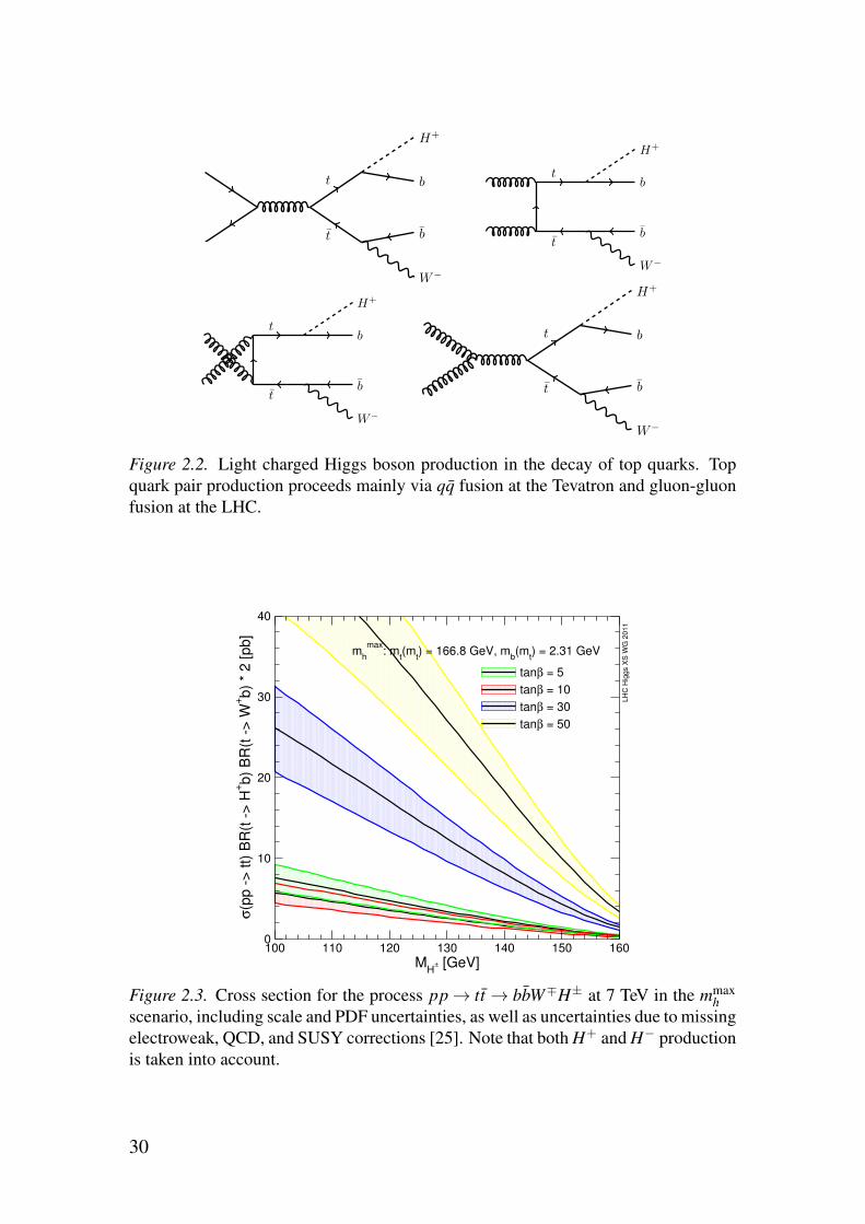
Light charged Higgs bosons would be readily produced in the decays of topquarks via t → bH+. Top quarks are abundantly produced at both the Tevatronand at the LHC in the form of tt pairs. Charged Higgs boson production canthus proceed at tree-level as shown in Figure 2.2. D0 has set an upper limit onB(t → bH+) around 0.2 assuming B(H+ → τν)+B(H+ → cs) = 1, witha somewhat stronger limit if instead B(H+ → τν) = 1, while CDF excludedB(t → bH+) above 0.1 if B(H+ → cs) = 1 [23, 24].

Figure 2.3 shows the cross section for pp → tt → bbW∓H± at 7 TeV in themmax

h scenario, and its dependence on mH+ and tanβ [25]. At the LHC, nocombined search has yet been performed, but the limits from the Tevatron onindividual H+ branching fractions have been significantly improved, as willbe shown in section 3.2.2.

Heavy charged Higgs boson production at hadron colliders

With the full 8 TeV LHC dataset available, focus has shifted towards searchesfor heavy charged Higgs bosons. If mH+ > mt , any Standard Model particlemediating the H+ production is necessarily off-shell. The main productionmode of a heavy charged Higgs boson is then in association with a top quark:pp→ tH+(b). There are two ways of calculating this process. In a Five-Flavor

28

Figure 2.1. Branching fractions of the charged Higgs boson in the MSSM mmaxh (top

row), mmod+h (middle row), and mmod−

h (bottom row) scenarios with tanβ = 10 (leftcolumn) and tanβ = 50 (right column) [21].

29

H+

bt

W−

bt

H+

bt

W−

bt

H+

bt

W−

bt

H+

bt

W−

bt

Figure 2.2. Light charged Higgs boson production in the decay of top quarks. Topquark pair production proceeds mainly via qq fusion at the Tevatron and gluon-gluonfusion at the LHC.

100 110 120 130 140 150 160

MH

± [GeV]

0

10

20

30

40

σ(p

p -

> tt)

BR

(t -

> H

+b)

BR

(t -

> W

+b)

* 2 [

pb]

mh

max: m

t(m

t) = 166.8 GeV, m

b(m

t) = 2.31 GeV

tanβ = 5

tanβ = 10

tanβ = 30

tanβ = 50

LH

C H

iggs X

S W

G 2

011

Figure 2.3. Cross section for the process pp → tt → bbW∓H± at 7 TeV in the mmaxh

scenario, including scale and PDF uncertainties, as well as uncertainties due to missingelectroweak, QCD, and SUSY corrections [25]. Note that both H+ and H− productionis taken into account.

30

bH

+

t

b

H+

t

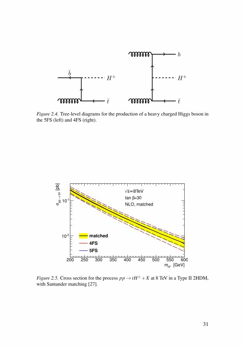
Figure 2.4. Tree-level diagrams for the production of a heavy charged Higgs boson inthe 5FS (left) and 4FS (right).

Figure 2.5. Cross section for the process pp → tH±+X at 8 TeV in a Type II 2HDM,with Santander matching [27].

31

Scheme (5FS) calculation, the b quark is considered massless and is treated asa constituent of the proton. It may therefore appear in the initial state, andcharged Higgs boson production can proceed via gb → tH+. If the processtakes place at such an energy scale that the b quark mass can not be ignored, aFour-Flavor Scheme (4FS) should be used, in which there are only four mass-less quarks in the proton and the b quark must itself be produced in the hardprocess: gg → tH+b. This treatment gives a better description of the kine-matics and is needed if the b quark receives a large pT, but is computationallymore challenging due to the higher particle multiplicity. A 5FS calculationis also less convergent in a perturbation series due to potentially large loga-rithms involving the ratio of the hard scale and the b quark mass appearing inthe splitting of gluons into collinear bb pairs, which are not summed to all or-ders. The 4FS and 5FS tree-level processes are shown in Figure 2.4. It must bestressed that they are not independent, but are different approximations of thesame underlying process, valid in the limits mH±/mb → 1 and mH±/mb → ∞,respectively. In the intermediate region, so-called Santander matching [26] canbe used to interpolate between the 4FS and 5FS predictions. Figure 2.5 showsthe 4FS, 5FS, and matched cross sections at 8 TeV in a Type II 2HDM [27].

At the Tevatron, the D0 experiment performed a search for a heavy chargedHiggs boson with a mass in the range 180–300 GeV and decaying to tb, butwith limited sensitivity to a Type II 2HDM [28].

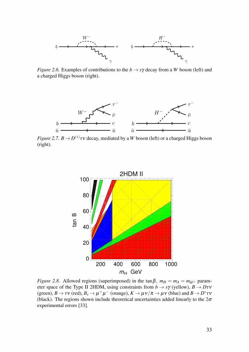
2.3.3 Effects on B-physics observablesDecays of B-mesons are sensitive to the presence of charged Higgs bosons.A succinct review of the experimental situation is given in Ref. [29]. Animportant example is the decay b → sγ shown in Figure 2.6, for which thecontribution of additional diagrams involving a charged Higgs boson may sig-nificantly enhance the branching fraction. Measurements of the decays of theB-meson, with the quark content db, excludes charged Higgs bosons with amass below 360 GeV in a Type II 2HDM [30].

Tauonic decay modes of B-mesons, as illustrated in Figure 2.7, can be an-other strong test for the presence of charged Higgs bosons thanks to the highmass of the tau lepton. BABAR has measured the ratios

R(D) =B(B → Dτν)

B(B → Dℓν)= 0.440±0.058(stat)±0.042(syst), (2.10)

R(D∗) =B(B → D∗τν)B(B → D∗ℓν)

= 0.332±0.024(stat)±0.018(syst), (2.11)

where ℓ is either an electron or a muon [31]. These results have a combineddeviation of 3.4σ from the Standard Model values of

RSM(D) = 0.297±0.017, RSM(D∗) = 0.252±0.003. (2.12)

32

γ

b

W−

s

γ

b

H−

s

Figure 2.6. Examples of contributions to the b → sγ decay from a W boson (left) anda charged Higgs boson (right).

b

τ−

νW

−

c

u u

b

τ−

νH

−

c

u u

Figure 2.7. B → D(∗)τν decay, mediated by a W boson (left) or a charged Higgs boson(right).

Figure 2.8. Allowed regions (superimposed) in the tanβ , mH = mA = mH± param-eter space of the Type II 2HDM, using constraints from b → sγ (yellow), B → Dτν(green), B → τν (red), Bs → µ+µ− (orange), K → µν/π → µν (blue) and B → D∗τν(black). The regions shown include theoretical uncertainties added linearly to the 2σexperimental errors [33].

33

This evidence for new physics is also supported by a 1.6σ deviation ofthe branching fraction B(B → τν) [32]. Figure 2.8 shows the impact of anumber of flavor-physics results on the Type II 2HDM. The measurementof R(D(∗)) is incompatible with the constraints from all other measurementsand can therefore not be explained within this model [33]. This conclusionholds also for the MSSM. However, a generic Type III model could possiblyaccommodate all constraints.

34

Part II: Experiment

3. The Large Hadron Collider

The Large Hadron Collider (LHC) [34], built and operated by the EuropeanOrganization for Nuclear Research (CERN), is the world’s largest and mostpowerful particle collider. It is designed to accelerate two beams of up to2808 bunches of 1.15× 1011 protons with a 25 ns separation and to delivercollisions with a center-of-mass energy of up to 14 TeV at a target luminosityof 1034 cm−2s−1. The analyses presented in this thesis use data collectedduring 2011 and 2012, when the LHC operated with several key parametersbelow their design values and delivered proton-proton collisions with center-of-mass energies of 7 TeV, respectively 8 TeV. These datasets neverthelesspresent an opportunity to study physics processes at energies never probedbefore in a laboratory setting. In addition to proton-proton collisions, the LHCalso performs heavy ion collisions, which are not discussed in this thesis.

The high bunch intensity required to meet the target luminosity excludedthe use of an anti-proton beam for the LHC. Counter-rotating beams of same-charge particles, however, require two separate magnet systems. Due to thelimited space in the LHC tunnel, which previously housed the Large Electron-Positron Collider (LEP), the machine uses a design with two sets of super-conducting magnets and beamlines sharing the same cryostat. The magnetsare based on niobium-titanium coils, cooled to 1.9 K using superfluid heliumand generating magnetic fields of up to 8.3 T. Over 1600 main magnets areused to control the beams. Although a hadron accelerator does not suffer pro-hibitively large energy losses from synchrotron radiation and could ideally bemade nearly circular, the LHC follows the layout of the LEP tunnel with eightstraight sections and eight arcs for a total circumference close to 27 km.

The LHC is linked to the rest of the accelerator complex at CERN, whichprovides it with 450 GeV protons. After their injection into the LHC, particlesare accelerated using 400 MHz superconducting cavities located in one of theeight straight sections. Two other straight sections contain sets of beam clean-ing collimators and a fourth is dedicated to the dumping system used to safelyextract the beams at the end of a run. The remaining four straight sections eachhave an interaction point where the beams cross. This is where the main LHCexperiments are placed. These are the general-purpose experiments ATLAS(which will be described in chapter 4) and CMS, and two more specializedexperiments: LHCb with the purpose to study B-physics, and the dedicatedheavy ion experiment ALICE. In LHCb and ALICE, the beams cross with re-duced overlap, as the experiments are designed for lower luminosities, whileATLAS and CMS make full use of the maximum possible luminosity providedby the LHC.

37

The LHC computing grid

The LHC experiments produce data at a truly massive scale – in total about30 petabytes per year. The Worldwide LHC Computing Grid (WLCG) con-nects more than 170 computing centers in 40 countries to provide the resourcesneeded for storing and analyzing the LHC data. A tiered architecture is usedby the WLCG: Tier 0, at CERN, safe-keeps a first copy of the raw data and per-forms a first-pass reconstruction. Thirteen large Tier 1 centers with sufficientstorage capacity perform reprocessing of the data and also provide storage ofraw, reconstructed, and simulated data. Around 160 Tier 2 sites located inuniversities and other scientific institutes provide additional storage, producesimulated events, and run end-user analysis jobs.

3.1 Experimental challengesDetectors at hadron colliders face challenges that are not present, or muchless severe, at e.g. an e+e− collider. The unprecedented collision energies andluminosity provided by the LHC also come at a cost to the experiments.

Hadrons are composite objects and energies such as those provided by theLHC are enough to resolve their internal structure, i.e. collisions can be seenas taking place between individual partons (quarks and gluons). Each partoncarries an unknown fraction of the total hadron momentum. The 7, 8 or 14 TeVcenter-of-mass energies mentioned throughout this thesis should therefore beseen as upper bounds on the energy available in a collision, while the ac-tual center-of-mass energy in an individual interaction between two partons isunknown and varying from event to event. In particular, the longitudinal mo-mentum is unknown, while the initial transverse momentum can be neglected.When analyzing hadron collisions, one is therefore mainly concerned withtransverse variables. Accurate simulations of proton-proton collisions requirethe use of experimentally determined Parton Distribution Functions (PDFs),which give the probability for a certain type of parton to have a certain frac-tion of the longitudinal momentum of the proton.

Physics processes in hadron collisions tend to be dominated by the stronginteraction, which mostly produces hadronic jets. Very high luminosities aretherefore needed in order to collect a sizable amount of “interesting” eventsinvolving more elusive electroweak processes, Higgs boson production, ornew physics. Hadron collisions also tend to produce events with high particlemultiplicities. This not only makes the reconstruction process more complex,but high collision rates and large event sizes also make it implausible to readout and record the detector data in every event. High-luminosity experimentstherefore need a trigger system to make real-time decisions of which events tosave. Furthermore, detectors need to be designed to cope with a high-radiationenvironment.

38

The instantaneous luminosity increases quadratically with the number ofprotons in each bunch and with the inverse of the bunch diameter, but only lin-early with the number of bunches. At some point, the luminosity is thereforemost efficiently increased by having as tightly squeezed bunches and as manyprotons per bunch as possible. This corresponds to increasing the mean num-ber of individual proton-proton collisions taking place in every bunch crossing.As the LHC experiments mainly search for very rare processes, at most one ofthe collisions in each bunch crossing, called the primary interaction, is likelyto be of interest. The other collisions are referred to as pile-up and bring anumber of problems. The interaction region has a longitudinal extension of afew centimeters and it is typically possible to associate tracks, and often evenphotons and jets, with individual collision points. However, the increased am-bient activity in the calorimeters makes it more challenging to determine thecorrect jet energy scale and also affects the measurement of missing transverseenergy (see section 5.2.6). More particles in each event also means more datato read out, process and store.

Considerations for charged Higgs boson searches

Charged Higgs bosons can be produced at the LHC in the decays of top quarks,in particular in tt pairs, or in association with top quarks. They may subse-quently decay predominantly into τν or tb. The Standard Model decay of thetop quark occurs almost exclusively via Wb. Events involving charged Higgsbosons would therefore have high jet multiplicities and require good jet recon-struction. Furthermore, the tagging of b-jets and hadronic tau decays requiregood tracking in the inner detector volume. The very large background ofmulti-jet events can be reduced by selecting events in which a top quark de-cays leptonically, i.e. with an electron or a muon in the final state. The leptoncan also be used for triggering, which is more straightforward than triggeringon jets. This is the strategy followed in the analyses presented in this the-sis. Electron reconstruction can be performed with a combination of trackingand calorimeter information, while muon reconstruction requires a dedicatedtracking system since muons are not absorbed in calorimeters and an innertracking system is typically not sufficient. To detect the presence of neutrinosproduced in association with electrons, muons, or tau leptons, a good recon-struction of missing transverse energy is also required.

3.2 Run 1 summaryThe first long near-continuous run of the LHC spanned over three years andresulted in several major scientific achievements, including the discovery ofthe Higgs boson, observations of the Ξ′−

b and Ξ∗−b resonances and of the rare

B0s → µ+µ− decay, new measurements of Standard Model processes, and

many searches for new physics.

39

Month in YearJan Apr Jul

Oct Jan Apr JulOct

-1fb

Tota

l In

teg

rate

d L

um

inosity

0

5

10

15

20

25

30

ATLAS

Preliminary

= 7 TeVs2011,

= 8 TeVs2012,

LHC Delivered

ATLAS Recorded

Good for Physics

-1 fbDelivered: 5.46-1 fbRecorded: 5.08

-1 fbPhysics: 4.57

-1 fbDelivered: 22.8-1 fbRecorded: 21.3

-1 fbPhysics: 20.3

Mean Number of Interactions per Crossing

0 5 10 15 20 25 30 35 40 45

/0.1

]-1

Record

ed L

um

inosity [pb

0

20

40

60

80

100

120

140

160

180 Online LuminosityATLAS

> = 20.7µ, <-1Ldt = 21.7 fb∫ = 8 TeV, s

> = 9.1µ, <-1Ldt = 5.2 fb∫ = 7 TeV, s

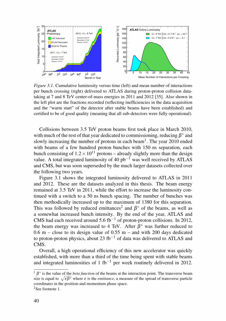
Figure 3.1. Cumulative luminosity versus time (left) and mean number of interactionsper bunch crossing (right) delivered to ATLAS during proton-proton collision data-taking at 7 and 8 TeV center-of-mass energies in 2011 and 2012 [35]. Also shown inthe left plot are the fractions recorded (reflecting inefficiencies in the data acquisitionand the “warm start” of the detector after stable beams have been established) andcertified to be of good quality (meaning that all sub-detectors were fully operational).

Collisions between 3.5 TeV proton beams first took place in March 2010,with much of the rest of that year dedicated to commissioning, reducing β ∗ andslowly increasing the number of protons in each beam1. The year 2010 endedwith beams of a few hundred proton bunches with 150 ns separation, eachbunch consisting of 1.2×1011 protons – already slightly more than the designvalue. A total integrated luminosity of 40 pb−1 was well received by ATLASand CMS, but was soon superseded by the much larger datasets collected overthe following two years.

Figure 3.1 shows the integrated luminosity delivered to ATLAS in 2011and 2012. These are the datasets analyzed in this thesis. The beam energyremained at 3.5 TeV in 2011, while the effort to increase the luminosity con-tinued with a switch to a 50 ns bunch spacing. The number of bunches wasthen methodically increased up to the maximum of 1380 for this separation.This was followed by reduced emittances2 and β ∗ of the beams, as well asa somewhat increased bunch intensity. By the end of the year, ATLAS andCMS had each received around 5.6 fb−1 of proton-proton collisions. In 2012,the beam energy was increased to 4 TeV. After β ∗ was further reduced to0.6 m – close to its design value of 0.55 m – and with 200 days dedicatedto proton-proton physics, about 23 fb−1 of data was delivered to ATLAS andCMS.

Overall, a high operational efficiency of this new accelerator was quicklyestablished, with more than a third of the time being spent with stable beamsand integrated luminosities of 1 fb−1 per week routinely delivered in 2012.

1 β ∗ is the value of the beta function of the beams at the interaction point. The transverse beamsize is equal to

�

εβ ∗ where ε is the emittance, a measure of the spread of transverse particlecoordinates in the position-and-momentum phase space.2See footnote 1.

40

The use of the 50 ns bunch spacing, as compared to the design value of 25 ns,was somewhat compensated for by the higher bunch intensity and lower thanexpected emittance. This made it possible to eventually reach an instantaneousluminosity of 7.7× 1033 cm−2s−1, close to the target of 1× 1034 cm−2s−1.The cost to the experiments was the high pile-up (as shown in Figure 3.1) withthe mean number of interactions per bunch crossing eventually reaching 37,almost twice the design value.

In addition to the proton physics program, the LHC also produced lead-leadcollisions with an energy of 2.76 TeV per nucleon, with a total of 177 µb−1

accumulated in 2010 and 2011. Before the start of the first Long Shutdown(LS1) in early 2013, the LHC also successfully delivered proton-lead colli-sions.

During LS1 (2013–2015), the collider is being prepared for higher energiesand luminosities. Upgrades and consolidation works are also undertaken bythe experiments, and in the earlier stages of the CERN chain of accelerators.

3.2.1 Discovery of the Higgs bosonThe most important result of the LHC Run 1 is the discovery of a Higgs boson[36, 37], achieved independently by the ATLAS and CMS collaborations. Themost important channels to study the Standard Model-like Higgs boson areits decay to two photons or two Z bosons that subsequently decay to electronsand/or muons. Both channels offer the possibility to precisely measure all finalstate particles and to reconstruct the Higgs boson mass with good resolution.As the Higgs boson only couples to massive particles, its decay to two photonsproceeds at lowest order via a heavy fermion or boson loop. This decay modeis therefore suppressed due to the additional vertex but is enhanced due to thestrong Yukawa coupling between the Higgs boson and the top quark, which isthe most important loop contribution. Other important Higgs decay channelsat the LHC are H → WW → lν lν (which has a large branching fraction butpoor mass resolution due to the presence of neutrinos) and H → ττ. The latterchannel offers, despite its lower resolution and large backgrounds, the bestdirect measurement of Higgs couplings to fermions. The decay into a pairof bottom quarks has the largest branching fraction of all decay modes for aHiggs boson mass below 135 GeV and is also analyzed, but is very difficultto isolate at a hadron collider due to the jet-rich background. Only productionmodes in association with a vector boson or a tt pair are therefore considered.

The mass of the Higgs boson is measured by combining the two high-resolution channels in both of the experiments. The measured values are:

ATLAS : mH = 125.36±0.37(stat)±0.18(syst) GeV [38],

CMS : mH = 125.03+0.26−0.27(stat)+0.13

−0.15(syst) GeV [39],

combination : mH = 125.09±0.21(stat)±0.11(syst) GeV [40].

(3.1)

41

ggF+ttH

fµ2− 1− 0 1 2 3 4 5 6 7

VB

F+

VH

f µ

2−

1−

0

1

2

3

4

5

6

7

ATLAS Preliminary-1 = 7 TeV, 4.5-4.7 fbs

-1 = 8 TeV, 20.3 fbs

= 125.36 GeVHm

* WW→H

* ZZ→H

bb→H

γγ →H

ττ →H

Standard Model

Best fit

68% CL

95% CL

(GeV)Hm123 124 125 126 127

SM

σ/σ

0.0

0.5

1.0

1.5

2.0

2.5Combined

taggedγγ →H

ZZ tagged→H

CMS

(7 TeV)-1

(8 TeV) + 5.1 fb-1

19.7 fb

ZZ→ + H γγ → H

Figure 3.2. Signal strengths and mass of the Higgs boson with best-fit values to thedata and 68% (full) and 95% (dashed) confidence level contours indicated. The leftplot [44] shows the ATLAS measured signal strength (defined as cross section timesbranching fractions, relative to the Standard Model expectation) for two groups ofproduction modes (gluon-gluon fusion and tt associated production, and vector bo-son fusion and Higgs-strahlung) in five different search channels. The right plot [39]shows the CMS measured mass and the total signal strength in the two high massresolution channels (the relative signal strength for the two decay modes is set to theStandard Model expectation).

A mass around 125 GeV is within 1.3σ of the expected value of 94+25−22 GeV

obtained from a global fit of Standard Model parameters to electroweak pre-cision data [41]. The observed decay modes and angular distributions of thedecay products are compatible with the particle having zero spin and positiveparity, as expected for the Standard Model Higgs boson, with alternative hy-potheses strongly disfavored [42, 43]. The couplings (assessed by measuringdifferent production modes as well as decay channels) are found to agree withthe Standard Model predictions [39, 44], as illustrated in Figure 3.2.

3.2.2 SUSY and 2HDM searchesA large number of searches for SUSY particles have been undertaken at theLHC, so far with negative results. Due to the proliferation of SUSY theo-ries, searches target simplified models that focus on a single production modeand one- or two-step decay chains. As an illustration, Figure 3.3 summarizesthe current status of SUSY searches in the ATLAS experiment. In particu-lar, gluinos and first- and second-generation squarks should be produced withlarge cross sections at the LHC and the lower limits on their masses approachor exceed 1 TeV in many important benchmark models.

The most stringent constraints on the MSSM Higgs sector is offered by thesearch for neutral Higgs bosons in the ττ final state, in particular at large tanβ .Figure 3.4 shows the ATLAS exclusion limits interpreted in the mmax

h , mmod−h ,

42

Mo

de

le,µ,τ,γ

Je

tsE

miss

T �Ld

t[fb−

1]M

as

slim

itR

efe

ren

ce

Inclusive Searches3rd gen.g med.

3rd gen. squarksdirect production

EWdirect

Long-livedparticles

RPV

Oth

er

MS

UG

RA

/CM

SS

M0

2-6

jets

Yes

20.3

m(q

)=m

(g)

14

05

.78

75

1.7

TeV

q,

g

qq,

q→qχ

010

2-6

jets

Yes

20.3

m( χ

01 )=0

Ge

V,m

(1stgen

.q)=

m(2

ndgen.q

)1

40

5.7

87

5850

GeV

q

qqγ,

q→qχ

01(c

om

pre

ssed)

1γ

0-1

jet

Yes

20.3

m(q

)-m( χ

01)

=m

(c)1

41

1.1

55

9250

GeV

q

gg,

g→qqχ

010

2-6

jets

Yes

20.3

m( χ

01 )=0

Ge

V1

40

5.7

87

51.3

3TeV

g

gg,

g→qqχ±1→

qqW±χ

011

e,µ3-6

jets

Yes

20

m( χ

01 )<3

00

Ge

V,m

( χ±

)=0

.5(m

( χ01 )+

m(g

))1

50

1.0

35

55

1.2

TeV

g

gg,

g→qq(ℓℓ/ℓν

/νν) χ

012

e,µ0-3

jets

-20

m( χ

01 )=

0G

eV

15

01

.03

55

51.3

2TeV

g

GM

SB

(ℓN

LS

P)

1-2τ

+0-1ℓ

0-2

jets

Yes

20.3

tanβ>

20

14

07

.06

03

1.6

TeV

g

GG

M(b

ino

NLS

P)

2γ

-Yes

20.3

m( χ

01 )>5

0G

eV

AT

LA

S-C

ON

F-2

01

4-0

01

1.2

8TeV

g

GG

M(w

ino

NLS

P)

1e,µ

+γ

-Yes

4.8

m( χ

01 )>5

0G

eV

AT

LA

S-C

ON

F-2

01

2-1

44

619

GeV

g

GG

M(h

iggsin

o-b

ino

NLS

P)

γ1

bYes

4.8

m( χ

01 )>2

20

Ge

V1

21

1.1

16

7900

GeV

g

GG

M(h

iggsin

oN

LS

P)

2e,µ

(Z)

0-3

jets

Yes

5.8

m(N

LS

P)>

20

0G

eV

AT

LA

S-C

ON

F-2

01

2-1

52

690

GeV

g

Gra

vitin

oLS

P0

mono-je

tYes

20.3

m(G

)>1.8×

10−

4e

V,m

(g)=

m(q

)=

1.5

Te

V1

50

2.0

15

18

865

GeV

F1/2

sca

le

g→bbχ

010

3b

Yes

20.1

m( χ

01 )<4

00

Ge

V1

40

7.0

60

01.2

5TeV

g

g→tt χ

010

7-1

0je

tsYes

20.3

m( χ

01 )<

35

0G

eV

13

08

.18

41

1.1

TeV

g

g→tt χ

010-1

e,µ3

bYes

20.1

m( χ

01 )<4

00

Ge

V1

40

7.0

60

01.3

4TeV

g

g→bt χ+1

0-1

e,µ3

bYes

20.1

m( χ

01 )<3

00

Ge

V1

40

7.0

60

01.3

TeV

g

b1 b

1 ,b

1 →bχ

010

2b

Yes

20.1

m( χ

01 )<9

0G

eV

13

08

.26

31

100-6

20

GeV

b1

b1 b

1 ,b

1 →t χ±1

2e,µ

(SS

)0-3

bYes

20.3

m( χ±1

)=2

m( χ

01 )1

40

4.2

50

0275-4

40

GeV

b1

t1 t1 ,t1 →

bχ±1

1-2

e,µ1-2

bYes

4.7

m( χ±1

)=

2m

( χ01 ),

m( χ

01 )=5

5G

eV

12

09

.21

02

,1

40

7.0

58

3110-1

67

GeV

t1

230-4

60

GeV

t1

t1 t1 ,t1 →

Wbχ

01or

t χ01

2e,µ

0-2

jets

Yes

20.3

m( χ

01 )=1

Ge

V1

40

3.4

85

3,1

41

2.4

74

290-1

91

GeV

t1

215-5

30

GeV

t1

t1 t1 ,t1 →

t χ01

0-1

e,µ1-2

bYes

20

m( χ

01 )=1

Ge

V1

40

7.0

58

3,1

40

6.1

12

2210-6

40

GeV

t1

t1 t1 ,t1 →

c χ01

0m

ono-je

t/ c-tag

Yes

20.3

m(t1 )-m

( χ01)<

85

Ge

V1

40

7.0

60

890-2

40

GeV

t1

t1 t1 (natu

ralG

MS

B)

2e,µ

(Z)

1b

Yes

20.3

m( χ

01 )>1

50

Ge

V1

40

3.5

22

2150-5

80

GeV

t1

t2 t2 ,t2 →

t1+

Z3

e,µ(Z

)1

bYes

20.3

m( χ

01 )<2

00

Ge

V1

40

3.5

22

2290-6

00

GeV

t2

ℓL,Rℓ

L,R

,ℓ→ℓ χ

012

e,µ0

Yes

20.3

m( χ

01 )=0

Ge

V1

40

3.5

29

490-3

25

GeV

ℓ

χ+1χ−1

,χ+1→ℓν(ℓν)

2e,µ

0Yes

20.3

m( χ

01 )=0

Ge

V,m

(ℓ,ν)=

0.5

(m( χ±1

)+m

( χ01 ))

14

03

.52

94

140-4

65

GeV

χ±1

χ+1χ−1

,χ+1→τν(τν)

2τ

-Yes

20.3

m( χ

01 )=0

Ge

V,m

(τ,ν

)=0

.5(m

( χ±1

)+m

( χ01 ))

14

07

.03

50

100-3

50

GeV

χ±1

χ±1χ

02 →ℓ

Lνℓ

Lℓ(νν),ℓν

ℓLℓ(νν)

3e,µ

0Yes

20.3

m( χ±1

)=m

( χ02 ),

m( χ

01 )=0

,m

( ℓ,ν)=

0.5

(m( χ±1

)+m

( χ01 ))

14

02

.70

29

700

GeV

χ±1, χ

02

χ±1χ

02 →Wχ

01Zχ

012-3

e,µ0-2

jets

Yes

20.3

m( χ±1

)=m

( χ02 ),

m( χ

01 )=0

,sle

pto

ns

de

co

up

led

14

03

.52

94

,1

40

2.7

02

9420

GeV

χ±1, χ

02

χ±1χ

02 →Wχ

01hχ

01 ,h→

bb/W

W/ττ/γγ

e,µ,γ

0-2

bYes

20.3

m( χ±1

)=m

( χ02 ),

m( χ

01 )=0

,sle

pto

ns

de

co

up

led

15

01

.07

11

0250

GeV

χ±1, χ

02

χ02 χ

03 ,χ

02,3→ℓ

Rℓ

4e,µ

0Yes

20.3

m( χ

02 )=m

( χ03 ),

m( χ

01 )=0

,m

(ℓ,ν)=

0.5

(m( χ

02 )+m

( χ01 ))

14

05

.50

86

620

GeV

χ02,3

Dire

ctχ+1χ−1

pro

d.,

long-live

dχ±1

Dis

app.

trk1

jet

Yes

20.3

m( χ±1

)-m( χ

01 )=

16

0M

eV,τ( χ±1 )=

0.2

ns

13

10

.36

75

270

GeV

χ±1

Sta

ble

,sto

pped

gR

-hadro

n0

1-5

jets

Yes

27.9

m( χ

01 )=1

00

Ge

V,1

0µ

s<τ(g)<

10

00

s1

31

0.6

58

4832

GeV

g

Sta

ble

gR

-hadro

ntrk

--

19.1

14

11

.67

95

1.2

7TeV

g

GM

SB

,sta

bleτ,χ

01 →τ(e,µ)+τ(e,µ)

1-2µ

--

19.1

10<

tanβ<

50

14

11

.67

95

537

GeV

χ01

GM

SB

,χ

01 →γG

,lo

ng-live

dχ

012γ

-Yes

20.3

2<τ( χ

01 )<3

ns,S

PS

8m

od

el

14

09

.55

42

435

GeV

χ01

qq,χ

01 →qqµ

(RP

V)

1µ

,dis

pl.

vtx

--

20.3

1.5<

cτ<

15

6m

m,B

R(µ

)=1

,m

( χ01 )=

10

8G

eV

AT

LA

S-C

ON

F-2

01

3-0

92

1.0

TeV

q

LF

Vp

p→ντ+

X,ντ →

e+µ

2e,µ

--

4.6

λ′311 =

0.1

0,λ

132 =0

.05

12

12

.12

72

1.6

1TeV

ντ

LF

Vp

p→ντ+

X,ντ →

e(µ)+τ

1e,µ

+τ

--

4.6

λ′311 =

0.1

0,λ

1(2)33 =0

.05

12

12

.12

72

1.1

TeV

ντ

Bilin

ear

RP

VC

MS

SM

2e,µ

(SS

)0-3

bYes

20.3

m(q

)=m

(g),

cτ

LS

P<

1m

m1

40

4.2

50

01.3

5TeV

q,

g

χ+1χ−1

,χ+1→

Wχ

01 , χ01 →

eeνµ,eµν

e4

e,µ-

Yes

20.3

m( χ

01 )>0

.2×

m( χ±1

),λ

121�

01

40

5.5

08

6750

GeV

χ±1

χ+1χ−1

,χ+1→

Wχ

01 , χ01 →ττν

e ,eτντ

3e,µ

+τ

-Yes

20.3

m( χ

01 )>0

.2×

m( χ±1

),λ

133�

01

40

5.5

08

6450

GeV

χ±1

g→qqq

06-7

jets

-20.3

BR

(t)=B

R(b

)=B

R(c)=

0%

AT

LA

S-C

ON

F-2

01

3-0

91

916

GeV

g

g→t1

t,t1 →

bs

2e,µ

(SS

)0-3

bYes

20.3

14

04

.25

0850

GeV

g

Scala

rcharm

,c→

c χ01

02

cYes

20.3

m( χ

01 )<2

00

Ge

V1

50

1.0

13

25

490

GeV

c

Ma

ss

sc

ale

[Te

V]

10−

11

√s

=7

TeV

full

data

√s

=8

TeV

partia

ld

ata

√s

=8

TeV

full

data

AT

LA

SS

US

YS

earc

hes*

-95

%C

LL

ow

er

Lim

itsS

tatu

s:

Fe

b2

01

5A

TL

AS

Pre

limin

ary

√s

=7

,8

Te

V

*On

lya

se

lectio

no

fth

eava

ilable

ma

ss

limits

on

new

sta

tes

or

ph

en

om

en

ais

sh

ow

n.

Alllim

itsq

uo

ted

are

ob

se

rved

min

us

1σ

the

ore

tica

lsig

na

lcro

ss

se

ctio

nu

nce

rtain

ty.

Figure 3.3. A representative selection of ATLAS searches for Supersymmetry.

43

and mmod+h scenarios [45]. Similar results are available from CMS [46]. The

overall most sensitive search channel for 2HDMs is A → Zh. ATLAS hassearched for decays of h to ττ or bb together with Z decays to electron ormuon pairs, as well as h decays to bb together with Z decays to neutrinos [47].Figure 3.5 shows the excluded parameter space in Type I, Type II, lepton-specific and flipped 2HDMs, with the constraints from A → Zh indicated inpink and the constraints from A → ττ indicated in blue. These plots are madeassuming that mh = 125 GeV and cos(β −α) = 0.1 (recall that small valuesof this quantity correspond to SM-like couplings of h). Furthermore, it isassumed that mA = mH = mH± . CMS searches for A → Zh are reported inRefs. [48, 49].

The single most sensitive channel for charged Higgs boson searches at theLHC is the all-hadronic final state including the hadronic decay of a tau lepton,i.e. gg→ tt → bb(W− → qq)(H+ → τ+ν) for a light charged Higgs boson andgg → b(t → qqb)(H+ → τ+ν) for a heavy charged Higgs boson. Interpreta-tions of the ATLAS results, which set upper limits on the product of branch-ing fractions B(t → bH+)×B(H+ → τ+ν) between 0.23% and 1.3% forcharged Higgs boson masses in the range 80–160 GeV and upper limits onσ(pp → tH++X)×B(H+ → τ+ν) between 0.76 pb and 4.5 fb for chargedHiggs boson masses in the range 180–1000 GeV, are shown in Figure 3.6 forthe mmax

h , mmod−h , and mmod+

h scenarios [50]. Similar results are available fromCMS [51]. For the decay H+ → cs, the experiments have placed upper limitson B(t → bH+)×B(H+ → cs) between 1% and 7% for charged Higgs bosonmasses in the range 80–160 GeV [52, 53]. CMS has also searched for heavycharged Higgs bosons decaying to tb in the dilepton final state, placing upperlimits on σ(pp → tH++X)×B(H+ → tb) in the range 0.4–4 pb for chargedHiggs boson masses in the range 180–600 GeV [54].

44

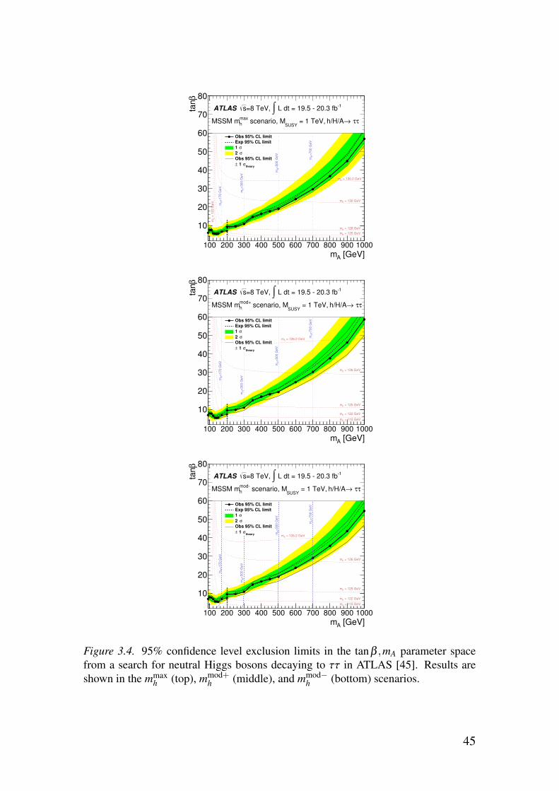
[GeV]Am100 200 300 400 500 600 700 800 900 1000

βta

n

10

20

30

40

50

60

70

80

=1

70

Ge

VH

m

=3

00

Ge

VH

m

=5

00

Ge

VH

m

=7

00

Ge

VH

m

= 1

22

Ge

Vh

m

= 125 GeVhm

= 128 GeVhm

= 130 GeVhm

= 130.2 GeVhm

Obs 95% CL limit

Exp 95% CL limit

σ1

σ2

Obs 95% CL limit

theoryσ 1 ±

-1 L dt = 19.5 - 20.3 fb∫=8 TeV, s ATLAS

ττ → h/H/A = 1 TeV,SUSY

scenario, Mmax

hMSSM m

[GeV]Am100 200 300 400 500 600 700 800 900 1000

βta

n

10

20

30

40

50

60

70

80

=1

70

Ge

VH

m

=3

00

Ge

VH

m

=5

00

Ge

VH

m

=7

00

Ge

VH

m

= 115 GeVhm

= 122 GeVhm

= 125 GeVhm

= 126 GeVhm

= 126.2 GeVhm

Obs 95% CL limit

Exp 95% CL limit

σ1

σ2

Obs 95% CL limit

theoryσ 1 ±

-1 L dt = 19.5 - 20.3 fb∫=8 TeV, s ATLAS

ττ → h/H/A = 1 TeV,SUSY

scenario, Mmod+

hMSSM m

[GeV]Am100 200 300 400 500 600 700 800 900 1000

βta

n

10

20

30

40

50

60

70

80

=1

70

Ge

VH

m

=3

00

Ge

VH

m

=5

00

Ge

VH

m

=7

00

Ge

VH

m

= 115 GeVhm

= 122 GeVhm

= 125 GeVhm

= 126 GeVhm

= 126.2 GeVhm

Obs 95% CL limit

Exp 95% CL limit

σ1

σ2

Obs 95% CL limit

theoryσ 1 ±

-1 L dt = 19.5 - 20.3 fb∫=8 TeV, s ATLAS

ττ → h/H/A = 1 TeV,SUSY

scenario, Mmod-

hMSSM m

Figure 3.4. 95% confidence level exclusion limits in the tanβ ,mA parameter spacefrom a search for neutral Higgs bosons decaying to ττ in ATLAS [45]. Results areshown in the mmax

h (top), mmod+h (middle), and mmod−

h (bottom) scenarios.

45

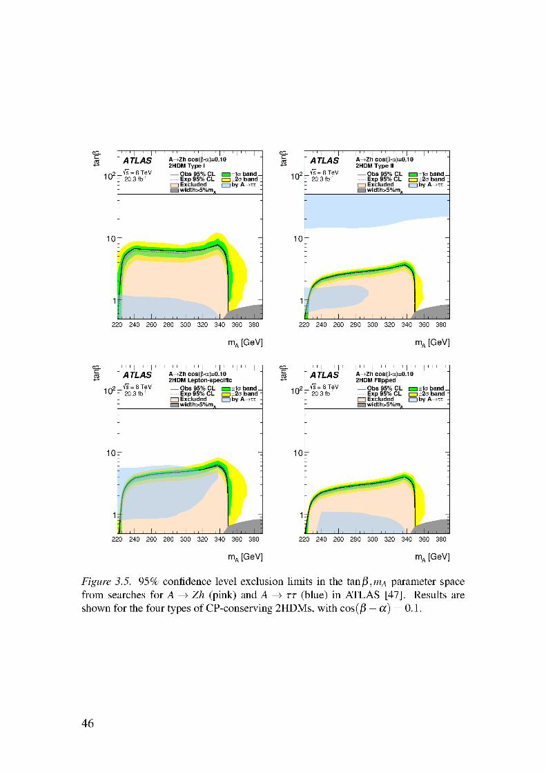
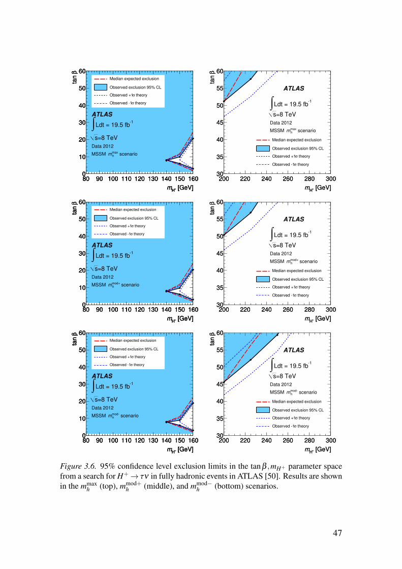
[GeV]+Hm

80 90 100 110 120 130 140 150 160

βta

n

0

10

20

30

40

50

60

[GeV]+Hm

80 90 100 110 120 130 140 150 160

βta

n

0

10

20

30

40

50

60

[GeV]+Hm

80 90 100 110 120 130 140 150 160

βta

n

0

10

20

30

40

50

60Median expected exclusion

Observed exclusion 95% CL

theoryσObserved +1

theoryσObserved -1

-1Ldt = 19.5 fb∫=8 TeVs

Data 2012

scenario maxh

mMSSM

ATLAS

[GeV]+Hm

200 220 240 260 280 300

βta

n

30

35

40

45

50

55

60

[GeV]+Hm

200 220 240 260 280 300

βta

n

30

35

40

45

50

55

60

Median expected exclusion

Observed exclusion 95% CL

theoryσObserved +1

theoryσObserved -1

-1Ldt = 19.5 fb∫=8 TeVs

ATLAS

Data 2012

scenario maxh

mMSSM

[GeV]+Hm

80 90 100 110 120 130 140 150 160

βta

n

0

10

20

30

40

50

60

[GeV]+Hm

80 90 100 110 120 130 140 150 160

βta

n

0

10

20

30

40

50

60

[GeV]+Hm

80 90 100 110 120 130 140 150 160

βta

n

0

10

20

30

40

50

60Median expected exclusion

Observed exclusion 95% CL

theoryσObserved +1

theoryσObserved -1

-1Ldt = 19.5 fb∫=8 TeVs

Data 2012

scenario mod+h

mMSSM

ATLAS

[GeV]+Hm

200 220 240 260 280 300

βta

n

30

35

40

45

50

55

60

[GeV]+Hm

200 220 240 260 280 300

βta

n

30

35

40

45

50

55

60

Median expected exclusion

Observed exclusion 95% CL

theoryσObserved +1

theoryσObserved -1

-1Ldt = 19.5 fb∫=8 TeVs

ATLAS

Data 2012

scenario mod+h

mMSSM

[GeV]+Hm

80 90 100 110 120 130 140 150 160

βta

n

0

10

20

30

40

50

60

[GeV]+Hm

80 90 100 110 120 130 140 150 160

βta

n

0

10

20

30

40

50

60

[GeV]+Hm

80 90 100 110 120 130 140 150 160

βta

n

0

10

20

30

40

50

60Median expected exclusion

Observed exclusion 95% CL

theoryσObserved +1

theoryσObserved -1

-1Ldt = 19.5 fb∫=8 TeVs

Data 2012

scenario mod-h

mMSSM

ATLAS

[GeV]+Hm

200 220 240 260 280 300

βta

n

30

35

40

45

50

55

60

[GeV]+Hm

200 220 240 260 280 300

βta

n

30

35

40

45

50

55

60

Median expected exclusion

Observed exclusion 95% CL

theoryσObserved +1

theoryσObserved -1

-1Ldt = 19.5 fb∫=8 TeVs

ATLAS

Data 2012

scenario mod-h

mMSSM

Figure 3.6. 95% confidence level exclusion limits in the tanβ ,mH+ parameter spacefrom a search for H+ → τν in fully hadronic events in ATLAS [50]. Results are shownin the mmax

h (top), mmod+h (middle), and mmod−

h (bottom) scenarios.

47

4. The ATLAS experiment

The ATLAS experiment [55] is a multi-purpose detector designed to make fulluse of the rich LHC physics potential, especially in the search for the StandardModel Higgs boson and new physics phenomena at the TeV scale. To covera wide range of interesting final states, it identifies and measures electrons,photons, muons, Emiss

T , and jets, with tagging of hadronic tau decays and b-jets. To be sensitive to rare processes, ATLAS takes advantage of the fullluminosity offered by the LHC, which means that all of its sub-detectors needto be fast, radiation-hard, and able to handle large amounts of pile-up.

An overview of the ATLAS experiment is shown in Figure 4.1. It is con-structed with a forward-backward symmetric geometry consisting of a largebarrel cylinder surrounding the beamline around the collision point, and end-cap plugs for near-hermetic coverage. Measuring 44 m in length and 25 m indiameter, and weighing 7000 tons, it is the largest of the LHC experiments.

The design of the detector was largely driven by the choice of magnet sys-tem, which consists of a thin superconducting solenoid surrounding the innerdetector and three sets of eight superconducting toroids integrated in the muonsystem. The inner detector consists of semiconductor pixel and strip detectors,and a straw tube transition radiation tracker, providing vertexing, momen-tum measurement and particle identification capabilities. Outside the innerdetector and the solenoid magnet are liquid argon electromagnetic samplingcalorimeters, surrounded by hadronic calorimeters using scintillating tiles inthe barrel and liquid argon in the end-caps. The outermost and physicallylargest part is the muon system, consisting of multi-wire chambers, single-wire drift tubes and resistive plate chambers, with different technologies usedto provide both precision tracking and fast trigger capabilities.

Coordinate system

A right-handed Cartesian coordinate system with its origin at the center of thedetector (the nominal interaction point) is defined in ATLAS such that the z-axis lies along the beam pipe, the y-axis points upwards and the x-axis pointstowards the center of the LHC ring. Spherical coordinates are often used aswell, with φ being the azimuthal angle in the x-y plane and θ being the polarangle in the y-z plane.

The pseudorapidity η is a function of θ such that

η =− ln tan

�

θ

2

�

. (4.1)

48

Figure 4.1. The ATLAS detector [55].

In the low-mass limit, the pseudorapidity of a particle is a good approximationof its rapidity,

yr =12

ln

�

E + pz

E − pz

�

, (4.2)

which has the convenient property that rapidity differences Δyr are invariantunder Lorentz boosts along the z-axis, i.e. Δyr between two collision productsis independent of the unknown longitudinal momenta of the colliding partons.The angular distance between two directions in the η-φ space is defined as

ΔR =�

(Δφ)2 +(Δη)2. (4.3)

4.1 Inner detectorThe purpose of the inner detector is to provide tracking and transverse mo-mentum measurements of charged particles. It uses a combination of precisiontrackers, which allow accurate vertexing and impact parameter measurementsfor heavy-flavor and tau lepton tagging, and a larger gaseous tracking volumethat also provides electron identification capabilities via detection of transitionradiation. The arrangement of these detectors is shown in Figure 4.2, with thehighly granular semiconductor pixel and microstrip detectors covering the re-gion |η | < 2.5 and the transition radiation tracker limited to |η | < 2.0. Thedesign resolution of the inner detector is σpT/pT = 0.05%pT ⊕1%. It is ulti-

49

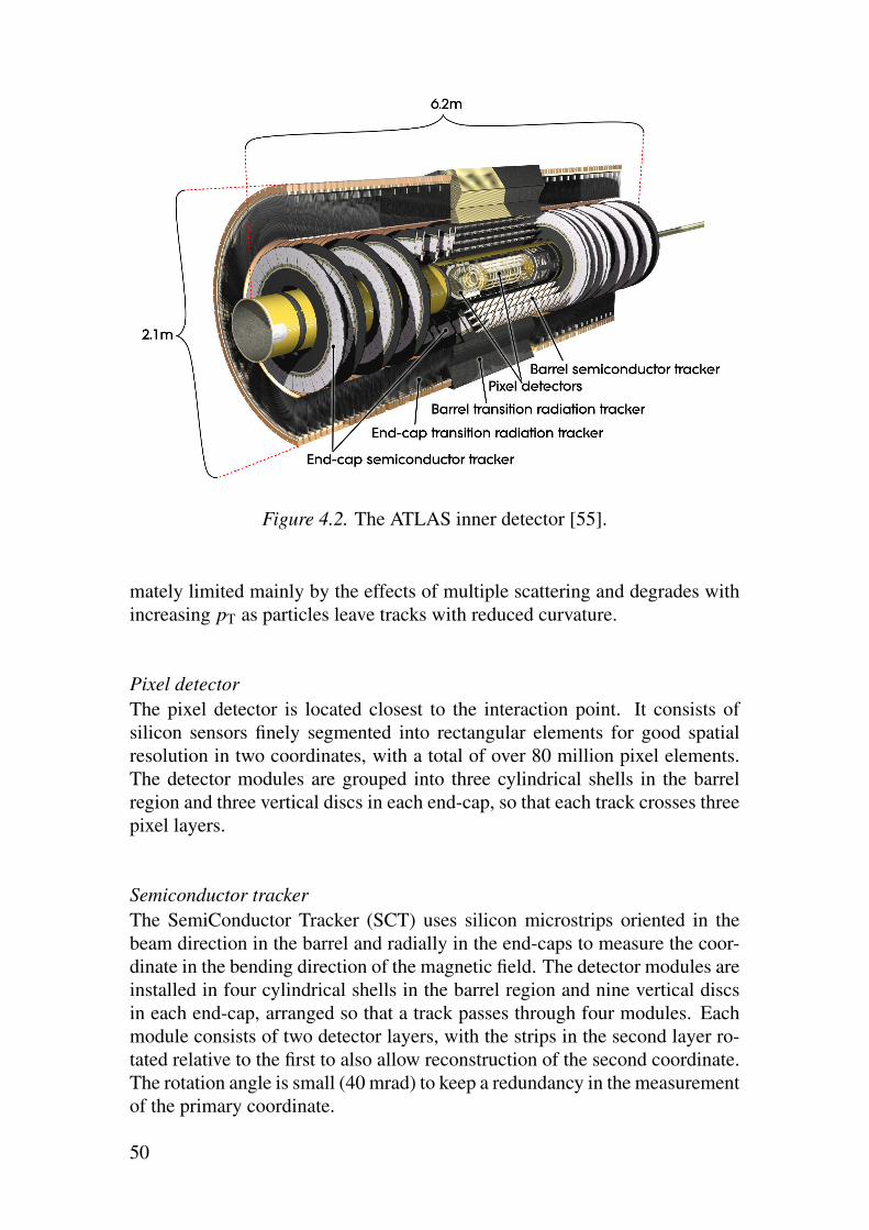
Figure 4.2. The ATLAS inner detector [55].

mately limited mainly by the effects of multiple scattering and degrades withincreasing pT as particles leave tracks with reduced curvature.

Pixel detector

The pixel detector is located closest to the interaction point. It consists ofsilicon sensors finely segmented into rectangular elements for good spatialresolution in two coordinates, with a total of over 80 million pixel elements.The detector modules are grouped into three cylindrical shells in the barrelregion and three vertical discs in each end-cap, so that each track crosses threepixel layers.

Semiconductor tracker

The SemiConductor Tracker (SCT) uses silicon microstrips oriented in thebeam direction in the barrel and radially in the end-caps to measure the coor-dinate in the bending direction of the magnetic field. The detector modules areinstalled in four cylindrical shells in the barrel region and nine vertical discsin each end-cap, arranged so that a track passes through four modules. Eachmodule consists of two detector layers, with the strips in the second layer ro-tated relative to the first to also allow reconstruction of the second coordinate.The rotation angle is small (40 mrad) to keep a redundancy in the measurementof the primary coordinate.

50

Transition radiation tracker

The Transition Radiation Tracker (TRT) consists of densely packed thin strawtubes interleaved with a transition radiation material. The straws are orientedparallel to the beam axis in the barrel region and radially in the end-caps,thereby providing R-φ respectively z-φ positioning only. The lower intrinsicresolution of the straw tubes compared to the silicon detectors is compensatedfor by a large number of hits (36 on average) and longer track length in theTRT. This tracking device also provides electron identification thanks to theemission and detection of transition radiation, with an average of 7–10 transi-tion radiation hits expected from electrons with a transverse momentum above2 GeV.

4.2 CalorimetersThe calorimeters, shown in Figure 4.3, are designed to measure the energy ofelectrons and photons with a resolution of σE/E = 10%/

√E ⊕0.7%, and of

hadronic jets with a resolution of σE/E = 50%/√

E ⊕ 3% (which becomesσE/E = 100%/

√E ⊕ 10% above |η | = 3.2). The constant terms account

for local non-uniformities in the calorimeter response, the energy-dependentstochastic terms correspond to statistical fluctuations, and the effects of elec-tronic noise are negligibly small. Statistical fluctuations become less detri-mental with increasing energy. In contrast to the inner detector, the resolutiontherefore improves with increasing energy.

The high resolution is ensured by the thickness of the calorimeters, whichis more than 22 radiation lengths in the electromagnetic calorimeter and ap-proximately 10 interaction lengths in the hadronic calorimeter, providing goodcontainment1. Together with the large η coverage (up to |η | = 4.9), this alsoallows for a good Emiss

T measurement. The thickness of the calorimeters is alsocrucial to prevent punch-through of hadrons into the muon system.

The electromagnetic (EM) calorimeter is a sampling calorimeter using leadabsorber plates and liquid argon as the active material. Liquid argon is useddue to its radiation tolerance and linear, time-stable, response. To ensure fullφ coverage, the absorbers and electrodes are folded in a zig-zag accordionshape. The central part of the EM calorimeter consists of two half-barrels,together covering the region |η | < 1.475. Each end-cap consists of an innerand an outer wheel, together covering the region 1.375 < |η | < 3.2. In theprecision-measurement region matched to the inner detector, |η | < 2.5, theEM calorimeter has three sampling layers, while it has two sampling layers inthe region 2.5 < |η | < 3.2. The innermost layer has the highest granularity,

1The radiation length is the mean distance which an electron travels before having lost a fraction1− 1

e of its initial energy due to bremsstrahlung. The interaction length is the mean distancewhich a hadron travels before undergoing an inelastic nuclear interaction. These numbers arehighly material-dependent.

51

Figure 4.3. The ATLAS calorimeters [55].

with strip cells of size Δη ×Δφ = 0.003×0.1 in the central part. In the region|η |< 1.8, the calorimeter is also complemented with a thin presampling layerof liquid argon which is used to correct for energy lost in the material upstreamof the calorimeter (up to several radiation lengths).

ATLAS has three hadronic calorimeters: the tile calorimeter, the HadronicEnd-cap Calorimeter (HEC), and the Forward Calorimeter (FCal). The tilecalorimeter consists of a central barrel part and two extended barrels, seg-mented in depth in three layers, and together covering the region |η | < 1.7.It uses steel as absorbing material and scintillating tiles as active material. Inthe HEC and FCal, covering larger rapidities, the liquid argon technology isused, again because of its radiation tolerance. The HEC, covering the region1.5 < |η |< 3.2, uses copper plates as absorbers and consists of two indepen-dent wheels per end-cap, each divided into two segments in depth, for a totalof four layers in each end-cap. The FCal, covering the very forward region3.1 < |η |< 4.9, consists of three modules in each end-cap. Copper is used asabsorbing material in the innermost module in each end-cap, while tungstenis used in the other two in order to provide good containment in this relativelysmall detector. The first module is optimized for electromagnetic measure-ments, thereby complementing the EM calorimeter. For good coverage andminimum radiation background in the muon spectrometer, both the HEC andthe FCal are integrated in the same cryostats as the EM end-cap calorimeters.

52

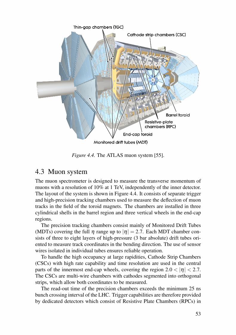
Figure 4.4. The ATLAS muon system [55].

4.3 Muon systemThe muon spectrometer is designed to measure the transverse momentum ofmuons with a resolution of 10% at 1 TeV, independently of the inner detector.The layout of the system is shown in Figure 4.4. It consists of separate triggerand high-precision tracking chambers used to measure the deflection of muontracks in the field of the toroid magnets. The chambers are installed in threecylindrical shells in the barrel region and three vertical wheels in the end-capregions.

The precision tracking chambers consist mainly of Monitored Drift Tubes(MDTs) covering the full η range up to |η | = 2.7. Each MDT chamber con-sists of three to eight layers of high-pressure (3 bar absolute) drift tubes ori-ented to measure track coordinates in the bending direction. The use of sensorwires isolated in individual tubes ensures reliable operation.

To handle the high occupancy at large rapidities, Cathode Strip Chambers(CSCs) with high rate capability and time resolution are used in the centralparts of the innermost end-cap wheels, covering the region 2.0 < |η | < 2.7.The CSCs are multi-wire chambers with cathodes segmented into orthogonalstrips, which allow both coordinates to be measured.

The read-out time of the precision chambers exceeds the minimum 25 nsbunch crossing interval of the LHC. Trigger capabilities are therefore providedby dedicated detectors which consist of Resistive Plate Chambers (RPCs) in

53

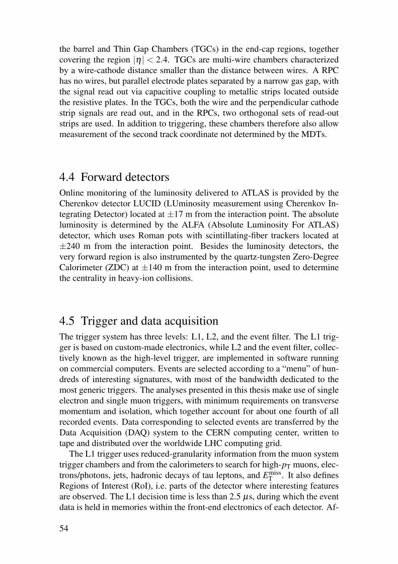
the barrel and Thin Gap Chambers (TGCs) in the end-cap regions, togethercovering the region |η | < 2.4. TGCs are multi-wire chambers characterizedby a wire-cathode distance smaller than the distance between wires. A RPChas no wires, but parallel electrode plates separated by a narrow gas gap, withthe signal read out via capacitive coupling to metallic strips located outsidethe resistive plates. In the TGCs, both the wire and the perpendicular cathodestrip signals are read out, and in the RPCs, two orthogonal sets of read-outstrips are used. In addition to triggering, these chambers therefore also allowmeasurement of the second track coordinate not determined by the MDTs.

4.4 Forward detectorsOnline monitoring of the luminosity delivered to ATLAS is provided by theCherenkov detector LUCID (LUminosity measurement using Cherenkov In-tegrating Detector) located at ±17 m from the interaction point. The absoluteluminosity is determined by the ALFA (Absolute Luminosity For ATLAS)detector, which uses Roman pots with scintillating-fiber trackers located at±240 m from the interaction point. Besides the luminosity detectors, thevery forward region is also instrumented by the quartz-tungsten Zero-DegreeCalorimeter (ZDC) at ±140 m from the interaction point, used to determinethe centrality in heavy-ion collisions.

4.5 Trigger and data acquisitionThe trigger system has three levels: L1, L2, and the event filter. The L1 trig-ger is based on custom-made electronics, while L2 and the event filter, collec-tively known as the high-level trigger, are implemented in software runningon commercial computers. Events are selected according to a “menu” of hun-dreds of interesting signatures, with most of the bandwidth dedicated to themost generic triggers. The analyses presented in this thesis make use of singleelectron and single muon triggers, with minimum requirements on transversemomentum and isolation, which together account for about one fourth of allrecorded events. Data corresponding to selected events are transferred by theData Acquisition (DAQ) system to the CERN computing center, written totape and distributed over the worldwide LHC computing grid.

The L1 trigger uses reduced-granularity information from the muon systemtrigger chambers and from the calorimeters to search for high-pT muons, elec-trons/photons, jets, hadronic decays of tau leptons, and Emiss

T . It also definesRegions of Interest (RoI), i.e. parts of the detector where interesting featuresare observed. The L1 decision time is less than 2.5 µs, during which the eventdata is held in memories within the front-end electronics of each detector. Af-

54

ter this time, if the event is accepted, it is read out and buffered by the DAQsystem. The bandwidth of this operation limits the L1 trigger rate to 75 kHz.

Data corresponding to the RoI identified by the L1 trigger (on average 2%of the overall data in each event) is passed on to the L2 trigger, which uses thisextended information to refine the L1 selection and reduces the acceptancerate to about 5 kHz. The L2 processing time is approximately 40 ms.

The final event selection is performed by the event filter, which uses offlineanalysis procedures to perform a full event reconstruction and reduces the out-put rate to approximately 400 Hz. The reconstruction takes about four secondsper event and, at this point, the DAQ capacity is higher than the available pro-cessing power. An additional 200 events per second (passing lower priority L2triggers) are therefore stored in a “delayed stream” for reconstruction betweendata-taking periods.

4.6 Software4.6.1 Detector control systemThe Detector Control System (DCS) provides a high-level interface for the op-eration of the ATLAS detectors and associated technical infrastructure. Thisincludes the control and monitoring of equipment such as power supplies,cooling, and environmental sensors. The DCS is responsible for safely tran-sitioning the hardware between well-defined operational states and signalingany problematic conditions. It monitors and records operational data, and alsohandles communication with other systems such as the ATLAS DAQ and theLHC beam information.

The base of the DCS software is WinCC, an industrial Supervisory ControlsAnd Data Acquisition (SCADA) product which provides, among other things,a scripting facility, user interfaces in the form of alarm screens and fully pro-grammable control panels, and a generic application programming interfacefor extended functionality. A key feature of WinCC is its high scalability. Thisis crucial for the ATLAS DCS, which needs to process data from over 200 000sensors. Different WinCC instances, called “projects”, can be connected viaa LAN to form a distributed system allowing information exchange betweenall connected projects. The ATLAS DCS comprises about 150 projects, eachof which is running on a dedicated server, organized in a three-layer archi-tecture as illustrated in the top part of Figure 4.5. The first layer consists ofthe so-called Local Control Stations (LCS), which are connected to the front-end electronics of a set of related hardware. The second layer consists ofSub-detector Control Stations (SCS), which integrate associated systems toprovide stand-alone control of each sub-detector. The third layer consists ofGlobal Control Stations (GCS), providing e.g. human interfaces in the ATLAScontrol room for the high-level operation of the experiment.

55

WinCC is oriented around the concept of "data points", which are datastructures used to read and write information to and from connected equip-ment as well as between projects. An alarm mechanism is provided, withconfigurable levels for each data point, and the options to mask known alarmsor require acknowledgement by the operator. Data point values are recordedin an Oracle database for later analysis. Some of this information is also usedfor physics reconstruction.

For the physical connection between front-end devices and control stations,the industrial Controller Area Network (CAN) fieldbus and the CANopen pro-tocol are used whenever possible. CAN is a high-speed network system whichprevents message collisions and provides good error detection and recovery. Itis also tolerant to strong magnetic fields, in contrast to e.g. Ethernet. In mostcases, the software interface to the SCADA system is composed of device-specific server applications providing access to the equipment via the industrystandard OPC protocol, for which WinCC provides a client.

The DCS is modeled as a hierarchical Finite State Machine (FSM), whichallows homogeneous control of all connected systems. The lower level FSMelements are managed by each LCS. They correspond to individual or groupsof devices, which may be structured into logical units according to purposeor physical location. These are in turn grouped into representations of sub-detectors and sub-detector partitions at the SCS level. A GCS contains thetop node of the hierarchy, which allows control of the complete experiment.As an example, part of the FSM tree is illustrated in the lower part of Fig-ure 4.5. Commands are propagated downwards and state changes are propa-gated upwards in the hierarchy. The state is a property of each FSM element,representing its condition and readiness for physics data-taking. Each elementautomatically assumes the most severe state reported by any of its underly-ing elements. Similarly, each element also has a status property indicatingthe highest severity of alarms active for the underlying devices, allowing errordetection at any level of the hierarchy.

4.6.2 SimulationMonte Carlo modeling is used to simulate physics processes in ATLAS. In thefirst step, the interaction of two partons participating in a LHC proton-protoncollision is simulated. This is called the hard process, and it is simulated byan event generator program. Different types of hard processes are typicallysimulated separately. The order of a generator refers to the complexity of theFeynman diagrams describing the type of hard process that the generator im-plements. A Leading-Order (LO) diagram contains only the minimum numberof vertices through which a type of process can take place, while higher-orderdiagrams can provide a more complete description, including the effects ofradiation and loop corrections.

56

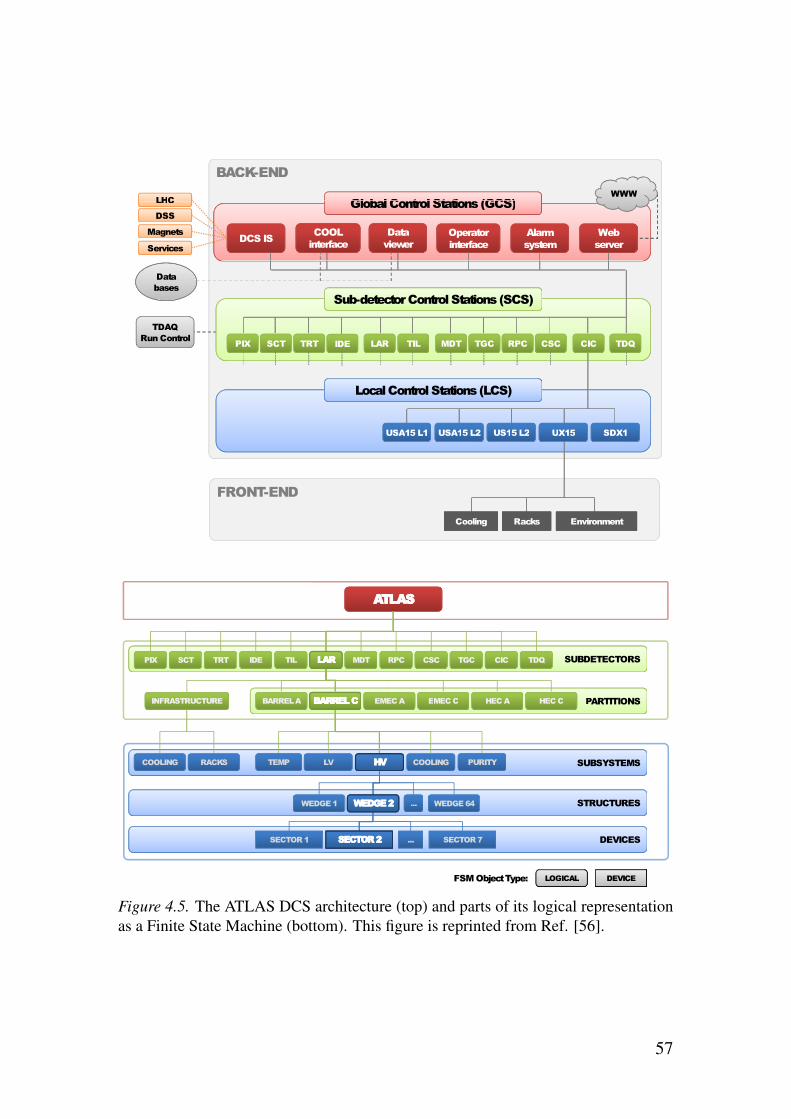
Figure 4.5. The ATLAS DCS architecture (top) and parts of its logical representationas a Finite State Machine (bottom). This figure is reprinted from Ref. [56].

57

Higher-order corrections involving the strong interaction that are not in-cluded in the event generator are subsequently approximated in the parton

shower. This step gives an effective description of the large amounts of gluonradiation emitted by partons involved in the large momentum transfers of thehard interaction. The gluons themselves emit new partons, which produceeven more gluons, and so on, until hadronization occurs. Interactions of rem-nants of the original protons, called the underlying event, and finally the decayof unstable hadrons are also simulated.

A range of available programs are used depending on the process beingstudied, and different programs may be used for different steps of the simu-lation. The programs used to simulate the signal and background processesstudied in this thesis are listed in section 5.1.

Long-lived particles in the simulated events are propagated through a de-tailed simulation of the ATLAS detectors, implemented using the GEANT4toolkit [57]. Interactions with all active detector elements are recorded, andthe response of the experiment is approximated in a process called digitization,in which the effects of noise and timing constraints of the readout electronicsand DAQ system are included. The result is a collection of hits, which arethen passed to the same reconstruction algorithms as real data from the de-tectors. The full GEANT4 simulation is very detailed, and consequently ratherslow. An alternative simulation using parametrized descriptions of the ATLASdetectors is occasionally used to trade precision for speed.

All simulation tasks, from event generation to detector simulation, are han-dled by a central ATLAS software framework named ATHENA and take placeon the WLCG grid.

4.6.3 Reconstruction and analysisThe ATHENA software also handles reconstruction of physics objects (elec-trons, muons, jets, etc.). Like simulation tasks, this is also typically donein large coordinated campaigns on the WLCG grid. The reconstruction, inwhich simulated events and real data are treated on equal footing, proceedsin two steps. The first step is stand-alone reconstruction of primitive objectswithin the different sub-systems of the experiment. Charged particle tracks areformed from hits in the inner detector, energy clusters are formed from energydepositions in the calorimeters, and muon tracks are formed from hits in themuon system. This information is stored in Event Summary Data (ESD) files.

The second step is the combined reconstruction, during which informa-tion from all sub-systems are combined to form high-level objects. Electronsare formed from a track in the inner detector and an electromagnetic cluster.Muons are reconstructed by matching a track in the muon spectrometer to atrack in the inner detector or to small energy depositions in the calorimeter.Jets are formed by grouping energy clusters in the calorimeters, and tracking

58

information from the inner detector is added to identify b-jets and hadronic taudecays. Tracking information is also used to reconstruct the primary vertex.Multiple algorithms exist for the reconstruction of each type of object. Theoutput of this step is therefore multiple collections of electrons, jets, etc. – allwith different definitions. In addition, tracks and energy deposits may at thispoint be double-counted between different types of objects. An object pre-selection is later performed in each analysis to ensure a self-consistent eventdescription. The output of the combined reconstruction are Analysis ObjectData (AOD) files.

Analysis tasks can also be performed within ATHENA, but are often insteadimplemented as stand-alone applications based on ROOT [58] and using so-called D3PD (from Derived Physics Data) files as input (this is also the casefor the analyses presented in this thesis). D3PD files contain selected subsetsof the AOD content, stored as primitive data types. During LS1, ATLAS istransitioning to a new analysis model in which the (somewhat redundant) AODand D3PD files are replaced by a common, object-oriented, “xAOD” format.This is foreseen to reduce the total storage space needed.

The EventLoop analysis framework

During the preparation of this thesis, the author has been involved in the de-velopment and support of a light-weight and extensible ROOT-based analysisframework called EVENTLOOP. The aim of the EVENTLOOP project is toprovide users with a truly uniform interface for configuring and running theiranalysis jobs on different back ends, including one or multiple cores of a localworkstation, PROOF-farms [59], various batch systems, and the WLCG grid.EVENTLOOP was partly used to produce the results presented in part III of thisthesis, and has been adopted as the officially supported analysis framework bythe ATLAS Analysis Software Group.

EVENTLOOP is based on the ROOTCORE build system, which defines astructure for modular software packages. An analysis software consists of acollection of packages, typically including a few core framework components,ATLAS common tools for applying object corrections and evaluating uncer-tainties, and the user provided code that defines the analysis task. The EVENT-LOOP suite of packages includes SAMPLEHANDLER, and EVENTLOOP itself.

SAMPLEHANDLER manages references to the input files, which may belocated on a local disk or on remote resources, including the WLCG grid.Collections of input files are defined based on e.g. the simulated physics pro-cess or the data-taking period, and can be searched, split or joined based ontags. Arbitrary meta-data based on key-value pairs can also be assigned toeach collection, and can be queried by the user’s code during execution.

EVENTLOOP is responsible for job management and steering the execution.The analysis code is written as algorithms, which are C++ classes that definethe logic to be executed for each event, while EVENTLOOP manages input andoutput streams (files or chains of files). Multiple algorithms may be added

59

to a single job, and may produce any number of common or isolated outputstreams.

EVENTLOOP has a modular architecture with optional packages providedfor optimized reading of D3PD and xAOD files, ROOT ntuple management,“white board” services for inter-algorithm communication, or even parsingplain text formulas for setting up simple analyses with no code at all. Thesemay be used as building blocks for a full analysis, or replaced with customsolutions – EVENTLOOP is not tied to any specific input or output formator type of analysis, the only requirement is that the user’s code operates onindividual events.

Jobs are configured by ROOT macros. Algorithm classes are instantiatedand can be manipulated during the configuration. Their state is then savedto disk using a serialization mechanism provided by ROOT. The saved file isshipped to the place of execution where the state of the algorithm is recovered.This eliminates the need for auxiliary configuration files and command lineoptions. Instead, full and direct interaction with each algorithm is possible inthe job macro, including the setting of data members, function calls, and otheroperations. This can also be performed interactively, if desired.

In the job macro, a driver object is instantiated. The driver handles the pro-cess of submitting jobs to the desired processing system, as well as retrievingand merging the output upon completion. Advanced drivers may also monitorthe job progress and resubmit problematic jobs. For long-running jobs, usersmay log out from the local workstation and reconnect with running jobs at alater point. On the processing back end, a worker object iterates over all inputdata, feeding events to each algorithm, and manages the output. There aredriver-worker pairs for most popular platforms for ROOT-based analysis. Themost complex drivers are those interfacing to the ATLAS grid tools due to themassive scale, range of configuration possibilities, and inherent unreliabilityof such jobs. The grid worker also has special features for reporting errorsand job statistics to the ATLAS grid job management system. The followingexample illustrates a typical EVENTLOOP job steering macro:

60

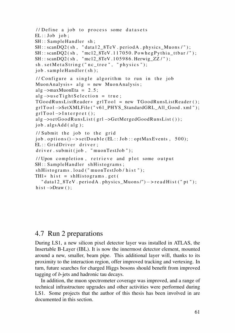
/ / D e f in e a j o b t o p r o c e s s some d a t a s e t sEL : : Job j o b ;SH : : SampleHandler sh ;SH : : scanDQ2 ( sh , " data12_8TeV . per iodA . phys ics_Muons / " ) ;SH : : scanDQ2 ( sh , " mc12_8TeV . 1 1 7 0 5 0 . P o w h e g P y t h i a _ t t b a r / " ) ;SH : : scanDQ2 ( sh , " mc12_8TeV . 1 0 5 9 8 6 . Herwig_ZZ / " ) ;sh . s e t M e t a S t r i n g ( " n c _ t r e e " , " p h y s i c s " ) ;j o b . s amp leHand le r ( sh ) ;

/ / C o n f i g u r e a s i n g l e a l g o r i t h m t o run i n t h e j o bMuonAnalysis ∗ a l g = new MuonAnalysis ;a lg −>maxMuonEta = 2 . 5 ;a lg −> u s e T i g h t S e l e c t i o n = t r u e ;TGoodRunsLis tReader ∗ g r l T o o l = new TGoodRunsLis tReader ( ) ;g r l T o o l −>SetXMLFile ( " v61_PHYS_StandardGRL_All_Good . xml " ) ;g r l T o o l −> I n t e r p r e t ( ) ;a lg −>s e t G o o d R u n s L i s t ( g r l −>GetMergedGoodRunsList ( ) ) ;j o b . a lgsAdd ( a l g ) ;

/ / Submit t h e j o b t o t h e g r i dj o b . o p t i o n s ()−> s e t D o u b l e ( EL : : Job : : optMaxEvents , 5 0 0 ) ;EL : : G r i d D r i v e r d r i v e r ;d r i v e r . su bmi t ( job , " muonTestJob " ) ;

/ / Upon comple t i on , r e t r i e v e and p l o t some o u t p u tSH : : SampleHandler s h H i s t o g r a m s ;s h H i s t o g r a m s . l o a d ( " muonTestJob / h i s t " ) ;TH1∗ h i s t = s h H i s t o g r a m s . g e t (

" data12_8TeV . per iodA . phys ics_Muons /")−> r e a d H i s t ( " p t " ) ;h i s t −>Draw ( ) ;

4.7 Run 2 preparationsDuring LS1, a new silicon pixel detector layer was installed in ATLAS, theInsertable B-Layer (IBL). It is now the innermost detector element, mountedaround a new, smaller, beam pipe. This additional layer will, thanks to itsproximity to the interaction region, offer improved tracking and vertexing. Inturn, future searches for charged Higgs bosons should benefit from improvedtagging of b-jets and hadronic tau decays.

In addition, the muon spectrometer coverage was improved, and a range oftechnical infrastructure upgrades and other activities were performed duringLS1. Some projects that the author of this thesis has been involved in aredocumented in this section.

61

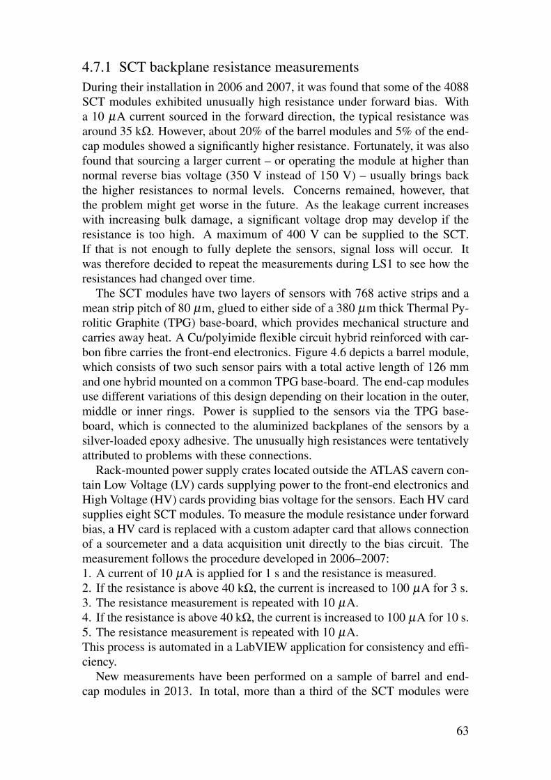
4.7.1 SCT backplane resistance measurementsDuring their installation in 2006 and 2007, it was found that some of the 4088SCT modules exhibited unusually high resistance under forward bias. Witha 10 µA current sourced in the forward direction, the typical resistance wasaround 35 kΩ. However, about 20% of the barrel modules and 5% of the end-cap modules showed a significantly higher resistance. Fortunately, it was alsofound that sourcing a larger current – or operating the module at higher thannormal reverse bias voltage (350 V instead of 150 V) – usually brings backthe higher resistances to normal levels. Concerns remained, however, thatthe problem might get worse in the future. As the leakage current increaseswith increasing bulk damage, a significant voltage drop may develop if theresistance is too high. A maximum of 400 V can be supplied to the SCT.If that is not enough to fully deplete the sensors, signal loss will occur. Itwas therefore decided to repeat the measurements during LS1 to see how theresistances had changed over time.

The SCT modules have two layers of sensors with 768 active strips and amean strip pitch of 80 µm, glued to either side of a 380 µm thick Thermal Py-rolitic Graphite (TPG) base-board, which provides mechanical structure andcarries away heat. A Cu/polyimide flexible circuit hybrid reinforced with car-bon fibre carries the front-end electronics. Figure 4.6 depicts a barrel module,which consists of two such sensor pairs with a total active length of 126 mmand one hybrid mounted on a common TPG base-board. The end-cap modulesuse different variations of this design depending on their location in the outer,middle or inner rings. Power is supplied to the sensors via the TPG base-board, which is connected to the aluminized backplanes of the sensors by asilver-loaded epoxy adhesive. The unusually high resistances were tentativelyattributed to problems with these connections.

Rack-mounted power supply crates located outside the ATLAS cavern con-tain Low Voltage (LV) cards supplying power to the front-end electronics andHigh Voltage (HV) cards providing bias voltage for the sensors. Each HV cardsupplies eight SCT modules. To measure the module resistance under forwardbias, a HV card is replaced with a custom adapter card that allows connectionof a sourcemeter and a data acquisition unit directly to the bias circuit. Themeasurement follows the procedure developed in 2006–2007:1. A current of 10 µA is applied for 1 s and the resistance is measured.2. If the resistance is above 40 kΩ, the current is increased to 100 µA for 3 s.3. The resistance measurement is repeated with 10 µA.4. If the resistance is above 40 kΩ, the current is increased to 100 µA for 10 s.5. The resistance measurement is repeated with 10 µA.This process is automated in a LabVIEW application for consistency and effi-ciency.

New measurements have been performed on a sample of barrel and end-cap modules in 2013. In total, more than a third of the SCT modules were

63

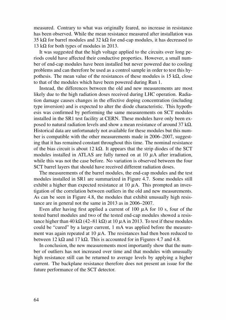
measured. Contrary to what was originally feared, no increase in resistancehas been observed. While the mean resistance measured after installation was35 kΩ for barrel modules and 32 kΩ for end-cap modules, it has decreased to13 kΩ for both types of modules in 2013.

It was suggested that the high voltage applied to the circuits over long pe-riods could have affected their conductive properties. However, a small num-ber of end-cap modules have been installed but never powered due to coolingproblems and can therefore be used as a control sample in order to test this hy-pothesis. The mean value of the resistances of these modules is 15 kΩ, closeto that of the modules which have been powered during Run 1.

Instead, the differences between the old and new measurements are mostlikely due to the high radiation doses received during LHC operation. Radia-tion damage causes changes in the effective doping concentration (includingtype inversion) and is expected to alter the diode characteristic. This hypoth-esis was confirmed by performing the same measurements on SCT modulesinstalled in the SR1 test facility at CERN. These modules have only been ex-posed to natural radiation levels and show a mean resistance of around 37 kΩ.Historical data are unfortunately not available for these modules but this num-ber is compatible with the other measurements made in 2006–2007, suggest-ing that it has remained constant throughout this time. The nominal resistanceof the bias circuit is about 12 kΩ. It appears that the strip diodes of the SCTmodules installed in ATLAS are fully turned on at 10 µA after irradiation,while this was not the case before. No variation is observed between the fourSCT barrel layers that should have received different radiation doses.

The measurements of the barrel modules, the end-cap modules and the testmodules installed in SR1 are summarized in Figure 4.7. Some modules stillexhibit a higher than expected resistance at 10 µA. This prompted an inves-tigation of the correlation between outliers in the old and new measurements.As can be seen in Figure 4.8, the modules that exhibit unusually high resis-tance are in general not the same in 2013 as in 2006–2007.

Even after having first applied a current of 100 µA for 10 s, four of thetested barrel modules and two of the tested end-cap modules showed a resis-tance higher than 40 kΩ (42–81 kΩ) at 10 µA in 2013. To test if these modulescould be “cured” by a larger current, 1 mA was applied before the measure-ment was again repeated at 10 µA. The resistances had then been reduced tobetween 12 kΩ and 17 kΩ. This is accounted for in Figures 4.7 and 4.8.

In conclusion, the new measurements most importantly show that the num-ber of outliers has not increased over time and that modules with unusuallyhigh resistance still can be returned to average levels by applying a highercurrent. The backplane resistance therefore does not present an issue for thefuture performance of the SCT detector.

64

4.7.2 Heater pads control system upgradeElectric resistance heating pads are used to maintain specific temperatures atvarious points within the inner detector. The most critical region is the thermalenclosure separating the SCT (which may be cooled to temperatures as low as−25 ◦C) from the TRT (which is operated at room temperature). Acciden-tal cooling would not only be detrimental to the operation of the TRT but itcould also physically damage the detector. To maintain the temperature differ-ence while placing a minimum amount of material between the detectors, theenclosure is actively heated.

The heater pads consist of thin (5–8 µm) copper tracks with a resistance of32–65 Ω sandwiched between two polyimide sheets. The heater pads rangefrom 0.04 to 0.64 m2 in size and provide a power output between 12 and120 W. There are in total 280 pads with a total heating capacity of 23 kW,installed along the pixel detector support tube, the TRT barrel, the SCT bar-rel and SCT end-caps, and the inner detector end-plates. They are operatedfrom a 48 V power source. With voltage drop across the cabling, there isnominally 40 V across the pads. The relatively low voltage is chosen out ofsafety concerns, as some heater pads are operated also during maintenanceaccess to the inner detector in order to keep temperatures above the caverndew-point. Heater pads are also equipped with 10 kΩ Negative TemperatureCoefficient (NTC) thermistors for monitoring the temperature in the vicinityof each heater. Not all installed heater pads are currently used for active heat-ing, but all available NTC thermistors are used to monitor the temperaturein various locations. Active heaters use the temperature readings to keep thetemperature at the desired level using Proportional-Integral-Derivative (PID)regulation. Some heaters are configured in a master/slave fashion, in whichcase multiple heaters follow the temperature readings of a single thermistor,effectively linking them together to a larger heating element.

Heater power is controlled by current pulses of varying length. Switchingon and off is done over a period of about 1 ms to limit electromagnetic inter-ference with sensitive detector elements. The switching is handled by custommade switching cards, each of which contains switching elements controlling16 channels, together with power handling electronics and an on-board con-troller in the form of a CERN Embedded Logical Monitoring Board (ELMB).The ELMB features an 8-bit microprocessor running at 4 MHz, multiple I/Ochannels, and a CAN bus interface. The switching cards are installed in rack-mounted crates in the relatively low radiation environment of the two under-ground caverns located next to the experiment. In each location, there is alsoa controller card. A number of safety features are in place to prevent damageto the ATLAS detector in the event of a component failure causing a too highpower output, one of which is the controller cards. They can prevent currentflow through connected heater pads independently of the switching circuits.The current is also limited by fuses in each switching element. Each ELMB

65

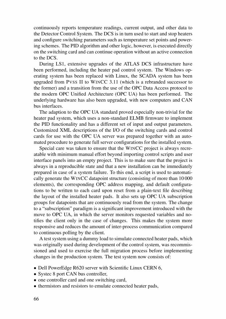
continuously reports temperature readings, current output, and other data tothe Detector Control System. The DCS is in turn used to start and stop heatersand configure switching parameters such as temperature set points and power-ing schemes. The PID algorithm and other logic, however, is executed directlyon the switching card and can continue operation without an active connectionto the DCS.

During LS1, extensive upgrades of the ATLAS DCS infrastructure havebeen performed, including the heater pad control system. The Windows op-erating system has been replaced with Linux, the SCADA system has beenupgraded from PVSS II to WINCC 3.11 (which is a rebranded successor tothe former) and a transition from the use of the OPC Data Access protocol tothe modern OPC Unified Architecture (OPC UA) has been performed. Theunderlying hardware has also been upgraded, with new computers and CANbus interfaces.

The adaption to the OPC UA standard proved especially non-trivial for theheater pad system, which uses a non-standard ELMB firmware to implementthe PID functionality and has a different set of input and output parameters.Customized XML descriptions of the I/O of the switching cards and controlcards for use with the OPC UA server was prepared together with an auto-mated procedure to generate full server configurations for the installed system.

Special care was taken to ensure that the WINCC project is always recre-atable with minimum manual effort beyond importing control scripts and userinterface panels into an empty project. This is to make sure that the project isalways in a reproducible state and that a new installation can be immediatelyprepared in case of a system failure. To this end, a script is used to automati-cally generate the WINCC datapoint structure (consisting of more than 10 000elements), the corresponding OPC address mapping, and default configura-tions to be written to each card upon reset from a plain-text file describingthe layout of the installed heater pads. It also sets up OPC UA subscriptiongroups for datapoints that are continuously read from the system. The changeto a “subscription” paradigm is a significant improvement introduced with themove to OPC UA, in which the server monitors requested variables and no-tifies the client only in the case of changes. This makes the system moreresponsive and reduces the amount of inter-process communication comparedto continuous polling by the client.

A test system using a dummy load to simulate connected heater pads, whichwas originally used during development of the control system, was recommis-sioned and used to exercise the full migration process before implementingchanges in the production system. The test system now consists of:

• Dell PowerEdge R620 server with Scientific Linux CERN 6,• Systec 8 port CAN bus controller,• one controller card and one switching card,• thermistors and resistors to emulate connected heater pads,

66

• WINCC 3.11 with a similar setup as on the production system (this instance,however, is configured to run stand-alone while the production version ispart of a distributed system),

• OPC UA Server,• UAEXPERT software for interactive communication with the OPC UA server,• low level tools for frame-by-frame debugging of CAN communication.

After migration of the production system, this setup is used for continuingwork on the heater pad control system. During LS1, the software/hardwaremapping of heater pads was also verified and corrected, and additional up-dates were made to the software, including control panel functions and alarmstatus definitions. Documentation on how to handle hardware failures was alsoassembled.

67

Part III: Data analyses

5. Analysis techniques

5.1 Signal and background processesThis thesis presents searches for light and heavy charged Higgs bosons pro-duced, respectively, in top quark decays and in association with a top quark.Final states involving leptons (electrons and muons) and b quarks are usedin all analyses. The largest backgrounds thus come from Standard Modelprocesses with top quarks, in particular the process gg → tt → bbW+W−,and also from vector boson production in association with jets. The mod-eling of signal events and the main backgrounds is performed with MonteCarlo simulations. Some backgrounds are difficult to simulate correctly andare therefore estimated using data-driven techniques. In particular, this is thecase for multi-jet processes. Such events can yield “fake” or non-prompt lep-tons that are misidentified as electrons or muons from the hard process. Thisbackground is always estimated using the matrix method, which will be de-scribed in section 5.3. With the event selections considered in the follow-ing, backgrounds with misidentified hadronic tau decays arise mainly fromtt events. The misidentification probability is, however, not expected to bewell reproduced by the simulation. In analyses of the data collected in 2011,this background is estimated using simulated events corrected to account forthe misidentification probabilities measured in the data. In analyses of thedata collected in 2012, this background is instead estimated with the matrixmethod, which does not directly depend on simulated events.

5.1.1 Data samplesOnly events recorded with stable proton beams and all ATLAS detectors fullyoperational are used for the analyses presented here. The 2011 dataset with√

s = 7 TeV fulfilling these conditions corresponds to an integrated lumi-nosity of 4.6 fb−1 with an uncertainty of 3.9%, while the 2012 dataset with√

s = 8 TeV corresponds to an integrated luminosity of 20.3 fb−1 with an un-certainty of 2.8%. The analysis presented in section 6.1 is performed with onlythe first 1.03 fb−1 of data collected in 2011. Events are only used for analysisif they fulfill basic data quality criteria and also do not contain any jet con-sistent with having originated from instrumental effects such as calorimeternoise or non-collision backgrounds. Events are also required to have at leastfive tracks with pT > 400 MeV associated to the primary vertex. The primaryvertex is the reconstructed vertex with the highest ∑ p2

T of associated tracks.

71

In all analyses, events are triggered by unprescaled single-lepton (electronor muon) triggers with the lowest threshold available in each data-taking pe-riod. An OR condition with a trigger having a higher pT threshold but relaxedisolation requirements allows for improved efficiency during the data-takingof later periods in 2011 and during 2012.

5.1.2 Simulated eventsThe main samples of simulated events are summarized in Tables 5.1 and 5.2.The listed cross sections depend on the exact generator settings, which ofteninclude filters for “interesting” events containing high-pT leptons, and shouldnot be compared directly between e.g. samples of different center-of-mass en-ergies. Details on each process are given in the sections below.

Signal processes

Three types of signal samples with light charged Higgs bosons have been used:tt → bbH+W−, tt → bbH−W+, and tt → bbH+H−, where the charged Higgsbosons decays into τν . The cross sections of the signal processes dependonly on the total cross section for tt production and on the branching fractionB(H+ → τν). These events are simulated with PYTHIA 6 [60], using theCTEQ6L1 PDF set [61]. For the analyses of 7 TeV data, samples are generatedwith the charged Higgs boson mass mH+ between 90 GeV and 160 GeV, insteps of 10 GeV. For the analyses of 8 TeV data, the mass range is increasedto 80 GeV ≤ mH+ ≤ 160 GeV.

Heavy charged Higgs bosons are only searched for in the analyses of 8 TeVdata, where the mass range 180 GeV ≤ mH+ ≤ 1 TeV is considered. Eventsare generated with POWHEG [62], using the CT10 PDF set [63], according tothe 5FS process gb → tH+. The parton shower, hadronization, and underlyingevent are simulated with PYTHIA 8 [64]. The charged Higgs boson decaysvia H+ → τν . Samples are generated with mH+ at 180 GeV, 190 GeV, thenin steps of 25 GeV in the range 200–600 GeV, and finally at 750 GeV and1 TeV. The ratio between the natural width of the charged Higgs boson andits mass is 3.5% for a mass of 600 GeV in the Type II 2HDM with tanβ = 50,and decreases rapidly with lower values of tanβ . As this is much smallerthan the experimental resolution, events are generated with the narrow-widthapproximation ΓH+ = 0 in order to obtain model-independent results.

For charged Higgs bosons close to the mass of the top quark, there is inter-ference between the two production mechanisms. Presently, no event genera-tor approved for use in ATLAS takes this interference into account. This massregion is also more difficult to study experimentally as one of the b quarks isproduced nearly at rest. Hence, this region is not included in the analyses.

72

Table 5.1. Simulated events used for analysis of 7 TeV data. All processes except Wt

production are required to contain at least one lepton ℓ = e,µ,τ in the decay chain.

In the analysis of early data presented in section 6.1, MC@NLO is used also for the

t-channel production of single top quark events, and the V +heavyflavor samples are

not included. The W + c(c)+ jets samples are used only in section 6.3.

Process Generator Cross section [pb]

tt MC@NLO 90.6Single top quark (t-channel) ACERMC 20.9Single top quark (s-channel) MC@NLO 1.5Single top quark (Wt-channel) MC@NLO 15.7W + jets ALPGEN 3.1×104

Wbb+ jets ALPGEN 1.3×102

Wcc+ jets ALPGEN 3.6×102

Wc+ jets ALPGEN 1.1×103

Z/γ∗+ jets (mℓℓ > 10 GeV) ALPGEN 1.5×104

Z/γ∗bb+ jets (mℓℓ > 30 GeV) ALPGEN 38.7WW HERWIG 17.0ZZ HERWIG 1.3WZ HERWIG 5.5tt → bbH±W∓, tt → bbH+H− with H+ → τν PYTHIA −

Table 5.2. Simulated events used for analysis of 8 TeV data. All processes except Wt

production are required to contain at least one lepton ℓ= e,µ,τ in the decay chain.

Process Generator Cross section [pb]

tt POWHEG 137.3Single top quark (t-channel) POWHEG 28.4Single top quark (s-channel) POWHEG 1.8Single top quark (Wt-channel) POWHEG 22.4W + jets ALPGEN 3.6×104

Wbb+ jets ALPGEN 1.5×102

Wcc+ jets ALPGEN 4.8×102

Wc+ jets ALPGEN 1.7×103

Z/γ∗+ jets (mℓℓ > 10 GeV) ALPGEN 5.2×103

Z/γ∗bb+ jets (mℓℓ > 30 GeV) ALPGEN 60.7Z/γ∗cc+ jets (mℓℓ > 30 GeV) ALPGEN 2.3×102

WW HERWIG 20.9ZZ HERWIG 1.5WZ HERWIG 7.0tt → bbH±W∓ with H+ → τν PYTHIA −tH+ with H+ → τν POWHEG −

73

Backgrounds with top quarks

In the analyses using 7 TeV data, the generation of Standard Model tt andsingle top quark events is performed with MC@NLO [65], with the exceptionthat in the analyses described in sections 6.2 and 6.3, ACERMC [66] is usedfor t-channel single top quark production. The parton shower, hadronization,and underlying event are simulated with HERWIG [67] and JIMMY [68] forevents generated with MC@NLO and with PYTHIA 6 for events generatedwith ACERMC. In the analysis using 8 TeV data, the generation of SM tt

and single top quark events is performed with POWHEG. The parton shower,hadronization, and underlying event are simulated with PYTHIA 8. The PDFset used is CT10. The nominal simulations of tt events are also compared withalternative samples to evaluate the systematic uncertainty associated with thechoice of event generator and parton shower programs, as will be detailed inthe description of each analysis. The top quark mass is taken to be 172.5 GeVin all samples. Inclusive cross sections are taken from approximate next-to-next-to-leading-order (NNLO) calculations for tt production at 7 TeV [69] and8 TeV [70], and for single top quark production [71–73]. Overlaps in the finalstates between the Wt and tt samples are removed.

In the analyses using 8 TeV data, a reweighting scheme is applied to the tt

events based on the generator level pT of both the top quark and the tt system.The applied weights were derived to improve agreement between simulatedevents and the measured tt differential cross section at 7 TeV [74].

Backgrounds with vector bosons

Single vector boson production is simulated with ALPGEN [75], using theCTEQ6L1 PDF set. In the analyses using 7 TeV data, the parton shower,hadronization, and underlying event are added with POWHEG and JIMMY. Inthe analyses using 8 TeV data, PYTHIA 8 is used. Inclusive W + jets andZ/γ∗+ jets samples are formed by adding samples generated with up to fiveadditional partons. The so-called MLM parton-jet matching scheme [76] isused to avoid overlap of parton configurations created by the event generatorand the parton shower. In most analyses, dedicated samples containing addi-tional b and c quarks are used in order to have a larger fraction of such events.Overlaps with events in the inclusive sample are removed. The cross sectionsare normalized to NNLO predictions [77, 78]. Diboson (WW , ZZ, and WZ)events are simulated with HERWIG and normalized to NLO predictions [79].

Pile-up, tuning, and charged leptons

All simulated events described above are overlaid with a variable numberof minimum-bias events in order to simulate the effect of multiple pp colli-sions. PYTHIA 6 is used to generate these events for the 7 TeV samples, whilePYTHIA 8 is used for the 8 TeV samples. At an early stage in each analysis,the simulated events are reweighted to match the distribution of the average

74

Number of vertices with 5 or more tracks0 2 4 6 8 10 12 14

Events

(unit a

rea)

0

0.05

0.1

0.15

0.2

0.25

0.3

0.35

0.4

)-1 Data 2011 (1.03 fb

MC, after pile-up reweighting

MC, before pile-up reweighting

Figure 5.1. Example of pile-up reweighting of a tt Monte Carlo (MC) sample tomatch the distribution of the average number of simultaneous pp collisions in data.The reweighting is validated by comparing the normalized distributions of the numberof reconstructed vertices.

number of pp collisions per bunch crossing in the corresponding data sample,as illustrated in Figure 5.1.

Some tools are tuned to describe ATLAS data. The AUET2 tune is usedwith HERWIG and PYTHIA 6, except when interfaced to ACERMC, in whichcase the AUET2B tune is used [80, 81]. The Perugia 2011 C tune [82] is usedwith PYTHIA 8. In all cases, except with PYTHIA 8, TAUOLA [83] is usedto model the decays of tau leptons and PHOTOS [84] is used to model photonradiation from charged leptons.

5.2 Particle identification5.2.1 ElectronsElectrons traverse the inner detector and deposit most of their energy in theelectromagnetic calorimeter. Electron candidates are therefore reconstructedby finding a cluster of energy deposits in the calorimeter that matches, bothin terms of position and energy, a track in the inner detector. The trans-verse energy of the electron candidate is defined as ET ≡ Eclus/cosh(ηtrack),combining the precision information on the track direction with the supe-rior resolution of the calorimeter at high energies. The analyses presentedin this thesis require electrons to have ET larger than 15–25 GeV and to bewithin |ηclus| < 2.47. In the transition region between the barrel and end-cap calorimeters (1.37 < |ηclus|< 1.52), the electron identification and energyresolution are degraded by the large amount of material in front of the instru-mented layers. Electrons in this region are therefore excluded.

75

The electron identification is refined by a set of quality requirements oncalorimeter and track variables that include information on the shower shape,the number of hits in the inner detector, and the longitudinal impact parameterwith respect to the primary vertex. The exact criteria used have evolved overtime but typically correspond to an electron efficiency of 70–80% given theabove mentioned ET thresholds. To favor prompt electrons over electrons pro-duced inside jets, tracking- and calorimeter-based isolation requirements areimposed within cones of radius R = 0.2 respectively 0.3 around the electron.The thresholds used are ET- and η-dependent to give a flat efficiency of about90% for true isolated electrons. The track-based isolation for electrons was alater introduction and is not used in the analysis presented in section 6.1.

5.2.2 MuonsMuons penetrate all ATLAS detectors. All detector systems can thereforecontribute to the muon reconstruction and identification. The analyses doc-umented in this thesis use muons reconstructed with a track in both the innerdetector and the muon spectrometer, with quality requirements on the numberof hits and on the longitudinal impact parameter with respect to the primaryvertex. Muons must therefore be in the range |η | < 2.5 covered by the innerdetector. The muon pT is obtained as a weighted combination of both tracks.It is required to be at least 15 GeV in the analyses using data with

√s = 7 TeV

and at least 25 GeV in the analyses using data with√

s = 8 TeV. To reduce thecontribution of muons produced inside jets, isolation requirements are applied.The analyses of 7 TeV data use fixed thresholds on the transverse momentumof inner detector tracks and calorimeter energy deposits (excluding those orig-inating from the muon itself) within cones of radius R = 0.2 respectively 0.3.In the analysis of 8 TeV data, only the track-based isolation is used, but with apT-dependent cone size.

5.2.3 JetsJets are reconstructed from energy clusters in the calorimeters using the anti-kt algorithm [85, 86] with a size parameter value R = 0.4. Two differentjet energy calibration schemes [87] are used in the analyses presented here.The analyses of 7 TeV data use a scheme in which the (non-compensating)calorimeter cells are initially calibrated at the electromagnetic scale appropri-ate for energy deposits from electrons and photons. The energy of a recon-structed jet is then first corrected for pile-up effects and then restored to thehadronic energy scale based on correction factors derived from simulation.The analysis of 8 TeV data use jets reconstructed with locally calibrated clus-ters. In this scheme, which aims at reducing energy fluctuations, each clusteris individually classified as either electromagnetic or hadronic based on shape

76

variables. It is then calibrated accordingly, with additional corrections to ac-count for energy lost out of clusters and in dead material. The anti-kt algorithmis run over the locally calibrated clusters, and the reconstructed jets are cor-rected for pile-up. Only jets with pT above 20–25 GeV are considered in theanalyses presented here. Furthermore, the use of b-tagging (see below), whichrelies on tracking information, excludes the use of jets above |η |= 2.5.

Jet vertex fraction

To select jets originating from the hard-scatter interaction, the Jet Vertex Frac-tion (JVF) method [88] is used. The JVF quantity is the fraction of the totalmomentum of all charged particle tracks associated with the jet that originatefrom the primary vertex (pv):

JVF(jet,pv) =∑i

pT(trkjeti ,pv)

∑n

∑j

pT(trkjetj ,vtxn)

(5.1)

In all analyses, except section 6.1, jets with pT < 50 GeV and |η | < 2.4 arerequired to have JVF > 0.5 (jets that do not have any associated tracks areassigned JVF = 1). This selection is shown to be insensitive to pile-up.

bbb-tagging

Jets that originate from a b quark can be identified by tagging the decay of aB-hadron inside the jet. The large masses (> 5 GeV) and relatively long life-times (1.5 ps) of B-hadrons can be exploited for this purpose. The b-taggingmethods used in the analyses presented here ultimately rely on three differentalgorithms. The IP3D algorithm uses impact parameter significances in boththe longitudinal and transverse directions for all tracks within a jet. The SV1algorithm attempts to explicitly reconstruct a secondary vertex. Finally, theJetFitter algorithm seeks to reconstruct the full decay chain from a B-hadronto a charm hadron to its decay products, i.e. the common flight path and the po-sition of additional vertices along it. These methods are combined into highlyperformant taggers using neural networks. The dilepton analysis in section 6.1uses a b-tagger which combines information from JetFitter and IP3D, whilethe other analyses in this thesis use a b-tagger that also includes informationfrom SV1. In both cases, the working point has been chosen such that thetagging efficiency is approximately 70% in tt events.

5.2.4 Hadronic tau decaysThe tau lepton has a mean lifetime of only 0.3 ps, meaning that it decays veryclose to the interaction point. In the case of leptonic decays, it is not possibleto reliably identify electrons or muons as originating from a tau. However,

77

Table 5.3. Common decay modes of tau leptons [1].

Decay mode Branching fraction

Leptonic 35.2%eνeντ 17.8%µ νµ ντ 17.4%

1-prong hadronic 50.1%π−ντ 10.8%π−π0ντ 25.5%π−π0π0ντ 9.3%other 4.5%

3-prong hadronic 14.6%π−π−π+ντ 9.3%π−π−π+π0ντ 4.6%other 0.7%

approximately 65% of tau leptons decay to hadrons, and these decays haverather characteristic signatures. Table 5.3 summarizes the most common taudecay modes. The hadronic decay modes typically contain either one or threecharged pions, and are respectively referred to as 1-prong and 3-prong decays.

In order to reconstruct hadronically decaying tau leptons [89, 90], hence-forth denoted τhad, all anti-kt jets constructed with the size parameter R = 0.4are considered as τhad candidates if they have pT > 10 GeV and contain eitherone or three tracks within the central cone of radius R = 0.2. This would beconsistent with the presence of one or three charged pions among the tau decayproducts. Identification variables are then calculated and combined into multi-variate discriminants used to reject τhad candidates originating from jets andleptons. Variables related to the shower shape are used to discriminate betweenreal τhad candidates and jets, exploiting the fact that quark- or gluon-initiatedjets tend to be wider than jets from hadronic tau decays. The significance ofa reconstructed secondary vertex is also important, in particular for 3-prongτhad candidates. Variables based on tracking information are relatively robustagainst pile-up effects. To decrease the pile-up dependence of the calorimeterbased variables, only clusters within the central cone (R = 0.2) are consideredin the 2012 data (correspondingly R = 0.4 in 2011). Different sets of variablesare combined using either a projective Log-Likelihood function (LLH), whichassumes that the inputs are uncorrelated, or Boosted Decision Trees (BDT).In the analyses presented in this thesis, the LLH-based identification is usedwith the 2011 dataset, while the BDT is used with the 2012 dataset. Based onpT- and η-dependent thresholds on the discriminant output, τhad candidatesare accepted with an efficiency of 30% for 1-prong and 35% for 3-prong τhadcandidates in the 2011 data. In the 2012 data, these numbers become 40%and 35%, respectively. After rejection of a large fraction of τhad candidates

78

originating from jets, the background from electrons may become important,in particular for 1-prong τhad candidates. Electrons are rejected using a dedi-cated BDT, with input variables sensitive to the transition radiation emitted byan electron, as well as the shorter and narrower shower in the electromagneticcalorimeter compared to hadronic tau decays. Finally, a cut-based veto is em-ployed to suppress τhad candidates originating from an energetic calorimetercluster associated with a muon track in cases where the muon was not success-fully reconstructed in the muon spectrometer.

The τhad energy is calculated based on calorimeter clusters within the cen-tral cone, with a special calibration scheme appropriate for the specific mixtureof charged and neutral pions present in hadronic tau decays. Due to the use oftracking information, the τhad reconstruction is limited to the region |η |< 2.5covered by the inner tracker.

5.2.5 Removal of overlapping objectsWhen multiple objects overlap geometrically, the following steps are applied,in this order:1. a τhad object is removed if found within ΔR < 0.2 of a muon;2. a τhad object is removed if found within ΔR < 0.2 of an electron;3. a muon is removed if found within ΔR < 0.4 of a jet;4. the single closest jet to an electron is removed if it is within ΔR < 0.2;5. an electron is rejected if found within ΔR < 0.4 of a jet;6. a τhad object is removed if found within ΔR < 0.4 of a b-tagged jet;7. a jet is removed if found within ΔR < 0.4 of a τhad.The procedures involving τhad objects are only applied in analyses using theseobjects. The removal of a τhad object overlapping with a b-tagged jet is onlyperformed in the most recent analyses presented in section 6.3 and chapter 7,and in the latter case, only 3-prong τhad objects are considered in this step.Finally, in the rare case where an electron and a muon share a track in theinner detector, the whole event is discarded.

5.2.6 Missing transverse energyNeutrinos do not interact with any detector and hence are effectively invisible.Their presence in an event can be inferred, however, from an apparent viola-tion of momentum conservation in the transverse plane. The vector sum oftransverse momenta in an event is first constructed from all energy clusters inthe calorimeters, with the appropriate calibration of any associated high levelobjects, and from muon tracks reconstructed in the muon spectrometer. En-ergy deposited by muons in the calorimeter is taken into account with differenttreatments of isolated and non-isolated muons. Energy deposits in calorimetercells not associated to any object are also included. The analyses presented

79

in this thesis do not use any special treatment of τhad objects for this purpose,they are treated as ordinary jets. The magnitude of the total transverse mo-mentum is equal to that of the missing transverse momentum which would beneeded in the opposite direction in order to balance the total sum to zero. Itis denoted Emiss

T and would correspond to the transverse energy of a single,massless, undetected particle in the event.

5.3 The matrix methodNon-negligible backgrounds arise from events with misidentified leptons orhadronic tau decays. These include “fake” signatures of such objects and, inthe case of leptons, real but “non-prompt” leptons originating from hadronicobjects. Misidentified electrons arise from the semileptonic decays of b and c

quarks, photon conversion, and from jets that deposit a large fraction of theirenergy in the electromagnetic calorimeter. Misidentified muons arise fromsemileptonic decays of b and c quarks, in-flight decays of charged hadrons,and from punch-through of energetic particles into the muon system. Misiden-tified τhad objects are mainly caused by quark- or gluon-initiated jets, or fromelectrons, and to a lower extent by energy deposits in the calorimeter comingfrom passing muons.

In event selections requiring a single lepton, the largest such background isfrom multi-jet events. In event selections requiring two leptons or one leptonand a τhad, backgrounds with misidentified objects consist of tt and W + jetsevents with one real lepton and one misidentified lepton or τhad, and to a muchsmaller extent, events with two misidentified objects.

These backgrounds are particularly challenging to simulate accurately, andwould in addition require very large samples of simulated events due to theirlow probability to occur. Hence, they are estimated using data-driven tech-niques. In the analyses presented here, the so-called matrix method is fre-quently used for this purpose. This method uses object (mis)identificationprobabilities measured in data, simulated events, or a mixture of both, and canbe used to assess the backgrounds of events with one or several misidentifiedobjects, both in terms of overall normalization and in the distributions of anynumber of kinematic variables. It takes its name from a characteristic equationappearing in its derivation, as will be shown below.

5.3.1 Description of the matrix methodConsider first the case where only one reconstructed object (electron, muon orτhad) has a significant possibility of being misidentified. We define two eventselections, differing only in the isolation and/or identification criteria appliedto that type of object. The tight criteria correspond to the nominal object selec-tion (i.e. as detailed in section 5.2) and supposedly select mainly real objects.

80

The loose criteria select a larger fraction of events with misidentified objectsand are obtained by relaxing some of the requirements of the tight selection.By construction, the loose selection is a superset of the tight selection.

A sample of N events passing the loose object selection contains NT eventsin which the object fulfills the tight selection and NL events in which the objectfulfills the loose but not tight selection. It also contains Nr events with a real (r)object and Nm events with a misidentifed (m) object: Nr+Nm = N = NL+NT.We seek to determine the number of events in NT that are also in Nm, that is,the amount of events passing the tight selection that contain a misidentifiedobject.

If we define pr and pm as the probabilities for a real or misidentified object,respectively, to pass the tight criteria if it has already passed the loose criteria,the following relations can be established:

�

NT

NL

�

=

�

pr pm

1− pr 1− pm

�

�

Nr

Nm

�

. (5.2)

The number of events, NTm, in which the misidentified object passes the tight

selection can, after inverting the 2×2 matrix above, be written as:

NTm = pmNm =

pm pr

pr − pmNL +

pm(pr −1)pr − pm

NT. (5.3)

This equation is, however, only valid if pr and pm are constants. This is typi-cally not the case in a broad selection of events. Instead of directly calculatingNT

m for a whole selection of events, a weight is assigned to each individualevent and the total contribution of misidentified objects is obtained by sum-ming over all events. The weights, denoted wT for events that pass the tightselection and wL for events that pass the loose-but-not-tight selection, have theform:

wL =pm pr

pr − pm, wT =

pm(pr −1)pr − pm

, (5.4)

where pr and pm are now functions of the properties of the object of interest(for example its pT). Note that the weight is negative for events in the tightsample.

The (mis)identification probabilities must be measured, in the data or insimulated events. If the available control sample is of limited size, a too finebinning of pm and pr may introduce large statistical fluctuations of the mea-sured values. This effectively limits the number of variables that can be usedin the parametrization of pm and pr. If pm and pr depend only on largelyuncorrelated variables, however, the situation simplifies. With n uncorrelatedvariables xxx, pm and pr can be constructed by convoluting n one-dimensionalparametrizations. If �pm� and �pr� are the average values of pm respectively

81

pr over the whole data sample, the final identification and misidentificationprobabilities in each event are computed as:

pr = pr(x0)×n−1

∏i=1

pr(xi)

�pr�, pm = pm(x0)×

n−1

∏i=1

pm(xi)

�pm�. (5.5)

This method is used in the matrix method for misidentified leptons.

5.3.2 Two misidentified objectsHaving now established the strategy, the matrix method is easily generalizedto treat events with a larger number of potentially misidentified objects. Ofinterest in this thesis are events with two leptons, or one lepton and one τhad.In this case, we distinguish four classes of events, labeled rr, rm, mr, andmm. They correspond to events with two real objects, events with one realand one misidentified object (in two different combinations), and events withtwo misidentified objects. For each object, a nominal, tight (T) selection anda loose-but-not-tight (L) selection are defined.

A loose sample of events is again considered, consisting of the four subsetsNTT, NTL, NLT, and NLL. The composition of the loose sample in terms ofNrr events with two real objects, Nrm (Nmr) events where the first (second)object is real and the other one is misidentified, and Nmm events with twomisidentified objects, is not directly observable. The two sets of numbers arehowever related by:

NTT

NTL

NLT

NLL

=

pr1 pr2 pr1 pm2 pm1 pr2 pm1 pm2

pr1 pr2 pr1 pm2 pm1 pr2 pm1 pm2

pr1 pr2 pr1 pm2 pm1 pr2 pm1 pm2

pr1 pr2 pr1 pm2 pm1 pr2 pm1 pm2

×

Nrr

Nrm

Nmr

Nmm

(5.6)

where the numeric index distinguishes the two objects of interest, and theshort-hand notation p ≡ (1− p) is introduced to exhibit the regular structureof the matrix.

The number of events with two tight objects, where at least one of them ismisidentified, can be written as:

NTTmisid = NTT

rm +NTTmr +NTT

mm = pr1 pm2Nrm + pm1 pr2Nmr + pm1 pm2Nmm. (5.7)

As before, solving equation (5.6) for Nmm, Nmr and Nrm gives the weights tobe applied to events passing the LL, LT, TL, respectively TT selections:

wLL =−pr1 pr2 pm1 pm2

(pr1 − pm1)(pr2 − pm2), wTT = 1− pr1 pr2 pm1 pm2

(pr1 − pm1)(pr2 − pm2),

wLT =pr1 pr2 pm1 pm2

(pr1 − pm1)(pr2 − pm2), wTL =

pr1 pr2(1− pm1)pm2

(pr1 − pm1)(pr2 − pm2).

(5.8)

82

Similar weights can be derived for each of the indvidual NTTrm , NTT

mr , and NTTmm

contributions, which can reveal the sensitivity of the analysis to different com-binations of misidentified objects. The weights in equation (5.8) can also beconveniently expressed as functions of two sets of object-specific weights asconstructed in equation (5.4):

wLL =−wL1 ×wL

2 , wTT = wT1 +wT

2 −wT1 ×wT

2 ,

wTL = (1−wT1 )×wL

2 , wLT = wL1 × (1−wT

2 ).(5.9)

This form can have practical advantages if one wishes to combine the resultsof two independently developed methods for different object types.

5.4 Hypothesis testingAll results are interpreted by testing the compatibility of the data with thebackground-only and signal+background hypotheses using a modified fre-quentist profile likelihood method which incorporates systematic uncertaintiesas nuisance parameters and fits (profiles) them to the data. This procedure canminimize the impact of systematic uncertainties on the search sensitivity bytaking advantage of background-dominated control regions.

5.4.1 Statistical modelLet m and n be the number of events that are expected respectively observedto pass some selection criteria. The expected number of events m depends onsome parameter of interest µ , describing the strength of the signal process.It is chosen such that µ = 0 corresponds to the background-only hypothesisand larger values of µ correspond to increasing amounts of signal. Uncertain-ties in the calculation of m are described by its additional dependence on aset of nuisance parameters θθθ with unknown values. Each nuisance parameterθi is, however, provided with a nominal estimate θi and a Gaussian constraintp(θi|θi) which gives the estimated probability density of having obtained theestimate θi if the true value is in fact θi. A nuisance parameter could for exam-ple be the integrated luminosity, in which case θi is the measured luminosityand the standard deviation of p(θi|θi) is the uncertainty on the measurement.The likelihood of the model parameters µ and θθθ having certain values giventhe observed n events is equal to the probability of obtaining the observed n

events given those parameter values:

L (µ,θθθ) = Poisson(n|m(µ,θθθ))∏i

p(θi|θi). (5.10)

This likelihood function describes a simple event counting experiment. Typi-cally, the search sensitivity is improved by examining the distribution of some

83

discriminating variable among the selected events. A likelihood function canthen be built from the expected and observed number of events, m j and n j,found in each bin j of the distribution of this variable.

Furthermore, an analysis may simultaneously use multiple event selections.We call each event selection a Signal Region (SR) if it is expected to containa significant amount of events from the signal process, or a Control Region(CR) if it mainly contributes to the sensitivity by constraining the nuisanceparameters. The resulting likelihood is then given by:

L (µ,θθθ) = ∏k

∏jk

Poisson(n jk |mjk(µ,θθθ))∏i

p(θi|θi), (5.11)

where each region k may use a different discriminating variable with jk bins,or none (in which case jk has only one possible value and n jk corresponds toall events found in that region).

Light charged Higgs boson

In searches for a light charged Higgs boson appearing in the decay of a topquark, the parameter of interest is the branching fraction B ≡ B(t → bH+).Varying this parameter changes not only the expected amount of signal butalso the expected amount of background from tt → bbW+W− events. Thecross sections of the possible tt decays are:

tt → bbW+W− : σbbWW = σtt × (1−B)2 (5.12)

tt → bbH±W∓ : σbbHW = σtt ×2B(1−B) (5.13)

tt → bbH+H− : σbbHH = σtt ×B2. (5.14)

As B is assumed to be small, the tt → bbH+H− process is ignored in theanalyses presented here, unless otherwise stated. If an event selection has theacceptance rates εW and εH for tt → bbW+W− respectively tt → bbH±W∓ (asdetermined in the analysis), then the expected number of events m is given by:

m = mW +mH +mother = mtt

�

(1−B)2εW +2B(1−B)εH

�

+mother, (5.15)

where mtt is the product of σtt and the integrated luminosity, and mother ac-counts for non-tt backgrounds.

Heavy charged Higgs boson

At first order, the presence of a heavy charged Higgs boson does not affect thebackgrounds. The parameter of interest is therefore simply the cross sectionfor heavy charged Higgs boson production. This is similar to the case of theStandard Model Higgs boson searches at the LHC, however in that case (seeFigure 3.2), µ is typically expressed in units of the cross section predicted bythe Standard Model. Here, the focus is on model-independent searches, hencethere is no predicted cross section and µ is a dimensionful quantity.

84

5.4.2 Exclusion limitsIf the data appears to be compatible with the background-only hypothesis, theanalysis proceeds by rejecting the signal hypothesis for various values of µ .The test statistic used is the one-sided profile likelihood ratio [91],

qµ ≡

−2logL (µ, ˆ

θθθ µ)

L (0, ˆθθθ 0)

µ < 0,

−2logL (µ, ˆ

θθθ µ)

L (µ, θθθ)0 ≤ µ ≤ µ ,

0 µ > µ .

(5.16)

It is constructed by fitting the model parameters to the data to find the values

θθθ and µ that maximize L (µ, θθθ), as well as the nuisance parameter values ˆθθθ µ

that maximize L (µ, ˆθθθ µ) for a given µ . The test statistic is then a function

of µ alone and can be seen as a measure of the discrepancy between the dataand a given hypothesis about the value of µ: higher qµ values correspond toan increasing disagreement. The difference is quantified by calculating theprobability, under the given hypothesis, of obtaining a value of qµ at least aslarge as the observed value, qobs

µ .If P(qµ ≥ qobs

µ |µ) < α , then this value of µ could be regarded as excludedat a confidence level of 1−α . A problem with this approach, however, isthat it is susceptible to P(qµ ≥ qobs

µ |µ) dropping below α due to a statisticalfluctuation of qobs

µ . This may lead us to exclude a hypothesis to which theexperiment is not actually sensitive. In fact, in the limit where the amount ofsignal is very small compared to the background, the probability for this tohappen approaches α . We therefore use the CLs method [92], which weightsthe probability of obtaining qobs

µ under a given hypothesis about the value of µ

with the probability of obtaining qobs0 under the background-only hypothesis,

µ = 0. The hypothesis is rejected at the confidence level 1−α if

CLs ≡P(qµ ≥ qobs

µ |µ)P(qµ ≥ qobs

µ |0) < α. (5.17)

The CLs method ensures that the signal hypothesis will not be excluded ifthe data disagrees with both the signal and background-only hypotheses. Inparticular, if the distributions of the test statistic are very similar for the twohypotheses, then the CLs quantity always remains large – this means that noexclusion is made if the experiment can not distinguish between the signal andbackground-only hypotheses. Because the denominator in the definition ofCLs is a probability, it is never larger than one. The CLs method therefore pro-duces exclusion limits that are more conservative than using P(qµ ≥ qobs

µ |µ)directly.

85

As is the convention1 at the LHC, α is chosen to be 0.05. The analysis isthen carried out by starting from the background-only hypothesis and increas-ing µ until CLs reaches α . Upper limits on µ are thus obtained at the 95%confidence level. Expected limits in the absence of signal are determined byrepeating the procedure while using an artificial “Asimov” dataset as input in-stead of the actual data. The Asimov dataset is an estimate of what the datawould look like in the absence of statistical fluctuations, if the background-only hypothesis was true. It is created by profiling the nuisance parameterswhile fixing µ = 0 and then constructing a representative dataset from the cor-responding expected m values. As the fitted values of θθθ are obtained whileforcing the background-only hypothesis, they are not necessarily close to theirtrue values if there is indeed some signal events present in the data. The ex-pected limits can therefore be seen as somewhat conservative.

Asimov datasets also have another important use. In order to calculateP(qµ ≥ qobs

µ |µ), one needs to know the probability density function of qµ .It can be obtained from numerous Monte Carlo pseudo-experiments, but thiscan be computationally expensive. We instead make use of the asymptoticapproximation that, in the large sample limit, qµ always follows a non-centralhalf χ2-distribution, the median of which can be estimated using an Asimovdataset corresponding to that value of µ [91].

1 In the context of excluding a signal hypothesis. For the purpose of establishing a discovery

– which means rejecting the background-only hypothesis – a much smaller α , correspondingto five standard deviations, is normally used. The reason for this is that multiple searches (indifferent mass ranges, for example) are carried out simultaneously, which increases the risk offalse positives. When attempting to reject the signal hypothesis, however, increasing the searchrange only makes it more difficult to exclude the signal everywhere.

86

6. Searches for H+ → τν in 7 TeV data

In this chapter, three searches for a light charged Higgs boson decaying to

τν are presented, based on the 7 TeV dataset collected by ATLAS in 2011.

It is assumed that B(H+ → τν) = 100%. In all cases, the signal process

is characterized by the additional presence of a top quark that decays to an

electron or a muon. This high-pT lepton clearly distinguishes these events

from most of the multi-jet background, and is used for triggering.

The cleanest channel is the dilepton final state, where the tau originating

from the charged Higgs boson also decays leptonically. The dilepton chan-

nel was analyzed with the first 1.03 fb−1 of pp collision data recorded at√s = 7 TeV. However, only modest sensitivity to a light charged Higgs boson

was achieved in this channel and the analysis was not repeated with the full

dataset.

Instead, focus was shifted to events where the tau lepton decays hadron-

ically (τhad). The hadronic decay modes of the tau have higher branching

fractions, and yield events with fewer neutrinos, but come with a challenging

background in the form of quark- or gluon-initiated jets that may be misiden-

tified as hadronic tau decays. Because the misidentification probability is not

expected to be well-modeled by Monte-Carlo simulations, it is measured in

control regions in the data. The lepton+τhad channel was analyzed using

the full 2011 dataset, corresponding to an integrated luminosity of 4.6 fb−1.

and upper limits on B(t → bH+) extracted using the EmissT distribution. The

data was then re-analyzed with a simultaneous treatment of the dilepton and

lepton+τhad channels. This analysis performed as a test of lepton universal-

ity in tt events, in the form of an event-counting experiment, where the role of

the dilepton channel is primarily to constrain the uncertainties on the back-

grounds, rather than providing direct sensitivity to the signal. Events where

the reconstructed τhad has the same sign of charge as the lepton are subtracted

from the events where they have opposite charges, which cancels the contribu-

tions of gluons and b-jets misidentified as hadronic tau decays. The ratio of

lepton+τhad and dilepton events is found to be consistent with the Standard

Model prediction. Upper limits on B(t → bH+) are set in the range 3.2–4.4%

for H+ masses within 90–140 GeV. Combinations of these results with those

of other ATLAS searches for charged Higgs bosons, and interpretations in the

MSSM mmaxh scenario were also performed.

In this chapter, three searches for a light charged Higgs boson decaying toτν are presented, based on the 7 TeV dataset collected in 2011. Here, it is

87

assumed that B(H+ → τν) = 100%. In all cases, the signal process is char-acterized by the additional presence of a top quark that decays to an electronor a muon. This high-pT lepton clearly distinguishes these events from mostof the multi-jet background, and is used for triggering. The cleanest channel(with the least amount of difficult-to-handle backgrounds with misidentifiedobjects) is the dilepton final state, where the tau originating from the chargedHiggs boson also decays leptonically. The dilepton channel was analyzed withthe first 1.03 fb−1 of pp collision data recorded at

√s = 7 TeV. However, only

modest sensitivity to a light charged Higgs boson was achieved in this chan-nel and the analysis was not repeated with the full dataset. Instead, focuswas shifted to events where the tau lepton decays hadronically (τhad). Thehadronic decay modes of the tau have higher branching fractions, and yieldevents with fewer neutrinos, but come with a challenging background in theform of quark- or gluon-initiated jets that may be misidentified as hadronictau decays. Methods for estimating this background, with decreasing relianceon simulation, were developed. The lepton+τhad channel was analyzed usingthe full 2011 dataset, corresponding to an integrated luminosity of 4.6 fb−1.The data was then re-analyzed with a simultaneous treatment of the dileptonand lepton+τhad channels. This analysis is cast as a test of lepton universalityin tt events, in the form of an event-counting experiment, where the role ofthe dilepton channel is primarily to constrain the uncertainties on the back-grounds, rather than providing direct sensitivity to the signal.

The analyses presented in this chapter all use single-lepton triggers witha pT threshold of 20–22 GeV for electrons and at 18 GeV for muons. Withthese thresholds, electrons with ET > 25 GeV and muons with pT > 20 GeVare guaranteed to be in the plateau region of the trigger efficiency curve.

6.1 Dilepton channelWith the first 1.03 fb−1 of ATLAS data collected at

√s = 7 TeV in 2011, a

search for light charged Higgs bosons in tt events was performed using finalstates with two charged leptons (electrons or muons). This analysis is alsodocumented in Ref. [93]. Figure 6.1 illustrates the contribution from eventsinvolving a charged Higgs boson. If some fraction of top quark decays happenvia t → bH+ and the charged Higgs boson decays solely into τν , a smallincrease in the number of tt events with two charged leptons in the final stateis expected, because the tau lepton decays leptonically more often than the W

boson does: B(H+ → τν → ℓ+3ν) = 35% while B(W → ℓ+Nν) = 25%,where ℓ denotes either an electron or a muon. However, relying only on thedetection of a small excess of such events would give limited sensitivity to thepresence of a charged Higgs boson in tt decays. Kinematic variables that canfurther discriminate between events with and without charged Higgs bosonshave therefore been identified [94].

88

b

t

H+

ντ

τ+

ℓ+

νℓ

ντ

b

νℓ

ℓ−

t W−

Figure 6.1. Feynman diagram of a tt event involving a charged Higgs boson, with twocharged leptons ℓ= e,µ in the final state.

Discriminating variables

One useful quantity is the invariant mass mbℓ of the b quark and the leptoncoming from the same top quark. It is used here in the form of the variablecosθ ∗

ℓ defined as

cosθ ∗ℓ =

2m2bℓ

m2t −m2

W

−1 ≈ 4pb · pℓ

m2t −m2

W

−1 (6.1)

with pb · pℓ = EbEℓ(1− cosθbℓ), where pb,ℓ are the four-momenta of the b

quark and the lepton, and θbℓ is the angle between them. The approximationin equation (6.1) is valid if the masses of the b quark and the lepton are ne-glected so that m2

bℓ = 2pb · pℓ. Equation (6.1) contains only Lorentz invariantproducts and can be computed in any reference frame. The use of cosθ ∗

ℓ inanalyses of top quark decays originates in measurements of W polarization,where θ ∗

ℓ is the angle between the lepton momentum and the helicity axis inthe W rest frame. Here, the lepton is assumed to appear via the decay of atau, which dilutes the polarization information. The discriminating power ofcosθ ∗

ℓ instead comes from the fact that the lepton in this case receives a lowermomentum than if it would come directly from the decay of a W boson. Thisreduction of the lepton momentum is somewhat counteracted if the chargedHiggs boson is heavier than the W , however that instead reduces the momen-tum available to the b quark. Top quarks decaying via a charged Higgs bosontherefore produce cosθ ∗

ℓ values close to −1.The generalized charged Higgs boson transverse mass mH

T2 [95] is alsoused. This is the maximum charged Higgs boson mass allowed in an event,given the known masses of the W boson and the top quark, as well as conser-vation of momentum in the transverse directions. Following the notation of

89

Figure 6.1, if one top quark decays into bW− and the other top quark decaysinto bH+, then the following set of constraints apply:

(pH++ pb)2 = m2

t ,

(pℓ−+ pνℓ)2 = m2

W ,

(pℓ−+ pνℓ + pb)2 = m2

t , (6.2)

(pνℓ)2 = 0,

�pTH+ − �pT

ℓ+ + �pTνℓ = �pT

miss.

Here, pH+and pνℓ represent the unknown quantities in the event. With the six

constraints of (6.2), there are two degrees of freedom over which the chargedHiggs boson mass is maximized to obtain mH

T2. Note that the decay products ofthe charged Higgs boson are not explicitly included in these equations, as thiswould not supply any additional constraint on the mass of the charged Higgsboson. The charged Higgs boson can be replaced by a W+ and the constraintsof (6.2) hold even if there is no tau lepton in the event. The mH

T2 quantity istherefore always the upper bound on the mass of the boson mediating the topquark decay. By definition, it lies between the true mass of the charged Higgsboson and the mass of the top quark: mH+ ≤ mH

T2 ≤ mt . This is true even if thetop quark radiates a gluon before it decays, as this can only lower the value ofmH

T2, which is nevertheless still bounded from below by mH+ .The variable mH

T2 is called the generalized charged Higgs boson transversemass because of its relation to other transverse mass observables. The widelyused W transverse mass mW

T is defined as�

mWT

�2= 2pℓTEmiss

T (1− cosΔφℓ,miss). (6.3)

In an event with a single charged lepton ℓ and a single neutrino, mWT can be

obtained by minimizing the invariant mass of these objects subject to the con-straint that the neutrino must be massless,

�

mWT

�2= min{(pmiss)2=0}

�

�

pℓ+ pmiss�2

�

. (6.4)

If the single charged lepton comes from the decay of a tau lepton, which couldin turn be the decay product of a charged Higgs boson, then the constraint�

pmiss�2

= 0 is not valid as there are three neutrinos in the event. One caninstead define the charged Higgs boson transverse mass mH

T by using a con-straint on the top quark mass:

�

mHT

�2= max{(pmiss+pℓ+pb)2=m2

t }

�

�

pℓ+ pmiss�2

�

. (6.5)

Note that, while mWT is obtained as the result of a minimization, mH

T is the resultof a maximization. Finally, in events with two charged leptons in the final

90

state, there are neutrinos appearing in the decays of both top quarks. With theset of constraints (6.2), the generalized charged Higgs boson transverse massmH

T2 can in turn be written as a maximization of mHT ,

mHT2 = max

{constraints}[mH

T (�pTH+

)]. (6.6)

The variable mHT has an analytical expression,

�

mHT (�pT

H+)�2

=

��

m2t +(�pT

H++ �pT

b)2 − pbT

�2

−�

�pTH+

�2, (6.7)

while the maximization of mHT2 over the remaining parameter must be done

numerically.

Event selection

In this analysis, events are selected if:• There are exactly two oppositely charged leptons with ET > 15 GeV (elec-

trons) or pT > 15 GeV (muons).• At least one of the leptons is matched to the single-lepton trigger object with

ET > 25 GeV (electron) or pT > 20 GeV (muon).• There are at least two jets with pT > 20 GeV.• Exactly two of the jets are b-tagged.In order to compute cosθ ∗

ℓ and mHT2, each of the two leptons and the two b-jets

must be assigned to either of the two top quarks, one of which is assumed tohave decayed via a charged Higgs boson. There is a four-fold ambiguity inthis assignment, which is resolved as follows. First, ℓ-b pairings that yieldunphysical cosθ ∗

ℓ values (i.e. larger than 1) are assumed to be incorrect andare discarded. If both possible ℓ-b combinations in an event have cosθ ∗

ℓ < 1,then the solution which minimizes ΔR(ℓ,b)pair1 +ΔR(ℓ,b)pair2 is chosen. Theefficiency of this procedure to find correct ℓ-b pairings is 66% in simulatedtt events. Then, the ℓ-b pair with the smallest cosθ ∗

ℓ value is assigned to thetop quark decay involving the H+. The efficiency of this second assignmentis 62% in simulated tt events with a 130 GeV charged Higgs boson.

To further reduce the contribution of non-tt backgrounds, the following re-quirements are also made:• for µµ events with an azimuthal angle Δφµµ > 3.1, the impact parameters

of the muons with respect to the primary vertex must not exceed 0.5 mm inorder to rule out the presence of a cosmic muon,

• for ee and µµ events, the dilepton invariant mass mℓℓ must be larger than15 GeV and must satisfy |mℓℓ−mZ|> 10 GeV, together with Emiss

T > 40 GeV,to reduce the contribution of Z → ℓℓ events,

• for eµ events, the scalar sum of the transverse energies of the two leptonsand all selected jets must satisfy ∑ET > 130 GeV,

91

• the event kinematics must fit the tt hypothesis, i.e. the computation of mHT2

must converge.A signal region is then defined by requiring cosθ ∗

ℓ < −0.6 on the “H+ side”of the event while a control region enriched with tt → bbW+W− is defined byrequiring cosθ ∗

ℓ > −0.4. For the events falling in the signal region, the mHT2

distribution is used to set an upper limit on B(t → bH+).

Background estimation

Contributions from Standard Model tt, single top quark, Z+ jets, and dibosonprocesses are estimated using simulated events. Among these, the backgroundfrom tt → bbW+W− events is by far the largest. The Standard Model crosssection for this process is 165 pb, however this prediction is not valid in thepresence of a charged Higgs boson. For this reason, and in order to reducethe impact of systematic uncertainties, a fiducial cross section σbbWW is deter-mined using the control region cosθ ∗

ℓ > −0.4, which is mostly free of signalevents. The Standard Model tt Monte Carlo sample is then normalized to thevalue of σbbWW , which is fitted together with the signal cross section. Withthe mH+ = 130 GeV signal hypothesis, the best fit value of σbbWW is 150.4 pb.

W + jets and multi-jet events with one or two misidentified leptons consti-tute a small but non-negligible background. This background is estimated ina data-driven way using the matrix method described in section 5.3. Loose

leptons are defined with relaxed identification criteria in the case of electronsand relaxed isolation criteria in the case of muons. The lepton identificationprobabilities pr are measured in Z → ℓℓ events with a dilepton invariant massin the range 86–96 GeV. The lepton misidentification probabilities pm aremeasured in a control region enriched with multi-jet events, obtained by re-quiring 5 GeV < Emiss

T < 20 GeV. The (mis)identification probabilities pm

and pr are parametrized as functions of the type of lepton (electron or muon),its pseudorapidity, pT or ET, and the number of jets and b-jets in the event.These dependencies are treated as uncorrelated and are convoluted using theprocedure described in section 5.3.

Systematic uncertainties

Table 6.1 summarizes the systematic uncertainties considered in this analysis.These include uncertainties on the signal and background estimates, which arefurther discussed below, as well as a 3.7% uncertainty on the measurement ofthe integrated luminosity [96].

Systematic uncertainties on the detector simulation

A range of systematic uncertainties on the detector simulation are considered.They are related to how well the simulated events reproduce the ATLAS datain terms of trigger, reconstruction, and identification (ID) efficiencies, as wellas the energy or momentum scale and resolution of reconstructed objects. Theimpact of each uncertainty is evaluated by performing the analysis again while

92

shifting the relevant parameter by ±1 standard deviation, as listed in Table 6.1(the methods used to derive these numbers are discussed in Ref. [93] and ref-erences therein). The largest uncertainties are the jet energy scale (up to 14%)and resolution (up to 30%), b-tagging efficiency (up to 16%) and misidentifi-cation probability (up to 21%), where all quoted numbers depend on the pT

and η of the object in question. All shifts in the energy/momentum scale orresolution of reconstructed objects are propagated to the reconstructed Emiss

T .

Systematic uncertainties on the tt modeling

When this analysis was performed, no higher-order generator for H+ eventswas available. Hence, in order to account for the inaccuracy of a leading-order simulation, the relative acceptance difference between Standard Modeltt events generated with MC@NLO and the (leading-order) ACERMC genera-tor in the region cosθ ∗

ℓ <−0.6 is added as an uncertainty to the leading-orderH+ simulation made with PYTHIA. Uncertainties on the Standard Model tt

event generation and on the parton shower modeling are estimated by com-paring the nominal prediction from MC@NLO interfaced to HERWIG/JIMMY

with the prediction from POWHEG interfaced to PYTHIA. Using ACERMCinterfaced to PYTHIA, the largest acceptance difference obtained when vary-ing initial- and final-state radiation parameters within a range of values notexcluded by data is taken as an uncertainty on initial- and final-state radiation.These uncertainties are all treated as variations of the normalization only.

Systematic uncertainties on the data-driven background estimation

The lepton misidentification probabilities are determined in a control regiondominated by gluon-initiated jets, but are used in data events with a higherfraction of quark-initiated jets. This may introduce a bias on the estimate ofthe background with misidentified leptons, which is evaluated by comparingthe misidentification probability in simulated multi-jet and Zbb events. Themisidentification probabilities computed with these two samples are found todiffer by up to 25%. The measurements of the misidentification probabilitiesare also affected by the uncertainties on the detector simulation, which entervia the subtraction of simulated events with true leptons. In addition, smallvariations (1–5%) of the (mis)identification probabilities are observed whenvarying the Z mass window and Emiss

T requirements used to define the con-trol regions. A total uncertainty of 28% is assigned to the background withmisidentified leptons.

Results

Among the selected events, a mostly signal-free control region (CR) is definedas containing the events with cosθ ∗

ℓ >−0.4. In contrast, the signal region (SR)is defined as containing the events with cosθ ∗

ℓ <−0.6, which includes the bulkof selected events with a charged Higgs boson. For further signal-backgrounddiscrimination, the distribution of the mH

T2 variable within the signal region

93

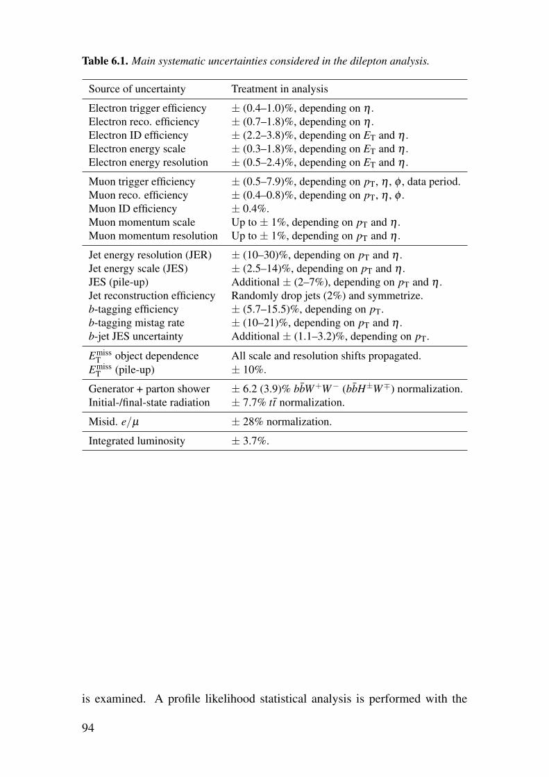
Table 6.1. Main systematic uncertainties considered in the dilepton analysis.

Source of uncertainty Treatment in analysis

Electron trigger efficiency ± (0.4–1.0)%, depending on η .Electron reco. efficiency ± (0.7–1.8)%, depending on η .Electron ID efficiency ± (2.2–3.8)%, depending on ET and η .Electron energy scale ± (0.3–1.8)%, depending on ET and η .Electron energy resolution ± (0.5–2.4)%, depending on ET and η .

Muon trigger efficiency ± (0.5–7.9)%, depending on pT, η , φ , data period.Muon reco. efficiency ± (0.4–0.8)%, depending on pT, η , φ .Muon ID efficiency ± 0.4%.Muon momentum scale Up to ± 1%, depending on pT and η .Muon momentum resolution Up to ± 1%, depending on pT and η .

Jet energy resolution (JER) ± (10–30)%, depending on pT and η .Jet energy scale (JES) ± (2.5–14)%, depending on pT and η .JES (pile-up) Additional ± (2–7%), depending on pT and η .Jet reconstruction efficiency Randomly drop jets (2%) and symmetrize.b-tagging efficiency ± (5.7–15.5)%, depending on pT.b-tagging mistag rate ± (10–21)%, depending on pT and η .b-jet JES uncertainty Additional ± (1.1–3.2)%, depending on pT.

EmissT object dependence All scale and resolution shifts propagated.

EmissT (pile-up) ± 10%.

Generator + parton shower ± 6.2 (3.9)% bbW+W− (bbH±W∓) normalization.Initial-/final-state radiation ± 7.7% tt normalization.

Misid. e/µ ± 28% normalization.

Integrated luminosity ± 3.7%.

is examined. A profile likelihood statistical analysis is performed with the

94

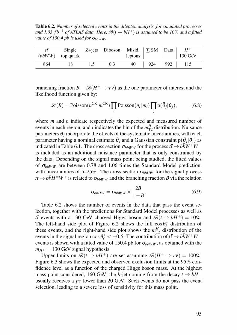
Table 6.2. Number of selected events in the dilepton analysis, for simulated processes

and 1.03 f b−1 of ATLAS data. Here, B(t → bH+) is assumed to be 10% and a fitted

value of 150.4 pb is used for σbbWW .

tt Single Z+jets Diboson Misid. ∑ SM Data H+

(bbWW ) top quark leptons 130 GeV

864 18 1.5 0.3 40 924 992 115

branching fraction B ≡ B(H+ → τν) as the one parameter of interest and thelikelihood function given by:

L (B) = Poisson(nCR|mCR)∏i

Poisson(ni|mi)∏j

p(θ j|θ j), (6.8)

where m and n indicate respectively the expected and measured number ofevents in each region, and i indicates the bin of the mH

T2 distribution. Nuisanceparameters θ j incorporate the effects of the systematic uncertainties, with eachparameter having a nominal estimate θ j and a Gaussian constraint p(θ j|θ j) asindicated in Table 6.1. The cross section σbbWW for the process tt → bbW+W−

is included as an additional nuisance parameter that is only constrained bythe data. Depending on the signal mass point being studied, the fitted valuesof σbbWW are between 0.78 and 1.06 times the Standard Model prediction,with uncertainties of 5–25%. The cross section σbbHW for the signal processtt → bbH±W∓ is related to σbbWW and the branching fraction B via the relation

σbbHW = σbbWW × 2B

1−B. (6.9)

Table 6.2 shows the number of events in the data that pass the event se-lection, together with the predictions for Standard Model processes as well astt events with a 130 GeV charged Higgs boson and B(t → bH+) = 10%.The left-hand side plot of Figure 6.2 shows the full cosθ ∗

ℓ distribution ofthese events, and the right-hand side plot shows the mH

T2 distribution of theevents in the signal region cosθ ∗

ℓ <−0.6. The contribution of tt → bbW+W−

events is shown with a fitted value of 150.4 pb for σbbWW , as obtained with themH+ = 130 GeV signal hypothesis.

Upper limits on B(t → bH+) are set assuming B(H+ → τν) = 100%.Figure 6.3 shows the expected and observed exclusion limits at the 95% con-fidence level as a function of the charged Higgs boson mass. At the highestmass point considered, 160 GeV, the b-jet coming from the decay t → bH+

usually receives a pT lower than 20 GeV. Such events do not pass the eventselection, leading to a severe loss of sensitivity for this mass point.

95

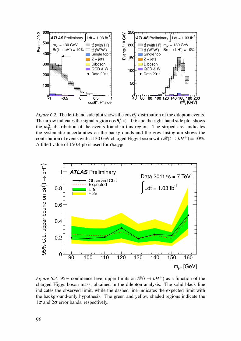
side+

*, Hθcos-1 -0.5 0 0.5 1

Events

/ 0

.2

0

100

200

300

400

500

600

side+

*, Hθcos-1 -0.5 0 0.5 1

Events

/ 0

.2

0

100

200

300

400

500

600

ATLAS Preliminary

= 130 GeV+H

m

) = 10%+

bH→Br(t

-1Ldt = 1.03 fb∫

)+

(with Htt

)-

W+

(WttSingle top

Z + jets

Diboson

QCD & W

Data 2011

[GeV]HT2m

40 60 80 100 120 140 160 180 200

Events

/ 1

0 G

eV

0

50

100

150

200

250

[GeV]HT2m

40 60 80 100 120 140 160 180 200

Events

/ 1

0 G

eV

0

50

100

150

200

250

ATLAS Preliminary

= 130 GeV+H

m

) = 10%+

bH→Br(t

-1Ldt = 1.03 fb∫

)+

(with Htt

)-

W+

(WttSingle top

Z + jets

Diboson

QCD & W

Data 2011

Figure 6.2. The left-hand side plot shows the cosθ ∗ℓ distribution of the dilepton events.

The arrow indicates the signal region cosθ ∗ℓ <−0.6 and the right-hand side plot shows

the mHT2 distribution of the events found in this region. The striped area indicates

the systematic uncertainties on the backgrounds and the grey histogram shows thecontribution of events with a 130 GeV charged Higgs boson with B(t → bH+)= 10%.A fitted value of 150.4 pb is used for σbbWW .

[GeV]+H

m

90 100 110 120 130 140 150 160

+ b

H→

t 9

5%

C.L

. u

pp

er

bo

un

d o

n B

r

0

0.2

0.4

0.6

0.8

1

Observed CLsExpected

σ 1±σ 2±

ATLAS Preliminary = 7 TeVsData 2011

-1Ldt = 1.03 fb∫

Figure 6.3. 95% confidence level upper limits on B(t → bH+) as a function of thecharged Higgs boson mass, obtained in the dilepton analysis. The solid black lineindicates the observed limit, while the dashed line indicates the expected limit withthe background-only hypothesis. The green and yellow shaded regions indicate the1σ and 2σ error bands, respectively.

96

6.2 Lepton+tau channelThis section describes a search for the process tt → bbH±W∓ → bbτ±ℓ∓ννcarried out with the full 2011 dataset, i.e. an integrated luminosity of 4.6 fb−1.Here, the tau lepton decays hadronically, in contrast to the analysis presentedin the previous section, which relied on the fully leptonic tau decay modes.The use of a hadronically decaying tau lepton, τhad, introduces more difficult-to-handle backgrounds but allows a higher overall search sensitivity. Thisanalysis, which is also documented in Ref. [97], relies on the theoretical tt

production cross section σtt = 167+17−18 pb [69] and uses the Emiss

T distributionto extract upper limits on B(t → bH+).

Event Selection

Events are selected for further analysis if these requirements are fulfilled:• The event contains exactly one electron or muon with ET > 25 GeV (elec-

tron) or pT > 20 GeV (muon).• The lepton must be matched to the single-lepton trigger object.• The event contains exactly one τhad with pT > 20 GeV, |η | < 2.3, and an

electric charge opposite to that of the lepton.• The event contains at least two jets with pT > 20 GeV.• At least one of the jets is b-tagged.• The collection of tracks originating from the primary vertex must satisfy

ΣptrackT > 100 GeV.

Only τhad objects passing the LLH identification and other criteria listed insection 5.2.4 are considered. Tracks that enter the computation of Σptrack

T musthave at least pT > 1 GeV, at least one hit in the pixel detector and at leastsix hits in the SCT. The requirement on a minimum amount of transverse mo-mentum in the event reduces the amount of multi-jet events otherwise passingthe selection. As this quantity is constructed using tracks originating from theprimary vertex, it is less sensitive to pile-up than the sum of transverse energydeposits in the calorimeter used in e.g. the dilepton analysis. The efficiencyof the full event selection is 23–40% (19–32%) for signal events in the muon(electron) channel, reaching a maximum value at a charged Higgs boson massaround 110 GeV.

Backgrounds with a misidentified lepton

As in the dilepton analysis, misidentified leptons constitute a background thatmust be estimated in a data-driven way. However, this background is slightlymore severe in this case, as each event now contains only a single electronor muon. Similarly to the dilepton analysis, the amount of events with amisidentified lepton passing the event selection is estimated using the matrixmethod, with lepton identification probabilities measured in Z → ℓℓ events andmisidentification probabilities measured in low-Emiss

T multi-jet events. The(mis)identification probabilities are parametrized as functions of the type of

97

lepton (electron or muon), its pseudorapidity, the distance ΔR to the closestjet, the number of b-tagged jets, the number of τhad objects, the pT of theleading jet, and the data-taking period. The (mis)identification probabilitiesdo vary slightly between data-taking periods as the pT threshold of the triggerchanged during the year.

Backgrounds with misidentified hadronic tau decays

Monte Carlo simulations are used to estimate the Standard Model backgroundswith a real lepton. These include events with top quark pairs, single top quarks,W and Z bosons produced in association with jets, and diboson pairs. Onlyabout 44% of the identified τhad objects in the simulated events are matchedto a hadronically decaying tau lepton at the generator level. However, theτhad misidentification probability is not expected to be well modeled in thesimulation. The simulated events must therefore be corrected based on τhadmisidentification probabilities measured in data.

Jets misidentified as hadronic tau decays

The probability for a jet to be misidentified as a τhad is measured in data usinga control sample enriched in W + jets events. These events are required topass the same lepton selection criteria as used in the main event selection.In addition, events must have a τhad candidate and Emiss

T > 40 GeV, but no b-tagged jets. The τhad candidates are not required to pass the LLH identificationcriteria but must have pT > 20 GeV and |η |< 2.3, and they must not be withinΔR < 0.2 of an electron or muon. About 0.5% of the selected events containa true τhad. Simulated events with a true τhad (which are assumed to be wellmodeled) are subtracted from the data in order to remove this component.

Like the dominant tt background, the control sample contains events wherehigh-pT jets mainly originate from quarks instead of gluons. It does, however,contain a much smaller fraction of b-jets. The probability for a b-jet to bemisidentified as a τhad is lower than for a jet originating from a light quark, asthe track multiplicity in a b-jet is higher. The visible mass measurement usedin the τhad identification also offers some discrimination between a b-jet anda τhad object. The difference between the tt and W + jets enriched regions istreated as a systematic uncertainty and is evaluated using simulation.

Having subtracted the events with a true τhad, the jet → τhad misidentifi-cation probability is defined as the number of τhad candidates passing the tauLLH identification criteria divided by the total number of τhad candidates. Itis measured as a function of pT, η , and the number of associated tracks. Themisidentification probability is found to be on average 7% for 1-prong tausand 2% for 3-prong taus.

In order to construct an estimate of the background with jets misidentifiedas hadronic tau decays, the measured jet → τhad misidentification probabilityis applied as a weight to all τhad candidates in simulated tt, single top quark,W + jets, Z/γ∗+ jets and diboson events. The τhad candidate is then treated as

98

Table 6.3. Number of events with jets misidentified as hadronic tau decays, as pre-

dicted using the misidentification probabilities measured in data, and compared with

the result of applying the LLH algorithm to the simulated events. The uncertainties

are statistical only, related to the number of data events in the control region and to

the limited number of simulated events passing the LLH criterion, respectively.

Sample Nominal estimate Simulation only

tt 900±15 877±6W + jets 150±3 145±9Single top quark 81±1 61±2Z/γ∗+ jets 44±1 69±4Diboson 6±1 8±1

if it had passed the tau identification, the corresponding jet is removed, and themodified event is passed through the nominal event selection. If it is accepted,it is kept with the weight given by the jet → τhad misidentification probabilitymeasured in data. The corresponding event yields are shown in Table 6.3.Misidentified τhad objects also appear in multi-jet events. To pass the eventselection, however, such events must also contain a misidentified lepton andare therefore accounted for in the data-driven estimation of that background.

Electrons misidentified as hadronic tau decays

Electrons misidentified as hadronic tau decays constitute a comparably smallbackground. It is estimated in a similar manner as the jet → τhad background,using e → τhad misidentification probabilities measured in Z → ee events [98].The average misidentification probability is 0.2%. In this case, the misidenti-fication probability is the same in tt events as it is in the control region.

Backgrounds with real hadronic tau decays

The remaining backgrounds are tt, single top quark, W + jets, Z/γ∗ + jets,and diboson events with a real lepton and a real τhad object. Nominally, thesebackgrounds are estimated using simulation only.

A data-simulation hybrid embedding method is used to cross-check thebackground simulations. This method consists of selecting events in data thatmatch the nominal event selection, except for having a muon in place of theτhad object. This muon is then replaced with a τhad simulated with TAUOLA.This way, most features of the event, including the underlying event, pile-upeffects, jet distributions, and overall normalization, are obtained directly fromthe data. The embedding of the simulated τhad takes place at the detector level,meaning that individual tracks and calorimeter energy deposits of the muonare replaced. The momentum of the tau is rescaled with respect to the muonto take into account its higher mass. When selecting events for the embeddingprocedure, the pT threshold of the muon is lower than that used for the τhadin the analysis to avoid biasing the event selection. This sample constructed

99

using embedding reproduces both the overall normalization and the shape ofthe simulated backgrounds within statistical uncertainties, which provides avalidation of the Monte Carlo simulation.

Systematic uncertainties

Table 6.4 lists the systematic uncertainties considered in this analysis. Un-certainties related to the simulation of signal and background processes aretreated similarly as in the dilepton analysis. The largest uncertainties are thejet energy scale (up to 14%) and resolution (up to 30%). Additional uncer-tainties are also introduced in this analysis, related to the τhad identificationefficiency (up to 7%) and energy scale (up to 5%).

The different jet composition (the fractions of jets initiated by light quarks,b quarks, or gluons) between the W + jets dominated region used to measurethe jet → τhad misidentification probability and the tt dominated signal regionis treated as a systematic uncertainty on the background estimation, and isevaluated using simulation. It is found to affect the estimation of this back-ground by up to 11%. A further 2% uncertainty is contributed by the statisticaluncertainty on the control sample. In the case of e → τhad misidentification,systematic uncertainties arise from the subtraction of electroweak and multi-jet backgrounds and from correlations between tag and probe objects in thedetermination of the misidentification probability in Z → ee events.

Systematic uncertainties on the estimate of misidentified leptons have alarger impact than in the dilepton analysis. They arise mostly from instru-mental uncertainties entering via the subtraction of simulated events with trueleptons in the computation of the misidentification probability, and from the jetcomposition (39%, evaluated by comparing the misidentification probabilityin simulated multi-jet and Zbb events).

Results

The observed number of events in the data after applying the event selection isshown in Table 6.5, together with the predictions under the background-onlyhypothesis, as well as for an alternative scenario where B(t → bH+) = 5%and mH+ = 130 GeV. The backgrounds with real and misidentified hadronictau decays are scaled to match the change in B(tt → bbW+W−) in the pres-ence of a charged Higgs boson, while the total tt cross section is constrainedto its theoretical value σtt = 167+17

−18 pb, to which an additional 6% uncertaintyis added to account for possible supersymmetric loop corrections [99].

The EmissT distributions in the e + τhad and µ + τhad channels are shown

in Figure 6.4. The data is found to be compatible with the background-onlyhypothesis. Upper limits on the branching fraction B(t → bH+) are there-fore extracted with the profile likelihood method, using the Emiss

T distribution(combined from both channels) as a discriminating variable. The expectedand observed limits at 95% confidence level according to the CLs definitionare shown in Figure 6.5.

100

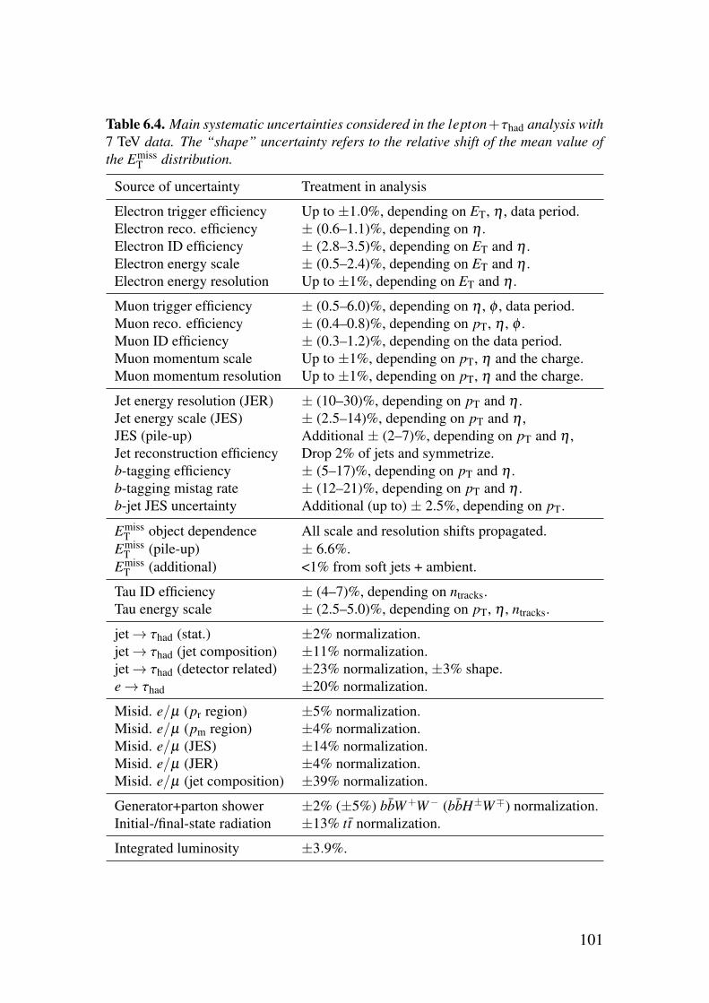
Table 6.4. Main systematic uncertainties considered in the lepton+τhad analysis with

7 TeV data. The “shape” uncertainty refers to the relative shift of the mean value of

the EmissT distribution.

Source of uncertainty Treatment in analysis

Electron trigger efficiency Up to ±1.0%, depending on ET, η , data period.Electron reco. efficiency ± (0.6–1.1)%, depending on η .Electron ID efficiency ± (2.8–3.5)%, depending on ET and η .Electron energy scale ± (0.5–2.4)%, depending on ET and η .Electron energy resolution Up to ±1%, depending on ET and η .

Muon trigger efficiency ± (0.5–6.0)%, depending on η , φ , data period.Muon reco. efficiency ± (0.4–0.8)%, depending on pT, η , φ .Muon ID efficiency ± (0.3–1.2)%, depending on the data period.Muon momentum scale Up to ±1%, depending on pT, η and the charge.Muon momentum resolution Up to ±1%, depending on pT, η and the charge.

Jet energy resolution (JER) ± (10–30)%, depending on pT and η .Jet energy scale (JES) ± (2.5–14)%, depending on pT and η ,JES (pile-up) Additional ± (2–7)%, depending on pT and η ,Jet reconstruction efficiency Drop 2% of jets and symmetrize.b-tagging efficiency ± (5–17)%, depending on pT and η .b-tagging mistag rate ± (12–21)%, depending on pT and η .b-jet JES uncertainty Additional (up to) ± 2.5%, depending on pT.

EmissT object dependence All scale and resolution shifts propagated.

EmissT (pile-up) ± 6.6%.

EmissT (additional) <1% from soft jets + ambient.

Tau ID efficiency ± (4–7)%, depending on ntracks.Tau energy scale ± (2.5–5.0)%, depending on pT, η , ntracks.

jet → τhad (stat.) ±2% normalization.jet → τhad (jet composition) ±11% normalization.jet → τhad (detector related) ±23% normalization, ±3% shape.e → τhad ±20% normalization.

Misid. e/µ (pr region) ±5% normalization.Misid. e/µ (pm region) ±4% normalization.Misid. e/µ (JES) ±14% normalization.Misid. e/µ (JER) ±4% normalization.Misid. e/µ (jet composition) ±39% normalization.

Generator+parton shower ±2% (±5%) bbW+W− (bbH±W∓) normalization.Initial-/final-state radiation ±13% tt normalization.

Integrated luminosity ±3.9%.

101

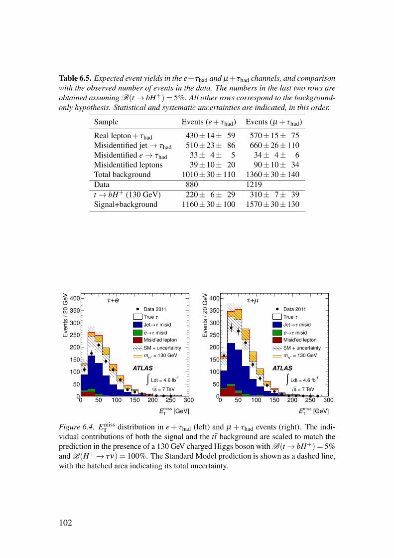
Table 6.5. Expected event yields in the e+τhad and µ+τhad channels, and comparison

with the observed number of events in the data. The numbers in the last two rows are

obtained assuming B(t → bH+) = 5%. All other rows correspond to the background-

only hypothesis. Statistical and systematic uncertainties are indicated, in this order.

Sample Events (e+τhad) Events (µ +τhad)

Real lepton+τhad 430±14± 59 570±15± 75Misidentified jet → τhad 510±23± 86 660±26±110Misidentified e → τhad 33± 4± 5 34± 4± 6Misidentified leptons 39±10± 20 90±10± 34Total background 1010±30±110 1360±30±140Data 880 1219t → bH+ (130 GeV) 220± 6± 29 310± 7± 39Signal+background 1160±30±100 1570±30±130

[GeV]miss

TE

0 50 100 150 200 250 300

Events

/ 2

0 G

eV

0

50

100

150

200

250

300

350

400

) = 5%+

bH→tB(

Data 2011

τTrue

misidτ→Jet

misidτ→e

Misid’ed lepton

SM + uncertainty

= 130 GeV+H

m

-1 Ldt = 4.6 fb∫

= 7 TeVs

e+τ

ATLAS

[GeV]miss

TE

0 50 100 150 200 250 300

Events

/ 2

0 G

eV

0

50

100

150

200

250

300

350

400

) = 5%+

bH→tB(

Data 2011

τTrue

misidτ→Jet

misidτ→e

Misid’ed lepton

SM + uncertainty

= 130 GeV+H

m

-1 Ldt = 4.6 fb∫

= 7 TeVs

µ+τ

ATLAS

Figure 6.4. EmissT distribution in e+ τhad (left) and µ + τhad events (right). The indi-

vidual contributions of both the signal and the tt background are scaled to match theprediction in the presence of a 130 GeV charged Higgs boson with B(t → bH+)= 5%and B(H+ → τν) = 100%. The Standard Model prediction is shown as a dashed line,with the hatched area indicating its total uncertainty.

102

[GeV]+H

m

90 100 110 120 130 140 150 160

+ b

H→

t B

-210

-110

1

Observed CLsExpected

σ 1±σ 2±

ATLAS

Data 2011

= 7 TeVs

-1Ldt = 4.6 fb∫

+leptonτ

Figure 6.5. Expected and observed 95% confidence level exclusion limits on thebranching fraction B(t → bH+) for a range of charged Higgs boson masses between90 and 160 GeV, and with the assumption B(H+ → τν) = 100%, as obtained in theanalysis of lepton+τhad events in 7 TeV data.

103

6.3 Test of lepton universality in tt eventsThe analysis presented here uses an alternative technique for charged Higgsboson searches in tt events. As W bosons decay with equal branching fractionsto all leptons, whereas charged Higgs bosons decay predominantly to τν , thepresence of charged Higgs bosons can be detected by searching for a violationof the lepton universality in top quark decays. This analysis uses the full2011 dataset of pp collisions at

√s = 7 TeV, with an integrated luminosity

of 4.6 fb−1, and it uses both dilepton events and lepton+τhad events. Leptonuniversality in tt decays is tested by comparing the ratio of the number oflepton+τhad events to the number of dilepton events found in the data to thevalue of that ratio predicted by the Standard Model. There are two motivationsfor the use of a ratio. First, while tau leptons decay leptonically more often(35% of the time) than W bosons (25% of the time), their decay productsusually have a lower pT than if they would come directly from a W bosonand are therefore less likely to be detected. The number of observed dileptonevents is therefore expected to decrease in the presence of a charged Higgsboson decaying to τν , while the number of lepton+τhad events is expected toincrease. The ratio of the two event yields is therefore more sensitive to thepresence of a charged Higgs boson than either of the two channels alone. Inaddition, many systematic uncertainties affect both channels in the same wayand their effects are therefore expected to cancel out when the ratio of eventyields is computed. This analysis is also documented in Ref. [100].

Event selection

The following event selection is applied in order to select a sample enrichedin tt events:• The event must contain at least one electron or muon, having ET > 25 GeV

(electron) or pT > 25 GeV (muon).• The lepton must be matched to the single-lepton trigger object.• The event must contain at least two b-tagged jets with pT > 20 GeV.• The event must have Emiss

T > 40 GeV and a solution for mHT2 > 0.

In addition, lepton+τhad events must satisfy the following requirements:• There must be no additional charged lepton in the event.• The event must have exactly one τhad with pT > 25 GeV and |η |< 2.3.Dilepton events are instead selected by requiring:• There must be exactly one additional charged lepton in the event.• The second lepton also has ET > 25 GeV (pT > 25 GeV).• The two leptons have different flavors.The τhad or non-trigger matched lepton is forced to be on the “H+side” in thecalculation of mH

T2. Two b-tagged jets are required in order to select a purett sample. This leads to a lower acceptance for charged Higgs boson massesclose to that of the top quark, when one of the b quarks receive very littletransverse momentum. However, the aim of this search is mainly to improve

104

the sensitivity in the low end of the considered mass range, i.e. close to theW mass, where the previous searches did not offer a strong discriminationbetween signal and background events. The selected events are categorizedbased on whether they fire the single-electron trigger or the single-muon trig-ger, and each category contains both lepton+τhad and dilepton events. In thefollowing, the lepton appearing first in a final state designation corresponds tothe trigger used to select the event. The category of electron-triggered eventstherefore consists of e+τhad and e+µ events. The category of muon-triggeredevents consists of µ + τhad and µ + e events. Dilepton events firing both theelectron trigger and the muon trigger are assigned to both categories. Thisoverlap of categories is accounted for when the exclusion limits are computed.

Backgrounds with misidentified objects

Backgrounds with misidentified leptons

The contributions of backgrounds with misidentified leptons are estimatedwith the matrix method. The same implementation as in section 6.2 is used.Neither the requirement of two b-tagged jets nor the presence of a second lep-ton is found to have a significant impact on the predictive power of the method.It is validated by comparing the distributions of kinematic variables, includingthe lepton pT and Emiss

T , between the data and the total background predictionin e+ jets, µ + jets, e+µ , and µ +e events without τhad or b-jet requirements,and no significant deviations are found.

Backgrounds with misidentified hadronic tau decays

In simulated tt events, about 51% of τhad objects passing the lepton+ τhadselections correspond to a true tau lepton at the generator level, and 3% ofτhad objects originate from electrons or muons. The contribution of eventswhere an electron or a muon is misidentified as a τhad in data is estimated byapplying scale factors to simulated events as described in section 6.2. Theremaining 46% of events (according to simulation) contain jets misidentifiedas τhad objects. This component is also determined by correcting simulatedevents with scale factors measured in data, as described below.

A new technique to reduce the uncertainty on the jet → τhad misidentifi-cation probability is introduced in this analysis. In the lepton+ τhad analy-sis presented in section 6.2, the largest contribution to this uncertainty is thedifference in jet composition between W + jets events, where the misidentifi-cation probability is measured, and tt events, where it is applied. This comesfrom the fact that the jet→ τhad misidentification probability depends on whichtype of parton (light quark, heavy quark, or gluon) originally initiated the jet.However, contributions from jets other than those initiated by light quarks canbe effectively eliminated by classifying events based on whether the electriccharge of the τhad has the opposite sign (OS) or same sign (SS) compared tothat of the lepton. Except for a few rare cases of charge misidentification,

105

real τhad objects in tt and signal events all belong to the OS category. Insteadof considering only OS events as in section 6.2, however, the SS events arenow retained as well, but are assigned a negative weight. The final event yieldcorresponds to the number of OS events minus the number of SS events (OS-SS). Gluons do not carry electric charge and are therefore equally likely to bemisidentified as τhad objects of either charge, and b quarks tend to be producedin pairs (in particular in tt events). Both contributions are therefore expectedto cancel in the OS-SS procedure. Light-quark initiated jets in tt events withleptons are largely dominated by the fully hadronic decay of a top quark andare therefore not charge-symmetric. They contribute more to the OS categoryand are thus not eliminated. The procedure is demonstrated in Figure 6.6,based on a control region enriched in W +>2 jets events, selected as follows:• The event contains exactly one electron or muon, having ET (electron) or pT

(muon) larger than 25 GeV.• The lepton is matched to the single-lepton trigger object.• The event contains at least one τhad candidate, which is not required to pass

the LLH identification.• There are at least two jets in addition to the τhad candidate.• No jet is b-tagged.• The event has Emiss

T > 40 GeV and mT > 30 GeV.The requirement on the W transverse mass mT, defined as in equation (6.3),aims at reducing the contribution of Z + jets events with real tau leptons. Asin tt events, light-quark jets in these events are predominantly produced withan opposite sign of charge compared to the lepton. Figure 6.6 shows thatcontributions from jets initiated by gluons and b quarks are removed by theOS-SS subtraction, which therefore has two important effects. It reduces thetotal amount of misidentified hadronic tau decays, and it makes the misiden-tification probability more uniform between different event selections by onlyleaving jets initiated by light quarks.

Scale factors used to weight events with jets misidentified as τhad candidatesin the simulation are then derived from the W+> 2jets event selection in data.It can be seen in Figure 6.6, which includes τhad candidates with one or threetracks, that there are more such τhad candidates in the simulated events thanin the data. It was found that the track multiplicities of jets misidentified asτhad candidates are not well modeled by the simulation. Track multiplicityscale factors for τhad candidates are therefore computed. For this purpose,the track multiplicity (ranging from 1 to 9) distributions of misidentified τhadcandidates in data and in simulation are separately normalized to the sameunit area, and scale factors needed to correct the shape of the distribution inthe simulated events to that in the data are computed. Only 1-track and 3-trackτhad candidates are eventually used in the analysis, the corresponding scalefactors are 0.71±0.03 for 1-track τhad candidates and 0.92±0.03 for 3-trackτhad candidates, where the uncertainties are statistical in nature.

106

[GeV]Tm

0 50 100 150 200

Events

/ 1

0 G

eV

-8

-6

-4

-2

0

2

4

6

8

10

123

10×

ATLAS

OS

SS

Data 2011

τtrue

lepton

light quark

b quark

gluon

-1Ldt = 4.6 fb∫

= 7 TeVs

[GeV]Tm

0 50 100 150 200

Events

/ 1

0 G

eV

-0.5

0

0.5

1

1.5

2

2.5

3

3.5

43

10×

ATLAS

OS-SS

Data 2011

τtrue

lepton

light quark

b quark

gluon

-1Ldt = 4.6 fb∫

= 7 TeVs

Figure 6.6. Distributions of mT after applying the W+ > 2jets event selection (therequirement mT > 30 GeV is not applied in these plots). The colors correspond to thetype of highest-energy generator-level particle found within a cone of radius R = 0.2around the τhad candidate. The left-hand side plot shows OS and SS events withpositive respectively negative weights, while the right-hand side plot shows the resultof subtracting the SS events from the OS events.

The probability for a light-quark initiated jet to also pass the τhad identifi-cation criteria is then measured in the data, also using the W+ > 2jets eventselection. This misidentification probability is binned in pT and the number oftracks, Ntrack

τ , of the τhad candidate, as well as in the number of tracks, Ntrackiso ,

in the τhad isolation cone, defined as the volume 0.2 < ΔR < 0.4 around theτhad object. The parametrization of the misidentification probability by Ntrack

isois a new feature in this analysis, as it was found that this corrects well forresidual differences between W + jets events and tt events. The misidentifi-cation probabilities are shown in Figure 6.7, with two different binnings. Afull parametrization in all three variables is used in the analysis. The trackmultiplicity scale factors and misidentification scale factors are applied to allsimulated OS-SS events with τhad candidates matched to jets. A combinedprobability of p1(1− p2)+ p2(1− p1) is assigned to events with two τhad can-didates, where p1 and p2 are the individual misidentification probabilities.

Systematic uncertainties

The same systematic uncertainties on the detector simulation and the eventgenerators as discussed in section 6.2 are evaluated. However, in most cases,they are expected to have a smaller impact in this analysis, as they largelycancel in the ratio calculation. The distributions of the number Ntrack

τ of asso-ciated τhad tracks and the number Ntrack

iso of tracks in the isolation cone of jetsmisidentified as τhad candidates in the alternative tt samples are reweighted ina correlated way to match those of the nominal tt sample before applying theNtrackτ scale factors measured in data, which are found to well reproduce the

107

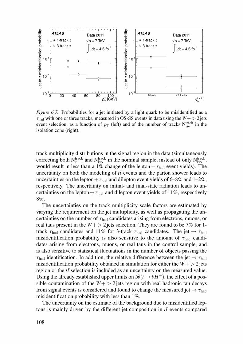
[GeV]τT

p0 20 40 60 80 100

mis

identification p

robabili

tyτ

Jet-

to-

-310

-210

-110

1 τ1-track

τ3-track

Data 2011

-1Ldt = 4.6 fb∫ = 7 TeVs

ATLAS

trackisoN

0 track 1 tracks≥

mis

identification p

robabili

tyτ

Jet-

to-

-310

-210

-110

1 τ1-track

τ3-track

Data 2011

-1Ldt = 4.6 fb∫ = 7 TeVs

ATLAS

Figure 6.7. Probabilities for a jet initiated by a light quark to be misidentified as aτhad with one or three tracks, measured in OS-SS events in data using the W+> 2jetsevent selection, as a function of pT (left) and of the number of tracks Ntrack

iso in theisolation cone (right).

track multiplicity distributions in the signal region in the data (simultaneouslycorrecting both Ntrack

τ and Ntrackiso in the nominal sample, instead of only Ntrack

iso ,would result in less than a 1% change of the lepton+ τhad event yields). Theuncertainty on both the modeling of tt events and the parton shower leads touncertainties on the lepton+τhad and dilepton event yields of 6–8% and 1–2%,respectively. The uncertainty on initial- and final-state radiation leads to un-certainties on the lepton+ τhad and dilepton event yields of 11%, respectively8%.

The uncertainties on the track multiplicity scale factors are estimated byvarying the requirement on the jet multiplicity, as well as propagating the un-certainties on the number of τhad candidates arising from electrons, muons, orreal taus present in the W+> 2jets selection. They are found to be 7% for 1-track τhad candidates and 11% for 3-track τhad candidates. The jet → τhadmisidentification probability is also sensitive to the amount of τhad candi-dates arising from electrons, muons, or real taus in the control sample, andis also sensitive to statistical fluctuations in the number of objects passing theτhad identification. In addition, the relative difference between the jet → τhadmisidentification probability obtained in simulation for either the W+> 2jetsregion or the tt selection is included as an uncertainty on the measured value.Using the already established upper limits on B(t → bH+), the effect of a pos-sible contamination of the W+ > 2jets region with real hadronic tau decaysfrom signal events is considered and found to change the measured jet → τhadmisidentification probability with less than 1%.

The uncertainty on the estimate of the background due to misidentified lep-tons is mainly driven by the different jet composition in tt events compared

108

to the control region where the lepton misidentification probabilities are de-rived. In total, the uncertainty on the background with misidentified leptonsis 38% for electron-triggered events and 49% for muon-triggered events. Asthis background is relatively small, however, the effect on the total event yieldratios is only 3.5% and 4.3%, respectively.

Results

The observed OS-SS event yields N in each of the e+ τhad, e+ µ , µ + τhad,and µ +e selections are shown in Table 6.6 together with the predicted valuesfor the background-only hypothesis or in the presence of a 130 GeV chargedHiggs boson. The event yields are used to compute the ratios:

Re =N (e+τhad)

N (e+µ)and Rµ =

N (µ +τhad)

N (µ + e). (6.10)

Figure 6.8 shows the dependence of Re and Rµ on B(t → bH+) for a H+

mass of 130 GeV, assuming B(H+ → τν) = 100%. Electrons and muonsproduced via t → bH+ → bτν → bℓννν typically have lower pT than thoseproduced via t → bW → bℓν . They are therefore less likely to pass the eventselection requirements. Despite the fact that the branching fraction of H+ intoelectrons and muons via the above mentioned process is higher than that of theW boson, the event yields in the dilepton final states decrease in the presence ofa charged Higgs boson, thereby contributing to the increase of Re and Rµ . Fora charged Higgs boson mass of 160 GeV, the rate at which Re and Rµ changewith B(t → bH+) is five times times lower and the analysis is correspondinglyless sensitive. At this point, both the lepton+τhad and dilepton event yieldsdecrease with B(t → bH+) because the b-jet coming from t → bH+ receivesa low pT, but the dilepton event yield decreases faster.

Table 6.7 shows the predicted and observed values of Re and Rµ . The dataare found to be compatible with the Standard Model expectation. Note thatthe relative uncertainties on the expected ratios are smaller than the sum ofthe uncertainties on the corresponding event yields. This is because many sys-tematic uncertainties are correlated across the lepton+τhad and dilepton eventselections, leading to Re and Rµ being largely insensitive to them. Table 6.8shows the sensitivity of Re and Rµ to individual uncertainties.

Exclusion limits

Upper limits on the branching fraction B(t → bH+) at 95% confidence levelaccording to the CLs criterion are determined using the profile likelihoodmethod described in section 5.4, with one important modification. The quan-tities Re and Rµ are ratios of two Poisson variables, the probability densityfunction of which is unknown. However, the quantity Nℓℓ′ +Nℓτ is also Pois-son distributed with a rate mℓℓ′ +mℓτ, and 0 ≤ Nℓℓ′ ≤ Nℓℓ′ +Nℓτ. Nℓℓ′ must

109

Table 6.6. Expected event yields and comparison with the observed number of events

in the data. Combined statistical and systematic uncertainties are shown. The num-

bers in the last two rows are obtained assuming B(t → bH+) = 3% with a charged

Higgs boson mass of 130 GeV. All other rows correspond to the background-only

hypothesis. Here, V denotes a vector boson.

Sample N (e+τhad) N (e+µ) N (µ +τhad) N (µ + e)

Misid. leptons −0.8± 3.0 94 ± 37 0.2± 1.0 74 ± 37V +jets, VV 2.1± 0.9 0.7± 0.4 2.6± 1.6 0.7± 0.4Single top 3.3± 0.8 24 ± 4 4.6± 0.9 18 ± 3tt 111 ±25 980 ±200 131 ±28 740 ±150Total bkg. 116 ±25 1100 ±210 138 ±29 830 ±160

Data 144 1247 153 929

t → bH+ 30 ± 4 27 ± 4 35 ± 4 20 ± 3Signal+bkg. 139 ±28 1070 ±200 166 ±32 810 ±150

Table 6.7. Predicted and observed event yield ratios.

Ratio Re Rµ

Standard Model prediction 0.105±0.012 (stat+syst) 0.166±0.017 (stat+syst)Measured value 0.115±0.010 (stat) 0.165±0.015 (stat)

) [%]+ bH→t B(

0 0.5 1 1.5 2 2.5 3 3.5 4 4.5 5

[%

]e

/Re

RΔ

+ X

) or

µe

N/N

(Δ

+ X

),

ha

dτ

eN

/N(

Δ

-20

-10

0

10

20

30

40

50

60

70

µ / e+had

τRatio e+

hadτEvent yield e+

µEvent yield e+

ATLAS Simulation

= 130 GeV+H

m

) [%]+ bH→t B(

0 0.5 1 1.5 2 2.5 3 3.5 4 4.5 5

[%

]µ

/Rµ

RΔ

+ X

) or

eµ

N/N

(Δ

+ X

),

ha

dτ

µN

/N(

Δ

-20

-10

0

10

20

30

40

50

60

70

+eµ /had

τ+µRatio

hadτ+µEvent yield

+eµEvent yield

ATLAS Simulation

= 130 GeV+H

m

Figure 6.8. The predicted relative change of the event yields N (e + τhad) andN (e+µ), and of their ratio Re (left) and the predicted relative change of the eventyields N (µ +τhad) and N (µ + e), and of their ratio Rµ (right). The plots show thedependence of these variables on the branching fraction B(t → bH+) in the presenceof a charged Higgs boson with a mass of 130 GeV.

110

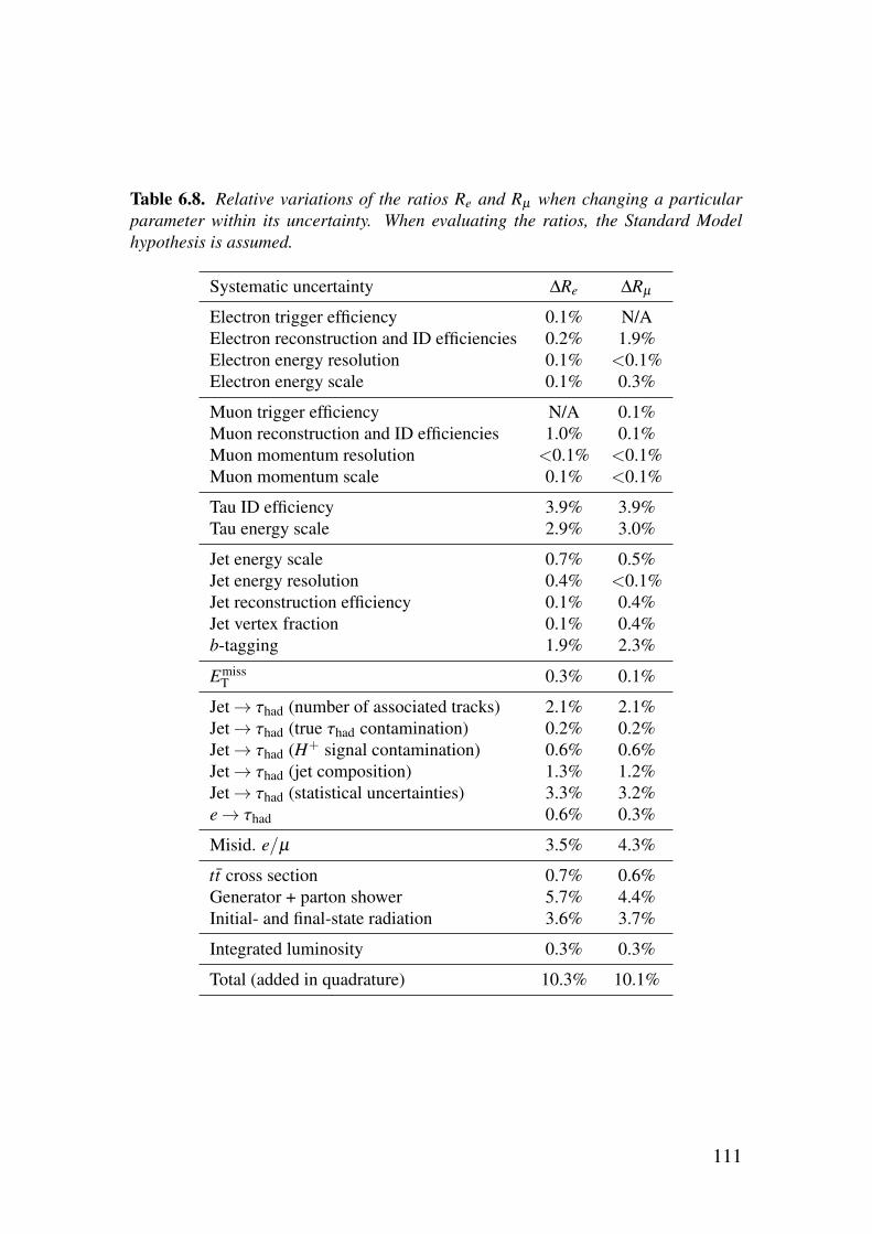
Table 6.8. Relative variations of the ratios Re and Rµ when changing a particular

parameter within its uncertainty. When evaluating the ratios, the Standard Model

hypothesis is assumed.

Systematic uncertainty ΔRe ΔRµ

Electron trigger efficiency 0.1% N/AElectron reconstruction and ID efficiencies 0.2% 1.9%Electron energy resolution 0.1% <0.1%Electron energy scale 0.1% 0.3%

Muon trigger efficiency N/A 0.1%Muon reconstruction and ID efficiencies 1.0% 0.1%Muon momentum resolution <0.1% <0.1%Muon momentum scale 0.1% <0.1%

Tau ID efficiency 3.9% 3.9%Tau energy scale 2.9% 3.0%

Jet energy scale 0.7% 0.5%Jet energy resolution 0.4% <0.1%Jet reconstruction efficiency 0.1% 0.4%Jet vertex fraction 0.1% 0.4%b-tagging 1.9% 2.3%

EmissT 0.3% 0.1%

Jet → τhad (number of associated tracks) 2.1% 2.1%Jet → τhad (true τhad contamination) 0.2% 0.2%Jet → τhad (H+ signal contamination) 0.6% 0.6%Jet → τhad (jet composition) 1.3% 1.2%Jet → τhad (statistical uncertainties) 3.3% 3.2%e → τhad 0.6% 0.3%

Misid. e/µ 3.5% 4.3%

tt cross section 0.7% 0.6%Generator + parton shower 5.7% 4.4%Initial- and final-state radiation 3.6% 3.7%

Integrated luminosity 0.3% 0.3%

Total (added in quadrature) 10.3% 10.1%

111

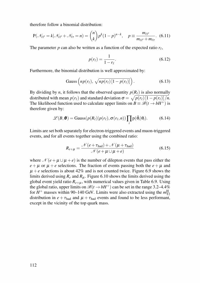
therefore follow a binomial distribution:

P(Nℓℓ′ = k|Nℓℓ′ +Nℓτ = n) =

�

n

k

�

pk(1− p)n−k, p ≡ mℓℓ′

mℓℓ′ +mℓτ. (6.11)

The parameter p can also be written as a function of the expected ratio rℓ,

p(rℓ) =1

1− rℓ. (6.12)

Furthermore, the binomial distribution is well approximated by:

Gauss�

np(rℓ),�

np(rℓ) [1− p(rℓ)]�

. (6.13)

By dividing by n, it follows that the observed quantity p(Rℓ) is also normallydistributed with mean p(rℓ) and standard deviation σ =

�

p(rℓ) [1− p(rℓ)]/n.The likelihood function used to calculate upper limits on B ≡ B(t → bH+) istherefore given by:

L (B,θθθ) = Gauss(p(Rℓ)|p(rℓ),σ(rℓ,n))∏i

p(θi|θi). (6.14)

Limits are set both separately for electron-triggered events and muon-triggeredevents, and for all events together using the combined ratio:

Re+µ =N (e+τhad)+N (µ +τhad)

N (e+µ ∪µ + e)(6.15)

where N (e+µ ∪µ + e) is the number of dilepton events that pass either thee+ µ or µ + e selections. The fraction of events passing both the e+ µ andµ + e selections is about 42% and is not counted twice. Figure 6.9 shows thelimits derived using Re and Rµ . Figure 6.10 shows the limits derived using theglobal event yield ratio Re+µ , with numerical values given in Table 6.9. Usingthe global ratio, upper limits on B(t → bH+) can be set in the range 3.2–4.4%for H+ masses within 90–140 GeV. Limits were also extracted using the mH

T2distribution in e+ τhad and µ + τhad events and found to be less performant,except in the vicinity of the top quark mass.

112

[GeV]+H

m

90 100 110 120 130 140 150 160

+ b

H→

t B

0

0.05

0.1

0.15

0.2

0.25

0.3

Observed 95% CLExpected

σ 1±σ 2±

ATLAS Data 2011

= 7 TeVs

-1Ldt = 4.6 fb∫

eR

[GeV]+H

m

90 100 110 120 130 140 150 160

+ b

H→

t B

0

0.05

0.1

0.15

0.2

0.25

0.3

Observed 95% CLExpected

σ 1±σ 2±

ATLAS Data 2011

= 7 TeVs

-1Ldt = 4.6 fb∫

µR

Figure 6.9. Expected and observed 95% confidence level upper limits on B(t → bH+)for H+ masses between 90 and 160 GeV and assuming B(H+ → τν) = 100%, usingthe event yield ratios Re (top) and Rµ (bottom).

113

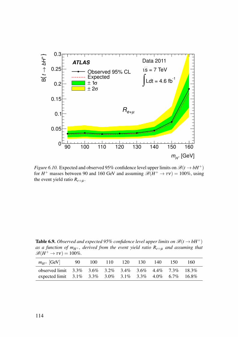
[GeV]+H

m

90 100 110 120 130 140 150 160

+ b

H→

t B

0

0.05

0.1

0.15

0.2

0.25

0.3

Observed 95% CLExpected

σ 1±σ 2±

ATLAS Data 2011

= 7 TeVs

-1Ldt = 4.6 fb∫

µe+R

Figure 6.10. Expected and observed 95% confidence level upper limits on B(t → bH+)for H+ masses between 90 and 160 GeV and assuming B(H+ → τν) = 100%, usingthe event yield ratio Re+µ .

Table 6.9. Observed and expected 95% confidence level upper limits on B(t → bH+)as a function of mH+ , derived from the event yield ratio Re+µ and assuming that

B(H+ → τν) = 100%.

mH+ [GeV] 90 100 110 120 130 140 150 160

observed limit 3.3% 3.6% 3.2% 3.4% 3.6% 4.4% 7.3% 18.3%expected limit 3.1% 3.3% 3.0% 3.1% 3.3% 4.0% 6.7% 16.8%

114

[GeV]+H

m

90 100 110 120 130 140 150 160

+ b

H→

t 9

5%

C.L

. u

pp

er

bo

un

d o

n B

r

0

0.05

0.1

0.15

0.2

0.25

0.3

0.35

0.4

Observed CLsExpected

σ 1±σ 2±

ATLAS Preliminary = 7 TeVsData 2011

-1Ldt = 1.03 fb∫

[GeV]+H

m

90 100 110 120 130 140 150 160

+ b

H→

t 9

5%

C.L

. u

pp

er

bo

un

d o

n B

r

0

0.05

0.1

0.15

0.2

0.25

0.3

0.35

0.4

Observed CLsExpected

σ 1±σ 2±

ATLAS Preliminary = 7 TeVsData 2011

-1Ldt = 1.03 fb∫

Figure 6.11. 95% confidence level upper limits on B(t → bH+), with the assumptionthat B(H+ → τν) = 100%, as obtained in the lepton+ jets channel [93] (left) andwith a combination of the lepton+ jets and dilepton channels (right) using early 2011data.

6.4 Combinations and interpretationsIn parallel with the dilepton analysis, another search for charged Higgs bosonsin events with a leptonically decaying tau was also performed by ATLAS,using the lepton+ jets final state (in this case, the top quark on the “W side” ofthe event is assumed to decay hadronically). This analysis is also documentedin Ref. [93], and the resulting exclusion limits are shown in the left-hand sideplot of Figure 6.11. The right-hand side plot shows the result of a combinationof the lepton+ jets and dilepton (see Figure 6.3) channels. As the dileptonchannel contributes very little additional sensitivity, the decision was made toexclude it from future analyses.

The analysis of the lepton+ jets channel was however repeated with thefull 2011 dataset, together with the lepton+τhad channel (see section 6.2) andthe all-hadronic τhad + jets channel [97]. The limits obtained for the lepton+jets and τhad + jets channels are shown in Figure 6.12 (see Figure 6.5 for thelepton+τhad result). The result of a combination of all three channels is shownin Figure 6.13, in the form of model-independent upper limits on B(t → bH+)as well as their interpretation in the MSSM mmax

h scenario.The individually most sensitive channel is τhad+ jets. Figures 6.14 and 6.15

show the result of a combination of the τhad+ jets analysis with the test of lep-ton universality (Figure 6.9). As expected, exclusion limits are particularlyimproved for low charged Higgs boson masses where the latter has more sen-sitivity. The direct search in the lepton+τhad channel has comparable sensi-tivity to the τhad + jets channel for low masses, but can not easily be includedin this combination as it is not statistically independent from the test of leptonuniversality.

115

[GeV]+H

m

90 100 110 120 130 140 150 160

+ b

H→

t B

-210

-110

1

Observed CLsExpected

σ 1±σ 2±

ATLAS

Data 2011

= 7 TeVs

-1Ldt = 4.6 fb∫

lepton+jets

[GeV]+H

m

90 100 110 120 130 140 150 160

+ b

H→

t B

-210

-110

1

Observed CLsExpected

σ 1±σ 2±

ATLAS

Data 2011

= 7 TeVs

-1Ldt = 4.6 fb∫

+jetsτ

Figure 6.12. 95% confidence level upper limits on B(t → bH+), with the assumptionthat B(H+ → τν) = 100%, as obtained in the lepton+ jets channel (left) and in theτhad + jets channel (right) [97].

[GeV]+H

m

90 100 110 120 130 140 150 160

+ b

H→

t B

-210

-110

1

Observed CLsExpected

σ 1±σ 2±

ATLAS

Data 2011

= 7 TeVs

-1Ldt = 4.6 fb∫

combined

[GeV]+H

m

90 100 110 120 130 140 150 160

βta

n

0

10

20

30

40

50

60

Median expected exclusion

Observed exclusion 95% CL

theoryσObserved +1

theoryσObserved -1

-1Ldt = 4.6 fb∫Data 2011

=7 TeVs maxh

m

ATLAS

Figure 6.13. 95% confidence level upper limits on B(t → bH+), with the assump-tion that B(H+ → τν) = 100%, obtained by combining the lepton+ jets, τhad + jets(both from Ref. [97]), and lepton+τhad channels (left), and their interpretation in theMSSM mmax

h scenario (right).

116

[GeV]+H

m

90 100 110 120 130 140 150 160

+ b

H→

t B

-210

-110

1

Observed CLsExpected

σ 1±σ 2±

ATLAS Data 2011

= 7 TeVs

-1Ldt = 4.6 fb∫

+jetsτ + µe+R

Figure 6.14. 95% confidence level upper limits on B(t → bH+), with the assumptionthat B(H+ → τν) = 100%, obtained with a combination of the direct search in theτhad + jets channel and the event yield ratio Re+µ .

[GeV]+H

m

90 100 110 120 130 140 150 160

βta

n

10

20

30

40

50

60

Median expected exclusion

Observed exclusion 95% CL

theoryσObserved +1

theoryσObserved -1

-1Ldt = 4.6 fb∫

Data 2011

=7 TeVs maxh

m

+jetsτ + µ+eR

ATLAS

Figure 6.15. 95% confidence level exclusion limits in the parameter space of theMSSM mmax

h scenario, as obtained from the combination of the τhad + jets channeland the event yield ratio Re+µ .

117

7. Searches for H+ → τν in 8 TeV data

With the data collected at√

s = 8 TeV in 2012, corresponding to an integratedluminosity of 20.3 fb−1, the lepton+τhad and dilepton channels are analyzedsimultaneously. As in the test of lepton universality in tt decays presented insection 6.3, this allows for many systematic uncertainties to be constrained bythe background-rich dilepton channel. In contrast to the strategy used in the7 TeV analysis, however, the full distribution of a transverse mass variable isnow used to achieve higher sensitivity for charged Higgs boson masses fur-ther away from that of the W boson. The search is also extended to considercharged Higgs bosons with masses of up to 1 TeV, i.e. heavy charged Higgsbosons (see section 2.3.2), produced in association with a top quark. Thetransverse mass variable used to discriminate between signal and backgroundamong lepton+τhad events is

mT =�

2pτTEmissT (1− cosΔφτ,miss), (7.1)

where Δφτ,miss is the azimuthal angle between the τhad and the missing trans-verse momentum. Note that, here, mT is an effective quantity which in additionto the decay products of the charged Higgs boson also contains a contributionfrom a neutrino that is produced in association with the electron or muon inthe leptonic decay of the associated top quark. Nevertheless, it offers goodseparation between signal and background, in particular for high masses, asshown in Figure 7.1. Dilepton events are binned in the maximum mT valueconstructed with either of the leptons in place of the τhad in equation (7.1).

7.1 Event selectionSingle-lepton triggers with an ET threshold of 24 GeV or 60 GeV for electronsand a pT threshold of 24 GeV or 36 GeV for muons are used. Events are thenselected in the lepton+τhad channel, labeled as the Signal Region (SR), if theyfulfill the following criteria:• The event must contain exactly one loose lepton with ET > 25 GeV (elec-

tron) or pT > 25 GeV (muon).• The lepton must be matched to the single-lepton trigger object.• The event must also contain exactly one loose τhad with pT > 25 GeV and|η |< 2.3.

• The lepton and the τhad object must have electric charges of opposite signs.

118

) [GeV]miss

T, E

hadτ(TM

0 50 100 150 200 250 300 350 400

Events

/ 2

0 G

eV

0

200

400

600

800

1000

1200

1400

1600

1800 tt

Misid. tau

Z + jets

Single top

Diboson

130 GeV+

H

250 GeV+

H

Bkg. total unc.

-1 L dt = 20.3 fb∫

= 8 TeVs

, SRτ + µe/

1 + 2 b-jets

Figure 7.1. Comparison of the mT distribution for the Standard Model backgrounds(stacked histograms) and two signal samples with charged Higgs boson masses of130 GeV and 250 GeV in the lepton+τhad channel. The normalization of the twosignal samples correspond to B(t → bH+) = 10% or a production cross section of10 pb, respectively.

• The event must have EmissT > 25 GeV.

• The event must contain at least one jet with pT > 25 GeV.• Exactly one or two jets must be b-tagged.• The lepton and the τhad must also pass the tight criteria.The first steps are performed with loose selection criteria for all leptons andτhad objects. Loose electrons and muons are defined with relaxed identificationand isolation criteria, respectively. For the τhad identification, the BDT-basedidentification is used. Loose τhad objects are defined with a relaxed require-ment on the BDT score. Events with a τhad in the region 1.37 < |η | < 1.52,corresponding to the transition regions between the barrel and the end-caps,are discarded. A reliable electron identification is not available in this regionand the e → τhad misidentification probability is increased, as such objects arenot removed due to overlapping reconstructed electrons.

Dilepton events, labeled as the Control Region (CR), are selected if theyfulfill the following criteria:• The event must contain exactly one loose electron with ET > 25 GeV and

exactly one loose muon with pT > 25 GeV.• At least one of the leptons must be matched to a single-lepton trigger object.• The leptons must have electric charges of opposite signs.• The event must have Emiss

T > 25 GeV.• The event must contain zero, one, or two b-tagged jets with pT > 25 GeV.• Both leptons must also pass the tight criteria.

119

7.2 Backgrounds with misidentified hadronic tau decaysWith the tight BDT-based τhad identification, 69% of the τhad objects in sim-ulated tt events passing the SR selection are matched to a real hadronic taudecay at the generator level. Meanwhile, 28% of the τhad objects are matchedto a quark- or gluon-initiated jet, and the remaining 3% are matched to anelectron or a muon. The background with jets misidentified as hadronic taudecays is estimated in a data-driven way with the matrix method. With thismethod, not only are the misidentification probabilities measured in data, butthe distributions of τhad candidates are also taken from the data itself ratherthan from simulation. The loose and tight τhad selections used to define the(mis)identification probability are here defined with different thresholds onthe output of the BDT-based τhad identification. In contrast, in the previouslypresented analyses, the loose definition included all τhad candidates, i.e. with-out any requirement on the LLH or BDT identification criteria. It was foundthat, by retaining some requirement on the BDT score, a large fraction of τhadcandidates matched to jets initiated by b quarks and gluons can be eliminated.The misidentification probabilities for the remaining jets initiated by b quarksand gluons are also closer to that of jets initiated by light quarks than if all τhadcandidates were included in the loose sample. This strategy therefore ensuresa more uniform jet → τhad misidentification probability pm across samples ofevents with different fractions of jets initiated by light quarks, b quarks, orgluons, hence there is no need for the OS-SS procedure of section 6.3.

The identification probability for real hadronic tau decays, pr, is computedusing simulated events of Standard Model processes. The BDT-based τhadidentification is designed to give an approximately flat identification probabil-ity of real τhad objects with respect to pT and η [90]. A small pT-dependenceis nevertheless observed and pr is therefore computed as a function of pT. It isalso determined separately for 1-prong and 3-prong τhad objects. In the com-putation of pr, a small contribution of electrons and muons reconstructed asτhad objects are included. These backgrounds are determined separately, andare therefore not considered as misidentified τhad objects in the context of thematrix method, but are included in the definition of real τhad objects.

The jet → τhad misidentification probability pm is measured in the data,using an event selection enriched in W + jets events, where the W boson decaysto an electron or a muon. These events are selected as follows:• The event must contain exactly one loose lepton with ET > 25 GeV (elec-

tron) or pT > 25 GeV (muon).• The lepton must be matched to the trigger object and also pass the tight

criteria.• The event must contain exactly one loose τhad with pT > 25 GeV.• The lepton and the τhad object must have electric charges of opposite signs.• The event must not contain any b-tagged jets.

• The event must have mWT =

�

2pℓTEmissT (1− cosΔφℓ,miss)> 50 GeV.

120

) [GeV]hadτ(T

p20 40 60 80 100 120 140 160 180 200

tau (

mis

)identification p

robabili

ty

0

0.1

0.2

0.3

0.4

0.5

0.6

0.7

0.8

0.9

1

1-prong, real

<1.37η1-prong, misid. >1.52η1-prong, misid.

3-prong, real3-prong, misid.

hadτ + µe/

Figure 7.2. The τhad (mis)identification probabilities used in the matrix method.

The contamination arising from events where the τhad originates from a realhadronic tau decay, an electron, or a muon is subtracted using simulated events.The misidentification probability pm is then computed as the rate at which theloose τhad object, assumed to originate from a quark- or gluon-initiated jet,also passes the tight τhad identification. It is measured separately for 1-prongand 3-prong τhad objects, and as a function of pT. For 1-prong τhad objects,pm is also measured separately for the low (|η |< 1.37) and high (|η |> 1.52)pseudorapidity regions. Here, the pT- and η-dependencies are not treated asuncorrelated. Instead, a two dimensional binning of pm is used. For 3-prongτhad objects, the difference between the misidentification probabilities in thetwo regions of |η | is found to be small and within the statistical uncertainties.The η-dependence of pm for 3-prong τhad objects is therefore ignored. Thedistributions of pm and pr used in the matrix method are shown in Figure 7.2.The dependence of pm and pr on other variables, including the flavor of theassociated lepton and the number of b-tagged jets, was investigated and foundto be negligible.

As in the previously presented analyses, the background with electronsand muons misidentified as hadronic tau decays are estimated using simu-lated events. In the case of electrons, scale factors are applied to match themisidentification probabilities measured in data.

121

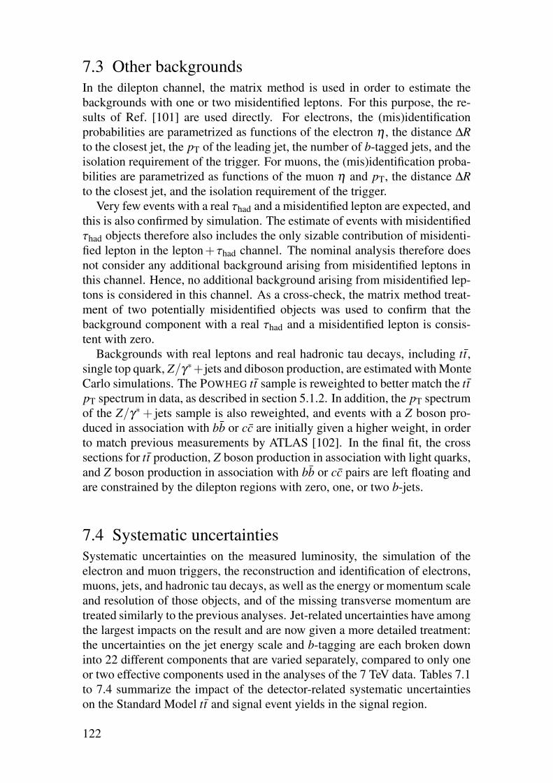
7.3 Other backgroundsIn the dilepton channel, the matrix method is used in order to estimate thebackgrounds with one or two misidentified leptons. For this purpose, the re-sults of Ref. [101] are used directly. For electrons, the (mis)identificationprobabilities are parametrized as functions of the electron η , the distance ΔR

to the closest jet, the pT of the leading jet, the number of b-tagged jets, and theisolation requirement of the trigger. For muons, the (mis)identification proba-bilities are parametrized as functions of the muon η and pT, the distance ΔR

to the closest jet, and the isolation requirement of the trigger.Very few events with a real τhad and a misidentified lepton are expected, and

this is also confirmed by simulation. The estimate of events with misidentifiedτhad objects therefore also includes the only sizable contribution of misidenti-fied lepton in the lepton+τhad channel. The nominal analysis therefore doesnot consider any additional background arising from misidentified leptons inthis channel. Hence, no additional background arising from misidentified lep-tons is considered in this channel. As a cross-check, the matrix method treat-ment of two potentially misidentified objects was used to confirm that thebackground component with a real τhad and a misidentified lepton is consis-tent with zero.

Backgrounds with real leptons and real hadronic tau decays, including tt,single top quark, Z/γ∗+jets and diboson production, are estimated with MonteCarlo simulations. The POWHEG tt sample is reweighted to better match the tt

pT spectrum in data, as described in section 5.1.2. In addition, the pT spectrumof the Z/γ∗+ jets sample is also reweighted, and events with a Z boson pro-duced in association with bb or cc are initially given a higher weight, in orderto match previous measurements by ATLAS [102]. In the final fit, the crosssections for tt production, Z boson production in association with light quarks,and Z boson production in association with bb or cc pairs are left floating andare constrained by the dilepton regions with zero, one, or two b-jets.

7.4 Systematic uncertaintiesSystematic uncertainties on the measured luminosity, the simulation of theelectron and muon triggers, the reconstruction and identification of electrons,muons, jets, and hadronic tau decays, as well as the energy or momentum scaleand resolution of those objects, and of the missing transverse momentum aretreated similarly to the previous analyses. Jet-related uncertainties have amongthe largest impacts on the result and are now given a more detailed treatment:the uncertainties on the jet energy scale and b-tagging are each broken downinto 22 different components that are varied separately, compared to only oneor two effective components used in the analyses of the 7 TeV data. Tables 7.1to 7.4 summarize the impact of the detector-related systematic uncertaintieson the Standard Model tt and signal event yields in the signal region.

122

The systematic uncertainties arising from both the generation and partonshower model in tt events and in signal events are evaluated by comparing theresults obtained using POWHEG interfaced to PYTHIA 8 with MC@NLO inter-faced to HERWIG. The systematic uncertainties originating from initial- andfinal-state radiation are evaluated for the tt background and low mass signalevents using Standard Model tt samples generated with ACERMC interfacedto PYTHIA 6, in which parameters controlling the jet production rate are var-ied. For the high mass signal, this uncertainty is evaluated by varying scaleparameters in dedicated signal samples generated with POWHEG interfacedto PYTHIA 8. An additional uncertainty coming from the difference betweenthe calculation of heavy charged Higgs boson production based on 4FS or5FS is considered and is evaluated with MADGRAPH interfaced to PYTHIA 8.Table 7.5 summarizes the impact of the generator-related systematic uncer-tainties on the Standard Model tt and signal event yields.

All systematic uncertainties are propagated through the matrix method usedto estimate the background arising from misidentified hadronic tau decays. Asthis background is relatively large, this is preferred over the use of an effectiveuncertainty that would not have the proper correlations with the correspond-ing variations of the simulated backgrounds. Uncertainties on the simulationaffect the measurement of the misidentification probability pm in data via thesubtraction of events with real taus, needed to obtain a pure sample of misiden-tified hadronic tau decays in the data. The uncertainties on the tau identifica-tion and electron-veto BDTs also affect the identification probability pr, whichis computed using simulated events.

Additional uncertainties on the background with misidentified hadronic taudecays arise from the statistical uncertainties on pm and pr, and from the dif-ference in jet composition between the region used to measure pm and thesignal region. The statistical uncertainty on each bin of pm and pr is consid-ered separately. The uncertainty related to the jet composition is evaluatedusing simulation. The misidentification probability is computed using simu-lated events passing the same selection as used to measure pm in data, andusing simulated events passing the signal selection. The relative difference(computed separately for each bin) is taken as an uncertainty on the valuesof pm measured in the data. Tables 7.6 and 7.7 summarize the impact of themain systematic uncertainties on the background arising from misidentifiedhadronic tau decays in the signal region with one or two b-tagged jets.

To simplify the fitting procedure, systematic uncertainties that have negligi-ble effects are pruned from the model and the corresponding nuisance param-eters are instead fixed to their nominal values. Normalization uncertainties areremoved if the impact on the event yield is less than 0.5%. Uncertainties thataffect the shape of the fitted histograms are removed if the relative variation isless than 0.5% in each bin.

123

Table 7.1. The effects of systematic uncertainties on the final Standard Model tt event

yield in the e+τhad and µ +τhad channels with 1 b-tagged jet.

Event yield shiftSource of uncertainty e+τhad µ +τhad

b-jet (mis)tag efficiency 0.6% 0.7%Jet energy scale (baseline) 0.3% 0.5%Jet energy scale (flavor) < 0.1% 0.3%Jet energy scale (b-jet specific) 0.2% 0.1%Jet vertex fraction < 0.1% 0.7%Emiss

T soft terms resolution < 0.1% < 0.1%Emiss

T soft terms scale 0.1% 0.2%Tau electron-veto 0.3% 0.2%Tau energy scale 2.5% 2.6%Tau identification 1.9% 2.0%Lepton ET/pT scale 0.3% < 0.1%Lepton ET/pT resolution 0.1% < 0.1%Lepton trigger and identification < 0.1% 1.9%

Table 7.2. The effects of systematic uncertainties on the final Standard Model tt event

yield in the e+τhad and µ +τhad channels with 2 b-tagged jets.

Event yield shiftSource of uncertainty e+τhad µ +τhad

b-jet (mis)tag efficiency 5.1% 5.0%Jet energy scale (baseline) 1.4% 1.2%Jet energy scale (flavor) 0.2% 0.3%Jet energy scale (b-jet specific) 0.7% 1.0%Jet vertex fraction 0.3% 0.2%Emiss

T soft terms resolution < 0.1% 0.1%Emiss

T soft terms scale 0.1% 0.1%Tau electron-veto 0.2% 0.2%Tau energy scale 2.7% 2.9%Tau identification 1.9% 1.9%Lepton ET/pT scale 0.2% < 0.1%Lepton ET/pT resolution 0.1% < 0.1%Lepton trigger and identification < 0.1% 1.9%

124

Table 7.3. The effects of systematic uncertainties on the final signal event yield in the

e+ τhad and µ + τhad channels with 1 b-tagged jet, assuming a charged Higgs boson

mass of 200 GeV.

Event yield shiftSource of uncertainty e+τhad µ +τhad

b-jet (mis)tag efficiency 1.9% 2.2%Jet energy scale (baseline) 1.3% 1.0%Jet energy scale (flavor) 0.1% 0.2%Jet energy scale (b-jet specific) 0.8% 0.6%Jet vertex fraction 0.3% 0.6%Emiss

T soft terms resolution 0.2% 0.4%Emiss

T soft terms scale < 0.1% 0.2%Tau electron-veto < 0.1% < 0.1%Tau energy scale 0.6% 0.6%Tau identification 1.8% 1.9%Lepton ET/pT scale 0.3% 0.1%Lepton ET/pT resolution 0.2% 0.3%Lepton trigger and identification < 0.1% 1.8%

Table 7.4. The effects of systematic uncertainties on the final signal event yield in the

e+τhad and µ +τhad channels with 2 b-tagged jets, assuming a charged Higgs boson

mass of 100 GeV.

Event yield shiftSource of uncertainty e+τhad µ +τhad

b-jet (mis)tag efficiency 5.2% 4.9%Jet energy scale (baseline) 1.4% 2.8%Jet energy scale (flavor) 0.2% 0.8%Jet energy scale (b-jet specific) 0.1% 1.7%Jet vertex fraction 0.2% 0.5%Emiss

T soft terms resolution 0.6% 0.8%Emiss

T soft terms scale 0.1% 0.3%Tau electron-veto < 0.1% 0.1%Tau energy scale 2.2% 2.4%Tau identification 1.9% 2.1%Lepton ET/pT scale 0.7% 0.2%Lepton ET/pT resolution 0.2% 0.3%Lepton trigger and identification < 0.1% 1.8%

125

Table 7.5. The effects of systematic uncertainties arising from Standard Model (SM)

tt and signal event modeling on the overall normalization of each sample.

Source of uncertainty Total event yield shift

Generator and parton shower (SM and low-mass H+) 3.2%Generator and parton shower (high-mass H+) 5.4%Initial- and final-state radiation (SM and low-mass H+) 7.7%Initial- and final-state radiation (high-mass H+) < 1%High-mass H+production (4FS vs 5FS) < 1%

Table 7.6. The effects of systematic uncertainties on the final event yield predicted

by the matrix method used to estimate the jet → τhad background in the e+ τhad and

µ +τhad channels with 1 b-tagged jet.

Event yield shiftSource of uncertainty e+τhad µ +τhad

Jet energy scale (baseline) 1.8% 1.6%Jet energy scale (flavor composition) 1.9% 1.7%Emiss

T soft terms 3.8% 3.7%Tau electron veto 2.2% 2.4%Tau energy scale 2.6% 2.4%Jet → τhad pm (jet composition) 1.7% 1.7%Jet → τhad pm, pr (stat) 1.8% 2.0%

Table 7.7. The effects of systematic uncertainties on the final event yield predicted

by the matrix method used to estimate the jet → τhad background in the e+ τhad and

µ +τhad channels with 2 b-tagged jets.

Event yield shiftSource of uncertainty e+τhad µ +τhad

b-jet (mis)tag efficiency 1.0% 1.0%Jet energy scale (baseline) 1.8% 1.9%Jet energy scale (flavor composition) 1.8% 1.8%Emiss

T soft terms 3.6% 3.8%Tau electron veto 2.7% 2.5%Tau energy scale 2.4% 2.6%Jet → τhad pm (jet composition) 1.5% 1.6%Jet → τhad pm, pr (stat) 2.6% 2.4%

126

7.5 ResultsThe analysis is performed using separate categories of events with zero, one,or two b-tagged jets in the control region, while the signal region is mergedto contain events with either one or two b-tagged jets. This is done in orderto reduce the uncertainty on the b-jet multiplicity arising from the choice ofcalculation scheme for the high mass signal process. Figure 7.3 shows the ex-pected and observed distributions of the lepton pT, the pT of the τhad object,and Emiss

T in the signal region. Figure 7.4 shows the expected and observed dis-tributions of the dilepton invariant mass in the control regions. When comput-ing exclusion limits, the electron- and muon-triggered events are merged. Thenormalization of the background from Standard Model tt events with real lep-tons and hadronic tau decays is allowed to float freely and is constrained by themostly signal-free dilepton channel. The predicted and observed distributionsof (maximum) mT in the signal region and the control regions, used as inputsto the limit computation, are shown in Figure 7.5. The best-fit values of thenuisance parameters under the background-only hypothesis, with their profileduncertainties, are shown in Figure 7.6. The data favors a tt cross section about11% lower than the theoretical prediction, calculated at NNLO in QCD includ-ing resummation of next-to-next-to-leading logarithmic (NNLL) soft gluonterms [70] for a top quark mass of 172.5±1 GeV with PDF and αs uncertain-ties determined using the PDF4LHC prescription [103]. The theoretical crosssection with its uncertainties is 252.89+6.39

−8.64(scale)+7.58−7.33(mt)

+11.67−11.67(PDF+αs)

pb. If the fit is performed under the signal hypothesis, the best-fit value of thesignal strength becomes slightly negative – which does not correspond to aphysically meaningful scenario – but is consistent with zero within its uncer-tainty.

The effect of systematic uncertainties is important only for light chargedHiggs bosons. For high H+ masses, the statistical uncertainty is dominant.Figures 7.7 and 7.8 show the pulls on the nuisance parameters for signalmasses of 130 GeV and 250 GeV. The ±1σ error bars indicated in red arethe estimated uncertainties on the nominal values of these nuisance parametersas inserted in the fit. An unconditional fit is performed, leaving all nuisanceparameters floating. The fit is then repeated for each uncertainty, leaving theparameter of interest floating while all others are fixed to their best-fit values.The black points represent the shift of the best-fit value with respect to theoriginal value of each parameter, in units of the original uncertainty, and theblack error bar represents the new uncertainty. If the black error bar is smallerthan the red error band, then the computed uncertainty is smaller than the oneused as input to the fit, and vice versa. The yellow and hatched blue bands rep-resent the pre-fit and post-fit impact of each nuisance parameter on the fittedvalue of the signal strength. The nuisance parameters are ranked accordingto their post-fit impact on the signal strength. Only the most important nui-sance parameters are shown. The dominating uncertainties are related to the

127

jet energy scale and to the modeling of tt events. The single largest uncer-tainty is related the effect of the jet composition on the jet energy scale. It isa centrally derived value that is designed to be applicable to any analysis ofATLAS data and therefore assumes completely unknown fractions of quark-and gluon-initiated jets.

The expected and observed limits are shown in Figures 7.9 and 7.10. Upperlimits are set on the branching fraction B(t → bH+)×B(H+ → τν) in therange 1.1–0.3% for 80 GeV ≤ mH+ ≤ 160 GeV, and on the signal cross sectiontimes B(H+ → τν) in the range 0.93–0.03 pb for 180 GeV ≤ mH+ ≤ 1 TeV.Alternative strategies using the OS-SS weighting, the ratio Re+µ , or the mH

T2variable for the limit setting were explored but were not found to significantlyimprove the result. The observed limit presents a downward deviation withrespect to the expected limit along the whole mass range. This effect is drivenby the electron channel, where the deviation is maximal in the signal massrange 110–250 GeV. It can be traced to a deficit of events in the region100 GeV < mT < 200 GeV as well as in the high mass region mT > 300 GeV.Excluding these problematic bins and recomputing the limits would improvethe compatibility between the observed and expected limits to within one stan-dard deviation, while strongly reducing the sensitivity.

7.6 Combination and interpretationThe results presented here are complementary to the search performed with theτhad+ jets final state, which has also been updated with the 8 TeV dataset [50].The lepton+τhad channel is less sensitive than the τhad + jets channel, due tothe lower branching fraction, and in the case of a light charged Higgs boson,the presence of an additional neutrino in the event which significantly worsensthe resolution of the transverse mass. A combination of the two channels cannevertheless improve upon the τhad + jets result, in particular in the very lowmass region mH+ < 100 GeV where the expected exclusion limit is improvedby up to 35%. The downward fluctuation observed in the data further improvesthe observed limits, which are up to 40% lower in the low mass region for thecombination than for τhad + jets alone, and up to 20% lower in the high massregion. The combined limits are shown in Figure 7.11. The observed upperlimits on the product of branching fractions B(t → bH+)×B(H+ → τν) varyin the range 0.6–0.15% for 80 GeV ≤ mH+ ≤ 160 GeV, while the observedupper limits on the production cross section are in the range 0.43–0.004 pb for180 GeV ≤ mH+ ≤ 1 TeV. Figure 7.12 shows an interpretation of this result inthe updated mmax

h , mmod+h , and mmod−

h benchmark scenarios of the MSSM.

128

Conclusion

This thesis has described searches for charged Higgs bosons decaying to a taulepton and a neutrino, performed using data recorded by the ATLAS experi-ment in 2011 and 2012. Final states with two charged leptons, or with onecharged lepton and a hadronically decaying tau were used, and charged Higgsboson masses below and above that of the top quark were considered. Simu-lated backgrounds with real leptons and hadronic tau decays were normalizedto data using control regions, and backgrounds with misidentified leptons orhadronic tau decays were estimated from the data itself. With 20.3 fb−1 of datacollected at a center-of-mass energy of 8 TeV, upper limits at 95% confidencelevel are placed on the branching fraction B(t → bH+)×B(H+ → τ+ν) inthe range 1.1–0.3% for charged Higgs boson masses between 80 GeV and160 GeV, and on the top-quark associated charged Higgs boson productioncross section in the range 0.93–0.03 pb for charged Higgs boson masses be-tween 180 GeV and 1 TeV. Both the expected and observed limits are the bestobtained to date in this search channel. A combination of these results witha search performed using the fully hadronic final state yields correspondinglimits of 0.6–0.15% for the low mass range and 0.43–0.004 pb for the highmass range.

During the preparation of this thesis, a Higgs boson was observed for thefirst time by the ATLAS and CMS collaborations. This proves the existenceof at least one scalar field and encourages further searches for additional Higgsbosons. The focus of future searches for charged Higgs bosons will undoubtedlybe on the high mass regime. The decay mode of the charged Higgs bosoninto a tau lepton and a neutrino remains a search channel of high interest dueto the relatively clean event signatures and its sizable branching fraction inlarge parts of the parameter space. The analysis of the lepton + τhad finalstate presented in this thesis is less sensitive than the previously publishedanalysis of the τhad + jets final state, and should be seen as complementary tothat search. However, its importance will increase as higher mass ranges areprobed, when the relative importance of the missing transverse momentumcontributed by the neutrino appearing in the Standard Model leptonic decay ofthe top quark is reduced. With 20.3 fb−1 of 8 TeV data, the sensitivity of theanalysis is limited by statistical uncertainties. When more data is collectedduring Run 2 of the LHC, the sensitivity of this channel can therefore beexpected to increase. Interesting prospects for improving the analysis strategyinclude the use of tau polarization information as the charged Higgs boson andthe W boson have a different spin.

129

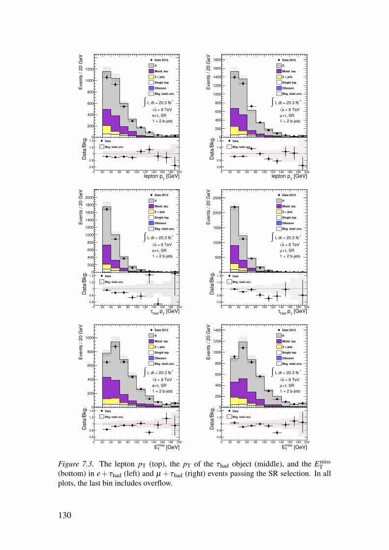
Eve

nts

/ 2

0 G

eV

200

400

600

800

1000

1200

Data 2012

tt

Misid. tau

Z + jets

Single top

Diboson

Bkg. total unc.

-1 L dt = 20.3 fb∫

= 8 TeVs

, SRτe+

1 + 2 b-jets

[GeV]T

lepton p0 20 40 60 80 100 120 140 160 180 200

Da

ta/B

kg

.

0.6

0.8

1

1.2

1.4 Data

Bkg. total unc.

0

Eve

nts

/ 2

0 G

eV

200

400

600

800

1000

1200

1400

1600

1800 Data 2012

tt

Misid. tau

Z + jets

Single top

Diboson

Bkg. total unc.

-1 L dt = 20.3 fb∫

= 8 TeVs

, SRτ+µ1 + 2 b-jets

[GeV]T

lepton p0 20 40 60 80 100 120 140 160 180 200

Da

ta/B

kg

.

0.6

0.8

1

1.2

1.4 Data

Bkg. total unc.

0

Eve

nts

/ 2

0 G

eV

200

400

600

800

1000

1200

1400

1600

1800

2000Data 2012

tt

Misid. tau

Z + jets

Single top

Diboson

Bkg. total unc.

-1 L dt = 20.3 fb∫

= 8 TeVs

, SRτe+

1 + 2 b-jets

[GeV]T

phad

τ0 20 40 60 80 100 120 140 160 180 200

Da

ta/B

kg

.

0.6

0.8

1

1.2

1.4 Data

Bkg. total unc.

0

Eve

nts

/ 2

0 G

eV

500

1000

1500

2000

2500Data 2012

tt

Misid. tau

Z + jets

Single top

Diboson

Bkg. total unc.

-1 L dt = 20.3 fb∫

= 8 TeVs

, SRτ+µ1 + 2 b-jets

[GeV]T

phad

τ0 20 40 60 80 100 120 140 160 180 200

Da

ta/B

kg

.

0.6

0.8

1

1.2

1.4 Data

Bkg. total unc.

0

Eve

nts

/ 2

0 G

eV

200

400

600

800

1000

Data 2012

tt

Misid. tau

Z + jets

Single top

Diboson

Bkg. total unc.

-1 L dt = 20.3 fb∫

= 8 TeVs

, SRτe+

1 + 2 b-jets

[GeV]missTE

0 20 40 60 80 100 120 140 160 180 200

Da

ta/B

kg

.

0.6

0.8

1

1.2

1.4 Data

Bkg. total unc.

0

Eve

nts

/ 2

0 G

eV

200

400

600

800

1000

1200

1400 Data 2012

tt

Misid. tau

Z + jets

Single top

Diboson

Bkg. total unc.

-1 L dt = 20.3 fb∫

= 8 TeVs

, SRτ+µ1 + 2 b-jets

[GeV]missTE

0 20 40 60 80 100 120 140 160 180 200

Da

ta/B

kg

.

0.6

0.8

1

1.2

1.4 Data

Bkg. total unc.

0

Figure 7.3. The lepton pT (top), the pT of the τhad object (middle), and the EmissT

(bottom) in e+ τhad (left) and µ + τhad (right) events passing the SR selection. In allplots, the last bin includes overflow.

130

Eve

nts

/ 2

0 G

eV

1000

2000

3000

4000

5000Data 2012

tt

Diboson

Z + jets

Single top

Misid. lep

Bkg. total unc.

-1 L dt = 20.3 fb∫

= 8 TeVs

, CRµe

0 b-jet

) [GeV]µM(e, 0 50 100 150 200 250 300

Da

ta/B

kg

.

0.6

0.8

1

1.2

1.4 Data

Bkg. total unc.

0

Eve

nts

/ 2

0 G

eV

500

1000

1500

2000

2500

3000 Data 2012

tt

Diboson

Z + jets

Single top

Misid. lep

Bkg. total unc.

-1 L dt = 20.3 fb∫

= 8 TeVs

, CRµe

1 b-jet

) [GeV]µM(e, 0 50 100 150 200 250 300

Da

ta/B

kg

.

0.6

0.8

1

1.2

1.4 Data

Bkg. total unc.

0

Eve

nts

/ 2

0 G

eV

200

400

600

800

1000

1200

1400

1600Data 2012

tt

Diboson

Z + jets

Single top

Misid. lep

Bkg. total unc.

-1 L dt = 20.3 fb∫

= 8 TeVs

, CRµe

2 b-jets

) [GeV]µM(e, 0 50 100 150 200 250 300

Da

ta/B

kg

.

0.6

0.8

1

1.2

1.4 Data

Bkg. total unc.

0

Figure 7.4. The eµ invariant mass in dilepton events passing the CR selection with 0b-tagged jets (top), 1 b-tagged jet (bottom left) or 2 b-tagged jets (bottom right). In allplots, the last bin includes overflow.

131

Events

/ 2

0 G

eV

500

1000

1500

2000

2500

3000

3500

4000

4500 Data 2012

tt

Diboson

Z + jets

Single top

Misid. lep

Bkg. total unc.

-1 L dt = 20.3 fb∫

= 8 TeVs

, CRµe

0 b-jet

) [GeV]miss

T(l, E

Tmax M

0 50 100 150 200 250 300

Da

ta/B

kg

.

0.6

0.8

1

1.2

1.4 Data

Bkg. total unc.

0

Events

/ 2

0 G

eV

500

1000

1500

2000

2500

3000

3500

4000 Data 2012

tt

Diboson

Z + jets

Single top

Misid. lep

Bkg. total unc.

-1 L dt = 20.3 fb∫

= 8 TeVs

, CRµe

1 b-jet

) [GeV]miss

T(l, E

Tmax M

0 50 100 150 200 250 300

Da

ta/B

kg

.

0.6

0.8

1

1.2

1.4 Data

Bkg. total unc.

0

Events

/ 2

0 G

eV

200

400

600

800

1000

1200

1400

1600

1800

2000

Data 2012

tt

Diboson

Z + jets

Single top

Misid. lep

Bkg. total unc.

-1 L dt = 20.3 fb∫

= 8 TeVs

, CRµe

2 b-jets

) [GeV]miss

T(l, E

Tmax M

0 50 100 150 200 250 300

Da

ta/B

kg

.

0.6

0.8

1

1.2

1.4 Data

Bkg. total unc.

0

Events

/ 2

0 G

eV

200

400

600

800

1000

1200

1400

1600

1800 Data 2012

tt

Misid. tau

Z + jets

Single top

Diboson

Bkg. total unc.

-1 L dt = 20.3 fb∫

= 8 TeVs

, SRτ + µe/

1 + 2 b-jets

) [GeV]miss

T, E

hadτ(TM

0 20 40 60 80 100 120 140 160 180 200

Da

ta/B

kg

.

0.6

0.8

1

1.2

1.4 Data

Bkg. total unc.

0

Figure 7.5. The inputs to the fit: the maximum transverse mass of dilepton eventspassing the CR selection with 0 b-tagged jets (top left), 1 b-tagged jet (top right), and2 b-tagged jets (bottom left), as well as the transverse mass of lepton+τhad eventspassing the SR selection with one or two b-tagged jets. In all plots, the last bin includesoverflow.

132

Events

/ 2

0 G

eV

500

1000

1500

2000

2500

3000

3500

4000

4500 Data 2012

tt

Diboson

Z + jets

Single top

Misid. lep

Bkg. total unc.

-1 L dt = 20.3 fb∫

= 8 TeVs

, CRµe

0 b-jet

) [GeV]miss

T(l, E

Tmax M

0 50 100 150 200 250 300

Da

ta/B

kg

.

0.6

0.8

1

1.2

1.4 Data

Bkg. total unc.

0

Events

/ 2

0 G

eV

500

1000

1500

2000

2500

3000

3500

Data 2012

tt

Diboson

Z + jets

Single top

Misid. lep

Bkg. total unc.

-1 L dt = 20.3 fb∫

= 8 TeVs

, CRµe

1 b-jet

) [GeV]miss

T(l, E

Tmax M

0 50 100 150 200 250 300

Da

ta/B

kg

.

0.6

0.8

1

1.2

1.4 Data

Bkg. total unc.

0

Events

/ 2

0 G

eV

200

400

600

800

1000

1200

1400

1600

1800

2000

Data 2012

tt

Diboson

Z + jets

Single top

Misid. lep

Bkg. total unc.

-1 L dt = 20.3 fb∫

= 8 TeVs

, CRµe

2 b-jets

) [GeV]miss

T(l, E

Tmax M

0 50 100 150 200 250 300

Da

ta/B

kg

.

0.6

0.8

1

1.2

1.4 Data

Bkg. total unc.

0

Events

/ 2

0 G

eV

200

400

600

800

1000

1200

1400

1600Data 2012

tt

Misid. tau

Z + jets

Single top

Diboson

Bkg. total unc.

-1 L dt = 20.3 fb∫

= 8 TeVs

, SRτ + µe/

1 + 2 b-jets

) [GeV]miss

T, E

hadτ(TM

0 20 40 60 80 100 120 140 160 180 200

Da

ta/B

kg

.

0.6

0.8

1

1.2

1.4 Data

Bkg. total unc.

0

Figure 7.6. Post-fit plots of the maximum transverse mass of dilepton events passingthe CR selection with 0 b-tagged jets (top left), 1 b-tagged jet (top right), and 2 b-tagged jets (bottom left), as well as the transverse mass of lepton+τhad events passingthe SR selection with one or two b-tagged jets. In these plots, the best-fit values of allnuisance parameters under the background-only hypothesis, and their uncertainties,are shown. The last bin includes overflow.

133

-60 -40 -20 0 20 40 60

b−tag efficiency, component 5

b−mistag rate, component 1

JES (detector), component 1

b−tag efficiency, component 1

Misid. tau (jet composition)

Initial− and final−state radiation

Electron ID

JES (b−jet)

JES (flavor response)

JES (model), component 1

Tau ID (syst)

Tau ID (stat)

Tau energy scale

Generator and parton shower

JES (flavor composition)

µΔ

-0.004 -0.003 -0.002 -0.001 0 0.001 0.002 0.003 0.004

θΔ)/0

θ - θ(

-2 -1 0 1 2

Pull

1 standard deviation

µPrefit Impact on

µPostfit Impact on

= 8 TeVs

-1Ldt = 20.3 fb∫

=130 GeVH+m

Figure 7.7. Pull distribution for the mH+ = 130 GeV hypothesis. The black markersindicate the shift of the best-fit value of each parameter with respect to its nominalvalue in units of one standard deviation (red) as indicated on the bottom axis, while theyellow and hatched blue bands respectively show the pre- and post-fit impacts on thefitted signal strength as indicated on the top axis. The 15 most important parametersare shown. Some of the uncertainties related to the jet energy scale (JES) or b-taggingare split into several effective components.

134

-0.6 -0.4 -0.2 0 0.2 0.4 0.6

JES (eta intercalibration)

b−tag efficiency, component 1

b−mistag rate, component 11

Muon ID

JES (flavor composition)

Jet energy resolution

Initial− and final−state radiation

JES (model), component 1

Electron energy scale

JES (flavor response)

JES (detector), component 1

Muon trigger efficiency

b−tag efficiency, component 5

Tau electron veto

Generator and parton shower

µΔ

-0.4 -0.3 -0.2 -0.1 0 0.1 0.2 0.3 0.4

θΔ)/0

θ - θ(

-2 -1 0 1 2

Pull

1 standard deviation

µPrefit Impact on

µPostfit Impact on

= 8 TeVs

-1Ldt = 20.3 fb∫

=250 GeVH+m

Figure 7.8. Pull distribution for the mH+ = 250 GeV hypothesis. The black markersindicate the shift of the best-fit value of each parameter with respect to its nominalvalue in units of one standard deviation (red) as indicated on the bottom axis, while theyellow and hatched blue bands respectively show the pre- and post-fit impacts on thefitted signal strength as indicated on the top axis. The 15 most important parametersare shown. Some of the uncertainties related to the jet energy scale (JES) or b-taggingare split into several effective components.

135

[GeV]+Hm80 90 100 110 120 130 140 150 160

ν)+ τ

→ +

H B

(×

+ b

H)

→t

B(

-310

-210

-110

1

Observed CLs

Expected

σ 1±

σ 2±

Data 2012

= 8 TeVs

-1Ldt = 20.3 fb∫

[GeV]+Hm80 90 100 110 120 130 140 150 160

ν)+ τ

→ +

H B

(×

+ b

H)

→t

B(

-310

-210

-110

1

Observed CLs

Expected

σ 1±

σ 2±

Data 2012

= 8 TeVs

-1Ldt = 20.3 fb∫

[GeV]+Hm80 90 100 110 120 130 140 150 160

ν )

+ τ →

+H

B(

×+

bH

)→

t B

(

-310

-210

-110

1

Observed CLs

Expected

σ 1±

σ 2±

Data 2012

= 8 TeVs

-1Ldt = 20.3 fb∫

Figure 7.9. Expected and observed 95% confidence level upper limits on lightcharged Higgs boson production, obtained with electron-triggered events (top), muon-triggered events (middle) and a combination of both (bottom).

136

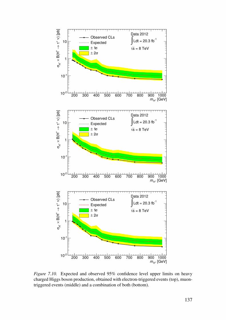
[GeV]+H

m

200 300 400 500 600 700 800 900 1000

) [p

b]

ν + τ

→ +

B(H

× +

Hσ

-210

-110

1

10Observed CLs

Expected

σ 1±

σ 2±

Data 2012

= 8 TeVs

-1Ldt = 20.3 fb∫

[GeV]+H

m

200 300 400 500 600 700 800 900 1000

) [p

b]

ν + τ

→ +

B(H

× +

Hσ

-210

-110

1

10Observed CLs

Expected

σ 1±

σ 2±

Data 2012

= 8 TeVs

-1Ldt = 20.3 fb∫

[GeV]+H

m

200 300 400 500 600 700 800 900 1000

) [p

b]

ν + τ

→ +

B(H

× +

Hσ

-210

-110

1

10Observed CLs

Expected

σ 1±

σ 2±

Data 2012

= 8 TeVs

-1Ldt = 20.3 fb∫

Figure 7.10. Expected and observed 95% confidence level upper limits on heavycharged Higgs boson production, obtained with electron-triggered events (top), muon-triggered events (middle) and a combination of both (bottom).

137

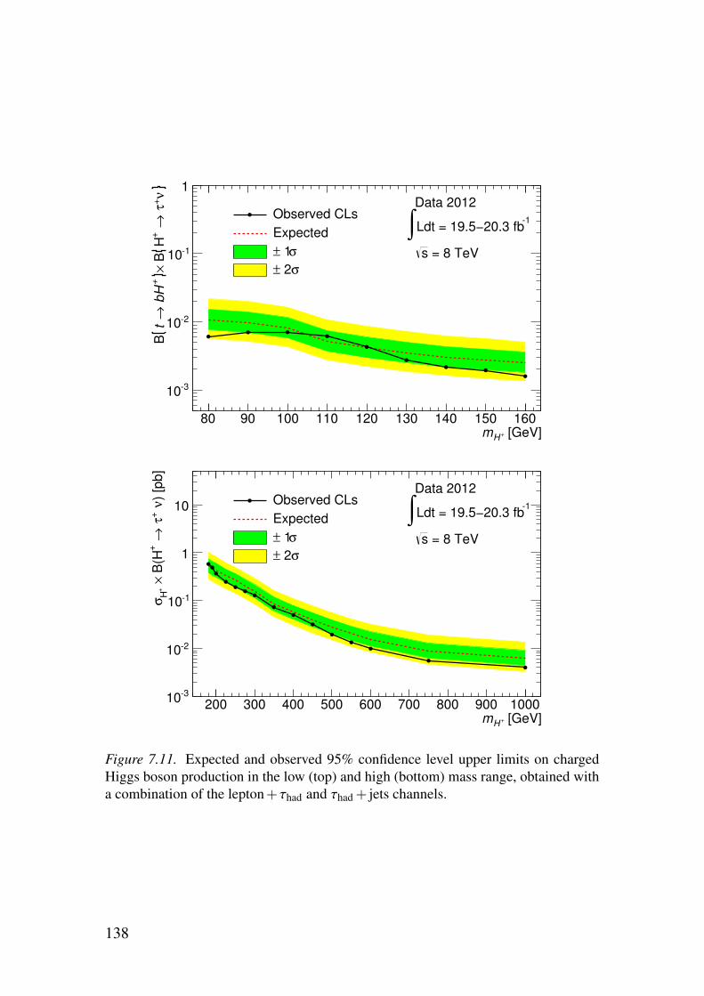
[GeV]+H

m

80 90 100 110 120 130 140 150 160

ν+ τ

→ +

H B

×+

bH

→t

B

-310

-210

-110

1

Observed CLs

Expected

σ 1±

σ 2±

Data 2012

= 8 TeVs

-1Ldt = 19.5−20.3 fb∫

[GeV]+H

m

200 300 400 500 600 700 800 900 1000

) [p

b]

ν + τ

→ +

B(H

× +

Hσ

-310

-210

-110

1

10 Observed CLs

Expected

σ 1±

σ 2±

Data 2012

= 8 TeVs

-1Ldt = 19.5−20.3 fb∫

Figure 7.11. Expected and observed 95% confidence level upper limits on chargedHiggs boson production in the low (top) and high (bottom) mass range, obtained witha combination of the lepton+τhad and τhad + jets channels.

138

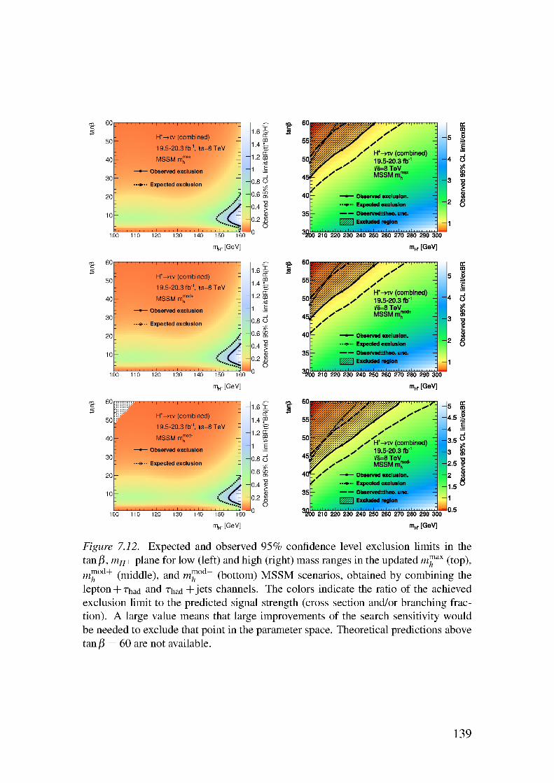
At the time of writing, the restart of the LHC at√

s = 13 TeV is imminent.This will mark the beginning of a new chapter of Higgs physics. Up to now,the discovered Higgs boson appears to be consistent with that predicted bythe Standard Model. Establishing or disproving this fact will be a key taskfor the LHC in the years to come. With higher collision energies than everbefore, and higher integrated luminosity, we can expect detailed measurementsof the discovered Higgs boson, and increased sensitivities in many searches foradditional Higgs bosons. This will either validate the last unexplored sector ofthe Standard Model, or possibly let us discover something completely new.

140

Résumé en français

1. Le Modèle Standard de la physique des particulesLa physique des particules est l’étude des composants microscopiques élé-mentaires présents dans notre Univers. Toute structure de cet Univers, que cesoit un atome, un grain de poussière ou une galaxie, est formée de particulesdites élémentaires. Les atomes, par exemple, qui composent toute la matièreterrestre, comportent des électrons qui orbitent autour d’un noyau, qui est lui-même assemblé à partir de protons et de neutrons, lesquels sont formés dequarks up et down. L’électron a deux frères plus lourds: le muon et le tau. Pourchacune de ces particules, il existe un neutrino correspondant. Les neutrinossont des particules électriquement neutres presque sans masse qui interagis-sent très faiblement avec toute la matière. Ces particules forment les leptons.Les quarks up et down ont aussi des frères plus lourds: les quarks charméet top, et les quarks étrange et bottom. Les leptons et les quarks sont tousdes fermions de spin 1

2 . Chaque fermion a aussi une anti-particule de chargeélectrique opposée. Nous ne savons toujours pas si l’anti-neutrino est uneparticule différente du neutrino. Les fermions interagissent les uns avec lesautres en échangeant d’autres particules de spin entier qui sont par conséquentdes bosons. À l’échelle microscopique, les forces résultent de ces échanges:la force électromagnétique est transmise par les photons, l’interaction forteprovient de l’échange de gluons, et la force faible est convoyée par les bosonsW± et Z. La force forte, qui agit entre les quarks, forme des systèmes liésappelés hadrons (le proton et le neutron sont des exemples de hadrons).

Le Modèle Standard est une théorie quantique qui décrit toutes les partic-ules élémentaires connues et leurs interactions. L’une des hypothèses sous-jacentes du Modèle Standard est que les lois de la nature doivent être invari-antes sous certaines transformations, dites transformations de jauge. Une con-séquence de ceci est que les particules élémentaires ne devraient pas avoirde masse. Leur masse apparaît par le biais d’interactions avec un champ deHiggs, qui est un champ scalaire qui possède aujourd’hui une valeur moyennenon nulle dans le vide. Ces interactions produisent également le mélange desétats massifs et d’interaction des neutrinos et des quarks. Le champ de Higgsdu Modèle Standard donne lieu à une nouvelle particule, le boson de Higgs,qui a été découverte en 2012 au CERN par les collaborations ATLAS et CMS.

Le Modèle Standard est une théorie du monde microscopique dont pra-tiquement toutes les prédictions ont été confirmées expérimentalement. Pour-tant, il est largement admis que ce ne peut être une théorie complète de la

141

nature. En effet, le Modèle Standard est incapable d’expliquer l’asymétriematière-antimatière de l’univers, la nature microscopique de la matière noireobservée par ses effets gravitationnels, et de nombreux autres phénomènescosmologiques tels l’expansion accéléré de notre Univers. Dans le ModèleStandard, la masse du boson de Higgs est en principe sujette à de grandescorrections quantiques, exigeant du point de vue de la théorie des annulationsanormalement fines afin de préserver une valeur finie de l’ordre de 125 GeV.Tous ces points motivent la recherche de nouveaux processus physiques mi-croscopiques allant au-delà du Modèle Standard.

2. Au-delà du Modèle StandardLe Modèle Standard utilise une forme minimale du mécanisme dites Brout-Englert-Higgs pour atteindre une brisure de symétrie électrofaible. Il n’y a pasde motivation théorique pour cela à part de juste sa simplicité. Or, la réalitépeut être plus compliquée. De nombreuses extensions possibles du ModèleStandard ont été proposées, dont certaines comprennent des champs de Higgssupplémentaires. Dans un modèle à deux Higgs-Doublet (2HDM) il ya deuxchamps scalaires de doublet valeurs complexes, par rapport à un seul dans leModèle Standard. Le secteur de Higgs du Modèle Standard SupersymétriqueMinimum (MSSM), qui peut résoudre un nombre des problèmes évoqués dansle chapitre précédent, est un 2HDM. En tout 2HDM, il ya cinq bosons deHiggs: La CP-même h et H, le CP-odd A et H± chargée électriquement. Cettethèse présente des recherches pour les bosons de Higgs chargés.

Dans le MSSM, un boson de Higgs chargé se désintègre principalement parH+ → tb ou en particules supersymétriques lorsque cela est permis cinéma-tiquent. La désintegration en quarks de différentes générations est défavoriséeet le mode dominant quand tb est interdit cinématiquement n’est pas cb, maisτν . Le mode de désintégration préféré dans quarks légers est la place cs. Pourles modes de désintégration leptoniques, les fractions de branchement rela-tives sont directement proportionnelles à la masse au carré du lepton chargé.Une désintégration en µν et eν ne sont alors pas possibles par plusieurs ordresde grandeur.

Dans un collideur de hadrons, des bosons de Higgs chargés peuvent êtreproduites dans les désintégrations de quarks top, qui sont produites princi-palement dans la forme de tt paires. Si les bosons de Higgs chargés sontplus lourdes que les quark top, ils seraient plutôt fabriqués en association avecun quark top. Dans le premier cas, le boson de Higgs chargé se désintègreprincipalement dans un tau et un neutrino, alors que dans le dernier cas, il sedésintègre principalement dans un quark top et un quark bottom.

142

3. Le Grand collisionneur de hadronsLe Large Hadron Collider (Grand collisionneur de hadrons, LHC), situé auCERN à Genève, en Suisse, est le collisionneur de particules le plus puissantdu monde. Le LHC est un accélérateur synchrotron, près de 27 km de circon-férence, équipés de plus de 1600 aimants supraconducteurs fonctionnant à 1,9K et capable de générer des champs magnetique de jusqu’à 8,3 T. Il accélèredeux faisceaux tournant en sens inverse de particules de la même charge àl’aide de 400 MHz cavités supraconductrices. Il y a des installations expéri-mentales où les faisceaux se croisent à quatre points le long de la machine.

Les analyses présentées dans cette thèse utilisent des données recueillies en2011 et 2012, lorsque le LHC a livré des collisions proton-proton à des éner-gies de 7 TeV et 8 TeV dans le centre de masse. Une luminosité instantanée de7,7×1033 cm−2s−1 a été atteint, et des lunminosities intégrés jusqu’à 6 fb−1

(23 fb−1) de 7 TeV (8 TeV) ont été delivrés le nombre de collisions à des ex-périences. Ces données présentent une opportunité pour étudier les processusde physique à des énergies jamais sondé auparavant dans un environnementde laboratoire.

Le résultat le plus important de la première manche du LHC a été la dé-couverte d’un boson de Higgs avec une masse de 125 GeV. Cela confirmel’existence d’au moins un champ de Higgs. Les mesures des accouplements,de spin et la parité de la particule découverte sont compatibles avec les prédic-tions du modèle standard. Les expériences du LHC ont aussi cherché, entreautres choses, les particules supersymétriques et bosons de Higgs supplémen-taires mais ils n’ont pas trouvé une preuve de l’existence de telles particules.

4. L’expérience ATLASLe détecteur ATLAS a été conçu pour explorer l’intégralité du potentiel dephysique offert par le LHC. Au centre d’ATLAS, se trouve un trajectomètrequi mesure la quantité de mouvement des particules chargées, avec une réso-lution de σpT/pT = 0,05%pT ⊕1%. Du centre vers l’extérieur, cet instrumentest subdivisé en un détecteur à pixels de silicium, suivi d’un détecteur à bandesde semi-conducteur (SCT), et d’un détecteur de traces composé de tubes à ray-onnement de transition (TRT). Ce trajectomètre est plongé dans un solénoïdesupraconducteur développant un champ magnétique axial de 2 T.

Le calorimètre d’ATLAS utilise la technologie à argon liquide dans unrayon de 2 m autour de l’axe du faisceau, et à tuiles scintillantes au-delà.L’énergie des électrons et des photons est mesurée avec une résolution deσE/E = 10%/

√E ⊕ 0.7%. Celle des jets hadroniques est obtenue avec une

résolution de σE/E = 50%/√

E ⊕3%.Tout à l’extérieur d’ATLAS, on trouve le spectromètre à muons qui se com-

pose séparément de chambres à dérive de précision et de détecteurs gazeuxassurant le déclenchement. Le champ magnétique de déviation est fourni

143

par trois ensembles d’aimants toroïdaux supraconducteurs. Le spectromètreà muons peut mesurer la quantité de mouvement transverse de muons avecune résolution de 10 % à 1 TeV, indépendamment du détecteur interne.

ATLAS est équipé d’un système de déclenchement à trois niveaux qui estutilisé pour réduire le taux d’événements à environ 400 Hz.

Dans le cadre des préparatifs pour la deuxième campagne de prise de don-nées du LHC, l’auteur a contribué à des améliorations du système de contrôlequi maintient la séparation thermique entre le SCT et le TRT . Des mesures dela résistance des modules du SCT sous une polarisation directe ont égalementété réalisées. Aucune augmentation significative de cette résistance depuis lamise en service d’ATLAS n’a été observée.

Le logiciel d’ATLAS, qui comprend le système de contrôle-commande,d’acquisition de données, les programmes de simulation, de reconstructionet d’analyse des événements, est également décrit dans ce chapitre, en mettantl’accent sur les contributions personnelles de l’auteur.

5. Les techniques d’analyseLe premier lot de données enregistrées en 2011 par ATLAS à

√s = 7 TeV

correspond à une luminosité intégrée de 4,6 fb−1. Le deuxième lot recueilli en2012 à

√s = 8 TeV totalise une luminosité intégrée de 20,3 fb−1.

Les électrons sont reconstruits en faisant correspondre les dépôts d’énergiegroupés en amas dans le calorimètre électromagnétique à des traces recon-struites dans le trajectomètre. Les muons induisent des traces observées dansle trajectomètre et dans le spectromètre à muons. Les jets hadroniques sontmesurés dans les calorimètres en utilisant l’algorithme de reconstruction anti-kt avec un rayon de gerbe de 0,4. Les données mesurées dans le trajectomètrepermettent l’identification des jets hadroniques provenant de vertex primairesainsi que des jets initiés par un quark b. Les désintégrations hadroniques desleptons tau sont reconstruites à partir des jets possédant une ou trois tracesassociées, et à l’aide d’algorithmes multivariés destinés à éliminer ceux quiparmi eux proviennent de jets initiés par des quarks ou des gluons.

Cette thèse présente la recherche de bosons de Higgs chargés, légers lorsqueceux-ci sont produits dans la désintégration de quarks top, ou lourds lorsqu’ilssont générés en association avec un quark top. Les bruits de fond princi-paux proviennent alors des processus du Modèle Standard avec productionde quarks top, et en particulier du processus gg → tt → bbW+W−, ainsi quede la production de bosons vecteurs en association avec des jets. La modélisa-tion des événements de signal et des processus de bruit de fond principaux estréalisée par simulation Monte Carlo.

Certains bruits de fond, en particulier ceux qui découlent de faux leptonstau mal identifiés, sont difficiles à simuler correctement et sont donc estimésen utilisant des techniques basées sur les données réelles. La méthode de la

144

matrice est l’une de ces techniques. Elle utilise les probabilités d’identificationcorrecte et erronée mesurées dans les données réelles, sur des événementssimulés, ou dans un mélange des deux. Elle peut être utilisée pour évaluerla normalisation et les distributions – fonctions de variables cinématiques –d’événements de bruit de fond avec un ou plusieurs objets mal identifiés.

Tous les résultats des analyses présentées dans cette thèse sont interprétésen testant la compatibilité des données avec tout d’abord l’hypothèse du Mod-èle Standard uniquement, et ensuite l’hypothèse du Modèle Standard avec unsignal de boson de Higgs chargé, le tout en utilisant une méthode fréquentistede vraisemblance profilée modifiée qui intègre des incertitudes systématiquestraitées comme des paramètres de nuisance ajustés aux données. Cette méth-ode permet de minimiser l’impact des incertitudes systématiques sur la sensi-bilité de recherche en tirant profit de régions de contrôle dominées par le bruitde fond.

6. Recherche d’un boson de Higgs chargé sedésintégrant en un lepton tau et un neutrino tau dans lesdonnées prises à 7 TeVDans ce chapitre, sont présentées trois recherches d’un boson de Higgs chargéet léger, qui serait généré dans la désintégration de quarks top et qui se désin-tégrerait en τν . Elles font appel aux données recueillies par ATLAS en 2011 à7 TeV. Toutes ces analyses partent de l’hypothèse que B(H+ → τν) = 100%.Dans tous les cas, le signal est caractérisé par la présence additionnelle d’unquark top (produit par paires) qui se désintègre en un électron ou un muon. Celepton de haut pT permet de distinguer clairement ces événements de la plupartdes fonds multi-jets, et est en conséquence utilisé pour le déclenchement.

En principe, le canal le plus propre est l’état final dilepton, où le tau prov-enant du boson de Higgs se désintègre d’une manière leptonique. Le canaldilepton a été analysé sur les premières données de collisions pp enregistrées à√

s = 7 TeV, correspondant à une luminosité intégrée de 1,03 fb−1. Les résul-tats montrent que cette analyse a une sensibilité modeste à l’observation d’unboson de Higgs chargé et léger. Elle n’a donc pas été répétée sur l’ensembledes données.

Au vu de ce constat, l’accent a été mis sur le canal où le lepton tau sedésintègre hadroniquement (τhad). Les modes de désintégration hadroniquedu lepton tau ont des fractions de branchement plus élevées, et conduisent àdes événements qui comportent moins de neutrinos. Cependant, ce canal estentaché d’un bruit fond difficile à estimer, provenant de jets initiés par desquark ou des gluons, qui peuvent être à tort identifiés comme des désintégra-tions hadroniques de leptons tau. Puisque cette probabilité de confusion esttrès difficile à modéliser précisément par des simulations Monte-Carlo, elle

145

a été mesurée dans des régions de contrôle sur les données réelles. Le canallepton+τhad a été analysé sur l’ensemble complet des données acquises en2011, correspondant à une luminosité intégrée de 4,6 fb−1. En l’absence designal observé, des limites supérieures sur le rapport de branchement B(t →bH+) on été extraites en utilisant la distribution Emiss

T de l’énergie transversemanquante.

Par ailleurs, les données ont été réanalysées avec un traitement simultanédes canaux dileptonique et lepton+τhad. Cette analyse qui se présente sous laforme d’un comptage d’événements, a été conçue comme un test de l’universal-ité leptonique dans les événements tt. Ici le rôle du canal dileptonique consisteprincipalement à contraindre les incertitudes sur les bruits de fond, plutôt quede fournir une sensibilité directe au signal. Les événements dans lesquels leτhad reconstruit a le même signe de charge que le lepton sont soustraits desévénements dans lesquels ils ont des signes de charges opposés, ce qui annuleles contributions des jets de gluons et de quarks bottom feignant une désin-tégration hadronique d’un lepton tau. Le nombre d’événements lepton+τhadet dileptoniques est finalement mesuré comme étant conforme à la prévisiondu Modèle Standard. Des limites supérieures sur B(t → bH+) sont alorsdéduites. Elles vont de 3,2 à 4,4% pour des masses de H+ allant de 90 à 140GeV.

La combinaison de ces résultats avec ceux obtenus par d’autres recherchesmenées au sein d’ATLAS au sujet de bosons de Higgs chargés, ainsi que leurinterprétation dans le scénario mmax

h du MSSM sont également présentées.

7. Recherches d’un boson de Higgs chargé décroissanten un lepton tau et un neutrino dans les données acquisesà 8 TeVLes données recueillies à

√s = 8 TeV en 2012, correspondant à une lumi-

nosité intégrée de 20,3 fb−1, ont fait l’objet d’une analyse simultanée descanaux lepton+τhad et dilepton. Comme lors du test de l’universalité lep-tonique dans la désintégration des quarks top présenté dans le chapitre précé-dent, l’adjonction du canal dileptonique permet de réduire les incertitudessystématiques du bruit de fond. Cependant, à la différence de ce qui avaitété fait à 7 TeV, le test de présence d’un signal est mené sur la distributiond’une variable de masse transverse, laquelle permet d’améliorer la sensibilitéd’observation d’un boson de Higgs chargé pour des masses plus grandes quecelle du boson W . Cette recherche a été conduite pour une masse du boson deHiggs chargé allant jusqu’à 1 TeV, qui serait produit dans ce cas en associationavec un quark top.

Le bruit de fond provenant de l’erreur d’identification de jets hadroniquesqui sont parfois confondus avec des désintégrations hadroniques de leptons

146

tau, est estimé par l’usage de la technique dite de la matrice, appliquée sur lesdonnées réelles. Cette méthode permet de mesurer les probabilités d’erreursd’identification directement dans les données réelles, en utilisant de vraiesdésintégrations hadroniques de leptons tau plutôt que celles fournies par lasimulation.

Les principales incertitudes systématiques de cette analyse sont liées àl’étalonnage de l’énergie des jets et à la modélisation des événements tt. Dansla région de contrôle dileptonique dominée par le bruit de fond, l’analyse esteffectuée à l’aide de catégories distinctes d’événements avec zéro, un, ou deuxjets étiquetés b, tandis que la région où l’on attend un signal est fusionnée pourcontenir les événements avec un ou deux jets étiquetés b, ceci dans le but deréduire l’incertitude sur la multiplicité des jets étiquetés b, découlant du choixdu schéma de calcul pour les signaux de masse élevée. Des limites supérieuressont obtenues sur le rapport d’embranchement B(t → bH+)×B(H+ → τν)qui varie de 1,1 à 0,3% pour 80 GeV ≤ mH+ ≤ 160 GeV, et sur la section ef-ficace du signal fois B(H+ → τν) qui va de 0,93 à 0,03 pb pour 180 GeV ≤mH+ ≤ 1 TeV. Ces limites observées sont légèrement plus basses que cellesauxquelles on s’attendait.

Ces résultats sont complémentaires avec ceux obtenus par la recherche ef-fectuée dans l’état final τhad + jets , qui a également été refaite sur l’ensembledes données acquises à 8 TeV. La combinaison des résultats de ces deux anal-yses repoussent les limites obtenues par le canal τhad + jets seul, en particulierdans la région de très faible masse mH+ < 100 GeV où l’amélioration de lalimite d’exclusion va jusqu’à 35%. La fluctuation négative observée dans lesdonnées réelles améliore encore les limites observées: jusqu’à 40% de mieuxdans la région de faible masse pour les résultats combinés par rapport à cequi est obtenu avec le canal τhad + jets seul, et jusqu’à 20% de mieux dansla région de masse élevée. Les limites supérieures observées sur le produitdu rapport d’embranchement B(t → bH+)×B(H+ → τν) varient de 0,6 à0,15% pour 80 GeV ≤ mH+ ≤ 160 GeV, tandis que les limites supérieures ob-servées sur la section efficace de production sont de l’ordre de 0,43 à 0,004 pbpour 180 GeV ≤ mH+ ≤ 1 TeV. Ces résultats sont également interprétés dansle cadre du MSSM.

ConclusionCette thèse a décrit la recherche d’un boson de Higgs chargé se désintégrant enun lepton tau et un neutrino à l’aide des données enregistrées par l’expérienceATLAS en 2011 et 2012. Dans cette étude, nous avons considéré les étatsfinaux comportant soit deux leptons chargés, ou un lepton chargé et une dés-intégration hadronique d’un lepton tau. Deux cas de figures de production debosons de Higgs chargés ont été considérés: pour un boson de Higgs chargédont la masse serait inférieure à celle du quark top, celui-ci serait produit dans

147

la désintégration des quarks top; dans le cas inverse, le boson de Higgs chargéserait produit en association avec un quark top.

Les bruits de fond comportant de vrais leptons et de vraies désintégrationshadroniques de leptons tau ont été simulés, puis ont été normalisés aux don-nées en utilisant des régions de contrôle où le signal attendu est par naturetrès faible. Les bruits de fond incluant des leptons ou des désintégrationshadroniques de lepton tau mal identifiés ont été estimés à partir des don-nées elles-mêmes. Avec 20,3 fb−1 de données enregistrées à une énergiede 8 TeV dans le centre de masse des collisions, des limites supérieures àun niveau de confiance de 95% sont placées sur le rapport d’embranchementB(t → bH+)×B(H+ → τ+ν). Leurs valeurs vont de 1,1 à 0,3% pour unemasse du boson de Higgs chargé allant de 80 GeV à 160 GeV. Pour unemasse du boson de Higgs chargé comprise entre 180 GeV et 1 TeV, ces limitesconcernent la section efficace de production d’un boson de Higgs chargé enassociation avec un quark top. Leurs valeurs varient de 0,93 à 0,03 pb sur ledomaine de masse afférant. Les limites présentées dans cette thèse sont lesmeilleures obtenues à ce jour dans ce canal de recherche. Une combinaisonde ces résultats avec une autre recherche effectuée en exploitant l’état finalentièrement hadronique conduit à des limites allant de 0,6 à 0,15 % pour unboson de Higgs chargé léger (mH+ < mt), et de 0,43 à 0,04 pb pour le casd’un boson de Higgs lourd (mH+ > mt).

Lors de la préparation de cette thèse, un boson de Higgs neutre a été ob-servé pour la première fois par les collaborations ATLAS et CMS. Ceci prouvel’existence d’au-moins un champ scalaire fondamental et nous encourage àpoursuivre les recherches de bosons de Higgs supplémentaires. Le future desrecherches dans ce domaine résidera sans aucun doute dans le régime de masseélevée: mH+ > mt . Le mode de désintégration du boson de Higgs chargé dansun lepton tau et un neutrino restera un canal de recherche d’un grand intérêten raison de sa signature expérimentale relativement propre et de son rapportd’embranchement important dans certaines parties de l’espace des paramètres.

L’analyse de l’état final lepton+ τhad présentée dans cette thèse est moinssensible que l’analyse précédemment publiée qui exploitait l’état final τhad +jets, et doit être considérée comme complémentaire pour ce type de recherche.Néanmoins, son importance augmentera dès lors que des domaines de masseplus élevés seront explorés, puisque l’importance relative de l’impulsion trans-verse manquante emportée par le neutrino apparaissant dans la désintégra-tion standard du quark top sera réduite. Avec 20,3 fb−1 de données recueil-lies à 8 TeV, la sensibilité de l’analyse est limitée par les incertitudes statis-tiques. Lorsque plus de données seront enregistrées lors de la deuxième péri-ode d’exploitation du LHC, la sensibilité de ce canal pourrait augmenter. Desperspectives intéressantes pour l’amélioration de cette analyse résident dansl’utilisation des informations de polarisation du lepton tau, car le boson deHiggs chargé et le boson W portent des spins différents: 0 et 1.

148

Au moment de l’écriture de ce document, le redémarrage du LHC à√

s =13 TeV est imminent. Cela marquera le début d’un nouveau chapitre de laphysique du boson de Higgs. Jusqu’à présent, le boson de Higgs découvertsemble être compatible avec celui prédit par le modèle standard. Confirmerou réfuter ce fait sera la tâche essentielle du LHC pour les années à venir.

149

Sammanfattning på svenska

Inom partikelfysiken studeras universums minsta byggstenar. Allting, fråndammkorn till galaxer, består på en fundamental nivå av elementarpartiklar.Atomer, som bygger upp all materia här på jorden, består till exempel av elek-troner som kretsar kring en kärna bestående av neutroner och protoner, som isin tur består av upp-kvarkar och ned-kvarkar. Elektronen har två tyngre släk-tingar: myonen och tauonen. För var och en av dessa finns också en neutrino.Neutrinerna är närapå masslösa partiklar som interagerar väldigt svagt medsin omgivning. Upp- och ned-kvarkarna har också tyngre släktingar: charm-och topp-kvarkarna, respektive sär- och botten-kvarkarna. Dessa partiklar ut-gör tillsammans fermionerna. Varje fermion har också en anti-partikel medmotsatt elektrisk laddning. Fermionerna växelverkar med varandra genomatt utbyta andra partiklar som kallas för bosoner. På så vis uppstår kraftermellan partiklarna: den elektromagnetiska kraften som förmedlas av fotonen,den starka kraften som förmedlas av gluonerna, och den svaga kraften somförmedlas av W±- och Z-bosonerna. Den starka kraften, som verkar mel-lan kvarkarna, binder ihop dessa till sammansatta objekt som kallas hadroner(protonen och neutronen är exempel på hadroner).

Standardmodellen är en kvantfältteori som beskriver alla kända elemen-tarpartiklar och deras växelverkan genom de tre nämnda krafterna. Standard-modellen bygger i stor utsträckning på att fysikens lagar måste vara invariantaunder vissa lokala transformationer (så kallade gaugetransformationer) ochdetta förutsätter att elementarpartiklarna från början är masslösa. De får istäl-let sina massor genom interaktioner med ett Higgsfält. Higgsfältet har denspeciella egenskapen att dess styrka inte är noll när dess energi är som lägst.Även i vakuum genomsyras rymden därför av ett starkt Higgsfält och genomkontakt med detta fält får partiklarna sina massor. Higgsfältet ger också up-phov till en ny partikel, den så kallade Higgsbosonen. Genom upptäckten avHiggsbosonen vet vi att Higgsfältet existerar och att den teoretiska beskrivnin-gen av hur partiklarna får sina massor verkar stämma med verkligheten.

Det finns vissa problem som inte kan förklaras inom standardmodellen ochdet står klart att den förr eller senare måste utvidgas till en större teori. Imånga föreslagna utvidgningar av standardmodellen förekommer mer än ettHiggsfält, och därmed också mer än en Higgsboson. I den enklaste utöknin-gen lägger man helt enkelt till ett extra Higgsfält liknande det som beskrivsav standardmodellen. Då uppstår totalt fem Higgsbosoner, varav tre är elek-triskt neutrala och två är elektriskt laddade. Det är jakten på dessa laddadeHiggsbosoner som är ämnet för den här avhandlingen.

150

För att hitta spår av nya partiklar studerar man hur högenergetiska partiklarinteragerar med varandra. Den stora hadronkollideraren LHC (Large HadronCollider) vid forskningslaboratoriet CERN i Genève, Schweiz, är världenskraftfullaste partikelaccelerator. Hadronerna som kollideras är oftast protoner.När två protoner – eller rättare sagt, kvarkar och gluoner inuti protonerna –kolliderar, omvandlas deras rörelseenergi till nya partiklar. Många partiklarär instabila och sönderfaller snabbt till andra partiklar, till exempel elektroner,myoner eller hadroner. Utmaningen är sedan att detektera dessa och försökaåterskapa vilka sorts partiklar som från början bildades i kollisionen.

ATLAS är ett stort experiment vid LHC, som bland annat är utrustat medspårdetektorer och kalorimetrar för att mäta olika egenskaper hos olika par-tiklar. I den här avhandlingen beskriver jag analyser av data från ATLASi syfte att hitta tecken på existensen av laddade Higgsbosoner. Detta görsgenom att studera proton-proton kollisioner där topp-kvarkar bildas. Eftersomtopp-kvarken är den tyngsta av alla elementarpartiklar så har den en särskiltstark koppling till Higgsbosonerna. Om de laddade Higgsbosonerna är lättareän topp-kvarken så kan topp-kvarken därför sönderfalla till en laddad Higgs-boson och en botten-kvark. Om de laddade Higgsbosonerna däremot är tyngreän topp-kvarken så produceras en laddad Higgsboson vid LHC oftast tillsam-mans med en topp-kvark. I båda fallen så antas den laddade Higgsbosonenhär sönderfalla till en tauon – som är den tyngsta av leptonerna – och en neu-trino. Tauonen sönderfaller i sin tur till en eller flera neutriner tillsammans medantingen en elektron, en myon, eller en smal “jet” av hadroner. Analyser somutnyttjar det hadroniska sönderfallet av tauonen har visat sig ha störst käns-lighet för laddade Higgsbosoner. Hadroniska sönderfall av tauoner är docksvåra att skilja från de andra typer av jets som bildas i stort antal vid proton-proton kollisioner. Det är dessutom svårt att simulera hur ofta andra typer avjets felidentifieras som hadroniska sönderfall av tauoner. Särskilt fokus i dettaarbete har därför lagts på att utveckla metoder för att estimera hur stor den härbakgrunden är.

Med antagandet att en laddad Higgsboson alltid sönderfaller till en tauonoch en neutrino kan man på 95% konfidensnivå konstatera att om en topp-kvark kan sönderfalla till en botten-kvark och en laddad Higgsboson med enmassa1 mellan 80 och 160 GeV så måste detta ske för mindre än 1% av allatopp-kvarkar, samt att om en laddad Higgsboson med en massa mellan 180 och1000 GeV produceras tillsammans med en topp-kvark så måste tvärsnittet2 förden processen vara mindre än 1 pb.

1Inom partikelfysiken används ett system av enheter där naturkonstanten c, ljusets hastiget ivakuum, har värdet 1 och massa kan uttryckas i Giga-elektronvolt (GeV). En elektronvolt ärden energi som krävs för att flytta en elektron över en potentialskillnad på en Volt. Protonenväger 0,94 GeV och topp-kvarken väger ca 173 GeV.2Tvärsnittet är ett mått på hur ofta en viss process inträffar vid en partikelkollision. Med etttvärsnitt på 1 pico-barn (pb) skulle det finnas ca 20000 händelser med laddade Higgsbosoner iden data som ATLAS samlat in under 2012.

151

Acknowledgements

During my doctoral studies, I have had the good fortune of being surroundedby incredibly nice, knowledgeable, and helpful people, without whom thisthesis would not have been possible. First and foremost, I want to expressmy deepest gratitude to my supervisors Arnaud Ferrari, Johann Collot, andMattias Ellert for their support and guidance throughout this work, and notleast for their careful reading of many drafts of this document. Arnaud hassupervised my work since I was a master’s student, and I could not have askedfor a better balance between friendship and mentorship, thoughtful directionand freedom to pursue my own interests. Special thanks to Johann for helpwith all practical matters before, during, and after my stay in Grenoble, and formany insightful discussions. Thanks also to Mattias for patiently answeringall my questions about grid-computing

Thanks to Gunnar Ingelman and Tord Ekelöf for getting me interested inparticle physics and for arranging the first opportunities for me to enter into thefield. Thanks to Richard Brenner for lots of good advice and encouragement.

I owe many thanks to all members of the ATLAS charged Higgs, DCS, andanalysis software communities. A few of my closest collaborators deserve spe-cial mention: Daniel Pelikan, my good friend and fellow charged Higgs bosonhunter since day one; Liron Barak, supplier of inspirational enthusiasm, goodadvice and delicious treats; Camila Rangel Smith, a fantastic addition to theUppsala team during the last year; and Max Isacson, resident Viking and plot-maker extraordinaire. Thanks to Silje Hattrem Raddum, Justin Griffiths, andJana Schaarschmidt for computing the exclusion limits. Thanks to Ewa Sta-necka for countless hours of help with the heater pad system. Thanks to NilsKrumnack for guiding me in software development. Thanks to Elin BergeåsKuutmann for answering my questions about calorimeters.

My sincere thanks go to all other past and present colleagues in Uppsala,Grenoble and at CERN. In particular to my former officemate Mengqing Wuwho always brightened my day. And to Inger Ericson and Anic Vey for patientdealings with all practical matters. Thanks to Elias Coniavitis for lots of goodadvice and shared frustrations over many lunches. Thanks to my colleague andflatmate Dominik Werder, for beautiful music and for overlooking my abuseof common living space during the writing of this thesis.

Thanks also to my family, in particular to my parents Sten and Christina,for all their help and encouragement. Finally, to Angela, the best support inall possible worlds. I love you.

152

References

[1] Particle Data Group, K.A. Olive et al., Review of Particle Physics, Chin. Phys.C38 (2014) 090001.

[2] P. Higgs, Broken symmetries, massless particles and gauge fields, PhysicsLetters 12 (1964) 132–133.

[3] F. Englert and R. Brout, Broken Symmetry and the Mass of Gauge Vector

Mesons, Phys. Rev. Lett. 13 (1964) 321–323.

[4] P. W. Higgs, Broken Symmetries and the Masses of Gauge Bosons, Phys. Rev.Lett. 13 (1964) 508–509.

[5] G. Guralnik, C. Hagen, and T. Kibble, Global Conservation Laws and

Massless Particles, Phys. Rev. Lett. 13 (1964) 585–587.

[6] S. Weinberg, A Model of Leptons, Phys. Rev. Lett. 19 (1967) 1264–1266.

[7] T. D. Lee, A Theory of Spontaneous T Violation, Phys. Rev. D8 (1973)1226–1239.

[8] R. D. Peccei and H. R. Quinn, CP Conservation in the Presence of

Pseudoparticles, Phys. Rev. Lett. 38 (1977) 1440–1443.

[9] J. E. Kim, Light pseudoscalars, particle physics and cosmology, PhysicsReports 150 (1987) 1–177.

[10] J. Gunion, H. Haber, G. Kane, and S. Dawson, The Higgs Hunter’s Guide.Frontiers in Physics. Perseus Publishing, 2000.

[11] G. Branco et al., Theory and phenomenology of two-Higgs-doublet models,Phys. Rept. 516 (2012) 1–102, arXiv:1106.0034 [hep-ph].

[12] E. A. Paschos, Diagonal neutral currents, Phys. Rev. D15 (1977) 1966–1972.

[13] S. L. Glashow and S. Weinberg, Natural conservation laws for neutral

currents, Phys. Rev. D15 (1977) 1958–1965.

[14] R. Haag, J. T. Lopuskanski, and M. Sohnius, All possible generators of

supersymmetries of the S-matrix, Nuclear Physics B88 (1975) 257–274.

[15] S. Adler and W. Bardeen, Absence of higher-order corrections in the

anomalous axial-vector divergence equation, Physical Review 182 (1969)1517–1536.

[16] S. Treiman, R. Jackiw, and D. Gross, Lectures on Current Algebra and Its

Applications. Princeton series in physics. Princeton University Press, 1972.

[17] M. S. Carena, S. Heinemeyer, C. Wagner, and G. Weiglein, Suggestions for

improved benchmark scenarios for Higgs boson searches at LEP-2,arXiv:hep-ph/9912223 [hep-ph].

153

[18] M. S. Carena, S. Heinemeyer, C. Wagner, and G. Weiglein, Suggestions for

benchmark scenarios for MSSM Higgs boson searches at hadron colliders,Eur.Phys.J. C26 (2003) 601–607, arXiv:hep-ph/0202167 [hep-ph].

[19] M. Carena et al., MSSM Higgs Boson Searches at the LHC: Benchmark

Scenarios after the Discovery of a Higgs-like Particle, Eur. Phys. J. C73

(2013) 2552, arXiv:1302.7033 [hep-ph].

[20] A. Djouadi, The Anatomy of electro-weak symmetry breaking Tome II: The

Higgs bosons in the minimal supersymmetric model, Phys. Rept. 459 (2008)1–241, arXiv:hep-ph/0503173.

[21] LHC Higgs Cross Section Working Group, S. Heinemeyer et al., Handbook of

LHC Higgs Cross Sections: 3. Higgs Properties, CERN-2013-004 (2013),arXiv:1307.1347 [hep-ph].

[22] ALEPH, DELPHI, L3, OPAL, LEP Collaborations, G. Abbiendi et al., Search

for Charged Higgs bosons: Combined Results Using LEP Data, Eur. Phys. J.C73 (2013) 2463, arXiv:1301.6065 [hep-ex].

[23] D0 Collaboration, V. Abazov et al., Search for charged Higgs bosons in top

quark decays, Phys. Lett. B 682 (2009) 278–286, arXiv:0908.1811[hep-ex].

[24] CDF Collaboration, T. Aaltonen et al., Search for charged Higgs bosons in

decays of top quarks in p anti-p collisions at√

s = 1.96 TeV, Phys. Rev. Lett.103 (2009) 101803, arXiv:0907.1269 [hep-ex].

[25] LHC Higgs Cross Section Working Group, S. Dittmaier et al., Handbook of

LHC Higgs Cross Sections: 2. Differential Distributions, CERN-2012-002(2012), arXiv:1201.3084 [hep-ph].

[26] R. Harlander, M. Kramer, and M. Schumacher, Bottom-quark associated

Higgs-boson production: reconciling the four- and five-flavour scheme

approach, arXiv:1112.3478 [hep-ph].

[27] M. Flechl et al., Improved cross-section predictions for heavy charged Higgs

boson production at the LHC, arXiv:1409.5615 [hep-ph].

[28] D0 Collaboration, V. Abazov et al., Search for charged Higgs bosons decaying

to top and bottom quarks in pp collisions, Phys. Rev. Lett. 102 (2009) 191802,arXiv:0807.0859 [hep-ex].

[29] A. Crivellin, Charged Higgs: Interpretation of B-physics results,PoS(Charged2014)015 (2014), arXiv:1412.2512 [hep-ph].

[30] T. Hermann, M. Misiak, and M. Steinhauser, B → Xsγ in the Two Higgs

Doublet Model up to Next-to-Next-to-Leading Order in QCD, JHEP 1211

(2012) 036, arXiv:1208.2788 [hep-ph].

[31] BaBar Collaboration, J. Lees et al., Evidence for an excess of B → D(∗)τ−ντdecays, Phys. Rev. Lett. 109 (2012) 101802, arXiv:1205.5442 [hep-ex].

[32] CKMfitter Group, J. Charles et al., CP violation and the CKM matrix:

Assessing the impact of the asymmetric B factories, Eur. Phys. J. C41 (2005)1–131, arXiv:hep-ph/0406184 [hep-ph].

154

[33] A. Crivellin, A. Kokulu, and C. Greub, Flavor-phenomenology of

two-Higgs-doublet models with generic Yukawa structure, Phys. Rev. D87

(2013) 094031, arXiv:1303.5877 [hep-ph].

[34] L. Evans and P. Bryant, LHC Machine, JINST 3 (2008) S08001.

[35] ATLAS Collaboration.http://twiki.cern.ch/twiki/bin/view/AtlasPublic/LuminosityPublicResults.

[36] ATLAS Collaboration, Observation of a new particle in the search for the

Standard Model Higgs boson with the ATLAS detector at the LHC, Phys. Lett.B 716 (2012) 1–29.

[37] CMS Collaboration, Observation of a new boson at a mass of 125 GeV with

the CMS experiment at the LHC, Phys. Lett. B 716 (2012) 30–61.

[38] ATLAS Collaboration, Measurement of the Higgs boson mass from the H → γγand H → ZZ∗ → 4ℓ channels in pp collisions at center-of-mass energies of 7

and 8 TeV with the ATLAS detector, Phys. Rev. D90 (2014) 052004.

[39] CMS Collaboration, Precise determination of the mass of the Higgs boson and

tests of compatibility of its couplings with the standard model predictions

using proton collisions at 7 and 8 TeV, arXiv:1412.8662 [hep-ex].

[40] ATLAS and CMS Collaborations, Combined Measurement of the Higgs Boson

Mass in pp Collisions at√

s = 7 and 8 TeV with the ATLAS and CMS

Experiments, ATLAS-HIGG-2014-14, CMS-HIG-14-042 (2015),arXiv:1503.07589 [hep-ex].

[41] The Gfitter Group, M. Baak et al., The Electroweak Fit of the Standard Model

after the Discovery of a New Boson at the LHC, Eur. Phys. J. C72 (2012) 2205.

[42] ATLAS Collaboration, Evidence for the spin-0 nature of the Higgs boson using

ATLAS data, Phys. Lett. B 726 (2013) 120–144.

[43] CMS Collaboration, Constraints on the spin-parity and anomalous HVV

couplings of the Higgs boson in proton collisions at 7 and 8 TeV,arXiv:1411.3441 [hep-ex].

[44] ATLAS Collaboration, Measurements of the Higgs boson production and

decay rates and coupling strengths using pp collision data at√

s = 7 and 8

TeV in the ATLAS experiment, ATLAS-CONF-2015-007 (2015),http://cds.cern.ch/record/2002212.

[45] ATLAS Collaboration, Search for neutral Higgs bosons of the minimal

supersymmetric standard model in pp collisions at√

s = 8 TeV with the

ATLAS detector, JHEP 1411 (2014) 056, arXiv:1409.6064 [hep-ex].

[46] CMS Collaboration, Search for neutral MSSM Higgs bosons decaying to a

pair of tau leptons in pp collisions, JHEP 1410 (2014) 160,arXiv:1408.3316 [hep-ex].

[47] ATLAS Collaboration, Search for a CP-odd Higgs boson decaying to Zh in pp

collisions at√

s = 8 TeV with the ATLAS detector, arXiv:1502.04478[hep-ex].

155

[48] CMS Collaboration, Searches for heavy Higgs bosons in two-Higgs-doublet

models and for t → ch decay using multilepton and diphoton final states in pp

collisions at 8 TeV, Phys. Rev. D90 (2014) 112013, arXiv:1410.2751[hep-ex].

[49] CMS Collaboration, Search for a pseudoscalar boson A decaying into a Z and

an h boson in the llbb final state, CMS-PAS-HIG-14-011 (2014),http://cds.cern.ch/record/1969698.

[50] ATLAS Collaboration, Search for charged Higgs bosons decaying via

H± → τ±ν in fully hadronic final states using pp collision data at√

s = 8 TeV

with the ATLAS detector, JHEP 1503 (2015) 088, arXiv:1412.6663[hep-ex].

[51] CMS Collaboration, Search for charged Higgs bosons with the H+ → τνdecay channel in the fully hadronic final state at

√s = 8 TeV,

CMS-PAS-HIG-14-020, CERN (2014),http://cds.cern.ch/record/1950346.

[52] ATLAS Collaboration, Search for a light charged Higgs boson in the decay

channel H+ → cs in tt events using pp collisions at√

s = 7 TeV with the

ATLAS detector, Eur. Phys. J. C73 (2013) 2465, arXiv:1302.3694[hep-ex].

[53] CMS Collaboration, Search for H+ to cs decay, CMS-PAS-HIG-13-035(2014), http://cds.cern.ch/record/1728343.

[54] CMS Collaboration, Search for a heavy charged Higgs boson in proton-proton

collisions at sqrts=8 TeV with the CMS detector, CMS-PAS-HIG-13-026(2014), http://cds.cern.ch/record/1755203.

[55] ATLAS Collaboration, The ATLAS Experiment at the CERN Large Hadron

Collider, JINST 3 (2008) S08003.

[56] A. Barriuso Poy et al., The detector control system of the ATLAS experiment,JINST 3 (2008) P05006.

[57] J. Allison et al., Geant4 developments and applications, IEEE Trans. Nucl.Sci. 53 (2006) 270–278.

[58] R. Brun and F. Rademakers, ROOT: An object oriented data analysis

framework, Nucl. Instrum. Meth. A389 (1997) 81–86.

[59] M. Ballintijn et al., Parallel interactive data analysis with PROOF, Nucl.Instrum. Meth. A559 (2006) 13–16.

[60] T. Sjostrand, S. Mrenna, and P. Z. Skands, PYTHIA 6.4 Physics and Manual,JHEP 0605 (2006) 026, arXiv:hep-ph/0603175 [hep-ph].

[61] P. M. Nadolsky et al., Implications of CTEQ global analysis for collider

observables, Phys. Rev. D78 (2008) 013004, arXiv:0802.0007 [hep-ph].

[62] S. Frixione, P. Nason, and C. Oleari, Matching NLO QCD computations with

Parton Shower simulations: the POWHEG method, JHEP 0711 (2007) 070,arXiv:0709.2092 [hep-ph].

156

[63] H.-L. Lai et al., New parton distributions for collider physics, Phys. Rev. D82

(2010) 074024, arXiv:1007.2241 [hep-ph].

[64] T. Sjostrand, S. Mrenna, and P. Z. Skands, A Brief Introduction to PYTHIA 8.1,Comput. Phys. Commun. 178 (2008) 852–867, arXiv:0710.3820[hep-ph].

[65] S. Frixione and B. R. Webber, Matching NLO QCD computations and parton

shower simulations, JHEP 0206 (2002) 029, arXiv:hep-ph/0204244[hep-ph].

[66] B. P. Kersevan and E. Richter-Was, The Monte Carlo event generator AcerMC

versions 2.0 to 3.8 with interfaces to PYTHIA 6.4, HERWIG 6.5 and ARIADNE

4.1, Comput. Phys. Commun. 184 (2013) 919–985.

[67] G. Corcella et al., HERWIG 6: An Event generator for hadron emission

reactions with interfering gluons (including supersymmetric processes), JHEP0101 (2001) 010, arXiv:hep-ph/0011363 [hep-ph].

[68] J. Butterworth, J. R. Forshaw, and M. Seymour, Multiparton interactions in

photoproduction at HERA, Z. Phys. C72 (1996) 637–646,arXiv:hep-ph/9601371 [hep-ph].

[69] M. Aliev et al., HATHOR: HAdronic Top and Heavy quarks crOss section

calculatoR, Comput. Phys. Commun. 182 (2011) 1034–1046,arXiv:1007.1327 [hep-ph].

[70] M. Czakon and A. Mitov, Top++: A Program for the Calculation of the

Top-Pair Cross-Section at Hadron Colliders, Comput. Phys. Commun. 185

(2014) 2930, arXiv:1112.5675 [hep-ph].

[71] N. Kidonakis, NNLL resummation for s-channel single top quark production,Phys. Rev. D81 (2010) 054028, arXiv:1001.5034 [hep-ph].

[72] N. Kidonakis, Next-to-next-to-leading-order collinear and soft gluon

corrections for t-channel single top quark production, Phys. Rev. D83 (2011)091503, arXiv:1103.2792 [hep-ph].

[73] N. Kidonakis, Two-loop soft anomalous dimensions for single top quark

associated production with a W− or H−, Phys. Rev. D82 (2010) 054018,arXiv:1005.4451 [hep-ph].

[74] ATLAS Collaboration, Measurements of normalized differential cross sections

for ttbar production in pp collisions at sqrt(s)=7 TeV using the ATLAS

detector, Phys. Rev. D90 (2014) 072004, arXiv:1407.0371 [hep-ex].

[75] M. L. Mangano et al., ALPGEN, a generator for hard multiparton processes in

hadronic collisions, JHEP 0307 (2003) 001, arXiv:hep-ph/0206293[hep-ph].

[76] J. Alwall et al., Comparative study of various algorithms for the merging of

parton showers and matrix elements in hadronic collisions, Eur. Phys. J. C53

(2008) 473–500, arXiv:0706.2569 [hep-ph].

[77] R. Gavin, Y. Li, F. Petriello, and S. Quackenbush, FEWZ 2.0: A code for

hadronic Z production at next-to-next-to-leading order, Comput. Phys.

157

Commun. 182 (2011) 2388–2403, arXiv:1011.3540 [hep-ph].

[78] R. Gavin, Y. Li, F. Petriello, and S. Quackenbush, W Physics at the LHC with

FEWZ 2.1, Comput. Phys. Commun. 184 (2013) 208–214, arXiv:1201.5896[hep-ph].

[79] J. M. Campbell, R. K. Ellis, and C. Williams, Vector boson pair production at

the LHC, JHEP 1107 (2011) 018, arXiv:1105.0020 [hep-ph].

[80] ATLAS Collaboration, New ATLAS event generator tunes to 2010 data,ATL-PHYS-PUB-2011-008 (2011),http://http://cds.cern.ch/record/1345343.

[81] ATLAS Collaboration, ATLAS tunes of PYTHIA 6 and Pythia 8 for MC11,ATL-PHYS-PUB-2011-009 (2011),http://cds.cern.ch/record/1363300.

[82] P. Z. Skands, Tuning Monte Carlo Generators: The Perugia Tunes, Phys. Rev.D82 (2010) 074018, arXiv:1005.3457 [hep-ph].

[83] Z. Was and P. Golonka, TAUOLA as tau Monte Carlo for future applications,Nucl. Phys. Proc. Suppl. 144 (2005) 88–94, arXiv:hep-ph/0411377[hep-ph].

[84] E. Barberio, B. van Eijk, and Z. Was, PHOTOS: a universal Monte Carlo for

QED radiative corrections in decays, Comput. Phys. Commun. 66 (1991)115–128.

[85] M. Cacciari and G. P. Salam, Dispelling the N3 myth for the kt jet-finder, Phys.Lett. B641 (2006) 57–61, arXiv:hep-ph/0512210 [hep-ph].

[86] M. Cacciari, G. P. Salam, and G. Soyez, The Anti-k(t) jet clustering algorithm,JHEP 0804 (2008) 063, arXiv:0802.1189 [hep-ph].

[87] ATLAS Collaboration, Jet energy measurement with the ATLAS detector in

proton-proton collisions at√

s = 7 TeV, Eur. Phys. J. C73 (2013) 2304,arXiv:1112.6426 [hep-ex].

[88] ATLAS Collaboration, Pile-up subtraction and suppression for jets in ATLAS,ATLAS-CONF-2013-083 (2013), http://cds.cern.ch/record/1570994.

[89] ATLAS Collaboration, Performance of the Reconstruction and Identification

of Hadronic Tau Decays in ATLAS with 2011 Data, ATLAS-CONF-2012-142(2012), http://cds.cern.ch/record/1485531.

[90] ATLAS Collaboration, Identification of the Hadronic Decays of Tau Leptons in

2012 Data with the ATLAS Detector, ATLAS-CONF-2013-064 (2013),http://cds.cern.ch/record/1562839.

[91] G. Cowan, K. Cranmer, E. Gross, and O. Vitells, Asymptotic formulae for

likelihood-based tests of new physics, Eur. Phys. J. C71 (2011) 1554,arXiv:1007.1727 [physics.data-an].

[92] A. L. Read, Presentation of search results: The CL(s) technique, J. Phys. G28

(2002) 2693–2704.

158

[93] ATLAS Collaboration, Search for a charged Higgs boson decaying via

H+ → τlep +ν in tt events with one or two light leptons in the final state using

1.03 f b−1 of pp collision data recorded at√

s = 7 TeV with the ATLAS

detector, ATLAS-CONF-2011-151 (2011),http://cds.cern.ch/record/1398187.

[94] ATLAS Collaboration, Study of discriminating variables for charged Higgs

boson searches in tt events with leptons, using 35 pb−1 of data from the

ATLAS detector, ATLAS-CONF-2011-018 (2011),http://cds.cern.ch/record/1336747.

[95] E. Gross and O. Vitells, Transverse mass observables for charged Higgs boson

searches at hadron colliders, Phys. Rev. D81 (2010) 055010,arXiv:0907.5367 [hep-ph].

[96] ATLAS Collaboration, Luminosity Determination in pp Collisions at√s = 7 TeV using the ATLAS Detector in 2011, ATLAS-CONF-2011-116

(2011), http://cds.cern.ch/record/1376384.

[97] ATLAS Collaboration, Search for charged Higgs bosons decaying via

H+ → τν in top quark pair events using pp collision data at√

s = 7 TeV with

the ATLAS detector, JHEP 1206 (2012) 039, arXiv:1204.2760 [hep-ex].

[98] ATLAS Collaboration, Performance of the Reconstruction and Identification

of Hadronic Tau Decays with ATLAS, ATLAS-CONF-2011-152 (2011),http://cds.cern.ch/record/1398195/.

[99] D. Ross and M. Wiebusch, MSSM Effects in Top-antitop Production at the

LHC, JHEP 0711 (2007) 041, arXiv:0707.4402 [hep-ph].

[100] ATLAS Collaboration, Search for charged Higgs bosons through the violation

of lepton universality in tt events using pp collision data at√

s = 7 TeV with

the ATLAS experiment, JHEP 1303 (2013) 076, arXiv:1212.3572[hep-ex].

[101] ATLAS Collaboration, Estimation of non-prompt and fake lepton backgrounds

in final states with top quarks produced in proton-proton collisions at√s = 8 TeV with the ATLAS detector, ATLAS-CONF-2014-058 (2014),http://cds.cern.ch/record/1951336.

[102] ATLAS Collaboration, Measurement of the production cross section of jets in

association with a Z boson in pp collisions at√

s = 7 TeV with the ATLAS

detector, JHEP 1307 (2013) 032, arXiv:1304.7098 [hep-ex].

[103] M. Botje et al., The PDF4LHC Working Group Interim Recommendations,arXiv:1101.0538 [hep-ph].

159