Prospecting for new physics in the

Higgs and flavor sectors

A dissertation submitted to theGradute School

of the University of Cincinnatiin partial fulfillment of the

requirements for the degree of

Doctor of Philosophy

in the department of Physicsof the College of Arts and Sciences

by

Fady Bishara

M.S. University of Cincinnati

May 2015

Committee chair: Jure Zupan, Ph.D.

Acknowledgements

This thesis is the culmination of six years of hard work. However, the same amount ofhard work would not have reaped this result in a vacuum. Therefore, I would like totake this opportunity to acknowledge some of those who have guided and supportedme throughout the process.

First and foremost, I would like to thank my advisor, Jure Zupan, not only for thecountless hours we spent discussing physics but also for invaluable career advice. Iwould also like to thank Roni Harnik, my adoptive advisor for the last two years.

The physics department at the University of Cincinnati where I spent the first fouryears of my Ph.D. studies provided an incredibly supportive environment. I wouldparticularly like to thank Philip Argyres, Paul Esposito, Alex Kagan, and Rohana Wije-wardhana. They were always generous with their time whether to discuss physics or togive advice. And also my colleagues with whom I spent many hours doing homeworkor studying for the qualifying exams.

The Fermilab theory department provided a truly collaborative environment dur-ing the last two years and for this I am grateful. I have spent many hours discussingphysics in an office on the third floor or by the coffee machine and I learned a tremen-dous amount form the scientists, postdocs, students, and visitors there. In particular, Iwould like to thank Prateek Agrawal, Paddy Fox, and Felix Yu.

Since every project was done in collaboration with other physicists, I would like tothank my collaborators without whom this thesis would not have been possible – theirnames are listed on the ‘Author list’ page.

Last, but certainly not least, I would like to thank my wife, Sarah, whose constantsupport and encouragement made even the toughest days bearable.

Abstract

We explore two directions in beyond the standard model physics: darkmatter model building and probing new sources of CP violation. In darkmatter model building, we consider two scenarios where the stability ofdark matter derives from the flavor symmetries of the standard model.The first model contains a flavor singlet dark matter candidate whose cou-plings to the visible sector are proportional to the flavor breaking parame-ters. This leads to a metastable dark matter with TeV scale mediators. Inthe second model, we consider a fully gauged SU(3)3 flavor model witha flavor triplet dark matter. Consequently, the dark matter multiplet ischarged while the standard model fields are neutral under a remnant Z3which ensures dark matter stability. We show that a Dirac fermion darkmatter with radiative splitting in the multiplet must have a mass in therange [0:5; 5] TeV in order to satisfy all experimental constraints. We thenturn our attention to Higgs portal dark matter and investigate the possi-bility of obtaining bounds on the up, down, and strange quark Yukawacouplings. If Higgs portal dark matter is discovered, we find that directdetection rates are insensitive to vanishing light quark Yukawa couplings.We then review flavor models and give the expected enhancement or sup-pression of the Yukawa couplings in those models. Finally, in the last twochapters, we develop techniques for probing CP violation in the Higgs cou-pling to photons and in rare radiative decays of B mesons. While theoret-ically clean, we find that these methods are not practical with current andplanned detectors. However, these techniques can be useful with a dedi-cated detector (e.g., a gaseous TPC). In the case of radiative B meson decayB0 ! (K ! K) , the techniques we develop also allow the extractionof the photon polarization fraction which is sensitive to new physics con-tributions since, in the standard model, the right(left) handed polarizationfraction is of O(QCD=mb) for B0(B0) meson decays.

Author list

I would like to acknowledge my collaborators. Without their contributions,this thesis would not have been possible.

chapter 2: Jure Zupan.chapter 3: Admir Greljo, Jernej Kamenik, Emmanuel Stamou, and Jure Zu-pan.chapter 4: Joachim Brod, Patipan Uttarayat, and Jure Zupan.chapter 5: Yuval Grossman, Roni Harnik, Dean Robinson, Jing Shu, andJure Zupan.chapter 6: Dean Robinson.

Contents

1 Introduction 1

2 Continuous Flavor Symmetries and the Stability of Asymmetric Dark Matter 62.1 Introduction . . . . . . . . . . . . . . . . . . . . . . . . . . . . . . . . . . . 62.2 Dark matter mass in asymmetric dark matter models . . . . . . . . . . . 82.3 Metastability and flavor breaking . . . . . . . . . . . . . . . . . . . . . . . 12

2.3.1 Minimal Flavor Violation . . . . . . . . . . . . . . . . . . . . . . . 142.3.2 Spontaneously broken horizontal symmetries . . . . . . . . . . . 17

2.4 Indirect detection . . . . . . . . . . . . . . . . . . . . . . . . . . . . . . . . 192.5 Mediator models . . . . . . . . . . . . . . . . . . . . . . . . . . . . . . . . 21

2.5.1 MFV model with scalar mediators . . . . . . . . . . . . . . . . . . 222.5.2 FN model with fermionic and scalar mediators . . . . . . . . . . . 24

2.6 Experimental signatures of the mediators . . . . . . . . . . . . . . . . . . 262.6.1 Flavor constraints . . . . . . . . . . . . . . . . . . . . . . . . . . . . 262.6.2 Relic abundance and direct detection . . . . . . . . . . . . . . . . 302.6.3 Collider signatures . . . . . . . . . . . . . . . . . . . . . . . . . . . 31

2.7 Chapter summary . . . . . . . . . . . . . . . . . . . . . . . . . . . . . . . . 35

3 Dark Matter And Gauged Flavor Symmetries 373.1 Introduction . . . . . . . . . . . . . . . . . . . . . . . . . . . . . . . . . . . 373.2 Stability of flavored dark matter . . . . . . . . . . . . . . . . . . . . . . . . 393.3 Gauged flavor interactions and dark matter . . . . . . . . . . . . . . . . . 41

3.3.1 Fermionic flavored dark matter . . . . . . . . . . . . . . . . . . . . 443.3.2 Scalar flavored dark matter . . . . . . . . . . . . . . . . . . . . . . 48

3.4 Dark matter and new physics phenomenology . . . . . . . . . . . . . . . 493.4.1 Scan results . . . . . . . . . . . . . . . . . . . . . . . . . . . . . . . 503.4.2 Thermal relic . . . . . . . . . . . . . . . . . . . . . . . . . . . . . . 53

i

3.4.2.1 Fermionic dark matter . . . . . . . . . . . . . . . . . . . 543.4.2.2 Scalar dark matter . . . . . . . . . . . . . . . . . . . . . . 56

3.4.3 Cosmology . . . . . . . . . . . . . . . . . . . . . . . . . . . . . . . 583.4.4 Direct and indirect dark matter searches . . . . . . . . . . . . . . . 613.4.5 Searches at the LHC . . . . . . . . . . . . . . . . . . . . . . . . . . 643.4.6 Flavor constraints . . . . . . . . . . . . . . . . . . . . . . . . . . . . 66

3.5 Benchmarks . . . . . . . . . . . . . . . . . . . . . . . . . . . . . . . . . . . 693.6 Chapter summary . . . . . . . . . . . . . . . . . . . . . . . . . . . . . . . . 76

4 Nonstandard Yukawa couplings and Higgs portal dark matter 804.1 Introduction . . . . . . . . . . . . . . . . . . . . . . . . . . . . . . . . . . . 804.2 Higgs portal with non-trivial flavor structure . . . . . . . . . . . . . . . . 82

4.2.1 Annihilation cross sections . . . . . . . . . . . . . . . . . . . . . . 844.2.2 Relic abundance . . . . . . . . . . . . . . . . . . . . . . . . . . . . 874.2.3 Invisible decay width of the Higgs . . . . . . . . . . . . . . . . . . 904.2.4 Indirect detection . . . . . . . . . . . . . . . . . . . . . . . . . . . . 924.2.5 Direct detection . . . . . . . . . . . . . . . . . . . . . . . . . . . . . 95

4.3 Changes to Yukawa couplings in new physics models . . . . . . . . . . . 1014.3.1 Dimension-Six Operators with Minimal Flavor Violation . . . . . 1024.3.2 Multi-Higgs-doublet model with natural flavor conservation . . 1054.3.3 Type-II Two-Higgs-Doublet Model . . . . . . . . . . . . . . . . . . 1074.3.4 Higgs-dependent Yukawa Couplings . . . . . . . . . . . . . . . . 1084.3.5 Randall-Sundrum models . . . . . . . . . . . . . . . . . . . . . . . 1104.3.6 Composite pseudo-Goldstone Higgs . . . . . . . . . . . . . . . . . 112

4.4 Constraining the light-quark Yukawa couplings . . . . . . . . . . . . . . 1144.5 Chapter summary . . . . . . . . . . . . . . . . . . . . . . . . . . . . . . . . 117

5 Probing CP Violation in h! with Converted Photons 1195.1 Introduction . . . . . . . . . . . . . . . . . . . . . . . . . . . . . . . . . . . 1195.2 Higgs diphoton decay with CP violation . . . . . . . . . . . . . . . . . . . 123

5.2.1 Motivation for measuring CP-violation in di-photons . . . . . . . 1235.2.2 Helicity interference . . . . . . . . . . . . . . . . . . . . . . . . . . 1265.2.3 A thought experiment with polarizers . . . . . . . . . . . . . . . . 127

5.3 Bethe-Heitler photon conversion . . . . . . . . . . . . . . . . . . . . . . . 1295.3.1 Photon propagation and conversion . . . . . . . . . . . . . . . . . 1295.3.2 Angular resolution limitations . . . . . . . . . . . . . . . . . . . . 130

ii

5.3.3 Nuclear form factor . . . . . . . . . . . . . . . . . . . . . . . . . . . 1325.4 The Higgs-Bethe-Heitler process . . . . . . . . . . . . . . . . . . . . . . . 134

5.4.1 Amplitude and cross-section . . . . . . . . . . . . . . . . . . . . . 1345.4.2 Helicity structure . . . . . . . . . . . . . . . . . . . . . . . . . . . . 1365.4.3 The Bethe-Heitler helicity amplitudes . . . . . . . . . . . . . . . . 139

5.5 Sensitivity to CPV . . . . . . . . . . . . . . . . . . . . . . . . . . . . . . . . 1425.5.1 Differential scattering rate . . . . . . . . . . . . . . . . . . . . . . . 1435.5.2 Global sensitivity to CP violation . . . . . . . . . . . . . . . . . . . 1445.5.3 Differential azimuthal scattering rate . . . . . . . . . . . . . . . . 1465.5.4 CPV enhancing cuts . . . . . . . . . . . . . . . . . . . . . . . . . . 148

5.5.4.1 Cuts on collective kinematics . . . . . . . . . . . . . . . . 1495.5.4.2 Cuts on individual photon conversions . . . . . . . . . 1515.5.4.3 Cut scheme efficiencies . . . . . . . . . . . . . . . . . . . 153

5.5.5 Triple products . . . . . . . . . . . . . . . . . . . . . . . . . . . . . 1555.6 Chapter summary . . . . . . . . . . . . . . . . . . . . . . . . . . . . . . . . 157

6 Probing the photon polarization in B ! K with conversion 1596.1 Introduction . . . . . . . . . . . . . . . . . . . . . . . . . . . . . . . . . . . 1596.2 Amplitudes . . . . . . . . . . . . . . . . . . . . . . . . . . . . . . . . . . . 162

6.2.1 Amplitude factorization . . . . . . . . . . . . . . . . . . . . . . . . 1626.2.2 Kinematics . . . . . . . . . . . . . . . . . . . . . . . . . . . . . . . . 1646.2.3 Helicity amplitude factors . . . . . . . . . . . . . . . . . . . . . . . 1656.2.4 Full Amplitude . . . . . . . . . . . . . . . . . . . . . . . . . . . . . 169

6.3 Observables . . . . . . . . . . . . . . . . . . . . . . . . . . . . . . . . . . . 1706.3.1 Differential rate . . . . . . . . . . . . . . . . . . . . . . . . . . . . . 1706.3.2 Polarization and weak phase observables . . . . . . . . . . . . . . 1736.3.3 Statistics and Sensitivity Enhancements . . . . . . . . . . . . . . . 175

6.4 Simulations . . . . . . . . . . . . . . . . . . . . . . . . . . . . . . . . . . . 1776.4.1 Relative Oscillation Amplitude . . . . . . . . . . . . . . . . . . . . 1776.4.2 Statistics Enhancements . . . . . . . . . . . . . . . . . . . . . . . . 179

6.5 Chapter summary . . . . . . . . . . . . . . . . . . . . . . . . . . . . . . . . 181

7 Conclusion 183

iii

A Appendix to Chapter 2 185A.I Operators in four component notation . . . . . . . . . . . . . . . . . . . . 185A.II Asymmetric DM relic density . . . . . . . . . . . . . . . . . . . . . . . . . 186A.III Calculation of the DM decay time . . . . . . . . . . . . . . . . . . . . . . . 191A.IV Loop functions in neutral meson mixing . . . . . . . . . . . . . . . . . . . 194

B Appendix to Chapter 3 197B.I Minimal flavour violation with gauged flavor symmetries . . . . . . . . 197B.II Thermal relic computation . . . . . . . . . . . . . . . . . . . . . . . . . . . 200B.III Higgs coupling Feynman rules . . . . . . . . . . . . . . . . . . . . . . . . 205

C Appendix to Chapter 5 206C.I Spinor-helicity formalism . . . . . . . . . . . . . . . . . . . . . . . . . . . 206C.II BH spin-helicity amplitudes . . . . . . . . . . . . . . . . . . . . . . . . . . 209C.III Polarization-decomposed HBH rate . . . . . . . . . . . . . . . . . . . . . 212C.IV Numerical simulations of Bethe-Heitler conversion . . . . . . . . . . . . 214C.V Analysis for qq ! . . . . . . . . . . . . . . . . . . . . . . . . . . . . . . 215C.VI Monte Carlo numerical schemes . . . . . . . . . . . . . . . . . . . . . . . 218

D Appendix to Chapter 6 222D.I The B ! Ke+e squared matrix element by polarization decomposition 222D.II B rapidity distribution . . . . . . . . . . . . . . . . . . . . . . . . . . . . . 223D.III The Monte Carlo event generator . . . . . . . . . . . . . . . . . . . . . . . 224

Bibliography 259

iv

List of Figures

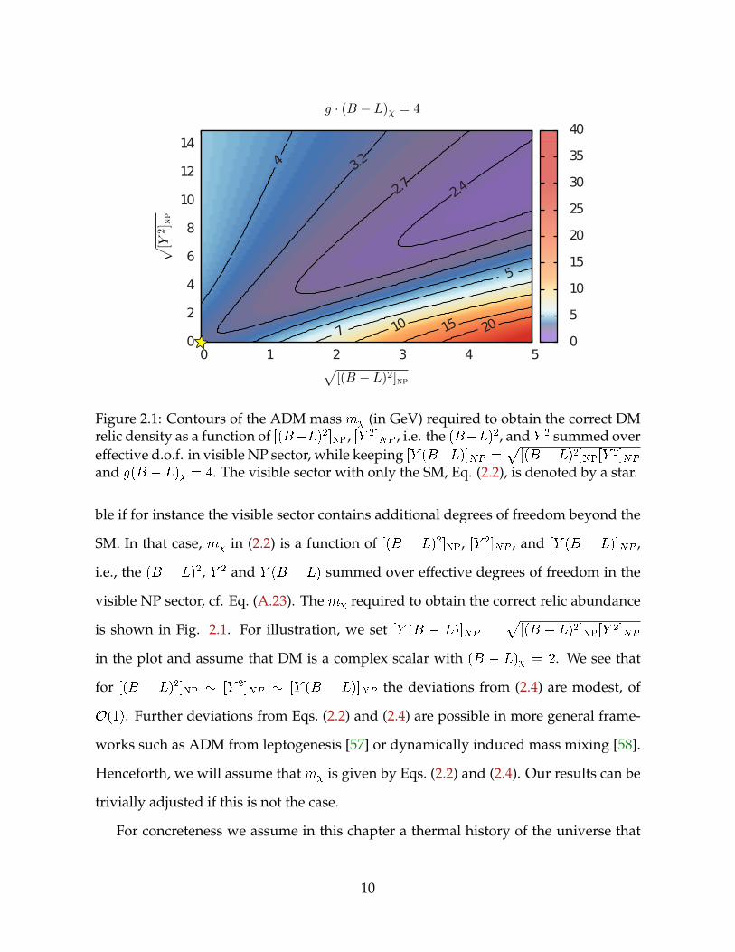
2.1 Contours of the ADM mass m (in GeV) required to obtain the correctDM relic density as a function of [(B L)2]NP, [Y 2]NP , i.e. the (B L)2,and Y 2 summed over effective d.o.f. in visible NP sector, while keeping[Y (B L)]NP =

p[(B L)2]NP[Y 2]NP and g(B L) = 4. The visible

sector with only the SM, Eq. (2.2), is denoted by a star. . . . . . . . . . . 102.2 Feynman diagram for the decay of DM with B = 1 assuming MFV. This

amplitude leads to the partial decay width (1) in Eq. (2.13). . . . . . . . 14

2.3 The solid blue (red dashed) line denotes theB = 2 DM lifetime as a func-tion of m for the MFV (FN) case, fixing the NP scale to = 1(3) TeV.Assuming the dominance of one decay mode, the green (orange) lineshows the constraint on the decay time from FERMI-LAT [70] for bb(+) final states using the NFW profile. The dash-dotted red lineshows the AMS-02 [71] constraint on ! + decay time derivedin [72], while the light blue line shows the Super-Kamiokande [73] con-straint on the ! decay time obtained in [74]. The purple line showsthe upper limit on ! uds and ! cbs decay times (indistinguishableat the scale of the figure) obtained in [37]. . . . . . . . . . . . . . . . . . . 20

2.4 The decay in the MFV mediator model through the off-shell scalarmediators L;R; 'L (left), and through the off-shell fermion and scalar mediators in the FN model (right). . . . . . . . . . . . . . . . . . . . . . 24

2.5 Box diagrams contributing to the neutral meson mixing. In the MFVmodel, there is also a contribution with both L and 'L in the loop, whileR contributions are suppressed and can be ignored. . . . . . . . . . . . 27

2.6 Meson mixing constraints on the couplings 1;2 in the MFV mediatormodel (left) and gq;d in the FN model (right), taking mL = m'L = 500

GeV and m = 200 GeV, m = 20 GeV respectively. The excluded re-gions lie above and to the right of the curves. . . . . . . . . . . . . . . . . 30

v

2.7 The gg ! y (solid blue), qq ! y (dot-dashed red) and gq ! j (solidlight blue) contributions to the pair-production and single-productioncross-section at the LHC with

ps = 14 TeV as a function of a mass of a

color triplet scalar , a mediator in the FN model. . . . . . . . . . . . . . 322.8 Constraints on the scalar mediator in the FN model, and L, 'L, R

in the MFV model that follow from the CMS search for pair-produceddijet-resonances [84]. The states in the same flavor multiplet are takento be mass-degenerate. . . . . . . . . . . . . . . . . . . . . . . . . . . . . . 33

2.9 The 95% exclusion limit on y production in the FN model for the bb

final state, where escapes the detector and sbottom search applies [85].The solid blue (dashed red) line is for ! b branching ratios of 50%and 100%. . . . . . . . . . . . . . . . . . . . . . . . . . . . . . . . . . . . . 34

3.1 Radiative corrections due to FGBs, AQ; Au; AD, split the DM multiplet . 443.2 Typical radiative splitting of the fermionic DM multiplet withm31 (m32)

shown in red (blue) as a function of gU , while all other parameters arekept fixed at gQ = 0:4; gD = 0:5, Mu = 600GeV, Md = 400GeV, u = 1,0u = 0:5, d = 0:25, 0d = 0:3. . . . . . . . . . . . . . . . . . . . . . . . . . 45

3.3 The results of the scan for fermionic DM with radiative mass splitting(upper left panel), in the large mass splitting limit (upper right panel)and scalar (lower panel) flavored DM. Constraints from perturbativity(grey), t0 (dark magenta) and dijet resonance (orange) searches, flavorbounds (light magenta), early-time cosmology (blue) and direct DM de-tection (brown) are consecutively applied. Allowed parameter pointsare denoted by green. For scalar flavor DM (right) we show the LUX andperturbativity bounds as two grey bands. The four benchmark pointsfor fermionic flavored DM are denoted by a diamond, a triangle, a hex-agram and a pentagram. . . . . . . . . . . . . . . . . . . . . . . . . . . . . 51

3.4 The ratio of masses of the next-to-lightest to the lightest FGBs,mA23=mA24

for radiatively split DM multiplet (upper left panel), and for the largemass splitting limit (upper right panel), as functions of the DM mass,m1 , for the fermionic flavored DM. Lower panel shows the relative ra-diative mass splitting in the DM multiplet. The constraints due to per-turbativity (grey), too large relic abundance (light blue), early cosmol-ogy (dark blue), flavor and direct bounds (dark red), are applied consec-utively, leaving allowed points (green). . . . . . . . . . . . . . . . . . . . 52

vi

3.5 The maximal decay time of the two heavy states in the DM multiplet asfunctions of DM mass (left) and the minimal mass splitting in the DMmultiplet (right) for radiatively split fermionic flavored DM. The colorcoding is as in Fig. 3.4. . . . . . . . . . . . . . . . . . . . . . . . . . . . . . 53

3.6 The Feynman diagrams for the dominant processes in the DM annihi-lation for fermionic (left) and scalar (right) flavored DM. For scalar DMonly one representative diagram is shown; other relevant final states in-clude bb; cc; and tt; hh; ZZ (when kinematically allowed). . . . . . . . 54

3.7 The Higgs–DM coupling, H , as a function of DM mass that gives thecorrect relic abundance for the Higgs portal scalar DM (red band). Theupper (lower) dashed edge corresponds to the limit where 2;3 decaymuch after (before) the thermal freeze-out of 1. The LUX bound, as-suming correct relic abundance, is shown as a shaded grey region. . . . 58

3.8 The predicted spin-independent cross section for DM scattering on nu-clei as a function of DM mass for radiatively split fermionic DM (left)and in the large mass-splitting limit (right). The LUX bound is the brownshaded region. The color coding for the points is as in Fig. 3.3. . . . . . . 63

3.9 The dijet production cross section at 8TeV LHC as a function of the light-est FGB mass for radiatively split fermionic DM (left) and in the largemass splitting limit (right). The 95% CL limit from Ref. [133] is denotedwith a solid orange line. The color coding is the same as in Fig. 3.4. . . . 64

3.10 Mass spectrum and flavor decomposition (upper panel), DM relic den-sity as a function of the DM mass with all other parameters fixed (lowerleft panel) and the pattern of effects in selected flavor observables (lowerright panel) for the fermionic flavored DM benchmark 1. The inputbenchmark-point parameters are listed in the center. See text for details. 71

3.11 Same as Fig. 3.10 for benchmark 2. . . . . . . . . . . . . . . . . . . . . . . 733.12 Same as Fig. 3.10 for benchmark 3. . . . . . . . . . . . . . . . . . . . . . . 743.13 Same as Fig. 3.10 for benchmark 4. . . . . . . . . . . . . . . . . . . . . . . 75

4.1 DM annihilation channels in the Higgs-portal models. . . . . . . . . . . 85

vii

4.2 Bounds from LUX (blue band), XENON100 (green band) and the in-visible Higgs decay width (black dashed line and grey region) on theHiggs-portal coupling g for scalar DM, assuming vanishing (left) andSM (right) Yukawa couplings to u, d, s quarks. The red line denotes gas a function of DM mass, m, for which the correct relic abundanceis obtained, while g in the yellow region leads to non-perturbativelylarge Higgs decay width, h > mh, and is excluded. Constraints fromFermi-LAT searches for DM annihilation in dwarf spheroidal galaxiesare denoted by the orange band. . . . . . . . . . . . . . . . . . . . . . . . 87

4.3 Bounds on the Higgs-portal coupling g for scalar DM, assuming max-imal allowed values for the Yukawa couplings to the u, d, s quarks (leftto right), keeping all the other couplings to their SM values. The colorcoding is the same as in Fig. 4.2. . . . . . . . . . . . . . . . . . . . . . . . 88

4.4 Bounds on the Higgs-portal coupling for vector DM, assuming vanish-ing (left) and SM (right) Yukawa couplings to u, d, s quarks. The colorcoding is the same as in Fig. 4.2. . . . . . . . . . . . . . . . . . . . . . . . . 89

4.5 Bounds on the Higgs-portal coupling for vector DM, assuming maximalallowed values for the Yukawa couplings to the u, d, s quarks (left toright), keeping all the other couplings to their SM values. The colorcoding is the same as in Fig. 4.2. . . . . . . . . . . . . . . . . . . . . . . . 90

4.6 Bounds on the Higgs-portal coupling for Dirac DM, assuming = 1 TeVand vanishing (left) and SM (right) Yukawa couplings to u, d, s quarks.The color coding is the same as in Fig. 4.2. . . . . . . . . . . . . . . . . . 91

4.7 Bounds on the Higgs-portal coupling for Dirac DM, assuming = 1

TeV and maximal allowed values for the Yukawa couplings to the u, d, squarks (left to right), keeping all the other couplings to their SM values.The color coding is the same as in Fig. 4.2. . . . . . . . . . . . . . . . . . 92

4.8 Bound on the pseudoscalar Higgs-portal coupling for Dirac DM, assum-ing = 1 TeV and vanishing (left) and SM (right) Yukawa couplings tou, d, s quarks. The color coding is the same as in Fig. 4.2. . . . . . . . . . 93

4.9 Bounds on the pseudoscalar Higgs-portal coupling for Dirac DM, as-suming = 1 TeV and maximal allowed values for the Yukawa cou-plings to the u, d, s quarks (left to right), keeping all the other couplingsto their SM values. The color coding is the same as in Fig. 4.2. . . . . . . 94

viii

4.10 The effect of large light-quark Yukawa couplings on the indirect detec-tion bounds from Fermi-LAT observations of Milky Way dwarf spheroidalsatellite galaxies [130]. . . . . . . . . . . . . . . . . . . . . . . . . . . . . . 94

4.11 Left: The ratio of direct detection bounds on g from Xenon target vary-ing u (dark red), d (light red), or s (blue), and the bound on g as-suming SM Higgs Yukawa couplings. The LHC upper bounds on i aredenoted by vertical dashed lines with shaded regions excluded. Right:the ratio of predicted scattering cross sections. The dotted lines corre-spond to negative values of q. . . . . . . . . . . . . . . . . . . . . . . . . 99

4.12 The -ray excess in the recently discovered dwarf spheroidal galaxyReticulum 2, interpreted as a signal of DM annihilating into bb pairs,is shown as the black 1 contour (see Ref. [231] for details). The orangelines show the 95% CL exclusion limits at the 14-TeV LHC (solid line)and a prospective 100-TeV hadron collider (dashed line), obtained byrescaling the bounds given in Ref. [156]. The remaining color coding isthe same as in Fig. 4.2. See text for more details. . . . . . . . . . . . . . . 115

5.1 An illustration of an example of a CPV sensitive observable in h ! ! 4e. The Higgs decays to on-shell photons which convert in thedetector. The distribution of the azimuthal angle ' between the twoplanes formed by each positron and its parent photon depends on theHiggs couplings to CP even and odd operators. The electrons do notneed to be co-planar with the corresponding photon-positron planes.The positron-photon plane is shown in magenta and the electron-photonplane in blue. For further details and subtleties see the main text. . . . . 121

5.2 A linear polarization thought experiment in Higgs rest frame. P1;2 arelinear polarizers oriented orthogonal to the photon momentum direc-tion. The angle is measured between the linear polarization vectors(m)"lin1;2. . . . . . . . . . . . . . . . . . . . . . . . . . . . . . . . . . . . . . . 128

5.3 The contributions to photon cross-section on 28Si, (28Si), from BH e+e

pair production in nuclear field (solid blue line), pair production dueto scattering on electron cloud (red dashed), Compton scattering (dot-dashed yellow) and Rayleigh scattering (magenta double dot-dashed),as a function of photon energy E . Calculated using NIST’s XCOMdatabase [271]. . . . . . . . . . . . . . . . . . . . . . . . . . . . . . . . . . 130

ix

5.4 Cumulative distributions of Bethe-Heitler conversion cross-section fora photon with E = 60 [GeV] scattering on a 28Si nucleus, with re-spect to various opening angle cuts. Three distributions are shown:P (`` > cut), i.e. with photon-lepton opening angles, , unconstrained(blue line); P (+ and `` > cut) with electron-photon opening angle unconstrained (red dashed line); P ( and `` > cut) (black dot-dashedline). . . . . . . . . . . . . . . . . . . . . . . . . . . . . . . . . . . . . . . . 131

5.5 The elastic form factor Gel2 (q

2). The dashed lines show the limiting be-havior Geq

2 a4q4 for ja2 q2j 1 (green dashed line) and Gel2 1 for

ja2 q2j 1 (red dashed line). The scale at which screening of the nucleusbecomes important is denoted by a, which is smaller than the Si atomicradius, ratom. At scales well outside the atom, corresponding to smallq2, nuclear conversion is suppressed by the form factor screening. . . 133

5.6 Definitions of local spherical polar angles fi ; ig. Note in particularthat azimuthal angles, i are positively oriented with respect to theirparent photons, and are defined with respect to an azimuth ^(m)x com-mon to both branches. Polar angles are defined with respect to parentphoton momentum (black dotted). . . . . . . . . . . . . . . . . . . . . . . 141

5.7 Top panel: ZB in the c ~c plane, with the SM point at (c; ~c) = (0:81; 0).Bottom panel: Zc

B as a function of = tan1(~c=c). The scatter of the datapoints is a numerical artifact. . . . . . . . . . . . . . . . . . . . . . . . . . 145

5.8 Left: Illustration of O(1) oscillations and phase shifts in the HBH differ-ential rate for a sample coplanar kinematic configuration. The azimuthalangle ' in this slice is defined as in Eq. (5.46). The kinematic configura-tion is: Ei+ = Ei = mh=4; i+ = 104; i = 2i+ so that 10 1

and + = , cf. analysis of Eq. (5.51). Right: The azimuthal distributiond=d' for = 0 and for = =4 with a polar angle cut i > 105 and`` > 105. The modulation amplitude is 2%, but will grow to O(1) onceoptimization cuts are applied, see Sec. 5.5.4. . . . . . . . . . . . . . . . . 149

x

5.9 The differential HBH rate d=d' as a function of the azimuthal angle 'between the positrons setting the CPV parameter to = 0 (blue his-tograms) and = =4 (red histograms). The histograms are binnedMonte Carlo events with different cuts on parameters Tn, Eq. (5.52), asdenoted in the panels. The solid blue (red dot-dashed) curves are theresult of fitting the normalized binned events to Eq. (5.50) for the = 0

( = =4) cases with also floated in the fit. The angular resolution cutis `` > cut = 105. . . . . . . . . . . . . . . . . . . . . . . . . . . . . . . . 151

5.10 The same as in Fig. 5.9, but with the opening angle cut `` > cut = 104. 1525.11 Top panels: The azimuthal distributions d=d' for = 0 (grey his-

tograms) and for = =20; =4 (blue histograms, left and right top pan-els) with S1;2 > 1 on the domain 1;2 2 [3=4; 5=4]. The solid (dashed)curves denote fits to Eq. (5.48), with a free parameter in the fits. Thebottom left (right) panel shows the acoplanarity distributions, d=d, (+ ) mod 2 for each photon branch, displayed by blue andgray histograms respectively, with = =4 and no S cut (S1;2 > 1). Notethat the scale varies between these two plots. The corresponding cumu-lative acoplanarity distributions cdf() for each branch are denoted bysolid black and grey dashed lines on each plot. In all panels the angularresolution cut (5.38) of cut = 105 was applied. . . . . . . . . . . . . . . 154

5.12 Comparison of different sensitivity parameter cut schemes, in terms ofcut efficiency, for various angular resolution cuts. The black data pointon each plot denotes the efficiency and hBi=hAi for its angular resolutioncut alone, with no enhancements from sensitivity parameter cuts. . . . . 156

6.1 Kinematic configuration and coordinate choices. B momentum is de-noted by pB, and azimuthal angles are defined with respect to the K- decay plane (blue). This plane contains (m)p and (m)k ((m)P and (m)k)in the lab frame (K or B rest frames); momenta lying in this plane ineach frame are shown in gray. Left: Lepton polar angles and az-imuthal angles in the lab frame. Middle: K and K polar angles inthe K rest frame. Right: The photon polar angle, , in the B rest frame. 166

xi

6.2 Left: The fit value for C with the 1 error band as a function of the po-lar angle cuts ``; > c (see Fig. 6.1). The peak value of C approximatelycoincides with the peak of the marginal distribution (see the left panelof Fig. D.2). Right: Normalized differential distribution dR=d for fourdifferent (r; + ) couplets and c = 106. Also shown are theory pre-dictions (gray) for the input values of (r; + ) and the extracted valueC[c = 106] in eq. (6.41). . . . . . . . . . . . . . . . . . . . . . . . . . . . . 178

6.3 Upper panels: The coefficient C as a function of the cut efficiency for theS (blue) and T (gold) kinematic cuts, with polar cuts c = 106 (left)and c = 5 104 (right). The colored regions depict the 2 statis-tical error bands. The equivalent effective statistics curve = 1, i.e.C = C0=

pN=N0, is also shown (gray). Lower panels: Statistics enhance-

ment as a function of the cut efficiency. The maxima correspond to theoptimum cuts S > Sopt

c and T > T optc (colored dots in all panels). . . . . 179

6.4 The enhancement in C as a function of S . The secondary y-axis showsthe corresponding cut efficiency. The colored regions depict the 2statistical error bands. . . . . . . . . . . . . . . . . . . . . . . . . . . . . . 180

A.1 Example Feynman diagrams for the decay of B = 2 DM. The diagramon the left shows the tree level decay whereas the one on the right showsthe loop-induced decay. . . . . . . . . . . . . . . . . . . . . . . . . . . . . 192

B.1 The FGB contributions to V A current operator in the effective weakHamiltonian. Left panel shows the values of the complex ratio Cbd

1 =Cbs1

for our scan points, with green points satisfying all constraints, magentapoints excluded by flavor constraints and grey points by perturbativ-ity considerations. The point Cbd

1 =Cbs1 = (V

td=Vts)

2, obtained if theMFV operator with the smallest number of Yukawa insertions domi-nates, is denoted by a cross. The right panel shows the cumulative func-tion PMFV (n), see Eq. (B.4). . . . . . . . . . . . . . . . . . . . . . . . . . . 198

B.2 The FGB contributions to V + A current operator in the effective weakHamiltonian. Left panel shows the complex ratio ~Cbd

1 = ~Cbs1 for our scan

points with the same color coding as in Fig. B.1. The point ~Cbd1 = ~C

bs1 =

(md=ms)2(V

td=Vts)

2, obtained if the MFV operator with the smallest num-ber of Yukawa insertions dominates, is denoted by a cross. The rightpanel shows the cumulative function ~PMFV(n), see Eq. (B.6). . . . . . . . 200

xii

B.3 The fraction of benchmarks as a function of the off-diagonal couplingsof the heaviest and next-to-heaviest DM components to the lightest FGB(A24) normalized by the diagonal coupling of the heaviest component. . 202

C.1 Spectrum of the positron energy E+ = E+=E . No opening angle cutwas applied in the left hand figure and an opening angle cut of 104 wasapplied in the right hand one. The histograms were created with MCevents and the solid curves are results of numerically integrating thedifferential cross section. The dashed curve in both figures is the resultof numerically integrating the differential cross section over the entirerange of as opposed over the range [0:6; 1:4]. . . . . . . . . . . . . . 215

C.2 Polar angle distribution of the leptons. No opening angle cut was ap-plied in the left hand figure and an opening angle cut of 104 was ap-plied in the right hand one. The histograms were created with MCevents and the solid curves are results of numerically integrating thedifferential rate expression. The small bump in the right hand figure( 104) is a result of applying an opening angle cut. Its location is afunction of the cut. . . . . . . . . . . . . . . . . . . . . . . . . . . . . . . . 216

C.3 Left: Distribution of the azimuthal angle between the leptons. The his-tograms were created with MC events and the solid curves are resultsof numerically integrating the differential rate expression. Right: Thecumulative distribution function of the relative azimuthal orientation,P (= 2 [1; 1 + ]), from numerical integration. . . . . . . . . . . . 217

D.1 Left: The cumulative distribution function (CDF) of the opening anglebetween the leptons. Right: The normalized distribution of the photonenergy in units of the B mass for two different `` cuts. . . . . . . . . . . 225

D.2 Left: The normalized polar angle distribution of the positron for twodifferent values of the opening angle cut ``. Right: the positron energyas a fraction of the photon energy for two values of ``. The distributionexhibits the expected behavior for BH conversion. It is symmetric about1=2 and prefers that one lepton carry a larger fraction of the photon energy.226

xiii

List of Tables

2.1 Leading decay modes for the B = 1; 2; 3 ADM assuming MFV or FN fla-vor breaking. The dimensionality of the decaying operators are denotedin the 2nd column. With the suppression scales given in the 6th and9th column the ADM decay time is ' 1026 s. The B = 3 ADM decaysto quarks are kinematically forbidden. . . . . . . . . . . . . . . . . . . . . 17

2.2 The gauge and global charge assignment for the three scalar mediators,L, 'L and R, in the first UV completion toy model for which we as-sume the MFV flavor breaking pattern. . . . . . . . . . . . . . . . . . . . 22

2.3 Gauge and B L charges of the mediators and in the second UVcompletion toy model. We also assume the FN flavor breaking pattern. . 24

2.4 The 95 % C.L. bounds on the MFV and FN mediator models from mesonmixing. Taking mL = m'L = m = 1 TeV and 1 = 2(gq = gd) gives theupper bounds on the couplings in the 2nd(4th) column. Taking in turn1;2 = gq;d = 1 gives lower bounds on the mediator masses in the 3rdand 5th columns. The mass of the fermion in the FN model is fixed tom = 20 GeV (see Sec. 2.6.3). The bounds are not very sensitive to m . . 29

4.1 Predictions for the flavor diagonal up-type Yukawa couplings in a num-ber of new physics models (see text for details). . . . . . . . . . . . . . . 102

4.2 Predictions for the flavor diagonal down-type Yukawa couplings in anumber of new physics models (see text for details). . . . . . . . . . . . . 103

4.3 Predictions for the flavor violating up-type Yukawa couplings in a num-ber of new physics models (see text for details). In the SM, NFC andthe tree-level MSSM the Higgs Yukawa couplings are flavor diagonal.The estimates of the CP -violating versions of the flavor-changing tran-sitions, ij=t, are the same as the CP -conserving ones, apart from sub-stituting “Im” for “Re” in the “MFV” row. . . . . . . . . . . . . . . . . . 104

xiv

4.4 Predictions for the flavor violating down-type Yukawa couplings in anumber of new physics models (see text for details). In SM, NFC andtree level MSSM the Higgs Yukawa couplings are flavor diagonal. Theestimates of theCP -violating versions of the flavor-changing transitions,ij=b, are the same as the CP -conserving ones, apart from substituting“Im” for “Re” in the “MFV” row. . . . . . . . . . . . . . . . . . . . . . . . 104

5.1 Expected number of events after the application of S or T cuts with`` > 104 to obtain hBi=hAi 20%. The Higgs production cross sectionincludes the gluon fusion and VBF channels only and is taken from [287]. 155

6.1 Extracted values of r and (+ ) from an MC sample with input values(0:2; =4). . . . . . . . . . . . . . . . . . . . . . . . . . . . . . . . . . . . . . 181

A.1 Partial decay widths, i, and related decay times, i = 1=i, for rep-resentative decay channels above kinematical thresholds (1st column)assuming the MFV flavor breaking ansatz. The EFT scale is set to = 1

TeV. The last column denotes whether the dominant amplitude is treelevel or 1-loop, while the 2nd and the 3rd columns give the decay ver-tex transition and the partonic transition after the potentialW exchange,respectively. . . . . . . . . . . . . . . . . . . . . . . . . . . . . . . . . . . . 196

C.1 The details on the MC generation of BH events, with phase space vari-ables (1st column) for C (C++/Java) generated in the range given in the2nd (4th) column according to the distribution given in the 3rd (5th) col-umn (for details see text). . . . . . . . . . . . . . . . . . . . . . . . . . . . 220

xv

Chapter 1

Introduction

It is worth emphasizing a remarkable fact: we understand the physics of our Universe

on distance scales that span 40 orders of magnitude. This understanding has been dis-

tilled through the scientific process into two phenomenological theories: the standard

model of particle physics (SM), and the cold dark matter model with the addition of

a cosmological constant (CDM). The former describes the interactions of the funda-

mental particles while the latter describes the evolution and dynamics of our Universe

on the largest scales.

Thus far, all experimental tests of the SM are in good agreement with its predictions.

There are, nonetheless, tantalizing experimental “anomalies” that are in tension with

the SM predcitions. At the time of this writing the anomalies included: the muon

g 2 anomaly (3:6), the B meson anomaly in B0 ! K+ (2:9)1, and a putative

signal of flavor violation in the Higgs decay h ! (2:6) to name just a few. Such

deviations could be signals of new physics beyond the SM (BSM). Moreover, the SM

leaves some unanswered questions which include

The origin of neutrino masses

1Taking the [4-6] GeV2 bin only.

1

The hierarchy problem

Dark matter

The flavor puzzle

The origin of the matter/anti-matter asymmetry

The answer to some of these questions could, and in some cases must, lie in BSM

physics.

In this thesis, we will focus on BSM physics related to DM and CP violation (CPV)

which is related to the matter/anti-matter asymmetry. In particular, we will explore

two DM model building scenarios where the DM stability derives from flavor symme-

tries. Then, on a more speculative note, we will exploit the Higgs portal DM model

to constrain the light Yukawa couplings. Finally, we will develop a technique to probe

CPV in Higgs couplings and show that this technique could also be useful to probe

BSM physics effects in radiative rare B meson decays.

Dark matter stability and the SM flavor structure

The SM Lagrangian (LSM) possesses an enhanced U(3)5 symmetry in the high energy

limit where all the fermion masses are negligible in comparison with the energy scale

(mf ! 0). Focusing on the quark sector, the subgroup

GF SU(3)Q SU(3)U SU(3)D U(3)3 (1.1)

is only broken by the SM Yukawa interactions. However, LSM can be made formally

invariant under GF if the Yukawa matrices are promoted to spurions (spurious field

degrees of freedom) which transform non-trivially under GF . This is a useful way to

parametrize the breaking of the flavor symmetry GF in BSM models. Further, asserting

2

that the only source of flavor breaking is from the SM Yukawas goes by the name of

minimal flavor violation (MFV).

As we will see in chapter 2, invoking the MFV hypothesis in a BSM model leads

to additional suppression in the Wilson coefficient of the effective operators. This sup-

pression will afford us a metastable DM candidate with TeV scale mediators. The TeV

scale is significant for two reasons. Firstly, because TeV scale mediators are accessi-

ble at the large hadron collider (LHC) and hence allow us to discover or exclude the

proposed toy models. Second, solutions to the hierarchy problem which was briefly

mentioned above typically require new physics at the TeV scale to cancel the quadratic

divergence of the Higgs mass.

If GF is broken by spurions that have zero triality 2, there is a discrete Z3 subgroup

that is left unbroken. This is useful because there exists a subgroup of the direct prod-

uct Z3 Zc3 which we call Z

3 that is consequently left unbroken3. Not only that, but

all SM fields are singlets under Z3 . Thus, the lightest state that carries a charge under

Z3 is automatically stable and could therefore be a DM candidate. We will explore the

phenomenology (DM and flavor) in a flavor model where GF is fully gauged.

Matter/anti-matter asymmetry and CPV in the SM

There is observational evidence that the Universe is made up entirely of matter and not

antimatter.Antimatter appears to be predominantly a secondary by-product of parti-

cle collisions, e.g. at particle accelerators or between cosmic rays and the interstellar

medium (ISM) or the earth’s atmosphere. There are three required conditions in order

for the Universe to evolve a net baryon asymmetry – the Sakharov conditions [3]: i)

Baryon number violation, ii) C and CP violation, and iii) departures from thermal equi-

2See, e.g., [1] for a definition of triality for SU(3) tensors and [2] for the definition of flavor triality.3Here, Zc

3 is the center group of the QCD gauge group SU(3)c.

3

librium. Here, C is charge conjugation and CP is charge conjugation combined with a

parity transformation. The SM does provide all the necessary ingredients. However,

the parameters of the SM are not sufficient for successful baryogenesis. For instance,

the only CP violating parameter in the SM is the phase of the CKM matrix and it is not

sufficient to produce the observed asymmetry. On the other hand, the departure from

local thermal equilibrium condition could be fulfilled by the phase transition between

the broken and unbroken phases of the electroweak gauge group. Unfortunately, the

parameters of the Higgs potential (the cubic and quartic couplings) only allow for weak

first order phase transition which is insufficient to satisfy the third condition Sakharov

condition.

Another possibility for BSM sources of CP violation (CPV) could be in the Higgs

sector. Since its discovery, the experimental constraints on the couplings of the Higgs

boson to the SM gauge bosons and third generation fermions have become statisti-

cally significant. This does not preclude couplings between the Higgs boson and new

heavy fermions for example. In general, such couplings could be CP violating. If these

fermions are too heavy to be probed directly at the LHC, they could still be discovered

via quantum effects. For example, if they are colored, they would contribute to gluon

fusion which is the main production mode of the Higgs at the LHC. Further, if they are

electrically charged, they would contribute to the h ! process which is one of the

cleanest signals of the Higgs due to low backgrounds. This possibility is investigated

in detail in chapter 5 where we develop observables sensitive to CPV in the Higgs

coupling to photons.

Organization

The thesis is organized as follows. In chapter 2, we investigate a model of asymmet-

ric dark matter where the DM is neutral under the SM flavor group but its couplings

4

are proportional to flavor breaking. The DM in this case is metastable and its lifetime

is bounded by indirect searches from -ray telescopes. Flavor suppression, however,

allows the EFT scale to be at the TeV and thus have interesting signatures at the LHC.

In chapter 3, we turn our attention to flavored DM that is charged under the SM flavor

group. Here, the DM is absolutely stable due to a remnant Z3 subgroup that survives

flavor breaking. We then discuss the phenomenology of the DM and the mediators in

the context of a non-MFV gauged flavor model. In chapter 4, we discuss the possibility

of constraining the light-quark Yukawa couplings in the case of a Higgs portal DM.

While current and future colliders are not sensitive to these small Yukawas, DM direct

detection rates are. By exploiting the complementarity between different searches, we

point out that if Higgs portal DM is discovered, we would obtain a non-trivial con-

straint to the light Yukawas. In chapter 5, we switch our focus to CPV in Higgs decays

to two photons and we develop observables sensitive to CPV. Finally, in chapter 6,

we exploit the same technique developed in chapter 5 to extract the photon helicity

fraction and weak and strong phases in the B ! K radiative decay. An order 1

helicity fraction or weak phase would be a clear signal of new physics.

5

Chapter 2

Continuous Flavor Symmetries and the

Stability of Asymmetric Dark Matter

2.1 Introduction

Dark matter (DM) is stable on cosmological time-scales. A principal question about the

nature of DM is: what mechanism ensures its stability? Commonly, this is assumed to

be a result of an exact symmetry (for a concise review of proposed stabilization mech-

anisms see, e.g., [4]). One possibility is that the stability of DM is ensured by a gauge

symmetry mimicking the way QED gauge invariance ensures the stability of the elec-

tron in the standard model [5–7]. A more frequent choice is to introduce a Z2 symmetry

by hand. A prominent example is R-parity in the MSSM which both stabilizes DM and

ensures the stability of the proton [8–10]. An exact Z2 symmetry can be generated dy-

namically, e.g., as a remnant of a spontaneously broken U(1) gauge symmetry, such as

U(1)BL [11–13]. An attractive possibility is that Z2, and consequently the DM stabil-

ity, is an accidental symmetry. Examples include minimal DM [14, 15], hidden vector

DM [16], and weakly interacting stable pions [17].

In this chapter, we explore a possibility that the discrete Z2 that ensures the stability

6

of DM is both accidental and approximate. As a result, the DM is metastable with decay

times potentially close to the present observational bound of & 1026s. We focus on

a particular subset of asymmetric DM models [18] where DM carries baryon number.

For recent reviews of asymmetric DM, see [19, 20]. Our working assumptions are

Baryon number is a conserved quantum number (it could, for instance, be gauged

at high scales).

There is a sector that efficiently annihilates away the symmetric component. The

exact form is not directly relevant for our discussion.

The observed flavor structure in the quark sector is explained by flavor dynamics

in the UV while DM is not charged under flavor.

The flavor dynamics fixes the flavor structure of dark sector couplings to the visible

sector in the same way that it fixes the structure of the SM Yukawa interactions. This

has two important consequences. First, the exchange of DM in the loops does not

generate dangerously large Flavor Changing Neutral Currents (FCNCs). Secondly, and

most importantly, a flavor singlet DM is stable on cosmological timescales even for TeV

scale mediators between the dark and visible sectors. In this case, the nature of DM

stability can even be probed directly at the LHC.

The underlying flavor symmetry is crucial for the stability of DM. We will demon-

strate this for two realizations of flavor physics: the Minimal Flavor Violation (MFV)

hypothesis and for abelian horizontal symmetries in the case where DM carries baryon

number 2. In this case the mediators leading to the decay of DM can be at O(100GeV).In contrast, for completely anarchic flavor couplings where DM couples to all quark

flavors with O(1) couplings, the indirect DM bounds would require the mediators to

have masses in the O(10TeV) range.

The implications of continuous flavor symmetries for DM interactions have also

7

been explored in [2, 21–30]. Our analysis differs from these studies in that we are as-

suming that DM is a flavor singlet (as is the case in most models of DM). This, along

with its small mass and conserved baryon number, also ensures that DM is metastable

in our setup. The stability of symmetry-less DM in the context of discrete flavor groups

has been discussed in [31] (for the potential relation of discrete flavor groups in the

leptonic sector and the stability of DM, see also [32–34]). Furthermore, the stability of

asymmetric DM due to a mirror baryon number was explored in [35] or due to frac-

tional baryon number in [36]. The decaying DM in the context of ADM models was

explored in [37–40].

The chapter is structured as follows. In Sec. 2.2, we review the relation between

DM mass and relic abundance in asymmetric DM models. In Sec. 2.3, we give two ex-

amples of flavor breaking models at the level of Effective Field Theory (EFT) analysis

that can lead to metastable asymmetric DM. In Sec. 2.4, we derive the indirect detec-

tion bounds on the two EFT set-ups. In Sec. 2.5, we give two examples of mediators

that would lead to the EFT set-ups discussed in Sec. 2.4. The relevant bounds on the

mediator masses and couplings, including collider signatures, are derived in Sec. 2.6.

Conclusions are given in Sec. 2.7, while appendices contain technical details.

2.2 Dark matter mass in asymmetric dark matter models

Asymmetric Dark Matter (ADM) models [18, 41–54] address the question of why the

DM density, , and the baryon density in the universe, B, are so close to each other,

' 5:3B [55]. In the standard weakly interacting massive particle (WIMP) models

of DM this is to some extent pure coincidence. In this case DM is a thermal relic and

0:265

h

0:673

2

3 1027 cm3s1

h vi ; (2.1)

8

with h vi the thermally averaged DM annihilation cross section. The coincidence

B then arises due to a fortuitous size of the annihilation cross section for a

weakly coupled weak scale DM – the WIMP miracle.

In contrast, in ADM models the observed DM is not a thermal relic. Its relic abun-

dance reflects the asymmetry in DM, , and anti-DM, y, densities in the early universe.

The and y annihilate away, and only the asymmetric component remains. The coin-

cidence of and B is then due to the fact that the DM relic abundance has the same

origin as the baryon asymmetry. The difference between and B is simply due to

the fact that the DM particle is more massive than a proton by a factor of a few. More

precisely, to explain the observed the DM’s mass needs to be (see Appendix A.II)

m = N0mpB

1

(B L); (2.2)

where mp is the proton mass. Here (B L) is the B L charge of the field. The

exact value of numerical prefactor N0 ' O(1) depends on when the operators trans-

ferring the baryon asymmetry between the visible and the dark sector decouple. For

decoupling temperature above electroweak phase transition, and assuming that there

are only the SM fields in the visible sector, gives N0 = 1:255 for DM that is a complex

scalar or a Dirac fermion. In this case the required DM mass is

m = (6:2 0:4)GeV1

(B L); (2.3)

where the error reflects the errors on = 0:265 0:011 and B = 0:0499 0:0022 [55,

56]. We thus have

m = f6:2; 3:1; 2:1gGeV; for (B L) = f1; 2; 3g; (2.4)

where we only quote the central values. Deviations from the above relations are possi-

9

0

2

4

6

8

10

12

14

0 1 2 3 4 50

5

10

15

20

25

30

35

40

2015107

5

4 3.2

2.7 2.4

Figure 2.1: Contours of the ADM mass m (in GeV) required to obtain the correct DMrelic density as a function of [(BL)2]NP, [Y 2]NP , i.e. the (BL)2, and Y 2 summed overeffective d.o.f. in visible NP sector, while keeping [Y (BL)]NP =

p[(B L)2]NP[Y 2]NP

and g(B L) = 4. The visible sector with only the SM, Eq. (2.2), is denoted by a star.

ble if for instance the visible sector contains additional degrees of freedom beyond the

SM. In that case, m in (2.2) is a function of [(B L)2]NP, [Y 2]NP , and [Y (B L)]NP ,

i.e., the (B L)2, Y 2 and Y (B L) summed over effective degrees of freedom in the

visible NP sector, cf. Eq. (A.23). The m required to obtain the correct relic abundance

is shown in Fig. 2.1. For illustration, we set [Y (B L)]NP =p[(B L)2]NP[Y 2]NP

in the plot and assume that DM is a complex scalar with (B L) = 2. We see that

for [(B L)2]NP [Y 2]NP [Y (B L)]NP the deviations from (2.4) are modest, of

O(1). Further deviations from Eqs. (2.2) and (2.4) are possible in more general frame-

works such as ADM from leptogenesis [57] or dynamically induced mass mixing [58].

Henceforth, we will assume that m is given by Eqs. (2.2) and (2.4). Our results can be

trivially adjusted if this is not the case.

For concreteness we assume in this chapter a thermal history of the universe that

10

closely resembles the one in [18] which has several distinct epochs relevant for the

ADM relic density. At high temperatures, a B L asymmetry is generated, e.g., via

GUT-like baryogenesis [18] or via leptogenesis [57]. The BL asymmetry is efficiently

transferred between the visible and the DM sectors through asymmetric interactions.

We do not require a discrete Zn symmetry in the dark sector so that, unlike [18], the

asymmetric interactions can involve just a single field. At low energies, they have a

schematic form

Oasymm: C

6(qq)3; (2.5)

taking (B L) = 2 complex scalar DM as an example. Here, C is a flavor-dependent

coefficient. The asymmetric interactions freeze out at temperature Tf m,

below which the B L asymmetries in the visible and dark sectors are separately con-

served. If the flavor breaking is due to a spontaneously broken horizontal symmetry

(see Sec. 2.3.2), the freeze out temperature for the above dimension 10 operator in Eq.

(2.5) is, using Naive Dimensional Analysis (NDA),

Tf 1:66pg (162)3 8

C2

12

mPL

1=11

' 480 GeV: (2.6)

In the numerical evaluation, we used the lower bound = = 1:9 TeV from

indirect detection Eq. (2.22), taken the effective number of relativistic d.o.f. to be g =

108:75, corresponding to the SM with a complex scalar DM, and set C = 1 which is

appropriate for the b ! bsctb transition dominance (with any permutation of the

flavors). Note that Tf is above the electroweak phase transition temperature Tew 170

GeV. It is also well below so that the use of EFT is justified. If the mediator scale were

too low, . 730 GeV (or . 400 GeV for MFV breaking), the asymmetric operator

would not freeze out before electroweak phase transition started. Consequently, the

DM quantum number would not be conserved and the DM density would be washed

out. This places a lower bound on the asymmetric mediator masses to be above a few

11

hundred GeV.

Finally, at temperatures below DM mass the bulk of the DM efficiently annihilates

back to the visible sector through symmetric interactions leaving only the small asym-

metric component. We have nothing new to say about this mechanism and refer the

reader to a set of model building ideas already present in the literature [19, 59–62].

2.3 Metastability and flavor breaking

We show next that the DM in ADM models can be stable on cosmological time-scales

without invoking discrete Zn symmetries. We assume that the SM quark flavor struc-

ture is explained by a continuous flavor group and that the DM carries nonzero baryon

number. This is a crucial ingredient in the argument. Since DM is not charged under

the flavor group, while the SM fields are, there are no interactions between DM and

the SM in the limit that the flavor group is unbroken (all flavor singlet interactions are

forbidden by baryon number conservation). All the interactions between DM and the

visible sector thus have to be flavor breaking and this leads to a significant suppression

of the DM decay time.

We show this explicitly for two examples of flavor breaking: i) the MFV ansatz,

where all the flavor breaking is assumed to be due to the SM Yukawas, and ii) the

spontaneously broken horizontal U(1) symmetries. Integrating out the NP fields gives

the effective DM decay Lagrangian

L =Xi

Ci(Di4)

Oi: (2.7)

The sizes of the Wilson coefficients, Ci, are fixed by the assumed flavor generating

mechanism. We consider the case of DM, , that is a SM gauge singlet but carries

nonzero baryon number, B 6= 0. The lowest dimensional asymmetric local operators

12

thus have the generic form

Oi = [uc]nu [dc]nd [q]nq ; (2.8)

where we do not show the contractions of SM gauge indices. Here (nu + nd + nq)

mod 3 = 0 since DM is a color singlet. Note that DM needs to carry an integer baryon

number in order not to forbid all the asymmetric interactions with the visible sector.

Above, uc, dc are the electroweak singlets and q represents the electroweak doublet

left-handed quark fields in two component notation, with q being the corresponding

complex conjugated Weyl spinor, see App. A.I. In the down-quark mass basis they are

uc ! ucMASS; dc ! dcMASS; q =

u

d

!VCKM uMASS

dMASS

: (2.9)

The SM Yukawa matrices are then

YD ! YdiagD ; YU ! VCKMY

diagU ; (2.10)

with Y diagD;U the diagonal Yukawa matrices.

As an example, let us consider fermionicB = 1 DM. Two distinct types of operators

are allowed

O(B=1)1 = (uc)(dcdc)! (ucMASS)(d

cMASS d

cMASS);

O(B=1)2 = ( q)(d

c q) ! (uMASSVCKM)(d

cMASSd

MASS);

(2.11)

where ; are SU(2)L indices while the SU(3)C and flavor indices are implicit and we

have chosen one possible Lorentz contraction denoted by the parentheses.

13

Figure 2.2: Feynman diagram for the decay of DM with B = 1 assuming MFV. Thisamplitude leads to the partial decay width

(1) in Eq. (2.13).

2.3.1 Minimal Flavor Violation

The MFV assumption is that, also in the NP sector, the flavor is broken only by the

SM Yukawas YU;D [63–67]. The MFV assumption can be most succinctly cast in the

spurion language [64]. In the limit of vanishing quark masses the SM quark sector

enjoys an enhanced flavor symmetry GF = SU(3)Q SU(3)U SU(3)D. The Yukawa

interactions ucY yUqH , dcY y

DqHc are formally invariant under GF , if YU;D are promoted

to spurions, i.e. if they are assumed to transform under GF as YU ! Y 0U = UQYUU

yU ,

YD ! Y 0D = UQYDU

yD. Here UQ;U;D are transformations from SU(3)Q;U;D, respectively.

This means that the low energy operators in (2.7) also need to be formallyGF invari-

ant. Keeping only the minimal insertion of Yukawas, the operators O1;2 in Eq. (2.11)

for B = 1 DM are

O(B=1)1 =

ucY

yUYD

K

dcNd

cM

KNM

! ucMASSY

diagyU V y

CKMYdiagD

K

[dcMASS]N [d

cMASS]M

KNM ;

O(B=1)2 =( qKi)([d

cY

yD]Nq

M j)

ijKNM

! uMASSV

yCKM

K

[dcMASSY

diagyD ]N[d

MASS]M

KNM ;

(2.12)

where ; ; are the color indices, and K;N;M run over the quark generations.

The two operators lead to the ! bus decay at the partonic level which is the least

14

suppressed kinematically allowed transition. For the operatorO1, this transition arises

at 1-loop and requires two chirality flips, see Fig. 2.2. The decay amplitude scales as

ytyb with an extra loop factor and a chirality flip suppression mtQCD=m2W . To be

conservative, we count the chirality flip suppression due to the light u; d; s quarks as

proportional to QCD and not to the much smaller quark masses. The operatorO2 leads

to the decay ! bus at tree level with the decay amplitude suppressed by ybVub.

Once the quarks hadronize, the decays appear as ! b, or ! bK, with any

number of pions. Using NDA to estimate the decay width gives (setting Vtb ' Vud ' 1)

(1) (ytyb)2

8

m

4 1

162mtQCD

m2W

2m

162= 6:6 1051GeV

yb0:024

24:0 106TeV

4

;

(2) jybVubj28

m

4 m

162= 6:6 1051GeV

yb0:024

24:3 107TeV

4

;

(2.13)

for the case where O1 and O2 dominate the decay, respectively. The last 1=162 factor

is due to three body final state and is required to obtain the correct estimate for the

inclusive decay width as can be seen from the optical theorem and the use of the OPE.

In the numerics, we use mt = 173 GeV, m = 6:2 GeV, jVubj = 0:00415. The numerical

prefactor 6:6 1051 GeV = 1=(1026s) is chosen to make contact with the bounds on the

DM lifetime from indirect DM searches.

Note that MFV leads to two sources of suppression. First, there is the suppression

of the Wilson coefficients due to Yukawa insertions, yb 0:024 for O1 and ybVub 104 for O2. In addition, there is a loop suppression for O1 where the decay has to

proceed through an off-shell top quark. Without these additional suppressions, the

bounds from indirect DM detection would require about two orders larger NP scale,

& 4:3 109 TeV.

The suppression factors are much larger for B = 2 DM, in which case the DM is a

15

scalar, and the asymmetric operators start at dimension 10. We investigate in detail the

operator

O(B=2)1 = (dcKd

cN)([q

YD]M0qK00)(q

N 0 0q

M 0 )

KNMK0N 0M 0

00 0

! ([dcMASS]K[dcMASS]N)([u

MASSV

yCKMY

diagD ]M0 [d

MASS]K00)

([uMASSVy

CKM]N 0 0 [dMASS]M 0 )

KNMK0N 0M 0

00 0 ;

(2.14)

that gives the least suppressed decay amplitude. Above, we chose one of the possible

color contractions, implicitly assumed contractions of weak indices within brackets,

and only kept the weak contraction leading to the largest decay rate in the second line.

The correct relic abundance requires a DM mass ofm = 3:10:2 GeV, assuming the

SM field content at the time of the decoupling of the asymmetric operators. We assume

that m < m+c+m = 3:48 GeV, and thus below the threshold for the ! +

c de-

cay, kinematically forbidding the ! udc dds partonic transition. The least suppressed

partonic level transition is therefore ! uds uds resulting, after hadronization, in the

decays ! 00;+;p;0n; : : : . The NDA estimate of the decay width is then

(1) jybV 2ubj2

8

m

12 m

(162)4= 6:6 1051GeV

yb0:024

20:63 TeV

12

: (2.15)

The MFV assumption results in the ybV 2ub suppression of the Wilson coefficient. The

1=(162)4 factor reflects the fact that, in the OPE, the leading contribution starts at 5

loops. The use of the OPE may be suspect for such low m masses and one could

expect O(1) corrections to the above estimate from additional soft gluon loops.

Indirect DM searches require the NP scale to be & 0:49 TeV. This corresponds to

the bounds on the masses of the mediators between the dark and the visible sectors,

16

ADM model MFV FN

B Dim. m [GeV] decay [s] [TeV] decay [s] [TeV]

1 6 6.2 ! bus 1026 4:0 106 ! bus 1026 8:1 108

2 10 3.1 ! udsuds 1026 0:63 ! udsuds 1026 2:5

3 15 2.1 forbidden 1 – forbidden 1 –

Table 2.1: Leading decay modes for the B = 1; 2; 3 ADM assuming MFV or FN flavorbreaking. The dimensionality of the decaying operators are denoted in the 2nd column.With the suppression scales given in the 6th and 9th column the ADM decay time is ' 1026 s. The B = 3 ADM decays to quarks are kinematically forbidden.

mmediator & 490 GeV, mmediator & 210 GeV, and mmediator & 90 GeV, if the operator (2.14)

arises at tree level, 1-loop, or 2-loops, respectively. The mediators can thus be searched

for at the LHC as discussed in Sec. 2.6.3. Note that the flavor suppression was essential

to have such a low bound on the NP scale . Without it, and taking the Wilson coef-

ficient to be 1, the indirect bounds on the stability of DM would require & 7:3 TeV,

implying that the mediators were most likely out of reach of the LHC.

The bound on the NP scale is quite sensitive to the actual value of m. For larger

values of m, the can decay to top and bottom quarks reducing the loop and CKM

suppression of the decay width. This is illustrated in Fig. 2.3, where the NP scale is

fixed to MFV = 1 TeV and m is varied. As the kinematic thresholds for the decays

to c or b quarks are reached, this results in a change of several orders of magnitude in

the predicted decay time.

2.3.2 Spontaneously broken horizontal symmetries

The suppression we found above using the MFV ansatz is model dependent. To illus-

trate this point we turn to U(1) Frogatt-Nielsen (FN) models of spontaneously broken

horizontal symmetries [68]. The suppression of the Wilson coefficients in the effective

Lagrangian (2.7) is then given by the horizontal charges of the quarks in the operators.

17

For instance, for the two B = 1 DM operators in (2.7)

O(B=1)1 = (dcK) (u

cNd

cM)! ( [dcMASS]K) ([u

cMASS]N [d

cMASS]M);

O(B=1)2 = ( qKi)(d

cNq

Mj)

ij ! ( [uMASS]K) ([dcMASS]N [d

MASS]M) ;

(2.16)

the Wilson coefficients are

C1 jH(dcK)+H(u

cN )+H(d

cM )j; C2 jH(qK)+H(d

cN )H(qM )j: (2.17)

Here H(ucK); : : : , with H(qK) = H(qK), are the horizontal U(1) charges of the quarks,

and 0:2 is the expansion parameter. The dependence of the operators and Wil-

son coefficients on the generational indices KNM is implicit as are color, weak, and

Lorentz contractions in (2.16).

An example of a horizontal charge assignment that gives phenomenologically sat-

isfactory quark masses and CKM matrix elements is [69],

H(q; dc; uc))

0BBBB@

1 2 3

q 3 2 0

dc 3 2 2

uc 3 1 0

1CCCCA; (2.18)

where the column labels f1; 2; 3g correspond to the first, second, and third generations

of quarks.

Since the heavier flavors carry smaller charges the DM preferentially decays into the

heaviest accessible states. As in MFV, the dominant decay is ! bus, except that the

ybVub 5 suppression gets replaced by a much more modest jH(q1)+H(sc)H(q3)j =

. This is the largest scaling allowed by FN charges. In concrete UV mediator models

the suppression can, in fact, be much more severe as we will see explicitly in the next

18

Section.

For B = 2 DM the least suppressed operator is

O(B=2)1 = (dcKd

cN)(q

Mq

K0)(qN 0qM 0)

! ([dcMASS]K [dcMASS]N)([u

MASS]M [d

MASS]K0)([uMASS]N 0 [dMASS]M 0);

(2.19)

suppressing, again, the color and weak contractions. The corresponding Wilson coef-

ficient is suppressed by

C1 jH(dcK)+H(d

cN )H(qM )H(qK0 )H(qN0 )H(qM0 )j: (2.20)

At the partonic level, the dominant decay is ! uss uds with a Wilson coefficient

that is of parametric size jH(dc)+H(sc)2H(q2)2H(q1)j = 5. Note that in MFV this

process proceeded through 2 loops so that the suppression was much more severe,

VtsVub=(162)2 5=(162)2 at the amplitude level. While the suppression in the FN

case is much less than in the MFV case, it is still nontrivial. It lowers the scale of NP

allowed by indirect DM searches from & 7:3 TeV, in the case of no flavor structure,

to & 2:5 TeV in the FN case. Taking the bound from DM indirect detection searches

gives & 1:9 TeV. If the operator arises at tree level, 1-loop or 2-loops, this corresponds

to mediator masses, mmediator & 1:9 TeV, mmediator & 830 GeV, and mmediator & 360 GeV,

respectively.

2.4 Indirect detection

The asymmetric operators discussed in the previous section lead to a decaying DM

which can be potentially seen in indirect DM searches. In our models, the decays

hadronicaly. The decay products thus contain a number of charged particles and pho-

tons. The flavor composition of the final state depends on the mass, m, and also on

19

105

1010

1015

1020

1025

1030

1035

1040

2 3 5 7 10 15 20 30 40 50

τ[s

]

mχ [GeV]

12 3 5 7 10 15 20 30 40 50

MFVFNFERMI χ → bb NFWFERMI χ → µ+µ− NFWIbarra et al. χ → µ+µ− (AMS-02 data)Covi et al. χ → νν (Super-K)Zhao & Zurek – UDDH

ΛMFV = 1 TeV

ΛFN = 3 TeV

ΛMFV = 1 TeV

ΛFN = 3 TeV

Figure 2.3: The solid blue (red dashed) line denotes theB = 2 DM lifetime as a functionof m for the MFV (FN) case, fixing the NP scale to = 1(3) TeV. Assuming the dom-inance of one decay mode, the green (orange) line shows the constraint on the decaytime from FERMI-LAT [70] for bb (+) final states using the NFW profile. The dash-dotted red line shows the AMS-02 [71] constraint on ! + decay time derivedin [72], while the light blue line shows the Super-Kamiokande [73] constraint on the! decay time obtained in [74]. The purple line shows the upper limit on ! udsand ! cbs decay times (indistinguishable at the scale of the figure) obtained in [37].

the assumed flavor breaking pattern. In Section 2.3, we discussed in detail the case of

6.2 GeV B = 1 DM, which decays through ! bus and a 3.1 GeV B = 2 DM that

decays through ! uds uds. After hadronization, these result in the decays ! 0b 0

and ! 00, respectively. The dominant decays for other DM masses, assuming

the MFV or FN flavor breaking patterns, are given in Appendix A.III. The DM lifetime

dependence on m is shown in Fig. 2.3 after fixing the NP scale to be = 1(3) TeV for

the MFV (FN) flavor breaking.

To guide the eye, we also show in Fig. 2.3 the following bounds from indirect DM

searches. The green (orange) line shows the constraint on the DM decay time from

FERMI-LAT [70] for ! bb(+) decays using the NFW profile. The dash-dotted

20

light red line shows the results of an analysis [72] based on AMS-02 [71] and assuming

! +. The light blue line shows the result of an analysis [74] assuming ! decay based on Super-Kamiokande [73] bounds. The purple line is an exclusion

curve from [37] based on galactic and extragalactic gamma ray flux measurements by

Fermi [75–77]. The authors in [37] consider ! uds and ! cbs decays as two

extreme choices for the flavor structure of the final states. The derived bounds on the

lifetime differ by less then a factor of 2 such that the two bounds overlap on the

scale of Fig. 2.3. The decays we consider fall between these two extreme choices with

potentially weakened bounds in our cases abovem & O(10) GeV due to the increased

multiplicity of final states. The bounds cross the expected decay times atm 5 GeV

for MFV = 1 TeV suppression scale in the case of MFV flavor breaking and at m 4

GeV for FN = 3 TeV suppression scale in the case of FN flavor breaking.

For the 3:1 GeV B = 2 DM, we thus find that, for the MFV case, the indirect detec-

tion requires

MFV & 0:49 TeV; (2.21)

where the dominant operator is given in (2.14). For the FN case the bound is

FN & 1:9 TeV; (2.22)

where the least suppressed operator is given in (2.19).

2.5 Mediator models

The EFT analysis of metastable ADM using asymmetric operators is an appropriate

approach to derive the indirect DM detection signatures as we did in the previous sec-

tion. However, for DM direct detection searches and the DM production at colliders,

the dominant signals are due to either a single mediator exchange or from direct pro-

21

Field SU(3)C SU(2)L U(1)Y GF U(1)BL

L 3 1 1=3 (6;1;1) 2=3

'L 6 1 1=3 (3;1;1) 2=3

R 3 1 2=3 (3;1;1) 2=3

Table 2.2: The gauge and global charge assignment for the three scalar mediators, L,'L and R, in the first UV completion toy model for which we assume the MFV flavorbreaking pattern.

duction of the mediators. To assess the reach of these DM searches, the UV completions

to our models are therefore needed.

We introduce two toy model UV completions that can generate the dimension 10

effective operators; that is, the operator in Eq. (2.14) for the MFV case and the operator

in Eq. (2.19) for the FN case. The EFT operators are generated when the TeV medi-

ators are integrated out. In our first model, all the mediators are scalars, while in the

second model there is also a fermionic mediator. The flavor structure in either of the

two models could be of the MFV or of the FN type. For concreteness we fix the first

model to have the MFV flavor breaking, and the second model to have the FN flavor

breaking.

2.5.1 MFV model with scalar mediators

The SM is extended by the DM, , and three flavor multiplets of scalar mediators – a

color anti-triplet L and a color sextet 'L, both with hypercharge 1=3, and a color sextet

R with hypercharge 2=3 (see Table 2.2). They transform under the flavor group GF

as (6;1;1), (3;1;1), and (3;1;1), respectively. The interaction Lagrangian between

22

mediators and the SM is thus given by

LINT 12KABI [L]

I

qA;iq

B;j

ij +

22K ['L]

A

qB;iq

C;j

ijABC

+32[YD]

AX [R]A;

dcY; d

cZ;

XY Z + 4 K

ABI

K y[L]

I['L]

A[R]B; + h:c:;

(2.23)

where the flavor indices A;B;C belong to SU(3)Q and X; Y; Z to SU(3)D. The QCD

indices are , while the weak isospin indices are denoted by i; j. The flavor in-

dex I and color index run from 1 to 6. The matrices of the Clebsch-Gordan coef-

ficients, KABI and K

, are the same as in [78] and satisfy the completeness relation

( KABI ) KCD

I = 12(DA

CB + CA

DB ), and similary for K

. In the second line of (2.23), the

down Yukawa insertions make the interaction term with right-handed down quarks

formally invariant under GF .

Integrating out the mediators L;R; 'L; gives the decay operator (2.14), with the

Wilson coefficientC16

= 1

8

1234m2Lm2'Lm2R

: (2.24)

For 1 = 2 = 3 = 4 = 1 the bounds from indirect DM searches thus require

mL;R;'L & 450 GeV, if all the mediator masses are the same. This should be appro-

priately rescaled if either i have smaller values or if all masses are not the same. For

instance, for i = 0:3 the mass degenerate case of the mediators is bounded from below

by mL;R;'L & 200 GeV. Since the mediators carry color charges, they can be searched

for at the LHC as discussed in Section 2.6.3 below.

Note that, for the Lagrangian in Eq. (2.23) the common scenario where the sym-

metric component of density annihilates through a dark photon [19, 59–61] is phe-

nomenologically not viable. In this case, at least some of the SM quark fields would

need to carry a dark U(1) charge in conflict with the low energy constraints if dark

photon is light. A viable possibility, on the other hand, is the annihilation of y to a

23

Figure 2.4: The decay in the MFV mediator model through the off-shell scalar medi-ators L;R; 'L (left), and through the off-shell fermion and scalar mediators in theFN model (right).

pair of light scalars along the lines of Ref. [79].

2.5.2 FN model with fermionic and scalar mediators

In the second model the SM is supplemented with a DM scalar , a Dirac fermion

and a complex scalar with SM gauge assignments as in Table 2.3. The relevant terms

in the baryon number conserving interaction Lagrangian are

LINT gq;AB2

qjA;iq

kB;j

ij + gd;A

dcA;

+g2( c c) + h:c: ; (2.25)

Field SU(3)C SU(2)L U(1)Y U(1)BL

3 1 1=3 2=3

1 1 0 1

Table 2.3: Gauge and B L charges of the mediators and in the second UV com-pletion toy model. We also assume the FN flavor breaking pattern.

24

where, for the couplings gq, gd, we also denote the flavor dependence. If the flavor

breaking is of the FN type and the mediators do not carry a horizontal charge, then

gq;AB gqjH(qA)+H(qB)j; gd;A gd

jH(dA)j; (2.26)

where gq;d O(1).Integrating out the mediators generates the operator (2.19) with the Wilson coeffi-

cient

C6' 1

8m2 m

4

ggq;M;K0gq;N 0M 0gd;Kgd;N 1

8m2 m

4

jH(dcK)j+jH(d

cN )j+jH(qM )+H(qK0 )j+jH(q

0N )+H(qM0 )j:

(2.27)

Note that the flavor suppression here is parametrically different than in (2.20) which

was obtained by assuming that the FN scale is close to the TeV scale and that the inter-

actions of DM with the visible sector involve the FN fields. In the above model, how-

ever, the FN scale can be arbitrarily high and only fixes the flavor interactions between

the mediator and the SM fields. Consequently, the leading decay is now ! ussuds

where the suppression for the amplitude is jH(dc)j+jH(sc)j+2jH(q2)+H(q1)j 15, to be

compared with the 4 suppression in the more conservative case considered in Section

2.3.2 where the leading decay is ! udsuds. The indirect detection bound (2.22) thus

translates in our toy mediator model to m; & 130 GeV for mass degenerate and .

However, since the coupling to the third generation quarks is O(1), the scalar media-

tors should in fact be heavier than the top quark in order not to modify its total decay

width.

The scaling (2.26) changes if the mediators carry nonzero horizontal charges. For in-

stance, if the horizontal charge of is nonzero,H() 6= 0, one has gq;AB jH(qA)+H(qB)H()j,

gd;A jH(dA)+H()j. In this case, the indirect detection bounds need to be appropriately

rescaled. For 2 H() 5 the Wilson coefficient is still given by (2.27) and thus

25

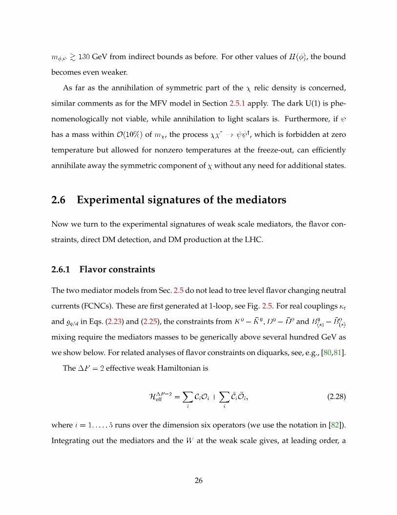
m; & 130 GeV from indirect bounds as before. For other values of H(), the bound

becomes even weaker.

As far as the annihilation of symmetric part of the relic density is concerned,

similar comments as for the MFV model in Section 2.5.1 apply. The dark U(1) is phe-

nomenologically not viable, while annihilation to light scalars is. Furthermore, if

has a mass within O(10%) of m, the process y ! y, which is forbidden at zero

temperature but allowed for nonzero temperatures at the freeze-out, can efficiently

annihilate away the symmetric component of without any need for additional states.

2.6 Experimental signatures of the mediators

Now we turn to the experimental signatures of weak scale mediators, the flavor con-

straints, direct DM detection, and DM production at the LHC.

2.6.1 Flavor constraints

The two mediator models from Sec. 2.5 do not lead to tree level flavor changing neutral

currents (FCNCs). These are first generated at 1-loop, see Fig. 2.5. For real couplings i

and gq=d in Eqs. (2.23) and (2.25), the constraints from K0 K0; D0 D0 and B0(s) B0

(s)

mixing require the mediators masses to be generically above several hundred GeV as

we show below. For related analyses of flavor constraints on diquarks, see, e.g., [80,81].

The F = 2 effective weak Hamiltonian is

HF=2eff =

Xi

CiOi +Xi

~Ci ~Oi; (2.28)

where i = 1; : : : ; 5 runs over the dimension six operators (we use the notation in [82]).

Integrating out the mediators and the W at the weak scale gives, at leading order, a

26

Figure 2.5: Box diagrams contributing to the neutral meson mixing. In the MFV model,there is also a contribution with both L and 'L in the loop, while R contributions aresuppressed and can be ignored.

nonzero Wilson coefficient for the operator

O1 = ( S PLD)( S PLD

) = (sd)sd

; (2.29)

in the case of the MFV model, and for both O1 and its parity conjugate operator

~O1 = ( S PRD)( S PRD

) = (scdc)scd

c; (2.30)

in the case of the FN model. Above, we first give the operators in the 4-component

notation and then also in the 2-component notation (for our notation see Appendix

A.I).

In the matching there are two types of contributions: in the first, only the mediators

run in the loop whereas in the second, both the scalar mediator and the W boson run

in the loop, see Fig. 2.5. For the MFV model, these give for the K0 K0, D0 D0, and

27

B(s) B(s) mixing

CMFV1K =

1

642m2

n(VcsV

cd)

241 + 342 221

22

F (xc) + 4g2w

22G(xw; xc)

+ c! t

2VcsVcdVtsV

td

h 41 + 342 221

22

F F (xc; xt) + 4g2w

22G

F (xw; xc; xt)io;

(2.31)

CMFV1D =

1

642m2

n(VusV

cs)

241 + 342 221

22

F (xs) + 4g2w

22G(xw; xs)

+ s! b

2VusVcsVubV

cb

h 41 + 342 221

22

F F (xs; xb) + 4g2w

22G

F (xw; xs; xb)io;

(2.32)

CMFV1Bq =

1

642m2

(VtbVtq)

241 + 342 221

22

F (xt) + 4g2w

22G(xw; xt)

; (2.33)

where q = d; s, xi = (mi=m)2, and we have set mu = md = 0 and assumed, for simplic-

ity, that the and ' are mass degenerate. The loop functions F (x), F F (x1; x2),G(x1; x2),

and GF (x1; x2; x3) are given in Appendix A.IV. As in the SM, the largest contribution

to the K0 K0 mixing is due to the charm-charm loop while, for B0q Bq

0 mixing, the

top loop dominates as expected.

For the FN model, the Wilson coefficients are given by

CFN1K

10g4q162m2

hH(xt) + 24HF (xc; xt)

i; ~CFN

1K 10g4d162m2

H(x ); (2.34)

CFN1Bd

6g4q162m2

hH(xt) + 24HF (xc; xt)

i; ~CFN

1Bd 10g4d

162m2

H(x ); (2.35)

CFN1Bs

4g4q162m2

hH(xt) + 24HF (xc; xt)

i; ~CFN

1Bd 8g4d

162m2

H(x ); (2.36)

while CFN1D = CFN

1K and ~CFN1D = 0. Above, we have indicated the scaling of different contri-

butions to the Wilson coefficient in terms of = 0:2, cf. Sec. 2.3.2. In the numerics we

use the equality sign. The loop functions H(x) and HF (x1; x2) are given in Appendix

A.IV.

28

MFV FN

1;2 < mL;'L > gq;d < m >

K0 K0 0.33 2.9 TeV 0.63 570 GeV

Bd Bd 1.3 710 GeV 0.54 1 TeV

Bs Bs 1.3 780 GeV 0.59 840 GeV

D0 D0 30 34 GeV 4.3 56 GeV

Table 2.4: The 95 % C.L. bounds on the MFV and FN mediator models from mesonmixing. Taking mL = m'L = m = 1 TeV and 1 = 2(gq = gd) gives the upper boundson the couplings in the 2nd(4th) column. Taking in turn 1;2 = gq;d = 1 gives lowerbounds on the mediator masses in the 3rd and 5th columns. The mass of the fermionin the FN model is fixed to m = 20 GeV (see Sec. 2.6.3). The bounds are not verysensitive to m .

Note that the above Wilson coefficients contain log(mi=m) that can become large

for m mi. We do not attempt to resum these logarithms which also means that

we treat all the NP contributions as local. We expect that our numerical results can

receive O(1) corrections due to neglected terms. This is within the precision required

for our analysis. Though, we do include the usual RGE effects due to the NLO QCD

running of the effective weak Hamiltonian from the weak scale to the low energy. For

constraints from K0 K0 and B(s) B(s) mixing we use the recent results of a fit

to the mixing parameters in [83]. The constraints from D D0 mixing are obtained

by assuming that the NP contribution saturates mD so that in the equation xD =

2h D0jHC=2

eff jD0i =D, valid in the limit of no CP violation, we only include the NP

contribution [82]. The resulting bounds on couplings and masses are shown in Tab. 2.4.

In the case of the MFV model, the most severe bound comes from K0 K0 and is due

to K . Since we assume that all the i in (2.23) are real, the NP contribution does carry

a weak phase due to the VtsV td CKM factors and does contribute to K . In contrast, in

the FN model the NP contributions to the mixing do not carry a weak phase and thus

do not have an effect on K . Therefore, the bounds from K0 K0 mixing are much less

29

0

0.2

0.4

0.6

0.8

1

0 0.25 0.5 0.75 1 1.25 1.5 1.75 2

κ2

κ1

mφL= mϕL

= 500 GeV

K0− K

0

Bd − Bd

Bs − Bs0

0.5

1

1.5

2

0 0.5 1 1.5 2

gd

gq

mφ = 200 GeV; mψ = 20 GeV

K0− K0

Bd − BdBs − BsD0

− D0

Figure 2.6: Meson mixing constraints on the couplings 1;2 in the MFV mediator model(left) and gq;d in the FN model (right), taking mL = m'L = 500 GeV and m = 200GeV, m = 20 GeV respectively. The excluded regions lie above and to the right of thecurves.

severe.

In Fig. 2.6, we show the constraint on the couplings 1;2 in the MFV model, fixing

mL = m'L = 500 GeV (left figure), and the constraints on gq;d in the FN model, fixing

m = 200 GeV, m = 20 GeV (right figure). Since, in the case of MFV, the largest

contribution to K0 K0 is from the mediator-W loop, the K bound places a stringent

constraint on 2. Since the NP contributions to the meson mixing were assumed to be

CP conserving in the case of the FN model, the couplings gd;q O(1) are allowed even

for m as low as 200 GeV.

2.6.2 Relic abundance and direct detection

We note in passing that the virtual exchanges of the mediators generate contact oper-

ators of the schematic form yqq that contribute to the y annihilation cross section

and to the cross section for DM scattering on nuclei. The symmetric couplings of DM

and the mediators, of schematic form yy, do not suffice to create large enough an-

nihilation cross sections that would annihilate away the symmetric component of DM

relic abundance.

30

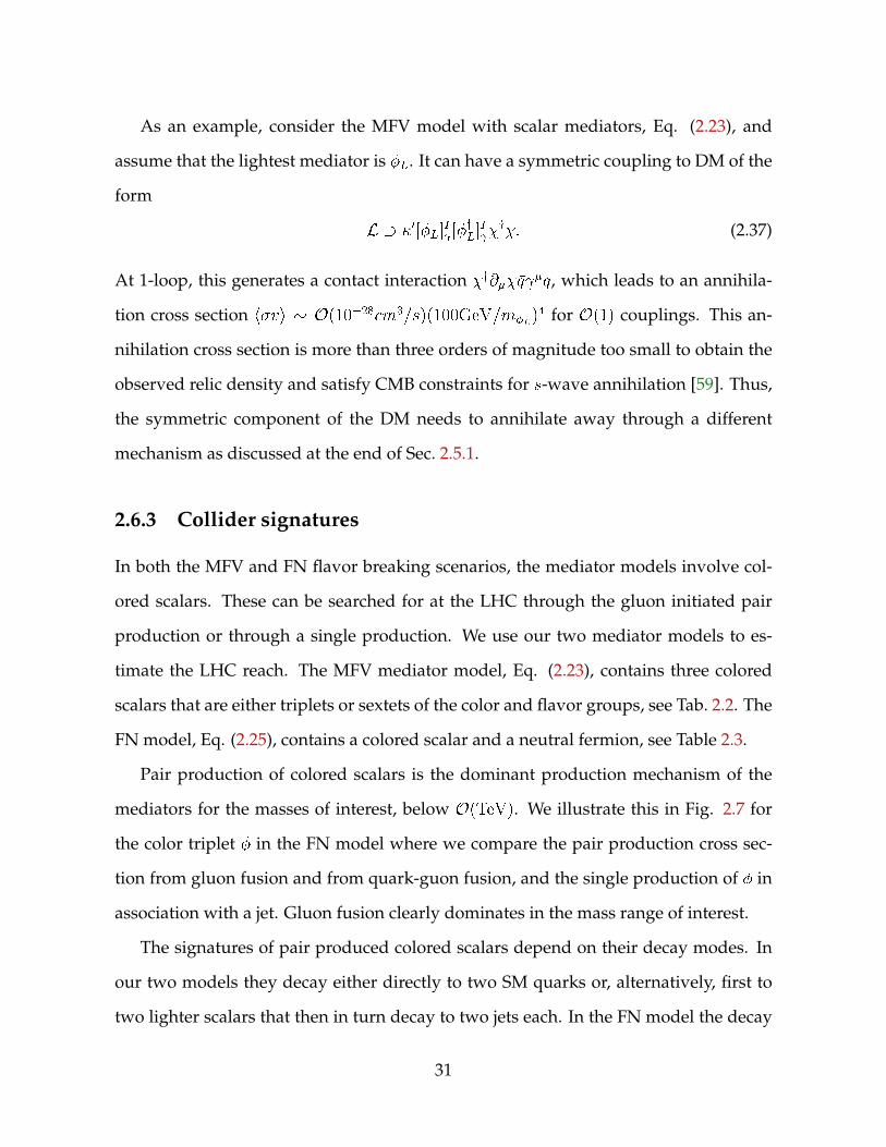
As an example, consider the MFV model with scalar mediators, Eq. (2.23), and

assume that the lightest mediator is L. It can have a symmetric coupling to DM of the

form

L 0[L]I [

yL]I

y: (2.37)

At 1-loop, this generates a contact interaction y@q q, which leads to an annihila-

tion cross section hvi O(1028cm3=s)(100GeV=mL)4 for O(1) couplings. This an-

nihilation cross section is more than three orders of magnitude too small to obtain the

observed relic density and satisfy CMB constraints for s-wave annihilation [59]. Thus,

the symmetric component of the DM needs to annihilate away through a different

mechanism as discussed at the end of Sec. 2.5.1.

2.6.3 Collider signatures

In both the MFV and FN flavor breaking scenarios, the mediator models involve col-

ored scalars. These can be searched for at the LHC through the gluon initiated pair

production or through a single production. We use our two mediator models to es-

timate the LHC reach. The MFV mediator model, Eq. (2.23), contains three colored

scalars that are either triplets or sextets of the color and flavor groups, see Tab. 2.2. The

FN model, Eq. (2.25), contains a colored scalar and a neutral fermion, see Table 2.3.

Pair production of colored scalars is the dominant production mechanism of the

mediators for the masses of interest, below O(TeV). We illustrate this in Fig. 2.7 for

the color triplet in the FN model where we compare the pair production cross sec-

tion from gluon fusion and from quark-guon fusion, and the single production of in

association with a jet. Gluon fusion clearly dominates in the mass range of interest.

The signatures of pair produced colored scalars depend on their decay modes. In

our two models they decay either directly to two SM quarks or, alternatively, first to

two lighter scalars that then in turn decay to two jets each. In the FN model the decay

31

0.001

0.01

0.1

1

10

100

0.2 0.3 0.5 0.7 1

Tot

alcr

oss-

sect

ion

[pb]

Mφ [TeV]

√s = 14 TeV

gg → φφ†

qq → φφ†

gq → φ+ j

Figure 2.7: The gg ! y (solid blue), qq ! y (dot-dashed red) and gq ! j (solidlight blue) contributions to the pair-production and single-production cross-section atthe LHC with

ps = 14 TeV as a function of a mass of a color triplet scalar , a mediator

in the FN model.

! j is also possible. The flavor composition of the jets depends on the flavor

quantum numbers of the scalar. For instance, the states in the L flavor multiplet can

decay either predominantly through L ! tb, L ! bj, or L ! jj, depending on the

flavor numbers of L (and similarly for 'L), see Eq. (2.23). The scalars in the R flavor

multiplet, on the other hand, decay through R ! bj or R ! jj, again depending on

the flavor index carried by the R state. In the FN model one needs to require m > mt

in order not to modify the total decay width of the top quark, see Sec. 2.5. Then, the

dominant decay is either ! b or ! tb, depending on the relative sizes of the two

couplings, while the other decays are suppressed by additional powers of .

To get a rough estimate of the LHC sensitivity we treat all the decay modes as

two-jet final states (this overestimates the reach slightly since, for the tj final state, the

real efficiency is expected to be lower). The strongest constraint on pair-production

of the lightest scalar mediators then comes from the search for pair-produced dijet

32

0.0001

0.001

0.01

0.1

1

10

0.3 0.5 0.7 1 1.2 1.5

Tot

alcr

oss-

sect

ion

[pb]

mφ [TeV]

√s = 7 TeV

CMS paired dijets – ±1σ

CMS paired dijets – observedFN – gg → φφ†

MFV – gg → φLφ†L

MFV – ϕLϕ†L

MFV – φRφ†R

Figure 2.8: Constraints on the scalar mediator in the FN model, and L, 'L, R in theMFV model that follow from the CMS search for pair-produced dijet-resonances [84].The states in the same flavor multiplet are taken to be mass-degenerate.

resonances from CMS at 7 TeV LHC with integrated luminosity of 5 fb1 [84]. This

places the bounds m > 470 GeV in the case of FN model assuming that ! b

decay is negligible, and mL> 620 GeV, m'L

> 910 GeV, mR> 580 GeV in the case

of MFV flavor breaking as shown in Fig. 2.8. Note that when all three mediators are

degenerate in mass, the color sextet scalar has the largest pair production cross section

due to the large color factor.

In the FN model, a new experimental signature is obtained in the limit gd 2gq.

Then the dominant decay of is ! b . In order not to have fast decaying DM

m > m=2. Using NDA the decay length is

c( ! bbc) g2qg

2d

8 1

8

1

162m5

m4

!1

30m20GeVm

5 m

750GeV

40:03gqgd

2

:

(2.38)

For light enough (or heavy enough ), the fermion does not decay in the detec-

33

0

100

200

300

400

500

200 300 400 500 600 700 800

mψ

[GeV

]

mφ [GeV]

BR(φ→ bψ) = 1BR(φ→ bψ) = 0.5

Figure 2.9: The 95% exclusion limit on y production in the FN model for the bb final state, where escapes the detector and sbottom search applies [85]. The solidblue (dashed red) line is for ! b branching ratios of 50% and 100%.

tor and appears as E=T . The pp! y pair production then results in 2j +E=T or 2b+E=T

final state, and is bounded from sbottom searches as shown in Fig. 2.9. The resulting

bound is m > 550(760) GeV for m = 20 GeV and BR(! b) = 0:5(1:0). The choice

gq = gd = 0:03 in Eq. (2.38) gives BR( ! b ) BR( ! s ) = 0:33. For the same

input parameters, the single production of in association with b, t, or has a cross

section 7 102 fb while the pair production is dominated by the process ss !

and has a negligible cross section of 4 104 fb.

The single production of mediators, e.g., ud ! , ud ! L, ud ! 'L, ds ! R,

is suppressed due to the small couplings of the mediators to the first and the second

generation quarks. Similarly, the single production from heavy quarks in the initial

state suffers from the PDF suppression.

For single top production, the MFV model gives the largest contribution with a

cross-section of (ud ! L ! tb)MFV = 7:6 106 pb for mL = 500 GeV andps = 8

34

TeV. This is well below the SM production cross section. Thus, the ATLAS and CMS

combined measurement of the single top cross section atps = 8 TeV, 85 12 pb [86]

and so does not impose any limits on the mediator model.

The production of the DM, , can occur from the decay of heavier mediators. For

instance, for 4 3 and R heavy enough, the dominant decay mode of 3 is 3 !'yL

yL. Pair production pp! R

yR would thus result in 8j+E=T signature where paired

dijets would reconstruct L and 'L mass peaks (depending on the flavor assignments

some of the jets can be replaced by t of b jets).

2.7 Chapter summary

In this chapter, we have shown that for asymmetric DM (ADM) models, the stability of

DM on cosmological time scales may be purely accidental. We did not require that the

DM to be charged under an ad-hoc conserved Zn symmetry. Rather, we assumed that

such a discrete symmetry is explicitly broken by the mediator interactions that transfer

the B L between the DM sector and the visible sector in the early universe. Such

asymmetric interactions are necessary in all models of ADM though they may be made

to obey a Z4 symmetry (i.e. one can demand that they involve only the ! visible or

yy ! visible transitions instead of ! visible transitions as in our case).

At low energies, the DM then carries a conserved charge that is broken only by

the higher dimensional operators obtained by integrating out the mediators. Such op-

erators also lead to DM decays. In this chapter, we explored the role of continuous

flavor symmetries for the properties of such decaying DM focusing on the case where

DM that carries nonzero baryon number. For B = 1 DM, the direct detection bounds

are evaded if the mediators are above 4109 TeV assumingO(1) couplings. However,

if quark flavor breaking is of the MFV type, the mediators can be lighter by around two

orders of magnitude. For B = 2 DM, the scale of the mediators can be much lighter

35

(O(8TeV) for O(1) couplings). This is then lowered by an order of magnitude if quark

flavor breaking is of the MFV or Froggatt-Nielsen type. The mediators that would lead

to indirect DM signals in the next generation of experiments can thus be, at the same

time, searched for at the LHC.

We have explored this possibility by constructing two mediator models, one with

assumed MFV and one with a FN flavor breaking pattern. The MFV mediator model

(Eq. (2.23)) contains three colored scalars that are either triplets or sextets of the color

and the flavor groups, see Table 2.2. The FN model (Eq. (2.25)), on the other hand, con-

tains one colored scalar and one neutral fermion, see Table 2.3. These mediators gen-

erate FCNCs at 1-loop. While this leads to nontrivial constraints on their masses and

couplings, the mediators can still be as light as a few 100 GeV with O(1) couplings.

Since the mediators are charged under QCD, they can be singly or pair-produced at

the LHC with large cross sections. This means that the searches at the LHC can lead

to interesting constraints or discoveries. The signatures depend on how the mediators

decay. In the FN model, for instance, the decay to heavy quarks, ! tb, is favored.

Modifying the paired dijet searches to the pp ! ! tbtb signal could thus enhance

the reach of the LHC in the search for these mediators. In the MFV model, on the other

hand, paired light dijets, paired tb, and paired bj are possible. Other signatures are

discussed in Sec. 2.6.3.

In conclusion, ADM can quite generically be metastable with a possibility of com-

plementary signals in indirect detection and at the LHC.

36

Chapter 3

Dark Matter And Gauged Flavor

Symmetries

3.1 Introduction

The stability of dark matter (DM) is commonly assumed to be due to an exact dis-

crete symmetry, Zn. This can either be imposed by hand or have a dynamical origin.

Examples include R-parity in the MSSM [87], and flavor symmetries in the leptonic

sector [33, 34, 88–90]. Here, we explore the intriguing possibility raised in Refs. [2, 25]

that the stability of DM is due to the Z3 center group of the global GSMF SU(3)Q SU(3)U SU(3)D quark flavor symmetry. While GSMF is broken by the SM Yukawa

interactions, its subgroup Z3 remains unbroken in the SM. More generally, it remains

exact also in the presence of New Physics (NP), if the flavor breaking is of Minimally

Flavor Violating (MFV) type, i.e. only due to the SM Yukawas. The lightest neutral

state that is odd under Z3 is therefore stable and is a DM candidate. This is the idea

behind MFV dark matter [2, 23, 25].

Requiring MFV is sufficient, but not necessary. In this chapter we formulate a gen-

eral condition for flavored DM using flavor triality (see Eq. (3.3) below). For example,

37

any spurion in the bifundamental of GSMF leaves the above Z3 unbroken. The flavor

breaking can thus be quite far from MFV and still have stability of DM guaranteed

by the flavor dynamics. To illustrate this point we consider the model of Ref. [91]

where the flavor-breaking spurions have the form Y 1u;d and are thus canonically not

of the MFV type. In this model the SM quark flavor symmetry GSMF is fully gauged

giving rise to flavor-gauge bosons, the Yukawas are promoted to physical scalar fields

(flavons) transforming under flavor, and in addition there is a set of chiral fermions

that cancel the anomalies in the flavor-gauge sector.

Using this renormalizable model we show below that a thermal relic DM can be in

a nontrivial representation of GSMF . There are two conflicting constraints on this setup.

On the one hand, Flavor Changing Neutral Current (FCNC) constraints impose lower

bounds on the masses of states in nontrivial flavor representations. On the other hand,

a DM relic density consistent with observations requires large enough DM annihilation

cross section so that some of these same particles need to be sufficiently light. Both of

these requirements are satisfied for O(TeV) DM mass. This is low enough that it may

be tested by direct and indirect DM detection experiments and searched for at high-

energy particle colliders.

While the phenomenology of flavored DM models can be found in Refs. [21, 24–

26, 28, 29, 92–97], the construction of an explicit renormalizable model with inclusion

of flavor-gauge interactions is new. Within our framework, the constraints on DM

are more severe compared to a generic Effective Field Theory (EFT) analysis [2, 23].

In particular, the flavor constraints from new fermionic states, and the fact that the

vacuum expectation values (vevs) of the flavon fields need to reproduce the quark

masses, makes the structure of the theory much more rigid and predictive.

This chapter is structured as follows. In Sec. 3.3 we derive general conditions for

DM to be stabilized by the exact accidental flavor symmetry of the SM (flavor trial-

ity). An explicit realization of this possibility is introduced in Sec. 3.3 in the form of a

38

model with fully gauged GSMF . The resulting DM, flavor, and collider phenomenology

is analyzed in detail in Sec. 3.4. We summarize our conclusions in Sec. 3.6, while more

technical details of some of our computations are relegated to the Appendices.

3.2 Stability of flavored dark matter

We start by formulating the general conditions required for flavored DM to be stable

due to flavor triality. The SM exhibits a large global flavor symmetry U(3)Q U(3)U U(3)DU(3)LU(3)E in the limit of vanishing Yukawa interactions. In this chapter we

focus on the quark sector. This has the global symmetry GSMF U(1)Y U(1)BU(1)PQ.

The three U(1) factors are the hypercharge, baryon number (B), and the Peccei-Quinn

symmetry, respectively. The remaining semisimple group is GSMF = SU(3)QSU(3)U SU(3)D. The SM quarks transform under it as

QL (3; 1; 1) ; UR (1; 3; 1) ; DR (1; 1; 3) : (3.1)

The GSMF global symmetry is broken by the SM Yukawa terms

LY = QL~HyuUR + QLHydDR + h:c: ; (3.2)

where ~H = i2H. LY is formally invariant under GF if yu;d are promoted to spurions

that transform as (3; 3; 1) and (3; 1; 3) [63, 64, 66, 67, 98–100]. NP is of MFV type if yu;d

are the only flavor-breaking spurions also in the NP sector.

The SM Yukawa couplings in Eq. (3.2) break U(1)PQ and break GSMF to its center

group ZUDQ3 , under which all three generations of quarks transform as

fUR; DR; QLg ! ei2=3fUR; DR; QLg . In the SM the ZUDQ3 is identical to a subgroup

39

of U(1)B. This is no longer true in the presence of NP. In MFV for instance, ZUDQ3

remains exact, while U(1)B can be broken, e.g., by dimension-9 operators [101] (see

also [25]).

The ZUDQ3 may be the underlying reason for the stability of DM. To make this ex-

plicit it is useful to introduce Z3 , a diagonal subgroup of ZUDQ

3 Zc3. Here, Zc

3 is the

center group of color SU(3)c, under which fUR; DR; QLg ! ei2=3fUR; DR; QLg . All

the SM fields are thus Z3 singlets. In MFV NP Z

3 is exact, so that the lightest Z3 odd

particle is stable and can be a DM candidate [25].

We generalize this observation beyond MFV. To this end, we introduce the notion

of flavor triality [25]. Consider a field X in the GSMF representation X (nXQ ;mXQ )

(nXU ;mXU ) (nXD ;m

XD), where nXi ;mX

i are the Dynkin coefficients of the corresponding

SU(3)i group. We call flavor triality the quantity

(nX mX)mod 3; (3.3)

where nX = nXQ + nXU + nXD and mX = mXQ +mX

U +mXD .

The basic requirements for flavored DM to be stable due to Z3 are the following.

First of all, GSMF needs to be a good symmetry in the UV. Secondly, GSMF needs to be bro-

ken only by spurions hiwith zero flavor triality, (nhimhi)mod 3 = 0. This ensures

that Z3 is unbroken. (The spurions hi need to be color singlets in order not to break

color.) The lightest Z3 odd state is then stable. If it is a color singlet it is a potential

DM candidate. This also means that DM is in a nontrivial flavor representation with

nonzero flavor triality, (n m)mod 3 6= 0.

The above shows that models with flavored DM can deviate significantly from

MFV. In particular, Z3 is not broken by a vev of any field that is in an adjoint or in

a bifundamental of GSMF . Specifically, any function f(yu; yd) leaves Z3 unbroken. More

generally, additional flavor-breaking sources that transform as (8; 1; 1), (1; 3; 3); : : : may

40

be present without spoiling DM stability. While the flavor structure of such NP models

is not of MFV type in general, the stability of DM is still a consequence of an unbroken

flavor subgroup. DM is in a nontrivial representation of the flavor group, leading to

distinct phenomenology depending on the nature of the flavor breaking and on which

flavor multiplet belongs to.

An important starting point in the above discussion was the assumption that GSMF is

a good symmetry in the UV. This is most easily achieved, if GSMF is gauged. We explore

this possibility in the remainder of the chapter.

3.3 Gauged flavor interactions and dark matter

We gauge the full SM quark-flavor symmetry GSMF . The fermionic sector is extended to

cancel the anomalies of the new gauge sector. We use the model of Ref. [91] that allows

for O(TeV) flavor gauge bosons (FGBs). The SM Yukawas, yu;d, arise from the vevs of

new scalar fields transforming as

Yu (3; 3; 1) ; Yd (3; 1; 3) ; (3.4)

under GSMF . The minimal set of chiral fermions that ensures anomaly cancellation of

the new gauged sector is

uR (3; 1; 1) ; dR (3; 1; 1) ; uL (1; 3; 1) ; dL (1; 1; 3) ; (3.5)

where the index L andR represents their chirality. Together with the SM fermions they,

therefore, form vector-like representations of GSMF . The SM gauge quantum numbers of

uR;dR;uL;dL are the same as for UR; DR; UR; DR, respectively, i.e., they are SU(2)L

singlets but charged under U(1)Y . Because the new fermions are vector-like under the

41

SM, e.g, uR transforms like uL under the SM, all anomalies in the SM sector cancel.

Remarkably, with the above fermionic content also all mixed gauge anomalies cancel.

In fact, one could also gauge two additional flavor diagonal U(1)’s, U(1)U and U(1)D,

as well as U(1)BL, a possibility that we do not pursue further, but is discussed in

Ref. [91].

The Yukawa and relevant mass terms in the Lagrangian are [91]

Lmass u QL~HuR + 0u uLYuuR +Mu

uLUR

+ d QLHdR + 0d dLYddR +MddLDR + h:c:;

(3.6)

where (0)u;d are flavor-universal coupling constants and Mu;d flavor-universal mass pa-

rameters. The mass terms in Eq. (3.6) mix the states uL;uR and UL;R forming mass

eigenstates ui and u0i, where i = 1; 2; 3 is the generation index (and similarly for down-

quark states). After electroweak symmetry breaking the masses for the two mass-

eigenstate sets are, in the limit mu0i mui , [91, 102]

mui vp2

uMu

0uhYuii; mu0i

0uhYuii: (3.7)

The mass matrix for the FGBs, AaA, A = Q;U;D and a = 1; : : : ; 8, is governed by the

vevs of the Yu;d scalar fields and the gauge couplings, [91, 102]

M2AB

ab=

1

4gAgB Tr

hYuifa; bghYuy(ABAQ 2AQBU +Q$ U+ U; u$ D; d;

(3.8)

with a the Gell-Mann SU(3) matrices. The mass matrix is 24 24 dimensional. We

denote the mass-ordered eigenstates by Am, m = 1; : : : ; 24, where A24 is the lightest

one. The lightest gauge boson is found to be along the three diagonal 8 directions.

This is a consequence of hYui and hYdi being almost aligned and with very hierarchical

eigenvalues, where the hYui33 and hYdi33 are the smallest eigenvalues.

42

The SM Yukawas, yu;d, are generated after Yu;d obtain a vev and the i fields are

integrated out. To first order in Mu;d=hYu;di, this gives

yu ' uMu

0uhYui; yd ' dMd

0dhYdi: (3.9)

The SM Yukawas, yu;d, are non-analytic functions of the spurions hYu;di, which sig-

nals that the theory is strictly speaking not MFV. Analogously, the NP states, u0i; d0i and

Am, have masses that are non-analytic in terms of the SM Yukawas. However, the low-

energy observables, with only the SM fields on the external legs can be MFV-like. If the

Mu;d=hYu;di suppressed terms are kept in Eq. (3.9), the yu;d become more involved func-

tions of hYu;di1. These are analytic in hYu;di1 since the effects of NP states decouple

in the hYu;di ! 1 limit. Similarly, the NP contributions to the low-energy observables

Ci take the form Ci = F (hYui1; hYdi1) = ~F (yu; yd), with F; ~F analytic functions. One

can thus expand Ci = a1yuyyu+a2(yuy

yu)

2+b1yuyyuydy

yd+ , where we assumed for illus-

tration that the transition is due to the left-handed quark current. As long as there are

no large flavor-conserving ratios, i.e., as long as (uMu=0u)=(dMd=

0d) 1=jVcbj, the

Taylor expansion can be truncated after a few terms (see Ref. [100] for a more detailed

discussion). In this limit, the low-energy effects are of the MFV type, suppressing the

FCNCs to acceptable levels already for NP states at the electroweak scale. In a numeri-

cal analysis that we perform in Appendix B.I, we find that the expansion of the effective

weak Hamiltonian in terms of SM Yukawa couplings can indeed still be performed for

FGB contributions.

Since hYu;di are in the bifundamental representation of GSMF , the Z3 remains unbro-

ken. As argued above the Z3 can be used to make flavored DM candidates stable. We

consider two examples: i) a fermionic DM in a vector-like representation of GSMF that

thermalizes with the visible sector through FGBs, and ii) a scalar flavored DM, that

interacts with the visible sector by exchanging FGBs as well as the Higgs.

43

❯

Figure 3.1: Radiative corrections due to FGBs, AQ; Au; AD, split the DM multiplet .

3.3.1 Fermionic flavored dark matter

The DM in the first model is a massive Dirac fermion, , in a vector-like representation

of SU(3)U ,

(1; 3; 1) ; (3.10)

so that no gauge anomalies are induced. Its mass term is

Lmass = m0 : (3.11)

Since is charged under Z3 , the lightest member of the triplet is stable. Note that

we could also gauge a larger global group GSMF SU(3), with transforming under

SU(3). That we identify SU(3) with SU(3)U is a model-building choice.

The DM flavor triplet, , is split by radiative corrections due to the exchanges of

FGBs, see Fig. 3.1. In the m0 mA limit, the DM mass splitting at one-loop is given by

m = 3

4

g2U162

m0

1

3Tr

; (3.12)

where m is a 33 matrix and so is a(logM2A=

2)abb. The FGB mass matrixM2A

is given in Eq. (3.8), while the a; b indices run only over the eight SU(3)U generators.

The unphysical dependence cancels in the r.h.s. of Eq. (3.12). The i, i = 1; 2; 3; mass

eigenstates are obtained by diagonalizing the mass matrix m. And is a function

of Y yuYu and Y y

uYdYyd Yu vev combinations, making the mass eigen-basis slightly mis-

aligned with respect to the up-quark one. The 1 mass receives contributions from the

44

Dm31

Dm32

0.0 0.1 0.2 0.3 0.4 0.5

10-5

10-4

0.001

0.01

gU

Dm

ijm

Χ

Figure 3.2: Typical radiative splitting of the fermionic DM multiplet with m31 (m32)shown in red (blue) as a function of gU , while all other parameters are kept fixed atgQ = 0:4; gD = 0:5, Mu = 600GeV, Md = 400GeV, u = 1, 0u = 0:5, d = 0:25, 0d = 0:3.

heaviest FGBs (cf. section 3.5). The lightest state is thus 1, i.e., with the predominantly

up-quark flavor, while the heaviest is the top-flavored state, 3.

In the numerics we use the exact one-loop expressions for the DM mass splitting,

=3

2aWa+8;m

B1(m

2;m

2Am ;m

2)B0(m

2;m

2Am ;m

2)Wym;c+8c : (3.13)

Summation over FGB mass eigenstate indices m = 1; : : : ; 24 and over a; c = 1; : : : ; 8 is

understood. The 24 24 dimensional matrix W diagonalizes the gauge-boson mass

matrix and B0;1 are the Veltman-Passarino functions. Typical values of the mass split-

ting as a function of gU are shown in Fig. 3.2. Denoting mij mi mj , we see

that m32 m31, so that the lightest state 1 is split away from 2 and 3, with

the latter approximately degenerate, m2 ' m3 . This is very different from MFV

DM [2, 23, 25] where the DM mass splitting is assumed to be expandable in the SM

Yukawa couplings. In that case one has an approximate U(2) symmetry for the first

two generations giving m1 ' m2 , while the top-flavored DM, 3, is split away from

the first two generations, and can be either significantly heavier or lighter.

The relation m32 m31 signifies that our flavored DM is non-MFV. The flavor

45

gauge group SU(3)U is broken by the FGB vevs hYui. This breaking is larger in the first

two generations. Since the quark masses are inversely proportional to hYui, this leads

to an approximate global U(2)U symmetry in the quark sector. Such an approximate

symmetry is not found for the radiative corrections to DM masses, mi . The DM mul-

tiplet has a chiral symmetry in the limit m ! 0 ensuring that the radiative corrections

are proportional to m and only log-dependent on FGB masses. The splitting does not

vanish in the hYui ! 1 limit (or, equivalently, yu ! 0 limit), since in this limit the

SU(3)U gauge group is still completely broken. Numerically, for m TeV the split-

tings are m31 O(10GeV) and m32 O(1GeV) for gU 0:4 and can be less than a

pion mass for an order of magnitude smaller gU .

The DM multiplet can be split more significantly if there is flavor breaking be-

yond hYui, hYdi. As an example we consider an additional scalar field in the adjoint

of SU(3)U , U (1; 8; 1). The DM mass Lagrangian now reads

L0mass = m0

LR + LUR + h:c: ; (3.14)

and yields DM masses that are split already at tree level, m = hUi. We assume

that hUi is aligned with Y yUYU . Then the two diagonalize in the same basis givingO(1)

splitting between all three members of the multiplet. The alignment is not needed in

general, but does simplify our analysis. For the same reason, we also take the first state

to be the lightest one, m1 < m2;3 .

The i interact with the SM through FGBs. This also induces the decay of the heav-

ier two states in the DM multiplet, 2;3, to 1. We parametrize the relevant interactions

46

with

L (gm )ij i jA

m

+ uk GuRkl;mPR +

GuLkl;mPLulAm+ dk

GdRkl;mPR +

GdLkl;mPL dlAm ;(3.15)

where PR;L 12(1 5) and k; l = 1; : : : ; 6. The couplings of i to the gauge bosons are

(gm )ji = (1

2gUU

yUnWnmU)ji ; (3.16)

where U diagonalizes the m mass matrix, U ymU = m, and W diagonalizes the

gauge-boson mass matrix. The explicit form of FGB couplings to exotic and SM quarks,Gu=dL=R

kl;m

, can be found in Appendix A.2 of Ref. [102].

The partial decay width for i ! jqlqk is, neglecting hadronization effects,

(i ! jqlqk) =3

(2)3m5

ij

15

hXm

(gm )ij1

m2Am

GuLkl;m2 + L! Ri; (3.17)

where the sum runs over the FGB mass eigenstates m = 1; : : : ; 24. Expression (3.17) is

valid in the jmijj mi limit, and neglecting the quark masses. The above approxi-

mations are valid for all the values of parameter for which the correct relic abundance

is obtained and the FCNC, collider and direct DM detection constraints are satisfied.

If the mass splitting is less than the pion mass the decay i ! jqlqk is kinemat-

ically not allowed. The heavier i states then decay radiatively to i ! j . For

our purposes an order of magnitude estimate of the decay width suffices. The naive

47

dimensional analysis estimate gives

(i ! j ) m9

ij

8

1

162

4

2 24Xm;f

(gm )ij

m2Am

Q2u

m2f

GuLff;m GuRff;m2

+ u! d

35 ;(3.18)

where Qu = 2=3 and Qd = 1=3 are the electromagnetic charges of up and down

quarks. The sum over m runs over the FGB mass eigenstates, while the sum over f is

over the SM quarks and exotic states, of mass mf (for up, down and strange quarks

this needs to be replaced with QCD).

3.3.2 Scalar flavored dark matter

The second model has scalar DM, , in a fundamental representation of SU(3)U

(1; 3; 1) : (3.19)

The main difference with the fermionic flavored DM from the previous subsection is

that the scalar DM interacts with the visible sector via two different types of interac-

tions. The first is its couplings to the FGBs, which is similar to the case of the fermionic

DM. The second is a direct coupling to the Higgs

LDMint = H(y)(HyH) : (3.20)

For a thermal relic the DM annihilations proceed predominantly through the Higgs

portal. The interactions via FGBs are subdominant except if m ' maA=2 for some

Aa. Unless this is the case, the fact that the DM carries a flavor quantum number is

exhibited only through the multiplicity of the states.

48

After electroweak symmetry breaking, the DM–Higgs interactions are given by

LDMint Hvh+ v2=2

y ; (3.21)

and the DM mass term m20

y is shifted by the Higgs condensate to give the DM mass

of

m2 = m2

0 + v2=2 : (3.22)

The vevs of the flavons, hYui and hYdi, split the DM multiplet at tree level through

L 1(ya)Tr(Y y

uaYu) + 2(

yfa; bg)Tr(Y yu fa; bgYu) : (3.23)

The spectrum is also split by radiative corrections due to FGBs. These are quadratically

divergent and proportional to the square of the FGB mass. In principle, it is possible

to fine tune the tree-level and loop contributions to give almost degenerate DM fla-

vor multiplet. However, given the hierarchical FGB masses, it is more likely that the

DM multiplet is split completely, and only the lightest state is relevant for DM phe-

nomenology. Depending on the signs of i in Eq. (3.23) the lightest component can

be either top-quark or up-quark flavored. We choose the latter option in the numerics

for easier comparison with the fermionic case.

3.4 Dark matter and new physics phenomenology

We turn next to the phenomenology of the flavored DM models. We perform a scan

over the parameters of the models and show that the lowest DM states, both for the

fermionic DM, , and the scalar DM, , can be thermal relics. To make the scan nu-

merically tractable we rely on several approximations in calculating the relic density,

which we explain below. We also discuss the predictions for direct DM detection, and

49

the constraints from FCNCs and collider searches.

3.4.1 Scan results

In the scan we fix u = 1 and vary d 2 [1=(4); 1]. The range is chosen with the

expectation that one will be able to accommodate both the SM top and bottom quark

Yukawas as well as satisfy electroweak precision constraints and direct t0 and b0 searches [91].

In addition we vary conservatively 0u;d 2 [1=(4)2; 4] , gQ;U;D 2 [1=(4)2; 4] , and

Mu;d 2 [0:2; 20]TeV. To a good approximation, the variation of Mu effectively compen-

sates the fact that we do not vary u as seen from Eq. (3.9). We have verified that

further extending these parameter ranges does not extend the viable DM-model pa-

rameter space. For instance, the upper ranges of gQ;U;D and 0u;d already lie in the non-

perturbative regime. To ensure perturbative control we require that all the FGB decay

widths satisfy Am < 0:5mAm , and that the radiative mass splitting for the fermionic

DM is jmijj < 0:5m. This imposes upper bounds on gQ;U;D that are typically close top4. Similar constraints on 0u;d are expected to follow from analogous considerations

in the flavored Higgs sector, i.e., by requiring the total widths of the flavored scalars

Yu;d to be small compared to their masses.

The results of the scan are shown in Figs. 3.3, 3.4, 3.5. Fig. 3.3 (upper panels) show

the results of the scan for fermionic DM model with radiative (left) and large tree-

level mass splitting (right). Fig. 3.3 (lower panel) instead shows the results of the scan

for scalar DM. All the points shown in Fig. 3.3 give the correct relic DM abundance,

DM. Different colors denote consecutively applied constraints. The grey points fail

the perturbativity requirement, Am < 0:5mAm , jmijj < 0:5m discussed above. The

points in brown are excluded by direct DM detection, the points in dark magenta by t0

direct searches and the points in orange by dijet resonance searches. The flavor bounds

exclude points in light magenta, while cosmological considerations – mainly from big

50

Figure 3.3: The results of the scan for fermionic DM with radiative mass splitting (up-per left panel), in the large mass splitting limit (upper right panel) and scalar (lowerpanel) flavored DM. Constraints from perturbativity (grey), t0 (dark magenta) and di-jet resonance (orange) searches, flavor bounds (light magenta), early-time cosmology(blue) and direct DM detection (brown) are consecutively applied. Allowed parame-ter points are denoted by green. For scalar flavor DM (right) we show the LUX andperturbativity bounds as two grey bands. The four benchmark points for fermionicflavored DM are denoted by a diamond, a triangle, a hexagram and a pentagram.

51

Figure 3.4: The ratio of masses of the next-to-lightest to the lightest FGBs, mA23=mA24

for radiatively split DM multiplet (upper left panel), and for the large mass splittinglimit (upper right panel), as functions of the DM mass, m1 , for the fermionic flavoredDM. Lower panel shows the relative radiative mass splitting in the DM multiplet. Theconstraints due to perturbativity (grey), too large relic abundance (light blue), earlycosmology (dark blue), flavor and direct bounds (dark red), are applied consecutively,leaving allowed points (green).

bang nucleosynthesis – exclude points in dark blue. The green points are allowed by

all constraints. In Figs. 3.4 and 3.5 we also show the points where it is not possible to

obtain the correct relic abundance (denoted by light blue), and denote by dark red the

points excluded by the combined direct-detection, collider and flavor constraints.

For fermionic DM the observed relic abundance requires resonantly enhanced an-

nihilation through s-channel exchange of the lightest FGB, A24, see Fig. 3.6 (left). This

leads to the correlation mi ' mA24=2 shown in Fig. 3.3 (upper panels). It is possible

to obtain the correct relic abundance also if the DM mass is only approximately half

52

Figure 3.5: The maximal decay time of the two heavy states in the DM multiplet asfunctions of DM mass (left) and the minimal mass splitting in the DM multiplet (right)for radiatively split fermionic flavored DM. The color coding is as in Fig. 3.4.

of the lightest FGB (points away from the diagonal in Fig. 3.3 (upper panels)). These

points require at least some of the couplings to be large and are excluded by flavor, col-

lider, direct detection, or perturbativity constraints. For the allowed points the relation

mi ' mA24=2 is satisfied to within a few decay widths of A24, i.e. to within O(10%).The scalar flavored DM, on the other hand, predominantly annihilates through the

Higgs portal, see Fig. 3.6 (right). There is thus no relation between m and mA24 , as

seen in Fig. 3.3 (lower panel).

In the remainder of this section we discuss how the various constraints on the DM

model were obtained.

3.4.2 Thermal relic

For the calculation of the DM relic density we follow Refs. [103, 104]. To speed-up

the numerical scan we work in the non-relativistic limit, using the freeze-out approx-

imation. The details of the calculation are given in Appendix B.II. Among viable pa-

rameter points we choose four benchmarks that satisfy all other experimental con-

straints. For the benchmark points we verify the DM relic abundance calculation using

the MadDM [105] package. We computed the required Feynman rules using the Feyn-

53

χ

χ

q

q

A24

φ

φ†

W+

W−

h

Figure 3.6: The Feynman diagrams for the dominant processes in the DM annihilationfor fermionic (left) and scalar (right) flavored DM. For scalar DM only one representa-tive diagram is shown; other relevant final states include bb; cc; and tt; hh; ZZ (whenkinematically allowed).

rules [106] package.

3.4.2.1 Fermionic dark matter

In the fermionic DM model the DM annihilation to quarks is dominated by s-channel

exchange of the lightest FGB, A24, see Fig. 3.6 (left panel). The i i ! ujuj annihilation

cross section is given by

(i i ! ujuj) '(g24 )

2ii

4

s1=2s+ 2m2

i

ps 4m2

i

GuV 2jj;24 + GuA2jj;24(sm2

A24)2 +m2

A242A24

; (3.24)

where

GuV;A =GuL GuR=2; (3.25)

ps is the center of mass energy and A24 ;mA24 are the decay width and mass of the

lightest FGB, respectively. In Eq. (3.24) we have neglected quark masses; the full ex-

pression is given in Eq. (B.14). The i i ! djdj annihilation cross section follows from

Eq. (3.24) by replacing u! d. The full decay width of the lightest FGB is the sum of all

partial decay widths for kinematically allowed channels,

(A24 ! ujuj) ' m24A

4

GuV 2jj;24 + GuA2jj;24 : (3.26)

54

In the above expression we have neglected the quark masses for simplicity, with the

full expression given in Eq. (B.15). The rates for A24 ! i i; djdj are obtained by trivial

coupling replacements and by correcting the color multiplicity factors.

The correct relic abundance requires resonant annihilation,m ' mA24=2, see Fig. 3.3

(upper panels). This implies an upper bound on the DM mass through the following

argument. The thermally averaged DM annihilation cross section scales in the narrow

width approximation as

hvi / g4A24

mA24A24+O(A24=mA24) 1

hY i2A24: (3.27)

Here, we used the approximate scaling for the FGB masses and decay widths, mA24 hY iA24gA24 , A24 (gA24)

2mA24 . The hY iA24 and gA24 are, respectively, the projections of

the Yu;d vevs and gQ;U;D couplings onto the lightest FGB, A24. The DM relic abundance

is DM / 1=hvi / hY i2A24 and thus depends predominantly only on the flavon vevs.

Not exceeding the relic abundance puts an upper bound hY iA24 . O(few 100GeV),

almost independent of the DM mass. Since mA24 hY iA24gA24 , and gA24 .p4 for the

theory to be perturbative, this also sets an upper bound on the lightest FGB mass. This

in turn implies an upper bound on the DM mass through the relation m ' mA24=2.

In the limit where only 1 contributes to the DM relic abundance we find, using the

scan, an upper boundm1 . 10 TeV. The approximation is valid if 2;3 states decay well

before 1 freezes out (i.e. 2;3 . 1011 s for m 1TeV). For purely radiative DM mass

splitting this is never the case (c.f. Fig. 3.5). Instead, if 2;3 decay after decoupling,

they will also contribute to the final DM relic abundance and one needs to sum all

three contributions. In this case, the constraints on the mass spectrum become much

more severe. In particular, in order for all components to annihilate efficiently their

masses need to be within a few decay widths away from the lightest FGB (LFGB) mass.

This in turn implies that the (radiative) DM mass splitting has to be of the order of the

55

LFGB width. Since the splitting increases with gU we expect these effects to decrease

the effective thermal DM annihilation cross section much before the theory becomes

non-perturbative. Indeed we find, using the scan, an upper bound m1 . 5TeV.

Fig. 3.4 (upper panels) shows the ratio of masses of the next-to-lightest and the

lightest FGB, mA23=mA24 , as a function of DM mass m1 for radiatively split DM mul-

tiplet (left) and in the large mass splitting limit (right). In most of the parameter space

satisfying the DM constraint A23 is much heavier than A24 so that the effects of higher

resonances are indeed negligible. This justifies the use of only the lightest FGB when

calculating the DM density in the scan.

Fig. 3.4 (lower panel) shows the relative radiative mass splitting m21=m1 and

m31=m1 as a function of the DM mass, m1 (both splittings are shown in one plot).

In most cases the mass splitting is below O(10%) in order for all components to lie

close to the resonant condition, as anticipated.

3.4.2.2 Scalar dark matter

For scalar DM the interactions with the visible sector are mainly due to the Higgs-

portal operator, H(y)(HyH), in Eq. (3.20). The interactions due to the exchanges of

FGBs are subleading except for the resonant annihilation regions m1 ' mA24=2. By

adjusting the value of H one can obtain the correct relic abundance for any mass of

m1 irrespective of the lightest FGB mass, mA24 , see Fig. 3.3 (bottom panel). In the

calculation of the thermal relic abundance we include the following annihilation chan-

nels: y11 ! bb; cc; +; W+W; ZZ; hh and tt, see Fig. 3.6. The annihilation cross

56

sections are

(y11 ! ff) =2Hm

2fNc

1 4m2

f=s3=2

8q1 4m2

1=s [(m2

h s)2 +m2h

2h]; (3.28)

(y11 ! V V ) =cV

2H

16s

p1 4m2

V =s(12m4V 4m2

V s+ s2)q1 4m2

1=s(m2

h s)2 +m2h

2h

; (3.29)

where cW = 1, cZ = 1=2 and

(y11 ! hh) =2H32s

p1 4m2

h=s(2m2

h + s)2 +m2h

2h

q1 4m2

1=s(m2

h s)2 +m2h

2h

: (3.30)

The thermally averaged cross sections and relic abundances are computed follow-

ing the prescription described in Appendix B.II. The results of the scan are given in

Fig. 3.3 (bottom panel). In Fig. 3.7 we plot the coupling H necessary to obtain cor-

rect DM relic density as a function of the DM mass, m1 . As commented in Sec. 3.3.2

the flavon vevs split the lightest DM state 1 from the heavier ones, such that only 1

contributes to DM (lower dashed line). Instead, if the splitting is too small for 2;3 to

decay before freeze-out, all three components contribute (upper dashed line). In both

cases, requiring the Higgs-portal coupling H <p4, such that the relic-abundance

calculation is well in the perturbative regime, limits the DM mass m1 . 8TeV.

Note that the role of the Higgs portal may be played by other light scalars. In

Ref. [97] the flavon field of the Abelian horizontal symmetry was used to enhance

the DM annihilation cross section. If the flavons are light, they can also modify the

phenomenology of the fermionic flavored DM, allowing DM annihilation into flavons.

In this case the DM phenomenology of the fermionic flavored DM would be closer to

the one of our scalar DM model.

57

LUX

Wh2 =0.12

Higgs portal

50 100 500 1000 500010-4

0.001

0.01

0.1

1

mΦ1@GeVD

ΛH

Figure 3.7: The Higgs–DM coupling, H , as a function of DM mass that gives thecorrect relic abundance for the Higgs portal scalar DM (red band). The upper (lower)dashed edge corresponds to the limit where 2;3 decay much after (before) the thermalfreeze-out of 1. The LUX bound, assuming correct relic abundance, is shown as ashaded grey region.

3.4.3 Cosmology

The heavier flavored DM states, both for the fermionic DM, 2;3, and scalar DM, 2;3,

are unstable. They decay through the i ! j qq0 transition when the mass splitting is

larger than the pion mass, and through the i ! j otherwise, cf. Eqs. (3.17), (3.18).

The SM particles in the final state of these decays can have various observable effects

in cosmology and astrophysics.

The two relevant sets of parameters are the lifetimes of the two heavy states, 2;3 ,

and the related mass splittings of the DM multiplet (with respect to the lightest state),

m31;m21. The lifetimes determine at which cosmological epoch the heavy states

decay. The mass splittings control the released combined electromagnetic and hadronic

energy, Evis ' m21;31. They also determine the relic abundances of the heavy states.

Generically, near the degenerate limit each state contributes roughly a third of the total

58

DM relic abundance, DM. Close to the resonant condition m ' mA24=2 the 1;2;3 relic

abundances may differ from DM=3, depending on the common DM mass and relative

mass splittings.

For the scalar DM the mass splitting is expected to be large. The 2;3 therefore decay

before primordial nucleosynthesis. The decays yield negligible entropy release due to

the small 2;3 abundances. Such scenarios are basically unconstrained by current cos-

mological observations. The same is true for the fermionic DM if additional spurions

split the DM multiplet at tree level.

If the fermionic DM multiplet is split solely by radiative corrections, the 2;3 and

1 are generically much more degenerate, cf. Fig. 3.4 (right). The 2;3 states are then

potentially long lived. For 2;3 O(101 s1012 s) the decays may affect the primordial

generation of light nuclear elements [107]. For longer lifetimes, 2;3 O(1010 s1013 s),

the 2;3 decays distort the thermalization of the CMB by injecting high-energy photons

into the plasma before recombination, which is strongly constrained [108, 109]. The

2;3 states with lifetimes longer than 2;3 & 1010 s are ruled out, if the injected photons

carry energy above the thresholds of the efficient thermalization processes. Typically

this is a fraction of the electron mass. For even longer lifetimes, 2;3 & 1013 s, the 2;3

states decay after recombination. This results in photons that free-stream to us and

can be searched for in diffuse galactic and extra-galactic gamma and X-ray spectra. A

combination of measurements excludes scenarios with 2;3 . 1026 s all the way down

to m21;31 & O(10) keV [110].

In the remainder of this section we consider in more detail the region 2;3 101 s1012 s, where the big bang nucleosynthesis (BBN) provides the most stringent con-

straints [107, 111]. The injection of energetic photons or hadrons from 2;3 decays dur-

ing or after BBN adds an additional non-thermal component to the plasma that can

modify the abundances of the light elements [112–116]. The bounds differ depending

on whether the decays result in hadronic or electromagnetic showers in the plasma.

59

The most stringent bounds are for a relic that produces mostly hadronic showers. This

is because the electromagnetically interacting particles such as photons and electrons

thermalize very quickly by interacting with the tail of the CMB distribution until the

universe is 106 s old. In our case, the decays 2;3 ! 1qq0 are always kinematically

allowed for 2;3 < 1012 s. The 2;3 decays thus predominantly produce a small number

of hadronic jets with a combined released hadronic energy Ehad ' Evis.

There are three distinct ranges of lifetimes [117]. For 0:1 s . 2;3 . 100 s the domi-

nant effect is the inter-conversion between protons and neutrons, which overproduces

the 4He abundance. For longer lifetimes, 100 s . 2;3 . 107 s, hadro-dissociation is

the most efficient process and the bounds come from the non-thermal production of Li

and D. At late times, 107 s . 2;3 . 1012 s, photo-dissociation caused by direct electro-

magnetic showers or by electromagnetic showers from daughter hadrons can lead to

overproduction of 3He.

We impose the 4He, D and 3He constraints1 using the results in Ref. [117]. The vis-

ible energy release in the decays is Evis m21;31. For 100GeV< m21;31 < 10TeV

the constraints derived from the three relic mass benchmarks in Ref. [117] are well ap-

proximated by a power-law scaling with Eivis . The exponents for the three constraints

are 4He 1=3, D 1=2 and 3He 1. For inter-conversion and hadro-dissociation the

power-law scaling is expected to break down at energies below O(10)GeV due to the

presence of hadronic thresholds [117]. We thus do not extrapolate the fit results for 4He

and D for m21;31 below 10GeV. We assume that the photo-dissociation effects retain

approximate power law behavior forEvis large compared to the binding energies of the

light nuclei, which is of the order of few tens of MeV. In our model for 2;3 < 102(12) s,

the mass splitting, m21;31, is always above 10(0.1) GeV. Our approximations are thus

1The measured 4He abundance has shifted upwards significantly since the publicaton of Ref. [117].This should weaken the constraints for 2;3 . 100 s. The upward shift has no consequences for ourconclusions since we find that the 4He constraint from Ref. [117] is already never important in excludingthe viable parameter space in our models.

60

always valid for ranges of lifetimes for which the 3He constraints are the most strin-

gent. For the deuterium bound, on the other hand, the power-law scaling is expected

to fail for part of the parameter space where the bound is the most stringent, since

m21;31 can be as low as a few GeV. We have checked using the power-law derived

bound that these regions are excluded by several orders of magnitude. This gives us

confidence to conclude that they remain excluded even with a more faithful treatment

of hadro-dissociation effects.

In Fig. 3.5 we show the distribution of 2;3 lifetimes in the viable parameter space

of the fermionic DM model. The cosmological constraints rule out all points with

2;3 & 100 s, which is the range of lifetimes for which the deuterium bound becomes ef-

fective. The points with lifetimes 2;3 . 100 s, on the other hand, are never excluded by

cosmological constraints. This is the range of lifetimes where the most strigent bound

comes from the 4He abundance, which, however, is not sufficient to exclude any of our

fermionic DM model points.

3.4.4 Direct and indirect dark matter searches

Both fermionic and scalar flavored DM can produce direct detection signal from DM

scattering on nuclei. For fermionic DM the scattering is due to t-channel exchanges

of FGBs. For scalar DM the scattering is dominated by the Higgs exchange in the t-

channel, while the contribution of FGBs is in general negligible.

The spin-independent interactions with the nucleons for the fermionic flavored DM

are described by the following effective Lagrangian [118, 119]

Ldir: = fp( )(p p) + fn( )(n

n) : (3.31)

The Wilson coefficients fp and fn are the couplings to protons and neutrons, respec-

61

tively,

fp =Xm

(gm )112GuV 11;m +

GdV 11;mm2Am

and fn =Xm

(gm )11

GuV 11;m + 2GdV 11;m

m2Am

:

(3.32)

Gu;dV are the vectorial couplings of FGBs to quarks, defined in Eq. (3.25). The spin-

independent DM–nucleon cross section as measured by the LUX experiment [120] is

SIN =

1 +

Z

A

fpfn 1

2 2nf 2n

; (3.33)

where n is the reduced mass of the (; n) system. The Xenon atomic and mass num-

bers are denoted by Z and A, respectively. We thus have Z = 54, while A varies

between 128 and 134. With the above relations we calculate the DM–nucleon cross sec-

tion and compare it with the current best limits reported by the LUX experiment [120].

The results of the scan are shown in Fig. 3.8. Most of the points lie well below the

present LUX bound. This is a consequence of the fact that the relic abundance is given

by the s-channel resonant annihilation, while the direct detection scattering is due to

t-channel exchanges of FGBs and thus not resonantly enhanced.

For scalar flavored DM the dominant scattering is through t-channel Higgs-boson

exchange. This leads to the spin-independent scattering on nucleonN = n; p; [121,122]

SIN =2Hf

2N;h

4

m1mN

m1 +mN

2m2N

m4hm

21

: (3.34)

The Higgs–nucleon coupling is

fN;h =2

9+7

9

Xq

f (N)q ; (3.35)

where the sum runs over the light quarks, q = u; d; s. f (N)q are defined by the matrix

62

ë

ë

ë

ë

ë

ëë

ë

ë

ë

ë

ë

ë

ë

ë

ë

ë

ë

ë

ëë

ë

ë

ë

ë

ë

ë

ë

ë

ë

ë

ë

ë

ë

ë

ëë

ë

ë

ëëë

ëë

ë

ë

ë

ë

ëë

ë

ë

ë

ë

ë

ë

ë

ë

ë

ë

ë

ë

ë

ëë

ë

ë

ë

ë

ë

ë

ë

ë

ë

ë

ëë

ë

ë

ë

ë

ë

ë

ë

ë ë

ë

ë

ë

ë

ë

ëë

ë

ë

ë

ë

ëë

ë

ëë

ë

ë

ë

ë

ë

ë

ë

ë

ëë

ëëë

ë

ë

ë

ëë

ë

ëë

ë

ë

ë ë

ë

ë

ë

ë

ë

÷÷

ìì

òòøø

LUX

0.05 0.10 0.50 1.00 5.0010.0010-49

10-48

10-47

10-46

10-45

10-44

mΧ1@TeVD

ΣSI

@cm

2D

NonperturbativeT ' direct searchDijet resonances

ë Flavor bounds Direct detection Cosmological bounds

All constraints OK

Figure 3.8: The predicted spin-independent cross section for DM scattering on nucleias a function of DM mass for radiatively split fermionic DM (left) and in the large mass-splitting limit (right). The LUX bound is the brown shaded region. The color codingfor the points is as in Fig. 3.3.

elements of the light-quark scalar currents, mNf(N)q hN jmqqqjNi. For the s quark

we use the lattice determination f(N)s = 0:043 0:011 [123]. The matrix elements for

u and d quarks depend strongly on N -scattering data. A Baryon Chiral Perturbation

Theory (BPT) analysis of the N -scattering data gives N = 59(7)MeV [124]. This

is in agreement with a BPT fit to world lattice Nf = 2 + 1 QCD data, which gives

N = 52(3)(8)MeV [125]. Including both (1232) and finite-spacing parametrization

in the fit shifts the central value to N = 44MeV. To be conservative we use N =

(50 15)MeV that leads to f(p)u = (1:8 0:5) 102, f (p)d = (3:4 1:1) 102, f (n)u =

(1:6 0:5) 102, f (n)d = (3:8 1:1) 102 by using expressions in Refs. [126, 127]. This

results in fN;h = (29:7 1:3) 102 where we averaged over Higgs couplings to proton

and neutron (the difference is an order of magnitude smaller than the quoted error).

The resulting bound from the LUX experiment, assuming correct relic abundance, is

shown in Fig. 3.7 and constrains m1 & 150GeV.

Finally, we discuss the constraints from indirect DM searches. The flavored DM

annihilates to quarks so that the most constraining indirect DM searches are due to

the photon and antiproton cosmic-ray fluxes. The constraints from the antiproton flux

63

Figure 3.9: The dijet production cross section at 8TeV LHC as a function of the lightestFGB mass for radiatively split fermionic DM (left) and in the large mass splitting limit(right). The 95% CL limit from Ref. [133] is denoted with a solid orange line. The colorcoding is the same as in Fig. 3.4.

are quite dependent on the propagation model. This can lead to almost an order of

magnitude difference in uncertainty on the value of the excluded annihilation cross

section [128].

For instance, by using the MED propagation model the antiproton-flux measure-

ment by Pamela [129] constrains the DM mass to be m & 20GeV if the y ! bb

annihilation dominates. Similar sensitivity is expected from annihilations to other

quarks. The FERMI-LAT measurements of the photon flux from dwarf spheroidals

bound m & 100GeV for thermal DM annihilating to quarks [130] (there are also

slightly less stringent constraints from -ray emissions from the Large Magellanic Cloud

[131], and from isotropic -ray background [132]).

3.4.5 Searches at the LHC

The searches for particles beyond the SM at the LHC are sensitive to the lightest new

states in our models. The searches for dijet resonances impose constraints on the mass

of the lightest FGB [133], and the searches for vector-like T and B quarks impose con-

straints on the mass of the lightest quark partners u0i; d0i [134].

64

The FGBs are narrow resonances that have flavor-conserving as well as flavor-

violating couplings to the SM quarks, ui; di, and to the quark partners, u0i; d0i. Since the

FGBs are not colored they do not directly couple to gluons. At the partonic level the

production process is dominated by qiqj ! Am ! qkql. The FGBs would then appear

as resonances in the dijet invariant-mass spectrum. For the most part, the LHC dijet

resonance searches are relevant only for the lightest FGB which has, to a very good

approximation, flavor-diagonal couplings to quarks. In this case, the cross section for

pp! jj is given by [135, 136]

(pp! qq) =Xi;j

Z s

4m2j

dM 2

s

Z YB

YB

dyB

Z zo

zo

dz fip

eyBfip

eyB 12

d

dzij: (3.36)

The partonic differential cross section is given by

d

dzij =

1

32f

M 2

(M 2 m2Am)

2+m2

Am2Am

Gu;dV 2ii;m +Gu;dA 2ii;m

Gu;dV 2jj;m +

Gu;dA 2jj;m 1 + 2fz2+ 4

Gu;dV 2jj;m Gu;dA 2jj;m m2j

M 2

;

(3.37)

where, in the partonic center of mass frame, M is the total energy, f is the velocity

of the final-state quarks, z = cos is the cosine of the polar angle of the outgoing

quark w.r.t. the direction of the incoming quark, and the couplings GV , GA of FGBs

to quarks were defined in Eq. (3.25). We have only included the s-channel contribu-

tion that dominates on the FGB resonance peak. Terms odd in z were dropped in the

differential cross section since they vanish after integration. The predicted dijet cross

sections at the LHC withps = 8TeV are shown in Fig. 3.9, where the 95% CL ex-

clusion from Ref. [133] is denoted with a solid orange line. This mostly excludes the

points where the lightest FGB has large couplings to the quarks. Such points are in

fact already mostly excluded either by the perturbativity requirement or from flavor

constraints.

65

The quark partners, u0i; d0i, have an inverted mass hierarchy w.r.t. the SM quarks so

that in most of our scan points the t0 is the lightest state. The bound on the t0 mass

depends on the t0 ! bW , tZ, and th branching ratios. The respective partial decay

widths are given by

(t0 ! bW ) =g2w64

jsuL3V33cdL3j2m3t0

m2W

1 x2W

2 1 + 2x2W

; (3.38)

(t0 ! tZ) =g2w128

(cuL3suL3)2 m

3t0

m2W

q1 (xZ + xt)

2 1 (xZ xt)2

1 x2Z 1 + 2x2Z x2t

x2t1 x2t

;

(3.39)

(t0 ! th) =2u64

mt0

q1 (xh + xt)

2 1 (xh xt)2

s2uR3s2uL3 + c2uR3c2uL3

1 + x2t x2h

4suR3 suL3 cuR3 cuL3 xt;

(3.40)

where xi = mi=mt0 and si; ci are the sines and cosines of the mixing angles between

the SM and exotic quarks, while V is a unitary matrix describing the misalignment

of the Yu and Yd vevs. Their definitions can be found in Ref. [102], where also the

relevant Feynman rules are given. (We present the relevant Higgs Feynman rules in

App. B.III, correcting an obvious typographical error of Ref. [102].) In Eq. (3.38) we

took the limit xb ! 0 that is justified since mt0 mb. We use the above expressions for

the t0 ! bW; tZ; th branching ratios to obtain the 95% confidence-level bound on the t0

mass by interpolating between quoted observed-limits table in [134].

3.4.6 Flavor constraints

The model of gauged-flavor symmetries in Eq. (3.6) was designed to be compatible

with new TeV-scale dynamics and at the same time satisfy the tight flavor constraints

from FCNC observables. The FCNCs induced by the exchange of new states are thus

66

relatively mild. The light flavor-violating gauge bosons mediate F = 2 transitions at

the tree-level, while the light exotic quarks modify the loop-induced SM process. These

modifications are large enough that they restrict the parameter space of the model

[102]. All the flavor-violating parameters in the model are fixed by requiring hYui and

hYdi to reproduce the observed masses and mixings in the quark sector. The size of

the induced FCNCs thus depend only on a relatively small set of flavor conserving

parameters in the model, the flavor symmetric masses and couplings. Following the

analysis in Ref. [102] we focus on F = 2 observables in the neutral B and K sectors,

and on Bs ! Xs .

In our analysis we include the mass differences in the neutral K0, B0s , and B0

d sec-

tors, mK , mBd , and mBs , respectively. We also include the indirect CP violation

in the kaon sector, "K , and the mixing-induced CP asymmetries S Ks and S . The

corresponding mixing amplitude

2mM (MM12 )

= hM jHM=2e jMi ; (3.41)

where M = K0; B0d ; B

0s , controls all of these observables.

Two NP contributions to MM12 dominate. These are the tree-level exchanges of FGBs

and the loop-induced SM-like contribution with internal up-type quarks, including ex-

otic quarks. For the later contribution we first integrate out at the EW scale, W ' mW ,

the exotic quarks together with the W and the top quark. In this step we ignore the

hierarchy of masses between the exotic quarks and top. This is a good approximation

for the dominant contribution that comes from t0. The theory matches onto the EFT

with the SM effective weak operators. We perform the Renormalization Group (RG)

of the Wilson coefficients to the low scale at which the hadronic matrix elements are

evaluated on the lattice. For the tree-level FGB exchanges the hard scale is given by

the corresponding gauge-boson masses. We integrate out the FGB at the correspond-

67

ing hard scale and RG evolve the Wilson coefficients to the hadronic scale. The FGB

exchanges generate four-fermion operators with the Dirac structures that differ from

the SM one, namely ( fi PRfj)( fj PRfi) and ( fi PRfj)( fj

PLfi), where i; j are the

flavor indices. The RG evolution is implemented following Ref. [137] (for further de-

tails and the dependence of the numerical relevance with the scale see also Ref. [102]).

For the non-perturbative inputs, the decay constants and the bag parameters, we use

the current lattice averages [138].

The mass difference in the neutral kaon sector, mK , and the CP-violating param-

eter "K are given by

MK = 2Re (MK0

12 ); "K ="e

i'"

p2M exp

K

Im (MK0

12 ) ; (3.42)

with '" = (43:51 0:05) and " = 0:923 0:006, which includes long-distance effects

in both ImMK0

12 [139] and in the decay, i.e. ImK0

12 [140]. Our SM expectation for "K

incorporates the known Next-to-Next-to-Leading-Order (NNLO) QCD corrections due

to the charm [141] and charm–top [142] contributions.

The mass differences in the neutral B sectors are given by

MBq = 2jMBq12 j; with q = d; s: (3.43)

The CP violation in the neutral B sector is probed by the time-dependent asymmetries

in the decays B0d ! KS and B0

s ! that define the observables

S Ks = sin(2 + 2Bd) and S = sin(2jsj+ 2Bs) ; (3.44)

respectively. In the conventional parametrization of the CKM matrix the SM phases

are given by V SMtd = jV SM

td jei and V SMts = jV SM

ts jeis . The NP phases are defined

through the relation MBq12 = jMBq

12 j e2i(q+Bq ). The tree level exchanges of FGBs induce

68

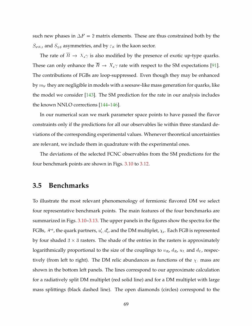
such new phases in F = 2 matrix elements. These are thus constrained both by the

S KSand S asymmetries, and by "K in the kaon sector.

The rate of B ! Xs is also modified by the presence of exotic up-type quarks.

These can only enhance the B ! Xs rate with respect to the SM expectations [91].

The contributions of FGBs are loop-suppressed. Even though they may be enhanced

bymb0 they are negligible in models with a seesaw-like mass generation for quarks, like

the model we consider [143]. The SM prediction for the rate in our analysis includes

the known NNLO corrections [144–146].

In our numerical scan we mark parameter space points to have passed the flavor

constraints only if the predictions for all our observables lie within three standard de-

viations of the corresponding experimental values. Whenever theoretical uncertainties

are relevant, we include them in quadrature with the experimental ones.

The deviations of the selected FCNC observables from the SM predictions for the

four benchmark points are shown in Figs. 3.10 to 3.12.

3.5 Benchmarks

To illustrate the most relevant phenomenology of fermionic flavored DM we select

four representative benchmark points. The main features of the four benchmarks are

summarized in Figs. 3.10–3.13. The upper panels in the figures show the spectra for the

FGBs, Am, the quark partners, u0i; d0i, and the DM multiplet, i. Each FGB is represented

by four shaded 3 3 rasters. The shade of the entries in the rasters is approximately

logarithmically proportional to the size of the couplings to uR, dR, uL and dL, respec-

tively (from left to right). The DM relic abundances as functions of the 1 mass are

shown in the bottom left panels. The lines correspond to our approximate calculation

for a radiatively split DM multiplet (red solid line) and for a DM multiplet with large

mass splittings (black dashed line). The open diamonds (circles) correspond to the

69

solutions of the coupled Boltzmann equations for the radiative (large) splitting cases

which were calculated in MadDM. The approximate and MadDM relic-abundance calcu-

lations are in very good agreement for this small subset of benchmarks. In general,

however, a disagreement of up O(30%) could be expected due to the approximations

(see App. B.II for a more detailed discussion). The bottom right panels show the pull

in selected flavor observables, i.e., the differences between theoretical predictions and

measurements normalized to the 1- uncertainties. The uncertainties were obtained by

adding in quadrature the theory and experimental errors. The four benchmark points

are also marked in Figs. 3.3, 3.4, and 3.5 with a diamond (1), a five-point star (2), a

triangle (3), and a six-point star (4).

“Benchmark 1” is an example of fermionic flavored DM, where the DM multiplet is

light, with mass below 1TeV. The mass of the lightest state in the DM multiplet ism1 '520(540)GeV if it lies just below (above) the LFGB resonance. If the mass splitting

between 1, 2 and 3 is solely due to radiative corrections, 2 and 3 are almost mass

degenerate with masses roughly 10GeV above m1 , and 3 is about 100MeV heavier

than 2. The lightest quark partner is t0 with a mass mt0 ' 1:3TeV. The lightest FGB has

a mass mA24 ' 1:1TeV. All the remaining NP states are above 7TeV. This benchmark

point demonstrates that even parameter regions with low lying FGBs can be consistent

with both the resonance searches and the FCNC bounds. The most robust constraints

in this parameter region come from cosmology (in case of radiatively-split DM masses)

and dijet-resonance searches (see Figs. 3.5 and 3.9). Note in particular that for the

completely (mass) decoupled fermionic DM scenario, in which cosmology bounds are

absent, all experimental constraints can be satisfied even for DM (and LFGB) masses

below few 100GeV.

The bottom left panel in Fig. 3.10 shows the predicted relic abundance for this

benchmark, if only the DM mass is varied, which also modifies the splitting within

the DM triplet. Relic abundance consistent with observations is obtained for a mass of

70

u'

c'

t'

d'

s'

b'

Χ1Χ2,31

10

102

103

104

105

Mu=980.GeV, Λu=1., Λu'

=11.8, Md=700.GeV, Λd=0.82, Λd'

=3.8, gQ=0.126, gU=0.41, gD=0.237

mi@

TeV

D

Benchmark 1

400 450 500 550 600 650 700mχ1 [GeV]

10−3

10−2

10−1

100

101

102

103

104

105

Ωh

2

χ1 [Approx]

χ1 [MadDM]

χ1+χ2+χ3 [Approx]

χ1+χ2+χ3 [MadDM]

ΕK

DmK

Dmd

Dms

SΨKs

SΨΦ

b®sΓ

-2 -1 0 1 2

HO-OexpL∆O

Figure 3.10: Mass spectrum and flavor decomposition (upper panel), DM relic densityas a function of the DM mass with all other parameters fixed (lower left panel) and thepattern of effects in selected flavor observables (lower right panel) for the fermionicflavored DM benchmark 1. The input benchmark-point parameters are listed in thecenter. See text for details.

71

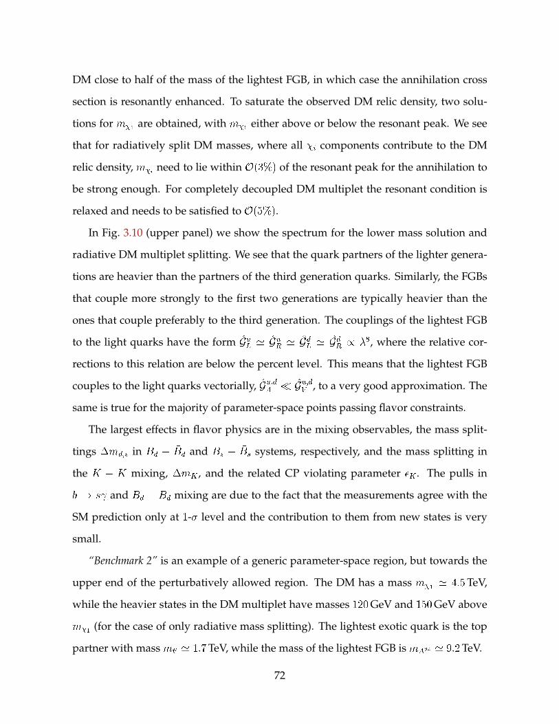
DM close to half of the mass of the lightest FGB, in which case the annihilation cross

section is resonantly enhanced. To saturate the observed DM relic density, two solu-

tions for m1 are obtained, with m1 either above or below the resonant peak. We see

that for radiatively split DM masses, where all i components contribute to the DM

relic density, mi need to lie within O(3%) of the resonant peak for the annihilation to

be strong enough. For completely decoupled DM multiplet the resonant condition is

relaxed and needs to be satisfied to O(5%).In Fig. 3.10 (upper panel) we show the spectrum for the lower mass solution and

radiative DM multiplet splitting. We see that the quark partners of the lighter genera-

tions are heavier than the partners of the third generation quarks. Similarly, the FGBs

that couple more strongly to the first two generations are typically heavier than the

ones that couple preferably to the third generation. The couplings of the lightest FGB

to the light quarks have the form GuL ' GuR ' GdL ' GdR / 8, where the relative cor-

rections to this relation are below the percent level. This means that the lightest FGB

couples to the light quarks vectorially, Gu;dA Gu;dV , to a very good approximation. The

same is true for the majority of parameter-space points passing flavor constraints.

The largest effects in flavor physics are in the mixing observables, the mass split-

tings md;s in Bd Bd and Bs Bs systems, respectively, and the mass splitting in

the K K mixing, mK , and the related CP violating parameter K . The pulls in

b ! s and Bd Bd mixing are due to the fact that the measurements agree with the

SM prediction only at 1- level and the contribution to them from new states is very

small.

“Benchmark 2” is an example of a generic parameter-space region, but towards the

upper end of the perturbatively allowed region. The DM has a mass m1 ' 4:5TeV,

while the heavier states in the DM multiplet have masses 120GeV and 150GeV above

m1 (for the case of only radiative mass splitting). The lightest exotic quark is the top

partner with mass mt0 ' 1:7TeV, while the mass of the lightest FGB is mA24 ' 9:2TeV.

72

u'

c'

t'

d'

s'

b' Χ1Χ2,3

1

10

102

103

104

105

Mu=980.GeV, Λu=1., Λu'

=0.79, Md=360.GeV, Λd=0.146, Λd'

=0.91, gQ=1.93, gU=0.47, gD=3.4

mi@

TeV

D

Benchmark 2

3500 4000 4500 5000 5500 6000mχ1 [GeV]

10−3

10−2

10−1

100

101

102

103

Ωh

2

χ1 [Approx]

χ1 [MadDM]

χ1+χ2+χ3 [Approx]

χ1+χ2+χ3 [MadDM]

ΕK

DmK

Dmd

Dms

SΨKs

SΨΦ

b®sΓ

-2 -1 0 1 2

HO-OexpL∆O

Figure 3.11: Same as Fig. 3.10 for benchmark 2.

73

u'

c'

t'

d'

s'

b'

Χ1Χ2,3

1

10

102

103

104

105

Mu=1210.GeV, Λu=1., Λu'

=1.3, Md=293.GeV, Λd=0.36, Λd'

=1.24, gQ=0.45, gU=0.46, gD=0.82

mi@

TeV

D

Benchmark 3

1200 1400 1600 1800 2000mχ1 [GeV]

10−3

10−2

10−1

100

101

102

103

Ωh

2

χ1 [Approx]

χ1 [MadDM]

χ1+χ2+χ3 [Approx]

χ1+χ2+χ3 [MadDM]

ΕK

DmK

Dmd

Dms

SΨKs

SΨΦ

b®sΓ

-2 -1 0 1 2

HO-OexpL∆O

Figure 3.12: Same as Fig. 3.10 for benchmark 3.

For such high DM masses it is barely possible to obtain the correct relic abundance

(see the lower left panel in Fig. 3.11). Therefore, the DM mass is finely tuned to be

exactly on the resonant peak (see the lower left panel in Fig. 3.11), so mi ' mA24=2.

Because of the high masses of the NP states the direct searches (direct DM detection,

t0 searches and dijet resonance searches) as well as the indirect flavor constraints are

easily avoided, although K K mixing does receive non-negligible contributions.

Also in this case, the couplings of the lightest FGB to the light quarks have the form

GuL ' GuR ' GdL ' GdR / 8, so the couplings of the lightest FGB to quarks are to a good

extent vectorial.

74

u'

c'

t'

d'

s'

b'

Χ1Χ2,3

1

10

102

103

104

105

Mu=830.GeV, Λu=1., Λu'

=3.5, Md=1920.GeV, Λd=0.096, Λd'

=0.48, gQ=1.89, gU=0.312, gD=1.93

mi@

TeV

D

Benchmark 4

2500 3000 3500 4000mχ1 [GeV]

10−3

10−2

10−1

100

101

102

Ωh

2

χ1 [Approx]

χ1 [MadDM]

χ1+χ2+χ3 [Approx]

χ1+χ2+χ3 [MadDM]

ΕK

DmK

Dmd

Dms

SΨKs

SΨΦ

b®sΓ

-2 -1 0 1 2

HO-OexpL∆O

Figure 3.13: Same as Fig. 3.10 for benchmark 4.

“Benchmark 3” is an example of a generic parameter space in which all the cou-

plings of the model are well below the pertubativity bounds. The lightest FGB has a

mass mA24 ' 5TeV while all other FGBs have masses above 100TeV. The lightest part-

ner quark is t0 with mass mt0 ' 2TeV. The DM states have masses m1 ' 2:4TeV and

m2 ' m3 = 2:5TeV (for radiative mass splitting). All direct experimental constraints

as well indirect flavor bounds are easily satisfied in this case. For radiatively DM mass

splitting the cosmological constraints are the most constraining. In particular, requir-

ing small enough 2;3 (or equivalently large enough m21;31) typically imposes a lower

bound on gU .

75

“Benchmark 4” is an example of the case in which the next-to-lightest FGBs have

masses not too far from the lightest FGB. In the benchmark point the lightest FGB has

a mass mA24 ' 8:3TeV, while the next to lightest FGBs have masses mA23 ' mA22 '19TeV, mA21 ' 39TeV. In this case the deviations from the GuL ' GuR ' GdL ' GdR / 8 re-

lation for the lightest FGB coupling to quarks are ofO(10%). Nonetheless, this does not

have a significant effect on the computation of the DM relic abundance. This is demon-

strated in Fig. 3.13 bottom left panel where a comparison is shown between the relic-

abundance calculation neglecting (dashed lines, labelled “Approx”) and including (full

lines, using MadDM) flavor off-diagonal lightest FGB couplings and contributions of

heavier FGBs. For a more detailed discussion of these effects see Appendix B.II.

The lightest quark partner is t0 with mass mt0 ' 1:4TeV, and is significantly lighter

than all FGBs and also DM. The DM states are degenerate to a good approximation,

with masses m1 = 4:1TeV and m2 ' m3 ' 4:2TeV. Because of the light t0 the flavor

constraints are nontrivial, and there are visible effects inBd andBs mixing observables.

3.6 Chapter summary

We investigated the possibility that DM is in a nontrivial representation of the contin-

uous flavor group GSMF = SU(3)QSU(3)U SU(3)D. The two main results are that (i)

one can have a viable model of DM where DM is stable because it is charged under Z3

– a discrete central subgroup of GSMF and color SU(3), and (ii) that the DM spectrum

can be very non-MFV like, while all the low-energy constraints will appear MFV-like.

Z3 is exactly conserved in many models of flavor. For instance, it remains unbro-

ken for MFV new physics. More generally, Z3 remains exact if the flavor group GSMF

is broken only by the vevs of scalar fields, or condensates, with zero flavor triality.

Examples of zero flavor triality fields are scalars in bifundamental or in adjoint repre-

sentations of the flavor SU(3)’s. The basic requirement for this set-up is that GSMF is a

76

good symmetry in the UV. This is achieved, if GSMF is fully gauged in the UV, which is

the possibility we explored. The DM is then stable because it is Z3 odd, while all SM

fields are Z3 even.

We investigated two different types of flavored DM models: (i) models in which

the leading interaction of the DM with the visible sector is through the flavored gauge

bosons (FGBs), and (ii) models in which the contributions from the FGB exchanges are

subleading.

As an example of the first type of models we considered a Dirac fermion DM that

is in a fundamental representation of SU(3)U . The relic abundance is fixed by the res-

onant DM annihilation to SM particles through the s-channel exchange of the lightest

FGB. The DM is thus required to have a mass of about half of the lightest FGB’s mass.

This in turn implies that the FGBs cannot be arbitrarily heavy, but at most O(10TeV).

Such light FGBs are possible, if the masses of FGBs are inversely proportional to the

corresponding quark masses. That is, if the FGBs that couple most strongly to light

quarks are also the heaviest. To achieve this we adopted the model of Ref. [91] in

which the inverse proportionality is achieved by introducing a set of quark partners

also necessary to cancel gauge anomalies. The same quark partners also mix with the

SM quarks and lead to the mass hierarchy of the SM quark masses.

The flavor and collider phenomenology of the model is very similar to the case

where DM is not considered. The fact that the first-generation quark partners are the

heaviest and that the spectrum is completely split, signals the non-MFV character of

the model. However, the low-energy consequences are MFV-like (see Appendix B.I).

The flavor constraints are satisfied even with FGBs and the top-quark partner, with

masses potentially well below the TeV scale. The relevant direct collider searches are

the searches for dijet resonances and t0 searches. They exclude part of the available pa-

rameter space. Requiring that there is a thermal relic DM introduces new constraints.

Because DM is part of a flavor multiplet the heavier DM states need to decay before

77

big bang nucleosynthesis. In the case of radiatively-split fermionic DM this excludes

a large part of the parameter space. The remaining points are mostly safe from direct-

detection bounds. The fact that the DM mass is related to the FGB mass by the require-

ment of almost resonant annihilation sets both lower and upper bounds on the DM

mass. Requiring that the theory is perturbative also puts an upper bound on the DM

mass, m1 . 5TeV. On the other hand, requiring that the FGBs satisfy flavor and direct

constraints and that DM is simultaneously in accordance with cosmological constraints

leads to a lower bound on the DM mass,m1 & 500GeV. Improved bounds on dijet res-

onances at the LHC are expected to further strengthen this constraint (see Fig. 3.9).

We have also considered the possibility that the DM multiplet is split due to an

extra source of flavor breaking. Also in this case, the correct relic abundance requires

resonant annihilation. The DM mass is in thus still roughly equal to half of the mass

of the lightest FGB. However, the heavier DM states decay well before big bang nu-

cleosynthesis so that a much wider range of DM masses is phenomenologically viable.

In our scan this includes DM masses as light as 100GeV (with very small couplings to

FGBs) and up to 10TeV.

A possible signal of the gauged flavor model with fermionic DM at the LHC are

mono-jets, where the lightest FGB is produced associated with initial state radiation

and decays to 1 pairs. The 1s are expected to be non-relativistic in the lightest FGB’s

rest frame, as their combined mass needs to be close to the FGB mass to fulfill the res-

onance condition for relic DM abundance. In the event that such a signal would even-

tually emerge, the corresponding dijet-resonance signal is generically also expected in

the model. A final possibility in the case of radiatively split DM mass spectrum is that

some of the lightest FGBs decay to slow-moving 2;3. They in turn decay within the

detector, leaving (highly) displaced vertices, isolated hits in the calorimeter or in the

muon chambers. Unfortunately, in most of the parameter space 2;3 are expected to

decay well outside the detectors, see Fig. 3.5, leaving mono-jets as the only signal.

78

In the second type of models, where FGB exchanges give only subleading contribu-

tions, the only visible consequence of the flavor dynamics on the DM is that DM is sta-

ble. The DM mass and the mass of the lightest FGB are no longer connected. We show

this in the example of scalar flavored DM, in which the dominant interactions with the

visible sector are through the Higgs portal operator. In this case the phenomenology

of the DM is to a very good approximation the same as in the Higgs-portal scalar DM,

while the dynamics of FGBs and quark partners is unrelated to DM.

In short, we have shown, using an explicit renormalizable model, that it is possible

for flavored DM to be a thermal relic. The considered model is not the only choice.

One could consider DM in other representations of GSMF . Our analysis can be extended

also in other ways: for instance, by enlarging the global symmetry as in Ref. [24] and

subsequently gauging it. For instance, with our field content the global group is GSMF SU(3), where is in the fundamental of SU(3). In our work we have identified

SU(3) with SU(3)U , but other choices could be made. Yet another possibility is to

gauge only part of GSMF , for instance a U(2)3 GSMF . Note that for fermionic DM, Z3

is part of an accidental U(1) acting in the dark sector. The U(1) can be broken by

the dimension-7 operator LH, but is exact in our renormalizable model. It can in

principle be gauged and lead to additional phenomenology. If DM is a scalar, U(1)

can be broken already at the renormalizable level, leaving only Z3 exact.

79

Chapter 4

Nonstandard Yukawa couplings and

Higgs portal dark matter

4.1 Introduction

In Higgs-portal models [147–156] of dark matter (DM) the Higgs is usually assumed

to be completely Standard Model (SM) like apart from its couplings to DM. Experi-

mentally, only the couplings of the Higgs to the heaviest particles of the SM are cur-

rently well constrained. The couplings to gauge bosons are found to be in agree-

ment with the SM predictions at the O(20%) level, while the constraints on the cou-

plings to third-generation fermions are somewhat weaker [157, 158]. Much less is

known experimentally about the couplings of the Higgs to the first two generations

of fermions. The couplings to u; d; s, and c quarks could be as large as the SM bottom

Yukawa coupling or be absent altogether [159–162]. The Higgs couplings to top and

bottom quarks will be quite well known by the end of the high-luminosity LHC run.

Some progress is also expected on the measurements of Higgs couplings to charm and

strange quarks [159–161].

Large u-, d-, and s-quark Yukawa couplings, comparable in size to the b-quark

80

Yukawa, generically require fine-tuning. A large Yukawa coupling implies a large

contribution to the quark mass from the Higgs vacuum expectation value (vev). This

would then need to be cancelled by a different contribution to the u-, d-, and s-quark

masses, unrelated to the Higgs vev. The opposite limit, where the observed Higgs does

not couple to the light quarks at all is easier to entertain. It simply requires a separate

source of the light-quark masses (for an extreme example see, e.g., [163]).

Modified light-quark Yukawa couplings could, in principle, have important impli-

cations for DM phenomenology. In this article we investigate how the Higgs-portal

DM predictions change if the Higgs couplings to the light quarks differ from the SM

expectations. We first allow for an arbitrary flavor structure of the Higgs Yukawa

couplings, only requiring that they satisfy the current experimental bounds. In Sec-

tion 4.2 we derive the implications for direct DM detection, indirect DM detection and

the collider searches. We show that vanishing couplings of the Higgs to light quarks

only have a relatively small impact on these observables. Saturating the loose current

bounds on the light-quark Yukawa couplings would, on the other hand, lead to dras-

tically enhanced scattering cross sections on nuclei while leaving the relic density and

annihilation cross sections

Clearly, an enhancement of the light-quark Yukawas by factors of O(100) or more,

as allowed by current data, requires considerable fine tuning of the quark-mass terms

and hence seems quite unlikely. In Section 4.3 we, therefore, explore the deviations

in the Higgs Yukawa couplings for a number of beyond-the-SM scenarios and flavor

models. This leads to more realistic expectations as to how large the deviations in

the direct DM detection rates can be due to the poorly known Higgs couplings to the

light quarks. Note that we assume the DM to be a flavor singlet and that the new flavor

structure of the interactions with the visible sector is only due to the modification of the

SM Higgs couplings. DM that is in a nontrivial flavor multiplet has been investigated

in [21, 23–26, 29, 39, 94, 96, 97, 164, 165], while our study is closer in spirit to the work

81

in [28, 93, 166] where the flavor dependence of the DM signals for flavor-singlet DM

has been explored.

A somewhat surprising result of our investigation is that, if DM is discovered and

turns out to be a thermal relic predominantly interacting through a Higgs portal, it

could be used to constrain the light-quark Yukawa couplings. This is discussed in

more detail in Section 4.4.

We summarize the results of this chapter in Section 4.5.

4.2 Higgs portal with non-trivial flavor structure

We assume that DM and the SM fields are the only light degrees of freedom. The

remaining new physics (NP) particles can be integrated out so that one can use an

Effective Field Theory (EFT) approach. The couplings of DM to the SM are given by

the Higgs-portal Lagrangian

L =

8>>>>><>>>>>:g

yHyH ; scalar DM;

g1

HyH + i~g

1

5H

yH ; fermion DM;

g2H

yH; vector DM.

(4.1)

Above, the fermion DM can be either a Dirac or Majorana fermion (in either case we

use four component notation). After electroweak symmetry breaking (EWSB) we have

HyH =1

2

v2W + 2vWh+ h2

; (4.2)

where vW = 246 GeV is the vacuum expectation value (vev) of the Higgs field. The

above interactions therefore lead to annihilation of DM into both single Higgs, ! h,

and double Higgs, ! hh, final states.

The Higgs-portal operator for fermionic DM has mass dimension five and is sup-

82

pressed by the new physics scale . The Higgs-portal interaction for fermionic DM can

also be re-written as L = (g + i~g)LRHyH= + h:c:. For ~g 6= 0 the interaction is

thus both P - and CP -violating. The interaction for vector DM is most probably also

due to a higher-dimensional operator in the full theory. For instance, if arises from

a spontaneously broken gauge symmetry in the dark sector, then g v2D=2, where

vD is the vev of the field that breaks the dark sector gauge invariance, while is the

mass of the mediator between DM and the Higgs.

The relevant terms, after EWSB, in the effective Lagrangian for the Higgs couplings

to the SM particles are given by

Le = qmq

vWqqh `

m`

vW h+ V

2m2

W

vWW+W

+m2Z

vWZZ

h

m2h

2vWh3 + NPg

s12vW

hGaG

a

(4.3)

where the i are real. A sum over the SM quarks, q = u; d; s; c; b; t, and charged leptons,

` = e; ; is implied, and we have assumed custodial symmetry. The h! coupling

is not relevant for DM phenomenology, since its effects are suppressed compared to the

Higgs couplings to gluons.1 The couplings are normalized such that q = ` = V =

= 1 correspond to the SM. The experimental constraints on the couplings of the light

quarks to the Higgs, obtained from a global fit to current data, are juj < 0:98mb=mu,

jdj < 0:93mb=md, jsj < 0:70mb=md, where only one of the light Yukawa couplings was

left to float in the fit, while all the other Higgs couplings are set to the SM values [159].

Higgs couplings to the light quarks of a size comparable to the coupling to the b quark

are thus still allowed. In (4.3) we do not allow for flavor violating Higgs couplings,

since these are already tightly constrained from both Higgs decays and low-energy

observables [167–170].1It could be relevant for direct detection if the scattering on electrons dominates. This requires very

light DM, of order the electron mass. Such light Higgs-portal DM is excluded by the constraints on theHiggs invisible branching ratio.

83

In the SM, keeping the Higgs on shell, the hGG coupling arises predominantly from

the one-loop top-quark contribution. The NPg in (4.3) encodes only the potential NP

contributions, and vanishes in the SM. In the global fits a parameter g is introduced

that gives the total h ! gg amplitude, including the SM contributions [157, 158]. We

have (see, e.g., [171])

g ' 1:03t + NPg : (4.4)

At present, significant CP -violating Higgs couplings to fermions and gluons are

still allowed experimentally (see, e.g., [172]), so we also discuss their effect on the Higgs

interactions with DM:

Le;CPV = i~qmq

vWq 5qh i~`

m`

vW 5`h+ ~NPg

s8vW

hGaeGa : (4.5)

Here, the ~i are real parameters; in the SM, we have ~i = 0. Moreover, Ga is the gluon

field-strength tensor and eGa; = 12Ga

its dual. The normalization of the hG ~G

term is chosen such that integrating out the top at one loop one obtains ~g = ~t + ~NPg .

Accordingly, we have Br(h ! gg) / 2g + (3~g=2)2. The CP -violating couplings of the

Higgs to ZZ and WW are already well constrained, and we thus set them to zero. In

the numerical analysis below, we will also assume ~i = 0, for simplicity.

The modified Higgs couplings change the usual Higgs-portal predictions for DM

annihilation rates, the relic abundance, and direct detection rates. In the following, we

discuss these modifications in detail.

4.2.1 Annihilation cross sections

The dominant DM annihilation cross sections in the Higgs-portal models are !bb;W+W; ZZ; tt, and ! hh. The first four proceed through the s-channel Higgs

exchange, while ! hh receives additional contributions from t- and u-channel

84

χ

χ†

h

b,W+, Z, t, h

b,W−, Z, t, h

χ

χ†

h

h

χ

χ†

h

h

χ

χ

χ†

h

h

χ

Figure 4.1: DM annihilation channels in the Higgs-portal models.

exchange as well as from the four-point contact interaction (cf. Fig. 4.1). The ! bb

channel is only relevant if the other channels are not kinematically allowed, i.e. for

light DM masses, m < mW .

The ! bb annihilation cross section assuming SM Higgs couplings is given for

scalar (S), Dirac fermion (DF ), and vector (V ) DM by

Sbbvrel

SM

=Nc

4

g2m2b

3b

(sm2h)

2+m2

h2h

; (4.6)

DFbb vrel

SM

=Nc

8

m2b

2

g2s 4m2

+ ~g2 s

(sm2h)

2+m2

h2h

3b ; (4.7)

Vbbvrel

SM

=Nc

9

g216

m2b

m4

3b

1 r +

3

4r2

s2

(sm2h)

2+m2

h2h

; (4.8)

where, here and below,ps is the center-of-mass energy, rk = 4m2

k=s, k =p1 rk is

the velocity of particle k, and vrel = 2 is the relative velocity of the DM particles. If

the Higgs coupling to the b-quarks differs from the SM value, the annihilation cross

section is rescaled as

bb =2b + ~2b=

2b

SMbb : (4.9)

The annihilation cross sections f f to the other fermions are obtained with the obvious

replacement b ! f in the above expressions. Since the Higgs couplings to the light

quarks are poorly constrained experimentally, the DM annihilation to two light quarks

can be comparable to ! bb and can be important for light DM, m < mW .

85

For heavy DM, m > mW , the annihilation cross-sections into a pair of W or Z

bosons are

V V = 2V SMV V ; (4.10)

V = W;Z. The annihilation cross sections assuming the SM Higgs couplings to W are

given by

(SWWvrel)SM =g28W

1 rW +

3

4r2W

s

(sm2h)

2+m2

h2h

; (4.11)

(DFWWvrel)SM =1

162W

1 rW +

3

4r2W

sg2s 4m2

+ ~g2 s

(sm2

h)2+m2

h2h

; (4.12)

(VWWvrel)SM =g2

288

s

m4

W

1 rW +

3

4r2W

1 r +

3

4r2

s2

(sm2h)

2+m2

h2h

;

(4.13)

for scalar, Dirac fermion, and vector DM, respectively. The ! ZZ annihilation cross

section is obtained by replacing W ! Z, and multiplying all expressions by an extra

factor of 1/2 since one has two indistinguishable particles in the final state.

The ! hh annihilation cross sections for scalar, Dirac fermion, and vector DM,

are given by

Shhvrel =hg

2

64m2

1 +

3M2h

4m2 M2

h

2v2WgM2

h 2m2

2; (4.14)

DFhh vrel =h~g2 + g2

2

322

1 +

3M2h

4m2 M2

h

+4gmv

2W

(2m2 M2

h)

2; (4.15)

Vhhvrel =h

576m2

3g2

3M

2h

4m2 M2

h

+ 1

2

+4g4v

4W

(2m2 M2

h)2

6 4M2

h

m2

+M4

h

m4

+16g3v

2W

2m2 M2

h

3M

2h

4m2 M2

h

+ 1

1 M2

h

4m2

: (4.16)

In this result we display only the leading terms in the expansion in powers of . The

86

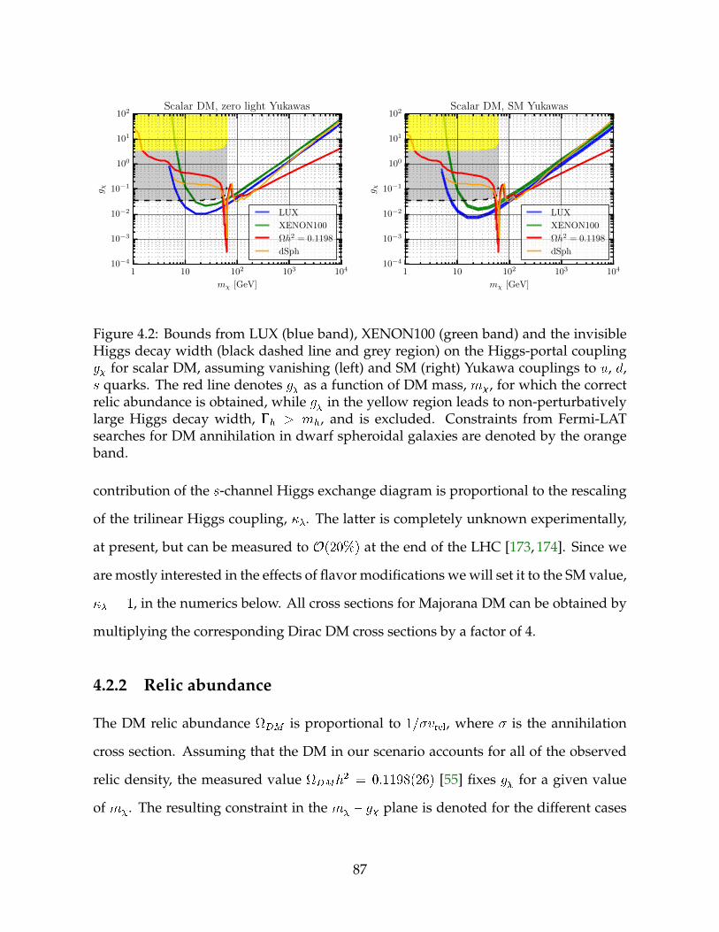
1 10 102 103 104

mχ [GeV]

10−4

10−3

10−2

10−1

100

101

102

g χScalar DM, zero light Yukawas

LUX

XENON100

Ωh2 = 0.1198

dSph

1 10 102 103 104

mχ [GeV]

10−4

10−3

10−2

10−1

100

101

102

g χ

Scalar DM, SM Yukawas

LUX

XENON100

Ωh2 = 0.1198

dSph

Figure 4.2: Bounds from LUX (blue band), XENON100 (green band) and the invisibleHiggs decay width (black dashed line and grey region) on the Higgs-portal couplingg for scalar DM, assuming vanishing (left) and SM (right) Yukawa couplings to u, d,s quarks. The red line denotes g as a function of DM mass, m, for which the correctrelic abundance is obtained, while g in the yellow region leads to non-perturbativelylarge Higgs decay width, h > mh, and is excluded. Constraints from Fermi-LATsearches for DM annihilation in dwarf spheroidal galaxies are denoted by the orangeband.

contribution of the s-channel Higgs exchange diagram is proportional to the rescaling

of the trilinear Higgs coupling, . The latter is completely unknown experimentally,

at present, but can be measured to O(20%) at the end of the LHC [173, 174]. Since we

are mostly interested in the effects of flavor modifications we will set it to the SM value,

= 1, in the numerics below. All cross sections for Majorana DM can be obtained by

multiplying the corresponding Dirac DM cross sections by a factor of 4.

4.2.2 Relic abundance

The DM relic abundance DM is proportional to 1=vrel, where is the annihilation

cross section. Assuming that the DM in our scenario accounts for all of the observed

relic density, the measured value DMh2 = 0:1198(26) [55] fixes g for a given value

of m. The resulting constraint in the m – g plane is denoted for the different cases

87

1 10 102 103

mχ [GeV]

10−5

10−4

10−3

10−2

10−1

100

101g χ

Scalar DM, κu = 0.98mb/mu

1 10 102 103

mχ [GeV]

Scalar DM, κd = 0.93mb/md

1 10 102 103 104

mχ [GeV]

Scalar DM, κs = 0.70mb/ms

LUX

XENON100

Ωh2 = 0.1198

dSph

Figure 4.3: Bounds on the Higgs-portal coupling g for scalar DM, assuming maximalallowed values for the Yukawa couplings to the u, d, s quarks (left to right), keeping allthe other couplings to their SM values. The color coding is the same as in Fig. 4.2.

by a red line in Figs. 4.2 to 4.9. In Fig. 4.2, we compare two limits of the Higgs portal

for the scalar DM: the case where the Higgs does not couple to the light quarks at all

(left panel) to the case where the Higgs has SM Yukawa couplings (right panel). The

two relic abundance curves coincide apart from very light DM, with m below the

charm and tau threshold. If such light DM did not couple to the u; d and s quarks, this

would result in noticeably reduced annihilation cross sections and, thus, in larger relic

abundance. In both cases, the dominant annihilation process is still given by !h ! gg. For very light DM the correct relic abundance is obtained only if the coupling

of the Higgs to DM, g, is nonperturbatively large. The yellow regions in Fig. 4.2 denote

the value of g for which the total Higgs decay width would be larger than its mass,

h > mh, and are thus excluded.

The same comments apply to the case of vector DM, shown in Fig. 4.4,CP -conserving

Dirac fermion DM, shown in Fig. 4.6,CP -violating Dirac fermion DM, shown in Fig. 4.8,

and also for Majorana fermion DM. For light DM,m . 30GeV, the correct relic density

requires a non-perturbatively large coupling g so that the predictions should be taken

only as O(1) estimates in that region. Note that all these non-perturbative regions are,

in addition, excluded by bounds on the decay width of the Higgs into invisible final

88

1 10 102 103 104

mχ [GeV]

10−4

10−3

10−2

10−1

100

101

102

g χVector DM, zero light Yukawas

LUX

XENON100

Ωh2 = 0.1198

dSph

1 10 102 103 104

mχ [GeV]

10−4

10−3

10−2

10−1

100

101

102

g χ

Vector DM, SM Yukawas

LUX

XENON100

Ωh2 = 0.1198

dSph

Figure 4.4: Bounds on the Higgs-portal coupling for vector DM, assuming vanishing(left) and SM (right) Yukawa couplings to u, d, s quarks. The color coding is the sameas in Fig. 4.2.

states (see the discussion in Section 4.2.3).

In Figs. 4.3, 4.5, 4.7, and 4.9, we show the relic abundance curves for g as a function

of m for the case where the light Yukawa couplings saturate their upper experimen-

tal bound. The left panels show the case where u = 0:98mb=mu and all the other

couplings at their SM values, the middle panels the case where d = 0:93mb=md, and

the right panels the case where s = 0:70mb=ms. In all of these cases the cross sec-

tion for DM annihilation to light jets, ( ! jj), coming from DM annihilating to

light quarks, is comparable to the annihilation cross section to b-jets, ( ! bb). For

m . mW these are the two dominant annihilation modes. Since the annihilation cross

sections to b-jets and light jets are comparable, the relic abundance curve show only a

small change in g when the b-quark threshold is reached. This should be compared

with the case of the SM Yukawa couplings shown in the right panels of Figs. 4.2, 4.4, 4.6,

and 4.8. In this case the ! jj annihilation is almost exclusively due to DM anni-

hilating to two gluons, so that ( ! jj) ( ! bb), while the annihilation into

two light quarks is negligible. For m . mW and SM Yukawas, the required g is thus

bigger by 30% 40% than in the case of light Yukawas at their present experimental

89

1 10 102 103

mχ [GeV]

10−4

10−3

10−2

10−1

100

101g χ

Vector DM, κu = 0.98mb/mu

1 10 102 103

mχ [GeV]

Vector DM, κd = 0.93mb/md

1 10 102 103 104

mχ [GeV]

Vector DM, κs = 0.70mb/ms

LUX

XENON100

Ωh2 = 0.1198

dSph

Figure 4.5: Bounds on the Higgs-portal coupling for vector DM, assuming maximalallowed values for the Yukawa couplings to the u, d, s quarks (left to right), keeping allthe other couplings to their SM values. The color coding is the same as in Fig. 4.2.

limits, and exhibits a significant jump below the b-quark threshold.

4.2.3 Invisible decay width of the Higgs

The bounds on the invisible decay width of the Higgs boson provide stringent con-

straints on Higgs-portal DM [153]. The partial h! decay widths are given by

S =g216

v2WMh

;

DF =g28Mh

v2W2

3 +~g28Mh

v2W2

;

V =g2

128

M3hv

2W

m4

1 r +

34r2;

(4.17)

where r = 4m2=M

2h and =

p1 r.

The current best limits on the invisible branching fraction of the SM Higgs are ob-

tained from Zh production. The CMS collaboration gives a 95% CL limit of Br(h !inv) < 0:58 forMh = 125GeV [175] and ATLAS finds Br(h! inv) < 0:75 forMh = 125:5

GeV [176]. Note that the increased light-quark Yukawa couplings, at their presently

allowed values, do not appreciably change the Higgs production cross section [159].

Their main effect is to increase the total decay width of the Higgs and thus reduce the

90

1 10 102 103 104

mχ [GeV]

10−2

10−1

100

101

102

g χDirac DM, zero light Yukawas

LUX

XENON100

Ωh2 = 0.1198

dSph

1 10 102 103 104

mχ [GeV]

10−2

10−1

100

101

102

g χ

Dirac DM, SM Yukawas

LUX

XENON100

Ωh2 = 0.1198

dSph

Figure 4.6: Bounds on the Higgs-portal coupling for Dirac DM, assuming = 1 TeVand vanishing (left) and SM (right) Yukawa couplings to u, d, s quarks. The colorcoding is the same as in Fig. 4.2.

branching ratios to the other decay modes:

Br(h! ) =(h! )

(h! ) + toth 1 +Pq(

2q 1)BrSM(h! qq)

: (4.18)

In Figs. 4.2 to 4.9 we denote the bound on g corresponding to the ATLAS upper limit

on Br(h! inv) with a dashed black line and grey out the excluded region in the g vs.

m plane. We see that the light DM Higgs portal, m . mh=2 is excluded by the Higgs

invisible decay width.

Vector boson fusion, gluon fusion and ttH production, with the off-shell Higgs go-

ing to two DM particles, can provide some limited sensitivity to DM masses above

mh=2. A combination of the searches in the three channels at a 100 TeV collider could

exclude the scalar thermal relic DM Higgs portal for DM masses in parts of the mh=2 .

m . mW interval at 95% C.L. [156] (these result receives only a negligible correction

if light quark Yukawa couplings are enhanced). For m < mh=2 the invisible Higgs

decay width is, however, always the most constraining [177].

91

1 10 102 103

mχ [GeV]

10−4

10−3

10−2

10−1

100

101

102g χ

Dirac DM, κu = 0.98mb/mu

1 10 102 103

mχ [GeV]

Dirac DM, κd = 0.93mb/md

1 10 102 103 104

mχ [GeV]

Dirac DM, κs = 0.70mb/ms

LUX

XENON100

Ωh2 = 0.1198

dSph

Figure 4.7: Bounds on the Higgs-portal coupling for Dirac DM, assuming = 1 TeVand maximal allowed values for the Yukawa couplings to the u, d, s quarks (left toright), keeping all the other couplings to their SM values. The color coding is the sameas in Fig. 4.2.

4.2.4 Indirect detection

In indirect signals of DM annihilation, the effect of changing the light-quark Yukawa

couplings within the presently experimentally allowed ranges leads to at most O(1)effects. Further, the effect is present only for DM masses below the W threshold where

the dominant annihilation channel is into the bb final state. For example, Fig. 4.10

shows the recast of the Fermi-LAT bound from dwarf spheroidals [130] for scalar DM,

following the procedure outlined below.

Photon flux measurements with -ray telescopes can put a strong bound on the

annihilation cross-section of the DM. The strongest bound in the DM mass range of in-

terest has been recently released by the Fermi-LAT collaboration [130] based on Pass 8

observation data of the Milky Way dwarf spheroidal satellite galaxies (dSphs). There

is also a recent analysis based on the Dark Energy Survey (DES) dSph candidates us-

ing the Fermi-LAT data [178]. While this bound is competitive with the one from the

known dSphs, it is still weaker on its own. One could also consider the bounds from

the isotropic gamma ray background (IGRB) [132]. In our analysis, we recast the Fermi-

LAT bound on the bb final state using a simple re-weighting procedure of the photon

92

1 10 102 103 104

mχ [GeV]

10−3

10−2

10−1

100

101

102

g χDirac DM, CPV, zero light Yukawas

LUX

XENON100

Ωh2 = 0.1198

dSph

1 10 102 103 104

mχ [GeV]

10−3

10−2

10−1

100

101

102

g χ

Dirac DM, CPV, SM Yukawas

LUX

XENON100

Ωh2 = 0.1198

dSph

Figure 4.8: Bound on the pseudoscalar Higgs-portal coupling for Dirac DM, assuming = 1 TeV and vanishing (left) and SM (right) Yukawa couplings to u, d, s quarks. Thecolor coding is the same as in Fig. 4.2.

spectra which will be discussed below.

The observed differential photon flux from the annihilation of dark matter is given

byd

dE d=

1

4

1

2m2

J

"Xf

hvifdN f

dE

#; (4.19)

where J is an astrophysical factor which depends on the distance to the source and the

dark matter density profile. The factor in the brackets is the one most interesting for

our purposes. It depends on the velocity-averaged cross-section and photon spectrum

per DM annihilation.

The Fermi-LAT analysis gives bounds for the different final states separately while

we have an admixture of final states. In order to recast the bound, we rely on the

observation that for heavy DM the photon spectra from DM annihilation into quarks,

gauge bosons, and the Higgs boson all peak at approximately the same photon energy

and have approximately the same shape. Therefore, to extract the bound on the DM

93

1 10 102 103

mχ [GeV]

10−3

10−2

10−1

100

101

102g χ

Dirac DM, CPV, κu = 0.98mb/mu

1 10 102 103

mχ [GeV]

Dirac DM, CPV, κd = 0.93mb/md

1 10 102 103 104

mχ [GeV]

Dirac DM, CPV, κs = 0.70mb/ms

LUX

XENON100

Ωh2 = 0.1198

dSph

Figure 4.9: Bounds on the pseudoscalar Higgs-portal coupling for Dirac DM, assuming = 1 TeV and maximal allowed values for the Yukawa couplings to the u, d, s quarks(left to right), keeping all the other couplings to their SM values. The color coding isthe same as in Fig. 4.2.

101 102 103

mχ [GeV]

10−4

10−3

10−2

0.1

1

10

102

g χ

Scalar Higgs Portal

Ωh2 = 0.1198

dSph – SM Yuk.dSph – yu = 0.98yb

Figure 4.10: The effect of large light-quark Yukawa couplings on the indirect detectionbounds from Fermi-LAT observations of Milky Way dwarf spheroidal satellite galax-ies [130].

Higgs portal coupling g, it is sufficient to find the zeros of the polynomial

f(g) =Xf

hvif dN f

dE

!PEAK

hviFERMIb

dN b

dE

!PEAK

; (4.20)

where in the last term, hviFERMIb is the bound from the Fermi-LAT analysis on the

velocity-averaged cross-section. The photon spectra were obtained from the interpola-

tion tables provided in the PPPC4DMID package [179]. In all cases except for the hh final

94

state, f(g) has only one zero up to a sign ambiguity. For the hh final state, however,

the zero of f(g) closest to the g corresponding to ! bb is the one used to rescale

the Fermi-LAT bound on g as a function of m. The resulting bounds are shown in

Figs. 4.2 to 4.9.

4.2.5 Direct detection

We have seen so far that most DM observables exhibit only a weak dependence on

the light-quark Yukawas. This is not the case for the direct DM detection. In fact,

modifying the light-quark Yukawa couplings can significantly change the predictions

for DM – nucleus scattering cross sections.

The differential cross section for spin-independent DM scattering on a nucleus is

given byd

dER=

mA

2Av2rel

jMj232s

; (4.21)

whereER is the nuclear recoil energy,mA is the mass of the nucleus, A mmA=(m+

mA) is the reduced mass of the DM – nucleus system, s = (m + mA)2 is the center-

of-mass energy, vrel is the DM velocity in the detector rest frame, and jMj2 is the spin-

averaged squared matrix element.

The matrix element M depends on the effective Higgs couplings to the nucleus.

Since the momentum exchanges in DM scattering on nuclei are much smaller than the

Higgs mass, we can calculate jMj2 by first integrating out the Higgs and the heavy

quarks (t, b, c). This gives an EFT with light quarks and gluons interacting with DM

95

through local operators, described by the effective Lagrangians

LS = gvWm2h

(y)Sq ; (4.22)

LF =1

gvWm2h

()Sq + 1

~gvWm2h

(i 5)Sq : (4.23)

LV =gvW2m2

h

()Sq ; (4.24)

for scalar, fermion, and vector DM, respectively. The scalar current is the same in all

three cases:

Sq =Xq

qmq

vWqq Cg s

12vWGaG

a +Xq

i~qmq

vWq 5q ~Cg s

8vWGaeGa : (4.25)

Here, the last two terms arise from CP -violating Higgs couplings. The sums are over

the light quarks q = u; d; s. The heavy quarks are integrated out and contribute only

via the gluonic terms in the current. For the two corresponding dimensionless Wilson

coefficients we have

Cg = NPg + t + b + c ; ~Cg = ~NPg + ~t + ~b + ~c ; (4.26)

where the first contribution is from tree-level matching, and the remaining from one-

loop matching, working in the limit of heavy quarks. This is well justified for top

and bottom quarks. For scattering on heavy nuclei, e.g., on Xe or W, the maximal

momentum exchanges for DM with mass above approximately 1 TeV may, however,

start to become comparable to the charm-quark mass. We neglect these effects, while

they may need to be included in the future if such heavy DM is discovered.

CP -violating Higgs couplings to light quarks lead to spin-dependent interactions of

DM with the target nuclei. The corresponding scattering rates are suppressed relative

to the spin-independent interaction rates from CP -conserving Higgs couplings. We

96

will therefore neglect the CP -violating interactions in our numerical analysis of direct

detection scattering rates; i.e., we will set ~q = 0, ~Cq = 0 from now on.

The nucleon matrix elements of the remaining terms in the scalar current Sq are

conventionally parametrized by (see, e.g., [87]),

hN jmqqqjNi = mNf(N)Tq ; (4.27)

hN j s12

GG jNi = 2

27mNf

(N)TG : (4.28)

In the heavy-quark limit for t; b; c the trace anomaly equation leads to the relation [87,

180]

f(N)TG = 1

Xq=u;d;s

f(N)Tq : (4.29)

We can also define the effective Higgs coupling to nucleon as the expectation value of

the scalar current,

f(N)S hN jSqjNi = mN

vW

h 227Cg +

Xq

q 2

27Cgf(N)Tq

i: (4.30)

The exclusion curves from LUX [120] and Xenon100 [181], assuming a local DM

density of 0.3 GeV/cm3, are shown in Figs. 4.2 to 4.9 as blue and red bands, respec-

tively. The width of the exclusion curves represents the uncertainties in the hadronic

matrix elements of the light-quark scalar currents. For the s quark we use the lattice

determination f(N)Ts = 0:043 0:011 [123]. The matrix elements for u and d quarks can

be related to the N term. A Baryon Chiral Perturbation Theory (BPT) analysis of

the N scattering data gives N = 59(7) MeV [124]. This is in agreement with BPT

fit to world lattice Nf = 2 + 1 QCD data, which gives N = 52(3)(8) MeV [125].

Including both (1232) and finite spacing parametrization in the fit shifts the cen-

tral value to N = 44MeV. To be conservative we use N = (50 15)MeV, which

97

gives f (p)Tu = (1:8 0:5) 102, f (p)Td = (3:4 1:1) 102, f (n)Tu = (1:6 0:5) 102,

f(n)Td = (3:8 1:1) 102, using the expressions in [126, 127]. For the effective Higgs

coupling to nucleons this gives

f(p)S =

mW

vW

h(1:8 0:5)u + (3:4 1:1)d + (4:3 1:1)s

+ (6:70 0:12)c + b + t + NPg

i 102 ;

(4.31)

f(n)S =

mW

vW

h(1:6 0:5)u + (3:8 1:1)d + (4:3 1:1)s

+ (6:69 0:12)c + b + t + NPg

i 102 :

(4.32)

We use the results in [182] to relate the nuclear matrix elements to actual scattering

rates on nuclei via nuclear form factors.

We show the direct detection exclusion limits for SM (u;d;s = 1) or vanishing

(u;d;s = 0) light-quark Yukawa couplings in the right and left panels in Figs. 4.2, 4.4, 4.6,

and 4.8, respectively. The exclusion limits are approximately two times weaker in the

latter case; the constraint does not vanish because, for small values of the light-quark

Yukawas, the scattering cross section is dominated by the gluon part of the scalar cur-

rent, Eq. (4.25). When the light-quark Yukawas are taken to be at the upper limit of

their experimentally allowed range, i.e. comparable to the SM bottom Yukawa, the di-

rect detection bounds on g become significantly stronger, by a factor of about mb=mq

(Figs. 4.3, 4.5, 4.7, and 4.9).

It is interesting to note that, because of the dominance of the gluon contribution,

for small light-quark Yukawas the theory uncertainty in the exclusion bands is signif-

icantly smaller than if the light Yukawa couplings are allowed to saturate the present

experimental bounds. (The nuclear matrix element of the effective gluon term has

smaller relative uncertainties than the corresponding matrix elements of mqqq since

f(N)TG f

(N)Tq .)

98

10−1 100 101 102 103 104

κq

0.0

0.2

0.4

0.6

0.8

1.0

1.2g

max

χ(κq)/g

max

χ(1

)

κm

ax

s

κm

ax

d

κm

ax

u

Ratio of direct detection limits

κsκdκu

10−1 100 101 102 103 104

|κq|

10−4

10−3

10−2

10−1

100

101

102

103

104

σd.d.

/σ

SM

d.d.

κm

ax

s

κm

ax

d

κm

ax

u

Ratio of direct detection cross sections

κsκdκu

Figure 4.11: Left: The ratio of direct detection bounds on g from Xenon target varyingu (dark red), d (light red), or s (blue), and the bound on g assuming SM HiggsYukawa couplings. The LHC upper bounds on i are denoted by vertical dashed lineswith shaded regions excluded. Right: the ratio of predicted scattering cross sections.The dotted lines correspond to negative values of q.

For m smaller than a few TeV, the DM direct detection bounds are compatible

with the thermal relic Higgs-portal DM only if light quark Yukawas are well below

the present experimental bounds (the exception is a pseudoscalar fermion DM with

enhanced strange Yukawa, where the bound is m & mh=2, see Fig. 4.9). This means

that if thermal relic DM is discovered, it would immediately place an upper bound on

u; d; s, assuming Higgs-portal mediation (unless in the case of fermion DM that has

purely pseudoscalar couplings). We comment in more detail on that observation in

Section 4.4.

Since the DM – nucleus scattering cross section is the only DM observable that

exhibits a rather pronounced dependence on the values of the light-quark Yukawas,

we study this dependence in more detail.

In Fig. 4.11 (left) we show how the direct detection bounds on g are affected by

99

changes in the values of the light-quark Yukawas. We plot the ratio

g =gmax (q)

gmax (1); (4.33)

where gmax (q) is the upper bound on g obtained from direct detection experiments

for a given value of q, with q = u; d; s. Hence, gmax (1) is the bound obtained assuming

SM Yukawa couplings. Its value depends on m, on whether DM is a scalar, fermion,

or vector, and on the experiment that measured the bounds. Similarly, also gmax (q)

depends on m, the spin of DM, and the experiment; however, all these dependences

cancel in the ratio g . The ratio g thus only depends on q and on which target mate-

rial was used to derive the direct detection bounds. In Fig. 4.11 we show g for a Xenon

target, varying in turn u (dark red line), d (light red) and s (blue), while keeping all

other parameters fixed to their SM values. We set the hadronic matrix element f (N)Tq to

their present central values, anticipating that in the future their uncertainties will be

further reduced. In Fig. 4.11 (right) we show a closely related quantity – the ratio of

the scattering cross sections with varied u;d;s and the scattering cross section with SM

Yukawa couplings, d:d:=SMd:d:.

Fig. 4.11 illustrates clearly that the difference between the bounds where one of

the light quark Yukawa couplings is taken to be small or vanish completely, and the

bounds where all the couplings are SM-like, is very small, O(10%). Saturating the

present experimental bounds on u or d, the allowed value of g could lie two orders

of magnitude below what one obtains for the case of SM Yukawa couplings. Such

large values for the light-quark Yukawas are not very likely to be realized in a concrete

model, as we will discuss in the next section. However, it is very interesting to observe

that even a moderate increase of the values of the light-quark Yukawa couplings to

only a few times their SM values can have a significant effect on the direct detection

bounds, enhancing the scattering cross sections by up to a factor of ten.

100

Finally, in the right panel of Fig. 4.11 we show the cross section ratios for negative

values of the q (dotted lines). We see that the interference of the light-quark contribu-

tions with the effective gluon interaction can, in principle, lead to a strong reduction of

the scattering cross section.

4.3 Changes to Yukawa couplings in new physics models

So far we allowed the Yukawa couplings of the Higgs to quarks to have arbitrary val-

ues, only restricting them to lie within the bounds obtained from global fits to LHC

data. For simplicity, we also neglected flavor violation and CP violation when dis-

cussing their impact on the DM interactions.

Of course, changes of the Yukawa couplings by several orders of magnitude, as al-

lowed by current experimental constraints on the light-quark Yukawas, are not very

likely to be realized in a complete model, and might require significant fine tuning of

the corresponding quark masses. In this section we investigate how large the devia-

tions from the SM Yukawa interactions can be in popular models of NP with viable

flavor structures.

Tables 4.1 and 4.2 summarize the predictions for the effective Yukawa couplings in

the Standard Model (SM), in multi-Higgs-doublet models (MHDM) with natural flavor

conservation (NFC) [183, 184], in the MSSM at tree level, the Giudice-Lebedev model

of quark masses (GL) [185], in NP models with minimal flavor violation (MFV) [64], in

Randall-Sundrum models (RS) [186], and in models with a composite Higgs, realized

as a pseudo-Nambu-Goldstone boson (pNGB) [187–190]. For completeness, we in-

clude both the flavor-conserving and flavor-violating Yukawa interactions, and allow

for CP violation. The Higgs couplings to quarks are thus described by

Le;q = qmq

vWqqh i~q

mq

vWq 5qh

hqq0 + i~qq0

qLq

0Rh+ h:c:

i; (4.34)

101

Model t c(u)=t ~t=t ~c(u)=t

SM 1 1 0 0

NFC Vhu vW =vu 1 0 0

MSSM cos= sin 1 0 0

GL 1 +O(2) ' 3(7) O(2) O(c(u))

GL2 cos= sin ' 3(7) O(2) O(c(u))

MFV 1 +Re(auv2W+2bum

2t )

2 12Re(bu)m2

t

2

=(auv2W+2bum2t )

2

=(auv2W )2

RS 1O

v2Wm2KK

Y 2

1 +O

v2Wm2KK

Y 2

1 +O

v2Wm2KK

Y 2

1 +O

v2Wm2KK

Y 2

pNGB 1 +Ov2Wf2

+O

y2

2 v2W

M2

1 +O

y2

2 v2W

M2

O

y2

2 v2W

M2

O

y2

2 v2W

M2

Table 4.1: Predictions for the flavor diagonal up-type Yukawa couplings in a numberof new physics models (see text for details).

where a sum over the SM quark fields is understood. The first two terms are flavor

diagonal, with the first term CP conserving and the second term CP violating, and

coincide with the definitions in eqs. (4.3) and (4.5), respectively. The terms in square

brackets are flavor violating, with the real (imaginary) part of the coefficient CP con-

serving (violating). In the SM we have q = 1, while ~q = qq0 = ~qq0 = 0. The

flavor-violating couplings in the above set of NP models are collected in Tables 4.3 and

4.4. These tables complement the analyses in [191–193] (see also [194], where implica-

tions of a negative top-quark Yukawa were explored, and [195] for an indirect bound

on the down-quark Yukawa in alignment models).

4.3.1 Dimension-Six Operators with Minimal Flavor Violation

We start our discussion by considering dimension-six operators arising from integrat-

ing out NP at a high scale . In addition, we assume that the flavor breaking in the

NP sector is only due to the SM Yukawas, i.e. that NP satisfies the Minimal Flavor Vi-

olation (MFV) hypothesis [63,64,66,67,98–100]. Integrating out the new physics states

102

Model b s(d)=b ~b=b ~s(d)=b

SM 1 1 0 0

NFC Vhd vW =vd 1 0 0

MSSM sin= cos 1 0 0

GL ' 3 ' 5=3(7=3) O(1) O(s(d)=b)

GL2 sin= cos ' 3(5) O(2) O(s(d)=b)

MFV 1 +Re(adv2W+2cdm

2t )

2 12Re(cd)m2

t

2

=(adv2W+2cdm2t )

2

=(adv2W+2cdjVts(td)j2m2t )

2

RS 1O

v2Wm2KK

Y 2

1 +O

v2Wm2KK

Y 2

1 +O

v2Wm2KK

Y 2

1 +O

v2Wm2KK

Y 2

pNGB 1 +Ov2Wf2

+O

y2

2 v2W

M2

1 +O

y2

2 v2W

M2

O

y2

2 v2W

M2

O

y2

2 v2W

M2

Table 4.2: Predictions for the flavor diagonal down-type Yukawa couplings in a num-ber of new physics models (see text for details).

gives for the Higgs couplings to quarks

LEFT = Yu QLHcuR + Yd QLHdR +

Y 0u

2QLH

cuR(HyH) +

Y 0d

2QLHdR(H

yH) + h.c. ; (4.35)

where is the scale of new physics and Hc = i2H. We identify the NP scales

in the up- and down-quark sectors for simplicity. There are also modifications of

quark kinetic terms through dimension-six derivative operators. These can be ab-

sorbed in (4.35) using equations of motion [196]. The quark mass matrices and Yukawa

couplings after EWSB are thus

Mq =vWp2

Yq + Y 0

q

v2W22

; yq = Yq + 3Y 0

q

v2W22

; q = u; d : (4.36)

Because Yq and Yq0 appear in two different combinations in Mq and yq, the two, in

general, cannot be made diagonal in the same basis.

In MFV the coefficients of the dimension-six operators can be expanded in terms of

103

Model ct(tc)=t ut(tu)=t uc(cu)=t

GL & GL2 (2) (2) 3

MFV Recum

2bV

()cb

2

p2mt(c)

vW

Recum

2bV

()ub

2

p2mt(u)

vW

Recum

2bVub(cb)V

cb(ub)

2

p2mc(u)

vW

RS ()2mt(c)

vWY 2 v2W

m2KK

()3mt(u)

vWY 2 v2W

m2KK

()1mc(u)

vWY 2 v2W

m2KK

pNGB O(y2mt

vW

L(R);2L(R);3m2W

M2

) O(y2mt

vW

L(R);1L(R);3m2W

M2

) O(y2mc

vW

L(R);1L(R);2m2W

M2

)

Table 4.3: Predictions for the flavor violating up-type Yukawa couplings in a numberof new physics models (see text for details). In the SM, NFC and the tree-level MSSMthe Higgs Yukawa couplings are flavor diagonal. The estimates of the CP -violatingversions of the flavor-changing transitions, ij=t, are the same as the CP -conservingones, apart from substituting “Im” for “Re” in the “MFV” row.

Model bs(sb)=b bd(db)=b sd(ds)=b

GL & GL2 3(2) 2 3(4)

MFV Recdm

2tV

()ts

2

p2ms(b)

vW

Recdm

2tV

()td

2

p2md(b)

vW

Recdm

2tV

ts(td)Vtd(ts)

2

p2ms(d)

vW

RS ()2mb(s)

vWY 2 v2W

m2KK

()3mb(d)

vWY 2 v2W

m2KK

()1ms(d)

vWY 2 v2W

m2KK

pNGB O(y2mb

vW

L(R);2L(R);3m2W

M2

) O(y2mb

vW

L(R);1L(R);3m2W

M2

) O(y2ms

vW

L(R);1L(R);2m2W

M2

)

Table 4.4: Predictions for the flavor violating down-type Yukawa couplings in a num-ber of new physics models (see text for details). In SM, NFC and tree level MSSMthe Higgs Yukawa couplings are flavor diagonal. The estimates of the CP -violatingversions of the flavor-changing transitions, ij=b, are the same as the CP -conservingones, apart from substituting “Im” for “Re” in the “MFV” row.

Yu;d,

Y 0u = auYu + buYuY

yuYu + cuYd Y

yd Yu + ;

Y 0d = adYd + bdYd Y

yd Yd + cdYuY

yuYd + :

(4.37)

with aq; bq; cq O(1). Working to first order in dimension-six operator insertions we

can thus write for the Yukawa couplings, in the mass eigenbases for up and down

104

quarks respectively,

yu =h1 +

v2W2

au + bu(y

uSM)

2 + cuV (ydSM)

2V y + iyuSM ;

yd =h1 +

v2W2

ad + bd(y

dSM)

2 + cdVy(yuSM)

2V + iydSM :

(4.38)

Here yu;dSM are the diagonal matrices of the SM Yukawa couplings, while V is the Cabibbo-

Kobayashi-Maskawa (CKM) matrix. In general, the coefficients aq; bq; cq are complex

so that CP -violating Higgs couplings arise at O(v2W=2). Flavor-violating Higgs cou-

plings arise first from the terms proportional to cu;d in the Yukawa expansion and are

thus suppressed by the corresponding CKM matrix elements. In Tables 4.1-4.4 we

collect the values for flavor-conserving and flavor-violating Yukawa couplings in the

“MFV” row, assuming that all the coefficients aq; bq; cq are O(1), and show only the

numerically leading non-SM contributions. In the expressions we also set Vtb to unity.

The corrections to DM phenomenology are dominated by changes of the third-

generation Yukawa couplings. The MFV corrections to light-quark Yukawa couplings

are all either additionally CKM suppressed or involve extra insertions of light-quark

masses. Hence the theory error in Higgs-portal DM phenomenology due to Yukawa

coupling uncertainties will be small in MFV models of NP once the Higgs couplings to

top and bottom quarks are well measured.

4.3.2 Multi-Higgs-doublet model with natural flavor conservation

In MHDMs there are no tree-level FCNCs if natural flavor conservation is assumed [183,

184]. Under this assumption we can choose a Higgs doublet basis in which only one

doublet, Hu, couples to the up-type quarks, and only one Higgs doublet, Hd, couples

to the down-type quarks2. After EWSB the two doublets obtain the vevs vu and vd,

respectively. On the other hand, the vevs of all Higgs doublets contribute to the W

2Note that Hu = Hd is included as a special case.

105

and Z masses. They satisfy the sum rule v2W =P

i v2i , where the sum is over all Higgs

doublets.

The neutral scalar components of Hi are (vi + hi)=p2, where the dynamical fields

hi are a linear combination of the neutral Higgs mass eigenstates (and include hu and

hd). We thus have hi = Vhih + : : :, where Vhi are elements of the unitary matrix V that

diagonalizes the neutral-Higgs mass terms and we only write down the contribution

of the lightest Higgs, h. Under the assumptions above, the mass and Yukawa terms

can be diagonalized in the same basis, so that there is no flavor violation and no CP

violation in the Yukawa interactions:

qq0 = ~qq0 = 0 ; ~q = 0 : (4.39)

We obtain a universal shift in all up-quark Yukawa couplings, and a different universal

shift in all down-quark Yukawa couplings, given by

u = c = t = VhuvWvu

; d = s = b = VhdvWvd

: (4.40)

Since the shifts are universal over generations, the precise measurements of the Higgs

couplings to top and bottom quarks will also determine the Higgs couplings to light

quarks. Both t and b are expected to be known with O(5%) precision after the end of

the high-luminosity LHC run [197, 198]. The uncertainties in the DM direct detection

rates due to uncertainties in the Yukawa couplings will thus be negligible, assuming

NFC. Note that the Higgs portal with an additional SM singlet mixing with the Higgs

is also described by the above modifications of fermion couplings, with a completely

universal shift i = cos , where is the singlet–Higgs mixing angle [199, 200].

Our analysis of modified Higgs-portal DM phenomenology given in Section 4.2

applies in the somewhat special limit where the DM only couples to the lightest mass-

106

eigenstate h. For instance, for scalar DM the general Higgs portal is

LNFC = g;ijyHy

iHj: (4.41)

If the hermitian matrix of couplings g;ij is such that it has h as the only eigenstate with

nonzero eigenvalue, then our analysis in Section 4.2 applies unchanged. In general,

however, all the expressions in Section 4.2 get corrected by terms of order 1=m2Hi

due

to exchanges of heavy Higgs bosons with masses mHi. If DM is heavy, m > mHi

, the

presence of heavy Higgs bosons would also open new annihilation channels.

4.3.3 Type-II Two-Higgs-Doublet Model

The MSSM tree-level Higgs potential and the couplings to quarks are the same as in

the type-II two-Higgs-doublet model (2HDM), see, e.g., [201]. This is an example of

a 2HDM with natural flavor conservation in which vu = sin vW , vd = cos vW . The

mixing of hu;d into the Higgs mass-eigenstates h and H is given by

0B@huhd

1CA =

0B@ cos sin

sin cos

1CA0B@h

H

1CA ; (4.42)

where h is the observed SM-like Higgs. Thus

u = c = t =cos

sin ;

d = s = b = sin

cos ;

(4.43)

while the flavor-violating and/or CP -violating Yukawas are zero. In the decoupling

limit ( = =2) the heavy Higgs bosons become infinitely heavy, while the Yukawa

couplings tend toward their SM value, i = 1. The global fits to Higgs data in type-II

2HDM already constrain ' =2 [171,202,203] so that in this case the corrections to

107

Higgs-portal DM phenomenology due to non-standard Higgs Yukawa couplings are

small.

As in the case of MHDM, the DM phenomenology of Section 4.2 remains unchanged

only in the limit where the DM couples to the light Higgs h but not to the heavy Higgs

H . In the general case, our analysis gets corrections that are relatively suppressed by

O(m2h=m

2H). If we are not too far away from the decoupling limit these corrections can

be neglected, while in parts of the parameter space, where cancellation can occur, the

extra contributions are numerically important [154].

4.3.4 Higgs-dependent Yukawa Couplings

In the model of quark masses introduced by Giudice and Ledebev (GL) [185] the Higgs-

quark interactions are written in terms of effective operators

Lq = cuij

HyH

M2

nuijQL;iuR;jH

c + cdij

HyH

M2

ndijQL;idR;jH + h.c. : (4.44)

They can be thought of as arising from integrating out heavy mediators at a large mass

scale M . In this model the light quarks couple to the Higgs only through operators

with mass dimension higher than four, i.e., for light quarks we have nu;dij 6= 0. The

values of the integers nu;dij , and of the coefficients cu;dij that take values of order unity,

are chosen such that the hierarchies of the observed quark masses and mixing angles

are explained, after EWSB, in terms of the expansion parameter v2W=M2 1=60.

Thus, the Yukawa couplings are of the form

yu;dij = (2nu;dij + 1)(yu;dij )SM : (4.45)

108

After mass diagonalization the SM Yukawas are diagonal in the same basis as the quark

masses, (yu;dij )SM / ijmu;di , while the yu;dij are not diagonal in the same basis3. Using the

ansatz nu;dij = ai + bu;dj with a = (1; 1; 0), bd = (2; 1; 1), and bu = (2; 0; 0), this gives the

deviations in the Yukawa couplings collected in Tables 4.1-4.4 in the row denoted by

“GL”. Since the couplings to the bottom quark is enhanced by a large factor, b ' 3, the

simplest version of the GL model is already excluded by the Higgs data on h ! WW ,

h! ZZ and h! decays.

We therefore modify the initial GL proposal and assume that we have two Higgs

doublets in (4.44), Hu that only gives masses to up-type quarks and Hd that only gives

masses to down-type quarks. The correct mass and CKM angle hierarchy is obtained

by using bd = (1; 0; 0) in the ansatz for ndij , and leaving a and bu unchanged. This gives

satisfactory Higgs phenomenology at present as long as b = sin= cos ' 1 up to

O(20%). In this limit also t = cos= sin ' 1. The scaling of Yukawa couplings for

this modification of the GL model is shown in Tables 4.1-4.4 in the row denoted by

“GL2”.

In the GL model it is natural that the Higgs is the only state that couples to DM.

The GL model is thus an example of Higgs-portal DM where the light-quark Yukawa

couplings can substantially differ from their SM values. For instance, in GL2 u ' 7t,

d ' 5b, s ' 3b, c ' 3t. The coupling of DM to gluons (4.25) Cg ' 4t + b,

so that Cg (5=3)CSMg , and ~Cg O(Cg). Taking b ' 1, this means that the effective

Higgs coupling to nucleons, governing the direct DM detections rates, gets enhanced

compared to the SM Higgs Yukawa couplings by

f(p)S

f(p)S jSM

' 1:2t + 1:3b ' 2:5 ;f(n)S

f(n)S jSM

' 1:3t + 1:3b ' 2:6 : (4.46)

3Note that the mixing of contributions from different effective operators that may have large relativephases could lead to sizeable CP-violating contributions to the Yukawa couplings.

109

Here most of the enhancement over the SM comes from enhanced u and d, which is

also the reason for enlarged isospin breaking (the difference between f (p)S and f (n)S ). As

a result of larger couplings to light quarks the spin-independent DM scattering cross

section can thus be enhanced by an order of magnitude in the GL2 model of light-quark

masses.

4.3.5 Randall-Sundrum models

The Randall-Sundrum (RS) warped extra-dimensional models with the SM fields prop-

agating in the bulk provide a solution to the hierarchy problem and simultaneously

explain the hierarchy of the SM fermion masses without large hierarchies in the ini-

tial five-dimensional (5D) Lagrangian [186, 204, 205]. The fermion zero modes are

either localized toward the UV brane (for lighter fermions) or toward the IR brane

(the top, the left-handed b quark and potentially the right-handed c quark) [206, 207].

The Higgs field and the Higgs vev are both localized toward the IR brane. Integrat-

ing out the Kaluza-Klein (KK) modes and working in the limit of a brane-localized

Higgs, the SM quark mass matrices are given, to leading order in v2W=m2KK , by [208]

(see also [209–217], and Ref. [218] for a bulk Higgs scenario)

Md(u)ij =

FqY

5D1(2)Fd(u)

ijvW : (4.47)

Here, mKK is the KK mass scale. The Fq;u;d are diagonal 3 3 matrices of fermion

wave-functions for the left-handed electroweak quark doublets and the right-handed

electroweak up and down quark singlets, respectively, evaluated at the IR brane. As-

suming flavor anarchy, the 5D Yukawa matrices for up and down quarks, Y 5D1;2 , are

general 3 3 complex matrices with O(1) entries. For a Higgs field propagating in the

bulk, 5D gauge invariance guarantees Y 5D1 = Y 5D

2 [208].

At leading order in v2W=m2KK the Higgs Yukawas are aligned with the quark masses,

110

i.e.,

Mu;d = yu;dvWp2+O(v2W=m2

KK) : (4.48)

The misalignment arises from dimension-six operators that are generated by tree-level

KK quark exchanges. They give

yu(d)

ijp2

vW

Mu;d

ij 2

3Fqi

Y 3Fuj(dj)v2Wm2KK

; (4.49)

where Y is a typical value of the dimensionless 5D Yukawa coupling and is in numer-

ical analyses typically taken to be below Y . 4 (see, e.g., [212]). The Higgs mediated

FCNCs are thus suppressed by the same zero-mode wave-function overlaps that also

suppress the quark masses, giving rise to the RS GIM mechanism [219–221].

Using that the CKM matrix elements are given by Vij Fqi=Fqj for i < j, Eq. (4.49)

can be rewritten as

yu(d)

ijp2

vW

Mu;d

ij 2

3Y 2 v2Wm2KK

8>>>><>>>>:muj(dj)

vWVij ; i < j ;

1 ; i = j ;

mui(di)

vWV 1ij ; j < i :

(4.50)

This yields the i collected in Tables 4.1-4.4. In the numerical analysis of ref. [208]

the diagonal values i were typically found to be smaller than one, with deviations

in t up to 30%, b up to 15%, in s;c up to 5%, and in u;d of 1% (these estimates

were obtained fixing the mass of the first KK gluon excitation to 3:7 TeV, above the

present ATLAS bound [222]). The effective Higgs coupling to nucleons, f (N)S , thus

only gets reduced by O(10%), giving a O(20%) smaller DM scattering cross section

on nuclei, compared to the case of SM Yukawa couplings. The largest effect arises in

DM annihilations to top quarks, where the cross section can be reduced by a factor of

two, while the annihilation cross section to bb pairs can be 30% smaller than for SM

111

Yukawa couplings.

4.3.6 Composite pseudo-Goldstone Higgs

Finally, we investigate the possibility that the Higgs is a pseudo-Goldstone boson aris-

ing from the spontaneous breaking of a global symmetry in a strongly coupled sec-

tor [187–190]. We assume that the SM fermions couple linearly to composite operators

OL;R [223],

qL;iQL;iO

iR + uR;juR;jO

jL + h:c: ; (4.51)

where i; j are flavor indices. This is the 4D dual of the fermion mass generation in 5D

RS models. The Higgs couples to the composite sector with a typical coupling y. The

SM masses and Yukawa couplings then arise from expanding the two-point functions

of the OL;R operators in powers of the Higgs field [224], giving rise to four- and higher-

dimensional Higgs operators, such as in (4.35).

The new ingredient, related to the pNGB nature of the Higgs, is that the shift sym-

metry dictates the form of the higher-dimensional operators. The flavor structure and

the composite Higgs coset structure completely factorize if the SM fields couple to

only one composite operator. The general decomposition of Higgs couplings then be-

comes [224] (see also [225, 226])

Yu QLHuR + Y 0uQLHuR

(HyH)

2+ : : : ! cuij P (h=f) Q

iLHu

jR ; (4.52)

and similarly for the down quarks. Here P (h=f) = a0 + a2(h=f)2 + : : : is an analytic

function whose form is fixed by the structure of the spontaneous breaking and the

embedding of the SM fields in the global symmetry of the strongly coupled sector,

while f is the equivalent of the pion decay constant and is of order vW . Since the flavor

structure of the coefficients of the dimension-four and dimension-six operators is the

112

same, they can be diagonalized simultaneously. All corrections to the quark Yukawa

couplings from this effect are therefore strictly diagonal, and we have

q 1 +Ov2Wf 2

: (4.53)

For example, for the models based on the breaking of SO(5) to SO(4), the diagonal

Yukawa couplings can be written as [227]

q =1 + 2m (1 + 2m+ n)(vW=f)

2p1 (vW=f)2

; (4.54)

where n;m are positive integers. The MCHM4 model corresponds to m = n = 0, while

MCHM5 is given by m = 0; n = 1.

The flavor-violating contributions to the quark Yukawa couplings then arise only

from corrections to the quark kinetic terms. That is, they are related to dimension-six

operators of the form [224]

qLi =DqLHyH

2; uRi =DuR

HyH

2; : : : : (4.55)

These operators arise from the exchange of composite vector resonances with typi-

cal mass M . After using the equations of motion they contribute to the mis-

alignment between the fermion masses and the corresponding Yukawa couplings. The

NDA estimates for these corrections are, neglecting relative O(1) contributions in the

sum [161, 224, 228],

uij 2y2v2WM2

qL;i

qL;j

muj

vW+ uR;i

uR;j

mui

vW

; (4.56)

and similarly for the down quarks. If the strong sector is CP violating, then ~u;dij u;dij .

The exchange of composite vector resonances contributes also to the flavor diagonal

113

Yukawa couplings, shifting the estimate (4.53) by (note the different normalizations of

q and qq0 in (4.34))

qi 2y2v2WM2

hqL;i2+uR;i

2i: (4.57)

This shift can be large for the quarks with a large composite component if the Higgs is

strongly coupled to the vector resonances, y 4, and these resonances are relatively

light,M 4vW 3 TeV. The left-handed top and bottom, as well as the right-handed

top, are expected to be composite, explaining the large top mass (i.e., qL;3 uR;3 1). In the anarchic flavor scenario, one expects the remaining quarks to be mostly

elementary (so the remaining i 1). However, if there is some underlying flavor

alignment, it is also possible that the light quarks are composite. This is most easily

achieved in the right-handed sector [226, 229, 230]. Taking all right-handed up-type

quarks fully composite, and assuming that this results in a shift u c t 1,

this would lead to an increase in the effective Higgs coupling to nucleons, f (N)S , of

about 50%, and an increase in the DM-nucleon scattering rate of about 100%.

4.4 Constraining the light-quark Yukawa couplings

If DM is a thermal relic interacting with ordinary matter predominantly via SM Higgs

exchange, direct detection scattering rates immediately give information about the

light-quark Yukawa couplings once the coupling of the DM particle to the Higgs par-

ticle is fixed.

In fact, DM scattering in direct detection searches would be one of the very few

possible probes of the light-quark Yukawa couplings. The interactions of the Higgs

boson with u, d, or s quarks give rise to flavor-conserving neutral currents. Off-shell

Higgs contributions in processes with only SM external particles always compete with

other, much larger flavor-conserving neutral currents induced by gluon, photon, or

114

10 102 103

mχ [GeV]

10−2

10−1

100

101

102

g χ

Dirac DM, CPV, SM Yukawas

LUX

XENON100

Ωh2 = 0.1198

Ret2 (1σ)

95% CL excl.

Figure 4.12: The -ray excess in the recently discovered dwarf spheroidal galaxy Retic-ulum 2, interpreted as a signal of DM annihilating into bb pairs, is shown as the black1 contour (see Ref. [231] for details). The orange lines show the 95% CL exclusion lim-its at the 14-TeV LHC (solid line) and a prospective 100-TeV hadron collider (dashedline), obtained by rescaling the bounds given in Ref. [156]. The remaining color codingis the same as in Fig. 4.2. See text for more details.

Z exchange. This leaves us with two options: either to consider on-shell Higgs de-

cays [159–161], or to use new probes, such as DM scattering in direct detection experi-

ments.

In principle, there is enough information to make a closed argument. Suppose that

indirect DM searches yield a positive DM annihilation signal for m > mh=2. At the

end of the high-luminosity LHC run, the Higgs couplings to W , Z, t, and b will be

precisely determined. Assuming that DM is a thermal relic interacting only through

the Higgs portal, this fixes the value of g since the annihilation cross section for m >

mh=2 is otherwise almost completely controlled by the Higgs couplings to W , Z, and

t. In principle, a consistency check that the DM is really interacting through a Higgs

portal could be provided, for a very limited range of DM masses m & mh=2, by a

100-TeV hadron collider [156].

After the discovery of DM, the direct detection searches would immediately imply

an upper bound on the light-quark Yukawa couplings. As an illustration, consider the

115

excess in -ray emmission in the recently discovered dwarf spheroidal galaxy Reticu-

lum 2 [178]. Let’s take the bold step of interpreting this signal as originating from DM

annihilating into bb pairs (see Ref. [231] for details). Assuming the Dirac-fermion DM

scenario with purely CP-violating couplings, we obtain a 1 region in them – ~g plane

that is not yet excluded by direct detection constraints, denoted by the orange lines in

Fig. 4.12. Note that part of this region is consistent with DM furnishing the dominant

component of the observed relic density while at the same time not being excluded by

the invisible Higgs decay width. Concentrating on the overlap region, m 75GeV,

a comparison with the ratios shown in Fig. 4.11 would immediately imply an upper

bound of u . 10, d . 10, s . 12 from the LUX direct detection search (allowing

only one of the Yukawa couplings to float at a time).

These estimates could potentially be loosened by uncertainties in the DM velocity

profile and the local DM density. On the other hand, if DM is discovered in direct

detection the relative size of the light-quark Yukawas could be probed by comparing

scattering rates on different target materials.

An additional cross check of our scenario could be provided by searches for DM

production at hadron colliders. In Fig. 4.12 we denote the 95% CL exclusion limits,

assuming 3000/fb of data, at the 14-TeV LHC by a solid orange line and at a prospective

100-TeV hadron collider by a dashed orange line. These curves have been obtained by

converting the bounds in Ref. [156] to the case of Dirac DM using FeynRules [106] and

MadGraph5 [232]. We see that, while the LHC will be sensitive to a part of the interesting

region in parameter space, the scenario of m = 75GeV DM can be excluded only at a

100-TeV collider.

116

4.5 Chapter summary

Not much is known experimentally about the couplings of the Higgs to light quarks.

It is entirely possible that the Higgs couples only to the third generation of fermions.

Experimentally equally viable is the possibility that the light-quark Yukawas are sig-

nificantly enhanced, up to O(50) for s and up to O(103) for u and d. Such extremely

large enhancements are not natural from a model-building point of view as they re-

quire a large fine tuning of the light-quark masses, but at present cannot be excluded

experimentally.

Modified Yukawa couplings to light quarks could have implications for DM searches.

In this chapter, we focused on Higgs-portal DM. We considered constraints on scalar,

vector, and fermionic Higgs-portal models of DM from relic density, direct and indi-

rect detection, and the invisible Higgs width. A central result of our analysis is that, for

phenomenologically viable Higgs-portal DM, there is a relatively small change in the

predictions between the case where the Higgs is SM like and the case where the Higgs

couples only to the third generation of fermions. For direct detection this is a conse-

quence of the fact that, for very small light-quark Yukawas, the scattering cross section

is dominated by the effective Higgs-gluon coupling, which is obtained by integrating

out the heavy quarks. For instance, setting all the light quark Yukawa couplings to

zero reduces the direct detection scattering cross section by 50% compared to the

case where the light quark Yukawa couplings are assumed to have SM values. Simi-

larly, the relic abundance and indirect detection signals are dominated by the heaviest

kinematically open annihilation channels, diminishing the importance of Higgs cou-

plings to light quarks.

On the other hand, saturating the experimentally allowed values for the light-quark

Yukawas, the DM direct detection rates can increase by four orders of magnitude com-

117

pared to the case where the light-quark Yukawa couplings are kept at their SM values.

Moreover, negative values of the light-quark Yukawa couplings can result in a strong

reduction of the nucleon scattering rates. The changes in DM annihilation rates are

much smaller. The annihilation of DM into light quarks is a subleading effect, unless

m < mW . Even in this case, the dominant annihilation channel is into bb pairs, while

the annihilation to light quarks can constitute at most an O(1) fraction if the current

experimental upper bounds on the light-quark Yukawa couplings are saturated. A

Higgs-portal for DM in this mass range is excluded either by bounds on the invisible

Higgs decay width or by indirect DM searches.

We also investigated the expected sizes of corrections to DM phenomenology due

to changes in Yukawa couplings in a number of new physics models. The largest de-

viation in expected DM scattering rate on nucleons was found for a modified Giudice-

Lebedev model of light-quark masses where up to an order of magnitude enhance-

ment due to corrections to light-quark Yukawa couplings are possible. Similarly, an

O(1) change of the scattering rate is anticipated in a pseudo-Goldstone Higgs scenario

with composite right-handed light quarks while in RS models with anarchic flavor a

reduction of about 20% can be expected. The effects in MFV models, multi-Higgs mod-

els with natural flavor conservation, and the type-II two-Higgs-doublet model (i.e.,

the tree-level Higgs sector of the MSSM), on the other hand, are expected to be much

smaller.

Finally, we point out that a discovery of Higgs-portal DM in indirect searches would

immediately imply an upper bound on the light-quark Yukawa couplings due to the

upper bounds in direct DM searches.

118

Chapter 5

Probing CP Violation in h! with

Converted Photons

5.1 Introduction

The recent discovery of a Higgs-like boson [233, 234] has prompted intense interest in

the precise measurement of its couplings and properties. Such measurements are a

direct probe of new physics (NP) beyond the Standard Model (SM), especially since

many extensions of the SM modify the Higgs couplings to gauge bosons and fermions.

Of particular interest is a search for parity and CP violating Higgs decays, since

these would be a clear signal of NP [172, 235–251]. In Higgs decays to vector bosons

the CP violating effects can only be due to irrelevant NP operators. Fortunately, in the

SM h ! (and h ! Z ) decays are also due to irrelevant operators, with the first

non-zero contribution occurring at one-loop. Thus we can expect large CP violating

effects from weak scale NP in h! . In contrast, the h! ZZ and h! WW decays

proceed in the SM through relevant tree-level operators tightly related to the Z and W

masses. CP violating effects from NP are expected to be comparatively small in these

decay modes.

119

In the presence of CPV, the total h ! decay rate must be proportional to the

sum of squares of CP-even and CP-odd terms – i.e jCPevenj2 + jCPoddj2 – and therefore,

by comparing the h ! rate to the SM expectation, one may probe for NP directly.

However, this type of search cannot distinguish between CP-even and CP-odd NP

contributions to the total rate. Moreover if the CP-odd contribution is small, then CPV

signals are quadratically suppressed, and if it so happens that NP enters both the CP

even and odd terms, such that the total h! rate matches the SM expectation, then

one cannot detect NP at all. Probing the differential h ! rate for CPV ameliorates

these problems. In the first instance, the differential rate may feature an interference

term of the form 2CPevenCPodd. Combined with non-interfering terms, one may dis-

tinguish CP-even and CP-odd NP contributions. Secondly, small CPV signals are only

linearly suppressed in this interference term.

The h ! phase space distribution alone, however, is not sensitive to CP vio-

lating effects, since the Higgs decays isotropically to two photons. Nevertheless, the

underlying CPV structure in the differential h ! rate may be determined if one

is able to measure the linear polarizations of the outgoing photons. This in itself is

an old idea, first proposed for the determination of the 0 parity [252–254] and, more

recently, to probe NP effects in radiative B decays [255]. It relies on the fact that a

spin-0 particle decays to either two positive or two negative helicity photon states,

which acquire a relative CPV phase in the presence of non-trivial CP structure. The

linearly polarized photon states are a superposition of both helicities, permitting one

to extract this CPV phase. It is not feasible to directly measure the linear polariza-

tion of O(60 GeV) photons from Higgs decay. However, in both the ATLAS [256] and

CMS [257] detectors roughly half of the photons from Higgs decays convert via the

well-known Bethe-Heitler (BH) process into e+e pairs inside the silicon tracker. This

has an important benefit: the orientation of the produced e+e pairs encodes the un-

derlying CP structure. Figure 5.1 illustrates an observable expected to be sensitive to

120

Figure 5.1: An illustration of an example of a CPV sensitive observable in h! ! 4e.The Higgs decays to on-shell photons which convert in the detector. The distributionof the azimuthal angle ' between the two planes formed by each positron and its par-ent photon depends on the Higgs couplings to CP even and odd operators. The elec-trons do not need to be co-planar with the corresponding photon-positron planes. Thepositron-photon plane is shown in magenta and the electron-photon plane in blue. Forfurther details and subtleties see the main text.

CPV.

Previous proposals to measure CPV in h! , or in other neutral meson diphoton

decays, via double photon conversion appear in Refs. [235, 254, 258]. We extend these

studies by performing an analysis of the actual manner in which the leptonic phase

space encodes the CP violating effects. We examine the encoding of CPV in the doubly

converted Higgs diphoton decay – hereafter the Higgs-Bethe-Heitler (HBH) process

– both analytically and numerically, making use of the spinor-helicity formalism to

obtain compact expressions for the full differential scattering rate and its leading order

terms.

A key difficulty in extracting CPV signals from differential scattering rates like

d=d', defined in Fig. 5.1, is that the signal is largely washed out under integration

over the other phase space variables. However, in this work we use our analytic control

of the full differential scattering rate to show that large CPV signals may be achieved.

We find certain observables exhibit O(1) sensitivity to CP violating effects on small

regions of the phase space, corresponding to a small fraction of the converted decays.

121

These regions are identified by sensitivity parameters, derived from our analysis. We

show analytically and confirm numerically that if one cuts the HBH event data accord-

ing to these sensitivity parameters, the CPV signal is dramatically improved.

Performing such an experiment will be difficult. For example, one must resolve the

opening angles in the photon conversion, and this requires extremely accurate tracking

resolution. Other subtle effects, such as soft scatterings of the electron and positron in

the detector material need also to be examined. In addition, reaching a sensitivity to

Higgs couplings would require obtaining a signal-rich sample of h ! events. Our

approach here is to defer these considerations to future work, and consider mainly the

theoretical aspects of this process. In doing this, our intent is to motivate a very chal-

lenging measurement, perhaps to be done after the LHC upgrade or in a future Higgs

factory. We note however, that as a warm-up to Higgs studies, photon conversions

can be studied in background samples as a test of the standard model (we present the

phase space structure of qq ! with converted photons in an appendix).

This chapter is structured as follows. In Section 5.2 we first present a motivating

phenomenological analysis of the expected size of CP violation in Higgs decays, fol-

lowed by an analysis of the unconverted h ! process. This is presented in the lan-

guage of helicity amplitudes and we show that the CPV terms in the differential rate

arise from helicity amplitude interference. In Section 5.3 we discuss photon propaga-

tion and conversion in modern detectors, angular resolution limits, and the central role

of the nuclear form factor in Bethe-Heitler conversion. In Section 5.4 we then proceed

to examine the HBH process itself, presenting explicit results within the spinor-helicity

formalism for the leading order HBH square amplitude. This is followed in Section 5.5

by a derivation of CPV observables and their sensitivity parameters for the special case

that the Higgs is at rest. These sensitivity parameters can be used as cuts, which extract

the phase space regions on which we expect O(1) CPV effects. Numerical simulations

are presented which confirm these expectations, and further compare the performance

122

of the various sensitivity parameter cuts. In this work we focus on the h ! de-

cay, but our analysis can be used to examine other searches, e.g., for h ! Z or other

decays involving converted photons.

5.2 Higgs diphoton decay with CP violation

5.2.1 Motivation for measuring CP-violation in di-photons

The CP structure of Higgs decays was already studied experimentally in h ! ZZ

decays [259, 260], with pure pseudo-scalar coupling disfavored at more than 3 [260].

Still, there is strong motivation to measure CPV also in loop induced h ! decays.

The motivation is based on the expected sizes of CP violating and CP conserving terms

in h ! and h ! ZZ decays. After electroweak symmetry breaking (EWSB), the

relevant terms in the effective Lagrangian at the scale ' mh=2 are

Le cVm2Z

vhZZ + c

vhFF

+ cZZ

vhZZ

+ ~cZZ

2vhZ ~Z

+ ~c

2vhF ~F

; (5.1)

in which F and Z are respectively the photon and Z field strengths, and ~X =

X , 0123 = 1, while v = 246 GeV is the Higgs vev. Taking Higgs to be a scalar, the

first line of Eq. (6.2) contains CP even and the second line CP odd operators.1 Present

data imply cV = 1:04 0:13 [261], assuming CP conservation. If either ~cZZ or ~c are

found to be non-zero,2 CPV in Higgs couplings and thus NP will be discovered. The

couplings c and ~c arise at one-loop in perturbative UV theories, and can be at most

1Since all the couplings are C even, P and CP violation are the same. While we hereafter always referto CP violation, it should be kept in mind that it is equivalent to parity violation for this effective theory.

2In fact, ~c may be non-zero at three loops in the SM [262]. However, since this contribution falls wellbelow the feasible detection threshold for the experiments under consideration in this work, we neglectthis contribution, and treat the SM value as ~c = 0.

123

O(1) in order to agree with the observed h ! rate. For example, ~c can arise from

a massive NP fermion loop that is axially coupled to the Higgs. Note that in Eq. (6.2)

we integrated out both W and t loop contributions to c, so that cSM = 0:81 in the SM.

Similarly, the dimension 5 couplings of Higgs to ZZ, cZZ and ~cZZ , also arise at one-loop

order. In generic NP models we thus expect c cZZ and ~c ~cZZ .

The h ! ZZ decay is dominated by the CP even renormalizable coupling cV ,

while the h ! decay is given by higher dimensional operators. The relative size of

CP violating effects in any channel is given by the ratio of the interference terms to the

total amplitude squared. For h! ZZ the CP odd interference term is proportional to

(=2)~cZZcV , while the total squared amplitude is dominated by c2V . The typical size

of CPV observables in h! ZZ is therefore set by the ratio of the two,

rZZ =

2

~cZZcV

O(103) ; (5.2)

for O(1) couplings. In the diphoton channel both terms are loop suppressed and the

figure of merit for CP violation is

r =c~c

c2 + ~c2 O(1) ; (5.3)

again assuming O(1) couplings. As will become clear, the measurement of CPV in

h! is a challenging one, especially in comparison to the relatively straightforward

measurement in h ! ZZ. However, the expected size of the effect may partially

compensate for this.

In addition to the CPV observables discussed in this chapter, the CPV operator in

Eq. (6.2) also modifies the overall h! decay rate, so that

(h! )

(h! )SM=c2 + ~c2

c2SM; (5.4)

124

where (h ! )SM is the SM rate. The total rate is only quadratically sensitive to

CP violating NP because the interference terms integrate to zero over phase space.In

contrast, the differential rates contain CP odd terms proportional to c~c and thus may be

linear in the NP coupling. This can lead to substantial increase in sensitivity for small

~c.

Before proceeding, two remarks are in order. First, it is important to mention that

there are severe constraints on ye~c from bounds on the electric dipole moment of the

electron [263–265]. Taking the electron yukawa, ye, to be the SM one, this gives ~c .

103. These bounds are, however, absent in the limit where the 125 GeV Higgs does

not couple to electrons (for other possibilities in concrete UV models, see [263,266]). A

strong motivation for contemplating a non-zero value of ~c is, for instance, that it would

be generated by new CP sources in models that lead to electroweak baryogenesis, see

e.g., [266]. An independent measurement of ~c is thus desirable.

Second, we assumed here that c and ~c are real. In the SM c obtains its dominant

contribution from a W loop and a smaller destructive contribution from a top quark

loop. However, there is also a smaller contribution from b quark and light quarks.

These can go on-shell in the loop, generating complex effective couplings c and ~c. This

means that c and ~c obtain a relative strong phase. The result of such a strong phase,

when combined with the weak phase, would be to induce direct CPV in decay, such

that the decay rate of the Higgs into two positive helicity photons is not the same as

into two negative ones. These strong phases are of O(1%) in the SM [267, 268], and

we assume the strong phases are similarly small for NP effects. Consequently, we

neglect direct CPV, and assume that c and ~c are real.

125

5.2.2 Helicity interference

We proceed to examine the unconverted h! process. The effective operator medi-

ating h! decay has the general form, cf. Eq. (6.2),

He = c vhFF

~c

2

vhF ~F

: (5.5)

For a Higgs that is a scalar, the first term is CP even and the second is CP odd. CP is

therefore violated if the CP phase

tan1(~c=c) ; (5.6)

is found to be non-zero.

The h! helicity amplitudes are (dropping the overall =v factor, cf. Eq. (5.5))

iM12 =

k1, λ1

k2, λ2

= ch(k1 k2)(("11 ) ("22 )) (k1 ("22 ))(k2 ("11 ))

i+ ~c

k1; ("

11 ); k2; ("

22 );

(5.7)

where ki are the photon momenta, "ii is the polarization vector of the ith photon

(i = 1; 2) with helicity i = , and [p; q; r; s] pqrs. A Latin subscript i = 1; 2

hereafter denotes the corresponding photon. To compute helicity amplitudes we em-

ploy the spinor-helicity formalism, see Appendix C.I for our conventions and a brief

review. Using Eqs. (C.5), (C.6) and (C.10), one finds that the non-zero helicity ampli-

tudes are

M = m2h(c i~c) = m2

h

pc2 + ~c2 ei ; (5.8)

126

whileM = 0 as expected from angular momentum conservation (cf. also the results

of, e.g., [269,270] for h! ZZ). We see that CPV introduces a relative phase, , between

the two-photon helicity amplitudes. Furthermore, a differential rate may depend on

if and only if there is interference betweenM++ andM, or more precisely, between

amplitudes involving the ++ and photon helicity configurations. We call such

interference helicity interference.

Let us now translate Eq. (5.8) into a Hilbert space language. The final states of

h! decay are the two-photon states j++i and ji, with indicating the helicity

of each photon, so that CPji = ji. Eq. (5.8) then translates to

He jhi /pc2 + ~c2

ei j++i+ ei ji

: (5.9)

As above, the CP phase appears as a relative phase between the j++i and ji terms.

Now, the total rate for h! decay is proportional to

Xf=++;

jhf jHe jhij2 =X

f=++;

jMf j2 : (5.10)

Orthogonality of j++i and j i ensures that the total rate is independent of , i.e.,

there is no helicity interference. In contrast, any experiment for which the final state is a

linear superposition of the two helicity states would generate helicity interference. This

is the case at collider experiments in which the on-shell photons with definite helicity

are intermediate states: The final state is a converted photon – an e+e pair with a

particular set of momenta – which has non-vanishing overlap with both helicities.

5.2.3 A thought experiment with polarizers

The overlap of each photon helicity with a BH pair will determine the strength of helic-

ity interference and our ultimate sensitivity to the Higgs CP properties. The details at

127

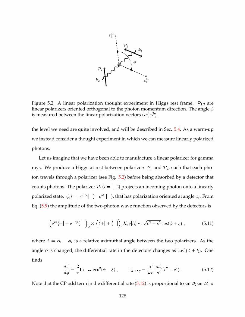
k1

k2 εlin1

εlin2

φ

P1

P2

Figure 5.2: A linear polarization thought experiment in Higgs rest frame. P1;2 arelinear polarizers oriented orthogonal to the photon momentum direction. The angle is measured between the linear polarization vectors (m)"lin1;2.

the level we need are quite involved, and will be described in Sec. 5.4. As a warm-up

we instead consider a thought experiment in which we can measure linearly polarized

photons.

Let us imagine that we have been able to manufacture a linear polarizer for gamma

rays. We produce a Higgs at rest between polarizers P1 and P2, such that each pho-

ton travels through a polarizer (see Fig. 5.2) before being absorbed by a detector that

counts photons. The polarizer Pi (i = 1; 2) projects an incoming photon onto a linearly

polarized state, jii = eii j+i+eii ji, that has polarization oriented at angle i. From

Eq. (5.9) the amplitude of the two-photon wave function observed by the detectors is

eih+j+ eihj

2h+j+ hj

1He jhi

pc2 + ~c2 cos(+ ) ; (5.11)

where = 1 2 is a relative azimuthal angle between the two polarizers. As the

angle is changed, the differential rate in the detectors changes as cos2( + ). One

findsd

d=

2

h! cos

2(+ ) ; h! =2

43m3h

v2(c2 + ~c2) : (5.12)

Note that the CP odd term in the differential rate (5.12) is proportional to sin 2 sin 2 /

128

c~c sin 2. The differential rate is thus linearly sensitive to CPV coupling ~c, whereas the

total rate is quadratically sensitive.

In summary, we have shown that only the terms receiving contributions from both

of the definite helicity two-photon amplitudes, so that there is helicity interference, are

sensitive to the CPV phase . These interference effects can in principle be of O(1) in

size.

5.3 Bethe-Heitler photon conversion

We now study the process that can be used for photon polarization measurement,

namely the conversion of a photon into an e+e pair in matter. In this section we

study a conversion of single isolated photon, which we will then use in the Sec. 5.4 for

the case of h! with converted photons.

5.3.1 Photon propagation and conversion

Photon conversion to e+e pairs may proceed either by Dalitz conversion in vacuum,

for an off-shell intermediate photon, or by BH conversion on atomic nuclei, which

occurs for on-shell photons (for a review see, e.g., [272, 273]). The Dalitz conversion

rate carries a suppression factor of O(104), and is not of immediate practical inter-

est. Moreover it mainly proceeds via a longitudinal photon so that the above helicity

analysis no longer applies. In contrast, the CMS and ATLAS pixel detectors contain

a significant amount of material, so that 50% of photons convert inside the track-

ing systems via the BH process [274, 275]. Based on the composition of the detectors,

we assume in this work that the target nucleus is always 28Si, at rest in the laboratory

frame. This nucleus is spin-0, and has no nuclear magnetic moment. We therefore do

not consider the effects of target polarization on the BH process [276].

One might be concerned by the prospect of photon polarization decoherence for

129

10−14

10−12

10−10

10−8

10−6

10−4

10−2

1 10 100

σγ(2

8Si)

[bar

ns/

atom

]

Eγ [GeV]

1

100

1 10 100

Nuc. p.p.

Elec. p.p.

Compton

Rayleigh

Figure 5.3: The contributions to photon cross-section on 28Si, (28Si), from BH e+e

pair production in nuclear field (solid blue line), pair production due to scatteringon electron cloud (red dashed), Compton scattering (dot-dashed yellow) and Rayleighscattering (magenta double dot-dashed), as a function of photon energyE . Calculatedusing NIST’s XCOM database [271].

the photons propagating inside the silicon. However, at photon energies O(mh=2)

the pair production in the nuclear field is by far the largest contribution to the photon

scattering cross-section in an atomic lattice [277], see Fig. 5.3. As a result, to an excellent

approximation, the photons remain coherent up until their BH conversion. We shall

also assume that the BH scattering is quasi-elastic, i.e. that the target nucleus remains

in a coherent state during and after the scattering. For the kinematics considered, the

quasi-elastic limit is an excellent approximation of the full BH conversion [272, 273].

5.3.2 Angular resolution limitations

Following the h ! experiment discussed in Sec. 5.2.3, in order to measure the

CPV in a doubly converted h ! decay, we might expect that angular distributions

between planes formed by spatial momenta need to be measured. There are several

possible planar distributions that can be constructed, involving either:

i) The e+e plane formed by the e+e momenta, or;

130

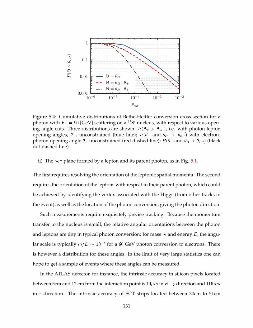
0.001

0.01

0.1

1

10−6 10−5 10−4 10−3 10−2

P(Θ

>θcut)

θcut

Θ = θℓℓ

Θ = θℓℓ, θ+

Θ = θℓℓ, θ±

Figure 5.4: Cumulative distributions of Bethe-Heitler conversion cross-section for aphoton with E = 60 [GeV] scattering on a 28Si nucleus, with respect to various open-ing angle cuts. Three distributions are shown: P (`` > cut), i.e. with photon-leptonopening angles, , unconstrained (blue line); P (+ and `` > cut) with electron-photon opening angle unconstrained (red dashed line); P ( and `` > cut) (blackdot-dashed line).

ii) The e plane formed by a lepton and its parent photon, as in Fig. 5.1.

The first requires resolving the orientation of the leptonic spatial momenta. The second

requires the orientation of the leptons with respect to their parent photon, which could

be achieved by identifying the vertex associated with the Higgs (from other tracks in

the event) as well as the location of the photon conversion, giving the photon direction.

Such measurements require exquisitely precise tracking. Because the momentum

transfer to the nucleus is small, the relative angular orientations between the photon

and leptons are tiny in typical photon conversion: for mass m and energy E, the angu-

lar scale is typically m=E 105 for a 60 GeV photon conversion to electrons. There

is however a distribution for these angles. In the limit of very large statistics one can

hope to get a sample of events where these angles can be measured.

In the ATLAS detector, for instance, the intrinsic accuracy in silicon pixels located

between 5cm and 12 cm from the interaction point is 10m inR direction and 115m

in z direction. The intrinsic accuracy of SCT strips located between 30cm to 51cm

131

from the interactions point is 17m (R ) and 580m(z) [278]. One may therefore

hope to measure the orientations of the e+e plane even for opening angles as small as

`` 104 103, where the relative leptonic angle `` is defined by

cos `` =(m)p+ (m)pj(m)p+jj(m)pj ; (5.13)

for leptonic spatial momenta (m)p. By comparison, a 60 GeV photon converting to a

ee+ pair has an opening angle of `` > 104 in 38% of the cases and `` > 103 in 4%

of the cases. The full cumulative distribution for `` > cut, is shown in Fig. 5.4.

Another experimental challenge is the multiple scattering of outgoing electrons

when traversing the detector medium. This can affect the measurement of the electron

direction and thus the orientation of the e+e or e plane. Using Eq. (30.15) in [277],

the width of the angular distribution is 104 for a 30 GeV electron, assuming it tra-

verses ` = 0:1 radiation lengths of the material. This width roughly scales asp`=E,

where E is the lepton energy. The measurement of polarization planes in the current

and future detectors will thus be challenging, but may be achievable on a statistical

basis. Bearing in mind these experimental questions, in the remainder of this chapter

we adopt a theoretical approach to this problem: We consider a thought experiment

where all angles can be resolved and explore the sensitivity to Higgs parameters in

this best-case scenario.

5.3.3 Nuclear form factor

The BH conversion depends on a momentum transfer, q, between the photon and the

nucleus. Assuming quasi-elastic scattering, the photo-nuclear scattering is encoded in

an elastic nuclear form factor Gel2 [q

2] (see Eq. (5.22) below). This form factor plays an

important role of suppressing scattering at low q2, that is, at scales larger than the Si

atom.

132

10−10

10−8

10−6

10−4

10−15 10−14 10−13 10−12 10−11 10−10 10−9 10−8

Gel 2(q

2)

−q2 [GeV2]

r−2

atom

a−2

0.01

1

100Gel

2 ∼ a4 q4

Gel2 ∼ 1

Figure 5.5: The elastic form factor Gel2 (q

2). The dashed lines show the limiting behaviorGeq2 a4q4 for ja2 q2j 1 (green dashed line) and Gel

2 1 for ja2 q2j 1 (red dashedline). The scale at which screening of the nucleus becomes important is denoted by a,which is smaller than the Si atomic radius, ratom. At scales well outside the atom, corre-sponding to small q2, nuclear conversion is suppressed by the form factor screening.

Let us discuss briefly the behavior of the nuclear form factor. The threshold for an

E ' 60 GeV photon to convert to an e+e pair is at q2 = 4m4=E2 ' 1018 GeV2, with

m the electronic mass, but can occur at momentum transfers as large as q2 106

GeV2. This should be compared with the radius of the Si atom, ratom ' 1:1 A [279]

or r2atom ' 1012 GeV2, and with the nuclear radius rnuclear ' 4 fm which gives r2nucl '103 GeV2. Within the q2 range of interest for conversion – 1018 up to 106 GeV2 –

the nuclear charge is thus screened at low q2 by the atomic shell electrons. In this

work we use the simple expression for the atomic form factor [280] described in detail

in [272] and given by

Gel2 (q

2) =a4q4

(1 a2q2)2; (5.14)

where a = 184:15(2:718)1=2Z1=3=m and Z is the atomic number of the nucleus. For

28Si, a2 = 1:22 1010 GeV2. There are two limits of interest. The first is ja2 q2j 1

in which Gel2 1, the second is the limit ja2 q2j 1 in which Gel

2 q4, see Fig. 5.5.

That is, the form factor suppresses the BH cross-section for small q2 a2. To the

133

extent that the 1=q4 factor in the BH cross-section determines the dominant phase space

configurations of the final states, this suppression significantly alters the important

regions of phase space for BH conversion up to the a2 scale. Specifically, the form

factor increases the probability of significantly acoplanar BH conversions.

5.4 The Higgs-Bethe-Heitler process

In this section we present a formal analysis of the Higgs-Bethe-Heitler (HBH) process,

h ! with both photons converting to e+e pairs. The main result is that we ob-

tain compact, leading order expressions for the HBH rate, and gain insight into the

structure of the terms sensitive to CP violation.

5.4.1 Amplitude and cross-section

The amplitude of interest is given by a menorah diagram, consisting of a h ! and

two BH conversion subdiagrams, summed over internal photon polarizations, viz.

iM1rs2rs =

k1, λ1

k2, λ2

p1+ , s1

p1− , r1

p2+ , s2

p2− , r2

P

P ′1µ

P

P ′2

ν

q1

q2

+ lepton exchanges

=1

X1;2

hck1 k2g k1k

2

+ ~ck1k2

i("1 )("2 )[M

BH]11rs [M

BH]

22rs ;

(5.15)

134

in which = v=e6, for QED coupling e. The BH amplitudes are

[MBH]

iirs

= uri(pi)

="i

i

=pi =ki m

+ i

=ki =pi+m

="ivsi(pi+) ; (5.16)

where we have not yet taken nuclear form factors into account, and kept explicit the

corresponding Lorentz index of the nuclear electromagnetic current. The Latin sub-

scripts, i = 1; 2, label each photon, while si, ri = 1; 2 are respectively the positron

and electron spins (see Eq. (C.8)), and i = the outgoing photon helicities from the

h ! vertex. We have also suppressed repetitions of the photon index, such that

Xirs is henceforth a shorthand for Xirisi. We shall often refer to the BH subdiagrams for

each photon as the photon branch.

We assume both nuclei are initially at rest in the lab frame, so P = (M; (m)0)

where M is the mass of the nucleus. The Higgs need not be at rest in the lab frame. As

discussed in Sec. 5.3.1, we assume quasi-elastic scattering, that is P 02i = P 2 =M2. This

implies that 2qi P + q2i = 0, and so

Ei Ei+ Ei + q2i =2M = 0 ; (5.17)

where Ei, Ei are the photon and lepton energies respectively. It is also convenient to

define

Qi

1

M

P qi

qi Pq2i

=

1

M

P +

qi2

; (5.18)

under quasi-scattering conditions. The exchange energy with the nucleus q0i P00i

P 0i M . I.e. the nucleus velocity is non-relativistic, so to an excellent approximation,

it follows that

Ei ' Ei+ + Ei ; Qi ' (1; (m)0) ; (5.19)

135

in the lab frame.

We define the BH nuclear form factor tensors on each photon branch [272],

Wi = W1(q

2i )

g qi q

i

q2i

+W2(q

2i )Q

iQ

i ; (5.20)

such that the unpolarized HBH squared amplitude

jMj2Yi=1;2

2M(M2 P 0i2) =

1

q41q42

Xri;si

M1rs2rsM00

1rs2rsW10W20 : (5.21)

On the left of Eq. (5.21) we have factored out the functions that enforce quasi-elastic

scattering. The form factor W1(q2) = 0 for quasi-elastic scattering on a spin-0 nuclear

target [276], while

W2(q2) = 2M(M2 P 02)Gel

2 (q2) ; (5.22)

in which Gel2 (q

2) is the form factor given in Eq. (5.14). Hence the unpolarized HBH

squared amplitude reduces to

jMj2 = Gel2 (q

21)G

el2 (q

22)

q41q42

Xri;si

M1rs2rsM00

1rs2rsQ1Q10Q2Q20 : (5.23)

5.4.2 Helicity structure

One may calculate jMj2 via the usual Feynman method, which relies on polarization

completeness relations to compute traces. This approach leads to thousands of terms,

of which the naıvely dominant terms cancel due to Ward identities. Extracting lead-

ing order expressions is therefore difficult, and moreover, high numerical precision is

required for numerical stability. As an alternative, we employ a spin and helicity anal-

ysis combined with the spinor-helicity formalism to compute the HBH amplitudes.

These may be subsequently squared and summed over external spins to produce the

136

full HBH rate. In the following we provide a brief overview of these results, while

details are provided in Appendices C.I and C.II.

The BH spin-helicity amplitudes are defined as

irs [MBH]

irsQi=q

2i : (5.24)

With reference to Eqs. (5.15) and (5.23), the HBH spin-helicity amplitudes are corre-

spondingly

iM121rs2rs =

pG1G2

hck1 k2g k1k

2

+ ~ck1k2

i("1 )("2 )11rs

22rs ; (5.25)

where we introduced the abbreviation

Gi Gel2 (q

2i ) : (5.26)

Making use of the spinor-helicity formalism (see Appendix C.I), we obtain the spin

amplitudes

M1rs2rs X12

M121rs2rs =

m2h

pG1G2

pc2 + ~c2

ei+1rs

+2rs + ei1rs

2rs

: (5.27)

These are reminiscent of equation (5.9) with final leptonic spin states hrisij and irs /hsiriji, as expected. The HBH square-amplitude is correspondingly

jMj2 X1rs2rs

X12

M121rs2rs

2 = m4hG1G2

c2 + ~c2

42

X1rs2rs

+1rs+2rsei + 1rs2rse

i2 : (5.28)

Note that the sum over photon polarizations is inside the absolute value as expected

for entangled h ! 2 ! 2(e+e) decay, but the sum over lepton spins is incoherent.

Eq. (5.28) shows that the BH spin-helicity amplitudes irs are all one needs to deter-

137

mine the entire HBH square amplitude. Parity invariance of the BH amplitudes relates

amplitudes of opposite helicity and spins to their complex conjugates,

(+rs) = rs

rs ; (5.29)

where s is the opposite spin to s, and 2rs = 1, rs = rs. Hence we need only determine

+irs . We shall see below that spinor-helicity methods, when applied to irs , also allow

for a well-controlled expansion of dominant, sub-dominant and negligible terms in

jMj2.We see explicitly from Eq. (5.28) that the helicity interference terms are equivalent to

the -dependent terms, as discussed in sections 5.2.2 and 5.2.3. For a particular leptonic

spin configuration fri; sig, helicity interference occurs so long as +irs and irs are both

non-zero. However, we see in appendix C.II, and in particular in Eq. (C.13), that for

our particular choice of spinor basis (see Eq. (C.8))

ji11 j ji12j ji21j ji22 j ; (5.30)

or equivalently j+i22j j+i12j j+i21j j+i11 j. This hierarchy means that we may

therefore discard any terms containing either +i22 or i11 as subleading. It follows that

the leading order squared amplitude is

jMj2 ' m4h

c2 + ~c2

42G1G2

(21112112+ 2

Xj 6=k

rk 6=sk

j11krs2+Xr1 6=s1r2 6=s2

+1rs+2rsei + 1rs2rse

i2);

(5.31)

while the leading interference term is

jMj2int' 2m4

h

c2 + ~c2

2G1G2Re

n112

121212

221e2i

o: (5.32)

138

We see that only 12;21 (or equivalently +21;12) amplitudes enter the leading order -

dependent interference terms.

The CP odd helicity interference term in (5.32) is proportional to c~c,

jMj2int;CPodd

= 2m4h

c~c

2G1G2Im

n112

121212

221

o: (5.33)

Note that interference terms between amplitudes, produced by the FF and F ~F oper-

ators respectively, are CP odd. However, the helicity amplitudes under consideration

here receive contributions from both CP odd and CP even operators – manifestly they

depend on – and hence helicity interference terms contain both CP-even and CP-odd

pieces. Consequently, we interpret the remaining piece of the helicity interference term

to be the CP-even piece,

jMj2int;CPeven

= m4h

c2 ~c2

2G1G2Re

n112

121212

221

o: (5.34)

This term has quadratic dependence on ~c2, albeit a different one than the total rate

(5.12).

5.4.3 The Bethe-Heitler helicity amplitudes

In Eqs. (5.31) and (5.32) we have expressed the leading order HBH rate and interfer-

ence term in terms of individual BH helicity amplitudes, rs. In this subsection we

proceed to present the leading order terms of these amplitudes in a readily accessible

notation, for the special case that the Higgs is at rest in the lab frame. The results below

are achieved via spinor-helicity techniques; a more comprehensive presentation of the

derivation of these results is provided in Appendix C.II. There, explicit results for each

spin helicity amplitude irs are collected in Eqs. (C.12), while the leading order results,

obtained by power counting in m=mh, are provided in (C.13). The compact results be-

139

low will permit us, in the next section of this chapter, to study the encoding of the CPV

structure in the HBH rate at an analytic level.

Before proceeding, we may first derive a new result concerning the well-studied

unpolarized BH square amplitude, jMBHi j2 =P

rs jirsj2. Using Eqs. (C.12) one may

show that

jMBHi j2 ' 8Gim2

q4i

Ei(ki pi) Ei+(ki pi+)

(ki pi)(ki pi+)2 4

Giq2i

E2i++ E2

i

(ki pi)(ki pi+): (5.35)

This compact expression for the BH rate in the quasi-elastic scattering limit is novel to

this work. A numerical analysis and validation of the resulting BH differential cross-

section is provided in Appendix C.IV.

Now, in the special case that the Higgs is at rest in the lab frame, that is (m)Ph =

(m)0, Eqs. (C.13) for the irs collapse to very simple expressions. Using the leading

order results (C.13) and assuming 1, for each branch one finds

11 = (+22) '2p2 + q2

1

1 + 2+2+

1

1 + 22

;

1221= +(+21

12) ' 2

p2 + q2

+ +

++e

i+

1 + 2+2+

+ e

i

1 + 22

;

22 = (+11) ' 0 :

(5.36)

Here and are respectively the polar and azimuthal angles defined with respect

to the branch parent photon momentum, as shown in Fig. 5.6, and E=m 1.

We also assume that the O() terms do not cancel completely. The latter may occur on

the phase space slice ++ = and j +j = , corresponding to minimal jq2j.Excellent numerical validation of this expansion implies that the neighborhood of this

phase space slice, on which the expansion fails, is actually of negligibly small measure.

140

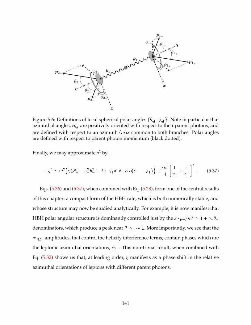
k1

k2

x

φ1+

φ1−

θ1+

θ1−

p1+

p1−

x

p2+ φ2+

p2−φ2−

θ2+

θ2−

Figure 5.6: Definitions of local spherical polar angles fi ; ig. Note in particular thatazimuthal angles, i are positively oriented with respect to their parent photons, andare defined with respect to an azimuth ^(m)x common to both branches. Polar anglesare defined with respect to parent photon momentum (black dotted).

Finally, we may approximate q2 by

q2 ' m2 2+

2+ + 2

2 + 2 ++ cos( +)

+m2

4

1

++

1

2: (5.37)

Eqs. (5.36) and (5.37), when combined with Eq. (5.28), form one of the central results

of this chapter: a compact form of the HBH rate, which is both numerically stable, and

whose structure may now be studied analytically. For example, it is now manifest that

HBH polar angular structure is dominantly controlled just by the k p+=m2 ' 1+

denominators, which produce a peak near 1. More importantly, we see that the

12;21 amplitudes, that control the helicity interference terms, contain phases which are

the leptonic azimuthal orientations, i . This non-trivial result, when combined with

Eq. (5.32) shows us that, at leading order, manifests as a phase shift in the relative

azimuthal orientations of leptons with different parent photons.

141

5.5 Sensitivity to CPV

In this section we assess the potential sensitivity to CP violation. To do this, we con-

sider a number of CPV sensitive observables and propose several sets of kinematic

cuts that can enhance the CPV signal. These sets of cuts require that the lepton-lepton

opening angle (5.13), ``, can be resolved, as well as the two photon-lepton angles, .

In the following we mostly consider angular resolution cuts of the form

`` ; > cut : (5.38)

Following Sec. 5.3.2, we apply an angular resolution cut cut = 104, which is at the

edge of what may be possible with present detectors, and a looser, futuristic cut =

105, intended to show that very large CPV effects are possible in principle.

We emphasize that as our measurement is a novel, challenging one, our goal here

is not to conduct a full collider analysis including backgrounds. Rather our aim is to

identify the types of observables that can probe CP violation in h ! , and estimate

how well they do under ideal circumstances: a high efficiency in reconstructing con-

versions and a signal rich channel. This is in the anticipation that such circumstances

might materialize in a future LHC running or at a Higgs factory.

142

5.5.1 Differential scattering rate

The HBH differential scattering rate for the full 3 ! 6 process (Higgs plus two nuclei

to two nuclei and two e+e pairs) in the lab frame is

d / jMj2dh! dBH1dBH2

/ 1

(2)12jMj2

Yi=1;2=

d3(m)pi2Ei

Yi=1;2

d3(m)P 0i

2E 0i

d3(m)ki2Ei

(4)(qi + pi++ pi ki)

(4)(Ph k1 k2) ;

(5.39)

with jMj2 given by Eq. (5.28). Integrating over the out-going nuclear momenta and all

other momenta in delta functions, we obtain in the limit jqj M

d / 1

(2)12m2h

4M2jMj2

Yi=1;2=

j(m)pijdidE1dE2d1 ; (5.40)

with di the solid angle for each lepton momentum (m)pi , and d1 the solid angle

for photon ‘1’. The photon labels are extrinsic. We take photon ‘1’, say, as westwards

going (if Higgs is not at rest one can also take it to be, e.g., the more energetic photon).

For simplicity, we assume henceforth that the Higgs is at rest in the lab frame, that

is Ph = (mh; (m)0). In the Higgs rest frame the photon angular dependence is isotropic,

and the integration over d1 is trivial. Dropping the prefactors, the differential scatter-

ing rate becomes

d / jMj2 Yi=1;2=

j(m)pijdidE1dE2 : (5.41)

We may now proceed to consider CPV observables.

143

5.5.2 Global sensitivity to CP violation

In principle all the information about ~c 6= 0 (or equivalently 6= 0) is encoded in the full

HBH differential distribution. The coefficient ~cmay be determined by a matrix element

method [281–286], as long as backgrounds can be kept under control. Estimating the

full power of the matrix element method is beyond the scope of this work.

To test the sensitivity of HBH to ~c we instead introduce a parameter

ZB(c; ~c) =

R jd(SM)=dPS d(c; ~c)=dPSj dPS

(SM): (5.42)

The parameter ZB can be thought of as a proxy for the sensitivity of the matrix element

method, once one integrates over the full phase space. In the top panel of Fig. 5.7 we

show the value of ZB in the (c; ~c) plane. There we see that the deviation from the SM is

mostly due to the c2 + ~c2 enhancement of the h ! rate, which need not arise from

CP violation. Such an enhancement is best detected by measuring the overall h !

rate, and not using our method.

To assess the sensitivity to CP violation alone, we should restrict our attention to

the circular contour c2+~c2 = c2SM, on which the total HBH rate matches the SM rate for

any . This contour is shown as a white circle in the top panel of Fig. 5.7. To this end,

we define a second quantity

ZcB() ZB()

c2+~c2=c2SM

=

R d(0)=dPS d()=dPS dPS

(0); (5.43)

where d() is the differential HBH rate with the enhancement of the total h! rate

factored out,

d(c; ~c)=dPS =(c2 + ~c2)

c2SMd()=dPS: (5.44)

Note that in general ZB 2 [0;1), but ZcB 2 [0; 2].

144

ZBZB

-1 -0.5 0 0.5 1

c

0

0.2

0.4

0.6

0.8

1

c

0

0.2

0.4

0.6

0.8

1

SM point

-1 -0.5 0 0.5 1

0

0.2

0.4

0.6

0.8

1

0

0.2

0.4

0.6

0.8

1

SM point

0

0.01

0.02

0.03

0.04

0.05

0.06

0.07

0.08

0.09

0.1

0 0.25 0.5 0.75 1

Zc B

ξ/π

Curves: f(ξ) = C0 sin ξ

θℓℓ > 10−5, C0 = 0.09

θℓℓ > 10−4, C0 = 0.06

Figure 5.7: Top panel: ZB in the c ~c plane, with the SM point at (c; ~c) = (0:81; 0).Bottom panel: Zc

B as a function of = tan1(~c=c). The scatter of the data points is anumerical artifact.

The bottom panel in Fig. 5.7 shows the value of ZcB as a function of . The sinusoidal

dependence of ZcB on is not unexpected. For instance, in the h! toy example we

considered in Sec. 5.2.3, in which the angle between linear polarizations is measured,

one has from Eq. (5.12)

ZcB()

h!

=1

Z 2

0

j cos2(+ ) cos2()jd =4

j sin j : (5.45)

By comparing this toy system with HBH, it is therefore natural to deduce thatZcB()=j sin j

provides a measure of the average CPV signal size obtainable via the matrix element

145

method, for any c; ~c. That is, this measure is independent of and the overall normal-

ization c2 + ~c2. The fit in Fig. 5.7 suggests this CPV signal is O(10%) for an angular

resolution cut `` > 105, and O(5%) for `` > 104. Hence, for the most pessimistic

case that there is no deviation from the SM in the total h ! rate the detection of

NP from the full matrix element method will be challenging, even if there is large CPV

component in h! .

5.5.3 Differential azimuthal scattering rate

Let us also consider the sensitivity of an experiment in which just one relative az-

imuthal angle – the difference of the azimuthal angles between two opposite branch

leptons – is reconstructed, such as the experiment described in Fig. 5.1. From Eqs. (5.28)

and (5.36) we saw that manifests as a phase shift in the relative azimuthal orienta-

tion of leptons on different branches. It is instructive to write down this manifestation

explicitly. Let us transform from the azimuthal coordinates i to the coordinates

' 1+ + 2+ ; "i i i+ ; (5.46)

and choose 1+ = 0, without loss of generality. With this choice ' and "1 2 [0; 2),

while "2 2 (2; 2). For the case that the Higgs is at rest, we find from Eqs. (5.31) and

(5.36) that the HBH square amplitude, and thus the leading order differential scattering

rate, takes the generic form

d=dPS =1

q41q42

a+

Xj

bj cos "j +Xk

ck cosnk"1 +mk"2 + 2'+ 2

; (5.47)

where a, bj and ck are real functions of i and i – they span the energy, polar angle

phase space, denoted hereafter by PS ; – but are independent of the azimuthal struc-

ture, and nk, mk are positive integers that satisfy nk +mk = 0; 1, or 2. From Eq. (5.37),

146

one sees that the 1=q4 factors depend on both the azimuthal and polar angles, but in

a way such that q4 = (1 + cos ")2, where < 1. Hence 1=q4 may be expanded in a

power series of cos " < 1. Integrating over the " acoplanarity angles, one may then

show that, with respect to the azimuthal structure, only constant or cos(2'+ 2) terms

survive. That is, the leading order differential scattering rate

d

d' dPS ;= (c2 + ~c2)

hA ; + B ; cos(2'+ 2)

i; (5.48)

in which the ; subscript denotes exclusive dependence on the energy polar angle

phase space, PS ;.

The results (5.47) or (5.48) show that -dependence and ; -dependence factorize.

Hence appears only in the azimuthal structure as a phase shift. Specifically, the CPV

parameter manifests itself in the inter-branch azimuthal structure in the differential

rated

d'= (c2 + ~c2)

hA ;

PS ;

+B ;PS ;

cos(2'+ 2)i; (5.49)

which we have now shown is oscillatory with respect to ' at leading order. Note that

we could have chosen ' to be any of the four inter-branch angles '12 1 + 2 ,

where , = , of which three are linearly independent. Results similar to Eq. (5.48)

follow with appropriate replacements.

In the right panel of Fig. 5.8 we show the differential distribution d=d' for HBH

events (including a loose cut on the polar angles, at 105) for two values of . It is

evident that the oscillation amplitude, hBi=hAi, is small – approximately 2% – when

averaged over all of the phase space PS ;.

The key question we now wish to address is whether such a small oscillation am-

plitude is because of small, O(1%) oscillations, or whether there is an O(1%) part of

the phase space where deviations from the SM are O(1). In the language of Eq. (5.48),

147

this question can be rephrased in a precise manner: Is hBiU=hAiU small for all U PS,

or does there exist U PS such that hBiU=hAiU is O(1). The latter possibility is phe-

nomenologically preferred, since it permits the extraction of an O(1) CPV signal on U ,

which would scale better with increasing statistics.

To address this question, let us begin by examining the coplanar limit. In this limit

the acoplanarity angles "1;2 are both zero, and we have from Eq. (5.47)

d

d' dPS ;= Aco

; + Bco ; cos(2 + 2') : (5.50)

In the coplanar limit the size of the modulation is given by

Bco ;Aco ;

=Yi=1;2

Ri(1 i+i+ ii)2

(1 + 2i+2i+)(1 + 2i

2i) +Ri( ii + i+i+)

2; (5.51)

where Ri 2 i+ i=( 2i+

+ 2i). The ratio Bco=Aco is small when 1, i.e. near

the peak of the square matrix element, but Bco=Aco ! 1, for 1 and not much

bigger than . An example is shown in Fig. 5.8, where Ei and i are held fixed such

that i m=Ei and + . In this slice of phase space the azimuthal oscillation

amplitude is large and there is a strong sensitivity to CPV. This shows that regions of

phase space with large CPV signals exist.

5.5.4 CPV enhancing cuts

We now use the results from Sec. 5.4.2 to design kinematic cuts that enhance the sen-

sitivity of d=d' to CP violation. That is, we seek to enhance the ratio hBi=hAi for a

particular subset of the HBH event sample. The cuts we propose fall into two classes:

those which are placed on the kinematics of the whole event; and those which are

placed independently on individual photons and their daughter leptons. As they use

all of the information in the event, including correlations among the two photons, one

148

0

1

0 1/2 1 3/2 2

dΓ/d

PS

[arb

it.

unit

s]

ϕ/π

ξ = 0

ξ = π/4

ξ = π/20

0.5

1

0 1/2 1 3/2 2

dΓ/

dϕ

[arb

it.un

its]

ϕ/π

SM ξ = 0BSM ξ = π/4

Figure 5.8: Left: Illustration ofO(1) oscillations and phase shifts in the HBH differentialrate for a sample coplanar kinematic configuration. The azimuthal angle ' in this sliceis defined as in Eq. (5.46). The kinematic configuration is: Ei+ = Ei = mh=4; i+ =104; i = 2i+ so that 10 1 and + = , cf. analysis of Eq. (5.51). Right:The azimuthal distribution d=d' for = 0 and for = =4 with a polar angle cuti > 105 and `` > 105. The modulation amplitude is 2%, but will grow toO(1) onceoptimization cuts are applied, see Sec. 5.5.4.

might expect that the former produce better CPV signals compared to the latter. As we

shall see, however, both classes of cuts perform approximately equally well in enhanc-

ing hBi=hAi on their respective phase space subregions.

5.5.4.1 Cuts on collective kinematics

The helicity interference terms (5.32) in the HBH rate arise dominantly from the term

Re(112121212

221e2i). We can use this observation to pick only events in which

112121212

221

is comparable to the rest of the squared amplitude. With reference to

Eqs. (5.33) and (5.34) we thus introduce several sensitivity parameters Tn

Tn Xn,"1112112 + X

j 6=k

rk 6=sk

j11krs2 + Xn#; (5.52)

149

where n =M (0); R(0); J (0), with

XM = 4j112121212221j ; XR = 4Re[112121212

221] ; XJ = 4Im[112

121212

221] ;

and XM0;R0;J0 =Xj 6=k

r 6=s;6=

jrsk 2 + XM;R;J : (5.53)

The first two terms of the denominator in Eq. (5.52) are simply the independent parts

of the HBH squared amplitude (5.31), while the Xn’s are various pieces of the inter-

ference terms. In particular, TM is the magnitude of the full leading order interference

term, while TR;J are respectively the CP-even and CP-odd interference terms. We ex-

pect each to be useful gauge of sensitivity to CPV independent of . For example, cuts

on TR and TJ will enhance the azimuthal modulations in the = 0 and = =4 respec-

tively, and can thus be used to distinguish among these. In all cases Ti ! 1 (Ti ! 0)

implies full (no) CPV sensitivity.

For all numerical analysis we use three private Monte Carlo codes that were cross-

checked. The details on Monte Carlo event generation can be found in Appendix C.VI.

Placing a cut on Tn produces an event sample with large hBi=hAi ratio. This is shown

in Fig. 5.9 for opening angle cut `` > 105 and in Fig. 5.10 for opening angle cut of

`` > 104. The d=d' distributions are shown for two choices of CPV parameters,

= 0 (blue histograms) and = =4 (red histograms). The fits to the functional form

(5.48) of the d=d' HBH differential rate are shown as solid blue and dot-dashed red

lines, respectively. The efficiencies of the cuts for the examples shown in Figs. 5.9

and 5.10 are 1% for the upper panels and 0:1% for the lower panels (the exact

values of efficiencies depend on the value of ). The presence of 6= 0 exhibits itself as

the expected phase shift in d=d' differential rate (5.48).

From Figs. 5.9 and 5.10 we see that it is possible to select regions of phase space such

that hBi=hAi O(1). In particular the average modulation hBi=hAi is large (small) for

150

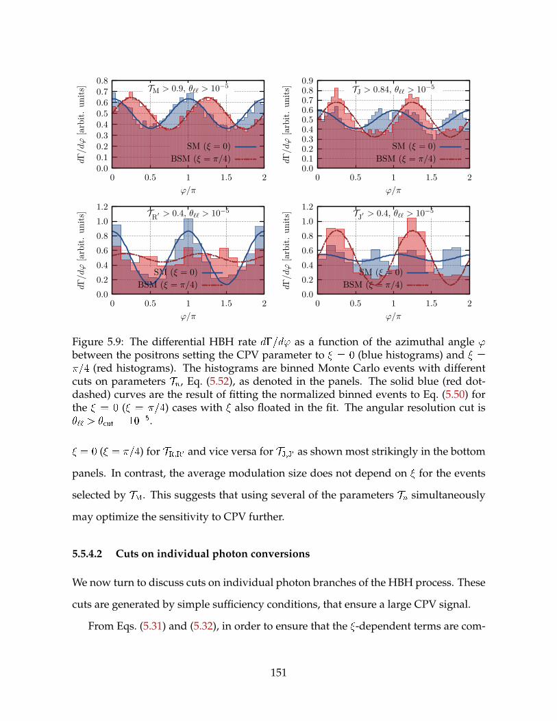
0.00.10.20.30.40.50.60.70.8

0 0.5 1 1.5 2

dΓ/

dϕ

[arb

it.un

its]

ϕ/π

TM > 0.9, θ`` > 10−5

SM (ξ = 0)BSM (ξ = π/4)

0.00.10.20.30.40.50.60.70.80.9

0 0.5 1 1.5 2

dΓ/

dϕ

[arb

it.un

its]

ϕ/π

TJ > 0.84, θ`` > 10−5

SM (ξ = 0)BSM (ξ = π/4)

0.00.20.40.60.81.01.2

0 0.5 1 1.5 2

dΓ/

dϕ

[arb

it.un

its]

ϕ/π

TR′ > 0.4, θ`` > 10−5

SM (ξ = 0)BSM (ξ = π/4)

0.00.20.40.60.81.01.2

0 0.5 1 1.5 2

dΓ/

dϕ

[arb

it.un

its]

ϕ/π

TJ′ > 0.4, θ`` > 10−5

SM (ξ = 0)BSM (ξ = π/4)

Figure 5.9: The differential HBH rate d=d' as a function of the azimuthal angle 'between the positrons setting the CPV parameter to = 0 (blue histograms) and ==4 (red histograms). The histograms are binned Monte Carlo events with differentcuts on parameters Tn, Eq. (5.52), as denoted in the panels. The solid blue (red dot-dashed) curves are the result of fitting the normalized binned events to Eq. (5.50) forthe = 0 ( = =4) cases with also floated in the fit. The angular resolution cut is`` > cut = 105.

= 0 ( = =4) for TR;R0 and vice versa for TJ;J0 as shown most strikingly in the bottom

panels. In contrast, the average modulation size does not depend on for the events

selected by TM. This suggests that using several of the parameters Tn simultaneously

may optimize the sensitivity to CPV further.

5.5.4.2 Cuts on individual photon conversions

We now turn to discuss cuts on individual photon branches of the HBH process. These

cuts are generated by simple sufficiency conditions, that ensure a large CPV signal.

From Eqs. (5.31) and (5.32), in order to ensure that the -dependent terms are com-

151

0.00.10.20.30.40.50.60.7

0 0.5 1 1.5 2

dΓ/

dϕ

[arb

it.un

its]

ϕ/π

TM > 0.9, θ`` > 10−4

SM (ξ = 0)BSM (ξ = π/4)

0.00.10.20.30.40.50.60.7

0 0.5 1 1.5 2

dΓ/

dϕ

[arb

it.un

its]

ϕ/π

TJ > 0.84, θ`` > 10−4

SM (ξ = 0)BSM (ξ = π/4)

0.00.10.20.30.40.50.60.7

0 0.5 1 1.5 2

dΓ/

dϕ

[arb

it.un

its]

ϕ/π

TR′ > 0.4, θ`` > 10−4

SM (ξ = 0)BSM (ξ = π/4)

0.00.10.20.30.40.50.60.7

0 0.5 1 1.5 2

dΓ/

dϕ

[arb

it.un

its]

ϕ/π

TJ′ > 0.4, θ`` > 10−4

SM (ξ = 0)BSM (ξ = π/4)

Figure 5.10: The same as in Fig. 5.9, but with the opening angle cut `` > cut = 104.

parable to the full rate, it suffices to require ji12i21 j & ji11j2 on each branch (i = 1; 2)

independently. For the case that the Higgs is at rest, using (5.36), this sufficiency con-

dition is implied by S & 1 for each branch, where

S 2(1 cos )

+

( + + )2

++

( 2+2+ 2

2)

2

(1 + 2+

2+)(1 + 2

2) : (5.54)

For brevity, we have dropped the Latin branch index, and here j +j is the

acoplanarity angle.

It is notable that this sufficiency condition weights the desirable energy-polar angle

regions of phase space inversely by the amount of acoplanarity. Specifically, S = 0 in

the exact coplanar configuration = 0. Of course, S is not a necessary condition for

a large CPV signal, so relatively coplanar events – i.e. events for which cut of

the event sample (cut = 0:4 or 0:25 for our MC, see App. C.VI) – may in principle

152

significantly contribute to large CPV signals in d=d'. Also note that symmetric con-

versions, i.e. ++ ' , are more likely to produce a large S , and hence a strong

interference effect.

Fig. 5.11 shows the results of the S1;2 > 1 cut for the angular resolution cut (5.38)

cut = 105 for = 0 compared to = =20 (top left) or =4 (top right). Note we

also constrain the acoplanarity 1;2 2 [3=4; 5=4], since we do not expect extremely

acoplanar events to encode polarization information. The angular resolution cut alone

retains approximately 40% of the total HBH events on this acoplanar domain; for =

=4, the corresponding azimuthal distribution is shown in Fig. 5.8. The addition of

the S1;2 > 1 cut reduces the cut efficiency to 2:6%, but unlike Fig. 5.8, now hBi=hAi O(0:2). The phase shift due to non-zero is clearly visible in both plots, and the value

of extracted from the fits agrees with the input values of = =20 or =4 respectively.

Finally, the bottom panels of Fig. 5.11 displays the acoplanarity on each branch for

the = =4 HBH events with no S cut compared to the S1;2 > 1 cuts. We see that the

S cut mildly favors acoplanar events, as it broadens the acoplanarity distribution and

disfavors relatively coplanar events. For example, we see that events with acoplanarity

< 1% are disfavored in the cut distribution, and we also see that the full width at half

maximum of the acoplanar distribution increases by 50%, from 0:04 to 0:06, under

the S > 1 cut. The excellent performance of S compared to Tn cuts (see Fig. 5.12 and

Sec. 5.5.4.3 below) therefore suggests that acoplanar events – e.g. with 6 cut – play

an important role in encoding the CPV signal.

5.5.4.3 Cut scheme efficiencies

It remains to determine the efficiency of the above cut schemes. In Fig. 5.12 we show

the CPV signal hBi=hAi for the various Tn and S schemes as a function of the fraction of

the total MC event sample, not rejected by combined sensitivity and angular resolution

cuts. Up to small corrections this fraction is the absolute cut efficiency, see Appendix

153

0

0.5

1

0 1/2 1 3/2 2

dΓ/

dϕ

[arb

it.un

its]

ϕ/π

SM ξ = 0BSM ξ = π/4

0

0.5

1

0 1/2 1 3/2 2

dΓ/

dϕ

[arb

it.un

its]

ϕ/π

SM ξ = 0BSM ξ = π/4

0

1

0.8 0.9 1 1.1 1.20

0.2

0.4

0.6

0.8

1

dΓ/

dδφ

[arb

it.un

its]

cdf(δ

φ)

δφ/π

0

1

0.8 0.9 1 1.1 1.20

0.2

0.4

0.6

0.8

1

dΓ/

dδφ

[arb

it.un

its]

cdf(δ

φ)

δφ/π

Figure 5.11: Top panels: The azimuthal distributions d=d' for = 0 (grey histograms)and for = =20; =4 (blue histograms, left and right top panels) with S1;2 > 1 on thedomain 1;2 2 [3=4; 5=4]. The solid (dashed) curves denote fits to Eq. (5.48), with a free parameter in the fits. The bottom left (right) panel shows the acoplanaritydistributions, d=d, (+ ) mod 2 for each photon branch, displayed byblue and gray histograms respectively, with = =4 and no S cut (S1;2 > 1). Note thatthe scale varies between these two plots. The corresponding cumulative acoplanaritydistributions cdf() for each branch are denoted by solid black and grey dashed lineson each plot. In all panels the angular resolution cut (5.38) of cut = 105 was applied.

C.VI for details. For comparison, the data point with only angular resolution cuts is

also shown for each plot.

We see that an increase of the CPV signal by an order of magnitude roughly requires

an order of magnitude penalty in sample size. Moreover, for high cut efficiencies,

the Si scheme provides the largest CPV signal. In contrast, in the low efficiency, but

higher signal regions, the Tn schemes outperform the Si cuts. To give an idea about the

feasibility of this analysis at the (HL/HE-)LHC, Table 5.1 gives the expected number of

154

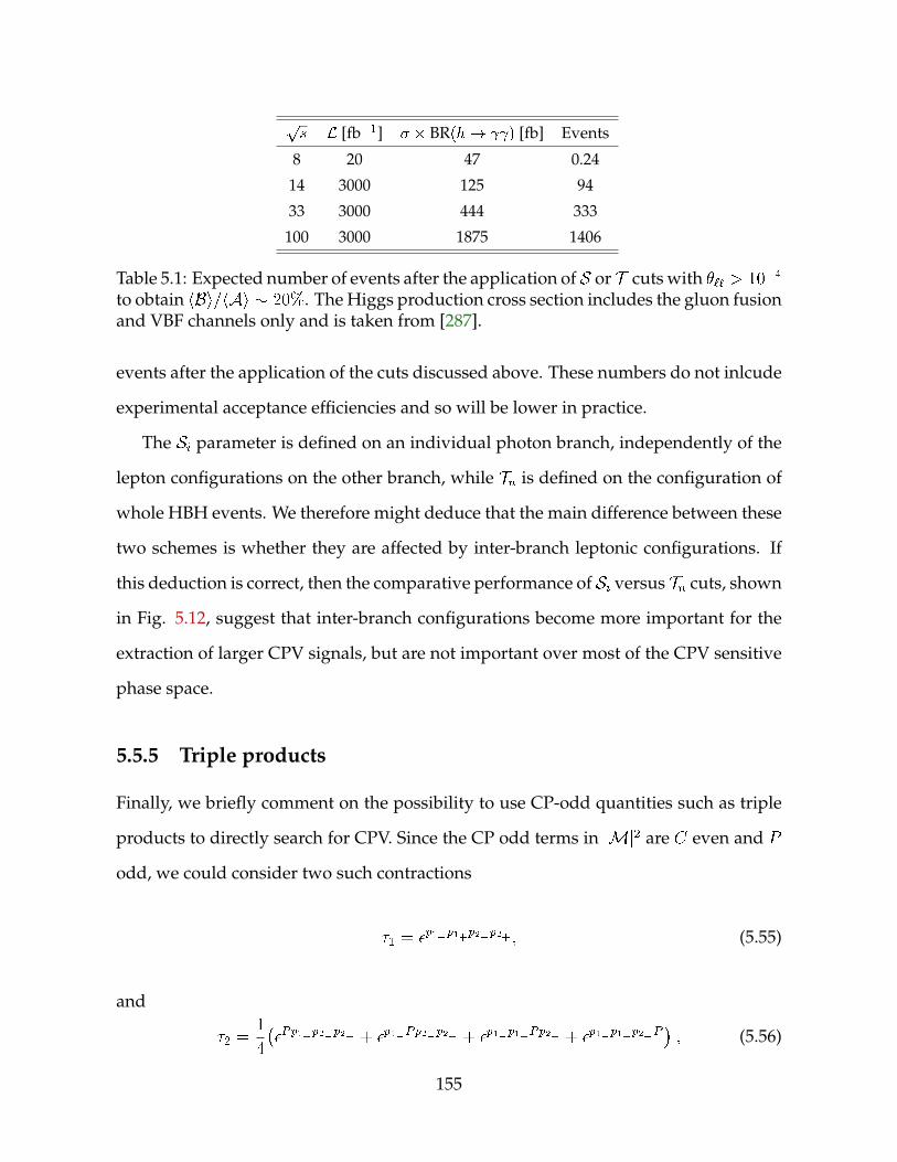
ps L [fb1] BR(h! ) [fb] Events

8 20 47 0.24

14 3000 125 94

33 3000 444 333

100 3000 1875 1406

Table 5.1: Expected number of events after the application of S or T cuts with `` > 104

to obtain hBi=hAi 20%. The Higgs production cross section includes the gluon fusionand VBF channels only and is taken from [287].

events after the application of the cuts discussed above. These numbers do not inlcude

experimental acceptance efficiencies and so will be lower in practice.

The Si parameter is defined on an individual photon branch, independently of the

lepton configurations on the other branch, while Tn is defined on the configuration of

whole HBH events. We therefore might deduce that the main difference between these

two schemes is whether they are affected by inter-branch leptonic configurations. If

this deduction is correct, then the comparative performance of Si versus Tn cuts, shown

in Fig. 5.12, suggest that inter-branch configurations become more important for the

extraction of larger CPV signals, but are not important over most of the CPV sensitive

phase space.

5.5.5 Triple products

Finally, we briefly comment on the possibility to use CP-odd quantities such as triple

products to directly search for CPV. Since the CP odd terms in jMj2 are C even and P

odd, we could consider two such contractions

1 = p1p1+p2p2+ ; (5.55)

and

2 =1

4

Pp1+p2p2+ + p1Pp2p2+ + p1p1+Pp2+ + p1p1+p2P

; (5.56)

155

0.01

0.1

1

10−4 10−3 10−2 10−1

〈B〉/

〈A〉

Cut efficiency

θ`` > 10−5, θi± > 10−5, ξ = 0

STMTM′

TRTR′

TJTJ′

1

θ`` > 10−5, θi± > 10−5, ξ = 0

0.001

0.01

0.1

1

10−4 10−3 10−2 10−1

〈B〉/

〈A〉

Cut efficiency

θ`` > 10−4, θi± > 2 × 10−5, ξ = 0

STMTM′

TRTR′

TJTJ′

1

θ`` > 10−4, θi± > 2 × 10−5, ξ = 0

0.01

0.1

1

10−4 10−3 10−2 10−1

〈B〉/

〈A〉

Cut efficiency

θ`` > 10−5, ξ = 0

STMTM′

TRTR′

TJTJ′

1

θ`` > 10−5, ξ = 0

0.001

0.01

0.1

1

10−4 10−3 10−2 10−1

〈B〉/

〈A〉

Cut efficiency

θ`` > 10−4, ξ = 0

STMTM′

TRTR′

TJTJ′

1

θ`` > 10−4, ξ = 0

Figure 5.12: Comparison of different sensitivity parameter cut schemes, in terms ofcut efficiency, for various angular resolution cuts. The black data point on each plotdenotes the efficiency and hBi=hAi for its angular resolution cut alone, with no en-hancements from sensitivity parameter cuts.

where P = (M; (m)0) is the nucleus momentum, and pqrs is shorthand for the Levi-

Civita contraction pqrs. In terms of scalar triple products,

1 = E1+(m)p1 ((m)p2+ (m)p2) E1(m)p1+ ((m)p2+ (m)p2) + 1$ 2 ;

2 =Mh(m)p1 ((m)p2+ (m)p2) (m)p1+ ((m)p2+ (m)p2) + 1$ 2

i:

(5.57)

Note, that 2 is not strictly speaking C-even, since it involves the nucleus momentum.

However, BH conversion on nucleus is the same as on anti-nucleus within our un-

certainties. This is equivalent to leaving P unchanged under C transformation. A

detailed analysis is beyond the scope of our work, but we remark in passing that a

straightforward use of the S and Tn cuts does not lead to appreciable non-zero value

156

of hi. Further investigation is warranted.

5.6 Chapter summary

In this work we have studied how to probe the underlying CP couplings of the Higgs to

two photons, which undergo Bethe-Heitler conversion on nuclei. We have shown that

sensitivity to CP violating couplings is possible only if there is interference between

conversion amplitudes with different photon helicity. Using spinor helicity methods,

we have computed compact, leading order expressions for these amplitudes, which

are novel to this work. Our analytical control of the leading order h ! BH! 4e

full differential scattering rate permits us to show that: (i) the differential rate with

respect to the relative azimuthal angles between leptons with different parent photons

is oscillatory; (ii) CPV is encoded as a phase shift in such distributions; and (iii) we may

construct various sensitivity parameter cuts that extract the regions of phase space on

which such oscillations – the CPV signal – are order unity on average. These analytical

results have been confirmed and explored with numerical simulations, including a

comparison of the relative effectiveness of the different sensitivity parameters.

For simplicity we restricted our numerical and CP sensitivity analysis to the case

that the Higgs is at rest in the lab frame. This is not the case in the LHC experiments,

and this assumption needs to be lifted for more realistic studies. We note, in this vein,

that Eqs. (C.13) hold also for the boosted Higgs case, although Eqs. (5.36) do not. The

sensitivity parameter cut schemes are expected to work comparatively well in the case

that the Higgs is boosted, too. On a similar note, we expect these sensitivity cuts to

enhance the full matrix element method. This method, as characterized by the param-

eter ZcB, appears to be a few times more sensitive to CPV than experiments measuring

a single relative azimuthal angle. This leaves open the possibility of further improved

CPV signals, compared to those shown in this work.

157

We do not expect a h! BH! 4e experiment to be straightforward, and further ex-

perimental and theoretical studies are needed in order to see if the methods discussed

in this chapter can be used in practice. From an experimental viewpoint, it needs to be

determined how well one can reconstruct the electron and positron momenta for open-

ing angles 104 or even down to m=mh 105, and whether there are significant

rescatterings after BH production. Already from our preliminary studies it is clear that

large statistical datasets and fine granularity of the detectors will be needed, such as

at the proposed HE-LHC, VLHC or TLEP [288]. Experimentally, the situation may be

more favorable in such a machine, having a larger amount of statistics and better kine-

matic control of the Higgs. A completely independent direction for measuring the CP

violating coupling of Higgs to photons – and a direction not explored in this chapter

– would be the use of polarized photon beams at a photon collider. From a theoretical

viewpoint, it also remains to determine and search for other CPV sensitive observables

apart from the azimuthal distributions discussed here.

Lastly, while we focussed on Higgs diphoton decays in this work, most of this anal-

ysis holds for any pair of correlated photons. They can arise from a resonance, like

the Higgs, or from scattering events. While the details have to be determined in a

case-by-case basis, the principles, such as helicity interference, are the same.

158

Chapter 6

Probing the photon polarization in

B ! K with conversion

6.1 Introduction

Measurement of the photon polarization in b ! s radiative decays has been of long-

standing interest. Within the Standard Model (SM), flavor-changing electroweak inter-

actions maximally violate parity, so that one expects the fraction of left-handed photons

in b ! s processes to be order unity, up to small corrections arising from either the

non-zero strange quark mass or from higher order QCD contributions. In contrast, cer-

tain New Physics (NP) scenarios may generate b! s operators of comparable size to

the SM terms, but with exotic parity structure, significantly modifying the expected ra-

tio of left- versus right-handed photons – the photon polarization ratio. Measurement

of this ratio therefore has the potential to test the parity structure of b ! s operators

against SM expectations, as well as either constrain or detect the signatures of such NP

scenarios.

The b ! s photon polarization ratio may be measured via various different ap-

proaches. Dominantly right-handed photon production in resonant B ! (K1(1400)!

159

K) generates an up-down asymmetry of the photon momentum with respect to the

K1 ! K decay plane [289, 290]. This up-down asymmetry was recently measured

by the LHCb collaboration [291]. However, a theoretical prediction for the asymmetry

is not yet available, so that the photon polarization ratio cannot yet be extracted from

these results or compared to SM expectations. Along similar lines, the photon polar-

ization ratio may also be probed by measuring the spin fraction of ’s in unpolarized

b ! decays [292], or by measuring an angular asymmetry between the b spin

and the outgoing photon momentum for polarized b ! [293]. Other methods

look for time dependent CP violation induced by mixing of B ! K and B ! K ,

which is proportional to the photon polarization ratio [294,295]. Additionally one may

probe the polarization ratio by looking for asymmetries in angular observables in res-

onant B ! K`+` or B ! `+` [295, 296], or look for transverse asymmetries in

the dilepton invariant mass for non-resonant B ! K`+` [297].

In this work we focus on the B ! (K ! K+) process, in which the on-shell

photon subsequently undergoes Bethe-Heitler (BH) nuclear conversion inside the de-

tector to a lepton-antilepton pair. The cross-section for BH pair conversion of GeV

photons is approximately two (eight) orders of magnitude larger than the Compton

(Rayleigh) scattering cross-section ( [55]; see chapter 32), so that to an excellent ap-

proximation the emitted photon does not decohere before conversion. The B ! K

photon polarization ratio, r, is precisely defined via the amplitude ratio

rei(+) A(B ! K L)

A(B ! K R); (6.1)

in which () is a relative weak (strong) phase. In the SM, r is expected to be at most

qcd=mb [298], while the weak phase is suppressed by qcd=mb jVubV us=VtbV

tsj

1. Hence measurement of not only r, as discussed above, but also may test SM

expectations: Measuring either r or O(1) would be highly suggestive of NP effects.

160

Measurement of r via BH conversion was first considered in Ref. [255]. In that anal-

ysis, theB meson was assumed to be at rest relative to the conversion nucleus. Further,

the conversion itself was assumed be to a perfect linear polarizer of the photon, so that

the conversion leptons and photon are constrained to be coplanar. However, in prac-

tice the B meson is typically at least semi-relativistic, and typically an O(1) fraction

of conversion events have non-negligible acoplanarity (see e.g. Ref. [299]). This leads

to a richer phase space structure for the outgoing conversion leptons, kaon and pion.

Moreover, interference effects between the B ! K decay and the BH conversion

amplitudes were not included. The key motivation to reconsider the above analysis,

then, is to include these B-boost, acoplanarity and interference effects. We exploit re-

cent compact results for BH conversion spin-helicity amplitudes [299] to construct the

full B ! (K ! K+)( BH! e+e) amplitude, and show that interference between its

decay and conversion components permits both r and to be probed by the kinematic

configuration of the final state conversion leptons, kaon and pion. In particular, we de-

velop an angular observable that probes both of these parameters. This new analysis

admits arbitrary boosts of the parent B meson relative to the BH conversion nucleus,

and includes lepton-photon acoplanarity, which turns out to play an important role in

enhancing the r- and -sensitive interference effects.

Performing an experiment to measure r and with this technique will be challeng-

ing. In the first instance, precise reconstruction of the leptonic momenta is required,

which can only be achieved, even in principle, if the leptonic opening angles are larger

than the angular resolution of the detector. Typically, the leptonic opening angle after

BH conversion is `` me=E 104, for typical photon energies in a B ! K

decay with a semirelativistic B. Specifically, for a photon of energy . 5 GeV, the

probability for `` > 104 (103) is 98% (43%). Hence exquisite angular resolutions

will be required. A further complicating factor is the multiple rescattering of the lep-

tons in the detector material after conversion. The rms rescattering angle in matter is

161

' (13:6 MeV=E`)px=x0 [55], where x=x0 is the path length inside the detector in units

of radiation length. For x=x0 few % – a typical value – the rescattering angle is com-

parable to the typical opening angle, ``. Finally, the probability of photon conversion

itself is typically low at current and planned B factories, being at most of order a few

percent. This probability depends mildly on the detector design. For example, it is

approximately 3%, 2-3%, and 6% at BaBar [300], LHCb [301], and Belle II [302] respec-

tively. For all these reasons, this technique will likely only be feasible with a dedicated

detector element that has a large scattering length, e.g. a gaseous TPC [303].

For these reasons, in this work we shall restrict ourselves to a thought experiment-

type approach. That is, we develop explicit analytic expressions for amplitudes and

observables with respect to the underlying B ! (K ! K+)( BH! e+e) process

alone, but do not include smearing from leptonic rescattering and limited kinematic

resolution, or realistic detector simulations. Based on the results of this work, future

studies may perhaps incorporate these latter effects.

6.2 Amplitudes

6.2.1 Amplitude factorization

Keeping operators up to dimension five, the effective theory of interest for B ! K

and B ! K decays may be written in the general form

Le = gkByK

F + g?B

yK~F + gk B

y KF

+ g? By K~F ; (6.2)

where ~X X=2, and the dimensionful couplings generically contain relative

strong phases. We consider only K decays to charged pseudoscalars, i.e. K ! K+

or K ! K+. The sign of the pion or kaon charge therefore tags the K versus

162

the K, and hence tags the parent meson as either a B or B, up to electroweak loop

suppressed corrections. Hence we neglect interference effects from B- B mixing.

We assume the conversion nucleus is spin-0, e.g. a 28Si nucleus, which is the domi-

nant silicon isotope. The external quantum numbers for the fullB ! (K ! K+)( BH!

e+e) helicity amplitudes are then just the spins of the electron and positron, denoted

r and s = 1; 2 respectively. It follows that the full helicity amplitudes

Mrs =B K∗

p, κ

γk, λ

pK

pπ

p−, r

p+, sq

P P ′

+ lepton exchanges

= ig pp=m

2K

p2 m2K + imKK

X=

[AB!K ][AK!K+ ]

[ABH]rs : (6.3)

nearby to the K Breit-Wigner peak. Here = ( = ; 0) is the helicity of the

photon (K), and k (p) is the photon (K) momentum; P (P 0) denotes the incoming

(outgoing) nuclear momentum, with nuclear mass P 2 = P02 = M2; p (pK;) denote

the momenta of the leptons (kaon and pion); and finally q denotes the momentum

exchange with the nucleus.

Momentum and angular momentum conservation in the B ! K process ensure

that AB!K must annihilate the longitudinal component of the K propagator. Ap-

plying the polarization completeness relation for p2 6= 0,

X=;0

(p)(p) = g + pp=p

2 ; (6.4)

163

we may factorize the full helicity amplitude into three helicity amplitude factors,

Mrs =i

p2 m2K + imKK

X;

[AB!K ][AK!K+ ]

[ABH]rs : (6.5a)

Similarly for the B ! ( K ! K+)( BH! e+e) process

Mrs =i

p2 m2K + imKK

X;

[A B! K ][AK

!K+ ]

[ABH]rs : (6.5b)

Here and hereafter we neglect the mass splittings of the B- B and K- K systems, and

denote the masses (momenta) of both CP conjugate states by mB and mK (pB and p)

respectively.

6.2.2 Kinematics

The amplitude factors in eqs. (6.5) are Lorentz invariants, and are naturally expressed

with respect to kinematic coordinates that are defined in different frames. That is, the

full 2! 5 phase space – the full coherent process is BN ! K+`+`N , for nucleus N

– is factored into two 1! 2 phase spaces, corresponding toB ! K andK ! K+,

and one 2 ! 3 phase space for the BH conversion. In general, a 2 ! 5 phase space is

fully specified by eleven coordinates. Two of these are the photon and K invariant

masses. The former is fixed to k2 = 0 for an on-shell internal photon. With regard to

the K invariant mass, it is convenient to define hereafter the dimensionless quantity

s p2=m2K : (6.6)

In the narrow width limit, the Breit-Wigner factor

1

j(s 1)m2K + imKKj2 !

1

mKK

[(s 1)m2K ] : (6.7)

164

That is, the narrow width limit corresponds to an on-shell K. Since, however, the K

has a finite width – K=mK 5% – and need not be precisely on-shell, we shall treat

s as a phase space variable: The Breit-Wigner ensures s is typically nearby to the K

mass shell up to the K width, i.e. s ' 1 up to variations K=mK .

In the case that the photon conversion material is cold, the lab frame coincides

with the frame in which the BH conversion nucleus is at rest. The following choices,

shown in Fig. 6.1, for the remaining nine coordinates then prove convenient for the

construction of compact and intuitive results: the lepton polar and azimuthal angles

and and the energies E, defined in the nuclear rest frame – the lab frame – with

respect to the photon momentum and theK- decay plane, defined by (m)p and (m)k;

the photon polar angle, , defined with respect to the nuclear momentum, (m)P , in

the B rest frame; the K polar and azimuthal angles K and K , defined in the K rest

frame with respect to the photon momentum, (m)k, and the plane defined by (m)P and

(m)k in that frame. Note that the K- decay plane is invariant under boosts between

the lab, K and B rest frames, and therefore equivalent to the plane defined by (m)P

and (m)k in either the K or B rest frames, as shown in Fig. 6.1.

6.2.3 Helicity amplitude factors

With these choices, we now proceed to explicitly compute the amplitude factors [MB!K ],

[MK!K+ ], and [MBH]

rs. Applying a light-cone decomposition to p, we define its as-

sociated null momentum with respect to the photon, i.e.

~p p p2k

2p k ; (6.8)

and make the polarization gauge choices

K

(p) = hk

jj~pip2hkj~pi ;

(k) = h

kjjkip2hkjki ; (6.9)

165

φ−

p−θ−

pB

p

kφ+

p+

θ+

N

θ``

θK

pK

k, pB

P

K∗ φK

pπ

P

k

p

θγ

B

Figure 6.1: Kinematic configuration and coordinate choices. B momentum is denotedby pB, and azimuthal angles are defined with respect to the K- decay plane (blue).This plane contains (m)p and (m)k ((m)P and (m)k) in the lab frame (K or B restframes); momenta lying in this plane in each frame are shown in gray. Left: Leptonpolar angles and azimuthal angles in the lab frame. Middle: K and K polarangles in the K rest frame. Right: The photon polar angle, , in the B rest frame.

for k an arbitrary null reference momentum. From the effective theory (6.2) one may

then show that the B ! K and B ! K helicity amplitudes are

[AB!K ] = (gk ig?)(m

2B m2

K s) ;

[A B! K ] = (gk ig?)(m

2B m2

K s) ; (6.10)

and [MB!K ] = [MB!K ]

0 = 0. Note that, by definition, A(B ! K R;L) [MB!K ]

. It follows from eq. (6.1) and its CP conjugate that

gk ig?gk + ig?

= rei(+) andgk + ig?gk ig?

= rei() : (6.11)

166

Hence

[AB!K ]++ = (gk + ig?)(m

2B m2

K s) ;

[AB!K ] = rei(+)(gk + ig?)(m

2B m2

K s) ;

[A B! K ]++ = rei()(gk ig?)(m

2B m2

K s) ;

[A B! K ] = (gk ig?)(m

2B m2

K s) : (6.12)

The reference gauge momentum k in eqs. (6.9) is so far arbitrary. However, a par-

ticularly convenient choice is

k 2P kM2

P k ; (6.13)

where P 2 = M2 is the nuclear mass. In the lab frame – the nuclear rest frame – this

choice (6.13) ensures that for k = E (1; ^(m)k) then simply k = E (1; ^(m)k). We

assume the nuclear scattering is coherent and quasi-elastic, i.e. that P 02 = M2 – equiv-

alently q0 P 00 P 0 = q2=(2M) in the lab frame – and that the outgoing nucleus is

non-relativistic, so that the momentum exchange with the nucleus j(m)qj M (see

Refs [272, 273, 304] for a review of BH conversion). With these assumptions and the

choice of k in eq. (6.13), the BH spin-helicity amplitudes collapse to a simple form in

the limit that the polar angles 1 and Lorentz factors E=m 1, where m is

the lepton mass [299]. At leading order in these limits,

[ABH]rs ' e3rs ; (6.14)

167

with

11 = (+22) = 2p2 +

pG(q2)q2

1

1 + 2+2+

1

1 + 22

;

1221= +(+21

12) = 2p2 +

pG(q2)q2

+ +

++e

i+

1 + 2+2+

+ e

i

1 + 22

;

22 = (+11) = 0 ;

(6.15)

in which

q2 ' m2 2+

2+ + 2

2 + 2 ++ cos( +)

+m2

4

1

++

1

2: (6.16)

Here G(q2) is the BH quasi-elastic form factor for the photo-nuclear vertex [272, 273],

G(q2) =M2a4q4=(1 a2q2)2 ; (6.17)

in which a = 184:15(2:718)1=2Z1=3=m and Z is the atomic number of the nucleus.

This form factor encodes electronic screening of the nucleus, and regulates the 1=q2

pole in the amplitudes. From eqs. (6.15), one sees that the BH amplitudes are maximal

at 1. That is, the typical lepton polar angle m=E. It also follows that

the typical momentum exchange q2 m2, i.e. j(m)qj2 M2 in concordance with our

assumption of non-relativistic scattering.

It now remains to compute the K ! K+ and K ! K+ helicity amplitudes.

Only transverse K modes are generated by the B ! K amplitude. Since K p = 0

and p = pK + p, these amplitudes must therefore take the form

[AK!K+ ] = gKK(p)

pK p

; (6.18)

where gK is a dimensionless coupling, containing a strong phase. There are no other

168

weak phases as K decays strongly to K. Under the polarization conventions (6.9),

and computing in the K rest frame defined by Fig. 6.1, the helicity amplitudes are just

spherical harmonics

[AK!K+ ](K ; K) =

eiKp2gKpK sin K ; (6.19)

with the momentum

pK 1

s1=2mK

m2K s (mK +m)

21=2

m2K s (mK m)

21=2

: (6.20)

Under CP, note that the amplitude transforms as

[CP AK!K+ ](K ; K) = [AK

!K+ ]

(K ; K) = [AK!K+ ](K ;K) : (6.21)

That is, defining K and K with respect to K rest frame just as for the K in Fig. 6.1,

then

[AK!K+ ]

(K ; K) =eiKp

2gKpK sin K : (6.22)

6.2.4 Full Amplitude

Applying all the results (6.12), (6.15), (6.19) and (6.22) to eqs. (6.5), and defining jj2 P;r;s jrsj2, the unpolarized square amplitudes

jMj2 = A(r) sin2 K

njj2 + 8r

1 + r2Reh12

21e

i(+2K)io

;

jMj2 = A(r) sin2 K

njj2 + 8r

1 + r2Reh12

21e

i(2K)io

;

(6.23)

169

in which

A(r) e3

4(1 + r2)

jgk + ig?j2jgKj2jm2

K(s 1) + imKKj2p2K(m

2B m2

K s)2 ;

A(r) e3

4(1 + r2)

jgk ig?j2jgKj2jm2

K(s 1) + imKKj2p2K(m

2B m2

K s)2 :

(6.24)

Eqs. (6.23) compactly express the unpolarized square amplitude for the fullB ! (K !K+)(

BH! e+e) process in terms of just the BH conversion helicity amplitudes (6.15)

and trigonometric (exponential) functions of the kinematic observables K (K). The

dependence on the parameters r, and is explicit and elementary.

As a cross-check of these results, we provide an alternative and more traditional

derivation of the square amplitude in Appendix D.I, via construction of linearly po-

larized photon BH amplitudes. The consequent result (D.4) and the square ampli-

tude (6.23) are in excellent numerical agreement in the 1 and 1 regime,

applicable to the B ! (K ! K+)( BH! e+e) process. Note that the result (D.4)

does not incorporate these approximations, so that the compact and explicit eqs. (6.23)

are strictly an approximation to eq. (D.4).

6.3 Observables

6.3.1 Differential rate

Making use of the explicit r and dependence in the square amplitude results (6.23),

we may now proceed to extract r and sensitive observables. First, however, we con-

struct the full differential rate. The factorization (6.5) ensures that the phase space

with an on-shell internal photon may be partitioned into a B ! (K ! K) cas-

cade decay and a N ! `+`N conversion. That is, the differential rate for the full

170

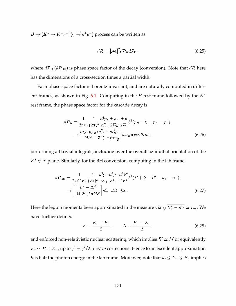
B ! (K ! K+)( BH! e+e) process can be written as

dR =M2dPBdPBH (6.25)

where dPB (dPBH) is phase space factor of the decay (conversion). Note that dR here

has the dimensions of a cross-section times a partial width.

Each phase space factor is Lorentz invariant, and are naturally computed in differ-

ent frames, as shown in Fig. 6.1. Computing in the B rest frame followed by the K

rest frame, the phase space factor for the cascade decay is

dPB =1

2mB

1

(2)5d3p2E

d3pK2EK

d3k

2E 4(pB k pK p) ;

! mKpKs1=2

m2B m2

K s

32(2)4m3B

dKd cos ds ; (6.26)

performing all trivial integrals, including over the overall azimuthal orientation of the

K- -N plane. Similarly, for the BH conversion, computing in the lab frame,

dPBH =1

2M2E

1

(2)5d3p+2E+

d3p2E

d3P 0

2E 04(P + k P 0 p+ p) ;

! E2 2

64(2)5M2Ed+dd : (6.27)

Here the lepton momenta been approximated in the measure viapE2 m2 ' E. We

have further defined

E E+ + E

2; E+ E

2; (6.28)

and enforced non-relativistic nuclear scattering, which implies E 0 'M or equivalently

E ' E++E, up to q0 = q2=2M m corrections. Hence to an excellent approximation

E is half the photon energy in the lab frame. Moreover, note that m E E implies

171

that

2 (m E ; E m) : (6.29)

At an e+e B-factory, such as Belle or BaBar, the e+e ! ! B B production fac-

torizes from the subsequent B decays, because the B is a pseudoscalar. In this type of

collider, the rapidity of parent B meson in the lab frame has a known prior probability

distribution, fB()d, determined by the collider configuration, and enters as an inde-

pendent phase space factor in dR. In Appendix D.II we include a derivation of the B

rapidity pdf (D.10), for an e+e machine. We shall restrict ourselves hereafter to the

case that fB() is known. In this case, note that the energy E is fully specified by , s

and , viz.

E(; ; s) m2B m2

K s

4mB

cosh + cos sinh

; (6.30)

so that the lepton energies can be expressed in terms of , s, and , via eqs. (6.28).

In our discussion of the kinematics above, it was convenient to express the amplitudes

in terms of the ten phase space coordinates s, , E, K and . We see here, how-

ever, that for the differential rate, it is more natural to choose and as phase space

coordinates rather than E. Combining the above results together, the full differential

rate

dR =M2fB()mKpK

s1=2

m2B m2

K s

4(4)9m3B

E2(; ; s)2

M2E(; ; s)dKd+ddd cos dsd :

(6.31)

172

6.3.2 Polarization and weak phase observables

Let us now define a further change of azimuthal angular coordinates, modulo 2

+ + + 2K ;

+ + 2K ;

' + : (6.32)

The angle ' encodes the acoplanarity of the leptons with respect to the photon, with

coplanarity corresponding to ' = . Note that K and are defined with opposite

orientations around the photon momentum direction ^(m)k (see Fig. 6.1). For coplanar

conversion leptons and a stationary B in the lab frame, then corresponds to the

relative twist between the positron-electron conversion plane and theK- decay plane.

Similarly, would then correspond to the averaged orientation of the positron-electron

conversion plane and the K- decay plane with respect to the K- decay plane.

From eq. (6.16), the momentum exchange has the form q2 / 1 + cos', with < 1.

It follows from eqs. (6.15), (6.23) and (6.31) that the differential rate can be written in

the form

dR =X

k

ak cosk(')

hA1 + A2 cos( + ' )+

A3 cos( ' ) + A4 cos( )i; (6.33)

where ak and Ai are purely functions of the phase space orthogonal to , and '. That

is, ak and Ai are functions of s, , ;K; and . Integrating over all phase space except

d , we see that the marginal differential rates for B ! (K ! K+)( BH! e+e) and

173

B ! ( K ! K+)( BH! e+e) must respectively have the form

dRd

=R2

h1 2r

1 + r2C cos( )

i;

dRd

=R2

h1 2r

1 + r2C cos( + )

i:

(6.34)

Eqs. (6.23) tell us that the cosine coefficient C arises from a ratio of BH interference

terms to the BH squared amplitude, and is therefore independent of r or . In other

words, this coefficient is the same for both of the CP conjugate processes, and is B !K operator independent. We have chosen the relative sign of C in eqs (6.34) to antic-

ipate the choice that ensures C > 0. Further, we have chosen the normalization of C in

eqs (6.34) to ensure, via positive semi-definiteness of dR=d , that jCj 1, noting that

the r dependent factor 2r=(1 + r2) 1 for any r. The coefficient C may then be inter-

preted as the maximum possible ratio of the amplitude of dR=d oscillations to their

average value, R=2. Hereafter we call this ratio the relative oscillation amplitude.

Eqs (6.34) are the main results of this chapter. Once the model-independent coeffi-

cient C is computed, then measurement of the relative oscillation amplitude in dR=d permits extraction of r up to the two-fold ambiguity r $ 1=r. Further, measurement

of the average phase shift (phase shift difference) between dR=d and dR=d per-

mits extraction of the weak (strong) phase (). Equivalently, one may construct two

forward-backward type asymmetries. Defining the four quadrants I : 2 [0; =2],

II : 2 [=2; ], III : 2 [; 3=2] and IV : 2 [3=2; 2] then

R1

ZIII+III+IV

dRd

d =2

2r

1 + r2C sin(+ )

R1

ZI+II+IIIIV

dRd

d =2

2r

1 + r2C cos(+ ) ;

(6.35a)

174

and moreover

R1ZIII+III+IV

dRd

d =2

2r

1 + r2C sin( )

R1ZI+II+IIIIV

dRd

d =2

2r

1 + r2C cos( ) :

(6.35b)

Note that all four symmetries have an upper bound 2=. For known C, one may extract

r and from these two sets of asymmetries.

6.3.3 Statistics and Sensitivity Enhancements

Before proceeding to numerical computation of C, let us pause to consider the statistical

confidence in the extraction of r and . We focus on their extraction from the asym-

metries (6.35). These asymmetries are expectation values of a random variable defined

to take the values 1 on the quadrants I, II, III and IV, as specified in eqs. (6.35). For

a sample of N 1 events, the corresponding error X =p(1X2)=N ' 1=

pN , for

X = , , , and . The statistical confidence at which one rejects the SM val-

ues XSM – thus measuring NP effects – is then characterized by the chi-square statistic

(X XSM)2=2X .

As shown in Ref. [299] and below, special ‘sensitivity parameter’ kinematic cuts

may enhance C on the resulting remaining phase space. The construction of these cuts

is motivated by the observation, from eqs. (6.23), that C is enhanced on those areas

of phase space in which the BH interference term, 1221, is comparable or larger

than terms in the total BH square amplitude jj2 =P;r;s jrsj2. For example, one may

175

define the sensitivity parameter

S j1221j=j11j2

' 2(1 cos[j+ j ])

+

( + + )2

++

( 2+2+ 2

2)

2

(1 + 2+

2+)(1 + 2

2) :

(6.36)

Requiring S & 1 produces an event-level kinematic cut that typically leads to O(1)enhancements of C on the remaining phase space, as will be verified below. Note that

the (1cos[j+j]) factor in eq. (6.36) implies that S ' 0 for coplanar events, and

moroever that a lower bound on S typically favors events with higher acoplanarity.

One may also consider other sensitivity parameters, such as

T 2j1221j=jj2 ; (6.37)

which is normalized such that T 2 [0; 1].

Let us define C0 (N0) to be the relative oscillation amplitude (number of events) in

the absence of S or T cuts, and write

Cc C[S > Sc; T > Tc] ; Nc N [S > Sc; T > Tc] : (6.38)

Compared to the Sc = Tc = 0 case, the application of sensitivity parameter cuts scales

the NP statistical confidence by the factor

X XSM

X

2 S>Sc;T >Tc

X

X XSM

2

'Cc

C0

2Nc

N0; (6.39)

for X = , , , and . That is, the enhancement Cc=C0 achieved by the sensi-

tivity parameter cuts competes with the corresponding increase in the statistical error,pN0=Nc, since necessarily Nc < N0. We shall see in the next section that there are

176

choices of Sc and Tc for which > 1. For the purpose of measuring NP effects, this

is equivalent to an effective increase in the sample size N0 7! N0 – an increase in the

effective statistics.

6.4 Simulations

6.4.1 Relative Oscillation Amplitude

Extraction of the relative oscillation amplitude coefficient C is achieved numerically

via Monte-Carlo (MC) generation of B ! (K ! K+)( BH! e+e) events according

to the differential rate (6.31). We use the matrix element in eq. (D.4), generated from

linearly polarized photon amplitudes. Though it does not provide the same analytical

insight as the matrix element generated from spinor-helicity methods (6.23), this matrix

element is as numerically stable as the latter, and moreover, acts as a convenient cross-

check of the analytic results in eqs. (6.23) and (6.34).

For the numerical results shown in this chapter, we use a private MC code written

in C/Python. For simplicity, we apply the narrow K limit (6.7), which fixes the K to

be on-shell. We assume the nominal Belle(II) parameters [302] (see also App. D.II) in

order to determine the B rapidity distribution fB(), which is peaked at ' 0:29.

More details of the operation of this MC generator are included in Appendix D.III.

We have further checked the numerical results with a second private MC, written in

C++/Java, that makes use of the matrix element (6.23). In both codes, we discard the

overall normalization of the matrix element – e.g. A(r) in eqs. (6.23) – since we are

concerned only with the relative oscillation amplitude, C.

In order to account for limited angular resolution, we include hereafter cuts on the

lepton polar angles, , and opening angle, ``, defined in Fig. 6.1. We will consider a

177

10−6 10−5 10−4 10−3

θc

0.10

0.12

0.14

0.16

0.18

0.20C(θ ``,±>θ c

)

0.0 0.5 1.0 1.5 2.0

ψ/π

0.40

0.45

0.50

0.55

0.60

Norm

ali

zed

even

ts

(0.1, 0)

(0.2, π/4)

(0.5, π/3)

(1.0, π/2)

Figure 6.2: Left: The fit value for C with the 1 error band as a function of the polarangle cuts ``; > c (see Fig. 6.1). The peak value of C approximately coincides with thepeak of the marginal distribution (see the left panel of Fig. D.2). Right: Normalizeddifferential distribution dR=d for four different (r; + ) couplets and c = 106. Alsoshown are theory predictions (gray) for the input values of (r; + ) and the extractedvalue C[c = 106] in eq. (6.41).

uniform polar cut

``; > c ; (6.40)

for various values of c. In particular, we consider two benchmark cases c = 106

and 5 104. The former captures almost all conversion leptons in the B ! (K !K+)(

BH! e+e) process for semirelativistic B’s, while the latter might be plausibly

achievable in the near- to mid-term future. To extract C, we fit eq. (6.34) to the dR=d histograms for various choices of r and + , including the couplets fr; + g =

f(0:1; 0); (0:2; =4); (0:5; =3); (1:0; =2)g. In Fig. 6.2 we show the extracted C as a func-

tion of the c cuts. The maximal relative oscillation amplitude one can expect is of

O(20%), and the benchmark extracted C values are

C[c = 106] = 0:173 0:001; and C[c = 5 104] = 0:150 0:003 ; (6.41)

where the errors are purely statistical in origin. We also show in Fig. 6.2 typical dR=d histograms for various choices of r and + . The expected shifted and amplitude-

modulated cosine can be clearly seen. Applying the extracted value for C, these his-

178

0.2

0.6

1.0

C

θ``,± > 10−6

STΣ = 1

θ``,± > 5× 10−4

10−2 10−1 1

1

2

3

Σ

10−2 10−1 1

Net cut efficiency ε

Figure 6.3: Upper panels: The coefficient C as a function of the cut efficiency for the S(blue) and T (gold) kinematic cuts, with polar cuts c = 106 (left) and c = 5 104

(right). The colored regions depict the 2 statistical error bands. The equivalenteffective statistics curve = 1, i.e. C = C0=

pN=N0, is also shown (gray). Lower panels:

Statistics enhancement as a function of the cut efficiency. The maxima correspond tothe optimum cuts S > Sopt

c and T > T optc (colored dots in all panels).

tograms are in excellent agreement with the theory predictions (6.34).

6.4.2 Statistics Enhancements

Incorporating the S and T kinematic cuts, we show in Fig. 6.3 the absolute enhance-

ment of C as a function of the net cut efficiency, , for the two benchmark polar angle

cuts. The net cut efficiency is defined hereafter to be the fraction of events kept after

application of both kinematic and polar cuts. The pure S cuts – that is, C(S > Sc; T > 0)

– provide the larger enhancement at high cut efficiencies. At lower efficiencies the pure

T cut provides the larger enhancement. The C and dependence on Sc may be read off

from Fig. 6.4.

179

0 2 4 6 8 10Sc

0.1

0.4

0.7

C(S>S c

)ε; θc = 10−6

ε; θc = 5× 10−4

C; θc = 10−6

C; θc = 5× 10−410−2

10−1

1

Net

cut

effici

ency

ε

Figure 6.4: The enhancement in C as a function of S . The secondary y-axis shows thecorresponding cut efficiency. The colored regions depict the2 statistical error bands.

Comparing to the equivalent effective statistics curve = 1 – i.e. C = C0=pN=N0

– we see in Fig. 6.3 that the C dependence initially rises faster than C0=pN=N0. This

means that for low values of Sc and Tc, the statistics on the S and T cut phase space

is enhanced compared to the full data set. The explicit dependence is also shown in

Fig. 6.3. In particular, one sees that for c = 5 104, the statistical enhancement is

optimized at Soptc = 1:1 (T opt

c = 0:62) corresponding to = 3:6 ( = 2:5).

To demonstrate the efficacy of these statistics enhancements, in Table 6.1 we com-

pute the extracted values for r and + , along with their statistical errors, with and

without the optimal Soptc and T opt

c cuts. We use an MC sample generated from an in-

put couplet (r; + ) = (0:2; =4), containing a total of N = 104 events. This roughly

corresponds to 50 ab1 of data – a benchmark luminosity at Belle II [302] – and a per-

cent level photon conversion rate with ideal acceptance efficiency. The polar cut is

c = 5 104. The extracted values are obtained by two different methods, first from a

fit to the differential rate eq. (6.34) and second from the quadrant asymmetries (6.35).

The statistical errors for the optimized kinematic S and T cuts are a O(1) factor

smaller than for the full data set, as expected from the above numerical analysis: Ap-

plication of these sensitivity parameter cuts improves the statistical power of the r and

180

MethodS; T > 0 S > Sopt

c T > T optc

r (+ )= r (+ )= r (+ )=

dR=d 0:1940:017

0:2550:026

0:1940:010

0:2630:015

0:1900:013

0:2470:020

, 0:2170:005

0:2160:157

0:2030:003

0:2480:088

0:1920:003

0:2320:112

Table 6.1: Extracted values of r and ( + ) from an MC sample with input values(0:2; =4).

extraction from B ! (K ! K+)( BH! e+e) events. Moreover, even without

these enhancements, both r and are extracted with sufficient numerical precision to

probe NP effects at the r 1 or 1 level.

6.5 Chapter summary

In this chapter we have presented the helicity amplitudes and differential rate for the

B ! K ! K+ process, in which the photon undergoes subsequent nuclear

conversion to a lepton pair. Interference between the intermediate, on-shell photon

polarizations in the coherent B ! (K ! K+)( BH! e+e) process produces oscil-

lations in the angular kinematic observable . Measuring the amplitude and phase of

these oscillations – or equivalently two quadrant-type asymmetries and – per-

mits extraction in principle of the polarization ratio, r, and the relative weak phase, ,

of the right- and left-handed B ! K amplitudes. In this manner, SM expectations

for both r and may be tested.

We have employed private Monte Carlo simulations to compute the distribution

and asymmetries as a function of r, and kinematic cuts. In particular, kinematic cuts

with respect to the sensitivity parameters S and T may sufficiently amplify these oscil-

lations, such that the overall statistical power of the r and measurement is increased

by an O(1) factor.

Implementing this approach using converted photons will be experimentally chal-

181

lenging, not least because of the high angular resolution required to reconstruct the

conversion lepton kinematics. Moreover, a detector whose thickness is on the order

of one radiation length or less is required to avoid multiple leptonic rescatterings, that

otherwise smear the lepton kinematics. Nonetheless, the theoretically clean nature of

the r- and -sensitive observables presented in this work may perhaps encourage the

use of this technique in a future dedicated detector element.

182

Chapter 7

Conclusion

While the standard model of particle physics has successfully withstood many exper-

imental tests, it still leaves many questions unanswered. Attempting to answer these

questions motivates one to propose physics beyond the standard model. Moreover,

possible solutions to the hierarchy problem in addition to the WIMP miracle single out

the TeV scale as the energy scale of new physics. In the first part of this thesis, we

explored three different dark matter models where both the dark matter candidate and

the mediators between the visible and dark sectors are at the TeV scale. While, in the

second part, we were motivated by the matter/antimatter asymmetry to look for new

sources of CP violation. We focused on developing tools for probing CP violation in

the Higgs and flavor sectors.

Starting with DM model building, we exploited the flavor symmetries of the stan-

dard model to stabilize a dark matter candidate using two different approaches. In chap-

ter 2, we showed that exploiting the flavor structure of the SM can lead to metastable

DM with TeV scale mediators even if the DM itself is flavor neutral. We did this in

two different flavor breaking scenarios: in the context of minimal flavor violation and

in a Froggatt-Nielsen flavor model. In chapter 3, we turned our attention to flavored

dark matter in a fully gauged SU(3)3 flavor model. We took advantage of a remnant

183

Z3 symmetry that is useful to stabilize a dark matter that carries a flavor charge and

investigated its phenomenology. We then showed that, in the case of a fermionic dark

matter candidate where the only source of splitting in the multiplet is from radiative

corrections involving the flavor gauge bosons, the dark matter mass must lie in the

range [0:5; 5] TeV to satisfy all experimental constraints.

On a more speculative note, in chapter 4 we investigated the possibility of obtaining

bounds on the up, down, and strange quark Yukawa couplings if Higgs portal dark

matter is discovered. Surprisingly, we found that while in the limit where the light

Yukawas tend to zero there is virtually no effect on the direct detection rate while,

in the limit where they are allowed to saturate the current experimental bounds, the

direct detection rate can be enhanced by four orders of magnitude. We then reviewed

a range of flavor models to determine the expected enhancement or suppression of the

light Yukawa couplings in realistic model building scenarios.

Finally, we developed techniques for measuring CP violation in the Higgs coupling

to photons in chapter 5 and in rare radiative decays of B mesons in chapter 6. We

found that while these techniques provide a theoretically clean probe of CPV, they

require specialized detectors in order to be practical.

In summary, the standard model does not provide answers for well motivated

questions including the microscopic theory of dark matter and the source of the mat-

ter/antimatter asymmetry. We attempted to address the aforementioned questions in

this thesis. However, the topics considered here are too rich for one thesis and provide

a solid basis for an ongoing exploration.

184

A — Appendix to Chapter 2

A.I Operators in four component notation

In the chapter we are using a two-component notation, where the left-handed Weyl

fermion fields (qi; uc; dc; li; ec) have hypercharges (+1=6;2=3;+1=3;1=2;+1) andBL charges (1=3;1=3;1=3;1;+1). The higgs doublet is denoted by H and has Y =

+1=2, while ~H = i2H. The two Weyl spinors of the DM Dirac fermion are and

c with B L = 1 and +1, respectively. Finally, is the complex scalar DM with

B L = 2. Capital letters denote four-component spinors following the notation in

[305]. The DM Dirac fermion and its charge conjugate C are

=

0B@

cy _

1CA ; C =

0B@ c

y _

1CA ; (A.1)

while = ( c; _). Writing for the two-component spinors q1 = uL, q2 = dL and

`1 = L, `2 = eL, suppressing generation indices, we introduce

U =

0B@uLucy _

1CA ; D =

0B@dLdcy _

1CA ; E =

0B@eLecy _

1CA ; N =

0B@Lcy _

1CA ; (A.2)

185

where c is the right-handed neutrino field introduced for completeness. If neutrino is

Majorana, L = c. The weak doublets in the four-component notation are

QL = (UL; DL); LL = (NL; EL); (A.3)

with UL PLU , etc, and similarly UR PRU;DR PRD; :::. Some examples of the

relevant asymmetric operators in the two- and four-component notations are given

below.

dim 6: Q(6)1 = (qiq

i)(dc c) = (QCLiQ

iL)(D

CPR); (A.4)

Q(6)2 = (ucdc)(dc c) = (UPLD

C)(DPLC); (A.5)

dim 10: Q(10)1 = (dcdc)(qi q

i)(qj qj) = (DPLD

C)(QLiPRQCiL )(QLiPRQ

CiL ): (A.6)

A.II Asymmetric DM relic density

Here we review the relations between the DM relic density and the DM mass in ADM

models. We assume that the operator(s) transferring the B L asymmetry from the

visible to the dark sector decouple above electroweak phase transition, TC > Tew 170

GeV [306], as is the case for our ADM models, see Sec. 2.2. We first assume that the

visible sector consists below TC of only the SM fields (we will later relax this). The

number density asymmetry for relativistic particles is

(n n)i =T 3

6giiT; (A.7)

where n(n) are the particle(anti-particle) number densities, i is the chemical potential

for species i, and gi = gi(gi=2) for bosons (fermions) with gi internal degrees of freedom

so that gi = 1 for a Weyl fermion, while gi = 2 for a Dirac fermion or a complex scalar.

186

All the SM particles are in chemical equilibrium, so that the chemical potentials are

proportional to the conserved quantum numbers [307]. Above the electroweak phase

transition these are B L, Y and SU(2)L, while B + L is broken by sphalerons. Thus

(see also [308])

i = (T3)ic3 + YicY + (B L)icBL; (A.8)

where the ci are constants that we determine from net weak isospin, hypercharge and

B L densities. The net weak isospin charge density in the universe normalized to

entropy density is

T3 /Xi

gi (T3)i i =Xi

gi (T3)2i c3 + 0 cY + 0 cBL = 0: (A.9)

For the first equality we used that for each SU(2) multipletP

i(T3)i = 0, and in the

second equality that the net T3 charge is zero since SU(2)L is not explicitly broken.

Thus c3 = 0 and the SU(2)L charge of a particle does not contribute to its chemical

potential.

Flavor mixing ensures that the chemical potentials for SM Weyl fermions from dif-

ferent generations are the same. Similarly, SU(2)L interactions ensure that uL = dL Q, and `L = L. We thus have

H = 12cY ; L = 1

2cY cBL; E = cY cBL;

Q = 16cY + 1

3cBL; U = 2

3cY + 1

3cBL; D = 1

3cY + 1

3cBL;

(A.10)

while for the gauge bosons G = W = B = 0. The net hypercharge of the universe is

187

thus

Y /Xi

gi (Y )i i =1

22 2H +Nf

1

22L E +Nc

1

6 2Q +

2

3U 1

3D

= 2H +Nf (Q + 2U D L E) = 11cY + 8cBL;

(A.11)

where Nf = 3 is the number of generations and Nc is the number of colors. Setting the

net hypercharge density in the universe to zero, Y = 0, gives

cY = 8

11cBL: (A.12)

The net BL number density in the visible sector (i.e. excluding the BL asymmetry

carried by the fields in the dark sector) is then

B L / Nf (2L E + 2Q + U + D) =79

11cBL: (A.13)

There are two types of interactions between the dark and visible sector: the asym-

metric interactions that involve a single field, and the symmetric interactions of the

form y times the SM fields. The symmetric operators keep the dark and the visible

sectors in thermal equilibrium. The asymmetric interactions are suppressed, and de-

couple at temperatures well above the mass. At lower temperatures the number is

thus effectively conserved. The chemical potential is the same as it was before the

decoupling. We thus have

i = (B L)icBL; (A.14)

where (B L)i is the B L charge of the i field. Here we allow for several i fields

in the dark sector and also define the weighted B L charge of the dark sector fields

188

as

(B L)sum Xi

gi(B L)i: (A.15)

The net number density normalized to entropy density we denote by and is

/Xi

gii = (B L)sum cBL: (A.16)

SinceBL and are conserved quantum numbers below the decoupling temperature,

each of the number densities scales as R3 as universe expands. The ratio

B L=

B L

decoup:

=11

79(B L)sum ; (A.17)

thus stays fixed.

Even if at the decoupling there are more i dark sector states, we assume that DM

is composed only from one state, . We therefore have for the ratio of baryon and dark

matter energy densitiesB

=mp

m

B

B L

B L

: (A.18)

The ratio of net B and B L numbers B=(B L) = 28=79 = 0:354 just above the elec-

troweak phase transition [307]. This remains essentially unchanged even if sphaleron

and top mass effects are taken into account, in which case using results from [306, 309]

one has B=(B L) = 0:349 for both scalar and fermionic DM. Using (B L)= =

79=(11(B L)sum ) from (A.17) finally leads to

m = 2:509mpB

1

(B L)sum= (12:5 0:8)GeV

1

(B L)sum; (A.19)

where in the last equality we used = 0:265 0:011 and B = 0:0499 0:0022 [55].

Note that the error is dominated by the experimental determination of DM and baryon

densities. For instance, the difference between B=(B L) determination with and

189

without sphaleron effects leads to a smaller shift in m than the above quoted error.

We turn next to the case of additional fields in the visible sector. An example would

be that SM gets completed to the MSSM. The relation between Y;B L and the con-

stants cY;BL can be written in the matrix form

0B@ Y

B L

1CA =15

42gT

0B@ Pi giY

2i

Pi giYi(B L)iP

i giYi(B L)iP

i gi(B L)2i

1CA 0B@ cY

cBL

1CA=

15

42gT

0B@ 11 + [Y 2]NP 8 + [Y (B L)]NP

8 + [Y (B L)]NP 13 + [(B L)2]NP

1CA 0B@ cY

cBL

1CA :

(A.20)

Here we defined

[Y 2]NP =Xi

giY2i ; [Y (B L)]NP =

Xi

giYi(B L)i; [(B L)2]NP =Xi

gi(B L)2i ;

(A.21)

where the sums run over the new states only. The solution for B L in terms of cBL

is obtained by solving the above matrix equation setting Y = 0, from which

B L =15 cBL42gT

13 + [(B L)2]NP (8 + [Y (B L)]NP)

2

11 + [Y 2]NP

: (A.22)

The net charge is still given by Eq. (A.17), while the ratio B= is given by (A.18)

with (BL)= fixed at the decoupling temperature andB=(BL) at the electroweak

phase transition. We thus have

m = mpB

B

B L

13 + [(B L)2]NP (8 + [Y (B L)]NP)

2

(11 + [Y 2]NP)2

1

(B L)sum; (A.23)

where B=(B L) = 0:349 and (B L)sum given in (A.15).

190

A.III Calculation of the DM decay time

Here we give further details of the DM lifetime calculation in the MFV and FN models

for B = 2 DM, Sec. 2.3, while also varying the DM mass. The results are shown in

Fig. 2.3. There are three different types of dimension 10 operators that can lead to DM

decay, of schematic form (dcdc)(dcdc)(ucuc), (dcdc)(dcuc)(qq), and (qq)(qq)(dcdc).

For the same NP suppression scale the last type of operators gives the shortest life-

time. The dominant effective decay Lagrangian is thus, schematically,

L(B=2)dec C6(qq)(qq)(dcdc); (A.24)

where C is a flavor-dependent Wilson coefficient, the brackets enclose Lorentz con-

tracted pairs, and summation over different flavor, color and weak isospin contractions

is understood.

In Sec. 2.3 we included the SM Yukawa insertions in the definition of the operators.

To unify the notation we instead use in this appendix the convention that the Wilson

coefficient C encodes all the flavor suppressions. The effective decay Lagrangian is

thus, going to the mass basis, and displaying the flavor indices only,

L(B=2)dec: C IJBCEF

6uI u

J d

Bd

EdcCd

cF; (A.25)

where the flavor dependent Wilson coefficients are

C IJBCEF(MFV) ' [VCKM]IA [Y

diagd ]B [VCKM]JD "

ABC"DEF; (A.26)

C IJBCEF(FN) ' jH(qI)H(qJ)H(qB)H(qE)+H(d

cC)+H(d

cF)j; (A.27)

191

Figure A.1: Example Feynman diagrams for the decay of B = 2 DM. The diagram onthe left shows the tree level decay whereas the one on the right shows the loop-induceddecay.

The partial decay width for ! qqqqdd transition is then, using NDA,

' C28

1

(162)4

m

12m: (A.28)

The factor 1=(8) 1=(162)4 results from integrating over the 6-body phase space.

For the MFV flavor breaking case there are several subtleties when calculating the

decay width. For instance, the Levi-Civita tensor contractions lead to vanishing oper-

ators for some of the color and Lorentz contractions. Another subtlety is that the tree

decay may be strongly CKM suppressed so that the leading decay amplitude is the

1-loop one, see Fig. A.1. The decay width can thus be estimated as

(! uIuJdBdEdcC d

cF ) ' max

8>><>>:CIJBCEF(MFV)

2

8

1

162

4 m

12m;

1162

[VCKM]IX [VCKM]YE

2 CYJBCXF(MFV)

2

8

1

162

4 m

12m:

(A.29)

where the first (second) line gives the NDA estimates for the tree level (1-loop) domi-

nated decay width. The W emitted from the left-handed quark lines coming from the

effective decay vertex gives the additional CKM factors in the second line.

An example where the leading decay amplitude is generated at 1-loop is the B = 2

192

ADM withm = 3:3GeV, discussed in Sec. 2.3. Decays into final states with one charm,

bottom or top quark are kinematically forbidden. For instance, the lightest B = 2 final

states with one valence charm quark are +c + and n+0

c . The first has the valence

quark content udc+ dds and the rest mass m+c+m = 3:48 GeV, while the valence

quark content of the second is udd + ddc and its rest mass mn + m0c = 3:4 GeV. In

contrast, the decays to 0 ( uds) or 0 ( uds) baryons are allowed. Eq. (A.29) gives

MFVTREE

! 00

' ysV 2ub

2 1

8

1

162

4 m

12m; (A.30)

MFVLOOP

! 00

' ybVubVts162

21

8

1

162

4 m

12m; (A.31)

with the same estimate, within our precision, for the ! 0;0 or ! 0;0 decays.

Note that in the 1-loop amplitude the partonic transition at the decay vertex, !udb + tds, carries no CKM suppression. Furthermore, the ys Yukawa insertion in the

tree level amplitude is replaced by yb. The b and t quark lines then convert to u and

s quark lines via W exchange, as shown in Fig. A.1. The smaller CKM and Yukawa

suppressions compensate the loop factor so that the 1-loop amplitude dominates, with

the NDA estimate MFVLOOP=

MFVTREE O(10).

This procedure can be repeated for different DM masses, arriving at the dominant

decay modes as a function of m. The results are listed in Table A.1, where we give

the kinematical thresholds (1st column) for a number of decay channels (4th column),

along with the corresponding partonic transitions (3rd column) and the decay vertex

transitions (2nd column). The latter two differ for the loop processes, cf. Fig. A.1. The

total decay width for givenm is then the sum of partial decay widths, i, (5th column)

for the decay channels that are kinematically allowed. For convenience we also give

the decay times, i, (6th column) that correspond to individual partial decay widths.

Note that in the calculation of the partial decay widths we neglect the phase space

193

suppression, while the quoted i in Table A.1 are obtained from the NDA estimates

(A.29) with m at the kinematical threshold, and setting = 1TeV.

In the case of FN flavor breaking the leading tree level and loop induced decay

widths for B = 2, m = 3:3 GeV DM have the NDA estimates of

FNTREE

! 00

' 22 1

8

1

162

4 m

12m; (A.32)

FNLOOP

! 00

' 4

162

21

8

1

162

4 m

12m: (A.33)

In this case the tree level decay dominates over the loop induced decay by four orders

of magnitude. The dominance of the tree level decay amplitude over the 1-loop decay

amplitude holds also, if the DM mass is varied. This can be traced to the following

difference between the MFV and FN ansatze. In the MFV case the Levi-Civita tensors

enforce that two quark flavors in the effective decay vertex need to be from the third

generation. This can be changed either by using the VCKM misalignment or through

a loop transition. In FN flavor structure ansatz, on the other hand, the flavor indices

need not be antisymmetric.

A.IV Loop functions in neutral meson mixing

Here we list the analytical form of the loop functionsF (x); F F (x1; x2); G(x1; x2); GF (x1; x2;x 3)

and H(x), HF (x1; x2) that appear in the 1-loop expressions for the Wilson coefficients

in the neutral meson mixing, Sec. 2.6.1. The mediator loop functions with mass degen-

erate quarks in the loop are given by

F (x) = xH(x); H(x) =1

(1 x)31 x2 + 2x log(x)

; (A.34)

194

while for two different quarks running in the loop they are

F F (xi; xj) =xixj

(1 xi) (1 xj)+

"xixj log (xi)

(1 xi)2 (xi xj)

+ xi $ xj

#; (A.35)

HF (xi; xj) =1

(1 xi) (1 xj)+

"x2i log (xi)

(1 xi)2 (xi xj)

+ xi $ xj

#: (A.36)

The loop functions for the mediator-W loops are

G(xw; x) =x

xw

"xw + x

(x 1) (x xw) x (2xxw x2w 2xw + x2) log(x)

(x 1)2 (x xw) 2

+2xxw log (xw)

(x xw) 2 (xw 1)

#;

(A.37)

GF (xw; xi; xj) =xixjxw

"(xi + xw) log (xi)

(1 xi) (xi xj) (xw xi)+ xi $ xj

2xw log (xw)

(1 xw) (xw xi) (xw xj)

#:

(A.38)

195

T/h [GeV] Decay vertex Partonic Final State i [GeV] i [s] Process

2.06 ! cudbsd ! udd uds n+ 0 1:34 1060 4:91 1035 Loop

2.23 ! uusdsd ! uds uds 0 + 0 3:74 1055 1:76 1030 Tree

2.43 ! cusbsd ! uds uss 0 + 0 4:25 1057 1:55 1032 Loop

3.48 ! ccdssd ! udc dds +c + 1:23 1055 5:33 1030 Loop

3.61 ! ucsdsd ! udc dss +c + 1:87 1050 3:52 1025 Tree

3.81 ! ccsdsd ! uds ssc 0 +0c 1:42 1052 4:62 1027 Loop

3.79 ! ccsdsd ! usc dss +c + 1:33 1052 4:96 1027 Loop

4.63 ! ccdbsd ! dcc dds +cc + 1:01 1052 6:51 1027 Loop

4.93 ! ccsdsd ! ddc dsc 0c + 0c 1:04 1046 6:33 1021 Tree

5.17 ! ccsbsd ! dsc ssc 0c +0c 4:14 1052 1:59 1027 Loop

6.56 ! cudsbd ! udd udb n+ 0b 7:25 1054 9:08 1028 Loop

6.73 ! uudbsd ! udd usb n+ 0b 1:87 1045 3:53 1020 Tree

6.94 ! uusbsd ! uss udb 0 + 0b 5:18 1044 1:27 1019 Tree

7.10 ! cusdbs ! uss usb 0 + 0b 3:49 1052 1:89 1027 Loop

8.07 ! ucbdbd ! udb ddc 0b +0c 2:16 1051 3:05 1026 Loop

8.09 ! ucbdsd ! udb dsc 0b + 0c 2:00 1042 3:30 1017 Tree

8.31 ! ucbssd ! udb ssc 0b +0c 5:33 1041 1:24 1016 Tree

8.48 ! ucbsbs ! usb ssc 0b +0c 7:66 1050 8:59 1024 Loop

11.24 ! uubdbd ! udb udb 0b + 0b 2:24 1042 2:93 1017 Tree

11.41 ! uubbsd ! udb usb 0b + 0b 9:86 1038 6:68 1012 Tree

11.58 ! uubsbs ! usb usb 0b + 0b 2:94 1042 2:24 1017 Tree

Table A.1: Partial decay widths, i, and related decay times, i = 1=i, for represen-tative decay channels above kinematical thresholds (1st column) assuming the MFVflavor breaking ansatz. The EFT scale is set to = 1 TeV. The last column denoteswhether the dominant amplitude is tree level or 1-loop, while the 2nd and the 3rdcolumns give the decay vertex transition and the partonic transition after the potentialW exchange, respectively.

196

B — Appendix to Chapter 3

B.I Minimal flavour violation with gauged flavor sym-

metries

In this appendix we verify numerically that the Wilson coefficients in the weak Hamil-

tonian for Bd and Bs mixing,

HB=2e =

5Xi=1

Cbqi Q

bqi +

5Xi=1

~Cbqi~Qbqi ; (B.1)

generated from exchanges of flavored gauge bosons, are of the MFV type. A tree level

exchange of FGB generates contributions to Bd mixing through operators

Qbd1 = dL b

LdL b

L; Qbd

3 = dRbLdRb

L; (B.2)

and ~Qbd1 ; ~Q

bd3 , that follow from Qbd

1 ; Qbd3 with PL $ PR exchange (the remaining opera-

tors can be found in, e.g., Ref. [82]). If the lightest FGB has predominantly left-handed

couplings, then Cbd1 Wilson coefficient is the largest one, while if the lightest FGB is

coupling predominantly to the right-handed quarks, the ~Cbd1 dominates. For compara-

ble left-handed and right-handed couplings all four Wilson coefficients, Cbd1;3, ~Cbd

1;3, are

important. Analogous discussion applies to the case of FGB contributions toBs mixing

which are obtained with a trivial d! s exchange.

197

0.0 0.5 1.0 1.5 2.00.0

0.2

0.4

0.6

0.8

1.0

n

PM

FVHn

L

Figure B.1: The FGB contributions to V A current operator in the effective weakHamiltonian. Left panel shows the values of the complex ratio Cbd

1 =Cbs1 for our

scan points, with green points satisfying all constraints, magenta points excludedby flavor constraints and grey points by perturbativity considerations. The pointCbd

1 =Cbs1 = (V

td=Vts)

2, obtained if the MFV operator with the smallest number ofYukawa insertions dominates, is denoted by a cross. The right panel shows the cu-mulative function PMFV (n), see Eq. (B.4).

As discussed in Section 3.3 the contributions from the gauged flavor model can be

expanded in terms of the SM Yukawas. The contributions due to FGB exchanges can

thus be written as

Cbd1 = c1(yuy

yu)

213+ c2(yuy

yu)13(ydy

ydyuy

yu)13+ = c1(V

tdVtb)

2+ c2y2d(V

tdVtb)

2+ ; (B.3)

where (yd)ij = diag(yd; ys; yb), and we have set yt = 1 in the second equality. In (B.3) we

kept only the two terms relevant for the discussion below. The same expansion applies

for Cbs1 with d! s replacement in (B.3).

In Fig. B.1 (left) we show the ratio Cbd1 =C

bs1 , i.e. the NP contribution to the V A

quark current operator due to tree level FGB exchanges. Note that the ratio Cbd1 =C

bs1

can be complex. If the c1 term dominates then Cbd1 =C

bs1 ' (V

td=Vts)

2. This is denoted

by a cross in Fig. B.1 (left). The addition of the operators with extra insertions of ydyyd

lead to Cbd1 =C

bs1 not beign equal to (V

td=Vts)

2. We have verified that the curve for

Cbd1 =C

bs1 shown in Fig. B.1 (left) can be fit with the form of Cbd;bs

1 in (B.3), taking

c1 real and c2 complex, where c1 varies from being O(1) to being vanishingly small.

The points in our scan can be grouped into two sets. For the first set of points both c1

198

and c2 terms are sizeable. For the second set of points the c1 term is negligible and c2

dominates. This is shown in Fig. B.1 (right) where we plot the cumulative distribution

function

PMFV(n) =NjCbd

1 =Cbs1 j (md=ms)

njV td=V

tsj2

Ntotal: (B.4)

The function PMFV(n) can be interpreted as the fraction of points that have the ratio

jCbd1 =C

bs1 j effectively dominated by operators with up to ynd insertions. That is, the

points dominated by the c1 term contribute to PMFV(0) (and to PMFV(n) with n 0),

while the points dominated by the c2 term ontribute to PMFV(2) (and to PMFV(n) with

n 2). The points with both c1 and c2 start contributing to PMFV(n) for n somewhere

between 0 and 2, depending on the relative sizes of c1 and c2. Fig. B.1 (right) shows

that a subleading (but nonzero) set of points is dominated by the c1 term, about 10%

points have both c1 and c2 terms sizeable, while about 80% of points are dominated by

the c2 term.

Similar analysis can be made for V +A operators, ~Qbd1 and ~Qbs

1 . One can expand the

FGB contributions to their respective Wilson coefficients in terms of the SM Yukawas

~Cbd1 = ~c1(y

ydyuy

yuyb)

213 + ~c2(y

ydyuy

yuyb)13(y

ydydy

ydyuy

yuyb)13 +

= ~c1y2dy

2b (V

tdVtb)

2 + ~c2y4dy

2b (V

tdVtb)

2 + ;(B.5)

and similarly for ~Cbs1 with d ! s replacement. We show in Fig. B.2 (left) the ratio

~Cbd1 = ~C

bs1 for our scan. If the ~c1 term dominates, then ~Cbd

1 = ~Cbs1 = (md=ms)

2(V td=V

ts)

2,

which is denoted by the cross in Fig. B.2 (left). The points for which also the ~c2 operator

(and other operators denoted by ellipses above) is important then lie away from the

~Cbd1 = ~C

bs1 = (md=ms)

2(V td=V

ts)

2 region. We also define a cumulative function

~PMFV(n) =Nj ~Cbd

1 = ~Cbs1 j (md=ms)

n+2jV td=V

tsj2

Ntotal: (B.6)

199

0.0 0.5 1.0 1.5 2.00.0

0.2

0.4

0.6

0.8

1.0

n

P

MFV

HnL

Figure B.2: The FGB contributions to V + A current operator in the effective weakHamiltonian. Left panel shows the complex ratio ~Cbd

1 = ~Cbs1 for our scan points with

the same color coding as in Fig. B.1. The point ~Cbd1 = ~C

bs1 = (md=ms)

2(V td=V

ts)

2, ob-tained if the MFV operator with the smallest number of Yukawa insertions dominates,is denoted by a cross. The right panel shows the cumulative function ~PMFV(n), see Eq.(B.6).

The values for ~PMFV(n) are shown in Fig. B.2 (right). We see that also in this case the

points cluster into two groups, with vanishing ~c1 term or with both ~c1 and ~c2 relevant.

The above analysis demonstrates that the FGB contributions to the Wilson coeffi-

cients in the effective weak hamiltonian can be expanded in terms of the SM Yukawas

which is a hallmark of (general) MFV. In particular, the expansion in terms of md;s=mb

and off-diagonal CKM elements can be still performed and is not ruined by the large

ratios of scales present in the problem such as the very disparate FGB masses.

B.II Thermal relic computation

In this appendix we describe the calculation of relic density that was used in the scans

in the main part of the paper. Several approximations to the coupled Boltzmann equa-

tions were necessary in order to reduce the evaluation time per benchmark and thus

allow adequate coverage of the parameter space. We find the approximate solutions to

be in agreement with the full solutions at theO(30%) level. The full numerical solution

of the Boltzmann equations was obtained with MadDM [105] using a UFO model file [310],

which was generated with the FeynRules package [106].

200

Denoting the DM multiplet by ', where ' is either a Dirac fermion or a complex

scalar, the most general set of coupled Boltzmann equations reads [103]

dn'idt

+ 3Hn'i =Xj

h('i'j $ XX) vlabin'in'j nEQ

'inEQ'j

Xj 6=i

h('iX $ 'jX)vlabin'i

nEQ'i

nEQ'j

n'j

nEQX

Xj 6=i

h('i'j $ 'k'`)vlabin'in'j

nEQ'inEQ'j

nEQ'k'

EQ`

n'kn'`

Xj 6=i

h('j;i ! 'i;jX)in'j;i + h('j;iX ! 'i;j)in'j;inEQX

;

(B.7)

where X denotes a generic SM state. For large mass splittings between the ' compo-

nents it is sufficient to consider the lightest 'i state in Eq. (B.7). The contributions to

the DM relic density from the heavy ' components are exponentially suppressed by

corresponding Boltzmann factors and can be neglected within our precision. In con-

trast, when the mass splittings are small the full set of coupled Boltzmann equations

in Eq. (B.7) needs to be considered. Nevertheless, even in this case several approxima-

tions are possible for our model, as we explain below.

First of all, the coannihilation of different 'i components into SM particles, 'i'j !XX (i 6= j), can be safely neglected in our model. In benchmarks that survive the

experimental constraints the off-diagonal couplings of the lightest FGB to ' are much

smaller than the diagonal ones, see Fig. B.3. Secondly, in the calculation of DM relic

density we also neglect the flavor-changing DM scattering off the thermal background,

'iX ! 'jX . The'iX ! 'jX scattering can be important if h('iX ! 'jX)vlabi = h('i'j ! XX) vlabi &n'j=n

EQX 109. In this case the off-diagonal couplings of O(104) relative to the di-

agonal ones are in principle large enough to have O(1) effects on the relic density,

and neglecting 'iX ! 'jX may not be justified. Therefore, for the benchmarks with

(g24 )23=(g24 )33 > 3 104 and small mass splittings among ', we explicitly verified us-

201

0.0001 0.0002 0.0003∣∣∣(g24χ

)2,3

∣∣∣ /∣∣∣(g24

χ

)3,3

∣∣∣

0.0

0.1

0.2

0.3

0.4

Fra

ctio

nof

ben

chm

arks

Figure B.3: The fraction of benchmarks as a function of the off-diagonal couplings ofthe heaviest and next-to-heaviest DM components to the lightest FGB (A24) normalizedby the diagonal coupling of the heaviest component.

ing MadDM that neglecting 'iX ! 'jX scattering leads to a change in DM relic density

smaller than O(30%).Finally, we are able to neglect the pure DM scattering process in the third line of

Eq. (B.7) since h('i'j $ 'k'`)vlabi h('i'j $ XX) vlabi in our model. The largest

contribution to this process is from diagonal couplings between the FGB and DM.

This process can couple the evolution of the DM species if h('i'j $ 'k'`)vlabi h('i'j $ XX) vlabi. The diagonal FGB couplings to the quarks and to the DM of

the same generation are approximately equal. By accounting for the color factors and

the multiplicity of channels when annihilating into SM fields one concludes that the

pure DM scattering is indeed subleading.

Therefore, for almost mass degenerate 'i it is sufficient to consider a set of uncou-

pled Boltzmann equations

dn'idt

+ 3Hn'i = Xj

h('i'i $ XX) vlabin2'i nEQ

'i2: (B.8)

The DM relic abundance is in this case the sum of relic abundances for each of the

202

three components obtained from the above set of equations (the heavy ' components,

in our case '2 and '3, decay after their respective freeze-outs and contribute to the '1

DM relic abundance). In contrast, for large mass splittings the heavy ' components

are irrelevant for the calculation of the DM relic abundance. This is then obtained from

Eq. (B.8) by considering only the lightest DM state, in our case '1.

We calculate the DM relic abundance from Eq. (B.8) using the freeze-out approxi-

mation [104], which gives

h2 =1:07 109 GeV1

J(xf )pgMPl

; (B.9)

where MPl = 1:22 1019 GeV, g is the total number of effectively relativistic degrees

of freedom at the time of the freeze-out, and

J(xf ) =

Z 1

xf

dxhvlabithx2

: (B.10)

The freeze-out temperature (xf = m'1=Tf ) is obtained by solving

xf = ln0:038 geff MPlm'1 hvlabithp

gxf; (B.11)

where the thermally-averaged cross section is

hvlabith =2x

32p

Z 1

0

evlabp ex d ; (B.12)

with vlab = 2p(1 + )=(1+ 2) and = s=(2m'1)

2 1. The freeze-out approximation is

accurate to a few percent with respect to the full numerical solution of the Boltzmann

equation [103].

The fermionic flavored DM annihilates through the s-channel exchange of FGBs. In

this case, the integration over x can be performed analytically and the double integral

in Eq. (B.10) reduces to a single one that can be efficiently evaluated numerically. In

203

particular,

J(xf ) =

Z 1

0

2vlabErfc(pxf) d : (B.13)

We evaluate the above integral numerically in the parameter scan.

In the annihilation cross section of the fermionic flavored DM we keep the domi-

nant contribution – the s-channel exchange of the lightest FGB, A24. The annihilation

cross section for i i ! ujuj (and similarly for i i ! djdj ) is given by

(i i ! ujuj) =(g24 )

2ii

4

ss 4m2

uj

s 4m2i

1 +

2m2i

s

GuV 2jj;24 s+ 2m2

uj

+GuA2jj;24 s 4m2

uj

sm2

A24

2+m2

A242A24

;

(B.14)

where the vector and axial-vector couplings to quarks, GA;V , were defined in Eq. (3.25),ps is the center-of-mass energy and A24 is the total decay width of the lightest FGB.

The decay rate for A24 ! ujuj assuming mA24 > 2muj is

(A24 ! ujuj) =m24A

4

s1 4m2

uj

m2A24

"GuV 2jj;24 1 +

2m2uj

m2A24

!+GuA2jj;24

1 4m2

uj

m2A24

!#:

(B.15)

The rate for A24 ! i i; djdj is obtained after trivial replacements for masses and cou-

plings (and dividing by theNc color factor for decays to i i). The total FGB decay rate

is obtained after summing over all kinematically allowed decay channels.

204

B.III Higgs coupling Feynman rules

As noted in Sec. 3.4.5, the h ff Feynman rules given in Appendix A.1 of Ref. [102]

contain a typo. The corrected Feynman rules are given here.

f

f

h =ip2(CL PL + CR PR) (B.16)

where the couplings CL and CR are:

huiui : CL = CR = +u suRi cuLi

hu0iu0i : CL = CR = u cuRi suLi

huiu0i :

(CR = u cuRi cuLiCL = +u suRi suLi

hu0iui :

(CR = +u suRi suLi

CL = u cuRi cuLi

(B.17)

205

C — Appendix to Chapter 5

C.I Spinor-helicity formalism

In this paper we extensively use the spinor-helicity formalism, in which the sigma

matrices a _a solder null momenta to Weyl spinors, that transform under the spinor

irreducible representations of the covering group SL(2,C). For a review see e.g. Ref.

[311] or [312].

For a null momentum k, the associated Weyl spinors k are soldered via

k =1

2hkjjki ; =k k

a _a = (k)a(k) _a ; (C.1)

in which we have written the dotted and undotted Weyl spinors in the notation

hkj (k)a ; hk+j (k) _a ; jk+i (k)a ; jki (k)

_a ; (C.2)

so hk+jj`+i = (k) _a _aa(`)a, hkjj`i = (k)

aa _a(`)_a. Upper and lower indices

are related by the usual epsilon contractions, in particular _aa ab _a

_bb_b. In this no-

tation, the sign superscripts denote the helicities of the in-going and out-going states,

corresponding to kets and bras respectively. In particular, note that jkiy = hkj by

construction, hkjj`i do not exist, while hkjj`i = h`+jjk+i. For null momenta

206

k and ` we often write the bilinears

hk `i hkj`+i = (k)a(`)a ; [k `] hk+j`i = (k) _a(`)

_a ; (C.3)

so h` ki = hk `i, [` k] = [k `], hk `i[` k] = 2k ` and hk `i = [` k].

In this notation, definite helicity polarization vectors associated to k may have form

"(k; r) = hrjjkip2hrjki ; (C.4)

with r a reference null momentum. One may show via the Fierz relations that these

polarization vectors satisfy the axiomatic requirements k " = 0, " (") = " " =

1 and " " = 0. In the present work, a particularly convenient choice of reference

momenta is

r1 = k2 ; r2 = k1 ; (C.5)

where r1;2 (k1;2) are reference momenta (photon momenta) corresponding to polariza-

tion vectors "1;2 defined in (5.7). We shall always make this choice of reference mo-

menta.

The dotted and undotted Weyl spinors have explicit representations in terms of the

momentum components in a particular basis, up to a free choice of phase. For example,

for a null momentum k = (k0; k1; k2; k3), a possible choice is

(k)a =

8>>><>>>:k1 + ik2pk0 k3

;pk0 k3

; k3 < 0 ;p

k0 + k3 ;k1 ik2pk0 + k3

; k3 > 0 :

(C.6)

The components of the upper dotted spinor are immediately specified through the

relation (k)_a = [(k)

a]y, and the lower index spinors through appropriate epsilon con-

tractions. With this choice and a choice of basis, all spinor objects – e.g. hk `i – can be

207

evaluated explicitly, just as momentum objects may be, e.g. k `. Note that for our Weyl

spinor phase choice (C.6) one has hk1 k2i = [k2 k1] = mh.

The Dirac spinors of massive particles may also be represented in the spinor-helicity

formalism, via the application of a light-cone decomposition. For a massive spinor of

momentum p and mass m, we define an associated null momentum

~p = p m2

2p `` ; or equivalently p = ~p +

m2

2~p `` ; (C.7)

where ` is a null reference momentum. The spinors then decompose similarly as

u1(p) = j~p+i+ m

[~p `]j`i; u2(p) = j~pi m

h` ~pij`+i;

u1(p) = h~p+j+ m

h` ~pih`j; u2(p) = h~pj m

[~p `]h`+j;

v1(p) = j~pi+ m

h` ~pi j`+i; v2(p) = j~p+i m

[~p `]j`i;

v1(p) = h~pj+ m

[~p `]h`+j; v2(p) = h~p+j m

h` ~pih`j : (C.8)

One may verify that these spinors satisfy the canonical requirements uu = 2m, vv =

2m, vu = uv = 0 and the completeness relationsP

j ujuj = =p + m and

Pj v

jvj =

=p m. Just as for the polarization vectors, one is free to choose the null reference

momentum. This choice amounts to a choice of ‘gauge’, under which the unpolarized

square amplitude must be invariant, but the polarized square amplitudes are not. In

this work, we shall always make the reference momenta choices

`1 = k2 and `2 = k1 : (C.9)

These are convenient choices for the purposes of extracting the leading order BH he-

licity amplitudes, as below.

Finally, together with the several well-known spinor identities, the following iden-

208

tity is especially useful for computing terms involving Levi-Civita contractions,

_aa

_bb

_cc

_dd 4i

_d _aba

_b _cdc _d _cbc

_b _ada: (C.10)

C.II BH spin-helicity amplitudes

Here we write down explicit expressions for the helicity amplitudes irs . From Eqs. (5.16)

and (5.24) one has (suppressing the branch index)

rs = i

2q2ur(p)

="=p =k +m

k p =Q+ =Q=k =p+ +m

k p+ ="vs(p+)

= i

2q2

Xj

ur="ujuj =Qvs

k p ur =Qvjvj="vs

k p+

ur="=k =Qvs

k p +ur =Q=k="vs

k p+

; (C.11)

where u = u(p) and v = v(p+). Applying the light cone decomposition (C.8) with

reference choices specified in (C.4) and (C.9), gives the full results for each spin helicity

209

amplitude

11 = (+22) =1

q2p2

m [` ~p] hk ~pi h`j =Qj~p+i

k p [k `] h` ~pi +m [` ~p+] hk ~p+i h`j =Qj~p+i

k p+ [k `] h` ~pi m [` ~p] hk ~pi h~p+j =Qj`+i

k p [k `] h` ~p+i +m [` ~p+] hk ~p+i h~p+j =Qj`+i

k p+ [k `] h` ~p+i m hk `i hkj =Qj~p+i

k p h` ~pi +m hk `i h~p+j =Qjk+i

k p+ h` ~p+i

12 = +(+21) =

1

q2p2

m2 hk `i hkj =Qj`i

k p [` ~p+] h` ~pi +m2 hk ~p+i h`j =Qj`ik p+ [k `] h` ~pi

m2 [` ~p] hk ~pi h`j =Qj`ik p [k `] [` ~p+] h` ~pi [` ~p] hk ~pi h~p+j =Qj~p++i

k p [k `]+[` ~p+] hk ~p+i h~p+j =Qj~p++i

k p+ [k `] +hk ~p+i h~p+j =Qjk+i

k p+

21 = +(+12)

=1

q2p2

[k ~p] hk ~pi h~pj =Qj~p+i

k p [k `] +[` ~p+] hk ~p+i h~pj =Qj~p+i

k p+ [k `]+m2 hk `i h`+j =Qjk+ik p+ [` ~p] h` ~p+i +

m2 [` ~p+] hk ~p+i h`+j =Qj`+ik p+ [k `] [` ~p] h` ~p+i

m2 hk ~pi h`+j =Qj`+ik p [k `] h` ~p+i hk ~pi hk

j =Qj~p+ik p

22 = (+11) =

1

q2p2

m hk ~pi hkj =Qj`i

k p [` ~p+] +m hk ~p+i h~pj =Qj`i

k p+ [k `] m [` ~p] hk ~pi h~pj =Qj`i

k p [k `] [` ~p+] +m hk ~p+i h`+j =Qjk+i

k p+ [` ~p]+m [` ~p+] hk ~p+i h`+j =Qj~p++i

k p+ [k `] [` ~p] m hk ~pi h`+j =Qj~p++ik p [k `]

: (C.12)

As per the main text, we have dropped the photon subscripts, and k; ` = k1; k2 or

k2; k1 for parent photon 1 and 2 respectively. Squaring these amplitudes, taking traces

and summing, one obtains the full Bethe-Heitler square amplitude that is obtained by

the usual Feynman methods.

We can further extract dominant terms of the BH spin-helicity amplitudes by ob-

serving that if qi mh, then hk1 k2i hki pii etc. Moreover, in expressions such as

+12 or +21, we may discard subdominant O(m2=ki pj 6=i) terms. This leads to the fol-

lowing leading order results in m2=ki pj 6=i and hki pii=hk1 k2i for the BH spin-helicity

210

amplitudes

11 = (+22) 'm

q2p2

hk `ih~p+j0jk+ik p+h` ~p+i hk `ih~p

++j0jk+i

k ph` ~pi;

12 = (+21) ' hk ~p+ih~p+j0jk+i

q2p2k p+

[` ~p]hk ~pih~p+j0j~p++iq2p2k p[k `]

+[` ~p+]hk ~p+ih~p+j0j~p++i

q2p2k p+[k `]

m2hk `ihkj0j`iq2p2k p[` ~p+]h` ~pi

;

21 = (+12) ' hk ~pih~p++j0jk+i

q2p2k p

[` ~p]hk ~pih~pj0j~p+iq2p2k p[k `]

+[` ~p+]hk ~p+ih~pj0j~p+i

q2p2k p+[k `]

+m2hk `ihkj0j`i

q2p2k p+[` ~p]h` ~p+i

;

22 = (+11) ' 0 ; (C.13)

in which we have dropped the photon subscripts, and uniform overall signs or factors

of i; k; ` = k1; k2 or k2; k1 for photon 1 and 2 respectively; and the spinor notation is de-

tailed in Appendix C.I. The parity relations (5.29) are satisfied as expected. Eqs. (5.28)

and (C.13) together provide a compact expression of the leading order HBH square

amplitude.

It should be understood that the particular form for the spin helicity amplitudes

above depends on the choice of reference momenta, because the amplitudes explic-

itly depend on polarization vectors and spinors (see App. C.I). Moreover, the ability

to straightforwardly expand the full results to the leading order results depends on

a sensible choice of reference momenta. In contrast, the full unpolarized BH rate is

independent of polarizations and spinors, as a result of spinor and polarization vec-

tor completeness, and therefore must be independent of any such reference momenta

choice.

211

C.III Polarization-decomposed HBH rate

Here we give the explicit results of a Higgs-Bethe-Heitler Feynman type calculation.

To preempt the loss of numerical precision from large cancellations due to the Ward

identity, we do not use polarization completeness relations. Rather, we retain the po-

larization vectors explicitly in the HBH rate. In the case that the Higgs is at rest in

the lab frame, we simply use a Cartesian basis for the polarization vectors, aligning

the back-to-back photons with the z-axis. That is, in the HBH square amplitude we

coherently sum over the polarization basis

1(k1;2) = (0; 1; 0; 0) and 2(k1;2) = (0; 0; 1; 0) : (C.14)

The squared matrix element for the process h+N1 +N2 ! (k1) (k2) +N1 +N2 !4`+N 0

1 +N 02 is given by

jMj2 = AAXpols

a,b,c,d

ha (k1)

b (k2)

c(k1)

d(k2)

a0(k1)

c0(k1)

b0(k2)

d0 (k2)

iBH00

1 BH00

2

(C.15)

where the tensor A is

A = c (k1 k2 g k2k1) + ~c k1k2 : (C.16)

The BHi factors are the polarized Bethe-Heitler squared amplitudes for a photon i,

212

including form factor contributions, these are in general

BHab =G

q4(k p)2(k p+)2(h

2(k p)(k p+)2EE+ m2 p+ p

Babk;p+8E+

M(k p+)2(k p)BabP;p + (k p+)2(4E2

+ + q2)Fabp

+ (p+ p)i

8(k p)2(k p+)2PaP b

M2

2

M(k p)(k p+)

q2 + 2 (E(k p) + E+(k p+))BabP;k

+ 2(k p)(k p+)(q2 4EE+)Babp+;p+ 2(k p)(k p+)

(k p + k p+)2 + q2E2

gab

4(k p)(k p+)2EE+ m2 p r kakb) ; (C.17)

whereFab` = `akb+`bka2`a`b andBab`1`2 = `a1`

b2+`

b1`a2. The photon momentum is denoted

by k and the lepton momenta by p+; p. M and m are the masses of the nucleus and

lepton respectively. Assuming that the Higgs is at rest in the lab frame and that the

photon is in the z-direction, as in Eq. (C.14), the previous expression simplifies to

BHab ' 2Gq4

(gabE2 q

2 + (k p + k p+)2

(k p)(k p+) 4

Ep+p

a

k p +Epp

a+

k p+

Ep+p

b

k p +Epp

b+

k p+

);

(C.18)

where, in the second term, we expanded terms of the formp4E2 q2 to leading or-

der in q2=E2. We have checked that the helicity formalism results and the Feynman

diagram calculation results for HBH rate agree.

Finally, the unpolarized BH rate can be obtained from Eq. (C.18) simply by averag-

ing over the photon polarization as follows

hjMj2i = 1=2BH11 + BH22

: (C.19)

It is instructive to use the polarization vector completeness relation to obtain an ex-

213

pression in terms of Lorentz dot products. In this case, starting with Eq. (C.17), the BH

rate is given by

hjMj2i = 4G E2

+ E2+

q2 k p k p+ + 8

Gm2 (k pE k p+E+)2

q4 (k p)2 (k p+)2

+ 2Gm2 (k p + k p+)2q2 (k p)2 (k p+)2 2

G k pk p+(k p)2 (k p+)2 4

G (k p) 2 + (k p+)2q4 (k p) (k p+)

4G k p + k p+q2 k p k p+ ; (C.20)

where the leading terms – the terms on the first line – reproduce Eq. (5.35).

C.IV Numerical simulations of Bethe-Heitler conversion

In this appendix we present numerical evaluations of several differential BH rates.

The numerics were done in two ways: by numerically integrating the full tree-level

analytical results – i.e. the BH rate arising from Eqs. (C.12) or (C.17) with appropriate

integration measures – using the CUBA library [313]; and with a Monte Carlo (MC)

code developed privately (the details are given in Appendix C.VI). Fig. C.1 shows the

differential distribution of the positron energy fraction E+ = E+=E . For efficiency

the MC simulation (blue binned histogram) is generated with a cut on the difference

of electron and positron azimuthal angles, (+ ) mod 2 2 [0:6; 1:4] (see

App. C.VI). This agrees with the numerical integration (red line) for the same cuts on

.

Fig. C.1 (right) shows the positron energy distribution after applying the opening

angle cut of `` > 104 on the angle between e+ and e momenta. The MC agrees with

the full numerical integration of the BH rate even though the cut is still applied in

the generation of the events . Fig. C.1 demonstrates that the asymmetric configurations,

where one of the two leptons carries the larger part of the photon energies, are the more

214

0.00.20.40.60.81.01.21.4

0 0.2 0.4 0.6 0.8 1

Nor

m.

even

ts/b

in

E+

θ`` > 0

MC eventsRestr. P.S.

Full P.S.0.00.51.01.52.02.53.03.5

0 0.2 0.4 0.6 0.8 1

Nor

m.

even

ts/b

in

E+

θ`` > 10−4 MC eventsRestr. P.S.

Full P.S.

Figure C.1: Spectrum of the positron energy E+ = E+=E . No opening angle cut wasapplied in the left hand figure and an opening angle cut of 104 was applied in theright hand one. The histograms were created with MC events and the solid curves areresults of numerically integrating the differential cross section. The dashed curve inboth figures is the result of numerically integrating the differential cross section overthe entire range of as opposed over the range [0:6; 1:4].

probable ones, especially for non-zero opening angles.

Fig. C.2 shows the positron polar angle distribution and demonstrates the com-

bined effect of the Si nuclear form factor and the smaller available phase space that

suppress very small momentum transfers and thus very small polar angles. The peak

is at m=E 105 both for the distribution without a cut on the e+e opening angle

``, Fig. C.2 (left), and for the case where `` > 104 is imposed, Fig. C.2 (right). This

cut also results in an additional peak in the distribution, cf. Fig. C.2 (right).

In Fig. C.3, the distribution in the relative azimuthal angle of the two leptons is

shown. The majority of the events are close to the coplanar configuration, where the

photon and the two lepton momenta all lie in the same plane. However, it is notewor-

thy that approximately 40% of BH events have acoplanarity of 5% or more.

C.V Analysis for qq !

Performing the measurement proposed in this work faces two main challenges: first,

resolving and reconstructing the electron and positron directions; and second identify-

215

05000

1000015000200002500030000

10−7 10−6 10−5 10−4 10−3 10−2

Nor

m.

even

ts/b

in

θ+

θ`` > 0 MC eventsRestr. P.S.

Full P.S.

02000400060008000

1000012000140001600018000

10−7 10−6 10−5 10−4 10−3 10−2

Nor

m.

even

ts/b

in

θ+

θ`` > 10−4 MC eventsRest. P.S.

Full P.S.

Figure C.2: Polar angle distribution of the leptons. No opening angle cut was appliedin the left hand figure and an opening angle cut of 104 was applied in the right handone. The histograms were created with MC events and the solid curves are results ofnumerically integrating the differential rate expression. The small bump in the righthand figure ( 104) is a result of applying an opening angle cut. Its location is afunction of the cut.

ing a background-poor sample of events with Higgs decaying to diphotons. Regard-

ing the first challenge, one might simply ask how well and with what efficiency can

the LHC or a future collider detector reconstruct the details of photon conversion. To

do so, the experimental collaborations may wish to test the polarization structure of

a standard model (non-Higgs) amplitude. To demonstrate that there is a non-trivial

structure to be measured in SM conversions, we briefly analyze here the leading pro-

duction of diphotons at the LHC.

The dominant diphoton production (and dominant background for Higgs to pho-

tons events) is qq ! scattering. This has tree-level spin-helicity amplitude

[MBG]12rs =

P+, s

P−, r

k1, λ1

k2, λ2

+ u channel ; (C.21)

in which r = 1; 2 (s = 1; 2) is the spin of the (anti)-fermion, and 1;2 = are the usual

photon helicities. The two photons then convert in the tracker. The background rate

216

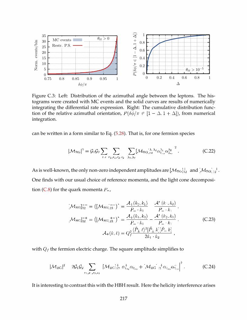
05

101520253035

0.75 0.8 0.85 0.9 0.95 1

Nor

m.

even

ts/b

in

δφ/π

θ`` > 0MC eventsRestr. P.S.

0

0.2

0.4

0.6

0.8

1

0 0.2 0.4 0.6 0.8 1

P(δ

φ/π

∈[1

−Δ

,1+

Δ])

Δ

θ`` > 10−5

Figure C.3: Left: Distribution of the azimuthal angle between the leptons. The his-tograms were created with MC events and the solid curves are results of numericallyintegrating the differential rate expression. Right: The cumulative distribution func-tion of the relative azimuthal orientation, P (= 2 [1 ; 1 + ]), from numericalintegration.

can be written in a form similar to Eq. (5.28). That is, for one fermion species

jMBGj2 = G1G2Xr;s

Xr1;s1;r2;s2

X1;2

[MBG]12rs 11rs

22rs

2 : (C.22)

As is well-known, the only non-zero independent amplitudes are [MBG]+12 and [MBG]

+12 .

One finds with our usual choice of reference momenta, and the light cone decomposi-

tion (C.8) for the quark momenta P,

[MBG]+12 =

[MBG]

+21

=A+(k2; k1)

P+ k1 A(k1; k2)

P k1 ;

[MBG]+12 =

[MBG]

+21

=A+(k1; k2)

P+ k1 A(k2; k1)

P k1 ;

A(k; `) = Q2f

h ~P `i2[ ~P k][ ~P k]2k1 k2 ;

(C.23)

with Qf the fermion electric charge. The square amplitude simplifies to

jMBGj2 = 2G1G2X

r1;s1;r2;s2

[MBG]+12

+1rs

2rs + [MBG]

+12

1rs

+2rs

2 : (C.24)

It is interesting to contrast this with the HBH result. Here the helicity interference arises

217

in terms of the form 112+212121

+221

, rather than from 112212121

221

as we found for

HBH. Since +12 = (21), etc, it follows from the explicit results (5.36) that this helicity

flip on branch ‘2’ produces a phase change 2 ! 2 in the background interference

term, compared to the HBH interference terms.

To compare with the Higgs rest frame HBH rate (5.48), we assume the quark centre

of mass frame aligns with the nuclear rest frame. Integrating all over azimuthal struc-

ture except 1+2+ (cf. ' = 1++2+ in Eq. (5.46)), one finds that the background

rate has the formd

d dPS ;= ABG

; + BBG ; cos(2 ) : (C.25)

We see that this differential rate has sinusoidal dependence on the mean azimuthal

orientation, , of the outgoing positrons, with respect to, say, the incoming quarks –

the beamline – rather than the inter-branch lepton azimuthal orientation, ', as in HBH.

Moreover, the phase change 2 ! 2 ensures background is flat in '. Note also

that unlike the HBH process, the [MBG]+ factors ensure this background rate features

higher spin waves, so that its angular differential structure will differ from the HBH

structure, too.

In summary, the leading-order doubly-converted qq ! square amplitude is

given explicitly by Eqs. (C.23) and (C.24) combined with the BH spin-helicity am-

plitudes (C.13). In the qq center of mass frame, the corresponding leading order BH

amplitudes are given in Eqs. (5.36).

C.VI Monte Carlo numerical schemes

To generate Monte Carlo (MC) events for the HBH process, we first generate unpolar-

ized BH events and then use the von Neumann rejection technique to re-weight the

events according to the HBH differential rate. For a single HBH event one needs two

218

BH events taken from disjoint MC samples. Therefore, we first describe the generation

of unpolarized BH events.

The phase space for a single BH event, N ! e+eN , is five dimensional. We take

z-axis to be the incoming photon direction. For conversion of unpolarized photons,

the kinematics are invariant under overall azimuthal rotations around the z axis. We

therefore fix the positron azimuthal angle to zero. The remaining four coordinates are

chosen to be the electron energy fraction E = E=E , two transformed polar angles,

t1 = log10(+) and t2 = log10(), and the azimuthal angle of the electron (see Fig.

5.6 for definitions).

For MC we used two independent private codes. One is written in C and the other

in C++/Java. To populate the BH phase space we first randomly generate the values

for E, t1;2 and according to either uniform distributions or conveniently chosen

initial probability density functions (PDFs) and then unweight to obtain the BH event

distribution.

For the C code, the initial PDFs are as follows. For a 60 GeV photon, generating

E according to a uniform distribution results in an efficiency of 70%. We therefore

generate a uniform distribution of E 2 [m=E ; 1 m=E ]. The transformed polar

angle variables, t1 and t2, are generated according to uniform distributions in a suitable

numerical range, see Table C.1. Using the coordinates t1;2 captures the fact that electron

and positron distributions are sharply peaked around m=E. The BH events are

also dominated by kinematic configurations that are not too far from the coplanar one.

We therefore generate in the range [0:6; 1:4], which suffices for our precision.

To capture the fact that the BH distribution is peaked toward = = 1, the C code

generates according to a Cauchy distribution (Lorentzian) with location parameter

xo = and scale parameter = 0:03 [314] to improve the efficiency. The C++/Java

uses similar initial data, with the exception of slightly different ranges and that is

populated by a uniform distribution on a slightly narrowed domain 2 [3=4; 5=4]

219

C C++/Java

Parameter Range PDF Range PDF

E [m=E ; 1m=E ] Uniform [m=E ; 1m=E ] Uniform

t1 [7;2] Uniform [6;3] Uniform

t2 [7;2] Uniform [6;3] Uniform

[0:6; 1:4] Lorentzian [3=4; 5=4] Uniform

Table C.1: The details on the MC generation of BH events, with phase space variables(1st column) for C (C++/Java) generated in the range given in the 2nd (4th) columnaccording to the distribution given in the 3rd (5th) column (for details see text).

(see Table. C.1).

In the next step we unweight the events generated from initial PDFs to obtain the

proper BH distribution. In the unweighting, the events are rejected with a probability

that is 1 w, with w = (dBH=dPS)=max(dBH=dPS). The BH MC event sample was

validated by comparing the generated event distributions to the results of numerical

integration of BH differential cross-sections as shown in Figs. C.1, C.2 and C.3. Addi-

tionally, in Figs. C.1 and C.2, the distributions with a cut on the opening angle between

e+ and e of `` > 104 are shown. The MC sample is in excellent agreement with the

results of numerical integration.

In the final step, we convert the generated BH events into MC event samples for the

HBH process. To do so, two disjoint BH samples were used – one sample per photon

branch. The rate for two BH events is given by (dBH1=dPS)(dBH2=dPS). To obtain the

proper HBH even rates, we use the standard reweighting technique where events are

rejected according to the weight

w =(dHBH=dPS)[']

(dBH1=dPS) (dBH2=dPS); (C.26)

where the twist angle between the positrons, ', is populated by a uniform distribution

on [0; 2].

220

The two MC codes have been cross tested. In numerics we use 3 106 HBH events

from the C generator and 8 105 HBH events from the C++/Java MC generator.

221

D — Appendix to Chapter 6

D.I The B ! Ke+e squared matrix element by polar-

ization decomposition

The effective Lagrangian in eq. (6.2) gives the following Feynman rule for the BK

vertex:

γ(k)λ, µ

K∗(p)κ, ν

= igkm2

BKg 2kp+ 2g?k

p

(D.1)

where m2BK m2

B m2K . The amplitude for B ! K with being the photon

helicity is then given by

N = gK

ngkm2

BK" (pK p) 2 " p [k (pK p)]

2g? (pK p) "

k p

o (D.2)

The BH squared amplitude in the nuclear rest frame for a linearly polarized photon in

the +z direction with polarizations = f1; 2g is

BH0 ' 2e6Gq4

(g

0E2 q

2 + (k p + k p+)2

(k p)(k p+) 4

Ep+p

k p +Epp

+

k p+

Ep+p

0

k p +Epp

0

+

k p+

!);

(D.3)

222

where terms of O(q2=E2) were dropped (see Appendix C in [299] for details). The

squared amplitude is then given by

jMj2 =X

;02f1;2g

NN 0BH0 : (D.4)

A numerical comparison between the above expression and eq. (6.23) shows excellent

agreement over the entire phase space (sampled uniformly).

D.II B rapidity distribution

Consider an e+e ! ! B B factory, and let denote the polar angle of the B’s

with respect to the electron beamline in the center of mass frame. The amplitude for

production Mprod sin, and so the probability distribution

p(cos) =3

4

1 cos2

: (D.5)

Here and in the following we neglect effects of lab frame angular acceptance cuts,

which may non-trivially restrict the domain of both and .

In the center of mass frame – the rest frame of the – eachB has energyE = m=2:

hereafter the superscript denotes center-of-mass frame quantities. The corresponding

rapidity, which we choose to be positive by convention on the branch 2 [0; ],

= cosh1(m=2mB) ; (D.6)

and the B speed in this frame = tanh().

At B-factories the lab frame electron and position beam energies, E, are asymmet-

ric, but are chosen such that the is on shell, i.e. 4E+E = m2. For example, at Belle

II the beams are planned to be E+ = 7 GeV and E = 4 GeV. The boost rapidity of the

223

center of mass frame with respect to the lab frame is correspondingly

= cosh1[(E+ + E)=m] : (D.7)

The rapidity of the B in the lab frame may now be written as a function of cos, viz.

(cos) = cosh1ncosh

cosh + cos sinh

o; (D.8)

and its pdf, by definition

fB() =

Z 1

1

d cos p(cos)[ (cos)] : (D.9)

Under a change of variables = (cos), one finds

fB() =3

4 cosh

Z +

jj

d[ ] sinh

sinh

1

cosh cosh cosh

sinh sinh

2=

3 sinh

4 sinh sinh

1

cosh cosh cosh

sinh sinh

2; j j < < + ;

(D.10)

and zero otherwise. Note that fB itself has zeroes at each end of its non-trivial domain,

i.e. at = + and jj. The boost at the pdf peak is peak = (E++E)=(2m). E.g.

for the Belle II parameters, the peak peak = sinh cosh1( peak) = 0:29. This is the boost

of B’s emitted at = =2, and matches the quoted B design boost at Belle II [302].

D.III The Monte Carlo event generator

This appendix describes in more detail the MC event generator written in C and Python.

The B ! (K ! K) phase space is generated as follows. The B rapidity is sampled

from the PDF given in eq. (D.10) while the photon polar angle and the K polar and

224

10−5 10−4 10−3 10−2 10−1

θ0

0.0

0.2

0.4

0.6

0.8

1.0P

(θ``>θ 0

)

0.3 0.4 0.5 0.6 0.7

Eγ/mB

0.0

0.2

0.4

0.6

0.8

1.0

Nor

mal

ized

even

ts

θ`` > 10−6

θ`` > 10−3

Figure D.1: Left: The cumulative distribution function (CDF) of the opening anglebetween the leptons. Right: The normalized distribution of the photon energy in unitsof the B mass for two different `` cuts.

azimuthal angles are generated uniformly in the appropriate frame. On the other hand,

since in BH photon conversion the leptons are produced with preferentially small an-

gles with respect to the photon direction, the lepton polar angles are generated uni-

formly on a log scale. This is implemented via the transformed variables t = log10

where t are uniformly distributed and with t 2 [5;1]. Moreover, the azimuthal

angle separation between the leptons () is peaked around and so, to improve the

efficiency of the generator, is sampled from a Cauchy distribution. All other BH

variables are generated uniformly.

The weight associated with each event is proportional to the matrix element (D.4).

The events are unweighted using the standard procedure. That is, the weights are

normalized to the largest weight and the event is kept if its normalized weight is larger

than a random number on [0; 1]. Of course, this procedure assumes that the phase

space was sufficiently sampled such that the largest weight found is close to the global

maximum.

Using this procedure, we generate MC samples for many choices of (r; + ) cou-

plets with 500k events per sample. Some representative distributions from the (0:1; 0)

sample are shown in Figs D.1 and D.2. In particular, the left panel in Fig. D.1 shows the

225

10−5 10−4 10−3 10−2

θ+

0

200

400

600

800

1000

1200

1400N

orm

aliz

edev

ents

θ`` > 10−6

θ`` > 10−3

0.0 0.2 0.4 0.6 0.8 1.0

E+/Eγ

0.00.20.40.60.81.01.21.41.61.8

Nor

mal

ized

even

ts

θ`` > 10−6

θ`` > 10−3

Figure D.2: Left: The normalized polar angle distribution of the positron for two dif-ferent values of the opening angle cut ``. Right: the positron energy as a fraction of thephoton energy for two values of ``. The distribution exhibits the expected behaviorfor BH conversion. It is symmetric about 1=2 and prefers that one lepton carry a largerfraction of the photon energy.

cumulative distribution function for the opening angle between the leptons `` while

the right panel shows the distribution of photons energies. Figure D.2 shows the polar

angle and fractional energy distribution of the positron.

226

Bibliography

[1] H. M. Georgi, Lie algebras in particle physics; 2nd ed. Frontiers in Physics. Perseus,

Cambridge, 1999.

[2] B. Batell, J. Pradler, and M. Spannowsky, Dark Matter from Minimal Flavor

Violation, JHEP 1108 (2011) 038, [arXiv:1105.1781].

[3] A. Sakharov, Violation of CP Invariance, c Asymmetry, and Baryon Asymmetry of the

Universe, Pisma Zh.Eksp.Teor.Fiz. 5 (1967) 32–35.

[4] T. Hambye, On the stability of particle dark matter, PoS IDM2010 (2011) 098,

[arXiv:1012.4587].

[5] L. Ackerman, M. R. Buckley, S. M. Carroll, and M. Kamionkowski, Dark Matter

and Dark Radiation, Phys.Rev. D79 (2009) 023519, [arXiv:0810.5126].

[6] J. L. Feng, H. Tu, and H.-B. Yu, Thermal Relics in Hidden Sectors, JCAP 0810 (2008)

043, [arXiv:0808.2318].

[7] J. L. Feng, M. Kaplinghat, H. Tu, and H.-B. Yu, Hidden Charged Dark Matter,

JCAP 0907 (2009) 004, [arXiv:0905.3039].

[8] G. R. Farrar and P. Fayet, Phenomenology of the Production, Decay, and Detection of

New Hadronic States Associated with Supersymmetry, Phys.Lett. B76 (1978) 575–579.

227

[9] S. Dimopoulos, S. Raby, and F. Wilczek, Proton Decay in Supersymmetric Models,

Phys.Lett. B112 (1982) 133.

[10] G. R. Farrar and S. Weinberg, Supersymmetry at Ordinary Energies. 2. R Invariance,

Goldstone Bosons, and Gauge Fermion Masses, Phys.Rev. D27 (1983) 2732.

[11] M. Kadastik, K. Kannike, and M. Raidal, Matter parity as the origin of scalar Dark

Matter, Phys.Rev. D81 (2010) 015002, [arXiv:0903.2475].

[12] M. Kadastik, K. Kannike, and M. Raidal, Dark Matter as the signal of Grand

Unification, Phys.Rev. D80 (2009) 085020, [arXiv:0907.1894].

[13] M. Frigerio and T. Hambye, Dark matter stability and unification without

supersymmetry, Phys.Rev. D81 (2010) 075002, [arXiv:0912.1545].

[14] M. Cirelli and A. Strumia, Minimal Dark Matter: Model and results, New J.Phys. 11

(2009) 105005, [arXiv:0903.3381].

[15] M. Cirelli, N. Fornengo, and A. Strumia, Minimal dark matter, Nucl.Phys. B753

(2006) 178–194, [hep-ph/0512090].

[16] T. Hambye, Hidden vector dark matter, JHEP 0901 (2009) 028, [arXiv:0811.0172].

[17] Y. Bai and R. J. Hill, Weakly Interacting Stable Pions, Phys.Rev. D82 (2010) 111701,

[arXiv:1005.0008].

[18] D. E. Kaplan, M. A. Luty, and K. M. Zurek, Asymmetric Dark Matter, Phys.Rev.

D79 (2009) 115016, [arXiv:0901.4117].

[19] K. M. Zurek, Asymmetric Dark Matter: Theories, Signatures, and Constraints,

Phys.Rept. 537 (2014) 91–121, [arXiv:1308.0338].

[20] K. Petraki and R. R. Volkas, Review of asymmetric dark matter, Int.J.Mod.Phys. A28

(2013) 1330028, [arXiv:1305.4939].

228

[21] J. Kile and A. Soni, Flavored Dark Matter in Direct Detection Experiments and at

LHC, Phys.Rev. D84 (2011) 035016, [arXiv:1104.5239].

[22] H. Davoudiasl, D. E. Morrissey, K. Sigurdson, and S. Tulin, Baryon Destruction

by Asymmetric Dark Matter, Phys.Rev. D84 (2011) 096008, [arXiv:1106.4320].

[23] L. Lopez-Honorez and L. Merlo, Dark matter within the minimal flavour violation

ansatz, Phys.Lett. B722 (2013) 135–143, [arXiv:1303.1087].

[24] P. Agrawal, M. Blanke, and K. Gemmler, Flavored dark matter beyond Minimal

Flavor Violation, JHEP 1410 (2014) 72, [arXiv:1405.6709].

[25] B. Batell, T. Lin, and L.-T. Wang, Flavored Dark Matter and R-Parity Violation,

JHEP 1401 (2014) 075, [arXiv:1309.4462].

[26] P. Agrawal, B. Batell, D. Hooper, and T. Lin, Flavored Dark Matter and the Galactic

Center Gamma-Ray Excess, Phys.Rev. D90 (2014), no. 6 063512,

[arXiv:1404.1373].

[27] U. Haisch, A. Hibbs, and E. Re, Determining the structure of dark-matter couplings

at the LHC, Phys.Rev. D89 (2014), no. 3 034009, [arXiv:1311.7131].

[28] J. F. Kamenik and J. Zupan, Discovering Dark Matter Through Flavor Violation at

the LHC, Phys.Rev. D84 (2011) 111502, [arXiv:1107.0623].

[29] P. Agrawal, S. Blanchet, Z. Chacko, and C. Kilic, Flavored Dark Matter, and Its

Implications for Direct Detection and Colliders, Phys.Rev. D86 (2012) 055002,

[arXiv:1109.3516].

[30] A. Merle and V. Niro, Deriving Models for keV sterile Neutrino Dark Matter with the

Froggatt-Nielsen mechanism, JCAP 1107 (2011) 023, [arXiv:1105.5136].

229

[31] Y. Kajiyama, K. Kannike, and M. Raidal, Symmetryless Dark Matter, Phys.Rev.

D85 (2012) 033008, [arXiv:1111.1270].

[32] M. Lattanzi, R. A. Lineros, and M. Taoso, Connecting neutrino physics with dark

matter, arXiv:1406.0004.

[33] M. Hirsch, S. Morisi, E. Peinado, and J. Valle, Discrete dark matter, Phys.Rev. D82

(2010) 116003, [arXiv:1007.0871].

[34] M. Boucenna, S. Morisi, E. Peinado, Y. Shimizu, and J. Valle, Predictive discrete

dark matter model and neutrino oscillations, Phys.Rev. D86 (2012) 073008,

[arXiv:1204.4733].

[35] H. An, S.-L. Chen, R. N. Mohapatra, and Y. Zhang, Leptogenesis as a Common

Origin for Matter and Dark Matter, JHEP 1003 (2010) 124, [arXiv:0911.4463].

[36] K. Agashe and G. Servant, Warped unification, proton stability and dark matter,

Phys.Rev.Lett. 93 (2004) 231805, [hep-ph/0403143].

[37] Y. Zhao and K. M. Zurek, Indirect Detection Signatures for the Origin of Asymmetric

Dark Matter, JHEP 1407 (2014) 017, [arXiv:1401.7664].

[38] L. Feng and Z. Kang, Decaying Asymmetric Dark Matter Relaxes the AMS-Fermi

Tension, JCAP 1310 (2013) 008, [arXiv:1304.7492].

[39] I. Masina, P. Panci, and F. Sannino, Gamma Ray Constraints on Flavor Violating

Asymmetric Dark Matter, JCAP 1212 (2012) 002, [arXiv:1205.5918].

[40] I. Masina and F. Sannino, Charge Asymmetric Cosmic Rays as a probe of Flavor

Violating Asymmetric Dark Matter, JCAP 1109 (2011) 021, [arXiv:1106.3353].

[41] S. Nussinov, Technocosmology — could a technibaryon excess provide a “natural”

missing mass candidate?, Physics Letters B 165 (1985), no. 1–3 55 – 58.

230

[42] S. M. Barr, R. S. Chivukula, and E. Farhi, Electroweak Fermion Number Violation

and the Production of Stable Particles in the Early Universe, Phys.Lett. B241 (1990)

387–391.

[43] D. B. Kaplan, A Single explanation for both the baryon and dark matter densities,

Phys.Rev.Lett. 68 (1992) 741–743.

[44] S. M. Barr, Baryogenesis, sphalerons and the cogeneration of dark matter, Phys.Rev.

D44 (1991) 3062–3066.

[45] S. Dodelson, B. R. Greene, and L. M. Widrow, Baryogenesis, dark matter and the

width of the Z, Nucl.Phys. B372 (1992) 467–493.

[46] V. A. Kuzmin, A Simultaneous solution to baryogenesis and dark matter problems,

Phys.Part.Nucl. 29 (1998) 257–265, [hep-ph/9701269].

[47] M. Fujii and T. Yanagida, A Solution to the coincidence puzzle of Omega(B) and

Omega (DM), Phys.Lett. B542 (2002) 80–88, [hep-ph/0206066].

[48] D. Hooper, J. March-Russell, and S. M. West, Asymmetric sneutrino dark matter

and the Omega(b) / Omega(DM) puzzle, Phys.Lett. B605 (2005) 228–236,

[hep-ph/0410114].

[49] R. Kitano and I. Low, Dark matter from baryon asymmetry, Phys.Rev. D71 (2005)

023510, [hep-ph/0411133].

[50] S. B. Gudnason, C. Kouvaris, and F. Sannino, Towards working technicolor:

Effective theories and dark matter, Phys.Rev. D73 (2006) 115003, [hep-ph/0603014].

[51] R. Kitano, H. Murayama, and M. Ratz, Unified origin of baryons and dark matter,

Phys.Lett. B669 (2008) 145–149, [arXiv:0807.4313].

231

[52] L. J. Hall, J. March-Russell, and S. M. West, A Unified Theory of Matter Genesis:

Asymmetric Freeze-In, arXiv:1010.0245.

[53] J. March-Russell and M. McCullough, Asymmetric Dark Matter via Spontaneous

Co-Genesis, JCAP 1203 (2012) 019, [arXiv:1106.4319].

[54] M. L. Graesser, I. M. Shoemaker, and L. Vecchi, Asymmetric WIMP dark matter,

JHEP 1110 (2011) 110, [arXiv:1103.2771].

[55] Particle Data Group Collaboration, K. Olive et al., Review of Particle Physics,

Chin.Phys. C38 (2014) 090001.

[56] Planck Collaboration, P. Ade et al., Planck 2013 results. XVI. Cosmological

parameters, arXiv:1303.5076.

[57] A. Falkowski, J. T. Ruderman, and T. Volansky, Asymmetric Dark Matter from

Leptogenesis, JHEP 1105 (2011) 106, [arXiv:1101.4936].

[58] Y. Cui, L. Randall, and B. Shuve, Emergent Dark Matter, Baryon, and Lepton

Numbers, JHEP 1108 (2011) 073, [arXiv:1106.4834].

[59] T. Lin, H.-B. Yu, and K. M. Zurek, On Symmetric and Asymmetric Light Dark

Matter, Phys.Rev. D85 (2012) 063503, [arXiv:1111.0293].

[60] T. Cohen, D. J. Phalen, A. Pierce, and K. M. Zurek, Asymmetric Dark Matter from

a GeV Hidden Sector, Phys.Rev. D82 (2010) 056001, [arXiv:1005.1655].

[61] M. Blennow, E. Fernandez-Martinez, O. Mena, J. Redondo, and P. Serra,

Asymmetric Dark Matter and Dark Radiation, JCAP 1207 (2012) 022,

[arXiv:1203.5803].

232

[62] J. March-Russell, J. Unwin, and S. M. West, Closing in on Asymmetric Dark Matter

I: Model independent limits for interactions with quarks, JHEP 1208 (2012) 029,

[arXiv:1203.4854].

[63] R. S. Chivukula and H. Georgi, Composite Technicolor Standard Model, Phys.Lett.

B188 (1987) 99.

[64] G. D’Ambrosio, G. Giudice, G. Isidori, and A. Strumia, Minimal flavor violation:

An Effective field theory approach, Nucl.Phys. B645 (2002) 155–187,

[hep-ph/0207036].

[65] L. Hall and L. Randall, Weak scale effective supersymmetry, Phys.Rev.Lett. 65 (1990)

2939–2942.

[66] A. J. Buras, Minimal flavor violation, Acta Phys.Polon. B34 (2003) 5615–5668,

[hep-ph/0310208].

[67] A. Buras, P. Gambino, M. Gorbahn, S. Jager, and L. Silvestrini, Universal

unitarity triangle and physics beyond the standard model, Phys.Lett. B500 (2001)

161–167, [hep-ph/0007085].

[68] C. Froggatt and H. B. Nielsen, Hierarchy of Quark Masses, Cabibbo Angles and CP

Violation, Nucl.Phys. B147 (1979) 277.

[69] M. Leurer, Y. Nir, and N. Seiberg, Mass matrix models: The Sequel, Nucl.Phys. B420

(1994) 468–504, [hep-ph/9310320].

[70] LAT Collaboration, M. Ackermann et al., Constraints on the Galactic Halo Dark

Matter from Fermi-LAT Diffuse Measurements, Astrophys.J. 761 (2012) 91,

[arXiv:1205.6474].

233

[71] AMS Collaboration, M. Aguilar et al., First Result from the Alpha Magnetic

Spectrometer on the International Space Station: Precision Measurement of the

Positron Fraction in Primary Cosmic Rays of 0.5–350 GeV, Phys.Rev.Lett. 110 (2013),

no. 14 141102.

[72] A. Ibarra, A. S. Lamperstorfer, and J. Silk, Dark matter annihilations and decays

after the AMS-02 positron measurements, arXiv:1309.2570.

[73] Super-Kamiokande Collaboration, S. Desai et al., Search for dark matter WIMPs

using upward through-going muons in Super-Kamiokande, Phys.Rev. D70 (2004)

083523, [hep-ex/0404025].

[74] L. Covi, M. Grefe, A. Ibarra, and D. Tran, Neutrino Signals from Dark Matter

Decay, JCAP 1004 (2010) 017, [arXiv:0912.3521].

[75] Fermi-LAT Collaboration, M. Ackermann, M. Ajello, W. Atwood, L. Baldini,

J. Ballet, G. Barbiellini, D. Bastieri, K. Bechtol, R. Bellazzini, B. Berenji, et al.,

Fermi-LAT Observations of the Diffuse Gamma-Ray Emission: Implications for Cosmic

Rays and the Interstellar Medium, Astrophys.J. 750 (2012) 3, [arXiv:1202.4039].

[76] LAT Collaboration, M. Ackermann et al., Fermi LAT Search for Dark Matter in

Gamma-ray Lines and the Inclusive Photon Spectrum, Phys.Rev. D86 (2012) 022002,

[arXiv:1205.2739].

[77] Fermi-LAT Collaboration, A. Abdo et al., The Spectrum of the Isotropic Diffuse

Gamma-Ray Emission Derived From First-Year Fermi Large Area Telescope Data,

Phys.Rev.Lett. 104 (2010) 101101, [arXiv:1002.3603].

[78] T. Han, I. Lewis, and T. McElmurry, QCD Corrections to Scalar Diquark Production

at Hadron Colliders, JHEP 1001 (2010) 123, [arXiv:0909.2666].

234

[79] B. Bhattacherjee, S. Matsumoto, S. Mukhopadhyay, and M. M. Nojiri,

Phenomenology of light fermionic asymmetric dark matter, JHEP 1310 (2013) 032,

[arXiv:1306.5878].

[80] G. F. Giudice, B. Gripaios, and R. Sundrum, Flavourful Production at Hadron

Colliders, JHEP 1108 (2011) 055, [arXiv:1105.3161].

[81] B. Grinstein, A. L. Kagan, J. Zupan, and M. Trott, Flavor Symmetric Sectors and

Collider Physics, JHEP 1110 (2011) 072, [arXiv:1108.4027].

[82] UTfit Collaboration, M. Bona et al., Model-independent constraints on F = 2

operators and the scale of new physics, JHEP 0803 (2008) 049, [arXiv:0707.0636].

[83] J. Charles, S. Descotes-Genon, Z. Ligeti, S. Monteil, M. Papucci, et al., Future

sensitivity to new physics in Bd, Bs and K mixings, Phys.Rev. D89 (2014) 033016,

[arXiv:1309.2293].

[84] CMS Collaboration, S. Chatrchyan et al., Search for pair-produced dijet resonances

in four-jet final states in pp collisions atps = 7 TeV, Phys.Rev.Lett. 110 (2013)

141802, [arXiv:1302.0531].

[85] CMS Collaboration, Search for direct production of bottom squark pairs, Tech. Rep.

CMS-PAS-SUS-13-018, CERN, Geneva, 2014.

[86] ATLAS and CMS Collaboration, Combination of single top-quark cross-sections

measurements in the t-channel atps = 8 TeV with the ATLAS and CMS experiments,

Tech. Rep. CMS-PAS-TOP-12-002, ATLAS-COM-CONF-2013-061,

ATLAS-CONF-2013-098, 2013.

[87] G. Jungman, M. Kamionkowski, and K. Griest, Supersymmetric dark matter,

Phys.Rept. 267 (1996) 195–373, [hep-ph/9506380].

235

[88] M. Boucenna, M. Hirsch, S. Morisi, E. Peinado, M. Taoso, et al., Phenomenology of

Dark Matter from A4 Flavor Symmetry, JHEP 1105 (2011) 037, [arXiv:1101.2874].

[89] D. Meloni, S. Morisi, and E. Peinado, Neutrino phenomenology and stable dark

matter with A4, Phys.Lett. B697 (2011) 339–342, [arXiv:1011.1371].

[90] M. Lindner, D. Schmidt, and T. Schwetz, Dark Matter and Neutrino Masses from

Global U(1)BL Symmetry Breaking, Phys.Lett. B705 (2011) 324–330,

[arXiv:1105.4626].

[91] B. Grinstein, M. Redi, and G. Villadoro, Low Scale Flavor Gauge Symmetries, JHEP

1011 (2010) 067, [arXiv:1009.2049].

[92] C.-J. Lee and J. Tandean, Lepton-Flavored Scalar Dark Matter with Minimal Flavor

Violation, arXiv:1410.6803.

[93] F. Bishara and J. Zupan, Continuous Flavor Symmetries and the Stability of

Asymmetric Dark Matter, JHEP 1501 (2015) 089, [arXiv:1408.3852].

[94] A. Hamze, C. Kilic, J. Koeller, C. Trendafilova, and J.-H. Yu, Lepton-Flavored

Asymmetric Dark Matter and Interference in Direct Detection, Phys.Rev. D91 (2015),

no. 3 035009, [arXiv:1410.3030].

[95] A. Kumar and S. Tulin, Top-flavored dark matter and the forward-backward

asymmetry, Phys.Rev. D87 (2013), no. 9 095006, [arXiv:1303.0332].

[96] J. Kile, A. Kobach, and A. Soni, Lepton-Flavored Dark Matter, arXiv:1411.1407.

[97] L. Calibbi, A. Crivellin, and B. Zaldivar, The Flavour Portal to Dark Matter,

arXiv:1501.0726.

236

[98] E. Gabrielli and G. Giudice, Supersymmetric corrections to epsilon prime / epsilon at

the leading order in QCD and QED, Nucl.Phys. B433 (1995) 3–25,

[hep-lat/9407029].

[99] A. Ali and D. London, Profiles of the unitarity triangle and CP violating phases in the

standard model and supersymmetric theories, Eur.Phys.J. C9 (1999) 687–703,

[hep-ph/9903535].

[100] A. L. Kagan, G. Perez, T. Volansky, and J. Zupan, General Minimal Flavor

Violation, Phys.Rev. D80 (2009) 076002, [arXiv:0903.1794].

[101] C. Smith, Proton stability from a fourth family, Phys.Rev. D85 (2012) 036005,

[arXiv:1105.1723].

[102] A. J. Buras, M. V. Carlucci, L. Merlo, and E. Stamou, Phenomenology of a Gauged

SU(3)3 Flavour Model, JHEP 1203 (2012) 088, [arXiv:1112.4477].

[103] P. Gondolo and G. Gelmini, Cosmic abundances of stable particles: Improved

analysis, Nucl.Phys. B360 (1991) 145–179.

[104] K. Griest and D. Seckel, Three exceptions in the calculation of relic abundances,

Phys.Rev. D43 (1991) 3191–3203.

[105] M. Backovic, K. Kong, and M. McCaskey, MadDM v.1.0: Computation of Dark

Matter Relic Abundance Using MadGraph5, Physics of the Dark Universe 5-6 (2014)

18–28, [arXiv:1308.4955].

[106] A. Alloul, N. D. Christensen, C. Degrande, C. Duhr, and B. Fuks, FeynRules 2.0 -

A complete toolbox for tree-level phenomenology, Comput.Phys.Commun. 185 (2014)

2250–2300, [arXiv:1310.1921].

[107] B. Fields and S. Sarkar, Big-Bang nucleosynthesis (2006 Particle Data Group

mini-review), astro-ph/0601514.

237

[108] W. Hu and J. Silk, Thermalization and spectral distortions of the cosmic background

radiation, Phys.Rev. D48 (1993) 485–502.

[109] W. Hu and J. Silk, Thermalization constraints and spectral distortions for massive

unstable relic particles, Phys.Rev.Lett. 70 (1993) 2661–2664.

[110] R. Essig, E. Kuflik, S. D. McDermott, T. Volansky, and K. M. Zurek, Constraining

Light Dark Matter with Diffuse X-Ray and Gamma-Ray Observations, JHEP 1311

(2013) 193, [arXiv:1309.4091].

[111] F. Iocco, G. Mangano, G. Miele, O. Pisanti, and P. D. Serpico, Primordial

Nucleosynthesis: from precision cosmology to fundamental physics, Phys.Rept. 472

(2009) 1–76, [arXiv:0809.0631].

[112] D. Lindley, Cosmological Constraints on the Lifetime of Massive Particles,

Astrophys.J. 294 (1985) 1–8.

[113] M. Reno and D. Seckel, Primordial Nucleosynthesis: The Effects of Injecting

Hadrons, Phys.Rev. D37 (1988) 3441.

[114] S. Dimopoulos, R. Esmailzadeh, L. J. Hall, and G. Starkman, Is the Universe

Closed by Baryons? Nucleosynthesis With a Late Decaying Massive Particle,

Astrophys.J. 330 (1988) 545.

[115] R. J. Scherrer and M. S. Turner, Primordial Nucleosynthesis with Decaying Particles.

1. Entropy Producing Decays. 2. Inert Decays, Astrophys.J. 331 (1988) 19–32.

[116] J. R. Ellis, G. Gelmini, J. L. Lopez, D. V. Nanopoulos, and S. Sarkar, Astrophysical

constraints on massive unstable neutral relic particles, Nucl.Phys. B373 (1992)

399–437.

[117] M. Kawasaki, K. Kohri, and T. Moroi, Big-Bang nucleosynthesis and hadronic decay

of long-lived massive particles, Phys.Rev. D71 (2005) 083502, [astro-ph/0408426].

238

[118] G. Belanger, F. Boudjema, A. Pukhov, and A. Semenov, Dark matter direct

detection rate in a generic model with micrOMEGAs 2.2, Comput.Phys.Commun. 180

(2009) 747–767, [arXiv:0803.2360].

[119] G. Arcadi, Y. Mambrini, M. H. G. Tytgat, and B. Zaldivar, Invisible Z 0 and dark

matter: LHC vs LUX constraints, JHEP 1403 (2014) 134, [arXiv:1401.0221].

[120] LUX Collaboration, D. Akerib et al., First results from the LUX dark matter

experiment at the Sanford Underground Research Facility, Phys.Rev.Lett. 112 (2014),

no. 9 091303, [arXiv:1310.8214].

[121] A. Urbano and W. Xue, Constraining the Higgs portal with antiprotons,

arXiv:1412.3798.

[122] J. M. Cline and K. Kainulainen, Electroweak baryogenesis and dark matter from a

singlet Higgs, JCAP 1301 (2013) 012, [arXiv:1210.4196].

[123] P. Junnarkar and A. Walker-Loud, Scalar strange content of the nucleon from lattice

QCD, Phys.Rev. D87 (2013), no. 11 114510, [arXiv:1301.1114].

[124] J. Alarcon, J. Martin Camalich, and J. Oller, The chiral representation of the N

scattering amplitude and the pion-nucleon sigma term, Phys.Rev. D85 (2012) 051503,

[arXiv:1110.3797].

[125] L. Alvarez-Ruso, T. Ledwig, J. Martin Camalich, and M. Vicente Vacas, Nucleon

mass and pion-nucleon sigma term from a chiral analysis of lattice QCD world data,

EPJ Web Conf. 73 (2014) 04015.

[126] A. Crivellin, F. D’Eramo, and M. Procura, New Constraints on Dark Matter

Effective Theories from Standard Model Loops, Phys.Rev.Lett. 112 (2014) 191304,

[arXiv:1402.1173].

239

[127] A. Crivellin, M. Hoferichter, and M. Procura, Accurate evaluation of hadronic

uncertainties in spin-independent WIMP-nucleon scattering: Disentangling two- and

three-flavor effects, Phys.Rev. D89 (2014), no. 5 054021, [arXiv:1312.4951].

[128] M. Boudaud, M. Cirelli, G. Giesen, and P. Salati, A fussy revisitation of antiprotons

as a tool for Dark Matter searches, arXiv:1412.5696.

[129] O. Adriani, G. Bazilevskaya, G. Barbarino, R. Bellotti, M. Boezio, et al.,

Measurement of the flux of primary cosmic ray antiprotons with energies of 60-MeV to

350-GeV in the PAMELA experiment, JETP Lett. 96 (2013) 621–627.

[130] Fermi-LAT Collaboration, M. Ackermann et al., Searching for Dark Matter

Annihilation from Milky Way Dwarf Spheroidal Galaxies with Six Years of Fermi-LAT

Data, arXiv:1503.0264.

[131] M. R. Buckley, E. Charles, J. M. Gaskins, A. M. Brooks, A. Drlica-Wagner, et al.,

Search for Gamma-ray Emission from Dark Matter Annihilation in the Large

Magellanic Cloud with the Fermi Large Area Telescope, Phys.Rev.D (2015)

[arXiv:1502.0102].

[132] Fermi-LAT Collaboration, M. Ackermann et al., Limits on Dark Matter

Annihilation Signals from the Fermi LAT 4-year Measurement of the Isotropic

Gamma-Ray Background, arXiv:1501.0546.

[133] ATLAS Collaboration, G. Aad et al., Search for new phenomena in the dijet mass

distribution using pp collision data atps = 8 TeV with the ATLAS detector,

arXiv:1407.1376.

[134] CMS Collaboration, S. Chatrchyan et al., Inclusive search for a vector-like T quark

with charge 23

in pp collisions atps = 8 TeV, Phys.Lett. B729 (2014) 149–171,

[arXiv:1311.7667].

240

[135] E. Eichten, I. Hinchliffe, K. D. Lane, and C. Quigg, Super Collider Physics,

Rev.Mod.Phys. 56 (1984) 579–707.

[136] K. D. Lane and M. Ramana, Walking technicolor signatures at hadron colliders,

Phys.Rev. D44 (1991) 2678–2700.

[137] A. J. Buras, S. Jager, and J. Urban, Master formulae for Delta F=2 NLO QCD factors

in the standard model and beyond, Nucl.Phys. B605 (2001) 600–624,

[hep-ph/0102316].

[138] J. Laiho, E. Lunghi, and R. S. Van de Water, Lattice QCD inputs to the CKM

unitarity triangle analysis, Phys.Rev. D81 (2010) 034503, [arXiv:0910.2928].

[139] A. J. Buras, D. Guadagnoli, and G. Isidori, On K beyond lowest order in the

Operator Product Expansion, Phys.Lett. B688 (2010) 309–313, [arXiv:1002.3612].

[140] A. J. Buras and D. Guadagnoli, Correlations among new CP violating effects in F

= 2 observables, Phys.Rev. D78 (2008) 033005, [arXiv:0805.3887].

[141] J. Brod and M. Gorbahn, Next-to-Next-to-Leading-Order Charm-Quark

Contribution to the CP Violation Parameter K and MK , Phys.Rev.Lett. 108 (2012)

121801, [arXiv:1108.2036].

[142] J. Brod and M. Gorbahn, K at Next-to-Next-to-Leading Order: The

Charm-Top-Quark Contribution, Phys.Rev. D82 (2010) 094026, [arXiv:1007.0684].

[143] A. J. Buras, L. Merlo, and E. Stamou, The Impact of Flavour Changing Neutral

Gauge Bosons on B ! Xs , JHEP 1108 (2011) 124, [arXiv:1105.5146].

[144] M. Misiak, H. Asatrian, K. Bieri, M. Czakon, A. Czarnecki, et al., Estimate of

B(anti-B —&gt; X(s) gamma) at O(alpha(s)**2), Phys.Rev.Lett. 98 (2007) 022002,

[hep-ph/0609232].

241

[145] P. Gambino and M. Misiak, Quark mass effects in anti-B —&gt; X(s gamma),

Nucl.Phys. B611 (2001) 338–366, [hep-ph/0104034].

[146] M. Misiak and M. Steinhauser, NNLO QCD corrections to the anti-B —&gt; X(s)

gamma matrix elements using interpolation in m(c), Nucl.Phys. B764 (2007) 62–82,

[hep-ph/0609241].

[147] B. Patt and F. Wilczek, Higgs-field portal into hidden sectors, hep-ph/0605188.

[148] J. March-Russell, S. M. West, D. Cumberbatch, and D. Hooper, Heavy Dark

Matter Through the Higgs Portal, JHEP 0807 (2008) 058, [arXiv:0801.3440].

[149] S. Andreas, T. Hambye, and M. H. Tytgat, WIMP dark matter, Higgs exchange and

DAMA, JCAP 0810 (2008) 034, [arXiv:0808.0255].

[150] C. Englert, T. Plehn, D. Zerwas, and P. M. Zerwas, Exploring the Higgs portal,

Phys.Lett. B703 (2011) 298–305, [arXiv:1106.3097].

[151] O. Lebedev, H. M. Lee, and Y. Mambrini, Vector Higgs-portal dark matter and the

invisible Higgs, Phys.Lett. B707 (2012) 570–576, [arXiv:1111.4482].

[152] L. Lopez-Honorez, T. Schwetz, and J. Zupan, Higgs portal, fermionic dark matter,

and a Standard Model like Higgs at 125 GeV, Phys.Lett. B716 (2012) 179–185,

[arXiv:1203.2064].

[153] A. Djouadi, A. Falkowski, Y. Mambrini, and J. Quevillon, Direct Detection of

Higgs-Portal Dark Matter at the LHC, Eur.Phys.J. C73 (2013), no. 6 2455,

[arXiv:1205.3169].

[154] A. Greljo, J. Julio, J. F. Kamenik, C. Smith, and J. Zupan, Constraining Higgs

mediated dark matter interactions, JHEP 1311 (2013) 190, [arXiv:1309.3561].

242

[155] M. A. Fedderke, J.-Y. Chen, E. W. Kolb, and L.-T. Wang, The Fermionic Dark

Matter Higgs Portal: an effective field theory approach, JHEP 1408 (2014) 122,

[arXiv:1404.2283].

[156] N. Craig, H. K. Lou, M. McCullough, and A. Thalapillil, The Higgs Portal Above

Threshold, arXiv:1412.0258.

[157] ATLAS Collaboration, Combined coupling measurements of the Higgs-like boson

with the ATLAS detector using up to 25 fb1 of proton-proton collision data, Tech.

Rep. ATLAS-CONF-2013-034, CERN, Geneva, Mar, 2013.

[158] CMS Collaboration, Combination of standard model Higgs boson searches and

measurements of the properties of the new boson with a mass near 125 GeV, Tech. Rep.

CMS-PAS-HIG-13-005, CERN, Geneva, 2013.

[159] A. L. Kagan, G. Perez, F. Petriello, Y. Soreq, S. Stoynev, et al., An Exclusive

Window onto Higgs Yukawa Couplings, arXiv:1406.1722.

[160] G. Perez, Y. Soreq, E. Stamou, and K. Tobioka, Constraining the Charm Yukawa

and Higgs-quark Universality, arXiv:1503.0029.

[161] C. Delaunay, T. Golling, G. Perez, and Y. Soreq, Enhanced Higgs boson coupling to

charm pairs, Phys.Rev. D89 (2014), no. 3 033014, [arXiv:1310.7029].

[162] A. Efrati, A. Falkowski, and Y. Soreq, Electroweak constraints on flavorful effective

theories, arXiv:1503.0787.

[163] R. A. Porto and A. Zee, The Private Higgs, Phys.Lett. B666 (2008) 491–495,

[arXiv:0712.0448].

[164] C. Kilic, M. D. Klimek, and J.-H. Yu, Signatures of Top Flavored Dark Matter,

arXiv:1501.0220.

243

[165] P. Agrawal, Z. Chacko, C. Kilic, and C. B. Verhaaren, A Couplet from Flavored

Dark Matter, arXiv:1503.0305.

[166] I.-W. Kim and K. M. Zurek, Flavor and Collider Signatures of Asymmetric Dark

Matter, Phys.Rev. D89 (2014), no. 3 035008, [arXiv:1310.2617].

[167] R. Harnik, J. Kopp, and J. Zupan, Flavor Violating Higgs Decays, JHEP 1303 (2013)

026, [arXiv:1209.1397].

[168] CMS Collaboration, V. Khachatryan et al., Search for lepton-flavour-violating

decays of the Higgs boson, arXiv:1502.0740.

[169] G. Blankenburg, J. Ellis, and G. Isidori, Flavour-Changing Decays of a 125 GeV

Higgs-like Particle, Phys.Lett. B712 (2012) 386–390, [arXiv:1202.5704].

[170] A. Goudelis, O. Lebedev, and J.-h. Park, Higgs-induced lepton flavor violation,

Phys.Lett. B707 (2012) 369–374, [arXiv:1111.1715].

[171] D. Carmi, A. Falkowski, E. Kuflik, T. Volansky, and J. Zupan, Higgs After the

Discovery: A Status Report, JHEP 1210 (2012) 196, [arXiv:1207.1718].

[172] J. Brod, U. Haisch, and J. Zupan, Constraints on CP-violating Higgs couplings to the

third generation, JHEP 1311, 180 (2013) [arXiv:1310.1385].

[173] F. Goertz, A. Papaefstathiou, L. L. Yang, and J. Zurita, Higgs Boson self-coupling

measurements using ratios of cross sections, JHEP 1306 (2013) 016,

[arXiv:1301.3492].

[174] D. E. Ferreira de Lima, A. Papaefstathiou, and M. Spannowsky, Standard model

Higgs boson pair production in the ( bb )( bb ) final state, JHEP 1408 (2014) 030,

[arXiv:1404.7139].

244

[175] CMS Collaboration, S. Chatrchyan et al., Search for invisible decays of Higgs bosons

in the vector boson fusion and associated ZH production modes, Eur.Phys.J. C74 (2014)

2980, [arXiv:1404.1344].

[176] ATLAS Collaboration, G. Aad et al., Search for Invisible Decays of a Higgs Boson

Produced in Association with a Z Boson in ATLAS, Phys.Rev.Lett. 112 (2014) 201802,

[arXiv:1402.3244].

[177] M. Endo and Y. Takaesu, Heavy WIMP through Higgs portal at the LHC, Phys.Lett.

B743 (2015) 228–234, [arXiv:1407.6882].

[178] Fermi-LAT, DES Collaboration, A. Drlica-Wagner et al., Search for Gamma-Ray

Emission from DES Dwarf Spheroidal Galaxy Candidates with Fermi-LAT Data,

Astrophys.J. (2015) [arXiv:1503.0263].

[179] M. Cirelli, G. Corcella, A. Hektor, G. Hutsi, M. Kadastik, et al., PPPC 4 DM ID: A

Poor Particle Physicist Cookbook for Dark Matter Indirect Detection, JCAP 1103

(2011) 051, [arXiv:1012.4515].

[180] M. A. Shifman, A. Vainshtein, and V. I. Zakharov, Remarks on Higgs Boson

Interactions with Nucleons, Phys.Lett. B78 (1978) 443.

[181] XENON100 Collaboration, E. Aprile et al., Dark Matter Results from 225 Live

Days of XENON100 Data, Phys.Rev.Lett. 109 (2012) 181301, [arXiv:1207.5988].

[182] A. L. Fitzpatrick, W. Haxton, E. Katz, N. Lubbers, and Y. Xu, The Effective Field

Theory of Dark Matter Direct Detection, JCAP 1302 (2013) 004, [arXiv:1203.3542].

[183] S. L. Glashow and S. Weinberg, Natural Conservation Laws for Neutral Currents,

Phys.Rev. D15 (1977) 1958.

[184] E. Paschos, Diagonal Neutral Currents, Phys.Rev. D15 (1977) 1966.

245

[185] G. F. Giudice and O. Lebedev, Higgs-dependent Yukawa couplings, Phys.Lett. B665

(2008) 79–85, [arXiv:0804.1753].

[186] L. Randall and R. Sundrum, A Large mass hierarchy from a small extra dimension,

Phys.Rev.Lett. 83 (1999) 3370–3373, [hep-ph/9905221].

[187] M. J. Dugan, H. Georgi, and D. B. Kaplan, Anatomy of a Composite Higgs Model,

Nucl.Phys. B254 (1985) 299.

[188] H. Georgi, D. B. Kaplan, and P. Galison, Calculation of the Composite Higgs Mass,

Phys.Lett. B143 (1984) 152.

[189] D. B. Kaplan, H. Georgi, and S. Dimopoulos, Composite Higgs Scalars, Phys.Lett.

B136 (1984) 187.

[190] D. B. Kaplan and H. Georgi, SU(2) x U(1) Breaking by Vacuum Misalignment,

Phys.Lett. B136 (1984) 183.

[191] A. Dery, A. Efrati, Y. Nir, Y. Soreq, and V. Susic, Model building for flavor changing

Higgs couplings, Phys.Rev. D90 (2014), no. 11 115022, [arXiv:1408.1371].

[192] A. Dery, A. Efrati, G. Hiller, Y. Hochberg, and Y. Nir, Higgs couplings to fermions:

2HDM with MFV, JHEP 1308 (2013) 006, [arXiv:1304.6727].

[193] A. Dery, A. Efrati, Y. Hochberg, and Y. Nir, What if BR(h! )=BR(h! )

does not equal m2=m

2?, JHEP 1305 (2013) 039, [arXiv:1302.3229].

[194] S. El Hedri, P. J. Fox, and J. G. Wacker, Exploring the dark side of the top Yukawa,

arXiv:1311.6488.

[195] F. Goertz, Indirect Handle on the Down-Quark Yukawa Coupling, Phys.Rev.Lett. 113

(2014), no. 26 261803, [arXiv:1406.0102].

246

[196] J. Aguilar-Saavedra, A Minimal set of top-Higgs anomalous couplings, Nucl.Phys.

B821 (2009) 215–227, [arXiv:0904.2387].

[197] CMS Collaboration, Projected Performance of an Upgraded CMS Detector at the

LHC and HL-LHC: Contribution to the Snowmass Process, arXiv:1307.7135.

[198] ATLAS Collaboration, Physics at a High-Luminosity LHC with ATLAS,

arXiv:1307.7292.

[199] A. Falkowski, C. Gross, and O. Lebedev, A second Higgs from the Higgs portal,

arXiv:1502.0136.

[200] V. Martin-Lozano, J. M. Moreno, and C. B. Park, Resonant Higgs boson pair

production in the hh! bb WW ! bb`+` decay channel, arXiv:1501.0379.

[201] H. E. Haber and G. L. Kane, The Search for Supersymmetry: Probing Physics Beyond

the Standard Model, Phys.Rept. 117 (1985) 75–263.

[202] A. Falkowski, F. Riva, and A. Urbano, Higgs at last, JHEP 1311 (2013) 111,

[arXiv:1303.1812].

[203] B. Grinstein and P. Uttayarat, Carving Out Parameter Space in Type-II Two Higgs

Doublets Model, JHEP 1306 (2013) 094, [arXiv:1304.0028].

[204] T. Gherghetta and A. Pomarol, Bulk fields and supersymmetry in a slice of AdS,

Nucl.Phys. B586 (2000) 141–162, [hep-ph/0003129].

[205] Y. Grossman and M. Neubert, Neutrino masses and mixings in nonfactorizable

geometry, Phys.Lett. B474 (2000) 361–371, [hep-ph/9912408].

[206] S. J. Huber and Q. Shafi, Fermion masses, mixings and proton decay in a

Randall-Sundrum model, Phys.Lett. B498 (2001) 256–262, [hep-ph/0010195].

247

[207] S. J. Huber, Flavor violation and warped geometry, Nucl.Phys. B666 (2003) 269–288,

[hep-ph/0303183].

[208] A. Azatov, M. Toharia, and L. Zhu, Higgs Mediated FCNC’s in Warped Extra

Dimensions, Phys.Rev. D80 (2009) 035016, [arXiv:0906.1990].

[209] S. Casagrande, F. Goertz, U. Haisch, M. Neubert, and T. Pfoh, Flavor Physics in

the Randall-Sundrum Model: I. Theoretical Setup and Electroweak Precision Tests,

JHEP 0810 (2008) 094, [arXiv:0807.4937].

[210] M. Bauer, S. Casagrande, U. Haisch, and M. Neubert, Flavor Physics in the

Randall-Sundrum Model: II. Tree-Level Weak-Interaction Processes, JHEP 1009 (2010)

017, [arXiv:0912.1625].

[211] R. Malm, M. Neubert, K. Novotny, and C. Schmell, 5D perspective on Higgs

production at the boundary of a warped extra dimension, JHEP 1401 (2014) 173,

[arXiv:1303.5702].

[212] P. R. Archer, M. Carena, A. Carmona, and M. Neubert, Higgs Production and

Decay in Models of a Warped Extra Dimension with a Bulk Higgs, JHEP 1501 (2015)

060, [arXiv:1408.5406].

[213] M. Blanke, A. J. Buras, B. Duling, S. Gori, and A. Weiler, F=2 Observables and

Fine-Tuning in a Warped Extra Dimension with Custodial Protection, JHEP 0903

(2009) 001, [arXiv:0809.1073].

[214] M. Blanke, A. J. Buras, B. Duling, K. Gemmler, and S. Gori, Rare K and B Decays

in a Warped Extra Dimension with Custodial Protection, JHEP 0903 (2009) 108,

[arXiv:0812.3803].

248

[215] M. E. Albrecht, M. Blanke, A. J. Buras, B. Duling, and K. Gemmler, Electroweak

and Flavour Structure of a Warped Extra Dimension with Custodial Protection, JHEP

0909 (2009) 064, [arXiv:0903.2415].

[216] K. Agashe, G. Perez, and A. Soni, Collider Signals of Top Quark Flavor Violation

from a Warped Extra Dimension, Phys.Rev. D75 (2007) 015002, [hep-ph/0606293].

[217] K. Agashe, A. Azatov, Y. Cui, L. Randall, and M. Son, Warped Dipole Completed,

with a Tower of Higgs Bosons, arXiv:1412.6468.

[218] B. M. Dillon and S. J. Huber, Non-Custodial Warped Extra Dimensions at the LHC?,

JHEP 1506 (2015) 066, [arXiv:1410.7345].

[219] G. Cacciapaglia, C. Csaki, J. Galloway, G. Marandella, J. Terning, et al., A GIM

Mechanism from Extra Dimensions, JHEP 0804 (2008) 006, [arXiv:0709.1714].

[220] K. Agashe, G. Perez, and A. Soni, Flavor structure of warped extra dimension

models, Phys.Rev. D71 (2005) 016002, [hep-ph/0408134].

[221] K. Agashe, G. Perez, and A. Soni, B-factory signals for a warped extra dimension,

Phys.Rev.Lett. 93 (2004) 201804, [hep-ph/0406101].

[222] A search for tt resonances using lepton plus jets events in proton-proton collisions atps = 8 TeV with the ATLAS detector, Tech. Rep. ATLAS-CONF-2015-009, CERN,

Geneva, Mar, 2015.

[223] D. B. Kaplan, Flavor at SSC energies: A New mechanism for dynamically generated

fermion masses, Nucl.Phys. B365 (1991) 259–278.

[224] K. Agashe and R. Contino, Composite Higgs-Mediated FCNC, Phys.Rev. D80

(2009) 075016, [arXiv:0906.1542].

249

[225] M. Gillioz, R. Grober, C. Grojean, M. Muhlleitner, and E. Salvioni, Higgs

Low-Energy Theorem (and its corrections) in Composite Models, JHEP 1210 (2012)

004, [arXiv:1206.7120].

[226] C. Delaunay, C. Grojean, and G. Perez, Modified Higgs Physics from Composite

Light Flavors, JHEP 1309 (2013) 090, [arXiv:1303.5701].

[227] A. Pomarol and F. Riva, The Composite Higgs and Light Resonance Connection,

JHEP 1208 (2012) 135, [arXiv:1205.6434].

[228] A. Azatov, G. Panico, G. Perez, and Y. Soreq, On the Flavor Structure of Natural

Composite Higgs Models &amp; Top Flavor Violation, JHEP 1412 (2014) 082,

[arXiv:1408.4525].

[229] M. Redi and A. Weiler, Flavor and CP Invariant Composite Higgs Models, JHEP

1111 (2011) 108, [arXiv:1106.6357].

[230] M. Redi, Composite MFV and Beyond, Eur.Phys.J. C72 (2012) 2030,

[arXiv:1203.4220].

[231] A. Geringer-Sameth, M. G. Walker, S. M. Koushiappas, S. E. Koposov,

V. Belokurov, et al., Evidence for Gamma-ray Emission from the Newly Discovered

Dwarf Galaxy Reticulum 2, arXiv:1503.0232.

[232] J. Alwall, R. Frederix, S. Frixione, V. Hirschi, F. Maltoni, et al., The automated

computation of tree-level and next-to-leading order differential cross sections, and their

matching to parton shower simulations, JHEP 1407 (2014) 079, [arXiv:1405.0301].

[233] CMS Collaboration, S. Chatrchyan et al., Observation of a new boson at a mass of

125 GeV with the CMS experiment at the LHC, Phys.Lett. B716 (2012) 30–61,

[arXiv:1207.7235].

250

[234] ATLAS Collaboration, G. Aad et al., Observation of a new particle in the search for

the Standard Model Higgs boson with the ATLAS detector at the LHC, Phys.Lett. B716

(2012) 1–29, [arXiv:1207.7214].

[235] M. Voloshin, CP Violation in Higgs Diphoton Decay in Models with Vectorlike Heavy

Fermions, Phys. Rev. D 86 (2012) 093016, [arXiv:1208.4303].

[236] Y. Chen and R. Vega-Morales, Extracting Effective Higgs Couplings in the Golden

Channel, arXiv:1310.2893.

[237] I. Anderson, S. Bolognesi, F. Caola, Y. Gao, A. V. Gritsan, et al., Constraining

anomalous HVV interactions at proton and lepton colliders, arXiv:1309.4819.

[238] Y. Sun, X.-F. Wang, and D.-N. Gao, CP mixed property of the Higgs-like particle in

the decay channel h! ZZ ! 4l, arXiv:1309.4171.

[239] R. Boughezal, T. J. LeCompte, and F. Petriello, Single-variable asymmetries for

measuring the ‘Higgs’ boson spin and CP properties, arXiv:1208.4311.

[240] S. Bolognesi, Y. Gao, A. V. Gritsan, K. Melnikov, M. Schulze, et al., On the spin

and parity of a single-produced resonance at the LHC, Phys.Rev. D86 (2012) 095031,

[arXiv:1208.4018].

[241] R. Harnik, A. Martin, T. Okui, R. Primulando, and F. Yu, Measuring CP Violation

in h! + at Colliders, Phys.Rev. D88 (2013) 076009, [arXiv:1308.1094].

[242] S. Berge, W. Bernreuther, and H. Spiesberger, Higgs CP properties using the tau

decay modes at the ILC, arXiv:1308.2674.

[243] J. R. Dell’Aquila and C. A. Nelson, Usage of the or T Anti-t Decay Mode to

Distinguish an Intermediate Mass Higgs Boson From a Technipion, Nucl.Phys. B320

(1989) 86–102.

251

[244] J. R. Dell’Aquila and C. A. Nelson, CP Determination for New Spin Zero Mesons by

the Decay Mode, Nucl.Phys. B320 (1989) 61.

[245] B. Grzadkowski and J. Gunion, Using decay angle correlations to detect CP violation

in the neutral Higgs sector, Phys.Lett. B350 (1995) 218–224, [hep-ph/9501339].

[246] G. Bower, T. Pierzchala, Z. Was, and M. Worek, Measuring the Higgs boson’s parity

using tau —¿ rho nu, Phys.Lett. B543 (2002) 227–234, [hep-ph/0204292].

[247] M. Worek, Higgs CP from H / A0 —¿ tau tau decay, Acta Phys.Polon. B34 (2003)

4549–4560, [hep-ph/0305082].

[248] K. Desch, Z. Was, and M. Worek, Measuring the Higgs boson parity at a linear

collider using the tau impact parameter and tau —¿ rho nu decay, Eur.Phys.J. C29

(2003) 491–496, [hep-ph/0302046].

[249] S. Berge and W. Bernreuther, Determining the CP parity of Higgs bosons at the LHC

in the tau to 1-prong decay channels, Phys.Lett. B671 (2009) 470–476,

[arXiv:0812.1910].

[250] S. Berge, W. Bernreuther, and J. Ziethe, Determining the CP parity of Higgs bosons

at the LHC in their tau decay channels, Phys.Rev.Lett. 100 (2008) 171605,

[arXiv:0801.2297].

[251] S. Berge, W. Bernreuther, B. Niepelt, and H. Spiesberger, How to pin down the CP

quantum numbers of a Higgs boson in its tau decays at the LHC, Phys.Rev. D84 (2011)

116003, [arXiv:1108.0670].

[252] C. N. Yang, Selection rules for the dematerialization of a particle into two photons,

Phys. Rev. 77 (Jan, 1950) 242–245.

[253] C. N. Yang, Possible experimental determination of whether the neutral meson is scalar

or pseudoscalar, Phys. Rev. 77 (Mar, 1950) 722–723.

252

[254] N. M. Kroll and W. Wada, Internal pair production associated with the emission of

high-energy gamma rays, Phys. Rev. 98 (Jun, 1955) 1355–1359.

[255] Y. Grossman and D. Pirjol, Extracting and using photon polarization information in

radiative B decays, JHEP 0006 (2000) 029, [hep-ph/0005069].

[256] ATLAS Collaboration, G. Aad et al., Search for the Standard Model Higgs boson in

the diphoton decay channel with 4.9 fb1 of pp collisions atps = 7 TeV with ATLAS,

Phys.Rev.Lett. 108 (2012) 111803, [arXiv:1202.1414].

[257] CMS Collaboration, S. Chatrchyan et al., Search for the standard model Higgs boson

decaying into two photons in pp collisions atps = 7 TeV, Phys.Lett. B710 (2012)

403–425, [arXiv:1202.1487].

[258] W. N. Cottingham and I. B. Whittingham, Signals of higgs sector CP violation in

neutral higgs boson decays, Phys. Rev. D 52 (Jul, 1995) 539–542.

[259] ATLAS Collaboration, Measurements of the properties of the higgs-like boson in the

four lepton decay channel with the atlas detector, Tech. Rep.

ATLAS-CONF-2013-013, CERN, 2013.

[260] CMS Collaboration, S. Chatrchyan et al., Study of the mass and spin-parity of the

higgs boson candidate via its decays to z boson pairs, Phys.Rev.Lett. 110 (2013)

081803, [arXiv:1212.6639].

[261] G. Belanger, B. Dumont, U. Ellwanger, J. Gunion, and S. Kraml, Global fit to

Higgs signal strengths and couplings and implications for extended Higgs sectors,

arXiv:1306.2941.

[262] A. Czarnecki and B. Krause, On the dipole moments of fermions at two loops, Acta

Phys.Polon. B28 (1997) 829–834, [hep-ph/9611299].

253

[263] D. McKeen, M. Pospelov, and A. Ritz, Modified Higgs branching ratios versus CP

and lepton flavor violation, Phys.Rev. D86 (2012) 113004, [arXiv:1208.4597].

[264] ACME Collaboration, Order of Magnitude Smaller Limit on the Electric Dipole

Moment of the Electron, arXiv:1310.7534.

[265] J. Fan and M. Reece, Probing Charged Matter Through Higgs Diphoton Decay,

Gamma Ray Lines, and EDMs, JHEP 1306 (2013) 004, [arXiv:1301.2597].

[266] J. Shu and Y. Zhang, Impact of a CP Violating Higgs: from LHC to Baryogenesis,

Phys.Rev.Lett. 111 (2013) 091801, [arXiv:1304.0773].

[267] A. Y. Korchin and V. A. Kovalchuk, Polarization effects in the Higgs boson decay to

gamma Z and test of CP and CPT symmetries, Phys.Rev. D88 (2013) 036009,

[arXiv:1303.0365].

[268] A. Y. Korchin and V. Kovalchuk, Higgs Boson Decay to Z and Test of CP and CPT

Symmetries, Acta Phys.Polon. B44 (2013), no. 11 2121–2128.

[269] W.-Y. Keung, I. Low, and J. Shu, Landau-Yang Theorem and Decays of a Z’ Boson

into Two Z Bosons, Phys.Rev.Lett. 101 (2008) 091802, [arXiv:0806.2864].

[270] Q.-H. Cao, C. Jackson, W.-Y. Keung, I. Low, and J. Shu, The Higgs Mechanism and

Loop-induced Decays of a Scalar into Two Z Bosons, Phys.Rev. D81 (2010) 015010,

[arXiv:0911.3398].

[271] M. Berger, J. Hubbell, S. Seltzer, J. Chang, J. Coursey, R. Sukumar, D. Zucker,

and K. Olsen, “XCOM: Photon cross section database version 1.5.” National

Institute of Standards and Technology, 2010.

[272] Y.-S. Tsai, Pair production and bremsstrahlung of charged leptons, Rev. Mod. Phys. 46

(Oct, 1974) 815–851.

254

[273] Y.-S. Tsai, Erratum: Pair production and bremsstrahlung of charged leptons, Rev. Mod.

Phys. 49 (Apr, 1977) 421–423.

[274] CMS Collaboration, Updated measurements of the Higgs boson at 125 GeV in the two

photon decay channel, Tech. Rep. CMS-PAS-HIG-13-001, CERN, Geneva, 2013.

[275] ATLAS Collaboration, Measurements of the properties of the Higgs-like boson in the

two photon decay channel with the ATLAS detector using 25 fb1 of proton-proton

collision data, Tech. Rep. ATLAS-CONF-2013-012, CERN, Geneva, Mar, 2013.

[276] S. Drell and J. Walecka, Electrodynamic processes with nuclear targets, Annals of

Physics 28 (1964), no. 1 18 – 33.

[277] Particle Data Group Collaboration, J. Beringer et al., The review of particle

physics, Phys. Rev. D 86 (2012) 010001.

[278] ATLAS Collaboration, G. Aad et al., The atlas collaboration, JINST 3 (2008), no. 08

S08003.

[279] J. C. Slater, Atomic radii in crystals, The Journal of Chemical Physics 41 (1964), no. 10

3199–3204.

[280] L. Schiff, Energy-angle distribution of thin target bremsstrahlung, Physical Review 83

(1951), no. 2 252.

[281] D0 Collaboration, V. Abazov et al., A precision measurement of the mass of the top

quark, Nature 429 (2004) 638–642, [hep-ex/0406031].

[282] D0 Collaboration, V. Abazov et al., Helicity of the w boson in lepton + jets events,

Physics Letters B 617 (2005), no. 1–2 1 – 10.

[283] P. Artoisenet, V. Lemaitre, F. Maltoni, and O. Mattelaer, Automation of the matrix

element reweighting method, JHEP 1012 (2010) 068, [arXiv:1007.3300].

255

[284] R. H. Dalitz and G. R. Goldstein, Decay and polarization properties of the top quark,

Phys. Rev. D 45 (Mar, 1992) 1531–1543.

[285] F. Fiedler, A. Grohsjean, P. Haefner, and P. Schieferdecker, The Matrix Element

Method and its Application in Measurements of the Top Quark Mass,

Nucl.Instrum.Meth. A624 (2010) 203–218, [arXiv:1003.1316].

[286] K. Kondo, Dynamical likelihood method for reconstruction of events with missing

momentum. ii. mass spectra for 2! 2 processes, Journal of the Physical Society of

Japan 60 (1991), no. 3 836–844.

[287] R. Tanaka, C. Mariotti, S. Heinemeyer, and G. Passarino, “Lhc higgs cross

section working group: Recommended values on sm higgs xs at

7/8/14/33/...100 tev for hl-lhc and he-lhc.”

[288] S. Dawson, A. Gritsan, H. Logan, J. Qian, C. Tully, et al., Higgs Working Group

Report of the Snowmass 2013 Community Planning Study, arXiv:1310.8361.

[289] M. Gronau, Y. Grossman, D. Pirjol, and A. Ryd, Measuring the photon polarization

in B —&gt; K pi pi gamma, Phys.Rev.Lett. 88 (2002) 051802, [hep-ph/0107254].

[290] M. Gronau and D. Pirjol, Photon polarization in radiative B decays, Phys.Rev. D66

(2002) 054008, [hep-ph/0205065].

[291] LHCb Collaboration, R. Aaij et al., Observation of Photon Polarization in the

b! s Transition, Phys.Rev.Lett. 112 (2014), no. 16 161801, [arXiv:1402.6852].

[292] T. Mannel and S. Recksiegel, Probing the helicity structure of b —¿ s gamma in

Lambda(b) —¿ Lambda gamma, Acta Phys.Polon. B28 (1997) 2489–2493,

[hep-ph/9710287].

[293] G. Hiller and A. Kagan, Probing for new physics in polarized Lambda(b) decays at the

Z, Phys.Rev. D65 (2002) 074038, [hep-ph/0108074].

256

[294] D. Atwood, M. Gronau, and A. Soni, Mixing induced CP asymmetries in radiative

B decays in and beyond the standard model, Phys.Rev.Lett. 79 (1997) 185–188,

[hep-ph/9704272].

[295] F. Kruger, L. M. Sehgal, N. Sinha, and R. Sinha, Angular distribution and CP

asymmetries in the decays B ! K+ee+ and B ! +ee+, Phys.Rev. D61

(2000) 114028, [hep-ph/9907386].

[296] C. Kim, Y. G. Kim, C.-D. Lu, and T. Morozumi, Azimuthal angle distribution in

B ! K(! K)`+` at low invariant m(`+`) region, Phys.Rev. D62 (2000)

034013, [hep-ph/0001151].

[297] D. Melikhov, N. Nikitin, and S. Simula, Probing right-handed currents in B —&gt;

K* lepton+ lepton- transitions, Phys.Lett. B442 (1998) 381–389, [hep-ph/9807464].

[298] B. Grinstein, Y. Grossman, Z. Ligeti, and D. Pirjol, The Photon polarization in B

—&gt; X gamma in the standard model, Phys.Rev. D71 (2005) 011504,

[hep-ph/0412019].

[299] F. Bishara, Y. Grossman, R. Harnik, D. J. Robinson, J. Shu, et al., Probing CP

Violation in h! with Converted Photons, JHEP 1404 (2014) 084,

[arXiv:1312.2955].

[300] BaBar Collaboration, D. Boutigny et al., BaBar technical design report, .

[301] LHCb Collaboration, R. Aaij et al., LHCb Detector Performance, Int.J.Mod.Phys.

A30 (2015) 1530022, [arXiv:1412.6352].

[302] Belle II Collaboration, T. Abe et al., Belle II Technical Design Report,

arXiv:1011.0352.

257

[303] D. Bernard, HARPO-A gaseous TPC for high angular resolution -ray astronomy and

polarimetry from the MeV to the TeV, Nuclear Instruments and Methods in Physics

Research A 718 (Aug., 2013) 395–399, [arXiv:1210.4399].

[304] J. W. MOTZ, H. A. OLSEN, and H. W. KOCH, Pair production by photons, Rev.

Mod. Phys. 41 (Oct, 1969) 581–639.

[305] H. K. Dreiner, H. E. Haber, and S. P. Martin, Two-component spinor techniques and

Feynman rules for quantum field theory and supersymmetry, Phys.Rept. 494 (2010)

1–196, [arXiv:0812.1594].

[306] M. D’Onofrio, K. Rummukainen, and A. Tranberg, The sphaleron rate at the

electroweak crossover with 125 GeV Higgs mass, PoS LATTICE2012 (2012) 055,

[arXiv:1212.3206].

[307] J. A. Harvey and M. S. Turner, Cosmological baryon and lepton number in the

presence of electroweak fermion number violation, Phys.Rev. D42 (1990) 3344–3349.

[308] B. Feldstein and A. L. Fitzpatrick, Discovering Asymmetric Dark Matter with

Anti-Neutrinos, JCAP 1009 (2010) 005, [arXiv:1003.5662].

[309] Y. Burnier, M. Laine, and M. Shaposhnikov, Baryon and lepton number violation

rates across the electroweak crossover, JCAP 0602 (2006) 007, [hep-ph/0511246].

[310] C. Degrande, C. Duhr, B. Fuks, D. Grellscheid, O. Mattelaer, et al., UFO - The

Universal FeynRules Output, Comput.Phys.Commun. 183 (2012) 1201–1214,

[arXiv:1108.2040].

[311] L. J. Dixon, Calculating scattering amplitudes efficiently, hep-ph/9601359.

[312] L. J. Dixon, E. N. Glover, and V. V. Khoze, MHV rules for Higgs plus multi-gluon

amplitudes, JHEP 0412 (2004) 015, [hep-th/0411092].

258

[313] T. Hahn, CUBA: A Library for multidimensional numerical integration,

Comput.Phys.Commun. 168 (2005) 78–95, [hep-ph/0404043].

[314] N. L. Johnson, S. Kotz, and N. Balakrishnan, Continuous Univariate Distributions,

Vol. 1. Wiley-Interscience, second ed., 1994.

259