arX

iv:0

912.

0886

v2 [

hep-

th]

5 J

un 2

010

Neumann Casimir effect: a singular boundary-interaction approach

C. D. Foscoa, F. C. Lombardob, and F. D. MazzitellibaCentro Atomico Bariloche and Instituto Balseiro,

Comision Nacional de Energıa Atomica,

R8402AGP Bariloche, Argentina andbDepartamento de Fısica Juan Jose Giambiagi,

FCEyN UBA, Facultad de Ciencias Exactas y Naturales,

Ciudad Universitaria, Pabellon I, 1428 Buenos Aires, Argentina.

(Dated: today)

Dirichlet boundary conditions on a surface can be imposed on a scalar field, by coupling it quadrat-ically to a δ-like potential, the strength of which tends to infinity. Neumann conditions, on the otherhand, require the introduction of an even more singular term, which renders the reflection and trans-mission coefficients ill-defined because of UV divergences. We present a possible procedure to tamethose divergences, by introducing a minimum length scale, related to the non-zero ‘width’ of anonlocal term. We then use this setup to reach (either exact or imperfect) Neumann conditions,by taking the appropriate limits. After defining meaningful reflection coefficients, we calculate theCasimir energies for flat parallel mirrors, presenting also the extension of the procedure to the caseof arbitrary surfaces. Finally, we discuss briefly how to generalize the worldline approach to thenonlocal case, what is potentially useful in order to compute Casimir energies in theories containingnonlocal potentials; in particular, those which we use to reproduce Neumann boundary conditions.

PACS numbers: 03.70.+k; 11.10.Gh; 42.50.Pv; 03.65.Db

I. INTRODUCTION

Material bodies can modify the vacuum structure of a quantum field theory, giving rise to interestingphysical phenomena, like forces between neutral objects (Casimir effect) and changes in the decay rates ofexcited atoms [1]. In some cases, the effect of the bodies can be grossly described by assuming that the fieldssatisfy exact Dirichlet or Neumann boundary conditions on their surfaces. This idealization, as well as theperfect conductor approximation in QED, must of course be modified to cope with more realistic situations.Indeed, inside a real conductor the fields do not vanish. A more realistic description corresponds to a linearrelation between the field (and its derivative) on one side of the conducting interface and the same objectson the other.Boundary conditions are just an effective, approximate, macroscopic way of taking into account the effects

of the interaction between the vacuum quantum fields and microscopic matter degrees of freedom insidethe bodies. A more refined way of taking that interaction into account is to use linear response theory,whereby a generally nonlocal, quadratic effective action for the quantum field is obtained. The details aboutthe microscopic interaction become then subsumed into the nonlocal kernels of this effective action term[2]. This procedure does not, in general, yield exact boundary conditions: on the one hand, the kernel isdifferent from zero on a finite width region. On the other, in a realistic situation, it is a smooth bilocalfunction. Within the context of Casimir physics, there are several reasons to consider this and other kindsof ‘imperfect’ versions of the exact Dirichlet and Neumann boundary conditions. Firstly, phenomenologytells us that realistic models for the electromagnetic properties of neutral bodies can hardly be described by‘sharp’ boundary conditions on the quantum fields. Secondly, the perfect conductor approximation presentsdifficulties, even from a purely theoretical standpoint: divergences of the vacuum energy density close tothe surfaces [3] and, as a consequence, some ambiguities and even conceptual problems in the calculationof self-energies [4] and its concomitant gravitational effects [5]. Finally, there may be a practical reason touse a sharp but imperfect version of a boundary condition: Dirichlet Boundary Conditions (DBC) can beimplemented numerically as interaction terms involving surface deltas, taking the strong coupling limit atthe end. The analogue procedure is not known, however, for the case of Neumann Boundary Conditions

2

(NBC). Note that an alternative approach to Neumann boundary conditions, in terms of a special kind of“matching conditions” has been introduced in [6].In this letter we study the problem of imposing (NBC) on a massless real scalar field, by means of boundary

interaction terms. There is, at first sight, a straightforward solution to this problem, namely, to adapt theapproach followed for the Dirichlet case, to impose a different boundary condition. That would imply to useinteraction terms proportional to the normal derivative of the δ-function. However, because these are highlysingular objects, the situation becomes more subtle. Indeed, as we have shown in a previous paper [7], inorder to compute the Casimir energy for potentials containing derivatives of the δ-function, it is necessaryto introduce an ultraviolet regulator. We will show that the ultraviolet cutoff is needed to compute thetransmission and reflection coefficients for a single mirror. We shall introduce that cutoff explicitly into thetheory, by considering nonlocal interaction terms, showing also that the cutoff can be naturally interpretedas the inverse of the width of the mirror.The structure of this letter is as follows: In Section II we compute the reflection coefficients for theories

described by local and nonlocal potentials, emphasizing the difficulties that the straightforward approach tothe NBC has. We then calculate, in Section III, the Casimir energy for flat mirrors using Lifshitz formula[8], both in the local and nonlocal cases. We finally present, in Section IV the construction of nonlocalpotentials for mirrors of arbitrary shape, and also a possible generalization of the worldline approach to copewith nonlocal potentials. This would allow one, in principle, to extend the worldline approach [9] to thecalculation of Casimir energies in the Neumann case, by taking the appropriate limit.

II. BOUNDARY CONDITIONS AND INTERACTION TERMS

Throughout this letter, we shall consider a massless real scalar field ϕ(x) in d + 1 dimensions as the‘vacuum’ (as opposed to matter) field. The aim of this section is to derive the boundary conditions for thevacuum field from the knowledge of the interaction term that accounts for its coupling to a mirror, by solvingits equations of motion. In particular, we want to explore the nonlocal and NBC cases.To that end, we first define the action S, which will be assumed to be of the form:

S(ϕ) = S0(ϕ) + SI(ϕ) (1)

where the free action S0 is given by

S0(ϕ) =1

2

∫dd+1x ∂µϕ(x)∂

µϕ(x) (2)

while the term that implements the interaction with the mirror has the structure

SI(ϕ) = −1

2

∫dd+1x

∫dd+1x′ϕ(x)V (x, x′)ϕ(x′) , (3)

with a real and symmetric kernel V (x, x′). The explicit form of the kernel depends on the details of theinteraction between the quantum scalar field and the degrees of freedom in the mirror. The kernel V (x, x′)is assumed to be invariant under translations in time (x0) and in the parallel (xi, i = 1, . . . , xd−1) spatialcoordinates. Thus, denoting by x‖ all the coordinates except xd, we assume that:

V (x, x′) = V (x‖ − x′‖;x

d, x′d) . (4)

Then the equations of motion adopt the nonlocal form:

2ϕ(x‖, xd) = −

∫dd+1x′V (x‖ − x′

‖;xd, x′d)ϕ(x′

‖, x′d) . (5)

3

Then we take advantage of translation invariance in x‖ to use the Fourier transformed version of (5):

(∂2d + k2) ϕ(k, xd) =

∫dx′d V (k;xd, x′d) ϕ(k, x′d) , (6)

where we introduced kα, α = 0, 1, . . . , d− 1, and:

ϕ(x‖, xd) =

∫ddk

(2π)deik·x‖ ϕ(k, xd)

V (x‖ − x′‖, x

d) =

∫ddk

(2π)deik·(x‖−x′

‖) V (k;xd, x′d) . (7)

We are interested in solutions that look like plane waves far from the mirror, and we want to be able toextract from the solution the reflection and transmission coefficients. It is then natural to treat the systemas a scattering problem, writing the solution by means of the corresponding Lippmann-Schwinger (L-S)equation:

ϕ(k, xd) = ϕ(0)(k, xd)

+

∫dx′d

∫dx′′d ∆(k;xd, x′d)V (k;x′d, x′′d)ϕ(k, x′′d) , (8)

where ϕ(0) is the (incident) free-particle wave, solution of

(∂2d + k2)ϕ(0)(k, xd) = 0 . (9)

and ∆ is the retarded Green’s function. We shall assume the free-particle solution to correspond to a wave

incident from xd < 0, namely: ϕ(0)(k, xd) = eikdxd

, where kd ≡√(k0)2 −

∑d−1i=1 (k

i)2 = k > 0 and k0 > 0,

which are just the mass shell conditions.On the other hand, the retarded Green’s function satisfies:

(∂2d + k2)∆(k;xd − x′d) = δ(xd − x′d) , (10)

(with retarded boundary conditions) and may be written more explicitly as follows:

∆(k;xd − x′d) =

∫dν

2πeiν(x

d−x′d) 1

−ν2 + (k0 + iη)2 −∑d−1

i=1 (ki)2

= −i

2keik |xd−x′d| . (11)

Let us now solve the L-S equation in some particular cases.

A. Dirichlet-like boundary conditions

As a warming-up exercise, we consider a local kernel VD which may be used to impose Dirichlet likeboundary conditions:

VD(k, xd, x′d) ≡ µ0(k) δ(xd) δ(x′d) . (12)

Inserting this into (8), we obtain:

ϕ(k, xd) = ϕ(0)(k, xd) + µ0(k)∆(k;xd, 0) ϕ(k, 0) , (13)

4

whence we obtain, by evaluating the equation above at xd = 0:

ϕ(k, 0) =1

1 + iµ0(k)2k

, (14)

and, finally:

ϕ(k, xd) = eikxd

−iµ0(k)2k

1 + iµ0(k)2k

eik|xd| ≡ ϕ(k, xd) = eikx

d

+ r(k)eik|xd| . (15)

When |µ0(k)|2k → ∞, we see that ϕ(k, xd) = 0 for xd > 0, r(k) = −1, the wave is perfectly reflected and

the field satisfies DBC at xd = 0. An interesting particular case is µ0(k) = γk, that produces a constantreflection coefficient and DBC in the limit γ → ∞. This kind of potentials are generated by massless fermionfields confined to the mirror [10].In the general case, the reflection (R) and transmission (T ) coefficients are:

R = |r(k)|2 =

|µ0(k)|2

4(kd)2

1 + |µ0(k)|2

4k2 − Im(µ0)k

T = |1 + r(k)|2 =1− Im(µ0)

k

1 + |µ0(k)|2

4k2 − Im(µ0)k

. (16)

It is easy to check that R+ T = 1.

B. Neumann-like boundary conditions

In this case, we consider a kernel:

VN (k, xd, x′d) ≡ µ2(k) δ′(xd) δ′(x′d) . (17)

Now we obtain the relation:

ϕ(k, xd) = ϕ(0)(k, xd) + µ2(k)[ ∂

∂x′d∆(k;xd, x′d)

]x′d=0

ϕ′(k, 0) , (18)

which yields ϕ(k, 0) = ϕ(0)(k, 0) (= 1), i.e., no effect on the value of the incident wave at the mirror. Onthe other hand, by taking a derivative with respect to xd above, and setting xd = 0:

ϕ′(k, 0) =ϕ

′(0)(k, 0)

1− µ2(k)D(k), (19)

where:

D(k) ≡[ ∂2

∂xd∂x′d∆(k;xd, x′d)

]xd=0,x′d=0

. (20)

This quantity is ill-defined. Indeed, we see that it is linearly divergent in the UV (large momenta in the xd

direction). Introducing a momentum cutoff Λ, we see that its regularized version, Dreg(k,Λ), behaves asfollows:

Dreg(k,Λ) ∼ −Λ

π− i

k

2. (21)

5

There is a very clear physical meaning in this cutoff: indeed, as we shall show in the next subsection, itmay be interpreted as due to a finite width ǫ for the mirror. In particular, it may be implemented by usinga kernel similar to the one in this subsection, but with the derivatives of the deltas replaced by one of itsapproximants.Keeping the cutoff Λ

π≡ ǫ−1 finite, we find a relation involving the derivatives of the free and exact field

configurations:

ϕ′(k, 0) =ϕ

′(0)(k, 0)

1 + µ2(k)(ǫ−1 + ik2 ). (22)

It is possible (and convenient) in this context to hide the cutoff, by relating it to a quantity with a moredirect physical meaning, playing the role of a renormalization condition. For example, introducing the ratio:

α ≡[ ϕ′(k, 0)

ϕ′(0)(k, 0)

]k→0

, (23)

we may write ǫ in terms of α and µ2(0): ǫ−1 = µ−1

2 (0)(α−1 − 1).Then we may write the general solution for the field in terms of the function µ2 and the constant α:

ϕ(k, xd) = eikxd

− r(k) sign(xd)eik|xd| , (24)

where:

r(k) ≡ikµ2(k)

2

1 + µ2(k)µ2(0)

(α−1 − 1) + ikµ2(k)2

=ikµ2(k)

2

1 + µ2(k)(ǫ−1 + ik2 ). (25)

It is clear that NBC emerge if r(k) → 1, and this is the case for an infinitesimal µ2(k) = −ǫ. Indeed, writingµ−12 = −ǫ−1 + Γ−1 we have

r(k) =1

1− 2iΓk

. (26)

Note that, in the limit Γk ≫ 1, this corresponds to a “soft” NBC with ϕ′(k, 0) ∼ Γ−1.

C. Nonlocal kernel

We consider here a case which includes the mirror’s size into the game, albeit not in the most general form.It does allow one, however, to reach both the Dirichlet and Neumann cases as particular limits. Besides, itautomatically introduces a regularization (related to a finite width) for the Neumann case.This example corresponds simply to using the kernel:

Vǫ(k;xd, x′d) = σ(k) gǫ(x

d) gǫ(x′d) (27)

where gǫ(xd) is a function localized on a region of size ǫ. We shall assume, for the sake of concreteness, its

support to be the interval [−ǫ/2,+ǫ/2]. It may even depend on k: everything we shall do in what followswould remain valid had one included such a dependence. The same holds true for an eventual dependenceof σ on ǫ. As already stressed, one can think of the nonlocal kernel as coming from the integration ofmicroscopic degrees of freedom living on the mirror and interacting with the quantum field ϕ. Althoughfrom this point of view the form of the kernel given in (27) may be non realistic, it will be sufficient in orderto show the regularizing effect of a nonlocality in the normal direction.

6

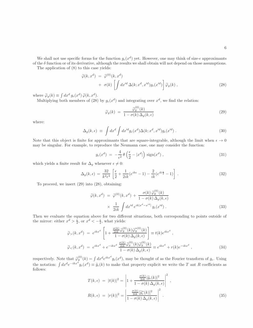
We shall not use specific forms for the function gǫ(xd) yet. However, one may think of size-ǫ approximants

of the δ function or of its derivative, although the results we shall obtain will not depend on those assumptions.The application of (8) to this case yields:

ϕ(k, xd) = ϕ(0)(k, xd)

+ σ(k)

[∫dx′d ∆(k;xd, x′d)gǫ(x

′d)

]ϕg(k) , (28)

where ϕg(k) ≡∫dxd gǫ(x

d) ϕ(k, xd).

Multiplying both members of (28) by gǫ(xd) and integrating over xd, we find the relation:

ϕg(k) =ϕ(0)g (k)

1− σ(k)∆g(k, ǫ)(29)

where:

∆g(k, ǫ) ≡

∫dxd

∫dx′dgǫ(x

d)∆(k;xd, x′d)gǫ(x′d) . (30)

Note that this object is finite for approximants that are square-integrable, although the limit when ǫ → 0may be singular. For example, to reproduce the Neumann case, one may consider the function:

gǫ(xd) = −

4

ǫ2θ( ǫ

2− |xd|

)sign(xd) , (31)

which yields a finite result for ∆g whenever ǫ 6= 0:

∆g(k, ǫ) =32

k2ǫ4

[ǫ

2+

1

2ik(eikǫ − 1)−

2

ik(eik

ǫ

2 − 1)

]. (32)

To proceed, we insert (29) into (28), obtaining:

ϕ(k, xd) = ϕ(0)(k, xd) +σ(k) ϕ

(0)g (k)

1− σ(k)∆g(k, ǫ)

×1

2ik

∫dx′d eik|x

d−x′d| gǫ(x′d) . (33)

Then we evaluate the equation above for two different situations, both corresponding to points outside ofthe mirror: either xd > ǫ

2 , or xd < − ǫ

2 , what yields:

ϕ>(k, xd) = eikx

d

[1 +

σ(k)2ik ϕ

(0)g (k)ϕ

∗(0)g (k)

1− σ(k)∆g(k, ǫ)

]≡ t(k)eikx

d

,

ϕ<(k, xd) = eikx

d

+ e−ikxd

σ(k)2ik ϕ

(0)g (k)ϕ

(0)g (k)

1− σ(k)∆g(k, ǫ)≡ eikx

d

+ r(k)e−ikxd

, (34)

respectively. Note that ϕ(0)g (k) =

∫dxdeikx

d

gǫ(xd), may be thought of as the Fourier transform of gǫ. Using

the notation:∫dxde−ikxd

gǫ(xd) ≡ gǫ(k) to make that property explicit we write the T ant R coefficients as

follows:

T (k, ǫ) = |t(k)|2 =

∣∣∣∣∣1 +σ(k)2ik |gǫ(k)|

2

1− σ(k)∆g(k, ǫ)

∣∣∣∣∣

2

,

R(k, ǫ) = |r(k)|2 =

∣∣∣∣∣

σ(k)2ik [g∗ǫ (k)]

2

1− σ(k)∆g(k, ǫ)

∣∣∣∣∣

2

. (35)

7

After some calculations it is possible to show that R+T = 1. At this point it is worth to note that, generallyspeaking, nonlocality can induce violations to this relation, since the interaction with microscopic degreesof freedom in the mirror may affect unitarity. However, this is not the case for nonlocal kernels of the form(27).For the Neumann-like case, we may consider the ǫ → 0 limit with the gǫ introduced in (31). This yields

for ∆g the asymptotic behaviour:

∆g(k, ǫ) ∼ −4

3ǫ−1 − i

k

2, ǫ ∼ 0 , (36)

as it may be seen from (32).Note that, for the same approximant, we find:

gǫ(k) = −16

ikǫ2sin2(

kǫ

4) . (37)

To reach the exact NBC from the nonlocal case, one may use an appropriate dependence of σ, namely,choosing a σ(k, ǫ) such that that condition is approached in the limit when ǫ → 0. To that end, we take thederivative of (33) at the origin, and see that, when ǫ ∼ 0:

ϕ′(k, 0) ≃ ik

[1 +

k

2i

σ(k, ǫ)

1− σ(k, ǫ)∆g(k, ǫ)

](38)

thus, using a σ such that:

σ(k, ǫ)

1− σ(k, ǫ)∆g(k, ǫ)= −

2i

k, (39)

yields NBC, i.e. r(k) = 1 and t(k) = 0. It is worth noting that, as in the local case, the NBC are obtainedfor an infinitesimal value of σ, that is σ ≃ −3ǫ/4.Finally, we stress that the Dirichlet-like case is obtained by considering gǫ to tend to a δ function. This

implies gǫ(k) → 1, and ∆g(kǫ) →1

2ik , what (setting σ → µ0) reproduces the Dirichlet like case result.

III. CASIMIR ENERGY

We will now compute the Casimir energy for the configuration of two identical mirrors centered at xd = 0and xd = a in 3+1 dimensions. In principle, the Casimir energy can be obtained from the nonlocal effectiveaction using path integral techniques [7, 11]. However, it is simpler to use Lifshitz formula [8]. Indeed,we just need the analytic continuation to the imaginary frequency axis of the reflection coefficients alreadycomputed in the previous section. The reflection coefficients r(k) depend on the wave vector kα = (k0, k1, k2).Denoting by r the analytic continuation r = r(k0 = iξ, k1, k2), according to Lifshitz formula, the Casimirenergy then reads

E(a) =1

2π

∫ ∞

0

dξ

∫d2k

(2π)2log(1 − r2e−2κa) , (40)

where κ =√k21 + k22 + ξ2.

It is easy to see that, due to the symmetries we are assuming, r depends only on κ. Therefore, usingspherical coordinates in momentum space Lifshitz formula can be written as

E(a) =1

4π2

∫ ∞

0

dκ κ2 log(1− r2e−2κa) , (41)

8

which is well defined as long as r2 < 1.Let us now discuss the main properties of the reflection coefficients, for the local and nonlocal interaction

terms previously considered. For the Dirichlet-like boundary conditions considered in Section 2.1, the analyticcontinuation of the reflection coefficient, which can be read from (15), is given by:

r2 =

(µ0(κ)

2κ+ µ0(κ)

)2

. (42)

Note that r is well defined and smaller than 1 for µ0(κ) > 0. Besides, it does reproduce the DirichletCasimir energy in the limit µ0(κ)/κ → ∞. Inserting Eq.(42) into Eq.(41) we reproduce the usual result forδ-potentials [12].For the local Neumann-like case described in Section 2.2, the reflection coefficient is given in (25), and its

analytic continuation reads

r2 =

[µ2(κ)κ

2 + µ2(κ)(2ǫ−1 + κ)

]2, (43)

and it is well-defined except when −ǫ < µ2(κ) < 0. The Neumann Casimir energy can be reproduced whenµ2 → −ǫ from below.For the Neumann-like nonlocal boundary term considered in Section 2.3, equations (34) and (37) allow we

to derive

r2 =

[128 σ

ǫ4κ3(1 − σ∆g)sinh4(

κǫ

4)

]2, (44)

where σ and ∆g denote the analytic continuations of σ and ∆g respectively. In order to reproduce Neumannboundary conditions, σ must be a rather involved function of κ and ǫ. However, when computing the Casimirenergy for mirrors separated by a distance a ≫ ǫ, we expect the relevant values of κ to satisfy κǫ ≪ 1. Inthis limit, that function simplifies to σ = − 3

4ǫ. If we assume that σ is a constant, the Casimir energy for this

reflection coefficient is well defined as long as σ < − 34ǫ or σ > 0. These properties are illustrated in Fig. 1.

0

0.1

0.2

0.3

0.4

0.5

0.6

0.7

0.8

0.9

1

0 1 2 3 4 5 6 7 8 9 10

r2

k ε

σ / ε=−1σ / ε=−0.75σ / ε=0.25

FIG. 1: The reflection coefficient given in (44) as a function of x = κǫ, for different values of σ/ǫ. In the particularcase σ/ǫ = −0.75, the reflection coeficient tends to 1, reproducing NBC for x ≪ 1.

9

IV. GENERALIZATION TO ARBITRARY SURFACES AND WORLDLINE APPROACH

In the previous sections, we have introduced nonlocal interaction terms, which may be regarded as ‘reg-ularized’ versions of the terms one should introduce to impose Dirichlet or Neumann boundary conditions.Indeed, the singular terms involving Dirac’s δ function or its derivatives disappear, at the price of introducinga finite length scale.That step is not necessary for the Dirichlet case (unless one wanted to describe a medium with an intrinsic

nonlocality). On the other hand, because of its highly singular nature, a local Neumann term should beapproached as a special limit of a nonlocal term. Indeed, one should do so in order to tame the infinitiesthat otherwise would pop up at a very early stage, namely, when calculating the reflection and transmissioncoefficients, before dealing with the Casimir energy.The explicit construction of the nonlocal terms has, however, only been carried out for the simplest possible

case, regarding the mirror’s geometry. Indeed, we have considered terms which, in the local limit, wouldcorrespond to a plane mirror at xd = 0.Let us now extend the construction to more general surfaces. We have in mind a situation where one

really wants to deal with a Neumann-like condition on a local (zero-width) surface and, in order to do that,one temporarily introduces a small nonlocality along the normal direction to the surface, on a length scale∼ ǫ. That nonlocality is introduced to regularize the problem, and it should disappears in the end whenone takes the ‘zero width Neumann limit’ ǫ → 0 (and the corresponding limit for the coupling constant).Because of this reason, we shall make use of some simplifications that stem from the fact that, even though itis different from zero, ǫ is very small in comparison with the other characteristic length scales in the system.The only assumption about the surface will be that it is piecewise regular. Besides, it is sufficient to

consider just one surface. Indeed, for more than one surface, one just have to add more terms to the action:one for every disconnected piece. Also, for the sake of simplicity, we shall first assume that the nonlocalityonly exists for the normal direction to the surface. Finally, we shall restrict our study to the case of surfacesin three-dimensional space.Let us begin by writing the well-known local interaction term, corresponding to Dirichlet like boundary

conditions, for a zero-width static surface Σ, and generalize it to the nonlocal case afterwards. This surfacewill be assumed to be given in parametric form:

Σ : (σ1, σ2) → Y(σ) , Y(σ) ∈ R(3) . (45)

Then, the local Dirichlet-like interaction term SΣ(σ), is:

SΣ(ϕ) =µ0

2

∫dx0dσ1dσ2

√G(σ)

(ϕ[x0,Y(σ)]

)2(46)

where G(σ) ≡ det[Gab(σ)], with Gab(σ) ≡ Ta(σ) ·Tb(σ), a, b = 1, 2, and Ta(σ) ≡ ∂aY(σ).We then introduce a nonlocality in this term, proceeding as follows: we first construct the finite volume

region, Σǫ, that results from ‘dragging’ Σ along the normal direction. The volume Σǫ is spanned by introduceda new parameter, η (to be denoted also by σ3), in such a way that:

Σǫ : (σ1, σ2, η) → X(σ, η) , (47)

such that X(σ, 0) = Y(σ), ∀σ. η will have infinitesimal values around zero and we want it to introducedepartures in the normal direction only. Then, to first-order in η, a parametrization for Σǫ can be explicitlywritten:

X(σ, η) = X(σ, 0) + [∂ηX(σ, η)]η=0 η + O(η2)

= Y(σ) + N(σ) η + O(η2) , (48)

where we introduced the unit normal vector field:

N(σ) =T1(σ) ×T2(σ)

|T1(σ) ×T2(σ)|, (49)

10

at each point of the surface (which is assumed to be regular).In these coordinates, for small η, and using the index 3 for η, the metric tensor Gij(σ, η), (i, j = 1, 2, 3)

on Σǫ becomes: Gab(σ, η) = Gab(σ), Gaj(σ, η) = Gja(σ, η) = 0, and G33 = 1.With these conventions, we may write the local term above as follows:

SΣ(ϕ) =µ0

2

∫dx0dσ1dσ2dη

√G(σ) δ(η)

(ϕ[x0,X(σ, η)]

)2

=µ0

2

∫dx0dσ1dσ2

√G(σ)

(ϕ[x0,Y(σ)]

)2, (50)

as it should be.The nonlocal term (either Dirichlet or Neumann-like) is then constructed in a quite straightforward way:

SΣǫ(ϕ) =

λ

2

∫dx0dσ1dσ2

√G(σ) dη dη′gǫ(η) gǫ(η

′)

× ϕ[x0,X(σ, η)] ϕ[x0,X(σ, η′)] , (51)

where gǫ has the form of an approximant of the δ in the Dirichlet case, and of its derivative in the Neumanncase. Note that, with our conventions, η has the dimensions of a length. Thus we may effectively assumethat because of the function gǫ, the relevant range of η is ∼ [− ǫ

2 ,ǫ2 ].

As a concrete example, we may write SΣǫfor a sphere of radius R:

SΣǫ(ϕ) =

λ

2R2

∫dx0 dθ dϕ sin2 θ dr dr′gǫ(r) gǫ(r

′)

× ϕ[x0,X(θ, ϕ, r)] ϕ[x0,X(θ, ϕ, r′)] , (52)

where we used spherical coordinates.We conclude by presenting the implementation of this type of term within the worldline approach to

Casimir effect [9], a very useful tool for the calculation of Casimir energies. The usual worldline applies,by construction, to Dirichlet-like boundary conditions, which emerge as the result of the introduction of alocal potential term. On the other hand, as we have shown, Neumann conditions require the considerationof nonlocal terms, even when one is interested in imposing Neumann boundary conditions on a zero-widthsurface.Let us consider here the changes one has to introduce in the worldline approach, to be able to deal with

nonlocal potentials (we have in mind just the kind of nonlocality considered in the previous sections). Forthe Casimir energy of a (massive, for the sake of completeness) field in the worldline approach, the startingpoint is formally the same as in the local case; indeed, one first defines an effective action Γ[Vǫ]:

Γ[Vǫ] =1

2Tr ln

[−∂2 +m2 + Vǫ

−∂2 +m2

](53)

where now Vǫ is an operator whose matrix elements, in the coordinate representation, are:

Vǫ(x, x′) = 〈x|Vǫ|x

′〉 = 〈x0,x|Vǫ|x′0,x

′〉

= µ0 δ(x0 − x′0)

∫d2σ

√G(σ)

∫dη dη′

× gǫ(η)δ(3)

(x−X(σ, η)

)gǫ(η

′) δ(3)(x′ −X(σ, η′)

)(54)

(we follow here the usual convention whereby Dirac’s notation is used for the Hilbert space of functions ofx).Then, using Frullani’s representation [13] for the logarithm of a ratio, one has:

Γ[Vǫ] = −1

2

∫ ∞

0+

dT

T[K(T )−K0(T )] , (55)

11

where:

K(T ) =

∫d4xK(x, T ;x, 0) , (56)

K(x′′, T ;x′, 0) ≡ 〈x′′|e−TH |x′〉 , (57)

with H = p2 + m2 + Vǫ ≡ H0 + Vǫ, and

K0(x′′, T ;x′, 0) ≡ 〈x′′|e−TH0 |x′〉 . (58)

The only place where a departure with respect to the local case appears is in the path integral represen-tation for K(T ). Partitioning the T interval into many equal steps and evaluating the transition amplitudefor an infinitesinal evolution in each step, one realizes that, in the limit when the number of steps tends toinfinity, the following path integral representation emerges:

K(T ) = N e−m2T

∫

x(T )=x(0)

Dx e−S[x] (59)

where:

S[x] ≡ S0[x] + SI [x] (60)

with

S0[x] =

∫ T

0

dτ1

4x2(τ) , (61)

SI [x] =

∫ T

0

dτ

∫ T

0

dτ ′ Vǫ[x(τ), x(τ′)] , (62)

and N is a factor that comes from the path integration over momenta, and is independent of the potential.Finally, coming back to the effective action, and using the known result for the free transition amplitude,

one may write:

Γ[Vǫ] = −1

2

1

(4π)d+1

2

∫ ∞

0+

dT

T 1+ d+1

2

e−m2T[〈e−SI [x]〉 − 1

], (63)

where

〈e−SI [x]〉 =

∫x(0)=x(T )

Dx e−SI [x] e−S0[x]

∫x(0)=x(T )

Dx e−S0[x]. (64)

We do not dwell with the numerical evaluation of this kind of path integral, which may certainly be moredifficult than its local counterpart, since the interaction term is not simply the integral of a local function oftime. However, since the scale of nonlocality is assumed to be small, we expect the properties of the integralnot to be dramatically different to the standard ones. Finally, a scaling to unit proper time may be of courseimplemented in a similar way to the local case, as well as the extraction of a ‘center of mass’ for the closedpaths involved in the integral over paths.

12

V. CONCLUSIONS

We have shown that NBC can be obtained by coupling the field to an interaction term which, if one wantedto have well-defined transmission and reflection properties, has to include an intrinsic regularization. Wehave also provided an explicit mechanism to introduce that regularization in the calculation.That regularization may be naturally thought of as due to two sources: a finite width, and a finite nonlocal

coupling. Neumann conditions on a zero width surface emerge when one takes a special limit, whereby thecoupling constant is related to the width. One may then conclude that, to reach NBC, one needs essentiallyjust one constant to control the UV behaviour, rather than two independent scales. Of course, if one wantedto deal with a phenomenological model where the nonlocal term is derived, one may obtain more that onescale, and the resulting boundary conditions may exhibit a richer structure.We have presented a possible way to implement the kind of path integral that one would require if one

wanted to use a worldline approach to nonlocal terms. We believe such an approach might shed light on theproperties of the Casimir energy with NBC for arbitrary surfaces.

Acknowledgements

C.D.F. thanks CONICET, ANPCyT and UNCuyo for financial support. The work of F.D.M. and F.C.Lwas supported by UBA, CONICET and ANPCyT.

[1] M. Bordag, U. Mohideen, and V. M. Mostepanenko, Phys. Rep. 353, 1 (2001); K. A. Milton, The Casimir Effect:

Physical Manifestations of the Zero-Point Energy (World Scientific, Singapore, 2001); S. Reynaud et al., C. R.Acad. Sci. Paris IV-2, 1287 (2001); K. A. Milton, J. Phys. A: Math. Gen. 37, R209 (2004); S.K. Lamoreaux, Rep.Prog. Phys. 68, 201 (2005); M. Bordag, G.L. Klimchitskaya, U. Mohideen, and V. M. Mostepanenko, Advancesin the Casimir Effect, Oxford University Press, Oxford, 2009.

[2] C. D. Fosco, F. C. Lombardo and F. D. Mazzitelli, Phys. Rev. D 77, 085018 (2008).[3] D. Deutsch and P. Candelas, Phys. Rev. D 20, 3063 (1979).[4] N. Graham, R. L. Jaffe, V. Khemani, M. Quandt, O. Schroeder and H. Weigel, Nucl. Phys. B 677, 379 (2004).[5] R. Estrada, S. A. Fulling, Z. Liu, L. Kaplan, K. Kirsten and K. A. Milton, J. Phys. A 41, 164055 (2008).[6] P.B. Gilkey, K. Kirsten, D. Vassilevich, Lett. Math. Phys. 63 (2003) 29.[7] C. D. Fosco, F. C. Lombardo and F. D. Mazzitelli, Phys. Rev. D 80, 085004 (2009).[8] E.M. Lifshitz, Sov.Phys. JETP 2, 73 (1956); C. Genet, A. Lambrecht and S. Reynaud, Phys. Rev. A 67, 043811

(2003).[9] H. Gies, K. Langfeld and L. Moyaerts, JHEP 0306, 018 (2003).

[10] C. D. Fosco, F. C. Lombardo and F. D. Mazzitelli, Phys. Lett. B 669, 371 (2008).[11] R. Golestanian and M. Kardar, Phys. Rev. A 58, 1713 (1998).[12] M. Bordag, M. Hennig and D. Robaschik, J. Phys. A:Math. Gen25, 4483 (1992); K. Milton, J. Phys. A: Math.

Gen 37, 6391 (2004); K. A. Milton and J. Wagner, J. Phys. A 41, 155402 (2008).[13] H. Jeffreys and B. S. Jeffreys, Methods of Mathematical Physics, 3rd ed. Cambridge, England: Cambridge

University Press, pp. 406-407 (1988).