Homogenization of Neumann boundary data with

fully nonlinear operator

Sunhi Choi ∗, Inwon C. Kim†, and Ki-Ahm Lee‡

Abstract

In this paper we study periodic homogenization problems for solu-

tions of fully nonlinear PDEs, in half-spaces with oscillatory Neumann

boundary data. We show the existence, uniqueness of the homogenized

Neumann data for a given half-space. Moreover, we show that there ex-

ists a continuous extension of the homogenized slope as the normal of the

half-space varies over “irrational” directions.

1 Introduction

In this paper, we consider the averaging phenomena for solutions of uniformlyelliptic nonlinear PDEs, in half-spaces coupled with oscillatory Neumann bound-ary data. To be precise, let Mn−1 be the normed space of symmetric n × nmatrices and consider the function F (M) : Mn−1 → IR which satisfies

(F1) F is uniformly elliptic, i.e., there exists constants 0 < λ < Λ such that

λ‖N‖ ≤ F (M)− F (M +N) ≤ Λ‖N‖ for any N ≥ 0;

(F2) (homogeneity) F (tM) = tF (M) for any M ∈ Mn−1 and t > 0. In partic-ular F (0) = 0;

The homogeneity condition (F2) can be relaxed (e.g. see (F4) of [3]). Typicalexamples of nonlinear operators which satisfy (F1)-(F3) are the Pucci extremaloperators:

P+(D2u(x)) := λ∑

µi<0

µi + Λ∑

µi≥0

µi; P−(D2u(x)) := Λ∑

µi<0

µi + λ∑

µi≥0

µi

where µ1, · · · , µn are eigenvalues of D2u(x).

∗Dept. of Mathematics, University of Arizona. schoi@math.arizona.edu.†Dept. of Mathematics, UCLA. ikim@math.ucla.edu. Partially supported by NSF DMS-

0970072.‡School of Mathematical Sciences, Seoul National University, South Korea. ki-

ahm@math.snu.ac.kr. Partially supported by NRF MEST 2010- 0001985.

1

Let (e1, ..., en) be an orthonormal basis of IRn and suppose g(x) : IRn → IRsatisfies

(a) g ∈ Cβ(IRn), for some 0 < β ≤ 1;

(b) g(x+ ek) = g(x) for x ∈ IRn for k = 1, ..., n.

Next, for given p ∈ IRn let Πν(p) be a strip domain in IRn with unit normal ν,that is

Πν(p) = x : −1 ≤ (x− p) · ν ≤ 0, where |ν| = 1. (1)

With F, g and Πν be as given above, our goal is to describe the limitingbehavior of uǫ as ǫ → 0, where uǫ satisfies

(Pǫ)

F (D2uǫ) = 0 in Πν(p)

ν ·Duǫ = g(xǫ ) on Γ0 := (x− p) · ν = 0.

u = 1 on ΓI := (x− p) · ν = −1.

The fixed boundary data on ΓI is introduced to avoid discussion of the compat-ibility condition on g and to ensure the existence of uǫ.

Homogenization of elliptic, divergence-form equations, with oscillatory coef-ficients and co-normal boundary data, is a classical subject. Let Ω be an openand bounded subset of IRn. Consider uǫ : Ω → IR solving

∇ · (A(x

ǫ)∇uǫ) = 0, (2)

with the Neumann (co-normal) condition

ν · (A(x/ǫ)∇u)(x) = g(x/ǫ), x ∈ ∂Ω. (3)

The problem (2)-(3) has been widely studied and by now has been well-understood(see [4] for an overview): first let us consider the case when Ω is a half-space:i.e. let

Ω = Σν := x : (x− p) · ν ≤ 0.

We define the averaged Neumann data

µ(ν, ǫ) :=

∫

(x−p)·ν=0,|x−p|≤1

g(x

ǫ)dx. (4)

By integration by parts one can show that uǫ locally uniformly converges to acontinuous function u0 : Ω → IR as ǫ → 0 if and only if µ(ν) := limǫ→0 µ(ν, ǫ)exists, and that u0 solves the averaged equation

(Pdiv)

−∇ · (A0∇u0)(x) = 0 for x ∈ Ω,

ν · (A0∇u0) = µ(ν) for x ∈ ∂Ω.

Therefore different results hold depending on the choice of p and ν:

2

(a) If ν is parallel to a vector in ZZn (i.e. ν is a “rational” vector), then µ(ν)exists if p = 0, and

µ(ν) = the average of g(y) on the hyperplane x · ν = 0.

(b) If ν is a rational vector and p 6= 0, then there may be no limit of µ(ν, ǫ)and uǫ can have different subsequential limits.

(c) If ν is not a rational vector, then due to Weyl’s equi-distribution theorem(Lemma 2.5) µ(ν, ǫ) converges to

µ(ν) =< g >:=

∫

[0,1]ng(y)dy,

independent of the choice of p. In particular, the homogenized slope µ(ν)is discontinuous at every rational direction ν, but otherwise continuous.

From above results, the divergence form of the operator, and the fact thatrational directions are of zero measure in Sn−1 := x ∈ IRn : |x| = 1, thefollowing results hold for the general domain Ω: if ∂Ω does not contain flat pieceswhose normal vectors belong to IRZZn, then uǫ converges locally uniformly tothe solution u0 of (Pdiv) with µ(ν) replaced by < g >. We refer to [4] fordetailed analysis. Note that u0 is smooth up to the boundary due to the factthat < g > is continuous (constant in particular).

For nonlinear or non-divergence type operators, or for linear operators withoscillatory nonlinear boundary data, little is known for the homogenization ofthe oscillating Neumann boundary data. Most available results concern half-space domains going through the origin with its normal pointing to a rationaldirection. In [14], Tanaka considered some model problems in half-space whoseboundary is parallel to the axes of the periodicity by purely probabilistic meth-ods. In [2], Arisawa studied special cases of problems in oscillatory domainsnear half spaces going through the origin, using viscosity solutions as well asstochastic control theory. Generalizing the results of [2], Barles, Da Lio andSouganidis [3] studied the problem for operators with oscillating coefficients,in half-space type domains whose boundary is parallel to the axes of periodic-ity, with a series of assumptions which guarantee the existence of approximatecorrector.

In this paper we extend above results to the setting of general half-spaces Πν ,defined in (1), where p is not necessarily zero and ν ranges over all directions inIRn. In particular we show the continuity properties of the homogenized slopeµ(ν) over the normal directions ν (see Theorem 1.2 (ii)), with the hope thatsuch results will lead to better understanding of homogenization phenomena indomains with general geometry (work in progress). Note that, as observed inthe linear case, homogenized slope may not exist if ν is parallel to a vector inZZn and if p 6= 0, therefore the best result we can hope for is the existence

3

of the continuous function µ(ν) : Sn−1 → IR such that µ(ν) = µ(ν) for ν ∈Sn−1 − IRZZn. This is precisely what we will show.

Before stating the main theorem, let us introduce some notations.

Definition 1.1.

1. ν ∈ Sn−1 is a rational direction if ν ∈ IRZZn.

2. ν ∈ Sn−1 is an irrational direction if ν is not a rational direction.

Theorem 1.2 (Main Theorem). For a given p ∈ IRn, let uǫ solve (Pǫ). Thenthe following holds:

(i) Let ν be an irrational direction. Then there is a unique constant µ(ν) ∈[min g,max g] such that uǫ locally uniformly converges to the solution of

(P )

F (D2u) = 0 in Πν

ν ·Du = µ(ν) on Γ0

u = 1 on ΓI .

(ii) µ(ν) : (Sn−1− IRZZn) → IR has a continuous extension µ(ν) : Sn−1 → IR.

(iii) For rational directions ν, if Γ0 goes through the origin (that is if p = 0),then the statement in (i) holds for ν as well.

(iv) [Error estimate] Let ν be an irrational direction. Then for uǫ and u solving(Pǫ) and (P ), we have the following estimate: for any 0 < α < 1, thereexists a constant Cα > 0 such that

|uǫ − u| ≤ Cαω(ǫ)α in Πν . (5)

Here ω(ǫ) depends on the “discrepancy” associated to ν as defined in (7).

Remark 1.3. Our method can be applied to the operators of the formF (D2u, x) = f(x) with F and f continuous in x, but we will restrict ourselves tothe simple case discussed in (Pǫ) for the clarity of exposition. On the other hand,our proof for the continuity of µ(ν) (Theorem 1.2 (ii)), presented in section 4.2,cannot handle the case where the operator F depends on the oscillatory variablex/ǫ (see Remark 4.9).

Acknowledgement We thank Takis Souganidis for helpful discussionsas well as motivating the problem. We also thank Luis Caffarelli for helpfuldiscussions regarding Remark 1.3.

4

2 Preliminary results

Let Ω be an open, bounded domain. Let ΓI be a part of its boundary, anddefine Γ0 := ∂Ω− ΓI . For a continuous function f(x, ν) : IRn × Sn−1 → IR, letus recall the definition of viscosity solutions for the following problem:

(P )f

F (D2u) = 0 in Ω;

ν ·Du = f(x, ν) on ∂Ω− ΓI ;

u = 1 on ΓI ,

where ν = νx denotes the outward normal at x ∈ ∂Ω with respect to Ω.The following definition is equivalent to the ones given in [8]:

Definition 2.1. (a) An upper semi-continuous function u : Ω → IR is a vis-cosity subsolution of (P )f if

(i) u ≤ 1 on ΓI ;

(ii) For given domain Σ ⊂ IRn, u cannot cross from below any C2 func-tion φ in Σ which satisfies

F (D2φ) > 0 in Ω ∩ Σ;ν ·Dφ > f(x, ν) on Γ0 ∩Σ;

φ > u on (∂Σ ∪ ΓI) ∩ Σ.

(b) A lower semi-continuous function u : Ω → IR is a viscosity supersolutionof (P )f if

(i) u ≥ 1 on K,

(ii) For a given domain Σ ⊂ IRn,u cannot cross from above any C2 func-tion ϕ which satisfies

F (D2φ) < 0 in Ω ∩ Σ;ν ·Dφ < f(x, ν) on Γ0 ∩Σ;

φ < u on (∂Σ ∪ ΓI) ∩ Σ.

(c) u is a viscosity solution of (P )f if u is both a viscosity sub- and superso-lution of (P )f .

Existence and uniqueness of viscosity solutions of (P )f is based on the com-parison principle we state below:

Theorem 2.2 (Section V, [10]). Suppose Ω,ΓI , Γ0, F and ν are as given above,and let f : IRn×Sn−1 → IR be continuous. Let u and v respectively be a viscositysub- and supersolution of (P )f in a domain Σ ⊂ IRn. If u ≤ v on ∂Σ, thenu ≤ v in Ω.

5

For details on the proof of the above theorem as well as well-posedness ofthe problem (P )f , we refer to [8],[9], [10].

Next we state some regularity results that will be used in the paper.

Theorem 2.3. [Chapter 8, [5], modified for our setting] Let u be a viscositysolution of F (D2u) = 0 in a domain Ω. Then for any 0 < α < 1 and for anycompact subset Ω′ of Ω, we have

‖u‖Cα(Ω′) ≤ Cd−α‖u‖L∞(Ω)

where C > 0 depends on n, λ,Λ and d = d(Ω′, ∂Ω).

Theorem 2.4 (Theorem 8.1 and Theorem 8.2 in [13]). Let

B+r := |x| < r ∩ x · en ≥ 0 and Γ := x · en = 0 ∩B1.

Let u be a viscosity solution of

F (D2u) = 0 in B+1

ν ·Du = g in Γ.

(a) Suppose g is bounded. Then u is in Cα(B+1/2) for some α = α(n, λ,Λ).

Moreover, we have the estimate

‖u‖Cα(B+

1/2)≤ C(‖u‖

L∞(B+

1)+max ‖g‖).

(b) Suppose g ∈ Cβ(IRn) where 0 < β ≤ 1. Then u is in C1,γ(B+1/2) where

γ = min(α0, β) and α0 = α0(n, λ,Λ). Moreover, we have the estimate

‖u‖C1,α(B+

1/2)≤ C(‖u‖

L∞(B+

1)+ ‖g‖Cβ)

In (a)-(b), C denotes a positive constant depending only on n, λ,Λ and α.

Let us next discuss the averaging property of the sequence (nx)n mod 1,where x is an irrational number, and its applications to multi-dimensions whichwill serve useful in our analysis in section 3. Since we obtain estimates onthe convergence rate of solutions for (Pǫ) in our result, we are particularlyinterested in the estimates on the rate of convergence of the sequence (nx)n tothe uniform distribution (Definition 2.6). We begin with recalling the notion ofequi-distribution.

• A bounded sequence (x1, x2, x3...) of real numbers is said to be equi-distributedon an interval [a, b] if for any [c, d] ⊂ [a, b] we have

limn→∞

|x1, ..., xn ∩ [c, d]|

n=

d− c

b− a.

Here |x1, ..., xn ∩ [c, d]| denotes the number of elements.

• The sequence (x1, x2, x3, ...) is said to be equidistributed modulo 1 if (x1 −[x1], x2 − [x2], ...) is equidistributed in the interval [0, 1].

6

Lemma 2.5 ([15], Weyl’s equidistribution theorem). If a is an irrational num-ber, (a, 2a, 3a, ...) is equidistributed modulo 1.

To discuss quantitative versions of Lemma 2.5, we introduce the notion ofdiscrepancy. The following definition is from the book [12].

Definition 2.6. Let (xk), k = 1, 2, ..., be a sequence in IR. For a subset E ⊂[0, 1], let A(E;N) denote the number of points xn, 1 ≤ n ≤ N , that lie in E.

(a) The sequence (xn), n = 1, 2, .... is said to be uniformly distributed mode 1in IR if

limN→∞

A(E;N)

N= µ(E)

for all E = [a, b). Here µ denotes the Lebesgue measure.

(b) For x ∈ [0, 1], let us define the discrepancy

DN(x) := supE=[a,b)

∣

∣

∣

A(E;N)

N− µ(E)

∣

∣

∣,

where A(E;N) is defined with the sequence (kx), k ∈ IN , modulo 1.

It easily follows from Lemma 2.5 that the sequence (xk) = (kx)k∈IN is uni-formly distributed modulo 1 for any irrational number x ∈ IR. In particularDN(x) converges to zero as N → ∞.

Next, let Sn−1 = ν ∈ IRn : |ν| = 1. For a direction ν = (ν1, ..., νn) ∈ Sn−1,let νi be the component with the biggest size, i.e.,

|νi| = max|νj| : 1 ≤ j ≤ n

(If there are multiple components then we choose the one with largest index).Let Hν be the hyperplane in IRn, which passes through 0 and is normal to

ν, i.e.,Hν = x ∈ IRn : x · ν = 0.

Since νi 6= 0, there exists m(ν) such that (1, ..., 1,m(ν), 1, ..., 1) ∈ Hν , i.e.,

(1, ..., 1,m(ν), 1, ..., 1) · ν = 0 (6)

where m(ν) is the i-th component of (1, ..., 1,m(ν), 1, ..., 1). Then we define

ων(ǫ) := DN(m(ν)), where N = ǫ−9/10. (7)

Note that, if m(ν) is irrational, then ων(ǫ) → 0 as ǫ → 0.

Now we are ready to state our quantitative estimate on the averaging prop-erties of the vector sequence (nν) with an irrational direction ν, which will beused in the rest of the paper. Recall that for ν ∈ Sn−1,Πν(p) = x : −1 ≤ (x− p) · ν ≤ 0. Denote Γ0 = x : (x− p) · ν = 0 and define

Hν = x : x · ν = 0.

7

Lemma 2.7. For ν ∈ IRn and x0 ∈ Πν , let H(x0) := Hν + x0. Let 0 < ǫ <dist(x0,Γ0).

(i) Suppose that ν is a rational direction. Then for any x ∈ H(x0), there isy ∈ H(x0) such that

|x− y| ≤ Mνǫ; y − x0 ∈ ǫZZn

where Mν > 0 is a constant depending on ν.

(ii) Suppose that ν is an irrational direction, and let w : [0, 1) → IR+ definedas in (7). Then there exists a dimensional constant M > 0 such that suchthat the following is true: for any x ∈ H(x0), there is y ∈ IRn such that

|x− y| ≤ Mǫ1/10; y − x0 ∈ ǫZZn

anddist(y,H(x0)) < ǫων(ǫ), (8)

where ων is as given in (7).

(iii) If ν is an irrational direction, then for any z ∈ IRn and δ > 0, there isw ∈ H(x0) such that

|z − w| ≤ δ mod ǫZZn.

Proof. The proof of (i) is immediate from the fact that for any rational directionν, there exists an integer M > 0 depending on ν such that Mν ∈ ZZn.

Next, we prove (ii). Let ν be an irrational direction in IRn. Without loss ofgenerality, we may assume

|νn| = max|νj | : 1 ≤ j ≤ n.

Let x be any point on H(x0): after a translation we may assume that x = 0.Choose m such that

ǫ(1, 1, .., 1,m) ∈ H(x0).

Note that M = |m| ≤ n2. Also note that m is irrational since ν is an irrationaldirection. Since H(x0) contains x = 0,

kǫ(1, 1, .., 1,m) ∈ H(x0) for any integer k.

Consider the sequence (km), k ∈ IN . From the definition of ω(ǫ) and thediscrepancy function DN (m), it follows that any interval [a, b] ⊂ [0, 1] of lengthω(ǫ) contains at least one point km (mod 1), for some k ≤ N = ǫ−9/10.

Hence for anyz = (0, 0, ..., 0, xn) ∈ [0, ǫ]n,

there existsw = kǫ(1, 1, .., 1,m) ∈ H(x0), 0 ≤ k ≤ ǫ−9/10

8

such that|z − w| ≤ ǫω(ǫ) mod ǫZZn.

Similarly, for any z ∈ [0, ǫ]n, there exists w ∈ H(x0)∩ (kǫ(1, 1, ..., 1,m)+ [0, ǫ]n)such that

|z − w| ≤ ǫω(ǫ) mod ǫZZn; 0 ≤ k ≤ ǫ−9/10. (9)

We continue with the proof of (ii). Recall that the coordinates are shiftedso that x = 0. Thus it suffices to find y ∈ IRn such that

|x− y| = |y| ≤ Mǫ1/10; |y − x0| = 0 mod ǫZZn

anddist(y,H(x0))| < ǫων(ǫ).

By (9), there exists w ∈ H(x0) such that

|x− w| = |w| ≤ Mkǫ ≤ Mǫ1/10 (10)

and|x0 − w| ≤ ǫων(ǫ) mod ǫZZn. (11)

Given w satisfying (11), we can take y ∈ IRn such that

|x0 − y| = 0 mod ǫZZn, and |y − w| ≤ ǫων(ǫ).

Then by (10)

|y| ≤ |y − w|+ |w| ≤ Mǫ1/10 + ǫων(ǫ) ≤ Mǫ1/10.

Also since w is contained in H(x0),

dist(y,H(x0)) ≤ |y − w| ≤ ǫων(ǫ)

(iii) is a direct consequence of (9).

3 In the strip domain

Fix p ∈ IRn and ν ∈ Sn−1 such that p · ν 6= 0. Let

Π = Πν = x ∈ IRn : −1 ≤ (x− p) · ν ≤ 0

We consider a bounded viscosity solution uǫ of

(Pǫ)

F (D2uǫ) = 0 in Π

∂uǫ/∂ν = g(x/ǫ) on Γ0 := x : (x − p) · ν = 0

uǫ = 1 on ΓI := x : (x − p) · ν = −1.

Below we prove existence and uniqueness of uǫ.

9

Lemma 3.1. Let f(x) : IRn → IR be continuous and bounded. Let Πν be asgiven above and define BR(p) := |x − p| ≤ R. Suppose w1 and w2 solve, inthe viscosity sense,

(a) F (D2w1) ≤ 0, F (D2w2) ≥ 0 in ΣR := Πν(p) ∩BR(p);

(b) ∂w1/∂ν ≤ f(x) ≤ ∂w2/∂ν on Γ0;

(c) w1 = w2 on ΓI ;

(d) w1 = −M , w2 = M on Π ∩BR(p).

Then, for R > 2 and C = nΛλ we have

w1 ≤ w2 ≤ w1 +3CM

R2in Π ∩B1(p).

Proof. Without loss of generality, let us set ν = en and p = 0. The firstinequality, w1 ≤ w2, directly follows from Theorem 2.2 To show the secondinequality, consider ω := w1 +M(h1 + h2), where

h1 =1

R2((x1)

2 + ...+ (xn)2) and h2 =

C

R2(1− (xn)

2)

with C =nΛ

λ. We claim w2 ≤ ω. To see this, note that

F (D2ω) = F (D2w1 +D2h1 +D2h2)

≥ F (D2w1) +2

R2(Cλ− nΛ) ≥ F (D2w1) in ΣR.

On the boundary of ΣR, ω satisfies

∂xn ω = ∂xnω1 = ∂xnω2 on ΣR ∩ xn = 0

andw2 ≤ ω on Γ0 ∩BR(0) and on ∂BR(0) ∩ Πν(p).

It follows from Theorem 2.2 that w2 ≤ ω in ΣR, and we are done.

Lemma 3.2. There exists a unique bounded solution u of (Pǫ).

Proof. 1. Let ΣR be as given in Lemma 3.1, and consider the viscosity solutionωR(x) of (Pǫ) in ΣR with with the lateral boundary data M = 1 on ∂BR(p)∩Π.The existence and uniqueness of the viscosity solution ωR is shown, for example,in [8], [9], [10].

Note that, by the maximum principle, ωR ≤ 1 + max(g) in ΣR. Due toTheorem 2.4 and Arzela-Ascoli Theorem, ωR locally uniformly converges to acontinuous function uǫ(x). Then the stability property of viscosity solutions itfollows that uǫ(x) is a viscosity solution of (Pǫ).

10

2. To show uniqueness, suppose u1 and u2 are both viscosity solutions of(Pǫ) with |u1|, |u2| ≤ M . Then Lemma 3.1 yields that, for any point q ∈ Γ0 andany R > 2,

|u1 − u2| ≤ O(1/R2) in B1(q) ∩ Π.

Hence u1 = u2.

The following is immediate from Theorem 2.2 and the construction of uǫ inabove lemma.

Corollary 3.3. Suppose u and v are bounded and continuous in Πν(p) andsolve

(a) F (D2u) ≤ 0 ≤ F (D2v) in Πν(p);

(b) u ≤ v on ΓI ;

(c) ∂u∂ν ≤ f(x) ≤ ∂v

∂ν on Γ0,

where f(x) : IRn → IR is continuous. Then u ≤ v in Πν(p).

In the rest of this section we will repeatedly use the fact that linear profilesas well as constants solve F (D2u) = 0.

Lemma 3.4. Let Πν(p) as given in (Pǫ) and let 0 < ǫ < 1. Suppose that w1

and w2 are bounded and solve, in the viscosity sense,

F(

D2wi

)

= 0 in Πν(p);|w1 − w2| ≤ ǫ on ΓI ;∂w1/∂ν − ∂w2/∂ν = A on Γ0.

Then there exists a positive constant C = C(A) such that

|w1 − w2| ≥ C − ǫ in Πν(p) ∩B1/2(p).

Proof. Let w := w2+h, where h(x) = A(x−p)·ν+A−ǫ. Then ∂ω/∂ν = ∂ω1/∂νon Γ0. Also, ω ≤ w1 on ΓI . Therefore Corollary 3.3 yields that w2 + h ≤ w1.Since h ≥ A/2− ǫ in B1/2(p), we are done.

Lemma 3.5. Let let Π = Π + aν for some 0 ≤ a ≤ Aǫ where 0 < A < 1.Suppose uǫ and uǫ are bounded and solve (Pǫ) respectively in the domains Πand Π. Then we have

|uǫ − uǫ| ≤ C(Aβ + ǫα) in Π ∩ Π,

where α is as given in Theorem 2.4 and β is the Holder exponent of g.

11

Proof. 1. Let vǫ(x) = uǫ(x + aν) so that vǫ and uǫ are defined in the samedomain Π. Since g(x) ∈ Cβ(IRn), |∂vǫ/∂ν − ∂uǫ/∂ν| ≤ wβ(ǫ) on Γ0.

2. On ΓI , uǫ = vǫ = 1. Hence one can compare uǫ ± w(ǫ)(1 + (x − p) · ν)with vǫ and apply Theorem 2.2 to obtain

|uǫ − vǫ| ≤ wβ(ǫ) in Π.

Due to the Holder continuity of uǫ given by Theorem 2.4, |vǫ − uǫ| ≤ CAβ + ǫα

in Π ∩ Π. This finishes the proof.

The next lemma follows from Theorem 2.4 (b).

Lemma 3.6. Let vj be a bounded solution of (Pǫ) with a constant Neumanncondition g(x) = µj. If µj → µ, then vj converges to v such that ∂v/∂ν = µ onΓ0.

4 Proof of the Main Theorem

In this section, we prove the main theorem of the paper, Theorem 1.2.

4.1 Proof of Theorem 1.2 (i), (iii) and (iv)

RecallΓ0 = x : (x− p) · ν = 0; ΓI = x : (x− p) · ν = −1.

Due to the uniform Holder regularity of uǫ (Theorem 2.4(a)), along subse-quences uǫj → u in Πν . Note that there could be different limits along differentsubsequences ǫj. Below we will show that if ν is an irrational direction then allsubsequential limits of uǫ coincide.

Suppose0 ∈ Πν = −1 < (x − p) · ν < 0.

Let us choose one of the convergent subsequence uǫj and denote uǫj = uj. Thenfor each j, there exists a constant µj and a function vj in Πν(p) such that

(Pµj )

F (D2vj) = 0 in Πν(p)

∂vj/∂ν = µj on Γ0

vj = uj = 1 on ΓI

vj = uj at x = 0.

Lemma 4.1. µj → µ for some µ as j → ∞. (µ may be different for differentsubsequences ǫj.)

12

Proof. Suppose not, then there would be a constant A > 0 such that for anyN > 0, |µm − µn| ≥ A for some m,n > N . Then by Lemma 3.4,

|vm(0)− vn(0)| ≥ CA.

This contradicts the fact that vj(0) = uj(0), since uj(0) → u(0) as j → ∞.

The next lemma states that uǫ looks like a linear profile with respect to thedirection ν as ǫ → 0.

Lemma 4.2. Away from the Neumann boundary Γ0, uǫ is almost a constanton hyperplanes parallel to Γ0. More precisely, let x0 ∈ Πν(p) with dist(x0,Γ0) >ǫ1/20. Then for 0 < α < 1 the following holds:

(i) If ν is a rational direction, there exists a constant C > 0 depending on ν,α and n, such that for any x ∈ H(x0) := (x− x0) · ν = 0

|uǫ(x)− uǫ(x0)| ≤ Cǫα/2. (12)

(ii) If ν is any irrational direction, there exists a constant C > 0 dependingon α and n, such that for any x ∈ H(x0)

|uǫ(x) − uǫ(x0)| ≤ Cǫα/20 + Cwν(ǫ)α (13)

where wν : [0,∞) → [0,∞) is a mode of continuity given as in (ii) ofLemma 2.7.

Proof. First, let ν be a rational direction. Lemma 2.7 implies that for anyx ∈ H(x0), there is y ∈ H(x0) such that |x − y| ≤ Mνǫ and uǫ(y) = uǫ(x0).Then by Theorem 2.3,

|uǫ(x0)− uǫ(x)| ≤ Cǫ−α/20(Mνǫ)α ≤ Cǫα/2.

Next, we assume that ν is an irrational direction and x ∈ H(x0). By (ii) ofLemma 2.7, there exists y ∈ IRn such that |x− y| ≤ Mǫ1/10, y − x0 ∈ ǫZZn and

dist(y,H(x0)) < ǫw(ǫ). (14)

Then we obtain

|uǫ(x0)− uǫ(x)| ≤ |uǫ(x0)− uǫ(y)|+ |uǫ(y)− uǫ(x)|

≤ Cw(ǫ)β + |uǫ(y)− uǫ(x)|

≤ Cw(ǫ)β + Cǫ−α/20(Mǫ1/10)α

≤ Cw(ǫ)β + Cǫα/20, (15)

where the second inequality follows from Lemma 3.5 with (14), and the thirdinequality follows from Theorem 2.3.

13

By Lemma 4.2 and by the comparison principle (Theorem 2.2), we obtainthe following estimate: For x ∈ Π,

|uǫ(x) − vǫ(x)| ≤ Λ(ǫ) (16)

where

Λ(ǫ) =

Cǫα/2 if ν is a rational direction

Cǫα/20 + Cwν(ǫ)β if ν is any irrational direction.

Lemma 4.3. lim vj = lim uj and hence ∂u/∂ν = µ on Γ0.

Proof. Observe that vj solves (Pǫj ) with g = µj : Note that vj is then a linearprofile, i.e., vj(x) = µj((x − p) · ν + 1) + 1. Let x0 be a point between Γ0 andH(0). Then by Lemma 4.2, applied to uj and vj ,

|(uj(x)− vj(x))− (uj(x0)− vj(x0))| ≤ Cw(ǫj). (17)

for all x ∈ H(x0), if j is sufficiently large. Suppose now that

uj(x0)− vj(x0) > c > 0 for sufficiently large j.

Then due to (16) uj − vj ≥ c/2 on H(x0) if j is sufficiently large. Note that uj

can be constructed as the locally uniform liimt of uj,R, where uj,R solves

F (D2uj,R) = 0 in BR(x0) ∩ Π; uj,R = vj on ∂BR(x0) ∩ Π

with

uj,R = 1 on ΓI ;∂

∂νuj,R(x) = g(

x

ǫj) on Γ0.

Comparing uj,R and vj + c((x− x0) · ν + 1) on the domain

BR(x0) ∩ x : −1 ≤ (x− p) · ν ≤ (x− x0) · ν

for sufficiently large R then yields that uj,R(0) ≥ vj(0) + c0 for all sufficientlylarge R, which would contradict the fact that vj(0) = uj(0). Similarly the caselim infj(uj(x0)− vj(x0) < 0 can be excluded. and it follows that

|uj(x0)− vj(x0)| → 0 as j → ∞.

Hence we get vj → u in each compact subset of Π. By Lemma 4.1 andLemma 3.6, the limit u = v of vj satisfies ∂u/∂ν = µ on Γ0.

Lemma 4.4. If ν is an irrational direction, ∂u/∂ν = µν for a constant µν

which depends on ν, not on the subsequence ǫj.

14

Proof. 1. Let 0 < η < ǫ be sufficiently small. Let

wǫ(x) =uǫ(ǫx)

ǫ, wη(x) =

uη(ηx)

η

and denote by Γ1 and Γ2 as the corresponding Neumann boundary of wǫ andwη, respectively. By (iii) of Lemma 2.7, for a point p ∈ IRn, there exist q1 ∈ Γ1

and q2 ∈ Γ2 such that

|p− q1| ≤ η mod ZZn, and |p− q2| ≤ η mod ZZn.

Hence after translations by p− q1 and p− q2, we may suppose that wǫ(x) andwη(x) are defined, respectively, on the extended strips

Ωǫ := x : −1

ǫ≤ (x − p) · ν ≤ 0

and

Ωη := x : −1

η≤ (x− p) · ν ≤ 0.

Here wǫ = 1/ǫ on (x − p) · ν = − 1ǫ and wη = 1/η on (x − p) · ν = − 1

η.

Moreover on Γ0 := (x− p) · ν = 0 we have

∂wǫ/∂ν = g1(x) := g(x− z1) and ∂wη/∂ν = g2(x) := g(x− z2)

where |z1|, |z2| ≤ η. Observe that since g has Holder exponent 0 < β ≤ 1,|g1 − g2| ≤ ηβ .

Let vǫ be a solution of the problem (Pǫ) with constant Neumann data∂vǫ/∂ν = µǫ on Γ0 such that vǫ coincides with uǫ at x = 0 and on ΓI . By (16)

|wǫ(x) −vǫ(ǫx)

ǫ| ≤

Cǫα/20 + Cw(ǫ)β

ǫ. (18)

Note that vǫ is a linear profile: indeed

vǫ(ǫx)

ǫ= µǫ((x− p) · ν +

1

ǫ) +

1

ǫ.

¿From (18) and the comparison principle, it follows that

(µǫ − Λ(ǫ))((x − p) · ν +1

ǫ) ≤ wǫ(x) −

1

ǫ≤ (µǫ + Λ(ǫ))((x − p) · ν +

1

ǫ) (19)

where Λ(ǫ) = Cǫα/20 + Cw(ǫ)β .

2. (19) means that the slope of wǫ in the direction of ν (i.e. ν · Dwǫ) isbetween µǫ +Λ(ǫ) and µǫ −Λ(ǫ) on x : (x− p) · ν = − 1

ǫ. Now let us considerlinear profiles

l1(x) = a1(x− p) · ν + b1 and l2(x) = a2(x− p) · ν + b2,

15

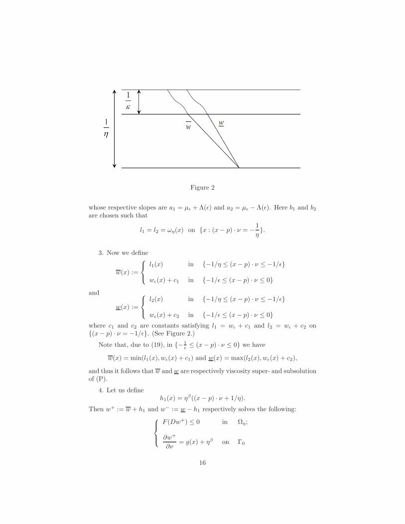
Figure 2

whose respective slopes are a1 = µǫ + Λ(ǫ) and a2 = µǫ − Λ(ǫ). Here b1 and b2are chosen such that

l1 = l2 = ωη(x) on x : (x− p) · ν = −1

η.

3. Now we define

w(x) :=

l1(x) in −1/η ≤ (x− p) · ν ≤ −1/ǫ

wǫ(x) + c1 in −1/ǫ ≤ (x− p) · ν ≤ 0

and

w(x) :=

l2(x) in −1/η ≤ (x− p) · ν ≤ −1/ǫ

wǫ(x) + c2 in −1/ǫ ≤ (x− p) · ν ≤ 0

where c1 and c2 are constants satisfying l1 = wǫ + c1 and l2 = wǫ + c2 on(x− p) · ν = −1/ǫ. (See Figure 2.)

Note that, due to (19), in − 1ǫ ≤ (x− p) · ν ≤ 0 we have

w(x) = min(l1(x), wǫ(x) + c1) and w(x) = max(l2(x), wǫ(x) + c2),

and thus it follows that w and w are respectively viscosity super- and subsolutionof (P).

4. Let us defineh1(x) = ηβ((x − p) · ν + 1/η).

Then w+ := w + h1 and w− := w − h1 respectively solves the following:

F (Dw+) ≤ 0 in Ωη;

∂w+

∂ν= g(x) + ηβ on Γ0

16

and

F (Dw−) ≥ 0 in Ωη

∂w−

∂ν= g(x)− ηβ on Γ0.

Since |g − g| ≤ ηβ and w+ = w− = wη on (x − p) · ν = − 1η, from the

comparison principle for (Pǫ) it follows that

w− ≤ wη ≤ w+ in Ωη. (20)

Hence we conclude|µη − µǫ| ≤ Λ(ǫ) + ηβ , (21)

where µη is the slope of vη, and Λ(ǫ) = Cǫα/20 + Cw(ǫ)β → 0 as ǫ → 0.

The proof of the following lemma is immediate from Lemma 4.4 and (21) .

Lemma 4.5. [Error estimate: Theorem 1.2 (iv)] For any irrational directionν, there is a unique homogenized slope µ(ν) ∈ IR and ǫ0 = ǫ0(ν) > 0 such thatfor 0 < ǫ < ǫ0 the following holds: for any 0 < α < 1, there exists a constantC = C(α, n, λ,Λ) such that

|uǫ(x)− (1+µ(ν)((x− p) · ν+1))| ≤ Λ(ǫ) := Cǫα/20+Cwν(ǫ)α in Πν(p), (22)

where ων(ǫ) is as given in (7).

Lemma 4.6. Let ν be a rational direction. If the Neumann boundary Γ0 passesthrough p = 0, then there is a unique homogenized slope µ(ν) for which the resultof Lemma 4.5 holds with Λ(ǫ) = Cǫα/2.

Proof. The proof is parallel to that of Lemma 4.4. Let ωǫ and ωη be as given inthe proof of Lemma 4.4. Note that since Ωǫ and Ωη have their Neumann bound-aries passing through the origin, ∂wǫ/∂ν = g(x) = ∂wη/∂ν without translationof the x variable, and thus we do not need to use the properties of hyperplaneswith an irrational normal (Lemma 2.7 (b)) to estimate the error between theshifted Neumann boundary datas.

Remark 4.7. As mentioned in the introduction, if ν is a rational direction withp 6= 0, the values of g(·/ǫ) on ∂Ωǫ and ∂Ωη may be very different under anytranslation, and thus the proof of Lemma 4.4 fails. In this case uǫ may convergeto solutions of different Neumann boundary data depending on the subsequences.

17

4.2 Proof of Theorem 1.2 (ii)

Proposition 4.8 (Theorem 1.2 (ii)). The homogenized limit µ(ν), defined inLemma 4.5 for irrational directions in Sn−1, has a continuous extension µ(ν) :Sn−1 → IR.

Proof. Let us fix a unit vector ν ∈ Sn−1. Then we will show that there existsa positive constant C > 0 depending on ν such that the following holds: Givenδ > 0 there exists ǫ > 0 such that for any two irrational directions ν1, ν2 ∈ Sn−1

|µ(ν1)− µ(ν2)| < Cδ1/2 whenever 0 < |ν1 − ν|, |ν2 − ν| < ǫ. (23)

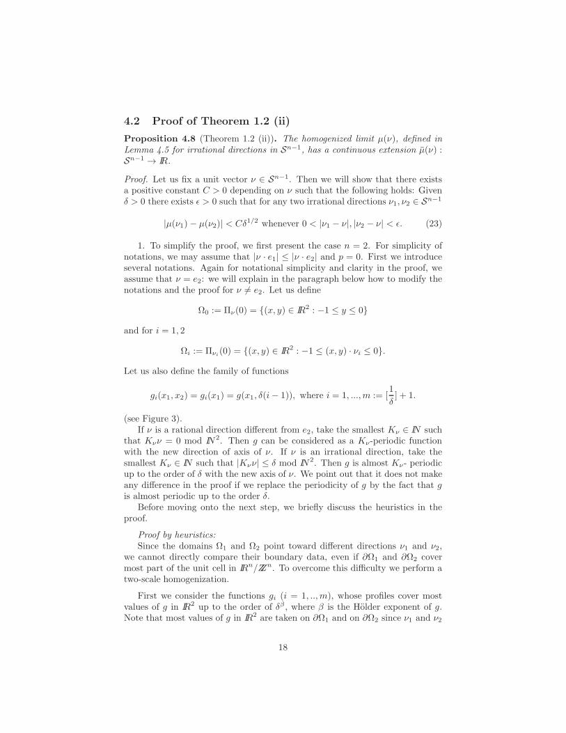
1. To simplify the proof, we first present the case n = 2. For simplicity ofnotations, we may assume that |ν · e1| ≤ |ν · e2| and p = 0. First we introduceseveral notations. Again for notational simplicity and clarity in the proof, weassume that ν = e2: we will explain in the paragraph below how to modify thenotations and the proof for ν 6= e2. Let us define

Ω0 := Πν(0) = (x, y) ∈ IR2 : −1 ≤ y ≤ 0

and for i = 1, 2

Ωi := Πνi(0) = (x, y) ∈ IR2 : −1 ≤ (x, y) · νi ≤ 0.

Let us also define the family of functions

gi(x1, x2) = gi(x1) = g(x1, δ(i− 1)), where i = 1, ...,m := [1

δ] + 1.

(see Figure 3).If ν is a rational direction different from e2, take the smallest Kν ∈ IN such

that Kνν = 0 mod IN2. Then g can be considered as a Kν-periodic functionwith the new direction of axis of ν. If ν is an irrational direction, take thesmallest Kν ∈ IN such that |Kνν| ≤ δ mod IN2. Then g is almost Kν- periodicup to the order of δ with the new axis of ν. We point out that it does not makeany difference in the proof if we replace the periodicity of g by the fact that gis almost periodic up to the order δ.

Before moving onto the next step, we briefly discuss the heuristics in theproof.

Proof by heuristics:Since the domains Ω1 and Ω2 point toward different directions ν1 and ν2,

we cannot directly compare their boundary data, even if ∂Ω1 and ∂Ω2 covermost part of the unit cell in IRn/ZZn. To overcome this difficulty we perform atwo-scale homogenization.

First we consider the functions gi (i = 1, ..,m), whose profiles cover mostvalues of g in IR2 up to the order of δβ , where β is the Holder exponent of g.Note that most values of g in IR2 are taken on ∂Ω1 and on ∂Ω2 since ν1 and ν2

18

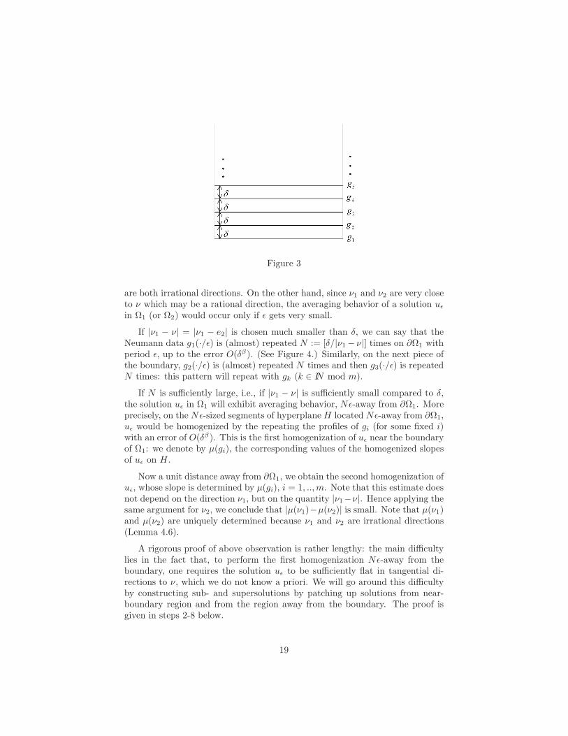
Figure 3

are both irrational directions. On the other hand, since ν1 and ν2 are very closeto ν which may be a rational direction, the averaging behavior of a solution uǫ

in Ω1 (or Ω2) would occur only if ǫ gets very small.

If |ν1 − ν| = |ν1 − e2| is chosen much smaller than δ, we can say that theNeumann data g1(·/ǫ) is (almost) repeated N := [δ/|ν1 − ν|] times on ∂Ω1 withperiod ǫ, up to the error O(δβ). (See Figure 4.) Similarly, on the next piece ofthe boundary, g2(·/ǫ) is (almost) repeated N times and then g3(·/ǫ) is repeatedN times: this pattern will repeat with gk (k ∈ IN mod m).

If N is sufficiently large, i.e., if |ν1 − ν| is sufficiently small compared to δ,the solution uǫ in Ω1 will exhibit averaging behavior, Nǫ-away from ∂Ω1. Moreprecisely, on the Nǫ-sized segments of hyperplaneH located Nǫ-away from ∂Ω1,uǫ would be homogenized by the repeating the profiles of gi (for some fixed i)with an error of O(δβ). This is the first homogenization of uǫ near the boundaryof Ω1: we denote by µ(gi), the corresponding values of the homogenized slopesof uǫ on H .

Now a unit distance away from ∂Ω1, we obtain the second homogenization ofuǫ, whose slope is determined by µ(gi), i = 1, ..,m. Note that this estimate doesnot depend on the direction ν1, but on the quantity |ν1−ν|. Hence applying thesame argument for ν2, we conclude that |µ(ν1)−µ(ν2)| is small. Note that µ(ν1)and µ(ν2) are uniquely determined because ν1 and ν2 are irrational directions(Lemma 4.6).

A rigorous proof of above observation is rather lengthy: the main difficultylies in the fact that, to perform the first homogenization Nǫ-away from theboundary, one requires the solution uǫ to be sufficiently flat in tangential di-rections to ν, which we do not know a priori. We will go around this difficultyby constructing sub- and supersolutions by patching up solutions from near-boundary region and from the region away from the boundary. The proof isgiven in steps 2-8 below.

19

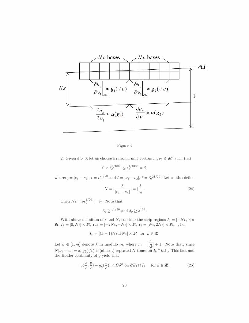
Figure 4

2. Given δ > 0, let us choose irrational unit vectors ν1, ν2 ∈ IR2 such that

0 < ǫ1/10000 ≤ ǫ

1/10000 = δ,

whereǫ0 = |ν1 − e2|, ǫ = ǫ21/200 and ǫ = |ν2 − e2|, ǫ = ǫ0

21/20. Let us also define

N = [δ

|ν1 − en|] = [

δ

ǫ0]. (24)

Then Nǫ = δǫ1/200 := δ0. Note that

δ0 ≥ ǫ1/20 and δ0 ≥ δ100.

With above definition of ǫ and N , consider the strip regions I0 = [−Nǫ, 0]×IR, I1 = [0, Nǫ]× IR, I−1 = [−2Nǫ,−Nǫ]× IR, I2 = [Nǫ, 2Nǫ]× IR,..., i.e.,

Ik = [(k − 1)Nǫ, kNǫ]× IR for k ∈ ZZ.

Let k ∈ [1,m] denote k in modulo m, where m = [1

δ] + 1. Note that, since

N |ν1− en| = δ, gk(·/ǫ) is (almost) repeated N times on Ik ∩∂Ω1. This fact andthe Holder continuity of g yield that

|g(x

ǫ,y

ǫ)− gk(

x

ǫ)| < Cδβ on ∂Ω1 ∩ Ik for k ∈ ZZ. (25)

20

3. Let wǫ solve (P ) : F (D2wǫ) = 0 in Ω0 with

∂wǫ

∂ν(x, 0) = gk(

x

ǫ) for (x, 0) ∈ Ik ∩ y = 0

wǫ = 1 on y = −1.

Next let uǫ solve (P ) in Ω1 with

∂uǫ

∂ν1(x, 0) = g(

x

ǫ,y

ǫ) on (x, y) · ν1 = 0,

uǫ = 1 on (x, y) · ν1 = −1.

Let µ(wǫ) (µ(uǫ)) be chosen as the slope µj in the linearized problem (Pµj )in section 4, where uj is replaced by wǫ (uǫ) and the reference point x = 0 isreplaced by x = −e2/2 = (0,−1/2). (Recall that we assumed 0 ∈ ∂Ω1, and(0,−1/2) ∈ Ωi for i = 1, 2.) µ(wǫ) and µ(uǫ) then denote the slopes of a linearapproximation of ωǫ and uǫ. From (25) it follows that

|µ(wǫ)− µ(uǫ)| < Cδβ . (26)

We point out that µ(wǫ) and µ(uǫ) respectively converge to a unique limitas ǫ → 0 since ν1 is irrational.

4.We begin with introducing µ1/N (gk), which denotes the average of slope for

our solution, δ0 = Nǫ-away from the Neumann boundary y = 0, in Ik.

Let us define

H := ∂Ω0 −Nǫν = ∂Ω0 −Nǫe2 = (x, y) : y = −δ0.

Let η = 1/N and let wη,1 solve

F (D2wη,1) = 0 in −δ0 ≤ y ≤ 0

wη,1 = wǫ(0,−δ) on H = y = −δ0

∂wη,1

∂y(x, 0) = g1(

xǫ , 0) on ∂Ω0 = y = 0

where g1(x, 0) = g1(x + k, 0) for k ∈ ZZ. Let µ 1N(g1) be the slope of the linear

approximation of wη,1, defined as below: choose a linear solution vη,1(·) suchthat

F (D2vη,1) = 0 in −δ0 ≤ y ≤ 0

vη,1 = wη,1(0,−δ0) on H = y = −δ0

vη,1(0,−δ02 ) = wη,1(0,−

δ02 )

∂vη,1∂y

(x, 0) = µ 1N(g1) on ∂Ω0 = y = 0.

21

Since g1(x, 0) is periodic on y = 0 with period ǫ and δ0 = Nǫ, we canapply Lemma 4.2 (i), using the fact that δ0 ≥ ǫ1/20 , to conclude that

|wη,1(x, y)− (wη,1(0,−δ02) + µ1/N (g1)(y +

δ02))| ≤ Cδ1+β

0 (27)

on y = − δ02 ∩I1. Similarly one can define wη,k and vη,k for k ∈ ZZ to conclude

that

|wη,k(x, y)− (wη,k((k − 1)δ0,−δ02) + µ1/N (gk)(y +

δ02))| ≤ Cδ1+β

0 (28)

on y = − δ02 ∩ Ik.

5. We will now construct barriers which bound wǫ from above and below,by pasting together the near- boundary and the rest of the region together asfollows. First we construct a supersolution of (Pǫ). Let ρǫ solve the Neumannboundary problem away from the boundary y = 0:

F (D2ρǫ) = 0 in −1 ≤ y ≤ −δ0

∂ρǫ∂y

= Λ(x) on H = y = −δ0

ρǫ = 1 on y = −1

Here Λ(x) is a holder continuous function obtained by approximatingµ1/N (gk)+2δα0

0 in each Nǫ-strip, where the constant 0 < α0 < 1 will be decidedbelow. Here the holder continuity of Λ(x) is obtained by the fact that gk andgj differs from each other by ((k − j)δ0)

β and they are apart by (k − j)Nǫ ≥(k − j)δ1000 .

Then Theorem 2.4 (b) yields that ρǫ ∈ C1,γ up to H , where γ depends onβ and n. Therefore there exists a constant 0 < α0 < 1 such that the followingholds: in each δ1−α0

0 -neighborhood of a point (x0,−δ0) ∈ H , we have

|ρǫ(x,−δ0)− ρǫ(x0,−δ0)− α(x0)(x− x0)| ≤ δ1+α0

0 , (29)

where α(x0) is the tangential derivative of ρǫ at (x0,−δ0).

6. Next we construct the near-boundary barrier:

F (D2fǫ) = 0 in −δ0 ≤ y ≤ 0

fǫ = ρǫ on H = y = −δ0

∂fǫ∂y

= gk(xǫ ) on y = 0

22

Let us now estimate the slope of fǫ on H . Let us choose a constant µǫ and thecorresponding linear profile φǫ such that

F (D2φǫ) = 0 in −δ0 ≤ y ≤ 0

φǫ(x,−δ) = fǫ(0,−δ0) on H

φǫ(0,−δ2 ) = fǫ(0,−

δ02 )

∂φǫ

∂y= µǫ on ∂Ω0 = y = 0.

(29) and and the comparison principle (Theoren 2.2), as well as the localizationargument as in the proof of Lemma 3.1 applied to the rescaled function

(δ0)−1fǫ(

(x− x0)

δ0+ x0,

y

δ0)− α(x0)(x− x0)

in the region −1 ≤ y ≤ 0 ∩ |x| ≤ δ−α0

0 yields that

|φǫ − fǫ| ≤ Cδ1+α0

0 in −δ0 ≤ y ≤ 0 ∩ |x| ≤ δ1−α0

0 (30)

Putting the estimates (28) and (30) together, it follows that for any(x0,−δ0) ∈ H we have

|fǫ(x, y)− (α(x0)(x − x0)+ µ1/N (gk)(y + δ02 ))| ≤ δ1+α0

0

on y = − δ02 ∩ |x− x0| ≤ δ1−α0

0 ,

for appropriate k in each δ-strip. Using (29), (4.2) and the C1,γ regularity of fǫup to its Dirichlet boundary, we obtain that

∂fǫ∂y

≤ Λ(x),

which then makes the following function a supersolution of (Pǫ):

ρǫ:=

ρǫ in −1 ≤ y ≤ −δ0

fǫ in −δ0 ≤ y ≤ 0.

Similarly, one can construct a subsolution ρǫ of (Pǫ) by replacing Λ(x) givenin the construction of ρǫ by Λ(x) := Λ(x)− 4δα0

0 , such that

ρǫ ≤ wǫ ≤ ρǫ. (31)

7. Parallel arguments as in steps 2 to 4 apply to the other direction ν2: ifwe define ǫ, M and H by

|ν2 − e2| = ǫ < ǫ, M = [δ0ǫ], and H = y = −Mǫ,

23

then we can construct barriers ρǫ and ρǫsuch that

ρǫ ≤ wǫ(x) ≤ ρǫ

(32)

with their corresponding Neumann boundary conditions on H :

∂

∂yρǫ,

∂

∂yρǫ= µ 1

M(gk) +O(δα0

0 ) on H ∩ Ik, (33)

where their respective derivative is taken as a limit from the region−1 ≤ y < −δ0.

8. Now we proceed to estimate the averaging behavior of uǫ away from theNeumann boundary. By Lemma 4.6,

|µ 1N(gk)− µ 1

M(gk)| < m(

1

N) + (

1

M)β , (34)

where m(1

N) = CN−α/20. Let us denote µ 1

N(gk) = µk,N and let h and h

respectively solve

F (D2h) = 0 in −1 ≤ y ≤ −Nǫ

h = 1 on y = −1

∂h

∂ν= µk,N on H ∩ Ik

and

F (D2h) = 0 in −1 ≤ y ≤ −Mǫ

h = 1 on y = −1

∂h

∂ν= µk,M on H ∩ Ik.

Let µ(h) and µ(h) be the respective slope of linear approximation for h and h.Then it follows from (34) that if δ0 ∼ Nǫ ∼ Mǫ is sufficiently small,

|µ(h)− µ(h)| < C(m(1

N) + (

1

M)β). (35)

Lastly, observe that by (31) and (32), there exists 0 < γ < 1 such that

|µ(wǫ)− µ(h)| < Cδγ and |µ(wǫ)− µ(h)| < Cδγ .

The above inequalities and (35) yield

|µ(wǫ)− µ(wǫ)| < C(δγ +m(1

N) + (

1

M)β).

24

Then we conclude from (26) that

|µ(uǫ)− µ(uǫ)| < C(δγ +m(1

N) + (

1

M)β). (36)

9. Lastly we estimate the rate of convergence of µ(uǫ) to µ(ν1) as ǫ → 0.The claim is that

|µ(ν1)− µ(uǫ)| ≤ C(ǫβ0 + ǫ21α/2000 + ǫ

1/200 ).

We will argue similarly as in the proof of Lemma 4.2 (ii). Let us define vǫ,the linear approximation of uǫ, as in (Pµj ) of section 4.1, where the referencefunction uj is replaced by uǫ.

Recall that Ω1 = y : −1 ≤ y · ν1 ≤ 0. We define

Ω1 := Ω1 ∩ y : y · ν1 ≤ −Nǫδ−1ν1,

and L := ∂Ω1 −Nǫδ−1ν1. Then for any given x0 ∈ L and for any x ∈ L, thereexists y ∈ IR2 such that |x− y| ≤ Nǫm, x0 − y = 0 mod ǫZZ2, and

dist(y, L) ≤ ǫ|ν1 − e2| = ǫǫ0.

(recall that m = [1

δ] + 1.) Then by arguing as in (15), for x ∈ L,

|uǫ(x0)− uǫ(x)| ≤ Cǫβ0 + C(Nǫδ−1)α(Nǫm)α ≤ C(ǫβ0 + ǫα/10).

Hence due to the comparison principle (Theorem 2.2) applied to uǫ and vǫ inthe domain Ω1 , we obtain

|uǫ − vǫ| ≤ C(ǫβ0 + ǫα/10 +Nǫδ−1) = C(ǫβ0 + ǫ21α/2000 + ǫ

1/200 ). (37)

Following the proof of (21) using (37) instead of (16), to conclude

|µ(uǫ)− µ(ν1)| ≤ C(ǫβ0 + ǫ21α/2000 + ǫ

1/200 ) ≤ δ.

Parallel arguments applies to ν2. Combing the above inequality with (36),

|µ(ν1)− µ(ν2)| ≤ C(δγ +m(1

N) + (

1

M)β).

Since N and M grow to infinity as ǫ and ǫ go to zero, the above inequalityproves the lemma.

10. For the general dimensions n > 2, let us define

gi(x1, ..., xn−1, xn) = gi(x1, ..., xn−1) = g(x1, ..., xn−1, δ(i− 1))

for i = 0, 1, ...,m := [δ−1]. Let us also define

Ik1,k2,...,kn−1:= [(k1 − 1)Nǫ, k1Nǫ]× ...× [(kn−1 − 1)Nǫ, kn−1Nǫ]× IR.

Then parallel arguments as in steps 1 to 9 would apply to yield the propositionin IRn.

25

Remark 4.9. The proof breaks down for F = F (D2u, xǫ ) since the idea of

perturbing the problem by tilting the Neumann boundary and its boundary data,i.e., the approximation of uη by wη in step 3., does not apply if the insideoperator also depends on x

ǫ .

References

[1] C. Aistleitner, On the law of the iterated logarithm for the discrepancy ofsequencies (nkx) with multidimensional indicies. Unif. Distrib. Theory2 (2007): 89–104.

[2] M. Arisawa, Long-time averaged reflection force and homogenization ofoscillating Neumann boundary conditions, Ann. Inst. H. Poincare Anal.Lineaire 20 (2003), pp. 293-332.

[3] G. Barles, F. Da Lio, P. L. Lions and P.E. Souganidis, Ergodic problemsand periodic homogenization for fully nonlinear equations in half-typedomains with Neumann boundary conditions, Indiana University Math-ematics Journal 57, No. 5 (2008), pp 2355-2376.

[4] A. Bensoussan, J. L. Lions, and G. Papanicolaou. Asymptotic analy-sis for periodic structures, volume 5 of Studies in Mathematics and itsApplications. North- Holland Publishing Co., Amsterdam, 1978.

[5] L. A. Caffarelli, X. Cabre, Fully Nonlinear Elliptic Equations, AMS Col-loquium Publications, Vol. 43. Providence, RI.

[6] F. Camilli, C. Marchi, Rates of convergence in periodic homogenizationof fully nonlinear uniformly elliptic PDEs, Nonlinearity 22 (2009), pp.1481-1498.

[7] L. A. Caffarelli and P. E. Souganidis, Rates of convergence for the ho-mogenization of fully nonlinear uniformly elliptic pde in random media,Invent. Math. . 180 No. 2 (2010) pp. 301-360.

[8] M. Crandall, H. Ishiii and P. L. Lions, Users’ Guide to viscosity solutionsof second order partial differential equations. Bull. Amer. Math. Soc. 27,No.1 (1992): 1-67.

[9] H. Ishii, Fully nonlinear oblique derivative problems for nonlinear second-order elliptic PDEs, Duke Math. J. 62 (1991) 663–691.

[10] H. Ishii, P.L. Lions, Viscosity solutions of fully nonlinear second-order el-liptic partial differential equations, J. Differential Equations 83 (1) (1990)26–78.

[11] A. Khinchin, Einige Satze uber Kettenbruche mit arithmetischen An-wendungen auf die Theorie der Diophantischen Approximationen. Math.Ann. 92 (1924): 115–125.

26

[12] L. Kuipers and H. Niederreiter, Uniform Distribution of Sequences, Pureand Applied Mathematics - Wiley, 1974. New York.

[13] E. Milakis and L. Silvestre, Regularity for Fully Nonlinear Elliptic Equa-tions with Neumann boundary data, Comm. PDE. 31 (2006), pp. 1227-1252.

[14] H. Tanaka, Homogenization of diffusion processes with boundary condi-tions, Stochastic Analysis and Applications, Adv. Probab. Related Top-ics, vol. 7, Dekker, New York, 1984, pp. 411-437.

[15] H. Weyl, Uber ein in der Theorie der sakutaren Storungen vorkom-mendes Problem, Rendiconti del Circolo Matematico di Palemo 330(1910), pp. 377-407.

27