Journal of mathematics and computer science 12 (2014), 253-262

New Implementation of Reproducing Kernel Hilbert Space Method for

Solving a Class of Third-order Differential Equations

Eslam Moradi1,*, Aasadolla Yusefi1, Abolfazl Abdollahzadeh2, Elham Tila3

𝟏Department of Mathematics, Faculty of Mathematical Sciences and Computer, Kharazmi

University,50 Taleghani Avenue, 1561836314 Tehran, Iran 2Department of Mathematics, Faculty of Mathematical Sciences and Statistics, Birjand

University, Birjand, Iran 3Department of Mathematics Sciences and Statistics, Islamic Azad University, Dezful

Branch, Dezful, Iran

*E-mail: eslam.moradi@gmail.com (Eslam Moradi; The corresponding author)

Article history:

Received July 2014

Accepted August 2014

Available online August 2014

Abstract

In this paper, we apply the new implementation of reproducing kernel Hilbert space method to give the

approximate solution to some third-order boundaryvalue problems with variable coefficients. In this

method, the analytical solution is expressed in the form of a series. At the end, two examples are given to

illustrate implementation, accuracy and effectiveness of the method.

Keywords: Reproducing kernel Hilbert space method; Boundary value problems; Third-order differential

equations; Approximatesolution.

1. Introduction

Reproducing kernel Hilbert space method is a promising method which has beenapplied more

and more for solving various problems such asordinary differential equations, partial differential

equations,differential-difference equations, integral equations, and etc. inthe previous decades

[1]-[22]. Approximate solutionof the Fredholm integral equation of the first kind in the

E. Moradi, A. Yusefi, A. Abdollahzadeh, E. Tila/ J. Math. Computer Sci. 12 (2014), 253-262

254

reproducing kernel Hilbert space was presented by Du and Cui [3,4], solution of a system of

linear Volterraintegral equations was discussed by Yang et al. [5],solvability of a class of

Volterra integral equations with weaklysingular kernel using reproducing kernel Hilbert

space method were investigated in [6,7,8],Geng[9] explained how to solve the Fredholm

integralequation of the third kind in the reproducing kernel Hilbertspace method. These are a

bunch of extensive works related to reproducing kernel Hilbertspace method for solving integral

equations.

In 1986, Cui Minggen[10] gave the reproducing kernel space 𝑊21[𝑎, 𝑏] and its reproducing

kernel. This technique has successfully been treated singular linear two-point boundary value

problems [11,12],singular nonlinear second-order boundary value problems [13,14,15,16],

nonlinear system of boundary value problems [17],third-order boundary value problems [18,19],

fifth-order boundary value problems [20], and nonlinear partialdifferential equations [21] in

recent years.

This paper investigates the approximate solution of the following third-order boundary

value problem using new implementation of reproducing kernel Hilbertspace method

𝑦′′′ 𝑥 + 𝑝 𝑥 𝑦 𝑥 = 𝑓 𝑥 , 0 ≤ 𝑥 ≤ 1,

𝑦 0 = 𝐴, 𝑦′ 0 = 𝐵, 𝑦′(1) = 𝐶, (1)

where𝑝 𝑥 , 𝑓(𝑥) are analytical known functions defined on theinterval [0,1], unknown function

𝑦(𝑥) is continuouson the interval [0,1] and 𝐴, 𝐵, 𝐶 are finite real constants.

Several numerical techniques have been proposed to solve high-order differential equations

[23,24,25].

As we known, Gram-Schmidt orthogonalization process isnumerically unstable and in addition it

may take a lot oftime to produce numerical approximation. Here, instead ofusing orthogonal

process, we successfully make use of thebasic functions which are obtained by reproducing

kernel Hilbertspace method.

This paper is organized as follows. In thefollowing section, we introduce some useful definitions

and theorems. Section 3 is devoted to solve Eq. (1) by new implementation of reproducing kernel

Hilbert space method. Two numerical examples are presented in Section 4. We end the paper

with a few conclusions.

2. Reproducing Kernel Spaces

In this section, we follow the recent work of [1]-[22] and represent some useful materials.

Definition 1.

Let ℋ , < . , . >ℋ be a Hilbert space of real-valued functions on some nonempty set 𝒳. A

function𝑘: 𝒳 × 𝒳 → ℝ is said to be the reproducing kernel of ℋ if and only if

1. 𝑘 𝑥, . ∈ ℋ, ∀𝑥 ∈ 𝒳,

2. < 𝜑 . ,𝑘 𝑥, . >ℋ= 𝜑 𝑥 , ∀𝜑 ∈ ℋ, ∀𝑥 ∈ 𝒳, 𝑟𝑒𝑝𝑟𝑜𝑑𝑢𝑐𝑖𝑛𝑔 𝑝𝑟𝑜𝑝𝑒𝑟𝑡𝑦 .

E. Moradi, A. Yusefi, A. Abdollahzadeh, E. Tila/ J. Math. Computer Sci. 12 (2014), 253-262

255

It is known that the reproducing kernel of a reproducing kernel Hilbertspace is unique and the

existence of a reproducing kernel is according to the Riesz Representation Theorem. The

reproducing kernel 𝑘 of a Hilbert space ℋ quite determines the spaceℋ. Each set of functions

𝜑𝑖 𝑖=1∞ which converges strongly to a function 𝜑in ℋ, converges also in the pointwise sense. In

addition, this convergence is uniform on every subset of 𝒳 on which 𝑥 ↦ 𝑘(𝑥, 𝑥) is bounded.

Definition 2.

𝑊24 0,1 = 𝑦 𝑥 𝑦′′′ 𝑥 𝑖𝑠 𝑎𝑛 𝑎𝑏𝑠𝑜𝑙𝑢𝑡𝑒 𝑐𝑜𝑛𝑡𝑖𝑛𝑢𝑜𝑢𝑠 𝑟𝑒𝑎𝑙 𝑣𝑎𝑙𝑢𝑒𝑑 𝑓𝑢𝑛𝑐𝑡𝑖𝑜𝑛 𝑎𝑛𝑑 𝑦 4 𝑥

∈ 𝐿2 0,1 , 𝑦(0) = 𝑦′(0) = 𝑦′(1) = 0}.

The inner product and the norm in the function space 𝑊24 0,1 are defined as follows.

< 𝑢, 𝑣 >𝑊2

4 = 𝑢′′(0)𝑣′′(0) + 𝑢 4 𝑥 𝑣 4 (𝑥)𝑑𝑥1

0

,

u 𝑊2

4 = < 𝑢, 𝑢 >𝑊24 .

Let's assume that function 𝑅 𝑥, 𝑡 ∈ 𝑊24[0,1]satisfies the following generalized differential

equations

𝜕8𝑅(𝑥, 𝑡)

𝜕𝑡8= 𝛿(𝑡 − 𝑥),

R x, 1 −𝜕7𝑅 𝑥 ,1

𝜕𝑡7 = 0,

𝜕4𝑅(𝑥 ,1)

𝜕𝑡4 = 0, 𝜕4𝑅(𝑥 ,0)

𝜕𝑡4 ,

𝜕5𝑅(𝑥, 1)

𝜕𝑡5= 0,

𝜕5𝑅(𝑥, 0)

𝜕𝑡5.

(2)

where𝛿 is the Dirac delta function. Therefore, the following theorem holds.

Theorem 1.Under the assumptions of Eq. (2), Hilbert space 𝑊24[0,1]isa reproducing kernel

Hilbertspace with the reproducing kernel function 𝑅(𝑥, 𝑡), namely for any 𝑦 𝑡 ∈ 𝑊24[0,1]and

each fixed 𝑥 ∈ [0,1], there exists 𝑅 𝑥, 𝑡 ∈ 𝑊24[0,1], 𝑡 ∈ [0,1], such that

< 𝑦 . ,𝑅 𝑥, . >𝑊24 = 𝑦(𝑥).

While𝑥 ≠ 𝑡, function 𝑅(𝑥, 𝑡) is the solution of the followingconstant linear homogeneous

differential equation with 8 orders,

𝜕8𝑅(𝑥, 𝑡)

𝜕𝑡8= 0, (3)

with the boundary conditions:

E. Moradi, A. Yusefi, A. Abdollahzadeh, E. Tila/ J. Math. Computer Sci. 12 (2014), 253-262

256

R x, 1 −𝜕7𝑅 𝑥 ,1

𝜕𝑡7 = 0,

𝜕4𝑅(𝑥 ,1)

𝜕𝑡4 = 0, 𝜕4𝑅(𝑥 ,0)

𝜕𝑡4 ,

𝜕5𝑅(𝑥, 1)

𝜕𝑡5= 0,

𝜕5𝑅(𝑥, 0)

𝜕𝑡5.

(4)

We know that Eq. (3) has characteristic equation 𝜆8 = 0, and theeigenvalue 𝜆 = 0 is a root

whose multiplicity is 8. Hence, the general solution of Eq. (2) is

𝑅 𝑥, 𝑡 =

𝑐𝑖 𝑥

8

𝑖=1

𝑡𝑖−1, 𝑡 ≤ 𝑥,

𝑑𝑖 𝑥

8

𝑖=1

𝑡𝑖−1, 𝑡 > 𝑥.

(5)

Now, we are ready to calculate the coefficients 𝑐𝑖 𝑥 and 𝑑𝑖 𝑥 , 𝑖 = 1, … ,8. Since

𝜕8𝑅(𝑥, 𝑡)

𝜕𝑡8= 𝛿(𝑡 − 𝑥),

we have

∂kR x, x+

∂tk=

∂kR x, x−

∂tk, k = 0, … ,6,

∂7R x, x+

∂tk−

∂7R x, x−

∂tk= 1.

(6)

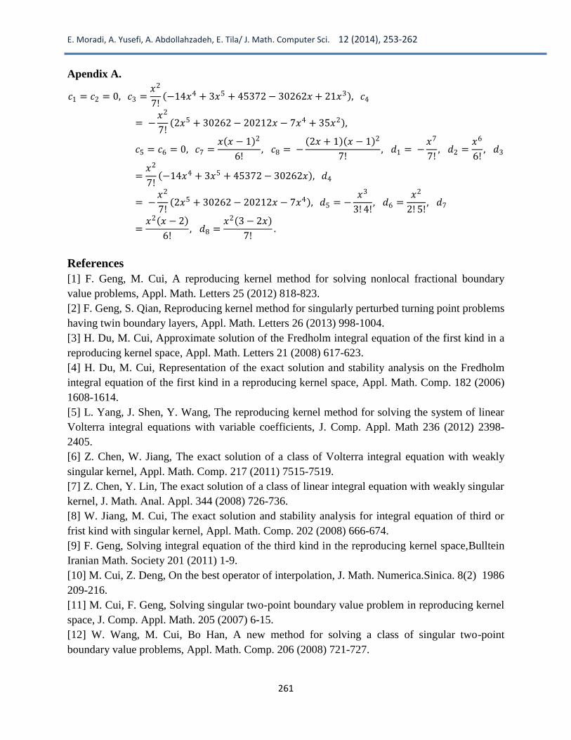
Then, using Eqs. (4) and (6), the unknown coefficients of Eq. (5) are uniquely obtained (in

Apendix A).

Definition 3.

𝑊21 0,1

= 𝑦 𝑥 𝑦 𝑥 𝑖𝑠 𝑎𝑛 𝑎𝑏𝑠𝑜𝑙𝑢𝑡𝑒 𝑐𝑜𝑛𝑡𝑖𝑛𝑢𝑜𝑢𝑠 𝑟𝑒𝑎𝑙 𝑣𝑎𝑙𝑢𝑒𝑑 𝑓𝑢𝑛𝑐𝑡𝑖𝑜𝑛 on the interval 0,1 𝑎𝑛𝑑 𝑦′ 𝑥

∈ 𝐿2 0,1 }.

The inner product and the norm in the function space 𝑊21[0,1] are defined as follows.

< 𝑢, 𝑣 >𝑊2

1 = 𝑢(0)𝑣(0) + 𝑢′ 𝑥 𝑣 ′(𝑥)𝑑𝑥1

0

,

u 𝑊2

1 = < 𝑢, 𝑢 >𝑊21 .

Theorem 2.Hilbert space 𝑊21 0,1 is a reproducing kernel space with the reproducing kernel

function

E. Moradi, A. Yusefi, A. Abdollahzadeh, E. Tila/ J. Math. Computer Sci. 12 (2014), 253-262

257

𝑄 𝑥, 𝑡 = 1 + t, 𝑡 ≤ 𝑥,1 + x, 𝑡 > 𝑥,

that is, for any 𝑦 𝑡 ∈ 𝑊21 0,1 and each fixed 𝑥 ∈ [0,1], it follows that

< 𝑦 . ,𝑄 𝑥, . >𝑊21 = 𝑦 𝑥 .

3. Reproducing Kernel Hilbert Space Method

We suppose that Eq. (1) has a unique solution. To deal with the system, we consider Eq. (1) as

𝕃𝑦 𝑥 = 𝑓 𝑥 , 0 ≤ 𝑥 ≤ 1, (7)

where 𝕃𝑦 𝑥 = 𝑦′′′(𝑥) + 𝑝(𝑥) 𝑦(𝑥), it is clear that 𝕃 is the bounded linear operator of

𝑊24 0,1 → 𝑊2

1 0,1 . We shall give the representation of analytical solution of Eq. (7) in the

space𝑊24[0,1]. Set 𝜑𝑖(𝑥) = 𝑄(𝑥𝑖 , 𝑥) and 𝜓𝑖 𝑥 = 𝕃∗𝜑𝑖 𝑥 , 𝑖 = 1,2, …, where 𝑄(𝑥𝑖 , 𝑥) is the

reproducing kernel of 𝑊21 0,1 and 𝕃∗ is the adjoint operator of 𝕃.

Theorem 3.Let 𝑥𝑖 𝑖=1∞ be a dense subset of interval $[0,1]$, then 𝜓𝑖 𝑥 𝑖=1

∞ is a complete

system of 𝑊24[0,1] and 𝜓𝑖(𝑥) = 𝕃𝑡 𝑅 𝑥, 𝑡 |𝑡=𝑥𝑖

, where the subscript 𝑡 in the operator 𝕃 indicates

that the operator 𝕃applies to the functionof 𝑡.

Usually, a normalized orthogonal system is constructed from 𝜓𝑖 𝑥 𝑖=1∞ by using the Gram-

Schmidt algorithm, and then the approximate solution be obtained by calculating a truncated

series based on these functions. However, Gram-Schmidt algorithm has some drawbacks such as

numerical instability and high volume of computations. Here, to fix these flaws, we state the

following Theorem in which the following notation are used.

𝒂 =

𝑎 1𝑎 2

⋮𝑎 𝑁

, 𝒂 =

𝑎 1𝑎 2

⋮𝑎 𝑁

, 𝑭 =

𝑓 1𝑓 2⋮

𝑓 𝑁

, 𝐵 =

𝛽11 0𝛽21 𝛽22

⋯00

⋮ ⋱ ⋮𝛽𝑁1 𝛽𝑁2 ⋯ 𝛽𝑁𝑁

,

Ψ =

𝜓11 𝜓12

𝜓21 𝜓22⋯

𝜓1𝑁

𝜓2𝑁

⋮ ⋱ ⋮𝜓𝑁1 𝜓𝑁2 ⋯ 𝜓𝑁𝑁

, Ψ =

𝜓 11 𝜓 12

𝜓 21 𝜓 22

⋯𝜓 1𝑁

𝜓 2𝑁

⋮ ⋱ ⋮𝜓 𝑁1 𝜓 𝑁2 ⋯ 𝜓 𝑁𝑁

,

where 𝜓𝑖𝑗 =< 𝕃𝜓𝑗 , 𝜓𝑖 >, 𝜓 𝑖𝑗 =< 𝕃𝜓𝑗 , 𝜓 𝑖 >, 𝑓 𝑖 =< 𝑓, 𝜓𝑖 >, 𝛽𝑖𝑖 > 0, 𝑖, 𝑗 = 1, … , 𝑁.

E. Moradi, A. Yusefi, A. Abdollahzadeh, E. Tila/ J. Math. Computer Sci. 12 (2014), 253-262

258

Theorem 4.Suppose that 𝜓𝑖 𝑥 𝑖=1∞ a linearly independent set in 𝑊2

4 0,1 and 𝜓 𝑖 𝑥 𝑖=1

∞ be a

normalized orthogonal system in 𝑊24 0,1 , such that 𝜓 𝑖 𝑥 = 𝛽𝑖𝑘𝜓𝑘(𝑥)𝑖

𝑘=1 . If 𝑦 𝑥 =

𝑎 𝑖𝜓𝑖 𝑥 ∞𝑖=1 ≃ 𝑦𝑁(𝑥) = 𝑎 𝑖𝜓𝑖 𝑥

𝑁𝑖=1 = 𝑎 𝑖𝜓 𝑖(𝑥)𝑁

𝑖=1 then Ψ𝒂 = 𝑭 .

Proof.Suppose that 𝑦 𝑥 ∈ 𝑊24 0,1 then 𝑦(𝑥) = 𝑎 𝑖𝜓𝑖 𝑥

∞𝑖=1 = 𝑎 𝑖𝜓 𝑖(𝑥)∞

𝑖=1 . Now, by

truncating N-term of the two series, because of 𝑦𝑁(𝑥) = 𝑎 𝑖𝜓𝑖 𝑥 𝑁𝑖=1 = 𝑎 𝑖𝜓 𝑖(𝑥)𝑁

𝑖=1 and since

𝜓 𝑖 𝑥 = 𝛽𝑖𝑘𝜓𝑘(𝑥)𝑖𝑘=1 so

𝑎 𝑖𝜓𝑖 𝑥

𝑁

𝑖=1

= 𝑎 𝑖𝜓 𝑖(𝑥)

𝑁

𝑖=1

= 𝑎 𝑖

𝑁

𝑖=1

𝛽𝑖𝑘𝜓𝑘 𝑥

𝑖

𝑘=1

=

𝑁

𝑘=1

𝑎 𝑖𝛽𝑖𝑘

𝑁

𝑖=𝑘

𝜓𝑘 𝑥 .

Due to the linear independence of 𝜓𝑖 𝑥 𝑖=1∞ ,𝑎 𝑘 = 𝑎 𝑖𝛽𝑖𝑘

𝑁𝑖=𝑘 , 𝑘 = 1, … , 𝑁 therefore

𝒂 = 𝐵𝑇𝒂 . (8)

Eq. (7), imply 𝕃𝑦𝑁 𝑥 = 𝑓 𝑥 . For 𝑖 = 1, … , 𝑁 we have

< 𝕃𝑦𝑁 ,𝜓 𝑖 > = < 𝑓 , 𝜓 𝑖 > ⇒ 𝑎 𝑗 < 𝕃𝜓 𝑗 , 𝜓 𝑖 >

𝑁

𝑗=1

= < 𝑓 , 𝜓 𝑖 >

⇒ 𝑎 𝑗 𝛽𝑖𝑘 𝛽𝑗𝑙

𝑗

𝑙=1

𝑖

𝑘=1

< 𝕃𝜓𝑙 , 𝜓𝑘 >

𝑁

𝑗=1

= 𝛽𝑖𝑘

𝑖

𝑘=1

< 𝑓 , 𝜓𝑘 >

⇒ 𝑎 𝑗 𝛽𝑖𝑘

𝑗

𝑙=1

𝑖

𝑘=1

< 𝕃𝜓𝑙 , 𝜓𝑘 > 𝛽𝑙𝑗𝑇

𝑁

𝑗=1

= 𝛽𝑖𝑘

𝑖

𝑘=1

< 𝑓 , 𝜓𝑘 >

⇒ 𝑎 𝑗

𝑁

𝑗=1

𝐵 Ψ𝐵𝑇 𝑖𝑗 = 𝛽𝑖𝑘

𝑖

𝑘=1

< 𝑓 , 𝜓𝑘 >

⇒ 𝐵 Ψ𝐵𝑇 𝒂 = 𝐵𝑭 .

Eq. (8), imply 𝐵 Ψ𝒂 = 𝐵𝑭 , hence

Ψ𝒂 = 𝑭 . ∎

It is necessary to mention that here we solve the system Ψ𝒂 = 𝑭 which obtained without using

the Gram-Schmidt algorithm.

4. Numerical examples

To illustrate the effectiveness and the accuracy of the proposed method, two numerical examples

are considered in this section. Figures 1,2,3 and 4 show that the approximate solution and its

E. Moradi, A. Yusefi, A. Abdollahzadeh, E. Tila/ J. Math. Computer Sci. 12 (2014), 253-262

259

derivatives up to third-order, converge to the exact solution and its derivatives. We solved these

examplesby the reproducing kernel Hilbert space method with 𝑥𝑖 =𝑖−1

𝑁−1, 𝑖 = 1, … , 𝑁for 𝑁 = 5.

Figure 1: Comparison between approximate solution and the exact

solution for Example 1 for 𝑁 = 5.

Example 1.We consider the following third-order BVP

y′′′ x − xy x = x3 − 2x2 − 5x − 3 ex , 0 ≤ x ≤ 1,

𝑦 0 = 0, 𝑦′ 0 = 1, 𝑦′ 1 = −𝑒.

The exact solution of the above system is 𝑦(𝑥) = 𝑥 1 − 𝑥 𝑒𝑥 .

Figure 2: The absolute error between approximate solution and the exact

solutionand its derivatives for Example 1 for 𝑁 = 5.

Example 2.Consider the following third-order BVP

y′′′ x − xy x = 1 − x ex , 0 ≤ x ≤ 1,

𝑦 0 = 1, 𝑦′ 0 = 1, 𝑦′ 1 = 𝑒.

E. Moradi, A. Yusefi, A. Abdollahzadeh, E. Tila/ J. Math. Computer Sci. 12 (2014), 253-262

260

The exact solution of the above system is 𝑦(𝑥) = 𝑒𝑥 .

Figure 3: Comparison between approximate solution and the exact

solution for Example 2 for 𝑁 = 5.

4. Conclusions

In this paper, we introduced the new implementation of reproducing kernel Hilbert space method

to obtain the approximate solution to some third-order boundary value problems with variable

coefficients. The reliability of the method and reduction of the amount of computation gives this

method a wider applicability.The obtained numerical results confirm that the method is rapidly

convergentand show that the approximate solutionconverge to the exact solution.

Figure 4: The absolute error between approximate solution and the exact

solutionand its derivatives for Example 2 for 𝑁 = 5.

E. Moradi, A. Yusefi, A. Abdollahzadeh, E. Tila/ J. Math. Computer Sci. 12 (2014), 253-262

261

Apendix A.

𝑐1 = 𝑐2 = 0, 𝑐3 =𝑥2

7! −14𝑥4 + 3𝑥5 + 45372 − 30262𝑥 + 21𝑥3 , 𝑐4

= −𝑥2

7! 2𝑥5 + 30262 − 20212𝑥 − 7𝑥4 + 35𝑥2 ,

𝑐5 = 𝑐6 = 0, 𝑐7 =𝑥 𝑥 − 1 2

6!, 𝑐8 = −

2𝑥 + 1 𝑥 − 1 2

7!, 𝑑1 = −

𝑥7

7!, 𝑑2 =

𝑥6

6!, 𝑑3

=𝑥2

7! −14𝑥4 + 3𝑥5 + 45372 − 30262𝑥 , 𝑑4

= −𝑥2

7! 2𝑥5 + 30262 − 20212𝑥 − 7𝑥4 , 𝑑5 = −

𝑥3

3! 4!, 𝑑6 =

𝑥2

2! 5!, 𝑑7

=𝑥2 𝑥 − 2

6!, 𝑑8 =

𝑥2 3 − 2𝑥

7!.

References

[1] F. Geng, M. Cui, A reproducing kernel method for solving nonlocal fractional boundary

value problems, Appl. Math. Letters 25 (2012) 818-823.

[2] F. Geng, S. Qian, Reproducing kernel method for singularly perturbed turning point problems

having twin boundary layers, Appl. Math. Letters 26 (2013) 998-1004.

[3] H. Du, M. Cui, Approximate solution of the Fredholm integral equation of the first kind in a

reproducing kernel space, Appl. Math. Letters 21 (2008) 617-623.

[4] H. Du, M. Cui, Representation of the exact solution and stability analysis on the Fredholm

integral equation of the first kind in a reproducing kernel space, Appl. Math. Comp. 182 (2006)

1608-1614.

[5] L. Yang, J. Shen, Y. Wang, The reproducing kernel method for solving the system of linear

Volterra integral equations with variable coefficients, J. Comp. Appl. Math 236 (2012) 2398-

2405.

[6] Z. Chen, W. Jiang, The exact solution of a class of Volterra integral equation with weakly

singular kernel, Appl. Math. Comp. 217 (2011) 7515-7519.

[7] Z. Chen, Y. Lin, The exact solution of a class of linear integral equation with weakly singular

kernel, J. Math. Anal. Appl. 344 (2008) 726-736.

[8] W. Jiang, M. Cui, The exact solution and stability analysis for integral equation of third or

frist kind with singular kernel, Appl. Math. Comp. 202 (2008) 666-674.

[9] F. Geng, Solving integral equation of the third kind in the reproducing kernel space,Bulltein

Iranian Math. Society 201 (2011) 1-9.

[10] M. Cui, Z. Deng, On the best operator of interpolation, J. Math. Numerica.Sinica. 8(2) 1986

209-216.

[11] M. Cui, F. Geng, Solving singular two-point boundary value problem in reproducing kernel

space, J. Comp. Appl. Math. 205 (2007) 6-15.

[12] W. Wang, M. Cui, Bo Han, A new method for solving a class of singular two-point

boundary value problems, Appl. Math. Comp. 206 (2008) 721-727.

E. Moradi, A. Yusefi, A. Abdollahzadeh, E. Tila/ J. Math. Computer Sci. 12 (2014), 253-262

262

[13] F. Geng, M. Cui, Solving singular nonlinear two-point boundary value problems in the

reproducing kernel space, J. of the Korean Math. Society 45 (3) (2008), 631-644.

[14] F. Geng, M. Cui, Solving singular nonlinear second-order periodic boundary value problems

in the reproducing kernel space, Appl. Math. Comp. 192 (2007), 389-398.

[15] W. Jiang, M. Cui, Y. Lin, Anti-periodic solutions for Rayleigh-type equations via the

reproducing kernel Hilbert space method, Commun Nonlinear SciNumerSimulat 15 (2010)

1754-1758.

[16] E. Babolian, Sh. Javadi and E. Moradi, RKM for the Numerical Solution ofBratu’s Initial

Value Problem, submitted on December 27, 2013.

[17] F. Geng, Iterative reproducing kernel method for a beam equation with third-order nonlinear

boundary conditions, Mathematical Sciences 2012, 6:1.

[18] B. Wu, X. Li, Application of reproducing kernel method to third order three-point boundary

value problems, Appl. Math. Comp. 217 (2010) 3425-3428.

[19] F. Geng, M. Cui, Solving a nonlinear system of second order boundary value problems, J.

Math. Anal. Appl. 327 (2007), 1167-1181.

[20] Gh. Akram, H. Rehman, Solution of fifth order boundary value problems in reproducing

kernel space, Middle-East Journal of Scientific Research 10(2) 2011, 191-195.

[21] M. Mohammadi, R. Mokhtari, Solving the generalized regularized long wave equation on

the basis of a reproducing kernel space, J. Comp. Appl. Math. 235 (2011) 4003-4014.

[22] M. Cui, Y. Lin, Nonlinear numerical analysis in reproducing kernel Hilbert space, Nova

Science Publisher, New York, 2009.

[23] M. Rabbani,New Homotopy Perturbation Method to Solve Non-Linear Problems,

Journal of mathematics and computer Science 7 (2013) 272 – 275.

[24] M. Saravi, A. Nikkar, M. Hermann, J. Vahidi, R. Ahari, A New Modified Approach for

solving seven-order Sawada-Kotara equations, Journal of mathematics and computer Science 6

(2013) 230-237.

[25] S.Gh. Hosseini, S.M. Hosseini, M. Heydari, M. Amini,The analytical solution of singularly

perturbed boundary value problems, Journal of mathematics and computer science 10 (2014), 7-

22.