Dixon-EDF: A Premier Method for Parametric

Polynomial Systems

Robert H. Lewis

Fordham University, New York, NY 10458, USA

http://fordham.academia.edu/RobertLewis

Google: Robert Lewis Fordham

Using examples of interest from real problems, we will

discuss the Dixon-EDF resultant as a method of solving

parametric polynomial systems. We will briefly describe the

method itself, then discuss problems arising in geometric

computing, flexibility of molecules, chemical reactions, game

theory, operations research, di↵erential equations, and oth-

ers. We will compare Dixon-EDF to several implementations

of Grobner bases algorithms on several systems. We find that

Dixon-EDF is greatly superior.

Everyone knows about systems of linear equations:

3x + 4y � 2z = 0

5x + 2y � 3z = 5

�x + 3y + z = �4

They become matrix problems. One way to solve is Cramer’s

Rule:

Let M = [[ 3 4 -2

5 2 -3

-1 3 1 ]]

and

Let M 0 = [[ 0 4 -2

5 2 -3

-4 3 1 ]]

Then

x = Det(M 0)/Det(M) = (-18) / (-9) = 2

i.e., the system of 3 equations in 3 variables has been re-

placed by 1 equation in 1 variable

A x = B where B = Det(M 0) and A = Det(M)

2

Same idea to solve for y, z.

Also Gaussian elimination, to solve for all vars at once.

A variation is to allow parameters. For example, replace

the equations above with

3x + 4y � 2z = a

5x + 2y � 3z = b

�x + 3y + z = c

same idea, but M 0 now contains a, b, c. Answer is:

x = (11a� 10b� 8c)/(-9)

But what about polynomial equations?

Many students meet this topic only in LaGrange multipliers,

a method of optimizing in several variables with constraints.

3

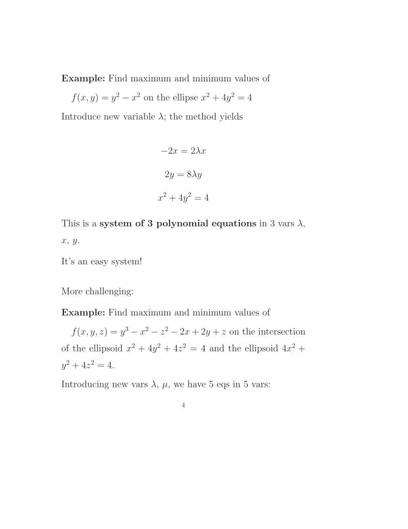
Example: Find maximum and minimum values of

f(x, y) = y2 � x2 on the ellipse x2 + 4y2 = 4

Introduce new variable �; the method yields

�2x = 2�x

2y = 8�y

x2 + 4y2 = 4

This is a system of 3 polynomial equations in 3 vars �,

x, y.

It’s an easy system!

More challenging:

Example: Find maximum and minimum values of

f(x, y, z) = y3� x2� z2� 2x + 2y + z on the intersection

of the ellipsoid x2 + 4y2 + 4z2 = 4 and the ellipsoid 4x2 +

y2 + 4z2 = 4.

Introducing new vars �, µ, we have 5 eqs in 5 vars:

4

�2x� 2 = 2�x + 8µx

3y2 + 2 = 8�y + 2µy

�2z + 1 = 8�z + 8µz

x2 + 4y2 + 4z2 = 4

4x2 + y2 + 4z2 = 4

Now what?

Quick summary: Determinants are calculated and a single

resultant equation for one of the variables alone, say x, is

determinded. The resultant is:

32400x10+32760x8+14400x7�50399x6�4240x5�27566x4�22864x3 + 31609x2 + 13632x� 5376 = 0

A numerical solver gives four real roots, approximately x =

0.87867, 0.27046, 0.808709, -0.882501 Similarly get y, z,

etc.

Won’t talk here about Grobner Bases, an alternate way to

solve polynomial systems.

5

Resultants are like Cramer’s Rule, Grobner Bases are like

Gaussian elimination.

Resultants

A method for solving systems of polynomial equations

f1(x, y, z, . . . , a, b, . . .) = 0

f2(x, y, z, . . . , a, b, . . .) = 0

f3(x, y, z, . . . , a, b, . . .) = 0

. . . . . .

First Case: We have n equations in n�1 variables x, y, z, . . ..

We also have a number of parameters a, b, c, . . ..

A resultant is a single polynomial derived from a system of

polynomial equations that encapsulates the solution (com-

mon zero) to the system. We want to eliminate the variables

and have one polynomial – the resultant – in the parameters.

For a common solution to the system, it is necessary (and

often su�cient) that this resultant vanish.

6

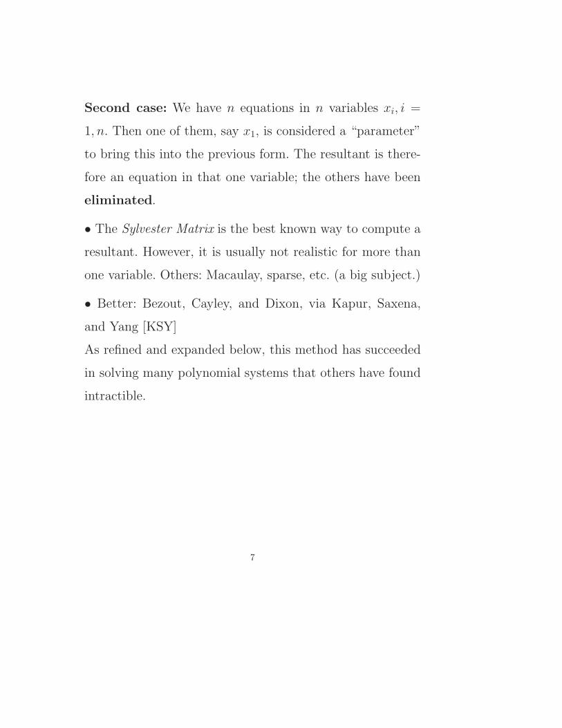
Second case: We have n equations in n variables xi, i =

1, n. Then one of them, say x1, is considered a “parameter”

to bring this into the previous form. The resultant is there-

fore an equation in that one variable; the others have been

eliminated.

• The Sylvester Matrix is the best known way to compute a

resultant. However, it is usually not realistic for more than

one variable. Others: Macaulay, sparse, etc. (a big subject.)

• Better: Bezout, Cayley, and Dixon, via Kapur, Saxena,

and Yang [KSY]

As refined and expanded below, this method has succeeded

in solving many polynomial systems that others have found

intractible.

7

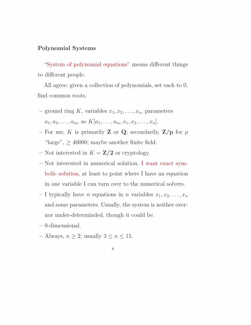
Polynomial Systems

“System of polynomial equations” means di↵erent things

to di↵erent people.

All agree: given a collection of polynomials, set each to 0,

find common roots.

– ground ring K, variables x1, x2, . . . , xn, parameters

a1, a2, . . . , am, so K[a1, . . . , am, x1, x2, . . . , xn].

– For me, K is primarily Z or Q; secondarily, Z/p for p

“large”, � 40000; maybe another finite field.

– Not interested in K = Z/2 or cryptology.

– Not interested in numerical solution. I want exact sym-

bolic solution, at least to point where I have an equation

in one variable I can turn over to the numerical solvers.

– I typically have n equations in n variables x1, x2, . . . , xn

and some parameters. Usually, the system is neither over-

nor under-determinded, though it could be.

– 0-dimensional.

– Always, n � 2; usually 3 n 15.

8

What does “solve the system” mean?

I mean I have eliminated all but one of the variables. So,

I am left with one equation in one variable and the parame-

ters. (Some want a triangular system.) If desired, numerical

values for the parameters can then be substituted, and the

variable obtained numerically.

1 Methods of Solution

– triangularize the system

– Grobner bases

– resultants

Resultants and Grobner Bases

We symbolically solve systems of multivariate polynomials

by computing the resultant. All but one variable have been

eliminated. Of course, this can be done several times to solve

for as many variables as are desired - in parallel.

The Bezout-Dixon method produces a matrix whose de-

terminant is a multiple of the resultant.

9

Dixon-EDF [8] is a way to compute the resultant without

first finding the entire determinant. Often the determinant

is too large to compute, but it has many spurious factors

and so the resultant is much smaller than the determinant.

Often the resultant occurs with multiplicity. We detect these

polynomial factors “early,” hence EDF = Early Detection of

Factors. The output of the algorithm is a list of polynomials

whose product is the determinant. Interesting problems tend

to have many factors.

There is no guarantee that this will work better than a

standard determinant method. However, on many real prob-

lems from interesting applications, it does very well [9], [10].

Grobner Bases are well known. They have many applica-

tions, among which is solving systems of polynomial equa-

tions.

Let us emphasize a key di↵erence between resultant solu-

tions and Grobner bases solutions. The resultant of a system

of n polynomials in n variables is a single polynomial in one

variable (and, usually, parameters). A Grobner basis used

10

this way yields polynomials in triangular form. That is, the

first polynomial contains only one variable (and the parame-

ters), the second has two variables, etc.

It seems reasonable that the Grobner basis is more “com-

plete”, and may well take longer to compute. However, often

the single resultant is su�cient, and in any event, one may

compute the resultants for di↵erent desired variables in par-

allel on di↵erent machines. This is a huge advantage.

Over the last 15 years I have noticed agan and again that

when engineers, scientists, and most mathematicians want to

solve a polynomial system, they want a symbolic solution.

They try Grobner Bases, usually in either Maple or Mathe-

matica. Many many times, the program crashes or the user

finally gives up after many hours.

Many many times these systems would be far easier to

solve with Dixon-EDF.

I do not know of any examples where Grobner bases are

better than Dixon-EDF. If you think you do, tell me!

11

Computations in this paper were run on an Intel Imac at

2.3 ghz with 4 gigabytes of RAM, and on faster servers with

32 gig. Dixon-EDF was run in Fermat [7].

BTW, EDF also works on the Macaulay resultant matrix.

Apparently this is not well known. Dixon is enormously su-

perior.

2 Brief Explanation of Dixon-EDF

This has been published [8], [10].

• The resultant is a factor of the determinant of the “second

Dixon matrix,” M . M contains polynomials in the parame-

ters and the one remaining variable.

• We wish to avoid simply computing the determinant of M .

Instead we begin to column normalize the matrix M .

• To avoid creating large messy denominators (rational func-

tions) we pull out denominators from each row as soon as

they arise. Then later we factor out gcds whenever possible

from the numerators in each row and column.

12

• We keep track of all denominators and gcds so discovered.

We check often to see if some poly in the denominator list

has a common gcd with some poly in the numerator list; if

so we divide it out. In the end, the denominator list must be

all 1. The product of the numerator list is Det[M].

• This can work e�ciently because the the determinant of

the second Dixon matrix M usually has many factors. This

is a bad way of computing the det of a random matrix. But

“random” matrices are seldom of interest.

• Subtleties: pivot strategy, run first over Z/p.

Simple example:

Given initially

M0 = ( 9 2

4 4 )

numerators: denominators:

We factor a 2 out of the second column, then a 2 from the

second row. Thus:

13

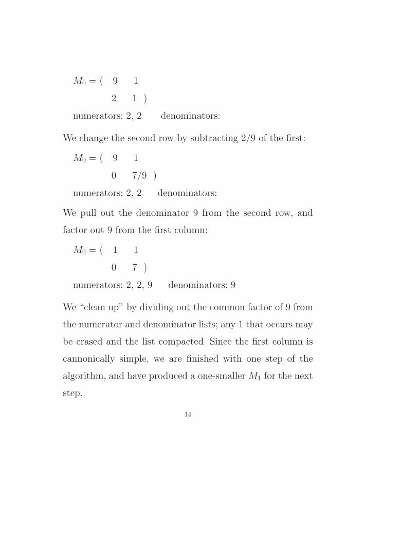
M0 = ( 9 1

2 1 )

numerators: 2, 2 denominators:

We change the second row by subtracting 2/9 of the first:

M0 = ( 9 1

0 7/9 )

numerators: 2, 2 denominators:

We pull out the denominator 9 from the second row, and

factor out 9 from the first column:

M0 = ( 1 1

0 7 )

numerators: 2, 2, 9 denominators: 9

We “clean up” by dividing out the common factor of 9 from

the numerator and denominator lists; any 1 that occurs may

be erased and the list compacted. Since the first column is

cannonically simple, we are finished with one step of the

algorithm, and have produced a one-smaller M1 for the next

step.

14

M1 = (7)

numerators: 2, 2 denominators:

The algorithm terminates by pulling out the 7:

numerators: 2, 2, 7 denominators:

As expected (since the original matrix contained all integers)

the denominator list is empty. The product of all the entries

in the numerator list is the determinant, but we never needed

to deal with any number larger than 9.

Example: Computational Geometry, Heron’s formula

The familiar Heron’s formula is the relation between the

area and sides a, b, c of a triangle:

A2 = s(s� a)(s� b)(s� c)

This can be easily derived as the resultant of a polynomial

system:

(0, a) side on x-axis, point (x, y) in first quadrant, lengths

b and c; obvious equations:

15

x2 + y2 � c2,

(x� a)2 + y2 � b2,

2A� a y

Eliminate x and y, get answer of A in terms of a, b, c.

Now, more fun: easily generalize to 3, 4, 5, . . ., dimensions.

Here’s the system for 5 dimensions, after some routine sim-

plifications, 15 equations:

y2 + x2 � cs2, �2 as x + cs2 � bs2 + as2,

z12 + y12 + x12 � fs2, �2 as x1 + fs2 � ds2 + as2,

�2 y y1� 2xx1 + fs2 � es2 + cs2,

w22 + z22 + y22 + x22 � gs2, �2 as x2� hs2 + gs2 + as2,

�2 y y2� 2xx2� is2 + gs2 + cs2,

�2 z1 z2� 2 y1 y2� 2x1x2� js2 + gs2 + fs2,

u32+w32+z32+y32+x32�ks2, �2 as x3�ls2+ks2+as2,

�2 y y3� 2xx3�ms2 + ks2 + cs2,

�2 z1 z3� 2 y1 y3� 2x1x3� ns2 + ks2 + fs2,

�2w2w3� 2 z2 z3� 2 y2 y3� 2x2x3� os2 + ks2 + gs2,

�as y z1w2u3 + 120V

There are 15 coordinate variables to eliminate.

16

The Dixon matrix is 313x313. EDF finishes completely in

9 minutes, 844 meg RAM. But the answer appears before

that. As often happens with EDF, the answer appears on

the list of factors early, after 4 minutes, 50 meg. It has 823

terms. At completion, the list of numerator-terms is a lot of

1s plus:

6 6 6 6 6 6 6 6 6 6 6 6 6 6 6 6 6 6 6 6 6 6 6 6 6 4161 130 6

823 130 6 823 6 22 22 22 6 22 6 130 6 10000 6 130 6 10000

22 6 6 22 6 22 10000 57147 57147

After cancelling all common factors it is:

1 823 130 6 22

All Grobner basis routines, Maple and Mathematica, crash

and burn.

17

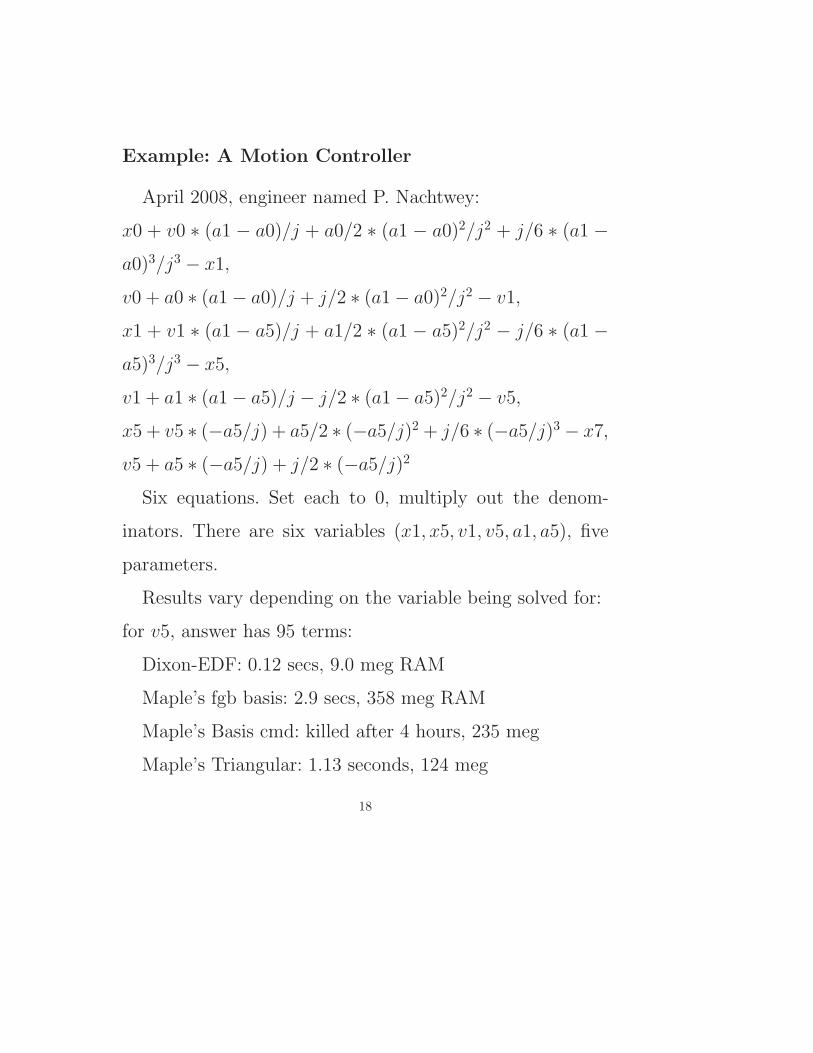
Example: A Motion Controller

April 2008, engineer named P. Nachtwey:

x0 + v0 ⇤ (a1 � a0)/j + a0/2 ⇤ (a1 � a0)2/j2 + j/6 ⇤ (a1 �a0)3/j3 � x1,

v0 + a0 ⇤ (a1� a0)/j + j/2 ⇤ (a1� a0)2/j2 � v1,

x1 + v1 ⇤ (a1 � a5)/j + a1/2 ⇤ (a1 � a5)2/j2 � j/6 ⇤ (a1 �a5)3/j3 � x5,

v1 + a1 ⇤ (a1� a5)/j � j/2 ⇤ (a1� a5)2/j2 � v5,

x5 + v5 ⇤ (�a5/j) + a5/2 ⇤ (�a5/j)2 + j/6 ⇤ (�a5/j)3 � x7,

v5 + a5 ⇤ (�a5/j) + j/2 ⇤ (�a5/j)2

Six equations. Set each to 0, multiply out the denom-

inators. There are six variables (x1, x5, v1, v5, a1, a5), five

parameters.

Results vary depending on the variable being solved for:

for v5, answer has 95 terms:

Dixon-EDF: 0.12 secs, 9.0 meg RAM

Maple’s fgb basis: 2.9 secs, 358 meg RAM

Maple’s Basis cmd: killed after 4 hours, 235 meg

Maple’s Triangular: 1.13 seconds, 124 meg

18

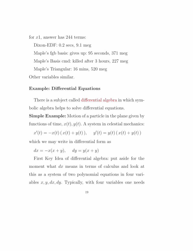
for x1, answer has 244 terms:

Dixon-EDF: 0.2 secs, 9.1 meg

Maple’s fgb basis: gives up: 95 seconds, 371 meg

Maple’s Basis cmd: killed after 3 hours, 227 meg

Maple’s Triangular: 16 mins, 520 meg

Other variables similar.

Example: Di↵erential Equations

There is a subject called di↵erential algebra in which sym-

bolic algebra helps to solve di↵erential equations.

Simple Example: Motion of a particle in the plane given by

functions of time, x(t), y(t). A system in celestial mechanics:

x0(t) = �x(t) (x(t) + y(t) ), y0(t) = y(t) (x(t) + y(t) )

which we may write in di↵erential form as

dx = �x(x + y), dy = y(x + y)

First Key Idea of di↵erential algebra: put aside for the

moment what dx means in terms of calculus and look at

this as a system of two polynomial equations in four vari-

ables x, y, dx, dy. Typically, with four variables one needs

19

four equations to proceed; here we have only two. Next key

idea: generate more equations by di↵erentiating the first two:

dx + x(x + y),

dy � y(x + y),

ddx + dx(x + y) + x(dx + dy),

ddy � dy(x + y)� y(dx + dy)

Dixon yields the resultant, a di↵erential equation in only

the x-related variables. The resultant is x ddx+2x2 dx, which

would be traditionally written as x d2xdt2 + 2x2 dx

dt = 0.

Better Example: The example in the previous section is

so small that virtually any technique would have succeeded

in eliminating the y’s. In a recent paper on biological mod-

eling, Boulier [1] considers a problem of mRNA gene tran-

sciption, resulting in a system of seven di↵erential equations

20

(The dot above a letter means derivative with respect to

time.)

To proceed, Boulier, who was evidently not aware of the

Dixon resultant, makes some strong assumptions (most of

the derivs. set to 0) that greatly simplify the system and

proceeds with another technique, Grobner bases [13].

After di↵erentiating to get new equations, we have 15

equations. All first derivatives. remain.

EDF takes 10 seconds (solving for C):

1 1 1 1 1 1 1 1 1 1 1 1 1 1 1 1 1 1 1 1 1 1 1 1 1 1 1 1 1 1 1 1

1 1 1 1 1 2 1 1 1 1 1 1 1 1 1 1 1 1 1 1 1 1 1 1 2 2 1 1 1 1 3 1

1 1 1 1 3 5 1 3 1 2 1 2 2 2 1 1 6 1 2 1 3 1 2 2 2 2 2 2 1 1 1 1

1 1 1 1 1 1 1 1 1 1 1 1 1 1 3 3 1 3 1 2 2 1 1 2 1 2 2 1 175 2 1

12 2 2 175 1 20

Maple:

• builtin Basis command: kernel panic. memory allocaton

failed. 13.5 minutes, 514 MEG

• fgb basis: Error, Sorry the size of the matrix is too big.

204 meg. 113 secs.

21

• Triangularize: kernel connection lost. 68 mins. 519 meg

3 Example: Autocatalytic reactions

From Wikipedia:

Autocatalytic reactions are chemical reactions in which

at least one of the products is also a reactant. The

rate equations for autocatalytic reactions are funda-

mentally nonlinear. This nonlinearity can lead to the

spontaneous generation of order.

An autocatlytic reaction is one in which a chemical (“species”)

acts to increase the rate of its producing reaction.

In many autocatlytic systems complex dynamics are seen,

including multiple steady-states and periodic orbits.

The dynamics and chemistry of oscillating reactions has

only been the subject of study for the last 50 years, starting

with the work of Boris Belousov. Belousov was studying the

Krebs cycle when he stumbled upon an oscillating system.

He witnessed a mixture of citric acid, bromate, and cerium

22

catalyst in a sulfuric acid solution undergoing periodic color

changes. (A movie exists.)

The scientific community of the time believed that oscil-

lations in a chemical system were disallowed by thermody-

namic laws, so Belousov’s work was met with great skepti-

cism.

4 Basic equations

A chemical reaction of two reactants and two products can

be written as

aA + bB ! s S + t T

where the lower case letters are stoichiometric coe�cients

and the capital Latin letters represent chemical species. The

chemical reaction proceeds in both the forward and reverse

direction. This equation is easily generalized to any number

of reactants, products, and reactions.

23

4.1 Chemical equilibrium

In chemical equilibrium the forward and reverse reaction

rates are such that each chemical species is being created

at the same rate it is being destroyed. In other words, the

rate of the forward reaction is equal to the rate of the reverse

reaction.

k+[A]a [B]b = k�[S]s [T ]t

Here, the brackets indicate the amount of the chemical

species, in moles, and k+ and k� are rate coe�cients.

[Note: products because rate of change is proportional to

amount present.]

Autocatalytic reactions are those in which at least one of

the products is a reactant. Perhaps the simplest autocat-

alytic reaction can be written

A + B ! 2B

This reaction is one in which a molecule of species A in-

teracts with a molecule of species B. The A molecule is con-

verted into a B molecule. The final product consists of the

24

original B molecule plus the B molecule created in the re-

action.

This yields the equations:

d[A]dt = �k+ [A][B] + k� [B]2

d[B]dt = k+[A][B]� k�[B]2

Set these to 0 to find the “steady state”, or equilibrium.

Henceforth we will drop the [ and ].

4.2 The Brusselator

The mechanism for the Brusselator is given by:

A! X

2X + Y ! 3X (1)

B + X ! Y + C

X ! D

The two species of interest to us are X and Y , the auto-

catalytic species. The di↵erential equations given in dimen-

sionless form for these species are:

25

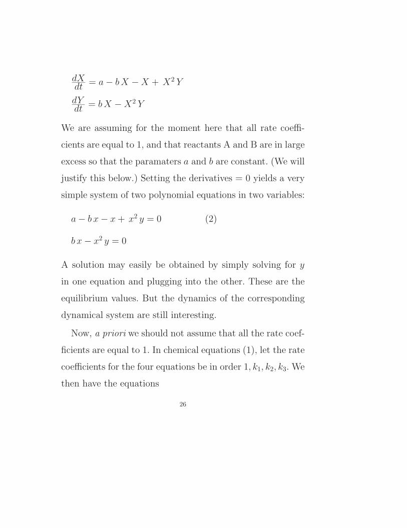
dXdt = a� bX �X + X2 Y

dYdt = bX �X2 Y

We are assuming for the moment here that all rate coe�-

cients are equal to 1, and that reactants A and B are in large

excess so that the paramaters a and b are constant. (We will

justify this below.) Setting the derivatives = 0 yields a very

simple system of two polynomial equations in two variables:

a� b x� x + x2 y = 0 (2)

b x� x2 y = 0

A solution may easily be obtained by simply solving for y

in one equation and plugging into the other. These are the

equilibrium values. But the dynamics of the corresponding

dynamical system are still interesting.

Now, a priori we should not assume that all the rate coef-

ficients are equal to 1. In chemical equations (1), let the rate

coe�cients for the four equations be in order 1, k1, k2, k3. We

then have the equations

26

dXdt = a� k2 bX � k3 X + k1 X2Y

dYdt = k2 bX � k1 X2Y

yielding the polynomial system

a� k2 b x� k3 x + k1 x2y = 0

k2 b x� k1 x2y = 0

All of these ki may be removed with simple substitutions.

First, replace y with y/k1. That eliminates k1. To eliminate

k2 set b = b/k2. For k3 set x = x k3, b = b k3, and a = a k23.

We are back to the simple system (2).

27

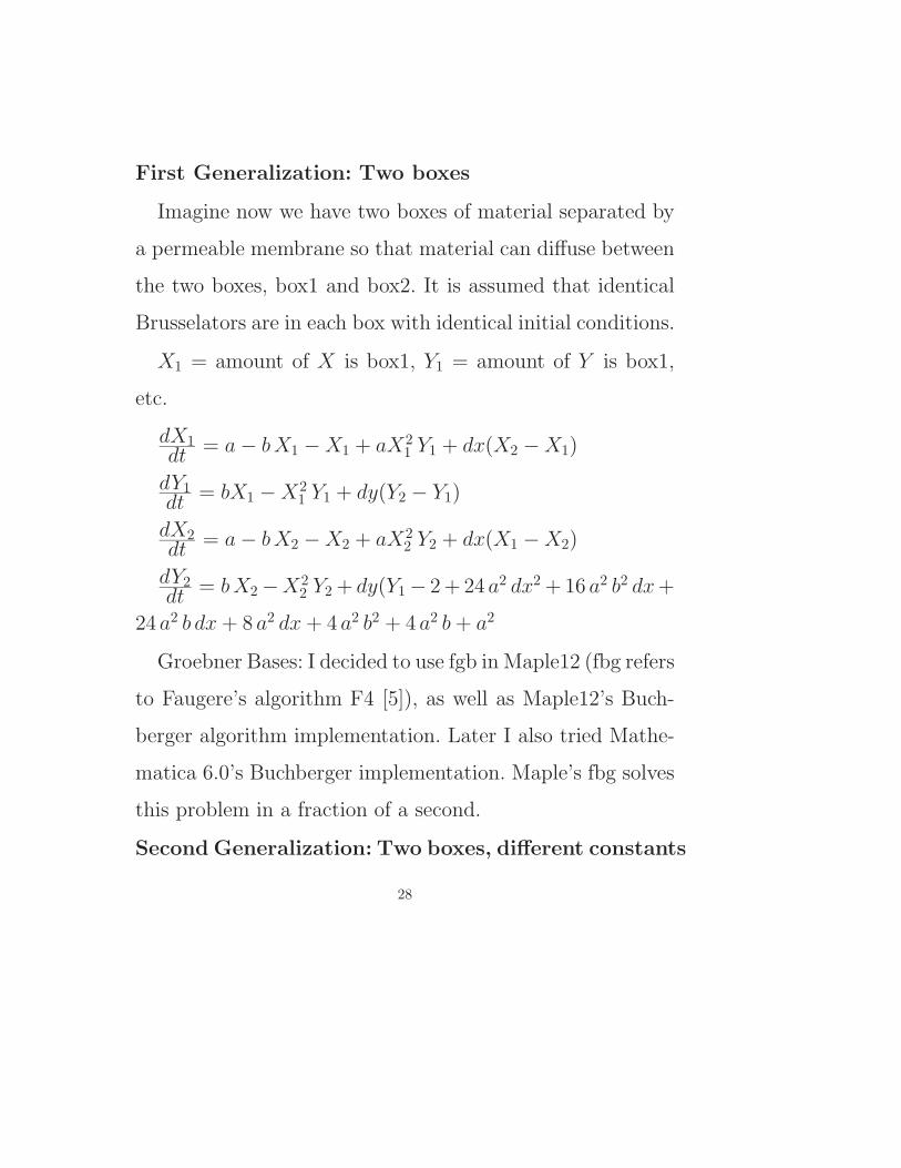
First Generalization: Two boxes

Imagine now we have two boxes of material separated by

a permeable membrane so that material can di↵use between

the two boxes, box1 and box2. It is assumed that identical

Brusselators are in each box with identical initial conditions.

X1 = amount of X is box1, Y1 = amount of Y is box1,

etc.

dX1dt = a� bX1 �X1 + aX2

1 Y1 + dx(X2 �X1)

dY1dt = bX1 �X2

1 Y1 + dy(Y2 � Y1)

dX2dt = a� bX2 �X2 + aX2

2 Y2 + dx(X1 �X2)

dY2dt = bX2�X2

2 Y2 + dy(Y1� 2 + 24 a2 dx2 + 16 a2 b2 dx +

24 a2 b dx + 8 a2 dx + 4 a2 b2 + 4 a2 b + a2

Groebner Bases: I decided to use fgb in Maple12 (fbg refers

to Faugere’s algorithm F4 [5]), as well as Maple12’s Buch-

berger algorithm implementation. Later I also tried Mathe-

matica 6.0’s Buchberger implementation. Maple’s fbg solves

this problem in a fraction of a second.

Second Generalization: Two boxes, di↵erent constants

28

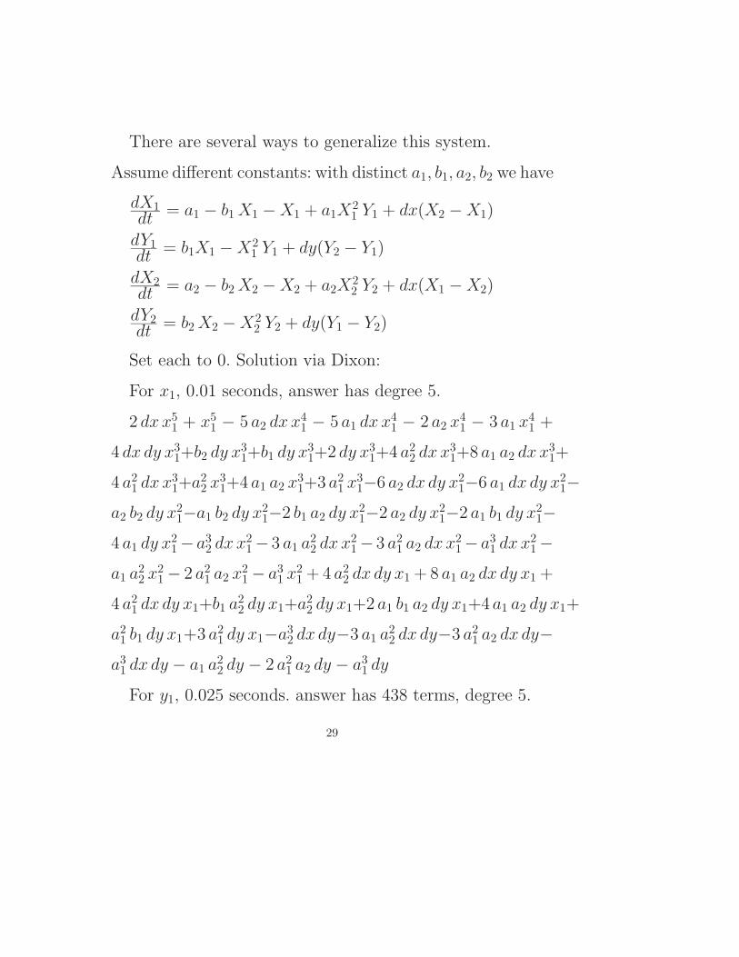
There are several ways to generalize this system.

Assume di↵erent constants: with distinct a1, b1, a2, b2 we have

dX1dt = a1 � b1 X1 �X1 + a1X2

1 Y1 + dx(X2 �X1)

dY1dt = b1X1 �X2

1 Y1 + dy(Y2 � Y1)

dX2dt = a2 � b2 X2 �X2 + a2X2

2 Y2 + dx(X1 �X2)

dY2dt = b2 X2 �X2

2 Y2 + dy(Y1 � Y2)

Set each to 0. Solution via Dixon:

For x1, 0.01 seconds, answer has degree 5.

2 dxx51 + x5

1 � 5 a2 dxx41 � 5 a1 dxx4

1 � 2 a2 x41 � 3 a1 x4

1 +

4 dx dy x31+b2 dy x3

1+b1 dy x31+2 dy x3

1+4 a22 dxx3

1+8 a1 a2 dxx31+

4 a21 dxx3

1+a22 x3

1+4 a1 a2 x31+3 a2

1 x31�6 a2 dx dy x2

1�6 a1 dx dy x21�

a2 b2 dy x21�a1 b2 dy x2

1�2 b1 a2 dy x21�2 a2 dy x2

1�2 a1 b1 dy x21�

4 a1 dy x21�a3

2 dxx21� 3 a1 a2

2 dxx21� 3 a2

1 a2 dxx21�a3

1 dxx21�

a1 a22 x2

1� 2 a21 a2 x2

1� a31 x2

1 + 4 a22 dx dy x1 + 8 a1 a2 dx dy x1 +

4 a21 dx dy x1+b1 a2

2 dy x1+a22 dy x1+2 a1 b1 a2 dy x1+4 a1 a2 dy x1+

a21 b1 dy x1+3 a2

1 dy x1�a32 dx dy�3 a1 a2

2 dx dy�3 a21 a2 dx dy�

a31 dx dy � a1 a2

2 dy � 2 a21 a2 dy � a3

1 dy

For y1, 0.025 seconds. answer has 438 terms, degree 5.

29

For Groebner bases, fgb, 0.08 seconds for x1, 0.4 seconds

for y1.

Third Generalization: Three boxes

Assume there are 3 boxes in a row, A, B, C. A touches only

B, C touches only B. Permeable membranes at boundaries A-

B and B-C. Three pairs of two variables: x1, y1, x2, y2, x3, y3,

six equations:

dxx3 + dxx2 + x21 y1 � 2 dxx1 � b1 x1 � x1 + a1

dy y3 + dy y2 � x21 y1 � 2 dy y1 + b1 x1

x22 y2 � dxx2 � b1 x2 � x2 + dxx1 + a1

�x22 y2 � dy y2 + b1 x2 + dy y1

x23 y3 � dxx3 � b1 x3 � x3 + dxx1 + a1

�x23 y3 � dy y3 + b1 x3 + dy y1

With Maple 12:

out := fgb gbasis(sys,[x2,x3,y1,y2,y3] , [x1, dx, dy, a1, b1])

After about 10 seconds: error message, “Length of output

exceeds limit of 1000000”

30

Dixon for x1 takes 0.113 seconds. Answer factors into two

polynomials, of 50 terms and 30 terms.

Dixon for y1 takes 1.5 seconds. Answer factors into two

polynomials, of 245 terms and 94 terms.

Let’s make it more interesting: assume the permeability

coe�cients are di↵erent for two di↵erent membranes; i.e.

dx12, dy12, dx13, dy13. Make changes in above six equations.

Dixon for x1 takes 5.8 seconds. Answer has 6428 terms.

Maple12, builtin Groebner routine, gave error message af-

ter 391 seconds. fgb gave up after 178 seconds with message

“Error, (in fgbrs:-fgb gbasis) Sorry the size of the matrix is

too big.”

I also tried Mathematica 6.0 on this system. It’s builtin

Groebner basis command was still running after 130 hours

and 750 megabytes of RAM.

Dixon for y1 takes 4 minutes. Answer has 144658 terms,

degree 18.

Another variation: three boxes meeting symmetrically, like

three sectors of a circle, each having central angle of 120 de-

31

grees. Assume the permeability coe�cients are di↵erent for

the three di↵erent membranes; i.e. dx12, dy12, dx13, dy13, dx23, dy23.

Dixon for x1 takes 2 minutes 30 seconds. Answer has 3558455

terms, degree 18.

All Grobner basis routines fail miserably.

32

Example: Computational Chemistry

Joint with Evangelos A. Coutsias, UNM, Stony Brook.

Protein flexibility has been a major research topic in com-

putational chemistry for a number of years, and it has a key

role for many important functions of proteins as molecular

machines.

A polypeptide backbone can be modeled as a polygonal

line whose edges and angles are fixed while some of the dihe-

dral angles formed by successive triplets of edges can vary

freely. It is well known that a segment of backbone both of

whose ends are fixed will be (generically) flexible if it in-

cludes more than six free torsions. Resultant methods have

been applied successfuly to this problem.

In this work we focus on non-generically flexible structures

that are rigid but become continuously movable if certain

symmetries and relations exist.

This subject has a long history.

33

– In 1812, Cauchy considered flexibility of three dimen-

sional polyhedra, where each joint can pivot or hinge. He

proved that if the polyhedron is convex it must be rigid

– cannot be flexible.

– Bricard (1896) following Cauchy found flexible non-convex

but intercrossing octahedra – they do not live in 3-space.

– Following Bricard’s ideas, Connelly (1978) found non-

convex genuine flexible polyhedra that do live in 3-space.

4.3 Computer Algebra Approach

Triangles are obviously NOT flexible. Quadrilaterals ob-

viously ARE flexible. Generically flexible.

34

Fig. 1. Flexing a quadrilateral.

But a fifth bar makes it inflexible, at least generically:

Fig. 2. A fifth rod kills flexibility.

Note well: there are five rigid bars in the above picture,

not seven.

35

We have a new approach to understanding flexibility, us-

ing symbolic computation. We describe the geometry

of the object or molecule with a set of multivari-

ate polynomial equations. We solve it with resultants

(EDF).

Then given the resultant res, we created an algorithm

Solve that examines res and determines relations for the

structure to be flexible.

The basic idea of Solve is simple:

• The variables in the equations are sines or cosines of

certain angles in the figure. If it is flexible, there are

infinitely many possible values for an angle.

• But res is a polynomial in, say, cosine, ca. It cannot

have infinitely many solutions – unless all the coe�-

cients (polynomials in the parameters) vanish.

Here is an easy example. If res were

(s9 s8 � s7 s6) ca2 + (s42 � s3

2) ca + s8 � s6,

36

one solution would be the collection (or table ) of the three

relations s9 = s7, s8 = s6, s4 = s3.

We have applied this to a significant arrangement of quadralat-

erals “equivalent” to Bricard’s octahedra with a resultant

of 190181 terms.

But first let’s look at a simpler example.

37

Toy Example: Quadrilateral With Bar

Fig. 3. With fifth rod, labeling angles, vertices, and lengths.

Let sa = sin(↵), ca = cos(↵), cb = cos(�), sb = sin(�).

Let point A = (ax, ay), C = (cx, cy), D = (dx, dy), etc.

The four equations are

sa2 + ca2 � 1 = 0, sb2 + cb2 � 1 = 0,

(bx� cx)2 + (by � cy)2 � s25 = 0,

(ax� dx)2 + (ay � dy)2 � s24 = 0

where

38

ax = s7 ca, cx = s3 + s2 cb, cy = s2 sb, etc. There are 4

variables sa, ca, sb, cb and 7 parameters si. Equations (3)

and (4) have ten terms and are rather messy.

EDF computes the resultant for ca in 0.14 seconds on a

three-year old Imac. It has 162 terms.

Solve finds two solutions (one degenerate) in 0.2 secs:

table 1 =

2666666666664

s6 , s7

s1 , s2

s3 , s5

s4 , s5

3777777777775

table 2 =

266666664

s6 , 0

s7 , 0

s4 , s5

377777775

[Degenerate means some side = 0 or some angle remains

constant throughout the flex.]

39

Fig. 4. Check the solutions for flexibility.

Now the Real Example:

40

This is described by a system of 6 equations in 6 variables

and 11 parameters. The resultant, computable only by

EDF (23 minutes), has 190181 terms.

The problem: It is generically rigid. Find a way that this

becomes flexible. One way: if all the quadrilaterals are

parallelograms.

I developed an algorithm that analyses the resultant and

finds flexibility. One totally new way was found recently.

Irrational. Movie.

http://home.bway.net/lewis/flex.MP4

Movie

Demo.

41

5 Conclusions

We found great success in applying Dixon-EDF to poly-

nomial systems arising in important applications. Dixon-

EDF succeeds in many other systems [9], [10]. Maple12,

15 failed repeatedly with two implementations of Grobner

bases, as do Mathematica and Singular (one example).

• Dixon-EDF is a powerful tool for symbolic solution of

systems of multivariate equations.

• Dixon-EDF succeeds where other methods fail.

• Anyone want to implement EDF on some other sys-

tem? Let me know. Great undergraduate project!

• Open challenge: Solve one of these problems with Grobner

bases. Compare time and space usage.

• On arbitrary made-up test problems, the method does

not do especially well. On real problems from interest-

ing applications, it does extremely well.

• Dixon-EDF is curiously underappreciated.

42

References

1. J. L. Awange, Grobner bases, multipolynomial resultants and Gauss-Jacobi combina-

torial algorithms - adjustment of nonlinear GPS/LPS observations, Dissertation (D93),

Geodatisches Institute der Universitat Stuttgart (2002).

2. R. Datta, Using computer algebra to find Nash equilibria. ISSAC’03, August 3 – 6,

2003, Philadelphia, Pennsylvania USA.

3. R. Datta, Finding all Nash equilibria of a finite game using polynomial algebra.

http://arxiv.org/abs/math.AC/0612462. 2006.

4. A. L. Dixon, The eliminant of three quantics in two independent variables. Proc.

London Math. Soc. 6 (1908) 468 – 478.

5. J.-C. Faugere, A new e�cient algorithm for computing Groebner bases (F4). Journal

of Pure and Applied Algebra (Elsevier Science) 139 (1999) 61 – 88.

6. G. H. Golub and V. Pereyra, The di↵erentiation of pseudo-inverses and nonlinear least

squares problems whose variables separate, SIAM J. Num. Anal. 10 (1973) 413 – 432.

7. R. H. Lewis, Computer algebra system Fermat. http://home.bway.net/lewis/

8. R. H. Lewis, Heuristics to accelerate the Dixon resultant, Mathematics and Computers

in Simulation 77, Issue 4 (2008) 400 – 407.

9. R. Lewis and S. Bridgett, Conic tangency equations arising from Apollonius problems

in biochemistry, Mathematics and Computers in Simulation 61(2) (2003) 101 – 114.

10. R. H. Lewis, and E. A. Coutsias, Algorithmic search for flexibility using resultants of

polynomial systems; in Automated Deduction in Geometry, 6th International Work-

shop, ADG 2006. Springer-Verlag. LNCS 4869 (2007) 68 – 79.

11. J. Nash and L. Shapley, A simple three-person poker game, contributions to the theory

of games, pp. 105 – 116. Annals of Mathematics Studies, 24. Princeton University Press,

Princeton, NJ, 1950.

12. B. Palancz, R. H. Lewis, P. Zaletnyik, and J. Awange, Computational study

of the 3D a�ne transformation part I. 3-point problem. March 2008. online at

http://library.wolfram. com/infocenter/MathSource/7090/

13. B. Palancz, J. Awange, P. Zaletnyik, and R. H. Lewis, Linear homotopy solution

of nonlinear systems of equations in geodesy, Journal of Geodesy. September 2009.

http://www.springerlink.com/content/78qh80606j224341/

43

14. E. Papp and L. Szucs, Transformation methods of the traditional and satellite based

networks (in Hungarian with English abstract), Geomatikai Kozlemenyek VIII (2005)

85 – 92.

15. H. Spath, A numerical method for determining the spatial Helmert transformation in

case of di↵erent scale factors, Zeitschrift fur Geodasie, Geoinformation und Landman-

agement 129 (2004) 255 – 257.

16. B.Sturmfels, Solving systems of polynomial equations. CBMS Regional Conference

Series in Mathematics 97, American Mathematical Society, Providence, 2003.

17. Global positioning system. http://en.wikipedia.org/wiki/Global Positioning System

(2008).

44