Codes, arrangements, matroids, and their polynomial links
161
Codes, arrangements, matroids, and their polynomial links
-
Upload
khangminh22 -
Category
Documents
-
view
0 -
download
0
Transcript of Codes, arrangements, matroids, and their polynomial links

Codes, arrangements, matroids,and their polynomial links

Copyright c© 2012 by Relinde Jurrius.Unmodified copies may be freely distributed.
A catalogue record is available from the Eindhoven University of Technology Library.ISBN: 978-90-386-3194-3
Printed by Wöhrmann Printing Service, Zutphen, The Netherlands

Codes, arrangements, matroids,and their polynomial links
PROEFSCHRIFT
ter verkrijging van de graad van doctor aan deTechnische Universiteit Eindhoven, op gezag van derector magnificus, prof.dr.ir. C.J. van Duijn, voor een
commissie aangewezen door het College voorPromoties in het openbaar te verdedigen
op woensdag 29 augustus 2012 om 16.00 uur
door
Relinde Petronella Maria Johanna Jurrius
geboren te Haarlem
Dit proefschrift is goedgekeurd door de promotor:
prof.dr. H.C.A. van Tilborg
Copromotor:dr. G.R. Pellikaan

Codes, arrangements, matroids,and their polynomial links
Many mathematical objects are closely related to each other. While studying certain as-pects of a mathematical object, one tries to find a way to “view” the object in a way thatis most suitable for a specific problem. Or, in other words, one tries to find the best wayto model the problem. Many related fields of mathematics have evolved from one anotherthis way. In practice, it is very useful to be able to transform a problem into other termi-nology: it gives a lot more available knowledge and that can be helpful to solve a problem.
This thesis deals with various closely related fields in discrete mathematics, starting fromlinear error-correcting codes and their weight enumerator. We can generalize the weightenumerator in two ways, to the extended and generalized weight enumerators. The setof generalized weight enumerators is equivalent to the extended weight enumerator.
Summarizing and extending known theory, we define the two-variable zeta polynomialof a code and its generalized zeta polynomial. These polynomials are equivalent to theextended and generalized weight enumerator of a code.
We can determine the extended and generalized weight enumerator using projective sys-tems. This calculation is explicitly done for codes coming from finite projective and affinespaces: these are the simplex code and the first order Reed-Muller code. As a result wedo not only get the weight enumerator of these codes, but it also gives us informationon their geometric structure. This is useful information in determining the dimension ofgeometric designs.
To every linear code we can associate a matroid that is representable over a finite field. Afamous and well-studied polynomial associated to matroids is the Tutte polynomial, orrank generating function. It is equivalent to the extended weight enumerator. This leadsto a short proof of the MacWilliams relations for the extended weight enumerator.
For every matroid, its flats form a geometric lattice. On the other hand, every geomet-ric lattice induces a simple matroid. The Tutte polynomial of a matroid determines thecoboundary polynomial of the associated geometric lattice. In the case of simple ma-troids, this becomes a two-way equivalence.
Another polynomial associated to a geometric lattice (or, more general, to a poset) is

ii Codes, arrangements, matroids, and their polynomial links
the Möbius polynomial. It is not determined by the coboundary polynomial, neither theother way around. However, we can give conditions under which the Möbius polynomialof a simple matroid together with the Möbius polynomial of its dual matroid definesthe coboundary polynomial. The proof of these relations involves the two-variable zetapolynomial, that can be generalized from codes to matroids.
Both matroids and geometric lattices can be truncated to get an object of lower rank.The truncated matroid of a representable matroid is again representable. Truncation for-mulas exist for the coboundary and Möbius polynomial of a geometric lattice and thespectrum polynomial of a matroid, generalizing the known truncation formula of theTutte polynomial of a matroid.
Several examples and counterexamples are given for all the theory. To conclude, we givean overview of all polynomial relations.

Outline and origin of research
It is common to start a thesis with a chapter that lists the necessary background infor-mation about the research topics of the thesis. Such a chapter summarizes definitionsand known results that are necessary for understanding the new results. I choose to di-vide this background information into four chapters, treating linear codes (Chapter 1),projective systems and arrangements (Chapter 4), matroids (Chapter 7), and geometriclattices (Chapter 9). I think this outline improves readability of the thesis, especially forsomeone who is only interested in parts of the results.
The outline of this thesis is mainly taken from [58]. This paper gives an overview ofthe connections between codes, arrangements, and matroids. It originates from lecturenotes for the 2009 Soria Summer School in Computational Mathematics. Since it givesa very thorough introduction to the subjects in the title, the introduction chapters onlinear codes (Chapter 1) and matroids (Chapter 7) are highly condensed versions of thematerial in the paper. Chapter 4 on projective systems and arrangements is fairy similarto Section 4 of [58] and Chapter 9 on geometric lattices is like Section 7 of [58] but withless examples. Chapter 10 is roughly a copy of Section 8 in [58].
My research on weight enumerators and their generalizations, as well as the connectionto matroids, started in the final project for my Masters degree. Chapter 2 on generalizedand extended weight enumerators and Chapter 8 on the Tutte polynomial originate frommy Master thesis [52]. This results were also presented at the Workshop on Coding andCryptography [55].
Chapter 3 studies the zeta polynomial of a code and its generalizations. Most of this isa summary of known results, therefore this material is unpublished. The novelty is thatit is written in the context of Chapter 2, showing clearly the close relation between thevarious generalizations of the zeta function and the similar generalizations of the weightenumerator. The theory is also used in Chapter 11.
Chapter 5 contains the results of my paper in Designs, Codes and Cryptography [53].Chapter 6 reports on ongoing research on the coset leader weight enumerator. The firstresults on that topic were presented at the Symposium on Information Theory in theBenelux [56].
Most of my PhD research involves matroids and their associated polynomials. In Chap-ter 11 new results are explained about the relation between the Möbius and coboundary

iv Outline and origin of research
polynomial [54]. Chapter 13 contains new results on truncation [57]. Both papers will bepublished in a special issue of Mathematics in Computer Science on matroids in codingtheory and related topics.
The spectrum polynomial is introduced in Chapter 12 and a concrete calculation is given.I was hoping to achieve new results on the link between the spectrum polynomial andthe Tutte polynomial, but unfortunately was not able to. Therefore, Chapter 12 does notcontain enough new information for publication.
Finally, in Chapter 14 an overview is given of the established polynomial links. Parts ofthis chapter come from [58].
New resultsThe new research in this thesis is published in three journal papers [53, 54, 57], twoconference proceedings [55, 56] and a book chapter [58]. We summarize the new resultscontained in this thesis.
• A generalization of a method by Tsfasman and Vladut to determine the generalizedand extended weight enumerator.
• Establishing the two-way correspondence between the generalized and extendedweight enumerator.
• An example showing that the generalized and extended weight enumerator are notenough to distinguish between codes with the same parameters.
• An overview of the relations between generalizations of the zeta function for codesintroduced by Duursma and the generalized and extended weight enumerator.
• Determination of the generalized and extended weight enumerators for the q-arySimplex codes and the q-ary first order Reed-Muller codes and a complete deter-mination of the set of supports of subcodes and words in an extension code.
• Some preliminary results on the coset leader and list enumerator.
• Results on the connection between weight enumerators and the Tutte polynomial.
• A study of the relations between the Möbius and coboundary polynomial, includingexamples that show that the two polynomials do, in general, not determine eachother.
• Results on the representation of the truncation of a matroid.
• A general approach to truncation formulas, leading to truncation formulas for theMöbius and spectrum polynomial.
• An overview of the relations between polynomials studied in this thesis.

Contents
Codes, arrangements, matroids, and their polynomial links i
Outline and origin of research iii
I Codes 1
1 Introduction to linear codes 31.1 Linear codes . . . . . . . . . . . . . . . . . . . . . . . . . . . . . . . . . . . 31.2 Weight distributions . . . . . . . . . . . . . . . . . . . . . . . . . . . . . . 41.3 Duality . . . . . . . . . . . . . . . . . . . . . . . . . . . . . . . . . . . . . 51.4 MDS codes . . . . . . . . . . . . . . . . . . . . . . . . . . . . . . . . . . . 51.5 Cosets and syndromes . . . . . . . . . . . . . . . . . . . . . . . . . . . . . 61.6 Equivalence . . . . . . . . . . . . . . . . . . . . . . . . . . . . . . . . . . . 71.7 Gaussian binomials and other products . . . . . . . . . . . . . . . . . . . . 7
2 The extended and generalized weight enumerator 92.1 Generalized weight enumerators . . . . . . . . . . . . . . . . . . . . . . . . 92.2 Extended weight enumerator . . . . . . . . . . . . . . . . . . . . . . . . . 132.3 Connections . . . . . . . . . . . . . . . . . . . . . . . . . . . . . . . . . . . 162.4 Application to MDS codes . . . . . . . . . . . . . . . . . . . . . . . . . . . 19
3 Zeta functions and their generalizations 233.1 The (two-variable) zeta function . . . . . . . . . . . . . . . . . . . . . . . 233.2 The generalized zeta function . . . . . . . . . . . . . . . . . . . . . . . . . 25
II Codes and arrangements 31
4 Introduction to arrangements 334.1 Projective systems and hyperplane arrangements . . . . . . . . . . . . . . 334.2 Geometric interpretation of weight enumeration . . . . . . . . . . . . . . . 34
5 Weight enumeration of codes from finite spaces 375.1 Codes from a finite projective space . . . . . . . . . . . . . . . . . . . . . 375.2 Codes from a finite affine space . . . . . . . . . . . . . . . . . . . . . . . . 395.3 Application and links to other problems . . . . . . . . . . . . . . . . . . . 42

vi Contents
6 The coset leader weight enumerator 436.1 Coset leader and list weight enumerator . . . . . . . . . . . . . . . . . . . 436.2 Examples . . . . . . . . . . . . . . . . . . . . . . . . . . . . . . . . . . . . 456.3 Connections and duality properties . . . . . . . . . . . . . . . . . . . . . . 46
III Codes, arrangements and matroids 49
7 Introduction to matroids 517.1 Matroids . . . . . . . . . . . . . . . . . . . . . . . . . . . . . . . . . . . . . 517.2 Duality . . . . . . . . . . . . . . . . . . . . . . . . . . . . . . . . . . . . . 527.3 Matroids, arrangements and codes . . . . . . . . . . . . . . . . . . . . . . 537.4 Internal and external activity . . . . . . . . . . . . . . . . . . . . . . . . . 54
8 The Tutte polynomial 578.1 Weight enumerators and the Tutte polynomial . . . . . . . . . . . . . . . 578.2 MacWilliams type property for duality . . . . . . . . . . . . . . . . . . . . 60
9 Introduction to geometric lattices 639.1 Posets . . . . . . . . . . . . . . . . . . . . . . . . . . . . . . . . . . . . . . 639.2 Chains and the Möbius function . . . . . . . . . . . . . . . . . . . . . . . 649.3 More on posets and lattices . . . . . . . . . . . . . . . . . . . . . . . . . . 669.4 Applications and examples . . . . . . . . . . . . . . . . . . . . . . . . . . . 679.5 Geometric lattices . . . . . . . . . . . . . . . . . . . . . . . . . . . . . . . 689.6 Some examples of geometric lattices . . . . . . . . . . . . . . . . . . . . . 699.7 Geometric lattices and matroids . . . . . . . . . . . . . . . . . . . . . . . . 71
10 Characteristic polynomials and their generalizations 7310.1 The characteristic and coboundary polynomial . . . . . . . . . . . . . . . 7310.2 The Möbius polynomial and Whitney numbers . . . . . . . . . . . . . . . 7510.3 Minimal codewords and subcodes . . . . . . . . . . . . . . . . . . . . . . . 7710.4 The characteristic polynomial of an arrangement . . . . . . . . . . . . . . 7810.5 The characteristic polynomial of a code . . . . . . . . . . . . . . . . . . . 8010.6 Examples and counterexamples . . . . . . . . . . . . . . . . . . . . . . . . 82
11 Relations between the Möbius and coboundary polynomials 8711.1 Connections . . . . . . . . . . . . . . . . . . . . . . . . . . . . . . . . . . . 8711.2 Independence of duality relations . . . . . . . . . . . . . . . . . . . . . . . 9111.3 Divisibility arguments . . . . . . . . . . . . . . . . . . . . . . . . . . . . . 9411.4 Zeta polynomials . . . . . . . . . . . . . . . . . . . . . . . . . . . . . . . . 9511.5 Open questions . . . . . . . . . . . . . . . . . . . . . . . . . . . . . . . . . 97
12 The spectrum polynomial 9912.1 Calculations using combinatorics . . . . . . . . . . . . . . . . . . . . . . . 9912.2 Calculations using ordered matroids . . . . . . . . . . . . . . . . . . . . . 101
13 Truncation formulas 10313.1 Truncation of matroids and geometric lattices . . . . . . . . . . . . . . . . 103
BIBLIOGRAPHY vii
13.2 Representation of a truncated matroid . . . . . . . . . . . . . . . . . . . . 10513.3 Truncation and the coboundary polynomial . . . . . . . . . . . . . . . . . 10613.4 Truncation and the Möbius polynomial . . . . . . . . . . . . . . . . . . . . 10913.5 Truncation and the spectrum polynomial . . . . . . . . . . . . . . . . . . 11113.6 Applications and generalizations . . . . . . . . . . . . . . . . . . . . . . . 114
14 Overview of polynomial relations 117
Bibliography 121
Notations 129
Index 135
Samenvatting in het Nederlands 139Talen om de wereld om je heen te beschrijven . . . . . . . . . . . . . . . . . . . 139Polynomen . . . . . . . . . . . . . . . . . . . . . . . . . . . . . . . . . . . . . . 140Foutverbeterende codes . . . . . . . . . . . . . . . . . . . . . . . . . . . . . . . 140Arrangementen van lijnen in een vlak . . . . . . . . . . . . . . . . . . . . . . . 142Matroïden . . . . . . . . . . . . . . . . . . . . . . . . . . . . . . . . . . . . . . . 145Tenslotte . . . . . . . . . . . . . . . . . . . . . . . . . . . . . . . . . . . . . . . 146
Curriculum Vitae 147
Acknowledgments 149

viii Contents

Part I
Codes
1

1Introduction to linear codes
The idea of error-correcting codes is to add redundant information to a message in sucha way that it is possible to detect or even correct errors after transmission. In writtenlanguage, this redundant information is already present: misspellings and typos in a textseldom lead to misinterpretation of the meaning of the text. In the sequences of zerosand ones used in digital communication, this redundant information is not automaticallypresent.Legend goes that Hamming was so frustrated the computer halted every time it detectedan error after he handed in a stack of punch cards, he thought about a way the computerwould be able not only to detect the error but also to correct it automatically. He came upwith the nowadays famous code named after him. Whereas the theory of Hamming [45]is about the actual construction, the encoding and decoding of codes and uses tools fromcombinatorics and algebra, the approach of Shannon [84] leads to information theory andhis theorems tell us what is and what is not possible in a probabilistic sense.This thesis will focus on error-correcting codes as mathematical objects: we are notinterested in the practical issues of encoding and decoding. Also, we will only considerlinear codes. In this chapter we give the necessary definitions for our purpose. For a morethorough treatment of the theory of error-correcting codes, see Berlekamp [11], Blahut[16], MacWilliams and Sloan [70], or Van Lint [98].
1.1 Linear codes
Definition 1.1. Let q be a prime power, and let Fq be the finite field with q elements. Alinear subspace of Fnq of dimension k is called a linear [n, k] code and is usually denotedby C. The elements of the code are called (code)words.
A code can be given by writing down all elements, but because the code is a linearsubspace, it has a basis.
Definition 1.2. A generator matrix of a linear [n, k] code C is a k × n matrix of fullrank over Fq whose rows form a basis of C. It is usually denoted by G.
Note that this matrix is not unique. We can rewrite the definition of a code in terms ofthe generator matrix:
C = {mG : m ∈ Fkq}.

4 Introduction to linear codes
A second way to describe a linear code is not by its basis, but as the null space of amatrix.
Definition 1.3. A parity check matrix of a linear [n, k] code C is an (n− k)×n matrixof full rank over Fq such that C is the null space of this matrix. It is usually denoted byH.
Like the generator matrix, the parity check matrix is not unique. We can rewrite thedefinition of a code in terms of the parity check matrix:
C = {c ∈ Fnq : HcT = 0}.
We will assume all our codes to be nondegenerate: there are no coordinates that are zerofor all codewords, i.e., the generator matrix does not contain any zero columns.
1.2 Weight distributions
For a vector x ∈ Fnq the support is the set indexing its nonzero coordinates. The (Ham-ming) weight is the number of nonzero coordinates of the vector, i.e., the size of itssupport. So, the zero vector has weight 0 and the maximum possible weight is n. The(Hamming) distance between two vectors is the number of coordinates where the vectorsdiffer. In a linear code C the minimum of all nonzero distances between codewords iscalled the minimum distance. Because C is assumed to be linear, this is equal to theminimum nonzero weight of the code. We summarize all this in the following definition:
Definition 1.4. Let C be a linear [n, k] code and let x,y ∈ Fnq . Then we define
supp(x) = {i : xi 6= 0},wt(x) = |supp(x)|,d(x,y) = |{i : xi 6= yi}|,
d = min{d(x,y) : x,y ∈ C,x 6= y}= min{wt(x) : x ∈ C,x 6= 0}.
The number of codewords c ∈ C with wt(c) = w is denoted by Aw. Note that A0 = 1and that d is the smallest w > 0 for which Aw > 0. The numbers Aw for all 0 ≤ w ≤ nform the weight distribution of the code. They also form the coefficients of the weightenumerator :
Definition 1.5. The (homogeneous) weight enumerator of a linear [n, k] code C is thepolynomial
WC(X,Y ) =
n∑w=0
AwXn−wY w.
Another way to define the weight enumerator is
WC(X,Y ) =∑c∈C
Xn−wt(c)Y wt(c).
We will always use this homogeneous form of the weight enumerator. There is also theone-variable form,WC(Z), which is connected to the homogeneous form viaWC(X,Y ) =XnWC(Y X−1) and WC(Z) = WC(1, Z).

1.3 Duality 5
1.3 Duality
Let < , > be the inner product on Fnq given by the symmetric linear form < x,y >=∑ni=1 xiyi. Then the dual code of a linear [n, k] code C over Fq is the subspace of Fnq
orthogonal to C with respect to < , >.
Definition 1.6. Let C be a linear [n, k] code over Fq. Then the dual code is
C⊥ = {x ∈ Fnq : < x, c >= 0 for all c ∈ C}.
It is clear that the dual code is again a linear code of length n over Fq and has dimensionn− k. Furthermore, (C⊥)⊥ = C.
Theorem 1.7. Let C be a linear [n, k] code over Fq with generator matrix G. Then C⊥is a linear [n, n− k] code with parity check matrix G.
Proof. By definition, C is the row space of G. Since C⊥ is the subspace orthogonal toC, it is the null space of G. Hence G is a parity check matrix for C⊥.
The minimum distance of the dual code is usually denoted by d⊥. It is not determinedby the minimum distance of the code itself. However, the weight enumerators of C andC⊥ do determine each other.
Theorem 1.8 (MacWilliams). Let C be a linear [n, k] code over Fq. Then
WC⊥(X,Y ) = q−kWC(X + (q − 1)Y,X − Y ).
Proof. See [70, Theorem 5.2.1] for a proof for binary codes. A general proof will begiven via matroids in Theorem 2.19.
1.4 MDS codes
The following proposition gives a method to determine the minimum distance of a codeby looking at linear dependencies between the columns of a parity check matrix.
Proposition 1.9. Let H be a parity check matrix of a code C. Then the minimumdistance d of C is the smallest integer d such that there are d columns of H that arelinearly dependent.
Proof. Let h1, . . . ,hn be the columns of H. Let c be a nonzero codeword of weight w.Let supp(c) = {j1, . . . , jw} with 1 ≤ j1 < . . . < jw ≤ n. Then HcT = 0, so cj1hj1 +. . . + cjwhjw = 0 with cji 6= 0 for all i = 1, . . . , w. Therefore, the columns hj1 , . . . ,hjware dependent.Conversely, if hj1 , . . . ,hjw are dependent, then there exist constants a1, . . . , aw, not allzero, such that a1hj1 + . . . + awhjw = 0. Let c be the word defined by cj = 0 if j 6= jifor all i, and cj = ai if j = ji for some i. Then HcT = 0, hence c is a nonzero codewordof weight at most w.
With this proposition, we can prove the following important bound for linear codes.

6 Introduction to linear codes
Theorem 1.10 (Singleton bound). Let C be a linear [n, k] code over Fq. Then d ≤n− k + 1.
Proof. Let H be a parity check matrix of C. This is an (n − k) × n matrix of rankn − k. The minimum distance of C is the smallest integer d such that H has d linearlydependent columns, by Proposition 1.9. This means that every d − 1 columns of H arelinearly independent. Hence, the column rank of H is at least d− 1. By the fact that thecolumn rank of a matrix is equal to the row rank, we have n − k ≥ d − 1. This impliesthe Singleton bound.
Definition 1.11 (MDS code). A linear [n, k] code C is called maximum distance sepa-rable if it achieves the Singleton bound, i.e., if d = n− k + 1.
Theorem 1.12. The dual of an MDS code is also an MDS code, with d⊥ = k + 1.
Proof. Let C be an MDS code and let H be a parity check matrix for C. The Singletonbound for the dual code C⊥ tells us that d⊥ ≤ k + 1. Suppose we have a word c ∈ C⊥of weight w with 0 < w ≤ k. Then at least n − k coordinates of c are zero. Take anyn− k of these coordinates, and let H ′ be the (n− k)× (n− k) submatrix of H consistingof the columns corresponding to these coordinates. The row rank of H ′ is strictly lessthan n−k, because a linear combination of them gives the chosen n−k zero coordinatesof c. This means the column rank of H ′ is also strictly less then n − k. Hence we havefound n− k linearly dependent columns in H. But since d = n− k + 1, this contradictsProposition 1.9. Therefore, there can not be a word of weight 0 < w ≤ k in C⊥, sod⊥ = k + 1 and C⊥ is an MDS code.
1.5 Cosets and syndromes
We define the distance between a vector x ∈ Fnq and the code C as the minimum of alldistances between x and a codeword in C, so d(C,x) = min{d(c,x) : c ∈ C}.
Definition 1.13. The covering radius ρ(C) of C is the maximum possible distance avector x ∈ Fnq can have to the code. In other words, it is the smallest ρ such thatd(C,x) ≤ ρ for all x ∈ Fnq .
Let x be a vector in Fnq . We call the set x+C = {x+c : c ∈ C} the coset of x with respectto C. If x is a codeword, the coset is equal to the code itself. If x is not a codeword, thecoset is not a linear subspace.
Definition 1.14. A coset leader of x + C is an element of minimal weight in the cosetx + C.
The coset leader of the coset x+C is unique if d(C,x) ≤ (d−1)/2. If ρ(C) is the coveringradius of the code, then there is at least one codeword c such that d(c,x) ≤ ρ(C). Hencethe weight of a coset leader is at most ρ(C).
We know we can write a linear code as the nullspace of its parity check matrix: HcT = 0for all words c ∈ C. For a vector x ∈ Fnq that is not in C, HxT is not zero.

1.6 Equivalence 7
Definition 1.15. Let C be a linear [n, k] code with parity check matrix H. For everyx ∈ Fnq , we call s = HxT the syndrome of x. The syndrome is zero if and only if x is acodeword.
Note that all vectors in a coset x + C have the same syndrome s = HxT , since for allcodewords c we have H(x + c)T = HxT +HcT = s + 0 = s.
1.6 Equivalence
We will now define what it means for two codes to be equivalent. There are several waysto do this. The most easy one is to call two linear [n, k] codes over Fq equivalent if theyare equal, i.e., if the row space of their generator matrices is the same. We are giving amore general definition, in order to let equivalent codes coincide with equivalent matroidsand projective systems.
Definition 1.16. Two linear [n, k] codes over Fq are called equivalent if their generatormatrices are the same up to
• left multiplication with an invertible k × k matrix over Fq;
• permutation of the columns;
• multiplication of columns with an element of F ∗q .
The last property is sometimes referred to as generalized equivalence or monomial equiv-alence. Note that two equivalent codes have the same weight distribution.
1.7 Gaussian binomials and other products
The following definition is not directly related to linear codes, but we will use it mainlyin the theory about weight enumerators of linear codes.
Definition 1.17. We introduce the following notations:
[m, r]q =
r−1∏i=0
(qm − qi),
〈r〉q = [r, r]q,[k
r
]q
=[k, r]q〈r〉q
.
The first number is equal to the number ofm×r matrices of rank r over Fq. The second isthe number of bases of Frq. The third number is the Gaussian binomial and it representsthe number of r-dimensional subspaces of Fkq . The following useful relation can easily beverified from the definitions:
[m, r]q =q−r(m−r)〈m〉q〈m− r〉q
.

8 Introduction to linear codes

2The extended and generalized
weight enumerator
The weight enumerator is an important and well-studied polynomial. Besides its intrinsicimportance as a mathematical object, it is used in the probability treatment of codes.For example, the weight enumerator of a binary code is very useful if we want to studythe probability that a received message is closer to a different codeword than to thecodeword sent. (Or, rephrased: the probability that a maximum likelihood decoder makesa decoding error.) This chapter treats two generalizations of the weight enumerator ofa linear code, how to compute them, and the connections between them. Most of thematerial in this chapter comes from [52] and [55].The notion of the generalized weight enumerator was first introduced by Helleseth, Kløveand Mykkeltveit [49, 61] and later studied by Wei [101]. See also Simonis [85]. This notionhas applications in the wire-tap channel II [78] and trellis complexity [42]. The weightenumerator of extension codes has been studied for example by Kløve [61], but never inthe form of the extended weight enumerator. We generalize the method of Tsfasman andVladut [92] to determine the generalized and extended weight enumerator.
2.1 Generalized weight enumerators
Instead of looking at words of C, we consider all the subcodes of C of a certain dimensionr. We say that the support of a subcode is equal to the union of all the supports of wordsin the subcode. The coordinates that are not in the support of the subcode are zero forall the words in the subcode. The weight of a subcode (also called the effective lengthor support weight) is the size of its support. The smallest weight for which a subcode ofdimension r exists is called the r-th generalized Hamming weight of C. To summarize:
Definition 2.1. Let D be an r-dimensional subcode of a linear [n, k] code C. Then wedefine
supp(D) =⋃c∈D
supp(c),
wt(D) = |supp(D)|,dr = min{wt(D) : D ⊆ C subcode,dimD = r}.

10 The extended and generalized weight enumerator
Note that d0 = 0 and d1 = d, the minimum distance of the code. If the code is nondegen-erate, then dk = n. We list two important facts about the generalized Hamming weights.The first theorem was proved in [101] and [61], the second theorem follows directly fromthe first and Theorem 1.10.
Theorem 2.2. The generalized Hamming weights form a strictly increasing sequence,that is:
d0 < d1 < d2 < . . . < dk.
Theorem 2.3 (Generalized Singleton bound). Let C be a linear [n, k] code over Fq. Thendr ≤ n− k + r.
An MDS code attains the generalized Singleton bound for all 0 ≤ r ≤ k because ofTheorem 2.2.
The number of subcodes with a given weight w and dimension r is denoted by A(r)w .
Together they form the r-th generalized weight distribution of the code. Just as withthe ordinary weight distribution, we can define a polynomial with the distribution ascoefficients: the generalized weight enumerator .
Definition 2.4. For 0 ≤ r ≤ k the r-th generalized weight enumerator is given by
W(r)C (X,Y ) =
n∑w=0
A(r)w Xn−wY w,
where A(r)w = |{D ⊆ C subcode : dimD = r,wt(D) = w}|.
We can see from this definition that A(0)0 = 1 and A(r)
0 = 0 for all 0 < r ≤ k. Furthermore,every 1-dimensional subspace of C contains q−1 nonzero codewords, so (q−1)A
(1)w = Aw
for 0 < w ≤ n. This means we can find back the original weight enumerator by using
WC(X,Y ) = W(0)C (X,Y ) + (q − 1)W
(1)C (X,Y ).
The following notations are introduced to find a formalism for the computation of theweight enumerator. This method is based on Katsman and Tsfasman [60]. Later we willencounter two more methods: by matroids and the Tutte polynomial in Chapter 8 andby geometric lattices and the characteristic polynomial in Chapter 10.
Definition 2.5. For a subset J of [n] := {1, 2, . . . , n} define
C(J) = {c ∈ C : cj = 0 for all j ∈ J},l(J) = dimC(J).
Thus the subcode C(J) is the code C shortened by J , and embedded in Fnq again. Wegive two lemmas about the determination of l(J) that will become useful later.
Lemma 2.6. Let C be a linear [n, k] code with generator matrix G. Let J ⊆ [n] and|J | = t. Let GJ be the k × t submatrix of G formed by the columns of G indexed by J ,and let r(J) be the rank of GJ . Then the dimension l(J) is equal to k − r(J).

2.1 Generalized weight enumerators 11
Proof. Let CJ be the code generated by GJ . Consider the projection map π : C → Ftqgiven by deleting the coordinates that are not indexed by J . Then π is a linear map,the image of C under π is CJ and the kernel is C(J) by definition. It follows thatdimCJ + dimC(J) = dimC. So, l(J) = k − r(J).
Lemma 2.7. Let d and d⊥ be the minimum distance of C and C⊥, respectively. LetJ ⊆ [n] and |J | = t. Then
l(J) =
{k − t, for all t < d⊥,
0, for all t > n− d.
Proof. Let t > n − d and let c ∈ C(J). Then J is contained in the complement ofsupp(c), so t ≤ n − wt(c). It follows that wt(c) ≤ n − t < d, so c is the zero word andtherefore l(J) = 0.Let G be a generator matrix for C, then G is also a parity check matrix for C⊥. We sawin Lemma 2.6 that l(J) = k − r(J), where r(J) is the rank of the matrix formed by thecolumns of G indexed by J . Let t < d⊥, then every t-tuple of columns of G is linearlyindependent by Proposition 1.9, so r(J) = t and l(J) = k − t.
Note that by the Singleton bound we have d⊥ ≤ n−(n−k)+1 = k+1 and n−d ≥ k−1,so for t = k both of the above cases apply. This is no problem, because if t = k thenk − t = 0. We furthermore introduce the following:
Definition 2.8. For J ⊆ [n] and r ≥ 0 an integer we define:
B(r)J = |{D ⊆ C(J) : D subspace of dimension r}|,
B(r)t =
∑|J|=t
B(r)J .
Note that B(r)J =
[l(J)r
]q. For r = 0 this gives B(0)
t =(nt
). Therefore, we see that in
general l(J) = 0 does not imply B(r)J = 0, because
[00
]q
= 1. But if r 6= 0, we do have
that l(J) = 0 implies B(r)J = 0 and B(r)
t = 0.
Proposition 2.9. Let r be an integer. Let dr be the r-th generalized Hamming weight ofC, and d⊥ the minimum distance of the dual code C⊥. Then we have
B(r)t =
{ (nt
) [k−tr
]q
for all t < d⊥
0 for all t > n− dr.
Proof. The first case is a direct corollary of Lemma 2.7, since there are(nt
)subsets
J ⊆ [n] with |J | = t. The proof of the second case goes analogously to the proof ofthe same lemma: let |J | = t, t > n − dr and suppose there is a subspace D ⊆ C(J) ofdimension r. Then J is contained in the complement of supp(D), so t ≤ n − wt(D). Itfollows that wt(D) ≤ n − t < dr, which is impossible, so such a D does not exist. So,B
(r)J = 0 for all J with |J | = t and t > n− dr and therefore B(r)
t = 0 for t > n− dr.
We can check that the formula is well-defined: if t < d⊥ then l(J) = k − t. If alsot > n− dr, we have t > n− dr ≥ k− r by the generalized Singleton bound. This implies
12 The extended and generalized weight enumerator
r > k − t = l(J), so[k−tr
]q
= 0. The relation between B(r)t and A(r)
w becomes clear in
the next proposition.
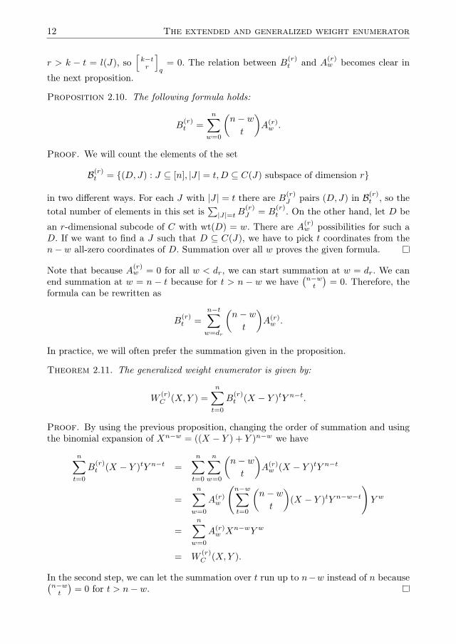
Proposition 2.10. The following formula holds:
B(r)t =
n∑w=0
(n− wt
)A(r)w .
Proof. We will count the elements of the set
B(r)t = {(D,J) : J ⊆ [n], |J | = t,D ⊆ C(J) subspace of dimension r}
in two different ways. For each J with |J | = t there are B(r)J pairs (D,J) in B(r)
t , so thetotal number of elements in this set is
∑|J|=tB
(r)J = B
(r)t . On the other hand, let D be
an r-dimensional subcode of C with wt(D) = w. There are A(r)w possibilities for such a
D. If we want to find a J such that D ⊆ C(J), we have to pick t coordinates from then− w all-zero coordinates of D. Summation over all w proves the given formula.
Note that because A(r)w = 0 for all w < dr, we can start summation at w = dr. We can
end summation at w = n − t because for t > n − w we have(n−wt
)= 0. Therefore, the
formula can be rewritten as
B(r)t =
n−t∑w=dr
(n− wt
)A(r)w .
In practice, we will often prefer the summation given in the proposition.
Theorem 2.11. The generalized weight enumerator is given by:
W(r)C (X,Y ) =
n∑t=0
B(r)t (X − Y )tY n−t.
Proof. By using the previous proposition, changing the order of summation and usingthe binomial expansion of Xn−w = ((X − Y ) + Y )n−w we have
n∑t=0
B(r)t (X − Y )tY n−t =
n∑t=0
n∑w=0
(n− wt
)A(r)w (X − Y )tY n−t
=
n∑w=0
A(r)w
(n−w∑t=0
(n− wt
)(X − Y )tY n−w−t
)Y w
=
n∑w=0
A(r)w Xn−wY w
= W(r)C (X,Y ).
In the second step, we can let the summation over t run up to n−w instead of n because(n−wt
)= 0 for t > n− w.

2.2 Extended weight enumerator 13
It is possible to determine the A(r)w directly from the B(r)
t , by using the next proposition.
Proposition 2.12. The following formula holds:
A(r)w =
n−dr∑t=n−w
(−1)n+w+t
(t
n− w
)B
(r)t .
Proof. For w < dr the summation is empty, which gives the correct formula A(r)w = 0.
For w ≥ dr we rewrite the generalized weight enumerator in the form of Theorem 2.11.By using the binomial expansion of (X − Y )t, substituting w = n− t+ j, and changingthe order of summation we find that
W(r)C (X,Y ) =
n−dr∑t=0
B(r)t (X − Y )tY n−t
=
n−dr∑t=0
B(r)t
t∑j=0
(t
j
)(−1)jXt−jY j
Y n−t
=
n−dr∑t=0
n∑w=n−t
B(r)t
(t
t− n+ w
)(−1)w+t−nXn−wY w
=
n∑w=dr
n−dr∑t=n−w
(−1)n+w+t
(t
n− w
)B
(r)t Xn−wY w.
The given formula follows from comparing with Definition 2.4 of the generalized weightenumerator.
Note that, like in Proposition 2.10, we can take the summation up to n instead of n−dr,because B(r)
t = 0 for t < n− dr by Proposition 2.9.
2.2 Extended weight enumerator
Let G be the generator matrix of a linear [n, k] code C over Fq. Then we can form the[n, k] code C ⊗ Fqm over Fqm by taking all Fqm -linear combinations of the codewords inC. We call this the extension code of C over Fqm . We denote the number of codewordsin C ⊗ Fqm of weight w by AC⊗Fqm ,w. We can determine the weight enumerator of suchan extension code by using only the code C.
By embedding its entries in Fqm , we find that G is also a generator matrix for theextension code C ⊗ Fqm . In Lemma 2.6 we saw that l(J) = k − r(J). Because r(J) isindependent of the extension field Fqm , we have dimFq C(J) = dimFqm (C⊗Fqm)(J). Thismotivates the usage of U as a variable for qm in the next definition.
Definition 2.13. Let C be a linear code over Fq. Then we define
BJ(U) = U l(J) − 1,
Bt(U) =∑|J|=t
BJ(U).

14 The extended and generalized weight enumerator
The extended weight enumerator is given by
WC(X,Y, U) = Xn +
n∑t=0
Bt(U)(X − Y )tY n−t.
Note that BJ(qm) is the number of nonzero codewords in (C ⊗ Fqm)(J).
Proposition 2.14. Let d and d⊥ be the minimum distance of C and C⊥ respectively.Then we have
Bt(U) =
{ (nt
)(Uk−t − 1) for all t < d⊥
0 for all t > n− d.
Proof. The proof is similar to the proof of Proposition 2.9 and is a direct consequenceof Lemma 2.7. For t < d⊥ we have l(J) = k − t, so BJ(U) = Uk−t − 1 and Bt(U) =(nt
)(Uk−t − 1). For t > n− d we have l(J) = 0, so BJ(U) = 0 and Bt(U) = 0.
Theorem 2.15. The following holds:
WC(X,Y, U) =
n∑w=0
Aw(U)Xn−wY w
with Aw(U) ∈ Z[U ] given by A0(U) = 1 and
Aw(U) =
n∑t=n−w
(−1)n+w+t
(t
n− w
)Bt(U)
for 0 < w ≤ n.
Proof. Note that Aw(U) = 0 for 0 < w < d because the summation is empty. Bysubstituting w = n− t+ j and reversing the order of summation, we have
WC(X,Y, U) = Xn +
n∑t=0
Bt(U)(X − Y )tY n−t
= Xn +
n∑t=0
Bt(U)
t∑j=0
(t
j
)(−1)jXt−jY j
Y n−t
= Xn +
n∑t=0
t∑j=0
(−1)j(t
j
)Bt(U)Xt−jY n−t+j
= Xn +
n∑t=0
n∑w=n−t
(−1)t−n+w
(t
t− n+ w
)Bt(U)Xn−wY w
= Xn +
n∑w=0
n∑t=n−w
(−1)n+w+t
(t
n− w
)Bt(U)Xn−wY w.
Since the second term is zero for w = 0, we see that WC(X,Y, U) is of the form∑nw=0Aw(U)Xn−wY w with Aw(U) of the form given in the theorem.

2.2 Extended weight enumerator 15
Note that in the definition of Aw(U) we can let the summation over t run up to n − dinstead of n, because Bt(U) = 0 for t > n− d.
Proposition 2.16. The following formula holds:
Bt(U) =
n−t∑w=d
(n− wt
)Aw(U).
Proof. We start with the extended weight enumerator in the form of Theorem 2.15 andthen rewrite as follows.
WC(X,Y, U) = Xn +
n∑w=d
Aw(U)((X − Y ) + Y )n−wY w
= Xn +
n∑w=d
Aw(U)
(n−w∑t=0
(n− wt
)(X − Y )tY n−w−t
)Y w
= Xn +
n∑w=d
n−w∑t=0
Aw(U)
(n− wt
)(X − Y )tY n−t
= Xn +
n∑t=0
n−t∑w=d
(n− wt
)Aw(U)(X − Y )tY n−t
The given formula follows from comparing with Definition 2.13 of the extended weightenumerator.
Note that, unlike in Proposition 2.10, we can not let the summation start at w = 0. Thisis because Aw(U) = 1 6= 0. We can let the summation run up to w = n, because thebinomial is zero for w > n− t.
As we said before, the motivation for looking at the extended weight enumerator comesfrom the extension codes. In the next proposition we show that the extended weightenumerator for U = qm is indeed the weight enumerator of the extension code C ⊗ Fqm .
Proposition 2.17. Let C be a linear [n, k] code over Fq. Then we have
WC(X,Y, qm) = WC⊗Fqm (X,Y ).
Proof. For w = 0 it is clear that A0(qm) = AC⊗Fqm ,0 = 1, so assume w 6= 0. It isenough to show that Aw(qm) = (qm − 1)A
(1)C⊗Fqm ,w. First we have
Bt(qm) =
∑|J|=t
BJ(qm)
=∑|J|=t
|{c ∈ (C ⊗ Fqm)(J) : c 6= 0}|
= (qm − 1)∑|J|=t
|{D ⊆ (C ⊗ Fqm)(J) : dimD = 1}
= (qm − 1)B(1)t (C ⊗ Fqm).

16 The extended and generalized weight enumerator
We also know that Aw(U) and Bt(U) are related the same way as A(1)w and B(1)
t . Com-bining this proves the statement.
Because of Proposition 2.17 we can interpret WC(X,Y, U) as the weight enumerator ofthe extension code over the algebraic closure of Fq. For further applications, the nextway of writing the extended weight enumerator will be useful.
Proposition 2.18. The extended weight enumerator of a linear code C can be writtenas
WC(X,Y, U) =
n∑t=0
∑|J|=t
U l(J)(X − Y )tY n−t.
Proof. By rewriting and using the binomial expansion of ((X − Y ) + Y )n, we get
n∑t=0
∑|J|=t
U l(J)(X − Y )tY n−t
=
n∑t=0
(X − Y )tY n−t∑|J|=t
((U l(J) − 1) + 1
)
=
n∑t=0
(X − Y )tY n−t
∑|J|=t
(U l(J) − 1) +
(n
t
)=
n∑t=0
Bt(U)(X − Y )tY n−t +
n∑t=0
(n
t
)(X − Y )tY n−t
=
n∑t=0
Bt(U)(X − Y )tY n−t +Xn
= WC(X,Y, U).
The MacWilliams identity we saw in Theorem 1.8 can be extended to the extended weightenumerator. We will give the proof of this theorem in Section 8.2.
Theorem 2.19 (MacWilliams). Let C be a code and let C⊥ be its dual. Then the extendedweight enumerator of C completely determines the extended weight enumerator of C⊥ andvice versa, via the following formula:
WC⊥(X,Y, U) = U−kWC(X + (U − 1)Y,X − Y,U).
2.3 Connections
There is a connection between the extended weight enumerator and the generalized weightenumerators. We first prove the next proposition.
Proposition 2.20. Let C be a linear [n, k] code over Fq, and let Cm be the linear sub-space consisting of the m × n matrices over Fq whose rows are in C. Then there is anisomorphism of Fq-vector spaces between C ⊗ Fqm and Cm.

2.3 Connections 17
Proof. First, fix an isomorphism ϕ : Fqm → Fmq . (For example, let α be a primitivem-th root of unity in Fqm and write an element of Fqm in a unique way on the basis(1, α, α2, . . . , αm−1).) We now create a map C⊗Fqm → Cm as follows. Let c = (c1, . . . , cn)be a word in C⊗Fqm . Apply ϕ coordinate-wise to c, and write the ϕ(ci) as column vectors.This gives an m× n matrix over Fq. The rows of this matrix are words of C, because Cand C ⊗ Fqm have the same generator matrix. This map is clearly injective. There are(qm)k = qkm words in C ⊗ Fqm , and the number of elements of Cm is (qk)m = qkm,so our map is a bijection. Moreover, the map is Fq-linear, so it gives an isomorphism ofFq-vector spaces C ⊗ Fqm → Cm.
Note that this isomorphism depends on the choice of an isomorphism ϕ : Fqm → Fmq .The use of this isomorphism for the proof of Theorem 2.23 was suggested by Simonis[85]. We also need the next lemma.
Lemma 2.21. Let c ∈ C ⊗ Fqm and M ∈ Cm the corresponding m × n matrix undera given isomorphism. Let D ⊆ C be the subcode generated by the rows of M . Thensupp(c) = supp(D) and hence wt(c) = wt(D).
Proof. Since ϕ : Fqm → Fmq is an isomorphism, we have that ϕ(ci) = 0 if and only ifci = 0. Also, the i-th column of M is zero if and only if i /∈ supp(D). Therefore,wt(c) =wt(D).
Proposition 2.22. Let C be a linear code over Fq. Then the weight enumerator of anextension code and the generalized weight enumerator are connected via
Aw(qm) =
m∑r=0
[m, r]qA(r)w .
Proof. We count the number of words in C ⊗ Fqm of weight w in two ways, using thebijection of Proposition 2.20. The first way is just by substituting U = qm in Aw(U):since AC⊗Fqm ,w = Aw(qm) by Proposition 2.17, this gives the left side of the equation.For the second way we use Lemma 2.21. Fix a weight w and a dimension r. There are A(r)
w
subcodes of C of dimension r and weight w. Every such subcode is generated by an r×nmatrix whose rows are words of C. Left multiplication by a m× r matrix of rank r givesan element of Cm that generates the same subcode of C, and all such elements of Cmare obtained this way. The number of m× r matrices of rank r is [m, r]q, so summationover all dimensions r gives
Aw(qm) =
k∑r=0
[m, r]qA(r)w .
We can let the summation run up to m, because A(r)w = 0 for r > k and [m, r]q = 0 for
r > m. This proves the given formula.
This result first appears in [49, Theorem 3.2], although the term “generalized weightenumerator” was yet to be invented. In general, we have the following theorem.

18 The extended and generalized weight enumerator
Theorem 2.23. Let C be a linear code over Fq. Then the extended weight enumeratorand the generalized weight enumerators are connected via
WC(X,Y, U) =
k∑r=0
r−1∏j=0
(U − qj)
W(r)C (X,Y ).
Proof. If we know A(r)w for all r, we can determine Aw(qm) for every m. If we have
k+ 1 values of m for which Aw(qm) is known, we can use Lagrange interpolation to findAw(U), for this is a polynomial in U of degree at most k. In fact, we have
Aw(U) =
k∑r=0
r−1∏j=0
(U − qj)
A(r)w .
This formula has the right degree and is correct for U = qm for all integer values m ≥ 0,so we know it must be the correct polynomial. Now the theorem follows.
The converse of the theorem is also true: we can write the generalized weight enumeratorin terms of the extended weight enumerator. We first give a combinatorial identity thatwe will use in several rewriting proofs. It is a generalization of Newton’s binomial identityto the Gaussian binomial and can be proven by induction.
Lemma 2.24. For every positive integer r the following identity holds:
r−1∏j=0
(Z − qj) =
r∑j=0
[r
j
]q
(−1)r−jq(r−j2 )Zj .
Theorem 2.25. Let C be a linear code over Fq. Then the generalized weight enumeratorand the extended weight enumerator are connected via
W(r)C (X,Y ) =
1
〈r〉q
r∑j=0
[r
j
]q
(−1)r−jq(r−j2 ) WC(X,Y, qj).
Proof. We consider the generalized weight enumerator in terms of Theorem 2.11. Rewrit-
2.4 Application to MDS codes 19
ing that expression gives the following:
W(r)C (X,Y ) =
n∑t=0
B(r)t (X − Y )tY n−t
=
n∑t=0
∑|J|=t
[l(J)
r
]q
(X − Y )tY n−t
=n∑t=0
∑|J|=t
r−1∏j=0
ql(J) − qj
qr − qj
(X − Y )tY n−t
=1∏r−1
v=0(qr − qv)
n∑t=0
∑|J|=t
r−1∏j=0
(ql(J) − qj)
(X − Y )tY n−t
=1
〈r〉q
n∑t=0
∑|J|=t
r∑j=0
[r
j
]q
(−1)r−jq(r−j2 )qj·l(J)(X − Y )tY n−t
=1
〈r〉q
r∑j=0
[r
j
]q
(−1)r−jq(r−j2 )
n∑t=0
∑|J|=t
(qj)l(J)(X − Y )tY n−t
=1
〈r〉q
r∑j=0
[r
j
]q
(−1)r−jq(r−j2 ) WC(X,Y, qj).
In the fourth step, we use the identity in Lemma 2.24. The last step follows from Propo-sition 2.18. See also [1, 20, 61, 99, 87].
2.4 Application to MDS codes
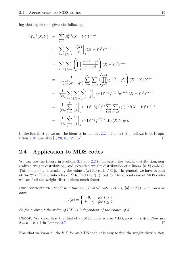
We can use the theory in Sections 2.1 and 2.2 to calculate the weight distribution, gen-eralized weight distribution, and extended weight distribution of a linear [n, k] code C.This is done by determining the values l(J) for each J ⊆ [n]. In general, we have to lookat the 2n different subcodes of C to find the l(J), but for the special case of MDS codeswe can find the weight distributions much faster.
Proposition 2.26. Let C be a linear [n, k] MDS code. Let J ⊆ [n] and |J | = t. Then wehave
l(J) =
{0, for t > k,
k − t, for t ≤ k.
So for a given t the value of l(J) is independent of the choice of J .
Proof. We know that the dual of an MDS code is also MDS, so d⊥ = k + 1. Now used = n− k + 1 in Lemma 2.7.
Now that we know all the l(J) for an MDS code, it is easy to find the weight distribution.

20 The extended and generalized weight enumerator
Theorem 2.27. Let C be an MDS code with parameters [n, k]. Then the generalizedweight distribution is given by
A(r)w =
(n
w
)w−d∑j=0
(−1)j(w
j
)[w − d+ 1− j
r
]q
.
The coefficients of the extended weight enumerator for w > 0 are given by
Aw(U) =
(n
w
)w−d∑j=0
(−1)j(w
j
)(Uw−d+1−j − 1).
Proof. We will give the construction for the generalized weight enumerator here: thecase of the extended weight enumerator is similar and is left as an exercise. We knowfrom Proposition 2.26 that for an MDS code, B(r)
t depends only on the size of J , soB
(r)t =
(nt
) [k−tr
]q. Using this in the formula for A(r)
w and substituting j = t− n+w, we
have
A(r)w =
n−dr∑t=n−w
(−1)n+w+t
(t
n− w
)B
(r)t
=
n−dr∑t=n−w
(−1)t−n+w
(t
n− w
)(n
t
)[k − tr
]q
=
w−dr∑j=0
(−1)j(n
w
)(w
j
)[k + w − n− j
r
]q
=
(n
w
)w−dr∑j=0
(−1)j(w
j
)[w − d+ 1− j
r
]q
.
In the second step, we are using the binomial equivalence(n
t
)(t
n− w
)=
(n
n− w
)(n− (n− w)
t− (n− w)
)=
(n
w
)(w
n− t
).
So for all MDS-codes the extended and generalized weight distributions are completelydetermined by the parameters [n, k]. But not all such codes are equivalent. We canconclude from this, that the generalized and extended weight enumerators are not enoughto distinguish between codes with the same parameters. We illustrate the non-equivalenceof two MDS codes by an example.
Example 2.28. Let C be a linear [n, 3] MDS code over Fq and let n ≥ 5. Because C isMDS we have d = n− 2 ≥ 3. We now view the n columns of G as distinct points in theprojective plane P2(Fq), say P1, . . . , Pn. The MDS property that every k columns of Gare independent is now equivalent to saying that no three points are on a line.To see that these n points do not always determine an equivalent code, consider the

2.4 Application to MDS codes 21
following construction. Through the n points there are(n2
)= N lines, the set N . These
lines determine (the generator matrix of) an [n, 3] code C. The minimum distance of thecode C is equal to the total number of lines minus the maximum number of lines from Nthrough an arbitrary point P ∈ P2(Fq). If P /∈ {P1, . . . , Pn} then the maximum numberof lines from N through P is at most 1
2n, since no three points of N lie on a line. IfP = Pi for some i ∈ [n] then P lies on exactly n − 1 lines of N , namely the lines PiPjfor j 6= i. Therefore, the minimum distance of C is d = N − n+ 1.
We now have constructed an [n, 3, N −n+ 1] code C from the original code C. Note thattwo codes C1 and C2 are generalized equivalent if C1 and C2 are generalized equivalent.The generalized and extended weight enumerators of an MDS code of length n and di-mension k are completely determined by the pair (n, k), but this is not generally true forthe weight enumerator of C.
Take for example n = 6 and q = 9, then C is a [15, 3, 10] code. Look at the codes C1 andC2 generated by the following matrices respectively, where α ∈ F9 is a primitive element: 1 1 1 1 1 1
0 1 0 1 α5 α6
0 0 1 α3 α α3
,
1 1 1 1 1 10 1 0 α7 α4 α6
0 0 1 α5 α 1
.
Being both MDS codes, the weight distribution is (1, 0, 0, 120, 240, 368). If we now applythe above construction, we get C1 and C2 generated by 1 0 0 1 1 α4 α6 α3 α7 α 1 α2 1 α7 1
0 1 0 α7 1 0 0 α4 1 1 0 α6 α 1 α3
0 0 1 1 0 1 1 1 0 0 1 1 1 1 1
,
1 0 0 α7 α2 α3 α 0 α7 α7 α4 α7 α 0 00 1 0 1 0 α3 0 α6 α6 0 α7 α α6 α3 α0 0 1 α5 α5 α6 α3 α7 α4 α3 α5 α2 α4 α α5
.
The weight distributions of C1 and C2 are, respectively,
(1, 0, 0, 0, 0, 0, 0, 0, 0, 0, 48, 0, 16, 312, 288, 64) and(1, 0, 0, 0, 0, 0, 0, 0, 0, 0, 48, 0, 32, 264, 336, 48).
So the latter two codes are not generalized equivalent, and therefore not all [6, 3, 4] MDScodes over F9 are generalized equivalent.
Another example was given in [86, 22] showing that two [6, 3, 4] MDS codes could havedistinct covering radii.

22 The extended and generalized weight enumerator

3Zeta functions and their
generalizations
The notion of a zeta function originates from the theory of algebraic curves. Via alge-braic geometry codes Duursma extended the definition to linear codes [36, 37]. The zetafunction admits two generalizations, along the same lines as the generalizations of theweight enumerator in Chapter 2. We can extend the field over which the code is defined:this leads to the two-variable zeta function. Looking at subcodes instead of codewordsleads to the generalized zeta function.Most of this chapter is a summary of known results from Duursma [39], but presented ina way to match with the previous chapter. The definition of the generalized zeta functionvia generalized binomial moments differs from the approach in [39]. Where Duursma usesthe decomposition of zeta functions to define the generalized zeta function, we find inTheorem 3.8 new formulas that directly express the coefficients of the generalized zetapolynomial in terms of the generalized binomial moments.The theory in this chapter is also used in Chapter 11. Following the literature, we willrestrict ourselves in this chapter to codes with minimum distance and dual minimumdistance at least three, i.e., d, d⊥ ≥ 3.
3.1 The (two-variable) zeta function
The two-variable zeta polynomial is extensively studied by Duursma [39], who definedand studied the one-variable case in [36, 37].
Definition 3.1. Let C be a linear [n, k, d] code over Fq with extended weight enumer-ator WC(X,Y, U). The two-variable zeta polynomial PC(T,U) of this code is the uniquepolynomial in Q[T,U ] of degree at most n−d in T such that if we expand the generatingfunction
PC(T,U)
(1− T )(1− TU)(Y (1− T ) +XT )n
as a power series in the variable T , we get
. . .+ . . . Tn−d−1 +WC(X,Y, U)−Xn
U − 1Tn−d + . . . Tn−d+1 + . . . .
24 Zeta functions and their generalizations
The quotient ZC(T,U) = PC(T,U)/((1 − T )(1 − TU)) is called the two-variable zetafunction.
Just as with the extended weight enumerator, the variable U can be interpreted as thesize of the finite field over which the code is defined. We will often refer to the zetapolynomial in the following form:
PC(T,U) =
r∑i=0
Pi(U)T i.
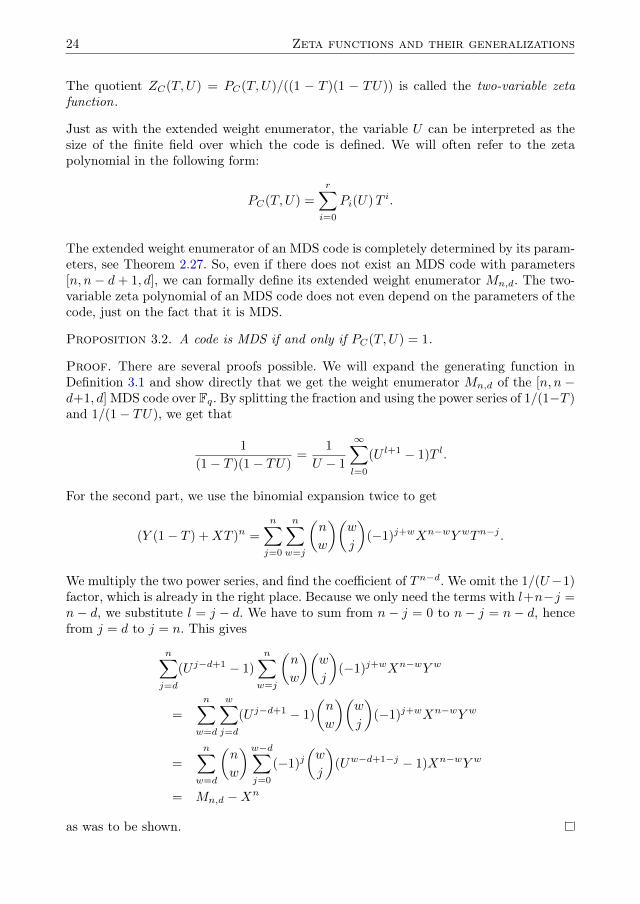
The extended weight enumerator of an MDS code is completely determined by its param-eters, see Theorem 2.27. So, even if there does not exist an MDS code with parameters[n, n− d+ 1, d], we can formally define its extended weight enumerator Mn,d. The two-variable zeta polynomial of an MDS code does not even depend on the parameters of thecode, just on the fact that it is MDS.
Proposition 3.2. A code is MDS if and only if PC(T,U) = 1.
Proof. There are several proofs possible. We will expand the generating function inDefinition 3.1 and show directly that we get the weight enumerator Mn,d of the [n, n −d+1, d] MDS code over Fq. By splitting the fraction and using the power series of 1/(1−T )and 1/(1− TU), we get that
1
(1− T )(1− TU)=
1
U − 1
∞∑l=0
(U l+1 − 1)T l.
For the second part, we use the binomial expansion twice to get
(Y (1− T ) +XT )n =
n∑j=0
n∑w=j
(n
w
)(w
j
)(−1)j+wXn−wY wTn−j .
We multiply the two power series, and find the coefficient of Tn−d. We omit the 1/(U−1)factor, which is already in the right place. Because we only need the terms with l+n−j =n− d, we substitute l = j − d. We have to sum from n− j = 0 to n− j = n− d, hencefrom j = d to j = n. This gives
n∑j=d
(U j−d+1 − 1)
n∑w=j
(n
w
)(w
j
)(−1)j+wXn−wY w
=
n∑w=d
w∑j=d
(U j−d+1 − 1)
(n
w
)(w
j
)(−1)j+wXn−wY w
=
n∑w=d
(n
w
)w−d∑j=0
(−1)j(w
j
)(Uw−d+1−j − 1)Xn−wY w
= Mn,d −Xn
as was to be shown.

3.2 The generalized zeta function 25
Theorem 3.3. The zeta polynomial gives us a way to write the extended weight enumer-ator with respect to a basis of MDS weight enumerators:
WC(X,Y, U) = P0(U)Mn,d + P1(U)Mn,d+1 + . . .+ Pr(U)Mn,d+r.
Proof. This follows directly from Definition 3.1 and Proposition 3.2.
We treat some more properties of the two-variable zeta polynomial. The proofs are similarto the case of the one-variable zeta polynomial as treated in [39].
Proposition 3.4. The degree of PC(T,U) in T is n− d− d⊥ + 2.
Proof. Assume that Pr(U) is not zero and apply Theorem 3.3 to the dual code C⊥.This expression starts with the dual of Mn,d⊥+r. Since the dual of an MDS code is againan MDS code by Theorem 1.12, it is equal to Mn,n−d+2+r. Therefore, n+ 2− d− r = d⊥
and hence r = n− d− d⊥ + 2.
A way to interpret this degree n − d − d⊥ + 2 is to view it as a measure for how “faraway” a code is from being MDS.
Proposition 3.5. For the two-variable zeta polynomial of a code C and dual C⊥ wehave
PC⊥(T,U) = PC
(1
TU,U
)Un−k+1−dTn−d−d
⊥+2.
Proof. Apply the MacWilliams identity for the extended weight enumerator in Theorem2.19 to the expression in Theorem 3.3. This gives that WC⊥(X,Y, U) is equal to
= U−kWC(X + (U − 1)Y,X − Y )
= U−k(P0(U)Mn,d(X + (U − 1)Y,X − Y ) + . . .
+Pr(U)Mn,d+r(X + (U − 1)Y,X − Y ))
= U−k(Pr(U)Un−d−r+1Mn,n−d+2−r + . . .+ P0(U)Un−d−1Mn,n−d+2
)and the Proposition follows.
3.2 The generalized zeta function
In Definition 3.1 of the zeta function, the coefficient of Tn−d in the power series is exactlythe first generalized weight enumerator W (1)
C (X,Y ). This motivates the definition of ageneralized zeta function of a linear code.
Duursma [39] uses normalized binomial moments to define the two-variable zeta polyno-mial. These binomial moments are quite similar to the B(r)
t we encountered in Section2.1, because Duursma’s kS is equal to l(J) for S = [n]\J . To avoid confusion, the capitalB is only used in the meaning of Section 2.1. We can generalize the normalized binomialmoments in the following way:

26 Zeta functions and their generalizations
Definition 3.6. The generalized binomial moments of a linear code are given by
b(r)i =
B
(r)n−dr−i/
(n
dr+i
), for 0 ≤ i ≤ n− d⊥ − dr,
0, for i < 0,[k−n+i+dr
r
]q, for i > n− d⊥ − dr.
This definition is well defined by Proposition 2.9.
Definition 3.7. The generalized zeta function of a linear code is the generating functionfor the generalized binomial moments:
Z(r)C (T ) =
∞∑i=0
b(r)i T i.
Theorem 3.8. The generalized zeta function is a rational function given by
Z(r)C (T ) =
P(r)C (T )
(1− T )(1− qT ) · · · (1− qrT ),
where P (r)C (T ) is a polynomial of degree n− d⊥ − dr + r + 1 with coefficients given by
P(r)i =
r+1∑j=0
[r + 1
j
]q
(−1)jq(j2)b
(r)i−j .
Proof. We will first show the formula for the P (r)i , and then show that they are almost
all zero, hence P (r)i is indeed a polynomial. We start with a combinatorial statement,
using Lemma 2.24.r∏j=0
(1− qjT ) = T r+1r∏j=0
(1
T− qj
)
=
r+1∑j=0
[r + 1
j
]q
(−1)r+1−jq(r+1−j
2 )T r+1−j
=
r+1∑j=0
[r + 1
j
]q
(−1)jq(j2)T j .
From this, we can find how P(r)C (T ) looks like:
P(r)C (T ) = Z
(r)C (T ) · (1− T )(1− qT ) · · · (1− qrT )
=
( ∞∑i=0
b(r)i T i
)·
r+1∑j=0
[r + 1
j
]q
(−1)jq(j2)T j
.
If we look at the coefficient of T i when we expand this function in the variable T , we getexactly the formula for P (r)
i . For i < 0, this is clearly zero, because b(r)i = 0 for i < 0.
3.2 The generalized zeta function 27
Therefore, it is left to show that P (r)i = 0 for i > n− d⊥ − dr + r + 1.
Assume that i > n−d⊥−dr+r+1. Then we can determine the value for P (r)i because we
know the value of all b(r)i−j for 0 ≤ j ≤ r+1 by Proposition 2.9. We put s = k−n+ i+dr,rewrite, use Lemma 2.24, put j = r + 1− j, and rewrite some more. This gives
P(r)i =
r+1∑j=0
[r + 1
j
]q
(−1)jq(j2)b
(r)i−j
=r+1∑j=0
[r + 1
j
]q
(−1)jq(j2)[k − n+ i− j + dr
r
]q
=
r+1∑j=0
[r + 1
j
]q
(−1)jq(j2)[s− jr
]q
=
r+1∑j=0
[r + 1
j
]q
(−1)jq(j2)r−1∏i=0
(qs−j − qi
qr − qi
)
=1
〈r〉q
r+1∑j=0
[r + 1
j
]q
(−1)jq(j2)r−1∏i=0
(qs−j − qi)
=1
〈r〉q
r+1∑j=0
[r + 1
j
]q
(−1)jq(j2)
r∑i=0
[ri
]q
(−1)r−iq(r−i2 )qi(s−j)
=1
〈r〉q
r∑i=0
[ri
]q
(−1)r−iq(r−i2 )qis
r+1∑j=0
[r + 1
j
]q
(−1)jq(j2)q−ij
=1
〈r〉q
r∑i=0
[ri
]q
(−1)r−iq(r−i2 )qis
r+1∑j=0
[r + 1
j
]q
(−1)r+1−jq(r+1−j
2 )q−i(r+1−j)
=1
〈r〉q
r∑i=0
[ri
]q
(−1)r−iq(r−i2 )qi(s+r+1)
r∏j=0
(q−i − qj)
=1
〈r〉q
r∑i=0
[ri
]q
(−1)r−iq(r−i2 )qi(s+r+1)q−i(r+1)
r∏j=0
(1− qj−i)
=1
〈r〉q
r∑i=0
[ri
]q
(−1)r−iq(r−i2 )qis
r∏j=0
(1− qj−i).
Since both i and j sum over the same range, the factor 1 − qj−i becomes zero in everyterm of the summation and thus this whole expression is equal to zero. This shows thatthe generalized zeta function is indeed a rational function of the given form.
The next theorem shows that the generalized zeta function determines the generalizedweight enumerator of the code.
Theorem 3.9. If we expand the generating function Z(r)C (T ) · (Y (1 − T ) + XT )n in T ,
it has expansion. . .+W
(r)C (x, y) Tn−dr + . . . .

28 Zeta functions and their generalizations
Proof. We want to determine the coefficient of Tn−dr in the generating function
(∑i
b(r)i T i
)·
n∑j=0
n∑w=j
(n
w
)(w
j
)(−1)j+wXn−wY wTn−j
.
We need the terms with i + n − j = n − dr, so let i = j − dr. Then changing the orderof summation, setting n− j = t and factoring out binomials gives that
n∑j=dr
b(r)j−dr
n∑w=j
(n
w
)(w
j
)(−1)j+wXn−wY w
=
n∑w=dr
w∑j=dr
b(r)j−dr
(n
w
)(w
j
)(−1)j+wXn−wY w
=
n∑w=dr
n−dr∑t=n−w
b(r)n−t−dr
(n
w
)(w
n− t
)(−1)n−t+wXn−wY w
=
n∑w=dr
n−dr∑t=n−w
B(r)t(nt
) (nt
)(t
n− w
)(−1)n−t+wXn−wY w
=
n∑w=dr
n∑t=n−w
B(r)t
(t
n− w
)(−1)n+t+wXn−wY w
=
n∑w=dr
A(r)w Xn−wY w
= W(r)C (X,Y )
which was to be proved.
Corollary 3.10. For all MDS codes, we have P (r)C = 1.
Proof. From Theorem 3.8 we know that the degree of P (r)(T ) is equal to n−d⊥−dr +
r+ 1, so for MDS codes this degree is 0. Therefore, we only have to show that P (r)0 = 1.
We use the formula in Theorem 3.8 for this:
P(r)0 =
r+1∑j=0
[r + 1
j
]q
(−1)jq(j2)b
(r)−j .
Since b(r)i = 0 for i < 0, the only nonzero term in the above summation is at j = 0,so P (r)
0 = b(r)0 . In Theorem 2.27 we found that B(r)
t =(nt
) [k−tr
]qfor MDS codes. This

3.2 The generalized zeta function 29
means that
P(r)0 = b
(r)0
= B(r)n−dr/
(n
dr
)=
(n
t
)[k − n+ dr
r
]q
/
(n
dr
)=
[rr
]q
= 1
as was to be shown.
Because of the previous corollary, we can interpret the generalized zeta polynomial asa way to write a weight enumerator with respect to a “basis” of weight enumerators ofMDS codes. This follows directly from the previous theory.
Theorem 3.11. Denote by M (r)n,dr
the generalized weight enumerator of an MDS code oflength n and minimum distance d = dr − r + 1. Then the weight enumerator of a codewith generalized zeta polynomial P (r)(T ) is given by
W(r)C (X,Y ) = P
(r)0 M
(r)n,dr−r+1 + P
(r)1 M
(r)n,dr−r+2 + . . .+ P
(r)
n−d⊥−dr+r+1M
(r)
n,n−d⊥+2.

30 Zeta functions and their generalizations

Part II
Codes and arrangements
31


4Introduction to arrangements
An arrangement of hyperplanes is simply an n-tuple of hyperplanes in some affine orprojective space. If an arrangement is defined over the real affine space, an interestingquestion is in how many regions the real affine space is divided by the arrangement. Theanswer to this question is given by the characteristic polynomial, that we will encounterin Chapter 10. If an arrangement is defined over a projective space, it becomes the dualnotion of a projective system. Important for our purposes are arrangements and projectivesystems defined over finite fields, because of their close relation to weight enumerationof linear codes.In this chapter, we will only give the basic definitions of arrangements and projectivesystems. For a more extensive introduction, see for example Stanley [88] or Orlik andTerao [76]. The connection with weight enumeration is a summary of the work fromKatsman, Tsfasman and Vladut [60, 92, 93].
4.1 Projective systems and hyperplane arrangements
Let F be a field. A projective system P = (P1, . . . , Pn) in Pr(F), the projective space overF of dimension r, is an n-tuple of points Pj in this projective space, such that not allthese points lie in a hyperplane.
Let Pj be given by the homogeneous coordinates (p0j : p1j : . . . : prj) and let GP be the(r+1)×n matrix with (p0j , p1j , . . . , prj)
T as j-th column. Then GP has rank r+1, sincenot all points lie in a hyperplane. If F is a finite field, then GP is the generator matrixof a nondegenerate code over F of length n and dimension r + 1.Conversely, let G be a generator matrix of a nondegenerate linear [n, k] code C over Fq,so G has no zero columns. Take the columns of G as homogeneous coordinates of pointsin Pk−1(Fq). This gives the projective system PG over Fq of G. Note that for all extensioncodes of C, the associated projective system consists of the points of PG embedded inPk−1(Fqm).
An n-tuple (H1, . . . ,Hn) of hyperplanes in Fk is called an arrangement in Fk. We usuallydenote an arrangement by A. The arrangement is called simple if all the n hyperplanesare mutually distinct. The arrangement is called central if all the hyperplanes are linear

34 Introduction to arrangements
subspaces. A central arrangement is called essential if the intersection of all its hyper-planes is equal to {0}.
Let G = (gij) be a generator matrix of a nondegenerate linear [n, k] code C, so G has nozero columns. Let Hj be the linear hyperplane in Fkq with equation
g1jX1 + · · ·+ gkjXk = 0.
The arrangement (H1, . . . ,Hn) associated with G will be denoted by AG. The arrange-ment associated with an extension code of C consists of the hyperplanes of AG embeddedin Fkqm .
In case of a central arrangement one considers the hyperplanes in Pk−1(F). Note thatprojective systems and essential arrangements are dual notions and that there is a one-to-one correspondence between equivalence classes of nondegenerate [n, k] codes over Fq,equivalence classes of projective systems over Fq of n points in Pk−1(Fq), and equivalenceclasses of essential arrangements of n hyperplanes in Pk−1(Fq).
4.2 Geometric interpretation of weight enumeration
We can write a codeword c ∈ C as c = xG, with x ∈ Fkq . The i-th coordinate of c is zeroif and only if the standard inner product of x and the i-th column of G is zero. In termsof projective systems: Pi is in the hyperplane perpendicular to x. See Figure 4.1.�
���
0
1× k k × n 1× nmessage m generator matrix G codeword c
Figure 4.1: The geometric determination of the weight of a codeword
Proposition 4.1. Let C be a linear nondegenerate [n, k] code over Fq with generatormatrix G. Let PG be the projective system of G. The code has minimum distance d if andonly if n− d is the maximal number of points of PG in a hyperplane of Pk−1(Fq).
Proof. See Katsman, Tsfasman and Vladut [60, 92, 93].
We can translate Proposition 4.1 for an arrangement.
Proposition 4.2. Let C be a nondegenerate code over Fq with generator matrix G andlet c be a codeword c = xG for some x ∈ Fkq . Then n − wt(c) is equal to the number ofhyperplanes in AG through x.
Remark 4.3. Recall that in Definitions 2.5 and 2.13 we introduced C(J) and BJ(U) forthe determination of the weight enumerator. Let AG = (H1, . . . ,Hn) be the arrangement
4.2 Geometric interpretation of weight enumeration 35
associated to the nondegenerate code C. The encoding map x 7→ xG = c from vectorsx ∈ Fkq to codewords gives the following isomorphism of vectorspaces:⋂
j∈JHj∼= C(J).
Furthermore, BJ(q) is equal to the number of nonzero codewords c ∈ C that are zero atall j in J and this is equal to the number of nonzero elements of the intersection
⋂j∈J Hj .
A similar remark holds for words in an extension code C ⊗ Fqm .
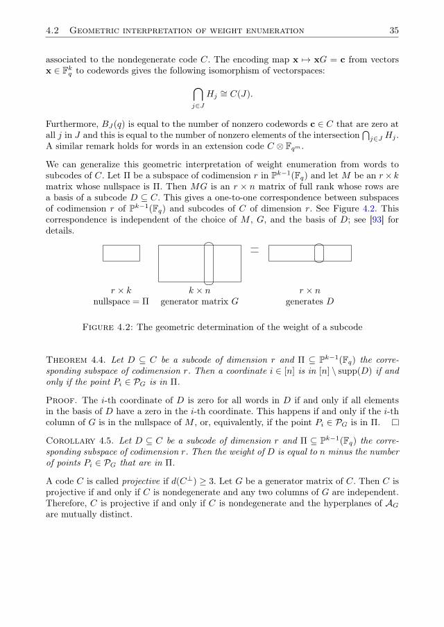
We can generalize this geometric interpretation of weight enumeration from words tosubcodes of C. Let Π be a subspace of codimension r in Pk−1(Fq) and let M be an r× kmatrix whose nullspace is Π. Then MG is an r × n matrix of full rank whose rows area basis of a subcode D ⊆ C. This gives a one-to-one correspondence between subspacesof codimension r of Pk−1(Fq) and subcodes of C of dimension r. See Figure 4.2. Thiscorrespondence is independent of the choice of M , G, and the basis of D; see [93] fordetails. �
���
����r × k k × n r × n
nullspace = Π generator matrix G generates D
Figure 4.2: The geometric determination of the weight of a subcode
Theorem 4.4. Let D ⊆ C be a subcode of dimension r and Π ⊆ Pk−1(Fq) the corre-sponding subspace of codimension r. Then a coordinate i ∈ [n] is in [n] \ supp(D) if andonly if the point Pi ∈ PG is in Π.
Proof. The i-th coordinate of D is zero for all words in D if and only if all elementsin the basis of D have a zero in the i-th coordinate. This happens if and only if the i-thcolumn of G is in the nullspace of M , or, equivalently, if the point Pi ∈ PG is in Π.
Corollary 4.5. Let D ⊆ C be a subcode of dimension r and Π ⊆ Pk−1(Fq) the corre-sponding subspace of codimension r. Then the weight of D is equal to n minus the numberof points Pi ∈ PG that are in Π.
A code C is called projective if d(C⊥) ≥ 3. Let G be a generator matrix of C. Then C isprojective if and only if C is nondegenerate and any two columns of G are independent.Therefore, C is projective if and only if C is nondegenerate and the hyperplanes of AGare mutually distinct.

36 Introduction to arrangements

5Weight enumeration of codes from
finite spaces
In the previous chapter, we have described a geometric method to determine the extendedand generalized weight distribution of a code. We will apply this theory to projectivesystems coming from projective and affine spaces: the corresponding codes are the q-arySimplex code and the q-ary first order Reed-Muller code. As a result of the calculations,we will not only determine the generalized and equivalent weight enumerators of thesecodes, but we also completely determine the set of supports of subcodes and words in anextension code.This chapter is a copy of [53].
5.1 Codes from a finite projective space
Consider the projective system P that consists of all the points in Ps−1(Fq) withoutmultiplicities. The corresponding code is the Simplex code:
Definition 5.1. The q-ary Simplex code Sq(s) is a linear [(qs − 1)/(q − 1), s] code overFq. The columns of the generator matrix of the code are all possible nonzero vectors inFsq, up to multiplication by a scalar.
The correspondence between P and the Simplex code is independent of the choice of agenerator matrix. We use this correspondence to determine the extended weight enumer-ator of the Simplex code. We do this via the generalized weight enumerators.
Theorem 5.2. The generalized weight enumerators of the Simplex code Sq(s) are, for0 ≤ r ≤ s, given by
WSq(s)(X,Y ) =[sr
]qX(qs−r−1)/(q−1)Y (qs−qs−r)/(q−1).
Proof. We use Corollary 4.5 to determine the weights of all subcodes of Sq(s). Fix adimension r. Let D ⊆ Sq(s) be some subcode of dimension r that corresponds to thesubspace Π ⊆ Ps−1(Fq) of codimension r. The weight ofD is equal to nminus the numberof points in P that are in Π. Because all points of Ps−1(Fq) are in P, the weight is the

38 Weight enumeration of codes from finite spaces
same for all D and it is equal to n minus the total number of points in Π. This meansthe weight of D is equal to
qs − 1
q − 1− qs−r − 1
q − 1=qs − qs−r
q − 1
and the theorem follows.
From the previous calculation and Theorem 4.4 the next statement follows.
Corollary 5.3. Let D be some subcode of dimension r of the Simplex code Sq(s). Thenthe points in P indexed by [n] \ supp(D) are all the points in the corresponding subspaceΠ of codimension r in Ps−1(Fq).We can now write down the extended weight enumerator of the Simplex code:
Theorem 5.4. The extended weight enumerator of the Simplex code Sq(s) is equal to
WSq(s)(X,Y, U) =
s∑r=0
r−1∏j=0
(U − qj)
[sr
]qX(qs−r−1)/(q−1)Y (qs−qs−r)/(q−1).
Proof. We use the correspondence between the generalized and extended weight enu-merator in Theorem 2.23:
WSq(s)(X,Y, U) =
s∑r=0
r−1∏j=0
(U − qj)
WSq(s)(X,Y )
=
s∑r=0
r−1∏j=0
(U − qj)
[sr
]qX(qs−r−1)/(q−1)Y (qs−qs−r)/(q−1).
In combination with the isomorphism of Proposition 2.20 and Lemma 2.21, we get thefollowing consequence.
Corollary 5.5. The points in P indexed by the complement of the support of a word ofweight (qs−qs−r)/(q−1) in the extension code Sq(s)⊗Fqm for r ≤ m are all the points ina subspace of Ps−1(Fq) of codimension r and every subspace of Ps−1(Fq) of codimensionr occurs in this manner.
Example 5.6. We consider the Simplex code S2(3). It is a binary [7, 3] code. Its extendedweight enumerator has coefficients
A0(U) = 1,
A1(U) = 0,
A2(U) = 0,
A3(U) = 0,
A4(U) = 7(U − 1),
A5(U) = 0,
A6(U) = 7(U − 1)(U − 2),
A7(U) = (U − 1)(U − 2)(U − 4).

5.2 Codes from a finite affine space 39
Note that for any code we have A0(U) = 1 for the zero word, and all other polynomialsare divisible by (U − 1) because over the “field of size one” we only have the zero word.In the binary case U = 2, the polynomials for A6(U) and A7(U) vanish and the code hasonly one nonzero weight. For U = 22 = 4, A7(U) still vanishes, it is a two-weight code.For U = 23 and higher extensions we get all three possible nonzero weights.
5.2 Codes from a finite affine space
It may sound a bit strange to talk about the projective system coming from an affinespace. To solve this, remember that we can construct the finite affine space As−1(Fq) bydeleting a hyperplane from Ps−1(Fq). Therefore, let the projective system P consists ofall points in Ps−1(Fq) minus the points in a hyperplane H of Ps−1(Fq). Without loss ofgenerality, we can choose H to be the hyperplane X1 = 0. The corresponding code is(monomial equivalent to) the first order q-ary Reed-Muller code, and we can define it inthe following way:
Definition 5.7. The first order q-ary Reed-Muller codeRMq(1, s−1) is a linear [qs−1, s]code over Fq. The generator matrix consists of the all-one row, and the other positionsin the columns of the generator matrix are all possible vectors in Fs−1
q .
Note that the linear dependence between the columns of the generator matrix is nowequal to the dependence between the corresponding affine points: this property is veryuseful if we want to talk about the matroid associated to the code, see [73].
We will use the projective system described above to determine the extended weightenumerator of the first order Reed-Muller code. We do this via the generalized weightenumerators.
Theorem 5.8. The generalized weight enumerators of the first order Reed-Muller codeRMq(1, s− 1) are, for 0 < r < s, given by
W(r)RMq(1,s−1)(X,Y ) =
[s− 1
r − 1
]q
Y n + qr[s− 1
r
]q
Xqs−1−rY q
s−1−qs−1−r.
The extremal cases are, as always, given by
W(0)RMq(1,s−1)(X,Y ) = Xn,
W(s)RMq(1,s−1)(X,Y ) = Y n.
Proof. We use Corollary 4.5 to determine the weights of all subcodes of RMq(1, s−1).Fix a dimension r, with 0 ≤ r ≤ s. Let D ⊆ RMq(1, s−1) be some subcode of dimensionr that corresponds to the subspace Π ⊆ Ps−1(Fq) of codimension r. The weight of D isequal to n minus the number of points in P that are in Π. There are two possibilities:
1. Π ⊆ H;
2. Π 6⊆ H.

40 Weight enumeration of codes from finite spaces
In the first case, we cannot have r = 0, since then Π is the whole of Ps−1(Fq) and thiscannot be contained in the hyperplane H. So, let r > 0. Now none of the points of Pare in Π, since no points of H are in P. Therefore, supp(D) = [n] and wt(D) = n.The number of such codes is equal to the number of subspaces of codimension r − 1 inH ∼= PG(s− 2, q), and this is
[s−1r−1
]q. Hence for 0 < r ≤ s we get the following term for
the generalized weight enumerator: [s− 1
r − 1
]q
Y n.
In the second case, we do not have to consider r = s, since then Π is the empty set andthis was already included in the previous case. So, let r < s. Now Π and H intersect ina subspace of codimension r in H. The points of P that are in Π, are all those points ofΠ that are not in Π ∩H. By the construction of the affine space As−1(Fq), the points ofΠ\ (Π∩H) form a subspace of As−1(Fq) of codimension r. The number of points in sucha subspace is qs−1−r, so wt(D) = n− qs−1−r = qs−1− qs−1−r. The number of such codesis equal to the number of subspaces of codimension r in As−1(Fq), and this is qr
[s−1r
]q.
Therefore, this case gives the following term for the generalized weight enumerator, for0 ≤ r < s:
qr[s− 1
r
]q
Xqs−1−rY q
s−1−qs−1−r.
Summing up this two cases leads to the given formulas.
From the previous calculation and Theorem 4.4 the next statement follows.
Corollary 5.9. Let D be some subcode of dimension r of the first order Reed-Mullercode RMq(1, s−1). Then either supp(D) = [n] or the points in P indexed by [n]\supp(D)are all the points in the corresponding subspace Π of codimension r in As−1(Fq) and everysubspace of As−1(Fq) of codimension r occurs in this manner.
We can now write down the extended weight enumerator of the first order Reed-Mullercode:
Theorem 5.10. The extended weight enumerator of the first order Reed-Muller codeRMq(1, s− 1) is equal to
WRMq(1,s−1)(X,Y, U) =
s∑r=1
r−1∏j=0
(U − qj)
[s− 1
r − 1
]q
Y n
+
s−1∑r=0
r−1∏j=0
(U − qj)
qr[s− 1
r
]q
Xqs−1−rY q
s−1−qs−1−r.
Proof. We use the correspondence between the generalized and extended weight enu-

5.2 Codes from a finite affine space 41
merator in Theorem 2.23:
WRMq(1,s−1)(X,Y, U) =
s∑r=0
r−1∏j=0
(U − qj)
WSq(s)(X,Y )
= Xn +
s−1∑r=1
r−1∏j=0
(U − qj)
([s− 1
r − 1
]q
Y n
+qr[s− 1
r
]q
Xqs−1−rY q
s−1−qs−1−r
)+ Y n
=
s∑r=1
r−1∏j=0
(U − qj)
[s− 1
r − 1
]q
Y n
+
s−1∑r=0
r−1∏j=0
(U − qj)
qr[s− 1
r
]q
Xqs−1−rY q
s−1−qs−1−r.
In combination with the isomorphism of Proposition 2.20 and Lemma 2.21, we get thefollowing consequence.
Corollary 5.11. The points in P indexed by the complement of the support of a wordof weight qs−1− qs−1−r in the extension code RMq(1, s− 1)⊗Fqm for r ≤ m are all thepoints in a subspace of As−1(Fq) of codimension r.
Example 5.12. We consider the Reed-Muller code RM2(1, 3). It is a binary [8, 4] code.Its extended weight enumerator has coefficients
A0(U) = 1,
A1(U) = 0,
A2(U) = 0,
A3(U) = 0,
A4(U) = 14(U − 1),
A5(U) = 0,
A6(U) = 28(U − 1)(U − 2),
A7(U) = 8(U − 1)(U − 2)(U − 4),
A8(U) = (U − 1)(U3 − 7U2 + 21U − 21).
As noticed in Example 5.6, for any code we have A0(U) = 1 for the zero word, and allother polynomials are divisible by (U − 1) because over the “field of size one” we onlyhave the zero word. In the binary case U = 2, the polynomials for A6(U) and A7(U)vanish and we get a two-weight code. For U = 22 = 4, A7(U) still vanishes. For U = 23
and higher extensions we get all four possible nonzero weights.This example and the previous Example 5.6 also illustrate that the binary Simplex codeS2(s) is equivalent to the binary Reed-Muller code RM2(1, s) shortened at the firstcoordinate.

42 Weight enumeration of codes from finite spaces
5.3 Application and links to other problems
We found direct formulas for the extended weight enumerator of the q-ary Simplex codeand the q-ary first order Reed-Muller code. Following from this calculations, we found thegeometrical structure of the supports of the subcodes and of words in extension codes.This triggers a lot of links with other problems in discrete mathematics and coding theory.The following list is by no means exhaustive, but it hopefully serves as encouragementand inspiration for further research.
Mphako [73] calculated the Tutte polynomial of the matroids coming from finite projec-tive and affine spaces. She does this by using the equivalence between the Tutte poly-nomial and the coboundary polynomial, that we will treat in Chapter 10. The formulasfound by Mphako indeed coincide with the extended weight enumerators we found in thischapter.
We calculated the extended weight enumerator for the first order (q-ary) Reed-Mullercode. The weight enumeration of higher order Reed-Muller codes is an open problem.The generalized Hamming weights of q-ary Reed-Muller codes were found by Heijnenand Pellikaan [46].
It is known that the binary r-th order Reed-Muller codes RM2(r,m) arise from thedesign of points and subspaces of codimension r in the affine space Am(F2), see [5]. Theq-ary analogue of this statement is treated in [6]. In Corollary 5.11 we saw that the com-plements of supports of the words in the extension code RMq(1, s−1)⊗Fqm contain thedesign of points and subspaces of codimension r in As−1(Fq) for r ≤ m. This suggestssome kind of link between extension codes of the first order Reed-Muller code and thehigher order Reed-Muller codes. If we can make this link explicit, it might lead to moreinsights to the weight enumeration of higher order Reed-Muller codes.
We encountered two types of two-weight codes in this paper: the first order Reed-Mullercode, and the extension of the Simplex code Sq(s) ⊗ Fq2 . How do these codes fit intothe classification of two-weight codes from Calderbank and Kantor [28]? Is the quadraticextension code of the simplex code unique?
For every design, one can talk about its p-rank. Tonchev [91] generalized this concept tothe dimension of a design, and formulated an analogue of the Hamada conjecture. Usingthe results in this chapter, Jungnickel and Tonchev [50] worked on the characterizationof the classical geometric designs. This led to a new invariant for incidence structures[51].

6The coset leader weight
enumerator
The probability of error in error-detection can be expressed in terms of the weight enu-merator of a code [63], and for error-correction the coset leader weight enumerator isused [70]. The coset leader weight enumerator is also used in steganography to computethe average of changed symbols [74, 75]. The computation of the weight enumerator of acode is NP-hard [12, 100]. The complexity of computing the coset leader weight enumer-ator of a code is considered extremely difficult [47]. The size of lists of nearest codewordsis considered in the list decoding of Reed-Solomon codes [59, 90]. This motivates thedefinition of the list weight enumerator and its extension.This chapter reports on ongoing research that was first presented in [56].
6.1 Coset leader and list weight enumerator
Definition 6.1. Let C be a [n, k] linear code over Fq and let y ∈ Fnq . The weight of thecoset y + C is defined by
wt(y + C) = min{wt(y + c) : c ∈ C}.
A coset leader is a choice of an element y ∈ Fnq of minimal weight in its coset, that iswt(y) = wt(y + C). Let αi be the number of cosets of C that are of weight i. Let λi bethe number of y in Fnq that are of minimal weight i in their coset. Then αC(X,Y ), thecoset leader weight enumerator of C and λC(X,Y ), the list weight enumerator of C, arepolynomials defined by
αC(X,Y ) =
n∑i=0
αiXn−iY i and λC(X,Y ) =
n∑i=0
λiXn−iY i.
See [47, 70]. The covering radius ρ(C) of C is the maximal i such that αi(C) 6= 0.

44 The coset leader weight enumerator
We have αi = λi =(ni
)(q − 1)i for all i ≤ (d− 1)/2, where d is the minimum distance of
C. The coset leader weight enumerator gives a formula for the probability of error, thatis the probability that the output of the decoder is the wrong codeword. In this decodingscheme the decoder uses the chosen coset leader as the error vector. See [70, Chap.1 §5].The list weight enumerator is of interest in case the decoder has as output the list of allnearest codewords [59, 90].
Consider the functions αi(U) and λi(U) such that αi(qm) and λi(qm) are equal to thenumber of cosets of weight i and the number of elements in Fnqm of minimal weight i inits coset, respectively with respect to the extended code C ⊗ Fqm .
Definition 6.2. The extended coset leader weight enumerator and the extended listweight enumerator are defined by
αC(X,Y, U) =
n∑i=0
αi(U)Xn−iY i and λC(X,Y, U) =
n∑i=0
λi(U)Xn−iY i.
In [47, Theorem 2.1] it is shown that the function αi(U) is determined by finitely manydata for all extensions of Fq. This shows by Lagrange interpolation, that the αi(U) arepolynomials in the variable U . In fact, let C be a linear [n, k] code over Fq. Then thereare well defined nonnegative integers Fij such that
αC(X,Y, U) = 1 +
n−k∑i=1
n−k∑j=1
Fij(U − 1)(U − q) · · · (U − qj−1)Xn−iY i.
This is similar to the expression of the extended weight enumerator in terms of thegeneralized weight enumerator in Proposition 2.22. See also [47, 62].
Remark 6.3. Although the extended weight enumerator of a code contains a lot ofinformation of a code, it does not determine the coset leader weight enumerator or eventhe covering radius of a code. See [22]. For instance all [n, k, n− k+ 1] codes over Fq areMDS and have the same generalized and extended weight enumerator by Theorem 2.27but the covering radius varies for fixed n, k and q.
As noted in Section 1.5, there is a one-to-one correspondence between cosets and syn-dromes. It is a well known fact that a coset leader corresponds to a minimal way to writeits syndrome as a linear combination of the columns of a parity check matrix. This ideais formalized as follows.
Definition 6.4. Let H be a parity check matrix of a linear [n, k] code C over Fq andlet y be a vector in Fnq . Let s = HyT be the syndrome of this word with respect to H.The weight of s with respect to H, also called the syndrome weight of s, is defined by
wtH(s) = wt(y + C).
Note that αi is the number of syndromes in Fn−kq with respect to H that are of weighti. See [47, Definition 2.1].

6.2 Examples 45
The geometric interpretation of the weight of a coset and the syndrome weight is asfollows. Let hj be the j-th column of H and let J ⊆ [n]. Let VJ be the vector subspaceof Fn−kq that is generated by the vectors hTj with j ∈ J . Then we define
Vt =⋃|J|=t
VJ .
Proposition 6.5. Let s in Fn−kq be a syndrome with respect to H. Then
wtH(s) = t if and only if s ∈ Vt \ Vt−1.
Corollary 6.6. Let C be a linear [n, k] code with parity check matrix H. Then αi isthe number of vectors that are in the span of i columns of H but not in the span of i− 1columns of H.
Let J consist of t elements. If VJ has dimension t′, then there is a J ′ ⊆ J consisting oft′ elements such that the hi with i ∈ J ′ are independent. As a result, VJ = VJ′ . Now VJis a subspace of the column space of H, which has dimension n − k. Hence there is anI ⊆ [n] consisting of n− k elements such that J ′ ⊆ I and hi, i ∈ I are independent. So
VJ =⋂
i∈(I\J′)
VI\{i}
is an intersection of the n− k − t′ hyperplanes VI\{i}.
6.2 Examples
Example 6.7. Let C = Fnq . Then λC(X,Y, U) = αC(X,Y, U) = Xn.
Example 6.8. Let C = {0}. Then λi(U) = αi(U) =(ni
)(U−1)iXn−iY i and λC(X,Y, U) =
αC(X,Y, U) = (X + (U − 1)Y )n.
Example 6.9. Let C be the dual of the [n, 1, n] repetition code. Then λC(X,Y, U) =Xn + n(U − 1)Xn−1Y and αC(X,Y, U) = Xn + (U − 1)Xn−1Y .
Example 6.10. Let C be the [n, 1, n] repetition code. Then this code has not such aneasy description of λC(X,Y, U) and αC(X,Y, U) as the previous example. Apart fromthe known expressions for λi(U) and αi(U) for i ≤ (n− 1)/2 that hold for every code wehave that λn−1(U) = nαn−1(U) and αn−1(U) = (U − 1)(U − 2) · · · (U − n+ 1).
Example 6.11. Let C be the binary Hamming code of length 7. This is the dual ofthe binary Simplex code S2(3), see Example 5.6. Its parity check matrix consists of allpossible nonzero vectors in F3
2, and the corresponding arrangement is shown in Figure6.1.We can determine the extended coset leader weight enumerator by Corollary 6.6. Asalways, we have α0(U) = 1, this is the code itself. There are seven projective points inthe arrangement, so α1(U) = 7(U − 1). On each of the seven lines there are (U + 1)points, of which we counted already three per line, so α2(U) = 7(U − 1)(U − 2). Since
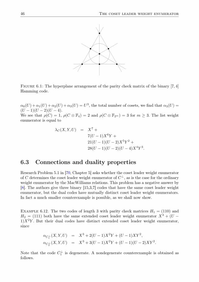
46 The coset leader weight enumerator
Figure 6.1: The hyperplane arrangement of the parity check matrix of the binary [7, 4]Hamming code.
α0(U) +α1(U) +α2(U) +α3(U) = U3, the total number of cosets, we find that α3(U) =(U − 1)(U − 2)(U − 4).We see that ρ(C) = 1, ρ(C ⊗ F4) = 2 and ρ(C ⊗ F2m) = 3 for m ≥ 3. The list weightenumerator is equal to
λC(X,Y, U) = X7 +
7(U − 1)X6Y +
21(U − 1)(U − 2)X5Y 2 +
28(U − 1)(U − 2)(U − 4)X4Y 3.
6.3 Connections and duality properties
Research Problem 5.1 in [70, Chapter 5] asks whether the coset leader weight enumeratorof C determines the coset leader weight enumerator of C⊥, as is the case for the ordinaryweight enumerator by the MacWilliams relations. This problem has a negative answer by[8]. The authors give three binary [15,3,7] codes that have the same coset leader weightenumerator, but the dual codes have mutually distinct coset leader weight enumerators.In fact a much smaller counterexample is possible, as we shall now show.
Example 6.12. The two codes of length 3 with parity check matrices H1 = (110) andH2 = (111) both have the same extended coset leader weight enumerator X3 + (U −1)X2Y . But their dual codes have distinct extended coset leader weight enumerator,since
αC⊥1 (X,Y, U) = X3 + 2(U − 1)X2Y + (U − 1)XY 2,
αC⊥2 (X,Y, U) = X3 + 3(U − 1)X2Y + (U − 1)(U − 2)XY 2.
Note that the code C⊥1 is degenerate. A nondegenerate counterexample is obtained asfollows.

6.3 Connections and duality properties 47
Example 6.13. Let C3 and C4 be the two [6, 3] codes over F2 with generator matrices 1 0 0 1 0 10 1 0 0 1 10 0 1 0 0 1
,
1 0 0 1 0 10 1 0 0 1 10 0 1 1 0 0
.
The next table shows the coefficients of the extended coset leader weight enumerator andthe extended list weight enumerator of the codes and their duals. The values for i = 0are left out: they are all equal to 1.
i C3 C4
1 5(U − 1) 5(U − 1)αC,i 2 2(U − 1)(3U − 5) 2(U − 1)(3U − 5)
3 (U − 1)(U − 2)(U − 3) (U − 1)(U − 2)(U − 3)1 4(U − 1) 5(U − 1)
αC⊥,i 2 3(U − 1)(2U − 3) 2(U − 1)(3U − 5)3 (U − 1)(U − 2)(U − 3) (U − 1)(U − 2)(U − 3)1 6(U − 1) 6(U − 1)
λC,i 2 2(U − 1)(7U − 12) 2(U − 1)(7U − 11)3 12(U − 1)(U − 2)(U − 3) 13(U − 1)(U − 2)(U − 3)1 6(U − 1) 6(U − 1)
λC⊥,i 2 13(U − 1)2 2(U − 1)(7U − 11)3 12(U − 1)(U − 2)(U − 3) 13(U − 1)(U − 2)(U − 3)
We see that the extended coset leader weight enumerator of the two codes are equal,but none of the other polynomials, so they are not defined by the extended coset leaderweight enumerator. It is an open question if the list weight enumerator determines anyof the polynomials αC(X,Y, U), λC⊥(X,Y, U) and WC(X,Y, U).
The Newton radius measures up to which weight all cosets have a unique coset leader.It was introduced by Helleseth and Kløve in [48]. The Newton radius also indicates upto which term the coset leader weight enumerator and list weight enumerator coincide.Therefore, studying the Newton radius might give us more information on the openquestions above.

48 The coset leader weight enumerator
Part III
Codes, arrangements andmatroids
49


7Introduction to matroids
Matroids were introduced by Whitney [107] and independently by Van der Waerden[97], axiomatizing and generalizing the concepts of “independence” in linear algebra and“cycle-free” in graph theory. Matroid theory makes it possible to study these concept ina more abstract way. Many topics in discrete mathematics have strong connections withmatroid theory: for example graph theory, linear algebra, coding theory and projectivegeometry. Also, matroids have important applications in combinatorial optimization.If we want to study links between various fields of discrete mathematics – like in thisthesis – matroids are almost unavoidable. This chapter gives a short introduction ofthe necessary definitions. A characteristic of matroids is, that there are many ways todefine them: for an overview of definitions, see Brylawsky’s appendix in [105]. For morebackground reading on matroid theory, see Kung [66], Welsh [103], White [105, 106] orthe latest edition of Oxley [77].
7.1 Matroids
Definition 7.1. A matroid M is a pair (E, I) consisting of a finite set E and a collectionI of subsets of E called the independent sets, such that the following three conditionshold.
(I.1) ∅ ∈ I.
(I.2) If J ⊆ I and I ∈ I, then J ∈ I.
(I.3) If I, J ∈ I and |I| < |J |, then there exists a j ∈ (J \ I) such that I ∪ {j} ∈ I.
A subset of E that is not independent is called dependent . A dependent subset of E forwhich deleting any element always gives an independent set, is a minimal dependent setor a circuit . An independent subset of E for which adding an extra element of E alwaysgives a dependent set, is a maximal independent set or a basis. It follows from condition(I.3) that every basis has the same number of elements. This is called the rank of thematroid. We define the rank of a subset of E to be the size of the largest independentset contained in it. A subset of E for which adding an extra element of E always gives aset of higher rank, is a closed set or flat . (In fact, we can show that by adding an extra

52 Introduction to matroids
element to a subset, the rank will increase by at most one.) The closure of a subset of Eis the intersection of all flats containing it. We summarize all this in the next definition.
Definition 7.2. For a matroid (E, I) its dependent sets, circuits, bases, rank functionand flats are defined by
D = {D ⊆ E : D 6∈ I},C = {C ⊆ E : C 6∈ I,∀c ∈ C : C \ {c} ∈ I},
r(J) = max{|J ′| : J ′ ⊆ J, J ′ ∈ I},B = {B ⊆ E : r(B) = |B| = r(E)},F = {F ⊆ E : ∀e ∈ E \ F : r(F ∪ {e}) > r(F )},J = ∩{F ∈ F : J ⊆ F}.
All the properties defined above can each be used to determine a matroid completely. Foran overview of equivalent (also called cryptomorphic) definitions of matroids, see [105,Appendix].
A well known and, in most cases, easy to handle matroid is the uniform matroid.
Definition 7.3. Let n and k be nonnegative integers such that k ≤ n. Let In,k = {I ⊆[n] : |I| ≤ k}. Then Un,k = ([n], In,k) is a matroid that is called the uniform matroid ofrank k on n elements. A subset B of [n] is a basis of Un,k if and only if |B| = k. Therank of a subset J is equal to its size if |J | < k and otherwise equal to k. The dependentsets are the subsets of [n] of size at least k+ 1. The matroid Un,n has no dependent setsand is called free.
Let e, f ∈ E be elements of M . If {e} is a dependent set, then e is called a loop. If eand f are two distinct elements that are not loops and r({e, f}) = 1, then e and f arecalled parallel . A matroid is called simple if it has no loops and no parallel elements. Forevery matroid, we can delete loops and associate every parallel class to one element, toget another matroid. This matroid is the simplification M of the matroid.
Definition 7.4. LetM1 = (E1, I1) andM2 = (E2, I2) be matroids. A map ϕ : E1 → E2
is called a morphism of matroids if ϕ(I) is dependent in M2 for all I that are dependentin M1. The map is called an isomorphism of matroids if it is a morphism of matroidsand there exists a map ψ : E2 → E1 such that it is a morphism of matroids and it is theinverse of ϕ. The matroids are called isomorphic if there is an isomorphism of matroidsbetween them.
7.2 Duality
Because a matroid is completely determined by its set of bases, we can define the dualof a matroid in the following way:
Definition 7.5. Let M = (E,B) be a matroid defined by its set of bases. Then its dualis the matroid M∗ = (E,B∗) with the same underlying set and set of bases
B∗ = {E \B : B ∈ B}.

7.3 Matroids, arrangements and codes 53
We can express the rank function of the dual matroid in terms of the rank function ofthe matroid itself.
Proposition 7.6. Let (E, I) be a matroid with rank function r. Then the dual matroidhas rank function r∗ given by
r∗(J) = |J | − r(E) + r(E \ J).
Proof. The proof is based on the observation that r(J) = maxB∈B |B ∩ J | and B \ J =B ∩ (E \ J).
r∗(J) = maxB∈B∗
|B ∩ J |
= maxB∈B|(E \B) ∩ J |
= maxB∈B|J \B|
= |J | −minB∈B|J ∩B|
= |J | − (|B| −maxB∈B|B \ J |)
= |J | − r(E) + maxB∈B|B ∩ (E \ J)|
= |J | − r(E) + r(E \ J).
The following property links circuits to flats of rank r∗(E)− 1 in the dual matroid.
Proposition 7.7. LetM be a matroid and let C be a circuit ofM . Then the complementof C in E is a flat of M∗ of rank r∗(M∗)− 1.
Proof. First, we consider what happens if we add an element c ∈ C to E \ C.
r∗((E \ C) ∪ {c}) = |(E \ C) ∪ {c}| − r(E) + r(C \ {c})= |(E \ C)|+ 1− r(E) + r(C)
= r∗(E \ C) + 1.
So E \C is a flat of M∗. Now we determine the rank of E \C. By definition, C \{c} is anindependent set, so it is a subset of a basis B ofM . The complement B∗ = E\B is a basisof M∗ and therefore has rank r∗(M∗). Because B∗ is contained in (E \C)∪{c}, we haver∗((E \C)∪ {c}) = r∗(B∗) = r(M∗). This means E \C is a flat of rank r∗(M∗)− 1.
A circuit ofM∗ is called a cocircuit ofM . The flats of size r(M)−1 are sometimes calledhyperplanes, but we will not use this terminology to avoid confusion with hyperplanearrangements.
7.3 Matroids, arrangements and codes
Let G be a k × n matrix with entries in a field F. Let E be the set [n] indexing thecolumns of G and IG be the collection of all subsets I of E such that the submatrix GI

54 Introduction to matroids
consisting of the columns of G at the positions of I are independent. ThenMG = (E, IG)is a matroid. Suppose that F is a finite field and G1 and G2 are generator matrices ofa code C, then (E, IG1
) = (E, IG2). So, the matroid MC = (E, IC) of a code C is well
defined by (E, IG) for some generator matrix G of C. The function r(J) as defined inLemma 2.6 is exactly the rank function of the matroid MC . Also, the matroids (MC)∗
and MC⊥ are isomorphic.
If C is degenerate, then there is a position i such that ci = 0 for every codeword c ∈ C.All such positions correspond one-to-one with loops of MC . If C is nondegenerate, thenMC has no loops, and the positions i and j with i 6= j are parallel in MC if and only ifthe i-th column of G is a scalar multiple of the j-th column. The code C is projective ifand only if the arrangement AG is simple if and only if the matroid MC is simple. An[n, k] code C is MDS if and only if the matroid MC is the uniform matroid Un,k.
Let J be a subset of [n] and let C(J) as in Definition 2.5. Then the closure J is equal tothe complement in [n] of the support of C(J) and thus C(J) = C(J).
A matroidM is called realizable or representable over the field F if there exists a matrix Gwith entries in F such thatM is isomorphic withMG. Linear codes correspond to matroidsthat are representable over finite fields. But this is not a one-to-one correspondence:codes that are not equivalent can correspond to the same matroid. See Theorem 2.27:MDS codes with the same parameters need not to be equivalent as codes, but theydo correspond to the same uniform matroid. Also, a matroid can be representable overseveral finite fields of different characteristic: these representations clearly do not giveequivalent codes.Deciding whether a matroid is representable, and over which field, is an important topic inmatroid theory. For more on representable matroids see Tutte [96] and Whittle [108, 109].
7.4 Internal and external activity
Let M = (E,B) be a matroid. Let B ∈ B be a basis and e an element in E \ B. ThenB∪{e} is a dependent set, so it contains a circuit. It is not difficult to show (but it needsa little more theory then explained in this chapter) that this circuit is unique: we call itthe fundamental circuit of e with respect to B. It is clear that e has to be contained inits fundamental circuit. Dually, let e ∈ B. Then (E \B) ∪ {e} is a dependent set in M∗and it contains a unique cocircuit. This cocircuit is called the fundamental cocircuit ofe with respect to B. Fundamental circuits and cocircuits play an important role in theinvestigation of representable matroids.
Definition 7.8. Let M = (E, I) be a matroid and let ω be a linear order on E. Thenthe tuple (E,ω, I) is called an ordered matroid .
Choosing an ordering for a matroid can be compared to choosing a basis for a linearvector space (or, choosing a generator matrix for a linear code): it makes proving sometheorems much easier, but you have to take care that the result is independent of thechoice of the basis. In general, we will not assume any ordering on a matroid, unless it isspecified otherwise.Let M be an ordered matroid and let B be a basis of M . An element e ∈ E \B is called

7.4 Internal and external activity 55
externally B-active if it is the smallest element of its fundamental circuit with respectto B for the given ordering. An element e ∈ B is internally B-active if it is the smallestelement of its fundamental cocircuit with respect to B. The set of internally B-activeelements in M is equal to the set of externally E \B-active elements in M∗.
Definition 7.9. Let M = (E, I) be an ordered matroid. The external activity ε(B) ofa basis B is the number of externally B-active elements. The internal activity ι(B) of abasis B is the number of internally B-active elements.
In this thesis we will use ordered matroid only if we want to say something about internaland external activity. See Etienne and Las Vergnas [40] for more information about thetopic. We will use Definition 7.9 in Chapter 12 to define the spectrum polynomial.

56 Introduction to matroids

8The Tutte polynomial
One of the most studied polynomials in matroid theory is the Tutte polynomial. It hasits origin in graph theory, see [94, 95]. Its importance comes from the fact that the Tuttepolynomial obeys a formula for deletion and contraction. Moreover, all matroid invariantsthat obey the same rule are evaluations of the Tutte polynomial. We refer to Brylawskyand Oxley [27] for an exhaustive treatment of this matter.It was shown by Greene [43] that the weight enumerator of a linear code is one of themany matroid invariants that is determined by the Tutte polynomial. In this chapterwe generalize the result of Greene to the extended and generalized weight enumerators.The result of Greene goes one way: the weight enumerator of a code is determined bythe Tutte polynomial of the associated matroid, but not the other way around. For theextended weight enumerator and the set of generalized weight enumerators, this is a two-way equivalence: the extended weight enumerator determines the Tutte polynomial, andvice versa.Just as Greene used his connection between the Tutte polynomial and the weight enu-merator to give a proof of the MacWilliams identity, we will use the connection betweenthe extended weight enumerator and the Tutte polynomial to prove the MacWilliamsidentity for the extended weight enumerator (see Theorem 2.19). Because of the two-way equivalence between the extended weight enumerator and the Tutte polynomial, theproof reduces to rewriting.The results in this chapter originate from [52]. Closely related results on codes, matroidsand MacWilliams type identities can be found in the work of Barg [9] and Britz et al.[18, 19, 17, 21, 23].
8.1 Weight enumerators and the Tutte polynomial
Definition 8.1. For a matroid M = (E, I) with rank function r the Whitney rankgenerating function is defined by
RM (X,Y ) =∑J⊆E
Xr(E)−r(J)Y |J|−r(J)

58 The Tutte polynomial
and the Tutte polynomial is defined by
tM (X,Y ) =∑J⊆E
(X − 1)r(E)−r(J)(Y − 1)|J|−r(J).
In other words,tM (X,Y ) = RM (X − 1, Y − 1).
Remark 8.2. Both polynomials had been studied for decades before they were discoveredto be so closely related. For a nice historical overview, see Section 3.1 of [83]. The Tuttepolynomial was originally defined on graphs. In matroid terms, this definition reads
tM (X,Y ) =∑B∈B
Xι(B)Y ε(B)
where ι(B) and ε(B) are the internal and external activity of the basis B as in Definition7.9. This formula explains why the coefficients of the Tutte polynomial, just as thecoefficients of the rank generating function, are always positive.
As we have seen, we can interpret a linear [n, k] code C over Fq as a matroid via thecolumns of a generator matrix.
Proposition 8.3. Let C be an [n, k] code over Fq. Then the Tutte polynomial tC(X,Y )associated with the matroid MC of the code C is
tC(X,Y ) =
n∑t=0
∑|J|=t
(X − 1)l(J)(Y − 1)l(J)−(k−t).
Proof. This follows from l(J) = k − r(J) by Lemma 2.6 and r(M) = k.
This formula and Proposition 2.18 suggest the next connection between the weight enu-merator and the Tutte polynomial. Greene [43] was the first to notice this connection.
Theorem 8.4. Let C be an [n, k] code over Fq. Then the following holds for the Tuttepolynomial and the extended weight enumerator:
WC(X,Y, U) = (X − Y )kY n−k tC
(X + (U − 1)Y
X − Y,X
Y
).
Proof. By using Proposition 8.3 about the Tutte polynomial, rewriting, and Proposition2.18 we get
(X − Y )kY n−k tC
(X + (U − 1)Y
X − Y,X
Y
)= (X − Y )kY n−k
n∑t=0
∑|J|=t
(UY
X − Y
)l(J)(X − YY
)l(J)−(k−t)
= (X − Y )kY n−kn∑t=0
∑|J|=t
U l(J)Y k−t(X − Y )−(k−t)
=
n∑t=0
∑|J|=t
U l(J)(X − Y )tY n−t
= WC(X,Y, U).

8.1 Weight enumerators and the Tutte polynomial 59
We use the extended weight enumerator here, because extending a code does not changethe generator matrix and therefore leaves the matroidMC invariant. The converse of thistheorem is also true: the Tutte polynomial is completely defined by the extended weightenumerator.
Theorem 8.5. Let C be an [n, k] code over Fq. Then the following holds for the extendedweight enumerator and the Tutte polynomial:
tC(X,Y ) = Y n(Y − 1)−kWC(1, Y −1, (X − 1)(Y − 1)).
Proof. The proof of this theorem is analogous to the proof of the previous theorem.
Y n(Y − 1)−kWC(1, Y −1, (X − 1)(Y − 1))
= Y n(Y − 1)−kn∑t=0
∑|J|=t
((X − 1)(Y − 1))l(J)
(1− Y −1)tY −(n−t)
=
n∑t=0
∑|J|=t
(X − 1)l(J)(Y − 1)l(J)Y −t(Y − 1)tY −(n−t)Y n(Y − 1)−k
=
n∑t=0
∑|J|=t
(X − 1)l(J)(Y − 1)l(J)−(k−t)
= tC(X,Y ).
We see that the Tutte polynomial depends on two variables, while the extended weightenumerator depends on three variables. This is no problem, because the weight enumer-ator is given in its homogeneous form here: we can view the extended weight enumeratoras a polynomial in two variables via WC(Z,U) = WC(1, Z, U).Greene [43] already showed that the Tutte polynomial determines the weight enumera-tor, but not the other way round. By using the extended weight enumerator, we get atwo-way equivalence and the proof reduces to rewriting.
We can also give expressions for the generalized weight enumerator in terms of the Tuttepolynomial, and the other way round. The first formula was found by Britz [21] andindependently by Jurrius [52].
Theorem 8.6. For the generalized weight enumerator of an [n, k] code C and the asso-ciated Tutte polynomial we have that W (r)
C (X,Y ) is equal to
1
〈r〉q
r∑j=0
[r
j
]q
(−1)r−jq(rj)(X − Y )kY n−k tC
(X + (qj − 1)Y
X − Y,X
Y
).
And, conversely,
tC(X,Y ) = Y n(Y − 1)−kk∑r=0
r−1∏j=0
((X − 1)(Y − 1)− qj)
W(r)C (1, Y −1).

60 The Tutte polynomial
Proof. For the first formula, use Theorems 2.25 and 8.4. Use Theorems 2.23 and 8.5for the second formula.
8.2 MacWilliams type property for duality
For both codes and matroids we defined the dual structure. These objects obviouslycompletely define there dual. But how about the various polynomials associated to acode and a matroid? Does a polynomial associated to a code/matroid determine thesame polynomial associated to the dual code/matroid? We already saw that there isin fact such a relation for the weight enumerator and the extended weight enumerator,namely the MacWilliams identities in Theorem 1.8 and Theorem 2.19. To prove thesetheorems, we may use the relation between the extended weight enumerator and theTutte polynomial, because of the following simple and very useful relation between theTutte polynomial of a matroid and its dual.
Theorem 8.7. Let tM (X,Y ) be the Tutte polynomial of a matroid M , and let M∗ be thedual matroid. Then
tM (X,Y ) = tM∗(Y,X).
Proof. Let M be a matroid on the set E. Then M∗ is a matroid on the same set. Bythe definition of the dual matroid, we have r∗(E) + r(E) = |E|. In Proposition 7.6 weproved r∗(J) = |J | − r(E) + r(E \ J). Substituting these relations into the definition ofthe Tutte polynomial for the dual code, gives
tM∗(X,Y ) =∑J⊆E
(X − 1)r∗(E)−r∗(J)(Y − 1)|J|−r
∗(J)
=∑J⊆E
(X − 1)r∗(E)−|J|−r(E\J)+r(E)(Y − 1)r(E)−r(E\J)
=∑J⊆E
(X − 1)|E\J|−r(E\J)(Y − 1)r(E)−r(E\J)
= tM (Y,X)
In the last step, we use that the summation over all J ⊆ E is the same as a summationover all E \ J ⊆ E. This proves the theorem.
We will now prove Theorem 2.19:
WC⊥(X,Y, U) = U−kWC(X + (U − 1)Y,X − Y,U).
Proof (Theorem 2.19). Let G be the matroid associated to the code. Using the pre-vious theorem and the relation between the weight enumerator and the Tutte polynomialfrom Theorem 8.4, we find
U−kWC(X + (U − 1)Y,X − Y,U)
= U−k(UY )k(X − Y )n−k tC
(X
Y,X + (U − 1)Y
X − Y
)= Y k(X − Y )n−k tC⊥
(X + (U − 1)Y
X − Y,X
Y
)= WC⊥(X,Y, U).

8.2 MacWilliams type property for duality 61
Note in the last step that dimC⊥ = n− k, and n− (n− k) = k.
We can use the relations in Theorems 2.23 and 2.25 to prove the MacWilliams identitiesfor the generalized weight enumerator.
Theorem 8.8. Let C be a code and let C⊥ be its dual. Then the generalized weightenumerators of C completely determine the generalized weight enumerators of C⊥ andvice versa, via the following formula:
W(r)
C⊥(X,Y ) =
r∑j=0
j∑l=0
(−1)r−jq(r−j2 )−j(r−j)−l(j−l)−jk
〈r − j〉q〈j − l〉qW
(l)C (X + (qj − 1)Y,X − Y ).
Proof. We write the generalized weight enumerator in terms of the extended weightenumerator, use the MacWilliams identities for the extended weight enumerator, andconvert back to the generalized weight enumerator.
W(r)
C⊥(X,Y ) =
1
〈r〉q
r∑j=0
[r
j
]q
(−1)r−jq(r−j2 )WC⊥(X,Y, qi)
=
r∑j=0
(−1)r−jq(r−j2 )−j(r−j)
〈j〉q〈r − j〉qq−jkWc(X + (qj − 1)Y,X − Y, qj)
=
r∑j=0
(−1)r−jq(r−j2 )−j(r−j)−jk
〈j〉q〈r − j〉q
×j∑l=0
〈j〉qql(j−l)〈j − l〉q
W(l)C (X + (qj − 1)Y,X − Y )
=
r∑j=0
j∑l=0
(−1)r−jq(r−j2 )−j(r−j)−l(j−l)−jk
〈r − j〉q〈j − l〉q
×W (l)C (X + (qj − 1)Y,X − Y ).
This theorem was proved by Kløve [62]. This proof uses only half of the relations be-tween the generalized weight enumerator and the extended weight enumerator: usingboth makes the proof much shorter.

62 The Tutte polynomial

9Introduction to geometric lattices
In matroid theory, an interesting structure associated to a matroid is its lattice of flats:it is at the basis of many enumeration problems in matroid theory. This lattice is ageometric lattice. There are, roughly speaking, two ways to define a geometric lattice:as the lattice of flats of a matroid, or via the combinatorics of posets, lattices and theMöbius function. Since we already introduced matroids, the first approach is fairly short:see Section 9.7.It requires some work to define a geometric lattice via lattices. However, the theory oflattices is very useful when studying hyperplane arrangements, as we will see in thenext chapter. Therefore, we consider in this chapter the theory of posets, lattices andthe Möbius function. Geometric lattices are defined and their connection with matroidsare given. We will give several examples of the theory. For more background on thecombinatorics in this chapter, see Aigner [1], Rota [81], or Stanley [87]. The connectionwith hyperplane arrangements can be found in Cartier [29], Orlik and Terao [76], orStanley [88].
9.1 Posets
Definition 9.1. Let P be a set and ≤ a relation on P such that for all x, y, z ∈ P :
(PO.1) x ≤ x (reflexive).
(PO.2) If x ≤ y and y ≤ x, then x = y (anti-symmetric).
(PO.3) If x ≤ y and y ≤ z, then x ≤ z (transitive).
The pair (P,≤), or just P , is called a poset with partial order ≤ on the set P .
The elements x and y in P are called comparable if x ≤ y or y ≤ x. If x ≤ y and x 6= y,we say x < y. We use the following notation for some parts of a poset we often refer to.
Px = {y ∈ P : x ≤ y}P x = {y ∈ P : y ≤ x}
[x, y] = {z ∈ P : x ≤ z ≤ y}

64 Introduction to geometric lattices
We call [x, y] the interval between x and y. Note that [x, y] = Px ∩ P y.
Let P be a poset. If P has an element 0P such that 0P is the unique minimal element ofP , then 0P is called the minimum of P . Similarly 1P is called the maximum of P if 1Pis the unique maximal element of L. If x, y ∈ P and x ≤ y, then the interval [x, y] hasminimum x and maximum y. Suppose that P has 0P and 1P as minimum and maximum,also denoted by 0 and 1, respectively. Then 0 ≤ x ≤ 1 for all x ∈ P .Let x, y ∈ P . We call y a cover of x if x < y and there is no z such that x < z < y. Wedenote this by xl y. The elements x and y have a least upper bound if there is a z ∈ Psuch that x ≤ z and y ≤ z, and if x ≤ w and y ≤ w, then z ≤ w for all w ∈ P . If x andy have a least upper bound, then such an element is unique and it is called the join of xand y and is denoted by x ∨ y. Similarly the greatest lower bound of x and y is defined.If it exists, then it is unique and it is called the meet of x and y and denoted by x ∧ y.We summarize this in the following definition.
Definition 9.2. For every poset P and elements x, y ∈ P , we can define the following.
0P The minimum of P .
1P The maximum of P .
xl y y is a cover of x.
x ∨ y The least upper bound, or join, of x and y.
x ∧ y The greatest lower bound, or meet, of x and y.
A poset L is called a lattice if x ∨ y and x ∧ y exist for all x, y ∈ L.
Remark 9.3. Let (P,≤) be a finite poset with maximum 1 such that x∧ y exists for allx, y ∈ P . The collection {z : x ≤ z, y ≤ z} is finite and not empty, since it contains 1.The meet of all the elements in this collection is well defined and is given by
x ∨ y =∧{z : x ≤ z, y ≤ z}.
Hence P is a lattice. Similarly, P is a lattice if P is a finite poset with minimum 0 suchthat x ∨ y exists for all x, y ∈ P , since x ∧ y =
∨{z : z ≤ x, z ≤ y}.
9.2 Chains and the Möbius function
A chain is a (subset of a) poset in which any two elements are comparable. We call a chainfinite (or infinite) when the cardinality of the chain is finite (or infinite). Let r ≥ 0 be aninteger and let x, y ∈ P . If a chain is finite, we can write it as x = x0 < x1 < · · · < xr = yand we say this is a chain from x to y of length r. We denote by cr(x, y) the number ofchains of length r from x to y. The number cr(x, y) is finite if the poset P is finite. Theposet is called locally finite if cr(x, y) is finite for all x, y ∈ P and every integer r ≥ 0. Aposet P is locally finite if and only if [x, y] is finite for all x ≤ y in P . Note that a posetcan be locally finite and still have infinite chains.
Proposition 9.4. Let P be a locally finite poset and let x ≤ y in P . Then

9.2 Chains and the Möbius function 65
(N.1) c0(x, y) = 0 if x and y are not comparable.
(N.2) c0(x, x) = 1 and cr(x, x) = 0 for all r > 0, and c0(x, y) = 0 if x < y.
(N.3) cr+1(x, y) =∑x≤z<y cr(x, z) =
∑x<z≤y cr(z, y).
Proof. Statements (N.1) and (N.2) are trivial. Let z < y and let x = x0 < x1 < · · · <xr = z be a chain of length r from x to z. Then x = x0 < x1 < · · · < xr < xr+1 = yis a chain of length r + 1 from x to y and every chain of length r + 1 from x to y isobtained uniquely in this way. Hence cr+1(x, y) =
∑x≤z<y cr(x, z). The last equality is
proved similarly.
The chain x = y0 < y1 < · · · < ys = y from x to y is called an extension of the chainx = x0 < x1 < · · · < xr = y if {x0, x1, . . . , xr} is a subset of {y0, y1, . . . , ys}. A chainfrom x to y is called maximal if there is no extension to a longer chain from x to y. In amaximal chain, we have that x = x0 l x1 l · · ·l xr = y.
Definition 9.5. The Möbius function of a locally finite poset P , denoted by µP or µ,is defined by
µ(x, y) =
∞∑r=0
(−1)rcr(x, y).
We write µ(x) = µ(0, x) and µ(P ) = µ(0, 1) if P is finite.
Proposition 9.6. Let P be a locally finite poset. Then for all x, y ∈ P :(M.1) µ(x, y) = 0 if x and y are not comparable.
(M.2) µ(x, x) = 1.
(M.3) If x < y, then∑x≤z≤y µ(x, z) =
∑x≤z≤y µ(z, y) = 0.
(M.4) If x < y, then µ(x, y) = −∑x≤z<y µ(x, z) = −
∑x<z≤y µ(z, y).
Proof. (M.1) and (M.2) follow from (N.1) and (N.2), respectively, of Proposition 9.4.(M.3) is clearly equivalent to (M.4). If x < y, then c0(x, y) = 0. So
µ(x, y) =
∞∑r=1
(−1)rcr(x, y)
=
∞∑r=0
(−1)r+1cr+1(x, y)
= −∞∑r=0
(−1)r∑
x≤z<y
cr(x, z)
= −∑
x≤z<y
∞∑r=0
(−1)rcr(x, z)
= −∑
x≤z<y
µ(x, z).
The first and last equality use the definition of µ. The second equality starts countingat r = 0 instead of r = 1, the third uses (N.3) of Proposition 9.4 and in the fourth theorder of summation is interchanged.

66 Introduction to geometric lattices
cd
bcd��
abcd$$
acd''
��
bd
��abd''
��
bc
��abc''
zz
ad
�� ��
ac
ww ��
ab
ww ��
Figure 9.1: The Hasse diagram of a poset. The elements are the subsets of {a, b, c, d}of size at least 2 and the partial order is given by inverse inclusion.
Remark 9.7. (M.2) and (M.4) of Proposition 9.6 can be used as an alternative way tocompute µ(x, y) by induction.
9.3 More on posets and lattices
Definition 9.8. A poset can be visualized by a Hasse diagram. The Hasse diagram of aposet P is a directed graph that has the elements of P as vertices, and there is a directededge from y to x if and only if y is a cover of x.
See Figure 9.1 for an example of a poset with a minimum but without a maximum. Ifwe “turn upside down” the Hasse diagram of a poset, we get the inverse poset.
Definition 9.9. Let P be a poset. The inverse poset i(P ) of P contains the sameelements as P , but the order is reversed: x ≥i y in the inverse poset if and only if x ≤ yin the original poset.
If P is a finite poset, then the Möbius function µP (y, x) is well-defined and µi(P )(x, y) =µP (y, x). If the poset has a minimum and maximum, then the inverse poset has a maxi-mum and minimum: 0P = 1i(P ) and 1P = 0i(P ). The Hasse diagram of i(P ) is obtainedby reversing all arrows in the Hasse diagram of P . Sometimes the inverse poset is calledthe dual poset. We will not use this terminology, because it does not coincide with thenotion of “dual” that we use for codes and matroids.
Definition 9.10. Let (P1,≤1) and (P2,≤2) be posets. A map ϕ : P1 → P2 is calledmonotone if ϕ(x) ≤2 ϕ(y) for all x ≤1 y in P1. The map ϕ is called strictly monotoneif ϕ(x) <2 ϕ(y) for all x <1 y in P1. The map is called an isomorphism of posets ifit is strictly monotone and there exists a strictly monotone map ψ : P2 → P1 that isthe inverse of ϕ. The posets are called isomorphic if there is an isomorphism of posetsbetween them.
If ϕ : P1 → P2 is an isomorphism between locally finite posets with a minimum, thenµP2
(ϕ(x), ϕ(y)) = µP1(x, y) for all x, y in P1. If (L1,≤1) and (L2,≤2) are isomorphic
posets and L1 is a lattice, then L2 is also a lattice.

9.4 Applications and examples 67
9.4 Applications and examples
In this section we will see some examples to motivate the study of posets, lattices andthe Möbius function.
Definition 9.11. Let P be a locally finite poset with a minimum element. Let A be anabelian group and f : P → A a map from P to A. The sum function f of f is defined by
f(x) =∑y≤x
f(y).
Define similarly the sum function f of f by f(x) =∑x≤y f(y) if P is a locally finite
poset with a maximum element.
Note that the sum function is well-defined, because in a locally finite poset all intervalsare finite, and in particular [0, x] and [x, 1], if the poset has a minimum and maximumelement, respectively.
Theorem 9.12 (Möbius inversion formula). Let P be a locally finite poset with a mini-mum element. Then
f(x) =∑y≤x
µ(y, x)f(y).
Similarly, f(x) =∑x≤y µ(x, y)f(y) if P is a locally finite poset with a maximum element.
Proof. Let x be an element of P . Then∑y≤x
µ(y, x)f(y) =∑y≤x
∑z≤y
µ(y, x)f(z)
=∑z≤x
f(z)∑
z≤y≤x
µ(y, x)
= f(x)µ(x, x) +∑z<x
f(z)∑
z≤y≤x
µ(y, x)
= f(x).
The first equality uses the definition of f(y). In the second equality the order of summa-tion is interchanged. In the third equality the first summation is split in the parts z = xand z < x, respectively. Finally µ(x, x) = 1 and the second summation is zero for allz < x, by Proposition 9.6. The proof of the second equality is similar.
Example 9.13. Let L be the collection of all finite subsets of a given set X . Let ≤ bedefined by the inclusion, that means I ≤ J if and only if I ⊆ J . Then 0L = ∅, and L hasa maximum if and only if X is finite in which case 1L = X . For X = {a, b, c, d} the Hassediagram of the lattice is given in Figure 9.2.Let I, J ∈ L and I ≤ J . Then |I| ≤ |J | <∞. Let m = |J | − |I|. Then
cr(I, J) =∑
m1<m2<...<mr−1<m
(m2
m1
)(m3
m2
)· · ·(
m
mr−1
).
Hence L is locally finite. L is finite if and only if X is finite. Furthermore, I ∨ J = I ∪ Jand I ∧ J = I ∩ J , so L is a lattice. Using Remark 9.7 we see that µ(I, J) = (−1)|J|−|I|
if I ≤ J . This is much easier than computing µ(I, J) by means of Definition 9.5.

68 Introduction to geometric lattices
Example 9.14. Let X = [n] and let k be an integer between 0 and n. Let Lk = {X}and Li be the collection of all subsets of X of size i for all i < k. Let the partial order begiven by the inclusion. Then L is a poset and µ(I, J) = (−1)|J|−|I| if I ≤ J and |J | < kas in Example 9.13, and µ(I,X ) = −
∑I≤J<X (−1)|J|−|I| for all I < X by Proposition
9.6.
Example 9.15. Now suppose again that X = [n]. Let L be the poset of subsets of X .Let A1, . . . , An be a collection of subsets of a finite set A. Define for a subset J of X
AJ =⋂j∈J
Aj and f(J) =
∣∣∣∣∣AJ \(⋃I<J
AI
)∣∣∣∣∣ .Then AJ is the disjoint union of the subsets AI \ (
⋃K<I AK) for all I ≤ J . Hence the
sum function is equal to
f(J) =∑I≤J
f(I) =∑I≤J
∣∣∣∣∣AI \( ⋃K<I
AK
)∣∣∣∣∣ = |AJ |.
Möbius inversion gives that∣∣∣∣∣AJ \(⋃I<J
AI
)∣∣∣∣∣ =∑I≤J
(−1)|J|−|I||AI |,
which is called the principle of inclusion/exclusion.
Example 9.16. A variant of the principle of inclusion/exclusion is given as follows.Let H1, . . . ,Hn be a collection of subsets of a finite set H. Let L be the poset of allintersections of theHj with the reverse inclusion as partial order. ThenH is the minimumof L and H1 ∩ · · · ∩Hn is the maximum of L. Let x ∈ L. Define
f(x) =
∣∣∣∣∣x \(⋃x<y
y
)∣∣∣∣∣ .Then
f(x) =∑x≤y
f(y) =∑x≤y
∣∣∣∣∣y \(⋃y<z
z
)∣∣∣∣∣ = |x|.
Hence ∣∣∣∣∣x \(⋃x<y
y
)∣∣∣∣∣ =∑x≤y
µ(x, y)|y|.
9.5 Geometric lattices
Definition 9.17. A poset P satisfies the Jordan-Dedekind property if all maximal chainsbetween the same elements have the same finite length. If moreover all maximal chainswith endpoint x have the same length, this length is called the rank of x. We denote itby rP (x) or simply r(x).

9.6 Some examples of geometric lattices 69
The following proposition follows directly from the definition:
Proposition 9.18. Let P be a poset with minimum 0. Then P satisfies the Jordan-Dedekind property if and only if it admits a rank function r : P → N0 that satisfies thefollowing:
• r(0) = 0;
• xl y ⇒ r(y) = r(x) + 1.
We will define some more properties posets and lattices can have.
Definition 9.19. Let P be a poset with minimum 0. An atom is an element a ∈ P thatcovers 0. The poset is said to be atomic if every element except 0 is the join of atoms.
Definition 9.20. Let L be a lattice. It is called semimodular if for all x, y ∈ L
x ∧ y l x⇒ y l x ∨ y.
The notion of semimodularity is often encountered in the context of a function. Forlattices, we can prove that the same holds.
Lemma 9.21. A semimodular lattice satisfies the Jordan-Dedekind property.
Theorem 9.22. Let L be a lattice with minimum 0. The lattice is semimodular if andonly if it has a rank function r such that for all x, y ∈ L
r(x ∧ y) + r(x ∨ y) ≤ r(x) + r(y).
We can now define the notion of a geometric lattice.
Definition 9.23. A lattice is called geometric if it is
(GL.1) atomic;
(GL.2) semimodular;
(GL.3) without infinite chains.
Let L be a geometric lattice. We call the set Lj = {x ∈ L : r(x) = j} the j-th level of L.The Hasse diagram of L is a graph that has the elements of L as vertices. If x, y ∈ L andxly, then x and y are connected by an edge. So, only elements between two consecutivelevels Lj and Lj+1 are connected by an edge. See Figure 9.2 for an example. The Hassediagram of P considered as a poset as in Definition 9.8 is the directed graph with anarrow from y to x if x, y ∈ L and xl y.
9.6 Some examples of geometric lattices
Example 9.24. Let L be the collection of all finite subsets of a given set X as in Example9.13. For X = {a, b, c, d} the Hasse diagram is drawn in Figure 9.2. The atoms are thesingleton sets, i.e., the subsets consisting of exactly one element of X . Every x ∈ L isthe finite union of its singleton subsets, so L is atomic and r(x) = |x|. Now y covers x

70 Introduction to geometric lattices
{a, b, c, d}
{a, b, c}
{a, b}
{a}
∅
{b}
{a, c}
{c}
{b, c}
{a, b, d}
{a, d}
{d}
{b, d}
{a, c, d}
{c, d}
{b, c, d}
Figure 9.2: The Hasse diagram of the geometric lattice of all subsets of {a, b, c, d}
if and only if there is an element Q not in x such that y = x ∪ {Q}. If x 6= y and xand y both cover z, then there is an element P not in z such that x = z ∪ {P}, andthere is an element Q not in z such that y = z ∪ {Q}. Now P 6= Q, since x 6= y. Hencex ∨ y = z ∪ {P,Q} covers x and y. Hence L is semimodular. Furthermore, L is locallyfinite, and L is a geometric lattice if and only if X is finite.
Example 9.25. Let F be a field and let V = (v1, . . . ,vn) be an n-tuple of nonzero vectorsin Fk. Let L = L(V) be the collection of all linear subspaces of Fk that are generated bysubsets of V, with inclusion as partial order. Therefore, L is finite and a fortiori locallyfinite. By definition {0} is the linear subspace space generated by the empty set. Then0L = {0} and 1L is the subspace generated by all v1, . . . ,vn. Furthermore L is a latticewith x ∨ y = x+ y and
x ∧ y =∨{z : z ≤ x, z ≤ y}
by Remark 9.3. Let aj be the linear subspace generated by vj . Then a1, . . . , an are theatoms of L. Let x be the subspace generated by {vj : j ∈ J}. Then x =
∨j∈J aj . If x
has dimension r, then there exists a subset I of J such that |I| = r and x =∨i ∈ Iai.
Hence L is atomic and r(x) = dim(x). Now x ∧ y ⊆ x ∩ y, so
r(x ∨ y) + r(x ∧ y) ≤ dim(x+ y) + dim(x ∩ y) = r(x) + r(y).
Hence the semimodular inequality holds and L is a geometric lattice.
Example 9.26. Let F be a field and let A = (H1, . . . ,Hn) be an arrangement over F ofhyperplanes in the vector space V = Fk. Let L = L(A) be the collection of all nonemptyintersections of elements of A. By definition Fk is the empty intersection. Define thepartial order ≤ by
x ≤ y if and only if y ⊆ x.
Then V is the minimum element and {0} is the maximum element. Furthermore
x ∨ y = x ∩ y if x ∩ y 6= ∅, and x ∧ y =⋂{z : x ∪ y ⊆ z}.

9.7 Geometric lattices and matroids 71
Suppose that A is a central arrangement. Then x∩y is nonempty for all x, y ∈ L, so x∨yand x ∧ y exist for all x, y ∈ L and L is a lattice. Let vj = (v1j , . . . , vkj) be a nonzerovector such that
∑ki=1 vijXi = 0 is a homogeneous equation of Hj . Let V = (v1, . . . ,vn).
Consider the map ϕ : L(V)→ L(A) defined by
ϕ(x) =⋂j∈J
Hj if x is the subspace generated by {vj : j ∈ J}.
Now x ⊂ y if and only if ϕ(y) ⊂ ϕ(x) for all x, y ∈ L(V). Therefore, ϕ is a strictlymonotone map. Furthermore ϕ is a bijection and its inverse map is also strictly monotone.Hence L(V) and L(A) are isomorphic lattices. Therefore L(A) is also a geometric lattice.
9.7 Geometric lattices and matroids
The notion of a geometric lattice is cryptomorphic to the concept of a matroid: that is,almost equivalent. See [13, 27, 29, 32, 77, 88] for proofs of the statements in this section.First, we see that we can associate a matroid with every geometric lattice.
Proposition 9.27. Let L be a finite geometric lattice and let M(L) be the set of allatoms of L. Let I(L) be the collection of all subsets I = {a1, . . . , ar} of atoms of M(L)such that r(a1 ∨ . . . ∨ ar) = r. Then (M(L), I(L)) is a matroid.
On the other hand, we can associate a lattice to every matroid.
Proposition 9.28. Let M be a matroid and let L(M) be the set of all flats of M . ThenL(M) with the inclusion as partial order is a lattice with
F1 ∧ F2 = F1 ∩ F2, F1 ∨ F2 = F1 ∪ F2.
We call L(M) the lattice of flats of M .
This lattice is actually a geometric lattice, but the correspondence between matroids andgeometric lattices is in general not one-to-one.
Proposition 9.29. Let M be a matroid. Then L(M) with the inclusion as partial orderis a geometric lattice and L(M) is isomorphic with L(M).
The inverse of the first statement also holds, leading to the next theorem.
Theorem 9.30. A lattice is geometric if and only if it is the lattice of flats of a matroid.
If we start with a geometric lattice L, thenM(L) is a simple matroid and thus L(M(L)) =L. If we start with a matroid M , we find that M(L(M)) = M . We conclude that thereis a one-to-one correspondence between simple matroids and geometric lattices.
Example 9.31. The geometric lattice of the matroid Un,k, see Definition 7.3, is isomor-phic with the lattice consisting of [n] and all its subsets of size at most k − 1. We willrefer to this geometric lattice as the uniform lattice. See Figure 9.2 for the geometriclattice of the free matroid of size 4.

72 Introduction to geometric lattices
Let G be a generator matrix of a code C. The simplified matrix G is the matrix obtainedfrom G by deleting all zero columns from G and all columns that are a scalar multipleof a previous column. The simplified code C of C is the code with generator matrix G.Every simplified code is projective. Note that this definition of C does not depend onthe choice of the generator matrix G of C. Therefore the matroids MG and MG areisomorphic.

10Characteristic polynomials and
their generalizations
In this chapter we treat the characteristic polynomial of a geometric lattice. This is gen-eralized in two variable polynomials in two ways: the coboundary polynomial and theMöbius polynomial.The coboundary polynomial was originally studied by Crapo [31] in connection withgraph coloring. For simple matroids and codes the coboundary polynomial is equivalentto the Tutte polynomial and the extended weight enumerator.The Möbius polynomial (also known as “Whitney polynomial”) was originally defined byZaslavsky for hyperplanes [110] and signed graphs [111]. An important property is that itdetermines the Whitney numbers. We will show that the Möbius function also containsinformation on the number of minimal subcodes and codewords.For both polynomials, we show how to calculate them in the specific case of an arrange-ment and code. The coboundary and Möbius polynomial do, in general, not determineeach other. This will be shown by examples of three dimensional codes. More relationsbetween the two polynomials can be found in the next chapter.
10.1 The characteristic and coboundary polynomial
Definition 10.1. Let L be a finite geometric lattice. The characteristic polynomial ofL is defined by
χL(U) =∑x∈L
µL(x)Ur(L)−r(x).
The two-variable characteristic polynomial or coboundary polynomial is defined by
χL(S,U) =∑x∈L
∑x≤y∈L
µ(x, y)Sa(x)Ur(L)−r(y)
where a(x) is the number of atoms a in L such that a ≤ x.
Note that µ(L) = µ(0, 1) = χL(0) and χL(0, U) = χL(U), because for S = 0 the onlynonzero term has a(x) = 0, so x = 0L. Also, the number a(x) is equal to |x| in M(L).

74 Characteristic polynomials and their generalizations
Remark 10.2. Let n be the number of atoms of L. Then the following relation holds forthe coboundary polynomial in terms of characteristic polynomials:
χL(S,U) =
n∑i=0
Siχi(U) with χi(U) =∑x∈La(x)=i
χLx(U).
The polynomial χi(U) is called the i-defect polynomial. See [31, 27].
Example 10.3. Let L be the lattice of all subsets of a given finite set of r elements as inExamples 9.13 and 9.24. Then r(x) = a(x) and µ(x, y) = (−1)a(y)−a(x) if x ≤ y. Hence
χL(U) =
r∑j=0
(r
j
)(−1)jUr−j = (U − 1)r and χi(U) =
(r
i
)(U − 1)r−i.
Therefore χL(S,U) = (S + U − 1)r.
An important property of the coboundary polynomial is that is it is determined by therank generating function.
Theorem 10.4. The coboundary polynomial χL(S,U) of a finite geometric lattice L isrelated to the Whitney rank generating function of M(L) by the formula
χL(S,U) = (S − 1)r(L)RM(L)
(U
S − 1, S − 1
).
Proof. In [30, p. 605], Crapo proved that the coboundary polynomial is equal to
χL(S,U) =∑
x⊆M(L)
(S − 1)|x|Ur(L)−r(x).
The proof uses a generalization to matroids of the Möbius inversion formula in Theo-rem 9.12. Crapo used this result in [31, Theorem II] to prove the relation to the rankgenerating function. In our notation, the proof is as follows.
χL(S,U) =(S − 1)r(L)−r(x)
(S − 1)r(L)−r(x)
∑x⊆M(L)
(S − 1)|x|Ur(L)−r(x)
= (S − 1)r(L)∑
x⊆M(L)
(S − 1)|x|−r(x)
(U
S − 1
)r(L)−r(x)
= (S − 1)r(L)RM(L)
(U
S − 1, S − 1
)We use that r(M) = r(M(L)).
Corollary 10.5. We have the following relations between tM(L)(X,Y ) and χL(S,U):
χL(S,U) = (S − 1)r(L)tM(L)
(S + U − 1
S − 1, S
)and, vice versa,
tM(L)(X,Y ) = (Y − 1)−r(L)χL(Y, (X − 1)(Y − 1)).
Therefore the polynomials χL(S,U) and tM(L)(X,Y ) completely determine each other.

10.2 The Möbius polynomial and Whitney numbers 75
Starting with an arbitrary matroid M one has the associated geometric lattice L(M),but M(L(M)) is isomorphic with M if and only if M is simple by Proposition 9.29.Therefore, tM (X,Y ) and χL(M)(S,U) completely determine each other if M is simple,but tM (X,Y ) is a stronger invariant than χL(M)(S,U) if M is not simple. We will seea counterexample in Example 10.34. The relation between tM(L)(X,Y ) and χL(S,U)shows great similarity with the formula in Theorem 8.5. Combining the relations givesthe next theorem.
Theorem 10.6. For projective codes, the coboundary polynomial of the geometric lat-tice associated to the code is the reciprocal inhomogeneous form of the extended weightenumerator of the code:
χL(MC)(S,U) = SnWC(1, S−1, U).
This means χi(U) = An−i(U).
Example 10.7. Consider the uniform lattice Un,k. Determining its coboundary polyno-mial is now quite easy: use Theorem 10.6 and the extended weight enumerator of anMDS code we found in Theorem 2.27.
10.2 The Möbius polynomial and Whitney numbers
Definition 10.8. Let P be a poset that satisfies the Jordan-Dedekind property. ThenP has a rank function by Proposition 9.18. The Möbius polynomial of P is defined by
µP (S,U) =∑x∈P
∑x≤y∈P
µ(x, y)Sr(x)Ur(P )−r(y).
Note that for a geometric lattice L we have µL(0, U) = χL(0, U) = χL(U).
Remark 10.9. Let r be the rank of the geometric lattice L. Then the following relationholds for the Möbius polynomial in terms of characteristic polynomials:
µL(S,U) =
r∑i=0
Siµi(U) with µi(U) =∑x∈Li
χLx(U).
Example 10.10. In Examples 9.24 and 10.3 we considered the lattice L of all subsets ofa given finite set of r elements. Since r(x) = a(x) for all x ∈ L, the Möbius polynomialof L is equal to the coboundary polynomial of L, so µL(S,U) = (S + U − 1)r.
Remark 10.11. Let L be a geometric lattice. Then
r(L)∑i=0
µi(U) = µL(1, U)
=∑y∈L
∑0≤x≤y
µ(x, y)Ur(L)−r(y)
= Ur(L)

76 Characteristic polynomials and their generalizations
since∑
0≤x≤y µ(x, y) = 0 for all 0 < y in L by Proposition 9.6. Similarly∑ni=0 χi(U) =
χL(1, U) = Ur(L). Also∑nw=0Aw(U) = Uk for the extended weights of a code of dimen-
sion k by Propositions 2.14 and 2.16 for t = 0.
Example 10.12. Let L be the uniform lattice Un,k. Then µi(U) and χi(U) are bothequal to
(ni
)(U − 1)n−i for all i < k as in Example 10.3, and χi(U) = 0 for all k ≤ i < n,
since a(1L) = n, r(1L) = k and a(x) = r(x) for all x in Li and i < k. Remark 10.11implies
µk(U) = Uk −∑i<k
(n
i
)(U − 1)n−i and χn(U) = Uk −
∑i<k
(n
i
)(U − 1)n−i.
An important reason to study the Möbius polynomial is because it determines the Whit-ney numbers. See [44], [27, §6.6.D], [77, Chapter 15], and [87, §3.11].
Definition 10.13. Let L be a finite geometric lattice. The Whitney numbers wi and Wi
of the first and second kind, respectively, are defined by
wi =∑x∈Li
µ(x) and Wi = |Li|.
The doubly indexed Whitney numbers wij and Wij of the first and second kind , respec-tively, are defined by
wij =∑x∈Li
∑y∈Lj
µ(x, y) and Wij = |{(x, y) : x ∈ Li, y ∈ Lj , x ≤ y}|.
In particular, wj = w0j and Wj = W0j .
Remark 10.14. We have that
χL(U) =
r(L)∑i=0
wiUr(L)−i and µL(S,U) =
r(L)∑i=0
r(L)∑j=0
wijSiUr(L)−j .
Hence the (doubly indexed) Whitney numbers of the first kind are determined by µL(S,U).The leading coefficient of
µi(U) =∑x∈Li
∑x≤y
µ(x, y)Ur(Lx)−rLx (y)
is equal to∑x∈Li µ(x, x) = |Li| = Wi. Hence the Whitney numbers of the second kind
Wi are also determined by µL(S,U). We will see in Example 10.35 that the Whitneynumbers are not determined by χL(S,U). Finally, let r = r(L). Then
µr−1(U) = (U − 1) ·Wr−1.
There are a lot of open conjectures about the sequences of Whitney numbers. A sequenceof real numbers (v0, v, . . . , vr) is called unimodal if
vi ≥ min{vi−1, vi+1} for all 0 < i < r.

10.3 Minimal codewords and subcodes 77
The sequence is called logarithmically concave or log-concave if
v2i ≥ vi−1vi+1 for all 0 < i < r.
The Whitney numbers of the first kind are alternating in sign. That is:
w+i := (−1)iwi > 0 for all i.
It was conjectured by Rota [82] that the Whitney numbers w+i are unimodal. See [102,
Problem 12]. Welsh [103] conjectured that the Whitney numbers w+i are log-concave by
generalizing a conjecture of Read [80] on graphs. It was shown that the following weakerversion of the unimodal property is true for a matroid M of rank r:
w+i < w+
j for all 0 ≤ i ≤ r/2 and i < j ≤ r − i.
See [2, Corollary 8.4.2]. For a recent overview of all conjectures, see [77, §15.2].
10.3 Minimal codewords and subcodes
Definition 10.15. A minimal codeword of a code C is a codeword whose support doesnot properly contain the support of another codeword.
The zero word is a minimal codeword. Note that a nonzero scalar multiple of a minimalcodeword is again a minimal codeword. Nonzero minimal codewords play a role in min-imum distance decoding [4, 9, 10], in secret sharing schemes, and in access structures[72, 89]. We can generalize this notion to subcodes instead of words.
Definition 10.16. A minimal subcode of dimension r of a code C is an r-dimensionalsubcode whose support is not properly contained in the support of another r-dimensionalsubcode.
A minimal codeword generates a minimal subcode of dimension one, and all the elementsof a minimal subcode of dimension one are minimal codewords. A codeword of minimalweight is a nonzero minimal codeword, but the converse is not always the case.
In Example 10.35 we will see two codes that have the same Tutte polynomial, but adifferent number of minimal codewords. Hence the number of minimal codewords andsubcodes is not determined by the Tutte polynomial. However, the number of minimalcodewords and the number of minimal subcodes of a given dimension are given by theMöbius polynomial.
Theorem 10.17. Let C be a code of dimension k and let 0 ≤ r ≤ k. Then the numberof minimal subcodes of dimension r is equal to Wk−r, the (r − k)-th Whitney number ofthe second kind, and it is determined by the Möbius polynomial.
Proof. LetD be a subcode of C of dimension r and let J be the complement in [n] of thesupport of D. If d ∈ D and dj 6= 0, then j ∈ supp(D) and j 6∈ J . Hence D ⊆ C(J). Nowsuppose moreover that D is a minimal subcode of C. Without loss of generality we mayassume that D is systematic at the first r positions, i.e., that D has a generator matrix ofthe form (Ir|A). Denote the i-th row of this matrix by di. Let c ∈ C(J). If c−
∑ri=1 cidi
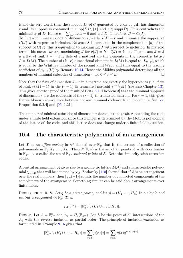
78 Characteristic polynomials and their generalizations
is not the zero word, then the subcode D′ of C generated by c,d2, . . . ,dr has dimensionr and its support is contained in supp(D) \ {1} and 1 ∈ supp(D). This contradicts theminimality of D. Hence c−
∑ri=1 cidi = 0 and c ∈ D. Therefore, D = C(J).
To find a minimal subcode of dimension r, we fix l(J) = r and minimize the support ofC(J) with respect to inclusion. Because J is contained in the complement in [n] of thesupport of C(J), this is equivalent to maximizing J with respect to inclusion. In matroidterms this means we are maximizing J for r(J) = k − l(J) = k − r. This means J = Jis a flat of rank k − r. The flats of a matroid are the elements in the geometric latticeL = L(M). The number of (k−r)-dimensional elements in L(M) is equal to |Lk−r|, whichis equal to the Whitney number of the second kind Wk−r and thus equal to the leadingcoefficient of µk−r(U) by Remark 10.14. Hence the Möbius polynomial determines all thenumbers of minimal subcodes of dimension r for 0 ≤ r ≤ k.
Note that the flats of dimension k− r in a matroid are exactly the hyperplanes (i.e., flatsof rank r(M) − 1) in the (r − 1)-th truncated matroid τ r−1(M) (see also Chapter 13).This gives another proof of the result of Britz [21, Theorem 3] that the minimal supportsof dimension r are the cocircuits of the (r−1)-th truncated matroid. For r = 1, this givesthe well-known equivalence between nonzero minimal codewords and cocircuits. See [77,Proposition 9.2.4] and [96, 1.21].
The number of minimal subcodes of dimension r does not change after extending the codeunder a finite field extension, since this number is determined by the Möbius polynomialof the lattice of the code, and this lattice does not change under a finite field extension.
10.4 The characteristic polynomial of an arrangement
Let X be an affine variety in Ak defined over Fq, that is, the zeroset of a collection ofpolynomials in Fq[X1, . . . , Xk]. Then X (Fqm) is the set of all points X with coordinatesin Fqm , also called the set of Fqm-rational points of X . Note the similarity with extensioncodes.
A central arrangement A gives rise to a geometric lattice L(A) and characteristic polyno-mial χL(A) that will be denoted by χA. Zaslavsky [110] showed that ifA is an arrangementover the real numbers, then |χA(−1)| counts the number of connected components of thecomplement of the arrangement. Something similar can be said about arrangements overfinite fields.
Proposition 10.18. Let q be a prime power, and let A = (H1, . . . ,Hn) be a simple andcentral arrangement in Fkq . Then
χA(qm) = |Fkqm \ (H1 ∪ . . . ∪Hn)|.
Proof. Let A = Fkqm and Aj = Hj(Fqm). Let L be the poset of all intersections of theAj with the reverse inclusion as partial order. The principle of inclusion/exclusion asformulated in Example 9.16 gives that
|Fkqm \ (H1 ∪ · · · ∪Hn)| =∑x∈L
µ(x)|x| =∑x∈L
µ(x)qm dim(x).

10.4 The characteristic polynomial of an arrangement 79
The expression on the right hand side is equal to χA(qm), since L is isomorphic with thegeometric lattice L(A) of the arrangement A = (H1, . . . ,Hn) with rank function r = rL,so dim(x) = r(L) − r(x). See also [7, Theorem 2.2], [15, Proposition 3.2], [32, Sect. 16]and [76, Theorem 2.69].
Definition 10.19. Let A = (H1, . . . ,Hn) be a central simple arrangement over the fieldF in Fk and let J ⊆ [n]. Define HJ = ∩j∈JHj . Consider the decreasing sequence
Nk ⊂ Nk−1 ⊂ · · · ⊂ N1 ⊂ N0
of algebraic subsets of the affine space Ak, defined by
Ni =⋃J⊆[n]r(HJ )=i
HJ .
DefineMi = Ni \ Ni+1.
Note that N0 = Ak, N1 = ∪nj=1Hj , Nk = {0} and Nk+1 = ∅. Furthermore, Ni is a unionof linear subspaces of Ak all of dimension k − i. Remember from Remark 4.3 that HJ
is isomorphic with C(J) in case A is the arrangement of the generator matrix G of thecode C.
Proposition 10.20. Let A = (H1, . . . ,Hn) be a central simple arrangement over thefield F in Fk. Let z(x) = {j ∈ [n] : x ∈ Hj} and r(x) = r(Hz(x)) the rank of x forx ∈ Ak. Then
Ni = {x ∈ Ak : r(x) ≥ i} and Mi = {x ∈ Ak : r(x) = i}.
Proof. Let x ∈ Ak and c = xG. Let x ∈ Ni. Then there exists a J ⊆ [n] such thatr(HJ) = i and x ∈ HJ . So, cj = 0 for all j ∈ J and J ⊆ z(x). Hence Hz(x) ⊆ HJ andtherefore r(x) = r(Hz(x)) ≥ r(HJ) = i. The converse implication is proved similarly. Thestatement aboutMi is a direct consequence of the one about Ni.
Proposition 10.21. Let A be a central simple arrangement over Fq and let L = L(A)be the geometric lattice of A. Then
µi(qm) = |Mi(Fqm)|.
Proof. Remember from Remark 10.9 that µi(U) =∑r(x)=i χLx(U). Let L = L(A)
and x ∈ L. Then x is an intersection of hyperplanes of A, i.e., x = ∪i∈IHi. Let l bethe dimension of x. We define the arrangement Ax to be the arrangement in Flq of allhyperplanes x∪Hj in x such that x∪Hj 6= ∅ and x∪HJ 6= x, for a chosen isomorphismof x with Flq. Then L(Ax) = Lx.Let ∪Ax be the union of the hyperplanes of Ax. Then |(x \ (∪Ax))(Fqm)| = χLx(qm) byProposition 10.18. NowMi is the disjoint union of complements of the arrangements ofAx for all x ∈ L such that r(x) = i by Proposition 10.20. Hence
|Mi(Fqm)| =∑x∈Lr(x)=i
|(x \ (∪Ax))(Fqm)|
=∑x∈Lr(x)=i
χLx(qm).

80 Characteristic polynomials and their generalizations
See also [7, Theorem 6.3].
10.5 The characteristic polynomial of a code
Proposition 10.22. Let C be a nondegenerate linear code over Fq. Then
An(U) = χC(U).
Proof. The short proof is given by χC(U) = χC(0, U) = χ0(U) = An(U). The geometricinterpretation is as follows.The elements in Fkqm \ (H1 ∪ · · · ∪Hn) correspond one-to-one to codewords of weight nin C ⊗ Fqm by Proposition 4.2 and because the arrangements corresponding to C andto C ⊗ Fqm are the same. Therefore, An(qm) = χC(qm) for all positive integers m byProposition 10.18. Hence An(U) = χC(U).
Definition 10.23. Let G be a generator matrix of an [n, k] code C over Fq. Define
Yi = {x ∈ Ak : wt(xG) ≤ n− i} and Xi = {x ∈ Ak : wt(xG) = n− i}.
The Yi form a decreasing sequence
Yn ⊆ Yn−1 ⊆ . . . ⊆ Y1 ⊆ Y0
of algebraic subsets of Ak, and Xi = Yi \ Yi+1. Suppose that G has no zero column andlet AG be the arrangement of G. Then
Xi = {x ∈ Ak : x is in exactly i hyperplanes of AG}.
Proposition 10.24. Let C be a projective code of length n. Then
χi(qm) = |Xi(Fqm)| = An−i(q
m).
Proof. Every x ∈ Fkqm corresponds one-to-one to a codeword in C ⊗ Fqm via the mapx 7→ xG. Therefore, |Xi(Fqm)| = An−i(q
m). Also, An−i(qm) = χi(qm) for all i, by
Theorem 10.6. See also [3, Theorem 3.3].
Note that the statement |Xi(Fqm)| = An−i(qm) and its proof are the the affine versions
of Proposition 4.2 and its proof.
Remark 10.25. Another way to define Xi is the collection of all points P ∈ Ak such thatP is on exactly i distinct hyperplanes of the arrangement AG. Denote the arrangement ofhyperplanes in Pk−1 also by AG and let P be the point in Pk−1 corresponding to P ∈ Ak.Define
X i = {P ∈ Pk−1 : P is on exactly i hyperplanes of AG}.
For all i < n the polynomial χi(U) is divisible by U − 1. Define χi(U) = χi(U)/(U − 1).Then χi(qm) = |X i(Fqm)| for all i < n by Proposition 10.24.

10.5 The characteristic polynomial of a code 81
Theorem 10.26. Let G be a generator matrix of a nondegenerate code C. Let AG be theassociated central arrangement. Let d⊥ = d(C⊥). Then Ni ⊆ Yi for all i and equalityholds for all i < d⊥. Also, Mi = Xi for all i < d⊥ − 1. If furthermore C is projective,then
µi(U) = χi(U) = An−i(U) for all i < d⊥ − 1.
Proof. A more general version of this statement will be proven in Theorem 11.4, usingmatroids. Here we give the proof for codes and arrangements.Let x ∈ Ni. Then x ∈ HJ for some J ⊆ [n] such that r(HJ) = i. This means |J | ≥ i andwt(xG) ≤ n− i by Proposition 4.2. Hence x ∈ Yi and therefore Ni ⊆ Yi.Let i < d⊥ and x ∈ Yi. Then wt(xG) ≤ n − i. Let J = supp(xG). Then |J | ≥ i. Takea subset I of J such that |I| = i. Then x ∈ HI and r(I) = |I| = i by Lemma 2.7, sincei < d⊥. Hence x ∈ Ni and therefore Yi ⊆ Ni, Yi = Ni for all i < d⊥, andMi = Xi forall i < d⊥ − 1.The code is nondegenerate, so d⊥ ≥ 2. Suppose furthermore that C is projective. Thenµi(U) = χi(U) = An−i(U) for all i < d⊥ − 1, by Theorem 10.6 and Propositions 10.24and 10.21.
Remember that the extended and generalized weight enumerators are determined by thepair (n, k) for an [n, k] MDS code by Theorem 2.27. If C is an [n, k] code, then d⊥ is atmost k + 1 by the Singleton bound. Furthermore d⊥ = k + 1 if and only if C is MDS ifand only if C⊥ is MDS.
Definition 10.27. An [n, k, d] code is called almost MDS if d = n − k. The code C iscalled near MDS if both C and C⊥ are almost MDS.
So d⊥ = k if and only if C⊥ is almost MDS. If C is almost MDS, then C⊥ is notnecessarily almost MDS. See [33] for more on near-MDS codes.
Proposition 10.28. Let C be an [n, k, d] code such that C⊥ is MDS or almost MDS andk ≥ 3. Then both χC(S,U) and WC(X,Y, U) determine µC(S,U). In particular:
µi(U) = χi(U) = An−i(U) for all i < k − 1,
µk−1(U) =
n−1∑i=k−1
χi(U) =
n−1∑i=k−1
An−i(U),
and µk(U) = 1.
Proof. Let C be a code such that d(C⊥) ≥ k ≥ 3. Then C is projective and µi(U) =χi(U) = An−i(U) for all i < k − 1 by Theorem 10.26. Furthermore, µk(U) = χn(U) =A0(U) = 1.Finally let L = L(C). Then
∑ki=0 µi(U) = Uk,
∑ni=0 χi(U) = Uk and
∑ni=0Ai(U) = Uk
by Remark 10.11. Hence the formula for µk−1(U) holds. Therefore, µC(S,U) is deter-mined both by WC(X,Y, U) and χC(S,U).
Projective codes of dimension 3 are examples of codes C such that C⊥ is almost MDS.In the following we will give explicit formulas for µC(S,U) for such codes.

82 Characteristic polynomials and their generalizations
Let C be a projective code of length n and dimension 3 over Fq with generator matrixG. The arrangement AG = (H1, . . . ,Hn) of planes in F3
q is simple and essential, andthe corresponding arrangement of lines in P2(Fq) is also denoted by AG. We defined inRemark 10.25 that
X i(Fqm) = {P ∈ P2(Fqm) : P is on exactly i lines of AG}
and χi(qm) = |X i(Fqm)| for all i < n.Note that for projective codes of dimension 3 we have X i(Fqm) = X i(Fq) for all positiveintegers m and 2 ≤ i < n. Abbreviate in this case χi(qm) = χi for 2 ≤ i < n.
Proposition 10.29. Let C be a projective code of length n and dimension 3 over Fq.Then
µ0(U) = (U − 1)(U2 − (n− 1)U +
∑n−1i=2 (i− 1)χi − n+ 1
),
µ1(U) = (U − 1)(nU + n−
∑n−1i=2 iχi
),
µ2(U) = (U − 1)(∑n−1
i=2 χi
),
µ3(U) = 0.
Proof. A more general statement and proof is possible for [n, k] codes C such thatd⊥ ≥ k, using Proposition 10.28, the fact that Bt(U) = Uk−t − 1 for all t < d⊥ byLemma 2.7, and the expression of Bt(U) in terms of Aw(U) by Proposition 2.16. We willgive a second geometric proof for the special case of projective codes of dimension 3.By Lagrange interpolation it is enough to show this proposition with U = qm for all m.Note that µi(qm) is the number of elements ofMi(Fqm) by Proposition 10.21. Let P bethe corresponding point in P2(Fqm) for P ∈ F3
qm and P 6= 0. Abbreviate Mi(Fqm) byMi and defineMi = {P : P ∈Mi}. So, |Mi| = (qm − 1)|Mi| for all i < 3.When P ∈ M2, we have P ∈ Hj ∩ Hk for some j 6= k. Hence P ∈ X i(Fq) for somei ≥ 2, since the code is projective. This meansM2 is the disjoint union of the X i(Fq) for2 ≤ i < n. Therefore, |M2| =
∑n−1i=2 χi.
We have P ∈M1 if and only if P is on exactly one line Hj . There are n lines, and everyline has qm + 1 points that are defined over Fqm . If i ≥ 2, then every P ∈ X i(Fq) is on ilines Hj . Hence |M1| = n(qm + 1)−
∑n−1i=2 iχi.
Finally, P2(Fqm) is the disjoint union ofM0,M1 andM2. The numbers |M2| and |M1|are already computed, and |P2(Fqm)| = q2m + qm + 1. From this we derive the numberof elements ofM0.
Note that µi(U) is divisible by U −1 for all 0 ≤ i < k. Define µi = µi(U)/(U −1). Definesimilarly Aw = Aw(U)/(U − 1) for all 0 < w ≤ n.
10.6 Examples and counterexamples
Example 10.30. Consider the matrix G given by
G =
1 0 0 0 1 1 10 1 0 1 0 1 10 0 1 1 1 0 1
.

10.6 Examples and counterexamples 83
Let C be the code over Fq with generator matrix G. For q = 2, this is the simplex codeS2(2). The columns of G represent also the coefficients of the lines of AG. The projectivepicture of AG is given in Figure 10.1.
H2
H4
H5
H6
H1
H4
H3
H6
H5
H7 H7
H1
H3
H2
Figure 10.1: The arrangement of G for q odd and q even
If q is odd, then there are 3 points on two lines and 6 points on three lines, so χ2 = 3and χ3 = 6. The number of points that are on one line is equal to the number ofpoints on each of the seven lines, minus the points we already counted, with multiplicity:7(U + 1)− 3 · 2− 6 · 3 = 7U − 17. There are no points on more than three lines, so χi = 0for i > 3. We calculate χ0 via χ0 + χ1 + χ2 + χ3 = U2 + U + 1.If q is even, we can do the same kind of calculation. The values of µi can be calculatedusing Proposition 10.29, but they follow more directly from Proposition 10.28. The resultsare in the next table:
i 0 1 2 3 4 5 6 7
χi U2 − 6U + 9 7U − 17 3 6 0 0 0q odd Ai 0 0 0 6 3 7U − 17 U2 − 6U + 9
µi U2 − 6U + 9 7U − 17 9 1χi U2 − 6U + 8 7U − 14 0 7 0 0 0
q even Ai 0 0 0 7 0 7U − 14 U2 − 6U + 8µi U2 − 6U + 8 7U − 14 7 1
Note that there is a codeword of weight 7 in case q is even and q > 4 or q is odd andq > 3, since A7 = (U − 2)(U − 4) or A7 = (U − 3)2, respectively.
Example 10.31. Let G be a 3 × n generator matrix of an MDS code. As mentioned inExample 2.28, the lines of the arrangement AG are in general position. That means thatevery two distinct lines meet in one point and every three mutually distinct lines have anempty intersection, so χ2 =
(n2
)and χi = 0 for all i > 2. By Proposition 10.29 we have
µ2 =(n2
)and µ1 = nU + 2n− n2 and µ0 = U2− (n− 1)U +
(n−1
2
). By Proposition 10.21

84 Characteristic polynomials and their generalizations
we find Ai = 0 for 0 < i < n − 2, An−2 = χ2 and An−1 = χ1 = µ1 and An = χ0 = µ0.The values found for the extended weight enumerator are in agreement with Theorem2.27.
Example 10.32. Let a and b be positive integers such that 2 < a < b and let n = a+ b.Let G be a 3 × n generator matrix of a nondegenerate code. Suppose that there aretwo points P and Q in the projective plane over Fq such that the a + b lines of theprojective arrangement of AG consists of a distinct lines incident with P , and b distinctlines incident with Q and there is no line incident with P and Q. Then χ2 = An−2 = ab,χa = Ab = 1 and χb = Aa = 1. Hence µ2(U) = ab+ 2. Furthermore
µ1 = An−1 = (a+ b)U − 2ab,
µ0 = An = U2 − (a+ b− 1)U + ab− 1
and Ai = 0 for all i /∈ {a, b, n− 2, n− 1, n}.
Example 10.33. Let a, b and c be positive integers such that 2 < a < b < c. Letn = a + b + c. Let G be a 3 × n generator matrix of a nondegenerate code C(a, b, c).Suppose that there are three points P , Q and R in the projective plane over Fq such thatthe lines of the projective arrangement of AG consist of a distinct lines incident with Pand not with Q and R, b distinct lines incident with Q and not with P and R, and cdistinct lines incident with R and not with P and Q. The a lines through P intersectthe b lines through Q in ab points. Similar statements hold for the lines through P andR intersecting in ac points, and the lines through Q and R intersecting in bc points.Suppose that all these ab + bc + ac intersection points are mutually distinct, so everyintersection point lies on exactly two lines of the arrangement. If q is large enough, thensuch a configuration exists.The number of points on two lines of the arrangement is χ2 = ab + bc + ca. Since P isthe unique point on exactly a lines of the arrangement, we have χa = 1. Similarly χb =χc = 1. Finally, χi = 0 for all 2 ≤ i < n and i /∈ {2, a, b, c}. Propositions 10.28 and 10.29imply that An−a = An−b = An−c = 1 and An−2 = ab+ bc+ ca and µ2 = ab+ bc+ ca+ 3.Furthermore
µ1 = χ1 = An−1 = nU − 2(ab+ bc+ ca),
µ0 = χ0 = An = U2 − (n− 1)U + ab+ bc+ ca− 2
and Ai(U) = 0 for all i 6∈ {0, n− c, n− b, n− a, n− 2, n− 1, n}.Therefore, WC(a,b,c)(X,Y, U) = WC(a′,b′,c′)(X,Y, U) if and only if (a, b, c) = (a′, b′, c′),and µC(a,b,c)(S,U) = µC(a′,b′,c′)(S,U) if and only if a + b + c = a′ + b′ + c′ andab+ bc+ ca = a′b′ + b′c′ + c′a′. In particular, let C1 = C(3, 9, 14) and C2 = C(5, 6, 15).Then C1 and C2 are two projective codes with the same Möbius polynomial µC(S,U)but distinct extended weight enumerators and coboundary polynomial χC(S,U).Now d(C(a, b, c)) = n − c. Hence d(C1) = 12 and d(C2) = 11. Therefore, µC(S,U) doesnot determine the minimum distance, although it gives the number of minimal codewords.
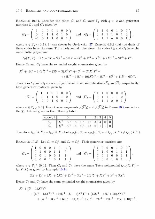
10.6 Examples and counterexamples 85
Example 10.34. Consider the codes C3 and C4 over Fq with q > 2 and generatormatrices G3 and G4 given by
G3 =
1 1 0 0 1 0 00 1 1 1 0 1 0−1 0 1 1 0 0 1
and G4 =
1 1 0 0 1 0 00 1 1 1 0 1 00 1 1 a 0 0 1
,
where a ∈ Fq \ {0, 1}. It was shown by Brylawsky [27, Exercise 6.96] that the duals ofthese codes have the same Tutte polynomial. Therefore, the codes C3 and C4 have thesame Tutte polynomial
tC(X,Y ) = 2X + 2Y + 3X2 + 5XY + 4Y 2 +X3 +X2Y + 2XY 2 + 3Y 3 + Y 4.
Hence C3 and C4 have the extended weight enumerator given by
X7 + (2U − 2)X4Y 3 + (3U − 3)X3Y 4 + (U2 − U)X2Y 5+
+ (5U2 − 15U + 10)XY 6 + (U3 − 6U2 + 11U − 6)Y 7.
The codes C3 and C4 are not projective and their simplifications C3 and C4, respectively,have generator matrices given by
G3 =
1 1 0 1 0 00 1 1 0 1 0−1 0 1 0 0 1
and G4 =
1 1 0 0 0 00 1 1 1 1 00 1 1 a 0 1
,
where a ∈ Fq \{0, 1}. From the arrangements A(C3) and A(C4) in Figure 10.2 we deducethe χi that are given in the following table.
code \ i 0 1 2 3 4 5
C3 U2 − 5U + 6 6U − 12 3 4 0 0C4 U2 − 5U + 6 6U − 13 6 1 1 0
Therefore, tC3(X,Y ) = tC4(X,Y ), but χC3(S,U) 6= χC4(S,U) and tC3(X,Y ) 6= tC4
(X,Y ).
Example 10.35. Let C5 = C⊥3 and C6 = C⊥4 . Their generator matrices are
G5 =
1 0 0 0 1 0 −10 1 0 0 1 1 00 0 1 0 0 1 10 0 0 1 0 1 1
and G6 =
1 0 0 0 1 0 00 1 0 0 1 1 10 0 1 0 0 1 10 0 0 1 0 1 a
,
where a ∈ Fq \ {0, 1}. Then C5 and C6 have the same Tutte polynomial tC⊥(X,Y ) =tC(Y,X) as given by Example 10.34:
2X + 2Y + 4X2 + 5XY + 3Y 2 + 3X3 + 2X2Y +XY 2 + Y 3 + 3X4.
Hence C5 and C6 have the same extended weight enumerator given by
X7 + (U − 1)X5Y 2
+ (6U − 6)X4Y 3 + (2U2 − U − 1)X3Y 4 + (15U2 − 43U + 28)X2Y 5
+ (7U3 − 36U2 + 60U − 31)XY 6 + (U4 − 7U3 + 19U2 − 23U + 10)Y 7.

86 Characteristic polynomials and their generalizations
H2
H1
H3
H5
H6
H4 H1
H6 H5
H4
H3
H2
Figure 10.2: The arrangements of G3 and G4
The geometric lattice L(C5) has atoms a, b, c, d, e, f, g corresponding to the first, second,etc. column of G5. The second level of L(C5) consists of the following 17 elements:
abe, ac, ad, af, ag, bc, bd, bf, bg, cd, ce, cf, cg, de, df, dg, efg.
The third level consists of the following 12 elements:
abce, abde, abefg, acdg, acf, adf, bcdf, bcg, bdg, cde, cefg, defg.
Similarly, the geometric lattice L(C6) has atoms a, b, c, d, e, f, g corresponding to the first,second, etc. column of G6. The second level of L(C6) consists of the following 17 elements:
abe, ac, ad, af, ag, bc, bd, bf, bg, cd, ce, cf, cg, de, dfg, ef, eg.
The third level consists of the following 13 elements:
abce, abde, abef, abeg, acd, acf, acg, adfg, bcdfg, cde, cef, ceg, defg.
Theorem 10.26 implies that µ0(U) and µ1(U) are the same for both codes and equal to
µ0(U) = χ0(U) = A7(U) = (U − 1)(U − 2)(U2 − 4U + 5)
µ1(U) = χ1(U) = A6(U) = (U − 1)(7U2 − 29U + 31).
The polynomials µ3(U) and µ2(U) are given in the following table using Remarks 10.14and 10.11.
C5 C6
µ2(U) 17U2 − 49U + 32 17U2 − 50U + 33µ3(U) 12U − 12 13U − 13
This example shows that for projective codes the Möbius polynomial µC(S,U) is notdetermined by the coboundary polynomial χC(S,U).

11Relations between the Möbius and
coboundary polynomials
When studying polynomial invariants of matroids, much attention is given to the Tuttepolynomial, see Chapter 8. Many other polynomials associated to graphs, arrangements,linear codes and matroids turn out to be an evaluation of the Tutte polynomial, or definethe Tutte polynomial. Sometimes the polynomials and the Tutte polynomial determineeach other.In Chapter 10 we discussed two other polynomial invariants of matroids: the coboundarypolynomial and the Möbius polynomial. The former is, for simple matroids, equivalentto the Tutte polynomial, see Corollary 10.5. The latter, however, is not, as we showed bythe examples in Section 10.6.It follows that, in general, the coboundary polynomial and the Möbius polynomial donot determine each other. Less is known about more specific cases. In this chapter wewill investigate if it is possible that the Möbius polynomial of a matroid, together withthe Möbius polynomial of the dual matroid, define the coboundary polynomial of thematroid. In some cases, the answer is affirmative, and we will give two constructions todetermine the coboundary polynomial in these cases.This chapter is a copy of [54].
11.1 Connections
For a matroid M with rank function r and dual matroid M∗, we will study the followingparameters:
• n, the number of elements of M and M∗;
• k, the rank of M ;
• d, the size of the smallest cocircuit in M (i.e., circuit in M∗);
• d∗, the size of the smallest circuit in M (i.e., cocircuit in M∗).

88 Relations between the Möbius and coboundary polynomials
Note that if a matroid is representable over a finite field, then there is a linear code associ-ated to it with length n, dimension k, minimum distance d and dual minimum distance d∗.
Throughout this chapter, we will restrict ourselves to simple matroids. Also the dual ofa matroid is assumed to be simple. This implies d > 2 and d∗ > 2. In this case, thereis a two-way equivalence between matroids and geometric lattices: we will freely changebetween these objects when necessary.
Some natural questions arise about the dependencies between the coboundary polyno-mial and Möbius polynomial of a matroid and its dual. First of all, do the coboundaryand Möbius polynomial determine each other? The answer is “no”, even if both the ma-troid and its dual are simple. We have seen counterexamples in Examples 10.33 and 10.35.
In Corollary 10.5 we saw that the coboundary polynomial is equivalent to the Tuttepolynomial. The Tutte polynomial of a matroid is determined by the Tutte polynomial ofthe dual matroid, as we saw in Theorem 8.7. Therefore, the same holds for the coboundarypolynomials of a matroid and its dual.
Theorem 11.1. Let χM (S,U) be the coboundary polynomial of a simple matroid M withsimple dual M∗. Let χM∗(S,U) be the coboundary polynomial of M∗. Then
χM∗(S,U) = (S − 1)nU−kχM
(S + U − 1
S − 1, U
).
Proof. The rewriting is analogous to the proof of Theorem 2.19 in Section 8.2. We useCorollary 10.5 and Theorem 8.7.
(S − 1)nU−kχM
(S + U − 1
S − 1, U
)= (S − 1)nU−k
(U
S − 1
)ktM
(S,S + U − 1
S − 1
)= (S − 1)n−ktM∗
(S + U − 1
S − 1, S
)= χM∗(S,U).
Note that in the last step we use that the rank of M∗ is equal to n− k.
One might notice the resemblance between this theorem and the MacWilliams relationsfor the extended weight enumerator in 2.19. This is because of the relation in Theorem10.6.
The question comes up if such a duality relation also exists for the Möbius polynomial.To answer this, we need some more theory.
Lemma 11.2. Let M be a matroid. Then for all elements x ∈M with r(x) < d∗ − 1, wehave |x| = r(x). Furthermore, if M is simple, we have a(x) = r(x) in the correspondinggeometric lattice.

11.1 Connections 89
Proof. By definition, d∗ is the size of the smallest circuit in M and thus the size of thesmallest dependent set in M . It has rank d∗ − 1. This means all elements x ∈M of rankr(x) < d∗ − 1 are independent and have |x| = r(x). For simple matroids, |x| = a(x) inthe corresponding geometric lattice.
Proposition 11.3. Given the Möbius polynomial µM (S,U) of a matroid. Then we candetermine the parameter d∗ of the matroid M .
Proof. The coefficient of the term SiUk−j in the Möbius polynomial is given by∑x∈Lr(x)=i
∑y∈Lr(y)=j
µ(x, y).
These numbers are the doubly-indexed Whitney numbers of the first kind, see Section10.2. In the case j = i, we just count the number of elements in L of rank i, i.e., thenumber of flats of rank i inM . These are the Whitney numbers of the second kind. FromLemma 11.2 it now follows that for i < d∗−1 all elements of rank i are flats, so there are(ni
)of them. For i ≥ d∗− 1, the number of flats is strictly smaller then
(ni
). Therefore we
can determine d∗ from the Möbius polynomial of M .
In the previously mentioned Example 10.33, we have two matroids with the same Möbiuspolynomial but with different d. By Proposition 11.3, this means that their duals cannothave the same Möbius polynomial. This gives a negative answer to the question in [58,§10.5] if the Möbius polynomial of a matroid and its dual are determined by each other.
To summarize, together with Theorem 11.1 we know the following about the coboundaryand Möbius polynomials of a matroid and its dual:
• The coboundary polynomial χM (S,U) of a matroid and the coboundary polynomialχM∗(S,U) of the dual matroid completely determine each other.
• The Möbius polynomial µM (S,U) of a matroid does not determine the Möbiuspolynomial µM∗(S,U) of the dual matroid.
• The coboundary polynomial χM (S,U) does not determine the Möbius polynomialµM (S,U). The same holds in the dual case.
• The Möbius polynomial µM (S,U) does not determine the coboundary polynomialχM (S,U).
The last three statements also hold in caseM and/orM∗ are not simple. In this chapter,we will address another question between dependencies:
Given the Möbius polynomials µM (S,U) and µM∗(S,U) of a matroid and itsdual. Do they determine χM (S,U)?
We will see that, in some cases, the answer is “yes”. Proposition 11.3 tells us that theMöbius polynomial gives us information about the dual of the matroid. This is the reasonto ask if the Möbius polynomial of the matroid, together with the Möbius polynomial ofits dual, determine the coboundary polynomial.For completeness, note that µM (S,U) and µM∗(S,U) define not only d∗ and d, respec-tively, but also n and k: the degree of µM (S,U) in S is r(M) = k, and the degree ofµM∗(S,U) in S is r∗(M∗) = n− k.

90 Relations between the Möbius and coboundary polynomials
Theorem 11.4. Let M be a matroid, and let the Möbius polynomial µM (S,U) be given.Then part of the coboundary polynomial χM (S,U) is determined from this:
χi(U) =
µi(U), for i < d∗ − 1,0, for n− d < i < n,1, for i = n.
Proof. The first equality follows from Proposition 11.3, the definition of the Möbiusand coboundary polynomial, and Lemma 11.2. We proved this statement for codes andarrangements in Theorem 10.26. If d is the smallest size of a cocircuit in M , then n−d isthe biggest size of a hyperplane inM and thus the biggest size of a flat with rank smallerthen k in M . This implies the second equality. The third equality is obvious from thedefinition of the coboundary polynomial.
Using this theorem, we can determine the value of χi(U) for (d∗−1)+(d−1)+1 = d∗+d−1values of i. This leaves n+ 1− (d∗ + d− 1) = n− d− d∗ + 2 of the χi(U) unknown. Wecan say the same about the coefficients χ∗i (U) of the coboundary polynomial χM∗(S,U)of the dual matroid. The idea is to use Theorem 11.1 to calculate the missing values ofχi(U) and χ∗i (U). We first rewrite Theorem 11.1 to a more convenient form.
Proposition 11.5. Let χi(U) be the coefficients of the coboundary polynomial of a sim-ple matroid M with simple dual M∗. Let χ∗i (U) be the coefficients of the coboundarypolynomial of M∗. Then
Uv−kn∑i=v
(i
v
)χi(U) =
n∑i=n−v
(i
n− v
)χ∗i (U), v = 0, . . . , n.
Proof. This is obtained by rewriting the formula in Theorem 11.1. This is analogousto the rewriting of the MacWilliams relations from coding theory, see for example [70,§5.2]. Replacing S by S + 1, binomial expanding and reversing the order of summationgives:
n∑i=0
χ∗i (U)Si = (S − 1)nU−kn∑i=0
χi(U)
(S + U − 1
S − 1
)in∑i=0
χ∗i (U)(S + 1)i = SnU−kn∑i=0
χi(U)
(S + U
S
)in∑i=0
χ∗i (U)
i∑v=0
(i
v
)Sv = U−k
n∑i=0
Sn−iχi(U)
i∑v=0
(i
v
)Si−vUv
n∑v=0
Svn∑i=v
(i
v
)χ∗i (U) =
n∑v=0
Sn−vUv−kn∑i=v
(i
v
)χi(U)
n∑v=0
Sn−vn∑
i=n−v
(i
n− v
)χ∗i (U) =
n∑v=0
Sn−vUv−kn∑i=v
(i
v
)χi(U).
Comparing the coefficients of Sn−v leads to the given formula.

11.2 Independence of duality relations 91
In some cases, the relations from Theorem 11.4 and Propositions 11.5 are enough to com-pletely determine the coboundary polynomial χM (S,U) from the polynomials µM (S,U)and µM∗(S,U).
Theorem 11.6. LetM be a matroid with 2(d+d∗) ≥ n+3. Then the Möbius polynomialsµM (S,U) and µM∗(S,U) determine χM (S,U).
We give three ways to prove this theorem, exploiting various techniques in matroid theory.The first two proofs show that the proposed construction, using the duality relations inProposition 11.5, indeed works. For the third proof, we use the theory of zeta polynomials.
11.2 Independence of duality relations
Proof (Theorem 11.6). We try to determine the coboundary polynomials of M andM∗ simultaneously. First we use Theorem 11.4 for M and M∗. This gives us the value ofχi(U) for i < d∗ − 1 and i > n− d, and the value of χ∗i (U) for i < d− 1 and i > n− d∗.So we are left with the unknowns
χd∗−1(U), χd∗(U), . . . , χn−d(U), χ∗d−1(U), χ∗d(U), . . . , χ∗n−d∗(U).
This are 2(n−d−d∗+2) variables. Proposition 11.5 gives us n+1 equations. In order forthis system to be solvable, we need at least as may equations as unknowns. This means
n+ 1 ≥ 2(n− d− d∗ + 2)
n+ 1 ≥ 2n+ 4− 2(d+ d∗)
2(d+ d∗) ≥ n+ 3.
We now need to show that, given 2(d + d∗) ≥ n + 3, we have enough independentequations. Since all the coefficients of the equations are known, it is possible to do thisdirectly, but that gives lengthy calculations. We will give a more graphical approach.First, we visualize how Proposition 11.5 looks like in matrix form. The grey areas of thematrices are filled with nonzero entries, the white areas contain only zeros. The vectorsare filled with light grey, because it does not matter if the entries are zero or not.
=
χ χ∗
From the triangular shape of the matrices, it is clear that they both have full rank –something we could have also concluded from the fact that the relation in Theorem 11.1is a two way equivalence. We order the system now in a way that all unknowns are onthe left hand side. This means for the first matrix we “cut off” d∗ − 1 columns at the

92 Relations between the Möbius and coboundary polynomials
right of the matrix, and d− 1 at the left, since they correspond to values of i for whichχi(U) is known. For the second matrix, it is the other way around. Since we assumed2(d+ d∗) ≥ n+ 3, we are cutting off at least half of the rows. The new system looks likethis:
− =
χ χ∗
The vector on the right hand side is known and depends on d, d∗ and the two Möbiuspolynomials. The matrices both have full rank n−d−d∗+2, as is clear from their shape.We can write this as one system by “glueing together” the matrices on the left hand side.
=
We need to show that this matrix has full rank. Have a look at the bottom d rows ofthis matrix. The complete left side is zero, so we ignore that for a moment. The rightside has all entries nonzero, and from Proposition 11.5 we know the entries are binomialcoefficients:
(d−1d−1
) (dd−1
)· · ·
(n−d∗d−1
)...
......(
d−11
) (d1
)· · ·
(n−d∗
1
)(d−1
0
) (d0
)· · ·
(n−d∗
0
)
.
By the inductive relations between binomial coefficients, we can perform row operationson this matrix to obtain
0 0 · · ·(n−d−d∗+1
d−1
)...
......
0(
11
)· · ·
(n−d−d∗+1
1
)(00
) (10
)· · ·
(n−d−d∗+1
0
)
.

11.2 Independence of duality relations 93
Flipping the matrix upside down, we have obtained the following picture:
=
In this picture, we show the case for d < n−d−d∗+2. If we had d ≥ n−d−d∗+2, we wouldhave obtained a matrix that was of full rank and we were done. If d∗ ≥ n−d−d∗+ 2, wecan changeM andM∗ and we are also done. So from now on, assume d, d∗ < n−d−d∗+2.Call the left and the right half of the matrix L and R. Suppose a linear combination of thecolumns of the matrix is zero. Since all columns inside L and inside R are independent,this means we can make a linear combination l of columns of L and a linear combinationr of columns of R that are both nonzero and a nonzero multiple of each other.By the shape of L and R, the first d∗ and the last d entries of l and r have to be zero.We will show that the remaining n− d− d∗ + 1 entries of l and r cannot be multiples ofeach other.Crucial in the proof is that all rows of L are multiplied with a different power of U ,whereas R is completely filled with integers. Therefore, any linear combination of columnsof R will have the same powers of U involved in every nonzero entry, even if we take thecoefficients of the linear combination to be polynomials in U and U−1. On the otherhand, the entries of l will all have different powers of U involved. The only possibility tocancel this out, is if we can have only one nonzero entry in l and r, at the same place.We focus now on the matrix L. It has maximal (column) rank n − d − d∗ + 2. FromProposition 11.5 we know the entries are binomial coefficients, with every row multipliedwith another (possibly negative) power of U . The first d∗ rows form a matrix withrank d∗, from the same reasoning we used for the last d rows of R. So if we make alinear combination of the columns of L where the first d∗ entries are zero, there aren − d − d∗ + 2 − d∗ = n − d − 2d∗ + 2 free variables involved. Note we assumed d∗ <n− d− d∗ + 2, so this number is positive. We can use those free variables to make moreentries of l zero: add one of the middle n− d− d∗ + 1 rows of L as an extra constraint,and choose one of the free variables in a way that the corresponding entry in l becomeszero. We are left with
n− d− d∗ + 1− (n− d− 2d∗ + 2) = d∗ − 1 ≥ 2
entries of l that are not zero. They also cannot be zero “by accident” since the middlen − d − d∗ + 1 rows of L form a matrix of full rank. So l cannot have only one nonzeroentry, as was to be shown.To summarize, we have shown that we can use Theorem 11.4 and some of the equations inProposition 11.5 to find χM (S,U) from µM (S,U) and µM∗(S,U) if 2(d+d∗) ≥ n+3.
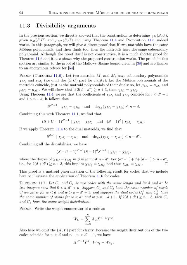
94 Relations between the Möbius and coboundary polynomials
11.3 Divisibility arguments
In the previous section, we directly showed that the construction to determine χM (S,U),given µM (S,U) and µM∗(S,U) and using Theorem 11.4 and Proposition 11.5, indeedworks. In this paragraph, we will give a direct proof that if two matroids have the sameMöbius polynomials, and their duals too, then the matroids have the same coboundarypolynomial. Although the proof itself is not constructive, it is a much shorter proof forTheorem 11.6 and it also shows why the proposed construction works. The proofs in thissection are similar to the proof of the Mallows-Sloane bound given in [38] and are thanksto an anonymous referee for [54].
Proof (Theorem 11.6). Let two matroids M1 and M2 have coboundary polynomialsχM1
and χM2(we omit the (S,U) part for clarity). Let the Möbius polynomials of the
matroids coincide, just as the matroid polynomials of their duals: so, let µM1= µM2
andµM∗1 = µM∗2 . We will show that if 2(d+ d∗) ≥ n+ 3, then χM1 = χM2 .Using Theorem 11.4, we see that the coefficients of χM1 and χM2 coincide for i < d∗ − 1and i > n− d. It follows that
Sd∗−1 | χM1 − χM2 and degS(χM1 − χM2) ≤ n− d.
Combining this with Theorem 11.1, we find that
(S + U − 1)d∗−1 | χM∗1 − χM∗2 and (S − 1)d | χM∗1 − χM∗2 .
If we apply Theorem 11.4 to the dual matroids, we find that
Sd−1 | χM∗1 − χM∗2 and degS(χM∗1 − χM∗2 ) ≤ n− d∗.
Combining all the divisibilities, we have
(S + U − 1)d∗−1(S − 1)dSd−1 | χM∗1 − χM∗2 ,
where the degree of χM∗1 −χM∗2 in S is at most n−d∗. For (d∗−1)+d+(d−1) > n−d∗,i.e., for 2(d+ d∗) ≥ n+ 3, this implies χM∗1 = χM∗2 and thus χM1 = χM2 .
This proof is a matroid generalization of the following result for codes, that we includehere to illustrate the application of Theorem 11.6 for codes.
Theorem 11.7. Let C1 and C2 be two codes with the same length and let d and d∗ betwo integers such that 0 < d, d∗ < n. Suppose C1 and C2 have the same number of wordsof weight w for w < d and w > n− d∗ + 1, and suppose the dual codes C⊥1 and C⊥2 havethe same number of words for w < d∗ and w > n− d+ 1. If 2(d+ d∗) ≥ n+ 3, then C1
and C2 have the same weight distribution.
Proof. Write the weight enumerator of a code as
WC =
n∑w=0
AwXn−wY w.
Also here we omit the (X,Y ) part for clarity. Because the weight distributions of the twocodes coincide for w < d and n− w < d∗ − 1, we have
Xd∗−1Y d | WC1−WC2
.

11.4 Zeta polynomials 95
Applying the MacWilliams relations gives
(X + (q − 1)Y )d∗−1 | WC∗1
−WC∗2and (X − Y )d | WC∗1
−WC∗2.
Because the weight distributions of the dual codes coincide for w < d∗ and n−w < d−1,we have
Xd−1Y d∗| WC∗1
−WC∗2.
Combining the divisibilities, we find that
(X + (q − 1)Y )d∗−1(X − Y )dXd−1Y d
∗| WC∗1
−WC∗2.
The total degree of all terms in WC∗1−WC∗2
is n. So, for (d∗ − 1) + d+ (d+ 1) + d∗ > n,i.e., for 2(d+ d∗) ≥ n+ 3, this implies WC∗1
= WC∗2and thus WC1
= WC2.
Note that in this theorem d and d∗ do not necessarily have to be the minimum distanceand dual minimum distance of the code. As long as the total length of the four intervalson which the weights agree is big enough, the theorem holds.
11.4 Zeta polynomials
In Chapter 3 we discussed the zeta polynomial of a code. We will extend this theory tomatroids, and use it to give another construction to prove Theorem 11.6. Just as withthe other polynomials, we often refer to the zeta polynomial in the following form:
PC(T,U) =
r∑i=0
Pi(U)T i.
Duursma [39] extended the definition of the zeta polynomial to matroids. We choose asimilar approach and use that we can talk about the extended weight enumerator of amatroid, via its equivalence with the Tutte polynomial (see Theorems 8.4 and 8.5).
Theorem 11.8. Let M be a matroid with coboundary polynomial χM (S,U). The two-variable zeta polynomial PM (T,U) of this matroid is the unique polynomial in Q[T,U ]of degree at most n− d in T such that if we expand the generating function
PM (T,U)
(1− T )(1− TU)(1 + (S − 1)U)n
as a power series in the variable T , we get
. . .+ . . . Tn−d−1 +χM (S,U)− Sn
U − 1Tn−d + . . . Tn−d+1 + . . . .
Proof. Apply X = 1 and Y = S−1 in the definition of the zeta function and multiplythe whole equation with Sn.
Z(T,U) · (Y (1− T ) +XT )n = . . .+WC(X,Y, U)−Xn
U − 1Tn−d + . . .
Z(T,U) · Sn · (S−1(1− T ) + T )n = . . .+WC(1, S−1, U)− 1
U − 1SnTn−d
Z(T,U) · (1 + (S − 1)T )n = . . .+χM (S,U)− Sn
U − 1Tn−d + . . .

96 Relations between the Möbius and coboundary polynomials
Propositions 3.2, 3.4, and 3.5 and Theorem 3.3 have a direct analogue for matroids. LetXn,d be the coboundary polynomial of the uniform matroid on n elements with rankn− d+ 1.
Proposition 11.9. A matroid is uniform if and only if PM (T,U) = 1.
Theorem 11.10. The zeta polynomial gives us a way to write the coboundary polynomialwith respect to a basis of coboundary polynomials of uniform matroids:
χM (S,U) = P0(U)Xn,d + P1(U)Xn,d+1 + . . .+ Pr(U)Xn,d+r.
Proposition 11.11. The degree of PM (T,U) in T is n− d− d∗ + 2.
Proposition 11.12. For the two-variable zeta polynomial of a matroid M and dual M∗we have
PM∗(T,U) = PM
(1
TU,U
)Un−k+1−dTn−d−d
∗+2.
We are now ready to give an alternative proof of Theorem 11.6 using the two-variablezeta polynomial.
Proof (Theorem 11.6). Our goal is to determine all the coefficients Pj(U) of the two-variable zeta polynomial, and thus the coboundary polynomial χM (S,U). Denote thecoefficient of Sj in Xn,d by Xn,d,j . We know the exact value of these coefficients, just likewe know the extended weight enumerator of MDS codes, see Theorem 2.27. So, we cansplit up Theorem 11.10 in n+ 1 equations:
χj(U) =
n−d−d∗+2∑i=0
Pi(U)Xn,d+i,j , j = 0, . . . , n.
Not all of these equations are helpful in determining the Pi(U). For j < d∗ − 1 andj > n − d the χj(U) are known by Theorem 11.4. In the case n − d < j < n we haveχj(U) = 0 and also Xn,d+i,j = 0 for all i, so the corresponding equations just state 0 = 0.For d∗− 1 ≤ j ≤ n− d we don’t know χj(U), so these equations are also not helpful. Weare left with the equations for j < d∗− 1 and j = n, so d∗ equations in the n− d− d∗+ 3unknown Pi(U).We can do the same for the dual matroid, leading to d equations in the n − d − d∗ + 3unknown P ∗i (U). From Proposition 11.12 it follows that
P ∗i (U) = U i−k−1+d∗Pn−d−d∗+2−i(U),
so we can replace the P ∗i (U) one-to-one by the appropriate Pi(U). So all together, wehave d+d∗ equations in n−d−d∗+3 unknown Pi(U). To get at least as many equationsas unknowns, we need
d+ d∗ ≥ n− d− d∗ + 3
2(d+ d∗) ≥ n+ 3.
This is the same bound we already obtained in Theorem 11.6.

11.5 Open questions 97
11.5 Open questions
We have seen two methods to determine the coboundary polynomial χM (S,U) of a ma-troid from the Möbius polynomials µM (S,U) and µM∗(S,U) of a matroid and its dual.Both methods rely on duality relations for, respectively, the coboundary and Tutte poly-nomial.
Theorem 11.6 is valid for matroids that are “close” to the uniform matroid. Stated interms of codes, this means codes with a minimum distance and dual minimum distancethat is high, so the code is “close to MDS”. Examples of such codes are MDS codes itself(but this is a trivial example, since there is only one uniform matroid given length andrank) and near-MDS codes, these are codes with d = n − k and d⊥ = k (see Definition10.27). Also almost-MDS codes with k ≤ n/2 are in this category. See Boer [33] for moreon almost-MDS codes and Faldum and Willems [41] for more on codes that are close toMDS. Other specific codes that have 2(d + d∗) ≥ n + 3 are the q-ary Hamming codes(and their duals, the simplex codes) and the first order q-ary Reed-Muller codes. Thesecodes were treated in Chapter 5.
A logical question is now: how sharp is the bound in Theorem 11.6? To look for an ex-ample to show the bound is tight, we need two matroids with the same parameters and2(d + d∗) < n + 3 that have equal Möbius polynomials µM (S,U) and µM∗(S,U) butdifferent coboundary polynomial χM (S,U). The smallest case is d = d∗ = 3 (becauseotherwise the matroid is not simple) and thus n = 10.An exhaustive computer search on 260 random matrices with the desired parameters andk = 5 did not lead to such an example, so there is room for improvement on the boundin Theorem 11.6.
In Proposition 6.3 of [24] the issue is addressed how many Tutte polynomials there are,given the size and rank of a matroid. This is done by looking at the affine space generatedby the coefficients of the Tutte polynomial, and determining its dimension. See also [25].It would be interesting to see if we can do the same thing for the Möbius polynomial,given n, k, d and d∗. If we determine the dimension of the affine space generated by thecoefficients of the Möbius polynomial of a matroid and its dual, we can compare it tothe dimension for the Tutte polynomial. This could give us more information about therelations between the Möbius and coboundary polynomials in general.

98 Relations between the Möbius and coboundary polynomials

12The spectrum polynomial
The spectrum polynomial of a matroidM without loops was introduced by Kook, Reinerand Stanton to show that the spectra of the combinatorial Laplace operators on theindependent complex IN(M) are nonnegative and integral [65]. The spectrum polynomialcontains the same information as these spectra, hence the name spectrum polynomial. Themain results concerning the spectrum polynomial are the recurrence relations by Kook[64] and the generalization of Denham [34] to an invariant that specializes to both theTutte polynomial and to the spectrum polynomial. Since it is a matroid invariant, it istempting to compare the spectrum polynomial to the Tutte polynomial. Kook et al. [65]showed that the Tutte polynomial does not determine the spectrum polynomial. Theopposite problem is still open.In this chapter we calculate the spectrum polynomial of the uniform matroidM of rank kon n elements. We give two different methods, using equivalent definitions of the spectrumpolynomial.
12.1 Calculations using combinatorics
The spectrum polynomial has the following combinatorial definition.
Definition 12.1. Let M = (E, I) be a matroid and L(M) the associated geometriclattice. Then the spectrum polynomial of M is defined by
SpecM (S,U) =∑
x,y∈L(M)
|χ(IN(x))| |µL(M)(x, y)|Ur(y)S|x|,
where |x| is the number of elements of M that are in the flat x and χ(IN(x)) is thereduced Euler characteristic of the independence complex of x.
The value of |x| is equal to a(x) for all flats x if M is a simple matroid. The followingformula holds by [14, p. 238]:
|χ(IN(M))| = RM (−1, 0) =∑I∈I
(−1)r(M)−|I|.
We will start by calculating the Möbius function of the uniform lattice.

100 The spectrum polynomial
Lemma 12.2. The Möbius function of the uniform lattice Un,k is given by
µ(x, y) =
0, if x 6≤ y,(−1)|y|−|x|, if y 6= 1,∑k−|x|i=1 (−1)i
(n−|x|i−1
), if y = 1.
Proof. We know µ(x, x) = 1 and µ(x, y) = 0 if x and y are not comparable. If x ≤ y,we get an alternating sum of binomial coefficients. For y 6= 1 the corresponding lattice isthe full powerset, so µ(x, y) = (−1)|y|−|x|, see for example [29].
Theorem 12.3. The spectrum polynomial of the uniform matroid Un,k is equal to
SpecUn,k(S,U) =
k−1∑r=0
(n
r
)Ur +
(n− 1
k − 1
)Uk +
(n− 1
k
)SnUk.
Proof. The Möbius function of the uniform lattice was calculated in Lemma 12.2. Wecontinue with the calculation of the Euler characteristic χ(IN(x)). We first look at thecase x 6= 1. Then all subsets of x are independent: summing over their rank, the Eulercharacteristic becomes
|x|∑i=0
(−1)|x|−i(|x|i
).
This expression is zero, except for x = 0, the empty set: then χ = 1. If x = 1 the Eulercharacteristic is equal to
k∑i=0
(−1)k−i(n
i
).
We have enough information now to calculate the spectrum polynomial. We only haveto look at three cases, since for the others the Euler characteristic is zero:
1. y 6= 1 and x = 0,
2. y = 1 and x = 0,
3. y = x = 1.
For the first one, the value in the inner summation of the spectrum polynomial is 1, sowe just have to count the number of elements on each level of L. The second and thirdcase are just filling in the right values in the Möbius function and Euler characteristic.So, we have
1.(nr
)Ur for all r < k,
2. Uk ·∣∣∣∑k
i=0(−1)k−i(ni
)∣∣∣ · 1 · Sn,3. Uk · 1 ·
∣∣∣∑ki=1(−1)i
(ni−1
)∣∣∣ · S0.

12.2 Calculations using ordered matroids 101
The summation in the second case can be rewritten as
k∑i=0
(−1)k−i(n
i
)= (−1)k
k∑i=0
(−1)i(n
i
)= (−1)2k
(n− 1
k
),
so the absolute value of this is(n−1k
). The summation in the third case can be rewritten
similarly:k∑i=1
(−1)i(
n
i− 1
)= (−1)
k−1∑i=0
(−1)i(n
i
)= (−1)k
(n− 1
k − 1
),
which has absolute value(n−1k−1
). Note that these two binomials add up to
(nk
), the number
of bases of M . Filling in the calculated expressions for the Euler characteristic and theMöbius function, we find that the spectrum polynomial of the uniform matroid Un,k isequal to the given formula.
12.2 Calculations using ordered matroids
Another way of defining the spectrum polynomial is based on the next theorem, see [65,Theorem 1].
Theorem 12.4. Let M = (E,ω, I) be an ordered matroid. Then we can decompose eachindependent set I into two disjoint sets I = I1∪I2 such that I1 is a base of internal activity0 for the flat |I1| and I2 is a base of external activity 0 for the contracted matroid I\I1.
Proof. The desired decomposition can be obtained by the following algorithm:
1. Start with I1 = I and let V = I1.
2. Pick the smallest element e ∈ I1 with respect to ω.
3. Find the fundamental cocircuit of e with respect to I1 in V , i.e. the unique cocircuitin V − I1 + e.
4. If e is the smallest element in this cocircuit (i.e. internally active in I1), remove itfrom I1 and redefine V = I1.
5. Take the next e ∈ I1 with respect to ω and return to Step 3. If there are no elementsleft in V , we are done.
See [65] for a proof that this construction indeed gives the decomposition from the the-orem.
Definition 12.5. Let M = (E,ω, I) be an ordered matroid. Then the spectrum polyno-mial of M is defined by
SpecM (S,U) =∑I∈I
S|I1|Ur(I).
We can now give a proof of Theorem 12.3 that uses an ordering of the matroid.
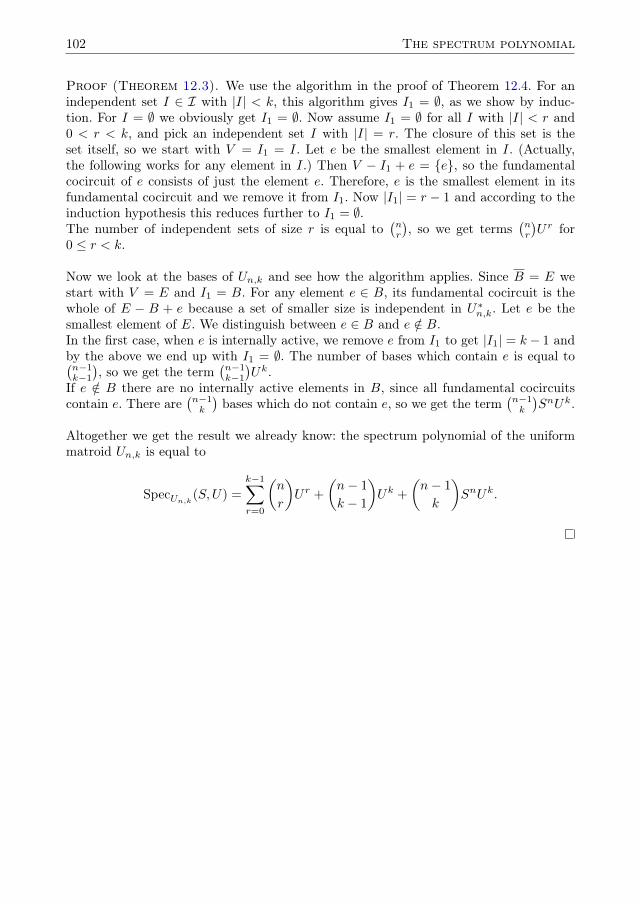
102 The spectrum polynomial
Proof (Theorem 12.3). We use the algorithm in the proof of Theorem 12.4. For anindependent set I ∈ I with |I| < k, this algorithm gives I1 = ∅, as we show by induc-tion. For I = ∅ we obviously get I1 = ∅. Now assume I1 = ∅ for all I with |I| < r and0 < r < k, and pick an independent set I with |I| = r. The closure of this set is theset itself, so we start with V = I1 = I. Let e be the smallest element in I. (Actually,the following works for any element in I.) Then V − I1 + e = {e}, so the fundamentalcocircuit of e consists of just the element e. Therefore, e is the smallest element in itsfundamental cocircuit and we remove it from I1. Now |I1| = r − 1 and according to theinduction hypothesis this reduces further to I1 = ∅.The number of independent sets of size r is equal to
(nr
), so we get terms
(nr
)Ur for
0 ≤ r < k.
Now we look at the bases of Un,k and see how the algorithm applies. Since B = E westart with V = E and I1 = B. For any element e ∈ B, its fundamental cocircuit is thewhole of E − B + e because a set of smaller size is independent in U∗n,k. Let e be thesmallest element of E. We distinguish between e ∈ B and e /∈ B.In the first case, when e is internally active, we remove e from I1 to get |I1| = k− 1 andby the above we end up with I1 = ∅. The number of bases which contain e is equal to(n−1k−1
), so we get the term
(n−1k−1
)Uk.
If e /∈ B there are no internally active elements in B, since all fundamental cocircuitscontain e. There are
(n−1k
)bases which do not contain e, so we get the term
(n−1k
)SnUk.
Altogether we get the result we already know: the spectrum polynomial of the uniformmatroid Un,k is equal to
SpecUn,k(S,U) =
k−1∑r=0
(n
r
)Ur +
(n− 1
k − 1
)Uk +
(n− 1
k
)SnUk.

13Truncation formulas
The mathematical meaning of truncation is just as it is in every day life: cutting some-thing off. In the situation of this chapter, we will be “cutting off” matroids and geometriclattices by ‘removing’ their hyperplanes and bases, respectively. An overview of morepossible constructions on matroids and geometric lattices can be found in [26].Britz [21] showed that the rank generating function of a truncated matroid is defined bythe rank generating function of the matroid itself. It is a natural question to ask if thereare similar truncation formulas for other polynomials. We will give truncation formulasfor the coboundary, Möbius and spectrum polynomial. The outline of the combinatorialproof for these formulas is the same for all three polynomials.This chapter is a copy of [57].
13.1 Truncation of matroids and geometric lattices
We can define the truncation of a matroid in several equivalent ways, just as we can definea matroid in terms of its independent sets, bases, rank function, flats, circuits, etcetera.We will give some equivalent definitions that are most suitable for our purposes. For amore extensive list, see [26].
Definition 13.1. The truncation of a matroid M of rank r(M) = r ≥ 1 is denoted byτ(M). It has the same set of elements asM and it has the following equivalent definitions:
• The independent sets of τ(M) are all the independent sets of M , except those ofrank r.
• The rank function of τ(M) is given by rτ(M)(A) = min{rM (A), r − 1}.
• The bases of τ(M) are the independent sets of rank r − 1 in M .
The truncation of a matroid is again a matroid.
Example 13.2. Consider the uniform matroid M = Un,r on n elements of rank r ≥ 1.Then τ(M) = Un,r−1.
For a geometric lattice, the definition is more straightforward.

104 Truncation formulas
Definition 13.3. The truncation of a geometric lattice L of rank r(L) = r ≥ 1 withpartial ordering ≤ has as elements all the elements of L except those of rank r− 1, withthe same partial ordering ≤. It is denoted by τ(L).
The truncation of a geometric lattice is again a geometric lattice. Note that the trun-cations of a matroid and a geometric lattice each have rank r − 1. For a matroid M ,we denote by L(M) its associated geometric lattice of flats. Conversely, for a geometriclattice L, we denote by M(L) its associated matroid. Then τ(M(L)) = M(τ(L)) andτ(L(M)) = L(τ(M)).
Instead of removing all elements of rank r − 1 from a geometric lattice, one might askwhat happens if we remove all elements of rank 1, the atoms, from the geometric lattice.Unfortunately, the resulting structure is no longer a geometric lattice. We therefore loosenour definitions to get a class of objects that is closed under this “truncation from below”.If we start with a geometric lattice and drop the requirements that it is atomic and thatits rank function is semimodular, we get a poset with rank function, see Proposition 9.18.
Definition 13.4. The upper truncation of a poset with rank function P of rank r(P ) =r ≥ 1 with partial ordering ≤ has as elements all the elements of P except those of rankr − 1, with the same partial ordering ≤. It is denoted by τ+(P ). The lower truncationof P has as elements all the elements of P except those of rank 1, with the same partialordering ≤. It is denoted by τ−(P ).
Again, truncating lowers the rank by 1, so τ+(P ) and τ−(P ) both have rank r − 1.
Lower truncation can be described in terms of upper truncation and inversion (see Defi-nition 9.9): the lower truncation of a poset can be obtained by first inverting the poset,then taking upper truncation, and then inverting back again. On the other hand, wecan obtain upper truncation by first inverting, then taking lower truncation, and theninverting back again.
Let L be a geometric lattice of rank r, and P (L) its associated poset with rank function.Then P (τ(L)) = τ+(P (L)). But it is not true that τ−(P (L)) is the poset of some sortof truncation of the geometric lattice L, since it is not always the case that the rankfunction on τ−(P (L)) is semimodular.
Example 13.5. Consider M = U4,4, the uniform matroid on 4 elements of rank 4. Let Lbe the lattice of flats ofM , and P the associated poset of L with rank function. Considerx = {1, 2} and y = {3, 4} in τ−(P ). The meet and join of x and y in τ−(P ) are givenby x ∧ y = ∅ and x ∨ y = {1, 2, 3, 4}, respectively. Then rτ−(P )(x) = rτ−(P )(y) = 1 andrτ−(P )(x ∧ y) = 0 and rτ−(P )(x ∨ y) = 3. Hence τ−(P ) is not a geometric lattice.
There is a natural way to extend the lattice τ−(L) to a geometric lattice, called Dilworthcompletion. See [26, §7.7], [35], [67], and [104, §12]. The result of this completion is referredto as the Dilworth truncation of a lattice. It can be viewed as the smallest geometric latticethat contains τ−(L). Since our techniques for finding truncation formulas do not applyto the Dilworth truncation, we will not go into the details of its definition.
13.2 Representation of a truncated matroid 105
13.2 Representation of a truncated matroid
It was shown by Mason [71, §2.4] that if a matroid is representable over a field, thenits Dilworth truncation is representable over an extension of that field. For ordinarytruncation this question is addressed in [26, Prop. 7.4.10]: if M is a matroid that isrepresentable over the field F, then τ(M) is a representable matroid over a transcendentalextension of F. We will give a stronger version of this result.
Example 13.6. Consider the simplex code C of dimension 3 over the finite field with qelements. This code has length n = q2 + q+ 1 and minimum distance q2. The associatedmatroid M = MC is by definition representable. The truncation τ(M) is the uniformmatroid Un,2. Now Un,2 is representable over Fq if and only if n is at most q+1. Thereforeτ(M) is representable over any extension of Fq3 but it is not representable over Fq itself.
Theorem 13.7. Let M be a matroid of rank k on n elements that is representable overa field F.
1. If F is infinite, then τ(M) is representable over F.
2. If F is finite consisting of q elements and m ≥ dlogq((nk−1
))e + 1, then τ(M) is
representable over Fqm .
Proof. Suppose that M is a matroid of rank k on the set E = {1, . . . , n} and M isrepresented by a k × n matrix G of rank k over F. A subset I of E is an independentset of M if and only if the columns of G enumerated by I are independent. Let C be thesubspace of Fn generated by the rows of G. Then C has dimension k, since G has rankk. The idea of the proof is to show that a “generic” subspace of C of dimension k − 1represents τ(M). In order to have enough space one has to extend the field F in case itis finite, since a finite union of hyperplanes in Fn might be equal to Fn. The details aresimilar as given in the proof of Proposition 5.1 of [79].The space C is the null space of a (n−k)×n matrix H of rank n−k over F. Let |I| = k.Then I is a basis of M if and only if the columns of H enumerated by J = E \ I areindependent. Let t = n − k and let H(j1, . . . , jt) be the t × t matrix obtained from Hby taking the columns numbered by j1, . . . , jt ∈ J , where 1 ≤ j1 < . . . < jt ≤ n. Let∆(j1, . . . , jt) be the determinant of H(j1, . . . , jt).Now let I be a basis of τ(M) and let J = E \ I. Then |I| = k − 1 and there exists an iin J such that I ∪ {i} is a basis of M . Hence the columns of H enumerated by J \ {i}are independent. Let J = {j1, . . . , jt+1} for some 1 ≤ j1 < . . . < jt+1 ≤ n. Consider thelinear function given by
fI(X1, . . . , Xn) =
t+1∑s=1
(−1)s∆(j1, . . . , js, . . . , jt+1)Xjs ,
where (j1, . . . , js, . . . , jt+1) is the t-tuple obtained from (j1, . . . , js, . . . , jt+1) by deletingthe s-th element. There exists an s such that js = i and the corresponding determinant∆(j1, . . . , js, . . . , jt+1) is not zero. Hence the above equation is not identically zero anddefines a hyperplane HI in Fn with equation fI(X1, . . . , Xn) = 0 for every basis I ofτ(M). Consider the product
f(X1, . . . , Xn) =∏
I basis of MfI(X1, . . . , Xn).
106 Truncation formulas
So, f(X1, . . . , Xn) is a nonzero polynomial. If F is infinite, then this polynomial is noteverywhere zero on Fn by [69, V §4 Corollary 3]. Therefore there exists an element x ∈ Fnsuch that f(x1, . . . , xn) is not zero.If F is finite, then F = Fq and we assumed m ≥ dlogq(
(nk−1
))e+ 1. So qm >
(nk−1
). Hence
(qm)n >
(n
k − 1
)(qm)n−1.
The number of basis of τ(M) is at most(nk−1
). Therefore, Fnqm has more elements than the
union of all hyperplanes HI with I a basis of τ(M). So there exists an element x ∈ Fnqmthat does not lie in this union.In both cases an n-tuple x is found, possibly over an extension of F such that fI(x1, . . . , xn)is not zero for every basis I of τ(M). Let H be the (t+ 1)×n matrix obtained by addingto H the row x. Then for every basis I of τ(M) the columns of H enumerated by thecomplement of I are independent, because the determinant of the corresponding squarematrix of size t+ 1 is equal to fI(x) 6= 0.The conclusion is that the null space of H is a subspace of C of dimension k − 1 thatrepresents τ(M).
13.3 Truncation and the coboundary polynomial
For polynomials associated with matroids and geometric lattices, one might ask if wecan find the polynomial of their truncation from the polynomial of the original structure.The answer is positive for the characteristic polynomial, see [26, p. 149]. For the rankgenerating function RM (X,Y ) of a matroid we have the following theorem, proved byBritz [21, Prop. 15].
Theorem 13.8 (Truncation formula). Let M be a matroid. Then
X ·Rτ(M)(X,Y ) = RM (X,Y ) + (XY − 1) ·RM (0, Y ).
In this section, we will consider the same question for the coboundary polynomial.
Theorem 13.9. Let L be a geometric lattice of rank r ≥ 3. Then
U · χτ(L)(S,U) = χL(S,U) + (U − 1) · χL(S, 0).
Proof. The identity is a direct consequence of Theorem 13.8 using the relation betweenthe rank generating and coboundary polynomial from Theorem 10.4.
Since the coboundary polynomial is equivalent to the rank generating function, it is clearthat a truncation formula for the coboundary polynomial should exist. However, thedefinition of the coboundary polynomial makes it possible to find a more general ideabehind this truncation formula, that can also be applied to other polynomial invariantsthat are not equivalent to (or determined by) the rank generating function.
Theorem 13.10. Let f(S,U) be a polynomial invariant of a matroid, geometric lattice,or poset with rank function that has rank r and can be written as
f(S,U) =
r∑i=0
fj(S)Ur−j .

13.3 Truncation and the coboundary polynomial 107
Let f ′ be the corresponding polynomial invariant of the truncation of the matroid, geo-metric lattice, or poset with rank function. So, we can write
f ′(S,U) =
r−1∑i=0
f ′j(S)Ur−1−j .
If the coefficients fj(S) and f ′(S) are related via{f ′j(S) = fj(S), for j ≤ r − 2,f ′j(S) = fj(S) + fj+1(S), for j = r − 1.
then the following truncation formula holds:
U · f ′(S,U) = f(S,U) + (U − 1) · f(S, 0).
Proof. The proof is given by rewriting.
U · f ′(S,U) =
r−1∑i=0
f ′j(S)Ur−j
=
r−2∑i=0
fj(S)Ur−j + U · (fr−1(S) + fr(S))
=
r−1∑i=0
fj(S)Ur−j + U · fr(S)
=
r∑i=0
fj(S)Ur−j − fr(S) + U · fr(S)
= f(S,U) + (U − 1) · f(S, 0).
We can use this formula to give a different proof of Theorem 13.9.
Proof (Theorem 13.9). We can not directly apply Theorem 13.10 to the coboundarypolynomial: we will use the following reduced form, where we delete the highest degreeterms in S. Let m be the number of atoms of L and let
χL(S,U) = χL(S,U)− Sm =
r∑j=0
χj(S)Ur−j ,
whereχj(S) =
∑aL(x)=ii<m
∑x≤y
rL(y)=j
µL(x, y)Si.
Let the reduced coboundary polynomial of the truncated geometric lattice be given by
χ′(S,U) =
r−1∑i=0
χ′j(S)Ur−1−j .
108 Truncation formulas
We need to show the relations of Theorem 13.10. Note that if rL(x) ≤ r−2, then rL(x) =rτ(L)(x) and aL(x) = aτ(L)(x). Also, if r(x), r(y) ≤ r − 2, then µL(x, y) = µτ(L)(x, y).Therefore, χ′j(S) = χj(S) for j ≤ r − 2.It is left to show that χr−1(S) + χr(S) = χ′r−1(S), that is,∑
aL(x)=ii<m
∑x≤y
rL(y)=r−1
µL(x, y)Si +∑
aL(x)=ii<m
µL(x, 1L)Si =∑
aτ(L)(x)=ii<m
µτ(L)(x, yτ(L))Si.
Since aL(x) < m, we have rL(x) < r in every summation. We split into two parts. IfrL(x) = r− 1 = rτ(L)(x), then aτ(L)(x) = m, so the right hand side of the summation is0. The left hand side of the summation is then equal to∑
aL(x)=ii<m
Si (1− 1) = 0,
so this cancels out. Now suppose rL(x) = rτ(L)(x) ≤ r − 2. We can drop the firstsummation and the factor Si, because they are the same on both sides. So, we need toshow that ∑
x≤yrL(y)=r−1
µL(x, y) + µL(x, 1L) = µτ(L)(x, yτ(L)).
We will use the induction formula for the Möbius function: for x < y, it holds that∑x≤z≤y
µL(x, z) =∑
x≤z≤y
µL(z, y) = 0.
If we use this on the left hand side, we get∑x≤y
rL(y)=r−1
µL(x, y) + µL(x, 1L) =∑x≤y
rL(y)=r−1
µL(x, y)−∑
x≤z<1L
µL(x, z)
= −∑x≤z
rL(z)≤r−2
µL(x, z).
The right hand side is equal to
µτ(L)(x, 1τ(L)) = −∑
x≤z<1τ(L)
µτ(L)(x, z)
= −∑x≤z
rτ(L)(z)≤r−2
µτ(L)(x, z)
= −∑x≤z
rL(z)≤r−2
µL(x, z)
We conclude that χr−1(S) + χr(S) = χ′r−1(S), so the reduced coboundary polynomialsatisfies the conditions in Theorem 13.10 and therefore has a truncation formula. Sincethe term Sm that we omitted does not change under truncation, we get the truncationformula as is Theorem 13.9.

13.4 Truncation and the Möbius polynomial 109
Example 13.11. The uniform matroid Un,r has rank generating function
RUn,r (X,Y ) =
r−1∑i=0
(n
i
)Xr−i +
n∑i=r
(n
i
)Y i−r,
as follows directly from the definitions. Since the coboundary polynomial is defined bythe rank generating function (see Theorem 10.4), we can find the coboundary polynomialof the uniform geometric lattice:
χUn,r (S,U) =
r−1∑i=0
(n
i
)(S − 1)iUr−i +
n∑i=r
(n
i
)(S − 1)i.
In this form many terms cancel each other. For example, U7,3 has coboundary polynomial
χU7,3(S,U) = S7 + 21S2(U − 1) + 7S(U2 − 6U + 5) + (U3 − 7U2 + 21U − 15).
In the form as above, it is straightforward to verify the truncation formula for thecoboundary polynomial for arbitrary uniform geometric lattices. In case of the latticeU7,3, its truncation U7,2 has coboundary polynomial
χU7,2(S,U) = S7 + 7S(U − 1) + (U2 − 7U + 6).
13.4 Truncation and the Möbius polynomial
The combinatorial proof for the truncation formula in Theorem 13.9 is also applicableto other polynomials. In this section we treat the Möbius polynomial. We loosen to thecase of posets with rank functions, so we can also address the lower truncation.
Theorem 13.12. Let P be a poset with rank function of rank r. Then
U · µτ+(P )(S,U) = µP (S,U) + (U − 1) · µP (S, 0) + Sr−1U − SrU.
Proof. Just as in the case of the coboundary polynomial, we will use a reduced formof the polynomial to work with. Let
µP (S,U) = µP (S,U)− Sr =
r∑j=0
µj(S)Ur−j ,
whereµj(S) =
∑rP (x)=ii<r
∑x≤y
rP (y)=j
µP (x, y)Si.
Note that the sets {x ∈ L : aL(x) < m} and {x ∈ L : rL(x) < r} are the same, sothe proof that the reduced Möbius polynomial obeys the constrains in Theorem 13.10is exactly the same as in the case of the reduced coboundary polynomial. Hence thereduced Möbius polynomial has a truncation formula as in Theorem 13.10. To switchto the non-reduced Möbius polynomial, −USr−1 gets added at the left hand side of theformula, and −Sr− (U −1)Sr at the right hand side. This gives the term +Sr−1U −SrUin the formula.

110 Truncation formulas
Example 13.13. We consider again the uniform geometric lattice L = Un,r. For allelements x ∈ Un,r with rL(x) < r(L), we have that aL(x) = rL(x). Therefore thecoboundary polynomial and the Möbius polynomial differ only in the leading term: forthe coboundary polynomial this is Sn, while for the Möbius polynomial it is Sr(L). Forexample, the Möbius polynomial of the geometric lattice U7,3 is equal to
µU7,3(S,U) = S3 + 21S2(U − 1) + 7S(U2 − 6U + 5) + (U3 − 7U2 + 21U − 15).
The Möbius polynomial of its truncation U7,2 is equal to
µU7,2(S,U) = S2 + 7S(U − 1) + (U2 − 7U + 6).
Comparing with Example 13.11, we see why the term Sr−1U − SrU is needed in thetruncation formula of the Möbius polynomial.We would like to mention that it is possible to give a general formula for the Möbiuspolynomial of a uniform geometric lattice, see Example 10.12. Checking the truncationformula directly in the case of a general uniform geometric lattice is therefore possible,but we leave the rather lengthy calculation to the reader.
For posets, we can find a similar truncation formula for the lower truncation.
Theorem 13.14. Let P be a poset with rank function of rank r. Then
S · µτ−(P )(S,U) = µP (S,U) + (S − 1) · µP (0, U) + SUr−1 − SUr.
Proof. We prove this formula by using the inverse poset, see Definition 9.9. The Möbiuspolynomial of the inverse poset i(P ) is found by interchanging the variables in the Möbiuspolynomial of the original poset P :
µi(P )(S,U) =∑
x∈i(P )
∑y∈i(P )
µi(P )(x, y)Sri(P )(x)Ur(i(P ))−ri(P )(y)
=∑x∈P
∑y∈P
µP (y, x)Sr−rP (x)Ur−(r−rP (y))
=∑x∈P
∑y∈P
µP (x, y)UrP (x)Sr−rP (y)
= µP (U, S).
This makes it possible to derive the formula for lower truncation directly from the formulafor upper truncation. We start with the formula for upper truncation in Theorem 13.12:
U · µτ+(P )(S,U) = µP (S,U) + (U − 1) · µP (S, 0) + Sr−1U − SrU.
For the inverse of P , the same formula holds:
U · µτ+(i(P ))(S,U) = µi(P )(S,U) + (U − 1) · µi(P )(S, 0) + Sr−1U − SrU.
Now we use that τ+(i(P )) = i(τ−(P )) and µi(P )(S,U) = µP (U, S):
U · µτ−(P )(U, S) = µP (U, S) + (U − 1) · µP (0, S) + Sr−1U − SrU.
Interchanging S and U gives the formula for lower truncation.

13.5 Truncation and the spectrum polynomial 111
13.5 Truncation and the spectrum polynomial
We discussed the spectrum polynomial in Chapter 12. By a slight change of variables,we get a polynomial on which we can apply the same technique as before to prove atruncation formula.
Definition 13.15. Let M be a matroid and L = L(M) its associated geometric lattice.Let
νM (x, y) = (−1)rM (x)µL(x, y) |χ(IN(x))|
and define the reciprocal alternating spectrum polynomial of M by
RaspM (S,U) =∑x∈L
∑x≤y∈L
νM (x, y)S|x|Ur(L)−rL(y).
Note the similarity to the definition of the coboundary polynomial. The polynomialRaspM (S,U) is equivalent to the spectrum polynomial.
Theorem 13.16. The polynomial RaspM (S,U) is the reciprocal alternating polynomialof SpecM (S,U) in U :
RaspM (S,U) = Ur(M) SpecM (S,− 1
U).
Proof. Let L = L(M). Using the fact that |µ(x, y)| = (−1)r(y)−r(x)µ(x, y) and rewritinggives:
Ur(M) SpecM (S,− 1
U)
= Ur(M)∑x∈L
∑x≤y∈L
|µL(x, y)| |χ(IN(x))|S|x|(−U−1)r(y)
= Ur(M)∑x∈L
∑x≤y∈L
(−1)r(y)−r(x)µL(x, y) |χ(IN(x))|S|x|(−U−1)r(y)
= Ur(M)∑x∈L
∑x≤y∈L
(−1)r(x)µL(x, y) |χ(IN(x))|S|x|(U−1)r(y)
=∑x∈L
∑x≤y∈L
νM (x, y)S|x|Ur(M)−r(y)
= RaspM (S,U).
We omit the subscripts L and M by the rank function to emphasize the cryptomorphismbetween L(M) and M .
We need the following computational lemmas about RaspM and νM .
Lemma 13.17. Let BM be the collection of all bases of a matroid M . Then
RaspM (1, 0) = (−1)r(M)|BM |.

112 Truncation formulas
Proof. Let I be the set of independent sets of M , and let L = L(M).
RaspM (1, 0) =∑x∈L
νM (x, 1L)
=∑x∈L
(−1)r(x)µL(x, 1L)∑I⊆xI∈I
(−1)r(x)−|I|
=∑I∈I
(−1)−|I|∑
I≤x≤1L
µL(x, 1L)
=∑B∈B
(−1)−r(M)
= (−1)−r(M)|BM |.
Lemma 13.18. Let M be a matroid and x < y elements of L = L(M). Then νM (x, y)has the following induction formula:∑
x≤z≤y
νM (x, z) =∑
x≤z≤y
νM (z, y) = 0.
Proof. For x < y we have
νM (x, y) = (−1)rM (x)|χ(IN(x))|µL(x, y)
= (−1)rM (x)|χ(IN(x))|∑
x≤z<y
−µL(x, z)
= −∑
x≤z<y
νM (x, z).
This implies the given induction fomula.
We can now prove a truncation formula for the polynomial RaspM (S,U).
Theorem 13.19. Let M be a matroid of rank r on a set of m elements. Then
U · Raspτ(M)(S,U) = RaspM (S,U) + (U − 1) · RaspM (S, 0)− SmU · RaspM (1, 0).
Proof. Just as in the previous cases, we will use a reduced form of the polynomial towork with. Let
RaspM (S,U) = RaspM (S,U)− νM (1M , 1M )Sm =
r∑j=0
Raspj(S)Ur−j ,
whereRaspj(S) =
∑|x|=ii<m
∑x≤y
rM (y)=j
νM (x, y)Si.

13.5 Truncation and the spectrum polynomial 113
Note that the sets {x ∈ M : |x| < m} and {x ∈ M : rM (x) < r} are the sameand that Lemma 13.18 gives the same induction formula for ν(x, y) as we have forµ(x, y) so again we can copy the previous proofs to show that the reduced Rasp poly-nomial obeys the constrains in Theorem 13.10. Hence the reduced Rasp polynomial hasa truncation formula as in Theorem 13.10. To switch to the non-reduced Rasp polyno-mial, −ντ(M)(1τ(M), 1τ(M))S
mU gets added at the left hand side of the formula, and−νM (1M , 1M )Sm − (U − 1)νM (1M , 1M ) at the right hand side. In total, we have to add−SmU times the following:
νM (1M , 1M )− ντ(M)(1τ(M), 1τ(M))
= (−1)r · 1 ·∑I∈IM
(−1)r−|I| − (−1)r−1 · 1 ·∑
I∈Iτ(M)
(−1)r−1−|I|
= (−1)r
∑I∈IM\BM
(−1)r−|I| +∑I∈BM
(−1)r−r +∑
I∈IM\BM
(−1)r−1−|I|
= (−1)r
∑I∈BM
1
= (−1)r|BM |.
Combining with Lemma 13.17, the theorem follows.
The truncation formula for RaspM (S,U) also makes it possible to determine the spec-trum polynomial of a truncated matroid from the spectrum polynomial of the matroiditself. However, if we try to apply Theorem 13.16 directly to the truncation formula forRaspM (S,U), we run into trouble with the terms that have U = 0. To avoid this, no-tice that the term RaspM (S, 0) actually means “write RaspM (S,U) as a polynomialin U and take the coefficient of U0”. In terms of the spectrum polynomial, this is“write SpecM (S,U) as a polynomial in U , take the coefficient of Ur(M) and multiplyby (−1)r(M)”. This motivates the following definition.
Definition 13.20. The polynomials Si(S) are the coefficients of the spectrum polyno-mial, written as a polynomial in U :
SpecM (S,U) =
r(M)∑i=0
Si(S)U i.
From this definition, it follows that we can write
RaspM (S,U) =
r(M)∑i=0
(−1)iSi(S)Ur(M)−i.
We use this to prove the truncation formula for the spectrum polynomial.
Theorem 13.21. Let M be a matroid of rank r on a set of m elements. Then
Specτ(M)(S,U) = SpecM (S,U)− Ur−1(U + 1) · Sr(S) + SmUr−1 · Sr(1).

114 Truncation formulas
Proof. The truncation formula for RaspM (S,U) can be written as
U · Raspτ(M)(S,U) = RaspM (S,U) + (−1)r(U − 1) · Sr(S)− (−1)rSmU · Sr(1).
Using the equivalence in Theorem 13.16, we get
U ·Ur−1·Specτ(M)(−1
U, S) = Ur ·SpecM (− 1
U, S)+(−1)r(U−1)·Sr(S)−(−1)rSmU ·Sr(1).
Applying the transformation U → − 1U and multiplying by (−U)r gives the desired
truncation formula for the spectrum polynomial.
Example 13.22. In Chapter 12, we calculated the spectrum polynomial of the uniformmatroid. It is not difficult to see that this polynomial obeys the truncation formula forthe spectrum polynomial. For example, we have
RaspU3,7(S,U) = U3 − 7U2 + 21U − 15− 20S7
SpecU3,7(S,U) = 20U3S7 + 15U3 + 21U2 + 7U + 1
and for the truncation
RaspU2,7(S,U) = U2 − 7U + 6 + 15S7
SpecU2,7(S,U) = 15U2S7 + 6U2 + 7U + 1.
13.6 Applications and generalizations
There are several constructions on matroids closely related to the ordinary truncation,for example the previously mentioned Dilworth truncation, the principal truncation,and weak and strong maps, see [26, 35, 67, 68]. It would be interesting to see whethertruncation-like formulas also exist for these constructions.
We showed that the truncation of a matroid M that is representable over a finite fieldis representable over a finite extension of the same finite field. We gave an upper boundfor the extension degree that is needed. However, in practice it is possible that τ(M) isalready representable over a much smaller extension field. We might be able to achievebetter bounds if we use the extended weight enumerator. If M is representable over afinite field, then all codes associated to it have the same extended weight enumerator,which we denote by WM (X,Y, U). Using the relations with the rank generating functionand the coboundary polynomial, we find that
U ·Wτ(M)(X,Y, U) = WM (X,Y, U) + (U − 1) ·WM (X,Y, 0).
Thus we can determine the extended weight enumerator of the truncated matroid. If thetruncated matroid is representable over a field of size q, the polynomial Wτ(M)(X,Y, q)should have only nonnegative coefficients. It is often not difficult to see for which valuesof q this happens, as we illustrate by an example.

13.6 Applications and generalizations 115
Example 13.23. Let M be the matroid represented over Fq with q > 2 by 1 0 0 1 1 0 00 1 0 0 1 1 10 0 1 0 1 1 α
.
The extended weight enumerator of this matroid is given by
X7 + 2(U − 1)X4Y 3 + 3(U − 1)X3Y 4 + U(U − 1)X2Y 5 + (U − 1)(U − 2)(U − 3)Y 7.
The extended weight enumerator of the truncated matroid is thus
Wτ(M)(X,Y, U) = X7 + (U − 1)X2Y 5 + 5(U − 1)XY 6 + (U − 1)(U − 5)Y 7.
We see that if U is at least 5, then all coefficients are positive. Hence τ(M) is representableover F5, for example by (
1 0 1 1 1 1 10 1 1 0 2 3 4
).
If we represent M over F3, then the bound in Theorem 13.7 gives that τ(M) is repre-sentable over the field of size 34 = 81. If we start with a field of larger size, the boundbecomes even bigger.
The truncation formula for the Möbius polynomial gives relations between the Whitneynumbers of a poset with rank function P and the Whitney numbers of its truncationsτ−(P ) and τ+(P ). This gives an approach to a proof by induction of the several unimodalconjectures considering Whitney numbers, see Section 10.2.We saw that the lower truncation of a geometric lattice does not need to be a geometriclattice. Also, the unimodal conjectures are not true for posets with rank function in gen-eral. So the challenge is to find a class of objects that is “in between” posets with rankfunction and geometric lattices: this class needs to be closed under lower truncation,while still the unimodal property holds. Also, for the induction to work, the smallestcases in this class need to be proved unimodal.
The spectrum polynomial is in general not determined by the rank generating functionof a matroid. In order to find counterexamples for the implication in the other direction,we see from the truncation formulas for the coboundary and Rasp polynomial that it issufficient to find a counterexample with respect to the one variable polynomials in S,setting T = 0.

116 Truncation formulas

14Overview of polynomial relations
In this thesis we have established various links between polynomial invariants of codes,arrangements and matroids. In this chapter, we give an overview of the relations betweenthese polynomials.
We started in Chapter 2 with the relation between the extended weight enumerator andthe set of generalized weight enumerators. One may wonder if the method of generalizingand extending the weight enumerator can be continued, creating the generalized extendedweight enumerator, in order to get a stronger invariant. The answer is no: the generalizedextended weight enumerator can be defined, but does not contain more information thanthe two underlying polynomials. The original weight enumerator WC(X,Y ) contains lessinformation and therefore does not determine WC(X,Y, U) or {W (r)
C (X,Y )}kr=0. See Si-monis [85].
In Chapter 3 we studied two generalizations of the zeta polynomial. The relations aresummarized in Figure 14.1. The generalized polynomials on the right represent the gen-eralized polynomials for all dimensions r = 0, . . . , k. The relations labeled with a D canbe found in Duursma [39]. We see there are no arrows from the weight enumerator tothe zeta polynomial: this is because the relation the other way around is not a lineartransformation, like for example between the sets Aw(U) and Bt(U). However, we canlink a normalized version of the weight enumerator to the zeta polynomial, see [37, 39].
PC(T,U)66
D.
vvDf.3.1
��
oo D. // P (r)C (T )
Th.3.9�� D. ''
{Bt(U)}nt=0
Th.2.15 // WC(X,Y, U)Pr.2.16oo
Th.2.25 // W (r)C (X,Y )
Th.2.23oo
Pr.2.10 // {B(r)t }nt=0
Th.2.11oo
Th.3.8
gg
Figure 14.1: Relations between the weight enumerator and zeta polynomial
In Chapter 6 we investigated relations between the extended weight enumerator, theextended coset leader weight enumerator, the extended list weight enumerator and the

118 Overview of polynomial relations
same polynomials of the dual code. In Figure 14.2 we see an overview. The arrows endingin × mean that the polynomial at the start does not define the polynomial at the endpoint. If an arrow is labeled by a question mark, it means it is unknown if the polynomialat the start defines the polynomial at the end point. The figure is symmetric in the verticalaxis because of duality.
αC(X,Y, U)?Ex.6.13?
Ex.6.13wwEx.6.13
��
αC⊥(X,Y, U)
Ex.6.13
((Ex.6.13
��
WC(X,Y, U)pp
Th.2.19..
Rem.6.3
S
Rem.6.3
+
WC⊥(X,Y, U)
Rem.6.3
,
Rem.6.3RλC(X,Y, U) oo
? //?
gg?
OO
λC⊥(X,Y, U)
?
66?
OO
Figure 14.2: Relations between the extended weight enumerator and the extended list-and coset weight enumerator
We have established relations between the generalized weight enumerators for 0 ≤ r ≤ k,the extended weight enumerator and the Tutte polynomial in Chapter 8. We summarizethis in Figure 14.3. We see that the Tutte polynomial, the extended weight enumeratorand the collection of generalized weight enumerators all contain the same amount ofinformation about a code, because they completely define each other.
WC(X,Y, U)
Th.2.25yy
Th.8.5
��{W (r)
C (X,Y )}kr=0
Th.2.2344
oo Th.8.6 // tC(X,Y )
Th.8.4
OO
Figure 14.3: Relations between the weight enumerator and Tutte polynomial
The polynomials tC(X,Y ), RMC(X,Y ) and χC(S,U) determine each other on the class
of projective codes by Theorem 10.4. This is summarized in Figure 14.4. The dottedarrows only apply if the matroid is simple or, equivalently, if the code is projective.
The polynomials χC(S,U) and µC(S,U) do not determine each other in general byExamples 10.33 and 10.35. However, in Chapter 11 we saw that sometimes the pairµM (S,U) and µM∗(S,U) does define χM (S,U).

119
WC(X,Y, U)
Th.10.6
��
Th.8.5 // tC(X,Y )
��
Th.8.4oo
Df.8.1xxRMC
(X,Y )
Df.8.1
88
Th.10.4wwχC(S,U)
Th.10.6
OO
Co.10.5 //
Th.10.4
77
tC(X,Y )
OO
Co.10.5oo
Figure 14.4: Relations between the weight enumerator, characteristic and Tutte poly-nomial

120 Overview of polynomial relations

Bibliography
[1] M. Aigner. Combinatorial theory. Springer, New York, 1979.
[2] M. Aigner. Whitney numbers. In N. White, editor, Combinatorial geometries,pages 139–160. Cambridge University Press, Cambridge, 1987.
[3] F. Ardila. Computing the Tutte polynomial of a hyperplane arrangement. PacificJ. Math., 230:1–26, 2007.
[4] A. Ashikhmin and A. Barg. Minimal vectors in linear codes. IEEE Trans. Inform.Theory, 44:2010–2017, 1998.
[5] E. F. Assmus, Jr. On the Reed-Muller codes. Discrete Math., 106/107:25–33, 1992.
[6] E. F. Assmus, Jr. and J. D. Key. Designs and their codes. Cambridge UniversityPress, 1992.
[7] C. A. Athanasiadis. Characteristic polynomials of subspace arrangements and finitefields. Adv. Math., 122:193–233, 1996.
[8] T. Baicheva, I. Bouyukliev, S. Dodunekov, and W. Willems. Teaching linear codes.In International Congress MASSEE, 2003.
[9] A. Barg. The matroid of supports of a linear code. AAECC, 8:165–172, 1997.
[10] A. Barg. Complexity issues in coding theory. In V. S. Pless, W. Huffman, andR. Brualdi, editors, Handbook of coding theory, volume 1, pages 649–754. North-Holland, Amsterdam, 1998.
[11] E. R. Berlekamp. Algebraic coding theory. Aegon Park Press, Laguna Hills, 1984.
[12] E. R. Berlekamp, R. J. McEliece, and H. C. A. van Tilborg. On the inherentintractability of certain coding problems. IEEE Trans. Inform. Theory, 24:384–386, 1978.
[13] G. Birkhoff. Abstract linear dependence and lattices. Amer. J. Math., 56:800–804,1935.
[14] A. Björner. The homology and shallability of matroids and geometric lattices.In N. White, editor, Matroid applications, pages 226–280. Cambridge UniversityPress, Cambridge, 1992.

122 Bibliography
[15] A. Björner and T. Ekedahl. Subarrangments over finite fields: Chomological andenumerative aspects. Adv. Math., 129:159–187, 1997.
[16] R. E. Blahut. Theory and practice of error control codes. Addison-Wesley, Reading,1983.
[17] D. Britz, T. Britz, K. Shiromoto, and H. Sørensen. The higher weight enumeratorsof the doubly-even, self-dual [48, 24, 12] code. IEEE Trans. Inform. Theory, 53:2567–2571, 2007.
[18] T. Britz. Relations, matroids and codes. PhD thesis, Univ. Aarhus, 2002.
[19] T. Britz. MacWilliams identities and matroid polynomials. Electron. J. Combin.,9, 2002.
[20] T. Britz. Extensions of the critical theorem. Discrete Math., 305:55–73, 2005.
[21] T. Britz. Higher support matroids. Discrete Math., 307:2300–2308, 2007.
[22] T. Britz and C. G. Rutherford. Covering radii are not matroid invariants. DiscreteMath., 296:117–120, 2005.
[23] T. Britz and K. Shiromoto. A MacWillimas type identity for matroids. DiscreteMath., 308:4551–4559, 2008.
[24] T. H. Brylawski. The Tutte polynomial. I. General theory. In C.I.M.E. SummerSchools, 1980.
[25] T. H. Brylawski. The affine dimension of the space of intersection matrices. Rend.Mat. (6), 13(1):59–68, 1980.
[26] T. H. Brylawski. Constructions. In N. White, editor, Theory of matroids, pages127–223. Cambridge University Press, Cambridge, 1986.
[27] T. H. Brylawski and J. G. Oxley. The Tutte polynomial and its applications.In N. White, editor, Matroid Applications, pages 173–226. Cambridge UniversityPress, Cambridge, 1992.
[28] R. Calderbank and W. M. Kantor. The geometry of two-weight codes. Bull. Lond.Math. Soc., 18:97–122, 1986.
[29] P. Cartier. Les arrangements d’hyperplans: un chapitre de géométrie combinatoire.Seminaire N. Bourbaki, 561:1–22, 1981.
[30] H. Crapo. Möbius inversion in lattices. Arch. Math., 19:595–607, 1968.
[31] H. Crapo. The Tutte polynomial. Aequationes Math., 3:211–229, 1969.
[32] H. Crapo and G. C. Rota. On the foundations of combinatorial theory: Combina-torial geometries. MIT Press, Cambridge MA, 1970.
[33] M. A. de Boer. Almost MDS codes. Des. Codes Cryptogr., 9:143–155, 1996.

Bibliography 123
[34] G. Denham. The combinatorial Laplacian of the Tutte complex. J. Algebra, 242:160–175, 2001.
[35] R. P. Dilworth. Dependence relations in a semimodular lattice. Duke Math. J., 11:575–587, 1944.
[36] I. M. Duursma. Weight distributions of geometric Goppa codes. Trans. Amer.Math. Soc., 351:3609–3639, 1999.
[37] I. M. Duursma. From weight enumerators to zeta functions. Discrete Appl. Math.,111:55–73, 2001.
[38] I. M. Duursma. Extremal weight enumerators and ultraspherical polynomials.Discrete Math., 268:103–127, 2003.
[39] I. M. Duursma. Combinatorics of the two-variable zeta function. In G. L. Mullen,A. Poli, and H. Stichtenoth, editors, International Conference on Finite Fieldsand Applications, volume 2948 of Lecture Notes in Comput. Sci., pages 109–136.Springer, 2003.
[40] G. Etienne and M. Las Vergnas. External and internal elements of a matroid basis.Discrete Math., 179:111–119, 1995.
[41] A. Faldum and W. Willems. Codes of small defect. Des. Codes Cryptogr., 10(3):341–350, 1997.
[42] G. D. Forney. Dimension/length profiles and trellis complexity of linear block codes.IEEE Trans. Inform. Theory, 40:1741–1752, 1994.
[43] C. Greene. Weight enumeration and the geometry of linear codes. Stud. Appl.Math., 55:119–128, 1976.
[44] C. Greene and T. Zaslavsky. On the interpretation of Whitney numbers througharrangements of hyperplanes, zonotopes, non-Radon partitions and orientations ofgraphs. Trans. Amer. Math. Soc., 280:97–126, 1983.
[45] R. W. Hamming. Error detecting and error correcting codes. Bell System Tech.J., 29:147–160, 1950.
[46] P. Heijnen and R. Pellikaan. Generalized Hamming weights of q-ary Reed-Mullercodes. IEEE Trans. Inform. Theory, 44:181–196, 1998.
[47] T. Helleseth. The weight distribution of the coset leaders of some classes of codeswith related parity-check matrices. Discrete Math., 28:161–171, 1979.
[48] T. Helleseth and T. Kløve. The Newton radius of codes. IEEE Trans. Inform.Theory, 43(6):1820–1831, 1997.
[49] T. Helleseth, T. Kløve, and J. Mykkeltveit. The weight distribution of irreduciblecyclic codes with block lengths n1((ql − 1)/n). Discrete Math., 18:179–211, 1977.
[50] D. Jungnickel and V. D. Tonchev. A Hamada type characterization of the classicalgeometric designs. Des. Codes Cryptogr., DOI: 10.1007/s10623-011-9580-3, 2011.

124 Bibliography
[51] D. Jungnickel and V. D. Tonchev. New invariants for incidence structures. Des.Codes Cryptogr., DOI: 10.1007/s10623-012-9636-z, 2012.
[52] R. P. M. J. Jurrius. Classifying polynomials of linear codes. Master’s thesis, LeidenUniversity, 2008.
[53] R. P. M. J. Jurrius. Weight enumeration of codes from finite spaces. Des. CodesCryptogr., 63(3):321–330, 2012.
[54] R. P. M. J. Jurrius. Relations between Möbius and coboundary polynomials. Math.Comput. Sci., DOI: 10.1007/s11786-012-0117-6, 2012. To appear.
[55] R. P. M. J. Jurrius and R. Pellikaan. Extended and generalized weight enumera-tors. In T. Helleseth and Ø. Ytrehus, editors, Proc. Int. Workshop on Coding andCryptography WCC-2009, pages 76–91. Selmer Center, Bergen, 2009.
[56] R. P. M. J. Jurrius and R. Pellikaan. The extended coset leader weight enumerator.In F. Willems and T. Tjalkens, editors, Proc. 30th Symposium 2009 on InformationTheory in the Benelux, pages 217–224, 2009.
[57] R. P. M. J. Jurrius and R. Pellikaan. Truncation formulas for invariant polynomialsof matroids and geometric lattices. Math. Comput. Sci., 2011. To appear.
[58] R. P. M. J. Jurrius and R. Pellikaan. Codes, arrangements and matroids. Ser.Coding Theory Cryptol. World Scientific Publishing, To appear, 2012.
[59] J. Justesen and T. Høholdt. Bounds on list decoding of MDS codes. IEEE Trans.Inform. Theory, 47:1604–1609, 2001.
[60] G. L. Katsman and M. A. Tsfasman. Spectra of algebraic-geometric codes. Probl.Inf. Transm., 23:19–34, 1987.
[61] T. Kløve. The weight distribution of linear codes over GF(ql) having generatormatrix over GF(q). Discrete Math., 23:159–168, 1978.
[62] T. Kløve. Support weight distribution of linear codes. Discrete Math., 106/107:311–316, 1992.
[63] T. Kløve. Codes for error detection, volume 2 of Series on Coding Theory andCryptology. World Scientific Publishing, 2007.
[64] W. Kook. Recurrence relations for the spectrum polynomial of a matroid. DiscreteApplied Mathematics, 143:312–317, 2004.
[65] W. Kook, V. Reiner, and D. Stanton. Combinatorial Laplacians of matroid com-plexes. J. Amer. Math. Soc., 13:129–148, 2000.
[66] J. P. S. Kung. A source book in matroid theory. Birkhäuser, Boston, 1986.
[67] J. P. S. Kung. Strong maps. In N. White, editor, Theory of matroids, pages 224–253.Cambridge University Press, Cambridge, 1986.
[68] J. P. S. Kung and H. Q. Nguyen. Weak maps. In N. White, editor, Theory ofmatroids, pages 254–271. Cambridge University Press, Cambridge, 1986.

Bibliography 125
[69] S. Lang. Algebra. Addison-Wesley, Reading, 1965.
[70] F. J. MacWilliams and N. J. A. Sloane. The theory of error-correcting codes.North-Holland Mathematical Library, Amsterdam, 1977.
[71] J. H. Mason. Matroids as the study of geometrical configurations. In M. Aigner,editor, Higher combinatorics, pages 133–176. Reidel Publ. Comp., Dordrecht, 1977.
[72] J. L. Massey. Minimal codewords and secret sharing. In Proc. Sixth Joint Swedish-Russian Workshop on Information Theory, Molle, Sweden, pages 276–279, 1993.
[73] E. G. Mphako. Tutte polynomials of perfect matroid designs. Combin. Probab.Comput., 9:363–367, 2000.
[74] M. Munuera. Steganography and error-correcting codes. Signal Processing, 87(6):1528–1533, 2007.
[75] M. Munuera. Steganography from a coding theory point of view. Series on CodingTheory and Cryptology. World Scientific Publishing, To appear, 2012.
[76] P. Orlik and H. Terao. Arrangements of hyperplanes, volume 300. Springer-Verlag,Berlin, 1992.
[77] J. G. Oxley. Matroid theory. Oxford University Press, Oxford, second edition, 2011.
[78] L. H. Ozarev and A. D. Wyner. Wire-tap channel II. AT&T Bell Labs Tech. J.,63:2135–2157, 1984.
[79] R. Pellikaan. On the existence of error-correcting pairs. J. Statist. Plann. Inference,51:229–242, 1996.
[80] R. C. Read. An introduction to chromatic polynomials. J. Combin. Theory Ser.A, 4:52–71, 1968.
[81] G. C. Rota. On the foundations of combinatorial theory I: Theory of Möbiusfunctions. Z. Wahrscheinlichkeitstheorie und Verw. Gebiete, 2:340–368, 1964.
[82] G. C. Rota. Combinatorial theory, old and new. In Proc. Int. Congress Math. 1970(Nice), volume 3, pages 229–233, Paris, 1971. Gauthier-Villars.
[83] C. G. Rutherford. Matroids, codes and their polynomial links. PhD thesis, QueenMary University of London, 2001.
[84] A. Shannon. A mathematical theory of communication. Bell System Tech. J., 27:379–423 and 623–656, 1948.
[85] J. Simonis. The effective length of subcodes. AAECC, 5:371–377, 1993.
[86] A. N. Skorobogatov. Linear codes, strata of Grassmannians, and the problems ofSegre. In H. Stichtenoth and M. A. Tsfasman, editors, Coding Theory and AlgebraicGeometry, volume 1518 of Lecture Notes in Math., pages 210–223. Springer-Verlag,Berlin, 1992.

126 Bibliography
[87] R. P. Stanley. Enumerative combinatorics, volume 1. Cambridge University Press,Cambridge, 1997.
[88] R. P. Stanley. An introduction to hyperplane arrangements. In Geometric com-binatorics, number 13 in IAS/Park City Math. Ser., pages 389–496. Amer. Math.Soc., Providence, RI, 2007.
[89] D. R. Stinson. Cryptography, theory and practice. CRC Press, Boca Raton, 1995.
[90] M. Sudan. Decoding of Reed-Solomon codes beyond the error-correction bound.J. Complexity, 13:180–193, 1997.
[91] V. D. Tonchev. Linear perfect codes and a characterization of the classical designs.Des. Codes Cryptogr., 17:121–128, 1999.
[92] M. A. Tsfasman and S. G. Vladut. Algebraic-geometric codes. Kluwer AcademicPublishers, Dordrecht, 1991.
[93] M. A. Tsfasman and S. G. Vladut. Geometric approach to higher weights. IEEETrans. Inform. Theory, 41:1564–1588, 1995.
[94] W. T. Tutte. A ring in graph theory. Proc. Amer. Math. Soc., 43:26–40, 1947.
[95] W. T. Tutte. A contribution to the theory of chromatic polynomials. Canad. J.Math., 6:80–91, 1954.
[96] W. T. Tutte. Lectures on matroids. Journal of Research of the National Bureau ofStandards, Sect. B, 69:1–47, 1965.
[97] B. L. van der Waerden. Modern Algebra, volume 1. Springer Verlag, Berlin, secondedition, 1937.
[98] J. H. van Lint. Introduction to coding theory, volume 86 of Graduate Texts in Math.Springer, Berlin, third edition, 1999.
[99] J. H. van Lint and R. M. Wilson. A course in combinatorics. Cambridge UniversityPress, Cambridge, 1992.
[100] A. Vardy. The intractability of computing the minimum distance of a code. IEEETrans. Inform. Theory, 43:1757–1766, 1997.
[101] V. K. Wei. Generalized Hamming weights for linear codes. IEEE Trans. Inform.Theory, 37:1412–1418, 1991.
[102] D. J. A. Welsh. Combinatorial problems in matroid theory. In D. Welsh, editor,Combinatorial mathematics and its applications, pages 291–306. Academic Press,London, 1972.
[103] D. J. A. Welsh. Matroid theory. Academic Press, London, 1976.
[104] D. J. A. Welsh. Matroids: Fundamental concepts. In R. L. Graham, M. Grötschel,and L. Lovász, editors, Handbook of combinatorics, volume 1, pages 483–526. Else-vier Scientific Publishers, Amsterdam, 1995.

Bibliography 127
[105] N. White. Theory of matroids, volume 26 of Encyclopedia Math. Appl. CambridgeUniversity Press, Cambridge, 1986.
[106] N. White. Matroid applications, volume 40 of Encyclopedia Math. Appl. CambridgeUniversity Press, Cambridge, 1992.
[107] H. Whitney. On the abstract properties of linear dependence. Amer. J. Math., 57:509–533, 1935.
[108] G. Whittle. A charactrization of the matroids representable over GF(3) and therationals. J. Combin. Theory Ser. B, 65:222–261, 1995.
[109] G. Whittle. On matroids representable over GF(3) and other fields. Trans. Amer.Math. Soc., 349:579–603, 1997.
[110] T. Zaslavsky. Facing up to arrangements: Face-count formulas for partitions ofspace by hyperplanes, volume 1. Amer. Math. Soc., Providence, RI, 1975.
[111] T. Zaslavsky. Signed graph colouring. Discrete Math., 39:215–228, 1982.

128 Bibliography

Notations
Part I: Codes
Aw number of codewords of weight w
AC⊗Fqm ,w number of codewords in C ⊗ Fqm of weight w
A(r)w number of subcodes of dimension r and weight w
Aw(U) coefficient of Xn−wY w in the extended weight enumerator
b(r)i generalized binomial moment
B(r)J number of r-dimensional subspaces of C(J)
BJ(U) U l(J) − 1
B(r)t sum of all B(r)
J with |J | = t
Bt(U) sum of all BJ(U) with |J | = t
c codeword
C linear code
C⊥ dual code of C
C ⊗ Fqm extension code of C over Fqm
C(J) all codewords of C with cj = 0 for all j ∈ J
Cm linear subspace of all m× n matrices whose rows are words of C
d minimum distance of a code
d⊥ minimum distance of the dual code
d(C,x) distance between the vector x and the code C
dr r-th generalized Hamming weight of a code
d(x,y) Hamming distance between the vectors x and y
Fq finite field with q elements
G generator matrix of a code
GJ submatrix of G formed by the columns of G indexed by J
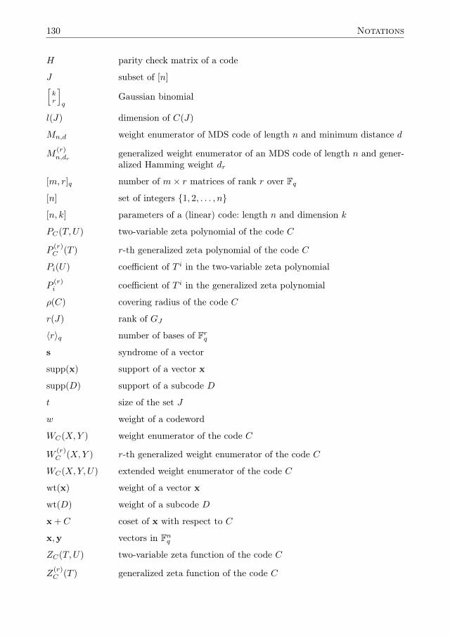
130 Notations
H parity check matrix of a code
J subset of [n][kr
]q
Gaussian binomial
l(J) dimension of C(J)
Mn,d weight enumerator of MDS code of length n and minimum distance d
M(r)n,dr
generalized weight enumerator of an MDS code of length n and gener-alized Hamming weight dr
[m, r]q number of m× r matrices of rank r over Fq[n] set of integers {1, 2, . . . , n}
[n, k] parameters of a (linear) code: length n and dimension k
PC(T,U) two-variable zeta polynomial of the code C
P(r)C (T ) r-th generalized zeta polynomial of the code C
Pi(U) coefficient of T i in the two-variable zeta polynomial
P(r)i coefficient of T i in the generalized zeta polynomial
ρ(C) covering radius of the code C
r(J) rank of GJ
〈r〉q number of bases of Frqs syndrome of a vector
supp(x) support of a vector x
supp(D) support of a subcode D
t size of the set J
w weight of a codeword
WC(X,Y ) weight enumerator of the code C
W(r)C (X,Y ) r-th generalized weight enumerator of the code C
WC(X,Y, U) extended weight enumerator of the code C
wt(x) weight of a vector x
wt(D) weight of a subcode D
x + C coset of x with respect to C
x,y vectors in FnqZC(T,U) two-variable zeta function of the code C
Z(r)C (T ) generalized zeta function of the code C

131
Part II: Codes and arrangements
A arrangement of hyperplanes
AG arrangement of hyperplanes associated to a (generator) matrix G
αC(X,Y ) coset leader weight enumerator of the code C
αC(X,Y, U) extended coset leader weight enumerator of the code C
αi number of cosets of weight i
αi(U) coefficient of Xn−iY i in the extended coset leader weight enumerator
F field, not necessarily finite
GP matrix associated to the projective system P
hj j-th column of a parity check matrix H
Hj hyperplane in an arrangement
λC(X,Y ) list weight enumerator of the code C
λC(X,Y, U) extended list weight enumerator of the code C
λi number of vectors in Fnq that are of minimal weight i in their coset
λi(U) coefficient of Xn−iY i in the extended list weight enumerator
P projective system
PG projective system associated to a (generator) matrix G
Pj point in a projective system
Π subspace of Pk−1(Fq)
Pr(F) projective space of dimension r over the field F
RMq(1, s− 1) first order q-ary Reed-Muller code of dimension s
Sq(s) q-ary Simplex code of dimension s
VJ subspace of Fn−kq generated by the vectors hTj with j ∈ J
Vt union of all VJ with |J | = t
wtH(s) syndrome weight of s with respect to H
wt(y + C) weight of the coset y + C
Part III: Codes, arrangements and matroids
0P minimum of the poset P
1P maximum of the poset P
≤ partial order
Aw(U) Aw(U)/(U − 1)
a(x) number of atoms a of a geometric lattice such that a ≤ x

132 Notations
B collection of bases of a matorid
B basis of a matroid
B∗ collection of bases of the dual matroid
C collection of circuits of a matorid
C circuit of a matroid
χA(U) characteristic polynomial of the arrangement A
χ(IN(x)) reduced Euler characteristic of the independence complex of x
χi(U) coefficient of Si in the coboundary polynomial
χi(U) χi(U)/(U − 1)
χ∗i (U) coefficient of Si in the coboundary polynomial of the dual matroid
χL(S,U) coboundary polynomial of the geometric lattice L
χL(U) characteristic polynomial of the geometric lattice L
χM (S,U) coboundary polynomial of the simple matroid M
cr(x, y) number of chains of length r from x to y in a poset
C simplification of the code C
D collection of dependent sets of a matorid
D dependent set of a matroid
d size of the smallest cocircuit in a matroid
d∗ size of the smallest circuit of a matroid
E finite set, ground set of a matroid
e, f elements of a matroid
ε(B) external activity of the basis B
F collection of flats of a matorid
F flat of a matroid
f : P → A map from the poset P to the abelian group A
f sum function of f
f sum function of f
G simplification of the (generator) matrix G
HJ intersection of all hyperplanes Hj with j ∈ J
I collection of independent sets of a matroid
I independent set of a matorid
IC collection of independent sets associated to the code C

133
IG collection of independent sets associated to the (generator) matrix G
I(L) collection of independent sets associated to the geometric lattice L
ι(B) internal activity of the basis B
i(P ) inverse poset of the poset P
J closure of the subset J in a matroid
k rank of a matroid
L lattice
L(A) geometric lattice associated to the arrangement A
Lj j-th level of the geometric lattice L
L(M) lattice of flats of the matroid M
M matroid
M∗ dual of the matroid M
MC matroid associated to the code C
MG matroid associated to the (generator) matrix G
Mi Ni \ Ni+1
M(L) matroid associated to the geometric lattice L
M simplification of the matroid M
µ(x) µ(0, x)
µi(U) coefficient of Si in the Möbius polynomial
µi(U) µi(U)/(U − 1)
µM (S,U) Möbius polynomial of the simple matroid M
µ(P ) µ(0, 1) in a finite poset P
µP (S,U) Möbius polynomial of the poset P with rank function
µP (x, y) Möbius function of the poset P
n number of elements of a matroid
Ni union of all HJ with J ⊆ [n] and r(HJ) = i
νM (x, y) (−1)rM (x)µL(x, y) |χ(IN(x))|, with x, y ∈ L(M)
ω linear ordering on the ground set of a matroid
P poset
Pi(U) coefficient of T i in the two-variable zeta polynomial
P ∗i (U) coefficient of T i in the two-variable zeta polynomial of the dual matroid
PM (T,U) two-variable zeta polynomial of the matroid M

134 Notations
P x all elements y in a poset with y ≤ x
Px all elements y in a poset with x ≤ y
RaspM (S,U) reciprocal alternating spectrum polynomial
r(M) rank of the matroid M
r(J) rank of the subset J of a matroid
r∗(J) rank of the subset J in the dual matroid
RM (X,Y ) Whitney rank generating function of the matroid M
r(x) rank of the element x of a poset
SpecM (S,U) spectrum polynomial of the matroid M
τ+(P ) upper truncation of the poset with rank function P
τ−(P ) lower truncation of the poset with rank function P
τ(L) truncation of the geometric lattice L
τ(M) truncation of the matroid M
tC(X,Y ) Tutte polynomial of the matroid associated to the code C
tM (X,Y ) Tutte polynomial of the matroid M
Un,k uniform matroid on n elements of rank k
wi Whitney number of the first kind
Wi Whitney number of the second kind
wij doubly indexed Whitney number of the first kind
Wij doubly indexed Whitney number of the second kind
X affine variety
X (Fqm) set of Fqm-rational points of the affine variety X
Xi set of all x ∈ Ak such that wt(xG) = n− i
x, y, z elements of a poset or lattice
xl y y is a cover of x
[x, y] interval between x and y
x ∨ y join of x and y
x ∧ y meet of x and y
Yi set of all x ∈ Ak such that wt(xG) ≤ n− i

Index
activityexternal, 55internal, 55
affine variety, 78anti-symmetric, 63arrangement, 33
central, 33essential, 34simple, 33
atom, 69atomic, 69
B-activeexternally, 54internally, 55
basis, 51bound
greatest lower, 64least upper, 64
chain, 64extension of, 65finite, 64infinite, 64maximal, 65
circuit, 51fundamental, 54
closed set, 51closure, 52cocircuit, 53
fundamental, 54code
dual, 5extension, 13linear, 3MDS, 6nondegenerate, 4projective, 35
Reed-Muller, 39Simplex, 37simplified, 72
codeword, 3minimal, 77
comparable, 63coset, 6coset leader, 6cover, 64covering radius, 6cryptomorphic, 52, 71
dependent set, 51distance
between a vector and a code, 6between two vectors, 4minimum, 4
equivalencegeneralized, 7monomial, 7of arrangements, 34of codes, 7of projective systems, 34
flat, 51function
generalized zeta, 26Möbius, 65sum, 67two-variable zeta, 24Whitney rank generating, 57
Gaussian binomial, 7generalized binomial moment, 26
Hasse diagramof a geometric lattice, 69
135

136 Index
of a poset, 66
independent set, 51interval, 64inverse
poset, 66isomorphism
of matroids, 52of posets, 66
join, 64Jordan-Dedekind property, 68
lattice, 64geometric, 69of flats, 71uniform, 71
level, 69
Möbius inversion formula, 67MacWilliams identity, 5
of extended weight enumerator, 16matrix
generator, 3parity check, 4simplified, 72
matroid, 51dual, 52element, 52
loop, 52parallel, 52
free, 52ordered, 54realizable, 54representable, 54simple, 52uniform, 52
maximum of a poset, 64MDS, 6
almost, 81near, 81
meet, 64minimum of a poset, 64morphism
of a matroid, 52
Newton radius, 47
partial order, 63
polynmiali-defect, 74
polynomialcharacteristic, 73coboundary, 73generalized zeta, 26Möbius, 75spectrum, 99Tutte, 58two-variable zeta, 23, 95
poset, 63locally finite, 64
principle of inclusion/exclusion, 68projective system, 33
rankof a matroid, 51of a subset, 51
Rasp, 111rational points, 78reduced Euler characteristic, 99reflexive, 63
semimodular, 69sequence
log-concave, 77unimodal, 76
simplification, 52Singleton bound, 6
generalized, 10spectrum polynomial, 101subcode, 9
minimal, 77support
of a codeword, 4of a subcode, 9
syndrome, 7
transitive, 63truncation
Dilworth, 104lower, 104of a geometric lattice, 104of a matroid, 103upper, 104
weightof a codeword, 4

Index 137
of a subcode, 9syndrome, 44
weight distribution, 4generalized, 10
weight enumerator, 4coset leader, 43extended, 14extended coset leader, 44extended list, 44generalized, 10list, 43of an MDS code, 19of Reed-Muller code, 39, 40of Simpex code, 37, 38
Whitney number, 76doubly indexed, 76first kind, 76second kind, 76

138 Index

Samenvatting in het Nederlands
Deze samenvatting is bedoeld voor iedereen die denkt niets van dit proefschrift te zullenbegrijpen, maar wel graag wil weten waar het over gaat. Er is geen wiskundige voorkennisnodig om de volgende pagina’s te lezen. Als je die wel hebt, lees dan ook de samenvattingvoorin dit proefschrift en probeer daarna de hoofdstukken die beginnen met “Introductionto. . . ” te lezen.
Talen om de wereld om je heen te beschrijven
Om de wereld om ons heen te beschrijven, gebruiken mensen taal. Er zijn een heleboeltalen op de wereld om de wereld mee te beschrijven, maar ze zijn niet allemaal hetzelfde.Zo heeft het Nederlands een heleboel woorden om verschillende soorten regen te beschrij-ven, omdat het zo vaak regent in Nederland. Kijk je naar een meer Mediterrane taal zoalsItaliaans, dan zal je veel minder verschillende woorden voor “regen” tegenkomen, vanwegehet droge klimaat. Niet alle Nederlandse woorden voor verschillende soorten regen kan jedus letterlijk naar het Italiaans vertalen. Als je een verhaal schrijft over regen, dan is hetNederlands dus een goede keus. Maar als je een verhaal over sneeuw gaat schrijven, kanje beter de taal van de Eskimo’s nemen: volgens de legende hebben die meer dan veertigverschillende woorden voor verschillende varianten van sneeuw.
In de wiskunde is hetzelfde aan de hand. Als je bepaalde eigenschappen van wiskundigeobjecten bestudeert, dan zoek je naar de beste manier om “tegen de zaak aan te kijken”.Met andere woorden, je zoekt het beste model voor het probleem. Het is erg handig omverschillende manieren te hebben om tegen hetzelfde wiskundige object aan te kijken.Door je probleem te “vertalen” naar een ander model, heb je opeens een stuk meer ken-nis ter beschikking om het probleem op te lossen. Vraagstukken die ingewikkeld lijken,hebben misschien wel een eenvoudige oplossing als je ze naar een ander wiskundig modelvertaalt.
Om te kunnen wisselen tussen verschillende talen, heb je goede woordenboeken nodig. Ditproefschrift is een soort wiskundig woordenboek. Het beschrijft hoe je kan vertalen tussendrie wiskundige objecten: codes, arrangementen, en matroïden. In het bijzonder behan-delt dit “woordenboek” hoe je bepaalde informatie over de drie objecten die gevangenis in polynomen kan vertalen. Ook worden stellingen over een van de drie objecten be-wezen met behulp van vertalingen tussen de verschillende objecten en polynomen. In dezesamenvatting vind je een uitleg over de drie objecten en de polynomen die erbij horen.

140 Samenvatting in het Nederlands
Polynomen
In dit proefschrift bestuderen we eigenschappen van wiskundige objecten die we kunnenweergeven als een rij getallen. We kijken hoe dit werkt met behulp van een voorbeeld.Stel, een leraar geeft een proefwerk, waarbij de leerlingen een cijfer tussen de 1 en de 10kunnen scoren. Om bij te houden hoeveel leerlingen welk cijfer hebben gehaald, schrijftde leraar de volgende rijt op:
(1, 0, 0, 3, 3, 7, 8, 5, 2, 1).
De getallen staan voor aantallen leerlingen. De plaats in de rij waarop een getal staat,geeft het cijfer aan. Er is dus één leerling met een 1, geen leerlingen met een 2 of 3, drieleerlingen met een 4, etcetera. Uit deze rij kan je snel informatie halen. Zo zie je dater 30 leerlingen in de klas zitten. Om te kijken hoeveel leerlingen een voldoende hebbengehaald, tellen we de cijfers vanaf plaats 6 bij elkaar op: dit zijn 23 leerlingen.In deze rij van tien cijfers kunnen we nog wel makkelijk zien waar de zesde plaats is.Maar als we lange rijtjes bekijken, wordt dat lastiger. We kunnen de rij getallen daaromals volgt opschrijven:
X + 3X4 + 3X5 + 7X6 + 8X7 + 5X8 + 2X9 +X10.
Deze manier van schrijven noemen we een polynoom. In dit polynoom is X de vari-abele, die schrijven we meestal met een hoofdletter. De getallen rechts van de X zijnde exponenten, de getallen links de coëfficiënten. In ons voorbeeld worden de cijfers dusweergegeven door de exponenten. Het aantal leerlingen dat een bepaald cijfer haalt, vindje in de bijbehorende coëfficiënt. We gaan nu bekijken wat de polynomen zijn die horenbij codes, arrangementen en matroïden.
Foutverbeterende codes
Je kent vast wel de stukken tekst die op internet rondzwerven waarbij van alle woordende letters door elkaar zijn gehusseld, behalve de eerste en de laatste letter. Het blijktvaak dat je, met een beetje moeite, die tekst nog gewoon kan lezen. Dat komt doordatonze taal redundante informatie bevat. Dit betekent dat onze woorden veel korter ge-weest zouden zijn, als we simpelweg alle mogelijke rijtjes van letters een betekenis haddengegeven. Dat heeft natuurlijk allerlei praktische nadelen, bijvoorbeeld de uitspraak. Een
r1 m3 r2
m1
r3
m2m4
Figuur 1: Schematische weergave van de Hamming code
141
belangrijk voordeel van van woorden met redundante informatie is het volgende: als jeeen typefout maakt, of even je spellingsregels bent vergeten, dan kan je dat gemakke-lijk corrigeren. Je lees dan een rij letters die geen bestaand woord is, maar wel op eenbestaand woord lijkt. Dus corrigeer je naar het bestaande woord.
Computers werken, net als andere digitale apparaten zoals je mobiele telefoon of cd-speler, met nullen en enen. Toen computers net waren uitgevonden en nog met pons-kaarten werkten, werden alle opdrachten voor de computer vertaald naar nullen en enen.Alle rijtjes van nullen en enen betekenden iets anders. Maar naar mate computers vakergebruikt werden, merkten de mensen die ermee werkten dat dit nogal eens voor foutenzorgde. Als de computer ergens een 0 in een 1 veranderde, of andersom, liep direct hethele programma vast. Naar verluidt was ene Richard Hamming zo gefrustreerd over dezefouten, dat hij de code bedacht die later naar hem vernoemd is.Het idee van Hamming was dat een computer een leesfout moest kunnen corrigeren, netals dat wij spelfouten in woorden kunnen corrigeren. Dat deed hij door redundante infor-matie toe te voegen aan de commando’s voor de computer. De commando’s die Hammingaan de computer gaf, bestonden uit vier bits: het waren rijen van vier getallen die elk 0of 1 zijn, bijvoorbeeld 1101. De bits noemen we m1, m2, m3, en m4. Hamming zette debits in drie cirkels, zoals je ziet in Figuur 1. Vervolgens berekende hij drie bits redun-dante informatie: r1, r2 en r3. Hij deed dat op zo’n manier, dat in elke cirkel een evenaantal (dus 0, 2 of 4) enen kwam te staan. Deze bits plakte hij achter het oorspronkelijkecommando.
In plaats van de gebruikelijke 4 bits, bestonden de commando’s die Hamming aan decomputer gaf nu uit 7 bits. Maar niet elke rij van 7 enen of nullen kan voorkomen. Erkan bijvoorbeeld nooit maar één 1 voorkomen in de rij. (Zie je waarom?) De toegestanerijtjes noemen we codewoorden. Het aantal bits in een codewoord noemen we de lengtevan de code en de bits noemen we ook wel coördinaten.
Stel, het bericht dat we door willen sturen heeft m1 = 1, m2 = 1, m3 = 0 en m4 = 1.De redundante bits zijn dan r1 = 0, r2 = 0 en r3 = 1. Het codewoord dat bij dit berichthoort, is dus 1101001. Stel nu dat er iets mis gaat bij het inlezen van dit codewoord:de tweede coördinaat verandert in een 0, dus de computer leest 1001001. Om te kijkenwelk bericht hierbij hoort, maakt de computer gebruik van het cirkeldiagram uit Figuur1 en vult het ontvangen woord hier in. Je zit dit in Figuur 2. De computer controleertof in iedere cirkel een even aantal enen staat. Dat is niet het geval in de bovenste cirkelen in de linker cirkel. In de rechter cirkel staat wel het juiste aantal enen. De computerconcludeert nu dat de fout is gemaakt in de coördinaat die zowel in de linker cirkel alsin de bovenste cirkel staat: dat is de coördinaat m2. Op die manier kan de computer deontvangen rij corrigeren naar het codewoord 1101001.
Hoe “goed” een code is, hangt af van hoeveel fouten verbeterd kunnen worden en hoeveelredundante informatie je daarvoor nodig hebt. Van meer redundantie wordt je computertrager, dus je wil er niet teveel van hebben. Maar je wil ook het risico op fouten beperken.Informatie die kan helpen deze afweging te maken, is het gewicht van de codewoorden inde code. Het gewicht van een codewoord is het aantal coördinaten dat niet nul is. Hetgewicht van het codewoord 1101001 is dus vier. Hoeveel codewoorden er zijn met welk

142 Samenvatting in het Nederlands
0 0 0
0
1
01
Figuur 2: Een ontvangen bericht in de Hamming code
gewicht, kunnen we opschrijven in een polynoom dat het gewichtsverdelingspolynoom heet(in het Engels: weight enumerator). Het gewichtsverdelingspolynoom van de Hammingcode is
1 + 7X3 + 7X4 +X7.
Dit betekent dat er één woord is van gewicht nul (namelijk 0000000), één woord vangewicht zeven (namelijk 1111111), zeven woorden van gewicht drie, en zeven woordenvan gewicht vier. Probeer maar eens of je alle zestien woorden van de Hamming code opkan schrijven! (Tip: gebruik het schema uit Figuur 1. Hoeveel mogelijkheden zijn er voorm1, m2, m3 en m4?)
Arrangementen van lijnen in een vlak
Een arrangement is eigenlijk heel simpel een verzameling van lijnen in een vlak. Nietzoveel aan, zou je zeggen. Maar je kan er aardig wat aan rekenen. Iets dat voor dehand ligt is het volgende: stel dat we een bepaalde hoeveelheid lijnen in het vlak hebbengetekend. (We gaan er meestal vanuit dat ons papier oneindig groot is en dat de lijnenoneindig lang doorlopen.) In hoeveel verschillende gebieden heb je het vlak dan verdeeld?Als je één lijn in het vlak tekent, dan deelt deze lijn het vlak in twee stukken. Als je er eentweede lijn bij tekent, dan zul je meestal vier stukken krijgen. Tenzij de lijnen toevalligprecies evenwijdig lopen: dan hebben we het vlak in drie stukken gedeeld. Bij drie lijnenin een driehoek deel je het vlak in zeven stukken. Als de drie lijnen toevallig alledrie doorhetzelfde punt gaan, dan verdelen we het vlak in zes “taartpunten”. Ook als twee vande drie lijnen evenwijdig lopen, krijgen we zes stukken. Als alle drie de lijnen evenwijdigzijn, hebben we maar vier stukken. Je ziet: alleen het aantal lijnen geeft niet genoeginformatie over het aantal stukken waarin ze het vlak verdelen. Je moet ook iets wetenover parallelle lijnen en over punten waar meer dan twee lijnen samenkomen.
Nu is het in de vlakke meetkunde zoals we die gewend zijn, een vrij unieke gebeurtenis alstwee lijnen evenwijdig lopen of als drie lijnen door één punt gaan. Als je twee willekeurigelijnen tekent, zullen ze elkaar vrijwel altijd snijden. Maar in de wiskunde die we in ditproefschrift gebruiken, is de meetkunde eindig en projectief. Deze twee woorden hebbenenige uitleg nodig. Met eindig bedoelen we niet het eindig zijn zoals een bladzijde indit proefschrift. We spreken af dat maar eindig veel lijnen en eindig veel punten bij onzemeetkunde horen. Dan heeft elke lijn maar eindig veel punten en gaan er maar eindig veel

143
Figuur 3: Een projectief vlak van 13 punten en 13 lijnen
lijnen door elk punt – in tegenstelling tot de gewone vlakke meetkunde met oneindig veelpunten op een lijn en oneindig veel lijnen door een punt. Dat een meetkunde projectiefis, betekent het volgende:
• Door ieder tweetal punten gaat precies één lijn.
• Ieder tweetal lijnen snijdt elkaar in precies één punt.
• (Er is ook nog een eis die bepaalde extreme situaties uitsluit, die zullen we hier nietbehandelen.)
De eerste eis zal je niet zoveel verbazen: dat is in de gewone vlakke meetkunde ook hetgeval. Maar de tweede eis heeft een belangrijk gevolg: parallelle lijnen bestaan niet in deprojectieve meetkunde!Omdat zo’n eindige projectieve meetkunde nogal abstract klinkt, staat in Figuur 3 eenvoorbeeld. Er zijn projectieve vlakken met verschillende aantallen punten en lijnen: wesperen af dat dit eindige projectieve vlak uit 13 punten en 13 lijnen bestaat. Iedere lijnbevat 4 punten en door ieder punt gaan 4 lijnen – dat kan niet anders als je 13 punten en13 lijnen hebt, maar het gaat wat ver om hier uit te leggen waarom. In de figuur lopen delijnen niet helemaal recht en lopen soms over elkaar heen terwijl ze geen snijpunt hebben,maar dat komt omdat het papier waarop ze gedrukt zijn, niet een eindig projectief vlak is.
We gaan nu kijken naar een arrangement in dit projectieve vlak. Je ziet het in Figuur4. Het arrangement bestaat uit zes lijnen. Zoals gezegd, komen er geen parallelle lijnenvoor. Maar je ziet dat er best veel punten zijn waar meer dan twee lijnen doorheen gaan:doordat er maar eindig veel lijnen zijn, zullen veel vaker drie of meer lijnen door hetzelfdepunt gaan.
Wat gaan we nu tellen aan een arrangement? Het aantal gebieden waarin het vlak verdeeldwordt, heeft niet echt een betekenis in het projectieve vlak. We tellen daarom hoeveelpunten er zijn waar een bepaald aantal lijnen doorheen gaat. Die informatie vatten we
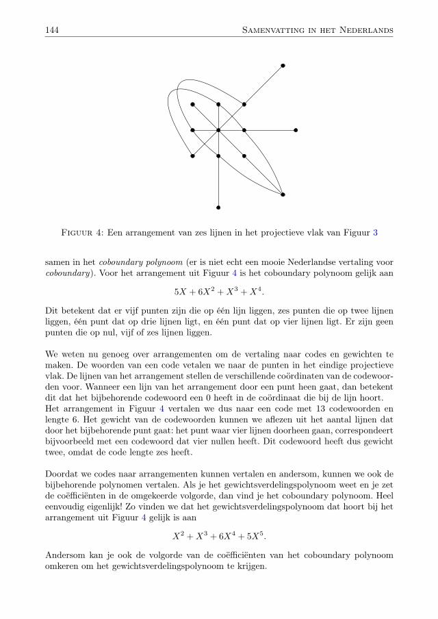
144 Samenvatting in het Nederlands
Figuur 4: Een arrangement van zes lijnen in het projectieve vlak van Figuur 3
samen in het coboundary polynoom (er is niet echt een mooie Nederlandse vertaling voorcoboundary). Voor het arrangement uit Figuur 4 is het coboundary polynoom gelijk aan
5X + 6X2 +X3 +X4.
Dit betekent dat er vijf punten zijn die op één lijn liggen, zes punten die op twee lijnenliggen, één punt dat op drie lijnen ligt, en één punt dat op vier lijnen ligt. Er zijn geenpunten die op nul, vijf of zes lijnen liggen.
We weten nu genoeg over arrangementen om de vertaling naar codes en gewichten temaken. De woorden van een code vetalen we naar de punten in het eindige projectievevlak. De lijnen van het arrangement stellen de verschillende coördinaten van de codewoor-den voor. Wanneer een lijn van het arrangement door een punt heen gaat, dan betekentdit dat het bijbehorende codewoord een 0 heeft in de coördinaat die bij de lijn hoort.Het arrangement in Figuur 4 vertalen we dus naar een code met 13 codewoorden enlengte 6. Het gewicht van de codewoorden kunnen we aflezen uit het aantal lijnen datdoor het bijbehorende punt gaat: het punt waar vier lijnen doorheen gaan, correspondeertbijvoorbeeld met een codewoord dat vier nullen heeft. Dit codewoord heeft dus gewichttwee, omdat de code lengte zes heeft.
Doordat we codes naar arrangementen kunnen vertalen en andersom, kunnen we ook debijbehorende polynomen vertalen. Als je het gewichtsverdelingspolynoom weet en je zetde coëfficiënten in de omgekeerde volgorde, dan vind je het coboundary polynoom. Heeleenvoudig eigenlijk! Zo vinden we dat het gewichtsverdelingspolynoom dat hoort bij hetarrangement uit Figuur 4 gelijk is aan
X2 +X3 + 6X4 + 5X5.
Andersom kan je ook de volgorde van de coëfficiënten van het coboundary polynoomomkeren om het gewichtsverdelingspolynoom te krijgen.

145
Matroïden
Stel, we hebben een arrangement, zoals in de vorige sectie beschreven. Wanneer we maarnaar een aantal lijnen uit het arrangement kijken, noemen we dit een deelverzameling.We spreken af dat een deelverzameling alle lijnen van het arrangement mag bevatten, ofhelemaal geen. We gaan nu aan elke deelverzameling een getal toekennen: de rang. Inhet geval van het arrangement uit Figuur 4 is de rang minimaal 0 en maximaal 3. Derang is 0 als de deelverzameling uit nul lijnen bestaat, 1 als de deelverzameling uit éénlijn bestaat, en 2 als de deelverzameling uit twee lijnen bestaat. Bij een deelverzamelingvan drie of meer lijnen, moeten we een beetje opletten: als alle lijnen door hetzelfde puntgaan, is de rang 2; als dat niet het geval is, is de rang 3.Het zal je niet verbazen dat we deze informatie ook weer kunnen samenvatten in eenpolynoom: het Whitney rang-polynoom, genoemd naar de wiskundige Whitney die hetals eerste opschreef. Dit polynoom heeft niet één, maar twee variabelen. De exponentvan X geeft de grootte van de deelverzameling aan, de exponent van Y de rang vandie deelverzameling. De coëfficiënt geeft aan hoeveel deelverzamelingen er zijn van eenbepaalde grootte en rang. Voor het voorbeeld uit Figuur 4 is het Whitney rang-polynoomgelijk aan
1 + 6XY + 15X2Y 2 + 5X3Y 2 +X4Y 2 + 15X3Y 3 + 14X4Y 3 + 6X5Y 3 +X6Y 3.
Hier betekent 5X3Y 2 dat er vijf deelverzamelingen zijn die uit drie lijnen bestaan diedoor hetzelfde punt gaan. Als we alle coëfficiënten bij elkaar optellen, zie je dat er in to-taal 64 deelverzamelingen zijn. De coëfficiënten van het Whitney-polynoom vertellen ietsover wanneer meerdere lijnen door hetzelfde punt gaan. Door een slimme combinatie vandeze coëfficiënten te nemen, kunnen we dan ook zowel het gewichtsverdelingspolynoomals het coboundary polynoom bepalen.
De rang van de deelverzamelingen van een arrangement voldoet aan een aantal eisen. Deeerste twee kan je zelf controleren voor ons voorbeeld.
• De rang van een deelverzameling is altijd minstens 0 en maximaal het aantal lijnenin de deelverzameling.
• Als je een lijn toevoegt aan een deelverzameling, dan blijft de rang van de deelverza-meling gelijk of gaat met één omhoog.
• (Er is ook nog een eis over wat er gebeurt met de rang als je twee deelverzamelingensamenvoegt, maar die is te ingewikkeld om hier uit te leggen.)
Het blijkt dat deze eisen niet alleen gelden voor de rang van deelverzamelingen van ar-rangementen. Je kan ook deelverzamelingen nemen van andere wiskundige structuren endaar een rang voor definiëren. Je kan zelfs helemaal niet vastleggen waarvan je deelverza-melingen neemt. Je zou bij wijze van spreken vijftien verschillende soorten fruit kunnennemen en alle deelverzamelingen een rang geven die aan de eisen voldoet. Het wiskundigeobject dat hoort bij een aantal “dingen” en een rang voor elke deelverzameling die aanbovenstaande eisen voldoet, heet eenmatroïde. De “dingen” heten elementen, bijvoorbeeldde lijnen van een arrangement. Voor iedere matroïde kan je het Whitney rang-polynoomopschrijven.

146 Samenvatting in het Nederlands
Alle arrangementen en codes zijn te vertalen naar matroïden, maar niet alle matroïdenzijn ook een arrangement of een code. Er zijn veel meer matroïden dan dat er codes enarrangementen zijn. De matroïde is dan ook de meest “algemene” en abstracte structuurdie in dit proefschrift aan de orde komt. Toch blijkt het handig te zijn om juist eenalgemenere structuur te onderzoeken. De dingen die je kan laten zien over matroïden,kan je toepassen naar een heleboel verschillende voorbeelden. Net zoals dat onderzoeknaar zoogdieren toepassingen heeft voor koeien, paarden, walvissen en mensen.
Tenslotte
Ik hoop dat het lezen van deze samenvatting het een beetje duidelijker maakt waar ik mede afgelopen vier jaar mee bezig heb gehouden. Ik hoop in elk geval mijn enthousiasmevoor mijn onderzoek over te brengen.
Tijdens het schrijven heb ik mij enkele wiskundige vrijheden veroorloofd, met name bijde definitie van het Whitney rang-polynoom (zie Definition 8.1 in dit proefschrift) ende gewichtsverdeling van het arrangement uit Figuur 4 (zie Example 10.34 in dit proef-schrift). Ook heb ik voor het gemak alleen arrangementen van lijnen in het vlak behan-deld, in plaats van arrangementen van hypervlakken in ruimtes van willekeurige dimensie.De wiskundigen die toch deze samenvatting zijn gaan lezen, zijn bij deze uitgedaagd dezevrijheden te corrigeren.
Curriculum Vitae
Relinde Jurrius was born on February 25, 1984 in Haarlem, The Netherlands. In 2002 sheobtained her gymnasium diploma from the Coornhert Lyceum in Haarlem. In the sameyear she started studying both mathematics and astronomy at Leiden University. Aftercompleting the first year (propedeuse) in the two subjects, she continued in mathematics.
Relinde wrote her bachelor thesis Algebraïsche topology en de fixpuntstelling van Lefshetz(Algebraic topology and the Lefshetz fixed point theorem) under supervision of dr. Robinde Jong. After obtaining her bachelors degree in 2005, she was in the board of the stu-dents rowing club Asopos de Vliet for the academic year 2005–2006. When she continuedwith her master studies, she learned about coding theory via a course in the nationalMasterMath program. It gained her interest, and she wrote her master thesis Classifyingpolynomials of linear codes under joint supervision of dr. Robin de Jong from LeidenUniversity and dr. Ruud Pellikaan from Eindhoven University of Technology. Relindeobtained her masters degree in 2008.
In October 2008, Relinde started as a PhD student at Eindhoven University of Technol-ogy under supervision of dr. Ruud Pellikaan. She continued the work from her masterthesis and extended her area of interest to arrangements and matroids. This thesis is theresult of her research from 2008 to 2012.
Relinde likes sharing her enthusiasm for mathematics with others. Every summer shespends a week at math camp with Vierkant voor Wiskunde. She helps organizing thecamp and writing the material. Furthermore, she was involved in organizing the DutchMathematical Olympiad and setting up a new round in the contest. To show high schoolgirls that science is not just something for boys, she is a ‘role-model’ for VHTO.
During the day, as a break from work, Relinde likes to play the violin. She started playinglong time ago and was in various orchestras. Currently, she plays in the Philips SymphonyOrchestra, where she is also in the board as treasurer.

148 Curriculum Vitae

Acknowledgments
Although this thesis contains hours and hours of work by myself, it would not have ex-isted without the help of many people in my working environment.
Het is onder promovendi niet ongebruikelijk af en toe te zeuren over je begeleider. Ikbegon dan altijd op te scheppen: dat ik de vrijheid kreeg weken niets van me te latenhoren, maar wel altijd langs kon komen. Dat we er allebei niet van houden een uur voorde deadline pas een artikel af te hebben. Dat ik er vaak pas achteraf achter kwam dat iktoch weer subtiel de goede (onderzoeks)richting in was gestuurd. En bovenal, dat ik defijne kneepjes van het vak kon afkijken van een goede wetenschapper. Beste hr. Pellikaan,beste Ruud, heel erg veel dank.
Henk, ik hoop dat ik later net zo’n goede professor word als jij.
I would like to express my gratitude also to the other members of my defense committee:Aart Blokhuis, Andries Brouwer, Tom Høhold, Dieter Jungnickel, Tanja Lange and Jackvan Wijk. Thank you for traveling to Eindhoven for my defense, reading my thesis andsuggesting further improvements.
During my time as a PhD student I had multiple interesting and inspiring discussionswith other mathematicians around the world. In particular I wish to thank VladimirTonchev for asking the question that led to Chapter 5 of this thesis, as well as to manyideas for further research.
Sebastiaan, bedankt voor het inkleuren van de cover van dit boekje. Vanessa en Sietse,heel fijn dat jullie de Nederlandse samenvatting wilden lezen en vragen stelden die ik zelfniet had kunnen bedenken.
My colleagues at the Security and the Discrete Mathematics group provided an excel-lent working atmosphere. In particular my fellow PhD students: thank you Reza, Peter,Michael, José, other Peter, Jing, Christiane, Gaëtan, Bruno, Ruben, Daniel, jet anotherPeter, Sebastiaan, Mayla, Antonino, Elisa, Dion, Jan-Jaap, Meilof, Thijs, Sokratis, andour visitor Irene. It was a pleasure having coffee with you.
Tenslotte een warm woord van dank voor onze secretaresses Anita, Jolande, en Rianne.Er zouden heel veel praktische zaken mis gaan zonder jullie – en het zou ook een stukminder gezellig zijn.


![On the Schultz polynomial, Modified Schultz polynomial, Hosoya polynomial and Wiener index of circumcoronene series of benzenoid. [7]](https://static.fdokumen.com/doc/165x107/6316d8360f5bd76c2f02aa3c/on-the-schultz-polynomial-modified-schultz-polynomial-hosoya-polynomial-and-wiener.jpg)