Polynomial Stability in Two-Dimensional MagnetoElasticity

IMA Journal of Applied Mathematics (2001) 66, 269–283

Polynomial stability in two-dimensional magneto-elasticity

JAIME E. MUNOZ RIVERA†Department of Research and Development, National Laboratory for Scientific

Computation, Rua Getulio Vargas 333, Quitandinha, CEP 25651-070 Petropolis,RJ and UFRJ, Rio de Janeiro, Brasil

AND

REINHARD RACKE‡Department of Mathematics and Statistics, University of Konstanz, Box D 187,

78457 Konstanz, Germany

[Received on 5 May 2000]

For a class of bounded reference configurations that are of partially rectangular type,the linear system of magneto-elasticity in two space dimensions is considered and apolynomial decay rate of the energy as time tends to infinity is proved.

Keywords: isotropic elasticity; Lyapunov functional; uniform stability.

1. Introduction

We consider the following linear initial boundary-value problem in magneto-elasticitywhich describes, for a homogenous isotropic medium with bounded reference configu-ration Ω ⊂ R

2, the interaction between elastic movements and a magnetic field. Thegoverning differential equations for the displacement vector u = (u1, u2, 0)′ = u(t, x)

depending on the time variable t 0 and on the space variable x ∈ Ω , and for themagnetic field h = (h1, h2, 0)′ = h(t, x) are

utt − µ∆u − (λ + µ)∇ div u − α[∇ × h]×

H= 0, (1.1)

ht − ∆h − β∇ × [ut×

H ] = 0, (1.2)

cp. Eringen & Maugin (1990). Here λ, µ and κ are positive constants. The coupling

constants α, β satisfy αβ > 0;

H= (H, 0, 0)′ is a constant vector with H = 0.Additionally, one has initial conditions

u(0, x) = u0(x), ut (0, x) = u1(x), h(0, x) = h0(x) (1.3)

and the following classical Dirichlet-type boundary conditions:

u = 0, ν × (∇ × h) = 0, ν · h = 0 on Γ := ∂Ω . (1.4)

†Email: [email protected]‡Corresponding author; Email: [email protected]

c© The Institute of Mathematics and its Applications 2001

270 J. E. M. RIVERA AND R. RACKE

Moreover,

div h = 0, (1.5)

which follows from (1.2) if div h0 = 0. The vector ν = (ν1, ν2, 0)′ = ν(x) denotes theexterior normal vector in x ∈ Γ , the boundary of Ω .

Note that the system above is very similar to the isotropic thermoelastic system. Themain difference is that now the dissipation is given by the magnetic field instead of thetemperature. In thermoelasticity it is well known by now that for materials configured inbounded domains of R

n , for n > 1, there is no decay in general. This ineffectiveness of thethermal dissipation is due essentially to the degree of freedom of the displacement vectorfield, which is greater than the degree of freedom of the temperature when the dimension isgreater than n = 1. In magneto-elasticity the situation is different, because the dissipativemechanism and the displacement have the same degree of freedom. But now, this systemintroduces an additional difficulty given by the coupling term. Making a closer analysis ofthe system (see (2.3)–(2.6) of Section 2) we see that the dissipative term is coupled onlyto the gradient of the second component of the displacement, while the first component iscoupled to the second one only by (2.3), (2.4) through its mixed derivatives, which is verysubtle. The main question here is whether the dissipation given by the magnetic field isstrong enough to produce a uniform rate of decay for the whole system. If so, what type ofrate of decay can we expect? It seems to us that there is not yet any result about this topic.To fill part of this gap we study this topic here.

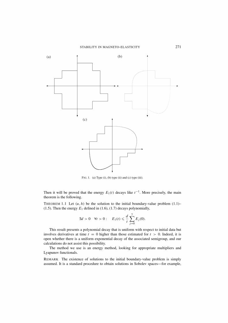
The main result of this paper is to show that the solution of the magneto-elastic systemdecays polynomially as time goes to infinity. To show this we assume that the boundary Γis smooth with the exception of at most finitely many points. This is in accordance withthe following assumption on the two-dimensional domain Ω . Without loss of generality wemay assume that 0 ∈ Ω and additionally that Ω is connected and of partially rectangulartype which means that it is homeomorphic to the unit ball and one of the following threeconditions (i)–(iii) is satisfied.

(i) Ω is the union of finitely many rectangles with axes paralles to the x1- and x2-axes,respectively; see Fig. 1a.

(ii) Ω satisfies ν1ν2 = 0 in the first quadrant (where x1 0 and x2 0) and in the thirdquadrant (where x1 0 and x2 0). In the second and fourth quadrants Ω satisfiesxν δ0 > 0, for some δ0; see Fig. 1b.

(iii) Ω satisfies ν1ν2 = 0 in the second and fourth quadrants. In the first and thirdquadrants Ω satisfies xν δ0 > 0, for some δ0; see Fig. 1c.

REMARK By domains of partially rectangular type (i), all sufficiently smoothly bounded,connected domains can be exhausted; also all connected Jordan measurable sets.

The energy E = E(t)(of first order) associated to the equations (1.1), (1.2) is given by

E(t) := E(t; u, h) := 1

2

∫Ω

(|ut |2 + µ|∇u|2 + (µ + λ)| div u|2 + α

β|h|2

)(t, x) dx .

(1.6)

We shall also use energy terms of higher order given for j ∈ N by

E j (t) := E(t; ∂j

t u, ∂j

t h). (1.7)

STABILITY IN MAGNETO-ELASTICITY 271

(a) (b)

(c)

FIG. 1. (a) Type (i), (b) type (ii) and (c) type (iii).

Then it will be proved that the energy E1(t) decays like t−1. More precisely, the maintheorem is the following.

THEOREM 1.1 Let (u, h) be the solution to the initial boundary-value problem (1.1)–(1.5). Then the energy E1 defined in (1.6), (1.7) decays polynomially,

∃d > 0 ∀t > 0 : E1(t) d

t

7∑j=0

E j (0).

This result presents a polynomial decay that is uniform with respect to initial data butinvolves derivatives at time t = 0 higher than those estimated for t > 0. Indeed, it isopen whether there is a uniform exponential decay of the associated semigroup, and ourcalculations do not assist this possibility.

The method we use is an energy method, looking for appropriate multipliers andLyapunov functionals.

REMARK The existence of solutions to the initial boundary-value problem is simplyassumed. It is a standard procedure to obtain solutions in Sobolev spaces—for example,


via semigroup theory, cp. Perla Menzala & Zuazua (1998). The assumed smoothness ofthe initial data is described by the finiteness of the right-hand side in the estimate inTheorem 1.1.

The time-asymptotic behaviour for the initial boundary-value problem has been studiedby Perla Menzala & Zuazua (1998). They proved the decay of E(t) to zero for fixed initialdata; no uniformity was given, but more general domains, also in three space dimensions,were considered. For a damping boundary condition of memory type, replacing u = 0, theauthors (1999) proved the exponential stability. We also mention the results on polynomialdecay for the corresponding Cauchy problem contained in the papers by Andreou &Dassios (1997) and by the authors (1999). For earlier papers on magneto-elasticity, forexample, for plane waves see the references in Perla Menzala & Zuazua (1998) and in thepaper by the authors (1999).

REMARK We remark that an additional damping as in magneto-thermo-elasticity (see theauthors’ (1999) paper) is of course likely to lead to a similar result. The damping willcertainly not give worse decay, but we conjecture that it will also not improve the decayessentially.

In connection with the question of optimal decay rates it should be mentioned thatfor the related thermo-elastic system exponential decay can only be expected in specialsituations like radial symmetry, for example, see Jiang et al. (1998), but not in general, seeKoch (2000) or Lebeau & Zuazua (1999).

In Section 2 we shall present appropriate multipliers and the essential estimates for thecomponents of the final Lyapunov functional. Theorem 1.1 is then proved in Section 3.

2. Multipliers and energy estimates

It is easy to verify that

d

dtE(t; u, h) = −α

β

∫Ω

|∇ × h|2 dx

and, in general,d

dtE j (t) = −α

β

∫Ω

|∇ × ∂j

t h|2 dx .

Using the fact that Ω is simply connected, we conclude that∫Ω

|h|2 dx +∫Ω

|∇h|2 dx c∫Ω

|∇ × h|2 dx

(cf. Duvaut & Lions (1976, p. 356) or Leis (1986, p. 157)), hence

d

dtE j (t) −c

∫Ω

|∇∂j

t h|2 dx, j = 0, . . . , 7. (2.1)

Here and in the sequel c will denote various positive constants not depending on t oron the initial data. Using the notation

∂ j := ∂

∂ x j, j = 1, 2,


simple calculations give

∇ × h = (0, 0, ∂1h2 − ∂2h1)′,

(∇ × h)×

H= H(0, ∂1h2 − ∂2h1, 0)′,

ut×

H= H(0, 0, −u2t )

′,

∇ × (ut×

H) = H(−∂2u2t , ∂1u2

t , 0)′,ν × (∇ × h) = (ν2(∂1h2 − ∂2h1), −ν1(∂1h2 − ∂2h1), 0)′.

In particular, the boundary condition ν × (∇ × h)|Γ = 0 turns into

(∂1h2 − ∂2h1)|Γ = 0. (2.2)

The functionω := ∂1h2 − ∂2h1

denotes the two-dimensional rotation of (h1, h2)′, and the differential equations (1.1), (1.2)can be written as

u1t t − µ∆u1 − (µ + λ)∂2

1 u1 − (µ + λ)∂1∂2u2 = 0, (2.3)

u2t t − µ∆u2 − (µ + λ)∂2

2 u2 − (µ + λ)∂1∂2u1 = αHω, (2.4)

h1t − ∆h1 = −β H∂2u2

t (2.5)

h2t − ∆h2 = β H∂1u2

t . (2.6)

We introduce the following functionals as abbreviations:

A1u1 := −µ∆u1 − (µ + λ)∂21 u1,

A2u2 := −µ∆u2 − (µ + λ)∂22 u2,

E1(t) := 12

∫Ω

|u1t |2 + µ|∇u1|2 + (µ + λ)|∂1u1|2 dx .

In the next lemma we define the functional which shows the dissipative properties ofthe second component of the displacement.

LEMMA 2.1 Let

Φ1 := Φ1(t) :=∫Ω

ωu2t + ω∆u2 − β H(µ + λ)∂2u2∂1u1 dx − β HE1(t).

Then

d

dtΦ1 = −β H

∫Ω

|∇u2t |2 dx +

∫Ω

ωt∆u2 dx + αH∫Ω

|ω|2 dx +∫Ω

ωA2u2 dx

+ (µ + λ)

∫Ω

h1t ∂1u1 dx .


Proof. From the equations (2.5) and (2.6) we obtain

d

dt

∫Ω

h1∂2u2t dx =

∫Ω

h1t ∂2u2

t + h1∂2u2t t dx

=∫Ω

∆h1∂2u2t dx − β H

∫Ω

|∂2u2t |2 dx −

∫Ω

∂2h1u2t t dx

=∫Ω


∫Ω

|∂2u2t |2 dx −

∫Ω

∂2h1 A2u2 dx

− (µ + λ)

∫Ω

∂1∂2u1∂2h1 dx − αH∫Ω

∂2h1ω dx .

Similarly, using (2.3), (2.6), we get

− d

dt

∫Ω

h2∂1u2t dx = −

∫Ω


∫Ω

|∂1u2t |2 dx

+∫Ω

∂1h2 A2u2 dx + (µ + λ)

∫Ω

∂1∂2u1∂1h2 dx + αH∫Ω

∂1h2ω dx .

Summing up the last two identities we obtain

d

dt

∫Ω

ωu2t dx = d

dt

∫Ω

h1∂2u2t − h2∂1u2

t dx

=∫Ω

∇ω∇u2t dx︸︷︷︸

=: I1

−β H∫Ω

|∇u2t |2 dx

+∫Ω

ωA2u2 dx + (µ + λ)

∫Ω

ω∂1∂2u1 dx︸︷︷︸=: I2

+αH∫Ω

|ω|2 dx . (2.7)

Note that, since ω|Γ = 0,

I1 = −∫Ω

ω∆u2t dx = − d

dt

∫Ω

ω∆u2 dx +∫Ω

ωt∆u2 dx (2.8)

and

I2 = −(µ + λ)

∫Ω

∂2ω∂1u1 dx .

Since

div h = 0

we have

∂2ω = −∆h1,


therefore we get

I2 = (µ + λ)

∫Ω

∆h1∂1u1 dx

= (µ + λ)

∫Ω

(h1t + β H∂2u2

t )∂1u1 dx

= (µ + λ)

∫Ω

h1t ∂1u1 dx + β H(µ + λ)

∫Ω

∂2u2t ∂1u1 dx

= (µ + λ)

∫Ω

h1t ∂1u1 dx + β H(µ + λ)

d

dt

∫Ω

∂2u2∂1u1 dx

− β H(µ + λ)

∫Ω

∂1u1t ∂2u2 dx . (2.9)

Multiplying equation (2.3) by u1t we get

d

dtE1(t) = −(µ + λ)

∫Ω

∂1u1t ∂2u2 dx .

Substituting this identity into (2.9) we obtain

I2 = (µ + λ)

∫Ω

h1t ∂1u1 dx + d

dt

β H(µ + λ)

∫Ω

∂2u2∂1u1 dx + β H(µ + λ)E1(t)

.

(2.10)

Recalling the definition of Φ1 the conclusion follows from (2.7), (2.8), (2.10).

Following Lemma 2.1 and since (ut , ht ) also satisfies (1.1), (1.2) and (1.4), (1.5) wecan introduce functionals Φ2 and Φ3 in the following way. Writing

Φ1(t) = Φ1(t; u, h)

we have (see Lemma 2.1)

d

dtΦ1(t; ut , ht ) = −β H

∫Ω

|∇u2t t |2 dx +

∫Ω

ωt t∆u2t dx

+ αH∫Ω

|ωt |2, dx +∫Ω

ωt A2u2t dx + (µ + λ)

∫Ω

h1t t∂1u1

t dx

= −β H∫Ω

|∇u2t t |2 dx + d

dt

∫Ω

ωt t∆u2 dx

−∫Ω

ωt t t∆u2 dx + αH∫Ω

|ωt |2 dx + d

dt

∫Ω

ωt A2u2 dx

−∫Ω

ωt t A2u2 dx + (µ + λ)d

dt

∫Ω

h1t t∂1u1 dx − (µ + λ)

∫Ω

∂1u1 dx

which implies for

Φ2(t) := Φ2(t; u, h) := Φ1(t; ut , ht ) −∫Ω

ωt t∆u2 + ωt A2u2 − (µ + λ)h1t t∂1u1 dx


the identity

d

dtΦ2(t) = −βh

∫Ω

|∇u2t t |2 dx −

∫Ω

ωt t t∆u2 dx + αH∫Ω

|ωt |2 dx

−∫Ω

ωt t A2u2 dx − (µ + λ)

∫Ω

h1t t t∂1u1 dx . (2.11)

Similarly we can define

Φ3(t) := Φ2(t; ut , ht ) −∫Ω

ωt t t t∆u2 + ωt t t A2u2 + (µ + λ)h1t t t t∂1u1 dx .

Then we have

d

dtΦ3(t) = −β H

∫Ω

|∇u2t t t |2 dx +

∫Ω

ωt t t t t∆u2 dx

+ αH∫Ω

|ωt t |2 dx +∫Ω

ωt t t t A2u2 dx + (µ + λ)

∫Ω

h1t t t t t∂1u1 dx . (2.12)

The following lemma plays an important role in the sequel because it will connect thedissipative properties of the magnetic field with the first component of the displacementvector field.

LEMMA 2.2 Let

q(x) := (x2 − δx1, x1 − δx2)′

for some δ ∈ R, and let

F(t) :=∫Ω

u2t t q∇ut + A2u2

t q∇u1 dx .

Then for |δ| sufficiently large—only depending on the domain Ω—we have

d

dtF(t) −(µ + λ)

∫Ω

|∇u1t |2 dx + c

∫Γ

∣∣∣∣∂u2t t

∂ν

∣∣∣∣∣∣∣∣∂u1

∂ν

∣∣∣∣ ds

+ c∫Ω

|∇u2t t ||∆u1| dx + c

∫Ω

|ωt ||∇u1t | dx .

Proof. The main idea to show the above inequality is to use (2.3)–(2.6) to connect thedissipation given by h to u1. Then we will use the geometrical properties of the domain to


eliminate unpleasant boundary terms in u1. In fact let us consider

d

dt

∫Ω

u2t t q1∂1u1

t dx =∫Ω

u2t t t q1∂1u1

t dx +∫Ω

u2t t q1∂1u1

t t dx

= −∫Ω

A2u2t q1∂1u1

t dx + µ + λ

2

∫Ω

q1∂2|∂1u1t |2 dx

+ αH∫Ω

ωt q1∂1u1t dx

= − d

dt

∫Ω

A2u2t q1∂1u1 dx +

∫Ω

A2u2t t q1∂1u1

t dx

+ µ + λ

2

∫Γ

q1ν2|∂1u1t |2 ds − µ + λ

2

∫Ω

∂2q1|∂1u1t |2 dx

+ αH∫Ω

ωt q1∂1u1t dx . (2.13)

Note that

∫Ω

A2u2t t q1∂1u1 dx = −µ

∫Γ

∂u2t t

∂νq1∂1u1 ds − (µ + λ)

∫Γ

ν2∂2u2t t q1∂1u1 ds

+ (µ + λ)

∫Ω

∂2u2t t [∂2q1∂1u1 + q1∂1∂2u1] dx

+ µ

∫Ω

∇u2t t [∇q1∂1u1 + q1∂1∇u1] dx

from which we conclude that

d

dt

∫Ω

u2t t q1∂1u1

t dx +∫Ω

A2u2t q1∂1u1 dx

= µ + λ

2

∫Γ

q1ν2|∂1u1t |2 ds − µ

∫Γ

∂u2t t

∂νq1∂1u1 ds

− (µ + λ)

∫Γ

ν2q1∂2u2t t∂1u1 ds + (µ + λ)

∫Ω

∂2u2t t [∂2q1∂1u1 + q1∂1∂2u1] dx

+ µ

∫Ω

∇u2t t [∇q1∂1u1 + q1∂1∇u1] dx − (µ + λ)

∫Ω

∂2q1|∂1u1t |2 dx

+ αH∫Ω

ωt q1∂1u1t dx


= µ + λ

2

∫Γ

q1ν21ν2

∣∣∣∣∂u1t

∂ν

∣∣∣∣ ds − µ

∫Γ

∂u2t t

∂νq1ν1

∂u1

∂νds

− (µ + λ)

∫Γ

ν22q1ν1

∂u2t t

∂ν

∂u1

∂νds

+ (µ + λ)

∫Ω

∂2u2t t [∂2q1∂1u1 + q1∂1∂2u1] dx

+ µ

∫Ω

∇u2t t [∇q1∂1u1 + q1∂1∇u1] dx − (µ + λ)

∫Ω

∂2q1|∂1u1t | dx

+ αH∫Ω

ωt q1∂1u1t dx . (2.14)

Similarly we obtain

d

dt

∫Ω

u2t t q2∂2u1 dx +

∫Ω

A2u2t q2∂2u1 dx

= µ + λ

2

∫Γ

q2ν1ν22

∣∣∣∣∂u1t

∂ν

∣∣∣∣2

ds − µ

∫Γ

∂u2t t

∂νq2ν2

∂u1

∂νds

− (µ + λ)

∫Γ

q2ν21ν2

∂u2t t

∂ν

∂u1

∂νds + (µ + λ)

∫Ω

∂2u2t t [∂2q2∂2u1 + q2∂

22 u1] dx

+ µ

∫Ω

∇u2t t [∇q2∂2u1 + q2∂2∇u1] dx − (µ + λ)

∫Ω

∂1q2|∂2u1t |2 dx

+ αH∫Ω

ωt q2∂2u1t dx . (2.15)

Summing up (2.14) and (2.15) we get

d

dtF(t) = d

dt

∫Ω

u2t t q∇ut dx +

∫Ω

A2u2t q∇u1 dx

= µ + λ

2

∫Γ

ν1ν2[ν1q1 + ν2q2]∣∣∣∣∂u1

t

∂ν

∣∣∣∣2

ds

− µ

∫Γ

∂u2t t

∂νqν

∂u1

∂νds − (µ + λ)

∫Γ

ν1ν2[q1ν2 + q2ν1]∂u2t t

∂ν

∂u1

∂νds

+ (µ + λ)

∫Ω

∂2u2t t [∂2q1∂1u1 + ∂2q2∂2u1 + q1∂1∂2u1 + q2∂

22 u1] dx

+ µ

∫Ω

∇u2t t [∇q1∂1u1 + ∇q2∂2u1 + q1∂1∇u1 + q2∂2∇u1] dx

− (µ + λ)

∫Ω

∂2q1|∂1u1t |2 + ∂1q2|∂2u1

t | dx

+ αH∫Ω

ωt [q1∂1u1t + q2∂2u1

t ] dx,


which implies that

d

dtF(t) µ + λ

2

∫Γ

ν1ν2ν · q

∣∣∣∣∂u1t

∂ν

∣∣∣∣2

ds︸︷︷︸=:I3

− (µ + λ)

∫Ω

|∇u1t |2 dx + c

∫Γ

∣∣∣∣∂u2t t

∂ν

∣∣∣∣2∣∣∣∣∂u1

∂ν

∣∣∣∣ ds

+ c∫Ω

|∇u2t t ||∆u1| dx + c

∫Ω

|ωt ||∇u1t | dx . (2.16)

Now we use that Ω is of partial rectangular type (i), (ii) or (iii).For type (i) we have ν1ν2 = 0, hence

I3 = 0.

For type (ii) we have for δ positive and sufficiently large (only depending on Ω )

I3 0.

For type (iii) we have for δ negative and |δ| sufficiently large (only depending on Ω )

I3 0.

That is, for all types (i), (ii), (iii) we have

I3 0, (2.17)

provided δ is chosen appropriately. The assertion of the lemma now follows from (2.16)and (2.17).

Lemma 2.2 gives a good estimate for u1, except for the boundary term which containsthe normal derivative on u2

t t . To estimate this surface integral we will use the followinglemma applied to u1

t and u2t t .

LEMMA 2.3 Let g ∈ C1(R2), g = (g1, g2)′ such that gν γ > 0 for some γ . Then

− d

dt

∫Ω

u2t gk∂ku2 dx −µ

2

∫Γ

gkνk

∣∣∣∣∂u2

∂ν

∣∣∣∣ ds

+ c∫Ω

|u2t |2 + |∇u2|2 dx − (µ + λ)

∫Ω

gk∂1∂2u1∂ku2 dx

+ αH∫Ω

ωgk∂ku2 dx .


Proof.

d

dt

∫Ω

u2t gk∂ku2 dx =

∫Ω

u2t t gk∂ku2 dx +

∫Ω

u2t gk∂ku2

t dx

= µ

∫Ω

∆u2gk∂ku2 dx + (µ + λ)

∫Ω

∂22 u2gk∂ku2 dx

+ 12

∫Ω

gk∂k |u2t |2 dx + (µ + λ)

∫Ω

∂1∂2u1gk∂ku2 dx

+ αH∫Ω

ωgk∂ku2 dx

= µ

∫Γ

∂u2

∂νgk∂ku2 ds + (µ + λ)

∫Γ

ν2∂2u2gk∂ku2 ds

− µ

∫Ω

∇u2∇gk∂ku2 dx − µ

∫Ω

∇u2gk∂k∇u2 dx

− (µ + λ)

∫Ω

∂2u2∂2gk∂ku2 dx − (µ + λ)

∫Ω

∂2u2gk∂2∂ku2 dx

− 12

∫Ω

∂k gk |u2t |2 dx + 1

2

∫Γ

gkνk |u2t |2 ds

+ (µ + λ)

∫Ω

gk∂1∂2u1∂ku2 dx + αH∫Ω

ωgk∂ku2 dx .

This implies that

d

dt

∫Ω

u2t gk∂ku2 dx = µ

2

∫Γ

gkνk

∣∣∣∣∂u2

∂ν

∣∣∣∣2

ds + µ + λ

2

∫Γ

gkνk |∂2u2|2 ds

− 12

∫Ω

∂k gk|u2t |2 − µ|∇u2|2 − (µ + λ)|∂2u2|2 dx

− µ

∫Ω

∇u2∇gk∂ku2 dx − (µ + λ)

∫Ω

∂2u2∂2gk∂ku2 dx

+ (µ + λ)

∫Ω

gk∂1∂2u1∂ku2 dx + αH∫Ω

ωgk∂ku2 dx

+ 12

∫Γ

gkνk |u2t |2 ds.

This implies that

− d

dt

∫Ω

u2t gk∂ku2 dx −µ

2

∫Γ

gkνk

∣∣∣∣∂u2

∂ν

∣∣∣∣2

ds + c∫Ω

|u2t |2 + |∇u2|2 dx

− (µ + λ)

∫Ω

gk∂1∂2u1∂ku2 dx − αH∫Ω

ωgk∂ku2 dx

which completes the proof of Lemma 2.3.

Let us extend Lemma 2.3 to time derivatives of u and h. Since (ut , ht ) satisfy


essentially the same equations as (u, h), we have

− d

dt

∫Ω

u2t t gk∂ku2

t dx −µ

2

∫Γ

gkνk

∣∣∣∣∂u2t

∂ν

∣∣∣∣2

ds + c∫Ω

|u2t t |2 + |∇u2

t |2 dx

− (µ + λ)

∫Ω

gk∂1∂2u1t ∂ku2

t dx − αH∫Ω

ωt gk∂ku2t dx . (2.18)

Defining

J (t; u, h) := −∫Ω

u2t gk∂ku2 dx

we conclude from (2.18) that

d

dtJ (t; ut , ht ) −µ

2

∫Γ

gkνk

∣∣∣∣∂u2t

∂ν

∣∣∣∣2

ds

+ c∫Ω

|u2t t |2 + |∇u2

t |2 dx − (µ + λ)d

dt

∫Ω

gk∂1∂2u1∂ku2t dx

+ (µ + λ)

∫Ω

gk∂1∂2u1∂ku2t t dx − αH

∫Ω

ωt gk∂ku2t dx

which implies for the functional

J2(t) := J2(t; u, h) := J (t; ut , ht ) + (µ + λ)

∫Ω

gk∂1∂2u1∂ku2t dx

that

d

dtJ2(t) −µ

2

∫Γ

gkνk

∣∣∣∣∂u2t

∂ν

∣∣∣∣2

ds + c∫Ω

|u2t t |2 + |∇u2

t |2 dx

+ (µ + λ)

∫Ω

gk∂1∂2u1∂ku2t t dx − αH

∫Ω

ωt gk∂ku2t dx . (2.19)

Similarly, defining

J3(t) := J2(t; ut , ht ) + (µ + λ)

∫Ω

gk∂1∂2u1∂ku2t t t dx,

we conclude that

d

dtJ3(t) −µ

2

∫Γ

gkνk

∣∣∣∣∂u2t t

∂ν

∣∣∣∣2

ds + c∫Ω

|u2t t t |2 + |∇u2

t t |2 dx

− (µ + λ)

∫Ω

gk∂1∂2u1∂ku2t t t t dx − αH

∫Ω

ωt t gk∂ku2t t dx . (2.20)

If we define the functional (cp. (2.12))

Φ4(t) := Φ3(t; ut , ht )−∫Ω

ωt t t t t t∆u2 dx −∫Ω

ωt t t t t A2u2 dx − (µ+λ)

∫Ω

h1t t t t t∂1u1 dx,


we get for N > N1 > 0 sufficiently large (observe that gkνk γ > 0):

d

dtN1 J3(t) + NΦ3(t) + NΦ4(t)

− N1µ

4γ

∫Γ

∣∣∣∣∂u2t t

∂ν

∣∣∣∣2

ds − N

2

∫Ω

|u2t t t |2 + |∇u2

t t t |2 + |∇u2t t t t |2 dx

+ cεN

( ∫Ω

|∆u1|2 + |∆u2|2 dx

)+ Cε N

∫Ω

(7∑

j=2

|∂ jt w|2 +

5∑j=3

|∂t h|2)

dx,

(2.21)

where ε > 0 is small and Cε = C(ε) is a positive constant. Using Lemma 2.1 andLemma 2.2 we conclude that

d

dtF(t) + N1 J3(t) + NΦ3(t) + NΦ4(t)

− N1µγ

4

∫Γ

∣∣∣∣∂u2t t

∂ν

∣∣∣∣2

ds − N

4

∫Ω

|u2t t t |2 + |∇u2

t t t |2 + |∇u2t t t t |2 dx

− µ + λ

4

∫Ω

|∇u1t |2 dx + 2ε

∫Ω

|∆u|2 dx − cN

2

∫Ω

|∇u2t |2 dx

+ Cε

∫Ω

( 7∑j=0

|∂ jt w|2 +

5∑j=3

|∂ jt h|2

)dx . (2.22)

Finally we obtain, using the differential equations once more, and writing Au :=(A1u1, A2u2)′,

d

dt

∫Ω

ut Au dx =∫Ω

µ|∇ut |2 + (µ + λ)| div ut |2 dx −∫Ω

|Au|2 dx + αH∫Ω

ωAu dx

from which we get

d

dt

∫Ω

ut Au dx c∫Ω

|∇ut |2 dx − 12

∫Ω

|Au|2 dx + c∫Ω

|ω|2 dx . (2.23)

3. Proof of Theorem 1.1

Let L denote the following Lyapunov functional:

L(t) :=7∑

k=0

Mk Ek(t) + N (Φ1(t) + Φ3(t) + Φ4(t)) + F(t) + N1 J3(t) +∫Ω

ut Au dx,

with Mk > 0. Then we obtain (ε > 0 sufficiently small in (2.22)) for sufficiently largeMk , combining (2.1), Lemma 2.1, (2.22) and (2.23), that there exists k0 > 0 such that fort 0:

d

dtL(t) −k0 E1(t) − k0

∫Γ

∣∣∣∣∂u2t t

∂ν

∣∣∣∣2

ds − k0

7∑j=0

∫Ω

|∂ jt ω|2 dx

−k0 E1(t)


which implies, since L(t) 0 for large Mk , that

∫ t

0E1(s) ds 1

k0L(0) d

7∑j=0

E j (0) (3.1)

for some d > 0. Observing (2.1) we have

d

dt(t E1(t)) = E1(t) + t

d

dtE1(t) E1(t)

which implies, using (3.1), that

E1(t) d

t

7∑j=0

E j (0).

Acknowledgement

The authors were supported by a CNPq-DLR grant.

REFERENCES

ANDREOU, E. & DASSIOS, G. 1997 Dissipation of energy for magnetoelastic waves in a conductivemedium. Q. Appl. Math., 55, 23–39.

DUVAUT, G. & LIONS, J. L. 1976 Inequalities in Mechanics and Physics. Die Grundlehren dermathematischen Wissenschaften 219. Berlin: Springer.

ERINGEN, C. A. & MAUGIN, G. A. 1990 Electrodynamics of Continua I. New York: Springer.JIANG, S., MUNOZ RIVERA, J. E. & RACKE, R. 1998 Asymptotic stability and global existence

in thermoelasticity with symmetry. Q. Appl. Math., 56, 259–275.KOCH, H. 2000 Slow decay in linear thermo-elasticity. Q. Appl. Math., 58, 601–612.LEBEAU, G. & ZUAZUA, E. 1999 Decay rates for the three-dimensional linear system

of thermoelasticity. Arch. Ration. Mech. Anal., 148, 179–231.LEIS, R. 1986 Initial Boundary Value Problems in Mathematical Physics. Stuttgart: Teubner;

Chichester: Wiley.MUNOZ RIVERA, J. E. & RACKE, R. 2001 Magneto–thermo-elasticity—large time behavior

for linear systems. Adv. Diff. Eqns, 6, 359–384.PERLA MENZALA, G. & ZUAZUA, E. 1998 Energy decay of magnetoelastic waves in a

bounded conductive medium. Asymptotic Anal., 18, 349–362.

Polynomial Stability in Two-Dimensional MagnetoElasticity

Documents

Transcript of Polynomial Stability in Two-Dimensional MagnetoElasticity