Prediction of stability of one-dimensional natural circulation with a low diffusion numerical scheme

Prediction of stability of one-dimensionalnatural circulation with a low diffusion

numerical scheme

Walter Ambrosinia,*, Juan Carlos Ferrerib,1

aUniversita di Pisa, Dipartimento di Ingegneria Meccanica, Nucleare e della Produzione,

Via Diotisalvi 2, 56126 Pisa, ItalybAutoridad Regulatoria Nuclear, Av. Libertador 8250, 1429 Buenos Aires, Argentina

Received 24 March 2003; accepted 10 April 2003

Abstract

This paper presents the results obtained in the analysis of stability of flow in single-phasenatural circulation loops by a computer program incorporating two different numericalschemes for the discretisation of the energy balance equation. In particular, in addition to an

usual first order upwind scheme, a low diffusion numerical method, devised as an applicationof a classical second order explicit upwind scheme, has been introduced by simply using anappropriate definition of the ‘‘donor cell rule’’. Both transient behaviour and linear stability

are addressed, the latter obtained by a numerical perturbation technique providing full con-sistency with the transient algorithm. The behaviour of heat structures is also accounted forboth in the non-linear transient program and in its linearised counterpart. After a detaileddescription of the adopted models, examples of their application are provided in the paper,

addressing single-phase natural circulation loop behaviour. The results obtained by the lowdiffusion scheme are compared with those provided by the first order numerical scheme andwith available information from a previous work on experimental loop behaviour, showing a

remarkable improvement in the reliability of stability predictions.# 2003 Elsevier Science Ltd. All rights reserved.

Annals of Nuclear Energy 30 (2003) 1505–1537

www.elsevier.com/locate/anucene

0306-4549/03/$ - see front matter # 2003 Elsevier Science Ltd. All rights reserved.

doi:10.1016/S0306-4549(03)00119-1

* Corresponding author. Tel.: +39-050-836673; fax: +39-050-836665.

E-mail addresses: [email protected] (W. Ambrosini), [email protected]

(J.C. Ferreri).1 Tel.: +54-11-4379-8345; fax: +54-11-4379 8460.

http://www.sciencedirect.com



http://www.elsevier.com/locate/anucene/a4.3d

mailto:[email protected]

mailto:[email protected]

1. Introduction

Transient analysis of fluid-dynamic systems by finite difference numerical schemes isvery sensitive to the effects resulting from the discretisation of governing partial differ-ential equations. In some instances, these effects may even change the qualitative trendof the predicted evolution in time with respect to exact solutions or observed experi-mental behaviour. Truncation error is mainly responsible for this problem resulting inthe appearance of spurious derivative terms in the partial differential equation actuallysolved by the numerical method (see, e.g., Minkowycz et al., 1988; Fletcher, 2001).On the other hand, it must be mentioned that other sources of discrepancy

between experiments and predictions are recognised to arise in this frame. Forinstance, a well known additional source of error is due to the adoption of the usualconstitutive laws for friction and heat transfer obtained for fully developed forcedconvection, which may be considerably different from the ones appropriate fortransient natural circulation (see e.g., Creveling et al., 1975; Vijayan and Aus-tregesilo, 1994). Nevertheless, minimising spurious numerical effects can be con-sidered a first necessary step in any activity aimed at the qualification of modellingtools for the dynamic analysis of natural circulation loops; in fact, no reliable dis-cussion of the effects of constitutive laws on calculated results can be carried outunless a reasonable convergence of the numerical solution is achieved. This basicstep is taken as the main objective in the present paper.The unwanted results of truncation error are often referred to as ‘‘numerical diffu-

sion’’. Both dissipation and dispersion are distinguished in this regard, corresponding tothe spurious even or odd order derivative terms added in balance equations. This prob-lem has been extensively studied in the past and the effects of truncation error in thediscretisation of advection-dominated flow problems are described in most textbooksaddressing computational fluid dynamics (see e.g., Minkowycz et al., 1988; Fletcher,2001). The subject has also been given attention in relation with the development ofsystem codes for nuclear reactor analysis (see e.g., Mahaffy, 1993), though it is clear thatlow numerical diffusion was not a primary requirement for loss of coolant analysis tools,which should instead be robust enough as to provide reliable results on dynamic, fastvarying transient conditions. In this respect, it can be recognised that robustness ofteninvolves the deliberate introduction of some degree of numerical diffusion.However, when flow stability is considered, numerical diffusion must be mini-

mised, as it has mainly the tendency to damp oscillations owing to its dissipativeeffects. When dealing with single-phase natural circulation loops, the discretisationof the energy balance equation is the key feature in determining the degree ofnumerical diffusion. This equation has the classical form of unsteady advection withheat source, the latter resulting from the presence of surfaces that supply to the fluidthe thermal power driving the flow.Several numerical methods are available to deal with such basic type of hyperbolic

equations. Interesting discussions of numerical schemes for hyperbolic and hyper-bolic–parabolic equations can be found in different books appeared in the last decades(e.g., Tannehill, 1988; LeVeque, 1990; Toro, 2001; Fletcher, 2001), which summarisethe vast body of literature produced on the subject up to the present time. In these

1506 W. Ambrosini, J.C. Ferreri / Annals of Nuclear Energy 30 (2003) 1505–1537

books, attention is mainly devoted to the capabilities of the wide variety of availablenumerical schemes in reproducing the challenging features of the solutions of linearand non-linear hyperbolic equations. Shock-capturing capabilities and high orderaccuracy are generally considered among themost important characteristics, especiallyfor such applications as dam-break problems or shock wave propagation in gases.This material offers a sound basis of knowledge and techniques for proposing solu-

tions to the problem of minimising numerical diffusion and its effects in the predictionof stability in natural circulation loops. Previous work in relation to both single-phasethermosyphon loop and boiling channel stability was aimed to quantify these effects inrelevant cases (Ambrosini and Ferreri, 1998, 2000; Ambrosini et al., 2000, Ferreri andAmbrosini, 2002). Some of the outcomes of these studies are summarised hereafter:

� truncation error may considerably change the predicted stability map for agiven natural circulation problem, depending on the adopted space and timediscretisation;

� different first order and second order, explicit and implicit numerical schemeswere considered and their adequacy for stability analyses was assessed; it wasfound that, as expected, second order methods behave much better than firstorder ones, showing weaker numerical effects and a faster convergence to theexact reference solutions with a minimum detail in spatial discretisation;

� system codes adopted in the safety analysis of light water reactors, based onfirst order numerical schemes, are clearly prone to the problems broughtabout by numerical diffusion when applied to flow stability analyses.

On the basis of the above background, it is possible to develop an ad hoc tech-nique dealing with the problem, at least in the relevant case of single-phase naturalcirculation. A way for mitigating the effects of spurious damping is here proposed,bearing in mind the following guidelines, drawn from previous experience:

� the proposed numerical scheme should be easily applicable in control volumediscretisation of balance equations, which is the technique generally adoptedin codes for nuclear reactor analysis;

� second order schemes are accurate enough to effectively avoid most of thespurious damping introduced by numerical discretisation; as shown in pre-vious work (Ambrosini and Ferreri, 1998), the second order derivative termappearing in the expression of truncation error of first order numericalmethods is mainly responsible for damping: this term vanishes in the case ofsecond order schemes;

� an upwind discretisation is desirable, as it preserves the transportive prop-erties of the advection equation, pointed out by its hyperbolic character.

In compliance with the above, a particular form of the ‘‘donor cell rule’’, usuallyadopted to evaluate advective fluxes in control volume discretisation of balanceequations, has been developed. As known, ‘‘donor cell rules’’ specify the propertiesof the fluid flowing through any junction separating control volumes, which are

W. Ambrosini, J.C. Ferreri / Annals of Nuclear Energy 30 (2003) 1505–1537 1507

preferably determined on the basis of the direction of flow, in order to preserve arough coherence with the direction of the characteristic lines of the consideredhyperbolic problem. The particular form of this rule here adopted is based on theWarming–Beam upwind explicit scheme (see e.g., Warming and Beam, 1975; Tan-nehill, 1988), whose effectiveness in stability analyses was assessed in previous work(Ambrosini and Ferreri, 1998).One important advantage of using a modified donor-cell rule lies in the possibility

to shift from a first order to a low diffusion scheme by just changing the definition ofthe ‘‘donored’’ temperatures (or enthalpies) at junctions, leaving the rest of thesolution algorithm unchanged. This is a very useful feature for code applications, asa minimum change in the program structure is needed to implement this capability,requiring just a suitable parameter definition in the discretised equations.A computer program implementing the low diffusion numerical scheme and a

usual first order upwind scheme has been developed and applied to different testcases. The program is suited for both non-linear transient analysis and for the con-struction of linear stability maps as a function of dimensional variables defining theboundary conditions of real loops. In this aim, in addition to the balance equationsfor the fluid, energy balance in heat structures is also considered, allowing for arealistic representation of actual experimental facilities.First results related to the prediction of stability in natural circulation loops have

been already presented elsewhere (Ambrosini, 2001; Ambrosini et al., 2001). In thepresent paper, a detailed description of the adopted numerical scheme is proposedtogether with the description of results obtained in its application to both Welan-der’s problem (Welander, 1967) and experimental tests loops adopted by Vijayanand Austregesilo (1994) and Vijayan et al. (1995).

2. Balance equations for single-phase natural circulation

Let us consider a single-phase closed loop with assigned geometry. With the usualassumption of a Boussinesq fluid and considering an arbitrary distribution of heatsources and sinks, the equations governing the dynamics of the flow are:

� energy balance:

�fCp;fAf ;i@Tf

@t

��i

þCp;fW@Tf

@s

��i

¼ Pinw;ih

inw;i Tw;i � Tf ;i

� �ð1Þ

� momentum balance:

�fAf ;iDsidwidt

¼� Af ;iDsi�fgi 1� �f Tf ;i � T0f

� �� frict

f ;i Dsi f 0 Reið Þ þ Af ;iKi� � 1

2�f wij jwi � Af ;iDpi � Af ;iDpacc;i

ð2Þ


e, despite of the use of spatial derivatives it has been implicitly assumed in the
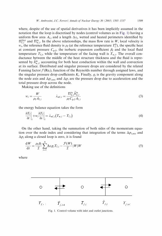
whernotation that the loop is discretised by nodes (control volumes as in Fig. 1) having auniform flow area Af,i and a length �si, wetted and heated perimeters identified byfrict
f ;i and inw;i. In the above relationships, the mass flow rate is W, local velocity is

wi, the reference fluid density is �f (at the reference temperature T0f ), the specific heat

at constant pressure Cp,f, the isobaric expansion coefficient �f and the local fluidtemperature Tf,i, while the temperature of the facing wall is Tw,i. The overall con-ductance between the middle of the heat structure thickness and the fluid is repre-sented by hin

w;i, accounting for both heat conduction within the wall and convectionat its surface. Distributed and singular pressure drops are considered by the relatedFanning factor f 0 Reið Þ, function of the Reynolds number through assigned laws, andthe singular pressure drop coefficients Ki. Finally, gi is the gravity component alongthe node axis and �pi,acc and �pi are the pressure drop due to acceleration and thetotal pressure drop across the node.Making use of the definitions

wi ¼W

�fAf ;ilwf ;i ¼

inw;ih

inw;i

�fCp;fAf ;ið3Þ

the energy balance equation takes the form

@Tf

@t

��i

þwi@Tf

@s

��i

¼ lwf ;i Tw;i � Tf ;i

� �ð4Þ

On the other hand, taking the summation of both sides of the momentum equa-tion over the node index and considering that integration of the terms �pi,acc and�pi along a closed loop is zero, it is found

dW

dt¼

�f�f

I

XNi¼1

DsigiTf ;i �F Wð Þ

IWj jW ð5Þ

where

Fig. 1. Control volume with inlet and outlet junctions.


I ¼XNi¼1

DsiAf ;i

� �F Wð Þ ¼

XNi¼1

frictf ;i Dsi

2�fA3f ;i

f 0 Reið Þ

" #þXNsing

k¼1

Kk

2�fA2f ;k

" #ð6Þ

As it can be seen, it is assumed that singular pressure drops are not assigned ineach node but at Nsing specified locations, characterised only by a reference area Af,k.Finally, a lumped parameter approach is used for representing heat structure

behaviour, leading to the following energy balance equation:

dTw;i

dt¼ �lw;iTw;i þQw;i ð7Þ

where

loutw;i ¼

houtw;i

outw;i

Aw;i�w;iCpw;ilin

w;i ¼hin

w;iinw;i

Aw;i�w;iCpw;ið8Þ

lw;i ¼ loutw;i þ lin

w;i Qw;i ¼q000w;i

�w;iCpw;iþ lout

w;i Toutf ;i þ lin

w;iTf ;i ð9Þ

in which the temperature of the outer fluid Toutf ;i and the outer structure surface

conductance houtw;i appear together with structure density �w,i, specific heat Cpw,i,

cross section area Aw,i and outer perimeter outw;i . Moreover, q000w;i is the specific power

per unit volume possibly generated in the structure material by electrical heating orany other means. As mentioned, the evaluation of the inner and outer surface con-ductances hin

w;i and houtw;i involves to calculate (or impose) inner and outer fluid heat

transfer coefficients and appropriate conductive resistances between the middle ofthe structure thickness and the two surfaces; this is made accepting conventionalheat transfer correlations for forced internal flow (e.g., the Colburn correlation) andassuming cylindrical structure shells.

3. Discretisation of the energy equation

3.1. First order upwind scheme

In a conventional control volume upwind explicit formulation, the energy Eq. (4)is discretised in space and time according to Fig. 1, in the following form:

Tnþ1f ;i ¼ Tnf ;i þ

wni DtDsi

T:nf ;i�1 � T

:nf ;i

� �þ Sni Dt i ¼ 1; . . . ;Nð Þ ð10Þ

where the source term is defined as Sni ¼ lfw;i T�n;nþ1w;i � Tnf ;i

� �and the dotted tem-

peratures represent the ‘‘donored’’ values at junctions defined as:

Wn5 0 ) T:nf ;i ¼ Tnf ;i i ¼ 1; . . . ;Nð Þ ð11Þ


Wn < 0 ) T:nf ;i ¼ Tnf ;iþ1 i ¼ 1; . . . ;N� 1ð Þ ð12Þ

T:nf ;N ¼ Tnf ;1 ð13Þ

Temperature T� n;nþ1w;i is an appropriate time-averaged structure temperature and we

define now, for future reference, the node Courant number appearing explicitly inEq. (10):

cni ¼wni DtDsi

ð14Þ

For a closed loop, a periodic temperature distribution must be imposed by therelationships:

Tnf ;0 ¼ Tnf ;N Wn5 0 ð15Þ

Tnf ;Nþ1 ¼ Tnf ;1 Wn < 0 ð16Þ

For similar reasons, whenever above and in the following the subscript i takesnon-positive values, periodicity of the temperature distribution along the closed loopis again assumed (e.g., T

:nf ;0 ¼ T

:nf ;N, T

:nf ;�1 ¼ T

:nf ;N�1).

3.2. Low diffusion upwind scheme

The point of interest here is whether it is possible to increase the order of accuracyof the numerical method while keeping two useful characteristics of the previous firstorder scheme:

� the control volume formulation, a widespread feature in system codes, whichallows expressing the energy balance in terms of energy variation in the nodescaused by advective and source contributions;

� the capability to propagate the relevant information along the characteristiclines or suitable approximations of them.

The upwind explicit scheme proposed by Warming and Beam (see e.g., Warmingand Beam, 1975; Tannehill, 1988) appears quite appropriate for this purpose. Toavoid unnecessary complications, let us firstly refer to a uniform spatial discretisa-tion in an adiabatic pipe with uniform cross section, then extending the obtainedresults to more general conditions. With such assumptions and in the case of for-ward flow, the Warming–Beam scheme takes the form

Tnþ1f ;i ¼ Tnf ;i � c

n Tnf ;i � Tnf ;i�1

� �þ1

2cn 1� cnð Þ Tnf ;i � 2Tnf ;i�1 þ T

nf ;i�2

� �ð17Þ

where the Courant number cn ¼ wDt=Ds does not depend on the particular con-sidered node.This scheme can be put in a donor-cell formulation like:


Tnþ1f ;i ¼ Tnf ;i þ

wni DtDsi

T:nf ;i�1 � T

:nf ;i

� �ð18Þ

in which

T:nf ;i ¼ 1� �w½ Tnf ;i þ �wT

nf ;i�1 T

:nf ;i�1 ¼ 1� �w½ Tnf ;i�1 þ �wT

nf ;i�2 ð19Þ

�w � �w cnð Þ ¼

1

2cn � 1ð Þ ð20Þ

In particular, with reference to Fig. 2, it can be seen that:

� n:n n 1 n n

� �
c ¼ 0 ) Tf ;i ¼ Tf ;i þ 2
Tf ;i � Tf ;i�1

T:nf ;i�1 ¼ Tnf ;i�1 þ

1

2Tnf ;i�1 � T

nf ;i�2

� � ð21Þ

this is coherent with a linear extrapolation of the temperature trend up to thedownwind boundary of each node;

� cn ¼ 1 ) T:n ¼ Tn T

:n ¼ Tn ð22Þ
f ;i f ;i f ;i�1 f ;i�1
these relationships suggest that the average temperature of the fluid crossingthe downwind junction during the time-step is the average temperature of thefluid initially present in the node, coherently with the fact that the fluid in thenode is completely swept away during the time step;

Fig. 2. Calculation cell for the Warming–Beam scheme with forward flow.


� n:n 1 n n

� �
c ¼ 2 ) Tf ;i ¼ 2
Tf ;i þ Tf ;i�1

T:nf ;i�1 ¼

1

2Tnf ;i�1 þ T

nf ;i�2

� � ð23Þ

the fluid initially contained in two nodes is now completely swept away duringthe time-step duration: the average fluid temperature flowing through thedownwind junction is therefore the arithmetic mean of the average tempera-tures in the two nodes.

This physically meaningful interpretation of the above relationships allows to easilyextend the treatment to the cases of backward flow and non-uniform mesh size andpipe flow area, as it will be briefly reported later in this section.A further step must now be made, introducing an appropriate formulation for the

case of non-zero source terms. In the light of the above interpretation, it is clearthat since the sources acting in each node have the effect to modify the temperatureof the fluid during each time step with respect to the initial values, they also affectthe value of the donored temperatures. Assuming that Eq. (10) still represents thediscrete energy balance in the case of the low diffusion scheme with sources, it istherefore justified to search for an expression of the donored temperatures havingthe form

T:nf ;i ¼ 1� �w½ Tnf ;i þ �w Tnf ;i�1 þD

ni ð24Þ

where the term Dni depends on the value of the sources.

Additional requirements must be imposed to specify the value of Dni . The way

here chosen in this purpose is to firstly consider that in a transient calculation pro-gressively approaching a steady-state condition the temperature increment acrosseach node is given by the steady energy balance

T:nf ;i ¼ T

:nf ;i�1 þ

DswnSni ð25Þ

Here and in the following the superscript n is kept for variables involved insteady-state formulations in order to indicate that, though stationary conditionsare under discussion, a transient calculation approaching them is beingconsidered.In such a case, the calculated space averaged node temperatures should approach

a constant value that can be expressed as a weighted average of the inlet and theoutlet fluid temperatures (i.e., the donored ones). So, with a certain degree of free-dom, we can define a weighting parameter ni 04ni 4 1

� �, independent on the

adopted time step, such that:

Tnf ;i ¼ ni T:nf ;i þ 1� ni

� �T:nf ;i�1 ð26Þ

Eq. (25) can be used to eliminate T:nf ;i from (26), obtaining


Tnf ;i ¼ T:nf ;i�1 þ ni

DswnSni ð27Þ

Similarly it can be easily found that:

Tnf ;i�1 ¼ T:nf ;i�1 � 1� ni�1

� � DswnSni�1 ð28Þ

Therefore, the difference between two consecutive values of space averaged nodefluid temperatures is given by

Tnf ;i � Tnf ;i�1 ¼ ni

DswnSni þ 1� ni�1

� � DswnSni�1 ð29Þ

By combining the relationship (24) with (25) and (26), the required expression forDni is reached after some algebra:

Dni ¼ 1� ni þ ni �w

� � DswnSni þ 1� ni�1

� ��w

DswnSni�1 ð30Þ

As it can be easily checked, substitution of the expression for the donored tem-peratures given by (24) and (30) into the steady energy balance (25) leads to thefollowing relationship

1� �w½ Tnf ;i � Tnf ;i�1 � ni

DswnSni � 1� ni�1

� � DswnSni�1

�

þ �w Tnf ;i�1 � Tnf ;i�2 � ni�1

DswnSni�1 � 1� ni�2

� � DswnSni�2

�¼ 0 ð31Þ

that, for arbitrary �w, represents a system of equations equivalent to (29).The definition of the constant ni must be now given attention. In principle, any

admissible value 04ni 4 1 could be chosen. However, we can take profit of thisdegree of freedom in order to improve accuracy of the method in representing thespatial trend of temperature in steady-state conditions. Writing the local steady-stateenergy balance equation in each node in the form

wn@Tnf;i@s

¼ Sni ¼ lwf ;i T�n;nþ1w;i � Tnf ;i

� �; ð32Þ

assuming Tnf ;i ¼ Tnf ;i sð Þ within the node and imposing the boundary condition

Tnf ;i 0ð Þ ¼ T:nf ;i�1 ð33Þ

Eq. (32) can be solved to give

Tnf ;i sð Þ ¼ T:nf ;i�1e

�ms þ T� n;nþ1w;i 1� e�ms½ ð34Þ

where it has been put


m ¼lwf ;i

wnð35Þ

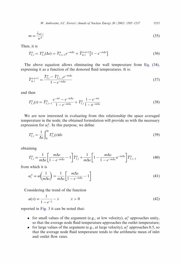
Then, it is

T:nf ;i ¼ Tnf ;i Dsð Þ ¼ T

:nf ;i�1e

�mDs þ T� n;nþ1w;i 1� e�mDs

� �ð36Þ

The above equation allows eliminating the wall temperature from Eq. (34),expressing it as a function of the donored fluid temperatures. It is:

T� n;nþ1w;i ¼

T:nf ;i � T

:nf ;i�1e

�mDs

1� e�mDsð37Þ

and then

Tnf ;i sð Þ ¼ T:nf ;i�1

e�ms � e�mDs

1� e�mDsþ T

:nf ;i

1� e�ms

1� e�mDsð38Þ

We are now interested in evaluating from this relationship the space averagedtemperature in the node; the obtained formulation will provide us with the necessaryexpression for ni . In this purpose, we define

Tnf ;i ¼1

Ds

ðDs0

Tnf ;i sð Þds ð39Þ

obtaining

Tnf ;i ¼1

mDsmDs

1� e�mDs� 1

� �T:nf ;i þ

1

mDs1�

mDs1� e�mDs

e�mDs� �

T:nf ;i�1 ð40Þ

from which it is

ni ¼ 1

mDs

� �¼

1

mDsmDs

1� e�mDs� 1

� �ð41Þ

Considering the trend of the function

xð Þ ¼1

1� e�1x

� x x > 0 ð42Þ

reported in Fig. 3 it can be noted that:

� for small values of the argument (e.g., at low velocity), ni approaches unity,so that the average node fluid temperature approaches the outlet temperature;

� for large values of the argument (e.g., at large velocity), ni approaches 0.5, sothat the average node fluid temperature tends to the arithmetic mean of inletand outlet flow rates.


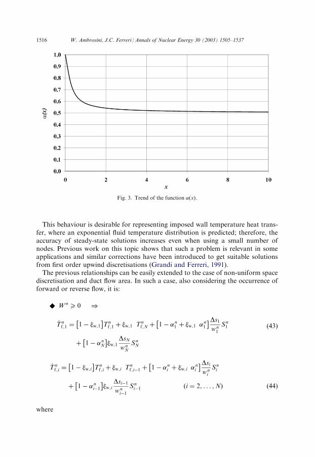
This behaviour is desirable for representing imposed wall temperature heat trans-fer, where an exponential fluid temperature distribution is predicted; therefore, theaccuracy of steady-state solutions increases even when using a small number ofnodes. Previous work on this topic shows that such a problem is relevant in someapplications and similar corrections have been introduced to get suitable solutionsfrom first order upwind discretisations (Grandi and Ferreri, 1991).The previous relationships can be easily extended to the case of non-uniform space

discretisation and duct flow area. In such a case, also considering the occurrence offorward or reverse flow, it is:

Wn5 0 )

T:nf ;1 ¼ 1� �w;1

� �Tnf ;1 þ �w;1 T

nf ;N þ 1� n1 þ �w;1 n1

� �Ds1wn1

Sn1

þ 1� nN� �

�w;1DsNwnN

SnN

ð43Þ

T:nf ;i ¼ 1� �w;i

� �Tnf ;i þ �w;i T

nf ;i�1 þ 1� ni þ �w;i

ni

� �DsiwniSni

þ 1� ni�1

� ��w;i

Dsi�1

wni�1

Sni�1 i ¼ 2; . . . ;Nð Þ ð44Þ

where

Fig. 3. Trend of the function (x).


�w;1 ¼ �w;1 Wnð Þ ¼

WnDt� �fAf ;1Ds1�fAf ;NDsN þ �fAf ;1Ds1

ð45Þ

�w;i ¼ �w;i Wnð Þ ¼

WnDt� �fAf;iDsi�fAf ;i�1Dsi�1 þ �fAf ;iDsi

i ¼ 2; . . . ;Nð Þ ð46Þ

ni ¼ wni

lnwf;iDsi

!¼

wnilnwf ;iDsi

lnwf;iDsiwni

1� e�

l nwf ;iw niDsi

� 1

2664

3775 i ¼ 1; . . . ;Nð Þ ð47Þ

Wn < 0 )

T:nf ;i ¼ 1� �w;i W

nð Þ� �

Tnf ;iþ1 þ �w;i Wnð ÞTnf ;iþ2

þ 1� niþ1 þ �w;i niþ1

� � Dsiþ1

wniþ1

�� Sniþ1 þ 1� niþ2

� ��w;i

Dsiþ2

w niþ2

�� Sniþ2

i ¼ 1; . . . ;N� 2ð Þ

ð48Þ

T:nf ;N�1 ¼ 1� �w;N�1

� �Tnf ;N þ �w;N�1 T

nf ;1 þ 1� nN þ �w;N�1 nN

� � DsNwnN�� SnN

þ 1� n1� �

�w;N�1Ds1wn1�� Sn1 ð49Þ

T:nf ;N ¼ 1� �w;N

� �Tnf ;1 þ �w;N Tnf ;2

þ 1� n1 þ �w;N n1� � Ds1

wn1�� Sn1 þ 1� n2

� ��w;N

Ds2wn2�� Sn2 ð50Þ

where

�w;i ¼ �w;i Wnð Þ ¼

Wnj jDt� �fAf ;iþ1Dsiþ1

�fAf ;iþ2Dsiþ2 þ �fAf ;iþ1Dsiþ1i ¼ 1; . . . ;N� 2ð Þ ð51Þ

�w;N�1 ¼ �w;N�1 Wnð Þ ¼

Wnj jDt� �fAf ;NDsN�fAf ;1Ds1 þ �fAf ;NDsN

ð52Þ

�w;N ¼ �w;N Wnð Þ ¼

Wnj jDt� �fAf ;1Ds1�fAf ;2Ds2 þ �fAf ;1Ds1

ð53Þ


ni ¼ wni

lnwf;iDsi

!¼

wni��

lnwf ;iDsi

lnwf;iDsiwni��

1� e�

l nwf ;i

w nij jDsi

� 1

26664

37775 i ¼ 1; . . . ;Nð Þ ð54Þ

It is interesting to note that, putting �w;i ¼ 0 and ni ¼ 1 in each node, the lowdiffusion scheme reverts to the classical first order upwind scheme with pointwiseevaluation of the source as described in Section 3.1. On the other hand, putting�w;i ¼ 0 and assuming ni as given by Eq. (47) or (54) allows to obtain a first ordermethod having a similar advantage in evaluating steady-state conditions as obtainedby appropriate correction factors in Ambrosini and Ferreri (1998).

4. Transient solution procedure

The equations expressing energy balance in the fluid and in the structures andmomentum balance in the fluid are combined to calculate the transient behaviour ofthe system. Momentum equation is discretised in time giving

Wnþ1 ¼

Wn þ�f�fDt

I

XNi¼1

DsigiTnþ1f ;i

1þF Wnð ÞDt

IWnj j

ð55Þ

On the other hand, the relationship to advance in time heat structure temperatureis obtained making use of the analytical solution of the related energy balanceequation:

Tnþ1w;i ¼ Tnw;ie

�l nw;iDt þQn

w;i

lnw;i

1� e�l nw;iDth i

ð56Þ

The corresponding time-averaged heat structure temperature during the time-stepis

T� n;nþ1w;i ¼ Tnw;i

1� e�l nw;iDt

lnw;iDtþQn

w;i

lnw;i

1�1� e�l nw;iDt

lnw;iDt

" #ð57Þ

Steady-state forms of the above equations are firstly solved when initialisationfrom stationary conditions is required. The algorithm to calculate steady stateinvolves two nested iteration loops: on energy balance, to assure periodicity of thecalculated temperature distribution along the loop, and on momentum balance, toreach the necessary equilibrium between buoyancy and friction.The algorithm for time advancement of the transient calculation includes the

solution of the energy equations in both the fluid and the walls on the basis of old


time-step flow rate and the solution of momentum equation on the basis of updatedfluid temperature values.

5. Methodology of linear stability analysis

In previous work (Ambrosini and Ferreri, 1998), a methodology was developedfor studying the linear stability behaviour of steady-state conditions in single-phasethermosyphon loops ‘‘as predicted’’ by a given numerical method. This methodol-ogy involved the explicit differentiation of numerically discretised equations aroundthe addressed steady-state condition obtaining Jacobian matrices to be used in pro-ducing a matrix, identified as A, embedding the linear dynamics of the system. Inparticular, if

F y nþ1; y n; p� �

¼ 0 ð58Þ

represents the numerical scheme, relating the (2N+1)-vector of system state vari-ables, y (N fluid temperatures, N wall temperatures and the loop flow rate) at twosubsequent time levels (tn and tn+1) and p is a vector of physical and numericalparameters, it is:

�y nþ1 ¼ �@F

@y nþ1

��s� ��1

�@F

@y n

��s� �

�y n ¼ A ys; pð Þ�y n ð59Þ

in which the superscript s identifies the considered steady-state conditions. Discus-sion of the eigenvalues of A allows getting information about stability. In particular,the spectral radius of the matrix, �A, can be used to define the following usefulquantity

zR ¼1

Dtln �Að Þ ð60Þ

where Dt ¼ tnþ1 � tn is the adopted time increment. This quantity takes negative orpositive values for stable or unstable behaviour, respectively; discussing the value ofzR for different values of the independent physical or numerical parameters allowssetting up quantitative stability maps. Similarly, other useful information can beobtained, e.g., on the frequency of the fastest growing (or least damped) oscillations(see Ambrosini and Ferreri, 1998).The approach based on the calculation of Jacobian matrices turned out useful for

automatic sensitivity analyses, as reported in Ferreri and Ambrosini (2001). A dif-ferent approach has been also utilised (Ambrosini, 2001) that has the advantage toavoid the cumbersome algebra involved in getting the Jacobians and is more com-putationally oriented. This methodology makes direct use of the transient solutionalgorithm, introducing small perturbations in the components of vector yn aroundsteady-state values to construct the matrix A by repeatedly advancing the transientalgorithm. This procedure assures complete coherence between the results of the


linear stability analysis and those of the transient non-linear calculations. As a fur-ther advantage, the same methodology could be applied to complex codes whosemodels are very complicated or even completely unknown. However, as mentionedin Ambrosini (2001), numerical differentiation has also drawbacks related to theoptimum choice of perturbations in variables, whose values must be carefully selec-ted to avoid obtaining inaccurate data.This technique will be anyway adopted in the following to obtain maps showing

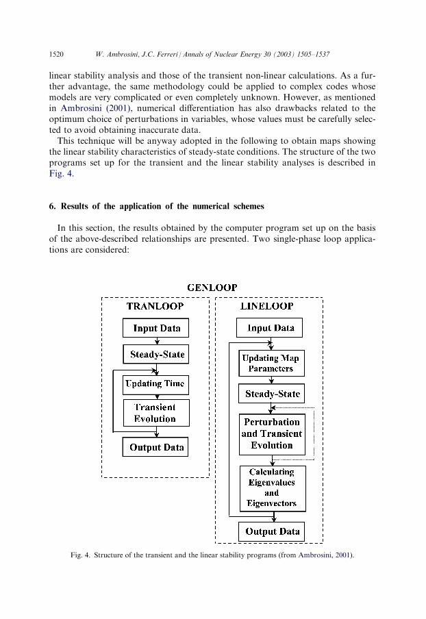
the linear stability characteristics of steady-state conditions. The structure of the twoprograms set up for the transient and the linear stability analyses is described inFig. 4.

6. Results of the application of the numerical schemes

In this section, the results obtained by the computer program set up on the basisof the above-described relationships are presented. Two single-phase loop applica-tions are considered:

Fig. 4. Structure of the transient and the linear stability programs (from Ambrosini, 2001).


� the first one is related to an idealised loop analysed by Welander (1967) whichhas been the subject of extensive studies in previous work, aimed atdemonstrating the effects of truncation error on numerical prediction ofstability in single-phase loops (see e.g., Ambrosini and Ferreri, 1998);

� the second one is related to experiments performed by Vijayan and co-workers in rectangular loops (Vijayan et al., 1995), exhibiting unstablebehaviour; such loop configuration was already addressed in dimensionlessform in a previous study by the Authors (Ambrosini and Ferreri, 2000).

These problems are here considered for comparing the behaviour of the two descri-bed explicit upwind schemes, trying to draw conclusions about the suitability of theadopted low diffusion donor-cell rule.

6.1. Welander’s problem

An extended description of the problem is reported in the original work byWelander (1967) and in a mentioned previous paper by the Authors (Ambrosini andFerreri, 1998). It is here recalled that the problem refers to a single-phase loop con-sisting of two tall vertical adiabatic legs joined by two very short horizontal pipesequipped with relatively large heat transfer coefficients with imposed temperatures,namely the ‘‘source’’ (at the bottom) and the ‘‘sink’’ (at the top). Depending on theratio between buoyancy and friction, the loop may show stable or unstable beha-viour; in the latter case, the flow rate shows oscillations that are progressivelyamplified leading to alternating flow reversals.In order to study the problem in dimensional form, a particular physical con-

figuration of the system, already addressed in Ambrosini and Ferreri (1998), isconsidered: the two vertical adiabatic legs have a length of 10 m and a diameterof 0.1 m, the horizontal pipes have the same diameter and a length of 0.1 m, withan imposed heat transfer coefficient of 20000 W/(m2 K) and surface temperaturesof 30 and 20 �C, respectively for the source and the sink. The working fluid ischosen to be water. To keep coherence with a previous application of RELAP5to the same problem, the friction factor is evaluated making use of a relationshipproperly accounting for the transition from laminar to turbulent flow (Churchill,1977).Three different steady-state conditions are possible for the system, with clockwise,

counter-clockwise and zero flow. The non-zero flow steady-state conditions have thefollowing characteristics:

� the steady-state flow rate is the same for both, except for the flow direction;� in steady-state, turbulent flow is achieved as the Reynolds number is in the

order of 10000; this justifies the extension of the original treatment byWelander (1967), related to laminar flow, to turbulent flow conditions, per-formed in previous work (Ambrosini and Ferreri, 1998);

� with the considered values of the physical parameters, both non-zero flowsteady-state conditions are linearly unstable; this feature allows discussing the


effect of the different numerical schemes on the predicted system behaviour,taking this case as a reference unstable one.

It is here remarked that the present discussion is focused only on the numericalaspects of stability prediction. From this viewpoint, some aspects deserving parti-cular attention for practical applications are disregarded. Among these aspects are:a) the adequacy of friction laws devised on the basis of fully developed flow data inpredicting natural circulation (that is a common assumption in most practicalsituations) and b) the realism of some of the assumptions adopted in defining theproblem (e.g., the adiabatic legs, the imposed heat transfer coefficient in the sourceand the sink). All these aspects are momentarily neglected to focus our attention onthe behaviour of the system as predicted by the different numerical schemes.Figs. 5 and 6 present the results obtained by the conventional first order explicit

upwind scheme, i.e., based on the usual donor-cell rule. The calculations have beenperformed with a constant time-step (�t=0.5 s), starting the transient from steady-state conditions with an initial perturbation in flow rate. Different numbers of nodeshave been adopted to discretise the 10 m long legs, while a single node was alwaysused to represent the 0.1 m long source and sink. The Figures clearly show theinfluence of truncation error on stability predictions in the case of first orderschemes, confirming that coarse nodalisations may artificially stabilise physicallyunstable systems. These results were fully expected and are completely consistentwith those previously obtained by RELAP5 and also by purposely-developed smallcodes for the same problem (see Ambrosini and Ferreri, 1998).

Fig. 5. Welander’s Problem: flow rate as a function of time predicted with the 1st order explicit upwind

scheme (10 and 30 nodes per leg; �t=0.5 s).


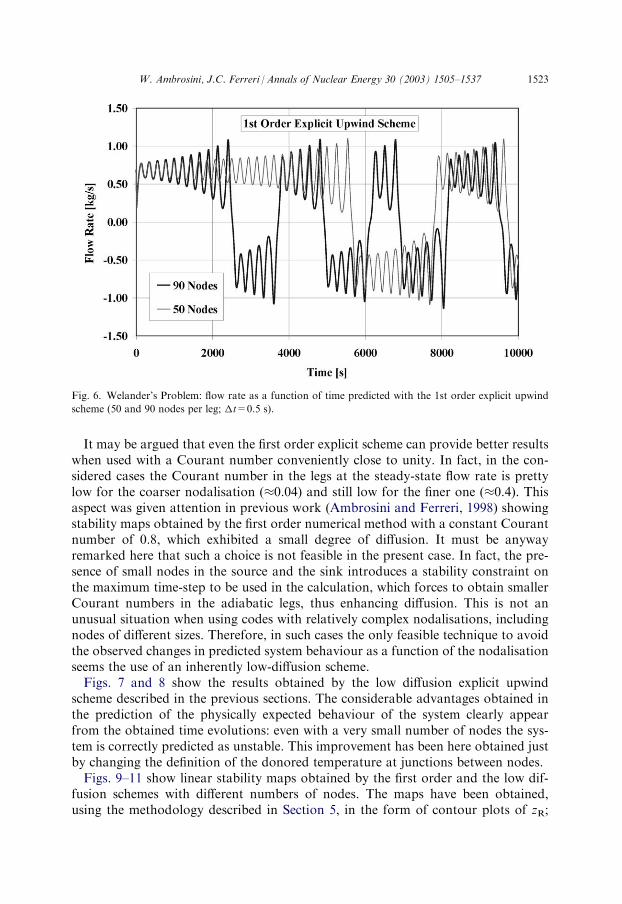
It may be argued that even the first order explicit scheme can provide better resultswhen used with a Courant number conveniently close to unity. In fact, in the con-sidered cases the Courant number in the legs at the steady-state flow rate is prettylow for the coarser nodalisation (�0.04) and still low for the finer one (�0.4). Thisaspect was given attention in previous work (Ambrosini and Ferreri, 1998) showingstability maps obtained by the first order numerical method with a constant Courantnumber of 0.8, which exhibited a small degree of diffusion. It must be anywayremarked here that such a choice is not feasible in the present case. In fact, the pre-sence of small nodes in the source and the sink introduces a stability constraint onthe maximum time-step to be used in the calculation, which forces to obtain smallerCourant numbers in the adiabatic legs, thus enhancing diffusion. This is not anunusual situation when using codes with relatively complex nodalisations, includingnodes of different sizes. Therefore, in such cases the only feasible technique to avoidthe observed changes in predicted system behaviour as a function of the nodalisationseems the use of an inherently low-diffusion scheme.Figs. 7 and 8 show the results obtained by the low diffusion explicit upwind

scheme described in the previous sections. The considerable advantages obtained inthe prediction of the physically expected behaviour of the system clearly appearfrom the obtained time evolutions: even with a very small number of nodes the sys-tem is correctly predicted as unstable. This improvement has been here obtained justby changing the definition of the donored temperature at junctions between nodes.Figs. 9–11 show linear stability maps obtained by the first order and the low dif-

fusion schemes with different numbers of nodes. The maps have been obtained,using the methodology described in Section 5, in the form of contour plots of zR;

Fig. 6. Welander’s Problem: flow rate as a function of time predicted with the 1st order explicit upwind

scheme (50 and 90 nodes per leg; �t=0.5 s).


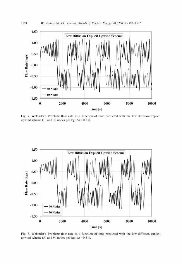
Fig. 7. Welander’s Problem: flow rate as a function of time predicted with the low diffusion explicit

upwind scheme (10 and 30 nodes per leg; �t=0.5 s).

Fig. 8. Welander’s Problem: flow rate as a function of time predicted with the low diffusion explicit

upwind scheme (50 and 90 nodes per leg; �t=0.5 s).


Fig. 9. Welander’s Problem: linear stability map for the 1st order scheme with 30 nodes per leg.

Fig. 10. Welander’s Problem: linear stability map for the 1st order scheme with 90 nodes per leg.


regions of positive values refer to unstable conditions, whereas regions of negativevalues refer to stable ones. As it can be noted, the first order scheme reveals to bevery sensitive to changes in the number of nodes; in particular, using 30 nodes perleg results in a strong overprediction of the stability region (Fig. 9), while increasingthe number of nodes per leg to 90 leads to a much smaller stable region (Fig. 10).This is in agreement with the results of the transient calculations and gives a clearerperspective of the effects of truncation error on predicted stability. On the otherhand, the use of the low diffusion scheme with only 30 nodes per leg provides a mapshowing nearly the same quantitative information as the one with 90 nodes (com-pare Figs. 11 and 12); this clearly points out the better performance of this methodin stability analyses.

6.2. Rectangular loops

Vijayan et al. (1995) describe the application of the ATHLET code (Burwell et al.,1989) to experiments performed in rectangular loops having the same shape andheight, but different pipe diameters. The loops, having inner diameters of 6 mm, 11mm and 23.2 mm were made by borosilicate glass pipes and were equipped with anelectrical heater and a heat exchanger cooler. The height of the loops is 2.1 m andthe length of the heating and cooling sections is equal to 0.8 m, while four connect-ing pipes having a length of 0.17 m are present in the horizontal parts. Only the 23.2

Fig. 11. Welander’s Problem: linear stability map for the low diffusion scheme with 30 nodes per leg.


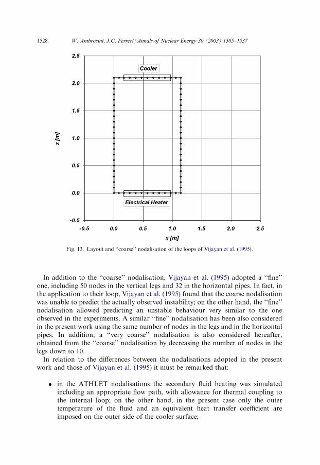
mm inner diameter loop exhibited unstable behaviour; for this reason this loop willbe taken into particular consideration in the following.Fig. 13 reports the layout of the loop and a ‘‘coarse’’ nodalisation used in the

present work similar to the one adopted by Vijayan et al. (1995) with the ATHLETcode. As it can be noted, 21 nodes have been used in the vertical legs and 12 nodes inthe horizontal pipes. Though not shown in the figure, the nodalisation includes alsoheat structures all along the loop with an imposed outer surface heat transfer coef-ficient of 7 W/(m2 K) as suggested in the referenced paper. The outer environmenttemperature has been arbitrarily assumed to be 20 �C, owing to lack of informationabout the value adopted with ATHLET. The heater power has been directly injectedwithin the thickness of the related structure. On the other hand, the outer heattransfer coefficient in the cooler has been guessed as 1000 W/(m2 K) on the basis ofdata reported for the 420 W power case (4.5 lpm of secondary flow), while the sec-ondary fluid temperature has been kept uniform and constant at 31 �C, i.e., thenominal value of inlet temperature in one of the considered calculation cases. Assuggested by Vijayan et al. (1995), the form loss coefficients in the four 90� elbowshave been assumed equal to 0.75 and in three locations 0.4 form loss coefficientshave been introduced to account for corresponding tee junctions. In addition, inorder to improve coherence with the predictions of the mentioned paper, the sameform of the Colebrook–White relationship (see Vijayan et al., 1995) has been adop-ted for distributed friction.

Fig. 12. Welander’s Problem: linear stability map for the low diffusion scheme with 90 nodes per leg.


In addition to the ‘‘coarse’’ nodalisation, Vijayan et al. (1995) adopted a ‘‘fine’’one, including 50 nodes in the vertical legs and 32 in the horizontal pipes. In fact, inthe application to their loop, Vijayan et al. (1995) found that the coarse nodalisationwas unable to predict the actually observed instability; on the other hand, the ‘‘fine’’nodalisation allowed predicting an unstable behaviour very similar to the oneobserved in the experiments. A similar ‘‘fine’’ nodalisation has been also consideredin the present work using the same number of nodes in the legs and in the horizontalpipes. In addition, a ‘‘very coarse’’ nodalisation is also considered hereafter,obtained from the ‘‘coarse’’ nodalisation by decreasing the number of nodes in thelegs down to 10.In relation to the differences between the nodalisations adopted in the present

work and those of Vijayan et al. (1995) it must be remarked that:

� in the ATHLET nodalisations the secondary fluid heating was simulatedincluding an appropriate flow path, with allowance for thermal coupling tothe internal loop; on the other hand, in the present case only the outertemperature of the fluid and an equivalent heat transfer coefficient areimposed on the outer side of the cooler surface;

Fig. 13. Layout and ‘‘coarse’’ nodalisation of the loops of Vijayan et al. (1995).


� owing to the use of the Boussinesq approximation, in the present model thefluid is considered incompressible and there is no need to simulate theexpansion tank and the related surge line, as made with ATHLET formaintaining a definite system pressure;

� a lumped parameter model is here used for heat structures, while in systemcodes finite difference techniques are used to solve the heat conductionequation within the structure thickness.

Fig. 14 shows the results obtained by the first order upwind scheme for the threedifferent nodalisations, with a time step �t=0.1 s. The calculations refer to the casewith a heater power of 420 W and have been started by initialising the fluid and heatstructure temperature distributions at steady-state conditions, then imposing a smallfinite perturbation in the flow rate. As expected, the results point out a decreasinglevel of diffusion with increasing the detail in the nodalisation. In particular, the useof the ‘‘very coarse’’ and ‘‘coarse’’ nodalisations results in the prediction of a stablebehaviour, while the ‘‘fine’’ nodalisation leads to instability.This behaviour is in contrast with the predictions by the low diffusion upwind

scheme, reported in Fig. 15. As it can be noted the three nodalisations do not fail inpredicting unstable behaviour, regardless of their spatial detail. In addition, thepredicted time evolutions are very similar, though a clear sensitivity to initial con-ditions is observed due the chaotic nature of the oscillations.The effect of time-step on the predicted stability behaviour has been also investi-

gated. Figs. 16 and 17 report the results obtained for the first order and the low dif-fusion upwind schemes with the coarse nodalisation changing the time step from 0.05s to 0.1 and 0.5 s. In the case of the first order scheme (Fig. 16), the effect of changing

Fig. 14. 23.2 mm I.D. loop of Vijayan et al. (1995): predicted flow rate for the 1st order upwind scheme

with three different nodalisations (�t=0.5 s).


Fig. 15. 23.2 mm I.D. loop of Vijayan et al. (1995): predicted flow rate for the low diffusion upwind

scheme with three different nodalisations (�t=0.5 s).

Fig. 16. 23.2 mm I.D. loop of Vijayan et al. (1995): predicted flow rate for the 1st order upwind scheme

with three different time steps.


the time-step from 0.1 to 0.5 s is considerable, while a very weak increase in dampingcan be observed by decreasing �t from 0.1 s to 0.05 s. This occurs because of thechange in the numerical dissipation, which in the modified equation is quantified bythe presence of a second order derivative term whose coefficient has the form

D ¼wj jDs2

1�wj jDtDs

� �ð61Þ

Therefore, only when �t is comparable with Ds= wj j numerical diffusion may appre-ciably decrease. On the other hand, the behaviour of the low diffusion upwindscheme appears almost insensitive to the changes in time-step (Fig. 17).Fig. 18 shows the time trends of the inlet and the outlet heater fluid temperatures

obtained by the low diffusion upwind scheme with the coarse nodalisation. Com-paring these data with the corresponding trends reported in Vijayan et al. (1995)from both the experiment and the ATHLET calculations with the fine nodalisation,a striking similarity is found (see e.g., Fig. 5b in the mentioned paper). A morecomplete perspective of the calculated fluid temperature evolution along the loopcan be obtained from Fig. 19, reporting the space-time trend of this variable eval-uated with the low diffusion scheme and the coarse nodalisation. The chaotic natureof the phenomenon is pointed out by the continuously changing pattern of fluidtemperature, which is slightly modified at each flow reversal.As far as linear stability is concerned, Figs. 20 and 21 report information obtained

by the linearised program for the 23.2 mm I.D. loop with both the first order upwindand the low diffusion schemes as a function of heater power and secondary fluidtemperature. It can be observed that, as already noted for Welander’s problem,

Fig. 17. 23.2 mm I.D. loop of Vijayan et al. (1995): predicted flow rate for the low diffusion upwind

scheme with three different time steps.


Fig. 18. 23.2 mm I.D. loop of Vijayan et al. (1995): heater and cooler outlet fluid temperature for the low

diffusion upwind scheme.

Fig. 19. 23.2 mm I.D. loop of Vijayan et al. (1995): space–time fluid temperature trend along the loop

(coarse nodalisation, low diffusion upwind scheme, �t=0.5 s).


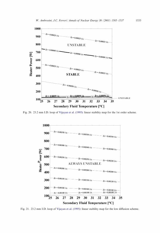
Fig. 20. 23.2 mm I.D. loop of Vijayan et al. (1995): linear stability map for the 1st order scheme.

Fig. 21. 23.2 mm I.D. loop of Vijayan et al. (1995): linear stability map for the low diffusion scheme.


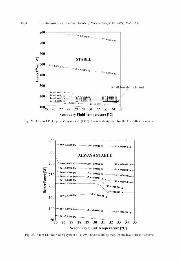
Fig. 22. 11 mm I.D. loop of Vijayan et al. (1995): linear stability map for the low diffusion scheme.

Fig. 23. 6 mm I.D. loop of Vijayan et al. (1995): linear stability map for the low diffusion scheme.


numerical diffusion introduced by the first order discretisation strongly affects sta-bility, which is mostly avoided by the use of the low diffusion numerical scheme. Forthe two loops with 6 and 11 I.D., Figs. 22 and 23 report the related stability maps,which are coherent with the information available from Vijayan et al. (1995) on theirobserved stable behaviour.

7. Conclusions

The low diffusion scheme proposed in this work has some characteristics thatmake it suitable for application in codes as those developed for the analysis of thethermal–hydraulic behaviour of nuclear reactors. In particular, when used in con-junction with a classical explicit control volume discretisation of the energy equationmaking use of upwind differencing, the adopted donor cell rule provides a straight-forward means of increasing the order of accuracy of the numerical scheme, stronglydecreasing the effects of truncation error on stability predictions.The analysis of Welander’s problem and of the experimental rectangular loops

studied by Vijayan et al. (1995) showed that the low diffusion scheme when appliedin single-phase flow has the following advantages with respect to the classical firstorder upwind differencing:

� it provides reliable predictions of stability even with coarse nodalisations;� the increase in the number of nodes rapidly improves the level of convergence

of the results: as it was seen the ‘‘coarse’’ and ‘‘fine’’ nodalisations for Vija-yan’s loop predicted very similar behaviour;

� the predicted time trend of variables is much less sensitive to changes in timestep.

The above advantages clearly appeared in the application to one-dimensionalsingle-phase flow; a further study is needed for assessing the feasibility of the appli-cation of a similar scheme in two-phase flow problems. A major difficulty in thisrespect is that some two-fluid codes are based on a differential problem having an ill-posed mathematical character, which discourages any attempt to increase the levelof accuracy of the numerical method, possibly leading to the prediction of unex-pected unstable behaviour.However, when single-phase stability problems are addressed the low diffusion

scheme showed to be capable of very good performances. This suggests that themethod could be considered in codes as an option to be activated at least whendealing with single-phase flow to get dissipation-free results, strongly improving thereliability of their stability predictions.The obtained results suggest topics to be considered for further work:

� the analysis of possible variants in the proposed scheme; for instance, thepresently adopted formulations are based on a treatment of the source termwhich has been devised on the basis of considerations related to the prediction


of the steady-state temperature distribution; this choice revealed to be effec-tive in reducing diffusion, but it is possible that different choices reveal moreadequate or meaningful; moreover, the effect in stability problems of the well-known weaknesses of second order numerical methods when predicting sharptemperature fronts (e.g, spurious spatial oscillations) must be carefullyassessed to avoid the prediction of unphysical behaviour when discontinuoustemperature distributions are dealt with;

� the application of the low diffusion scheme to boiling channel stability: in aprevious work the homogeneous equilibrium model was adopted for studyingstability of a boiling channel by numerical discretisation techniques(Ambrosini et al., 1999, 2000); the use of the present scheme in such a casewill clarify which difficulties must be coped with and which benefits can beobtained in the application to a problem of considerable importance fornuclear technology.

Finally, it must be mentioned that the application of the described methodologyfor linear stability analysis is providing interesting results in the calculation ofeigenvalues and eigenvectors of unstable systems (Ambrosini, 2001). Eigenvectors,in particular, provide quantitative information on the spatial distribution of systemvariables (like fluid and structure temperatures) that contribute to generate anyobserved linear (i.e., small) oscillation around steady-state conditions. This kind ofinformation provides further insight into the subtle details of the dynamics ofunstable flow systems.

References

Ambrosini, W. 2001. On Some Physical and Numerical Aspects in Computational Modelling of One-

dimensional Flow Dynamics. Invited lecture. In: Ferreri, J.C., Gnavi, G., Menendez, A., Rosen, M.

(Eds.), Proceedings of Fluidos-2001—VII International Seminar on Fluid Mechanics, Physics of Fluids

and Associated Complex Systems, 17–19 October 2001, Buenos Aires, Argentina.

W. Ambrosini, F. D’Auria, A. Pennati, J.C. Ferreri, 2001. Numerical effects in the prediction of single-

phase natural circulation stability. In: 19th UIT National Heat Transfer Conference 2001, 25–27 June

2001, Modena, p. 313.

Ambrosini, W., Di Marco, P., Ferreri, J.C., 2000. Linear and non-linear analysis of density wave

instability phenomena. Heat and Technology 18 (1), 2000. ).

Ambrosini, W., Di Marco, P., Susanek, A. 1999. Prediction of boiling channel stability by a finite-differ-

ence numerical method. In: 2nd International Symposium on Two-Phase Flow Modelling and Experi-

mentation, 23–26 May 1999, Pisa, Italy.

Ambrosini, W., Ferreri, J.C., 1998. The effect of truncation error on numerical prediction of stability

boundaries in a natural circulation single-phase loop. Nuclear Engineering and Design 183, 53–76.

Ambrosini, W., Ferreri, J.C., 2000. Stability analysis of single-phase thermosyphon loops by finite differ-

ence numerical methods. Nuclear Engineering and Design 201, 11–23.

Burwell, M.J., Lerchl, G., Miro, J., Teschendorff, V., Wolfert, K. 1989. The thermalhydraulic code

ATHLET for analysis of PWR and BWR systems. In: Proc. of 4th Int. Topical Meet. on Nuclear

Reactor Thermal-Hydraulics (NURETH-4), Karlsruhe, Germany, 10–13 October 2, pp. 1234–1239.

Creveling, H.F., De Paz, J.F., Baladi, J.Y., Schoenals, R.J., 1975. Stability characteristics of a single-

phase free convection loop. J. Fluid Mech. 67 (1), 65–84.


Churchill, S.W., 1977. Friction equation spans all fluid flow regimes. Chemical Eng. 84 (24), 91–92.

Ferreri, J.C., Ambrosini, W., 2001. Calculation of sensitivity to parameters in single-phase natural circu-

lation using ADIFOR. Int. J. Computational Fluid Dynamics 16 (4), 277–281.

Ferreri, J.C., Ambrosini, W., 2002. On the analysis of thermal-fluid-dynamic instabilities via numerical

discretization of conservation equations. Nuclear Engineering and Design 215, 153–170.

Fletcher, C.A.J. 2001. Computational Techniques for Fluid Dynamics, Vol. 1, second ed. Springer.

Grandi, G.M. and Ferreri, J.C. 1991. Limitations of the Use of One-volume Heat Exchanger Repre-

sentation, Unpublished Technical Memo, CNEA, Ger. Seg. Rad. y Nuclear, 1991. (reported in Ferreri,

J.C., Ambrosini, W., US-NRC NUREG/IA-151, 1999).

LeVeque, R.J., 1990. Numerical Methods for Conservation Laws. Birkhauser Verlag.

Mahaffy, J.H., 1993. Numerics of codes: stability, diffusion and convergence. Nuclear Engineering and

Design 145, 131–145.

Minkowycz, W.J., Sparrow, E.M., Schneider, G.E., Pletcher, R.H., 1988. Handbook of Numerical Heat

Transfer. John Wiley and Sons.

Tannehill, J.C., 1988. Hyperbolic and hyperbolic-parabolic systems. In: Minkowycz, W.J., Sparrow,

E.M., Schneider, G.E., Pletcher, R.H. (Eds.), Handbook of Numerical Heat Transfer. John Wiley and

Sons.

Toro, E.F., 2001. Shock Capturing Methods for Free-Surface Shallow Flows. John Wiley and Sons.

Vijayan, P.K., Austregesilo, H., Teschendorff, V., 1995. Simulation of the unstable behavior of single-

phase natural circulation with repetitive flow reversals in a rectangular loop using the computer code

ATHLET. Nuclear Engineering and Design 155, 623–641.

Vijayan, P.K., Austregesilo, H., 1994. Scaling laws for single-phase natural circulation loops. Nuclear

Engineering and Design 152, 331–347.

Warming, R.F. and Beam, R.M. 1975. Upwind second-order difference schemes and applications in

unsteady auerodynamic flows. In: Proc. AIAA 2nd Computational Fluid Dynamics Conf., Hartford, CT,

pp. 17–28.

Welander, P., 1967. On the oscillatory instability of a differentially heated fluid loop. J. Fluid Mech. 29

(1), 17–30.


Prediction of stability of one-dimensional natural circulation with a low diffusion numerical scheme

Documents

Transcript of Prediction of stability of one-dimensional natural circulation with a low diffusion numerical scheme