5

An Introduction to Computational DiffusionMRI: the Diffusion Tensor and Beyond

Daniel C. Alexander

Department of Computer Science, University College London, Gower Street,London, WC1E 6BT, UKD.Alexander@cs.ucl.ac.uk

Summary. This chapter gives an introduction to the principles of diffusion mag-netic resonance imaging (MRI) with emphasis on the computational aspects. Itintroduces the philosophies underlying the technique and shows how to sensitizeMRI measurements to the motion of particles within a sample material. The mainbody of the chapter is a technical review of diffusion MRI reconstruction algorithms,which determine features of the material microstructure from diffusion MRI mea-surements. The focus is on techniques developed for biomedical diffusion MRI, butmost of the methods discussed are applicable beyond this domain. The review be-gins by showing how the standard reconstruction algorithms in biomedical diffusionMRI, diffusion-tensor MRI and diffusion spectrum imaging, arise from the principlesof the measurement process. The discussion highlights the weaknesses of the stan-dard approaches to motivate the development of a new generation of reconstructionalgorithms and reviews the current state-of-the-art. The chapter concludes with abrief discussion of diffusion MRI applications, in particular fibre tracking, followedby a summary and a glimpse into the future of diffusion MRI acquisition and recon-struction.

5.1 Introduction

Diffusion magnetic resonance imaging (MRI) provides a unique probe into themicrostructure of materials. The method observes the displacements of par-ticles that are subject to Brownian motion within a sample material. Specifi-cally, it measures the probability density function p of particle displacementsx over a fixed time t. The microstructure of the material determines the mo-bility of the particles within and thus determines p. Conversely, features of pprovide information about the material microstructure.

In biomedical diffusion MRI, the particles of interest are usually watermolecules. Water is a major constituent of biological tissue. Water moleculeswithin tissue undergo random motion due to thermal fluctuations. Currently,brain imaging is the most common application of biomedical diffusion MRI.

84 D. C. Alexander

(a) (b)

(c) (d)

Fig. 5.1. See colour plates. Schematic diagrams four microstructures found in thebrain. The black lines are barriers to the movement of water molecules. The redcontours show the expected shape of p in each tissue. Panel (a) shows a fluid-filledregion. Panel (b) shows isotropic grey matter. Panels (c) and (d) show white matterwith one and two dominant fibre orientations, respectively

The brain has a complex architecture of grey-matter areas connected by white-matter fibres. Diffusion MRI allows non-invasive mapping of the connectivityof the brain.

Figure 5.1 shows schematic diagrams of four different microstructures thatappear in brain tissue together with contours of the p that we expect to observewithin each kind of tissue. The diagrams do not aim to reproduce true brain-tissue microstructure, but merely to show how different shapes of p can arisefrom different configurations of barriers to water mobility. Some regions ofthe brain, such as the ventricles, contain mostly cerebro-spinal fluid (CSF)and Fig. 5.1(a) depicts such a fluid-filled region. Microstructural barriers towater mobility are sparse in these regions, although a few membranes may bepresent. The function p is isotropic, since displacements are equally likely inall directions. Figure 5.1(b) depicts grey-matter microstructure. Grey matteris dense tissue containing many barriers to water mobility, such as cell wallsand membranes. However, the barriers in grey matter often, as in the picture,have no preferred orientation and so hinder the water movement equally inall directions. The function p thus remains isotropic, but is less spread out

5 Introduction to Diffusion MRI 85

than in the CSF region, since the average length of displacements is smaller.Figure 5.1(c) depicts the microstructure in a white-matter fibre bundle. Whitematter contains bundles of parallel axon fibres that connect different regionsof the brain. The orientations of the cell walls that form barriers to watermobility have much greater consistency in white matter than in grey matter.The microstructure hinders movement more in directions perpendicular tothe fibre than along the fibre axis. Displacements along the fibre are largeron average than displacements across it and p is anisotropic with a ridgein the direction of the fibre. More complex microstructure also appears inwhite matter. Figure 5.1(d) depicts the microstructure at an orthogonal fibrecrossing. Displacements are largest on average in the fibre directions and phas ridges in the directions of each fibre. Other configurations of white matterfibres also occur in the brain.

If we can determine the orientations of the ridges of p, we can infer thedominant orientations of the microstructural fibres. With fibre-orientationestimates in each voxel of a three-dimensional MR image volume, we canfollow fibres through the image, using so-called ‘tractography’ algorithms, seeChap. 7 by Vilanova et al., and construct a connectivity map of the imagedsample.

The following length scales of brain tissue and the measuring process helpappreciation of the discussion in the rest of the chapter:

• The voxel volume in biomedical MRI is of order 10−9 m3.• The diffusion time, t, in biomedical diffusion MRI is of order 10−2 s and,

over this time, the root-mean-squared displacement of water molecules isin the micrometer range.

• The diameters of axon fibres in human white matter can reach 2.50 ×10−5 m, but most axon-fibre diameters are less than 10−6 m [1, 2, 3].

• Coherent white-matter fibre-bundles vary widely in size from several cen-timetres across down to a few axons.

• The packing density of axon fibres in white matter is of order 1011 m−2

[1, 2, 3].

The next section introduces the basic diffusion MRI measurement and itsrelationship to the function p. Section 5.3 reviews diffusion MRI reconstructionalgorithms, which determine features of the microstructure from diffusion MRImeasurements. Section 5.4 gives a brief review of diffusion MRI applicationsthat concentrates on fibre-tracking and connectivity-mapping methods. Weconclude in Sect. 5.5 with a summary of the field and some pointers for futureresearch in diffusion MRI methods.

5.2 Diffusion-Weighted MRI

Diffusion-weighted MRI acquires measurements that are sensitive to the mo-tion of nuclei possessing a net spin (‘spins’), most commonly hydrogen nuclei.

86 D. C. Alexander

Γ1Γ

READOUT

2

δ

∆

δ

TE

TE/2

P180P90

Fig. 5.2. Shows the pulsed-gradient spin-echo sequence

We can sensitize the MRI measurement to spin displacements by introducingmagnetic-gradient pulses to the standard spin-echo sequence (or other stan-dard sequences, such as the stimulated-echo sequence). Figure 5.2 shows thepulsed-gradient spin-echo (PGSE) sequence [4], which is the most commonpulse sequence for diffusion-weighted MRI. The scanner maintains a constantand approximately homogeneous magnetic field H0 over the sample. The spinsalign with H0 and have a slightly higher probability of having spin up statethan spin down, which causes a non-zero net magnetization of the material.The 90◦ radio-frequency (RF) pulse P90, centred at time τ = 0, tips the spinsinto the ‘transverse’ plane perpendicular to H0. The spins then precess aboutH0 at the Larmor frequency, which is proportional to |H0|. Immediately afterP90, the spins precess in phase so that the net magnetization rotates aboutH0. Inhomogeneities in H0 cause the spin precessions to dephase graduallyso that the net magnetization decays. The 180◦ RF pulse P180, centred attime τ = TE/2 where TE is the ‘echo time’, negates the phase of each spin.In the absence of the gradient pulses Γ1 and Γ2, the rate of dephasing is thesame before and after P180 so the spins come back into phase at time TE.The ‘spin echo’ occurs when the spins come back into phase and recover theirnet magnetization, which is the MR signal.

The spatially homogeneous diffusion-weighting gradient offsets the phaseof each spin by a linear function of the spin position. A gradient pulse Γ offsetsthe phase of a spin at position r by r · q, where

q = γ

∫ ∞

0

∫∫Γ(τ)dτ ,

Γ(τ) is the component of the magnetic-field gradient parallel to H0 (i.e.(∇H0) H0) at time τ and γ is the gyromagnetic ratio of the spins. The gyro-magnetic ratio for protons in water, which are usually the spins in biomedical

5 Introduction to Diffusion MRI 87

diffusion MRI, is 2.675 × 108 s−1T−1. In practice, the pulses are usually ap-proximately rectangular (with brief rise and fall times) so that Γ1 and Γ2

have constant value g over the pulse duration δ and q = γδg. Since P180negates the phase of each spin, Γ2 cancels the phase offset from Γ1 for a sta-tionary spin. However, if a spin moves from position r1 to r2 between the twopulses, it retains a residual phase offset of q · (r2 − r1) = q · x, where x is thespin displacement. The magnetic moment of the spin at the spin echo is thusM exp(iq ·x), whereM is the magnitude of the magnetic moment. The MRIsignal A (q) is the magnetization of all contributing spins. If we sum over allpossible spin displacements, we see that

A (q) = A (0)∫

p(x) exp(iq · x)dx ,

where A (0) is the signal with no diffusion-weighting gradients and the inte-gral is over three-dimensional space. Diffusion MRI usually assumes that thelocal advection velocity is zero (no net motion of the spin population), so thatp(x) = p(−x) and A (q) is real valued in the absence of noise. Moreover, weuse the normalized signal

A(q) = (A (0))−1A (q) =∫

p(x) cos(q · x)dx , (5.1)

which is the Fourier transform of the function p at wavenumber q. A mea-surement A(q) thus provides the apparent diffusion coefficient (ADC) d =−b−1 log(A(q)), where b = t|q|2 is the diffusion-weighting factor , on the as-sumption that p is an isotropic zero-mean Gaussian function [4, 5]. Researchersin the 1980s [6, 7] combined the basic diffusion-weighted NMR measurementdescribed above with MRI to obtain image maps of the ADC.

The derivation of equation (5.1) assumes that the movement of particlesduring the gradient pulses is negligible. This assumption is justified if δ is smallcompared with the pulse separation ∆, which is then the diffusion time t = ∆.In practice however, δ and ∆ usually have similar magnitude, as in Fig. 5.2.When δ is non-negligible, the phase offset of a spin depends on its trajectoryduring Γ1 and Γ2 rather than just its displacement, which complicates themodel relating the measurements to p; see discussions in [5, 8, 9]. With someassumptions, we can model the effects of non-negligible δ analytically. Forexample, if p is Gaussian and the gradient pulses are rectangular, then non-negligible δ reduces t to an effective diffusion time of ∆ − δ/3, see [4, 5].The effective diffusion time reduces still further for higher moments of p [10].Mitra and Halperin [9] show that, if p is the displacement density of thecentres of mass (COM) of particle trajectories over time δ, rather than thedisplacements of particles themselves, equation (5.1) holds with t = ∆ evenwith non-negligible δ. The COM displacement density has similar shape to theparticle displacement density (though somewhat blurred) and, in particular,indicates fibre directions in the same way. Thus, although non-negligible δ

88 D. C. Alexander

confounds absolute measurements of the particle displacement density, thefeatures of p of interest in brain imaging are relatively unaffected. Lori et al. [8]and Brihuega-Moreno et al. [11] provide some further analysis of the non-negligible ∆ problem.

The MRI measurement is complex-valued, since the magnetization hasmagnitude and phase. Often the phase of the measurements is discarded,since inhomogeneities in H0 and movement of the sample make it unstable.In practice, it is common to take the modulus of A (q) as the real-valued MRsignal. An additive Gaussian noise model is common in MRI. With this model,the real and imaginary parts of the signal are independent and identicallydistributed with distribution N(0, σ2). Noise on the modulus of the signal thusfollows a Rician distribution [12], which tends to a Gaussian distribution as thesignal-to-noise ratio increases. A common measurement of quality of diffusionMRI data sets is the signal-to-noise ratio S = A (0)/σ of the measurementwith q = 0, where A is the noise-free signal.

5.3 Diffusion MRI Reconstruction Algorithms

This section reviews diffusion MRI reconstruction algorithms. We focus hereon reconstructing fibre orientations, but note that some diffusion MRI tech-niques aim to estimate other features of the microstructure, such as the ratioof intracellular to extracellular water [13], by targeting other features of p.For this discussion, a diffusion MRI reconstruction algorithm inputs a set ofdiffusion-weighted MRI measurements from one voxel and outputs, at least,i) the number n of dominant fibre directions and ii) an estimate of each dom-inant fibre direction. Most of these algorithms determine a feature of p thathighlights fibre orientations. In addition to fibre-orientation estimates, thesefeatures of p usually provide scalar indices of shape that discriminate differ-ent kinds of material and can indicate the reliability of the fibre-orientationestimates.

5.3.1 Diffusion Tensor MRI

Diffusion-tensor (DT) MRI [14] computes the apparent diffusion tensor onthe assumption that p is a zero-mean trivariate Gaussian distribution:

p(x) = G(x;D, t) , (5.2)

where

G(x;D, t) = ((4πt)3 det(D))−12 exp

(−xT D−1x

4t

),

D is the diffusion tensor and t is the diffusion time. Since the Gaussian functionhas a single ridge, DT-MRI assumes n = 1. Substitution of (5.2) into (5.1)gives

5 Introduction to Diffusion MRI 89

A(q) = exp(−tqT Dq) . (5.3)

If we take the logarithm of (5.3), we see that each A(q) provides a linearconstraint on the elements of D. The Gaussian model has six free parame-ters, which are the elements of the symmetric three-by-three matrix D. Tofit the six free parameters, we need a minimum of six A(q) with indepen-dent q, although many more are often acquired. Note that six A(q) requires aminimum of seven A (q) including one for normalization. Practitioners mostoften use the linear least-squares fit of D to the log measurements. However,fitting directly using equation (5.3), as in [15], can improve results, since theerror distribution is closer to normal on A(q) than on log(A(q)). When fittingdirectly to A(q), we can include constraints on the diffusion tensor, such aspositive definiteness, using the Cholesky decomposition as in [15], or cylindri-cal symmetry, by writing

D = αnnT + βI , (5.4)

where n is the principal direction of the diffusion tensor, I is the identity tensorand D has eigenvalues α + β, β and β.

Diffusion-tensor MRI generalizes the ADC calculation from simple diff-usion-weighted MRI to three dimensions. It provides two extra insights intothe material microstructure over simple diffusion-weighted MRI. First, it pro-vides rotationally invariant statistics of the anisotropy of p, which reflect theanisotropy of the microstructure. Second, it provides an estimate of the dom-inant orientation of microstructural fibres. The eigenvalues λ1 ≥ λ2 ≥ λ3 ofD determine the shape of p. The Gaussian function has ellipsoidal contoursand the relative lengths of the major axes of the ellipsoids have the sameproportions as the (λi)

12 . Statistics of anisotropy come from the distribution

of eigenvalues. A common statistic is the fractional anisotropy [16]

ν =

(32

3∑i=1

(λi −

13Tr(D)

)2) 1

2(

3∑i=1

λ2i

)− 12

, (5.5)

which is the normalized standard deviation of the eigenvalues. Figure 5.3(a)shows ν over a coronal slice through a healthy human brain. The highestvalues of ν are in regions of dense white matter, such as the corpus callosum,where the fibres are packed most densely and have consistent orientation.Other common scalar statistics derived from the diffusion tensor are Tr(D)and the skewness µ. The trace of the diffusion tensor Tr(D) =

∑3i=1 λi is

proportional to the mean squared displacement of water molecules and thusindicates the mobility of water molecules within each voxel, which reflects thedensity of microstructural barriers. The skewness

µ =

(92

3∑i=1

(λi −

13Tr(D)

)3) 1

3(

3∑i=1

λ3i

)− 13

, (5.6)

90 D. C. Alexander

(a) (b)

(c) (d)

(e) (f)

Fig. 5.3. See colour plates. Shows various features of p plotted over a coronal slicethrough a healthy human brain. Panel (a) shows the fractional anisotropy, ν. Panel(b) shows Tr(D). Panels (c) shows the skewness, µ. Panel (d) shows the colour codedprincipal direction, e1. Panel (e) shows the output of Alexander’s voxel classificationalgorithm (Sect. 5.3.2); black is background, blue is order 0, white is order 2 andpink is order 4. Panel (f) shows the spherical-harmonic anisotropy (Sect. 5.3.2). Inffeach panel, the upper region of interest contains some grey matter (top), part of thecorpus callosum (middle) and some CSF (bottom). The lower region contains thefibre crossing in the pons

is close to zero for isotropic diffusion tensors with near spherical contours(λ1 ≈ λ2 ≈ λ3), positive for prolate diffusion tensors with cigar-shaped con-tours (λ1 � λ2 ≈ λ3) and negative for oblate diffusion tensors with pancake-shaped contours (λ1 ≈ λ2 � λ3). Figures 5.3(b) and 5.3(c) show Tr(D) and µ,respectively, over the coronal slice in Fig. 5.3(a). The highest values of Tr(D)are in the ventricles and other regions of cerebro-spinal fluid, where the densityof barriers to water mobility is low. The skewness is positive in most white-matter regions. In some white-matter regions, such as the pons, the skewnessis negative showing oblate diffusion tensors. Oblate diffusion tensors arise inregions contain orthogonally crossing fibres, as depicted in Fig. 5.1(d), where

5 Introduction to Diffusion MRI 91

the best-fit Gaussian model has oblate contours. Many other configurationsof fibres or microstructures can also give rise to oblate diffusion tensors.

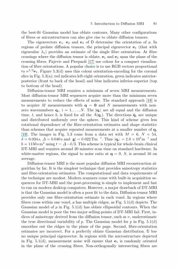
The eigenvectors e1, e2 and e3 of D determine the orientation of p. Inregions of prolate diffusion tensors, the principal eigenvector e1 (that witheigenvalue λ1) provides an estimate of the single fibre orientation. At fibrecrossings where the diffusion tensor is oblate, e1 and e2 span the plane of thecrossing fibres. Pajevic and Pierpaoli [17] use colour for a compact visualiza-tion of fibre orientations. A popular choice is to use RGB vectors proportionalto ν1/2e1. Figure 5.3(d) uses this colour orientation-encoding for the coronalslice in Fig. 5.3(a); red indicates left-right orientation, green indicates anterior-posterior (front to back of the head) and blue indicates inferior-superior (topto bottom of the head).

Diffusion-tensor MRI requires a minimum of seven MRI measurements.Most diffusion-tensor MRI sequences acquire more than the minimum sevenmeasurements to reduce the effects of noise. The standard approach [18] isto acquire M measurements with q = 0 and N measurements with non-zero wavenumbers qi, i = 1, . . . , N . The |qi| are all equal and the diffusiontime, t, and hence b, is fixed for all the A(qi). The directions qi are uniqueand distributed uniformly over the sphere. This kind of scheme gives lessrotational dependence of the fibre-orientation estimates and shape statisticsthan schemes that acquire repeated measurements at a smaller number of qi

[19]. The images in Fig. 5.3 come from a data set with M = 6, N = 54,δ = 0.034 s, ∆ = 0.040 s and |g| = 0.022Tm−1. Thus |qi| = 2.0 ×105m−1 andb = 1150 s m2 using t = ∆−δ/3. This scheme is typical for whole-brain clinicalDT-MRI and requires around 20 minutes scan time on standard hardware. Inwhite-matter regions, the signal to noise ratio at q = 0, S, is around 16 onaverage.

Diffusion-tensor MRI is the most popular diffusion MRI reconstruction al-gorithm by far. It is the simplest technique that provides anisotropy statisticsand fibre-orientation estimates. The computational and data requirements ofthe technique are modest. Modern scanners come with built-in acquisition se-quences for DT-MRI and the post-processing is simple to implement and fastto run on modern desktop computers. However, a major drawback of DT-MRIis that the Gaussian model is often a poor fit to the data. Diffusion-tensor MRIprovides only one fibre-orientation estimate in each voxel. In regions wherefibres cross within one voxel, p has multiple ridges, as Fig. 5.1(d) depicts. TheGaussian model of p in Fig. 5.1(d) has oblate ellipsoidal contours. When theGaussian model is poor the two major selling-points of DT-MRI fail. First, in-dices of anisotropy derived from the diffusion tensor, such as ν, underestimatethe true directional variability of p. The Gaussian model for p in Fig. 5.1(d)smoothes out the ridges in the plane of the page. Second, fibre-orientationestimates are incorrect. For a perfectly oblate Gaussian distribution, D hasno unique principal eigenvector. In regions with the microstructure depictedin Fig. 5.1(d), measurement noise will ensure that e1 is randomly orientedin the plane of the crossing fibres. Non-orthogonally intersecting fibres are

92 D. C. Alexander

potentially more dangerous. The single fibre-orientation estimate from DT-MRI then lies consistently between the two true fibre directions; see [20] foran example.

5.3.2 Modelling the ‘ADC Profile’

Equation (5.3) shows that, with no noise, log(A) is quadratic in q when p isGaussian. Several authors model log(A) with higher-order polynomials bothto detect departures from the Gaussian model and to obtain more reliableindices of anisotropy.

Frank [21] and Alexander et al. [22] both fit the spherical-harmonic seriesto log(A) at a fixed |q|. In the literature, the term ‘ADC profile’ refers to−b−1 log(A) as a function of x with fixed |q|. The spherical harmonics YlmYY ,l = 0, . . . ,∞, m = −l, . . . , l, form a basis for complex-valued functions on theunit sphere in three dimensions S2. Thus we can write any complex-valuedfunction f of the sphere as

f =∞∑

l=0

l∑m=−l

almYlmYY .

Each spherical-harmonic series containing only terms up to order l = L isthe restriction to S2 of an order L polynomial, and vice versa. Series withonly even-order terms are symmetric, so that f(x) = f(−x), and constrainingboth Im(al0) = 0 and alm = (−1)ma

l(−m) for all l and m ensures that f

is real-valued [22]. Reference [22] shows how to compute the least-squares-fitsymmetric real-valued spherical-harmonic series to log(A(qi)), i = 1, . . . , N ,robustly via a single matrix multiplication.

If log(A) is quadratic, its spherical-harmonic series contains only terms upto order 2. If the fitted spherical-harmonic series contains significant higher-order terms, the Gaussian model for p is poor. Frank [21] observes signif-icant fourth-order terms in the spherical-harmonic series in various white-matter regions in the human brain. Alexander [22] uses the analysis ofvariance (ANOVA) test for deletion of variables, the ‘F -test’ [23], to choosethe lowest-order series that fits the data. This simple voxel-classification algo-rithm classifies each voxel as isotropic (order 0), anisotropic Gaussian (order2), or non-Gaussian (order 4 or above). Results show clusters of order 4 voxelsin several fibre-crossing regions in human-brain data similar to that used forFig. 5.3. Figure 5.3(e) shows Alexander’s voxel classification over the coronalslice in Fig. 5.3(a). Order 4 voxels appear consistently in the pons and otherfibre crossings showing failure of the Gaussian model.

Spherical-harmonic models of log(A) provide anisotropy indices that arerobust to departures from the Gaussian model. The moments of a sphericalfunction f are

ωn[f ] = (4π)n/2

∫fn(x)dx .

5 Introduction to Diffusion MRI 93

A general index of anisotropy of f is (ω1[f ])−1(ω2[f ] − (ω1[f ])2)1/2. For areal-valued symmetric spherical-harmonic series, ω1[f ] = 4πa00 and ω2[f ] =4π∑∞

l=0

∑2lm=−2l |a(2l)m|2. Figure 5.3(f) shows the spherical-harmonic aniso-

tropy from series including terms up to order 4. Differences between thespherical-harmonic anisotropy and ν are more noticeable at higher b. Othermoments may also provide useful shape indices.

Ozarslan et al. [24] use a higher-order tensor model of log(A) so that

log(A(q)) = −tq(j)D(2j)qj , (5.7)

where the term on the right contains the contraction of the order 2j ten-sor D(2j) by q(j), which is the outer product of q(1) = q and q(j−1). Thetensors D(2j) are real valued and have symmetry ensuring that log(A(q)) =log(A(−q)). It is straightforward to demonstrate that the unique elementsof the tensor model in (5.7) with order 2j are a linear transformation of thereal and imaginary parts of the coefficients of the real symmetric spherical-harmonic model including terms up to order 2j. In this sense, the two methodsare equivalent, both theoretically and computationally. Liu et al. [10] modellog(A(q)) by a sequence of higher-order tensors, which includes both odd andeven-order tensors. The inclusion of odd-order tensors allows the model tocapture non-symmetric spin displacements.

Neither the spherical-harmonic nor the higher-order-tensor models providefibre-orientation estimates. Both model log(A) rather than p and the peaks oflog(A) at a fixed radius are not in the directions of the ridges of p in general.The scalar anisotropy of log(A) correlates with that of p, so we can computeanisotropy indices from log(A). Also when p is Gaussian, A is Gaussian, sowe can infer departures from the Gaussian model of p from departures of theA(qi) from the best-fit Gaussian. To estimate fibre orientations, however, wemust invert the Fourier transform in (5.1) and reconstruct directional featuresof p.

5.3.3 Multi-Compartment Models

A simple generalization of DT-MRI replaces the Gaussian model for p with amixture of Gaussian densities:

p(x) =n∑

i=1

aiG(x;Di, t) , (5.8)

where each ai ∈ [0, 1] and∑

i ai = 1. Particle displacements in media contain-ing n distinct compartments, between which no exchange of particles occurs,follow the distribution in equation (5.8) if the displacement density in the i-thcompartment, which has volume fraction ai, is G(x;Di, t).

We take the Fourier transform of (5.8) and substitute into (5.1) to relatethe measurement values to the model parameters (Di and ai, i = 1, . . . , n):

94 D. C. Alexander

A(q) =n∑

i=1

ai exp(−tqT Diq) .

The constraint on the model parameters from each measurement is non-linearso we must fit the model to the data by non-linear optimization using, forexample, a Levenberg–Marquardt algorithm [25]. The principal eigenvector ofeach Di provides a fibre-orientation estimate. The multi-compartment modelassumes n is fixed. Practical considerations, such as the number of MRI mea-surements and the measurement noise level, limit the number of orientationsthe method can resolve reliably. Most work to date uses a maximum n of 2.

Two problems accompany the use of multi-compartment models. First, thechoice of n presents a model-selection problem. Second, the non-linear fittingprocedure is unstable and starting-point dependent, because of local minimain the objective function. Parker and Alexander [26] and Blyth et al. [27] useAlexander’s voxel classification algorithm [22] to solve the model-selectionproblem. They use n = 2 in order 4 voxels, where DT-MRI fails, and n = 1elsewhere. This method does not extend naturally above n = 2, however. Al-though a fourth-order polynomial is a good approximation to log(A) from amixture of two Gaussian densities [21], a mixture of three Gaussians does notnecessarily require a sixth-order polynomial. Tuch [28] thresholds the corre-lation of the measurements with their predictions from a single-componentmodel to decide whether to use one or two components. Constraints on thediffusion tensors in the multi-compartment model can help stabilize the fittingprocedure. For example, we can enforce positive definiteness on the Di, usingthe Cholesky decomposition [29], or cylindrical symmetry on Di using equa-tion (5.4), or specific eigenvalues as in [28]. Spatial regularization techniquesalso help overcome the fitting problem by ensuring voxel to voxel coherence,see [29] and Chap. 9 by Pasternak et al.

5.3.4 Fibre Models

A similar model-based approach [30] assumes that particles belong to oneof two populations: a restricted population within or around microstructuralfibres and a free population that are unaffected by microstructural barriers.With negligible exchange between the populations, p = apf +(1−a)pr, wherepf is the spin-displacement density for the free population, pr that for therestricted population, and a is the fraction of particles in the free population.Behrens et al. [30] use an isotropic Gaussian model for pf . They use a Gaussianmodel for pr in which the diffusion tensor has only one non-zero eigenvalue sothat particle displacement is restricted to a line. Assaf et al. [31] describe asimilar approach. They model pr with Neuman’s model for restricted diffusionin a cylinder [32]. The fitted pr provides the fibre-orientation estimate. For pf ,which they call the ‘hindered compartment’, they use an anisotropic Gaussianmodel.

5 Introduction to Diffusion MRI 95

Both approaches extend naturally to the multiple-fibre case by includingmultiple restricted populations in the model, which gives a more physically-based mixture model than the multi-compartment models in Sect. 5.3.3. Inthe multiple-fibre case, fibre-model approaches have the same model-selectionand fitting problems as multi-compartment models. Assaf et al. [31] showpromising results in the two-fibre case in simulation.

5.3.5 Diffusion Spectrum Imaging

Diffusion spectrum imaging [33], unlike the approaches discussed earlier inthis section, does not use a parametric model for p. Instead, DSI reconstructsa discrete representation of p directly from measurements on a regular grid ofwavenumbers via a fast Fourier transform. The reconstruction gives values ofp on a grid of displacements.

The orientation distribution function (ODF)

φ(x) =∫ ∞

0

∫∫p(αx)dα , (5.9)

where x is a unit vector in the direction of x, is the radial projection of p ontothe unit sphere. The ODF has peaks in the directions in which p has mostmass and thus has peaks in the directions of the ridges of p. In DSI, therefore,the peaks of φ provide the fibre-orientation estimates. The function φ can havemultiple pairs of equal and opposite peaks. Each pair provides a separate fibre-orientation estimate, which enables DSI to resolve the orientations of fibresthat cross within a single voxel. The ODF also provides anisotropy indices.For example, we can use the standard deviation (ω2[φ] − 4π)1/2 of φ as ananalogue of the fractional anisotropy, ν.

Qualitative results from DSI in [33, 34] and subsequent publications showODF peaks in the expected fibre directions at known crossings in human andanimal brain data. However, the results also show ODFs with multiple peaksin grey-matter regions and it is unclear whether these peaks show genuineanatomic structure or simply arise from measurement noise. Diffusion spec-trum imaging has clear advantages over DT-MRI and multi-compartmentmodelling, since it can resolve multiple fibre orientations, it does not requirenon-linear fitting and it does not involve a model-selection problem. Despiteits advantages, DSI is not used as widely as DT-MRI. The main drawbackof the technique is that acquisition times are long, since it requires an or-der of magnitude more measurements than DT-MRI to get sufficient detailin the reconstructed p. Wedeen and Tuch and coworkers [33, 34] use around500 measurements for DSI. They acquire images with 64 × 10−9 m3 voxels,compared with 10 × 10−9 m3 voxels typical in DT-MRI, to keep the acquisi-tion time manageable. Furthermore, DSI ignores the effects of non-negligibleδ discussed at the end of Sect. 5.2.

96 D. C. Alexander

5.3.6 A New Generation of Multiple-Fibre Reconstructions

The main drawback of DSI is the long acquisition time. However, in manyapplications, DSI wastes much of the information in the measurements. Theprojection of p onto the sphere to obtain the ODF, φ, discards the radial com-ponent of p to which much of the information in the measurements contributes.In some applications, the radial component of p may be useful. However,the primary interest is often in the angular structure, which provides fibre-orientation estimates and anisotropy indices. An emerging new generation ofdiffusion MRI reconstruction algorithm reconstructs the angular structure ofp directly from the measurements. Rather than acquiring measurements on agrid of wavenumbers, as in DSI, the new methods use sets of wavenumberschosen to contribute mostly to the angular structure of p. Specifically, meth-ods to date use the spherical acquisition schemes popular in DT-MRI (seeSect. 5.3.1).

Approximations to the ODF

Several methods approximate the ODF from measurements acquired using aspherical acquisition scheme. Tuch’s q-ball imaging method [34, 35] approxi-mates the ODF by the Funk transform [36] of the measurements. (For brevityin the remainder of the chapter, we shall refer to Tuch’s method simply as‘q-ball’.) The Funk transform is a mapping between functions of the sphere.The value of the Funk transform of a function f at a point x is the inte-gral of f over the great circle perpendicular to x. In [34], Tuch shows that,in the absence of noise, the approximation becomes closer as |q| increases.Qualitative results in [34, 35] show good agreement between q-ball and fullDSI in a fibre-crossing region in the human brain. Tuch uses high-quality testdata with N = 492 and with |q| = 3.6 × 105 m−1 (b = 4.0 × 109 s m−2) and|q| = 5.4 × 105 m−1 (b = 12.0 × 109 s m−2). Lin et al. [37] propose a similaralgorithm independently. They test their algorithm on data acquired from aphantom containing water-filled capillaries in two orientations, which simu-lates crossing white-matter fibres. The algorithm recovers the orientation ofthe capillaries consistently.

In Chap. 10 and [38], Ozarslan et al. fit higher-order tensor models (seeSect. 5.3.2) to measurements from a spherical acquisition scheme. They as-sume that A(q) decays exponentially with increasing |q| and fixed q. Thisassumption allows them to estimate the measurements on a regular grid ofwavenumbers, which they use as input to DSI. The method finds the ridgedirections of simple test functions and qualitative results on rat-brain data,with N = 81 and b = 1.5× 109 sm2, are promising.

Deconvolution Techniques

Deconvolution methods generalize the fibre-model methods by assuming adistribution of fibre orientations. The diffusion MRI signal is the convolution

5 Introduction to Diffusion MRI 97

of the fibre orientation distribution (FOD) with the response from a singlefibre [30, 39, 40]. Any fibre model can provide the response for a single fi-bre. References [30, 39] use Gaussian fibre models. Tournier [40] derives afibre model directly from the data by taking an average signal from the mostanisotropic voxels. Deconvolution is linear using a linear set of basis func-tions, such as the spherical harmonics, for the FOD [39, 40]. The peaks ofthe FOD provide fibre-orientation estimates. Like the ODF, the FOD canhave any number of pairs of equal and opposite peaks and each pair pro-vides a separate fibre-orientation estimate. Thus, deconvolution methods avoidthe model-selection problems associated with multi-compartment and fibremodels.

Other Methods

Jansons and Alexander’s PASMRI algorithm [41] computes another featureof p called the persistent angular structure (PAS). The PAS is the function ˜of the sphere that, when embedded in three-dimensional space on a sphere ofradius r, has Fourier transform that best fits the measurements. Thus

p = arg minp

[N∑

i=1

(A(qi)− A(qi; p)

)2]

,

whereA(qi; p) =

∫p(x) cos(rqi · x)dx . (5.10)

Jansons and Alexander use a maximum-entropy parametrization of . Theyfit the N + 1 parameters of ˜ using a Levenberg–Marquardt algorithm andnumerical approximations of the integrals in (5.10). The function ˜ can haveany number of pairs of equal and opposite peaks and each pair provides afibre-orientation estimate. The parameter r controls the smoothness of p.

The iterative optimization required to compute ˜ makes PASMRI a muchslower algorithm than the other algorithms discussed in this section. How-ever, Alexander [42] shows that PASMRI reconstructs fibre directions moreconsistently than q-ball. On the human-brain data used for Fig. 5.3, the q-ball algorithm fails to resolve the orientations at known fibre-crossings, wherePASMRI succeeds. Simulations show that PASMRI is more sensitive than q-ball to anisotropy in test functions and recovers ridge directions more reliably,particularly at low b and S. Figures 5.4 and 5.5 show the PAS, computed byPASMRI, and ODF, approximated by q-ball, respectively, in the coronal brainslice in Fig. 5.3. The PAS has sharper peaks than the ODF and resolves thecrossing fibres in the pons more consistently.

Liu et al. [10] outline a general inversion of their higher-order-tensor seriesmodel (see Sect. 5.3.2) of log(A) to obtain p. They simulate random walks ofmolecules through restricted media to obtain synthetic MRI measurements. Insimulation, the reconstructed p reflects the geometry of several simple media.

98 D. C. Alexander

Fig. 5.4. See colour plates. Shows the PAS (in red) in brain voxels of the coronalslice in Fig. 5.3 superimposed on the fractional anisotropy map

Liu et al. use the phase of the MRI measurements and include odd-ordertensors in their model, which allows them to determine net motion of particles(advection) as well as symmetric motion.

5.4 Applications

Diffusion-tensor MRI is now a routine clinical technique. Scalar statistics de-rived from the apparent diffusion tensor, such as Tr(D) and the fractionalanisotropy [16], are used to study a broad range of conditions including stroke,epilepsy, multiple sclerosis, dementia and many other white-matter diseases;see [43] for a recent review. Diffusion MRI is also used to probe the mi-crostructure of a variety of other materials including muscle tissue, e.g. in theheart [44], cartilage [45], plant tissue [46] and porous rock [47].

A major application area of diffusion MRI is fibre-tracking or ‘tractog-raphy’. References [48, 49] contain reviews of tractography techniques with

5 Introduction to Diffusion MRI 99

Fig. 5.5. See colour plates. Shows the ODF (in red) approximated using q-ball inbrain voxels of the coronal slice in Fig. 5.3 superimposed on the fractional anisotropymap

qualitative and quantitative performance comparisons. Chapter 7 by Vilanovaet al. also discusses tractography techniques. Simple ‘streamline’ tractogra-phy algorithms trace fibre trajectories by following fibre-orientation estimatesfrom point to point through an image volume. Probabilistic tractography al-gorithms use a probability density function to model the uncertainty in thefibre-orientation estimate in each voxel. The algorithms run repeated stream-line tractography processes with fibre-orientation estimates drawn from themodel in each voxel. The fraction of streamlines that pass through a voxelprovides an index of the connectivity of that voxel to the starting point. Thedistributions on the fibre-orientation estimates generally come from modellingthe distribution of estimates from repeated trials of adding synthetic noise tothe measurements. Some implementations [20, 50] use shape indices, suchas the fractional anisotropy, to predict the parameters of the distribution.

Most tractography in the literature uses DT-MRI for fibre-orientation es-timates. Several authors [20, 26, 27, 34, 51] use multiple-fibre reconstructions

100 D. C. Alexander

in tractography applications. Tractography algorithms based on multiple-fibrereconstruction use fibre-orientation estimates from multi-compartment mod-els [20, 26, 27] or the peaks of the ODF [34] or PAS [51] together with un-certainty models obtained from simulations. Blyth et al. [27] provide directevidence that multiple-fibre reconstruction improves tractography results overDT-MRI. One might be tempted to use the PAS, the ODF or the FOD as adirect estimate of the distribution of fibre orientations for probabilistic trac-tography. However, the physical basis of these functions is a gross simplifica-tion of the complex distribution of barriers to diffusion within material suchas brain tissue. Any supposed relationship between these features of p and thetrue distribution of fibre orientations would require a great deal of validationand verification.

Tractography algorithms have undergone intensive development since theintroduction of DT-MRI and exciting applications are now beginning toemerge. By mapping fibre pathways in abnormal brains [52, 53], we canmonitor disease progression and assist neurosurgical planning. Probabilistictractography has led to profound insights in human neuroanatomy [26, 54]and highlights region-connectivity differences between normal and patientgroups [55]. Behrens et al. [54] use probabilistic tractography to segment thehuman thalamus into regions that connect to different cortical regions. Thesegmentation they produce is consistent among individuals and similar to aconnectivity-based segmentation of the monkey thalamus performed by his-tology. Barrick et al. [56] use a similar idea to segment the whole human braininto connected regions. Behrens et al. [57] also propose a method for automaticsegmentation based on connectivity information. For the future, tractographyand connectivity-mapping hold great promise for studies of brain develop-ment [58, 59].

5.5 Discussion

We have reviewed the principles of diffusion MRI measurements and recon-struction. We have seen how the standard diffusion MRI reconstruction al-gorithms, in particular DT-MRI and DSI, arise from a simple model relatingthe measurements to the spin-displacement density function p. We have high-lighted the drawbacks of these basic approaches: DT-MRI provides only asingle fibre-orientation estimate in each voxel and fails at fibre crossings; DSIrequires too many measurements for routine use on current hardware. We havereviewed a new generation of multiple-fibre reconstruction algorithms, includ-ing multi-compartment and fibre models and all the methods in Sect. 5.3.6,that can resolve the orientations of crossing fibres from sparse sets of mea-surements, similar to those acquired routinely in DT-MRI.

The new generation of reconstruction algorithms is still in its infancy andrequires refinement and validation before routine application in clinical stud-ies. As yet, no single algorithm has emerged as a comprehensive replacement

5 Introduction to Diffusion MRI 101

for DT-MRI. The most tested new algorithms, which are multi-compartmentmodels, PASMRI and q-ball, all have problems. Multi-compartment modelshave problems with model selection and model fitting. The q-ball algorithmdoes not resolve crossing fibres reliably on current standard data sets, butdoes produce acceptable results with a moderate increase in data quality [42].The PASMRI algorithm works well on current data, but is too computation-ally heavy in practice. The great interest in fibre tractography continues toexpand. Such are the problems caused by fibre crossings that development ofthe new algorithms will be rapid and we can expect to see them in routineuse within the next few years.

We shall conclude with some specific questions for the further developmentof diffusion MRI reconstruction algorithms:

What New Shape Indices Can We Derivefrom Multiple-Fibre Reconstructions?

Multiple-fibre reconstructions produce a range of new features of p that canprovide new scalar indices of shape beyond the common anisotropy and skew-ness statistics. We can compute higher-order moments of these functions,which may highlight previously unseen tissue-type boundaries. The number ofpeaks and relative peak strength of the PAS, ODF or FOD may also provideuseful stains for analysis and diagnosis.

How Reliable are Fibre-Orientation Estimates and Shape Indices?

We can determine the accuracy of fibre-orientation estimates in simulationfrom test functions, as in [41], and also with bootstrap methods from re-peated scanner acquisitions, as in [60]. Such experiments on multiple-fibrereconstructions will provide performance comparisons for selecting the bestalgorithms and uncertainty estimates for probabilistic tractography. We canassess the reliability of shape indices in the same ways. The reliability de-termines the diagnostic power of shape indices as well as their potential asindicators of fibre-orientation-estimate accuracy in probabilistic tractography.These performance estimates will depend on the imaging parameters, such as|q|, t, N , M and S. We must optimize the trade-off between imaging timeand data quality to maximize performance.

Can We Detect and Reject Spurious Structure in Isotropic Areas?

A major concern with multiple-fibre reconstructions is that they often showspurious structure in isotropic regions. Jansons and Alexander [41] and Alex-ander [61] illustrate this problem on synthetic data for PASMRI and q-ball. Onscanner data, these methods invariably produce functions with strong peaksin grey-matter and CSF regions. However, the fibre orientation estimates have

102 D. C. Alexander

little or no voxel-to-voxel coherence, which suggests that the peaks come frommeasurement noise rather than genuine anatomy. The success of the new gen-eration of algorithms will require methods for distinguishing spurious fromgenuine structure. Voxel classification algorithms, such as Alexander’s [22],may help solve the problem, as may methods that analyze voxel-to-voxel con-sistency.

Can We Do Better than Spherical Acquisition Schemes?

In the literature, multi-compartment models and fibre models, ODF approxi-mations, PASMRI and deconvolution methods mostly use data acquired witha spherical acquisition scheme. However, these methods can work with dataacquired with any set of qi. Other distributions of sample points surely existthat will improve the methods, but the diffusion MRI community is yet toinvestigate methods for choosing and optimizing these distributions.

What is the Best Model for p in Brain Tissue?

The literature contains a variety of parametric models for p in white-matterfibres; see for example [30, 31, 39, 40]. Multi-compartment, fibre-model anddeconvolution methods can use any such model. Quantitative comparisonsof these models, again using simulations and bootstrap techniques, will de-termine which models best fit the data and produce the most reliable fibre-orientation estimates and shape statistics.

Can We Estimate the Fibre-Orientation Distribution Reliably?

Diffusion-weighted MRI [4, 5, 6, 7] and one-dimensional q-space imaging [5]were the first generation of diffusion MRI algorithms. The second genera-tion, diffusion-tensor MRI and DSI, generalizes the first to three-dimensions.The third generation consists of the multiple-fibre reconstructions from datadesigned to emphasize the angular structure of p. Despite the names of thefeatures of p that these algorithms compute (‘orientation-distribution func-tion’ and ‘fibre-orientation distribution’), only the peaks of these functionsare generally considered reliable as fibre-orientation estimates. Perhaps gen-eration four will provide reliable estimates of the true distribution of fibreorientations within each voxel of an image and help distinguish crossing, kiss-ing and diverging patterns of fibres.

The questions above are the tip of an iceberg. The remaining chaptersof this book will reveal many other questions that demand answers in thisexciting, expanding and fast-moving area of research.

5 Introduction to Diffusion MRI 103

Acknowledgements

The author would like to thank Dr. Claudia Wheeler-Kingshott from theInstitute of Neurology, University College London, who provided the MRI dataused to generate the images in this chapter. Dr. Dave Tuch, from the AthinoulaA. Martinos Imaging Center for Biomedical Imaging, Massachusetts GeneralHospital, provided the code for the q-ball algorithm. Dr. Alexander’s work issupported by the MIAS IRC, EPSRC GR/N14248/01 and MRC D2025/31,and EPSRC GR/T22858/01.

References

1. Pierpaoli C, Jezzard P, Basser P J, Barnett A and Di Chiro G 1996 Diffusiontensor MR imaging of the human brain Radiology 201 637–48

2. Blinkov S and Glezer I 1968 The human brain in figures and tables New York,USA: Plenum Press

3. Highley J R, Esiri M M, McDonald B, Cortina-Borja M, Herron B M and CrowT J 1999 The size and fibre composition of the corpus callosum with respect togender and schizophrenia: a post-mortem study Brain 122 99–110

4. Stejskal E O and Tanner T E 1965 Spin diffusion measurements: spin echoes inthe presence of a time-dependent field gradient The Journal of Chemical Physics42 288–92

5. Callaghan P T 1991 Principles of Magnetic Resonance Microscopy Oxford, UK:Oxford Science Publications

6. Merboldt K D, Hanicke W and Frahm J 1985 Self-diffusion NMR imaging usingstimulated echoes Journal of Magnetic Resonance 64 479–486

7. LeBihan D and Breton E 1985 Imagerie de diffusion in-vivo par resonance mag-netique nucleaire C. R. Acad. Sci. (Paris) 301 1109-1112

8. Lori N F, Conturo T E and Le Bihan D 2003 Definition of displacement proba-bility and diffusion time in q-space magnetic resonance measurements that usefinite-duration diffusion-encoding gradients Journal of Magnetic Resonance 165185–195

9. Mitra P P and Halperin B I 1995 Effects of finite gradient-pulse widths in pulsed-field-gradient diffusion measurements Journal of Magnetic Resonance 113 94–101

10. Liu C, Bammer R, Acar B and Moseley M E 2004 Characterizing Non-GaussianDiffusion by Using Generalized Diffusion Tensors Magnetic Resonance in Medi-cine 51 924–937

11. Brihuega-Moreno O, Heese F P, Tejos C and Hall L D 2004 Effects of, andcorrections for, cross-term interactions in q-space MRI Magnetic Resonance inMedicine 51 1048–1054

12. Sijbers J, den Dekker A J, Van Audekerke J, Verhoye M, Van Dyck D 1998Estimation of the noise in magnitude MR images Magnetic Resonance Imaging16 87–90.

13. Inglis B A, Bossart E L, Buckley D L, Wirth E D, Mareci T H 2001 Visualizationof neural tissue water compartments using biexponential diffusion tensor MRIMagnetic Resonance in Medicine 45 580–587.

104 D. C. Alexander

14. Basser P J, Matiello J and Le Bihan D 1994 MR diffusion tensor spectroscopyand imaging Biophysical Journal 66 259–67

15. Wang Z, Vemuri B C, Chen Y and Mareci T 2003 A constrained variational prin-ciple for direct estimation and smoothing of the diffusion tensor field from DWIProc. of 18th International Conference on Information Processing in MedicalImaging (Ambleside) (Springer: LNCS 2732) 660–671

16. Basser P J and Pierpaoli C 1996 Microstructural and physiological featuresof tissues elucidated by quantitative diffusion tensor MRI Journal of MagneticResonance Series B 111 209–19

17. Pajevic S and Pierpaoli C 1999 Color schemes to represent the orientation ofanisotropic tissues from diffusion tensor data: application to white matter fibretract mapping in the human brain Magnetic Resonance in Medicine 42 526–540

18. Jones D K, Horsfield M A and Simmons A 1999 Optimal strategies for measur-ing diffusion in anisotropic systems by magnetic resonance imaging MagneticResonance in Medicine 42 515–525

19. Jones D K 2004 The effect of gradient sampling schemes on measures derivedfrom diffusion tensor MRI: a Monte Carlo study Magnetic Resonance in Medi-cine 51 807–815

20. Parker G J M and Alexander D C 2003 Probabilistic Monte Carlo Based Map-ping of Cerebral Connections Utilising Whole-Brain Crossing Fibre InformationProc. of 18th International Conference on Information Processing in MedicalImaging (Ambleside) (Springer: LNCS 2732) 684–695

21. Frank L R 2002 Characterization of anisotropy in high angular resolutiondiffusion-weighted MRI Magnetic Resonance in Medicine 47 1083–99

22. Alexander D C, Barker G J and Arridge S R 2002 Detection and modeling ofnon-Gaussian apparent diffusion coefficient profiles in human brain data Mag-netic Resonance in Medicine 48 331–40

23. Armitage P and Berry G 1971 Statistical methods in medical research Oxford,UK: Blackwell Scientific Publications

24. Ozarslan E and Mareci T H 2003 Generalized diffusion tensor imaging andanalytical relationships between diffusion tensor imaging and high angular res-olution diffusion imaging Magnetic Resonance in Medicine 50 955–965

25. Press W H, Teukolsky S A, Vettering W T and Flannery B P 1988 NumericalRecipes in C New York, USA: Press Syndicate of the University of Cambridge

26. Parker G J M, Luzzi S, Alexander D C, Wheeler-Kingshott C A M, Ciccarelli Oand Lambon-Ralph M A 2004 Non-invasive structural mapping of two auditory-language pathways in the human brain Neuroimage In press

27. Blyth R, Cook P A and Alexander D C 2003 Tractography with multiple fibredirections Proc. 11th Annual Meeting of the ISMRM (Toronto) (Berkeley, USA:ISMRM) 240

28. Tuch D S, Reese T G, Wiegell M R, Makris N, Belliveau J W and Wedeen V J2002 High angular resolution diffusion imaging reveals intravoxel white matterfiber heterogeneity Magnetic Resonance in Medicine 48 577–582

29. Chen Y, Guo W, Zeng Q, He G, Vemuri B and Liu Y 2004 Recovery of intra-voxel structure from HARD DWI Proc. IEEE International Symposium on Bio-medical Imaging (Arlington) (IEEE)

30. Behrens T E J, Woolrich M W, Jenkinson M, Johansen-Berg H, Nunes R G,Clare S, Matthews P M, Brady J M and Smith S M 2003 Characterization andpropagation of uncertainty in diffusion-weighted MR imaging Magnetic Reso-nance in Medicine 50 1077–1088

5 Introduction to Diffusion MRI 105

31. Assaf Y, Freidlin R Z, Rohde G K and Basser P J 2004 New modelling andexperimental framework to characterize hindered and restricted water diffusionin brain white matter Magnetic Resonance in Medicine 52 965–978

32. Neuman C H 1974 Spin echo of spins diffusing in a bounded medium Journalof Chemical Physics 60 4508–4511

33. Wedeen V J, Reese T G, Tuch D S, Dou J-G, Weiskoff R M and Chessler D1999 Mapping fiber orientation spectra in cerebral white matter with Fourier-transform diffusion MRI Proc. 7th Annual Meeting of the ISMRM (Philadelphia)(Berkeley, USA: ISMRM) 321

34. Tuch D S 2002 Diffusion MRI of Complex Tissue Structure Doctor of Philosophyin Biomedical Imaging at the Massachusetts Institute of Technology

35. Tuch D S, Reese T G, Wiegell M R and Wedeen V J 2003 Diffusion MRI ofcomplex neural architecture Neuron 40 885–895

36. S Helgason 1999 The Radon Transform Birkhauser37. Lin C P, Tseng W Y I, Kuo L, Wedeen V J and Chen J H 2003 Mapping orien-

tation distribution function with spherical encoding Proc. 11th Annual Meetingof the ISMRM (Toronto) (Berkeley, USA: ISMRM) 2120

38. Ozarslan E, Vemuri B C and Mareci T H 2004 Fiber orientation mapping usinggeneralized diffusion tensor imaging Proc. IEEE International Symposium onBiomedical Imaging (Arlington) (IEEE)

39. Anderson A and Ding Z 2002 Sub-voxel measurement of fiber orientation usinghigh angular resolution diffusion tensor imaging Proc. 10th Annual Meeting ofthe ISMRM (Honolulu) (Berkeley, USA: ISMRM) 440

40. Tournier J-D, Calamante F, Gadian D G and Connelly A 2004 Direct estimationof the fiber orientation density function from diffusion-weighted MRI data usingspherical deconvolution NeuroImage 23 1176–1185

41. Jansons K M and Alexander D C 2003 Persistent Angular Structure: new in-sights from diffusion MRI data Inverse Problems 19 1031–1046

42. Alexander D C 2004 A comparison of q-ball and PASMRI on sparse diffusionMRI data Proc. 12th Annual Meeting of the ISMRM (Kyoto) (Berkeley, USA:ISMRM) 90

43. Dong Q, Welsh R C, Chenevert T L, Carlos R C, Maly-Sundgren P, Gomez-Hasan D M and Mukherji S K 2004 Clinical applications of diffusion tensorimaging Journal of Magnetic Resonance Imaging 19 6–18

44. Dou J, Reese T G, Tseng W-Y I and Wedeen V J 2002 Cardiac diffusion MRIwithout motion effects Magnetic Resonance in Medicine 48 105–114

45. Hsu E W and Setton L A 1999 Diffusion tensor microscopy of the intervertebraldisc annulus fibrosus Magnetic Resonance in Medicine 41 992–999

46. Li T-Q 1997 Porous structure of cellulose fibers studied by Q-Space NMR Imag-ing Langmuir 13 3570–3574

47. Mansfield P and Issa B 1994 Studies of fluid transport in porous rocks by echo-planar MRI Magnetic Resonance Imaging 12 275–278

48. Mori S and van Zijl P C M 2002 Fiber tracking: principles and strategies – atechnical review NMR in Biomedicine 15 468–480

49. Lori N F, Akbudak E, Shimony J S, Cull T S, Snyder A Z, Guillory R K andConturo T E 2002 Diffusion tensor fiber tracking of human brain connectivity:acquisition methods, reliability analysis and biological results NMR in Biomedi-cine 15 494–515

106 D. C. Alexander

50. Cook P A, Alexander D C and Parker G J M 2004 Modelling noise-induced fibre-orientation error in diffusion-tensor MRI Proc. IEEE International Symposiumon Biomedical Imaging (Arlington) (IEEE)

51. Parker G J M and Alexander D C 2005 Probabilistic anatomic connectivityderived from the microscopic persistent angular structure of cerebral tissue.Philosophical Transactions of the Royal Society In press

52. Clark C A, Barrick T R, Murphy M M, Bell B A 2003 White matter fibertracking in patients with space-occupying lesions of the brain: a new techniquefor neurosurgical planning? NeuroImage 20 1601–1608

53. Mori S, Frederiksen K, van Zijl P C M, Steiltjes B, Kraut M A, Solaiyappan Mand Pomper M G 2002 Brain white matter anatomy of tumor patients evaluatedwith diffusion tensor imaging Annals of Neurology 51 377–380

54. Behrens T E J, Johansen-Berg H, Woolrich M W, Smith S M, Wheeler-Kingshott C A M, Boulby P A, Barker G J, Sillery E L, Sheehan K, Ciccarelli O,Thompson A J, Brady J M and Matthews P M 2003 Non-invasive mapping ofconnections between human thalamus and cortex using diffusion imaging NatureNeuroscience 7 750–757

55. Ciccarelli O, Toosey A T, Parker G J M, Wheeler-Kingshott C A M, BarkerG J, Miller D H and Thompson A J 2003 Diffusion tractography based groupmapping of major white-matter pathways in the human brain NeuroImage 191545–1555

56. Barrick T R, Lawes I N and Clark C A 2004 Automatic segmentation of whitematter pathways by application of a region growing algorithm Proc. 12th AnnualMeeting of the ISMRM (Kyoto) (Berkeley, USA: ISMRM) 619

57. Behrens T E J, Johansen-Berg H, Drobnjak I, Brady J M, Matthews P M, SmithS M and Higham D J 2004 Delineation of functional subunits in the humancortex from diffusion based connectivity matrices Proc. 12th Annual Meeting ofthe ISMRM (Kyoto) (Berkeley, USA: ISMRM) 621

58. Mori S, Itoh R, Zhang J Y, Kaufmann W E, van Zijl P C M, Solaiyappan Mand Yarowsky P 2001 Diffusion tensor imaging of the developing mouse brainMagnetic Resonance in Medicine 46 18–23

59. Ulug A M 2002 Monitoring brain development with quantitative diffusion tensorimaging Developmental Science 5 286–292

60. Jones D K 2003 Determining and visualizing uncertainty in estimates of fiberorientation from diffusion tensor MRI Magnetic Resonance in Medicine 49 7–12

61. Alexander D C 2005 Multiple-fibre reconstruction algorithms in diffusion MRIAnnals of the New York Academy of Sciences In Press