Statistics on the Manifold of Multivariate Normal Distributions:

Theory and Application to Diffusion Tensor MRI Processing†

Christophe Lenglet (christophe.lenglet@sophia.inria.fr)

I.N.R.I.A Sophia-Antipolis, 2004 Route des lucioles, Sophia-Antipolis, FRANCE

Mikael Rousson (mikael.rousson@siemens.com)

Siemens Corporate Research, 755 College Road East, Princeton, NJ 08540, USA

Rachid Deriche (rachid.deriche@sophia.inria.fr)

I.N.R.I.A Sophia-Antipolis, 2004 Route des lucioles, Sophia-Antipolis, FRANCE

Olivier Faugeras (olivier.faugeras@sophia.inria.fr)

I.N.R.I.A Sophia-Antipolis, 2004 Route des lucioles, Sophia-Antipolis, FRANCE

October 10, 2005

Abstract. This paper is dedicated to the statistical analysis of the space of multivariate

normal distributions with an application to the processing of Diffusion Tensor Images (DTI).

It relies on the differential geometrical properties of the underlying parameters space, en-

dowed with a Riemannian metric, as well as on recent works that led to the generalization

of the normal law on Riemannian manifolds. We review the geometrical properties of the

space of multivariate normal distributions with zero mean vector and focus on an original

characterization of the mean, covariance matrix and generalized normal law on that manifold.

We extensively address the derivation of accurate and efficient numerical schemes to estimate

these statistical parameters. A major application of the present work is related to the analysis

and processing of DTI datasets and we show promising results on synthetic and real examples.

Keywords: multivariate normal distribution, symmetric positive-definite matrix, information

geometry, Riemannian geometry, Fisher information matrix, geodesics, geodesic distance, Ricci

tensor, curvature, statistics, mean, covariance matrix, diffusion tensor magnetic resonance

imaging

† Paper to appear in the Journal of Mathematical Imaging and Vision (Springer), in

2005 at: www.springeronline.com/sgw/cda/frontpage/0,0,5-0-70-35618158-0,0.html

2

1. Introduction

The definition of differential geometrical structures for statistical models started

in 1936 with the work of Mahalanobis (Mahalanobis, 1936) on multivariate

normal distributions of fixed covariance matrix. Since then, several authors in

information geometry (Madsen, 1978), (Amari, 1990) and references therein, and

physics (Caticha, 2000) have contributed to the description of those geometries.

Rao (Rao, 1945) expressed one of the fundamental results in 1945 by showing

that it was possible to use the Fisher information matrix as a Riemannian metric

between parameterized probability density functions (pdf). In 1982, Burbea and

Rao (Burbea and Rao, 1982) proposed a unified approach to the derivation of

metrics in pdfs spaces. They introduced the notion of φ-functional whose Hessian

in a direction of the tangent space of the parameters space is taken as the metric.

Following the pioneering work of Rao (Rao, 1945), and a theorem by Jensen

(1976, private communication in (Atkinson and Mitchell, 1981)), Atkinson and

Mitchell obtained closed-form expressions for the geodesic distances between

elements of well-known families of distributions such as multivariate normal pdfs

of fixed mean. We focus, in this paper, on the geometrical properties of those

particular distributions and make use of results stated in (Skovgaard, 1984),

(Burbea, 1986), (Calvo and Oller, 1991) and (Forstner and Moonen, 1999) to

propose a novel framework for the statistical analysis of a set of multivariate

normal pdfs.

In (Pennec, 2004), the author generalized the notion of normal law to random

samples of primitives belonging to an n-dimensional Riemannian manifold M.

In that framework, and under certain technical hypothesis, it is possible to define

the mean, as proposed by Karcher (Karcher, 1977) and Kendall (Kendall, 1990),

as well as the covariance matrix of a subset ofM. Using an information minimiza-

tion approach, Pennec approximated the normal model by the usual Gaussian

3

in the tangent space TθM at the mean value θ ∈M.

We propose to combine the Riemannian characterization of the multivariate

normal model, based on the Fisher information matrix, with this notion of gen-

eralized normal law on manifolds to study the statistical properties of a special

type of dataset obtained from a recent magnetic resonance imaging technique

known as Diffusion Tensor Imaging (DTI). We also derive original, accurate and

efficient computational tools to process these images.

Diffusion magnetic resonance imaging was introduced in the middle of the 1980s

(Le Bihan et al., 1986) and acquires, at each voxel, data allowing the recon-

struction of a probability density function characterizing the average motion of

water molecules. As of today, it is the only non-invasive method that allows to

distinguish the anatomical structures of the cerebral white matter. Well-known

examples are the corpus callosum, the arcuate fasciculus or the corona radiata.

These are commissural, associative and projective neural pathways, the three

main types of fiber bundles, respectively connecting the two hemispheres, regions

of a given hemisphere or the cerebral cortex with subcortical areas. Diffusion MRI

is particularly relevant to a wide range of clinical applications related to patholo-

gies such as acute brain ischemia, stroke, Alzheimer’s disease or schizophrenia.

It is also extremely useful in order to identify the neural connectivity patterns

of the human brain (Lenglet et al., 2004a) and references therein.

In 1994, Basser et al. (Basser et al., 1994) proposed to model the probability

density function of the water molecules motion x ∈ R3, at each voxel of a

diffusion MR image, by a normal distribution of mean x = 0µm/ms and whose

covariance matrix is given by the diffusion tensor. Diffusion Tensor Imaging

thus produces a three-dimensional image containing, at each voxel, a 3 × 3

symmetric positive-definite matrix corresponding to the covariance matrix of the

underlying Brownian motion of water molecules. Although this model becomes

insufficient at voxels where many neuronal fibers exist (Tuch et al., 2003), it

4

has proven to be very useful to characterize the diffusion properties of struc-

tured biological tissues. The estimation of these tensors requires the acquisition

of diffusion weighted images (DWI) in several non-collinear sampling direc-

tions as well as a T2-weighted image and numerous algorithms have already

been proposed to tackle this task (Mangin et al., 2002), (Wang et al., 2004),

(Tschumperle and Deriche, 2003) and references therein. Diffusion tensors must

be understood as parameters of normal distributions and, as such, perfectly fit

the model we are about to develop.

Contributions:

Preliminary results were presented by the authors in (Lenglet et al., 2004b),

(Lenglet et al., 2005) and (Lenglet et al., 2004c). Other works related to the

statistical analysis or filtering of DTI datasets have been carried out by Basser et

al. (Basser and Pajevic, 2003), Pennec et al. (Pennec et al., 2004) and Fletcher

and Joshi (Fletcher and Joshi, 2004). In (Basser and Pajevic, 2003), a symmet-

ric positive-definite fourth-order tensor is used to encode the variability of a

set of diffusion tensors but the geometry of the parameters space is not taken

into account as in the other works. Barbaresco et al. used similar ideas in

(Barbaresco et al., 2004) for purposes related to the anisotropic regularization

of normal or Gamma law parameters and of radar or Doppler data. In this

paper, we derive and experiment with original methods to compute the mean

and covariance matrix of a set of multivariate normal distributions. We also show

how to compute and use the Ricci curvature tensor in order to accurately ap-

proximate a normal law on the manifoldM of multivariate normal distributions.

We successfully apply these numerical schemes to tackle, in an original manner,

important processing tasks for diffusion tensor datasets.

Paper organization:

Section 2 reviews necessary material related to the Riemannian geometry of the

5

multivariate normal model. Section 3 introduces the theoretical basis and the

numerical schemes that lead to an approximated normal law on the manifold

described in section 2. In section 4, we first provide a simple algorithm to

generate random normal distributions following a given normal law. We also

demonstrate that the correct estimation of diffusion tensors can be easily solved

by a gradient descent algorithm similar to the one used to compute the mean. We

finally present a novel approach embedding our statistical model into a level-set

framework to perform the segmentation of DTI datasets. For each of these three

applications, numerical experiments are conducted on synthetic or real data to

illustrate their respective performance.

2. The Riemannian Geometry of the Multivariate Normal Model

We hereafter review important notions that led to the metrization of probability

density functions spaces and apply them to the multivariate normal model with

fixed zero mean. This yields a characterization of the connection and curvature

of that space as well as the definition of a distance between normal distributions

under certain regularity conditions.

2.1. Metrization of the Space of Probability Density Functions

We start by a general characterization of the space of probability density func-

tions, together with the characterization of its possible metrics. Let L1(X , µ)

denote the space of integrable µ-measurable real functions defined over the space

X ⊂ Rm, e.g.:

L1(X , µ) = p : ‖p‖µ =

∫

X|p(x)|dµ(x) <∞

We are interested in the subset P of L1+ such that:

P = p ∈ L1+ : ‖p‖µ = 1

6

with L1+ = p ∈ L1(X , µ) : p(x) ≥ 0 for µ-almost all x ∈ X

Let φ be a continuous real function on Iφ ⊂ R+ and Fφ(X , µ) the set of µ-

measurable functions p defined over X and taking values in Iφ. The φ-entropy

functional introduced in (Burbea and Rao, 1982) is defined as:

Hφ(p) = −∫

Xφ(p(x))dµ(x) ∀p ∈ L1

φ = L1+ ∩ Fφ

The second order differential of the entropy functional Hφ at p in the direction

of f ∈ L1φ is given by:

d2Hφ(p; f) = −∫

Xφ′′(p(x))(f(x))2dµ(x)

We now introduce the set of parameters θ : θ = (θ1, ..., θn) ∈ O ⊂ Rn. This

set defines a manifoldM in Rn and we consider the subset FM of Pφ = P ∩Fφ:

FM = p(x|θ) ∈ Pφ : x ∈ X , θ ∈M

FM is the family of probability density functions of the random variable x ∈ Xparameterized by the n-dimensional vector θ. We wish to quantify the second

variation of the entropy functional Hφ in the direction dp(.|θ) of the tangent

space TM, with:

dp(.|θ) =n∑

i=1

∂p(.|θ)∂θi

dθi

denoting the first order approximation of the difference between the densities

associated with the parameters θ and θ + dθ. Hence the second variation of Hφ

at θ writes:

d2Hφ(p(.|θ); dp(.|θ)) = −∫

Xφ′′(p(x|θ))(dp(x|θ))2dµ(x)

Under the assumption that φ is convex in Iφ, we set:

ds2φ(θ) = −d2Hφ(p(.|θ); dp(.|θ)) =

n∑

i,j=1

g(φ)ij (θ)dθidθj

with

g(φ)ij (θ) =

∫

Xφ′′(p(x|θ))∂p(x|θ)

∂θi

∂p(x|θ)∂θj

dµ(x)

7

g(φ)ij defines a positive-definite form on the tangent space TM and thus gives a

Riemannian metric on M, an n× n matrix known as the φ-entropy metric.

The line element ds = (ds2φ(θ))1/2 is easily seen to be invariant under transfor-

mation of θ. Consequently, g(φ)ij (θ) is a second order covariant symmetric tensor.

Various possible choices for the entropy function φ have been proposed. We

concentrate, in this paper, on the Shannon entropy associated with φ(p) =

p log p, ∀p ∈ FM. Then,

H(p) = −∫

Xp(x|θ) log p(x|θ)dµ(x)

and the components of the metric tensor gij, known as the Fisher information

matrix, become:

gij(θ) =

∫

X

∂ log p(x|θ)∂θi

∂ log p(x|θ)∂θj

p(x|θ)dµ(x) = E[∂ log p(x|θ)

∂θi

∂ log p(x|θ)∂θj

]

It is interesting to note that, in this case, the squared line element ds2φ(θ) coin-

cides with the variance of the relative difference between p(.|θ) and p(.|θ + dθ).

Indeed, we have:

dp(.|θ)p(.|θ) =

p(.|θ + dθ)− p(.|θ)p(.|θ) =

n∑

i=1

∂ log p(.|θ)∂θi

dθi

It follows that the expected value of the relative difference is zero since

∫

X

(∂ log p(x|θ)

∂θidθi

)p(x|θ)dµ(x) =

∂

∂θi

(∫

Xp(x|θ)dµ(x)

)dθi = 0

but that its variance does not vanish and defines a positive-definite quadratic

form ds2(θ) =∑n

i,j=1 gijdθidθj, based on the Fisher information matrix, that can

be used as a metric. We exploit that result in the next section to describe the dif-

ferential geometrical properties of the space of multivariate normal distributions

with fixed zero mean.

8

2.2. Geometrical Properties of the Multivariate Normal Model

Our ultimate goal being to define statistics between multivariate normal distri-

butions and to apply it to diffusion tensor data, in other words 3-variate normal

distributions with zero mean, we identify the space of parameters M = θ :

θ = (θ1, ..., θn) ∈ O ⊂ Rn with the manifold S+(m,R) and endow it with the

information metric gij, i, j = 1, ..., n previously introduced.

S+(m,R) denotes the set of m×m (m = 3 in our case) real symmetric positive-

definite matrices. Its elements are used to describe the covariance matrices of the

zero mean normal distributions. Through the mapping that associates to each

Σ ∈ S+(m,R) its components σrs, r ≤ s, r, s = 1, ...,m, we see that S+(m,R)

is isomorphic to Rn with n = 12m(m + 1). Hence, from now on, the elements of

parameter space M will simply be the components of the covariance matrices

Σ and linearly accessed through the mapping θi = σi = σrs with i = 1, ..., n,

r ≤ s = 1, ...,m and θ1 = σ11, θ2 = σ12, ..., θ6 = σ33.

We denote by Ei, i = 1, ..., n the canonical basis of the tangent space TS+(m,R) =

S(m,R) (e.g. the space of vector fields). We equally denote by E∗i , i = 1, ..., n

the dual basis of the cotangent space T ∗S+(m,R) = S∗(m,R) (e.g. the space of

differential forms). The tangent space S(m,R) coincides with the space of m×msymmetric matrices and the basis is given by:

Ei = Ers

1rr , r = s

(1rs + 1sr) , r 6= sE∗i = E∗rs

1rr , r = s

12(1rs + 1sr) , r 6= s

where 1rs stands for the m ×m matrix with 1 at row r and column s and 0

everywhere else. For the clarity of expressions, we will drop the references to m

and R in S+(m,R) when no ambiguity is possible.

9

As detailed by the authors of (Skovgaard, 1984), (Burbea, 1986), (Eriksen, 1986),

(Calvo and Oller, 1991) and (Forstner and Moonen, 1999), we can characterize

S+ as a Riemannian manifold for which closed form expressions are available for

the metric g, the Christoffel symbols and the associated affine connection, the

Riemann curvature tensor, the solution of the geodesic equations as well as for

the geodesic distance (also known as Rao’s distance). Those constitute all the

fundamental mathematical tools that we need to derive algorithms for the mean

and covariance matrix of elements of S+ and express a generalized normal law

on this manifold.

2.2.1. Metric Tensor, Affine Connection and Curvature Tensors

The proofs of the theorems stated in this section are available in (Skovgaard, 1981).

2.2.1.1. The metric tensor

The metric tensor for S+, derived from the Fisher information matrix presented

in section 2.1, is given by the following theorem:

THEOREM 2.2.1. The Riemannian metric for the space S+(m,R) of multivari-

ate normal distributions with zero mean is given, ∀Σ ∈ S+(m,R) by the twice

covariant tensor:

gij = g(Ei, Ej) = 〈Ei, Ej〉Σ =1

2tr(Σ−1EiΣ

−1Ej) i, j = 1, ..., n (1)

In practice, this means that for any vectors A,B ∈ S, their inner product relative

to Σ is 〈A,B〉Σ = 12tr(Σ−1AΣ−1B). In particular, the distance between two

infinitesimally close elements Σ and Σ + dΣ of S+, with respect to Σ, is:

‖dΣ‖Σ =

√1

2tr((Σ−1dΣ)2)

It is very informative, at this stage, to look at the well-known Kullback-Leibler

divergence Dkl, or relative entropy, that the authors already used for the seg-

mentation task that will be addressed in the last section of this paper. In

10

(Lenglet et al., 2004b), they used it as a measure of dissimilarity between prob-

ability density functions, as often done in the information theory community.

However, it can be shown by a second order Taylor expansion of the relative

entropy between two infinitesimally close pdfs parameterized by Σ and Σ + dΣ

(assuming that Dkl is twice differentiable around p(x|Σ)) that:

Dkl(p(x|Σ), p(x|Σ + dΣ)) =

∫

Xp(x|Σ) log

p(x|Σ)

p(x|Σ + dΣ)dµ(x)

=1

2

∫

X

(1

p2(x|Σ)

∂p(x|Σ)

∂σi

∂p(x|Σ)

∂σj− 1

p(x|Σ)

∂2p(x|Σ)

∂σi∂σj

)p(x|Σ)dσidσjdµ(x)

which can be shown to reduce to:

Dkl(p(x|Σ), p(x|Σ + dΣ)) =1

2E[∂ log p(x|Σ)

∂σi

∂ log p(x|Σ)

∂σj

]dσidσj

if the partial derivatives with respect to σi and σj commute with the integral.

As a consequence, the relative entropy simply equals half of the squared line

element ds2 and it coincides with the geodesic distance for infinitesimal distances.

Computing it between distant pdfs would yield a result very different from the

geodesic distance.

2.2.1.2. The choice of the affine connection

We now would like to define two fundamental tensors in Riemannian geometry

for the manifold S+. They are respectively known as the Riemann and Ricci

curvature tensor and will be denoted by R and R. The latter will play an

important role in the expression of the generalized normal law on S+.

But before being able to define these elements, we have to choose a Riemannian

connection ∇ which allows us to map any tangent space TΣ1S+ at Σ1 to the

tangent space TΣ2S+ at Σ2. This mapping depends on the curve Σ(t) connecting

Σ1 and Σ2. This way, even if Σ(t) is a loop, the tangent space TΣ1S+ is mapped

onto itself along this curve but, the origin of TΣ1S+ might be mapped onto

another point (e.g. not itself). The change in the direction of a vector under this

mapping characterizes the curvature of the manifold.

11

The canonical affine connection on a Riemannian manifold is known as the

Levi-Civita connection (or covariant derivative). An important property of this

connection is that it is compatible with the metric. In other words, the covariant

derivative of the metric is zero. The Levi-Civita connection coefficients are given

by the n3 functions called the Christoffel symbols of the second kind Γkij defined

as (using Einstein’s summation convention):

Γkij = gklΓijl =1

2gkl(∂gjl∂σi

+∂gil∂σj− ∂gij∂σk

)i, j, k, l = 1, ..., n (2)

Using the local coordinates, the Christoffel symbols can also be expressed in

terms of the elements of the canonical and dual basis Eii=1,...,n and E∗i i=1,...,n.

Γ(Ei, Ej;E∗k) = E∗k .(∇F

EiEj) (3)

By the fact that (see lemma 2.3 in (Skovgaard, 1981)):

∂g(Ei, Ej)

∂σk= −1

2tr(Σ−1EkΣ

−1EiΣ−1Ej)−

1

2tr(Σ−1EiΣ

−1EkΣ−1Ej)

the following result can be proved from equation 2:

Γ(Ei, Ej;E∗k) = −1

2tr(EiΣ

−1EjE∗k)− 1

2tr(EjΣ

−1EiE∗k) (4)

It is then possible to use this result in order to derive the expression of the unique

affine connection (Levi-Civita)∇F associated with the Fisher information metric

from equation 3. However, other connections have been proposed and we still

need to make a choice since this will greatly influence the curvature properties

of the manifold. Amari (Amari, 1990) has indeed introduced a one-parameter

family of affine connections, known as the α-connections, in order to better

represent the intrinsic properties of the family of probability distributions. The

α-connections are defined in the following manner:

〈∇αEiEj, Ek〉Σ = 〈∇F

EiEj, Ek〉Σ + αT (Ei, Ej, Ek)

where we remind that 〈., .〉Σ denotes the inner product and the third-order

symmetric tensor Tijk is defined as

Tijk = E[∂ log p(x|θ)

∂σi

∂ log p(x|θ)∂σj

∂ log p(x|θ)∂σk

]

12

Obviously, we see that the 0-connection boils down to the Levi-Civita connection.

We recall that it is the only one to be compatible with the metric, in other words,

the only one by which the parallel transport of a vector does not affect its length.

The α-connections are not compatible with the metric for α 6= 0.

Moreover, it was stated in (Burbea, 1986) that, for any exponential family (a

special type of distributions in which the multivariate normal model can be

recast), the α-Riemann curvature tensor writes:

Rαijkl = (1− α2)RF

ijkl

thus giving an α-curvature to the multivariate normal model distinct from the

curvature induced by the Levi-Civita connection for all α 6= 0. Because of

their non-compatibility with the metric and their induced 0-curvature, the ±1-

connections (respectively known as Efron and David connections) do not seem

to be good candidates for the following derivations of statistics on the mani-

fold of multivariate normal distributions. We will indeed require our space to

exhibit a non-positive sectional curvature in order to ensure the existence and

uniqueness of the Riemannian barycenter. For this reason, we will work with

the classical Levi-Civita connection in the remaining developments. We have to

notice, however, that α-connections with α 6= ±1 will have to be investigated.

2.2.1.3. The curvature tensors

The Riemann curvature tensor for S+, derived from the Fisher information met-

ric presented in section 2.1, is given by the following theorem (see (Skovgaard, 1981)):

THEOREM 2.2.2. The Riemann curvature tensor derived from the Fisher in-

formation metric and the classical Levi-Civita affine connection in S+(m,R) is

given by:

RFijkl = RF (Ei, Ej, Ek, El) =

1

4tr(EjΣ

−1EiΣ−1EkΣ

−1ElΣ−1)

− 1

4tr(EiΣ

−1EjΣ−1EkΣ

−1ElΣ−1)

13

where Ei, Ej, Ek and El denote the elements of the canonical basis of vector

fields and Σ ∈ S+(m,R)

The important point is that we can now compute the sectional curvature κ of the

manifold S+ and verify that it is actually non-constant and, more importantly,

non-positive. A sectional curvature is associated to any two-dimensional subset of

vectors E in the tangent space at Σ, TΣS+. It is defined as the Gaussian curvature

of that hypersurface made of the set of points reached by the geodesics starting

at Σ in all the directions described by the plane E .

It can be shown that, if we denote by ρ2rs = σ2

rs

σrrσssthe correlation coefficient

between the components σrs, r ≤ s, r, s = 1, ...,m of the covariance matrices Σ,

the sectional curvature at Σ is given, for r 6= s, by

1. κ(E ,Σ) = − ρ2rs

1+ρ2rs

if E = span(Err, Ess)

2. κ(E ,Σ) = − 12

if E = span(Err, Ers)

which indeed depends on Σ and is non-positive.

Finally, we can derive the Ricci curvature tensor R, which is defined as the

contraction of the Riemann curvature tensor, and which can be thought of as

the Laplacian of the Riemannian metric. It is a symmetric, n × n covariant

tensor. We recall that the Riemann tensor can be expressed in terms of the

partial derivatives of the metric:

Rlijk =

∂Γlik∂σj− ∂Γlij∂σk

+ ΓmikΓlmj − ΓmijΓ

lmk

and the expression of the Ricci tensor follows:

Rij = Rkijk = Rijklg

kl (5)

where gkl denotes the inverse of the metric. Summarizing everything, we have the

expression for Rijkl and gij. Symbolic calculations easily lead to the components

14

of the Ricci tensor in terms of the components of Σ. A quite interesting point is

that, by comparison of the Ricci tensor with the metric tensor, we can also deduce

that the space of zero mean multivariate normal distributions is, in general, not

an Einstein manifold. It is indeed a space of non-constant non-positive sectional

curvature for which the following equality does not hold:

Rij = Lgij

where L is some universal constant.

Now that we have defined the metric, connection and curvature in S+, we can

characterize the geodesics of that manifold.

2.2.2. Geodesics and Geodesic Distance between Normal Distributions

The geodesic distance D induced by the Riemannian metric g, derived from the

Fisher information matrix, was investigated for some parametric distributions in

(Atkinson and Mitchell, 1981), (Burbea and Rao, 1982), (Oller and Cuadras, 1985),

(Burbea, 1986), (Eriksen, 1986) and references therein. More recently, Calvo

and Oller derived an explicit solution of the geodesic equations for the general

multivariate normal model in (Calvo and Oller, 1991).

We recall that, if Σ : t 7→ Σ(t) ∈ M, ∀t ∈ [t1, t2] ⊂ R denotes a curve segment

in M between two parameterized distributions p(.|Σ1) and p(.|Σ2), its length is

expressed as:

LΣ(p(.|Σ1), p(.|Σ2)) =

∫ t2

t1

(〈Σ(t), Σ(t)〉Σ(t)

)1/2

dt

=

∫ t2

t1

(n∑

i,j=1

gij(Σ(t))dσi(t)

dt

dσj(t)

dt

)1/2

dt

A geodesic Σ(t) is a piecewise smooth curve characterized by the fact that it

is autoparallel, or in other words, that the field of tangent vectors Σ(t) stays

parallel along Σ(t). It is equivalent to say that, in coordinates notations, a curve

15

is a geodesic if and only if it is the solution of the n second order Euler-Lagrange

equations:

d2σk(t)

dt2+

n∑

i,j=1

Γkijdσi(t)

dt

dσj(t)

dt= 0 ∀k = 1, ..., n (6)

where we recall that the Γkij are the Christoffel symbols of the second kind.

Solving the Euler-Lagrange equations and evaluating the geodesic distance Dconstitute, in general, a difficult task. However, for the multivariate normal

model with zero mean, it can be proved that those equations reduce to:

d2Σ(t)

dt2− dΣ(t)

dtΣ(t)−1dΣ(t)

dt= 0 (7)

Proof. This is straightforward from the use of equation 4 in the general

geodesic equation 6.

It is interesting to note that the closed-form expression for the geodesic curves

Σ(t), t ∈ [t1, t2] ⊂ R and the geodesic distance have been independently derived

by several authors:

In (Skovgaard, 1981) and (Moakher, 2005), the geodesics equation were obtained

respectively by solving equation 7 and by identifying S+(m,R) with the quotient

space GL+(m,R)/SO(m,R). In this last case, it is easy to recast the expression

of the geodesics from any point Σ(0) of the space into the simpler configuration

Σ(0) = I, because of the invariance by congruence transformation of GL+(m,R).

Burbea (Burbea, 1986) addressed this problem by using the properties of the

group of automorphisms of S+ onto itself. Calvo and Oller, in (Calvo and Oller, 1991),

proposed a more general solution on the basis of the information geometry de-

scribed in (Skovgaard, 1984), (Burbea, 1986) and (Eriksen, 1986). They derived

an explicit expression of the geodesics for the multivariate normal model with

non-constant mean vector.

Regarding the geodesic distance, it seems to have been derived for the first time

in 1976 by Jensen (private communication in (Atkinson and Mitchell, 1981))

for multivariate distributions of fixed mean, and then again in the indepen-

16

dent work (Skovgaard, 1981). Another distinct work by Forstner and Moonen

(Forstner and Moonen, 1999) proposed the same distance measure with a sim-

ilar point of view as the one used in (Moakher, 2005). However, the geodesic

equations were not solved in (Forstner and Moonen, 1999). Other references re-

lated to the information geometry approach can be found in (Burbea, 1986) and

(Calvo and Oller, 1990). Motivated by medical image processing tasks, Fletcher

and Joshi (Fletcher and Joshi, 2004), Lenglet et al. (Lenglet et al., 2004c) and

Pennec et al. (Pennec et al., 2004) have recently used these results to derive

statistical and filtering tools on tensor fields.

As stated for example in (Moakher, 2005), the geodesic starting from Σ(t1) ∈ S+

in the direction Σ(t1) = Σ(t1)1/2XΣ(t1)1/2 with Σ(t1), X ∈ S = TS+ is given

by:

Σ(t) = Σ(t1)1/2 exp ((t− t1)X)Σ(t1)1/2 ∈ S+, ∀t ∈ [t1, t2] (8)

where the matrix square root is well-defined since it always applies to symmetric

positive-definite matrices. We recall that the geodesic distance D between any

two elements Σ1 and Σ2 of S+ is the length of the minimizing geodesic between

Σ1 and Σ2:

D(Σ1,Σ2) = infΣLΣ(Σ1,Σ2) : Σ1 = Σ(t1),Σ2 = Σ(t2)

It is given by the following theorem, whose original proof is available in an

appendix of (Atkinson and Mitchell, 1981) but different versions can also be

found in (Skovgaard, 1981) and (Forstner and Moonen, 1999).

THEOREM 2.2.3. (S.T. Jensen, 1976)

Consider the family of multivariate normal distributions with common mean vec-

tor but different covariance matrices. The geodesic distance between two members

of the family with covariance matrices Σ1 and Σ2 is given by

D(Σ1,Σ2) =

√1

2tr(log2(Σ

−1/21 Σ2Σ

−1/21 )) =

√√√√1

2

m∑

i=1

log2(ηi)

17

where ηi denote the m eigenvalues of the matrix Σ−1/21 Σ2Σ

−1/21 ∈ S+.

Properties of D:

D is indeed a distance on S+ and exhibits nice properties that we hereafter

summarize (see (Forstner and Moonen, 1999) for details and proofs):

[P1] Positivity: D(Σ1,Σ2) ≥ 0, D(Σ1,Σ2) = 0⇔ Σ1 = Σ2

[P2] Symmetry: D(Σ1,Σ2) = D(Σ2,Σ1)

[P3] Triangle inequality: D(Σ1,Σ3) ≤ D(Σ1,Σ2) +D(Σ2,Σ3)

[P4] Invariance under congruence transformations:

D(Σ1,Σ2) = D(PΣ1PT , PΣ2P

T )∀P ∈ GL+(m,R)

[P5] Invariance under inversion: D(Σ1,Σ2) = D(Σ−11 ,Σ−1

2 )

We must note however that no complete proof of [P3] was given in the work

by Forstner and Moonen. Now that we have setup all the mathematical tools

that we need, we define important statistical parameters on the manifold S+

and provide efficient numerical schemes to compute them. This will lead to the

definition of the generalized normal law on S+.

3. Statistics on Multivariate Normal Distributions

3.1. Intrinsic Mean

3.1.1. Definition

We propose a new gradient descent algorithm for the computation of the intrinsic

mean distribution of a set of multivariate normal distributions with zero mean

vector. It relies on the classical definition of the Riemannian center of mass and

uses the geodesics equation to derive a manifold-constrained numerical integrator

18

and thus ensures that each step forward of the gradient descent stays within the

space S+. As we will show in the numerical experiments, this method is very

efficient and usually converges in just a few iterations.

We seek to estimate the empirical mean as proposed by Frechet (Frechet, 1948),

Karcher (Karcher, 1977), Pennec (Pennec, 2004) or Moakher (Moakher, 2002).

DEFINITION 3.1.1. (Empirical Riemannian mean)

The normal distribution p(.|Σ) with zero mean vector, parameterized by Σ ∈S+(m,R), and defined as the empirical mean of N distributions p(.|Σk), k =

1, ..., N , achieves a local minimum of the objective function λ2 : S+(m,R)→ R+

known as the empirical variance and defined as:

λ2(Σ1, ...,ΣN ) =1

N

N∑

k=1

D2(Σk,Σ) = E[D2(Σk,Σ)] (9)

Karcher proved in (Karcher, 1977) that such a mean, also known as the Rie-

mannian barycenter, exists and is unique for manifolds of non-positive sectional

curvature. This was shown to be the case for S+ in the previous section so that

we can be assured to always find a solution, given that the numerical gradient

descent is carefully designed and does not get stuck in some local minimum.

In order to derive this gradient descent algorithm, we rely on the following

remarks (see (Chefd’hotel et al., 2004) and references therein for more details):

We want to derive a flow evolving an initial guess Σ(0) toward the mean of a

set of N elements of S+. If we denote by Σ(s), s ∈ [0,∞) the family of solutions

for:∂Σ(s)

∂s= V(Σ(s))

where V denotes the velocity (e.g. the tangent vector) driving the evolution, we

have the equivalence:

Σ(s) ∈ S+(m,R), ∀s > 0

⇔ Σ(0) ∈ S+(m,R) and V(Σ(s)) ∈ TΣ(s)S+(m,R) = S(m,R), ∀s > 0

19

In other words, we are guaranteed to stay in S+ as long as Σ(0) does and that

the velocity belongs to the space of real symmetric matrices. We shall see that

the artificial time-step ds will be directly related to the geodesic parameter t

through the definition of the exponential map.

We identify the velocity V with the opposite of the gradient of the objective

function λ2(Σ1, ...,ΣN ). This was shown to be (see (Moakher, 2005)):

∇λ2(Σ1, ...,ΣN ) =Σ(s)

N

N∑

k=1

log(Σ−1k Σ(s)) (10)

Hence the evolution:

∂Σ(s)

∂s= −Σ(s)

N

N∑

k=1

log(Σ−1k Σ(s)) (11)

3.1.2. Numerical Implementation

As mentioned in (Chefd’hotel et al., 2004), the corresponding numerical imple-

mentation has to be dealt with carefully and we have to build a step-forward

operator Kds such that the discrete flow:

Σl+1 = Kds(Σl), Σ(0) ∈ S+

provides an intrinsic, or ”consistent”, approximation of the evolution equation 11

(l denotes the discrete version of the continuous family parameter s and we have

dropped the overline for the clarity of the expressions). As we have previously

pointed out, a closed-form expression for the geodesics of S+ does exist. Hence,

all we need to do is to make sure that we perform our gradient descent along the

geodesics of the manifold. If we were to simply move in the direction given by

−ds∇λ2, we would have to check, at every single step, that the current estimate

of the mean lies within S+ and reproject it if needed. Instead, we have the

following proposition:

20

PROPOSITION 3.1.1. For any Σ(s) ∈ S+(m,R), s ∈ [0,∞) and any tangent

vector V = −∇λ2 ∈ S(m,R), an intrinsic (or consistent) approximation of the

flow 11 can be obtained by using the step-forward operator:

Kds(Σl) = Σ1/2l exp (−dsΣ−1/2

l ∇λ2Σ−1/2l )Σ

1/2l (12)

Proof. The geodesic starting from Σ(s) and pointing in the direction of interest

V = Σ(s)1/2XΣ(s)1/2, X ∈ S(m,R) is given by:

Σ(s+ ds) = Σ(s)1/2 exp (dsX)Σ(s)1/2 ∀ds ∈ [0, 1]

If V is now identified with the opposite of the gradient of any objective functional

λ2 (which is in S(m,R)), we obtain:

X = −Σ(s)−1/2∇λ2Σ(s)−1/2 and

Σ(s+ ds) = Σ(s)1/2 exp (−dsΣ(s)−1/2∇λ2Σ(s)−1/2)Σ(s)1/2

Identifying Σ(s) with the current estimate of the solution of the gradient descent

Σl yields the result.

It is natural to ask how this numerical scheme compares to the gradient descent

associated with the following step-forward operator:

Kds(Σl) = Σl − ds∇λ2 (13)

We have the following proposition:

PROPOSITION 3.1.2. The extrinsic step-forward operator 13 is a first order

approximation of the operator of Proposition 3.1.1.

Proof. Recalling that the matrix exponential is defined by the following power

series:

exp (A) =∞∑

n=0

An

n!= I + A+

AA

2+AAA

6+ ... ∀A ∈ S(m,R)

21

A first order expansion of 12 yields:

Kds(Σl) = Σ1/2l (I− dsΣ−1/2

l ∇λ2Σ−1/2l )Σ

1/2l

= Σl − ds∇λ2

The exponential map is defined from [0, 1] onto S+. The optimal time step ds is

then equal to 1 and we have checked that the gradient descent is indeed stable

for any value of ds between 0 and 1. The optimal step-forward operator is then

expressed as follows:

K(Σl) = Σ1/2l exp (−Σ

−1/2l ∇λ2Σ

−1/2l )Σ

1/2l

This will be illustrated in the section dedicated to the numerical experiments.

3.1.3. Conclusion

We now come back to the derivation of a numerical algorithm to estimate the

Riemannian barycenter Σ of a set of parameterized multivariate normal distri-

butions with zero mean vector. We make use of the explicit expression of the

gradient ∇λ2 given in 10. This yields the simple step-forward operator:

Kds(Σl) = Σ1/2

l exp

(−ds 1

NΣ

1/2

l

(N∑

k=1

log(Σ−1k Σl)

)Σ−1/2

l

)Σ

1/2

l (14)

whose associated flow converges toward the barycenter for any initial guess Σ0.

At this stage, we can verify that our result is consistent with the gradient descent

proposed in (Pennec et al., 2004). Indeed, using the fact that ∀A,B ∈ GL(m,R),

log (A−1BA) = A−1 log (B)A and log (A−1) = − log (A), we have:

Σ1/2

l exp(−ds 1

NΣ

1/2

l

(∑Nk=1 log(Σ−1

k Σl))

Σ−1/2

l

)Σ

1/2

l

= Σ1/2

l exp(−ds 1

N

(∑Nk=1 log

(Σ

1/2

l Σ−1k ΣlΣ

−1/2

l

)))Σ

1/2

l

= Σ1/2

l exp(ds 1

N

(∑Nk=1 log

(Σ−1/2

l ΣkΣ−1/2

l

)))Σ

1/2

l

which coincides with the result in the above mentioned work.

22

3.2. Intrinsic Covariance Matrix and Principal Modes

We propose a new algorithm for the computation of the intrinsic empirical

covariance matrix of a set of N multivariate normal distributions with zero

mean vector. We follow (Charpiat et al., 2003), and references therein, where

this problem was addressed in the infinite dimensional case of a set of planar

closed curves.

The works of (Fletcher and Joshi, 2004) and (Pennec et al., 2004) are closely

related. They derived the expression of the Riemannian logarithmic map by

considering S+ as a homogeneous space and using the invariance property of the

metric under congruence transformation. In (Lenglet et al., 2004c), we address

this problem with an information geometric approach. As it will become clear in

the following, we use the gradient of the squared geodesic distance as the initial

velocity of the unique geodesic connecting two elements of S+. The estimation

of the covariance matrix becomes then computationally easier.

Our objective is to derive an intrinsic numerical scheme for the estimation of the

covariance matrix Λ relative to the empirical mean Σ of N normal distributions

and using the explicit solution of the geodesic distance. As we consider the

6-dimensional manifold of parameterized normal distributions with zero mean

vector, we will naturally end up with Λ ∈ S+(6,R) acting on the space S(6,R).

We associate to each of the N normal distributions p(.|Σk) the unique tangent

vector βk ∈ S(m,R) (seen as an element of Rn) such that the empirical mean Σ is

mapped onto Σk by the exponential map expΣ (βk) = Σ1/2

exp(

Σ−1/2

βkΣ−1/2

)Σ

1/2

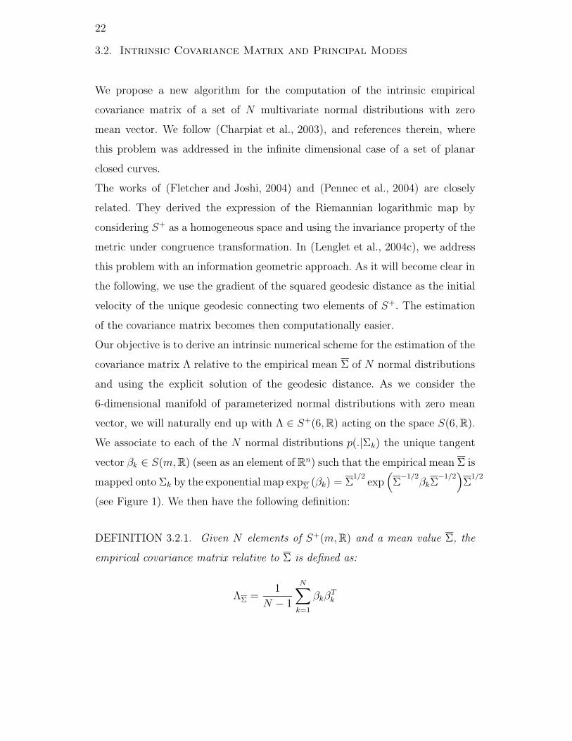
(see Figure 1). We then have the following definition:

DEFINITION 3.2.1. Given N elements of S+(m,R) and a mean value Σ, the

empirical covariance matrix relative to Σ is defined as:

ΛΣ =1

N − 1

N∑

k=1

βkβTk

23

Figure 1. Depiction of the velocity field βk at the empirical mean Σ (The black lines represent

the geodesics between each pair (Σk,Σ) and the green arrows are the associated initial tangent

vectors βk)

We identify the βk with the opposite of the gradient of the squared geodesic

distance function ∇D2(Σk,Σ). As detailed in (Moakher, 2005), we have:

∇D2(Σk,Σ) = Σ log(Σ−1k Σ)

Once we have computed Λ, it is fairly easy and instructive, in order to further

understand the structure of our subset of normal distributions, to compute

the eigenvalues and eigenvectors of the covariance matrix. Fletcher and Joshi

(Fletcher et al., 2003) generalized the notion of Principal Component Analysis

to Lie groups by seeking geodesic submanifolds, by analogy with the lower-

dimensional linear subspaces of PCA, that maximize the projected variance of

the data. They successfully applied this method to diffusion tensor datasets in

(Fletcher and Joshi, 2004). This actually amounts to characterizing the tangent

space at the mean element Σ through classical PCA in order to construct an

orthogonal basis of tangent vectors vk, k = 1, ..., d ≤ n that can be used to

generate l-dimensional subspaces Vl = span(v1, ..., vl), l ≤ n that maximize the

projected variance. The vk are defined as the set of eigenvectors of the covariance

matrix Λ. However, since we have the geodesics equation in S+, we have a closed-

form expression to generate elements of any geodesic submanifold Hk defined as

the exponential mapping of the Vk.

24

Indeed, we can define any linear combination of the vk, v =∑d

k=1 αkvk ∈ S(m,R)

and then compute the unique element C of S+(m,R) reached by following the

geodesic emanating from Σ in the direction v and computed as:

C = Σ1/2

exp

(Σ−1/2

(d∑

k=1

αkvk

)Σ−1/2

)Σ

1/2(15)

It is straightforward to apply our definition of the covariance matrix Λ to com-

pute those principal modes. In the next section, we will see how the covari-

ance matrix must be modified, because of the manifold curvature, to yield the

concentration matrix and an approximated continuous Gaussian pdf on S+.

3.3. A Generalized Normal Law between Multivariate Normal

Distributions of Zero Mean Vector

Our last contribution uses the various quantities derived up to that point and

fully exploits the information they provide in order to derive the expression of

a normal law on S+. We proceed by using the appropriate quantities in the

generalization of the normal distribution to Riemannian manifolds proposed in

(Pennec, 2004) for sufficiently concentrated probability density functions, e.g. for

small covariance matrices. The main idea of this work was to correctly deal with

the curvature of the manifold since it modifies the definition of the concentration

matrix γ. In Euclidean space, this matrix is simply the inverse of the covariance

matrix Λ. On a Riemannian manifold, we must incorporate the contribution of

the Ricci curvature tensor R. We have the following theorem :

THEOREM 3.3.1. The generalized normal distribution in S+(m,R) for a co-

variance matrix Λ of small variance σ2 = tr(Λ) is of the form:

q(Σ|Σ,Λ) =1 +O(σ3) + ε(σ

ξ)

√(2π)m(m+1)/2|Λ|

exp−βTγβ

2∀Σ ∈ S+(m,R)

25

Σ is computed as in section 3.1.

β is defined as −∇D2(Σ,Σ) = −Σ log(Σ−1Σ) and expressed in vector form.

The concentration matrix is γ = Λ−1−R/3 +O(σ) + ε(σξ), with Λ defined as in

section 3.2 and R as in section 2.2.1 (both are computed at location Σ).

ξ is the injectivity radius at Σ and ε is such that lim0+ x−ωε(x) = 0 ∀ω ∈ R+.

It should be clear now that, in section 3.2, the contribution of the Ricci curvature

tensor was not taken into account and the concentration matrix was identified

with the inverse of the empirical covariance matrix Λ. When approximating

a continuous probability density function such as q(Σ|Σ,Λ) in the theorem

above, equation 5 can be used to compute the tensor R and, hence, to modify

the covariance matrix in order to reflect the local curvature properties of the

manifold.

4. Applications, Diffusion Tensor Images Processing

We now would like to propose three interesting applications of the theory we

just developed, our major purpose being diffusion tensor images processing. The

first application is very simple and shows how to consistently generate a set of

random covariance matrices so that they follow our generalized normal law. The

second application deals with the issue of the estimation of diffusion tensors.

We will show how to derive robust gradient descent algorithms that naturally

ensure the symmetry and positiveness of the estimated tensors by evolving in S+.

Finally, we will embed our statistical framework into a level-set based algorithm

to segment anatomical structures of interest in the brain white matter from

diffusion tensor images.

26

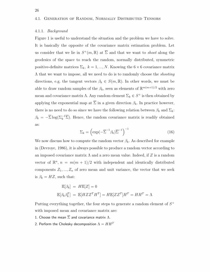
4.1. Generation of Random, Normally Distributed Tensors

4.1.1. Background

Figure 1 is useful to understand the situation and the problem we have to solve.

It is basically the opposite of the covariance matrix estimation problem. Let

us consider that we lie in S+(m,R) at Σ and that we want to shoot along the

geodesics of the space to reach the random, normally distributed, symmetric

positive-definite matrices Σk, k = 1, ..., N . Knowing the 6× 6 covariance matrix

Λ that we want to impose, all we need to do is to randomly choose the shooting

directions, e.g. the tangent vectors βk ∈ S(m,R). In other words, we must be

able to draw random samples of the βk, seen as elements of Rm(m+1)/2 with zero

mean and covariance matrix Λ. Any random element Σk ∈ S+ is then obtained by

applying the exponential map at Σ in a given direction βk. In practice however,

there is no need to do so since we have the following relation between βk and Σk:

βk = −Σ log(Σ−1k Σ). Hence, the random covariance matrix is readily obtained

as:

Σk =(

exp(−Σ−1βk)Σ

−1)−1

(16)

We now discuss how to compute the random vector βk. As described for example

in (Devroye, 1986), it is always possible to produce a random vector according to

an imposed covariance matrix Λ and a zero mean value. Indeed, if Z is a random

vector of Rn, n = m(m + 1)/2 with independent and identically distributed

components Z1, ..., Zn of zero mean and unit variance, the vector that we seek

is βk = HZ, such that:

E[βk] = HE[Z] = 0

E[βkβTk ] = E[HZZTHT ] = HE[ZZT ]HT = HHT = Λ

Putting everything together, the four steps to generate a random element of S+

with imposed mean and covariance matrix are:

1. Choose the mean Σ and covariance matrix Λ.

2. Perform the Cholesky decomposition Λ = HHT

27

3. Generate a random vector Z ∈ Rn as described above and form βk = HZ

4. Compute Σk =(

exp(−Σ−1βk)Σ

−1)−1

with βk reshaped as an element of S(m,R).

We illustrate this method with the following example and use it to demonstrate the

performance of the numerical schemes described in section 3.

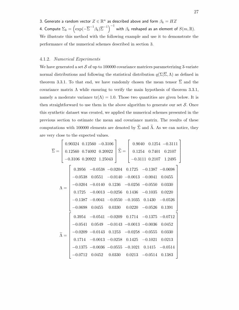
4.1.2. Numerical Experiments

We have generated a set S of up to 100000 covariance matrices parameterizing 3-variate

normal distributions and following the statistical distribution q(Σ|Σ,Λ) as defined in

theorem 3.3.1. To that end, we have randomly chosen the mean tensor Σ and the

covariance matrix Λ while ensuring to verify the main hypothesis of theorem 3.3.1,

namely a moderate variance tr(Λ) = 1.0. Those two quantities are given below. It is

then straightforward to use them in the above algorithm to generate our set S. Once

this synthetic dataset was created, we applied the numerical schemes presented in the

previous section to estimate the mean and covariance matrix. The results of these

computations with 100000 elements are denoted by Σ and Λ. As we can notice, they

are very close to the expected values.

Σ =

0.90324 0.12560 −0.3106

0.12560 0.74092 0.20922

−0.3106 0.20922 1.25043

Σ =

0.9040 0.1254 −0.3111

0.1254 0.7401 0.2107

−0.3111 0.2107 1.2495

Λ =

0.3956 −0.0538 −0.0204 0.1725 −0.1387 −0.0698

−0.0538 0.0551 −0.0140 −0.0013 −0.0041 0.0455

−0.0204 −0.0140 0.1236 −0.0256 −0.0550 0.0330

0.1725 −0.0013 −0.0256 0.1436 −0.1035 0.0220

−0.1387 −0.0041 −0.0550 −0.1035 0.1430 −0.0526

−0.0698 0.0455 0.0330 0.0220 −0.0526 0.1391

Λ =

0.3954 −0.0541 −0.0209 0.1714 −0.1375 −0.0712

−0.0541 0.0549 −0.0143 −0.0013 −0.0036 0.0452

−0.0209 −0.0143 0.1253 −0.0258 −0.0555 0.0330

0.1714 −0.0013 −0.0258 0.1425 −0.1021 0.0213

−0.1375 −0.0036 −0.0555 −0.1021 0.1415 −0.0514

−0.0712 0.0452 0.0330 0.0213 −0.0514 0.1383

28

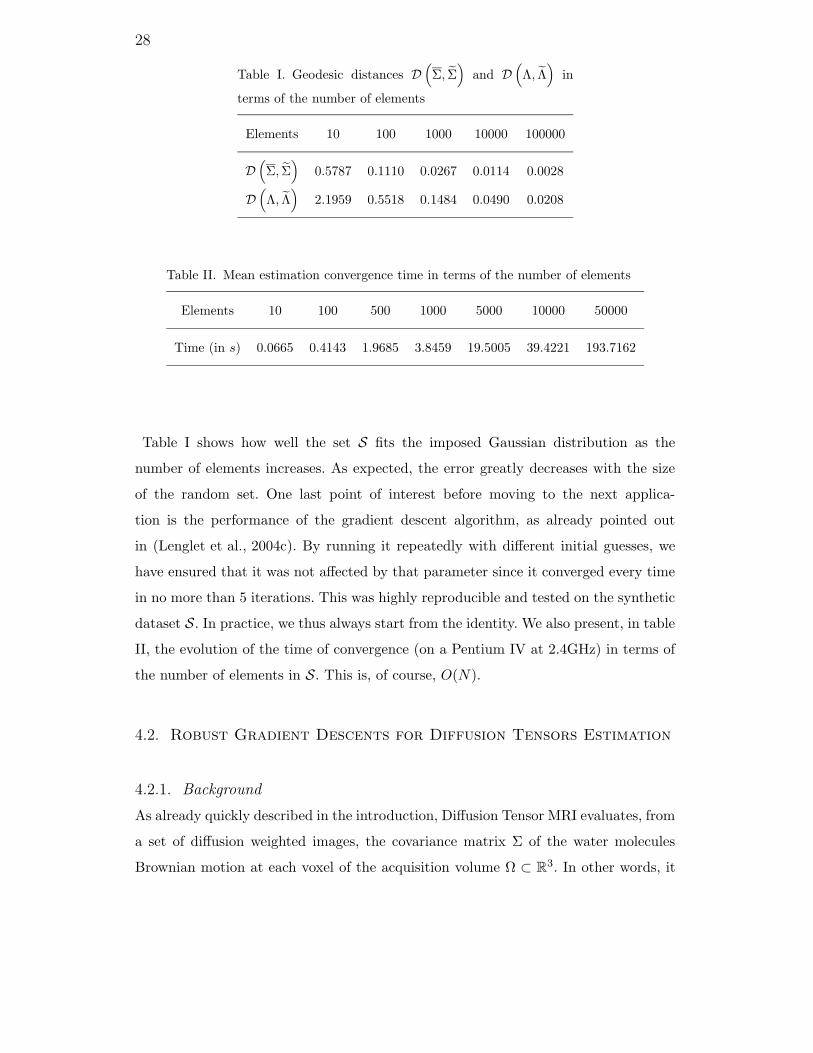
Table I. Geodesic distances D(

Σ, Σ)

and D(

Λ, Λ)

in

terms of the number of elements

Elements 10 100 1000 10000 100000

D(

Σ, Σ)

0.5787 0.1110 0.0267 0.0114 0.0028

D(

Λ, Λ)

2.1959 0.5518 0.1484 0.0490 0.0208

Table II. Mean estimation convergence time in terms of the number of elements

Elements 10 100 500 1000 5000 10000 50000

Time (in s) 0.0665 0.4143 1.9685 3.8459 19.5005 39.4221 193.7162

Table I shows how well the set S fits the imposed Gaussian distribution as the

number of elements increases. As expected, the error greatly decreases with the size

of the random set. One last point of interest before moving to the next applica-

tion is the performance of the gradient descent algorithm, as already pointed out

in (Lenglet et al., 2004c). By running it repeatedly with different initial guesses, we

have ensured that it was not affected by that parameter since it converged every time

in no more than 5 iterations. This was highly reproducible and tested on the synthetic

dataset S. In practice, we thus always start from the identity. We also present, in table

II, the evolution of the time of convergence (on a Pentium IV at 2.4GHz) in terms of

the number of elements in S. This is, of course, O(N).

4.2. Robust Gradient Descents for Diffusion Tensors Estimation

4.2.1. Background

As already quickly described in the introduction, Diffusion Tensor MRI evaluates, from

a set of diffusion weighted images, the covariance matrix Σ of the water molecules

Brownian motion at each voxel of the acquisition volume Ω ⊂ R3. In other words, it

29

approximates the probability density function modeling the motion of water molecules

by a 3-variate normal distribution of zero mean vector x ∈ R3.

The estimation of the field of 3×3 symmetric positive-definite matrices Σ is performed

by using the Stejskal-Tanner equation (Stejskal and Tanner, 1965) for anisotropic dif-

fusion. This equation relates the magnetic resonance signal attenuation to the diffusion

tensor and the sequence parameters:

Sk(w) = S0(w) exp (−bgTk Σ(w)gk) ∀w ∈ Ω, k = 1, ...,M (17)

gk are the M normalized non-collinear gradient directions corresponding to each dif-

fusion weighted image (DWI) Sk and b is the diffusion weighting factor. Moreover

a regular T2-weighted image S0 must be acquired. Many approaches have already

been derived to estimate the diffusion tensors Σ from a set of DWI (at least 6) and

references can be found for example in (Westin et al., 2002), (Mangin et al., 2002),

(Wang et al., 2004), (Tschumperle and Deriche, 2003).

Following (Tschumperle and Deriche, 2003), we will show how intrinsic numerical schemes

in S+, similar to the gradient descent proposed to estimate the empirical mean, can be

derived. We will not incorporate any smoothness constraint on the tensor field but the

major advantage of this approach is to naturally evolve in S+. Compared to simple

least squares, where the tensor components are obtained by solving a linear system

derived from the M Stejskal-Tanner equations, this ensures the symmetry and positive

definiteness of each diffusion tensor. Moreover, the combination of robust regression

methods with this intrinsic gradient descent enables us to propose a more reliable and

efficient estimation method.

We seek to minimize the following objective function at each w ∈ Ω by searching for

the optimal Σ ∈ S+:

E(S0, ..., SM ) =M∑

k=1

ψ

(1

blnSkS0

+ gTk Σgk

)

where ψ : R→ R is a real-valued functional that, in the M-estimators framework, tries

to reduce the effect of outliers by replacing the classical squared residual ψ(rk) = r2k/2

by another function with a unique minimum at zero and chosen to be less increasing

than the square function (see for example (Zhang, 1997)). In order to minimize this

energy through a gradient descent, we follow exactly the same idea as for the mean

30

and thus need to compute the gradient of E. We recall that, given a smooth function

f : Σ ∈ S+ 7→ f(Σ) ∈ R, its derivative in the direction v at Σ:

Df(Σ)v = lims→0

f(Σ + sv)− f(Σ)

s

and the inner product 〈., .〉Σ, the gradient ∇f exists and is unique by the Riesz-Frechet

theorem. It is defined by the relationship:

Df(Σ)v =df(Σ(t))

dt

∣∣∣∣t=0

= 〈∇f(Σ(t)), v〉Σ(t)

∣∣t=0

where Σ(t) is the unique geodesic starting from Σ(0) = Σ in the direction v = Σ(0).

With the residual rk(Σ(t)) = 1b ln Sk

S0+ gTk Σ(t)gk we have by the chain rule:

dψ(rk(Σ(t)))

dt

∣∣∣∣t=0

=dψ(rk)

drk

∣∣∣∣t=0

m∑

i,j=1

∂rk(Σ(t))

∂Σij(t)

dΣij(t)

dt

∣∣∣∣∣∣t=0

=dψ(rk)

drktr

(drk(Σ(t))

dΣ(t)

(dΣ(t)

dt

)T)∣∣∣∣∣t=0

= ψ′(rk)tr(gkg

Tk Σ(0)

)

= ψ′(rk)tr(

Σ−1ΣgkgTk ΣTΣ−T Σ(0)

)

= ψ′(rk)tr(

Σ−1Σgk (Σgk)T Σ−1Σ(0)

)

Hence, ∇ψ(rk(Σ)) = ψ′(rk(Σ))Σgk (Σgk)T ∈ S(m,R) and finally:

∇E =M∑

k=1

ψ′(rk(Σ))Σgk (Σgk)T

We can use the intrinsic step-forward integrator of proposition 3.1.1 to obtain the

gradient descent (which depends on the function ψ) to be carried out at each voxel w

of the volume Ω:

Σl+1 = Σ1/2l exp (−dsΣ−1/2

l ∇EΣ−1/2l )Σ

1/2l

= Σ1/2l exp

(−dsΣ−1/2

l

(M∑

k=1

ψ′(rk(Σl))Σlgk (Σlgk)T

)Σ−1/2l

)Σ

1/2l

4.2.2. Numerical Experiments

The numerical scheme given above has been implemented for various well-known

functions ψ, namely the Cauchy, Fair, Huber and Tukey M-estimators, and their

31

associated influence function ψ′(rk). In practice however, we use Huber’s function since

this estimator is very satisfactory with the classical tuning constant c = 1.2107 which

allows to achieve an asymptotic efficiency of 95% on the standard normal distribution.

The combination of the M-estimators with our intrinsic gradient descent has shown

to be far less sensitive to noise than the classical least squares and to naturally avoid

the estimation of non-positive definite tensors. By applying a least squares estimation

procedure on various DTI datasets, we usually obtained a few thousands non-positive

definite tensors. This is obviously always corrected by our method. We however need

to point out the higher computational overhead of the gradient descent, by comparison

to least squares which are almost instantaneous.

To prove the robustness of our method, we have generated a synthetic dataset con-

sisting of a 50 × 50 tensor field divided in 2 regions: the background and a 20 × 20

square area centered at pixel (25, 25). Each region was assigned with a distinct mean

tensor and covariance matrix. We used the method proposed in the previous section to

randomly choose the tensors belonging to each region. They follow 2 different normal

distributions and thus span a wide range of tensor configurations, which is desirable to

consistently evaluate the performance of our estimator. The tensor field is presented

on figure 2 left where each of the 3 × 3 matrix is depicted as a 3D ellipsoid. We

created an artificial set of diffusion weighted images from this tensor field by using the

Stejskal-Tanner equation 17. S0 was taken to be constant and equal to 10 everywhere

while the b-factor was set to 1s.mm−2. Finally, 12 gradient directions gk were used and

given by the vertices of the icosahedron. The images were corrupted by a Gaussian

noise with variance 0.52 (images intensity amplitude was approximately [2, 10]).

We performed the estimation of the diffusion tensors by least squares and by gradient

descent with 600 iterations and a time step ds = 0.2. It was then possible to compare

the accuracy of the reconstructed tensor fields by computing the geodesic distance

between the tensor estimates and the ground-truth data at each voxel. Table III sum-

marizes the results and is a striking proof of the gradient descent approach superiority.

We also applied our approach to a real set of diffusion weighted images. They were

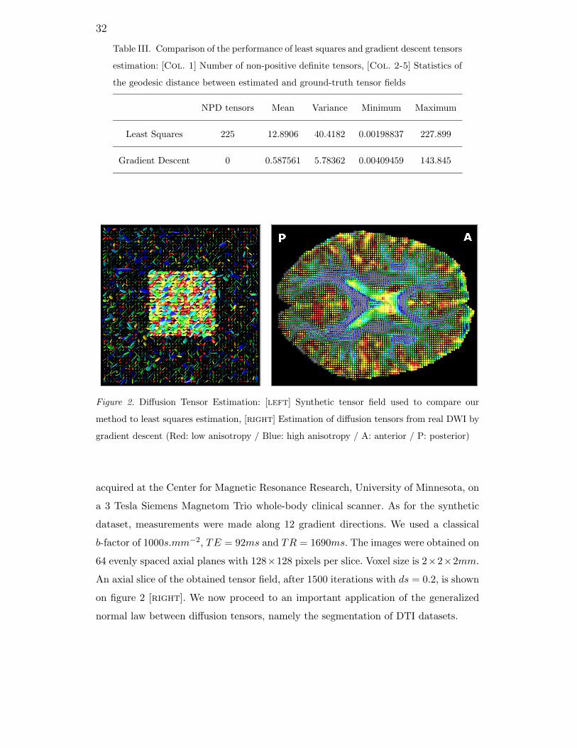
32

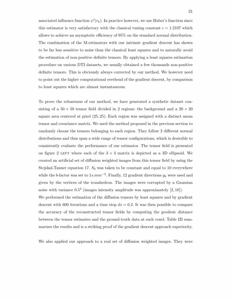
Table III. Comparison of the performance of least squares and gradient descent tensors

estimation: [Col. 1] Number of non-positive definite tensors, [Col. 2-5] Statistics of

the geodesic distance between estimated and ground-truth tensor fields

NPD tensors Mean Variance Minimum Maximum

Least Squares 225 12.8906 40.4182 0.00198837 227.899

Gradient Descent 0 0.587561 5.78362 0.00409459 143.845

Figure 2. Diffusion Tensor Estimation: [left] Synthetic tensor field used to compare our

method to least squares estimation, [right] Estimation of diffusion tensors from real DWI by

gradient descent (Red: low anisotropy / Blue: high anisotropy / A: anterior / P: posterior)

acquired at the Center for Magnetic Resonance Research, University of Minnesota, on

a 3 Tesla Siemens Magnetom Trio whole-body clinical scanner. As for the synthetic

dataset, measurements were made along 12 gradient directions. We used a classical

b-factor of 1000s.mm−2, TE = 92ms and TR = 1690ms. The images were obtained on

64 evenly spaced axial planes with 128×128 pixels per slice. Voxel size is 2×2×2mm.

An axial slice of the obtained tensor field, after 1500 iterations with ds = 0.2, is shown

on figure 2 [right]. We now proceed to an important application of the generalized

normal law between diffusion tensors, namely the segmentation of DTI datasets.

33

4.3. Statistical and Level-Set based DTI Segmentation

4.3.1. Background

It is well-known that normal brain functions require specific cortical regions to commu-

nicate through fiber pathways. Most of the existing techniques addressing the issue of

the anatomical connectivity mapping work on a fiber-wise basis. However, it should be

pointed out that all those relying on DTI, and not on HARDI (high angular resolution

diffusion imaging (Tuch et al., 2003)), cannot overcome the fiber crossing problem.

Adding to that, very few techniques take into account the global coherence existing

among fibers of a given tract. For example, Corouge et al. (Corouge et al., 2004)

have proposed to cluster and align fibers but their method relies on the classical

streamline approach to fiber tracking (Mori et al., 1999) which is known to be very

sensible to noise and unreliable in areas of fiber crossings. In this section, we do not

address the fiber crossing problem but rather propose a statistical and level-set based

DTI segmentation algorithm to extract fiber bundles. Contrary to the methods in

(Zhukov et al., 2003), (Wiegell et al., 2003), (Feddern et al., 2004),

(Wang and Vemuri, 2004b), (Wang and Vemuri, 2004a), and (Jonasson et al., 2004),

our approach is grounded on the statistical characterization of the regions to be

extracted. A level-set framework is setup to evolve a surface while maximizing the

likelihood of the region of interest.

Let B be the optimal boundary between the object to extract Ω1 and the background

Ω2 so that Ω = Ω1∪Ω2. We introduce the level-set function (Dervieux and Thomasset, 1979),

(Dervieux and Thomasset, 1980) and (Osher and Sethian, 1988) φ : Ω → R, defined

as follows:

φ(w) = 0, if w ∈ Bφ(w) = DEucl(w,B), if w ∈ Ω1

φ(w) = −DEucl(w,B), if w ∈ Ω2.

where DEucl(w,B) stands for the Euclidean distance between w and B. Furthermore,

let Hε(.) and δε(.) be regularized versions of the Heaviside and Dirac functions as

defined in (Chan and Vese, 1999). If we denote by q1 and q2 the normal probability

density functions modeling the distributions of the diffusion tensors respectively in Ω1

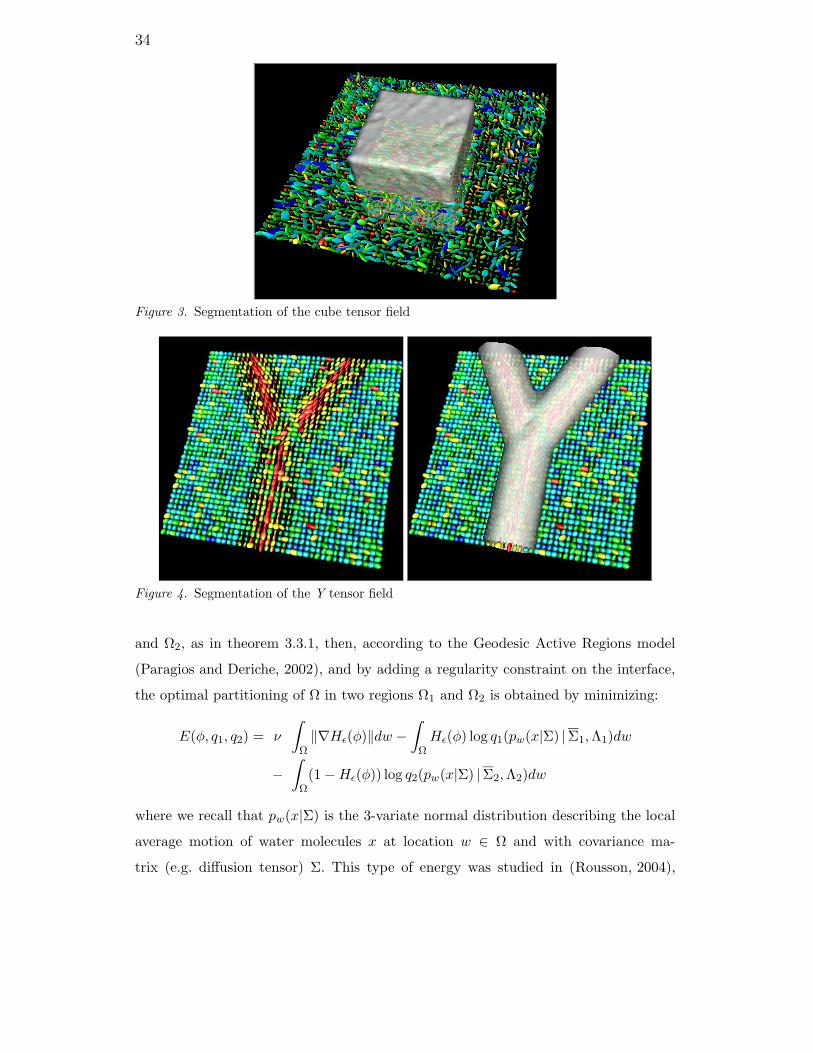
34

Figure 3. Segmentation of the cube tensor field

Figure 4. Segmentation of the Y tensor field

and Ω2, as in theorem 3.3.1, then, according to the Geodesic Active Regions model

(Paragios and Deriche, 2002), and by adding a regularity constraint on the interface,

the optimal partitioning of Ω in two regions Ω1 and Ω2 is obtained by minimizing:

E(φ, q1, q2) = ν

∫

Ω‖∇Hε(φ)‖dw −

∫

ΩHε(φ) log q1(pw(x|Σ) |Σ1,Λ1)dw

−∫

Ω(1−Hε(φ)) log q2(pw(x|Σ) |Σ2,Λ2)dw

where we recall that pw(x|Σ) is the 3-variate normal distribution describing the local

average motion of water molecules x at location w ∈ Ω and with covariance ma-

trix (e.g. diffusion tensor) Σ. This type of energy was studied in (Rousson, 2004),

35

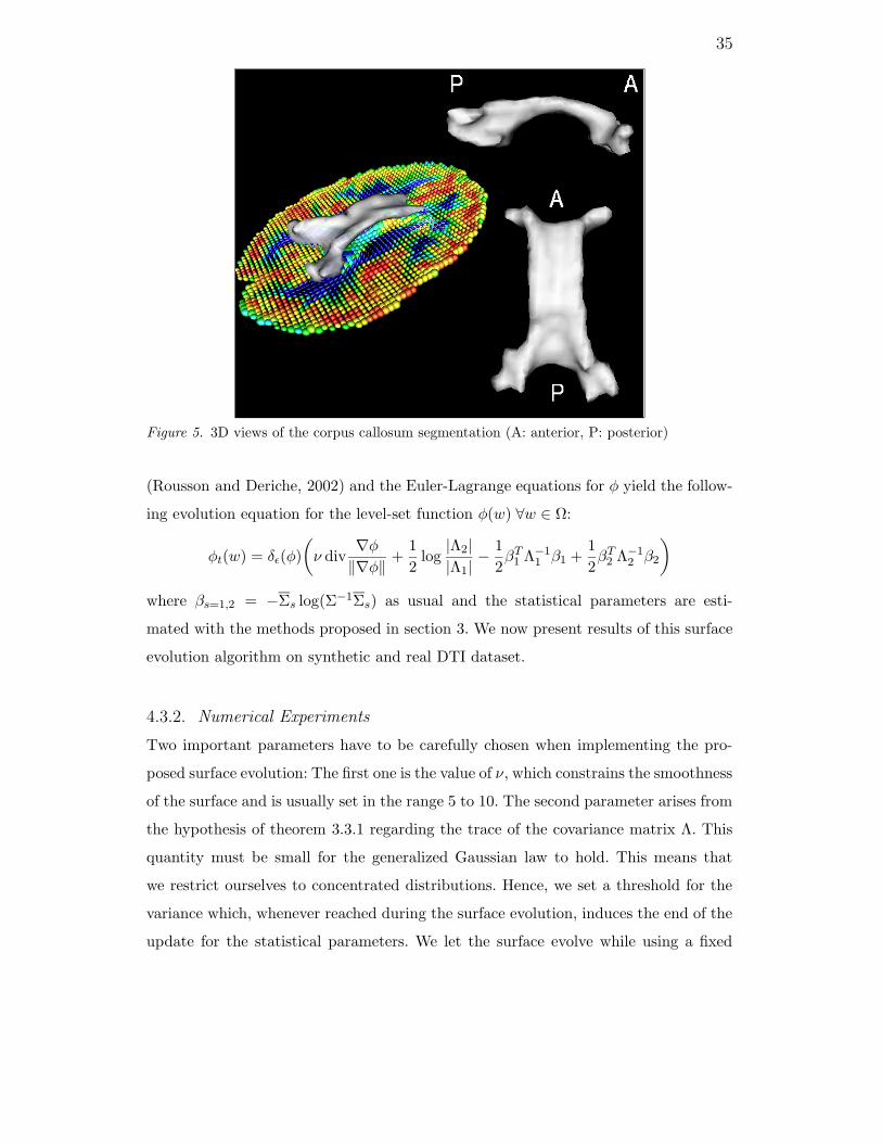
Figure 5. 3D views of the corpus callosum segmentation (A: anterior, P: posterior)

(Rousson and Deriche, 2002) and the Euler-Lagrange equations for φ yield the follow-

ing evolution equation for the level-set function φ(w) ∀w ∈ Ω:

φt(w) = δε(φ)

(ν div

∇φ‖∇φ‖ +

1

2log|Λ2||Λ1|

− 1

2βT1 Λ−1

1 β1 +1

2βT2 Λ−1

2 β2

)

where βs=1,2 = −Σs log(Σ−1Σs) as usual and the statistical parameters are esti-

mated with the methods proposed in section 3. We now present results of this surface

evolution algorithm on synthetic and real DTI dataset.

4.3.2. Numerical Experiments

Two important parameters have to be carefully chosen when implementing the pro-

posed surface evolution: The first one is the value of ν, which constrains the smoothness

of the surface and is usually set in the range 5 to 10. The second parameter arises from

the hypothesis of theorem 3.3.1 regarding the trace of the covariance matrix Λ. This

quantity must be small for the generalized Gaussian law to hold. This means that

we restrict ourselves to concentrated distributions. Hence, we set a threshold for the

variance which, whenever reached during the surface evolution, induces the end of the

update for the statistical parameters. We let the surface evolve while using a fixed

36

mean and covariance matrix to model the distribution of the tensors in Ω1 and Ω2.

Finally, it turns out that, within the limits of theorem 3.3.1, the term involving the

Ricci tensor R/3 can be neglected since we found a difference of at least 2 orders of

magnitude between Λ−1 and R/3.

In order to validate the algorithm on ground-truth data, we have extended the syn-

thetic tensor field of the previous section to a 50 × 50 × 50 3D volume composed of

a background and a 20 × 20 × 20 cube centered at location (25, 25, 25). The tensors

in these two regions follow distinct normal distributions with different means and

covariance matrices. We initialized the segmentation process with a small sphere inside

the 20× 20× 20 cube and were able to extract the whole object as shown on figure 3.

We have also generated a more complex synthetic 40× 40× 40 dataset composed by a

diverging tensor field and a background of isotropic tensors (see figure 4). Within the

Y shape, tensors fractional anisotropy decreases as we get away from the center-line.

Noise was added to the original dataset by using the method presented in section 4.1.

Our method was able to extract the Y shape after about 30 iterations.

We also applied the algorithm to extract the corpus callosum from various real diffusion

tensors datasets estimated by our gradient descent method. The corpus callosum is

a very important part of the brain white matter that connects areas of each hemi-

spheres together. Diffusion weighted images were acquired at the Center for Magnetic

Resonance Research, University of Minnesota. We used 81 gradient directions so that

the resulting tensors were accurately estimated. With a b-factor of 1000s.mm−2,

TE = 109ms and TR = 5100ms, the images were obtained on 24 evenly spaced

axial planes with 64 × 64 pixels per slice. Voxel size is 3 × 3 × 3mm. By initializ-

ing our segmentation algorithm with a small sphere within the corpus callosum and

evolving it as described above, we managed to extract the volume presented on figure

5. Despite the relatively low resolution of the dataset, the algorithm performs quite

well thanks to the good classification power of the generalized normal law and to the

level-set implementation. We also applied our segmentation scheme to a dataset used

in the previous section. The final surface is presented on figure 6. Visual inspection of

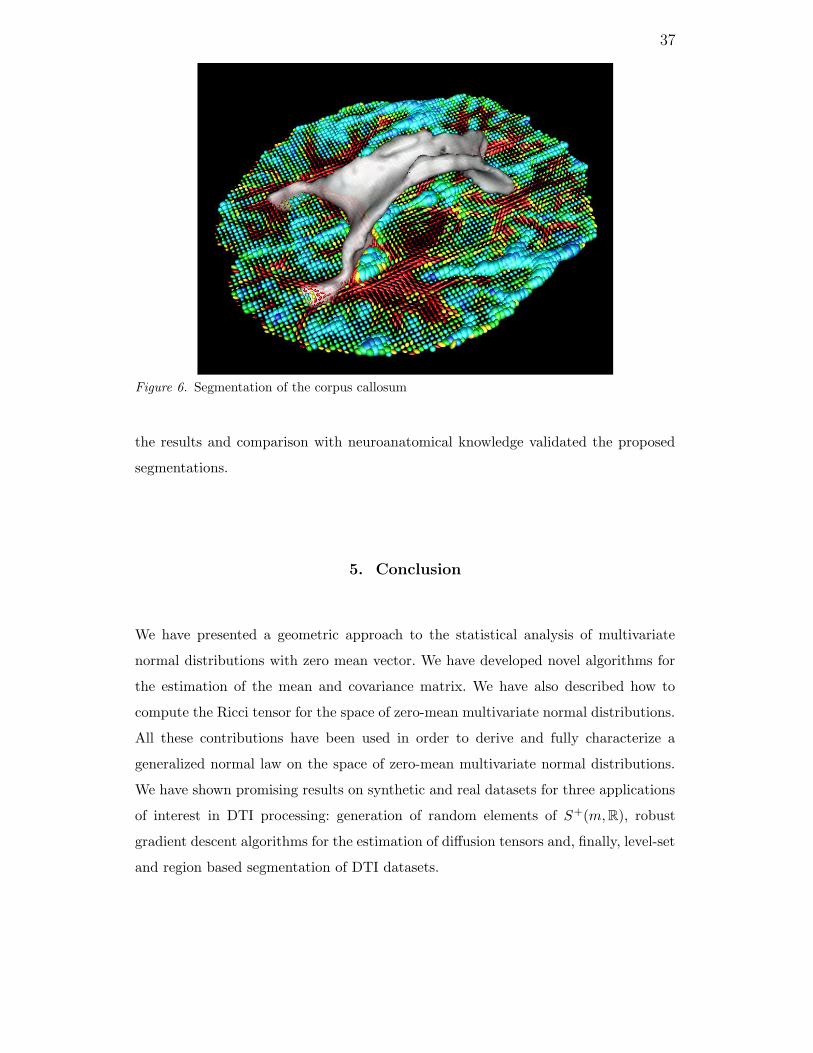
37

Figure 6. Segmentation of the corpus callosum

the results and comparison with neuroanatomical knowledge validated the proposed

segmentations.

5. Conclusion

We have presented a geometric approach to the statistical analysis of multivariate

normal distributions with zero mean vector. We have developed novel algorithms for

the estimation of the mean and covariance matrix. We have also described how to

compute the Ricci tensor for the space of zero-mean multivariate normal distributions.

All these contributions have been used in order to derive and fully characterize a

generalized normal law on the space of zero-mean multivariate normal distributions.

We have shown promising results on synthetic and real datasets for three applications

of interest in DTI processing: generation of random elements of S+(m,R), robust

gradient descent algorithms for the estimation of diffusion tensors and, finally, level-set

and region based segmentation of DTI datasets.

38

6. Acknowledgments

The authors would like to thank G. Sapiro (Department of Electrical and Computer

Engineering, University of Minnesota, Minneapolis, USA), S. Lehericy and K. Ugur-

bil (Center for Magnetic Resonance Research, University of Minnesota, Minneapolis,

USA) for their valuable comments and their expertise to acquire the data used in this

paper. This research was partially supported by grants NSF-0404617 US-France (IN-

RIA) Cooperative Research, NIH-R21-RR019771, NIH-RR08079, the MIND Institute,

the Keck foundation and the Region Provence-Alpes-Cote d’Azur.

References

Amari, S.: 1990, Differential-Geometrical Methods in Statistics, Lectures Notes in Statistics.

Springer-Verlag.

Atkinson, C. and A. Mitchell: 1981, ‘Rao’s Distance Measure’. Sankhya: The Indian Journal

of Stats. 43(A), 345–365.

Barbaresco, F., C. Germond, and N. Rivereau: 2004, ‘Advanced Radar Diffusive CFAR based

on Geometric Flow and Information Theories and its Extension for Doppler and Polari-

metric Data’. In: Proc. International Conference on Radar Systems, Toulouse, France,

2004

Basser, P., J. Mattiello, and D. Le Bihan: 1994, ‘MR Diffusion Tensor Spectroscopy and

Imaging’. Biophysica 66, 259–267.

Basser, P. and S. Pajevic: 2003, ‘A normal distribution for tensor-valued random variables:

Applications to Diffusion Tensor MRI’. IEEE Transactions on Medical Imaging 22(7),

785–794.

Burbea, J.: 1986, ‘Informative Geometry of Probability Spaces’. Expositiones Mathematica 4,

347–378.

Burbea, J. and C. Rao: 1982, ‘Entropy Differential Metric, Distance and Divergence Measures

in Probability Spaces: A Unified Approach’. Journal of Multivariate Analysis 12, 575–596.

Calvo, M. and J. Oller: 1991, ‘An Explicit Solution of Information Geodesic Equations for the

Multivariate Normal Model’. Statistics and Decisions 9, 119–138.

39

Calvo, M. and J. Oller: 1990, ‘A Distance between Multivariate Normal Distributions Based

in an Embedding into a Siegel Group’. Journal of Multivariate Analysis 35, 223–242

Caticha, A.: 2000, ‘Change, Time and Information Geometry’. In: Proc. Bayesian Inference

and Maximum Entropy Methods in Science and Engineering, Vol. 568. pp. 72–82.

Chan, T. and L. Vese: 1999, ‘An active contour model without edges’. In: Scale-Space Theories

in Computer Vision, Vol. 1682 of Lecture Notes in Computer Science. Springer–Verlag, pp.

141–151.

Charpiat, G., O. Faugeras, and R. Keriven: 2003, ‘Approximations of shape metrics and

application to shape warping and shape statistics’. Research Report 4820, INRIA, Sophia

Antipolis.

Chefd’hotel, C., D. Tschumperle, R. Deriche, and O. Faugeras: 2004, ‘Regularizing Flows for

Constrained Matrix-Valued Images’. Journal of Mathematical Imaging and Vision 20(1-2),

147–162.

Corouge, I., S. Gouttard, and G. Gerig: 2004, ‘A Statistical Shape Model of Individual Fiber

Tracts Extracted from Diffusion Tensor MRI’. In: Proc. Seventh Intl. Conf. on Medi-

cal Image Computing and Computer Assisted Intervention, Vol. 3217 of Lecture Notes in

Computer Science, pp. 671–679.

Dervieux, A. and F. Thomasset: 1979, ‘A finite element method for the simulation of Rayleigh-

Taylor instability’. Lecture Notes in Mathematics 771, 145–159.

Dervieux, A. and F. Thomasset: 1980, ‘Multifluid incompressible flows by a finite element

method’. In: Proc. Seventh Intl. Conf. on Numerical Methods in Fluid Dynamics, Vol. 141

of Lecture Notes in Physics, pp. 158–163.

Devroye, L.: 1986, Non-Uniform Random Variate Generation. Springer–Verlag.

Eriksen, P.: 1986, ‘Geodesics Connected with the Fisher Metric on the Multivariate Manifold’.

Preprint 86-13, Institute of Electronic Systems, Aalborg University, Denmark.

Feddern, C., J. Weickert, B. Burgeth, and M. Welk: 2004, ‘Curvature-driven PDE methods

for matrix-valued images’. Technical Report 104, Department of Mathematics, Saarland

University, Saarbrucken, Germany.

Fletcher, P. and S. Joshi: 2004, ‘Principal Geodesic Analysis on Symmetric Spaces: Statistics of

Diffusion Tensors’. In: Proc. ECCV’04 Workshop Computer Vision Approaches to Medical

Image Analysis, Vol. 3117 of Lecture Note in Computer Science, pp. 87–98.

Fletcher, P. T., C. Lu, and S. Joshi: 2003, ‘Statistics of shape via principal geodesic analysis

on Lie groups’. In: Proc. IEEE Conf. on Computer Vision and Pattern Recognition, pp.

95–101.

40

Forstner, W. and B. Moonen: 1999, ‘A metric for covariance matrices’. Technical report,

Stuttgart University, Dept. of Geodesy and Geoinformatics.

Frechet, M.: 1948, ‘Les elements aleatoires de nature quelconque dans un espace distancie.

Annales de l’Institut Henri Poincare X(IV), 215–310.

Jonasson, L., X. Bresson, P. Hagmann, O. Cuisenaire, R. Meuli, and J. Thiran:2004, ‘White

matter fiber tract segmentation in DT-MRI using geometric flows’. Medical Image Analysis,

9(3):223–236, June 2005.

Karcher, H.: 1977, ‘Riemannian centre of mass and mollifier smoothing’. Comm. Pure Appl.

Math 30, 509–541.

Kendall, W.: 1990, ‘Probability, convexity, and harmonic maps with small image i: uniqueness

and fine existence’. Proc. London Math. Soc. 61(2), 371–406.

Le Bihan, D., E. Breton, D. Lallemand, P. Grenier, E. Cabanis, and M. Laval-Jeantet: 1986,

‘MR Imaging of Intravoxel Incoherent Motions: Application to Diffusion and Perfusion in

Neurologic Disorders’. Radiology pp. 401–407.

Lenglet, C., R. Deriche, and O. Faugeras: 2004a, ‘Inferring White Matter Geometry from

Diffusion Tensor MRI: Application to Connectivity Mapping’. In: Proc. Eighth European

Conference on Computer Vision, Vol. 3024 of Lecture Notes in Computer Science, pp.

127–140.

Lenglet, C., M. Rousson, and R. Deriche: 2004b, ‘Segmentation of 3D Probability Density

Fields by Surface Evolution: Application to diffusion MRI’. In: Proc. Seventh Intl. Conf.

on Medical Image Computing and Computer Assisted Intervention, Vol. 3216 of Lecture

Notes in Computer Science, pp.18–25.

Lenglet, C., M. Rousson, R. Deriche, O. Faugeras, S. Lehericy and K. Ugurbil: 2005, ‘A

Riemannian Approach to Diffusion Tensor Images Segmentation’. In: Proc. Information

Processing in Medical Imaging, Glenwood Springs, CO, USA, July 2005.

Lenglet, C., M. Rousson, R. Deriche, and O. Faugeras: 2004c, ‘Statistics on Multivariate

Normal Distributions: A Geometric Approach and its Application to Diffusion Tensor MRI’.

Research Report 5242, INRIA, Sophia Antipolis.

Madsen, L.: 1978, ‘The geometry of statistical models’. Ph.D. thesis, University of Copenhagen.

Mahalanobis, P.: 1936, ‘On the generalized distance in statistics’. Proceedings of the Indian

National Institute Science 2, 49–55.

Mangin, J., C. Poupon, C. Clark, and I. Le Bihan, D.and Bloch: 2002, ‘Distortion correction

and robust tensor estimation for MR diffusion imaging’. Medical Image Analysis 6(3),

191–198.

41

Moakher, M.: 2002, ‘Means and Averaging in the Group of Rotations’. SIAM J. Matrix Anal.

Appl. 24(1), 1–16.

Moakher, M.: 2005, ‘A differential geometric approach to the geometric mean of symmetric

positive-definite matrices’. SIAM J. Matrix Anal. Appl. 26(3), 735–747

Mori, S., B. Crain, V. Chacko, and P. V. Zijl: 1999, ‘Three-DImensional Tracking of Axonal

Projections in the Brain by Magnetic Resonance Imaging’. Annals of Neurology 45(2),

265–269.

Oller, J. and C. Cuadras: 1985, ‘Rao’s Distance for Negative Multinomial Distributions’.

Sankhya: The Indian Journal of Stats. 47, 75–83.

Osher, S. and J. Sethian: 1988, ‘Fronts propagating with curvature dependent speed: algorithms

based on the Hamilton–Jacobi formulation’. Journal of Computational Physics 79, 12–49.

Paragios, N. and R. Deriche: 2002, ‘Geodesic active regions: a new paradigm to deal with

frame partition problems in computer vision’. Journal of Visual Communication and Image

Representation 13(1/2), 249–268.

Pennec, X.: 2004, ‘Probabilities and Statistics on Riemannian Manifolds: A Geometric

Approach’. Research Report 5093, INRIA, Sophia Antipolis.

Pennec, X., P. Fillard, and N. Ayache: 2004, ‘A Riemannian Framework for Tensor Computing’.

Research Report 5255, INRIA, Sophia Antipolis.

Rao, C.: 1945, ‘Information and Accuracy Attainable in the Estimation of Statistical

Parameters’. Bull. Calcutta Math. Soc. 37, 81–91.

Rousson, M.: 2004, ‘Cues Integrations and Front Evolutions in Image Segmentation’. Ph.D.

thesis, Universite de Nice-Sophia Antipolis.

Rousson, M. and R. Deriche: 2002, ‘A Variational Framework for Active and Adaptative

Segmentation of Vector Valued Images’. In: Proc. IEEE Workshop on Motion and Video

Computing, pp. 56–62.

Skovgaard, L.: 1981, ‘A Riemannian Geometry of the Multivariate Normal Model’. Technical

Report 81/3, Statistical Research Unit, Danish Medical Research Council, Danish Social

Science Research Council.

Skovgaard, L.: 1984, ‘A Riemannian Geometry of the Multivariate Normal Model’. Scandina-

vian Journal of Statistics 11, 211–233.

Stejskal, E. and J. Tanner: 1965, ‘Spin diffusion measurements: spin echoes in the presence of

a time-dependent field gradient’. Journal of Chemical Physics 42,

42

Tschumperle D. and R. Deriche: 2003, ‘Variational Frameworks for DT-MRI Estimation,

Regularization and Visualization’. In: Proc. Ninth International Conference on Computer

Vision, pp. 116–122.

Tuch, D.S., T.G. Reese, M.R. Wiegell, and V.J. Wedeen: 2003, ‘Diffusion MRI of complex

neural architecture’. Neuron, 40, 885–895.

Wang, Z. and B. Vemuri: 2004a, ‘An Affine Invariant Tensor Dissimilarity Measure and its

Application to Tensor-valued Image Segmentation’. In: Proc. IEEE Conf. on Computer

Vision and Pattern Recognition, pp.228–233.

Wang, Z. and B. Vemuri: 2004b, ‘Tensor Field Segmentation Using Region Based Active

Contour Model’. In: Eighth European Conference on Computer Vision, Vol. 3024 of Lecture

Notes in Computer Science, pp. 304–315.

Wang, Z., B. Vemuri, Y. Chen, and T. Mareci: 2004, ‘A constrained variational principle for

direct estimation and smoothing of the diffusion tensor field from complex DWI’. IEEE

Transactions on Medical Imaging 23(8), 930–939.

Westin, C., S. Maier, H. Mamata, A. Nabavi, F. Jolesz, and R. Kikinis: 2002, ‘Processing

and Visualization for Diffusion Tensor MRI’. In: In Medical Image Analysis, Vol. 6(2). pp.

93–108.

Wiegell, M., D. Tuch, H. Larson, and V. Wedeen: 2003, ‘Automatic Segmentation of Thalamic

Nuclei from Diffusion Tensor Magnetic Resonance Imaging’. NeuroImage 19, 391–402.

Zhang, Z: 1997, ‘Parameter Estimation Techniques: A Tutorial with Application to Conic

Fitting’. International Journal of Image and Vision Computing 15(1), 59–76.

Zhukov, L., K. Museth, D. Breen, R. Whitaker, and A. Barr: 2003, ‘Level Set Segmentation and

Modeling of DT-MRI Human Brain Data’. Journal of Electronic Imaging 12(1), 125–133.