Energy Postgraduate Conference 2013

S. Chifamba1, D. Botes2, P. M. Bokov2, A. Muronga1 1University of Johannesburg 2South African Nuclear Energy Corporation (Necsa)

Polynomial Interpolation of the Few Group Homogenized

Cross Sections of a Mixed Oxide Fuel Assembly

Introduction

1. In nuclear reactor calculations, we estimate

operational and safety parameters of a reactor,

e.g., power, neutron multiplication factor, etc.

2. Explicit modelling of a reactor may result in

computationally expensive calculations. At the

same time, the calculations must be done within

a limited timeframe.

3. Modelling of a reactor may be simplified so that

results can be obtained faster within acceptable

accuracy.

4. Some calculational tools which are extensively

used in reactor core neutronics calculations use

few group nodal diffusion methods.

5. In these methods, the reactor core is divided

into nodes, which are large homogenized

regions.

6. These calculations need some neutronic cross sections which need to be averaged over space

and energy through the process of

homogenization. 2 MOX Fuel Assembly

A PWR reactor

Few Group Homogenized Cross Sections

3

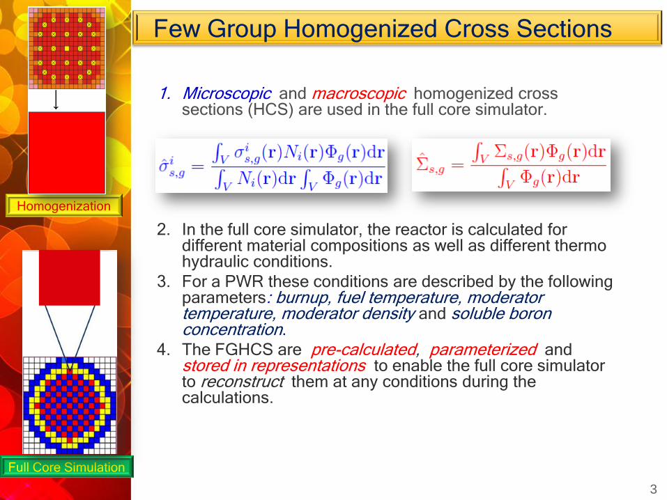
1. Microscopic and macroscopic homogenized cross sections (HCS) are used in the full core simulator.

2. In the full core simulator, the reactor is calculated for different material compositions as well as different thermo hydraulic conditions.

3. For a PWR these conditions are described by the following parameters: burnup, fuel temperature, moderator temperature, moderator density and soluble boron concentration.

4. The FGHCS are pre-calculated, parameterized and stored in representations to enable the full core simulator to reconstruct them at any conditions during the calculations.

Homogenization

Full Core Simulation

Lagrange Interpolation and Sparse Grids

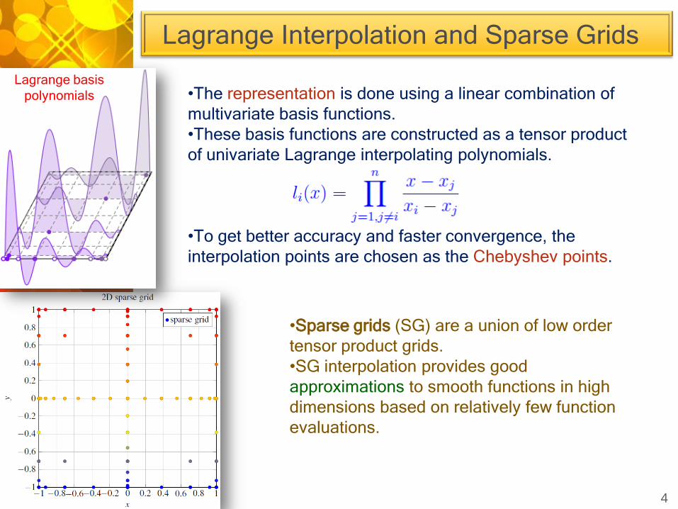
•Sparse grids (SG) are a union of low order

tensor product grids.

•SG interpolation provides good

approximations to smooth functions in high

dimensions based on relatively few function

evaluations.

4

•The representation is done using a linear combination of

multivariate basis functions.

•These basis functions are constructed as a tensor product

of univariate Lagrange interpolating polynomials.

•To get better accuracy and faster convergence, the

interpolation points are chosen as the Chebyshev points.

Lagrange basis

polynomials

Lagrange Interpolation and Sparse Grids

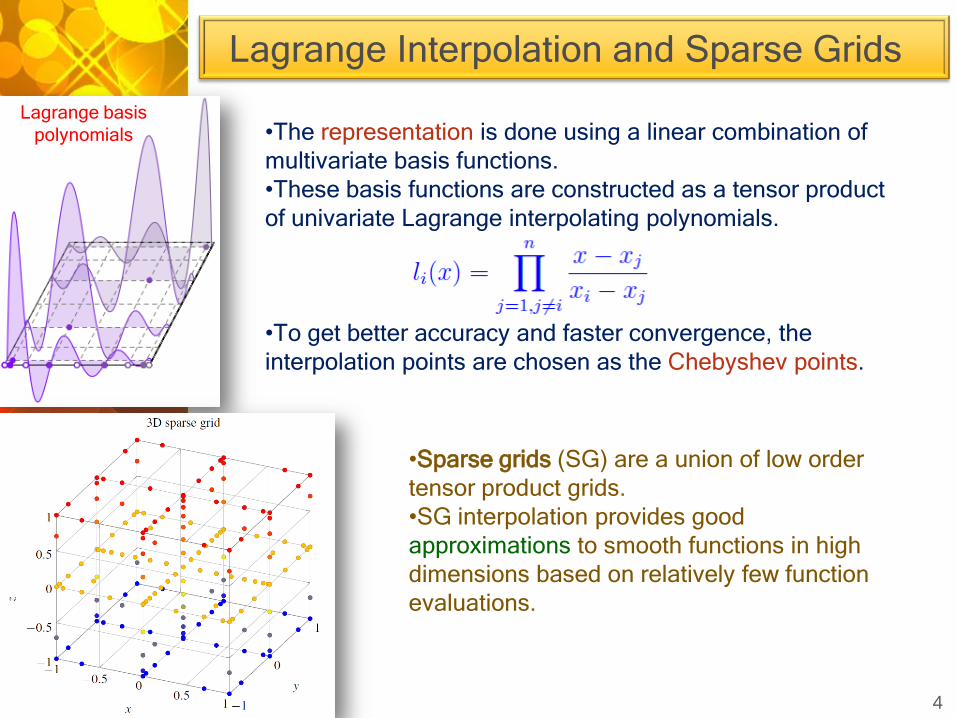
•Sparse grids (SG) are a union of low order

tensor product grids.

•SG interpolation provides good

approximations to smooth functions in high

dimensions based on relatively few function

evaluations.

4

•The representation is done using a linear combination of

multivariate basis functions.

•These basis functions are constructed as a tensor product

of univariate Lagrange interpolating polynomials.

•To get better accuracy and faster convergence, the

interpolation points are chosen as the Chebyshev points.

Lagrange basis

polynomials

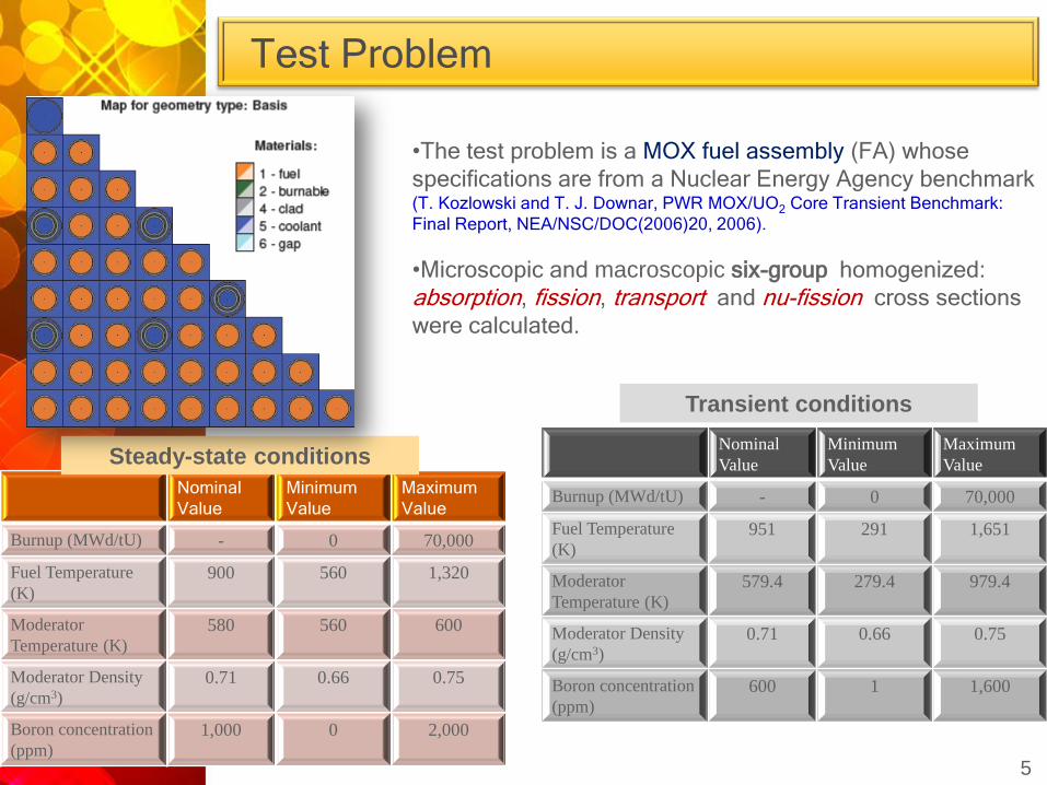
Test Problem

•The test problem is a MOX fuel assembly (FA) whose

specifications are from a Nuclear Energy Agency benchmark (T. Kozlowski and T. J. Downar, PWR MOX/UO2 Core Transient Benchmark:

Final Report, NEA/NSC/DOC(2006)20, 2006).

•Microscopic and macroscopic six-group homogenized:

absorption, fission, transport and nu-fission cross sections

were calculated.

Nominal

Value

Minimum

Value

Maximum

Value

Burnup (MWd/tU) - 0 70,000

Fuel Temperature

(K)

900 560 1,320

Moderator

Temperature (K)

580 560 600

Moderator Density

(g/cm3)

0.71 0.66 0.75

Boron concentration

(ppm)

1,000 0 2,000

5

Steady-state conditions Nominal

Value

Minimum

Value

Maximum

Value

Burnup (MWd/tU) - 0 70,000

Fuel Temperature

(K)

951 291 1,651

Moderator

Temperature (K)

579.4 279.4 979.4

Moderator Density

(g/cm3)

0.71 0.66 0.75

Boron concentration

(ppm)

600 1 1,600

Transient conditions

Maximum and Average Errors of the Interpolation

• The interpolation was done on sparse

grids with: 241, 801, 2433, 6993,

19313 and 51713 points.

• Error checked on 4,096 independent

quasi-random points.

• Maximum (Fig. A) and Average (Fig.

B) relative interpolation errors for

absorption cross section for group 6

U-238, Pu-241 and macroscopic

cross sections.

• The expected accuracy for the

average error achieved with only 801

samples.

• The unexpected behavior of Pu-241

will be investigated.

• The source(s) of the high maximum

errors will be investigated.

6

Fig. A

Fig. B

Acceptable maximum

error = 0.1%

Acceptable average

error = 0.05%

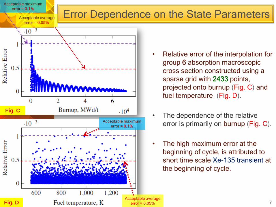
Error Dependence on the State Parameters

• Relative error of the interpolation for

group 6 absorption macroscopic

cross section constructed using a

sparse grid with 2433 points,

projected onto burnup (Fig. C) and

fuel temperature (Fig. D).

• The dependence of the relative

error is primarily on burnup (Fig. C).

• The high maximum error at the

beginning of cycle, is attributed to

short time scale Xe-135 transient at

the beginning of cycle.

7

Fig. C

Fig. D

Fig. C

Fig. D

Acceptable maximum

error = 0.1%

Acceptable average

error = 0.05%

Acceptable maximum

error = 0.1%

Acceptable average

error = 0.05%

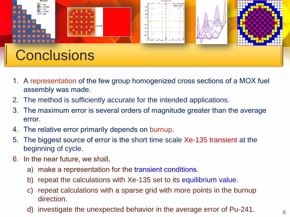
Conclusions

8

1. A representation of the few group homogenized cross sections of a MOX fuel

assembly was made.

2. The method is sufficiently accurate for the intended applications.

3. The maximum error is several orders of magnitude greater than the average

error.

4. The relative error primarily depends on burnup.

5. The biggest source of error is the short time scale Xe-135 transient at the

beginning of cycle.

6. In the near future, we shall,

a) make a representation for the transient conditions.

b) repeat the calculations with Xe-135 set to its equilibrium value.

c) repeat calculations with a sparse grid with more points in the burnup

direction.

d) investigate the unexpected behavior in the average error of Pu-241.