A Fortran 77 package for column reduction ofpolynomial matrices

A.J. GeurtsDepartment of Mathematics and Computing Sciences

Eindhoven University of TechnologyP.O.Box 513, 5600 MB Eindhoven, The Netherlands

email wstasli@urc.tue.nl, fax +31 40 243 66 85

C. Praagman1

Department of Econometrics

University of GroningenP.O.Box 800, 9700 AV Groningen, The Netherlands

email:c.praagman@eco.rug.nl, fax:31 50 363 37 20

July 10, 1998

1corresponding author

Abstract

A polynomial matrix is called column reduced if its column degrees are as low as possiblein some sense. Two polynomial matrices P and R are called unimodularly equivalent ifthere exists a unimodular polynomial matrix U such that PU = R. Every polynomialmatrix is unimodularly equivalent to a column reduced polynomial matrix.In this paper a subroutine is described that takes a polynomial matrix P as input and yieldson output a unimodular matrix U and a column reduced matrix R such that PU = R,actually PU − R is near zero. The subroutine is based on an algorithm, described in apaper by Neven and Praagman. The subroutine has been tested with a number of exampleson different computers, with comparable results. The performance of the subroutine onevery example tried is satisfactory in the sense that the magnitude of the elements of theresidual matrix PU − R is about ‖P‖‖U‖EPS, where EPS is the machine precision. Toobtain these results a tolerance, used to determine the rank of some (sub)matrices, hasto be set properly. The influence of this tolerance on the performance of the algorithm isdiscussed, from which a guideline for the usage of the subroutine is derived.

AMS subject classification: 65F30, 15A23, 93B10, 15A22, 15A24,15A33, 93B10, 93B17, 93B25

CR subject classification: Algorithms, Reliability, F 2.1 Computa-tions on matrices, Computations on poly-nomials, G 1.3 Linear systems, G 4 Algo-rithm analysis

Keywords: Column Reduction, Fortran subroutine

1 Introduction

Polynomial matrices, i.e. matrices of which the elements are polynomials (or equivalentlypolynomials with matrix coefficients), play a dominant role in modern systems theory.Consider for instance a set of n variables w = (w1, . . . , wn)′. Suppose that these variablesare related by a set of m higher order linear differential equations with constant coefficients:

P0w + P1d

dtw + P2

d2

dt2w + . . .+ Pq

dq

dtqw = 0, (1)

where Pk, k = 0, . . . , q are m× n constant matrices. Define the m× n polynomial matrixP by

P (s) =q∑

k=0

Pksk,

then this set of equations 1 can be written concisely as

P (d

dt)w = 0. (2)

In the behavioral approach to systems theory equation 2, together with a specificationof the function class to which the solutions should belong, describes a system. For example(C∞(R+), P (d/dt)w = 0) describes a system. The behavior of this system consists of allw ∈ Rn, of which the components are C∞ functions on [0,∞), that satisfy equation 2.Many properties of the behavior of the system can be derived immediately from propertiesof the polynomial matrix P (see Willems [17, 18, 19]).

The information contained in P can be redundant, in which case the polynomial matrixcan be replaced by another polynomial matrix of lower degree or smaller size withoutchanging the set of trajectories satisfying the equations. For several reasons a minimaldescription can be convenient. This could be purely a matter of simplicity, but there arealso cases in which a minimal description has additional value. For instance if one looksfor state space or input-output representations of the system. Depending on the goal onehas in mind, minimality can have different meanings, but in important situations a rowor column reduced description supplies a minimal description. For instance in the work ofWillems on behaviors one finds the search for a row reduced P that describes the samebehavior as equation 2.

Other examples that display the importance of column or row reduced polynomialmatrices may be found in articles on inversion of polynomial matrices [7, 10, 24], or inpapers on a polynomial matrix version of the Euclidean algorithm [4, 16, 21, 23, 25], wherea standing assumption is that one of the matrices involved is column reduced.

Since P is row reduced if and only if its transpose P ′ is column reduced, the problemsof row reduction and column reduction are equivalent.

In this paper a subroutine is presented that determines a column reduced matrix uni-modularly equivalent to a given polynomial matrix. The algorithm underlying the subrou-tine has been developed in several stages: the part of the algorithm in which a minimal

1

basis of the right null space of a polynomial matrix is calculated is an adaptation of thealgorithm described in Beelen [2]. The original idea of the algorithm has been describedin Beelen, van den Hurk, Praagman [3], and successive improvements have been report-ed in Neven [11], Praagman [13, 14]. The paper by Neven and Praagman [12] gives thealgorithm in its most general form, exploiting the special structure of the problem in thecalculation of the kernel of a polynomial matrix. The subroutine we describe here is animplementation of the algorithm in the latter paper.

The algorithm was intended to perform well in all cases. But it turned out that theroutine has difficulties in some special cases, that in some sense might be described assingular. We give examples in section 8, and discuss these difficulties in detail in section 9.A crucial role is played by a tolerance, TOL, used in rank determining steps, which has tobe set properly.

2 Preliminaries

Let us start with introducing some notations and recalling some definitions:Let R[s] denote the ring of polynomials in s with real coefficients, let Rn[s] be the set

of column vectors of length n with elements in R[s]. Clearly Rn[s] is a free module overR[s].

Remark. Recall that, loosely speaking, a set M is called a module over a ring R if any twoelements in M can be added, and any element of M can be multiplied by an arbitrary elementfrom R. A set m1, . . . ,mr ∈M is called a set of generators of M if any element m ∈M can bewritten as a linear combination of the generators: m =

∑rimi for some ri ∈ R. The module is

free if there exists a set of generators such that the ri are unique. Note that if R is a field, thena module is just a vector space.

Let Rm×n[s] be the ring of m × n matrices with elements in R[s]. Let P ∈ Rm×n[s].Then d(P ), the degree of P , is defined as the maximum of the degrees of the elements ofP , and dj(P ), the j-th column degree of P , as the maximum of the degrees in the j-thcolumn. δ(P ) is the array of integers obtained by arranging the column degrees of P innon-decreasing order.

The leading column coefficient matrix of P , Γc(P ), is the constant matrix, of which thej-th column is obtained by taking from the j-th column of P the coefficients of the term

with degree dj(P ). Let Pj(s) =∑dj(P )k=0 Pjks

k be the j-th column of P, then the j-th columnof Γc(P ) equals

Γc(P )j = Pjdj(P ).

Definition 1. Let P ∈ Rm×n[s]. P is called column reduced, if there exists a permutationmatrix T, such that P = (0, P1)T , where Γc(P1) has full column rank.

2

Remark. Note that we do not require Γc(P ) to be of full column rank. In the literature there issome ambiguity about column properness and column reducedness. We follow here the definitionof Willems [17]: P is column proper if Γc(P ) has full column rank, and column reduced if theconditions in the definition above are satisfied.

A square polynomial matrix U ∈ Rn×n[s] is unimodular if det(U) ∈ R\{0} or, equiv-alently, if U−1 exists and is also polynomial. Two polynomial matrices P ∈ Rm×n[s]and R ∈ Rm×n[s] are called unimodularly equivalent if there exists a unimodular matrixU ∈ Rn×n[s] such that PU = R. It is well known that every regular polynomial matrix isunimodularly equivalent to a column proper matrix, see Wolovich [20]. Kailath [8] statesthat the above result can be extended to polynomial matrices of full column rank withoutchanging the proof. In fact the proof in [20] is sufficient to establish that any polynomialmatrix is unimodularly equivalent to a column reduced matrix. Furthermore, Wolovich’sproof implies immediately that the column degrees of the column reduced polynomial ma-trix do not exceed those of the original matrix, see Neven and Praagman [12].

Theorem 1. Let P ∈ Rm×n[s], then there exists a U ∈ Rn×n[s], unimodular, such thatR = PU is column reduced. Furthermore δ(R) ≤ δ(P ) totally.

Although the proof of this theorem in the above sources is constructive, it is not suitedfor practical computations, for reasons explained in a paper by Van Dooren [15]. Example 3in section 8 illustrates this point. In Neven and Praagman [12] an alternative, constructiveproof is given on which the algorithm, underlying the subroutine we describe here, is based.

The most important ingredient of the algorithm is the calculation of a minimal basis ofthe right null space of a polynomial matrix associated with P .

Definition 2. Let M be a submodule of Rn[s]. Then Q ∈ Rn×r[s] is called a minimalbasis of M if Q is column proper and the columns of Q span M.

In the algorithm a minimal basis is calculated for the module

ker(P, −Im) = {v ∈ Rn+m[s] | (P, −Im)v = 0},

see [3]. Here and in the sequel Im will denote the identity matrix of size m.The first observation is that if (U ′, R′)′ is such a basis, with U ∈ Rn×n[s], then U is

unimodular, see [3, 12]. Of course, R = PU , but although (U ′, R′)′ is minimal and hencecolumn reduced, this does not necessarily hold for R. Take for example

P (s) =

(1 s0 1

).

Then (U(s)R(s)

)=

1 00 11 s0 1

3

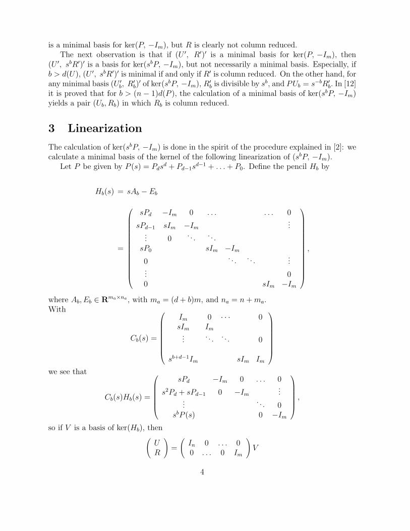
is a minimal basis for ker(P, −Im), but R is clearly not column reduced.The next observation is that if (U ′, R′)′ is a minimal basis for ker(P, −Im), then

(U ′, sbR′)′ is a basis for ker(sbP, −Im), but not necessarily a minimal basis. Especially, ifb > d(U), (U ′, sbR′)′ is minimal if and only if R′ is column reduced. On the other hand, forany minimal basis (U ′b, R

′b)′ of ker(sbP, −Im), R′b is divisible by sb, and PUb = s−bR′b. In [12]

it is proved that for b > (n− 1)d(P ), the calculation of a minimal basis of ker(sbP, −Im)yields a pair (Ub, Rb) in which Rb is column reduced.

3 Linearization

The calculation of ker(sbP, −Im) is done in the spirit of the procedure explained in [2]: wecalculate a minimal basis of the kernel of the following linearization of (sbP, −Im).

Let P be given by P (s) = Pdsd + Pd−1s

d−1 + . . .+ P0. Define the pencil Hb by

Hb(s) = sAb −Eb

=

sPd −Im 0 . . . . . . 0

sPd−1 sIm −Im...

... 0. . .

. . .

sP0 sIm −Im0

. . .. . .

...... 00 sIm −Im

,

where Ab, Eb ∈ Rma×na , with ma = (d+ b)m, and na = n+ma.With

Cb(s) =

Im 0 · · · 0sIm Im

.... . .

. . . 0

sb+d−1Im sIm Im

we see that

Cb(s)Hb(s) =

sPd −Im 0 . . . 0

s2Pd + sPd−1 0 −Im...

.... . . 0

sbP (s) 0 −Im

,so if V is a basis of ker(Hb), then(

UR

)=

(In 0 . . . 00 . . . 0 Im

)V

4

is a basis for ker(sbP, −Im) ([2]). In [12] it is proved that δ(V ) = δ((U ′, R′)′) and that Vis minimal if and only if (U ′, R′)′ is minimal. So the problem is to calculate a minimalbasis for ker(Hb).

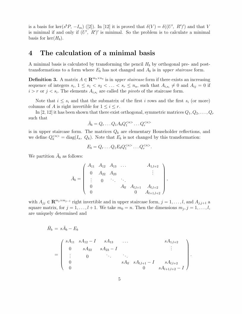
4 The calculation of a minimal basis

A minimal basis is calculated by transforming the pencil Hb by orthogonal pre- and post-transformations to a form where Eb has not changed and Ab is in upper staircase form.

Definition 3. A matrix A ∈ Rma×na is in upper staircase form if there exists an increasingsequence of integers si, 1 ≤ s1 < s2 < . . . < sr ≤ na, such that Ai,si 6= 0 and Aij = 0 ifi > r or j < si. The elements Ai,si are called the pivots of the staircase form.

Note that i ≤ si and that the submatrix of the first i rows and the first si (or more)columns of A is right invertible for 1 ≤ i ≤ r.

In [2, 12] it has been shown that there exist orthogonal, symmetric matrices Q1, Q2, . . . , Qr

such thatAb = Qr . . . Q1AbQ

<n>1 . . . Q<n>

r

is in upper staircase form. The matrices Qk are elementary Householder reflections, andwe define Q<n>

k = diag(In, Qk). Note that Eb is not changed by this transformation:

Eb = Qr . . . Q1EbQ<n>1 . . . Q<n>

r .

We partition Ab as follows:

Ab =

A11 A12 A13 . . . A1,l+2

0 A22 A23...

... 0. . .

. . .

0 All Al,l+1 Al,l+2

0 0 Al+1,l+2

,

with Ajj ∈ Rmj×mj−1 right invertible and in upper staircase form, j = 1, . . . , l, and Aj,j+1 asquare matrix, for j = 1, . . . , l+ 1. We take m0 = n. Then the dimensions mj, j = 1, . . . , l,are uniquely determined and

Hb = sAb − Eb

=

sA11 sA12 − I sA13 . . . sA1,l+2

0 sA22 sA23 − I...

... 0. . .

. . .

0 sAll sAl,l+1 − I sAl,l+2

0 0 sAl+1,l+2 − I

.

5

Let A∗b be the submatrix of A(k−1)b = Qk−1 . . . Q1AbQ

<n>1 . . . Q<n>

k−1 obtained by deletingthe first k−1 rows, and let sk be the column index of the first nonzero column in A∗b . ThenQk transforms this (sub)column into the first unit vector and lets the first k − 1 rows and

the first sk − 1 columns of A(k−1)b invariant. Consequently, post-multiplication with Q<n>

k

leaves the first n+ k − 1 columns of A(k−1)b unaltered.

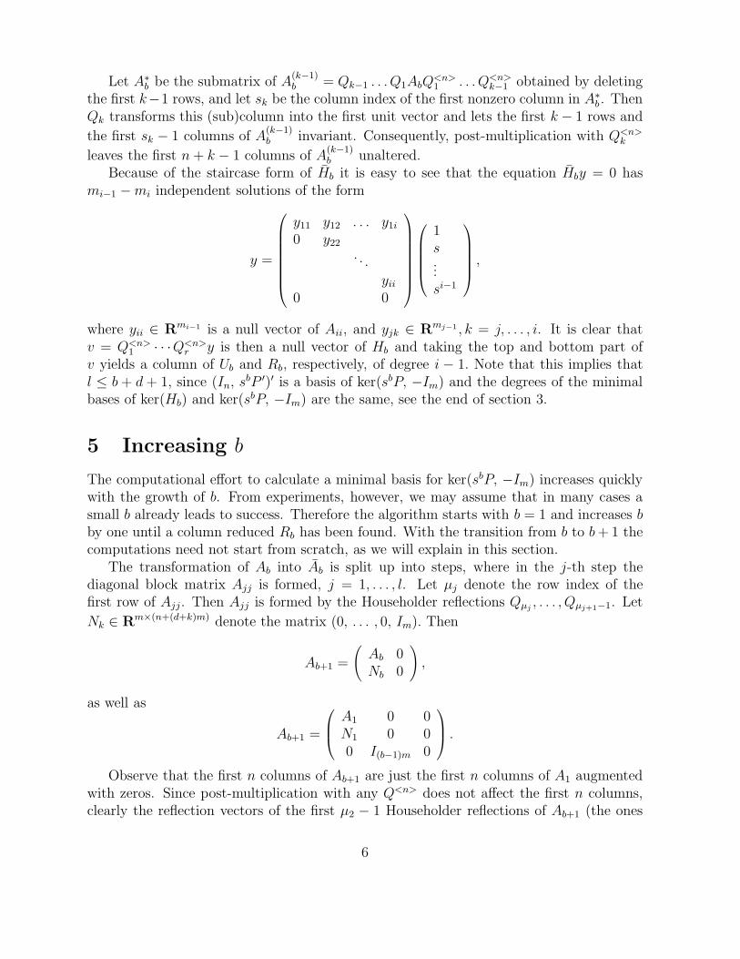
Because of the staircase form of Hb it is easy to see that the equation Hby = 0 hasmi−1 −mi independent solutions of the form

y =

y11 y12 . . . y1i

0 y22

. . .

yii0 0

1s...si−1

,

where yii ∈ Rmi−1 is a null vector of Aii, and yjk ∈ Rmj−1 , k = j, . . . , i. It is clear thatv = Q<n>

1 · · ·Q<n>r y is then a null vector of Hb and taking the top and bottom part of

v yields a column of Ub and Rb, respectively, of degree i − 1. Note that this implies thatl ≤ b+ d+ 1, since (In, s

bP ′)′ is a basis of ker(sbP, −Im) and the degrees of the minimalbases of ker(Hb) and ker(sbP, −Im) are the same, see the end of section 3.

5 Increasing b

The computational effort to calculate a minimal basis for ker(sbP, −Im) increases quicklywith the growth of b. From experiments, however, we may assume that in many cases asmall b already leads to success. Therefore the algorithm starts with b = 1 and increases bby one until a column reduced Rb has been found. With the transition from b to b+ 1 thecomputations need not start from scratch, as we will explain in this section.

The transformation of Ab into Ab is split up into steps, where in the j-th step thediagonal block matrix Ajj is formed, j = 1, . . . , l. Let µj denote the row index of thefirst row of Ajj. Then Ajj is formed by the Householder reflections Qµj , . . . , Qµj+1−1. Let

Nk ∈ Rm×(n+(d+k)m) denote the matrix (0, . . . , 0, Im). Then

Ab+1 =

(Ab 0Nb 0

),

as well as

Ab+1 =

A1 0 0N1 0 00 I(b−1)m 0

.Observe that the first n columns of Ab+1 are just the first n columns of A1 augmented

with zeros. Since post-multiplication with any Q<n> does not affect the first n columns,clearly the reflection vectors of the first µ2 − 1 Householder reflections of Ab+1 (the ones

6

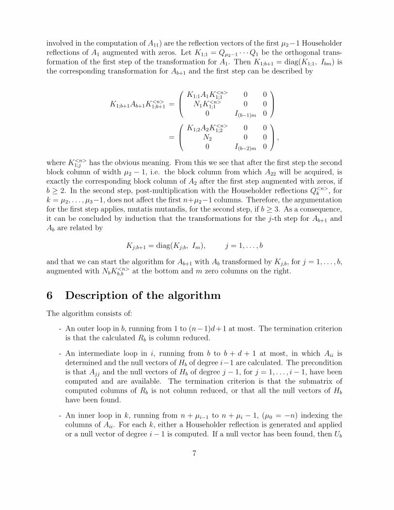
involved in the computation of A11) are the reflection vectors of the first µ2−1 Householderreflections of A1 augmented with zeros. Let K1;1 = Qµ2−1 · · ·Q1 be the orthogonal trans-formation of the first step of the transformation for A1. Then K1;b+1 = diag(K1;1, Ibm) isthe corresponding transformation for Ab+1 and the first step can be described by

K1;b+1Ab+1K<n>1;b+1 =

K1:1A1K<n>1;1 0 0

N1K<n>1;1 0 0

0 I(b−1)m 0

=

K1;2A2K<n>1;2 0 0

N2 0 00 I(b−2)m 0

,where K<n>

1;j has the obvious meaning. From this we see that after the first step the secondblock column of width µ2 − 1, i.e. the block column from which A22 will be acquired, isexactly the corresponding block column of A2 after the first step augmented with zeros, ifb ≥ 2. In the second step, post-multiplication with the Householder reflections Q<n>

k , fork = µ2, . . . , µ3−1, does not affect the first n+µ2−1 columns. Therefore, the argumentationfor the first step applies, mutatis mutandis, for the second step, if b ≥ 3. As a consequence,it can be concluded by induction that the transformations for the j-th step for Ab+1 andAb are related by

Kj;b+1 = diag(Kj;b, Im), j = 1, . . . , b

and that we can start the algorithm for Ab+1 with Ab transformed by Kj,b, for j = 1, . . . , b,augmented with NbK

<n>b,b at the bottom and m zero columns on the right.

6 Description of the algorithm

The algorithm consists of:

- An outer loop in b, running from 1 to (n−1)d+1 at most. The termination criterionis that the calculated Rb is column reduced.

- An intermediate loop in i, running from b to b + d + 1 at most, in which Aii isdetermined and the null vectors of Hb of degree i−1 are calculated. The preconditionis that Ajj and the null vectors of Hb of degree j − 1, for j = 1, . . . , i− 1, have beencomputed and are available. The termination criterion is that the submatrix ofcomputed columns of Rb is not column reduced, or that all the null vectors of Hb

have been found.

- An inner loop in k, running from n + µi−1 to n + µi − 1, (µ0 = −n) indexing thecolumns of Aii. For each k, either a Householder reflection is generated and appliedor a null vector of degree i− 1 is computed. If a null vector has been found, then Ub

7

and Rb are extended with one column and Rb is checked on column reducedness. Theloop is terminated after k = n+ µi − 1 or if the extended Rb is not column reduced.

The algorithm uses a tolerance to determine the rank of the diagonal blocks Aii fromwhich the null vectors of Hb and consequently the computed solution is derived. Anappropriate tolerance is needed to find the solution. But the value of the tolerance doesnot influence the accuracy of the computed solution.

7 The implementation

The algorithm has been implemented in the subroutine COLRED. The subroutine iswritten according to the standards of SLICOT, see [22], with a number of auxiliaries. It isbased on the linear algebra packages BLAS [9, 5] and LAPACK [1]. The complete code ofan earlier (slightly different) version of the routines and an example program are includedin a report by the authors [6].

COLRED takes a polynomial matrix P as its input, and yields on output a unimodularmatrix U , and a column reduced polynomial matrix R such that PU−R is near zero. Rankdetermination plays an important role in the algorithm, and the user is asked to specifyon input a parameter TOL, that sets a threshold value below which matrix elements, thatare essential in the rank determination procedure, are considered zero. If TOL is set toosmall, it is replaced by a default value in the subroutine.

Concerning the numerical aspects we like to make the following remark: The algorithmused by the routine involves the construction of a special staircase form of a linearization of(sbP (s), −I) with pivots considered to be non-zero when they are greater than or equal toTOL. These pivots are then inverted in order to construct the columns of ker (sbP (s), −I).The user is recommended to choose TOL of the order of the relative error in the elementsof P (s). If TOL is chosen too small, then a very small element of insignificant value maybe taken as pivot. As a consequence, the correct null-vectors, and hence R(s), may not befound. In the case that R(s) has not been found and in the case that the elements of thecomputed U(s) and R(s) are large relative to the elements of P (s) the user should considertrying several values of TOL.

8 Examples

In this section we describe a few examples. All examples were run on four computers, aVAX-VMS, a VAX-UNIX, a SUN and on a 486 personal computer. The numerical valuesthat we present here were produced on the VAX-VMS computer. Its machine precisionis 2−56 ≈ 1.4 · 10−17. Unless explicitly mentioned, the examples were run with TOL = 0,forcing the subroutine to take the default value (see section 7) for the tolerance.

The first example is taken from the book of Kailath [8], and has been discussed beforein [3] and [12].

8

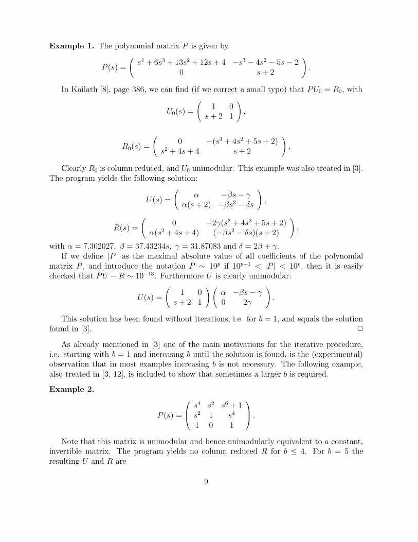
Example 1. The polynomial matrix P is given by

P (s) =

(s4 + 6s3 + 13s2 + 12s+ 4 −s3 − 4s2 − 5s− 2

0 s+ 2

).

In Kailath [8], page 386, we can find (if we correct a small typo) that PU0 = R0, with

U0(s) =

(1 0

s+ 2 1

),

R0(s) =

(0 −(s3 + 4s2 + 5s+ 2)

s2 + 4s+ 4 s+ 2

),

Clearly R0 is column reduced, and U0 unimodular. This example was also treated in [3].The program yields the following solution:

U(s) =

(α −βs− γ

α(s+ 2) −βs2 − δs

),

R(s) =

(0 −2γ(s3 + 4s2 + 5s+ 2)

α(s2 + 4s+ 4) (−βs2 − δs)(s+ 2)

),

with α = 7.302027, β = 37.43234s, γ = 31.87083 and δ = 2β + γ.If we define |P | as the maximal absolute value of all coefficients of the polynomial

matrix P , and introduce the notation P ∼ 10p if 10p−1 < |P | < 10p, then it is easilychecked that PU − R ∼ 10−13. Furthermore U is clearly unimodular:

U(s) =

(1 0

s+ 2 1

)(α −βs− γ0 2γ

).

This solution has been found without iterations, i.e. for b = 1, and equals the solutionfound in [3]. 2

As already mentioned in [3] one of the main motivations for the iterative procedure,i.e. starting with b = 1 and increasing b until the solution is found, is the (experimental)observation that in most examples increasing b is not necessary. The following example,also treated in [3, 12], is included to show that sometimes a larger b is required.

Example 2.

P (s) =

s4 s2 s6 + 1s2 1 s4

1 0 1

.Note that this matrix is unimodular and hence unimodularly equivalent to a constant,

invertible matrix. The program yields no column reduced R for b ≤ 4. For b = 5 theresulting U and R are

9

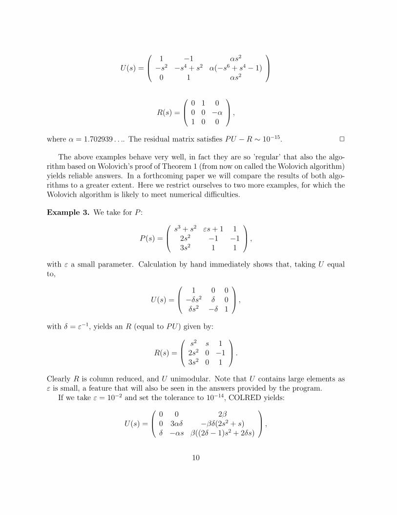
U(s) =

1 −1 αs2

−s2 −s4 + s2 α(−s6 + s4 − 1)0 1 αs2

R(s) =

0 1 00 0 −α1 0 0

,where α = 1.702939 . . .. The residual matrix satisfies PU −R ∼ 10−15. 2

The above examples behave very well, in fact they are so ’regular’ that also the algo-rithm based on Wolovich’s proof of Theorem 1 (from now on called the Wolovich algorithm)yields reliable answers. In a forthcoming paper we will compare the results of both algo-rithms to a greater extent. Here we restrict ourselves to two more examples, for which theWolovich algorithm is likely to meet numerical difficulties.

Example 3. We take for P :

P (s) =

s3 + s2 εs+ 1 12s2 −1 −13s2 1 1

,with ε a small parameter. Calculation by hand immediately shows that, taking U equalto,

U(s) =

1 0 0−δs2 δ 0δs2 −δ 1

,with δ = ε−1, yields an R (equal to PU) given by:

R(s) =

s2 s 12s2 0 −13s2 0 1

.Clearly R is column reduced, and U unimodular. Note that U contains large elements asε is small, a feature that will also be seen in the answers provided by the program.

If we take ε = 10−2 and set the tolerance to 10−14, COLRED yields:

U(s) =

0 0 2β0 3αδ −βδ(2s2 + s)δ −αs β((2δ − 1)s2 + 2δs)

,

10

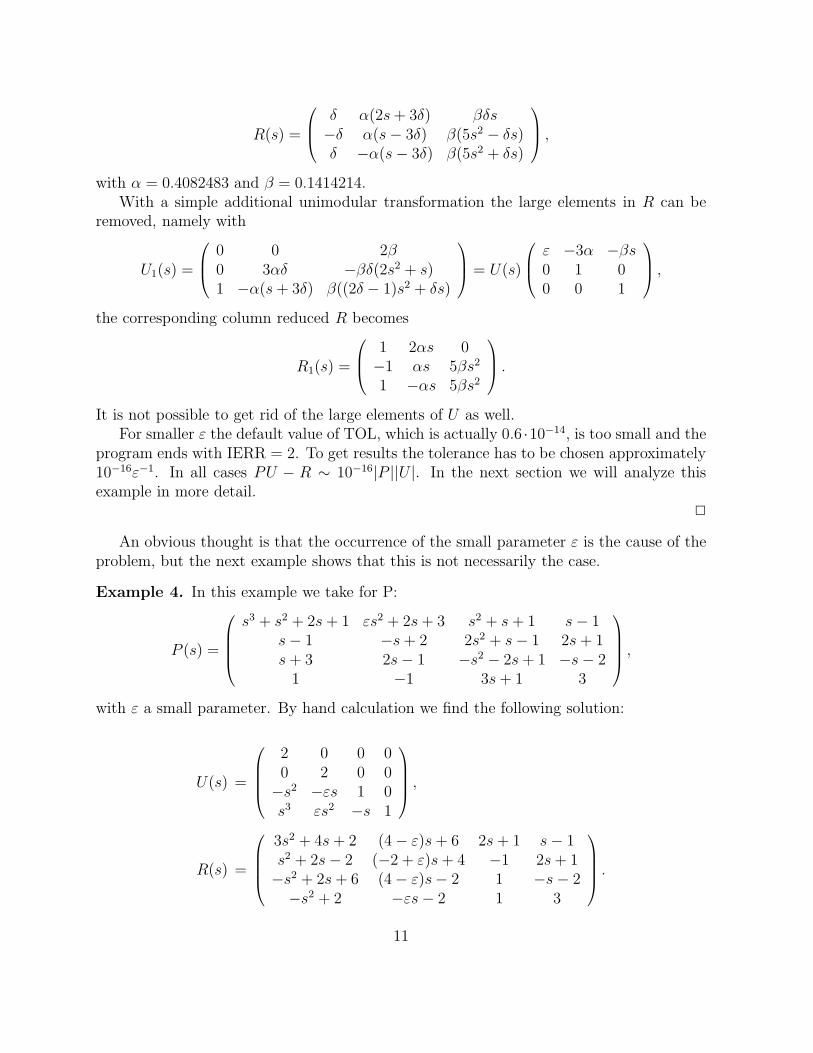
R(s) =

δ α(2s+ 3δ) βδs−δ α(s− 3δ) β(5s2 − δs)δ −α(s− 3δ) β(5s2 + δs)

,with α = 0.4082483 and β = 0.1414214.

With a simple additional unimodular transformation the large elements in R can beremoved, namely with

U1(s) =

0 0 2β0 3αδ −βδ(2s2 + s)1 −α(s+ 3δ) β((2δ − 1)s2 + δs)

= U(s)

ε −3α −βs0 1 00 0 1

,the corresponding column reduced R becomes

R1(s) =

1 2αs 0−1 αs 5βs2

1 −αs 5βs2

.It is not possible to get rid of the large elements of U as well.

For smaller ε the default value of TOL, which is actually 0.6 ·10−14, is too small and theprogram ends with IERR = 2. To get results the tolerance has to be chosen approximately10−16ε−1. In all cases PU − R ∼ 10−16|P ||U |. In the next section we will analyze thisexample in more detail.

2

An obvious thought is that the occurrence of the small parameter ε is the cause of theproblem, but the next example shows that this is not necessarily the case.

Example 4. In this example we take for P:

P (s) =

s3 + s2 + 2s+ 1 εs2 + 2s+ 3 s2 + s+ 1 s− 1

s− 1 −s+ 2 2s2 + s− 1 2s+ 1s+ 3 2s− 1 −s2 − 2s+ 1 −s− 2

1 −1 3s+ 1 3

,with ε a small parameter. By hand calculation we find the following solution:

U(s) =

2 0 0 00 2 0 0−s2 −εs 1 0s3 εs2 −s 1

,

R(s) =

3s2 + 4s+ 2 (4− ε)s+ 6 2s+ 1 s− 1s2 + 2s− 2 (−2 + ε)s+ 4 −1 2s+ 1−s2 + 2s+ 6 (4− ε)s− 2 1 −s− 2−s2 + 2 −εs− 2 1 3

.

11

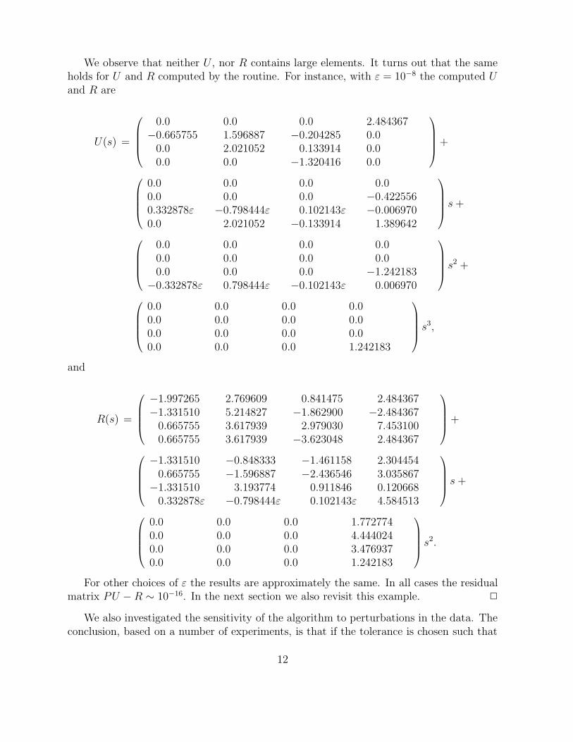
We observe that neither U , nor R contains large elements. It turns out that the sameholds for U and R computed by the routine. For instance, with ε = 10−8 the computed Uand R are

U(s) =

0.0 0.0 0.0 2.484367−0.665755 1.596887 −0.204285 0.0

0.0 2.021052 0.133914 0.00.0 0.0 −1.320416 0.0

+

0.0 0.0 0.0 0.00.0 0.0 0.0 −0.4225560.332878ε −0.798444ε 0.102143ε −0.0069700.0 2.021052 −0.133914 1.389642

s+

0.0 0.0 0.0 0.00.0 0.0 0.0 0.00.0 0.0 0.0 −1.242183−0.332878ε 0.798444ε −0.102143ε 0.006970

s2 +

0.0 0.0 0.0 0.00.0 0.0 0.0 0.00.0 0.0 0.0 0.00.0 0.0 0.0 1.242183

s3,

and

R(s) =

−1.997265 2.769609 0.841475 2.484367−1.331510 5.214827 −1.862900 −2.484367

0.665755 3.617939 2.979030 7.4531000.665755 3.617939 −3.623048 2.484367

+

−1.331510 −0.848333 −1.461158 2.304454

0.665755 −1.596887 −2.436546 3.035867−1.331510 3.193774 0.911846 0.120668

0.332878ε −0.798444ε 0.102143ε 4.584513

s+

0.0 0.0 0.0 1.7727740.0 0.0 0.0 4.4440240.0 0.0 0.0 3.4769370.0 0.0 0.0 1.242183

s2.

For other choices of ε the results are approximately the same. In all cases the residualmatrix PU − R ∼ 10−16. In the next section we also revisit this example. 2

We also investigated the sensitivity of the algorithm to perturbations in the data. Theconclusion, based on a number of experiments, is that if the tolerance is chosen such that

12

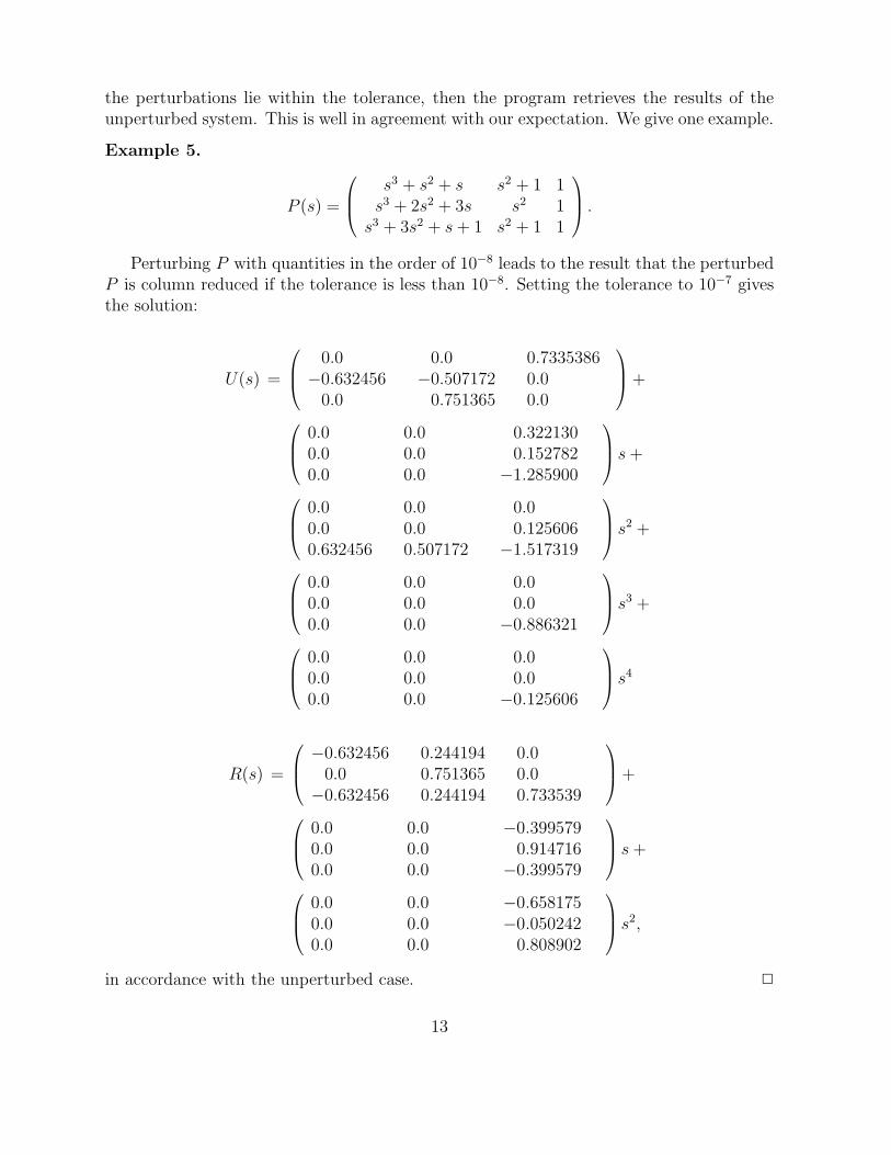
the perturbations lie within the tolerance, then the program retrieves the results of theunperturbed system. This is well in agreement with our expectation. We give one example.

Example 5.

P (s) =

s3 + s2 + s s2 + 1 1s3 + 2s2 + 3s s2 1s3 + 3s2 + s+ 1 s2 + 1 1

.Perturbing P with quantities in the order of 10−8 leads to the result that the perturbed

P is column reduced if the tolerance is less than 10−8. Setting the tolerance to 10−7 givesthe solution:

U(s) =

0.0 0.0 0.7335386−0.632456 −0.507172 0.0

0.0 0.751365 0.0

+

0.0 0.0 0.3221300.0 0.0 0.1527820.0 0.0 −1.285900

s+

0.0 0.0 0.00.0 0.0 0.1256060.632456 0.507172 −1.517319

s2 +

0.0 0.0 0.00.0 0.0 0.00.0 0.0 −0.886321

s3 +

0.0 0.0 0.00.0 0.0 0.00.0 0.0 −0.125606

s4

R(s) =

−0.632456 0.244194 0.00.0 0.751365 0.0−0.632456 0.244194 0.733539

+

0.0 0.0 −0.3995790.0 0.0 0.9147160.0 0.0 −0.399579

s+

0.0 0.0 −0.6581750.0 0.0 −0.0502420.0 0.0 0.808902

s2,

in accordance with the unperturbed case. 2

13

9 Discussion

First we examine example 3 of section 8, namely

Pε(s) =

s3 + s2 εs+ 1 12s2 −1 −13s2 1 1

,The Uε and Rε that will result from the algorithm, if calculations are performed exactly,

are

Uε(s) =

0 0 2β0 3αδ −βδ(2s2 + s)δ −αs β((2δ − 1)s2 + 2δs)

,

Rε(s) =

δ α(2s+ 3δ) βδs−δ α(s− 3δ) β(5s2 − δs)δ −α(s− 3δ) β(5s2 + δs)

,with α = 1

6

√6, β = 1

10

√2 and δ = ε−1.

In section 8 we saw that the tolerance for which this result is obtained by the routineis proportional to ε−1. Close examination of the computations reveals that the computedAb (see section 4) gets small pivots, which cause growing numbers in the computation ofthe right null vectors until overflow occurs, and a breakdown of the process if the toleranceis too small. Scaling of a null vector, which at first sight suggests itself, may suppress theoverflow and thereby hide the problem at hand. In this example the effect of scaling isthat, if ε tends to zero, then Uε tends to a singular matrix and Rε to a constant matrix ofrank 1.

Is there any reason to believe that there exists an algorithm which yields an R contin-uously depending on ε in a neighborhood of 0? Observe that

- det(Pε)(s) = −5εs3, so Pε is singular for ε = 0;

- δ(Rε) = (0, 1, 2) if ε 6= 0 and δ(R0) = (−1, 0, 3) (We use the convention that the zeropolynomial has degree −1).

We conclude that the entries of Uε and Rε do not depend continuously on ε in a neighbor-hood of ε = 0. Even stronger: There do not exist families {Vε}, {Sε}, continuous in ε = 0such that for all ε, Vε is unimodular, Sε column reduced, and PεVε = Sε. This is what wecall a singular case.

Example 4, though at first sight similar, is quite different from example 3. Due to thefact that the third column of P minus s times its fourth column equals (2s+1,−1,−1,−1)t,the term εs2 in the element P12 is not needed to reduce the first column. As a consequence,the elements of Uε and Rε depend continuously on ε and no large entries occur. This is

14

also shown in the solution found by hand calculations. This feature is not recognized bythe Wolovich algorithm. That is why we suspect the Wolovich algorithm to behave badlyon this type of problems. Perturbation of Pε, for instance changing the (4,4) entry from 3to 3 + η, destroys this property. The resulting matrix behaves similar to example 3. Tocompare examples 3 and 4 we observe that in example 4:

- det(Pε,η) 6= 0 for all values of ε and η. So this property is not characteristic;

- in the unperturbed case, η = 0, δ(Rε) = (1, 1, 1, 2) for all ε. If η 6= 0, then δ(Rε) =(1, 1, 2, 2) for ε 6= 0 and (1, 1, 1, 3) if ε = 0. Here again we conclude that in this caseno algorithm can yield Uε,η, Rε,η continuous in ε = 0. So for η = 0 the problem isregular and for η 6= 0 the problem is singular.

Remark. Singularity in the sense just mentioned may appear in a more hidden form. Forinstance, if in example 4 the third column is added to the second, resulting in P12 = (1 + ε)s2 +3s+ 4, we get a similar behavior depending on the values of η and ε. Though ε in P12 is likely tobe a perturbation, its effect is quite different from the effects of the perturbations in example 5.

For perturbations as in example 5 the tolerance should at least be of the magnitude ofthe uncertainties in the data to find out whether there is a non-column-reduced polynomialmatrix in the range of uncertainty. In cases like example 5 it may be wise to run thealgorithm for several values of the tolerance.

10 Conclusions

In this paper we described a subroutine which is an implementation of the algorithmdeveloped by Neven and Praagman [12]. The routine asks for the polynomial matrix Pto be reduced, and a tolerance. The tolerance is used for rank determination within theaccuracy of the computations. Thus the tolerance influences whether or not the correctsolution is found, but does not influence the accuracy of the solution.

We gave five examples. In all cases the subroutine performs satisfactorily, i.e. thecomputed solution has a residual matrix PU −R, that satisfies |PU −R| < K|P ||U |EPS,where EPS is the machine precision, and K = ((d(P ) + 1)m)2. Normally the toleranceshould be chosen in agreement with the accuracy of the elements of P , with a lower bound(default value) of the order of EPS times K|P |. In some cases the tolerance has to be set toa larger value than the default value in order to get significant results. Therefore, in case offailure, or if there is doubt about the correctness of the solution, the user is recommendedto run the program with several values of the tolerance.

At this moment we are optimistic about the performance of the routine. The only casesfor which we had some difficulties to get the solution were what we called singular cases.As we argued in the last section, the nature of this singularity will frustrate all algorithms.We believe, although we cannot prove it at this moment, that the algorithm is numericallystable in the sense that the computed solution satisfies |PU − R| < K|P ||U |EPS.

15

Acknowledgements

We would like to thank Herman Willemsen (TUE) for testing the routines on differentcomputers.

References

[1] Anderson e.a., E. LAPACK, Users’ Guide. SIAM, Philadelphia, 1992.

[2] Beelen, T. New algorithms for computing the Kronecker structure of a pencil withapplications to systems and control theory. PhD thesis, Eindhoven University of Tech-nology, 1987.

[3] Beelen, T., van den Hurk, G., and Praagman, C. A new method for com-puting a column reduced polynomial matrix. Systems and Control Letters 10 (1988),217–224.

[4] Codenotti, B., and Lotti, G. A fast algorithm for the division of two polynomialmatrices. IEEE Transactions on Automatic Control 34 (1989), 446–448.

[5] Dongarra, J., Du Croz, J., Hammarling, S., and Hanson, R. An extendedset of Fortan Basic Linear Algebra Subprograms. ACM TOMS 14 (1988), 1–17.

[6] Geurts, A., and Praagman, C. A Fortran subroutine for column reduction ofpolynomial matrices. SOM, Research Report 94004, Groningen and EUT-Report 94-WSK-01, Eindhoven, 1994.

[7] Inouye, I. An algorithm for inverting polynomial matrices. International Journal ofControl 30 (1979), 989–999.

[8] Kailath, T. Linear systems. Prentice-Hall, 1980.

[9] Lawson, C., Hanson, R., Kincaid, D., and Krogh, F. Basic Linear AlgebraSubprograms for Fortran Usage. ACM TOMS 5 (1979), 308–323.

[10] Lin, C.-A., Yang, C.-W., and Hsieh, T.-F. An algorithm for inverting rationalmatrices. Systems & Control Letters 26 (1996), to appear.

[11] Neven, W. Polynomial methods in systems theory. Master’s thesis, EindhovenUniversity of Technology, 1988.

[12] Neven, W., and Praagman, C. Column reduction of polynomial matrices. LinearAlgebra and its Applications 188–189 (1993), 569–589. Special issue on NumericalLinear Algebra Methods for Control, Signals and Systems.

16

[13] Praagman, C. Inputs, outputs and states in the representation of time series. InAnalysis and Optimization of Systems (Berlin, 1988), A. Bensoussan and J. Lions,Eds., INRIA, Springer, pp. 1069–1078. Lecture Notes in Control and InformationSciences 111.

[14] Praagman, C. Invariants of polynomial matrices. In Proceedings of the First ECC(Grenoble, 1991), I. Landau, Ed., INRIA, pp. 1274–1277.

[15] Van Dooren, P. The computation of Kronecker’s canonical form of a singular pencil.Linear Algebra and its Applications 27 (1979), 103–140.

[16] Wang, Q., and Zhou, C. An efficient division algorithm for polynomial matrices.IEEE Transactions on Automatic Control 31 (1986), 165–166.

[17] Willems, J. From time series to linear systems: Part 1,2,3. Automatica 22/23(1986/87), 561–580, 675–694, 87–115.

[18] Willems, J. Models for dynamics. Dynamics reported 2 (1988), 171–269.

[19] Willems, J. Paradigms and puzzles in the theory of dynamical systems. IEEETrans. Automat. Control 36 (1991), 259–294.

[20] Wolovich, W. Linear multivariable systems. Springer Verlag, Berlin, New York,1978.

[21] Wolovich, W. A division algorithm for polynomial matrices. IEEE Transactionson Automatic Control 29 (1984), 656–658.

[22] Working Group on Software (WGS). SLICOT: Implementation and Docu-mentation Standards, vol. 90-01 of WGS-report. WGS, Eindhoven/Oxford, May 1990.

[23] Zhang, S. The division of polynomial matrices. IEEE Transactions on AutomaticControl 31 (1986), 55–56.

[24] Zhang, S. Inversion of polynomial matrices. International Journal of Control 46(1987), 33–37.

[25] Zhang, S., and Chen, C.-T. An algorithm for the division of two polynomialmatrices. IEEE Transactions on Automatic Control 28 (1983), 238–240.

17