A Mathematical Introduction to Matrices
138
A A Mathematical Introduction to Matrices Matrices are objects which have special properties and there are a number of rules which must be adhered to in order to manipulate them in a consistent (and correct) manner. A matrix can most readily be defined as an n × m array of numbers which is comprised of n rows and m columns. For example, a two- by-one matrix (two rows and one column) has the general form a b whereas a three-by-two matrix (three rows and two columns) has the general form ⎛ ⎝ a b c d e f ⎞ ⎠ . In these examples a, b, . . . , f may be real or complex numbers. To refer to individual elements of the matrix we use the notation a i,j to denote the element in the i th row and the j th column. Using this notation the three-by-two example could be written in the general form ⎛ ⎝ a 1,1 a 1,2 a 2,1 a 2,2 a 3,1 a 3,2 ⎞ ⎠ . Matrices for which n = m (so that the number of rows equal the number of columns) are referred to as square matrices. If m = 1 then the matrix is simply a column vector (as in the first example above). If n = 1 (the matrix has only
-
Upload
khangminh22 -
Category
Documents
-
view
0 -
download
0
Transcript of A Mathematical Introduction to Matrices
AA Mathematical Introduction to Matrices
Matrices are objects which have special properties and there are a number ofrules which must be adhered to in order to manipulate them in a consistent(and correct) manner. A matrix can most readily be defined as an n×m arrayof numbers which is comprised of n rows and m columns. For example, a two-by-one matrix (two rows and one column) has the general form(
a
b
)
whereas a three-by-two matrix (three rows and two columns) has the generalform ⎛
⎝ a b
c d
e f
⎞⎠ .
In these examples a, b, . . . , f may be real or complex numbers. To refer toindividual elements of the matrix we use the notation ai,j to denote the elementin the ith row and the jth column. Using this notation the three-by-two examplecould be written in the general form⎛
⎝ a1,1 a1,2
a2,1 a2,2
a3,1 a3,2
⎞⎠ .
Matrices for which n = m (so that the number of rows equal the number ofcolumns) are referred to as square matrices. If m = 1 then the matrix is simplya column vector (as in the first example above). If n = 1 (the matrix has only
324 A. A Mathematical Introduction to Matrices
one row) then we refer to it as a row vector. A scalar is simply a matrix in whichboth n and m are equal to one (that is, a one-by-one matrix). Throughout thistext we will adopt the universal convection that both vectors and matrices aredenoted by a bold font1. In general we shall use upper-case letters to denotematrices and lower-case for vectors.
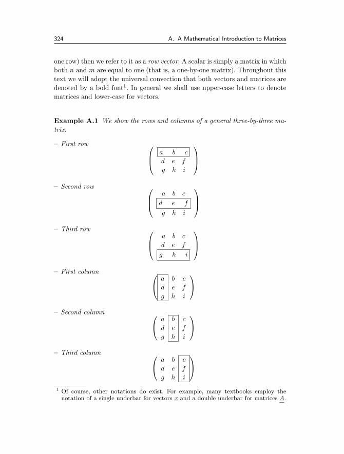
Example A.1 We show the rows and columns of a general three-by-three ma-trix.
– First row ⎛⎜⎝ a b c
d e f
g h i
⎞⎟⎠
– Second row ⎛⎜⎝
a b c
d e f
g h i
⎞⎟⎠
– Third row ⎛⎜⎝
a b c
d e f
g h i
⎞⎟⎠
– First column ⎛⎝ a b c
d e f
g h i
⎞⎠
– Second column ⎛⎝ a b c
d e f
g h i
⎞⎠
– Third column ⎛⎝ a b c
d e f
g h i
⎞⎠
1 Of course, other notations do exist. For example, many textbooks employ thenotation of a single underbar for vectors x and a double underbar for matrices A.
A. A Mathematical Introduction to Matrices 325
Of all the operations which can be performed on matrices one of the simplestis that of transposition (or taking the transpose of a matrix); this operation isusually denoted by a subscript T or a prime ′. If A is n-by-m then B = AT ism-by-n, where the elements of B are defined by
bj,i = ai,j i = 1, · · · , n; j = 1, · · · , m;
the transpose is thus obtained by interchanging the rows and columns of matrixA to give the matrix B = AT . If the matrix A is square then the operationof taking the transpose is equivalent to a reflection in the leading diagonal(which runs from the top left corner to the bottom right). Matrices for whichAT = A are referred to as symmetric and those for which AT = −A are anti-symmetric2. In the case of three-by-three matrices the general symmetric andanti-symmetric three-by-three matrices can be written as
Asymm =
⎛⎝ a b c
b d e
c e f
⎞⎠ and Aanti =
⎛⎝ 0 b c
−b 0 e
−c −e 0
⎞⎠ .
where a, b, . . . , f ∈ C. We remark that if the complex conjugate transpose of amatrix (with elements a∗
j,i) is equal to the matrix then it is called Hermitianand if it is equal to minus its complex conjugate transpose then it is referredto as skew Hermitian.
We pause here to state that A = B implies that ai,j = bi,j for all theelements of the matrices, whereas A = B only requires that ai,j = bi,j for onepair (i, j).
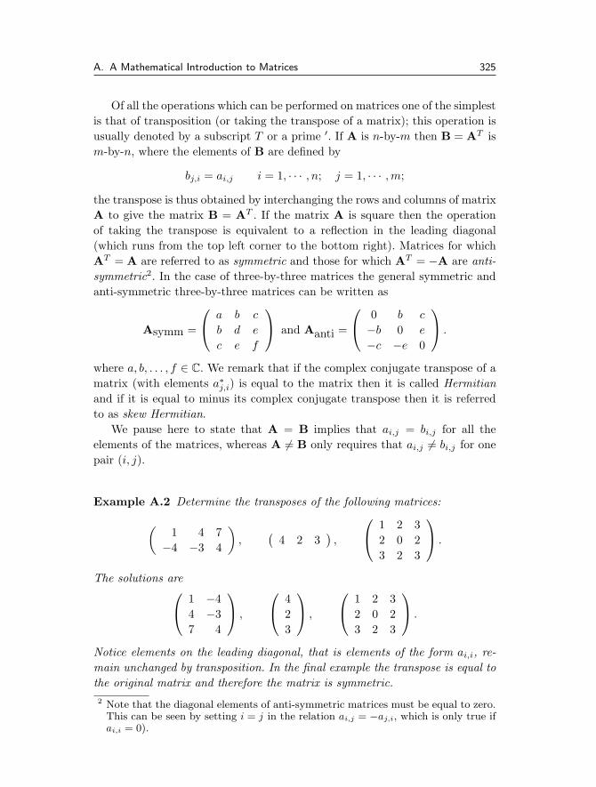
Example A.2 Determine the transposes of the following matrices:
(1 4 7
−4 −3 4
),
(4 2 3
),
⎛⎝ 1 2 3
2 0 23 2 3
⎞⎠ .
The solutions are⎛⎝ 1 −4
4 −37 4
⎞⎠ ,
⎛⎝ 4
23
⎞⎠ ,
⎛⎝ 1 2 3
2 0 23 2 3
⎞⎠ .
Notice elements on the leading diagonal, that is elements of the form ai,i, re-main unchanged by transposition. In the final example the transpose is equal tothe original matrix and therefore the matrix is symmetric.2 Note that the diagonal elements of anti-symmetric matrices must be equal to zero.
This can be seen by setting i = j in the relation ai,j = −aj,i, which is only true ifai,i = 0).
326 A. A Mathematical Introduction to Matrices
The usual arithmetic operations of addition, subtraction and multiplicationalso apply to matrices. However, there are now several additional rules (orconstraints) under which these operations can be performed on two (or more)matrices. These are outlined below.
Addition and subtraction: two matrices can only be added together if they arethe same size (that is, they have the same number of rows and the samenumber of columns). In this case the operation of addition is performedelement by element. For example, if A,B are both n-by-m matrices thenC = A + B is defined as the matrix with elements ci,j = ai,j + bi,j . Asimilar rule holds for subtraction.
Scalar multiplication: matrices of any size can be multiplied by scalars. Themultiplication is performed element by element so that C = λA whereci,j = λai,j .
Matrix multiplication: in order to multiply two matrices A and B together thenumber of columns of A must equal the number of rows of B. To performthe multiplication we “multiply” the first row of A by the first column ofB, multiplying the first element of each together and then the second ones,etc, and finally adding up all the results. This gives the element in the topleft hand corner. We then proceed to multiply the first row by the secondcolumn in the same manner (and put the result in the first row, secondcolumn). Mathematically this can be written as
ci,j =m∑
k=1
ai,kbk,j i = 1, · · · , n; j = 1, · · · , p,
where A is n-by-m and B is m-by-p. Then the answer C is n-by-p.
This rule for matrix multiplication highlights one of their important proper-ties, namely that the order of multiplication is important. In this example,with A an n-by-m matrix and B an m-by-p matrix, the operation “A timesB” is defined. However, the operation “B times A” (that is, pre-multiplyingmatrix A by matrix B) is not defined unless p = n. Even if p = n, in gen-eral AB = BA. This is equivalent to saying that, unlike scalar multiplication,matrix multiplication is not commutative.
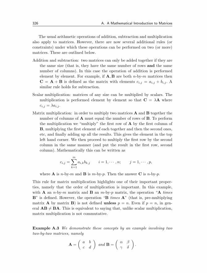
Example A.3 We demonstrate these concepts by an example involving twotwo-by-two matrices, namely
A =(
a b
c d
)and B =
(α β
γ δ
).

A. A Mathematical Introduction to Matrices 327
The sum C = A + B is determined as follows. Firstly the element c1,1 isobtained by adding the corresponding elements in A and B, so that
(a b
c d
)+(
α β
γ δ
)=
(a + α
).
Now for the c1,2 entry (the top right element):(a b
c d
)+
(α β
γ δ
)=
(a + α b + β
).
Similarly for c2,1 (the bottom left element)
(a b
c d
)+
(α β
γ δ
)=
(a + α b + β
c + γ
)
and finally for c2,2 (the bottom right element) we have(a b
c d
)+
(α β
γ δ
)=
(a + α b + β
c + γ d + δ
).
Example A.4 An example of multiplication of two two-by-two matrices willserve to highlight the differences between addition and multiplication of matri-ces. Consider the matrices
A =(
a b
c d
)and B =
(α β
γ δ
).
By our earlier rule the product C = AB is defined and is determined as follows.We start with the top left entry, namely c1,1 (formed by multiplying the firstrow of A by the first column of B)(
a b
c d
)(α β
γ δ
)=
(a × α + b × γ
);
now the top right entry, namely c1,2 (which is formed by multiplying the firstrow of A by the second column of B)
(a b
c d
)(α β
γ δ
)=
(a × α + b × γ a × β + b × δ
);

328 A. A Mathematical Introduction to Matrices
next the bottom left entry, namely c2,1 (which is formed by multiplying thesecond row of A by the first column of B)
(a b
c d
)(α β
γ δ
)=
(a × α + b × γ a × β + b × δ
c × α + d × γ
);
and finally the bottom right entry, namely c2,2 (which is formed by multiplyingthe second row of A by the second column of B)
(a b
c d
)(α β
γ δ
)=
(a × α + b × γ a × β + b × δ
c × α + d × γ c × β + d × δ
).
In general, to calculate the ci,j entry we multiply the ith row of the first matrixA by the jth column of the second matrix B term by term.
Example A.5 Calculate the product AB of the matrices
A =(
1 −10 3
)and B =
( −2 14 −2
).
Using the method given in the previous example
AB =(
1 −10 3
)( −2 14 −2
)
=(
1 × (−2) + (−1) × 4 1 × 1 + (−1) × (−2)0 × (−2) + 3 × (4) 0 × 1 + 3 × (−2)
)
=( −6 3
12 −6
).
(It is worth practising these calculations; try calculating the product BA your-self by hand.).
We now turn our attention to matrix multiplication in which the matrices arenot necessarily square.
Example A.6 Consider the matrices
A =(
3 0 −1−4 2 2
), B =
⎛⎝ −1 7
3 5−2 0
⎞⎠ and C =
(2 0
−1 −3
).

A. A Mathematical Introduction to Matrices 329
Calculate the quantities: AB, BA, A+BT , AC, AT C, 3C+2(AB)T , (AB)Cand finally A (BC), where possible (and if not, state the reason why the calcu-lations cannot be performed).
We shall start (for the first couple of examples) by providing full solutionsand thereafter just give answers with a minimum of intermediate steps. So,
AB =(
3 0 −1−4 2 2
)⎛⎝ −1 7
3 5−2 0
⎞⎠
=(
3 × (−1) + 0 × 3 + (−1) × (−2) 3 × 7 + 0 × 5 + (−1) × (0)(−4) × (−1) + 2 × 3 + 2 × (−2) (−4) × 7 + 2 × 5 + 2 × (0)
)
=( −1 21
6 −18
).
Similarly
BA =
⎛⎝ −1 7
3 5−2 0
⎞⎠(
3 0 −1−4 2 2
)
=
⎛⎝ −1 × 3 + 7 × (−4) −1 × 0 + 7 × 2 −1 × (−1) + 7 × 2
3 × 3 + 5 × (−4) 3 × 0 + 5 × 2 3 × (−1) + 5 × 2−2 × 3 + 0 × (−4) −2 × 0 + 0 × 2 −2 × (−1) + 0 × 2
⎞⎠
=
⎛⎝ −31 14 15
−11 10 7−6 0 2
⎞⎠
A + BT =(
3 0 −1−4 2 2
)+( −1 3 −2
7 5 0
)
=(
2 3 −33 7 2
).
It is not possible to pre-multiply matrix A by C since A is two-by-three and C istwo-by-two, so the inner dimensions do not agree (that is, the second dimensionof the first matrix and the first dimension of the second matrix are different).For the next example AT C we observe that AT is three-by-two so that the innerdimensions agree and hence the calculation is possible. We obtain
AT C =
⎛⎝ 3 −4
0 2−1 2
⎞⎠(
2 0−1 −3
)=
⎛⎝ 10 12
−2 −6−4 −6
⎞⎠ .
330 A. A Mathematical Introduction to Matrices
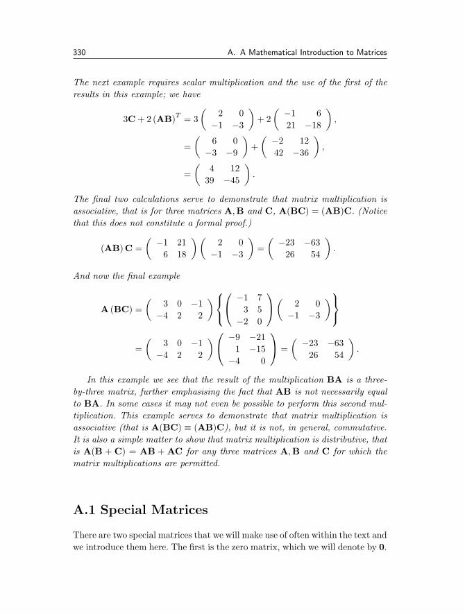
The next example requires scalar multiplication and the use of the first of theresults in this example; we have
3C + 2 (AB)T = 3(
2 0−1 −3
)+ 2
( −1 621 −18
),
=(
6 0−3 −9
)+( −2 12
42 −36
),
=(
4 1239 −45
).
The final two calculations serve to demonstrate that matrix multiplication isassociative, that is for three matrices A,B and C, A(BC) = (AB)C. (Noticethat this does not constitute a formal proof.)
(AB)C =( −1 21
6 18
)(2 0
−1 −3
)=( −23 −63
26 54
).
And now the final example
A (BC) =(
3 0 −1−4 2 2
)⎧⎨⎩⎛⎝ −1 7
3 5−2 0
⎞⎠(
2 0−1 −3
)⎫⎬⎭
=(
3 0 −1−4 2 2
)⎛⎝ −9 −21
1 −15−4 0
⎞⎠ =
( −23 −6326 54
).
In this example we see that the result of the multiplication BA is a three-by-three matrix, further emphasising the fact that AB is not necessarily equalto BA. In some cases it may not even be possible to perform this second mul-tiplication. This example serves to demonstrate that matrix multiplication isassociative (that is A(BC) ≡ (AB)C), but it is not, in general, commutative.It is also a simple matter to show that matrix multiplication is distributive, thatis A(B + C) = AB + AC for any three matrices A,B and C for which thematrix multiplications are permitted.
A.1 Special Matrices
There are two special matrices that we will make use of often within the text andwe introduce them here. The first is the zero matrix, which we will denote by 0.
A.2 Inverses of Matrices 331
This is simply a matrix whose elements are all equal to zero3. Not surprisingly,the zero matrix has no effect when it is added to another matrix (of the samesize). So A + 0 = A = 0 + A. We will make use of this matrix to initialisematrices in preparation to assigning answers to a matrix.
The second important matrix we will have call to use often with the text isthe identity (or unit) matrix, denoted by I. The identity matrix I is a n-by-nmatrix whose elements consist of 1s (ones) along the main diagonal and arezero everywhere else. For example, the three-by-three identity matrix is givenby
I =
⎛⎝ 1 0 0
0 1 00 0 1
⎞⎠ .
Multiplying a square n-by-n matrix A by I has no effect:
AI = A = IA.
A.2 Inverses of Matrices
The inverse of a matrix, written as A−1, is defined as the matrix which whenpre- and post-multiplied by the matrix A produces the identity matrix I:
A−1A = AA−1 = I.
Only square matrices can have an inverse but it is only a subset of all squarematrices for which the inverse exists. The existence of the inverse of a matrix(that is, whether the matrix is invertible or not) is intimately linked with thedeterminant of the matrix. We introduce this, and many other properties ofmatrices, in Chapter 6.
The utility of the inverse of a matrix is best seen when solving systems ofequations. An example will serve by way of illustration.
Example A.7 Consider the system of simultaneous equations:
x1 + x2 = 3, (A.1a)
x1 + 2x2 = 5. (A.1b)
3 Of course, we could include the dimensions of the matrix by writing 0nm to denotethat it is an n-by-m matrix. We will adopt the convention in the text that whenwe refer to the zero matrix we are taking a matrix of the appropriate size requiredfor the operation.
332 A. A Mathematical Introduction to Matrices
These equations can be solved using conventional means. To do this we firstsubtract (A.1a) from (A.1b) to give
x1 + 2x2 − (x1 + x2) = 5 − 3
or
x2 = 2,
and now substituting back into either equation (let us use (A.1a)) we have
x1 + 2 = 3
which gives
x1 = 1.
We can just as easily write the system (A.1) as a matrix equation(1 11 2
)(x1
x2
)=(
35
)
or as
Ax = b.
Try multiplying out the matrix equation to check you get (A.1a) and (A.1b).Elementary linear algebra shows that the solution is given by A−1b, which canbe written in MATLAB as inv(A)*b or A\b. The operator \ determines theeffect of multiplying by the inverse of the first argument on the second, withoutever constructing the inverse. The code for this example would be:
>> A = [1 1; 1 2]; % Initialise the matrix A
>> b = [3; 5]; % Initialise the vector b
>> x = inv(A)*b % Determine the solution vector x
Before we proceed we note in the previous three lines of MATLAB code every-thing after the percent sign % is taken by MATLAB to be a comment. Com-ments are a useful way of making your MATLAB code readable by both youand others.
We can check the answer from our matrix computation by typing A*x, whichshould be equal to b.

A.2 Inverses of Matrices 333
Example A.8 Determine the vector x which satisfies the equation Ax = bwhere
A =
⎛⎜⎜⎝
1 2 3 44 3 2 11 0 −1 0
−1 1 −1 1
⎞⎟⎟⎠ and b =
⎛⎜⎜⎝
5101520
⎞⎟⎟⎠ .
We enter the matrix A and vector b directly using
>> A = [1 2 3 4; ...
4 3 2 1; ...
1 0 -1 0; ...
-1 1 -1 1];
>> b = [5; 10; 15; 20];
(Note we have used the three dots ... (or ellipsis) to indicate to MATLAB thatthe input line continues. It is good practise to have a space before the dots atthe end of the line.) These results can then be used to form x:
>> inv(A)*b
ans =
3.2500
4.5000
-11.7500
7.0000
This solution was obtained by considering the equation Ax = b and pre-multiplying each side by the inverse of the matrix A (we have deliberately chosenA so that its inverse exists). This gives A−1Ax = A−1b but we recall from thedefinition of the inverse that A−1A = I and that Ix = x. Hence we have thesolution x = A−1b.

BGlossary of Useful Terms
This appendix is provided purely as a guide. MATLAB has a very informativehelp feature help command which is supplemented with several other featureslookfor maths. You can also access the help files on the web helpdesk.
This appendix is broken down into:
– arithmetic and logical operators– symbols– plotting commands– general MATLAB commands
B.1 Arithmetic and Logical Operators
+, - Used to add or subtract variables of the same size together, whether theyare matrices, vectors or scalars.�
�
�
�
A = [1 2; 3 4];
B = ones(2);
A + B
A - B
5 + 0.5
7 - 4
336 B. Glossary of Useful Terms
It is also worth noting that these operations will add (or subtract) scalarquantities from matrices. For instance:
�
�
�A = ones(3);
B = A + 2;
C = 3 - A;
This produces a three-by-three matrix full of threes in B and a three-by-three matrix full of twos in C. MATLAB will complain if these operationsare not viable.
*, / Used to multiply or divide variables as long as the operation is mathe-matically viable:�
�
�
�
4 * 3.2
4 / 2.3
A = [1 2; 3 4];
B = ones(2);
A * B
A / B
The last two operations give AB and AB−1. Notice that the multiplica-tion operation is only viable if the inner dimensions agree: the number ofcolumns of the first matrix must equal the number of rows of the second.
It can also multiply (or divide) matrices by scalars:
�
�
�A = ones(3);
B = A/3;
C = A*4;
These commands give B as a three-by-three matrix full of 1/3’s and C as athree-by-three matrix full of fours.
.* This binary operator allows one to perform multiplication calculations el-ement by element on arrays of the same size. If we consider the vectorsx = (x1, x2, x3, x4) and y = (y1, y2, y3, y4). Then the calculation x‘.*’ygives (x1y1, x2y2, x3y3, x4y4). Notice that both x and y were row vectorsof length 4 and so is the answer. Let us consider the example:

B.1 Arithmetic and Logical Operators 337
�
�
�A = [4 3; 2 1];
B = [1 2; 3 4];
C = A.*B;
This does the calculation element-wise and gives the result:
C =(
4 × 1 3 × 22 × 3 1 × 4
)=(
4 66 4
).
This command can also be used on values which are scalars, so for instanceA = ones(2); B = A.*2; gives B as a matrix full of twos.
The most common use of this operator is again in the construction offunctions.
�
�
�x = 1:5;
f = x.*sin(x);
g = (3*x+4).*(x+2);
This gives us x = [1 2 3 4 5] and then: f = x sin x evaluated at thosepoints, i.e. [sin(1) 2*sin(2) 3*sin(3) 4*sin(4) 5*sin(5)]; and g =(3x+ 4)(x+ 2) at the points. Notice it is not necessary to use the operator.* when calculating 3*x since 3 is a scalar.
./ This binary operator allows one to perform division calculations elementby element on arrays of the same size. If we consider the vectors x =(x1, x2, x3, x4) and y = (y1, y2, y3, y4), then the calculation x‘./’y gives(x1/y1, x2/y2, x3/y3, x4/y4). Notice that both x and y were row vectors oflength 4 and so is the answer. Let us consider the example:
�
�
�A = [4 3; 2 1];
B = [1 2; 3 4];
C = A./B;
This does the calculation element-wise and gives the result:
C =(
4/1 3/22/3 1/4
)=(
4 32
23
14
).
This command can also be used on values which are scalars, so for instanceA = ones(2); B = A./2; gives B as a matrix full of halves.
The most common use of this operator is in the construction of functions.
338 B. Glossary of Useful Terms
�
�
�x = 1:5;
f = x./sin(x);
g = (3*x+4)./(x+2);
This gives us x = [1 2 3 4 5] and then: f = x/ sin x evaluated atthose points, i.e. [1/sin(1) 2/sin(2) 3/sin(3) 4/sin(4) 5/sin(5)];and g = (3x + 4)/(x + 2) at the points.
We can use this command where either of its arguments are scalars (in fact,it is necessary for this example).��
��
x = [1 2 3 4 5];
y = 2./x
This gives [2/1 2/2 2/3 2/4 2/5]. This construction is useful whenworking out functions of the form f(x) = 2/x.
.ˆ This binary operator allows one to perform exponentiation (raising to apower) calculations element by element on arrays of the same size. If weconsider the vectors x = (x1, x2, x3, x4) and y = (y1, y2, y3, y4), then thecalculation x‘.ˆ’y gives (xy1
1 , xy22 , xy3
3 , xy44 ). Notice that both x and y were
row vectors of length 4 and so is the answer. Let us consider the example:
�
�
�A = [4 3; 2 1];
B = [1 2; 3 4];
C = A.ˆB;
This does the calculation element-wise and gives the result:
C =(
41 32
23 14
)=(
4 98 1
).
This command can also be used on values which are scalars, so for instanceA = ones(2); B = A.ˆ2; gives B as a matrix full of ones (that is onesquared).
The most common use of this operator is in the construction of functions.
�
�
�x = 1:5;
f = x.ˆ(x+1);
g = (3*x+4).ˆx;
B.1 Arithmetic and Logical Operators 339
This gives us x = [1 2 3 4 5] and then: f = xx+1 evaluated at thosepoints, i.e. [1ˆ2 2ˆ3 3ˆ4 4ˆ5 5ˆ6]; and g = (3x + 4)x at the points.
As with the operator ‘./’ we can use this command when either of itsarguments are scalars. For instance: �
��
x = 1:5;
y = 2.ˆx;
z = x.ˆ2;
This gives y=[2ˆ1 2ˆ2 2ˆ3 2ˆ4 2ˆ5] and z=[1ˆ2 2ˆ2 3ˆ2 4ˆ2 5ˆ2].
\ This works out the effect of pre-multiplying by the inverse of the first ar-gument on the second argument. So if we want to solve the set of linearequations represented in the matrix equation Ax = b, we need to constructx = A−1b.
�
�
�A = [1 2; 3 4];
b = [2; 3];
x = A\b;
This solves the set of equations:
x1 + 2x2 = 2
3x1 + 4x2 = 3.
by defining
A =(
1 23 4
)and b =
(23
),
with x = (x1, x2)T .
== Checks equality, rather than sets equal. This is usually exploited withinlogical statements with scalars:�
�
�
�
if i==7
disp(’ i is seven ’)
else
disp(’ i is not seven ’)
end
This can be used in other forms: x = 1:12; mod(x,3)==0. This gives theoutput:

340 B. Glossary of Useful Terms
0 0 1 0 0 1 0 0 1 0 0 1
that is it is true provided the corresponding element of x is divisible by 3.
∼= Checks not equal to. Again this is mainly used in logical statements withscalars:�
�
�
�
if i˜=7
disp(’ i is not seven ’)
else
disp(’ i is equal to seven ’)
end
This can be used inline x = 1:12; mod(x,3)∼=0. This gives the output:
1 1 0 1 1 0 1 1 0 1 1 0
that is it is true provided the corresponding element of x is not divisibleby 3. Note: great care is needed with this command since the simple orderchange to y=∼x means set y equal to not(x).
>, >= Checks greater than and greater than or equal to. Mainly used withscalars within logical statements:
�
�
�
�
if i>7
disp(’ i is greater than seven ’)
end
if i>=7
disp(’ i is greater than or equal to seven ’)
end
Can be used for an array x = 1:12; x>7 which gives
0 0 0 0 0 0 0 1 1 1 1 1
whereas x = 1:12; x>=7 gives

B.1 Arithmetic and Logical Operators 341
0 0 0 0 0 0 1 1 1 1 1 1
that is the second one is true for x = 7.
<, <= Checks less than and less than or equal to. Mainly used with scalarswithin logical statements:
�
�
�
�
if i<7
disp(’ i is less than seven ’)
end
if i<=7
disp(’ i is less than or equal to seven ’)
end
Can be used for an array x = 1:12; x<7 gives
1 1 1 1 1 1 0 0 0 0 0 0
whereas x = 1:12; x<=7
1 1 1 1 1 1 1 0 0 0 0 0
that is the second one is true for x = 7.
all This returns a value of true if all of the arguments are true: all(x.ˆ2>0)would be true (provided all the values of x are real); x = 1:12; all(x>0)
would give true since all the elements of x are positive.
and Boolean operator for and can also use &. This is true only if both itsarguments are true.
�
��
if and(x>7,x<9)
disp(’ x is between 7 and 9’)
end
This can also be written as x>7 & x<9 and can be applied to arrays, sothat x = 1:12; and(x>7,x<9) gives:

342 B. Glossary of Useful Terms
0 0 0 0 0 0 0 1 0 0 0 0
any This returns a value of true if any of the arguments are true: any(x<0)would be true if any of the values in the vector x are strictly negative; x =
1:12; any(x>10) would be true since some elements of x are greater than10.
find Provides a list of integers when the condition is true, for instance x =
1:10; [i]=find(x.ˆ2>26); gives the locations i=[6 7 8 9 10].
not Negates logical variables, can also use ∼. This can be used to turn trueinto false and vice versa, so that
�
��
if not(x>=7)
disp(’ x is not greater than or equal to 7’)
end
This could also be written as ∼(x>=7). This can be applied to arrays, sothat x = 1:12; not(x>=7) gives:
1 1 1 1 1 1 0 0 0 0 0 0
or Boolean operator for or can also use |. This is true provided one of itsarguments is true.
�
��
if or(x<7,x>9)
disp(’ x is less than 7 or greater than 9’)
end
This can also be written as x<7 | x>9 and can be applied to arrays, sothat x = 1:12; or(x<7,x>9) gives:
1 1 1 1 1 1 0 0 0 1 1 1
xor Exclusive or. This gives true if one of the values is true and false if theyare both false or both true.

B.2 Symbols 343
�
�
�x = [0 0 1 1];
y = [0 1 0 1];
xor(x,y)
gives [0 1 1 0].
We note that this can also be done for or and and.
B.2 Symbols
... Used to link lines together (but cannot be used within a string): �
��
x = 1:10;
f = x.ˆ2+sqrt(x.ˆ2+1) ...
+ cos(x)./x;
This gives the function f = x2 +√
x2 + 1 + cos x/x at the values from x
equals 1 to 10.
% Means the rest of the line is a comment. It also has special meaning at thestart of a code. It can be very useful for eliminating the execution of certainlines of a code.
�
�
�
�
% This code calculates the value
% of x times sin(x)
f = x.*sin(x);
% and the value of cos(xˆ2)
g = cos(x.ˆ2); % where x can be a vector.
If this code was saved as mycode.m then typing help mycode would pro-duce:
This code calculates the value
of x times sin(x)
344 B. Glossary of Useful Terms
; Used at the end of a phrase to suppress output. It can occur at the physicalend of a line or at the end of a set of commands.
�
�
�a = ones(2);
b = ones(2); c = ones(2);
d1 = ones(2); d2 = ones(2)
This code will set up the two-by-two matrices a, b, c, d1 and d2 full of ones.It will only report on the initiation of d2 since this phrase is not concludedwith a semicolon.
It can also be used to end lines within matrices (enclosed within pairs ofsquare brackets)��
��A= [ 1 2; 3 4];
This gives the matrix
A =(
1 23 4
).
(Note that the semicolon is used in both its incarnations here.) We notethat both uses of the semicolon correspond to the end of the phrase: itis merely that the square brackets are unbalanced in the latter case soMATLAB knows that it is going to read the next line of the matrix.
: Used to delimit values when setting up a vector and also to refer to entirerows or columns of matrices. When setting a row vector there are twosyntaxes:��
��
x1 = 1:12
x2 = 1:2:13
The first of these commands sets up an array from 1 to 12 in steps ofunity (and is equivalent to 1:1:12) whereas the second array runs from1 to 13 in steps of 2, thus it yields [1 3 5 7 9 11 13]. The syntaxesare a:b (an array from a to a value not exceeding b in steps of unity)and a:h:b (an array from a to a value not exceeding b in steps of h)(see also linspace). Note that h can be negative 11:(-2):1 gives [11 9
7 5 3 1]. We note that the length of an array set up using a:h:b is not(b−a)/h (presuming that this is an integer), but (b−a)/h+1. For example0:0.1:1 has eleven points [0 0.1 0.2 0.3 0.4 0.5 0.6 0.7 0.8 0.9
1.0] rather than ten. This dimension can be determined using length.

B.2 Symbols 345
The second use of this symbol allows reference to all viable values of a rowor column.
�
�
�
�
A = [11 12 13; 21 22 23; 31 32 33];
A(1,:) % First row of A
A(:,2) % Second column of A
A(:,:) % Whole of A.
A(:,1:2) % First and second columns of A
A(1:2:3,:) % First and third rows of A
A(1:2,1:2) % Top left two-by-two corner of A
, Can be used to delimit sets of commands where feedback is required:��
��a = 1, b = 2
and to separate elements of matrices on a particular line��
��A = [1,2,3,4;5,6,7,8];
It is also used to separate arguments of functions��
��x = linspace(0,1,200);
’ ’ Used to surround strings and for passing arguments to various functions:
�
�a = ’Do robots dream of electronic sheep?’
x = 1:12;
y = x.ˆ2;
plot(x,y,’LineWidth’,2)
see the comments on plot below.
’ Gives the complex conjugate transpose of a matrix. If the n-by-m matrixA has elements ai,j , then B = A’ is m-by-n and has elements bi,j = a∗
j,i
(where i ∈ {1, · · · , m} and j ∈ {1, · · · , n}).
346 B. Glossary of Useful Terms
��
��
A = [1+2*i 2-i; 3 4+i];
B = A’;
This gives
B =(
1 − 2i 32 + i 4 − i
).
.’ Gives the transpose of a matrix. If the n-by-m matrix A has elements ai,j ,then B = A.’ is m-by-n and has elements bi,j = aj,i (where i ∈ {1, · · · , m}and j ∈ {1, · · · , n}).��
��
A = [1+2*i 2-i; 3 4+i];
B = A.’;
This gives
B =(
1 + 2i 32 − i 4 + i
).
It is better to use this form rather than A’ unless you are concerned withissues of complex matrices.
(space) Can be used to separate elements of matrices, as for the comma; butcannot be used to separate commands. Hence we can use:��
��
A = [1 2 3; 4 5 6];
B = [ 1:3 ; 3 2 1];
The reason that (space) cannot be used to delimit commands is that itcan occur naturally within a command, for instance a = 2 which is usedrather than a=2 merely to improve the readability of the code.
. decimal point – This can be used firstly as the mathematical decimal point:3.145 or 567.3245. It is also used to punctuate file names into two parts:an identifier (descriptive of the contents of the code, or its function) andthen the file’s type (.m, .mat, .dat or .fig). For this reason you shouldonly have one ‘.’ in each number or filename.
[ ] used to enclose elements of a vector or matrix:
�
�A = [1 2 3 5 6 7];
B = [1 2 3;
3 4 5];
ms = [’Vector array’ ’ of strings’];

B.3 Plotting Commands 347
These brackets should balance.
( ) used to surround mathematical expressions and lists of arguments forfunctions:
�
�
�x= 1:12
y = 1./(x.ˆ2+1);
z = x.*sin(y);
Again these brackets should balance.
B.3 Plotting Commands
Before we start this section we need to discuss the idea of a handle. This isessentially a variable which allows us to access properties of an object.
>> x = 1:12; y = x.ˆ2;
>> h = plot(x,y)
>> get(h)
Color = [0 0 1]
EraseMode = normal
LineStyle = -
LineWidth = [0.5]
Marker = none
MarkerSize = [6]
MarkerEdgeColor = auto
MarkerFaceColor = none
XData = [ (1 by 12) double array]
YData = [ (1 by 12) double array]
ZData = []
ButtonDownFcn =
Children = []
Clipping = on
CreateFcn =
DeleteFcn =
BusyAction = queue
HandleVisibility = on
Interruptible = on
Parent = [3.00012]
348 B. Glossary of Useful Terms
Selected = off
SelectionHighlight = on
Tag =
Type = line
UserData = []
Visible = on
The variable h allows us to access all of these commands, which can be changedusing the command set, for instance set(h,’MarkerSize’,10).
axes Used to initiate a set of axes
�
�figure(1)
h = axes
figure(2)
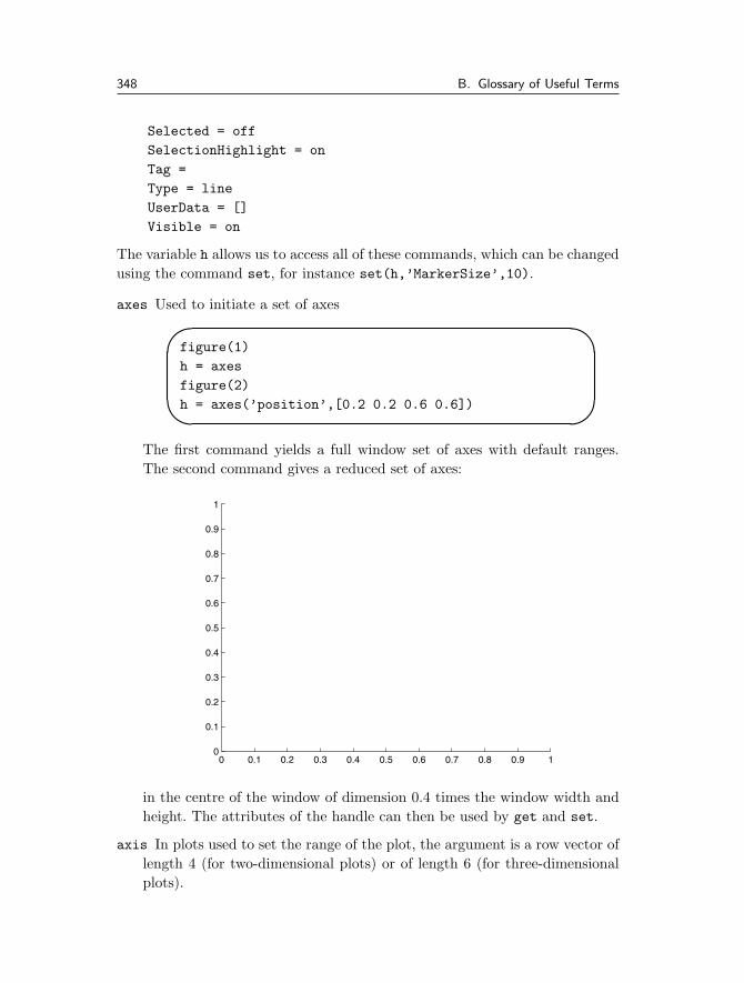
h = axes(’position’,[0.2 0.2 0.6 0.6])
The first command yields a full window set of axes with default ranges.The second command gives a reduced set of axes:
0 0.1 0.2 0.3 0.4 0.5 0.6 0.7 0.8 0.9 10
0.1
0.2
0.3
0.4
0.5
0.6
0.7
0.8
0.9
1
in the centre of the window of dimension 0.4 times the window width andheight. The attributes of the handle can then be used by get and set.
axis In plots used to set the range of the plot, the argument is a row vector oflength 4 (for two-dimensional plots) or of length 6 (for three-dimensionalplots).
B.3 Plotting Commands 349
�
�
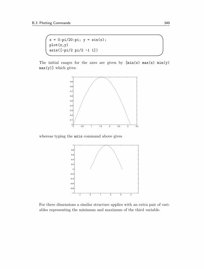
�x = 0:pi/20:pi; y = sin(x);
plot(x,y)
axis([-pi/2 pi/2 -1 1])
The initial ranges for the axes are given by [min(x) max(x) min(y)
max(y)] which gives:
0 0.5 1 1.5 2 2.5 3 3.50
0.1
0.2
0.3
0.4
0.5
0.6
0.7
0.8
0.9
1
whereas typing the axis command above gives
−1 0 1 2 3 4−1
−0.8
−0.6
−0.4
−0.2
0
0.2
0.4
0.6
0.8
1
For three dimensions a similar structure applies with an extra pair of vari-ables representing the minimum and maximum of the third variable.

350 B. Glossary of Useful Terms
�
�
�
�
t = linspace(0,2*pi);
x = cos(t);
y = sin(t);
z = t;
plot3(x,y,z)
grid on
axis([-1.5 1.5 -1.5 1.5 -pi/2 2*pi])
This gives the plot:
−1.5−1
−0.50
0.51
1.5
−1.5
−1
−0.5
0
0.5
1
1.5
−1
0
1
2
3
4
5
6
We have used grid on to add the dotted lines.
The command can also be used as:
�
�
�
�
axis off % Removes the axis from the current figure
axis equal % Sets the axis scaling to be equal.
axis square % Sets the axis to be square.
axis tight % Uses the max and min of the
% data for axis limits
for more variants see help axis.
bar Produces a bar chart of the data.
B.3 Plotting Commands 351
�
�
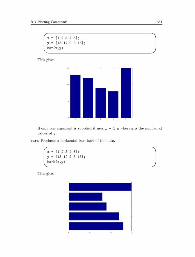
�x = [1 2 3 4 5];
y = [13 12 9 8 15];
bar(x,y)
This gives:
1 2 3 4 50
5
10
15
If only one argument is supplied it uses x = 1:m where m is the number ofvalues of y.
barh Produces a horizontal bar chart of the data.
�
�
�x = [1 2 3 4 5];
y = [13 12 9 8 15];
barh(x,y)
This gives:
0 5 10 15
1
2
3
4
5
352 B. Glossary of Useful Terms
If only one argument is supplied it uses x = 1:m where m is the number ofvalues of y.
clf This clears the current figure, in fact it removes all children with visiblehandles. It removes any axes from the current figure. It is useful to use thisbefore we start plotting.
close This is used to close figures; close all closes all figures. There arebasically three syntaxes:
�
�
�close % Closes the current figure
close(4) % closes figure number 4
close all % closes all figures.
This can be used for other windows by using their handle: close(h) closesthe window with handle h.
figure This brings the requested figure to the fore, or creates it if it doesn’texist.
�
�
�
�
figure % Creates a figure
figure(3) % Ensures that Figure No. 3 is the current
% figure and is at the fore.
figure(h) % Ensures that the figure with the handle
% h is the current figure
gca Returns the handle to the current axis; this allows various properties tobe displayed (get) and modified (set).
There are many variables involved:
>> x = 1:12; y=x.ˆ2;>> plot(x,y)>> h = gca>> get(h)
AmbientLightColor = [1 1 1]Box = onCameraPosition = [6 75 17.3205]CameraPositionMode = autoCameraTarget = [6 75 0]CameraTargetMode = autoCameraUpVector = [0 1 0]CameraUpVectorMode = autoCameraViewAngle = [6.60861]
B.3 Plotting Commands 353
CameraViewAngleMode = autoCLim = [0 1]CLimMode = autoColor = [1 1 1]CurrentPoint = [ (2 by 3) double array]ColorOrder = [ (7 by 3) double array]DataAspectRatio = [6 75 1]DataAspectRatioMode = autoDrawMode = normalFontAngle = normalFontName = HelveticaFontSize = [10]FontUnits = pointsFontWeight = normalGridLineStyle = :Layer = bottomLineStyleOrder = -LineWidth = [0.5]NextPlot = replacePlotBoxAspectRatio = [1 1 1]PlotBoxAspectRatioMode = autoProjection = orthographicPosition = [0.13 0.11 0.775 0.815]TickLength = [0.01 0.025]TickDir = inTickDirMode = autoTitle = [287.001]Units = normalizedView = [0 90]XColor = [0 0 0]XDir = normalXGrid = offXLabel = [288]XAxisLocation = bottomXLim = [0 12]XLimMode = autoXScale = linearXTick = [ (1 by 7) double array]XTickLabel =
024681012
XTickLabelMode = autoXTickMode = autoYColor = [0 0 0]YDir = normalYGrid = offYLabel = [289]YAxisLocation = left
354 B. Glossary of Useful Terms
YLim = [0 150]YLimMode = autoYScale = linearYTick = [0 50 100 150]YTickLabel =
050100150
YTickLabelMode = autoYTickMode = autoZColor = [0 0 0]ZDir = normalZGrid = offZLabel = [290]ZLim = [-1 1]ZLimMode = autoZScale = linearZTick = [-1 0 1]ZTickLabel =ZTickLabelMode = autoZTickMode = auto
ButtonDownFcn =Children = [285]Clipping = onCreateFcn =DeleteFcn =BusyAction = queueHandleVisibility = onHitTest = onInterruptible = onParent = [1]Selected = offSelectionHighlight = onTag =Type = axesUIContextMenu = []UserData = []Visible = on
gcf Returns the handle of the current figure. This allows various properties tobe displayed (get) and modified (set).
�
�x = 1:12; y = x.ˆ2;
plot(x,y)
h = gcf
get(h)
B.3 Plotting Commands 355
returns the list printed on page 348.
get Extracts a particular attribute from a list, retrieved for example by gca
or gcf.
>> x = 1:12; y = x.ˆ2;
>> plot(x,y)
>> h = gcf
>> a = gca
>> get(h,’Color’)
ans =
0.8000 0.8000 0.8000
>> get(a,’YTick’)
ans =
0 50 100 150
The colour variable is returned as a triple (a one-by-three vector giving theRGB (Red-Green-Blue) value). The values associated with the axis and thefigure can be changed using the set command.
ginput Returns coordinates of mouse clicks on the current figure in terms ofaxis units; very useful for obtaining initial estimates for roots (see alsozoom).
�
�x = 0:pi/20:4*pi;
y = sin(x);
plot(x,y)
[xp,yp]= ginput
Notice that control is passed over to the figure and the points are stored inthe arrays xp and yp (until the return key is hit). The command can alsobe used as n = 10; [xp,yp] = ginput(n) to only get 10 points.
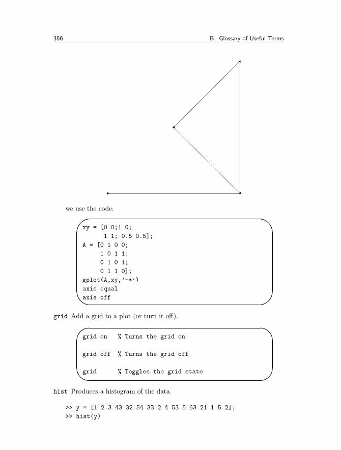
gplot Plot a graph using the vertices and the adjacency matrix. To plot thegraph
356 B. Glossary of Useful Terms
we use the code:�
�
�
�
xy = [0 0;1 0;
1 1; 0.5 0.5];
A = [0 1 0 0;
1 0 1 1;
0 1 0 1;
0 1 1 0];
gplot(A,xy,’-*’)
axis equal
axis off
grid Add a grid to a plot (or turn it off).�
�
�
�
grid on % Turns the grid on
grid off % Turns the grid off
grid % Toggles the grid state
hist Produces a histogram of the data.
>> y = [1 2 3 43 32 54 33 2 4 53 5 63 21 1 5 2];
>> hist(y)

B.3 Plotting Commands 357
gives
0 10 20 30 40 50 60 700
1
2
3
4
5
6
7
8
9
We can use a second argument for hist to define the number of bins.
hold Stops overwriting of current figure.
�
�
�
�
hold on % Turns the hold on
hold off % Turns the hold off
hold % Toggles the hold state
This is useful for putting multiple lines on a plot.�
�
�
�
x = 0:pi/20:pi;
y = sin(x);
z = cos(2*x);
clf
plot(x,y)
hold on
plot(x,z)
hold off
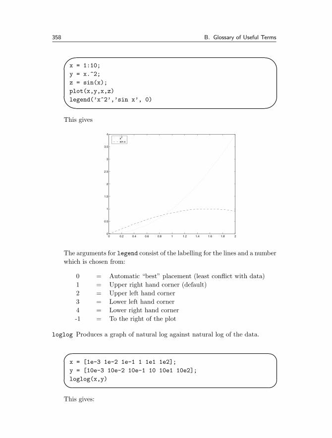
legend Used to add a “legend” to a figure, to describe the lines.
358 B. Glossary of Useful Terms
�
�
�
�
x = 1:10;
y = x.ˆ2;
z = sin(x);
plot(x,y,x,z)
legend(’xˆ2’,’sin x’, 0)
This gives
0 0.2 0.4 0.6 0.8 1 1.2 1.4 1.6 1.8 20
0.5
1
1.5
2
2.5
3
3.5
4
x2
sin x
The arguments for legend consist of the labelling for the lines and a numberwhich is chosen from:
0 = Automatic “best” placement (least conflict with data)1 = Upper right hand corner (default)2 = Upper left hand corner3 = Lower left hand corner4 = Lower right hand corner-1 = To the right of the plot
loglog Produces a graph of natural log against natural log of the data.
�
�
�x = [1e-3 1e-2 1e-1 1 1e1 1e2];
y = [10e-3 10e-2 10e-1 10 10e1 10e2];
loglog(x,y)
This gives:

B.3 Plotting Commands 359
10−3
10−2
10−1
100
101
102
10−2
10−1
100
101
102
103
see also semilogx and semilogy.
plot Used to set up figures and plotting of data. The simplest form would beplot(x,y). This command is extremely powerful and has many variants(typing help plot helps tremendously).
x = -1:0.1:1;
y = x.ˆ3;
plot(x,y) % Produces a simple plot of y=xˆ3
% using the default line colour
plot(x,y,’go’) % Produces a simple plot of y=xˆ3
% using green circles.
The arguments in plot either occur: in pairs in which they are pairs ofcoordinates for plotting or in triples in which case they are pairs of coordi-nates and the line style with which the data is to be plotted. You can alsodefine variables associated with the plot in the statement:��
��plot(x,y,’LineWidth’,2)
plots the line but with a thicker line.
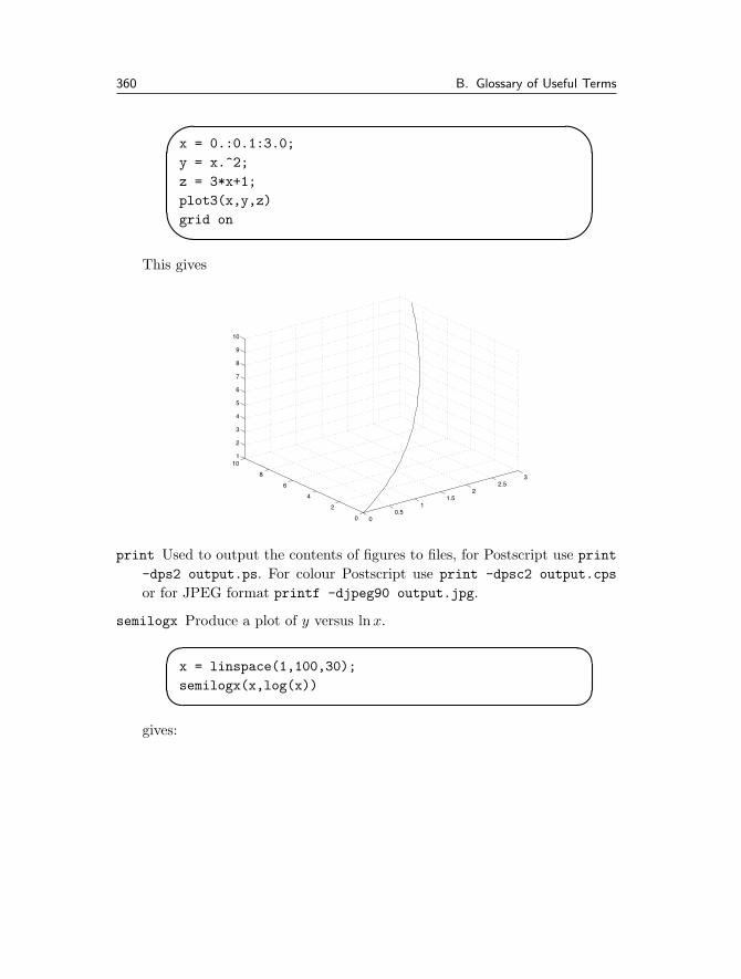
plot3 This is similar to plot but gives a line in three dimensions.
360 B. Glossary of Useful Terms
�
�
�
�
x = 0.:0.1:3.0;
y = x.ˆ2;
z = 3*x+1;
plot3(x,y,z)
grid on
This gives
00.5
11.5
22.5
3
0
2
4
6
8
101
2
3
4
5
6
7
8
9
10
print Used to output the contents of figures to files, for Postscript use print
-dps2 output.ps. For colour Postscript use print -dpsc2 output.cps
or for JPEG format printf -djpeg90 output.jpg.
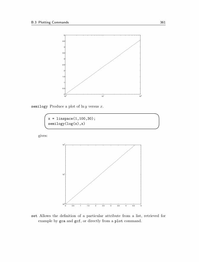
semilogx Produce a plot of y versus ln x.��
��
x = linspace(1,100,30);
semilogx(x,log(x))
gives:
B.3 Plotting Commands 361
100
101
102
0
0.5
1
1.5
2
2.5
3
3.5
4
4.5
5
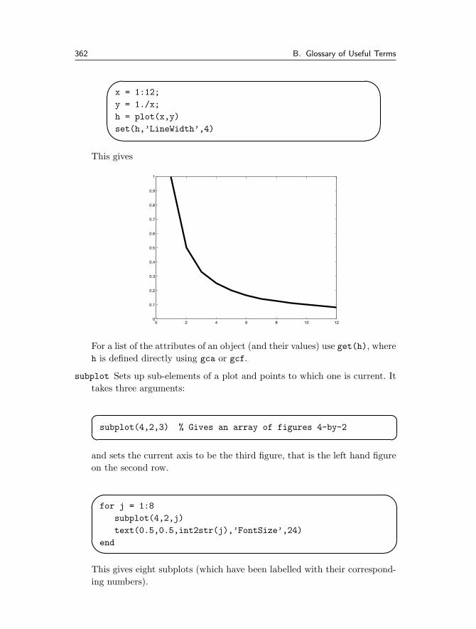
semilogy Produce a plot of ln y versus x.��
��
x = linspace(1,100,30);
semilogy(log(x),x)
gives:
0 0.5 1 1.5 2 2.5 3 3.5 4 4.5 510
0
101
102
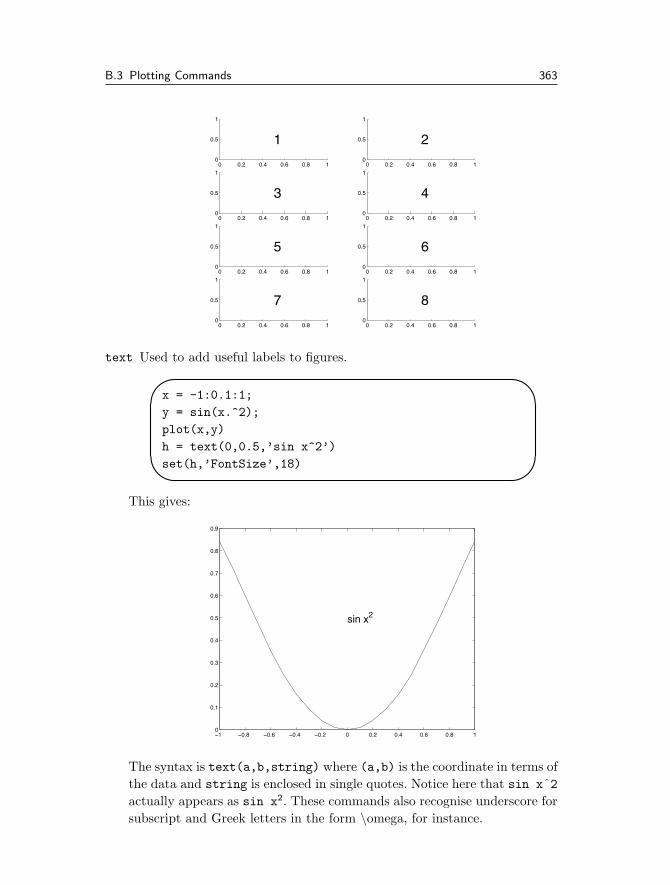
set Allows the definition of a particular attribute from a list, retrieved forexample by gca and gcf, or directly from a plot command.
362 B. Glossary of Useful Terms
�
�x = 1:12;
y = 1./x;
h = plot(x,y)
set(h,’LineWidth’,4)
This gives
0 2 4 6 8 10 120
0.1
0.2
0.3
0.4
0.5
0.6
0.7
0.8
0.9
1
For a list of the attributes of an object (and their values) use get(h), whereh is defined directly using gca or gcf.
subplot Sets up sub-elements of a plot and points to which one is current. Ittakes three arguments:
��
��subplot(4,2,3) % Gives an array of figures 4-by-2
and sets the current axis to be the third figure, that is the left hand figureon the second row.
�
�
�
for j = 1:8
subplot(4,2,j)
text(0.5,0.5,int2str(j),’FontSize’,24)
end
This gives eight subplots (which have been labelled with their correspond-ing numbers).
B.3 Plotting Commands 363
0 0.2 0.4 0.6 0.8 10
0.5
1
1
0 0.2 0.4 0.6 0.8 10
0.5
1
2
0 0.2 0.4 0.6 0.8 10
0.5
1
3
0 0.2 0.4 0.6 0.8 10
0.5
1
4
0 0.2 0.4 0.6 0.8 10
0.5
1
5
0 0.2 0.4 0.6 0.8 10
0.5
1
6
0 0.2 0.4 0.6 0.8 10
0.5
1
7
0 0.2 0.4 0.6 0.8 10
0.5
1
8
text Used to add useful labels to figures.�
�
�
�
x = -1:0.1:1;
y = sin(x.ˆ2);
plot(x,y)
h = text(0,0.5,’sin xˆ2’)
set(h,’FontSize’,18)
This gives:
−1 −0.8 −0.6 −0.4 −0.2 0 0.2 0.4 0.6 0.8 10
0.1
0.2
0.3
0.4
0.5
0.6
0.7
0.8
0.9
sin x2
The syntax is text(a,b,string) where (a,b) is the coordinate in terms ofthe data and string is enclosed in single quotes. Notice here that sin xˆ2actually appears as sin x2. These commands also recognise underscore forsubscript and Greek letters in the form \omega, for instance.
364 B. Glossary of Useful Terms
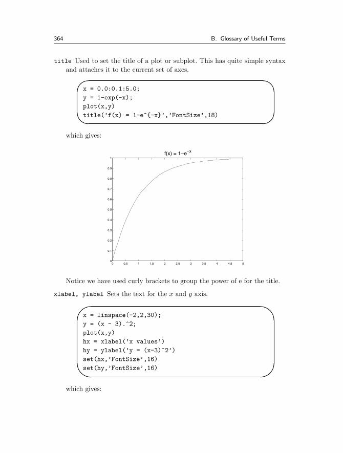
title Used to set the title of a plot or subplot. This has quite simple syntaxand attaches it to the current set of axes.
�
�x = 0.0:0.1:5.0;
y = 1-exp(-x);
plot(x,y)
title(’f(x) = 1-eˆ{-x}’,’FontSize’,18)
which gives:
0 0.5 1 1.5 2 2.5 3 3.5 4 4.5 50
0.1
0.2
0.3
0.4
0.5
0.6
0.7
0.8
0.9
1f(x) = 1−e−x
Notice we have used curly brackets to group the power of e for the title.
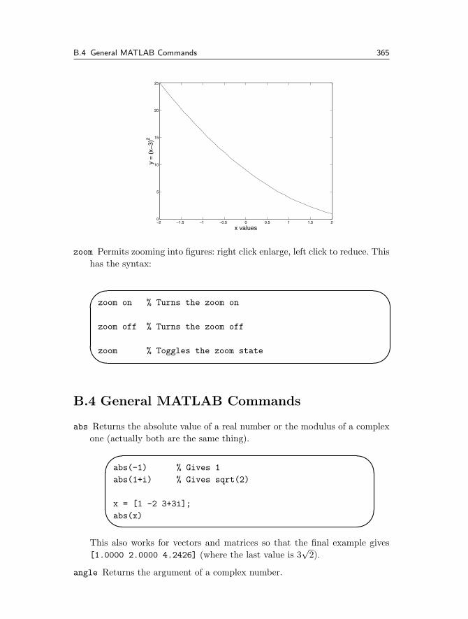
xlabel, ylabel Sets the text for the x and y axis.�
�
�
�
x = linspace(-2,2,30);
y = (x - 3).ˆ2;
plot(x,y)
hx = xlabel(’x values’)
hy = ylabel(’y = (x-3)ˆ2’)
set(hx,’FontSize’,16)
set(hy,’FontSize’,16)
which gives:
B.4 General MATLAB Commands 365
−2 −1.5 −1 −0.5 0 0.5 1 1.5 20
5
10
15
20
25
x values
y =
(x−
3)2
zoom Permits zooming into figures: right click enlarge, left click to reduce. Thishas the syntax:
�
�
�
�
zoom on % Turns the zoom on
zoom off % Turns the zoom off
zoom % Toggles the zoom state
B.4 General MATLAB Commands
abs Returns the absolute value of a real number or the modulus of a complexone (actually both are the same thing).�
�
�
�
abs(-1) % Gives 1
abs(1+i) % Gives sqrt(2)
x = [1 -2 3+3i];
abs(x)
This also works for vectors and matrices so that the final example gives[1.0000 2.0000 4.2426] (where the last value is 3
√2).
angle Returns the argument of a complex number.
366 B. Glossary of Useful Terms
�
�
�angle(sqrt(-1)) % This gives pi/2
angle(2) % This gives 0
angle(-2) % This gives pi
This can be used for an array of values and returns a vector of the samesize full of the corresponding arguments.
atan2 Gives the arctangent with values between (−π, π]. (see also tan,atan).Rather than calculating y/x and then taking the arctangent this functiontakes account of which quadrant the value is in.
�
�
�atan2(1,1) % Gives pi/4
atan2(-1,-1) % Gives -3pi/4
atan2(1,0) % Gives pi/2
Note that the y value is given first. This command can be used to determinethe argument of a complex number as atan2(imag(z),real(z)) (whichcan be compared with angle(z).
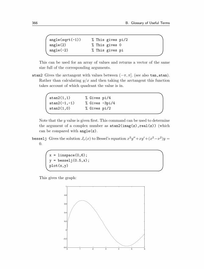
besselj Gives the solution Jν(x) to Bessel’s equation x2y′′+xy′+(x2−ν2)y =0.
�
�
�x = linspace(0,6);
y = besselj(0.5,x);
plot(x,y)
This gives the graph:
0 1 2 3 4 5 6−0.4
−0.2
0
0.2
0.4
0.6
0.8
1
B.4 General MATLAB Commands 367
The parameter ν is set to be 1/2 here and in fact J 12(x) = sinx/
√x.
There are other Bessel functions: bessely(nu,x), besseli(nu,x) andbesselk(nu,x).
break Stop current level of execution and go back to the previous level, forinstance exit a function.�
�
�
�
function [sx] = takesqrt(x)
if x<0
disp(’ x is negative ’)
sx = NaN;
break
end
sx = sqrt(x);
This routine finds the square root of positive quantities and breaks if x isnegative.
case Elements of a switch list, plausible values which the argument can take(see switch entry for example).
ceil Rounds up to the integer above, has the syntax ceil(x) where x can bea matrix, vector or scalar.
>> x = [0.3 0.9; 1.01 -2.3];
>> ceil(x)
ans =
1 1
2 -2
clear Used to reset objects; clear variables removes all variables.
�
�
�
�
clear all % Clears variables, globals, fns etc
clear variables % Clear all variables
clear global % Clear global variables
clear % Same as clear variable
clear x % Clear local variable x
clear x* % Clear local variables starting with x.
368 B. Glossary of Useful Terms
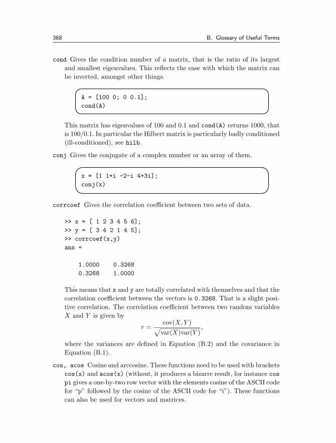
cond Gives the condition number of a matrix, that is the ratio of its largestand smallest eigenvalues. This reflects the ease with which the matrix canbe inverted, amongst other things.��
��
A = [100 0; 0 0.1];
cond(A)
This matrix has eigenvalues of 100 and 0.1 and cond(A) returns 1000, thatis 100/0.1. In particular the Hilbert matrix is particularly badly conditioned(ill-conditioned), see hilb.
conj Gives the conjugate of a complex number or an array of them.��
��
x = [1 1+i -2-i 4+3i];
conj(x)
corrcoef Gives the correlation coefficient between two sets of data.
>> x = [ 1 2 3 4 5 6];
>> y = [ 3 4 2 1 4 5];
>> corrcoef(x,y)
ans =
1.0000 0.3268
0.3268 1.0000
This means that x and y are totally correlated with themselves and that thecorrelation coefficient between the vectors is 0.3268. That is a slight posi-tive correlation. The correlation coefficient between two random variablesX and Y is given by
r =cov(X, Y )√
var(X)var(Y ),
where the variances are defined in Equation (B.2) and the covariance inEquation (B.1).
cos, acos Cosine and arccosine. These functions need to be used with bracketscos(x) and acos(x) (without, it produces a bizarre result, for instance cospi gives a one-by-two row vector with the elements cosine of the ASCII codefor “p” followed by the cosine of the ASCII code for “i”). These functionscan also be used for vectors and matrices.
B.4 General MATLAB Commands 369
�
�
�x = 0:pi/20:pi;
y = cos(x)
z = acos(y)
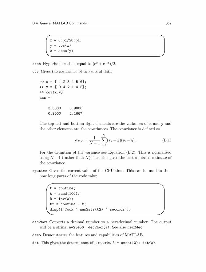
cosh Hyperbolic cosine, equal to (ex + e−x)/2.
cov Gives the covariance of two sets of data.
>> x = [ 1 2 3 4 5 6];
>> y = [ 3 4 2 1 4 5];
>> cov(x,y)
ans =
3.5000 0.9000
0.9000 2.1667
The top left and bottom right elements are the variances of x and y andthe other elements are the covariances. The covariance is defined as
σXY =1
N − 1
N∑i=1
(xi − x)(yi − y). (B.1)
For the definition of the variance see Equation (B.2). This is normalisedusing N − 1 (rather than N) since this gives the best unbiased estimate ofthe covariance.
cputime Gives the current value of the CPU time. This can be used to timehow long parts of the code take:�
�
�
�
t = cputime;
A = rand(100);
B = inv(A);
t2 = cputime - t;
disp([’Took ’ num2str(t2) ’ seconds’])
dec2hex Converts a decimal number to a hexadecimal number. The outputwill be a string; a=23456; dec2hex(a). See also hex2dec.
demo Demonstrates the features and capabilities of MATLAB.
det This gives the determinant of a matrix. A = ones(10); det(A).
370 B. Glossary of Useful Terms
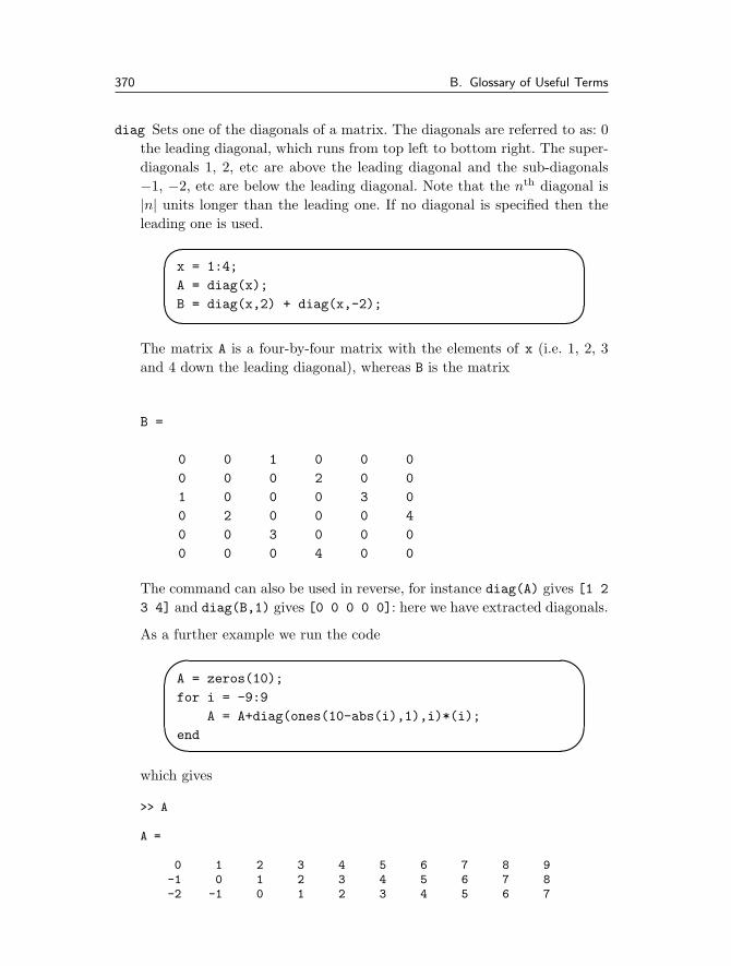
diag Sets one of the diagonals of a matrix. The diagonals are referred to as: 0the leading diagonal, which runs from top left to bottom right. The super-diagonals 1, 2, etc are above the leading diagonal and the sub-diagonals−1, −2, etc are below the leading diagonal. Note that the nth diagonal is|n| units longer than the leading one. If no diagonal is specified then theleading one is used.
�
�
�x = 1:4;
A = diag(x);
B = diag(x,2) + diag(x,-2);
The matrix A is a four-by-four matrix with the elements of x (i.e. 1, 2, 3and 4 down the leading diagonal), whereas B is the matrix
B =
0 0 1 0 0 0
0 0 0 2 0 0
1 0 0 0 3 0
0 2 0 0 0 4
0 0 3 0 0 0
0 0 0 4 0 0
The command can also be used in reverse, for instance diag(A) gives [1 2
3 4] and diag(B,1) gives [0 0 0 0 0]: here we have extracted diagonals.
As a further example we run the code
�
�A = zeros(10);
for i = -9:9
A = A+diag(ones(10-abs(i),1),i)*(i);
end
which gives
>> A
A =
0 1 2 3 4 5 6 7 8 9-1 0 1 2 3 4 5 6 7 8-2 -1 0 1 2 3 4 5 6 7
B.4 General MATLAB Commands 371
-3 -2 -1 0 1 2 3 4 5 6-4 -3 -2 -1 0 1 2 3 4 5-5 -4 -3 -2 -1 0 1 2 3 4-6 -5 -4 -3 -2 -1 0 1 2 3-7 -6 -5 -4 -3 -2 -1 0 1 2-8 -7 -6 -5 -4 -3 -2 -1 0 1-9 -8 -7 -6 -5 -4 -3 -2 -1 0
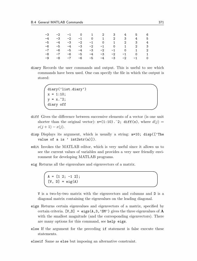
diary Records the user commands and output. This is useful to see whichcommands have been used. One can specify the file in which the output isstored:
�
�diary(’list.diary’)
x = 1:10;
y = x.ˆ2;
diary off
diff Gives the difference between successive elements of a vector (is one unitshorter than the original vector): x=(1:10).ˆ2; diff(x), where d(j) =x(j + 1) − x(j).
disp Displays its argument, which is usually a string: a=10; disp([’The
value of a is ’ int2str(a)]).
edit Invokes the MATLAB editor, which is very useful since it allows us tosee the current values of variables and provides a very user friendly envi-ronment for developing MATLAB programs.
eig Returns all the eigenvalues and eigenvectors of a matrix.��
��
A = [1 2; -1 2];
[V, D] = eig(A)
V is a two-by-two matrix with the eigenvectors and columns and D is adiagonal matrix containing the eigenvalues on the leading diagonal.
eigs Returns certain eigenvalues and eigenvectors of a matrix, specified bycertain criteria. [V,D] = eigs(A,3,’SM’) gives the three eigenvalues of Awith the smallest magnitude (and the corresponding eigenvectors). Thereare many options for this command, see help eigs.
else If the argument for the preceding if statement is false execute thesestatements.
elseif Same as else but imposing an alternative constraint.
372 B. Glossary of Useful Terms
end This command ends all of the loop structures and for each starting argu-ment there must be a corresponding end (used with for, if, switch andwhile).
eps The distance from 1.0 to the next largest floating point number. So MAT-LAB cannot tell the difference between 1 and 1+eps/2, for instance.
error Causes the code to stop execution; error(’Broken!’) usually usedwithin a conditional statement.
exist Checks to see whether an object exists: �
��
if ˜exist(’a’)
disp([’The variable a ’ ...
’does not exist’])
This can be used beyond variables: see the help lines for the command.
exp Evaluate the expression ex, can be used with vectors and matrices.
expm Evaluate the expression eA, where A is a matrix. This differs fromexp(A), which evaluates ex for all the elements of A rather than eA whichis given by:
eA ≡ I +∞∑
j=1
Aj
j!.
eye Sets up the identity matrix: eye(n) gives In.
factor Gives the prime factors of an integer.
factorial This calculates the factorial of an integer n: factorial(n) givesn!.
feval Evaluates a function, either user-defined or intrinsic. feval(’sin’,pi).
fix Rounds to the nearest integer (closest to zero), also works for matrices.
fliplr Flips an object left to right. This has no effect on column vectors.��
��
x = 1:6;
y = fliplr(x)
sets y to be [6 5 4 3 2 1]. This also works with matrices.
flipud Flips an object upside down. This has no effect on row vectors.
B.4 General MATLAB Commands 373
��
��
x = transpose(1:6);
y = flipud(x)
sets y to be [6; 5; 4; 3; 2; 1]. This also works with matrices.
floor Rounds down to the integer below, also works for matrices.
fmins This uses the Nelder–Mead simplex (direct search) method to find theminimum of a function. For instance to find the minimum of the functionf(x1, x2) = (x1 + 2x2 − 1)2/(x2
2 + 1) we use��
��
function [f]=func(x)
f = (x(1)+2*x(2)-1)ˆ2/(x(2)ˆ2+1);
and the command [x]=fmins(’func’,[0 0]).
for Defines the start of a loop which runs over a list of objects.�
�
�
N = 10
for j = 2:10
disp(j)
end
displays the numbers from 2 to 10.
format Used to specify how MATLAB displays variables. The options can beretrieved using help format.
full Tells the programme to treat the matrix as full, rather than sparse.
�
�
�A = [1 0 2; 0 -2 0; -1 0 0];
B = sparse(A);
C = full(B);
>> A
A =
1 0 2
0 -2 0
-1 0 0
374 B. Glossary of Useful Terms
>> B
B =
(1,1) 1
(3,1) -1
(2,2) -2
(1,3) 2
and C is back to A again.
function Occurs at the start of a function definition;function [v1,v2]=testfn(in1,in2,in3).
fzero Determines one zero of the function passed as the first argument tofzero. This function takes many different arguments and these can bedisplayed using help fzero.��
��
f = inline(’sin(3*x)’);
x = fzero(f,2);
finds a zero of the function f(x) = sin 3x near x equals two.
Zero found in the interval: [1.8869, 2.1131].
>> x
x =
2.0944
gcd Gives the greatest common divisor of two integers. This is unity if theyare coprime: used as gcd(x,y).
global This enables variables to be accessed from other places in the codewithout being passed directly as an argument. There needs to be a global
statement in the context in which the variable is defined and also one whereit is used.
help Gives help on MATLAB commands and can be used to expand the ma-terial given in this glossary.
helpbrowser Launches a web browser help facility (MATLAB 6).
B.4 General MATLAB Commands 375
helpdesk Provides access to the web-based help facility.
hex2dec Converts a hexadecimal number to a decimal: the input needs to bea string; a=’FF0’; hex2dec(a). See also dec2hex.
hilb(n) This sets up the n-by-n Hilbert matrix with entries (A)i,j = 1/(i+j).
i,j Initially set to be the square root of minus 1. These can be used to set upcomplex numbers:��
��
a = 3 + 2*i;
b = -4 + j;
(Note that once either of these variables has been used in another contextthey will not necessarily be equal to
√−1.)
if Start of a conditional block: if the statement is true then execute its con-tents. �
��
if x>1
disp(’x is greater than 1’)
end
This statement uses the logical structures described in section B.1.
imag Gives the imaginary part of a complex number; imag(1+i) gives 1.
Inf This represents answers which are infinite, for instance 1/0.
inline Used to define functions which will be evaluated inline, see the helpfunction; g = inline(’tˆ2’) gives g = t2 and then it can be used infeval as feval(g,5).
input Used for user entry of data a=input(’Enter a: ’);; can also be usedto enter strings name = input(’Enter name ’,s);.
int2str This takes an integer and returns a string: int2str(10) gives ’10’.
inv Works out the inverse of a matrix (if it exists). �
��
a = [1 3; 2 -1];
b = inv(a);
a * b
This gives the two-by-two identity (which could be constructed using thecommand eye(2)).
376 B. Glossary of Useful Terms
isempty Checks whether a variable is empty. �
��
if isempty(x)
disp(’x is empty’)
end
This means that the array has either zero rows or zero columns but stillexists; to check the existence of a variable use the exist command.
isreal Checks whether a variable is real.��
��
isreal(exp(0))
isreal(exp(i))
Care is needed since this command checks to see if the imaginary part of thecomplex number is exactly zero and does not allow for computation errors:for instance eiπ = −1, but the command isreal(exp(i*pi)) suggests thatthe quantity is complex.
isprime Checks whether a variable is prime: isprime(24) gives false (that iszero) whereas isprime(3571) gives true (that is one).
length Gives the length of a vector or alternatively the larger dimension of amatrix:
�
�a = [1 2 3; 4 5 6];
b = 1:16
length(a)
length(b)
gives the values 3 and 16 respectively.
linspace Sets up a grid of one hundred points from the first argument to thesecond. If there are three arguments use this as the number of points inthe grid.��
��
x = linspace(0,1,6);
z = linspace(1,10);
This gives x = [0 0.2 0.4 0.6 0.8 1] and z being the array runningfrom 1 to 10 in steps of (10 − 1)/99; since the endpoints are included thestep length is not (10 − 1)/100 as you might initially expect.
B.4 General MATLAB Commands 377
load Reads in data, either directly into variable load data (which loadsdata.mat) or load ’data.dat’ which returns a matrix data.
log Natural logarithms.��
��
x = [1 exp(1) exp(2)]
y = log(x)
This would be written mathematically as y = lnx.
log10 Logarithm to base ten.��
��
x = [1 10 10ˆ2]
y = log10(x)
This would be written mathematically as y = log10x. We note that log10x =lnx/ ln 10.
lookfor Allows one to search help files for any command which has a stringin its specification lookfor bessel.
lower Converts the characters in a string to lower case:��
��
name = ’Bob Roberts’;
lower(name)
This gives bob roberts (the opposite command is upper).
lu This produces the LU decomposition of a matrix and can provide informa-tion concerning pivoting.��
��
A = [1 2 3; -1 3 2; -1 0 1];
[L,U] = lu(A)
Gives
L =
1.0000 0 0
-1.0000 1.0000 0
-1.0000 0.4000 1.0000
378 B. Glossary of Useful Terms
U =
1 2 3
0 5 5
0 0 2
To obtain the pivoting information we would have used [L,U,P] = lu(A).In this case P is the three-by-three identity.
magic Returns a magic square:
>> magic(4)
ans =
16 2 3 13
5 11 10 8
9 7 6 12
4 14 15 1
Notice that not only do the rows, columns and diagonals add up to 34, butso do the four numbers in each corner, the numbers in each two-by-twoblock in the corner and the central two-by-two block.
max This returns the maximum of a vector: if a matrix is supplied it returns avector providing the maxima along the rows.��
��
x = 0:pi/4:2*pi
max(sin(x))
gives 1, and
�
�
�A = [1 2 3; 4 5 6];
max(A)
max(transpose(A))
gives [4 5 6] (that is the maxima of the columns) and [3 6] (the max-ima of the rows), respectively. Instead of using the transpose we can usethe syntax max(A,[],2), which determines the maximum along the sec-ond dimension. To find the maximum of a two-dimensional array we usemax(max(A)).
B.4 General MATLAB Commands 379
mean Calculates the mean of a set of data, 1/nn∑
i=1xi.
��
��mean([1 2 3 4 5 6 7])
This can also be used on matrices:
�
�
�a = [1 2 3; 4 5 6];
mean(a,1)
mean(a,2)
the former giving the averages of the columns and the latter the averagesof the rows.
median Gives the median of a set of data, that is the one in the middle whenthe data is ordered. This works in the same way as mean on matrices.
min Similar to max but giving the minimum.
mod This gives the remainder when the first argument is divided by the second.If used in the context mod(x,1) this gives the fractional part of x. It issimilar to rem.
NaN Not-a-Number, used to return quantities which are not assigned, for in-stance 0/0.
norm Gives the mathematical norm of a quantity, particularly useful for work-ing out the length of vectors. For vectors we have��
��norm(v,p)
gives (n∑
i=1
|vi|p)1/p
.
If p equals two this is a “conventional” norm and the commands
norm(v,inf)
norm(v,-inf)
give max(abs(V)) and min(abs(V)), respectively.
380 B. Glossary of Useful Terms
num2str Converts a number to a string with a specified number of digits;num2str(pi,4). This can also be used without specifying the number ofdigits (which uses the default corresponding to four places after the decimalpoint).
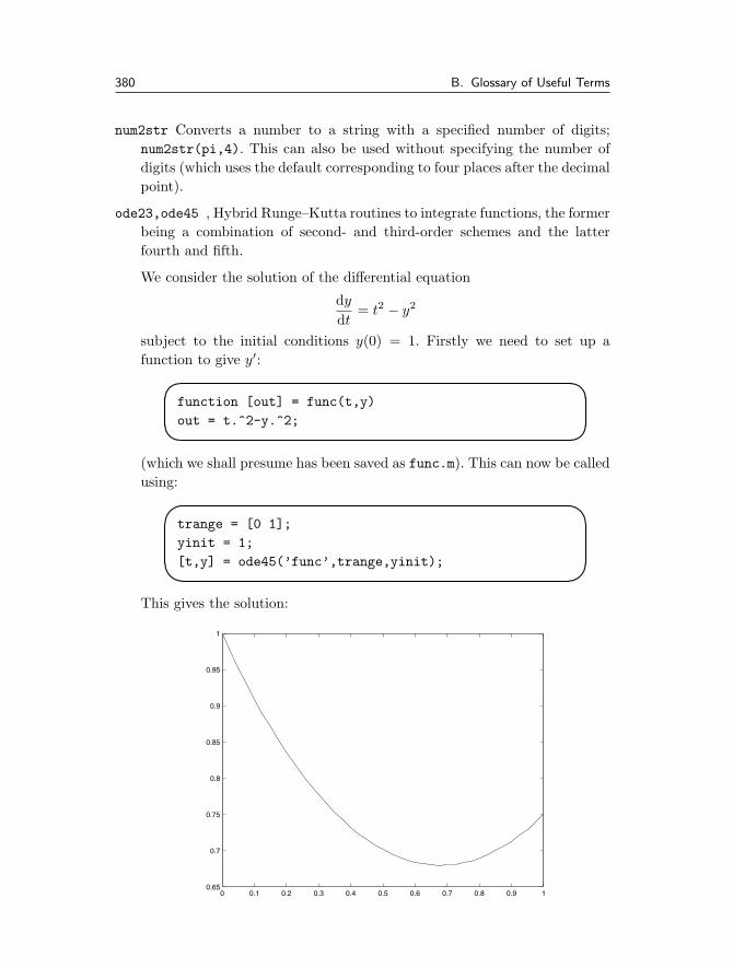
ode23,ode45 , Hybrid Runge–Kutta routines to integrate functions, the formerbeing a combination of second- and third-order schemes and the latterfourth and fifth.
We consider the solution of the differential equation
dy
dt= t2 − y2
subject to the initial conditions y(0) = 1. Firstly we need to set up afunction to give y′:��
��
function [out] = func(t,y)
out = t.ˆ2-y.ˆ2;
(which we shall presume has been saved as func.m). This can now be calledusing:
�
�
�trange = [0 1];
yinit = 1;
[t,y] = ode45(’func’,trange,yinit);
This gives the solution:
0 0.1 0.2 0.3 0.4 0.5 0.6 0.7 0.8 0.9 10.65
0.7
0.75
0.8
0.85
0.9
0.95
1

B.4 General MATLAB Commands 381
We can set tolerances, amongst other options. Consider the system of dif-ferential equations
dx
dt= t − y
dy
dt= x,
subject to the initial conditions x(0) = y(0) = 0. We introduce the vectory = (x(t), y(t))T , and as such we modify the code func.m to be:�
�
�
�
function [out] = func(t,in)
% in(1) is x(t) and in(2) is y(t).
out = zeros(2,1);
out(1) = t-in(2);
out(2) = in(1);
This is called using the code:
trange = [0 1];
yinit = [0; 0];
options = odeset(’RelTol’,1e-4,’AbsTol’,[1e-4 1e-4]);
ode45(’func’,trange,yinit,options);
This is for the above version of func.m for the coupled first-order systems,which sets the relative tolerance to be 1e-4 and the absolute tolerances tobe [1e-4 1e-5]. This gives:
0 0.1 0.2 0.3 0.4 0.5 0.6 0.7 0.8 0.9 10
0.05
0.1
0.15
0.2
0.25
0.3
0.35
0.4
0.45
0.5
382 B. Glossary of Useful Terms
The upper line is x(t) and the lower one is y(t).
ones Sets up a matrix full of ones. ones(n,m) gives A which is an n-by-mmatrix for which ai,j = 1. ones(n) gives a square matrix (n-by-n).
otherwise If none of the cases correspond to the argument of the switch
command then these statements are executed.
path A list of places MATLAB looks for files, also serves as a command toalter this variable. This command varies on different platforms and as suchyou should look at help path.
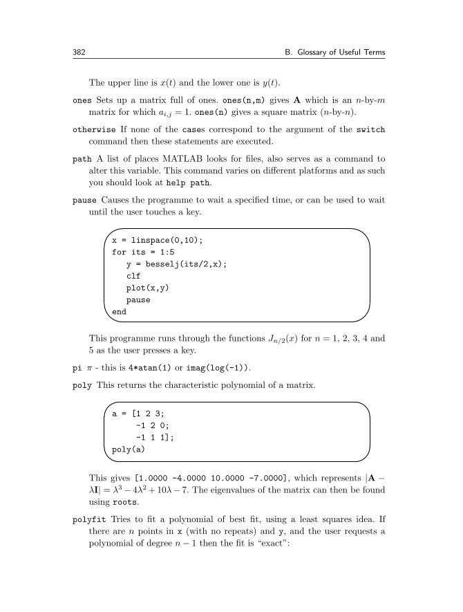
pause Causes the programme to wait a specified time, or can be used to waituntil the user touches a key.�
�
�
�
x = linspace(0,10);
for its = 1:5
y = besselj(its/2,x);
clf
plot(x,y)
pause
end
This programme runs through the functions Jn/2(x) for n = 1, 2, 3, 4 and5 as the user presses a key.
pi π - this is 4*atan(1) or imag(log(-1)).
poly This returns the characteristic polynomial of a matrix.
�
�a = [1 2 3;
-1 2 0;
-1 1 1];
poly(a)
This gives [1.0000 -4.0000 10.0000 -7.0000], which represents |A −λI| = λ3 − 4λ2 + 10λ − 7. The eigenvalues of the matrix can then be foundusing roots.
polyfit Tries to fit a polynomial of best fit, using a least squares idea. Ifthere are n points in x (with no repeats) and y, and the user requests apolynomial of degree n − 1 then the fit is “exact”:
B.4 General MATLAB Commands 383
�
�
�x = [1 2 3];
y = [4 5 -2];
p = polyfit(x,y,2);
Note that the coefficients are returned with the one corresponding to thelargest power first. This gives the quadratic −4x2 + 13x − 5: howeverpolyfit(x,y,1) on the same data gives the straight line −3x+25/3 (whichis the line of best fit). It is possible to get information about the level ofthe fit using the form [p,s] = polyfit(x,y,1). The object s containsinformation, for instance the covariance s.R.
polyval Evaluates a polynomial specified by its coefficients at a set of datapoints y=polyval(c,x).
�
�
�x = [1 2 3];
c = [-4 13 -5];
y = polyval(c,x);
This reconstructs the data used in the example for polyfit. Notice thatthe coefficients are given with the one corresponding to the largest powerfirst.
primes Lists the primes up to and including the argument. The syntax issimply n=20; primes(n).
prod Similar to sum and gives the product of the elements of the vector x, so
that prod(x) returnsn∏
i=1xi.
�
�x = 1:10;
prod(x) % Gives 10!
z = [1 4 5 6 -2];
prod(z)
The factorial could also be found using factorial.
rand Generates random numbers between zero and one. This can be used toform a matrix of random numbers as well. There are many versions of theargument for this command, see help rand.
randn Generates normally distributed real numbers: again can be used to gen-erate matrices randn(n,m).
384 B. Glossary of Useful Terms
randperm Generates a random permutation of a list of objects: To rearrangethe letters of our names:�
�
�
�
s = ’otto denier’;
for its = 1:20
l = randperm(11);
s(l)
pause
end
rank This yields the rank of a set of linear equations and can be used tosee whether the system has no solutions, a unique solution or an infinitenumber of solutions (yielding information about the degrees of freedom).
�
�A = [-1 1 1 2;
3 -1 1 1;
0 0 1 2];
rank(A)
real Gives the real part of a complex number real(z), where z can be ascalar, vector or matrix.
realmax This is the largest floating point number representable on the com-puter.
realmin This is the smallest floating point number representable on the com-puter.
rem This is the remainder attained by dividing the first argument by the secondone: rem(3.32,1.1) gives 0.02.
�
�rem([3 4 5],2) % Gives 1 0 1
rem(5,[1 2 3]) % Gives 0 1 2
rem([3 4 5],[1 2 3])
% Gives 0 0 2
reshape This simply reshapes a matrix into a new shape. This is used mostcommonly to make a vector into a matrix, but can be used to reshape
matrices.
B.4 General MATLAB Commands 385
�
�s = rand(100,1);
a = reshape(s,10,10);
b = [1 3 4; 2 3 4];
d = reshape(b,1,6);
This gives d = [1 2 3 4 4]; the elements of b are read column-wise.
roots This gives the roots of the polynomial which is passed to the routine.For instance to find the roots of the cubic x3 + 4x2 + 7x + 2 we use��
��
co = [1 4 7 2];
roots(co)
Notice again that the coefficients are listed with the one corresponding tothe largest power first (similarly for polyfit and polyval).
round Rounds to the nearest integer.
save Saves values of variables to a .mat file.
sin, asin Sine and arcsine. These functions need to be used with bracketssin(x) and asin(x) (without, it produces bizarre results, for instance sinpi gives a one-by-two row vector with the elements sine of the ASCII codefor “p” followed by the sine of the ASCII code for “i”). These functionscan also be used for vectors and matrices.
�
�
�x = -pi/2:pi/20:pi/2;
y = sin(x)
z = asin(y)
sinh Hyperbolic sine.
size Returns the dimensions of a matrix: [rows,cols]=size(A).
sort This returns a list of numbers sorted into ascending order, together witha map from their original position to that in the revised list.
sparse Defines the matrix as sparse so that the computer only operates onnon-zero entries: this can dramatically reduce the time spent doing com-putations (see full).
spline Fits cubic splines through a set of data points (x, f) and evaluatesthem at a further set of points z; y=spline(x,f,z).
386 B. Glossary of Useful Terms
sqrt This finds the square root of a matrix element by element. If necessarythe answer may be returned as a complex number.
std Calculates the standard deviation of a vector.
str2mat As the name suggests, this takes a string and returns a matrix.
sum This sums the contents of a vector, or the rows of a matrix. It can also becalled with a second argument which defines which dimension needs to besummed.
switch This defines the start of a group of statements, the argument for whichis a variable, the likely values of which are listed in the cases.
tan,atan Tangent and arctangent. These functions need to be used with brack-ets tan(x) and atan(x) (without, it produces bizarre results, for instancetan pi gives a one-by-two row vector with the elements tangent of theASCII code for “p” followed by the tangent of the ASCII code for “i”).These functions can also be used for vectors and matrices.
�
�
�x = 0:pi/20:pi/4;
y = tan(x)
z = atan(y)
(see also atan2).
tour Gives a tour of the facilities of MATLAB.
transpose Returns the transpose of a matrix: can also be done using A.’.(Note that A’ transposes and also takes the conjugate.)
type Prints out the contents of a MATLAB script.
upper Converts the characters in a string to upper case:��
��
name = ’Bob Roberts’;
upper(name)
This gives BOB ROBERTS (the opposite command is lower).
var Gives the variance of a set of data. The covariance is defined as
σX =1
N − 1
N∑i=1
(xi − x)2. (B.2)
B.4 General MATLAB Commands 387
warning Allows codes to issue warnings when there may be problems. Is alsoused to affect how the system issues warnings.
which Tells a user where a MATLAB file can be found, and which version isgoing to be run.
while Defines the start of a loop which is continued while a certain conditionis fulfilled.
whos List of all variables (with details): this can be restricted using things likewhos a*.
zeros Sets up a matrix full of zeros: zeros(n,m) gives A which is an n-by-mmatrix for which ai,j = 0. zeros(n) gives 0n.

CSolutions to Tasks
Please note that these solutions are given for guidance only and are by no meansunique. At the outset we shall give MATLAB output: however subsequently weshall merely give the commands which can be used to solve the problems.
C.1 Solutions for Tasks from Chapter 1
Solution 1.1 The MATLAB code to solve these problems is:�
�
�
�
x = 1.3;
p = xˆ2+3*x+1
x = 30/180*pi;
y = sin(x);
x = 1;
f = atan(x);
x = sqrt(3)/2;
h = acos(x);
g = sin(h)
390 C. Solutions to Tasks
The values this returns are: 6.5900, 0.5000, 0.7854 (which is π/4) and0.5000.
Solution 1.2 To calculate the function y(x) = |x| sin x2 we use the code:��
��
x = pi/3;
y = abs(x)*sin(xˆ2);
and similarly for x = π/6. Notice care is needed with the brackets and thesyntax.
Solution 1.3 The MATLAB commands to determine these quantities are:
sin(pi/2);
cos(pi/3);
tan(60/180*pi);
x=0.5; log(x+sqrt(xˆ2+1)) (and with x=1);
x=0; x/((xˆ2+1)*sin(x))
and finally x=pi/4; x/((xˆ2+1)*sin(x)).
Notice the penultimate part of this task generates NaN: this is because MATLABdoes not know how to evaluate zero divided by zero.
Solution 1.4 This is a matter of either typing out all the values or exploitingthe fact that MATLAB can operate on vectors. We can use the code:�
�
�
�
x = [0.3 1/3 0.5 1/2 1.65 -1.34];
round(x)
ceil(x)
floor(x)
fix(x)
This example is included to help understand the role of various MATLAB com-mands which can be used to return different roundings to appropriate integers.
Solution 1.5 The difference between rem and mod can be illustrated using they value of 4. Thus we have

C.1 Solutions for Tasks from Chapter 1 391
>> x=[3 4 5]
x =
3 4 5
>> rem(x,4)
ans =
3 0 1
>> mod(x,4)
ans =
3 0 1
>> rem(x,-4)
ans =
3 0 1
>> mod(x,-4)
ans =
-1 0 -3
>>
So for the second argument being positive we have that rem and mod are equiva-lent, whereas for negative values the remainder is signed (thus it shows whetherit is positive or negative).
Solution 1.6 The MATLAB code is:
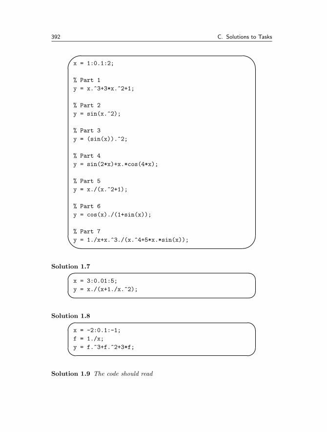
392 C. Solutions to Tasks
�
�
�
�
x = 1:0.1:2;
% Part 1
y = x.ˆ3+3*x.ˆ2+1;
% Part 2
y = sin(x.ˆ2);
% Part 3
y = (sin(x)).ˆ2;
% Part 4
y = sin(2*x)+x.*cos(4*x);
% Part 5
y = x./(x.ˆ2+1);
% Part 6
y = cos(x)./(1+sin(x));
% Part 7
y = 1./x+x.ˆ3./(x.ˆ4+5*x.*sin(x));
Solution 1.7��
��
x = 3:0.01:5;
y = x./(x+1./x.ˆ2);
Solution 1.8
�
�
�x = -2:0.1:-1;
f = 1./x;
y = f.ˆ3+f.ˆ2+3*f;
Solution 1.9 The code should read

C.1 Solutions for Tasks from Chapter 1 393
�
�
�
�
clear all
x = linspace(0,1,200);
g = x.ˆ3+1;
h = x+2;
z = x.ˆ2;
y = cos(x*pi);
f = y.*z./(g.*h);
f(200)
The errors were: the second line should have been first, else this cleared out thecontents of x. The default number of points for linspace is 100, so this neededto be specified as being 200. There were dots missing from the definition of gand the calculation of f. MATLAB distinguishes between upper and lower casein variable names so we need to use h rather than H. The command to calculatey needs brackets around the argument of the cosine function and an asteriskbetween x and pi. As mentioned above the dots were missing from f and thedenominator of the fraction needed to be contained within brackets. Finally theanswer needs to be printed (which could have been done at the prompt).
Solution 1.10 The code should read
�
�x = linspace(-2,2,20);
c = [1 0 0 0 -1];
y = polyval(c,x);
plot(x,y)
The errors were: in the first line the vector as defined would contain 21 entries(try typing length(x) after running the original code). A quartic actually has5 coefficients, so there was a zero missing in the definition of c and finally thex and y needed to be transposed in the plotting command.
This gives the figure

394 C. Solutions to Tasks
−2 −1.5 −1 −0.5 0 0.5 1 1.5 2−2
0
2
4
6
8
10
12
14
16
Solution 1.11 The corrected code should be�
�
�
�
x = 0:0.1:3;
f = x.ˆ3.*cos(x+1);
% x = 2
f(21)
% x = 3
f(end)
C.2 Solutions for Tasks from Chapter 2
Solution 2.1 This is hopefully just a matter of typing the code and saving theanswer correctly.
Solution 2.2 The revised code could be:�
�
�
�
a = input(’Enter a : ’);
b = input(’Enter b : ’);
res = aˆb;
str1 = ’The answer is ’;
str2 = ’ when ’ ;
str3 = ’ is raised to the power ’;
disp([str1 num2str(res) str2 ...
num2str(a) str3 num2str(b)]);
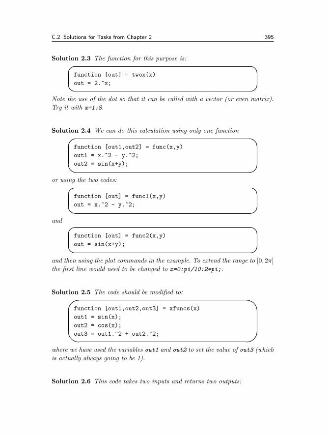
C.2 Solutions for Tasks from Chapter 2 395
Solution 2.3 The function for this purpose is:��
��
function [out] = twox(x)
out = 2.ˆx;
Note the use of the dot so that it can be called with a vector (or even matrix).Try it with x=1:8.
Solution 2.4 We can do this calculation using only one function
�
�
�function [out1,out2] = func(x,y)
out1 = x.ˆ2 - y.ˆ2;
out2 = sin(x+y);
or using the two codes:��
��
function [out] = func1(x,y)
out = x.ˆ2 - y.ˆ2;
and ��
��
function [out] = func2(x,y)
out = sin(x+y);
and then using the plot commands in the example. To extend the range to [0, 2π]the first line would need to be changed to x=0:pi/10:2*pi;.
Solution 2.5 The code should be modified to:
�
�function [out1,out2,out3] = xfuncs(x)
out1 = sin(x);
out2 = cos(x);
out3 = out1.ˆ2 + out2.ˆ2;
where we have used the variables out1 and out2 to set the value of out3 (whichis actually always going to be 1).
Solution 2.6 This code takes two inputs and returns two outputs:
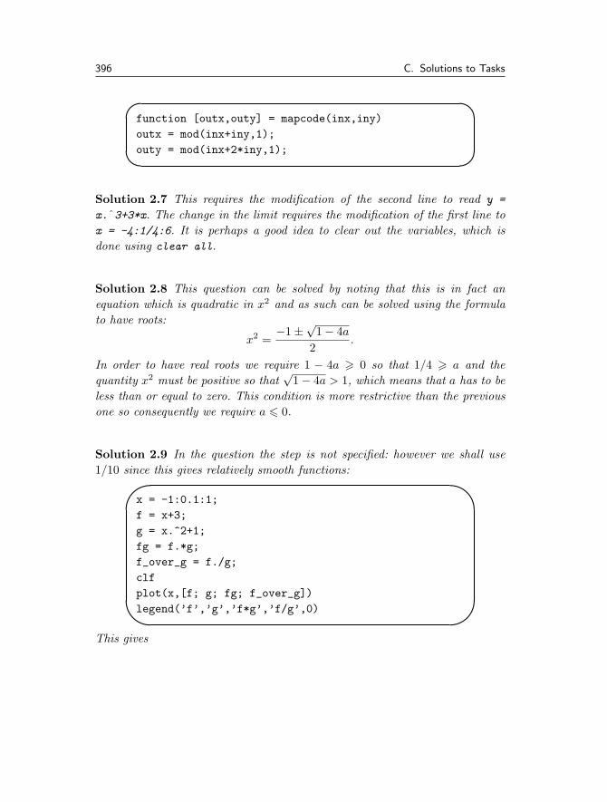
396 C. Solutions to Tasks
�
�
�function [outx,outy] = mapcode(inx,iny)
outx = mod(inx+iny,1);
outy = mod(inx+2*iny,1);
Solution 2.7 This requires the modification of the second line to read y =
x.ˆ3+3*x. The change in the limit requires the modification of the first line tox = -4:1/4:6. It is perhaps a good idea to clear out the variables, which isdone using clear all.
Solution 2.8 This question can be solved by noting that this is in fact anequation which is quadratic in x2 and as such can be solved using the formulato have roots:
x2 =−1 ± √
1 − 4a
2.
In order to have real roots we require 1 − 4a � 0 so that 1/4 � a and thequantity x2 must be positive so that
√1 − 4a > 1, which means that a has to be
less than or equal to zero. This condition is more restrictive than the previousone so consequently we require a � 0.
Solution 2.9 In the question the step is not specified: however we shall use1/10 since this gives relatively smooth functions:�
�
�
�
x = -1:0.1:1;
f = x+3;
g = x.ˆ2+1;
fg = f.*g;
f_over_g = f./g;
clf
plot(x,[f; g; fg; f_over_g])
legend(’f’,’g’,’f*g’,’f/g’,0)
This gives
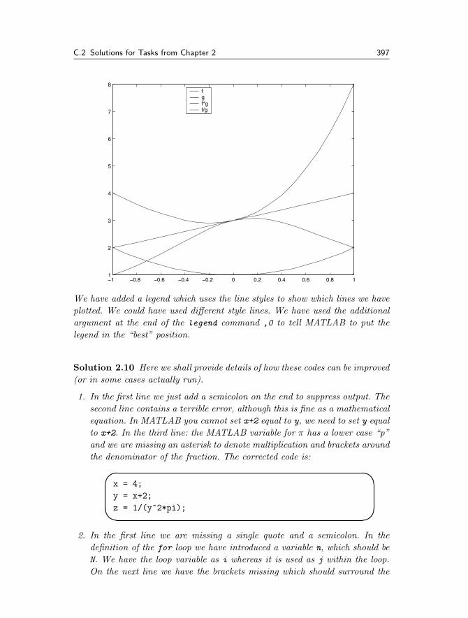
C.2 Solutions for Tasks from Chapter 2 397
−1 −0.8 −0.6 −0.4 −0.2 0 0.2 0.4 0.6 0.8 11
2
3
4
5
6
7
8fgf*gf/g
We have added a legend which uses the line styles to show which lines we haveplotted. We could have used different style lines. We have used the additionalargument at the end of the legend command ,0 to tell MATLAB to put thelegend in the “best” position.
Solution 2.10 Here we shall provide details of how these codes can be improved(or in some cases actually run).
1. In the first line we just add a semicolon on the end to suppress output. Thesecond line contains a terrible error, although this is fine as a mathematicalequation. In MATLAB you cannot set x+2 equal to y, we need to set y equalto x+2. In the third line: the MATLAB variable for π has a lower case “p”and we are missing an asterisk to denote multiplication and brackets aroundthe denominator of the fraction. The corrected code is:
�
�
�x = 4;
y = x+2;
z = 1/(yˆ2*pi);
2. In the first line we are missing a single quote and a semicolon. In thedefinition of the for loop we have introduced a variable n, which should beN. We have the loop variable as i whereas it is used as j within the loop.On the next line we have the brackets missing which should surround the
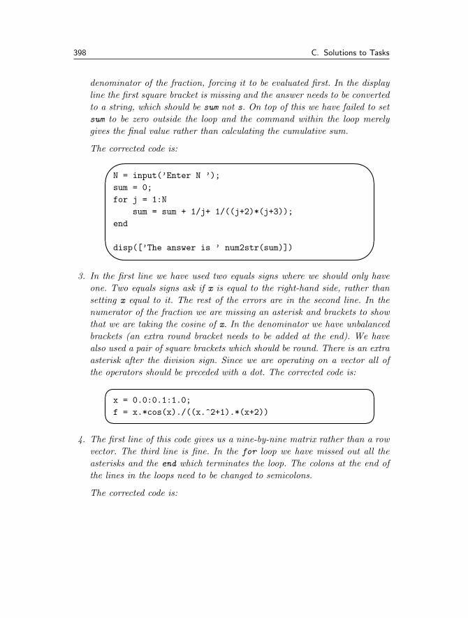
398 C. Solutions to Tasks
denominator of the fraction, forcing it to be evaluated first. In the displayline the first square bracket is missing and the answer needs to be convertedto a string, which should be sum not s. On top of this we have failed to setsum to be zero outside the loop and the command within the loop merelygives the final value rather than calculating the cumulative sum.
The corrected code is:�
�
�
�
N = input(’Enter N ’);
sum = 0;
for j = 1:N
sum = sum + 1/j+ 1/((j+2)*(j+3));
end
disp([’The answer is ’ num2str(sum)])
3. In the first line we have used two equals signs where we should only haveone. Two equals signs ask if x is equal to the right-hand side, rather thansetting x equal to it. The rest of the errors are in the second line. In thenumerator of the fraction we are missing an asterisk and brackets to showthat we are taking the cosine of x. In the denominator we have unbalancedbrackets (an extra round bracket needs to be added at the end). We havealso used a pair of square brackets which should be round. There is an extraasterisk after the division sign. Since we are operating on a vector all ofthe operators should be preceded with a dot. The corrected code is:��
��
x = 0.0:0.1:1.0;
f = x.*cos(x)./((x.ˆ2+1).*(x+2))
4. The first line of this code gives us a nine-by-nine matrix rather than a rowvector. The third line is fine. In the for loop we have missed out all theasterisks and the end which terminates the loop. The colons at the end ofthe lines in the loops need to be changed to semicolons.
The corrected code is:
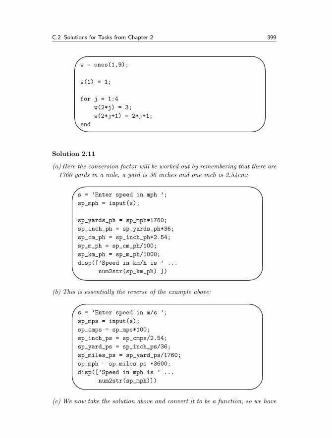
C.2 Solutions for Tasks from Chapter 2 399
�
�
�
�
w = ones(1,9);
w(1) = 1;
for j = 1:4
w(2*j) = 3;
w(2*j+1) = 2*j+1;
end
Solution 2.11
(a) Here the conversion factor will be worked out by remembering that there are1760 yards in a mile, a yard is 36 inches and one inch is 2.54cm:�
�
�
�
s = ’Enter speed in mph ’;
sp_mph = input(s);
sp_yards_ph = sp_mph*1760;
sp_inch_ph = sp_yards_ph*36;
sp_cm_ph = sp_inch_ph*2.54;
sp_m_ph = sp_cm_ph/100;
sp_km_ph = sp_m_ph/1000;
disp([’Speed in km/h is ’ ...
num2str(sp_km_ph) ])
(b) This is essentially the reverse of the example above:�
�
�
�
s = ’Enter speed in m/s ’;
sp_mps = input(s);
sp_cmps = sp_mps*100;
sp_inch_ps = sp_cmps/2.54;
sp_yard_ps = sp_inch_ps/36;
sp_miles_ps = sp_yard_ps/1760;
sp_mph = sp_miles_ps *3600;
disp([’Speed in mph is ’ ...
num2str(sp_mph)])
(c) We now take the solution above and convert it to be a function, so we have

400 C. Solutions to Tasks
�
�
�
�
function [output] = change(input);
sp_mph = input;
sp_yards_ph = sp_mph*1760;
sp_inch_ph = sp_yards_ph*36;
sp_cm_ph = sp_inch_ph*2.54;
sp_m_ph = sp_cm_ph/100;
sp_km_ph = sp_m_ph/1000;
output = sp_km_ph;
(d) This shows that a sprinter will run at 22 mph on average since they do 100metres in 10 seconds, that is 10 metres per second.
Solution 2.12 This is accomplished using the code:�
�
�
�
x = linspace(-pi/2,pi/2);
f = x./(1+x.ˆ2);
g = tan(x);
fg = g./(1+g.ˆ2);
gf = f./(1+f.ˆ2);
plot(x,fg,x,gf)
Solution 2.13 This is done using the code:�
�
�
�
a = input(’Coefficient of x squared: );
b = input(’Coefficient of x:’);
c = input(’The constant:’);
y = linspace(0,pi);
x = sin(y);
q = a*x.ˆ2+b*x+c;
plot(y,q)
C.3 Solutions for Tasks from Chapter 3
Solution 3.1 The required code is:
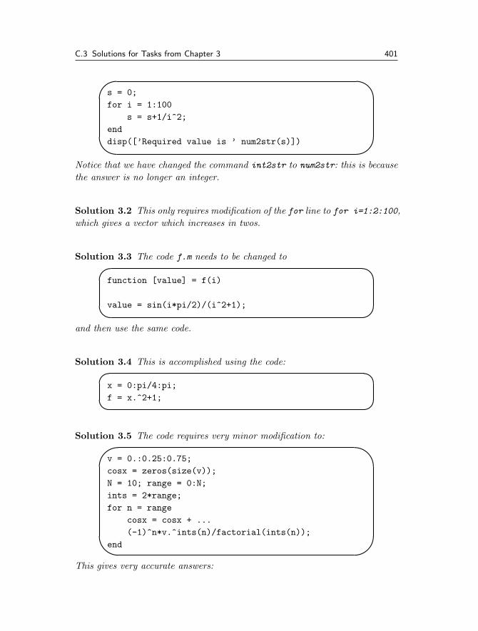
C.3 Solutions for Tasks from Chapter 3 401
�
�
�
�
s = 0;
for i = 1:100
s = s+1/iˆ2;
end
disp([’Required value is ’ num2str(s)])
Notice that we have changed the command int2str to num2str: this is becausethe answer is no longer an integer.
Solution 3.2 This only requires modification of the for line to for i=1:2:100,which gives a vector which increases in twos.
Solution 3.3 The code f.m needs to be changed to
�
�
�function [value] = f(i)
value = sin(i*pi/2)/(iˆ2+1);
and then use the same code.
Solution 3.4 This is accomplished using the code:��
��
x = 0:pi/4:pi;
f = x.ˆ2+1;
Solution 3.5 The code requires very minor modification to:�
�
�
�
v = 0.:0.25:0.75;
cosx = zeros(size(v));
N = 10; range = 0:N;
ints = 2*range;
for n = range
cosx = cosx + ...
(-1)ˆn*v.ˆints(n)/factorial(ints(n));
end
This gives very accurate answers:

402 C. Solutions to Tasks
cos(v)-cosx
ans =
0 0 0 0
This means that the difference between the MATLAB and the series answersare less than eps.
Solution 3.6 We can use code which performs the summations separately fordifferent values of N or note that SN+1 = SN + 1/(N + 1)2 where S1 = 1.
This leads to the simple code:
�
�s(1) = 1;
for n = 1:2000
s(n+1) = s(n)+1/(n+1)ˆ2;
end
This gives a value which when divided by π2 allows one to appreciate that c ∼ 6.In fact
∞∑i=1
1n2 =
π2
6.
Solution 3.7 We solve this task by using a nested loop structure�
�
�
�
for p = 1:4
sum = 0;
for j = 1:(p+1)
sum = sum + jˆp;
end
disp([’ sum for p=’ ...
int2str(p) ’ is ’ int2str(sum)])
end
Solution 3.8 The codes for this task are:
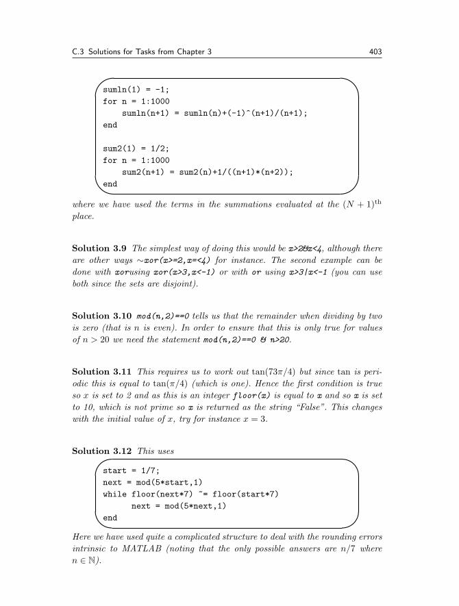
C.3 Solutions for Tasks from Chapter 3 403
�
�
�
�
sumln(1) = -1;
for n = 1:1000
sumln(n+1) = sumln(n)+(-1)ˆ(n+1)/(n+1);
end
sum2(1) = 1/2;
for n = 1:1000
sum2(n+1) = sum2(n)+1/((n+1)*(n+2));
end
where we have used the terms in the summations evaluated at the (N + 1)th
place.
Solution 3.9 The simplest way of doing this would be x>2&x<4, although thereare other ways ∼xor(x>=2,x=<4) for instance. The second example can bedone with xorusing xor(x>3,x<-1) or with or using x>3|x<-1 (you can useboth since the sets are disjoint).
Solution 3.10 mod(n,2)==0 tells us that the remainder when dividing by twois zero (that is n is even). In order to ensure that this is only true for valuesof n > 20 we need the statement mod(n,2)==0 & n>20.
Solution 3.11 This requires us to work out tan(73π/4) but since tan is peri-odic this is equal to tan(π/4) (which is one). Hence the first condition is trueso x is set to 2 and as this is an integer floor(x) is equal to x and so x is setto 10, which is not prime so x is returned as the string “False”. This changeswith the initial value of x, try for instance x = 3.
Solution 3.12 This uses�
�
�
�
start = 1/7;
next = mod(5*start,1)
while floor(next*7) ˜= floor(start*7)
next = mod(5*next,1)
end
Here we have used quite a complicated structure to deal with the rounding errorsintrinsic to MATLAB (noting that the only possible answers are n/7 wheren ∈ N).
404 C. Solutions to Tasks
Solution 3.13 We have
�
�n = 1:50;
f = n.ˆ3-n.ˆ2+40;
ii = find(f > 1000 & mod(n,3) ˜= 0);
n(ii)
Solution 3.14 The key here is to start with the string of the first ten letters,namely “abcdefghij”. We ask the user to enter the first value of n outside thewhile loop: this avoids the need for the first flag. The required code is then:�
�
�
�
str = ’abcdefghij’;
msg = ’Enter an integer from 1 to 10: ’;
n = input(msg);
while (round(n)˜=n) | (n<1 | n>10)
warning(’ Not valid ’)
n = input(msg);
end
str(1:n)
Solution 3.15 Although this problem can be solved in one code it is preferableto use a couple of functions. The first one checks whether a character is a letter(lower or upper case):�
�
�
�
function [val] = isletter(charac)
lchar = lower(charac(1));
if lchar>=’a’ & lchar <=’z’
val = 1;
else
val = 0;
end
Firstly the first character is extracted and converted to lower case. Then a checkis made to see if it is a character in the lower case alphabet: if it is the variableval is set to be true (that is 1). A similar code checks for whether a characteris a digit:
C.3 Solutions for Tasks from Chapter 3 405
�
�
�
�
function [val] = isdigit(charac)
lchar = charac(1);
if lchar>=’0’ & lchar <=’9’
val = 1;
else
val = 0;
end
We can now use the functions:�
�
�
�
msg = ’Please enter a letter and a digit ’;
str = input(msg,’s’);
while ˜isletter(str(1)) | ˜isdigit(str(2))
warning(’This is not valid’)
str = input(msg,’s’);
end
The argument of the while loop checks to see if either of the conditions isn’tsatisfied (and as such uses or, that is the vertical line).
Solution 3.16 This can be done with the code:�
�
�
�
x = linspace(-3,5,100);
for i = 1:length(x)
if x(i) >= -1 & x(i) <= 1
f(i) = x(i)ˆ2;
elseif x(i) > 1 & x(i) < 4
f(i) = 1;
else
f(i) = 0;
end
end
plot(x,f)
axis([-3 5 -0.5 1.5])
The final command is added purely so that the curve can be distinguished fromthe axis. This gives
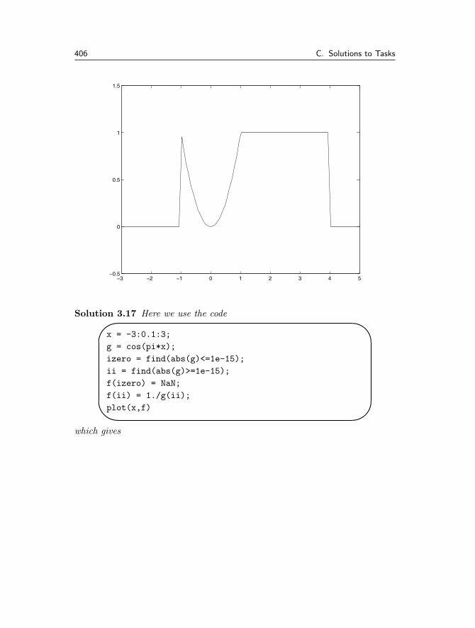
406 C. Solutions to Tasks
−3 −2 −1 0 1 2 3 4 5−0.5
0
0.5
1
1.5
Solution 3.17 Here we use the code�
�
�
�
x = -3:0.1:3;
g = cos(pi*x);
izero = find(abs(g)<=1e-15);
ii = find(abs(g)>=1e-15);
f(izero) = NaN;
f(ii) = 1./g(ii);
plot(x,f)
which gives

C.3 Solutions for Tasks from Chapter 3 407
−3 −2 −1 0 1 2 3−4
−3
−2
−1
0
1
2
3
4
and the choice of 10−15 is in a sense arbitrary, but reflects how close we cometo the singularities.
Solution 3.18 The first line contains a spelling mistake: the command shouldbe linspace. The second line is missing brackets around x and a semicolon.In the definition of the for loop we should have used a colon rather than asemicolon. In both the logical expressions on the if and the elseif lines thesecond reference to the array x uses i rather than j. The first logical expressionshould use an ampersand (&) rather than the word and; similarly the secondone should also have an ampersand rather than the word or. The first part ofthe second expression x(j) should be checked to be greater than one or equal toone (although this change is academic). The following line should refer to x(j)
rather than the entire vector x, and should be finished off with a semicolon.The variable zero is used without definition. Finally we are missing an end
statement to balance with the for; a fact which would be clear if the correctindentation was used.
The corrected code is:
408 C. Solutions to Tasks
�
�
�
�
x = linspace(-4,4);
N = length(x);
for j = 1:N
if x(j) >= 0 & x(j) <= 1
f(j) = x(j);
elseif x(j) >= 1 & x(j) < 2
f(j) = 2 - x(j);
else
f(j) = 0;
end
end
C.4 Solutions for Tasks from Chapter 4
Solution 4.1 The solution to this task involves noting that the zeros of a func-tion f(x) = g(x)h(x) will occur at the zeros of the functions g(x) and h(x),provided neither of the functions are singular. In this case g(x) = x is zero atx = 0 and h(x) = sinx is zero at 0, π, 2π and 3π (within the range [0, 10]).
Solution 4.2 We note that cosh x = (ex + e−x)/2 so in order for cosh x to bezero we require that ex = −e−x or multiplying through by ex that e2x = −1, butsince ex > 0 for all x, this can never be so. Consequently cosh x is never zero.Similarly for sinhx we find that e2x = 1 which is only true when x = 0, whichis the single isolated zero of sinhx. The zeros of the function of f(x) occur atthe zeros of coshm x and sinhn x, which are only at x = 0 (in which case it isan n-fold zero).
Solution 4.3 We consider the discriminant of the equation, which is b2 − 4.For two real roots we have b2 > 4, in which case |b| > 2, for one real root thediscriminant is zero, so that b = 2 and finally for complex roots the discriminantis negative so that |b| < 2. This can be verified graphically using:
C.4 Solutions for Tasks from Chapter 4 409
�
�b = input(’Value of b ’);
x = -10:0.1:10;
f = x.ˆ2+b*x+1;
plot(x,f)
Notice that we have chosen the range [−10, 10] but we could have used knowledgeof the structure of the function to make sure that both roots were on the image(where |b| > 2).
Solution 4.4 We shall try to write the equation in the form
cos θ sin x + sin θ cos x
cos θ
in which case tan θ = β, in which case sin θ = β/√
1 + β2 and cos θ =1/√
1 + β2. Now the function f(x) can be written as
f(x) =sin(θ + x)
cos θ,
which has zeros at sin(θ+x) = 0, hence x = nπ−θ where θ = sin−1(β/√
1 + β2)(which is evaluated in MATLAB using asin). If β = 0 then θ = 0 and if β = 1then θ = π/4.
Solution 4.5 The equation f(x) = 0 can be rewritten in many forms butwe choose x = cos−1(sin x/2) so that a fixed point scheme would be xn+1 =cos−1 ((sinxn)/2) and the corresponding code is:��
��
function g = eqn(x)
g = acos(sin(x)/2);
The roots of this function can be determined analytically using a similar methodto the previous example and are found to be nπ + θ where θ = sin−1(2/
√5).
Solution 4.6 The roots of this equation occur at
xb =−b ± √
b2 − 42
.
Firstly considering the option g(x) = −(x2 + 1)/b we have that g′ = −2x/b
which at the roots is
g′(xb) = 1 ∓√
1 − 4b2 .

410 C. Solutions to Tasks
Considering |b| > 2 the modulus of this function is greater than one for theroot corresponding to the negative sign and less than one for the root with thepositive sign. For the other option we find that
g′(x) =b
2√−(bx + 1)
.
When the roots are substituted in we find that the above situation is reversed.Using the code
�
�
�function g = eqn(x)
b = 3;
g = -(xˆ2+1)/b;
or with the alternative final line g = -sqrt(-(b*x+1)); we find starting withan initial guess of −1 we get different roots depending on which fixed pointscheme we use.
Solution 4.7 We change the file func.m to be��
��
function [f] = func(x)
f = 2*x.ˆ2-x.ˆ3+sin(x);
Using the routine we produce the plot
1 1.2 1.4 1.6 1.8 2 2.2 2.4 2.6 2.8 3−10
−8
−6
−4
−2
0
2
4
Using 2 and 3 as the ends of the range we obtain
>> mbisect
Root = 2.1741 found in 14 iterations
with a tolerance of 1 × 10⁻⁴.
C.4 Solutions for Tasks from Chapter 4 411
Solution 4.8 The function f(x) = cos 3x has three zeros in the range 0 to π.Using the full range, we encounter the left root π/6 (in fact we should checkwhether f((b + a)/2) is smaller than the tolerance, which it is in this case. Forthe other two ranges we can select the lower or upper root. We note that thescheme still works for an odd number of roots (since the scheme eliminatesthem in pairs).
Solution 4.9 This is merely a matter of setting up the routines��
��
function [f] = func(x)
f = x.*cos(x)-sin(x);��
��
function [fp] = func_prime(x)
fp = -x.*sin(x);
��
��
function [f] = func(x)
f = (x.ˆ3-x).*sin(x);
�
�
�function [fp] = func_prime(x)
fp = (3*x.ˆ2-1).*sin(x) ...
+(x.ˆ3-x).*cos(x);
The roots of the first function are at x = 0 and x ≈ ±4.41 and many otherroots which tend to the zeros of cos x (as x increases).
The other function has zeros at x = 0 and 1, and then at nπ where n ∈ Z.
Solution 4.10 The zeros of this function occur where x − x3 = nπ. In orderto obtain initial estimates for the range we plot the function
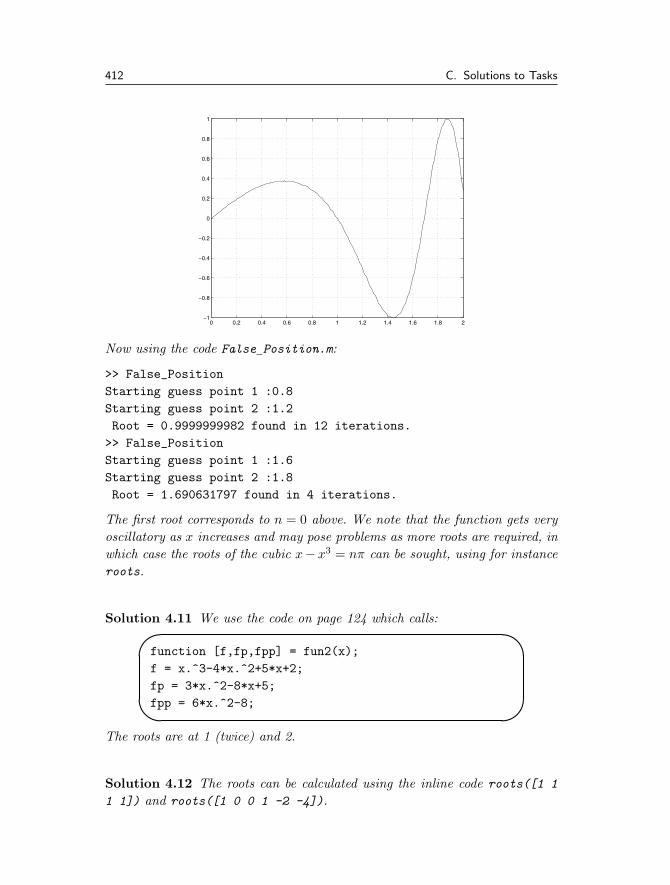
412 C. Solutions to Tasks
0 0.2 0.4 0.6 0.8 1 1.2 1.4 1.6 1.8 2−1
−0.8
−0.6
−0.4
−0.2
0
0.2
0.4
0.6
0.8
1
Now using the code False Position.m:
>> False_Position
Starting guess point 1 :0.8
Starting guess point 2 :1.2
Root = 0.9999999982 found in 12 iterations.
>> False_Position
Starting guess point 1 :1.6
Starting guess point 2 :1.8
Root = 1.690631797 found in 4 iterations.
The first root corresponds to n = 0 above. We note that the function gets veryoscillatory as x increases and may pose problems as more roots are required, inwhich case the roots of the cubic x − x3 = nπ can be sought, using for instanceroots.
Solution 4.11 We use the code on page 124 which calls:
�
�function [f,fp,fpp] = fun2(x);
f = x.ˆ3-4*x.ˆ2+5*x+2;
fp = 3*x.ˆ2-8*x+5;
fpp = 6*x.ˆ2-8;
The roots are at 1 (twice) and 2.
Solution 4.12 The roots can be calculated using the inline code roots([1 1
1 1]) and roots([1 0 0 1 -2 -4]).

C.4 Solutions for Tasks from Chapter 4 413
Solution 4.13 This can be done using the code��
��
function [f]=func1(x)
f = x.*sin(x)+cos(x);
and then use the code fzero(’ff’,3) which gives the root ≈ 2.7984. There aremany others. For the other cases the roots are: sin x = 0 or sin x = ±1, so thatx = nπ/2 (n ∈ Z); in this case fzero fails and returns a root at x = 1. Thecode has mistaken the fact that the function changes sign for a root.
Solution 4.14 The function J1/2(x) is actually sin x/√
x and consequently theroots are nπ. The code needed for fzero is��
��
function [f] = ourbess(x)
f = besselj(1/2,x);
and then fzero(’ourbess’,3).
Solution 4.15 The function we want to find the zeros of is f(x) = x sin x −x2 cos x − 1 which has derivative f ′(x) = sin x + x cos x − 2x cos x + x2 sin x =(1 + x2) sinx − x cos x. The correct definitions for f(x) and f ′(x) are:��
��
function [out] = f(in)
out = in.*sin(in)-in.ˆ2.*cos(in)-1;
f.m
��
��
function [out] = fp(in)
out = (1+in.ˆ2).*sin(in)-in.*cos(in);
fp.m
and the code to use these would be�
�
�
x = 0;
for j = 1:10
x = x -f(x)/fp(x);
end
(notice that the second term in this expression was the wrong way up in thequestion). This code could be written far more eloquently.
414 C. Solutions to Tasks
C.5 Solutions for Tasks from Chapter 5
Solution 5.1 This code inputs four values which represent the points (x1, y1)and (x2, y2). These are then made into vectors x and y, where the former con-tains the x coordinates and the latter the y coordinates. The command polyfit
fits a straight line through the points and returns y = mx + c, where the gra-dient m is the first element of p and the intercept c is the second. Then thefinal command displays the result. If the user enters both values of y, the sameequation is just returned as m = 0 and c equals that value. On the other handif two values of x are the same then MATLAB tries to give the line an infinitegradient, since it should be of the form x = d.
Solution 5.2 We write the quadratic as y = a + b(x − x0) + c(x − x0)(x − x1)where we choose x0 as the x coordinate of one of the points. For conveniencewe shall take the origin as the first point so that x0 = 0 and we see thata = 0. Using the point (2,−1) as the next point we note that the quadratic isy = bx + cx(x − 2) and −1 = 2b. Finally the condition that the curve goesthrough the final point yields the equation 5 = −5/2 + 15c so that c = 1/2.Hence the quadratic is
y = −12x +
12x(x − 2)
=x(x − 3)
2.
Solution 5.3 We use the code:�
�
�
�
x = 0:10;
co = [1 3 2];
y = x.ˆ2+3*x+2;
for i = 1:3
xv = i-0.5;
p = polyfit(x(i:(i+1)),y(i:(i+1)),1);
err(i) = polyval(p,xv)-polyval(co,xv);
end
This gives the same error in each case, namely 1/4 (which we would expect fromunderstanding the error associated with this method of interpolation (considerthe second derivative)).
Solution 5.4 This quadratic will be of the form cx(π − x) (since it is zero at

C.5 Solutions for Tasks from Chapter 5 415
0 and π). The value of c can be determined from the condition that the curvegoes through the final point which gives
y =4x
π2 (π − x).
Solution 5.5 Since the cubic is zero at the points 0 and π we know that it is ofthe form x(π−x)(a(x−π/2)+b). The values of a and b can be determined fromthe other points: (π/2, 1) gives b = 4/π2; finally (−π/2,−1) gives a = 16/(3π2).Hence the cubic is
y = x(π − x)(
163π3 (x − π/2) +
4π2
)
= x(π − x)(
16x
3π3 x +4
3π2
).
Solution 5.6 For this we shall use the MATLAB command spline so that�
�
�
�
x = -pi:(pi/2):pi;
y = [0 -1 0 1 0];
z = -pi:(pi/20):pi;
f = spline(x,y,z);
plot(z,f,x,y,’o’,’MarkerSize’,14)
This gives:
−4 −3 −2 −1 0 1 2 3 4−1.5
−1
−0.5
0
0.5
1
1.5
416 C. Solutions to Tasks
Solution 5.7 Here we shall use the method of least squares. As such we shallproduce details of the formulation. We calculate the sum of the squares of theerrors:
e =n∑
i=1
(a sin xi + b cos xi − fi)2
and partially differentiating with respect to a and b we have
∂e
∂a=
n∑i=1
sin xi(a sin xi + b cos xi − fi)
∂e
∂b=
n∑i=1
cos xi(a sin xi + b cos xi − fi).
These equations can be rewritten in matrix form as:⎛⎜⎜⎝
n∑i=1
sin2 xi
n∑i=1
sin xi cos xi
n∑i=1
cos xi sin xi
n∑i=1
cos2 xi
⎞⎟⎟⎠(
a
b
)=
⎛⎜⎜⎝
n∑i=1
fi sin xi
n∑i=1
fi cos xi
⎞⎟⎟⎠ .
This can be solved using the code:�
�
�
�
x = 0:0.1:1.0;
f = [3.16 3.01 2.73 2.47 2.13 1.82 ...
1.52 1.21 0.76 0.43 0.03];
A = [sum(sin(x).ˆ2) sum(cos(x).*sin(x)); ...
sum(cos(x).*sin(x)) sum(cos(x).ˆ2)];
r = [sum(f.*sin(x)); sum(f.*cos(x))];
sol = A\r;
This gives
sol =
-1.9941
3.1892
The original data was actually generated with −2 and 3.2, and then noise wasadded.
Solution 5.8 This can be done by hand but in fact MATLAB will actuallyreturn the required coefficients.
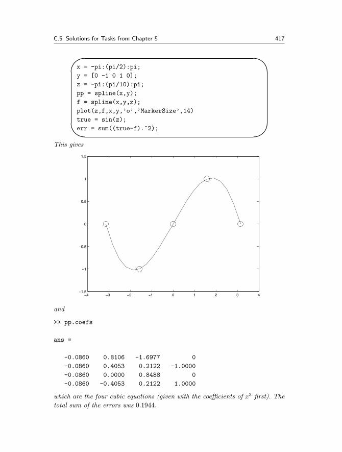
C.5 Solutions for Tasks from Chapter 5 417
�
�
�
�
x = -pi:(pi/2):pi;
y = [0 -1 0 1 0];
z = -pi:(pi/10):pi;
pp = spline(x,y);
f = spline(x,y,z);
plot(z,f,x,y,’o’,’MarkerSize’,14)
true = sin(z);
err = sum((true-f).ˆ2);
This gives
−4 −3 −2 −1 0 1 2 3 4−1.5
−1
−0.5
0
0.5
1
1.5
and
>> pp.coefs
ans =
-0.0860 0.8106 -1.6977 0
-0.0860 0.4053 0.2122 -1.0000
-0.0860 0.0000 0.8488 0
-0.0860 -0.4053 0.2122 1.0000
which are the four cubic equations (given with the coefficients of x3 first). Thetotal sum of the errors was 0.1944.
418 C. Solutions to Tasks
Solution 5.9 The corrected code is:�
�
�
�
x = 2:11;
f = polyval([1 0 0 -1],x) + sin(x);
% x = 4.5
r = 3:4;
c = polyfit(x(r),f(r),1);
yy = polyval(c,4.5)
% x = 15 (extrapolation)
r = length(x)-1:length(x);
c = polyfit(x(r),f(r),1);
yy = polyval(c,15);
C.6 Solutions for Tasks from Chapter 6
Solution 6.1 These calculations can be repeated using the code�
�
�
�
A = [3 0 -1; -4 2 2];
B = [-1 7; 3 5; -2 0];
C = [2 0; -1 -3];
A*B
B*A
A+transpose(B)
A*C
A*transpose(C)
3*C+2*transpose(A*B)
(A*B)*C
A*(B*C)
Solution 6.2 Notice that here we set up the matrix A before changing the ele-ments and this is unnecessary but good practice. Also it is not necessary to setup r and this can be defined inline. The definition of r allows for more versatilecode.
C.6 Solutions for Tasks from Chapter 6 419
�
�r = 1:4;
A = zeros(4);
A(1,r) = r;
A(r,4) = flipud(r’);
Note that the final command could also be replaced by A(flipud(r),1)=r’;;you should try to understand this command.
Solution 6.3 Here we rely on the fact that MATLAB knows that a matrix witha super- or sub-diagonal of length 9 is a ten-by-ten matrix.��
��a = diag(ones(1,9),1)+diag(-ones(1,9),-1);
Solution 6.4 This is just a matter of typing the commands: however youshould be able to decide which ones are viable before doing this.
Solution 6.5 The code to solve these problems is given by:�
�
�
�
A = [ 1 2; 3 4];
B = [3 4; -1 2];
A*B
C = [3 5; 6 -2];
D = [-1 0; 2 1];
2*C-4*D
E = [1 3 5];
F = [2 -1; -1 0; 7 -2];
E*F
This gives the answers
ans =
1 8
5 20
ans =
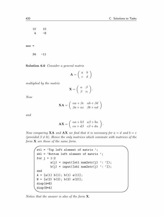
420 C. Solutions to Tasks
10 10
4 -8
ans =
34 -11
Solution 6.6 Consider a general matrix
A =(
a b
c d
)
multiplied by the matrix
X =(
α β
β α
).
Now
XA =(
αa + βc αb + βd
βa + αc βb + αd
)
and
AX =(
αa + bβ aβ + bα
cα + dβ cβ + dα
).
Now comparing XA and AX we find that it is necessary for a = d and b = c
(provided β = 0). Hence the only matrices which commute with matrices of theform X are those of the same form.�
�
�
�
stl = ’Top left element of matrix ’;
sbl = ’Bottom left element of matrix ’;
for j = 1:2
a(j) = input([stl num2str(j) ’: ’]);
b(j) = input([sbl num2str(j) ’: ’]);
end
A = [a(1) b(1); b(1) a(1)];
B = [a(2) b(2); b(2) a(2)];
disp(A*B)
disp(B*A)
Notice that the answer is also of the form X.
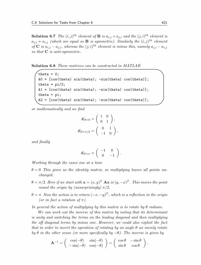
C.6 Solutions for Tasks from Chapter 6 421
Solution 6.7 The (i, j)th element of B is ai,j + aj,i and the (j, i)th element isaj,i + ai,j (which are equal so B is symmetric). Similarly the (i, j)th elementof C is ai,j − aj,i, whereas the (j, i)th element is minus this, namely aj,i − ai,j
so that C is anti-symmetric.
Solution 6.8 These matrices can be constructed in MATLAB�
�
�
�
theta = 0;
A0 = [cos(theta) sin(theta); -sin(theta) cos(theta)];
theta = pi/2;
A1 = [cos(theta) sin(theta); -sin(theta) cos(theta)];
theta = pi;
A2 = [cos(theta) sin(theta); -sin(theta) cos(theta)];
or mathematically and we find
A|θ=0 =(
1 00 1
),
A|θ=π/2 =(
0 1−1 0
),
and finally
A|θ=π =( −1 0
0 −1
).
Working through the cases one at a time
θ = 0 This gives us the identity matrix, so multiplying leaves all points un-changed.
θ = π/2 Here if we start with x = (x, y)T Ax is (y, −x)T . This moves the pointround the origin by (unsurprisingly) π/2.
θ = π Now the action is to return (−x,−y)T , which is a reflection in the origin(or in fact a rotation of π).
In general the action of multiplying by this matrix is to rotate by θ radians.We can work out the inverse of this matrix by noting that its determinant
is unity and switching the terms on the leading diagonal and then multiplyingthe off diagonal terms by minus one. However, we could also exploit the factthat in order to invert the operation of rotating by an angle θ we merely rotateby θ in the other sense (or more specifically by −θ). The inverse is given by
A−1 =(
cos(−θ) sin(−θ)− sin(−θ) cos(−θ)
)=(
cos θ − sin θ
sin θ cos θ
).
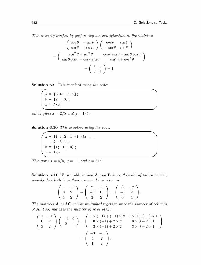
422 C. Solutions to Tasks
This is easily verified by performing the multiplication of the matrices(cos θ − sin θ
sin θ cos θ
)(cos θ sin θ
− sin θ cos θ
)
=(
cos2 θ + sin2 θ cos θ sin θ − sin θ cos θ
sin θ cos θ − cos θ sin θ sin2 θ + cos2 θ
)
=(
1 00 1
)= I.
Solution 6.9 This is solved using the code:
�
�
�A = [3 4; -1 2];
b = [2 ; 0];
x = A\b;
which gives x = 2/5 and y = 1/5.
Solution 6.10 This is solved using the code:
�
�A = [1 1 2; 1 -1 -3; ...
-2 -5 1];
b = [1; 0 ; 4];
x = A\b
This gives x = 4/5, y = −1 and z = 3/5.
Solution 6.11 We are able to add A and B since they are of the same size,namely they both have three rows and two columns.⎛
⎝ 1 −10 23 2
⎞⎠+
⎛⎝ 2 −1
−1 03 2
⎞⎠ =
⎛⎝ 3 −2
−1 26 4
⎞⎠ .
The matrices A and C can be multiplied together since the number of columnsof A (two) matches the number of rows of C.⎛⎝ 1 −1
0 23 2
⎞⎠( −1 0
2 1
)=
⎛⎝ 1 × (−1) + (−1) × 2 1 × 0 + (−1) × 1
0 × (−1) + 2 × 2 0 × 0 + 2 × 13 × (−1) + 2 × 2 3 × 0 + 2 × 1
⎞⎠
=
⎛⎝ −3 −1
4 21 2
⎞⎠ .
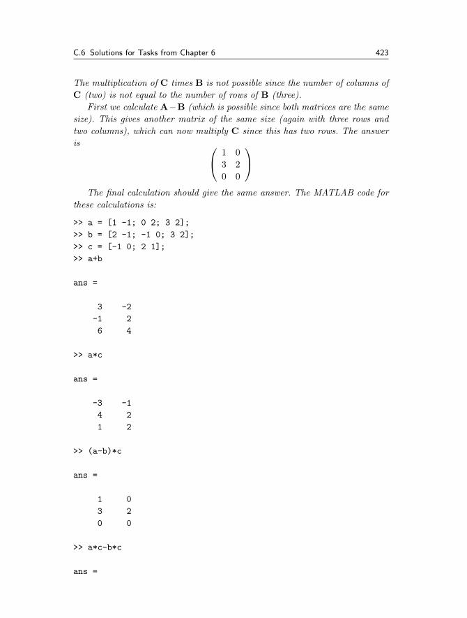
C.6 Solutions for Tasks from Chapter 6 423
The multiplication of C times B is not possible since the number of columns ofC (two) is not equal to the number of rows of B (three).
First we calculate A−B (which is possible since both matrices are the samesize). This gives another matrix of the same size (again with three rows andtwo columns), which can now multiply C since this has two rows. The answeris ⎛
⎝ 1 03 20 0
⎞⎠
The final calculation should give the same answer. The MATLAB code forthese calculations is:
>> a = [1 -1; 0 2; 3 2];
>> b = [2 -1; -1 0; 3 2];
>> c = [-1 0; 2 1];
>> a+b
ans =
3 -2
-1 2
6 4
>> a*c
ans =
-3 -1
4 2
1 2
>> (a-b)*c
ans =
1 0
3 2
0 0
>> a*c-b*c
ans =

424 C. Solutions to Tasks
1 0
3 2
0 0
Solution 6.12 These calculations can both be performed and the solutions are(310
)and
(16 −2 9 −30 2 −5 −1
)
which can be checked using MATLAB
>> [1 -1 2; 3 0 1]*[3; 2; 1]
ans =
3
10
>> [5 -2;-1 2]*[4 0 1 -1; 2 1 -2 -1]
ans =
16 -2 9 -3
0 2 -5 -1
Solution 6.13 The results of both calculations merely returns the matrix un-changed. This is the effect of multiplying by the identity.
Solution 6.14 Firstly, we reflect in the leading diagonal to give AT so that
AT =
⎛⎝ 3 0
2 −1−1 −2
⎞⎠
The results of the multiplications are
(14 00 5
)and
⎛⎝ 9 6 −3
6 5 0−3 0 5
⎞⎠ ,
which can also be done using MATLAB code:
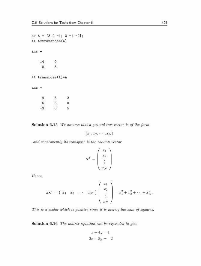
C.6 Solutions for Tasks from Chapter 6 425
>> A = [3 2 -1; 0 -1 -2];
>> A*transpose(A)
ans =
14 0
0 5
>> transpose(A)*A
ans =
9 6 -3
6 5 0
-3 0 5
Solution 6.15 We assume that a general row vector is of the form
(x1, x2, · · · , xN )
and consequently its transpose is the column vector
xT =
⎛⎜⎜⎜⎝
x1
x2...
xN
⎞⎟⎟⎟⎠
Hence
xxT =(
x1 x2 · · · xN
)⎛⎜⎜⎜⎝
x1
x2...
xN
⎞⎟⎟⎟⎠ = x2
1 + x22 + · · · + x2
N .
This is a scalar which is positive since it is merely the sum of squares.
Solution 6.16 The matrix equation can be expanded to give
x + 4y = 1
−2x + 3y = −2
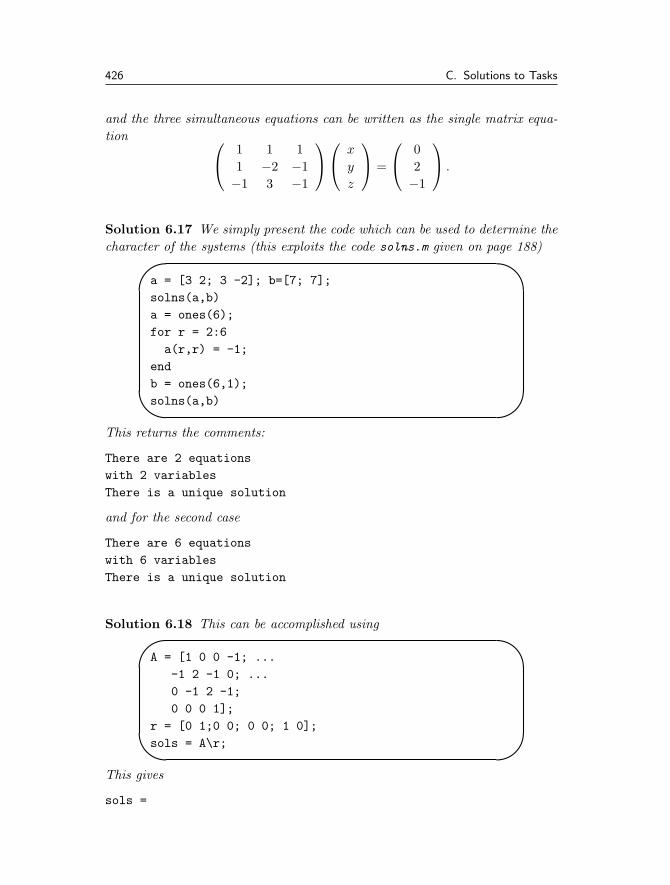
426 C. Solutions to Tasks
and the three simultaneous equations can be written as the single matrix equa-tion ⎛
⎝ 1 1 11 −2 −1
−1 3 −1
⎞⎠⎛⎝ x
y
z
⎞⎠ =
⎛⎝ 0
2−1
⎞⎠ .
Solution 6.17 We simply present the code which can be used to determine thecharacter of the systems (this exploits the code solns.m given on page 188)�
�
�
�
a = [3 2; 3 -2]; b=[7; 7];
solns(a,b)
a = ones(6);
for r = 2:6
a(r,r) = -1;
end
b = ones(6,1);
solns(a,b)
This returns the comments:
There are 2 equations
with 2 variables
There is a unique solution
and for the second case
There are 6 equations
with 6 variables
There is a unique solution
Solution 6.18 This can be accomplished using�
�
�
�
A = [1 0 0 -1; ...
-1 2 -1 0; ...
0 -1 2 -1;
0 0 0 1];
r = [0 1;0 0; 0 0; 1 0];
sols = A\r;
This gives
sols =
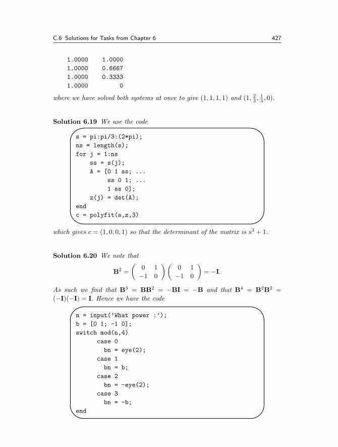
C.6 Solutions for Tasks from Chapter 6 427
1.0000 1.0000
1.0000 0.6667
1.0000 0.3333
1.0000 0
where we have solved both systems at once to give (1, 1, 1, 1) and (1, 23 , 1
3 , 0).
Solution 6.19 We use the code�
�
�
�
s = pi:pi/3:(2*pi);
ns = length(s);
for j = 1:ns
ss = s(j);
A = [0 1 ss; ...
ss 0 1; ...
1 ss 0];
z(j) = det(A);
end
c = polyfit(s,z,3)
which gives c = (1, 0, 0, 1) so that the determinant of the matrix is s3 + 1.
Solution 6.20 We note that
B2 =(
0 1−1 0
)(0 1
−1 0
)= −I.
As such we find that B3 = BB2 = −BI = −B and that B4 = B2B2 =(−I)(−I) = I. Hence we have the code�
�
�
�
n = input(’What power :’);
b = [0 1; -1 0];
switch mod(n,4)
case 0
bn = eye(2);
case 1
bn = b;
case 2
bn = -eye(2);
case 3
bn = -b;
end
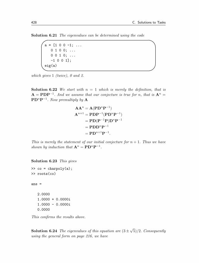
428 C. Solutions to Tasks
Solution 6.21 The eigenvalues can be determined using the code�
�
�
�
a = [1 0 0 -1; ...
0 1 0 0; ...
0 0 1 0; ...
-1 0 0 1];
eig(a)
which gives 1 (twice), 0 and 2.
Solution 6.22 We start with n = 1 which is merely the definition, that isA = PDP−1. And we assume that our conjecture is true for n, that is An =PDnP−1. Now premultiply by A
AAn = A(PDnP−1)
An+1 = PDP−1(PDnP−1)
= PD(P−1P)DnP−1
= PDDnP−1
= PDn+1P−1.
This is merely the statement of our initial conjecture for n + 1. Thus we haveshown by induction that An = PDnP−1.
Solution 6.23 This gives
>> co = charpoly(a);
>> roots(co)
ans =
2.0000
1.0000 + 0.0000i
1.0000 - 0.0000i
0.0000
This confirms the results above.
Solution 6.24 The eigenvalues of this equation are (3 ± √5)/2. Consequently
using the general form on page 216, we have
C.7 Solutions for Tasks from Chapter 7 429
x(t) =1√5
{12
((3 +
√5)e(3−√
5)t/2 − (3 −√
5)e(3+√
5)t/2)I
+(e(3−√
5)t/2 − e(3+√
5)t/2)A}( 1
−1
).
C.7 Solutions for Tasks from Chapter 7
Solution 7.1 Please try it yourself first but this is the answer (or one of them):�
�
�
�
for i = 1:12
switch mod(i,3)
case 0
f(i) = 1;
case 1
f(i) = 2;
case 2
f(i) = 3;
end
end
There are many alternatives, for instance f = mod(1:12,3)+1;.
Solution 7.2 For the one third case, we can work through the code with N = 9,so that
rodd=1:2:N gives [1 3 5 7 9]
reven=2:2:(N-1) gives [2 4 6 8]
weights(rodd=2) gives [2 0 2 0 2 0 2 0 2]
weights(1)=1 gives [1 0 2 0 2 0 2 0 2]
weights(N)=1 gives [1 0 2 0 2 0 2 0 1]
weights(reven)=4 gives = [1 4 2 4 2 4 2 4 1]

430 C. Solutions to Tasks
and for the three eighths rule with N = 10 we have
m=(N-1)/3 gives 3
rdiff=3*(1:(m-1))+1 gives [3*(1:2)+1] that is [4 7]
weights=3*ones(1,N) gives [3 3 3 3 3 3 3 3 3 3]
weights(1) gives [1 3 3 3 3 3 3 3 3 3]
weights(N) gives [1 3 3 3 3 3 3 3 3 1]
weights(rdiff)=2 gives [1 3 3 2 3 3 2 3 3 1]
Solution 7.3 This is done using the code:��
��
function [val] = fn(x)
val = log(x+sqrt(x.ˆ2+1));
Solution 7.4 We shall use forty points (which should be more than enough)and note that the exact answer is
3∫x=1
x2 − 3x + 2 dx =[x3
3− 3x2
2+ 2x
]3
1=
23.
The code is�
�
�
�
N = 40;
x = linspace(1,3,N);
f = x.ˆ2-3*x+2;
h = x(2)-x(1);
integral = (sum(f)-f(1)/2-f(N)/2)*h;
This gives the value 0.6675, which is within 8.7 × 10⁻⁴ of the exact answer.Notice that by using either of Simpson’s rules we could have retrieved the exactanswer, since the original curve is a quadratic.
Solution 7.5 We use N = 11 and modify Simpson’s 1/3 rule code on page233, so that we have
C.7 Solutions for Tasks from Chapter 7 431
�
�
�
�
x = linspace(0,1,11);
h = x(2)-x(1);
N = length(x);
rodd = 1:2:N;
reven = 2:2:(N-1);
weights(rodd) = 2; weights(1) = 1;
weights(N) = 1; weights(reven) = 4;
f = x.ˆ3-x+1;
integral = h/3*sum(weights.*f);
disp([integral])
This gives an answer of 0.75. The exact answer is1∫
0
x3 − x + 1 dx =[x4
4− x2
2+ x
]1
0=
34.
So the scheme does exceedingly well and the error is of the order 10−16. Thisis unsurprising since the error is proportional to the fourth derivative, which isidentically zero for a cubic.
Solution 7.6 In this task we produce a minor modification of the previoussolution: the first line needs to read x=linspace(0,pi,N); and the line definingf(x) needs modifying to f=sin(x). This now allows us to try different valuesof N , which we do with a loop structure:�
�
�
�
Ns = 5:2:19;
for N = Ns
clear rodd reven weights f x
x = linspace(0,pi,N);
h = x(2)-x(1);
rodd = 1:2:N;
reven = 2:2:(N-1);
weights(rodd) = 2;
weights(1) = 1; weights(N) = 1;
weights(reven) = 4;
f = sin(x);
integral(N) = h/3*sum(weights.*f);
end
plot(Ns,abs(integral-2))
This gives
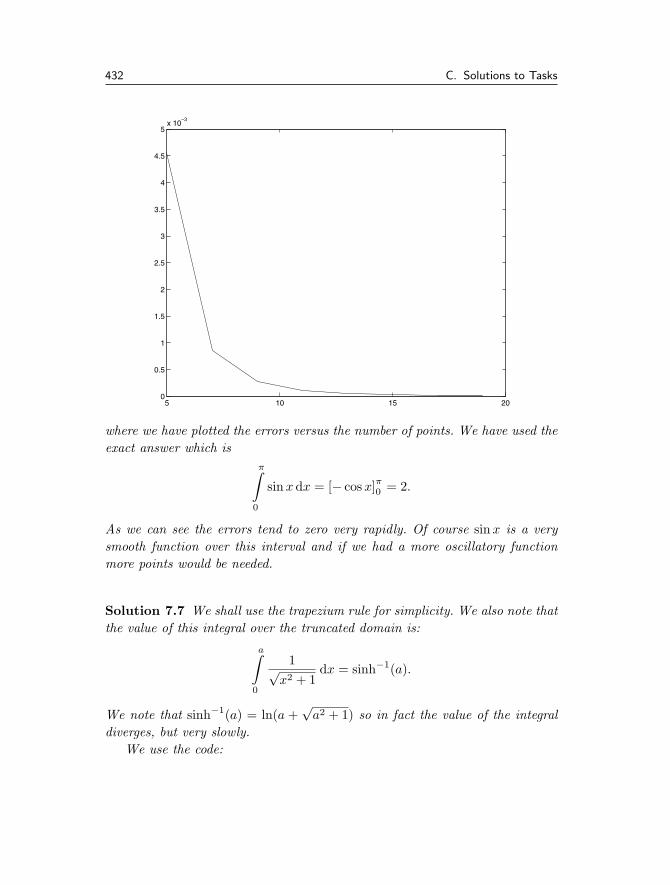
432 C. Solutions to Tasks
5 10 15 200
0.5
1
1.5
2
2.5
3
3.5
4
4.5
5x 10
−3
where we have plotted the errors versus the number of points. We have used theexact answer which is
π∫0
sin xdx = [− cos x]π0 = 2.
As we can see the errors tend to zero very rapidly. Of course sin x is a verysmooth function over this interval and if we had a more oscillatory functionmore points would be needed.
Solution 7.7 We shall use the trapezium rule for simplicity. We also note thatthe value of this integral over the truncated domain is:
a∫0
1√x2 + 1
dx = sinh−1(a).
We note that sinh−1(a) = ln(a +√
a2 + 1) so in fact the value of the integraldiverges, but very slowly.
We use the code:
C.7 Solutions for Tasks from Chapter 7 433
�
�
�
�
X = input(’Truncate at:’);
N = ceil(X)*3;
x = linspace(0,X,N);
h = x(2)-x(1);
f = 1./sqrt(x.ˆ2+1);
int = (sum(f)-f(1)/2-f(N)/2)*h
The second line ensures that the step sizes will be smaller than 1/3. This gives:
>> diverge
Truncate at:10
int =
2.9981
>> diverge
Truncate at:100
int =
5.2983
>> diverge
Truncate at:1000
int =
7.6009
which as we see increases as the truncation point increases. (The correspondingvalues of arcsinh are 2.9982, 5.2983 and 7.6009; so that the integration does agood job).
Solution 7.8 We can use the code:

434 C. Solutions to Tasks
�
�
�
�
theta = 0:pi/20:(pi/2-pi/20);
N = 20;
for it = 1:length(theta);
theta1 = theta(it);
clear grid f
grid = linspace(theta1,pi-theta1,N);
f = sqrt(1+cos(grid).ˆ2);
h = grid(2)-grid(1);
arclen(it) = (sum(f)-f(1)/2-f(N)/2)*h;
end
plot(theta/pi*180,arclen)
xlabel(’\theta degrees’)
ylabel(’Arc length’)
which gives
0 10 20 30 40 50 60 70 80 900
0.5
1
1.5
2
2.5
3
3.5
4
θ degrees
Arc
leng
th
Solution 7.9 Firstly we give details of the analytical solution:
10∫0
cos x
x1/2 dx =
ε∫0
cos x
x1/2 dx +
10∫ε
cos x
x1/2 dx
For the first of these integrals we approximate cos x by 1 − x2/2 (that is the
C.7 Solutions for Tasks from Chapter 7 435
first two terms in its Taylor series).
ε∫0
1x1/2 − x3/2
2dx =
[2x1/2 − x5/2
5
]=[2ε1/2 − ε5/2
5
].
We can now use the code�
�
�
�
clear all
epsil = input(’Epsilon :’);
int1 = 2*epsilˆ(0.5)-epsilˆ(2.5)/5;
N = 100;
x = linspace(epsil,10,N);
h = x(2)-x(1);
f = cos(x)./sqrt(x);
int2 = (sum(f)-f(1)/2-f(N)/2)*h;
int = int1+int2;
The first integral gives a significant contribution.
Solution 7.10 The quadratic through the three points is
y(x) = a0 + (x − x0)∆a1 + (x − x0)(x − x1)a2
where the constants are
a0 = f0
a1 =f1 − f0
x1 − x0
a2 =(f2 − f0)(x1 − x0) − (f1 − f0)(x2 − x0)
(x1 − x0)(x2 − x0)(x2 − x1)
Now integrating
x2∫x=x0
y(x) dx
x2∫x=x0
a0 + (x − x0)a1 + (x − x0)(x − x1)a2 dx
Solution 7.11 Here we need to use the code��
��
function [f] = fxlnx(x)
f = x.*log(x);
436 C. Solutions to Tasks
and then use the code quad(’fxlnx’,1,2). This gives 0.63629536463993 (us-ing format long). The exact value can be calculated using integration by parts
2∫x=1
q ln q dq =[12q2 ln q
]2
x=1−
2∫x=1
q
2dq
= 2 ln 2 −[q2
4
]2
x=1
= 2 ln 2 − 34.
The value of this expression agrees very well with that above.
C.8 Solutions for Tasks from Chapter 8
Solution 8.1 Let us firstly find the exact solution. Start by dividing the equa-tion through by y and then integrate with respect to t which gives∫
1y
dy
dtdt = −
∫ √t dt,
hence we have
ln y = −23t3/2 + C.
This can be rearranged to give
y = Ae− 23 t
32
and the particular solution can be found by setting y(0) = 1, which gives A = 1.
In order to obtain the numerical solution the code should be modified to�
�
�
�
dt = 0.05;
t = 0.0:dt:1.0;
y = zeros(size(t));
y(1) = 1;
for ii=1:(length(t)-1)
y(ii+1) = y(ii) + dt * (-y(ii)*sqrt(t(ii)));
end
exact = exp(-2/3*(t).ˆ(3/2));
plot(t,y,t,exact,’--’)
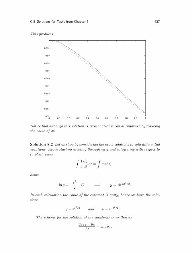
C.8 Solutions for Tasks from Chapter 8 437
This produces
0 0.1 0.2 0.3 0.4 0.5 0.6 0.7 0.8 0.9 10.5
0.55
0.6
0.65
0.7
0.75
0.8
0.85
0.9
0.95
1
Notice that although this solution is “reasonable” it can be improved by reducingthe value of dt.
Solution 8.2 Let us start by considering the exact solutions to both differentialequations. Again start by dividing through by y and integrating with respect tot, which gives ∫
1y
dy
dtdt =
∫±t dt,
hence
ln y = ± t2
2+ C =⇒ y = Ae±t2/2.
In each calculation the value of the constant is unity, hence we have the solu-tions
y = et2/2 and y = e−t2/2.
The scheme for the solution of the equations is written as
yn+1 − yn
∆t= ±tnyn,
438 C. Solutions to Tasks
which can be rearranged to give
yn+1 = yn + ±∆t tnyn = yn
(1 + ±n∆t2
),
where we have used the fact that tn = n∆t.Let us consider the first case. Start with n = 0
y1 = 1
and now n = 1, etc.
y2 = 1(
1 +116
)=
1716
,
y3 =1716
(1 +
216
)=
153128
,
y4 =153144
(1 +
316
)=
29072028
≈ 1.419 .
The exact answer is e1/2 ≈ 1.648, hence the absolute error is |1.419 − e1/2| ≈0.229 and the relative error is |1.419−e1/2|/e1/2 ≈ 0.139 (or this can be writtenas 13.9%).
Now we can repeat the calculation for the other case
y1 = 1
and now n = 1, etc.
y2 = 1(
1 − 116
)=
1516
y3 =1516
(1 − 2
16
)=
105128
y4 =105128
(1 − 3
16
)=
13652048
.
Here the absolute error is ≈ 0.21378 whereas the relative error is 0.352 (oraround 35%). Despite the absolute errors being comparable the relative errorsare different (due to the magnitude of the answers involved).
It is up to the individual as to which error is best to use and this generallycomes with experience.
Solution 8.3 The code for this task is
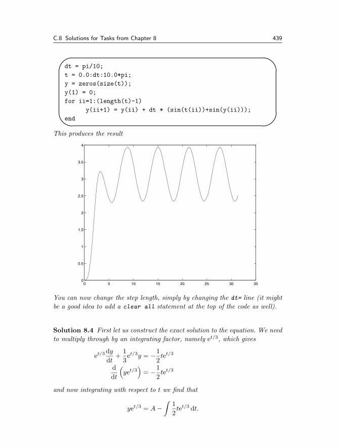
C.8 Solutions for Tasks from Chapter 8 439
�
�
�
�
dt = pi/10;
t = 0.0:dt:10.0*pi;
y = zeros(size(t));
y(1) = 0;
for ii=1:(length(t)-1)
y(ii+1) = y(ii) + dt * (sin(t(ii))+sin(y(ii)));
end
This produces the result
0 5 10 15 20 25 30 350
0.5
1
1.5
2
2.5
3
3.5
4
You can now change the step length, simply by changing the dt= line (it mightbe a good idea to add a clear all statement at the top of the code as well).
Solution 8.4 First let us construct the exact solution to the equation. We needto multiply through by an integrating factor, namely et/3, which gives
et/3 dy
dt+
13et/3y = −1
2tet/3
ddt
(yet/3
)= −1
2tet/3
and now integrating with respect to t we find that
yet/3 = A −∫
12tet/3 dt.

440 C. Solutions to Tasks
Now integrating the right hand side by parts gives
yet/3 = A −{[
32tet/3
]−∫
32et/3 dt
},
yet/3 = A −{
32tet/3 − 9
2et/3
}.
Hence we have the solution
y = Ae−t/3 −{
32t − 9
2
}.
Now applying the boundary condition gives A = −9/2. The solution is
y =92
(1 − e−t/3
)− 3t
2.
Now consider the discretised form of the equation, which is
yn+1 − yn
∆t= − tn+1
2− yn+1
3,
which can be rearranged to give
yn+1 =1
1 + ∆t3
(yn − ∆t
tn+1
2
).
Now with ∆t = 1/3 and n = 0 this gives
y1 =1
1 + 19
(0 − 1
31
3 × 2
)=
910
(− 1
18
)= − 1
20,
and now with n = 1
y2 =910
(− 1
20− 1
32
3 × 2
)= − 29
200,
and finally for n = 2 which gives y3 = y(1)
y3 =910
(− 29
200− 1
33
3 × 2
)= − 561
2000.
The code to produce this and the other required solutions is
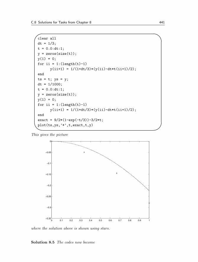
C.8 Solutions for Tasks from Chapter 8 441
�
�
�
�
clear all
dt = 1/3;
t = 0.0:dt:1;
y = zeros(size(t));
y(1) = 0;
for ii = 1:(length(t)-1)
y(ii+1) = 1/(1+dt/3)*(y(ii)-dt*t(ii+1)/2);
end
ts = t; ys = y;
dt = 1/1000;
t = 0.0:dt:1;
y = zeros(size(t));
y(1) = 0;
for ii = 1:(length(t)-1)
y(ii+1) = 1/(1+dt/3)*(y(ii)-dt*t(ii+1)/2);
end
exact = 9/2*(1-exp(-t/3))-3/2*t;
plot(ts,ys,’*’,t,exact,t,y)
This gives the picture
0 0.1 0.2 0.3 0.4 0.5 0.6 0.7 0.8 0.9 1−0.35
−0.3
−0.25
−0.2
−0.15
−0.1
−0.05
0
where the solution above is shown using stars.
Solution 8.5 The codes now become

442 C. Solutions to Tasks
��
��
function [value] = odes(t,y)
value = tˆ2-yˆ2;
and
�
�
�y0 = 0;
tspan = [0 2];
[t,y] = ode45(’odes’,tspan,y0);
These give
0 0.2 0.4 0.6 0.8 1 1.2 1.4 1.6 1.8 20
0.2
0.4
0.6
0.8
1
1.2
1.4
1.6
1.8
Solution 8.6 The solution to this equation can be obtained by multiplying bythe integrating factor et and then integrating by parts. After application of theinitial condition we find that
y(t) = t2 − 2t + 2 − e−t.
The numerical solution can be determined using:
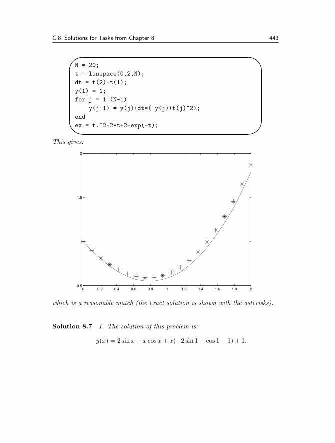
C.8 Solutions for Tasks from Chapter 8 443
�
�
�
�
N = 20;
t = linspace(0,2,N);
dt = t(2)-t(1);
y(1) = 1;
for j = 1:(N-1)
y(j+1) = y(j)+dt*(-y(j)+t(j)ˆ2);
end
ex = t.ˆ2-2*t+2-exp(-t);
This gives:
0 0.2 0.4 0.6 0.8 1 1.2 1.4 1.6 1.8 20.5
1
1.5
2
which is a reasonable match (the exact solution is shown with the asterisks).
Solution 8.7 1. The solution of this problem is:
y(x) = 2 sinx − x cos x + x(−2 sin 1 + cos 1 − 1) + 1.
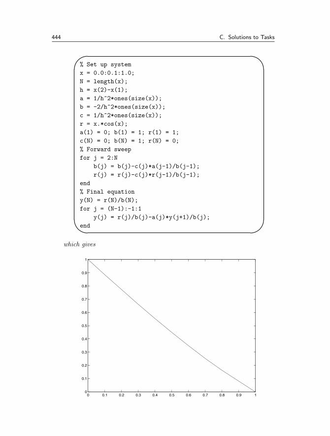
444 C. Solutions to Tasks
�
�
�
�
% Set up system
x = 0.0:0.1:1.0;
N = length(x);
h = x(2)-x(1);
a = 1/hˆ2*ones(size(x));
b = -2/hˆ2*ones(size(x));
c = 1/hˆ2*ones(size(x));
r = x.*cos(x);
a(1) = 0; b(1) = 1; r(1) = 1;
c(N) = 0; b(N) = 1; r(N) = 0;
% Forward sweep
for j = 2:N
b(j) = b(j)-c(j)*a(j-1)/b(j-1);
r(j) = r(j)-c(j)*r(j-1)/b(j-1);
end
% Final equation
y(N) = r(N)/b(N);
for j = (N-1):-1:1
y(j) = r(j)/b(j)-a(j)*y(j+1)/b(j);
end
which gives
0 0.1 0.2 0.3 0.4 0.5 0.6 0.7 0.8 0.9 10
0.1
0.2
0.3
0.4
0.5
0.6
0.7
0.8
0.9
1
C.8 Solutions for Tasks from Chapter 8 445
2. The analytic solution here is:
y(x) = 2 sinx − x cos x − x − 2 sin 1 + cos 1 + 1.�
�
�
�
% Set up system
x = 0.0:0.1:1.0;
N = length(x);
h = x(2)-x(1);
a = 1/hˆ2*ones(size(x));
b = -2/hˆ2*ones(size(x));
c = 1/hˆ2*ones(size(x));
r = x.*cos(x);
a(1) = -1; b(1) = 1; r(1) = 0;
c(N) = 0; b(N) = 1; r(N) = 0;
% Forward sweep
for j = 2:N
b(j) = b(j)-c(j)*a(j-1)/b(j-1);
r(j) = r(j)-c(j)*r(j-1)/b(j-1);
end
% Final equation
y(N) = r(N)/b(N);
for j = (N-1):-1:1
y(j) = r(j)/b(j)-a(j)*y(j+1)/b(j);
end
which gives
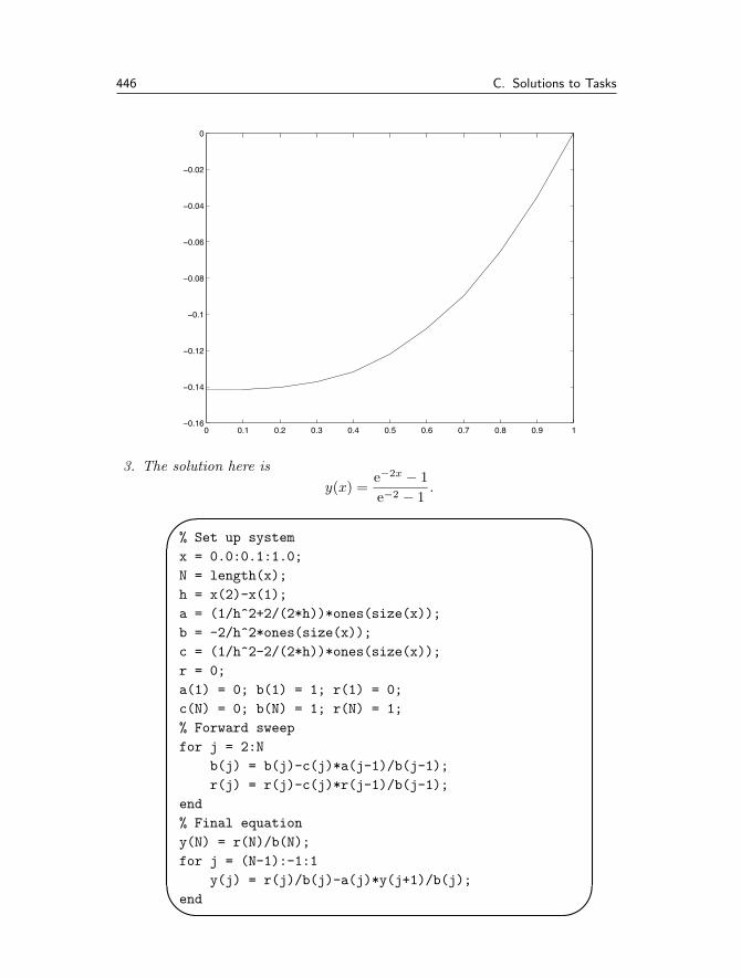
446 C. Solutions to Tasks
0 0.1 0.2 0.3 0.4 0.5 0.6 0.7 0.8 0.9 1−0.16
−0.14
−0.12
−0.1
−0.08
−0.06
−0.04
−0.02
0
3. The solution here isy(x) =
e−2x − 1e−2 − 1
.�
�
�
�
% Set up system
x = 0.0:0.1:1.0;
N = length(x);
h = x(2)-x(1);
a = (1/hˆ2+2/(2*h))*ones(size(x));
b = -2/hˆ2*ones(size(x));
c = (1/hˆ2-2/(2*h))*ones(size(x));
r = 0;
a(1) = 0; b(1) = 1; r(1) = 0;
c(N) = 0; b(N) = 1; r(N) = 1;
% Forward sweep
for j = 2:N
b(j) = b(j)-c(j)*a(j-1)/b(j-1);
r(j) = r(j)-c(j)*r(j-1)/b(j-1);
end
% Final equation
y(N) = r(N)/b(N);
for j = (N-1):-1:1
y(j) = r(j)/b(j)-a(j)*y(j+1)/b(j);
end

C.8 Solutions for Tasks from Chapter 8 447
which yields
0 0.1 0.2 0.3 0.4 0.5 0.6 0.7 0.8 0.9 10
0.1
0.2
0.3
0.4
0.5
0.6
0.7
0.8
0.9
1
Solution 8.8 The exact solution here is
y(t) =13
(t − 1√
3sin
√3t
).
By discretising the equation we have
yn+1 = 2yn − yn−1 + ∆t2 (−3yn + tn) .
The initial conditions can be realised by setting y1 = 0 and y2 = 0 as a resultof the fact that y′(0) ≈ (y2 − y1)/∆t = 0.�
�
�
�
N = 20;
t = linspace(0,1,N);
dt = t(2)-t(1);
y(1) = 0;
y(2) = 0;
for j = 2:N-1
y(j+1) = 2*y(j)-y(j-1) ...
+dtˆ2*(3*y(j)+t(j));
end
ex = (t-sin(sqrt(3)*t)/sqrt(3))/3;
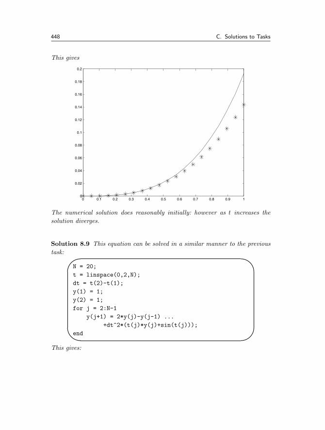
448 C. Solutions to Tasks
This gives
0 0.1 0.2 0.3 0.4 0.5 0.6 0.7 0.8 0.9 10
0.02
0.04
0.06
0.08
0.1
0.12
0.14
0.16
0.18
0.2
The numerical solution does reasonably initially: however as t increases thesolution diverges.
Solution 8.9 This equation can be solved in a similar manner to the previoustask:�
�
�
�
N = 20;
t = linspace(0,2,N);
dt = t(2)-t(1);
y(1) = 1;
y(2) = 1;
for j = 2:N-1
y(j+1) = 2*y(j)-y(j-1) ...
+dtˆ2*(t(j)*y(j)+sin(t(j)));
end
This gives:

C.8 Solutions for Tasks from Chapter 8 449
0 0.2 0.4 0.6 0.8 1 1.2 1.4 1.6 1.8 21
1.5
2
2.5
3
3.5
4
4.5
(the solution is expressible in terms of Airy functions, but this does not repre-sent a great advantage to us).
This second problem can be solved by setting up the discretised system
yn+1 − 2yn + yn−1
∆t2+ tnyn = sin tn
with the conditions that y1 = 0 (y(0) = 0) yN = 0 (y(2) = 0).�
�
�
�
N = 20;
t = linspace(0,2,N);
dt = t(2)-t(1);
A = zeros(N);
A = diag(-2/dtˆ2*ones(N,1)+t’,0) ...
+diag(1/dtˆ2*ones(N-1,1),-1) ...
+diag(1/dtˆ2*ones(N-1,1),1);
r = transpose(sin(t));
A(1,:) = 0;
A(1,1) = 1; r(1) = 0;
A(N,:) = 0;
A(N,N) = 1; r(N) = 0;
sol = A\r;
This gives:

450 C. Solutions to Tasks
0 0.2 0.4 0.6 0.8 1 1.2 1.4 1.6 1.8 2−0.7
−0.6
−0.5
−0.4
−0.3
−0.2
−0.1
0
0.1
Solution 8.10 This equation can be integrated directly by dividing through byy(t2 + 1). This gives
y′
y= − 2t
1 + t2
so thaty(t) =
11 + t2
.
The equation can be solved numerically using�
�
�
�
N = 50;
t = linspace(0,5,N);
dt = t(2)-t(1);
y(1) = 1;
for j = 1:(N-1)
y(j+1) = y(j)-dt*2*t(j)*y(j)/(1+t(j)ˆ2);
end
ex = 1./(1+t.ˆ2);
This yields
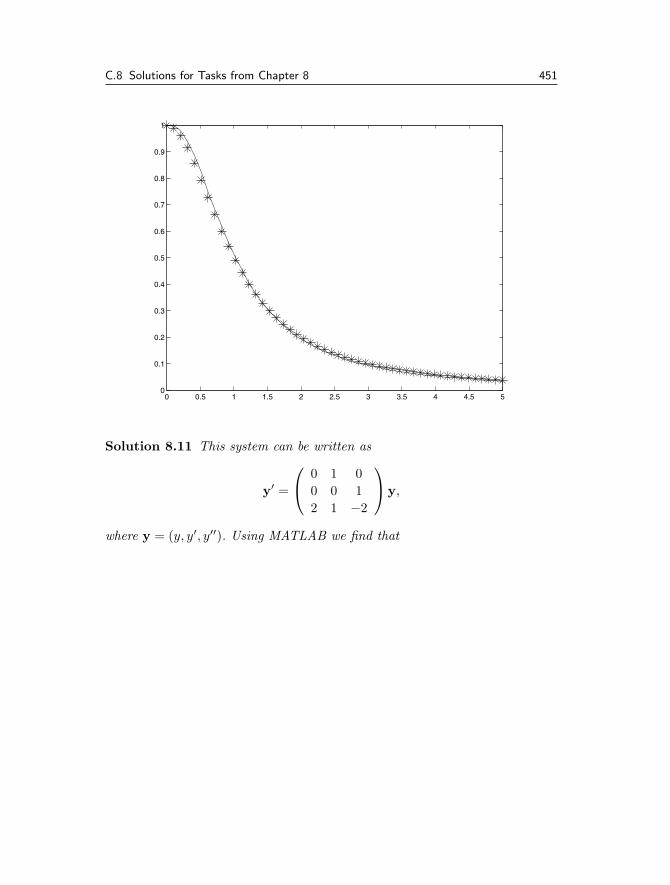
C.8 Solutions for Tasks from Chapter 8 451
0 0.5 1 1.5 2 2.5 3 3.5 4 4.5 50
0.1
0.2
0.3
0.4
0.5
0.6
0.7
0.8
0.9
1
Solution 8.11 This system can be written as
y′ =
⎛⎝ 0 1 0
0 0 12 1 −2
⎞⎠y,
where y = (y, y′, y′′). Using MATLAB we find that
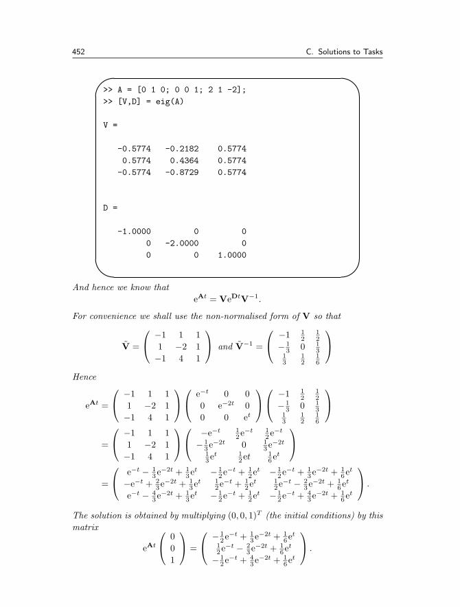
452 C. Solutions to Tasks
�
�
�
�
>> A = [0 1 0; 0 0 1; 2 1 -2];
>> [V,D] = eig(A)
V =
-0.5774 -0.2182 0.5774
0.5774 0.4364 0.5774
-0.5774 -0.8729 0.5774
D =
-1.0000 0 0
0 -2.0000 0
0 0 1.0000
And hence we know thateAt = VeDtV−1.
For convenience we shall use the non-normalised form of V so that
V =
⎛⎝ −1 1 1
1 −2 1−1 4 1
⎞⎠ and V−1 =
⎛⎝ −1 1
212
− 13 0 1
313
12
16
⎞⎠
Hence
eAt =
⎛⎝ −1 1 1
1 −2 1−1 4 1
⎞⎠⎛⎝ e−t 0 0
0 e−2t 00 0 et
⎞⎠⎛⎝ −1 1
212
− 13 0 1
313
12
16
⎞⎠
=
⎛⎝ −1 1 1
1 −2 1−1 4 1
⎞⎠⎛⎝ −e−t 1
2e−t 12e−t
− 13e−2t 0 1
3e−2t
13et 1
2et 16et
⎞⎠
=
⎛⎝ e−t − 1
3e−2t + 13et − 1
2e−t + 12et − 1
2e−t + 13e−2t + 1
6et
−e−t + 23e−2t + 1
3et 12e−t + 1
2et 12e−t − 2
3e−2t + 16et
e−t − 43e−2t + 1
3et − 12e−t + 1
2et − 12e−t + 4
3e−2t + 16et
⎞⎠ .
The solution is obtained by multiplying (0, 0, 1)T (the initial conditions) by thismatrix
eAt
⎛⎝ 0
01
⎞⎠ =
⎛⎝ − 1
2e−t + 13e−2t + 1
6et
12e−t − 2
3e−2t + 16et
− 12e−t + 4
3e−2t + 16et
⎞⎠ .
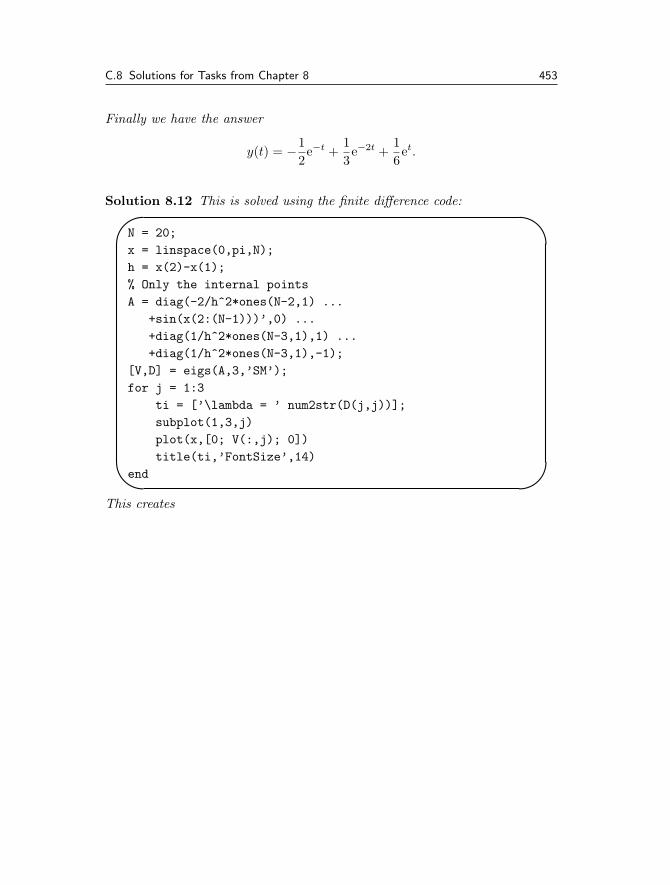
C.8 Solutions for Tasks from Chapter 8 453
Finally we have the answer
y(t) = −12e−t +
13e−2t +
16et.
Solution 8.12 This is solved using the finite difference code:�
�
�
�
N = 20;
x = linspace(0,pi,N);
h = x(2)-x(1);
% Only the internal points
A = diag(-2/hˆ2*ones(N-2,1) ...
+sin(x(2:(N-1)))’,0) ...
+diag(1/hˆ2*ones(N-3,1),1) ...
+diag(1/hˆ2*ones(N-3,1),-1);
[V,D] = eigs(A,3,’SM’);
for j = 1:3
ti = [’\lambda = ’ num2str(D(j,j))];
subplot(1,3,j)
plot(x,[0; V(:,j); 0])
title(ti,’FontSize’,14)
end
This creates
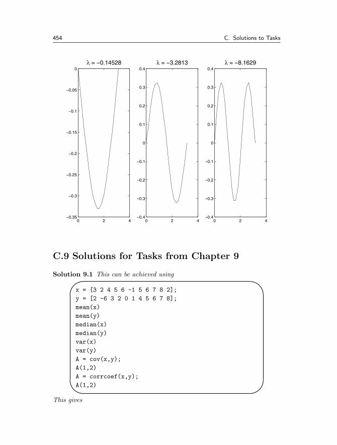
454 C. Solutions to Tasks
0 2 4−0.35
−0.3
−0.25
−0.2
−0.15
−0.1
−0.05
0λ = −0.14528
0 2 4−0.4
−0.3
−0.2
−0.1
0
0.1
0.2
0.3
0.4λ = −3.2813
0 2 4−0.4
−0.3
−0.2
−0.1
0
0.1
0.2
0.3
0.4λ = −8.1629
C.9 Solutions for Tasks from Chapter 9
Solution 9.1 This can be achieved using�
�
�
�
x = [3 2 4 5 6 -1 5 6 7 8 2];
y = [2 -6 3 2 0 1 4 5 6 7 8];
mean(x)
mean(y)
median(x)
median(y)
var(x)
var(y)
A = cov(x,y);
A(1,2)
A = corrcoef(x,y);
A(1,2)
This gives
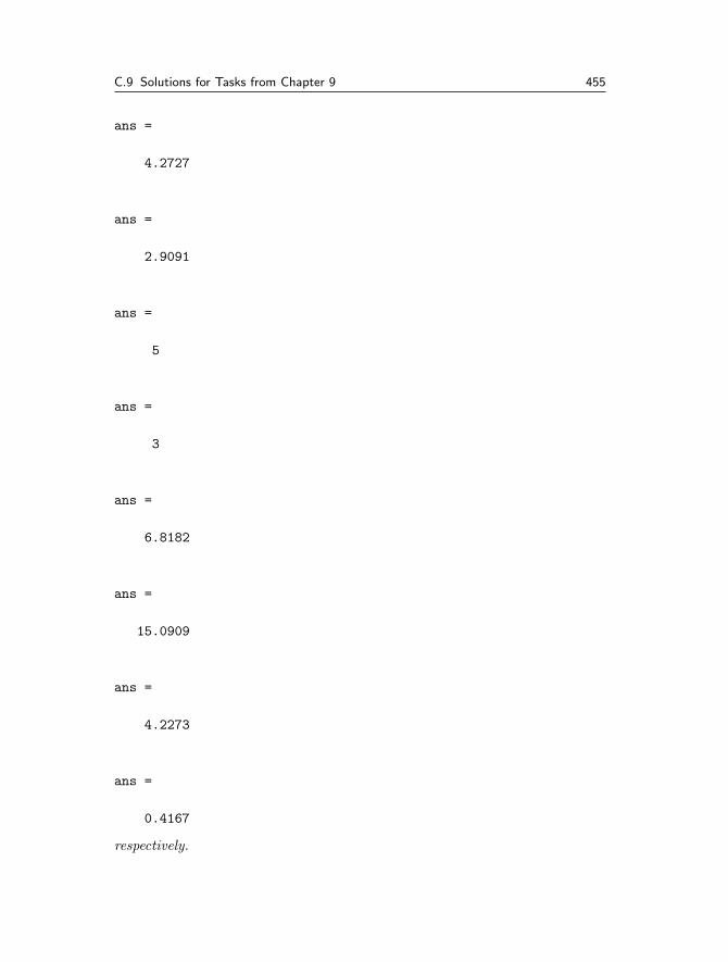
C.9 Solutions for Tasks from Chapter 9 455
ans =
4.2727
ans =
2.9091
ans =
5
ans =
3
ans =
6.8182
ans =
15.0909
ans =
4.2273
ans =
0.4167
respectively.

456 C. Solutions to Tasks
Solution 9.2 We note that if Y = aX + b then y = ax + b which can be seenby substitution into the formula for the mean. Similarly substituting this intothe expression for the correlation shows that
σXY =a√a2
=a
|a| = sign(a).
Solution 9.3 These two can be calculated using�
�
�
�
xb=mean(x);
vx=sum((x-xb).ˆ2)/length(x);
std_x=sqrt(vx);
skew=sum(((x-xb)/std_x).ˆ3)/length(x);
kurt=sum(((x-xb)/std_x).ˆ4)/length(x)-3;
Solution 9.4 In order to solve this problem we shall use a basic loop structure�
�
�
�
global mu
mu = 0.4;
x(1) = 0.25;
for i = 1:9
x(i+1) = map(x(i));
end
The value this code returns is 4.3420e-05 (notice if you get MATLAB to writeout x it will appear that this entry is zero, depending on the current format).
Solution 9.5 One value which works is µ = −2. Then use�
�
�
�
mu = -2;
co = [-muˆ3 2*muˆ3 -muˆ2*(1+mu) (muˆ2-1) 0];
[r] = roots(co);
x1 = r(3);
x2 = map(x1);
x3 = map(x2);
disp([x1 x2 x3])
Note that x2 is also a period 2 point and its image is x1. These values areactually given by
12
µ2 + µ ±√
µ4 − 2µ3 − 3µ2
µ2

C.9 Solutions for Tasks from Chapter 9 457
The real values of these roots occur for µ < −1 and µ > 3.
Solution 9.6 The code for this map is
�
�
�function [xn,yn] = map3(xo,yo)
xn = mod(xo+2*yo,1);
yn = mod(3*xo-2*yo,1);
Solution 9.7 The solution of the Henon map for cos α = 0.24 gives
−1 −0.8 −0.6 −0.4 −0.2 0 0.2 0.4 0.6 0.8 1−1
−0.8
−0.6
−0.4
−0.2
0
0.2
0.4
0.6
0.8
1
Index
* multiplication, 4, 6, 8, 15, 176+ addition, 8- subtraction, 8/ division, 8:, 171>> prompt, 2%, 332
Airy functions, 270, 273, 449ans, 3, 170ASCII, 55
Bessel functions, 132, 237, 238, 257, 270Boundary-value problems, 274, 276, 278
Comments, 41, 332Constants– eps, 7, 10, 53, 296, 372, 402– pi,π, 7, 73, 382, 393– realmax, 384– realmin, 384Curves of best fit, 152, 382, 383
Data Loading/Saving, 134–139Dot Arithmetic, 14, 15, 19, 54, 59, 98,
130, 178, 180, 181, 220– division, 14, 81, 178, 337– exponentiation, 14, 30–32, 36, 38, 43,
50, 77, 178, 338, 346, 395– multiplication, 14, 118, 178, 336, 398
Errors, 51–63– absolute, 52–54, 237, 266, 267, 438
– numerical, 51–54– relative, 52, 266, 267, 438– user, 54–63Explicit Methods, 248, 251, 253, 254,
256Extrapolation, 117, 133, 147, 167, 418
feval, 50, 51, 104, 107, 375Filenames, 28, 30, 135–137, 159, 346format– rat, 4, 7, 12, 13, 25, 75, 197Formatting, 12–13Functions– Mathematical– – acos - arccosine, 8, 368– – asin - arcsine, 8, 385– – atan - arctangent, see atan2– – atan2, 366, 386– – cos, 8, 181, 368– – cosh, 369– – exp - exponential, 9, 181, 372– – log - natural logarithm, 9, 360, 377– – log - logarithm base 10, 9– – ˆ - exponentiation, 9– – sinh, 181, 385– – sin, 8, 10, 181, 363, 385– – tan, 8, 386– MATLAB– – \, 332– – abs, 9– – all, 93, 341– – and, 83, 86, 341, 343, 407– – angle, 365, 366
460 Index
– – any, 93, 99, 342– – atan2, 366, 386– – axes, 348– – axis, 32, 38, 51, 157, 315, 322,
348–350, 356, 405– – bar, 297, 350– – barh, 351– – besselj, 132, 238, 366, 382, 413– – break, 92, 94, 127, 140, 145, 164,
214, 234, 322, 367– – case, 112, 115, 116, 367– – cd, 29– – ceil, 9, 25, 91, 367, 390, 433– – clear, 22– – clf, 39, 46, 107, 260, 262, 269, 315,
352, 357, 382, 396– – close, 352– – cond, 368– – conj, 368– – contour, 32, 39, 40– – contourf, 39– – corrcoef, 295, 368, 454– – cov, 295, 369, 454– – cputime, 201, 369– – dec2hex, 369, 375– – demo, 41, 369– – det, 214, 369, 427– – diag, 179, 182–185, 203, 217, 280,
286, 370, 419, 453– – diary, 371– – diff, 371– – dir, 30– – disp, 28, 41– – double, 234, 258, 259– – dsolve, 258– – edit, 27, 28, 59, 64, 371– – eig, 371, 428– – eigs, 208, 210, 211, 286, 371, 453– – else, 87, 88, 93, 99, 101, 114, 115,
119–122, 125, 127, 140, 159, 292,339, 340, 371, 405, 408
– – elseif, 87, 88, 95, 101, 115, 140,371, 405, 408
– – end, 60– – end of an array, 24– – error, 94, 97, 372– – exist, 96, 372, 376– – expm, 215, 372– – eye, 86, 179, 182, 195, 198, 203, 214,
372, 375, 428– – factor, 9, 11, 65, 87, 95, 271, 272,
372– – factorial, 66, 77, 372, 383, 401
– – fclose, 137, 138– – feval, 49–51, 103, 104, 106, 107,
111, 372, 375– – figure, 39, 59, 156, 257, 287, 348,
352– – find, 100, 143, 342– – fix, 9, 25, 372, 390– – fliplr, 217, 372– – flipud, 217, 372, 419– – floor, 9, 25, 91, 96, 99, 373, 390,
403– – fmins, 161, 162, 164, 373– – fminsearch, 161– – fopen, 137, 138– – for, 63–65, 70, 75, 82, 97, 297, 372,
373, 397, 398, 401, 407– – format, 4, 7, 12, 13, 25, 75, 197, 373,
436– – fprintf, 137, 138– – full, 204, 373, 385– – function, 30–34– – fzero, 128, 130, 132, 374, 413– – gac, 44– – gca, 301, 352, 355, 361, 362– – gcd, 374– – gcf, 44, 159, 354, 361, 362– – get, 44, 348, 352, 354, 355, 362– – ginput, 105, 106, 130, 355– – global, 111, 112, 156, 159, 165, 275,
319, 320, 367, 374, 456– – gplot, 355– – grid, 37, 51, 104–107, 109, 147, 148,
356, 360– – help, 2– – helpbrowser, 1, 374– – helpdesk, 1, 335, 375– – hex2dec, 369, 375– – hilb, 185, 368, 375– – hist, 298, 318, 356– – hold, 39, 46, 147, 148, 159, 260, 315,
357– – i, 375– – if, 83, 87, 90– – imag, 366, 375, 382– – Inf, 239, 375– – inline, 374, 375– – input, 28, 30, 31, 41, 58, 69, 72, 95,
119, 375– – int, 230, 233, 235– – int2str, 56, 57, 64, 65, 69–71, 74,
87, 119, 189, 362, 371, 375, 401, 402– – inv, 154, 201, 209, 210, 332, 333,
369, 375
Index 461
– – invhilb, 185– – isempty, 93, 140, 145, 376– – isprime, 49, 99, 376– – isreal, 93, 376– – j, 375– – legend, 46, 47, 269, 357, 396– – length, 14, 22, 36– – linspace, 14, 22– – load, 29, 135–137, 139, 146, 147,
154, 377– – log10, 9, 377– – loglog, 39, 358– – lookfor, 185, 186, 335, 377– – lower, 89, 90, 377, 404– – lu, 200, 377, 378– – magic, 185, 378– – max, 34, 51, 156, 159, 241, 305, 349,
378, 379– – mean, 292, 296, 298, 299, 318, 379,
454, 456– – median, 292, 379, 454– – meshgrid, 32, 39, 41– – min, 51, 106, 156, 159, 349, 379– – mod, 9, 25, 58, 80, 99, 234, 379, 390,
391– – NaN, 93, 94, 111, 379, 390– – nchoosek, 67– – norm, 127, 163–165, 379– – not, 83, 342– – num2str, 28, 41, 43, 56–58, 65, 71,
97, 112, 116, 119–122, 127, 156, 159,185, 241, 296, 380, 395, 398, 399,401, 420, 453
– – ode23, 265, 288, 380– – ode45, 265–267, 288, 380, 381, 442– – ones, 176, 182– – or, 83, 85, 86, 322, 342, 343, 403,
405, 407– – otherwise, 89, 90, 112, 115, 116, 382– – path, 29, 382– – pause, 159, 286, 382, 384– – plot, 21, 36–38, 354– – plot3, 350, 359– – poly, 22, 43, 206, 214, 382– – polyfit, 75, 148, 149– – polyval, 20, 21, 48– – precedence, 87– – primes, 383– – print, 159, 360– – prod, 12, 67, 68, 81, 383– – pwd, 30– – quad, 237, 238, 245, 436
– – rand, 175, 201, 295, 299, 305, 315,317, 369, 383, 385
– – randn, 298, 299, 383– – randperm, 300, 384– – rank, 187, 189, 384– – real, 305, 366, 384– – realmax, 7, 384– – realmin, 7, 384– – rem, 9, 11, 25, 85, 87, 307, 384, 391– – reshape, 384– – roots, 21, 22, 123, 126, 128, 132,
206, 214, 320, 382, 385, 412, 428, 456– – round, 9, 25, 95, 385, 390, 404– – rref, 195, 197, 198– – rrefmovie, 195– – save, 135, 136, 385– – semilogx, 39, 359, 360– – semilogy, 39, 359, 361– – set, 301, 348, 352, 354, 355, 361–364– – sign, 9, 95, 181– – size, 13, 22, 36– – sort, 292, 385– – sparse, 203, 210, 373, 385– – spline, 150, 152, 166, 385, 415, 417– – sqrt, 12, 343– – std, 293, 318, 386– – str2mat, 386– – subplot, 362, 453– – sum, 34, 35, 80, 81, 154, 229, 233,
236, 292, 293, 300, 386, 430, 431,433, 456
– – surf, 39, 40– – switch, 88–90, 112, 116, 367, 372,
382, 386, 428, 429– – syms, 230, 233, 235, 258– – text, 38, 202, 241, 260, 362, 363– – title, 38, 156, 159, 364, 453– – tour, 1, 386– – transpose, 175, 180, 373, 378, 386,
418, 425– – type, 5, 30, 42, 386– – upper, 89, 377, 386– – var, 293, 299, 386, 454– – warning, 94–96, 387, 404, 405– – what, 30– – which, 5, 30, 387– – while, 90–92, 96, 99, 111, 119–122,
317, 372, 387, 403–405– – who, 22, 31, 135– – whos, 22, 31, 134, 135, 137, 387– – xlabel, 38, 51, 202, 260, 262, 364– – xor, 83, 342, 343, 403– – ylabel, 38, 51, 364
462 Index
– – zeros, 77– – zoom, 105, 107, 109, 322, 355, 365
Geometric Progressions, 68, 79
Help commands– helpbrowser, 1, 374– helpdesk, 1, 335, 375– help, 1, 6, 13, 24, 25, 27, 29, 30, 41,
42, 47, 48, 87, 99, 127, 135, 138, 175,217, 237, 266, 335, 343, 350, 359, 371,373, 374, 382, 383
– lookfor, 185, 186, 335, 377
Implicit Methods, 251, 254, 288Interpolation, 117, 133, 147–158, 160,
414– cubic, 149– Lagrange polynomials, 142– linear, 149, 167– polynomials, 140, 148– splines, 150–152, 167, 385
Lagrange polynomials, 141, 142, 147LATEX, 38Linear Independence, 187Logical Operators, 335–343– Boolean algebra– – and, 341– – not, 83, 342– – or, 83, 85, 86, 322, 342, 343, 403,
405, 407– – xor, 83, 342, 343, 403– comparative, 83– ==, 60, 83, 85–87, 90, 92, 94, 95, 99,
111, 119–122, 159, 189, 233, 292, 296,339, 403
– <,<=, 84, 88, 101, 341, 404–406, 408– >,>=, 84, 86, 88, 99, 101, 145, 340,
342, 403–406, 408– <,<=, 341– =, 340
Matrices– eye, 86, 179, 182, 195, 198, 203, 214,
372, 375, 428– ones, 176, 182, 183, 219, 236, 243,
260, 262, 280, 286, 315, 335–338, 344,369, 382, 399, 419, 426, 430, 444, 445,447, 453
– zeros, 77, 156, 173, 175, 182, 241,250, 256, 257, 265, 269, 271, 272, 274,279, 280, 283, 284, 287, 310, 331, 387,419, 437, 439, 441
– addition, 174, 326–327– anti-symmetric, 220, 325, 421– associativity, 330– characteristic polynomials, 212–215,
223, 382– commutativity, 219, 326, 330, 420– determinants, 190–191, 198, 205, 206,
222, 331, 369, 421, 427– diagonals, 182–185, 191, 199, 207–209,
215, 218, 221, 259, 295, 325, 331, 370,371, 378, 421, 424
– distributivity, 330– eigenvalues, 204–208, 210–212,
214–216, 223, 286, 290, 368, 371, 382,428
– eigenvectors, 204–209, 215, 223, 371– exponentials, 214–216– full and sparse, 203, 204, 210, 215,
259, 263, 373, 385– Hermitian, 325– identity, see eye– inverses, 331–333– Inversion, 339– LU decomposition, 200, 377– multiplication, 326–328– penta-diagonal, 263– rank, 187–189, 198, 384– scalar multiplication, 206, 326– size, see size– Skew Hermitian, 325– square, 18, 182, 190, 208, 212, 220,
323, 325, 331, 382– symmetric, 210, 220, 325, 421– transpose, 180, 221, 325– tri-diagonal, 259– 0, see zeros
Nested if statements, 88Nested loops, 75, 82, 98, 234, 402Newton forward differences, 141, 142,
227, 230, 235, 251, 270Numbers– exponent Mantissa form, 7Numerical Integration, 225–245– Simpson’s 1
3 rule, 232, 234, 242, 243,430
– Simpson’s 38 rule, 236, 237, 242, 430
– Trapezium Rule, 228, 229, 234, 243,244, 300, 432
Object orientated programming, 4, 43,152
ODEs, 247
Index 463
– Crank–Nicolson, 247, 251, 253, 255,303, 306
– Euler, 247, 253, 256, 283, 284, 286,288, 303
– Runge–Kutta, 263, 266, 267, 270, 272,274, 288, 380
Operations– binary, 3, 9, 178, 180, 336–338– unary, 3, 180
Plotting, 21, 36–49Polynomials, 20, 41, 43– roots, 21Precedence, 5, 6– brackets, 4–6, 86– division, 5– exponentiation, 54– multiplication, 5Products, 81, 383
Root finding, 103– bisection, 113, 123, 131– fixed point iteration, 109, 131, 409,
410– initial estimates, 105, 109, 130, 355,
411– Newton-Raphson, 117–125– Newton–Raphson, 131, 132, 163, 247,
274, 313– secant, 117–125
Scalars, 2–12Simultaneous equations, 74, 220, 221,
331Sums of series, 73Symbols
– ..., 29, 58, 69, 74, 77, 96, 112, 116,119–122, 145, 159, 188, 211, 237, 256,269, 271, 272, 275, 280, 286, 333, 343,372, 395, 399, 402, 422, 426–428, 448,453
– %, 20, 41, 332, 343– apostrophe, see transpose– colon, 13, 17, 19, 59, 98, 171, 172, 344– comma, 345– decimal point, 138, 346, 380– quotes, 28, 42, 49, 65, 90, 136, 137,
345, 363– round brackets, 11, 30, 171, 347– semicolon, 2, 3, 6, 13, 31, 55–57, 64,
80, 81, 170, 171, 184, 344, 397, 398,407
– space, 346– square brackets, 30, 34, 57, 84, 170,
344, 346, 398
Taylor series, 76, 98, 117, 124, 125, 230,244, 248, 255, 259, 263, 264, 281, 282,435
Variables, 2–12– clearing, 22, 26, 56, 57, 59, 75, 137,
139, 147, 148, 300, 367, 393, 396, 435,439
– rules for naming, 4–5Vectors, 13–17– column vector, 35, 170–173, 182–184,
188, 273, 323, 425– row vector, 13–15, 33, 35, 43, 55, 70,
137, 170, 172, 173, 182, 185, 221, 324,336–338, 344, 348, 368, 372, 385, 386,398, 425