Positivity-Preserving H1 Model Reduction for Positive Systems

Ping Li James Lam Zidong Wang Paresh Date

August 31, 2010

Abstract

This paper is concerned with the model reduction of positive systems. For a given stable positive

system, our attention is focused on the construction of a reduced-order model in such a way that the

positivity of the original system is preserved and the error system is stable with a prescribed H1 per-

formance. Based upon a system augmentation approach, a novel characterization on the stability with

H1 performance of the error system is �rst obtained in terms of linear matrix inequality (LMI). Then, a

necessary and su¢ cient condition for the existence of a desired reduced-order model is derived accordingly.

A signi�cance of the proposed approach is that the reduced-order system matrices can be parametrized

by a positive de�nite matrix with �exible structure, which is fully independent of the Lyapunov matrix;

thus, the positivity constraint on the reduced-order system can be readily embedded in the model reduc-

tion problem. Furthermore, iterative LMI approaches with primal and dual forms are developed to solve

the positivity-preserving H1 model reduction problem. Finally, a compartmental network is provided to

show the e¤ectiveness of the proposed techniques.

Keywords: H1 performance; Iterative algorithm; Linear matrix inequality; Model reduction; Positive

systems.

1 Introduction

In many practical systems, there is such a kind of systems whose state variables are con�ned to be positive.

Such systems are frequently encountered in various �elds, for instance, biomedicine [1], pharmacokinetics

[2], chemical reactions [3] and internet congestion control [4]. These systems belong to the class of positive

systems, whose state variable and output are always positive (at least nonnegative) whenever the initial state

and the input are positive [5]. Positivity of the system state for all times will bring about many new issues,

which cannot be solved in general by using well-established methods for general linear systems, mainly due

to the fact that positive systems are de�ned on cones rather than linear spaces. Therefore, the study on

this kind of systems has drawn the attention of many researchers in recent years [6] [7] [8] [9].

On the other hand, mathematical modeling of positive systems often results in complex high-order

models, which will bring serious di¢ culties to analysis and synthesis of positive systems, irrespective of the

computational resources available [10]. Therefore, it is necessary to replace high-order models by reduced

The work was partially supported by GRF HKU 7137/09E.Ping Li (pingli@hkusua.hku.hk) and James Lam (james.lam@hku.hk) are with the Department of Mechanical Engineering,

The University of Hong Kong, Pokfulam Road, Hong Kong.Zidong Wang (Zidong.Wang@brunel.ac.uk) is with the Department of Information Systems and Computing, Brunel Uni-

versity, Uxbridge, Middlesex, UB8 3PH, UK.Paresh Date (paresh.date@brunel.ac.uk) is with the Department of Mathematical Sciences, Brunel University, Uxbridge,

Middlesex, UB8 3PH, UK.

1

ones with respect to some given criterion. In fact, such a topic is actually a model reduction problem in

control area, and has received considerable attention in the past decades [11] [12] [13] [14]. Amongst the

many optimality criteria for approximation, one is based on the H1 norm of the associated error system.

The characterization of H1 model reduction solution was �rst proposed in [15], and many important results

have been reported for various kinds of systems, such as stochastic systems [16] and switched systems [17].

Very recently, based on the methods of balanced truncation and matrices inequalities, the model reduction

problem for positive systems has been investigated in [18] and [19], respectively. It should be pointed out

that traditional approaches developed for general linear systems, including the widely adopted projection

approach and similarity transformation [16] [20], are no longer applicable for positive systems in general,

since they cannot guarantee the positivity of the reduced-order system. This indicates that conventional

approaches, if used to construct a reduced-order system, may generate a meaningless approximation for

the actual system whose state is always positive all the time. Therefore, it is necessary to develop new

approaches to the H1 model reduction problem for positive systems with positivity preserved. However,

such a problem has not been well studied in the literature, and still remains as a challenging open issue.

In this paper, we are concerned with the H1 model reduction problem for positive systems. More

speci�cally, for a given positive linear continuous-time system, the aim is to construct a positive lower-order

system such that the H1 norm of the di¤erence between the original system and the desired lower-order

one satis�es a prescribed H1 norm bound constraint. The main body is divided into two parts. In the �rst

part, by virtue of a system augmentation approach, the associated error system is represented as a singular

system form, and a novel characterization on the stability of the error system under the H1 performance

is derived in the form of LMI. An important feature of the results reported here is that the reduced-order

system matrices can be parametrized by a positive de�nite matrix with �exible structure, which is fully

independent of the Lyapunov matrix. Such a characterization will greatly facilitate the parametrization

with positivity constraints. In the second part, a necessary and su¢ cient condition for the existence of a

desired reduced-order system is �rstly proposed, then iterative LMI approaches are developed to compute

the reduced-order system matrices and optimize the initial values, respectively. Moreover, a dual approach,

together with the primal one, is further incorporated to improve the solvability of the positive-preserving

H1 model reduction problem.

2 System Description and Preliminaries

Notation: Let R be the set of real numbers; Rn denotes the n-column real vectors; Rn�m is the set of all realmatrices of dimension n �m: Rn�m+ represents the n �m dimensional matrices with positive components

and Rn+ , Rn�1+ : A matrix is said to be positive, if all its elements are positive. For a matrix A 2 Rn�n; it iscalled Metzler, if all its o¤-diagonal elements are positive. I represents the identity matrix with appropriate

dimension; For any real symmetric matrices P; Q; the notation P � Q (respectively, P > Q) means that

the matrix P �Q is positive semi-de�nite (respectively, positive de�nite). The notation L2 [0;1) representsthe space of square Lebesgue integrable functions over [0;1) with the usual norm jj � jj2 : For a transferfunction matrix G; its H1 norm is denoted as kGk1 : For a real matrix A, A? denotes the orthonormalcomplement of A; that is, AA? = 0 and

�A?�TA? = I: In addition, Her (M) , 1

2

�MT +M

�is de�ned

for any matrix M 2 Rn�n; diag (A1; A2; : : : ; AN ) denotes the block diagonal matrix with A1; A2; : : : ;AN on the diagonal. The superscript �T�denotes the transpose for vectors or matrices. Matrices, if their

dimensions are not explicitly stated, are assumed to have compatible dimensions for algebraic operations.

2

Consider the following linear asymptotically stable system:8><>:_x(t) = Ax(t) +Bu(t);

y(t) = Cx(t) +Du(t);

x(0) = x0;

(1)

where x(t) 2 Rn is the state vector, u(t) 2 Rm is the input vector, y(t) 2 Rq is the output or measurementvector. In this paper, we assume u 2 L2 [0;1), and A; B; C and D are real constant matrices with

appropriate dimensions.

We give the following de�nition on positive linear systems.

De�nition 1 ([5]) System (1) is said to be a positive linear system if for all x0 2 Rn+ and all input

u(t) 2 Rm+ ; we have x(t) 2 Rn+ and y(t) 2 Rq+ for t > 0:

The following lemma provides a well-known characterization of positive linear systems.

Lemma 1 ([5]) The system in (1) is positive if and only if A is Metzler, B; C and D are positive.

In this paper, we aim at approximating system (1) by a reduced-order stable system described by8><>:_xr(t) = Arxr(t) +Bru(t);

yr(t) = Crxr(t) +Dru(t);

xr(0) = xr0;

(2)

where xr(t) 2 Rnr is the state vector of the reduced-order system (2) with 0 < nr < n; and yr(t) 2 Rq: Ar;Br; Cr and Dr are matrices to be determined later.

For the stable system in (1), the transfer matrix from input u(t) to output y(t) is given by

Guy(s) = C (sI �A)�1B +D: (3)

Traditionally, the H1 model reduction problem was formulated by �nding a reduced-order system (2), such

that

kGuy � Guyrk1 < ; (4)

where

Guyr(s) = Cr (sI �Ar)�1Br +Dr (5)

is the transfer matrix of system (2) from u(t) to yr(t); and > 0 is a prescribed scalar.

However, such a speci�cation is not su¢ cient for positive systems, since as an approximation of system

(1), it is naturally desirable that system (2) should also be positive, like system (1) itself. That is, in addition

to the H1 performance in (4), the positivity should also be preserved when considering the model reduction

problem for the positive system in (1). To ensure the positivity of system (2), if follows from Lemma 1 that

Ar should be Metzler, Br; Cr and Dr should be positive.

For convenience, denote set S , f(Ar; Br; Cr; Dr) : Ar is Metzler, Br; Cr and Dr are positiveg :Let x(t) =

�xT (t); xTr (t)

�Tand e(t) = y(t)� yr(t): Then, from (1) and (2), we obtain the associated error

system as (_x(t) = Ax(t) + Bu(t);

e(t) = Cx(t) + Du(t);(6)

3

where

A =

"A 0

0 Ar

#; B =

"B

Br

#;

C =hC �Cr

i; D = D �Dr:

Obviously, condition in (4) is equivalent to

kGuek1 < ; (7)

where

Gue(s) = C�sI � A

��1B + D (8)

is the transfer matrix from u(t) to e(t). In addition, the stability of system (1) and (2) is naturally equivalent

to that of system (6).

Based on the above discussion, the problem of positivity-preserving H1 model reduction for positive

systems in (1) to be addressed in this paper is formulated as follows.

Problem PP-H1-MR (Positivity-Preserving H1 Model Reduction): Given a disturbance attenuation

level > 0; construct a system (2) such that the following two requirements are ful�lled simultaneously.

(1) (Ar; Br; Cr; Dr) 2 S.

(2) The error system in (6) is asymptotically stable and satis�es the H1 performance kGuek1 < .

The following result gives a fundamental characterization on the stability of (6) with H1 performance,

which will be used later.

Lemma 2 ([20]) The error system in (6) is asymptotically stable and satis�es kGuek1 < ; if and only if

there exists a matrix P > 0; such that264 AT P + P A P B CT

BT P � I DT

C D � I

375 < 0; (9)

where P is usually referred to as the Lyapunov matrix.

3 Analysis of Associated Error System

This section focuses on the stability analysis of the error system in (6) under theH1 performance. To achieve

this, we �rst represent system (6) by means of a system augmentation approach, which will facilitate the

parametrization on the positivity constraint. Then, a novel characterization on the stability and the H1performance of (6) is developed in terms of linear matrix inequality, which will play a key role for the

computation of the reduced-order system matrices.

4

3.1 System Augmentation Approach

To facilitate the construction of system (2), we de�ne

Gr =

"Ar Br

Cr Dr

#; (10)

which collects the representation for the system matrices in (2) into one matrix. We further make the

following de�nitions:

�A =

"A 0

0 0

#; �B =

"B

0

#; �C =

hC 0

i; �D = D;

�F =

"0 0

I 0

#; �M =

"0 I

0 0

#;

�N =

"0

I

#; �H =

h0 �I

i;

which are entirely in terms of the state space matrices for system (1), then we have

A = �A+ �FGr �M; B = �B + �FGr �N; (11)

C = �C + �HGr �M; D = �D + �HGr �N: (12)

Although the system matrices in (2) are encapsulated into Gr; one can see that it is still embedded

with two other matrices. In addition, when applying Lemma 2, we have that Gr is still coupled with the

Lyapunov matrix P ; which makes them hard to solve. More signi�cantly, such a problem will become more

di¢ cult and arduous, in particular when additional constraints on Gr are taken into account.

For convenience, denote set ~S , fGr : Gr is de�ned in (10) with (Ar; Br; Cr; Dr) 2 Sg :To overcome these di¢ culties, we introduce an auxiliary variable #(t) = Gr �Mx(t)+Gr �Nu(t), and de�ne

x(t) =hxT (t) #

T(t)

iTaccordingly. Then the error system in (6) can be equivalently described by the

following descriptor (or semi-state) system:(E _x(t) = Ax(t) +Bu(t);

e(t) = Cx(t) +Du(t);(13)

where

E =

"I 0

0 0

#; A =

"�A �F

Gr �M �I

#; B =

"�B

Gr �N

#;

C =h�C �H

i; D = �D:

Remark 1 A major obstacle for the construction of the reduced-order system in (2) is that it should be

positive, which results in the additional constraints on the system matrices Ar; Br; Cr; and Dr: Focusing

on this, one can see that the advantage of the above manipulations lies in the following aspects. First, these

system matrices are assembled to a single matrix Gr; which will be convenient for the synthesis consideration.

Second, by means of system augmentation approach in (13), Gr is successfully extracted from the middle of

two matrices, and can be further parametrized by a free positive de�nite matrix, which will be shown later.

Such an approach will introduce the �exibility to the construction of Gr; in particular when Gr has some

certain constraints.

5

3.2 Novel Stability and H1 Performance Characterization

Theorem 1 Given the system matrices Ar; Br; Cr and Dr: Then the following statements are equivalent:

(i) The error system in (6) is asymptotically stable, and satis�es kGuek1 < .

(ii) There exist matrices P > 0 and diagonal X > 0 such that

� ,

264 ATP + P TA P T (I + J)B CT

BT (I + J)TP �BTJT�P + P T

�JB � I DT

C D � I

375 < 0; (14)

where

P =

"P 0

�12XGr

�M 12X

#; I =

"I 0

0 I

#; J =

"0 0

0 I

#:

Proof: (ii))(i). Suppose there exist matrices P > 0 and diagonal X > 0 such that (14) holds. De�ne a

nonsingular matrix

T ,

266664I 0 0 0

Gr �M Gr �N 0 I

0 I 0 0

0 0 I 0

377775 :Pre- and post-multiplying (14) by T T and T , respectively, we have

� , T T�T =

266664AT P + P A P B CT P �F

BT P � I DT 0

C D � I �H�F T P 0 �HT �X

377775 < 0: (15)

Based on Lemma 2, the third leading principal submatrix of � indicates that the error system in (6) is

asymptotically stable, and satis�es kGuek1 < ; which completes this part of the proof.

(i))(ii). If the error system in (6) is asymptotically stable, and satis�es kGuek1 < , then it follows

from Lemma 2 that there exists a matrix P > 0; such that264 AT P + P A P B CT

BT P � I DT

C D � I

375 < 0:Then, for any diagonal S > 0; there exists a su¢ ciently large scalar � > 0 such that

� �S �

264 P �F0�H

375T 264 A

T P + P A P B CT

BT P � I DT

C D � I

375�1 264 P �F0

�H

375 < 0: (16)

By choosing X = �S and applying Schur complement equivalence to (16), we have

� = T�T�T�1 < 0;

which completes the whole proof. �

6

Remark 2 Although the conditions in (9) and (14) are equivalent, it should be pointed out that the LMIformulation in (14) has some advantages over the one in (9). First, with the LMI characterization in (14),

the reduced-order system matrices, or Gr equivalently, are not coupled with the Lyapunov matrix P any

more, but can be parametrized by a positive de�nite matrix X, which is fully independent of P . Second,

it follows from (16) that, if the error system in (6) is asymptotically stable and satis�es kGuek1 < ; the

existence of X will be naturally guaranteed. Finally, it is worth pointing out that the structure of X is rather

�exible. In fact, from the proof of ((ii))(i)), X can be chosen as X = �S; where S is required only to

be a positive de�nite matrix with � being su¢ ciently large. The freedom on the structure of X will greatly

facilitate the synthesis considered in this paper when additional constraints on Gr are imposed, which will

be shown subsequently.

4 Synthesis Condition and Algorithm

This section is devoted to the synthesis of the reduced-order system in (2). Based on the analysis in Section

3, a necessary and su¢ cient condition for the existence of a solution to Problem PP-H1-MR is obtained.

Then, iterative LMI approaches are developed to compute the reduced-order system matrices and opti-

mize the initial values, respectively. A dual approach to solving Problem PP-H1-MR is further addressed

subsequently, and the combination of the primal and the dual approach is proposed in the last subsection.

4.1 Existence of Positive Reduced-Order System

Theorem 2 Problem PP-H1-MR is solvable, if and only if there exists a matrix P > 0; a diagonal matrix

X > 0; matrices U; V; L1; L2; L3 and L4 such that

L =

"L1 L2

L3 L4

#2 ~S, (17)

� (U; V ) ,

266664�11 P �F + �MTLT �13 �CT

�F T P + L �M �X L �N �HT

�T13�NTLT �33 �DT

�C �H �D � I

377775 < 0; (18)

where

�11 = 2Her��AT P � UTL �M

�+ UTXU;

�13 = P �B � �MTLTV � UTL �N + UTXV;

�33 = �2Her�V TL �N

�+ V TXV � I:

In this case, the system matrices of (2) can be given as

Gr = X�1L: (19)

Proof: By expanding (14), we have266664�AT P + P �A� �MTGTr XGr

�M P �F + �MTGTr X P �B � �MTGTr XGr�N �CT

�F T P +XGr �M �X XGr �N �HT

�BT P � �NTGTr XGr�M �NTGTr X � �NTGTr XGr

�N � I �DT

�C �H �D � I

377775 < 0: (20)

7

Su¢ ciency: It follows from (17) and X > 0 diagonal, we have that Ar Metzler, Br; Cr and Dr positive.

From (19), we have L = XGr: Substituting this into (18), and observing that, for any U and V;

��TGTr XGr� � ��TGTr XGr�+ (�Gr�)T X (�Gr�)

= �2Her�TXGr�

�+TX;

where

� =h�M 0 �N

i; =

hU 0 V

i; (21)

we obtain that (20) holds, which further indicates that (14) holds. According to Theorem 1, this completes

the su¢ ciency proof.

Necessity: If Problem PP-H1-MR is solvable, then for the given error system in (6), it follows from

Theorem 1 that there exists a matrix P > 0; and a diagonal matrix X > 0 such that (14) holds, or

equivalently, (20) holds. Then, by choosing U = Gr �M and V = Gr �N; we have that

��TGTr XGr� = �2Her�TXGr�

�+TX;

where � and are de�ned in (21). Substituting this into (20), and letting L = XGr; one has that (18)

holds. This completes the whole proof. �

Remark 3 From the proof in Theorem 2, one can see that the construction matrix Gr is not coupled with

P ; but can be parametrized by X; which makes the construction speci�cation for Gr 2 ~S possible. Morespeci�cally, due to the fact that the structure of X is rather �exible, we can designate X to be a positive

diagonal matrix. As a matter of fact, X can be chosen as a positive diagonal matrix, or even a positive

scalar matrix, whereas no conservatism will be introduced consequently.

4.2 Iterative Approaches to Reduced-Order System Matrices Computation

Let us explain the conditions in Theorem 2 from a computational perspective. Obviously, the condition in

(17) can be viewed as a set of LMIs, which can be readily veri�ed by standard software. Now, we turn to

inequality (18), which is generally not a linear matrix inequality with respect to the parameters P ; X; U; V

and L: However, it can be easily observed that if U and V are held �xed, then it becomes an LMI problem

with respect to the remaining parameters. Note that the LMI problem is convex and can be e¢ ciently solved

if a feasible solution exists [21]. This leaves a natural problem about how to choose U and V properly. De�ne

a scalar � satisfying

� (U; V ) < ��; (22)

where

� = diag�I 0 I 0

�(23)

and � (U; V ) is de�ned in (18). Inspired by [22], it follows from the proof of Theorem 2 that � will achieve

its minimum when U = X�1L �M and V = X�1L �N; which leads to an iterative approach to solve inequality

(18).

Now, we are in a position to develop the following iterative LMI algorithm:

Algorithm 1 (ILMI Approach):

8

1. START: Set j = 1: For a given H1 performance level , compute the initial matrices U1 and V1 such

that the following auxiliary system,(_�x(t) = �A�x(t) + �F �#(t) + �Bu(t);

e(t) = �C�x(t) + �H�#(t) + �Du(t);(24)

with �#(t) = U1�x(t) + V1u(t) is asymptotically stable and the transfer function Tue(s) from u(t) to

e(t) satis�es kTuek1 < :

2. For �xed Uj and Vj ; solve the following convex optimization problem for the parameters in ,nP > 0; X > 0 is diagonal, and L1; L2; L3 and L4

o:

��j := min�j s.t.

8>>>><>>>>:L =

"L1 L2

L3 L4

#2 ~S

� (Uj ; Vj) < �j�

�j � �

;

where � � 0 is an arbitrary scalar. Denote the corresponding value of X and L as Xj and Lj ;

respectively.

3. If ��j � 0; then a desired parametric matrix Gr is obtained as Gr := X�1j Lj . STOP. If not, then go

to next step.

4. If������j � ��j�1� =��j ��� < �1, where �1 is a prescribed tolerance, then go to next step. If not, update

Uj+1 and Vj+1 as

Uj+1 := X�1j Lj �M; Vj+1 := X

�1j Lj �N:

Set j := j + 1; then go to Step 2.

5. A solution to Problem PP-H1-MR may not exist. STOP.

Remark 4 Note that the constraint �j � � is only added to make ��j bounded from below by a negative

scalar, and will not a¤ect the search of ��j , since we are only interested in the case ��j � 0. Meanwhile, it

can be seen that the sequence ��j is monotonically decreasing with respect to j; that is, ��j+1 � ��j : Therefore,

the convergence of the iterative process is naturally guaranteed.

The problem in Step 1 is convex, which can be regarded as a state-feedback H1 control problem.

Furthermore, if there are no matrices U1 and V1 such that system (24) is stable and satis�es kTuek1 < ;

then we can conclude immediately that there does not exist a solution to Problem PP-H1-MR. In addition,

it follows from Lemma 2 that �nding U1 and V1 is equivalent to �nding �Q > 0; W1 and V1 such that264 2Her��A �Q+ �FW1

��B + �FV1 �Q �CT +W T

1�HT

�BT + V T1�F T � I �DT + V T1

�HT

�C �Q+ �HW1�D + �HV1 � I

375 < 0 (25)

holds, then U1 can be obtained as U1 =W1�Q�1; and V1 can be given directly from (25).

In addition, it is well known that the performance of an iterative algorithm usually depends on the initial

starting points, and a poor selection of the initial value often results in the iterates being trapped at local

minima and the iterative process becomes sluggish, whereas good starting points lead to fast solution. This

leaves the problem for the optimization of U1 and V1.

9

In what follows of this subsection, we will show how to further improve the solvability of Algorithm 1 by

optimizing the initial values U1 and V1. It can be seen that if, for some G�r ; P� > 0; diagonal X� > 0; (20)

holds, then (18) will also be feasible, that is, � (U; V ) < 0; provided that (�G�r�)T X� (�G�r�) is

�small� enough. Thus, the solvability of the algorithm can be further improved by choosing the initial

values U1 and V1 such that (1 �G�r�)T X� (1 �G�r�)

is small enough, where1 =

hU1 0 V1

i(26)

and � is de�ned in (21). As we indicated previously that X� should be large, an alternative way is then to

make k1 �G�r�k su¢ ciently small. The following proposition provides an equivalent characterization ofhow k1 �G�r�k can be made as small as possible.

Theorem 3 Given � and 1 de�ned in (21) and (26), respectively, for a su¢ ciently small scalar " > 0;

the following statements are equivalent:

(i) There exists G�r such that system (6) is asymptotically stable with kGuek1 < ; and k1 �G�r�k � ".

(ii) System (24) is asymptotically stable with kTuek1 < ; and 1�? � ".

Proof: (i))(ii). First, we have 1�? = 1�? �G�r��? � k1 �G�r�k �? � ":In the following, we shall prove that system (24) is asymptotically stable with kTuek1 < : By de�ning

A =

264 �A �B 0

0 � 2 I 0

�C �D � 2 I

375 ; B =264 �F

0�H

375 ; K =

264 I 0 0

0 0 I

0 I 0

375 ; (27)

then according to Lemma 2, if system (6) is asymptotically stable with kGuek1 < ; then there exists �P > 0

such that

Her�(A+ BG�rK)

T P�< 0 (28)

holds, where

K = �K; P = diag��P I I

�:

In addition,

Her�(A+ B1K)T P

�= Her

�(A+ BG�rK)

T P�+Her

�(B (1 �G�r�)K)

T P�: (29)

Thus, if k1 �G�r�k is su¢ ciently small, then based on (28) and (29), we have that

Her�(A+ B1K)T P

�< 0; (30)

which is equivalent to inequality (25) with �Q = �P�1. Hence, system (24) is asymptotically stable with

kTuek1 < ; which completes the �rst part of the proof.

10

(ii))(i). For � de�ned in (21), we have that ��T = I; and �? can be explicitly given as

�? =

26666664I 0 0

0 0 0

0 I 0

0 0 I

0 0 0

37777775 :

If we select G�r = 1�T ; then

(1 �G�r�)h�T �?

i=h0 1�

?i:

Note thath�T �?

iis a permutation matrix, and consider the fact that

1 �G�r� =h0 1�

?i h

�T �?i�1

;

we have

k1 �G�r�k � h 0 1�

?i h �T �?

i�1 � ": (31)

In addition, if system (24) is asymptotically stable with kTuek1 < ; then Her�(A+ B1K)T P

�< 0:

With the similar proof line of ((i))(ii)), we have that (28) holds, which further indicates there exists G�rsuch that system (6) is asymptotically stable with kGuek1 < . This, together with (31), gives that (i)

holds, which completes the whole proof. �Clearly, Theorem 3 shows that if U1 and V1 can be chosen in such a way that (30) holds and

1�? is small enough, then it will be more likely for (18) to have a feasible solution. Typically, if " = 0; that

is, 1�? = 0; then (18) will also be feasible. Furthermore, in view of (17) and the proof of ((ii))(i)) in

Theorem 3, we have that 1�T 2 ~S. Summarizing the above discussion, we propose the following algorithmto �nd U1 and V1 such that the solvability of Algorithm 1 can be further improved.

Algorithm 2 (Initial Optimization):

1. START: Set j = 1: Solve the LMI in (25) to obtain Uj and Vj ; respectively.

2. For �xed j =hUj 0 Vj

i; solve the following LMI with respect to �Pj :

Her�(A+ BjK)T Pj

�< 0: (32)

where A, B, and K are de�ned in (27), and Pj = diag��Pj I I

�:

3. For �xed �Pj ; solve the following convex optimization problem with respect to j and "j :

"�j := minj"j s.t.

8>>>><>>>>:(32) holds

j�T 2 ~S"�"jI

�j�

?�Tj�

? �I

#< 0

:

Correspondingly, denote �j as the optimized value of j .

11

4. If����"�j � "�j�1� ="�j ��� < �2, where �2 is a prescribed tolerance, then go to next step. If not, setj+1 := �j

and j := j + 1; then go to Step 2.

5. An initial choice of U1 and V1 is obtained ashU1 0 V1

i:= �j : STOP.

Remark 5 Note that the stopping criterion suggested in Step 4 is heuristic, and the convergence of Algo-rithm 2 is naturally guaranteed, since "�j is monotonically decreasing with respect to j with a lower bound of

zero.

4.3 Further Results via Dual Approach

This subsection further studies the positive model reduction problem via dual approach. To be speci�c, we

introduce a new auxiliary variable �#(t) = �Mx(t) + �Nu(t); and de�ne �x(t) =hxT (t) �#

T(t)

iTaccordingly.

Thus, the error system in (6) can be equivalently described by the dual of system (13), shown as follows:(�E _�x(t) = �A�x(t) + �Bu(t);

e(t) = �C�x(t) + �Du(t);(33)

where

�E =

"I 0

0 0

#; �A =

"�A �FGr�M �I

#; �B =

"�B�N

#;

�C =h�C �HGr

i; �D = �D:

The motivation for introducing (33) is that optimality in the primal direction does not imply optimality in

the dual direction, therefore, it is possible that the primal problem which cannot be solved directly may

have solutions in their dual form.

In the following, we shall propose an equivalent characterization on the stability with H1 performance

of (6) as follows, which can be viewed as a dual form of Theorem 1.

Theorem 4 Given the system matrices Ar; Br; Cr and Dr: Then the following statements are equivalent:

(i) The error system in (6) is asymptotically stable, and satis�es kGuek1 < .

(ii) There exist matrices Q > 0 and diagonal Z > 0 such that

�� ,

2664�AQ+QT �A

TQT (I + J) �C

T �B

�C(I + J)TQ � �CJT

�Q+QT

�J �C

T � I �D

�BT �D

T � I

3775 < 0; (34)

where

Q =

"Q 0

�12ZG

Tr�F T 1

2Z

#; I =

"I 0

0 I

#; J =

"0 0

0 I

#:

Sketch of Proof: De�ne the nonsingular matrix �T as

�T ,

266664I 0 0 0�

�FGr�T �

�HGr�T

0 I

0 I 0 0

0 0 I 0

377775 ;12

then, by following a similar line of the proof in Theorem 1, the results can be readily obtained. �Consequently, the dual condition for the existence of a positive reduced-order system (2) can be estab-

lished as follows.

Theorem 5 Problem PP-H1-MR is solvable, if and only if there exists a matrix Q > 0; a diagonal matrix

Z > 0; matrices U; V; L1; L2; L3 and L4 such that

L =

"L1 L2

L3 L4

#2 ~S, (35)

�� (U; V ) ,

266664��11 Q �MT + �FL ��13 �B

�MQ+ LT �F T �Z LT �HT �N��T13

�HL ��33 �D�BT �NT �DT � I

377775 < 0; (36)

where

��11 = 2Her��AQ� ULT �F T

�+ UZUT ;

��13 = Q �CT � �FLV T � ULT �HT + UZV T ;

��33 = �2Her�V LT �HT

�+ V ZV T � I:

In this case, the system matrices of (2) can be given as

Gr = LZ�1: (37)

Based on Theorem 5, we present the following algorithm, which can be viewed as a dual of Algorithm 1.

Algorithm 3 (Dual ILMI Approach):

1. START: Set j = 1: For a given H1 performance level , compute the initial matrices U1 and V1 such

that the following auxiliary system,(_�x(t) = �AT �x(t) + �MT ��(t) + �CTw(t);

e(t) = �BT �x(t) + �NT ��(t) + �DTw(t);(38)

with ��(t) = UT1 �x(t) + VT1 w(t) is asymptotically stable and the transfer function Twe(s) from w(t) to

e(t) satis�es kTwek1 < :

2. For �xed Uj and Vj ; solve the following convex optimization problem for the parameters in z ,nQ > 0; Z > 0 is diagonal, L1; L2; L3 and L4

o:

��j := minz�j s.t.

8>>>><>>>>:L =

"L1 L2

L3 L4

#2 ~S

�� (Uj ; Vj) < �j�

�j � �

;

where � � 0 is an arbitrary scalar. Denote the corresponding value of Z and L as Zj and Lj ;

respectively.

3. If ��j � 0; then a desired parametric matrix Gr is obtained as Gr := LjZ�1j . STOP. If not, then goto next step.

13

4. If�����j � ��j�1� =��j �� < �3, where �3 is a prescribed tolerance, then go to next step. If not, update Uj+1

and Vj+1 as

Uj+1 := �FLjZ�1j ; Vj+1 := �HLjZ

�1j :

Set j := j + 1; then go to Step 2.

5. A solution to Problem PP-H1-MR may not exist. STOP.

The reason for the selection of U1 and V1 is the same as the one proposed in the last subsection, and

optimization of the initial values can be readily performed by using a similar approach in Algorithm 2. Note

that U1 and V1 are the �state feedback controller matrix�for system (38), or �observer matrices�for system

(24), which motivates us to call Algorithm 3 as the dual iterative LMI approach.

4.4 Combination of Primal and Dual Approaches

On one hand, although one may solve the positive model reduction problem by implementing Algorithm

1 or Algorithm 3 separately, it is possible that the iterates may get trapped in a local minimum. More

speci�cally, it may happen that the original problem is actually feasible, but a local minimum is achieved and

is unable to con�rm the feasibility of the problem. On the other hand, as we stated before, the optimality

in the primal direction does not imply that in the dual direction, thus, we may combine Algorithms 1 and

3 together to further improve the solvability of Problem PP-H1-MR. We summarize it in the following

algorithm:

Algorithm 4 (Primal-Dual ILMI Approach)

1. START: Run Algorithm 2 to �nd an initial value of U1 and V1. Set k = 0; and N as the maximum

number of iterations allowed.

2. While k < N do

(a) For �xed U1 and V1; run Algorithm 1, if ��j < 0; then Gr can be readily obtained as Gr := X�1j Lj .

STOP. Otherwise, running Algorithm 1 until ��j converges, which gives a temporary matrix G�rp

as G�rp := X�1j Lj : Set U1 := �FG�rp and V1 := �HG�rp, then go to next step.

(b) For �xed U1 and V1; run Algorithm 3, if ��j < 0; then Gr can be readily obtained as Gr := LjZ�1j .

STOP. Otherwise, running Algorithm 3 until ��j converges, which gives another temporary ma-

trix G�rd as G�rd := LjZ

�1j : Set U1 := G�rd �M; V1 := G

�rd�N , and k := k + 1.

End (while)

3. A solution to Problem PP-H1-MR may not exist. STOP.

Although Algorithm 4 is proposed to improve the solvability of Problem PP-H1-MR, it still cannot be

guaranteed to converge to the global optimum. In this sense, our algorithm does not completely solve the

problem. Nevertheless, the e¤ectiveness of the proposed approach will be further illustrated in the following

section.

14

5 Illustrative Example

Compartmental networks consist of a �nite number of homogeneous, well-mixed subsystems, called com-

partments, which exchange with each other and the environment [23]. Consider a compartmental network

of n compartments shown schematically in Figure 1.

Figure 1: Pro�le of linear compartmental networks

The quantity (or, concentration) of material involved in compartment i at time t is denoted as xi(t); kijxjis the �ow rate from compartment j to compartment i (k0ixi is the out�ow of compartment i); the in�ow

of compartment i is represented by Ii(t) =Pmj=1 bijuj(t); where uj(t) is the jth input resource. Thus, the

mathematical description for compartment i can be given as follows:

_xi(t) =nXj 6=i

[kijxj � kjixi]� k0ixi +mXj=1

bijuj(t); i = 1; 2; : : : ; n: (39)

Then, the system matrix A in (1) can be formulated as A = [aij ]n�n where

aij =

(��Pn

j 6=i kji + k0i�; i = j;

kij ; i 6= j;:

For illustration, we have constructed the compartmental model with six states shown in Figure 2.

Figure 2: Compartmental network with 6 state components

15

One can see that there are two completely connected subsystems each with three state components, and

they are linked through compartments 3 and 4: Here, we assume

k01 = 1:0; k21 = 0:3; k31 = 0:2; k02 = 0:8; k12 = 0:6;

k32 = 0:5; k03 = 1:0; k13 = 1:0; k23 = 0:2; k43 = 0:5;

k04 = 1:0; k34 = 1:0; k54 = 0:4; k64 = 0:6; k05 = 0:5;

k45 = 0:6; k65 = 0:5; k06 = 0:8; k46 = 0:5; k56 = 0:3;

b11 = 1:0; b22 = 1:0;

that is,

A =

26666666664

�1:5 0:6 1:0 0 0 0

0:3 �1:9 0:2 0 0 0

0:2 0:5 �2:7 1 0 0

0 0 0:5 �3 0:6 0:5

0 0 0 0:4 �1:6 0:3

0 0 0 0:6 0:5 �1:6

37777777775; B =

26666666664

1 0

0 1

0 0

0 0

0 0

0 0

37777777775:

It can be veri�ed that the system is stable, and we assume that the H1 performance level is prescribed as

= 0:1: The aim of this example is to construct 2-order positive reduced-order systems in two cases (with

di¤erent outputs) below in the form of (2) to approximate the original system.

Case I. Output is the sum of the quantity of material in the compartmental network, that is,

C =h1 1 1 1 1 1

i; D =

h0 0

i:

We �rst try to apply Algorithm 1 to solve Problem PP-H1-MR. Using the Matlab LMI Control Toolbox,

we obtain an initial value of U1 and V1 as

U int1 =

264 0 0 0 0 0 0 �0:5 0

0 0 0 0 0 0 0 �0:51 1 1 1 1 1 0 0

375 ; V int1 =

264 0 0

0 0

0 0

375 :It can be checked that no desired reduced-order system in (2) can be found by Algorithm 1. However, if

Algorithm 2 is further applied to optimize U1 and V1 with the tolerance level �2 = 10�2, then optimized

values of U1 and V1 can be obtained as

Uopt1 =

264 0 0 0 0 0 0 �2:5175 1:6949

0 0 0 0 0 0 1:6321 �2:50140 0 0 0 0 0 2:0279 1:9659

375 ; V opt1 =

264 0:2121 0:2300

0:2116 0:2332

0:0494 0:0376

375 :With these new initial values, we implement Algorithm 1 to solve Problem PP-H1-MR again, and an

��1 = �0:0443 < 0 is found after one iteration. Therefore, the condition in Theorem 2 is feasible with the

following solution:

X =

264 253:5817 0 0

0 363:4548 0

0 0 122:0049

375 ; L =264 �455:9701 241:7357 54:3521 59:1674

160:5375 �474:4492 77:3205 84:9729

219:9069 267:2964 5:9949 4:5524

375 :

16

Then, according to (19), a desired positive 2nd order model in (2) can be readily obtained with the

system matrices given as"Ar Br

Cr Dr

#=

264 �1:7981 0:9533

0:4417 �1:30540:2143 0:2333

0:2127 0:2338

1:8024 2:1909 0:0491 0:0373

375 :

Case II. Output is the quantity of material in Compartments 1 and 2, respectively, that is,

C =

"1 0 0 0 0 0

0 1 0 0 0 0

#; D =

"0 0

0 0

#:

It can be easily veri�ed that no solution can be found by running Algorithm 1, irrespective of whether

Algorithm 2 is applied or not. However, if Algorithm 4 is utilized to solve the problem with the tolerance

levels �1; �2; and �3 all speci�ed as 10�2; then after six iterations, a ��j = 0 is found in Step 2.b. Therefore,

the condition in Theorem 5 is feasible with the following solution:

Z =

266664167:5471 0 0 0

0 38:1587 0 0

0 0 753:6758 0

0 0 0 165:3818

377775 ; L =266664�307:0492 15:6431 1:5285 470:1873

5:9141 �35:2889 131:2422 0:0484

12:6363 142:1916 72:9519 0:0622

46:7395 42:7307 0:3559 13:9471

377775 :Then, according to (37), a desired positive 2nd order model in (2) can be readily obtained with the

system matrices given as

"Ar Br

Cr Dr

#=

266664�1:8326 0:4099

0:0353 �0:92480:0020 2:8430

0:1741 0:0003

0:0754 3:7263

0:2790 1:1198

0:0968 0:0004

0:0005 0:0843

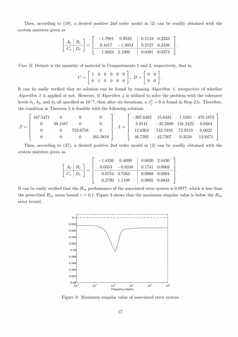
377775 :It can be easily veri�ed that the H1 performance of the associated error system is 0:0977; which is less than

the prescribed H1 norm bound = 0:1: Figure 3 shows that the maximum singular value is below the H1error bound.

10­2 10­1 100 101 102 1030.08

0.082

0.084

0.086

0.088

0.09

0.092

0.094

0.096

0.098

0.1

Frequency (rad/s)

Figure 3: Maximum singular value of associated error system

17

In addition, under the excitation of L2-input

u(t) =he�0:001t 1

0:2+0:005t

��cos � �10 t��� iT ;and zero initial conditions, Figures 4 and 5 depict the output trajectories of the original positive system and

those of the reduced-order positive system, respectively. It can be observed from these simulation results

that the obtained reduced model preserves the positivity and approximates the original system very well.

0 50 100 150 2000

0.5

1

1.5

2

2.5

T ime t

Syst

em o

utpu

t

Output y1 of original positive system

Output yr1 of reduced­order positive system

Figure 4: Output y1 of original positive system and yr1 of

reduced-order positive system

0 50 100 150 2000

0.5

1

1.5

2

2.5

3

T ime t

Syst

em o

utpu

t

Output y2 of original positive system

Output yr2 of reduced­order positive system

Figure 5: Output y2 of original positive system and yr2 of

reduced-order positive system

6 Conclusion

In this paper, we have presented a model reduction approach that preserves positivity and stability with H1performance of positive systems. In particular, we have proposed a novel characterization on the stability and

18

H1 performance of the associated error system by means of a system augmentation method, which ensures

the separation of the reduced-order system matrices to be constructed from the Lyapunov matrix. Based on

this new characterization, a necessary and su¢ cient condition for the existence of a desired reduced-order

system has been established in terms of matrix equalities, and a primal iterative LMI approach has been

developed to solve the condition. A heuristic algorithm has also been proposed to optimize the initial values.

Furthermore, a dual iterative LMI approach, together with the primal one, has been utilized to improve

the solvability of the positive-preserving H1 model reduction problem. Finally, the e¤ectiveness of the

proposed method has been illustrated by a compartmental network. The approach adopted in this paper

can be applied to tackle problems involving some constraints on elements of the required system matrices,

such as positivity and boundedness.

References

[1] M. Morari and A. Gentilini, �Challenges and opportunities in process control: Biomedical processes,�AIChE

Journal, vol. 47, no. 10, pp. 2140�2143, 2001.

[2] J. A. Jacquez, Compartmental Analysis in Biology and Medicine. University of Michigan Press, 1985.

[3] G. Silva-Navarro and J. Alvarez-Gallegos, �Sign and stability of equilibria in quasi-monotone positive nonlinear

systems,�IEEE Trans. Automat. Control, vol. 42, no. 3, pp. 403�407, Mar. 1997.

[4] R. Shorten, F. Wirth, and D. Leith, �A positive systems model of TCP-like congestion control: Asymptotic

results,�IEEE/ACM Trans. Networking, vol. 14, no. 3, pp. 616�629, Jun. 2006.

[5] L. Farina and S. Rinaldi, Positive Linear Systems: Theory and Applications. New York: Wiley-Interscience, 2000.

[6] B. D. O. Anderson, M. Deistler, L. Farina, and L. Benvenuti, �Nonnegative realization of a linear system with

nonnegative impulse response,�IEEE Trans. Circuits and Systems (I), vol. 43, no. 2, pp. 134�142, Feb. 1996.

[7] L. Benvenuti and L. Farina, �A tutorial on the positive realization problem,� IEEE Trans. Automat. Control,

vol. 49, no. 5, pp. 651�664, May. 2004.

[8] J. Back and A. Astol�, �Design of positive linear observers for positive linear systems via coordinate transforma-

tions and positive realizations,�SIAM J. Control Optim., vol. 47, no. 1, pp. 345�373, Jan. 2008.

[9] F. Knorn, O. Mason, and R. Shorten, �On linear co-positive Lyapunov functions for sets of linear positive

systems,�Automatica, vol. 45, pp. 1943�1947, 2009.

[10] A. C. Antoulas, Approximation of Large-Scale Dynamical Systems. Philadelphia, PA: SIAM, 2005.

[11] K. Glover, �All optimal Hankel-norm approximations of linear multi-variable systems and their L1-error bounds,�

Int. J. Control, vol. 39, no. 6, pp. 1115�1193, 1984.

[12] J. Lam, �Model reduction of delay systems using Padé approximants,�Int. J. Control, vol. 57, no. 2, pp. 377�391,

1993.

[13] W. Y. Yan and J. Lam, �An approximate approach to H2 optimal model reduction,� IEEE Trans. Automat.

Control, vol. 44, no. 7, pp. 1341�1358, Jul. 1999.

[14] M. Farhood, C. L. Beck, and G. E. Dullerud, �Model reduction of periodic systems: a lifting approach,�Auto-

matica, vol. 41, no. 6, pp. 1085�1090, 2005.

[15] D. Kavrano¼glu and M. Bettayeb, �Characterization of the solution to the optimal H1 model reduction problem,�

Systems & Control Letters, vol. 20, no. 2, pp. 99�107, 1993.

[16] S. Xu and T. Chen, �H1 model reduction in the stochastic framework,�SIAM J. Control Optim., vol. 42, no. 4,

pp. 1293�1309, 2003.

19

[17] L. Wu and W. Zheng, �Weighted H1 model reduction for linear switched systems with time-varying delay,�

Automatica, vol. 45, no. 1, pp. 186�193, 2009.

[18] T. Reis and E. Virnik, �Positivity preserving balanced truncation for descriptor systems,� SIAM J. Control

Optim., vol. 48, no. 4, pp. 2600�2619, 2009.

[19] J. Feng, J. Lam, Z. Shu, and Q. Wang, �Internal positivity preserved model reduction,� Int. J. Control, vol. 83,

no. 3, pp. 575�584, 2010.

[20] P. Gahinet and P. Apkarian, �A linear matrix inequality approach to H1 control,� Int. J. Robust & Nonlinear

Control, vol. 4, no. 4, pp. 421�448, 1994.

[21] S. Boyd, L. EI Ghaoui, E. Feron, and U. Balakrishnana, Linear Matrix Inequalities in System and Control Theory.

Philadephia, PA: SIAM, 1994.

[22] Y. Cao, J. Lam, and Y. Sun, �Static output feedback stabilization: An ILMI approach,�Automatica, vol. 34,

no. 12, pp. 1641�1645, 1998.

[23] K. Godfrey, Compartmental Models and Their Applications. London: Academic Press, 1983.

20