
Template-Based Inhomogeneity Correction in 3T MRI Brain Studies
15
IEEE TRANSACTIONS ON MEDICAL IMAGING, VOL. 29, NO. 11, NOVEMBER 2010 1927 Template-Based Inhomogeneity Correction in 3T MRI Brain Studies Marcelo A. Castro*, Jianhua Yao, Yuxi Pang, Christabel Lee, Eva Baker, John Butman, Iordanis E. Evangelou, and David Thomasson Abstract—Low noise, high resolution, fast and accurate maps from MRI images of the brain can be performed using a dual flip angle method. However, field inhomogeneity, which is particularly problematic at high field strengths (e.g., 3T), limits the ability of the scanner to deliver the prescribed flip angle, introducing errors into the maps that limit the accuracy of quantitative analyses based on those maps. A dual repetition time method was used for acquiring a map to correct that inhomogeneity. Additional inaccuracies due to misregistration of the acquired -weighted images were corrected by rigid registration, and the effects of misalignment on the maps were compared to those of inhomogeneity in 19 normal subjects. However, since map acquisition takes up precious scanning time and most retrospective studies do not have map, we designed a template-based correction strategy. maps from different subjects were aligned using a twelve-parameter affine registration. Recomputed maps showed an important improve- ment with respect to the noncorrected maps: histograms of all corrected maps exhibited two peaks corresponding to white and gray matter tissues, while unimodal histograms were observed in all uncorrected maps because of the inhomogeneity. A method to detect the best nonsubject-specific correction based on a set of features was designed. The optimum set of weighting factors for those features was computed. The best available correction was detected in almost all subjects while corrections comparable to the map corrected using the map from the same subject were detected in the others. Index Terms— inhomogeneity, brain, image registration, magnetic resonance images (MRI), mapping. Manuscript received July 10, 2009; revised May 26, 2010; accepted June 07, 2010. Date of publication June 21, 2010; date of current version November 03, 2010. The work of M. A. Castro was supported in part by CONICET (Ar- gentina). Asterisk indicates corresponding author. M. A. Castro is with the National Institutes of Health, Department of Radiology and Imaging Sciences (NIH-DR&IS), Bethesda, MD 20892 USA and also with CONICET, Universidad Tecnológica Nacional, Grupo de In- vestigación y Desarrollo en Bioingeniería (GIBIO), CP 1179 Buenos Aires, Argentina (e-mail: [email protected]). J. Yao, E. Baker, J. Butman, I. Evangelou, and D. Thomasson are with the National Institutes of Health, Department of Radiology and Imaging Sciences (NIH-DR&IS), Bethesda, MD 20892 USA (e-mail: [email protected]; [email protected]; [email protected]; [email protected]; [email protected]). Y. Pang is with the National Institutes of Health, Department of Radiology and Imaging Sciences (NIH-DR&IS), Bethesda, MD 20892 USA and is also with Philips Healthcare, Cleveland, OH 44102 USA (e-mail: [email protected]. gov). C. Lee was with National Institutes of Health, Department of Radiology and Imaging Sciences (NIH-DR&IS), Bethesda, MD 20892 USA. She is now with the Department of Radiology, Georgetown University Medical Center, Wash- ington DC 20007 USA (e-mail: [email protected]). Color versions of one or more of the figures in this paper are available online at http://ieeexplore.ieee.org. Digital Object Identifier 10.1109/TMI.2010.2053552 I. INTRODUCTION A CCURATE estimation of relaxation time from mag- netic resonance images (MRI) is essential for some clinical applications, such as dynamic contrast-enhanced MRI studies of cancer, which require low noise and high resolution over a large volume [1]–[3]. The variable flip angle method, which has been widely accepted to achieve those requirements in a reasonable time frame, is based on acquiring spoiled gradient recalled-echo (SPGR) images with various different flip angles with the repetition time held constant. Despite longer acquisition times, multiple flip angles (from three up to ten) are preferred when imaging over a large range [4], [5]. However, according to Wang et al. for any given ratio, there exist two optimal flip angles that minimize the uncertainty in the estimated values [6]. Intensity inhomogeneity is often seen in MR images and is caused by many factors. However, the electromagnetic interaction with the object is the primary cause of that inho- mogeneity [7]. Proper estimation requires minimizing the effects of spatial variations of the transmitted flip angle at every voxel, which is related to the prescribed flip angle as , where denotes the spatial variation of the radiofrequency (RF) or field [4]. In MRI systems with low static magnetic field , the Larmor frequency (i.e., the precession frequency of the hydrogen nuclei around the direction of the applied magnetic field), and hence the frequency of the field, is very low. In that case, since the dimension of the human body is a small fraction of that wavelength, its interaction with the field can be neglected. However, the main limitation of low field systems is their low signal-to-noise ratio (SNR), which is proportional to the field strength [8]. Therefore, higher fields (e.g., 3T) are preferred to increase SNR. However, inhomogeneity also increases because the influence of wavelength becomes much more relevant at 3T [9]. The wavelength in tissue, which is proportional to the inverse of the square root of the dielectric constant, is reduced due to higher dielectric constant in biolog- ical tissue (typically between 10 and 100). If the wavelength of the RF field is of the same order as the imaged object then either destructive or constructive interferences of the transmitted RF field may be observed resulting in a regional signal loss or regional brightening, respectively [10]. A discussion about different techniques used to address this problem has been presented in detail in at least three major reviews [11]–[13]. According to those reviews, correction methods can be classified in two main groups: retrospective 0278-0062/$26.00 © 2010 IEEE
-
Upload
independent -
Category
Documents
-
view
0 -
download
0
Transcript of Template-Based Inhomogeneity Correction in 3T MRI Brain Studies
IEEE TRANSACTIONS ON MEDICAL IMAGING, VOL. 29, NO. 11, NOVEMBER 2010 1927
Template-Based �� Inhomogeneity Correctionin 3T MRI Brain Studies
Marcelo A. Castro*, Jianhua Yao, Yuxi Pang, Christabel Lee, Eva Baker, John Butman,Iordanis E. Evangelou, and David Thomasson
Abstract—Low noise, high resolution, fast and accurate �
maps from MRI images of the brain can be performed using adual flip angle method. However, � field inhomogeneity, whichis particularly problematic at high field strengths (e.g., 3T), limitsthe ability of the scanner to deliver the prescribed flip angle,introducing errors into the � maps that limit the accuracy ofquantitative analyses based on those maps. A dual repetitiontime method was used for acquiring a � map to correct thatinhomogeneity. Additional inaccuracies due to misregistrationof the acquired �-weighted images were corrected by rigidregistration, and the effects of misalignment on the � maps werecompared to those of � inhomogeneity in 19 normal subjects.However, since � map acquisition takes up precious scanningtime and most retrospective studies do not have � map, wedesigned a template-based correction strategy. � maps fromdifferent subjects were aligned using a twelve-parameter affineregistration. Recomputed � maps showed an important improve-ment with respect to the noncorrected maps: histograms of allcorrected maps exhibited two peaks corresponding to white andgray matter tissues, while unimodal histograms were observed inall uncorrected maps because of the inhomogeneity. A method todetect the best nonsubject-specific � correction based on a set offeatures was designed. The optimum set of weighting factors forthose features was computed. The best available � correctionwas detected in almost all subjects while corrections comparableto the � map corrected using the � map from the same subjectwere detected in the others.
Index Terms— � inhomogeneity, brain, image registration,magnetic resonance images (MRI), � mapping.
Manuscript received July 10, 2009; revised May 26, 2010; accepted June 07,2010. Date of publication June 21, 2010; date of current version November03, 2010. The work of M. A. Castro was supported in part by CONICET (Ar-gentina). Asterisk indicates corresponding author.
M. A. Castro is with the National Institutes of Health, Department ofRadiology and Imaging Sciences (NIH-DR&IS), Bethesda, MD 20892 USAand also with CONICET, Universidad Tecnológica Nacional, Grupo de In-vestigación y Desarrollo en Bioingeniería (GIBIO), CP 1179 Buenos Aires,Argentina (e-mail: [email protected]).
J. Yao, E. Baker, J. Butman, I. Evangelou, and D. Thomasson are withthe National Institutes of Health, Department of Radiology and ImagingSciences (NIH-DR&IS), Bethesda, MD 20892 USA (e-mail: [email protected];[email protected]; [email protected]; [email protected];[email protected]).
Y. Pang is with the National Institutes of Health, Department of Radiologyand Imaging Sciences (NIH-DR&IS), Bethesda, MD 20892 USA and is alsowith Philips Healthcare, Cleveland, OH 44102 USA (e-mail: [email protected]).
C. Lee was with National Institutes of Health, Department of Radiology andImaging Sciences (NIH-DR&IS), Bethesda, MD 20892 USA. She is now withthe Department of Radiology, Georgetown University Medical Center, Wash-ington DC 20007 USA (e-mail: [email protected]).
Color versions of one or more of the figures in this paper are available onlineat http://ieeexplore.ieee.org.
Digital Object Identifier 10.1109/TMI.2010.2053552
I. INTRODUCTION
A CCURATE estimation of relaxation time from mag-netic resonance images (MRI) is essential for some
clinical applications, such as dynamic contrast-enhanced MRIstudies of cancer, which require low noise and high resolutionover a large volume [1]–[3]. The variable flip angle method,which has been widely accepted to achieve those requirementsin a reasonable time frame, is based on acquiring spoiledgradient recalled-echo (SPGR) images with various differentflip angles with the repetition time held constant. Despitelonger acquisition times, multiple flip angles (from three up toten) are preferred when imaging over a large range [4], [5].However, according to Wang et al. for any given ratio,there exist two optimal flip angles that minimize the uncertaintyin the estimated values [6].
Intensity inhomogeneity is often seen in MR images andis caused by many factors. However, the electromagneticinteraction with the object is the primary cause of that inho-mogeneity [7]. Proper estimation requires minimizing theeffects of spatial variations of the transmitted flip angleat every voxel, which is related to the prescribed flip angleas , where denotes the spatial variationof the radiofrequency (RF) or field [4]. In MRI systemswith low static magnetic field , the Larmorfrequency (i.e., the precession frequency of the hydrogen nucleiaround the direction of the applied magnetic field), and hencethe frequency of the field, is very low. In that case, sincethe dimension of the human body is a small fraction of thatwavelength, its interaction with the field can be neglected.However, the main limitation of low field systems is theirlow signal-to-noise ratio (SNR), which is proportional to thefield strength [8]. Therefore, higher fields (e.g., 3T) arepreferred to increase SNR. However, inhomogeneity alsoincreases because the influence of wavelength becomes muchmore relevant at 3T [9]. The wavelength in tissue, which isproportional to the inverse of the square root of the dielectricconstant, is reduced due to higher dielectric constant in biolog-ical tissue (typically between 10 and 100). If the wavelength ofthe RF field is of the same order as the imaged object then eitherdestructive or constructive interferences of the transmitted RFfield may be observed resulting in a regional signal loss orregional brightening, respectively [10].
A discussion about different techniques used to address thisproblem has been presented in detail in at least three majorreviews [11]–[13]. According to those reviews, correctionmethods can be classified in two main groups: retrospective
0278-0062/$26.00 © 2010 IEEE
1928 IEEE TRANSACTIONS ON MEDICAL IMAGING, VOL. 29, NO. 11, NOVEMBER 2010
methods and prospective methods. The retrospective methodssolve the undetermined problem (1) using only the uncorrectedimages under different assumptions about the acquisitionprocess. The original and corrected intensities are related by
(1)
where is the true intensity spatial distribution, is the mea-sured voxel intensity, is the bias or inhomogeneity field and
is the additive noise distribution at a voxel location. On the other hand, prospective methods rely on the
acquisition of additional data or prior knowledge resulting in asubject-specific correction. The aim of both approaches is to im-prove image quality to make quantitative analyses reliable.
A large number of retrospective methods to correct in-homogeneity can be found in the literature [13]–[27] and canbe grouped in at least three major categories. There is a firstcategory known as surface fitting that relies on the assumptionthat the inhomogeneity field is slowly varying. Therefore, it canbe approximated by a parametric smooth function whose pa-rameters can be estimated either by segmenting a set of voxelsthroughout different tissues [15], [17], [24], which provides in-formation about the inhomogeneity map, or by entropy mini-mization [18], [19], [22].
A second category includes methods that exploit the slowlyvarying characteristic of the inhomogeneous field to separate itfrom the true image by lowpass filtering. Due to their simplicityand efficiency they have been widely used [13], [14], [21]. Re-cently, lowpass filtering methods have been extended using thewavelet transform and were shown to be effective in removinginhomogeneity in images acquired with different kind of coils[16], [20].
There is a third group of retrospective methods known as sta-tistical methods that assume that the inhomogeneity field fol-lows a given distribution, or model that inhomogeneity as arandom process [23], [27].
A particular approach proposed by Sled et al. is the N3method [25], which derives a nonparametric model of the tissueintensity directly from the data, avoiding in this way someof the restrictive model assumptions found in other similarmethods. Particularly, the N3 method does not require a modelof the tissue intensities in terms of discrete tissue classes, nordoes it rely on a segmentation of the volume into homogeneousregions. The optimization criterion is to find the smooth, slowlyvarying multiplicative field that maximizes the frequency con-tent of the distribution of tissue intensities. Like in most otherretrospective nonuniformity correction methods, if the objectis itself a smooth and slowly varying field then the correctionfield that maximizes that frequency content will also removethe natural variations of the object. Particularly, the underlyingcell structure of different regions of the brain induces a rangeof intensities in structural -weighted MRI scans.An example is that of subcortical tissues in regions of thethalamus and lenticular nucleus, whose intensity in MRIis between that of pure white matter (WM) and gray matter(GM) and can exhibit a spatially varying range of intensities.Studholme developed a correction of brain MRI image distor-tion to address this limitation [26]. They performed a manual
segmentation-based bias estimation to provide an accuratetissue intensity template for bias correction and a 3-D modelof the intensity variation across the brain is created by fitting aB-spline model to this intensity profile. The aim of this methodis to capture the local intensity variation within a given kindof tissue, which should not be removed when compensatingthe global inhomogeneity due to the acquisition process, anduse it as a reference template. MRI data was registered to thetarget reference template using a free form volume deformationprocedure to separate smoothly varying inhomogeneity effectsfrom underlying anatomical structure.
Different prospective methods to compensate field inho-mogeneity by acquiring additional images have been presentedin the past. Ishimori et al. proposed a method to estimate andcorrect inhomogeneity that uses multiple SPGR for 3T spin-echo MRI, which relied on the acquisition of several imageswith different echo times and flip angles for a fixed[28]. To compute corrected maps, Mihara et al. usedmultisliced spoiled gradient echo sequences on a 1.5T scannerwith different and flip angles, requiring 29 min to acquirethe three images for each brain [29]. Treier presented a com-bined and mapping technique for estimation in ab-dominal contrast-enhanced MRI [30] that computes mapsfrom two images acquired using two optimal flip angles [6]and compensates the inhomogeneity using a subject-specific
map acquired by means of a dual method [31]. Deonipresented a method that combines the usual multiangle SPGRdata with at least one inversion-prepared SPGR data in orderto obtain an unique solution for the map, the factor propor-tional to the longitudinal magnetization and the spatial variationof the radiofrequency field by least square minimization, whichrequires 10 min for mm isotropic and maps acquisi-tion [32] with less than 5% of error, and 6:40 min for a map( matrix).
In the clinical setting, it is beneficial to minimize scanningtime and it would be desirable that corrections may be madefrom a template, obviating the need for obtaining a mapeach and every time a patient is scanned. Using templatemaps would also allow more accurate quantitative analyses instudies where maps were not previously acquired. However,using a single template map for all corrections may intro-duce additional inaccuracies. Alternatively, a set of templatemaps might minimize those inaccuracies provided that an effi-cient method to detect the most realistic map based on a setof features is available.
Our template-based correction method is based onTreier’s technique but with the incorporation of modules toalign acquired images and to transform maps from othersubjects. We validated the methodology using phantoms andinvestigated the shift in the mean value of the corrected mapwhen compared to the noncorrected one also reportedby Treier [30]. images used to produce maps mustbe aligned. We incorporated an image registration step andcompared the effects of misalignment between both acquired
images to those of inhomogeneity on the computedmaps. A sample of 19 normal volunteers who underwent brainMRI scanning was considered for this study. White and graymatter relaxation times were estimated from corrected maps

CASTRO et al.: TEMPLATE-BASED INHOMOGENEITY CORRECTION IN 3T MRI BRAIN STUDIES 1929
and compared to previously reported data [32]. Preliminary re-sults have already been presented [33]. inhomogeneity inmaps computed from registered images was also compensatedusing maps acquired from other subjects. Those maps werepreviously aligned using an affine registration algorithm. Theperformance of those corrections was evaluated. An automaticmethod to detect the map that performs the best correctionwhen compared to the map corrected with the proper map(called reference map, ) was designed based on a set offeatures and evaluated.
II. METHODS
A methodology to obtain maps from MRI images of thebrain with two optimal flip angles was used in nineteen normalvolunteers. In order to reduce the inhomogeneity produced bythe fluctuation around the prescribed flip angle, which is partic-ularly problematic in high field MRI studies, maps were gen-erated using a dual strategy [31] and incorporated into thecalculation. The implementation of the correction method-ology was evaluated using a phantom and the results were com-pared to those using an inversion recovery technique and theretrospective N3 method. Effects of image misalignment on thequality of maps were investigated by rigidly registering thetwo 3-D images acquired with different flip angles andcompared to those due to inhomogeneity. A Brain Extrac-tion Tool (BET), which is a 3-D method that uses a deformablemodel that evolves to fit the brain surface by the application of aset of locally adapted forces [34], was used to extract the brainsfrom the maps in order to compute intensity histograms. Inthose histograms, each tissue type, e.g., WM, GM, and cere-brospinal fluid (CSF), was modeled by Gaussian functions. Inorder to estimate the peak value and its standard deviationfor WM and GM tissues, mixed classes were neglected and athree-Gaussian fitting was used [35]. Ideal histograms of thewhole brain should exhibit two peaks corresponding to the WMand GM tissues, while CSF does not contribute to a third peakdue to its small volume. In addition, each map from alignedimages was corrected using the maps from all the other sub-jects. For that purpose, high flip angle images from dif-ferent subjects were registered to each other using a twelve-pa-rameter affine registration with mutual information metric andlinear interpolation, and the transformation obtained was ap-plied to the maps. The influence of the object position on the
maps was studied. maps corrected using both the propermap and the transformed maps from other subjects were
compared and the percentage of voxels whose relative differ-ence was less than a given threshold was used to quantify thequality of the correction. The whole sample was divided intotwo sets. From the reference set several features were computedand used to characterize the quality of the corrections in eachsubject in the learning set, which was utilized to detect the bestpossible correction. A training procedure was performed to findthe optimum set of weighting factors for each feature.
A. Subjects and Imaging
Nineteen normal volunteers (9 males and 10 females) withages between 23 and 62 mean stdev
without history of neurological diseases were considered in thisstudy. The imaging protocol was approved by the institutionalreview board and informed consent was obtained from allsubjects. Imaging was performed using a 3T Philips system(Philips, Best, The Netherlands) equipped with Explorergradients using a SENSE head coil. Two 3-D fast fieldecho (FFE) images (48 slices, FOV mm mm,slice thickness mm, matrix ) in an axialorientation were acquired using a dual flip angle SPGR pro-tocol ms ms , withflip angles selected to achieve maximum accuracy in therange of white and gray matter tissue [30]. Another twoimages (24 slices, FOV mm mm, slice thick-ness mm, matrix ) were simultaneouslycollected to produce maps from a dual- SPGR protocol
ms ms ms . The reducedresolution was chosen to avoid increased acquisition times.Repetition times were chosen based on the optimum ratio inthe range of 4-6 in order for the ratio between signal intensitiesfrom both images to be sensitive to flip angle variations, underthe condition [31]. The total acquisition timefor the four images and map generation is 7:30 min.
B. Misalignment Correction
A 3-D rigid registration algorithm based on the mutualinformation metric presented by Mattes et al. [36] usinglinear interpolation was incorporated into our code in orderto correct any possible misalignment between the twoimages used for the map calculation. The other twoimages used for the maps are not registered since they aresimultaneously acquired. The mutual information metricis an image discrepancy measure based on the analysis of thehistograms of both the reference and test images (2). Costfunction minimization requires the computation of the jointprobability distributions as well as the marginal probabilitydistributions of both the reference and test images .The six parameters of the transformation are obtained fromsuch minimization. The rigid transformation is suitable for theexpected movement of the head during the scanning and themutual information metric is a fast and accurate way to estimatethe image discrepancy given the small misalignments expectedin this kind of studies
(2)
C. Calculation With Correction of Inhomogeneity
The variable flip angle method for estimation is based onthe consecutive acquisition of SPGR ( -FFE) sequenceswith different flip angles. Our implementation of the mapgeneration is based on the two optimal flip angles method [6],which is described in the following paragraphs. Each acquired
image has a theoretical signal intensity that dependson the prescribed flip angle , the longitudinal magnetization
, the echo time , the repetition time , and the relax-ation times and (3). That theoretical signal intensity can

1930 IEEE TRANSACTIONS ON MEDICAL IMAGING, VOL. 29, NO. 11, NOVEMBER 2010
also be expressed as a linear relation between and(4)
(3)
(4)
The factor in (3) and (4) is approximately 1since the echo time in our images ms is muchsmaller than the expected value for white and gray matter at3T, which ranges between 50 ms and 100 ms [30], [37]. Underthis assumption the two optimal prescribed flip angles can becomputed from (5), resulting in and in orderfor the estimation to be accurate in the range for typical whiteand gray matter values at 3T [32]. The precision in (5) ismaximized for when fitting apolynomial for each ratio over a wide range [32], [37],where , and are the signal intensitiesof two given images and , and is the Ernst signal
(5)
For those signal intensities and corresponding to flipangles and , the slope in the linear relation (4) can beobtained (6) and used to compute (7) at every image voxel
(6)
(7)
inhomogeneity maps are generated from a dual tech-nique where two images are acquired with different but thesame and prescribed flip angle. Equation (8) shows the ratio
of the image intensities after applying the first-order approxi-mation to the exponential terms. Therefore, inhomogeneityvalues are computed from the ratio between the transmitted andprescribed flip angles (9) [31]
(8)
(9)
where is the ratio between the smaller and the larger repe-tition times ( for our acquisitions, as it was discussed inSection II-A). Maps are tri-linearly interpolated to obtain in-homogeneity values at and image nodes. Since mapsprovide a distribution of correction factors for the ideally uni-form prescribed flip angle, the corrected slope (10) is usedto compute the corrected values at every voxel [30], whichis given by (11)
(10)
(11)
Fig. 1. � value computed for typical maximum intensities � and � in ourbrain MRI acquisitions at flip angles of 5 and 15 , and � � �ms with: no�correction (textured line), � correction (solid line), linearized � correction(dotted line). � and � do not necessarily correspond to any real tissue.
In order to properly compute the maps from the im-ages, both with and without correction, those images arepreviously aligned using six-parameter rigid registration witha mutual information metric and linear interpolation, using 64histogram bins and the number of spatial samples equal to 1%of the image pixels.
Fig. 1 shows the relation between the corrected values andthe correction factor for a typical set of signal intensities, flipangles and repetition time computed using (7) and (11). It can beobserved that only if the inhomogeneity correction factors ofthose voxels in the volume are symmetrically distributed around
and the relation between and the correctedvalue is linear, then it is expected to have a corrected map thatpreserves the mean value with respect to the uncorrected one.But in real cases none of those assumptions can be observed.
inhomogeneity correction factors do not necessarily havea mean value of 1.0, therefore, there is no physical reason toexpect a symmetrical distribution. In addition, their dispersion islarge enough to have a considerable amount of voxels away fromthe region where the linear approximation is acceptable. If thedistribution of correction factors were symmetrically centeredat , corrected map will still have a higher meanvalue than that of the uncorrected one because of the nonlinearrelation (Fig. 1).
It is assumed that the images for a particular subjectare aligned with the corresponding map. However, even ifsmall misalignments were present, their impact is expected tobe small due to the small displacements expected in this kindof studies and the typical smoothness of maps. In order toestimate the typical maximum error because of those possiblemisalignments the signal intensities and at a voxel wherethe map exhibits the maximum variation in a selected sub-ject were used to compute the corrected value without mis-alignment and with a displacement of 5 mm between theimages and the map. That maximum error in the estima-tion was 4%, which was much smaller than the error betweenthe -corrected and uncorrected maps (14%). Most voxelswill exhibit much smaller errors given the smoothervariations in the map.
CASTRO et al.: TEMPLATE-BASED INHOMOGENEITY CORRECTION IN 3T MRI BRAIN STUDIES 1931
D. N3 Method
The prospective inhomogeneity correction methoddescribed in the previous section was compared to the ret-rospective N3 method [25] to evaluate the effect of the lackof information in retrospective methods when compared toprospective methods. The MIPAV implementation was used forcomparison purposes. The N3 method is an automatic non-parametric method for MRI inhomogeneity image correctionthat assumes a model of image formation as described in (1).Consider a noise-free case where the true intensities at eachvoxel location are independent identically dis-tributed variables. In that case, the logarithm of those variablesare related by
(12)
where , , and denotes , and , re-spectively. The distribution of values that each of these vari-ables take over the considered volume can be regarded as theprobability distribution of random variables, whose probabilitydensities will be called , and , respectively. Under theassumption that and are independent random variables,the distribution of their sum is found by convolution
(13)
Therefore, the nonuniformity distribution can be viewedas blurring the intensity distribution , which reduces its highfrequency components. The aim of this method is to find thesmooth, slowly varying, multiplicative field that maximizesthe frequency content of . A distribution is proposedby sharpening the distribution , and then a smooth fieldthat produces a distribution close to the one proposed isestimated. The distribution is typically well approximatedby a unimodal distribution. The noise-free assumption makes
approximately Gaussian. Since any Gaussian distributioncan be decomposed into a convolution of narrower Gaussiandistributions the space of all distributions correspondingto Gaussian distributed can be searched incrementally bydeconvolving narrow Gaussian distributions from subsequentestimates of iteratively.
The maps using correction , N3 correctionand no correction in a set brain MRI images of
normal volunteers were compared. The percentage of voxels inand whose relative difference is less than 10% when
compared to is computed for that purpose.
E. Template Based Correction
In order to reduce the scan time and also to correct studieswith no previous map, we designed a template based correc-tion strategy. This strategy corrects inhomogeneity in a givensubject by using a map from another subject after properregistration.
In this method, we first build a library of maps fromtraining studies acquired by the dual - method. Then, given
1http://mipav.cit.nih.gov
a new study , we examine it against every study in the library(we call it a template). The examination is conducted as follows.First, the images from study and template are alignedby means of a twelve-parameter affine registration method withmutual information metric and linear interpolation, using 64 his-togram bins and the number of spatial samples equal to 1% ofthe image pixels.
Afterwards, the map of template is aligned according tothat transformation in order to match the geometry of the subjectunder study . The correction of study is performed in thesame way as described in the Section II-C. Small inaccuraciesin the registration due to the use of the affine registration areexpected to have a small effect on the corrected maps becauseof the typical smoothness of the maps (see Section II-C). Toclarify the method, we define the following.
map of study before correction.
map of template before correction.
map of study (dual method), ifexists.
map of template (dual method).
Corrected map of study using ,if exists.
Corrected map of study using .
For each template correction of a study a total of six fea-tures are extracted from , , and and comparedto their reference values. A metric function comparing thefeatures computed for a given correction and the refer-ence values , is designed to select the most suitable mapfor study from the library. Each feature contributes with agiven weighting factor . The meaning of each feature andthe training process to determine the optimum set of weightingfactors is described in Section II-F. The template selection pro-cessing for study can be written as described in (14), whereis the selected template for study . For clarity, we defineas the map corrected by our template based method. We alsodefine , , , to represent , , ,
, for a known study . Fig. 2 exemplifies the methodology
(14)
F. Training and Metric Function Optimization
In the training procedure, both images and the mapare available, and and are computed for all studies.Ten studies were randomly selected and assigned to a learningset (LS) in order to determine the optimum set of weighting fac-tors . The remaining studies were assigned to a ref-erence set and used to determine the reference value for each

1932 IEEE TRANSACTIONS ON MEDICAL IMAGING, VOL. 29, NO. 11, NOVEMBER 2010
Fig. 2. Methodology to generate a � -corrected � map of subject � using the� map from subject � . (1) High-flip-angle � � images of subjects � and �
are aligned. (2) The transformation is applied to the � map of Subject � . (3)� � images of Subject � along with the transformed � map from Subject �are used to generated � . If the � map of Subject � is available, � canbe computed. If no � map is used, the uncorrected � map is generated.
feature needed to perform that optimization .For each template correction of every map in LS , thepercentage of voxels having a difference less than 10% with re-spect to is computed and compared to the same percentagefor . The ratio between those two percentages [forand ] is computed and normalized between 0 (worst cor-rection) and 1 (best correction), and a ranking list of all thoseratios is created. The correction with the highest value
is considered the best correction available for the
subject under study , producing a map called . Note thatthis characterization was used instead of the means square dif-ference because it is less affected by large differences in regionswhere the methodology is not designed to work well. No differ-ence in the ranking list was observed when using other thresh-olds different from 10%.
A set of six features with different weighting factors are con-sidered to detect and a training process is performed to
estimate the optimum set of factors so that equals .
Every feature computed for every in LS iscompared to the corresponding reference value . The ab-solute value of the difference between them
is computed, expecting lower values for better correc-tions (i.e., corrections that result in maps comparable to ).
For a given feature from subject , values are normal-ized between 0 and 1
(15)
TABLE ILIST OF FEATURES COMPUTED OVER THE LEARNING SET. � DENOTES THE
BRAIN VOLUME IN � MAP �, AND � DENOTES THE DISPERSION OF THE
NORMALIZED INTENSITY HISTOGRAM OF A GIVEN � MAP
Following, a brief description of the meaning of those fea-tures is included (see Table I). compares the mean valuesof the map to be corrected and that of the uncorrected
map whose map will be used for the correction . Itis expected that a map from a subject with an uncorrected
map whose mean value significantly differs from that ofthe map to be corrected, will not perform an acceptablecorrection. Given that the BET algorithm [34] may fail whenextracting the brain from inhomogeneous images, the corrected
map is used as a mask. compares the dispersion ofthe histogram of a given template correction with the averagedispersion computed over the reference set. comparesthe value of the white matter (WM) peak in the histogramof a given template correction with the average value ofthe white matter peak computed over the reference set.
performs the same comparison as , but for the gray matter
(GM) peak. is used to find the template correction whosemap has a histogram with the minimum ratio between the
maximum values of the white matter and gray matter peaks inthe three-Gaussian curve fitted from the normalized histogram( and ). is used to find thecorrection whose map has a histogram with the minimumratio between and the value at
valley between peaks in the three-Gaussian curvefitted from the normalized histogram. It was observed thatlower values of these last two features ( and ) are usually
CASTRO et al.: TEMPLATE-BASED INHOMOGENEITY CORRECTION IN 3T MRI BRAIN STUDIES 1933
associated to better corrections. Given the lack of informationabout what the reference values and should be,they were set to 0 in order to represent that the minimum willbe searched. For feature the reference value is clearly 0,while for features , , and , those reference values arecomputed as the averaged dispersion, WM and GM peaks ofthe histograms of reference maps (15). No correlation wasfound between the age, head size, and sex of a subject and thebest available template. Therefore, they were not included asfeatures.
For each subject in LS and each correction , a rankinglist of the metric function is created. The best correc-tion detected by the method produces a correctedmap , as it was defined in Section II-E. Afterwards, thecorrection is searched in the ranking list , and the number
is retrieved. If the method detects the best correction avail-
able, then and . In order to find the op-timum set of weighting factors an optimization processis performed
(16)
III. RESULTS
A. Phantom Evaluation of the Correction Methodology
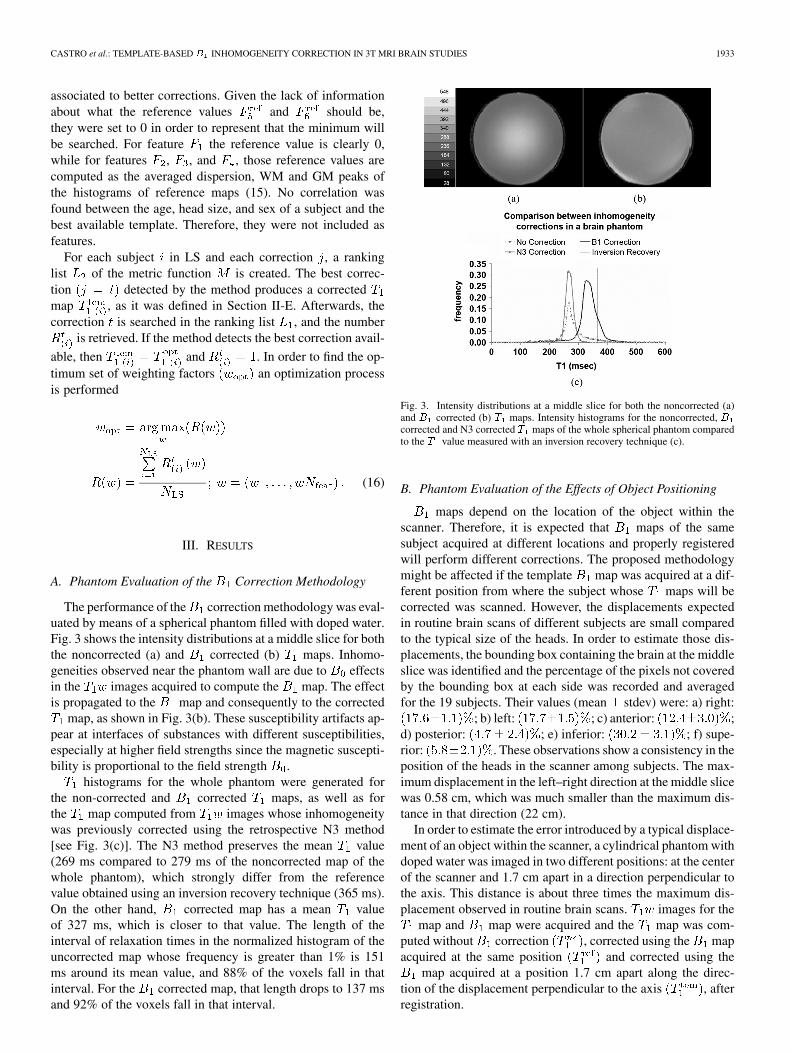
The performance of the correction methodology was eval-uated by means of a spherical phantom filled with doped water.Fig. 3 shows the intensity distributions at a middle slice for boththe noncorrected (a) and corrected (b) maps. Inhomo-geneities observed near the phantom wall are due to effectsin the images acquired to compute the map. The effectis propagated to the map and consequently to the corrected
map, as shown in Fig. 3(b). These susceptibility artifacts ap-pear at interfaces of substances with different susceptibilities,especially at higher field strengths since the magnetic suscepti-bility is proportional to the field strength .
histograms for the whole phantom were generated forthe non-corrected and corrected maps, as well as forthe map computed from images whose inhomogeneitywas previously corrected using the retrospective N3 method[see Fig. 3(c)]. The N3 method preserves the mean value(269 ms compared to 279 ms of the noncorrected map of thewhole phantom), which strongly differ from the referencevalue obtained using an inversion recovery technique (365 ms).On the other hand, corrected map has a mean valueof 327 ms, which is closer to that value. The length of theinterval of relaxation times in the normalized histogram of theuncorrected map whose frequency is greater than 1% is 151ms around its mean value, and 88% of the voxels fall in thatinterval. For the corrected map, that length drops to 137 msand 92% of the voxels fall in that interval.
Fig. 3. Intensity distributions at a middle slice for both the noncorrected (a)and � corrected (b) � maps. Intensity histograms for the noncorrected, �corrected and N3 corrected � maps of the whole spherical phantom comparedto the � value measured with an inversion recovery technique (c).
B. Phantom Evaluation of the Effects of Object Positioning
maps depend on the location of the object within thescanner. Therefore, it is expected that maps of the samesubject acquired at different locations and properly registeredwill perform different corrections. The proposed methodologymight be affected if the template map was acquired at a dif-ferent position from where the subject whose maps will becorrected was scanned. However, the displacements expectedin routine brain scans of different subjects are small comparedto the typical size of the heads. In order to estimate those dis-placements, the bounding box containing the brain at the middleslice was identified and the percentage of the pixels not coveredby the bounding box at each side was recorded and averagedfor the 19 subjects. Their values (mean stdev) were: a) right:
; b) left: ; c) anterior: ;d) posterior: ; e) inferior: ; f) supe-rior: . These observations show a consistency in theposition of the heads in the scanner among subjects. The max-imum displacement in the left–right direction at the middle slicewas 0.58 cm, which was much smaller than the maximum dis-tance in that direction (22 cm).
In order to estimate the error introduced by a typical displace-ment of an object within the scanner, a cylindrical phantom withdoped water was imaged in two different positions: at the centerof the scanner and 1.7 cm apart in a direction perpendicular tothe axis. This distance is about three times the maximum dis-placement observed in routine brain scans. images for the
map and map were acquired and the map was com-puted without correction , corrected using the mapacquired at the same position and corrected using the
map acquired at a position 1.7 cm apart along the direc-tion of the displacement perpendicular to the axis , afterregistration.
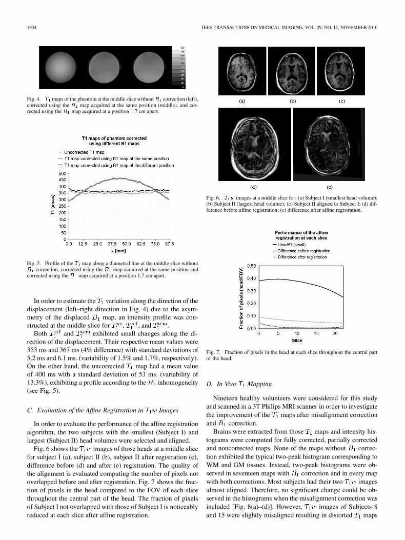
1934 IEEE TRANSACTIONS ON MEDICAL IMAGING, VOL. 29, NO. 11, NOVEMBER 2010
Fig. 4. � maps of the phantom at the middle slice without� correction (left),corrected using the � map acquired at the same position (middle), and cor-rected using the � map acquired at a position 1.7 cm apart.
Fig. 5. Profile of the � map along a diametral line at the middle slice without� correction, corrected using the � map acquired at the same position andcorrected using the � map acquired at a position 1.7 cm apart.
In order to estimate the variation along the direction of thedisplacement (left–right direction in Fig. 4) due to the asym-metry of the displaced map, an intensity profile was con-structed at the middle slice for , , and .
Both and exhibited small changes along the di-rection of the displacement. Their respective mean values were353 ms and 367 ms (4% difference) with standard deviations of5.2 ms and 6.1 ms. (variability of 1.5% and 1.7%, respectively).On the other hand, the uncorrected map had a mean valueof 400 ms with a standard deviation of 53 ms. (variability of13.3%), exhibiting a profile according to the inhomogeneity(see Fig. 5).
C. Evaluation of the Affine Registration in Images
In order to evaluate the performance of the affine registrationalgorithm, the two subjects with the smallest (Subject I) andlargest (Subject II) head volumes were selected and aligned.
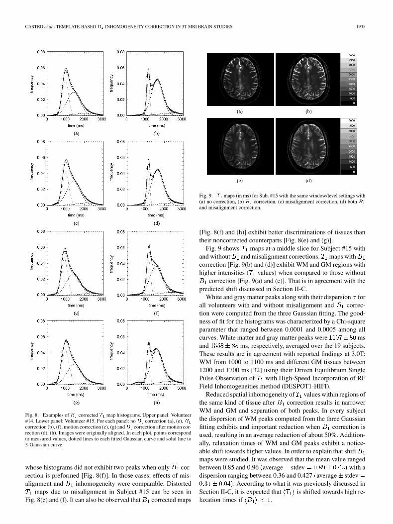
Fig. 6 shows the images of those heads at a middle slicefor subject I (a), subject II (b), subject II after registration (c),difference before (d) and after (e) registration. The quality ofthe alignment is evaluated computing the number of pixels notoverlapped before and after registration. Fig. 7 shows the frac-tion of pixels in the head compared to the FOV of each slicethroughout the central part of the head. The fraction of pixelsof Subject I not overlapped with those of Subject I is noticeablyreduced at each slice after affine registration.
Fig. 6. � � images at a middle slice for: (a) Subject I (smallest head volume);(b) Subject II (largest head volume); (c) Subject II aligned to Subject I; (d) dif-ference before affine registration; (e) difference after affine registration.
Fig. 7. Fraction of pixels in the head at each slice throughout the central partof the head.
D. In Vivo Mapping
Nineteen healthy volunteers were considered for this studyand scanned in a 3T Philips MRI scanner in order to investigatethe improvement of the maps after misalignment correctionand correction.
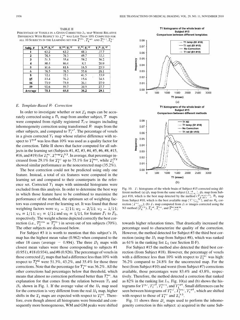
Brains were extracted from those maps and intensity his-tograms were computed for fully corrected, partially correctedand noncorrected maps. None of the maps without correc-tion exhibited the typical two-peak histogram corresponding toWM and GM tissues. Instead, two-peak histograms were ob-served in seventeen maps with correction and in every mapwith both corrections. Most subjects had their two imagesalmost aligned. Therefore, no significant change could be ob-served in the histograms when the misalignment correction wasincluded [Fig. 8(a)–(d)]. However, images of Subjects 8and 15 were slightly misaligned resulting in distorted maps
CASTRO et al.: TEMPLATE-BASED INHOMOGENEITY CORRECTION IN 3T MRI BRAIN STUDIES 1935
Fig. 8. Examples of� corrected � map histograms. Upper panel: Volunteer#14. Lower panel: Volunteer #15. For each panel: no� correction (a), (e),�correction (b), (f), motion correction (c), (g) and� correction after motion cor-rection (d), (h). Images were originally aligned. In each plot, points correspondto measured values, dotted lines to each fitted Gaussian curve and solid line to3-Gaussian curve.
whose histograms did not exhibit two peaks when only cor-rection is preformed [Fig. 8(f)]. In those cases, effects of mis-alignment and inhomogeneity were comparable. Distorted
maps due to misalignment in Subject #15 can be seen inFig. 8(e) and (f). It can also be observed that corrected maps
Fig. 9. � maps (in ms) for Sub. #15 with the same window/level settings with(a) no correction, (b) � correction, (c) misalignment correction, (d) both �and misalignment correction.
[Fig. 8(f) and (h)] exhibit better discriminations of tissues thantheir noncorrected counterparts [Fig. 8(e) and (g)].
Fig. 9 shows maps at a middle slice for Subject #15 withand without and misalignment corrections. maps withcorrection [Fig. 9(b) and (d)] exhibit WM and GM regions withhigher intensities ( values) when compared to those without
correction [Fig. 9(a) and (c)]. That is in agreement with thepredicted shift discussed in Section II-C.
White and gray matter peaks along with their dispersion forall volunteers with and without misalignment and correc-tion were computed from the three Gaussian fitting. The good-ness of fit for the histograms was characterized by a Chi-squareparameter that ranged between 0.0001 and 0.0005 among allcurves. White matter and gray matter peaks were msand ms, respectively, averaged over the 19 subjects.These results are in agreement with reported findings at 3.0T:WM from 1000 to 1100 ms and different GM tissues between1200 and 1700 ms [32] using their Driven Equilibrium SinglePulse Observation of with High-Speed Incorporation of RFField Inhomogeneities method (DESPOT1-HIFI).
Reduced spatial inhomogeneity of values within regions ofthe same kind of tissue after correction results in narrowerWM and GM and separation of both peaks. In every subjectthe dispersion of WM peaks computed from the three Gaussianfitting exhibits and important reduction when correction isused, resulting in an average reduction of about 50%. Addition-ally, relaxation times of WM and GM peaks exhibit a notice-able shift towards higher values. In order to explain that shiftmaps were studied. It was observed that the mean value rangedbetween 0.85 and 0.96 average stdev with adispersion ranging between 0.36 and 0.427 average stdev
. According to what it was previously discussed inSection II-C, it is expected that is shifted towards high re-laxation times if .
1936 IEEE TRANSACTIONS ON MEDICAL IMAGING, VOL. 29, NO. 11, NOVEMBER 2010
TABLE IIPERCENTAGE OF VOXELS IN A GIVEN CORRECTED � MAP WHOSE RELATIVE
DIFFERENCE WITH RESPECT TO � WAS LESS THAN 10% COMPUTED FOR
ALL 10 SUBJECTS IN THE LEARNING SET FOR � , � AND � , �
E. Template-Based Correction
In order to investigate whether or not maps can be accu-rately corrected using a map from another subject, mapswere computed from rigidly registered images includinginhomogeneity correction using transformed maps from theother subjects, and compared to . The percentage of voxelsin a given corrected map whose relative difference with re-spect to was less than 10% was used as a quality factor forthe correction. Table II shows that factor computed for all sub-jects in the learning set (Subjects #1, #2, #3, #4, #5, #6, #8, #15,#16, and #19) for , . In average, that percentage in-creased from 29.1% for up to 75.1% for , whileshowed similar performance as the noncorrected map (35.2%).
The best correction could not be predicted using only onefeature. Instead, a total of six features were computed in thelearning set and compared to their counterparts in the refer-ence set. Corrected maps with unimodal histograms wereexcluded from this analysis. In order to determine the best wayin which those feature have to be combined to maximize theperformance of the method, the optimum set of weighting fac-tors was computed over the learning set. It was found that thoseweighting factors were ; ; ;
; and , for feature to ,respectively. The weight scheme depicted correctly the best cor-rection (i.e., ) in seven out of ten subjects (70%).The other subjects are discussed below.
For Subject #3 it is worth to mention that this subject’smap has the highest mean value (0.962) when compared to theother 18 cases average . The three maps withclosest mean values were those corresponding to subjects #1(0.951), #18 (0.934), and #8 (0.926). The percentage of voxels inthose corrected maps that had a difference less than 10% withrespect to were 51.3%, 43.2%, and 35.4% for those threecorrections. Note that the percentage for was 36.2%. All theother corrections had percentages below that threshold, whichmeans that almost no correction performed better than . Anexplanation for that comes from the relation between and
shown in Fig. 1. If the average value of the map usedfor the correction is very different from the real map, highershifts in the maps are expected with respect to . There-fore, even though almost all histograms were bimodal and con-sequently more homogeneous, WM and GM peaks were shifted
Fig. 10. � histograms of the whole brain of Subject #15 corrected using dif-ferent method: (a)� map from the same subject �� �,� map from Sub-ject #18, which is the best map detected by the method �� �, � mapfrom Subject #10, which is the best available map �� �, and no � cor-rection �� �; (b) � map computed from � � images corrected using theN3 method �� �, � , � , and � .
towards higher relaxation times. That drastically increased thepercentage used to characterize the quality of the correction.However, the method detected for Subject #3 the third best cor-rection (using the map from Subject #8), which was rankedas 61% in the ranking list (see Section II-F).
For Subject #15 the method also detected the third best cor-rection (from Subject #18). However, the percentage of voxelswith a difference less than 10% with respect to was high:76.2% compared to 24.8% for the uncorrected map. For thebest (from Subject #10) and worst (from Subject #7) correctionsavailable, those percentages were 83.4% and 43.8%, respec-tively. Therefore, the method detected a correction that rankedas 82% in the ranking list . Fig. 10(a) and (b) shows the his-tograms for , , , and . Small differences can beseen between histograms of , , , which are shiftedwith respect to those of and .
Fig. 11 shows three maps used to perform the inhomo-geneity correction in this subject: a) acquired in the same Sub-

CASTRO et al.: TEMPLATE-BASED INHOMOGENEITY CORRECTION IN 3T MRI BRAIN STUDIES 1937
Fig. 11. � maps used to correct � maps of Subject #15 displayed with thesame window/level settings, showing the position of the profile line: (a) �map of Subject #15; (b) � map of Subject #18 (best correction detected byour method) after proper affine registration; (c) � map of Subject #10 (bestnon-subject-specific correction available) after proper affine registration.
Fig. 12. Percentage of pixels in those template� maps having a given relativedifference with respect to the reference � map.
ject #15; b) acquired in Subject #18 (best correction detected byour method); c) acquired in Subject #10 (best correction avail-able for this subject).
Fig. 12 shows the percentage of pixels in the templatemaps for Subject #15 for relative differences with respect tothe reference map less than 10%. Particularly, for the bestavailable map, 93.3% of the pixels have a difference less than3%. For the map detected by the method, that percentage is88.2%.
maps for Subject #15 are displayed in Fig. 13 under dif-ferent corrections: a) no correction; b) reference map
; c) N3 method ; d) corrected using the mapfrom the same Subject #15 but under a linear approximation
shown in Fig. 1; e) corrected using the map fromSubject #18 ; and f) corrected using the map fromSubject #10 . No relevant differences can be observedbetween those maps corrected with the map of the samesubject, with and without the linear approximation [Fig. 13(b)and (d)]. map corrected with the N3 method [Fig. 13(c)]shows lower intensities as in the noncorrected map [Fig. 13(a)],but without inhomogeneity throughout voxels of the same tis-sues. maps corrected with the map detect by our method
Fig. 13. � maps (in ms) for Subject #15 computed using different � cor-rections displayed with the same window/level settings: (a) no � correction,� ; (b) reference � map, � ; (c) N3 method, � ; (d) corrected using the� map from the same Subject #15 but under a linear approximation, � ; (e)corrected using the � map from Subject #18, � (best correction detectedby our method, � ); (f) corrected using the� map from Subject #10, �(best nonsubject-specific correction available, � ).
[Fig. 13(e)] and the best correction available [Fig. 13(f)] do notdiffer significantly. The corresponding histograms are shown inFig. 10(a) and (b). It can also be observed that , and
do not exhibit significant differences. has a lowermean value similar to that of .
For Subject #19 the method detected a correction thatranked as 41% in the list. However, given that for this sub-ject the best correction was comparable to (92.6%of the voxels had a difference less than 10%), that percentagewas 59.7% for , which was still higher than the 27.7% cor-responding to .
It is expected that the bigger the library size is, the more ac-curate the correction will be. However, the study does not con-tain sufficient number of cases to perform a reliable convergenceanalysis. Instead, we designed a simple experiment to estimatethe effect of the library size on the accuracy of the correction.For each subject in the learning set, the best template was re-moved from the library. Therefore, the method found the fol-lowing best template. The position in the ranking list was ob-tained and compared to the best template. For the seven caseswhere the method detected the best template the average po-sition in the ranking list dropped to 87%. The complete list isfound in Table III.
1938 IEEE TRANSACTIONS ON MEDICAL IMAGING, VOL. 29, NO. 11, NOVEMBER 2010
TABLE IIIPOSITIONS IN THE RANKING LIST OF THE TEMPLATE DETECTED BY
THE METHOD WHEN THE BEST TEMPLATE IS INCLUDED (A) AND
WHEN IT IS NOT CONSIDERED (B)
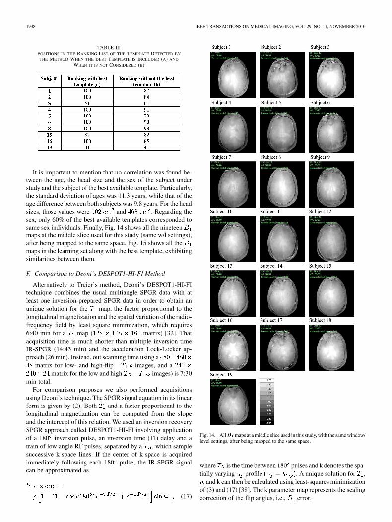
It is important to mention that no correlation was found be-tween the age, the head size and the sex of the subject understudy and the subject of the best available template. Particularly,the standard deviation of ages was 11.3 years, while that of theage difference between both subjects was 9.8 years. For the headsizes, those values were and . Regarding thesex, only 60% of the best available templates corresponded tosame sex individuals. Finally, Fig. 14 shows all the nineteenmaps at the middle slice used for this study (same w/l settings),after being mapped to the same space. Fig. 15 shows all themaps in the learning set along with the best template, exhibitingsimilarities between them.
F. Comparison to Deoni’s DESPOT1-HI-FI Method
Alternatively to Treier’s method, Deoni’s DESPOT1-HI-FItechnique combines the usual multiangle SPGR data with atleast one inversion-prepared SPGR data in order to obtain anunique solution for the map, the factor proportional to thelongitudinal magnetization and the spatial variation of the radio-frequency field by least square minimization, which requires6:40 min for a map ( matrix) [32]. Thatacquisition time is much shorter than multiple inversion timeIR-SPGR (14:43 min) and the acceleration Lock-Locker ap-proach (26 min). Instead, out scanning time using a
matrix for low- and high-flip images, and amatrix for the low and high images) is 7:30
min total.For comparison purposes we also performed acquisitions
using Deoni’s technique. The SPGR signal equation in its linearform is given by (2). Both and a factor proportional to thelongitudinal magnetization can be computed from the slopeand the intercept of this relation. We used an inversion recoverySPGR approach called DESPOT1-HI-FI involving applicationof a 180 inversion pulse, an inversion time (TI) delay and atrain of low angle RF pulses, separated by a , which samplesuccessive k-space lines. If the center of k-space is acquiredimmediately following each 180 pulse, the IR-SPGR signalcan be approximated as
(17)
Fig. 14. All� maps at a middle slice used in this study, with the same window/level settings, after being mapped to the same space.
where is the time between 180 pulses and k denotes the spa-tially varying profile . A unique solution for ,
, and k can then be calculated using least-squares minimizationof (3) and (17) [38]. The k parameter map represents the scalingcorrection of the flip angles, i.e., error.

CASTRO et al.: TEMPLATE-BASED INHOMOGENEITY CORRECTION IN 3T MRI BRAIN STUDIES 1939
Fig. 15. � maps of all subjects in the learning set along with the � mapof the best template, displayed at the middle slice with the same window/levelsettings.
Fig. 16. � map without� correction (a), with� correction (b) and� map(c) of a healthy volunteer using DESPOT-HI-FI method.
TABLE IVMEAN VALUES AND DEVIATION OF WM AND GM REGIONS IN
� MAP OF A HEALTHY VOLUNTEER USING DESPOT-HI-FIWITH AND WITHOUT � CORRECTION
In order to compare our methodology, based on Treier’smethod, to the Deoni’s DESPOT1-HI-FI mapping with cor-rection, we scanned an additional healthy volunteer using thattechnique. The acquisition time was 19 min for amatrix. maps acquired using Deoni’s and Treier’s techniquehad similar overall characteristics (see Fig. 16). Furthermore,mean WM and GM in the corrected and uncorrected maps arein the range of those found in our work (see Table IV).
IV. DISCUSSION
Accurate estimation of relaxation time from high magneticfield MRI using a dual flip angle method may require correctionof not only the transmitted flip angle inhomogeneity but alsoany possible image misalignment. In order to investigate thishypothesis we addressed both corrections by acquiring themap using a dual strategy and a rigid registration algorithm.
The correction module was evaluated using a sphericalphantom resulting in a narrower intensity histogram whosemean value is in agreement to that from an inversion recoverytechnique. It was also observed that retrospective methods likethe N3 method that preserve the mean value of the map donot show the observed shift in relaxation times betweenand . Although methods that preserve the mean value re-move the inhomogeneity producing bimodal histograms, those
values are shifted with respect to those in maps correctedwith a map. Those corrections may not be suitable for quan-titative analyses.
maps were analyzed in nineteen normal volunteers. Priorto correction, histograms of whole brain did not exhibit abimodal peak (WM and GM). On the other hand, all correctedhistograms showed two separated peaks whose values arein agreement with previously reported data. However, slightlymisaligned images used to compute maps resulted ininaccurate map in two subjects. In those cases, image mis-alignment and flip angle inhomogeneity produced comparableeffects on that map, whose histogram did not exhibit two peakswhen only correction was performed.
In order to obviate the need for obtaining a map eachand every time a patient is scanned, a template map maybe used instead. Therefore, each map was recomputed usingthe maps from the other subjects. For that purpose, twelve-parameter affine registration using mutual information metricwith linear interpolation was applied to each pair of high-flip-angle images. The computed transformation was applied to the
map in order to match the geometry of the subject understudy. Although most corrections reduced the inhomogeneity,the performance depends on the map used. Therefore, inorder to automatically detect the best map available, a setof features were computed and included with an optimum set ofweighting factors in the minimization of a metric function. Theset of features used allowed the detection of the best available
map in most cases. In the others, maps comparable to thereference one are obtained.
Although results are promising and have the potential for clin-ical applications, the methodology has some limitations. First,acquired maps exhibit different mean values. Therefore, if all
maps in the library significantly differ from the proper (evenunknown) map, a shift in the corrected values would be ex-pected. Therefore, even though the method may detect the bestavailable map, it may not produce a map that is accurateenough. In order to avoid that, a wide range of maps withdifferent characteristics should be included in that library. Eventhough that would increase the computational time to detect thebest correction, we still have a reduced acquisition time.
Secondly, this methodology has the potential to improve thecancer detection by means of more accurate maps. In orderto investigate whether or not the template correction of

1940 IEEE TRANSACTIONS ON MEDICAL IMAGING, VOL. 29, NO. 11, NOVEMBER 2010
Fig. 17. � weighted image (a) and � map (b) of a patient with a tumor inthe frontal region of the brain and ventricle enlargement.
maps of a patient with a brain tumor could be applied using alibrary containing maps of normal subjects, the weightedimages and map of a patient with a tumor in the frontalregion were studied. Fig. 17 shows a map (b) associatedwith obvious pathology on the correlated weighted image (a).While there is significant deviation from normal brain in termsof the image contrast in the enlarged ventricles as well as frontalcortex, the corresponding map is remarkably homogeneous.This is due to the predominant mechanism of RF inhomogeneitybeing due to the air water susceptibility interface as the RF wavetraverses the different media. Since most pathology will stillconsist of relatively homogeneous proton density the mapis quite similar to other normal volunteer maps.
Therefore, in order for the methodology to be applied to pa-tients with brain tumor, it should include a tumor segmentationmodule to compute the features only outside the tumor. Whilewe would expect the template method to yield improved resultson a clinical population, this work is currently being evaluatedprior to implementation. Furthermore, the accuracy of themapping process itself is limited if there is significant deviationfrom uniform proton density so correction with an inaccuratebut patient specific map will also decrease the accuracy ofthe calculated values.
V. CONCLUSION
The results presented in this work show that correction of bothimage misalignment and transmitted flip angle inhomogeneitymarkedly improve the accuracy of maps obtained by meansof a dual flip angle method at high fields. It was observed thatthe nonlinear relation between the correction factors at everyvoxel and the corrected value produce a shift in the meanvalue of the reference map when compared to the uncor-rected map. That may suggest that methods that preserve thatmean value could lead to inaccurate estimations regardlesstheir ability to maximize the homogeneity within each kind oftissue. Additionally, since in the clinical setting it is beneficial tominimize scanning time and it would be desirable that cor-rections may be made from a template, obviating the need forobtaining a map each and every time a patient is scanned.
inhomogeneity in maps computed from registered imageswere also compensated using maps acquired from other sub-jects, after being aligned using an affine registration algorithm.
When maps from other subjects are properly aligned,many corrected maps are comparable to the referencemap and a considerable number of other maps exhibit a relevant
improvement when compared to the noncorrected ones. An au-tomatic method to characterize the quality of the correction anddetect the map that best performs for a given subject wasdesigned and evaluated. Even though a larger study is neededto corroborate the efficiency of the method, these results arevery promising and have the potential for clinical application.
ACKNOWLEDGMENT
The authors would like to acknowledge Image ProcessingSpecialist F. Thomas at Clinical Image Processing Services(CIPS, DR&IS, National Institutes of Health, Bethesda, MD),for collaborating in the image processing.
REFERENCES
[1] P. L. Choyke, A. J. Dwyer, and M. V. Knopp, “Functional tumorimaging with dynamic contrast-enchanced magnetic resonanceimaging,” J. Magn. Reson. Imag., vol. 17, pp. 509–520, 2003.
[2] A. R. Padhani and J. E. Husband, “Dynamic contrast-enhanced MRIstudies in oncology, with an emphasis on quantification, validation andhuman studies,” Clin. Radiol., vol. 56, pp. 607–620, 2001.
[3] P. S. Tofts et al., “Estimating kinetic parameters from dynamic con-trast-enhanced t1-weighted MRI of a diffusible tracer: Strandarizedquantities and symbols,” J. Magn. Reson. Imag., vol. 10, no. 3, pp.223–232, 1999.
[4] H.-L. M. Cheng and G. A. Wright, “Rapid high-resolution � mappingby variable flip angles: Accurate and precise measurement in the pres-ence of radiofrequency field inhomogeneity,” Magn. Reson. Med., vol.55, pp. 566–574, 2006.
[5] S. C. L. Deoni, T. M. Peters, and B. K. Rutt, “Determination of optimalangles for variable nutation proton magnetic spin-lattice, � , spin-spin,� , relaxation times measurements,” Magn. Reson. Med., vol. 51, pp.194–199, 2004.
[6] H. Wang, S. Riederer, and J. Lee, “Optimizing the precision in � re-laxation estimation using limited flip angles,” Magn. Reson.Med., vol.5, pp. 399–416, 1987.
[7] J. G. Sled and G. B. Pike, “Understanding intensity non-uniformityin MRI,” Proc. MICCAI 1998, pp. 614–622, 1998, Lecture Notes onComputer Science.
[8] W. A. Edelstein, G. H. Glover, C. J. Hardy, and R. W. Redington, “Theintrinsic signal-to-Noise ratio in NMR imaging,” Magn. Reson. Med.,vol. 3, pp. 604–618, 1986.
[9] J. M. Jin, J. Chen, W. C. Chew, H. Gan, R. L. Magin, and P. J. Dim-bylow, “Computation of electromagnetic fields for high-frequencymagnetic resonance imaging applications,” Phys. Med. Biol., vol. 41,pp. 2719–2738, 1996.
[10] O. Dietrich, M. F. Reiser, and S. O. Schoenberg, “Artifacts in 3-TeslaMRI: Physical background and reduction strategies,” Eur. J. Radiol.,vol. 65, pp. 29–35, 2008.
[11] B. Belaroussi, J. Mille, S. Carme, Y. M. Zhu, and H. Benoit-Catin, “In-tensity non-uniformity correction in MRI: Existing methods and theirvalidation,” Med. Image Anal., vol. 10, pp. 234–246, 2006.
[12] U. Vovk, F. Pernus, and B. Likar, “A review of methods for correctionof intensity inhomogeneity in MRI,” IEEE Trans. Med. Imag., vol. 26,no. 3, pp. 405–421, Mar. 2007.
[13] Z. Hou, “A review on MR image intensity inhomogeneity correction,”Int. J. Biomed. Imag., vol. 2006, pp. 1–11, 2006.
[14] B. H. Brinkmann, A. Manduca, and R. A. Robb, “Optimized homomor-phic unsharp masking for MR grayscale inhomogeneity correction,”IEEE Trans. Med. Imag., vol. 17, no. 2, pp. 161–171, Apr. 1998.
[15] B. M. Dawant, A. P. Zijdenbos, and R. A. Margolin, “Correction of in-tensity variations in MR images for coumpted-aided tissue classifica-tion,” IEEE Trans. Med. Imag., vol. 12, no. 4, pp. 770–781, Dec. 1993.
[16] C. Han, T. S. Hatsukami, and C. Yuan, “A multi-scale methods for auto-matic correction of intensity non-uniformity in MR images,” J. Magn.Reson. Imag., vol. 13, pp. 428–436, 2001.
[17] A. W.-C. Liew and H. Yan, “An addaptive spatial fuzzy clustering al-gorithm for 3-D MR image segmentation,” IEEE Trans. Med. Imag.,vol. 22, no. 9, pp. 1063–1075, Sep. 2003.
[18] B. Likar, B. A. Maintz, and M. A. Viergever, “Retrospective shadingcorrection based on entropy minimization,” J. Microscopy, vol. 197,pp. 285–295, 2000.
[19] B. Likar, M. A. Viergever, and F. Pernus, “Retrospective correctionof MR intensity inhomogeneity by information minimization,” IEEETrans. Med. Imag., vol. 20, no. 12, pp. 1398–1410, Dec. 2001.

CASTRO et al.: TEMPLATE-BASED INHOMOGENEITY CORRECTION IN 3T MRI BRAIN STUDIES 1941
[20] F. Lin, Y. Chen, J. W. Belliveau, and L. L. Wald, “A wavelet-basedapproximation of surface coil sensitivity profiles for correction ofimage intensity inhomogeneity and parallel image reconstruction,”Hum. Brain Mapp., vol. 19, pp. 96–111, 2003.
[21] J. Luo, Y. Zhu, P. Clarysee, and I. Magnin, “Correction of bias fieldin MR images using singulatiry function analysis,” IEEE Trans. Med.Imag., vol. 24, no. 8, pp. 1067–1085, Aug. 2005.
[22] J. F. Mangin, “Entropy minimization for automatic correction of inten-sity nonuniformity,” presented at the IEEE Workshop on MathematicalMethods in Biomedical Image Analysis, Hilton Head Island, SC, 2000.
[23] J. L. Marroquin, B. C. Bemuri, S. Botello, F. Calderon, and A. Fer-nandez-Bouzas, “An accurate and efficient bayesian method for auto-matic segmentation of brain MRI,” IEEE Trans. Med. Imag., vol. 21,no. 8, pp. 934–945, Aug. 2002.
[24] C. R. Meyer, P. H. Bland, and J. Pipe, “Retrospective correction ofintensity inhomogeneities in MRI,” IEEE Trans. Med. Imag., vol. 14,no. 1, pp. 36–41, Mar. 1995.
[25] J. G. Sled and A. P. Zijdenbos, “A nonparametric method for automaticcorrection of intensity nonuniformity in MRI data,” IEEE Trans. Med.Imag., vol. 17, no. 1, pp. 87–97, Feb. 1998.
[26] C. Studholme, V. Cardenas, E. Song, F. Ezekiel, A. Maudsley, and M.Weiner, “Accurate template-based correction of brain MRI intensitydistortion with application to dementia and aging,” IEEE Trans. Med.Imag., vol. 23, no. 1, pp. 99–110, Jan. 2004.
[27] Y. Zhang, M. Brady, and S. Smith, “Segmentation of brain MR im-ages through a hidden Markov random field model and the expecta-tion-maximization algorithm,” IEEE Trans. Med. Imag., vol. 20, no. 1,pp. 45–57, Jan. 2001.
[28] Y. Ishimori, K. Yamada, H. Kimura, Y. Fujiwara, I. Yamaguchi, M.Monma, and H. Uematsu, “Correction of inhomogeneous RF fieldusing multiple SPGR signals for high-field spin-echo MRI,” Magn.Reson. Med. Sci., vol. 6, pp. 67–73, 2007.
[29] H. Mihara, M. Sekino, N. Iriguchi, and S. Ueno, “A method for anaccurate � relaxation-time measurement compensating � field in-homogeneity in magnetic-resonance imaging,” presented at the 49thAnnu. Conf. Magn. Magn. Mater., Jacksonville, FL, 2005.
[30] R. TrSeier, A. Steingoetter, M. Fried, W. Schwizer, and P. Boesiger,“Optimized and combined � and � mapping technique for fast ac-curate� quantification in constrast-enhanced abdominal MRI,” Magn.Reson. Med., vol. 57, pp. 568–576, 2007.
[31] V. Yarnykh, “Actual flip-angle imaging in the pulsed steady state: Amethod for rapid 3D mapping of the transmitted radiofrequency field,”Magn. Reson. Med., vol. 57, pp. 192–200, 2007.
[32] S. C. L. Deoni, “High-resolution � mapping of the brain at 3T withdriven equilibrium single pulse observation with � high-speed in-corporation of RF field inhomogeneities (DESPOT1-HIFI),” J. Magn.Reson. Imag., vol. 26, pp. 1106–1111, 2007.
[33] M. A. Castro, J. Yao, C. Lee, Y. Pang, E. Baker, J. Butman, and D.Thomasson, “� mapping with � field and motion correction inbrain MRI images: Application to brain DCE-MRI,” presented at theMICCAI 2008-Workshop Anal. Functional Med. Images, New York,2008.
[34] S. Smith, “Fast robust automated brain extraction,” Hum. Brain Mapp.,vol. 17, pp. 143–155, 2002.
[35] S. Ruan, C. Jaggi, J. Xue, J. Fadili, and D. Blovet, “Brain tissue classi-fication of magnetic resonance images using partial volume modeling,”IEEE Trans. Med. Imag., vol. 19, no. 12, pp. 1179–1187, Dec. 2000.
[36] P. Viola and W. M. Wells, III, “Alignment by maximization of mutualinformation,” Int. J. Comput. Vis., vol. 24, no. 2, pp. 137–154, 1997.
[37] S. C. L. Deoni, B. K. Rutt, and T. M. Peters, “Rapid combined � and� mapping using gradient recalled acquisition in the steady state,”Magn. Reson. Med., vol. 49, pp. 515–526, 2003.
[38] R. Stolleberg and P. Wach, “Imaging of the active � field in vivo,”Magn. Reson. Med., vol. 35, pp. 246–251, 1996.


![3T[WXaX^cbPX\TSc^VPX] U^aTXV]\TSXPPccT]cX^]](https://static.fdokumen.com/doc/165x107/633431d762e2e08d49028554/3twxaxcbpxtscvpx-uatxvtsxppcctcx.jpg)